petroleum production systems - ntnu
TRANSCRIPT
Petroleum Production Systems
Compendium
Prof. Milan Stanko

Trondheim, Norway
© 2020, Stanko.
Version 1.5.2 (May‐2020)
3
PREFACE
These notes address, hopefully in a simple manner, a variety of topics on production performance of oil and
gas fields.
The notes are given as supplementary material for the course Field Development and Operations (TPG4230)
taught at the Department of Geoscience and Petroleum of the Norwegian University of Science and
Technology (NTNU) in Trondheim, Norway. The course was designed in 2007 by Prof. Michael Golan and
teaches and integrates a variety of multi‐disciplinary petroleum engineering topics used in the development
and management of hydrocarbon reservoirs and fields.
The lectures of the course are video‐recorded and are available on my YouTube channel, under the following
link1. Each lecture has in the description links to my handwritten notes, video files and exercise class files that
were discussed.
I will do my best to update these notes often and more material will be added with time. Be aware that
references might be incomplete. If you have any comments or find errors, I appreciate you sending me an
email at milan.stanko(at)ntnu.no. Equation usage is intentionally reduced to a minimum as expressions are
usually provided in class or are available in other sources.
I appreciate and acknowledge the contribution, corrections, time and support of Prof. Michael Golan and Prof.
Curtis Whitson. Many of the ideas presented in the document are based on their work and their way of
thinking.
I appreciate the help and contributions of Ruben Ensalzado regarding document formatting, editing, re‐writing
numerous equations and general quality control.
Prof. Milan Stanko
1 https://www.youtube.com/channel/UCWMfsCe1NQMgx4UZWrVvFgA
4
CONTENTS
Preface 3
Contents 4
List of tables 8
List of figures 9
1. Field Performance 16
1.1. Reservoir 16
1.2. Production system (surface network) 18
1.3. Coupling reservoir models and models of the production system 19
1.4. Production potential 21
1.5. Production scheduling 22
1.6. Relationship between production potential and cumulative production 24
1.7. Production scheduling and planning using production potential curve 30
1.8. Applicability of the production potential concept in real fields and multi‐well production systems 34
References 35
2. Flow Performance in Production Systems 36
2.1. Inflow performance relationship 38
2.1.1. Undersaturated, vertical oil well 41
2.1.2. Vertical gas well 42
2.1.3. Saturated, vertical oil well 43
2.1.4. Composite IPR: Both undersaturated and saturated oil 46
2.1.5. Flow of associated products in an oil well: gas and water 47
2.1.6. IPR and water or gas coning 47
2.1.7. IPRs generated with reservoir simulator 48
2.2. Available and required pressure function 49
COMPLETION BITE: Tubulars 52
2.3. Flow equilibrium in production systems 54
2.3.1. Single well production system 54
2.3.2. Operational envelope: choke 57
2.3.3. Operational envelope: electric submersible pump 61
2.3.4. Operational envelope: dynamic gas compressor 63
2.3.1. Operational envelope: jet pump 66
2.4. Flow equilibrium in production networks 68
2.4.1. Solving network hydraulic equilibrium fixing well rates 71
2.4.2. Downhole networks 72
COMPLETION BITE: Sliding sleeve 73
Shifting procedure 75
References 76
3. Production Optimization 77
3.1. Optimizing a production system 77
3.1.1. Case 1: Gas‐lifted wells 79
COMPLETION BITE: gas‐lift valve 81
5
3.1.2. Case 2: Two gas wells equipped with wellhead chokes 85
3.1.3. Case 3: Two ESP‐lifted wells 88
3.2. Issues hindering the industrial scale adoption of model‐based production optimization 94
3.2.1. Foreign from the field’s reality 94
3.2.2. Models uncertainty 94
3.2.3. Non‐sustainability of the proposed solutions 94
References 95
4. Fluid Behavior Treatment in Oil and Gas Production Systems 96
4.1. The Black Oil Model 96
4.2. Variation of BO properties with temperature 101
4.3. Variation of BO properties with composition 103
4.4. BO correlations 107
4.5. BO properties in production calculations 108
4.6. Estimation of a new composition when the well GOR changes 109
References 110
5. The Field Development Process 111
5.1. Business case identification 114
5.1.1. Reserve estimation using probabilistic analysis 114
5.2. Project Planning 118
5.2.1. Feasibility studies 118
5.2.2. Concept planning (leading to dg2) 118
5.2.3. Field production profile and economic value 119
5.2.4. Pre‐Engineering (leading to DG3) 126
5.3. Project Execution 127
5.3.1. Detailed engineering, construction, testing and startup 127
5.4. Operations 127
5.5. Decommissioning and abandonment 127
References 129
6. Offshore Structures for Oil and Gas Production 130
6.1. Selection of proper marine structure 132
6.1.1. Water depth 132
6.1.2. Location of the Christmas tree 132
COMPLETION BITE: Wellhead architecture 132
Safety strategy for wells 135
6.1.3. Oil Storage 137
6.1.4. Marine loads on the offshore structure 137
6.1. Treatment of wind, waves and currents 139
References 144
7. Flow Assurance Management in Production Systems 145
7.1. Hydrates 146
7.1.1. Consequences 147
7.1.2. Management 147
7.2. Slugging 150
6
7.2.1. Consequences 151
7.2.2. Management 151
7.3. Scaling 152
7.3.1. Consequences 152
7.3.2. Management 152
7.4. Erosion 153
7.4.1. Consequences 153
7.4.2. Management 153
7.5. Corrosion 154
7.5.1. Consequences 154
7.5.2. Management 154
7.6. Wax Deposition 155
7.6.1. Consequences 156
7.6.2. Management 157
7.7. Oil‐Water Emulsions 158
7.7.1. Consequences 158
7.7.2. Management 160
7.1. Summary table 160
7.1. About chemical injection 161
References 163
Appendices 164
A. The Tubing Rate Equation in Vertical and Deviated Gas‐Wells 165
Derivation from first principles (pure SI system) 165
Pressure equation in practical field units (Metric) 167
Fetkovich Rate Equation 169
References 172
B. Choke Equations 173
Undersaturated oil flow 173
Dry gas flow 174
Oil‐Gas‐Water mixture 176
C. Pipe overall Heat Transfer Coefficient 179
Forced convection inside the pipe 179
Conduction in pipe wall 179
Conduction in insulating layer 179
Free‐forced convection in seabed 179
Overall heat transfer coefficient 180
D. Temperature Drop in Conduit 182
General expression 182
Derivation for liquids 182
With variable ambient temperature 184
Transient in formation or soil 184
E. Derivation of multiphase flow expressions 185
Relationship between holdup (HL), slip ratio (S) and quality (x) 185

7
Holdup average mixture density (ρm) 185
Effective momentum density 186
Kinetic energy‐average mixture density 186
F. Oil & Gas Processing Diagrams 188
G. Derivation of the expression of field producing gas‐oil ratio 190
H. Gas lift optimization 191
I. Some style comments for technical communication (paraphrasing the notes of M. Standing and M. Golan) 194
8
LIST OF TABLES
Table 2‐1. Presents the time required to pss for a gas reservoir with the characteristics and using Eq. 2‐1. 40
Table 3‐1. Polynomial coefficients 83
Table 4‐1. BO parameters 97
Table 4‐2. Selected correlations for BO parameters 107
Table 6‐1. Qualitative storage capacity of common offshore structures 137
Table 7‐1. summary table of flow assurance issues: causes, potential consequences, prevention and solution
measures and tools available for analysis 161
9
LIST OF FIGURES
Figure 1‐1. (a) Tank analogy of a (b) reservoir system 17
Figure 1‐2. Graphical depiction of the material balance approach 17
Figure 1‐3. IPR curve 19
Figure 1‐4. Time step of an explicit coupling scheme between a material balance model and a model of the
production system to predict production profile 20
Figure 1‐5. Explicit coupling between a reservoir simulation and a model of the production system 20
Figure 1‐6. (b) Well potential calculation vs. (a) Production potential calculation 21
Figure 1‐7. Production potential behavior vs. time when a production enhancement modification is performed
in the system 22
Figure 1‐8. Plateau production mode 23
Figure 1‐9. Production profile obtained when operating in decline mode 23
Figure 1‐10. Production rate behavior vs cumulative production for open choke and constant rate 24
Figure 1‐11. Changes of IPR with cumulative production 24
Figure 1‐12. Production rate behavior vs cumulative production for open choke showing the region of feasible
rates 25
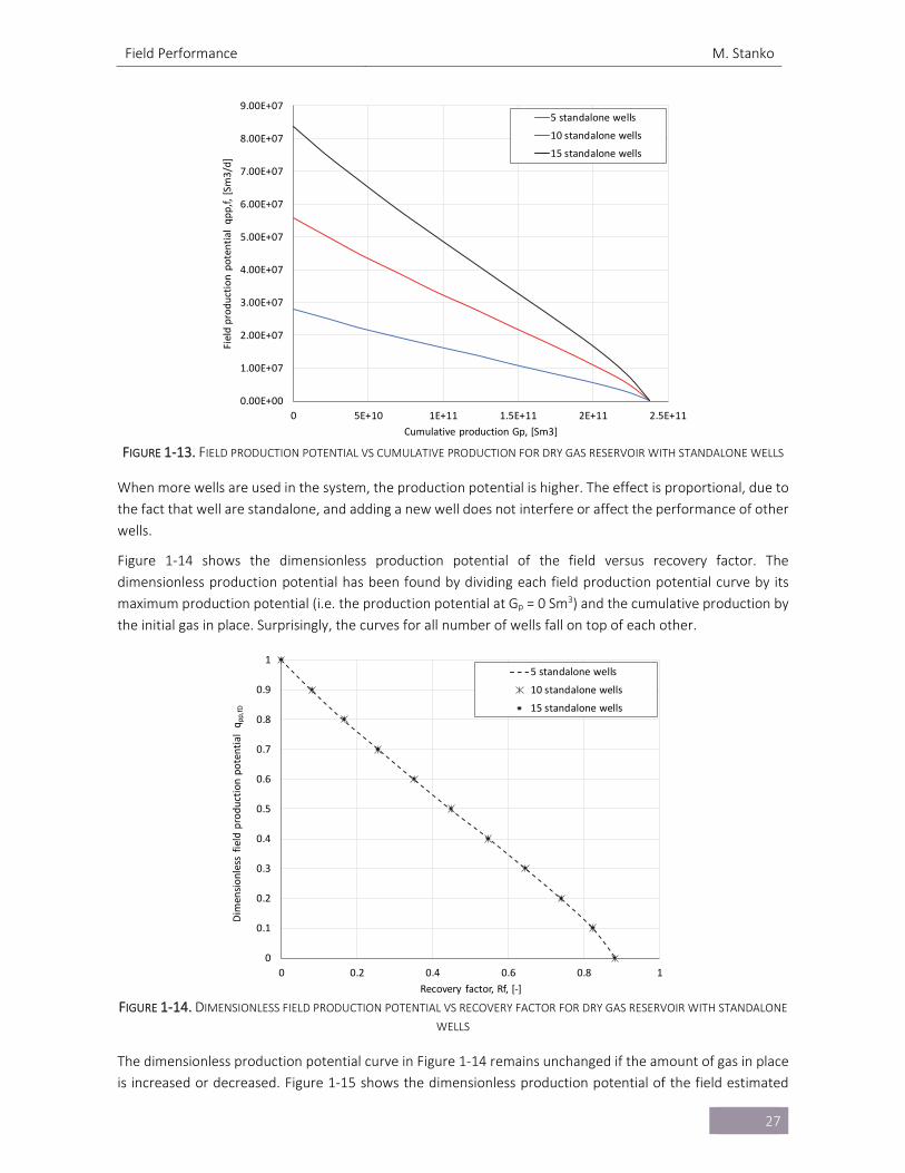
Figure 1‐13. Field production potential vs cumulative production for dry gas reservoir with standalone wells
27
Figure 1‐14. Dimensionless field production potential vs recovery factor for dry gas reservoir with standalone
wells 27
Figure 1‐15. Dimensionless field production potential vs recovery factor for dry gas reservoir with standalone
wells, sensitivity study on system properties 28
Figure 1‐16. Dimensionless field production potential vs recovery factor for dry gas reservoir with standalone
wells, network wells and considering IPR only. 29
Figure 1‐17. Dimensionless field production potential vs recovery factor for several production systems. 30
Figure 1‐18. Plateau mode production 31
Figure 1‐19. Example case: 2 standalone wells 32
Figure 1‐20. 4 different alternatives to produce the two wells system in plateau mode 34
Figure 2‐1. Simplified level and pressure control system in a separator 36
Figure 2‐2. Layout of two production systems 36
Figure 2‐3. IPR curve 37
Figure 2‐4. Production network with two wells 38
Figure 2‐5. Cross section of a vertical well depicting the coordinate system to plot pressure versus radius 39
Figure 2‐6. Evolution of pressure across the reservoir with time when put on production 39
Figure 2‐7. IPR predicted by Eq. 2. for undersaturated oil well and different reservoir pressures 42
10
Figure 2‐8. Graphic illustration of the process to estimate IPR with a reservoir simulator according to Astutik
(2012) 48
Figure 2‐9. Pipe segment 49
Figure 2‐10. Available pressure at pipe outlet for different flow rates and fixed inlet pressure 49
Figure 2‐11. Required pressure at pipe inlet for different flow rates and fixed outlet pressure 49
Figure 2‐12. Available wellhead pressure vs produced rate 50
Figure 2‐13. Available wellhead pressure with choke included vs produced rate 50
Figure 2‐14. Required flowing bottom‐hole pressure curve vs. produced rate 51
Figure 2‐15. Schematic representation of the mixture density variation with slip between gas and liquid
velocities 51
Figure 2‐16. Typical flow patterns along a wellbore as pressure and temperature decrease 52
Figure 2‐17. Two joints of tubing joined by a coupling, or an integrated joint 53
Figure 2‐18. Equilibrium flow rate of the system calculated by intersecting the available pressure curve
calculated from reservoir and the required pressure curve from separator 55
Figure 2‐19. Equilibrium flow rate of the system for: fully open choke and 75% open choke 55
Figure 2‐20. Equilibrium analysis excluding the wellhead choke to estimate choke pressure drop to achieve a
specific flow rate 56
Figure 2‐21. Equilibrium analysis excluding the ESP to estimate ESP pressure boost to achieve a specific flow
rate 56
Figure 2‐22. Equilibrium analysis excluding the choke to estimate choke pressure drop to achieve a specific
flow rate for different times 57
Figure 2‐23.Performance curve of a choke with fixed opening 57
Figure 2‐24. Positive (fixed) choke in critical regime (sonic velocity reached at the throat) 58
Figure 2‐25. Pressure along the axis of a bean choke 58
Figure 2‐26. Performance curve of a choke with fixed opening 59
Figure 2‐27. Performance curve of an adjustable choke for several choke openings 59
Figure 2‐28. Flow rate across different types of adjustable chokes with a fixed pressure drop and inlet pressure
60
Figure 2‐29. Wellhead equilibrium analysis for choke design for two depletion states 60
Figure 2‐30. Adjustable choke performance curve for different choke openings and two inlet pressures 61
Figure 2‐31. Pump performance curve, delta pressure vs local flow rate 61
Figure 2‐32. Pump performance curve operating with water or with an oil of 200 cp. Predicted with the method
described in the standard ANSI/HI 9.6.7‐2010 62
Figure 2‐33. ESP equilibrium analysis for ESP design for two depletion states 63
Figure 2‐34. ESP performance curve with operating points overimposed 63
11
Figure 2‐35. Pressure‐enthalpy diagram for methane depicting an isentropic compression process and a real
compression process 64
Figure 2‐36. Performance map of a gas compressor 65
Figure 2‐37. Simplified schematic of a jet pump 67
Figure 2‐38. Performance plot of a jet pump (taken from Beg and Sarshar[2‐7]) 67
Figure 2‐39. Production network with 3 wells. Available junction pressure curve for three wells and required
junction pressure curve for the pipeline 68
Figure 2‐40. Depiction of the production network model as a mathematical function 69
Figure 2‐41. Production network with 2 wells 69
Figure 2‐42. Well flow rate solutions for no choke, well 1 closed, and well 2 closed 70
Figure 2‐43. Well flow rate domain solution for the production system with 2 wells 70
Figure 2‐43. Well flow rate domain solution for the production system with 3 wells 71
Figure 2‐44. Well flow rate domain solution for the production system with 2 wells 72
Figure 2‐45. Horizontal wellbore with several sections delimited by packers 73
Figure 2‐46. Equivalent line diagram representing a sectioned horizontal wellbore 73
Figure 2‐47. Generic sliding sleeve configuration 74
Figure 2‐48. Details of the locking mechanism of the sleeve 74
Figure 2‐49. Details of the locking fingers on the sleeve that retract and expand when reciprocated axially
inside the sleeve 74
Figure 2‐50. Shifting sequence of a sliding sleeve using slickline 75
Figure 3‐1. Data assimilation process for the network model (adapted from Barros et al, 2015[3‐3]) 78
Figure 3‐2. Equilibrium flow rate of the system for: fully open choke, 75%, 50% and 25% open choke 79
Figure 3‐3. Natural equilibrium point calculated for well with no gas lift injection and with gas injection 80
Figure 3‐4. Natural equilibrium points calculated for different amounts of gas lift injected 80
Figure 3‐5. Gas‐lift performance relationship 80
Figure 3‐6. Mandrel types used to deploy gas‐lift valves 81
Figure 3‐7. Locking process of the gas lift valve in the mandrel pocket 82
Figure 3‐8. Sequence to retrieve a gas‐lift valve from the mandrel pocket 82
Figure 3‐9. Colormap and contour lines of total oil production as a function of lift‐gas injected in wells 1 and 2
83
Figure 3‐10. Color map and contour lines of oil production as a function of lift‐gas injected in wells 1 and 2.
Contour lines of total available gas‐lift rate. 84
Figure 3‐11. Production system with two dry gas wells 85
Figure 3‐12. Well flow rate domain solution for the production system with 2 wells 86
Figure 3‐13. Total gas production as a function of well 1 and well 2 rates 86
12
Figure 3‐14. Total gas production plotted on the feasibility region 87
Figure 3‐15. Well flow rate domain solution for the production system with 2 wells. Well 2 has a higher
deliverability than well 1 87
Figure 3‐16. Total gas production plotted on the feasibility region 88
Figure 3‐17. Two ESP‐lifted wells with common wellhead manifold discharging to a pipeline 89
Figure 3‐18. Total oil production color map for the complete ESP frequency range of wells 1 and 2 89
Figure 3‐19. Two ESP‐lifted wells with common wellhead manifold discharging to a pipeline. 91
Figure 3‐20. Two ESP‐lifted wells with common wellhead manifold discharging to a pipeline. 92
Figure 3‐21. Feasible operating region of a system with two ESP‐lifted wells with common wellhead manifold
discharging to a pipeline. 93
Figure 4‐1. Schematic representation of the flashing of oil and gas at local conditions to standard conditions
97
Figure 4‐2. Schematic of the process to generate BO properties 98
Figure 4‐3. Behavior of BO parameters vs. pressure for a fixed temperature 99
Figure 4‐4. Phase diagram of the hydrocarbon mixture used in Figure 4‐3 99
Figure 4‐5. Behavior of BO parameters vs. pressure for a fixed temperature 100
Figure 4‐6. Phase diagram of the hydrocarbon mixture used in Figure 4‐5 100
Figure 4‐7. Solution gas oil behavior with pressure for three temperatures 101
Figure 4‐8. Phase diagram of the hydrocarbon mixture used in Figure 4‐7 101
Figure 4‐9. Oil volume factor behavior with pressure for three temperatures 102
Figure 4‐10. Gas volume factor behavior with pressure for three temperatures 102
Figure 4‐11. Solution Oil‐gas ratio with pressure for three temperatures 103
Figure 4‐12. Phase diagram of the hydrocarbon mixture used in Figure 4‐12 103
Figure 4‐13. Black oil properties estimated for different compositions (GOR) 104
Figure 4‐14. Rs and 1/rs vs p computed for several GORs at constant temperature 105
Figure 4‐15. Oil well 106
Figure 4‐16. Variation of the phase envelope with changes in composition (GOR) 106
Figure 4‐17. Rs variation with composition when more gas flows into the wellbore 106
Figure 4‐18. Variation of main BO parameters with composition when more gas flows into the wellbore 107
Figure 4‐19. Transformation matrixes to take standard conditions rates to local conditions and vice versa 108
Figure 4‐20. Transformation matrixes to take standard conditions densities to local conditions and vice versa
108
Figure 4‐21. Recombination of source gas and oil to yield stream composition 109
Figure 5‐1. Field development timeline and the evolution of the value chain model after decision are made
112
13
Figure 5‐2. Detailed value chain components 112
Figure 5‐3. Field development process 113
Figure 5‐4. model or simulation with uncertainty in its input parameters 115
Figure 5‐5. probability distribution of initial oil in place calculated with monte carlo simulation and different
number of samples 116
Figure 5‐6. probability distribution of initial oil in place sampled from a normal distribution for different
number of samples 117
Figure 5‐7. Behavior of the present value of the revenue versus oil plateau rate for two numbers of wells 122
Figure 5‐8. Project NPV, PV revenue and CAPEX for 12 wells and versus the oil plateau rate for the case of
Nunes et al. (2018)[5‐1]. 122
Figure 5‐9. Color contour of NPV versus number of producing wells and field plateau rate 124
Figure 5‐10. Color contour of NPV versus number of producing Wells and field plateau rate, with modified
color scale. The blue line depicts field operating in decline from time zero 124
Figure 5‐11. Color contour of NPV versus number of producing wells and field plateau rate. 126
Figure 5‐12. Color contour of NPV versus number of producing wells and field plateau rate. 126
Figure 6‐1. Some common marine structures for oil and gas exploitation 131
Figure 6‐2. a) Catenary mooring, b) taut mooring. (Adapted from Chakrabarti[6‐5]) 131
Figure 6‐3. Water depth range of the most common offshore structures for hydrocarbon production 132
Figure 6‐4. Deployment of the conductor 133
Figure 6‐5. Run of the surface casing and casing head 133
Figure 6‐6. Details of the pressure port on the casing head to make the pressure test 134
Figure 6‐7. Casing head with the intermediate casing hanged 134
Figure 6‐8. Details of the casing hanger (slips and seals) 134
Figure 6‐9. Installation of the casing spool to the casing head 135
Figure 6‐10. Final configuration of the wellhead 135
Figure 6‐11. Top tension systems for production risers in floating structures (Adapted from Chakrabarti[6‐6])
136
Figure 6‐12. Wind and current loads on an offshore structure 137
Figure 6‐13. Examples of typical movements exhibited by offshore structures 138
Figure 6‐14. Heave RAO of a Sevan FPSO (taken from Saad et al. [6‐7]) 139
Figure 6‐15. Illustrative figure indicating natural periods of some offshore structures and excitation periods of
some environmental loads 139
Figure 6‐16. Wind rose, (Adapted from https://sustainabilityworkshop.autodesk.com/buildings/wind‐rose‐
diagrams) 140
Figure 6‐17. Two‐dimensional random wave time profile 140
14
Figure 6‐18. Contribution of individual regular waves 141
Figure 6‐19. Wave energy spectrum a) continuous and b) discretized 141
Figure 6‐20. Short term probability density function of wave elevation (a) and height (b) 142
Figure 6‐21. Scatter Diagram of long term wave statistics 142
Figure 6‐22. Pdf and cd of significant wave height for spectral period range 18‐19 s 143
Figure 7‐1. Flow assurance problems and their typical location in the production system 145
Figure 7‐2. A) appearance of a hydrate plug (photo taken from schroeder et al[7‐1] ), b) molecular structure of
a methane hydrate 146
Figure 7‐3. Hydrate formation region 147
Figure 7‐4. Evolution of p and T of the fluid when flowing along the production system 147
Figure 7‐5. Effect of inhibitor injection on the hydrate line 148
Figure 7‐6. Flow schematic of a subsea production system with hydrate inhibitor injection system 149
Figure 7‐7. Details of a subsea distribution unit. 149
Figure 7‐8. Hydrate and scale inhibitor injection system in the X‐mas tree 150
Figure 7‐9. Slug in a pipe section 150
Figure 7‐10. Flow pattern map for a horizontal pipe 151
Figure 7‐11. Stages of severe slugging in an S‐shaped riser 151
Figure 7‐12. Scale accumulation in choke (image taken from sandengen[7‐2] ) 152
Figure 7‐13. Erosion damage in a cage‐type choke [source unknown) 153
Figure 7‐14. CFD simulation of erosion in a production header 153
Figure 7‐15. a) Illustration or a corrosion reaction b) corrosion on a casing inside surface c) corrosion on tubing
154
Figure 7‐16. Wet gas flow in a horizontal flowline depicting top of line condensation 154
Figure 7‐17. Protective layer of FeCO3 formed on the metal surface b) inhibitors attached to the metal surface
155
Figure 7‐18. a) Wax crystals visible in a crude at WAT, b) WATs at different pressures in the phase diagram
155
Figure 7‐19. Crude oil not flowing once the pour point is reached 156
Figure 7‐20. a) wax plug retrieved topside (image taken from labes‐carrier et al[7‐3] ), b) evolution of the wax
thickness in a pipeline with time 156
Figure 7‐21. Flow schematic of a subsea production system with facilities for pigging and individual well testing
157
Figure 7‐22. a) oil (red) and water (White) originally separated, b) oil and water emulsion after vigorous stirring
in a blender. photos taken by hong[7‐4] 158
15
Figure 7‐23. Measured pressure drop in a horizontal pipe keeping the total flow rate constant and changing
water volume fraction, 𝒒𝒘/ 𝒒𝒘 𝒒𝒐 159
Figure 7‐24. oil‐water flow pattern map of water volume fraction versus mixture velocity for an upward pipe
inclination of 45°. figure adapted from rivera[7‐5] . 159
Figure 7‐25. Mixture viscosity behavior versus water volume fraction exhibited by the oil water mixture 160
Figure F‐1. Gas Processing from well to sales 188
Figure F‐2. Gas Processing from well to sales (including typical operating values) 189
Field Performance M. Stanko
16
1. FIELD PERFORMANCE
The flow interaction between reservoir and production system define the most important output of an oil and
gas asset: the production profile (the produced flow rates of oil or gas with time). The production profile is
one of the most important performance indicators of a field as it defines the revenue profile thus allowing to
compute the economic value of the asset.
The production profile is typically computed and predicted using analytical or numerical models (e.g.
simulators) that represent accurately the reservoir and production system. The fundamental idea is to produce
several times a “virtual field” testing different alternatives (e.g. production strategies, enhanced recovery
methods, etc.) to determine which one provides the best economic value. Once the best alternative is
determined, the production strategy is executed on the real asset.
This analysis is usually performed multiple times both during the field design phase and in the operational
phase. In the field design phase, the main goal is to compare different production and development strategies
and architectures. The numerical models are not yet fully defined and there are lot of uncertainties in the
input data. For an existing asset, it is usually used to foresee future problems, to evaluate the implementation
of Improved Oil Recovery (IOR) methods, drilling additional wells, among others. The numerical model is very
well defined and the historical production data has been used to reduce uncertainties in the models2 and
improve their predictability.
The two systems (reservoir and production system) are governed by different physical phenomena. However,
the field performance is defined by the interaction between them. When seen from the reservoir side, the
production system defines the back‐pressure acting on the sand‐face of the wells. When seen from the
production system side, the reservoir defines the amounts of fluids coming into the well and the formation
deliverability.
1.1. RESERVOIR
The reservoir is a heterogeneous porous media that contains oil, gas and water under pressure and where
wells have been drilled and completed. The wellbores are at a pressure lower than reservoir pressure which
causes the migration of fluid from the neighboring porous media to the wells. The flow deliverability of the
formation depends, among other things, on the pressure at the wellbore, the rock properties, the average
reservoir pressure, fluid properties, flow restrictions in the vicinity of the wellbore, extension and shape of the
drainage area. The deliverability of the reservoir will be typically reduced with time as fluids are drained from
it, the average pressure declines and the distribution and saturation of fluids in the reservoir changes.
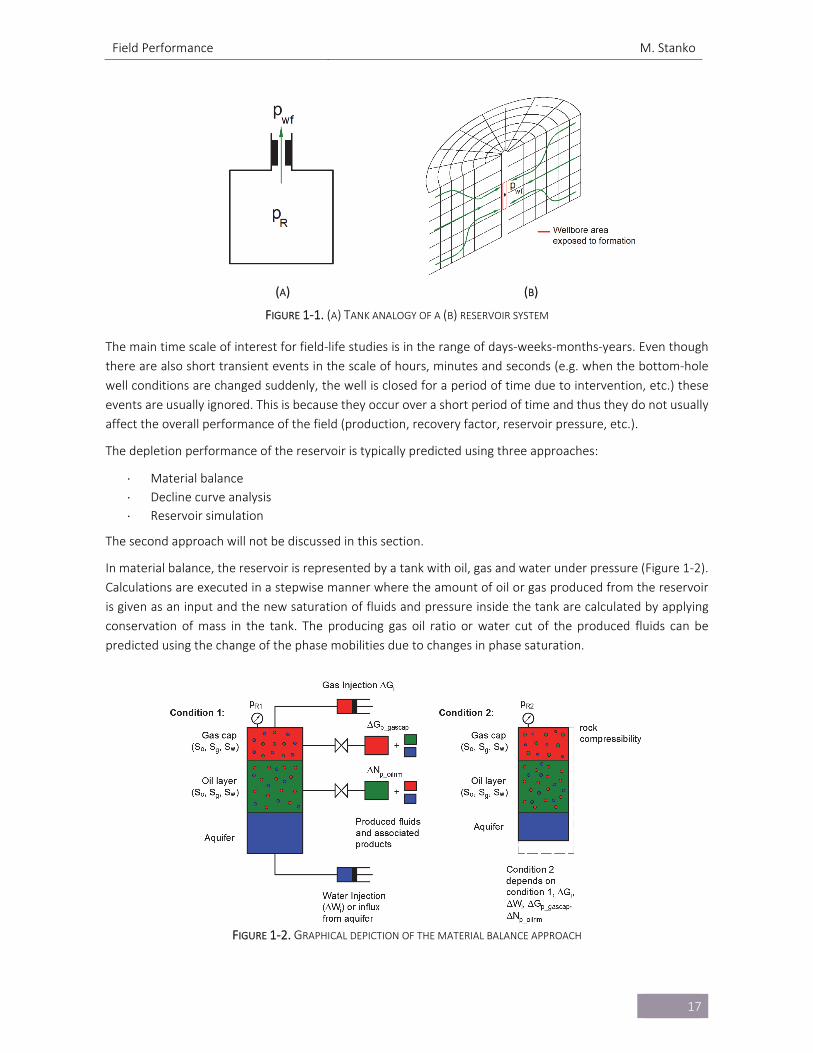
A simplistic but useful analogy of a reservoir system is a tank with fluid under pressure inside. The well is a
small exit port with a restriction. The average reservoir pressure (i.e. the tank pressure, pR) drives fluid from
the tank to the wellbore (pwf, pressure at the exit). The restriction represents the pressure losses that are
generated when the fluid flows through the formation towards the well. When fluid is drained from the tank
(formation) the tank pressure (reservoir pressure) is reduced, thus reducing the flow rate that the tank can
deliver at a fixed wellbore pressure.
2 Reservoir models are typically history matched to production data. Production system models are typically tuned with pressure, temperature and rate measurements along the production system.
Field Performance M. Stanko
17
(A) (B)
FIGURE 1‐1. (A) TANK ANALOGY OF A (B) RESERVOIR SYSTEM
The main time scale of interest for field‐life studies is in the range of days‐weeks‐months‐years. Even though
there are also short transient events in the scale of hours, minutes and seconds (e.g. when the bottom‐hole
well conditions are changed suddenly, the well is closed for a period of time due to intervention, etc.) these
events are usually ignored. This is because they occur over a short period of time and thus they do not usually
affect the overall performance of the field (production, recovery factor, reservoir pressure, etc.).
The depletion performance of the reservoir is typically predicted using three approaches:
Material balance
Decline curve analysis
Reservoir simulation
The second approach will not be discussed in this section.
In material balance, the reservoir is represented by a tank with oil, gas and water under pressure (Figure 1‐2).
Calculations are executed in a stepwise manner where the amount of oil or gas produced from the reservoir
is given as an input and the new saturation of fluids and pressure inside the tank are calculated by applying
conservation of mass in the tank. The producing gas oil ratio or water cut of the produced fluids can be
predicted using the change of the phase mobilities due to changes in phase saturation.
FIGURE 1‐2. GRAPHICAL DEPICTION OF THE MATERIAL BALANCE APPROACH
Field Performance M. Stanko
18
A material balance model requires the oil (or gas) cumulative production as an input and thus cannot be used
to predict the production output of the reservoir with time. For that purpose, an additional model must be
provided to quantify the pressure drop between reservoir and a downstream condition (e.g. bottom‐hole
pressure). This model is often an Inflow Performance Relationship curve.
A reservoir simulator is used when it is important to consider the spatial (2D or 3D) variation of properties (e.g.
pressure, saturation) in the reservoir with time. The reservoir model consists of a numerical discretization of
the porous media where mass conservation is applied in every sub‐volume. The flow between cells is described
using an expression for pressure drop in porous media (e.g. Darcy’s Law). Pressure or rate boundary conditions
are applied on the cells where the wells are and no flow conditions are typically applied at the outer edges of
the reservoir.
The model uses as input the initial distribution of pressure, porosities, permeabilities, fluid saturations, and it
computes the time evolution of pressure, oil, gas and water saturation. The simulation is controlled with both
a target rate and a minimum pressure at the well boundaries provided at each time step. The computation is
carried out in a stepwise manner, outputting results for pre‐specified time intervals.
During the solving process, the minimum pressure given is imposed on the well boundary. If the rate computed
is higher than the target rate specified, then the target rate is feasible. A series of iterations are then made
trying several pressure values until one value is found that gives exactly the target rate specified. On the other
hand, if the rate obtained is below the target rate, the target rate is not feasible and the well boundary
condition is the minimum pressure.
Depending of the complexity of the field, in some cases it is possible to use only the reservoir simulator to
predict its performance and neglect the rest of the production system. For example, in a field where each well
is producing to its own separator close to the wellhead, including tubing pressure drop tables in a reservoir
model provides an exact approximation of the field performance.
In reservoir simulation, the grid does not typically capture the near‐wellbore region in detail. The well usually
traverses through several blocks and the block size is much bigger than the wellbore radius. In consequence,
an IPR‐like equation (often called well index or WI) must be used; this equation relates the formation oil, water
and gas with the pressure difference between the block where the well is placed and the wellbore pressure.
1.2. PRODUCTION SYSTEM (SURFACE NETWORK)
The production system is the assembly of wells, pipes, valves, pumps, meters that have the function of
transporting fluids from the reservoir to the processing facilities in a controlled manner. When the fluid travels
from the reservoir(s) (source) to the separator(s) (sink), it must overcome energy losses (e.g. pressure and
temperature drop) and sometimes “compete” with other fluids in transportation conduits.
In contrast with the reservoir, the field‐life analysis of a production system is performed assuming that changes
in reservoir deliverability are slow enough so that the system progresses continuously from one steady‐state
to another. Therefore, the analysis is usually performed at a given point in time, ignoring all past and all present
conditions and using only the current deliverability of the reservoir. Other possible quick transients such as
slugging, intermittent production, etc. are not part of the scope of a field‐life analysis.
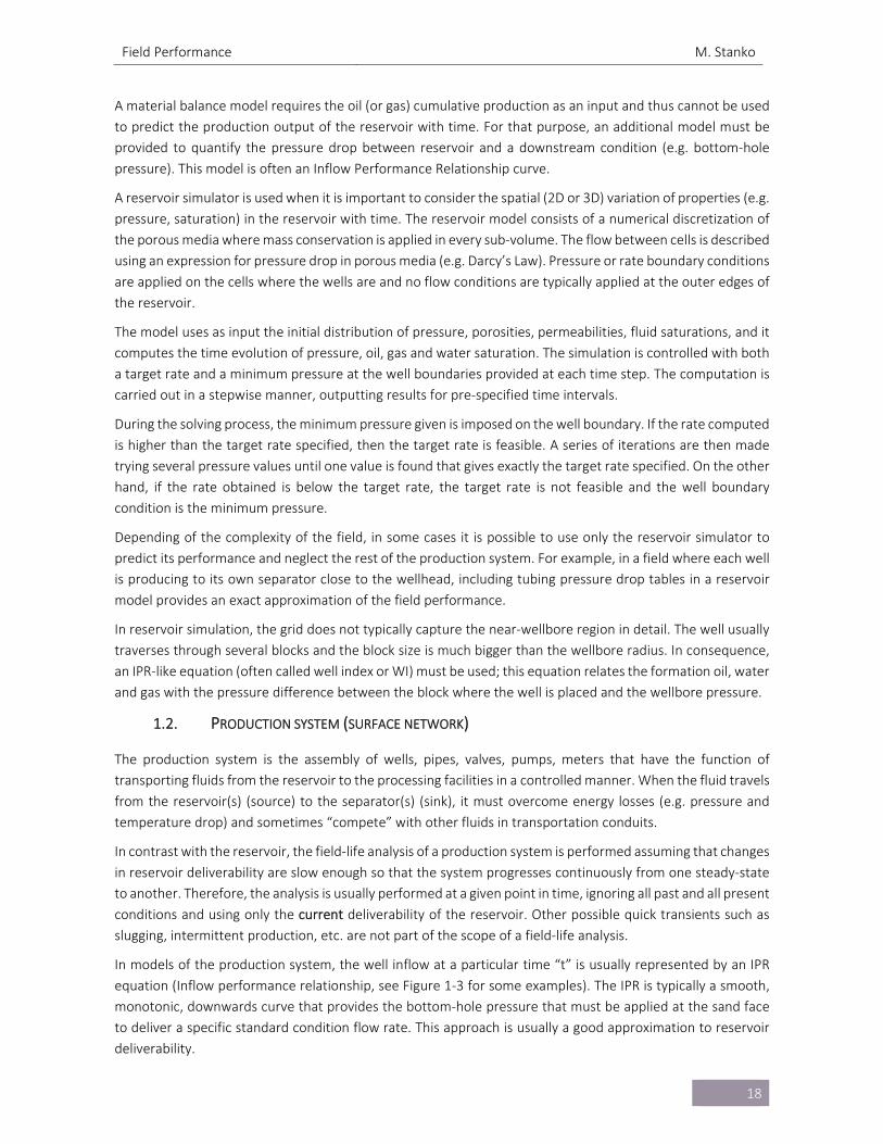
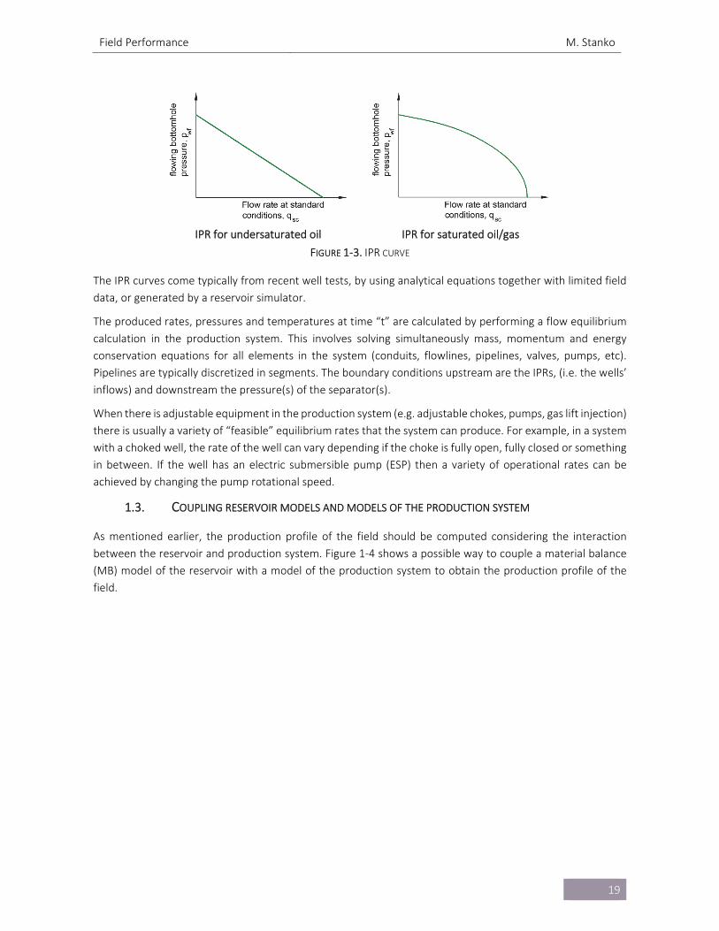
In models of the production system, the well inflow at a particular time “t” is usually represented by an IPR
equation (Inflow performance relationship, see Figure 1‐3 for some examples). The IPR is typically a smooth,
monotonic, downwards curve that provides the bottom‐hole pressure that must be applied at the sand face
to deliver a specific standard condition flow rate. This approach is usually a good approximation to reservoir
deliverability.
Field Performance M. Stanko
19
IPR for undersaturated oil IPR for saturated oil/gas
FIGURE 1‐3. IPR CURVE
The IPR curves come typically from recent well tests, by using analytical equations together with limited field
data, or generated by a reservoir simulator.
The produced rates, pressures and temperatures at time “t” are calculated by performing a flow equilibrium
calculation in the production system. This involves solving simultaneously mass, momentum and energy
conservation equations for all elements in the system (conduits, flowlines, pipelines, valves, pumps, etc).
Pipelines are typically discretized in segments. The boundary conditions upstream are the IPRs, (i.e. the wells’
inflows) and downstream the pressure(s) of the separator(s).
When there is adjustable equipment in the production system (e.g. adjustable chokes, pumps, gas lift injection)
there is usually a variety of “feasible” equilibrium rates that the system can produce. For example, in a system
with a choked well, the rate of the well can vary depending if the choke is fully open, fully closed or something
in between. If the well has an electric submersible pump (ESP) then a variety of operational rates can be
achieved by changing the pump rotational speed.
1.3. COUPLING RESERVOIR MODELS AND MODELS OF THE PRODUCTION SYSTEM
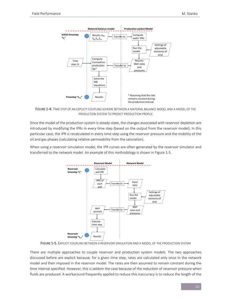
As mentioned earlier, the production profile of the field should be computed considering the interaction
between the reservoir and production system. Figure 1‐4 shows a possible way to couple a material balance
(MB) model of the reservoir with a model of the production system to obtain the production profile of the
field.
Field Performance M. Stanko
20
FIGURE 1‐4. TIME STEP OF AN EXPLICIT COUPLING SCHEME BETWEEN A MATERIAL BALANCE MODEL AND A MODEL OF THE
PRODUCTION SYSTEM TO PREDICT PRODUCTION PROFILE
Since the model of the production system is steady‐state, the changes associated with reservoir depletion are
introduced by modifying the IPRs in every time step (based on the output from the reservoir model). In this
particular case, the IPR is recalculated in every time step using the reservoir pressure and the mobility of the
oil and gas phases (calculating relative permeability from the saturation).
When using a reservoir simulation model, the IPR curves are often generated by the reservoir simulator and
transferred to the network model. An example of this methodology is shown in Figure 1‐5.
FIGURE 1‐5. EXPLICIT COUPLING BETWEEN A RESERVOIR SIMULATION AND A MODEL OF THE PRODUCTION SYSTEM
There are multiple approaches to couple reservoir and production system models. The two approaches
discussed before are explicit because, for a given time step, rates are calculated only once in the network
model and then imposed in the reservoir model. The rates are then assumed to remain constant during the
time interval specified. However, this is seldom the case because of the reduction of reservoir pressure when
fluids are produced. A workaround frequently applied to reduce this inaccuracy is to reduce the length of the
Initial timestep“t1”
Material balance model Production system Model
Transfer toCompute wells’ IPRs
Results: Well rates
and pressures
Transfer to
Solve the MB equations
Timestep “ti+1” Results
Run the model
Settings of adjustable elements (if
any)
Results, pRi, Sgi,Soi,Swi
Compute Cumulative production Qp*
Time
step t
* Assuming that the rate remains constant during the production interval
Calculate well IPR
Reservoir timestep “ti”
Reservoir Model Network Model
IPRs of each well
Input data
Transfer to
Run the model
Well rates and pressures
Transfer toWell controls
Execute time step
Reservoir timestep “ti+1” Results
Settings of adjustable elements (if
any)
Field Performance M. Stanko
21
time step. Explicit coupling strategies sometimes cause instabilities in the solution (oscillating production rates
with time). The reduction of time step length often eliminates this problem.
Explicit coupling strategies are suitable when the models of reservoir and production system are available in
two separate computational routines (often black box commercial packages) and are maintained and used
separately (e.g. by different departments within the company). An explicit coupling minimizes the required
transfer of information between models in every time step.
Other coupling approaches and a detailed discussion about coupling models or the reservoir and the
production system are discussed in detail by Barroux[1‐1].
1.4. PRODUCTION POTENTIAL
For a particular time “t” there will be either a unique rate that the field can produce (if there are no adjustable
elements in the system of they have a fixed setting) or a maximum rate that the field can produce (if there are
adjustable elements). We will refer to this unique or maximum rate that the field can produce at a given point
in time as: “production potential”.
For example, if the well has an adjustable choke the maximum rate is most likely achieved when the choke is
fully open. If the well has an electric submersible pump (ESP) then the maximum rate is probably achieved
when the pump rotational speed is highest. If adjustable elements are present in the system, it is usually
possible to produce any rate lower than the maximum rate by regulating such elements.
The production potential is different from the “well potential” variable printed in every time step by the
reservoir simulator. The well potential is the producing rate obtained when the minimum bottom‐hole
pressure is applied on the well boundary.
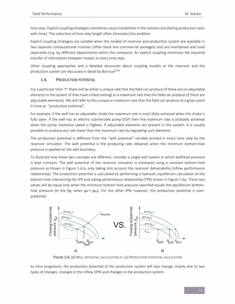
To illustrate how these two concepts are different, consider a single well system in which wellhead pressure
is kept constant. The well potential of the reservoir simulator is estimated using a constant bottom‐hole
pressure as shown in Figure 1‐6.b, only taking into account the reservoir deliverability (inflow performance
relationship). The production potential is calculated by performing a hydraulic equilibrium calculation at the
bottom‐hole intersecting the IPR and tubing performance relationship (TPR) shown in Figure 1‐6a. These two
values will be equal only when the minimum bottom‐hole pressure specified equals the equilibrium bottom‐
hole pressure (in the fig. when pR= pR3). For the other IPRs however, the production potential is over‐predicted.
A) B)
FIGURE 1‐6. (B) WELL POTENTIAL CALCULATION VS. (A) PRODUCTION POTENTIAL CALCULATION
As time progresses, the production potential of the production system will also change, mainly due to two
types of changes: changes in the inflow (IPR) and changes to the production system.
Field Performance M. Stanko
22
A strategy commonly used in reservoir management when producing the field in plateau mode is to allocate
production to individual wells using their potential. At a given time, the well and field potential are calculated,
and well split factor are computed by dividing the individual well production potential by the field production
potential. Then, the rate to be produced by each well is calculated by multiplying the field plateau rate by the
individual well split factor.
In a producing field, the reservoir deliverability follows a trend with depletion similar to reservoir pressure, i.e.
is reduced with time. This is not only due to reservoir pressure decline, but for example, in an oil well, an
increase of the well’s producing GOR and WC will reduce the oil productivity as well. Changes in reservoir
deliverability affect all components of the production system downstream the reservoir, for example if the
well producing gas oil ratio (GOR) changes, then pressure losses will change in all downstream conduits.
Some examples of changes to the production system are man‐made changes in the pipeline diameter,
lowering separator pressure, modification of choke opening, changes in well completion, installation of
artificial lift, well stimulation or fracking, etc. Other changes are reduction of the conduits’ cross section due
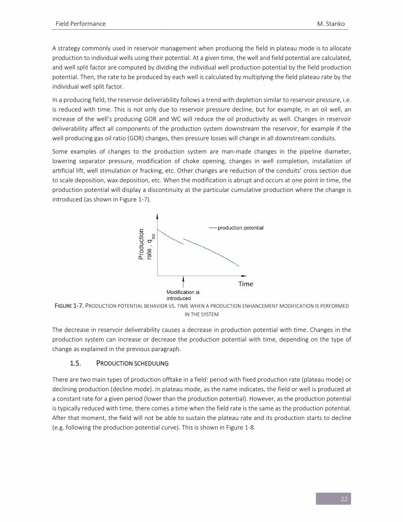
to scale deposition, wax deposition, etc. When the modification is abrupt and occurs at one point in time, the
production potential will display a discontinuity at the particular cumulative production where the change is
introduced (as shown in Figure 1‐7).
FIGURE 1‐7. PRODUCTION POTENTIAL BEHAVIOR VS. TIME WHEN A PRODUCTION ENHANCEMENT MODIFICATION IS PERFORMED
IN THE SYSTEM
The decrease in reservoir deliverability causes a decrease in production potential with time. Changes in the
production system can increase or decrease the production potential with time, depending on the type of
change as explained in the previous paragraph.
1.5. PRODUCTION SCHEDULING
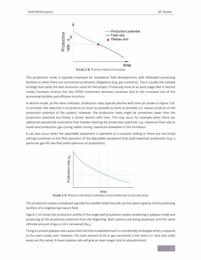
There are two main types of production offtake in a field: period with fixed production rate (plateau mode) or
declining production (decline mode). In plateau mode, as the name indicates, the field or well is produced at
a constant rate for a given period (lower than the production potential). However, as the production potential
is typically reduced with time, there comes a time when the field rate is the same as the production potential.
After that moment, the field will not be able to sustain the plateau rate and its production starts to decline
(e.g. following the production potential curve). This is shown in Figure 1‐8.
Field Performance M. Stanko
23
FIGURE 1‐8. PLATEAU PRODUCTION MODE
This production mode is typically employed for standalone field developments with dedicated processing
facilities or when there are contractual production obligations (e.g. gas contracts). This is usually the outtake
strategy that yields the best economic value for the project. Producing more at an early stage (like in decline
mode) increases revenue but the CAPEX investment becomes excessive due to the increased size of the
processing facilities and offshore structure.
In decline mode, as the name indicates, production rates typically decline with time (as shown in Figure 1‐9).
In principle, the objective is to produce as much as possible as early as possible (i.e. always produce at the
production potential of the system). However, the production rates might be sometimes lower than the
production potential but follow a similar decline with time. This may occur for example when there are
additional operational constraints that impede reaching the production potential, e.g. maximum flow rate to
avoid sand production, gas coning, water coning, maximum drawdown in the formation.
It can also occur when the adjustable equipment is operated at a constant setting or there are non‐trivial
settings (unknown to the field operator) of the adjustable equipment that yield maximum production (e.g. a
particular gas‐lift rate that yields optimum oil production).
FIGURE 1‐9. PRODUCTION PROFILE OBTAINED WHEN OPERATING IN DECLINE MODE
This production mode is employed typically for satellite fields that will use the spare capacity of the processing
facilities of a neighboring mature field.
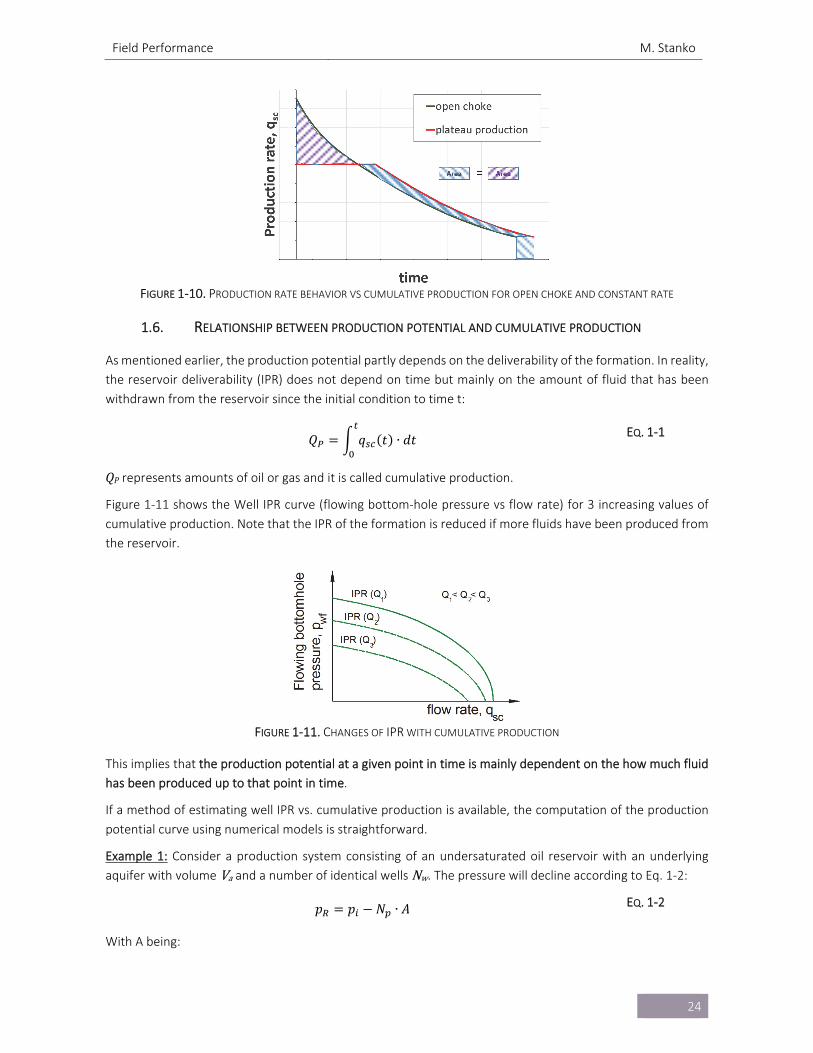
Figure 1‐10 shows the production profile of the single well production system producing in plateau mode and
producing at the production potential from the beginning. Both systems are being produced until the same
ultimate amount of gas or oil is recovered (QPU).
Fixing a constant plateau rate causes that the time to abandonment is considerably prolonged when compared
to the open choke case. However, the total amount of oil or gas recovered is the same (i.e. blue and violet
areas are the same). A lower plateau rate will give an even longer time to abandonment.
Field Performance M. Stanko
24
FIGURE 1‐10. PRODUCTION RATE BEHAVIOR VS CUMULATIVE PRODUCTION FOR OPEN CHOKE AND CONSTANT RATE
1.6. RELATIONSHIP BETWEEN PRODUCTION POTENTIAL AND CUMULATIVE PRODUCTION
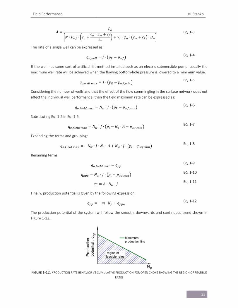
As mentioned earlier, the production potential partly depends on the deliverability of the formation. In reality,
the reservoir deliverability (IPR) does not depend on time but mainly on the amount of fluid that has been
withdrawn from the reservoir since the initial condition to time t:
𝑄 𝑞 𝑡 ∙ 𝑑𝑡 EQ. 1‐1
QP represents amounts of oil or gas and it is called cumulative production.
Figure 1‐11 shows the Well IPR curve (flowing bottom‐hole pressure vs flow rate) for 3 increasing values of
cumulative production. Note that the IPR of the formation is reduced if more fluids have been produced from
the reservoir.
FIGURE 1‐11. CHANGES OF IPR WITH CUMULATIVE PRODUCTION
This implies that the production potential at a given point in time is mainly dependent on the how much fluid
has been produced up to that point in time.
If a method of estimating well IPR vs. cumulative production is available, the computation of the production
potential curve using numerical models is straightforward.
Example 1: Consider a production system consisting of an undersaturated oil reservoir with an underlying
aquifer with volume Va and a number of identical wells Nw. The pressure will decline according to Eq. 1‐2:
𝑝 𝑝 𝑁 ∙ 𝐴 EQ. 1‐2
With A being:
Field Performance M. Stanko
25
𝐴𝐵
𝑁 ∙ 𝐵 , ∙ 𝑐𝑐 ∙ 𝑆 𝑐
𝑆 𝑉 ∙ 𝜙 ∙ 𝑐 𝑐 ∙ 𝐵 EQ. 1‐3
The rate of a single well can be expressed as:
𝑞 , 𝐽 ∙ 𝑝 𝑝 EQ. 1‐4
If the well has some sort of artificial lift method installed such as an electric submersible pump, usually the
maximum well rate will be achieved when the flowing bottom‐hole pressure is lowered to a minimum value:
𝑞 , 𝐽 ∙ 𝑝 𝑝 , EQ. 1‐5
Considering the number of wells and that the effect of the flow commingling in the surface network does not
affect the individual well performance, then the field maximum rate can be expressed as:
𝑞 , 𝑁 ∙ 𝐽 ∙ 𝑝 𝑝 , EQ. 1‐6
Substituting Eq. 1‐2 in Eq. 1‐6:
𝑞 , 𝑁 ∙ 𝐽 ∙ 𝑝 𝑁 ∙ 𝐴 𝑝 , EQ. 1‐7
Expanding the terms and grouping:
𝑞 , 𝑁 ∙ 𝐽 ∙ 𝑁 ∙ 𝐴 𝑁 ∙ 𝐽 ∙ 𝑝 𝑝 , EQ. 1‐8
Renaming terms:
𝑞 , 𝑞 EQ. 1‐9
𝑞 𝑁 ∙ 𝐽 ∙ 𝑝 𝑝 ,EQ. 1‐10
𝑚 𝐴 ∙ 𝑁 ∙ 𝐽 EQ. 1‐11
Finally, production potential is given by the following expression:
𝑞 𝑚 ∙ 𝑁 𝑞 EQ. 1‐12
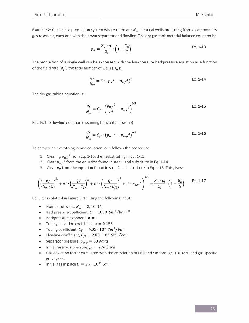
The production potential of the system will follow the smooth, downwards and continuous trend shown in
Figure 1‐12.
FIGURE 1‐12. PRODUCTION RATE BEHAVIOR VS CUMULATIVE PRODUCTION FOR OPEN CHOKE SHOWING THE REGION OF FEASIBLE
RATES
Field Performance M. Stanko
26
Example 2: Consider a production system where there are 𝑁 identical wells producing from a common dry
gas reservoir, each one with their own separator and flowline. The dry gas tank material balance equation is:
𝑝𝑍 ∙ 𝑝
𝑍∙ 1
𝐺𝐺
EQ. 1‐13
The production of a single well can be expressed with the low‐pressure backpressure equation as a function
of the field rate (𝑞 ), the total number of wells (𝑁 ):
𝑞𝑁
𝐶 ∙ 𝑝 𝑝 EQ. 1‐14
The dry gas tubing equation is:
𝑞𝑁
𝐶 ∙𝑝
𝑒𝑝
.
EQ. 1‐15
Finally, the flowline equation (assuming horizontal flowline):
𝑞𝑁
𝐶 ∙ 𝑝 𝑝. EQ. 1‐16
To compound everything in one equation, one follows the procedure:
1. Clearing 𝑝 from Eq. 1‐16, then substituting in Eq. 1‐15.
2. Clear 𝑝 from the equation found in step 1 and substitute in Eq. 1‐14.
3. Clear 𝑝 from the equation found in step 2 and substitute in Eq. 1‐13. This gives:
𝑞𝑁 ∙ 𝐶
𝑒 ∙𝑞
𝑁 ∙ 𝐶𝑒 ∙
𝑞𝑁 ∙ 𝐶
𝑒 ∙ 𝑝
.𝑍 ∙ 𝑝
𝑍∙ 1
𝐺𝐺
EQ. 1‐17
Eq. 1‐17 is plotted in Figure 1‐13 using the following input:
Number of wells, 𝑁 5, 10, 15 Backpressure coefficient, 𝐶 1000 𝑆𝑚 𝑏𝑎𝑟 ∙⁄ Backpressure exponent, 𝑛 1 Tubing elevation coefficient, 𝑠 0.155 Tubing coefficient, 𝐶 4.03 ∙ 10 𝑆𝑚 𝑏𝑎𝑟⁄
Flowline coefficient, 𝐶 2.83 ∙ 10 𝑆𝑚 𝑏𝑎𝑟⁄
Separator pressure, 𝑝 30 𝑏𝑎𝑟𝑎 Initial reservoir pressure, 𝑝 276 𝑏𝑎𝑟𝑎 Gas deviation factor calculated with the correlation of Hall and Yarborough, T = 92 oC and gas specific
gravity 0.5.
Initial gas in place 𝐺 2.7 ∙ 10 𝑆𝑚
Field Performance M. Stanko
27
FIGURE 1‐13. FIELD PRODUCTION POTENTIAL VS CUMULATIVE PRODUCTION FOR DRY GAS RESERVOIR WITH STANDALONE WELLS
When more wells are used in the system, the production potential is higher. The effect is proportional, due to
the fact that well are standalone, and adding a new well does not interfere or affect the performance of other
wells.
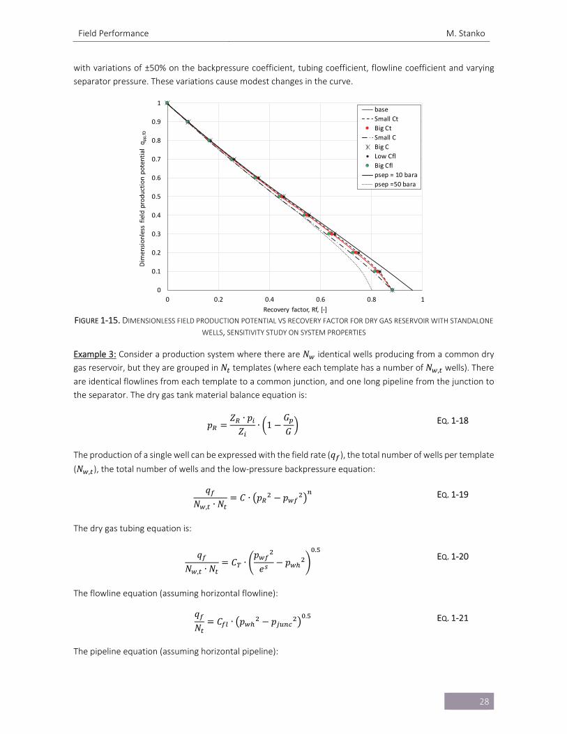
Figure 1‐14 shows the dimensionless production potential of the field versus recovery factor. The
dimensionless production potential has been found by dividing each field production potential curve by its
maximum production potential (i.e. the production potential at Gp = 0 Sm3) and the cumulative production by
the initial gas in place. Surprisingly, the curves for all number of wells fall on top of each other.
FIGURE 1‐14. DIMENSIONLESS FIELD PRODUCTION POTENTIAL VS RECOVERY FACTOR FOR DRY GAS RESERVOIR WITH STANDALONE
WELLS
The dimensionless production potential curve in Figure 1‐14 remains unchanged if the amount of gas in place
is increased or decreased. Figure 1‐15 shows the dimensionless production potential of the field estimated
0.00E+00
1.00E+07
2.00E+07
3.00E+07
4.00E+07
5.00E+07
6.00E+07
7.00E+07
8.00E+07
9.00E+07
0 5E+10 1E+11 1.5E+11 2E+11 2.5E+11
Field production potential q
pp,f, [Sm
3/d]
Cumulative production Gp, [Sm3]
5 standalone wells
10 standalone wells
15 standalone wells
0
0.1
0.2
0.3
0.4
0.5
0.6
0.7
0.8
0.9
1
0 0.2 0.4 0.6 0.8 1
Dim
ensionless field production potential qpp
,fD
Recovery factor, Rf, [‐]
5 standalone wells
10 standalone wells
15 standalone wells
Field Performance M. Stanko
28
with variations of ±50% on the backpressure coefficient, tubing coefficient, flowline coefficient and varying
separator pressure. These variations cause modest changes in the curve.
FIGURE 1‐15. DIMENSIONLESS FIELD PRODUCTION POTENTIAL VS RECOVERY FACTOR FOR DRY GAS RESERVOIR WITH STANDALONE
WELLS, SENSITIVITY STUDY ON SYSTEM PROPERTIES
Example 3: Consider a production system where there are 𝑁 identical wells producing from a common dry
gas reservoir, but they are grouped in 𝑁 templates (where each template has a number of 𝑁 , wells). There
are identical flowlines from each template to a common junction, and one long pipeline from the junction to
the separator. The dry gas tank material balance equation is:
𝑝𝑍 ∙ 𝑝
𝑍∙ 1
𝐺𝐺
EQ. 1‐18
The production of a single well can be expressed with the field rate (𝑞 ), the total number of wells per template
(𝑁 , ), the total number of wells and the low‐pressure backpressure equation:
𝑞𝑁 , ∙ 𝑁
𝐶 ∙ 𝑝 𝑝 EQ. 1‐19
The dry gas tubing equation is:
𝑞𝑁 , ∙ 𝑁
𝐶 ∙𝑝
𝑒𝑝
.
EQ. 1‐20
The flowline equation (assuming horizontal flowline):
𝑞𝑁
𝐶 ∙ 𝑝 𝑝. EQ. 1‐21
The pipeline equation (assuming horizontal pipeline):
0
0.1
0.2
0.3
0.4
0.5
0.6
0.7
0.8
0.9
1
0 0.2 0.4 0.6 0.8 1
Dim
ensionless field production potential qpp,fD
Recovery factor, Rf, [‐]
base
Small Ct
Big Ct
Small C
Big C
Low Cfl
Big Cfl
psep = 10 bara
psep =50 bara
Field Performance M. Stanko
29
𝑞 𝐶 ∙ 𝑝 𝑝.
EQ. 1‐22
To compound everything in one equation, one follows the procedure:
1. Clearing 𝑝 from Eq. 1‐22, then substituting in Eq. 1‐21.
2. Clear 𝑝 from the equation found in step 1 and substitute in Eq. 1‐20.
3. Clear 𝑝 from the equation found in step 2 and substitute in Eq. 1‐19.
4. Clear 𝑝 from the equation found in step 3 and substitute in Eq. 1‐18. This gives:
𝑞𝑁 , ∙ 𝑁 ∙ 𝐶
𝑒 ∙𝑞
𝑁 , ∙ 𝑁 ∙ 𝐶𝑒 ∙
𝑞𝐶
𝑒 ∙ 𝑝 𝑒
∙𝑞
𝐶 ∙ 𝑁
.
𝑍 ∙ 𝑝𝑍
∙ 1𝐺𝐺
EQ. 1‐23
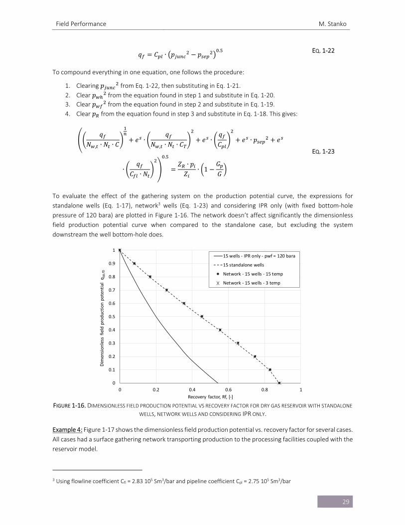
To evaluate the effect of the gathering system on the production potential curve, the expressions for
standalone wells (Eq. 1‐17), network3 wells (Eq. 1‐23) and considering IPR only (with fixed bottom‐hole
pressure of 120 bara) are plotted in Figure 1‐16. The network doesn’t affect significantly the dimensionless
field production potential curve when compared to the standalone case, but excluding the system
downstream the well bottom‐hole does.
FIGURE 1‐16. DIMENSIONLESS FIELD PRODUCTION POTENTIAL VS RECOVERY FACTOR FOR DRY GAS RESERVOIR WITH STANDALONE
WELLS, NETWORK WELLS AND CONSIDERING IPR ONLY.
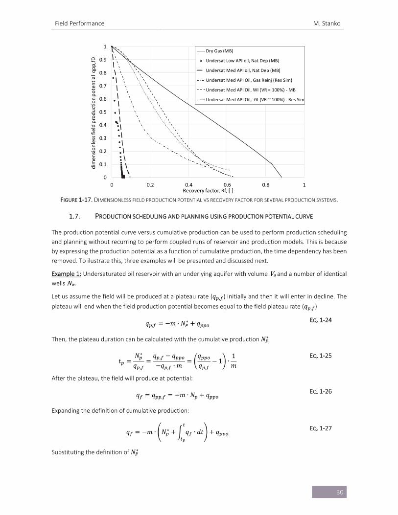
Example 4: Figure 1‐17 shows the dimensionless field production potential vs. recovery factor for several cases.
All cases had a surface gathering network transporting production to the processing facilities coupled with the
reservoir model.
3 Using flowline coefficient Cfl = 2.83 105 Sm3/bar and pipeline coefficient Cpl = 2.75 105 Sm3/bar
0
0.1
0.2
0.3
0.4
0.5
0.6
0.7
0.8
0.9
1
0 0.2 0.4 0.6 0.8 1
Dim
ensionless field production potential qpp
,fD
Recovery factor, Rf, [‐]
15 wells ‐ IPR only ‐ pwf = 120 bara
15 standalone wells
Network ‐ 15 wells ‐ 15 temp
Network ‐ 15 wells ‐ 3 temp
Field Performance M. Stanko
30
FIGURE 1‐17. DIMENSIONLESS FIELD PRODUCTION POTENTIAL VS RECOVERY FACTOR FOR SEVERAL PRODUCTION SYSTEMS.
1.7. PRODUCTION SCHEDULING AND PLANNING USING PRODUCTION POTENTIAL CURVE
The production potential curve versus cumulative production can be used to perform production scheduling
and planning without recurring to perform coupled runs of reservoir and production models. This is because
by expressing the production potential as a function of cumulative production, the time dependency has been
removed. To ilustrate this, three examples will be presented and discussed next.
Example 1: Undersaturated oil reservoir with an underlying aquifer with volume Va and a number of identical
wells Nw.
Let us assume the field will be produced at a plateau rate (𝑞 , ) initially and then it will enter in decline. The
plateau will end when the field production potential becomes equal to the field plateau rate (𝑞 , )
𝑞 , 𝑚 ∙ 𝑁∗ 𝑞 EQ. 1‐24
Then, the plateau duration can be calculated with the cumulative production 𝑁∗
𝑡𝑁∗
𝑞 ,
𝑞 , 𝑞𝑞 , ∙ 𝑚
𝑞𝑞 ,
1 ∙1𝑚
EQ. 1‐25
After the plateau, the field will produce at potential:
𝑞 𝑞 , 𝑚 ∙ 𝑁 𝑞 EQ. 1‐26
Expanding the definition of cumulative production:
𝑞 𝑚 ∙ 𝑁∗ 𝑞 ∙ 𝑑𝑡 𝑞 EQ. 1‐27
Substituting the definition of 𝑁∗
0
0.1
0.2
0.3
0.4
0.5
0.6
0.7
0.8
0.9
1
0 0.2 0.4 0.6 0.8 1
dim
ensionless field production potential qpp,fD
Recovery factor, Rf, [‐]
Dry Gas (MB)
Undersat Low API oil, Nat Dep (MB)
Undersat Med API oil, Nat Dep (MB)
Undersat Med API Oil, Gas Reinj (Res Sim)
Undersat Med API Oil, WI (VR = 100%) ‐ MB
Undersat Med API Oil, GI (VR ~ 100%) ‐ Res Sim
Field Performance M. Stanko
31
𝑞 𝑚 ∙ 𝑞 ∙ 𝑑𝑡 𝑚 ∙𝑞 𝑞
𝑚𝑞 EQ. 1‐28
Simplifying:
𝑞 𝑚 ∙ 𝑞 ∙ 𝑑𝑡 𝑞 _ EQ. 1‐29
A solution to this equation is:
𝑞 𝑞 , ∙ 𝑒 ∙ EQ. 1‐30
Therefore, if the production potential displays a linear behavior with respect to cumulative production, the
production profile post‐plateau has an exponential behavior with time. The coefficient of the exponential
function, that dictates the rate decline depends both on the decline characteristics of the reservoir (A), the flow “resistance” in the formation (and in principle, in the tubing and surface flowlines) and the number of
wells. If the number of wells is increased, the decline will become more pronounced.
The field production profile is given by the following equations:
𝑓𝑜𝑟 𝑡 𝑡 𝑞 𝑞 , EQ. 1‐31
𝑓𝑜𝑟 𝑡 𝑡 𝑞 𝑞 , ∙ 𝑒 ∙ EQ. 1‐32
Example 2: Plateau mode production
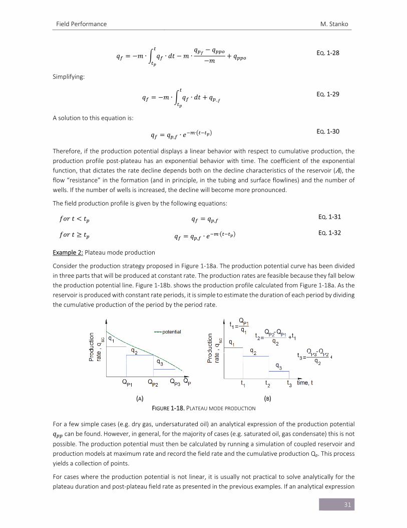
Consider the production strategy proposed in Figure 1‐18a. The production potential curve has been divided
in three parts that will be produced at constant rate. The production rates are feasible because they fall below
the production potential line. Figure 1‐18b. shows the production profile calculated from Figure 1‐18a. As the
reservoir is produced with constant rate periods, it is simple to estimate the duration of each period by dividing
the cumulative production of the period by the period rate.
(A) (B)
FIGURE 1‐18. PLATEAU MODE PRODUCTION
For a few simple cases (e.g. dry gas, undersaturated oil) an analytical expression of the production potential
𝑞 can be found. However, in general, for the majority of cases (e.g. saturated oil, gas condensate) this is not
possible. The production potential must then be calculated by running a simulation of coupled reservoir and
production models at maximum rate and record the field rate and the cumulative production Qp. This process
yields a collection of points.
For cases where the production potential is not linear, it is usually not practical to solve analytically for the
plateau duration and post‐plateau field rate as presented in the previous examples. If an analytical expression
Field Performance M. Stanko
32
is available, plateau duration can be estimated by substituting the desired plateau rate and solve the equation
(usually with a root solving method) for the cumulative production at plateau end 𝑄∗ . If a collection of points
is available, 𝑄∗ can be found by interpolating on the table. With 𝑄∗ and plateau rate, one can then calculate
plateau duration.
The post‐plateau field rate can be estimated by dividing the post‐plateau period in a series of discrete time
steps and expressing the cumulative production at time ti using the trapezoidal rule for numerical integration:
𝑄 𝑡 0.5 ∙ 𝑞 𝑡 𝑞 𝑡 ∙ 𝑡 𝑡 𝑄 𝑡 EQ. 1‐33
All rates in the post‐plateau period should fall on the production potential curve, i.e.
𝑞 𝑡 𝑓 𝑄 𝑡 EQ. 1‐34
Eq. 1‐33 and Eq. 1‐34 must be solved simultaneously for each time step ti and departing from plateau end. If
the production potential is available as a collection of points, Eq. 1‐34 means interpolation.
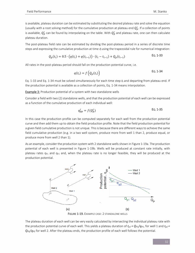
Example 3: Production potential of a system with two standalone wells
Consider a field with two (2) standalone wells, and that the production potential of each well can be expressed
as a function of the cumulative production of each individual well:
𝑞 𝑓 𝑄 EQ. 1‐35
In this case the production profile can be computed separately for each well from the production potential
curve and then add them up to obtain the field production profile. Note that the field production potential for
a given field cumulative production is not unique. This is because there are different ways to achieve the same
field cumulative production (e.g. in a two well system, produce more from well 1 than 2, produce equal, or
produce more from well 2 than 1).
As an example, consider the production system with 2 standalone wells shown in Figure 1‐19a. The production
potential of each well is presented in Figure 1‐19b. Wells will be produced at constant rate initially, with
plateau rates qP1 and qP2 and, when the plateau rate is no longer feasible, they will be produced at the
production potential.
(A) (B)
FIGURE 1‐19. EXAMPLE CASE: 2 STANDALONE WELLS
The plateau duration of each well can be very easily calculated by intersecting the individual plateau rate with
the production potential curve of each well. This yields a plateau duration of tp1=QP1/qP1, for well 1 and tp2=QP2/qP2 for well 2. After the plateau ends, the production profile of each well follows the potential.
Field Performance M. Stanko
33
A typical reservoir management problem consists of how to define well rates to maximize field plateau
duration when a fixed field rate is desired. If individual well plateau rates are to be kept constant, this can be
achieved by finding the plateau rates for which the plateau end occurs at the same time. If the production
potential curves are straight lines the following procedure is suitable:
The production potential curve for well 1:
𝑞 𝑚 ∙ 𝑄 𝑞 EQ. 1‐36
The cumulative production at which the production potential (qpp1) is equal to the plateau rate (qp1), i.e. QPp1, is:
𝑄𝑞 𝑞
𝑚 EQ. 1‐37
Similarly, for well 2:
𝑄𝑞 𝑞
𝑚 EQ. 1‐38
Then the plateau duration has to be the same for both wells:
𝑡𝑄𝑞
; 𝑡𝑄𝑞
EQ. 1‐39
Substituting Eq. 1‐37 and Eq. 1‐38 in Eq. 1‐39:
𝑞 𝑞𝑚 ∙ 𝑞
𝑞 𝑞𝑚 ∙ 𝑞
EQ. 1‐40
𝑞𝑞
1𝑚𝑚
∙𝑞
𝑞1
EQ. 1‐41
Eq. 1‐41 has two unknowns, therefore one more equation is needed. Clearing qp2 from the expression of the
total plateau rate:
𝑞 𝑞 𝑞 EQ. 1‐42
Substituting Eq. 1‐42 in Eq. 1‐41 yields:
𝑞 ∙ 𝑚 𝑚 𝑞 ∙ 𝑞 ∙ 𝑚 𝑞 ∙ 𝑚 𝑞 ∙ 𝑚 𝑞 ∙ 𝑚 𝑞 ∙ 𝑚 ∙ 𝑞0
EQ. 1‐43
Eq. 1‐43 can be solved with the quadratic formula to find qp1:
𝑎 𝑚 𝑚 EQ. 1‐44
𝑏 𝑞 ∙ 𝑚 𝑞 ∙ 𝑚 𝑞 ∙ 𝑚 𝑞 ∙ 𝑚 EQ. 1‐45
𝑐 𝑞 ∙ 𝑚 ∙ 𝑞 EQ. 1‐46
𝑞𝑏 √𝑏 4 ∙ 𝑎 ∙ 𝑐
2 ∙ 𝑎
EQ. 1‐47
Note that the main constraints used to solve this problem were that both wells must produce in plateau mode
with a constant rate and then will enter in decline at the same time. However, there are infinite alternatives
Field Performance M. Stanko
34
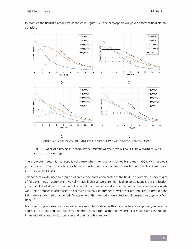
to produce the field at plateau rate as shown in Figure 1‐20 and each option will yield a different field plateau
duration.
(A) (B)
5
(C) (D)
FIGURE 1‐20. 4 DIFFERENT ALTERNATIVES TO PRODUCE THE TWO WELLS SYSTEM IN PLATEAU MODE
1.8. APPLICABILITY OF THE PRODUCTION POTENTIAL CONCEPT IN REAL FIELDS AND MULTI‐WELL
PRODUCTION SYSTEMS
The production potential concept is valid only when the reservoir (or well) producing GOR, WC, reservoir
pressure and IPR can be safely predicted as a function of its cumulative production and the transient period
(infinite acting) is short.
This concept can be used to design and predict the production profile of the field. For example, in early stages
of field planning an assumption typically made is that all wells are identical. In consequence, the production
potential of the field is just the multiplication of the number of wells time the production potential of a single
well. This approach is often used to estimate roughly the number of wells that are required to produce the
field rate for a desired time period. An example of this method is presented and discussed thoroughly by Van
Dam [1‐5].
For more complex cases, e.g. reservoirs that cannot be modeled with a material balance approach, an iterative
approach is often used (without using the production potential method) where field models are run multiple
times with different production rates and their results compared.
0 2 4 6 8 10 12 14 16
flow rate, [Sm
^3/d]
time, t, [t]
q_well_1
q_well_2
qpp_well_1
qpp_well_2
q_field
0 2 4 6 8 10 12 14 16
flow rate, [Sm
^3/d]
time, t, [t]
q_well_1
q_well_2
qpp_well_1
qpp_well_2
q_field
0 2 4 6 8 10 12 14 16
flow rate, [Sm
^3/d]
time, t, [t]
q_well_1
q_well_2
qpp_well_1
qpp_well_2
q_field
0 2 4 6 8 10 12 14 16
flow rate, [Sm
^3/d]
time, t, [t]
q_well_1
q_well_2
qpp_well_1
qpp_well_2
q_field
Field Performance M. Stanko
35
REFERENCES
[1‐1] Barroux, C., Duchet‐Suchaux, P., Samier, P. & Nabil, R. (2000). Linking Reservoir and Surface
Simulators: How to improve the Coupled Solutions. SPE‐65159. European Petroleum Conference.
Paris: Society of Petroleum Engineers.
[1‐2] Golan, M.; Whitson, C. H. (1986). Well Performance. Second Edition. Prentice‐Hall Inc. Englewood
Cliffs, New Jersey.
[1‐3] Nind, T. (1964). Principles of Oil Well Production. McGraw‐Hill.
[1‐4] Van Dam, J. (1986). Planning of Optimum Production from a Natural Gas Field. Journal of the
Institute of Petroleum 54 (521).
Flow Performance in Production Systems M. Stanko
36
2. FLOW PERFORMANCE IN PRODUCTION SYSTEMS
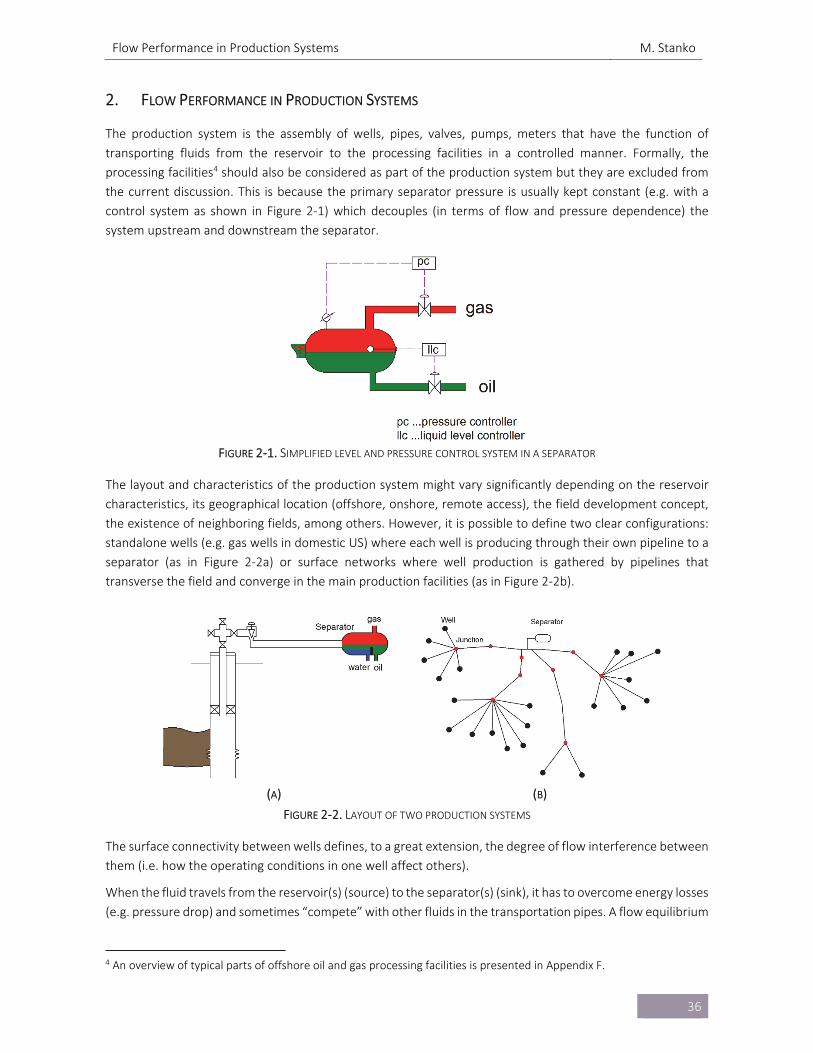
The production system is the assembly of wells, pipes, valves, pumps, meters that have the function of
transporting fluids from the reservoir to the processing facilities in a controlled manner. Formally, the
processing facilities4 should also be considered as part of the production system but they are excluded from
the current discussion. This is because the primary separator pressure is usually kept constant (e.g. with a
control system as shown in Figure 2‐1) which decouples (in terms of flow and pressure dependence) the
system upstream and downstream the separator.
FIGURE 2‐1. SIMPLIFIED LEVEL AND PRESSURE CONTROL SYSTEM IN A SEPARATOR
The layout and characteristics of the production system might vary significantly depending on the reservoir
characteristics, its geographical location (offshore, onshore, remote access), the field development concept,
the existence of neighboring fields, among others. However, it is possible to define two clear configurations:
standalone wells (e.g. gas wells in domestic US) where each well is producing through their own pipeline to a
separator (as in Figure 2‐2a) or surface networks where well production is gathered by pipelines that
transverse the field and converge in the main production facilities (as in Figure 2‐2b).
(A) (B)
FIGURE 2‐2. LAYOUT OF TWO PRODUCTION SYSTEMS
The surface connectivity between wells defines, to a great extension, the degree of flow interference between
them (i.e. how the operating conditions in one well affect others).
When the fluid travels from the reservoir(s) (source) to the separator(s) (sink), it has to overcome energy losses
(e.g. pressure drop) and sometimes “compete” with other fluids in the transportation pipes. A flow equilibrium
4 An overview of typical parts of offshore oil and gas processing facilities is presented in Appendix F.
Flow Performance in Production Systems M. Stanko
37
state is reached where the producing rates, pressures and temperatures of the system are a product of a
balance between the capacity of each source and the existing energy losses/additions.
Numerical models are often used to understand and estimate the flow equilibrium state of production
systems. The numerical model of a production system is usually a steady state representation that comprises
from the well bottom‐holes (source nodes) to the first stage separator(s) (sink nodes). The main purpose of
this model is to compute the rates from each well and the pressure and temperature distribution in the
production system.
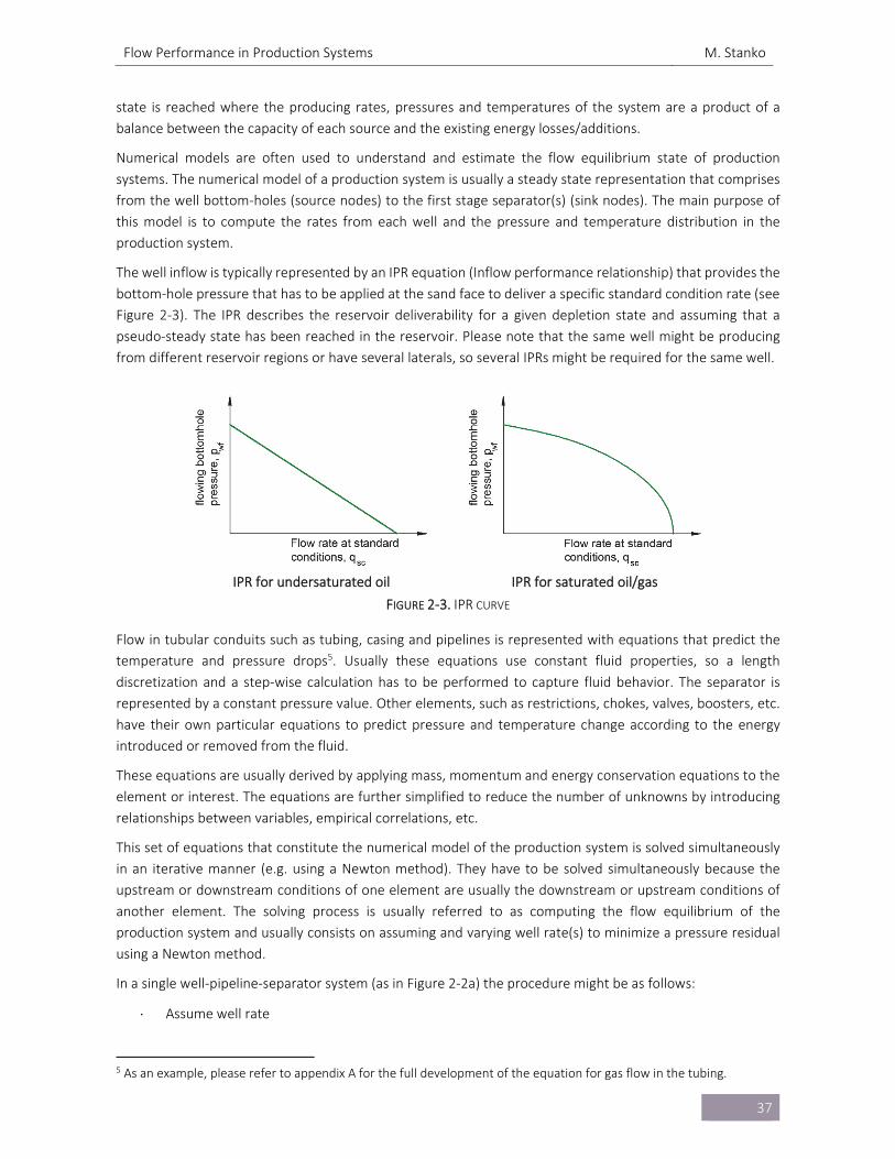
The well inflow is typically represented by an IPR equation (Inflow performance relationship) that provides the
bottom‐hole pressure that has to be applied at the sand face to deliver a specific standard condition rate (see
Figure 2‐3). The IPR describes the reservoir deliverability for a given depletion state and assuming that a
pseudo‐steady state has been reached in the reservoir. Please note that the same well might be producing
from different reservoir regions or have several laterals, so several IPRs might be required for the same well.
IPR for undersaturated oil IPR for saturated oil/gas
FIGURE 2‐3. IPR CURVE
Flow in tubular conduits such as tubing, casing and pipelines is represented with equations that predict the
temperature and pressure drops5. Usually these equations use constant fluid properties, so a length
discretization and a step‐wise calculation has to be performed to capture fluid behavior. The separator is
represented by a constant pressure value. Other elements, such as restrictions, chokes, valves, boosters, etc.
have their own particular equations to predict pressure and temperature change according to the energy
introduced or removed from the fluid.
These equations are usually derived by applying mass, momentum and energy conservation equations to the
element or interest. The equations are further simplified to reduce the number of unknowns by introducing
relationships between variables, empirical correlations, etc.
This set of equations that constitute the numerical model of the production system is solved simultaneously
in an iterative manner (e.g. using a Newton method). They have to be solved simultaneously because the
upstream or downstream conditions of one element are usually the downstream or upstream conditions of
another element. The solving process is usually referred to as computing the flow equilibrium of the
production system and usually consists on assuming and varying well rate(s) to minimize a pressure residual
using a Newton method.
In a single well‐pipeline‐separator system (as in Figure 2‐2a) the procedure might be as follows:
Assume well rate
5 As an example, please refer to appendix A for the full development of the equation for gas flow in the tubing.
Flow Performance in Production Systems M. Stanko
38
Compute bottom‐hole pressure from IPR equation.
Compute separator pressure using bottom‐hole pressure, well rate and pressure loss in tubing and
pipeline.
Compare if the separator pressure calculated is equal to the given separator pressure, if not, another
well rate is tried.
The process is repeated until the difference between the given and calculated separator pressure is
minimal.
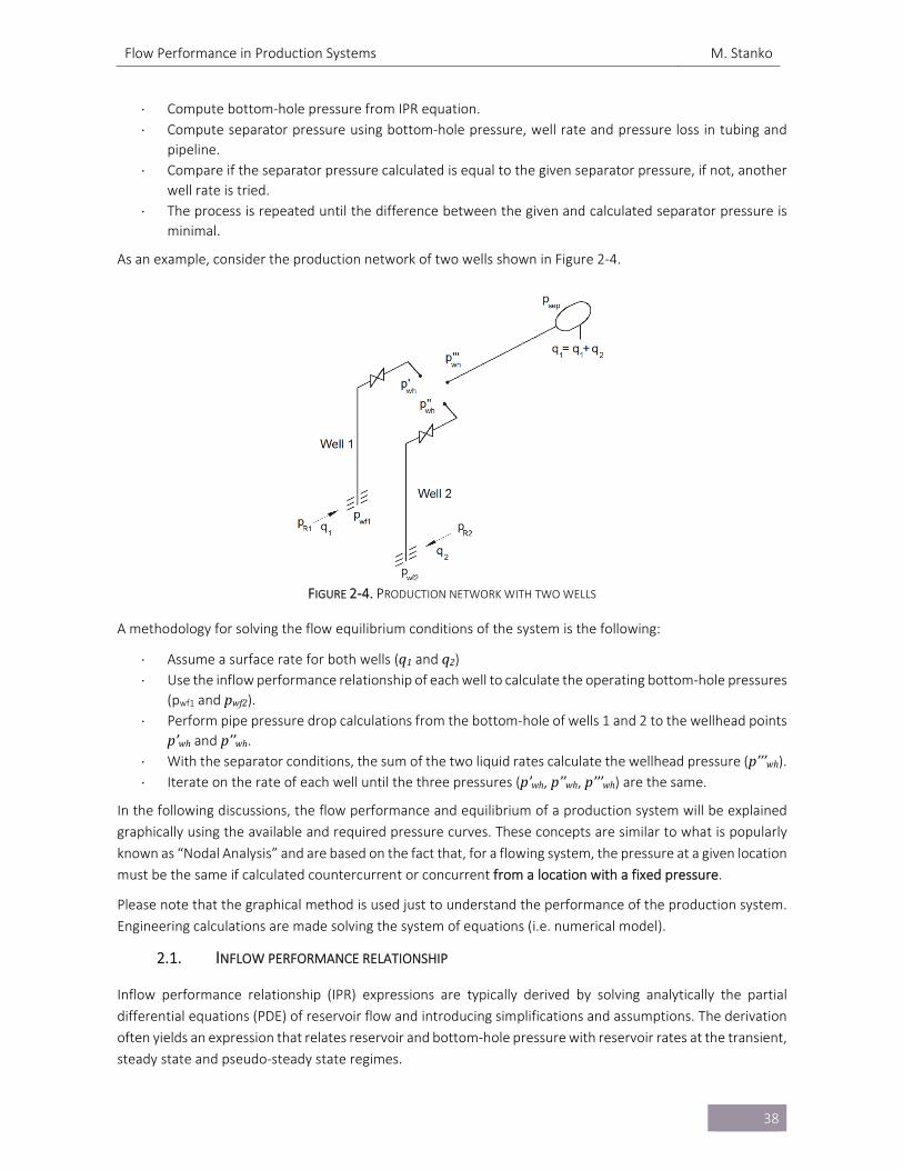
As an example, consider the production network of two wells shown in Figure 2‐4.
FIGURE 2‐4. PRODUCTION NETWORK WITH TWO WELLS
A methodology for solving the flow equilibrium conditions of the system is the following:
Assume a surface rate for both wells (q1 and q2) Use the inflow performance relationship of each well to calculate the operating bottom‐hole pressures
(pwf1 and pwf2). Perform pipe pressure drop calculations from the bottom‐hole of wells 1 and 2 to the wellhead points
p’wh and p’’wh. With the separator conditions, the sum of the two liquid rates calculate the wellhead pressure (p’’’wh). Iterate on the rate of each well until the three pressures (p’wh, p’’wh,p’’’wh) are the same.
In the following discussions, the flow performance and equilibrium of a production system will be explained
graphically using the available and required pressure curves. These concepts are similar to what is popularly
known as “Nodal Analysis” and are based on the fact that, for a flowing system, the pressure at a given location
must be the same if calculated countercurrent or concurrent from a location with a fixed pressure.
Please note that the graphical method is used just to understand the performance of the production system.
Engineering calculations are made solving the system of equations (i.e. numerical model).
2.1. INFLOW PERFORMANCE RELATIONSHIP
Inflow performance relationship (IPR) expressions are typically derived by solving analytically the partial
differential equations (PDE) of reservoir flow and introducing simplifications and assumptions. The derivation
often yields an expression that relates reservoir and bottom‐hole pressure with reservoir rates at the transient,
steady state and pseudo‐steady state regimes.
Flow Performance in Production Systems M. Stanko
39
In principle, there should be three independent IPRs, one for each phase that is produced from the formation
(oil, gas and water). However, often the IPR is made for one of the phases (the main phase, oil or gas) and the
other are expressed by using a ratio (gas oil ratio, GOR, water cut, WC). The ratio is often assumed to remain
constant when rate is varied.
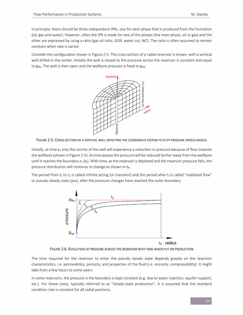
Consider the configuration shown in Figure 2‐5. The cross section of a radial reservoir is shown, with a vertical
well drilled in the center. Initially the well is closed so the pressure across the reservoir is constant and equal
to pRo. The well is then open and the wellbore pressure is fixed to pwf.
FIGURE 2‐5. CROSS SECTION OF A VERTICAL WELL DEPICTING THE COORDINATE SYSTEM TO PLOT PRESSURE VERSUS RADIUS
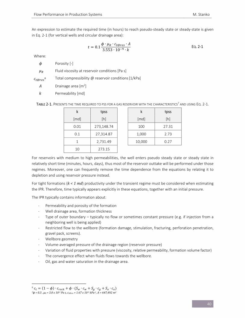
Initially, at time t1 only the vicinity of the well will experience a reduction in pressure because of flow towards the wellbore (shown in Figure 2‐5). As time passes the pressure will be reduced farther away from the wellbore
until it reaches the boundary re (t3). With time, as the reservoir is depleted and the reservoir pressure falls, the
pressure distribution will continue to change as shown in t4.
The period from t0 to t3 is called infinite acting (or transient) and the period after t3 is called “stabilized flow”
or pseudo steady state (pss), after the pressure changes have reached the outer boundary.
FIGURE 2‐6. EVOLUTION OF PRESSURE ACROSS THE RESERVOIR WITH TIME WHEN PUT ON PRODUCTION
The time required for the reservoir to enter the pseudo steady state depends greatly on the reservoir
characteristics, i.e. permeability, porosity, and properties of the fluid (i.e. viscosity, compressibility). It might
take from a few hours to some years.
In some reservoirs, the pressure is the boundary is kept constant (e.g. due to water injection, aquifer support,
etc.). For those cases, typically referred to as “steady‐state production”, it is assumed that the standard
condition rate is constant for all radial positions.
Flow Performance in Production Systems M. Stanko
40
An expression to estimate the required time (in hours) to reach pseudo‐steady state or steady‐state is given
in Eq. 2‐1 (for vertical wells and circular drainage area):
𝑡 0.1𝜙 ∙ 𝜇 ∙ 𝑐 @ ∙ 𝐴3.553 ∙ 10 ∙ 𝑘
EQ. 2‐1
Where:
𝜙 Porosity [‐]
𝜇 Fluid viscosity at reservoir conditions [Pa s]
𝑐 @6 Total compressibility @ reservoir conditions [1/kPa]
𝐴 Drainage area [m2]
𝑘 Permeability [md]
TABLE 2‐1. PRESENTS THE TIME REQUIRED TO PSS FOR A GAS RESERVOIR WITH THE CHARACTERISTICS7 AND USING EQ. 2‐1.
k tpss k tpss
[md] [h] [md] [h]
0.01 273,148.74 100 27.31
0.1 27,314.87 1,000 2.73
1 2,731.49 10,000 0.27
10 273.15
For reservoirs with medium to high permeabilities, the well enters pseudo steady state or steady state in
relatively short time (minutes, hours, days), thus most of the reservoir outtake will be performed under those
regimes. Moreover, one can frequently remove the time dependence from the equations by relating it to
depletion and using reservoir pressure instead.
For tight formations (k<1md) productivity under the transient regime must be considered when estimating
the IPR. Therefore, time typically appears explicitly in these equations, together with an initial pressure.
The IPR typically contains information about:
Permeability and porosity of the formation
Well drainage area, formation thickness
Type of outer boundary – typically no flow or sometimes constant pressure (e.g. if injection from a
neighboring well is being applied)
Restricted flow to the wellbore (formation damage, stimulation, fracturing, perforation penetration,
gravel pack, screens).
Wellbore geometry
Volume‐averaged pressure of the drainage region (reservoir pressure)
Variation of fluid properties with pressure (viscosity, relative permeability, formation volume factor)
The convergence effect when fluids flows towards the wellbore.
Oil, gas and water saturation in the drainage area.
6 𝑐 1 𝜙 ∙ 𝑐 𝜙 ∙ 𝑆 ∙ 𝑐 𝑆 ∙ 𝑐 𝑆 ∙ 𝑐 7ɸ =0.3,μR=3.0x10‐5Pas,ct@res=1.67x10‐5kPa‐1,A=647,492m2
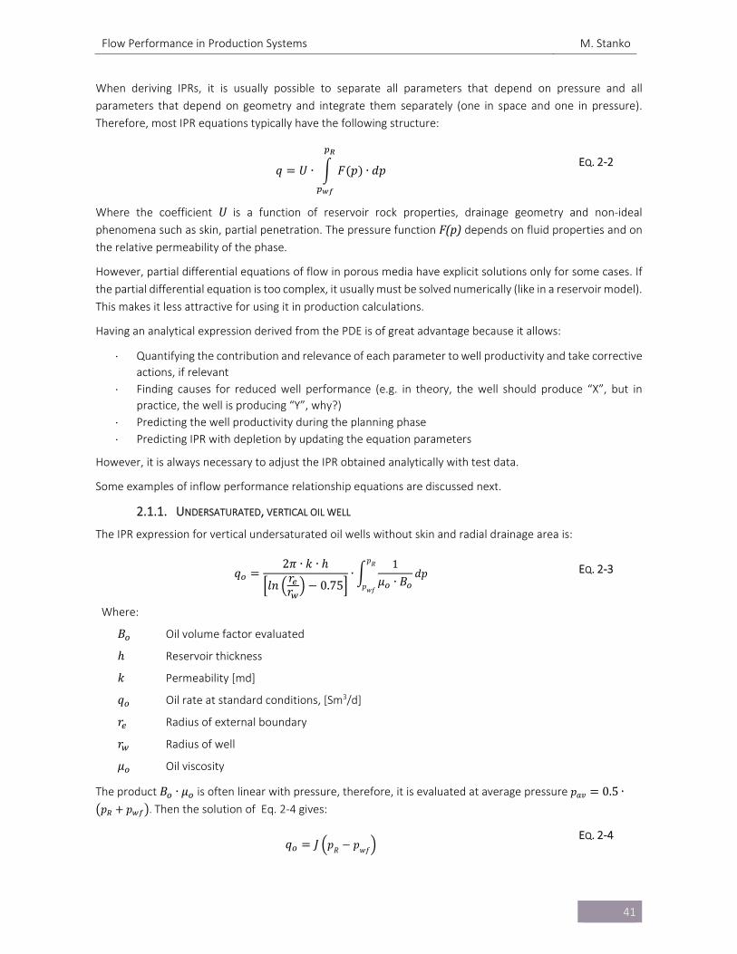
Flow Performance in Production Systems M. Stanko
41
When deriving IPRs, it is usually possible to separate all parameters that depend on pressure and all
parameters that depend on geometry and integrate them separately (one in space and one in pressure).
Therefore, most IPR equations typically have the following structure:
𝑞 𝑈 ∙ 𝐹 𝑝 ∙ 𝑑𝑝 EQ. 2‐2
Where the coefficient U is a function of reservoir rock properties, drainage geometry and non‐ideal
phenomena such as skin, partial penetration. The pressure function F(p) depends on fluid properties and on the relative permeability of the phase.
However, partial differential equations of flow in porous media have explicit solutions only for some cases. If
the partial differential equation is too complex, it usually must be solved numerically (like in a reservoir model).
This makes it less attractive for using it in production calculations.
Having an analytical expression derived from the PDE is of great advantage because it allows:
Quantifying the contribution and relevance of each parameter to well productivity and take corrective
actions, if relevant
Finding causes for reduced well performance (e.g. in theory, the well should produce “X”, but in
practice, the well is producing “Y”, why?)
Predicting the well productivity during the planning phase
Predicting IPR with depletion by updating the equation parameters
However, it is always necessary to adjust the IPR obtained analytically with test data.
Some examples of inflow performance relationship equations are discussed next.
2.1.1. UNDERSATURATED, VERTICAL OIL WELL
The IPR expression for vertical undersaturated oil wells without skin and radial drainage area is:
𝑞2𝜋 ∙ 𝑘 ∙ ℎ
𝑙𝑛𝑟𝑟 0.75
∙1
𝜇 ∙ 𝐵𝑑𝑝
𝑝𝑅
𝑝𝑤𝑓
EQ. 2‐3
Where:
𝐵 Oil volume factor evaluated
ℎ Reservoir thickness
𝑘 Permeability [md]
𝑞 Oil rate at standard conditions, [Sm3/d]
𝑟 Radius of external boundary
𝑟 Radius of well
𝜇 Oil viscosity
The product 𝐵 ∙ 𝜇 is often linear with pressure, therefore, it is evaluated at average pressure 𝑝 0.5 ∙𝑝 𝑝 . Then the solution of Eq. 2‐4 gives:
𝑞 𝐽 𝑝𝑅 𝑝𝑤𝑓 EQ. 2‐4
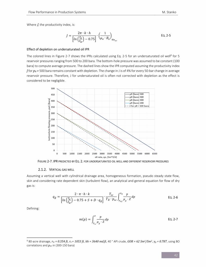
Flow Performance in Production Systems M. Stanko
42
Where J, the productivity index, is:
𝐽2𝜋 ∙ 𝑘 ∙ ℎ
𝑙𝑛𝑟𝑟 0.75
∙1
𝜇 ∙ 𝐵 @𝑝𝑎𝑣
EQ. 2‐5
Effect of depletion on undersaturated oil IPR
The colored lines in Figure 2‐7 shows the IPRs calculated using Eq. 2‐5 for an undersaturated oil well8 for 5
reservoir pressures ranging from 500 to 200 bara. The bottom‐hole pressure was assumed to be constant (100
bara) to compute average pressure. The dashed lines show the IPR computed assuming the productivity index
J for pR= 500 bara remains constant with depletion. The change in J is of 4% for every 50‐bar change in average
reservoir pressure. Therefore, J for undersaturated oil is often not corrected with depletion as the effect is
considered to be negligible.
FIGURE 2‐7. IPR PREDICTED BY EQ. 2. FOR UNDERSATURATED OIL WELL AND DIFFERENT RESERVOIR PRESSURES
2.1.2. VERTICAL GAS WELL
Assuming a vertical well with cylindrical drainage area, homogeneous formation, pseudo steady state flow,
skin and considering rate dependent skin (turbulent flow), an analytical and general equation for flow of dry
gas is:
𝑞2 ∙ 𝜋 ∙ ℎ ∙ 𝑘
𝑙𝑛𝑟𝑟 0.75 𝑆 𝐷 ∙ 𝑞
∙𝑇
𝑇 ∙ 𝑝𝑝
𝜇𝑔 ⋅ 𝑍𝑑𝑝
𝑝𝑅
𝑝𝑤𝑓
EQ. 2‐6
Defining:
𝑚 𝑝𝑝
𝜇𝑔 ⋅ 𝑍𝑑𝑝
𝑝
𝑝𝑠𝑐
EQ. 2‐7
8 80‐acre drainage, rw=0.354ft, re=1053ft, kh=3640md.ft, 40 ° API crude, GOR=62Sm3/Sm3, γg=0.787, using BO correlations and pav in (300‐150 bara)
Flow Performance in Production Systems M. Stanko
43
And applying this definition to Eq. 2‐3 gives:
𝑞2 ∙ 𝜋 ∙ ℎ ∙ 𝑘
𝑙𝑛𝑟𝑟 0.75 𝑆 𝐷 ∙ 𝑞
∙𝑇
𝑇 ∙ 𝑝𝑚 𝑝 𝑚 𝑝 EQ. 2‐8
Additionally, to avoid having the presence of the gas rate in both sides of the equation, the IPR equation can
be re‐written in the form:
𝑞2 ∙ 𝜋 ∙ ℎ ∙ 𝑘
𝑙𝑛𝑟𝑟 0.75 𝑆
∙𝑇
𝑇 ∙ 𝑝𝑚 𝑝 𝑚 𝑝
𝑛 EQ. 2‐9
With n accounting for the presence of turbulent (n=0.5) or laminar (n=1) flow.
Effect of depletion on dry gas IPR
There is no need to correct for depletion the dry gas IPR presented in Eq. 2‐9.
2.1.3. SATURATED, VERTICAL OIL WELL
Assuming a vertical well with cylindrical drainage area, homogeneous formation, pseudo steady state flow,
skin and considering rate dependent skin (turbulent flow), an analytical and general equation for flow of
undersaturated and saturated oil with simultaneous flow of gas and water is:
𝑞 ̄𝑘 ⋅ ℎ
18.665 ⋅ 𝑙𝑛𝑟𝑟 0.75 𝑠 𝐷 ⋅ 𝑞 ̄
𝑘𝜇 ⋅ 𝐵
𝑑𝑝 EQ. 2‐10
Where the pressure function is:
𝐹 𝑝𝑘
𝜇 ⋅ 𝐵 EQ. 2‐11
And U:
𝑈𝑘 ⋅ ℎ
18.665 ⋅ 𝑙𝑛𝑟𝑟 0.75 𝑠 𝐷 ⋅ 𝑞 ̄
EQ. 2‐12
If reservoir pressure is equal or below bubble point pressure ( 𝑝 𝑝 ), a typical assumption to solve the
pressure function integral is to consider the product ⋅
linear with pressure below the bubble point. By
assuming a straight line between zero (“0”) pressure and reservoir pressure and setting the value of the
pressure function equal to zero at the origin, the pressure function 𝐹 𝑝 becomes:
𝑘
𝜇 ⋅ 𝐵𝑘
𝜇 ⋅ 𝐵∙
𝑝𝑝 EQ. 2‐13
Substituting in the integral gives:
𝑘
𝜇 ⋅ 𝐵𝑑𝑝
𝑘𝜇 ⋅ 𝐵
∙𝑝
𝑝𝑑𝑝
𝑘𝜇 ⋅ 𝐵
1𝑝 ∙ 2
𝑝 𝑝 EQ. 2‐14
This expression can then be substituted back in Eq. 2‐10. Additionally, to avoid having the presence of the oil
rate in both sides of the equation, the IPR equation can be re‐written in the form:
𝑞 ̄ 𝐶 ⋅ 𝑝 𝑝 EQ. 2‐15
With
Flow Performance in Production Systems M. Stanko
44
𝐶
𝑘 ⋅ 𝑘 ⋅ ℎ18.665 ⋅ 2 ⋅ 𝜇 ⋅ 𝐵 ∙ 𝑝
1
𝐷 ⋅ 𝑙𝑛𝑟𝑟 0.75 𝑠
EQ. 2‐16
With n accounting for the presence of turbulent (n=0.5) or laminar (n=1) flow.
Eq. 2‐15 is called the backpressure equation, and it is often used for gas wells also. An equivalent form of this
equation is:
𝑞 ̄ 𝑞 ̄ , ⋅ 1
𝑝𝑝
EQ. 2‐17
With 𝑞 ̄ , 𝐶 ∙ 𝑝 ∙ .
Special case when n = 1
Another form9 of the backpressure equation when n = 1 is:
𝑞 ̄𝐽
2 ∙ 𝑝⋅ 𝑝 𝑝 EQ. 2‐18
and 𝐽 2 ∙ 𝐶 ∙ 𝑝
IPR equations Eq. 2‐15, Eq. 2‐17 and Eq. 2‐18 are usually used in two ways:
If no test or field data is available, use the analytical expression. This will require geometric
information, relative and absolute permeabilities, average oil saturation around the wellbore, fluid
properties, etc.
If test data is available, tune C and n, or 𝑞 ̄ , and n, or 𝐽 to match the results of the model to the
test values. At least two points are typically required. If only one test point is available, the
assumption n = 1 (laminar flow) is sometimes reasonable.
More general IPR equation: Whitson’s IPR and similarities to Vogel’s IPR
If the value of the pressure function at the origin is assumed to be non‐zero when computing the integral of
the pressure function, then the pressure function can be expressed as:
𝐹 𝑝
𝑘𝜇 ⋅ 𝐵
𝑘𝜇 ⋅ 𝐵
𝑘𝜇 ⋅ 𝐵
𝑘𝜇 ⋅ 𝐵
∙𝑝
𝑝 EQ. 2‐19
Or, equivalently:
𝐹 𝑝 𝐹 𝑝 0 𝐹 𝑝 𝐹 𝑝 0 ∙𝑝
𝑝 EQ. 2‐20
Therefore, the solution of the pressure function integral will have a linear term in addition to the quadratic
term:
𝐹 𝑝 𝑑𝑝 𝐹 𝑝 0 ∙ 𝑝 𝑝 𝐹 𝑝 𝐹 𝑝 0 ∙1
𝑝 ∙ 2𝑝 𝑝 EQ. 2‐21
Expanding terms:
𝐹 𝑝 𝑑𝑝 𝐹 𝑝 0 ∙ 𝑝 𝐹 𝑝 0 ∙ 𝑝 𝐹 𝑝 𝐹 𝑝 0 ∙1
𝑝 ∙ 2𝑝 𝑝 EQ. 2‐22
9 The IPR expression using 𝐽 is found by calculating the limit of the productivity index expression when bottom‐hole
pressure tends to reservoir pressure (done first by Evinger and Muskat). The usefulness of this expression is that J can be
computed at reservoir pressure.
Flow Performance in Production Systems M. Stanko
45
𝐹 𝑝 𝑑𝑝 𝐹 𝑝 0 ∙ 𝑝 𝐹 𝑝 0 ∙ 𝑝 𝐹 𝑝 ∙𝑝2
𝐹 𝑝 ∙𝑝𝑝 ∙ 2
𝐹 𝑝 0 ∙𝑝2
𝐹 𝑝 0 ∙𝑝𝑝 ∙ 2
EQ. 2‐23
Grouping terms by pressure:
𝐹 𝑝 𝑑𝑝 𝐹 𝑝 0 𝐹 𝑝 ∙
𝑝2
𝐹 𝑝 0 ∙ 𝑝𝐹 𝑝 𝐹 𝑝 0
2∙
𝑝𝑝
EQ. 2‐24
Dividing by 𝐹 𝑝 0 𝐹 𝑝 ∙
𝐹 𝑝 0 𝐹 𝑝 ∙𝑝2
∙ 𝐹 𝑝 𝑑𝑝
1𝐹 𝑝 0 ∙ 2
𝐹 𝑝 0 𝐹 𝑝∙
𝑝𝑝
𝐹 𝑝 𝐹 𝑝 0𝐹 𝑝 0 𝐹 𝑝
∙𝑝𝑝
EQ. 2‐25
Defining a variable “V”
𝑉
𝐹 𝑝 0 ∙ 2𝐹 𝑝 0 𝐹 𝑝
EQ. 2‐26
Therefore:
1 𝑉
𝐹 𝑝 𝐹 𝑝 0𝐹 𝑝 0 𝐹 𝑝
EQ. 2‐27
Substituting back in the integral of the pressure function:
𝐹 𝑝 0 𝐹 𝑝 ∙𝑝2
∙ 𝐹 𝑝 𝑑𝑝 1 𝑉 ∙𝑝𝑝
1 𝑉 ∙𝑝𝑝
EQ. 2‐28
Substituting Eq. 2‐28 back in the IPR equation:
𝑞 ̄2 ⋅ 𝑘 ⋅ ℎ
18.665 ⋅ 𝑙𝑛𝑟𝑟 0.75 𝑠 𝐷 ⋅ 𝑞 ̄ ∙ 𝐹 𝑝 0 𝐹 𝑝
1 𝑉 ∙𝑝𝑝
1 𝑉 ∙𝑝𝑝
EQ. 2‐29
Making 𝑞 ̄ , :
𝑞 ̄ ,2 ⋅ 𝑘 ⋅ ℎ
18.665 ⋅ 𝑙𝑛𝑟𝑟 0.75 𝑠 𝐷 ⋅ 𝑞 ̄ ∙ 𝐹 𝑝 0 𝐹 𝑝
EQ. 2‐30
The following expression is obtained:
𝑞 ̄ 𝑞 ̄ , 1 𝑉 ∙
𝑝𝑝
1 𝑉 ∙𝑝𝑝
EQ. 2‐31
Vogel’s equation is the particular case of V = 0.2 and neglecting rate dependent skin (D=0).
𝑞𝑞 ,
1 0.2 ∙𝑝𝑝
0.8 ∙𝑝𝑝
EQ. 2‐32
With qō,max=J·pR/1.8 (where J is the single‐phase oil productivity index using properties at current reservoir pressure).
The backpressure equation is the case with V = 0.
Flow Performance in Production Systems M. Stanko
46
Effect of depletion on saturated oil IPR
When the reservoir is depleted, reservoir pressure will decrease below the bubble point pressure, and fluid
properties and saturations around the wellbore will vary, and there will be simultaneous flows or gas, oil and
water towards the wellbore10. Therefore, the IPR will also change.
To estimate a new IPR, and if there are no changes in the rate dependent skin, outer flow boundaries, or skin,
and the backpressure equation (Eq. 2‐15) is used, then a new C can be found by using the expression:
𝐶 𝐶 ∙
𝑘𝜇 ⋅ 𝐵 ∙ 𝑝
𝑘𝜇 ⋅ 𝐵 ∙ 𝑝
EQ. 2‐33
If the version of the backpressure IPR with n = 1 is used (Eq. 2‐18), then a new productivity index J can be
found by using the expression:
𝐽 𝐽 ∙
𝑘𝜇 ⋅ 𝐵
𝑘𝜇 ⋅ 𝐵
EQ. 2‐34
In Whitson’s IPR both V and 𝑞 ̄ , change with depletion and must be updated (both have the term 𝐹 𝑝 ).
However, it is not possible to update them by scaling the constants using a mobility ratio as indicated above
because 𝐹 𝑝 is not alone when multiplying V and 𝑞 ̄ , .
When using Vogel’s IPR, V is left constant and equal to 0.2 with depletion, therefore, often 𝑞 ̄ , is updated
with depletion using the mobility ratio. However, this might not be completely applicable if it is considered
that 𝑞 ̄ , still contains the term 𝐹 𝑝 0 𝐹 𝑝 .
2.1.4. COMPOSITE IPR: BOTH UNDERSATURATED AND SATURATED OIL
If reservoir pressure is above the bubble point pressure, but the flowing bottom‐hole pressure is below the
bubble point pressure (𝑝 𝑝 𝑝 ), then, a suitable equation is a composite IPR, linear above the bubble
point and using the backpressure equation with n=1 below the bubble point is:
If 𝑝 𝑝 then:
𝑞 ̄ 𝐽 ∙ 𝑝𝑅 𝑝𝑤𝑓 EQ. 2‐35
Otherwise 𝑝 𝑝 then:
𝑞 ̄𝐽
2 ∙ 𝑝∙ 𝑝 𝑝 𝑞𝑜@𝑏 EQ. 2‐36
𝑞𝑜@ 𝐽 ∙ 𝑝 𝑝 EQ. 2‐37
𝑞 ̄𝐽
2 ∙ 𝑝∙ 𝑝 𝑝 𝐽 ∙ 𝑝𝑅 𝑝𝑏 EQ. 2‐38
The composite IPR can also be developed using Whitson’s or Vogel’s IPR.
10 This is evidenced often by a variation in the producing GOR. Please refer to Appendix G for an expression for GOR
variation with time.
Flow Performance in Production Systems M. Stanko
47
2.1.5. FLOW OF ASSOCIATED PRODUCTS IN AN OIL WELL: GAS AND WATER
With depletion, due to reservoir pressure reduction and neighboring injection, the saturation of gas and water
around the wellbore will change and the gas and water mobility will increase or decrease, therefore, changing
the producing GOR and WC.
If there is no gas coning from the gas cap nor water cusping from the water layer, then usually an IPR for the
oil phase is used, and the gas and water rates are calculated with the producing GOR and WC. Therefore, it is
typically assumed that GOR and WC remain constant for a given depletion state (or reservoir pressure) even
though there might be variations of 𝑝 for a given reservoir pressure.
The flow of oil and water is sometimes modeled by using a “compound” liquid IPR equation. The liquid IPR is
derived by writing two separate inflow performance relationships for oil and for water. For the case 𝑝 𝑝 :
𝑞 ̄𝐽
2 ∙ 𝑝⋅ 𝑝 𝑝 EQ. 2‐39
𝑞 ̄𝐽2 ∙ 𝑝
⋅ 𝑝 𝑝 EQ. 2‐40
Adding these two equations gives:
𝑞 𝑞 ̄ 𝑞 ̄
𝐽 𝐽2 ∙ 𝑝
⋅ 𝑝 𝑝𝐽
2 ∙ 𝑝⋅ 𝑝 𝑝 EQ. 2‐41
A similar development can be performed for the undersaturated oil case or when using the composite IPR.
Effect of depletion on liquid IPR
Similar to the case with saturated oil, to estimate a new IPR, and if there are no changes in the rate dependent
skin, outer flow boundaries, or skin with depletion, then a new Jl can be found by using the expression:
𝐽 , 𝐽 , ∙
𝑘𝜇 ⋅ 𝐵
𝑘𝜇 ⋅ 𝐵
𝑘𝜇 ⋅ 𝐵
𝑘𝜇 ⋅ 𝐵
EQ. 2‐42
2.1.6. IPR AND WATER OR GAS CONING
Coning from a gas cap or from the aquifer is usually established when the oil rate produced is greater than
critical oil rate or, equivalently, when the flowing bottom‐hole pressure is reduced below the critical bottom‐
hole pressure. The critical oil rate and critical bottom‐hole pressure will depend strongly on the distance
between the well and the water‐oil contact or the gas‐oil contact, among other parameters such as the vertical
permeability.
Immediately after gas or water breakthrough occurs, the oil rate will be severely reduced (for example, Asheim
reports ca 1/10 reduction in the oil rate in a well with water cusping in the Helder field). However, after some
time the oil rate will stabilize, when the transient coning crest stops changing, and the well will then produce
with a constant GOR or WC.
Analytical models seem to indicate that the value of the stabilized GOR or WC depends on the ratio between
the oil rate and the critical oil rate. Interestingly, the relationship is asymptotic, and there will be an oil rate
above which the WC or GOR won’t change significantly. For example, using the analytical steady‐state model
of Asheim for water coning from the aquifer to a horizontal, undersaturated oil well, the water ratio (𝑓
) has the upper limit:
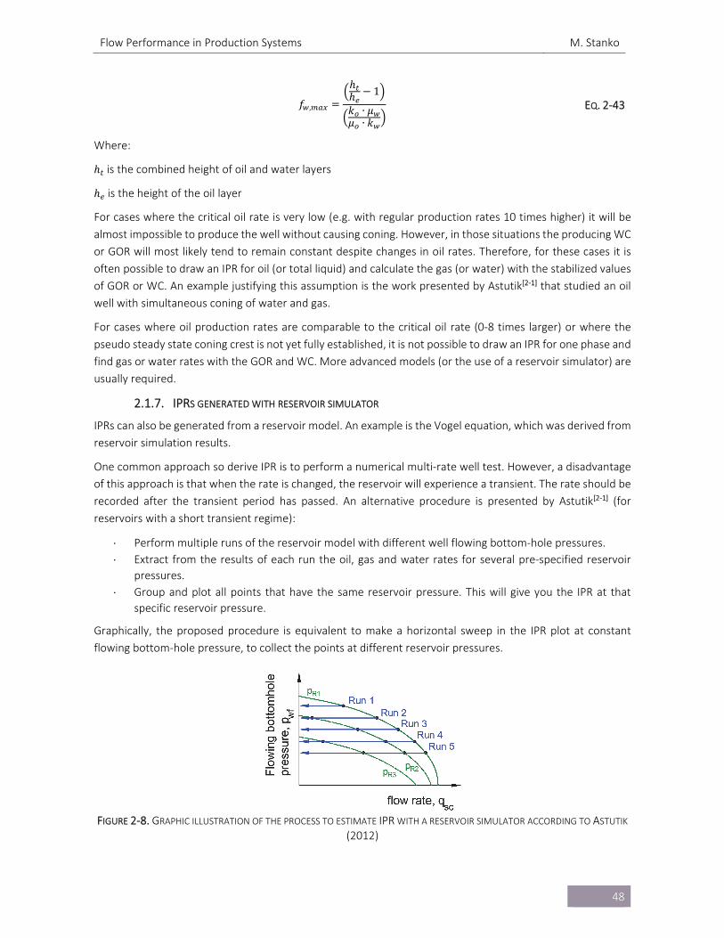
Flow Performance in Production Systems M. Stanko
48
𝑓 ,
ℎℎ 1
𝑘 ∙ 𝜇𝜇 ∙ 𝑘
EQ. 2‐43
Where:
ℎ is the combined height of oil and water layers
ℎ is the height of the oil layer
For cases where the critical oil rate is very low (e.g. with regular production rates 10 times higher) it will be
almost impossible to produce the well without causing coning. However, in those situations the producing WC
or GOR will most likely tend to remain constant despite changes in oil rates. Therefore, for these cases it is
often possible to draw an IPR for oil (or total liquid) and calculate the gas (or water) with the stabilized values
of GOR or WC. An example justifying this assumption is the work presented by Astutik[2‐1] that studied an oil
well with simultaneous coning of water and gas.
For cases where oil production rates are comparable to the critical oil rate (0‐8 times larger) or where the
pseudo steady state coning crest is not yet fully established, it is not possible to draw an IPR for one phase and
find gas or water rates with the GOR and WC. More advanced models (or the use of a reservoir simulator) are
usually required.
2.1.7. IPRS GENERATED WITH RESERVOIR SIMULATOR
IPRs can also be generated from a reservoir model. An example is the Vogel equation, which was derived from
reservoir simulation results.
One common approach so derive IPR is to perform a numerical multi‐rate well test. However, a disadvantage
of this approach is that when the rate is changed, the reservoir will experience a transient. The rate should be
recorded after the transient period has passed. An alternative procedure is presented by Astutik[2‐1] (for
reservoirs with a short transient regime):
Perform multiple runs of the reservoir model with different well flowing bottom‐hole pressures.
Extract from the results of each run the oil, gas and water rates for several pre‐specified reservoir
pressures.
Group and plot all points that have the same reservoir pressure. This will give you the IPR at that
specific reservoir pressure.
Graphically, the proposed procedure is equivalent to make a horizontal sweep in the IPR plot at constant
flowing bottom‐hole pressure, to collect the points at different reservoir pressures.
FIGURE 2‐8. GRAPHIC ILLUSTRATION OF THE PROCESS TO ESTIMATE IPR WITH A RESERVOIR SIMULATOR ACCORDING TO ASTUTIK
(2012)
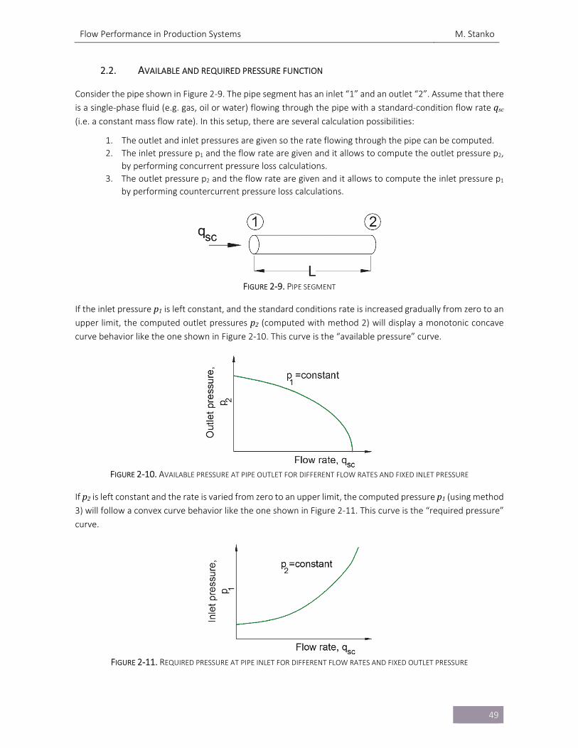
Flow Performance in Production Systems M. Stanko
49
2.2. AVAILABLE AND REQUIRED PRESSURE FUNCTION
Consider the pipe shown in Figure 2‐9. The pipe segment has an inlet “1” and an outlet “2”. Assume that there
is a single‐phase fluid (e.g. gas, oil or water) flowing through the pipe with a standard‐condition flow rate qsc (i.e. a constant mass flow rate). In this setup, there are several calculation possibilities:
1. The outlet and inlet pressures are given so the rate flowing through the pipe can be computed.
2. The inlet pressure p1 and the flow rate are given and it allows to compute the outlet pressure p2,
by performing concurrent pressure loss calculations.
3. The outlet pressure p2 and the flow rate are given and it allows to compute the inlet pressure p1
by performing countercurrent pressure loss calculations.
FIGURE 2‐9. PIPE SEGMENT
If the inlet pressure p1is left constant, and the standard conditions rate is increased gradually from zero to an
upper limit, the computed outlet pressures p2 (computed with method 2) will display a monotonic concave
curve behavior like the one shown in Figure 2‐10. This curve is the “available pressure” curve.
FIGURE 2‐10. AVAILABLE PRESSURE AT PIPE OUTLET FOR DIFFERENT FLOW RATES AND FIXED INLET PRESSURE
If p2 is left constant and the rate is varied from zero to an upper limit, the computed pressure p1 (using method
3) will follow a convex curve behavior like the one shown in Figure 2‐11. This curve is the “required pressure”
curve.
FIGURE 2‐11. REQUIRED PRESSURE AT PIPE INLET FOR DIFFERENT FLOW RATES AND FIXED OUTLET PRESSURE
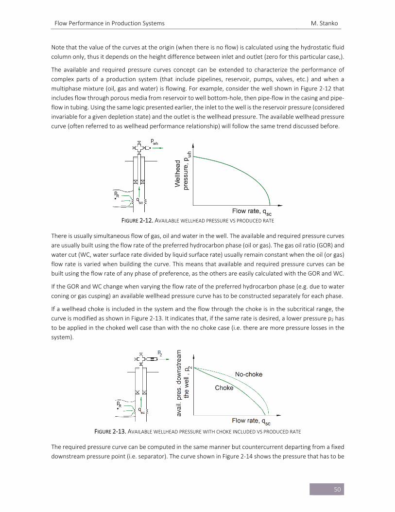
Flow Performance in Production Systems M. Stanko
50
Note that the value of the curves at the origin (when there is no flow) is calculated using the hydrostatic fluid
column only, thus it depends on the height difference between inlet and outlet (zero for this particular case,).
The available and required pressure curves concept can be extended to characterize the performance of
complex parts of a production system (that include pipelines, reservoir, pumps, valves, etc.) and when a
multiphase mixture (oil, gas and water) is flowing. For example, consider the well shown in Figure 2‐12 that
includes flow through porous media from reservoir to well bottom‐hole, then pipe‐flow in the casing and pipe‐
flow in tubing. Using the same logic presented earlier, the inlet to the well is the reservoir pressure (considered
invariable for a given depletion state) and the outlet is the wellhead pressure. The available wellhead pressure
curve (often referred to as wellhead performance relationship) will follow the same trend discussed before.
FIGURE 2‐12. AVAILABLE WELLHEAD PRESSURE VS PRODUCED RATE
There is usually simultaneous flow of gas, oil and water in the well. The available and required pressure curves
are usually built using the flow rate of the preferred hydrocarbon phase (oil or gas). The gas oil ratio (GOR) and
water cut (WC, water surface rate divided by liquid surface rate) usually remain constant when the oil (or gas)
flow rate is varied when building the curve. This means that available and required pressure curves can be
built using the flow rate of any phase of preference, as the others are easily calculated with the GOR and WC.
If the GOR and WC change when varying the flow rate of the preferred hydrocarbon phase (e.g. due to water
coning or gas cusping) an available wellhead pressure curve has to be constructed separately for each phase.
If a wellhead choke is included in the system and the flow through the choke is in the subcritical range, the
curve is modified as shown in Figure 2‐13. It indicates that, if the same rate is desired, a lower pressure p2 has
to be applied in the choked well case than with the no choke case (i.e. there are more pressure losses in the
system).
FIGURE 2‐13. AVAILABLE WELLHEAD PRESSURE WITH CHOKE INCLUDED VS PRODUCED RATE
The required pressure curve can be computed in the same manner but countercurrent departing from a fixed
downstream pressure point (i.e. separator). The curve shown in Figure 2‐14 shows the pressure that has to be
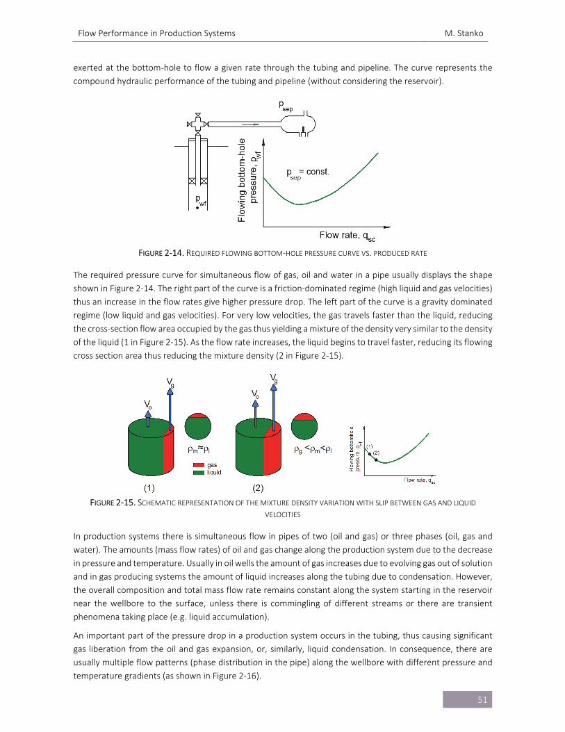
Flow Performance in Production Systems M. Stanko
51
exerted at the bottom‐hole to flow a given rate through the tubing and pipeline. The curve represents the
compound hydraulic performance of the tubing and pipeline (without considering the reservoir).
FIGURE 2‐14. REQUIRED FLOWING BOTTOM‐HOLE PRESSURE CURVE VS. PRODUCED RATE
The required pressure curve for simultaneous flow of gas, oil and water in a pipe usually displays the shape
shown in Figure 2‐14. The right part of the curve is a friction‐dominated regime (high liquid and gas velocities)
thus an increase in the flow rates give higher pressure drop. The left part of the curve is a gravity dominated
regime (low liquid and gas velocities). For very low velocities, the gas travels faster than the liquid, reducing
the cross‐section flow area occupied by the gas thus yielding a mixture of the density very similar to the density
of the liquid (1 in Figure 2‐15). As the flow rate increases, the liquid begins to travel faster, reducing its flowing
cross section area thus reducing the mixture density (2 in Figure 2‐15).
FIGURE 2‐15. SCHEMATIC REPRESENTATION OF THE MIXTURE DENSITY VARIATION WITH SLIP BETWEEN GAS AND LIQUID
VELOCITIES
In production systems there is simultaneous flow in pipes of two (oil and gas) or three phases (oil, gas and
water). The amounts (mass flow rates) of oil and gas change along the production system due to the decrease
in pressure and temperature. Usually in oil wells the amount of gas increases due to evolving gas out of solution
and in gas producing systems the amount of liquid increases along the tubing due to condensation. However,
the overall composition and total mass flow rate remains constant along the system starting in the reservoir
near the wellbore to the surface, unless there is commingling of different streams or there are transient
phenomena taking place (e.g. liquid accumulation).
An important part of the pressure drop in a production system occurs in the tubing, thus causing significant
gas liberation from the oil and gas expansion, or, similarly, liquid condensation. In consequence, there are
usually multiple flow patterns (phase distribution in the pipe) along the wellbore with different pressure and
temperature gradients (as shown in Figure 2‐16).
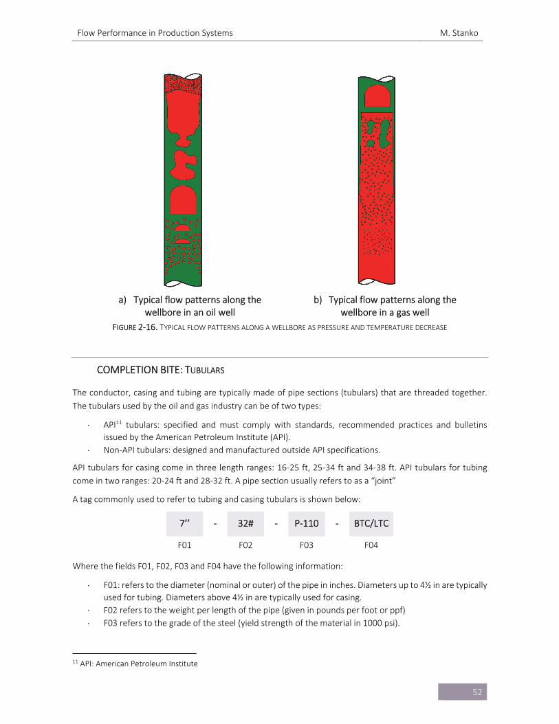
Flow Performance in Production Systems M. Stanko
52
a) Typical flow patterns along the wellbore in an oil well
b) Typical flow patterns along the wellbore in a gas well
FIGURE 2‐16. TYPICAL FLOW PATTERNS ALONG A WELLBORE AS PRESSURE AND TEMPERATURE DECREASE
COMPLETION BITE: TUBULARS
The conductor, casing and tubing are typically made of pipe sections (tubulars) that are threaded together.
The tubulars used by the oil and gas industry can be of two types:
API11 tubulars: specified and must comply with standards, recommended practices and bulletins
issued by the American Petroleum Institute (API).
Non‐API tubulars: designed and manufactured outside API specifications.
API tubulars for casing come in three length ranges: 16‐25 ft, 25‐34 ft and 34‐38 ft. API tubulars for tubing
come in two ranges: 20‐24 ft and 28‐32 ft. A pipe section usually refers to as a “joint”
A tag commonly used to refer to tubing and casing tubulars is shown below:
7’’ ‐ 32# ‐ P‐110 ‐ BTC/LTC
F01 F02 F03 F04
Where the fields F01, F02, F03 and F04 have the following information:
F01: refers to the diameter (nominal or outer) of the pipe in inches. Diameters up to 4½ in are typically
used for tubing. Diameters above 4½ in are typically used for casing.
F02 refers to the weight per length of the pipe (given in pounds per foot or ppf)
F03 refers to the grade of the steel (yield strength of the material in 1000 psi).
11 API: American Petroleum Institute
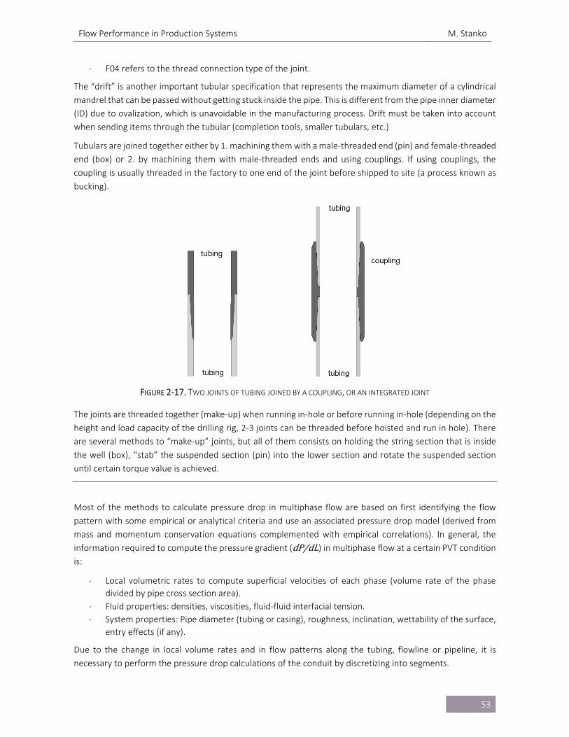
Flow Performance in Production Systems M. Stanko
53
F04 refers to the thread connection type of the joint.
The “drift” is another important tubular specification that represents the maximum diameter of a cylindrical
mandrel that can be passed without getting stuck inside the pipe. This is different from the pipe inner diameter
(ID) due to ovalization, which is unavoidable in the manufacturing process. Drift must be taken into account
when sending items through the tubular (completion tools, smaller tubulars, etc.)
Tubulars are joined together either by 1. machining them with a male‐threaded end (pin) and female‐threaded
end (box) or 2. by machining them with male‐threaded ends and using couplings. If using couplings, the
coupling is usually threaded in the factory to one end of the joint before shipped to site (a process known as
bucking).
FIGURE 2‐17. TWO JOINTS OF TUBING JOINED BY A COUPLING, OR AN INTEGRATED JOINT
The joints are threaded together (make‐up) when running in‐hole or before running in‐hole (depending on the
height and load capacity of the drilling rig, 2‐3 joints can be threaded before hoisted and run in hole). There
are several methods to “make‐up” joints, but all of them consists on holding the string section that is inside
the well (box), “stab” the suspended section (pin) into the lower section and rotate the suspended section
until certain torque value is achieved.
Most of the methods to calculate pressure drop in multiphase flow are based on first identifying the flow
pattern with some empirical or analytical criteria and use an associated pressure drop model (derived from
mass and momentum conservation equations complemented with empirical correlations). In general, the
information required to compute the pressure gradient (dP/dL) in multiphase flow at a certain PVT condition
is:
Local volumetric rates to compute superficial velocities of each phase (volume rate of the phase
divided by pipe cross section area).
Fluid properties: densities, viscosities, fluid‐fluid interfacial tension.
System properties: Pipe diameter (tubing or casing), roughness, inclination, wettability of the surface,
entry effects (if any).
Due to the change in local volume rates and in flow patterns along the tubing, flowline or pipeline, it is
necessary to perform the pressure drop calculations of the conduit by discretizing into segments.
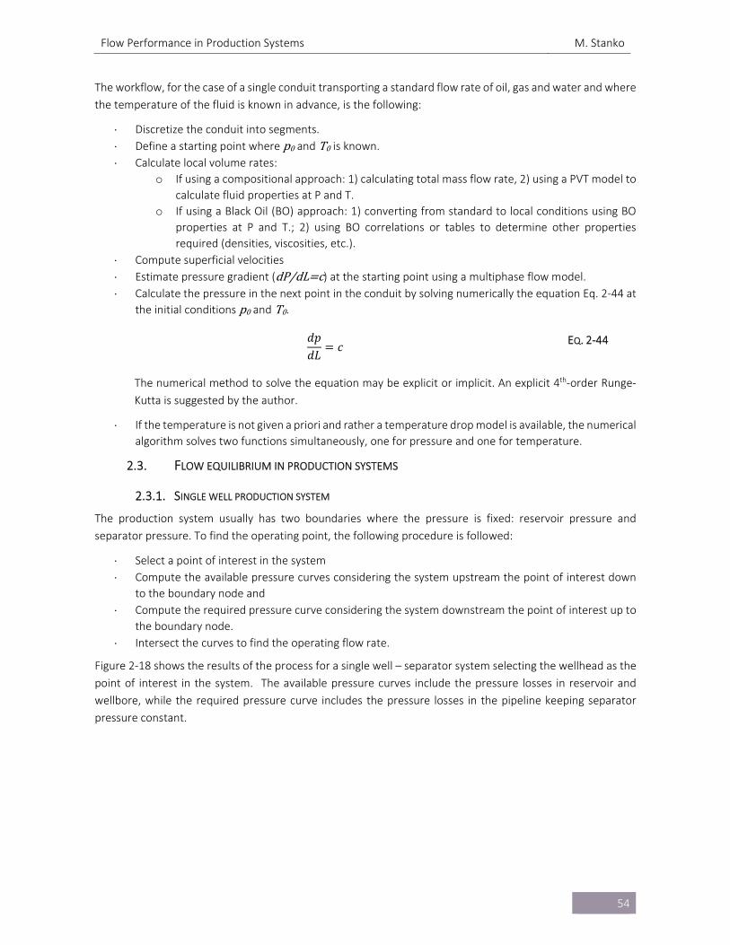
Flow Performance in Production Systems M. Stanko
54
The workflow, for the case of a single conduit transporting a standard flow rate of oil, gas and water and where
the temperature of the fluid is known in advance, is the following:
Discretize the conduit into segments.
Define a starting point where p0 and T0 is known.
Calculate local volume rates:
o If using a compositional approach: 1) calculating total mass flow rate, 2) using a PVT model to
calculate fluid properties at P and T.
o If using a Black Oil (BO) approach: 1) converting from standard to local conditions using BO
properties at P and T.; 2) using BO correlations or tables to determine other properties
required (densities, viscosities, etc.).
Compute superficial velocities
Estimate pressure gradient (dP/dL c) at the starting point using a multiphase flow model.
Calculate the pressure in the next point in the conduit by solving numerically the equation Eq. 2‐44 at
the initial conditions p0 and T0.
𝑑𝑝𝑑𝐿
𝑐 EQ. 2‐44
The numerical method to solve the equation may be explicit or implicit. An explicit 4th‐order Runge‐
Kutta is suggested by the author.
If the temperature is not given a priori and rather a temperature drop model is available, the numerical
algorithm solves two functions simultaneously, one for pressure and one for temperature.
2.3. FLOW EQUILIBRIUM IN PRODUCTION SYSTEMS
2.3.1. SINGLE WELL PRODUCTION SYSTEM
The production system usually has two boundaries where the pressure is fixed: reservoir pressure and
separator pressure. To find the operating point, the following procedure is followed:
Select a point of interest in the system
Compute the available pressure curves considering the system upstream the point of interest down
to the boundary node and
Compute the required pressure curve considering the system downstream the point of interest up to
the boundary node.
Intersect the curves to find the operating flow rate.
Figure 2‐18 shows the results of the process for a single well – separator system selecting the wellhead as the
point of interest in the system. The available pressure curves include the pressure losses in reservoir and
wellbore, while the required pressure curve includes the pressure losses in the pipeline keeping separator
pressure constant.
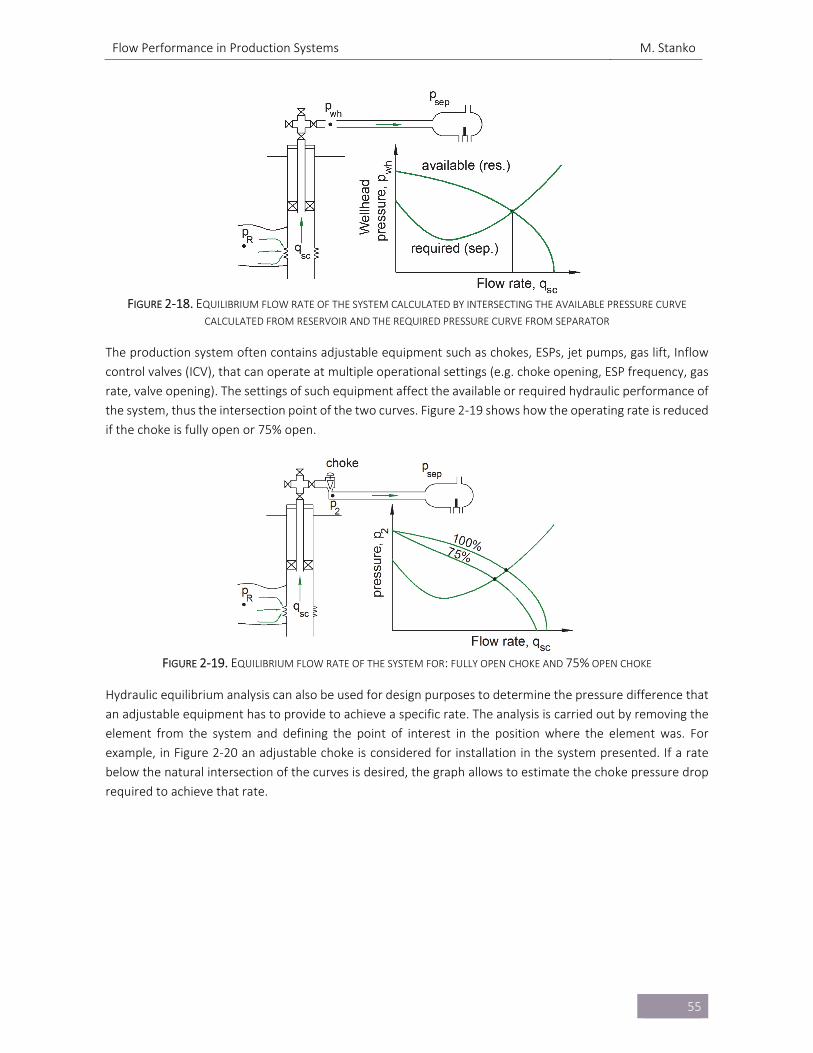
Flow Performance in Production Systems M. Stanko
55
FIGURE 2‐18. EQUILIBRIUM FLOW RATE OF THE SYSTEM CALCULATED BY INTERSECTING THE AVAILABLE PRESSURE CURVE
CALCULATED FROM RESERVOIR AND THE REQUIRED PRESSURE CURVE FROM SEPARATOR
The production system often contains adjustable equipment such as chokes, ESPs, jet pumps, gas lift, Inflow
control valves (ICV), that can operate at multiple operational settings (e.g. choke opening, ESP frequency, gas
rate, valve opening). The settings of such equipment affect the available or required hydraulic performance of
the system, thus the intersection point of the two curves. Figure 2‐19 shows how the operating rate is reduced
if the choke is fully open or 75% open.
FIGURE 2‐19. EQUILIBRIUM FLOW RATE OF THE SYSTEM FOR: FULLY OPEN CHOKE AND 75% OPEN CHOKE
Hydraulic equilibrium analysis can also be used for design purposes to determine the pressure difference that
an adjustable equipment has to provide to achieve a specific rate. The analysis is carried out by removing the
element from the system and defining the point of interest in the position where the element was. For
example, in Figure 2‐20 an adjustable choke is considered for installation in the system presented. If a rate
below the natural intersection of the curves is desired, the graph allows to estimate the choke pressure drop
required to achieve that rate.
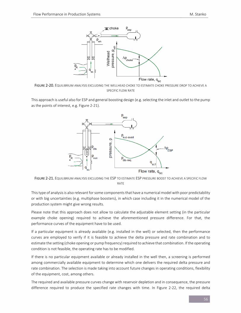
Flow Performance in Production Systems M. Stanko
56
FIGURE 2‐20. EQUILIBRIUM ANALYSIS EXCLUDING THE WELLHEAD CHOKE TO ESTIMATE CHOKE PRESSURE DROP TO ACHIEVE A
SPECIFIC FLOW RATE
This approach is useful also for ESP and general boosting design (e.g. selecting the inlet and outlet to the pump
as the points of interest, e.g. Figure 2‐21).
FIGURE 2‐21. EQUILIBRIUM ANALYSIS EXCLUDING THE ESP TO ESTIMATE ESP PRESSURE BOOST TO ACHIEVE A SPECIFIC FLOW
RATE
This type of analysis is also relevant for some components that have a numerical model with poor predictability
or with big uncertainties (e.g. multiphase boosters), in which case including it in the numerical model of the
production system might give wrong results.
Please note that this approach does not allow to calculate the adjustable element setting (in the particular
example choke opening) required to achieve the aforementioned pressure difference. For that, the
performance curves of the equipment have to be used.
If a particular equipment is already available (e.g. installed in the well) or selected, then the performance
curves are employed to verify if it is feasible to achieve the delta pressure and rate combination and to
estimate the setting (choke opening or pump frequency) required to achieve that combination. If the operating
condition is not feasible, the operating rate has to be modified.
If there is no particular equipment available or already installed in the well then, a screening is performed
among commercially available equipment to determine which one delivers the required delta pressure and
rate combination. The selection is made taking into account future changes in operating conditions, flexibility
of the equipment, cost, among others.
The required and available pressure curves change with reservoir depletion and in consequence, the pressure
difference required to produce the specified rate changes with time. In Figure 2‐22, the required delta
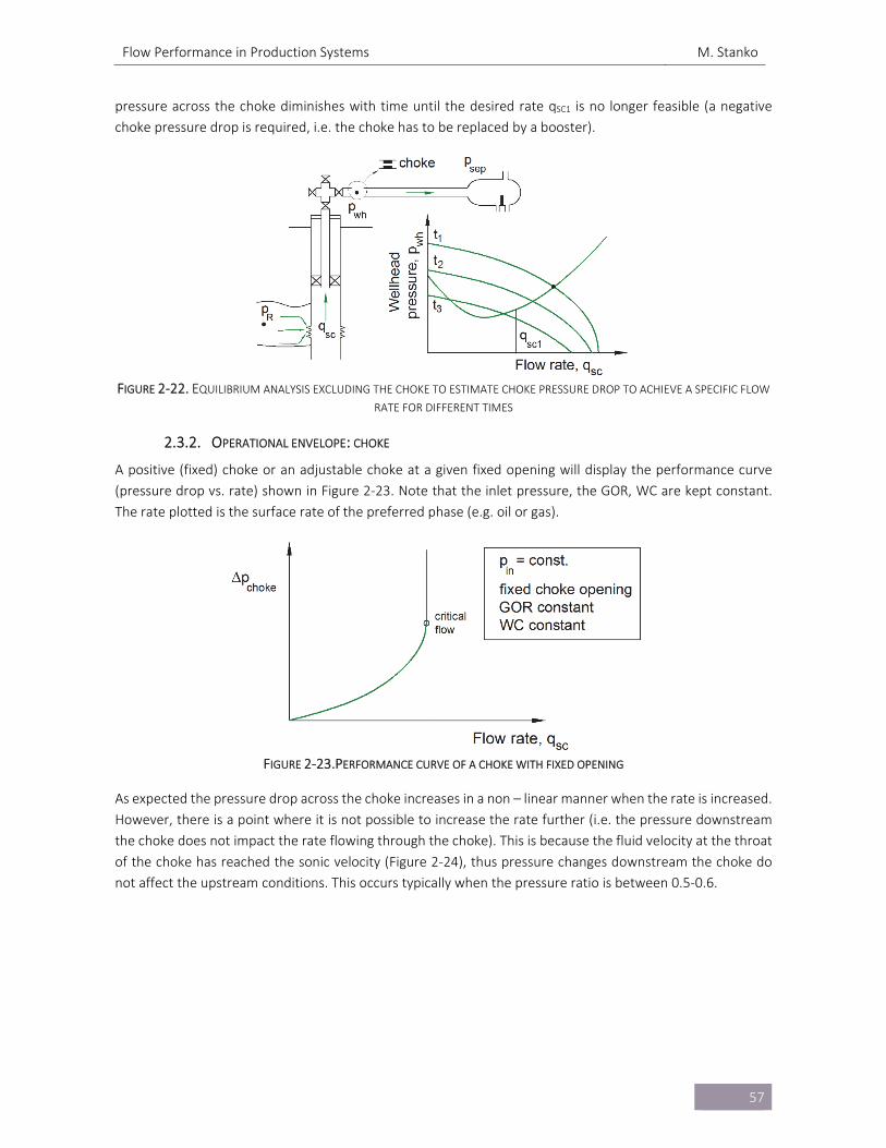
Flow Performance in Production Systems M. Stanko
57
pressure across the choke diminishes with time until the desired rate qSC1 is no longer feasible (a negative
choke pressure drop is required, i.e. the choke has to be replaced by a booster).
FIGURE 2‐22. EQUILIBRIUM ANALYSIS EXCLUDING THE CHOKE TO ESTIMATE CHOKE PRESSURE DROP TO ACHIEVE A SPECIFIC FLOW
RATE FOR DIFFERENT TIMES
2.3.2. OPERATIONAL ENVELOPE: CHOKE
A positive (fixed) choke or an adjustable choke at a given fixed opening will display the performance curve
(pressure drop vs. rate) shown in Figure 2‐23. Note that the inlet pressure, the GOR, WC are kept constant.
The rate plotted is the surface rate of the preferred phase (e.g. oil or gas).
FIGURE 2‐23.PERFORMANCE CURVE OF A CHOKE WITH FIXED OPENING
As expected the pressure drop across the choke increases in a non – linear manner when the rate is increased.
However, there is a point where it is not possible to increase the rate further (i.e. the pressure downstream
the choke does not impact the rate flowing through the choke). This is because the fluid velocity at the throat
of the choke has reached the sonic velocity (Figure 2‐24), thus pressure changes downstream the choke do
not affect the upstream conditions. This occurs typically when the pressure ratio is between 0.5‐0.6.
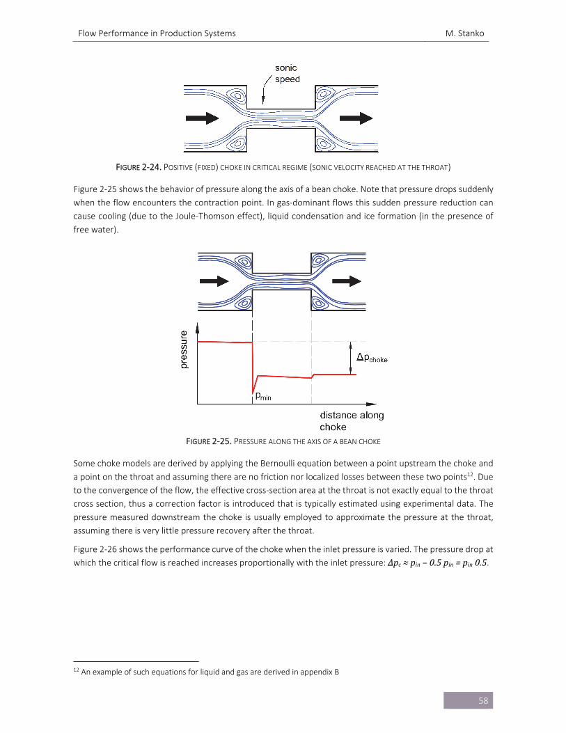
Flow Performance in Production Systems M. Stanko
58
FIGURE 2‐24. POSITIVE (FIXED) CHOKE IN CRITICAL REGIME (SONIC VELOCITY REACHED AT THE THROAT)
Figure 2‐25 shows the behavior of pressure along the axis of a bean choke. Note that pressure drops suddenly
when the flow encounters the contraction point. In gas‐dominant flows this sudden pressure reduction can
cause cooling (due to the Joule‐Thomson effect), liquid condensation and ice formation (in the presence of
free water).
FIGURE 2‐25. PRESSURE ALONG THE AXIS OF A BEAN CHOKE
Some choke models are derived by applying the Bernoulli equation between a point upstream the choke and
a point on the throat and assuming there are no friction nor localized losses between these two points12. Due
to the convergence of the flow, the effective cross‐section area at the throat is not exactly equal to the throat
cross section, thus a correction factor is introduced that is typically estimated using experimental data. The
pressure measured downstream the choke is usually employed to approximate the pressure at the throat,
assuming there is very little pressure recovery after the throat.
Figure 2‐26 shows the performance curve of the choke when the inlet pressure is varied. The pressure drop at
which the critical flow is reached increases proportionally with the inlet pressure: Δpc≈pin–0.5pin=pin0.5.
12 An example of such equations for liquid and gas are derived in appendix B
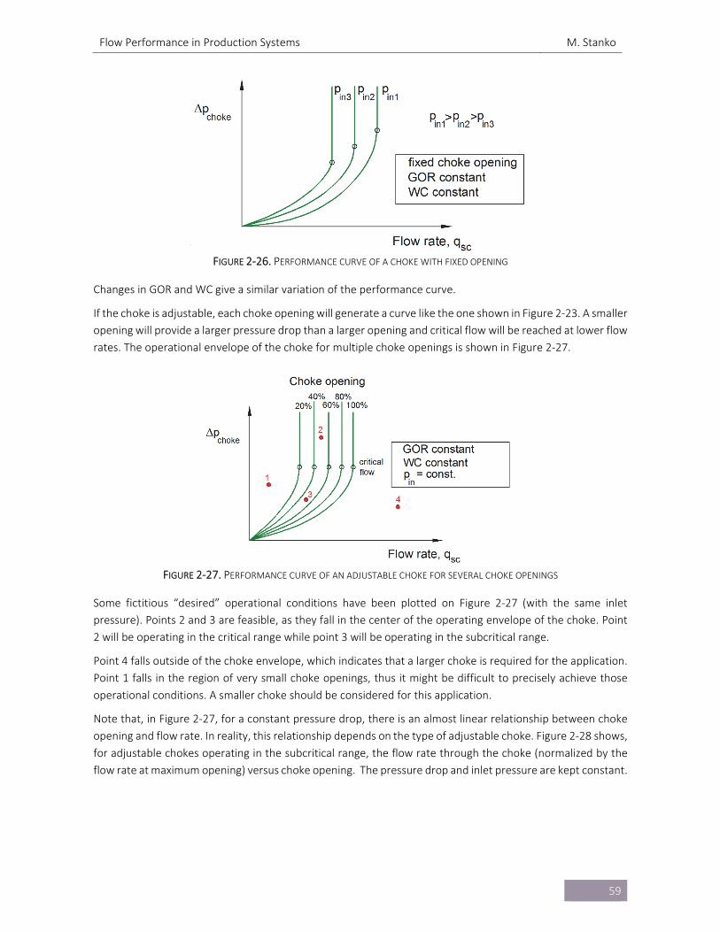
Flow Performance in Production Systems M. Stanko
59
FIGURE 2‐26. PERFORMANCE CURVE OF A CHOKE WITH FIXED OPENING
Changes in GOR and WC give a similar variation of the performance curve.
If the choke is adjustable, each choke opening will generate a curve like the one shown in Figure 2‐23. A smaller
opening will provide a larger pressure drop than a larger opening and critical flow will be reached at lower flow
rates. The operational envelope of the choke for multiple choke openings is shown in Figure 2‐27.
FIGURE 2‐27. PERFORMANCE CURVE OF AN ADJUSTABLE CHOKE FOR SEVERAL CHOKE OPENINGS
Some fictitious “desired” operational conditions have been plotted on Figure 2‐27 (with the same inlet
pressure). Points 2 and 3 are feasible, as they fall in the center of the operating envelope of the choke. Point
2 will be operating in the critical range while point 3 will be operating in the subcritical range.
Point 4 falls outside of the choke envelope, which indicates that a larger choke is required for the application.
Point 1 falls in the region of very small choke openings, thus it might be difficult to precisely achieve those
operational conditions. A smaller choke should be considered for this application.
Note that, in Figure 2‐27, for a constant pressure drop, there is an almost linear relationship between choke
opening and flow rate. In reality, this relationship depends on the type of adjustable choke. Figure 2‐28 shows,
for adjustable chokes operating in the subcritical range, the flow rate through the choke (normalized by the
flow rate at maximum opening) versus choke opening. The pressure drop and inlet pressure are kept constant.
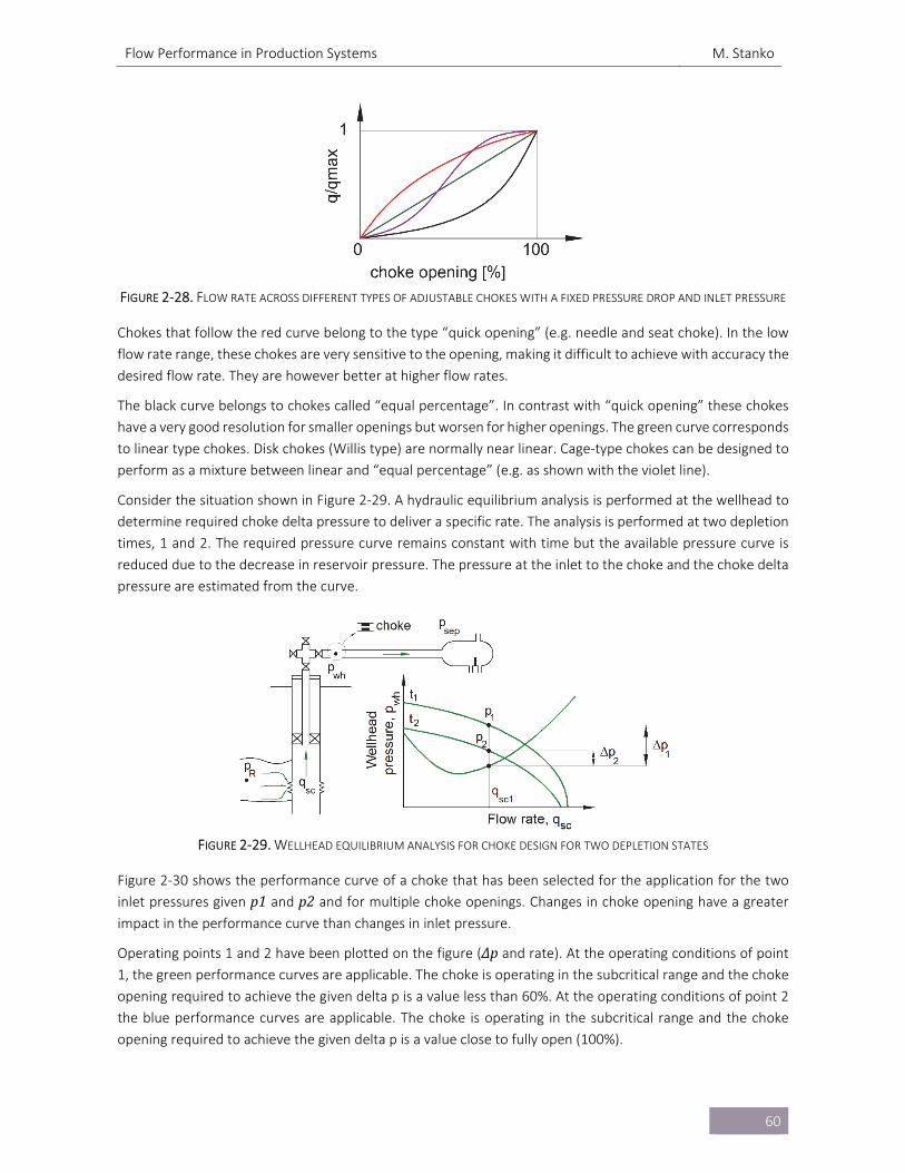
Flow Performance in Production Systems M. Stanko
60
FIGURE 2‐28. FLOW RATE ACROSS DIFFERENT TYPES OF ADJUSTABLE CHOKES WITH A FIXED PRESSURE DROP AND INLET PRESSURE
Chokes that follow the red curve belong to the type “quick opening” (e.g. needle and seat choke). In the low
flow rate range, these chokes are very sensitive to the opening, making it difficult to achieve with accuracy the
desired flow rate. They are however better at higher flow rates.
The black curve belongs to chokes called “equal percentage”. In contrast with “quick opening” these chokes
have a very good resolution for smaller openings but worsen for higher openings. The green curve corresponds
to linear type chokes. Disk chokes (Willis type) are normally near linear. Cage‐type chokes can be designed to
perform as a mixture between linear and “equal percentage” (e.g. as shown with the violet line).
Consider the situation shown in Figure 2‐29. A hydraulic equilibrium analysis is performed at the wellhead to
determine required choke delta pressure to deliver a specific rate. The analysis is performed at two depletion
times, 1 and 2. The required pressure curve remains constant with time but the available pressure curve is
reduced due to the decrease in reservoir pressure. The pressure at the inlet to the choke and the choke delta
pressure are estimated from the curve.
FIGURE 2‐29. WELLHEAD EQUILIBRIUM ANALYSIS FOR CHOKE DESIGN FOR TWO DEPLETION STATES
Figure 2‐30 shows the performance curve of a choke that has been selected for the application for the two
inlet pressures given p1 and p2 and for multiple choke openings. Changes in choke opening have a greater
impact in the performance curve than changes in inlet pressure.
Operating points 1 and 2 have been plotted on the figure (Δp and rate). At the operating conditions of point 1, the green performance curves are applicable. The choke is operating in the subcritical range and the choke
opening required to achieve the given delta p is a value less than 60%. At the operating conditions of point 2
the blue performance curves are applicable. The choke is operating in the subcritical range and the choke
opening required to achieve the given delta p is a value close to fully open (100%).
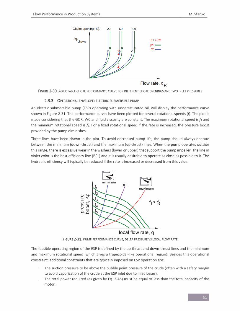
Flow Performance in Production Systems M. Stanko
61
FIGURE 2‐30. ADJUSTABLE CHOKE PERFORMANCE CURVE FOR DIFFERENT CHOKE OPENINGS AND TWO INLET PRESSURES
2.3.3. OPERATIONAL ENVELOPE: ELECTRIC SUBMERSIBLE PUMP
An electric submersible pump (ESP) operating with undersaturated oil, will display the performance curve
shown in Figure 2‐31. The performance curves have been plotted for several rotational speeds (f). The plot is made considering that the GOR, WC and fluid viscosity are constant. The maximum rotational speed is f1 and the minimum rotational speed is f5. For a fixed rotational speed if the rate is increased, the pressure boost provided by the pump diminishes.
Three lines have been drawn in the plot. To avoid decreased pump life, the pump should always operate
between the minimum (down‐thrust) and the maximum (up‐thrust) lines. When the pump operates outside
this range, there is excessive wear in the washers (lower or upper) that support the pump impeller. The line in
violet color is the best efficiency line (BEL) and it is usually desirable to operate as close as possible to it. The
hydraulic efficiency will typically be reduced if the rate is increased or decreased from this value.
FIGURE 2‐31. PUMP PERFORMANCE CURVE, DELTA PRESSURE VS LOCAL FLOW RATE
The feasible operating region of the ESP is defined by the up‐thrust and down‐thrust lines and the minimum
and maximum rotational speed (which gives a trapezoidal‐like operational region). Besides this operational
constraint, additional constraints that are typically imposed on ESP operation are:
The suction pressure to be above the bubble point pressure of the crude (often with a safety margin
to avoid vaporization of the crude at the ESP inlet due to inlet losses).
The total power required (as given by Eq. 2‐45) must be equal or less than the total capacity of the
motor.
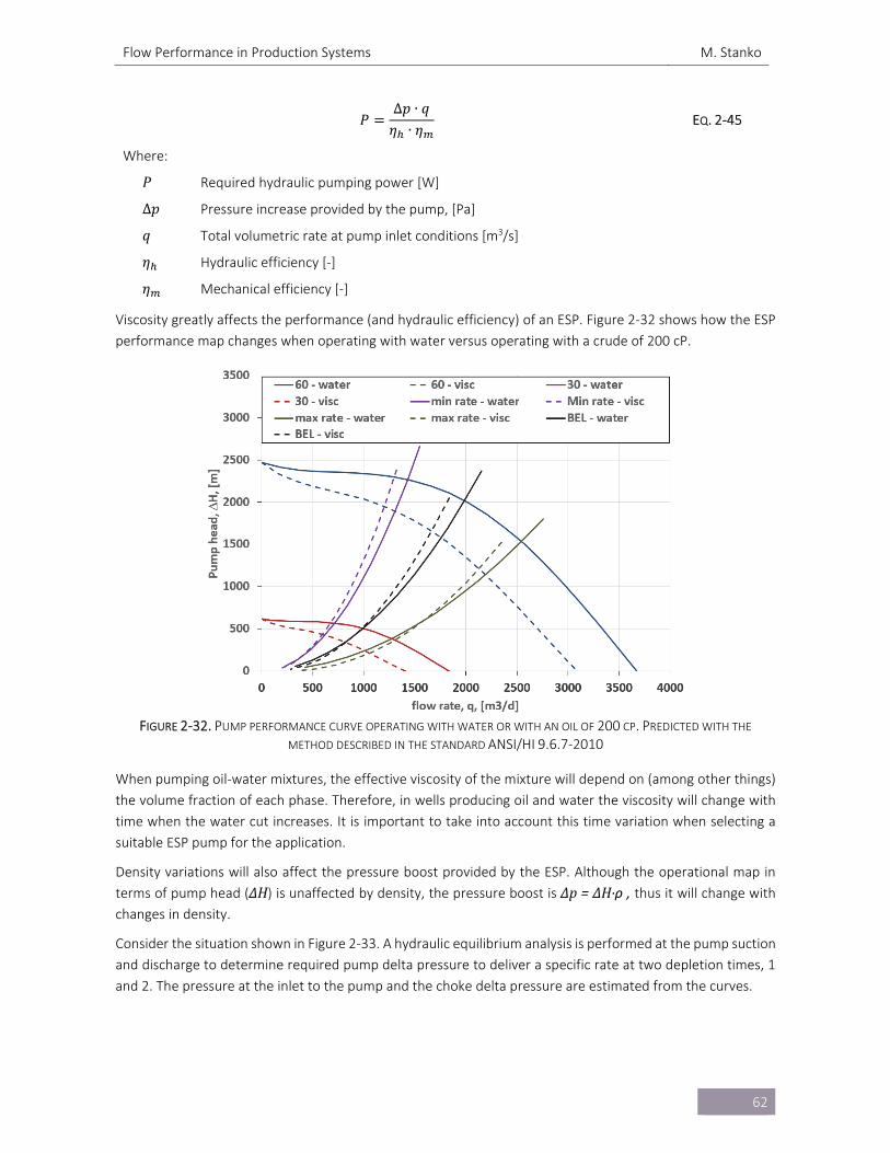
Flow Performance in Production Systems M. Stanko
62
𝑃Δ𝑝 ∙ 𝑞
𝜂 ∙ 𝜂 EQ. 2‐45
Where:
𝑃 Required hydraulic pumping power [W]
Δ𝑝 Pressure increase provided by the pump, [Pa]
𝑞 Total volumetric rate at pump inlet conditions [m3/s]
𝜂 Hydraulic efficiency [‐]
𝜂 Mechanical efficiency [‐]
Viscosity greatly affects the performance (and hydraulic efficiency) of an ESP. Figure 2‐32 shows how the ESP
performance map changes when operating with water versus operating with a crude of 200 cP.
FIGURE 2‐32. PUMP PERFORMANCE CURVE OPERATING WITH WATER OR WITH AN OIL OF 200 CP. PREDICTED WITH THE
METHOD DESCRIBED IN THE STANDARD ANSI/HI 9.6.7‐2010
When pumping oil‐water mixtures, the effective viscosity of the mixture will depend on (among other things)
the volume fraction of each phase. Therefore, in wells producing oil and water the viscosity will change with
time when the water cut increases. It is important to take into account this time variation when selecting a
suitable ESP pump for the application.
Density variations will also affect the pressure boost provided by the ESP. Although the operational map in
terms of pump head (ΔH) is unaffected by density, the pressure boost is Δp=ΔH∙ρ , thus it will change with changes in density.
Consider the situation shown in Figure 2‐33. A hydraulic equilibrium analysis is performed at the pump suction
and discharge to determine required pump delta pressure to deliver a specific rate at two depletion times, 1
and 2. The pressure at the inlet to the pump and the choke delta pressure are estimated from the curves.
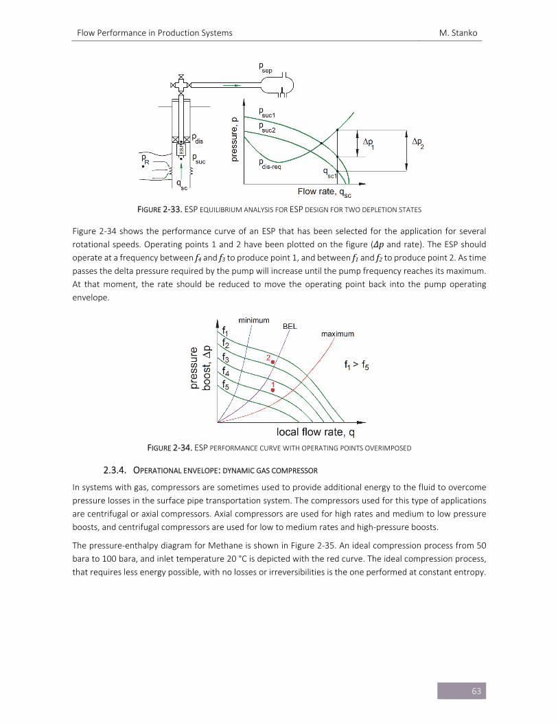
Flow Performance in Production Systems M. Stanko
63
FIGURE 2‐33. ESP EQUILIBRIUM ANALYSIS FOR ESP DESIGN FOR TWO DEPLETION STATES
Figure 2‐34 shows the performance curve of an ESP that has been selected for the application for several
rotational speeds. Operating points 1 and 2 have been plotted on the figure (Δp and rate). The ESP should operate at a frequency between f4 and f3 to produce point 1, and between f1 and f2 to produce point 2. As time
passes the delta pressure required by the pump will increase until the pump frequency reaches its maximum.
At that moment, the rate should be reduced to move the operating point back into the pump operating
envelope.
FIGURE 2‐34. ESP PERFORMANCE CURVE WITH OPERATING POINTS OVERIMPOSED
2.3.4. OPERATIONAL ENVELOPE: DYNAMIC GAS COMPRESSOR
In systems with gas, compressors are sometimes used to provide additional energy to the fluid to overcome
pressure losses in the surface pipe transportation system. The compressors used for this type of applications
are centrifugal or axial compressors. Axial compressors are used for high rates and medium to low pressure
boosts, and centrifugal compressors are used for low to medium rates and high‐pressure boosts.
The pressure‐enthalpy diagram for Methane is shown in Figure 2‐35. An ideal compression process from 50
bara to 100 bara, and inlet temperature 20 °C is depicted with the red curve. The ideal compression process,
that requires less energy possible, with no losses or irreversibilities is the one performed at constant entropy.
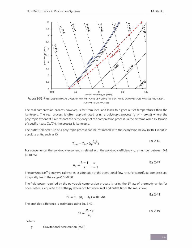
Flow Performance in Production Systems M. Stanko
64
FIGURE 2‐35. PRESSURE‐ENTHALPY DIAGRAM FOR METHANE DEPICTING AN ISENTROPIC COMPRESSION PROCESS AND A REAL
COMPRESSION PROCESS
The real compression process however, is far from ideal and leads to higher outlet temperatures than the
isentropic. The real process is often approximated using a polytropic process (p vn = const) where the polytropic exponent n represents the “efficiency” of the compression process. In the extreme when n=k(ratio of specific heats Cp/Cv), the process is isentropic.
The outlet temperature of a polytropic process can be estimated with the expression below (with T input in
absolute units, such as K):
𝑇 𝑇 ∙ 𝑟 EQ. 2‐46
For convenience, the polytropic exponent is related with the polytropic efficiency ηp, a number between 0‐1
(0‐100%):
𝜂𝑘 1
𝑘∙
𝑛𝑛 1
EQ. 2‐47
The polytropic efficiency typically varies as a function of the operational flow rate. For centrifugal compressors,
it typically lies in the range 0.65‐0.80.
The fluid power required by the polytropic compression process is, using the 1st law of thermodynamics for
open systems, equal to the enthalpy difference between inlet and outlet times the mass flow.
𝑊 𝑚 ∙ ℎ ℎ 𝑚 ∙ ∆ℎ EQ. 2‐48
The enthalpy difference is estimated using Eq. 2‐49:
∆ℎ𝐻 ∙ 𝑔
𝜂
EQ. 2‐49
Where:
𝑔 Gravitational acceleration [m/s2]
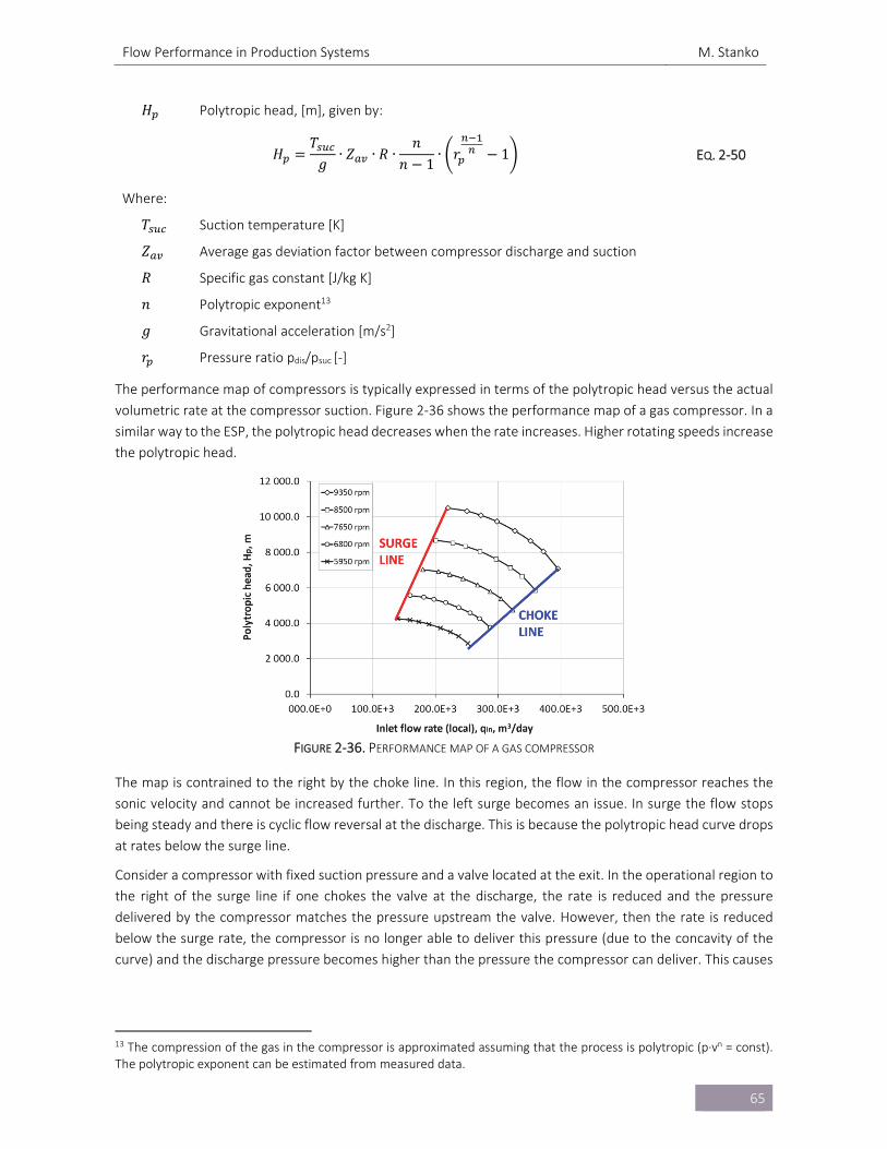
Flow Performance in Production Systems M. Stanko
65
𝐻 Polytropic head, [m], given by:
𝐻𝑇
𝑔∙ 𝑍 ∙ 𝑅 ∙
𝑛𝑛 1
∙ 𝑟 1 EQ. 2‐50
Where:
𝑇 Suction temperature [K]
𝑍 Average gas deviation factor between compressor discharge and suction
𝑅 Specific gas constant [J/kg K]
𝑛 Polytropic exponent13
𝑔 Gravitational acceleration [m/s2]
𝑟 Pressure ratio pdis/psuc [‐]
The performance map of compressors is typically expressed in terms of the polytropic head versus the actual
volumetric rate at the compressor suction. Figure 2‐36 shows the performance map of a gas compressor. In a
similar way to the ESP, the polytropic head decreases when the rate increases. Higher rotating speeds increase
the polytropic head.
FIGURE 2‐36. PERFORMANCE MAP OF A GAS COMPRESSOR
The map is contrained to the right by the choke line. In this region, the flow in the compressor reaches the
sonic velocity and cannot be increased further. To the left surge becomes an issue. In surge the flow stops
being steady and there is cyclic flow reversal at the discharge. This is because the polytropic head curve drops
at rates below the surge line.
Consider a compressor with fixed suction pressure and a valve located at the exit. In the operational region to
the right of the surge line if one chokes the valve at the discharge, the rate is reduced and the pressure
delivered by the compressor matches the pressure upstream the valve. However, then the rate is reduced
below the surge rate, the compressor is no longer able to deliver this pressure (due to the concavity of the
curve) and the discharge pressure becomes higher than the pressure the compressor can deliver. This causes
13 The compression of the gas in the compressor is approximated assuming that the process is polytropic (p∙vn = const). The polytropic exponent can be estimated from measured data.
Flow Performance in Production Systems M. Stanko
66
flow reversal. With the flow reversal, the pressure at the discharge decreases and falls within the compressor
curve again. The rate increases again and the cycle is repeated.
The performance map of a compressor will vary mainly with the inlet temperature, the molecular weight of
the gas (M) and the heat capacity ratio14 (k=Cp/Cv). If the curves at test conditions are known15, the following
expressions can be used to correct them and estimate the performance under different conditions:
𝑞 𝑞 ∙𝑘𝑘
∙𝑀𝑀
∙𝑇𝑇
EQ. 2‐51
𝐻 , 𝐻 , ∙𝑘𝑘
∙𝑀𝑀
∙𝑇𝑇
EQ. 2‐52
To avoid having a collection of curves each time these variables change, often the operating point is converted
to the test conditions using Eq. 2‐47 and Eq. 2‐48, and are plotted on the test performance map.
Besides the constraint that the operating points must fall on the compressor performance map, there are
some additional constraints that must be considered:
The required compression power (P) must be less than the power capacity of the driving motor. The
total required power can be computed with Eq. 2‐53.
𝑃∆ℎ ∙ 𝑚
𝜂
EQ. 2‐53
Where:
𝑚 Mass flow [kg/s]
𝜂 Mechanical efficiency [‐]
The temperature at the discharge must be kept below a maximum allowable value. This is usually due
to temperature limits in the compressor seals and safeguard the integrity of the downstream piping.
In systems where chemicals are injected (e.g. hydrate inhibitor), the temperature should also be kept
below the vaporization temperature of the chemical, to ensure its effectiveness.
The pressure at the suction must be above a minimum allowable value.
2.3.1. OPERATIONAL ENVELOPE: JET PUMP
A Jet pump, or ejector, is a device without moving parts in which a high‐pressure source fluid is injected to the
main fluid stream through a nozzle. Due to the high speed the high‐pressure fluid achieves in the nozzle, its
pressure is reduced significantly and creates a sucking effect. The suction side of the jet‐pump is then
connected to this location (Figure 2‐37). The high‐pressure fluid is usually single‐phase gas or liquid (oil or
water).
14 A empirical expression to estimate k is k= 1.30 – 0.31∙(g – 0.55) 15 Typically, 1 atm and 15.56 oC at the suction
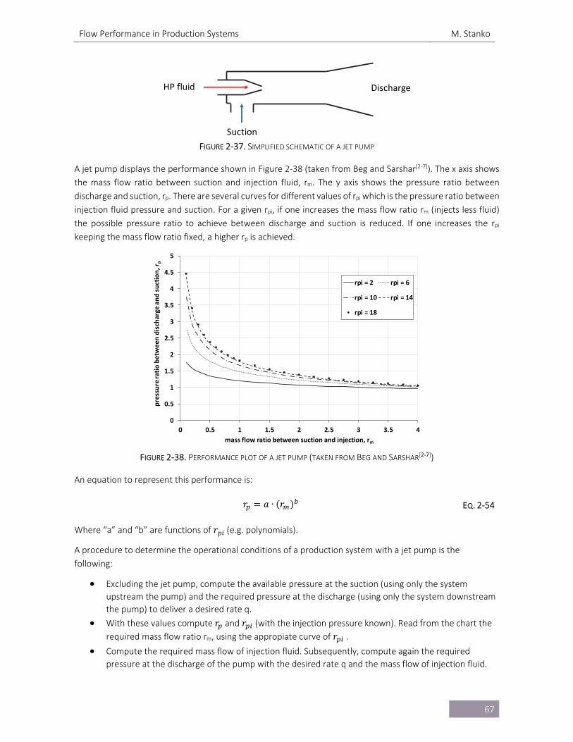
Flow Performance in Production Systems M. Stanko
67
FIGURE 2‐37. SIMPLIFIED SCHEMATIC OF A JET PUMP
A jet pump displays the performance shown in Figure 2‐38 (taken from Beg and Sarshar[2‐7]). The x axis shows
the mass flow ratio between suction and injection fluid, rm. The y axis shows the pressure ratio between
discharge and suction, rp. There are several curves for different values of rpi which is the pressure ratio between
injection fluid pressure and suction. For a given rpi, if one increases the mass flow ratio rm (injects less fluid)
the possible pressure ratio to achieve between discharge and suction is reduced. If one increases the rpi
keeping the mass flow ratio fixed, a higher rp is achieved.
FIGURE 2‐38. PERFORMANCE PLOT OF A JET PUMP (TAKEN FROM BEG AND SARSHAR[2‐7])
An equation to represent this performance is:
𝑟 𝑎 ∙ 𝑟 EQ. 2‐54
Where “a” and “b” are functions of 𝑟𝑝𝑖 (e.g. polynomials).
A procedure to determine the operational conditions of a production system with a jet pump is the
following:
Excluding the jet pump, compute the available pressure at the suction (using only the system
upstream the pump) and the required pressure at the discharge (using only the system downstream
the pump) to deliver a desired rate q.
With these values compute 𝑟 and 𝑟 (with the injection pressure known). Read from the chart the
required mass flow ratio rm, using the appropiate curve of 𝑟 .
Compute the required mass flow of injection fluid. Subsequently, compute again the required
pressure at the discharge of the pump with the desired rate q and the mass flow of injection fluid.
HP fluid
Suction
Discharge
0
0.5
1
1.5
2
2.5
3
3.5
4
4.5
5
0 0.5 1 1.5 2 2.5 3 3.5 4
pressure ratio betw
een
discharge and suction, r
p
mass flow ratio between suction and injection, rm
rpi = 2 rpi = 6
rpi = 10 rpi = 14
rpi = 18
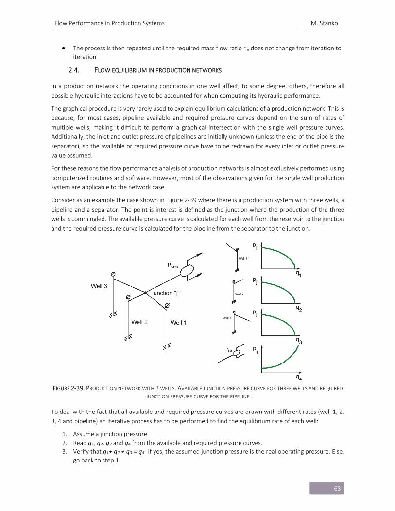
Flow Performance in Production Systems M. Stanko
68
The process is then repeated until the required mass flow ratio rm does not change from iteration to
iteration.
2.4. FLOW EQUILIBRIUM IN PRODUCTION NETWORKS
In a production network the operating conditions in one well affect, to some degree, others, therefore all
possible hydraulic interactions have to be accounted for when computing its hydraulic performance.
The graphical procedure is very rarely used to explain equilibrium calculations of a production network. This is
because, for most cases, pipeline available and required pressure curves depend on the sum of rates of
multiple wells, making it difficult to perform a graphical intersection with the single well pressure curves.
Additionally, the inlet and outlet pressure of pipelines are initially unknown (unless the end of the pipe is the
separator), so the available or required pressure curve have to be redrawn for every inlet or outlet pressure
value assumed.
For these reasons the flow performance analysis of production networks is almost exclusively performed using
computerized routines and software. However, most of the observations given for the single well production
system are applicable to the network case.
Consider as an example the case shown in Figure 2‐39 where there is a production system with three wells, a
pipeline and a separator. The point is interest is defined as the junction where the production of the three
wells is commingled. The available pressure curve is calculated for each well from the reservoir to the junction
and the required pressure curve is calculated for the pipeline from the separator to the junction.
FIGURE 2‐39. PRODUCTION NETWORK WITH 3 WELLS. AVAILABLE JUNCTION PRESSURE CURVE FOR THREE WELLS AND REQUIRED
JUNCTION PRESSURE CURVE FOR THE PIPELINE
To deal with the fact that all available and required pressure curves are drawn with different rates (well 1, 2,
3, 4 and pipeline) an iterative process has to be performed to find the equilibrium rate of each well:
1. Assume a junction pressure
2. Read q1, q2, q3 and q4 from the available and required pressure curves.
3. Verify that q1+q2+q3=q4. If yes, the assumed junction pressure is the real operating pressure. Else,
go back to step 1.
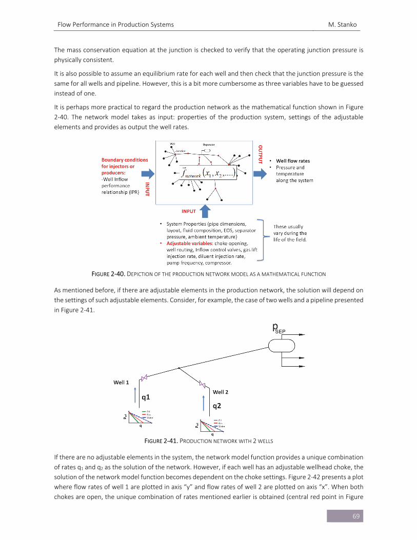
Flow Performance in Production Systems M. Stanko
69
The mass conservation equation at the junction is checked to verify that the operating junction pressure is
physically consistent.
It is also possible to assume an equilibrium rate for each well and then check that the junction pressure is the
same for all wells and pipeline. However, this is a bit more cumbersome as three variables have to be guessed
instead of one.
It is perhaps more practical to regard the production network as the mathematical function shown in Figure
2‐40. The network model takes as input: properties of the production system, settings of the adjustable
elements and provides as output the well rates.
FIGURE 2‐40. DEPICTION OF THE PRODUCTION NETWORK MODEL AS A MATHEMATICAL FUNCTION
As mentioned before, if there are adjustable elements in the production network, the solution will depend on
the settings of such adjustable elements. Consider, for example, the case of two wells and a pipeline presented
in Figure 2‐41.
FIGURE 2‐41. PRODUCTION NETWORK WITH 2 WELLS
If there are no adjustable elements in the system, the network model function provides a unique combination
of rates q1 and q2 as the solution of the network. However, if each well has an adjustable wellhead choke, the
solution of the network model function becomes dependent on the choke settings. Figure 2‐42 presents a plot
where flow rates of well 1 are plotted in axis “y” and flow rates of well 2 are plotted on axis “x”. When both
chokes are open, the unique combination of rates mentioned earlier is obtained (central red point in Figure
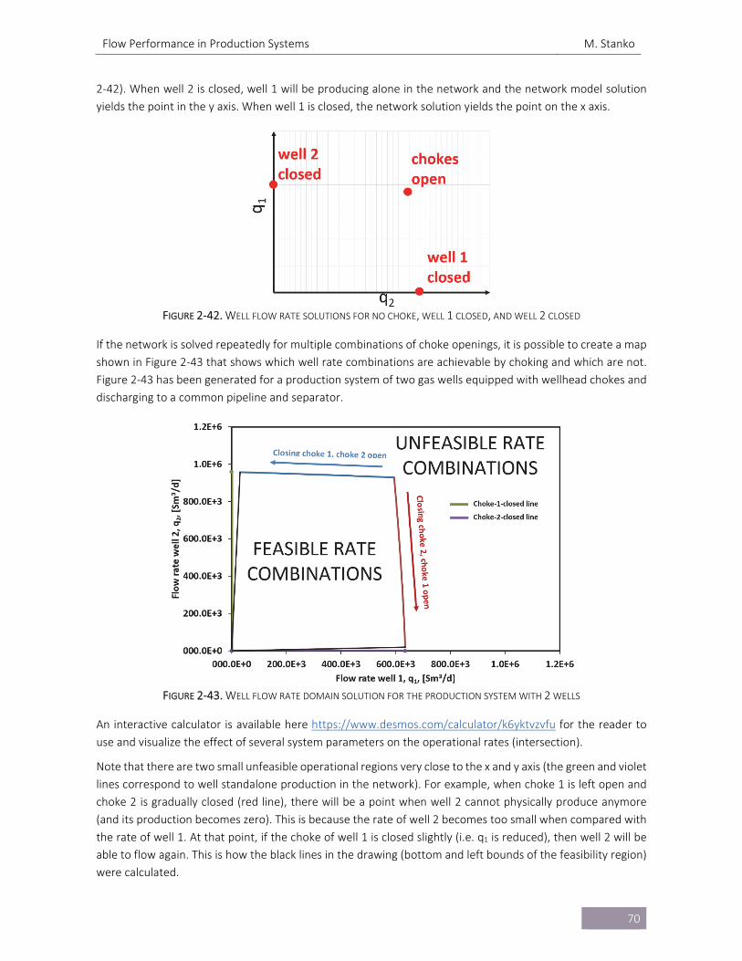
Flow Performance in Production Systems M. Stanko
70
2‐42). When well 2 is closed, well 1 will be producing alone in the network and the network model solution
yields the point in the y axis. When well 1 is closed, the network solution yields the point on the x axis.
FIGURE 2‐42. WELL FLOW RATE SOLUTIONS FOR NO CHOKE, WELL 1 CLOSED, AND WELL 2 CLOSED
If the network is solved repeatedly for multiple combinations of choke openings, it is possible to create a map
shown in Figure 2‐43 that shows which well rate combinations are achievable by choking and which are not.
Figure 2‐43 has been generated for a production system of two gas wells equipped with wellhead chokes and
discharging to a common pipeline and separator.
FIGURE 2‐43. WELL FLOW RATE DOMAIN SOLUTION FOR THE PRODUCTION SYSTEM WITH 2 WELLS
An interactive calculator is available here https://www.desmos.com/calculator/k6yktvzvfu for the reader to
use and visualize the effect of several system parameters on the operational rates (intersection).
Note that there are two small unfeasible operational regions very close to the x and y axis (the green and violet
lines correspond to well standalone production in the network). For example, when choke 1 is left open and
choke 2 is gradually closed (red line), there will be a point when well 2 cannot physically produce anymore
(and its production becomes zero). This is because the rate of well 2 becomes too small when compared with
the rate of well 1. At that point, if the choke of well 1 is closed slightly (i.e. q1 is reduced), then well 2 will be
able to flow again. This is how the black lines in the drawing (bottom and left bounds of the feasibility region)
were calculated.
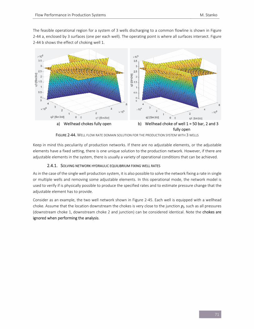
Flow Performance in Production Systems M. Stanko
71
The feasible operational region for a system of 3 wells discharging to a common flowline is shown in Figure
2‐44 a, enclosed by 3 surfaces (one per each well). The operating point is where all surfaces intersect. Figure
2‐44 b shows the effect of choking well 1.
a) Wellhead chokes fully open b) Wellhead choke of well 1 = 50 bar, 2 and 3
fully open
FIGURE 2‐44. WELL FLOW RATE DOMAIN SOLUTION FOR THE PRODUCTION SYSTEM WITH 3 WELLS
Keep in mind this peculiarity of production networks. If there are no adjustable elements, or the adjustable
elements have a fixed setting, there is one unique solution to the production network. However, if there are
adjustable elements in the system, there is usually a variety of operational conditions that can be achieved.
2.4.1. SOLVING NETWORK HYDRAULIC EQUILIBRIUM FIXING WELL RATES
As in the case of the single well production system, it is also possible to solve the network fixing a rate in single
or multiple wells and removing some adjustable elements. In this operational mode, the network model is
used to verify if is physically possible to produce the specified rates and to estimate pressure change that the
adjustable element has to provide.
Consider as an example, the two well network shown in Figure 2‐45. Each well is equipped with a wellhead
choke. Assume that the location downstream the chokes is very close to the junction pj, such as all pressures (downstream choke 1, downstream choke 2 and junction) can be considered identical. Note the chokes are
ignored when performing the analysis.
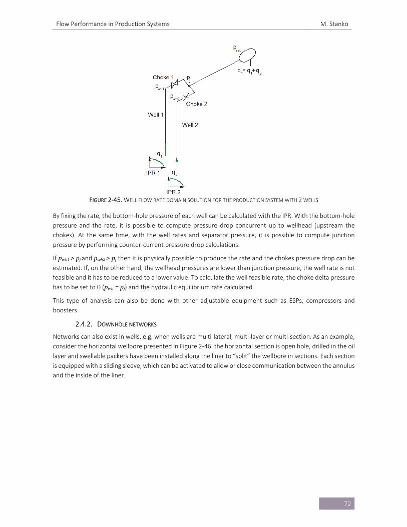
Flow Performance in Production Systems M. Stanko
72
FIGURE 2‐45. WELL FLOW RATE DOMAIN SOLUTION FOR THE PRODUCTION SYSTEM WITH 2 WELLS
By fixing the rate, the bottom‐hole pressure of each well can be calculated with the IPR. With the bottom‐hole
pressure and the rate, it is possible to compute pressure drop concurrent up to wellhead (upstream the
chokes). At the same time, with the well rates and separator pressure, it is possible to compute junction
pressure by performing counter‐current pressure drop calculations.
If pwh1>pj and pwh2>pj then it is physically possible to produce the rate and the chokes pressure drop can be estimated. If, on the other hand, the wellhead pressures are lower than junction pressure, the well rate is not
feasible and it has to be reduced to a lower value. To calculate the well feasible rate, the choke delta pressure
has to be set to 0 (pwh=pj) and the hydraulic equilibrium rate calculated.
This type of analysis can also be done with other adjustable equipment such as ESPs, compressors and
boosters.
2.4.2. DOWNHOLE NETWORKS
Networks can also exist in wells, e.g. when wells are multi‐lateral, multi‐layer or multi‐section. As an example,
consider the horizontal wellbore presented in Figure 2‐46. the horizontal section is open hole, drilled in the oil
layer and swellable packers have been installed along the liner to “split” the wellbore in sections. Each section
is equipped with a sliding sleeve, which can be activated to allow or close communication between the annulus
and the inside of the liner.
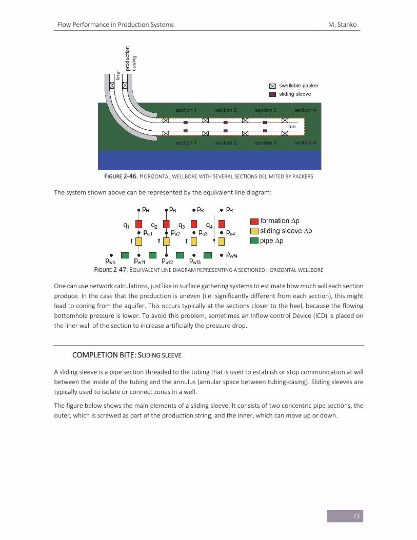
Flow Performance in Production Systems M. Stanko
73
FIGURE 2‐46. HORIZONTAL WELLBORE WITH SEVERAL SECTIONS DELIMITED BY PACKERS
The system shown above can be represented by the equivalent line diagram:
FIGURE 2‐47. EQUIVALENT LINE DIAGRAM REPRESENTING A SECTIONED HORIZONTAL WELLBORE
One can use network calculations, just like in surface gathering systems to estimate how much will each section
produce. In the case that the production is uneven (i.e. significantly different from each section), this might
lead to coning from the aquifer. This occurs typically at the sections closer to the heel, because the flowing
bottomhole pressure is lower. To avoid this problem, sometimes an Inflow control Device (ICD) is placed on
the liner wall of the section to increase artificially the pressure drop.
COMPLETION BITE: SLIDING SLEEVE
A sliding sleeve is a pipe section threaded to the tubing that is used to establish or stop communication at will
between the inside of the tubing and the annulus (annular space between tubing‐casing). Sliding sleeves are
typically used to isolate or connect zones in a well.
The figure below shows the main elements of a sliding sleeve. It consists of two concentric pipe sections, the
outer, which is screwed as part of the production string, and the inner, which can move up or down.
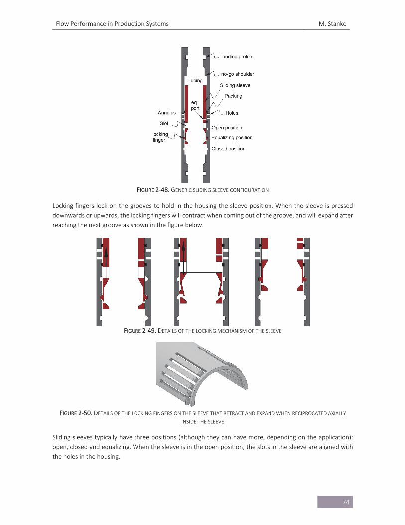
Flow Performance in Production Systems M. Stanko
74
FIGURE 2‐48. GENERIC SLIDING SLEEVE CONFIGURATION
Locking fingers lock on the grooves to hold in the housing the sleeve position. When the sleeve is pressed
downwards or upwards, the locking fingers will contract when coming out of the groove, and will expand after
reaching the next groove as shown in the figure below.
FIGURE 2‐49. DETAILS OF THE LOCKING MECHANISM OF THE SLEEVE
FIGURE 2‐50. DETAILS OF THE LOCKING FINGERS ON THE SLEEVE THAT RETRACT AND EXPAND WHEN RECIPROCATED AXIALLY
INSIDE THE SLEEVE
Sliding sleeves typically have three positions (although they can have more, depending on the application):
open, closed and equalizing. When the sleeve is in the open position, the slots in the sleeve are aligned with
the holes in the housing.
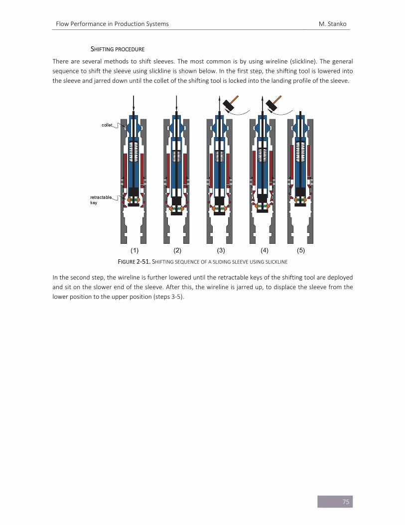
Flow Performance in Production Systems M. Stanko
75
SHIFTING PROCEDURE
There are several methods to shift sleeves. The most common is by using wireline (slickline). The general
sequence to shift the sleeve using slickline is shown below. In the first step, the shifting tool is lowered into
the sleeve and jarred down until the collet of the shifting tool is locked into the landing profile of the sleeve.
FIGURE 2‐51. SHIFTING SEQUENCE OF A SLIDING SLEEVE USING SLICKLINE
In the second step, the wireline is further lowered until the retractable keys of the shifting tool are deployed
and sit on the slower end of the sleeve. After this, the wireline is jarred up, to displace the sleeve from the
lower position to the upper position (steps 3‐5).
Flow Performance in Production Systems M. Stanko
76
REFERENCES
[2‐1] Astutik, W. (2012). IPR modeling for coning wells. Thesis for the degree of Master of Science.
Norwegian University of Science and Technology. Trondheim.
[2‐2] Crafton, J. Dyal, V. (1976). An Iterative Solution for the Gas Pipeline Network Problem. SPE‐6032.
Annual Fall Technical Conference and Exhibition of the SPE of AIME. Society of Petroleum
Engineers. New Orleans
[2‐3] Golan, M., Whitson, C. H. (1986). Well Performance. Second Edition. Prentice‐Hall Inc
[2‐4] Litvak, M., Darlow, B. (1995). Surface Network and Well Tubinghead Pressure Constraints in
Compositional Simulation. SPE‐29125. Symposium on Reservoir Simulation. Society of Petroleum
Engineers. San Antonio.
[2‐5] Tian, S., Adewumi, M. A New Algorithm for Analyzing and Designing Two Phase Flow Pipeline
Networks Paper 28177 presented at the 1993 AIChE spring National Meeting, Texas. 1993.
[2‐6] Whitson, C. H. (1983). Reservoir Well Performance and Predicting Deliverability. SPE12518.
[2‐7] Beg, N., Sarshar, Sacha. (2014). Engineers’ Handbook on Surface Jet pumps for Enhanced oil and gas
production. Caltec Limited.
Production Optimization M. Stanko
77
3. PRODUCTION OPTIMIZATION
In the industry, “Production optimization” is a wide term that englobes detecting opportunities to increase
field oil or gas production, cost reduction and implementing solutions to materialize them. The main principle
is to introduce small cost‐effective changes to improve the production system. Roughly speaking, the potential
increase in production that can be achieved by executing optimization lies someplace between 1‐30%.
Some actions that are typically executed to perform production optimization are:
Detect locations in the system with abnormally high‐pressure loss and flow restrictions
Verification of equipment design conditions vs actual operating conditions
Identification and addressing fluid sources that have disadvantageous characteristics (e.g. high water
cut, high H2S content)
Identify and correct system malfunctions and non‐intended behavior
Analyze and improve the logistics and planning of maintenance, replacement and installation of
equipment or in the execution of field activities.
Review the occurrence of failures and recognize patterns
Calibration of instrumentation
Identification of operational constraints (e.g. water handling capacity, power capacity)
Observe and analyze the response of the system when changes are introduced
Find control settings of equipment that give a production higher than current (or, preferably, that give
maximum production possible)
Identify bottlenecks
Identifying and monitoring key performance indicators (KPIs)
Some tools that are typically used for performing these actions are historic measured and reported data,
instrumentation readings, experiences reported by field operators and in‐house or commercial numerical
simulators.
However, formally speaking, the term “optimization” is wrongly used to characterize most of the activities
described above. In mathematics, optimization refers to find or determine the maximum or minimum value of
a function that is dependent on input parameters while honoring constraints. In practical production
optimization checks are seldom made to verify if the corrections and changes introduced in the system are in
fact the “best” possible alternative. Therefore, a better term to use to englobe most of the activities mentioned
above might be “production effectivization”.
In this chapter only one case of production optimization is discussed: finding control values in the system that
maximize an indicator of economic or system health. Some typical indicators are: oil and gas production rates,
revenue, net present value, ultimate recovery, cumulative production, inverse of lifting costs. The optimization
formulation usually includes multiple operational constraints.
3.1. OPTIMIZING A PRODUCTION SYSTEM
An existing or in‐planning production system has usually adjustable elements, design features that are yet
undecided upon or production and drilling schedules that are modifiable in time. It is usually desirable to find
the particular setting or values of such elements that provides the most attractive operational conditions
within the resources available. The definition of “most attractive operational conditions” depends on the
particular application, the field architecture, the resources available, but it is usually to produce maximum oil,
gas production or revenue (usually called the main objective function) while honoring multiple operational
constraints. Some typical constraints are keeping water production within processing capacity, oil and gas
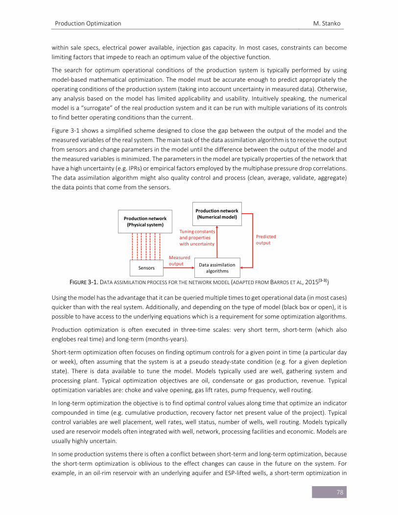
Production Optimization M. Stanko
78
within sale specs, electrical power available, injection gas capacity. In most cases, constraints can become
limiting factors that impede to reach an optimum value of the objective function.
The search for optimum operational conditions of the production system is typically performed by using
model‐based mathematical optimization. The model must be accurate enough to predict appropriately the
operating conditions of the production system (taking into account uncertainty in measured data). Otherwise,
any analysis based on the model has limited applicability and usability. Intuitively speaking, the numerical
model is a “surrogate” of the real production system and it can be run with multiple variations of its controls
to find better operating conditions than the current.
Figure 3‐1 shows a simplified scheme designed to close the gap between the output of the model and the
measured variables of the real system. The main task of the data assimilation algorithm is to receive the output
from sensors and change parameters in the model until the difference between the output of the model and
the measured variables is minimized. The parameters in the model are typically properties of the network that
have a high uncertainty (e.g. IPRs) or empirical factors employed by the multiphase pressure drop correlations.
The data assimilation algorithm might also quality control and process (clean, average, validate, aggregate)
the data points that come from the sensors.
FIGURE 3‐1. DATA ASSIMILATION PROCESS FOR THE NETWORK MODEL (ADAPTED FROM BARROS ET AL, 2015[3‐3])
Using the model has the advantage that it can be queried multiple times to get operational data (in most cases)
quicker than with the real system. Additionally, and depending on the type of model (black box or open), it is
possible to have access to the underlying equations which is a requirement for some optimization algorithms.
Production optimization is often executed in three‐time scales: very short term, short‐term (which also
englobes real time) and long‐term (months‐years).
Short‐term optimization often focuses on finding optimum controls for a given point in time (a particular day
or week), often assuming that the system is at a pseudo steady‐state condition (e.g. for a given depletion
state). There is data available to tune the model. Models typically used are well, gathering system and
processing plant. Typical optimization objectives are oil, condensate or gas production, revenue. Typical
optimization variables are: choke and valve opening, gas lift rates, pump frequency, well routing.
In long‐term optimization the objective is to find optimal control values along time that optimize an indicator
compounded in time (e.g. cumulative production, recovery factor net present value of the project). Typical
control variables are well placement, well rates, well status, number of wells, well routing. Models typically
used are reservoir models often integrated with well, network, processing facilities and economic. Models are
usually highly uncertain.
In some production systems there is often a conflict between short‐term and long‐term optimization, because
the short‐term optimization is oblivious to the effect changes can cause in the future on the system. For
example, in an oil‐rim reservoir with an underlying aquifer and ESP‐lifted wells, a short‐term optimization in
Production network (Physical system)
Production network (Numerical model)
SensorsData assimilation
algorithms
Measured output
Tuning constants and properties with uncertainty
Predicted output
Production Optimization M. Stanko
79
each time step would probably advice to increase the frequency of ESPs, to produce as much as possible.
However, a long‐term optimization will probably give more conservative ESP frequency values because it will
cause early water breakthrough and reduce ultimate recovery.
In very‐short term optimization the time scale is in seconds, minutes and hours. The objective function is
typically to maximize production, revenue, but it can also be to reduce and mitigate fluctuations (for example
inhibit severe slugging in a well by controlling a choke). Typical objective variables are valve opening, gas lift
rates, pump frequency. It can be deployed using transient or steady state models, but it can also be deployed
directly on the physical system.
For some types of production system, e.g. single choked well, or single ESP‐lifted well, finding the optimum
conditions is a trivial process, just opening the choke to its maximum (Figure 3‐2), or increasing the ESP
frequency to its maximum yields maximum oil production. For this type of cases the optimum point is defined
when operational constraints are met (e.g. power capacity feeding the ESP, sand production in the well,
maximum associated water produced etc.).
FIGURE 3‐2. EQUILIBRIUM FLOW RATE OF THE SYSTEM FOR: FULLY OPEN CHOKE, 75%, 50% AND 25% OPEN CHOKE
For other cases, e.g. gas lifted wells, diluent lifted wells, systems with jet pumps, networks with chokes or ESPs,
etc. there is usually a specific setting that yields optimum operational conditions. Three cases are discussed
next to exemplify these situations. Additionally, a long‐term production optimization case is presented in
section 5.2.3.
3.1.1. CASE 1: GAS‐LIFTED WELLS
Figure 3‐3 shows a well with a gas lift valve installed in it. The plot to the right shows: 1) pressures (at bottom‐
hole, located in the tubing directly in front of the discharge of the gas lift valve) required to flow against
separator pressure for several well oil rates and 2) pressures obtained when the fluid flows from the reservoir
to the same location for several well oil rates. The first curve is affected by the amount of gas injected while
the second doesn’t.
When no gas is injected (i.e. the GOR is the formation GOR), the natural equilibrium oil rate is given by the
intersection between the available (green) and required (magenta) pressure curves (please note that the
bottom‐hole pressure is plotted vs. oil rate). However, when gas is injected through the valve, the GOR of the
tubing and pipeline changes, thus changing the required pressure curve and the intersection point.
When gas is injected in the tubing, the density of the flowing mixture is reduced thus yielding less gravitational
pressure losses. However, the velocity of the mixture increases thus yielding more frictional pressure losses.
When low amounts of gas are injected, the reduction of gravitational pressure losses is higher than the
Production Optimization M. Stanko
80
increment of frictional pressure losses thus yielding a reduction of pressure in the tubing. However, when the
amount of gas injected is higher, the frictional pressure losses are higher than the reduction of gravitational
losses thus yielding an increase of pressure in the tubing. This change of trend is shown in Figure 3‐4.
FIGURE 3‐3. NATURAL EQUILIBRIUM POINT CALCULATED FOR WELL WITH NO GAS LIFT INJECTION AND WITH GAS INJECTION
FIGURE 3‐4. NATURAL EQUILIBRIUM POINTS CALCULATED FOR DIFFERENT AMOUNTS OF GAS LIFT INJECTED
The oil equilibrium rates for several gas lift rates are plotted in Figure 3‐5. This concave curve is called gas‐lift
performance relationship. The maximum oil production is highlighted in red, where the derivative of reservoir
oil production with respect to gas lift rate is equal to zero.
FIGURE 3‐5. GAS‐LIFT PERFORMANCE RELATIONSHIP
If maximum oil production is desired, the optimum gas injection rate is the x component of the red dot in
Figure 3‐5. However, there might be gas capacity constraints such as there is not enough gas capacity to deliver
this rate. For a single well problem, the optimum gas lift rate can be easily found by plotting the gas lift
performance curve and performing a visual inspection.
Production Optimization M. Stanko
81
COMPLETION BITE: GAS‐LIFT VALVE
Gas lift valves are deployed in a device called gas lift mandrel (as shown in Figure 3‐6) that is threaded to the
tubing. There are two main types of mandrels, retrievable and conventional.
FIGURE 3‐6. MANDREL TYPES USED TO DEPLOY GAS‐LIFT VALVES
In the case a retrievable mandrel is used, gas‐lift valves can be installed and retrieved at will using wireline or
coiled tubing. The process to lock the gas‐lift valve in the mandrel pocket is shown in Figure 3‐7.
Production Optimization M. Stanko
82
FIGURE 3‐7. LOCKING PROCESS OF THE GAS LIFT VALVE IN THE MANDREL POCKET
The process to retrieve the gas‐lift valve from the pocket is shown in Figure 3‐8.
FIGURE 3‐8. SEQUENCE TO RETRIEVE A GAS‐LIFT VALVE FROM THE MANDREL POCKET
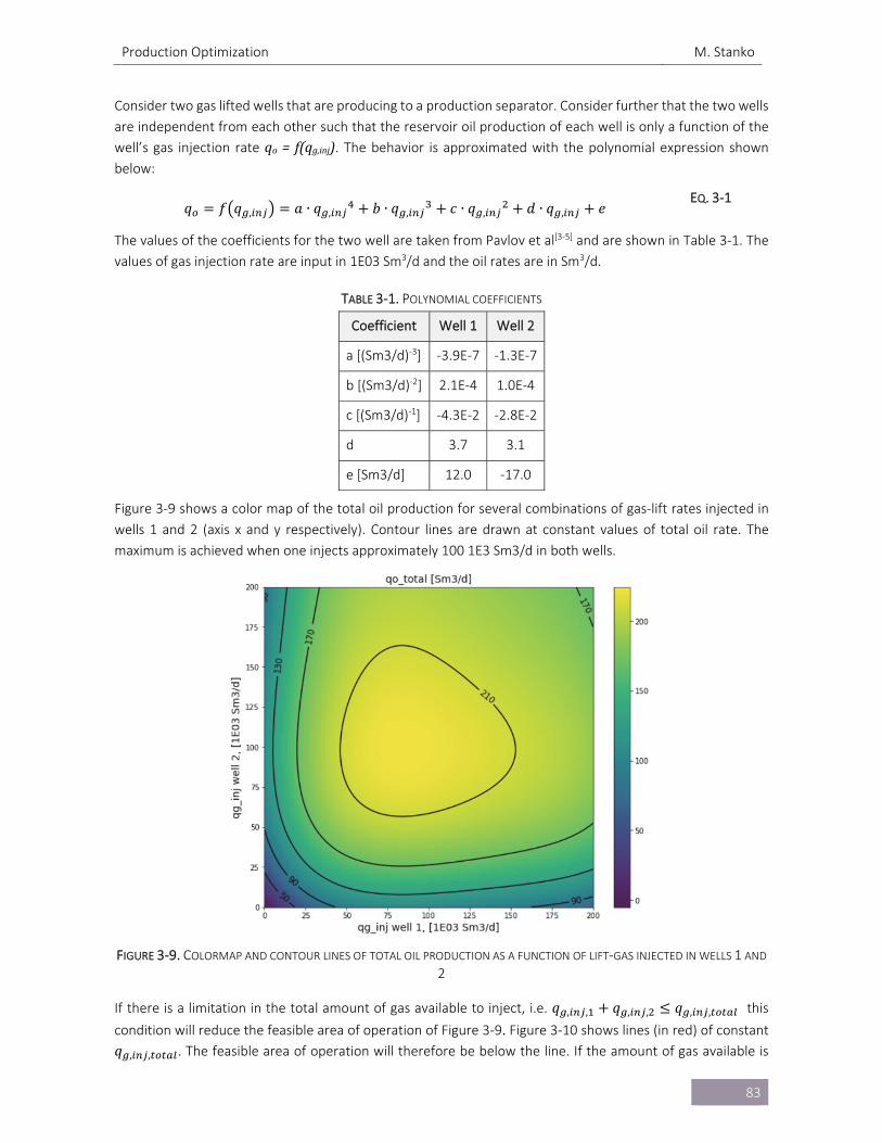
Production Optimization M. Stanko
83
Consider two gas lifted wells that are producing to a production separator. Consider further that the two wells
are independent from each other such that the reservoir oil production of each well is only a function of the
well’s gas injection rate qo= f(qg,inj). The behavior is approximated with the polynomial expression shown
below:
𝑞 𝑓 𝑞 , 𝑎 ∙ 𝑞 , 𝑏 ∙ 𝑞 , 𝑐 ∙ 𝑞 , 𝑑 ∙ 𝑞 , 𝑒 EQ. 3‐1
The values of the coefficients for the two well are taken from Pavlov et al[3‐5] and are shown in Table 3‐1. The
values of gas injection rate are input in 1E03 Sm3/d and the oil rates are in Sm3/d.
TABLE 3‐1. POLYNOMIAL COEFFICIENTS
Coefficient Well 1 Well 2
a [(Sm3/d)‐3] ‐3.9E‐7 ‐1.3E‐7
b [(Sm3/d)‐2] 2.1E‐4 1.0E‐4
c [(Sm3/d)‐1] ‐4.3E‐2 ‐2.8E‐2
d 3.7 3.1
e [Sm3/d] 12.0 ‐17.0
Figure 3‐9 shows a color map of the total oil production for several combinations of gas‐lift rates injected in
wells 1 and 2 (axis x and y respectively). Contour lines are drawn at constant values of total oil rate. The
maximum is achieved when one injects approximately 100 1E3 Sm3/d in both wells.
FIGURE 3‐9. COLORMAP AND CONTOUR LINES OF TOTAL OIL PRODUCTION AS A FUNCTION OF LIFT‐GAS INJECTED IN WELLS 1 AND
2
If there is a limitation in the total amount of gas available to inject, i.e. 𝑞 , , 𝑞 , , 𝑞 , , this
condition will reduce the feasible area of operation of Figure 3‐9. Figure 3‐10 shows lines (in red) of constant
𝑞 , , . The feasible area of operation will therefore be below the line. If the amount of gas available is
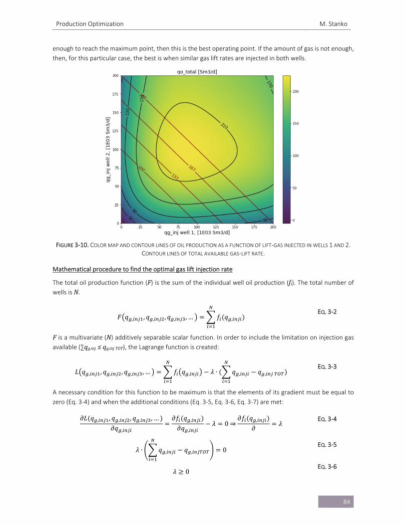
Production Optimization M. Stanko
84
enough to reach the maximum point, then this is the best operating point. If the amount of gas is not enough,
then, for this particular case, the best is when similar gas lift rates are injected in both wells.
FIGURE 3‐10. COLOR MAP AND CONTOUR LINES OF OIL PRODUCTION AS A FUNCTION OF LIFT‐GAS INJECTED IN WELLS 1 AND 2.
CONTOUR LINES OF TOTAL AVAILABLE GAS‐LIFT RATE.
Mathematical procedure to find the optimal gas lift injection rate
The total oil production function (F) is the sum of the individual well oil production (fi). The total number of
wells is N.
𝐹 𝑞 , , 𝑞 , , 𝑞 , , … 𝑓 𝑞 , EQ. 3‐2
F is a multivariate (N) additively separable scalar function. In order to include the limitation on injection gas
available (∑qg,inj≤qg,injTOT), the Lagrange function is created:
𝐿 𝑞 , , 𝑞 , , 𝑞 , , … 𝑓 𝑞 , 𝜆 ∙ 𝑞 , 𝑞 , EQ. 3‐3
A necessary condition for this function to be maximum is that the elements of its gradient must be equal to
zero (Eq. 3‐4) and when the additional conditions (Eq. 3‐5, Eq. 3‐6, Eq. 3‐7) are met:
𝜕𝐿 𝑞 , , 𝑞 , , 𝑞 , , …
𝜕𝑞 ,
𝜕𝑓 𝑞 ,
𝜕𝑞 ,𝜆 0 ⇒
𝜕𝑓 𝑞 ,
𝜕𝜆
EQ. 3‐4
𝜆 ∙ 𝑞 , 𝑞 , 0 EQ. 3‐5
𝜆 0 EQ. 3‐6
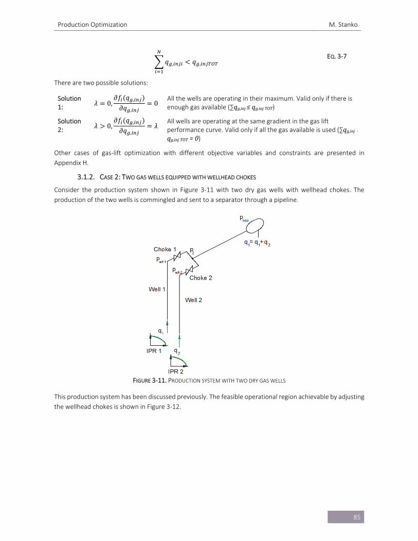
Production Optimization M. Stanko
85
𝑞 , 𝑞 , EQ. 3‐7
There are two possible solutions:
Solution 1:
𝜆 0,𝜕𝑓 𝑞 ,
𝜕𝑞 ,0
All the wells are operating in their maximum. Valid only if there is enough gas available (∑qg,inj≤qg,injTOT)
Solution 2:
𝜆 0,𝜕𝑓 𝑞 ,
𝜕𝑞 ,𝜆
All wells are operating at the same gradient in the gas lift performance curve. Valid only if all the gas available is used (∑qg,inj‐qg,injTOT=0)
Other cases of gas‐lift optimization with different objective variables and constraints are presented in
Appendix H.
3.1.2. CASE 2: TWO GAS WELLS EQUIPPED WITH WELLHEAD CHOKES
Consider the production system shown in Figure 3‐11 with two dry gas wells with wellhead chokes. The
production of the two wells is commingled and sent to a separator through a pipeline.
FIGURE 3‐11. PRODUCTION SYSTEM WITH TWO DRY GAS WELLS
This production system has been discussed previously. The feasible operational region achievable by adjusting
the wellhead chokes is shown in Figure 3‐12.
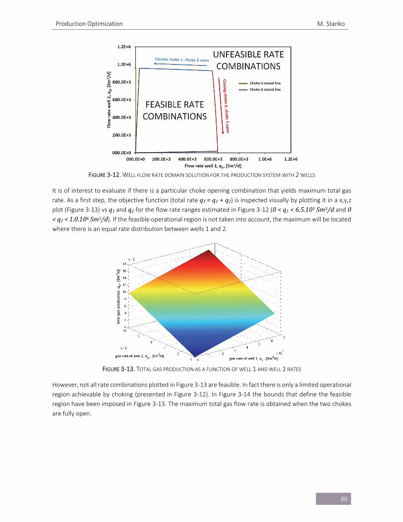
Production Optimization M. Stanko
86
FIGURE 3‐12. WELL FLOW RATE DOMAIN SOLUTION FOR THE PRODUCTION SYSTEM WITH 2 WELLS
It is of interest to evaluate if there is a particular choke opening combination that yields maximum total gas
rate. As a first step, the objective function (total rate qT=q1+q2) is inspected visually by plotting it in a x,y,z plot (Figure 3‐13) vs q1 and q2 for the flow rate ranges estimated in Figure 3‐12 (0<q1<6.5.105Sm3/d and 0<q2<1.0.106Sm3/d). If the feasible operational region is not taken into account, the maximum will be located
where there is an equal rate distribution between wells 1 and 2.
FIGURE 3‐13. TOTAL GAS PRODUCTION AS A FUNCTION OF WELL 1 AND WELL 2 RATES
However, not all rate combinations plotted in Figure 3‐13 are feasible. In fact there is only a limited operational
region achievable by choking (presented in Figure 3‐12). In Figure 3‐14 the bounds that define the feasible
region have been imposed in Figure 3‐13. The maximum total gas flow rate is obtained when the two chokes
are fully open.
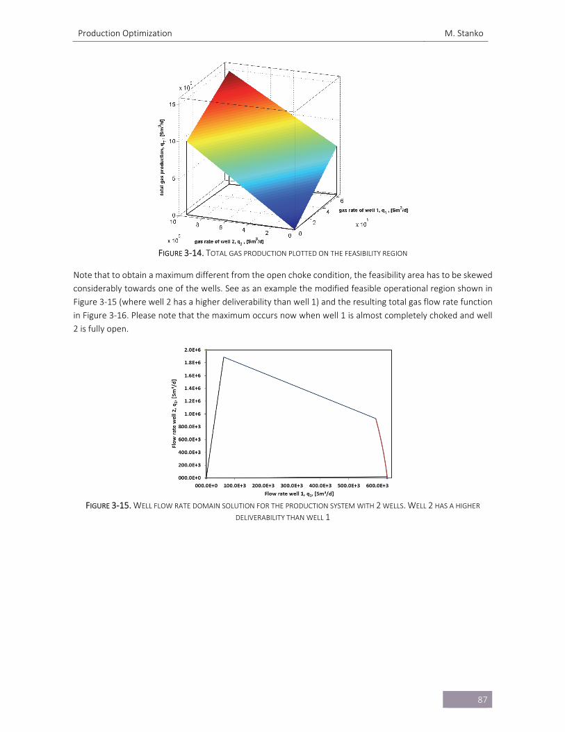
Production Optimization M. Stanko
87
FIGURE 3‐14. TOTAL GAS PRODUCTION PLOTTED ON THE FEASIBILITY REGION
Note that to obtain a maximum different from the open choke condition, the feasibility area has to be skewed
considerably towards one of the wells. See as an example the modified feasible operational region shown in
Figure 3‐15 (where well 2 has a higher deliverability than well 1) and the resulting total gas flow rate function
in Figure 3‐16. Please note that the maximum occurs now when well 1 is almost completely choked and well
2 is fully open.
FIGURE 3‐15. WELL FLOW RATE DOMAIN SOLUTION FOR THE PRODUCTION SYSTEM WITH 2 WELLS. WELL 2 HAS A HIGHER
DELIVERABILITY THAN WELL 1
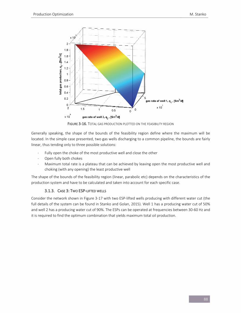
Production Optimization M. Stanko
88
FIGURE 3‐16. TOTAL GAS PRODUCTION PLOTTED ON THE FEASIBILITY REGION
Generally speaking, the shape of the bounds of the feasibility region define where the maximum will be
located. In the simple case presented, two gas wells discharging to a common pipeline, the bounds are fairly
linear, thus tending only to three possible solutions:
Fully open the choke of the most productive well and close the other
Open fully both chokes
Maximum total rate is a plateau that can be achieved by leaving open the most productive well and
choking (with any opening) the least productive well
The shape of the bounds of the feasibility region (linear, parabolic etc) depends on the characteristics of the
production system and have to be calculated and taken into account for each specific case.
3.1.3. CASE 3: TWO ESP‐LIFTED WELLS
Consider the network shown in Figure 3‐17 with two ESP‐lifted wells producing with different water cut (the
full details of the system can be found in Stanko and Golan, 2015). Well 1 has a producing water cut of 50%
and well 2 has a producing water cut of 90%. The ESPs can be operated at frequencies between 30‐60 Hz and
it is required to find the optimum combination that yields maximum total oil production.
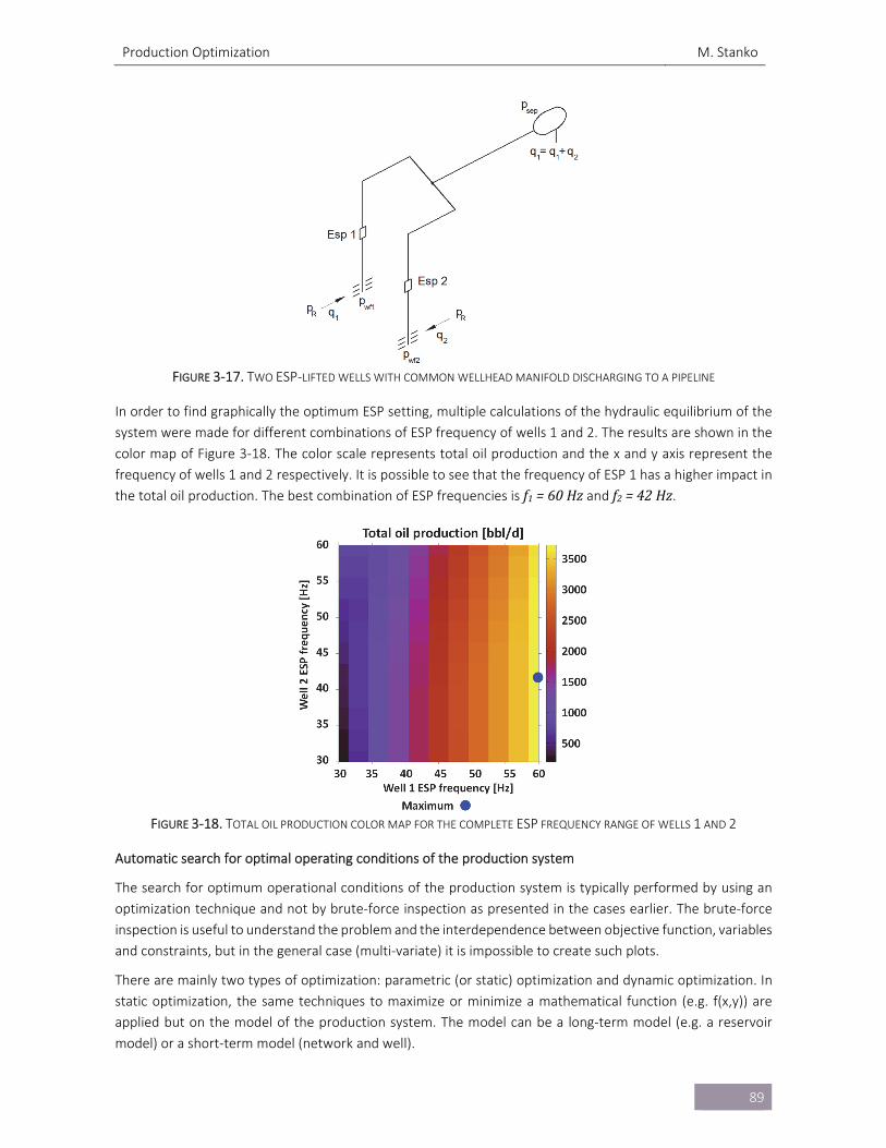
Production Optimization M. Stanko
89
FIGURE 3‐17. TWO ESP‐LIFTED WELLS WITH COMMON WELLHEAD MANIFOLD DISCHARGING TO A PIPELINE
In order to find graphically the optimum ESP setting, multiple calculations of the hydraulic equilibrium of the
system were made for different combinations of ESP frequency of wells 1 and 2. The results are shown in the
color map of Figure 3‐18. The color scale represents total oil production and the x and y axis represent the
frequency of wells 1 and 2 respectively. It is possible to see that the frequency of ESP 1 has a higher impact in
the total oil production. The best combination of ESP frequencies is f1=60Hz and f2=42Hz.
FIGURE 3‐18. TOTAL OIL PRODUCTION COLOR MAP FOR THE COMPLETE ESP FREQUENCY RANGE OF WELLS 1 AND 2
Automatic search for optimal operating conditions of the production system
The search for optimum operational conditions of the production system is typically performed by using an
optimization technique and not by brute‐force inspection as presented in the cases earlier. The brute‐force
inspection is useful to understand the problem and the interdependence between objective function, variables
and constraints, but in the general case (multi‐variate) it is impossible to create such plots.
There are mainly two types of optimization: parametric (or static) optimization and dynamic optimization. In
static optimization, the same techniques to maximize or minimize a mathematical function (e.g. f(x,y)) are
applied but on the model of the production system. The model can be a long‐term model (e.g. a reservoir
model) or a short‐term model (network and well).
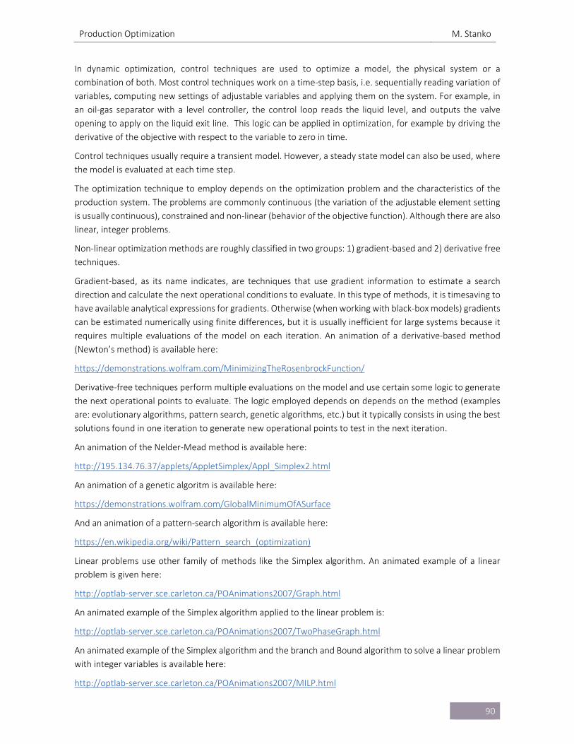
Production Optimization M. Stanko
90
In dynamic optimization, control techniques are used to optimize a model, the physical system or a
combination of both. Most control techniques work on a time‐step basis, i.e. sequentially reading variation of
variables, computing new settings of adjustable variables and applying them on the system. For example, in
an oil‐gas separator with a level controller, the control loop reads the liquid level, and outputs the valve
opening to apply on the liquid exit line. This logic can be applied in optimization, for example by driving the
derivative of the objective with respect to the variable to zero in time.
Control techniques usually require a transient model. However, a steady state model can also be used, where
the model is evaluated at each time step.
The optimization technique to employ depends on the optimization problem and the characteristics of the
production system. The problems are commonly continuous (the variation of the adjustable element setting
is usually continuous), constrained and non‐linear (behavior of the objective function). Although there are also
linear, integer problems.
Non‐linear optimization methods are roughly classified in two groups: 1) gradient‐based and 2) derivative free
techniques.
Gradient‐based, as its name indicates, are techniques that use gradient information to estimate a search
direction and calculate the next operational conditions to evaluate. In this type of methods, it is timesaving to
have available analytical expressions for gradients. Otherwise (when working with black‐box models) gradients
can be estimated numerically using finite differences, but it is usually inefficient for large systems because it
requires multiple evaluations of the model on each iteration. An animation of a derivative‐based method
(Newton’s method) is available here:
https://demonstrations.wolfram.com/MinimizingTheRosenbrockFunction/
Derivative‐free techniques perform multiple evaluations on the model and use certain some logic to generate
the next operational points to evaluate. The logic employed depends on depends on the method (examples
are: evolutionary algorithms, pattern search, genetic algorithms, etc.) but it typically consists in using the best
solutions found in one iteration to generate new operational points to test in the next iteration.
An animation of the Nelder‐Mead method is available here:
http://195.134.76.37/applets/AppletSimplex/Appl_Simplex2.html
An animation of a genetic algoritm is available here:
https://demonstrations.wolfram.com/GlobalMinimumOfASurface
And an animation of a pattern‐search algorithm is available here:
https://en.wikipedia.org/wiki/Pattern_search_(optimization)
Linear problems use other family of methods like the Simplex algorithm. An animated example of a linear
problem is given here:
http://optlab‐server.sce.carleton.ca/POAnimations2007/Graph.html
An animated example of the Simplex algorithm applied to the linear problem is:
http://optlab‐server.sce.carleton.ca/POAnimations2007/TwoPhaseGraph.html
An animated example of the Simplex algorithm and the branch and Bound algorithm to solve a linear problem
with integer variables is available here:
http://optlab‐server.sce.carleton.ca/POAnimations2007/MILP.html
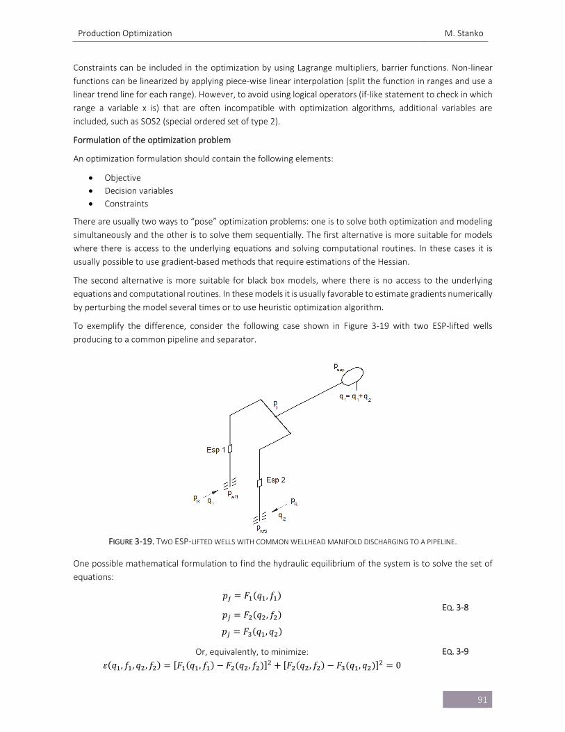
Production Optimization M. Stanko
91
Constraints can be included in the optimization by using Lagrange multipliers, barrier functions. Non‐linear
functions can be linearized by applying piece‐wise linear interpolation (split the function in ranges and use a
linear trend line for each range). However, to avoid using logical operators (if‐like statement to check in which
range a variable x is) that are often incompatible with optimization algorithms, additional variables are
included, such as SOS2 (special ordered set of type 2).
Formulation of the optimization problem
An optimization formulation should contain the following elements:
Objective
Decision variables
Constraints
There are usually two ways to “pose” optimization problems: one is to solve both optimization and modeling
simultaneously and the other is to solve them sequentially. The first alternative is more suitable for models
where there is access to the underlying equations and solving computational routines. In these cases it is
usually possible to use gradient‐based methods that require estimations of the Hessian.
The second alternative is more suitable for black box models, where there is no access to the underlying
equations and computational routines. In these models it is usually favorable to estimate gradients numerically
by perturbing the model several times or to use heuristic optimization algorithm.
To exemplify the difference, consider the following case shown in Figure 3‐19 with two ESP‐lifted wells
producing to a common pipeline and separator.
FIGURE 3‐19. TWO ESP‐LIFTED WELLS WITH COMMON WELLHEAD MANIFOLD DISCHARGING TO A PIPELINE.
One possible mathematical formulation to find the hydraulic equilibrium of the system is to solve the set of
equations:
𝑝 𝐹 𝑞 , 𝑓
𝑝 𝐹 𝑞 , 𝑓
𝑝 𝐹 𝑞 , 𝑞
EQ. 3‐8
Or, equivalently, to minimize:
𝜀 𝑞 , 𝑓 , 𝑞 , 𝑓 𝐹 𝑞 , 𝑓 𝐹 𝑞 , 𝑓 𝐹 𝑞 , 𝑓 𝐹 𝑞 , 𝑞 0 EQ. 3‐9
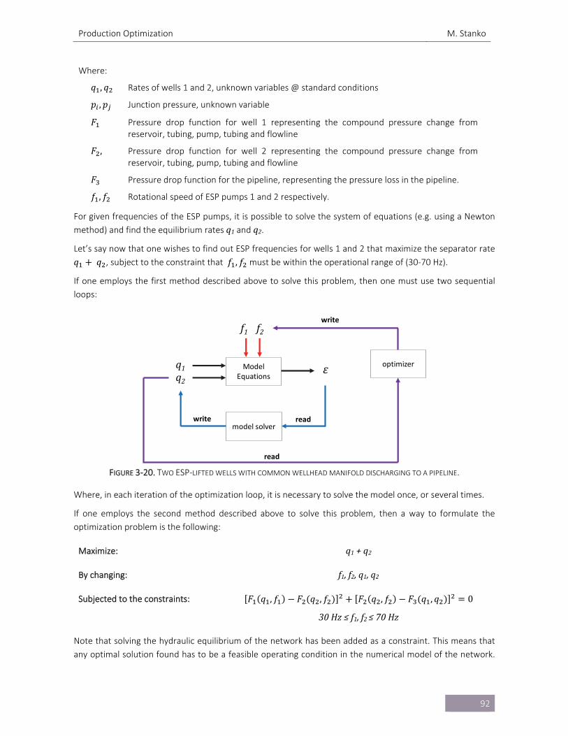
Production Optimization M. Stanko
92
Where:
𝑞 , 𝑞 Rates of wells 1 and 2, unknown variables @ standard conditions
𝑝 , 𝑝 Junction pressure, unknown variable
𝐹 Pressure drop function for well 1 representing the compound pressure change from reservoir, tubing, pump, tubing and flowline
𝐹 , Pressure drop function for well 2 representing the compound pressure change from reservoir, tubing, pump, tubing and flowline
𝐹 Pressure drop function for the pipeline, representing the pressure loss in the pipeline.
𝑓 , 𝑓 Rotational speed of ESP pumps 1 and 2 respectively.
For given frequencies of the ESP pumps, it is possible to solve the system of equations (e.g. using a Newton
method) and find the equilibrium rates q1 and q2.
Let’s say now that one wishes to find out ESP frequencies for wells 1 and 2 that maximize the separator rate 𝑞 𝑞 , subject to the constraint that 𝑓 , 𝑓 must be within the operational range of (30‐70 Hz).
If one employs the first method described above to solve this problem, then one must use two sequential
loops:
FIGURE 3‐20. TWO ESP‐LIFTED WELLS WITH COMMON WELLHEAD MANIFOLD DISCHARGING TO A PIPELINE.
Where, in each iteration of the optimization loop, it is necessary to solve the model once, or several times.
If one employs the second method described above to solve this problem, then a way to formulate the
optimization problem is the following:
Maximize: q1+q2
By changing: f1,f2,q1,q2
Subjected to the constraints: 𝐹 𝑞 , 𝑓 𝐹 𝑞 , 𝑓 𝐹 𝑞 , 𝑓 𝐹 𝑞 , 𝑞 0
30Hz≤f1,f2≤70Hz
Note that solving the hydraulic equilibrium of the network has been added as a constraint. This means that
any optimal solution found has to be a feasible operating condition in the numerical model of the network.
Model Equations
q1q2
f1 f2
𝜀
model solver
optimizer
write
read
readwrite
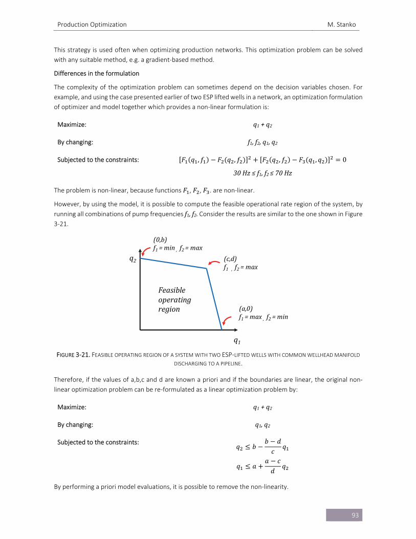
Production Optimization M. Stanko
93
This strategy is used often when optimizing production networks. This optimization problem can be solved
with any suitable method, e.g. a gradient‐based method.
Differences in the formulation
The complexity of the optimization problem can sometimes depend on the decision variables chosen. For
example, and using the case presented earlier of two ESP lifted wells in a network, an optimization formulation
of optimizer and model together which provides a non‐linear formulation is:
Maximize: q1+q2
By changing: f1,f2,q1,q2
Subjected to the constraints: 𝐹 𝑞 , 𝑓 𝐹 𝑞 , 𝑓 𝐹 𝑞 , 𝑓 𝐹 𝑞 , 𝑞 0
30Hz≤f1,f2≤70Hz
The problem is non‐linear, because functions 𝐹 , 𝐹 , 𝐹 . are non‐linear.
However, by using the model, it is possible to compute the feasible operational rate region of the system, by
running all combinations of pump frequencies f1,f2. Consider the results are similar to the one shown in Figure
3‐21.
FIGURE 3‐21. FEASIBLE OPERATING REGION OF A SYSTEM WITH TWO ESP‐LIFTED WELLS WITH COMMON WELLHEAD MANIFOLD
DISCHARGING TO A PIPELINE.
Therefore, if the values of a,b,c and d are known a priori and if the boundaries are linear, the original non‐
linear optimization problem can be re‐formulated as a linear optimization problem by:
Maximize: q1+q2
By changing: q1,q2
Subjected to the constraints: 𝑞 𝑏
𝑏 𝑑𝑐
𝑞
𝑞 𝑎𝑎 𝑐
𝑑𝑞
By performing a priori model evaluations, it is possible to remove the non‐linearity.
(c,d)f1, f2=max
(a,0)f1=max , f2=min
(0,b)f1=min , f2=max
q1
q2
Feasibleoperatingregion
Production Optimization M. Stanko
94
3.2. ISSUES HINDERING THE INDUSTRIAL SCALE ADOPTION OF MODEL‐BASED PRODUCTION OPTIMIZATION
The industry has been somewhat slow in accepting, adopting and implementing model‐bases optimization
solutions. This can be partly attributed to the following reasons:
3.2.1. FOREIGN FROM THE FIELD’S REALITY
Before embarking on a model‐based production optimization project It is always relevant to ask the question:
is optimization really necessary for this particular case? To execute production optimization entails extensive
use of human, computational resources and time so it is always best to be 100% sure that it is strictly necessary
for the particular case.
Also, is it actually possible to change the decision settings? Is the equipment or actuator functional and
available? Am I allowed to operate the control element? Is the actuator response time compatible with the
optimization workflow?
When formulating the optimization problem, it is crucial to deeply understand (as much as possible) the
underlying physical system. Furthermore, to identify the most important variables, objectives and constraints
and to avoid overcomplicating the problem. This might be sometimes difficult to distill properly during
communications between engineers partly due to lack of understanding of the underlying issues. The lack of
subsequent communication between the optimization engineer and the field operator worsens further the
problem.
3.2.2. MODELS UNCERTAINTY
The uncertainty associated with the numerical models is usually high and there is limited confidence on their
results (this is especially applicable to the case of reservoir models). This raises doubts about the applicability
of the optimum operational controls found and creates resistance and skepticism on the side of operators. It
is always good practice to vary the system parameters (e.g. with a probabilistic sampling method) and quantify
the effect it has on the optimum solution.
3.2.3. NON‐SUSTAINABILITY OF THE PROPOSED SOLUTIONS
Some factors that contribute to the lack of sustainability of the solutions are:
Lack of expertise on the industry side to understand the basics of the solution provided by consultants
or vendors.
Ease of use. Not understanding the solution added to difficulties using it often lead to abandoning it.
The usage of self‐programmed surrogate models that are not easily scalable and maintained. Many
engineers often prefer commercial software where their maintenance, upgrade and troubleshooting
are delegated to a third‐party company.
Lack of ownership by the industrial partner.
In the area of production optimization, sometimes it is very difficult to develop general solutions and platforms
that are suitable for the majority of field cases encountered. That is why field engineers should always
understand to a great degree the optimization solutions provided by external consultants and vendors.

Production Optimization M. Stanko
95
REFERENCES
[3‐1] Alarcon, G. A., Torres, C. F. & Gomez, L. E. (2002). Global optimization of gas allocation to a group of
wells in artificial lift using nonlinear constrained programming. Journal of Energy Resources
Technology124 (4).
[3‐2] Khan Academy (2018) Lagrange Multipliers, examples. Article retrieved from:
https://www.khanacademy.org/math/multivariable‐calculus/applications‐of‐multivariable‐
derivatives/constrained‐optimization/a/lagrange‐multipliers‐examples.
[3‐3] Barros, E.G.D., Van den Hof, P.M.J., Jansen, J.D. (2015). Value of Information in Closed‐Loop
Reservoir Management. Computational Geosciences 20 (3).
[3‐4] Simplex Optimization method. Article retrieved from:
http://www.chem.uoa.gr/applets/AppletSimplex/Appl_Simplex2.html
[3‐5] Pavlov, A., Haring, M., Fjalestad, K. (2017). Practical extremum‐seeking control for gas lifted oil
production. 2017 IEEE 56th Annual Conference on Decision and Control.
Fluid Behavior Treatment in Oil and Gas Production Systems M. Stanko
96
4. FLUID BEHAVIOR TREATMENT IN OIL AND GAS PRODUCTION SYSTEMS
There are two main methodologies to characterize and quantify fluid behavior: Black oil and compositional. In
the Black Oil (BO) approach three phases are considered: oil (liquid phase), gas (gaseous phase) and water
(liquid phase) and a set of variables are employed to relate the volumetric amounts of the phases at standard
conditions with the volumetric amounts at any pressure and temperature condition. The compositional
approach employs an equation of state (EOS) and the molar composition to estimate fluid properties
(determining numerically the number of phases and calculating their properties).
The BO model can be regarded as a subset of the compositional model where only two components are used:
oil and gas (in most cases water can be treated independently assuming that it does not partition in oil or gas).
The BO approach is still the preferred choice of engineers in the petroleum industry because it is more practical
(involves tangible amounts measured in the field) and it is faster than performing time consuming EOS
calculations.
In the past, BO properties were generated from correlations developed for particular fluids and applied to
other cases by using tuning parameters (e.g. typical approach used in commercial software for analysis of
production systems). Nowadays, the generalized procedure is to develop an EOS to characterize oil and gas
fluid behavior and then generate BO properties using this EOS. The BO parameters are pre‐computed and
stored in tables that can later be used as needed by engineers (e.g. in simulators).
The typical workflow to characterize a reservoir fluid is roughly as follows:
Sampling: a representative sample of the producing fluid is taken. This can be done in three typical
locations in the production system:
o Formation/Well bottom‐hole (oil and gas).
o Test Separator (oil and gas separately). They are later recombined depending on the individual
rates.
o Wellhead
Determine fluid composition: e.g. using gas chromatography.
Perform laboratory tests
o CCE Constant composition expansion
o DLE differential liberation experiment
o CVD Constant volume depletion
o MSF Multistage separator experiment
Develop a PVT model. Development of a physically consistent EOS that represents all the laboratory
tests considering the uncertainties associated to each test and the uncertainties in compositions, and
particularly the properties and amounts of heavy components. Pseudo‐components are typically
employed to represent groups of heavy components (e.g. C7 and above). The properties of such
pseudo‐components are adjusted such that they represent properly the original composition.
4.1. THE BLACK OIL MODEL
To simplify the discussion and the introduction of concepts, an initial assumption will be made that the overall
composition of the fluid stream under study is constant. This is generally not true because in a production
system there is mixing of streams with different compositions, the amounts of oil and gas produced by the
wells change in time due to depletion, gas conning, injection, etc. On a later section, once the basic concepts
are discussed, the consideration is removed.
This chapter does not discuss the presence of water (e.g. gas solubility in water) or the definition and
estimation of its BO properties. Please refer to Chapter 9 of Whitson[4‐1] for details on the topic.
Fluid Behavior Treatment in Oil and Gas Production Systems M. Stanko
97
The BO model is based on the situation when oil and gas at local p and T conditions are brought separately to standard conditions by passing them through the surface process (P) existing in the field (Figure 4‐1).
FIGURE 4‐1. SCHEMATIC REPRESENTATION OF THE FLASHING OF OIL AND GAS AT LOCAL CONDITIONS TO STANDARD CONDITIONS
Where the subscripts are:
�̅� surface gas component
�̅� surface oil component
𝑔 gas phase @ (p,T)
𝑜 oil phase @ (p,T)
Surface oil (Vō) will be generated from gas phase (Vōg) and from oil phase (Vōo) and surface gas (Vḡ) will be generated from gas phase (Vḡg) and from oil phase (Vḡo). Four BO parameters, p and T dependent, are then
defined to relate these 4 quantities with the local oil (Vo) and gas (Vg) volume and are summarized in Table
4‐1. These BO parameters are not strict thermodynamic properties, as their values depend on the reference
standard conditions employed (in SPE for instance it is 60°F and 1 atm), the surface process and the
composition.
TABLE 4‐1. BO PARAMETERS
BO Variable Definition
Oil Volume Factor 𝐵 𝑝, 𝑇𝑉 𝑝, 𝑇
𝑉
Gas Volume Factor 𝐵 𝑝, 𝑇𝑉 𝑝, 𝑇
𝑉
Solution Gas Oil Ratio 𝑅 𝑝, 𝑇𝑉
𝑉
Solution Oil Gas ratio 𝑟 𝑝, 𝑇𝑉
𝑉
Fluid Behavior Treatment in Oil and Gas Production Systems M. Stanko
98
These parameters constitute what is known as the “modified” BO formulation. The traditional BO formulation
does not include the Solution Oil Gas Ratio rs (sometimes called rv). This parameter is extremely important
when dealing with volatile oils and gas condensate fluids.
There are other BO properties that are often recorded at p, T such as oil viscosity (μo), gas viscosity (μg), oil‐gas interfacial tension (σog). These parameters are often required to perform numerical pressure and
temperature drop calculations in reservoir and production systems.
Note that when the fluid is taken to standard conditions through a specific surface process it will always give
the same GOR and the same oil and gas specific gravities at standard conditions (γo and γg) despite the local p and T conditions. This is the reason why the GOR, γg and γo are often used to characterize a given fluid.
For certain local p, T conditions, there might be only one phase in equilibrium (oil or gas). In that case, the BO
properties of the non‐existing phase are undefined.
Black oil parameters are usually computed using PVT software with a composition, an EOS (properly tuned to
lab data), and the surface process existing on the field (usually described as a series of separators). The
workflow is presented in Figure 4‐2 and is roughly as follows:
Take an arbitrary number of moles of the seed composition (zi) to p and T conditions and separate the oil and gas and store the values of local volumes. The oil will have a composition xi and the gas a composition yi.
Take the oil and gas separately through the surface process. At the output gather surface oil and all
surface gas and register the standard conditions volumes.
Compute BO parameters for the combination of p and T. Repeat for several combinations of p and T.
FIGURE 4‐2. SCHEMATIC OF THE PROCESS TO GENERATE BO PROPERTIES
The higher and lower limits for p and T depend on what the BO properties are going to be used for. For
simulations of the reservoir and production system, BO properties have to be generated for the highest and
lowest pressure and temperature expected. However, these values might be unknown a priori as they are
usually a result of the calculations or numerical models that use the BO properties.
It is not failsafe to generate BO properties just between the initial reservoir pressure and temperature and the
first stage separator pressure and temperature. For example, when compression or pumping exists on the
field, pressure and temperature might reach values above reservoir pressure (e.g. at the compressor or pump
discharge) or below separator pressure (e.g. at the compressor or pump suction).
Fluid Behavior Treatment in Oil and Gas Production Systems M. Stanko
99
If the pressure of interest p for which it is desired to generate BO properties is within the range of the pressure
values of the surface process, usually all separators (or equipment) that operate above the pressure p are
neglected in the surface process.
BO parameters are usually stored in a set of tables, where each one contains the variation with pressure for a
fixed temperature. Reservoir or production simulators perform linear (or bilinear) interpolation in these tables
to obtain BO properties at specific p and T conditions.
Figure 4‐3 presents a sketch of the variation of the BO properties versus pressure for a fixed temperature (e.g.
Reservoir) of the hydrocarbon mixture shown in Figure 4‐4. At the given temperature, single phase oil will be
formed for pressures equal or greater than the bubble point pressure.
OIL PHASE
Bo Rs o
GAS PHASE
rs Bg g
FIGURE 4‐3. BEHAVIOR OF BO PARAMETERS VS. PRESSURE FOR A FIXED TEMPERATURE
FIGURE 4‐4. PHASE DIAGRAM OF THE HYDROCARBON MIXTURE USED IN FIGURE 4‐3
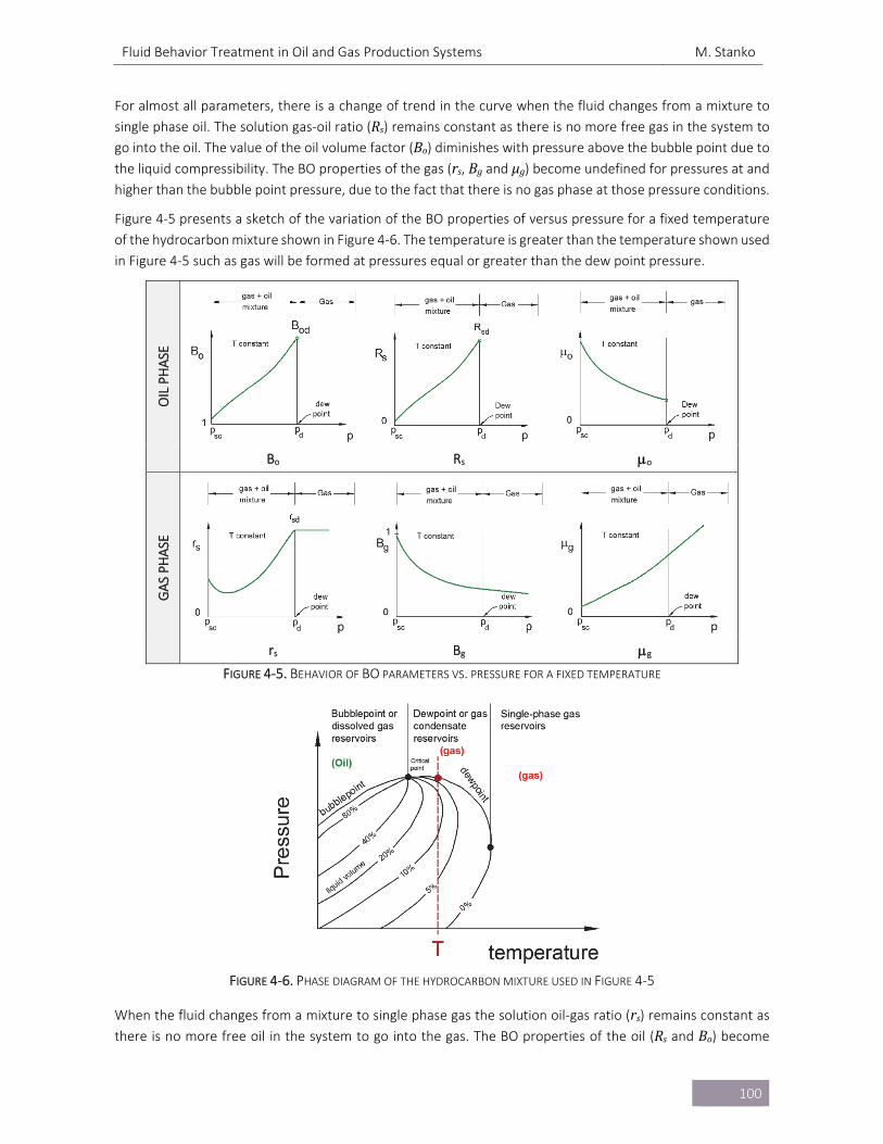
Fluid Behavior Treatment in Oil and Gas Production Systems M. Stanko
100
For almost all parameters, there is a change of trend in the curve when the fluid changes from a mixture to
single phase oil. The solution gas‐oil ratio (Rs) remains constant as there is no more free gas in the system to
go into the oil. The value of the oil volume factor (Bo) diminishes with pressure above the bubble point due to
the liquid compressibility. The BO properties of the gas (rs, Bg and μg) become undefined for pressures at and
higher than the bubble point pressure, due to the fact that there is no gas phase at those pressure conditions.
Figure 4‐5 presents a sketch of the variation of the BO properties of versus pressure for a fixed temperature
of the hydrocarbon mixture shown in Figure 4‐6. The temperature is greater than the temperature shown used
in Figure 4‐5 such as gas will be formed at pressures equal or greater than the dew point pressure.
OIL PHASE
Bo Rs o
GAS PH
ASE
rs Bg g
FIGURE 4‐5. BEHAVIOR OF BO PARAMETERS VS. PRESSURE FOR A FIXED TEMPERATURE
FIGURE 4‐6. PHASE DIAGRAM OF THE HYDROCARBON MIXTURE USED IN FIGURE 4‐5
When the fluid changes from a mixture to single phase gas the solution oil‐gas ratio (rs) remains constant as
there is no more free oil in the system to go into the gas. The BO properties of the oil (Rs and Bo) become
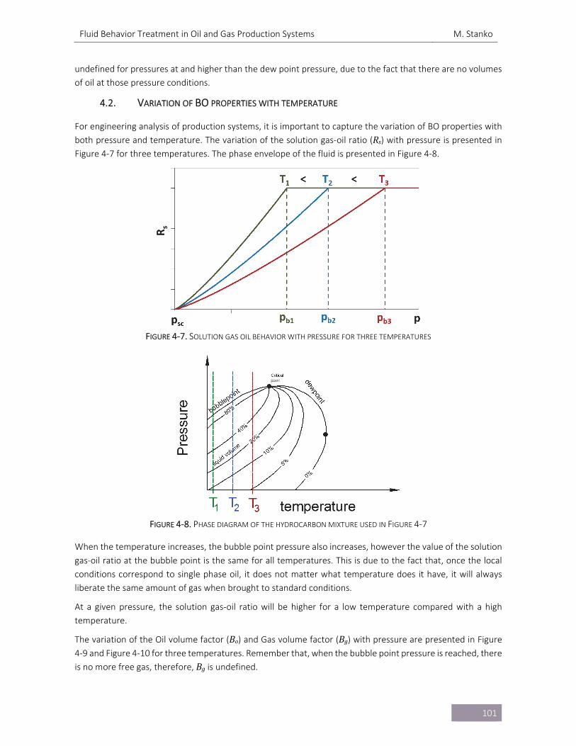
Fluid Behavior Treatment in Oil and Gas Production Systems M. Stanko
101
undefined for pressures at and higher than the dew point pressure, due to the fact that there are no volumes
of oil at those pressure conditions.
4.2. VARIATION OF BO PROPERTIES WITH TEMPERATURE
For engineering analysis of production systems, it is important to capture the variation of BO properties with
both pressure and temperature. The variation of the solution gas‐oil ratio (Rs) with pressure is presented in Figure 4‐7 for three temperatures. The phase envelope of the fluid is presented in Figure 4‐8.
FIGURE 4‐7. SOLUTION GAS OIL BEHAVIOR WITH PRESSURE FOR THREE TEMPERATURES
FIGURE 4‐8. PHASE DIAGRAM OF THE HYDROCARBON MIXTURE USED IN FIGURE 4‐7
When the temperature increases, the bubble point pressure also increases, however the value of the solution
gas‐oil ratio at the bubble point is the same for all temperatures. This is due to the fact that, once the local
conditions correspond to single phase oil, it does not matter what temperature does it have, it will always
liberate the same amount of gas when brought to standard conditions.
At a given pressure, the solution gas‐oil ratio will be higher for a low temperature compared with a high
temperature.
The variation of the Oil volume factor (Bo) and Gas volume factor (Bg) with pressure are presented in Figure 4‐9 and Figure 4‐10 for three temperatures. Remember that, when the bubble point pressure is reached, there
is no more free gas, therefore, Bg is undefined.
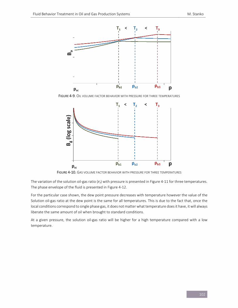
Fluid Behavior Treatment in Oil and Gas Production Systems M. Stanko
102
FIGURE 4‐9. OIL VOLUME FACTOR BEHAVIOR WITH PRESSURE FOR THREE TEMPERATURES
FIGURE 4‐10. GAS VOLUME FACTOR BEHAVIOR WITH PRESSURE FOR THREE TEMPERATURES
The variation of the solution oil‐gas ratio (rs) with pressure is presented in Figure 4‐11 for three temperatures.
The phase envelope of the fluid is presented in Figure 4‐12.
For the particular case shown, the dew point pressure decreases with temperature however the value of the
Solution oil‐gas ratio at the dew point is the same for all temperatures. This is due to the fact that, once the
local conditions correspond to single phase gas, it does not matter what temperature does it have, it will always
liberate the same amount of oil when brought to standard conditions.
At a given pressure, the solution oil‐gas ratio will be higher for a high temperature compared with a low
temperature.
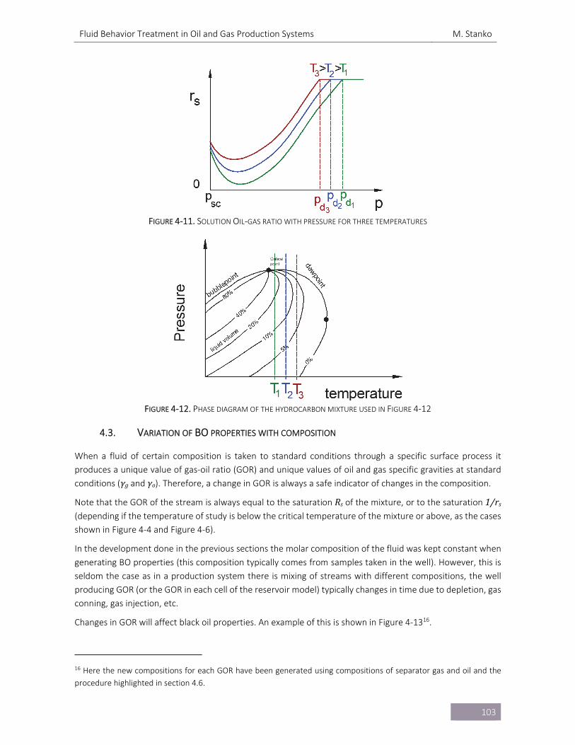
Fluid Behavior Treatment in Oil and Gas Production Systems M. Stanko
103
FIGURE 4‐11. SOLUTION OIL‐GAS RATIO WITH PRESSURE FOR THREE TEMPERATURES
FIGURE 4‐12. PHASE DIAGRAM OF THE HYDROCARBON MIXTURE USED IN FIGURE 4‐12
4.3. VARIATION OF BO PROPERTIES WITH COMPOSITION
When a fluid of certain composition is taken to standard conditions through a specific surface process it
produces a unique value of gas‐oil ratio (GOR) and unique values of oil and gas specific gravities at standard
conditions (γg and γo). Therefore, a change in GOR is always a safe indicator of changes in the composition.
Note that the GOR of the stream is always equal to the saturation Rsof the mixture, or to the saturation 1/rs(depending if the temperature of study is below the critical temperature of the mixture or above, as the cases
shown in Figure 4‐4 and Figure 4‐6).
In the development done in the previous sections the molar composition of the fluid was kept constant when
generating BO properties (this composition typically comes from samples taken in the well). However, this is
seldom the case as in a production system there is mixing of streams with different compositions, the well
producing GOR (or the GOR in each cell of the reservoir model) typically changes in time due to depletion, gas
conning, gas injection, etc.
Changes in GOR will affect black oil properties. An example of this is shown in Figure 4‐1316.
16 Here the new compositions for each GOR have been generated using compositions of separator gas and oil and the
procedure highlighted in section 4.6.
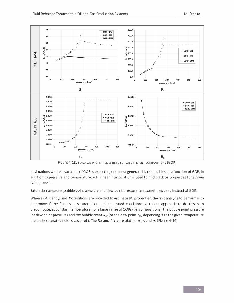
Fluid Behavior Treatment in Oil and Gas Production Systems M. Stanko
104
OIL PHASE
Bo Rs
GAS PH
ASE
rs Bg
FIGURE 4‐13. BLACK OIL PROPERTIES ESTIMATED FOR DIFFERENT COMPOSITIONS (GOR)
In situations where a variation of GOR is expected, one must generate black oil tables as a function of GOR, in
addition to pressure and temperature. A tri‐linear interpolation is used to find black oil properties for a given
GOR, p and T.
Saturation pressure (bubble point pressure and dew point pressure) are sometimes used instead of GOR.
When a GOR and p and T conditions are provided to estimate BO properties, the first analysis to perform is to
determine if the fluid is in saturated or undersaturated conditions. A robust approach to do this is to
precompute, at constant temperature, for a large range of GORs (i.e. compositions), the bubble point pressure
(or dew point pressure) and the bubble point Rsb (or the dew point rsd, depending if at the given temperature
the undersaturated fluid is gas or oil). The Rsb and 1/rsdare plotted vs pb and pd (Figure 4‐14).
0.0
0.5
1.0
1.5
2.0
2.5
3.0
3.5
0 100 200 300 400 500 600
Bo [m3/Sm
3]
pressure, p, [bara]
GOR = 143
GOR = 535
GOR = 1070
0.0
100.0
200.0
300.0
400.0
500.0
600.0
700.0
800.0
0 100 200 300 400 500 600
Rs [Sm3/Sm3]
pressure, p, [bara]
GOR = 143
GOR = 535
GOR = 1070
0.0E+00
1.0E‐04
2.0E‐04
3.0E‐04
4.0E‐04
5.0E‐04
6.0E‐04
7.0E‐04
8.0E‐04
9.0E‐04
1.0E‐03
0 100 200 300 400 500 600
rs, [Sm
3/Sm
3]
pressure, p, [bara]
GOR = 143
GOR = 535
GOR = 1070
0.0E+00
5.0E‐03
1.0E‐02
1.5E‐02
2.0E‐02
2.5E‐02
0 100 200 300 400 500 600
Bg, [m3/Sm
3]
pressure, p, [bara]
GOR = 143
GOR = 535
GOR = 1070
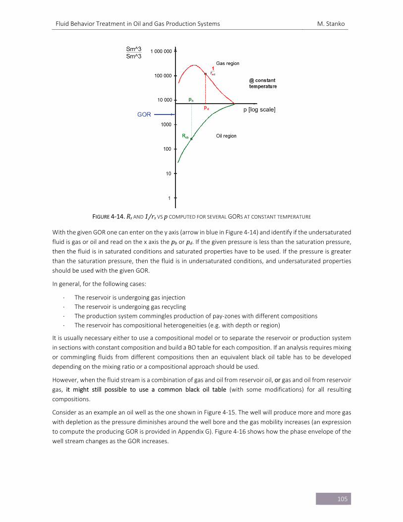
Fluid Behavior Treatment in Oil and Gas Production Systems M. Stanko
105
FIGURE 4‐14. Rs AND 1/rs VS p COMPUTED FOR SEVERAL GORS AT CONSTANT TEMPERATURE
With the given GOR one can enter on the y axis (arrow in blue in Figure 4‐14) and identify if the undersaturated
fluid is gas or oil and read on the x axis the pb or pd. If the given pressure is less than the saturation pressure, then the fluid is in saturated conditions and saturated properties have to be used. If the pressure is greater
than the saturation pressure, then the fluid is in undersaturated conditions, and undersaturated properties
should be used with the given GOR.
In general, for the following cases:
The reservoir is undergoing gas injection
The reservoir is undergoing gas recycling
The production system commingles production of pay‐zones with different compositions
The reservoir has compositional heterogeneities (e.g. with depth or region)
It is usually necessary either to use a compositional model or to separate the reservoir or production system
in sections with constant composition and build a BO table for each composition. If an analysis requires mixing
or commingling fluids from different compositions then an equivalent black oil table has to be developed
depending on the mixing ratio or a compositional approach should be used.
However, when the fluid stream is a combination of gas and oil from reservoir oil, or gas and oil from reservoir
gas, it might still possible to use a common black oil table (with some modifications) for all resulting
compositions.
Consider as an example an oil well as the one shown in Figure 4‐15. The well will produce more and more gas
with depletion as the pressure diminishes around the well bore and the gas mobility increases (an expression
to compute the producing GOR is provided in Appendix G). Figure 4‐16 shows how the phase envelope of the
well stream changes as the GOR increases.
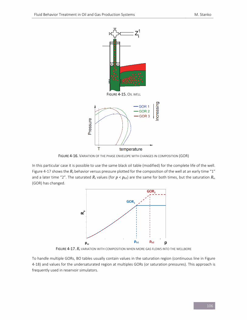
Fluid Behavior Treatment in Oil and Gas Production Systems M. Stanko
106
FIGURE 4‐15. OIL WELL
FIGURE 4‐16. VARIATION OF THE PHASE ENVELOPE WITH CHANGES IN COMPOSITION (GOR)
In this particular case it is possible to use the same black oil table (modified) for the complete life of the well.
Figure 4‐17 shows the Rs behavior versus pressure plotted for the composition of the well at an early time “1”
and a later time “2”. The saturated Rs values (for p< pb1) are the same for both times, but the saturation Rs, (GOR) has changed.
FIGURE 4‐17. Rs VARIATION WITH COMPOSITION WHEN MORE GAS FLOWS INTO THE WELLBORE
To handle multiple GORs, BO tables usually contain values in the saturation region (continuous line in Figure
4‐18) and values for the undersaturated region at multiples GORs (or saturation pressures). This approach is
frequently used in reservoir simulators.
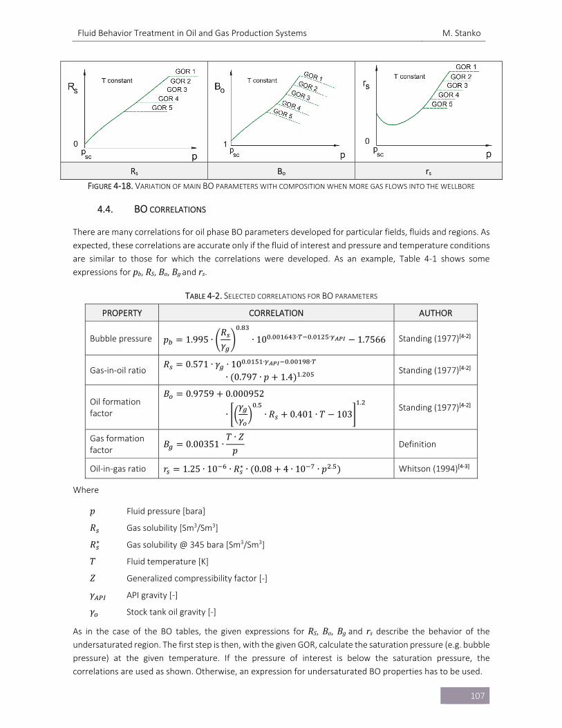
Fluid Behavior Treatment in Oil and Gas Production Systems M. Stanko
107
Rs Bo rs
FIGURE 4‐18. VARIATION OF MAIN BO PARAMETERS WITH COMPOSITION WHEN MORE GAS FLOWS INTO THE WELLBORE
4.4. BO CORRELATIONS
There are many correlations for oil phase BO parameters developed for particular fields, fluids and regions. As
expected, these correlations are accurate only if the fluid of interest and pressure and temperature conditions
are similar to those for which the correlations were developed. As an example, Table 4‐1 shows some
expressions for pb, RS, Bo, Bg and rs.
TABLE 4‐2. SELECTED CORRELATIONS FOR BO PARAMETERS
PROPERTY CORRELATION AUTHOR
Bubble pressure 𝑝 1.995 ∙𝑅𝛾
.
∙ 10 . ∙ . ∙ 1.7566 Standing (1977)[4‐2]
Gas‐in‐oil ratio 𝑅 0.571 ∙ 𝛾 ∙ 10 . ∙ . ∙
∙ 0.797 ∙ 𝑝 1.4 . Standing (1977)[4‐2]
Oil formation factor
𝐵 0.9759 0.000952
∙𝛾
𝛾
.∙ 𝑅 0.401 ∙ 𝑇 103
.
Standing (1977)[4‐2]
Gas formation factor
𝐵 0.00351 ∙𝑇 ∙ 𝑍
𝑝 Definition
Oil‐in‐gas ratio 𝑟 1.25 ∙ 10 ∙ 𝑅∗ ∙ 0.08 4 ∙ 10 ∙ 𝑝 . Whitson (1994)[4‐3]
Where
𝑝 Fluid pressure [bara]
𝑅 Gas solubility [Sm3/Sm3]
𝑅∗ Gas solubility @ 345 bara [Sm3/Sm3]
𝑇 Fluid temperature [K]
𝑍 Generalized compressibility factor [‐]
𝛾 API gravity [‐]
𝛾 Stock tank oil gravity [‐]
As in the case of the BO tables, the given expressions for RS, Bo, Bg and rs describe the behavior of the undersaturated region. The first step is then, with the given GOR, calculate the saturation pressure (e.g. bubble
pressure) at the given temperature. If the pressure of interest is below the saturation pressure, the
correlations are used as shown. Otherwise, an expression for undersaturated BO properties has to be used.
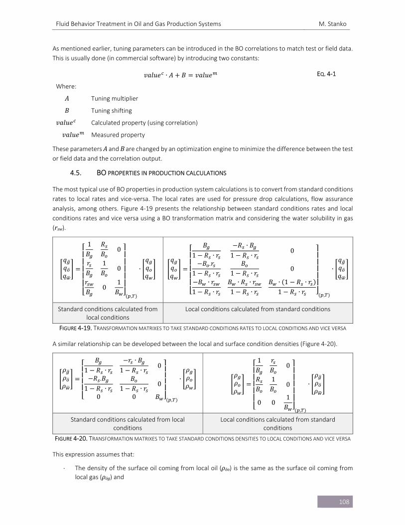
Fluid Behavior Treatment in Oil and Gas Production Systems M. Stanko
108
As mentioned earlier, tuning parameters can be introduced in the BO correlations to match test or field data.
This is usually done (in commercial software) by introducing two constants:
𝑣𝑎𝑙𝑢𝑒 ∙ 𝐴 𝐵 𝑣𝑎𝑙𝑢𝑒 EQ. 4‐1
Where:
𝐴 Tuning multiplier
𝐵 Tuning shifting
𝑣𝑎𝑙𝑢𝑒 Calculated property (using correlation)
𝑣𝑎𝑙𝑢𝑒 Measured property
These parameters A and B are changed by an optimization engine to minimize the difference between the test
or field data and the correlation output.
4.5. BO PROPERTIES IN PRODUCTION CALCULATIONS
The most typical use of BO properties in production system calculations is to convert from standard conditions
rates to local rates and vice‐versa. The local rates are used for pressure drop calculations, flow assurance
analysis, among others. Figure 4‐19 presents the relationship between standard conditions rates and local
conditions rates and vice versa using a BO transformation matrix and considering the water solubility in gas
(rsw).
𝑞𝑞𝑞
⎣⎢⎢⎢⎢⎢⎡
1𝐵
𝑅𝐵
0
𝑟𝐵
1𝐵
0
𝑟𝐵
01
𝐵 ⎦⎥⎥⎥⎥⎥⎤
,
∙𝑞𝑞𝑞
𝑞𝑞𝑞
⎣⎢⎢⎢⎢⎢⎡
𝐵
1 𝑅 ∙ 𝑟
𝑅 ∙ 𝐵
1 𝑅 ∙ 𝑟0
𝐵 ∙𝑟1 𝑅 ∙ 𝑟
𝐵1 𝑅 ∙ 𝑟
0
𝐵 ∙ 𝑟1 𝑅 ∙ 𝑟
𝐵 ∙ 𝑅 ∙ 𝑟1 𝑅 ∙ 𝑟
𝐵 ∙ 1 𝑅 ∙ 𝑟1 𝑅 ∙ 𝑟 ⎦
⎥⎥⎥⎥⎥⎤
,
∙𝑞𝑞𝑞
Standard conditions calculated from local conditions
Local conditions calculated from standard conditions
FIGURE 4‐19. TRANSFORMATION MATRIXES TO TAKE STANDARD CONDITIONS RATES TO LOCAL CONDITIONS AND VICE VERSA
A similar relationship can be developed between the local and surface condition densities (Figure 4‐20).
𝜌𝜌𝜌
⎣⎢⎢⎢⎢⎡
𝐵
1 𝑅 ∙ 𝑟
𝑟 ∙ 𝐵
1 𝑅 ∙ 𝑟0
𝑅 ∙𝐵
1 𝑅 ∙ 𝑟𝐵
1 𝑅 ∙ 𝑟0
0 0 𝐵 ⎦⎥⎥⎥⎥⎤
,
∙𝜌𝜌𝜌
𝜌𝜌𝜌
⎣⎢⎢⎢⎢⎢⎡
1𝐵
𝑟𝐵
0
𝑅𝐵
1𝐵
0
0 01
𝐵 ⎦⎥⎥⎥⎥⎥⎤
,
∙𝜌𝜌𝜌
Standard conditions calculated from local conditions
Local conditions calculated from standard conditions
FIGURE 4‐20. TRANSFORMATION MATRIXES TO TAKE STANDARD CONDITIONS DENSITIES TO LOCAL CONDITIONS AND VICE VERSA
This expression assumes that:
The density of the surface oil coming from local oil (ρōo) is the same as the surface oil coming from
local gas (ρōg) and
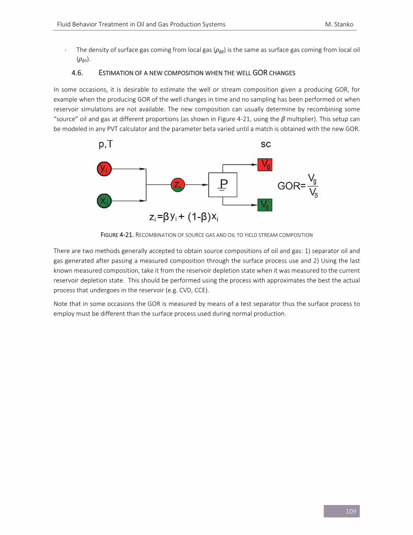
Fluid Behavior Treatment in Oil and Gas Production Systems M. Stanko
109
The density of surface gas coming from local gas (ρḡg) is the same as surface gas coming from local oil
(ρḡo).
4.6. ESTIMATION OF A NEW COMPOSITION WHEN THE WELL GOR CHANGES
In some occasions, it is desirable to estimate the well or stream composition given a producing GOR, for
example when the producing GOR of the well changes in time and no sampling has been performed or when
reservoir simulations are not available. The new composition can usually determine by recombining some
“source” oil and gas at different proportions (as shown in Figure 4‐21, using the β multiplier). This setup can
be modeled in any PVT calculator and the parameter beta varied until a match is obtained with the new GOR.
FIGURE 4‐21. RECOMBINATION OF SOURCE GAS AND OIL TO YIELD STREAM COMPOSITION
There are two methods generally accepted to obtain source compositions of oil and gas: 1) separator oil and
gas generated after passing a measured composition through the surface process use and 2) Using the last
known measured composition, take it from the reservoir depletion state when it was measured to the current
reservoir depletion state. This should be performed using the process with approximates the best the actual
process that undergoes in the reservoir (e.g. CVD, CCE).
Note that in some occasions the GOR is measured by means of a test separator thus the surface process to
employ must be different than the surface process used during normal production.

Fluid Behavior Treatment in Oil and Gas Production Systems M. Stanko
110
REFERENCES
[4‐1] Whitson, C.H. & Brule, M.R. (2000). Phase Behavior. Society of Petroleum Engineers. 978‐1‐55563‐
087‐4.
[4‐2] Standing, M.B. (1977). Volumetric and Phase Behavior of Oil Field Hydrocarbon Systems. 8th printing,
Society of Petroleum Engineers, Dallas.
[4‐3] Whitson, C. H. (1998). PVT Analysis Manual. Chapter 3. Norsk Hydro.
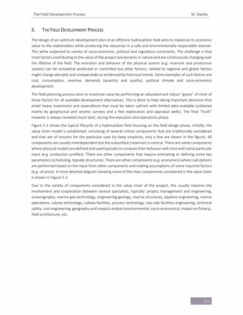
The Field Development Process M. Stanko
111
5. THE FIELD DEVELOPMENT PROCESS
The design of an optimum development plan of an offshore hydrocarbon field aims to maximize its economic
value to the stakeholders while producing the resources in a safe and environmentally responsible manner.
This while subjected to variety of socio‐economic, political and regulatory constraints. The challenge is that
most factors contributing to the value of the project are dynamic in nature and are continuously changing over
the lifetime of the field. The evolution and behavior of the physical system (e.g. reservoir and production
system) can be somewhat predicted or controlled but other factors, related to regional and global factors
might change abruptly and unexpectedly as evidenced by historical trends. Some examples of such factors are
cost, consumption, revenue, demands (quantity and quality), political climate and socio‐economic
development.
The field planning process aims to maximize value by performing an educated and robust “guess” of most of
these factors for all available development alternatives. This is done to help taking important decisions that
entail heavy investment and expenditure that must be taken upfront with limited data available (collected
mainly by geophysical and seismic surveys and a few exploration and appraisal wells). The final “truth”
however is always revealed much later, during the execution and operations phase.
Figure 5‐1 shows the typical lifecycle of a hydrocarbon field focusing on the field design phase. Initially, the
value chain model is established, consisting of several critical components that are traditionally considered
and that are of concern for the particular case (to keep simplicity, only a few are shown in the figure). All
components are usually interdependent but the subsurface (reservoir) is central. There are some components
where physical models are defined and used typically to compute their behavior with time with some particular
input (e.g. production profiles). There are other components that require estimating or defining some key
parameters (scheduling, topside structures). There are other components (e.g. economics) where calculations
are performed based on the input from other components and making assumptions of some required factors
(e.g. oil price). A more detailed diagram showing some of the main components considered in the value chain
is shown in Figure 5‐2.
Due to the variety of components considered in the value chain of the project, this usually requires the
involvement and cooperation between several specialists, typically: project management and engineering,
oceanography, marine geo‐technology, engineering geology, marine structures, pipeline engineering, marine
operations, subsea technology, subsea facilities, process technology, top‐side facilities engineering, technical
safety, cost engineering, geography and impacts analyst (environmental, socio‐economical, impact on fishery),
field architecture, etc.
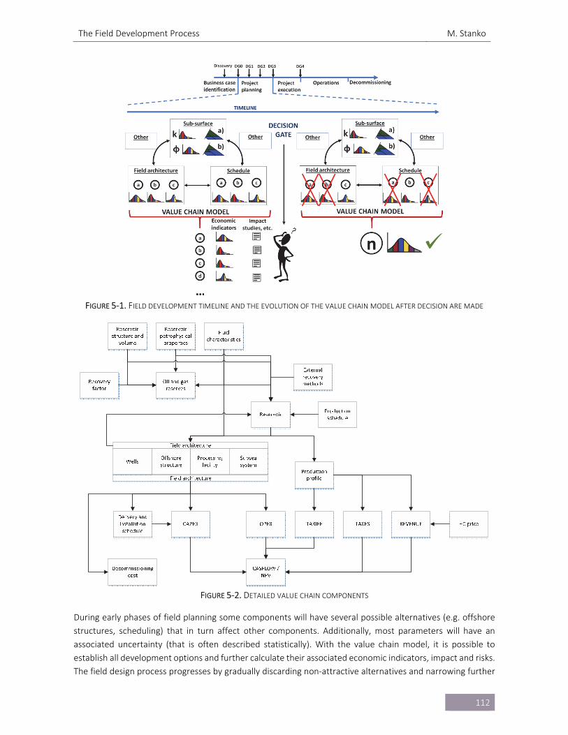
The Field Development Process M. Stanko
112
FIGURE 5‐1. FIELD DEVELOPMENT TIMELINE AND THE EVOLUTION OF THE VALUE CHAIN MODEL AFTER DECISION ARE MADE
FIGURE 5‐2. DETAILED VALUE CHAIN COMPONENTS
During early phases of field planning some components will have several possible alternatives (e.g. offshore
structures, scheduling) that in turn affect other components. Additionally, most parameters will have an
associated uncertainty (that is often described statistically). With the value chain model, it is possible to
establish all development options and further calculate their associated economic indicators, impact and risks.
The field design process progresses by gradually discarding non‐attractive alternatives and narrowing further
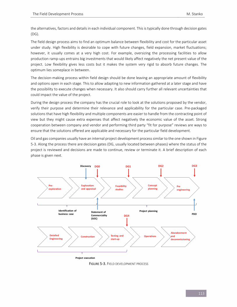
The Field Development Process M. Stanko
113
the alternatives, factors and details in each individual component. This is typically done through decision gates
(DG).
The field design process aims to find an optimum balance between flexibility and cost for the particular asset
under study. High flexibility is desirable to cope with future changes, field expansion, market fluctuations;
however, it usually comes at a very high cost. For example, oversizing the processing facilities to allow
production ramp‐ups entrains big investments that would likely affect negatively the net present value of the
project. Low flexibility gives less costs but it makes the system very rigid to absorb future changes. The
optimum lies someplace in between.
The decision‐making process within field design should be done leaving an appropriate amount of flexibility
and options open in each stage. This to allow adapting to new information gathered at a later stage and have
the possibility to execute changes when necessary. It also should carry further all relevant uncertainties that
could impact the value of the project.
During the design process the company has the crucial role to look at the solutions proposed by the vendor,
verify their purpose and determine their relevance and applicability for the particular case. Pre‐packaged
solutions that have high flexibility and multiple components are easier to handle from the contracting point of
view but they might cause extra expenses that affect negatively the economic value of the asset. Strong
cooperation between company and vendor and performing third party “fit for purpose” reviews are ways to
ensure that the solutions offered are applicable and necessary for the particular field development.
Oil and gas companies usually have an internal project development process similar to the one shown in Figure
5‐3. Along the process there are decision gates (DG, usually located between phases) where the status of the
project is reviewed and decisions are made to continue, review or terminate it. A brief description of each
phase is given next.
FIGURE 5‐3. FIELD DEVELOPMENT PROCESS
DG0 DG1 DG2 DG3
DG4
Identification of business case
Feasibility studies
Concept planning
Pre engineering
Operations
Abandonment and decommissioning
Project planning
Project execution
Testing and start‐up
ConstructionDetailed Engineering
Exploration and appraisal
Pre‐exploration
Discovery
Statement of Commerciality (SOC)
PDO
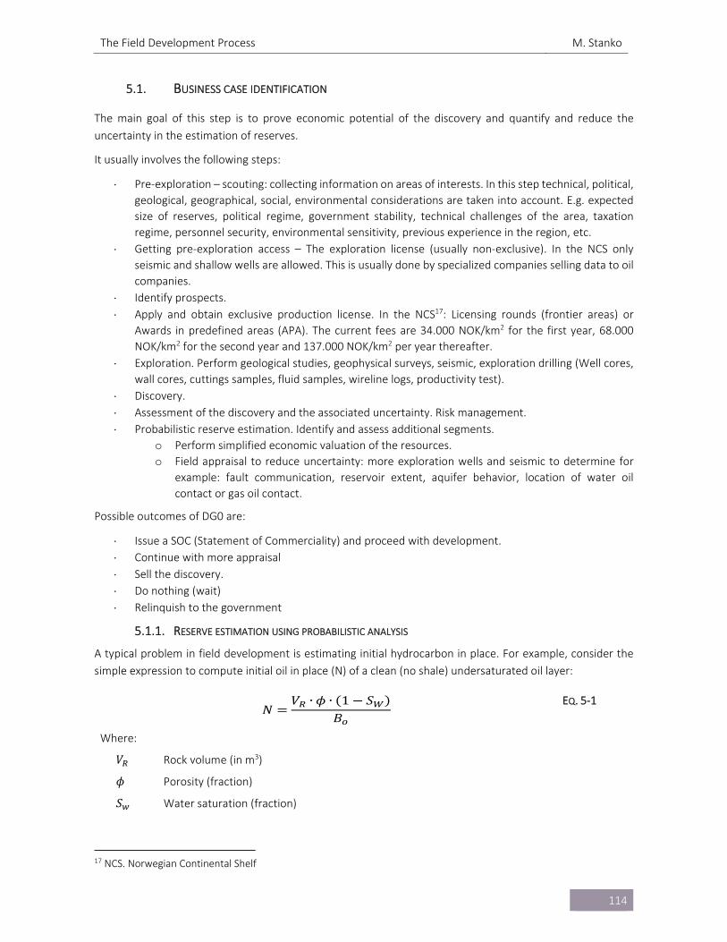
The Field Development Process M. Stanko
114
5.1. BUSINESS CASE IDENTIFICATION
The main goal of this step is to prove economic potential of the discovery and quantify and reduce the
uncertainty in the estimation of reserves.
It usually involves the following steps:
Pre‐exploration – scouting: collecting information on areas of interests. In this step technical, political,
geological, geographical, social, environmental considerations are taken into account. E.g. expected
size of reserves, political regime, government stability, technical challenges of the area, taxation
regime, personnel security, environmental sensitivity, previous experience in the region, etc.
Getting pre‐exploration access – The exploration license (usually non‐exclusive). In the NCS only
seismic and shallow wells are allowed. This is usually done by specialized companies selling data to oil
companies.
Identify prospects.
Apply and obtain exclusive production license. In the NCS17: Licensing rounds (frontier areas) or
Awards in predefined areas (APA). The current fees are 34.000 NOK/km2 for the first year, 68.000
NOK/km2 for the second year and 137.000 NOK/km2 per year thereafter.
Exploration. Perform geological studies, geophysical surveys, seismic, exploration drilling (Well cores,
wall cores, cuttings samples, fluid samples, wireline logs, productivity test).
Discovery.
Assessment of the discovery and the associated uncertainty. Risk management.
Probabilistic reserve estimation. Identify and assess additional segments.
o Perform simplified economic valuation of the resources.
o Field appraisal to reduce uncertainty: more exploration wells and seismic to determine for
example: fault communication, reservoir extent, aquifer behavior, location of water oil
contact or gas oil contact.
Possible outcomes of DG0 are:
Issue a SOC (Statement of Commerciality) and proceed with development.
Continue with more appraisal
Sell the discovery.
Do nothing (wait)
Relinquish to the government
5.1.1. RESERVE ESTIMATION USING PROBABILISTIC ANALYSIS
A typical problem in field development is estimating initial hydrocarbon in place. For example, consider the
simple expression to compute initial oil in place (N) of a clean (no shale) undersaturated oil layer:
𝑁𝑉 ∙ 𝜙 ∙ 1 𝑆
𝐵
EQ. 5‐1
Where:
𝑉 Rock volume (in m3)
𝜙 Porosity (fraction)
𝑆 Water saturation (fraction)
17 NCS. Norwegian Continental Shelf
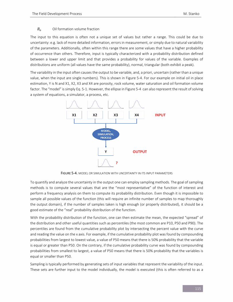
The Field Development Process M. Stanko
115
𝐵 Oil formation volume fraction
The input to this equation is often not a unique set of values but rather a range. This could be due to
uncertainty: e.g. lack of more detailed information, errors in measurement, or simply due to natural variability
of the parameters. Additionally, often within this range there are some values that have a higher probability
of occurrence than others. Therefore, input is typically characterized with a probability distribution defined
between a lower and upper limit and that provides a probability for values of the variable. Examples of
distributions are uniform (all values have the same probability), normal, triangular (both exhibit a peak).
The variability in the input often causes the output to be variable, and, a priori, uncertain (rather than a unique
value, when the input are single numbers). This is shown in Figure 5‐4. For our example on initial oil in place
estimation, Y is N and X1, X2, X3 and X4 are porosity, rock volume, water saturation and oil formation volume
factor. The “model” is simply Eq. 5‐1. However, the ellipse in Figure 5‐4 can also represent the result of solving
a system of equations, a simulator, a process, etc.
FIGURE 5‐4. MODEL OR SIMULATION WITH UNCERTAINTY IN ITS INPUT PARAMETERS
To quantify and analyze the uncertainty in the output one can employ sampling methods. The goal of sampling
methods is to compute several values that are the “most representative” of the function of interest and
perform a frequency analysis on them to compute its probability distribution. Even though it is impossible to
sample all possible values of the function (this will require an infinite number of samples to map thoroughly
the output domain), if the number of samples taken is high enough (or properly distributed), it should be a
good estimate of the “real” probability distribution of the function.
With the probability distribution of the function, one can then estimate the mean, the expected “spread” of
the distribution and other useful quantities such as percentiles (the most common are P10, P50 and P90). The
percentiles are found from the cumulative probability plot by intersecting the percent value with the curve
and reading the value on the x axis. For example, if the cumulative probability plot was found by compounding
probabilities from largest to lowest value, a value of P50 means that there is 50% probability that the variable
is equal or greater than P50. On the contrary, if the cumulative probability curve was found by compounding
probabilities from smallest to largest, a value of P50 means that there is 50% probability that the variables is
equal or smaller than P50.
Sampling is typically performed by generating sets of input variables that represent the variability of the input.
These sets are further input to the model individually, the model is executed (this is often referred to as a
The Field Development Process M. Stanko
116
“simulation”) and all outputs are recorded. A frequency analysis is then executed on the output to find the
probability distribution.
One popular sampling method is Monte Carlo. This method consists of choosing randomly a value of the
cumulative distribution function (cdf) of each input variable (if using a continuous probability function), obtain
a value of the variable and combine it with random values of other variables. It is advantageous to sample on
the cumulative distribution function as the number is bounded between 0 and 1. It also guarantees the
resulting sample of the input exhibits the same trend as the original probability distribution.
As an example, Figure 5‐5 shows the result of a Monte Carlo simulation18 of Eq. 5‐1, with increasing number
of samples. Above 1000 samples, the frequency distribution changes very little. By increasing the number of
samples, the probability distribution converges to a unique (the real) distribution.
101 samples 102 samples 103 samples
104 samples 105 samples 106 samples
FIGURE 5‐5. PROBABILITY DISTRIBUTION OF INITIAL OIL IN PLACE CALCULATED WITH MONTE CARLO SIMULATION AND DIFFERENT
NUMBER OF SAMPLES
To estimate the required number of iterations to perform in the Monte Carlo method, one uses statistical
inference. Consider that the probability distribution function of N is known and it displays a normal probability
distribution with mean 𝜇. If a sample of size “n” is taken from that “real” distribution (this is what Monte Carlo
does), the quantity T.
𝑇𝑋 𝜇
𝑆√𝑛
EQ. 5‐2
will be t‐distributed symmetrically around zero, with n‐1 degrees of freedom. 𝑋 is the mean of the sample and
S is the standard deviation of the sample.
18 Using uniform distribution for porosity (0.18‐0.3), rock volume (2000‐2500 MMbbl), oil saturation (0.8‐0.9) and oil
formation volume factor (1.35‐1.6)
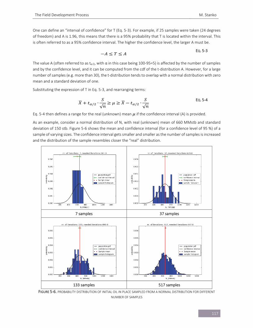
The Field Development Process M. Stanko
117
One can define an “interval of confidence” for T (Eq. 5‐3). For example, if 25 samples were taken (24 degrees
of freedom) and A is 1.96, this means that there is a 95% probability that T is located within the interval. This
is often referred to as a 95% confidence interval. The higher the confidence level, the larger A must be.
𝐴 𝑇 𝐴 EQ. 5‐3
The value A (often referred to as t, with α in this case being 100‐95=5) is affected by the number of samples
and by the confidence level, and it can be computed from the cdf of the t‐distribution A. However, for a large
number of samples (e.g. more than 30), the t‐distribution tends to overlap with a normal distribution with zero
mean and a standard deviation of one.
Substituting the expression of T in Eq. 5‐3, and rearranging terms:
𝑋 𝑡 / ∙𝑆
√𝑛𝜇 𝑋 𝑡 / ∙
𝑆
√𝑛
EQ. 5‐4
Eq. 5‐4 then defines a range for the real (unknown) mean 𝜇 if the confidence interval (A) is provided.
As an example, consider a normal distribution of N, with real (unknown) mean of 660 MMstb and standard
deviation of 150 stb. Figure 5‐6 shows the mean and confidence interval (for a confidence level of 95 %) of a
sample of varying sizes. The confidence interval gets smaller and smaller as the number of samples is increased
and the distribution of the sample resembles closer the “real” distribution.
7 samples 37 samples
133 samples 517 samples
FIGURE 5‐6. PROBABILITY DISTRIBUTION OF INITIAL OIL IN PLACE SAMPLED FROM A NORMAL DISTRIBUTION FOR DIFFERENT
NUMBER OF SAMPLES
The Field Development Process M. Stanko
118
To estimate the number of samples required in Monte Carlo, one can modify Eq. 5‐4 by specifying the error
(e) one wishes to achieve.
𝑒 𝑡 / ∙𝑆
√𝑛
EQ. 5‐5
e is the absolute error, and it is often expressed in terms of the mean of the sample, 𝑋, for example, by
multiplying it with a fraction F (between 0‐1). By substituting this in Eq. 5‐5, and clearing “n” it yields
𝑛 𝑡 / ∙𝑆
𝐹 ∙ 𝑋
EQ. 5‐6
To estimate a value of n, one must have performed at least one iteration, and S and 𝑋 should be available. There will be a new value of n for each iteration and one stops when n estimated is smaller than the actual
sample size.
Sometimes the number of iterations required for the Monte Carlo method to achieve an acceptable error are
too large to be practical, especially if the simulation running time is high. There are other methods that
perform a smarter sampling of the function (instead of random), that require less iterations. One of this
methods is Latin hypercube sampling. In Latin Hypercube sampling the steps are:
Define the number of samples “n” to use.
Subdivide the pdf of each input variable in “n” intervals of equal probability.
Create a set of “n” values for each variable by picking a random number in each interval (using the cdf
of each interval, just like in Monte Carlo).
Create “n” input sets by picking randomly a value of each variable set. It is not allowed to pick the
same value twice.
Run the simulations with the “n” input sets and apply a frequency analysis to the results.
5.2. PROJECT PLANNING
The main goal of the planning phase is to perform a systematic screening of concepts, to define a preferred
development concept and to evaluate its profitability, technical feasibility and HSE within acceptable levels of
uncertainty. Furthermore, to document the solution for delivery to the authorities managing the production
license.
5.2.1. FEASIBILITY STUDIES
The main goal of this step is to justify further development of the project, finding one or more concepts that
are technically, commercially and organizationally feasible. Some specific tasks of this phase are:
Define objectives of the development in line with the corporate strategy.
Establish feasible development scenarios.
Create a project timeline and a workplan.
Identify possible technology gaps and blockers.
Identify the needs for new technology.
Identify added value opportunities.
Cost evaluation for all options.
5.2.2. CONCEPT PLANNING (LEADING TO DG2)
Identify development concepts, rank them and select and document a viable concept (Base Case Scenario).
Evaluate and compare alternatives for development and screen out non‐viable options.
The Field Development Process M. Stanko
119
Elaborate a Project Execution Plan (PEP) which describes the project and management system.
Define the commercial aspects, legislation, agreements, licensing, financing, marketing and supply,
taxes.
Create and refine a static and a dynamic model of reservoir. Define the depletion and production
strategy.
Define an HSE program.
Flow assurance evaluation. Identification of challenged related with fluid properties, multiphase
handling and driving pressure.
Drilling and well planning.
Pre‐design of facilities.
Planning of operations, start‐up and maintenance.
Cost and manpower estimates of the best viable concept.
5.2.3. FIELD PRODUCTION PROFILE AND ECONOMIC VALUE
During the concept phase, one of the main tasks is to define the field production schedule that provides the
maximum economic value for the project. The economic value of the project could be estimated using
different financial evaluation approaches; one of the approaches is the net present value (NPV), calculated on
a yearly basis, which is defined as:
𝑓𝑅𝑡
1 𝑖 EQ. 5‐7
Where:
𝑖 Discount rate (usually a value around 8%)
𝑘 Counter for the number of years
𝑁 Total number of years
𝑅𝑡 Cash flow of year “k”
Neglecting royalties and tax payments (parameters which change from country to country, or even on license
type), the cashflow for the project can be expressed as:
𝑅𝑡 𝑅𝑒𝑣𝑒𝑛𝑢𝑒 𝑂𝑃𝐸𝑋 𝑞 𝐷𝑅𝐼𝐿𝐿𝐸𝑋 𝐶𝐴𝑃𝐸𝑋 𝑞 EQ. 5‐8
During the first years of the project, when the field is under construction and there is no production, only
drilling expenditures (also known as DRILLEX) and capital expenditures (CAPEX) are considered. CAPEX are
expenditures to acquire, design, manufacture and transport physical assets such as an offshore structure,
topside facilities, subsea system, etc. For later years, when the field is producing only revenue and operating
expenditures (OPEX) are considered.
The CAPEX related with the offshore structure and topside facilities depends strongly of the type and weight
of units and equipment that will be placed on the offshore structure. The type of units and equipment depend
on the treatment processes required for reservoir fluids, while the weight is given mainly by the maximum
liquid and gas processing capacities. Therefore, the offshore structure and topside CAPEX is a function of the
maximum field liquid rate (ql,max) and the maximum field gas rate (qg,max) produced during the life of the field.
The relationship is often assumed linear, as shown in equation Eq. 5‐9.
𝐶𝐴𝑃𝐸𝑋 𝐶 ∙ 𝑞 , 𝐶 ∙ 𝑞 , 𝐶 EQ. 5‐9
The Field Development Process M. Stanko
120
For some offshore structures that “house” wells (for example jackets, gravity‐based platforms, tension leg
platforms with dry Christmas trees), the CAPEX of offshore and topside also depends strongly of the number
of wells.
The subsea system CAPEX depends of several factors: number of wells, number of subsea manifolds and
flowlines, umbilicals, water depth, etc. Despite showing dependencies on these many factors, the subsea
CAPEX can be often expressed as function (often linear) with the number of wells.
𝐶𝐴𝑃𝐸𝑋 𝐶 𝐶 ∙ 𝑁 EQ. 5‐10
Where:
𝑁 Number of wells
DRILLEX is typically computed the well cost times the number of wells:
𝐷𝑅𝐼𝐿𝐿𝐸𝑋 𝑁 ∙ 𝑃 EQ. 5‐11
Where:
𝑃 Cost of drilling a well
The revenue function will be discussed next with an example. Due to the discounting factor, the production in
later years typically contributes less to the NPV than production in earlier years. Thus, one usually tends to
favor production in earlier years against production in later years.
Estimating the NPV of a undersaturated oil field operating in plateau mode
Using the equation derived in Example 1 of section 1.6, the field rate is a continuous function, given by:
𝐹𝑜𝑟 𝑡 𝑡 𝑞 𝑞 , EQ. 5‐12
𝐹𝑜𝑟 𝑡 𝑡 𝑞 𝑞 , ∙ 𝑒 ∙ EQ. 5‐13
With:
𝑡𝑞𝑞 ,
1 ∙1𝑚 EQ. 5‐14
𝑚 𝐴 ∙ 𝑁 ∙ 𝐽 EQ. 5‐15
𝑞 𝑁 ∙ 𝐽 ∙ 𝑝 𝑝 , EQ. 5‐16
𝐴𝐵
𝑁 ∙ 𝐵 , ∙ 𝑐𝑐 ∙ 𝑆 𝑐
𝑆 𝑉 ∙ 𝜙 ∙ 𝐵 ∙ 𝑐 𝑐 EQ. 5‐17
Assuming a constant value of the hydrocarbon price and using a continuous discounting with the exponential
function and discount rate “𝑖” the revenue stream at a given time is calculated by:
𝑁𝑃𝑉 𝑞 𝑡 ∙ 𝑃 ∙ 𝑒 ∙ 𝑑𝑡 EQ. 5‐18
Expanding the expression for the plateau and post‐plateau periods:
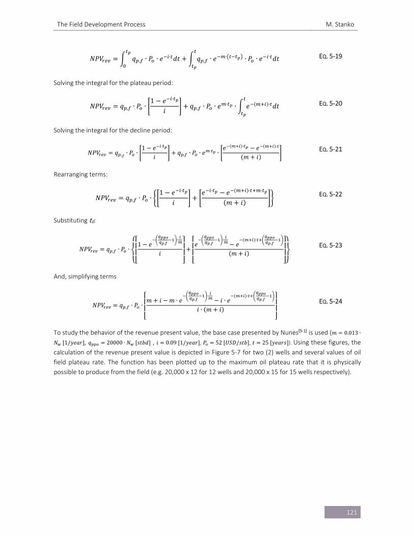
The Field Development Process M. Stanko
121
𝑁𝑃𝑉 𝑞 , ∙ 𝑃 ∙ 𝑒 ∙ 𝑑𝑡 𝑞 , ∙ 𝑒 ∙ ∙ 𝑃 ∙ 𝑒 ∙ 𝑑𝑡 EQ. 5‐19
Solving the integral for the plateau period:
𝑁𝑃𝑉 𝑞 , ∙ 𝑃 ∙1 𝑒 ∙
𝑖𝑞 , ∙ 𝑃 ∙ 𝑒 ∙ ∙ 𝑒 ∙ 𝑑𝑡 EQ. 5‐20
Solving the integral for the decline period:
𝑁𝑃𝑉 𝑞 , ∙ 𝑃 ∙1 𝑒 ∙
𝑖𝑞 , ∙ 𝑃 ∙ 𝑒 ∙ ∙
𝑒 ∙ 𝑒 ∙
𝑚 𝑖
EQ. 5‐21
Rearranging terms:
𝑁𝑃𝑉 𝑞 , ∙ 𝑃 ∙1 𝑒 ∙
𝑖𝑒 ∙ 𝑒 ∙ ∙
𝑚 𝑖
EQ. 5‐22
Substituting t0:
𝑁𝑃𝑉 𝑞 , ∙ 𝑃 ∙
⎩⎨
⎧
⎣⎢⎢⎡1 𝑒 ,
∙
𝑖⎦⎥⎥⎤
⎣⎢⎢⎡𝑒 ,
∙𝑒
∙,
𝑚 𝑖⎦⎥⎥⎤
⎭⎬
⎫
EQ. 5‐23
And, simplifying terms
𝑁𝑃𝑉 𝑞 , ∙ 𝑃 ∙
⎣⎢⎢⎡𝑚 𝑖 𝑚 ∙ 𝑒 ,
∙𝑖 ∙ 𝑒
∙,
𝑖 ∙ 𝑚 𝑖⎦⎥⎥⎤
EQ. 5‐24
To study the behavior of the revenue present value, the base case presented by Nunes[5‐1] is used (𝑚 0.013 ∙
𝑁 1/𝑦𝑒𝑎𝑟 , 𝑞 20000 ∙ 𝑁 𝑠𝑡𝑏𝑑 , 𝑖 0.09 1/𝑦𝑒𝑎𝑟 , 𝑃 52 𝑈𝑆𝐷/𝑠𝑡𝑏 , 𝑡 25 𝑦𝑒𝑎𝑟𝑠 ). Using these figures, the
calculation of the revenue present value is depicted in Figure 5‐7 for two (2) wells and several values of oil
field plateau rate. The function has been plotted up to the maximum oil plateau rate that it is physically
possible to produce from the field (e.g. 20,000 x 12 for 12 wells and 20,000 x 15 for 15 wells respectively).
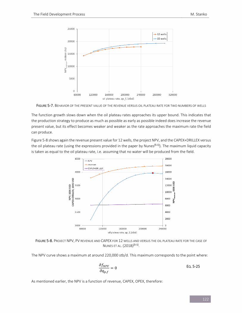
The Field Development Process M. Stanko
122
FIGURE 5‐7. BEHAVIOR OF THE PRESENT VALUE OF THE REVENUE VERSUS OIL PLATEAU RATE FOR TWO NUMBERS OF WELLS
The function growth slows down when the oil plateau rates approaches its upper bound. This indicates that
the production strategy to produce as much as possible as early as possible indeed does increase the revenue
present value, but its effect becomes weaker and weaker as the rate approaches the maximum rate the field
can produce.
Figure 5‐8 shows again the revenue present value for 12 wells, the project NPV, and the CAPEX+DRILLEX versus
the oil plateau rate (using the expressions provided in the paper by Nunes[5‐1]). The maximum liquid capacity
is taken as equal to the oil plateau rate, i.e. assuming that no water will be produced from the field.
FIGURE 5‐8. PROJECT NPV, PV REVENUE AND CAPEX FOR 12 WELLS AND VERSUS THE OIL PLATEAU RATE FOR THE CASE OF
NUNES ET AL. (2018)[5‐1].
The NPV curve shows a maximum at around 220,000 stb/d. This maximum corresponds to the point where:
𝜕𝑓𝜕𝑞 ,
0 EQ. 5‐25
As mentioned earlier, the NPV is a function of revenue, CAPEX, OPEX, therefore:
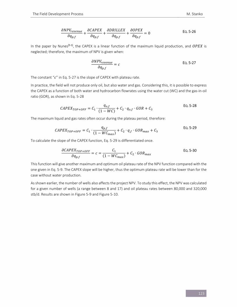
The Field Development Process M. Stanko
123
𝜕𝑁𝑃𝑉𝜕𝑞 ,
𝜕𝐶𝐴𝑃𝐸𝑋𝜕𝑞 ,
𝜕𝐷𝑅𝐼𝐿𝐿𝐸𝑋𝜕𝑞 ,
𝜕𝑂𝑃𝐸𝑋𝜕𝑞 ,
0 EQ. 5‐26
In the paper by Nunes[5‐1], the CAPEX is a linear function of the maximum liquid production, and 𝑂𝑃𝐸𝑋 is
neglected; therefore, the maximum of NPV is given when:
𝜕𝑁𝑃𝑉𝜕𝑞 ,
𝑐 EQ. 5‐27
The constant “𝑐” in Eq. 5‐27 is the slope of CAPEX with plateau rate.
In practice, the field will not produce only oil, but also water and gas. Considering this, it is possible to express
the CAPEX as a function of both water and hydrocarbon flowrates using the water cut (WC) and the gas‐in‐oil
ratio (GOR), as shown in Eq. 5‐28
𝐶𝐴𝑃𝐸𝑋 𝐶 ∙𝑞 ,
1 𝑊𝐶𝐶 ∙ 𝑞 , ∙ 𝐺𝑂𝑅 𝐶
EQ. 5‐28
The maximum liquid and gas rates often occur during the plateau period, therefore:
𝐶𝐴𝑃𝐸𝑋 𝐶 ∙𝑞 ,
1 𝑊𝐶𝐶 ∙ 𝑞, ∙ 𝐺𝑂𝑅 𝐶
EQ. 5‐29
To calculate the slope of the CAPEX function, Eq. 5‐29 is differentiated once.
𝜕𝐶𝐴𝑃𝐸𝑋𝜕𝑞 ,
𝑐𝐶
1 𝑊𝐶𝐶 ∙ 𝐺𝑂𝑅
EQ. 5‐30
This function will give another maximum and optimum oil plateau rate of the NPV function compared with the
one given in Eq. 5‐9. The CAPEX slope will be higher, thus the optimum plateau rate will be lower than for the
case without water production.
As shown earlier, the number of wells also affects the project NPV. To study this effect, the NPV was calculated
for a given number of wells (a range between 8 and 17) and oil plateau rates between 80,000 and 320,000
stb/d. Results are shown in Figure 5‐9 and Figure 5‐10.
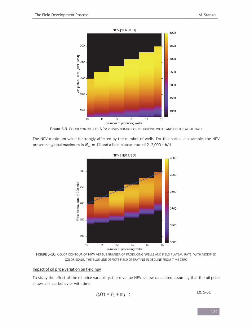
The Field Development Process M. Stanko
124
FIGURE 5‐9. COLOR CONTOUR OF NPV VERSUS NUMBER OF PRODUCING WELLS AND FIELD PLATEAU RATE
The NPV maximum value is strongly affected by the number of wells. For this particular example, the NPV
presents a global maximum in 𝑁 12 and a field plateau rate of 212,000 stb/d.
FIGURE 5‐10. COLOR CONTOUR OF NPV VERSUS NUMBER OF PRODUCING WELLS AND FIELD PLATEAU RATE, WITH MODIFIED
COLOR SCALE. THE BLUE LINE DEPICTS FIELD OPERATING IN DECLINE FROM TIME ZERO
Impact of oil price variation on field npv
To study the effect of the oil price variability, the revenue NPV is now calculated assuming that the oil price
shows a linear behavior with time:
𝑃 𝑡 𝑃 𝑚 ∙ 𝑡 EQ. 5‐31
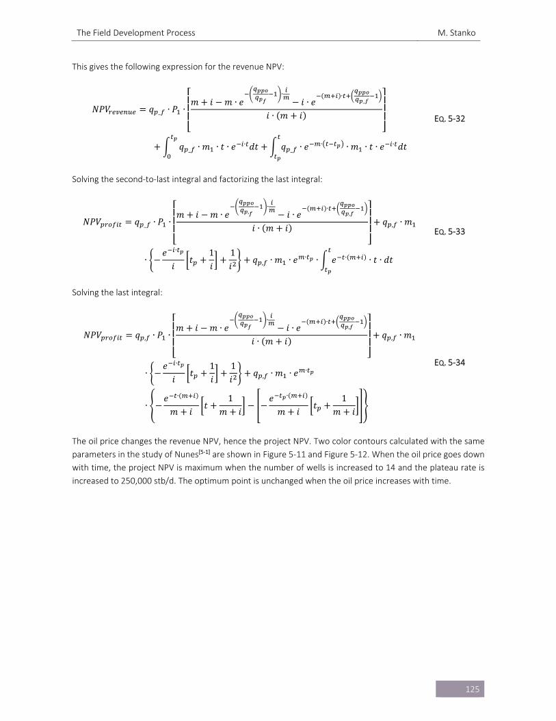
The Field Development Process M. Stanko
125
This gives the following expression for the revenue NPV:
𝑁𝑃𝑉 𝑞 _ ∙ 𝑃 ∙
⎣⎢⎢⎢⎡𝑚 𝑖 𝑚 ∙ 𝑒
∙𝑖 ∙ 𝑒
∙_
𝑖 ∙ 𝑚 𝑖⎦⎥⎥⎥⎤
𝑞 _ ∙ 𝑚 ∙ 𝑡 ∙ 𝑒 ∙ 𝑑𝑡 𝑞 _ ∙ 𝑒 ∙ ∙ 𝑚 ∙ 𝑡 ∙ 𝑒 ∙ 𝑑𝑡
EQ. 5‐32
Solving the second‐to‐last integral and factorizing the last integral:
𝑁𝑃𝑉 𝑞 _ ∙ 𝑃 ∙
⎣⎢⎢⎢⎡𝑚 𝑖 𝑚 ∙ 𝑒 ,
∙𝑖 ∙ 𝑒
∙,
𝑖 ∙ 𝑚 𝑖⎦⎥⎥⎥⎤
𝑞 , ∙ 𝑚
∙𝑒 ∙
𝑖𝑡
1𝑖
1𝑖
𝑞 , ∙ 𝑚 ∙ 𝑒 ∙ ∙ 𝑒 ∙ ∙ 𝑡 ∙ 𝑑𝑡
EQ. 5‐33
Solving the last integral:
𝑁𝑃𝑉 𝑞 , ∙ 𝑃 ∙
⎣⎢⎢⎢⎡𝑚 𝑖 𝑚 ∙ 𝑒
∙𝑖 ∙ 𝑒
∙,
𝑖 ∙ 𝑚 𝑖⎦⎥⎥⎥⎤
𝑞 , ∙ 𝑚
∙𝑒 ∙
𝑖𝑡
1𝑖
1𝑖
𝑞 , ∙ 𝑚 ∙ 𝑒 ∙
∙𝑒 ∙
𝑚 𝑖𝑡
1𝑚 𝑖
𝑒 ∙
𝑚 𝑖𝑡
1𝑚 𝑖
EQ. 5‐34
The oil price changes the revenue NPV, hence the project NPV. Two color contours calculated with the same
parameters in the study of Nunes[5‐1] are shown in Figure 5‐11 and Figure 5‐12. When the oil price goes down
with time, the project NPV is maximum when the number of wells is increased to 14 and the plateau rate is
increased to 250,000 stb/d. The optimum point is unchanged when the oil price increases with time.
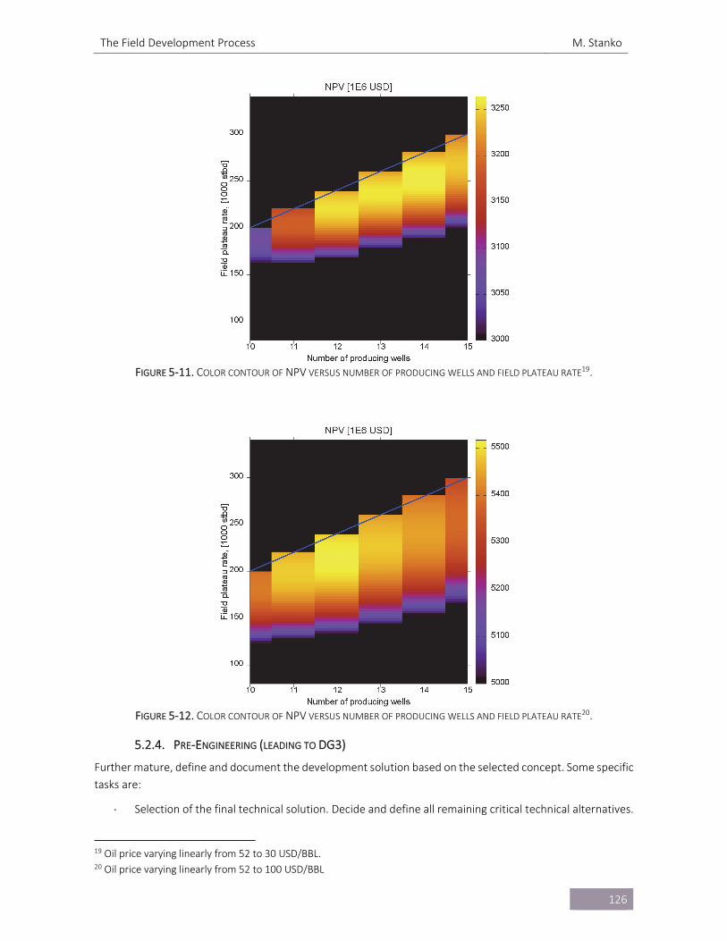
The Field Development Process M. Stanko
126
FIGURE 5‐11. COLOR CONTOUR OF NPV VERSUS NUMBER OF PRODUCING WELLS AND FIELD PLATEAU RATE19.
FIGURE 5‐12. COLOR CONTOUR OF NPV VERSUS NUMBER OF PRODUCING WELLS AND FIELD PLATEAU RATE20.
5.2.4. PRE‐ENGINEERING (LEADING TO DG3)
Further mature, define and document the development solution based on the selected concept. Some specific
tasks are:
Selection of the final technical solution. Decide and define all remaining critical technical alternatives.
19 Oil price varying linearly from 52 to 30 USD/BBL. 20 Oil price varying linearly from 52 to 100 USD/BBL
The Field Development Process M. Stanko
127
Execute Front‐End Engineering Design (FEED): determine technical requirements (arranged in
packages) for the project based on the final solution chosen. Estimate cost of each package.
Plan and prepare the execution phase.
Prepare for submission of the application to the authorities.
Perform the Environmental impact assessment.
Establish the basis for awarding contracts.
The outcome of DG3 is[5‐2]:
Issue plan for development and operations (PDO), plan for Installation and Operation of Facilities for
transport and utilization of petroleum (PIO), and Impact assessment report.
5.3. PROJECT EXECUTION
If the plan for development and operations is approved by the authorities, the project execution phase starts.
5.3.1. DETAILED ENGINEERING, CONSTRUCTION, TESTING AND STARTUP
Detailed design, procurement of the construction materials, construction, installation and
commissioning of the agreed facilities. This can be done in two ways:
o Individual contracts
o Detailed engineering
o Bids, contracts
o Construction, fabrication
o Installation
o Commissioning (Cold or Hot)
o Or using an EPCM (Engineering, procurement, construction, and management contract) with
one main contractor.
Constructing wells.
Perform hand over to asset, operations
Prepare for start‐up, operation and maintenance
5.4. OPERATIONS
Production startup, Build‐up phase, Plateau phase, decline phase, Tail production, Field shut‐down.
Maintenance.
Planning Improved Oil recovery methods.
Allocation and metering.
De‐bottlenecking.
Troubleshooting.
5.5. DECOMMISSIONING AND ABANDONMENT
Engineering “down and clean”: flushing and cleaning tanks, processing equipment, piping.
Coordinate with relevant environmental and governmental authorities.
Well plugging and abandonment (P&A)
Cut and remove well conductor and casing.
Remove topside equipment.
Removal of the offshore structure: Lifting operations and transport
Remove or bury subsea pipelines
Mark and register leftover installations on marine maps
Monitoring

The Field Development Process M. Stanko
128
Recovery of material: Scrap (steel) and recycling equipment (Gas turbines, separators, heat
exchangers, pumps, processing equipment)
Disposal of residues
The Field Development Process M. Stanko
129
REFERENCES
[5‐1] Nunes, G. C.; Da Silva, A. H & Esch, L.G. (2018). A Cost Reduction Methodology for Offshore Projects.
OTC‐28898‐MS. Offshore Technology Conference. Houston.
[5‐2] Norwegian Petroleum Directorate. Guidelines for PDO and PIO. Retrieved from
http://www.npd.no/Global/Engelsk/5‐Rules‐and‐regulations/Guidelines/PDO‐PIO‐
guidelines_2010.pdf, on Jan 9th, 2017.
[5‐3] Presentation “Field Development and Portfolio Evaluation”. Statoil. Retrieved from
http://www.uio.no/studier/emner/matnat/math/MEK4450/h15/ppt/l1‐2/10‐field‐development‐
and‐cvp‐process‐august‐2015.pdf on Jan 9th, 2017.
[5‐4] Jahn, F., Cook, M. & Graham, M. (2008). Hydrocarbon Exploration and Production. 2nd edition.
Elsevier Science. 978‐0‐08056‐8836.
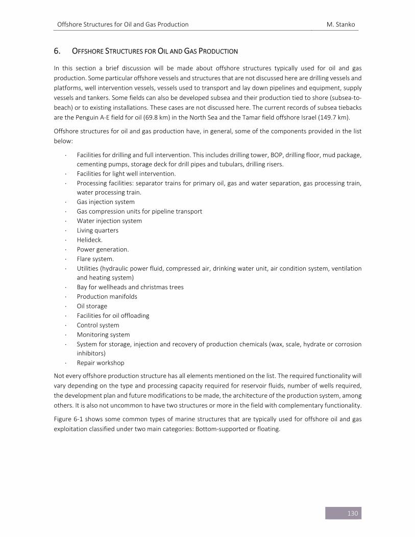
Offshore Structures for Oil and Gas Production M. Stanko
130
6. OFFSHORE STRUCTURES FOR OIL AND GAS PRODUCTION
In this section a brief discussion will be made about offshore structures typically used for oil and gas
production. Some particular offshore vessels and structures that are not discussed here are drilling vessels and
platforms, well intervention vessels, vessels used to transport and lay down pipelines and equipment, supply
vessels and tankers. Some fields can also be developed subsea and their production tied to shore (subsea‐to‐
beach) or to existing installations. These cases are not discussed here. The current records of subsea tiebacks
are the Penguin A‐E field for oil (69.8 km) in the North Sea and the Tamar field offshore Israel (149.7 km).
Offshore structures for oil and gas production have, in general, some of the components provided in the list
below:
Facilities for drilling and full intervention. This includes drilling tower, BOP, drilling floor, mud package,
cementing pumps, storage deck for drill pipes and tubulars, drilling risers.
Facilities for light well intervention.
Processing facilities: separator trains for primary oil, gas and water separation, gas processing train,
water processing train.
Gas injection system
Gas compression units for pipeline transport
Water injection system
Living quarters
Helideck.
Power generation.
Flare system.
Utilities (hydraulic power fluid, compressed air, drinking water unit, air condition system, ventilation
and heating system)
Bay for wellheads and christmas trees
Production manifolds
Oil storage
Facilities for oil offloading
Control system
Monitoring system
System for storage, injection and recovery of production chemicals (wax, scale, hydrate or corrosion
inhibitors)
Repair workshop
Not every offshore production structure has all elements mentioned on the list. The required functionality will
vary depending on the type and processing capacity required for reservoir fluids, number of wells required,
the development plan and future modifications to be made, the architecture of the production system, among
others. It is also not uncommon to have two structures or more in the field with complementary functionality.
Figure 6‐1 shows some common types of marine structures that are typically used for offshore oil and gas
exploitation classified under two main categories: Bottom‐supported or floating.
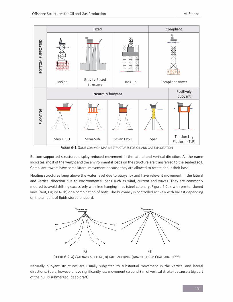
Offshore Structures for Oil and Gas Production M. Stanko
131
BOTTOM‐SUPP
ORTED
Fixed Compliant
Jacket Gravity‐Based Structure
Jack‐up Compliant tower
FLOATING
Neutrally buoyant Positively buoyant
Ship FPSO Semi‐Sub Sevan FPSO Spar Tension Leg
Platform (TLP)
FIGURE 6‐1. SOME COMMON MARINE STRUCTURES FOR OIL AND GAS EXPLOITATION
Bottom‐supported structures display reduced movement in the lateral and vertical direction. As the name
indicates, most of the weight and the environmental loads on the structure are transferred to the seabed soil.
Compliant towers have some lateral movement because they are allowed to rotate about their base.
Floating structures keep above the water level due to buoyancy and have relevant movement in the lateral
and vertical direction due to environmental loads such as wind, current and waves. They are commonly
moored to avoid drifting excessively with free hanging lines (steel catenary, Figure 6‐2a), with pre‐tensioned
lines (taut, Figure 6‐2b) or a combination of both. The buoyancy is controlled actively with ballast depending
on the amount of fluids stored onboard.
(A) (B)
FIGURE 6‐2. A) CATENARY MOORING, B) TAUT MOORING. (ADAPTED FROM CHAKRABARTI[6‐5])
Naturally buoyant structures are usually subjected to substantial movement in the vertical and lateral
directions. Spars, however, have significantly less movement (around 3 m of vertical stroke) because a big part
of the hull is submerged (deep draft).
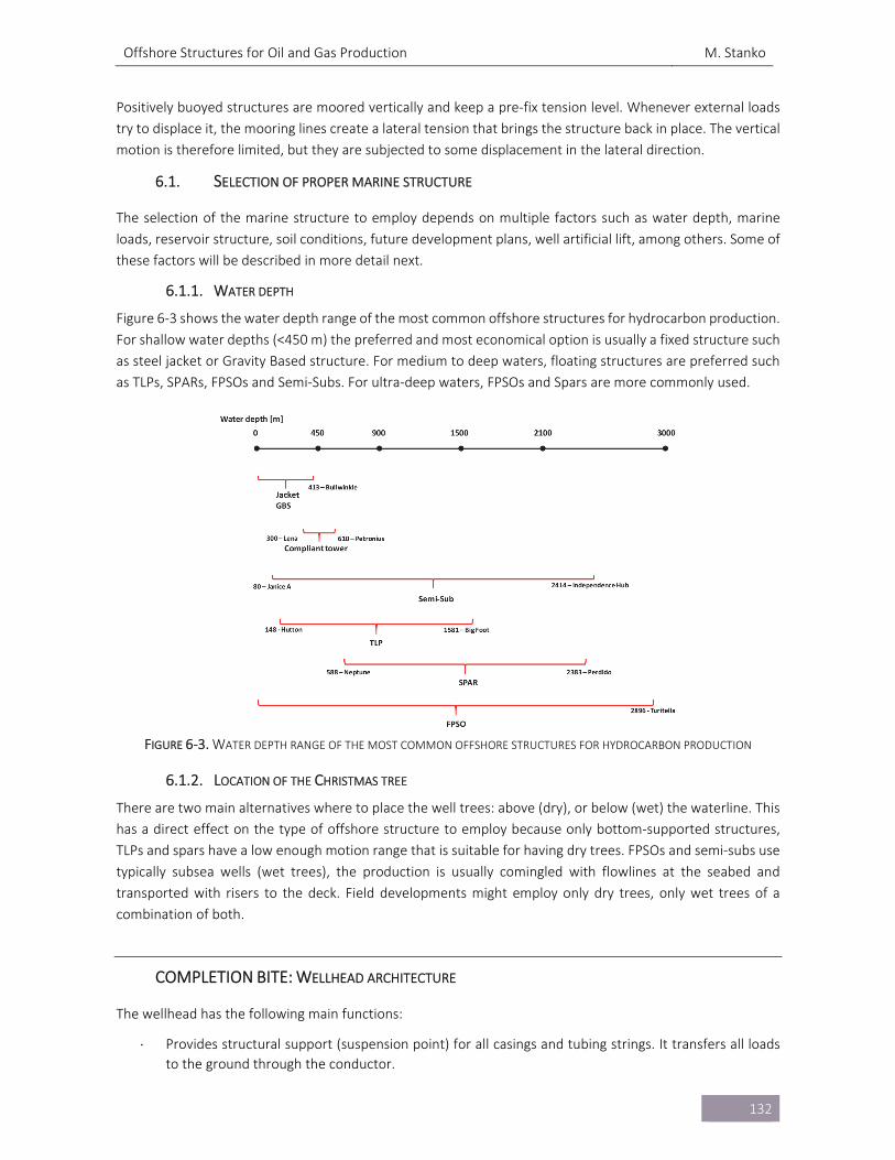
Offshore Structures for Oil and Gas Production M. Stanko
132
Positively buoyed structures are moored vertically and keep a pre‐fix tension level. Whenever external loads
try to displace it, the mooring lines create a lateral tension that brings the structure back in place. The vertical
motion is therefore limited, but they are subjected to some displacement in the lateral direction.
6.1. SELECTION OF PROPER MARINE STRUCTURE
The selection of the marine structure to employ depends on multiple factors such as water depth, marine
loads, reservoir structure, soil conditions, future development plans, well artificial lift, among others. Some of
these factors will be described in more detail next.
6.1.1. WATER DEPTH
Figure 6‐3 shows the water depth range of the most common offshore structures for hydrocarbon production.
For shallow water depths (<450 m) the preferred and most economical option is usually a fixed structure such
as steel jacket or Gravity Based structure. For medium to deep waters, floating structures are preferred such
as TLPs, SPARs, FPSOs and Semi‐Subs. For ultra‐deep waters, FPSOs and Spars are more commonly used.
FIGURE 6‐3. WATER DEPTH RANGE OF THE MOST COMMON OFFSHORE STRUCTURES FOR HYDROCARBON PRODUCTION
6.1.2. LOCATION OF THE CHRISTMAS TREE
There are two main alternatives where to place the well trees: above (dry), or below (wet) the waterline. This
has a direct effect on the type of offshore structure to employ because only bottom‐supported structures,
TLPs and spars have a low enough motion range that is suitable for having dry trees. FPSOs and semi‐subs use
typically subsea wells (wet trees), the production is usually comingled with flowlines at the seabed and
transported with risers to the deck. Field developments might employ only dry trees, only wet trees of a
combination of both.
COMPLETION BITE: WELLHEAD ARCHITECTURE
The wellhead has the following main functions:
Provides structural support (suspension point) for all casings and tubing strings. It transfers all loads
to the ground through the conductor.
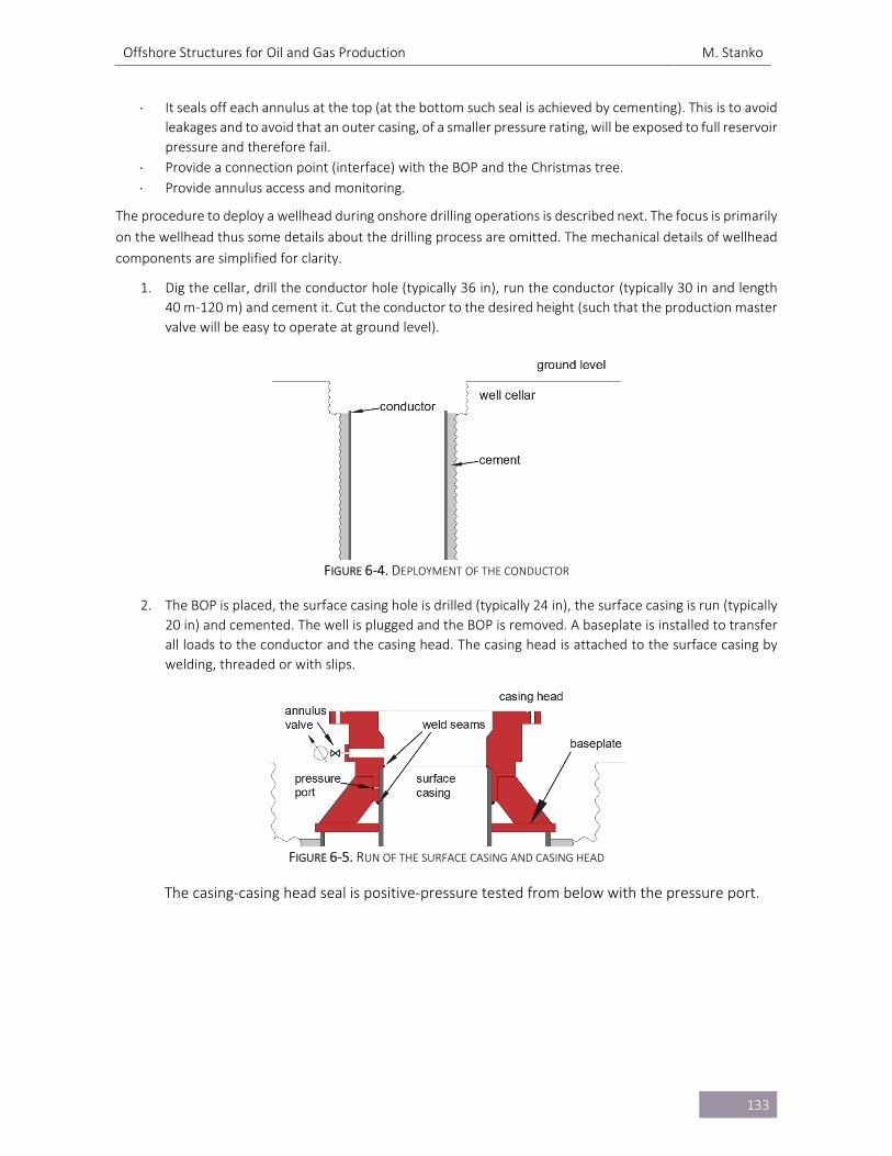
Offshore Structures for Oil and Gas Production M. Stanko
133
It seals off each annulus at the top (at the bottom such seal is achieved by cementing). This is to avoid
leakages and to avoid that an outer casing, of a smaller pressure rating, will be exposed to full reservoir
pressure and therefore fail.
Provide a connection point (interface) with the BOP and the Christmas tree.
Provide annulus access and monitoring.
The procedure to deploy a wellhead during onshore drilling operations is described next. The focus is primarily
on the wellhead thus some details about the drilling process are omitted. The mechanical details of wellhead
components are simplified for clarity.
1. Dig the cellar, drill the conductor hole (typically 36 in), run the conductor (typically 30 in and length
40 m‐120 m) and cement it. Cut the conductor to the desired height (such that the production master
valve will be easy to operate at ground level).
FIGURE 6‐4. DEPLOYMENT OF THE CONDUCTOR
2. The BOP is placed, the surface casing hole is drilled (typically 24 in), the surface casing is run (typically
20 in) and cemented. The well is plugged and the BOP is removed. A baseplate is installed to transfer
all loads to the conductor and the casing head. The casing head is attached to the surface casing by
welding, threaded or with slips.
FIGURE 6‐5. RUN OF THE SURFACE CASING AND CASING HEAD
The casing‐casing head seal is positive‐pressure tested from below with the pressure port.
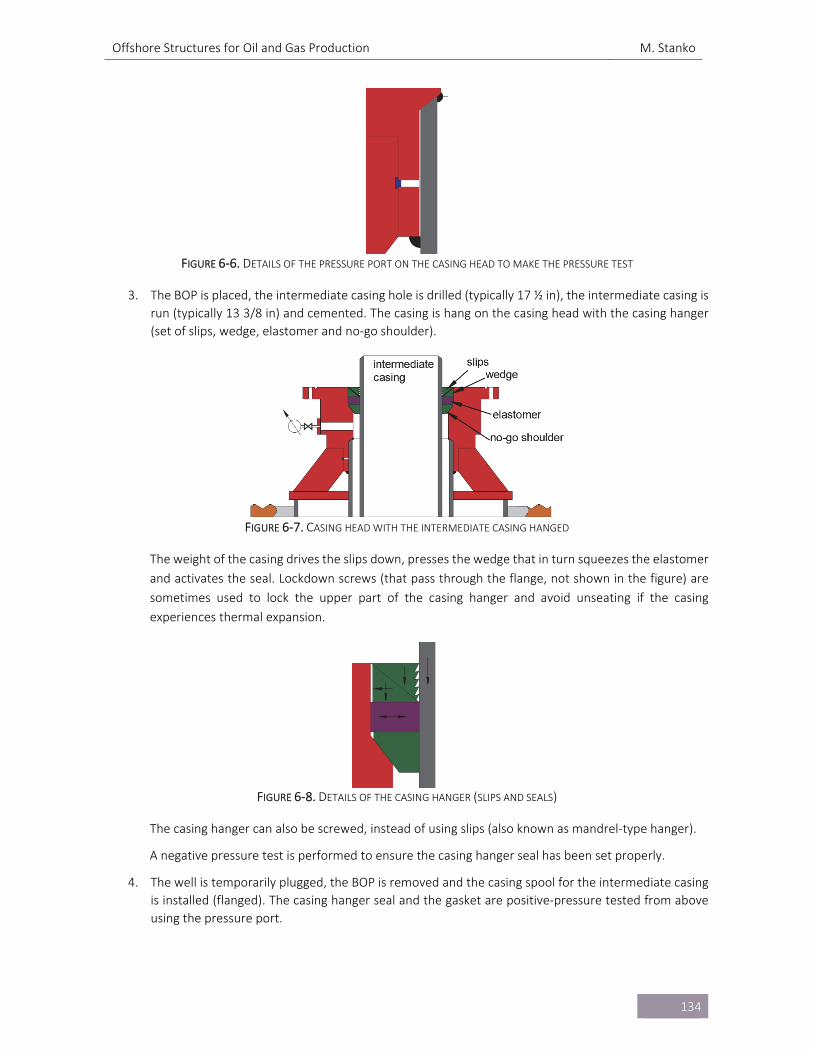
Offshore Structures for Oil and Gas Production M. Stanko
134
FIGURE 6‐6. DETAILS OF THE PRESSURE PORT ON THE CASING HEAD TO MAKE THE PRESSURE TEST
3. The BOP is placed, the intermediate casing hole is drilled (typically 17 ½ in), the intermediate casing is
run (typically 13 3/8 in) and cemented. The casing is hang on the casing head with the casing hanger
(set of slips, wedge, elastomer and no‐go shoulder).
FIGURE 6‐7. CASING HEAD WITH THE INTERMEDIATE CASING HANGED
The weight of the casing drives the slips down, presses the wedge that in turn squeezes the elastomer
and activates the seal. Lockdown screws (that pass through the flange, not shown in the figure) are
sometimes used to lock the upper part of the casing hanger and avoid unseating if the casing
experiences thermal expansion.
FIGURE 6‐8. DETAILS OF THE CASING HANGER (SLIPS AND SEALS)
The casing hanger can also be screwed, instead of using slips (also known as mandrel‐type hanger).
A negative pressure test is performed to ensure the casing hanger seal has been set properly.
4. The well is temporarily plugged, the BOP is removed and the casing spool for the intermediate casing
is installed (flanged). The casing hanger seal and the gasket are positive‐pressure tested from above
using the pressure port.
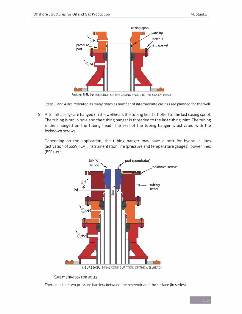
Offshore Structures for Oil and Gas Production M. Stanko
135
FIGURE 6‐9. INSTALLATION OF THE CASING SPOOL TO THE CASING HEAD
Steps 3 and 4 are repeated as many times as number of intermediate casings are planned for the well.
5. After all casings are hanged on the wellhead, the tubing head is bolted to the last casing spool. The tubing is ran in hole and the tubing hanger is threaded to the last tubing joint. The tubing is then hanged on the tubing head. The seal of the tubing hanger is activated with the lockdown screws.
Depending on the application, the tubing hanger may have a port for hydraulic lines (activation of SSSV, ICV), instrumentation line (pressure and temperature gauges), power lines (ESP), etc.
FIGURE 6‐10. FINAL CONFIGURATION OF THE WELLHEAD
SAFETY STRATEGY FOR WELLS
There must be two pressure barriers between the reservoir and the surface (in series)
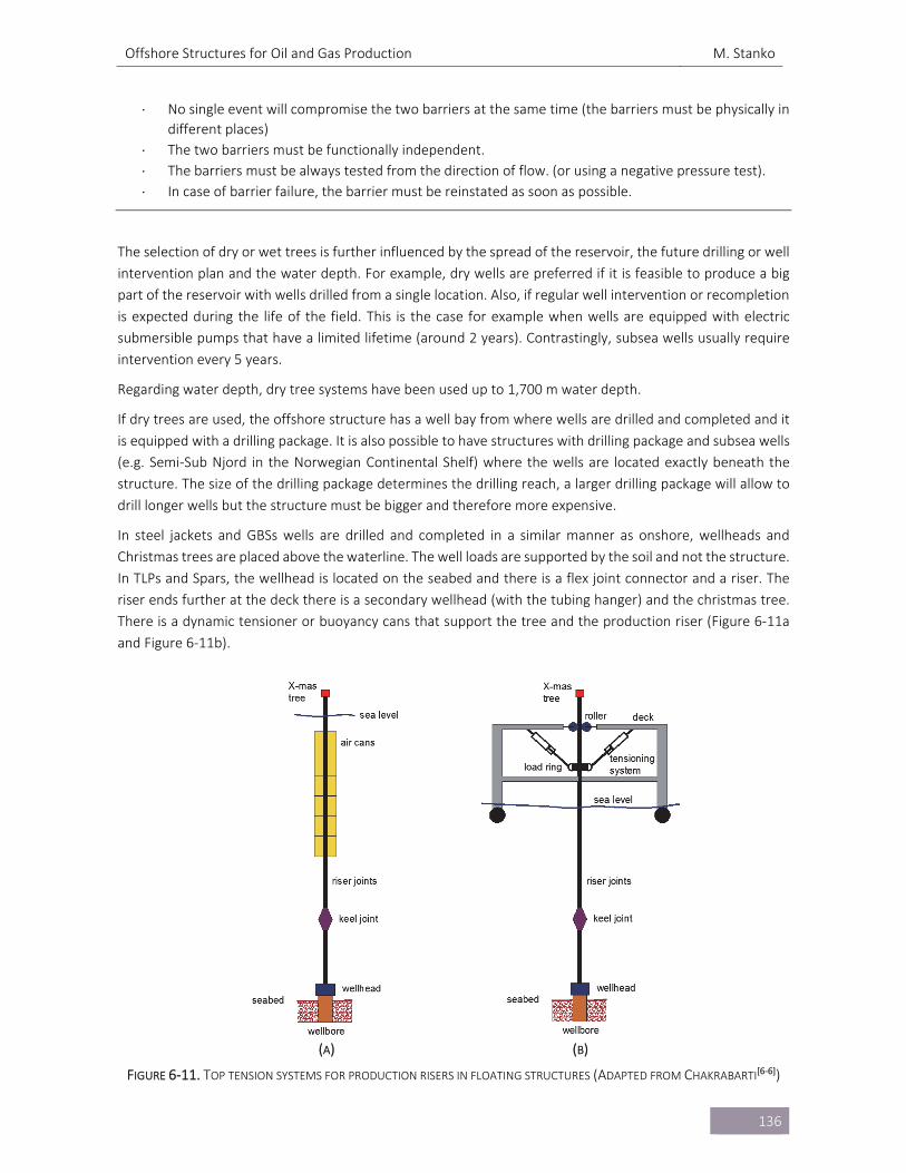
Offshore Structures for Oil and Gas Production M. Stanko
136
No single event will compromise the two barriers at the same time (the barriers must be physically in
different places)
The two barriers must be functionally independent.
The barriers must be always tested from the direction of flow. (or using a negative pressure test).
In case of barrier failure, the barrier must be reinstated as soon as possible.
The selection of dry or wet trees is further influenced by the spread of the reservoir, the future drilling or well
intervention plan and the water depth. For example, dry wells are preferred if it is feasible to produce a big
part of the reservoir with wells drilled from a single location. Also, if regular well intervention or recompletion
is expected during the life of the field. This is the case for example when wells are equipped with electric
submersible pumps that have a limited lifetime (around 2 years). Contrastingly, subsea wells usually require
intervention every 5 years.
Regarding water depth, dry tree systems have been used up to 1,700 m water depth.
If dry trees are used, the offshore structure has a well bay from where wells are drilled and completed and it
is equipped with a drilling package. It is also possible to have structures with drilling package and subsea wells
(e.g. Semi‐Sub Njord in the Norwegian Continental Shelf) where the wells are located exactly beneath the
structure. The size of the drilling package determines the drilling reach, a larger drilling package will allow to
drill longer wells but the structure must be bigger and therefore more expensive.
In steel jackets and GBSs wells are drilled and completed in a similar manner as onshore, wellheads and
Christmas trees are placed above the waterline. The well loads are supported by the soil and not the structure.
In TLPs and Spars, the wellhead is located on the seabed and there is a flex joint connector and a riser. The
riser ends further at the deck there is a secondary wellhead (with the tubing hanger) and the christmas tree.
There is a dynamic tensioner or buoyancy cans that support the tree and the production riser (Figure 6‐11a
and Figure 6‐11b).
(A) (B)
FIGURE 6‐11. TOP TENSION SYSTEMS FOR PRODUCTION RISERS IN FLOATING STRUCTURES (ADAPTED FROM CHAKRABARTI[6‐6])
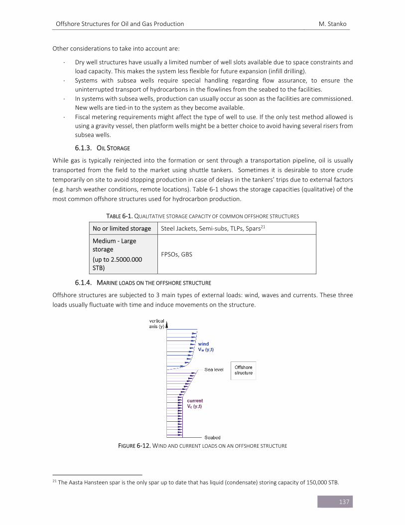
Offshore Structures for Oil and Gas Production M. Stanko
137
Other considerations to take into account are:
Dry well structures have usually a limited number of well slots available due to space constraints and
load capacity. This makes the system less flexible for future expansion (infill drilling).
Systems with subsea wells require special handling regarding flow assurance, to ensure the
uninterrupted transport of hydrocarbons in the flowlines from the seabed to the facilities.
In systems with subsea wells, production can usually occur as soon as the facilities are commissioned.
New wells are tied‐in to the system as they become available.
Fiscal metering requirements might affect the type of well to use. If the only test method allowed is
using a gravity vessel, then platform wells might be a better choice to avoid having several risers from
subsea wells.
6.1.3. OIL STORAGE
While gas is typically reinjected into the formation or sent through a transportation pipeline, oil is usually
transported from the field to the market using shuttle tankers. Sometimes it is desirable to store crude
temporarily on site to avoid stopping production in case of delays in the tankers’ trips due to external factors
(e.g. harsh weather conditions, remote locations). Table 6‐1 shows the storage capacities (qualitative) of the
most common offshore structures used for hydrocarbon production.
TABLE 6‐1. QUALITATIVE STORAGE CAPACITY OF COMMON OFFSHORE STRUCTURES
No or limited storage Steel Jackets, Semi‐subs, TLPs, Spars21
Medium ‐ Large storage
(up to 2.5000.000 STB)
FPSOs, GBS
6.1.4. MARINE LOADS ON THE OFFSHORE STRUCTURE
Offshore structures are subjected to 3 main types of external loads: wind, waves and currents. These three
loads usually fluctuate with time and induce movements on the structure.
FIGURE 6‐12. WIND AND CURRENT LOADS ON AN OFFSHORE STRUCTURE
21 The Aasta Hansteen spar is the only spar up to date that has liquid (condensate) storing capacity of 150,000 STB.
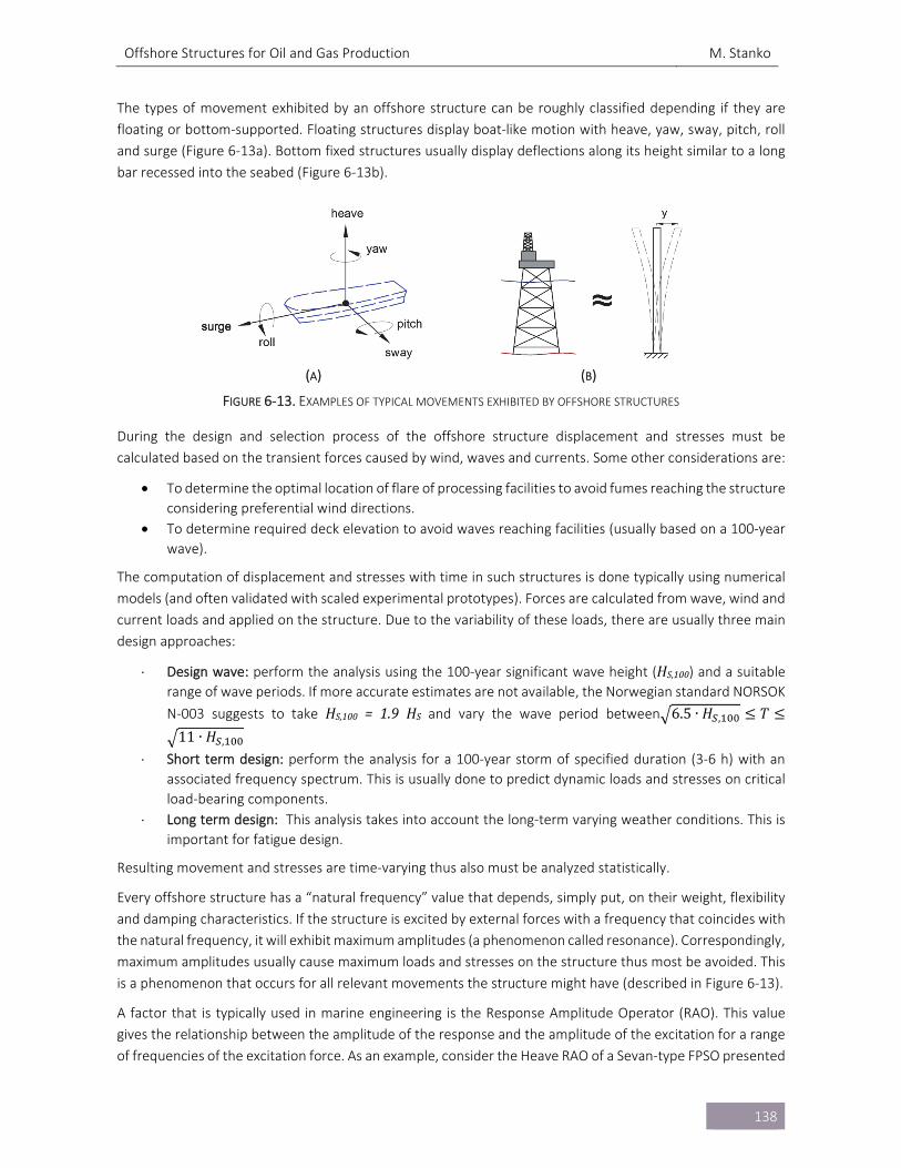
Offshore Structures for Oil and Gas Production M. Stanko
138
The types of movement exhibited by an offshore structure can be roughly classified depending if they are
floating or bottom‐supported. Floating structures display boat‐like motion with heave, yaw, sway, pitch, roll
and surge (Figure 6‐13a). Bottom fixed structures usually display deflections along its height similar to a long
bar recessed into the seabed (Figure 6‐13b).
(A) (B)
FIGURE 6‐13. EXAMPLES OF TYPICAL MOVEMENTS EXHIBITED BY OFFSHORE STRUCTURES
During the design and selection process of the offshore structure displacement and stresses must be
calculated based on the transient forces caused by wind, waves and currents. Some other considerations are:
To determine the optimal location of flare of processing facilities to avoid fumes reaching the structure
considering preferential wind directions.
To determine required deck elevation to avoid waves reaching facilities (usually based on a 100‐year
wave).
The computation of displacement and stresses with time in such structures is done typically using numerical
models (and often validated with scaled experimental prototypes). Forces are calculated from wave, wind and
current loads and applied on the structure. Due to the variability of these loads, there are usually three main
design approaches:
Design wave: perform the analysis using the 100‐year significant wave height (HS,100) and a suitable range of wave periods. If more accurate estimates are not available, the Norwegian standard NORSOK
N‐003 suggests to take HS,100 = 1.9 HS and vary the wave period between 6.5 ∙ 𝐻 , 𝑇
11 ∙ 𝐻 ,
Short term design: perform the analysis for a 100‐year storm of specified duration (3‐6 h) with an
associated frequency spectrum. This is usually done to predict dynamic loads and stresses on critical
load‐bearing components.
Long term design: This analysis takes into account the long‐term varying weather conditions. This is
important for fatigue design.
Resulting movement and stresses are time‐varying thus also must be analyzed statistically.
Every offshore structure has a “natural frequency” value that depends, simply put, on their weight, flexibility
and damping characteristics. If the structure is excited by external forces with a frequency that coincides with
the natural frequency, it will exhibit maximum amplitudes (a phenomenon called resonance). Correspondingly,
maximum amplitudes usually cause maximum loads and stresses on the structure thus most be avoided. This
is a phenomenon that occurs for all relevant movements the structure might have (described in Figure 6‐13).
A factor that is typically used in marine engineering is the Response Amplitude Operator (RAO). This value
gives the relationship between the amplitude of the response and the amplitude of the excitation for a range
of frequencies of the excitation force. As an example, consider the Heave RAO of a Sevan‐type FPSO presented
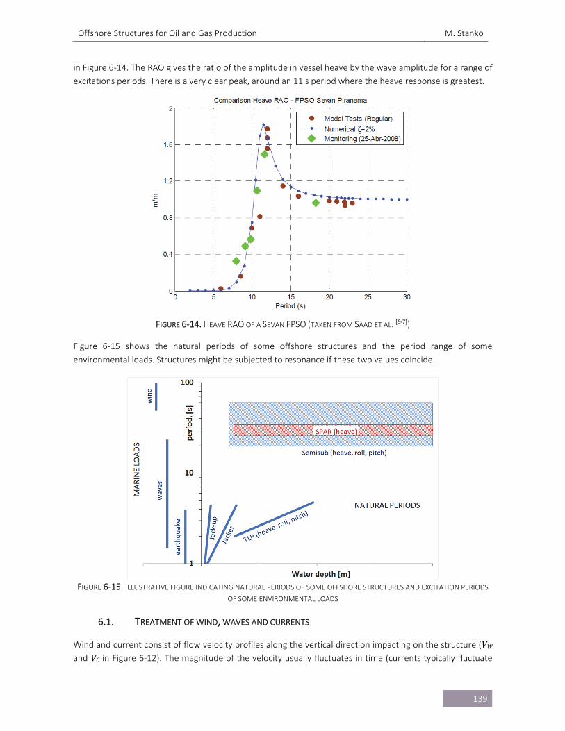
Offshore Structures for Oil and Gas Production M. Stanko
139
in Figure 6‐14. The RAO gives the ratio of the amplitude in vessel heave by the wave amplitude for a range of
excitations periods. There is a very clear peak, around an 11 s period where the heave response is greatest.
FIGURE 6‐14. HEAVE RAO OF A SEVAN FPSO (TAKEN FROM SAAD ET AL. [6‐7])
Figure 6‐15 shows the natural periods of some offshore structures and the period range of some
environmental loads. Structures might be subjected to resonance if these two values coincide.
FIGURE 6‐15. ILLUSTRATIVE FIGURE INDICATING NATURAL PERIODS OF SOME OFFSHORE STRUCTURES AND EXCITATION PERIODS
OF SOME ENVIRONMENTAL LOADS
6.1. TREATMENT OF WIND, WAVES AND CURRENTS
Wind and current consist of flow velocity profiles along the vertical direction impacting on the structure (VW and VC in Figure 6‐12). The magnitude of the velocity usually fluctuates in time (currents typically fluctuate
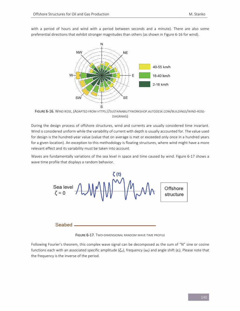
Offshore Structures for Oil and Gas Production M. Stanko
140
with a period of hours and wind with a period between seconds and a minute). There are also some
preferential directions that exhibit stronger magnitudes than others (as shown in Figure 6‐16 for wind).
FIGURE 6‐16. WIND ROSE, (ADAPTED FROM HTTPS://SUSTAINABILITYWORKSHOP.AUTODESK.COM/BUILDINGS/WIND‐ROSE‐
DIAGRAMS)
During the design process of offshore structures, wind and currents are usually considered time invariant.
Wind is considered uniform while the variability of current with depth is usually accounted for. The value used
for design is the hundred‐year value (value that on average is met or exceeded only once in a hundred years
for a given location). An exception to this methodology is floating structures, where wind might have a more
relevant effect and its variability must be taken into account.
Waves are fundamentally variations of the sea level in space and time caused by wind. Figure 6‐17 shows a
wave time profile that displays a random behavior.
FIGURE 6‐17. TWO‐DIMENSIONAL RANDOM WAVE TIME PROFILE
Following Fourier’s theorem, this complex wave signal can be decomposed as the sum of “N” sine or cosine
functions each with an associated specific amplitude (ζai), frequency (ωi) and angle shift (εi). Please note that the frequency is the inverse of the period.
Offshore Structures for Oil and Gas Production M. Stanko
141
FIGURE 6‐18. CONTRIBUTION OF INDIVIDUAL REGULAR WAVES
Information about the components that make up a particular signal is commonly displayed in a wave energy
spectrum (Figure 6‐19a). The spectrum is the result of applying a Fast Fourier Transform (FFT) to the wave
signal and displays wave energy spectrum (Sζ) vs frequency (ω). For particular case of a regular wave made of
a single frequency component, the spectrum will display just a delta in the corresponding frequency. Common
spectrum formulas are Pierson‐Moskowitz (P‐M) and JONSWAP.
(A) (B)
FIGURE 6‐19. WAVE ENERGY SPECTRUM A) CONTINUOUS AND B) DISCRETIZED
The spectrum is often presented in a discretized manner (Figure 6‐19b) where the frequency axis is split in
segments (of width Δωi) and each segment has an associated frequency value (ωi) and wave energy value (Sζi). The relationship between wave energy spectrum and wave elevation is shown in Eq. 6‐1.
𝜍 2 ∙ 𝑆 ∙ ∆𝜔 EQ. 6‐1
In short periods of time (typically 3 hours, called “sea state”) the spread in frequency is usually relatively low
(there is one dominant period called the “mean” period TZ) such that it is practically considered constant. The wave elevation is assumed to follow a Gaussian type probability density function (Figure 6‐20a) and the wave
height (H, distance between consecutive peak and valley) a Rayleigh distribution (Figure 6‐20b).
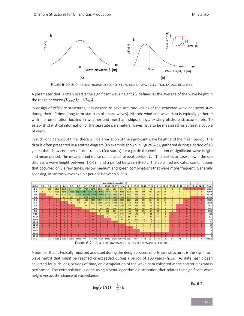
Offshore Structures for Oil and Gas Production M. Stanko
142
(A) (B)
FIGURE 6‐20. SHORT TERM PROBABILITY DENSITY FUNCTION OF WAVE ELEVATION (A) AND HEIGHT (B)
A parameter that is often used is the significant wave height Hs, defined as the average of the wave height in the range between (Hmax/3)–(Hmax).
In design of offshore structures, it is desired to have accurate values of the expected wave characteristics
during their lifetime (long term statistics of ocean waves). Historic wind and wave data is typically gathered
with instrumentation located in weather and merchant ships, buoys, existing offshore structures, etc. To
establish statistical information of the sea state parameters, waves have to be measured for at least a couple
of years.
In such long periods of time, there will be a variation of the significant wave height and the mean period. The
data is often presented in a scatter diagram (an example shown in Figure 6‐21, gathered during a period of 15
years) that shows number of occurrences (Sea states) for a particular combination of significant wave height
and mean period. The mean period is also called spectral peak period (Tp). The particular case shown, the sea displays a wave height between 1‐14 m and a period between 3‐20 s. The color red indicates combinations
that occurred only a few times, yellow medium and green combinations that were more frequent. Generally
speaking, in storms waves exhibit periods between 5‐25 s.
FIGURE 6‐21. SCATTER DIAGRAM OF LONG TERM WAVE STATISTICS
A number that is typically reported and used during the design process of offshore structures is the significant
wave height that might be reached or exceeded during a period of 100 years (HS,100). As data hasn’t been collected for such long periods of time, an extrapolation of the wave data collected in the scatter diagram is
performed. The extrapolation is done using a Semi‐logarithmic distribution that relates the significant wave
height versus the chance of exceedance.
log 𝑃 𝐻1𝑎
∙ 𝐻 EQ. 6‐2
Hs [m] 0‐3 3‐4 4‐5 5‐6 6‐7 7‐8 8‐9 9‐10 10‐11 11‐12 12‐13 13‐14 14‐15 15‐16 16‐17 17‐18 18‐19 19‐20 20‐21 21‐22 22‐23 23‐24 24‐25 Sum
0‐1 15 290 1367 2876 3716 3527 2734 1849 1138 656 362 192 101 52 26 13 7 3 2 1 0 0 0 18927
1‐2 1 81 1153 5308 12083 17323 18143 15262 10980 7053 4169 2316 1229 631 315 155 75 36 17 8 4 5 1 96348
2‐3 0 2 94 1050 4532 10304 15020 15953 13457 9752 5991 3403 1795 894 426 197 88 39 17 7 3 1 1 83026
3‐4 0 0 2 72 686 2782 6171 8847 9189 7493 5082 2991 1577 762 345 148 61 24 9 4 1 0 0 46246
4‐5 0 0 0 2 51 433 1645 3495 4807 4750 3638 2286 1229 584 251 100 37 13 5 1 0 0 0 23327
5‐6 0 0 0 0 2 39 294 1037 2069 2664 2440 1709 968 463 193 72 25 8 2 1 0 0 0 11986
6‐7 0 0 0 0 0 2 32 215 692 1264 1485 1228 767 382 159 57 18 5 1 0 0 0 0 6307
7‐8 0 0 0 0 0 0 2 27 157 447 730 762 555 302 130 46 14 4 1 0 0 0 0 3177
8‐9 0 0 0 0 0 0 0 2 23 112 276 392 355 223 104 38 11 3 1 0 0 0 0 1540
9‐10 0 0 0 0 0 0 0 0 2 19 77 160 192 148 79 31 9 2 0 0 0 0 0 719
10‐11 0 0 0 0 0 0 0 0 0 2 16 50 85 85 55 24 8 2 0 0 0 0 0 327
11‐12 0 0 0 0 0 0 0 0 0 0 2 12 29 40 33 18 7 2 0 0 0 0 0 143
12‐13 0 0 0 0 0 0 0 0 0 0 0 2 8 15 17 12 5 2 0 0 0 0 0 61
13‐14 0 0 0 0 0 0 0 0 0 0 0 0 2 5 7 6 4 1 0 0 0 0 0 25
14‐15 0 0 0 0 0 0 0 0 0 0 0 0 0 1 2 3 2 1 0 0 0 0 0 9
15‐16 0 0 0 0 0 0 0 0 0 0 0 0 0 0 1 1 1 1 0 0 0 0 0 4
16‐17 0 0 0 0 0 0 0 0 0 0 0 0 0 0 0 0 0 0 0 0 0 0 0 0
17‐18 0 0 0 0 0 0 0 0 0 0 0 0 0 0 0 0 0 0 0 0 0 0 0 0
Sum 16 373 2616 9308 21070 34410 44041 46687 42514 34212 24268 15503 8892 4587 2143 921 372 146 55 22 8 6 2 292172
Spectral Peak period (Tp) [s]
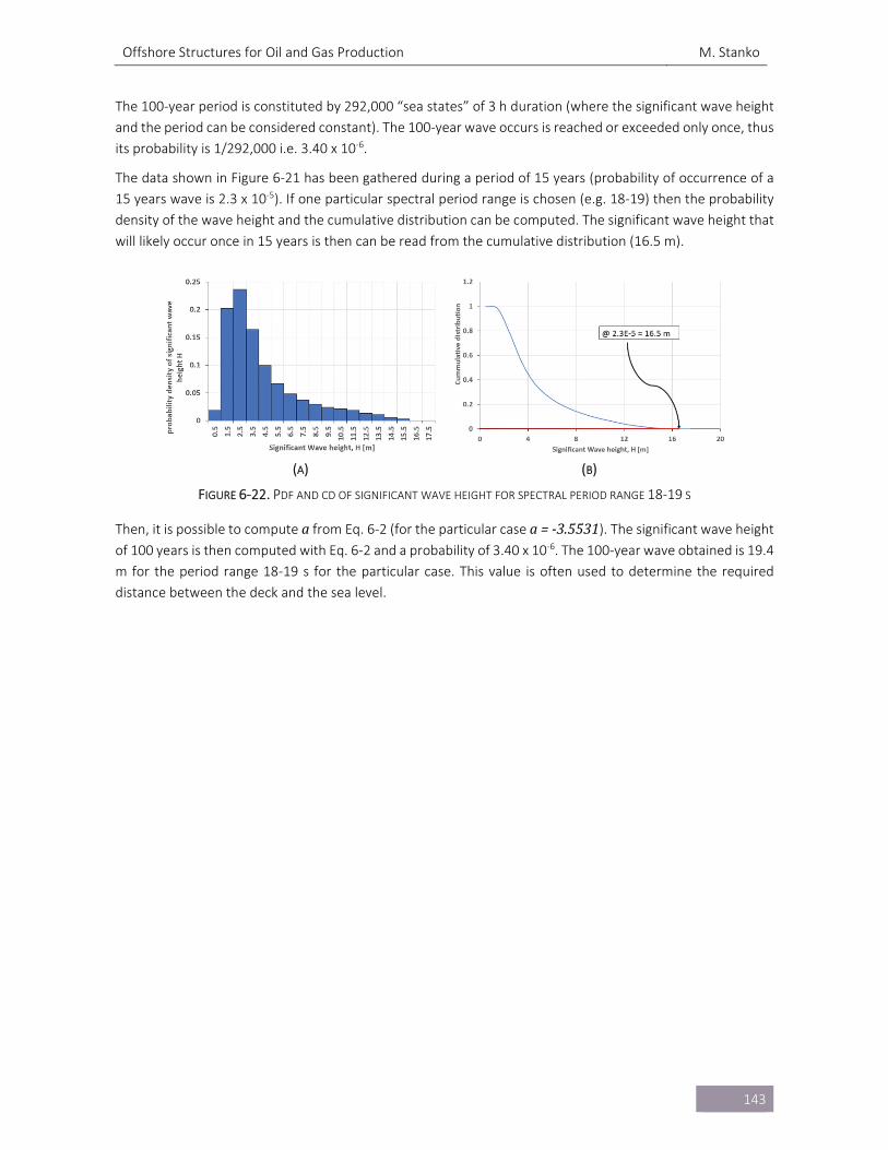
Offshore Structures for Oil and Gas Production M. Stanko
143
The 100‐year period is constituted by 292,000 “sea states” of 3 h duration (where the significant wave height
and the period can be considered constant). The 100‐year wave occurs is reached or exceeded only once, thus
its probability is 1/292,000 i.e. 3.40 x 10‐6.
The data shown in Figure 6‐21 has been gathered during a period of 15 years (probability of occurrence of a
15 years wave is 2.3 x 10‐5). If one particular spectral period range is chosen (e.g. 18‐19) then the probability
density of the wave height and the cumulative distribution can be computed. The significant wave height that
will likely occur once in 15 years is then can be read from the cumulative distribution (16.5 m).
(A) (B)
FIGURE 6‐22. PDF AND CD OF SIGNIFICANT WAVE HEIGHT FOR SPECTRAL PERIOD RANGE 18‐19 S
Then, it is possible to compute a from Eq. 6‐2 (for the particular case a=‐3.5531). The significant wave height of 100 years is then computed with Eq. 6‐2 and a probability of 3.40 x 10‐6. The 100‐year wave obtained is 19.4
m for the period range 18‐19 s for the particular case. This value is often used to determine the required
distance between the deck and the sea level.
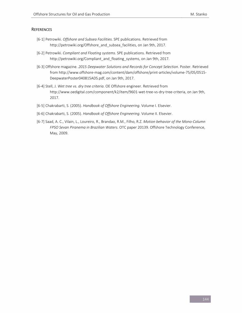
Offshore Structures for Oil and Gas Production M. Stanko
144
REFERENCES
[6‐1] Petrowiki. Offshore and Subsea Facilities. SPE publications. Retrieved from
http://petrowiki.org/Offshore_and_subsea_facilities, on Jan 9th, 2017.
[6‐2] Petrowiki. Compliant and Floating systems. SPE publications. Retrieved from
http://petrowiki.org/Compliant_and_floating_systems, on Jan 9th, 2017.
[6‐3] Offshore magazine. 2015 Deepwater Solutions and Records for Concept Selection. Poster. Retrieved
from http://www.offshore‐mag.com/content/dam/offshore/print‐articles/volume‐75/05/0515‐
DeepwaterPoster040815ADS.pdf, on Jan 9th, 2017.
[6‐4] Stell, J. Wet tree vs. dry tree criteria. OE Offshore engineer. Retrieved from
http://www.oedigital.com/component/k2/item/9601‐wet‐tree‐vs‐dry‐tree‐criteria, on Jan 9th,
2017.
[6‐5] Chakrabarti, S. (2005). Handbook of Offshore Engineering. Volume I. Elsevier.
[6‐6] Chakrabarti, S. (2005). Handbook of Offshore Engineering. Volume II. Elsevier.
[6‐7] Saad, A. C., Vilain, L., Loureiro, R., Brandao, R.M., Filho, R.Z. Motion behavior of the Mono‐Column
FPSO Sevan Piranema in Brazilian Waters. OTC paper 20139. Offshore Technology Conference,
May, 2009.
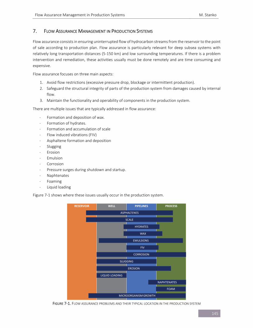
Flow Assurance Management in Production Systems M. Stanko
145
7. FLOW ASSURANCE MANAGEMENT IN PRODUCTION SYSTEMS
Flow assurance consists in ensuring uninterrupted flow of hydrocarbon streams from the reservoir to the point
of sale according to production plan. Flow assurance is particularly relevant for deep subsea systems with
relatively long transportation distances (5‐150 km) and low surrounding temperatures. If there is a problem
intervention and remediation, these activities usually must be done remotely and are time consuming and
expensive.
Flow assurance focuses on three main aspects:
1. Avoid flow restrictions (excessive pressure drop, blockage or intermittent production).
2. Safeguard the structural integrity of parts of the production system from damages caused by internal
flow.
3. Maintain the functionality and operability of components in the production system.
There are multiple issues that are typically addressed in flow assurance:
Formation and deposition of wax.
Formation of hydrates.
Formation and accumulation of scale
Flow induced vibrations (FIV)
Asphaltene formation and deposition
Slugging
Erosion
Emulsion
Corrosion
Pressure surges during shutdown and startup.
Naphtenates
Foaming
Liquid loading
Figure 7‐1 shows where these issues usually occur in the production system.
FIGURE 7‐1. FLOW ASSURANCE PROBLEMS AND THEIR TYPICAL LOCATION IN THE PRODUCTION SYSTEM
RESERVOIR WELL PIPELINES PROCESS
ASPHALTENES
SCALE
HYDRATES
WAX
EMULSIONS
FIV
CORROSION
SLUGGING
EROSION
LIQUID LOADING
NAPHTENATES
FOAM
MICROORGANISM GROWTH
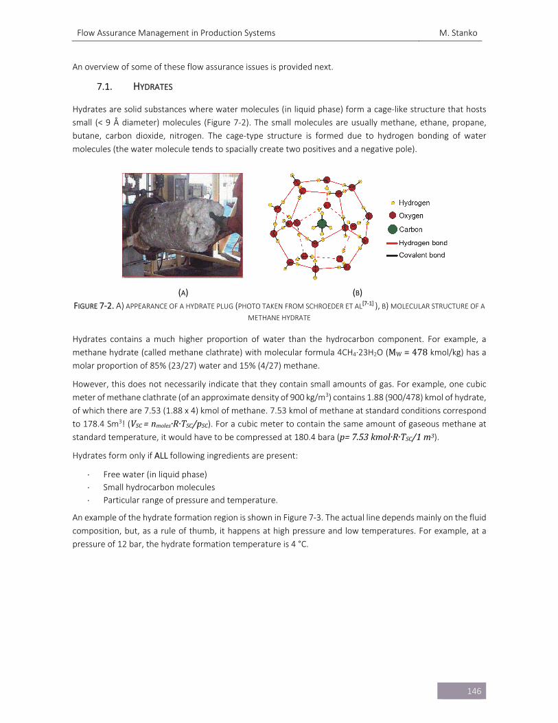
Flow Assurance Management in Production Systems M. Stanko
146
An overview of some of these flow assurance issues is provided next.
7.1. HYDRATES
Hydrates are solid substances where water molecules (in liquid phase) form a cage‐like structure that hosts
small (< 9 Å diameter) molecules (Figure 7‐2). The small molecules are usually methane, ethane, propane,
butane, carbon dioxide, nitrogen. The cage‐type structure is formed due to hydrogen bonding of water
molecules (the water molecule tends to spacially create two positives and a negative pole).
(A) (B)
FIGURE 7‐2. A) APPEARANCE OF A HYDRATE PLUG (PHOTO TAKEN FROM SCHROEDER ET AL[7‐1] ), B) MOLECULAR STRUCTURE OF A
METHANE HYDRATE
Hydrates contains a much higher proportion of water than the hydrocarbon component. For example, a
methane hydrate (called methane clathrate) with molecular formula 4CH4∙23H2O (MW = 478 kmol/kg) has a
molar proportion of 85% (23/27) water and 15% (4/27) methane.
However, this does not necessarily indicate that they contain small amounts of gas. For example, one cubic
meter of methane clathrate (of an approximate density of 900 kg/m3) contains 1.88 (900/478) kmol of hydrate,
of which there are 7.53 (1.88 x 4) kmol of methane. 7.53 kmol of methane at standard conditions correspond
to 178.4 Sm3! (VSC=nmoles·R·TSC/pSC). For a cubic meter to contain the same amount of gaseous methane at
standard temperature, it would have to be compressed at 180.4 bara (p=7.53kmol·R·TSC/1m3).
Hydrates form only if ALL following ingredients are present:
Free water (in liquid phase)
Small hydrocarbon molecules
Particular range of pressure and temperature.
An example of the hydrate formation region is shown in Figure 7‐3. The actual line depends mainly on the fluid
composition, but, as a rule of thumb, it happens at high pressure and low temperatures. For example, at a
pressure of 12 bar, the hydrate formation temperature is 4 °C.
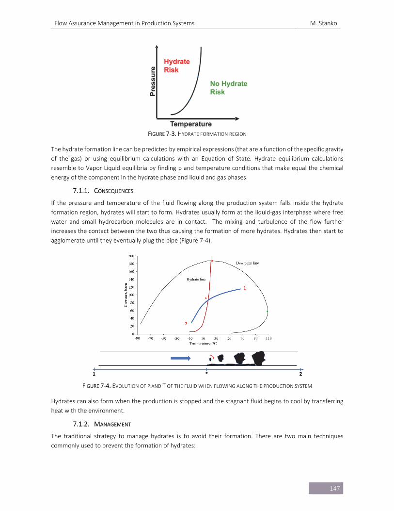
Flow Assurance Management in Production Systems M. Stanko
147
FIGURE 7‐3. HYDRATE FORMATION REGION
The hydrate formation line can be predicted by empirical expressions (that are a function of the specific gravity
of the gas) or using equilibrium calculations with an Equation of State. Hydrate equilibrium calculations
resemble to Vapor Liquid equilibria by finding p and temperature conditions that make equal the chemical
energy of the component in the hydrate phase and liquid and gas phases.
7.1.1. CONSEQUENCES
If the pressure and temperature of the fluid flowing along the production system falls inside the hydrate
formation region, hydrates will start to form. Hydrates usually form at the liquid‐gas interphase where free
water and small hydrocarbon molecules are in contact. The mixing and turbulence of the flow further
increases the contact between the two thus causing the formation of more hydrates. Hydrates then start to
agglomerate until they eventually plug the pipe (Figure 7‐4).
FIGURE 7‐4. EVOLUTION OF P AND T OF THE FLUID WHEN FLOWING ALONG THE PRODUCTION SYSTEM
Hydrates can also form when the production is stopped and the stagnant fluid begins to cool by transferring
heat with the environment.
7.1.2. MANAGEMENT
The traditional strategy to manage hydrates is to avoid their formation. There are two main techniques
commonly used to prevent the formation of hydrates:
1 2*
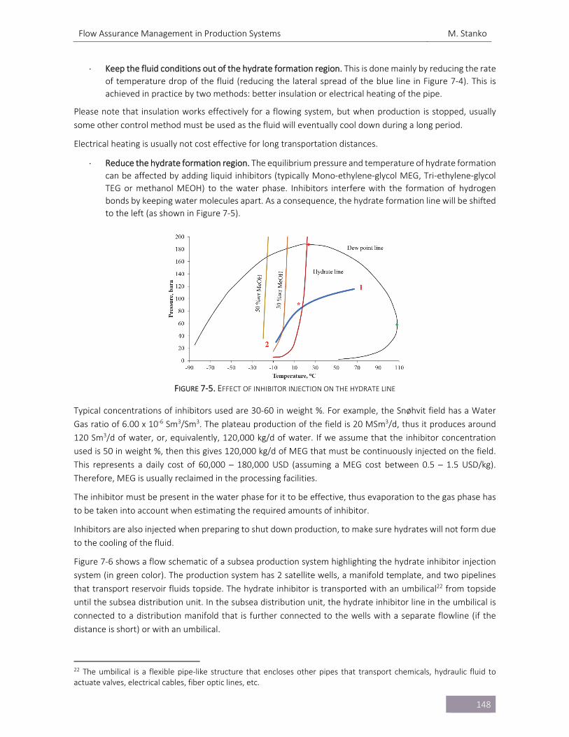
Flow Assurance Management in Production Systems M. Stanko
148
Keep the fluid conditions out of the hydrate formation region. This is done mainly by reducing the rate
of temperature drop of the fluid (reducing the lateral spread of the blue line in Figure 7‐4). This is
achieved in practice by two methods: better insulation or electrical heating of the pipe.
Please note that insulation works effectively for a flowing system, but when production is stopped, usually
some other control method must be used as the fluid will eventually cool down during a long period.
Electrical heating is usually not cost effective for long transportation distances.
Reduce the hydrate formation region. The equilibrium pressure and temperature of hydrate formation
can be affected by adding liquid inhibitors (typically Mono‐ethylene‐glycol MEG, Tri‐ethylene‐glycol
TEG or methanol MEOH) to the water phase. Inhibitors interfere with the formation of hydrogen
bonds by keeping water molecules apart. As a consequence, the hydrate formation line will be shifted
to the left (as shown in Figure 7‐5).
FIGURE 7‐5. EFFECT OF INHIBITOR INJECTION ON THE HYDRATE LINE
Typical concentrations of inhibitors used are 30‐60 in weight %. For example, the Snøhvit field has a Water
Gas ratio of 6.00 x 10‐6 Sm3/Sm3. The plateau production of the field is 20 MSm3/d, thus it produces around
120 Sm3/d of water, or, equivalently, 120,000 kg/d of water. If we assume that the inhibitor concentration
used is 50 in weight %, then this gives 120,000 kg/d of MEG that must be continuously injected on the field.
This represents a daily cost of 60,000 – 180,000 USD (assuming a MEG cost between 0.5 – 1.5 USD/kg).
Therefore, MEG is usually reclaimed in the processing facilities.
The inhibitor must be present in the water phase for it to be effective, thus evaporation to the gas phase has
to be taken into account when estimating the required amounts of inhibitor.
Inhibitors are also injected when preparing to shut down production, to make sure hydrates will not form due
to the cooling of the fluid.
Figure 7‐6 shows a flow schematic of a subsea production system highlighting the hydrate inhibitor injection
system (in green color). The production system has 2 satellite wells, a manifold template, and two pipelines
that transport reservoir fluids topside. The hydrate inhibitor is transported with an umbilical22 from topside
until the subsea distribution unit. In the subsea distribution unit, the hydrate inhibitor line in the umbilical is
connected to a distribution manifold that is further connected to the wells with a separate flowline (if the
distance is short) or with an umbilical.
22 The umbilical is a flexible pipe‐like structure that encloses other pipes that transport chemicals, hydraulic fluid to actuate valves, electrical cables, fiber optic lines, etc.
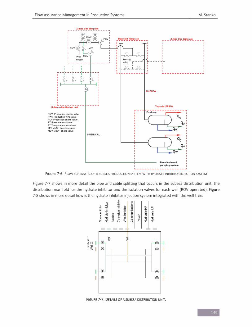
Flow Assurance Management in Production Systems M. Stanko
149
FIGURE 7‐6. FLOW SCHEMATIC OF A SUBSEA PRODUCTION SYSTEM WITH HYDRATE INHIBITOR INJECTION SYSTEM
Figure 7‐7 shows in more detail the pipe and cable splitting that occurs in the subsea distribution unit, the
distribution manifold for the hydrate inhibitor and the isolation valves for each well (ROV operated). Figure
7‐8 shows in more detail how is the hydrate inhibitor injection system integrated with the well tree.
FIGURE 7‐7. DETAILS OF A SUBSEA DISTRIBUTION UNIT.
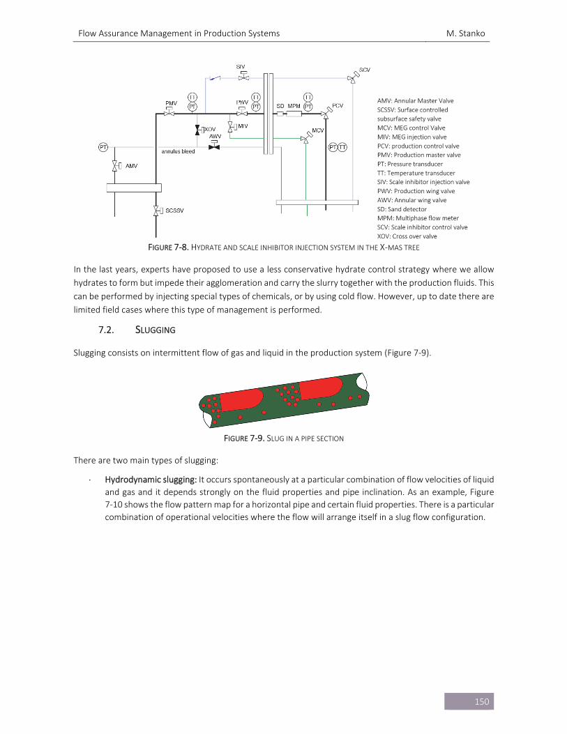
Flow Assurance Management in Production Systems M. Stanko
150
FIGURE 7‐8. HYDRATE AND SCALE INHIBITOR INJECTION SYSTEM IN THE X‐MAS TREE
In the last years, experts have proposed to use a less conservative hydrate control strategy where we allow
hydrates to form but impede their agglomeration and carry the slurry together with the production fluids. This
can be performed by injecting special types of chemicals, or by using cold flow. However, up to date there are
limited field cases where this type of management is performed.
7.2. SLUGGING
Slugging consists on intermittent flow of gas and liquid in the production system (Figure 7‐9).
FIGURE 7‐9. SLUG IN A PIPE SECTION
There are two main types of slugging:
Hydrodynamic slugging: It occurs spontaneously at a particular combination of flow velocities of liquid
and gas and it depends strongly on the fluid properties and pipe inclination. As an example, Figure
7‐10 shows the flow pattern map for a horizontal pipe and certain fluid properties. There is a particular
combination of operational velocities where the flow will arrange itself in a slug flow configuration.
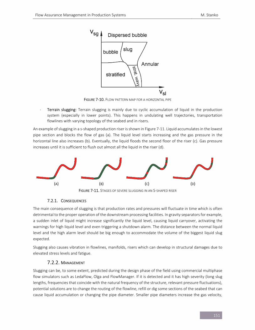
Flow Assurance Management in Production Systems M. Stanko
151
FIGURE 7‐10. FLOW PATTERN MAP FOR A HORIZONTAL PIPE
Terrain slugging: Terrain slugging is mainly due to cyclic accumulation of liquid in the production
system (especially in lower points). This happens in undulating well trajectories, transportation
flowlines with varying topology of the seabed and in risers.
An example of slugging in a s‐shaped production riser is shown in Figure 7‐11. Liquid accumulates in the lowest
pipe section and blocks the flow of gas (a). The liquid level starts increasing and the gas pressure in the
horizontal line also increases (b). Eventually, the liquid floods the second floor of the riser (c). Gas pressure
increases until it is sufficient to flush out almost all the liquid in the riser (d).
(A) (B) (C) (D)
FIGURE 7‐11. STAGES OF SEVERE SLUGGING IN AN S‐SHAPED RISER
7.2.1. CONSEQUENCES
The main consequence of slugging is that production rates and pressures will fluctuate in time which is often
detrimental to the proper operation of the downstream processing facilities. In gravity separators for example,
a sudden inlet of liquid might increase significantly the liquid level, causing liquid carryover, activating the
warnings for high liquid level and even triggering a shutdown alarm. The distance between the normal liquid
level and the high alarm level should be big enough to accommodate the volume of the biggest liquid slug
expected.
Slugging also causes vibration in flowlines, manifolds, risers which can develop in structural damages due to
elevated stress levels and fatigue.
7.2.2. MANAGEMENT
Slugging can be, to some extent, predicted during the design phase of the field using commercial multiphase
flow simulators such as LedaFlow, Olga and FlowManager. If it is detected and it has high severity (long slug
lengths, frequencies that coincide with the natural frequency of the structure, relevant pressure fluctuations),
potential solutions are to change the routing of the flowline, refill or dig some sections of the seabed that can
cause liquid accumulation or changing the pipe diameter. Smaller pipe diameters increase the gas velocity,
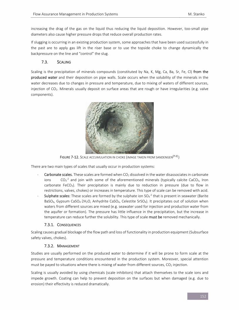
Flow Assurance Management in Production Systems M. Stanko
152
increasing the drag of the gas on the liquid thus reducing the liquid deposition. However, too‐small pipe
diameters also cause higher pressure drops that reduce overall production rates.
If slugging is occurring in an existing production system, some approaches that have been used successfully in
the past are to apply gas lift in the riser base or to use the topside choke to change dynamically the
backpressure on the line and “control” the slug.
7.3. SCALING
Scaling is the precipitation of minerals compounds (constituted by Na, K, Mg, Ca, Ba, Sr, Fe, Cl) from the
produced water and their deposition on pipe walls. Scale occurs when the solubility of the minerals in the
water decreases due to changes in pressure and temperature, due to mixing of waters of different sources,
injection of CO2. Minerals usually deposit on surface areas that are rough or have irregularities (e.g. valve
components).
FIGURE 7‐12. SCALE ACCUMULATION IN CHOKE (IMAGE TAKEN FROM SANDENGEN[7‐2] )
There are two main types of scales that usually occur in production systems:
Carbonate scales. These scales are formed when CO2 dissolved in the water disassociates in carbonate
ions CO3‐2 and join with some of the aforementioned minerals (typically calcite CaCO3, Iron
carbonate FeCO3). Their precipitation is mainly due to reduction in pressure (due to flow in
restrictions, valves, chokes) or increases in temperature. This type of scale can be removed with acid.
Sulphate scales: These scales are formed by the sulphate ion SO4‐2 that is present in seawater (Barite
BaSO4, Gypsum CaSO4∙2H2O, Anhydrite CaSO4, Celestite SrSO4). It precipitates out of solution when
waters from different sources are mixed (e.g. seawater used for injection and production water from
the aquifer or formation). The pressure has little influence in the precipitation, but the increase in
temperature can reduce further the solubility. This type of scale must be removed mechanically.
7.3.1. CONSEQUENCES
Scaling causes gradual blockage of the flow path and loss of functionality in production equipment (Subsurface
safety valves, chokes).
7.3.2. MANAGEMENT
Studies are usually performed on the produced water to determine if it will be prone to form scale at the
pressure and temperature conditions encountered in the production system. Moreover, special attention
must be payed to situations where there is mixing of water from different sources, CO2 injection.
Scaling is usually avoided by using chemicals (scale inhibitors) that attach themselves to the scale ions and
impede growth. Coating can help to prevent deposition on the surfaces but when damaged (e.g. due to
erosion) their effectivity is reduced dramatically.
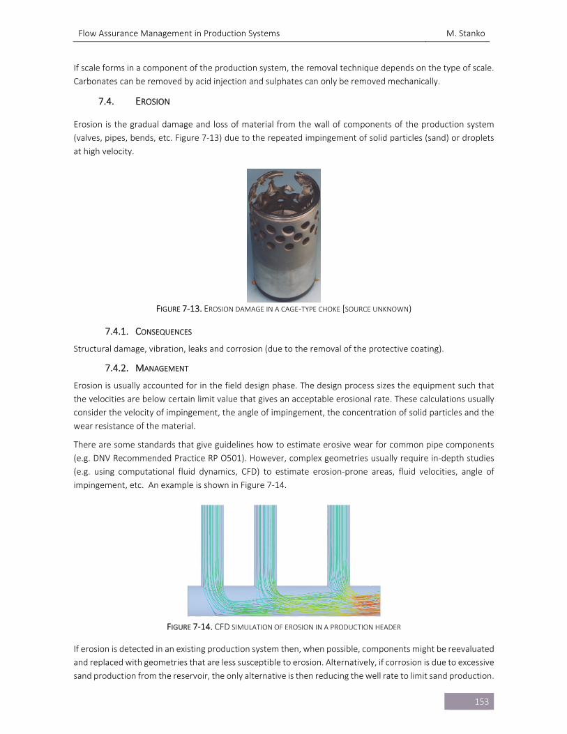
Flow Assurance Management in Production Systems M. Stanko
153
If scale forms in a component of the production system, the removal technique depends on the type of scale.
Carbonates can be removed by acid injection and sulphates can only be removed mechanically.
7.4. EROSION
Erosion is the gradual damage and loss of material from the wall of components of the production system
(valves, pipes, bends, etc. Figure 7‐13) due to the repeated impingement of solid particles (sand) or droplets
at high velocity.
FIGURE 7‐13. EROSION DAMAGE IN A CAGE‐TYPE CHOKE [SOURCE UNKNOWN)
7.4.1. CONSEQUENCES
Structural damage, vibration, leaks and corrosion (due to the removal of the protective coating).
7.4.2. MANAGEMENT
Erosion is usually accounted for in the field design phase. The design process sizes the equipment such that
the velocities are below certain limit value that gives an acceptable erosional rate. These calculations usually
consider the velocity of impingement, the angle of impingement, the concentration of solid particles and the
wear resistance of the material.
There are some standards that give guidelines how to estimate erosive wear for common pipe components
(e.g. DNV Recommended Practice RP O501). However, complex geometries usually require in‐depth studies
(e.g. using computational fluid dynamics, CFD) to estimate erosion‐prone areas, fluid velocities, angle of
impingement, etc. An example is shown in Figure 7‐14.
FIGURE 7‐14. CFD SIMULATION OF EROSION IN A PRODUCTION HEADER
If erosion is detected in an existing production system then, when possible, components might be reevaluated
and replaced with geometries that are less susceptible to erosion. Alternatively, if corrosion is due to excessive
sand production from the reservoir, the only alternative is then reducing the well rate to limit sand production.
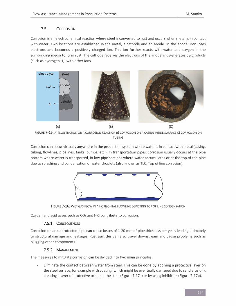
Flow Assurance Management in Production Systems M. Stanko
154
7.5. CORROSION
Corrosion is an electrochemical reaction where steel is converted to rust and occurs when metal is in contact
with water. Two locations are established in the metal, a cathode and an anode. In the anode, iron loses
electrons and becomes a positively charged ion. This ion further reacts with water and oxygen in the
surrounding media to form rust. The cathode receives the electrons of the anode and generates by‐products
(such as hydrogen H2) with other ions.
(A) (B) (C)
FIGURE 7‐15. A) ILLUSTRATION OR A CORROSION REACTION B) CORROSION ON A CASING INSIDE SURFACE C) CORROSION ON TUBING
Corrosion can occur virtually anywhere in the production system where water is in contact with metal (casing,
tubing, flowlines, pipelines, tanks, pumps, etc.). In transportation pipes, corrosion usually occurs at the pipe
bottom where water is transported, in low pipe sections where water accumulates or at the top of the pipe
due to splashing and condensation of water droplets (also known as TLC, Top of line corrosion).
FIGURE 7‐16. WET GAS FLOW IN A HORIZONTAL FLOWLINE DEPICTING TOP OF LINE CONDENSATION
Oxygen and acid gases such as CO2 and H2S contribute to corrosion.
7.5.1. CONSEQUENCES
Corrosion on an unprotected pipe can cause losses of 1‐20 mm of pipe thickness per year, leading ultimately
to structural damage and leakages. Rust particles can also travel downstream and cause problems such as
plugging other components.
7.5.2. MANAGEMENT
The measures to mitigate corrosion can be divided into two main principles:
Eliminate the contact between water from steel. This can be done by applying a protective layer on
the steel surface, for example with coating (which might be eventually damaged due to sand erosion),
creating a layer of protective oxide on the steel (Figure 7‐17a) or by using inhibitors (Figure 7‐17b).
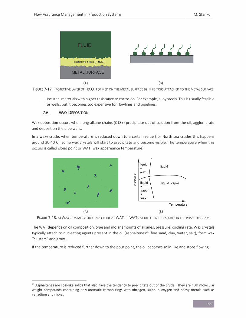
Flow Assurance Management in Production Systems M. Stanko
155
(A) (B)
FIGURE 7‐17. PROTECTIVE LAYER OF FECO3 FORMED ON THE METAL SURFACE B) INHIBITORS ATTACHED TO THE METAL SURFACE
Use steel materials with higher resistance to corrosion. For example, alloy steels. This is usually feasible
for wells, but it becomes too expensive for flowlines and pipelines.
7.6. WAX DEPOSITION
Wax deposition occurs when long alkane chains (C18+) precipitate out of solution from the oil, agglomerate
and deposit on the pipe walls.
In a waxy crude, when temperature is reduced down to a certain value (for North sea crudes this happens
around 30‐40 C), some wax crystals will start to precipitate and become visible. The temperature when this
occurs is called cloud point or WAT (wax appereance temperature).
(A) (B)
FIGURE 7‐18. A) WAX CRYSTALS VISIBLE IN A CRUDE AT WAT, B) WATS AT DIFFERENT PRESSURES IN THE PHASE DIAGRAM
The WAT depends on oil composition, type and molar amounts of alkanes, pressure, cooling rate. Wax crystals
typically attach to nucleating agents present in the oil (asphaltenes23, fine sand, clay, water, salt), form wax
“clusters” and grow.
If the temperature is reduced further down to the pour point, the oil becomes solid‐like and stops flowing.
23 Asphaltenes are coal‐like solids that also have the tendency to precipitate out of the crude. They are high molecular weight compounds containing poly‐aromatic carbon rings with nitrogen, sulphur, oxygen and heavy metals such as vanadium and nickel.
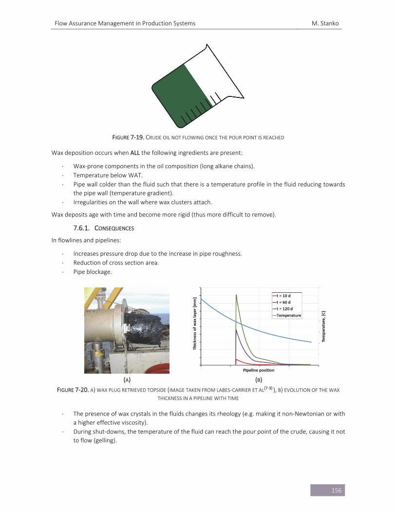
Flow Assurance Management in Production Systems M. Stanko
156
FIGURE 7‐19. CRUDE OIL NOT FLOWING ONCE THE POUR POINT IS REACHED
Wax deposition occurs when ALL the following ingredients are present:
Wax‐prone components in the oil composition (long alkane chains).
Temperature below WAT.
Pipe wall colder than the fluid such that there is a temperature profile in the fluid reducing towards
the pipe wall (temperature gradient).
Irregularities on the wall where wax clusters attach.
Wax deposits age with time and become more rigid (thus more difficult to remove).
7.6.1. CONSEQUENCES
In flowlines and pipelines:
Increases pressure drop due to the increase in pipe roughness.
Reduction of cross section area.
Pipe blockage.
(A) (B)
FIGURE 7‐20. A) WAX PLUG RETRIEVED TOPSIDE (IMAGE TAKEN FROM LABES‐CARRIER ET AL[7‐3] ), B) EVOLUTION OF THE WAX
THICKNESS IN A PIPELINE WITH TIME
The presence of wax crystals in the fluids changes its rheology (e.g. making it non‐Newtonian or with
a higher effective viscosity).
During shut‐downs, the temperature of the fluid can reach the pour point of the crude, causing it not
to flow (gelling).
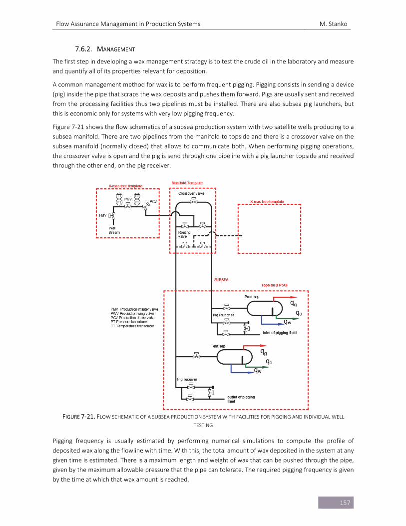
Flow Assurance Management in Production Systems M. Stanko
157
7.6.2. MANAGEMENT
The first step in developing a wax management strategy is to test the crude oil in the laboratory and measure
and quantify all of its properties relevant for deposition.
A common management method for wax is to perform frequent pigging. Pigging consists in sending a device
(pig) inside the pipe that scraps the wax deposits and pushes them forward. Pigs are usually sent and received
from the processing facilities thus two pipelines must be installed. There are also subsea pig launchers, but
this is economic only for systems with very low pigging frequency.
Figure 7‐21 shows the flow schematics of a subsea production system with two satellite wells producing to a
subsea manifold. There are two pipelines from the manifold to topside and there is a crossover valve on the
subsea manifold (normally closed) that allows to communicate both. When performing pigging operations,
the crossover valve is open and the pig is send through one pipeline with a pig launcher topside and received
through the other end, on the pig receiver.
FIGURE 7‐21. FLOW SCHEMATIC OF A SUBSEA PRODUCTION SYSTEM WITH FACILITIES FOR PIGGING AND INDIVIDUAL WELL
TESTING
Pigging frequency is usually estimated by performing numerical simulations to compute the profile of
deposited wax along the flowline with time. With this, the total amount of wax deposited in the system at any
given time is estimated. There is a maximum length and weight of wax that can be pushed through the pipe,
given by the maximum allowable pressure that the pipe can tolerate. The required pigging frequency is given
by the time at which that wax amount is reached.
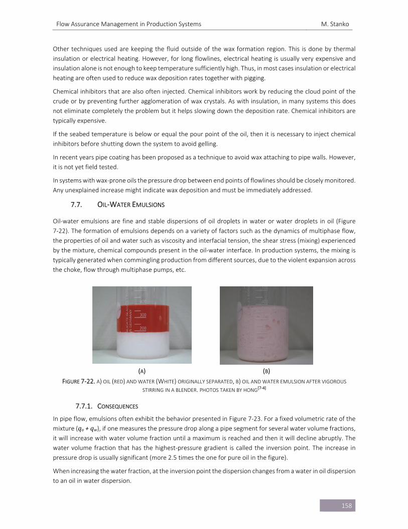
Flow Assurance Management in Production Systems M. Stanko
158
Other techniques used are keeping the fluid outside of the wax formation region. This is done by thermal
insulation or electrical heating. However, for long flowlines, electrical heating is usually very expensive and
insulation alone is not enough to keep temperature sufficiently high. Thus, in most cases insulation or electrical
heating are often used to reduce wax deposition rates together with pigging.
Chemical inhibitors that are also often injected. Chemical inhibitors work by reducing the cloud point of the
crude or by preventing further agglomeration of wax crystals. As with insulation, in many systems this does
not eliminate completely the problem but it helps slowing down the deposition rate. Chemical inhibitors are
typically expensive.
If the seabed temperature is below or equal the pour point of the oil, then it is necessary to inject chemical
inhibitors before shutting down the system to avoid gelling.
In recent years pipe coating has been proposed as a technique to avoid wax attaching to pipe walls. However,
it is not yet field tested.
In systems with wax‐prone oils the pressure drop between end points of flowlines should be closely monitored.
Any unexplained increase might indicate wax deposition and must be immediately addressed.
7.7. OIL‐WATER EMULSIONS
Oil‐water emulsions are fine and stable dispersions of oil droplets in water or water droplets in oil (Figure
7‐22). The formation of emulsions depends on a variety of factors such as the dynamics of multiphase flow,
the properties of oil and water such as viscosity and interfacial tension, the shear stress (mixing) experienced
by the mixture, chemical compounds present in the oil‐water interface. In production systems, the mixing is
typically generated when commingling production from different sources, due to the violent expansion across
the choke, flow through multiphase pumps, etc.
(A) (B)
FIGURE 7‐22. A) OIL (RED) AND WATER (WHITE) ORIGINALLY SEPARATED, B) OIL AND WATER EMULSION AFTER VIGOROUS
STIRRING IN A BLENDER. PHOTOS TAKEN BY HONG[7‐4]
7.7.1. CONSEQUENCES
In pipe flow, emulsions often exhibit the behavior presented in Figure 7‐23. For a fixed volumetric rate of the
mixture (qo+qw), if one measures the pressure drop along a pipe segment for several water volume fractions,
it will increase with water volume fraction until a maximum is reached and then it will decline abruptly. The
water volume fraction that has the highest‐pressure gradient is called the inversion point. The increase in
pressure drop is usually significant (more 2.5 times the one for pure oil in the figure).
When increasing the water fraction, at the inversion point the dispersion changes from a water in oil dispersion
to an oil in water dispersion.
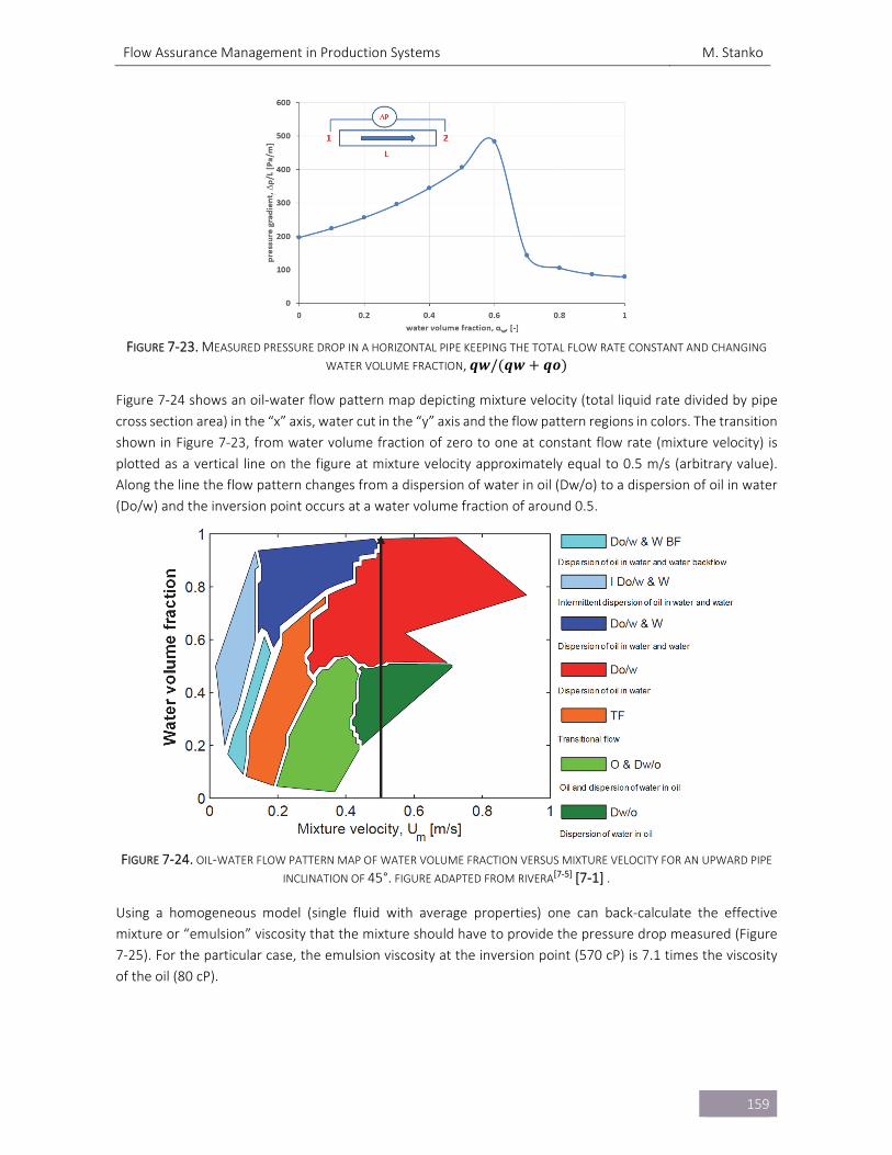
Flow Assurance Management in Production Systems M. Stanko
159
FIGURE 7‐23. MEASURED PRESSURE DROP IN A HORIZONTAL PIPE KEEPING THE TOTAL FLOW RATE CONSTANT AND CHANGING
WATER VOLUME FRACTION, 𝒒𝒘/ 𝒒𝒘 𝒒𝒐
Figure 7‐24 shows an oil‐water flow pattern map depicting mixture velocity (total liquid rate divided by pipe
cross section area) in the “x” axis, water cut in the “y” axis and the flow pattern regions in colors. The transition
shown in Figure 7‐23, from water volume fraction of zero to one at constant flow rate (mixture velocity) is
plotted as a vertical line on the figure at mixture velocity approximately equal to 0.5 m/s (arbitrary value).
Along the line the flow pattern changes from a dispersion of water in oil (Dw/o) to a dispersion of oil in water
(Do/w) and the inversion point occurs at a water volume fraction of around 0.5.
FIGURE 7‐24. OIL‐WATER FLOW PATTERN MAP OF WATER VOLUME FRACTION VERSUS MIXTURE VELOCITY FOR AN UPWARD PIPE
INCLINATION OF 45°. FIGURE ADAPTED FROM RIVERA[7‐5] [7‐1] .
Using a homogeneous model (single fluid with average properties) one can back‐calculate the effective
mixture or “emulsion” viscosity that the mixture should have to provide the pressure drop measured (Figure
7‐25). For the particular case, the emulsion viscosity at the inversion point (570 cP) is 7.1 times the viscosity
of the oil (80 cP).
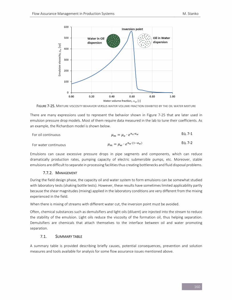
Flow Assurance Management in Production Systems M. Stanko
160
FIGURE 7‐25. MIXTURE VISCOSITY BEHAVIOR VERSUS WATER VOLUME FRACTION EXHIBITED BY THE OIL WATER MIXTURE
There are many expressions used to represent the behavior shown in Figure 7‐25 that are later used in
emulsion pressure drop models. Most of them require data measured in the lab to tune their coefficients. As
an example, the Richardson model is shown below.
For oil continuous 𝜇 𝜇 ∙ 𝑒 ∙ EQ. 7‐1
For water continuous 𝜇 𝜇 ∙ 𝑒 ∙ EQ. 7‐2
Emulsions can cause excessive pressure drops in pipe segments and components, which can reduce
dramatically production rates, pumping capacity of electric submersible pumps, etc. Moreover, stable
emulsions are difficult to separate in processing facilities thus creating bottlenecks and fluid disposal problems.
7.7.2. MANAGEMENT
During the field design phase, the capacity oil and water system to form emulsions can be somewhat studied
with laboratory tests (shaking bottle tests). However, these results have sometimes limited applicability partly
because the shear magnitudes (mixing) applied in the laboratory conditions are very different from the mixing
experienced in the field.
When there is mixing of streams with different water cut, the inversion point must be avoided.
Often, chemical substances such as demulsifiers and light oils (diluent) are injected into the stream to reduce
the stability of the emulsion. Light oils reduce the viscosity of the formation oil, thus helping separation.
Demulsifiers are chemicals that attach themselves to the interface between oil and water promoting
separation.
7.1. SUMMARY TABLE
A summary table is provided describing briefly causes, potential consequences, prevention and solution
measures and tools available for analysis for some flow assurance issues mentioned above.
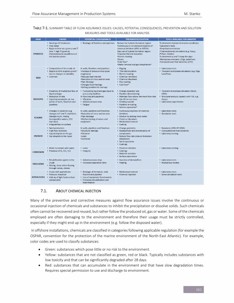
Flow Assurance Management in Production Systems M. Stanko
161
TABLE 7‐1. SUMMARY TABLE OF FLOW ASSURANCE ISSUES: CAUSES, POTENTIAL CONSEQUENCES, PREVENTION AND SOLUTION MEASURES AND TOOLS AVAILABLE FOR ANALYSIS
7.1. ABOUT CHEMICAL INJECTION
Many of the preventive and corrective measures against flow assurance issues involve the continuous or
occasional injection of chemicals and substances to inhibit the precipitation or dissolve solids. Such chemicals
often cannot be recovered and reused, but rather follow the produced oil, gas or water. Some of the chemicals
employed are often damaging to the environment and therefore their usage must be strictly controlled,
especially if they might end up in the environment (e.g. follow the disposed water).
In offshore installations, chemicals are classified in categories following applicable regulation (for example the
OSPAR, convention for the protection of the marine environment of the North‐East Atlantic). For example,
color codes are used to classify substances:
Green: substances which pose little or no risk to the environment.
Yellow: substances that are not classified as green, red or black. Typically includes substances with
low toxicity and that can be significantly degraded after 28 days.
Red: substances that can accumulate in the environment and that have slow degradation times.
Requires special permission to use and discharge to environment.
Flow Assurance Management in Production Systems M. Stanko
162
Black: substances that do not degrade, that are poisonous and that accumulate in the environment.
Permission to use and discharge is only given due to safety or critical technical reasons.
Some examples of red chemicals are emulsion inhibitors, wax inhibitors, anti‐foamers. However, these
substances are injected or accumulate main in the oil, and therefore will not end in the environment.
Some examples of yellow chemicals are scale inhibitors, biocides. These substances are soluble in water and
will follow injection water or disposed produced water.
MEG is often classified a green‐type substance. However, it is more economic to recover it from the production
water for reuse.
Flow Assurance Management in Production Systems M. Stanko
163
REFERENCES
[7‐1] Schroeder, Jr.; Chitwood, J. Krasin, T.; Lee, B.; Krohn, D.; Huizinga, M.; Paramonoff, A.;Schroeder, C.;
Gay, T.; Cercone, D.; Pappas, J. Development and Qualification of a Subsea 3000 Barrel Pressure
Compensated Chemical Storage and Injection System. OTC paper 26966. Offshore Technology
Conference, May, 2016.
[7‐2] Sandengen, K. Hydrates and Glycols MEG (Mono Ethylene Glycol) Injection and Processing.
Presentation at NTNU. September, 9. 2010.
[7‐3] Labes‐Carrier, C.; Rønningsen, H. P.; Kolnes, J.; Leporcher, E. Wax Deposition in North Sea Gas
Condensate and Oil Systems: Comparison Between Operational Experience and Model Prediction.
SPE paper 77573. SPE Annual Technical Conference and Exhibition. San Antonio, Texas. 2002.
[7‐4] Hong, C. Study on Ultrasonic Influence on Oil‐Water Emulsion Separation. Project Report. Norwegian
University of Science and Technology. 2017.
[7‐5] Rivera, R. Water Separation from Wellstream in Inclined Separation Tube with Distributed Tapping.
PhD Thesis. Norwegian University of Science and Technology. 2011.

Appendices M. Stanko
164
APPENDICES
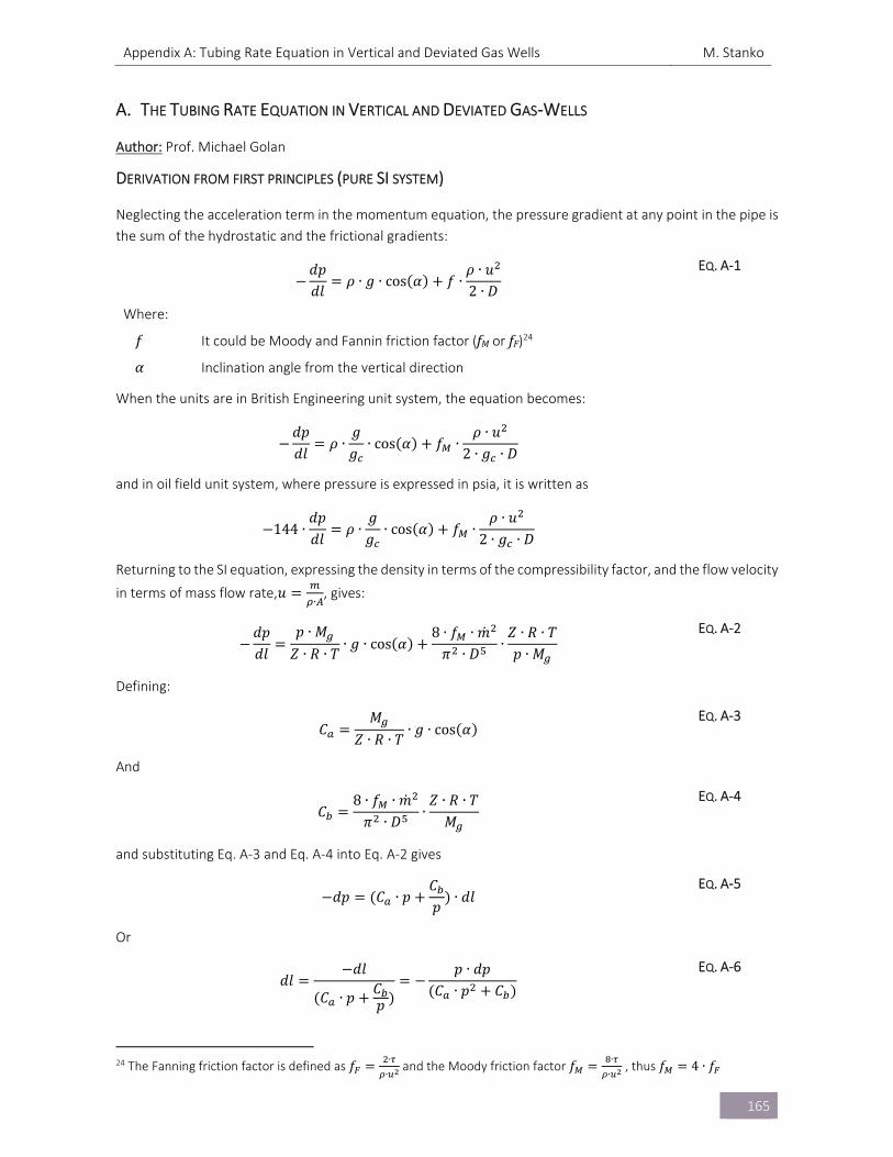
Appendix A: Tubing Rate Equation in Vertical and Deviated Gas Wells M. Stanko
165
A. THE TUBING RATE EQUATION IN VERTICAL AND DEVIATED GAS‐WELLS
Author: Prof. Michael Golan
DERIVATION FROM FIRST PRINCIPLES (PURE SI SYSTEM)
Neglecting the acceleration term in the momentum equation, the pressure gradient at any point in the pipe is
the sum of the hydrostatic and the frictional gradients:
𝑑𝑝𝑑𝑙
𝜌 ∙ 𝑔 ∙ cos 𝛼 𝑓 ∙𝜌 ∙ 𝑢2 ∙ 𝐷
EQ. A‐1
Where:
𝑓 It could be Moody and Fannin friction factor (fM or fF)24
𝛼 Inclination angle from the vertical direction
When the units are in British Engineering unit system, the equation becomes:
𝑑𝑝𝑑𝑙
𝜌 ∙𝑔𝑔
∙ cos 𝛼 𝑓 ∙𝜌 ∙ 𝑢
2 ∙ 𝑔 ∙ 𝐷
and in oil field unit system, where pressure is expressed in psia, it is written as
144 ∙𝑑𝑝𝑑𝑙
𝜌 ∙𝑔𝑔
∙ cos 𝛼 𝑓 ∙𝜌 ∙ 𝑢
2 ∙ 𝑔 ∙ 𝐷
Returning to the SI equation, expressing the density in terms of the compressibility factor, and the flow velocity
in terms of mass flow rate,𝑢∙, gives:
𝑑𝑝𝑑𝑙
𝑝 ∙ 𝑀
𝑍 ∙ 𝑅 ∙ 𝑇∙ 𝑔 ∙ cos 𝛼
8 ∙ 𝑓 ∙ 𝑚𝜋 ∙ 𝐷
∙𝑍 ∙ 𝑅 ∙ 𝑇𝑝 ∙ 𝑀
EQ. A‐2
Defining:
𝐶𝑀
𝑍 ∙ 𝑅 ∙ 𝑇∙ 𝑔 ∙ cos 𝛼
EQ. A‐3
And
𝐶8 ∙ 𝑓 ∙ 𝑚
𝜋 ∙ 𝐷∙
𝑍 ∙ 𝑅 ∙ 𝑇𝑀
EQ. A‐4
and substituting Eq. A‐3 and Eq. A‐4 into Eq. A‐2 gives
𝑑𝑝 𝐶 ∙ 𝑝𝐶𝑝
∙ 𝑑𝑙 EQ. A‐5
Or
𝑑𝑙𝑑𝑙
𝐶 ∙ 𝑝𝐶𝑝
𝑝 ∙ 𝑑𝑝𝐶 ∙ 𝑝 𝐶
EQ. A‐6
24 The Fanning friction factor is defined as 𝑓 ∙
∙ and the Moody friction factor 𝑓 ∙
∙ , thus 𝑓 4 ∙ 𝑓
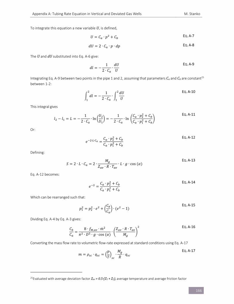
Appendix A: Tubing Rate Equation in Vertical and Deviated Gas Wells M. Stanko
166
To integrate this equation a new variable U, is defined,
𝑈 𝐶 ∙ 𝑝 𝐶 EQ. A‐7
𝑑𝑈 2 ∙ 𝐶 ∙ 𝑝 ∙ 𝑑𝑝 EQ. A‐8
The U and dU substituted into Eq. A‐6 give:
𝑑𝑙1
2 ∙ 𝐶∙
𝑑𝑈𝑈
EQ. A‐9
Integrating Eq. A‐9 between two points in the pipe 1 and 2, assuming that parameters Ca and Cb are constant25 between 1‐2:
𝑑𝑙1
2 ∙ 𝐶∙
𝑑𝑈𝑈
EQ. A‐10
This integral gives
𝑙 𝑙 𝐿1
2 ∙ 𝐶∙ ln
𝑈𝑈
12 ∙ 𝐶
∙ ln𝐶 ∙ 𝑝 𝐶𝐶 ∙ 𝑝 𝐶
EQ. A‐11
Or:
𝑒 ∙ ∙ 𝐶 ∙ 𝑝 𝐶𝐶 ∙ 𝑝 𝐶
EQ. A‐12
Defining:
𝑆 2 ∙ 𝐿 ∙ 𝐶 2 ∙𝑀
𝑍 ∙ 𝑅 ∙ 𝑇∙ 𝐿 ∙ 𝑔 ∙ cos 𝛼
EQ. A‐13
Eq. A‐12 becomes:
𝑒𝐶 ∙ 𝑝 𝐶𝐶 ∙ 𝑝 𝐶
EQ. A‐14
Which can be rearranged such that:
𝑝 𝑝 ∙ 𝑒𝐶𝐶
∙ 𝑒 1 EQ. A‐15
Dividing Eq. A‐4 by Eq. A‐3 gives:
𝐶𝐶
8 ∙ 𝑓 , ∙ 𝑚𝜋 ∙ 𝐷 ∙ 𝑔 ∙ cos 𝛼
∙𝑍 ∙ 𝑅 ∙ 𝑇
𝑀
EQ. A‐16
Converting the mass flow rate to volumetric flow‐rate expressed at standard conditions using Eq. A‐17
𝑚 𝜌 ∙ 𝑞𝑝𝑇
∙𝑀
𝑅∙ 𝑞
EQ. A‐17
25Evaluated with average deviation factor Zav=0.5·(Z1+Z2),average temperature and average friction factor
Appendix A: Tubing Rate Equation in Vertical and Deviated Gas Wells M. Stanko
167
results in:
𝐶𝐶
8 ∙ 𝑓 , ∙ 𝑍 ∙ 𝑇𝜋 ∙ 𝐷 ∙ 𝑔 ∙ cos 𝛼
∙𝑝𝑇
∙ 𝑞 EQ. A‐18
Substituting Eq. A‐18 into Eq. A‐15:
𝑝 𝑝 ∙ 𝑒8 ∙ 𝑓
𝜋 ∙ 𝐷 ∙ 𝑔 ∙ cos 𝛼∙
𝑝𝑇
∙ 𝑍 ∙ 𝑇 ∙ 𝑒 1 ∙ 𝑞 EQ. A‐19
Multiplying and dividing the second term on the right‐hand side with:
𝑆 2 ∙𝑀 ∙ 𝑔
𝑍 ∙ 𝑅 ∙ 𝑇∙ 𝐿 ∙ cos 𝛼 2 ∙
28.97 ∙ 𝛾 ∙ 𝑔
𝑍 ∙ 𝑅 ∙ 𝑇∙ 𝐿 ∙ cos 𝛼
EQ. A‐20
𝑝 𝑝 ∙ 𝑒28.97
𝑅∙
𝑝𝑇
𝑓 ∙ 𝐿 ∙ 𝛾 ∙ 𝑍 ∙ 𝑇 ∙𝑒 1𝑆 ∙ 𝐷
∙ 𝑞 EQ. A‐21
Solving for the flow rate:
𝑞𝜋4
∙𝑅
𝑀
.
∙𝑇𝑝
∙𝐷
𝑓 ∙ 𝐿 ∙ 𝛾 ∙ 𝑍 ∙ 𝑇
.
∙ 𝑝 𝑝 ∙ 𝑒 ∙𝑆
𝑒 1
.
EQ. A‐22
This equation relates the pressure at the top and the bottom of the tubing.
In fully turbulent flow (high Reynolds numbers), the friction factor depends essentially on the relative
roughness of the pipe, ε/D, and becomes independent of the Reynolds number. Measurements in gas wells
conducted by R.V.Smith, (1950), yielded a correlation for friction factor in tubings that became the norm for
most equations used by the gas industry and which appear in engineering handbooks. Smith’s measurements
are expressed in terms of friction factor as:
𝑓0.01748
𝐷 . ∙ |1 𝑚| ∙39.37 𝑖𝑛
1 𝑚
.
0.0077𝐷 .
EQ. A‐23
By defining the tubing constant 𝐶 :
𝐶𝜋4
∙𝑅
𝑀
.
∙𝑇𝑝
∙𝐷
𝑓 ∙ 𝐿 ∙ 𝛾 ∙ 𝑍 ∙ 𝑇
.
∙𝑆 ∙ 𝑒
𝑒 1
.
EQ. A‐24
This yields:
𝑞 𝐶 ∙𝑝
𝑒𝑝 ∙
.
EQ. A‐25
PRESSURE EQUATION IN PRACTICAL FIELD UNITS (METRIC)
Eq. A‐22 is rearranged to make it explicit with respect to bottom‐hole pressure:
𝑝 𝑝 ∙ 𝑒16𝜋
∙28.97
𝑅∙
𝑝𝑇
𝑓 ∙ 𝐿 ∙ 𝛾 ∙ 𝑍 ∙ 𝑇 ∙𝑒 1𝑆 ∙ 𝐷
∙ 𝑞 EQ. A‐26
Or:
Appendix A: Tubing Rate Equation in Vertical and Deviated Gas Wells M. Stanko
168
𝑝 𝑝 ∙ 𝑒 658 ∙ 𝑓 ∙ 𝐿 ∙ 𝛾 ∙ 𝑍 ∙ 𝑇 ∙𝑒 1𝑆 ∙ 𝐷
∙ 𝑞 EQ. A‐27
When converting to practical metric units, Sm3/d, bara, m, the equation becomes:
𝑝 𝑝 ∙ 𝑒 8.8 ∙ 10 ∙ 𝑓 ∙ 𝐿 ∙ 𝛾 ∙ 𝑍 ∙ 𝑇 ∙𝑒 1𝑆 ∙ 𝐷
∙ 𝑞 EQ. A‐28
Alternatively, if one chooses to introduce the definition of S (from Eq. A‐20) in Eq. A‐22, and rearrange it to
make it explicit with respect to bottom‐hole pressure:
𝑝 𝑝 ∙ 𝑒8 ∙ 𝑓
𝜋 ∙ 𝐷 ∙ 𝑔 ∙ cos 𝛼∙
𝑝𝑇
∙ 𝑍 ∙ 𝑇 ∙ 𝑒 1 ∙ 𝑞 EQ. A‐29
when substituting values for the constants:
𝑝 𝑝 ∙ 𝑒8
9.81 ∙ 𝜋∙
10293
∙ 𝑓 ∙ 𝑍 ∙ 𝑇 ∙𝑒 1
𝐷 ∙ cos 𝛼∙ 𝑞
EQ. A‐30
Giving
𝑝 𝑝 ∙ 𝑒 9624 ∙ 𝑓 ∙ 𝑍 ∙ 𝑇 ∙𝑒 1
𝐷 ∙ cos 𝛼∙ 𝑞
EQ. A‐31
When converting to practical metric units, Sm3/d, bara, m, the equation becomes
𝑝 𝑝 ∙ 𝑒9624
10 ∙ 86400∙ 𝑓 ∙ 𝑍 ∙ 𝑇 ∙
𝑒 1𝐷 ∙ cos 𝛼
∙ 𝑞 EQ. A‐32
Or
𝑝 𝑝 ∙ 𝑒 1.295 ∙ 10 ∙ 𝑓 ∙ 𝑍 ∙ 𝑇 ∙𝑒 1
𝐷 ∙ cos 𝛼∙ 𝑞
EQ. A‐33
The tubing gas equation expressed in terms of the bottom‐hole pressure translated to wellhead datum level
(Fetkovich approach)
In integrated gas field studies, it is convenient to analyze the flow of the entire production system using the
wellhead or the top of the well as a reference datum level. Mike Fetkovich has suggested this approach in a
1975 paper. He rearranged Eq. A‐22 as follows:
𝑞𝜋4
∙𝑅
𝑀
.
∙𝑇𝑝
∙𝐷
𝑓 ∙ 𝐿 ∙ 𝛾 ∙ 𝑍 ∙ 𝑇
.
∙𝑝
𝑒𝑝 ∙
𝑆 ∙ 𝑒𝑒 1
.
EQ. A‐34
Substituting 𝑝
𝑞𝜋4
∙𝑅
𝑀
,
∙𝑇𝑝
∙𝐷
𝑓 ∙ 𝐿 ∙ 𝛾 ∙ 𝑍 ∙ 𝑇
.
∙ 𝑝 𝑝 ∙𝑆 ∙ 𝑒
𝑒 1
.
EQ. A‐35
Where pw represents the flowing bottom hole pressure expressed at wellhead datum level. The quantity, pw is actually the bottom‐hole flowing pressure minus the hydrostatic pressure of the gas column.
Substituting the definition of S (Eq. A‐20) (all in pure SI system):
Appendix A: Tubing Rate Equation in Vertical and Deviated Gas Wells M. Stanko
169
𝑞𝜋4
∙𝑇𝑝
∙ 2 ∙ 𝑔 ∙ cos 𝛼 , ∙𝐷𝑓
.
∙𝑒 /
𝑍 ∙ 𝑇 ∙ √𝑒 1∙ 𝑝 𝑝 .
EQ. A‐36
In practical metric units, where: qscin [Sm3/d], pressure in [bara], length in [m] and temperature in [K], the
equation becomes:
𝑞86400 ∙ 𝜋
4∙ 2 ∙ 9.81 ∙ cos 𝛼 . ∙
2881
∙𝐷𝑓
.
∙𝑒 /
𝑍 ∙ 𝑇 ∙ √𝑒 1∙ 𝑝 𝑝 .
EQ. A‐37
Or
𝑞 86.56 ∙ 10 ∙ cos 𝛼 . ∙𝐷𝑓
.
∙𝑒 /
𝑍 ∙ 𝑇 ∙ √𝑒 1∙ 𝑝 𝑝 .
EQ. A‐38
In vertical wells H=L, and cos(α)=1. When substituting into the rate equation, together with the expression
for fully turbulent friction factor (Eq. A‐23) gives:
𝑞 0.986 ∙ 10 ∙𝐷 . ∙ 𝑒 /
𝑍 ∙ 𝑇 ∙ √𝑒 1∙ 𝑝 𝑝 .
EQ. A‐39
This is the metric version of the rate equation suggested by Fetkovich for integrated field studies.
In oilfield units (psia, MSCFD, ft, R), the datum corrected rate equation (Eq. A‐36) is:
𝑞 86.4 ∙𝜋4
∙52014.7
∙ 2 ∙ 32.17 ∙ cos 𝛼 . ∙𝐷
12 ∙ 𝑓
.
∙𝑒 /
𝑍 ∙ 𝑇 ∙ √𝑒 1∙ 𝑝 𝑝 .
EQ. A‐40
Substituting the expression for fully turbulent Moody friction factor (Eq. A‐23):
𝑞 693.034 ∙𝜋4
∙52014.7
∙ cos 𝛼 , ∙𝐷 .
12 ∙ 0.01748
,
∙𝑒 /
𝑍 ∙ 𝑇 ∙ √𝑒 1∙ 𝑝 𝑝 .
EQ. A‐41
Which finally gives:
𝑞 292.9 ∙𝐷 . ∙ 𝑒 /
𝑍 ∙ 𝑇 ∙ √𝑒 1∙ 𝑝 𝑝 .
EQ. A‐42
FETKOVICH RATE EQUATION
The equation used by Fetkovich in his 1975 is derived from the IOCC manual and is (rate is in MSCFD):
𝑞31.62 ∙ 𝑒 /
𝐹 ∙ 𝑍 ∙ 𝑇 ∙ √𝑒 1∙ 𝑝 𝑝 .
EQ. A‐43
where 𝐹.
.
Appendix A: Tubing Rate Equation in Vertical and Deviated Gas Wells M. Stanko
170
The relationship between Fr26and the friction factors is, by definition:
𝐹2.6665 ∙ 𝑓 ∙ 𝑞
𝐷
2.6665 ∙𝑓4 ∙ 𝑞
𝐷
EQ. A‐44
Where D is inner tubing diameter, in and q is the gas rate in MMSCFD.
By substituting the empirical value of Fr to the rate equation it becomes:
𝑞 292.9 ∙𝐷 . ∙ 𝑒 /
𝑍 ∙ 𝑇 ∙ √𝑒 1∙ 𝑝 𝑝 .
EQ. A‐45
For verification purposes, the equation will be converted to practical metric units
𝑞 292.9 ∙1000
1∙
135.14
∙39.37 ∙ 𝐷 . ∙ 𝑒 /
𝑍 ∙ 1.8 ∙ 𝑇 ∙ √𝑒 1∙
14.71
𝑝 𝑝 . EQ. A‐46
Or:
𝑞 0.986 ∙ 10 ∙𝐷 . ∙ 𝑒 /
𝑍 ∙ 𝑇 ∙ √𝑒 1∙ 𝑝 𝑝 .
EQ. A‐47
The relationship between fM and the Fr in the IOCC equation:
Interstate Oil Compact Commission “manual of Backpressure Testing of Gas Wells”, Oklahoma City, Oklahoma
Cullender and Smith (1956) introduced originally the dimensional expression Fr. It is a function of fM, flow rate, and pipe diameter. Back calculating the friction factor from the Fr used in the IOCC equation yields
𝑓0.00437
𝐷 . EQ. A‐48
𝑓0.01748
𝐷 . EQ. A‐49
Starting with the IOCC equation as listed in Fetkovich’s paper from 1975 (before dividing by eS for datum
change):
𝑝 𝑝 ∙ 𝑒𝑞 ∙ 𝐹 ∙ 𝑇 ∙ 𝑍
31.62∙ 𝑒 1
EQ. A‐50
Rearranging:
𝑝 𝑝 ∙ 𝑒𝐹 ∙ 𝑇 ∙ 𝑍
31.62∙ 𝑒 1 ∙ 𝑞
EQ. A‐51
where:
𝐹.
. , pipe diameter D in inch, and the gas rate in MSCFD.
(Note: there is an error in the pressure equation in the original 1975 paper where the equations are hand
written, there the number 31.62 is wrongly written as 1.000. The error has been corrected in later prints of
26 The dimensional expression Fr has been introduced originally by Cullender and Smith (1956) to facilitate another method to calculated bottom hole pressure accounting for changes in temperature and compressibility factor. The IOCC preferred to apply it in its manual rather than the dimensionless friction factor (Oklahoma City People versus the rest of the world).
Appendix A: Tubing Rate Equation in Vertical and Deviated Gas Wells M. Stanko
171
the paper, also be aware that the rate equation in most gas engineering manuals is reported in MMSCFD,
Fetkovich uses MSCFD in his analysis)
For comparison, taking any of the widely used engineering equations, for example in the SPE –Petroleum
Engineering Handbook (Chapter 34 “Wellbore Hydraulics” by Bertuzzi, Fetkovich, Poettmann and Thomas,
equation 44) which applies Moody friction factor fm:
𝑝 𝑝 ∙ 𝑒 25 ∙ 𝑓 ∙ 𝐻 ∙ 𝛾 ∙ 𝑍 ∙ 𝑇 ∙𝑒 1𝑆 ∙ 𝐷
∙ 𝑞 EQ. A‐52
or, by substituting the expression for S:
𝑝 𝑝 ∙ 𝑒 25 ∙ 𝑓 ∙ 𝑍 ∙ 𝑇 ∙𝑒 1
0.0375 ∙ 𝐷∙ 𝑞
EQ. A‐53
or in the The Canadian Energy Resource Conservation Board Manual (ERCB) on gas well testing which applies
Fanning friction factor (note that Moody factor is 4 times Fanning factor):
𝑝 𝑝 ∙ 𝑒 100 ∙ 𝑓 ∙ 𝐻 ∙ 𝛾 ∙ 𝑍 ∙ 𝑇 ∙𝑒 1𝑆 ∙ 𝐷
∙ 𝑞 EQ. A‐54
The units in these two equations are: P in [psia], vertical depth H in [ft], q = flow‐rate in [MMSCFD], d in [in], friction factor f [‐], and S is expressed by the following expression:
𝑆 2 ∙28.97 ∙ 𝛾 ∙ 𝑔
𝑍 ∙ 𝑇 ∙ 𝑅∙ 𝐻 2
28.97 ∙ 32.17410.732 ∙ 144 ∙ 32.174
∙𝛾
𝑍 ∙ 𝑇∙ 𝐻
0.0375 ∙𝛾
𝑍 ∙ 𝑇∙ 𝐻
EQ. A‐55
To back‐calculate the friction factor as implied by the IOCC equation, a comparison is made between the
second terms on the right‐hand side of the IOCC and the ERCB equations (converting it from MMSCFD to
MSCFD as used by the IOCC).
𝐹 ∙ 𝑍 ∙ 𝑇31.62
∙ 𝑒 1 ∙ 𝑞 100 ∙ 𝑓 ∙ 𝐻 ∙ 𝛾 ∙ 𝑍 ∙ 𝑇 ∙𝑒 1𝑆 ∙ 𝐷
∙ 𝑞 ∙ 10 EQ. A‐56
Substituting s in the denominator of the right‐hand side gives:
1000 ∙ 𝐹 ∙ 𝑍 ∙ 𝑇 ∙ 𝑒 1 ∙ 𝑞
100 ∙ 𝑓 ∙ 𝐻 ∙ 𝛾 ∙ 𝑍 ∙ 𝑇 ∙𝑒 1
0.0375 ∙𝛾 ∙ 𝐻
𝑍 ∙ 𝑇 ∙ 𝐷∙ 𝑞
EQ. A‐57
which, when compared with the relevant term in IOCC equation gives:
𝐹 0.1 ∙ 𝑓 ∙1
0.0375 ∙ 𝐷
EQ. A‐58
Solving for the Fanning Friction factor, 𝑓
𝑓 0.375 ∙ 𝐷 ∙ 𝐹 EQ. A‐59
and substituting 𝐹.
. gives:
Appendix A: Tubing Rate Equation in Vertical and Deviated Gas Wells M. Stanko
172
𝑓 0.375 ∙ 𝐷 ∙0.10797
𝐷 .
0.00437𝐷 .
EQ. A‐60
which is equivalent to:
𝑓 4 ∙0.10797
𝐷 . ∙ 0.375 ∙ 𝐷0.0174𝐷 .
EQ. A‐61
The diameter, 𝐷, in both expressions is in inch (While the pipe length in the equation is in ft).
REFERENCES
Katz, D.L., Cornel, D., Kobayashi, R., Poetmann, F.H., Vary, J.A. Elenbass, J.R., Weinaug, C.F. (1959).
Handbook of Natural Gas Engineering. McGraw‐Hill Publishing Company.
Smith, R.V. (1950). Determining Friction Factors for Measuring Productivity of Gas Wells. Trans AIME
189 (73).
Energy Resources Conservation Board (ERCB) (1975). Theory and Practice of the Testing of Gas Wells.
ERCB 73‐34, Third Edition, 1975.
Katz, D.L., & Lee, R.L., (1990). Natural Gas Engineering‐Production and Storage. McGraw‐Hill
Publishing Company.
Young, K.L. (1966). Effect of Assumptions Used to Calculate Bottom‐Hole Pressures in Gas Wells. SPE‐
1626. Society of Petroleum Engineers
Smith, R.V., Williams R.H., & Dewees, E.J. (1954). Measurements of Resistance to Flow of Fluids in
Natural Gas Wells. Trans AIME 201, pp. 279
Cullender M.H. & Smith R.V. (1956) Practical solution of the Gas Flow Equations for Wells and Pipelines
with Large Temperature Gradients. Trans AIME 207 pp. 281‐287.
Appendix B: Choke Equations M. Stanko
173
B. CHOKE EQUATIONS
UNDERSATURATED OIL FLOW
Based on a frictionless flow contraction from an upstream point 1 to a downstream point 2.
The single‐phase Bernoulli equation for steady state frictionless flow along a streamline, neglecting elevation
changes, is:
𝑑𝑝𝜌
𝑉 ∙ 𝑑𝑉 0 EQ. B‐1
Where:
𝑝 Pressure
𝜌 Density
𝑉 Velocity
Integrating Eq. B‐1 from point 1 to 2:
𝑑𝑝𝜌
𝑉 ∙ 𝑑𝑉 0 EQ. B‐2
Assuming incompressible flow:
𝑝 𝑝𝜌
𝑉 𝑉2
0 EQ. B‐3
The mass is conserved in the choke, thus:
𝑉 ∙ 𝐴 𝑉 ∙ 𝐴 EQ. B‐4
The area upstream the choke can be expressed with the diameter of the pipe upstream the choke:
𝐴𝜋 ∙ ∅
4
EQ. B‐5
In a similar way, the cross‐section area of 2:
𝐴𝜋 ∙ ∅
4
EQ. B‐6
Using Eq. B‐4, Eq. B‐5 and Eq. B‐6, it is possible to express V1 as a function of V2:
𝑉 𝑉 ∙𝐴𝐴
∙∅
∅
EQ. B‐7
To simplify the nomenclature, the ratio between the diameters is named beta (which, in a contraction, is
always less than 1):
𝛽∅∅
EQ. B‐8
Substituting Eq. B‐7 in Eq. B‐3:
Appendix B: Choke Equations M. Stanko
174
𝑝 𝑝𝜌
𝑉 𝑉 ∙ 𝛽2
EQ. B‐9
Clearing V2 in Eq. B‐9:
𝑉2 ∙ 𝑝 𝑝𝜌 ∙ 1 𝛽
EQ. B‐10
For petroleum production calculations, we often require the oil rate at standard conditions, not the velocity,
thus, multiplying Eq. B‐10 by A2 and the oil volume factor Bo,@2:
𝑞𝐴
𝐵 ,@∙
2 ∙ 𝑝 𝑝𝜌 ∙ 1 𝛽
EQ. B‐11
Where Bo,@2 and ρ are evaluated at p2 and T2.
As mentioned earlier, due to the “vena contracta” effect, the effective area at the throat is not exactly A2, but slightly less. Thus, a correction factor called the flow coefficient is introduced in Eq. B‐11:
𝑞𝐴 ∙ 𝐶𝐵 ,@
∙2 ∙ 𝑝 𝑝𝜌 ∙ 1 𝛽
EQ. B‐12
DRY GAS FLOW
(based on a frictionless flow contraction from an upstream point 1 to a downstream point 2)
Using Eq. B‐2 as the starting point, the term related to pressure and density remains valid; however, in gas
flow the velocity downstream is usually much higher than the velocity upstream, thus V22>>V12:
𝑑𝑝𝜌
𝑉2
0 EQ. B‐13
The density will vary inside the choke. An assumption commonly used is that the contraction process is
adiabatic (with an exponent k, the ratio between the specific heats of the gas):
𝑝 ∙ 𝜌 𝐶 EQ. B‐14
Where C is a constant. Substituting Eq. B‐14 in Eq. B‐13:
𝐶 ∙𝑑𝑝
𝑝
𝑉2
0 EQ. B‐15
Solving the integral:
𝐶 ∙𝑘
𝑘 1∙ 𝑝 𝑝
𝑉2
0 EQ. B‐16
The constant C is expressed in terms of the inlet conditions:
𝐶𝑝
𝜌
EQ. B‐17
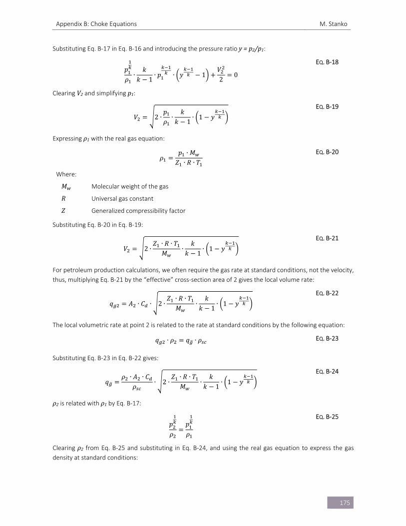
Appendix B: Choke Equations M. Stanko
175
Substituting Eq. B‐17 in Eq. B‐16 and introducing the pressure ratio y=p2/p1:
𝑝𝜌
∙𝑘
𝑘 1∙ 𝑝 ∙ 𝑦 1
𝑉2
0
EQ. B‐18
Clearing V2 and simplifying p1:
𝑉 2 ∙𝑝𝜌
∙𝑘
𝑘 1∙ 1 𝑦
EQ. B‐19
Expressing ρ1 with the real gas equation:
𝜌𝑝 ∙ 𝑀
𝑍 ∙ 𝑅 ∙ 𝑇
EQ. B‐20
Where:
𝑀 Molecular weight of the gas
𝑅 Universal gas constant
𝑍 Generalized compressibility factor
Substituting Eq. B‐20 in Eq. B‐19:
𝑉 2 ∙𝑍 ∙ 𝑅 ∙ 𝑇
𝑀∙
𝑘𝑘 1
∙ 1 𝑦
EQ. B‐21
For petroleum production calculations, we often require the gas rate at standard conditions, not the velocity,
thus, multiplying Eq. B‐21 by the “effective” cross‐section area of 2 gives the local volume rate:
𝑞 𝐴 ∙ 𝐶 ∙ 2 ∙𝑍 ∙ 𝑅 ∙ 𝑇
𝑀∙
𝑘𝑘 1
∙ 1 𝑦
EQ. B‐22
The local volumetric rate at point 2 is related to the rate at standard conditions by the following equation:
𝑞 ∙ 𝜌 𝑞 ∙ 𝜌 EQ. B‐23
Substituting Eq. B‐23 in Eq. B‐22 gives:
𝑞𝜌 ∙ 𝐴 ∙ 𝐶
𝜌∙ 2 ∙
𝑍 ∙ 𝑅 ∙ 𝑇𝑀
∙𝑘
𝑘 1∙ 1 𝑦
EQ. B‐24
ρ2 is related with ρ1 by Eq. B‐17:
𝑝
𝜌𝑝𝜌
EQ. B‐25
Clearing ρ2 from Eq. B‐25 and substituting in Eq. B‐24, and using the real gas equation to express the gas
density at standard conditions:
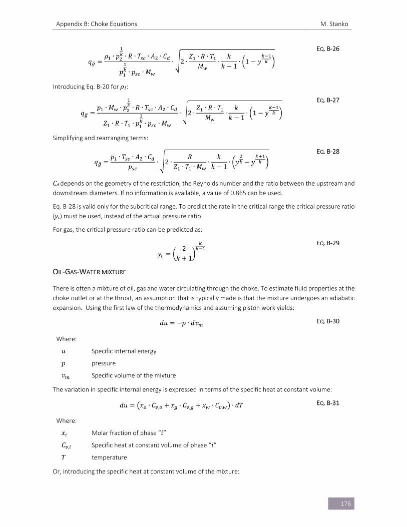
Appendix B: Choke Equations M. Stanko
176
𝑞𝜌 ∙ 𝑝 ∙ 𝑅 ∙ 𝑇 ∙ 𝐴 ∙ 𝐶
𝑝 ∙ 𝑝 ∙ 𝑀
∙ 2 ∙𝑍 ∙ 𝑅 ∙ 𝑇
𝑀∙
𝑘𝑘 1
∙ 1 𝑦
EQ. B‐26
Introducing Eq. B‐20 for ρ1:
𝑞𝑝 ∙ 𝑀 ∙ 𝑝 ∙ 𝑅 ∙ 𝑇 ∙ 𝐴 ∙ 𝐶
𝑍 ∙ 𝑅 ∙ 𝑇 ∙ 𝑝 ∙ 𝑝 ∙ 𝑀
∙ 2 ∙𝑍 ∙ 𝑅 ∙ 𝑇
𝑀∙
𝑘𝑘 1
∙ 1 𝑦
EQ. B‐27
Simplifying and rearranging terms:
𝑞𝑝 ∙ 𝑇 ∙ 𝐴 ∙ 𝐶
𝑝∙ 2 ∙
𝑅𝑍 ∙ 𝑇 ∙ 𝑀
∙𝑘
𝑘 1∙ 𝑦 𝑦
EQ. B‐28
Cd depends on the geometry of the restriction, the Reynolds number and the ratio between the upstream and
downstream diameters. If no information is available, a value of 0.865 can be used.
Eq. B‐28 is valid only for the subcritical range. To predict the rate in the critical range the critical pressure ratio
(yc) must be used, instead of the actual pressure ratio.
For gas, the critical pressure ratio can be predicted as:
𝑦2
𝑘 1
EQ. B‐29
OIL‐GAS‐WATER MIXTURE
There is often a mixture of oil, gas and water circulating through the choke. To estimate fluid properties at the
choke outlet or at the throat, an assumption that is typically made is that the mixture undergoes an adiabatic
expansion. Using the first law of the thermodynamics and assuming piston work yields:
𝑑𝑢 𝑝 ∙ 𝑑𝑣 EQ. B‐30
Where:
𝑢 Specific internal energy
𝑝 pressure
𝑣 Specific volume of the mixture
The variation in specific internal energy is expressed in terms of the specific heat at constant volume:
𝑑𝑢 𝑥 ∙ 𝐶 , 𝑥 ∙ 𝐶 , 𝑥 ∙ 𝐶 , ∙ 𝑑𝑇 EQ. B‐31
Where:
𝑥 Molar fraction of phase “𝑖”
𝐶 , Specific heat at constant volume of phase “𝑖”
𝑇 temperature
Or, introducing the specific heat at constant volume of the mixture:
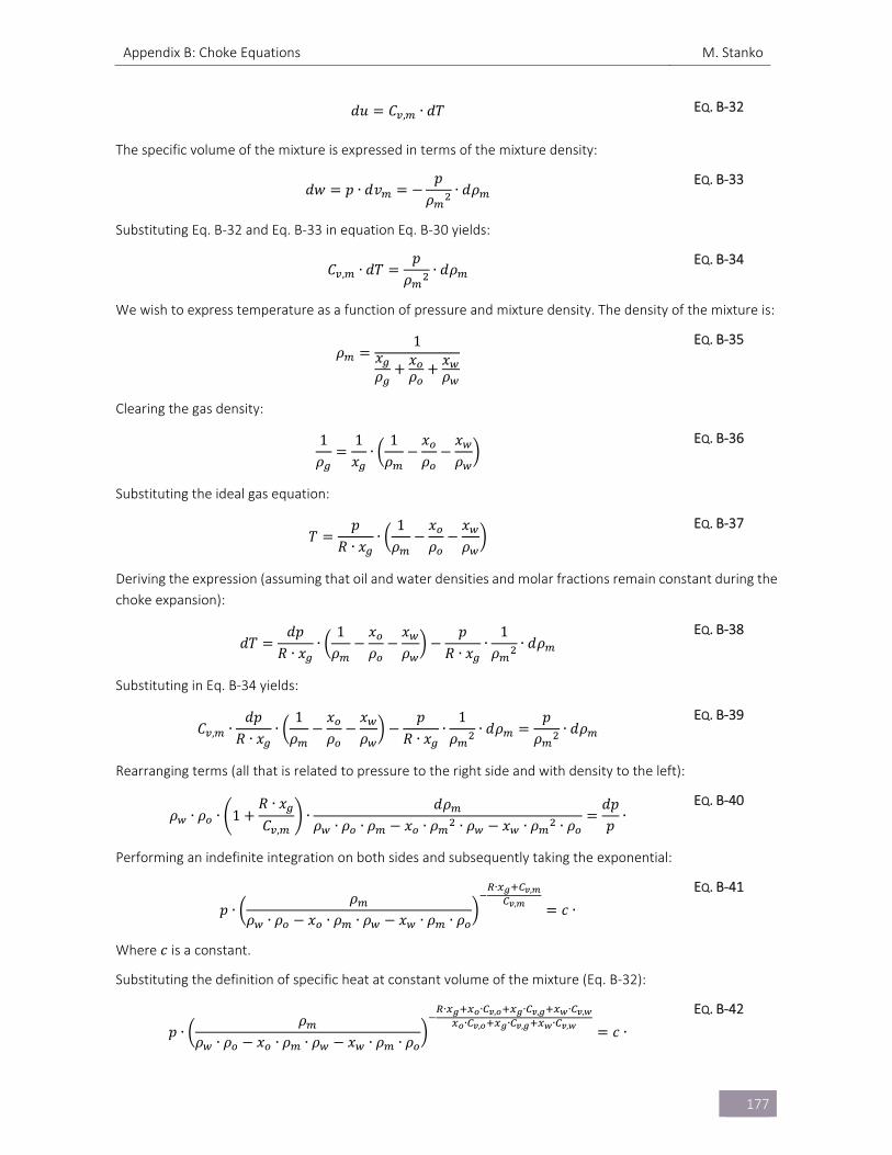
Appendix B: Choke Equations M. Stanko
177
𝑑𝑢 𝐶 , ∙ 𝑑𝑇 EQ. B‐32
The specific volume of the mixture is expressed in terms of the mixture density:
𝑑𝑤 𝑝 ∙ 𝑑𝑣𝑝
𝜌∙ 𝑑𝜌
EQ. B‐33
Substituting Eq. B‐32 and Eq. B‐33 in equation Eq. B‐30 yields:
𝐶 , ∙ 𝑑𝑇𝑝
𝜌∙ 𝑑𝜌
EQ. B‐34
We wish to express temperature as a function of pressure and mixture density. The density of the mixture is:
𝜌1
𝑥𝜌
𝑥𝜌
𝑥𝜌
EQ. B‐35
Clearing the gas density:
1𝜌
1𝑥
∙1
𝜌𝑥𝜌
𝑥𝜌
EQ. B‐36
Substituting the ideal gas equation:
𝑇𝑝
𝑅 ∙ 𝑥∙
1𝜌
𝑥𝜌
𝑥𝜌
EQ. B‐37
Deriving the expression (assuming that oil and water densities and molar fractions remain constant during the
choke expansion):
𝑑𝑇𝑑𝑝
𝑅 ∙ 𝑥∙
1𝜌
𝑥𝜌
𝑥𝜌
𝑝𝑅 ∙ 𝑥
∙1
𝜌∙ 𝑑𝜌
EQ. B‐38
Substituting in Eq. B‐34 yields:
𝐶 , ∙𝑑𝑝
𝑅 ∙ 𝑥∙
1𝜌
𝑥𝜌
𝑥𝜌
𝑝𝑅 ∙ 𝑥
∙1
𝜌∙ 𝑑𝜌
𝑝𝜌
∙ 𝑑𝜌 EQ. B‐39
Rearranging terms (all that is related to pressure to the right side and with density to the left):
𝜌 ∙ 𝜌 ∙ 1𝑅 ∙ 𝑥
𝐶 ,∙
𝑑𝜌𝜌 ∙ 𝜌 ∙ 𝜌 𝑥 ∙ 𝜌 ∙ 𝜌 𝑥 ∙ 𝜌 ∙ 𝜌
𝑑𝑝𝑝
∙ EQ. B‐40
Performing an indefinite integration on both sides and subsequently taking the exponential:
𝑝 ∙𝜌
𝜌 ∙ 𝜌 𝑥 ∙ 𝜌 ∙ 𝜌 𝑥 ∙ 𝜌 ∙ 𝜌
∙ ,
, 𝑐 ∙
EQ. B‐41
Where 𝑐 is a constant.
Substituting the definition of specific heat at constant volume of the mixture (Eq. B‐32):
𝑝 ∙𝜌
𝜌 ∙ 𝜌 𝑥 ∙ 𝜌 ∙ 𝜌 𝑥 ∙ 𝜌 ∙ 𝜌
∙ ∙ , ∙ , ∙ ,∙ , ∙ , ∙ , 𝑐 ∙
EQ. B‐42
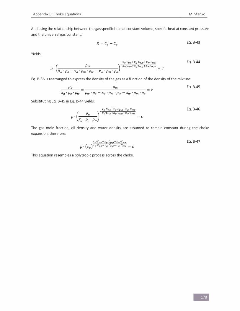
Appendix B: Choke Equations M. Stanko
178
And using the relationship between the gas specific heat at constant volume, specific heat at constant pressure
and the universal gas constant:
𝑅 𝐶 𝐶 EQ. B‐43
Yields:
𝑝 ∙𝜌
𝜌 ∙ 𝜌 𝑥 ∙ 𝜌 ∙ 𝜌 𝑥 ∙ 𝜌 ∙ 𝜌
∙ , ∙ , ∙ ,∙ , ∙ , ∙ , 𝑐
EQ. B‐44
Eq. B‐36 is rearranged to express the density of the gas as a function of the density of the mixture:
𝜌
𝑥 ∙ 𝜌 ∙ 𝜌𝜌
𝜌 ∙ 𝜌 𝑥 ∙ 𝜌 ∙ 𝜌 𝑥 ∙ 𝜌 ∙ 𝜌𝑐
EQ. B‐45
Substituting Eq. B‐45 in Eq. B‐44 yields:
𝑝 ∙𝜌
𝑥 ∙ 𝜌 ∙ 𝜌
∙ , ∙ , ∙ ,∙ , ∙ , ∙ ,
𝑐
EQ. B‐46
The gas mole fraction, oil density and water density are assumed to remain constant during the choke
expansion, therefore:
𝑝 ∙ 𝑣∙ , ∙ , ∙ ,∙ , ∙ , ∙ , 𝑐
EQ. B‐47
This equation resembles a polytropic process across the choke.
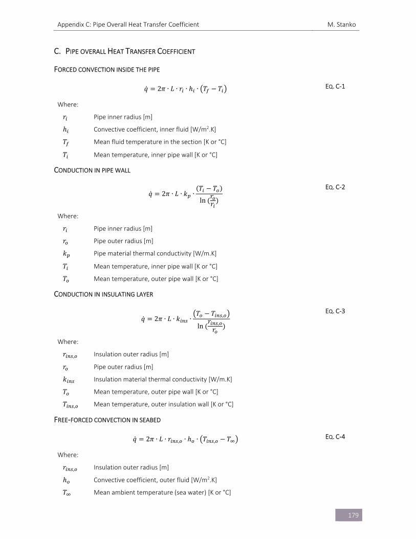
Appendix C: Pipe Overall Heat Transfer Coefficient M. Stanko
179
C. PIPE OVERALL HEAT TRANSFER COEFFICIENT
FORCED CONVECTION INSIDE THE PIPE
𝑞 2𝜋 ∙ 𝐿 ∙ 𝑟 ∙ ℎ ∙ 𝑇 𝑇 EQ. C‐1
Where:
𝑟 Pipe inner radius [m]
ℎ Convective coefficient, inner fluid [W/m2.K]
𝑇 Mean fluid temperature in the section [K or °C]
𝑇 Mean temperature, inner pipe wall [K or °C]
CONDUCTION IN PIPE WALL
𝑞 2𝜋 ∙ 𝐿 ∙ 𝑘 ∙𝑇 𝑇
ln𝑟𝑟
EQ. C‐2
Where:
𝑟 Pipe inner radius [m]
𝑟 Pipe outer radius [m]
𝑘 Pipe material thermal conductivity [W/m.K]
𝑇 Mean temperature, inner pipe wall [K or °C]
𝑇 Mean temperature, outer pipe wall [K or °C]
CONDUCTION IN INSULATING LAYER
𝑞 2𝜋 ∙ 𝐿 ∙ 𝑘 ∙𝑇 𝑇 ,
ln𝑟 ,
𝑟
EQ. C‐3
Where:
𝑟 , Insulation outer radius [m]
𝑟 Pipe outer radius [m]
𝑘 Insulation material thermal conductivity [W/m.K]
𝑇 Mean temperature, outer pipe wall [K or °C]
𝑇 , Mean temperature, outer insulation wall [K or °C]
FREE‐FORCED CONVECTION IN SEABED
𝑞 2𝜋 ∙ 𝐿 ∙ 𝑟 , ∙ ℎ ∙ 𝑇 , 𝑇 EQ. C‐4
Where:
𝑟 , Insulation outer radius [m]
ℎ Convective coefficient, outer fluid [W/m2.K]
𝑇 Mean ambient temperature (sea water) [K or °C]
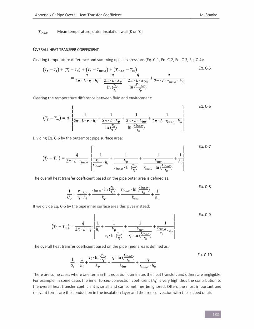
Appendix C: Pipe Overall Heat Transfer Coefficient M. Stanko
180
𝑇 , Mean temperature, outer insulation wall [K or °C]
OVERALL HEAT TRANSFER COEFFICIENT
Clearing temperature difference and summing up all expressions (Eq. C‐1, Eq. C‐2, Eq. C‐3, Eq. C‐4):
𝑇 𝑇 𝑇 𝑇 𝑇 𝑇 , 𝑇 , 𝑇𝑞
2𝜋 ∙ 𝐿 ∙ 𝑟 ∙ ℎ𝑞
2𝜋 ∙ 𝐿 ∙ 𝑘
ln𝑟𝑟
𝑞2𝜋 ∙ 𝐿 ∙ 𝑘
ln𝑟 ,
𝑟
𝑞2𝜋 ∙ 𝐿 ∙ 𝑟 , ∙ ℎ
EQ. C‐5
Clearing the temperature difference between fluid and environment:
𝑇 𝑇 𝑞 ∙
⎣⎢⎢⎢⎢⎡
12𝜋 ∙ 𝐿 ∙ 𝑟 ∙ ℎ
12𝜋 ∙ 𝐿 ∙ 𝑘
ln𝑟𝑟
12𝜋 ∙ 𝐿 ∙ 𝑘
ln𝑟 ,
𝑟
12𝜋 ∙ 𝐿 ∙ 𝑟 , ∙ ℎ
⎦⎥⎥⎥⎥⎤
EQ. C‐6
Dividing Eq. C‐6 by the outermost pipe surface area:
𝑇 𝑇𝑞
2𝜋 ∙ 𝐿 ∙ 𝑟 ,∙
⎣⎢⎢⎢⎢⎡
1𝑟
𝑟 ,∙ ℎ
1𝑘
𝑟 , ∙ ln𝑟𝑟
1𝑘
𝑟 , ∙ ln𝑟 ,
𝑟
1ℎ
⎦⎥⎥⎥⎥⎤
EQ. C‐7
The overall heat transfer coefficient based on the pipe outer area is defined as:
1𝑈
𝑟 ,
𝑟 ∙ ℎ
𝑟 , ∙ ln𝑟𝑟
𝑘
𝑟 , ∙ ln𝑟 ,
𝑟𝑘
1ℎ
EQ. C‐8
If we divide Eq. C‐6 by the pipe inner surface area this gives instead:
𝑇 𝑇𝑞
2𝜋 ∙ 𝐿 ∙ 𝑟∙
⎣⎢⎢⎢⎢⎡
1ℎ
1𝑘
𝑟 ∙ ln𝑟𝑟
1𝑘
𝑟 ∙ ln𝑟 ,
𝑟
1𝑟 ,
𝑟 ∙ ℎ
⎦⎥⎥⎥⎥⎤
EQ. C‐9
The overall heat transfer coefficient based on the pipe inner area is defined as:
1𝑈
1ℎ
𝑟 ∙ ln 𝑟𝑟
𝑘
𝑟 ∙ ln𝑟 ,
𝑟𝑘
𝑟𝑟 , ∙ ℎ
EQ. C‐10
There are some cases where one term in this equation dominates the heat transfer, and others are negligible.
For example, in some cases the inner forced‐convection coefficient (ℎ ) is very high thus the contribution to
the overall heat transfer coefficient is small and can sometimes be ignored. Often, the most important and
relevant terms are the conduction in the insulation layer and the free convection with the seabed or air.
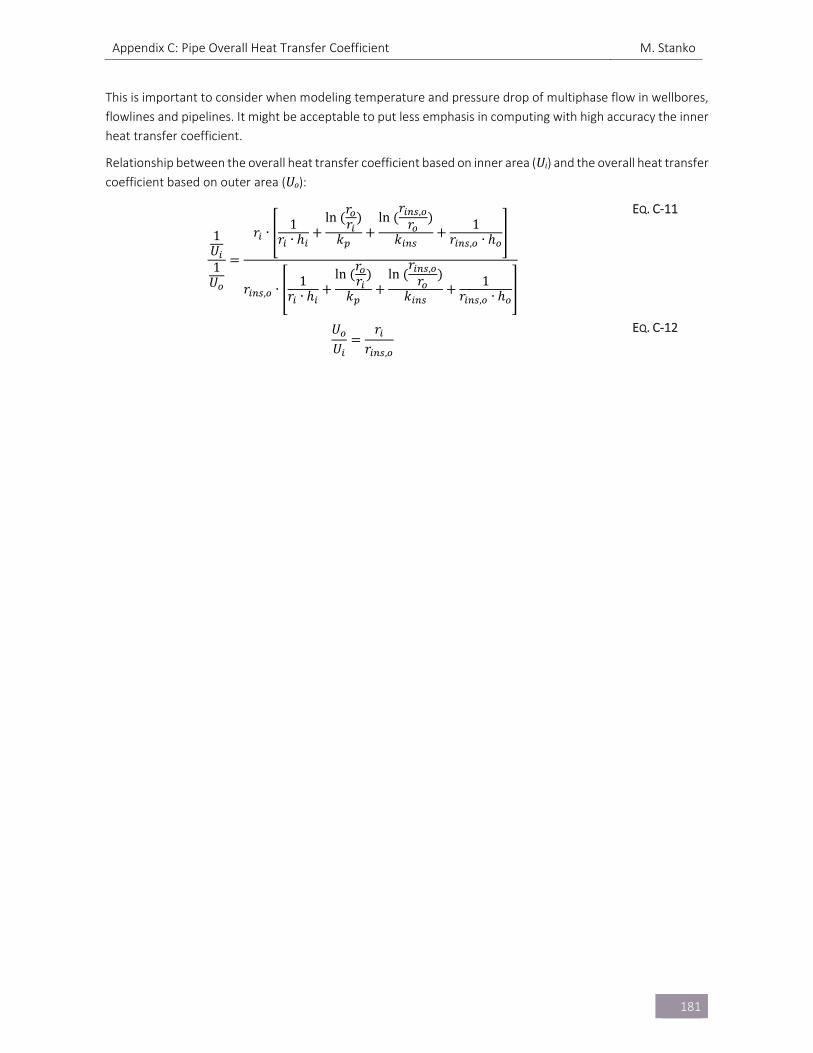
Appendix C: Pipe Overall Heat Transfer Coefficient M. Stanko
181
This is important to consider when modeling temperature and pressure drop of multiphase flow in wellbores,
flowlines and pipelines. It might be acceptable to put less emphasis in computing with high accuracy the inner
heat transfer coefficient.
Relationship between the overall heat transfer coefficient based on inner area (Ui) and the overall heat transfer coefficient based on outer area (Uo):
1𝑈1
𝑈
𝑟 ∙1
𝑟 ∙ ℎ
ln𝑟𝑟
𝑘
ln𝑟 ,
𝑟𝑘
1𝑟 , ∙ ℎ
𝑟 , ∙1
𝑟 ∙ ℎ
ln 𝑟𝑟
𝑘
ln 𝑟 ,
𝑟𝑘
1𝑟 , ∙ ℎ
EQ. C‐11
𝑈𝑈
𝑟𝑟 ,
EQ. C‐12
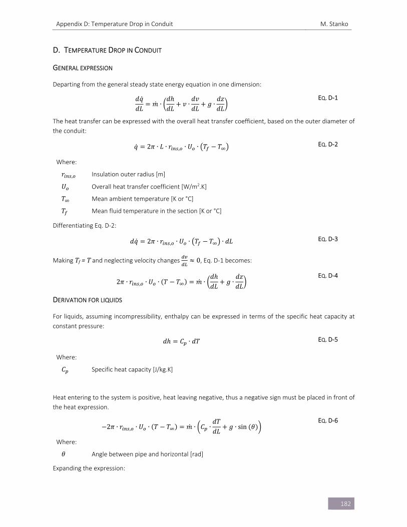
Appendix D: Temperature Drop in Conduit M. Stanko
182
D. TEMPERATURE DROP IN CONDUIT
GENERAL EXPRESSION
Departing from the general steady state energy equation in one dimension:
𝑑𝑞𝑑𝐿
𝑚 ∙𝑑ℎ𝑑𝐿
𝑣 ∙𝑑𝑣𝑑𝐿
𝑔 ∙𝑑𝑧𝑑𝐿
EQ. D‐1
The heat transfer can be expressed with the overall heat transfer coefficient, based on the outer diameter of
the conduit:
𝑞 2𝜋 ∙ 𝐿 ∙ 𝑟 , ∙ 𝑈 ∙ 𝑇 𝑇 EQ. D‐2
Where:
𝑟 , Insulation outer radius [m]
𝑈 Overall heat transfer coefficient [W/m2.K]
𝑇 Mean ambient temperature [K or °C]
𝑇 Mean fluid temperature in the section [K or °C]
Differentiating Eq. D‐2:
𝑑𝑞 2𝜋 ∙ 𝑟 , ∙ 𝑈 ∙ 𝑇 𝑇 ∙ 𝑑𝐿 EQ. D‐3
Making Tf=T and neglecting velocity changes 0, Eq. D‐1 becomes:
2𝜋 ∙ 𝑟 , ∙ 𝑈 ∙ 𝑇 𝑇 𝑚 ∙𝑑ℎ𝑑𝐿
𝑔 ∙𝑑𝑧𝑑𝐿
EQ. D‐4
DERIVATION FOR LIQUIDS
For liquids, assuming incompressibility, enthalpy can be expressed in terms of the specific heat capacity at
constant pressure:
𝑑ℎ 𝐶 ∙ 𝑑𝑇 EQ. D‐5
Where:
𝐶 Specific heat capacity [J/kg.K]
Heat entering to the system is positive, heat leaving negative, thus a negative sign must be placed in front of
the heat expression.
2𝜋 ∙ 𝑟 , ∙ 𝑈 ∙ 𝑇 𝑇 𝑚 ∙ 𝐶 ∙𝑑𝑇𝑑𝐿
𝑔 ∙ sin 𝜃 EQ. D‐6
Where:
𝜃 Angle between pipe and horizontal [rad]
Expanding the expression:
Appendix D: Temperature Drop in Conduit M. Stanko
183
𝑇 ∙ 2𝜋 ∙ 𝑟 , ∙ 𝑈 𝑇 ∙ 2𝜋 ∙ 𝑟 , ∙ 𝑈 𝑚 ∙ 𝐶 ∙𝑑𝑇𝑑𝐿
𝑚 ∙ 𝑔 ∙ sin 𝜃 EQ. D‐7
𝑑𝑇𝑑𝐿
𝑇 ∙2𝜋 ∙ 𝑟 , ∙ 𝑈
𝑚 ∙ 𝐶𝑇 ∙ 2𝜋 ∙ 𝑟 , ∙ 𝑈
𝑚 ∙ 𝐶𝑔 ∙ sin 𝜃
𝐶0
EQ. D‐8
For simplicity, we define the variable A:
𝐴𝑚 ∙ 𝐶
2𝜋 ∙ 𝑟 , ∙ 𝑈
EQ. D‐9
𝑑𝑇𝑑𝐿
𝑇 ∙1𝐴
𝑇𝐴
𝑔 ∙ sin 𝜃𝐶
0 EQ. D‐10
Solving the differential equation, using 𝑢 𝑒 and multiplying it by the above expression:
𝑢 ∙𝑑𝑇𝑑𝐿
𝑢 ∙ 𝑇 ∙1𝐴
𝑢 ∙𝑇𝐴
𝑔 ∙ sin 𝜃𝐶
EQ. D‐11
The product differentiating rule is defined as:
𝑑 𝑤 𝑥 ∙ 𝑣 𝑥𝑑𝑥
𝑑𝑤 𝑥𝑑𝑥
. 𝑣 𝑥 𝑤 𝑥 ∙𝑑𝑣 𝑥
𝑑𝑥
EQ. D‐12
Using the result from Eq. D‐12, it is possible to group Eq. D‐11 as follows:
𝑑 𝑢 ∙ 𝑇𝑑𝐿
𝑢 ∙𝑇𝐴
𝑔 ∙ sin 𝜃𝐶
EQ. D‐13
The resulting expression can be integrated by separating variables between the initial position “0” to a generic
position x in the pipe. This assumes that T∞, A, θ and Cpremain constant along the pipe length:
𝑒 ∙ 𝑑𝑇𝑇𝐴
𝑔 ∙ sin 𝜃𝐶
∙ 𝑒 ∙ 𝑑𝑥 EQ. D‐14
𝑒 ∙ 𝑇𝑇𝐴
𝑔 ∙ sin 𝜃𝐶
∙ 𝐴 ∙ 𝑒 EQ. D‐15
Where:
𝑇 Temperature of the fluid at pipe inlet [K or °C]
Evaluating at the integration limits:
𝑒 ∙ 𝑇 𝑥 𝑇𝑇𝐴
𝑔 ∙ sin 𝜃𝐶
∙ 𝐴 ∙ 𝑒 1 EQ. D‐16
𝑇 𝑥 𝑇 ∙ 𝑒𝑇𝐴
𝑔 ∙ sin 𝜃𝐶
∙ 𝐴 ∙ 1 𝑒 EQ. D‐17
This gives finally:
𝑇 𝑥 𝑇 𝑇 𝑥 0 𝑇 ∙ 𝑒1
𝐶∙ 𝑔 ∙ sin 𝜃 ∙ 𝐴 ∙ 1 𝑒
EQ. D‐18
Appendix D: Temperature Drop in Conduit M. Stanko
184
WITH VARIABLE AMBIENT TEMPERATURE
Ambient temperature could be variable, e.g. in a vertical tubing or casing along a formation. In this case, T∞ must be substituted by a function of x. Assuming a linear temperature gradient, T∞ can be expressed as:
𝑇 𝑥 𝑇 | sin 𝜃 ∙ 𝑥 ∙ 𝐺 EQ. D‐19
Where:
𝐺 Linear temperature gradient [K/m]
𝑇 | Temperature of the environment at the beginning of the section (negative if temperature is reduced with depth) [K or °C]
Substituting in Eq. D‐14
𝑒 ∙ 𝑑𝑇𝑇 |
𝐴sin 𝜃 ∙ 𝑥 ∙ 𝐺
𝐴𝑔 ∙ sin 𝜃
𝐶∙ 𝑒 ∙ 𝑑𝑥
EQ. D‐20
TRANSIENT IN FORMATION OR SOIL
When the temperature of the formation is changing, Uo must be substituted by the transient overall heat
transfer coefficient Uf(t), defined by:
𝑈 𝑡𝑈 ∙ 𝑘
𝑘 𝑟 , ∙ 𝑈 ∙ 𝑓 𝑡
EQ. D‐21
𝑓 𝑡 𝑙𝑛𝑟 ,
2 ∙ 𝛼 ∙ 𝑡0,29
EQ. D‐22
𝛼𝑘
𝜌 ∙ 𝐶 ,
EQ. D‐23
Where:
𝑘 Thermal conductivity, soil [W/m.K]
𝐶 , Specific heat capacity, soil [J/K.kg]
𝛼 Thermal diffusivity, soil [m2/s]
𝑡 Time [s]
Appendix E: Derivation of Multiphase Flow Expressions M. Stanko
185
E. DERIVATION OF MULTIPHASE FLOW EXPRESSIONS
RELATIONSHIP BETWEEN HOLDUP (HL), SLIP RATIO (S) AND QUALITY (x)
Using the relationship between real (ug) and superficial (usg) gas velocities:
𝑢 ∙ 𝐴 ∙ 1 𝐻 𝑢 ∙ 𝐴 EQ. E‐1
Where:
𝐴 Pipe cross‐section
Using the relationship between real (ul) and superficial (usl) liquid velocities:
𝑢 ∙ 𝐴 ∙ 𝐻 𝑢 ∙ 𝐴 EQ. E‐2
Dividing Eq. E‐1 by Eq. E‐2:
𝑢 ∙ 𝐴 ∙ 1 𝐻
𝑢 ∙ 𝐴 ∙ 𝐻
𝑢 ∙ 𝐴
𝑢 ∙ 𝐴
EQ. E‐3
Simplifying and introducing the definition of the slip ratio S=ug/ul:
𝑆 ∙ 1 𝐻𝐻
𝑢
𝑢
EQ. E‐4
The ratio of superficial velocities is expressed using the total mass flow rate (ṁ) and the quality (gas mass
fraction, x) and the densities of gas and liquid (ρl, ρg). The resulting expression is simplified:
𝑆 ∙ 1 𝐻𝐻
𝑚 ∙ 𝑥𝜌 ∙ 𝐴
𝑚 ∙ 1 𝑥𝜌 ∙ 𝐴
𝑥 ∙ 𝜌𝜌 ∙ 1 𝑥
EQ. E‐5
Clearing HL from Eq. E‐5:
𝑆 ∙ 1 𝐻𝐻
𝑆 ∙1
𝐻1
𝑥 ∙ 𝜌𝜌 ∙ 1 𝑥
EQ. E‐6
1𝐻
𝑥 ∙ 𝜌𝑆 ∙ 𝜌 ∙ 1 𝑥
1 EQ. E‐7
1𝐻
𝑥 ∙ 𝜌 𝑆 ∙ 𝜌 ∙ 1 𝑥
𝑆 ∙ 𝜌 ∙ 1 𝑥
EQ. E‐8
𝐻𝑆 ∙ 𝜌 ∙ 1 𝑥
𝑥 ∙ 𝜌 𝑆 ∙ 𝜌 ∙ 1 𝑥
EQ. E‐9
HOLDUP AVERAGE MIXTURE DENSITY (ρm)
The holdup average mixture density can be expressed as function of slip ratio (S), quality (gas mass fraction x) and the densities of gas and liquid (ρl, ρg). The density of the mixture is defined:
𝜌 1 𝐻 ∙ 𝜌 𝐻 ∙ 𝜌 EQ. E‐10
Substituting the holdup from Eq. E‐9 in Eq. E‐10:
Appendix E: Derivation of Multiphase Flow Expressions M. Stanko
186
𝜌 1𝑆 ∙ 𝜌 ∙ 1 𝑥
𝑥 ∙ 𝜌 𝑆 ∙ 𝜌 ∙ 1 𝑥∙ 𝜌
𝑆 ∙ 𝜌 ∙ 1 𝑥
𝑥 ∙ 𝜌 𝑆 ∙ 𝜌 ∙ 1 𝑥∙ 𝜌
EQ. E‐11
Simplifying:
𝜌𝑥 ∙ 𝜌
𝑥 ∙ 𝜌 𝑆 ∙ 𝜌 ∙ 1 𝑥∙ 𝜌
𝑆 ∙ 𝜌 ∙ 1 𝑥
𝑥 ∙ 𝜌 𝑆 ∙ 𝜌 ∙ 1 𝑥∙ 𝜌
EQ. E‐12
𝜌𝑥 𝑆 ∙ 1 𝑥𝑥
𝜌𝑆𝜌 ∙ 1 𝑥
EQ. E‐13
EFFECTIVE MOMENTUM DENSITY
𝑚𝜌 ∙ 𝐴
𝑚 ∙ 𝑢 𝑚 ∙ 𝑢 EQ. E‐14
1𝜌
𝐴𝑚
∙ 𝑚 ∙ 𝑢 𝑚 ∙ 𝑢 EQ. E‐15
1𝜌
𝐴𝑚
∙ 𝑥 ∙ 𝑢 1 𝑥 ∙ 𝑢 EQ. E‐16
1𝜌
𝐴𝑚
∙ 𝑢 ∙ 𝑥 ∙ 𝑆 1 𝑥 EQ. E‐17
1𝜌
𝐴𝑚
∙ 𝑢 ∙ 𝑆 ∙ 𝑥1 𝑥
𝑆
EQ. E‐18
The holdup can be introduced in the right‐hand side term using the following equation:
𝐴𝑚
∙ 𝑢 ∙ 𝑆𝐴𝑚
∙ 𝑢𝑚
𝑚∙
11 𝐻 ∙ 𝜌
𝑥 ∙1
1 𝐻 ∙ 𝜌
EQ. E‐19
Expressing the liquid holdup in terms of Eq. E‐9, Eq. E‐19 can be rewritten as:
𝐴𝑚
∙ 𝑢 ∙ 𝑆 𝑥 ∙1
1𝑆 ∙ 𝜌 ∙ 1 𝑥
𝑥 ∙ 𝜌 𝑆 ∙ 𝜌 ∙ 1 𝑥 ∙ 𝜌𝑥 ∙
1𝑥 ∙ 𝜌
𝑥 ∙ 𝜌 𝑆 ∙ 𝜌 ∙ 1 𝑥 ∙ 𝜌
EQ. E‐20
𝐴𝑚
∙ 𝑢 ∙ 𝑆𝑥 ∙ 𝜌 𝑆 ∙ 𝜌 ∙ 1 𝑥
𝜌 ∙ 𝜌𝑥
𝜌𝑆 ∙ 1 𝑥
𝜌
EQ. E‐21
Substituting Eq. E‐21 in Eq. E‐18:
1𝜌
𝑥𝜌
𝑆 ∙ 1 𝑥𝜌
∙ 𝑥1 𝑥
𝑆
EQ. E‐22
KINETIC ENERGY‐AVERAGE MIXTURE DENSITY
𝑚2 ∙ 𝜌 ∙ 𝐴
𝑢
2𝑢2
EQ. E‐23
1𝜌
2 ∙ 𝐴𝑚
∙𝑢
2𝑢2
EQ. E‐24
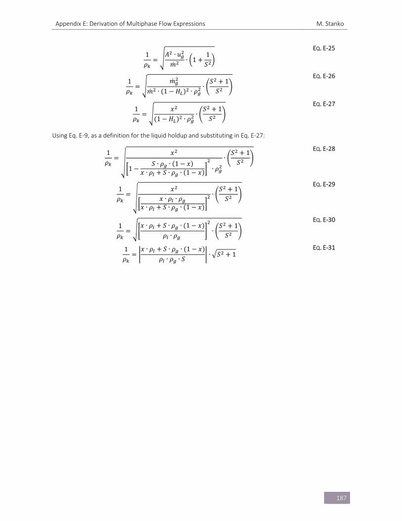
Appendix E: Derivation of Multiphase Flow Expressions M. Stanko
187
1𝜌
𝐴 ∙ 𝑢
𝑚∙ 1
1𝑆
EQ. E‐25
1𝜌
𝑚
𝑚 ∙ 1 𝐻 ∙ 𝜌∙
𝑆 1𝑆
EQ. E‐26
1𝜌
𝑥1 𝐻 ∙ 𝜌
∙𝑆 1
𝑆
EQ. E‐27
Using Eq. E‐9, as a definition for the liquid holdup and substituting in Eq. E‐27:
1𝜌
𝑥
1𝑆 ∙ 𝜌 ∙ 1 𝑥
𝑥 ∙ 𝜌 𝑆 ∙ 𝜌 ∙ 1 𝑥 ∙ 𝜌
∙𝑆 1
𝑆
EQ. E‐28
1𝜌
𝑥𝑥 ∙ 𝜌 ∙ 𝜌
𝑥 ∙ 𝜌 𝑆 ∙ 𝜌 ∙ 1 𝑥
∙𝑆 1
𝑆
EQ. E‐29
1𝜌
𝑥 ∙ 𝜌 𝑆 ∙ 𝜌 ∙ 1 𝑥
𝜌 ∙ 𝜌∙
𝑆 1𝑆
EQ. E‐30
1𝜌
𝑥 ∙ 𝜌 𝑆 ∙ 𝜌 ∙ 1 𝑥
𝜌 ∙ 𝜌 ∙ 𝑆∙ 𝑆 1
EQ. E‐31
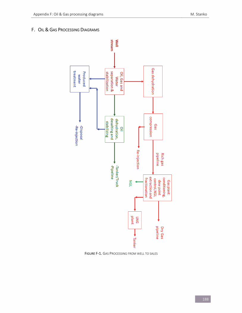
Appendix F: Oil & Gas processing diagrams M. Stanko
188
F. OIL & GAS PROCESSING DIAGRAMS
FIGURE F‐1. GAS PROCESSING FROM WELL TO SALES
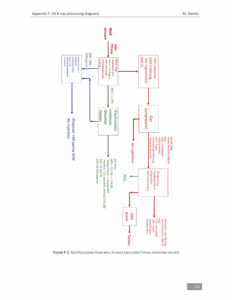
Appendix F: Oil & Gas processing diagrams M. Stanko
189
FIGURE F‐2. GAS PROCESSING FROM WELL TO SALES (INCLUDING TYPICAL OPERATING VALUES)
Appendix G: Derivation of the expression of field producing gas‐oil ratio M. Stanko
190
G. DERIVATION OF THE EXPRESSION OF FIELD PRODUCING GAS‐OIL RATIO
The producing gas oil ratio (𝑅 ) can be expressed as the ratio between gas rate and oil rate:
𝑅𝑞 𝑞𝑞 𝑞
EQ. G‐1
Neglecting the oil condensing from the gas (𝑞 0):
𝑅𝑞 𝑞
𝑞𝑞𝑞
𝑞𝑞
EQ. G‐2
The second term in the equation is the solution gas oil ratio (𝑅 ). The first term can be expressed as a local rate
of oil or gas times the oil volume factor and the gas volume factor.
𝑅
𝑞𝐵𝑞𝐵
𝑅 EQ. G‐3
The local flow rates depend on the IPR of each phase (and integrating the pressure function from pwf to pR).
However, as a simplification, if one considers the reservoir as a tank with uniform pressure pR then the integral
and well geometric effects disappear, and each rate will be proportional to kr/μ. Therefore:
𝑅
⎝
⎛
𝑘𝜇 𝐵
𝑘𝜇 𝐵 ⎠
⎞ 𝑅 EQ. G‐4
Appendix H: Gas lift optimization M. Stanko
191
H. GAS LIFT OPTIMIZATION
Example 1: Single well, unconstrained maximization of economic revenue by adjusting gas injection rate
A simple but very typical revenue function is defined by Eq. H‐1:
𝑓 𝑞 , 𝑞 ∙ 𝑃 𝑞 , ∙ 𝑃 𝑓 𝑞 , ∙ 𝑃 𝑞 , ∙ 𝑃 EQ. H‐1
Where:
𝑃 Oil price [USD/stb/d, USD/Sm3/d]
𝑃 Cost of injection gas [USD/MMSCFD, USD/MSm3/d]
𝑓 Revenue function
Deriving the function with respect to the adjustable variable:
𝑑𝑓 𝑞 ,
𝑑𝑞 ,
𝑑𝑓 𝑞 ,
𝑑𝑞 ,∙ 𝑃 𝑃 0 ⇒
𝑑𝑓 𝑞 ,
𝑑𝑞 ,
𝑃
𝑃
EQ. H‐2
The maximum revenue is therefore achieved for the point in the gas lift performance curve where the
derivative is exactly equal to the ratio between the injection gas cost and the oil price. In general, the gas price
is much smaller than the oil price, yielding that the derivative must be very close to zero.
Example 2: Single well, maximization of oil production with limited gas injection rate available
To include the limitation on injection gas available (qg,inj≤qg,injTOT) the Lagrange function[3‐2] is created:
𝐿 𝑞 , 𝑓 𝑞 , 𝜆 ∙ 𝑞 , 𝑞 , EQ. H‐3
The maximum is given when the derivative of the function with respect to the adjustable variable is equal to
zero (Eq. H‐4) and when the additional conditions (Eq. H‐5, Eq. H‐6, Eq. H‐7) are met:
𝑑𝐿 𝑞 ,
𝑑𝑞 ,
𝑑𝑓 𝑞 ,
𝑑𝑞 ,𝜆 0 ⇒
𝑑𝑓 𝑞 ,
𝑑𝑞 ,𝜆
EQ. H‐4
𝜆 ∙ 𝑞 , 𝑞 , 0 EQ. H‐5
𝜆 0 EQ. H‐6
𝑞 , 𝑞 , 0 EQ. H‐7
There are two possible solutions:
Solution 1:
𝜆 0,𝑑𝑓 𝑞 ,
𝑑𝑞 ,0
Valid only if there is enough gas available (qg,inj≤qg,injTOT)
Solution 2:
𝜆 0,𝑑𝑓 𝑞 ,
𝑑𝑞 ,𝜆
Valid only if all the gas available is used (qg,inj=qg,injTOT). Please note that due to the condition (Eq. H‐6) on lambda, the derivative MUST NOT be negative.
Example 3: Single well, maximization of revenue with limited gas injection rate.
The Lagrange function is created:
𝐿 𝑞 , 𝑓 𝑞 , 𝜆 ∙ 𝑞 , 𝑞 , EQ. H‐8
Appendix H: Gas lift optimization M. Stanko
192
The maximum is given when the derivative of the function with respect to the adjustable variable is equal to
zero (Eq. H‐9) and when the additional conditions (Eq. H‐10, Eq. H‐11, Eq. H‐12) are met:
𝜕𝐿 𝑞 ,
𝜕𝑞 ,
𝑑𝑓 𝑞 ,
𝑑𝑞 ,𝜆 0 ⇒
𝑑𝑓 𝑞 ,
𝑑𝑞 ,∙ 𝑃 𝑃 𝜆 ⇒
𝑑𝑓 𝑞 ,
𝑑𝑞 ,
𝜆 𝑃
𝑃
EQ. H‐9
𝜆 ∙ 𝑞 , 𝑞 , 0 EQ. H‐10
𝜆 0 EQ. H‐11
𝑞 , 𝑞 , 0 EQ. H‐12
There are two possible solutions:
Solution 1:
𝜆 0,𝑑𝑓 𝑞 ,
𝑑𝑞 ,
𝑃
𝑃
Valid only if there is enough gas available (qg,inj≤qg,injTOT)
Solution 2:
𝜆 0,𝑑𝑓 𝑞 ,
𝑑𝑞 ,
𝜆 𝑃
𝑃
Valid only if all the gas available is used (qg,inj=qg,injTOT).
Example 4: unconstrained oil production maximization on a group of wells by adjusting the individual well gas
lift injection rate
The present development assumes that the operation of an individual well is independent from the others
(the operating wellhead pressure remains constant despite of the operating conditions of the individual wells).
This is because the mathematical procedure employed requires the objective function (e.g. total oil
production) to be additively separable (a function that can expressed as the summation of two or more
functions each one depending on only one variable).
The total oil production function (F) is the sum of the individual (i) well oil production (fi). The total number of
wells is N.
𝐹 𝑞 , , 𝑞 , , 𝑞 , , … 𝑓 𝑞 , EQ. H‐13
F is a multivariate (N) additively separable scalar function. A necessary condition for this function to be maximum is that the elements of its gradient must be equal to zero:
𝜕𝐹 𝑞 , , 𝑞 , , 𝑞 , , …
𝜕𝑞 ,
𝜕𝑓 𝑞 ,
𝜕𝑞 ,0
EQ. H‐14
The maximum of the compound oil production is when all the oil production of the individual wells is also
maximum.
Example 5: Revenue maximization on a group of wells by adjusting the gas lift injection rate
The total revenue function (frevTOT) is the sum of the individual well oil production (frev,i). The total number of
wells is N.
𝑓 𝑞 , , 𝑞 , , 𝑞 , , … 𝑓 , 𝑞 , EQ. H‐15
Appendix H: Gas lift optimization M. Stanko
193
frevTOT is a multivariate (N) additively separable scalar function. A necessary condition for this function to be maximum is that the elements of its gradient must be equal to zero:
𝜕𝑓 𝑞 , , 𝑞 , , 𝑞 , , …
𝜕𝑞 ,
𝜕𝑓 , 𝑞 ,
𝜕𝑞 ,
𝜕𝑓 𝑞 ,
𝜕𝑞 ,∙ 𝑃 𝑃 0
EQ. H‐16
The maximum of the compound revenue is achieved when all the revenues of the individual wells are also
maximum.
Example 6: revenue maximization of a group of wells by adjusting the gas lift injection rate with limited gas
The total revenue function (frevTOT) is the sum of the individual well oil production (frev,i). The total number of
wells is N.
𝑓 𝑞 , , 𝑞 , , 𝑞 , , … 𝑓 , 𝑞 , EQ. H‐17
frevTOT is a multivariate (N) additively separable scalar function. In order to include the limitation on injection
gas available (∑qg,inj<qg,injTOT) the method of Lagrange multipliers is used. The Lagrange function is created:
𝐿 𝑞 , , 𝑞 , , 𝑞 , , … 𝑓 , 𝑞 , 𝜆 ∙ 𝑞 , 𝑞 , EQ. H‐18
A necessary condition for this function to be maximum is that the elements of its gradient must be equal to
zero (Eq. H‐19) and when the additional conditions (Eq. H‐20, Eq. H‐21, Eq. H‐22) are met:
𝜕𝐿 𝑞 , , 𝑞 , , 𝑞 , , …
𝜕𝑞 ,
𝜕𝑓 , 𝑞 ,
𝜕𝑞 ,𝜆 0 ⇒
𝜕𝑓 𝑞 ,
𝜕
𝜆 𝑃
𝑃
EQ. H‐19
𝜆 ∙ 𝑞 , 𝑞 , 0 EQ. H‐20
𝜆 0 EQ. H‐21
𝑞 , 𝑞 , EQ. H‐22
There are two possible solutions:
Solution 1:
𝜆 0,𝜕𝑓 𝑞 ,
𝜕𝑞 ,
𝑃
𝑃
All the wells are operating in their maximum revenue point. Valid only if there is enough gas available (∑qg,inj<qg,injTOT)
Solution 2:
𝜆 0,𝜕𝑓 𝑞 ,
𝜕𝑞 ,
𝜆 𝑃
𝑃
All wells are operating at the same derivative in the gas lift performance curve. Valid only if all the gas available is used (∑qg,inj‐qg,injTOT=0)
The procedure described is also applicable for any situation where the well (or group of wells) has a concave
performance curve of oil production vs an adjustable parameter. For example, ESP lifted wells with diluent
injection at the ESP suction also exhibit a similar performance curve.
Appendix I: Some Style Comments for Technical Communication M. Stanko
194
I. SOME STYLE COMMENTS FOR TECHNICAL COMMUNICATION (PARAPHRASING THE NOTES OF M. STANDING AND M. GOLAN)
Introduce smoothly the topic to the reader. Use as many aids as possible to accomplish that.
Think of what you want to communicate with the sentence before writing it.
Use active verbs.
Give the most important information at the beginning of the sentence. It must be clear and objective.
Differentiate between “observed”, “calculated”, “assumed”, “guessed”.
Limit sentences to 30 words.
Avoid clichés, watery and loaded statements that do not add any important information.
Reference properly your statements.
Give the proper context and take enough time when introducing and discussing a figure or a diagram.
All figures and tables should be discussed in the text.
Use proper English, select the right words and verbs.
Your statements should be, as much as possible, defendable in a court of Law.