probabilistic damage stability - ntnu open
TRANSCRIPT

Probabilistic Damage StabilityEvaluating the Attained Subdivision Index by
Analysing the Effect of Changes in the
Arrangement and Intact Stability for an
Offshore Vessel
Stian Røyset Salen
Marine Technology
Supervisor: Svein Aanond Aanondsen, IMTCo-supervisor: Bjørn Egil Asbjørnslett, IMT
Department of Marine Technology
Submission date: June 2016
Norwegian University of Science and Technology

i
Preface
This master’s thesis represents the finalisation of my MSc degree in Marine Technology,
Marine Systems Design from the Norwegian University of Science and Technology (NTNU).
The thesis counts 30 credits, which corresponds to the work rate of four regular courses at
NTNU. The study was carried out during the spring semester of 2016.
The work with the thesis started already during the fall semester of 2015, in the course
TMR4560 Marine Systems Design, Specialization Project, where the author wrote a project
thesis titled ‘A Pre-Study on Probabilistic Damage Stability’. The theory part of this project is
included in Chapter 2 of the master’s thesis.
The thesis aims to give naval architects a better insight to how probabilistic damage stability,
or more precisely the attained subdivision index, is influenced by certain changes in the
arrangement and intact stability for offshore vessels. A ‘wind farm service vessel’ that is
applicable to the SOLAS-2009 damage stability regulations, provided by Salt Ship Design, was
used to conduct the study.
The author of the thesis, Stian Røyset Salen, would first of all like to thank Johannes Eldøy in
Salt Ship Design for providing access to a NAPA-license throughout the semester. Having
access to this market-leading stability software, certainly lifted the quality of the study.
Furthermore, Ole Martin Djupvik in Salt Ship Design should be thanked for his endless support
during the semester. Without his help, the author would have struggled much more in the
process of learning how NAPA works. Additionally, Jørgen Hammersland and Frode Marton
Meling at Salt Ship Design deserve a thanks, for being helpful upon request from the author.
At last, the author is grateful for the guidance from the thesis’ primary and secondary
supervisors from NTNU, respectively Svein Aanond Aanondsen and Bjørn Egil Asbjørnslett.
Trondheim, 17/6/2016
Stian Røyset Salen

ii
iii
Abstract
The motivational basis and underlying goal of this master’s thesis is to provide more knowledge
to the ‘experience data bank’ for ship designers with respect to probabilistic damage stability
(PDS). More precisely, the thesis aims to give more insight to how certain changes in the
arrangement and intact stability affect the PDS or A-index for a specific offshore vessel.
The author has co-operated with Salt Ship Design in order to achieve the abovementioned goal;
a NAPA-license and GA drawings to a ‘wind farm service vessel (WFSV)’ were provided. In
agreement with Salt Ship Design, the following two objectives have been investigated:
1. What is the effect on the A-index of changing the size of the wing ballast tanks located
above the void ‘U-tanks’ at the mid-section of the WFSV, by changing the height of the
horizontal surface (‘U-deck’) separating these two tanks?
2. What is the effect on the A-index of changing the intact stability of the ship, i.e. the
ship’s initial GM values for the three subdivision draughts dS, dP and dL?
The background for the abovementioned goal and research questions, is the introduction of the
PDS regulations by IMO in 2009. Ship designers were then forced to use the probabilistic
approach instead of the deterministic approach (DDS), for certain vessel types when calculating
damage stability. PDS offers more freedom than DDS in the design of the ship’s internal
watertight arrangement. However, since PDS calculations usually are conducted at late design
stages due to the widely used top-down design approach, it may be challenging to utilise this
flexibility due to time pressure. Thus, ship designers often rely on experience, since there is
little time for research and optimisation. The author would therefore like to contribute with
more knowledge to the ship designers’ ‘experience data bank’. Furthermore, the results for
objective 1 and 2, respectively, are presented in the below figures:
0,52
0,53
0,54
0,55
0,56
0,57
0,58
0,59
0,60
0,61
7000 6600 6100 5600 5100 4600 4100 3600 3100 2600 2100 1600 1200
A-i
nd
ex
Placement of U-deck above baseline [mm]
Total A-index for different U-deck heightsA-index
R-index
Deck 1
Tanktop
Deck 2,Z06-Z07
Deck 2,Z13
Abstract
iv
From the results presented above, it can be concluded that the A-index in objective 1 generally
decreases when U-deck is lowered beneath the maximum value on the curve, which corresponds
to 5.6 m. From the analysis and discussion conducted in this study, it can furthermore be
concluded that the factors contributing to the change are si and vi. The pi-factor does not
contribute, since there are no changes in the arrangement in longitudinal or transverse direction.
Both the si- and vi-factor generally decreases when the U-deck height is decreased below 5.6
m. For the si-factor, this is most likely due to increasing heeling moments, in case of damage,
for larger sized wing ballast tanks; the si-factor is reduced due to larger heel angles. In addition,
larger wing ballast tanks leads to smaller U-tanks, thus the stabilising effect of the U-tanks is
reduced as well.
The results for objective 2 show that the A-index is generally better for larger initial GM values.
The analysis and discussion related to objective 2, additionally conclude that the A-index is
mainly dependent on the heeling moment in case of damage. The heeling moment will give the
ship a new floating position, i.e. the ship obtains an equilibrium heel angle larger than zero
degrees. This heel angle reduces the si-factor, which in turn reduces the A-index. The pi- and
vi-factor will not contribute to the changes in A-index for objective 2, because there are no
changes in the arrangement.
The abovementioned results and conclusions are the key findings in this thesis. Whether the
results are generic or not, is questionable; for offshore vessels with approximately the same
arrangement as the WFSV, the results from this thesis could be useful.
0,10
0,20
0,30
0,40
0,50
0,60
0,70
0,80
0,90
2 1,8 1,6 1,4 1,2 1 0,8 0,6 0,4 0,2 0,05
A-i
nd
ex
GML value [m]
Total A-index for different GM values
A-index
R-index
v
Sammendrag
Inspirasjonen bak, samt det underliggende målet, med denne masteroppgaven er å kunne bidra
til en kunnskapsøking blant skipsdesignere generelt, i forhold til probabilistisk skadestabilitet
(PDS). Mer spesifikt så satser oppgaven på å gi bedre innsikt i hvordan visse endringer i
arrangementet og intaktstabiliteten for et spesifikt skip påvirker PDS eller A-indeksen.
Forfatteren har samarbeidet med Salt Ship Design for å oppnå det overnevnte målet; en NAPA-
lisens og GA-tegninger for et ‘wind farm service vessel (WFSV)’ ble gitt til forfatteren. I
enighet med Salt Ship Design har de følgende problemstillingene blitt forsket på:
1. Hva er effekten på A-indeksen av å endre størrelsen på wing ballast tankene som er
lokalisert rett over de såkalte ‘U-tankene’, ved å endre høyden på den horisontale flaten
(‘U-dekk’) som skiller disse to tankene?
2. Hva er effekten på A-indeksen av å endre intaktstabiliteten til skipper, det vil si skipets
initiale GM-verdier for de tre lastkondisjonene dS, dP and dL?
Bakgrunnen for det overnevnte målet, samt problemstillingene over, er IMOs introduksjon av
det nye PDS-regelverket i SOLAS-2009. Skipsdesignere ble da tvunget til å bruke den
probabilistiske metoden fremfor den tradisjonelle, deterministiske metoden (DDS), for visse
skipstyper. PDS tilbyr designere mer fleksibilitet sammenlignet med DDS. Likevel, siden PDS-
beregninger vanligvis blir utført mot slutten av prosjekter, på grunn av den vidstrakte bruken
av ‘top-down’ designmetoden, kan det være utfordrende å utnytte denne fleksibiliteten. På
grunn av dette, stoler designere ofte på gammel kunnskap og erfaring, siden det som regel er
lite tid til forskning og optimalisering. Forfatteren av denne oppgaven ønsker derfor å bidra
med ytterligere kunnskap. Resultatene for problemstilling 1 og 2, respektivt, er videre presentert
i figurene som følger:
0,52
0,53
0,54
0,55
0,56
0,57
0,58
0,59
0,60
0,61
7000 6600 6100 5600 5100 4600 4100 3600 3100 2600 2100 1600 1200
A-i
nd
eks
Plassering av U-dekk over baseline [mm]
Total A-indeks for ulike U-dekk høyderA-index
R-index
Deck 1
Tanktop
Deck 2,Z06-Z07
Deck 2,Z13
Sammendrag
vi
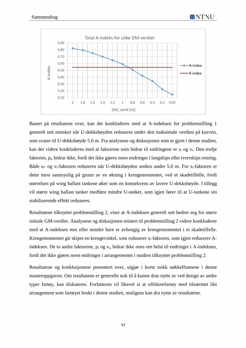
Basert på resultatene over, kan det konkluderes med at A-indeksen for problemstilling 1
generelt sett minsker når U-dekkshøyden reduseres under den maksimale verdien på kurven,
som svarer til U-dekkshøyde 5.6 m. Fra analysene og diskusjonen som er gjort i denne studien,
kan det videre konkluderes med at faktorene som bidrar til endringene er si og vi. Den tredje
faktoren, pi, bidrar ikke, fordi det ikke gjøres noen endringer i langskips eller tverrskips retning.
Både si- og vi-faktoren reduseres når U-dekkshøyden senkes under 5.6 m. For si-faktoren er
dette mest sannsynlig på grunn av en økning i krengemomentet, ved et skadetilfelle, fordi
størrelsen på wing ballast tankene øker som en konsekvens av lavere U-dekkshøyde. I tillegg
vil større wing ballast tanker medføre mindre U-tanker, som igjen fører til at U-tankene sin
stabiliserende effekt reduseres.
Resultatene tilknyttet problemstilling 2, viser at A-indeksen generelt sett bedrer seg for større
initiale GM-verdier. Analysene og diskusjonen relatert til problemstilling 2 videre konkluderer
med at A-indeksen mer eller mindre bare er avhengig av krengemomentet i et skadetilfelle.
Krengemomentet gir skipet en krengevinkel, som reduserer si-faktoren, som igjen reduserer A-
indeksen. De to andre faktorene, pi og vi, bidrar ikke noes om helst til endringer i A-indeksen,
fordi det ikke gjøres noen endringer i arrangementet i studien tilknyttet problemstilling 2.
Resultatene og konklusjonene presentert over, utgjør i korte trekk nøkkelfunnene i denne
masteroppgaven. Om resultatene er generelle nok til å kunne dras nytte av ved design av andre
typer fartøy, kan diskuteres. Forfatteren vil likevel si at offshorefartøy med tilnærmet likt
arrangement som fartøyet brukt i denne studien, muligens kan dra nytte av resultatene.
0,10
0,20
0,30
0,40
0,50
0,60
0,70
0,80
0,90
2 1,8 1,6 1,4 1,2 1 0,8 0,6 0,4 0,2 0,05
A-i
nd
eks
GML-verdi [m]
Total A-indeks for ulike GM-verdier
A-index
R-index
vii
Table of Contents
Preface ......................................................................................................................................... i
Abstract ..................................................................................................................................... iii
Sammendrag ............................................................................................................................... v
List of Figures ............................................................................................................................ x
List of Tables ........................................................................................................................... xiii
List of Equations ..................................................................................................................... xiv
List of Symbols ....................................................................................................................... xvi
List of Acronyms ..................................................................................................................... xix
1. Introduction ......................................................................................................................... 1
1.1 Historical Background and Motivation ....................................................................... 1
1.2 Previous Work ............................................................................................................. 3
1.3 Objectives and Scope of Work .................................................................................... 4
1.4 Limitations ................................................................................................................... 5
1.5 Thesis Structure ........................................................................................................... 5
2. Ship Stability Theory .......................................................................................................... 7
2.1 Introduction to Intact Stability ..................................................................................... 7
2.1.1 Transverse Stability .............................................................................................. 7
2.1.2 Longitudinal Stability ........................................................................................... 9
2.2 Introduction to Damage Stability .............................................................................. 10
2.2.1 The Lost Buoyancy Method ............................................................................... 11
2.2.2 Damage Stability Regulations ............................................................................ 12
2.3 Deterministic Damage Stability ................................................................................. 15
2.3.1 Calculation Method ............................................................................................ 15
2.3.2 Damage Extent ................................................................................................... 16
2.3.3 Requirements ...................................................................................................... 17
2.4 Probabilistic Damage Stability .................................................................................. 18
Table of Contents
viii
2.4.1 Limitations ......................................................................................................... 19
2.4.2 Subdivision Length ............................................................................................ 20
2.4.3 Required Subdivision Index R ........................................................................... 21
2.4.4 Attained Subdivision Index A ............................................................................ 23
2.4.5 Zone Division ..................................................................................................... 24
2.4.6 The Factor pi ....................................................................................................... 25
2.4.7 The Factor si ....................................................................................................... 34
2.4.8 The Factor vi ....................................................................................................... 38
3. Individual Study on Probabilistic Damage Stability ......................................................... 43
3.1 Approach ................................................................................................................... 43
3.2 Ship Particulars .......................................................................................................... 44
3.3 Software ..................................................................................................................... 45
3.4 Modelling in NAPA ................................................................................................... 45
3.4.1 Arrangement ....................................................................................................... 46
3.4.2 Time-Saving Measures ....................................................................................... 47
3.5 Calculation Procedure in NAPA ................................................................................ 48
3.5.1 Probabilistic Manager ........................................................................................ 48
3.5.2 Initial Conditions ................................................................................................ 49
3.5.3 Wind Profile and Heeling Moments ................................................................... 50
3.5.4 Subdivision Data ................................................................................................ 50
3.5.5 Openings and Compartment Connections .......................................................... 51
3.5.6 Time-Saving Measures ....................................................................................... 52
3.5.7 Objective 1 ......................................................................................................... 53
3.5.8 Objective 2 ......................................................................................................... 54
3.6 Analysis Tools in NAPA ........................................................................................... 55
3.6.1 SFAC Diagram ................................................................................................... 56
3.6.2 P1S Diagram ...................................................................................................... 58
4. Results of Individual Study ............................................................................................... 59
Table of Contents
ix
4.1 Objective 1: Changing the Height of U-deck ............................................................ 59
4.1.1 R-index ............................................................................................................... 59
4.1.2 A-index ............................................................................................................... 60
4.2 Objective 2: Changing the Initial GM Values ........................................................... 63
5. Analysis and Discussion ................................................................................................... 67
5.1 The Effect of Changing the U-deck height ................................................................ 67
5.1.1 The pi-factor ....................................................................................................... 69
5.1.2 The si-factor ........................................................................................................ 70
5.1.3 The vi-factor ....................................................................................................... 74
5.1.4 Total A-index ..................................................................................................... 77
5.2 The Effect of Changing the Initial GM Values ......................................................... 79
5.2.1 The pi- and vi-factor ........................................................................................... 81
5.2.2 The si-factor ........................................................................................................ 81
5.2.3 Total A-index ..................................................................................................... 85
5.3 Uncertainties .............................................................................................................. 86
6. Conclusion ........................................................................................................................ 88
6.1 Uncertainties .............................................................................................................. 89
6.2 Key Findings .............................................................................................................. 89
6.3 Further Work ............................................................................................................. 90
7. Bibliography ..................................................................................................................... 92
List of Appendices ................................................................................................................... 94

x
List of Figures
Figure 1. A cross-section of the ‘Wind Farm Service Vessel’ illustrating a void U-tank and wing
ballast tanks. ............................................................................................................................... 4
Figure 2. Transverse stability measurements for small angles. The figure is adapted from
Magnussen et al. (2014). ............................................................................................................ 7
Figure 3. An example of a GZ curve. The figure is inspired by Djupvik et al. (2015). ............. 8
Figure 4. A ship that is trimmed by the stern (positive trim). The figure is inspired by Patterson
and Ridley (2014). .................................................................................................................... 10
Figure 5. Damage stability requirements for all ships pre-2009. The figure is obtained from
Patterson and Ridley (2014). .................................................................................................... 14
Figure 6. Ship length as stated in ICCL-66. The figure is adapted from Djupvik et al. (2015).
.................................................................................................................................................. 16
Figure 7. Examples of how the subdivision length is determined. The figure is adapted from
Hjort and Olufsen (2014). ........................................................................................................ 20
Figure 8. Illustration of the loading conditions, mean draught and trim levels. The illustration
is obtained from IMO (2008c). ................................................................................................ 24
Figure 9. Possible single- and multi zone damages for a ship with 7 zones. The illustration is
adapted from DELFTship ; the original source is IMO (2008c). ............................................. 25
Figure 10. Distributions created based on statistics from the HARDER project (Hjort &
Olufsen, 2014) .......................................................................................................................... 27
Figure 11. ‘Damage category 1’ seen from above (Djupvik et al., 2015). ............................... 30
Figure 12. ‘Damage category 2’ seen from above (Djupvik et al., 2015). ............................... 31
Figure 13. ‘Damage category 3’ seen from above (Djupvik et al., 2015). ............................... 31
Figure 14. Distribution density (left) and distribution density function (right) for non-
dimensional penetration. The figure is adapted from Lützen (2001). ...................................... 32
Figure 15. Illustration of a typical GZ curve (left) and a GZ curve for submerged opening
(right). The illustration is obtained from Djupvik et al. (2015). .............................................. 37
Figure 16. A ship with a particular damage condition and corresponding H measures. The
illustration is obtained from Djupvik et al. (2015). .................................................................. 39
Figure 17. The use of the vi factor for different horizontal watertight arrangements. The
illustrations are adapted from IMO (2008c). ........................................................................... 39
List of Figures
xi
Figure 18. Vertical damage extent distribution for the old and new regulations. The figure is
adapted from Hjort and Olufsen (2014). .................................................................................. 41
Figure 19. Illustration of wing ballast tank, U-deck and U-tank, inspired by Figure 1. .......... 43
Figure 20. Profile view of the Wind Farm Service Vessel used in the study. .......................... 45
Figure 21. The three lower decks of the ship modelled in NAPA. .......................................... 46
Figure 22. Probabilistic Manager in NAPA. ............................................................................ 48
Figure 23. Wind profile of the ship created in NAPA. ............................................................ 50
Figure 24. Subdivision illustration from the NAPA results report, for the side profile view and
deck 2 of the ship. .................................................................................................................... 51
Figure 25. Illustration of how transverse bulkheads are placed at the same longitudinal location
on adjacent decks. .................................................................................................................... 52
Figure 26. Cross-section of the ship illustrating the relevant placements of U-deck. .............. 53
Figure 27. Illustration of the longitudinal U-deck range, which goes from zone 6 to zone 13.
.................................................................................................................................................. 54
Figure 28. Intact stability GM limit curve. ............................................................................... 55
Figure 29. SFAC diagram obtained from the NAPA results report. ........................................ 56
Figure 30. Single-zone damage case from zone 3. The figure is inspired by (Djupvik et al.,
2015). ........................................................................................................................................ 57
Figure 31. P1S diagram obtained from the NAPA results report. ............................................ 58
Figure 32. Plot of A-index vs. placement of U-deck................................................................ 60
Figure 33. Plot of A-index vs. placement of U-deck................................................................ 62
Figure 34. Plot of AC-index vs. placement of U-deck for all subdivision draughts. ................ 62
Figure 35. Plot of A-index vs. GML value. .............................................................................. 64
Figure 36. Plot of AC-index vs. GM values for all subdivision draughts. ................................ 65
Figure 37. Areas of particular interest on the A-index curve for different U-deck heights. .... 67
Figure 38. P1S diagram for U-deck height 2.6 m. ................................................................... 68
Figure 39. Illustration of a damaged wing ballast tank and corresponding bk-factor. ............. 69
Figure 40. SFAC diagram for dL, with U-deck height 2.6 m. .................................................. 71
Figure 41. Up-scaled SFAC diagrams for the single-zone damages in zone 9 and 10, with U-
deck height 5.6 m. .................................................................................................................... 71
Figure 42. Up-scaled SFAC diagrams for the single-zone damages in zone 9 and 10, with U-
deck height 4.6 m. .................................................................................................................... 72
Figure 43. Up-scaled SFAC diagrams for the single-zone damages in zone 9 and 10, with U-
deck height 3.6 m. .................................................................................................................... 72
List of Figures
xii
Figure 44. Up-scaled SFAC diagrams for the single-zone damages in zone 9 and 10, with U-
deck height 2.6 m. .................................................................................................................... 72
Figure 45. vi-factor for wing tank damage, with U-deck placed above the waterline. ............ 74
Figure 46. vi-factor for wing tank damage, with U-deck placed below the waterline. ............ 75
Figure 47. vi-factor for U-tank damage, with U-deck placed above the waterline. ................. 75
Figure 48. Mean development of the vi-factor for damage case A, B and C, for all three
subdivision draughts. ................................................................................................................ 76
Figure 49. Areas of particular interest on the A-index curve for different GM values. ........... 79
Figure 50. P1S diagram for GMS = 0.9 m and U-deck height 4.4 m. ...................................... 80
Figure 51. Development of the si-factor in zone 2, for loading condition dS and varying GMS
values. ....................................................................................................................................... 81
Figure 52. Damage case DS/SDSP2.2.2. ................................................................................. 82
Figure 53. Development of the si-factor for two-zone damages involving zone 10 and 11, for
loading condition dS and varying GMS values. ........................................................................ 84
Figure 54. Damage case DS/SDSP10-11.2.3-2. ....................................................................... 84
xiii
List of Tables
Table 1. Current damage stability regulations. The table is adapted from Patterson and Ridley
(2014). ...................................................................................................................................... 12
Table 2. IMO instruments containing DDS provisions, besides of SOLAS-74. The table is
adapted from Hjort and Olufsen (2014). .................................................................................. 15
Table 3. An overview of damage stability conventions and codes for different ship types
(Eklund & Lindroth, 2009; IMO, 2008b; Wärtsilä). ................................................................ 19
Table 4. Parameters used in the calculation of R-index (Hjort & Olufsen, 2014). .................. 21
Table 5. Loading conditions and the pi-, vi- and si-factors (Lützen, 2001; Patterson & Ridley,
2014). ........................................................................................................................................ 24
Table 6. Factors and notations used in the formula for the pi-factor (IMO, 2006). ................. 25
Table 7. Non-dimensional damage lengths used to calculate p(x1j,x2j) (IMO, 2006). ............ 26
Table 8. Notations and parameters used in the calculation of si (IMO, 2006). ........................ 34
Table 9. Factors and notations involved in the calculation of the vi factor (IMO, 2006). ....... 38
Table 10. Explanations to Figure 17 (IMO, 2008c). ................................................................ 39
Table 11. Key specifications of the ship modelled in NAPA. ................................................. 44
Table 12. Colour codes used in the graphical representation of the compartments arrangement
in NAPA. .................................................................................................................................. 46
Table 13. Intact stability and loading conditions for the WFSV in NAPA. ............................. 49
Table 14. Colour codes used in the SFAC diagrams (Djupvik et al., 2015; Puustinen, 2012). 57
Table 15. The damage cases used to investigate the vi-factor for objective 1. ........................ 76
Table 16. GM values selected for in-depth analysis and discussion. ....................................... 80
Table 17. NAPA results for damage case DS/SDSP2.2.2. ....................................................... 83
Table 18. NAPA results for damage case DS/SDSP10-11.2.3-2. ............................................ 84
xiv
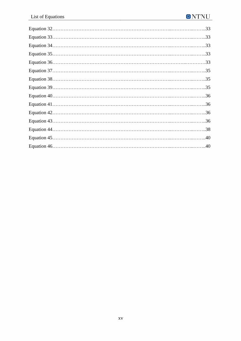
List of Equations
Equation 1………………………………………………………………..…………..……....16
Equation 2………...……………………………………………………………..……...……17
Equation 3………………………………………………………………..…………..……....18
Equation 4………………………………………………………………..…………..……....21
Equation 5………………………………………………………………..…………..……....21
Equation 6………………………………………………………………..…………..……....21
Equation 7………………………………………………………………..…………..……....23
Equation 8………………………………………………………………..…………..……....23
Equation 9………………………………………………………………..…………..……....25
Equation 10………………………………………………………………..…………..……..27
Equation 11………………………………………………………………..…………..……..28
Equation 12………………………………………………………………..…………..……..28
Equation 13………………………………………………………………..…………..……..28
Equation 14………………………………………………………………..…………..……..28
Equation 15………………………………………………………………..…………..……..28
Equation 16………………………………………………………………..…………..……..28
Equation 17………………………………………………………………..…………..……..29
Equation 18………………………………………………………………..…………..……..29
Equation 19………………………………………………………………..…………..……..29
Equation 20………………………………………………………………..…………..……..29
Equation 21………………………………………………………………..…………..……..29
Equation 22………………………………………………………………..…………..……..29
Equation 23………………………………………………………………..…………..……..29
Equation 24………………………………………………………………..…………..……..29
Equation 25………………………………………………………………..…………..……..30
Equation 26………………………………………………………………..…………..……..30
Equation 27………………………………………………………………..…………..……..31
Equation 28………………………………………………………………..…………..……..31
Equation 29………………………………………………………………..…………..……..31
Equation 30………………………………………………………………..…………..……..33
Equation 31………………………………………………………………..…………..……..33
List of Equations
xv
Equation 32………………………………………………………………..…………..……..33
Equation 33………………………………………………………………..…………..……..33
Equation 34………………………………………………………………..…………..……..33
Equation 35………………………………………………………………..…………..……..33
Equation 36………………………………………………………………………..…………33
Equation 37………………………………………………………………..…………..……..35
Equation 38………………………………………………………………..…………..……..35
Equation 39………………………………………………………………..…………..……..35
Equation 40………………………………………………………………..…………..……..36
Equation 41………………………………………………………………..…………..……..36
Equation 42………………………………………………………………..…………..……..36
Equation 43………………………………………………………………..…………..……..36
Equation 44………………………………………………………………..…………..……..38
Equation 45………………………………………………………………..…………..……..40
Equation 46………………………………………………………………..…………..……..40
xvi
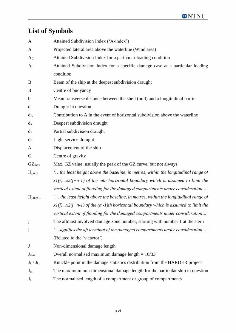
List of Symbols
A Attained Subdivision Index (‘A-index’)
A Projected lateral area above the waterline (Wind area)
AC Attained Subdivision Index for a particular loading condition
Ai Attained Subdivision Index for a specific damage case at a particular loading
condition
B Beam of the ship at the deepest subdivision draught
B Centre of buoyancy
b Mean transverse distance between the shell (hull) and a longitudinal barrier
d Draught in question
dA Contribution to A in the event of horizontal subdivision above the waterline
ds Deepest subdivision draught
dP Partial subdivision draught
dL Light service draught
Δ Displacement of the ship
G Centre of gravity
GZmax Max. GZ value; usually the peak of the GZ curve, but not always
Hj,n,m ‘…the least height above the baseline, in metres, within the longitudinal range of
x1(j)...x2(j+n-1) of the mth horizontal boundary which is assumed to limit the
vertical extent of flooding for the damaged compartments under consideration…’
Hj,n,m-1 ‘… the least height above the baseline, in metres, within the longitudinal range of
x1(j)...x2(j+n-1) of the (m-1)th horizontal boundary which is assumed to limit the
vertical extent of flooding for the damaged compartments under consideration…’
j The aftmost involved damage zone number, starting with number 1 at the stern
j ‘…signifies the aft terminal of the damaged compartments under consideration…’
(Related to the ‘v-factor’)
J Non-dimensional damage length
Jmax Overall normalised maximum damage length = 10/33
Jk / Jkn Knuckle point in the damage statistics distribution from the HARDER project
Jm The maximum non-dimensional damage length for the particular ship in question
Jn The normalised length of a compartment or group of compartments
List of Symbols
xvii
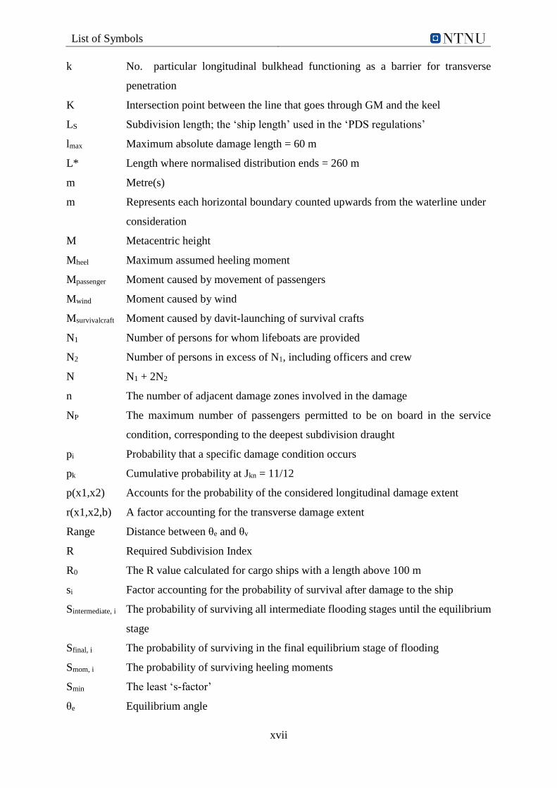
k No. particular longitudinal bulkhead functioning as a barrier for transverse
penetration
K Intersection point between the line that goes through GM and the keel
LS Subdivision length; the ‘ship length’ used in the ‘PDS regulations’
lmax Maximum absolute damage length = 60 m
L* Length where normalised distribution ends = 260 m
m Metre(s)
m Represents each horizontal boundary counted upwards from the waterline under
consideration
M Metacentric height
Mheel Maximum assumed heeling moment
Mpassenger Moment caused by movement of passengers
Mwind Moment caused by wind
Msurvivalcraft Moment caused by davit-launching of survival crafts
N1 Number of persons for whom lifeboats are provided
N2 Number of persons in excess of N1, including officers and crew
N N1 + 2N2
n The number of adjacent damage zones involved in the damage
NP The maximum number of passengers permitted to be on board in the service
condition, corresponding to the deepest subdivision draught
pi Probability that a specific damage condition occurs
pk Cumulative probability at Jkn = 11/12
p(x1,x2) Accounts for the probability of the considered longitudinal damage extent
r(x1,x2,b) A factor accounting for the transverse damage extent
Range Distance between θe and θv
R Required Subdivision Index
R0 The R value calculated for cargo ships with a length above 100 m
si Factor accounting for the probability of survival after damage to the ship
Sintermediate, i The probability of surviving all intermediate flooding stages until the equilibrium
stage
Sfinal, i The probability of surviving in the final equilibrium stage of flooding
Smom, i The probability of surviving heeling moments
Smin The least ‘s-factor’
θe Equilibrium angle
List of Symbols
xviii
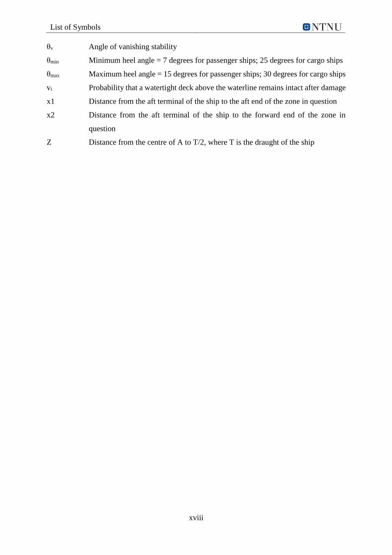
θv Angle of vanishing stability
θmin Minimum heel angle = 7 degrees for passenger ships; 25 degrees for cargo ships
θmax Maximum heel angle = 15 degrees for passenger ships; 30 degrees for cargo ships
vi Probability that a watertight deck above the waterline remains intact after damage
x1 Distance from the aft terminal of the ship to the aft end of the zone in question
x2 Distance from the aft terminal of the ship to the forward end of the zone in
question
Z Distance from the centre of A to T/2, where T is the draught of the ship

xix
List of Acronyms
A-index Attained Subdivision Index A
Ch. Chapter
DDS Deterministic damage stability
FSE Free surface effect
GA General Arrangement
HARDER Harmonization of Rules and Design Rationale
ICCL International Convention on Load Lines
IMO International Maritime Organization
LCB Longitudinal centre of buoyancy
LCF Longitudinal centre of flotation
LCG Longitudinal centre of gravity
LOA Length over all
LSA Life-saving appliances
LPP Length between perpendiculars
MCA Maritime and Coastguard Agency
MSC Maritime Safety Committee
PDF Portable Document Format
PDS Probabilistic damage stability
pdf Probability distribution function
PhD Doctor of Philosophy
Reg. Regulation
SPS Special Purpose Ship
SOLAS Safety of Life at Sea
WFSV Wind Farm Service Vessel

xx
1
1. Introduction
In an ideal world, Naval Architects would optimise ship designs in order to achieve the best
possible solutions in terms of: ship performance, environmental footprint, safety and costs for
instance. To find an optimal balance between all design parameters is unrealistic as time and
resources are limited in all projects. In ship design today, the top-down design approach is
widely used; main dimensions are determined first whereas more detailed design such as the
watertight subdivision appears later in the process. The watertight subdivision is restricted by
damage stability regulations, and the required calculations are time-consuming. Due to the time
pressure that usually occurs at the end of projects, it is thus advantageous to limit the number
of design iterations. Relying on previous experience is challenging when ship designs are
constantly developed. In consequence, predicting the outcome of the damage stability
calculations is not straightforward. Thus, to know the effects of certain changes in the internal
watertight arrangement of a ship at early design stages, would surely be beneficial in order to
reduce the number of iterations at late design stages.
1.1 Historical Background and Motivation
There are two applicable damage stability calculation methods for ships: deterministic damage
stability (DDS) and probabilistic damage stability (PDS). The appropriate method depends on
the ship in question. The probabilistic approach, which is based on damage statistics in terms
of the size and location of the damage on previously rammed ships, is considered to be more
rationale than the deterministic approach.
The development of PDS regulations started in the late 60s, and a few years later Resolution
A.265 (VIII) of SOLAS-74 entered into force. This was only an alternative to the deterministic
procedure for dry cargo ships and passenger ships, which still was a part of SOLAS. Today’s
prevailing PDS regulations can be found in SOLAS Chapter II-1, Part B-1, and stems from a
project called ‘Harmonization of Rules and Design Rationale’ (HARDER)’. The HARDER
project started to collect large amounts of collision and grounding data in 2001, with the aim of
harmonizing the damage stability regulations for all ship types. All existing approaches to PDS
calculations were re-evaluated and new formulations were proposed to the existing regulations.
The final proposals were adopted in 2005 by the Maritime Safety Committee (MSC), an
underlying committee of IMO, and the new regulations entered into force in 2009. These are
relevant for dry cargo ships with a length above 80 meters and passenger ships built after

Chapter 1. Introduction
2
January 1st, 2009. With the new PDS regulations in place, IMO actually proclaimed that DDS
has no future (Papanikolaou & Eliopoulou, 2008; Vassalos, 2014).
Due to the ‘Code of Safety for Special Purpose Ships, 2008’ (SPS Code), which was adopted
in 2008 by IMO Resolution MSC.266(84), Special Purpose Ships (SPSs) are also covered by
the PDS regulations. If a ship has SPS notation1, it is in general considered a passenger ship in
accordance with the damage stability regulations in SOLAS Chapter II-1, Part B-1. Platform
supply vessels (PSVs) are for instance not covered by the SPS Code, which means that PSVs
are excluded from the PDS regulations. IMO Resolution MSC.235(82) should then be applied,
which follows a deterministic approach. An increasing number of other offshore service vessel
(OSV) types, however, are classified with SPS notation; more OSVs than before are now
involved in operations that requires more on-board special personnel. Wind farm service vessels
could be an example of this.
There are certain design advantages with the probabilistic approach. One advantage with the
deterministic approach is the simple calculation procedure that makes it possible to quickly
estimate the survivability of ships. The complexity of the PDS regulations indicates that the
probabilistic approach is more accurate and realistic. Additionally, the PDS regulations offer
flexibility in the design of watertight arrangements which the DDS regulations cannot offer.
With the DDS regulations, the location of bulkheads is defined by pre-determined damage
extents. That is not the case with the PDS regulations; bulkheads can be placed anywhere. The
‘million-dollar question’ then arises: how can the ship designer take advantage of the flexibility
in design that the PDS regulations offer? (Djupvik, Aanondsen, & Asbjørnslett, 2015; Hjort &
Olufsen, 2014).
One obvious obstacle related to the abovementioned flexibility is the top-down design
approach. Top down design ironically makes the probabilistic approach less flexible than it
potentially could be and is unlikely to be switched out with a bottom-up approach. Thus, time
pressure will continue to be a limiting factor for PDS calculations at the end of projects. It is
therefore interesting to know as much as possible, on beforehand of projects, about effects that
certain design changes have on the results of PDS calculations. This problem is the motivational
basis for the master’s thesis.
1 ‘…a special purpose ship is a ship of not less than 500 gross tonnage which carries more than 12 special
personnel, i.e. persons who are specially needed for the particular operational duties of the ship and are carried
in addition to those persons required for the normal navigation, engineering and maintenance of the ship or
engaged to provide services for the persons carried on board.’ (IMO, 2008b)

Chapter 1. Introduction
3
1.2 Previous Work
There is a limited amount of existing research related to the objectives of the master’s thesis,
i.e. how changes in the arrangement and initial stability of an offshore vessel impacts the
attained subdivision index (A-index). Most research on probabilistic damage stability focus on
optimisation methods that can be used to maximise the A-index for passenger vessels or Ro-Ro
vessels. This research will not be elaborated further in this thesis as it is considered less relevant
for the topic of the thesis. For further reading on the subject it is referred to the PhD thesis by
Erik Sonne Ravn from 2003 and a study presented in the Journal of Shipping and Ocean
Engineering 2 in 2012 by Puisa, Tsakalakis and Vassalos (Puisa, Tsakalakis, & Vassalos, 2012;
Ravn, February 2003).
The master’s thesis written by Ole Martin Djupvik in 2015 at the Department of Marine
Technology at NTNU (Djupvik et al., 2015), seems to be the research with strongest relevance
to this master’s thesis. Mr. Djupvik looked at two different arrangement configurations for four
different sizes of an offshore vessel. He investigated how the placement of a specific
longitudinal bulkhead (LBH) typically located in the mid-ship section of offshore vessels
affects the A-index. It was also investigated whether or not this effect changes proportionally
with the size of the vessel, in order to see whether a generic model for optimal placement of the
LBH could be developed for offshore vessels in general. Such a model could not be developed,
unfortunately. However, Mr. Djupvik discovered for example that the A-index decreases when
damages to the wing ballast tanks becomes critical to the survivability of the vessel (Djupvik et
al., 2015).
Chapter 1. Introduction
4
1.3 Objectives and Scope of Work
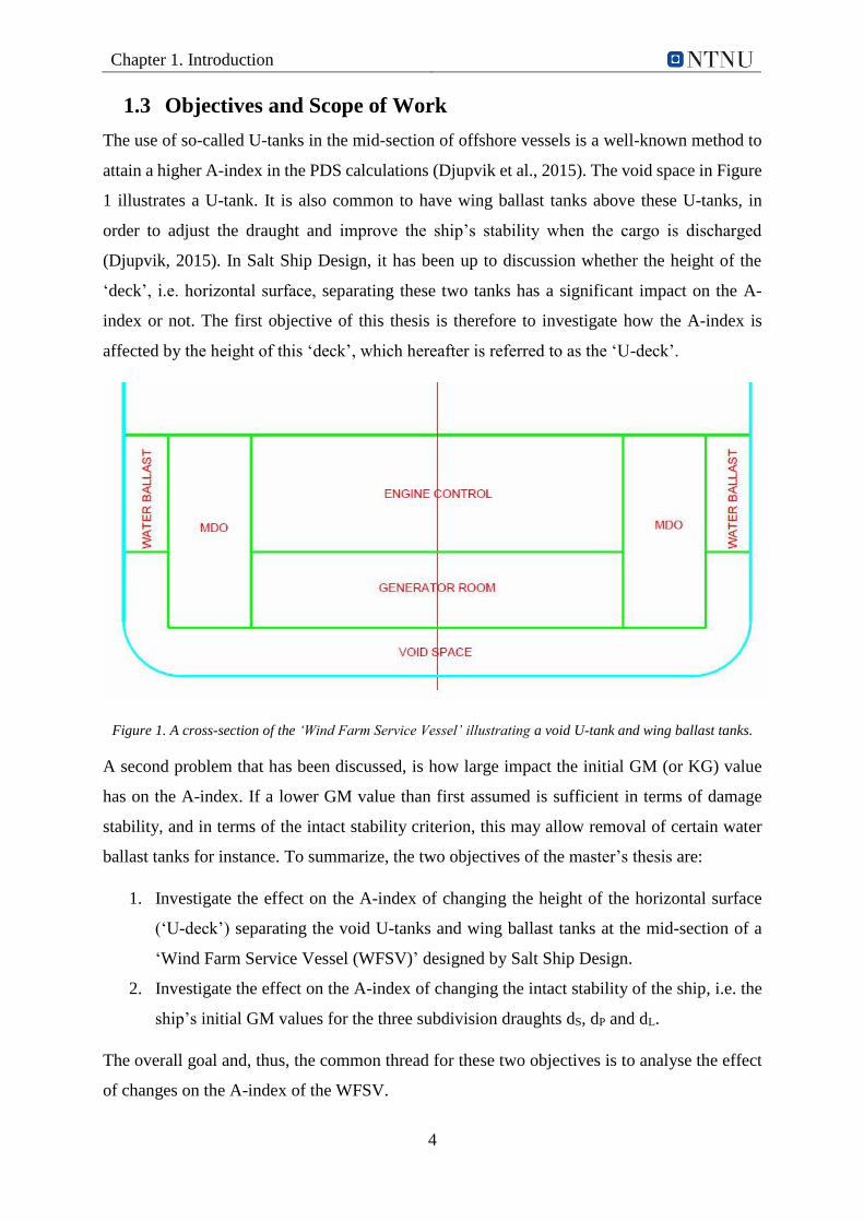
The use of so-called U-tanks in the mid-section of offshore vessels is a well-known method to
attain a higher A-index in the PDS calculations (Djupvik et al., 2015). The void space in Figure
1 illustrates a U-tank. It is also common to have wing ballast tanks above these U-tanks, in
order to adjust the draught and improve the ship’s stability when the cargo is discharged
(Djupvik, 2015). In Salt Ship Design, it has been up to discussion whether the height of the
‘deck’, i.e. horizontal surface, separating these two tanks has a significant impact on the A-
index or not. The first objective of this thesis is therefore to investigate how the A-index is
affected by the height of this ‘deck’, which hereafter is referred to as the ‘U-deck’.
Figure 1. A cross-section of the ‘Wind Farm Service Vessel’ illustrating a void U-tank and wing ballast tanks.
A second problem that has been discussed, is how large impact the initial GM (or KG) value
has on the A-index. If a lower GM value than first assumed is sufficient in terms of damage
stability, and in terms of the intact stability criterion, this may allow removal of certain water
ballast tanks for instance. To summarize, the two objectives of the master’s thesis are:
1. Investigate the effect on the A-index of changing the height of the horizontal surface
(‘U-deck’) separating the void U-tanks and wing ballast tanks at the mid-section of a
‘Wind Farm Service Vessel (WFSV)’ designed by Salt Ship Design.
2. Investigate the effect on the A-index of changing the intact stability of the ship, i.e. the
ship’s initial GM values for the three subdivision draughts dS, dP and dL.
The overall goal and, thus, the common thread for these two objectives is to analyse the effect
of changes on the A-index of the WFSV.
Chapter 1. Introduction
5
Briefly described, the scope of work related to the abovementioned objectives is:
- Carry out a literature study on intact stability, DDS and PDS – the theory that the
individual study in this thesis is built upon.
- Learn how the stability software NAPA works.
- Use NAPA to model the watertight arrangement of the ship used in the individual study.
- Use NAPA to calculate PDS for the ship in question, for objective 1 and 2 of the thesis.
- Post-process the results with Microsoft Excel or another software, in order to plot the
results and present them in a tidy manner.
- Analyse the results in-depth, i.e. study all ‘PDS factors’ that may have influenced the
results, to achieve a thorough understanding.
- Discuss the analysed results with respect to the objectives.
- Finally, draw conclusions and suggest further work.
1.4 Limitations
One ship is investigated with respect to the development of the A-index. Preferably, the study
should have been conducted for several offshore vessels that may apply to the SPS Code, to
obtain as generic results and conclusions as possible.
The scope of the study is furthermore limited to four variables: the height of the deck separating
the void U-tanks and wing ballast tanks, and the three GM values corresponding to the
subdivision draughts that are accounted for in the PDS regulations.
1.5 Thesis Structure
This master’s thesis follows the ‘IMRAD - Introduction, Methods, Results and Discussion’
style, with some alterations. For instance, a theory chapter regarding ship stability theory is
included in chapter 2, between the introduction in chapter 1 and the methods of the individual
study in chapter 0. This is considered beneficial, because some readers will benefit of having
PDS theory easily accessible when reading the thesis. Chapter 5 includes both analysis and
discussion of the results presented in chapter 4. A detailed content description for each chapter
is given below.
Chapter 1. Introduction
6
Chapter 2: Ship Stability Theory
This chapter presents theory on intact stability, DDS and PDS. One could say that the PDS part
of chapter 2 is a re-presentation of SOLAS-2009, but it better explains how the theory should
be interpreted. By studying this chapter, the reader should get a basic understanding of stability
and damage stability theory on ships, which will benefit the reader when studying the rest of
the thesis.
Chapter 3: Individual Study on Probabilistic Damage Stability
Chapter 0 describes how the individual study in this thesis was conducted, including some more
information regarding the two objectives of the thesis. The chapter also provides information
about the ship used in the study, and furthermore explains the approaches used to model the
ship and carry out PDS calculations in NAPA. Descriptions of some analysis tools in NAPA
are also given.
Chapter 4: Results of Individual Study
This chapter presents the post-processed results from the PDS calculations in NAPA. Some
comments and evaluation of the results are also included in chapter 4.
Chapter 5: Analysis and Discussion
In Chapter 5, the results from chapter 4 are analysed in-depth, in order to fully understand the
development of the ship’s damage stability. In addition to the results' analyses a discussion on
the quality and interpretation of results is given.
Chapter 6: Conclusion
Finally, conclusions regarding objective 1 and 2 of the thesis are drawn based on the analysed
results in chapter 5. Additionally, suggestions to further work related to the study conducted in
this master’s thesis are provided.
Chapter 7: Bibliography
All references that are referred to in the thesis are listed in Chapter 7.
7
2. Ship Stability Theory2
A ship’s ability to stay afloat relies on the stability of the ship. Ship stability may in simple
terms be defined as a ship’s ability to return to its upright position, i.e. an angle of heel equal
to 0°, after external forces have acted on the ship and, consequently, created a heeling moment.
External forces are often induced by environmental phenomena such as waves and wind, but
other sources may be shifting cargo, contact with obstacles in the sea or collision with other
ships. Generally, ship stability can be divided into two categories: intact stability and damage
stability (Magnussen, Amdahl, & Fuglerud, 2014).
2.1 Introduction to Intact Stability
Intact stability evaluates the stability of a ship in an undamaged condition, both in transverse
and longitudinal direction. It is assumed that the reader has basic knowledge regarding intact
stability, and it is not within the scope of the master’s thesis to go into full detail on the topic.
Some fundamentals that are considered important to have fresh in mind will be touched upon.
2.1.1 Transverse Stability
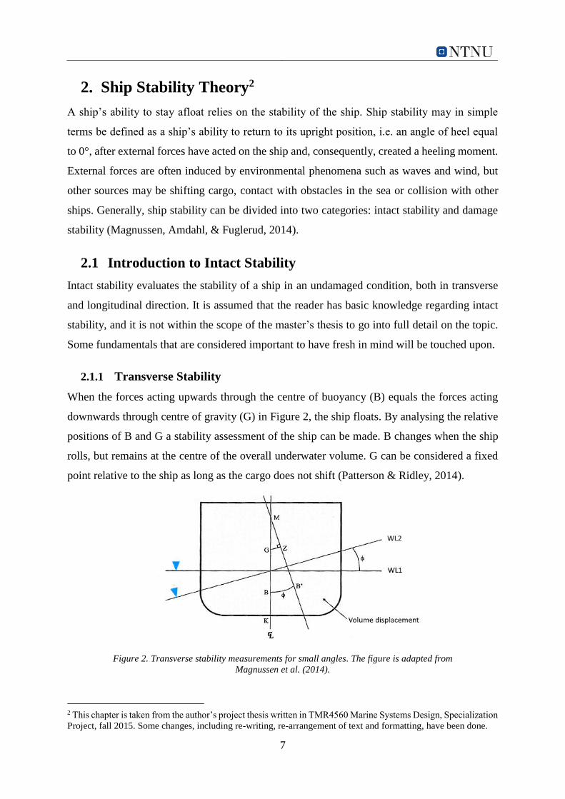
When the forces acting upwards through the centre of buoyancy (B) equals the forces acting
downwards through centre of gravity (G) in Figure 2, the ship floats. By analysing the relative
positions of B and G a stability assessment of the ship can be made. B changes when the ship
rolls, but remains at the centre of the overall underwater volume. G can be considered a fixed
point relative to the ship as long as the cargo does not shift (Patterson & Ridley, 2014).
Figure 2. Transverse stability measurements for small angles. The figure is adapted from
Magnussen et al. (2014).
2 This chapter is taken from the author’s project thesis written in TMR4560 Marine Systems Design, Specialization
Project, fall 2015. Some changes, including re-writing, re-arrangement of text and formatting, have been done.
8
Although the ship floats, it is not necessarily stable. A ship is considered stable when the
distance GM has a positive value. GM = KB + BM – KG. This method of using the metacentric
height (M) as a measure of stability is called initial stability, and is only valid for small angles,
i.e. up to 10 to 15 degrees of heel. That is because M is not considered stationary for larger
angles (Patterson & Ridley, 2014).
Instead a method called large angle stability is used. This method also utilizes B and G, but now
the heeling moment, or listing moment, caused by the misalignment of the forces acting through
these points are in focus. This moment is controlled by the transverse distance between G and
B, namely GZ, which is defined as the ship’s righting lever, or righting arm. The product of GZ
and the ship’s displacement, Δ, then defines the righting moment, or torque of the ship. When
the heeling moment equals the righting moment the ship enters a steady state of equilibrium,
and the angle of heel will stabilize at a specific value (Patterson & Ridley, 2014).
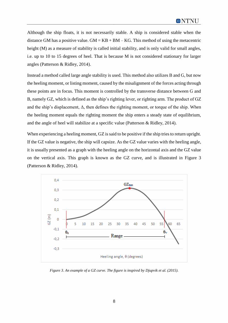
When experiencing a heeling moment, GZ is said to be positive if the ship tries to return upright.
If the GZ value is negative, the ship will capsize. As the GZ value varies with the heeling angle,
it is usually presented as a graph with the heeling angle on the horizontal axis and the GZ value
on the vertical axis. This graph is known as the GZ curve, and is illustrated in Figure 3
(Patterson & Ridley, 2014).
Figure 3. An example of a GZ curve. The figure is inspired by Djupvik et al. (2015).
9
θe is the angle of heel where the GZ value changes from negative to positive, and is known as
the equilibrium angle. θv is known as the angle of vanishing stability, and is the point where the
GZ value changes from positive to negative. Furthermore, the peak of the curve is known as
GZmax, and the range from θe to θv is naturally known as the range of stability, or just range. For
any vessel, it is possible to create a curve of righting moments. This will look identical to the
GZ curve, as the righting moment equals GZ multiplied with a constant. The area under this
curve up to a certain angle is equal to the energy needed to roll the vessel to that angle. The area
under the GZ curve up to a certain angle is thus proportional to the energy needed to roll the
vessel to that angle. In other words, the larger area under the curve, the more energy is needed
to roll the vessel (Patterson & Ridley, 2014).
IMO’s ‘International Code On Intact Stability, 2008’ (2008 IS Code), include requirements
both concerning the metacentric height criteria and minimum values for areas under the GZ
curve. The 2008 IS Code requires that the area under the GZ curve have minimum values
between specific angles, and that the peak of the GZ curve is in a certain region of the graph
(IMO, 2008a).
2.1.2 Longitudinal Stability
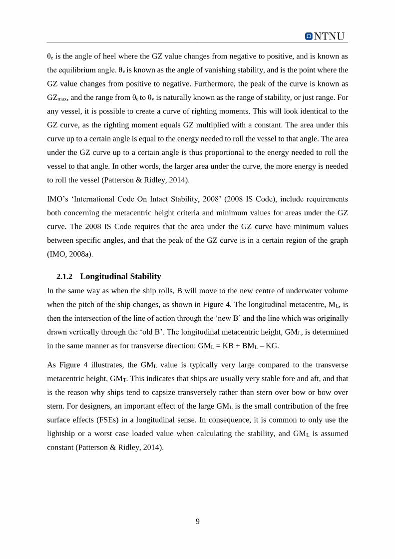
In the same way as when the ship rolls, B will move to the new centre of underwater volume
when the pitch of the ship changes, as shown in Figure 4. The longitudinal metacentre, ML, is
then the intersection of the line of action through the ‘new B’ and the line which was originally
drawn vertically through the ‘old B’. The longitudinal metacentric height, GML, is determined
in the same manner as for transverse direction: GML = KB + BML – KG.
As Figure 4 illustrates, the GML value is typically very large compared to the transverse
metacentric height, GMT. This indicates that ships are usually very stable fore and aft, and that
is the reason why ships tend to capsize transversely rather than stern over bow or bow over
stern. For designers, an important effect of the large GML is the small contribution of the free
surface effects (FSEs) in a longitudinal sense. In consequence, it is common to only use the
lightship or a worst case loaded value when calculating the stability, and GML is assumed
constant (Patterson & Ridley, 2014).
10
Figure 4. A ship that is trimmed by the stern (positive trim). The figure is inspired by
Patterson and Ridley (2014).
Furthermore, a ship is said to be trimmed if the draughts measured at the after perpendicular
and the forward perpendicular are different. The trim is controlled by the relative positions of
the longitudinal centres of buoyancy and gravity, abbreviated LCB and LCG respectively.
However, the trim is only said to be a part of the problem regarding longitudinal stability. The
draughts at both ends of the ship, which varies with the trim, and the draught at the longitudinal
centre of flotation (LCF) is of equal importance. At the LCF, the draught is independent of the
trim, as it is the rotation point in trim. The draught at this point is known as the true mean
draught, DTMD or DLCF, and is the value listed in the hydrostatic tables used in stability
calculations (Patterson & Ridley, 2014).
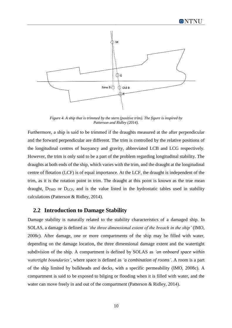
2.2 Introduction to Damage Stability
Damage stability is naturally related to the stability characteristics of a damaged ship. In
SOLAS, a damage is defined as ‘the three dimensional extent of the breach in the ship’ (IMO,
2008c). After damage, one or more compartments of the ship may be filled with water,
depending on the damage location, the three dimensional damage extent and the watertight
subdivision of the ship. A compartment is defined by SOLAS as ‘an onboard space within
watertight boundaries’, where space is defined as ‘a combination of rooms’. A room is a part
of the ship limited by bulkheads and decks, with a specific permeability (IMO, 2008c). A
compartment is said to be exposed to bilging or flooding when it is filled with water, and the
water can move freely in and out of the compartment (Patterson & Ridley, 2014).
11
2.2.1 The Lost Buoyancy Method
There are several ways to evaluate the trim and stability of a ship after flooding, but the most
common method adopted by IMO is known as ‘lost volume’ or ‘lost buoyancy’. The effect of
flooding is then determined in several steps (Patterson & Ridley, 2014):
1. Parallel sinkage (Initial sinkage)
2. New position of B
3. New BM and BML
4. New GM and GML
5. Resulting heel and trim
Steps 2 to 5 will not be explained, but some elaboration on step 1 is considered relevant within
the scope of the master’s thesis. First of all, when one or more compartments are flooded, the
ship will get a higher draught. This initial sinkage is known as parallel sinkage. Dependent on
the position of the compartments, the ship will also heel or trim. This is because the
compartments in question, before flooding, contributes to the overall underwater volume of the
ship. Thus they provide some of the ship’s total buoyancy force supporting the vessel. After
flooding, these compartments no longer provide this buoyancy, the total buoyancy force is
consequently reduced and the ship becomes less stable (Patterson & Ridley, 2014).
As the ship moves vertically downwards due to flooding, the total underwater volume will
gradually increase. The remaining buoyant volume is produced by the compartments that are
still intact. At some point, the force of buoyancy has increased enough to be back in equilibrium
with the gravity force, and the sinking stops. The overall underwater volume lost through
flooding is now equal to the underwater volume (buoyant volume) gained through sinkage. The
parallel sinkage can be determined from this principle (Patterson & Ridley, 2014).
The theory above assumes that the flooded compartments are completely filled with water. In
reality this may not be the case. In the machinery rooms for instance, there are engines and
other components that cannot flood. Let us say that these components take up 60% of the
machinery room, then this is modelled using a factor of 0.6. This is known as the compartment
permeability factor. The permeability has an effect on both the volume flooded and the
waterplane area lost. This is taken into account by adjusting the parallel sinkage formula
(Patterson & Ridley, 2014).
12
2.2.2 Damage Stability Regulations
Similar to intact stability, there are international regulations that ships must comply with
regarding damage stability. The regulations are quite complex and do not guarantee safety, but
they are meant to help the designers create safe ships. As explained previously, ships are
designed to be safe both concerning initial and large angle stability, and also to some extent
when the ship is damaged. The regulations introduced in Table 1 are developed in order to
increase the probability of survival in case of ship damage. However, this probability can only
be minimised; never set to zero. It is not possible to design an unsinkable passenger ship that is
still feasible to invest in. The master’s thesis will not go into detail on the regulations in the
below table, except for ‘regulation E’ which includes PDS, but a short introduction to each of
them is provided in this sub-section (Patterson & Ridley, 2014).
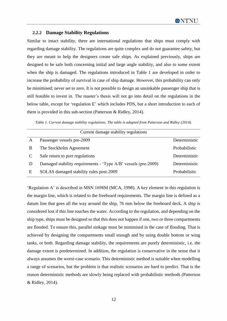
Table 1. Current damage stability regulations. The table is adapted from Patterson and Ridley (2014).
Current damage stability regulations
A Passenger vessels pre-2009 Deterministic
B The Stockholm Agreement Probabilistic
C Safe return to port regulations Deterministic
D Damaged stability requirements - ‘Type A/B’ vessels (pre-2009) Deterministic
E SOLAS damaged stability rules post-2009 Probabilistic
‘Regulation A’ is described in MSN 1698M (MCA, 1998). A key element in this regulation is
the margin line, which is related to the freeboard requirements. The margin line is defined as a
datum line that goes all the way around the ship, 76 mm below the freeboard deck. A ship is
considered lost if this line touches the water. According to the regulation, and depending on the
ship type, ships must be designed so that this does not happen if one, two or three compartments
are flooded. To ensure this, parallel sinkage must be minimised in the case of flooding. That is
achieved by designing the compartments small enough and by using double bottom or wing
tanks, or both. Regarding damage stability, the requirements are purely deterministic, i.e. the
damage extent is predetermined. In addition, the regulation is conservative in the sense that it
always assumes the worst-case scenario. This deterministic method is suitable when modelling
a range of scenarios, but the problem is that realistic scenarios are hard to predict. That is the
reason deterministic methods are slowly being replaced with probabilistic methods (Patterson
& Ridley, 2014).
13
The Stockholm Agreement described in MSC/Circ. 574, which is applicable to large Ro-Ro
passenger ships, is following a probabilistic approach. The agreement defines an additional
standard that neighbouring port states may apply to Ro-Ro passenger ships. These requirements
are not a part of the SOLAS Convention, as it in fact describes a maximum standard. The
standard assesses the probability of a ship surviving a damage causing water ingress. The
damage probability varies according to the location on the ship. The probability of compartment
flooding and the probability of surviving the compartment flooding are also taken into account
in the overall survival probability. The regulation requires the calculation of A and Amax,
respectively representing a subdivision index and a maximum value of survivability of the ship.
In addition, depending on the freeboard, a hypothetical effect of 0.5 m or less of water on the
vehicle deck closest to the waterline is included. (Hjort & Olufsen, 2014; Patterson & Ridley,
2014).
The safe return to port regulations were approved by IMO in 2006, and is applicable to certain
passenger ships with a length of 120 m and above. This set of regulations states that the safest
lifeboat is the ship itself; a ship should be able to survive a damage and return safely to port,
even in the event of flooding of any one single watertight compartment. In the case of more
than one flooded compartment, the ship should be designed to be evacuated safely within three
hours after the damage occurs (Patterson & Ridley, 2014).
Before 2009, the set of regulations in row D in Table 1, was mandatory to all type of ships. Two
ship types are defined: A (carrying liquid cargo in bulk) and B (all other ships). The regulations
are deterministic in the sense that the amount of damage on the ship is predetermined; the
damage is assumed to be over the entire depth of the vessel in vertical extent and whichever is
lesser of B/5 and 11.5 m in transverse extent. In longitudinal direction the damage is limited to
a single compartment between transverse bulkheads, given that any longitudinal bulkheads are
outside of the transverse damage extent. However, this is different for so-called B-60 and B-
100 ships. B-60s are required to survive flooding of any compartments with a permeability of
95%. B-100s must survive flooding of any two adjacent compartments. Both of the two latter
requirements are not required for machinery spaces if the ship is lesser than 150 m in length
(Patterson & Ridley, 2014).

14
For any type of ship with a keel-laying date before January 1st 2009, the minimum requirements
shown in Figure 5 are required (Patterson & Ridley, 2014).
Figure 5. Damage stability requirements for all ships pre-2009. The figure is obtained from
Patterson and Ridley (2014).
In 2009, IMO introduced new regulations for dry cargo and passenger ships, which are based
on a mix of deterministic and probabilistic approaches. This set of regulations is referred to as
the ‘PDS regulations’ in the master’s thesis, and will be explained in Section 2.4. The
deterministic damage stability regulations will be referred to as the ‘DDS regulations’ hereafter,
and is briefly presented in Section 2.3. To sum up Section 2.2 and introduce the PDS regulations
at the same time: the main factors that affect the three-dimensional damage extent of a ship with
a given watertight subdivision, are listed below (IMO, 2008c):
The zones or group of adjacent zones that are flooded (‘zones’ is defined later)
Loading condition; draught, trim and intact GM at the time of damage
Permeability of flooded compartments at the time of damage
Sea state at the time of damage
Factors such as possible heeling moments due to unsymmetrical weights

15
2.3 Deterministic Damage Stability
A deterministic approach is a perfectly predictable approach. That is, the approach follows a
completely known rule, e.g. a fixed procedure, so that a given input will always give the same
output. The states of a system described by a deterministic approach may be numbers specifying
physical characteristics of the system, for instance observables such as length or mass. For
damage stability of ships, the DDS regulations are said to follow a deterministic approach
because the ship must survive a predetermined amount of damage (Kirchsteiger, 1999;
Patterson & Ridley, 2014).
Deterministic damage stability is all about ensuring that a ship is ‘safe enough’. It has been the
dominating method for a long time, and the DDS regulations are still in use today due to various
reasons. First of all, the PDS regulations do not cover all ship types. Secondly, despite the DDS
regulations’ well-known conservatism, it has a long track-record, and the society tends to trust
well-proven methods. A, C and D in Table 1 in Sub-section 2.2.2 are following a deterministic
approach. As mentioned, these three regulations apply to different types of passenger ships. In
addition to the SOLAS-74 standard, which regulates ordinary passenger ships, Table 2 provides
an overview of other IMO instruments that contain DDS provisions (Hjort & Olufsen, 2014).
Table 2. IMO instruments containing DDS provisions, besides of SOLAS-74.
The table is adapted from Hjort and Olufsen (2014).
Regulatory framework Application area
ICCL-66 Cargo ships and tankers with reduced freeboard
MARPOL-73/78 Tankers carrying cargo oil
IBC Code Ships carrying dangerous chemicals in bulk
IGC Code Ships carrying liquefied gases in bulk
HSC Code High speed crafts
2.3.1 Calculation Method
The outcome of DDS calculations, i.e. whether the ship is ‘safe enough’ or not, mainly depends
on the ship size; the length, beam and depth of the ship in question. Together these three
parameters determine the damage extent of the ship, as explained in Sub-section 2.3.2. In
general, the parameters used in the calculations are the same for different ship types, but the
impact of the parameters differ. This impact depends on factors such as ship type, ship size,
cargo type and number of passengers.

16
Furthermore, the ship in question is required to survive certain damage scenarios, given by the
predetermined damage extent. The goal is of course to identify the most critical damage
scenarios. This is done by investigating all possible damage conditions within the boundaries
of the damage extent. All damage scenarios must comply with the requirements as defined in
SOLAS. Some of these requirements are presented in Sub-section 2.3.3. If the results from the
calculations are not up to standard, the ship will not be approved by the flag state or the
classification societies (Djupvik et al., 2015; Patterson & Ridley, 2014).
2.3.2 Damage Extent
The damage extent comprises the longitudinal-, transverse- and vertical extent of the damage.
The longitudinal damage extent is determined by the length of the ship, L, as calculated by
Equation 1 (Patterson & Ridley, 2014).
Longitudinal damage extent = min(3 + 0.03 ∙ 𝐿 , 11) [𝑚] (1)
The definition of the ship length goes all the way back to the International Convention on Load
Lines, 1966 (ICCL-66), which states: ‘“Length” means 96% of the total length on a waterline
at 85% of the least moulded depth measured from the top of the keel, or the length from the
fore-side of the stem to the axis of the rudder stock on that waterline, if that be greater. Where
the stem contour is concave above the waterline at 85% of the least moulded depth, both the
forward terminal of the total length and the fore–side of the stem respectively shall be taken at
the vertical projection to that waterline of the aftermost point of the stem contour (above that
waterline). In ships designed with a rake of keel the waterline on which this length is measured
shall be parallel to the designed waterline.’(IMO, 1966). This definition is still in use today,
and is illustrated in Figure 6 (Djupvik et al., 2015).
Figure 6. Ship length as stated in ICCL-66. The figure is adapted from Djupvik et al. (2015).

17
The transverse damage extent is determined by Equation 2, where B is the beam of the ship. B
is measured at the deepest subdivision draught (load line), from the ship side 90° onto the centre
line (Hjort & Olufsen, 2014; Patterson & Ridley, 2014).
Transverse damage extent = Min (
𝐵
5, 11.5) [𝑚] (2)
The vertical damage extent has no limitations, and is taken as the entire depth of the ship.
Furthermore, a worst-case loading scenario shall always be assumed. The permeability is set to
e.g. 95% for accommodation and 85% for machinery spaces. If a lesser damage causes a worse
condition, then the worst case shall be used (Patterson & Ridley, 2014).
2.3.3 Requirements
After the ship has reached equilibrium position in a damage scenario where one or more
compartments are exposed to flooding, and the lost buoyancy method is used to calculate the
damaged trim and stability, the following requirements must be met (Patterson & Ridley, 2014):
1. GM > 0.05 m
2. Heel angle ≤ 7° for one compartment flooding, or 12° for two or more adjacent
compartments.
3. Specific minimum requirements related to the area under the GZ curve (see Figure 5).
4. Range of stability ≥ 15°. This requirement may be reduced from 15° to 10° if the area
under the GZ curve increases by a certain ratio.
5. Peak GZ value = 𝑀𝑎𝑥(𝐻𝑒𝑒𝑙𝑖𝑛𝑔 𝑚𝑜𝑚𝑒𝑛𝑡
∆+ 0.04, 0.10) [𝑚], where the heeling moment is
generated by:
1. All passengers crowding to deck areas on one side of the ship where
the muster stations are located, with a passenger weight of 75 kg and
a density of 4 passengers to a square metre.
2. Davit launching of all fully loaded survival crafts on one side of the
ship.
3. Wind pressure = 120 N/m2 on one side of the ship.
For any type of passenger vessel, the margin line must not be submerged in the final
equilibrium position.
18
2.4 Probabilistic Damage Stability
Basically, what is a probabilistic approach? First of all, a probabilistic approach involves some
degree of uncertainty. Thus, ‘random variables’ are required to develop prediction models,
which for example can be used to describe the behaviour of a system. There is no universal
definition of ‘randomness’, but in the context of damage stability it means that accidents and
the damage extent of accidents are unpredictable. In order to map the unpredictable, the only
available analytical tool is probability theory. Past knowledge, e.g. damage statistics, can be
used to predict random factors that influence the final consequence of damage to a ship’s hull.
Such random factors may be the mass and the velocity of the ramming ship. The influence of
these random factors is different for ships with different characteristics; for instance, differences
in the range of permeability and service draught (IMO, 2008c; Kirchsteiger, 1999).
The PDS regulations that entered into force on the 1st of January 2009 as a part of SOLAS
Chapter II-1, Part B-1 Stability, applies to dry cargo ships with a length of 80 m or above and
all passenger ships with keel laying on or after this date. A passenger ship is per definition a
ship carrying more than 12 passengers. In addition, because the ‘Code of Safety for Special
Purpose Ships, 2008’ (SPS code) was adopted in 2008 by IMO Resolution MSC.266(84),
Special Purpose Ships (SPSs) are also covered. Furthermore, all the ships applicable to the PDS
regulations are required to have double bottom and automatic cross flooding arrangements that
stabilize the ship within 10 minutes. On top of this, if the ship is carrying over 36 passengers,
there are additional deterministic requirements. These will not be detailed here, as the scope of
this section is to explain the probabilistic approach (IMO, 2006, 2008b).
Whether a ship is ‘safe enough’ according to the PDS regulations or not, is determined by
Equation 3. In SOLAS Chapter II-1, Part B-1 Stability, Reg. 7, A is defined as the ‘Attained
Subdivision Index’ and R is defined as the ‘Required Subdivision Index’. Two different ships
are considered equally safe if they have the same value of A. The calculation of A is based on
the probability of damage, i.e. flooding of compartments, and the survivability of the ship after
flooding. This and more are explained in detail throughout this section (IMO, 2006, 2008c;
Patterson & Ridley, 2014).
𝐴 > 𝑅 (3)
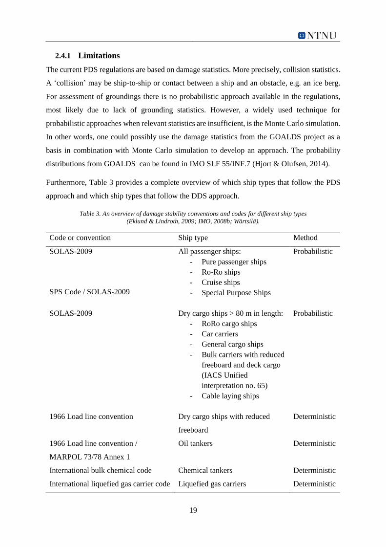
19
2.4.1 Limitations
The current PDS regulations are based on damage statistics. More precisely, collision statistics.
A ‘collision’ may be ship-to-ship or contact between a ship and an obstacle, e.g. an ice berg.
For assessment of groundings there is no probabilistic approach available in the regulations,
most likely due to lack of grounding statistics. However, a widely used technique for
probabilistic approaches when relevant statistics are insufficient, is the Monte Carlo simulation.
In other words, one could possibly use the damage statistics from the GOALDS project as a
basis in combination with Monte Carlo simulation to develop an approach. The probability
distributions from GOALDS can be found in IMO SLF 55/INF.7 (Hjort & Olufsen, 2014).
Furthermore, Table 3 provides a complete overview of which ship types that follow the PDS
approach and which ship types that follow the DDS approach.
Table 3. An overview of damage stability conventions and codes for different ship types
(Eklund & Lindroth, 2009; IMO, 2008b; Wärtsilä).
Code or convention Ship type Method
SOLAS-2009
SPS Code / SOLAS-2009
All passenger ships:
- Pure passenger ships
- Ro-Ro ships
- Cruise ships
- Special Purpose Ships
Probabilistic
SOLAS-2009 Dry cargo ships > 80 m in length:
- RoRo cargo ships
- Car carriers
- General cargo ships
- Bulk carriers with reduced
freeboard and deck cargo
(IACS Unified
interpretation no. 65)
- Cable laying ships
Probabilistic
1966 Load line convention Dry cargo ships with reduced
freeboard
Deterministic
1966 Load line convention /
MARPOL 73/78 Annex 1
Oil tankers Deterministic
International bulk chemical code Chemical tankers Deterministic
International liquefied gas carrier code Liquefied gas carriers Deterministic
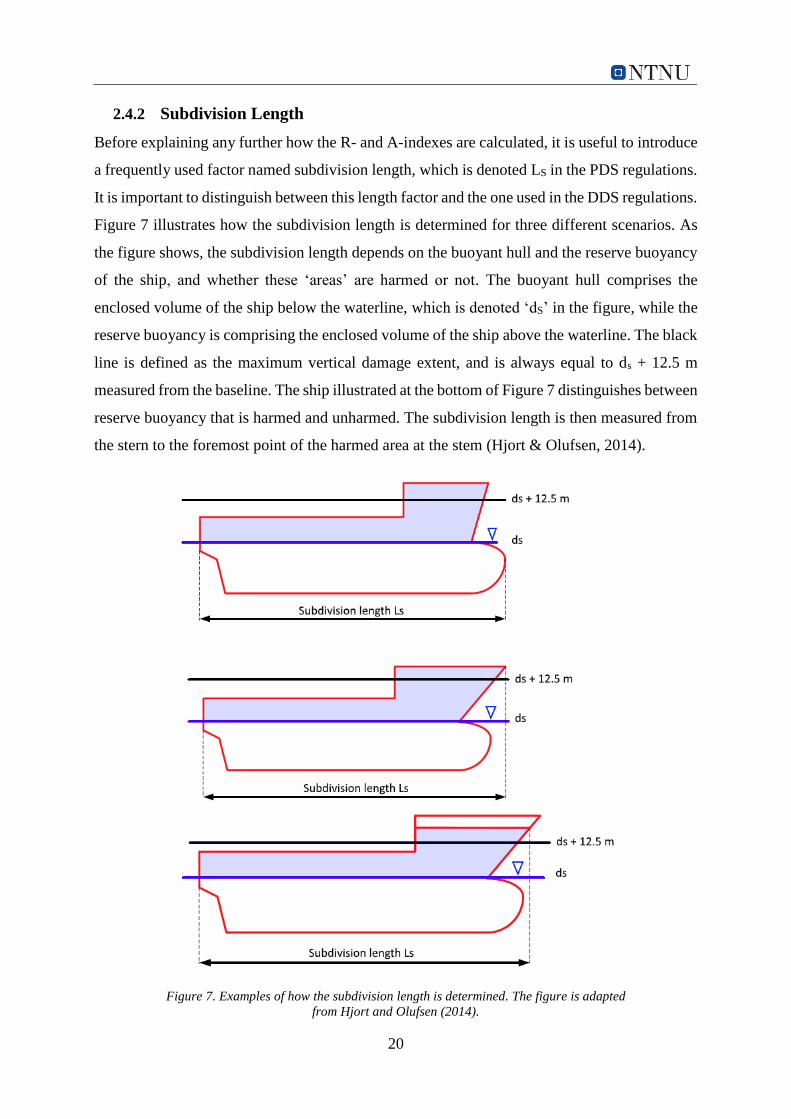
20
2.4.2 Subdivision Length
Before explaining any further how the R- and A-indexes are calculated, it is useful to introduce
a frequently used factor named subdivision length, which is denoted LS in the PDS regulations.
It is important to distinguish between this length factor and the one used in the DDS regulations.
Figure 7 illustrates how the subdivision length is determined for three different scenarios. As
the figure shows, the subdivision length depends on the buoyant hull and the reserve buoyancy
of the ship, and whether these ‘areas’ are harmed or not. The buoyant hull comprises the
enclosed volume of the ship below the waterline, which is denoted ‘dS’ in the figure, while the
reserve buoyancy is comprising the enclosed volume of the ship above the waterline. The black
line is defined as the maximum vertical damage extent, and is always equal to ds + 12.5 m
measured from the baseline. The ship illustrated at the bottom of Figure 7 distinguishes between
reserve buoyancy that is harmed and unharmed. The subdivision length is then measured from
the stern to the foremost point of the harmed area at the stem (Hjort & Olufsen, 2014).
Figure 7. Examples of how the subdivision length is determined. The figure is adapted
from Hjort and Olufsen (2014).
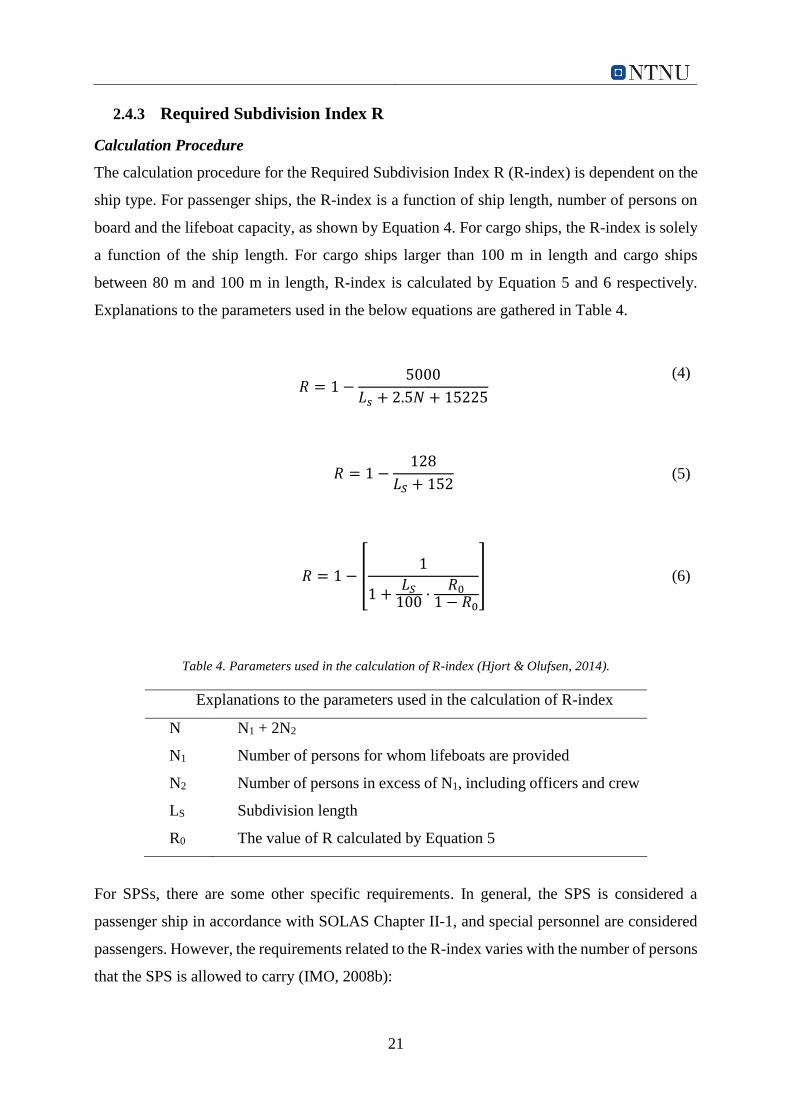
21
2.4.3 Required Subdivision Index R
Calculation Procedure
The calculation procedure for the Required Subdivision Index R (R-index) is dependent on the
ship type. For passenger ships, the R-index is a function of ship length, number of persons on
board and the lifeboat capacity, as shown by Equation 4. For cargo ships, the R-index is solely
a function of the ship length. For cargo ships larger than 100 m in length and cargo ships
between 80 m and 100 m in length, R-index is calculated by Equation 5 and 6 respectively.
Explanations to the parameters used in the below equations are gathered in Table 4.
𝑅 = 1 −5000
𝐿𝑠 + 2.5𝑁 + 15225
(4)
𝑅 = 1 −
128
𝐿𝑆 + 152 (5)
𝑅 = 1 − [1
1 +𝐿𝑆100 ·
𝑅01 − 𝑅0
] (6)
Table 4. Parameters used in the calculation of R-index (Hjort & Olufsen, 2014).
Explanations to the parameters used in the calculation of R-index
N N1 + 2N2
N1 Number of persons for whom lifeboats are provided
N2 Number of persons in excess of N1, including officers and crew
LS Subdivision length
R0 The value of R calculated by Equation 5
For SPSs, there are some other specific requirements. In general, the SPS is considered a
passenger ship in accordance with SOLAS Chapter II-1, and special personnel are considered
passengers. However, the requirements related to the R-index varies with the number of persons
that the SPS is allowed to carry (IMO, 2008b):
22
1. the R value is taken as R if the SPS is certified to carry 240 persons or more;
2. the R value is taken as 0.8R if the SPS is certified to carry not more than 60 persons;
and
3. the R value is determined by linear interpolation between the R values given in 1 and 2
above, if the SPS is carrying more than 60 but less than 240 persons.
Background
The R-index for passenger ships was established based on sample ship calculations from the
HARDER project (Hjort & Olufsen, 2014). More information on the development of the R-
index is difficult to obtain. Some insight is however provided by Gunnar Hjort, whom at the
time of writing worked under the title Principal Approval Engineer at DNV GL’s stability
section (Hjort, 2015):
An important objective of the development of PDS regulations was to ensure that new and
existing ships should have approximately the same level of safety with the PDS regulations.
Bearing this in mind, an initial formula for the R-index for passenger ships was developed in a
scientific manner, by carrying out multiple test runs using existing ships. The problem with this
approach was that the value of the R-index declined with increasing values of ship length and
number of passengers. This was totally unacceptable for the membership countries of IMO; it
was argued that it would give an unbalanced picture of the safety level of large existing
passenger ships. In consequence, a ‘political correct’ compromise was agreed upon and a new,
but not necessarily scientific ‘correct’ formula for the R-index was developed (Hjort, 2015).
The explanation of the declining value of R with the initial formula for passenger ships is not
clear, but some thoughts are summarized here:
With the old, deterministic rules the safety standard of the ship depended on the degree
of watertight subdivision of the ship, i.e. the number of watertight bulkheads fitted. The
damage extent represented the distance between watertight bulkheads, which was
maximum 11 m. Thus, for the larger ships that were defined as ‘two compartment ships’
by means of damage stability, the damage extent was 22 m. In comparison, the
maximum damage extent in the PDS regulations is 60 m. In other words, the relative
damage extent was very low for the large ships and, thus, one may expect a declining
R-index (Hjort, 2015).
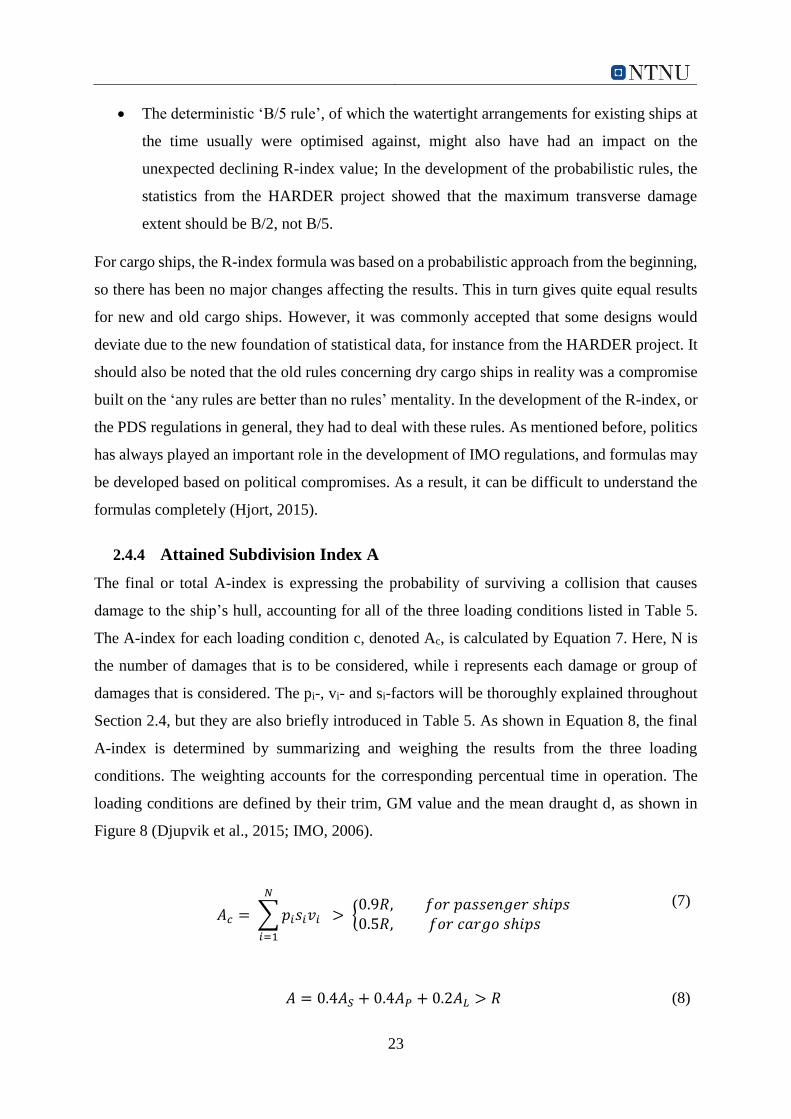
23
The deterministic ‘B/5 rule’, of which the watertight arrangements for existing ships at
the time usually were optimised against, might also have had an impact on the
unexpected declining R-index value; In the development of the probabilistic rules, the
statistics from the HARDER project showed that the maximum transverse damage
extent should be B/2, not B/5.
For cargo ships, the R-index formula was based on a probabilistic approach from the beginning,
so there has been no major changes affecting the results. This in turn gives quite equal results
for new and old cargo ships. However, it was commonly accepted that some designs would
deviate due to the new foundation of statistical data, for instance from the HARDER project. It
should also be noted that the old rules concerning dry cargo ships in reality was a compromise
built on the ‘any rules are better than no rules’ mentality. In the development of the R-index, or
the PDS regulations in general, they had to deal with these rules. As mentioned before, politics
has always played an important role in the development of IMO regulations, and formulas may
be developed based on political compromises. As a result, it can be difficult to understand the
formulas completely (Hjort, 2015).
2.4.4 Attained Subdivision Index A
The final or total A-index is expressing the probability of surviving a collision that causes
damage to the ship’s hull, accounting for all of the three loading conditions listed in Table 5.
The A-index for each loading condition c, denoted Ac, is calculated by Equation 7. Here, N is
the number of damages that is to be considered, while i represents each damage or group of
damages that is considered. The pi-, vi- and si-factors will be thoroughly explained throughout
Section 2.4, but they are also briefly introduced in Table 5. As shown in Equation 8, the final
A-index is determined by summarizing and weighing the results from the three loading
conditions. The weighting accounts for the corresponding percentual time in operation. The
loading conditions are defined by their trim, GM value and the mean draught d, as shown in
Figure 8 (Djupvik et al., 2015; IMO, 2006).
𝐴𝑐 = ∑𝑝𝑖𝑠𝑖𝑣𝑖
𝑁
𝑖=1
> {0.9𝑅, 𝑓𝑜𝑟 𝑝𝑎𝑠𝑠𝑒𝑛𝑔𝑒𝑟 𝑠ℎ𝑖𝑝𝑠0.5𝑅, 𝑓𝑜𝑟 𝑐𝑎𝑟𝑔𝑜 𝑠ℎ𝑖𝑝𝑠
(7)
𝐴 = 0.4𝐴𝑆 + 0.4𝐴𝑃 + 0.2𝐴𝐿 > 𝑅 (8)
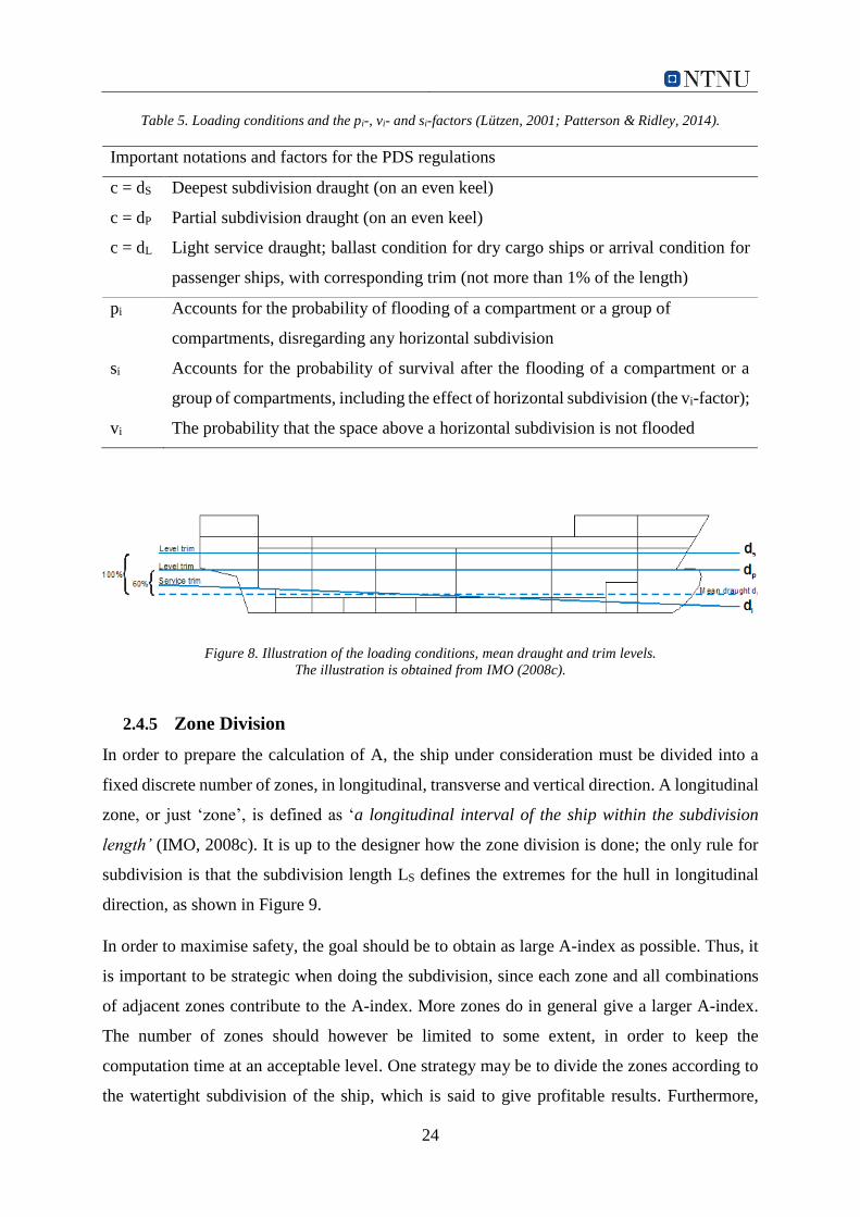
24
Table 5. Loading conditions and the pi-, vi- and si-factors (Lützen, 2001; Patterson & Ridley, 2014).
Important notations and factors for the PDS regulations
c = dS Deepest subdivision draught (on an even keel)
c = dP Partial subdivision draught (on an even keel)
c = dL Light service draught; ballast condition for dry cargo ships or arrival condition for
passenger ships, with corresponding trim (not more than 1% of the length)
pi Accounts for the probability of flooding of a compartment or a group of
compartments, disregarding any horizontal subdivision
si Accounts for the probability of survival after the flooding of a compartment or a
group of compartments, including the effect of horizontal subdivision (the vi-factor);
vi The probability that the space above a horizontal subdivision is not flooded
Figure 8. Illustration of the loading conditions, mean draught and trim levels.
The illustration is obtained from IMO (2008c).
2.4.5 Zone Division
In order to prepare the calculation of A, the ship under consideration must be divided into a
fixed discrete number of zones, in longitudinal, transverse and vertical direction. A longitudinal
zone, or just ‘zone’, is defined as ‘a longitudinal interval of the ship within the subdivision
length’ (IMO, 2008c). It is up to the designer how the zone division is done; the only rule for
subdivision is that the subdivision length LS defines the extremes for the hull in longitudinal
direction, as shown in Figure 9.
In order to maximise safety, the goal should be to obtain as large A-index as possible. Thus, it
is important to be strategic when doing the subdivision, since each zone and all combinations
of adjacent zones contribute to the A-index. More zones do in general give a larger A-index.
The number of zones should however be limited to some extent, in order to keep the
computation time at an acceptable level. One strategy may be to divide the zones according to
the watertight subdivision of the ship, which is said to give profitable results. Furthermore,
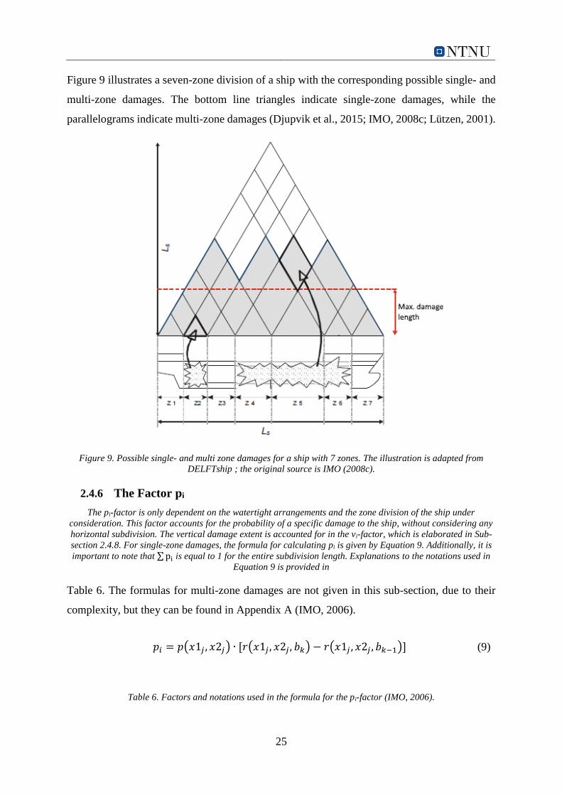
25
Figure 9 illustrates a seven-zone division of a ship with the corresponding possible single- and
multi-zone damages. The bottom line triangles indicate single-zone damages, while the
parallelograms indicate multi-zone damages (Djupvik et al., 2015; IMO, 2008c; Lützen, 2001).
Figure 9. Possible single- and multi zone damages for a ship with 7 zones. The illustration is adapted from
DELFTship ; the original source is IMO (2008c).
2.4.6 The Factor pi
The pi-factor is only dependent on the watertight arrangements and the zone division of the ship under
consideration. This factor accounts for the probability of a specific damage to the ship, without considering any
horizontal subdivision. The vertical damage extent is accounted for in the vi-factor, which is elaborated in Sub-
section 2.4.8. For single-zone damages, the formula for calculating pi is given by Equation 9. Additionally, it is
important to note that ∑pi is equal to 1 for the entire subdivision length. Explanations to the notations used in
Equation 9 is provided in
Table 6. The formulas for multi-zone damages are not given in this sub-section, due to their
complexity, but they can be found in Appendix A (IMO, 2006).
𝑝𝑖 = 𝑝(𝑥1𝑗 , 𝑥2𝑗) ∙ [𝑟(𝑥1𝑗 , 𝑥2𝑗 , 𝑏𝑘) − 𝑟(𝑥1𝑗 , 𝑥2𝑗 , 𝑏𝑘−1)] (9)
Table 6. Factors and notations used in the formula for the pi-factor (IMO, 2006).
26
Explanations to factors and notations related to the pi-factor
j The aftmost damage zone number involved in the accident, starting with number
1 at the stern.
k The number of a particular longitudinal bulkhead functioning as a barrier for
transverse penetration, counted from the shell towards the centre line (k = 0 for
the shell).
x1 Distance from the aft end (terminal) of the ship to the aft end of the zone in
question.
x2 Distance from the aft end (terminal) of the ship to the forward end of the zone in
question.
b Mean transverse distance in metres measured from the shell to the longitudinal
barrier in question. This distance is measured at the deepest subdivision load line,
and should never be taken as greater than B/2. If the shell and the longitudinal
barrier in question are not parallel to each other, then b is determined with an
assumed line, as defined by IMO Resolution MSC.281(85) – “Explanatory Notes
to the SOLAS Ch. II-1…Part B-1, Reg. 7-1.1.2”.
p(x1,x2) Accounts for the probability of the considered longitudinal damage extent.
r(x1,x2,b) A probability factor accounting for the transverse damage extent.
Background and Calculation of p(x1j,x2j)
The calculation of p(x1j,x2j) is carried out differently for three specific damage conditions, by
using a number of formulas provided in SOLAS Chapter II-1, Part B-1, Reg. 7-1. Some non-
dimensional lengths, which are key input to these formulas, are given in Table 7.
Table 7. Non-dimensional damage lengths used to calculate p(x1j,x2j) (IMO, 2006).
Explanations to non-dimensional damage lengths used to calculate p(x1j,x2j)
Jmax = 10/33 Overall normalised maximum damage length
Jkn = 5/33 Knuckle point in the distribution (Ls ≤ 198 m)
pk = 11/12 Cumulative probability at Jkn
lmax = 60 m Maximum absolute damage length
L* = 260 m Length where normalised distribution ends
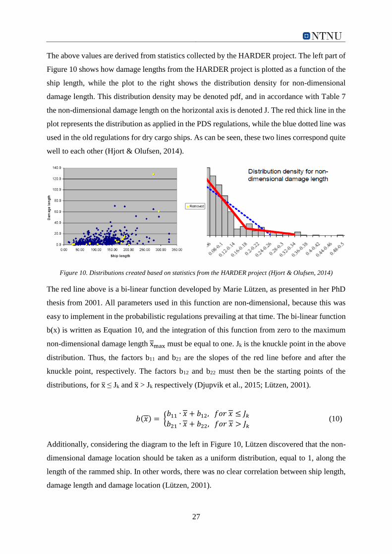
27
The above values are derived from statistics collected by the HARDER project. The left part of
Figure 10 shows how damage lengths from the HARDER project is plotted as a function of the
ship length, while the plot to the right shows the distribution density for non-dimensional
damage length. This distribution density may be denoted pdf, and in accordance with Table 7
the non-dimensional damage length on the horizontal axis is denoted J. The red thick line in the
plot represents the distribution as applied in the PDS regulations, while the blue dotted line was
used in the old regulations for dry cargo ships. As can be seen, these two lines correspond quite
well to each other (Hjort & Olufsen, 2014).
Figure 10. Distributions created based on statistics from the HARDER project (Hjort & Olufsen, 2014)
The red line above is a bi-linear function developed by Marie Lützen, as presented in her PhD
thesis from 2001. All parameters used in this function are non-dimensional, because this was
easy to implement in the probabilistic regulations prevailing at that time. The bi-linear function
b(x) is written as Equation 10, and the integration of this function from zero to the maximum
non-dimensional damage length xmax must be equal to one. Jk is the knuckle point in the above
distribution. Thus, the factors b11 and b21 are the slopes of the red line before and after the
knuckle point, respectively. The factors b12 and b22 must then be the starting points of the
distributions, for x̅ ≤ Jk and x̅ > Jk respectively (Djupvik et al., 2015; Lützen, 2001).
Additionally, considering the diagram to the left in Figure 10, Lützen discovered that the non-
dimensional damage location should be taken as a uniform distribution, equal to 1, along the
length of the rammed ship. In other words, there was no clear correlation between ship length,
damage length and damage location (Lützen, 2001).
𝑏(𝑥) = {𝑏11 ∙ 𝑥 + 𝑏12, 𝑓𝑜𝑟 𝑥 ≤ 𝐽𝑘𝑏21 ∙ 𝑥 + 𝑏22, 𝑓𝑜𝑟 𝑥 > 𝐽𝑘
(10)
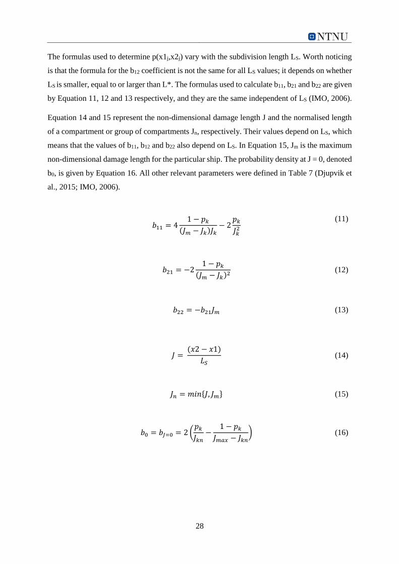
28
The formulas used to determine p(x1j,x2j) vary with the subdivision length LS. Worth noticing
is that the formula for the b12 coefficient is not the same for all LS values; it depends on whether
LS is smaller, equal to or larger than L*. The formulas used to calculate b11, b21 and b22 are given
by Equation 11, 12 and 13 respectively, and they are the same independent of LS (IMO, 2006).
Equation 14 and 15 represent the non-dimensional damage length J and the normalised length
of a compartment or group of compartments Jn, respectively. Their values depend on LS, which
means that the values of b11, b12 and b22 also depend on LS. In Equation 15, Jm is the maximum
non-dimensional damage length for the particular ship. The probability density at J = 0, denoted
b0, is given by Equation 16. All other relevant parameters were defined in Table 7 (Djupvik et
al., 2015; IMO, 2006).
𝑏11 = 41 − 𝑝𝑘
(𝐽𝑚 − 𝐽𝑘)𝐽𝑘− 2
𝑝𝑘
𝐽𝑘2
(11)
𝑏21 = −2
1 − 𝑝𝑘(𝐽𝑚 − 𝐽𝑘)2
(12)
𝑏22 = −𝑏21𝐽𝑚 (13)
𝐽 =
(𝑥2 − 𝑥1)
𝐿𝑆 (14)
𝐽𝑛 = 𝑚𝑖𝑛{𝐽, 𝐽𝑚} (15)
𝑏0 = 𝑏𝐽=0 = 2(
𝑝𝑘𝐽𝑘𝑛
−1 − 𝑝𝑘
𝐽𝑚𝑎𝑥 − 𝐽𝑘𝑛) (16)
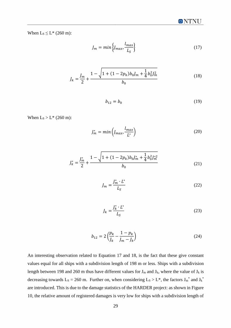
29
When LS ≤ L* (260 m):
𝐽𝑚 = 𝑚𝑖𝑛 {𝐽𝑚𝑎𝑥,
𝑙𝑚𝑎𝑥𝐿𝑆
} (17)
𝐽𝑘 =𝐽𝑚2+1 − √1 + (1 − 2𝑝𝑘)𝑏0𝐽𝑚 +
14𝑏0
2𝐽𝑚2
𝑏0
(18)
𝑏12 = 𝑏0 (19)
When LS > L* (260 m):
𝐽𝑚∗ = 𝑚𝑖𝑛 (𝐽𝑚𝑎𝑥,
𝑙𝑚𝑎𝑥𝐿∗
) (20)
𝐽𝑘∗ =
𝐽𝑚∗
2+1 − √1 + (1 − 2𝑝𝑘)𝑏0𝐽𝑚∗ +
14𝑏0
2𝐽𝑚∗2
𝑏0
(21)
𝐽𝑚 =
𝐽𝑚∗ ∙ 𝐿∗
𝐿𝑆 (22)
𝐽𝑘 =
𝐽𝑘∗ ∙ 𝐿∗
𝐿𝑆 (23)
𝑏12 = 2(
𝑝𝑘𝐽𝑘−1 − 𝑝𝑘𝐽𝑚 − 𝐽𝑘
) (24)
An interesting observation related to Equation 17 and 18, is the fact that these give constant
values equal for all ships with a subdivision length of 198 m or less. Ships with a subdivision
length between 198 and 260 m thus have different values for Jm and Jk, where the value of Jk is
decreasing towards LS = 260 m. Further on, when considering LS > L*, the factors Jm* and Jk
*
are introduced. This is due to the damage statistics of the HARDER project: as shown in Figure
10, the relative amount of registered damages is very low for ships with a subdivision length of
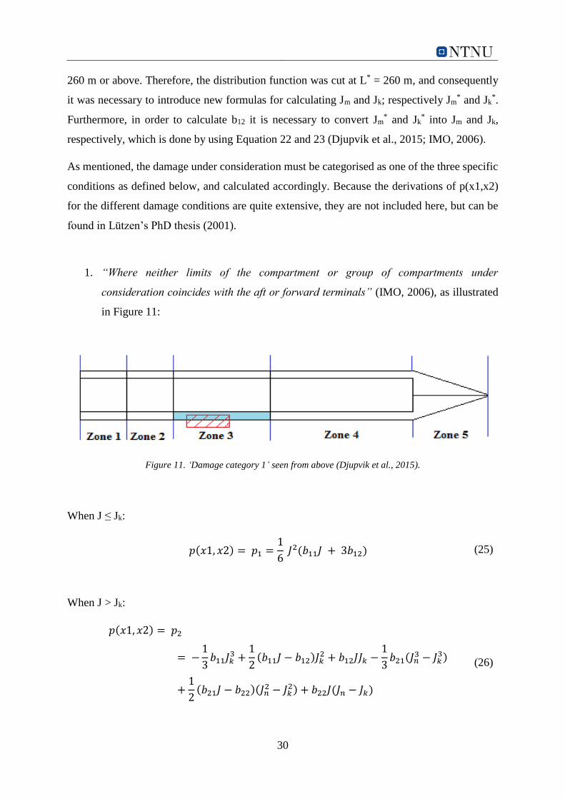
30
260 m or above. Therefore, the distribution function was cut at L* = 260 m, and consequently
it was necessary to introduce new formulas for calculating Jm and Jk; respectively Jm* and Jk
*.
Furthermore, in order to calculate b12 it is necessary to convert Jm* and Jk
* into Jm and Jk,
respectively, which is done by using Equation 22 and 23 (Djupvik et al., 2015; IMO, 2006).
As mentioned, the damage under consideration must be categorised as one of the three specific
conditions as defined below, and calculated accordingly. Because the derivations of p(x1,x2)
for the different damage conditions are quite extensive, they are not included here, but can be
found in Lützen’s PhD thesis (2001).
1. “Where neither limits of the compartment or group of compartments under
consideration coincides with the aft or forward terminals” (IMO, 2006), as illustrated
in Figure 11:
Figure 11. ‘Damage category 1’ seen from above (Djupvik et al., 2015).
When J ≤ Jk:
𝑝(𝑥1, 𝑥2) = 𝑝1 =
1
6 𝐽2(𝑏11𝐽 + 3𝑏12) (25)
When J > Jk:
𝑝(𝑥1, 𝑥2) = 𝑝2
= −1
3𝑏11𝐽𝑘
3 +1
2(𝑏11𝐽 − 𝑏12)𝐽𝑘
2 + 𝑏12𝐽𝐽𝑘 −1
3𝑏21(𝐽𝑛
3 − 𝐽𝑘3)
+1
2(𝑏21𝐽 − 𝑏22)(𝐽𝑛
2 − 𝐽𝑘2) + 𝑏22𝐽(𝐽𝑛 − 𝐽𝑘)
(26)
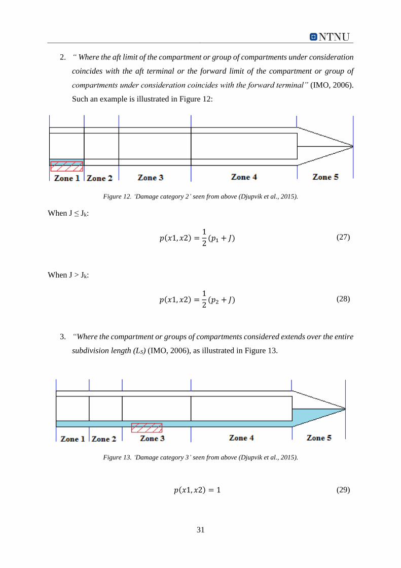
31
2. “ Where the aft limit of the compartment or group of compartments under consideration
coincides with the aft terminal or the forward limit of the compartment or group of
compartments under consideration coincides with the forward terminal” (IMO, 2006).
Such an example is illustrated in Figure 12:
Figure 12. ‘Damage category 2’ seen from above (Djupvik et al., 2015).
When J ≤ Jk:
𝑝(𝑥1, 𝑥2) =
1
2(𝑝1 + 𝐽) (27)
When J > Jk:
𝑝(𝑥1, 𝑥2) =
1
2(𝑝2 + 𝐽) (28)
3. “Where the compartment or groups of compartments considered extends over the entire
subdivision length (LS) (IMO, 2006), as illustrated in Figure 13.
Figure 13. ‘Damage category 3’ seen from above (Djupvik et al., 2015).
𝑝(𝑥1, 𝑥2) = 1 (29)
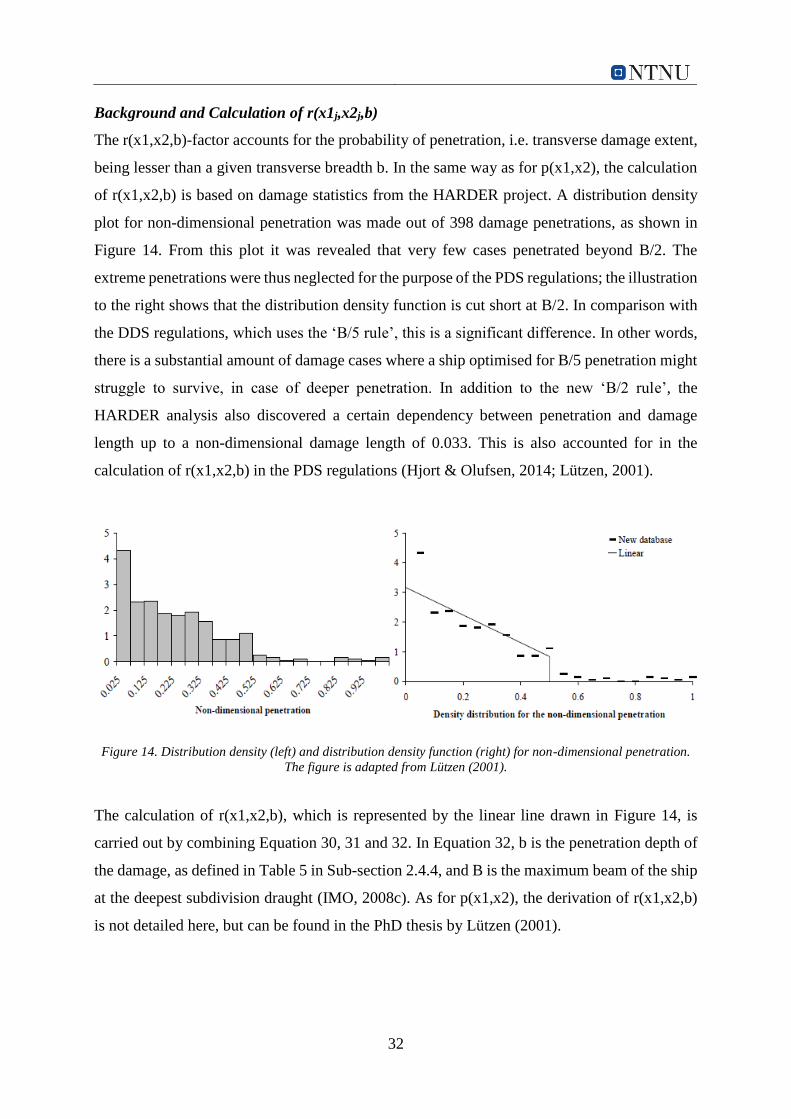
32
Background and Calculation of r(x1j,x2j,b)
The r(x1,x2,b)-factor accounts for the probability of penetration, i.e. transverse damage extent,
being lesser than a given transverse breadth b. In the same way as for p(x1,x2), the calculation
of r(x1,x2,b) is based on damage statistics from the HARDER project. A distribution density
plot for non-dimensional penetration was made out of 398 damage penetrations, as shown in
Figure 14. From this plot it was revealed that very few cases penetrated beyond B/2. The
extreme penetrations were thus neglected for the purpose of the PDS regulations; the illustration
to the right shows that the distribution density function is cut short at B/2. In comparison with
the DDS regulations, which uses the ‘B/5 rule’, this is a significant difference. In other words,
there is a substantial amount of damage cases where a ship optimised for B/5 penetration might
struggle to survive, in case of deeper penetration. In addition to the new ‘B/2 rule’, the
HARDER analysis also discovered a certain dependency between penetration and damage
length up to a non-dimensional damage length of 0.033. This is also accounted for in the
calculation of r(x1,x2,b) in the PDS regulations (Hjort & Olufsen, 2014; Lützen, 2001).
Figure 14. Distribution density (left) and distribution density function (right) for non-dimensional penetration.
The figure is adapted from Lützen (2001).
The calculation of r(x1,x2,b), which is represented by the linear line drawn in Figure 14, is
carried out by combining Equation 30, 31 and 32. In Equation 32, b is the penetration depth of
the damage, as defined in Table 5 in Sub-section 2.4.4, and B is the maximum beam of the ship
at the deepest subdivision draught (IMO, 2008c). As for p(x1,x2), the derivation of r(x1,x2,b)
is not detailed here, but can be found in the PhD thesis by Lützen (2001).

33
𝑟(𝑥1, 𝑥2, 𝑏) = 1 − (1 − 𝐶) ∙ [1 −
𝐺
𝑝(𝑥1, 𝑥2)] (30)
𝐶 = 12 ∙ 𝐽𝑏 ∙ (−45 ∙ 𝐽𝑏 + 4) (31)
𝐽𝑏 =
𝑏
15𝐵 (32)
The calculation of the G factor is dependent on the same damage conditions as for p(x1,x2):
1. “Where neither limits of the compartment or group of compartments under
consideration coincides with the aft or forward terminals” (IMO, 2006). Here, J0 is
given by equation 34.
𝐺 = 𝐺2 = −
1
3𝑏11𝐽𝑜
3 +1
2(𝑏11𝐽 − 𝑏12)𝐽0
2 + 𝑏12𝐽𝐽0 (33)
𝐽0 = min (𝐽, 𝐽𝑏) (34)
2. “ Where the aft limit of the compartment or group of compartments under consideration
coincides with the aft terminal or the forward limit of the compartment or group of
compartments under consideration coincides with the forward terminal” (IMO, 2006).
Here, G1 is given by ‘damage condition 3’, i.e. Equation 36.
𝐺 =
1
2(𝐺2 + 𝐺1𝐽) (35)
3. “Where the compartment or groups of compartments considered extends over the entire
subdivision length (LS) (IMO, 2006):
𝐺 = 𝐺1 =
1
2𝑏11𝐽𝑏
2 + 𝑏12𝐽𝑏 (36)

34
2.4.7 The Factor si
Calculation of the si Factor
The factor si is known as the survivability factor, because si accounts for the probability of
survival when the ship is exposed to flooding of a compartment or group of compartments after
a collision. This factor is quite complex to calculate, due to the large number of considerations
in the regulation. There are a lot of factors involved in the calculation process; some of them
are already defined in the master’s thesis. However, for the convenience of this sub-section, all
necessary factors are summarized in Table 8.
Table 8. Notations and parameters used in the calculation of si (IMO, 2006).
Parameters and notations related to the si-factor
θe Equilibrium heel angle in any stage of flooding
θv The angle at any stage of flooding where the righting lever, GZ, becomes
negative
θmin Minimum heel angle = 7 degrees for passenger ships; 25 degrees for cargo
ships
θmax Maximum heel angle = 15 degrees for passenger ships; 30 degrees for
cargo ships
Range The range of positive GZ values = θv - θe
GZmax The maximum positive GZ value [metres] up to θv
Sintermediate, i The probability of surviving all intermediate flooding stages until the
equilibrium stage
Sfinal, i The probability of surviving in the final equilibrium stage of flooding
Smom, i The probability of surviving heeling moments
Mheel Maximum assumed heeling moment
Displacement Intact displacement at the subdivision draught
Np The maximum number of passengers permitted to be on board in the
service condition, corresponding to the deepest subdivision draught
B Beam of the ship at the deepest subdivision draught
A Projected lateral area above the waterline
Z Distance from the centre of A to T/2, where T is the draught of the ship
P Wind pressure: P = 120 N/m2

35
The calculation of si is carried out using Equation 37. The index i represents the particular
damage case for the considered loading condition (IMO, 2006).
𝑠𝑖 = 𝑚𝑖𝑛[𝑠𝑖𝑛𝑡𝑒𝑟𝑚𝑒𝑑𝑖𝑎𝑡𝑒,𝑖, (𝑠𝑓𝑖𝑛𝑎𝑙,𝑖 ∙ 𝑠𝑚𝑜𝑚,𝑖)] (37)
In the calculation of sfinal,i, which is carried out using Equation 38, it is important to be aware
that the maximum values for GZmax and range are 0.12 m and 16 degrees respectively. This is
because sfinal,i is a probability number, thus its value must be equal to or lesser than 1. This
becomes clear when looking at the formula for K, which is represented by Equation 39. K is
included as a factor to ensure that the heel angles for the different ship types are acceptable
(Djupvik et al., 2015).
𝑠𝑓𝑖𝑛𝑎𝑙,𝑖 = 𝐾 ∙ [𝐺𝑍𝑚𝑎𝑥0.12
∙𝑅𝑎𝑛𝑔𝑒
16]
14 (38)
𝐾 =
{
√𝜃𝑚𝑎𝑥 − 𝜃𝑒𝜃𝑚𝑎𝑥 − 𝜃𝑚𝑖𝑛
, 𝑖𝑓 𝜃𝑚𝑖𝑛 < 𝜃𝑒 < 𝜃𝑚𝑎𝑥
1, 𝑖𝑓 𝜃𝑒 ≤ 𝜃𝑚𝑖𝑛0, 𝑖𝑓 𝜃𝑒 ≥ 𝜃𝑚𝑎𝑥
(39)
Additionally, Equation 39 states that sfinal,i is equal to zero in two different scenarios: when a
passenger ship heels more than 15 degrees (θmax) or when a cargo ship heels more than 30
degrees (θmax). In these two cases the survivability factor will not contribute to the A-index.
This is obviously important for Naval Architects to pay attention to when designing the
watertight arrangements (IMO, 2006).
Equation 40, which is used to calculate sintermediate,i, is very similar to the formula for sfinal,i. There
are three important differences, however: the factor k is removed from the equation, sintermediate,i
is taken as unity for cargo ships (sintermediate,i = 1) and the limits for GZmax and range are now
equal to or lesser than 0.05 m and 7 degrees respectively. In addition, if the intermediate heel
angle exceeds 15 degrees, the value of sintermediate,i is equal to zero. It should also be noted that
sintermediate,i must be taken as the least of the si-factors obtained from all flooding stages, including
the final stage before equalization (IMO, 2006).
36
𝑠𝑖𝑛𝑡𝑒𝑟𝑚𝑒𝑑𝑖𝑎𝑡𝑒,𝑖 = {[𝐺𝑍𝑚𝑎𝑥0.05
∙𝑅𝑎𝑛𝑔𝑒
7]
14, 𝑖𝑓 𝑖𝑛𝑡𝑒𝑟𝑚𝑒𝑑𝑖𝑎𝑡𝑒 ℎ𝑒𝑒𝑙 𝑎𝑛𝑔𝑙𝑒 ≤ 15°
0, 𝑖𝑓 𝑖𝑛𝑑𝑒𝑟𝑚𝑒𝑑𝑖𝑎𝑡𝑒 ℎ𝑒𝑒𝑙 𝑎𝑛𝑔𝑙𝑒 > 15°
(40)
At last, equation 41 is used to calculate the smom,i-factor. This factor accounts for the probability
of surviving heeling moments created by wind, movement of passengers or the lowering of
survival crafts, denoted Mpassenger, Mwind and Msurvivalcraft respectively. Similar to sintermediate,i,
smom,i is taken as unity for cargo ships.
𝑠𝑚𝑜𝑚,𝑖 = (𝐺𝑍𝑚𝑎𝑥 − 0.04) ∙ 𝐷𝑖𝑠𝑝𝑙𝑎𝑐𝑒𝑚𝑒𝑛𝑡
𝑀ℎ𝑒𝑒𝑙 = 𝑚𝑎𝑥(𝑀𝑝𝑎𝑠𝑠𝑒𝑛𝑔𝑒𝑟, 𝑀𝑤𝑖𝑛𝑑 , 𝑀𝑠𝑢𝑟𝑣𝑖𝑣𝑎𝑙𝑐𝑟𝑎𝑓𝑡) ≤ 1 (41)
The heeling moments Mpassenger and Mwind are calculated by Equation 42 and 43, respectively.
Explanations to the factors involved in these equations can be found in Table 8, except for the
constant value 9.806, which is the gravitational acceleration constant with the unit m/s2. As
mentioned, Mpassenger is caused by the movement of passengers. In case of an emergency
situation, the passengers will most likely crowd to one side of the ship where the mustering
stations and lifeboats are located. As Equation 42 reveals, the PDS regulations consider the
average weight of the passengers to be 75 kg or 0.075 tonnes, in similarity to the DDS
regulations. Furthermore, as an alternative to Equation 42, the deterministic approach used to
determine the ‘heeling moment’ as described in Sub-section 2.3.3 can be used (IMO, 2006).
𝑀𝑝𝑎𝑠𝑠𝑒𝑛𝑔𝑒𝑟 = (0.075 ∙ 𝑁𝑝) ∙ (0.45 ∙ 𝐵) [𝑡𝑜𝑛𝑛𝑒𝑠 ∙ 𝑚] (42)
𝑀𝑤𝑖𝑛𝑑 =
(𝑃 ∙ 𝐴 ∙ 𝑍)
9,806 [𝑡𝑜𝑛𝑛𝑒𝑠 ∙ 𝑚] (43)
Msurvivalcraft is defined in SOLAS as ‘the maximum assumed heeling moment due to the launching
of all fully loaded davit-launched survival craft on one side of the ship’ (IMO, 2006). This
heeling moment is not calculated by any one particular equation, but can be calculated
following five specific assumptions given in SOLAS Ch. II-1, Part B-1, Reg. 7-2 (IMO, 2006).

37
Another important consideration, is how to determine the GZmax value. This was briefly
introduced in Sub-section 2.1.1, but there might occur situations where this regular approach
no longer is appropriate. Such an example is the event of one or more submerged openings.
This is illustrated in the graph to the right of Figure 15, where GZmax is not located at the peak
of the curve. In this case, the GZmax value appears at θv and the GZ curve is cut at this point,
because the righting lever per definition becomes negative when an opening of the ship is
submerged. A common design strategy to avoid this problem is to place all openings at a certain
distance above the bulkhead deck (Djupvik et al., 2015; IMO, 2008c).
Figure 15. Illustration of a typical GZ curve (left) and a GZ curve for submerged opening (right). The
illustration is obtained from Djupvik et al. (2015).
Background of the si Factor
A number of the criteria in the PDS regulations concerning the si factor appear as deterministic.
Although, there are some elements that may be seen as probabilistic. For instance, the
probability of successful evacuation will increase with a low static heel angle, if it is ensured
that the evacuation routes not will be impeded by water. This is in fact nothing new, as the so-
called ‘margin line concept’ of the DDS regulations implicitly cover issues related to watertight
integrity, ship safety and the evacuation of passengers. However, an important difference
between the PDS regulations and the DDS regulations regarding passenger ships, is thus the
removal of the margin line requirements. The function of the margin line was to prohibit
immersion of water on the bulkhead deck, and this was considered as being in conflict with the
functionality of the probabilistic concept. However, it was realised that this change had to be
compensated by some explicit requirements considering watertight integrity and evacuation of
passengers. Examples here are design limitations related to watertight doors and launching
devices for life-saving appliances (LSA), respectively. Another important compromise, was the
introduction of ‘penalties’ on the A-index. These ‘penalties’ were given in the event of water
38
immersion of certain features, such as water on the bulkhead deck during evacuation,
immersion of vertical emergency escape hatches, and progressive flooding through unprotected
openings or damaged piping and ducts in the damage zone (Hjort & Olufsen, 2014).
Furthermore, the DDS and PDS regulations are quite similar in the sense that the GZ curve is
used to estimate the ship’s survivability. The difference becomes evident when looking at the
criteria used. In the DDS regulations, the ‘area criterion’ is used; the area under the GZ curve
must be greater than a certain value. The HARDER project revealed through model tests with
systematic variation in sea-states that this criterion was of secondary importance to the
survivability, as long as the range and GZmax values were sufficiently high. Therefore, the ‘area
criterion’ was dropped. It was also discovered that the ‘angle of equilibrium criterion’ was
secondary to some extent, but an increasing risk of shifting cargo and loose objects on deck
justified some limitations connected to heel angles. For passenger ships, the calculation of smom,i
was adopted from the wind, passenger and LSA heeling moment assumptions in the DDS
regulations. In the case of cargo ships, smom,i and sintermediate,i are always set to 1, as it was decided
to maintain the practice from the DDS regulations; there should be no requirements related to
the stability in the intermediate stages of flooding (Hjort & Olufsen, 2014).
2.4.8 The Factor vi
Calculation of the vi Factor
In the case of any horizontal watertight subdivisions above the waterline, the si value for the
lower compartments or group of compartments must be multiplied by the ‘reduction factor’ vi.
This factor accounts for the probability that the spaces above the horizontal boundary under
consideration remain intact after a ship collision. If these spaces are flooded due to a ship
collision, the residual stability of the ship will be reduced. In consequence, the ship’s buoyancy
changes and the GZ curve is affected. The vi factor is determined by Equation 44. The factors
and notations involved in the equation are described in Table 9. In addition, an illustration
exemplifying how the H measurements should be interpreted for a particular damage condition
is provided in Figure 16 (IMO, 2006).
𝑣𝑖 = 𝑣(𝐻𝑗,𝑛,𝑚, 𝑑) − 𝑣(𝐻𝑗,𝑛,𝑚−1, 𝑑), 𝑣𝑖𝜖[0,1] (44)
Table 9. Factors and notations involved in the calculation of the vi factor (IMO, 2006).

39
Parameters and notations related to the vi-factor
Hj,n,m ‘…the least height above the baseline, in metres, within the longitudinal range of
x1(j)...x2(j+n-1) of the mth horizontal boundary which is assumed to limit the
vertical extent of flooding for the damaged compartments under consideration;’
Hj,n,m-1 ‘… the least height above the baseline, in metres, within the longitudinal range of
x1(j)...x2(j+n-1) of the (m-1)th horizontal boundary which is assumed to limit the
vertical extent of flooding for the damaged compartments under consideration;’
j ‘signifies the aft terminal of the damaged compartments under consideration;’
n ‘the number of adjacent damage zones involved in the damage;’
m ‘ represents each horizontal boundary counted upwards from the waterline under
consideration;’
d ‘is the draught in question as defined in regulation 2…’
Figure 16. A ship with a particular damage condition and corresponding H measures.
The illustration is obtained from Djupvik et al. (2015).
As mentioned in Sub-section 2.4.2 and illustrated in Figure 17, the maximal vertical damage
extent is defined as d + 12.5 m. The location of watertight decks in the reserve buoyancy area
and application of the vi-factor, are also illustrated in Figure 17. Explanations to the below
illustrations are provided in Table 10.
Figure 17. The use of the vi factor for different horizontal watertight arrangements.
The illustrations are adapted from IMO (2008c).
Table 10. Explanations to Figure 17 (IMO, 2008c).
(1) (2) (3)
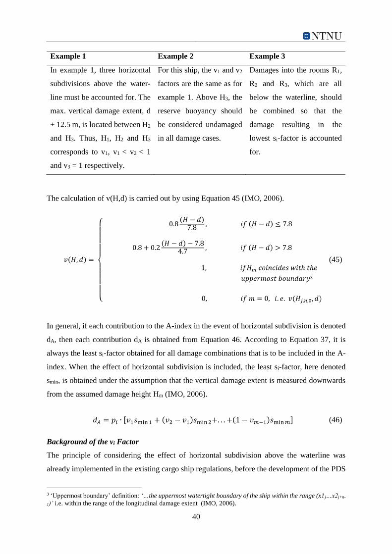
40
Example 1 Example 2 Example 3
In example 1, three horizontal
subdivisions above the water-
line must be accounted for. The
max. vertical damage extent, d
+ 12.5 m, is located between H2
and H3. Thus, H1, H2 and H3
corresponds to v1, v1 < v2 < 1
and v3 = 1 respectively.
For this ship, the v1 and v2
factors are the same as for
example 1. Above H3, the
reserve buoyancy should
be considered undamaged
in all damage cases.
Damages into the rooms R1,
R2 and R3, which are all
below the waterline, should
be combined so that the
damage resulting in the
lowest si-factor is accounted
for.
The calculation of v(H,d) is carried out by using Equation 45 (IMO, 2006).
In general, if each contribution to the A-index in the event of horizontal subdivision is denoted
dA, then each contribution dA is obtained from Equation 46. According to Equation 37, it is
always the least si-factor obtained for all damage combinations that is to be included in the A-
index. When the effect of horizontal subdivision is included, the least si-factor, here denoted
smin, is obtained under the assumption that the vertical damage extent is measured downwards
from the assumed damage height Hm (IMO, 2006).
𝑑𝐴 = 𝑝𝑖 ∙ [𝑣1𝑠min1 + (𝑣2 − 𝑣1)𝑠min2+. . . +(1 − 𝑣𝑚−1)𝑠min𝑚] (46)
Background of the vi Factor
The principle of considering the effect of horizontal subdivision above the waterline was
already implemented in the existing cargo ship regulations, before the development of the PDS
3 ‘Uppermost boundary’ definition: ‘…the uppermost watertight boundary of the ship within the range (x1j…x2j+n-
1)’ i.e. within the range of the longitudinal damage extent (IMO, 2006).
𝑣(𝐻, 𝑑) =
{
0.8
(𝐻 − 𝑑)7.8 , 𝑖𝑓 (𝐻 − 𝑑) ≤ 7.8
0.8 + 0.2(𝐻 − 𝑑) − 7.8
4.7, 𝑖𝑓 (𝐻 − 𝑑) > 7.8
1, 𝑖𝑓𝐻𝑚 𝑐𝑜𝑖𝑛𝑐𝑖𝑑𝑒𝑠 𝑤𝑖𝑡ℎ 𝑡ℎ𝑒
𝑢𝑝𝑝𝑒𝑟𝑚𝑜𝑠𝑡 𝑏𝑜𝑢𝑛𝑑𝑎𝑟𝑦3
0, 𝑖𝑓 𝑚 = 0, 𝑖. 𝑒. 𝑣(𝐻𝑗,𝑛,0, 𝑑)
(45)

41
regulations. The cargo ship rules were developed based on almost no statistics, but as time went
by, a certain tendency in ship collisions eventually became evident: many ships were rammed
by ships of equal size. In order to improve the old rules, it was decided to develop a formula
based on the length-dependent bow height requirements in ICCL-66. This formula included an
upper limit of 7 m above the waterline (Hjort & Olufsen, 2014).
Furthermore, new statistics from the HARDER project revealed that there was a significant
number of ship collisions resulting in more severe vertical damage extents than assumed by the
cargo ship regulations. An explanation is that the bow height requirement in ICCL-66 was a
minimum requirement. The upper limit was not defined, so many ships were built with higher
bows. In consequence, the new PDS regulations were developed based on all available statistics,
in addition to the old regulations and ‘as-built’ dimensions collected from the existing world
fleet. This is illustrated in Figure 18, where the red dotted line represents the formula
corresponding to the vi-factor used in the PDS regulations. With the new regulations, the
maximum vertical damage extent was increased from d + 7 m to d + 12.5 m, thus providing an
increased safety level (Hjort & Olufsen, 2014).
Figure 18. Vertical damage extent distribution for the old and new regulations.
The figure is adapted from Hjort and Olufsen (2014).

42
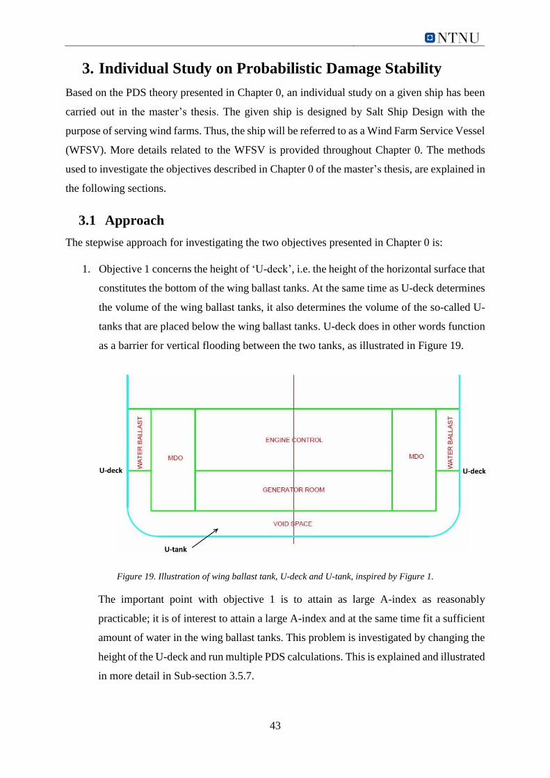
43
3. Individual Study on Probabilistic Damage Stability
Based on the PDS theory presented in Chapter 0, an individual study on a given ship has been
carried out in the master’s thesis. The given ship is designed by Salt Ship Design with the
purpose of serving wind farms. Thus, the ship will be referred to as a Wind Farm Service Vessel
(WFSV). More details related to the WFSV is provided throughout Chapter 0. The methods
used to investigate the objectives described in Chapter 0 of the master’s thesis, are explained in
the following sections.
3.1 Approach
The stepwise approach for investigating the two objectives presented in Chapter 0 is:
1. Objective 1 concerns the height of ‘U-deck’, i.e. the height of the horizontal surface that
constitutes the bottom of the wing ballast tanks. At the same time as U-deck determines
the volume of the wing ballast tanks, it also determines the volume of the so-called U-
tanks that are placed below the wing ballast tanks. U-deck does in other words function
as a barrier for vertical flooding between the two tanks, as illustrated in Figure 19.
Figure 19. Illustration of wing ballast tank, U-deck and U-tank, inspired by Figure 1.
The important point with objective 1 is to attain as large A-index as reasonably
practicable; it is of interest to attain a large A-index and at the same time fit a sufficient
amount of water in the wing ballast tanks. This problem is investigated by changing the
height of the U-deck and run multiple PDS calculations. This is explained and illustrated
in more detail in Sub-section 3.5.7.
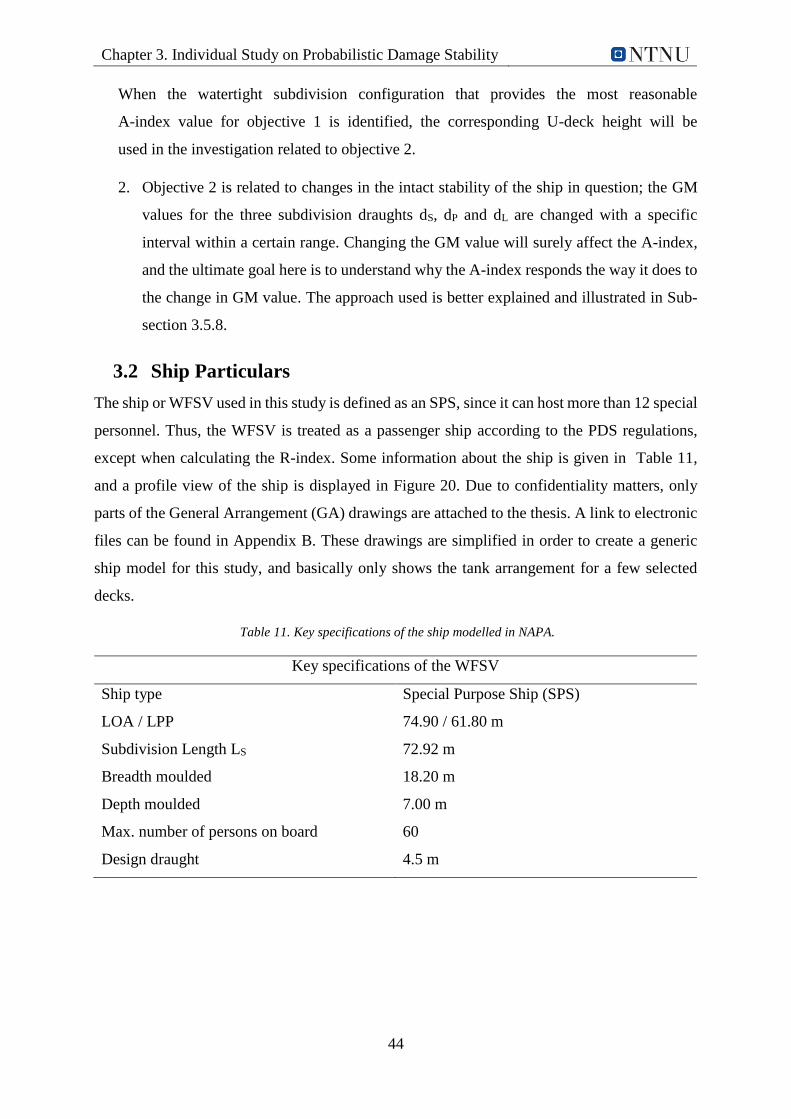
Chapter 3. Individual Study on Probabilistic Damage Stability
44
When the watertight subdivision configuration that provides the most reasonable
A-index value for objective 1 is identified, the corresponding U-deck height will be
used in the investigation related to objective 2.
2. Objective 2 is related to changes in the intact stability of the ship in question; the GM
values for the three subdivision draughts dS, dP and dL are changed with a specific
interval within a certain range. Changing the GM value will surely affect the A-index,
and the ultimate goal here is to understand why the A-index responds the way it does to
the change in GM value. The approach used is better explained and illustrated in Sub-
section 3.5.8.
3.2 Ship Particulars
The ship or WFSV used in this study is defined as an SPS, since it can host more than 12 special
personnel. Thus, the WFSV is treated as a passenger ship according to the PDS regulations,
except when calculating the R-index. Some information about the ship is given in Table 11,
and a profile view of the ship is displayed in Figure 20. Due to confidentiality matters, only
parts of the General Arrangement (GA) drawings are attached to the thesis. A link to electronic
files can be found in Appendix B. These drawings are simplified in order to create a generic
ship model for this study, and basically only shows the tank arrangement for a few selected
decks.
Table 11. Key specifications of the ship modelled in NAPA.
Key specifications of the WFSV
Ship type Special Purpose Ship (SPS)
LOA / LPP 74.90 / 61.80 m
Subdivision Length LS 72.92 m
Breadth moulded 18.20 m
Depth moulded 7.00 m
Max. number of persons on board 60
Design draught 4.5 m

Chapter 3. Individual Study on Probabilistic Damage Stability
45
Figure 20. Profile view of the Wind Farm Service Vessel used in the study.
3.3 Software
The work that has been done to achieve the results presented in Chapter 4, has been carried out
using the market-leading stability software NAPA. Salt Ship Design provided a license with
access outside of normal working hours throughout the duration of the master’s thesis. A laptop
with pre-installed VPN and remote desktop connection was also provided, in order to be
connected to the Salt Ship Design network and their databases.
In addition to the NAPA stability software, AutoCAD has been used to investigate and modify
GA drawings. AutoCAD is free to use for students for non-commercial purposes. To avoid that
the co-operation with Salt Ship Design could be seen as a problem, in terms of commercial use
of the student license, a professional license provided by Salt Ship Design was used instead.
3.4 Modelling in NAPA
The recommendation from Salt Ship Design was to model the GA of the ship in NAPA from
scratch, instead of copying the existing project from the database. This approach is time-
demanding for beginners, but it was considered to be beneficial in the long run; it is easier to
notice errors and analyse the results with a good understanding of the software. NAPA for
Design Manuals and frequent communication with supervisors from Salt Ship Design was
helpful in the process.
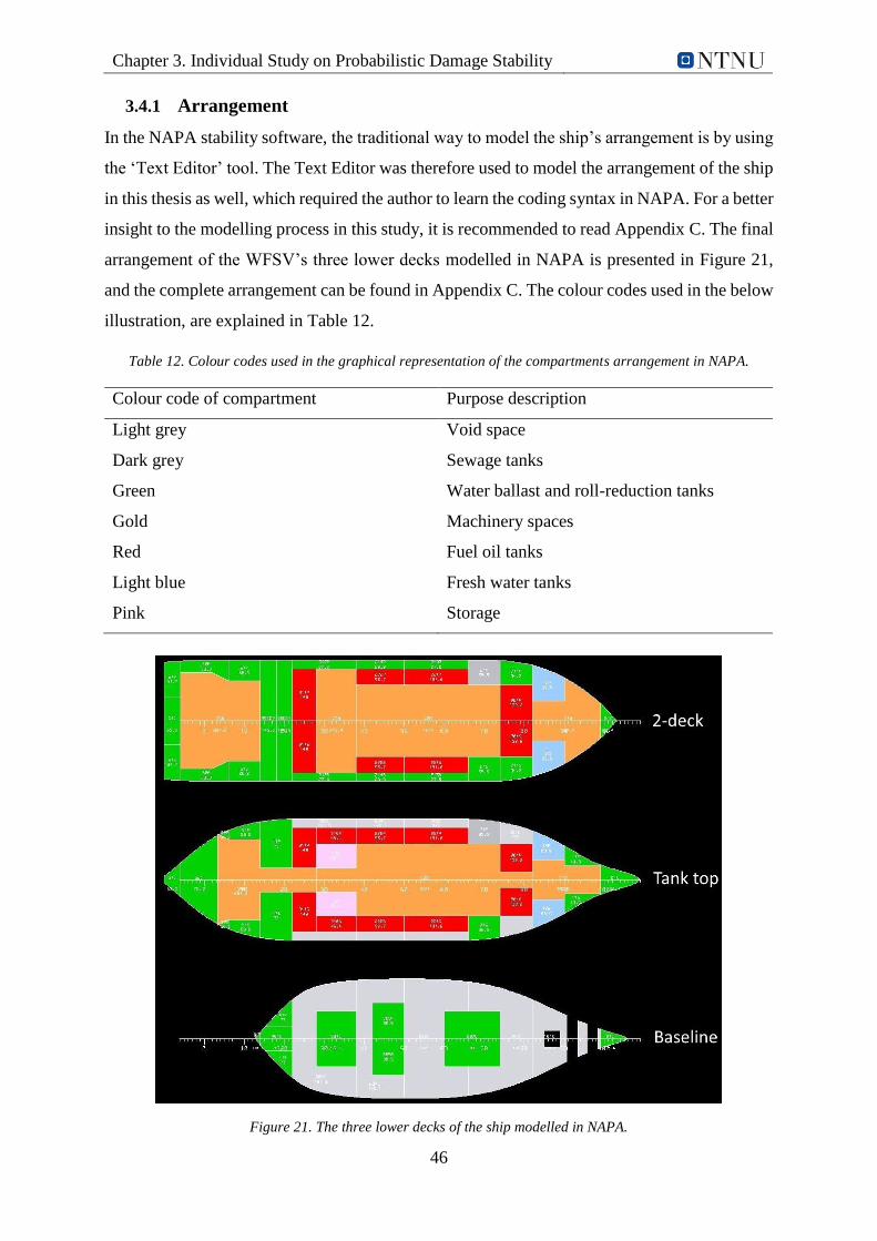
Chapter 3. Individual Study on Probabilistic Damage Stability
46
3.4.1 Arrangement
In the NAPA stability software, the traditional way to model the ship’s arrangement is by using
the ‘Text Editor’ tool. The Text Editor was therefore used to model the arrangement of the ship
in this thesis as well, which required the author to learn the coding syntax in NAPA. For a better
insight to the modelling process in this study, it is recommended to read Appendix C. The final
arrangement of the WFSV’s three lower decks modelled in NAPA is presented in Figure 21,
and the complete arrangement can be found in Appendix C. The colour codes used in the below
illustration, are explained in Table 12.
Table 12. Colour codes used in the graphical representation of the compartments arrangement in NAPA.
Colour code of compartment Purpose description
Light grey Void space
Dark grey Sewage tanks
Green Water ballast and roll-reduction tanks
Gold Machinery spaces
Red Fuel oil tanks
Light blue Fresh water tanks
Pink Storage
Figure 21. The three lower decks of the ship modelled in NAPA.
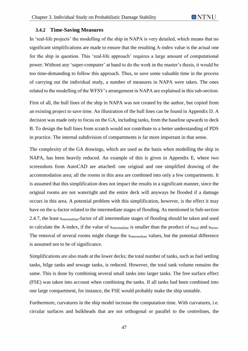
Chapter 3. Individual Study on Probabilistic Damage Stability
47
3.4.2 Time-Saving Measures
In ‘real-life projects’ the modelling of the ship in NAPA is very detailed, which means that no
significant simplifications are made to ensure that the resulting A-index value is the actual one
for the ship in question. This ‘real-life approach’ requires a large amount of computational
power. Without any ‘super-computer’ at hand to do the work in the master’s thesis, it would be
too time-demanding to follow this approach. Thus, to save some valuable time in the process
of carrying out the individual study, a number of measures in NAPA were taken. The ones
related to the modelling of the WFSV’s arrangement in NAPA are explained in this sub-section.
First of all, the hull lines of the ship in NAPA was not created by the author, but copied from
an existing project to save time. An illustration of the hull lines can be found in Appendix D. A
decision was made only to focus on the GA, including tanks, from the baseline upwards to deck
B. To design the hull lines from scratch would not contribute to a better understanding of PDS
in practice. The internal subdivision of compartments is far more important in that sense.
The complexity of the GA drawings, which are used as the basis when modelling the ship in
NAPA, has been heavily reduced. An example of this is given in Appendix E, where two
screenshots from AutoCAD are attached: one original and one simplified drawing of the
accommodation area; all the rooms in this area are combined into only a few compartments. It
is assumed that this simplification does not impact the results in a significant manner, since the
original rooms are not watertight and the entire deck will anyways be flooded if a damage
occurs in this area. A potential problem with this simplification, however, is the effect it may
have on the si-factor related to the intermediate stages of flooding. As mentioned in Sub-section
2.4.7, the least sintermediate-factor of all intermediate stages of flooding should be taken and used
to calculate the A-index, if the value of sintermediate is smaller than the product of sfinal and smom.
The removal of several rooms might change the sintermediate values, but the potential difference
is assumed not to be of significance.
Simplifications are also made at the lower decks; the total number of tanks, such as fuel settling
tanks, bilge tanks and sewage tanks, is reduced. However, the total tank volume remains the
same. This is done by combining several small tanks into larger tanks. The free surface effect
(FSE) was taken into account when combining the tanks. If all tanks had been combined into
one large compartment, for instance, the FSE would probably make the ship unstable.
Furthermore, curvatures in the ship model increase the computation time. With curvatures, i.e.
circular surfaces and bulkheads that are not orthogonal or parallel to the centrelines, the

Chapter 3. Individual Study on Probabilistic Damage Stability
48
pi-factor becomes more difficult to calculate because it depends on the bk-factor. The bk-factor
must in that case be calculated according to SOLAS MSC.281(85) – ‘Explanatory notes to the
SOLAS Chapter II-1 subdivision and damage stability regulations’. To save computation time,
most of the curvatures are therefore removed in the ship model, as illustrated in Appendix F.
3.5 Calculation Procedure in NAPA
Running PDS calculations in NAPA is a time-demanding process, even though time-saving
measures are taken. The calculation process itself is relatively straightforward, by using the
‘Probabilistic Manager’ tool in NAPA and reading the NAPA for Design Manuals.
3.5.1 Probabilistic Manager
The Probabilistic Manager is used to calculate the PDS. As illustrated in Figure 22, the
Probabilistic Manager window contains numerous macros that handles information from the
input text files. Some information must also be inserted manually. This is key information such
as initial loading conditions, vessel type, design draught, number of passengers, subdivision
data, protected and unprotected openings, compartment connections, the regulatory framework
to be applied, and not at least which text files that are used in the calculations.
Figure 22. Probabilistic Manager in NAPA.
Chapter 3. Individual Study on Probabilistic Damage Stability
49
When updating the ‘Calculate Stability’ macro, as shown in Figure 22, the PDS calculations
will initiate. Before this is done, the macros under the ‘Definitions’, ‘Damage Generation’ and
‘Calculation Summary Table’ folders must be updated in order to get correct results. The most
important macros are described in the following sub-sections. Furthermore, some methods that
can be used to analyse results of the PDS calculations are presented in Section 3.6. The
necessary information for analysing the results is found in the ‘Analyse Results’ folder, and the
information can be exported to a PDF file by printing the ‘Report’ folder.
3.5.2 Initial Conditions
The user must define three initial loading conditions in the Probabilistic Manager. The loading
conditions are defined by their trim, mean draught and GM (or KG) values, as well as the three
subdivision draughts that are used in the calculations – dS, dP and dL. As a first attempt to obtain
the required index R, the GM values are taken from the intact stability GM limit curve. This
curve is illustrated in Sub-section 3.5.8. If the A-index does not meet the criteria, i.e. if A < R,
a simple measure is usually to increase the GM values for the three subdivision draughts. The
GM values have a large effect on the PDS, so it is important to get this right in the Probabilistic
Manager. Table 13 presents the initial conditions used to solve objective 1 of the master’s thesis.
In objective 2, the approach is to experiment with different GM values, thus the below table is
not relevant for that case.
Table 13. Intact stability and loading conditions for the WFSV in NAPA.
Initial conditions for the WFSV in NAPA
Deepest s. draught - dS Partial s. draught - dP Light s. draught - dL
GM 1.3 1.1 1.0
KG 6.8 7.0 7.6
Draught, T 5.3 4.9 4.4
Additionally, the permeability of the different compartments used in this study are pre-set by
NAPA. The permeability makes sure that the tanks are not completely filled with water in case
of damage, because some of the space always will be occupied by something, e.g. machinery
components and piping. As can be seen in Appendix G, the values are default and seem
reasonable. It should also be mentioned that NAPA calculates PDS with empty tanks, e.g. there
is no water in the ballast tanks, and the maximum level of water in the tanks are thus determined
by the permeability (Djupvik, 2016).

Chapter 3. Individual Study on Probabilistic Damage Stability
50
3.5.3 Wind Profile and Heeling Moments
For NAPA to calculate the si-factor properly, a wind profile has been created in order to include
wind moments in the calculations. The superstructure of the ship defines the wind profile and
is automatically created in NAPA, as shown in Figure 23. The wind profile includes information
about the projected lateral wind area and its area centre. With this information and default
values for the wind force, the wind moment is calculated. Heeling moments due to the launching
of survival crafts and due to the crowding of passengers at the mustering stations in an
emergency situation, is also accounted for.
Figure 23. Wind profile of the ship created in NAPA.
3.5.4 Subdivision Data
The subdivision data is a central part of the probabilistic damage generation in NAPA; it is
crucial to do the subdivision of damage zones correctly, so the calculations are performed
according to the PDS regulations. As explained in Chapter 0, and illustrated in Figure 24, the
subdivision represents a grid of transversal, longitudinal and vertical boundaries. These
boundaries represent internal surfaces of the ship, i.e. transverse bulkheads, longitudinal
bulkheads and decks, respectively. Together the boundaries define the internal structure as far
as needed to get sufficiently different damage cases. The complete subdivision illustration from
the NAPA results report is attached to the thesis in Appendix H. The subdivision is done in a
table editor tool in NAPA and is mainly user input, as explained and illustrated in Appendix I.
Chapter 3. Individual Study on Probabilistic Damage Stability
51
Figure 24. Subdivision illustration from the NAPA results report, for the side profile view and deck 2 of the ship.
It might be confusing when comparing the subdivision illustration above to the GA drawings
made in AutoCAD. The red lines above are watertight boundaries in the subdivision table
representing bulkheads and decks. However, there are more red lines than bulkheads in the plan
view drawing of the deck illustrated in the above figure. Even though a bulkhead only is present
at one deck, for example, the corresponding watertight boundary appears on the plan view
drawing of all decks. The red lines that do not have black stripes show where subdivision occurs
at other decks on the vessel.
3.5.5 Openings and Compartment Connections
To include openings and connections between compartments, i.e. non-watertight doors in
practice, is critical in terms of achieving correct calculation results. Openings can be internal or
external. External openings may lead to water ingress of the ship, while internal openings may
lead the potential water ingress to flood several compartments. An example of a type of opening
is air ventilation. If an air ventilation opening becomes submerged in a damage situation, the
si-factor calculation will account for it; as illustrated in Figure 15 in Sub-section 2.4.7, the GZmax
and Range values are taken at the heel angle where the opening becomes submerged. In this
study, all openings and compartment connections that are considered to be of importance to the
results are included.
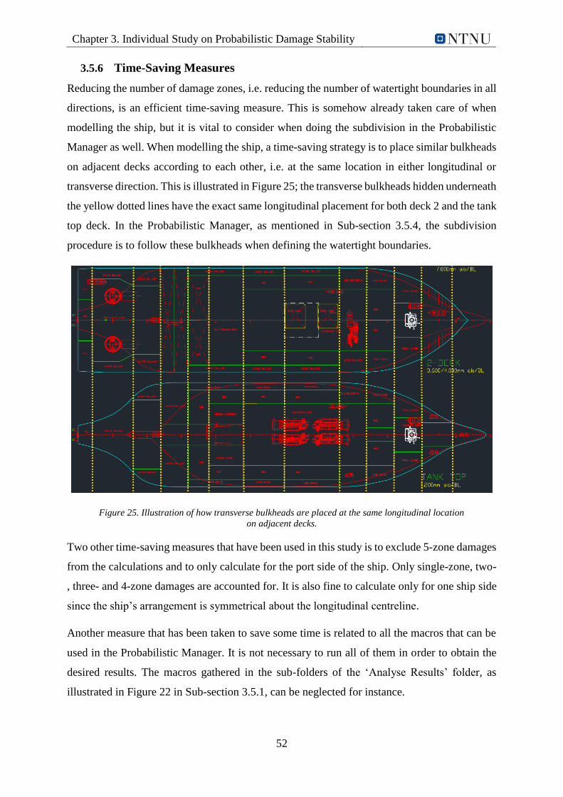
Chapter 3. Individual Study on Probabilistic Damage Stability
52
3.5.6 Time-Saving Measures
Reducing the number of damage zones, i.e. reducing the number of watertight boundaries in all
directions, is an efficient time-saving measure. This is somehow already taken care of when
modelling the ship, but it is vital to consider when doing the subdivision in the Probabilistic
Manager as well. When modelling the ship, a time-saving strategy is to place similar bulkheads
on adjacent decks according to each other, i.e. at the same location in either longitudinal or
transverse direction. This is illustrated in Figure 25; the transverse bulkheads hidden underneath
the yellow dotted lines have the exact same longitudinal placement for both deck 2 and the tank
top deck. In the Probabilistic Manager, as mentioned in Sub-section 3.5.4, the subdivision
procedure is to follow these bulkheads when defining the watertight boundaries.
Figure 25. Illustration of how transverse bulkheads are placed at the same longitudinal location
on adjacent decks.
Two other time-saving measures that have been used in this study is to exclude 5-zone damages
from the calculations and to only calculate for the port side of the ship. Only single-zone, two-
, three- and 4-zone damages are accounted for. It is also fine to calculate only for one ship side
since the ship’s arrangement is symmetrical about the longitudinal centreline.
Another measure that has been taken to save some time is related to all the macros that can be
used in the Probabilistic Manager. It is not necessary to run all of them in order to obtain the
desired results. The macros gathered in the sub-folders of the ‘Analyse Results’ folder, as
illustrated in Figure 22 in Sub-section 3.5.1, can be neglected for instance.
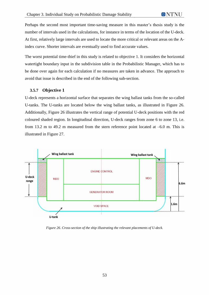
Chapter 3. Individual Study on Probabilistic Damage Stability
53
Perhaps the second most important time-saving measure in this master’s thesis study is the
number of intervals used in the calculations, for instance in terms of the location of the U-deck.
At first, relatively large intervals are used to locate the more critical or relevant areas on the A-
index curve. Shorter intervals are eventually used to find accurate values.
The worst potential time-thief in this study is related to objective 1. It considers the horizontal
watertight boundary input in the subdivision table in the Probabilistic Manager, which has to
be done over again for each calculation if no measures are taken in advance. The approach to
avoid that issue is described in the end of the following sub-section.
3.5.7 Objective 1
U-deck represents a horizontal surface that separates the wing ballast tanks from the so-called
U-tanks. The U-tanks are located below the wing ballast tanks, as illustrated in Figure 26.
Additionally, Figure 26 illustrates the vertical range of potential U-deck positions with the red
coloured shaded region. In longitudinal direction, U-deck ranges from zone 6 to zone 13, i.e.
from 13.2 m to 49.2 m measured from the stern reference point located at –6.0 m. This is
illustrated in Figure 27.
Figure 26. Cross-section of the ship illustrating the relevant placements of U-deck.
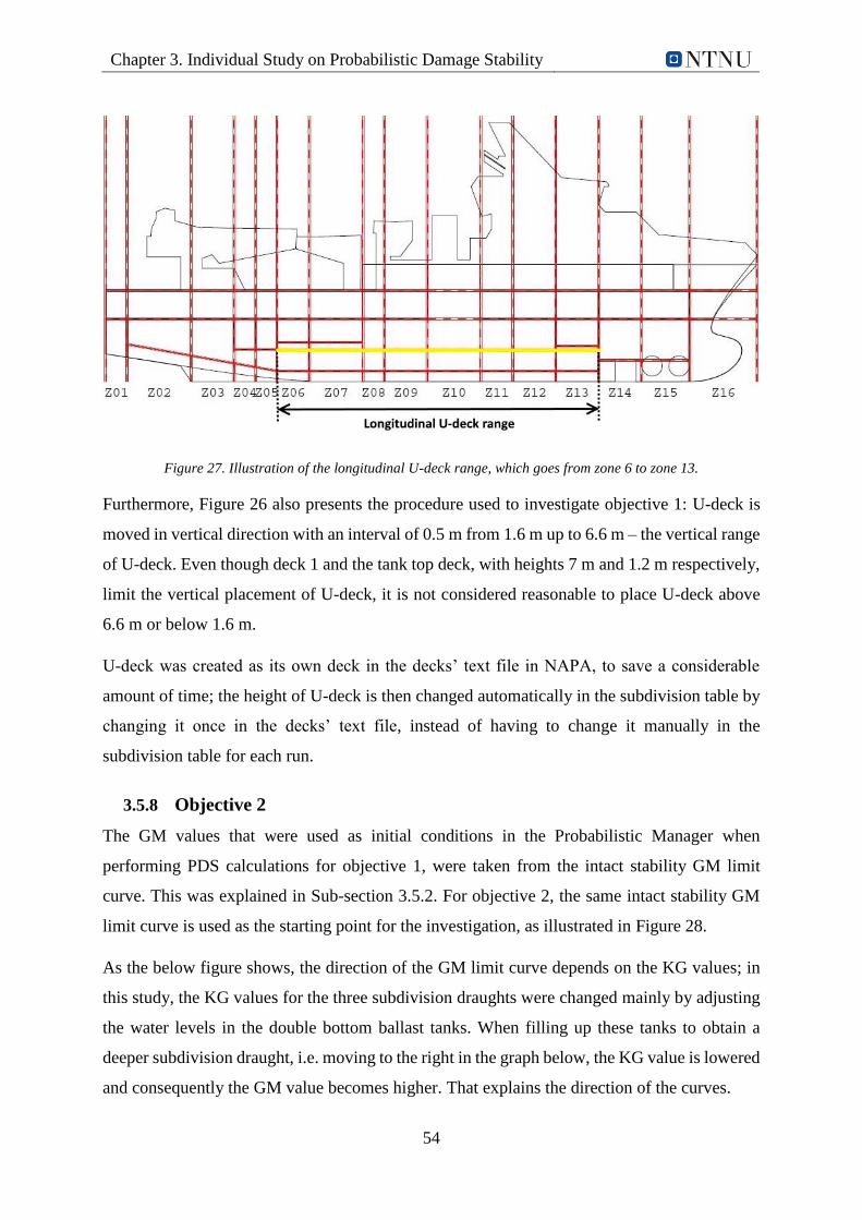
Chapter 3. Individual Study on Probabilistic Damage Stability
54
Figure 27. Illustration of the longitudinal U-deck range, which goes from zone 6 to zone 13.
Furthermore, Figure 26 also presents the procedure used to investigate objective 1: U-deck is
moved in vertical direction with an interval of 0.5 m from 1.6 m up to 6.6 m – the vertical range
of U-deck. Even though deck 1 and the tank top deck, with heights 7 m and 1.2 m respectively,
limit the vertical placement of U-deck, it is not considered reasonable to place U-deck above
6.6 m or below 1.6 m.
U-deck was created as its own deck in the decks’ text file in NAPA, to save a considerable
amount of time; the height of U-deck is then changed automatically in the subdivision table by
changing it once in the decks’ text file, instead of having to change it manually in the
subdivision table for each run.
3.5.8 Objective 2
The GM values that were used as initial conditions in the Probabilistic Manager when
performing PDS calculations for objective 1, were taken from the intact stability GM limit
curve. This was explained in Sub-section 3.5.2. For objective 2, the same intact stability GM
limit curve is used as the starting point for the investigation, as illustrated in Figure 28.
As the below figure shows, the direction of the GM limit curve depends on the KG values; in
this study, the KG values for the three subdivision draughts were changed mainly by adjusting
the water levels in the double bottom ballast tanks. When filling up these tanks to obtain a
deeper subdivision draught, i.e. moving to the right in the graph below, the KG value is lowered
and consequently the GM value becomes higher. That explains the direction of the curves.
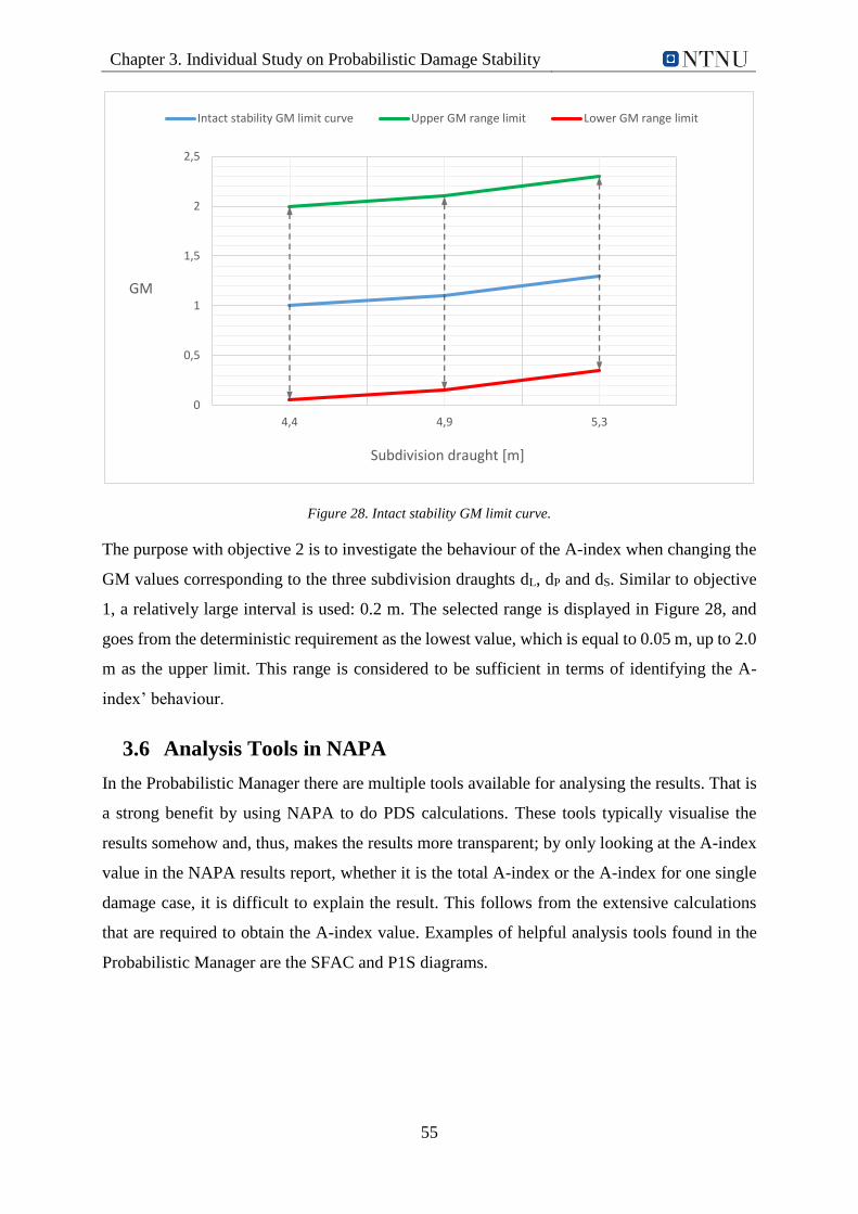
Chapter 3. Individual Study on Probabilistic Damage Stability
55
Figure 28. Intact stability GM limit curve.
The purpose with objective 2 is to investigate the behaviour of the A-index when changing the
GM values corresponding to the three subdivision draughts dL, dP and dS. Similar to objective
1, a relatively large interval is used: 0.2 m. The selected range is displayed in Figure 28, and
goes from the deterministic requirement as the lowest value, which is equal to 0.05 m, up to 2.0
m as the upper limit. This range is considered to be sufficient in terms of identifying the A-
index’ behaviour.
3.6 Analysis Tools in NAPA
In the Probabilistic Manager there are multiple tools available for analysing the results. That is
a strong benefit by using NAPA to do PDS calculations. These tools typically visualise the
results somehow and, thus, makes the results more transparent; by only looking at the A-index
value in the NAPA results report, whether it is the total A-index or the A-index for one single
damage case, it is difficult to explain the result. This follows from the extensive calculations
that are required to obtain the A-index value. Examples of helpful analysis tools found in the
Probabilistic Manager are the SFAC and P1S diagrams.
0
0,5
1
1,5
2
2,5
4,4 4,9 5,3
GM
Subdivision draught [m]
Intact stability GM limit curve Upper GM range limit Lower GM range limit
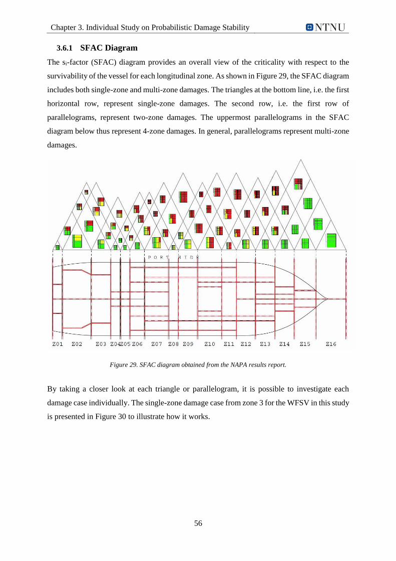
Chapter 3. Individual Study on Probabilistic Damage Stability
56
3.6.1 SFAC Diagram
The si-factor (SFAC) diagram provides an overall view of the criticality with respect to the
survivability of the vessel for each longitudinal zone. As shown in Figure 29, the SFAC diagram
includes both single-zone and multi-zone damages. The triangles at the bottom line, i.e. the first
horizontal row, represent single-zone damages. The second row, i.e. the first row of
parallelograms, represent two-zone damages. The uppermost parallelograms in the SFAC
diagram below thus represent 4-zone damages. In general, parallelograms represent multi-zone
damages.
Figure 29. SFAC diagram obtained from the NAPA results report.
By taking a closer look at each triangle or parallelogram, it is possible to investigate each
damage case individually. The single-zone damage case from zone 3 for the WFSV in this study
is presented in Figure 30 to illustrate how it works.

Chapter 3. Individual Study on Probabilistic Damage Stability
57
Figure 30. Single-zone damage case from zone 3. The figure is inspired by (Djupvik et al., 2015).
As visualised in Figure 30, no decks except for the tank top below the waterline are shown in
the SFAC diagram. The single-zone damage case in zone 3, which is illustrated in Figure 30,
deck 2 does not show. That is because the height of deck 2 in zone 3 is approximately 3 m,
according to the subdivision table in Appendix J, and the PDS regulations do not account for
groundings or collisions below the waterline. The waterline used in the SFAC diagram above
corresponds to the light service draught, which is 4.4 m in this study.
Furthermore, the bottom horizontal line in Figure 30 represents the tank top, the uppermost
horizontal line represents the maximum vertical damage extent, and the horizontal lines in
between represent the decks above the light service draught. The leftmost vertical line
represents the hull, the rightmost vertical line represents the centreline, and any vertical line in
between the latter two lines represents a longitudinal bulkhead. Furthermore, the colour codes
used in the SFAC diagrams are explained in Table 14 (Djupvik et al., 2015; Puustinen, 2012).
Table 14. Colour codes used in the SFAC diagrams (Djupvik et al., 2015; Puustinen, 2012).
Colour code Value of the s-factor
Green s ≥ 0.99
Yellow 0.05 ≤ s ≤ 0.99
Red s ≤ 0.05
White p ∙ r ∙ v < 0.00001
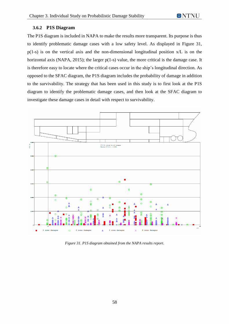
Chapter 3. Individual Study on Probabilistic Damage Stability
58
3.6.2 P1S Diagram
The P1S diagram is included in NAPA to make the results more transparent. Its purpose is thus
to identify problematic damage cases with a low safety level. As displayed in Figure 31,
p(1-s) is on the vertical axis and the non-dimensional longitudinal position x/L is on the
horizontal axis (NAPA, 2015); the larger p(1-s) value, the more critical is the damage case. It
is therefore easy to locate where the critical cases occur in the ship’s longitudinal direction. As
opposed to the SFAC diagram, the P1S diagram includes the probability of damage in addition
to the survivability. The strategy that has been used in this study is to first look at the P1S
diagram to identify the problematic damage cases, and then look at the SFAC diagram to
investigate these damage cases in detail with respect to survivability.
Figure 31. P1S diagram obtained from the NAPA results report.

59
4. Results of Individual Study
For the individual study, numerous calculations have been done in NAPA by following the
methods described in Chapter 0. Each calculation provides a results report that contains more
than 1000 pages of information. Considering the large number of reports in this study, these are
attached electronically, and can be found through a link in Appendix B. Thus, only the most
relevant information is included in the appendices, or presented in the thesis’ results or
discussion chapter. The results of the PDS calculations carried out for the objectives described
in Chapter 0 and 0, are presented in Chapter 4.
4.1 Objective 1: Changing the Height of U-deck
Section 4.1 presents the results related to objective 1 of the thesis; the aim of this section is to
show how the A-index varies with the placement of U-deck above the baseline. Graphs where
the A-index is plotted against the height of the U-deck are provided for all three subdivision
draughts individually, and for the total A-index. Regarding the A-index plots for the three
subdivision draughts, it is important to keep in mind that these A-index values have different
impact on the total A-index. As can be seen from Equation 8, which is re-presented below, AS,
AP and AL constitute 40%, 40% and 20% of the total A-index, respectively.
𝐴 = 0.4𝐴𝑆 + 0.4𝐴𝑃 + 0.2𝐴𝐿 > 𝑅
4.1.1 R-index
The method used to calculate the R-index was explained in Sub-section 2.4.3. Since the WFSV
used in the study is an SPS, a modified version of Equation 4 should be applied to calculate the
R-index, as re-presented in the below calculation. N is taken as 2 ∙ 60 = 120, because survival
craft moments are neglected. The 0.8 factor is included because the SPS carries not more than
60 personnel.
𝑅 = 0.8 ∙ [1 −5000
𝐿𝑠 + 2.5𝑁 + 15225] = 0.8 ∙ [1 −
5000
72.92 + 2.5 ∙ 120 + 15225 ] = 0,54356
This R-index value is equal to the one calculated by NAPA, as can be seen in Appendix K.

Chapter 4. Results of Individual Study
60
4.1.2 A-index
As Figure 32 reveals, there is a clear tendency regarding the A-index’ behaviour when changing
the U-deck height. Below U-deck height 5.6 m, which yields the maximum A-index value, the
A-index value is decreasing when reducing the height of U-deck. For larger U-deck heights
than 5.6 m, the A-index curve turns direction; the value of the A-index is decreasing when
increasing the height of U-deck.
The vertical lines in Figure 32 represent the decks that are located close to U-deck: deck 1, deck
2 and tank top deck. These decks are included in the plot because they function as vertical
barriers for flooding and, thus, they might impact the A-index. Deck 2 occurs in three of the
eight zones within the longitudinal range of U-deck, which stretches from zone 6 to zone 13,
and deck 2’s potential contribution will be discussed in Chapter 0.
Figure 32. Plot of A-index vs. placement of U-deck.
The development of the A-index in the above plot was expected; when U-deck is lowered, the
wing ballast tanks increase in volume and, consequently, a larger heeling moment can
potentially be created by damages that penetrate the wing ballast tanks. A larger heeling
moment reduces the survivability of the ship, which influences the A-index negatively. In the
damage case discussed here, the magnitude of the heeling moment depends on the draught of
the ship. As presented in Sub-section 3.5.2, the subdivision draughts used in this study are: dL
= 4.4 m, dP = 4.9 m and dS = 5.3 m. Bearing in mind that the A-index is equal to 0.2AL + 0.4AP
+ 0.4AS, it was expected that the A-index would be affected negatively by placing U-deck
anywhere below dS = 5.3 m, because sea water will flood the wing tanks below this height.
0,52
0,53
0,54
0,55
0,56
0,57
0,58
0,59
0,60
0,61
7000 6600 6100 5600 5100 4600 4100 3600 3100 2600 2100 1600 1200
A-i
nd
ex
Placement of U-deck above baseline [mm]
Total A-index for different U-deck heights
A-index
R-index
Deck 1
Tank top
Deck 2,Z06-Z07
Deck 2,Z13

Chapter 4. Results of Individual Study
61
At the same time as the wing ballast tanks increase in volume, when lowering the U-deck height,
the volumes of the U-tanks decrease. Offshore vessels are designed with U-tanks to increase
the survivability of the ship in case of damage. The larger the size of the U-tanks, the larger
effect the U-tanks have on the damage stability. U-tanks force the sea water to flood
symmetrically about the centreline of the ship and, thus, the higher sea water level in the U-
tanks, the bigger is the stabilizing effect. Of course, if the sea water reaches a certain level, and
KG as a result becomes sufficiently low, GM could turn out negative.
The development of the A-index curve in Figure 32 confirms the above theory. Both of the two
abovementioned effects drag the A-index in the same direction, when changing the U-deck
height. This can be explained with a scenario where several wing ballast tanks are damaged: A
larger U-deck height results in smaller wing ballast tank volumes and larger U-tank volumes,
which both contribute to lower heeling moment and, consequently, larger si-factor. A lower U-
deck height results in the opposite: larger wing ballast tank volumes and smaller U-tank
volumes, which increases the heeling moment and, consequently, decreases the si-factor.
In other words, the goal should be to find a U-deck height that provides a reasonable balance
between U-tank and wing ballast tank volumes, with respect to heeling moment in case of
damages involving U-deck. At the same time, it is important to remember that it is not only the
two abovementioned factors, i.e. the effect of wing ballast tanks and U-tanks, that affect the si-
factor in case of damage. There are numerous other damage cases, which involves other
compartment types and flooding scenarios. The focus in this part of the thesis is however on
damages that involve U-deck.
Furthermore, the key is to have as large wing ballast tanks as reasonably practicable. I.e., the
key is to maximise the A-index under the ‘restriction’ that the wing ballast tanks should have
room for a desired amount of ballast water. It is assumed that U-deck height 5.6 m, which
corresponds to the maximum value on the A-index curve, results in too small wing ballast tanks.
Thus, it is reasonable to proceed the study in objective 2 of the thesis with another U-deck
height. The relevant area on the graph from where the U-deck height shall be taken, seems to
range from approximately 4.1 m to 5.6 m – depending on how much ballast water the designer
wants to fit in the tanks. To improve the decision basis related to this ‘optimisation’ problem,
more data points and, thus, better accuracy in the relevant area on the graph is provided in
Figure 33.
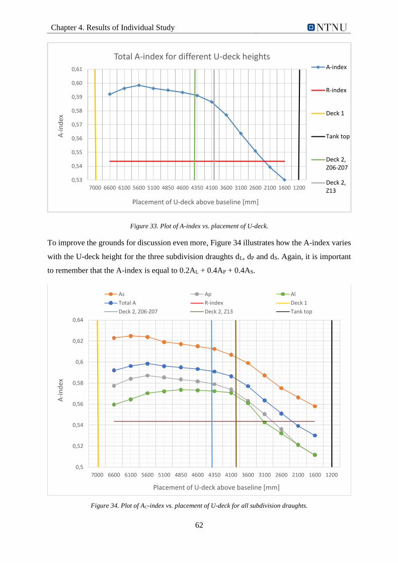
Chapter 4. Results of Individual Study
62
Figure 33. Plot of A-index vs. placement of U-deck.
To improve the grounds for discussion even more, Figure 34 illustrates how the A-index varies
with the U-deck height for the three subdivision draughts dL, dP and dS. Again, it is important
to remember that the A-index is equal to 0.2AL + 0.4AP + 0.4AS.
Figure 34. Plot of AC-index vs. placement of U-deck for all subdivision draughts.
0,53
0,54
0,55
0,56
0,57
0,58
0,59
0,60
0,61
7000 6600 6100 5600 5100 4850 4600 4350 4100 3600 3100 2600 2100 1600 1200
A-i
nd
ex
Placement of U-deck above baseline [mm]
Total A-index for different U-deck heightsA-index
R-index
Deck 1
Tank top
Deck 2,Z06-Z07
Deck 2,Z13
0,5
0,52
0,54
0,56
0,58
0,6
0,62
0,64
7000 6600 6100 5600 5100 4850 4600 4350 4100 3600 3100 2600 2100 1600 1200
A-i
nd
ex
Placement of U-deck above baseline [mm]
As Ap Al
Total A R-index Deck 1
Deck 2, Z06-Z07 Deck 2, Z13 Tank top
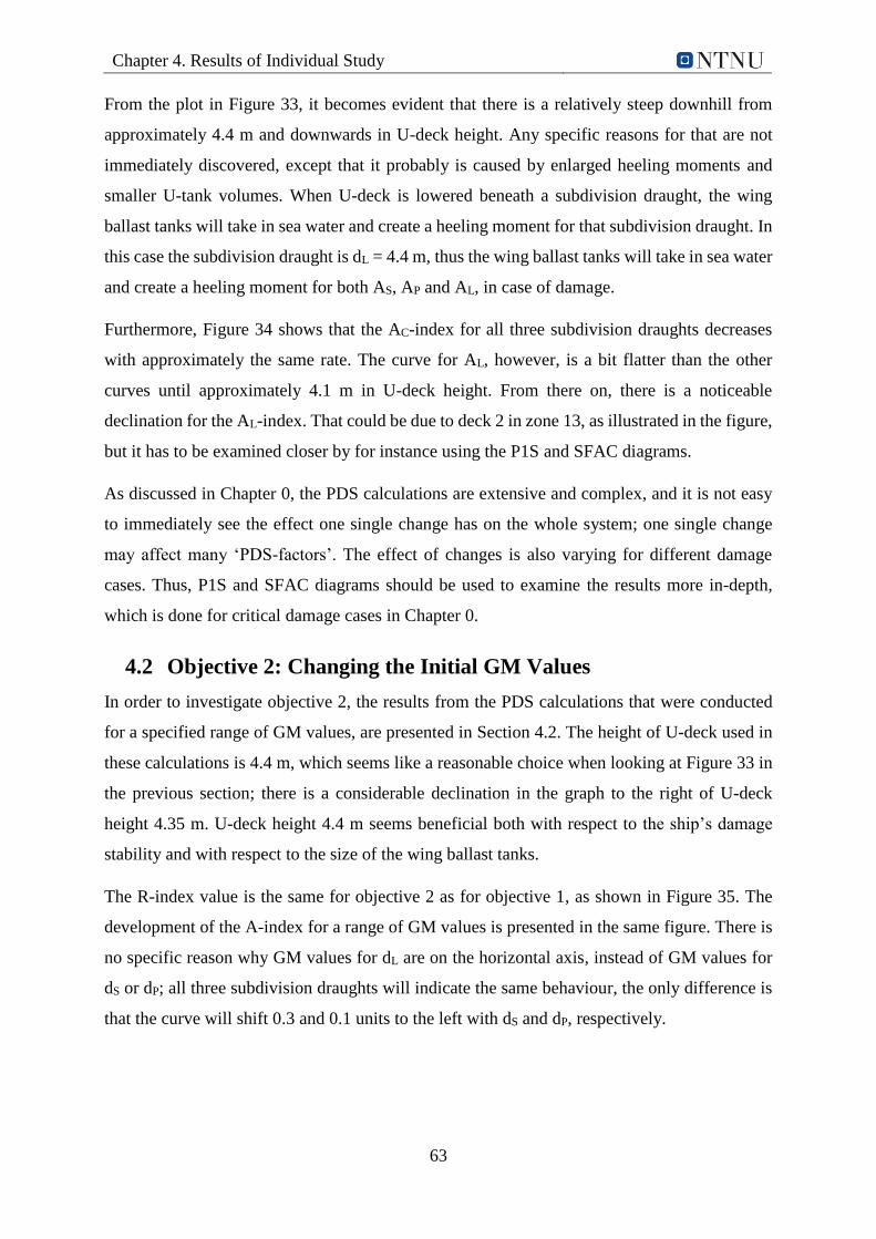
Chapter 4. Results of Individual Study
63
From the plot in Figure 33, it becomes evident that there is a relatively steep downhill from
approximately 4.4 m and downwards in U-deck height. Any specific reasons for that are not
immediately discovered, except that it probably is caused by enlarged heeling moments and
smaller U-tank volumes. When U-deck is lowered beneath a subdivision draught, the wing
ballast tanks will take in sea water and create a heeling moment for that subdivision draught. In
this case the subdivision draught is dL = 4.4 m, thus the wing ballast tanks will take in sea water
and create a heeling moment for both AS, AP and AL, in case of damage.
Furthermore, Figure 34 shows that the AC-index for all three subdivision draughts decreases
with approximately the same rate. The curve for AL, however, is a bit flatter than the other
curves until approximately 4.1 m in U-deck height. From there on, there is a noticeable
declination for the AL-index. That could be due to deck 2 in zone 13, as illustrated in the figure,
but it has to be examined closer by for instance using the P1S and SFAC diagrams.
As discussed in Chapter 0, the PDS calculations are extensive and complex, and it is not easy
to immediately see the effect one single change has on the whole system; one single change
may affect many ‘PDS-factors’. The effect of changes is also varying for different damage
cases. Thus, P1S and SFAC diagrams should be used to examine the results more in-depth,
which is done for critical damage cases in Chapter 0.
4.2 Objective 2: Changing the Initial GM Values
In order to investigate objective 2, the results from the PDS calculations that were conducted
for a specified range of GM values, are presented in Section 4.2. The height of U-deck used in
these calculations is 4.4 m, which seems like a reasonable choice when looking at Figure 33 in
the previous section; there is a considerable declination in the graph to the right of U-deck
height 4.35 m. U-deck height 4.4 m seems beneficial both with respect to the ship’s damage
stability and with respect to the size of the wing ballast tanks.
The R-index value is the same for objective 2 as for objective 1, as shown in Figure 35. The
development of the A-index for a range of GM values is presented in the same figure. There is
no specific reason why GM values for dL are on the horizontal axis, instead of GM values for
dS or dP; all three subdivision draughts will indicate the same behaviour, the only difference is
that the curve will shift 0.3 and 0.1 units to the left with dS and dP, respectively.
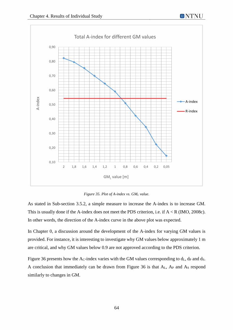
Chapter 4. Results of Individual Study
64
Figure 35. Plot of A-index vs. GML value.
As stated in Sub-section 3.5.2, a simple measure to increase the A-index is to increase GM.
This is usually done if the A-index does not meet the PDS criterion, i.e. if A < R (IMO, 2008c).
In other words, the direction of the A-index curve in the above plot was expected.
In Chapter 0, a discussion around the development of the A-index for varying GM values is
provided. For instance, it is interesting to investigate why GM values below approximately 1 m
are critical, and why GM values below 0.9 are not approved according to the PDS criterion.
Figure 36 presents how the AC-index varies with the GM values corresponding to dL, dP and dS.
A conclusion that immediately can be drawn from Figure 36 is that AL, AP and AS respond
similarly to changes in GM.
0,10
0,20
0,30
0,40
0,50
0,60
0,70
0,80
0,90
2 1,8 1,6 1,4 1,2 1 0,8 0,6 0,4 0,2 0,05
A-i
nd
ex
GML value [m]
Total A-index for different GM values
A-index
R-index
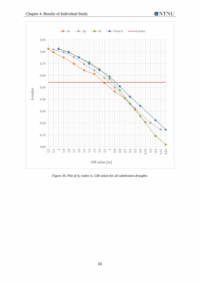
Chapter 4. Results of Individual Study
65
Figure 36. Plot of AC-index vs. GM values for all subdivision draughts.
0,00
0,10
0,20
0,30
0,40
0,50
0,60
0,70
0,80
0,90
2,3
2,1 2
1,9
1,8
1,7
1,6
1,5
1,4
1,3
1,2
1,1 1
0,9
0,8
0,7
0,6
0,5
0,4
0,3
5
0,3
0,2
0,1
5
0,0
5
A-i
nd
ex
GM value [m]
As Ap Al Total A R-index

66
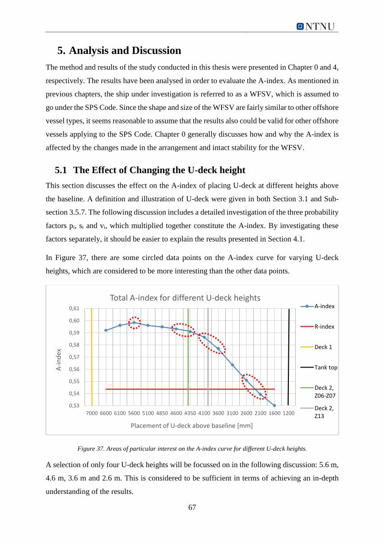
67
5. Analysis and Discussion
The method and results of the study conducted in this thesis were presented in Chapter 0 and 4,
respectively. The results have been analysed in order to evaluate the A-index. As mentioned in
previous chapters, the ship under investigation is referred to as a WFSV, which is assumed to
go under the SPS Code. Since the shape and size of the WFSV are fairly similar to other offshore
vessel types, it seems reasonable to assume that the results also could be valid for other offshore
vessels applying to the SPS Code. Chapter 0 generally discusses how and why the A-index is
affected by the changes made in the arrangement and intact stability for the WFSV.
5.1 The Effect of Changing the U-deck height
This section discusses the effect on the A-index of placing U-deck at different heights above
the baseline. A definition and illustration of U-deck were given in both Section 3.1 and Sub-
section 3.5.7. The following discussion includes a detailed investigation of the three probability
factors pi, si and vi, which multiplied together constitute the A-index. By investigating these
factors separately, it should be easier to explain the results presented in Section 4.1.
In Figure 37, there are some circled data points on the A-index curve for varying U-deck
heights, which are considered to be more interesting than the other data points.
Figure 37. Areas of particular interest on the A-index curve for different U-deck heights.
A selection of only four U-deck heights will be focussed on in the following discussion: 5.6 m,
4.6 m, 3.6 m and 2.6 m. This is considered to be sufficient in terms of achieving an in-depth
understanding of the results.
0,53
0,54
0,55
0,56
0,57
0,58
0,59
0,60
0,61
7000 6600 6100 5600 5100 4850 4600 4350 4100 3600 3100 2600 2100 1600 1200
A-i
nd
ex
Placement of U-deck above baseline [mm]
Total A-index for different U-deck heightsA-index
R-index
Deck 1
Tank top
Deck 2,Z06-Z07
Deck 2,Z13

Chapter 5. Analysis and Discussion
68
When investigating the U-deck heights selected above, U-deck height 2.6 m will be examined
first considering it has the lowest A-index and, thus, probably contains the most critical damage
cases. The strategy is to use the P1S diagram to identify critical damage cases within the
longitudinal range of U-deck with height 2.6 m. Then, SFAC diagrams are used to confirm the
findings from the P1S diagram, or to identify other interesting damage cases. Furthermore, the
SFAC diagrams for the most critical damage cases for all of the selected U-deck heights, are
studied closely to find out what happens with the si-, vi- and pi-factor.
The P1S diagram for U-deck height 2.6 m is presented in Figure 38. The black coloured square
marks the relevant longitudinal range of U-deck: zone 6 to zone 13. The damage cases with the
largest p(1-s) values and, thus, the lowest safety level within the longitudinal U-deck range, are
marked with a red coloured square.
Figure 38. P1S diagram for U-deck height 2.6 m.
In Figure 38, two-zone damages appear to be generally more critical than other damage cases.
It is not straightforward to find the reason for that, especially due to the complex formulas and
extensive procedure used to calculate the pi-factor both for single-zone and multi-zone
damages. These formulas are attached in Appendix A. Regarding the si-factor, it is expected
that the more zones that are involved in a damage, the more critical the damage becomes with
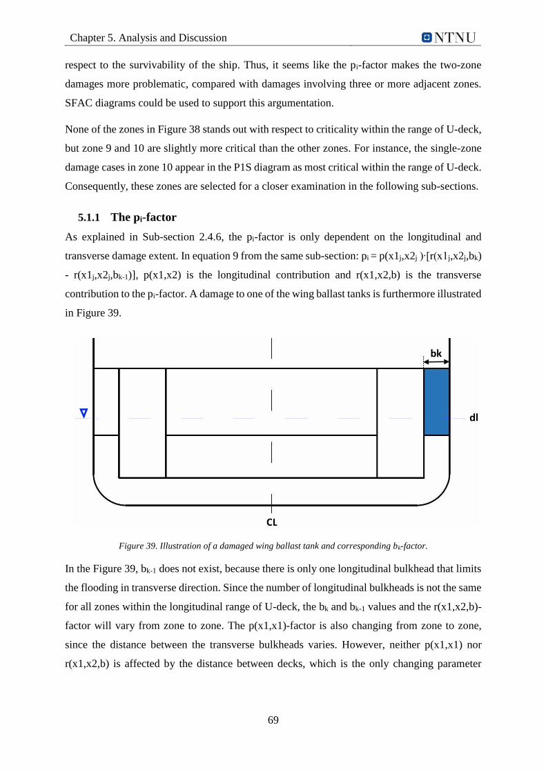
Chapter 5. Analysis and Discussion
69
respect to the survivability of the ship. Thus, it seems like the pi-factor makes the two-zone
damages more problematic, compared with damages involving three or more adjacent zones.
SFAC diagrams could be used to support this argumentation.
None of the zones in Figure 38 stands out with respect to criticality within the range of U-deck,
but zone 9 and 10 are slightly more critical than the other zones. For instance, the single-zone
damage cases in zone 10 appear in the P1S diagram as most critical within the range of U-deck.
Consequently, these zones are selected for a closer examination in the following sub-sections.
5.1.1 The pi-factor
As explained in Sub-section 2.4.6, the pi-factor is only dependent on the longitudinal and
transverse damage extent. In equation 9 from the same sub-section: pi = p(x1j,x2j )∙[r(x1j,x2j,bk)
- r(x1j,x2j,bk-1)], p(x1,x2) is the longitudinal contribution and r(x1,x2,b) is the transverse
contribution to the pi-factor. A damage to one of the wing ballast tanks is furthermore illustrated
in Figure 39.
Figure 39. Illustration of a damaged wing ballast tank and corresponding bk-factor.
In the Figure 39, bk-1 does not exist, because there is only one longitudinal bulkhead that limits
the flooding in transverse direction. Since the number of longitudinal bulkheads is not the same
for all zones within the longitudinal range of U-deck, the bk and bk-1 values and the r(x1,x2,b)-
factor will vary from zone to zone. The p(x1,x1)-factor is also changing from zone to zone,
since the distance between the transverse bulkheads varies. However, neither p(x1,x1) nor
r(x1,x2,b) is affected by the distance between decks, which is the only changing parameter
Chapter 5. Analysis and Discussion
70
regarding objective 1 of the thesis. In other words, the height of U-deck will not affect the pi-
factor.
5.1.2 The si-factor
As discussed in Sub-section 4.1.2, damages to the wing ballast tanks might have a considerable
effect on the si-factor; this type of damage can potentially create a heeling moment that makes
the ship heel over. In such case, the GZ curve changes and results in a reduced K value for heel
angles larger than 7 degrees. This can be seen from Equation 38 and 39 in Sub-section 2.4.7:
θmin is equal to 7 degrees, since the WFSV is treated as a passenger ship by the PDS regulations.
Thus an increase in θe reduces K and, consequently, the si-factor for heel angles larger than 7
degrees. On top of this, if the GZmax and range values are reduced below 0.12 and 16,
respectively, the si-factor will be reduced even more.
The abovementioned potential effects influence the A-index negatively. The magnitude of the
impact depends on the height of U-deck, as was thoroughly explained in Sub-section 4.1.2. It
should be added that the survivability, or the si-factor, of the ship depends on a number of other
factors than the height of U-deck. It is however the U-deck height that is in focus in Sub-section
5.1.2, and in Section 5.1.
The survivability of the ship for every single damage case is illustrated in SFAC diagrams in
the NAPA results report. NAPA creates one SFAC diagram for each subdivision draught. It
seems like dL is most critical with respect to survivability in this study, which is illustrated and
explained in Appendix L. The SFAC diagrams for dL for the selected U-deck heights are
therefore used as the basis in the following discussion, in order to be conservative.
Figure 40 furthermore presents the SFAC diagram for U-deck height 2.6 m. This U-deck height
is the most problematic of the selected U-deck heights in terms of A-index value. There is a
dotted circle in Figure 40, highlighting the damage zones considered to be most critical within
the U-deck range. The SFAC diagrams for the other selected U-deck heights can be found in
Appendix M.
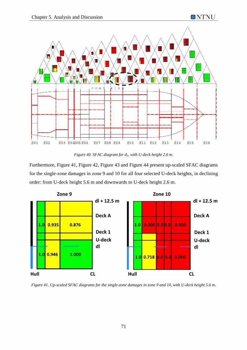
Chapter 5. Analysis and Discussion
71
Figure 40. SFAC diagram for dL, with U-deck height 2.6 m.
Furthermore, Figure 41, Figure 42, Figure 43 and Figure 44 present up-scaled SFAC diagrams
for the single-zone damages in zone 9 and 10 for all four selected U-deck heights, in declining
order: from U-deck height 5.6 m and downwards to U-deck height 2.6 m.
Figure 41. Up-scaled SFAC diagrams for the single-zone damages in zone 9 and 10, with U-deck height 5.6 m.
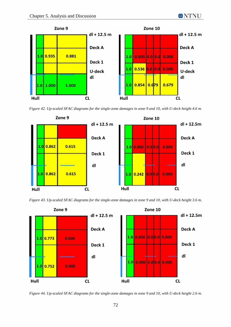
Chapter 5. Analysis and Discussion
72
Figure 42. Up-scaled SFAC diagrams for the single-zone damages in zone 9 and 10, with U-deck height 4.6 m.
Figure 43. Up-scaled SFAC diagrams for the single-zone damages in zone 9 and 10, with U-deck height 3.6 m.
Figure 44. Up-scaled SFAC diagrams for the single-zone damages in zone 9 and 10, with U-deck height 2.6 m.
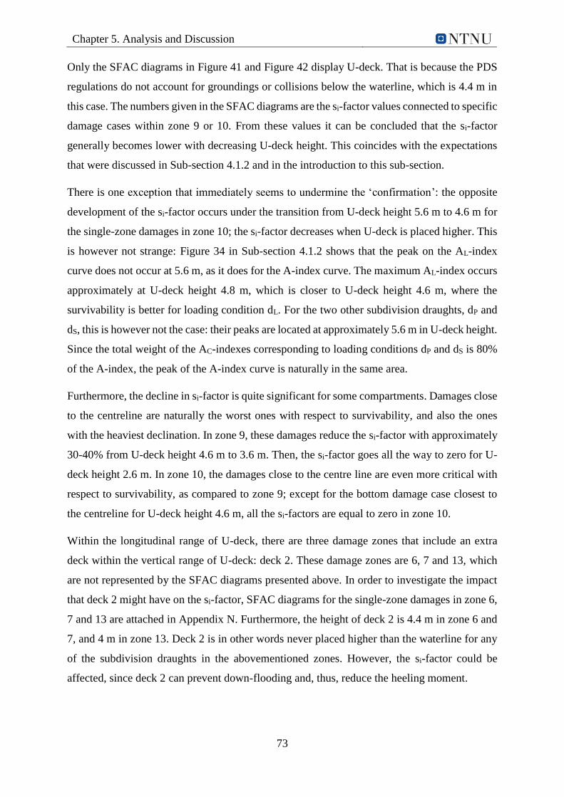
Chapter 5. Analysis and Discussion
73
Only the SFAC diagrams in Figure 41 and Figure 42 display U-deck. That is because the PDS
regulations do not account for groundings or collisions below the waterline, which is 4.4 m in
this case. The numbers given in the SFAC diagrams are the si-factor values connected to specific
damage cases within zone 9 or 10. From these values it can be concluded that the si-factor
generally becomes lower with decreasing U-deck height. This coincides with the expectations
that were discussed in Sub-section 4.1.2 and in the introduction to this sub-section.
There is one exception that immediately seems to undermine the ‘confirmation’: the opposite
development of the si-factor occurs under the transition from U-deck height 5.6 m to 4.6 m for
the single-zone damages in zone 10; the si-factor decreases when U-deck is placed higher. This
is however not strange: Figure 34 in Sub-section 4.1.2 shows that the peak on the AL-index
curve does not occur at 5.6 m, as it does for the A-index curve. The maximum AL-index occurs
approximately at U-deck height 4.8 m, which is closer to U-deck height 4.6 m, where the
survivability is better for loading condition dL. For the two other subdivision draughts, dP and
dS, this is however not the case: their peaks are located at approximately 5.6 m in U-deck height.
Since the total weight of the AC-indexes corresponding to loading conditions dP and dS is 80%
of the A-index, the peak of the A-index curve is naturally in the same area.
Furthermore, the decline in si-factor is quite significant for some compartments. Damages close
to the centreline are naturally the worst ones with respect to survivability, and also the ones
with the heaviest declination. In zone 9, these damages reduce the si-factor with approximately
30-40% from U-deck height 4.6 m to 3.6 m. Then, the si-factor goes all the way to zero for U-
deck height 2.6 m. In zone 10, the damages close to the centre line are even more critical with
respect to survivability, as compared to zone 9; except for the bottom damage case closest to
the centreline for U-deck height 4.6 m, all the si-factors are equal to zero in zone 10.
Within the longitudinal range of U-deck, there are three damage zones that include an extra
deck within the vertical range of U-deck: deck 2. These damage zones are 6, 7 and 13, which
are not represented by the SFAC diagrams presented above. In order to investigate the impact
that deck 2 might have on the si-factor, SFAC diagrams for the single-zone damages in zone 6,
7 and 13 are attached in Appendix N. Furthermore, the height of deck 2 is 4.4 m in zone 6 and
7, and 4 m in zone 13. Deck 2 is in other words never placed higher than the waterline for any
of the subdivision draughts in the abovementioned zones. However, the si-factor could be
affected, since deck 2 can prevent down-flooding and, thus, reduce the heeling moment.

Chapter 5. Analysis and Discussion
74
First of all, by looking at the P1S diagram in Figure 38, it does not seem like the single-zone
damages in zone 6, 7 and 13 are critical at all. This could be a result of a low pi-factor or a large
si-factor, or both. The SFAC diagrams in Appendix N furthermore indicate that the survivability
in general decreases when lowering the U-deck height in these zones, however not in the same
order of magnitude as for the single-zone damages in zone 9 and 10. In addition, it is assumed
that the pi-factor is fairly similar for all of the abovementioned damage cases. Thus, it seems
like deck 2 has a positive, minor effect on the si-factor, but not significant enough to prevent
the declination when lowering the U-deck height.
Based on the above discussion, it seems safe to conclude that the si-factors generally decrease
when the U-deck height is lowered beneath 5.6 m. As mentioned earlier, U-deck will probably
never be placed above this height anyway, due to practical reasons. Additionally, since the
development of the si-factor correlates quite well with the development of the A-index, the
results may indicate that the si-factor in general contributes significantly to the A-index. This
will be discussed further in Sub-section 5.1.4.
5.1.3 The vi-factor
U-deck is a horizontal surface that may, depending on its height and the damage scenario, limit
flooding vertically in case of damage. Either way, the vi-factor will change when U-deck is
moved in vertical direction, as long as the change in height occurs above the waterline. For U-
deck heights below the waterline, any changes will not influence the vi-factor. This is illustrated
below, where U-deck is placed above the waterline in Figure 45 and below the waterline in
Figure 46. Supporting literature can be found in Sub-section 2.4.8 of the thesis.
Figure 45. vi-factor for wing tank damage, with U-deck placed above the waterline.
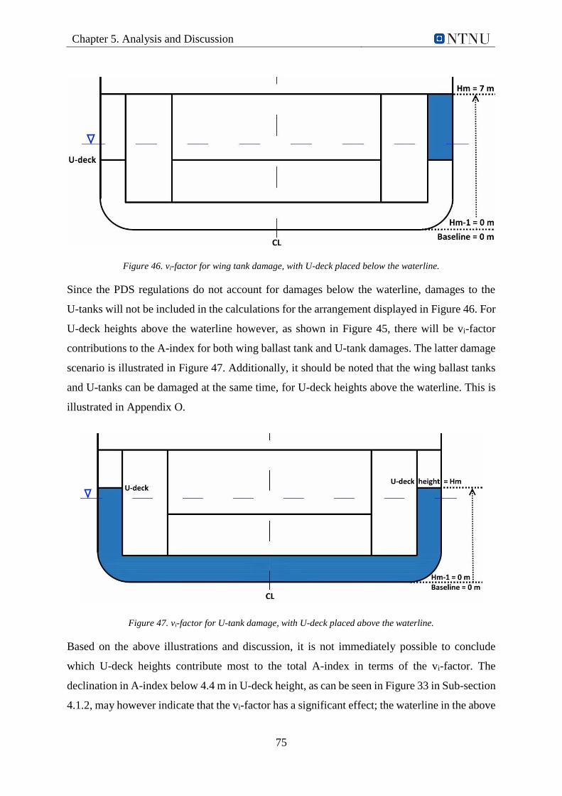
Chapter 5. Analysis and Discussion
75
Figure 46. vi-factor for wing tank damage, with U-deck placed below the waterline.
Since the PDS regulations do not account for damages below the waterline, damages to the
U-tanks will not be included in the calculations for the arrangement displayed in Figure 46. For
U-deck heights above the waterline however, as shown in Figure 45, there will be vi-factor
contributions to the A-index for both wing ballast tank and U-tank damages. The latter damage
scenario is illustrated in Figure 47. Additionally, it should be noted that the wing ballast tanks
and U-tanks can be damaged at the same time, for U-deck heights above the waterline. This is
illustrated in Appendix O.
Figure 47. vi-factor for U-tank damage, with U-deck placed above the waterline.
Based on the above illustrations and discussion, it is not immediately possible to conclude
which U-deck heights contribute most to the total A-index in terms of the vi-factor. The
declination in A-index below 4.4 m in U-deck height, as can be seen in Figure 33 in Sub-section
4.1.2, may however indicate that the vi-factor has a significant effect; the waterline in the above

Chapter 5. Analysis and Discussion
76
illustrations corresponds to dL = 4.4 m, and the overall vi-factor contribution is assumed to be
smaller for U-deck heights below the waterline. At the same time, the declination could also be
solely due to the reduction in si-factor. Hence, it is not easy to tell straight away which of the
vi- and si-factor that is most influential with respect to the A-index. This issue will be discussed
further in Sub-section 0.
To provide greater insight related to the vi-factors, calculations for the abovementioned damage
cases have been carried out according to the theory presented in Sub-section 2.4.8. The
calculations are conducted for all three loading conditions: dS, dP and dL. The damage cases
used in the calculations are presented in Table 15, and the corresponding Hm and Hm-1 values
for the selected U-deck heights can be found in Appendix P. For all three loading conditions, a
calculation of the vi-factor is done for each damage case listed in Table 15. The mean vi-factor
of the three damage cases, is then plotted for each loading condition against the selected U-
deck heights in Figure 48.
Table 15. The damage cases used to investigate the vi-factor for objective 1.
Damage case Damaged compartments Illustration of damage case
A Wing ballast tank Figure 45 / Figure 46
B U-tank Figure 47
C Wing ballast tank + U-tank Appendix O
Figure 48. Mean development of the vi-factor for damage case A, B and C, for all three subdivision draughts.
0,00
0,05
0,10
0,15
0,20
2,6 3,6 4,6 5,6
vi-f
acto
r
U-deck height above baseline [m]
Mean vi-factor development for damage case A, B and C, for dL, dP and dS
Mean dL
Mean dP
Mean dS
Overallweightedmean
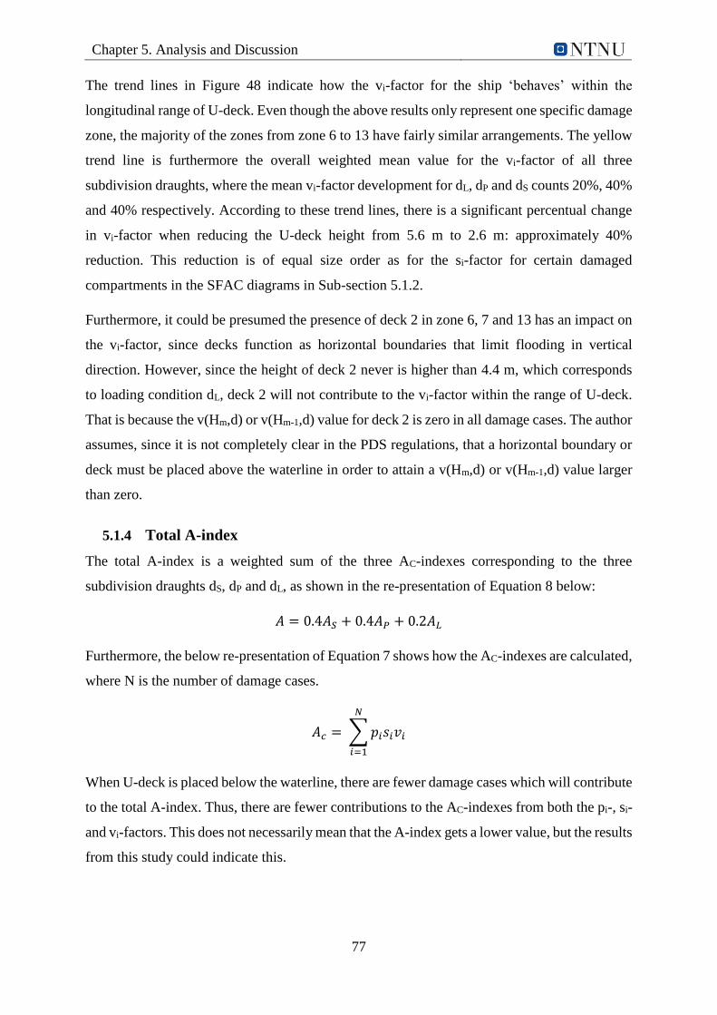
Chapter 5. Analysis and Discussion
77
The trend lines in Figure 48 indicate how the vi-factor for the ship ‘behaves’ within the
longitudinal range of U-deck. Even though the above results only represent one specific damage
zone, the majority of the zones from zone 6 to 13 have fairly similar arrangements. The yellow
trend line is furthermore the overall weighted mean value for the vi-factor of all three
subdivision draughts, where the mean vi-factor development for dL, dP and dS counts 20%, 40%
and 40% respectively. According to these trend lines, there is a significant percentual change
in vi-factor when reducing the U-deck height from 5.6 m to 2.6 m: approximately 40%
reduction. This reduction is of equal size order as for the si-factor for certain damaged
compartments in the SFAC diagrams in Sub-section 5.1.2.
Furthermore, it could be presumed the presence of deck 2 in zone 6, 7 and 13 has an impact on
the vi-factor, since decks function as horizontal boundaries that limit flooding in vertical
direction. However, since the height of deck 2 never is higher than 4.4 m, which corresponds
to loading condition dL, deck 2 will not contribute to the vi-factor within the range of U-deck.
That is because the v(Hm,d) or v(Hm-1,d) value for deck 2 is zero in all damage cases. The author
assumes, since it is not completely clear in the PDS regulations, that a horizontal boundary or
deck must be placed above the waterline in order to attain a v(Hm,d) or v(Hm-1,d) value larger
than zero.
5.1.4 Total A-index
The total A-index is a weighted sum of the three AC-indexes corresponding to the three
subdivision draughts dS, dP and dL, as shown in the re-presentation of Equation 8 below:
𝐴 = 0.4𝐴𝑆 + 0.4𝐴𝑃 + 0.2𝐴𝐿
Furthermore, the below re-presentation of Equation 7 shows how the AC-indexes are calculated,
where N is the number of damage cases.
𝐴𝑐 = ∑𝑝𝑖𝑠𝑖𝑣𝑖
𝑁
𝑖=1
When U-deck is placed below the waterline, there are fewer damage cases which will contribute
to the total A-index. Thus, there are fewer contributions to the AC-indexes from both the pi-, si-
and vi-factors. This does not necessarily mean that the A-index gets a lower value, but the results
from this study could indicate this.

Chapter 5. Analysis and Discussion
78
In this study, the A-index is declining below 5.6 m in U-deck height. From a U-deck height
approximately 4.4 m and downwards, which corresponds to waterline dL, the declination gets
steeper for the A-index. This strengthens the theory that the number of damage cases could be
of importance; when U-deck is placed below the waterline, the number of damage zones is
reduced, which in turn leads to fewer AC-index contributions. On the other hand, the A-index
continues to decline below all three subdivision draughts, i.e. below dL = 4.4 m, where the
number of damage zones will be constant for all U-deck heights. This weakens the theory in
the previous paragraph.
Furthermore, by knowing the pi-factor is constant for all U-deck heights, it is obvious that either
the si- or vi-factor, or both, contribute to the reduction in A-index for U-deck heights lower than
5.6 m. Based on the analysis and discussion in Sub-section 5.1.2 and 5.1.3, it seems safe to state
that both factors contribute to the reduction. Which of the factors that is most influential,
however, is harder to say.
One potential indicator, which leads the author to think that the si-factor might be more
influential, is the mean vi-factor curves presented in Figure 48. These trend lines only represent
the majority of the damage zones within the range of U-deck. Additionally, they do not
represent any other damage cases than the ones closest to the hull. This means that it might be
wrong to draw a conclusion based on this data. Irrespective of the latter uncertainty, the
abovementioned trend lines do not correspond very well with the A-index curve. For instance,
there does not seem to be a development for the vi-factor when moving U-deck from 3.6 m to
2.6 m. This is not the case with the si-factor, which is reduced all the way down from U-deck
height 5.6 m to 2.6 m for zone 6, 7, 9, 10 and 13 at least. In conclusion, the si-factor seems to
be more influential, under the assumption that the vi-factor development is valid.

Chapter 5. Analysis and Discussion
79
5.2 The Effect of Changing the Initial GM Values
This section discusses the influence changes in GM values have on the A-index for the three
subdivision draughts dL, dP and dS. The GM values will thus be referred to as the GML, GMP
and GMS, when discussing the change in A-index or AC-index for the different subdivision
draughts. Sub-section 3.5.8 and Section 4.2 constitute the basis for the following discussion.
Furthermore, by investigating the pi-, si- and vi-factors individually, it should be easier to break
down and understand the results.
Figure 49 re-presents the results from Section 4.2, but now the figure includes two circles that
indicate interesting areas on the graph with respect to further investigation. Additionally, it is
important to note that the results presented below and discussed in this section only are relevant
for U-deck height 4.4 m, as explained in Chapter 4.
Figure 49. Areas of particular interest on the A-index curve for different GM values.
0,00
0,10
0,20
0,30
0,40
0,50
0,60
0,70
0,80
0,90
2,3
2,1 2
1,9
1,8
1,7
1,6
1,5
1,4
1,3
1,2
1,1 1
0,9
0,8
0,7
0,6
0,5
0,4
0,3
5
0,3
0,2
0,1
5
0,0
5
A-i
nd
ex
GM value [m]
As Ap Al Total A R-index

Chapter 5. Analysis and Discussion
80
From Figure 49 it seems like the loading condition dS is most critical with respect to the A-
index, knowing that the AS-index weighs 40% of the A-index. Three different GMS values have
therefore been selected for a closer investigation: 0.9 m, 1.3 m and 1.9 m. GM values lower
than 0.9 m are not considered relevant, because their corresponding A-indexes are far from
being in compliance with the ‘PDS criteria’, i.e. A > R. Furthermore, the GMP and GML values
corresponding to the selected GMS values, are listed in Table 16.
Table 16. GM values selected for in-depth analysis and discussion.
GMS GMP GML
0.9 m 0.7 m 0.6 m
1.3 m 1.1 m 1.0 m
1.9 m 1.7 m 1.6 m
The same approach that was used to identify critical damage cases in Section 5.1, will be
followed in this section: the P1S diagram for GMS = 0.9 m will be used to find critical damage
cases, which subsequently will be studied in detail using SFAC diagrams. Additionally, the
si-, vi- and pi-factors are analysed individually. The P1S diagram for GMS = 0.9 m, with U-deck
height 4.4 m, is given in Figure 50.
Figure 50. P1S diagram for GMS = 0.9 m and U-deck height 4.4 m.

Chapter 5. Analysis and Discussion
81
The squares in Figure 50 enclose a selection of damage cases that may be considered critical,
where the single-zone damages in zone 2 clearly stand out as most severe. There are in addition
some relatively critical two-zone damages evenly distributed over the entire ship length, with
the majority encapsulated in the square to the right. The following damage cases will therefore
be subject to analysis: the single-zone damages in zone 2 and the two-zone damages involving
zone 10 and 11.
5.2.1 The pi- and vi-factor
There are no changes in the arrangement of the WFSV in objective 2 of the master’s thesis.
Thus, in similarity with objective 1 of the thesis, the pi-factor does not change. Additionally, as
opposed to objective 1 of the thesis, the vi-factor does not change since the height of all
horizontal surfaces remain the same. Consequently, the development of the A-index
corresponding to objective 2 of the thesis, must therefore be a result of changes in the si-factor.
This will be discussed in the following sub-section.
5.2.2 The si-factor
Up-scaled SFAC diagrams for the selected damage cases corresponding to objective 2 of the
thesis, for loading condition dS and the GMS values in Table 16, are provided in Figure 51 and
Figure 53. The complete SFAC diagrams are attached to the thesis in Appendix Q. The single-
zone damages in zone 2 will be investigated first, followed by the two-zone damage cases
involving zone 10 and 11.
Investigating the si-factor for the single-zone damages in zone 2:
Figure 51. Development of the si-factor in zone 2, for loading condition dS and varying GMS values.
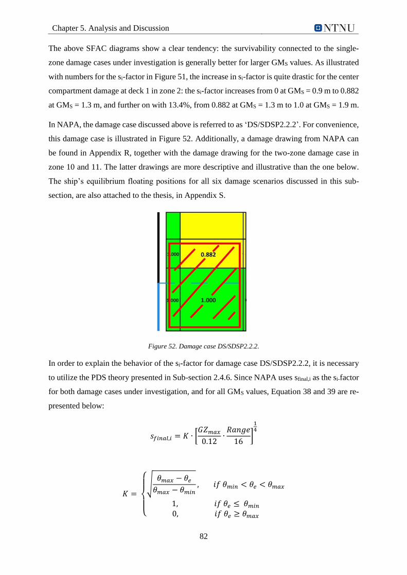
Chapter 5. Analysis and Discussion
82
The above SFAC diagrams show a clear tendency: the survivability connected to the single-
zone damage cases under investigation is generally better for larger GMS values. As illustrated
with numbers for the si-factor in Figure 51, the increase in si-factor is quite drastic for the center
compartment damage at deck 1 in zone 2: the si-factor increases from 0 at GMS = 0.9 m to 0.882
at GMS = 1.3 m, and further on with 13.4%, from 0.882 at GMS = 1.3 m to 1.0 at GMS = 1.9 m.
In NAPA, the damage case discussed above is referred to as ‘DS/SDSP2.2.2’. For convenience,
this damage case is illustrated in Figure 52. Additionally, a damage drawing from NAPA can
be found in Appendix R, together with the damage drawing for the two-zone damage case in
zone 10 and 11. The latter drawings are more descriptive and illustrative than the one below.
The ship’s equilibrium floating positions for all six damage scenarios discussed in this sub-
section, are also attached to the thesis, in Appendix S.
Figure 52. Damage case DS/SDSP2.2.2.
In order to explain the behavior of the si-factor for damage case DS/SDSP2.2.2, it is necessary
to utilize the PDS theory presented in Sub-section 2.4.6. Since NAPA uses sfinal,i as the si-factor
for both damage cases under investigation, and for all GMS values, Equation 38 and 39 are re-
presented below:
𝑠𝑓𝑖𝑛𝑎𝑙,𝑖 = 𝐾 ∙ [𝐺𝑍𝑚𝑎𝑥0.12
∙𝑅𝑎𝑛𝑔𝑒
16]
14
𝐾 =
{
√𝜃𝑚𝑎𝑥 − 𝜃𝑒𝜃𝑚𝑎𝑥 − 𝜃𝑚𝑖𝑛
, 𝑖𝑓 𝜃𝑚𝑖𝑛 < 𝜃𝑒 < 𝜃𝑚𝑎𝑥
1, 𝑖𝑓 𝜃𝑒 ≤ 𝜃𝑚𝑖𝑛0, 𝑖𝑓 𝜃𝑒 ≥ 𝜃𝑚𝑎𝑥
Chapter 5. Analysis and Discussion
83
Furthermore, the GZmax, equilibrium heel angle θe, Range and si-factor values for damage case
DS/SDSP2.2.2 is obtained from NAPA, and presented in Table 17 for the three selected GMS
values.
Table 17. NAPA results for damage case DS/SDSP2.2.2.
GMS [m] si-factor Heel angle θe [degrees] GZmax [m] Range [degrees]
0.9 0.000 - - -
1.3 0.882 8.8 0.24 41.2
1.9 1.000 2.8 0.64 47.2
According to the results in Table 17, the ship will capsize for damage case DS/SDSP2.2.2 when
the GMS value is 0.9 m. It is assumed that the ship also capsizes for lower GMS values if this
damage occurs. In other words, damage case DS/SDSP2.2.2 will not contribute to the A-index
when GMS ≤ 0.9 m. Furthermore, there is some uncertainty in the range 0.9 - 1.3 m for GMS,
but damage case DS/SDSP2.2.2 will definitely contribute to the A-index for GMS ≥ 1.3 m.
The floating positions for the damaged ship, which is illustrated in Appendix S, confirms the
development of the equilibrium heel angle in Table 17; for lower GMS values, the ship will heel
more. This development was expected from evaluating the SFAC diagrams; when the heel angle
increases, the si-factor decreases, and vice versa. This can also be explained by utilizing the
formula for sfinal,i. Since the values for GZmax and range never should be taken as larger than
0.12 and 16, respectively, the following occurs for both GMS = 1.3 m and GMS = 1.9 m:
𝑠𝑓𝑖𝑛𝑎𝑙,𝑖 = 𝐾 ∙ [𝐺𝑍𝑚𝑎𝑥0.12
∙𝑅𝑎𝑛𝑔𝑒
16]
14= 𝐾 ∙ [
0.12
0.12∙16
16]
14= 𝐾
It must therefore be the K-value, or more precisely the equilibrium heel angle θe, which
influences the si-factor. Since the ship in this study is considered a passenger ship in the PDS
regulations, the following applies for the results presented in Table 17: θmin = 7° and θmax = 15°.
This leads to:
For GMS = 1.9 m: 𝐾 = 1 , since θe < θmin
For GMS = 1.3 m: 𝐾 = √𝜃𝑚𝑎𝑥−𝜃𝑒
𝜃𝑚𝑎𝑥−𝜃𝑚𝑖𝑛= √
15 − 8.8
15 −7= 0.88 , since θmin < θe < θmax
Based on the discussion and calculations above, it should be safe to conclude that the heeling
moment has a large effect on the si-factor for damage case DS/SDSP2.2.2.
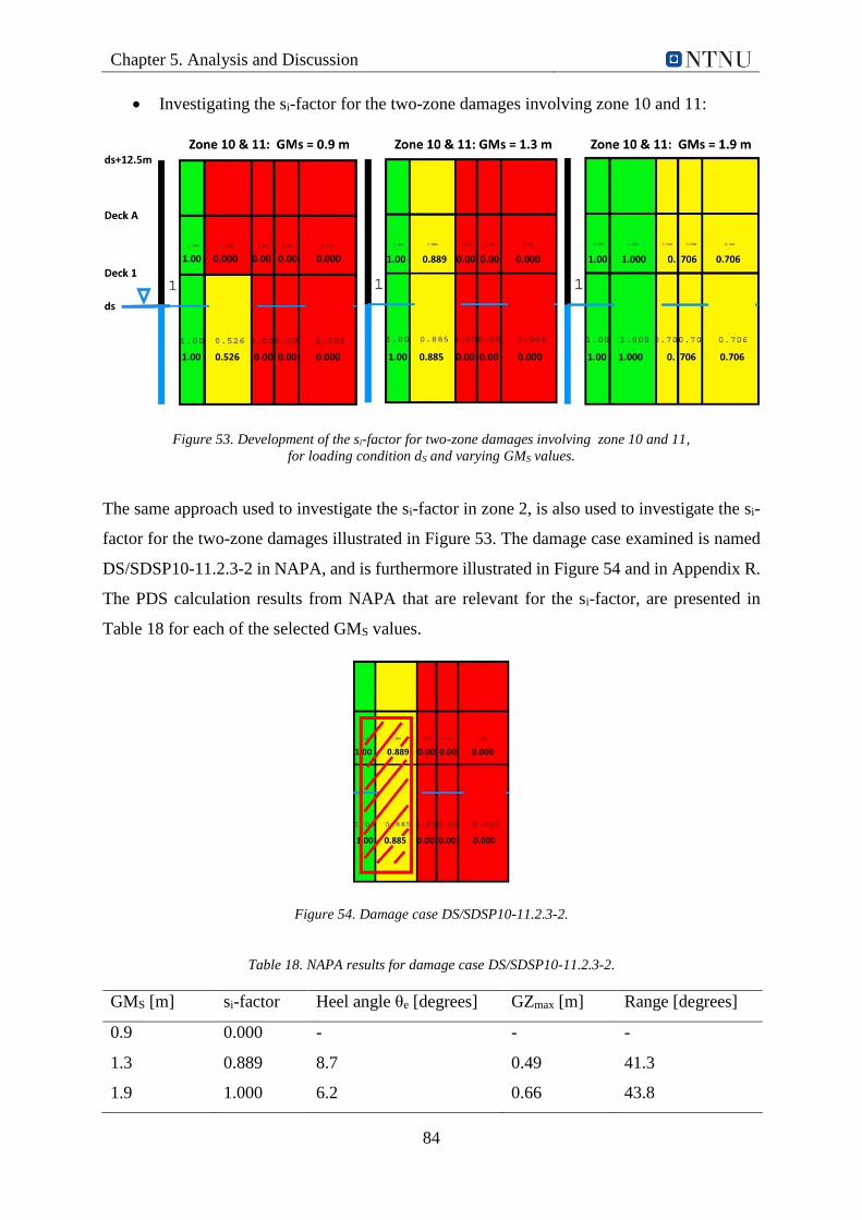
Chapter 5. Analysis and Discussion
84
Investigating the si-factor for the two-zone damages involving zone 10 and 11:
Figure 53. Development of the si-factor for two-zone damages involving zone 10 and 11,
for loading condition dS and varying GMS values.
The same approach used to investigate the si-factor in zone 2, is also used to investigate the si-
factor for the two-zone damages illustrated in Figure 53. The damage case examined is named
DS/SDSP10-11.2.3-2 in NAPA, and is furthermore illustrated in Figure 54 and in Appendix R.
The PDS calculation results from NAPA that are relevant for the si-factor, are presented in
Table 18 for each of the selected GMS values.
Figure 54. Damage case DS/SDSP10-11.2.3-2.
Table 18. NAPA results for damage case DS/SDSP10-11.2.3-2.
GMS [m] si-factor Heel angle θe [degrees] GZmax [m] Range [degrees]
0.9 0.000 - - -
1.3 0.889 8.7 0.49 41.3
1.9 1.000 6.2 0.66 43.8
Chapter 5. Analysis and Discussion
85
Similar to the single-zone damage case that was investigated in zone 2, namely DS/SDSP2.2.2,
the ship tends to heel less for larger GMS values. Additionally, the development of the si-factor
is almost identical for the two damage cases DS/SDSP2.2.2 and DS/SDSP10-11.2.3-2.
Furthermore, both the GZmax and Range values for DS/SDSP10-11.2.3-2 are larger than their
respective maximum values, with respect to the sfinal,i calculation. Thus, it is once again the K-
value that influences the si-factor. In similarity with damage case DS/SDSP2.2.2, K = 1 for
GMS = 1.9 m. In addition, the K-value for GMS = 1.3 m is approximately in the same order of
magnitude as for the two damage cases.
Based on the discussion on both damage case DS/SDSP2.2.2 and damage case DS/SDSP10-
11.2.3-2, it seems reasonable to assume that the ‘trend’ with increasing survivability for larger
GM values could be universal. Additionally, it looks like the K-factor, or more specifically the
equilibrium heel angle θe, is most influential with respect to the si-factor. In other words, the
heeling moment that occurs when the ship is damaged, has a significant impact on the si-factor.
5.2.3 Total A-index
Since both the pi- and vi-factors are constant, as mentioned in Sub-section 5.2.1, it is only the
si-factor that can influence the A-index in this study. Thus, as indirectly stated in the previous
sub-section, the ‘total’ A-index is more or less only dependent on the heeling moment in case
of damage. This heeling moment gives the ship a new floating position, i.e. the ship obtains an
equilibrium heel angle larger than zero degrees. This heel angle reduces the si-factor – the
survivability of the ship, which in turn reduces the A-index – the damage stability of the ship.

Chapter 5. Analysis and Discussion
86
5.3 Uncertainties
There are naturally uncertainties related to the results of the individual study in this thesis.
Sources of uncertainty could for example be limitations, simplifications and assumptions made
by the author. Thus, the following question arises: are the results and the post-analysis of the
results in this thesis valid, despite of the uncertainties?
It seems reasonable to begin the discussion related to the important question above, with the
simplifications made in the ship modelling process in NAPA. In this process, the internal
arrangement of the ship was heavily simplified as compared to the original GA drawings from
AutoCAD. The CAD-drawing of the simplified GA is the one that is attached to the thesis
electronically – a link is provided in Appendix B. Furthermore, the simplification of the
arrangement was a measure to save time. The author has been told that this is a standard
approach used by ship designers in real life. However, in real-life projects the tank arrangement
created in NAPA is a bit more detailed than in this study, and it usually includes more curvatures
(Djupvik, 2016). That makes the PDS calculations more time-consuming, but more accurate.
Despite this, it is assumed that none of the simplifications made in the arrangement have had
any significant effects on the results.
There are some uncertainties connected to the calculations conducted in NAPA, as well. For
instance, survival craft moments were neglected in all calculations. The effect of this measure
can be seen by looking at Equation 41 and Equation 37 from Sub-section 2.4.7, which are re-
presented below, respectively:
𝑠𝑚𝑜𝑚,𝑖 = (𝐺𝑍𝑚𝑎𝑥 − 0.04) ∙ 𝐷𝑖𝑠𝑝𝑙𝑎𝑐𝑒𝑚𝑒𝑛𝑡
𝑀ℎ𝑒𝑒𝑙 = 𝑚𝑎𝑥(𝑀𝑝𝑎𝑠𝑠𝑒𝑛𝑔𝑒𝑟 , 𝑀𝑤𝑖𝑛𝑑, 𝑀𝑠𝑢𝑟𝑣𝑖𝑣𝑎𝑙𝑐𝑟𝑎𝑓𝑡) ≤ 1
𝑠𝑖 = 𝑚𝑖𝑛[𝑠𝑖𝑛𝑡𝑒𝑟𝑚𝑒𝑑𝑖𝑎𝑡𝑒,𝑖, (𝑠𝑓𝑖𝑛𝑎𝑙,𝑖 ∙ 𝑠𝑚𝑜𝑚,𝑖)]
The results reports from NAPA, which also are attached to the thesis electronically, reveal that
the si-factors used in the calculations are sfinal,i. Additionally, the author could find no
information about smom,i in NAPA. Thus, supported by the above equation for si, the author
therefore assumes that smom,i = 1 for the damage cases in this study; i.e. numerator ≥
denominator in the equation for smom,i. Furthermore, since Msurvivalcraft is ignored in this study,
the denominator in the smom,i equation will take the maximum value of Mwind and Mpassenger in
all damage cases. Unless the value of Msurvivalcraft is significantly larger than the other two
heeling moments, neglecting Msurvivalcraft does not seem to influence the results, because smom,i
= 1 in any other case.
Chapter 5. Analysis and Discussion
87
The analysis and discussion that the author is most uncertain on, is furthermore related to the
vi-factor in Sub-section 5.1.3, i.e. for objective 1 of the thesis. The plots for the mean vi-factor
development presented in this sub-section, is in fact only valid for the damage cases in a couple
of zones within the range of U-deck. It is however assumed that the results will be fairly similar
for most of the other zones, within the abovementioned range, but that is not certain. This
uncertainty is thus a possible objective for further work related to this thesis.
Another uncertainty related to the vi-factor analysis in Sub-section 5.1.3, is that only the damage
cases closest to the hull are investigated. Based on the author’s understanding of the PDS
regulations, the vi-factor for U-deck will not contribute to the A-index for damages that
breaches the first longitudinal bulkhead (LBH) both below and above U-deck. There are
however other damage cases where the vi-factor will contribute to the A-index, for the latter
scenario, when U-deck is placed higher than dL = 4.4 m. These damages breach the first LBH
below U-deck only. In that case, according to the above sense of logic, the vi-factor for U-deck
will contribute to the A-index. In other words, the vi-factor for U-deck also contributes to the
A-index for damage cases that penetrates the first – and perhaps the second – LBH. Thus, any
conclusions drawn related to the vi-factor for objective 1 in this study, might not be valid for
damage cases that penetrate LBHs. These cases and damage cases in other zones where the
arrangement is slightly different, are potential research objectives for further work related to
changes in vi-factor for different U-deck heights.
A third uncertainty related to the vi-factor discussion, is the potential contribution from deck 2
within the range of U-deck. It has been assumed that deck 2 does not influence the vi-factor in
any damage cases within this range, since deck 2 never is placed higher than dL = 4.4 m above
the baseline. As mentioned in Sub-section 5.1.3, deck 2 must according to the author’s
understanding be placed higher than the lowest waterline in order to contribute to the vi-factor
in any damage case. The formulations in the PDS regulations are not clear on this matter, and
neither are the instructions in the NAPA for Design Manuals. However, if deck 2 contributes,
it is only for the light service draught dL, which in turn only contributes 20% to the A-index.
Thus, the influence is either way considered not to be of significance; the conclusions made in
Section 5.1 will not be altered by this potentially wrong assumption made by the author.
Obviously, there are a number of uncertainties related to this study. However, based on the
above discussion, the author would like to conclude that none of the uncertainties is of a size
that threatens the validity of the results – or the conclusions made in the analysis and discussion
chapter.
88
6. Conclusion
This master’s thesis investigates how changes in size of the wing ballast tanks and changes in
the initial GM values, for a WFSV designed by Salt Ship Design, influences the A-index. The
presentation of results, along with the analysis and discussion of these results, are based on PDS
calculations conducted in NAPA.
The results for objective 1 show that the A-index generally increases for larger U-deck heights,
all the way up to 5.6 m above the baseline. Thus it can be concluded that the height of U-deck
certainly influences the A-index, whereas positively when the height is increased up to 5.6 m.
It is not considered realistic to place U-deck above this height, considering that the wing ballast
tanks should have room for a sufficient amount of ballast water. The main contributions to the
A-index come from the si-factor, most likely due to heeling moments that causes changes in the
equilibrium heel angle. However, the vi-factor is also influential, but the impact is not as
consistent for all U-deck heights as compared to the si-factor. The pi-factor does not contribute
to changes in A-index for objective 1, since changes to the arrangement only are made in
vertical direction.
For objective 2, no changes are made to the arrangement of the ship in question. The selected
U-deck height for the study is 4.4 m, because of the corresponding trade-off between sufficient
A-index and sufficiently large wing ballast tanks is considered to be beneficial. Furthermore,
the results of the study reveal that the A-index increases almost proportionally with the GM
values, i.e. the A-index curve behaves linearly. Additionally, it can be concluded that GM
values around 1 m are critical with respect to the A-index, while GM values lower than this will
result in an A-index which does not meet the ‘PDS criterion’, i.e. A > R. The only factor that
contributes to changes in A-index, when varying the initial GM values for the ship, is the si-
factor; in such cases the A-index is heavily dependent on the heeling moment caused by
potential damage. The heeling moment causes a change in equilibrium heel angle, which in turn
affects the si-factor. I.e., when the initial GM values are increased, the heeling moment in case
of damage decreases. The si-factor thus increases and, consequently, the A-index is improved.
Neither of the pi- or vi-factors influence the changes in A-index in the study related to objective
2, because there are no changes in the arrangement.
Chapter 6. Conclusion
89
6.1 Uncertainties
The most important uncertainties related to the studies conducted, were discussed in Section
5.3. As the reader might have noticed, none of the uncertainties, except for the arrangement
simplifications, were related to objective 2 of the thesis. This is because the only possible
uncertainties regarding objective 2 would be related to the si-factor. For the si-factor, the
analysis tools in NAPA make the results more transparent, as compared to the pi- and vi-factor.
The development of the si-factor for different GM values was clear, as mentioned introductorily
in this chapter: the si-factor changes when the heeling moment changes; a larger heeling
moment causes a reduction in the si-factor. In other words, there are no uncertainties related to
objective 2 that threaten the validity of the results, the analysis and discussion of the results, or
conclusions drawn.
For objective 1, there are a few uncertainties related to the analysis of the results. The results
themselves should be correct; the A-index decreases when the U-deck height is lowered beneath
5.6 m, which is considered realistic. The uncertainties discussed in Section 5.3 are mainly
related to further work; investigations related to these uncertainties could be done in order to
further raise the confidence level on the conclusions made for objective 1.
6.2 Key Findings
The goal of the thesis is to contribute with more insight as to how changes made in the
arrangement and intact stability of offshore vessels impact the A-index. In order to achieve this
goal, the produced results were analysed in-depth and conclusions have been based on
discussion regarding these results. Arguably, this is done successfully; the results and
conclusions are not valid for all offshore vessels, but they are assumed to be valid for offshore
vessels with fairly similar arrangements as the WFSV used in this study. Finally, the key
findings in this thesis are:
The A-index does in general obtain a larger value when the size of the wing ballast tanks
is reduced – to a certain extent; when U-deck is placed above 5.6 m for the WFSV, the
A-index will not be improved anymore. However, it is not considered relevant to install
smaller wing ballast tanks than the size corresponding to this U-deck height.
The A-index is generally better for larger initial GM values, because the increase in GM
values results in smaller heeling moments in case of damage.
Chapter 6. Conclusion
90
6.3 Further Work
Some suggestions to further work are already mentioned in Section 5.3, where
uncertainties related to this study were discussed. For instance, there are uncertainties
related to the analysis of the vi-factor for objective 1 of the thesis. In order to increase
the reliability of the results for the vi-factor development, for different U-deck heights,
the following could be done:
- Investigate more damage zones in general; and
- Investigate damage cases penetrating longitudinal bulkheads within each zone.
Additionally, it could be investigated as to why the AS-index is most critical in the study
conducted for objective 2, while the AL-index seems to be most critical for objective 1.
Furthermore, the studies carried out for objective 1 and 2 in this thesis, could be carried
out for other types of offshore vessels as well. This would provide more generic results
which, consequently, could lead to conclusions valid for a wider range of vessels.

91
92
7. Bibliography
DELFTship. Single and Multizone Damages. In probabilistic-damage-stability_zone-
damage.png (Ed.): DELFTship.
Djupvik, O. M. (2015). [Phone conversation with Ole Martin Djupvik, 'Naval Architect' at
Wärtsilä Ship Design (previously)/Salt Ship Design (from 2016 and onwards)].
Djupvik, O. M. (2016). [Phone and email conversations with Ole Martin Djupvik, 'Naval
Architect' at Salt Ship Design (from 2016 and onwards)].
Djupvik, O. M., Aanondsen, S. A., & Asbjørnslett, B. E. (2015). Probabilistic Damage Stability
- Maximizing the Attained Index by Analyzing the Effects of Changes in the
Arrangement for Offshore Vessels: NTNU.
Eklund, R., & Lindroth, D. (2009). Workshop N2 - Damage Stability According to SOLAS 2009,
NAPA User Meeting 2009. NAPA Ltd.
Hjort, G. (2015). [Email correspondence with Gunnar Hjort, Principal Approval Engineer,
Stability section, DNV GL].
Hjort, G., & Olufsen, O. (2014). Probabilistic damage stability: DNV GL AS.
IMO. (1966). Load Lines, 1966/1988 - International Convention on Load Lines, 1966, as
Amended by the Protocol of 1988 - Articles of the International
Convention on Load Lines, 1966 - Article 2 - Definitions In I. M. Organization (Ed.).
IMO. (2006). SOLAS Chapter II-1 Construction - structure, Subdivision and Stability,
Machinery and Electrical Installations, Part B-1 Stability.: International Maritime
Organization.
IMO. (2008a). International Code on Intact Stability (2008 IS Code): International Maritime
Organization.
IMO. (2008b). Resolution MSC.266(84) - Code of safety for special purpose ships, 2008:
International Maritime Organization.
IMO. (2008c). Resolution MSC.281(85), Explanatory notes to the SOLAS Chapter II-1,
Subdivision and damage stability regulations, Part B.: International Maritime
Organization.
Kirchsteiger, C. (1999). On the use of probabilistic and deterministic methods in risk analysis.
Journal of Loss Prevention in the Process Industries, 12(5), 399-419. doi:
10.1016/S0950-4230(99)00012-1
Lützen, M. (2001). PhD thesis: Ship Collision Damage., Lyngby, Denmark.

93
Magnussen, E., Amdahl, J., & Fuglerud, G. (2014). Marin teknikk grunnlag : TMR4105 :
kompendium (5. utg. ed.). Trondheim: Akademika forlag Kompendieforlaget.
MCA. (1998). MSN 1698 (M) - The Merchant Shipping (Passenger Ship Construction: Ships
of Classes I, II and II(A)) Regulations 1998: Maritime and Coastguard Agency (MCA).
NAPA. (2015). NAPA for Design Manuals 2015.3.
Papanikolaou, A., & Eliopoulou, E. (2008). On the development of the new harmonised damage
stability regulations for dry cargo and passenger ships. Reliability Engineering and
System Safety, 93(9), 1305-1316. doi: 10.1016/j.ress.2007.07.009
Patterson, C. J., & Ridley, J. D. (2014). Ship stability, powering and resistance (Vol. 13).
London: Adlard Coles Nautical.
Puisa, R., Tsakalakis, N., & Vassalos, D. (2012). Reducing Uncertainty in Subdivision
Optimization. Journal of Shipping and Ocean Engineering 2.
Puustinen, O. (2012). Workshop 7, FAQ in NAPA Damage Stability. In N. Ltd. (Ed.): NAPA.
Ravn, E. S. (February 2003). Probabilistic Damage Stability of Ro-Ro Ships. (PhD Thesis),
Technical University of Denmark, Denmark.
Vassalos, D. (2014). Damage stability and survivability – ‘nailing’ passenger ship safety
problems. Ships and Offshore Structures, 9(3), 237-256. doi:
10.1080/17445302.2013.780397
Wärtsilä. Damage stability calculations. In f62e80491998c3f2a37e620b5dd160668285bc88
(Ed.). Encyclopedia of Ship Technology by Wärtsilä:
http://www.shippingencyclopedia.com/term/damage-stability-calculations: Wärtsilä.
94
List of Appendices
Appendix A – How pi is calculated for multi-zone damages ...................................................... I
Appendix B – Electronic files ................................................................................................... II
Appendix C – Modelling of ship arrangement in NAPA ......................................................... III
Appendix D – The ship’s buoyant hull created in NAPA ........................................................ VI
Appendix E – Simplification of GA in NAPA ........................................................................ VII
Appendix F – Reduction of curvatures in NAPA ................................................................. VIII
Appendix G – Permeability values in NAPA ........................................................................... IX
Appendix H – Subdivision data output: Subdivision drawing .................................................. X
Appendix I – Subdivision data input ........................................................................................ XI
Appendix J – Subdivision data output: Subdivision table ..................................................... XIII
Appendix K – R-index calculated in NAPA ......................................................................... XIV
Appendix L – How SFAC diagrams develop with the draught ............................................. XV
Appendix M – SFAC diagrams for the selected U-deck heights ......................................... XVII
Appendix N – SFAC diagrams for zone 6-7 and zone 13 ..................................................... XIX
Appendix O – vi-factor illustration for damaged wing tanks and U-tanks............................ XXI
Appendix P – Calculation input and results for vi-factor ..................................................... XXII
Appendix Q – SFAC diagrams for the selected GM values............................................... XXVI
Appendix R – Damage drawings from NAPA for objective 2 ....................................... XXVIII
Appendix S – Damaged floating positions for objective 2 ................................................. XXX
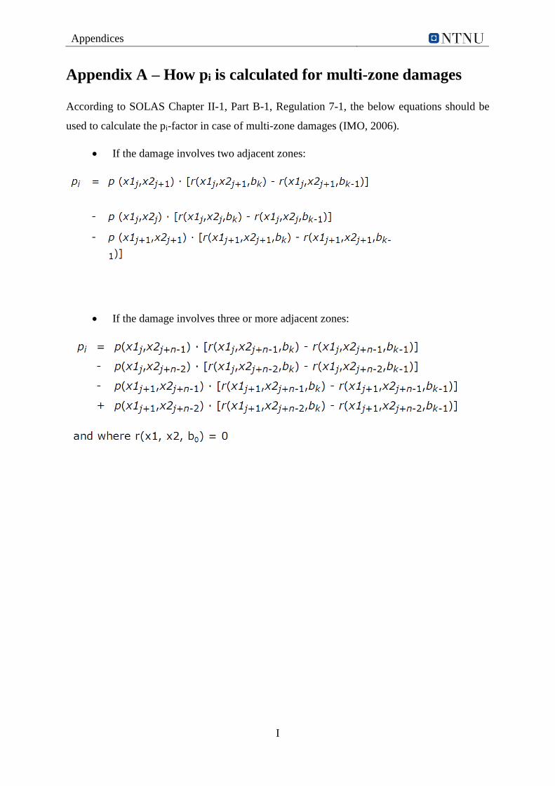
Appendices
I
Appendix A – How pi is calculated for multi-zone damages
According to SOLAS Chapter II-1, Part B-1, Regulation 7-1, the below equations should be
used to calculate the pi-factor in case of multi-zone damages (IMO, 2006).
If the damage involves two adjacent zones:
If the damage involves three or more adjacent zones:
Appendices
II
Appendix B – Electronic files
The electronic files attached to this master’s thesis are:
- Simplified GA drawings from AutoCAD, for the generic ship model used in this study.
These drawings do not represent the authentic vessel designed by Salt Ship Design.
- NAPA results report from all PDS calculations, for both objectives of the thesis.
- The author’s poster contribution to the Master Poster Exhibition at the Department of
Marine Technology, NTNU, in the spring semester of 2016.
The electronic files can be found by clicking on the following link https://daim.idi.ntnu.no/soek
and searching for the title of this thesis or name of the thesis’ author, for instance.
Appendices
III
Appendix C – Modelling of ship arrangement in NAPA
In the NAPA stability software, the traditional way to model the ship’s arrangement is by using
the ‘Text Editor’ tool. This method provides the possibility to organise the coding in separate
text files. Examples of names of such text files used in the master’s thesis are ‘Decks’, ‘Tanks’,
‘Tankplan’, ‘Damcomp’ and ‘Stabhull’. There are several other text files in a ‘real-life project’,
and it is left to the user to define the names, do all the coding and organise the coding in
appropriate files. A ‘room’ as defined by the Text Editor, i.e. tanks and rooms, is referred to as
a compartment. For any type of compartment, the coding syntax is similar. This is illustrated in
the below figure. Their respective codes are located in different text files, however.
All compartments must be added to the ‘Arrangement Table’ in NAPA. If this is not done, the
compartments will not be included in the calculations. The only user input here is the name of
the compartment that has already been defined in the text file, as well as the ‘purpose
description’ of the compartment like for instance ‘Water ballast’, ‘Accommodation’ or ‘Fuel
oil’. The ‘purpose description’ automatically defines the permeability of the compartment.
These are pre-set standard values in NAPA. Additionally, information such as location of the
compartment relative to the reference system, density of the content of the compartment and
volume of the compartment are filled in automatically. With this information given, NAPA also
calculates the mass attached to each compartment.
Especially the volume of the compartments is useful information; if this value is zero, then the
user can be certain that an error has been made. Most likely this error comes from the coding,
i.e. definition of the compartment in the text file, or maybe the decks or the hull of the ship is
defined wrongly in their respective text files.
The final watertight arrangement modelled in NAPA is presented in the figures below. In
respective order, the figures show: the ship in profile view, ‘A-deck', ‘1-deck’, ‘2-deck’, ‘Tank
top’ and ‘Baseline’. The colour codes are explained in table that follows after the figures.
Appendices
IV
Appendices
V
Colour code of compartment Purpose description
Light grey Void space
Dark grey Sewage (Grey water) tanks
Green Water ballast and roll-reduction tanks
Gold Machinery spaces
Red Fuel oil (MDO) tanks
Light blue Fresh water tanks
Pink Storage
Turquoise Accommodation
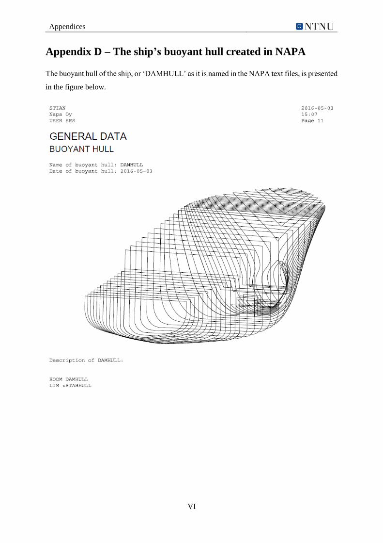
Appendices
VI
Appendix D – The ship’s buoyant hull created in NAPA
The buoyant hull of the ship, or ‘DAMHULL’ as it is named in the NAPA text files, is presented
in the figure below.
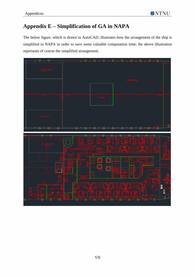
Appendices
VII
Appendix E – Simplification of GA in NAPA
The below figure, which is drawn in AutoCAD, illustrates how the arrangement of the ship is
simplified in NAPA in order to save some valuable computation time; the above illustration
represents of course the simplified arrangement.
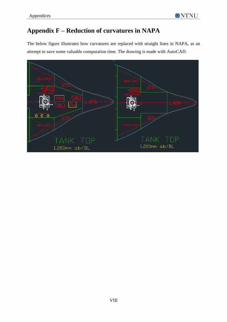
Appendices
VIII
Appendix F – Reduction of curvatures in NAPA
The below figure illustrates how curvatures are replaced with straight lines in NAPA, as an
attempt to save some valuable computation time. The drawing is made with AutoCAD.
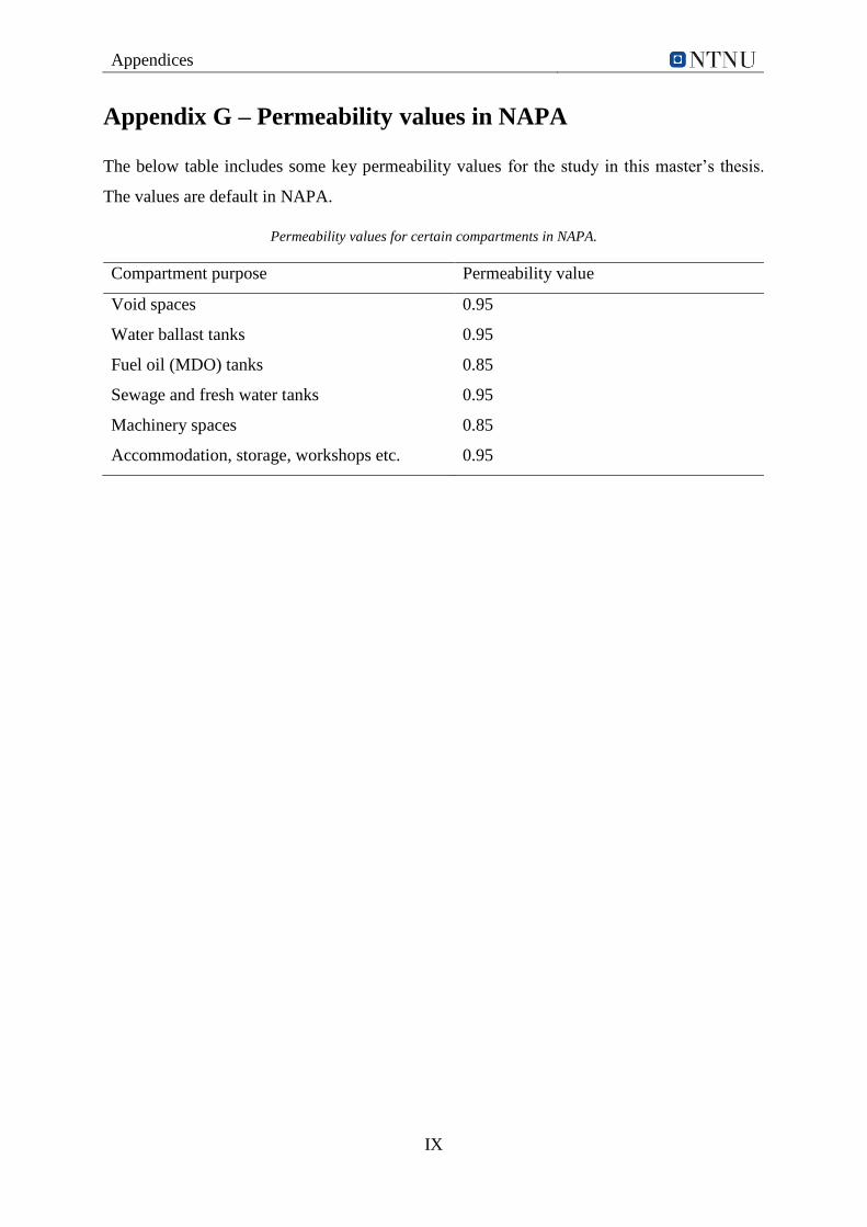
Appendices
IX
Appendix G – Permeability values in NAPA
The below table includes some key permeability values for the study in this master’s thesis.
The values are default in NAPA.
Permeability values for certain compartments in NAPA.
Compartment purpose Permeability value
Void spaces 0.95
Water ballast tanks 0.95
Fuel oil (MDO) tanks 0.85
Sewage and fresh water tanks 0.95
Machinery spaces 0.85
Accommodation, storage, workshops etc. 0.95
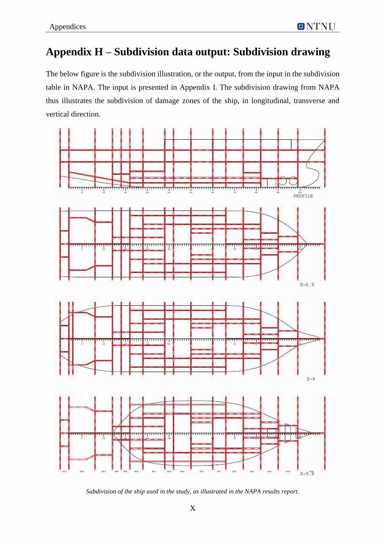
Appendices
X
Appendix H – Subdivision data output: Subdivision drawing
The below figure is the subdivision illustration, or the output, from the input in the subdivision
table in NAPA. The input is presented in Appendix I. The subdivision drawing from NAPA
thus illustrates the subdivision of damage zones of the ship, in longitudinal, transverse and
vertical direction.
Subdivision of the ship used in the study, as illustrated in the NAPA results report.
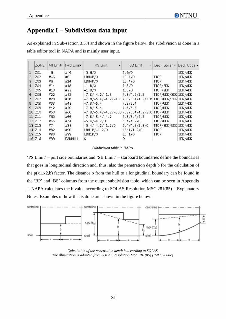
Appendices
XI
Appendix I – Subdivision data input
As explained in Sub-section 3.5.4 and shown in the figure below, the subdivision is done in a
table editor tool in NAPA and is mainly user input.
Subdivision table in NAPA.
‘PS Limit’ – port side boundaries and ‘SB Limit’ – starboard boundaries define the boundaries
that goes in longitudinal direction and, thus, also the penetration depth b for the calculation of
the p(x1,x2,b) factor. The distance b from the hull to a longitudinal boundary can be found in
the ‘BP’ and ‘BS’ columns from the output subdivision table, which can be seen in Appendix
J. NAPA calculates the b value according to SOLAS Resolution MSC.281(85) – Explanatory
Notes. Examples of how this is done are shown in the figure below.
Calculation of the penetration depth b according to SOLAS.
The illustration is adapted from SOLAS Resolution MSC.281(85) (IMO, 2008c).
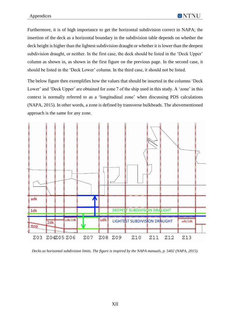
Appendices
XII
Furthermore, it is of high importance to get the horizontal subdivision correct in NAPA; the
insertion of the deck as a horizontal boundary in the subdivision table depends on whether the
deck height is higher than the lightest subdivision draught or whether it is lower than the deepest
subdivision draught, or neither. In the first case, the deck should be listed in the ‘Deck Upper’
column as shown in, as shown in the first figure on the previous page. In the second case, it
should be listed in the ‘Deck Lower’ column. In the third case, it should not be listed.
The below figure then exemplifies how the values that should be inserted in the columns ‘Deck
Lower’ and ‘Deck Upper’ are obtained for zone 7 of the ship used in this study. A ‘zone’ in this
context is normally referred to as a ‘longitudinal zone’ when discussing PDS calculations
(NAPA, 2015). In other words, a zone is defined by transverse bulkheads. The abovementioned
approach is the same for any zone.
Decks as horizontal subdivision limits. The figure is inspired by the NAPA manuals, p. 5402 (NAPA, 2015).

Appendices
XIII
Appendix J – Subdivision data output: Subdivision table
The figure, or table, below is the subdivision table that NAPA presents in the results report in
the Probabilistic Manager.
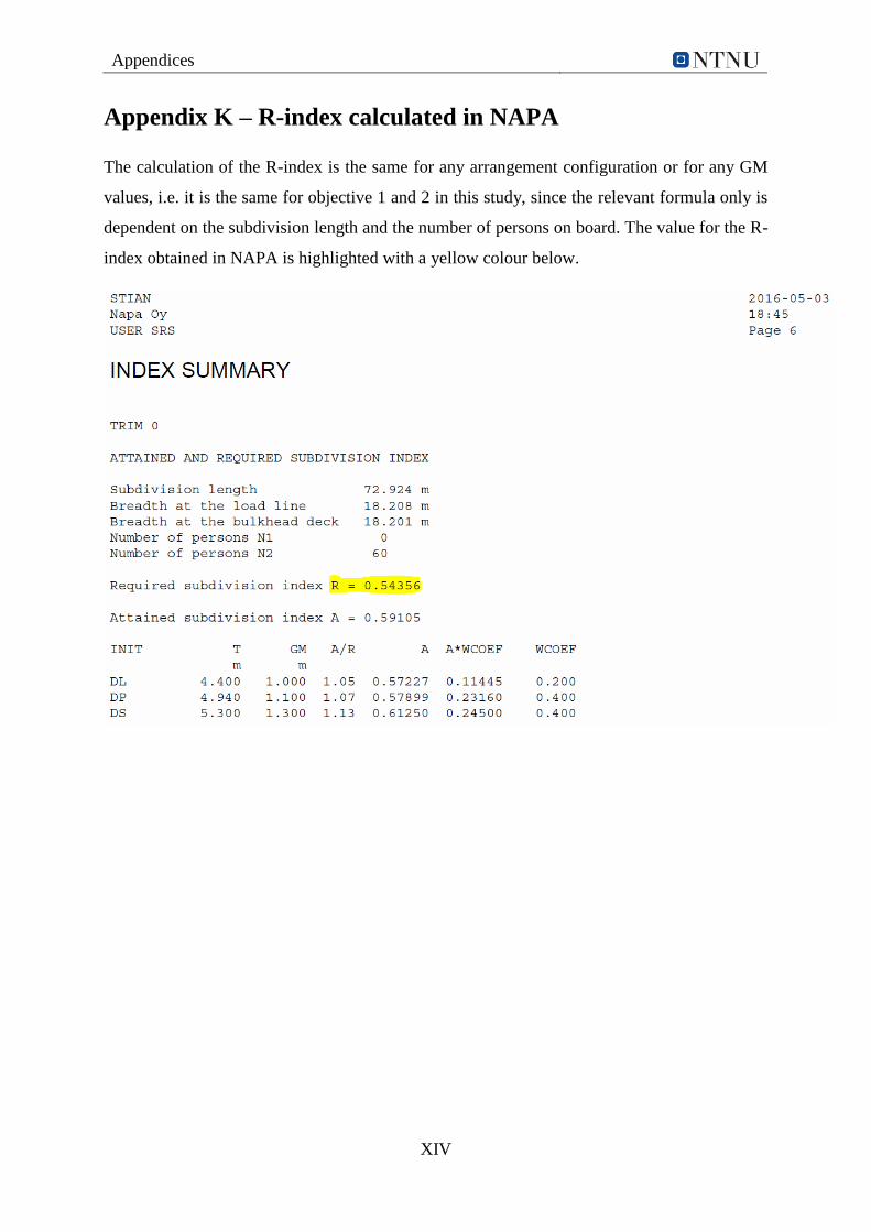
Appendices
XIV
Appendix K – R-index calculated in NAPA
The calculation of the R-index is the same for any arrangement configuration or for any GM
values, i.e. it is the same for objective 1 and 2 in this study, since the relevant formula only is
dependent on the subdivision length and the number of persons on board. The value for the R-
index obtained in NAPA is highlighted with a yellow colour below.
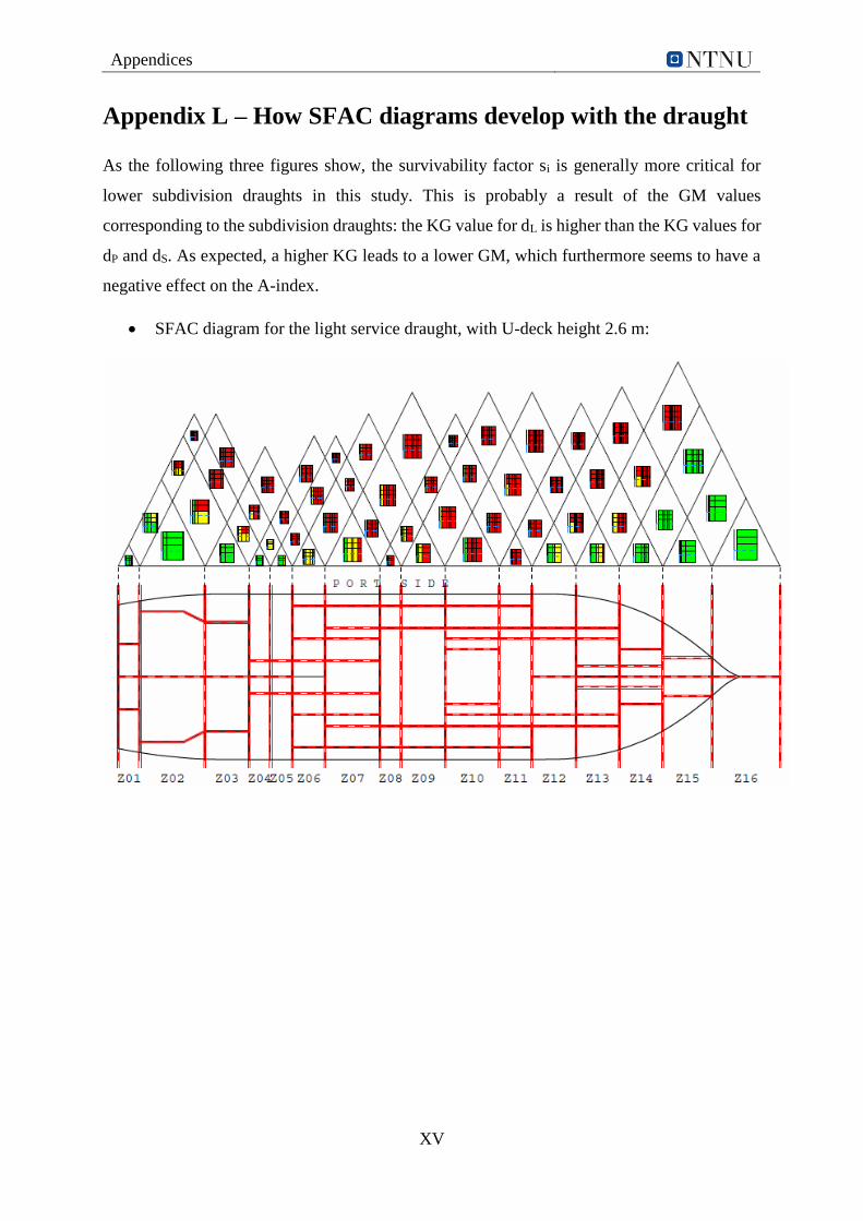
Appendices
XV
Appendix L – How SFAC diagrams develop with the draught
As the following three figures show, the survivability factor si is generally more critical for
lower subdivision draughts in this study. This is probably a result of the GM values
corresponding to the subdivision draughts: the KG value for dL is higher than the KG values for
dP and dS. As expected, a higher KG leads to a lower GM, which furthermore seems to have a
negative effect on the A-index.
SFAC diagram for the light service draught, with U-deck height 2.6 m:

Appendices
XVI
SFAC diagram for the partial subdivision draught, with U-deck height 2.6 m:
SFAC diagram for the deepest subdivision draught, with U-deck height 2.6 m:
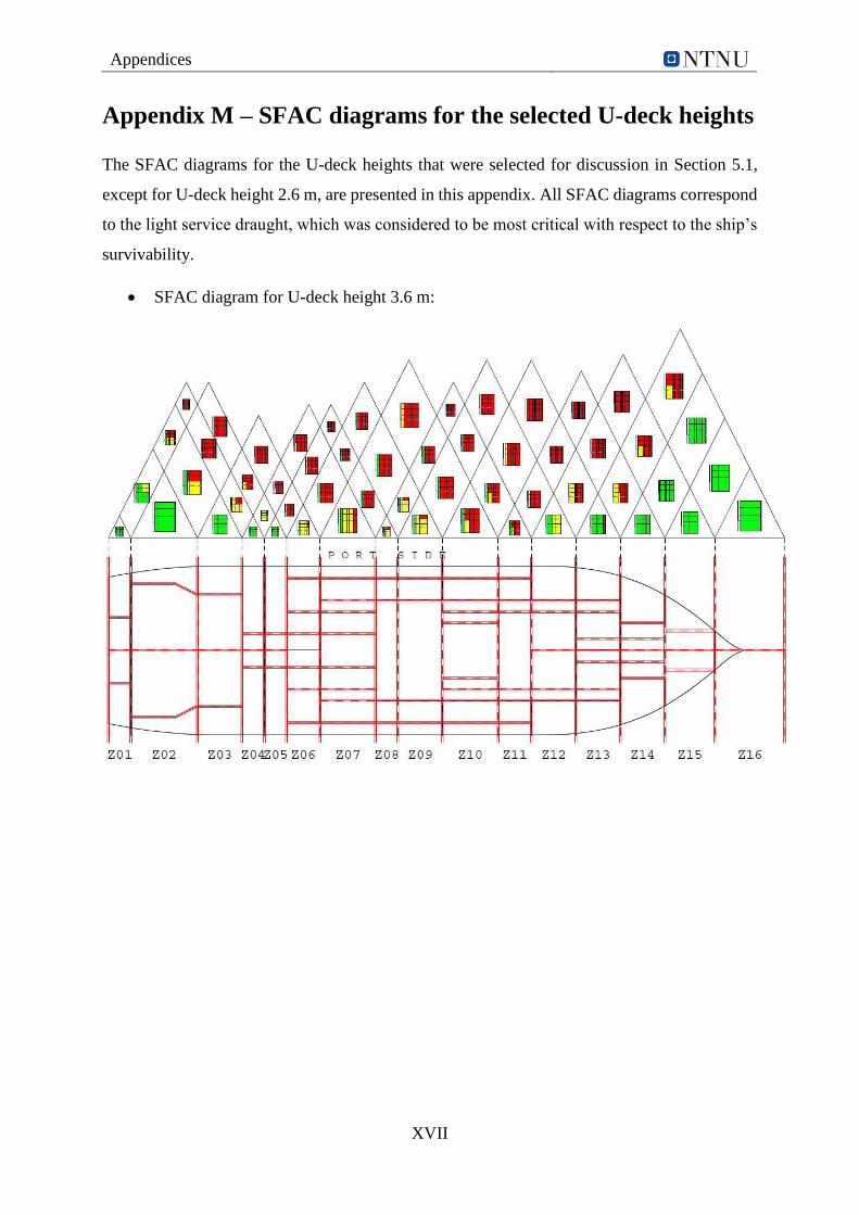
Appendices
XVII
Appendix M – SFAC diagrams for the selected U-deck heights
The SFAC diagrams for the U-deck heights that were selected for discussion in Section 5.1,
except for U-deck height 2.6 m, are presented in this appendix. All SFAC diagrams correspond
to the light service draught, which was considered to be most critical with respect to the ship’s
survivability.
SFAC diagram for U-deck height 3.6 m:
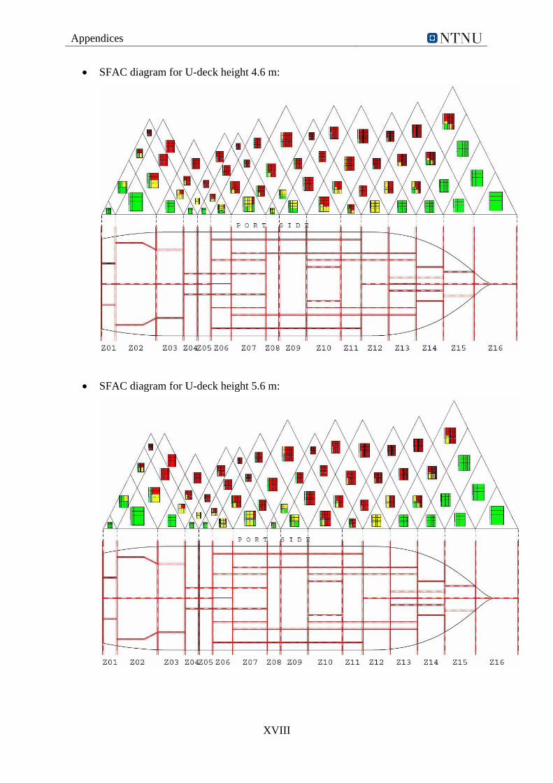
Appendices
XVIII
SFAC diagram for U-deck height 4.6 m:
SFAC diagram for U-deck height 5.6 m:

Appendices
XIX
Appendix N – SFAC diagrams for zone 6-7 and zone 13
SFAC diagrams for zone 6, 7 and 13, from the calculations for objective 1 of the thesis, are
presented in this appendix. This is done in order to investigate the development of the si-factor
in the zones where both deck 2 and U-deck are present. The development is investigated for
all of the selected U-deck heights, as can be seen below, for the light service draught (dL). Deck
2 is not displayed in the SFAC diagrams below, because deck 2 is not placed above the waterline
in any of the damage zones under investigation. However, a deck might have an effect on the
si-factor even though it is placed below the waterline.
U-deck height 5.6 m:
U-deck height 4.6 m:
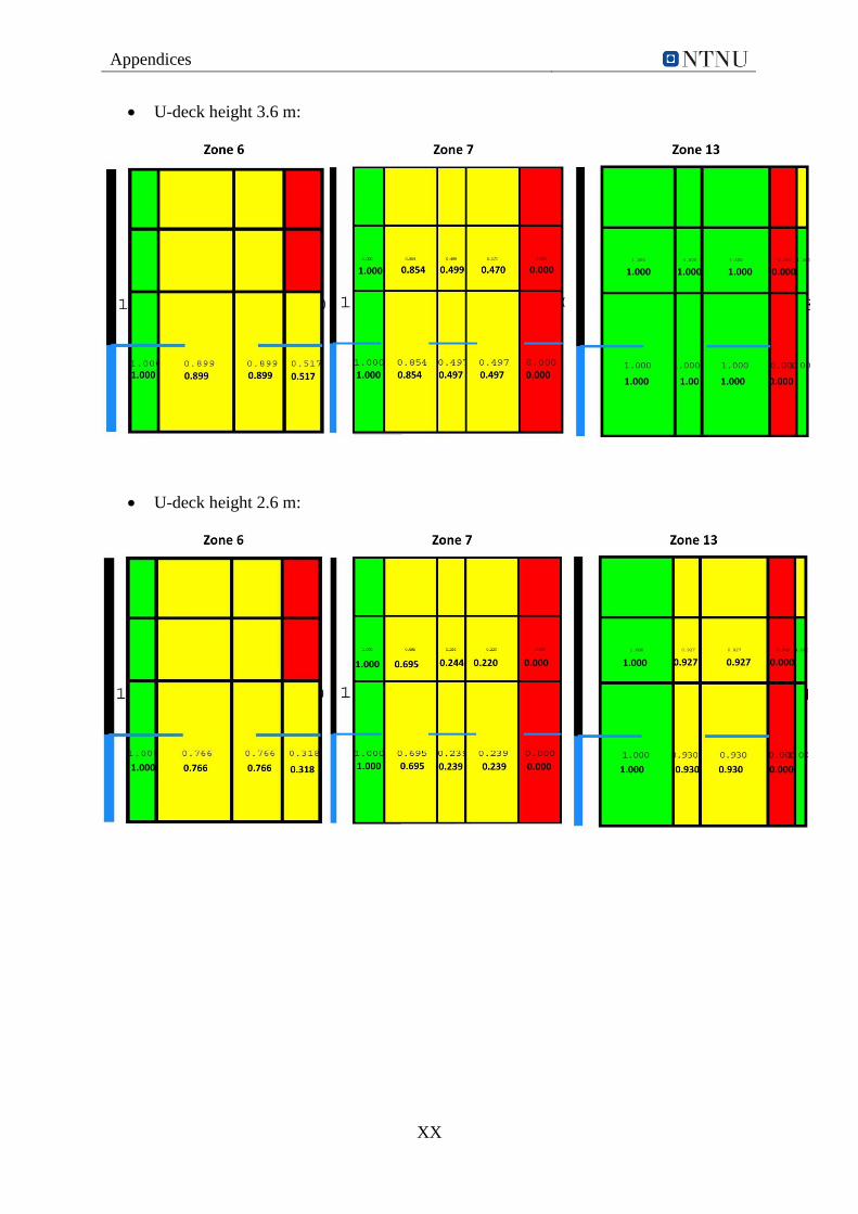
Appendices
XX
U-deck height 3.6 m:
U-deck height 2.6 m:
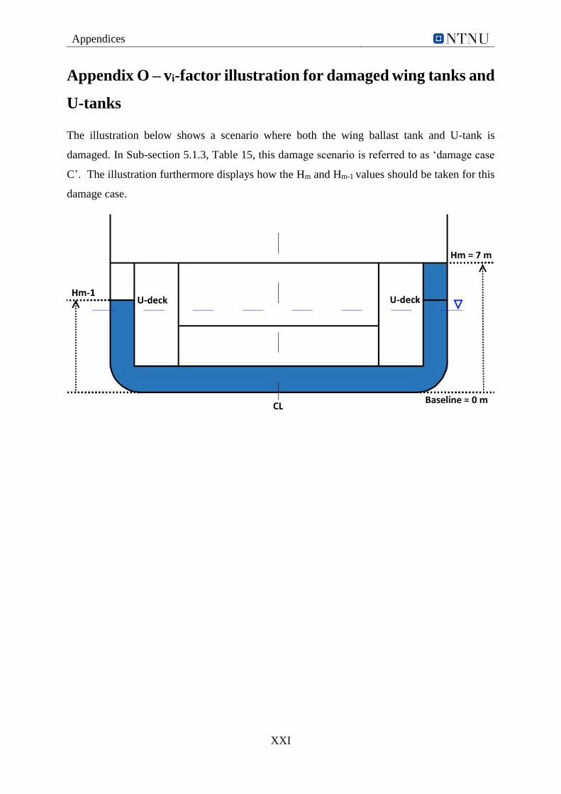
Appendices
XXI
Appendix O – vi-factor illustration for damaged wing tanks and
U-tanks
The illustration below shows a scenario where both the wing ballast tank and U-tank is
damaged. In Sub-section 5.1.3, Table 15, this damage scenario is referred to as ‘damage case
C’. The illustration furthermore displays how the Hm and Hm-1 values should be taken for this
damage case.
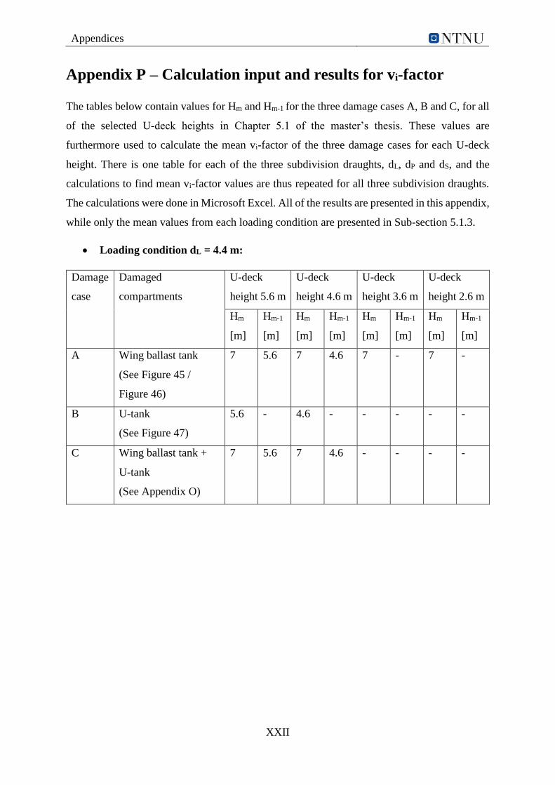
Appendices
XXII
Appendix P – Calculation input and results for vi-factor
The tables below contain values for Hm and Hm-1 for the three damage cases A, B and C, for all
of the selected U-deck heights in Chapter 5.1 of the master’s thesis. These values are
furthermore used to calculate the mean vi-factor of the three damage cases for each U-deck
height. There is one table for each of the three subdivision draughts, dL, dP and dS, and the
calculations to find mean vi-factor values are thus repeated for all three subdivision draughts.
The calculations were done in Microsoft Excel. All of the results are presented in this appendix,
while only the mean values from each loading condition are presented in Sub-section 5.1.3.
Loading condition dL = 4.4 m:
Damage
case
Damaged
compartments
U-deck
height 5.6 m
U-deck
height 4.6 m
U-deck
height 3.6 m
U-deck
height 2.6 m
Hm
[m]
Hm-1
[m]
Hm
[m]
Hm-1
[m]
Hm
[m]
Hm-1
[m]
Hm
[m]
Hm-1
[m]
A
Wing ballast tank
(See Figure 45 /
Figure 46)
7 5.6 7 4.6 7 - 7 -
B U-tank
(See Figure 47)
5.6 - 4.6 - - - - -
C Wing ballast tank +
U-tank
(See Appendix O)
7 5.6 7 4.6 - - - -
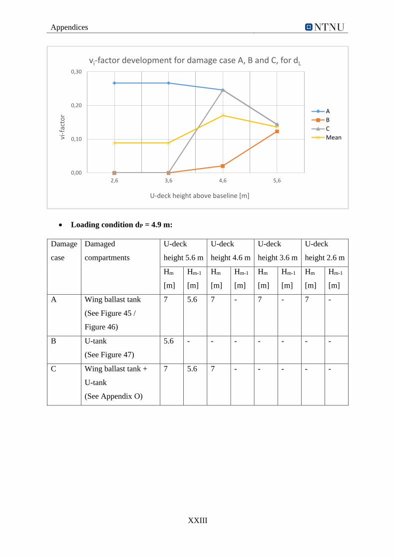
Appendices
XXIII
Loading condition dP = 4.9 m:
Damage
case
Damaged
compartments
U-deck
height 5.6 m
U-deck
height 4.6 m
U-deck
height 3.6 m
U-deck
height 2.6 m
Hm
[m]
Hm-1
[m]
Hm
[m]
Hm-1
[m]
Hm
[m]
Hm-1
[m]
Hm
[m]
Hm-1
[m]
A
Wing ballast tank
(See Figure 45 /
Figure 46)
7 5.6 7 - 7 - 7 -
B U-tank
(See Figure 47)
5.6 - - - - - - -
C Wing ballast tank +
U-tank
(See Appendix O)
7 5.6 7 - - - - -
0,00
0,10
0,20
0,30
2,6 3,6 4,6 5,6
vi-f
acto
r
U-deck height above baseline [m]
vi-factor development for damage case A, B and C, for dL
A
B
C
Mean
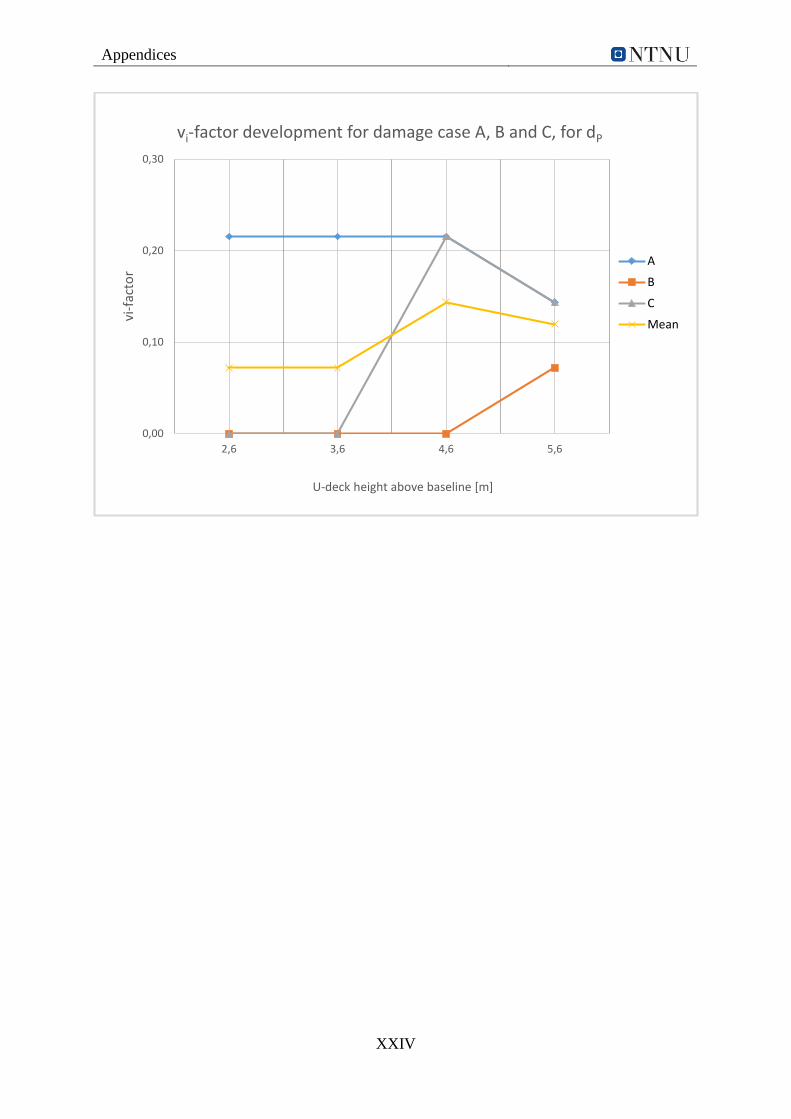
Appendices
XXIV
0,00
0,10
0,20
0,30
2,6 3,6 4,6 5,6
vi-f
acto
r
U-deck height above baseline [m]
vi-factor development for damage case A, B and C, for dP
A
B
C
Mean
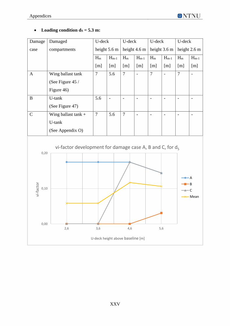
Appendices
XXV
Loading condition dS = 5.3 m:
Damage
case
Damaged
compartments
U-deck
height 5.6 m
U-deck
height 4.6 m
U-deck
height 3.6 m
U-deck
height 2.6 m
Hm
[m]
Hm-1
[m]
Hm
[m]
Hm-1
[m]
Hm
[m]
Hm-1
[m]
Hm
[m]
Hm-1
[m]
A
Wing ballast tank
(See Figure 45 /
Figure 46)
7 5.6 7 - 7 - 7 -
B U-tank
(See Figure 47)
5.6 - - - - - - -
C Wing ballast tank +
U-tank
(See Appendix O)
7 5.6 7 - - - - -
0,00
0,10
0,20
2,6 3,6 4,6 5,6
vi-f
acto
r
U-deck height above baseline [m]
vi-factor development for damage case A, B and C, for dS
A
B
C
Mean
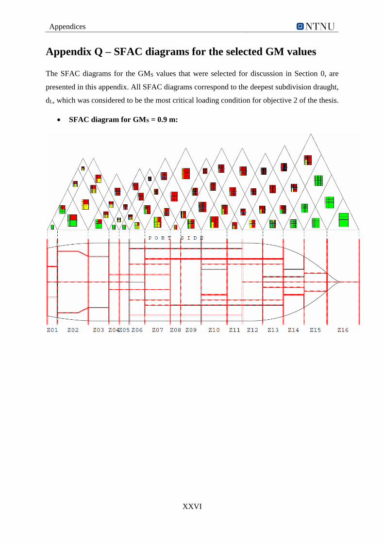
Appendices
XXVI
Appendix Q – SFAC diagrams for the selected GM values
The SFAC diagrams for the GMS values that were selected for discussion in Section 0, are
presented in this appendix. All SFAC diagrams correspond to the deepest subdivision draught,
dL, which was considered to be the most critical loading condition for objective 2 of the thesis.
SFAC diagram for GMS = 0.9 m:
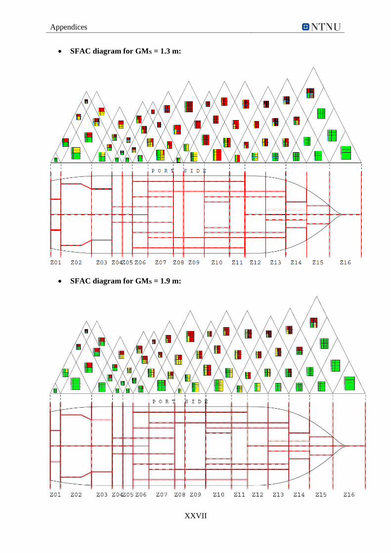
Appendices
XXVII
SFAC diagram for GMS = 1.3 m:
SFAC diagram for GMS = 1.9 m:
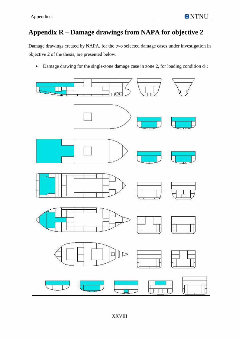
Appendices
XXVIII
Appendix R – Damage drawings from NAPA for objective 2
Damage drawings created by NAPA, for the two selected damage cases under investigation in
objective 2 of the thesis, are presented below:
Damage drawing for the single-zone damage case in zone 2, for loading condition dS:
Appendices
XXIX
Damage drawing for the two-zone damage case involving zone 10 and 11, for loading
condition dS:
Appendices
XXX
Appendix S – Damaged floating positions for objective 2
This appendix presents the equilibrium floating positions of the ship for the damage scenarios
discussed in Section 5.2.
Floating positions for the single-zone damage scenarios corresponding to the three
selected GMS values in zone 2:
- GMS = 0.9 m:
Appendices
XXXI
- GMS = 1.3 m:
- GMS = 1.9 m:
Appendices
XXXII
Floating positions for the two-zone damage scenarios corresponding to the three
selected GMS values in zone 10 and 11:
- GMS = 0.9 m:
- GMS = 1.3 m:
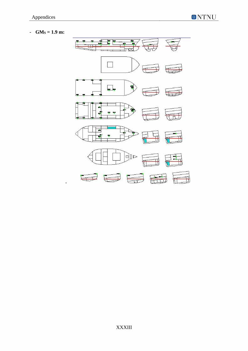
Appendices
XXXIII
- GMS = 1.9 m:
-