doctor thesis - ntnu open
TRANSCRIPT
Doctoral theses at NTNU, 2020:231
Doctoral theses at NTN
U, 2020:231
Ine L. Jernelv
Ine L. Jernelv
Mid-Infrared Tuneable LaserSpectroscopy for Glucose Sensing
ISBN 978-82-326-4810-8 (printed version)ISBN 978-82-326-4811-5 (electronic version)
ISSN 1503-8181
NTNU
Nor
weg
ian
Univ
ersi
ty o
fSc
ienc
e an
d Te
chno
logy
Facu
lty o
f Inf
orm
atio
n Te
chno
logy
and
Elec
tric
al E
ngin
eerin
gDe
part
men
t of E
lect
roni
c Sy
stem
s
Norwegian University of Science and Technology
Thesis for the degree of Philosophiae Doctor
Ine L. Jernelv
Mid-Infrared Tuneable LaserSpectroscopy for Glucose Sensing
Trondheim, August 2020
Faculty of Information Technologyand Electrical EngineeringDepartment of Electronic Systems

NTNUNorwegian University of Science and Technology
Thesis for the degree of Philosophiae Doctor
ISBN 978-82-326-4810-8 (printed version)ISBN 978-82-326-4811-5 (electronic version)ISSN 1503-8181
Doctoral theses at NTNU, 2020:231
© Ine L. Jernelv
Faculty of Information Technologyand Electrical EngineeringDepartment of Electronic Systems
Printed by Skipnes Kommunikasjon as

Abstract
Mid-infrared spectroscopy is a versatile analytical technique, with recent techno-logical developments that enable further advancements towards miniaturised andportable sensor applications. Quantum cascade lasers (QCLs) are infrared lasersthat are small, can be made tuneable, and can be engineered to cover a specificwavelength range. They therefore have high potential in a wavelength region wheretraditionally mainly spectrometers have been available. Mid-infrared spectroscopytargets the fundamental molecular vibrational levels, and measurements in thiswavelength range can provide unique features useful for classification, identifi-cation, and quantification of many materials. This technique is therefore highlysuitable for label-free and accurate measurements of an investigated sample.
The focus of this thesis is on biomedical applications of mid-infrared spectroscopy,specifically for glucose sensing. The aim is to develop an experimental setup andanalytical methods for fast and accurate measurements of glucose in biologicalfluids. Glucose sensing is a critical tool for management of diabetes, and currentcommercially available devices that measure subcutaneously have shortcomingssuch as a lag time compared to the actual blood glucose level. Fluid measure-ments in the peritoneal cavity have been suggested as a possible replacement forsubcutaneous monitoring. While previous research has investigated mid-infraredspectroscopy measurements for hospital settings or non-invasive monitoring, therehas been less interest in solutions targeted towards portable sensing. This work hastherefore concentrated on a fibre-coupled sensor system with a QCL source, withdevelopment towards a continuous glucose monitoring (CGM) device.
This thesis presents contributions on QCL-based spectroscopy and chemometricmethods. The included papers document the development and characterisation ofa fibre-coupled QCL setup. Additional investigation is done into signal-enhancedattenuated total reflection (ATR) spectroscopy, and a comprehensive study ofmultivariate analysis with convolutional neural networks and other chemometricmethods is also included. Finally, the system is employed for measurements ofphysiological glucose levels in peritoneal fluid samples from animal trials. Thepresented results show that fibre-coupled setups in transmission and ATR config-urations are both suitable for measurements of glucose in peritoneal fluid. Thissystem has a high potential for further testing in animal trials, and may be realisedas a CGM device for humans.
i

Acknowledgements
This thesis is a product of four years of hard work, and many people deservemention because of their involvement. Firstly, I want to thank my supervisor,Astrid Aksnes, for giving me the chance to start a PhD in a field that was almostcompletely new to me. Astrid has always provided a realistic perspective and soundadvice, and at the same time let me follow my own research ideas. I would alsolike to thank my co-supervisor, Dag Roar Hjelme, who has provided invaluabletechnical discussions throughout my studies, and has always taken a part in myproject. My project has been a part of the APT group at NTNU, and through thisgroup I have met many wonderful colleagues (ingen nevnt, ingen glemt), and theinterdisciplinary discussions have given very helpful insights.
I am grateful for my research stay at Tohoku University in Sendai, where ProfessorYuji Matsuura kindly opened his lab for me. Especially thanks to Dr. Saiko Kino,who instructed me on many instruments and taught me how to make optical fibres.The other students were also exceedingly welcoming, and the many lunchtimeconversations ensured that my Japanese improved dramatically.
I would like to acknowledge the work by the master students that I co-supervised,who have devoted many hours on this project and made several valuable contri-butions. I want to thank Karina Strøm in particular, who made several forays intoboth software development and experimental work, and who kept working just ashard even when I went off to Japan.
I am appreciative of my many colleagues at Gløs, in particular Karolina Milenkowhom I had the pleasure of sharing an office with for 3.5 years. She introduced meto the finer aspects of optical alignment, and gave helpful advice whenever I hadissues with my experimental setup. I am also grateful for the company from thecybernetics lunch gang during our long treks in search of edible food on campus.
I want to thank my family for having me grow up in the best environment possible,and for having a place I could always come back to. Mum, thank you for alwaysasking about my work. Dad, I wish you could have seen this. Lastly, thanks to mypartner and best friend, Trygve Ræder, whose impact on my life is too big to putinto words. Giitu!
iii

Contributions
The work that constitutes this thesis was carried out at the Department of ElectronicSystems, Norwegian University of Science and Technology (NTNU) in Trondheim,Norway, from May 2016 to May 2020. These studies have been performed underthe supervision of Professor Astrid Aksnes (NTNU), and co-supervisor Professor DagRoar Hjelme (NTNU). The work has been a part of the Artificial Pancreas Trondheim(APT) group at NTNU, with funding from the Research Council of Norway throughgrant numbers 248872 and 248810.
During the doctoral study I have been co-supervisor for three master students:Karina Strøm, Christian Furuseth, and Håvard Bakke Skjellerud. I have also hada three month research stay at the Matsuura Laboratory of the Graduate Schoolof Biomedical Engineering at Tohoku University. During this research stay I didexperimental work under the supervision of Professor Yuji Matsuura.
Publications
Paper II.L. Jernelv, K. Milenko, S.S. Fuglerud, D.R. Hjelme, R. Ellingsen, A. Aksnes, "Areview of optical methods for continuous glucose monitoring," Applied SpectroscopyReviews, Vol. 54(7), pp. 543-572, 2019.
I.L.J., R.E., D.R.H., and A.A. conceptualised this review article. I.L.J. wrote and pre-pared most of the original draft, K.M. and S.S.F. contributed one section each (Ramanspectroscopy and near-infrared spectroscopy, respectively). All authors reviewed theoriginal draft and contributed to the revision of the paper.
Paper III.L. Jernelv, K. Strøm, D.R. Hjelme, A. Aksnes, "Infrared Spectroscopy with a Fiber-Coupled Quantum Cascade Laser for Attenuated Total Reflection MeasurementsTowards Biomedical Applications," Sensors, Vol. 19(23), 5130, 2019.
All authors conceptualised and designed the experiments, I.L.J. and K.S. performedthe experiments. K.S. performed the simulations. I.L.J. implemented the code forthe analysis and analysed the results. I.L.J. wrote and prepared the original draft.A.A. and D.R.H. supervised the work. All authors reviewed the original draft andcontributed to the revision of the paper.
v
Paper III
I.L. Jernelv, K. Strøm, D.R. Hjelme, A. Aksnes, "Mid-infrared spectroscopy witha fiber-coupled tuneable quantum cascade laser for glucose sensing," Proceedingsof SPIE 11233, Optical Fibers and Sensors for Medical Diagnostics and TreatmentApplications XX, 1123311, 2020.
All authors conceptualised and designed the experiments, and K.S. did initial exper-imental work. I.L.J. performed the experiments included in the paper. I.L.J. imple-mented the code for the analysis and analysed the results. I.L.J wrote and prepared theoriginal draft. A.A. and D.R.H. supervised the work. All authors reviewed the originaldraft and contributed to the revision of the paper.
Paper IVI.L. Jernelv, J. Høvik, D.R. Hjelme, A. Aksnes, "Signal enhancement in microstruc-tured silicon attenuated total reflection elements with quantum cascade laser-basedspectroscopy," Proceedings of SPIE 11359, Biomedical Spectroscopy, Microscopy, andImaging, 113590A, 2020.
All authors conceptualised and designed the experiments. I.L.J. developed the experi-mental setup and performed the measurements. I.L.J. implemented the code for theanalysis and analysed the results. J.H. did the simulation work. I.L.J. wrote andprepared the original draft. A.A. and D.R.H. supervised the work. All authors reviewedthe original draft and contributed to the revision of the paper.
Paper VI.L. Jernelv, D.R. Hjelme, Y. Matsuura, A. Aksnes, "Convolutional neural networksfor classification and regression analysis of one-dimensional spectral data," Preprintpublished on arxiv.org, arXiv ID 2005.07530, 2020.
All authors conceptualised and designed the experiments. I.L.J. performed the mea-surements for the original dataset included in the study, and Y.M. supervised thisexperimental work. I.L.J. implemented the code for the analysis and analysed theresults. I.L.J. wrote and prepared the original draft. A.A. and D.R.H. supervised thework. All authors reviewed the original draft and contributed to the revision of thepaper.
Paper VII.L. Jernelv, D.R. Hjelme, A. Aksnes, "Infrared measurements of glucose in peritoneal
vi

fluid with a tuneable quantum cascade laser," Biomedical Optics Express, Vol. 11(7),pp. 3818-3829, 2020.
All authors conceptualised and designed the experiments. I.L.J. developed the ex-perimental setup and performed the measurements. I.L.J. implemented the code forthe analysis and analysed the results. I.L.J. wrote and prepared the original draft.A.A. and D.R.H. supervised the work. All authors reviewed the original draft andcontributed to the revision of the paper.
Software
SpecAnalysis: A Python software package for multivariate data analysis, withfunctionality for regression and classification analysis, as well as pre-processingand feature selection methods. Developed by I.L.J. with open source code freelyavailable online.
Other Results
Other results and conference contributions during the doctoral studies not directlyrelated to the thesis are:
1. I.L. Jernelv, K. Milenko, D.R. Hjelme, R. Ellingsen, S.M. Carlsen, A. Aksnes,"Optimising Multivariate Models for Glucose Measurements in an ATR-FTIR Spec-trometer." ICAVS9 (2017).
2. I.L. Jernelv, K. Milenko, R. Ellingsen, D.R. Hjelme, A. Aksnes, "ImprovingMultivariate Analysis Mid-Infrared Spectroscopy for Biosensing." Optical Sensors,(2018) JTu2a-49. Optical Society of America.
3. K.B. Milenko, I. L. Jernelv, S.S Fuglerud, A. Aksnes, R. Ellingsen, D.R. Hjelme,"Towards Fiber-Optic Raman Spectroscopy for Glucose Sensing" Specialty OpticalFibers, (2018) JTu2a-49. Optical Society of America.
4. S.S. Fuglerud, K.B. Milenko, I. L. Jernelv, R. Ellingsen, A. Aksnes, D.R. Hjelme, "Aminiaturized ball-lensed fiber optic NIR transmission spectroscopy-based glucosesensor" Specialty Optical Fibers, (2018) SeM3E-5. Optical Society of America.
vii

Contents
Abstract i
Acknowledgements iii
Contributions v
List of Abbreviations xi
1 Introduction 11.1 Aim of the Thesis . . . . . . . . . . . . . . . . . . . . . . . . . . . . 4
2 Background 52.1 Infrared Spectroscopy . . . . . . . . . . . . . . . . . . . . . . . . . 5
2.1.1 Light Interaction with Matter . . . . . . . . . . . . . . . . . 52.1.2 Absorption of Light . . . . . . . . . . . . . . . . . . . . . . . 8
2.2 Measurement Modalities . . . . . . . . . . . . . . . . . . . . . . . . 112.2.1 Transmission Measurements . . . . . . . . . . . . . . . . . . 112.2.2 Attenuated Total Reflection Spectroscopy . . . . . . . . . . . 132.2.3 Signal Enhancement . . . . . . . . . . . . . . . . . . . . . . 16
2.3 Systems for Mid-Infrared Spectroscopy . . . . . . . . . . . . . . . . 172.3.1 FTIR Spectrometers . . . . . . . . . . . . . . . . . . . . . . . 172.3.2 Tuneable Laser Spectroscopy . . . . . . . . . . . . . . . . . . 20
2.4 Optical Components . . . . . . . . . . . . . . . . . . . . . . . . . . 252.4.1 Detectors . . . . . . . . . . . . . . . . . . . . . . . . . . . . 252.4.2 Other Optical Components . . . . . . . . . . . . . . . . . . . 262.4.3 Optical Fibres in the Mid-Infrared . . . . . . . . . . . . . . . 26
2.5 Biomedical Mid-Infrared Spectroscopy . . . . . . . . . . . . . . . . 282.5.1 Glucose Sensing . . . . . . . . . . . . . . . . . . . . . . . . . 282.5.2 Other Application Areas . . . . . . . . . . . . . . . . . . . . 33
2.6 Multivariate Data Analysis . . . . . . . . . . . . . . . . . . . . . . . 342.6.1 Regression Analysis . . . . . . . . . . . . . . . . . . . . . . . 35
ix

2.6.2 Classification Methods . . . . . . . . . . . . . . . . . . . . . 382.6.3 Neural Networks . . . . . . . . . . . . . . . . . . . . . . . . 382.6.4 Practical Modelling . . . . . . . . . . . . . . . . . . . . . . . 392.6.5 Spectral Pre-Processing . . . . . . . . . . . . . . . . . . . . . 42
3 Methods 473.1 Experimental QCL Setups . . . . . . . . . . . . . . . . . . . . . . . 47
3.1.1 Transmission Setup . . . . . . . . . . . . . . . . . . . . . . . 503.1.2 ATR Setup . . . . . . . . . . . . . . . . . . . . . . . . . . . . 52
3.2 FTIR Spectroscopy . . . . . . . . . . . . . . . . . . . . . . . . . . . 533.3 Simulations . . . . . . . . . . . . . . . . . . . . . . . . . . . . . . . 533.4 Data Analysis and Software Development . . . . . . . . . . . . . . . 54
4 Summary of Papers 554.1 Evaluation of Optical Techniques . . . . . . . . . . . . . . . . . . . 564.2 Measurements of Synthetic Aqueous Solutions and System Bench-
marking . . . . . . . . . . . . . . . . . . . . . . . . . . . . . . . . . 574.3 Signal Enhancement . . . . . . . . . . . . . . . . . . . . . . . . . . 594.4 Data Analysis . . . . . . . . . . . . . . . . . . . . . . . . . . . . . . 604.5 Characterisation of Biological Fluids . . . . . . . . . . . . . . . . . 61
5 Conclusions 63
References 65References . . . . . . . . . . . . . . . . . . . . . . . . . . . . . . . . . . . 65
Publications 79Paper I . . . . . . . . . . . . . . . . . . . . . . . . . . . . . . . . . . . . . 81Paper II . . . . . . . . . . . . . . . . . . . . . . . . . . . . . . . . . . . . 119Paper III . . . . . . . . . . . . . . . . . . . . . . . . . . . . . . . . . . . . 135Paper IV . . . . . . . . . . . . . . . . . . . . . . . . . . . . . . . . . . . . 147Paper V . . . . . . . . . . . . . . . . . . . . . . . . . . . . . . . . . . . . 157Paper VI . . . . . . . . . . . . . . . . . . . . . . . . . . . . . . . . . . . . 177
x
List of Abbreviations
ANN Artificial neural networkAP Artificial pancreasATR Attenuated total reflectionBGL Blood glucose levelCGM Continuous glucose monitoringCNN Convolutional neural networkCV Cross-validationCW Continuous waveDFB Distributed feedbackDTGS Deuterated triglycine sulfateEC External cavityFEM Finite element methodFP Fabry-PérotFTIR Fourier transform infraredGOx Glucose oxidaseHWG Hollow-core waveguideICL Interband cascade laserICU Intensive care unitIP IntraperitonealIR InfraredIRE Internal reflection elementISF Interstitial fluidkNN k-nearest neighboursLV Latent variableMAE Mean absolute errorMAPE Mean absolute percentage errorMCT Mercury cadmium tellurideMHF Mode-hop-freeMIR Mid-infraredNIR Near-infraredOLS Ordinary least-squaresPC Principal componentPCA Principal component analysisPCR Principal component regression
xi
PLSR Partial least-squares regressionPOC Point-of-careQCL Quantum cascade laserRMSE Root-mean-square errorSC SubcutaneousSE Signal enhancementSEIRA Surface-enhanced infrared absorptionSEP Standard error of predictionSG Savitzky-GolaySi SiliconSMBG Self-monitoring of blood glucoseSNR Signal-to-noise ratioSPR Surface plasmon resonanceSVM Support vector machineTIR Total internal reflectionTLS Tuneable laser spectroscopy
xii
Chapter 1
Introduction
There is an increasing demand for sensor technology targeted towards real-time andin situ monitoring of various chemical and biological species. This is the case for awide range of applications, including food analysis, monitoring of hazardous gasesor greenhouse gases, chemical process monitoring and control, and diagnosticsin biomedicine. Optical spectroscopy techniques are a class of robust and reliablemeasurement methods for identification and quantification of analytes in complexsurroundings. In many cases these methods have been restricted to bulky equipmentwith free-space optics and measurements in a laboratory setting. A combinationof optical spectroscopy with fibre-optic sensing may remove these limitations andbring these methods into a new range of applications. Fibre-optic sensors areinteresting for applications where the measurement site can be difficult to access,as the source and detector can be placed remotely. One such application is glucosesensing, which is paramount for monitoring and treatment of diabetes.
Mid-infrared (MIR) spectroscopy has been a standard laboratory technique fordecades through the use of spectrometers for identification of organic and in-organic compounds. MIR spectroscopy is sensitive to fundamental vibrationaltransitions, and is consequently a technique with high specificity that can beused to identify, characterise, and quantify a large variety of molecular species.Molecules in gas/vapour, liquid, and solid phases can all be investigated with MIRspectroscopy. However, waveguide technology is less mature in the MIR rangecompared to the visible and near-infrared (NIR) wavelength regions, and MIRspectroscopy has therefore not enjoyed the same range of applications withine.g. process monitoring, environmental monitoring, or chemical/biomedical sens-ing. New developments such as commercially available tuneable MIR lasers andsignal-enhanced waveguides may solve some of the current bottlenecks. Thesetechnologies enable miniaturisation and higher sensitivity, and thereby adaptationof MIR spectroscopy for various portable and real-time monitoring applications.
1
Sensing in biomedicine is a substantial area where new sensor technologies arerequired. Healthcare costs are rising rapidly in the world due to chronic andlifestyle diseases, as well as due to ageing populations, and this is expected toput a strain on the future economy [1,2]. More efficient, improved, and cheaperbiomedical sensors is one avenue to reduce costs and improve patient outcomes.Biomedical monitoring often involves extracting a sample from a patient, which isthen measured in an external apparatus and later discarded. This can put an undueburden on the patient. One example is in intensive care units (ICUs) where patientsoften suffer from anaemia, which is detrimental to patient outcomes. Anaemia canbe exacerbated by blood draws, as blood samples are collected multiple times perday in the ICU [3,4]. Optical measurement methods can potentially replace manycurrent biomedical applications, and can enable real-time and point-of-care (POC)monitoring. Optical spectroscopy also fulfils many other sensor requirements suchas robustness, label-free sensing, fast response/measurement time, and a possibilityfor miniaturisation.
Glucose sensing is an important example of an application that is handled with POCmonitoring by diabetic patients, and glucose sensors comprise 85% of the worldmarket for biosensors [5]. Diabetic patients, especially those with type 1 diabetes,lose the ability to control their blood glucose level (BGL). Monitoring the BGL istherefore essential for diabetic patients in order to avoid low and high glucoselevels. In 1964, Dextrostix was developed as the first semi-quantitive glucose teststrip that could be employed for home use [6]. This test strip changed colour basedon a reaction with the enzyme glucose oxidase, and glucose concentration wasinitially estimated by eye. Since then better sensors with built-in electronic glucosemeasurements have been developed as hand-held devices, and even implantablesensors for continuous glucose monitoring (CGM) have become more common.However, these electrochemical devices use an enzymatic reaction for glucosesensing, and the device lifetime in the body is limited to 1–2 weeks. Subcutaneous(SC) measurements have also been found to lag behind the BGL by 5–15 minutes,which can be detrimental to glucose control during rapid changes in glucoselevels [7,8]. Extensive effort has been expended on research and development ofbetter alternatives, but so far no other options have come close to replacing theelectrochemical sensors.
MIR spectroscopy has been suggested and studied for glucose monitoring, mainlythrough non-invasive sensing or measurements of blood samples from patients.Brandstetter et al. [9], as well as Vahlsing et al. [10], have demonstrated glucose
2 Chapter 1 Introduction
measurements of blood serum and micro-dialysate samples in free-space trans-mission setups intended for an ICU setting. Liakat et al. [11] showed that a MIRlaser-based system could be used to determine glucose levels from reflection-modemeasurements of skin, while Kino et al. [12] demonstrated spectrometer-basedglucose sensing with measurements on the inner lip mucosa in humans. However,these non-invasive systems have lower sensitivity due to high water absorption inskin.
An implantable fibre-optic sensor in reflection mode could be suitable for real-time spectroscopy-based glucose monitoring, and would circumvent some of thechallenges inherent to MIR spectroscopy due to high water absorption. MIRspectroscopy has several features that are advantageous for continuous glucosemonitoring; reagent-free monitoring can increase the sensor lifetime, optical fibresare robust in biomedical environments as they can withstand temperature andpressure changes, and fibre-optic sensing allows for remote sensing into smallsample volumes. MIR spectroscopy is also very selective, which is advantageousfor quantitative determination of glucose in a complex biological environment.Today’s implantable CGM sensors measure glucose subcutaneously, which couldpotentially be handled by a fibre-optic sensor. Another alternative is to do sensingin the peritoneal cavity, which is the space between organs in the abdomen, asthis has been recently suggested as a better sensor site due to improved glucosedynamics [13]. Higher sensitivity might be needed in such environments, andthis can be achieved with signal-enhancement techniques. Signal enhancement ininfrared spectroscopy has been demonstrated with surface plasmon resonances inlayers of metal nanoparticles, as well as with 3-layer dielectric or semiconductorstructures [14,15]. These signal-enhancement methods may enable highly sensitivemeasurements with only one reflection in reflection-mode sensing, and therebyallow for miniaturised fibre probes.
This project has been a part of the research group Artificial Pancreas Trondheim,where the long-term goal has been to develop an automated system that combinesCGM and insulin infusions in diabetic patients. This automated system wouldform a basis for an artificial pancreas (AP), where the efficacy of the automationheavily depends on a rapid response to changes in the glucose level, as well as fastuptake of insulin. The focus of the AP development has therefore been towardsoperation in the peritoneal cavity, as this has been suggested as an avenue toachieve normalised glucose levels.
3
1.1 Aim of the ThesisGiven the above-mentioned issues with electrochemical glucose sensors, this thesisaimed to develop an optical sensor system for measurements of glucose in peritonealfluid. This sensor system was developed with in vivo operation in mind, and afibre-coupled system was therefore the basis of this work. The optical system wasbased on mid-infrared tuneable laser spectroscopy using a quantum cascade laser(QCL).
The main contributions of this thesis are summarised as follows:
• Evaluation of several optical spectroscopy methods with regard to their appli-cability for biomedical sensing, specifically for continuous glucose monitoring.This work resulted in a review article that covered optical measurementmethods for CGM.
• Design, construction, testing, and characterisation of a sensor system forglucose measurements in aqueous media. Initial measurements were donewith aqueous solutions due to ease of access.
• Exploration of a signal enhancement technique as a means to minimise sensorsize. Investigation of the signal enhancement effect in the QCL-based system,and whether or not any effective enhancement could be achieved.
• In-depth investigation of multivariate analysis methods for prediction ofanalyte concentrations, and application of convolutional neural networks toimprove prediction accuracy. In-house development of a software package,SpecAnalysis, with source code made freely available online.
• Demonstration of sensor system performance on peritoneal fluid samples frompigs. Measurements of physiological glucose concentrations, with sufficientaccuracy to maintain control of BGL.
The following chapters cover theoretical background related to the publicationsconnected to this thesis, as well as the methods used for this work. The backgroundcovers infrared spectroscopy, components used in the mid-infrared wavelengthregion, measurement modalities and signal enhancement, as well as biomedicalapplications and multivariate data analysis. The chapter on methods describesthe experimental setups used and the multivariate analysis of the spectral data.Following this are a summary of the included papers, an outlook on the presentedwork, and the publications included in this article collection.
4 Chapter 1 Introduction
Chapter 2
Background
This chapter covers relevant theoretical background for biomedical measurementsof aqueous fluids with mid-infrared (MIR) spectroscopy. Included topics rangefrom the fundamental physics behind infrared absorption, to the available opticalcomponents and measurement techniques in the mid-infrared wavelength range,to multivariate analysis used to investigate infrared spectral data.
2.1 Infrared Spectroscopy
Light can interact with matter in different ways, such as by scattering, transmission,reflection, and absorption. This section covers the physical origin of light absorptionand how this property can be used for wavelength-dependent measurements ofmatter. Infrared spectroscopy uses light in the infrared wavelength region to identifyand measure molecules, both qualitatively and quantitatively. Spectroscopy withinfrared light can be used on many organic and inorganic materials, and is useful inmany application areas such as food analysis, biomedical measurements, forensics,and environmental monitoring. Materials that have infrared-active vibrations canbe measured directly without any need for reagents, and the measurement processis non-destructive.
2.1.1 Light Interaction with Matter
Light is electromagnetic radiation, and the interaction between light and matter isgoverned by how the electric and magnetic fields from incident radiation interactwith electric charges in the matter. Specifically, incident light on some matter, forexample a molecule, will lead to a displacement of electrons in the matter. Theelectrons will oscillate with this incident field, which causes a separation of positive
5

and negative charges, and hence a dipole is created [16]. For a material thesesmaller dipole moments can be added up to a net polarisation. The net polarisation,P, in the matter is related to the incident electric field, E, as:
P = ε0χE (2.1)
where ε0 is the permittivity constant of vacuum and χ is a tensor that describes thematerial’s susceptibility, i.e. how much it reacts to an applied field, and may containhigher-order terms that depend on the electric field. The susceptibility is relatedto the relative permittivity as εr(ω) = 1 + χ. Relative permittivity is generally acomplex value, which can be divided into a real and an imaginary part:
εr(ω) = ε′r(ω) + iε′′r(ω) (2.2)
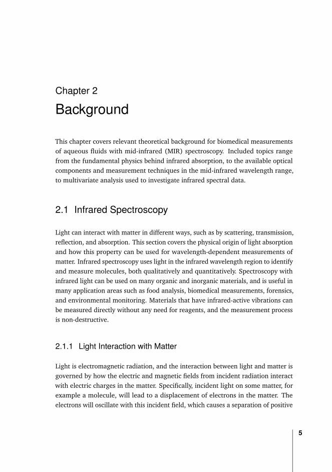
Eq. 2.1 can be expanded into a Taylor series with increasing orders of E and associ-ated constants, and the first term dominates at low field strength. Nonlinear effectsarise at high field strengths, but optical nonlinear effects will not be consideredfurther here and we refer the reader to Boyd [17] for more information. Theeffect of incident radiation on the displaced charges can be described as a dampedharmonic oscillator in a linear system, see Fig. 2.1. Let us consider a single electronbound to a nucleus, with incident radiation at a single frequency. The total electricforce for a linear system is then a sum of the forces acting on the charges:
md2xdt2
+ ksx + γdxdt
= eE (2.3)
In this system, a mass m oscillates with a displacement x, and and a balancingcounter-force is described by the spring constant ks. The oscillations are dampenedby energy loss, which is described by a damping coefficient, γ, and the velocity ofthe object.
The expression in Eq. 2.3 is a differential equation, and the solutions of suchequations are covered in many electromagnetics textbooks, e.g. by Saleh et al. [18].A solution on the form x = x0e
−iωt can be inserted into Eq. 2.3, and the result canbe used in Eq. 2.1 to give an expression for the susceptibility, χ, as a function of ω.An expression for the relative permittivity, also called the dielectric constant, canthen be found:
εr(ω) = 1 +ω2p
ω20 − ω2 − iγω
(2.4)
6 Chapter 2 Background
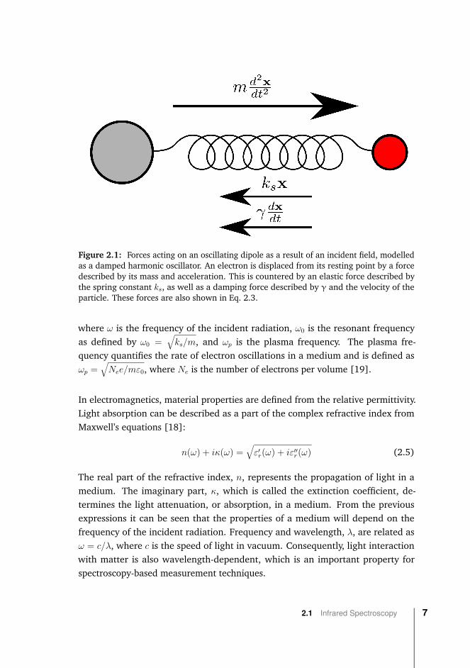
Figure 2.1: Forces acting on an oscillating dipole as a result of an incident field, modelledas a damped harmonic oscillator. An electron is displaced from its resting point by a forcedescribed by its mass and acceleration. This is countered by an elastic force described bythe spring constant ks, as well as a damping force described by γ and the velocity of theparticle. These forces are also shown in Eq. 2.3.
where ω is the frequency of the incident radiation, ω0 is the resonant frequencyas defined by ω0 =
√ks/m, and ωp is the plasma frequency. The plasma fre-
quency quantifies the rate of electron oscillations in a medium and is defined asωp =
√Nee/mε0, where Ne is the number of electrons per volume [19].
In electromagnetics, material properties are defined from the relative permittivity.Light absorption can be described as a part of the complex refractive index fromMaxwell’s equations [18]:
n(ω) + iκ(ω) =√ε′r(ω) + iε′′r(ω) (2.5)
The real part of the refractive index, n, represents the propagation of light in amedium. The imaginary part, κ, which is called the extinction coefficient, de-termines the light attenuation, or absorption, in a medium. From the previousexpressions it can be seen that the properties of a medium will depend on thefrequency of the incident radiation. Frequency and wavelength, λ, are related asω = c/λ, where c is the speed of light in vacuum. Consequently, light interactionwith matter is also wavelength-dependent, which is an important property forspectroscopy-based measurement techniques.
2.1 Infrared Spectroscopy 7

2.1.2 Absorption of Light
The previous section outlined how material properties are wavelength dependentin response to an electric field. In the same way, light itself will be affected as itinteracts with matter, and here we will discuss the theory behind light absorption.Absorption is a process where light interacts with a medium and the electromagneticenergy is transformed into internal energy. For example, a molecule can take energyfrom the incident radiation if the energy of a photon equals the difference of twoenergy levels in the molecule. In the case where the photon energy does not matchthe difference between energy levels, the molecule will not absorb any of theincident radiation.
Fig. 2.2 shows a band diagram with electronic energy transitions for infraredspectroscopy, as well as for UV/visible and Raman spectroscopy for comparison.Electrons will typically be in the lowest energy state, E0. When excitation light isintroduced, an electron may absorb a photon and thereby be excited to a higherenergy state. Infrared light, which has long wavelengths and thus low energy, canonly excite vibrational and rotational states in a molecule. Relaxation back to theground state usually occurs through release of energy in the form of heat.
Absorption bands are not equal in strength, and are characterised by the absorptioncross section σ(λ). The absorption cross section can be described as σ(λ) = κ/N ,where N is the atomic number density and κ is the extinction coefficient, whichwas shown to be a wavelength-dependent parameter in the last section. The totalabsorption probability can then be quantified with the absorption coefficient, µa.The absorption coefficient is defined as:
µa = C × σ(λ) (2.6)
where C is the concentration of the absorbing material. Light going through anabsorbing material will then have an incremental change in intensity as describedby:
dI
I= −µadx (2.7)
Integrating this gives an exponential function:
I(x) = I0e−µax (2.8)
8 Chapter 2 Background
Ener
gy
UV/vis IR Raman
Virtual
energy
levels
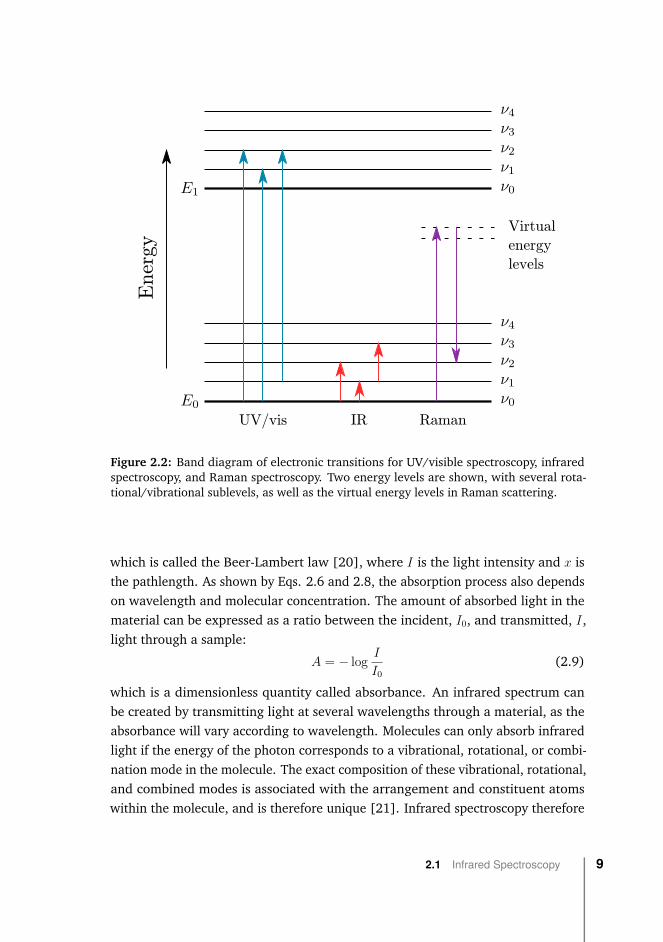
Figure 2.2: Band diagram of electronic transitions for UV/visible spectroscopy, infraredspectroscopy, and Raman spectroscopy. Two energy levels are shown, with several rota-tional/vibrational sublevels, as well as the virtual energy levels in Raman scattering.
which is called the Beer-Lambert law [20], where I is the light intensity and x isthe pathlength. As shown by Eqs. 2.6 and 2.8, the absorption process also dependson wavelength and molecular concentration. The amount of absorbed light in thematerial can be expressed as a ratio between the incident, I0, and transmitted, I,light through a sample:
A = − log I
I0(2.9)
which is a dimensionless quantity called absorbance. An infrared spectrum canbe created by transmitting light at several wavelengths through a material, as theabsorbance will vary according to wavelength. Molecules can only absorb infraredlight if the energy of the photon corresponds to a vibrational, rotational, or combi-nation mode in the molecule. The exact composition of these vibrational, rotational,and combined modes is associated with the arrangement and constituent atomswithin the molecule, and is therefore unique [21]. Infrared spectroscopy therefore
2.1 Infrared Spectroscopy 9
gives information which is unique to the particular material under investigation,and this can be used to investigate most kinds of organic or inorganic materials.
There are certain limitations to infrared spectroscopy. For some materials thesensitivity is quite low if the infrared activity is low, i.e. if the vibrational transitionhas a weak oscillatory dipole. In complex samples it can also be difficult todetect analytes with small concentrations, especially if they have absorption bandsthat overlap with other highly concentrated analytes. Infrared spectroscopy doesnot give any direct structural information on molecules, such as the position offunctional groups and molecular weight. Other complicating factors make infraredspectra more difficult to interpret, such as line broadening, heavily overlappingbands, and shifts in absorption bands due to hydrogen bonds, especially whenwater is used as a solvent. Additional bands are created when two photons areabsorbed simultaneously, called overtone and combination bands.
The infrared wavelength range is typically divided into three subranges: thenear-infrared (0.78–3 µm), the mid-infrared (3–50 µm), and the far-infrared(50 µm–1 mm) [22], although different sources use somewhat different definitions[23]. Near-infrared spectra are products of overtone or combination bands whichare typically less intense and broader than fundamental vibrational modes. Near-infrared spectroscopy is nevertheless a popular measurement method, in partdue to the low price of optical components in that wavelength range. The mid-infrared wavelength range encompasses fundamental vibrational modes, in additionto skeletal vibrations, which are vibrational modes that couple over the entiremolecule. Skeletal vibrations give a distinct spectral shape, and the region forskeletal vibrations (approximately 6.5–12 µm) is therefore called the fingerprintregion. The fundamental and skeletal vibrational modes are sharper and higher inintensity than e.g. overtones, which gives mid-infrared spectroscopy an advantagefor detection and quantification of materials. Far-infrared spectroscopy uses photonswith very low energy, and is typically used to investigate stretching modes inmolecules with heavy atoms or lattice vibrations in crystals. Since mid-infraredspectroscopy is the focus of this work, further sections will focus on spectroscopyin the mid-infrared wavelength range.
As a note on units, it is common in spectroscopy to use wavenumbers, which isthe number of wavelengths per unit distance, ν = 1/λ, typically given as cm-1. Inwavenumbers, the mid-infrared range is 3333–200 cm-1, and the region of skeletalvibrations is approximately 1500–800 cm-1.
10 Chapter 2 Background
2.2 Measurement Modalities
There are three main methods for direct MIR spectroscopy: transmission, internalreflection, and external reflection. Transmission and internal reflection will bediscussed here, as these measurement modalities are widely used for applicationsrelevant to this work.
2.2.1 Transmission Measurements
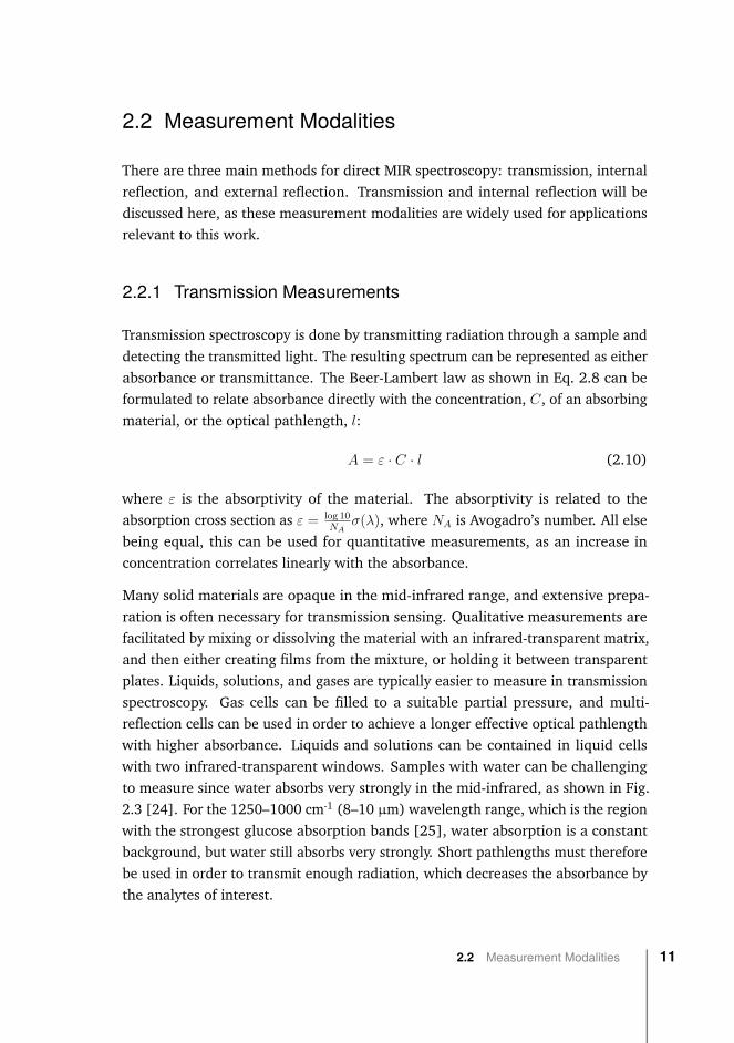
Transmission spectroscopy is done by transmitting radiation through a sample anddetecting the transmitted light. The resulting spectrum can be represented as eitherabsorbance or transmittance. The Beer-Lambert law as shown in Eq. 2.8 can beformulated to relate absorbance directly with the concentration, C, of an absorbingmaterial, or the optical pathlength, l:
A = ε · C · l (2.10)
where ε is the absorptivity of the material. The absorptivity is related to theabsorption cross section as ε = log 10
NAσ(λ), where NA is Avogadro’s number. All else
being equal, this can be used for quantitative measurements, as an increase inconcentration correlates linearly with the absorbance.
Many solid materials are opaque in the mid-infrared range, and extensive prepa-ration is often necessary for transmission sensing. Qualitative measurements arefacilitated by mixing or dissolving the material with an infrared-transparent matrix,and then either creating films from the mixture, or holding it between transparentplates. Liquids, solutions, and gases are typically easier to measure in transmissionspectroscopy. Gas cells can be filled to a suitable partial pressure, and multi-reflection cells can be used in order to achieve a longer effective optical pathlengthwith higher absorbance. Liquids and solutions can be contained in liquid cellswith two infrared-transparent windows. Samples with water can be challengingto measure since water absorbs very strongly in the mid-infrared, as shown in Fig.2.3 [24]. For the 1250–1000 cm-1 (8–10 µm) wavelength range, which is the regionwith the strongest glucose absorption bands [25], water absorption is a constantbackground, but water still absorbs very strongly. Short pathlengths must thereforebe used in order to transmit enough radiation, which decreases the absorbance bythe analytes of interest.
2.2 Measurement Modalities 11
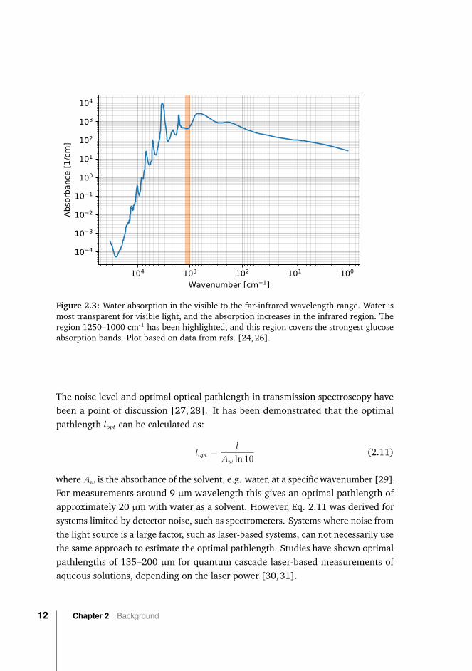
Figure 2.3: Water absorption in the visible to the far-infrared wavelength range. Water ismost transparent for visible light, and the absorption increases in the infrared region. Theregion 1250–1000 cm-1 has been highlighted, and this region covers the strongest glucoseabsorption bands. Plot based on data from refs. [24,26].
The noise level and optimal optical pathlength in transmission spectroscopy havebeen a point of discussion [27, 28]. It has been demonstrated that the optimalpathlength lopt can be calculated as:
lopt = l
Aw ln 10 (2.11)
whereAw is the absorbance of the solvent, e.g. water, at a specific wavenumber [29].For measurements around 9 µm wavelength this gives an optimal pathlength ofapproximately 20 µm with water as a solvent. However, Eq. 2.11 was derived forsystems limited by detector noise, such as spectrometers. Systems where noise fromthe light source is a large factor, such as laser-based systems, can not necessarily usethe same approach to estimate the optimal pathlength. Studies have shown optimalpathlengths of 135–200 µm for quantum cascade laser-based measurements ofaqueous solutions, depending on the laser power [30,31].
12 Chapter 2 Background
2.2.2 Attenuated Total Reflection Spectroscopy
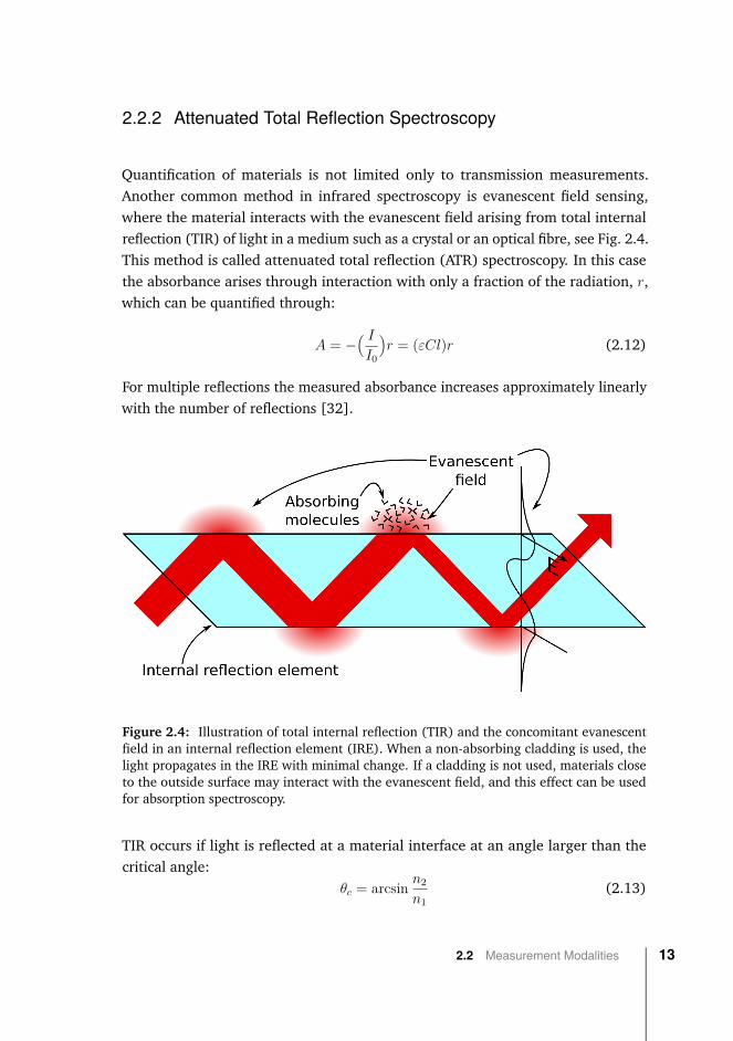
Quantification of materials is not limited only to transmission measurements.Another common method in infrared spectroscopy is evanescent field sensing,where the material interacts with the evanescent field arising from total internalreflection (TIR) of light in a medium such as a crystal or an optical fibre, see Fig. 2.4.This method is called attenuated total reflection (ATR) spectroscopy. In this casethe absorbance arises through interaction with only a fraction of the radiation, r,which can be quantified through:
A = −( II0
)r = (εCl)r (2.12)
For multiple reflections the measured absorbance increases approximately linearlywith the number of reflections [32].
Figure 2.4: Illustration of total internal reflection (TIR) and the concomitant evanescentfield in an internal reflection element (IRE). When a non-absorbing cladding is used, thelight propagates in the IRE with minimal change. If a cladding is not used, materials closeto the outside surface may interact with the evanescent field, and this effect can be usedfor absorption spectroscopy.
TIR occurs if light is reflected at a material interface at an angle larger than thecritical angle:
θc = arcsin n2
n1(2.13)
2.2 Measurement Modalities 13
as determined from Snell’s law. The interface must be between a material with highrefractive index, n1, such as an optical fibre or other waveguiding material, and amaterial with low refractive index, n2, e.g. a sample matrix. The process of TIRcarries with it a non-propagating component which extends into the neighbouringmaterial, called the evanescent field. The intensity of the evanescent field decaysexponentially from the material interface, as described by:
E = E0e−z/dp (2.14)
where E is the electric field intensity at a distance z from the interface, and E0 isthe electric field intensity at the material interface. The penetration depth, dp isgiven by:
dp = λ0
2πn1
√sin2 θ − (n2/n1)2
(2.15)
where λ0 is the free-space wavelength and θ is the angle of incidence. Absorbingmolecules close to the material interface may interact with the evanescent field,which creates an absorption spectrum, as mentioned previously. It has been shownthat absorbance is proportional to the effective penetration depth, de [33, 34],rather than the penetration depth, which is calculated as:
de = n21
cos θ
∫ ∞0
E2dz = n21E20dp
2 cos θ (2.16)
where n21 is the ratio between n2 and n1.
Mid-Infrared Waveguides
Fourier transform infrared (FTIR) spectrometers can often be fitted with an ATRsensing unit, which is especially useful for materials and solutions with high watercontent that would otherwise require measurements through a very thin layerin transmission mode. These ATR units use crystal prisms made from variousmaterials with single or multiple internal reflections, called internal reflectionelements (IREs). Some materials that are typically used for ATR spectroscopyare diamond, zinc selenide, ZnSe, and zinc sulphide, ZnS [35]. Diamond is aresilient material and can today be fabricated industrially, however it is still a veryexpensive prism material. ZnSe is much cheaper, but very soft and toxic to humans,and is therefore not a good material choice for some applications. ZnS offers agood compromise as a prism material, as it is cheap, has a low refractive index(approx. 2.2 at 10 µm), and is non-toxic. Lower refractive index gives a longer
14 Chapter 2 Background
penetration depth, which increases the interaction volume outside of the IRE. Thisgives a higher absorbance and higher signal-to-noise ratio (SNR) as compared toIREs with high refractive index. Using a fibre-coupled system simplifies furthersensor development with regard to portable sensing and reducing sensor formfactor. A combination of ATR spectroscopy and fibre-coupling could be used in aprobe design in a portable sensor.
Optical fibres can also be used for ATR sensing, after stripping away outside coatingand alternatively the cladding [36]. The fibre can be looped several times toincrease the sensing area in a liquid volume. Higher sensitivity can then be achievedin comparison to single bends or single-reflection prisms. However, evanescentsensing with fibres in the mid-infrared range has a few disadvantages. The fibresare usually several hundred micrometers in diameter, and a large bend radius musttherefore be used. This can be a major drawback if the intended application ise.g. a biomedical sensor, where sensor footprint is a critical parameter. The fibrecore can be pressed or tapered in order to reduce the dimensions and increase theevanescent field, but this also tends to put more mechanical strain on the fibre.Common optical fibre materials in MIR spectroscopy, such as silver halide materials,have also been found to be toxic as the fibres degrade and release particles in thesurrounding environment over time. The issue with toxicity can potentially besolved by e.g. encasing the sensor in a semipermeable membrane which allowsthe analyte of interest to pass through [37]. This could potentially also improvesensing as it would allow for a preliminary filtering of the analyte of interest.
Another option is to use integrated waveguides for evanescent field sensing inthe mid-infrared, in the interest of reduced form factor. Waveguides can be madewith common techniques for microfabrication, resulting in a light-guiding structureon top of a substrate. This increases the fraction of light available for sensing ascompared to ATR crystals or fibres and therefore also the measured signal. However,few transparent materials have been available as mid-infrared waveguides, and thefabricated structures are often quite lossy due to e.g. roughness at the waveguide-substrate interface. Liquid spectroscopy has been demonstrated with systemsbased on Ge and GaAs waveguides [38,39]. Tantalum pentoxide is one potentialwaveguide material in the MIR range that has received recent research interest,and newer structures for gas sensing have been demonstrated [40]. Losses alsooccur when coupling light from a laser into a waveguide. So although increasedsignal can be achieved, this is often counteracted by an increase in noise, resultingin little or no improvement for the SNR.
2.2 Measurement Modalities 15
For gas sensing, it is also possible to use the internal space of hollow-core fibres forspectroscopy. This is an improvement on traditional multi-pass gas cells, where therequired volume varies from a few hundred millilitres to several litres. Comparedto gas cells used for spectroscopy, hollow-core fibres also have more efficientinteraction volume sizes and faster flow times for sample replacement. However,hollow-core waveguides are sensitive to vibrations, which can affect measurementsin any sensing environment. Integrated hollow waveguides have been demonstratedby Wilk et al. [41], where a hollow waveguide was machined into an aluminiumblock for improved robustness.
2.2.3 Signal Enhancement
Surface-enhanced infrared absorption (SEIRA) is used in optical spectroscopyin order to increase the detected signal, and thereby the total sensitivity [42].Enhancement can be achieved with surface plasmon resonances (SPRs), whichoccur when incident radiation induces a resonant oscillation of electrons in theconduction band of a material, see Fig. 2.5a. SPRs can only be induced at aninterface between materials with negative and positive permittivity, such as ametal and a dielectric. This is typically realised by coating a surface with a layerof roughened metal or metal nanoparticles. Analytes close to the substrate arethen typically measured with internal or external reflection. SPR-based sensorsare commonly used in the visible/NIR range, as the technique can offer largesensitivity increases for optical methods that are otherwise not adequate. SPR-based sensors in the MIR range have been increasingly studied with enhancementfrom coated surfaces or deposited waveguides [14, 43, 44], as well as dopedwaveguide structures [45, 46]. SEIRA is usually reported to give enhancementfactors of 10-100 for MIR spectroscopy.
Enhancement has also been demonstrated through an interference effect withmicropillar silicon (Si) structures on Si wafer chips, and the principle is shownin Fig. 2.5b [15,47]. The advantage of these microstructures for enhancement isthat it is possible to use only one material for fabrication, and standard Si wafertechnology can be used to produce the chips. This enhancement effect has beendescribed several times previously for three-layer dielectric structures [48–50].This measurement technique has been reported to give signal enhancement up to afactor of 10.
16 Chapter 2 Background

MetalPrism
Surface plasmon
Field enhancement
Pillars
Si
b)a)
Figure 2.5: a) Signal enhancement through induction of surface plasmons using a metallayer or metal nanoparticles. b) Enhancement method using an interference effect in athree-layer dielectric, here exemplified with an Si IRE with micropillars.
Signal enhancement does not come without challenges. For SPR-based systems onecommon issue is sensor lifetime, as the thin metal layers or metal nanoparticleshave a tendency to degrade over time. This leads to a decline in sensor performance.A release of nanoparticles from the sensor surface also poses potential risks withregards to environmental safety in many applications [51,52]. Interference-basedsignal enhancement, on the other hand, has been shown to be associated witha simultaneous increase in noise, which can significantly reduce the achievedeffective enhancement factor [47].
2.3 Systems for Mid-Infrared Spectroscopy
Technical systems for MIR spectroscopy are based on either spectrometers ortuneable laser spectroscopy, which have several fundamental differences. In orderto appreciate how this can affect measurements in biomedical applications, thebasic principles of these systems are detailed below.
2.3.1 FTIR Spectrometers
Fourier transform infrared (FTIR) spectroscopy has been a routine laboratorytechnique for mid-infrared spectroscopy for decades, and has taken the place ofdispersive spectrometers [23]. Dispersive spectrometers are still commonly usedfor e.g. near-infrared spectroscopy. Commercially available FTIR spectrometerscombine a light source, interferometer, sample stage, and detector for a completesystem.
2.3 Systems for Mid-Infrared Spectroscopy 17
Michelson Interferometers
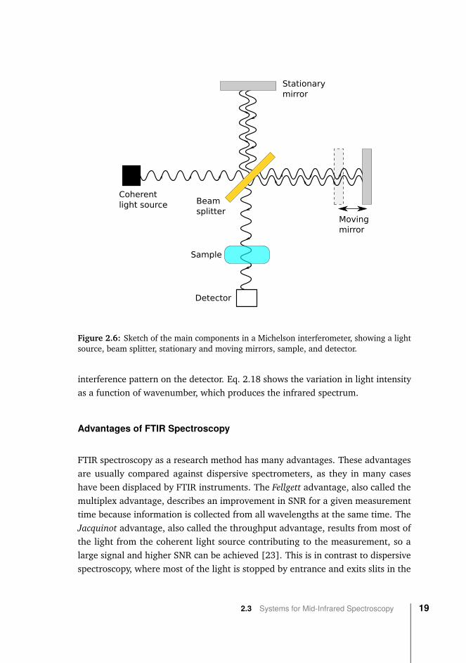
Michelson interferometers are the most common interferometers used in FTIRspectroscopy. As shown in Fig. 2.6, a Michelson interferometer consists of abeamsplitter, which is a semi-reflective film, and two perpendicular plane mirrors,one of which is moveable. The incident radiation travels towards the beamsplitter,where 50% of the beam is transmitted to one of the mirrors, while the remaining50% of the beam is reflected to the other mirror. The beams are reflected at themirrors, and then return to the beamsplitter where they recombine and interfere.The beam that emerges from the interferometer at 90◦ to the input beam is calledthe transmitted beam, and this is the beam (interferogram) detected in FTIRspectroscopy. Due to the nature of the beamsplitter, 50% of the total radiationreaches the sample, while 50% of the radiation is lost.
The optical path difference between the two arms of the interferometer is producedby the moving mirror. This path difference causes destructive and constructiveinterference between the beams, and results in an interferogram. The movingmirror is a critical part of the interferometer. It must be aligned accurately, andmust be able to trace the distance consistently so that the path correlates witha known value. Most modern FTIR systems use a separate laser to measure themirror position.
Fourier Transformation
FTIR spectroscopy works on the principle of Fourier transformation, which con-verts the interferogram measured by the detector into an infrared spectrum. Themain development that enabled widespread use of FTIR spectrometers was theintroduction of modern computers that were able to perform Fourier transformalgorithms in real time. The Fourier transformation, as used in FTIR spectroscopy,can be written as:
I(δ) =∫ ∞
0B(ν) cos(2πνδ) dnu. (2.17)
B(ν) =∫ ∞−∞
I(δ) cos(2πνδ) dδ. (2.18)
These equations relate the light intensity that reaches the detector, I(δ), to thespectral power density at a wavenumber ν, that is B(ν). Indeed, the equationsshow that it is possible to convert between I(δ) and B(ν). Eq. 2.17 shows howthe power density varies as a function of difference in pathlength, which is the
18 Chapter 2 Background
Beam splitter
Coherent light source
Stationarymirror
Sample
Movingmirror
Detector
Figure 2.6: Sketch of the main components in a Michelson interferometer, showing a lightsource, beam splitter, stationary and moving mirrors, sample, and detector.
interference pattern on the detector. Eq. 2.18 shows the variation in light intensityas a function of wavenumber, which produces the infrared spectrum.
Advantages of FTIR Spectroscopy
FTIR spectroscopy as a research method has many advantages. These advantagesare usually compared against dispersive spectrometers, as they in many caseshave been displaced by FTIR instruments. The Fellgett advantage, also called themultiplex advantage, describes an improvement in SNR for a given measurementtime because information is collected from all wavelengths at the same time. TheJacquinot advantage, also called the throughput advantage, results from most ofthe light from the coherent light source contributing to the measurement, so alarge signal and higher SNR can be achieved [23]. This is in contrast to dispersivespectroscopy, where most of the light is stopped by entrance and exits slits in the
2.3 Systems for Mid-Infrared Spectroscopy 19
monochromator. FTIR spectroscopy also benefits from rapid scanning and theassociated improvement in SNR is related to the number of scans as SNR ∝
√n.
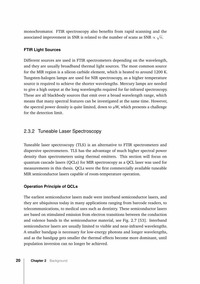
FTIR Light Sources
Different sources are used in FTIR spectrometers depending on the wavelength,and they are usually broadband thermal light sources. The most common sourcefor the MIR region is a silicon carbide element, which is heated to around 1200 K.Tungsten-halogen lamps are used for NIR spectroscopy, as a higher temperaturesource is required to achieve the shorter wavelengths. Mercury lamps are neededto give a high output at the long wavelengths required for far-infrared spectroscopy.These are all blackbody sources that emit over a broad wavelength range, whichmeans that many spectral features can be investigated at the same time. However,the spectral power density is quite limited, down to µW, which presents a challengefor the detection limit.
2.3.2 Tuneable Laser Spectroscopy
Tuneable laser spectroscopy (TLS) is an alternative to FTIR spectrometers anddispersive spectrometers. TLS has the advantage of much higher spectral powerdensity than spectrometers using thermal emitters. This section will focus onquantum cascade lasers (QCLs) for MIR spectroscopy as a QCL laser was used formeasurements in this thesis. QCLs were the first commercially available tuneableMIR semiconductor lasers capable of room-temperature operation.
Operation Principle of QCLs
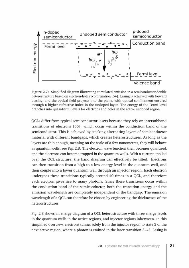
The earliest semiconductor lasers made were interband semiconductor lasers, andthey are ubiquitous today in many applications ranging from barcode readers, totelecommunications, to medical uses such as dentistry. These semiconductor lasersare based on stimulated emission from electron transitions between the conductionand valence bands in the semiconductor material, see Fig. 2.7 [53]. Interbandsemiconductor lasers are usually limited to visible and near-infrared wavelengths.A smaller bandgap is necessary for low-energy photons and longer wavelengths,and as the bandgap gets smaller the thermal effects become more dominant, untilpopulation inversion can no longer be achieved.
20 Chapter 2 Background
p-doped semiconductor
n-doped semiconductor
Fermi level
Fermi levelEle
ctro
n e
nerg
yUndoped semiconductor
Figure 2.7: Simplified diagram illustrating stimulated emission in a semiconductor doubleheterostructure based on electron-hole recombination [54]. Lasing is achieved with forwardbiasing, and the optical field projects into the plane, with optical confinement ensuredthrough a higher refractive index in the undoped layer. The energy of the Fermi levelbranches into quasi-Fermi levels for electrons and holes in the active undoped region.
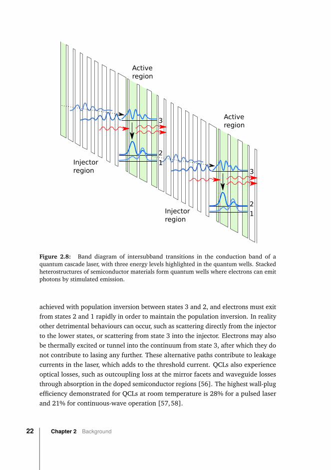
QCLs differ from typical semiconductor lasers because they rely on intersubbandtransitions of electrons [55], which occur within the conduction band of thesemiconductor. This is achieved by stacking alternating layers of semiconductormaterial with different bandgaps, which creates heterostructures. As long as thelayers are thin enough, meaning on the scale of a few nanometres, they will behaveas quantum wells, see Fig. 2.8. The electron wave function then becomes quantised,and the electrons can become trapped in the quantum wells. With a current appliedover the QCL structure, the band diagram can effectively be tilted. Electronscan then transition from a high to a low energy level in the quantum well, andthen couple into a lower quantum well through an injector region. Each electronundergoes these transitions typically around 40 times in a QCL, and thereforeeach electron gives rise to many photons. Since these transitions occur withinthe conduction band of the semiconductor, both the transition energy and theemission wavelength are completely independent of the bandgap. The emissionwavelength of a QCL can therefore be chosen by engineering the thicknesses of theheterostructures.
Fig. 2.8 shows an energy diagram of a QCL heterostructure with three energy levelsin the quantum wells in the active regions, and injector regions inbetween. In thissimplified overview, electrons tunnel solely from the injector region to state 3 of thenext active region, where a photon is emitted in the laser transition 3→2. Lasing is
2.3 Systems for Mid-Infrared Spectroscopy 21
Injector region
Activeregion
Injector region
Activeregion
3
2
13
2
1
Figure 2.8: Band diagram of intersubband transitions in the conduction band of aquantum cascade laser, with three energy levels highlighted in the quantum wells. Stackedheterostructures of semiconductor materials form quantum wells where electrons can emitphotons by stimulated emission.
achieved with population inversion between states 3 and 2, and electrons must exitfrom states 2 and 1 rapidly in order to maintain the population inversion. In realityother detrimental behaviours can occur, such as scattering directly from the injectorto the lower states, or scattering from state 3 into the injector. Electrons may alsobe thermally excited or tunnel into the continuum from state 3, after which they donot contribute to lasing any further. These alternative paths contribute to leakagecurrents in the laser, which adds to the threshold current. QCLs also experienceoptical losses, such as outcoupling loss at the mirror facets and waveguide lossesthrough absorption in the doped semiconductor regions [56]. The highest wall-plugefficiency demonstrated for QCLs at room temperature is 28% for a pulsed laserand 21% for continuous-wave operation [57,58].
22 Chapter 2 Background
The first working QCL was demonstrated by Faist et al. at Bell Labs in 1994 [59],and the concept of intersubband transitions in the conduction band of lasers wasalready suggested by Kazarinov et al. in 1971 [60]. Precision on the level of atomiclayers is necessary for growth of the QCL heterostructures, and this was enabled bydevelopment of the now staple tools in nanotechnology research, namely molecularbeam epitaxy (MBE) and metal-organic vapour phase epitaxy (MOVPE).
Bandstructure engineering can also be implemented for interband transitions inso-called interband cascade lasers (ICLs) [61, 62]. These lasers follow the sameprinciple as QCLs, where stacked heterostructures are used to form the gain element.Lasing in ICLs can be achieved at lower input powers than what is possible in QCLs.Currently 5.6 µm is the longest emission wavelength demonstrated at ambientconditions with CW operation [63].
QCLs and ICLs are important tools for research using mid-infrared wavelengths forspectroscopy. Previously, only spectrometers could cover large wavelength rangesin the mid-infrared, with very limited spectral power density. The other lasersources available were CO2 lasers and lead-salt lasers, as well as light sources basedon difference frequency generation or optical parametric oscillation. CO2 lasershave found many uses in industrial applications, with power levels up to severalhundred kWs. However, CO2 lasers are bulky as they are gas lasers, and can usuallyonly be used at a set few wavelengths. Lead-salt lasers can be made tuneableover small wavelength ranges, but have seen limited use as they often requirecryogenic cooling for operation. Mid-infrared radiation based on frequency combgeneration has also become available [64], and has demonstrated good resultsparticularly for gas spectroscopy [65, 66]. Frequency comb generation usuallyrequires femtosecond laser sources, which currently necessitates complex opticalsystems. Spectroscopy with frequency combs based on quantum cascade lasershas been demonstrated as a promising alternative, with potential for time-resolvedspectroscopy [67,68].
QCL Resonator Design
QCLs are classified according to their resonator design. The three resonators thatare most commonly used are Fabry-Pérot (FP), distributed feedback (DFB), andexternal-cavity (EC).
An FP resonator design is achieved by cleaving the ends of the laser chip in orderto make highly reflective end facets on the laser ridge. Light amplification is only
2.3 Systems for Mid-Infrared Spectroscopy 23
possible if the distance between the facets allows for constructive interference,in addition to the gain condition for the active material. FP-QCLs typically havemultimode emission, as the standing wave condition in the cavity is fulfilled forup to several hundred longitudinal modes. The emission covers a large spectralrange, up to 50 cm-1, and the wavelength can be controlled by adjusting thechip temperature. As a result of the multimode emission, FP-QCLs are oftenunsuitable for most applications in spectroscopy, especially gas spectroscopy andother applications where single-mode emission is required. However, these QCLshave found use in analysis of liquids [69], and in heterodyne spectroscopy [70].
A QCL with a DFB resonator uses a Bragg grating that is integrated into thelaser waveguide along the direction of light propagation. As a result, all modesexcept one will be lossy, and a single mode is chosen for emission. The emissionwavelength can be tuned over a small range of approximately 5 cm-1 by changingthe operation temperature or the injection current of the chip. DFB-QCLs have beenused for gas spectroscopy [71,72], as the single-mode emission enables accuratetargeting of specific spectral lines. Multiple DFB-QCLs can also be joined in anarray if a larger wavelength range is needed [73].
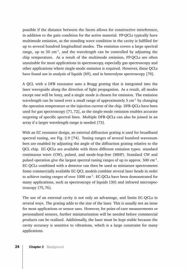
With an EC resonator design, an external diffraction grating is used for broadbandspectral tuning, see Fig. 2.9 [74]. Tuning ranges of several hundred wavenum-bers are enabled by adjusting the angle of the diffraction grating relative to theQCL chip. EC-QCLs are available with three different emission types: standardcontinuous wave (CW), pulsed, and mode-hop-free (MHF). Standard CW andpulsed operation give the largest spectral tuning ranges of up to approx. 500 cm-1.EC-QCLs combined with a detector can then be used as miniature spectrometer.Some commercially available EC-QCL models combine several laser heads in orderto achieve tuning ranges of over 1000 cm-1. EC-QCLs have been demonstrated formany applications, such as spectroscopy of liquids [30] and infrared microspec-troscopy [75,76].
The use of an external cavity is not only an advantage, and limits EC-QCLs inseveral ways. The grating adds to the size of the laser. This is usually not an issuefor most applications or sensor uses. However, for point-of-care measurements orpersonalised sensors, further miniaturisation will be needed before commercialproducts can be realised. Additionally, the laser must be kept stable because thecavity accuracy is sensitive to vibrations, which is a large constraint for manyapplications.
24 Chapter 2 Background

Lens Lens
QCL chip
Grating
Figure 2.9: Schematic illustration of an external-cavity QCL in a quasi-Littrow configura-tion. A moving grating is used to choose the emission wavelength, and the laser can bescanned over a broad wavelength range by continuously tuning the grating.
The wavelength accuracy and repeatability of commercial EC-QCLs are typicallylower than for DFB-QCLs, and multimode emission with fluctuations over time havebeen shown [77]. EC-QCLs are therefore less suitable for gas spectroscopy wherethe absorption features have narrow linewidths. EC-QCLs in CW-MHF operationhave been used for gas spectroscopy [78,79], however MHF operation results in nar-rower spectral coverage and slower tuning rates. Pulsed EC-QCLs also experiencevariation in pulse intensity at up to 3% standard deviation, which is a detrimentto quantitative measurements. This can be mitigated by averaging a set amountof pulses, which can reduce the energy variation to less than 0.1%. Averaging hasthe added effect of increasing measurement time, but the total measurement timecan still be kept to less than a minute for e.g. liquid spectroscopy. Pulsed operationhas lower energy consumption and reduces the need for water cooling, and pulsedoperation may therefore be advantageous for portable devices.
2.4 Optical Components
2.4.1 Detectors
Several detector types are used for MIR spectroscopy. Photoconductive detectorsare used if high sensitivity is required. These detectors are made from semiconduc-tor alloys, such as mercury cadmium telluride (MCT), indium antimonide (InSb),or similar materials, and detect electrons that are excited from the valence bandto the conduction band by incident photons. MCT detectors are widely used, and
2.4 Optical Components 25
require either liquid nitrogen cooling or multistage thermoelectric cooling. MCTdetectors with thermoelectric cooling are available commercially with detectivity upto 3×109 cm Hz1/2 W-1 at wavelengths up to 10.6 µm [80]. Pyroelectric or thermaldetectors may be used instead if lower detectivity is acceptable. Incident light isabsorbed onto a pyroelectric detector, which causes heating of a ferroelectric mate-rial in the detector, thus producing a pyroelectric voltage. Pyroelectric detectorshave traditionally used deuterated triglycine sulfate (DTGS) as a sensing element,but today several variations exist. These detectors are cheaper than photoconduc-tive detectors, and have higher potential for miniaturisation because they may beoperated without cooling. Detectors with quantum well structures have also beenshown to be suitable for photon detection [81]. These quantum hetereostructuredetectors base their operation on subband or intersubband transitions, similar toQCLs, and may enable further integration into a MIR sensor system.
2.4.2 Other Optical Components
Other optical components are necessary for e.g. light guiding in free-space systemsand for fibre-coupling. Metals such as aluminium, silver, and gold can be usedto coat mirrors, as these are reflective over long wavelength ranges. Borosilicateglasses, which are used for lenses and beamsplitters in the visible and near-infraredranges, become opaque in the mid-infrared. Instead, infrared-transparent inorganiccompunds such as CaF2, ZnSe, and KBr are used for components that transmitinfrared light [23]. The specific material used for the components is chosenaccording to the wavelength region of interest, as the material should have a hightransmission. For example, KBr can be used as a beamsplitter material for mid-infrared spectroscopy, and allows for measurements up to 25 µm before materialabsorption becomes an issue. Several infrared-transparent materials are sensitiveto moisture, which must be taken into consideration if water is used as a solvent.
2.4.3 Optical Fibres in the Mid-Infrared
Optical technology in the mid-infrared range has not enjoyed the same widespreaduse as near-infrared technologies, which is especially evident when consideringthe available optical fibres. 1.55 µm has become the standard wavelength for thetelecom industry [82], and the concomitant fibre development has resulted in silicafibres with approximately 0.2 dB/km loss at a price of less than 1 USD per metre. At
26 Chapter 2 Background
the same time, fibres suitable for mid-infrared wavelengths typically have losses of0.3 dB/m at 8 µm with prices of more than 100 USD per metre. Silica has increasedlosses for wavelengths longer than 1.8 µm due to multiphonon absorption, whichhas necessitated production of speciality mid-infrared fibres. Finding appropriatematerials has not been simple, and common mid-infrared fibres include exoticmaterials such as chalcogenide and tellurium-based glasses [83–86]. Chalcogenideglasses have been reported with losses down to 12 dB/km at 3 µm [87], howeverthe absorption in most chalcogenide systems increases rapidly above 8 µm. Silverhalide and hollow-core fibres have become the two most common fibre types forwavelengths longer than 8 µm.
Silver halide fibres are polycrystalline compounds of AgBrCl in various concentra-tions, and form soft and ductile materials [88]. These fibres are typically made withcore sizes of at least 300 µm, and are encapsulated in plastic or metallic tubing tomaintain structural integrity. As silver halide is very soft it can be looped with asmall bend radius without significant increase in optical loss, and can be used forevanescent field sensing.
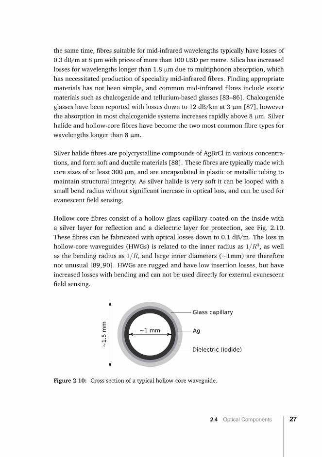
Hollow-core fibres consist of a hollow glass capillary coated on the inside witha silver layer for reflection and a dielectric layer for protection, see Fig. 2.10.These fibres can be fabricated with optical losses down to 0.1 dB/m. The loss inhollow-core waveguides (HWGs) is related to the inner radius as 1/R3, as wellas the bending radius as 1/R, and large inner diameters (∼1mm) are thereforenot unusual [89,90]. HWGs are rugged and have low insertion losses, but haveincreased losses with bending and can not be used directly for external evanescentfield sensing.
Glass capillary
Ag
Dielectric (Iodide)
~1
.5 m
m
~1 mm
Figure 2.10: Cross section of a typical hollow-core waveguide.
2.4 Optical Components 27
2.5 Biomedical Mid-Infrared Spectroscopy
Optical spectroscopy techniques in combination with lab-on-a-chip technology,waveguides, or fibre-optic sensors are increasingly being studied for biochemicalsensing. Such sensors may offer label-free sensing, possibilities for remote sensing,and high robustness in challenging environments. Mid-infrared (MIR) spectroscopyhas an especially large potential for real-time sensing in complex environmentsin biomedical applications. As mentioned, MIR spectroscopy gives unique finger-prints of molecules, and has more intense absorption bands than near-infraredspectroscopy. The relatively recent commercial availability of QCLs also means thatthis field is less mature than visible/near-infrared spectroscopy, and as such thereare many unrealised potential applications.
This chapter will discuss the current main biomedical application areas for MIRspectroscopy, with focus on glucose sensing for management of diabetes. Theimportance of glucose sensing, the principle behind commercial electrochemicalsensors, and sensor placement considerations will be introduced. These sectionsare only meant to give required background for a more in-depth discussion ofglucose sensing with MIR spectroscopy. More details can be found in Paper I and inthe references.
2.5.1 Glucose Sensing
Personal glucose sensors are essential for patients with diabetes, who have lostthe ability to control their own blood glucose level (BGL). Patients with type 1diabetes no longer produce the glucose-regulating hormone insulin, while patientswith type 2 diabetes have an increased resistance to the effects of insulin. Type 2diabetes is often managed through diet and medications, while type 1 diabetes,which affects 10% of diabetic patients, must be managed with self-monitoring ofblood glucose (SMBG) and insulin injections or infusions. The goal of this is tokeep the BGL within normoglycaemic levels, typically defined as 72–180 mg/dL(4–10 mM) [91]. Too low BGL, known as hypoglycaemia (<70 mg/dL, or 3.9 mM),can lead to seizures, loss of consciousness, and even death as the brain becomesstarved of glucose [92]. Too high BGL on the other hand, called hyperglycaemia(>180 mg/dL, or 10 mM), leads to serious long-term complications, including
28 Chapter 2 Background
kidney damage and nerve damage, which severely affects the quality of life fordiabetic patients [93].
Electrochemical Glucose Sensors
Glucose sensors used today by diabetic patients are either invasive or minimallyinvasive. The most common sensor type uses a fingerprick method where thepatient lances their finger to produce a blood drop, and then places this on aglucometer. The glucometer estimates the BGL from an enzymatic reaction withina few seconds. The basic principle of these electrochemical glucose sensors is tomeasure the current produced by oxidation of glucose molecules [94]. This can bewritten as a simplified reaction:
glucose + O2glucose oxidase−−−−−−−−→ gluconic acid + H2O2 (2.19)
An enzyme such as glucose oxidase (GOx) is used to facilitate this enzymaticreaction. In a second step the hydrogen peroxide dissociates:
H2O2 → O2 + 2H+ + 2e− (2.20)
and the resulting current is used as an estimate for the glucose concentration.Current electrochemical glucose sensors are more advanced than what the abovereactions indicate. For example, a mediator molecule is usually introduced as analternative synthetic electron acceptor. This eliminates the dependence on availableoxygen in the immediate area of the detector. These mediator molecules are alsomade to transport electrons from the enzyme to the electrode surface.
SMBG by fingerprick measurements gives information only at discrete points intime, and must be repeated several times per day for proper BGL control. Manypatients find this painful and cumbersome, and often measure less than the recom-mended minimum of 4 times per day [95]. Continuous glucose monitoring (CGM)devices based on electrochemical sensing have been developed as an alternative tofingerprick measurements. These devices are worn on the body for several days,and provide regularly updated BGL values.
Sensor Placement
Glucose sensing in humans for out-patient care requires a sensor system that isportable and ideally even wearable. The placement of a wearable sensor is a
2.5 Biomedical Mid-Infrared Spectroscopy 29
non-trivial and complex issue. Factors such as invasiveness, how cumbersome theyare, and how user-friendly they are must all be considered. Glucose sensing incombination with insulin infusions and a control system could be used to makean artificial pancreas (AP), which would mimic the function of healthy pancreaswith minimal patient involvement [96]. The sensor placement is also important inregard to development of an AP, as an AP needs to detect changes in glucose levelsfast for optimal control.
Electrochemical CGM devices are increasingly used by diabetic patients. Most ofthese devices are placed in a patch on the skin with a small filament implantedsubcutaneously (SC). An enzymatic reaction is then employed for glucose mea-surements, and the glucose levels are updated approximately every five minutes.These measurements are performed in the interstitial fluid (ISF), which is the fluidsurrounding cells in the intercellular matrix. CGM devices must be replaced every1-2 weeks due to decreased sensor performance, and the measured glucose levelsin the ISF have been found to lag behind the actual BGL by approximately 5-15minutes, which can be detrimental to diabetes management [7,8]. The sensor lagis a combination of physiological lag as glucose has to diffuse into the ISF, as wellas internal sensor lag (e.g. electrons being transported to the electrode). Thesesensor types require a lot of involvement from the patient, as the patient still hasto manage their own insulin infusions/injections based on the sensor data. Inaddition, the sensor must typically be calibrated against fingerprick measurementstwice per day, and because of this fingerprick measurements are not completelyavoided. An AP with SC glucose measurements and SC insulin infusions improvesglucose control, but still has limitations such as a significant amount of time spentin hyperglycaemia [97].
Non-invasive glucose sensing has for a long time been seen as the end goal fordiabetes management. Non-invasive sensing includes any methods that do notpenetrate the skin and should in theory be painless and less of a hassle than currentmethods. The main challenge for non-invasive methods is the lack of measureableglucose. It has been suggested that glucose levels can be measured in easilycollectable fluids, such as sweat [98], tears [99], or saliva [100], but the correlationwith the internal BGL has not been entirely convincing. Another option is tomeasure through the skin, which has proved difficult for most methods that havebeen investigated [101]. Methods such as reverse iontophoresis have been used toextract glucose molecules through the skin, with concentration measurements basedon the glucose diffusion rate. However, these devices were not very accurate, and
30 Chapter 2 Background
had side effects such as skin irritation [102]. There has also been research on opticalspectroscopy methods for non-invasive sensing, typically with light backreflectedfrom skin. Mid-infrared spectroscopy is difficult to use non-invasively due to highwater absorption, although some preliminary results of glucose measurements innon-diabetic subjects have been published [11,103]. Near-infrared spectroscopy isless affected by water absorption, but has much lower selectivity. Thus far, therehave been no commercially successful non-invasive glucose sensors.
Another possibly viable solution for glucose monitoring is to perform the sensingin the peritoneal space. The peritoneal cavity is the space between organs in theabdomen, and contains peritoneal fluid. The peritoneal fluid contains, among otherthings, white blood cells, proteins, lactate, as well as glucose. It has been suggestedthat measurements of glucose and injections of insulin in the peritoneum can moreclosely mimic the dynamics of a healthy pancreas, with both faster detection ofrapid changes in BGL and faster uptake of insulin [13, 104]. However, sensingin the peritoneal cavity is more invasive than currently employed methods, andcarries the risk of infection and pain. Short-term peritoneal glucose measurementswith electrochemical sensors have been demonstrated in an animal model [105]. Along-term study has also been described, although the full results have not beenpublished yet [106]. Sensing could be done with an optical fibre-based solutionby inserting the fibre through an abdominal port. Such ports have already seensome limited clinical use for intraperitoneal (IP) infusion of insulin, and this typeof insulin delivery has been shown to improve time spent in the normoglycaemicrange compared to subcutaneous insulin infusions [107, 108]. Development ofsuitable IP glucose sensing technology, together with IP insulin infusions, mayenable a safe and effective AP that requires minimal user input.
Glucose Sensing with Mid-Infrared Spectroscopy
Heise et al. showed one of the earliest studies of physiological glucose concentra-tions in whole blood using an ATR-FTIR spectrometer in 1989 [109]. The samegroup also demonstrated that multiple analyte concentrations, including glucose,could be determined in human blood plasma with FTIR spectroscopy in the sameyear [110]. Since then, FTIR spectroscopy has been used to measure glucose levelswith transmission through dried serum samples [111], and recently in transmissionconfiguration through otherwise untreated plasma samples [112].
Laser-based measurements of glucose in the MIR range were first demonstratedin the mid-2000’s, both on synthetic solutions and on serum samples [113,114].
2.5 Biomedical Mid-Infrared Spectroscopy 31
These studies used either multiple single-wavelength lead-salt lasers or QCLs, dueto a lack of tuneable lasers in the wavelength region. Vrancic et al. later showedpreliminary measurements of glucose levels in the ISF of rat models using only onesingle-wavelength laser [115]. This study employed transmission measurementsthrough a 20 µm gap between two fibres, and achieved quite accurate glucosemeasurements at 17.5% standard deviation. The authors acknowledged thataccurate measurements over a longer timeframe would require measurements atmultiple wavelengths in order to account for drift of the source and interferencefrom multiple analytes.
QCL-based MIR spectroscopy for glucose measurements has taken great stridesfollowing the recent commercial availability of broadly tuneable EC-QCLs. In 2013,Brandstetter et al. demonstrated accurate measurements of glucose and otheranalytes in human blood serum with an automated tuneable QCL-based system [9].More recently, the Heise group has shown a similar system for measurements ofmicro-dialysate samples from humans, using a QCL with four laser heads for a totaltuning range of over 1000 cm-1 [10,77]. In both cases these systems have aimed atrapid and reagent-free measurements for patients in an ICU setting.
As mentioned previously, Liakat et al. developed a sensor system based on detectionof backscattered light from the hand, although measurements were only shownfor a few subjects and a narrow glucose concentration range (75-160 mg/dL)[11]. Werth et al. improved the system by including an integrating sphere [116],but measurements in more subjects and over longer time spans are necessary tovalidate the sensitivity. Kino et al. have taken a different approach with ATRspectroscopy of the inner lip mucosa, so far with either an FTIR spectrometer orseveral single-wavelength QCLs [12]. Several groups have also developed variantsof photoacoustic or photothermal spectroscopy system with EC-QCL sources for non-invasive measurements [117–119], and photothermal deflection spectroscopy inparticular may enable non-invasive measurements in deeper skin layers comparedto direct ATR measurements.
Isensee et al. showed transflection measurements of glucose based on an im-plant meant for minimally invasive measurements [120]. So far, this system hasonly been demonstrated for measurements of synthetic aqueous solutions. Thereare otherwise few studies on systems meant for invasive or minimally invasivemeasurements of glucose, and few studies with fibre-coupled EC-QCLs that haveinvestigated the effect of fibre-coupled EC-QCL-based remote sensing.
32 Chapter 2 Background
Comparison of QCL-Based and FTIR Spectroscopy
The spectral power density of QCLs is several orders of magnitude higher thanfor FTIR spectrometers (104 is often reported). Higher spectral power density canbe used to achieve shorter measurement times and/or longer optical pathlengths,which can be advantageous for many applications. However, the advantage fromhigher spectral power density is difficult to leverage completely in practical applica-tions, especially for pulsed QCLs. In pulsed operation there is always some intensityvariability between pulses. As the variability is a random distribution around anaverage value, the laser noise can be reduced by averaging a set amount of pulses.Averaging over pulses will add to the measurement time, but QCL measurementsstill tend to be faster than FTIR measurements.
FTIR spectrometers are able to cover much broader spectral ranges than singletuneable QCLs. QCLs should be chosen carefully in order to cover the correctspectral range for any analytes of interest, and the target application shouldtherefore be clearly defined. FTIR spectrometers on the other hand are easier to useas standard laboratory equipment, as they cover the entire mid-infrared wavelengthrange. Several commercial products combine multiple EC-QCLs in order to cover alarger spectral area, but these are consequently more expensive and still cover lessthan 1/3 of the FTIR spectrum.
For miniaturised and portable sensor applications QCLs have a clear advantageover FTIR spectrometers regarding size. Traditional FTIR spectrometers use free-space optics, which makes them quite bulky. Miniaturised spectrometers basedon micro-electro-mechanical systems (MEMS) have been demonstrated [121], butthese typically have narrower tuning ranges, lower resolution, and lower sensitivity.EC-QCLs are compact compared to standard FTIR spectrometers. For applicationswhere even EC-QCLs are too big and vibrations could influence measurements, itcould be possible to instead use a few single-wavelength laser chips in an array. Thishas been investigated several times in relation to glucose sensing [77,103,113],and the results indicate that 5–10 wavenumbers may be sufficient to accuratelypredict glucose concentrations in ISF or blood micro-dialysate.
2.5.2 Other Application Areas
QCL-based spectroscopy has many other potential biomedical applications apartfrom glucose sensing, and a few other application areas will be outlined in order to
2.5 Biomedical Mid-Infrared Spectroscopy 33
give a perspective of these possibilities. Breath analysis is one area where opticalspectroscopy is a highly suitable measurement method. Standard methods for gasanalysis include mass spectroscopy and gas chromatography that use expensiveand large equipment, or low-cost semiconductor or electrochemical sensors, whichhave lower selectivity. QCL-based spectroscopy has been used to detect biomarkersin breath, which are low-concentration endogenous molecules that can be used totrack disease progression. These biomarkers include acetone, ammonia, carbonmonoxide, and nitric oxide, and studies have demonstrated both detection ofsingular gas species and multigas analysis [122–125]. Infrared spectroscopy hasalso been used to determine the 13CO2/12CO2-ratio [126, 127], which is used instudies of liver function where exogenous isotopes are introduced into the body.
Infrared microspectroscopy with QCLs has increasingly been studied and employedfor histopathology, i.e. tissue studies for disease diagnostics. Histopathology re-quires a tissue biopsy sample that is extensively prepared before investigation byan expert clinician. Diagnosis by eye is subjective and prone to error, and the entireprocess is very time-consuming. MIR microspectroscopy as a label-free method canpotentially reduce the required preparatory steps, while multivariate data analysiscan be used for accurate and objective identification of tissue changes. So far,QCL-based infrared microspectroscopy systems have been used to differentiatenormal and cancerous tissues, classify tissues at different cancer stages, as well asidentify other abnormal tissue changes [128–132]. FTIR-based microspectroscopyhas previously been extensively studied for histopathology diagnosis and othertissue analysis, but has failed to translate to clinical use, partly due to low SNR andslow data acquisition [133]. The newer studies with QCL-based systems show thatinfrared microspectroscopy may finally be used outside of a research setting.
2.6 Multivariate Data Analysis
For spectroscopy geared towards biomedical applications, one can expect to mea-sure complex samples with multiple analytes. Although single analytes have distinctand easily interpretable infrared spectra, samples such as bodily fluids have overlap-ping absorption bands and the resulting infrared spectra are typically very complex.As a result, spectral features can not easily be assigned to particular analytes, andsimple methods such as measuring the height of an absorption band can not be usedfor quantitative measurements. In some cases, processing such as centrifuging can
34 Chapter 2 Background
be applied to the samples to remove unwanted interfering analytes, thus giving lesscomplex spectra. However, for some applications, such as personalised sensors, it isnecessary to measure samples without any physical pretreatment. Data processingin the form of multivariate analysis has therefore become an important procedurefor quantitative analysis in mid-infrared spectroscopy.
The following sections will explain common regression models and classificationmethods for multivariate analysis, as well as methods for model validation andhow to present model error. Pre-processing methods and feature selection methodscommonly used for spectral data will also be described.
2.6.1 Regression Analysis
Regression analysis is a methodology used for estimating a set of dependent vari-ables, e.g. analyte concentrations, based on independent variables, e.g. data pointsin an infrared spectrum. The simplest type of regression is linear regression, whichfits a linear equation to the observed data, where the linear equation minimises thesum of squares distances between the measured data and the regression line. Sim-ple linear regression is vulnerable to noisy independent variables and overfitting,and is therefore typically not used as a stand-alone method to analyse spectral data.In addition, simple linear regression does not work on data where there are moreindependent variables than observations, which is often the case for spectral data.Different learning methods are used to overcome these issues, either by modifyingthe data prior to regression or by modifying the linear regression method.
Principal Component Regression
Principal component regression (PCR) combines principal component analysis(PCA) with linear regression by using the components from PCA as regression coef-ficients in a linear regression model. PCA is effectively a dimensionality reductionmethod, where the data of interest is transformed into a new coordinate systemaccording to the data variance [134]. Mathematically, this is done through a matrixtransformation of the independent variables, X:
X = TP′ + P (2.21)
T are the scores representing the original data in the transformed coordinate system,while P are the weights that the original data have to be multiplied with in order
2.6 Multivariate Data Analysis 35
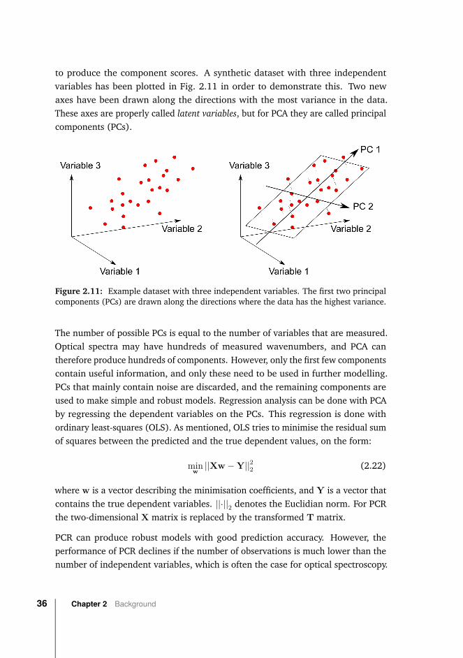
to produce the component scores. A synthetic dataset with three independentvariables has been plotted in Fig. 2.11 in order to demonstrate this. Two newaxes have been drawn along the directions with the most variance in the data.These axes are properly called latent variables, but for PCA they are called principalcomponents (PCs).
Figure 2.11: Example dataset with three independent variables. The first two principalcomponents (PCs) are drawn along the directions where the data has the highest variance.
The number of possible PCs is equal to the number of variables that are measured.Optical spectra may have hundreds of measured wavenumbers, and PCA cantherefore produce hundreds of components. However, only the first few componentscontain useful information, and only these need to be used in further modelling.PCs that mainly contain noise are discarded, and the remaining components areused to make simple and robust models. Regression analysis can be done with PCAby regressing the dependent variables on the PCs. This regression is done withordinary least-squares (OLS). As mentioned, OLS tries to minimise the residual sumof squares between the predicted and the true dependent values, on the form:
minw||Xw−Y||22 (2.22)
where w is a vector describing the minimisation coefficients, and Y is a vector thatcontains the true dependent variables. ||·||2 denotes the Euclidian norm. For PCRthe two-dimensional X matrix is replaced by the transformed T matrix.
PCR can produce robust models with good prediction accuracy. However, theperformance of PCR declines if the number of observations is much lower than thenumber of independent variables, which is often the case for optical spectroscopy.
36 Chapter 2 Background

In addition, PCR is very susceptible to data where variables with low variance alsohave high predictive power. Such low-variance components can easily be dropped,which is detrimental to the predictive power of the model.
Partial Least-Squares Regression
Partial least-squares regression (PLSR) performs dimensionality reduction on boththe independent and dependent variables [135]. PLSR is therefore very similarto PCR, which unlike PLSR only transforms the independent variables. PLSRcircumvents some of the issues with PCR, as the first latent variables are thosethat explain the most variance from both the independent and the dependentvariables.
PLSR tends to have better prediction accuracy than PCR on data from vibrationalspectroscopy, and generally uses fewer latent variables (LVs) to achieve this. Due tothe simpler, more robust, and better models, PLSR has become a staple regressionmethod for spectroscopy data. One drawback with both PLSR and PCR is that theLVs or PCs are less interpretable than the original independent variables.
Other Regression Methods
There are many other variants of linear regression methods that are variably usedin machine learning and sometimes for spectral data. For example, regularisationmethods (ridge, lasso, elastic net, etc.) add information to the data in order to de-crease the modelling complexity, and this can subsequently be used in combinationwith regression. Compared to OLS, these regularisation methods add a penaltyterm to the minimisation problem. For ridge regression, the minimisation problemis then of the form [136]:
minw||Xw−Y||22 + ||αw||22 (2.23)
where α is a penalty term that restricts the size of the coefficients. This is knownas the L2 penalty term, while lasso regularisation uses the L1 penalty term [137]and the elastic net combines these two penalty terms [138]. This approach differsfrom the dimensionality reduction methods such as PCR and PLSR, and can beadvantageous for certain types of data.
2.6 Multivariate Data Analysis 37
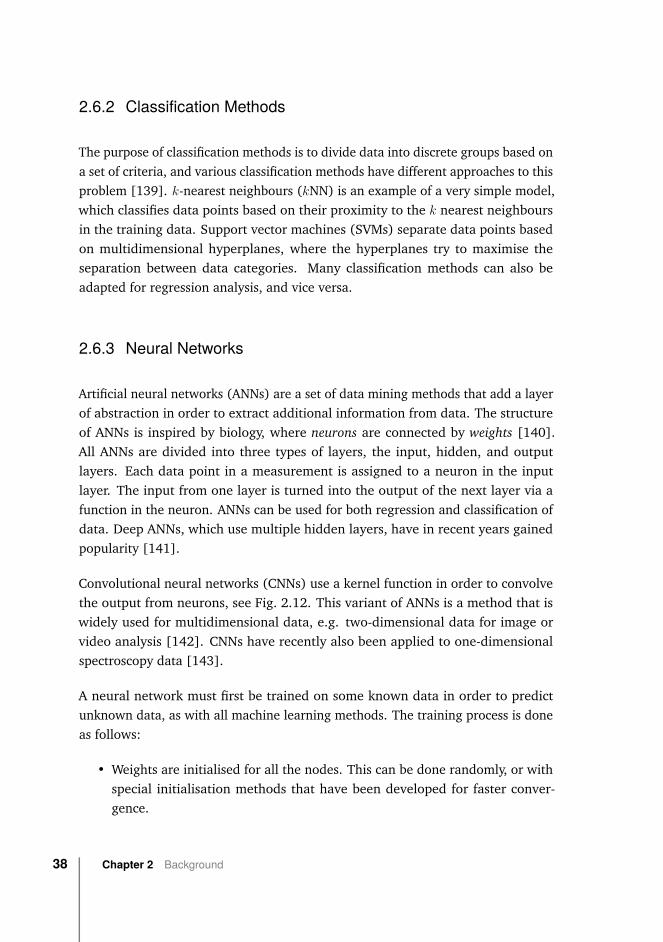
2.6.2 Classification Methods
The purpose of classification methods is to divide data into discrete groups based ona set of criteria, and various classification methods have different approaches to thisproblem [139]. k-nearest neighbours (kNN) is an example of a very simple model,which classifies data points based on their proximity to the k nearest neighboursin the training data. Support vector machines (SVMs) separate data points basedon multidimensional hyperplanes, where the hyperplanes try to maximise theseparation between data categories. Many classification methods can also beadapted for regression analysis, and vice versa.
2.6.3 Neural Networks
Artificial neural networks (ANNs) are a set of data mining methods that add a layerof abstraction in order to extract additional information from data. The structureof ANNs is inspired by biology, where neurons are connected by weights [140].All ANNs are divided into three types of layers, the input, hidden, and outputlayers. Each data point in a measurement is assigned to a neuron in the inputlayer. The input from one layer is turned into the output of the next layer via afunction in the neuron. ANNs can be used for both regression and classification ofdata. Deep ANNs, which use multiple hidden layers, have in recent years gainedpopularity [141].
Convolutional neural networks (CNNs) use a kernel function in order to convolvethe output from neurons, see Fig. 2.12. This variant of ANNs is a method that iswidely used for multidimensional data, e.g. two-dimensional data for image orvideo analysis [142]. CNNs have recently also been applied to one-dimensionalspectroscopy data [143].
A neural network must first be trained on some known data in order to predictunknown data, as with all machine learning methods. The training process is doneas follows:
• Weights are initialised for all the nodes. This can be done randomly, or withspecial initialisation methods that have been developed for faster conver-gence.
38 Chapter 2 Background
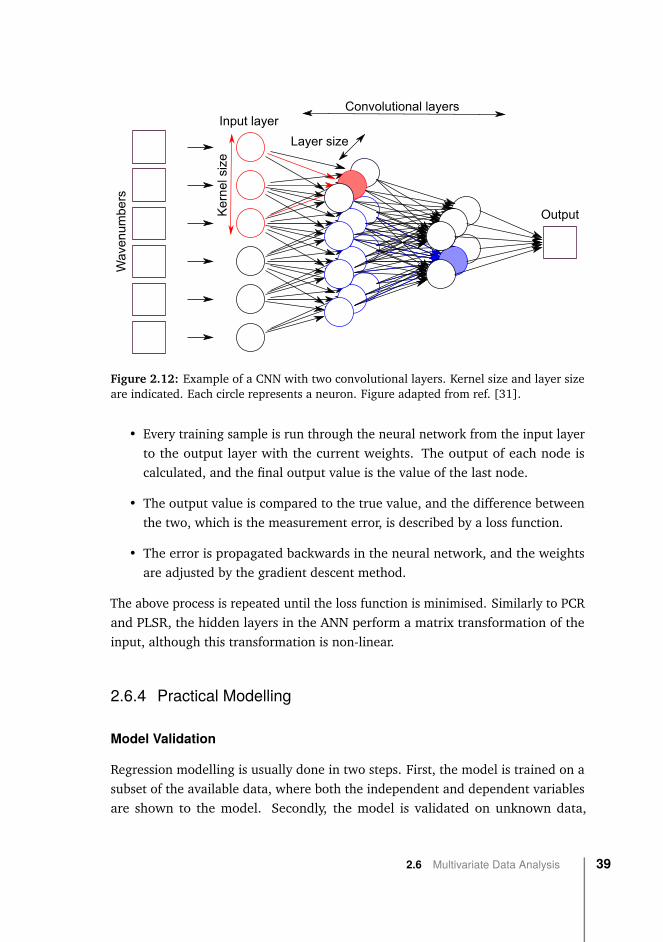
Wav
enum
bers
Ker
nel
siz
eOutput
Convolutional layersInput layer
Layer size
Figure 2.12: Example of a CNN with two convolutional layers. Kernel size and layer sizeare indicated. Each circle represents a neuron. Figure adapted from ref. [31].
• Every training sample is run through the neural network from the input layerto the output layer with the current weights. The output of each node iscalculated, and the final output value is the value of the last node.
• The output value is compared to the true value, and the difference betweenthe two, which is the measurement error, is described by a loss function.
• The error is propagated backwards in the neural network, and the weightsare adjusted by the gradient descent method.
The above process is repeated until the loss function is minimised. Similarly to PCRand PLSR, the hidden layers in the ANN perform a matrix transformation of theinput, although this transformation is non-linear.
2.6.4 Practical Modelling
Model Validation
Regression modelling is usually done in two steps. First, the model is trained on asubset of the available data, where both the independent and dependent variablesare shown to the model. Secondly, the model is validated on unknown data,
2.6 Multivariate Data Analysis 39
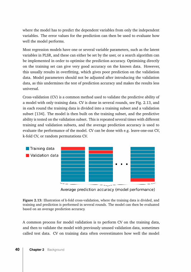
where the model has to predict the dependent variables from only the independentvariables. The error values for the prediction can then be used to evaluate howwell the model performs.
Most regression models have one or several variable parameters, such as the latentvariables in PLSR, and these can either be set by the user, or a search algorithm canbe implemented in order to optimise the prediction accuracy. Optimising directlyon the training set can give very good accuracy on the known data. However,this usually results in overfitting, which gives poor prediction on the validationdata. Model parameters should not be adjusted after introducing the validationdata, as this undermines the test of prediction accuracy and makes the results lessuniversal.
Cross-validation (CV) is a common method used to validate the predictive ability ofa model with only training data. CV is done in several rounds, see Fig. 2.13, andin each round the training data is divided into a training subset and a validationsubset [134]. The model is then built on the training subset, and the predictiveability is tested on the validation subset. This is repeated several times with differenttraining and validation subsets, and the average prediction accuracy is used toevaluate the performance of the model. CV can be done with e.g. leave-one-out CV,k-fold CV, or random permutations CV.
Figure 2.13: Illustration of k-fold cross-validation, where the training data is divided, andtraining and prediction is performed in several rounds. The model can then be evaluatedbased on an average prediction accuracy.
A common process for model validation is to perform CV on the training data,and then to validate the model with previously unused validation data, sometimescalled test data. CV on training data often overestimates how well the model
40 Chapter 2 Background
performs, and it is therefore common to get somewhat better prediction accuracyin the CV phase than on the unknown validation data.
Measures of Error
The performance of regression and classification models must be validated witha measure of error [144]. The achieved prediction accuracy is usually used tomeasure the difference between the predicted values and the observed (reference)values. Different error measurements can be used, including root-mean-squareerrors (RMSE), standard error of prediction (SEP), and coefficient of determination(R2). RMSE-values are commonly used, and are calculated as:
RMSE =√∑
n(yn − yn)2
N(2.24)
where yn is the predicted value, yn is the reference value, and N is the total numberof measurements. RMSE is a positive value where a lower value indicates a bettermodel, and for perfect prediction the RMSE is zero. RMSE is scale-dependent,which means that RMSE-values tend to increase if larger concentration ranges areused. One should therefore be careful when comparing RMSE between differentdatasets. RMSE is also sensitive to large deviations from the reference values, andis therefore disproportionally affected by outliers. SEP is similar to RMSE, butSEP does not include the bias, which is the average difference between y and y
in the prediction set [145]. This term is usually small, and therefore SEP usuallyyields values similar to RMSE. The coefficient of determination is a measure of theproportion of variance in the dependent variable that can be predicted from theindependent variable, and is defined as:
R2 = 1−∑n(yn − yn)2∑n(yn − y)2 (2.25)
where y is the mean of the measured values. R2=1 indicates that there is nounexplained variance, and for worse prediction accuracy R2 decreases.
Another alternative method for error measurements is to use the mean absoluteerror (MAE), which gives the average of the absolute errors between the predictionand reference values:
MAE =∑n |yn − yn|N
(2.26)
2.6 Multivariate Data Analysis 41
MAE avoids squaring the values, but is still scale-dependent like RMSE. The meanabsolute percentage error (MAPE) works around this by expressing MAE as apercentage error. MAE and MAPE are seen as more interpretable than RMSE-values,and as more informative since they are not weighted towards measurements withlarge deviations. However, it can be argued that RMSE-values are useful for sensordevelopment, as measurements with large errors can have a disproportionate effecton the user or patient. From this viewpoint, the MAE can give an overly optimisticview of the performance of both the sensor and the learning algorithm. Severalmeasure of errors may be reported for a dataset in order to more easily comparewith other literature.
2.6.5 Spectral Pre-Processing
Spectral pre-processing encompasses all methods applied to data prior to thelearning algorithm. The goal of pre-processing is to remove unwanted variations inthe data that are not related to variations in analyte concentrations [146]. Thisincludes environmental factors, drift in equipment, and so on. Such variations canaffect model accuracy heavily. Pre-processing methods should ideally be applied sothat the same procedure can be subsequently used on similar datasets. The twomain approaches are filtering/smoothing methods, which try to reduce noise, andscatter correction methods, which try to remove e.g. baseline shifts.
Feature selection can be seen as a type of pre-processing. However, feature selectionis performed quite differently to other pre-processing methods, and will thereforebe described in a separate section below.
Pre-Processing Methods
Common methods for spectral filtering/smoothing include Savitzky-Golay (SG)filtering, Fourier filtering, and moving average. For SG filtering a segment size isdefined, and a polynomial is fitted to each segment of the spectrum. SG filteringcan be adapted to data with different noise features, as the segment size andpolynomial order can be optimised. Fourier filtering is done by taking the Fouriertransform of the spectra, cutting of the Fourier signal at a certain frequency, andthen back-transforming the result. This method is very efficient, but there is a riskof removing informative features, or creating artefacts in the back-transformedspectrum. Moving average is a classical smoothing method where each data point
42 Chapter 2 Background
in a spectrum is replaced by the average of the adjacent data points. The numberof adjacent data points used for averaging is set by the user.
Scatter effects in spectra can be divided into effects that create spectral offsets,or spectral amplification. These are not necessarily caused by scattering directly,for example spectral offsets can be a result of source drift, but the mathematicalcorrection is the same in any case. The simplest way to correct for scatter effects isspectral differentiation by finite differences. The first derivative of the spectrumremoves any offsets, and the second derivative also removes linear trends. Thedisadvantage is that differentiation by finite differences amplifies noise in thespectra, and this is very detrimental to the regression if the SNR is low. This canbe ameliorated by filtering prior to differentiation, and SG filtering in particularis often used with differentiaton by taking the derivative of the fitted polynomialat each data point. Other methods have been designed to deal with scatteringeffects, including standard normal variate (SNV), multiplicative scatter correction(MSC) and extended MSC (EMSC). These methods are more commonly used innear-infrared spectroscopy, as scatter effects are more dominant due the longerpathlengths used. Simple baseline correction functions can also be used to removeoffset effects.
Pre-processing methods can be used in combination, however the optimal orderis not readily apparent. Various studies use different orders, and some studieshave shown different orders can have positive or negative outcomes dependingon the exact methods used [147]. Many studies have also found the optimalcombination of pre-processing methods for one or a few datasets, but the "optimum"seems to vary between datasets, sample types, and measurement methods. Theoptimal combination is usually found through an exhaustive search of all possiblecombinations of methods, although this is very time-consuming. Other approachessuch as experimental design or genetic algorithm searches have been used to searchthrough fewer combinations with minimal loss of accuracy, but such methods are sofar not extensively used [148,149]. The choice of pre-processing methods thereforeremains very user-defined and to some degree subjective.
Feature Selection
As the name implies, feature selection methods are used to select a certain subsetof spectral features, which are then used for further analysis [150]. Featureselection is a useful tool for analysis of spectral data for several reasons. Datasetsfrom vibrational spectroscopy often have few samples/measurements, and many
2.6 Multivariate Data Analysis 43
variables (features). Many, or even most, of these variables may not have anyrelevant information. It has been argued that the addition of irrelevant featuresshould not degrade a regression model. However, with enough irrelevant features,some of them will randomly correlate with other features, which complicates themodel and can lead to overfitting. As experimental equipment is not perfect,some of these irrelevant features can also be noisy. Adding noisy features is alsodetrimental to a regression model. A high number of variables also makes themodel less interpretable, and increases the computational demand for the datamodelling. One goal of feature selection is therefore to remove irrelevant features,but feature selection should be used carefully, so as to not remove relevant features.As with other pre-processing methods, feature selection should also be validatedwith cross-validation on the training set. Feature selection methods can broadly bedivided into three different categories, which are described below.
Filter methods: Features can be filtered by individually scoring them accordingto some requirement, e.g. how well they correlate with the response variable.This can be done directly prior to the regression model being run, and inthat case the filter is independent from the model. One example of this isthe Pearson correlation coefficient. Filter methods are very computationallyefficient and quite robust to overfitting. However, one must set a thresholdfor the filter, and the initial choice is often arbitrary. Filters also tend to selectredundant features, and any interactions between features are usually nottaken into account.
Wrapper methods: In wrapper methods several subsets of features are generatedand then searched through. The modelling accuracy is evaluated for eachfeature subset, and the best subset is selected. Wrapper methods are betterfor detecting possible interactions between variables, and can often find goodsubsets of features with fewer redundant variables. These methods are morecomputationally expensive, and with few measurements there is a biggerchance of overfitting to a suboptimal feature subset.
There are a number of ways to generate feature subsets. Forward selectionstarts with no features in the model, and iteratively adds the feature thatreduces the model error the most. Forward selection then stops when arequired number of features is obtained or a decided performance thresholdis reached. Backward elimination, on the other hand, starts with all featuresand iteratively removes the least important ones. Sequential feature selection
44 Chapter 2 Background
combines these two, by reconsidering dropped and added variables at eachstep. Moving window selection looks for one or more continuous regions offeatures, and selects the window(s) that achieve the best modelling accuracy.Genetic algorithms start with a randomised population of feature subsets,which are then mixed and mutated over several generations. These differentmethods all have advantages and disadvantages. For example, forwardselection and related methods can often get stuck in local maxima, whilesubsets found by genetic algorithms can be heavily affected by the initialpopulation of feature subsets.
Embedded methods: These methods have the feature selection built into the re-gression model. One large class of embedded methods are the regularisation-based approaches, which includes lasso, ridge regression, and elastic net. Allfeatures in the data are included in the model, but a penalty is applied onthe values of the regression coefficients. This penalty can shrink regressioncoefficients, and even reduce them to zero. Embedded methods performthe feature selection and regression modelling at the same time, and areless computationally expensive than wrapper methods. However, they aremore difficult to interpret, as the feature selection performance can not beseparated from the performance of the regression model. Embedded methodsare also not applicable to all types of data, and are therefore less universalthan other feature selection methods.
2.6 Multivariate Data Analysis 45

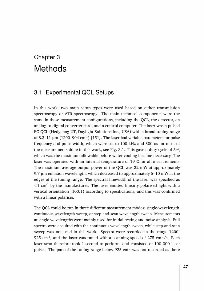
Chapter 3
Methods
3.1 Experimental QCL Setups
In this work, two main setup types were used based on either transmissionspectroscopy or ATR spectroscopy. The main technical components were thesame in these measurement configurations, including the QCL, the detector, ananalog-to-digital converter card, and a control computer. The laser was a pulsedEC-QCL (Hedgehog-UT, Daylight Solutions Inc., USA) with a broad tuning rangeof 8.3–11 µm (1200–904 cm-1) [151]. The laser had variable parameters for pulsefrequency and pulse width, which were set to 100 kHz and 500 ns for most ofthe measurements done in this work, see Fig. 3.1. This gave a duty cycle of 5%,which was the maximum allowable before water cooling became necessary. Thelaser was operated with an internal temperature of 19◦C for all measurements.The maximum average output power of the QCL was 22 mW at approximately9.7 µm emission wavelength, which decreased to approximately 5–10 mW at theedges of the tuning range. The spectral linewidth of the laser was specified as<1 cm-1 by the manufacturer. The laser emitted linearly polarised light with avertical orientation (100:1) according to specifications, and this was confirmedwith a linear polariser.
The QCL could be run in three different measurement modes; single-wavelength,continuous wavelength sweep, or step-and-scan wavelength sweep. Measurementsat single wavelengths were mainly used for initial testing and noise analysis. Fullspectra were acquired with the continuous wavelength sweep, while step-and-scansweep was not used in this work. Spectra were recorded in the range 1200–925 cm-1, and the laser was tuned with a scanning speed of 275 cm-1/s. Eachlaser scan therefore took 1 second to perform, and consisted of 100 000 laserpulses. The part of the tuning range below 925 cm-1 was not recorded as there
47
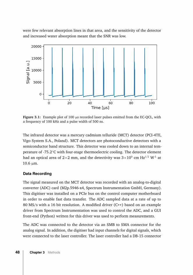
were few relevant absorption lines in that area, and the sensitivity of the detectorand increased water absorption meant that the SNR was low.
Figure 3.1: Example plot of 100 µs recorded laser pulses emitted from the EC-QCL, witha frequency of 100 kHz and a pulse width of 500 ns.
The infrared detector was a mercury cadmium telluride (MCT) detector (PCI-4TE,Vigo System S.A., Poland). MCT detectors are photoconductive detectors with asemiconductor band structure. This detector was cooled down to an internal tem-perature of -75.2◦C with four-stage thermoelectric cooling. The detector elementhad an optical area of 2×2 mm, and the detectivity was 3×109 cm Hz1/2 W-1 at10.6 µm.
Data Recording
The signal measured on the MCT detector was recorded with an analog-to-digitalconverter (ADC) card (M2p.5946-x4, Spectrum Instrumentation GmbH, Germany).This digitiser was installed on a PCIe bus on the control computer motherboardin order to enable fast data transfer. The ADC sampled data at a rate of up to80 MS/s with a 16 bit resolution. A modified driver (C++) based on an exampledriver from Spectrum Instrumentation was used to control the ADC, and a GUIfront-end (Python) written for this driver was used to perform measurements.
The ADC was connected to the detector via an SMB to SMA connector for theanalog signal. In addition, the digitiser had input channels for digital signals, whichwere connected to the laser controller. The laser controller had a DB-15 connector
48 Chapter 3 Methods
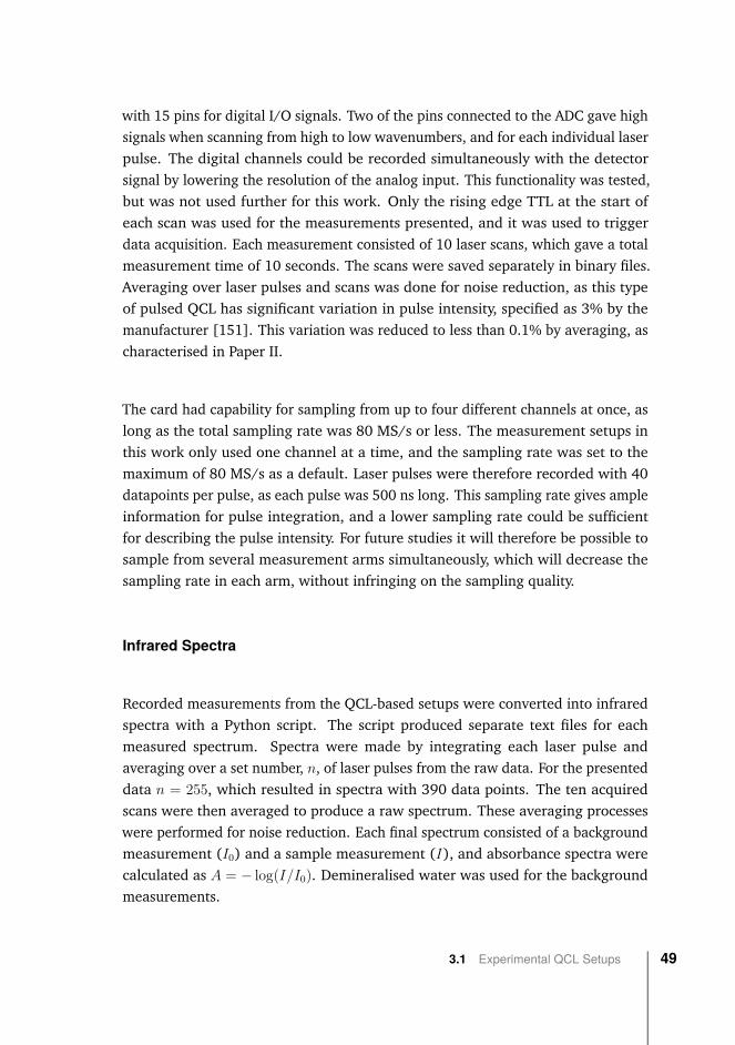
with 15 pins for digital I/O signals. Two of the pins connected to the ADC gave highsignals when scanning from high to low wavenumbers, and for each individual laserpulse. The digital channels could be recorded simultaneously with the detectorsignal by lowering the resolution of the analog input. This functionality was tested,but was not used further for this work. Only the rising edge TTL at the start ofeach scan was used for the measurements presented, and it was used to triggerdata acquisition. Each measurement consisted of 10 laser scans, which gave a totalmeasurement time of 10 seconds. The scans were saved separately in binary files.Averaging over laser pulses and scans was done for noise reduction, as this typeof pulsed QCL has significant variation in pulse intensity, specified as 3% by themanufacturer [151]. This variation was reduced to less than 0.1% by averaging, ascharacterised in Paper II.
The card had capability for sampling from up to four different channels at once, aslong as the total sampling rate was 80 MS/s or less. The measurement setups inthis work only used one channel at a time, and the sampling rate was set to themaximum of 80 MS/s as a default. Laser pulses were therefore recorded with 40datapoints per pulse, as each pulse was 500 ns long. This sampling rate gives ampleinformation for pulse integration, and a lower sampling rate could be sufficientfor describing the pulse intensity. For future studies it will therefore be possible tosample from several measurement arms simultaneously, which will decrease thesampling rate in each arm, without infringing on the sampling quality.
Infrared Spectra
Recorded measurements from the QCL-based setups were converted into infraredspectra with a Python script. The script produced separate text files for eachmeasured spectrum. Spectra were made by integrating each laser pulse andaveraging over a set number, n, of laser pulses from the raw data. For the presenteddata n = 255, which resulted in spectra with 390 data points. The ten acquiredscans were then averaged to produce a raw spectrum. These averaging processeswere performed for noise reduction. Each final spectrum consisted of a backgroundmeasurement (I0) and a sample measurement (I), and absorbance spectra werecalculated as A = − log(I/I0). Demineralised water was used for the backgroundmeasurements.
3.1 Experimental QCL Setups 49
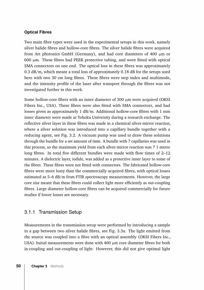
Optical Fibres
Two main fibre types were used in the experimental setups in this work, namelysilver halide fibres and hollow-core fibres. The silver halide fibres were acquiredfrom Art photonics GmbH (Germany), and had core diameters of 400 µm or600 µm. These fibres had PEEK protective tubing, and were fitted with opticalSMA connectors on one end. The optical loss in these fibres was approximately0.3 dB/m, which meant a total loss of approximately 0.18 dB for the setups usedhere with two 30 cm long fibres. These fibres were step index and multimode,and the intensity profile of the laser after transport through the fibres was notinvestigated further in this work.
Some hollow-core fibres with an inner diameter of 300 µm were acquired (OKSIFibers Inc., USA). These fibres were also fitted with SMA connectors, and hadlosses given as approximately 1 dB/m. Additional hollow-core fibres with 1 mminner diameter were made at Tohoku University during a research exchange. Thereflective silver layer in these fibres was made in a chemical silver-mirror reaction,where a silver solution was introduced into a capillary bundle together with areducing agent, see Fig. 3.2. A vacuum pump was used to draw these solutionsthrough the bundle for a set amount of time. A bundle with 7 capillaries was used inthis process, so the maximum yield from each silver-mirror reaction was 7 1-metrelong fibres. In total five different bundles were made with flow times of 2–12minutes. A dielectric layer, iodide, was added as a protective inner layer to some ofthe fibres. These fibres were not fitted with connectors. The fabricated hollow-corefibres were more lossy than the commercially acquired fibres, with optical lossesestimated as 5–6 dB/m from FTIR spectroscopy measurements. However, the largecore size meant that these fibres could collect light more efficiently as out-couplingfibres. Large diameter hollow-core fibres can be acquired commercially for futurestudies if lower losses are necessary.
3.1.1 Transmission Setup
Measurements in the transmission setup were performed by introducing a samplein a gap between two silver halide fibres, see Fig. 3.3a. The light emitted fromthe source was coupled into a fibre with an optical assembly (OKSI Fibers Inc.,USA). Initial measurements were done with 400 µm core diameter fibres for bothin-coupling and out-coupling of light. However, this did not give optimal light
50 Chapter 3 Methods
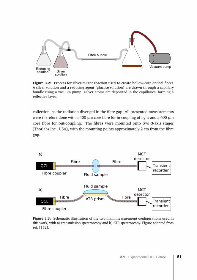
Vacuum pump
Fibre bundle
Silversolution
Reducing solution
Figure 3.2: Process for silver-mirror reaction used to create hollow-core optical fibres.A silver solution and a reducing agent (glucose solution) are drawn through a capillarybundle using a vacuum pump. Silver atoms are deposited in the capillaries, forming areflective layer.
collection, as the radiation diverged in the fibre gap. All presented measurementswere therefore done with a 400 µm core fibre for in-coupling of light and a 600 µmcore fibre for out-coupling. The fibres were mounted onto two 3-axis stages(Thorlabs Inc., USA), with the mounting points approximately 2 cm from the fibregap.
QCL
MCTdetector
Transientrecorder
Fibre Fibre
Fluid sample
a)
Fibre coupler
QCL
b)
QCL
MCTdetector
Transientrecorder
Fibre Fibre
Fluid sample
ATR prism
Fibre coupler
Figure 3.3: Schematic illustration of the two main measurement configurations used inthis work, with a) transmission spectroscopy and b) ATR spectroscopy. Figure adapted fromref. [152].
3.1 Experimental QCL Setups 51
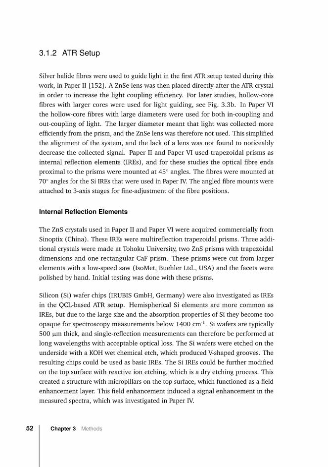
3.1.2 ATR Setup
Silver halide fibres were used to guide light in the first ATR setup tested during thiswork, in Paper II [152]. A ZnSe lens was then placed directly after the ATR crystalin order to increase the light coupling efficiency. For later studies, hollow-corefibres with larger cores were used for light guiding, see Fig. 3.3b. In Paper VIthe hollow-core fibres with large diameters were used for both in-coupling andout-coupling of light. The larger diameter meant that light was collected moreefficiently from the prism, and the ZnSe lens was therefore not used. This simplifiedthe alignment of the system, and the lack of a lens was not found to noticeablydecrease the collected signal. Paper II and Paper VI used trapezoidal prisms asinternal reflection elements (IREs), and for these studies the optical fibre endsproximal to the prisms were mounted at 45◦ angles. The fibres were mounted at70◦ angles for the Si IREs that were used in Paper IV. The angled fibre mounts wereattached to 3-axis stages for fine-adjustment of the fibre positions.
Internal Reflection Elements
The ZnS crystals used in Paper II and Paper VI were acquired commercially fromSinoptix (China). These IREs were multireflection trapezoidal prisms. Three addi-tional crystals were made at Tohoku University, two ZnS prisms with trapezoidaldimensions and one rectangular CaF prism. These prisms were cut from largerelements with a low-speed saw (IsoMet, Buehler Ltd., USA) and the facets werepolished by hand. Initial testing was done with these prisms.
Silicon (Si) wafer chips (IRUBIS GmbH, Germany) were also investigated as IREsin the QCL-based ATR setup. Hemispherical Si elements are more common asIREs, but due to the large size and the absorption properties of Si they become tooopaque for spectroscopy measurements below 1400 cm-1. Si wafers are typically500 µm thick, and single-reflection measurements can therefore be performed atlong wavelengths with acceptable optical loss. The Si wafers were etched on theunderside with a KOH wet chemical etch, which produced V-shaped grooves. Theresulting chips could be used as basic IREs. The Si IREs could be further modifiedon the top surface with reactive ion etching, which is a dry etching process. Thiscreated a structure with micropillars on the top surface, which functioned as a fieldenhancement layer. This field enhancement induced a signal enhancement in themeasured spectra, which was investigated in Paper IV.
52 Chapter 3 Methods
3.2 FTIR Spectroscopy
FTIR spectroscopy was used for initial measurements and comparison with theQCL-based measurements, as well as a separate study on data analysis. The pho-tonics lab at the Department of Electronics, NTNU had an Alpha II spectrometer(Bruker Optics Inc., USA) available. This was a compact FTIR spectrometer thatcould be used with either a module for transmission spectroscopy, or a modulefor ATR spectroscopy. Only the ATR module was used for this work, and it hada single-reflection diamond IRE. This FTIR spectrometer was operated with theOPUS software (Bruker Optics Inc., USA) installed on a separate computer. Thespectrometer saved data in the 4000-400 cm-1 spectral range. The acquired spectrawere made by averaging 128 scans in the spectrometer, which gave a measure-ment time of about 3 minutes. An initial resolution of 2 cm-1 was set for themeasurements, which was reduced to 1 cm-1 through a zero-filling factor of 2 inthe Fourier transform algorithm. Background spectra were obtained approximatelyevery 30 minutes. Spectra were saved in text files, and further analysis was donein a separate program.
A Tensor spectrometer (Tensor27, Bruker Optics Inc., USA) at Tohoku Universitywas used for a study on data analysis of spectral data. This spectrometer had acustom-built ATR module, which has been described by Kino et al. [12]. Lightemitted from the spectrometer was focussed into a hollow-core fibre, which guidedthe light to a ZnS prism. The light from this prism was focussed onto a liquidnitrogen-cooled infrared detector. The spectrometer was operated through theOPUS software. This spectrometer had a measurement range of 4000–500 cm-1. Theacquired spectra were measured with a resolution of 4 cm-1 and 32 spectrometerscans were averaged for each measurement. A zero-filling factor of 2 applied duringthe Fourier transformation brought the data point spacing down to 2 cm-1.
3.3 Simulations
Light propagation was simulated in the ZnS prisms in order to ensure an integralnumber of reflections through the prisms. The main parameters that were inves-tigated in these trapezoidal structures were prism height and length. Ray opticssimulations were performed with Zemax OpticStudio.
3.2 FTIR Spectroscopy 53
Behaviour in the Si IREs was investigated with the finite element method usingCOMSOL Multiphysics (Sweden). The Si IREs were simplified to a two-dimensional(2D) cross section. The light source was modelled as a plane wave with an incidenceangle of 41◦, based on an estimation of the angle of incidence. The field strengthof the evanescent field in the sample volume was integrated for both the basic andthe signal-enhanced Si IREs. The enhancement factor was then calculated as theratio of total field intensity between the two Si IRE types.
3.4 Data Analysis and Software Development
All multivariate analysis of spectral data for this thesis was done through Pythonprogramming. A software package, which we have called SpecAnalysis, wasassembled to enable automation of various analysis methods. SpecAnalysis iscapable of analysing data for both regression and classification, and contains manymethods for spectral pre-processing and feature selection. This software has beenmade available on GitHub (https://github.com/jernelv/SpecAnalysis).
SpecAnalysis is in part based on scikit-learn [153], which is a Python tool packagefor machine learning. Several of the included methods were also developed in-house. The software has a graphic user interface and functionality that allows theuser to test many different analysis parameters in sequence.
54 Chapter 3 Methods
Chapter 4
Summary of Papers
The main application for this work was mid-infrared spectroscopy of glucose inbiological fluids. The thesis itself spans across various methods for optimisationof the sensor system, measurements of synthetic aqueous solutions and biologicalfluids, as well as multivariate analysis of spectroscopy data. As a result, thethesis includes experimental work, simulations, as well as work on data analysismethods.
This chapter gives a brief overview and short discussion of each paper included inthe thesis.
55
4.1 Evaluation of Optical Techniques
Paper I
A review of optical methods for continuous glucose monitoringI.L. Jernelv, K. Milenko, S.S. Fuglerud, D.R. Hjelme, R. Ellingsen, A. AksnesApplied Spectroscopy Reviews, Vol. 54(7), pp. 543-572, 2019.
This work was a review of a selection of the available optical measurement methodsthat have been researched for continuous glucose monitoring (CGM). The ideawas to evaluate several potential techniques for glucose sensing in order to make amore informed choice regarding the thesis subject. The paper first introduced back-ground on BGL management required for diabetic patients, current electrochemicalCGM systems, and some considerations such as the sensor placement. Six mainoptical techniques were evaluated, namely near-infrared, mid-infrared, Raman, andfluorescence spectroscopy, as well as photoacoustic sensing and optical coherencetomography. The basic principles of these methods were outlined, together withspecific challenges for in vivo glucose measurements. An overview of the researchstatus for each method was then given, and a comparative discussion was includedat the end.
Prior to this publication, there were several other reviews of glucose sensor tech-nologies suggested as alternatives to electrochemical glucose sensors. Many ofthese were focussed on non-invasive sensor systems, or on sensor concepts thatwere relatively close to realisation of a device. This review concentrated on onlyoptical technologies regardless of intended sensor placement, and covered early-stage research in addition to more advanced sensor concepts. It was challengingto precisely compare different technologies, especially those with mainly early-stage research. Research groups were found to use different metrics to evaluatetheir sensor systems that were not necessarily directly comparable. Fluorescencespectroscopy had come furthest among the methods with several systems used inhuman trials and one system close to commercialisation.
MIR spectroscopy was seen as a measurement technique with low/medium maturityand a high development potential for biomedical applications. Tuneable lasersources with high spectral power density have only recently become available inthe MIR range, and the research effort is still in the early stages. MIR spectroscopytherefore became the focus of this thesis.
56 Chapter 4 Summary of Papers
4.2 Measurements of Synthetic Aqueous Solutions andSystem Benchmarking
Paper II
Infrared Spectroscopy with a Fiber-Coupled Quantum Cascade Laser for Atten-uated Total Reflection Measurements Towards Biomedical ApplicationsI.L. Jernelv, K. Strøm, D.R. Hjelme, A. AksnesSensors, Vol. 19(23), 5130, 2019.
In this work, we demonstrated QCL-based infrared spectroscopy with transmissionand ATR sensing for synthetic aqueous solutions. The transmission configurationused a gap between optical fibres for sensing, while the ATR configuration used amulti-reflection ZnS prism as a sensing surface. Silver halide fibres were used toguide the laser radiation in both sensing configurations.
Laser noise was characterised based on averaging over laser pulses and laser scans.A low relative standard deviation of the signal was found (0.07%) for settingsthat resulted in a measurement time of only 10 seconds. The solutions that weremeasured contained glucose, as well as albumin, lactate, and urea as interferinganalytes. Sets of the aqueous solutions were measured in both transmission andATR configurations. A ZnS prism with 5 reflections on the top surface was usedfor the ATR measurements, and the prism dimensions were determined based onray-tracing simulations. The measured spectra were investigated with multivariateanalysis, and it was demonstrated that both glucose and albumin concentrationscould be accurately determined in both measurement configurations. Glucoseconcentrations were determined with RMSECV<20 mg/dL for both transmissionand ATR measurements.
This benchmarking and characterisation showed that our system was stable and thatmeasurements with low noise level could be acquired. Simultaneous determinationof several analytes in aqueous solutions was also promising for further studies.
4.2 Measurements of Synthetic Aqueous Solutions and SystemBenchmarking
57
Paper III
Mid-infrared spectroscopy with a fiber-coupled tuneable quantum cascade laserfor glucose sensingI.L. Jernelv, K. Strøm, D.R. Hjelme, A. AksnesProceedings of SPIE 11233, Optical Fibers and Sensors for Medical Diagnostics andTreatment Applications XX, 1123311, 2020.
This paper is a continuation of the work in Paper II. A fibre-coupled QCL spec-troscopy setup was used to investigate more complex aqueous solutions in transmis-sion mode. Lower concentrations of glucose were used than in Paper I, and fructosewas added as an additional interfering analyte. A thorough characterisation of theoptimal transmission pathlength was demonstrated.
Similar to Brandstetter et al. [30], we showed that the optimal pathlength waslonger than the theoretical optimum, as the theoretical calculation does not accountfor the source intensity. We also found a longer optimal pathlength than in ref. [30]at 200 µm, and this can be attributed to the higher power of the QCL used inour study. The SNR did not improve as much as expected, but this might bea consequence of the fibre-coupled sensing and an introduction of mode noiseor interference. The relatively long pathlength is advantageous because of theincreased absorbance signal, and because the transmission gap becomes less proneto clogging.
As in Paper II, the concentrations of glucose and the other analytes could bedetermined accurately at the same time with PLS regression. The predictionaccuracies for glucose and albumin were improved by approximately 20% with theuse of a CNN for multivariate analysis. For glucose, the RMSECV was 10.7 mg/dLwith PLS regression and 8.3 mg/dL with CNN with a concentration range of0–600 mg/dL. This study demonstrated a robust characterisation of our QCL setupin transmission mode, and an in-depth analysis of complex aqueous solutions.
58 Chapter 4 Summary of Papers
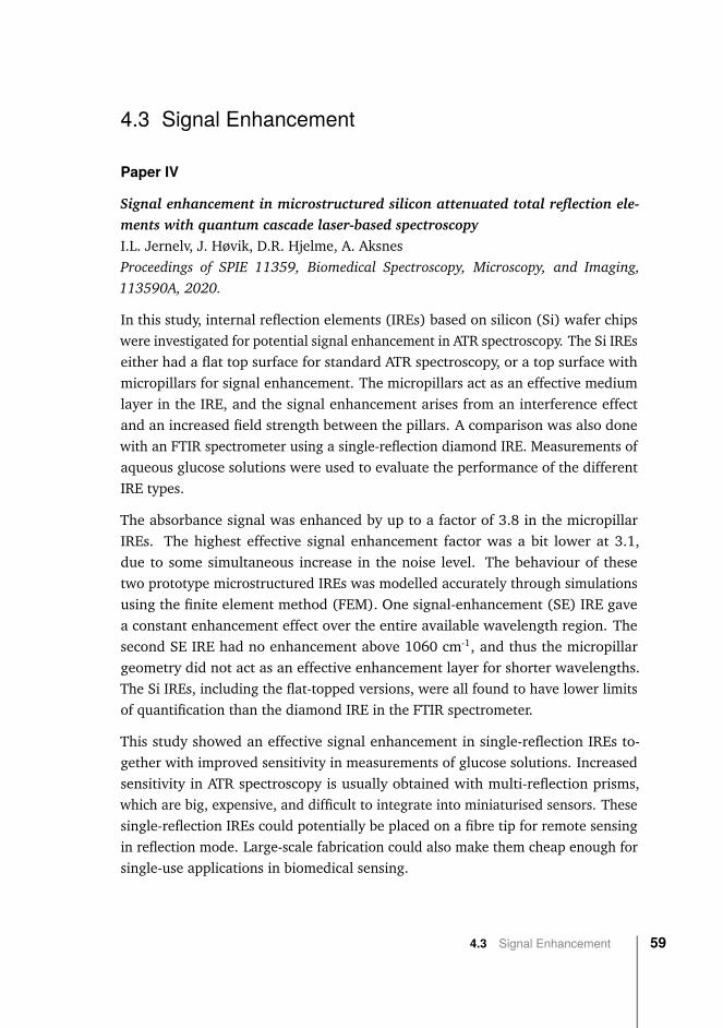
4.3 Signal Enhancement
Paper IV
Signal enhancement in microstructured silicon attenuated total reflection ele-ments with quantum cascade laser-based spectroscopyI.L. Jernelv, J. Høvik, D.R. Hjelme, A. AksnesProceedings of SPIE 11359, Biomedical Spectroscopy, Microscopy, and Imaging,113590A, 2020.
In this study, internal reflection elements (IREs) based on silicon (Si) wafer chipswere investigated for potential signal enhancement in ATR spectroscopy. The Si IREseither had a flat top surface for standard ATR spectroscopy, or a top surface withmicropillars for signal enhancement. The micropillars act as an effective mediumlayer in the IRE, and the signal enhancement arises from an interference effectand an increased field strength between the pillars. A comparison was also donewith an FTIR spectrometer using a single-reflection diamond IRE. Measurements ofaqueous glucose solutions were used to evaluate the performance of the differentIRE types.
The absorbance signal was enhanced by up to a factor of 3.8 in the micropillarIREs. The highest effective signal enhancement factor was a bit lower at 3.1,due to some simultaneous increase in the noise level. The behaviour of thesetwo prototype microstructured IREs was modelled accurately through simulationsusing the finite element method (FEM). One signal-enhancement (SE) IRE gavea constant enhancement effect over the entire available wavelength region. Thesecond SE IRE had no enhancement above 1060 cm-1, and thus the micropillargeometry did not act as an effective enhancement layer for shorter wavelengths.The Si IREs, including the flat-topped versions, were all found to have lower limitsof quantification than the diamond IRE in the FTIR spectrometer.
This study showed an effective signal enhancement in single-reflection IREs to-gether with improved sensitivity in measurements of glucose solutions. Increasedsensitivity in ATR spectroscopy is usually obtained with multi-reflection prisms,which are big, expensive, and difficult to integrate into miniaturised sensors. Thesesingle-reflection IREs could potentially be placed on a fibre tip for remote sensingin reflection mode. Large-scale fabrication could also make them cheap enough forsingle-use applications in biomedical sensing.
4.3 Signal Enhancement 59
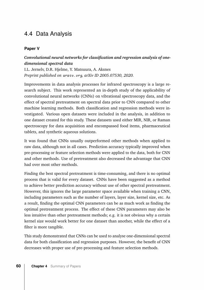
4.4 Data Analysis
Paper V
Convolutional neural networks for classification and regression analysis of one-dimensional spectral dataI.L. Jernelv, D.R. Hjelme, Y. Matsuura, A. AksnesPreprint published on arxiv.org, arXiv ID 2005.07530, 2020.
Improvements in data analysis processes for infrared spectroscopy is a large re-search subject. This work represented an in-depth study of the applicability ofconvolutional neural networks (CNNs) on vibrational spectroscopy data, and theeffect of spectral pretreatment on spectral data prior to CNN compared to othermachine learning methods. Both classification and regression methods were in-vestigated. Various open datasets were included in the analysis, in addition toone dataset created for this study. These datasets used either MIR, NIR, or Ramanspectroscopy for data acquisition and encompassed food items, pharmaceuticaltablets, and synthetic aqueous solutions.
It was found that CNNs usually outperformed other methods when applied toraw data, although not in all cases. Prediction accuracy typically improved whenpre-processing or feature selection methods were applied to the data, both for CNNand other methods. Use of pretreatment also decreased the advantage that CNNhad over most other methods.
Finding the best spectral pretreatment is time-consuming, and there is no optimalprocess that is valid for every dataset. CNNs have been suggested as a methodto achieve better prediction accuracy without use of other spectral pretreatment.However, this ignores the large parameter space available when training a CNN,including parameters such as the number of layers, layer size, kernel size, etc. Asa result, finding the optimal CNN parameters can be as much work as finding theoptimal pretreatment process. The effect of these CNN parameters may also beless intuitive than other pretreatment methods; e.g. it is not obvious why a certainkernel size would work better for one dataset than another, while the effect of afilter is more tangible.
This study demonstrated that CNNs can be used to analyse one-dimensional spectraldata for both classification and regression purposes. However, the benefit of CNNdecreases with proper use of pre-processing and feature selection methods.
60 Chapter 4 Summary of Papers

4.5 Characterisation of Biological Fluids
Paper VI
Infrared measurements of glucose in peritoneal fluid with a tuneable quantumcascade laserI.L. Jernelv, D.R. Hjelme, A. AksnesBiomedical Optics Express, Vol. 11(7), pp. 3818-3829, 2020.
In this work, fluid samples acquired from animal experiments were measured inQCL-based spectroscopy setups in order to test sensing performance on real-lifesamples. Peritoneal fluid and blood plasma samples from altogether six differentpigs were measured in both ATR and transmission configurations. Highly accuratepredictions of glucose levels were made for both measurement configurations,with mean absolute percentage error (MAPE) of 12.2% in the ATR configurationand 8.7% in the transmission configuration. Concentrations in the blood plasmasamples were predicted with even better accuracy (MAPE<8%), which can partiallybe attributed to the smaller dataset.
Spectra from the peritoneal fluid samples were also compared to the blood plasmaspectra. The general spectral shapes were found to be quite similar, although theblood plasma samples had an overall higher absorbance. The optical measurements,together with measurements of the albumin and total protein concentrations in aselection of the samples, supported the view that peritoneal fluid can be seen asultrafiltered plasma with lower concentration levels of major constituents. Opticalspectroscopy measurements may therefore be more straightforward in peritonealfluid, compared to blood plasma or ISF. This was also in part suggested by theregression analysis, as PLS models with 6 LVs were used for blood plasma, whileonly 5 LVs were necessary for the peritoneal fluid data.
This study demonstrated optical glucose detection at physiological concentrationsin peritoneal fluid for the first time. The QCL-based sensing approach is reagent-free with a measurement time of only 10 s, and there are several avenues for setupminiaturisation. The ATR configuration in particular lends itself well for point-of-care monitoring, as reflection-mode sensing can be realised with an IRE integratedon a fibre tip. A portable sensor will likely require smaller single-wavelength lasersthat are less sensitive to vibrations.
4.5 Characterisation of Biological Fluids 61

Chapter 5
Conclusions
The papers included in this thesis cover several aspects of QCL-based mid-infraredspectroscopy. The main intended application was continuous glucose monitoring.A sensor concept was realised through experimental verification of QCL-basedinfrared spectroscopy setups in ATR and transmission configurations, with multi-variate analysis of the resulting spectral data.
Current literature was reviewed in Paper I, which gave a perspective on variousoptical technologies that have been used for glucose measurements. Based onthis review, MIR spectroscopy was evaluated as a technology with low/mediummaturity for portable and miniaturised sensors, and high potential for sensordevelopment. Laser-based spectroscopy in particular has the possibility for fastand accurate measurements in a POC sensor. We therefore developed and built afibre-coupled QCL-based spectroscopy system, and characterised and benchmarkedthis system on aqueous solutions in Paper II and Paper III. In these studies, glucoseconcentrations were determined with RMSECV<20 mg/dL in the ATR configurationand RMSECV<10 mg/dL in transmission. Subsequently, peritoneal fluid from pigsused in animal trials was investigated in Paper VI. It was found that peritoneal fluidhad lower absorbance than blood plasma, and thus may be a less complex fluidfor optical measurements. Predictions of the glucose concentrations in peritonealfluid were demonstrated with with 8.7% and 12.2% MAPE in transmission andATR configurations, respectively. This is well within the requirement for glucosesensors, and is on par or better than commercially available electrochemical CGMdevices. Electrochemical sensors have a typical measurement time of 5 minutesand lag behind the BGL by 5-15 minutes, while our results were achieved witha measurement time of only 10 seconds, and this fast measurement time can beleveraged to provide better glucose control. Further miniaturisation is neededfor a practical POC sensor, and single-reflection IREs with signal enhancementbased on an interference effect were investigated in Paper IV as a means to achieve
63

a smaller sensing area. An enhancement of the SNR up to a factor of 3.1 wasdemonstrated.
The implemented regression methods were found to be highly accurate for predic-tion of glucose concentrations in both synthetic aqueous solutions and biologicalfluids from animal experiments. The effects of spectral pre-processing and differ-ent methods for concentration prediction were shown on the datasets that weremeasured in the QCL-based setups. In addition, a separate study was performed inPaper V in order to investigate spectral pre-processing and feature selection meth-ods on different publicly available datasets acquired with vibrational spectroscopy,both for regression and classification analysis. This work concentrated on convolu-tional neural networks (CNNs) as a way to reduce the need for pretreatment priorto analysis.
To summarise, this doctoral study has shown an in-depth investigation of spectroscopy-based measurements of glucose in peritoneal fluid, which has demonstrated thepotential for optical glucose monitoring in the peritoneal cavity.
Outlook
The papers published have demonstrated an ATR sensing concept with a fibre-coupled QCL, which is an important step towards an in vivo glucose sensor basedon mid-infrared spectroscopy. The work should be continued towards realisationof in vivo sensing in the peritoneal cavity of an animal model. Measurements inan animal model in transmission mode will also be possible, but is not necessarilyconducive to a practical device. Transmission gaps are prone to clogging, and thereare mechanical challenges involved in keeping the fibre ends aligned. Sensingin reflection mode is potentially more stable, and the input fibre can more easilybe used simultaneously as an output fibre in an ATR probe. Further work on thedata analysis methods should then be performed in order to confirm if a smallersubset of wavelengths can be used to accurately identify and measure the glucoseconcentration in a clinical setting.
The long-term goal of these developments is to facilitate rapid QCL-based spec-troscopy of glucose in the peritoneal cavity. Once accurate glucose sensing ispossible in humans with minimal delay, a combination with insulin infusions and acontrol system will enable a true artificial pancreas.
64 Chapter 5 Conclusions
References
[1] K. E. Thorpe, L. Allen, and P. Joski. The Role of Chronic Disease, Obesity, andImproved Treatment and Detection in Accounting for the Rise in HealthcareSpending Between 1987 and 2011. Applied Health Economics and HealthPolicy, 13(4):381–387, 2015.
[2] D. Howdon and N. Rice. Health care expenditures, age, proximity to deathand morbidity: Implications for an ageing population. Journal of HealthEconomics, 57:60–74, 2018.
[3] P. Thavendiranathan, A. Bagai, A. Ebidia, A. S. Detsky, and N. K. Choudhry.Do Blood Tests Cause Anemia in Hospitalized Patients? The Effect of Di-agnostic Phlebotomy on Hemoglobin and Hematocrit Levels. Journal ofGeneral Internal Medicine, 20(6):520–524, 2005.
[4] C. G. Koch, L. Li, Z. Sun, E. D. Hixson, A. Tang, S. C. Phillips, E. H. Blackstone,and J. M. Henderson. Hospital-Acquired Anemia: Prevalence, Outcomes,and Healthcare Implications. Journal of Hospital Medicine, 8(9):506–512,2013.
[5] A. P. F. Turner. Biosensors: sense and sensibility. Chem. Soc. Rev., 42(8):3184–3196, 2013.
[6] I. D. B. Rennie, H. Keen, and A. Southon. A Rapid Enzyme-Strip Method forEstimating Blood-Sugar. The Lancet, 284(7365):884–886, 1964.
[7] L. Dye, M. Mansfield, N. Lasikiewicz, L. Mahawish, R. Schnell, D. Talbot,H. Chauhan, F. Croden, and C. Lawton. Correspondence of continuousinterstitial glucose measurement against arterialised and capillary glucosefollowing an oral glucose tolerance test in healthy volunteers. British Journalof Nutrition, 103(1):134–140, 2010.
[8] M. Sinha, K. M. McKeon, S. Parker, L. G. Goergen, H. Zheng, F. H. El-Khatib, and S. J. Russell. A Comparison of Time Delay in Three ContinuousGlucose Monitors for Adolescents and Adults. Journal of Diabetes Scienceand Technology, 11(6):1132–1137, 2017.
[9] M. Brandstetter, T. Sumalowitsch, A. Genner, A. E. Posch, C. Herwig, A. Drolz,V. Fuhrmann, T. Perkmann, and B. Lendl. Reagent-free monitoring ofmultiple clinically relevant parameters in human blood plasma using a mid-infrared quantum cascade laser based sensor system. Analyst, 138(14):4022–4028, 2013.
References 65
[10] T. Vahlsing, S. Delbeck, J. Budde, D. Ihrig, S. Leonhardt, and H. M. Heise.Reliable glucose monitoring by ex-vivo blood micro-dialysis and infraredspectrometry for patients in critical care. In Proc. SPIE, Optical Diagnosticsand Sensing XVII: Toward Point-of-Care Diagnostics, volume 10072, 2017.
[11] S. Liakat, K. A. Bors, L. Xu, C. M. Woods, J. Doyle, and C. F. Gmachl.Noninvasive in vivo glucose sensing on human subject using mid-infraredlight. Biomed. Opt. Express, 5(7):2397–2404, 2014.
[12] S. Kino, S. Omori, T. Katagiri, and Y. Matsuura. Hollow optical-fiber basedinfrared spectroscopy for measurement of blood glucose level by usingmulti-reflection prism. Biomedical Optics Express, 7(2):701–708, 2016.
[13] D. R. Burnett, L. M. Huyett, H. C. Zisser, F. J. Doyle, and B. D. Mensh.Glucose sensing in the peritoneal space offers faster kinetics than sensing inthe subcutaneous space. Diabetes, 63(7):2498–2505, 2014.
[14] O. Bibikova, J. Haas, Á. I. López-Lorente, A. Popov, M. Kinnunen,Y. Ryabchikov, A. Kabashin, I. Meglinski, and B. Mizaikoff. Surface enhancedinfrared absorption spectroscopy based on gold nanostars and sphericalnanoparticles. Analytica Chimica Acta, 990:141–149, 2017.
[15] L. Sykora, A. Müller, A. Kondratiev, A. Roth, V. Mozin, A. Fehr, and G. Zör-nack. Silicon ATR crystal with subwavelength structures optimized for bloodanalysis. In Proc. SPIE, Optical Fibers and Sensors for Medical Diagnostics andTreatment Applications XIX, volume 10872, 2019.
[16] M. Quinten. Optical Properties of Nanoparticle Systems: Mie and beyond.John Wiley & Sons, Inc, Weinheim, Germany, 2010.
[17] R. W. Boyd. Nonlinear Optics. Academic Press, Burlington, MA, 2019.
[18] B. E. A. Saleh and M. C. Teich. Fundamentals of Photonics. John Wiley &Sons, Inc, 2007.
[19] C. Kittel. Introduction to Solid State Physics (Eight Edition). John Wiley &Sons, Ltd, Danvers, MA, 2005.
[20] L. V. Wang and H. Wu. Biomedical Optics: Principles and Imaging. John Wiley& Sons, Ltd, Hoboken, New Jersey, 2007.
[21] F. K. Tittel, D. Richter, and A. Fried. Mid-infrared laser applications in spec-troscopy. In Solid-state mid-infrared laser sources, pages 458–529. Springer,2003.
[22] BS ISO 20473:2007. Optics and photonics. Spectral bands. Standard,International Organization for Standardization, Geneva, CH, 2007.
66 References
[23] B. H. Stuart. Infrared Spectroscopy: Fundamentals and Applications. JohnWiley & Sons, 2004.
[24] J. E. Bertie and Z. Lan. Infrared Intensities of Liquids XX: The Intensity ofthe OH Stretching Band of Liquid Water Revisited, and the Best CurrentValues of the Optical Constants of H2O(1) at 25◦C Between 15,000 and 1cm-1. Applied Spectroscopy, 50(8):1047–1057, 1996.
[25] J.-J. Max and C. Chapados. Glucose And Fructose Hydrates in AqueousSolutions by IR Spectroscopy. J. Phys. Chem., 111:2679–2689, 2007.
[26] H. Buiteveld, J. H. M. Hakvoort, and M. Donze. Optical properties of purewater. In Proc. SPIE, Ocean Optics XII, volume 2258, pages 174–183, 1994.
[27] R. Cole. Optimum optical density in spectrophotometry. Journal of theOptical Society of America, 41(1):38–40, 1951.
[28] H. L. Mark and P. R. Griffiths. Analysis of Noise in Fourier Transform InfraredSpectra. Applied Spectroscopy, 56(5):633–639, 2002.
[29] P. S. Jensen and J. Bak. Near-Infrared Transmission Spectroscopy of AqueousSolutions: Influence of Optical Pathlength on Signal-to-Noise Ratio. AppliedSpectroscopy, 56(12):1600–1606, 2002.
[30] M. Brandstetter, L. Volgger, A. Genner, C. Jungbauer, and B. Lendl. Directdetermination of glucose, lactate and triglycerides in blood serum by atunable quantum cascade laser-based mid-IR sensor. Applied Physics B,110(2):233–239, 2013.
[31] I. L. Jernelv, K. Strøm, D. R. Hjelme, and A. Aksnes. Mid-infrared spec-troscopy with a fiber-coupled tuneable quantum cascade laser for glucosesensing. In Proc. SPIE, Optical Fibers and Sensors for Medical Diagnostics andTreatment Applications XX, volume 11233, 2020.
[32] C. Vigano, J. M. Ruysschaert, and E. Goormaghtigh. Sensor applications ofattenuated total reflection infrared spectroscopy. Talanta, 65(5):1132–1142,2005.
[33] N. J. Harrick and F. K. du Pré. Effective Thickness of Bulk Materials and ofThin Films for Internal Reflection Spectroscopy. Applied Optics, 5(11):1739,1966.
[34] L. A. Averett, P. R. Griffiths, and K. Nishikida. Effective path length inattenuated total reflection spectroscopy. Analytical Chemistry, 80(8):3045–3049, 2008.
[35] P. R. Griffiths and J. A. De Haseth. Fourier Transform Infrared Spectrometry.John Wiley & Sons, Inc, 2nd edition, 2007.
References 67
[36] N. Punjabi, J. Satija, and S. Mukherji. Evanescent Wave Absorption BasedFiber-Optic Sensor - Cascading of Bend and Tapered Geometry for EnhancedSensitivity. In A. Mason, S. Mukhopadhyay, and K. Jayasundera, editors,Sensing Technology: Current Status and Future Trends III. Smart Sensors,Measurement and Instrumentation, pages 25–45. Springer InternationalPublishing, 2015.
[37] S. Delbeck, L. Küpper, and H. M. Heise. Applications of tapered flat silverhalide fiber elements for infrared biospectroscopy with aspects of opticalstability and biocompatibility. In Proc. SPIE, Optical Fibers and Sensors forMedical Diagnostics and Treatment Applications XVIII, volume 10488, 2018.
[38] P. Wägli, Y. C. Chang, A. Homsy, L. Hvozdara, H. P. Herzig, and N. F. DeRooij. Microfluidic droplet-based liquid-liquid extraction and on-chip IRspectroscopy detection of cocaine in human saliva. Analytical Chemistry,85(15):7558–7565, 2013.
[39] M. Sieger, J. Haas, M. Jetter, P. Michler, M. Godejohann, and B. Mizaikoff.Mid-Infrared Spectroscopy Platform Based on GaAs/AlGaAs Thin-FilmWaveguides and Quantum Cascade Lasers. Analytical Chemistry, 88(5):2558–2562, 2016.
[40] M. Vlk, V. Mittal, G. S. Murugan, and J. Jágerská. Suspended Tantalum Pen-toxide Rib Waveguides for Laser Absorption Spectroscopy. In The EuropeanConference on Lasers and Electro-Optics, 2019.
[41] A. Wilk, J. C. Carter, M. Chrisp, A. M. Manuel, P. Mirkarimi, J. B. Alameda,and B. Mizaikoff. Substrate-integrated hollow waveguides: A new level ofintegration in mid-infrared gas sensing. Analytical Chemistry, 85(23):11205–11210, 2013.
[42] M Osawa. Surface-Enhanced Infrared Absorption. In S. Kawata, editor,Near-Field Optics and Surface Plasmon Polaritons. Topics in Applied Physics.Springer, Berlin, Heidelberg, 2001.
[43] Ó. Esteban, A. González-Cano, B. Mizaikoff, N. Díaz-Herrera, and M.-C.Navarrete. Generation of Surface Plasmons at Waveguide Surfaces in theMid-Infrared Region. Plasmonics, 7(4):647–652, 2012.
[44] L. V. Brown, X. Yang, K. Zhao, B. Y. Zheng, P. Nordlander, and N. J. Halas.Fan-Shaped Gold Nanoantennas above Reflective Substrates for Surface-Enhanced Infrared Absorption (SEIRA). Nano Letters, 15(2):1272–1280,2015.
[45] Y.-B. Chen. Development of mid-infrared surface plasmon resonance-basedsensors with highly-doped silicon for biomedical and chemical applications.Optics Express, 17(5):3130–3140, 2009.
68 References

[46] Á. I. López-Lorente, J. Izquierdo, C. Kranz, and B. Mizaikoff. Boron-dopeddiamond modified with gold nanoparticles for the characterization of bovineserum albumin protein. Vibrational Spectroscopy, 91:147–156, 2017.
[47] J. Haas, A. Müller, L. Sykora, and B. Mizaikoff. Analytical perfor-mance of µ-groove silicon attenuated total reflection waveguides. Analyst,144(10):3398–3404, 2019.
[48] F. Berz. On a quarter wave light condenser. British Journal of Applied Physics,16(11):1733–1738, 1965.
[49] P. Huber-Wälchli and Hs. H. Günthard. Interference Enhanced Attenu-ated Total Reflection (IEATR). A new technique for i.r. matrix spectroscopywith high sensitivity. Spectrochimica Acta Part A: Molecular Spectroscopy,34(12):1253–1262, 1978.
[50] S. Colburn, A. Zhan, and A. Majumdar. Tunable metasurfaces via subwave-length phase shifters with uniform amplitude. Scientific Reports, 7:40174,2017.
[51] C. Buzea, I. I. Pacheco, and K. Robbie. Nanomaterials and nanoparticles:Sources and toxicity. Biointerphases, 2(4):MR17–MR71, 2007.
[52] P. V. Asharani, Y. L. Wu, Z. Gong, and S. Valiyaveettil. Toxicity of silvernanoparticles in zebrafish models. Nanotechnology, 19(25):255102, 2008.
[53] M. Razeghi. Semiconductor Lasers. In Fundamentals of Solid State Engineer-ing. Springer, Boston, MA, 2006.
[54] P. Unger. High-Power Diode Lasers. Springer, Berlin, Heidelberg, 2007.
[55] J. Faist. Quantum Cascade Lasers. OUP Oxford, 2013.
[56] C. Gmachl, F. Capasso, D. L. Sivco, and A. Y. Cho. Recent progress inquantum cascade lasers and applications. Reports on Progress in Physics,64(11):1533–1601, 2001.
[57] A. Lyakh, M. Suttinger, R. Go, P. Figueiredo, and A. Todi. 5.6 µm quantumcascade lasers based on a two-material active region composition with aroom temperature wall-plug efficiency exceeding 28%. Applied PhysicsLetters, 109(12):121109, 2016.
[58] Y. Bai, N. Bandyopadhyay, S. Tsao, S. Slivken, and M. Razeghi. Roomtemperature quantum cascade lasers with 27% wall plug efficiency. AppliedPhysics Letters, 98(18), 2011.
[59] J. Faist, F. Capasso, D. L. Sivco, C. Sirtori, A. L. Hutchinson, and A. Y. Cho.Quantum Cascade Laser. Science, 264(5158):553–556, 1994.
References 69
[60] R. F. Kazarinov and R. A. Suris. Possibility of the amplification of electromag-netic waves in a semiconductor with a superlattices. Sov. Phys. Semicond.,7:707–709, 1971.
[61] R. Q. Yang. Infrared laser based on intersubband transitions in quantumwells. Superlattices and Microstructures, 17(1):77–83, 1995.
[62] M. Kim, C. L. Canedy, W. W. Bewley, C. S. Kim, J. R. Lindle, J. Abell,I. Vurgaftman, and J. R. Meyer. Interband cascade laser emitting at λ=3.75µm in continuous wave above room temperature. Applied Physics Letters,92(19):191110, 2008.
[63] W. W. Bewley, C. L. Canedy, C. S. Kim, M. Kim, C. D. Merritt, J. Abell,I. Vurgaftman, and J. R. Meyer. Continuous-wave interband cascade lasersoperating above room temperature at λ = 4.7-5.6 µm. Optics Express,20(3):3235–3240, 2012.
[64] A. Schliesser, N. Picqué, and T. W. Hänsch. Mid-infrared frequency combs.Nature Photonics, 6(7):440–449, 2012.
[65] F. Adler, P. Masłowski, A. Foltynowicz, K. C. Cossel, T. C. Briles, I. Hartl,and J. Ye. Mid-infrared Fourier transform spectroscopy with a broadbandfrequency comb. Optics Express, 18(21):21861, 2010.
[66] A. V. Muraviev, V. O. Smolski, Z. E. Loparo, and K. L. Vodopyanov. Massivelyparallel sensing of trace molecules and their isotopologues with broadbandsubharmonic mid-infrared frequency combs. Nature Photonics, 12(4):209–214, 2018.
[67] J. Faist, G. Villares, G. Scalari, M. Rösch, C. Bonzon, A. Hugi, and M. Beck.Quantum Cascade Laser Frequency Combs. Nanophotonics, 5(2):272–291,2016.
[68] G. Scalari, J. Faist, and N. Picqué. On-chip mid-infrared and THz frequencycombs for spectroscopy. Applied Physics Letters, 114(15):150401, 2019.
[69] J. Kuligowski, G. Quintás, and B. Lendl. High performance liquid chro-matography with on-line dual quantum cascade laser detection for thedetermination of carbohydrates, alcohols and organic acids in wine andgrape juice. Applied Physics B: Lasers and Optics, 99(4):833–840, 2010.
[70] Y. Wang, M. G. Soskind, W. Wang, and G. Wysocki. High-resolution multi-heterodyne spectroscopy based on Fabry-Perot quantum cascade lasers.Applied Physics Letters, 104(3):031114, 2014.
[71] M. Jahjah, W. Ren, P. Stefanski, R. Lewicki, J. Zhang, W. Jiang, J. Tarka,and F. K. Tittel. A compact QCL based methane and nitrous oxide sensor forenvironmental and medical applications. Analyst, 139(9):2065–2069, 2014.
70 References
[72] F. Kapsalidis, M. Shahmohammadi, M. J. Süess, J. M. Wolf, E. Gini, M. Beck,M. Hundt, B. Tuzson, L. Emmenegger, and J. Faist. Dual-wavelength DFBquantum cascade lasers: sources for multi-species trace gas spectroscopy.Applied Physics B: Lasers and Optics, 124(6):107, 2018.
[73] P. Rauter and F. Capasso. Multi-wavelength quantum cascade laser arrays.Laser and Photonics Reviews, 9(5):452–477, 2015.
[74] A. Hugi, R. Maulini, and J. Faist. External cavity quantum cascade laser.Semiconductor Science and Technology, 25(8):083001, 2010.
[75] G. Ramer, A. Balbekova, A. Schwaighofer, and B. Lendl. Method for Time-Resolved Monitoring of a Solid State Biological Film Using PhotothermalInfrared Nanoscopy on the Example of Poly-L-lysine. Analytical Chemistry,87(8):4415–4420, 2015.
[76] K. Yeh, S. Kenkel, J. N. Liu, and R. Bhargava. Fast Infrared Chemical Imagingwith a Quantum Cascade Laser. Analytical Chemistry, 87(1):485–493, 2015.
[77] M. Grafen, K. Nalpantidis, A. Ostendorf, D. Ihrig, and H. M. Heise. Character-ization of a multi-module tunable EC-QCL system for mid-infrared biofluidspectroscopy for hospital use and personalized diabetes technology. In Proc.SPIE, Optical Diagnostics and Sensing XVI: Toward Point-of-Care Diagnostics,volume 9715, 2016.
[78] G. Wysocki, R. Lewicki, R. F. Curl, F. K. Tittel, L. Diehl, F. Capasso, M. Troc-coli, G. Hofler, D. Bour, S. Corzine, R. Maulini, M. Giovannini, and J. Faist.Widely tunable mode-hop free external cavity quantum cascade lasers forhigh resolution spectroscopy and chemical sensing. Applied Physics B: Lasersand Optics, 92(3):305–311, 2008.
[79] R. Ghorbani and F. M. Schmidt. Real-time breath gas analysis of CO and CO2using an EC-QCL. Applied Physics B: Lasers and Optics, 123(5):144, 2017.
[80] Vigo System S.A. PCI-4TE detector. https://vigo.com.pl/produkty/pci-4te/. Accessed: 2020-05-09.
[81] C. Downs and T. E. Vandervelde. Progress in infrared photodetectors since2000. Sensors, 13(4):5054–5098, 2013.
[82] W. A. Gambling. The Rise and Rise of Optical Fibers. IEEE Journal on SelectedTopics in Quantum Electronics, 6(6):1084–1093, 2000.
[83] M. F. Churbanov, G. E. Snopatin, V. S. Shiryaev, V. G. Plotnichenko, andE. M. Dianov. Recent advances in preparation of high-purity glasses basedon arsenic chalcogenides for fiber optics. Journal of Non-Crystalline Solids,357(11-13):2352–2357, 2011.
References 71
[84] P. Lucas, Z. Yang, M. K. Fah, T. Luo, S. Jiang, C. Boussard-Pledel, M.-L.Anne, and B. Bureau. Telluride glasses for far infrared photonic applications.Optical Materials Express, 3(8):1049–1058, 2013.
[85] B. Bureau, C. Boussard, S. Cui, R. Chahal, M. L. Anne, V. Nazabal, O. Sire,O. Loréal, P. Lucas, V. Monbet, J.-L. Doualan, P. Camy, H. Tariel, F. Charp-entier, L. Quetel, J.-L. Adam, and J. Lucas. Chalcogenide optical fibers formid-infrared sensing. Optical Engineering, 53(2):027101, 2014.
[86] Z. Tang, V. S. Shiryaev, D. Furniss, L. Sojka, S. Sujecki, T. M. Benson, A. B.Seddon, and M. F. Churbanov. Low loss Ge-As-Se chalcogenide glass fiber,fabricated using extruded preform, for mid-infrared photonics. OpticalMaterials Express, 5(8):1722–1737, 2015.
[87] G. E. Snopatin, M. F. Churbanov, A. A. Pushkin, V. V. Gerasimenko, E. M.Dianov, and V. G. Plotnichenko. High purity arsenic-sulfide glasses andfibers with minimum attenuation of 12 dB/km. Optoelectronics and AdvancedMaterials - Rapid Communications, 3(7):669–671, 2009.
[88] N. Barkay, A. Levite, F. Moser, and A. Katzir. Mechanical properties of mixedsilver-halide crystals and polycrystalline optical fibers. Journal of AppliedPhysics, 64(10):5256–5258, 1988.
[89] J. A. Harrington. A Review of IR Transmitting, Hollow Waveguides. Fiberand Integrated Optics, 19(3):211–227, 2000.
[90] P. Patimisco, V. Spagnolo, M. S. Vitiello, G. Scamarcio, C. M. Bledt, and J. A.Harrington. Low-Loss Hollow Waveguide Fibers for Mid-Infrared QuantumCascade Laser Sensing Applications. Sensors, 13(1):1329–1340, 2013.
[91] T. Battelino, I. Conget, B. Olsen, I. Schütz-Fuhrmann, E. Hommel,R. Hoogma, U. Schierloh, N. Sulli, and J. Bolinder. The use and efficacy ofcontinuous glucose monitoring in type 1 diabetes treated with insulin pumptherapy: a randomised controlled trial. Diabetologia, 55(12):3155–3162,2012.
[92] B. M. Frier. Morbidity of hypoglycemia in type 1 diabetes. Diabetes Researchand Clinical Practice, 65S:S47–S52, 2004.
[93] D. M. Nathan. Long-Term Complications of Diabetes Mellitus. New EnglandJournal of Medicine, 328(23):1676–1685, 1993.
[94] J. Wang. Electrochemical glucose biosensors. Chem. Rev., 108(2):814–825,2008.
[95] A. E. Minder, D. Albrecht, J. Schäfer, and H. Zulewski. Frequency of bloodglucose testing in well educated patients with diabetes mellitus type 1: Howoften is enough? Diabetes Research and Clinical Practice, 101(1):57–61,2013.
72 References

[96] C. Cobelli, E. Renard, and B. Kovatchev. Artificial Pancreas: Past, Present,Future. Diabetes, 60(11):2672–2682, 2011.
[97] S. C. Christiansen, A. L. Fougner, Ø. Stavdahl, K. Kölle, R. Ellingsen, andS. M. Carlsen. A Review of the Current Challenges Associated with theDevelopment of an Artificial Pancreas by a Double Subcutaneous Approach.Diabetes Therapy, 8(3):489–506, 2017.
[98] J. Moyer, D. Wilson, I. Finkelshtein, B. Wong, and R. Potts. Correlation Be-tween Sweat Glucose and Blood Glucose in Subjects with Diabetes. DiabetesTechnology & Therapeutics, 14(5):398–402, 2012.
[99] J. T. Baca, D. N. Finegold, and S. A. Asher. Tear Glucose Analysis for theNoninvasive Detection and Monitoring of Diabetes Mellitus. The OcularSurface, 5(4):280–293, 2007.
[100] W. Zhang, Y. Du, and M. L. Wang. Noninvasive glucose monitoring usingsaliva nano-biosensor. Sensing and Bio-Sensing Research, 4:23–29, 2015.
[101] S. K. Vashist. Non-invasive glucose monitoring technology in diabetesmanagement: A review. Analytica Chimica Acta, 750:16–27, 2012.
[102] The Diabetes Research in Children Network (DirectNet) Study Group. ARandomized Multicenter Trial Comparing the GlucoWatch Biographer withStandard Glucose Monitoring in Children with Type 1 Diabetes. Diabetescare, 28(5):1101–1106, 2005.
[103] R. Kasahara, S. Kino, S. Soyama, and Y. Matsuura. Noninvasive glucosemonitoring using mid-infrared absorption spectroscopy based on a fewwavenumbers. Biomedical Optics Express, 9(1):289–302, 2018.
[104] A. L. Fougner, K. Kölle, N. K. Skjærvold, N. A. L. Elvemo, D. R. Hjelme,R. Ellingsen, S. M. Carlsen, and Ø. Stavdahl. Intraperitoneal Glucose Sens-ing is Sometimes Surprisingly Rapid. Modeling, Identification and Control,37(2):121–131, 2016.
[105] M. K. Åm, K. Kölle, A. L. Fougner, I. Dirnena-Fusini, P. C. Bösch, R. Ellingsen,D. R. Hjelme, Ø. Stavdahl, S. M. Carlsen, and S. C. Christiansen. Effect ofsensor location on continuous intraperitoneal glucose sensing in an animalmodel. PLoS ONE, 13(10):1–21, 2018.
[106] L. M. Huyett, R. Mittal, H. C. Zisser, E. S. Luxon, A. Yee, E. Dassau, F. J. Doyle,and D. R. Burnett. Preliminary Evaluation of a Long-Term IntraperitonealGlucose Sensor With Flushing Mechanism. Journal of Diabetes Science andTechnology, 10(5):1192–1194, 2016.
References 73
[107] A. Liebl, R. Hoogma, E. Renard, P. Geelhoed-Duijvestijn, E. Klein, J. Diglas,L. Kessler, V. Melki, P. Diem, J. M. Brun, P. Schaepelynck-Bélicar, and T. Frei.A reduction in severe hypoglycaemia in type 1 diabetes in a randomizedcrossover study of continuous intraperitoneal compared with subcutaneousinsulin infusion. Diabetes, Obesity and Metabolism, 11(11):1001–1008, 2009.
[108] E. Dassau, E. Renard, J. Place, A. Farret, M. J. Pelletier, J. Lee, L. M. Huyett,A. Chakrabarty, F. J. Doyle, and H. C. Zisser. Intraperitoneal insulin deliveryprovides superior glycaemic regulation to subcutaneous insulin deliveryin model predictive control-based fully-automated artificial pancreas inpatients with type 1 diabetes: a pilot study. Diabetes, Obesity and Metabolism,19(12):1698–1705, 2017.
[109] H. M. Heise, R. Marbach, G. Janatsch, and J. D. Kruse-Jarres. MultivariateDetermination of Glucose in Whole Blood by Attenuated Total ReflectionInfrared Spectroscopy. Anal. Chem., 61(18):2009–2015, 1989.
[110] G. Janatsch, J. D. Kruse-Jarres, R. Marbach, and H. M. Heise. MultivariateCalibration for Assays in Clinical Chemistry Using Attenuated Total ReflectionInfrared Spectra of Human Blood Plasma. Analytical Chemistry, 61(18):2016–2023, 1989.
[111] R. A. Shaw, S. Kotowich, M. Leroux, and H. H. Mantsch. Multianalyte serumanalysis using mid-infrared spectroscopy. Ann. Clin. Biochem., 35(5):624–632, 1998.
[112] T. E. Jessen, A. T. Höskuldsson, P. J. Bjerrum, H. Verder, L. Sørensen, P. S.Bratholm, B. Christensen, L. S. Jensen, and M. A. B. Jensen. Simultaneousdetermination of glucose, triglycerides, urea, cholesterol, albumin and to-tal protein in human plasma by Fourier transform infrared spectroscopy:Direct clinical biochemistry without reagents. Clinical Biochemistry, 47(13-14):1306–1312, 2014.
[113] W. B. Martin, S. Mirov, and R. Venugopalan. Middle Infrared, QuantumCascade Laser Optoelectronic Absorption System for Monitoring Glucose inSerum. Applied Spectroscopy, 59(7):881–884, 2005.
[114] A. Lambrecht, T. Beyer, K. Hebestreit, R. Mischler, and W. Petrich. Con-tinuous Glucose Monitoring by Means of Fiber-Based, Mid-Infrared LaserSpectroscopy. Applied spectroscopy, 60(7):729–736, jul 2006.
[115] C. Vrancic, N. Kröger, N. Gretz, S. Neudecker, A. Pucci, and W. Petrich. AQuantitative Look Inside the Body: Minimally Invasive Infrared Analysis inVivo. Analytical Chemistry, 86(21):10511–10514, 2014.
[116] A. Werth, S. Liakat, A. Dong, C. M. Woods, and C. F. Gmachl. Implementa-tion of an integrating sphere for the enhancement of noninvasive glucose
74 References
detection using quantum cascade laser spectroscopy. Applied Physics B,124(5):75, 2018.
[117] J. Kottmann, J. M. Rey, and M. W. Sigrist. Mid-Infrared PhotoacousticDetection of Glucose in Human Skin: Towards Non-Invasive Diagnostics.Sensors, 16(10):1–14, 2016.
[118] O. Hertzberg, A. Bauer, A. Küderle, M. A. Pleitez, and W. Mäntele. Depth-selective photothermal IR spectroscopy of skin: potential application fornon-invasive glucose measurement. Analyst, 142(3):495–502, 2017.
[119] J. Y. Sim, C.-G. Ahn, E. Jeong, and B. K. Kim. In vivo Microscopic Photoa-coustic Spectroscopy for Non-Invasive Glucose Monitoring Invulnerable toSkin Secretion Products. Scientific Reports, 8(1):1–11, 2018.
[120] K. Isensee, N. Müller, A. Pucci, and W. Petrich. Towards a quantum cascadelaser-based implant for the continuous monitoring of glucose. The Analyst,143(24):6025–6036, 2018.
[121] M. Erfan, Y. M. Sabry, B. Mortada, K. Sharaf, and D. Khalil. Mid infraredMEMS FTIR spectrometer. In Proc. SPIE, MOEMS and Miniaturized SystemsXV, volume 9760, 2016.
[122] A. Reyes-Reyes, R. C. Horsten, H. P. Urbach, and N. Bhattacharya. Studyof the Exhaled Acetone in Type 1 Diabetes Using Quantum Cascade LaserSpectroscopy. Analytical Chemistry, 87(1):507–512, 2015.
[123] K. Owen and A. Farooq. A calibration-free ammonia breath sensor using aquantum cascade laser with WMS 2f/1f. Applied Physics B: Lasers and Optics,116(2):371–383, 2014.
[124] A. De, G. Dutta Banik, A. Maity, M. Pal, and M. Pradhan. Continuous waveexternal-cavity quantum cascade laser-based high-resolution cavity ring-down spectrometer for ultrasensitive trace gas detection. Optics Letters,41(9):1949–1952, 2016.
[125] A. Reyes-Reyes, Z. Hou, E. van Mastrigt, R. C. Horsten, J. C. de Jongste,M. W. Pijnenburg, H. P. Urbach, and N. Bhattacharya. Multicomponentgas analysis using broadband quantum cascade laser spectroscopy. OpticsExpress, 22(15):18299–18309, 2014.
[126] V. L. Kasyutich and P. A. Martin. 13CO2/12CO2 isotopic ratio measurementswith a continuous-wave quantum cascade laser in exhaled breath. InfraredPhysics and Technology, 55(1):60–66, 2012.
[127] K. Wörle, F. Seichter, A. Wilk, C. Armacost, T. Day, M. Godejohann,U. Wachter, J. Vogt, P. Radermacher, and B. Mizaikoff. Breath analysis withbroadly tunable quantum cascade lasers. Analytical Chemistry, 85(5):2697–2702, 2013.
References 75
[128] N. Kröger-Lui, N. Gretz, K. Haase, B. Kränzlin, S. Neudecker, A. Pucci,A. Regenscheit, A. Schönhals, and W. Petrich. Rapid identification of gobletcells in unstained colon thin sections by means of quantum cascade laser-based infrared microspectroscopy. Analyst, 140(7):2086–2092, 2015.
[129] M. J. Pilling, A. Henderson, B. Bird, M. D. Brown, N. W. Clarke, and P. Gard-ner. High-throughput quantum cascade laser (QCL) spectral histopathol-ogy: A practical approach towards clinical translation. Faraday Discussions,187:135–154, 2016.
[130] H. Sreedhar, V. K. Varma, F. V. Gambacorta, G. Guzman, and M. J. Walsh.Infrared spectroscopic imaging detects chemical modifications in liver fibro-sis due to diabetes and disease. Biomedical Optics Express, 7(6):2419–2424,2016.
[131] B. Bird and J. Rowlette. High definition infrared chemical imaging ofcolorectal tissue using a Spero QCL microscope. Analyst, 142(8):1381–1386,2017.
[132] C. Kuepper, A. Kallenbach-Thieltges, H. Juette, A. Tannapfel,F. Großerueschkamp, and K. Gerwert. Quantum Cascade Laser-BasedInfrared Microscopy for Label-Free and Automated Cancer Classification inTissue Sections. Scientific Reports, 8(1):1–10, 2018.
[133] A. Ogunleke, V. Bobroff, H. H. Chen, J. Rowlette, M. Delugin, B. Recur,Y. Hwu, and C. Petibois. Fourier-transform vs. quantum-cascade-laser in-frared microscopes for histo-pathology: From lab to hospital? TrAC - Trendsin Analytical Chemistry, 89:190–196, 2017.
[134] H. Martens and M. Martens. Multivariate Analysis of Quality An Introduction.John Wiley & Sons, Ltd, 2001.
[135] S. Wold, M. Sjöström, and L. Eriksson. PLS-regression: A basic tool ofchemometrics. Chemometrics and Intelligent Laboratory Systems, 58(2):109–130, 2001.
[136] A. E. Hoerl. Application of Ridge Analysis to Regression Problems. ChemicalEngineering Progress, 58(3):54–59, 1962.
[137] R. Tibshirani. Regression Shrinkage and Selection via the Lasso. Journalof the Royal Statistical Society: Series B (Methodological), 58(1):267–288,1996.
[138] H. Zou and T. Hastie. Regularization and variable selection via the elasticnet. Journal of the Royal Statistical Society. Series B: Statistical Methodology,67(2):301–320, 2005.
[139] T. Hastie, R. Tibshirani, and J. Friedman. The Elements of Statistical Learning.Springer, New York, NY, second edition, 2009.
76 References
[140] J. M. Zurada. Introduction to artificial neural systems. West, 1992.
[141] J. Schmidhuber. Deep Learning in neural networks: An overview. NeuralNetworks, 61:85–117, 2015.
[142] W. Rawat and Z. Wang. Deep Convolutional Neural Networks for ImageClassification: A Comprehensive Review. Neural Computation, 29(9):2352–2449, 2017.
[143] J. Acquarelli, T. van Laarhoven, J. Gerretzen, T. N. Tran, L. M. C. Buydens,and E. Marchiori. Convolutional neural networks for vibrational spectro-scopic data analysis. Analytica Chimica Acta, 954:22–31, 2017.
[144] R. J. Hyndman and A. B. Koehler. Another look at measures of forecastaccuracy. International Journal of Forecasting, 22(4):679–688, 2006.
[145] T. Naes and T. Isaksson. SEP or RMSEP, Which is Best? NIR news, 2(4):16,1991.
[146] Å. Rinnan, F. van den Berg, and S. B. Engelsen. Review of the most com-mon pre-processing techniques for near-infrared spectra. TrAC - Trends inAnalytical Chemistry, 28(10):1201–1222, 2009.
[147] H. J. Butler, B. R. Smith, R. Fritzsch, P. Radhakrishnan, D. S. Palmer, andM. J. Baker. Optimised spectral pre-processing for discrimination of biofluidsvia ATR-FTIR spectroscopy. Analyst, 143(24):6121–6134, 2018.
[148] O. Devos and L. Duponchel. Parallel genetic algorithm co-optimizationof spectral pre-processing and wavelength selection for PLS regression.Chemometrics and Intelligent Laboratory Systems, 107(1):50–58, 2011.
[149] J. Gerretzen, E. Szymanska, J. J. Jansen, J. Bart, H. J. Van Manen, E. R.Van Den Heuvel, and L. M. C. Buydens. Simple and Effective Way forData Preprocessing Selection Based on Design of Experiments. AnalyticalChemistry, 87(24):12096–12103, 2015.
[150] G. Chandrashekar and F. Sahin. A survey on feature selection methods.Computers and Electrical Engineering, 40(1):16–28, 2014.
[151] DRS Daylight solutions, Hedgehog-UT. https://www.daylightsolutions.com/product/hedgehog/. Accessed: 2020-05-07.
[152] I. L. Jernelv, K. Strøm, D. R. Hjelme, and A. Aksnes. Infrared Spectroscopywith a Fiber-Coupled Quantum Cascade Laser for Attenuated Total ReflectionMeasurements Towards Biomedical Applications. Sensors, 19(23):5130,2019.
References 77

[153] F. Pedregosa, G. Varoquaux, A. Gramfort, V. Michel, B. Thirion, O. Grisel,M. Blondel, P. Prettenhofer, R. Weiss, V. Dubourg, J. Vanderplas, A. Passos,D. Cournapeau, M. Brucher, M. Perrot, and É. Duchesnay. Scikit-learn:Machine Learning in Python. Journal of Machine Learning Research, 12:2825–2830, 2011.
78 References

Publications
Publications 79

Paper IA review of optical methods for continuous glucose monitoringI.L. Jernelv, K. Milenko, S.S. Fuglerud, D.R. Hjelme, R. Ellingsen, A. AksnesApplied Spectroscopy Reviews, Vol. 54(7), pp. 543-572, 2019.
Note: This is the Accepted Manuscript version of the article published in AppliedSpectroscopy Reviews
Paper I 81

A Review of Optical Methods for Continuous Glucose Monitoring
Ine L. Jernelv*, Karolina Milenko, Silje S. Fuglerud, Dag R. Hjelme, Reinold
Ellingsen, Astrid Aksnes
Department of Electronic Systems, Norwegian University of Science and Technology, Trondheim,
Norway
Abstract Frequent glucose monitoring is a fundamental part of diabetes management, and good glucose
control is important for long-term health outcomes. New types of electrochemical sensors that allow
for continuous glucose monitoring (CGM) have become an important tool for diabetes
management, although they still have drawbacks such as short lifetime and a need for frequent
calibration. Other technologies are still being researched for CGM, in an attempt to replace the
electrochemical sensors. Optical methods have several advantages for CGM, including potentially
long sensor lifetimes and short measurement times, and many developments have been made over
the last decades.
This paper will review optical measurement methods for CGM, their challenges, and the current
research status. The different methods will be compared, and the future prospects for optical
methods will be discussed.
Keywords: optical spectroscopy; quantitative optical methods, biomedical applications, continuous
glucose monitoring, glucose sensors
Introduction The demand for cheap and user-friendly biosensors is continually growing, and blood glucose
monitoring, which is essential for diabetes management, contributes substantially to the world’s
biosensor market (1). Most current glucose sensors utilise an electrochemical reaction in order to
measure glucose, and these sensors have been greatly improved since their invention in the 1960’s
(2). However, electrochemical sensors still have some issues in terms of longevity, ease of use, and
accuracy. Many companies have tried to develop and commercialise alternatives to these sensors,
with limited success so far. Optical measurement methods are already widely used in both medical
Paper I 83
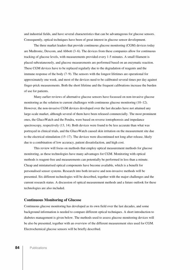
and industrial fields, and have several characteristics that can be advantageous for glucose sensors.
Consequently, optical techniques have been of great interest in glucose sensor development.
The three market leaders that provide continuous glucose monitoring (CGM) devices today
are Medtronic, Dexcom, and Abbott (3–6). The devices from these companies allow for continuous
tracking of glucose levels, with measurements provided every 1-5 minutes. A small filament is
placed subcutaneously, and glucose measurements are performed based on an enzymatic reaction.
These CGM devices have to be replaced regularly due to the degradation of reagents and the
immune response of the body (7–9). The sensors with the longest lifetimes are operational for
approximately one week, and most of the devices need to be calibrated several times per day against
finger-prick measurements. Both the short lifetime and the frequent calibrations increase the burden
of use for patients.
Many earlier reviews of alternative glucose sensors have focussed on non-invasive glucose
monitoring as the solution to current challenges with continuous glucose monitoring (10–12).
However, the non-invasive CGM devices developed over the last decades have not attained any
large-scale market, although several of them have been released commercially. The most prominent
ones, the GlucoWatch and the Pendra, were based on reverse iontophoresis and impedance
spectroscopy, respectively (13, 14). Both devices were found to be less accurate than what was
portrayed in clinical trials, and the GlucoWatch caused skin irritation on the measurement site due
to the electrical stimulation (15–17). The devices were discontinued not long after release, likely
due to a combination of low accuracy, patient dissatisfaction, and high cost.
This review will focus on methods that employ optical measurement methods for glucose
monitoring, as these technologies have many advantages for CGM. Monitoring with optical
methods is reagent-free and measurements can potentially be performed in less than a minute.
Cheap and miniaturised optical components have become available, which is a benefit for
personalised sensor systems. Research into both invasive and non-invasive methods will be
presented. Six different technologies will be described, together with the major challenges and the
current research status. A discussion of optical measurement methods and a future outlook for these
technologies are also included.
Continuous Monitoring of Glucose Continuous glucose monitoring has developed as its own field over the last decades, and some
background information is needed to compare different optical techniques. A short introduction to
diabetes management is given below. The methods used to assess glucose monitoring devices will
be also be presented, together with an overview of the different measurement sites used for CGM.
Electrochemical glucose sensors will be briefly described.
84 Publications
Glucose concentrations are typically given in units of mg/dl or mmol/l (also written mM). Medical
studies usually use mmol/l, while technical papers tend towards using mg/dl. This paper will report
glucose concentrations in mg/dl, and if the referenced article uses mmol/l this number will be given
in parentheses.
Management of Type 1 Diabetes In people with diabetes mellitus type 1 (DM1) an autoimmune process has destroyed the insulin-
producing beta cells in the pancreas. This makes patients with DM1 dependent on exogenous
supplies of insulin to control their glucose level. Insulin can be delivered by multiple daily
subcutaneous insulin injections, or by continuous subcutaneous (SC) delivery of insulin with an
insulin pump controlled by the patient (18). Insulin doses are adjusted according to physical
activity, meal size and composition, and the actual glucose level. Despite all efforts, most DM1
patients struggle to regulate their blood glucose level (BGL) in the desired range, and glucose can
easily depart outside of the normal physiological range, typically defined as 72-180 mg/dl (4-10
mmol/l) (19, 20). Hypoglycaemia occurs when the BGL is too low (<70 mg/dl or 3.9 mmol/l), and
can lead to seizures, loss of consciousness, and even death (21). Hyperglycaemia occurs when the
BGL is higher than 180 mg/dl (10 mmol/l), and can lead to serious long-term complications,
including kidney damage, diabetic retinopathy, heart disease and neuropathy (22).
Given the importance of keeping glucose in the desired range, management of DM1
includes frequent measurements of the BGL. Good control of the BGL reduces development of
long-term complications (23, 24). Finger-prick measurements of capillary blood glucose is still the
most prevalent form of daily self-monitoring of blood glucose (SMBG) in DM1 patients. These
measurements are performed by pricking the skin with a lancet, and placing a drop of blood on a
disposable test strip. A meter is used to measure the test strip and calculate the glucose level.
Diabetic patients are recommended to measure their glucose values at least four times per day, and
more often if they are at risk for large excursions from their target glucose level (25). However,
SMBG by finger-prick measurements is inconvenient and painful, and many diabetic patients
measure less frequently. Some even avoid glucose measurements for days or weeks. Another
disadvantage of these measurements is that they only provide information about the BGL at a single
point in time. Large excursions in the BGL during the day may be missed, no information on BGL
trends is available, and there is a complete lack of information at night. Hence, much effort has been
invested into making CGM devices. CGM devices are sensor systems that continually provide
glucose measurements for patients. Several of these devices are commercially available, and
researchers are still trying to develop more precise and robust methods for CGM. CGM has been
Paper I 85
shown to improve glucose control in patients with DM1 as compared to SMBG with finger-prick
measurements, especially in patients with otherwise poorly controlled glucose levels (26, 27). In
addition, CGM is a prerequisite for making fully automated delivery of insulin in patients with
DM1, also known as a closed-loop system or an artificial pancreas (28).
Assessing Glucose Monitoring The precision of CGM devices is often measured by mean or median average relative difference
(ARD), with most of the current commercial devices achieving median ARDs of 10-15 % and mean
ARDs of 15-20%. ARD is sometimes known as absolute relative error (ARE). The ARD for each
measurement is calculated as follows:
𝐴𝑅𝐷𝑖 = 100% × |𝑌𝑖 − 𝑦𝑖|
𝑌𝑖
where Yi is the reference glucose value and yi is the measured glucose value. The mean and median
ARDs are then calculated based on the individual ARDs. The reference glucose measurement is a
measurement of the BGL performed at the same time, typically done either with a blood-gas
analyser or another glucose monitoring device. ARDs are easy to calculate and interpret, but they
do not indicate the direction of the error and ARDs are usually lower if a smaller glucose range is
investigated.
Other common methods for evaluating glucose sensors are the Clarke error grid (CEG) and
the Parkes error grid (also called the consensus error grid), shown in Fig. 1 (29, 30). The CEG plots
the results from a glucose meter against a reference measurement method, and the plot is divided
into five clinically relevant areas. Zone A contains the values that are within an ARD of 20% of the
reference measurements, while zone B contains measurements with more than 20% error that would
still lead to correct treatment. Zone C and D contain measurements that would lead to unnecessary
treatment or a dangerous lack of treatment, respectively. Measurements in Zone E will indicate that
the patient is in hypoglycaemia when they in reality are hyperglycaemic, and vice versa. The Parkes
error grid uses the same regions as the CEG with similar definitions and improves upon some issues
with the CEG, such as the discontinuous transitions between some regions (e.g. direct transitions
between zone B and zone E for some glucose values).
86 Publications
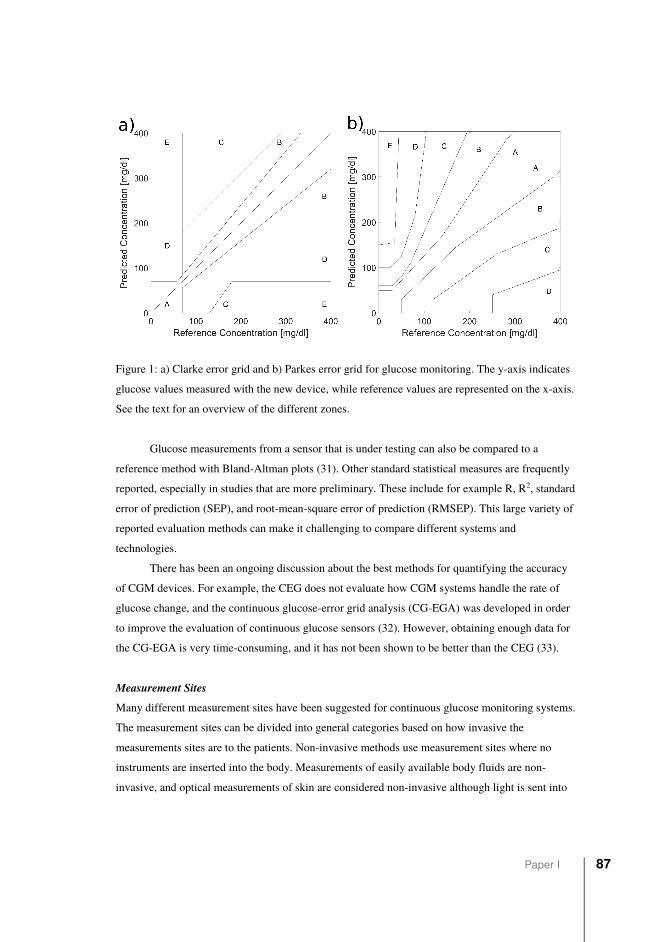
Figure 1: a) Clarke error grid and b) Parkes error grid for glucose monitoring. The y-axis indicates
glucose values measured with the new device, while reference values are represented on the x-axis.
See the text for an overview of the different zones.
Glucose measurements from a sensor that is under testing can also be compared to a
reference method with Bland-Altman plots (31). Other standard statistical measures are frequently
reported, especially in studies that are more preliminary. These include for example R, R2, standard
error of prediction (SEP), and root-mean-square error of prediction (RMSEP). This large variety of
reported evaluation methods can make it challenging to compare different systems and
technologies.
There has been an ongoing discussion about the best methods for quantifying the accuracy
of CGM devices. For example, the CEG does not evaluate how CGM systems handle the rate of
glucose change, and the continuous glucose-error grid analysis (CG-EGA) was developed in order
to improve the evaluation of continuous glucose sensors (32). However, obtaining enough data for
the CG-EGA is very time-consuming, and it has not been shown to be better than the CEG (33).
Measurement Sites Many different measurement sites have been suggested for continuous glucose monitoring systems.
The measurement sites can be divided into general categories based on how invasive the
measurements sites are to the patients. Non-invasive methods use measurement sites where no
instruments are inserted into the body. Measurements of easily available body fluids are non-
invasive, and optical measurements of skin are considered non-invasive although light is sent into
Paper I 87
the body. On the other hand, sensor systems that penetrate blood vessels or the abdominal cavity are
considered invasive. Methods that introduce sensor parts subcutaneously are often called
“minimally invasive”, as no blood vessels are compromised.
Non-invasive CGM systems have been pursued for several decades, with the goals of
improving the comfort and convenience of diabetic patients who have to monitor their glucose
levels daily. Measurements in sweat (34), saliva (35), and breath (36) have all been investigated, but
the concentration of glucose or other correlating analytes have generally been too low, have not
correlated well with the BGL, or have had too slow dynamics. Measuring in tear fluid has also been
suggested, where a sensor similar to a contact lens would have to be worn on the eye for continuous
measurements. However, the glucose concentration is much lower in tear fluid than in blood, and
the glucose levels in tear fluid and blood do not seem to correlate well throughout the day (37, 38).
Systems that measure through skin have therefore received the most attention among the different
non-invasive modalities. Many technologies have been investigated, including impedance
spectroscopy, ultrasound, reverse iontophoresis, as well as many optical methods (12). Light
penetrates from several micrometres to several millimetres into skin depending on wavelength, and
can also be used to measure in the aqueous humour of the eye. Optical methods have therefore
received a lot of attention for non-invasive CGM, and some of this research will be described
below.
Minimally invasive glucose measurements are typically performed by placing sensor parts
subcutaneously. The glucose measurements are then done in the interstitial fluid (ISF), which is the
fluid between tissue cells, rather than in the blood. In the steady state, i.e. when blood glucose is
stable, the glucose concentration in the ISF is quite similar to the BGL. However, glucose has to
diffuse from blood capillaries into the ISF, which causes a time delay in ISF glucose measurements
of approximately 5-10 minutes (39, 40). The commonly used electrochemical CGM systems, as
mentioned, measure glucose concentration subcutaneously. Optical measurement methods can also
be used to measure the ISF, with optical fibres and/or other sensor parts placed subcutaneously.
Recent research suggests that glucose measurements and insulin infusions directly in the
peritoneum (abdominal cavity) will give better dynamics for controlling glucose levels (41, 42).
Hence, investigations of sensing in peritoneal fluid may be an interesting avenue for CGM. The
CGM system could either be implantable or have the light source placed outside the body, which
would require a permanent port or fibre penetrating the abdominal wall to the measurement site.
There are challenges with both approaches. An implantable sensor would have to be robust and
durable without maintenance for a long time. An open port increases the danger of infection and
may cause discomfort for the user. The technological challenges for a port solution will be limited,
as similar port technology already exists for insulin administration (43). No matter which method is
88 Publications
used, sensing in the peritoneum will definitely be considered invasive. To our knowledge, no CGM
devices intended for peritoneal measurements have been developed yet, although some existing
devices have been modified and tested in animal models (44).
Electrochemical CGM Systems Devices using an SC sensor and the glucose-oxidase reaction are the most common CGM systems
used for daily management of diabetes. The sensors have a thin filament embedded subcutaneously,
which measures the glucose concentration. A transmitter is attached to the sensor and transfers data
to a device used for information display. A smartphone or an included receiver shows real-time data
from the sensor, often with trend arrows and alerts for hypo- and hyperglycaemia.
These sensors measure the glucose concentration via an electrochemical reaction (2). In the
basic reaction, glucose-oxidase facilitates the redox reaction of glucose with water, which produces
gluconolactone and hydrogen peroxide (glucose + O2 -> gluconolactone + H2O2). A small electrical
current amplifies the dissociation of hydrogen peroxide, which produces free electrons. The glucose
concentration in the immediate area is then determined from the electrical current resulting from
these electrons. Mediator molecules other than oxygen can be used as electron donors in order to
decrease the dependency on oxygen (45).
Due to the degradation of chemical reagents and biofouling the sensors have to be replaced
approximately once per week, depending on the manufacturer. The user can insert the device
without the help of medical personnel. The sensors also require a warm-up period after insertion,
where the glucose measurements are inaccurate for up to several hours, depending on the model.
This is possibly due to local trauma in the immediate area, which is caused by the sensor insertion.
In addition, regular injection of an SC foreign body may induce local SC fibroses or other tissue
changes over time (46). Most devices require calibrations twice per day, where the sensor is
calibrated against finger-prick measurements. If the calibration process is done while glucose levels
are rapidly changing, the measured glucose level on the device will not correlate well with the
actual BGL. The sensor measures the glucose concentration in the ISF rather than measuring blood
glucose directly, with the associated time delay as compared to the BGL. Additional delay is
introduced because of the reaction process, and because glucose must diffuse to the sensor filament
as the surrounding area becomes depleted (47). Consequently, alarms about low glucose levels can
occur after the patient has already started experiencing hypoglycaemia, where a prompt reaction is
often needed. However, many CGM systems use advanced algorithms to predict hypoglycaemia,
and can reduce the perceived time delay.
Despite several limitations, these devices generally measure glucose concentrations quite
well. Electrochemical CGM has become well established among physicians and patients, and has
Paper I 89
been shown to improve glucose control in patients. Any new inventions that seek to replace today’s
CGMs will likely have to significantly improve upon either reliability, sensitivity, specificity,
sensor lifetime, or perceived quality of life in order to succeed.
Optical Methods for Glucose Measurements Six main optical technologies are included in this review. Near-infrared, mid-infrared, Raman, and
photoacoustic spectroscopy are spectroscopic, meaning that they use the direct interaction between
light and glucose to determine the glucose concentration. Systems using fluorescence spectroscopy
do not measure glucose directly; rather, they typically measure the signal from molecules that can
reversibly bind to glucose. The last technology, optical coherence tomography, measures the change
in scattering properties in tissue as a function of glucose concentration. The following sections will
give an overview of how these technologies are used in glucose sensing. A brief description of the
technical aspects will be provided for each method, together with a discussion on challenges and a
review of the research status in the area. The examples of in vivo research are limited to more
recent and well-documented systems, with a focus on systems that are intended for personal use.
The research stage and other relevant characteristics of most of these systems are summarised in
Table 1.
Other optical techniques, such as measuring optical rotation (48), have been suggested for
glucose monitoring. However, the studies on these methods are sparse and often several decades
old. There are also studies that use variants of optical techniques, such as several recent studies
using photothermal deflection spectroscopy (49, 50). As these methods have mostly been
investigated by single research groups it is difficult to review how well they measure glucose. The
review will therefore be limited to the above-mentioned six technologies for conciseness.
Near-Infrared (NIR) Spectroscopy The near-infrared region extends from 700 to 2500 nm and contains absorption bands primarily
caused by hydrogen vibrations (CH, NH, OH). The short wave band (780-1500 nm) is used for non-
invasive measurements, while for aqueous measurements the first overtone (1500-1800 nm) and the
combination band (2050-2100 nm) are mostly used (51). The absorption bands are broad and easily
influenced by hydrogen bonding, temperature effects and molecules with similar absorption spectra.
NIR sources and detectors are readily available and cheap. Common sources are LED arrays for
non-invasive studies and tungsten-halogen lamps for benchtop measurements. Doped InGaAs
detectors are common, and cooled InSb detectors are also used.
In general, transmission spectroscopy is commonly used for aqueous solutions, while
reflectance spectroscopy is used for non-invasive measurements. The optimal path length through
90 Publications
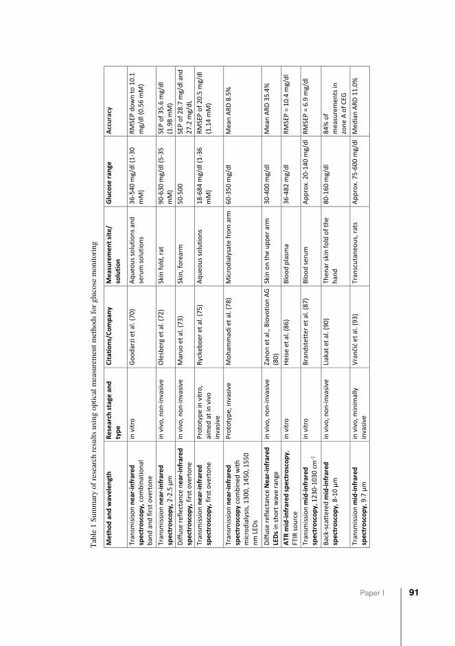
Tabl
e 1
Sum
mar
y of
rese
arch
resu
lts u
sing
opt
ical
mea
sure
men
t met
hods
for g
luco
se m
onito
ring
Method and wavelen
gth
Research stage and
type
Citations/Compan
y Measurement site/
solution
Glucose ran
ge
Accuracy
Transm
isison nearinfrared
spectroscopy, combinational
band and first overtone
in vitro
Goodarzi et al. (70)
Aqueo
us solutions and
serum solutions
36540 m
g/dl (130
mM)
RMSEP down to 10.1
mg/dl (0.56 mM)
Transm
ission nearinfrared
spectroscopy, 22.5 µm
in vivo, noninvasive
Olesberg et al. (72)
Skin fold, rat
90630 m
g/dl (535
mM)
SEP of 35.6 m
g/dl
(1.98 m
M)
Diffuse reflectance nearinfrared
spectroscopy, first overtone
in vivo, noninvasive
Maruo et al. (73)
Skin, forearm
50500
SEP of 28.7 m
g/dl and
27.2 m
g/dL
Transm
ission nearinfrared
spectroscopy, first overtone
Prototype in vitro,
aimed at in vivo
invasive
Ryckeboer et al. (75)
Aqueo
us solutions
18684 m
g/dl (136
mM)
RMSEP of 20.5 m
g/dl
(1.14 m
M)
Transm
ission nearinfrared
spectroscopy combined
with
microdialysis, 1300, 1450, 1550
nm LED
s
Prototype, invasive
Moham
madi et al. (78)
Microdialysate from arm
60350 m
g/dl
Mean ARD 8.5%
Diffuse reflectance Nearinfrared
LEDs in short wave range
in vivo, noninvasive
Zanon et al., Biovotion AG
(80)
Skin on the upper arm
30400 m
g/dl
Mean ARD 35.4%
ATR m
idinfrared spectroscopy,
FTIR source
in vitro
Heise et al. (86)
Blood plasm
a 36482 m
g/dl
RMSEP = 10.4 m
g/dl
Transm
ission m
idinfrared
spectroscopy, 12301030 cm
1
in vitro
Brandstetter et al. (87)
Blood serum
Approx. 20140 mg/dl RMSEP = 6.9 m
g/dl
Backscattered m
idinfrared
spectroscopy, 810 µm
in vivo, noninvasive
Liakat et al. (90)
Then
ar skin fold of the
hand
80160 m
g/dl
84%
of
measuremen
ts in
zone A of CEG
Transm
ission m
idinfrared
spectroscopy, 9.7 µm
in vivo, m
inim
ally
invasive
Vrančić et al. (93)
Transcutaneo
us, rats
Approx. 75600 mg/dl Med
ian ARD 11.0%
Paper I 91
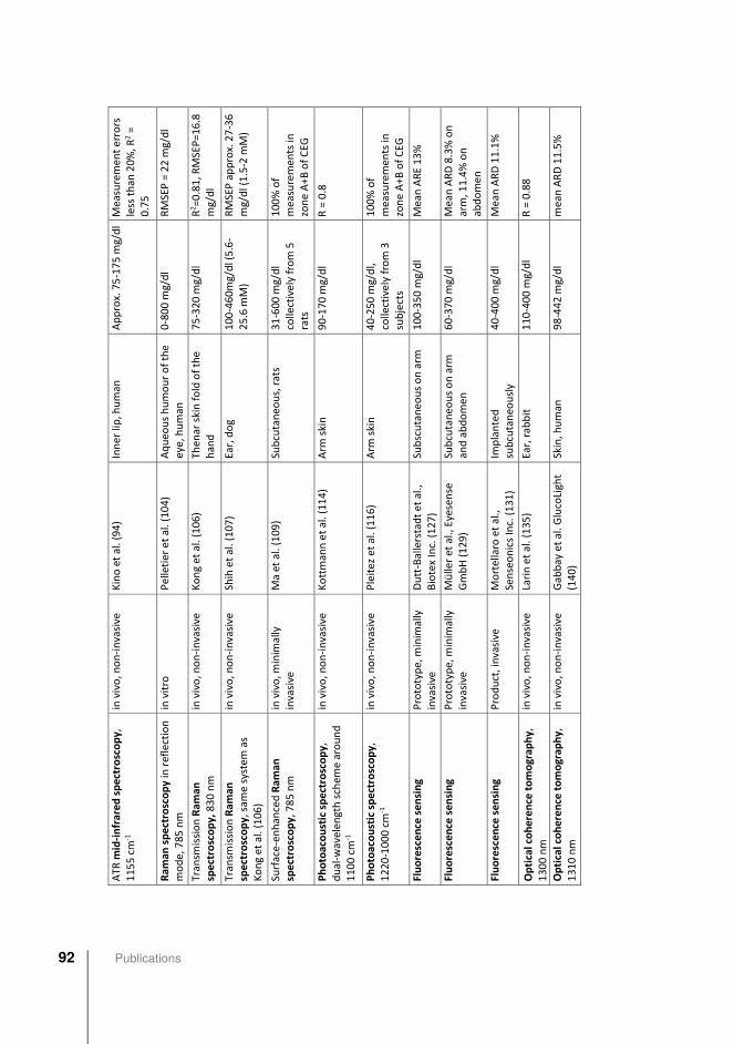
ATR
midinfrared spectroscopy,
1155 cm
1
in vivo, noninvasive
Kino et al. (94)
Inner lip, human
Approx. 75175 mg/dl Measuremen
t errors
less than 20%
, R2 =
0.75
Ram
an spectroscopy in reflection
mode, 785 nm
in vitro
Pelletier et al. (104)
Aqueo
us humour of the
eye, human
0800 m
g/dl
RMSEP = 22 m
g/dl
Transm
ission Ram
an
spectroscopy, 830 nm
in vivo, noninvasive
Kong et al. (106)
Then
ar skin fold of the
hand
75320 m
g/dl
R2=0.81, RMSEP=16.8
mg/dl
Transm
ission Ram
an
spectroscopy, sam
e system
as
Kong et al. (106)
in vivo, noninvasive
Shih et al. (107)
Ear, dog
100460m
g/dl (5.6
25.6 m
M)
RMSEP approx. 2736
mg/dl (1.52 mM)
Surfaceen
hanced Ram
an
spectroscopy, 785 nm
in vivo, m
inim
ally
invasive
Ma et al. (109)
Subcutaneo
us, rats
31600 m
g/dl
collectively from 5
rats
100% of
measuremen
ts in
zone A+B
of CEG
Photoacoustic spectroscopy,
dualw
avelen
gth schem
e around
1100 cm
1
in vivo, noninvasive
Kottmann et al. (114)
Arm
skin
90170 m
g/dl
R = 0.8
Photoacoustic spectroscopy,
12201000 cm
1
in vivo, noninvasive
Pleitez et al. (116)
Arm
skin
40250 m
g/dl,
collectively from 3
subjects
100% of
measuremen
ts in
zone A+B
of CEG
Fluorescen
ce sen
sing
Prototype, m
inim
ally
invasive
DuttBallerstadt et al.,
Biotex Inc. (127)
Subscutaneo
us on arm
100350 m
g/dl
Mean ARE 13%
Fluorescen
ce sen
sing
Prototype, m
inim
ally
invasive
Müller et al., Eyesense
GmbH (129)
Subcutaneo
us on arm
and abdomen
60370 m
g/dl
Mean ARD 8.3% on
arm, 11.4% on
abdomen
Fluorescen
ce sen
sing
Product, invasive
Mortellaro et al.,
Senseonics Inc. (131)
Implanted
subcutaneo
usly
40400 m
g/dl
Mean ARD 11.1%
Optical coherence tomograp
hy,
1300 nm
in vivo, noninvasive
Larin et al. (135)
Ear, rabbit
110400 m
g/dl
R = 0.88
Optical coherence tomograp
hy,
1310 nm
in vivo, noninvasive
Gabbay et al. G
lucoLight
(140)
Skin, human
98442 m
g/dl
mean ARD 11.5%
92 Publications
aqueous glucose samples in transmission mode is dependent on the wavelength and
instrumentation, and is in the range 0.5-5 mm (52). The effective path length for non-invasive
reflectance measurements is dependent on penetration depth and is heavily weighted towards the
upper layer of the skin. It has been estimated to 0.4 to 10 mm, depending on the wavelength (53–
55).
Challenges
Sensor placement is a great challenge for non-invasive measurements. The focus has mostly been
on the skin (finger-tip, forearm (56), upper-arm), but the eye (57), lip (58), tongue (59), and mouth
have also been suggested. Changes in the local environment such as a sunburn, fever, sweating,
swelling, or areas with scarring, tattoos or moles can interfere with the spectra, making the results
hard to reproduce in different physiological states and especially between patients. Zhang et al.
further discuss this issue for spectral data obtained by non-invasive measurements through the skin
(60). Although the results of calibration models look promising, there is a need for more validation
and variations over humidity, pressure, skin type, age, and other factors.
For invasive measurements in the ISF or the peritoneum, the water absorption is very high
around 1400 and 1900 nm, resulting in a weak signal and low signal-to-noise ratio (SNR). Invasive
measurements would also require a sensor structure that does not trigger immune responses and
does not cause discomfort to the user, which rules out materials such as uncoated glass (61).
Molecules with absorption spectra that are similar to glucose can cause interference in NIRS
measurements. Examples of known molecules with absorbance similar to glucose in the NIR range
are lactate, urea (62), and sugars such as fructose. Other molecules with similar spectra are
glutamine, ammonia, and glutamate (63). Interfering molecules represent a challenge for NIR
sensing if not included in the initial model, as the peaks are broad, overlapping, and the glucose
signal is relatively weak compared to the water absorption bands.
Research Status
Several groups have researched in vitro transmission NIRS glucose measurements in plasma (64–
66), whole blood (67), and other matrices designed to simulate bodily fluids (68). Depending on the
complexity of the matrix, the equipment, the concentration range investigated (typically 18-540
mg/dl), and the pre-processing methods (see (69) for a review of techniques), the RMSEP is
typically in the range 9 to 45 mg/dl. For example, glucose in the presence of urea and sodium D-
lactate has been reliably measured in the physiological range by Goodarzi et al. down to 36 mg/dl (2
mM) with an RMSEP down to 10.1 mg/dl (0.56 mM) (70).
Paper I 93
An application of NIR spectroscopy for non-invasive glucose sensing was patented by
Rosenthal et al. in 1992 and spurred intensive research within this area in the 90’s (71). Most of the
focus within NIRS sensing has been directed at non-invasive efforts, but advances past initial trials
have yet to be presented to the public. Arnold and Small have pointed out several parameters that
must be investigated in non-invasive sensing for comparability with other studies: spectral range,
degrees of freedom, path length, spectral variance and chemical basis of selectivity (54). Many
studies do not consider these parameters, making it difficult for the reader to assess whether the
correlation is due to glucose, some co-varying factor, or overfitting by the multivariate calibration
model. A study considering this was performed by Olesberg et al., who measured glucose non-
invasively on a skin fold on the back of one rat for approximately 7 hours (72). The glucose level
was increased to above 540 mg/dl (30 mM) and held there for 2 hours, when it was allowed to
return to normal. They used a fibre probe and found a SEP of 66.6 mg/dl (3.7 mM), which was
improved to 35.6 mg/dl (1.98 mM) when accounting for the time delay (15 minutes). Only one
animal was used, and the between-subject variation can therefore not be evaluated.
Maruo et al. demonstrated a non-invasive NIRS-based sensor with a SEP of less than 32.2
mg/dl in 2003 (56). One diabetic and five healthy human subjects were included in this study, and
the BGL was varied between 50 and 350 mg/dl. In 2006 they followed up with a clinical study with
five healthy and seven diabetic subjects, where glucose varied between 50 and 500 mg/dl, and they
obtained a SEP of 27.2 mg/dl (73). After this, they have been working on data analysis and
perturbations to the model to account for fat content. In 2015, they published a paper detailing how
a non-invasive model can be built based on Beer-Lambert’s law, without the use of chemometrics
(74).
The authors are not aware of any current non-invasive CGMs for DM1 on the international
market, although several companies have tried to develop non-invasive NIR-based sensors since the
late 90’s, such as Diasensor (Biocontrol Technology), SugarTrac (Lifetrac), and Dream Beam
(Futrex Medical Instrumentation). This stands as a testament to the complexity of the problem.
A less traditional approach to aqueous glucose sensing was proposed by Ryckeboer et al.,
who suggested measuring glucose by waveguide-based absorption spectroscopy on a silicon chip in
the range 1540-1610 nm (75). The results in vitro with glucose in range 18-684 mg/dl (1-36 mM)
were promising, with an RMSEP of 20.5 mg/dl (1.14 mM). There have been no clinical trials, but a
patent suggesting that the sensor can be miniaturised and implanted was granted in 2017 (76).
A minimally invasive chip-based NIR CGM sensor using microdialysis of ISF has been
suggested by Mohammadi et al. The sensor has been used in two in vivo trials, the first on 10 DM1
patients for 30 hours (77), and the second one with six subjects for 12 hours (78). The glucose
concentration range was approximately 60-350 mg/dl. The measurement accuracy was 13.8%
94 Publications
overall mean ARE in the first study, and a mean ARD of 8.5% was obtained in the second study.
The device offers an improvement over the electrochemical CGMs in that there are no degradable
enzymes and thus the device can be replaced less frequently. However, it suffers from the
aforementioned time lag in the ISF as compared to the BGL. The authors also reported issues with
air bubbles forming in the sensor.
Some groups have combined different technologies for improved glucose prediction. Most
notable within NIR technology is the research from the team around Caduff and Zanon (affiliated
with Biovotin AG), who have worked towards a non-invasive wearable multisensory system based
on dielectric spectroscopy (DS), temperature, humidity, and sweat sensors combined with 3 NIR
LEDs. In their latest study, the sensor was used by 20 DM1 subjects with BGL in the range 30-400
mg/dl, and a mean ARD of 35.4 % was obtained (79, 80). As the authors point out, they have some
challenges to overcome before the sensor matches the accuracy of CGMs on the market today. They
do not suggest to improve or add to the sensors, but rather to focus further efforts on development
of more complex algorithms.
Mid-Infrared (MIR) Spectroscopy Mid-infrared (MIR) spectroscopy uses light approximately in the 4000-400 cm-1 (2.5-25 µm) range,
although many applications focus on the 4000-1000 cm-1 (2.5-10 µm) range (81). Wavenumbers
(cm-1) are commonly used in the literature on mid-infrared spectroscopy, and will also mainly be
used in this article. Glucose has absorption peaks in several areas in the mid-infrared range, most
notably around 3000 cm-1, around 1400 cm-1, and in the 1200-1000 cm-1 range. Glucose absorbance
in the 1200-1000 cm-1 range has received the most attention for sensor studies, as the features
around 3000 cm-1 and 1400 cm-1 overlap with strong water absorption peaks. This absorbance is
related to the skeletal vibrations of glucose, i.e. vibrations that are characteristic for the entire
molecule.
Fourier transform infrared (FTIR) spectrometers are commonly used for benchtop infrared
spectroscopy. These spectrometers use radiation from infrared sources such as heated silicon
carbide elements, which cover the entire wavelength range. However, current FTIR spectrometers
are too large for personalised CGM devices, and the total light emitted is too weak for clinical
measurements. Few other radiation sources have existed in the MIR, and one of the biggest
limitations for MIR spectroscopy has therefore been the lack of high-energy sources. New avenues
have opened for MIR spectroscopy with the invention and development of quantum cascade lasers
(QCLs) (82, 83). A QCL is a type of semiconductor laser that can be tailored to specific single
wavelengths, or it can be tuneable over a desired wavelength range. Several detector types can be
used in the MIR range, including thermopile, pyroelectric, and photoconductive detectors.
Paper I 95
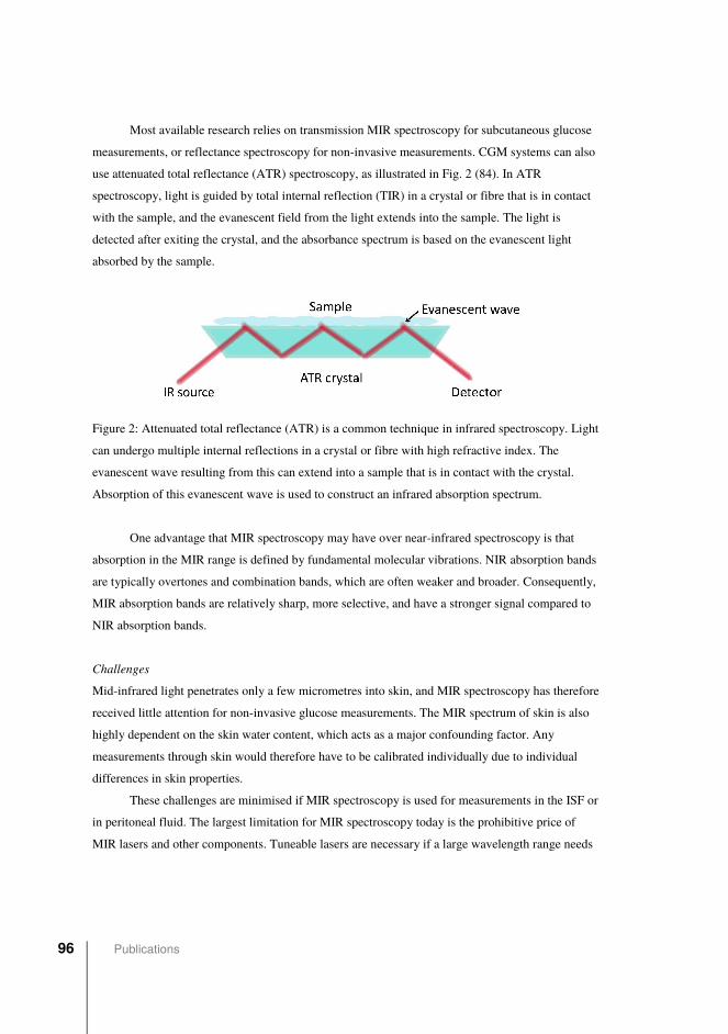
Most available research relies on transmission MIR spectroscopy for subcutaneous glucose
measurements, or reflectance spectroscopy for non-invasive measurements. CGM systems can also
use attenuated total reflectance (ATR) spectroscopy, as illustrated in Fig. 2 (84). In ATR
spectroscopy, light is guided by total internal reflection (TIR) in a crystal or fibre that is in contact
with the sample, and the evanescent field from the light extends into the sample. The light is
detected after exiting the crystal, and the absorbance spectrum is based on the evanescent light
absorbed by the sample.
Figure 2: Attenuated total reflectance (ATR) is a common technique in infrared spectroscopy. Light
can undergo multiple internal reflections in a crystal or fibre with high refractive index. The
evanescent wave resulting from this can extend into a sample that is in contact with the crystal.
Absorption of this evanescent wave is used to construct an infrared absorption spectrum.
One advantage that MIR spectroscopy may have over near-infrared spectroscopy is that
absorption in the MIR range is defined by fundamental molecular vibrations. NIR absorption bands
are typically overtones and combination bands, which are often weaker and broader. Consequently,
MIR absorption bands are relatively sharp, more selective, and have a stronger signal compared to
NIR absorption bands.
Challenges
Mid-infrared light penetrates only a few micrometres into skin, and MIR spectroscopy has therefore
received little attention for non-invasive glucose measurements. The MIR spectrum of skin is also
highly dependent on the skin water content, which acts as a major confounding factor. Any
measurements through skin would therefore have to be calibrated individually due to individual
differences in skin properties.
These challenges are minimised if MIR spectroscopy is used for measurements in the ISF or
in peritoneal fluid. The largest limitation for MIR spectroscopy today is the prohibitive price of
MIR lasers and other components. Tuneable lasers are necessary if a large wavelength range needs
96 Publications
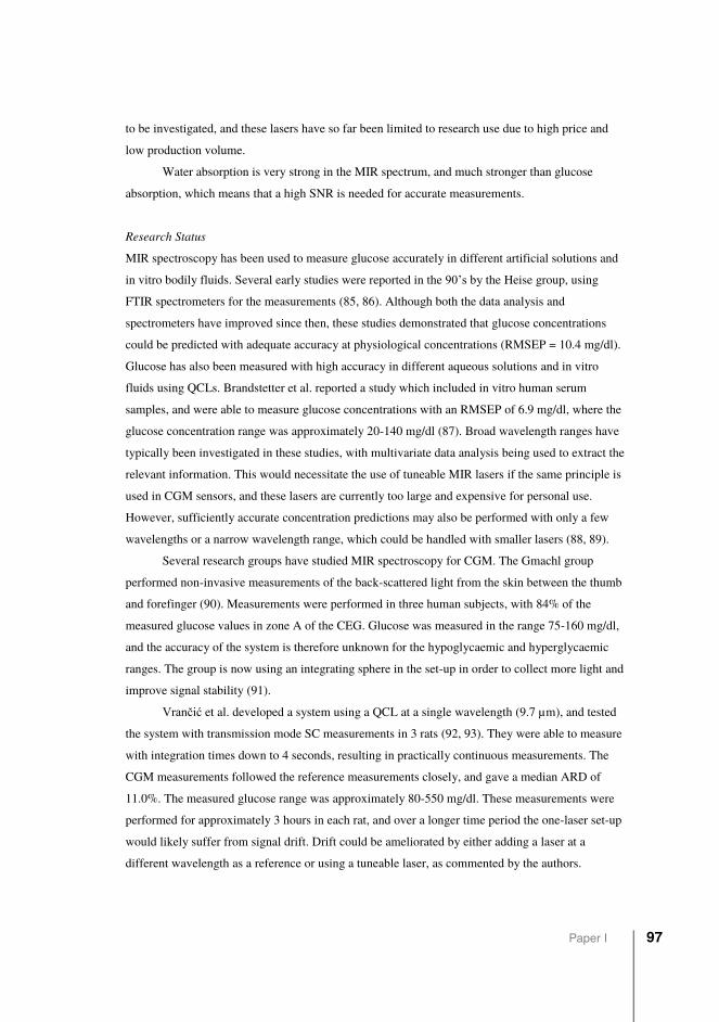
to be investigated, and these lasers have so far been limited to research use due to high price and
low production volume.
Water absorption is very strong in the MIR spectrum, and much stronger than glucose
absorption, which means that a high SNR is needed for accurate measurements.
Research Status
MIR spectroscopy has been used to measure glucose accurately in different artificial solutions and
in vitro bodily fluids. Several early studies were reported in the 90’s by the Heise group, using
FTIR spectrometers for the measurements (85, 86). Although both the data analysis and
spectrometers have improved since then, these studies demonstrated that glucose concentrations
could be predicted with adequate accuracy at physiological concentrations (RMSEP = 10.4 mg/dl).
Glucose has also been measured with high accuracy in different aqueous solutions and in vitro
fluids using QCLs. Brandstetter et al. reported a study which included in vitro human serum
samples, and were able to measure glucose concentrations with an RMSEP of 6.9 mg/dl, where the
glucose concentration range was approximately 20-140 mg/dl (87). Broad wavelength ranges have
typically been investigated in these studies, with multivariate data analysis being used to extract the
relevant information. This would necessitate the use of tuneable MIR lasers if the same principle is
used in CGM sensors, and these lasers are currently too large and expensive for personal use.
However, sufficiently accurate concentration predictions may also be performed with only a few
wavelengths or a narrow wavelength range, which could be handled with smaller lasers (88, 89).
Several research groups have studied MIR spectroscopy for CGM. The Gmachl group
performed non-invasive measurements of the back-scattered light from the skin between the thumb
and forefinger (90). Measurements were performed in three human subjects, with 84% of the
measured glucose values in zone A of the CEG. Glucose was measured in the range 75-160 mg/dl,
and the accuracy of the system is therefore unknown for the hypoglycaemic and hyperglycaemic
ranges. The group is now using an integrating sphere in the set-up in order to collect more light and
improve signal stability (91).
Vrančić et al. developed a system using a QCL at a single wavelength (9.7 µm), and tested
the system with transmission mode SC measurements in 3 rats (92, 93). They were able to measure
with integration times down to 4 seconds, resulting in practically continuous measurements. The
CGM measurements followed the reference measurements closely, and gave a median ARD of
11.0%. The measured glucose range was approximately 80-550 mg/dl. These measurements were
performed for approximately 3 hours in each rat, and over a longer time period the one-laser set-up
would likely suffer from signal drift. Drift could be ameliorated by either adding a laser at a
different wavelength as a reference or using a tuneable laser, as commented by the authors.
Paper I 97
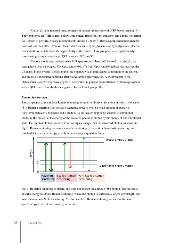
Kino et al. have reported measurements of human lip mucosa with ATR-based sensing (94).
They employed an FTIR source, hollow-core optical fibres for light transport, and a multi-reflection
ATR prism to perform glucose measurements around 1100 cm-1. They accomplished measurement
errors of less than 20%. However, they did not measure hyperglycaemic or hypoglycaemic glucose
concentrations, which limits the applicability of the results. This group has also reported early
results using a single-wavelength QCL source at 9.7 µm (95).
Glucose monitoring devices using MIR spectroscopy that could be used in a critical care
setting have been developed. The Optiscanner (96, 97) from Optiscan Biomedical has received the
CE mark. In this system, blood samples are obtained via an intravenous connection to the patient,
and glucose is measured in plasma after blood sample centrifugation. A spectrometer in the
Optiscanner uses 25 fixed wavelengths to determine the glucose concentration. A prototype system
with a QCL source has also been suggested by the Lendl group (98).
Raman SpectroscopyRaman spectroscopy employs Raman scattering in order to observe vibrational modes in molecules
(81). Raman scattering is an inelastic scattering process where a small amount of energy is
transferred between a molecule and a photon. As the scattering process couples to vibrational
modes in the molecule, the energy of the scattered photon is shifted by the energy of one vibrational
state. The emitted photon can have lower or higher energy than the absorbed photon, as shown in
Fig. 3. Raman scattering has a much smaller scattering cross section than elastic scattering, and
standard Raman spectroscopy usually requires long acquisition times.
Fig. 3: Rayleigh scattering is elastic, and does not change the energy of the photon. The molecule
absorbs energy in Stokes Raman scattering, where the photon is shifted to a longer wavelength, and
vice versa for anti-Stokes scattering. Measurements of Raman scattering are used in Raman
spectroscopy to detect and quantify molecules.
98 Publications
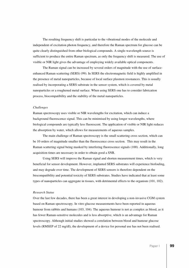
The resulting frequency shift is particular to the vibrational modes of the molecule and
independent of excitation photon frequency, and therefore the Raman spectrum for glucose can be
quite clearly distinguished from other biological compounds. A single-wavelength source is
sufficient to produce the entire Raman spectrum, as only the frequency shift is measured. The use of
visible or NIR light gives the advantage of employing widely available optical components.
The Raman signal can be increased by several orders of magnitude with the use of surface-
enhanced Raman scattering (SERS) (99). In SERS the electromagnetic field is highly amplified in
the presence of metal nanoparticles, because of local surface plasmon resonances. This is usually
realised by incorporating a SERS substrate in the sensor system, which is covered by metal
nanoparticles or a roughened metal surface. When using SERS one has to consider fabrication
process, biocompatibility and the stability of the metal nanoparticles.
Challenges
Raman spectroscopy uses visible or NIR wavelengths for excitation, which can induce a
background fluorescence signal. This can be minimised by using longer wavelengths, where
biological compounds are typically less fluorescent. The application of visible or NIR light reduces
the absorption by water, which allows for measurements of aqueous samples.
The main challenge of Raman spectroscopy is the small scattering cross section, which can
be 10 orders of magnitude smaller than the fluorescence cross section. This may result in the
Raman scattering signal being masked by interfering fluorescence signals (100). Additionally, long
acquisition times are necessary in order to obtain good a SNR.
Using SERS will improve the Raman signal and shorten measurement times, which is very
beneficial for sensor development. However, implanted SERS substrates will experience biofouling,
and may degrade over time. The development of SERS sensors is therefore dependent on the
biocompatibility and potential toxicity of SERS substrates. Studies have indicated that at least some
types of nanoparticles can aggregate in tissues, with detrimental effects to the organism (101, 102).
Research Status
Over the last few decades, there has been a great interest in developing a non-invasive CGM system
based on Raman spectroscopy. In vitro glucose measurements have been reported in aqueous
humour from rabbits and humans (103, 104). The aqueous humour is not as complex as blood, as it
has fewer Raman-sensitive molecules and is less absorptive, which is an advantage for Raman
spectroscopy. Although initial studies showed a correlation between blood and humour glucose
levels (RMSEP of 22 mg/dl), the development of a device for personal use has not been realised.
Paper I 99
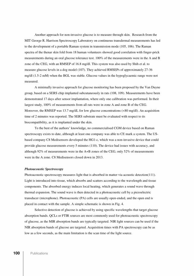
Another approach for non-invasive glucose is to measure through skin. Research from the
MIT George R. Harrison Spectroscopy Laboratory on continuous transdermal measurements has led
to the development of a portable Raman system in transmission mode (105, 106). The Raman
spectra of the thenar skin fold from 18 human volunteers showed good correlation with finger-prick
measurements during an oral glucose tolerance test. 100% of the measurements were in the A and B
zone of the CEG, with an RMSEP of 16.8 mg/dl. This system was also used by Shih et al. to
measure glucose levels in a dog model (107). They achieved RMSEPs of approximately 27-36
mg/dl (1.5-2 mM) when the BGL was stable. Glucose values in the hypoglycaemic range were not
measured.
A minimally invasive approach for glucose monitoring has been proposed by the Van Duyne
group, based on a SERS chip implanted subcutaneously in rats (108, 109). Measurements have been
demonstrated 17 days after sensor implantation, where only one calibration was performed. In their
largest study, 100% of measurements from all rats were in zone A and zone B of the CEG.
Moreover, the RMSEP was 13.7 mg/dL for low glucose concentrations (<80 mg/dl). An acquisition
time of 2 minutes was reported. The SERS substrate must be evaluated with respect to its
biocompatibility, as it is implanted under the skin.
To the best of the authors’ knowledge, no commercialised CGM device based on Raman
spectroscopy exists to date, although at least one company was able to CE mark a system. The US-
based company C8 Medisensors developed the HG1-c, which was a non-invasive device that could
provide glucose measurements every 5 minutes (110). The device had issues with accuracy, and
although 92% of measurements were in the A+B zones of the CEG, only 52% of measurements
were in the A zone. C8 Medisensors closed down in 2013.
Photoacoustic Spectroscopy Photoacoustic spectroscopy measures light that is absorbed in matter via acoustic detection(111).
Light is introduced into tissue, which absorbs and scatters according to the wavelength and tissue
components. The absorbed energy induces local heating, which generates a sound wave through
thermal expansion. The sound wave is then detected in a photoacoustic cell by a piezoelectric
transducer (microphone). Photoacoustic (PA) cells are usually open-ended, and the open end is
placed in contact with the sample. A simple schematic is shown in Fig. 4.
Selective detection of glucose is achieved by using specific wavelengths that target glucose
absorption bands. QCLs or FTIR sources are most commonly used for photoacoustic spectroscopy
of glucose, as the MIR absorption bands are typically targeted. NIR light sources can be used if the
NIR absorption bands of glucose are targeted. Acquisition times with PA spectroscopy can be as
low as a few seconds, as the main limitation is the scan time of the light source.
100 Publications
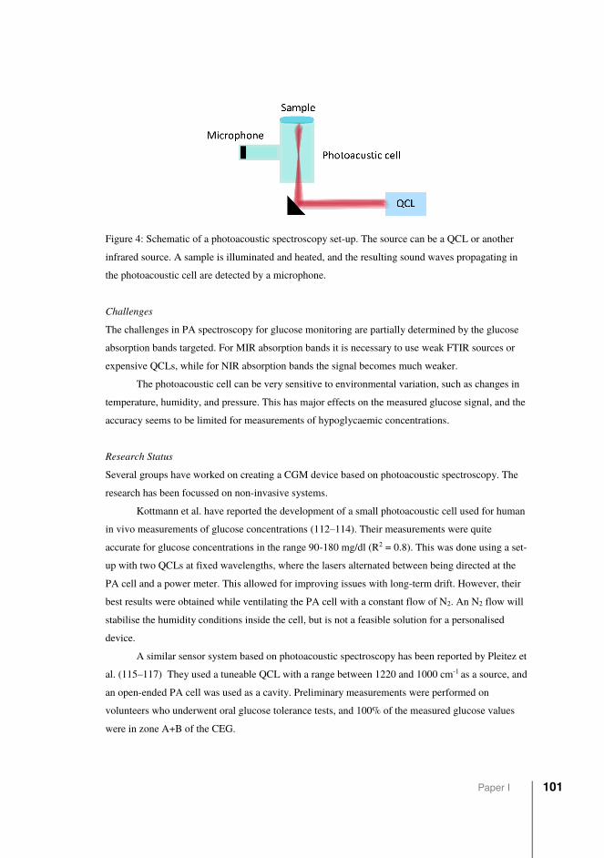
Figure 4: Schematic of a photoacoustic spectroscopy set-up. The source can be a QCL or another
infrared source. A sample is illuminated and heated, and the resulting sound waves propagating in
the photoacoustic cell are detected by a microphone.
Challenges
The challenges in PA spectroscopy for glucose monitoring are partially determined by the glucose
absorption bands targeted. For MIR absorption bands it is necessary to use weak FTIR sources or
expensive QCLs, while for NIR absorption bands the signal becomes much weaker.
The photoacoustic cell can be very sensitive to environmental variation, such as changes in
temperature, humidity, and pressure. This has major effects on the measured glucose signal, and the
accuracy seems to be limited for measurements of hypoglycaemic concentrations.
Research Status
Several groups have worked on creating a CGM device based on photoacoustic spectroscopy. The
research has been focussed on non-invasive systems.
Kottmann et al. have reported the development of a small photoacoustic cell used for human
in vivo measurements of glucose concentrations (112–114). Their measurements were quite
accurate for glucose concentrations in the range 90-180 mg/dl (R2 = 0.8). This was done using a set-
up with two QCLs at fixed wavelengths, where the lasers alternated between being directed at the
PA cell and a power meter. This allowed for improving issues with long-term drift. However, their
best results were obtained while ventilating the PA cell with a constant flow of N2. An N2 flow will
stabilise the humidity conditions inside the cell, but is not a feasible solution for a personalised
device.
A similar sensor system based on photoacoustic spectroscopy has been reported by Pleitez et
al. (115–117) They used a tuneable QCL with a range between 1220 and 1000 cm-1 as a source, and
an open-ended PA cell was used as a cavity. Preliminary measurements were performed on
volunteers who underwent oral glucose tolerance tests, and 100% of the measured glucose values
were in zone A+B of the CEG.
Paper I 101
A study of the Aprise sensor from Glucon Inc. was reported in 2007, which was a non-
invasive sensor based on photoacoustic spectroscopy (118). 62 subjects were included in the study,
and they underwent oral glucose tolerance, mixed meal, or glucose infusion tests. The study
achieved a mean ARD of 19.9% for the sensor, and 94.6% of the paired measurements were within
the A and B zones of the Clarke error grid. Although these preliminary results were quite good, the
device was never commercialised. The sensor has not been described further in peer-reviewed
literature, and the company website does not seem to be functional (glucon.com).
Fluorescence Sensing Many molecules in the body are fluorescent, meaning that they can emit light at specific
wavelengths after being excited by some incident radiation. Fluorescent molecules (fluorophores)
can also be fabricated with specific desired properties, such as binding affinities and emission
wavelengths, so that they are more useful in applications. Fluorescence sensing allows for very
sensitive measurements, which has made it an interesting technology for clinical applications.
Studies have shown that glucose emits fluorescent light, and that glucose concentration
affects fluorescence intensity. However, the direct fluorescent properties of glucose have not been a
large focus in CGM research due to the low signal produced and issues with interfering signals.
Instead, many research groups have tried to measure glucose via fluorescent labelling (119, 120). In
this case, a fluorescence signal is produced from an exogenous fluorophore, i.e. a fluorophore that is
introduced into the body. These fluorophores are engineered to form a complex with glucose
molecules and should only fluoresce in the presence of glucose, as illustrated in Fig. 5. The
fluorescent light intensity will depend on the glucose concentration, as more fluorophores are active
when there is more glucose nearby. Several fluorescent systems have been investigated for glucose
sensing, including boronic acid derivatives and concanavalin A (ConA). The chosen system should
have a high selectivity for glucose over similar molecules, and has to be biocompatible.
Figure 5: Sensing through fluorescent labelling. Fluorescence is suppressed when glucose is not
present. When glucose binds to the fluorophore, fluorescence can occur.
102 Publications
Light in the UV or visible light range is typically used in fluorescence spectroscopy; cheap
LEDs and photodiodes can therefore generally be used for measurements. These components can
also be made very small, which is beneficial for wearable sensor systems. The light source that is
used should not excite other endogenous fluorophores. Additionally, it is advantageous to create a
fluorescent system where the fluorescence does not overlap with the fluorescence of other
molecules, or with fluorescence absorption bands of other molecules, as this will be an interfering
factor.
Challenges
There are several limitations for non-invasive measurements using fluorescence spectroscopy, as
light scattered from skin would also be dependent on the amount of pigmentation and other
differences in skin properties.
For minimally invasive and invasive measurements, fluorescence spectroscopy would still
need calibration against finger-prick measurements. Drift of the fluorescence signal will occur both
due to drift of the source, as well as gradual loss of fluorophores due to photobleaching.
There have been issues with achieving a linear fluorescent signal over the entire
physiological range of glucose concentrations (119). Many fluorophores also bind other sugars such
as galactose and fructose. Issues with saturation and the presence of interferents therefore limits the
number of useful fluorophores.
Research Status
Several studies were conducted in the early 2000’s into different possible fluorophores for glucose
measurements, but many of these struggled with challenges such as low solubility and narrow
measurement ranges. Several groups have tried to develop contact lens glucose sensors using
fluorescence spectroscopy over the last decades (121–123). As mentioned, the glucose level in tear
fluid does not seem to correlate well with the BGL, which has been a challenge for this research.
A subcutaneous glucose sensor based on fluorescence spectroscopy was first suggested in
1979 by Schultz et al. (124) This sensor concept has been further researched by the same group
(125, 126), and is now under development by BioTex Inc. under the name Fluorescence Affinity
Sensor (FAS). This sensor utilises a fluorophore inside a hollow dialysis fibre that is connected to
an optical fibre, where fluorescence-labelled ConA is used as the fluorophore. Glucose displaces the
dextran bound to the ConA, which induces a fluorescent signal proportional to the glucose
concentration. The sensor has been tested in several pilot studies in humans and pigs (127, 128). For
the human pilot study, a mean ARE between the sensor and the reference measurement of 13% was
Paper I 103
achieved. The delay between the sensor measurement and the reference BGL was on average 4
minutes.
A clinical trial was reported by Müller et al., where they presented a similar fluorescence-
based CGM system called FiberSense (129). Their measurement method was also based on labelled
ConA. The sensor was implanted in two sites in six subjects for 14 days. The overall mean ARD
was 8.3% for sensors used on the upper arm, and 11.4% for sensors used on the abdomen. The
photometer with the source and detector was worn only during measurement sessions, while the
sensor head was worn continuously for the entire study. The measurement sessions lasted for
approximately 3 hours, and few data points were collected in the hypoglycaemic range. The sensor
was calibrated once per day against finger-prick measurements.
The American company Senseonics has released the Eversense CGM system in Europe after
receiving the CE mark in 2016. The Eversense has a mean ARD of 11.1% (130). This system
consists of an implantable sensor that is placed under the skin, a removable transmitter that is worn
over the sensor, and a smartphone app that receives the signal from the transmitter (131). The
sensor is cylindrical with dimensions 3.3 mm x 15 mm, and can be inserted subcutaneously through
a small incision. The sensor is approved for 90 days of continuous use before a replacement is
necessary.
The sensor itself consists of a small polymer case. A light-emitting diode (LED) in the case
excites the fluorophore and two photodiodes measure the fluorescent signal. The outside of the case
is covered in a glucose-indicating hydrogel. Glucose reversibly binds to a boronic-acid derivative,
which serves as the fluorescent indicator in the hydrogel.
To date, this is the only commercially available wearable CGM device that is based on an
optical method. The sensor has a long lifetime relative to other commercially available glucose
sensors, but must be placed through a small surgical incision in the arm by a physician. This may
give some discomfort and risk of infection, although questionnaires answered by users indicate that
the implantation is acceptable (132). Similar to other devices, the Eversense sensor also needs to be
calibrated with finger-prick measurements twice per day.
Optical Coherence Tomography Optical coherence tomography (OCT) is a measurement method that uses an interferometer with
low coherence light (133). OCT requires one reference and one sample arm for the light, a moving
window to vary the path length, and a photodetector for the signal. The light scattered back from
tissue is combined with light from the reference arm, and the interference signal is sent to the
photodetector. An interferogram is created if light from both arms has travelled the same optical
distance, i.e. within the coherence length. The refractive index of the ISF will change as the glucose
104 Publications
concentration changes, which in turn changes the scattering coefficient. This change in scattering
coefficient and concomitant variation in the interferogram is used to determine the glucose
concentration.
OCT typically employs light in the NIR range, and as in NIR spectroscopy relatively cheap
and small components are available. This method is used in several applications for 3D imaging
with micrometre resolution, such as imaging of biological tissues.
Challenges
OCT is sensitive to motion artefacts, as any changes to the reference or sample arm lengths will
interfere with the output signal. Non-invasive OCT is also sensitive to changes in the local
environment of the skin, such as variations in skin temperature, pH, and humidity.
The measured change in scattering coefficient is relatively small, which is a major challenge
for OCT in glucose sensing. The scattering coefficient can be affected by variations of other
physiological compounds, and corrections must be made for individual differences in skin
properties.
Research Status
There has been some research on OCT for non-invasive glucose measurements.
Larin et al. reported several studies that purported to show that OCT could be used to measure
blood glucose non-invasively (134, 135). In vivo measurements in their OCT system correlated
quite well with the BGL (R = 0.88), but both motion artefacts and skin temperature could
significantly affect the OCT signal.
Several other research groups have been able to attain similar results with OCT and related
systems, but it has not seemed to move past preliminary in vivo studies (136, 137). The company
GlucoLight apparently worked on a glucose monitoring device based on OCT, and filed several
patents in the late 2000’s (138, 139). A small pilot study based on this device was also published in
2008, where 12 subjects with DM1 and 15 subject with type 2 diabetes participated (140).
Measurements were conducted for 2 hours in each subject, and the device achieved a mean ARD of
11.5%. Hypoglycaemic glucose concentrations were not measured, and no further results from this
system have been reported.
Discussion The development of most optical methods for glucose monitoring is still progressing quite slowly,
with few systems reaching even the prototype stage. These optical methods share many of the same
challenges, such as a need for miniaturisation and high price of suitable components. There is also
Paper I 105
the inherent challenge of measurements based on intensity, as such measurements are prone to
signal drift. Many preliminary studies of new CGM methods also have problems with study size
and duration. In vivo studies will often have results for measurements in only one or a few subjects,
and for measurements performed over a few hours. This gives us some information on how a
system performs under optimal conditions, but tells us very little about the between-subject
variation and how the system performs for the entire lifetime of the device.
Additionally, there are separate issues for systems that attempt to measure non-invasively
and invasively. The main challenges for non-invasive measurements are improving the SNR,
correlation between measured glucose and the actual BGL, and the possible issues of calibrating the
device to individual differences in skin properties. As mentioned, many non-invasive methods
struggle with calibrating across individuals due to e.g. differences in skin water content and
pigmentation. The model may work well on the person that the calibration is built on, but is often
not transferable. Individual calibration can be implemented to improve device accuracy, although
this is time-consuming. The main challenges for invasive measurements include minimising
biofouling, extending sensor lifetime, correcting for signal drift, and ensuring patient acceptability.
Optical methods have several general advantages for CGM. Most optical techniques are
generally not dependent on any reagents, which means that the lifetime can be much longer than for
electrochemical sensors. This is especially important for minimally invasive and invasive
measurements. Even systems based on fluorescence spectroscopy, which are dependent on
fluorophores, seem to have much longer lifetimes than current electrochemical sensors. Optical
sensing does not consume glucose, and the glucose concentration is therefore unchanged in the area
surrounding the sensor. Non-invasive optical measurements would also have potential for pain-free
CGM that affects the body minimally, given that a high measurement accuracy can be achieved.
Smaller and cheaper components are continually being developed, which is an advantage for
personalised devices.
The different optical technologies all have advantages and disadvantages. Interesting in vivo
results have been shown using photoacoustic spectroscopy, but the sensitivity is too low for
accurate measurements at physiological concentrations. Raman spectroscopy suffers from a very
low signal that can be improved using SERS, but the challenge then becomes achieving stable
surface-enhancement. The SERS substrate may degrade over time in the body, which limits the
device lifetime and creates a risk for biotoxicity. NIRS has been explored extensively for non-
invasive CGM, but no devices have yet been successfully commercialised. There are relatively few
studies on MIRS for glucose measurements, as non-invasive measurements are less feasible than for
NIRS and the price of components is generally high. Studies have shown that both NIRS and MIRS
can measure glucose accurately in ISF and similar fluids, and these methods have high potential for
106 Publications
use in minimally invasive or invasive CGM systems. CGM systems that use fluorescent labelling
have progressed the furthest of all the optical methods. Several devices are in a prototype stage, and
the Eversense system is currently being commercialised. Glucose can be measured accurately with
good fluorescence labelling, and the sensors have long lifetimes.
Of course, it is difficult to predict how the other optical methods will fare in the future, and
if any of them are more likely to succeed due to technological advantages. There seems to be a
trend, especially in non-invasive glucose measurements, of increased focus on developing data
processing methods. This suggests that the instrumentation has reached a state where new advances
only provide incremental improvements in sensitivity and that smart enough algorithms may
account for the variable factors. Unless there is a large leap in technology or data processing
techniques, this may be a fundamental limit for non-invasive CGM with optical methods. Indeed,
with the implantable system from Eversense and many other groups working on invasive or
minimally invasive systems, it seems that we might be moving away from the idea of non-invasive
methods as the optimal solution. Minimally invasive sensors are already accepted by many patients
in the form electrochemical CGM devices. Utilising sensing systems developed for the peritoneum
is also a possibility, and may give faster sensor dynamics. This can lead to closed-loop systems that
more closely mimic the functions of a healthy pancreas.
Conclusions Current electrochemical CGM devices are an improvement for diabetes management as compared
to intermittent finger-prick measurements, but they have short sensor lifetimes and must be
calibrated against finger-prick measurements daily. Much effort has been spent on research into
glucose measurement methods that could potentially replace these devices. Optical methods have
many beneficial properties for CGM, but few devices have been commercialised despite decades of
research.
Electrochemical devices are now the gold standard for CGM, and new devices will likely
have to improve upon some aspects of these sensors in order to be accepted by patients and
physicians. Several studies have shown progress for sensor systems based on spectroscopy, with
some of the most promising results for MIR, NIR and Raman spectroscopy. Systems based on
fluorescent labelling sensors have been the most successful so far, with several prototypes in
development and one system being commercialised. The Eversense is a promising alternative to
current electrochemical methods; its main advantage seems to be the comparably long lifetime. As
long as patients tolerate the sensor insertion and removal, it may be the first optical CGM device to
enjoy success.
Paper I 107

Funding
This work was supported by the Research Council of Norway through the Double Intraperitoneal Artificial
Pancreas project, grant number 248872.
List of Abbreviations ARD – Absolute relative difference
ARE – Absolute relative error
ATR – Attenuated total reflectance
BGL – Blood glucose level
CEG – Clarke error grid
CG-EGA – Continuous glucose-error grid analysis
CGM – Continuous glucose monitoring
ConA – Concanavalin A
DM1 – Diabetes mellitus type 1
ISF – Interstitial fluid
FTIR – Fourier transform infrared
MIR – Mid-infrared
NIR – Near-infrared
OCT – Optical coherence tomography
PA - Photoacoustic
QCL – Quantum cascade laser
RMSEP – Root-mean-square error of prediction
SC – Subcutaneous
SEP – Standard error of prediction
SERS – Surface-enhanced Raman spectroscopy
SMBG – Self-monitoring of blood glucose
SNR – Signal-to-noise ratio
UV – Ultraviolet
108 Publications

1. Turner, A. P. F. (2013) Biosensors - Sense and sensitivity. Chem. Soc. Rev. 42 (8): 3184–3196.
2. Wang, J. (2008) Electrochemical glucose biosensors. Chem. Rev. 108 (2): 814–825. 3. Keenan, D. B., Mastrototaro, J. J., Zisser, H., Cooper, K. A., Raghavendhar, G., Lee, S. W.,
Yusi, J., Bailey, T. S., Brazg, R. L., and Shah, R. V. (2012) Accuracy of the Enlite 6-Day Glucose Sensor with Guardian and Veo Calibration Algorithms. Diabetes Technol. Ther. 14 (3): 225–231.
4. Bailey, T. S., Chang, A., and Christiansen, M. (2015) Clinical Accuracy of a Continuous Glucose Monitoring System With an Advanced Algorithm. J. Diabetes Sci. Technol. 9 (2): 209–214.
5. Thabit, H., Leelarathna, L., Wilinska, M. E., Elleri, D., Allen, J. M., Lubina-Solomon, A., Walkinshaw, E., Stadler, M., Choudhary, P., Mader, J. K., Dellweg, S., Benesch, C., Pieber, T. R., Arnolds, S., Heller, S. R., Amiel, S. A., Dunger, D., Evans, M. L., and Hovorka, R. (2015) Accuracy of Continuous Glucose Monitoring During Three Closed-Loop Home Studies Under Free-Living Conditions. Diabetes Technol. Ther. 17 (11): 801–807.
6. Weinstein, R. L., Schwartz, S. L., Brazg, R. L., Bugler, J. R., Peyser, T. A., and McGarraugh, G. V. (2007) Accuracy of the 5-Day FreeStyle Navigator Continuous Glucose Monitoring System. Diabetes Care 30 (5): 1125–30.
7. Valdes, T. I., and Moussy, F. (2000) In Vitro and In Vivo Degradation of Glucose OxidaseEnzyme Used for an Implantable Glucose Biosensor. Diabetes Technol. Ther. 2 (3): 367–376.
8. Scholten, K., and Meng, E. (2018) A review of implantable biosensors for closed-loop glucose control and other drug delivery applications. Int. J. Pharm.
9. Novak, M. T., Yuan, F., and Reichert, W. M. (2010) Modeling the relative impact of capsular tissue effects on implanted glucose sensor time lag and signal attenuation. Anal. Bioanal. Chem. 398 (4): 1695–1705.
10. Tura, A., Maran, A., and Pacini, G. (2007) Non-invasive glucose monitoring: Assessment of technologies and devices according to quantitative criteria. Diabetes Res. Clin. Pract. 77 (1): 16–40.
11. Girardin, C. M., Huot, C., Gonthier, M., and Delvin, E. (2009) Continuous glucose monitoring: A review of biochemical perspectives and clinical use in type 1 diabetes. Clin. Biochem. 42 (3): 136–142.
12. Vashist, S. K. (2012) Non-invasive glucose monitoring technology in diabetes management: A review. Anal. Chim. Acta 750: 16–27.
13. Potts, R. O., Tamada, J. A., and Tierney, M. J. (2002) Glucose monitoring by reverse iontophoresis. Diabetes. Metab. Res. Rev. 18 (Suppl. 1): S49–S53.
14. Caduff, A., Hirt, E., Feldman, Y., Ali, Z., and Heinemann, L. (2003) First human experiments with a novel non-invasive, non-optical continuous glucose monitoring system. Biosens. Bioelectron. 19 (3): 209–217.
15. The Diabetes Research in Children Network (DirectNet) Study Group. (2004) Accuracy of the GlucoWatch G2 Biographer and the Continuous Glucose Monitoring System During Hypoglycemia. Diabetes Care 27 (3): 722–726.
16. The Diabetes Research in Children Network (DirectNet) Study Group. (2005) Youth and Parent Satisfaction With Clinical Use of the GlucoWatch G2 Biographer in the Management of Pediatric Type 1 Diabetes. Diabetes Care 28 (8): 1929–1935.
Paper I 109

17. Wentholt, I. M. E., Hoekstra, J. B. L., Zwart, A., and DeVries, J. H. (2005) Pendra goes Dutch: lessons for the CE mark in Europe. Diabetologia 48 (6): 1055–1058.
18. Retnakaran, R., Hochman, J., DeVries, J. H., Hanaire-Broutin, H., Heine, R. J., Melki, V., and Zinman, B. (2004) Continuous Subcutaneous Insulin Infusion Versus Multiple Daily Injections: The impact of baseline A1c. Diabetes Care 27 (11): 2590–2596.
19. Battelino, T., Conget, I., Olsen, B., Schütz-Fuhrmann, I., Hommel, E., Hoogma, R., Schierloh, U., Sulli, N., and Bolinder, J. (2012) The use and efficacy of continuous glucose monitoring in type 1 diabetes treated with insulin pump therapy: A randomised controlled trial. Diabetologia 55 (12): 3155–3162.
20. Breton, M., Farret, A., Bruttomesso, D., Anderson, S., Magni, L., Patek, S., Man, C. D., Place, J., Demartini, S., Del Favero, S., Toffanin, C., Hughes-Karvetski, C., Dassau, E., Zisser, H., Doyle, F. J., De Nicolao, G., Avogaro, A., Cobelli, C., Renard, E., and Kovatchev, B. (2012) Fully Integrated Artificial Pancreas in Type 1 Diabetes: Modular Closed-Loop Glucose Control Maintains Near Normoglycemia. Diabetes 61 (9): 2230–2237.
21. Frier, B. M. (2004) Morbidity of hypoglycemia in type 1 diabetes. Diabetes Res. Clin. Pract. 65S: S47–S52.
22. Nathan, D. M. (1993) Long-Term Complications of Diabetes Mellitus. N. Engl. J. Med. 328: 1676–1685.
23. Wang, P. H., Lau, J., and Chalmers, T. C. (1993) Meta-analysis of effects of intensive blood-glucose control on late complications of type I diabetes. Lancet 341 (8856): 1306–1309.
24. The Diabetes Control and Complications Trial Research Group. (1993) The Effect of Intensive Treatment of Diabetes on the Development and Progression of Long-Term Complications in Insulin-Dependent Diabetes Mellitus. N. Engl. J. Med. 329 (14): 977–986.
25. Minder, A. E., Albrecht, D., Schäfer, J., and Zulewski, H. (2013) Frequency of blood glucose testing in well educated patients with diabetes mellitus type 1: How often is enough? Diabetes Res. Clin. Pract. 101 (1): 57–61.
26. Deiss, D., Bolinder, J., Riveline, J. P., Battelino, T., Bosi, E., Tubiana-Rufi, N., Kerr, D., and Phillip, M. (2006) Improved Glycemic Control in Poorly Controlled Patients with Type 1 Diabetes Using Real-Time Continuous Glucose Monitoring. Diabetes Care 29 (12): 2730–2732.
27. Pickup, J. C., Freeman, S. C., and Sutton, A. J. (2011) Glycaemic control in type 1 diabetes during real time continuous glucose monitoring compared with self monitoring of blood glucose: meta-analysis of randomised controlled trials using individual patient data. BMJ 343: d3805.
28. Cobelli, C., Renard, E., and Kovatchev, B. (2011) Artificial Pancreas: Past, Present, Future. Diabetes 60 (11): 2672–2682.
29. Clarke, W. L., Cox, D., Gonder-Frederick, L. A., Carter, W., and Pohl, S. L. (1987) Evaluating Clinical Accuracy of Systems for Self-Monitoring of Blood Glucose. Diabetes Care 10 (5): 622–628.
30. Parkes, J. L., Slatin, S. L., Pardo, S., and Ginsberg, B. H. (2000) A New Consensus Error Grid to Evaluate the Clinical Significance of Inaccuracies in the Measurement of Blood Glucose. Diabetes Care 23 (8): 1143–1148.
31. Bland, J. M., and Altman, D. G. (1986) Statistical Methods for Assessing Agreement Between Two Methods of Clinical Measurement. Lancet 327: 307–310.
32. Kovatchev, B. P., Gonder-Frederick, L. A., Cox, D. J., and Clarke, W. L. (2004) Evaluating the Accuracy of Continuous Glucose-Monitoring Sensors: Continuous glucose-error grid
110 Publications

analysis illustrated by TheraSense Freestyle Navigator data. Diabetes Care 27 (8): 1922–1928.
33. Wentholt, I. M., Hoekstra, J. B., and DeVries, J. H. (2006) A Critical Appraisal of the Continuous Glucose-Error Grid Analysis. Diabetes Care 29 (8): 1805–1811.
34. Moyer, J., Wilson, D., Finkelshtein, I., Wong, B., and Potts, R. (2012) Correlation Between Sweat Glucose and Blood Glucose in Subjects with Diabetes. Diabetes Technol. Ther. 14 (5): 398–402.
35. Sener, A., Jurysta, C., Bulur, N., Oguzhan, B., Satman, I., Yilmaz, T. M., and Malaisse, W. J. (2009) Salivary Glucose Concentration and Excretion in Normal and Diabetic Subjects. J. Biomed. Biotechnol. 2009.
36. Wang, C., Mbi, A., and Shepherd, M. (2010) A Study on Breath Acetone in Diabetic Patients Using a Cavity Ringdown Breath Analyzer: Exploring Correlations of Breath Acetone with Blood Glucose and Glycohemoglobin A1C. IEEE Sens. J. 10 (1): 54–63.
37. Baca, J. T., Taormina, C. R., Feingold, E., Finegold, D. N., Grabowski, J. J., and Asher, S. A. (2007) Mass Spectral Determination of Fasting Tear Glucose Concentrations in Nondiabetic Volunteers. Clin. Chem. 53 (7): 1370–1372.
38. Baca, J. T., Finegold, D. N., and Asher, S. A. (2007) Tear Glucose Analysis for the Noninvasive Detection and Monitoring of Diabetes Mellitus. Ocul. Surf. 5 (4): 280–293.
39. Wentholt, I. M., Vollebregt, M. A., Hart, A. A., Hoekstra, J. B., and DeVries, J. H. (2005)Comparison of a Needle-Type and a Microdialysis Continuous Glucose Monitor in Type 1 Diabetic Patients. Diabetes Care 28 (12): 2871–2876.
40. Basu, A., Dube, S., Veettil, S., Slama, M., Kudva, Y. C., Peyser, T., Carter, R. E., Cobelli, C., and Basu, R. (2015) Time Lag of Glucose From Intravascular to Interstitial Compartment in Type 1 Diabetes. J. Diabetes Sci. Technol. 9 (1): 63–68.
41. Burnett, D. R., Huyett, L. M., Zisser, H. C., Doyle, F. J., and Mensh, B. D. (2014) Glucose Sensing in the Peritoneal Space Offers Faster Kinetics Than Sensing in the Subcutaneous Space. Diabetes 63 (7): 2498–2505.
42. Fougner, A. L., Kölle, K., Skjærvold, N. K., Elvemo, N. A. L., Hjelme, D. R., Ellingsen, R., Carlsen, S. M., and Stavdahl, Ø. (2016) Intraperitoneal Glucose Sensing is Sometimes Surprisingly Rapid. Model. Identif. Control 37 (2): 121–131.
43. Renard, E. (2008) Insulin Delivery Route for the Artificial Pancreas: Subcutaneous, Intraperitoneal, or Intravenous? Pros and Cons. J. Diabetes Sci. Technol. 2 (4): 735–738.
44. Huyett, L. M., Mittal, R., Zisser, H. C., Luxon, E. S., Yee, A., Dassau, E., Doyle, F. J., and Burnett, D. R. (2016) Preliminary Evaluation of a Long-Term Intraperitoneal Glucose Sensor With Flushing Mechanism. J. Diabetes Sci. Technol. 10 (5): 1192–1194.
45. Heller, A., and Feldman, B. (2008) Electrochemical Glucose Sensors and Their Applications in Diabetes Management. Chem. Rev. 108 (7): 2482–2505.
46. Ward, W. K. (2008) A Review of the Foreign-Body Response to Subcutaneously-Implanted Devices: The Role of Macrophages and Cytokines in Biofouling and Fibrosis. J. Diabetes Sci. Technol. 2 (5): 768–777.
47. Keenan, D. B., Mastrototaro, J. J., Voskanyan, G., and Steil, G. M. (2009) Delays in Minimally Invasive Continuous Glucose Monitoring Devices: A Review of Current Technology. J. Diabetes Sci. Technol. 3 (5): 1207–14.
48. Purvinis, G., Cameron, B. D., and Altrogge, D. M. (2011) Noninvasive Polarimetric-Based Glucose Monitoring: An in Vivo Study. J. Diabetes Sci. Technol. 5 (2): 380–387.
Paper I 111

49. Pleitez, M. A., Hertzberg, O., Bauer, A., Seeger, M., Lieblein, T., Von Lilienfeld-Toal, H., and Mäntele, W. (2015) Photothermal deflectometry enhanced by total internal reflection enables non-invasive glucose monitoring in human epidermis. Analyst 140: 483–488.
50. Hertzberg, O., Bauer, A., Küderle, A., Pleitez, M. A., and Mäntele, W. (2017) Depth-selective photothermal IR spectroscopy of skin: potential application for non-invasive glucose measurement. Analyst 142: 495–502.
51. Yang, W., Liao, N., Cheng, H., Li, Y., Bai, X., and Deng, C. (2018) Determination of NIR informative wavebands for transmission non-invasive blood glucose measurement using a Fourier transform spectrometer. AIP Adv. 8 (3): 35216.
52. Jensen, P. S., and Bak, J. (2002) Near-Infrared Transmission Spectroscopy of Aqueous Solutions: Influence of Optical Pathlength on Signal-to-Noise Ratio. Appl. Spectrosc. 56 (12): 1600–1606.
53. Heise, H. M., Marbach, R., Koschinsky, T., and Gries, F. A. (1994) Noninvasive Blood Glucose Sensors Based on Near-Infrared Spectroscopy. Artif. Organs 18 (6): 439–447.
54. Arnold, M. A., and Small, G. W. (2005) Noninvasive Glucose Sensing. Anal. Chem. 77 (17): 5429–5439.
55. Liu, J., Liu, R., and Xu, K. (2015) Accuracy of Noninvasive Glucose Sensing Based on Near-Infrared Spectroscopy. Appl. Spectrosc. 69 (11): 1313–1318.
56. Maruo, K., Tsurugi, M., Tamura, M., and Ozaki, Y. (2003) In Vivo Noninvasive Measurement of Blood Glucose by Near-Infrared Diffuse-Reflectance Spectroscopy. Appl. Spectrosc. 57 (10): 1236–1244.
57. Schrader, W., Meuer, P., Popp, J., Kiefer, W., Menzebach, J. U., and Schrader, B. (2005) Non-invasive glucose determination in the human eye. J. Mol. Struct. 735–736 (Spec. Iss.): 299–306.
58. Marbach, R., Koschinsky, T. H., Gries, F. A., and Heise, H. M. (1993) Noninvasive Blood Glucose Assay by Near-Infrared Diffuse Reflectance Spectroscopy of the Human Inner Lip. Appl. Spectrosc. 47 (7): 875–881.
59. Burmeister, J. J., Arnold, M. A., and Small, G. W. (2000) Noninvasive Blood Glucose Measurements by Near-Infrared Transmission Spectroscopy Across Human Tongues. Diabetes Technol. Ther. 2 (1): 5–16.
60. Zhang, W., Liu, R., Zhang, W., Jia, H., and Xu, K. (2013) Discussion on the validity of NIR spectral data in non-invasive blood glucose sensing. Biomed. Opt. Express 4 (6): 789–802.
61. van der Kamp, K. W. H. J., Hauch, K. D., Feijen, J., and Horbett, T. A. (1995) Contact activation during incubation of five different polyurethanes or glass in plasma. J. Biomed. Mater. Res. 29: 1303–1306.
62. Ren, M., and Arnold, M. A. (2007) Comparison of multivariate calibration models for glucose, urea, and lactate from near-infrared and Raman spectra. Anal. Bioanal. Chem. 387 (3): 879–888.
63. Chung, H., Arnold, M. A., Rhiel, M., and Murhammer, D. W. (1996) Simultaneous Measurements of Glucose , Glutamine , Ammonia , Lactate , and Glutamate in Aqueous Solutions by Near-Infrared Spectroscopy. Appl. Spectrosc. 50 (2): 270–276.
64. Heise, H. M., Marbach, R., Bittner, A., and Koschinsky, T. (1998) Clinical chemistry and near infrared spectroscopy: Multicomponent assay for human plasma and its evaluation for the determination of blood substrates. J. Near Infrared Spectrosc. 6 (1): 361–374.
65. Turza, S., Mitsunori, K., and Kawano, S. (2006) Near infrared analysis of whole blood and
112 Publications

plasma in blood-collecting tubes. J. Near Infrared Spectrosc. 14: 147–153. 66. Sharma, S., Goodarzi, M., Delanghe, J., Ramon, H., and Saeys, W. (2014) Using
Experimental Data Designs and Multivariate Modeling to Assess the Effect of Glycated Serum Protein Concentration on Glucose Prediction from Near-Infrared Spectra of Human Serum. Appl. Spectrosc. 68 (4): 398–405.
67. Amerov, A. K., Chen, J., Small, G. W., and Arnold, M. A. (2005) Scattering and Absorption Effects in the Determination of Glucose in Whole Blood by Near-Infrared Spectroscopy. Anal. Chem. 77 (14): 4587–4594.
68. Kramer, K. E., and Small, G. W. (2009) Digital Filtering and Model Updating Methods for Improving the Robustness of Near-Infrared Multivariate Calibrations. Appl. Spectrosc. 63 (2): 246–255.
69. Goodarzi, M., Sharma, S., Ramon, H., and Saeys, W. (2015) Multivariate calibration of NIR spectroscopic sensors for continuous glucose monitoring. TrAC - Trends Anal. Chem. 67: 147–158.
70. Goodarzi, M., and Saeys, W. (2016) Selection of the most informative near infrared spectroscopy wavebands for continuous glucose monitoring in human serum. Talanta 146: 155–165.
71. Rosenthal, R. D., Paynter, L. N., and Mackie, L. H. (1992) Non-Invasive Measurement of Blood Glucose. U.S. Pat. No. 5,086,229.
72. Olesberg, J. T., Liu, L., Van Zee, V., and Arnold, M. A. (2006) In Vivo Near-Infrared Spectroscopy of Rat Skin Tissue with Varying Blood Glucose Levels. Anal. Chem. 78 (1): 215–223.
73. Maruo, K., Oota, T., Tsurugi, M., Nakagawa, T., Arimoto, H., Hayakawa, M., Tamura, M., Ozaki, Y., and Yamada, Y. (2006) Noninvasive Near-Infrared Blood Glucose Monitoring Using a Calibration Model Built by a Numerical Simulation Method : Trial Application to Patients in an Intensive Care Unit. Appl. Spectrosc. 60 (12): 1423–1431.
74. Maruo, K., and Yamada, Y. (2015) Near-infrared noninvasive blood glucose prediction without using multivariate analyses: introduction of imaginary spectra due to scattering change in the skin. J. Biomed. Opt. 20 (4): 47003.
75. Ryckeboer, E., Bockstaele, R., Vanslembrouck, M., and Baets, R. (2014) Glucose sensing by waveguide-based absorption spectroscopy on a silicon chip. Biomed. Opt. Express 5 (5): 1636–1648.
76. Delbeke, D., Baets, R., Bogaerts, W., and Ryckeboer, E. M. P. (2017) Implantable sensor. U.S. Pat. No. 9,532,738.
77. Ben Mohammadi, L., Klotzbuecher, T., Sigloch, S., Welzel, K., Göddel, M., Pieber, T. R., and Schaupp, L. (2014) In vivo evaluation of a chip based near infrared sensor for continuous glucose monitoring. Biosens. Bioelectron. 53: 99–104.
78. Ben Mohammadi, L., Klotzbuecher, T., Sigloch, S., Welzel, K., Goeddel, M., Pieber, T. R., and Schaupp, L. (2015) Clinical performance of a low cost near infrared sensor for continuous glucose monitoring applied with subcutaneous microdialysis. Biomed. Microdevices 17 (4): 73.
79. Caduff, A., Zanon, M., Zakharov, P., Mueller, M., Talary, M., Krebs, A., Stahel, W. A., and Donath, M. (2018) First Experiences With a Wearable Multisensor in an Outpatient Glucose Monitoring Study, Part I: The Users’ View. J. Diabetes Sci. Technol. 12 (3): 562–568.
80. Zanon, M., Mueller, M., Zakharov, P., Talary, M. S., Donath, M., Stahel, W. A., and Caduff, A. (2017) First Experiences With a Wearable Multisensor Device in a Noninvasive
Paper I 113
Continuous Glucose Monitoring Study at Home, Part II: The Investigators’ View. J. Diabetes Sci. Technol. 12 (3): 554–561.
81. Ellis, D. I., and Goodacre, R. (2006) Metabolic fingerprinting in disease diagnosis : biomedical applications of infrared and Raman spectroscopy. Analyst 131: 875–885.
82. Faist, J., Capasso, F., Sivco, D. L., Sirtori, C., Hutchinson, A. L., and Cho, A. Y. (1994) Quantum cascade laser. Science 264 (5158): 553–6.
83. Schwaighofer, A., Brandstetter, M., and Lendl, B. (2017) Quantum cascade lasers (QCLs) in biomedical spectroscopy. Chem. Soc. Rev. 46: 5903–5924.
84. Heise, H. M., Ku, L., and Butvina, L. N. (1998) Attenuated total reflection mid-infrared spectroscopy for clinical chemistry applications using silver halide fibers. Sensors Actuators B 51: 84–91.
85. Bhandare, P., Mendelson, Y., Peura, R. A., Janatsch, G., Kruse-Jarres, J. D., Marbach, R., and Heise, H. M. (1993) Multivariate Determination of Glucose in Whole Blood Using Partial Least-Squares and Artificial Neural Networks Based on Mid-Infrared Spectroscopy. Appl. Spectrosc. 47 (8): 1214–1221.
86. Heise, H. M., Marbach, R., Koschinsky, T., and Gries, F. A. (1994) Multicomponent Assay for Blood Substrates in Human Plasma by Mid-Infrared Spectroscopy and its Evaluation for Clinical Analysis. Appl. Spectrosc. 48 (1): 85–95.
87. Brandstetter, M., Volgger, L., Genner, A., Jungbauer, C., and Lendl, B. (2013) Direct determination of glucose, lactate and triglycerides in blood serum by a tunable quantum cascade laser-based mid-IR sensor. Appl. Phys. B 110 (2): 233–239.
88. Martin, W. B., Mirov, S., and Venugopalan, R. (2002) Using two discrete frequencies within the middle infrared to quantitatively determine glucose in serum. J. Biomed. Opt. 7 (4): 613–617.
89. Kasahara, R., Kino, S., Soyama, S., and Matsuura, Y. (2018) Noninvasive glucose monitoring using mid-infrared absorption spectroscopy based on a few wavenumbers. Biomed. Opt. Express 9 (1): 289–302.
90. Liakat, S., Bors, K. A., Xu, L., Woods, C. M., Doyle, J., and Gmachl, C. F. (2014) Noninvasive in vivo glucose sensing on human subject using mid-infrared light. Biomed. Opt. Express 5 (7): 2397–2404.
91. Werth, A., Liakat, S., Dong, A., Woods, C. M., and Gmachl, C. F. (2018) Implementation of an integrating sphere for the enhancement of noninvasive glucose detection using quantum cascade laser spectroscopy. Appl. Phys. B 124: 75.
92. Vrančić, C., Fomichova, A., Gretz, N., Herrmann, C., Neudecker, S., Pucci, A., and Petrich, W. (2011) Continuous glucose monitoring by means of mid-infrared transmission laser spectroscopy in vitro. Analyst 136 (6): 1192–1198.
93. Vrančić, C., Kruger, N., Gretz, N., Neudecker, S., Pucci, A., and Petrich, W. (2014) A quantitative look inside the body: Minimally invasive infrared analysis in vivo. Anal. Chem. 86 (21): 10511–10514.
94. Kino, S., Omori, S., Katagiri, T., and Matsuura, Y. (2016) Hollow optical-fiber based infrared spectroscopy for measurement of blood glucose level by using multi-reflection prism. Biomed. Opt. Express 7 (2): 701–708.
95. Yoshioka, K., Kino, S., and Matsuura, Y. (2017) Noninvasive measurement of blood glucose level using mid-infrared quantum cascade lasers. Biomed. Imaging Sens. Conf. 10251.
96. Magarian, P., and Sterling, B. (2009) Plasma-Generating Glucose Monitor Accuracy
114 Publications
Demonstrated in an Animal Model. J. Diabetes Sci. Technol. 3 (6): 1411–1418. 97. Barassi, A., Umbrello, M., Ghilardi, F., Damele, C. A. L., Massaccesi, L., Iapichino, G., and
Melzi d’Eril, G. V. (2015) Evaluation of the performance of a new OptiScannerTM 5000 system for an intermittent glucose monitoring. Clin. Chim. Acta 438: 252–254.
98. Brandstetter, M., Sumalowitsch, T., Genner, A., Posch, A. E., Herwig, C., Drolz, A., Fuhrmann, V., Perkmann, T., and Lendl, B. (2013) Reagent-free monitoring of multiple clinically relevant parameters in human blood plasma using a mid-infrared quantum cascade laser based sensor system. Analyst 138: 4022–4028.
99. Xu, H., Wang, X.-H., Persson, M. P., Xu, H. Q., Käll, M., and Johansson, P. (2004) Unified Treatment of Fluorescence and Raman Scattering Processes near Metal Surfaces. Phys. Rev. Lett. 93 (24): 243002.
100. Schrader, B. (1996) Raman spectroscopy in the near infrared - a most capable method of vibrational spectroscopy. Fresenius. J. Anal. Chem. 355 (3–4): 233–239.
101. Asharani, P. V., Lian Wu, Y., Gong, Z., and Valiyaveettil, S. (2008) Toxicity of silver nanoparticles in zebrafish models. Nanotechnology 19 (25): 255102.
102. Dykman, L. A., and Khlebtsov, N. G. (2014) Uptake of engineered gold nanoparticles into mammalian cells. Chem. Rev. 114 (2): 1258–1288.
103. Borchert, M. S., Storrie-Lombardi, M. C., and Lambert, J. L. (1999) A noninvasive glucose monitor: preliminary results in rabbits. Diabetes Technol. Ther. 1 (2): 145–151.
104. Pelletier, C. C., Lambert, J. L., and Borchert, M. (2005) Determination of glucose in human aqueous humor using Raman spectroscopy and designed-solution calibration. Appl. Spectrosc. 59 (8): 1024–1031.
105. Dingari, N. C., Barman, I., Kang, J. W., Kong, C.-R., Dasari, R. R., and Feld, M. S. (2011) Wavelength selection-based nonlinear calibration for transcutaneous blood glucose sensing using Raman spectroscopy. J. Biomed. Opt. 16 (8): 87009.
106. Kong, C. R., Barman, I., Dingari, N. C., Kang, J. W., Galindo, L., Dasari, R. R., and Feld, M. S. (2011) A novel non-imaging optics based Raman spectroscopy device for transdermal blood analyte measurement. AIP Adv. 1 (3): 32175.
107. Shih, W.-C., Bechtel, K. L., and Rebec, M. V. (2015) Noninvasive glucose sensing by transcutaneous Raman spectroscopy. J. Biomed. Opt. 20 (5): 51036.
108. Yuen, J. M., Shah, N. C., Walsh, J. T., Glucksberg, M. R., and Van Duyne, R. P. (2010) Transcutaneous Glucose Sensing by Surface-Enhanced Spatially Offset Raman Spectroscopy in a Rat Model. Anal. Chem. 82 (20): 8382–8385.
109. Ma, K., Yuen, J. M., Shah, N. C., Walsh, J. T., Glucksberg, M. R., and Van Duyne, R. P. (2011) In Vivo, Transcutaneous Glucose Sensing Using Surface-Enhanced Spatially Offset Raman Spectroscopy: Multiple Rats, Improved Hypoglycemic Accuracy, Low Incident Power, and Continuous Monitoring for Greater than 17 Days. Anal. Chem. 83 (23): 9146–9152.
110. Lipson, J., Bernhardt, J., Block, U., Freeman, W. R., Hofmeister, R., Hristakeva, M., Lenosky, T., McNamara, R., Petrasek, D., Veltkamp, D., and Waydo, S. (2009) Requirements for Calibration in Noninvasive Glucose Monitoring by Raman Spectroscopy. J. Diabetes Sci. Technol. 3 (2): 233–241.
111. West, G. A., Barrett, J. J., Siebert, D. R., and Reddy, K. V. (1983) Photoacoustic spectroscopy. Rev. Sci. Instrum. 54 (7): 797–817.
112. Kottmann, J., Rey, J. M., and Sigrist, M. W. (2011) New photoacoustic cell design for
Paper I 115
studying aqueous solutions and gels. Rev. Sci. Instrum. 82 (8): 84903. 113. Kottmann, J., Rey, J. M., Reichmann, E., and Sigrist, M. W. (2012) Glucose sensing in
human epidermis using mid-infrared photoacoustic detection. Biomed. Opt. Express 3 (4): 667–680.
114. Kottmann, J., Rey, J. M., and Sigrist, M. W. (2016) Mid-Infrared Photoacoustic Detection of Glucose in Human Skin: Towards Non-Invasive Diagnostics. Sensors 16 (10): 1–14.
115. Pleitez, M., Von Lilienfeld-Toal, H., and Mäntele, W. (2012) Infrared spectroscopic analysis of human interstitial fluid in vitro and in vivo using FT-IR spectroscopy and pulsed quantum cascade lasers (QCL): Establishing a new approach to non invasive glucose measurement. Spectrochim. Acta - Part A Mol. Biomol. Spectrosc. 85 (1): 61–65.
116. Pleitez, M. A., Lieblein, T., Bauer, A., Hertzberg, O., Von Lilienfeld-Toal, H., and Mäntele, W. (2013) In Vivo Noninvasive Monitoring of Glucose Concentration in Human Epidermis by Mid-Infrared Pulsed Photoacoustic Spectroscopy. Anal. Chem. 85 (2): 1013–1020.
117. Pleitez, M. A., Lieblein, T., Bauer, A., Hertzberg, O., Von Lilienfeld-Toal, H., and Mäntele, W. (2013) Windowless ultrasound photoacoustic cell for in vivo mid-IR spectroscopy of human epidermis: Low interference by changes of air pressure, temperature, and humidity caused by skin contact opens the possibility for a non-invasive monitoring of glucose in th. Rev. Sci. Instrum. 84 (8): 84901.
118. Weiss, R., Yegorchikov, Y., Shusterman, A., and Raz, I. (2007) Noninvasive Continuous Glucose Monitoring Using Photoacoustic Technology—Results from the First 62 Subjects. Diabetes Technol. Ther. 9 (1): 68–74.
119. Moschou, E. A., Sharma, B. V., Deo, S. K., and Daunert, S. (2004) Fluorescence Glucose Detection: Advances Toward the Ideal In Vivo Biosensor. J. Fluoresc. 14 (5): 535–547.
120. Pickup, J. C., Hussain, F., Evans, N. D., Rolinski, O. J., and Birch, D. J. S. (2005) Fluorescence-based glucose sensors. Biosens. Bioelectron. 20 (12): 2555–2565.
121. Badugu, R., Lakowicz, J. R., and Geddes, C. D. (2004) Ophthalmic glucose sensing: a novel monosaccharide sensing disposable and colorless lens. Analyst 129 (6): 516–521.
122. Badugu, R., Lakowicz, J. R., and Geddes, C. D. (2005) A glucose-sensing contact lens : from bench top to patient. Curr. Opin. Biotechnol. 16: 100–107.
123. Yao, H., Shum, A. J., Cowan, M., Lähdesmäki, I., and Parviz, B. A. (2011) A contact lens with embedded sensor for monitoring tear glucose level. Biosens. Bioelectron. 26 (7): 3290–3296.
124. Schultz, J. S., and Sims, G. (1979) Affinity sensors for individual metabolites. Biotechnol. Bioeng. Symp. (9): 65–71.
125. Schultz, J. S., Mansouri, S., and Goldstein, I. J. (1982) Affinity Sensor: A New Technique for Developing Implantable Sensors for Glucose and Other Metabolites. Diabetes Care 5 (3): 245–53.
126. Ballerstadt, R., and Schultz, J. S. (2000) A Fluorescence Affinity Hollow Fiber Sensor for Continuous Transdermal Glucose Monitoring. Anal. Chem. 72 (17): 4185–4192.
127. Dutt-Ballerstadt, R., Evans, C., Pillai, A. P., Orzeck, E., Drabek, R., Gowda, A., and McNichols, R. (2012) A Human Pilot Study of the Fluorescence Affinity Sensor for Continuous Glucose Monitoring in Diabetes. J. Diabetes Sci. Technol. 6 (2): 362–370.
128. Dutt-ballerstadt, R., Evans, C., Pillai, A. P., Gowda, A., Mcnichols, R., Rios, J., and Cohn, W. (2013) Acute In Vivo Performance Evaluation of the Fluorescence Affinity Sensor in the Intravascular and Interstitial Space in Swine. J. Diabetes Sci. Technol. 7 (1): 35–44.
116 Publications
129. Muller, A. J., Knuth, M., Nikolaus, K. S., Krivanek, R., Kuster, F., and Hasslacher, C. (2013) First clinical evaluation of a new percutaneous optical fiber glucose sensor for continuous glucose monitoring in diabetes. J. Diabetes Sci. Technol. 7 (1): 13–23.
130. Kropff, J., Choudhary, P., Neupane, S., Barnard, K., Bain, S. C., Kapitza, C., Forst, T., Link, M., Dehennis, A., and De Vries, J. H. (2017) Accuracy and Longevity of an Implantable Continuous Glucose Sensor in the PRECISE study: A 180-day, Prospective, Multicenter, Pivotal Trial. Diabetes Care 40 (1): 63–68.
131. Mortellaro, M., and DeHennis, A. (2014) Performance characterization of an abiotic and fluorescent-based continuous glucose monitoring system in patients with type 1 diabetes. Biosens. Bioelectron. 61: 227–231.
132. Barnard, K. D., Kropff, J., Choudhary, P., Neupane, S., Bain, S. C., Kapitza, C., Forst, T., Link, M., Mdingi, C., and DeVries, J. H. (2017) Acceptability of Implantable Continuous Glucose Monitoring Sensor. J. Diabetes Sci. Technol. 12 (3): 634–638.
133. Fercher, A. F., Drexler, W., Hitzenberger, C. K., and Lasser, T. (2003) Optical coherence tomography - principles and applications. Reports Prog. Phys. 66: 239–303.
134. Larin, K. V., Eledrisi, M. S., Motamedi, M., and Esenaliev, R. O. (2002) Noninvasive blood glucose monitoring with optical coherence tomography: A pilot study in human subjects. Diabetes Care 25 (12): 2263–2267.
135. Larin, K. V, Motamedi, M., Ashitkov, T. V, and Esenaliev, R. O. (2003) Specificity of noninvasive blood glucose sensing using optical coherence tomography technique: a pilot study. Phys. Med. Biol 48: 1371–1390.
136. Kinnunen, M., Myllylä, R., and Vainio, S. (2008) Detecting glucose-induced changes in in vitro and in vivo experiments with optical coherence tomography. J. Biomed. Opt. 13 (2): 21111.
137. John, P., Vasa, N. J., Unni, S. N., and Rao, S. R. (2017) Glucose sensing in oral mucosa simulating phantom using differential absorption based frequency domain low-coherence interferometry. Appl. Opt. 56 (29): 8257.
138. Schurman, M. J., and Shakespeare, W. J. (2007) Method and apparatus for monitoring glucose levels in a biological tissue. U.S Pat. No. 7,254,429.
139. Schurman, M. J., and Shakespeare, W. J. (2009) OCT based method for diagnosis and therapy. U.S. Pat. No. 7,510,849.
140. Gabbay, R. A., and Sivarajah, S. (2008) Optical Coherence Tomography-Based Continuous Noninvasive Glucose Monitoring in Patients with Diabetes. Diabetes Technol. Ther. 10 (3): 188–193.
Paper I 117

118 Publications

Paper IIInfrared Spectroscopy with a Fiber-Coupled Quantum Cascade Laser for Atten-uated Total Reflection Measurements Towards Biomedical ApplicationsI.L. Jernelv, K. Strøm, D.R. Hjelme, A. AksnesSensors, Vol. 19(23), 5130, 2019.
Paper II 119

sensors
Article
Infrared Spectroscopy with a Fiber-Coupled QuantumCascade Laser for Attenuated Total ReflectionMeasurements Towards Biomedical Applications
Ine L. Jernelv * , Karina Strøm, Dag Roar Hjelme and Astrid Aksnes
Department of Electronic Systems, Norwegian University of Science and Technology (NTNU),O.S. Bragstads plass 2A, 7491 Trondheim, Norway; [email protected] (K.S.); [email protected] (D.R.H.);[email protected] (A.A.)* Correspondence: [email protected]
Received: 15 October 2019; Accepted: 20 November 2019; Published: 23 November 2019 �����������������
Abstract: The development of rapid and accurate biomedical laser spectroscopy systems inthe mid-infrared has been enabled by the commercial availability of external-cavity quantumcascade lasers (EC-QCLs). EC-QCLs are a preferable alternative to benchtop instruments suchas Fourier transform infrared spectrometers for sensor development as they are small and havehigh spectral power density. They also allow for the investigation of multiple analytes due totheir broad tuneability and through the use of multivariate analysis. This article presents an invitro investigation with two fiber-coupled measurement setups based on attenuated total reflectionspectroscopy and direct transmission spectroscopy for sensing. A pulsed EC-QCL (1200–900 cm−1)was used for measurements of glucose and albumin in aqueous solutions, with lactate and urea asinterferents. This analyte composition was chosen as an example of a complex aqueous solutionwith relevance for biomedical sensors. Glucose concentrations were determined in both setup typeswith root-mean-square error of cross-validation (RMSECV) of less than 20 mg/dL using partialleast-squares (PLS) regression. These results demonstrate accurate analyte measurements, andare promising for further development of fiber-coupled, miniaturised in vivo sensors based onmid-infrared spectroscopy.
Keywords: biomedical spectroscopy; quantum cascade lasers; mid-infrared; glucose
1. Introduction
Sensor development in the mid-infrared (MIR) region is interesting for many applications,with research ranging from sensor chips for gas detection to biomedical applications [1,2]. Biomedicalapplications are particularly important due to rising costs associated with healthcare, and a need forrapid, reagent-free, and non-destructive measurement techniques. Sensing in the MIR wavelengthrange, typically defined as 2.5–25 µm (4000–400 cm−1), has advantages over several other opticalmeasurement methods [3]. For example, MIR spectroscopy measures the absorption of fundamentalmolecular vibrations, which gives relatively sharp and strong absorption bands.
MIR spectroscopy has been a standard laboratory technique for decades through the use ofe.g., Fourier-transform interferometer (FTIR) spectrometers, but these benchtop instruments haveseveral limitations regarding on-demand and portable sensing. FTIR spectrometers are traditionallybulky instruments with free-space optics and require relatively large sampling volumes. Additionally,FTIR spectrometers commonly use thermal emitters such as SiC globars, which provide a low overallspectral power density in the MIR wavelength range. Consequently, these spectrometers have hadlimited sensitivity for measurements of biomedical samples, as they usually contain water which
Sensors 2019, 19, 5130; doi:10.3390/s19235130 www.mdpi.com/journal/sensors
Paper II 121
Sensors 2019, 19, 5130 2 of 14
strongly absorbs in the MIR range. Other alternatives, such as CO2 lasers or lead–salt lasers, canprovide higher spectral power density. However, these lasers have seen limited use for biomedicalapplications due to narrow wavelength ranges, and a need for cryogenic operating temperatures inthe case of lead–salt lasers [4,5].
The introduction of broadly tuneable quantum cascade lasers (QCLs) has sparked new researchinterest within this field. The main advantage of QCLs is their high spectral emission power, which canreach a factor of 104 higher than that of the thermal sources used in FTIR spectrometers. Additionally,QCLs are small, can be made tuneable over several hundred wavenumbers, and can be operated withthermoelectric cooling [6]. This makes QCLs well-suited for sensor development. Several resonatordesigns are routinely used in QCLs [2]. The simplest design is the Fabry-Pérot (FP) resonator, which ismade by cleaving the ends of the gain chip. FP-QCLs have multimode emission, and can be tuneda few wavenumbers by changing the temperature or current over the chip. Singlemode emissionfrom a QCL can be achieved by making a Bragg grating on the laser chip, commonly referred to asdistributed feedback (DFB) technology. The tuning range of a DFB-QCL is approximately 5 cm−1,which makes this resonator design more suitable for gas spectroscopy, although multiple DFB-QCLscan be combined for a wider spectral range. The use of an external cavity (EC) provides a broadertuning range up to several hundred cm−1, with emission in either continuous wave or pulsed mode.EC-QCLs can therefore be used for detection of several analytes through multivariate analysis.
QCLs are particularly advantageous for biomedical applications. For benchtop uses the QCLsare compact, they have high spectral power density which gives a high signal-to-noise ratio (SNR)even in aqueous samples, and can reach measurement times down to a few seconds. For personal andportable uses, QCLs have a large potential for miniaturised sensors, especially with single-wavelengthlaser chips. Some miniaturised MIR sensors with thermal sources have been made, many withMOEMS-based (micro-opto-electromechanical systems) technology [7,8], but these are still most suitedfor gas sensing. Today, portable sensors that are used clinically instead typically rely on enzymaticreactions. As an example, glucose sensors for monitoring diabetes are the most common type ofportable biomedical sensor [9]. Monitoring the glucose level is essential for diabetic patients, and isdone either with fingerprick measurements of blood or with continuous glucose monitoring (CGM)devices worn on the body [10]. In both cases the measurements are facilitated by an enzymaticreaction, which for the CGM devices limits the sensor lifetime to less than two weeks due to sensorand reagent degradation [11,12]. Optical methods such as MIR spectroscopy can circumvent some ofthese difficulties as the measurements are reagent-free. However, other complications exist for opticalmethods, including differentiation of overlapping spectral bands and obtaining accurate measurementsof low analyte concentrations [13].
QCLs have been employed by several research groups in setups for glucose measurements, aimedat use in portable sensors or larger sensors for intensive care, mainly using variations of transmissionor attenuated total reflection (ATR) spectroscopy [14–20]. Promising initial results were also shown forin vivo glucose monitoring in interstitial fluid with a QCL, albeit with short-term measurements usinga single-wavelength laser [21]. Other variants such as measurements of the photoacoustic signal orbackreflected light from skin have also been investigated [22–26], but non-invasive sensing throughskin is challenging in the MIR range due to strong water absorption.
Transmission and ATR measurements are both done through absorption spectroscopy, but ATRspectrocopy uses the evanescent field decaying out from waveguides or prisms where radiation hasundergone total internal reflection (TIR). Different materials are used to enable evanescent sensing inATR spectroscopy. ZnS offers a good compromise as a prism material in biomedical applications as itis cheap, has a high refractive index (approx. 2.2 at 10 µm), and is non-toxic. The Matsuura group hasseveral publications on fiber-coupled ATR spectroscopy aimed toward non-invasive measurementsof the inner lip mucosa [16,27,28]. They have used either an FTIR spectrometer as a source, whichhas a low power density, or 2–3 single-wavelength QCLs, which suffers from drift between thelasers. Another recent study showed detection of glucose in saliva in an EC-QCL ATR setup,
122 Publications
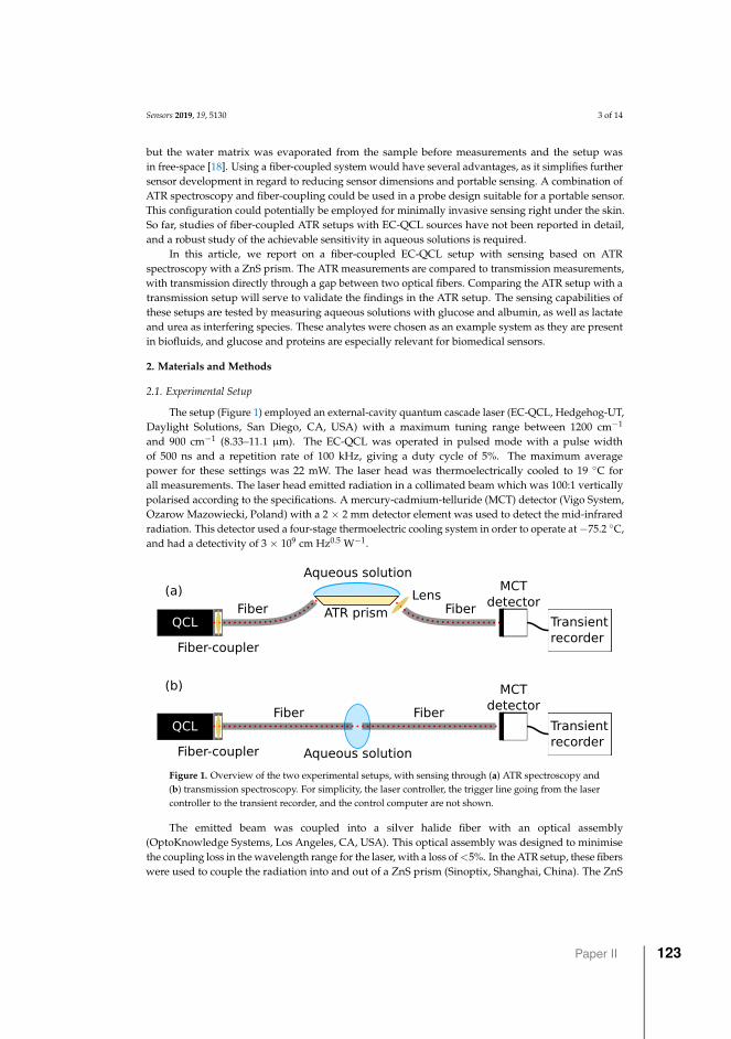
Sensors 2019, 19, 5130 3 of 14
but the water matrix was evaporated from the sample before measurements and the setup wasin free-space [18]. Using a fiber-coupled system would have several advantages, as it simplifies furthersensor development in regard to reducing sensor dimensions and portable sensing. A combination ofATR spectroscopy and fiber-coupling could be used in a probe design suitable for a portable sensor.This configuration could potentially be employed for minimally invasive sensing right under the skin.So far, studies of fiber-coupled ATR setups with EC-QCL sources have not been reported in detail,and a robust study of the achievable sensitivity in aqueous solutions is required.
In this article, we report on a fiber-coupled EC-QCL setup with sensing based on ATRspectroscopy with a ZnS prism. The ATR measurements are compared to transmission measurements,with transmission directly through a gap between two optical fibers. Comparing the ATR setup with atransmission setup will serve to validate the findings in the ATR setup. The sensing capabilities ofthese setups are tested by measuring aqueous solutions with glucose and albumin, as well as lactateand urea as interfering species. These analytes were chosen as an example system as they are presentin biofluids, and glucose and proteins are especially relevant for biomedical sensors.
2. Materials and Methods
2.1. Experimental Setup
The setup (Figure 1) employed an external-cavity quantum cascade laser (EC-QCL, Hedgehog-UT,Daylight Solutions, San Diego, CA, USA) with a maximum tuning range between 1200 cm−1
and 900 cm−1 (8.33–11.1 µm). The EC-QCL was operated in pulsed mode with a pulse widthof 500 ns and a repetition rate of 100 kHz, giving a duty cycle of 5%. The maximum averagepower for these settings was 22 mW. The laser head was thermoelectrically cooled to 19 ◦C forall measurements. The laser head emitted radiation in a collimated beam which was 100:1 verticallypolarised according to the specifications. A mercury-cadmium-telluride (MCT) detector (Vigo System,Ozarow Mazowiecki, Poland) with a 2 × 2 mm detector element was used to detect the mid-infraredradiation. This detector used a four-stage thermoelectric cooling system in order to operate at −75.2 ◦C,and had a detectivity of 3 × 109 cm Hz0.5 W−1.
QCL
MCTdetector
Transientrecorder
Fiber Fiber
Aqueous solution
QCL
(a)
(b)
QCL
MCTdetector
Transientrecorder
Fiber Fiber
Aqueous solution
ATR prism
Fiber-coupler
Fiber-coupler
Lens
Figure 1. Overview of the two experimental setups, with sensing through (a) ATR spectroscopy and(b) transmission spectroscopy. For simplicity, the laser controller, the trigger line going from the lasercontroller to the transient recorder, and the control computer are not shown.
The emitted beam was coupled into a silver halide fiber with an optical assembly(OptoKnowledge Systems, Los Angeles, CA, USA). This optical assembly was designed to minimisethe coupling loss in the wavelength range for the laser, with a loss of <5%. In the ATR setup, these fiberswere used to couple the radiation into and out of a ZnS prism (Sinoptix, Shanghai, China). The ZnS
Paper II 123

Sensors 2019, 19, 5130 4 of 14
prism was a trapezoid with 45 degree facets for in- and out-coupling of radiation. The top facet ofthe prism was 24 × 6 mm2, and the prism height was 2.4 mm. The silver halide fiber (Art photonics,Berlin, Germany) used for in-coupling had a core size of 400 µm, while the out-coupling fiber had acore size of 600 µm, both with optical losses of 0.2–0.3 dB/m. Radiation exiting from the ZnS prismwas focussed onto the out-coupling fiber using a ZnSe lens (Thorlabs, Newton, NJ, USA). In thetransmission measurements, the fibers were aligned and a 165 µm gap between the fibers was used forsensing. The transmission pathlength was chosen based on a trade-off between analyte absorbancesignal and the noise level, and was similar to the optimal pathlength found in other work [15].
Data acquisition was done with an analogue-to-digital converter card (M2p.5946-X4, 80 MS/s,16 bit, Spectrum Instrumentation, Großhansdorf, Germany). The digitiser was controlled with amodified driver written in C++, and operated via a GUI front-end written in Python. A triggersignal between the laser controller and the digitiser card was used to start the data acquisition foreach measurement. Spectra were acquired by operating the laser in scan-mode, where the laser wascontinuously tuned over a chosen wavelength range.
2.2. Data Processing
For each spectrum, a background measurement (I0) and a sample measurement (I) were recordedfor the 1200–925 cm−1 tuning range. Demineralised water was used for the background measurements.Each background and sample measurement consisted of ten scans over the tuning range. Spectrawere made by averaging over 255 laser pulses from the raw data, and then averaging over the10 acquired scans from each measurement, for the purpose of noise reduction. Each scan took 1 s toacquire with a tuning speed of 275 cm−1/s, and consisted of approximately 100,000 pulses. Eachspectrum was reduced to 390 data points after the spectral binning. From this, the absorbance spectraof the samples were calculated as A = −log(I/I0).
An alignment procedure was also performed on the spectra in order to correct for offset betweenscans and measurements. The scans were aligned to the first scan of each measurement by achi-squared minimisation algorithm. Subsequently, each sample measurement was aligned to abackground measurement.
Data analysis for prediction of analyte concentrations was done using a program developedin-house (Python). Partial least-squares (PLS) regression was used for prediction of glucoseconcentrations [29]. The data sets were standardised prior to PLSR by subtracting the mean andscaling to unit variance. Smoothing with a Savitzky–Golay filter was also applied as a pre-processingmethod [30]. The root-mean-square error of cross-validation (RMSECV) and the coefficient ofdetermination (R2) were used to evaluate the prediction accuracy of the regression. RMSECV wascalculated from either a leave-one-out cross-validation (LOOCV), leave-5-out cross-validation (L5OCV),or leave-one-dataset-out cross-validation (LDOCV).
We would like to note that RMSE-values are scale-dependent, which means that the RMSE willvary if different concentration ranges are used. As a result, RMSE-values are difficult to comparebetween studies if different concentration ranges are used. R2 has therefore been included as analternative evaluation metric.
2.3. Sample Overview
Aqueous solutions were made by dissolving the analytes in a phosphate-buffered saline (PBS)solution. PBS is a buffer solution that has ion concentrations matching the human body and helpsmaintain pH, and can be made by dissolving PBS tablets (VWR) in water. Glucose (D-(+)-glucose,Sigma Aldrich), albumin (bovine serum albumin, VWR), lactate (sodium L-lactate, Sigma Aldrich),and urea (Sigma Aldrich) were added to solutions in varying concentrations. 25 unique solutions weremade, with concentration ranges as shown in Table 1.
124 Publications
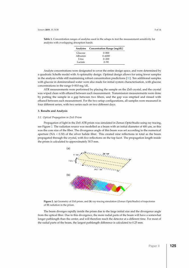
Sensors 2019, 19, 5130 5 of 14
Table 1. Concentration ranges of analytes used in the setups to test the measurement sensitivity foranalytes with overlapping absorption bands.
Analytes Concentration Range [mg/dL]
Glucose 0–800Albumin 0–6000
Urea 0–200Lactate 0–90
Analyte concentrations were designated to cover the entire design space, and were determined bya quadratic Scheffe model with A-optimality design. Optimal design allows for using fewer samplesin the analysis while still maintaining robust concentration predictions [31]. Ten additional sampleswith glucose in demineralised water were also made for initial system characterisation, with glucoseconcentrations in the range 0–810 mg/dL.
ATR measurements were performed by placing the sample on the ZnS crystal, and the crystalwas wiped clean with ethanol between each measurement. Transmission measurements were doneby putting the sample in a gap between two fibers, and the gap was emptied and rinsed withethanol between each measurement. For the two setup configurations, all samples were measured infour different series, with two series each on two different days.
3. Results and Analysis
3.1. Optical Propagation in ZnS Prism
Propagation of light in the ZnS ATR prism was simulated in Zemax OpticStudio using ray tracing,see Figure 2. The radiation source was modelled as a beam with an initial diameter of 400 µm, as thiswas the core size of the fiber. The divergence angle of this beam was set according to the numericalaperture (NA = 0.30) of the silver halide fiber. This created nine reflections in total as the beampropagated through the crystal, with five reflections on the top facet. The propagation length insidethe prism is calculated to approximately 30.5 mm.
(a)
(b)
Figure 2. (a) Geometry of ZnS prism, and (b) ray-tracing simulation (Zemax OpticStudio) of trajectoriesof IR radiation in the prism.
The beam diverges rapidly inside the prism due to the large initial size and the divergence anglefrom the optical fiber. Due to this divergence, the more radial parts of the beam will have a somewhatlonger pathlength than the center, and will therefore reach the detector at a different time. For most ofthe radial parts of the beam, the largest pathlength difference is calculated to 0.25 mm.
Paper II 125
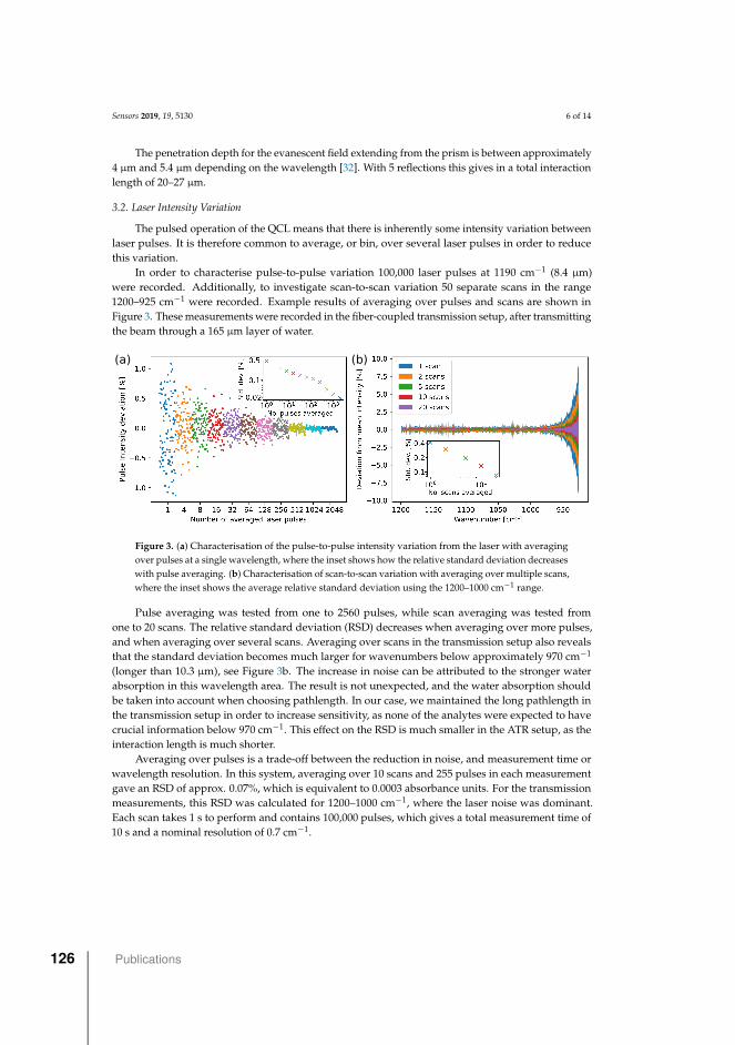
Sensors 2019, 19, 5130 6 of 14
The penetration depth for the evanescent field extending from the prism is between approximately4 µm and 5.4 µm depending on the wavelength [32]. With 5 reflections this gives in a total interactionlength of 20–27 µm.
3.2. Laser Intensity Variation
The pulsed operation of the QCL means that there is inherently some intensity variation betweenlaser pulses. It is therefore common to average, or bin, over several laser pulses in order to reducethis variation.
In order to characterise pulse-to-pulse variation 100,000 laser pulses at 1190 cm−1 (8.4 µm)were recorded. Additionally, to investigate scan-to-scan variation 50 separate scans in the range1200–925 cm−1 were recorded. Example results of averaging over pulses and scans are shown inFigure 3. These measurements were recorded in the fiber-coupled transmission setup, after transmittingthe beam through a 165 µm layer of water.
(a) (b)
Figure 3. (a) Characterisation of the pulse-to-pulse intensity variation from the laser with averagingover pulses at a single wavelength, where the inset shows how the relative standard deviation decreaseswith pulse averaging. (b) Characterisation of scan-to-scan variation with averaging over multiple scans,where the inset shows the average relative standard deviation using the 1200–1000 cm−1 range.
Pulse averaging was tested from one to 2560 pulses, while scan averaging was tested fromone to 20 scans. The relative standard deviation (RSD) decreases when averaging over more pulses,and when averaging over several scans. Averaging over scans in the transmission setup also revealsthat the standard deviation becomes much larger for wavenumbers below approximately 970 cm−1
(longer than 10.3 µm), see Figure 3b. The increase in noise can be attributed to the stronger waterabsorption in this wavelength area. The result is not unexpected, and the water absorption shouldbe taken into account when choosing pathlength. In our case, we maintained the long pathlength inthe transmission setup in order to increase sensitivity, as none of the analytes were expected to havecrucial information below 970 cm−1. This effect on the RSD is much smaller in the ATR setup, as theinteraction length is much shorter.
Averaging over pulses is a trade-off between the reduction in noise, and measurement time orwavelength resolution. In this system, averaging over 10 scans and 255 pulses in each measurementgave an RSD of approx. 0.07%, which is equivalent to 0.0003 absorbance units. For the transmissionmeasurements, this RSD was calculated for 1200–1000 cm−1, where the laser noise was dominant.Each scan takes 1 s to perform and contains 100,000 pulses, which gives a total measurement time of10 s and a nominal resolution of 0.7 cm−1.
126 Publications
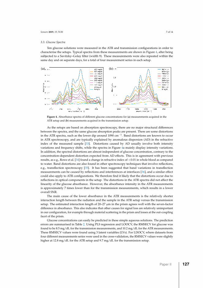
Sensors 2019, 19, 5130 7 of 14
3.3. Glucose Spectra
Ten glucose solutions were measured in the ATR and transmission configurations in order tocharacterise the setups. Typical spectra from these measurements are shown in Figure 4, after beingsubjected to a Savitzky–Golay filter (width 9). These measurements were also repeated within thesame day and on separate days, for a total of four measurement series in each setup.
(b)(a)
Figure 4. Absorbance spectra of different glucose concentrations for (a) measurements acquired in theATR setup and (b) measurements acquired in the transmission setup.
As the setups are based on absorption spectroscopy, there are no major structural differencesbetween the spectra, and the same glucose absorption peaks are present. There are some distortionsin the ATR spectra, such as the lower dip around 1090 cm−1. Band distortions are known to occurin ATR spectroscopy, and are typically explained by anomalous dispersion (AD) in the refractiveindex of the measured sample [33]. Distortions caused by AD usually involve both intensityvariations and frequency shifts, while the spectra in Figure 4a mainly display intensity variations.In addition, the spectral distortions are almost independent of glucose concentration, contrary to theconcentration-dependent distortion expected from AD effects. This is in agreement with previousresults, as e.g., Rowe et al. [34] found a change in refractive index of <0.01 in whole blood as comparedto water. Band distortions are also found in other spectroscopy techniques that involve reflections,e.g., transflection spectroscopy [35]. It has been suggested that band variations in transflectionmeasurements can be caused by reflections and interferences at interfaces [36], and a similar effectcould also apply to ATR configurations. We therefore find it likely that the distortions occur due toreflections in optical components in the setup. The distortions in the ATR spectra did not affect thelinearity of the glucose absorbance. However, the absorbance intensity in the ATR measurementsis approximately 7 times lower than for the transmission measurements, which results in a loweroverall SNR.
The main cause of the lower absorbance in the ATR measurements is the relatively shorterinteraction length between the radiation and the sample in the ATR setup versus the transmissionsetup. The estimated interaction length of 20–27 µm in the prism agrees well with the seven-factordifference in absorbance. This also indicates that other causes for signal loss are relatively unimportantin our configuration, for example through material scattering in the prism and losses at the out-couplingfacet of the prism.
Glucose concentrations can easily be predicted in these simple aqueous solutions. The predictionerrors are summarised in Table 2. Using PLS regression and LOOCV, the RMSECV for glucose wasfound to be 8.5 mg/dL for the transmission measurements, and 10.2 mg/dL for the ATR measurements.These RMSECV values were found using 3 latent variables (LVs). For LDOCV, where datasets fromfour different measurements series were used in the cross-validation, the RMSECV values were slightlyhigher at 12.8 mg/dL for the ATR setup and 9.7 mg/dL for the transmission setup.
Paper II 127
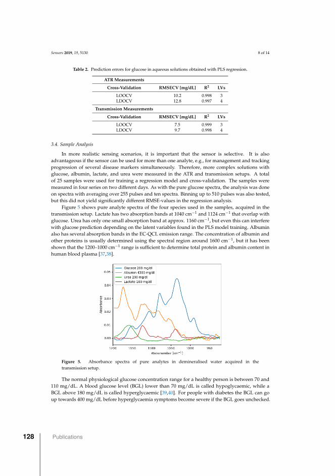
Sensors 2019, 19, 5130 8 of 14
Table 2. Prediction errors for glucose in aqueous solutions obtained with PLS regression.
ATR Measurements
Cross-Validation RMSECV [mg/dL] R2 LVs
LOOCV 10.2 0.998 3LDOCV 12.8 0.997 4
Transmission Measurements
Cross-Validation RMSECV [mg/dL] R2 LVs
LOOCV 7.5 0.999 3LDOCV 9.7 0.998 4
3.4. Sample Analysis
In more realistic sensing scenarios, it is important that the sensor is selective. It is alsoadvantageous if the sensor can be used for more than one analyte, e.g., for management and trackingprogression of several disease markers simultaneously. Therefore, more complex solutions withglucose, albumin, lactate, and urea were measured in the ATR and transmission setups. A totalof 25 samples were used for training a regression model and cross-validation. The samples weremeasured in four series on two different days. As with the pure glucose spectra, the analysis was doneon spectra with averaging over 255 pulses and ten spectra. Binning up to 510 pulses was also tested,but this did not yield significantly different RMSE-values in the regression analysis.
Figure 5 shows pure analyte spectra of the four species used in the samples, acquired in thetransmission setup. Lactate has two absorption bands at 1040 cm−1 and 1124 cm−1 that overlap withglucose. Urea has only one small absorption band at approx. 1160 cm−1, but even this can interferewith glucose prediction depending on the latent variables found in the PLS model training. Albuminalso has several absorption bands in the EC-QCL emission range. The concentration of albumin andother proteins is usually determined using the spectral region around 1600 cm−1, but it has beenshown that the 1200–1000 cm−1 range is sufficient to determine total protein and albumin content inhuman blood plasma [37,38].
Figure 5. Absorbance spectra of pure analytes in demineralised water acquired in thetransmission setup.
The normal physiological glucose concentration range for a healthy person is between 70 and110 mg/dL. A blood glucose level (BGL) lower than 70 mg/dL is called hypoglycaemic, while aBGL above 180 mg/dL is called hyperglycaemic [39,40]. For people with diabetes the BGL can goup towards 400 mg/dL before hyperglycaemia symptoms become severe if the BGL goes unchecked.
128 Publications
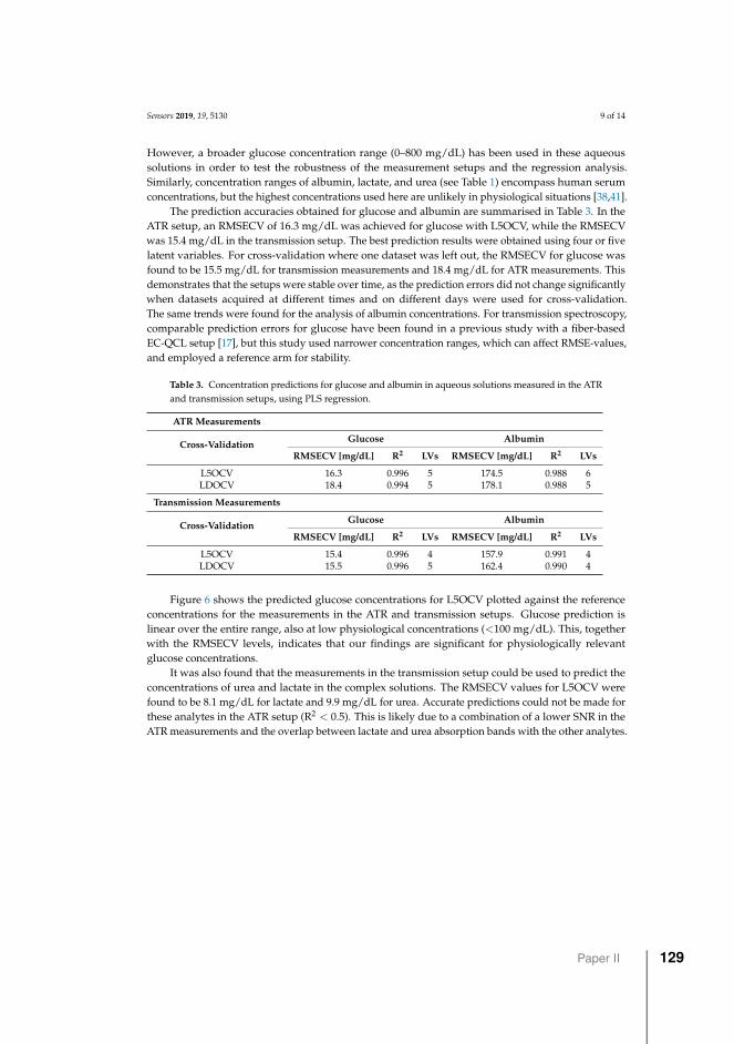
Sensors 2019, 19, 5130 9 of 14
However, a broader glucose concentration range (0–800 mg/dL) has been used in these aqueoussolutions in order to test the robustness of the measurement setups and the regression analysis.Similarly, concentration ranges of albumin, lactate, and urea (see Table 1) encompass human serumconcentrations, but the highest concentrations used here are unlikely in physiological situations [38,41].
The prediction accuracies obtained for glucose and albumin are summarised in Table 3. In theATR setup, an RMSECV of 16.3 mg/dL was achieved for glucose with L5OCV, while the RMSECVwas 15.4 mg/dL in the transmission setup. The best prediction results were obtained using four or fivelatent variables. For cross-validation where one dataset was left out, the RMSECV for glucose wasfound to be 15.5 mg/dL for transmission measurements and 18.4 mg/dL for ATR measurements. Thisdemonstrates that the setups were stable over time, as the prediction errors did not change significantlywhen datasets acquired at different times and on different days were used for cross-validation.The same trends were found for the analysis of albumin concentrations. For transmission spectroscopy,comparable prediction errors for glucose have been found in a previous study with a fiber-basedEC-QCL setup [17], but this study used narrower concentration ranges, which can affect RMSE-values,and employed a reference arm for stability.
Table 3. Concentration predictions for glucose and albumin in aqueous solutions measured in the ATRand transmission setups, using PLS regression.
ATR Measurements
Cross-Validation Glucose Albumin
RMSECV [mg/dL] R2 LVs RMSECV [mg/dL] R2 LVs
L5OCV 16.3 0.996 5 174.5 0.988 6LDOCV 18.4 0.994 5 178.1 0.988 5
Transmission Measurements
Cross-Validation Glucose Albumin
RMSECV [mg/dL] R2 LVs RMSECV [mg/dL] R2 LVs
L5OCV 15.4 0.996 4 157.9 0.991 4LDOCV 15.5 0.996 5 162.4 0.990 4
Figure 6 shows the predicted glucose concentrations for L5OCV plotted against the referenceconcentrations for the measurements in the ATR and transmission setups. Glucose prediction islinear over the entire range, also at low physiological concentrations (<100 mg/dL). This, togetherwith the RMSECV levels, indicates that our findings are significant for physiologically relevantglucose concentrations.
It was also found that the measurements in the transmission setup could be used to predict theconcentrations of urea and lactate in the complex solutions. The RMSECV values for L5OCV werefound to be 8.1 mg/dL for lactate and 9.9 mg/dL for urea. Accurate predictions could not be made forthese analytes in the ATR setup (R2 < 0.5). This is likely due to a combination of a lower SNR in theATR measurements and the overlap between lactate and urea absorption bands with the other analytes.
Paper II 129
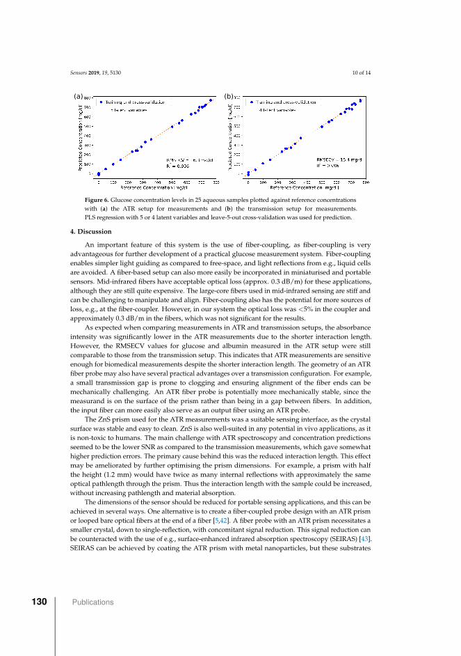
Sensors 2019, 19, 5130 10 of 14
(a) (b)
Figure 6. Glucose concentration levels in 25 aqueous samples plotted against reference concentrationswith (a) the ATR setup for measurements and (b) the transmission setup for measurements.PLS regression with 5 or 4 latent variables and leave-5-out cross-validation was used for prediction.
4. Discussion
An important feature of this system is the use of fiber-coupling, as fiber-coupling is veryadvantageous for further development of a practical glucose measurement system. Fiber-couplingenables simpler light guiding as compared to free-space, and light reflections from e.g., liquid cellsare avoided. A fiber-based setup can also more easily be incorporated in miniaturised and portablesensors. Mid-infrared fibers have acceptable optical loss (approx. 0.3 dB/m) for these applications,although they are still quite expensive. The large-core fibers used in mid-infrared sensing are stiff andcan be challenging to manipulate and align. Fiber-coupling also has the potential for more sources ofloss, e.g., at the fiber-coupler. However, in our system the optical loss was <5% in the coupler andapproximately 0.3 dB/m in the fibers, which was not significant for the results.
As expected when comparing measurements in ATR and transmission setups, the absorbanceintensity was significantly lower in the ATR measurements due to the shorter interaction length.However, the RMSECV values for glucose and albumin measured in the ATR setup were stillcomparable to those from the transmission setup. This indicates that ATR measurements are sensitiveenough for biomedical measurements despite the shorter interaction length. The geometry of an ATRfiber probe may also have several practical advantages over a transmission configuration. For example,a small transmission gap is prone to clogging and ensuring alignment of the fiber ends can bemechanically challenging. An ATR fiber probe is potentially more mechanically stable, since themeasurand is on the surface of the prism rather than being in a gap between fibers. In addition,the input fiber can more easily also serve as an output fiber using an ATR probe.
The ZnS prism used for the ATR measurements was a suitable sensing interface, as the crystalsurface was stable and easy to clean. ZnS is also well-suited in any potential in vivo applications, as itis non-toxic to humans. The main challenge with ATR spectroscopy and concentration predictionsseemed to be the lower SNR as compared to the transmission measurements, which gave somewhathigher prediction errors. The primary cause behind this was the reduced interaction length. This effectmay be ameliorated by further optimising the prism dimensions. For example, a prism with halfthe height (1.2 mm) would have twice as many internal reflections with approximately the sameoptical pathlength through the prism. Thus the interaction length with the sample could be increased,without increasing pathlength and material absorption.
The dimensions of the sensor should be reduced for portable sensing applications, and this can beachieved in several ways. One alternative is to create a fiber-coupled probe design with an ATR prismor looped bare optical fibers at the end of a fiber [5,42]. A fiber probe with an ATR prism necessitates asmaller crystal, down to single-reflection, with concomitant signal reduction. This signal reduction canbe counteracted with the use of e.g., surface-enhanced infrared absorption spectroscopy (SEIRAS) [43].SEIRAS can be achieved by coating the ATR prism with metal nanoparticles, but these substrates
130 Publications
Sensors 2019, 19, 5130 11 of 14
often have difficulties with stability and reproducibility. Another option is to fabricate micrometerstructures onto the sampling facet of the ATR crystal. Such structures on ATR crystals have beenshown to enhance the absorption signal up to a factor of 10–100 [44]. On the other hand, evanescentsensing with looped fibers can be used to maintain a long interaction length, while avoiding the needfor surface engineering. However, looped optical fibers are fragile and would likely need to be encasedin a flow-through chamber for stability.
For a portable sensor another avenue of size reduction is to use a smaller QCL source. As EC-QCLsare a recent commercial product, they will likely become somewhat smaller in the future. However,for personal and wearable sensors such as glucose sensors the dimensions must be reduced evenfurther. One option is to use a few single-wavelength laser chips in order to target the most informativewavenumbers. It has been suggested several times that only a few wavenumbers are needed for anadequately accurate prediction of glucose concentrations, also for non-invasive measurements [27,41].Robust measurements using a few wavenumbers must be tested thoroughly in realistic conditions inorder to confirm this.
This study has demonstrated the use of an EC-QCL on samples with glucose and albumin asan example. However, we would like to emphasise that measurements with QCLs in applicationsfor biomedicine and biotechnology have many additional potential uses where MIR spectroscopywith high sensitivity could replace other benchtop and portable measurement methods. In research,QCLs have so far also been used for breath analysis in order to detect disease markers, and inhistopathology to e.g., detect cancer [2,45,46]. EC-QCLs also have many potential uses where they canoutperform methods that today require labelling or reagents, such as protein analysis, cell studies andpharmaceutical and food analysis [47].
5. Conclusions
A fiber-coupled EC-QCL was used for multianalyte sensing in both ATR and transmissionmeasurement configurations. Glucose and albumin concentrations were determined in solutions thatalso contained urea and lactate, with promising results. The RMSECV values for glucose were wellunder 20 mg/dL, even though a broad concentration range was used. The low cross-validation errorswere also very promising considering the addition of other analytes with overlapping absorption bands.The simultaneous determination of several biomarkers is relevant for further sensor development,and the use of optimal design for analyte concentrations allowed for investigating the entire designspace for four analytes with relatively few samples, while still obtaining robust analyte predictions.This is advantageous for testing and characterisation of sensor setups, as fewer total measurements areneeded while precision is still maintained.
The intensity variation in the laser pulses was evaluated, and was decreased to an acceptable levelwith averaging while the measurement time did not exceed 10 s. Both setups were mechanically stableover time, and it was shown that measurements from different days could be used for concentrationpredictions. This concept study should be further assessed by measuring and analysing larger datasets,including samples of bodily fluids. As the ATR setup is fiber-coupled, it lends itself well to furtherdevelopments towards a miniaturised and portable sensor.
Future developments include improving the SNR in the ATR measurements through optimisationsof the prism dimensions. We will also investigate the feasibility of using a thin silicon crystal withmicrometer surface structures for signal enhancement as an ATR element. This could be a viablealternative for minimally invasive or non-invasive fiber-probe sensors for on-demand sensing.
Author Contributions: I.L.J. and K.S. conceptualised and designed the experiments; I.L.J and K.S. performed theexperiments; I.L.J. implemented the code for the analysis and analysed the results; I.L.J. prepared the originaldraft; A.A. and D.R.H. supervised and reviewed the paper; A.A. and D.R.H. acquired funding for the project.
Funding: This work was supported by the Research Council of Norway through the Double IntraperitonealArtificial Pancreas project, grant number 248872. The project is part of Center for Digital Life Norway and is alsosupported by the Research Council of Norway’s grant 248810.
Paper II 131
Sensors 2019, 19, 5130 12 of 14
Conflicts of Interest: The authors declare no conflict of interest.
References
1. Kosterev, A.; Wysocki, G.; Bakhirkin, Y.; So, S.; Lewicki, R.; Fraser, M.; Tittel, F.; Curl, R.F. Applicationof quantum cascade lasers to trace gas analysis. Appl. Phys. B Lasers Opt. 2008, 90, 165–176.s00340-007-2846-9. [CrossRef]
2. Schwaighofer, A.; Brandstetter, M.; Lendl, B. Quantum cascade lasers (QCLs) in biomedical spectroscopy.Chem. Soc. Rev. 2017, 46, 5903–5924. [CrossRef]
3. De Bruyne, S.; Speeckaert, M.M.; Delanghe, J.R. Applications of mid-infrared spectroscopy in the clinicallaboratory setting. Crit. Rev. Clin. Lab. Sci. 2018, 55, 1–20. [CrossRef]
4. Lambrecht, A.; Beyer, T.; Hebestreit, K.; Mischler, R.; Petrich, W. Continuous Glucose Monitoring by Meansof Fiber-Based, Mid-Infrared Laser Spectroscopy. Appl. Spectrosc. 2006, 60, 729–736. [CrossRef]
5. Yu, S.; Li, D.; Chong, H.; Sun, C.; Yu, H.; Xu, K. In vitro glucose measurement using tunable mid-infraredlaser spectroscopy combined with fiber-optic sensor. Biomed. Opt. Express 2013, 5, 275–286. [CrossRef]
6. Yao, Y.; Hoffman, A.J.; Gmachl, C.F. Mid-infrared quantum cascade lasers. Nat. Photonics 2012, 6, 432–439.[CrossRef]
7. Sandner, T.; Kenda, A.; Drabe, C.; Schenk, H.; Scherf, W. Miniaturized FTIR-spectrometer based on opticalMEMS translatory actuator. In MOEMS and Miniaturized Systems VI; Dickensheets, D.L., Gogoi, B.P.,Schenk, H., Eds.; International Society for Optics and Photonics: Bellingham, WA, USA, 2007; Volume 6466,pp. 1–12. [CrossRef]
8. Khalil, D.; Sabry, Y.; Omran, H.; Medhat, M.; Hafez, A.; Saadany, B. Characterization of MEMS FTIRspectrometer. In MOEMS and Miniaturized Systems X; Schenk, H., Piyawattanametha, W., Eds.; InternationalSociety for Optics and Photonics: Bellingham, WA, USA, 2011; Volume 7930, pp. 1–10. [CrossRef]
9. Turner, A.P.F. Biosensors—Sense and sensibility. Chem. Soc. Rev. 2013, 42, 3184–3196. [CrossRef]10. Heller, A.; Feldman, B. Electrochemical Glucose Sensors and Their Applications in Diabetes Management.
Chem. Rev. 2008, 108, 2482–2505. [CrossRef] [PubMed]11. Valdes, T.I.; Moussy, F. In Vitro and In Vivo Degradation of Glucose Oxidase Enzyme Used for an Implantable
Glucose Biosensor. Diabetes Technol. Ther. 2000, 2, 367–376. [CrossRef] [PubMed]12. Scholten, K.; Meng, E. A review of implantable biosensors for closed-loop glucose control and other drug
delivery applications. Int. J. Pharm. 2018, 544, 319–344. [CrossRef] [PubMed]13. Jernelv, I.L.; Milenko, K.; Fuglerud, S.S.; Hjelme, D.R.; Ellingsen, R.; Aksnes, A. A review of optical methods
for continuous glucose monitoring. Appl. Spectrosc. Rev. 2018, 54, 1–30. [CrossRef]14. Martin, W.B.; Mirov, S.; Venugopalan, R. Middle Infrared, Quantum Cascade Laser Optoelectronic
Absorption System for Monitoring Glucose in Serum. Appl. Spectrosc. 2005, 59, 881–884.0003702054411580. [CrossRef] [PubMed]
15. Brandstetter, M.; Volgger, L.; Genner, A.; Jungbauer, C.; Lendl, B. Direct determination of glucose, lactateand triglycerides in blood serum by a tunable quantum cascade laser-based mid-IR sensor. Appl. Phys. B2013, 110, 233–239. [CrossRef]
16. Kino, S.; Omori, S.; Katagiri, T.; Matsuura, Y. Hollow optical-fiber based infrared spectroscopy formeasurement of blood glucose level by using multi-reflection prism. Biomed. Opt. Express 2016, 7, 701–708.[CrossRef] [PubMed]
17. Haase, K.; Müller, N.; Petrich, W. Towards a continuous glucose monitoring system using tunablequantum cascade lasers. In Biomedical Vibrational Spectroscopy 2018: Advances in Research andIndustry; Mahadevan-Jansen, A., Petrich, W., Eds.; International Society for Optics and Photonics:Bellingham, WA, USA, 2018; Volume 1049008, pp. 1–8. [CrossRef]
18. Haas, J.; Catalán, E.V.; Piron, P.; Karlsson, M.; Mizaikoff, B. Infrared spectroscopy based on broadly tunablequantum cascade lasers and polycrystalline diamond waveguides. Analyst 2018, 143, 5112–5119. [CrossRef]
19. Isensee, K.; Müller, N.; Pucci, A.; Petrich, W. Towards a quantum cascade laser-based implant for thecontinuous monitoring of glucose. Analyst 2018, 143, 6025–6036. [CrossRef]
132 Publications

Sensors 2019, 19, 5130 13 of 14
20. Grafen, M.; Delbeck, S.; Busch, H.; Heise, H.M.; Ostendorf, A. Evaluation and benchmarking of anEC-QCL-based mid-infrared spectrometer for monitoring metabolic blood parameters in critical care units.In Optical Diagnostics and Sensing XVIII: Toward Point-of-Care Diagnostics; Coté, G.L., Ed.; International Societyfor Optics and Photonics: Bellingham, WA, USA, 2018; Volume 10501, pp. 1–9. [CrossRef]
21. Vrancic, C.; Kröger, N.; Gretz, N.; Neudecker, S.; Pucci, A.; Petrich, W. A Quantitative Look Inside the Body:Minimally Invasive Infrared Analysis in Vivo. Anal. Chem. 2014, 86, 10511–10514. [CrossRef]
22. Pleitez, M.A.; Lieblein, T.; Bauer, A.; Hertzberg, O.; von Lilienfeld-Toal, H.; Mäntele, W. In Vivo NoninvasiveMonitoring of Glucose Concentation in Human Epidermis by Mid-Infrared Pulsed PhotoacousticSpectroscopy. Anal. Chem. 2013, 85, 1013–1020. [CrossRef]
23. Liakat, S.; Bors, K.A.; Xu, L.; Woods, C.M.; Doyle, J.; Gmachl, C.F. Noninvasive in vivo glucose sensing onhuman subjects using mid-infrared light. Biomed. Opt. Express 2014, 5, 2397–2404. [CrossRef]
24. Kottmann, J.; Rey, J.M.; Sigrist, M.W. Mid-Infrared Photoacoustic Detection of Glucose in Human Skin:Towards Non-Invasive Diagnostics. Sensors 2016, 16, 1663. [CrossRef]
25. Hertzberg, O.; Bauer, A.; Küderle, A.; Pleitez, M.A.; Mäntele, W. Depth-selective photothermal IRspectroscopy of skin: Potential application for non-invasive glucose measurement. Analyst 2017, 142, 495–502.[CrossRef] [PubMed]
26. Sim, J.Y.; Ahn, C.G.; Jeong, E.J.; Kim, B.K. In vivo Microscopic Photoacoustic Spectroscopy forNon-Invasive Glucose Monitoring Invulnerable to Skin Secretion Products. Sci. Rep. 2018, 8, 1–11.s41598-018-19340-y. [CrossRef] [PubMed]
27. Kasahara, R.; Kino, S.; Soyama, S.; Matsuura, Y. Noninvasive glucose monitoring using mid-infraredabsorption spectroscopy based on a few wavenumbers. Biomed. Opt. Express 2018, 9, 289–302. [CrossRef][PubMed]
28. Matsuura, Y.; Koyama, T. Non-invasive blood glucose measurement using quantum cascade lasers.In Quantum Sensing and Nano Electronics and Photonics XVI; Razeghi, M., Lewis, J.S., Tournié, E.,Khodaparast, G.A., Eds.; International Society for Optics and Photonics: Bellingham, WA, USA, 2019;Volume 1092606, pp. 1–7. [CrossRef]
29. Martens, H.; Martens, M. Multivariate Analysis of Quality An Introduction; John Wiley & Sons: Hoboken, NJ,USA, 2001.
30. Rinnan, Å.; Van den Berg, F.; Engelsen, S.B. Review of the most common pre-processing techniques fornear-infrared spectra. Trends Anal. Chem. 2009, 28, 1201–1222. [CrossRef]
31. Sinha, B.K.; Mandal, N.K.; Pal, M.; Das, P. Optimal Mixture Experiments; Springer: Connaught Place, India,2014. [CrossRef]
32. Averett, L.A.; Griffiths, P.R.; Nishikida, K. Effective path length in attenuated total reflection spectroscopy.Anal. Chem. 2008, 80, 3045–3049. [CrossRef]
33. Boulet-Audet, M.; Buffeteau, T.; Boudreault, S.; Daugey, N.; Pézolet, M. Quantitative Determination of BandDistortions in Diamond Attenuated Total Reflectance Infrared Spectra. J. Phys. Chem. B 2010, 114, 8255–8261.[CrossRef]
34. Rowe, D.J.; Smith, D.; Wilkinson, J.S. Complex refractive index spectra of whole blood and aqueoussolutions of anticoagulants, analgesics and buffers in the mid-infrared. Sci. Rep. 2017, 7, 7356.s41598-017-07842-0. [CrossRef]
35. Miljkovic, M.; Bird, B.; Diem, M. Line shape distortion effects in infrared spectroscopy. Analyst 2012,137, 3954–3964. [CrossRef]
36. Lee, J. On the non-existence of the so-called “electric field standing wave effect” in transflection FTIR spectra.Vib. Spectrosc. 2017, 90, 104–111. [CrossRef]
37. Schwaighofer, A.; Montemurro, M.; Freitag, S.; Kristament, C.; Culzoni, M.J.; Lendl, B. Beyond FourierTransform Infrared Spectroscopy: External Cavity Quantum Cascade Laser-Based Mid-infrared TransmissionSpectroscopy of Proteins in the Amide I and Amide II Region. Anal. Chem. 2018, 90, 7072–7079.acs.analchem.8b01632. [CrossRef]
38. Brandstetter, M.; Sumalowitsch, T.; Genner, A.; Posch, A.E.; Herwig, C.; Drolz, A.; Fuhrmann, V.; Perkmann,T.; Lendl, B. Reagent-free monitoring of multiple clinically relevant parameters in human blood plasmausing a mid-infrared quantum cascade laser based sensor system. Analyst 2013, 138, 4022–4028. [CrossRef][PubMed]
Paper II 133
Sensors 2019, 19, 5130 14 of 14
39. Battelino, T.; Conget, I.; Olsen, B.; Schütz-Fuhrmann, I.; Hommel, E.; Hoogma, R.; Schierloh, U.; Sulli, N.;Bolinder, J. The use and efficacy of continuous glucose monitoring in type 1 diabetes treated with insulinpump therapy: A randomised controlled trial. Diabetologia 2012, 55, 3155–3162. [CrossRef] [PubMed]
40. Breton, M.; Farret, A.; Bruttomesso, D.; Anderson, S.; Magni, L.; Patek, S.; Man, C.D.; Place, J.; Demartini, S.;Del Favero, S.; et al. Fully Integrated Artificial Pancreas in Type 1 Diabetes: Modular Closed-Loop GlucoseControl Maintains Near Normoglycemia. Diabetes 2012, 61, 2230–2237. [CrossRef] [PubMed]
41. Martin, W.B.; Mirov, S.; Venugopalan, R. Using two discrete frequencies within the middle infrared toquantitatively determine glucose in serum. J. Biomed. Opt. 2002, 7, 613–617. [CrossRef]
42. Matsuura, Y.; Kino, S.; Katagiri, T. Hollow-fiber-based flexible probe for remote measurement of infraredattenuated total reflection. Appl. Opt. 2009, 48, 5396–5400. [CrossRef]
43. Andvaag, I.R.; Morhart, T.A.; Clarke, O.J.R.; Burgess, I.J. Hybrid Gold—Conductive Metal Oxide Films forAttenuated Total Reflectance Surface Enhanced Infrared Absorption Spectroscopy. ACS Appl. Nano Mater.2019, 2, 1274–1284. [CrossRef]
44. Sykora, L.; Müller, A.; Kondratiev, A.; Roth, A.; Mozin, V.; Fehr, A.; Zörnack, G. Silicon ATR crystalwith subwavelength structures optimized for blood analysis. In Optical Fibers and Sensors for MedicalDiagnostics and Treatment Applications XIX; Gannot, I., Ed.; International Society for Optics and Photonics:Bellingham, WA, USA, 2019; Volume 10872F, pp. 1–8. [CrossRef]
45. Henderson, B.; Khodabakhsh, A.; Metsälä, M.; Ventrillard, I.; Schmidt, F.M.; Romanini, D.; Ritchie, G.A.;te Lintel Hekkert, S.; Briot, R.; Risby, T.; et al. Laser spectroscopy for breath analysis: Towards clinicalimplementation. Appl. Phys. B Lasers Opt. 2018, 124, 1–21. [CrossRef]
46. Kuepper, C.; Kallenbach-Thieltges, A.; Juette, H.; Tannapfel, A.; Großerueschkamp, F.; Gerwert, K. QuantumCascade Laser-Based Infrared Microscopy for Label-Free and Automated Cancer Classification in TissueSections. Sci. Rep. 2018, 8, 7717. [CrossRef]
47. Lambrecht, A.; Pfeifer, M.; Konz, W.; Herbst, J.; Axtmann, F. Broadband spectroscopy with external cavityquantum cascade lasers beyond conventional absorption measurements. Analyst 2014, 139, 2070–2078.[CrossRef]
c© 2019 by the authors. Licensee MDPI, Basel, Switzerland. This article is an open accessarticle distributed under the terms and conditions of the Creative Commons Attribution(CC BY) license (http://creativecommons.org/licenses/by/4.0/).
134 Publications

Paper IIIMid-infrared spectroscopy with a fiber-coupled tuneable quantum cascade laserfor glucose sensingI.L. Jernelv, K. Strøm, D.R. Hjelme, A. AksnesProceedings of SPIE 11233, Optical Fibers and Sensors for Medical Diagnostics andTreatment Applications XX, 1123311, 2020.
Paper III 135

Mid-infrared spectroscopy with a fiber-coupled tuneablequantum cascade laser for glucose sensing
Ine L. Jernelv∗, Karina Strøm, Dag Roar Hjelme, and Astrid Aksnes
Department of Electronic Systems, Norwegian University of Science and Technology (NTNU),O.S. Bragstads plass 2A, 7491 Trondheim, Norway
ABSTRACT
A fiber-coupled transmission spectroscopy setup using a pulsed external-cavity quantum cascade laser (EC-QCL,1200-900 cm−1) has been developed and demonstrated for measurements of aqueous solutions. The system hasbeen characterised with regard to the laser noise and optimal optical pathlength. Solutions with glucose were usedto further test the setup, and glucose concentrations down to physiologically relevant levels (0-600 mg/dL) wereinvestigated. Albumin, lactate, urea, and fructose in various concentrations were added as interfering substancesas their absorption bands overlap with those of glucose, and because they may be of interest in a clinical setting.Analyte concentrations were predicted using partial least-squares (PLS) regression, and the root-mean-squareerror of cross-validation for glucose was 10.7 mg/dL. The advantages of using a convolutional neural network(CNN) for regression analysis in comparison to the PLS regression were also shown. The application of a CNNgave an improved prediction error (8.3 mg/dL), and was used to identify important spectral regions. Theseresults are comparable to state-of-the-art enzymatic glucose sensors, and are encouraging for further research onoptics-based glucose sensors.
Keywords: Quantum cascade laser, mid-infrared spectroscopy, biomedical sensing, laser spectroscopy, glucose
1. INTRODUCTION
The research effort on biomedical sensors is growing and rapidly developing, with blood glucose monitoringdominating the market for biomedical sensors.1 Glucose sensors are vital for diabetic patients, as these patientshave to monitor their blood glucose level in order to prevent long- and short-term complications. Most commercialglucose sensors today base their measurements on enzymatic reactions, and can be used either for finger-pricktests, or for minimally invasive continuous glucose monitoring (CGM). These sensors suffer a loss of accuracyand reliability over time due to sensor and enzyme degradation, and must typically be changed every 1-2 weeks.Optical spectroscopy may be a better alternative for CGM, as it is reagent-free and non-destructive.
Several research groups have worked with systems for biomedical laser spectroscopy in the mid-infrared fol-lowing the commerical availability of EC-QCLs. These systems have mainly used either free-space configurationswith liquid samples in transmission cells,2,3 or fiber-coupled setups with either transmission, reflectance, orattenuated total reflection (ATR) sensing modalities.4–7 Fiber-coupled setups are more practical for portablesensor development, while free-space setups can potentially be used for larger systems in e.g. intensive care.However, there have been few detailed studies using EC-QCLs as sources in fiber-coupled configurations.
In this study we present a fiber-coupled spectroscopy setup aimed at continuous glucose monitoring, witha broadly tuneable EC-QCL as a source. The system noise as a function of pathlength is characterised. Theperformance of the system is tested using aqueous solutions with glucose and several analytes with overlappingabsorption bands. We also show an application of a convolutional neural network as a method for regressionanalysis, and compare its performance to standard partial least-squares regression.
∗ [email protected]; phone +47 73594400
Optical Fibers and Sensors for Medical Diagnostics and Treatment Applications XX, edited by Israel GannotProc. of SPIE Vol. 11233, 1123311 · © 2020 SPIE · CCC code: 1605-7422/20/$21 · doi: 10.1117/12.2543984
Proc. of SPIE Vol. 11233 1123311-1
Downloaded From: https://www.spiedigitallibrary.org/conference-proceedings-of-spie on 23 Feb 2020Terms of Use: https://www.spiedigitallibrary.org/terms-of-use
Paper III 137
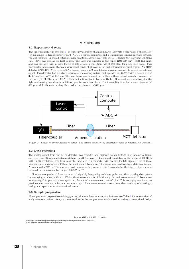
2. METHODS
2.1 Experimental setup
The experimental setup (see Fig. 1) in this study consisted of a mid-infrared laser with a controller, a photodetec-tor, an analog-to-digital converter card (ADC), a control computer, and a transmission sensing interface betweentwo optical fibers. A pulsed external-cavity quantum cascade laser (EC-QCL, Hedgehog-UT, Daylight SolutionsInc., USA) was used as the light source. The laser was tuneable in the range 1200-900 cm−1 (8.33-11.1 µm),and was operated with a pulse length of 500 ns and a repetition rate of 100 kHz, for a 5% duty cycle. Thiswavelength range covers the main vibrational bands of glucose in the mid-infrared fingerprint region. An MCTdetector (PCI-4TE, Vigo System S.A., Poland) with a 2x2 mm detector element was used to detect the infraredsignal. This detector had a 4-stage thermoelectric cooling system, and operated at -75.2◦C with a detectivity of3×109 cmHz1/2W−1 at 10.6 µm. The laser beam was focussed into a fiber with an optical assembly mounted onthe laser (OKSI Fibers Inc., USA). Silver halide fibers (Art photonics GmbH, Germany) were used to guide thelight and sensing was done in a 200 µm gap between two fibers. The in-coupling fiber had a core diameter of400 µm, while the out-coupling fiber had a core diameter of 600 µm.
Figure 1: Sketch of the transmission setup. The arrows indicate the direction of data or information transfer.
2.2 Data recording
The analog signal from the MCT detector was recorded and digitised by an M2p.5946-x4 analog-to-digitalconverter card (Spectrum-Instrumentation GmbH, Germany). This board could digitise the signal at 80 MS/swith 16 bit resolution. The laser controller had a DB-15 connector with 15 pins for I/O signals. One of thesepins generated a rising edge TTL at the start of each laser scan. This signal was used to trigger data acquisition.A scan speed of 275 cm−1/s was used, and data recording was active for 1 second after the trigger. Spectra wererecorded in the wavenumber range 1200-925 cm−1.
Spectra were produced from the detected signal by integrating each laser pulse, and then creating data pointsby averaging n pulses, with n = 255 for these measurements. Additionally, for each measurement 10 laser scanswere averaged to produce a raw spectrum, for a total measurement time of 10 s. This averaging was found toyield low measurement noise in a previous study.7 Final measurement spectra were then made by subtracting abackground spectrum of demineralised water.
2.3 Sample preparation
25 samples were prepared containing glucose, albumin, lactate, urea, and fructose, see Table 1 for an overview ofanalyte concentrations. Analyte concentrations in the samples were randomised according to an optimal design
Proc. of SPIE Vol. 11233 1123311-2
Downloaded From: https://www.spiedigitallibrary.org/conference-proceedings-of-spie on 23 Feb 2020Terms of Use: https://www.spiedigitallibrary.org/terms-of-use
138 Publications

model, in order to maintain experimental robustness with relatively few samples. A quadratic Scheffe modelwith A-optimality design was used for this sample set.
Analytes were dissolved in a phosphate-buffered saline (PBS) solution, which was made from PBS tabletsand demineralised water. PBS is a solution with ion concentrations similar to the concentrations in the humanbody, and works as a buffer to maintain a constant pH. A separate set of seven samples with only glucose indemineralised water was prepared, with a concentration range of 0-500 mg/dL.
Table 1: Concentration ranges for analytes in the complex aqueous solutions.
Analyte Concentration range
Glucose 0-600 mg/dL
Albumin 0-40 g/L
Lactate 0-250 mg/dL
Urea 0-250 mg/dL
Fructose 0-250 mg/dL
The additional analytes in the complex solutions were included based on their physiological relevance, as theyare present in blood plasma and interstitial fluid in humans. The concentrations of lactate, urea, and fructoseare exaggerated compared to physiological concentrations in order to increase the interference with the glucoselevels.
2.4 Data analysis
All data analysis in this study was done with the freely available software SpecAnalysis, which is availableon Github (https://github.com/jernelv/SpecAnalysis). This software is written in the Python programminglanguage, and provides a system for pre-processing, feature selection, and multivariate analysis of spectral data.
2.4.1 Standard regression analysis
The absorbance spectra acquired from the different solutions were first analysed with partial least-squares (PLS)regression. All samples were measured five times over a period of two weeks, giving five separate datasets.Analyte prediction was evaluated with root-mean-square error of cross-validation (RMSECV), and additionallywith the coefficient of determination (R2), as RMSE-values are scale-dependent. Cross-validation (CV) was donewith either leave-one-out (LOOCV) within datasets, or leave-one-dataset-out (LDOCV) between datasets.
The samples containing only glucose were analysed with PLS regression using 1 latent variable. PLS regressionwith 6 latent variables was used for the complex solutions. The data was mean centered and scaled prior to theregression analysis, and no other pre-processing was used.
2.4.2 Convolutional neural network
For further investigation of the acquired spectra we used a convolutional neural network (CNN) for concentrationprediction. CNNs are a type of data mining model commonly used for e.g. image analysis, and have recently beenapplied to one-dimensional vibrational spectra.8 CNNs are a variant of artificial neural networks (ANNs), whichhave previously been used for e.g. concentration prediction of glucose data from FTIR spectroscopy.9 TheseANNs used fully connected layers instead of convolutional layers, and had issues with overfitting on spectraldata.
Neural networks are based on connected artificial neurons, where each neuron has an activation function thattransforms an input into an output. These neurons are arranged in layers (see Fig. 2), which can be divided intoinput, output, and hidden layers. In standard ANNs the output of a neuron is used as input in every neuron inthe next layer, giving fully connected layers. In a CNN the input is convolved using one or more kernel functions,which effectively reduces the number of times the output is used as an input in the next layer. This gives fewerconnections and hidden variables in total, and CNNs are therefore computationally faster and are less prone tooverfitting than equivalent fully-connected models. Neurons are connected together with weighted connections,which are set to a random initial value. The weights are then adjusted during the training phase.
Proc. of SPIE Vol. 11233 1123311-3
Downloaded From: https://www.spiedigitallibrary.org/conference-proceedings-of-spie on 23 Feb 2020Terms of Use: https://www.spiedigitallibrary.org/terms-of-use
Paper III 139
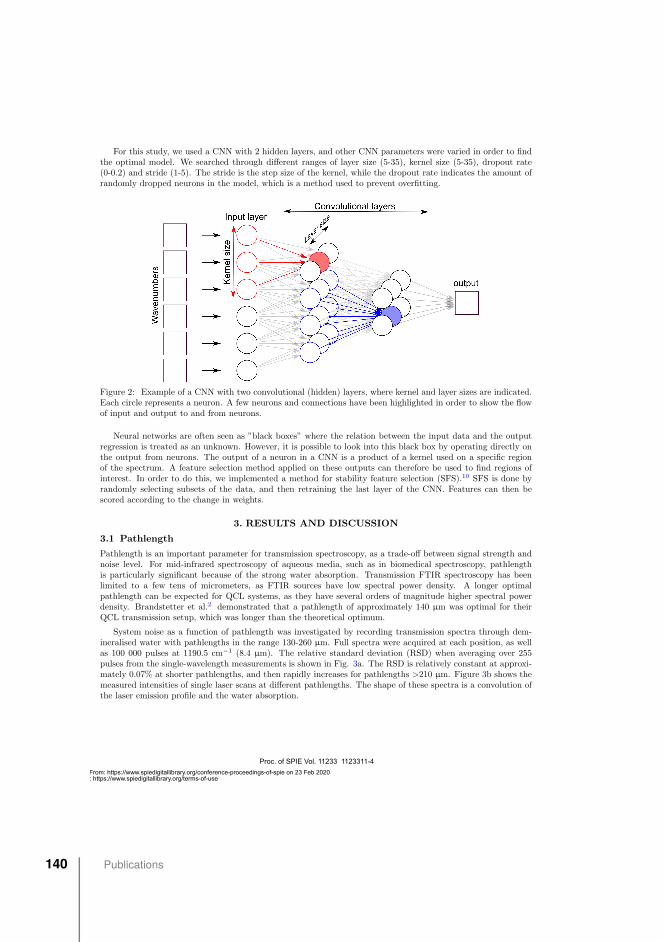
For this study, we used a CNN with 2 hidden layers, and other CNN parameters were varied in order to findthe optimal model. We searched through different ranges of layer size (5-35), kernel size (5-35), dropout rate(0-0.2) and stride (1-5). The stride is the step size of the kernel, while the dropout rate indicates the amount ofrandomly dropped neurons in the model, which is a method used to prevent overfitting.
Figure 2: Example of a CNN with two convolutional (hidden) layers, where kernel and layer sizes are indicated.Each circle represents a neuron. A few neurons and connections have been highlighted in order to show the flowof input and output to and from neurons.
Neural networks are often seen as ”black boxes” where the relation between the input data and the outputregression is treated as an unknown. However, it is possible to look into this black box by operating directly onthe output from neurons. The output of a neuron in a CNN is a product of a kernel used on a specific regionof the spectrum. A feature selection method applied on these outputs can therefore be used to find regions ofinterest. In order to do this, we implemented a method for stability feature selection (SFS).10 SFS is done byrandomly selecting subsets of the data, and then retraining the last layer of the CNN. Features can then bescored according to the change in weights.
3. RESULTS AND DISCUSSION
3.1 Pathlength
Pathlength is an important parameter for transmission spectroscopy, as a trade-off between signal strength andnoise level. For mid-infrared spectroscopy of aqueous media, such as in biomedical spectroscopy, pathlengthis particularly significant because of the strong water absorption. Transmission FTIR spectroscopy has beenlimited to a few tens of micrometers, as FTIR sources have low spectral power density. A longer optimalpathlength can be expected for QCL systems, as they have several orders of magnitude higher spectral powerdensity. Brandstetter et al.2 demonstrated that a pathlength of approximately 140 µm was optimal for theirQCL transmission setup, which was longer than the theoretical optimum.
System noise as a function of pathlength was investigated by recording transmission spectra through dem-ineralised water with pathlengths in the range 130-260 µm. Full spectra were acquired at each position, as wellas 100 000 pulses at 1190.5 cm−1 (8.4 µm). The relative standard deviation (RSD) when averaging over 255pulses from the single-wavelength measurements is shown in Fig. 3a. The RSD is relatively constant at approxi-mately 0.07% at shorter pathlengths, and then rapidly increases for pathlengths >210 µm. Figure 3b shows themeasured intensities of single laser scans at different pathlengths. The shape of these spectra is a convolution ofthe laser emission profile and the water absorption.
Proc. of SPIE Vol. 11233 1123311-4
Downloaded From: https://www.spiedigitallibrary.org/conference-proceedings-of-spie on 23 Feb 2020Terms of Use: https://www.spiedigitallibrary.org/terms-of-use
140 Publications
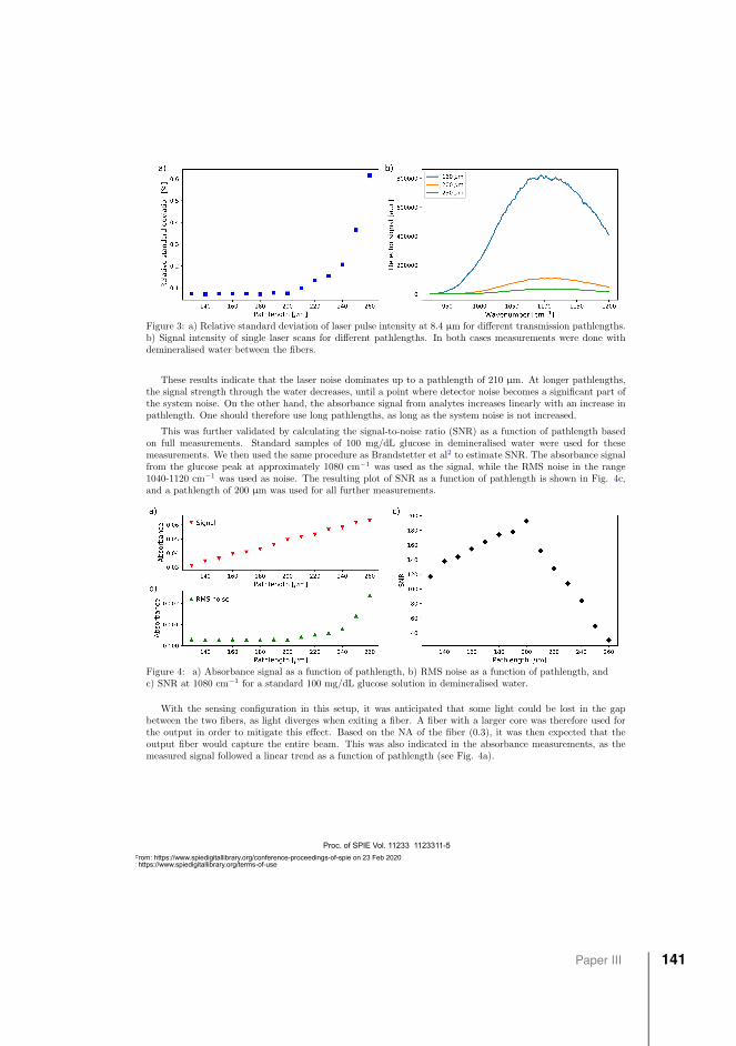
Figure 3: a) Relative standard deviation of laser pulse intensity at 8.4 µm for different transmission pathlengths.b) Signal intensity of single laser scans for different pathlengths. In both cases measurements were done withdemineralised water between the fibers.
These results indicate that the laser noise dominates up to a pathlength of 210 µm. At longer pathlengths,the signal strength through the water decreases, until a point where detector noise becomes a significant part ofthe system noise. On the other hand, the absorbance signal from analytes increases linearly with an increase inpathlength. One should therefore use long pathlengths, as long as the system noise is not increased.
This was further validated by calculating the signal-to-noise ratio (SNR) as a function of pathlength basedon full measurements. Standard samples of 100 mg/dL glucose in demineralised water were used for thesemeasurements. We then used the same procedure as Brandstetter et al2 to estimate SNR. The absorbance signalfrom the glucose peak at approximately 1080 cm−1 was used as the signal, while the RMS noise in the range1040-1120 cm−1 was used as noise. The resulting plot of SNR as a function of pathlength is shown in Fig. 4c,and a pathlength of 200 µm was used for all further measurements.
Figure 4: a) Absorbance signal as a function of pathlength, b) RMS noise as a function of pathlength, andc) SNR at 1080 cm−1 for a standard 100 mg/dL glucose solution in demineralised water.
With the sensing configuration in this setup, it was anticipated that some light could be lost in the gapbetween the two fibers, as light diverges when exiting a fiber. A fiber with a larger core was therefore used forthe output in order to mitigate this effect. Based on the NA of the fiber (0.3), it was then expected that theoutput fiber would capture the entire beam. This was also indicated in the absorbance measurements, as themeasured signal followed a linear trend as a function of pathlength (see Fig. 4a).
Proc. of SPIE Vol. 11233 1123311-5
Downloaded From: https://www.spiedigitallibrary.org/conference-proceedings-of-spie on 23 Feb 2020Terms of Use: https://www.spiedigitallibrary.org/terms-of-use
Paper III 141
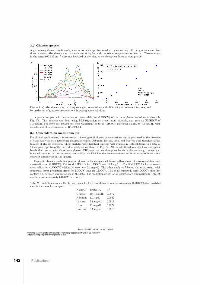
3.2 Glucose spectra
A preliminary characterisation of glucose absorbance spectra was done by measuring different glucose concentra-tions in water. Absorbance spectra are shown in Fig.5a, with the reference spectrum subtracted. Wavenumbersin the range 969-925 cm−1 were not included in the plot, as no absorption features were present.
Figure 5: a) Absorbance spectra of aqueous glucose solutions with different glucose concentrations, andb) prediction of glucose concentrations in pure glucose solutions.
A prediction plot with leave-one-out cross-validation (LOOCV) of the pure glucose solutions is shown inFig. 5b. This analysis was done using PLS regression with one latent variable, and gave an RMSECV of3.3 mg/dL. For leave-one-dataset-out cross-validation the total RMSECV increased slightly to 4.3 mg/dL, witha coefficient of determination of R2=0.9994.
3.3 Concentration measurements
For clinical applications, it is necessary to investigate if glucose concentrations can be predicted in the presenceof other analytes with interfering absorption bands. Albumin, lactate, urea, and fructose were therefore addedto a set of glucose solutions. These analytes were dissolved together with glucose in PBS solutions, to a total of25 samples. Spectra of the individual analytes are shown in Fig. 6a. All the additional analytes have absorptionbands that overlap with those from glucose. PBS also has two absorption bands in this wavelength range, andis scaled down to 1/3 for improved readability. As PBS has the same concentration in all samples it acts as aconstant interference in the spectra.
Figure 6b shows a prediction plot for glucose in the complex solutions, with one case of leave-one-dataset-outcross-validation (LDOCV). The total RMSECV for LDOCV was 10.7 mg/dL. The RMSECV for leave-one-outcross-validation (LOOCV) within datasets was 9.4 mg/dL. The other analytes followed the same trend, withsomewhat lower prediction errors for LOOCV than for LDOCV. This is as expected, since LOOCV does notcapture e.g. between-day variations in the data. The prediction errors for all analytes are summarised in Table 2,and for conciseness only LDOCV is reported.
Table 2: Prediction errors with PLS regression for leave-one-dataset-out cross-validation (LDOCV) of all analytesused in the complex samples.
Analyte RMSECV R2
Glucose 10.7 mg/dL 0.9972
Albumin 1.03 g/L 0.9922
Lactate 7.8 mg/dL 0.9917
Urea 11 mg/dL 0.9874
Fructose 8.7 mg/dL 0.9916
Proc. of SPIE Vol. 11233 1123311-6
Downloaded From: https://www.spiedigitallibrary.org/conference-proceedings-of-spie on 23 Feb 2020Terms of Use: https://www.spiedigitallibrary.org/terms-of-use
142 Publications
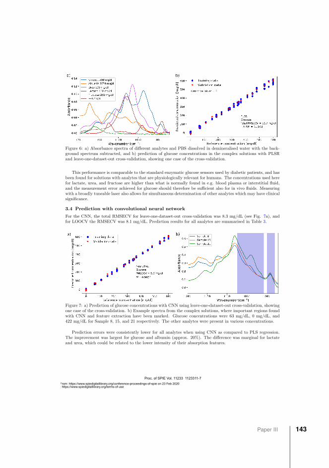
Figure 6: a) Absorbance spectra of different analytes and PBS dissolved in demineralised water with the back-ground spectrum subtracted, and b) prediction of glucose concentrations in the complex solutions with PLSRand leave-one-dataset-out cross-validation, showing one case of the cross-validation.
This performance is comparable to the standard enzymatic glucose sensors used by diabetic patients, and hasbeen found for solutions with analytes that are physiologically relevant for humans. The concentrations used herefor lactate, urea, and fructose are higher than what is normally found in e.g. blood plasma or interstitial fluid,and the measurement error achieved for glucose should therefore be sufficient also for in vivo fluids. Measuringwith a broadly tuneable laser also allows for simultaneous determination of other analytes which may have clinicalsignificance.
3.4 Prediction with convolutional neural network
For the CNN, the total RMSECV for leave-one-dataset-out cross-validation was 8.3 mg/dL (see Fig. 7a), andfor LOOCV the RMSECV was 8.1 mg/dL. Prediction results for all analytes are summarised in Table 3.
Figure 7: a) Prediction of glucose concentrations with CNN using leave-one-dataset-out cross-validation, showingone case of the cross-validation. b) Example spectra from the complex solutions, where important regions foundwith CNN and feature extraction have been marked. Glucose concentrations were 63 mg/dL, 0 mg/dL, and422 mg/dL for Sample 8, 15, and 21 respectively. The other analytes were present in various concentrations.
Prediction errors were consistently lower for all analytes when using CNN as compared to PLS regression.The improvement was largest for glucose and albumin (approx. 20%). The difference was marginal for lactateand urea, which could be related to the lower intensity of their absorption features.
Proc. of SPIE Vol. 11233 1123311-7
Downloaded From: https://www.spiedigitallibrary.org/conference-proceedings-of-spie on 23 Feb 2020Terms of Use: https://www.spiedigitallibrary.org/terms-of-use
Paper III 143

Table 3: Prediction errors with CNN regression for leave-one-dataset-out cross-validation of all analytes used inthe complex samples.
Analyte RMSECV R2
Glucose 8.3 mg/dL 0.9984
Albumin 0.89 g/L 0.9946
Lactate 7.5 mg/dL 0.9923
Urea 10.5 mg/dL 0.9885
Fructose 7.2 mg/dL 0.9945
Figure 7b shows the important spectral regions for glucose prediction as determined by CNN and stabilityfeature selection. The important regions are overlayed on three example spectra from the complex solutions. Thisfeature extraction has identified regions that overlap with glucose absorption features, which is not unexpected.It has also marked regions with relatively little interference from other analytes, which can be seen from Fig. 6.This indicates that feature extraction can be used as a tool to find out where the CNN is most sensitive to ananalyte of interest. This can be used to e.g. narrow down the region of interest for further sensor development.
4. CONCLUSIONS
Glucose concentrations were predicted with high accuracy in solutions with other analytes with interferingabsorption bands. An RMSECV of 10.7 mg/dL was shown with PLS regression, and this was further improvedto 8.3 mg/dL with regression based on CNN. Several analytes found in e.g. interstitial fluid were used in thesecomplex solutions, and the low prediction error achieved indicates that accurate in vivo measurements shouldbe possible. Simultaneous determination of several analytes was also demonstrated. This is promising for futuredevelopment of miniaturised sensors using optical fibers in the mid-infrared.
The high accuracy was in part achieved after a thorough analysis of the system noise. We showed that apathlength of 200 µm in aqueous solutions could be used without detriment to the noise level. At the sametime, this pathlength gave a higher absorbance signal, which resulted in a higher SNR as compared to longer orshorter pathlengths.
We also used a neural network in order to predict glucose concentration, and achieved better predictionerrors than those in the PLS regression. The CNN results demonstrate that improved data modelling can be animportant tool to achieve better prediction accuracies. Additional information could also be extracted from theCNN, such as the spectral regions where the model was most sensitive.
ACKNOWLEDGMENTS
This work was supported by the Research Council of Norway through the Double Intraperitoneal ArtificialPancreas project, grant number 248872. The project is part of Center for Digital Life Norway and is alsosupported by the Research Council of Norway’s grant 248810.
REFERENCES
[1] Turner, A. P. F., “Biosensors - Sense and sensibility,” Chem. Soc. Rev. 42(8), 3184–3196 (2013).
[2] Brandstetter, M., Volgger, L., Genner, A., Jungbauer, C., and Lendl, B., “Direct determination of glucose,lactate and triglycerides in blood serum by a tunable quantum cascade laser-based mid-IR sensor,” AppliedPhysics B 110(2), 233–239 (2013).
[3] Vahlsing, T., Delbeck, S., Budde, J., Ihrig, D., Leonhardt, S., and Michael Heise, H., “Reliable glucosemonitoring by ex-vivo blood microdialysis and infrared spectrometry for patients in critical care,” OpticalDiagnostics and Sensing XVII: Toward Point-of-Care Diagnostics, Proc. SPIE 10072 (2017).
[4] Isensee, K., Muller, N., Pucci, A., and Petrich, W., “Towards a quantum cascade laser-based implant forthe continuous monitoring of glucose,” The Analyst 143(24) (2018).
Proc. of SPIE Vol. 11233 1123311-8
Downloaded From: https://www.spiedigitallibrary.org/conference-proceedings-of-spie on 23 Feb 2020Terms of Use: https://www.spiedigitallibrary.org/terms-of-use
144 Publications
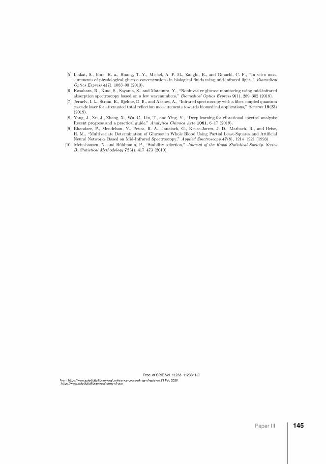
[5] Liakat, S., Bors, K. a., Huang, T.-Y., Michel, A. P. M., Zanghi, E., and Gmachl, C. F., “In vitro mea-surements of physiological glucose concentrations in biological fluids using mid-infrared light.,” BiomedicalOptics Express 4(7), 1083–90 (2013).
[6] Kasahara, R., Kino, S., Soyama, S., and Matsuura, Y., “Noninvasive glucose monitoring using mid-infraredabsorption spectroscopy based on a few wavenumbers,” Biomedical Optics Express 9(1), 289–302 (2018).
[7] Jernelv, I. L., Strøm, K., Hjelme, D. R., and Aksnes, A., “Infrared spectroscopy with a fiber-coupled quantumcascade laser for attenuated total reflection measurements towards biomedical applications,” Sensors 19(23)(2019).
[8] Yang, J., Xu, J., Zhang, X., Wu, C., Lin, T., and Ying, Y., “Deep learning for vibrational spectral analysis:Recent progress and a practical guide,” Analytica Chimica Acta 1081, 6–17 (2019).
[9] Bhandare, P., Mendelson, Y., Peura, R. A., Janatsch, G., Kruse-Jarres, J. D., Marbach, R., and Heise,H. M., “Multivariate Determination of Glucose in Whole Blood Using Partial Least-Squares and ArtificialNeural Networks Based on Mid-Infrared Spectroscopy,” Applied Spectroscopy 47(8), 1214–1221 (1993).
[10] Meinshausen, N. and Buhlmann, P., “Stability selection,” Journal of the Royal Statistical Society. SeriesB: Statistical Methodology 72(4), 417–473 (2010).
Proc. of SPIE Vol. 11233 1123311-9
Downloaded From: https://www.spiedigitallibrary.org/conference-proceedings-of-spie on 23 Feb 2020Terms of Use: https://www.spiedigitallibrary.org/terms-of-use
Paper III 145


Paper IVSignal enhancement in microstructured silicon attenuated total reflection ele-ments with quantum cascade laser-based spectroscopyI.L. Jernelv, J. Høvik, D.R. Hjelme, A. AksnesProceedings of SPIE 11359, Biomedical Spectroscopy, Microscopy, and Imaging,113590A, 2020.
Paper IV 147

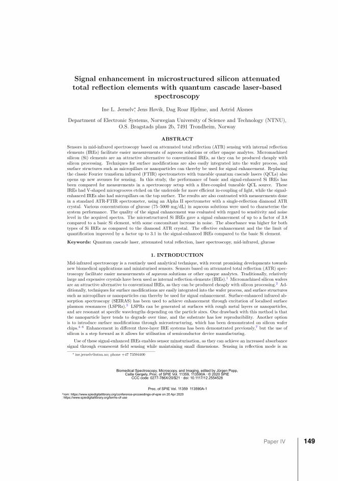
Signal enhancement in microstructured silicon attenuatedtotal reflection elements with quantum cascade laser-based
spectroscopy
Ine L. Jernelv∗, Jens Høvik, Dag Roar Hjelme, and Astrid Aksnes
Department of Electronic Systems, Norwegian University of Science and Technology (NTNU),O.S. Bragstads plass 2b, 7491 Trondheim, Norway
ABSTRACT
Sensors in mid-infrared spectroscopy based on attenuated total reflection (ATR) sensing with internal reflectionelements (IREs) facilitate easier measurements of aqueous solutions or other opaque analytes. Micromachinedsilicon (Si) elements are an attractive alternative to conventional IREs, as they can be produced cheaply withsilicon processing. Techniques for surface modifications are also easily integrated into the wafer process, andsurface structures such as micropillars or nanoparticles can thereby be used for signal enhancement. Replacingthe classic Fourier transform infrared (FTIR) spectrometers with tuneable quantum cascade lasers (QCLs) alsoopens up new avenues for sensing. In this study, the performance of basic and signal-enhanced Si IREs hasbeen compared for measurements in a spectroscopy setup with a fibre-coupled tuneable QCL source. TheseIREs had V-shaped microgrooves etched on the underside for more efficient in-coupling of light, while the signal-enhanced IREs also had micropillars on the top surface. The results are also contrasted with measurements donein a standard ATR-FTIR spectrometer, using an Alpha II spectrometer with a single-reflection diamond ATRcrystal. Various concentrations of glucose (75–5000 mg/dL) in aqueous solutions were used to characterise thesystem performance. The quality of the signal enhancement was evaluated with regard to sensitivity and noiselevel in the acquired spectra. The microstructured Si IREs gave a signal enhancement of up to a factor of 3.8compared to a basic Si element, with some concomitant increase in noise. The absorbance was higher for bothtypes of Si IREs as compared to the diamond ATR crystal. The effective enhancement and the the limit ofquantification improved by a factor up to 3.1 in the signal-enhanced IREs compared to the basic Si element.
Keywords: Quantum cascade laser, attenuated total reflection, laser spectroscopy, mid-infrared, glucose
1. INTRODUCTION
Mid-infrared spectroscopy is a routinely used analytical technique, with recent promising developments towardsnew biomedical applications and miniaturised sensors. Sensors based on attenuated total reflection (ATR) spec-troscopy facilitate easier measurements of aqueous solutions or other opaque analytes. Traditionally, relativelylarge and expensive crystals have been used as internal reflection elements (IREs).1 Micromachined silicon wafersare an attractive alternative to conventional IREs, as they can be produced cheaply with silicon processing.2 Ad-ditionally, techniques for surface modifications are easily integrated into the wafer process, and surface structuressuch as micropillars or nanoparticles can thereby be used for signal enhancement. Surface-enhanced infrared ab-sorption spectroscopy (SEIRAS) has been used to achieve enhancement through excitation of localised surfaceplasmon resonances (LSPRs).3 LSPRs can be generated at surfaces with rough metal layers or nanoparticles,and are resonant at specific wavelengths depending on the particle sizes. One drawback with this method is thatthe nanoparticle layer tends to degrade over time, and the substrate has low reproducibility. Another optionis to introduce surface modifications through microstructuring, which has been demonstrated on silicon waferchips.4–6 Enhancement in different three-layer IRE systems has been demonstrated previously,7 but the use ofsilicon is a step forward as it allows for utilisation of semiconductor device manufacturing.
Use of these signal-enhanced IREs enables sensor minaturisation, as they can achieve an increased absorbancesignal through evanescent field sensing while maintaining small dimensions. Sensing in reflection mode is an
∗ [email protected]; phone +47 73594400
Biomedical Spectroscopy, Microscopy, and Imaging, edited by Jürgen Popp,Csilla Gergely, Proc. of SPIE Vol. 11359, 113590A · © 2020 SPIE
CCC code: 0277-786X/20/$21 · doi: 10.1117/12.2554528
Proc. of SPIE Vol. 11359 113590A-1
Downloaded From: https://www.spiedigitallibrary.org/conference-proceedings-of-spie on 20 Apr 2020Terms of Use: https://www.spiedigitallibrary.org/terms-of-use
Paper IV 149
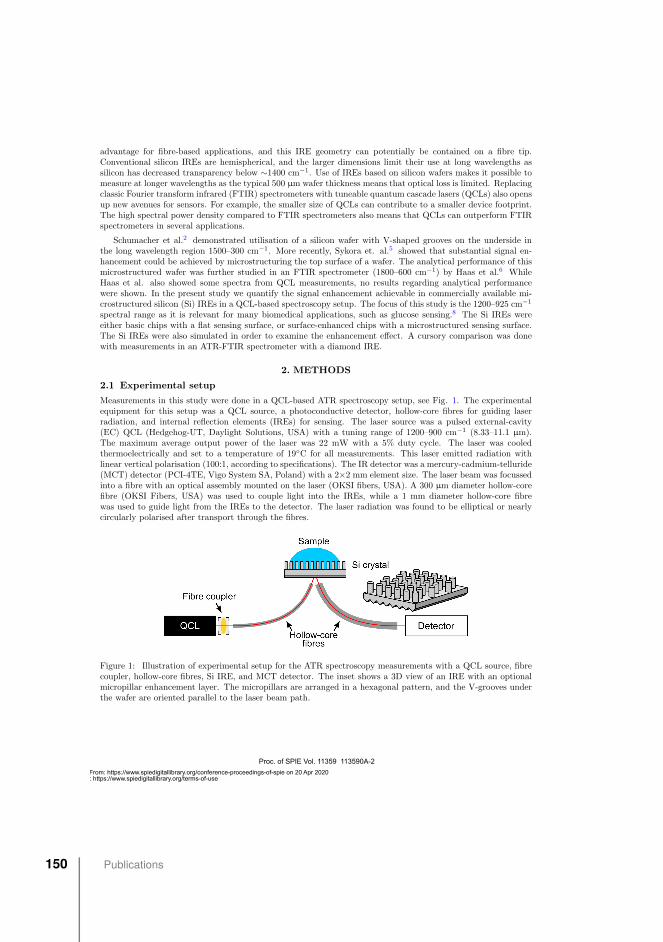
advantage for fibre-based applications, and this IRE geometry can potentially be contained on a fibre tip.Conventional silicon IREs are hemispherical, and the larger dimensions limit their use at long wavelengths assilicon has decreased transparency below ∼1400 cm−1. Use of IREs based on silicon wafers makes it possible tomeasure at longer wavelengths as the typical 500 µm wafer thickness means that optical loss is limited. Replacingclassic Fourier transform infrared (FTIR) spectrometers with tuneable quantum cascade lasers (QCLs) also opensup new avenues for sensors. For example, the smaller size of QCLs can contribute to a smaller device footprint.The high spectral power density compared to FTIR spectrometers also means that QCLs can outperform FTIRspectrometers in several applications.
Schumacher et al.2 demonstrated utilisation of a silicon wafer with V-shaped grooves on the underside inthe long wavelength region 1500–300 cm−1. More recently, Sykora et. al.5 showed that substantial signal en-hancement could be achieved by microstructuring the top surface of a wafer. The analytical performance of thismicrostructured wafer was further studied in an FTIR spectrometer (1800–600 cm−1) by Haas et al.6 WhileHaas et al. also showed some spectra from QCL measurements, no results regarding analytical performancewere shown. In the present study we quantify the signal enhancement achievable in commercially available mi-crostructured silicon (Si) IREs in a QCL-based spectroscopy setup. The focus of this study is the 1200–925 cm−1
spectral range as it is relevant for many biomedical applications, such as glucose sensing.8 The Si IREs wereeither basic chips with a flat sensing surface, or surface-enhanced chips with a microstructured sensing surface.The Si IREs were also simulated in order to examine the enhancement effect. A cursory comparison was donewith measurements in an ATR-FTIR spectrometer with a diamond IRE.
2. METHODS
2.1 Experimental setup
Measurements in this study were done in a QCL-based ATR spectroscopy setup, see Fig. 1. The experimentalequipment for this setup was a QCL source, a photoconductive detector, hollow-core fibres for guiding laserradiation, and internal reflection elements (IREs) for sensing. The laser source was a pulsed external-cavity(EC) QCL (Hedgehog-UT, Daylight Solutions, USA) with a tuning range of 1200–900 cm−1 (8.33–11.1 µm).The maximum average output power of the laser was 22 mW with a 5% duty cycle. The laser was cooledthermoelectrically and set to a temperature of 19◦C for all measurements. This laser emitted radiation withlinear vertical polarisation (100:1, according to specifications). The IR detector was a mercury-cadmium-telluride(MCT) detector (PCI-4TE, Vigo System SA, Poland) with a 2×2 mm element size. The laser beam was focussedinto a fibre with an optical assembly mounted on the laser (OKSI fibers, USA). A 300 µm diameter hollow-corefibre (OKSI Fibers, USA) was used to couple light into the IREs, while a 1 mm diameter hollow-core fibrewas used to guide light from the IREs to the detector. The laser radiation was found to be elliptical or nearlycircularly polarised after transport through the fibres.
Figure 1: Illustration of experimental setup for the ATR spectroscopy measurements with a QCL source, fibrecoupler, hollow-core fibres, Si IRE, and MCT detector. The inset shows a 3D view of an IRE with an optionalmicropillar enhancement layer. The micropillars are arranged in a hexagonal pattern, and the V-grooves underthe wafer are oriented parallel to the laser beam path.
Proc. of SPIE Vol. 11359 113590A-2
Downloaded From: https://www.spiedigitallibrary.org/conference-proceedings-of-spie on 20 Apr 2020Terms of Use: https://www.spiedigitallibrary.org/terms-of-use
150 Publications
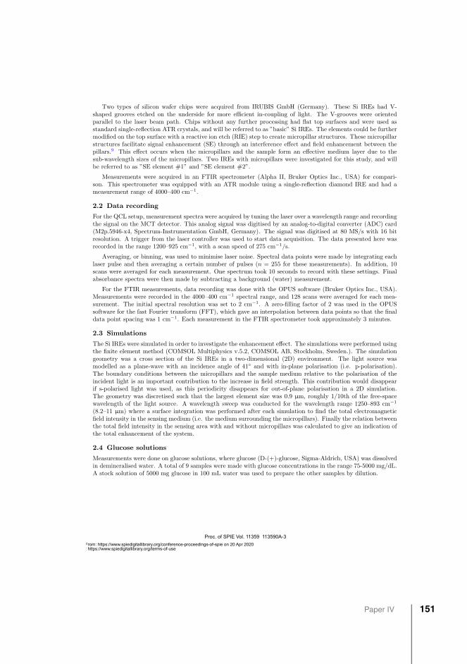
Two types of silicon wafer chips were acquired from IRUBIS GmbH (Germany). These Si IREs had V-shaped grooves etched on the underside for more efficient in-coupling of light. The V-grooves were orientedparallel to the laser beam path. Chips without any further processing had flat top surfaces and were used asstandard single-reflection ATR crystals, and will be referred to as ”basic” Si IREs. The elements could be furthermodified on the top surface with a reactive ion etch (RIE) step to create micropillar structures. These micropillarstructures facilitate signal enhancement (SE) through an interference effect and field enhancement between thepillars.9 This effect occurs when the micropillars and the sample form an effective medium layer due to thesub-wavelength sizes of the micropillars. Two IREs with micropillars were investigated for this study, and willbe referred to as ”SE element #1” and ”SE element #2”.
Measurements were acquired in an FTIR spectrometer (Alpha II, Bruker Optics Inc., USA) for compari-son. This spectrometer was equipped with an ATR module using a single-reflection diamond IRE and had ameasurement range of 4000–400 cm−1.
2.2 Data recording
For the QCL setup, measurement spectra were acquired by tuning the laser over a wavelength range and recordingthe signal on the MCT detector. This analog signal was digitised by an analog-to-digital converter (ADC) card(M2p.5946-x4, Spectrum-Instrumentation GmbH, Germany). The signal was digitised at 80 MS/s with 16 bitresolution. A trigger from the laser controller was used to start data acquisition. The data presented here wasrecorded in the range 1200–925 cm−1, with a scan speed of 275 cm−1/s.
Averaging, or binning, was used to minimise laser noise. Spectral data points were made by integrating eachlaser pulse and then averaging a certain number of pulses (n = 255 for these measurements). In addition, 10scans were averaged for each measurement. One spectrum took 10 seconds to record with these settings. Finalabsorbance spectra were then made by subtracting a background (water) measurement.
For the FTIR measurements, data recording was done with the OPUS software (Bruker Optics Inc., USA).Measurements were recorded in the 4000–400 cm−1 spectral range, and 128 scans were averaged for each mea-surement. The initial spectral resolution was set to 2 cm−1. A zero-filling factor of 2 was used in the OPUSsoftware for the fast Fourier transform (FFT), which gave an interpolation between data points so that the finaldata point spacing was 1 cm−1. Each measurement in the FTIR spectrometer took approximately 3 minutes.
2.3 Simulations
The Si IREs were simulated in order to investigate the enhancement effect. The simulations were performed usingthe finite element method (COMSOL Multiphysics v.5.2, COMSOL AB, Stockholm, Sweden.). The simulationgeometry was a cross section of the Si IREs in a two-dimensional (2D) environment. The light source wasmodelled as a plane-wave with an incidence angle of 41◦ and with in-plane polarisation (i.e. p-polarisation).The boundary conditions between the micropillars and the sample medium relative to the polarisation of theincident light is an important contribution to the increase in field strength. This contribution would disappearif s-polarised light was used, as this periodicity disappears for out-of-plane polarisation in a 2D simulation.The geometry was discretised such that the largest element size was 0.9 µm, roughly 1/10th of the free-spacewavelength of the light source. A wavelength sweep was conducted for the wavelength range 1250–893 cm−1
(8.2–11 µm) where a surface integration was performed after each simulation to find the total electromagneticfield intensity in the sensing medium (i.e. the medium surrounding the micropillars). Finally the relation betweenthe total field intensity in the sensing area with and without micropillars was calculated to give an indication ofthe total enhancement of the system.
2.4 Glucose solutions
Measurements were done on glucose solutions, where glucose (D-(+)-glucose, Sigma-Aldrich, USA) was dissolvedin demineralised water. A total of 9 samples were made with glucose concentrations in the range 75-5000 mg/dL.A stock solution of 5000 mg glucose in 100 mL water was used to prepare the other samples by dilution.
Proc. of SPIE Vol. 11359 113590A-3
Downloaded From: https://www.spiedigitallibrary.org/conference-proceedings-of-spie on 20 Apr 2020Terms of Use: https://www.spiedigitallibrary.org/terms-of-use
Paper IV 151

2.5 Analysis
Calibration curves were made based on the height of the largest glucose absorption band, at approximately1035 cm−1. The performance of the IREs was then evaluated based on absorbance signal, noise level, limitof quantification (LoQ) and effective enhancement for the signal-enhanced IREs. The enhancement factor wascalculated as signal-enhanced/basic absorption peak. Noise was calculated as the RMS-noise of blank spectra inthe spectral region 1055–1015 cm−1. Limit of quantification (LoQ) was then estimated based on a signal-to-noise(SNR) ratio of 10:1, where the signal was the height of the most intense absorption band and the RMS noisewas the noise level. The effectivity of the signal enhancement was then calculated as the ratio of SNR betweenthe signal-enhanced chips and the basic Si chips.
3. RESULTS AND DISCUSSION
3.1 IRE dimensions
The micropillar structures in the signal-enhanced Si IREs were imaged in a scanning electron microscope (ApreoSEM, FEI Company, USA), see Fig. 2.
Figure 2: SEM pictographs of Si chips with patterned micropillars, a) SE element #1 and b) SE element #2.The insets show side views at an angle of approximately 25 degrees.
Dimensions of the micropillars are summarised in Table 1. Micropillar dimensions were evaluated withImageJ, which is an open-source software for scientific image analysis. The pillar periodicity was essentially thesame, so the main differences between the IREs were the pillar diameter and height.
Table 1: Geometrical parameters for the Si IREs with micropillar structures.
Dimension SE element #1 SE element #2
Height 3.5 µm 1.66 µm
Pillar diameter 0.86 µm 0.57 µm
Period 1.25 µm 1.23 µm
Proc. of SPIE Vol. 11359 113590A-4
Downloaded From: https://www.spiedigitallibrary.org/conference-proceedings-of-spie on 20 Apr 2020Terms of Use: https://www.spiedigitallibrary.org/terms-of-use
152 Publications
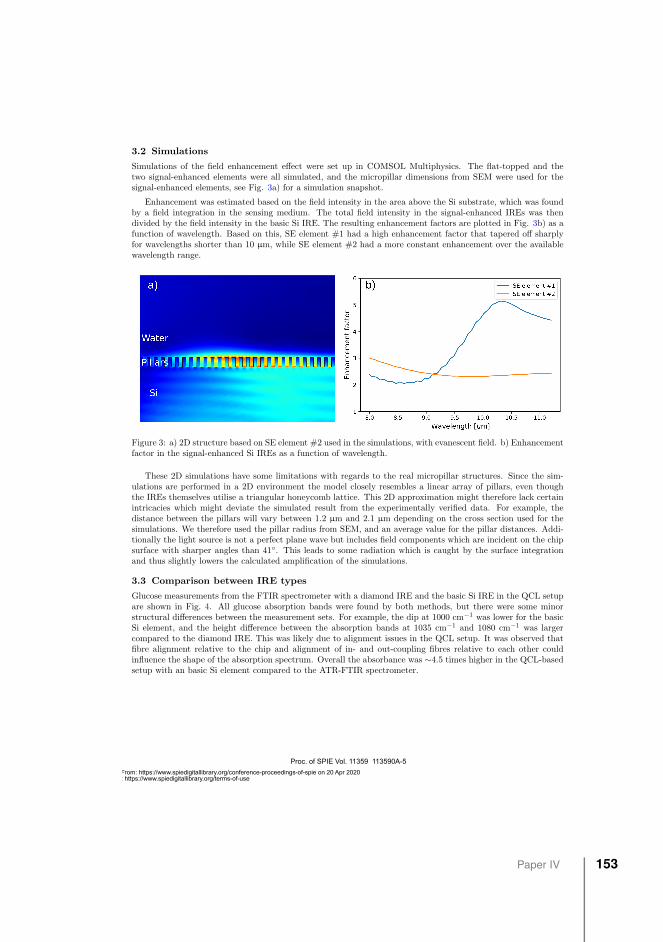
3.2 Simulations
Simulations of the field enhancement effect were set up in COMSOL Multiphysics. The flat-topped and thetwo signal-enhanced elements were all simulated, and the micropillar dimensions from SEM were used for thesignal-enhanced elements, see Fig. 3a) for a simulation snapshot.
Enhancement was estimated based on the field intensity in the area above the Si substrate, which was foundby a field integration in the sensing medium. The total field intensity in the signal-enhanced IREs was thendivided by the field intensity in the basic Si IRE. The resulting enhancement factors are plotted in Fig. 3b) as afunction of wavelength. Based on this, SE element #1 had a high enhancement factor that tapered off sharplyfor wavelengths shorter than 10 µm, while SE element #2 had a more constant enhancement over the availablewavelength range.
Figure 3: a) 2D structure based on SE element #2 used in the simulations, with evanescent field. b) Enhancementfactor in the signal-enhanced Si IREs as a function of wavelength.
These 2D simulations have some limitations with regards to the real micropillar structures. Since the sim-ulations are performed in a 2D environment the model closely resembles a linear array of pillars, even thoughthe IREs themselves utilise a triangular honeycomb lattice. This 2D approximation might therefore lack certainintricacies which might deviate the simulated result from the experimentally verified data. For example, thedistance between the pillars will vary between 1.2 µm and 2.1 µm depending on the cross section used for thesimulations. We therefore used the pillar radius from SEM, and an average value for the pillar distances. Addi-tionally the light source is not a perfect plane wave but includes field components which are incident on the chipsurface with sharper angles than 41◦. This leads to some radiation which is caught by the surface integrationand thus slightly lowers the calculated amplification of the simulations.
3.3 Comparison between IRE types
Glucose measurements from the FTIR spectrometer with a diamond IRE and the basic Si IRE in the QCL setupare shown in Fig. 4. All glucose absorption bands were found by both methods, but there were some minorstructural differences between the measurement sets. For example, the dip at 1000 cm−1 was lower for the basicSi element, and the height difference between the absorption bands at 1035 cm−1 and 1080 cm−1 was largercompared to the diamond IRE. This was likely due to alignment issues in the QCL setup. It was observed thatfibre alignment relative to the chip and alignment of in- and out-coupling fibres relative to each other couldinfluence the shape of the absorption spectrum. Overall the absorbance was ∼4.5 times higher in the QCL-basedsetup with an basic Si element compared to the ATR-FTIR spectrometer.
Proc. of SPIE Vol. 11359 113590A-5
Downloaded From: https://www.spiedigitallibrary.org/conference-proceedings-of-spie on 20 Apr 2020Terms of Use: https://www.spiedigitallibrary.org/terms-of-use
Paper IV 153
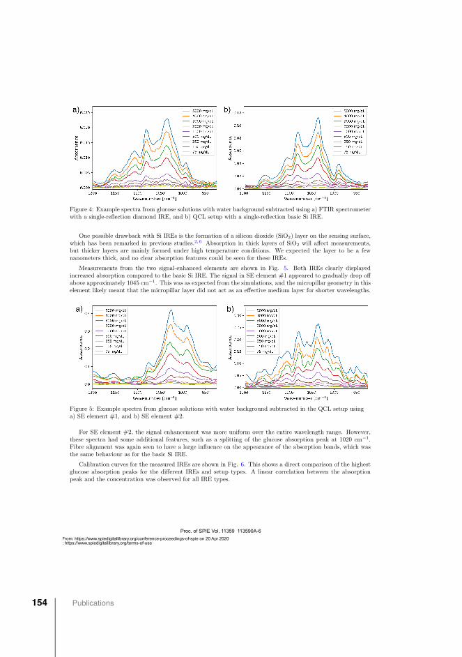
Figure 4: Example spectra from glucose solutions with water background subtracted using a) FTIR spectrometerwith a single-reflection diamond IRE, and b) QCL setup with a single-reflection basic Si IRE.
One possible drawback with Si IREs is the formation of a silicon dioxide (SiO2) layer on the sensing surface,which has been remarked in previous studies.2,6 Absorption in thick layers of SiO2 will affect measurements,but thicker layers are mainly formed under high temperature conditions. We expected the layer to be a fewnanometers thick, and no clear absorption features could be seen for these IREs.
Measurements from the two signal-enhanced elements are shown in Fig. 5. Both IREs clearly displayedincreased absorption compared to the basic Si IRE. The signal in SE element #1 appeared to gradually drop offabove approximately 1045 cm−1. This was as expected from the simulations, and the micropillar geometry in thiselement likely meant that the micropillar layer did not act as an effective medium layer for shorter wavelengths.
Figure 5: Example spectra from glucose solutions with water background subtracted in the QCL setup usinga) SE element #1, and b) SE element #2.
For SE element #2, the signal enhancement was more uniform over the entire wavelength range. However,these spectra had some additional features, such as a splitting of the glucose absorption peak at 1020 cm−1.Fibre alignment was again seen to have a large influence on the appearance of the absorption bands, which wasthe same behaviour as for the basic Si IRE.
Calibration curves for the measured IREs are shown in Fig. 6. This shows a direct comparison of the highestglucose absorption peaks for the different IREs and setup types. A linear correlation between the absorptionpeak and the concentration was observed for all IRE types.
Proc. of SPIE Vol. 11359 113590A-6
Downloaded From: https://www.spiedigitallibrary.org/conference-proceedings-of-spie on 20 Apr 2020Terms of Use: https://www.spiedigitallibrary.org/terms-of-use
154 Publications
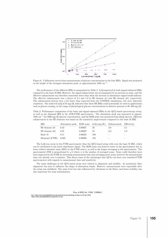
Figure 6: Calibration curves from measurements of glucose concentrations in the four IREs. Signal was measuredas the height of the strongest absorption peak, at approximately 1035 cm−1.
The performance of the different IREs is summarised in Table 2. LoQ improved in both signal-enhanced IREscompared to the basic Si IRE. However, the signal enhancement was accompanied by an increase in noise, and theeffective enhancement was therefore somewhat lower than what the increase in absorbance signal would indicate.The effective enhancement was a factor of 3.1 and 1.9 in SE element #1 and SE element #2, respectively.The enhancement factors were a bit lower than expected from the COMSOL simulations, but were otherwiseconsistent. The achieved LoQ of 35 mg/dL indicates that these SE IREs could potentially be used in applicationssuch as glucose sensing, as the range of physiological glucose concentrations in diabetic patients is 30–400 mg/dL.
Table 2: Performance comparison of the basic and signal-enhanced IREs in the QCL-based spectroscopy setup,as well as the diamond IRE in the ATR-FTIR spectrometer. The absorption peak was measured at approx.1035 cm−1 for 5000 mg/dL glucose concentration, and the RMS noise was measured from blank spectra. Effectiveenhancement in the SE elements was based on the sensitivity improvement compared to the basic Si IRE.
IRE Absorption peak RMS noise LoQ (mg/dL) Enhancement Effectivity
SE element #1 0.42 0.00027 35 3.8 3.1
SE element #2 0.25 0.00027 55 2.3 1.9
Basic Si 0.11 0.00022 100 - -
Diamond (FTIR) 0.023 0.00009 195 - -
The LoQ was worse in the FTIR spectrometer than the QCL-based setup with even the basic Si IRE, whichcan be attributed to the lower absorbance signal. The RMS noise was however lower in the spectrometer due tolower relative intensity noise (RIN) in the FTIR source, as well as the longer averaging in the spectrometer. Thespectrometer SNR is proportional to
√n where n is the number of averaged scans. Noise could therefore have
been improved in the FTIR by increasing measurement time and averaging more scans, however the measurementtime was already over 3 minutes. This shows some of the advantages that QCLs can have over standard FTIRspectrometers with regards to measurement time and sensitivity.
The main challenges in the QCL-based setup were related to alignment and stability. As mentioned, fibrealignment was seen to influence the shape of absorption bands. However, measurements were repeatable afterthe setup was stabilised. The noise level was also influenced by vibrations in the fibres, and hence stability wasalso important for noise minimisation.
Proc. of SPIE Vol. 11359 113590A-7
Downloaded From: https://www.spiedigitallibrary.org/conference-proceedings-of-spie on 20 Apr 2020Terms of Use: https://www.spiedigitallibrary.org/terms-of-use
Paper IV 155
4. CONCLUSIONS
This study evaluated the performance of microstructured Si elements with and without a signal enhancementlayer as IREs in a QCL-based ATR spectroscopy setup. The signal-enhanced chips were found to improve theabsorbance signal up to a factor of 3.8, while due to simultaneous increase in noise the LoQ improved by up toa factor of 3.1. Very different behaviours were seen in the two IREs with micropillars for signal enhancement,which shows that it is important to consider pillar geometry in relation to the wavelength region used. TheCOMSOL simulations agreed well with the experimental results. 3D simulations should be done in the future tofurther investigate the effect of the micropillar lattice structure, and the effect of polarisation.
These micromachined Si IREs can be mass-produced and may potentially be integrated in single-use ap-plications for e.g. biomedical measurements. The signal enhancement also gave good LoQs, considering thesingle-reflection geometries, and another possible application is to use these IREs as sensing surfaces for fibre-optic sensors in reflection mode. This work also demonstrated measurements with Si IREs below 1200 cm−1,which is usually considered opaque for Si components.
ACKNOWLEDGMENTS
The Research Council of Norway is acknowledged for the support to the Norwegian Micro- and Nano-FabricationFacility, NorFab, grant number 245963/F50, as well as the Double Intraperitoneal Artificial Pancreas project,grant number 248872. The project is part of Center for Digital Life Norway and is also supported by the ResearchCouncil of Norway’s grant 248810. The authors would like to thank Lorenz Sykora at IRUBIS GmbH for a helpfuldiscussion on the silicon internal reflection elements.
REFERENCES
[1] Jernelv, I. L., Strøm, K., Hjelme, D. R., and Aksnes, A., “Infrared spectroscopy with a fiber-coupled quantumcascade laser for attenuated total reflection measurements towards biomedical applications,” Sensors 19(23),5130 (2019).
[2] Schumacher, H., Kunzelmann, U., Vasilev, B., Eichhorn, K. J., and Bartha, J. W., “Applications of mi-crostructured silicon wafers as internal reflection elements in attenuated total reflection Fourier transforminfrared spectroscopy,” Applied Spectroscopy 64(9), 1022–1027 (2010).
[3] Bibikova, O., Haas, J., Lopez-Lorente, A. I., Popov, A., Kinnunen, M., Ryabchikov, Y., Kabashin, A.,Meglinski, I., and Mizaikoff, B., “Surface enhanced infrared absorption spectroscopy based on gold nanostarsand spherical nanoparticles,” Analytica Chimica Acta 990, 141–149 (2017).
[4] Morhart, T. A., Unni, B., Lardner, M. J., and Burgess, I. J., “Electrochemical ATR-SEIRAS Using Low-Cost,Micromachined Si Wafers,” Analytical Chemistry 89(21), 11818–11824 (2017).
[5] Sykora, L., Muller, A., Kondratiev, A., Roth, A., Mozin, V., Fehr, A., and Zornack, G., “Silicon ATRcrystal with subwavelength structures optimized for blood analysis,” Optical Fibers and Sensors for MedicalDiagnostics and Treatment Applications XIX 10872, 14 (2019).
[6] Haas, J., Muller, A., Sykora, L., and Mizaikoff, B., “Analytical performance of µ-groove silicon attenuatedtotal reflection waveguides,” Analyst 144(10), 3398–3404 (2019).
[7] Huber-Walchli, P. and Gunthard, H. H., “Interference Enhanced Attenuated Total Reflection (IEATR). Anew technique for i.r. matrix spectroscopy with high sensitivity,” Spectrochimica Acta Part A: MolecularSpectroscopy 34(12), 1253–1262 (1978).
[8] Jernelv, I. L., Milenko, K., Fuglerud, S. S., Hjelme, D. R., Ellingsen, R., and Aksnes, A., “A review of opticalmethods for continuous glucose monitoring,” Applied Spectroscopy Reviews 54(7), 543–572 (2019).
[9] Berz, F., “On a quarter wave light condenser,” British Journal of Applied Physics 16(11), 1733–1738 (1965).
Proc. of SPIE Vol. 11359 113590A-8
Downloaded From: https://www.spiedigitallibrary.org/conference-proceedings-of-spie on 20 Apr 2020Terms of Use: https://www.spiedigitallibrary.org/terms-of-use
156 Publications

Paper VConvolutional neural networks for classification and regression analysis of one-dimensional spectral dataI.L. Jernelv, D.R. Hjelme, Y. Matsuura, A. AksnesPreprint published on arxiv.org, arXiv ID 2005.07530, 2020.
Paper V 157

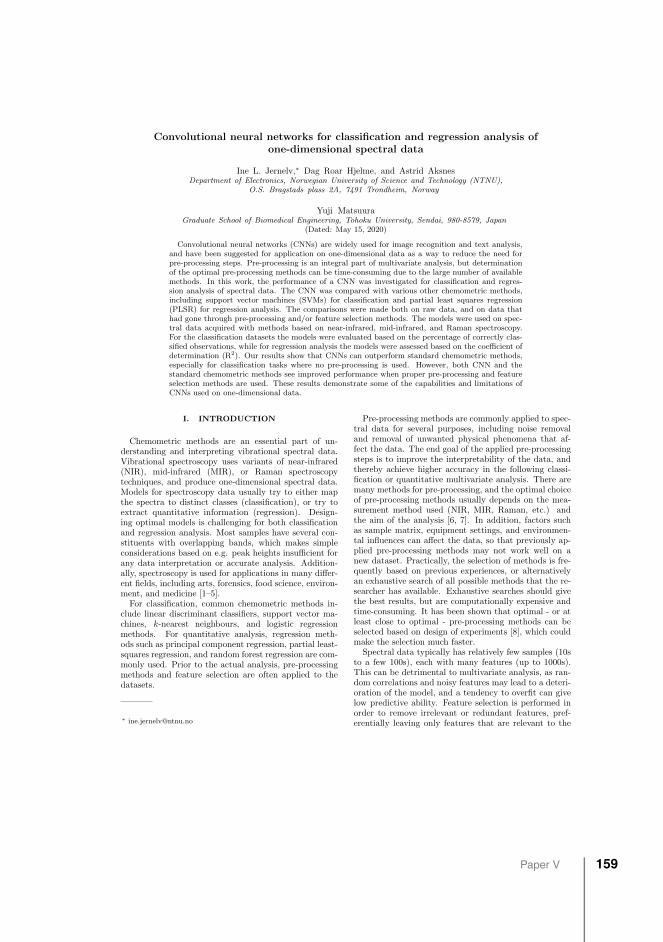
Convolutional neural networks for classification and regression analysis ofone-dimensional spectral data
Ine L. Jernelv,∗ Dag Roar Hjelme, and Astrid AksnesDepartment of Electronics, Norwegian University of Science and Technology (NTNU),
O.S. Bragstads plass 2A, 7491 Trondheim, Norway
Yuji MatsuuraGraduate School of Biomedical Engineering, Tohoku University, Sendai, 980-8579, Japan
(Dated: May 15, 2020)
Convolutional neural networks (CNNs) are widely used for image recognition and text analysis,and have been suggested for application on one-dimensional data as a way to reduce the need forpre-processing steps. Pre-processing is an integral part of multivariate analysis, but determinationof the optimal pre-processing methods can be time-consuming due to the large number of availablemethods. In this work, the performance of a CNN was investigated for classification and regres-sion analysis of spectral data. The CNN was compared with various other chemometric methods,including support vector machines (SVMs) for classification and partial least squares regression(PLSR) for regression analysis. The comparisons were made both on raw data, and on data thathad gone through pre-processing and/or feature selection methods. The models were used on spec-tral data acquired with methods based on near-infrared, mid-infrared, and Raman spectroscopy.For the classification datasets the models were evaluated based on the percentage of correctly clas-sified observations, while for regression analysis the models were assessed based on the coefficient ofdetermination (R2). Our results show that CNNs can outperform standard chemometric methods,especially for classification tasks where no pre-processing is used. However, both CNN and thestandard chemometric methods see improved performance when proper pre-processing and featureselection methods are used. These results demonstrate some of the capabilities and limitations ofCNNs used on one-dimensional data.
I. INTRODUCTION
Chemometric methods are an essential part of un-derstanding and interpreting vibrational spectral data.Vibrational spectroscopy uses variants of near-infrared(NIR), mid-infrared (MIR), or Raman spectroscopytechniques, and produce one-dimensional spectral data.Models for spectroscopy data usually try to either mapthe spectra to distinct classes (classification), or try toextract quantitative information (regression). Design-ing optimal models is challenging for both classificationand regression analysis. Most samples have several con-stituents with overlapping bands, which makes simpleconsiderations based on e.g. peak heights insufficient forany data interpretation or accurate analysis. Addition-ally, spectroscopy is used for applications in many differ-ent fields, including arts, forensics, food science, environ-ment, and medicine [1–5].
For classification, common chemometric methods in-clude linear discriminant classifiers, support vector ma-chines, k-nearest neighbours, and logistic regressionmethods. For quantitative analysis, regression meth-ods such as principal component regression, partial least-squares regression, and random forest regression are com-monly used. Prior to the actual analysis, pre-processingmethods and feature selection are often applied to thedatasets.
Pre-processing methods are commonly applied to spec-tral data for several purposes, including noise removaland removal of unwanted physical phenomena that af-fect the data. The end goal of the applied pre-processingsteps is to improve the interpretability of the data, andthereby achieve higher accuracy in the following classi-fication or quantitative multivariate analysis. There aremany methods for pre-processing, and the optimal choiceof pre-processing methods usually depends on the mea-surement method used (NIR, MIR, Raman, etc.) andthe aim of the analysis [6, 7]. In addition, factors suchas sample matrix, equipment settings, and environmen-tal influences can affect the data, so that previously ap-plied pre-processing methods may not work well on anew dataset. Practically, the selection of methods is fre-quently based on previous experiences, or alternativelyan exhaustive search of all possible methods that the re-searcher has available. Exhaustive searches should givethe best results, but are computationally expensive andtime-consuming. It has been shown that optimal - or atleast close to optimal - pre-processing methods can beselected based on design of experiments [8], which couldmake the selection much faster.
Spectral data typically has relatively few samples (10sto a few 100s), each with many features (up to 1000s).This can be detrimental to multivariate analysis, as ran-dom correlations and noisy features may lead to a deteri-oration of the model, and a tendency to overfit can givelow predictive ability. Feature selection is performed inorder to remove irrelevant or redundant features, pref-erentially leaving only features that are relevant to the
arX
iv:s
ubm
it/31
7912
6 [
cs.L
G]
15
May
202
0
Paper V 159
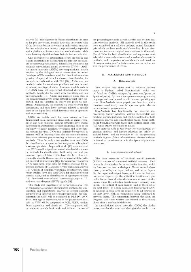
2
analysis [9]. The objective of feature selection is the sameas for pre-processing, namely increased interpretabilityof the data and better outcomes in multivariate analysis.Feature selection can be very computationally expensiveand a plethora of feature selection methods exist, whilesome learning algorithms have built-in feature selection.
One alternative to optimisation of pre-processing andfeature selection is to use learning models that are capa-ble of extracting fundamental information from data, forexample convolutional neural netoworks (CNNs). Artifi-cial neural networks (ANNs) are computational modelsinspired by the biological neural connections in brains.One-layer ANNs have been used for classification and re-gression of spectral data for almost three decades, forexample in combination with PLS [10]. ANNs are par-ticularly useful for non-linear problems and can be usedon almost any type of data. However, models such asPLS-ANN have not superseded standard chemometricmethods, largely due to issues with overfitting and lowinterpretability [11]. CNNs can improve upon this, asthe convolutional layers of the network are not fully con-nected, and are therefore in theory less prone to over-fitting. Additionally, the convolution leads to fewer freeparameters, and each layer becomes related to specificparts of the input data, which increases ease of operationand interpretability.
CNNs are widely used for data mining of two-dimensional data, including areas such as image recog-nition and text analysis. Neural networks have severalinteresting characteristics for data modelling, such as thecapability to model nonlinear responses and to accentu-ate relevant features. CNNs can therefore be expected toperform well on learning tasks also for one-dimensionaldata, even without pre-processing or feature extractionmethods. Thus far, only a few studies have used CNNsfor classification or quantitative analysis on vibrationalspectroscopic data. Acquarelli et al. [12] demonstratedthat CNNs could outperform several standard chemomet-ric methods for classification, both using raw and pre-processed spectral data. CNNs have also been shown toefficiently classify Raman spectra of mineral data with-out spectral preprocessing [13]. For quantitative analysisCNNs have been used both for feature selection for re-gression methods [14], and directly for regression analysis[15]. Outside of standard vibrational spectroscopy, somerecent studies have also used CNNs for analysis of otherspectral data, such as classification of hyperspectral data[16], functional near-infrared spectroscopy signals [17],and electrocardiogram (ECG) signals [18].
This study will investigate the performance of a CNNas compared to standard chemometric methods for clas-sification and quantitative analysis on several datasetsacquired with different spectroscopic methods. For clas-sification the CNN will be compared to PLS-DA, kNN,SVM, and logistic regression, while for quantitative anal-ysis the CNN will be compared to PCR, PLSR, randomforest regression, and elastic net. The comparison willbe made on models both with and without the use of
pre-processing methods, as well as with and without fea-ture selection methods. All methods used in this studywere assembled in a software package, named SpecAnal-ysis, which has been made available online. In our view,there are two main original contributions in this work:Use of CNNs for both classification and regression anal-ysis, with a comparison to several standard chemometricmethods, and comparison of models with additional useof pre-processing and/or feature selection, to further as-sess the performance of CNNs.
II. MATERIALS AND METHODS
A. Data analysis
The analysis was done with a software packagemade in Python, called SpecAnalysis, which canbe found on GitHub (https://github.com/jernelv/SpecAnalysis). Python is an open-source programminglanguage, and can be used on all common operating sys-tems. SpecAnalysis has a graphic user interface, and istherefore user-friendly even for spectroscopists who arenot experienced programmers.
SpecAnalysis has functionality for spectral pre-processing, feature selection, various chemometric andmachine learning methods, and can be employed for bothregression analysis and classification tasks. Some meth-ods in SpecAnalysis were based on tools from scikit-learn[19], while others were made in-house.
The methods used in this study for classification, re-gression analysis, and feature selection are briefly de-scribed below, and an overview of the pre-processingmethods is given. More information on the methods canbe found in the references or in the SpecAnalysis docu-mentation.
1. Convolutional neural network
The basic structure of artificial neural networks(ANNs) consists of connected artificial neurons. Eachneuron is characterised by an activation function, whichis a function that acts on the input. Neural networks havethree types of layers: input, hidden, and output layers.For the input and output layers, which are the first andlast layers respectively, the activation functions are gen-erally linear. Neural networks have one or more hiddenlayers, where the activation functions are normally non-linear. The output at each layer is used as the input ofthe next layer. In a fully-connected feed-forward ANN,all neurons in each layer are connected to all neurons inthe next layer, with no connections going backward toprevious layers. The connections between the layers areweighted, and these weights are learned in the trainingphase after a random initialisation.
In convolutional neural networks (CNNs) the hiddenlayers convolve the input and then give the result to the
160 Publications
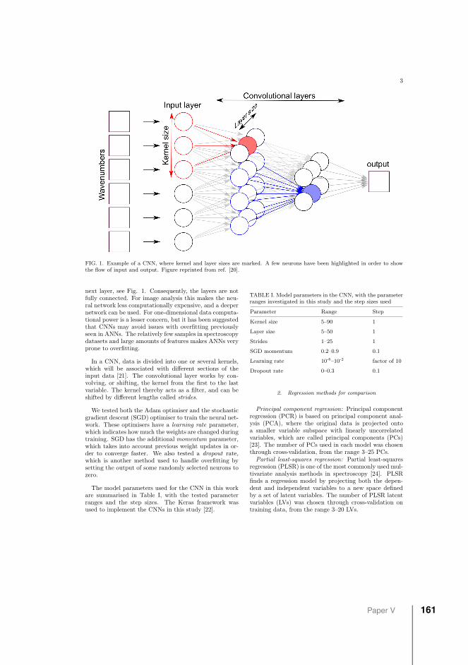
3
FIG. 1. Example of a CNN, where kernel and layer sizes are marked. A few neurons have been highlighted in order to showthe flow of input and output. Figure reprinted from ref. [20].
next layer, see Fig. 1. Consequently, the layers are notfully connected. For image analysis this makes the neu-ral network less computationally expensive, and a deepernetwork can be used. For one-dimensional data computa-tional power is a lesser concern, but it has been suggestedthat CNNs may avoid issues with overfitting previouslyseen in ANNs. The relatively few samples in spectroscopydatasets and large amounts of features makes ANNs veryprone to overfitting.
In a CNN, data is divided into one or several kernels,which will be associated with different sections of theinput data [21]. The convolutional layer works by con-volving, or shifting, the kernel from the first to the lastvariable. The kernel thereby acts as a filter, and can beshifted by different lengths called strides.
We tested both the Adam optimiser and the stochasticgradient descent (SGD) optimiser to train the neural net-work. These optimisers have a learning rate parameter,which indicates how much the weights are changed duringtraining. SGD has the additional momentum parameter,which takes into account previous weight updates in or-der to converge faster. We also tested a dropout rate,which is another method used to handle overfitting bysetting the output of some randomly selected neurons tozero.
The model parameters used for the CNN in this workare summarised in Table I, with the tested parameterranges and the step sizes. The Keras framework wasused to implement the CNNs in this study [22].
TABLE I. Model parameters in the CNN, with the parameterranges investigated in this study and the step sizes used
Parameter Range Step
Kernel size 5–90 1
Layer size 5–50 1
Strides 1–25 1
SGD momentum 0.2–0.9 0.1
Learning rate 10-6–10-2 factor of 10
Dropout rate 0–0.3 0.1
2. Regression methods for comparison
Principal component regression: Principal componentregression (PCR) is based on principal component anal-ysis (PCA), where the original data is projected ontoa smaller variable subspace with linearly uncorrelatedvariables, which are called principal components (PCs)[23]. The number of PCs used in each model was chosenthrough cross-validation, from the range 3–25 PCs.
Partial least-squares regression: Partial least-squaresregression (PLSR) is one of the most commonly used mul-tivariate analysis methods in spectroscopy [24]. PLSRfinds a regression model by projecting both the depen-dent and independent variables to a new space definedby a set of latent variables. The number of PLSR latentvariables (LVs) was chosen through cross-validation ontraining data, from the range 3–20 LVs.
Paper V 161
4
Random forest regression: Random forest (RF) is anensemble learning method that can be used for severalpurposes, and has been used successfully for regressionof spectral data [25]. Random forest regression worksby creating multiple decision trees, and combining thesefor regression analysis. RF regression was evaluated withmaximum tree depth for each dataset and 200–600 deci-sion trees.
Elastic net: Elastic net (Net) is another ensemblelearning method that combines the penalty variablesfrom lasso and ridge regression (L1 and L2, respectively)[26]. Elastic net was evaluated with an L1/L2 ratio of0–1 in increments of 0.1.
3. Classification methods for comparison
Partials least-squares discriminant analysis: PLS dis-criminant analysis (PLS-DA) uses classical PLSR on cat-egorical variables, which is enabled by dividing the cat-egorical variable into dummy variables that describe thecategories (also called one hot encoding) [27]. OptimalPLS-DA models were chosen based on LVs in the range3–20.k-nearest neighbours: k-nearest neighbours (kNN) is
a simple learning method that classifies predicted datapoints based on their distance from the k nearest neigh-bours in the training set [28]. The distance betweentest data and training data can be calculated in differentways, e.g. Euclidean, Chebyshev, or cosine. This studyused the Euclidean distance method as it is most com-mon, and the models have been optimised for k in therange 3–10.
Support vector machines: Support vector machines(SVMs) are a class of learning methods that try to findhyperplanes in a multidimensional space in order to di-vide data points into separate classes [29]. A supportvector classifier with a linear kernel was used for thisstudy.
Logistic regression: Logistic regression (LogReg) is acategorical method used to fit data with a special logisticfunction [30]. LogReg models can be considered simpli-fied ANNs with no hidden layers. We used a LogRegmodel with an L2 penalty.
4. Pre-processing methods
Various methods can be used on spectroscopic datato correct for scattering effects, including standard nor-mal variate (SNV) and multiplicative scattering correc-tion (MSC). Spectral derivatives can also widely used toremove unwanted spectral effects.
Filtering or smoothing methods can be used alone ondata to reduce noise. In addition, filtering methodsare used to improve the noise in spectral derivatives.Savitzky-Golay (SG) differentiation is by far the most
common method used. In the smoothing step for SG fil-tering a polynomial is fitted to the data points in thewindow using linear least-squares.
The pre-processing methods used in this study can bedivided into five separate steps, where some have differentpossible methods and associated variable parameters:
• Data binning: Binning together 1–16 data points
• Scatter correction:
– Normalisation
– Standard normal variate (SNV)
– Multiplicative scattering correction (MSC)
• Smoothing/filtering:
– Savitzky-Golay filter (order 1–3, width 5–21)
– Fourier filter
– Finite/infinite impulse response filters (But-terworth, Hamming, moving average)
• Baseline corrections:
– Subtract constant value
– Subtract linear background
– Spectral derivative (1st or 2nd derivative)
• Scaling:
– Mean centering
– Scaling
Note that this is a small subset of all possible pre-processing methods that exist, and we chose some generalmethods that are often applied to spectroscopy data [6,7]. There is a lack of consensus regarding the best orderof different pre-processing steps, and recent studies haveshown that there is no clear optimal order [31], althoughthe order can influence the prediction accuracy.
5. Feature selection
Spectral data can contain many hundreds or thousandsof spectral features. For most types of data, the spectracontain features that are either irrelevant or redundant.Many types of feature selection methods have been de-veloped, see refs. [9, 32] for extensive reviews. We testedthree different wrapper methods for the datasets in thisstudy, which are briefly described below. Wrapper meth-ods generally work by searching through several subsetsof features and choosing a feature subset based on pre-diction accuracy, see Fig. 2 for a schematic.
Sequential selection: In forward selection, one starts bychoosing the wavenumber which has the highest correla-tion with the Y-variable. The wavenumbers that givethe highest model improvements are then added itera-tively, until no improvements occur when more features
162 Publications
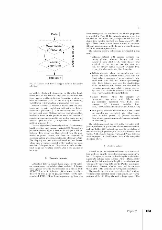
5
Data
Make subsetof features
Learning algorithm
Prediction
Find b
est su
bse
t
FIG. 2. General work flow of wrapper methods for featureselection.
are added. Backward elimination, on the other hand,starts with all the features, and tries to eliminate fea-tures that worsen the prediction. Sequential, or stepwise,selection combines these two methods by reconsideringvariables for re-introduction or removal at each step.
Moving Window: A window is moved over the spec-trum, and regression models are built using the data inthe window position [33]. The window size can be var-ied over a set range. Optimal spectral intervals can thenbe chosen, based on the prediction error and number ofregression components used in the model. Some movingwindow algorithms also try to optimise the selection ofmultiple windows [34].
Genetic Algorithm: Genetic algorithms (GA) for wave-length selection exist in many variants [35]. Generally, apopulation consisting of K vectors with length n are ini-tialised. Two vectors are then selected from the pop-ulation as parent vectors, and these are subjected tocrossover and/or mutation, resulting in offspring vectors.The offspring are then evaluated based on their fitness,where they are either rejected or they replace the worstmember of the population. Regression models are thenbuilt using the resulting vectors after a set amount ofiterations.
B. Example datasets
Datasets of different sample types acquired with differ-ent measurement methods have been analysed. A datasetwith aqueous solutions was measured in a custom-builtATR-FTIR setup for this study. Other openly availabledatasets of food items or pharmaceutical tablets mea-sured with FTIR, NIR or Raman spectroscopy have also
been investigated. An overview of the dataset propertiesis provided in Table II. For datasets with no preset testset, such as the Tablets data, we separated the data ran-domly into training and test sets based on a 67%/33%split. These datasets were chosen in order to representdifferent measurement methods and wavelength rangeswithin vibrational spectroscopy.
The following spectral datasets are investigated in thisstudy:
• Solutions dataset, with aqueous solutions con-taining glucose, albumin, lactate, and urea,measured with ATR-FTIR. This dataset wasacquired by the authors, see the next sec-tion for further details (dataset available fromhttps://github.com/jernelv/SpecAnalysis)
• Tablets dataset, where the samples are cate-gorised into four different tablet types with dif-ferent relative amounts of active materiel, mea-sured with both NIR and Raman spectroscopy[36]. Both datasets were used for classification,while the Tablets NIR dataset was also used forregression analysis since relative weight percent-age was also available (dataset available fromhttp://www.models.life.ku.dk/Tablets)
• Wines dataset, where the samples arecategorised into wines with different ori-gin countries, measured with FTIR spec-troscopy [37] (dataset available fromhttp://www.models.life.ku.dk/Wine GCMS FTIR)
• Fruit purees datasets measured with FTIR, wherethe samples are categorised into either straw-berry or other purees [38] (dataset availablefrom https://csr.quadram.ac.uk/example-datasets-for-download/)
The Solutions dataset was used in the regression anal-ysis for prediction of glucose and albumin concentrations,and the Tablets NIR dataset was used for prediction ofthe relative weight percentage of the active material. TheTablets NIR, Tablets Raman, Fruits, and Wines datasetswere employed for classification tasks of the categoriesdescribed above.
1. Solutions dataset
In total, 90 unique aqueous solutions were made withfour analytes, with the concentration ranges shown in Ta-ble III. Samples were made by dissolving the analytes in aphosphate-buffered saline solution (PBS). PBS is a buffersolution that helps maintain the pH in the solutions, andwas made by dissolving PBS powder (Wako) in deminer-alised water. Glucose, albumin, urea, and lactate werethen added to the solutions in varying concentrations.
The sample concentrations were determined with anoptimal design model in order to randomise the concen-trations while still filling the entire design space. The
Paper V 163
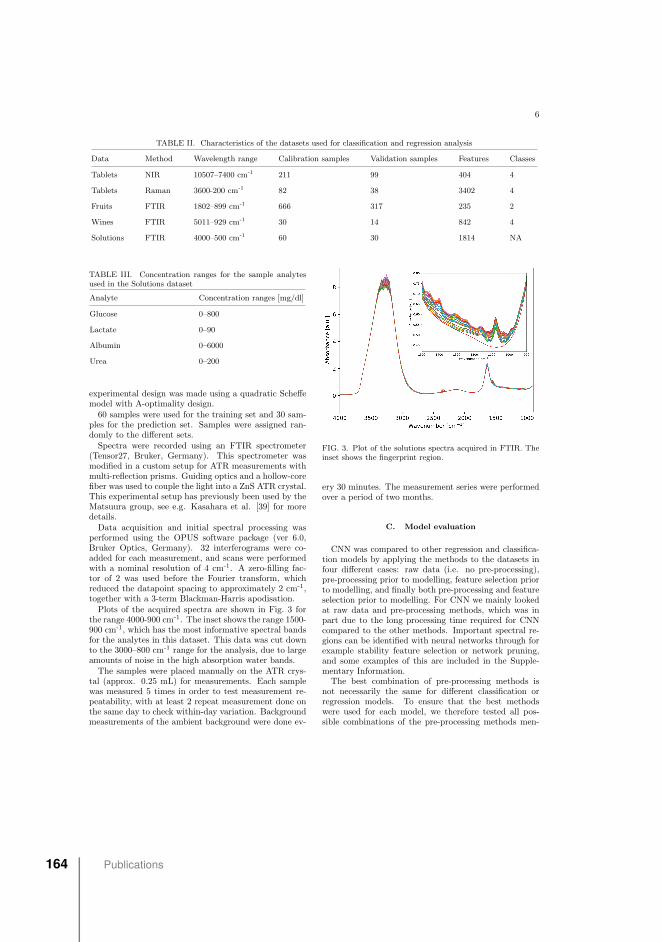
6
TABLE II. Characteristics of the datasets used for classification and regression analysis
Data Method Wavelength range Calibration samples Validation samples Features Classes
Tablets NIR 10507–7400 cm-1 211 99 404 4
Tablets Raman 3600-200 cm-1 82 38 3402 4
Fruits FTIR 1802–899 cm-1 666 317 235 2
Wines FTIR 5011–929 cm-1 30 14 842 4
Solutions FTIR 4000–500 cm-1 60 30 1814 NA
TABLE III. Concentration ranges for the sample analytesused in the Solutions dataset
Analyte Concentration ranges [mg/dl]
Glucose 0–800
Lactate 0–90
Albumin 0–6000
Urea 0–200
experimental design was made using a quadratic Scheffemodel with A-optimality design.
60 samples were used for the training set and 30 sam-ples for the prediction set. Samples were assigned ran-domly to the different sets.
Spectra were recorded using an FTIR spectrometer(Tensor27, Bruker, Germany). This spectrometer wasmodified in a custom setup for ATR measurements withmulti-reflection prisms. Guiding optics and a hollow-corefiber was used to couple the light into a ZnS ATR crystal.This experimental setup has previously been used by theMatsuura group, see e.g. Kasahara et al. [39] for moredetails.
Data acquisition and initial spectral processing wasperformed using the OPUS software package (ver 6.0,Bruker Optics, Germany). 32 interferograms were co-added for each measurement, and scans were performedwith a nominal resolution of 4 cm-1. A zero-filling fac-tor of 2 was used before the Fourier transform, whichreduced the datapoint spacing to approximately 2 cm-1,together with a 3-term Blackman-Harris apodisation.
Plots of the acquired spectra are shown in Fig. 3 forthe range 4000-900 cm-1. The inset shows the range 1500-900 cm-1, which has the most informative spectral bandsfor the analytes in this dataset. This data was cut downto the 3000–800 cm-1 range for the analysis, due to largeamounts of noise in the high absorption water bands.
The samples were placed manually on the ATR crys-tal (approx. 0.25 mL) for measurements. Each samplewas measured 5 times in order to test measurement re-peatability, with at least 2 repeat measurement done onthe same day to check within-day variation. Backgroundmeasurements of the ambient background were done ev-
FIG. 3. Plot of the solutions spectra acquired in FTIR. Theinset shows the fingerprint region.
ery 30 minutes. The measurement series were performedover a period of two months.
C. Model evaluation
CNN was compared to other regression and classifica-tion models by applying the methods to the datasets infour different cases: raw data (i.e. no pre-processing),pre-processing prior to modelling, feature selection priorto modelling, and finally both pre-processing and featureselection prior to modelling. For CNN we mainly lookedat raw data and pre-processing methods, which was inpart due to the long processing time required for CNNcompared to the other methods. Important spectral re-gions can be identified with neural networks through forexample stability feature selection or network pruning,and some examples of this are included in the Supple-mentary Information.
The best combination of pre-processing methods isnot necessarily the same for different classification orregression models. To ensure that the best methodswere used for each model, we therefore tested all pos-sible combinations of the pre-processing methods men-
164 Publications
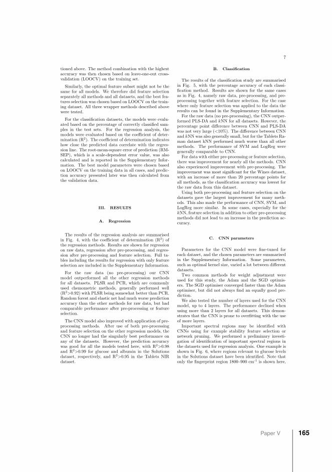
7
tioned above. The method combination with the highestaccuracy was then chosen based on leave-one-out cross-validation (LOOCV) on the training set.
Similarly, the optimal feature subset might not be thesame for all models. We therefore did feature selectionseparately all methods and all datasets, and the best fea-tures selection was chosen based on LOOCV on the train-ing dataset. All three wrapper methods described abovewere tested.
For the classification datasets, the models were evalu-ated based on the percentage of correctly classified sam-ples in the test sets. For the regression analysis, themodels were evaluated based on the coefficient of deter-mination (R2). The coefficient of determination indicateshow close the predicted data correlate with the regres-sion line. The root-mean-square error of prediction (RM-SEP), which is a scale-dependent error value, was alsocalculated and is reported in the Supplementary Infor-mation. The best model parameters were chosen basedon LOOCV on the training data in all cases, and predic-tion accuracy presented later was then calculated fromthe validation data.
III. RESULTS
A. Regression
The results of the regression analysis are summarisedin Fig. 4, with the coefficient of determination (R2) ofthe regression methods. Results are shown for regressionon raw data, regression after pre-processing, and regres-sion after pre-processing and feature selection. Full ta-bles including the results for regression with only featureselection are included in the Supplementary Information.
For the raw data (no pre-processing) our CNNmodel outperformed all the other regression methodsfor all datasets. PLSR and PCR, which are commonlyused chemometric methods, generally performed well(R2>0.92) with PLSR being somewhat better than PCR.Random forest and elastic net had much worse predictionaccuracy than the other methods for raw data, but hadcomparable performance after pre-processing or featureselection.
The CNN model also improved with application of pre-processing methods. After use of both pre-processingand feature selection on the other regression models, theCNN no longer had the singularly best performance onany of the datasets. However, the prediction accuracywas good for all the models tested here, with R2>0.98and R2>0.99 for glucose and albumin in the Solutionsdataset, respectively, and R2>0.95 in the Tablets NIRdataset.
B. Classification
The results of the classification study are summarisedin Fig. 5, with the percentage accuracy of each classi-fication method. Results are shown for the same casesas in Fig. 4, namely raw data, pre-processing, and pre-processing together with feature selection. For the casewhere only feature selection was applied to the data theresults can be found in the Supplementary Information.
For the raw data (no pre-processing), the CNN outper-formed PLS-DA and kNN for all datasets. However, thepercentage point difference between CNN and PLS-DAwas not very large (<10%). The difference between CNNand kNN was also generally small, but for the Tablets Ra-man dataset kNN performed much worse than all othermethods. The performance of SVM and LogReg weregenerally comparable to CNN.
For data with either pre-processing or feature selection,there was improvement for nearly all the methods. CNNalso experienced improvement with pre-processing. Theimprovement was most significant for the Wines dataset,with an increase of more than 20 percentage points forall methods, as the classification accuracy was lowest forthe raw data from this dataset.
Using both pre-processing and feature selection on thedatasets gave the largest improvement for many meth-ods. This also made the performance of CNN, SVM, andLogReg more similar. In some cases, especially for thekNN, feature selection in addition to other pre-processingmethods did not lead to an increase in the prediction ac-curacy.
C. CNN parameters
Parameters for the CNN model were fine-tuned foreach dataset, and the chosen parameters are summarisedin the Supplementary Information. Some parameters,such as optimal kernel size, varied a lot between differentdatasets.
Two common methods for weight adjustment wereused for this study, the Adam and the SGD optimis-ers. The SGD optimiser converged faster than the Adamoptimiser, but did not always find an equally good pre-diction.
We also tested the number of layers used for the CNNmodel, up to 4 layers. The performance declined whenusing more than 2 layers for all datasets. This demon-strates that the CNN is prone to overfitting with the useof more layers.
Important spectral regions may be identified withCNNs using for example stability feature selection ornetwork pruning. We performed a preliminary investi-gation of identification of important spectral regions inthe datasets used for regression analysis. One example isshown in Fig. 6, where regions relevant to glucose levelsin the Solutions dataset have been identified. Note thatonly the fingerprint region 1800–900 cm-1 is shown here,
Paper V 165
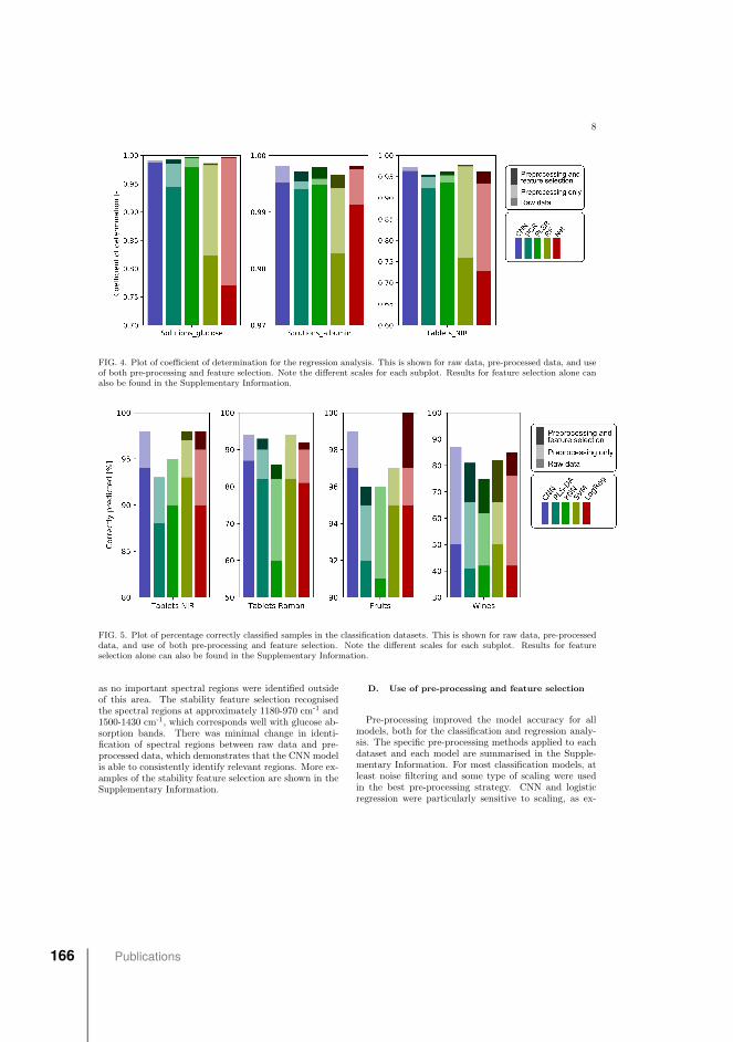
8
FIG. 4. Plot of coefficient of determination for the regression analysis. This is shown for raw data, pre-processed data, and useof both pre-processing and feature selection. Note the different scales for each subplot. Results for feature selection alone canalso be found in the Supplementary Information.
FIG. 5. Plot of percentage correctly classified samples in the classification datasets. This is shown for raw data, pre-processeddata, and use of both pre-processing and feature selection. Note the different scales for each subplot. Results for featureselection alone can also be found in the Supplementary Information.
as no important spectral regions were identified outsideof this area. The stability feature selection recognisedthe spectral regions at approximately 1180-970 cm-1 and1500-1430 cm-1, which corresponds well with glucose ab-sorption bands. There was minimal change in identi-fication of spectral regions between raw data and pre-processed data, which demonstrates that the CNN modelis able to consistently identify relevant regions. More ex-amples of the stability feature selection are shown in theSupplementary Information.
D. Use of pre-processing and feature selection
Pre-processing improved the model accuracy for allmodels, both for the classification and regression analy-sis. The specific pre-processing methods applied to eachdataset and each model are summarised in the Supple-mentary Information. For most classification models, atleast noise filtering and some type of scaling were usedin the best pre-processing strategy. CNN and logisticregression were particularly sensitive to scaling, as ex-
166 Publications
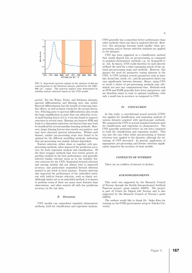
9
FIG. 6. Important spectral regions in the analysis of glucoseconcentrations in the Solutions dataset, plotted for the 1800–900 cm-1 region. The spectral regions were determined bystability feature selection based on the CNN model.
pected. For the Wines, Fruits, and Solutions datasets,spectral differentiation and filtering were also useful.Spectral differentiation has the benefit of removing base-line effects, as well as linear trends for the second deriva-tive. Filtering prior to spectral differentiation also avoidsthe large amplification in noise that can otherwise occur.A small binning factor of 2 or 4 was also found to improveoutcomes in several cases. Binning can improve SNR andleads to a dimension reduction; two factors that may bothbe beneficial for several machine learning methods. How-ever, larger binning factors were mostly not positive, andmay have obscured spectral information. Within eachdataset, similar pre-processing steps were found to beoptimal for the different modelling methods, indicatingthat pre-processing was mainly dataset-dependent.
Feature selection, either alone or together with pre-processing methods, often improved the prediction accu-racy for both regression analysis and classification. Ofthe three wrapper methods that were tested, genetic al-gorithm resulted in the best performance, and generallyselected similar relevant areas as in the stability fea-ture selection for the CNN. Sequential forward selectionand moving window did not always lead to improvedaccuracy, and particularly sequential forward selectionseemed to get stuck in local maxima. Feature selectionalso improved the performance of the embedded meth-ods with built-in feature selection, such as elastic net.Although elastic net is an embedded method, it is knownto perform worse if there are many more features thanobservations, and often started off with low predictionaccuracy on the raw data.
E. Discussion
CNN models can outperform standard chemometricmethods, both for classification and regression analysis.
CNN generally has a somewhat better performance thanother methods when raw data is analysed directly. How-ever, this advantage becomes much smaller when pre-processing and/or feature selection methods are appliedto the datasets.
CNN has been suggested as a classification methodthat would depend less on pre-processing as comparedto standard chemometric methods, e.g. by Acquarelli etal. [12]. In theory, CNN could therefore be used directlywithout the need for a time-consuming search of the op-timal pre-processing steps and methods. However, thisignores the need for parameter tuning inherent in theCNN. A CNN includes several parameters such as layersize, kernel size, stride, etc., and the parameter choice canvary significantly between datasets. Hence, using CNNto avoid a choice of pre-processing methods may ulti-mately not save any computational time. Methods suchas SVM and PLSR generally have fewer parameters, andare therefore easier to tune to optimal conditions, withonly a small loss in accuracy as compared to CNN.
IV. CONCLUSION
In this study, a convolutional neural network (CNN)was applied for classification and regression analysis ofvarious datasets acquired with spectroscopic methods.We compared the CNN to several standard methods usedfor classification and regression in chemometrics. TheCNN generally performed better on raw data comparedto both the classification and regression models. Thiswas also the case when either pre-processing or featureselection were applied to the datasets, although the ad-vantage of CNN decreased. In general, application ofappropriate pre-processing and feature selection signifi-cantly improves the accuracy of most models.
CONFLICTS OF INTEREST
There are no conflicts of interest to declare.
ACKNOWLEDGMENTS
This work was supported by the Research Councilof Norway through the Double Intraperitoneal ArtificialPancreas project, grant number 248872. The projectis part of Centre for Digital Life Norway and is alsosupported by the Research Council of Norway’s grant248810.
The authors would like to thank Dr. Saiko Kino fortraining on the FTIR spectrometer setup at Tohoku Uni-versity.
Paper V 167
10
[1] L. G. Thygesen, M. M. Løkke, E. Micklander and S. B.Engelsen, Trends in Food Science and Technology, 2003,14, 50–57.
[2] C. Kendall, M. Isabelle, F. Bazant-Hegemark, J. Hutch-ings, L. Orr, J. Babrah, R. Baker and N. Stone, Analyst,2009, 134, 1029–1045.
[3] R. S. Das and Y. K. Agrawal, Vibrational Spectroscopy,2011, 57, 163–176.
[4] C. K. Muro, K. C. Doty, J. Bueno, L. Halamkova andI. K. Lednev, Analytical Chemistry, 2015, 87, 306–327.
[5] F. Pozzi and M. Leona, Journal of Raman Spectroscopy,2016, 47, 67–77.
[6] A. Rinnan, F. van den Berg and S. B. Engelsen, TrAC -Trends in Analytical Chemistry, 2009, 28, 1201–1222.
[7] J. Engel, J. Gerretzen, E. Szymanska, J. J. Jansen,G. Downey, L. Blanchet and L. M. Buydens, TrAC -Trends in Analytical Chemistry, 2013, 50, 96–106.
[8] J. Gerretzen, E. Szymanska, J. J. Jansen, J. Bart, H. J.Van Manen, E. R. Van Den Heuvel and L. M. Buydens,Analytical Chemistry, 2015, 87, 12096–12103.
[9] T. Mehmood, K. H. Liland, L. Snipen and S. Sæbø,Chemometrics and Intelligent Laboratory Systems, 2012,118, 62–69.
[10] P. Bhandare, Y. Mendelson, R. A. Peura, G. Janatsch,J. D. Kruse-Jarres, R. Marbach and H. M. Heise, AppliedSpectroscopy, 1993, 47, 1214–1221.
[11] F. Marini, R. Bucci, A. L. Magrı and A. D. Magrı, Mi-crochemical Journal, 2008, 88, 178–185.
[12] J. Acquarelli, T. van Laarhoven, J. Gerretzen, T. N.Tran, L. M. Buydens and E. Marchiori, Analytica Chim-ica Acta, 2017, 954, 22–31.
[13] J. Liu, M. Osadchy, L. Ashton, M. Foster, C. J. Solomonand S. J. Gibson, Analyst, 2017, 142, 4067–4074.
[14] S. Malek, F. Melgani and Y. Bazi, Journal of Chemomet-rics, 2018, 32, 1–17.
[15] C. Cui and T. Fearn, Chemometrics and Intelligent Lab-oratory Systems, 2018, 182, 9–20.
[16] Y. Chen, H. Jiang, C. Li, X. Jia and P. Ghamisi, IEEETransactions on Geoscience and Remote Sensing, 2016,54, 6232–6251.
[17] R. Rosas-Romero, E. Guevara, K. Peng, D. K. Nguyen,F. Lesage, P. Pouliot and W. E. Lima-Saad, Computersin Biology and Medicine, 2019, 111, 103355.
[18] S. Kiranyaz, T. Ince and M. Gabbouj, IEEE Transactionson Biomedical Engineering, 2015, 63, 664–675.
[19] F. Pedregosa, G. Varoquaux, A. Gramfort, V. Michel,B. Thirion, O. Grisel, M. Blondel, P. Prettenhofer,R. Weiss, V. Dubourg, J. Vanderplas, A. Passos, D. Cour-
napeau, M. Brucher and E. Duchesnay, Journal of Ma-chine Learning Research, 2011, 12, 2825–2830.
[20] I. L. Jernelv, K. Strøm, D. R. Hjelme and A. Aksnes,Proc. SPIE 11233, Optical Fibers and Sensors for Med-ical Diagnostics and Treatment Applications XX, 2020,1123311, 1–9.
[21] I. Goodfellow, Y. Bengio and A. Courville, Deep learning,MIT press, 2016.
[22] N. Ketkar, Deep Learning with Python, Apress, Berkeley,CA., 2017.
[23] T. Næs and H. Martens, Journal of Chemometrics, 1988,2, 155–167.
[24] S. Wold, M. Sjostrom and L. Eriksson, Chemometricsand Intelligent Laboratory Systems, 2001, 58, 109–130.
[25] A. Liaw and M. Wiener, R news, 2002, 2, 18–22.[26] H. Zou and T. Hastie, Journal of the Royal Statistical
Society. Series B: Statistical Methodology, 2005, 67, 301–320.
[27] R. G. Brereton and G. R. Lloyd, Journal of Chemomet-rics, 2014, 28, 213–225.
[28] N. S. Altman, American Statistician, 1992, 46, 175–185.[29] C. Cortes and V. Vapnik, Machine Learning, 1995, 20,
273–297.[30] T. Hastie and R. Tibshirani, Journal of the American
Statistical Association, 1987, 82, 371–386.[31] H. J. Butler, B. R. Smith, R. Fritzsch, P. Radhakrishnan,
D. S. Palmer and M. J. Baker, Analyst, 2018, 143, 6121–6134.
[32] Y. Saeys, I. Inza and P. Larranaga, Bioinformatics, 2007,23, 2507–2517.
[33] J.-h. Jiang, R. J. Berry, H. W. Siesler and Y. Ozaki,Analytical Chemistry, 2002, 74, 3555–3565.
[34] S. Kasemsumran, Y. P. Du, K. Murayama, M. Huehneand Y. Ozaki, Analytica Chimica Acta, 2004, 512, 223–230.
[35] D. Jouan-Rimbaud, D. L. Massart, R. Leardi and O. E.De Noord, Analytical Chemistry, 1995, 67, 4295–4301.
[36] M. Dyrby, S. B. Engelsen, L. Nørgaard, M. Bruhn andL. Lundsberg-Nielsen, Applied Spectroscopy, 2002, 56,579–585.
[37] T. Skov, D. Ballabio and R. Bro, Analytica Chimica Acta,2008, 615, 18–29.
[38] J. K. Holland, E. K. Kemsley and R. H. Wilson, Journalof the Science of Food and Agriculture, 1998, 76, 263–269.
[39] R. Kasahara, S. Kino, S. Soyama and Y. Matsuura,Biomedical Optics Express, 2018, 9, 289–302.
168 Publications
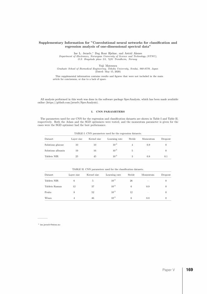
Supplementary Information for ”Convolutional neural networks for classification andregression analysis of one-dimensional spectral data”
Ine L. Jernelv,∗ Dag Roar Hjelme, and Astrid AksnesDepartment of Electronics, Norwegian University of Science and Technology (NTNU),
O.S. Bragstads plass 2A, 7491 Trondheim, Norway
Yuji MatsuuraGraduate School of Biomedical Engineering, Tohoku University, Sendai, 980-8579, Japan
(Dated: May 15, 2020)
This supplemental information contains results and figures that were not included in the mainarticle for conciseness, or due to a lack of space.
All analysis performed in this work was done in the software package SpecAnalysis, which has been made availableonline (https://github.com/jernelv/SpecAnalysis).
I. CNN PARAMETERS
The parameters used for our CNN for the regression and classification datasets are shown in Table I and Table II,respectively. Both the Adam and the SGD optimisers were tested, and the momentum parameter is given for thecases were the SGD optimiser had the best performance.
TABLE I. CNN parameters used for the regression datasets.
Dataset Layer size Kernel size Learning rate Stride Momentum Dropout
Solutions glucose 10 10 10-3 4 0.9 0
Solutions albumin 19 16 10-3 5 – 0
Tablets NIR 25 45 10-3 3 0.8 0.1
TABLE II. CNN parameters used for the classification datasets.
Dataset Layer size Kernel size Learning rate Stride Momentum Dropout
Tablets NIR 6 5 10-3 26 – 0
Tablets Raman 12 37 10-3 6 0.9 0
Fruits 8 52 10-3 12 – 0
Wines 4 46 10-3 6 0.8 0
arX
iv:s
ubm
it/31
7912
6 [
cs.L
G]
15
May
202
0
Paper V 169
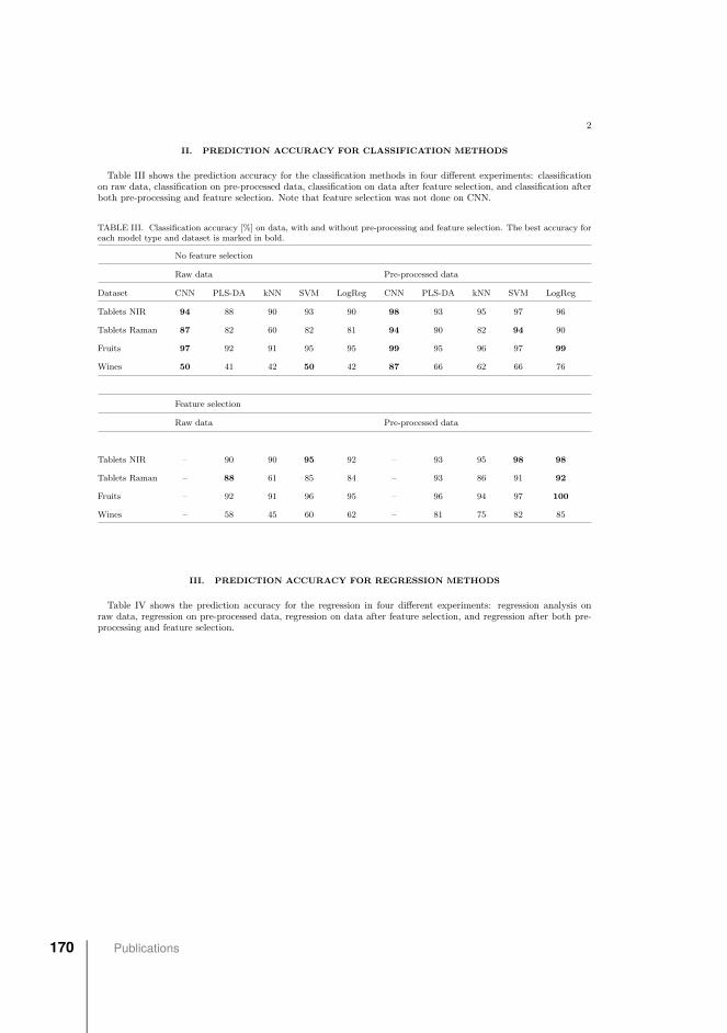
2
II. PREDICTION ACCURACY FOR CLASSIFICATION METHODS
Table III shows the prediction accuracy for the classification methods in four different experiments: classificationon raw data, classification on pre-processed data, classification on data after feature selection, and classification afterboth pre-processing and feature selection. Note that feature selection was not done on CNN.
TABLE III. Classification accuracy [%] on data, with and without pre-processing and feature selection. The best accuracy foreach model type and dataset is marked in bold.
No feature selection
Raw data Pre-processed data
Dataset CNN PLS-DA kNN SVM LogReg CNN PLS-DA kNN SVM LogReg
Tablets NIR 94 88 90 93 90 98 93 95 97 96
Tablets Raman 87 82 60 82 81 94 90 82 94 90
Fruits 97 92 91 95 95 99 95 96 97 99
Wines 50 41 42 50 42 87 66 62 66 76
Feature selection
Raw data Pre-processed data
Tablets NIR – 90 90 95 92 – 93 95 98 98
Tablets Raman – 88 61 85 84 – 93 86 91 92
Fruits – 92 91 96 95 – 96 94 97 100
Wines – 58 45 60 62 – 81 75 82 85
III. PREDICTION ACCURACY FOR REGRESSION METHODS
Table IV shows the prediction accuracy for the regression in four different experiments: regression analysis onraw data, regression on pre-processed data, regression on data after feature selection, and regression after both pre-processing and feature selection.
170 Publications
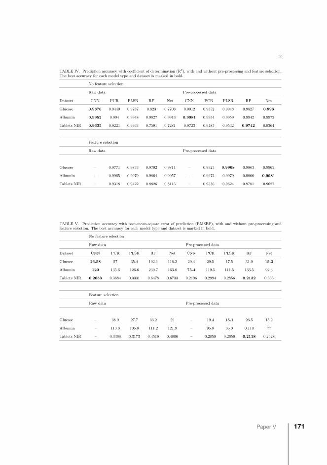
3
TABLE IV. Prediction accuracy with coefficient of determination (R2), with and without pre-processing and feature selection.The best accuracy for each model type and dataset is marked in bold.
No feature selection
Raw data Pre-processed data
Dataset CNN PCR PLSR RF Net CNN PCR PLSR RF Net
Glucose 0.9876 0.9449 0.9787 0.823 0.7708 0.9912 0.9852 0.9948 0.9827 0.996
Albumin 0.9952 0.994 0.9948 0.9827 0.9913 0.9981 0.9954 0.9959 0.9942 0.9972
Tablets NIR 0.9635 0.9221 0.9363 0.7591 0.7281 0.9723 0.9485 0.9532 0.9742 0.9364
Feature selection
Raw data Pre-processed data
Glucose – 0.9771 0.9833 0.9792 0.9811 – 0.9925 0.9968 0.9863 0.9965
Albumin – 0.9965 0.9979 0.9864 0.9957 – 0.9972 0.9979 0.9966 0.9981
Tablets NIR – 0.9318 0.9422 0.8826 0.8115 – 0.9536 0.9624 0.9781 0.9627
TABLE V. Prediction accuracy with root-mean-square error of prediction (RMSEP), with and without pre-processing andfeature selection. The best accuracy for each model type and dataset is marked in bold.
No feature selection
Raw data Pre-processed data
Dataset CNN PCR PLSR RF Net CNN PCR PLSR RF Net
Glucose 26.58 57 35.4 102.1 116.2 20.4 29.5 17.5 31.9 15.3
Albumin 120 135.6 126.6 230.7 163.8 75.4 119.5 111.5 133.5 92.3
Tablets NIR 0.2653 0.3684 0.3331 0.6478 0.6733 0.2196 0.2994 0.2856 0.2132 0.333
Feature selection
Raw data Pre-processed data
Glucose – 38.9 27.7 33.2 29 – 19.4 15.1 26.5 15.2
Albumin – 113.8 105.8 111.2 121.9 – 95.8 85.3 0.110 77
Tablets NIR – 0.3368 0.3173 0.4519 0.4806 – 0.2859 0.2656 0.2118 0.2628
Paper V 171

4
IV. PRE-PROCESSING METHODS
Several pre-processing methods were evaluated for this study, and an overview can be found in Table VI. These pre-processing methods were divided into five separate steps, and all possible combinations were tested for each datasetand each model. A more in-depth description of the various methods can be found in the Readme for the SpecAnalysissoftware package (https://github.com/jernelv/SpecAnalysis) or in the references in the main article.
TABLE VI. Alternatives for pre-processing methods used in this study.
1. Binning
- Binning together 1, 2, 4, 8, or 16 datapoints
2. Scatter correction
- Normalisation
- Standard normal variate (SNV)
- Multiple scatter correction (MSC)
3. Smoothing/filtering
- SG filter Polynomial order: 1, 2, or 3
Filter width: 3, 5, ..., 21 data points
- Fourier filter Window function: none, Blackman-Harris, Hamming, Hann
Filter cutoff: 20, 21, ... 50 points in Fourier space
Filter window size: 1.1, 1.2, 1.3
- Finite/infinite impulse response filters: Butterworth, Hamming, moving average (MA)
4. Baseline correction
- Subtract constant value
- Subtract linear background
- Spectral differentiation: 1st or 2nd derivative
5. Scaling
- Mean centering
- Scaling
172 Publications
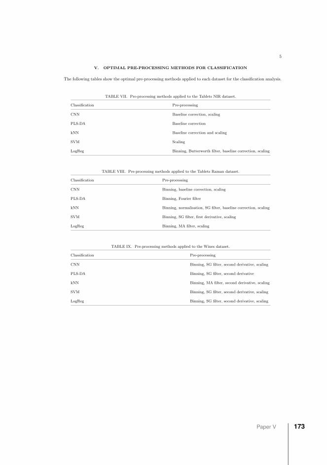
5
V. OPTIMAL PRE-PROCESSING METHODS FOR CLASSIFICATION
The following tables show the optimal pre-processing methods applied to each dataset for the classification analysis.
TABLE VII. Pre-processing methods applied to the Tablets NIR dataset.
Classification Pre-processing
CNN Baseline correction, scaling
PLS-DA Baseline correction
kNN Baseline correction and scaling
SVM Scaling
LogReg Binning, Butterworth filter, baseline correction, scaling
TABLE VIII. Pre-processing methods applied to the Tablets Raman dataset.
Classification Pre-processing
CNN Binning, baseline correction, scaling
PLS-DA Binning, Fourier filter
kNN Binning, normalisation, SG filter, baseline correction, scaling
SVM Binning, SG filter, first derivative, scaling
LogReg Binning, MA filter, scaling
TABLE IX. Pre-processing methods applied to the Wines dataset.
Classification Pre-processing
CNN Binning, SG filter, second derivative, scaling
PLS-DA Binning, SG filter, second derivative
kNN Binning, MA filter, second derivative, scaling
SVM Binning, SG filter, second derivative, scaling
LogReg Binning, SG filter, second derivative, scaling
Paper V 173
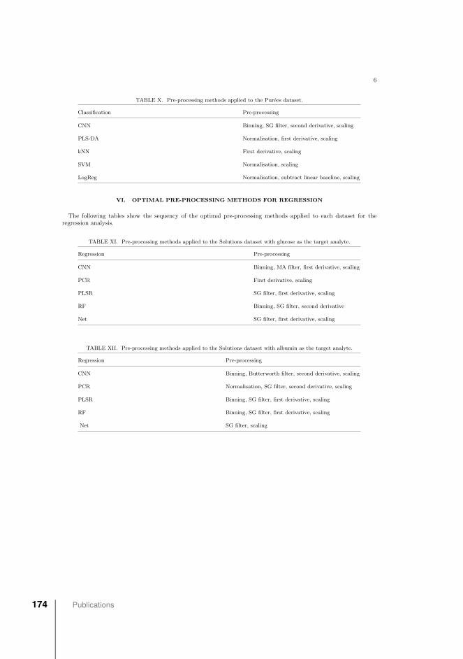
6
TABLE X. Pre-processing methods applied to the Purees dataset.
Classification Pre-processing
CNN Binning, SG filter, second derivative, scaling
PLS-DA Normalisation, first derivative, scaling
kNN First derivative, scaling
SVM Normalisation, scaling
LogReg Normalisation, subtract linear baseline, scaling
VI. OPTIMAL PRE-PROCESSING METHODS FOR REGRESSION
The following tables show the sequency of the optimal pre-processing methods applied to each dataset for theregression analysis.
TABLE XI. Pre-processing methods applied to the Solutions dataset with glucose as the target analyte.
Regression Pre-processing
CNN Binning, MA filter, first derivative, scaling
PCR First derivative, scaling
PLSR SG filter, first derivative, scaling
RF Binning, SG filter, second derivative
Net SG filter, first derivative, scaling
TABLE XII. Pre-processing methods applied to the Solutions dataset with albumin as the target analyte.
Regression Pre-processing
CNN Binning, Butterworth filter, second derivative, scaling
PCR Normalisation, SG filter, second derivative, scaling
PLSR Binning, SG filter, first derivative, scaling
RF Binning, SG filter, first derivative, scaling
Net SG filter, scaling
174 Publications
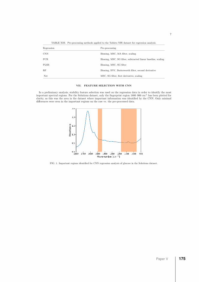
7
TABLE XIII. Pre-processing methods applied to the Tablets NIR dataset for regression analysis.
Regression Pre-processing
CNN Binning, MSC, MA filter, scaling
PCR Binning, MSC, SG filter, subtracted linear baseline, scaling
PLSR Binning, MSC, SG filter
RF Binning, SNV, Butterworth filter, second derivative
Net MSC, SG filter, first derivative, scaling
VII. FEATURE SELECTION WITH CNN
In a preliminary analysis, stability feature selection was used on the regression data in order to identify the mostimportant spectral regions. For the Solutions dataset, only the fingerprint region 1800–900 cm-1 has been plotted forclarity, as this was the area in the dataset where important information was identified by the CNN. Only minimaldifferences were seen in the important regions on the raw vs. the pre-processed data.
FIG. 1. Important regions identified for CNN regression analysis of glucose in the Solutions dataset.
Paper V 175
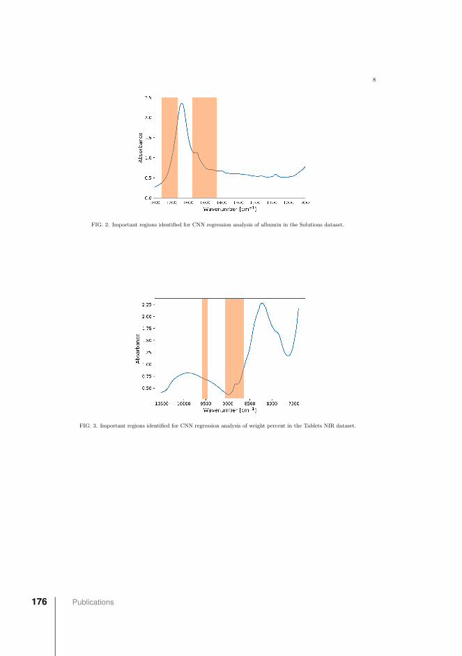
8
FIG. 2. Important regions identified for CNN regression analysis of albumin in the Solutions dataset.
FIG. 3. Important regions identified for CNN regression analysis of weight percent in the Tablets NIR dataset.
176 Publications

Paper VIInfrared measurements of glucose in peritoneal fluid with a tuneable quantumcascade laserI.L. Jernelv, D.R. Hjelme, A. AksnesBiomedical Optics Express, Vol. 11(7), pp. 3818-3829, 2020.
Paper VI 177

Research Article Vol. 11, No. 7 / 1 July 2020 / Biomedical Optics Express 3818
Infrared measurements of glucose in peritonealfluid with a tuneable quantum cascade laser
INE L. JERNELV,* DAG ROAR HJELME, AND ASTRID AKSNES
Department of Electronic Systems, Norwegian University of Science and Technology (NTNU), O.S.Bragstads plass 2A, 7491 Trondheim, Norway*[email protected]
Abstract: Fast and accurate continuous glucose monitoring is needed in future systems forcontrol of blood glucose levels in type 1 diabetes patients. Direct spectroscopic measurementof glucose in the peritoneal cavity is an attractive alternative to conventional electrochemicalsensors placed subcutaneously. We demonstrate the feasibility of fast glucose measurements inperitoneal fluid using a fibre-coupled tuneable mid-infrared quantum cascade laser. Mid-infraredspectra (1200–925 cm−1) of peritoneal fluid samples from pigs with physiological glucose levels(32–426 mg/dL, or 1.8–23.7 mmol/L) were acquired with a tuneable quantum cascade laseremploying both transmission and attenuated total reflection (ATR) spectroscopy. Using partialleast-squares regression, glucose concentrations were predicted with mean absolute percentageerrors (MAPEs) of 8.7% and 12.2% in the transmission and ATR configurations, respectively.These results show that highly accurate concentration predictions are possible with mid-infraredspectroscopy of peritoneal fluid, and represent a first step towards a miniaturised optical sensorfor intraperitoneal continuous glucose monitoring.
Published by The Optical Society under the terms of the Creative Commons Attribution 4.0 License. Furtherdistribution of this work must maintain attribution to the author(s) and the published article’s title, journalcitation, and DOI.
1. Introduction
Challenges related to chronic illnesses, an ageing population, and increased healthcare costs haveled to great interest in development of sensor solutions that enable real-time or point-of-care(POC) monitoring, such as glucose sensors for diabetic patients. Monitoring of blood glucoselevels (BGLs) is crucial for treatment of diabetes in order to avoid short- and long-term effectsrelated to low (hypoglycaemia) and high (hyperglycaemia) glucose levels for patients treated withinsulin [1–3]. Most commercially available glucose sensors are electrochemical and estimateglucose concentrations based on an enzymatic reaction, either with fingerprick measurements orwith a continuous glucose monitoring (CGM) device worn on the body [4].
Optical measurement methods have a large potential for CGM, as they may be fast and reagent-free [5]. Mid-infrared (MIR) spectroscopy has several characteristics that are advantageousfor POC monitoring. The MIR range, 2.5-25 µm, covers the fundamental vibrational androtational absorption bands of organic and inorganic molecules. MIR spectroscopy can therebyproduce relatively strong absorption bands with uniquely identifiable features. The commercialavailability of tuneable quantum cascade lasers (QCLs) has also opened up more avenues forMIR spectroscopy applications [6]. QCLs are small, with high spectral power density, and canbe engineered to cover a wanted wavelength region [7]. Tuneable QCLs have been used for invitro measurements of e.g. human blood serum [8], and promising preliminary investigationof subcutaneous glucose measurements in rats has been shown with a single-wavelength QCL[9]. For non-invasive approaches, Werth et al [10]. showed glucose measurements based onbackreflected light from the hand, while Kino et al [11]. determined glucose concentrations frommeasurements of the inner lip mucosa.
#393617 https://doi.org/10.1364/BOE.393617Journal © 2020 Received 25 Mar 2020; revised 29 Apr 2020; accepted 1 May 2020; published 18 Jun 2020
Paper VI 179
Research Article Vol. 11, No. 7 / 1 July 2020 / Biomedical Optics Express 3819
CGM devices used today are placed with a patch on for example the arm or the abdomen, witha small filament positioned under the skin. Through this, the glucose concentration is measuredin the interstitial fluid (ISF) between cells. This approach often improves control over the BGLcompared to fingerprick measurements as the user typically gets glucose measurements every 5minutes [12]. However, measuring glucose in the ISF is not without disadvantages. Glucosemolecules have to diffuse from capillaries to the ISF, in addition to the time constant between thetissue and the sensing site. Further uncertainties are introduced with changes in tissue dynamics,such as temperature and pressure in the region, as well as biofouling and encapsulation of thesensor due to an inflammatory response [13]. Subcutaneous (SC) glucose levels have beenreported to lag behind the BGL by 5-15 minutes, which can be detrimental to glucose control[14–16]. Similar delays have also been found for various non-invasive approaches. This mightbe a real limit to further advancement of diabetes treatment. An artificial pancreas (AP), whichwould be a fully automated system with glucose measurements and insulin infusions, woulddepend heavily on detecting rapid changes in the BGL [17,18].The abdominal cavity, or the peritoneal space, has been suggested as a potential site for
glucose measurements and insulin infusions [19–21]. Peritoneal fluid, which lubricates theorgan surfaces in the peritoneal space, contains glucose in similar concentrations to the BGL.Promising short-term studies with intraperitoneal (IP) glucose sensing using electrochemicalsensors have been reported [22], and some preliminary data from recent long-term studies havebeen demonstrated [23]. These studies have shown faster glucose sensing dynamics in theperitoneal space compared to SC sites, indicating that the intraperitoneal space may be a bettersite for a fully automated AP. Peritoneal fluid may be considered an ultrafiltered plasma, withlower cellularity and lower total protein content than e.g. serum or ISF. We therefore expect theperitoneal cavity to be an attractive site for mid-infrared spectroscopic CGM. Glucose sensing inperitoneal fluid with mid-infrared spectroscopy has so far not been investigated.In this study we demonstrate the feasibility of fast and accurate glucose measurements in
peritoneal fluid from pigs using a fibre-coupled mid-infrared quantum cascade laser. Thecompositions of pig blood and human blood are similar [24,25], and the optical properties areexpected to be similar. Due to this, and the general use of pigs as research animals, the resultspresented here should be transferable to humans. Highly accurate predictions of glucose levels inunknown fluid samples were achieved using regresssion methods on theMIR spectra. Comparableresults were achieved both in transmission and attenuated total reflection (ATR) configurationsusing two fibre-coupled setups developed with the aim of future in vivo applications. Thisdemonstrates the potential of mid-infrared spectroscopy as an optical measurement method forglucose monitoring in the peritoneal space.
2. Materials and methods
2.1. Biological samples
Peritoneal fluid and blood samples were collected from anaesthetised pigs that were used in animaltrials from November to December 2019 at the Department of Clinical and Molecular Medicine,NTNU, Trondheim. The animal experiments were approved by the Norwegian Food SafetyAuthority (FOTS number 12948), and were in accordance with "The Norwegian Regulationon Animal Experimentation" and "Directive 2010/63/EU on the protection of animals used forscientific purposes". Samples were acquired from a total of six pigs. The animals were a mixtureof male and female, and weighed 40-60 kg. No additional animals were sacrificed for these fluidmeasurements.
In total, 79 centrifuged peritoneal fluid samples from five different pigs, and 21 blood samplesfrom two different pigs were obtained. Sample details are summarised in Table 1. In addition,five non-centrifuged peritoneal samples were acquired from one pig for comparison with thecentrifuged peritoneal samples. Samples were kept in Eppendorf tubes with 1.5 mL volume
180 Publications
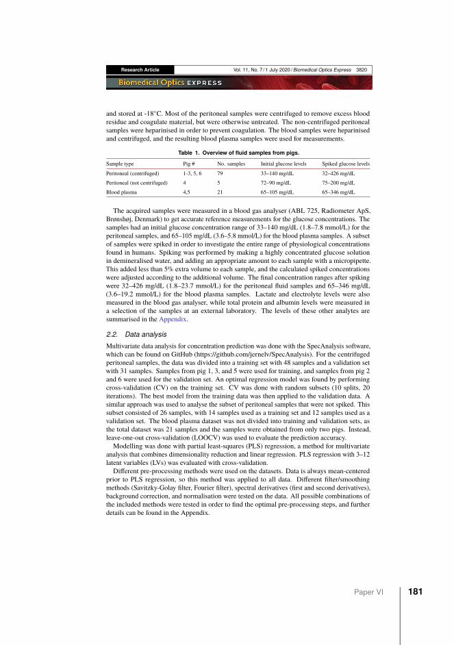
Research Article Vol. 11, No. 7 / 1 July 2020 / Biomedical Optics Express 3820
and stored at -18◦C. Most of the peritoneal samples were centrifuged to remove excess bloodresidue and coagulate material, but were otherwise untreated. The non-centrifuged peritonealsamples were heparinised in order to prevent coagulation. The blood samples were heparinisedand centrifuged, and the resulting blood plasma samples were used for measurements.
Table 1. Overview of fluid samples from pigs.
Sample type Pig # No. samples Initial glucose levels Spiked glucose levels
Peritoneal (centrifuged) 1-3, 5, 6 79 33–140 mg/dL 32–426 mg/dL
Peritoneal (not centrifuged) 4 5 72–90 mg/dL 75–200 mg/dL
Blood plasma 4,5 21 65–105 mg/dL 65–346 mg/dL
The acquired samples were measured in a blood gas analyser (ABL 725, Radiometer ApS,Brønshøj, Denmark) to get accurate reference measurements for the glucose concentrations. Thesamples had an initial glucose concentration range of 33–140 mg/dL (1.8–7.8 mmol/L) for theperitoneal samples, and 65–105 mg/dL (3.6–5.8 mmol/L) for the blood plasma samples. A subsetof samples were spiked in order to investigate the entire range of physiological concentrationsfound in humans. Spiking was performed by making a highly concentrated glucose solutionin demineralised water, and adding an appropriate amount to each sample with a micropipette.This added less than 5% extra volume to each sample, and the calculated spiked concentrationswere adjusted according to the additional volume. The final concentration ranges after spikingwere 32–426 mg/dL (1.8–23.7 mmol/L) for the peritoneal fluid samples and 65–346 mg/dL(3.6–19.2 mmol/L) for the blood plasma samples. Lactate and electrolyte levels were alsomeasured in the blood gas analyser, while total protein and albumin levels were measured ina selection of the samples at an external laboratory. The levels of these other analytes aresummarised in the Appendix.
2.2. Data analysis
Multivariate data analysis for concentration prediction was done with the SpecAnalysis software,which can be found on GitHub (https://github.com/jernelv/SpecAnalysis). For the centrifugedperitoneal samples, the data was divided into a training set with 48 samples and a validation setwith 31 samples. Samples from pig 1, 3, and 5 were used for training, and samples from pig 2and 6 were used for the validation set. An optimal regression model was found by performingcross-validation (CV) on the training set. CV was done with random subsets (10 splits, 20iterations). The best model from the training data was then applied to the validation data. Asimilar approach was used to analyse the subset of peritoneal samples that were not spiked. Thissubset consisted of 26 samples, with 14 samples used as a training set and 12 samples used as avalidation set. The blood plasma dataset was not divided into training and validation sets, asthe total dataset was 21 samples and the samples were obtained from only two pigs. Instead,leave-one-out cross-validation (LOOCV) was used to evaluate the prediction accuracy.Modelling was done with partial least-squares (PLS) regression, a method for multivariate
analysis that combines dimensionality reduction and linear regression. PLS regression with 3–12latent variables (LVs) was evaluated with cross-validation.Different pre-processing methods were used on the datasets. Data is always mean-centered
prior to PLS regression, so this method was applied to all data. Different filter/smoothingmethods (Savitzky-Golay filter, Fourier filter), spectral derivatives (first and second derivatives),background correction, and normalisation were tested on the data. All possible combinations ofthe included methods were tested in order to find the optimal pre-processing steps, and furtherdetails can be found in the Appendix.
Paper VI 181
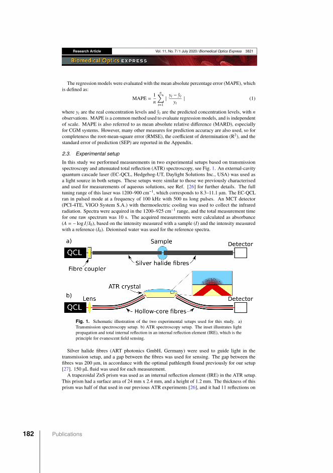
Research Article Vol. 11, No. 7 / 1 July 2020 / Biomedical Optics Express 3821
The regression models were evaluated with the mean absolute percentage error (MAPE), whichis defined as:
MAPE =1n
n∑t=1| yt − yt
yt| (1)
where yt are the real concentration levels and yt are the predicted concentration levels, with nobservations. MAPE is a common method used to evaluate regression models, and is independentof scale. MAPE is also referred to as mean absolute relative difference (MARD), especiallyfor CGM systems. However, many other measures for prediction accuracy are also used, so forcompleteness the root-mean-square error (RMSE), the coefficient of determination (R2), and thestandard error of prediction (SEP) are reported in the Appendix.
2.3. Experimental setup
In this study we performed measurements in two experimental setups based on transmissionspectroscopy and attenuated total reflection (ATR) spectroscopy, see Fig. 1. An external-cavityquantum cascade laser (EC-QCL, Hedgehog-UT, Daylight Solutions Inc., USA) was used asa light source in both setups. These setups were similar to those we previously characterisedand used for measurements of aqueous solutions, see Ref. [26] for further details. The fulltuning range of this laser was 1200–900 cm−1, which corresponds to 8.3–11.1 µm. The EC-QCLran in pulsed mode at a frequency of 100 kHz with 500 ns long pulses. An MCT detector(PCI-4TE, VIGO System S.A.) with thermoelectric cooling was used to collect the infraredradiation. Spectra were acquired in the 1200–925 cm−1 range, and the total measurement timefor one raw spectrum was 10 s. The acquired measurements were calculated as absorbance(A = − log I/I0), based on the intensity measured with a sample (I) and the intensity measuredwith a reference (I0). Deionised water was used for the reference spectra.
Fig. 1. Schematic illustration of the two experimental setups used for this study. a)Transmission spectroscopy setup. b) ATR spectroscopy setup. The inset illustrates lightpropagation and total internal reflection in an internal reflection element (IRE), which is theprinciple for evanescent field sensing.
Silver halide fibres (ART photonics GmbH, Germany) were used to guide light in thetransmission setup, and a gap between the fibres was used for sensing. The gap between thefibres was 200 µm, in accordance with the optimal pathlength found previously for our setup[27]. 150 µL fluid was used for each measurement.A trapezoidal ZnS prism was used as an internal reflection element (IRE) in the ATR setup.
This prism had a surface area of 24 mm x 2.4 mm, and a height of 1.2 mm. The thickness of thisprism was half of that used in our previous ATR experiments [26], and it had 11 reflections on
182 Publications
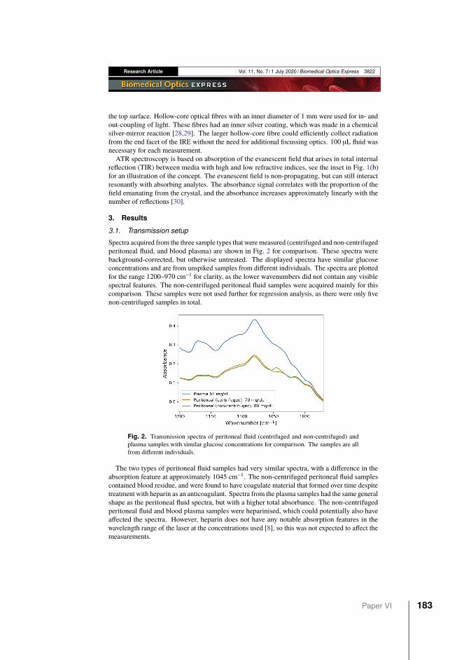
Research Article Vol. 11, No. 7 / 1 July 2020 / Biomedical Optics Express 3822
the top surface. Hollow-core optical fibres with an inner diameter of 1 mm were used for in- andout-coupling of light. These fibres had an inner silver coating, which was made in a chemicalsilver-mirror reaction [28,29]. The larger hollow-core fibre could efficiently collect radiationfrom the end facet of the IRE without the need for additional focussing optics. 100 µL fluid wasnecessary for each measurement.ATR spectroscopy is based on absorption of the evanescent field that arises in total internal
reflection (TIR) between media with high and low refractive indices, see the inset in Fig. 1(b)for an illustration of the concept. The evanescent field is non-propagating, but can still interactresonantly with absorbing analytes. The absorbance signal correlates with the proportion of thefield emanating from the crystal, and the absorbance increases approximately linearly with thenumber of reflections [30].
3. Results
3.1. Transmission setup
Spectra acquired from the three sample types that were measured (centrifuged and non-centrifugedperitoneal fluid, and blood plasma) are shown in Fig. 2 for comparison. These spectra werebackground-corrected, but otherwise untreated. The displayed spectra have similar glucoseconcentrations and are from unspiked samples from different individuals. The spectra are plottedfor the range 1200–970 cm−1 for clarity, as the lower wavenumbers did not contain any visiblespectral features. The non-centrifuged peritoneal fluid samples were acquired mainly for thiscomparison. These samples were not used further for regression analysis, as there were only fivenon-centrifuged samples in total.
Fig. 2. Transmission spectra of peritoneal fluid (centrifuged and non-centrifuged) andplasma samples with similar glucose concentrations for comparison. The samples are allfrom different individuals.
The two types of peritoneal fluid samples had very similar spectra, with a difference in theabsorption feature at approximately 1045 cm−1. The non-centrifuged peritoneal fluid samplescontained blood residue, and were found to have coagulate material that formed over time despitetreatment with heparin as an anticoagulant. Spectra from the plasma samples had the same generalshape as the peritoneal fluid spectra, but with a higher total absorbance. The non-centrifugedperitoneal fluid and blood plasma samples were heparinised, which could potentially also haveaffected the spectra. However, heparin does not have any notable absorption features in thewavelength range of the laser at the concentrations used [8], so this was not expected to affect themeasurements.
Paper VI 183
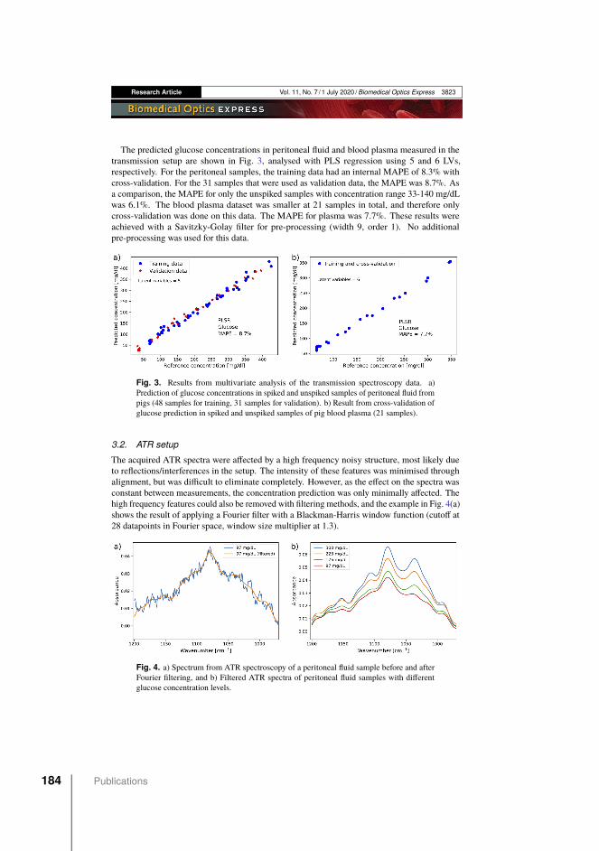
Research Article Vol. 11, No. 7 / 1 July 2020 / Biomedical Optics Express 3823
The predicted glucose concentrations in peritoneal fluid and blood plasma measured in thetransmission setup are shown in Fig. 3, analysed with PLS regression using 5 and 6 LVs,respectively. For the peritoneal samples, the training data had an internal MAPE of 8.3% withcross-validation. For the 31 samples that were used as validation data, the MAPE was 8.7%. Asa comparison, the MAPE for only the unspiked samples with concentration range 33-140 mg/dLwas 6.1%. The blood plasma dataset was smaller at 21 samples in total, and therefore onlycross-validation was done on this data. The MAPE for plasma was 7.7%. These results wereachieved with a Savitzky-Golay filter for pre-processing (width 9, order 1). No additionalpre-processing was used for this data.
Fig. 3. Results from multivariate analysis of the transmission spectroscopy data. a)Prediction of glucose concentrations in spiked and unspiked samples of peritoneal fluid frompigs (48 samples for training, 31 samples for validation). b) Result from cross-validation ofglucose prediction in spiked and unspiked samples of pig blood plasma (21 samples).
3.2. ATR setup
The acquired ATR spectra were affected by a high frequency noisy structure, most likely dueto reflections/interferences in the setup. The intensity of these features was minimised throughalignment, but was difficult to eliminate completely. However, as the effect on the spectra wasconstant between measurements, the concentration prediction was only minimally affected. Thehigh frequency features could also be removed with filtering methods, and the example in Fig. 4(a)shows the result of applying a Fourier filter with a Blackman-Harris window function (cutoff at28 datapoints in Fourier space, window size multiplier at 1.3).
Fig. 4. a) Spectrum from ATR spectroscopy of a peritoneal fluid sample before and afterFourier filtering, and b) Filtered ATR spectra of peritoneal fluid samples with differentglucose concentration levels.
184 Publications

Research Article Vol. 11, No. 7 / 1 July 2020 / Biomedical Optics Express 3824
Example spectra of peritoneal samples with glucose concentrations ranging from 97-300 mg/dLare plotted in Fig. 4(b). The spectra have noticeable changes in absorption features with increasingglucose concentrations, in particular around the 1035 cm−1 glucose absorption peak.For the ATR measurements, the predicted glucose concentrations for peritoneal fluid and
plasma samples are shown in Fig. 5. The achieved MAPE for glucose in peritoneal fluid was12.2%, and for blood plasma samples the MAPE for cross-validation was 7.8%. As in thetransmission measurements, the optimal models were found using 5 LVs for the peritoneal fluidmeasurements and 6 LVs for the blood plasma measurements. Application of a Fourier filterwith the same parameters as in Fig. 4 gave the lowest prediction errors. For the smaller dataset ofunspiked peritoneal fluid samples, the achieved MAPE was 10.5%.
Fig. 5. Results from multivariate analysis of the ATR spectroscopy data. a) Prediction ofglucose concentrations in spiked and unspiked samples of peritoneal fluid from pigs (48samples for training, 31 samples for validation). b) Result from cross-validation of glucoseprediction in spiked and unspiked samples of pig blood plasma (21 samples).
4. Discussion
Highly accurate prediction of glucose concentrations in peritoneal fluid was achieved with QCL-based spectroscopy with 8.7% and 12.2% MAPE in the transmission and ATR configurations,respectively. This is an encouraging preliminary result, as the accuracies of commercialelectrochemical CGM systems are in the range 9–20% [31,32]. The results are very promisingfor fast and accurate glucose prediction as the measurement time was only 10 seconds, comparedto electrochemical sensors that usually average over 5 minutes. Rapid measurements canpotentially contribute to improvements in the health outcomes of diabetes patients, as long-termcomplications can be reduced if the BGL is measured continuously with high accuracy andshort response time. Concentration prediction was also accurate for low glucose concentrations(<100 mg/dL), which is a critical concentration range for management of hypoglycaemia indiabetic patients. This is especially notable because the lowest concentration in the trainingset was 72 mg/dL, while the lowest concentration was 32 mg/dL in the validation set. Hence,the features in the measured spectra were still interpretable at very low concentrations, and theregression model could be extended to unknown concentrations. All measurements used forthe validation set were from different pigs than the data in the training set, which also showedthat accurate predictions could be made with samples from different individuals. Accuratepredictions through cross-validation were also found for the blood plasma samples. The separateanalysis of the unspiked peritoneal samples also demonstrated that glucose concentrations couldbe accurately determined in natural peritoneal fluid. The lower prediction errors compared to thefull analysis, at 6.1% and 10.5% for transmission and ATR spectroscopy, respectively, can beattributed to the smaller dataset and narrower concentration range.
Paper VI 185
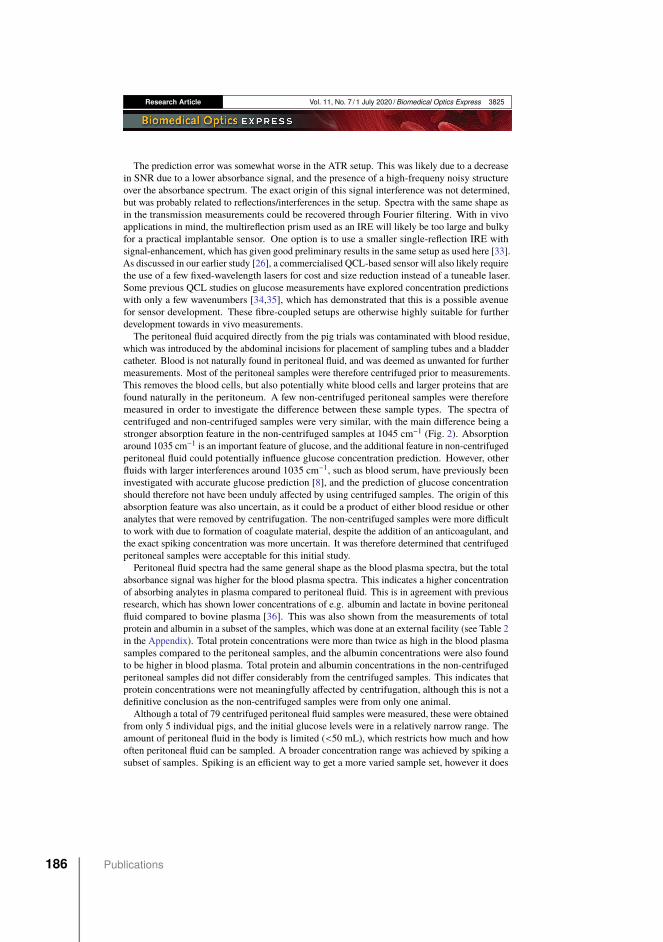
Research Article Vol. 11, No. 7 / 1 July 2020 / Biomedical Optics Express 3825
The prediction error was somewhat worse in the ATR setup. This was likely due to a decreasein SNR due to a lower absorbance signal, and the presence of a high-frequeny noisy structureover the absorbance spectrum. The exact origin of this signal interference was not determined,but was probably related to reflections/interferences in the setup. Spectra with the same shape asin the transmission measurements could be recovered through Fourier filtering. With in vivoapplications in mind, the multireflection prism used as an IRE will likely be too large and bulkyfor a practical implantable sensor. One option is to use a smaller single-reflection IRE withsignal-enhancement, which has given good preliminary results in the same setup as used here [33].As discussed in our earlier study [26], a commercialised QCL-based sensor will also likely requirethe use of a few fixed-wavelength lasers for cost and size reduction instead of a tuneable laser.Some previous QCL studies on glucose measurements have explored concentration predictionswith only a few wavenumbers [34,35], which has demonstrated that this is a possible avenuefor sensor development. These fibre-coupled setups are otherwise highly suitable for furtherdevelopment towards in vivo measurements.
The peritoneal fluid acquired directly from the pig trials was contaminated with blood residue,which was introduced by the abdominal incisions for placement of sampling tubes and a bladdercatheter. Blood is not naturally found in peritoneal fluid, and was deemed as unwanted for furthermeasurements. Most of the peritoneal samples were therefore centrifuged prior to measurements.This removes the blood cells, but also potentially white blood cells and larger proteins that arefound naturally in the peritoneum. A few non-centrifuged peritoneal samples were thereforemeasured in order to investigate the difference between these sample types. The spectra ofcentrifuged and non-centrifuged samples were very similar, with the main difference being astronger absorption feature in the non-centrifuged samples at 1045 cm−1 (Fig. 2). Absorptionaround 1035 cm−1 is an important feature of glucose, and the additional feature in non-centrifugedperitoneal fluid could potentially influence glucose concentration prediction. However, otherfluids with larger interferences around 1035 cm−1, such as blood serum, have previously beeninvestigated with accurate glucose prediction [8], and the prediction of glucose concentrationshould therefore not have been unduly affected by using centrifuged samples. The origin of thisabsorption feature was also uncertain, as it could be a product of either blood residue or otheranalytes that were removed by centrifugation. The non-centrifuged samples were more difficultto work with due to formation of coagulate material, despite the addition of an anticoagulant, andthe exact spiking concentration was more uncertain. It was therefore determined that centrifugedperitoneal samples were acceptable for this initial study.Peritoneal fluid spectra had the same general shape as the blood plasma spectra, but the total
absorbance signal was higher for the blood plasma spectra. This indicates a higher concentrationof absorbing analytes in plasma compared to peritoneal fluid. This is in agreement with previousresearch, which has shown lower concentrations of e.g. albumin and lactate in bovine peritonealfluid compared to bovine plasma [36]. This was also shown from the measurements of totalprotein and albumin in a subset of the samples, which was done at an external facility (see Table 2in the Appendix). Total protein concentrations were more than twice as high in the blood plasmasamples compared to the peritoneal samples, and the albumin concentrations were also foundto be higher in blood plasma. Total protein and albumin concentrations in the non-centrifugedperitoneal samples did not differ considerably from the centrifuged samples. This indicates thatprotein concentrations were not meaningfully affected by centrifugation, although this is not adefinitive conclusion as the non-centrifuged samples were from only one animal.
Although a total of 79 centrifuged peritoneal fluid samples were measured, these were obtainedfrom only 5 individual pigs, and the initial glucose levels were in a relatively narrow range. Theamount of peritoneal fluid in the body is limited (<50 mL), which restricts how much and howoften peritoneal fluid can be sampled. A broader concentration range was achieved by spiking asubset of samples. Spiking is an efficient way to get a more varied sample set, however it does
186 Publications
Research Article Vol. 11, No. 7 / 1 July 2020 / Biomedical Optics Express 3826
not necessarily reflect real-life variations. Peritoneal fluid is a complex matrix where severalcomponents are in equilibrium to some degree, and a change in glucose concentrations willusually occur together with a change in e.g. electrolyte levels. This could not be recreated withconcentration spiking. Some between-individual and within-individual variation in the samplesmight therefore have been missed. However, the validation results were very good consideringthe large range of glucose concentrations. In addition, the samples used for validation were fromdifferent pigs than the ones that were used for training the regression model, which shows thatconcentration predictions with high accuracy can be achieved across individuals.
5. Conclusion
QCL-based spectroscopy setups were used for direct and reagent-free measurements of glucoselevels in peritoneal fluid. Both direct transmission spectroscopy and evanescent field sensingwere accurate for glucose level prediction, with achieved MAPEs of 8.7% and 12.2%, respectively.Spectra acquired from peritoneal fluid were found to be similar to those from blood plasma, butwith less total overall absorbance.
This study demonstrates that glucose concentrations can be measured accurately in peritonealfluid, with similar results to previous studies using mid-infrared spectroscopy for measurementsof human blood serum [8]. Intraperitoneal sensing has been suggested as a faster and moreaccurate way of controlling glucose levels in diabetic patients. Future work should include invivo measurements in an animal model to confirm the functionality of this sensor system inrealistic sensing scenarios.
Appendix
Analyte overview
Table 2 summarises the fluid components that were measured in the peritoneal fluid samplesand the blood plasma samples. Glucose, lactate, and electrolyte (Na+, K+, Ca2+, Cl−) levelswere measured in in an ABL 725 blood gas analyser (ABL 725, Radiometer ApS, Brønshøj,Denmark). These measurements were done directly after each pig trial was finished, and thesamples were subsequently frozen at -18◦C. In addition, a selection of samples were sent toSentrallaboratoriet, Faculty of Veterinary Medicine, Norwegian University of Life Sciences(NMBU) for measurements of total protein and albumin. Total protein concentration wasmeasured with the Biuret method in an Advia 1800 Chemistry System (Siemens HealthineersAG, Germany). Albumin concentration was measured by capillary electrophoresis in a SebiaCapillarys 2 (Sebia GL, France). As total protein and albumin were measured in only a subset ofthe samples, it is likely that the concentrations ranges found were not completely representativeof the actual variance in the samples.
Pre-processing methods
The measured mid-infrared spectra consisted of 390 datapoints in the 1200-925 cm−1 range andhad a resolution of 0.7 cm−1. Pre-processing methods were tested on the raw spectra as a part ofthe data analysis, and the variants tested are detailed in Table 3.
Prediction accuracy
Various measures of prediction accuracy are used in multivariate analysis. Table 4 summarisesfour different measurement errors from the analysis of peritoneal fluid and blood plasma in theQCL-based transmission and ATR spectroscopy setups. These are mean absolute percentageerror (MAPE), root-mean-square error of prediction or cross-validation (RMSEP/RMSECV),coefficient of determination (R2), and standard error of prediction (SEP). Training and validationsets were used for the peritoneal fluid samples, and the prediction accuracies are based on the
Paper VI 187
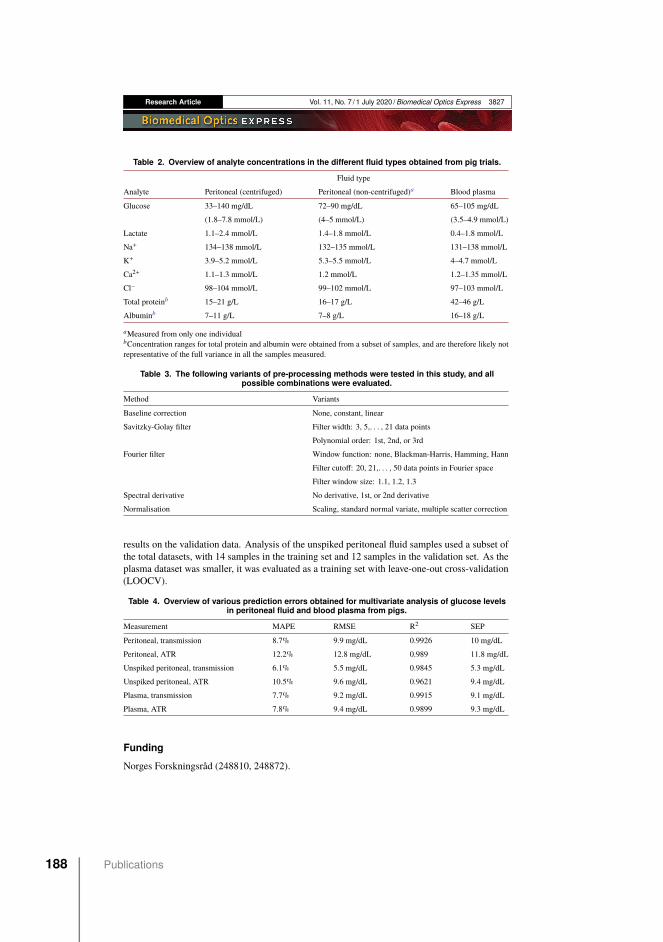
Research Article Vol. 11, No. 7 / 1 July 2020 / Biomedical Optics Express 3827
Table 2. Overview of analyte concentrations in the different fluid types obtained from pig trials.
Fluid type
Analyte Peritoneal (centrifuged) Peritoneal (non-centrifuged)a Blood plasma
Glucose 33–140 mg/dL 72–90 mg/dL 65–105 mg/dL
(1.8–7.8 mmol/L) (4–5 mmol/L) (3.5–4.9 mmol/L)
Lactate 1.1–2.4 mmol/L 1.4–1.8 mmol/L 0.4–1.8 mmol/L
Na+ 134–138 mmol/L 132–135 mmol/L 131–138 mmol/L
K+ 3.9–5.2 mmol/L 5.3–5.5 mmol/L 4–4.7 mmol/L
Ca2+ 1.1–1.3 mmol/L 1.2 mmol/L 1.2–1.35 mmol/L
Cl− 98–104 mmol/L 99–102 mmol/L 97–103 mmol/L
Total proteinb 15–21 g/L 16–17 g/L 42–46 g/L
Albuminb 7–11 g/L 7–8 g/L 16–18 g/L
aMeasured from only one individualbConcentration ranges for total protein and albumin were obtained from a subset of samples, and are therefore likely notrepresentative of the full variance in all the samples measured.
Table 3. The following variants of pre-processing methods were tested in this study, and allpossible combinations were evaluated.
Method Variants
Baseline correction None, constant, linear
Savitzky-Golay filter Filter width: 3, 5,. . . , 21 data points
Polynomial order: 1st, 2nd, or 3rd
Fourier filter Window function: none, Blackman-Harris, Hamming, Hann
Filter cutoff: 20, 21,. . . , 50 data points in Fourier space
Filter window size: 1.1, 1.2, 1.3
Spectral derivative No derivative, 1st, or 2nd derivative
Normalisation Scaling, standard normal variate, multiple scatter correction
results on the validation data. Analysis of the unspiked peritoneal fluid samples used a subset ofthe total datasets, with 14 samples in the training set and 12 samples in the validation set. As theplasma dataset was smaller, it was evaluated as a training set with leave-one-out cross-validation(LOOCV).
Table 4. Overview of various prediction errors obtained for multivariate analysis of glucose levelsin peritoneal fluid and blood plasma from pigs.
Measurement MAPE RMSE R2 SEP
Peritoneal, transmission 8.7% 9.9 mg/dL 0.9926 10 mg/dL
Peritoneal, ATR 12.2% 12.8 mg/dL 0.989 11.8 mg/dL
Unspiked peritoneal, transmission 6.1% 5.5 mg/dL 0.9845 5.3 mg/dL
Unspiked peritoneal, ATR 10.5% 9.6 mg/dL 0.9621 9.4 mg/dL
Plasma, transmission 7.7% 9.2 mg/dL 0.9915 9.1 mg/dL
Plasma, ATR 7.8% 9.4 mg/dL 0.9899 9.3 mg/dL
Funding
Norges Forskningsråd (248810, 248872).
188 Publications
Research Article Vol. 11, No. 7 / 1 July 2020 / Biomedical Optics Express 3828
Acknowledgments
This work was supported by the Research Council of Norway through the Double IntraperitonealArtificial Pancreas project, grant number 248872. The project is part of Centre for Digital LifeNorway and is also supported by the Research Council of Norway’s grant 248810.
The authors would like to thank Marte Kierulf Åm and Patrick Christian Bösch for collectingand preparing the fluid samples used in this study.
Disclosures
The authors declare no conflicts of interest.
References1. T. Battelino, I. Conget, B. Olsen, I. Schütz-Fuhrmann, E. Hommel, R. Hoogma, U. Schierloh, N. Sulli, and J. Bolinder,
“The use and efficacy of continuous glucose monitoring in type 1 diabetes treated with insulin pump therapy: Arandomised controlled trial,” Diabetologia 55(12), 3155–3162 (2012).
2. B. M. Frier, “Morbidity of hypoglycemia in type 1 diabetes,” Diabetes Res. Clin. Pract. 65, S47–S52 (2004).3. D. M. Nathan, “Long-Term Complications of Diabetes Mellitus,” N. Engl. J. Med. 328(23), 1676–1685 (1993).4. J. Wang, “Electrochemical glucose biosensors,” Chem. Rev. 108(2), 814–825 (2008).5. I. L. Jernelv, K. Milenko, S. S. Fuglerud, D. R. Hjelme, R. Ellingsen, and A. Aksnes, “A review of optical methods
for continuous glucose monitoring,” Appl. Spectrosc. Rev. 54(7), 543–572 (2019).6. A. Schwaighofer, M. Brandstetter, and B. Lendl, “Quantum cascade lasers (QCLs) in biomedical spectroscopy,”
Chem. Soc. Rev. 46(19), 5903–5924 (2017).7. A. Hugi, R. Maulini, and J. Faist, “External cavity quantum cascade laser,” Semicond. Sci. Technol. 25(8), 083001
(2010).8. M. Brandstetter, T. Sumalowitsch, A. Genner, A. E. Posch, C. Herwig, A. Drolz, V. Fuhrmann, T. Perkmann, and
B. Lendl, “Reagent-free monitoring of multiple clinically relevant parameters in human blood plasma using amid-infrared quantum cascade laser based sensor system,” Analyst 138(14), 4022–4028 (2013).
9. C. Vrančić, N. Kruger, N. Gretz, S. Neudecker, A. Pucci, and W. Petrich, “A quantitative look inside the body:Minimally invasive infrared analysis in vivo,” Anal. Chem. 86(21), 10511–10514 (2014).
10. A. Werth, S. Liakat, A. Dong, C. M. Woods, and C. F. Gmachl, “Implementation of an integrating sphere for theenhancement of noninvasive glucose detection using quantum cascade laser spectroscopy,” Appl. Phys. B 124(5), 75(2018).
11. S. Kino, S. Omori, T. Katagiri, and Y. Matsuura, “Hollow optical-fiber based infrared spectroscopy for measurementof blood glucose level by using multi-reflection prism,” Biomed. Opt. Express 7(2), 701–708 (2016).
12. J. C. Pickup, S. C. Freeman, and A. J. Sutton, “Glycaemic control in type 1 diabetes during real time continuousglucose monitoring compared with self monitoring of blood glucose: meta-analysis of randomised controlled trialsusing individual patient data,” BMJ 343(jul07 1), d3805 (2011).
13. K. L. Helton, B. D. Ratner, and N. A. Wisniewski, “Biomechanics of the sensor-tissue interface - Effects of motion,pressure, and design on sensor performance and foreign body response - Part II: Examples and application,” J.Diabetes Sci. Technol. 5(3), 647–656 (2011).
14. M. S. Boyne, D. M. Silver, J. Kaplan, and C. D. Saudek, “Timing of Changes in Interstitial and Venous BloodGlucose Measured with a Continuous Subcutaneous Glucose Sensor,” Diabetes 52(11), 2790–2794 (2003).
15. L. Dye, M. Mansfield, N. Lasikiewicz, L. Mahawish, R. Schnell, D. Talbot, H. Chauhan, F. Croden, and C. Lawton,“Correspondence of continuous interstitial glucose measurement against arterialised and capillary glucose followingan oral glucose tolerance test in healthy volunteers,” Br. J. Nutr. 103(1), 134–140 (2010).
16. M. Sinha, K. M. McKeon, S. Parker, L. G. Goergen, H. Zheng, F. H. El-Khatib, and S. J. Russell, “A Comparison ofTime Delay in Three Continuous Glucose Monitors for Adolescents and Adults,” J. Diabetes Sci. Technol. 11(6),1132–1137 (2017).
17. Ø. Stavdahl, A. L. Fougner, K. Kölle, S. C. Christiansen, R. Ellingsen, and S. M. Carlsen, “The Artificial Pancreas:A Dynamic Challenge,” IFAC-PapersOnLine 49(7), 765–772 (2016).
18. L. Huyett, E. Dassau, H. Zisser, and F. Iii, “Glucose Sensor Dynamics and the Artificial Pancreas,” IEEE Control.Syst. Mag. 38(1), 30–46 (2018).
19. D. R. Burnett, L. M. Huyett, H. C. Zisser, F. J. Doyle, and B. D. Mensh, “Glucose sensing in the peritoneal spaceoffers faster kinetics than sensing in the subcutaneous space,” Diabetes 63(7), 2498–2505 (2014).
20. A. L. Fougner, K. Kölle, N. K. Skjærvold, N. A. Elvemo, D. R. Hjelme, R. Ellingsen, S. M. Carlsen, and Ø. Stavdahl,“Intraperitoneal Glucose Sensing is Sometimes Surprisingly Rapid,” Model. Identif. Control. 37(2), 121–131 (2016).
21. M. K. Åm, A. L. Fougner, R. Ellingsen, D. R. Hjelme, P. C. Bösch, O. Stavdahl, S. M. Carlsen, and S. C. Christiansen,“Why intraperitoneal glucose sensing is sometimes surprisingly rapid and sometimes slow: A hypothesis,” Med.Hypotheses 132, 109318 (2019).
Paper VI 189
Research Article Vol. 11, No. 7 / 1 July 2020 / Biomedical Optics Express 3829
22. M. K. Åm, K. Kölle, A. L. Fougner, I. Dirnena-Fusini, P. C. Bösch, R. Ellingsen, D. R. Hjelme, O. Stavdahl, S. M.Carlsen, and S. C. Christiansen, “Effect of sensor location on continuous intraperitoneal glucose sensing in an animalmodel,” PLoS One 13(10), e0205447 (2018).
23. L. M. Huyett, R. Mittal, H. C. Zisser, E. S. Luxon, A. Yee, E. Dassau, F. J. Doyle, and D. R. Burnett, “PreliminaryEvaluation of a Long-Term Intraperitoneal Glucose Sensor With Flushing Mechanism,” J. Diabetes Sci. Technol.10(5), 1192–1194 (2016).
24. J. J. Kaneko, J. W. Harvey, and M. L. Bruss, Clinical Biochemistry in Domestic Animals, 6th ed (Academic Press,2008).
25. M. Laposata, Laposata’s Laboratory Medicine Diagnosis of Disease in Clinical Laboratory, 3rd ed (McGraw-HillEducation/Medical, 2018).
26. I. L. Jernelv, K. Strøm, D. R. Hjelme, and A. Aksnes, “Infrared Spectroscopy with a Fiber-Coupled Quantum CascadeLaser for Attenuated Total Reflection Measurements Towards Biomedical Applications,” Sensors 19(23), 5130(2019).
27. I. L. Jernelv, K. Strøm, D. R. Hjelme, and A. Aksnes, “Mid-infrared spectroscopy with a fiber-coupled tuneablequantum cascade laser for glucose sensing,” Proc. SPIE 1123, 36 (2020).
28. Y. W. Shi, K. Ito, L. Ma, T. Yoshida, Y. Matsuura, and M. Miyagi, “Fabrication of a polymer-coated silver hollowoptical fiber with high performance,” Appl. Opt. 45(26), 6736–6740 (2006).
29. K. Iwai, M. Miyagi, Y.-W. Shi, and Y. Matsuura, “Fabrication of silver-coated hollow fiber with an inner diameter of100 µm or less,” Proc. SPIE 7894, 78940B (2011).
30. C. Vigano, J. M. Ruysschaert, and E. Goormaghtigh, “Sensor applications of attenuated total reflection infraredspectroscopy,” Talanta 65(5), 1132–1142 (2005).
31. H. Kirchsteiger, L. Heinemann, G. Freckmann, V. Lodwig, G. Schmelzeisen-Redeker, M. Schoemaker, and L. DelRe, “Performance comparison of CGM systems: MARD values are not always a reliable indicator of CGM systemaccuracy,” J. Diabetes Sci. Technol. 9(5), 1030–1040 (2015).
32. D. Rodbard, “Continuous Glucose Monitoring: A Review of Successes,” Diabetes Technol. Ther. 18(S2), 3–13(2016).
33. I. L. Jernelv, J. Høvik, D. R. Hjelme, and A. Aksnes, “Signal enhancement in microstructured silicon attenuated totalreflection elements for quantum cascade laser-based spectroscopy,” Proc. SPIE 11359, 9 (2020).
34. W. B. Martin, S. Mirov, and R. Venugopalan, “Middle infrared, quantum cascade laser optoelectronic absorptionsystem for monitoring glucose in serum,” Appl. Spectrosc. 59(7), 881–884 (2005).
35. Y. Matsuura and T. Koyama, “Non-invasive blood glucose measurement using quantum cascade lasers,” Proc. SPIE39(2), 105–110 (2018).
36. T. Wittek, A. Grosche, L. Locher, A. Alkaassem, and M. Fürll, “Biochemical constituents of peritoneal fluid in cows,”Vet. Rec. 166(1), 15–19 (2010).
190 Publications