COMPENDIUM

TBT4135 Biopolymers

Bjørn E. Christensen

NOBIPOL

Department of Biotechnology NTNU

2013

2

PREFACE  

This compendium has been created from a series of lecture notes developed over the years since 1998, and handed out to the students as separate documents or files on It’s Learning. The notes and the compendium are motivated by the need to supplement the Smidsrød textbook with more examples from current research on biopolymers, especially polysaccharides, as well as giving the course a more chemical and biological profile. My intention is to use the compendium as the main document in my teaching, but the Smidsrød textbook is still required as it offers a deeper and more detailed description of the biophysical chemistry. The Smidsrød textbook, which itself is unique in its kind, is much based on the classical textbook by C. Tanford (Physical Chemistry of Macromolecules, Wiley, 1961), and therefore emphasizes the physical and theoretical aspects more than the chemical and biological. Both books were written at a time where the physical chemistry of macromolecules mainly focused on synthetic polymers, and examples from the biopolymer science were comparatively much less abundant. This situation has fortunately changed over the years. Many examples on important polysaccharides used in this compendium stems from research carried out by my colleagues and myself at NOBIPOL (Norwegian Biopolymer Laboratory), an interdisciplinary, bottom-up type of research group at NTNU. I need to thank professor emeritus Olav Smidsrød for introducing and developing the Biopolymer course at NTNU, and for establishing NOBIPOL as a highly profiled, internationally recognized and active research group. I also thank him for supervision from my time as his student in the area, and for all stimulating scientific discussions over the years. I also thank my current colleagues in NOBIPOL, in particular professors Gudmund Skjåk-Bræk, Kjell M. Vårum, Kurt. I. Draget, Svein Valla and Bjørn T. Stokke for valuable scientific input through publications and discussions. The thanks are extended to all previous and current students, PhD candidates, postdoctoral fellows, and young researchers associated with NOBIPOL. Special thanks also to my colleague professor Alexander Dikiy for allowing me to use his presentation on proteins in this compendium (Section 4.4) Trondheim, August 2013 Bjørn E. Christensen

3

Further development of the compendium

I have to apologize for the rather low technical quality (especially figures and figure legends) and some places a rather fragmented style of the current version of the compendium. For the 2013 version there was not sufficient time to prepare a technically perfect document before the start of the course.

The compendium will be constantly updated, and I expect to supplement with a few additional files on It’s Learning also in 2013.

Last update before printing: 12 Sept. 2013

4

CONTENTS  PART 1. Preface   2  1.1.  CARBOHYDRATE  FUNDAMENTALS:  MONOSACCHARIDES   10  1.1.1.  The  Fisher  projection   10  1.1.2.  D-­‐  and  L-­‐sugars   10  1.1.3.  Ring  formation  (alcohol  +  aldehyde  =  hemiacetal):  α-­‐  and  β-­‐forms  and  the  Haworth  formula   12  1.1.4.  Definition  of  α  and  β  (Haworth)  –  the  anomeric  carbon:   13  1.1.5.  Fisher-­‐Haworth  interconversion  rules:   13  1.1.6.  Example:  Alginate   14  1.1.7.  Epimers  and  anomers.   14  1.1.9.  The  shape  of  hexoses   16  1.1.10.  How  to  determine  whether  a  sugar  is  1C4  or  4C1   16  1.1.11.  A  strategy  for  determining  the  ring  form:   17  

1.2.  ALGINATES   19  1.2.1.  Introduction   19  1.2.2.  General   19  1.2.3.  Structure  of  alginates   20  1.2.4.  Content  and  distribution  of  M  and  G  in  alginates   23  1.2.5.  Examples:  Composition  of  some  algal  alginates   27  1.2.6.  Bacterial  alginates:   28  1.2.7.  Determination  of  composition  and  sequence  in  alginates   29  1.2.8.  NMR  of  alginates  –  a  brief  course  for  polysaccharide  chemists   30  1.2.9.  The  1H-­‐NMR  spectrum  of  D-­‐glucose  (in  D2O):   33  1.2.10.  Alginates:  The  1H-­‐NMR  spectrum   35  1.2.11.  Chain  length  (DPn)  from  NMR   37  1.2.12.  Studying  alginate  structure  and  epimerization  by  NMR   38  1.2.13.  Epimerization:  Macromolecular  consequences   39  1.2.14.  Gelation  with  calcium  ions:  Cross-­‐linking  of  G-­‐blocks   41  1.2.15.  Alginate,  alginic  acid:  different  salt  forms   42  1.2.16.  Size  and  shape  of  alginate  molecules  in  solution   42  1.2.17.  Alginates:  Properties  and  uses   44  1.2.18.  Gelation  with  Ca++:  Gel  strength  and  Young’s  modulus   44  1.2.19.  Cell  immobilization  and  encapsulation   45  1.2.20.  Homogeneous  gels  –  controlled  release  of  calcium  ions  (in  situ  gelation)   47  1.2.21.  Alginate  foams:  3D  cell  cultures   48  

1.3.  Chitin  and  chitosans   49  1.3.1.  General   49  1.3.2.  Chitin   49  1.3.3.  From  chitin  to  chitosan:  Chemical  de-­‐N-­‐acetylation   50  1.3.4.  Chain  geometry   50  1.3.5.  FA:  The  fraction  of  A  (GlcNAc)  residues   51  1.3.6.  Polyelectrolyte  properties   51  1.3.7.  Interactions  with  polyanions  (polyelectrolyte  complexes)   52  1.3.8.  Solubility  of  chitosans   52  1.3.9.  Chitosans:  Free  amine  form  and  salts   53  

5

1.4.  Cellulose  and  its  derivatives   55  1.4.1.  General.   55  1.4.2.  Chemical  structure   55  1.4.3.  Biosynthesis   56  1.4.4.  Solubility  and  crystallinity   56  1.4.5.  Cellulose  I.   57  1.4.6.  Cellulose  II   57  1.4.7.  Cellulose  solvents   58  1.4.8.  Alkaline  cellulose  -­‐  Mercerization   59  1.4.9.  Cellulose  derivatives   59  

1.5.  Starches   61  1.5.1.  General   61  1.5.2.  Amyloses  and  amylopectins:  Overview   62  1.5.3.  Amylose.   62  1.5.4.  Synthetic  amylose:  Perfect  model  substances?   63  1.5.5.  Amylopectin   64  1.5.6.  Cyclic  α-­‐1,4  glucans   64  1.5.7.  Shape  and  extension  of  amyloses  and  amylopectins  in  solution.   65  

1.6.  Pullulan:  Fundamentals  (keywords)   66  1.7.  Xanthan:  Fundamentals  (keywords)   67  1.8.  Carrageenans  and  agarose   68  1.9.  Hyaluronan  (hyaluronic  acid):  Fundamentals  (keywords)   70  1.10.  Heparin  fundamentals  (keywords)   72  1.11.  Dextrans   73  1.12.  Pectin  fundamentals   76  2.1.  MOLECULAR  WEIGHT  DISTRIBUTIONS  AND  AVERAGES   81  2.1.1.  Introduction   81  2.1.2.  DP:  Degree  of  polymerization   81  2.1.3.  Molecular  weight  (molar  mass)   81  2.1.4.  Polydispersity   82  2.1.5.  Molecular  weight  distributions   83  2.1.6.  Molecular  weight  averages:  Mn,  Mw  and  Mz   85  2.1.7.  DP  averages   87  2.1.8.  Continuous  distributions   87  2.1.9.  The  Kuhn  distribution   88  2.1.10  Practical  examples   88  

2.2.  THE  SHAPE  OF  BIOPOLYMERS  IN  SOLUTION   91  2.2.1.  Introduction  and  examples   91  2.2.2.  Radius  of  gyration  (RG)   94  2.2.3.  The  RG-­‐M  relationships  for  solid  spheres.   96  2.2.4.  The  RG-­‐M  relationships  for  rigid  rods.   97  2.2.5.  The  RG-­‐M  relationships  for  randomly  coiled  chains.   98  2.2.6.  Real  chains   102  2.2.7.  The  characteristic  ratio  (C∞):  A  stiffness  parameter   103  2.2.8.  Excluded  volume  effects  and  θ-­‐conditions   103  2.2.9.  How  to  determine  C∞  from  experiments?   104  2.2.10.  How  small  chains  can  we  analyse  using  the  random  coil  model?   107  2.2.11.  Other  stiffness  parameters  based  on  the  random  coil  model.   107  2.2.12.  The  radius  of  gyration  of  denatured  proteins   109  

6

2.2.13.  The  wormlike  chain  model  (WC)   109  2.2.14.  The  persistence  length   112  2.2.15.  Determination  of  the  persistence  length  from  experimental  data   113  

3.1.  POLYELECTROLYTE  FUNDAMENTALS   116  3.1.1.  Definition  and  introduction.   116  3.1.2.  Counterions:  Essential  components  with  major  influence   116  3.1.3.  Changing  counterions  (salt  forms)   117  3.1.4.  Polyelectrolyte  effects:  solubility   118  3.1.5.  Polyelectrolyte  effects:  Role  of  ionic  strength.   119  3.1.6.  Charge  manipulation:  pH  and  acid-­‐base  titration  –  basic  concepts   122  3.1.7.  Charges  and  isoelectric  point  of  an  amino  acid  protein   124  3.1.8.  Charges  and  isoelectric  point  of  a  protein   126  3.1.9.  Acid-­‐base  titrations  of  polyelectrolytes:  pKa  depends  on  the  degree  of  ionization   127  3.1.10.  Titration  of  chitosan:  A  polycationic  polysaccharide   131  3.1.11.  Polyelectrolyte  complexes   133  

3.2.  Thermodynamics:  Important  tool  in  biochemistry   135  3.2.1.  General  comments   135  3.2.2.  Introductory  example:  ITC  (Isothermal  titration  calorimetry)   136  3.2.3.  Thermodynamics  of  dilute  solutions:  Fundamentals  (keywords)   137  3.2.4.  The  general  thermodynamic  equation  for  dilute  solutions:   138  3.2.5.  Chemical  potential  of  a  simple  two-­‐component  system   140  3.2.6.  Second  virial  coefficient  (A2)   142  3.2.7.  A2:  High  or  low?   143  3.2.8.  A2:  Important  link  to  chain  statistics   144  3.2.9.  Finding  θ-­‐conditions  by  experiment   145  

3.3.  Osmometry   146  3.3.1.  General   146  3.3.2.  Using  osmometry  to  determine  Mn   147  3.3.3.  Polydispersity:  Osmometry  provides  Mn.   147  

3.4.  The  Donnan  equilibrium   149  3.4.1.  Definition   149  3.4.2.  Calculating  the  osmotic  pressure  and  A2   150  3.4.3.  A  practical  example:   151  3.4.4.  A2:  The  ideal  Donnan  term   152  3.4.5.  Osmotic  pressure  of  polyelectrolytes:  Calculations  and  examples.   153  

3.4.  Order-­‐disorder  transitions   156  4.1.  L-­‐AMINO  ACIDS  (overview)   158  4.1.1.  NON-­‐POLAR  (HYDROPHOBIC)  R-­‐GROUPS   158  4..1.2.  POLAR  (HYDROPHILIC)  R-­‐GROUPS   159  4.1.3.  CHARGED  R-­‐GROUPS   160  

4.2.  Amino  acid  composition   161  4.3.  PROTEIN  SEQUENCING   162  4.4.  PROTEIN  STRUCTURE   165  5.1.  Degradation  of  polysaccharides:  Chemistry   192  5.1.1.  Glycosidic  linkages   192  5.1.2.  Acid  hydrolysis  –  cyclic  mechanism   193  5.1.3.  Different  sugars  are  hydrolysed  at  very  different  rates   195  5.1.4.  Intramolecular  acid  hydrolysis  in  alginates   196  

7

5.1.5.  Side  reactions  in  strong  acids   197  5.1.6.  Alkaline  hydrolysis   198  5.1.7.  Alkaline  β-­‐elimination   198  5.1.8.  Enzymatic  degradation   198  5.1.9.  Degradation  by  free  radical  mechanism  (oxidative-­‐reductive  depolymerization  –  ORD)   200  5.1.10.  The  Fenton  chemistry   201  

5.2.  Polysaccharide  degradation:  Activation  energy  and  role  of  pH   202  5.2.1.  Introduction   202  5.2.2.  Role  of  temperature:  Activation  energies  and  Arrhenius  plots   202  5.2.3.  Role  of  pH.   206  

5.3.  Random  depolymerisation  of  linear  (unbranched)  polymers:  Changes  in  Mw  and  Mn   208  5.3.1.  Basic  equations  for  a  pseudo  first  order  reaction   208  5.3.2.  Example:  Analysis  of  a  polysaccharide  degradation  experiment:   210  5.3.3.  Towards  the  oligomer  range:  Higher  α  values   210  5.3.4.  Random  depolymerisation  of  linear  (unbranched)  polymers:  The  chain  length  distribution  (Wn)   212  

6.1.  Solution  viscosity  and  intrinsic  viscosity   216  6.1.1.  Viscosity  (symbol  η)  of  dilute  solutions   216  6.1.2.  Intrinsic  viscosity:  Definition  and  determination   219  6.1.3.  Intrinsic  viscosity  of  solid  spheres   220  6.1.4.  Intrinsic  viscosity  of  rigid  rods   221  6.1.5.  Intrinsic  viscosity  of  randomly  coiled  polymers   222  6.1.6.  The  Mark-­‐Houwink-­‐Sakurada  (MHS)  equation   223  6.1.7.  Using  the  MHS  equation  to  find  molecular  weights   225  6.1.8.  Using  the  intrinsic  viscosity  to  determine  the  shape  of  biopolymers  in  solution   227  

6.2.  Light  scattering   229  6.2.1.  General   229  6.2.2.  Scattering  from  a  single  particle   231  6.2.3.  Scattering  from  a  large  number  of  independent  particles   231  6.2.4.  Rayleigh-­‐Gans  scattering  from  large  particles  (RG  <  λ/2).   234  6.2.5.  Light  scattering  provides  Mw  and  RG,z  in  case  of  polydispersity   236  6.2.6.  Calculations  of  Mw,  A2  and  RG  from  light  scattering  measurements.   237  6.2.7.  The  Zimm  diagram.   240  6.2.8.  A  note  on  polyelectrolytes  in  relation  to  light  scattering   241  6.2.9.  Some  other  practical  aspects   241  6.2.10.  Light  scattering  in  practise.   242  

6.3.  Size-­‐exclusion  chromatography  (SEC)  of  biopolymers   244  6.3.1.  General   244  6.3.2.  SEC  separation  mechanism   244  6.3.3.  SEC  calibration   246  6.3.4.  SEC  ‘universal’  calibration   248  

6.4.  Size-­‐exclusion  chromatography  combined  with  on-­‐line  light  scattering  (SEC-­‐MALLS)   249  6.4.1.  General   249  6.4.2.  RG-­‐M  analysis  from  SEC-­‐MALLS   255  

6.5.  SMV:  SEC-­‐MALLS  with  an  additional  viscosity  detector   257  6.5.1.  General   257  6.5.2.  Further  analysis   259  

8

6.2.6.  Applying  the  wormlike  coil  model   259  6.6.  MASS  SPECTROMETRY  (MS)   261  7.1.  Lignin  and  lignosulphonates   266  7.2.  Polymers  and  Biopolymers  for  Enhanced  Oil  Recovery  (EOR)   270  7.2.1.  Key  properties  to  consider  for  an  EOR  polymer:   270  7.2.3.  PAAM:  Partially  hydrolyzed  poly(acrylamide):   270  7.2.4.  PAAM:  Molecular  characteristics:   271  

 

9

PART  1.  POLYSACCHARIDE  FUNDAMENTALS  

 

10

1.1.  CARBOHYDRATE  FUNDAMENTALS:  MONOSACCHARIDES  

Below is a brief overview of the basic rules in carbohydrate nomenclature, and how to interconvert between Fisher and Haworth formulae. The topic is also discussed in greater detail in chapter 4 of the textbook

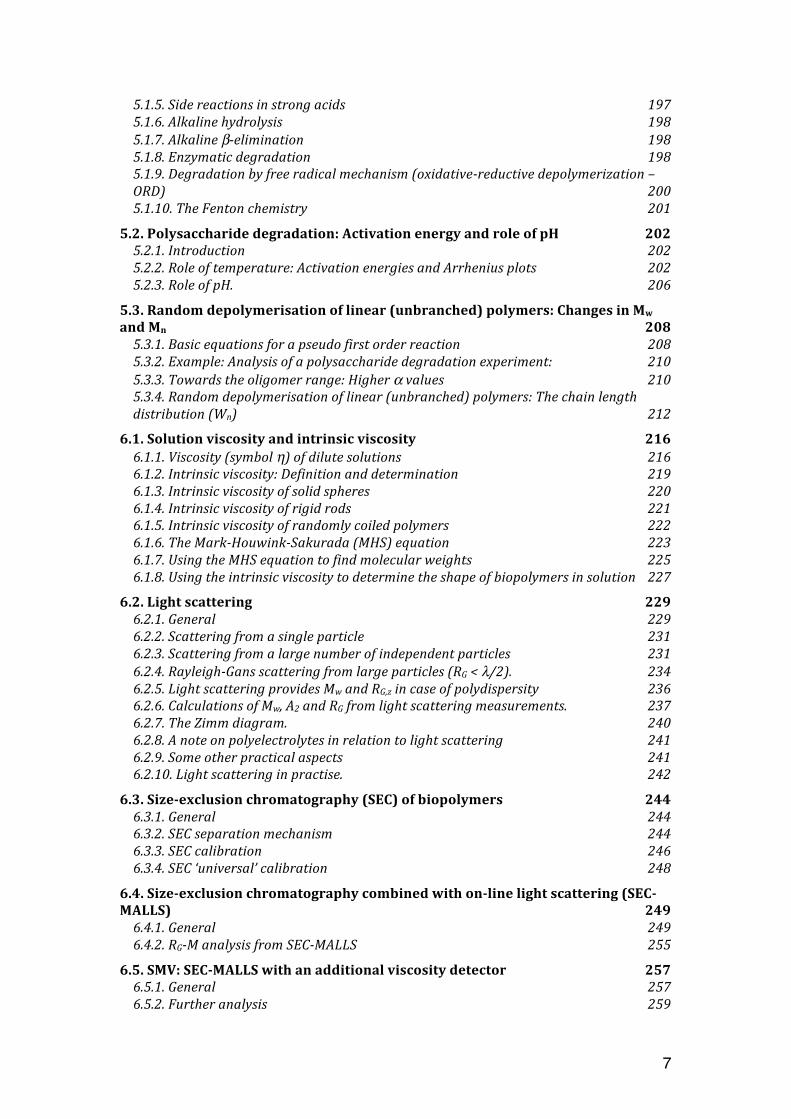
1.1.1.  The  Fisher  projection  

The Fisher projection is standard tool in organic chemistry to specify the stereochemistry at asymmetric carbons, which are abundant in carbohydrates.

Note the rule for distinguishing D- and L-sugars: The stereochemistry of the highest-numbered chiral carbon defines D or L. For hexoses (six carbon sugars) this corresponds to C-6, and for pentoses (five carbon sugars) C-5.

1.1.2.  D-­‐  and  L-­‐sugars  

D- and L-sugars having the same name (e.g. D- and L-glucose) are enantiomers. They are mirror images and cannot superimpose after rotation or translation.

11

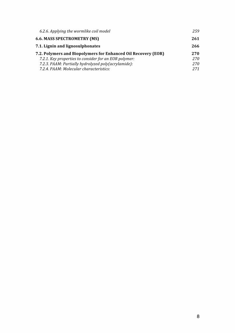
Note the rule: Changing the stereochemistry of ALL asymmetric carbons does not change the name, only the D/L situation. Implicitly, changing only the configuration at carbon 6 (in hexoses) not only changes from D to L (or vice versa), but also the name of the sugar. Example:

 

CHOOHHHHOOHHOHH

CH2OH

D-glucose

CHOOHHHHOOHHHOH

CH2OH

L-idose

12

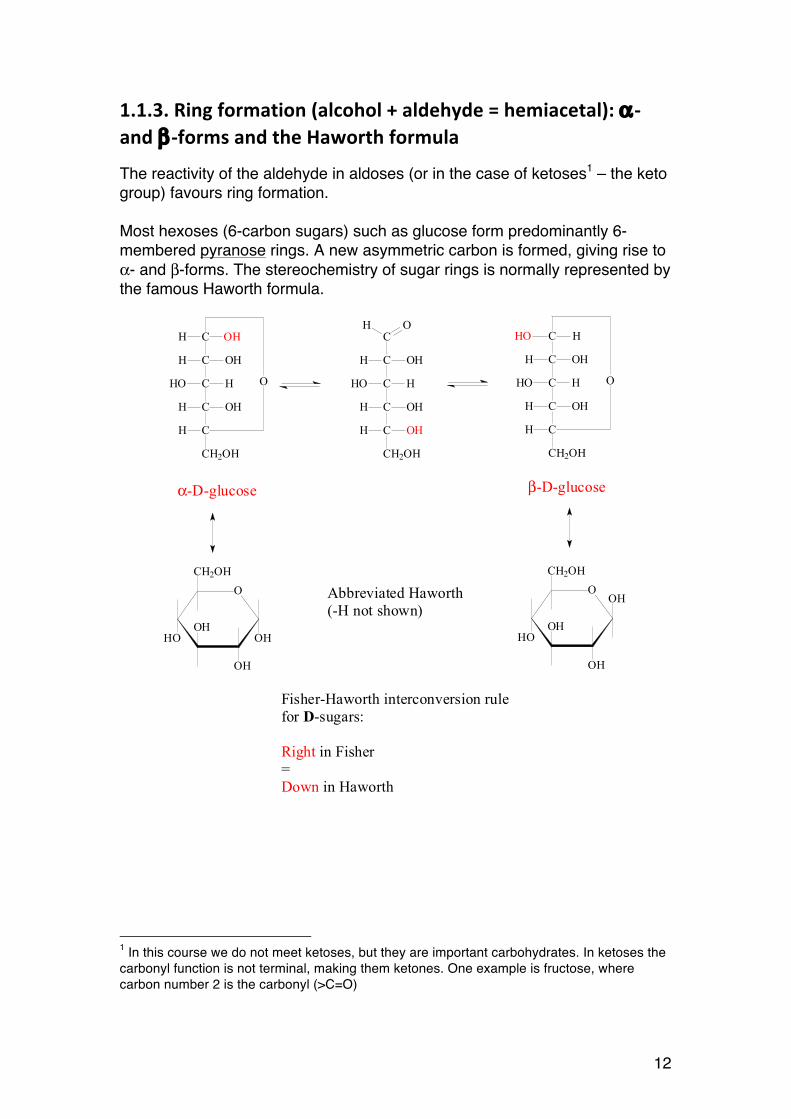
1.1.3.  Ring  formation  (alcohol  +  aldehyde  =  hemiacetal):  α-­‐  and  β-­‐forms  and  the  Haworth  formula  

The reactivity of the aldehyde in aldoses (or in the case of ketoses1 – the keto group) favours ring formation. Most hexoses (6-carbon sugars) such as glucose form predominantly 6-membered pyranose rings. A new asymmetric carbon is formed, giving rise to α- and β-forms. The stereochemistry of sugar rings is normally represented by the famous Haworth formula.

1 In this course we do not meet ketoses, but they are important carbohydrates. In ketoses the carbonyl function is not terminal, making them ketones. One example is fructose, where carbon number 2 is the carbonyl (>C=O)

C

C OHH

C HHO

C OHH

C OHH

CH2OH

OHC

C OHH

C HHO

C OHH

CH

CH2OH

OHH

O

C

C OHH

C HHO

C OHH

CH

CH2OH

HHO

O

α-D-glucose β-D-glucose

OOH

OH

CH2OH

HO

OH

O

OH

CH2OH

HO

OH

OH

Abbreviated Haworth(-H not shown)

Fisher-Haworth interconversion rulefor D-sugars:

Right in Fisher=Down in Haworth

13

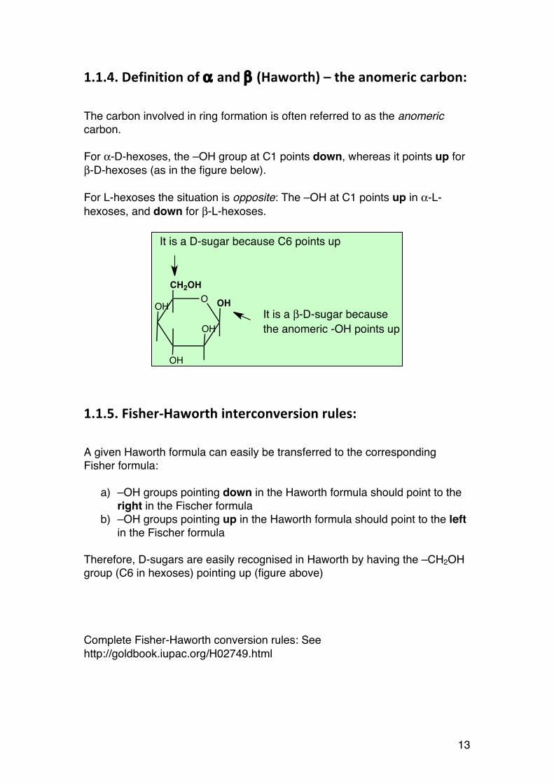
1.1.4.  Definition  of  α  and  β  (Haworth)  –  the  anomeric  carbon:  

The carbon involved in ring formation is often referred to as the anomeric carbon. For α-D-hexoses, the –OH group at C1 points down, whereas it points up for β-D-hexoses (as in the figure below). For L-hexoses the situation is opposite: The –OH at C1 points up in α-L-hexoses, and down for β-L-hexoses.

 

1.1.5.  Fisher-­‐Haworth  interconversion  rules:  

A given Haworth formula can easily be transferred to the corresponding Fisher formula:

a) –OH groups pointing down in the Haworth formula should point to the right in the Fischer formula

b) –OH groups pointing up in the Haworth formula should point to the left in the Fischer formula

Therefore, D-sugars are easily recognised in Haworth by having the –CH2OH group (C6 in hexoses) pointing up (figure above)

Complete Fisher-Haworth conversion rules: See http://goldbook.iupac.org/H02749.html

OCH2OH

OH

OH

OH

OH

It is a D-sugar because C6 points up

It is a β-D-sugar becausethe anomeric -OH points up

14

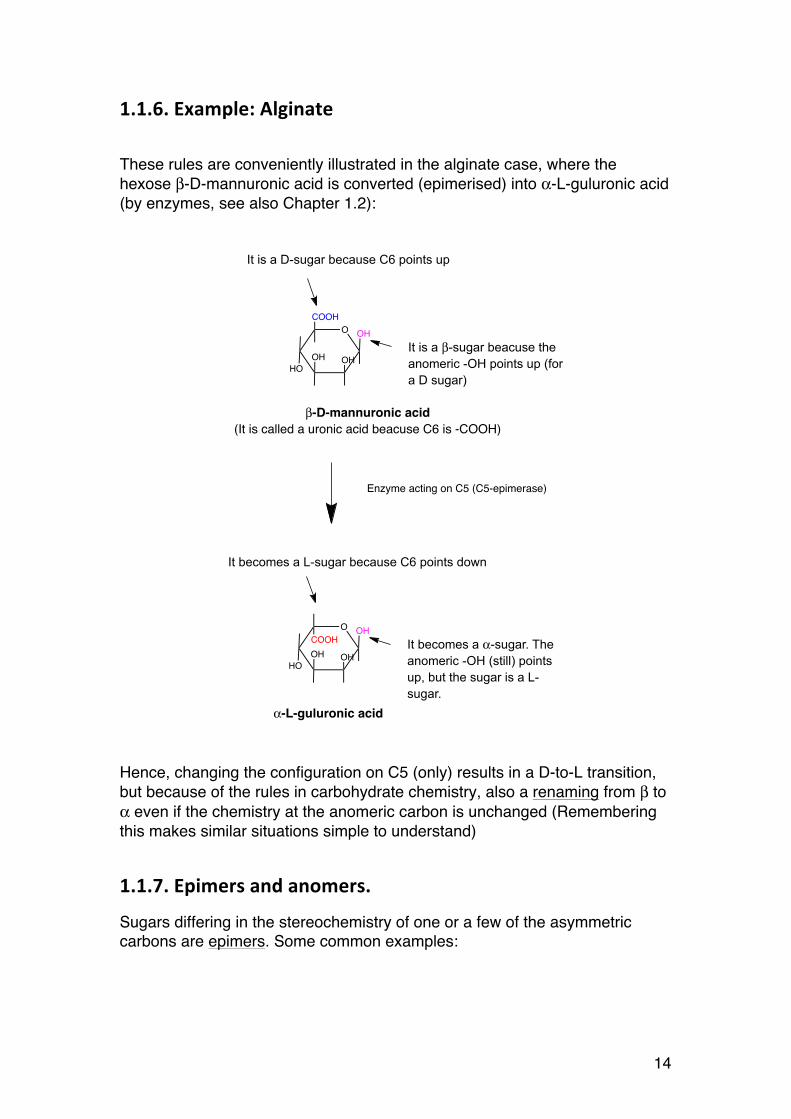
1.1.6.  Example:  Alginate  

These rules are conveniently illustrated in the alginate case, where the hexose β-D-mannuronic acid is converted (epimerised) into α-L-guluronic acid (by enzymes, see also Chapter 1.2):

Hence, changing the configuration on C5 (only) results in a D-to-L transition, but because of the rules in carbohydrate chemistry, also a renaming from β to α even if the chemistry at the anomeric carbon is unchanged (Remembering this makes similar situations simple to understand)

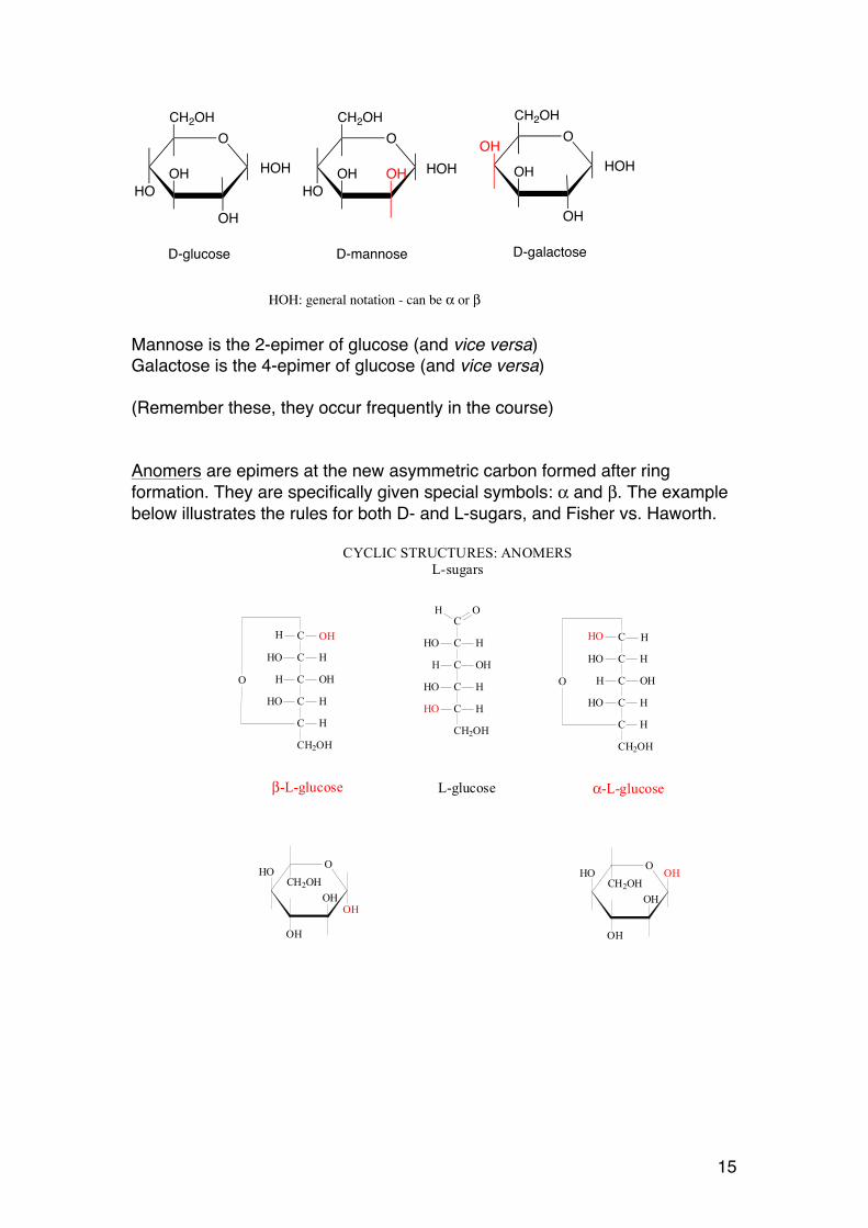
1.1.7.  Epimers  and  anomers.  

Sugars differing in the stereochemistry of one or a few of the asymmetric carbons are epimers. Some common examples:

OCOOH

OH

OHOHHO

It is a D-sugar because C6 points up

It is a β-sugar beacuse the anomeric -OH points up (for a D sugar)

β-D-mannuronic acid(It is called a uronic acid beacuse C6 is -COOH)

OCOOH

OH

OHOHHO

It becomes a L-sugar because C6 points down

It becomes a α-sugar. The anomeric -OH (still) points up, but the sugar is a L-sugar.

α-L-guluronic acid

Enzyme acting on C5 (C5-epimerase)

15

Mannose is the 2-epimer of glucose (and vice versa) Galactose is the 4-epimer of glucose (and vice versa) (Remember these, they occur frequently in the course) Anomers are epimers at the new asymmetric carbon formed after ring formation. They are specifically given special symbols: α and β. The example below illustrates the rules for both D- and L-sugars, and Fisher vs. Haworth.

OCH2OH

HOOH

OH

HOH

D-glucose

OCH2OH

HOOH OH HOH

D-mannose

OCH2OH

OHOH

OH

HOH

D-galactose

HOH: general notation - can be α or β

C

C HHO

C OHH

C HHO

C HHO

CH2OH

OH

L-glucose

C

C HHO

C OHH

C HHO

C H

CH2OH

HHO

O

OOH

OH

HOCH2OH

OH

α-L-glucose

C

C HHO

C OHH

C HHO

C H

CH2OH

OHH

O

O

OH

HOCH2OH

OH

OH

β-L-glucose

CYCLIC STRUCTURES: ANOMERSL-sugars

16

1.1.9.  The  shape  of  hexoses  

Cyclic sugars without double bonds2 cannot form flat structures as indicated by the Haworth formulae. The situation is similar to that of simple cyclic compounds such as cyclohexane. This is because of the sp3 hybridization of the carbons of the molecule, which forces the sugars to adapt specific shapes. The most common shapes of hexoses are: a) The 4C1 chair form (very abundant) b) The 1C4 chair form (less abundant, but important) c) Boat forms (uncommon except when chains are mechanically stretched) The naming refers to the position (above or below) of C1 and C4 relative to the plane formed by C2-C3-C5-O (shaded area in the figure):

In the 4C1 conformation carbon 4 is above the plane, and carbon 1 is below the plane.

1.1.10.  How  to  determine  whether  a  sugar  is  1C4  or  4C1  

Most of the hexoses that we encounter in this course as part of oligo-and polysaccharides exist only in the 4C1 chair form. A typical example is cellulose:

Cellulose consists only of β-1,4-linked D-glucose, which in the 4C1 chair form has all its heavy substituents (-OH and –CH2OH) in a stable, equatorial position.

Axial substituents destabilise the hexose rings. If a sufficient number of hydroxyls or –CH2OH groups (or other heavy/bulky groups) are axial, the 2 Unsaturated sugars do exist, for example the structure formed by alginate lyases of by alkaline β-elimination of alginates or pectins

O

123

4 5

OCH2OH

OHHO

OO

OCH2OH

OHHO

O

O

OH

OH O

CH2OH

O

OH

OH O

CH2OH

O

OH

OH O

CH2OH

O

OH

OH O

CH2OH

OO

123

4 5 1

234

5

4C1 1C4

17

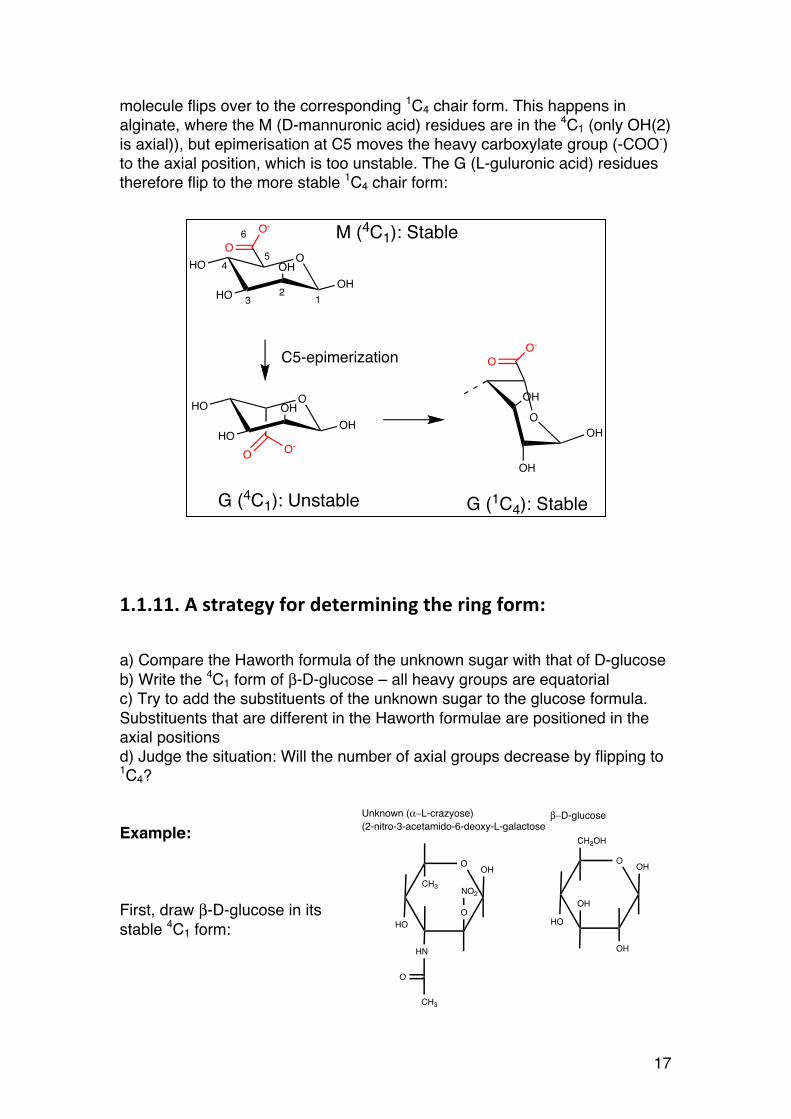
molecule flips over to the corresponding 1C4 chair form. This happens in alginate, where the M (D-mannuronic acid) residues are in the 4C1 (only OH(2) is axial)), but epimerisation at C5 moves the heavy carboxylate group (-COO-) to the axial position, which is too unstable. The G (L-guluronic acid) residues therefore flip to the more stable 1C4 chair form:

1.1.11.  A  strategy  for  determining  the  ring  form:  

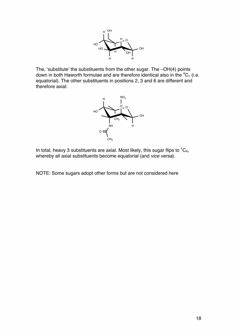
a) Compare the Haworth formula of the unknown sugar with that of D-glucose b) Write the 4C1 form of β-D-glucose – all heavy groups are equatorial c) Try to add the substituents of the unknown sugar to the glucose formula. Substituents that are different in the Haworth formulae are positioned in the axial positions d) Judge the situation: Will the number of axial groups decrease by flipping to 1C4? Example: First, draw β-D-glucose in its stable 4C1 form:

O

OH

OH

OH

O-

O

OOH

HO

O-

O

OHHO

M (4C1): Stable

OOH

HOO-

O

OHHO

G (4C1): Unstable G (1C4): Stable

C5-epimerization

123

4

6

5

O

CH2OH

OH

OH

OH

HO

O

CH3

OH

O

HN

HO

O

CH3

NO2

Unknown (α−L-crazyose)(2-nitro-3-acetamido-6-deoxy-L-galactose

β−D-glucose

18

The, ‘substitute’ the substituents from the other sugar. The –OH(4) points down in both Haworth formulae and are therefore identical also in the 4C1 (i.e. equatorial). The other substituents in positions 2, 3 and 6 are different and therefore axial:

In total, heavy 3 substituents are axial. Most likely, this sugar flips to 1C4, whereby all axial substituents become equatorial (and vice versa). NOTE: Some sugars adopt other forms but are not considered here

O

H

HO

H

HO

H

H

OHHOH

OH

O

H

HO

NH

O

H

CH3OH

O

CH3

NO2

19

1.2.  ALGINATES  

1.2.1.  Introduction  

In this course emphasis is placed on alginates, for several reasons:

• Their industrial importance • Hot topic – more than 1000 research articles and hundreds of patent

applications annually • National molecule of Norway – lots of research at NTNU (NOBIPOL) • Alginates beautifully illustrate both nomenclature and fundamental

chemistry of carbohydrates in general • One of the most studied polysaccharide families – reference materials

for comparing to other systems

1.2.2.  General  

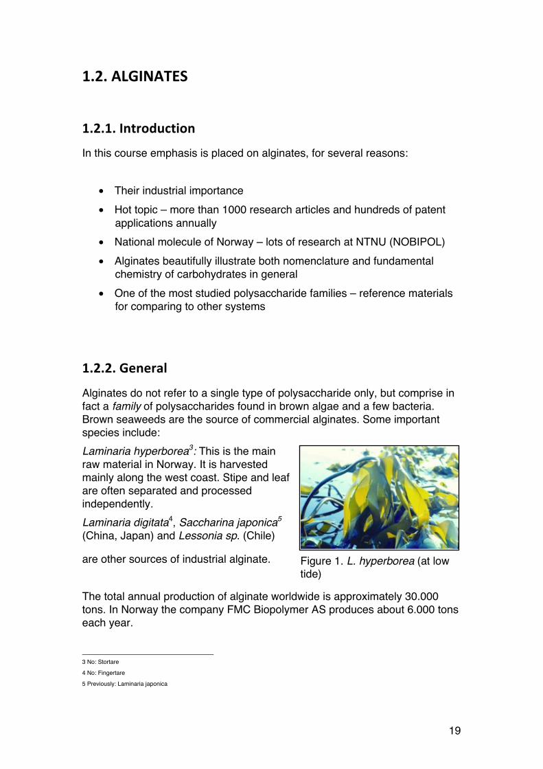
Alginates do not refer to a single type of polysaccharide only, but comprise in fact a family of polysaccharides found in brown algae and a few bacteria. Brown seaweeds are the source of commercial alginates. Some important species include: Laminaria hyperborea3: This is the main raw material in Norway. It is harvested mainly along the west coast. Stipe and leaf are often separated and processed independently. Laminaria digitata4, Saccharina japonica5 (China, Japan) and Lessonia sp. (Chile)

are other sources of industrial alginate. The total annual production of alginate worldwide is approximately 30.000 tons. In Norway the company FMC Biopolymer AS produces about 6.000 tons each year.

3 No: Stortare

4 No: Fingertare

5 Previously: Laminaria japonica

Figure 1. L. hyperborea (at low tide)

20

Alginates are used in the food industry (as thickeners and stabilizers), and in the pharmaceutical industry (tablet formulations, drug delivery, biomaterials for tissue engineering etc.) mainly due to their viscosifying and gelling (with Ca++) properties, but are also used in textile printing pastes, surface treatment of paper and cardboard, in welding electrodes. Most industrial applications of alginates are based on the ability of alginate solutions (2-10%) to form gels when calcium salts are added.

1.2.3.  Structure  of  alginates  

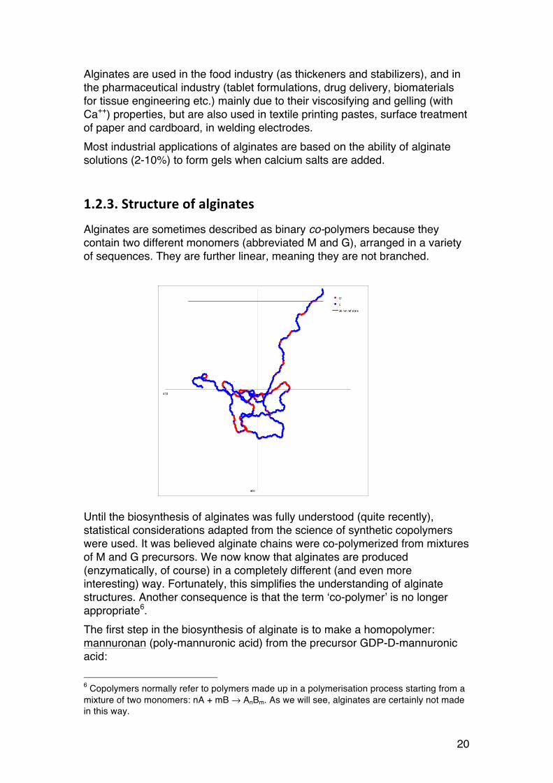
Alginates are sometimes described as binary co-polymers because they contain two different monomers (abbreviated M and G), arranged in a variety of sequences. They are further linear, meaning they are not branched.

Until the biosynthesis of alginates was fully understood (quite recently), statistical considerations adapted from the science of synthetic copolymers were used. It was believed alginate chains were co-polymerized from mixtures of M and G precursors. We now know that alginates are produced (enzymatically, of course) in a completely different (and even more interesting) way. Fortunately, this simplifies the understanding of alginate structures. Another consequence is that the term ‘co-polymer’ is no longer appropriate6. The first step in the biosynthesis of alginate is to make a homopolymer: mannuronan (poly-mannuronic acid) from the precursor GDP-D-mannuronic acid:

6 Copolymers normally refer to polymers made up in a polymerisation process starting from a mixture of two monomers: nA + mB → AnBm. As we will see, alginates are certainly not made in this way.

21

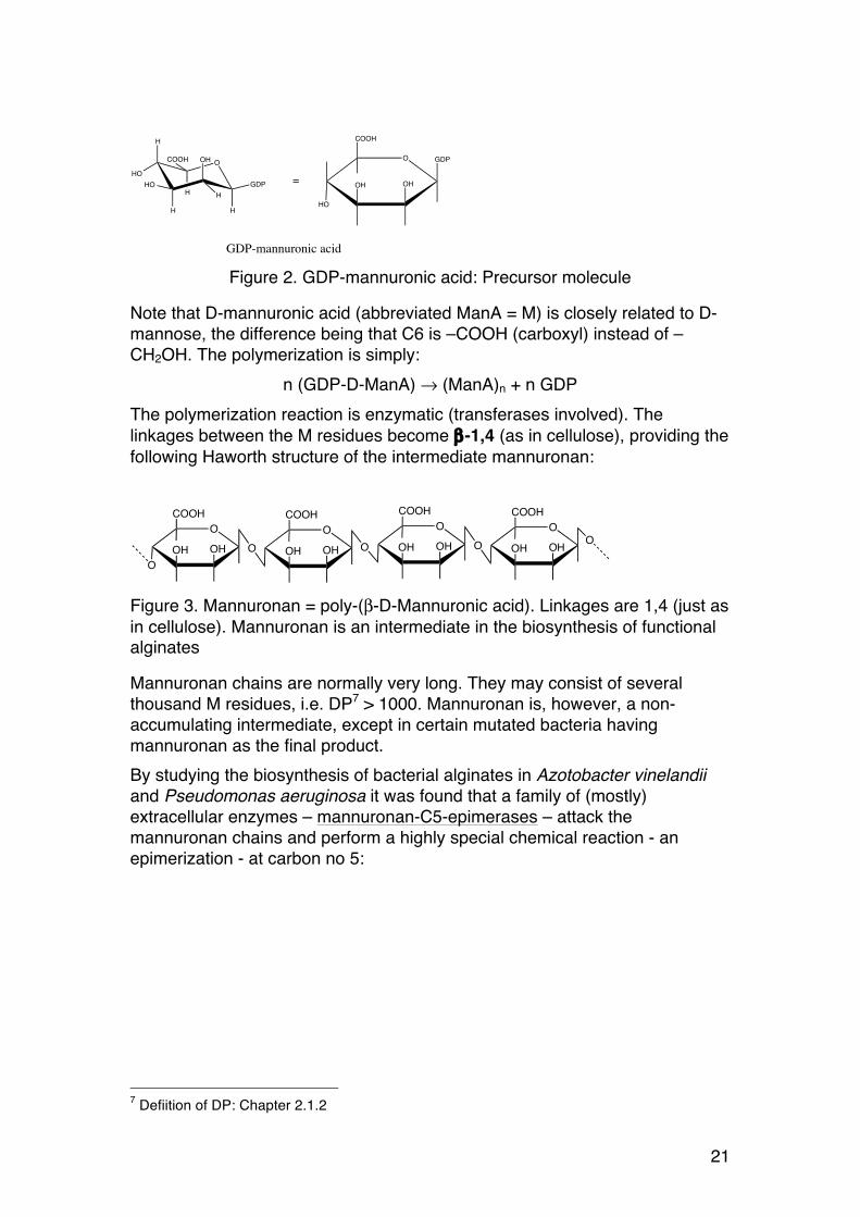
Figure 2. GDP-mannuronic acid: Precursor molecule

Note that D-mannuronic acid (abbreviated ManA = M) is closely related to D-mannose, the difference being that C6 is –COOH (carboxyl) instead of –CH2OH. The polymerization is simply:

n (GDP-D-ManA) → (ManA)n + n GDP The polymerization reaction is enzymatic (transferases involved). The linkages between the M residues become β-1,4 (as in cellulose), providing the following Haworth structure of the intermediate mannuronan:

Figure 3. Mannuronan = poly-(β-D-Mannuronic acid). Linkages are 1,4 (just as in cellulose). Mannuronan is an intermediate in the biosynthesis of functional alginates

Mannuronan chains are normally very long. They may consist of several thousand M residues, i.e. DP7 > 1000. Mannuronan is, however, a non-accumulating intermediate, except in certain mutated bacteria having mannuronan as the final product. By studying the biosynthesis of bacterial alginates in Azotobacter vinelandii and Pseudomonas aeruginosa it was found that a family of (mostly) extracellular enzymes – mannuronan-C5-epimerases – attack the mannuronan chains and perform a highly special chemical reaction - an epimerization - at carbon no 5:

7 Defiition of DP: Chapter 2.1.2

O

H

HO

H

HO

OH

H

HH

COOH

GDP

O

HO

GDP

OHOH

COOH

=

GDP-mannuronic acid

O

OOHOH

COOH

OO

OHOH

COOH

O

O

OHOH

COOH

OO

OHOH

COOH

O

22

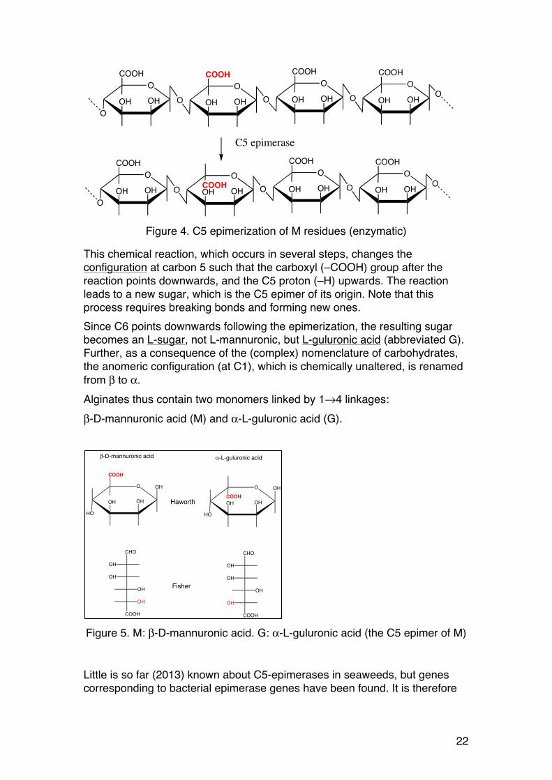
Figure 4. C5 epimerization of M residues (enzymatic)

This chemical reaction, which occurs in several steps, changes the configuration at carbon 5 such that the carboxyl (–COOH) group after the reaction points downwards, and the C5 proton (–H) upwards. The reaction leads to a new sugar, which is the C5 epimer of its origin. Note that this process requires breaking bonds and forming new ones. Since C6 points downwards following the epimerization, the resulting sugar becomes an L-sugar, not L-mannuronic, but L-guluronic acid (abbreviated G). Further, as a consequence of the (complex) nomenclature of carbohydrates, the anomeric configuration (at C1), which is chemically unaltered, is renamed from β to α. Alginates thus contain two monomers linked by 1→4 linkages: β-D-mannuronic acid (M) and α-L-guluronic acid (G).

Figure 5. M: β-D-mannuronic acid. G: α-L-guluronic acid (the C5 epimer of M)

Little is so far (2013) known about C5-epimerases in seaweeds, but genes corresponding to bacterial epimerase genes have been found. It is therefore

O

OOHOH

COOH

OO

OHOH

COOH

O

O

OHOH

COOH

OO

OHOH

COOH

O

O

OOHOH

COOH

OO

OHOHCOOH O

O

OHOH

COOH

OO

OHOH

COOH

O

C5 epimerase

O

HO

OH

OHOH

COOH

β-D-mannuronic acid

Haworth

CHO

OH

OH

OH

OH

COOH

Fisher

O

HO

OH

OHOHCOOH

CHO

OH

OH

OH

OH

COOH

α-L-guluronic acid

23

believed that algal alginates are a result of a biosynthesis similar to that of bacterial alginates.

1.2.4.  Content  and  distribution  of  M  and  G  in  alginates  

Several different epimerases act together to give a variety (in principle an indefinite number) of alginates, where the content of M and G may vary from below 20% G to more than 70% (e.g. outer cortex of L. hyperborea). The sequence of M and G can also vary. The epimerases are processive enzymes which first bind to the mannuronan chain and then work their way along the chain before they are released. Depending on the type of enzyme fundamentally different sequences are formed. For instance, the enzyme AlgE4 tends to produce polyalternating sequences: ..MMMMMMMMMMMMMMMM.. → .MMMGMGMGMGMGMGMMMMMM.... Another enzyme (AlgE6) forms long G-blocks: ..MMMMMMMMMMMMMMMM.. → ..MMMGGGGGGGGGGGGGGMMM.... Since many enzymes probably work together simultaneously, with different rates and specificities, and the starting point may be partly statistic (enzymes bind randomly to begin with), the epimerized alginates become complex mixtures displaying compositional heterogeneity. It is therefore very unlikely that two long alginate chains are identical. This certainly contrasts many regular polysaccharides (e.g. xanthan or agarose), not to mention proteins. Alginates with different sequences and G-contents may have widely different properties. To correlate these properties to the chemical structure we therefore need parameters describing both G-content and sequences more accurately than only percentages. The alginate field has therefore retained a sequence terminology originally developed for synthetic copolymers, namely fractions, or frequencies. The fraction of M and G residues is defined as:

FG = nGnG + nM

FM = nMnG + nM

= 1− FG

24

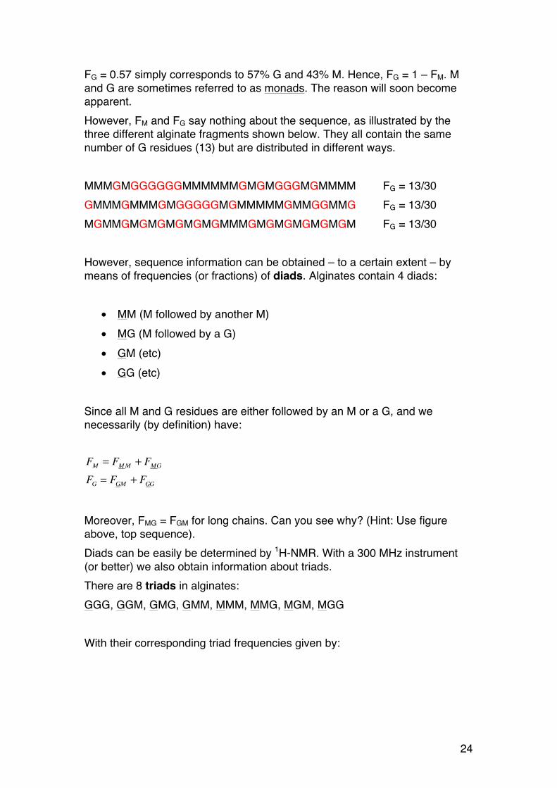
FG = 0.57 simply corresponds to 57% G and 43% M. Hence, FG = 1 – FM. M and G are sometimes referred to as monads. The reason will soon become apparent. However, FM and FG say nothing about the sequence, as illustrated by the three different alginate fragments shown below. They all contain the same number of G residues (13) but are distributed in different ways. MMMGMGGGGGGMMMMMMGMGMGGGMGMMMM FG = 13/30 GMMMGMMMGMGGGGGMGMMMMMGMMGGMMG FG = 13/30 MGMMGMGMGMGMGMGMMMGMGMGMGMGMGM FG = 13/30 However, sequence information can be obtained – to a certain extent – by means of frequencies (or fractions) of diads. Alginates contain 4 diads:

• MM (M followed by another M) • MG (M followed by a G) • GM (etc) • GG (etc)

Since all M and G residues are either followed by an M or a G, and we necessarily (by definition) have:

�

FM = FMM + FMG

FG = FGM + FGG Moreover, FMG = FGM for long chains. Can you see why? (Hint: Use figure above, top sequence). Diads can be easily be determined by 1H-NMR. With a 300 MHz instrument (or better) we also obtain information about triads. There are 8 triads in alginates: GGG, GGM, GMG, GMM, MMM, MMG, MGM, MGG With their corresponding triad frequencies given by:

25

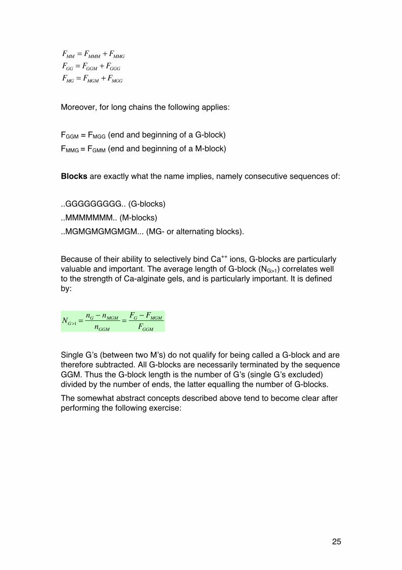
FMM = FMMM + FMMGFGG = FGGM + FGGGFMG = FMGM + FMGG Moreover, for long chains the following applies: FGGM = FMGG (end and beginning of a G-block) FMMG = FGMM (end and beginning of a M-block) Blocks are exactly what the name implies, namely consecutive sequences of: ..GGGGGGGGG.. (G-blocks) ..MMMMMMM.. (M-blocks) ..MGMGMGMGMGM... (MG- or alternating blocks). Because of their ability to selectively bind Ca++ ions, G-blocks are particularly valuable and important. The average length of G-block (NG>1) correlates well to the strength of Ca-alginate gels, and is particularly important. It is defined by:

�

NG>1 =nG − nMGMnGGM

=FG − FMGMFGGM

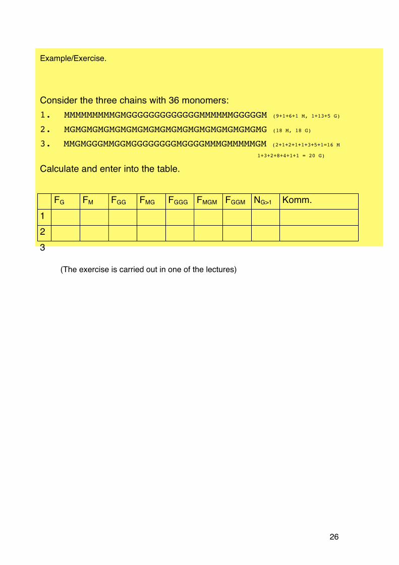
Single G’s (between two M’s) do not qualify for being called a G-block and are therefore subtracted. All G-blocks are necessarily terminated by the sequence GGM. Thus the G-block length is the number of G’s (single G’s excluded) divided by the number of ends, the latter equalling the number of G-blocks. The somewhat abstract concepts described above tend to become clear after performing the following exercise:

26

(The exercise is carried out in one of the lectures)

Example/Exercise.

Consider the three chains with 36 monomers: 1. MMMMMMMMMGMGGGGGGGGGGGGGMMMMMMGGGGGM (9+1+6+1 M, 1+13+5 G)

2. MGMGMGMGMGMGMGMGMGMGMGMGMGMGMGMGMGMG (18 M, 18 G)

3. MMGMGGGMMGGMGGGGGGGGMGGGGMMMGMMMMMGM (2+1+2+1+1+3+5+1=16 M

1+3+2+8+4+1+1 = 20 G)

Calculate and enter into the table. FG FM FGG FMG FGGG FMGM FGGM NG>1 Komm. 1 2 3

27

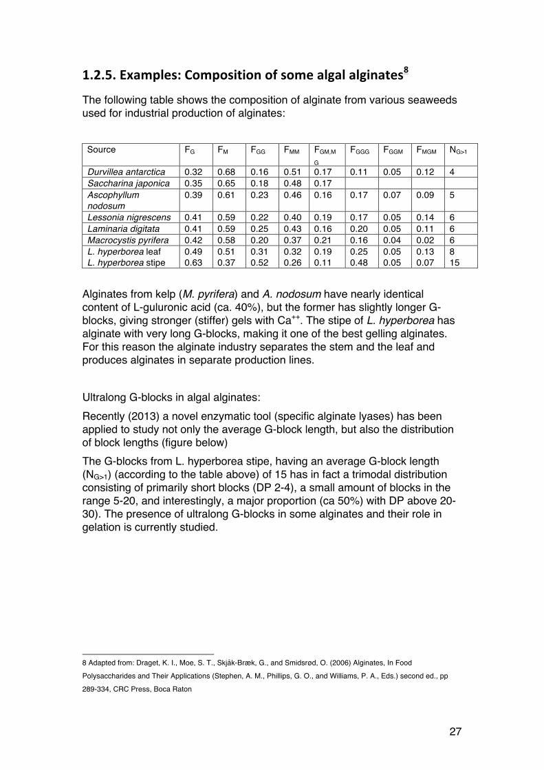
1.2.5.  Examples:  Composition  of  some  algal  alginates8  

The following table shows the composition of alginate from various seaweeds used for industrial production of alginates: Source FG FM FGG FMM FGM,M

G FGGG FGGM FMGM NG>1

Durvillea antarctica 0.32 0.68 0.16 0.51 0.17 0.11 0.05 0.12 4 Saccharina japonica 0.35 0.65 0.18 0.48 0.17 Ascophyllum nodosum

0.39 0.61 0.23 0.46 0.16 0.17 0.07 0.09 5

Lessonia nigrescens 0.41 0.59 0.22 0.40 0.19 0.17 0.05 0.14 6 Laminaria digitata 0.41 0.59 0.25 0.43 0.16 0.20 0.05 0.11 6 Macrocystis pyrifera 0.42 0.58 0.20 0.37 0.21 0.16 0.04 0.02 6 L. hyperborea leaf L. hyperborea stipe

0.49 0.63

0.51 0.37

0.31 0.52

0.32 0.26

0.19 0.11

0.25 0.48

0.05 0.05

0.13 0.07

8 15

Alginates from kelp (M. pyrifera) and A. nodosum have nearly identical content of L-guluronic acid (ca. 40%), but the former has slightly longer G-blocks, giving stronger (stiffer) gels with Ca++. The stipe of L. hyperborea has alginate with very long G-blocks, making it one of the best gelling alginates. For this reason the alginate industry separates the stem and the leaf and produces alginates in separate production lines. Ultralong G-blocks in algal alginates: Recently (2013) a novel enzymatic tool (specific alginate lyases) has been applied to study not only the average G-block length, but also the distribution of block lengths (figure below) The G-blocks from L. hyperborea stipe, having an average G-block length (NG>1) (according to the table above) of 15 has in fact a trimodal distribution consisting of primarily short blocks (DP 2-4), a small amount of blocks in the range 5-20, and interestingly, a major proportion (ca 50%) with DP above 20-30). The presence of ultralong G-blocks in some alginates and their role in gelation is currently studied.

8 Adapted from: Draget, K. I., Moe, S. T., Skjåk-Bræk, G., and Smidsrød, O. (2006) Alginates, In Food

Polysaccharides and Their Applications (Stephen, A. M., Phillips, G. O., and Williams, P. A., Eds.) second ed., pp

289-334, CRC Press, Boca Raton

28

Figure 6. Distribution of G-blocks in alginates from M. pyrifera (white), D. potatorium (gray) and L. hyperborea stipe (black). Adapted from Aarstad et al. (2012), Biomacromolecules, 13, 106-116.

1.2.6.  Bacterial  alginates:  

Bacterial alginates can in principle be produced by fermentation (A. vinelandii, P. aeruginosa and other Pseudomonads), but is currently complicated and non-profitable because the bacteria produce alginate-degrading enzymes (lyases). In contrast, xanthan is an industrially important bacterial polysaccharide produced by large-scale fermentation. FG FM FGG FMG

(FGM) FMM FGGG FMGM FGGM NG>1 Remarks

Pseudomonas aeruginosa

0.009 0.04 -0.10

1.00 0.90 -0.96

- -

- 0.04 -0.10

1.00 0.90 -0.96

- -

- 0.04 - 0.10

- -

- -

O-acetylated

Azotobacter vinelandii

0.45 0.55 0.42 0.03 0.52 O-acetylated (22%)

The alginates from wild type Pseudomonas species have generally low contents of L-guluronic acid, typically FG is in the range 0.04 – 0.10. Moreover, these G residues are single residues (MGM type). Hence, no G-blocks are found in these alginates. In recent years epimerase-negative mutants of Pseudomonas have been developed, enabling production of mannuronan (FG=0), which is a starting point for in vitro epimerization for tailoring of alginates with sequences not found in nature. Such alginates are extremely important tools for elucidating the complex structure-function relationships in alginates.

9 Top mutant, bottom: wild types

Ultralong G-blocks

DP of G-block obtained by HPAEC-PAD

29

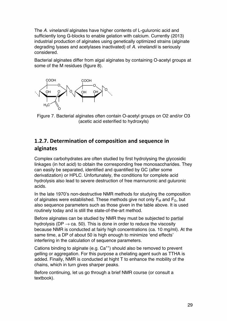
The A. vinelandii alginates have higher contents of L-guluronic acid and sufficiently long G-blocks to enable gelation with calcium. Currently (2013) industrial production of alginates using genetically optimized strains (alginate degrading lyases and acetylases inactivated) of A. vinelandii is seriously considered. Bacterial alginates differ from algal alginates by containing O-acetyl groups at some of the M residues (figure 8).

Figure 7. Bacterial alginates often contain O-acetyl groups on O2 and/or O3

(acetic acid esterified to hydroxyls)

1.2.7.  Determination  of  composition  and  sequence  in  alginates  

Complex carbohydrates are often studied by first hydrolysing the glycosidic linkages (in hot acid) to obtain the corresponding free monosaccharides. They can easily be separated, identified and quantified by GC (after some derivatization) or HPLC. Unfortunately, the conditions for complete acid hydrolysis also lead to severe destruction of free mannuronic and guluronic acids. In the late 1970’s non-destructive NMR methods for studying the composition of alginates were established. These methods give not only FM and FG, but also sequence parameters such as those given in the table above. It is used routinely today and is still the state-of-the-art method. Before alginates can be studied by NMR they must be subjected to partial hydrolysis (DP → ca. 50). This is done in order to reduce the viscosity because NMR is conducted at fairly high concentrations (ca. 10 mg/ml). At the same time, a DP of about 50 is high enough to minimize ‘end effects’ interfering in the calculation of sequence parameters. Cations binding to alginate (e.g. Ca++) should also be removed to prevent gelling or aggregation. For this purpose a chelating agent such as TTHA is added. Finally, NMR is conducted at hight T to enhance the mobility of the chains, which in turn gives sharper peaks. Before continuing, let us go through a brief NMR course (or consult a textbook).

O

OOH

COOH

OO

OHOH

COOH

O

OH3C

30

1.2.8.  NMR  of  alginates  –  a  brief  course  for  polysaccharide  chemists  

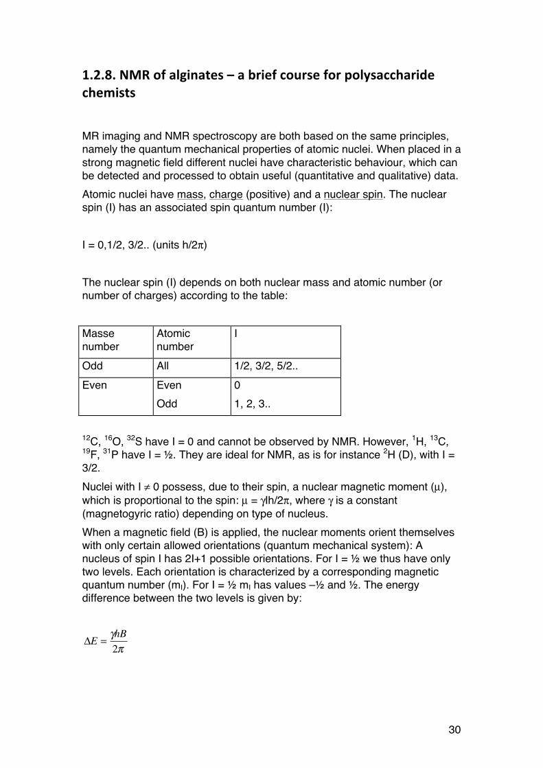
MR imaging and NMR spectroscopy are both based on the same principles, namely the quantum mechanical properties of atomic nuclei. When placed in a strong magnetic field different nuclei have characteristic behaviour, which can be detected and processed to obtain useful (quantitative and qualitative) data. Atomic nuclei have mass, charge (positive) and a nuclear spin. The nuclear spin (I) has an associated spin quantum number (I): I = 0,1/2, 3/2.. (units h/2π) The nuclear spin (I) depends on both nuclear mass and atomic number (or number of charges) according to the table: Masse number

Atomic number

I

Odd All 1/2, 3/2, 5/2.. Even Even

Odd 0 1, 2, 3..

12C, 16O, 32S have I = 0 and cannot be observed by NMR. However, 1H, 13C, 19F, 31P have I = ½. They are ideal for NMR, as is for instance 2H (D), with I = 3/2. Nuclei with I ≠ 0 possess, due to their spin, a nuclear magnetic moment (µ), which is proportional to the spin: µ = γIh/2π, where γ is a constant (magnetogyric ratio) depending on type of nucleus. When a magnetic field (B) is applied, the nuclear moments orient themselves with only certain allowed orientations (quantum mechanical system): A nucleus of spin I has 2I+1 possible orientations. For I = ½ we thus have only two levels. Each orientation is characterized by a corresponding magnetic quantum number (mI). For I = ½ mI has values –½ and ½. The energy difference between the two levels is given by:

�

ΔE =γhB2π

31

The distribution of nuclei with different spins (denoted +: with external field, -: against external field) is given by the Boltzmann formula:

�

N+

N−

= eΔEkT ≈1+ γ

h2π

⎛ ⎝

⎞ ⎠

BkT

⎛ ⎝

⎞ ⎠

We can transfer spins from the lower energy level to the higher by electromagnetic irradiation with energy corresponding to ΔE: ΔE = hν Here ν is the frequency if the irradiation. Each nucleus therefore has a characteristic resonance frequency:

�

ν =γB2π

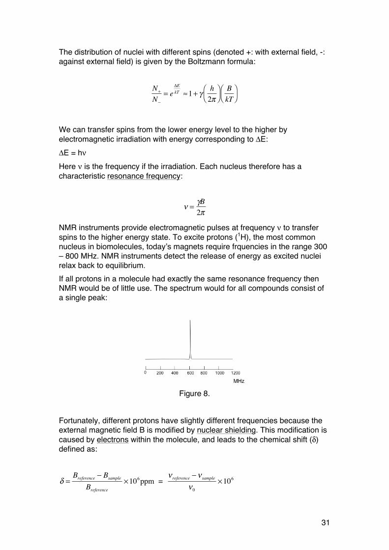
NMR instruments provide electromagnetic pulses at frequency ν to transfer spins to the higher energy state. To excite protons (1H), the most common nucleus in biomolecules, today’s magnets require frquencies in the range 300 – 800 MHz. NMR instruments detect the release of energy as excited nuclei relax back to equilibrium. If all protons in a molecule had exactly the same resonance frequency then NMR would be of little use. The spectrum would for all compounds consist of a single peak:

Fortunately, different protons have slightly different frequencies because the external magnetic field B is modified by nuclear shielding. This modification is caused by electrons within the molecule, and leads to the chemical shift (δ) defined as:

�

δ =Breference − Bsample

Breference

×106ppm = νreference −νsample

ν0

×106

Figure 8.

32

Here Breference is the magnetic field from the reference nuclei and Bsample is the field at the sample nuclei, ν0 is the instrument frequency (300 – 800 MHz). A common reference substance is tetramethylsilane (Si(CH3)4). For protons the chemical shift is related to the electron density around the nucleus. Electronegative substituents reduce the density, leading to ‘downfield shift’, or larger δ values. The figure below illustrates the chemical shift concept.

Figure 9

The proton NMR spectrum of glyceraldehyde in an organic solvent is useful to illustrate the main principles relevant for our use on carbohydrates:

33

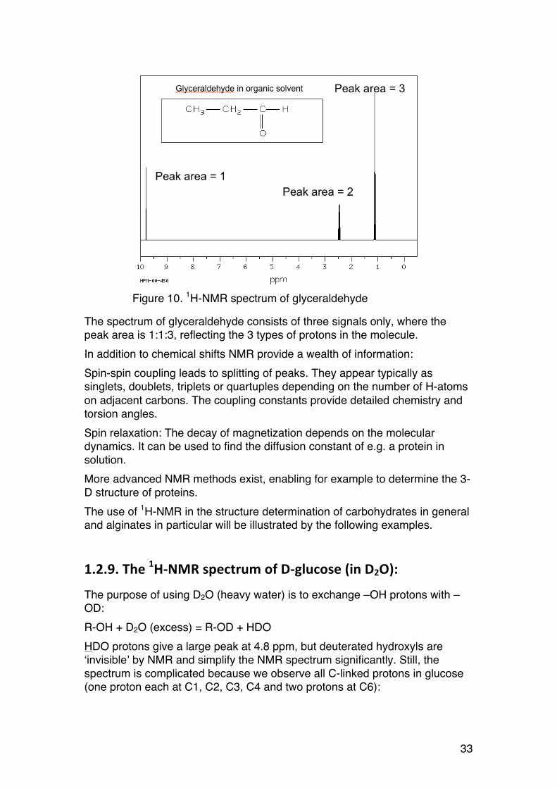
The spectrum of glyceraldehyde consists of three signals only, where the peak area is 1:1:3, reflecting the 3 types of protons in the molecule. In addition to chemical shifts NMR provide a wealth of information: Spin-spin coupling leads to splitting of peaks. They appear typically as singlets, doublets, triplets or quartuples depending on the number of H-atoms on adjacent carbons. The coupling constants provide detailed chemistry and torsion angles. Spin relaxation: The decay of magnetization depends on the molecular dynamics. It can be used to find the diffusion constant of e.g. a protein in solution. More advanced NMR methods exist, enabling for example to determine the 3-D structure of proteins. The use of 1H-NMR in the structure determination of carbohydrates in general and alginates in particular will be illustrated by the following examples.

1.2.9.  The  1H-­‐NMR  spectrum  of  D-­‐glucose  (in  D2O):  

The purpose of using D2O (heavy water) is to exchange –OH protons with –OD: R-OH + D2O (excess) = R-OD + HDO HDO protons give a large peak at 4.8 ppm, but deuterated hydroxyls are ‘invisible’ by NMR and simplify the NMR spectrum significantly. Still, the spectrum is complicated because we observe all C-linked protons in glucose (one proton each at C1, C2, C3, C4 and two protons at C6):

Figure 10. 1H-NMR spectrum of glyceraldehyde

34

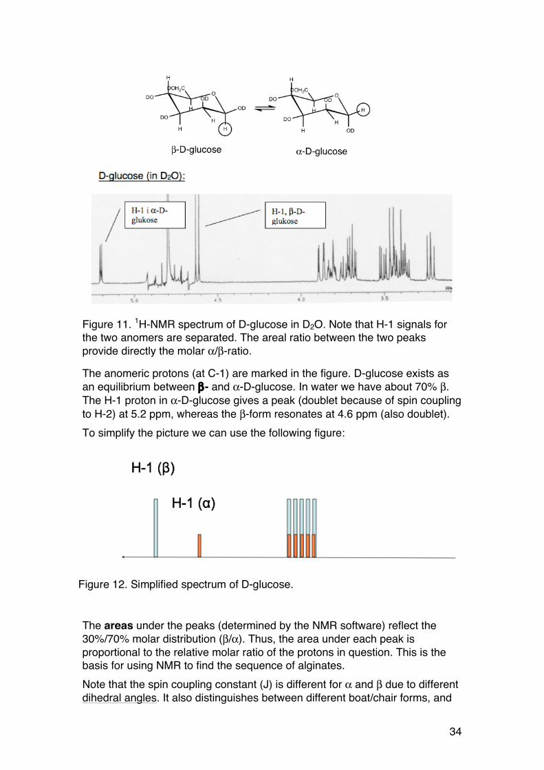
Figure 11. 1H-NMR spectrum of D-glucose in D2O. Note that H-1 signals for the two anomers are separated. The areal ratio between the two peaks provide directly the molar α/β-ratio.

The anomeric protons (at C-1) are marked in the figure. D-glucose exists as an equilibrium between β- and α-D-glucose. In water we have about 70% β. The H-1 proton in α-D-glucose gives a peak (doublet because of spin coupling to H-2) at 5.2 ppm, whereas the β-form resonates at 4.6 ppm (also doublet). To simplify the picture we can use the following figure:

The areas under the peaks (determined by the NMR software) reflect the 30%/70% molar distribution (β/α). Thus, the area under each peak is proportional to the relative molar ratio of the protons in question. This is the basis for using NMR to find the sequence of alginates. Note that the spin coupling constant (J) is different for α and β due to different dihedral angles. It also distinguishes between different boat/chair forms, and

Figure 12. Simplified spectrum of D-glucose.

35

can easily prove that glucose in water is in the 4C1 conformation (as shown in the figure).

1.2.10.  Alginates:  The  1H-­‐NMR  spectrum  

Figure 13

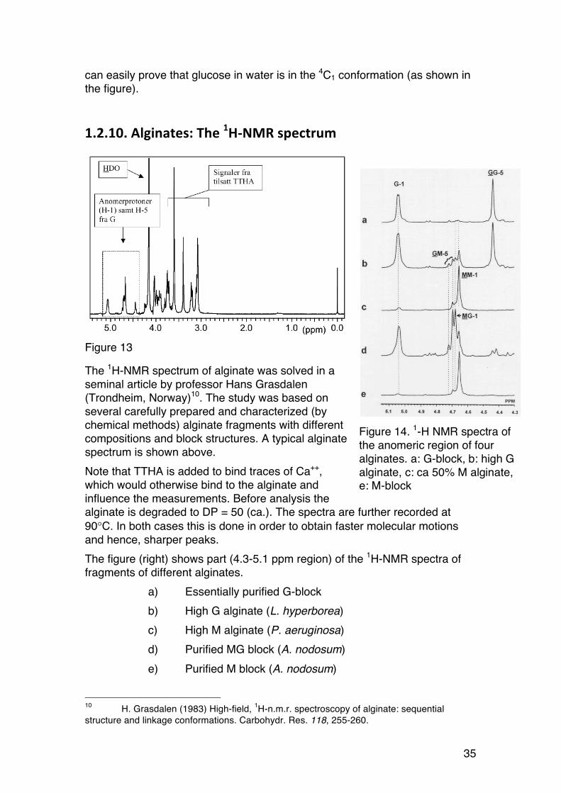
The 1H-NMR spectrum of alginate was solved in a seminal article by professor Hans Grasdalen (Trondheim, Norway)10. The study was based on several carefully prepared and characterized (by chemical methods) alginate fragments with different compositions and block structures. A typical alginate spectrum is shown above. Note that TTHA is added to bind traces of Ca++, which would otherwise bind to the alginate and influence the measurements. Before analysis the alginate is degraded to DP = 50 (ca.). The spectra are further recorded at 90°C. In both cases this is done in order to obtain faster molecular motions and hence, sharper peaks. The figure (right) shows part (4.3-5.1 ppm region) of the 1H-NMR spectra of fragments of different alginates.

a) Essentially purified G-block b) High G alginate (L. hyperborea) c) High M alginate (P. aeruginosa) d) Purified MG block (A. nodosum) e) Purified M block (A. nodosum)

10 H. Grasdalen (1983) High-field, 1H-n.m.r. spectroscopy of alginate: sequential structure and linkage conformations. Carbohydr. Res. 118, 255-260.

Figure 14. 1-H NMR spectra of the anomeric region of four alginates. a: G-block, b: high G alginate, c: ca 50% M alginate, e: M-block

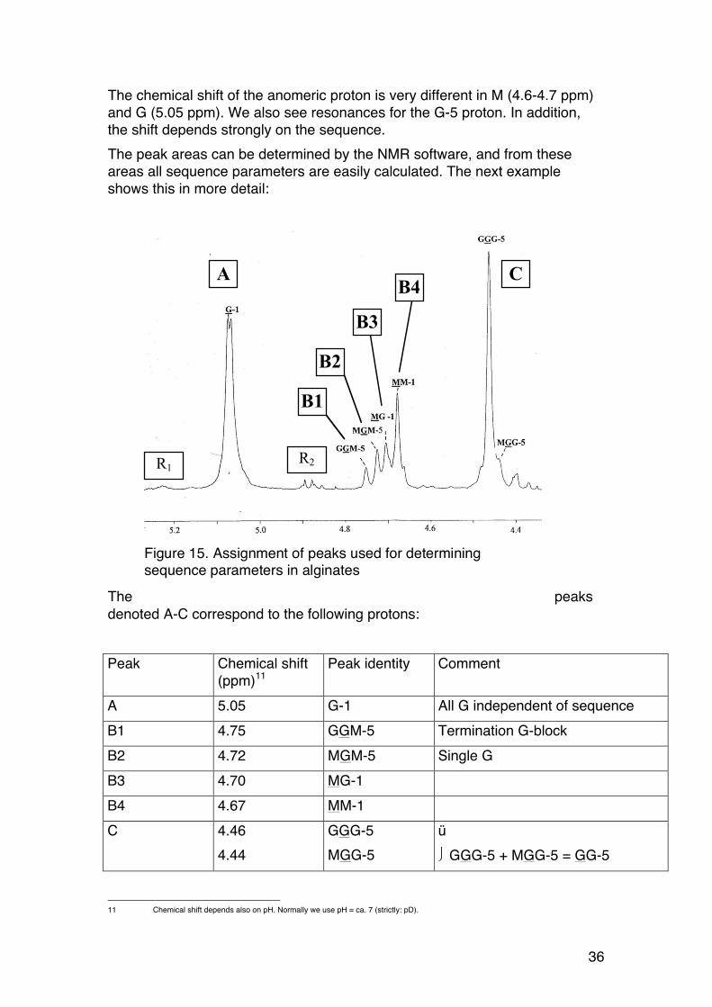
36

The chemical shift of the anomeric proton is very different in M (4.6-4.7 ppm) and G (5.05 ppm). We also see resonances for the G-5 proton. In addition, the shift depends strongly on the sequence. The peak areas can be determined by the NMR software, and from these areas all sequence parameters are easily calculated. The next example shows this in more detail:

The peaks denoted A-C correspond to the following protons: Peak Chemical shift

(ppm)11 Peak identity Comment

A 5.05 G-1 All G independent of sequence B1 4.75 GGM-5 Termination G-block B2 4.72 MGM-5 Single G B3 4.70 MG-1 B4 4.67 MM-1

C 4.46 4.44

GGG-5 MGG-5

ü ⎭ GGG-5 + MGG-5 = GG-5

11 Chemical shift depends also on pH. Normally we use pH = ca. 7 (strictly: pD).

A

B1

B2

B3

B4C

R2R1

Figure 15. Assignment of peaks used for determining sequence parameters in alginates

37

R1 and R2 ca. 5.2 and 4.9 Reducing ends12

M and G, both α and β-form

For each peak we obtain a corresponding peak area or intensity (denoted I). The sequence parameters are obtained as follows: FG = IA/[IA + (IB3 + IB4)] = IA/Itot

B3+B4 is the sum of all M’s. Next (by definition): FM = 1 - FG

Further: FGG = IC/Itot

FGGM = IB1/Itot

FMGM = IB2/Itot

FMG = FGM = IB3/Itot

FMM = IB4/Itot

The remaining parameters are easily obtained from those above: FGGG = FGG- FGGM

NG>1 = [FG - FMGM]/FGGM In practical situation at worksheet is used for the calculations. Only the NMR peak areas (A, B1, …) need to be entered to obtain all sequence parameters.

1.2.11.  Chain  length  (DPn)  from  NMR  

Separate signals from the reducing ends enable simple calculation of the number average degree of polymerization (DPn), the average number of monomers (monosaccharides) per chain: DPn = (nM + ng)/nred.ends = Itot/(IR1 + IR2)

12 Only seen in samples with very low DP

38

In practice, DPn values up to about 50 can be determined. Longer chains have correspondingly smaller end group signals, the area of which cannot be accurately determined. Note that this value is calculated for the degraded sample analyzed by NMR, not the parent sample (unless a low molecular weight alginate was made on purpose).

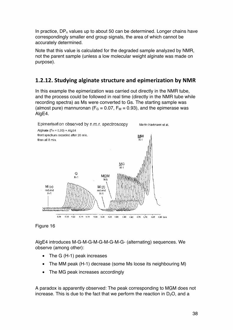
1.2.12.  Studying  alginate  structure  and  epimerization  by  NMR  

In this example the epimerization was carried out directly in the NMR tube, and the process could be followed in real time (directly in the NMR tube while recording spectra) as Ms were converted to Gs. The starting sample was (almost pure) mannuronan (FG = 0.07, FM = 0.93), and the epimerase was AlgE4.

Figure 16 AlgE4 introduces M-G-M-G-M-G-M-G-M-G- (alternating) sequences. We observe (among other):

• The G (H-1) peak increases • The MM peak (H-1) decrease (some Ms loose its neighbouring M) • The MG peak increases accordingly

A paradox is apparently observed: The peak corresponding to MGM does not increase. This is due to the fact that we perform the reaction in D2O, and a

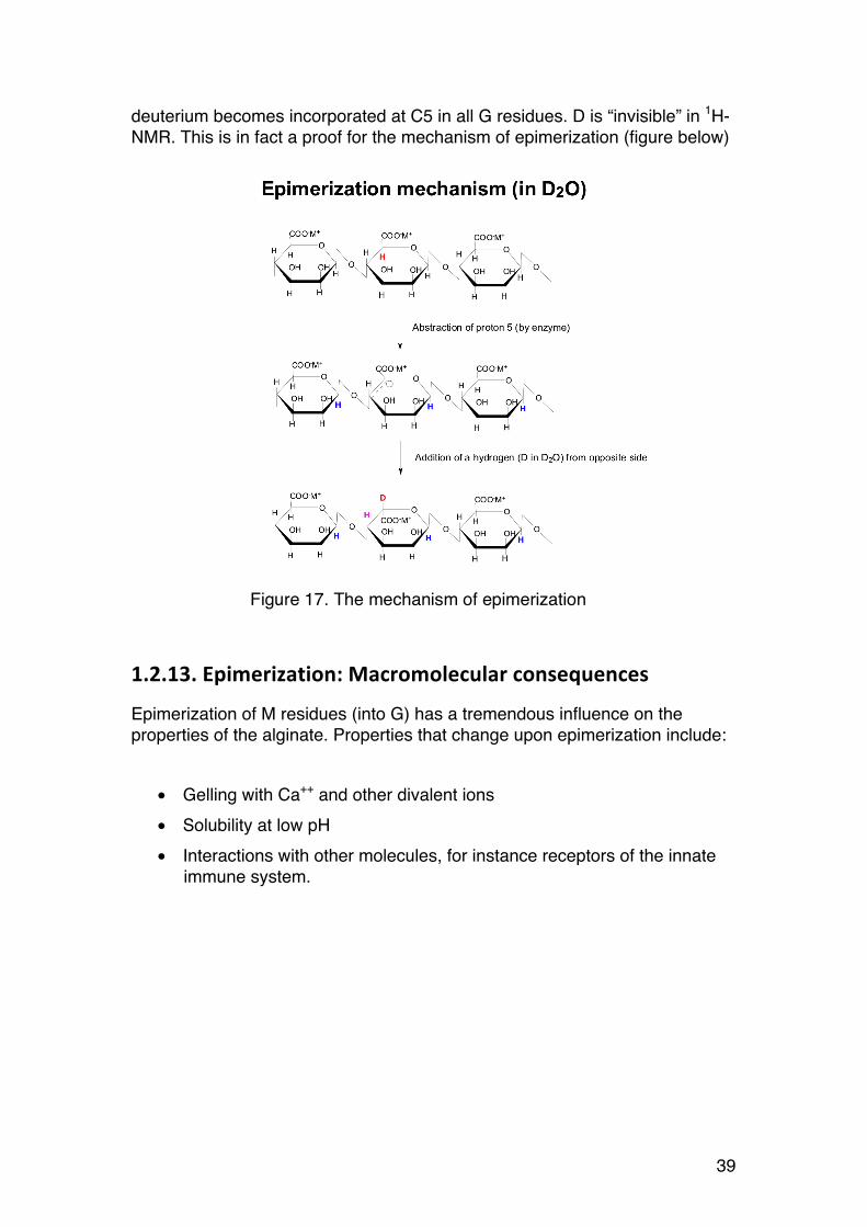
39

deuterium becomes incorporated at C5 in all G residues. D is “invisible” in 1H-NMR. This is in fact a proof for the mechanism of epimerization (figure below)

1.2.13.  Epimerization:  Macromolecular  consequences  

Epimerization of M residues (into G) has a tremendous influence on the properties of the alginate. Properties that change upon epimerization include:

• Gelling with Ca++ and other divalent ions • Solubility at low pH • Interactions with other molecules, for instance receptors of the innate

immune system.

Figure 17. The mechanism of epimerization

40

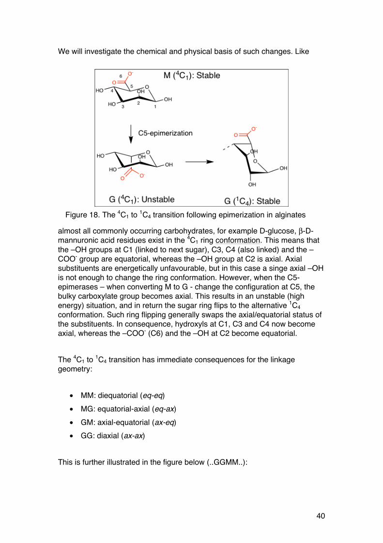
We will investigate the chemical and physical basis of such changes. Like

almost all commonly occurring carbohydrates, for example D-glucose, β-D-mannuronic acid residues exist in the 4C1 ring conformation. This means that the –OH groups at C1 (linked to next sugar), C3, C4 (also linked) and the –COO- group are equatorial, whereas the –OH group at C2 is axial. Axial substituents are energetically unfavourable, but in this case a singe axial –OH is not enough to change the ring conformation. However, when the C5-epimerases – when converting M to G - change the configuration at C5, the bulky carboxylate group becomes axial. This results in an unstable (high energy) situation, and in return the sugar ring flips to the alternative 1C4 conformation. Such ring flipping generally swaps the axial/equatorial status of the substituents. In consequence, hydroxyls at C1, C3 and C4 now become axial, whereas the –COO- (C6) and the –OH at C2 become equatorial. The 4C1 to 1C4 transition has immediate consequences for the linkage geometry:

• MM: diequatorial (eq-eq) • MG: equatorial-axial (eq-ax) • GM: axial-equatorial (ax-eq) • GG: diaxial (ax-ax)

This is further illustrated in the figure below (..GGMM..):

Figure 18. The 4C1 to 1C4 transition following epimerization in alginates

41

The diaxial GG linkage produces a cavity in the chain. Note that the diequatorial MM results in an extended chain similar to cellulose (which shares the same geometry). Also note that two adjacent M residues are rotated about 180° relative to one another (also like in cellulose).

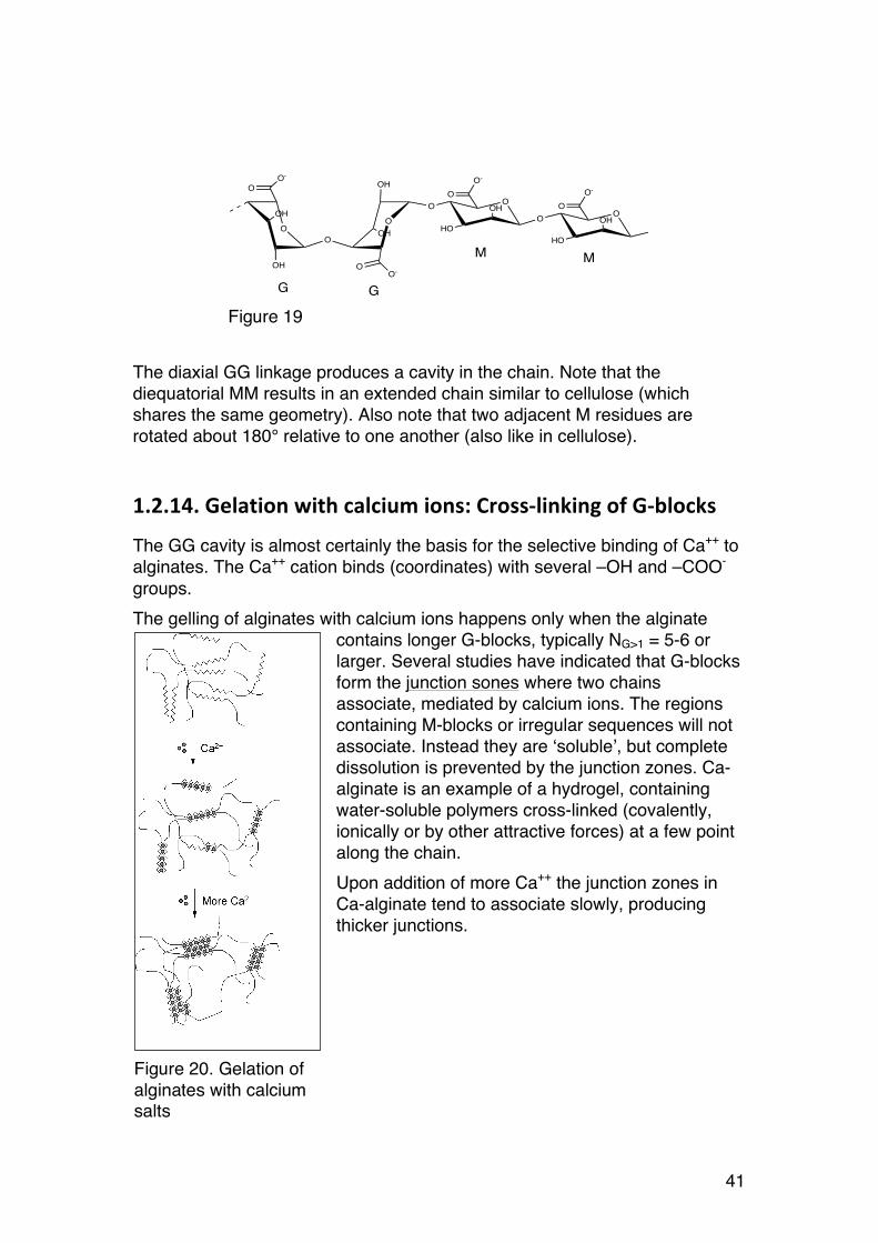
1.2.14.  Gelation  with  calcium  ions:  Cross-­‐linking  of  G-­‐blocks  

The GG cavity is almost certainly the basis for the selective binding of Ca++ to alginates. The Ca++ cation binds (coordinates) with several –OH and –COO- groups. The gelling of alginates with calcium ions happens only when the alginate

contains longer G-blocks, typically NG>1 = 5-6 or larger. Several studies have indicated that G-blocks form the junction sones where two chains associate, mediated by calcium ions. The regions containing M-blocks or irregular sequences will not associate. Instead they are ‘soluble’, but complete dissolution is prevented by the junction zones. Ca-alginate is an example of a hydrogel, containing water-soluble polymers cross-linked (covalently, ionically or by other attractive forces) at a few point along the chain. Upon addition of more Ca++ the junction zones in Ca-alginate tend to associate slowly, producing thicker junctions.

O

OH

OH

O

O-

O

OOH

OH

O-O

OOH

HO

O-

OO

OOH

HO

O-

OO

G G

M M

Figure 19

Figure 20. Gelation of alginates with calcium salts

42

1.2.15.  Alginate,  alginic  acid:  different  salt  forms  

We can easily manipulate the salt form of alginate, meaning (ex)changing the counterion, which accompanies the negatively charged carboxylate group to ensure macroscopic electroneutrality. Most commercial alginates are Na-alginate. The carboxylate group has a pKa of about 3.5. By lowering pH below pKa we obtain alginic acid: -COO- + H+ = -COOH In alginic acid essentially all carboxylate groups are protonated. To obtain 99% -COOH we must go 2 pH units below pKa

13 Alginic acid is insoluble in water, and acidification is a very convenient way to isolate alginate from an aqueous solution. Neutralization of alginic acid by the appropriate base is a convenient method to obtain any type of alginate (Na+, K+, (NH4)+, Li+, Mg++ etc): -COOH + KOH = -COO- K+ (potassium alginate) and similarly for other salts. Other methods such as dialysis or cation exchange chromatography are also used.

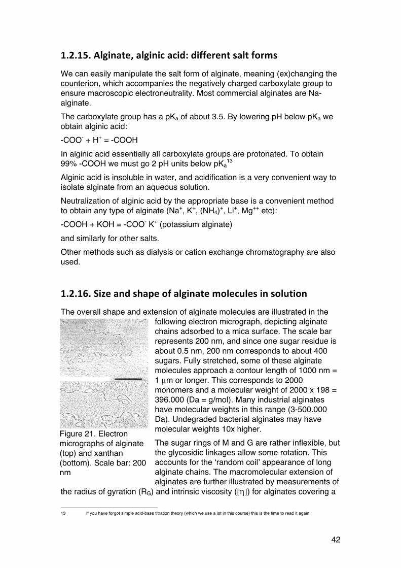
1.2.16.  Size  and  shape  of  alginate  molecules  in  solution  

The overall shape and extension of alginate molecules are illustrated in the following electron micrograph, depicting alginate chains adsorbed to a mica surface. The scale bar represents 200 nm, and since one sugar residue is about 0.5 nm, 200 nm corresponds to about 400 sugars. Fully stretched, some of these alginate molecules approach a contour length of 1000 nm = 1 µm or longer. This corresponds to 2000 monomers and a molecular weight of 2000 x 198 = 396.000 (Da = g/mol). Many industrial alginates have molecular weights in this range (3-500.000 Da). Undegraded bacterial alginates may have molecular weights 10x higher. The sugar rings of M and G are rather inflexible, but the glycosidic linkages allow some rotation. This accounts for the ‘random coil’ appearance of long alginate chains. The macromolecular extension of alginates are further illustrated by measurements of

the radius of gyration (RG) and intrinsic viscosity ([η]) for alginates covering a

13 If you have forgot simple acid-base titration theory (which we use a lot in this course) this is the time to read it again.

Figure 21. Electron micrographs of alginate (top) and xanthan (bottom). Scale bar: 200 nm

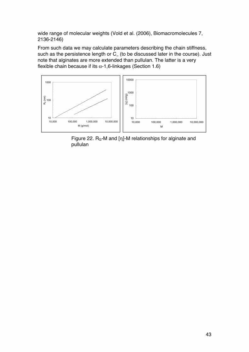
43

wide range of molecular weights (Vold et al. (2006), Biomacromolecules 7, 2136-2146) From such data we may calculate parameters describing the chain stiffness, such as the persistence length or C∞ (to be discussed later in the course). Just note that alginates are more extended than pullulan. The latter is a very flexible chain because if its α-1,6-linkages (Section 1.6)

10

100

1000

10,000 100,000 1,000,000 10,000,000

M (g/mol)

Rg (

nm

)

10

100

1000

10000

10,000 100,000 1,000,000 10,000,000

M [ !

] (m

l/g)

Figure 22. RG-M and [η]-M relationships for alginate and pullulan

44

1.2.17.  Alginates:  Properties  and  uses  

Since alginates comprise an almost indefinitely large family of polysaccharides, where chemical composition and molecular weight can vary within wide ranges (by selecting different raw materials or by controlled degradation), a correspondingly wide range of properies are found. Such differences are often basis for different applications.

1.2.18.  Gelation  with  Ca++:  Gel  strength  and  Young’s  modulus  

When Ca++ ions are added to a solution of Na alginate containing sufficiently long G-blocks, a rapid reaction takes place, leading to gelation. At a given (fixed) alginate concentration the strength of the gel increases with increasing NG>1 as shown below:

Gel strength’ is a rather inaccurate term. The symbol E used in the figure refers to Young’s modulus, which is a measure of elasticity when the gel is compressed. This is normally done in a texture analyzer, where a force (F) is applied to the gel, and the corresponding compression (ΔL) is recorded:

Figure 23. Olives containing pimiento made from alginate and mashed bell pepper

Figure 24.

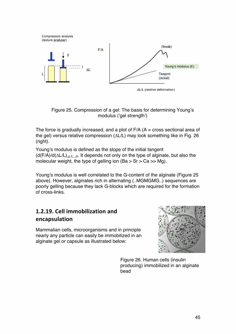
45

The force is gradually increased, and a plot of F/A (A = cross sectional area of the gel) versus relative compression (ΔL/L) may look something like in Fig. 26 (right). Young’s modulus is defined as the slope of the initial tangent (d(F/A)/d(ΔL/L)ΔL/L→0. It depends not only on the type of alginate, but also the molecular weight, the type of gelling ion (Ba > Sr > Ca >> Mg). Young’s modulus is well correlated to the G-content of the alginate (Figure 25 above). However, alginates rich in alternating (..MGMGMG..) sequences are poorly gelling because they lack G-blocks which are required for the formation of cross-links.

1.2.19.  Cell  immobilization  and  encapsulation  

Mammalian cells, microorganisms and in principle nearly any particle can easily be immobilized in an alginate gel or capsule as illustrated below:

Figure 25. Compression of a gel: The basis for determining Young’s modulus (’gel strength’)

Figure 26. Human cells (insulin producing) immobilized in an alginate bead

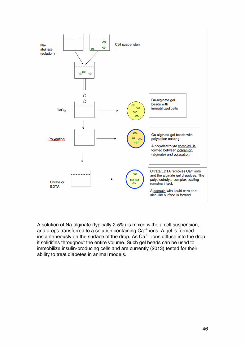
46

A solution of Na-alginate (typically 2-5%) is mixed withe a cell suspension, and drops transferred to a solution containing Ca++ ions. A gel is formed instantaneously on the surface of the drop. As Ca++ ions diffuse into the drop it solidifies throughout the entire volume. Such gel beads can be used to immobilize insulin-producing cells and are currently (2013) tested for their ability to treat diabetes in animal models.

Δl/L

47

1.2.20.  Homogeneous  gels  –  controlled  release  of  calcium  ions  (in  situ  gelation)  

When Na-alginate drops into a Ca++ solution gelation occurs instantaneously at the interface, whereas the inner part of the drop remains a solution because it takes time before Ca++ diffuses into the bead. Thus the gel becomes inhomogeneous. This applies in particular to gelation of larges volumes, for example when an alginate solution is mixed with a Ca++ solution. Small alginate beads (d < 1 mm) may be made homogeneous by gelation in the presence of NaCl or an osmolyte (e.g. mannitol). A more common approach suitable for both small beads and large gels is the CaCO3/GDL method. GDL refers to glucono-δ-lactone:

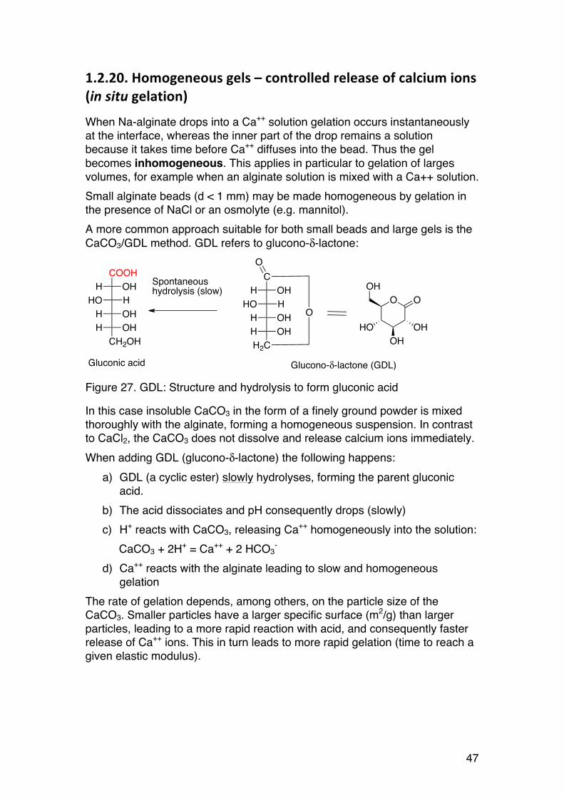
Figure 27. GDL: Structure and hydrolysis to form gluconic acid

In this case insoluble CaCO3 in the form of a finely ground powder is mixed thoroughly with the alginate, forming a homogeneous suspension. In contrast to CaCl2, the CaCO3 does not dissolve and release calcium ions immediately. When adding GDL (glucono-δ-lactone) the following happens:

a) GDL (a cyclic ester) slowly hydrolyses, forming the parent gluconic acid.

b) The acid dissociates and pH consequently drops (slowly) c) H+ reacts with CaCO3, releasing Ca++ homogeneously into the solution:

CaCO3 + 2H+ = Ca++ + 2 HCO3-

d) Ca++ reacts with the alginate leading to slow and homogeneous gelation

The rate of gelation depends, among others, on the particle size of the CaCO3. Smaller particles have a larger specific surface (m2/g) than larger particles, leading to a more rapid reaction with acid, and consequently faster release of Ca++ ions. This in turn leads to more rapid gelation (time to reach a given elastic modulus).

COOHOHHHHOOHHOHH

CH2OH

COHHHHOOHHOHH

H2C

O

OO O

HOOH

OH

OH

Glucono-δ-lactone (GDL)Gluconic acid

Spontaneoushydrolysis (slow)

48

1.2.21.  Alginate  foams:  3D  cell  cultures  

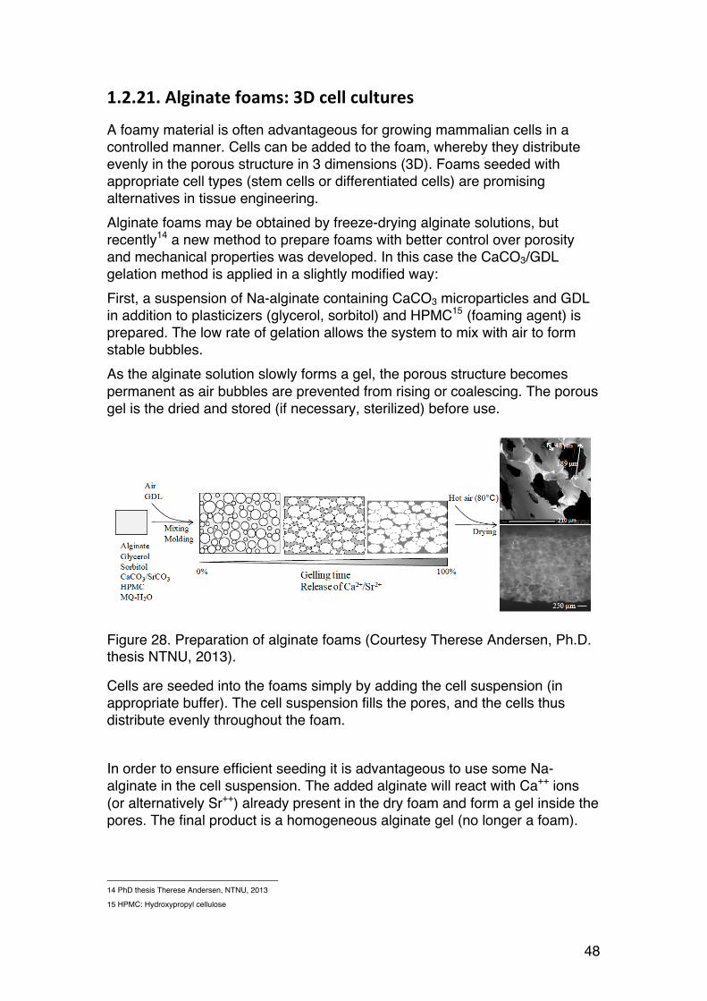
A foamy material is often advantageous for growing mammalian cells in a controlled manner. Cells can be added to the foam, whereby they distribute evenly in the porous structure in 3 dimensions (3D). Foams seeded with appropriate cell types (stem cells or differentiated cells) are promising alternatives in tissue engineering. Alginate foams may be obtained by freeze-drying alginate solutions, but recently14 a new method to prepare foams with better control over porosity and mechanical properties was developed. In this case the CaCO3/GDL gelation method is applied in a slightly modified way: First, a suspension of Na-alginate containing CaCO3 microparticles and GDL in addition to plasticizers (glycerol, sorbitol) and HPMC15 (foaming agent) is prepared. The low rate of gelation allows the system to mix with air to form stable bubbles. As the alginate solution slowly forms a gel, the porous structure becomes permanent as air bubbles are prevented from rising or coalescing. The porous gel is the dried and stored (if necessary, sterilized) before use.

Figure 28. Preparation of alginate foams (Courtesy Therese Andersen, Ph.D. thesis NTNU, 2013).

Cells are seeded into the foams simply by adding the cell suspension (in appropriate buffer). The cell suspension fills the pores, and the cells thus distribute evenly throughout the foam. In order to ensure efficient seeding it is advantageous to use some Na-alginate in the cell suspension. The added alginate will react with Ca++ ions (or alternatively Sr++) already present in the dry foam and form a gel inside the pores. The final product is a homogeneous alginate gel (no longer a foam).

14 PhD thesis Therese Andersen, NTNU, 2013

15 HPMC: Hydroxypropyl cellulose

49

1.3.  CHITIN  AND  CHITOSANS  

1.3.1.  General  

Annually (2012) more than 3000 research articles and a corresponding number of patent applications are being published in the chitosan field. Chitosans are in practice the only naturally occurring (and hence, biodegradable) cationic biopolymer (carrying positive charges) near pH 7, which are produced commercially. Because of their cationic properties chitosans interact with almost all kinds of surfaces, particles, cells and macromolecules that are negatively charged. This is the basis for a wide variety of applications, including for example drug and gene delivery, mucoadhesion, flocculation etc. Chitosans are in some cases antimicrobial, although the basis is not fully understood. In drug/gene delivery chitosans may be preferred over synthetic polycations due to their low cytotoxicity.

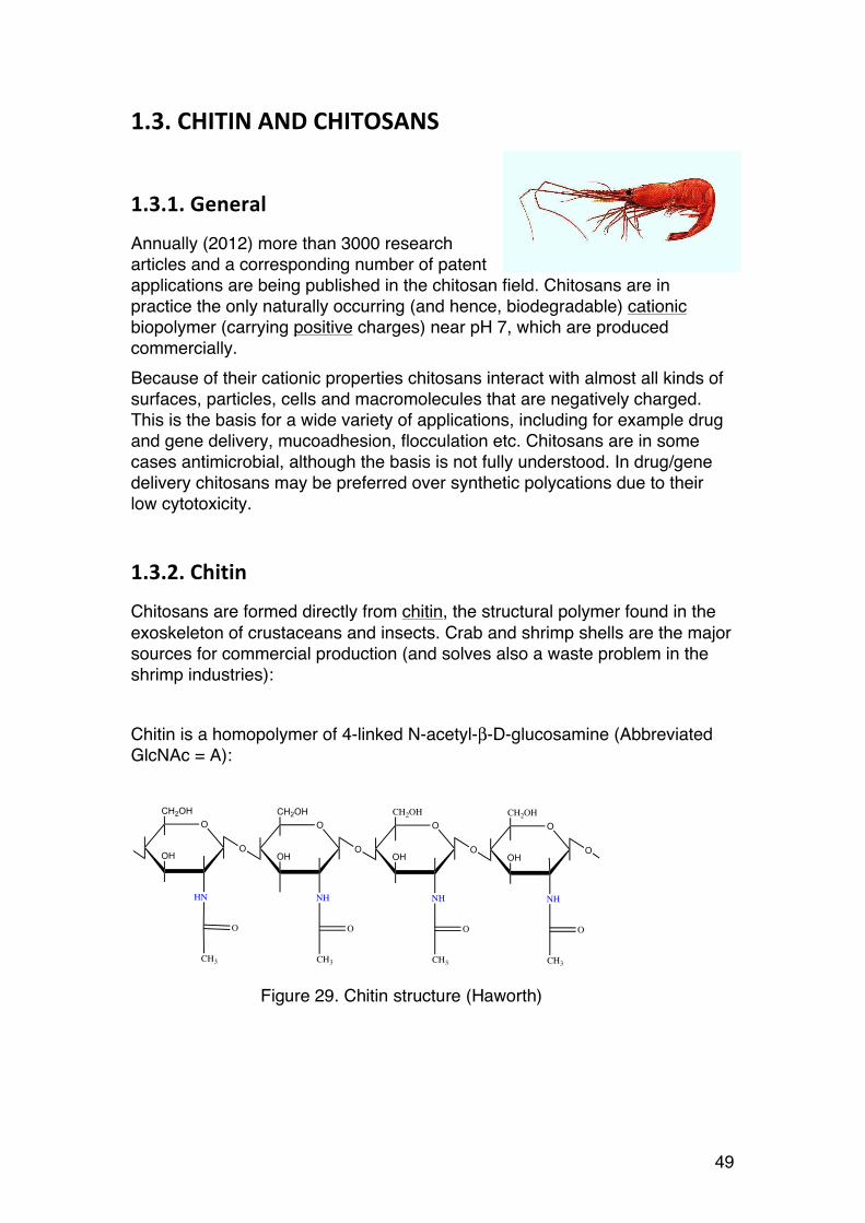
1.3.2.  Chitin  

Chitosans are formed directly from chitin, the structural polymer found in the exoskeleton of crustaceans and insects. Crab and shrimp shells are the major sources for commercial production (and solves also a waste problem in the shrimp industries): Chitin is a homopolymer of 4-linked N-acetyl-β-D-glucosamine (Abbreviated GlcNAc = A):

OCH2OH

OH

HN

O

OCH2OH

OH

NH

O

OCH2OH

OH

NH

O

OCH2OH

OH

NH

O

O O O O

CH3CH3CH3CH3

Figure 29. Chitin structure (Haworth)

50

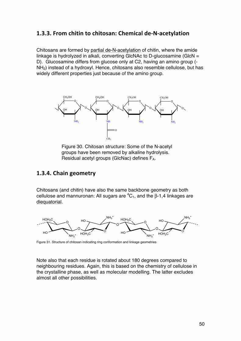
1.3.3.  From  chitin  to  chitosan:  Chemical  de-­‐N-­‐acetylation  

Chitosans are formed by partial de-N-acetylation of chitin, where the amide linkage is hydrolyzed in alkali, converting GlcNAc to D-glucosamine (GlcN = D). Glucosamine differs from glucose only at C2, having an amino group (-NH2) instead of a hydroxyl. Hence, chitosans also resemble cellulose, but has widely different properties just because of the amino group.

 

1.3.4.  Chain  geometry  

Chitosans (and chitin) have also the same backbone geometry as both cellulose and mannuronan: All sugars are 4C1, and the β-1,4 linkages are diequatorial.

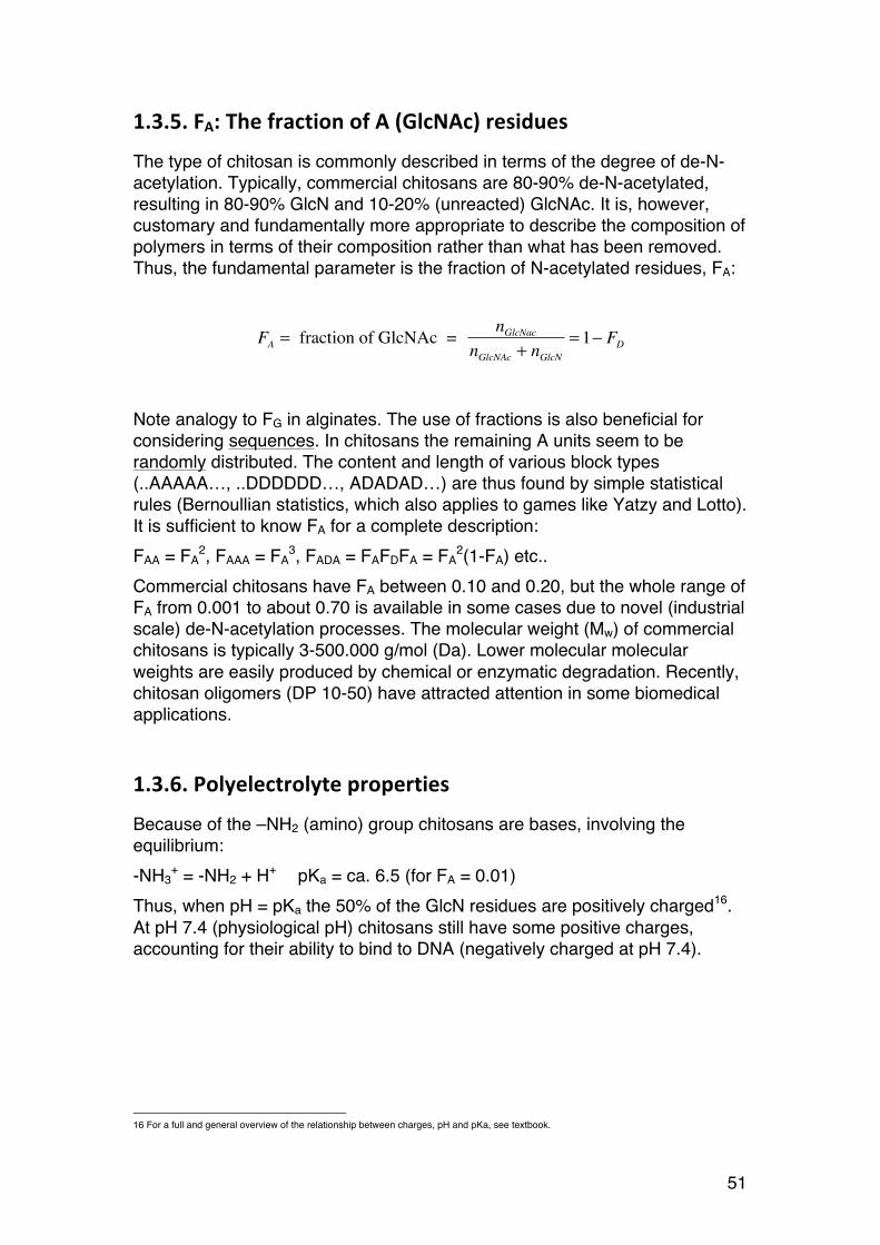
Figure 31. Structure of chitosan indicating ring conformation and linkage geometries

Note also that each residue is rotated about 180 degrees compared to neighbouring residues. Again, this is based on the chemistry of cellulose in the crystalline phase, as well as molecular modelling. The latter excludes almost all other possibilities.

OCH2OH

OH

NH2

O

OCH2OH

OH

NH

O

OCH2OH

OH

NH2

O

OCH2OH

OH

NH2

O

O

CH3

NH3+

OHOH2C

NH3+HO

OO

HOH2C

HOO

NH3+

OHOH2C

NH3+HO

OO

HOH2C

HO

Figure 30. Chitosan structure: Some of the N-acetyl groups have been removed by alkaline hydrolysis. Residual acetyl groups (GlcNac) defines FA.

51

1.3.5.  FA:  The  fraction  of  A  (GlcNAc)  residues  

The type of chitosan is commonly described in terms of the degree of de-N-acetylation. Typically, commercial chitosans are 80-90% de-N-acetylated, resulting in 80-90% GlcN and 10-20% (unreacted) GlcNAc. It is, however, customary and fundamentally more appropriate to describe the composition of polymers in terms of their composition rather than what has been removed. Thus, the fundamental parameter is the fraction of N-acetylated residues, FA:

�

FA = fraction of GlcNAc = nGlcNac

nGlcNAc + nGlcN= 1− FD

Note analogy to FG in alginates. The use of fractions is also beneficial for considering sequences. In chitosans the remaining A units seem to be randomly distributed. The content and length of various block types (..AAAAA…, ..DDDDDD…, ADADAD…) are thus found by simple statistical rules (Bernoullian statistics, which also applies to games like Yatzy and Lotto). It is sufficient to know FA for a complete description: FAA = FA

2, FAAA = FA3, FADA = FAFDFA = FA

2(1-FA) etc.. Commercial chitosans have FA between 0.10 and 0.20, but the whole range of FA from 0.001 to about 0.70 is available in some cases due to novel (industrial scale) de-N-acetylation processes. The molecular weight (Mw) of commercial chitosans is typically 3-500.000 g/mol (Da). Lower molecular molecular weights are easily produced by chemical or enzymatic degradation. Recently, chitosan oligomers (DP 10-50) have attracted attention in some biomedical applications.

1.3.6.  Polyelectrolyte  properties  

Because of the –NH2 (amino) group chitosans are bases, involving the equilibrium: -NH3

+ = -NH2 + H+ pKa = ca. 6.5 (for FA = 0.01) Thus, when pH = pKa the 50% of the GlcN residues are positively charged16. At pH 7.4 (physiological pH) chitosans still have some positive charges, accounting for their ability to bind to DNA (negatively charged at pH 7.4).

16 For a full and general overview of the relationship between charges, pH and pKa, see textbook.

52

1.3.7.  Interactions  with  polyanions  (polyelectrolyte  complexes)  

Polycations such as chitosans interact with polyanions to form polyelectrolyte complexes (PECs). Examples include alginate-chitosan or DNA-chitosan. The latter can be tailored to form nanoparticles, which are intensively studied as non-viral gene delivery vehicles. The basis for such interactions is the general interaction between oppositely charged polymers. This depends on pH as illustrated for alginate-chitosan: Alginates: pKA = ca. 3.5, below which alginates are neutral and do not interact. Above this value alginates are polyanionic (negatively charged) Chitosans: pKA = ca. 6.5, above which chitosans are neutral – and do not interact. Below this value chitosans are positively charged. It follows that alginate-chitosans PECs can only form between pH 3.5 and 6.5. Which pH-range would allow DNA-chitosan PECs?

1.3.8.  Solubility  of  chitosans

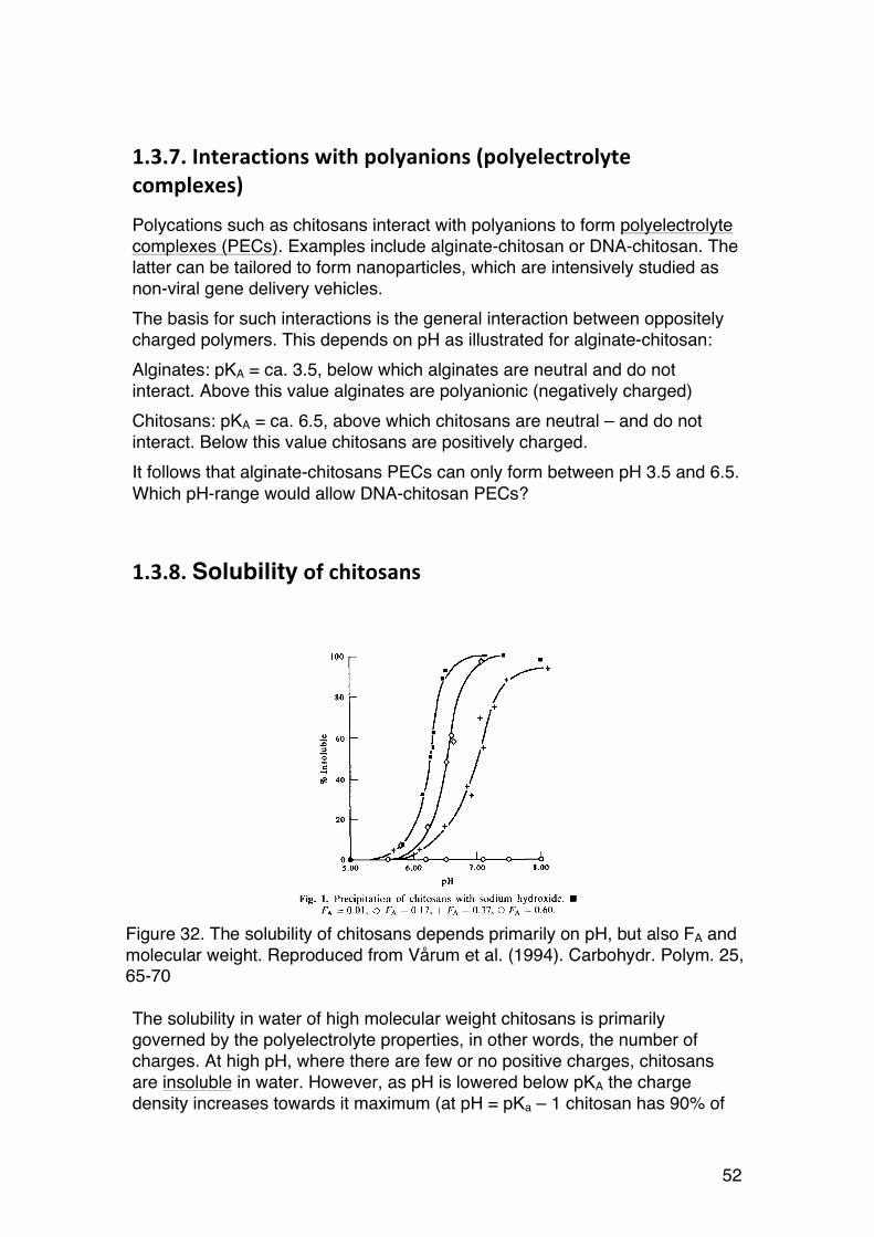
The solubility in water of high molecular weight chitosans is primarily governed by the polyelectrolyte properties, in other words, the number of charges. At high pH, where there are few or no positive charges, chitosans are insoluble in water. However, as pH is lowered below pKA the charge density increases towards it maximum (at pH = pKa – 1 chitosan has 90% of

Figure 32. The solubility of chitosans depends primarily on pH, but also FA and molecular weight. Reproduced from Vårum et al. (1994). Carbohydr. Polym. 25, 65-70

53

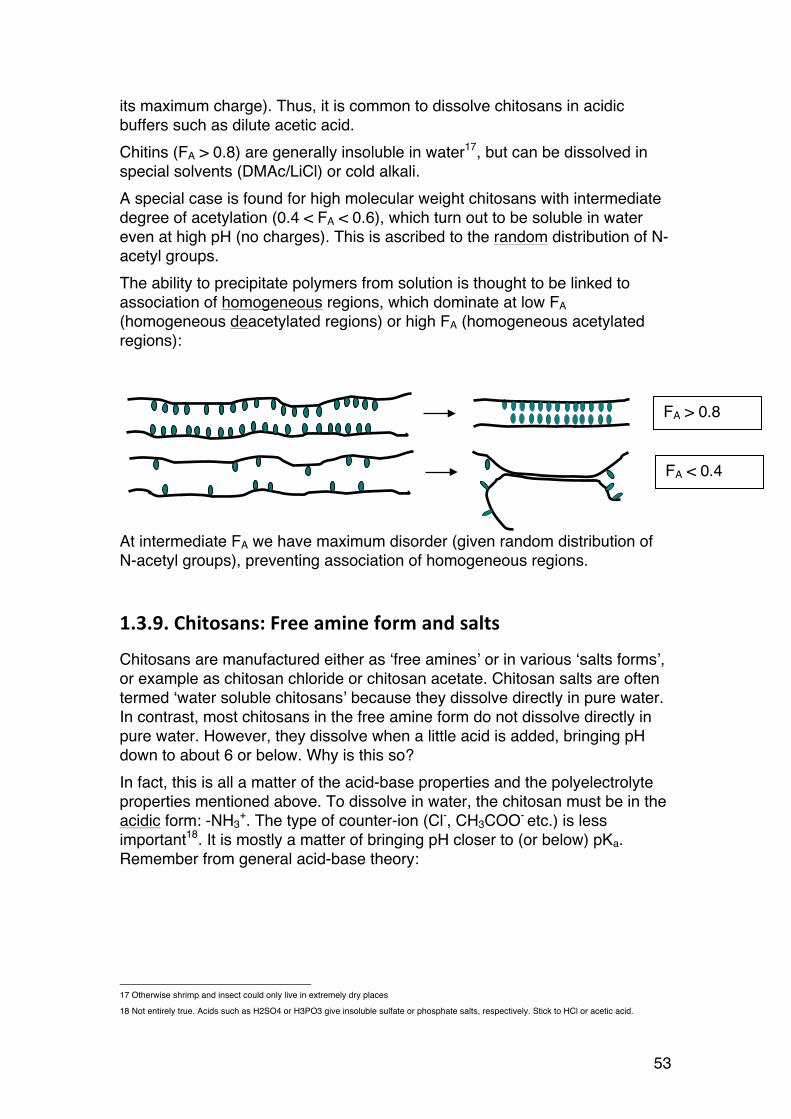
its maximum charge). Thus, it is common to dissolve chitosans in acidic buffers such as dilute acetic acid. Chitins (FA > 0.8) are generally insoluble in water17, but can be dissolved in special solvents (DMAc/LiCl) or cold alkali. A special case is found for high molecular weight chitosans with intermediate degree of acetylation (0.4 < FA < 0.6), which turn out to be soluble in water even at high pH (no charges). This is ascribed to the random distribution of N-acetyl groups. The ability to precipitate polymers from solution is thought to be linked to association of homogeneous regions, which dominate at low FA (homogeneous deacetylated regions) or high FA (homogeneous acetylated regions):

At intermediate FA we have maximum disorder (given random distribution of N-acetyl groups), preventing association of homogeneous regions.

1.3.9.  Chitosans:  Free  amine  form  and  salts  

Chitosans are manufactured either as ‘free amines’ or in various ‘salts forms’, or example as chitosan chloride or chitosan acetate. Chitosan salts are often termed ‘water soluble chitosans’ because they dissolve directly in pure water. In contrast, most chitosans in the free amine form do not dissolve directly in pure water. However, they dissolve when a little acid is added, bringing pH down to about 6 or below. Why is this so? In fact, this is all a matter of the acid-base properties and the polyelectrolyte properties mentioned above. To dissolve in water, the chitosan must be in the acidic form: -NH3

+. The type of counter-ion (Cl-, CH3COO- etc.) is less important18. It is mostly a matter of bringing pH closer to (or below) pKa. Remember from general acid-base theory:

17 Otherwise shrimp and insect could only live in extremely dry places

18 Not entirely true. Acids such as H2SO4 or H3PO3 give insoluble sulfate or phosphate salts, respectively. Stick to HCl or acetic acid.

FA > 0.8

FA < 0.4

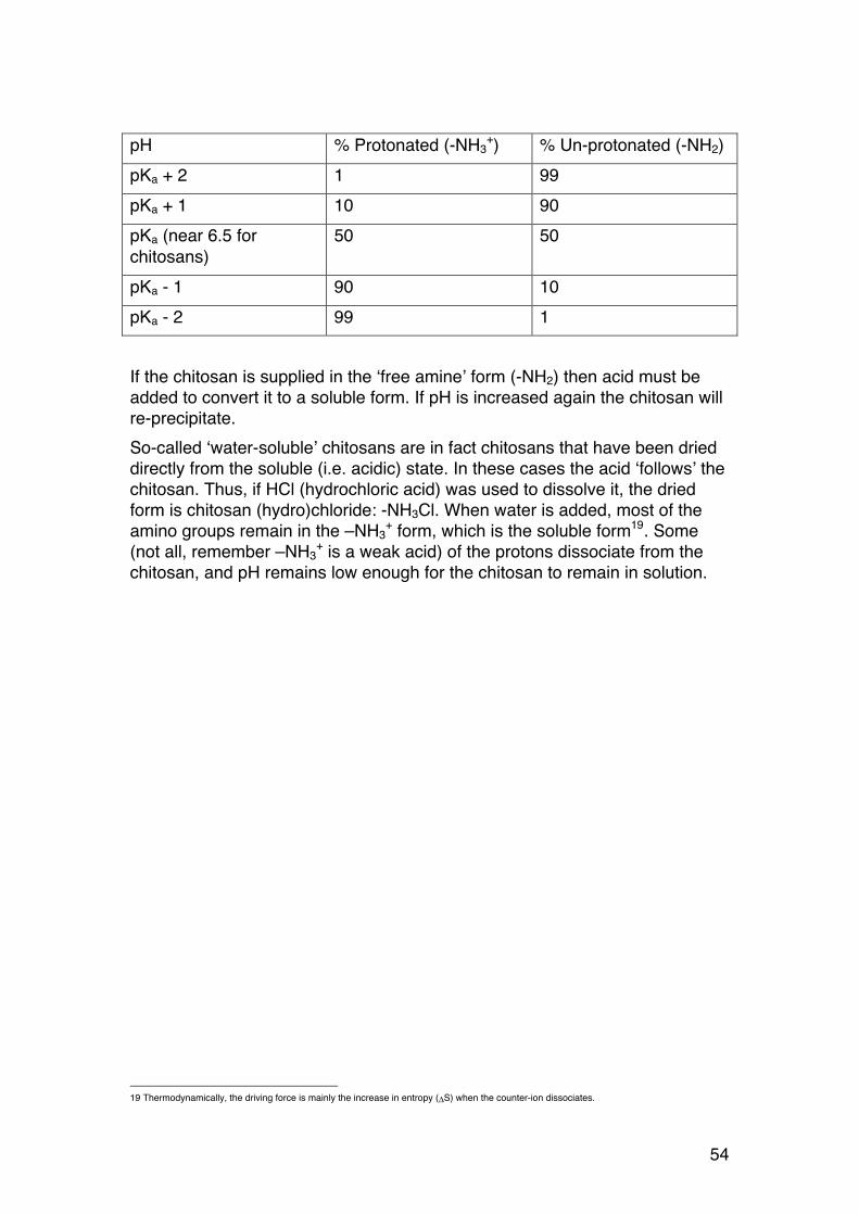
54

pH % Protonated (-NH3

+) % Un-protonated (-NH2) pKa + 2 1 99 pKa + 1 10 90 pKa (near 6.5 for chitosans)

50 50

pKa - 1 90 10 pKa - 2 99 1 If the chitosan is supplied in the ‘free amine’ form (-NH2) then acid must be added to convert it to a soluble form. If pH is increased again the chitosan will re-precipitate. So-called ‘water-soluble’ chitosans are in fact chitosans that have been dried directly from the soluble (i.e. acidic) state. In these cases the acid ‘follows’ the chitosan. Thus, if HCl (hydrochloric acid) was used to dissolve it, the dried form is chitosan (hydro)chloride: -NH3Cl. When water is added, most of the amino groups remain in the –NH3

+ form, which is the soluble form19. Some (not all, remember –NH3

+ is a weak acid) of the protons dissociate from the chitosan, and pH remains low enough for the chitosan to remain in solution.

19 Thermodynamically, the driving force is mainly the increase in entropy (ΔS) when the counter-ion dissociates.

55

1.4.  CELLULOSE  AND  ITS  DERIVATIVES  

1.4.1.  General.  

Cellulose is the most abundant biopolymer on the planet since it is the main constituent of wood (40-45% of the dry weight). It is a major component of the cell walls of plants, where it forms a composite with lignin and hemicelluloses. Cellulose is also formed by some bacteria such as Acetobacter xylinum. Cellulose is formed by CO2 fixation (photosynthesis). Biomass from plants is thus ‘CO2 neutral’ since the CO2 released by conversion of biomass to energy can be recycled back to biomass (plants). The efficiency of the conversion is currently a hot topic (for obvious reasons), and research on the biosynthesis, structure, properties and degradation of cellulose is intense and competitive. Cellulose degrading enzymes are continuously being tailored to obtain much faster degradation (which is inherently slow – just think of the low rate of rotting of wood). Another fascinating aspect is cellulose nanofibers, which possess promising properties in bionanotechnology.

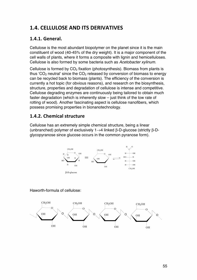
1.4.2.  Chemical  structure  

Cellulose has an extremely simple chemical structure, being a linear (unbranched) polymer of exclusively 1→4 linked β-D-glucose (strictly β-D-glycopyranose since glucose occurs in the common pyranose form).

Haworth-formula of cellulose:

O

OH

OH O

CH2OH

O

OH

OH O

CH2OH

O

OH

OH O

CH2OH

O

OH

OH O

CH2OH

O

HO

OH

OH

OH

CH2OH

HH

H

HH

O

HO

OH

OH

OH

CH2OH

=

β-D-glucose

COH

OHH

H

OHH

OHH

CH2OH

HO

56

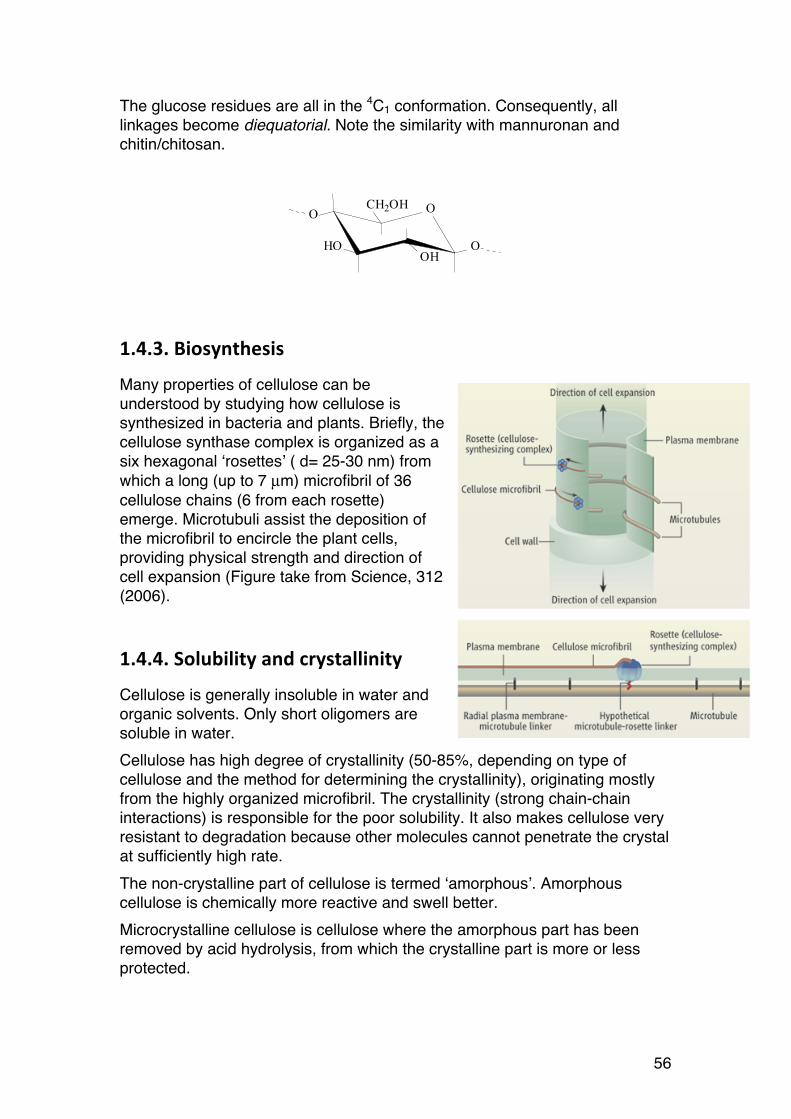
The glucose residues are all in the 4C1 conformation. Consequently, all linkages become diequatorial. Note the similarity with mannuronan and chitin/chitosan.

1.4.3.  Biosynthesis  

Many properties of cellulose can be understood by studying how cellulose is synthesized in bacteria and plants. Briefly, the cellulose synthase complex is organized as a six hexagonal ‘rosettes’ ( d= 25-30 nm) from which a long (up to 7 µm) microfibril of 36 cellulose chains (6 from each rosette) emerge. Microtubuli assist the deposition of the microfibril to encircle the plant cells, providing physical strength and direction of cell expansion (Figure take from Science, 312 (2006).

1.4.4.  Solubility  and  crystallinity  

Cellulose is generally insoluble in water and organic solvents. Only short oligomers are soluble in water. Cellulose has high degree of crystallinity (50-85%, depending on type of cellulose and the method for determining the crystallinity), originating mostly from the highly organized microfibril. The crystallinity (strong chain-chain interactions) is responsible for the poor solubility. It also makes cellulose very resistant to degradation because other molecules cannot penetrate the crystal at sufficiently high rate. The non-crystalline part of cellulose is termed ‘amorphous’. Amorphous cellulose is chemically more reactive and swell better. Microcrystalline cellulose is cellulose where the amorphous part has been removed by acid hydrolysis, from which the crystalline part is more or less protected.

O

OOH

HO

OCH2OH

57

1.4.5.  Cellulose  I.  

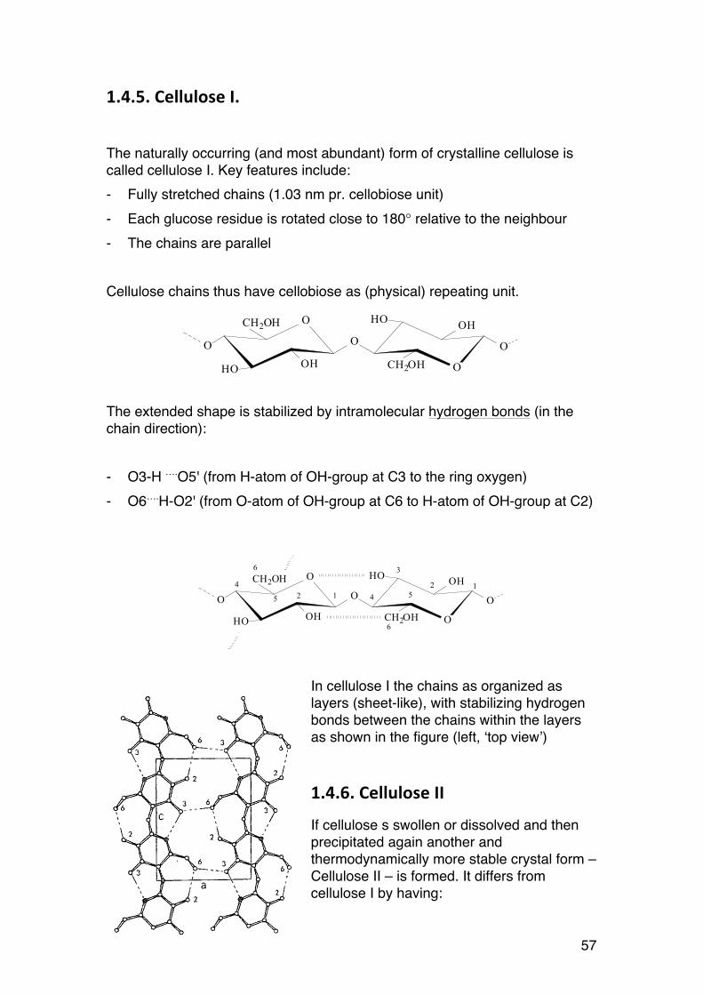
The naturally occurring (and most abundant) form of crystalline cellulose is called cellulose I. Key features include: - Fully stretched chains (1.03 nm pr. cellobiose unit) - Each glucose residue is rotated close to 180° relative to the neighbour - The chains are parallel Cellulose chains thus have cellobiose as (physical) repeating unit.

The extended shape is stabilized by intramolecular hydrogen bonds (in the chain direction): - O3-H ….O5' (from H-atom of OH-group at C3 to the ring oxygen) - O6….H-O2' (from O-atom of OH-group at C6 to H-atom of OH-group at C2)

In cellulose I the chains as organized as layers (sheet-like), with stabilizing hydrogen bonds between the chains within the layers as shown in the figure (left, ‘top view’)

1.4.6.  Cellulose  II  

If cellulose s swollen or dissolved and then precipitated again another and thermodynamically more stable crystal form – Cellulose II – is formed. It differs from cellulose I by having:

OCH2OH

OHHO

OO

OCH2OH

OHHO

O

OCH2OH

OHHO

OO

OCH2OH

OHHO

O12

3

4

5

6

124 5

6

58

- Antiparallel chains - Slight tilting of the chains - Stabilizing H-bonds between the layers Hence, cellulose II is a thermodynamically more stable form than cellulose I. The latter is therefore metastable.

1.4.7.  Cellulose  solvents  

Cellulose is, as already mentioned, completely insoluble in water. Certain solvents dissolve cellulose, including:

• Cadoxen: [Cd(en)3](OH)2 • CED (Cuen)20: [Cu(Ethylene diamine)2](OH)2

Both cadoxen and cuen are strongly alkaline. This facilitates dissolution (why?), but the cellulose degrades quite fast.

• Dimetylacetamide/LiCl. A relatively new, non-aqueous solvent, much used e.g. as solvent for molecular weight analysis.

• Ionic liquids, e.g. 1-butyl-3-methylimidazolium chloride (BMIMCl), 1-ethyl- 3-methylimidazolium chloride (EMIMCl), 1-butyl-2,3-dimethylimidazolium chloride (BDMIMCl), 1-allyl-2,3-dimethylimidazolium bromide (ADMIMBr) and 1-ethyl-3- methylimidazolium acetate (EMIMAc)

20 1 M CED is solvent for the SCAN-method for determining the solution viscosity (an calculation of molecular weight).

Axial projection of cellulose I (top) and cellulose II (bottom)

59

Cellulose will swell, but does normally not dissolve completely in 10% NaOH.

1.4.8.  Alkaline  cellulose  -­‐  Mercerization  

Alkaline cellulose is a very important step in derivatisation of cellulose. The term mercerization stems from its inventor, John Mercer (1844). The process is used in the production of cellulose xanthate, an intermediate in the production of viscose and cellophane, which are both regenerated cellulose. The underlying chemistry is essentially:

• Cell-OH + OH- → Cell-O- (hydroxyls become partly deprotonated at very hight pH)

• Cell-O- + CS2 → Cell-O-CS2- (reaction with carbon disulphide forming

soluble cellulose xanthate) • Cell-O-CS2

- + H+ → Cell-OH + CS2 (neutralization/acidification, regeneration of cellulose fibers)

1.4.9.  Cellulose  derivatives  

Cellulose derivatives have substituents attached to the hydroxyls. They are linked with ether (C-O-C) or ester (-(C=O)-O-C) linkages. The substituents interfere with the H-bonding and results in solubility in water. Cellulose derivatives are important industrial products (food additives, pharmaceutical excipients etc.) Cellulose ethers: Various ethers are formed by reacting alkaline cellulose (-O-) with alkyl halides, aryl halides or sulphates, alkene oxides, epoxides etc. CMC (carboxymethyl cellulose is a good example – and commercially very important as a food additive (E466):

• Alkaline cellulose is reacted with monochloroacetate (Na+ salt of monochloroacetic acid), resulting in nucleophilic substitution with Cl- as leaving group:

Cell-O- + ClCH2COO- → Cell-O-CH2COO- • Hydroksyethyl cellulose (HEC) is formed by reaction with ethylene

oxide:

H2C CH2O

Cell-O- + Cell-O-CH2CH2O-

60

• Methyl cellulose is formed by reaction with methyl chloride:

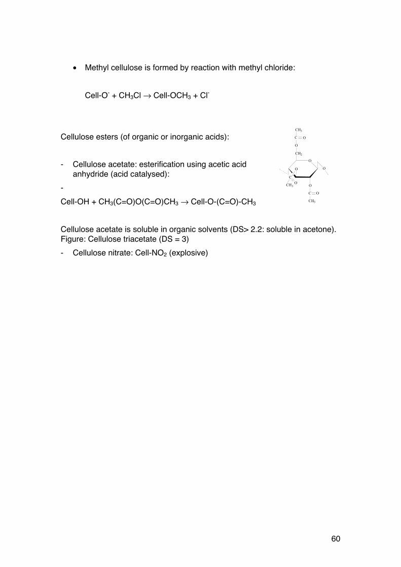
Cell-O- + CH3Cl → Cell-OCH3 + Cl- Cellulose esters (of organic or inorganic acids): - Cellulose acetate: esterification using acetic acid

anhydride (acid catalysed): - Cell-OH + CH3(C=O)O(C=O)CH3 → Cell-O-(C=O)-CH3

Cellulose acetate is soluble in organic solvents (DS> 2.2: soluble in acetone). Figure: Cellulose triacetate (DS = 3) - Cellulose nitrate: Cell-NO2 (explosive)

O

O

O O

CH2

O

C O

CH3

C

C O

CH3

OCH3

61

1.5.  STARCHES    

1.5.1.  General  

Starches are produced by all plants, and the starch-like glycogens are produced in animals (liver). In both cases they function mainly as energy reserves. Starches from tubers (e.g. potatoes) and seeds (e.g. corn, rice, wheat, rye..) are main agricultural products, and therefore main energy sources for humans in all parts of the world. Modern civilization totally depends on starches. In addition to the importance as food and food additives, starches and starch derivatives are basis for industrial applications in paper treatment (‘sizing’), glues, or as fabric stiffeners. Novel applications include low-calorie dietary fibers, biodegradable packaging materials, thin films, and thermoplastic materials. Native starches are found in granules (figure: wheat starch granules). Different plants have granules of different, but characteristic sizes and shapes (Rice: ca 2 µm, potato: up to 100 µm). They contain almost exclusively starch, in a dry and compact – and semi-crystalline - form. Upon heating (cooking), the granules absorb water. The process is called gelatinization, and involves swelling subsequently followed by bursting. By prolonged heating, the starch macromolecules dissolve in water. For scientific purposes, starches can also be dissolved in DMSO (dimethyl sulfoxide), or in alkali. The latter is a general procedure, which can be employed for many non-water soluble polysaccharides as long as they do not contain alkali labile linkages. Cooling of swollen (or even dissolved) starch leads to thickening, as observed by making a sauce. The macromolecules re-associate and expel water. This is called retrogradation. Dissolved starches can be fractionated into two classes of biopolymers, namely amylose and amylopectin. Despite they both consist only one sugar - α-D-glucose – they have very different macromolecular architectures and hence, very different properties. The biosynthesis of amylose and amylopectin is a highly complex, but well coordinated, process. It involves many genes and many enzymes, both by

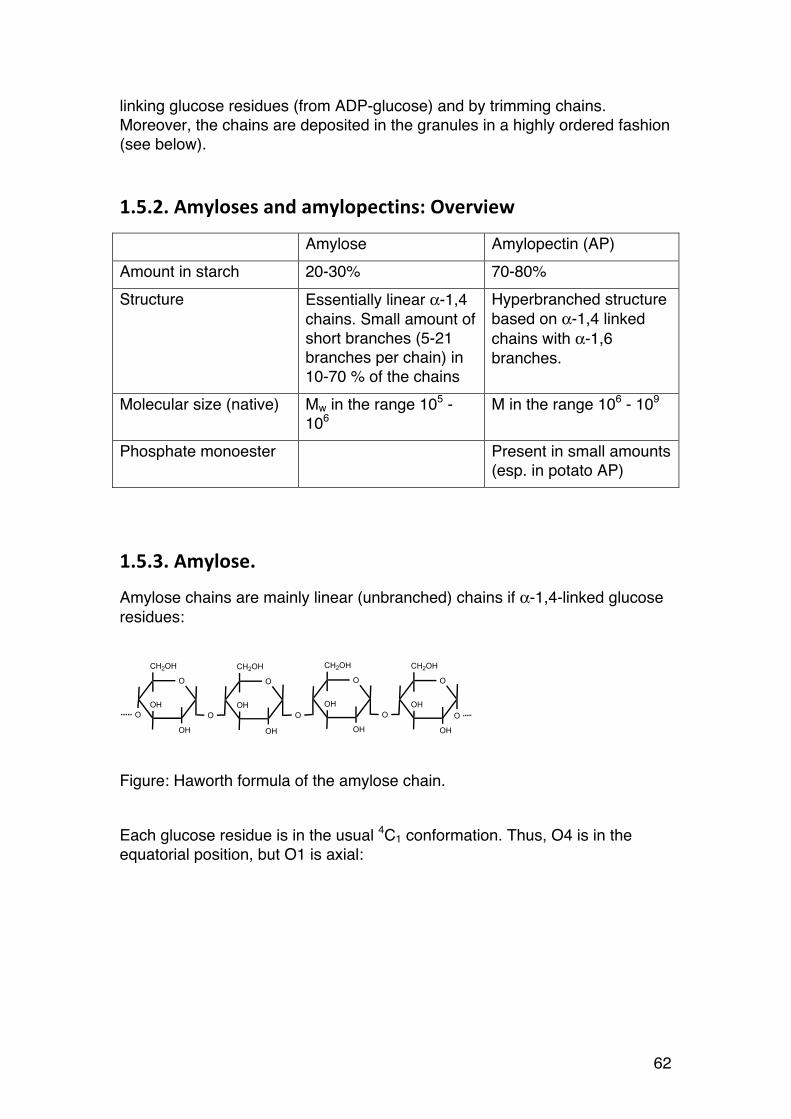
62

linking glucose residues (from ADP-glucose) and by trimming chains. Moreover, the chains are deposited in the granules in a highly ordered fashion (see below).

1.5.2.  Amyloses  and  amylopectins:  Overview  

Amylose Amylopectin (AP) Amount in starch 20-30% 70-80% Structure Essentially linear α-1,4

chains. Small amount of short branches (5-21 branches per chain) in 10-70 % of the chains

Hyperbranched structure based on α-1,4 linked chains with α-1,6 branches.

Molecular size (native) Mw in the range 105 - 106

M in the range 106 - 109

Phosphate monoester Present in small amounts (esp. in potato AP)

1.5.3.  Amylose.  

Amylose chains are mainly linear (unbranched) chains if α-1,4-linked glucose residues:

Figure: Haworth formula of the amylose chain. Each glucose residue is in the usual 4C1 conformation. Thus, O4 is in the equatorial position, but O1 is axial:

O

CH2OH

OH

OH

O

O

CH2OH

OH

OH

O

O

CH2OH

OH

OH

O

CH2OH

O

OH

OH

OO

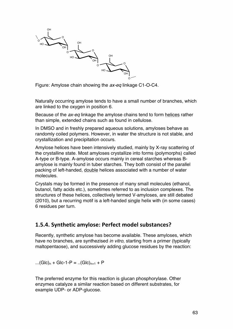
63

Figure: Amylose chain showing the ax-eq linkage C1-O-C4. Naturally occurring amylose tends to have a small number of branches, which are linked to the oxygen in position 6. Because of the ax-eq linkage the amylose chains tend to form helices rather than simple, extended chains such as found in cellulose. In DMSO and in freshly prepared aqueous solutions, amyloses behave as randomly coiled polymers. However, in water the structure is not stable, and crystallization and precipitation occurs. Amylose helices have been intensively studied, mainly by X-ray scattering of the crystalline state. Most amyloses crystallize into forms (polymorphs) called A-type or B-type. A-amylose occurs mainly in cereal starches whereas B-amylose is mainly found in tuber starches. They both consist of the parallel packing of left-handed, double helices associated with a number of water molecules. Crystals may be formed in the presence of many small molecules (ethanol, butanol, fatty acids etc.), sometimes referred to as inclusion complexes. The structures of these helices, collectively termed V-amyloses, are still debated (2010), but a recurring motif is a left-handed single helix with (in some cases) 6 residues per turn.

1.5.4.  Synthetic  amylose:  Perfect  model  substances?  

Recently, synthetic amylose has become available. These amyloses, which have no branches, are synthezised in vitro, starting from a primer (typically maltopentaose), and successively adding glucose residues by the reaction: ...(Glc)n + Glc-1-P = ..(Glc)n+1 + P The preferred enzyme for this reaction is glucan phosphorylase. Other enzymes catalyze a similar reaction based on different substrates, for example UDP- or ADP-glucose.

O

O

HO

O

OH

OH

O

HO

O

OH

OH

O

HO

O

OH

OH

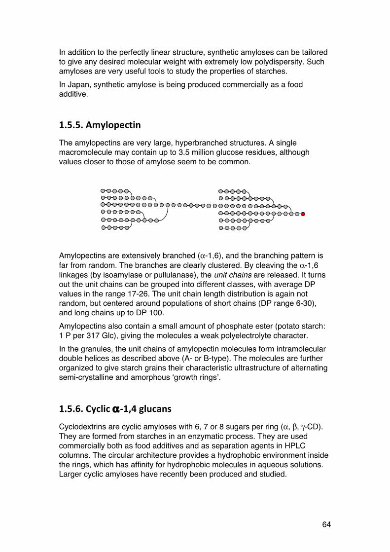
64

In addition to the perfectly linear structure, synthetic amyloses can be tailored to give any desired molecular weight with extremely low polydispersity. Such amyloses are very useful tools to study the properties of starches. In Japan, synthetic amylose is being produced commercially as a food additive.

1.5.5.  Amylopectin  

The amylopectins are very large, hyperbranched structures. A single macromolecule may contain up to 3.5 million glucose residues, although values closer to those of amylose seem to be common. Amylopectins are extensively branched (α-1,6), and the branching pattern is far from random. The branches are clearly clustered. By cleaving the α-1,6 linkages (by isoamylase or pullulanase), the unit chains are released. It turns out the unit chains can be grouped into different classes, with average DP values in the range 17-26. The unit chain length distribution is again not random, but centered around populations of short chains (DP range 6-30), and long chains up to DP 100. Amylopectins also contain a small amount of phosphate ester (potato starch: 1 P per 317 Glc), giving the molecules a weak polyelectrolyte character. In the granules, the unit chains of amylopectin molecules form intramolecular double helices as described above (A- or B-type). The molecules are further organized to give starch grains their characteristic ultrastructure of alternating semi-crystalline and amorphous ‘growth rings’.

1.5.6.  Cyclic  α-­‐1,4  glucans  

Cyclodextrins are cyclic amyloses with 6, 7 or 8 sugars per ring (α, β, γ-CD). They are formed from starches in an enzymatic process. They are used commercially both as food additives and as separation agents in HPLC columns. The circular architecture provides a hydrophobic environment inside the rings, which has affinity for hydrophobic molecules in aqueous solutions. Larger cyclic amyloses have recently been produced and studied.

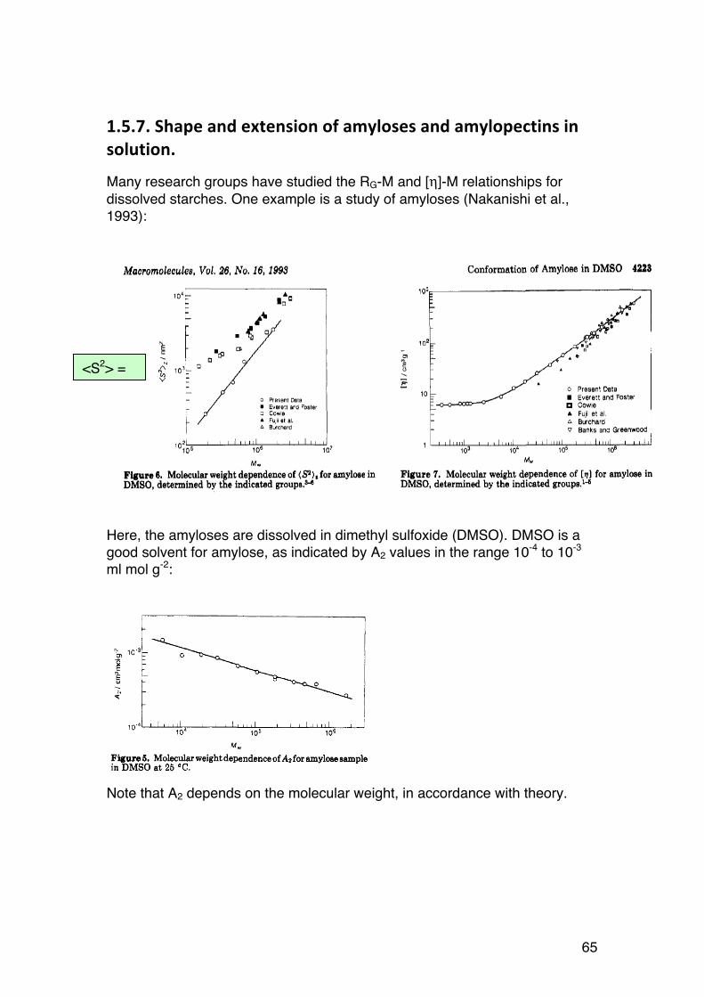
65

1.5.7.  Shape  and  extension  of  amyloses  and  amylopectins  in  solution.  

Many research groups have studied the RG-M and [η]-M relationships for dissolved starches. One example is a study of amyloses (Nakanishi et al., 1993):

Here, the amyloses are dissolved in dimethyl sulfoxide (DMSO). DMSO is a good solvent for amylose, as indicated by A2 values in the range 10-4 to 10-3 ml mol g-2:

Note that A2 depends on the molecular weight, in accordance with theory.

<S2> = RG

2

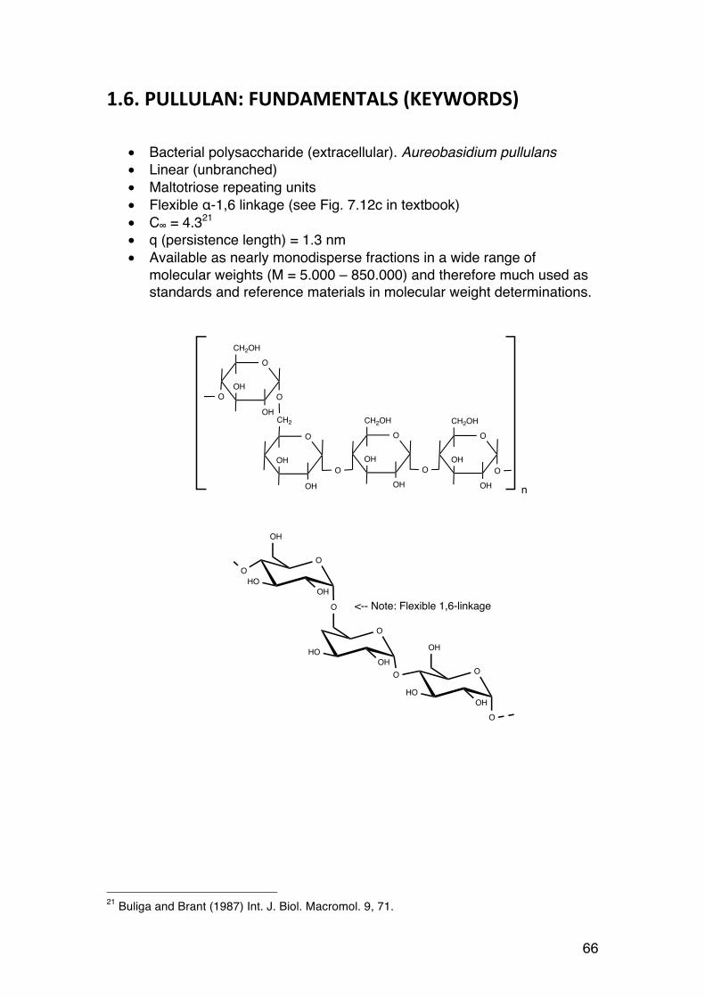
66

1.6.  PULLULAN:  FUNDAMENTALS  (KEYWORDS)  

• Bacterial polysaccharide (extracellular). Aureobasidium pullulans • Linear (unbranched) • Maltotriose repeating units • Flexible α-1,6 linkage (see Fig. 7.12c in textbook) • C∞ = 4.321 • q (persistence length) = 1.3 nm • Available as nearly monodisperse fractions in a wide range of

molecular weights (M = 5.000 – 850.000) and therefore much used as standards and reference materials in molecular weight determinations.

21 Buliga and Brant (1987) Int. J. Biol. Macromol. 9, 71.

O

CH2OH

O

OH

OHO

OO

HOOH

OH

O

CH2

OH

OH

O

CH2OH

OH

OH

O

CH2OH

OOH

OHOO

O

HO

OOH

O

O

HO

O

OH

OH

n

<-- Note: Flexible 1,6-linkage

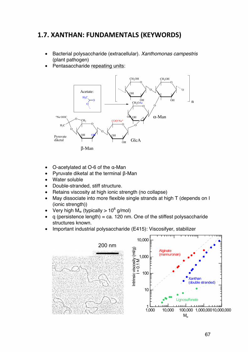
67

1,000 10,000 100,000 1,000,00010,000,000Mw

1

10

100

1,000

10,000

Intri

nsic

visc

osity

( ml /g

)I =

0. 1

M

Xanthan(double stranded)

Alginate(mannuronan)

Lignosulfonate

1.7.  XANTHAN:  FUNDAMENTALS  (KEYWORDS)  

• Bacterial polysaccharide (extracellular). Xanthomonas campestris

(plant pathogen) • Pentasaccharide repeating units:

• O-acetylated at O-6 of the α-Man • Pyruvate diketal at the terminal β-Man • Water soluble • Double-stranded, stiff structure. • Retains viscosity at high ionic strength (no collapse) • May dissociate into more flexible single strands at high T (depends on I

(ionic strength)) • Very high Mw (typically > 106 g/mol) • q (persistence length) = ca. 120 nm. One of the stiffest polysaccharide

structures known. • Important industrial polysaccharide (E415): Viscosifyer, stabilizer

OCH2OH

OH

OH

OCH2OH

OH

OCH2OAc

OH OH

OCOO-Na+

OH

OH

OCH2

OH OH

O O

O

O

O

O

O

+Na-OOC

H3C

n

β-Man

GlcA

α-Man

Acetate:H3C

OO

Pyruvatediketal

200 nm

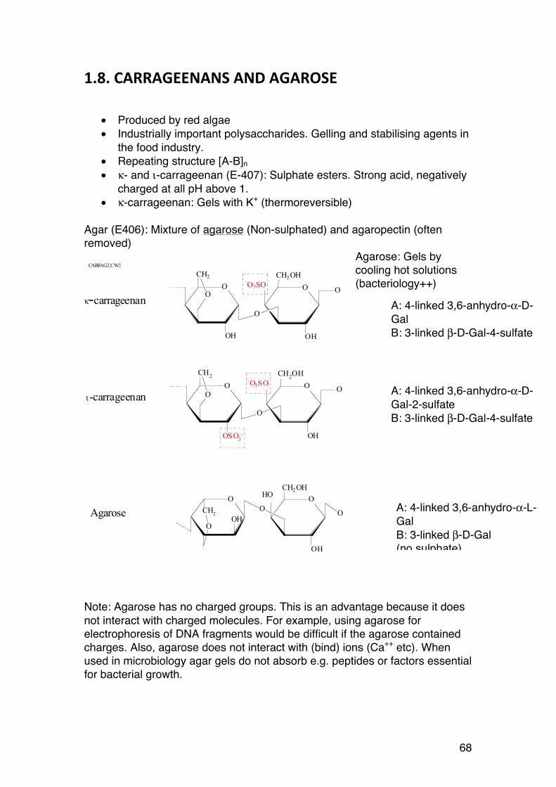
68

1.8.  CARRAGEENANS  AND  AGAROSE  

• Produced by red algae • Industrially important polysaccharides. Gelling and stabilising agents in

the food industry. • Repeating structure [A-B]n • κ- and ι-carrageenan (E-407): Sulphate esters. Strong acid, negatively

charged at all pH above 1. • κ-carrageenan: Gels with K+ (thermoreversible)

Agar (E406): Mixture of agarose (Non-sulphated) and agaropectin (often removed)

Agarose: Gels by cooling hot solutions (bacteriology++)

Note: Agarose has no charged groups. This is an advantage because it does not interact with charged molecules. For example, using agarose for electrophoresis of DNA fragments would be difficult if the agarose contained charges. Also, agarose does not interact with (bind) ions (Ca++ etc). When used in microbiology agar gels do not absorb e.g. peptides or factors essential for bacterial growth.

A: 4-linked 3,6-anhydro-α-D-Gal B: 3-linked β-D-Gal-4-sulfate

A: 4-linked 3,6-anhydro-α-D-Gal-2-sulfate B: 3-linked β-D-Gal-4-sulfate

A: 4-linked 3,6-anhydro-α-L-Gal B: 3-linked β-D-Gal (no sulphate)

ι-carrageenan

CARRAG2.CW2

O

OH

CH2

O

O

CH2OH

OH

-O3SO OO

κ-carrageenan

OCH2 O O

CH2OH

OH

HO O

OOH

Agarose

OO

-O3SO

OH

CH2OH

O

O

CH2

OSO3-

O

69

Chair forms: All linkages are diequatorial: D-Gal: 4C1 just like glucose (axial OH(4) does not destabilise sufficiently to flip over to 1C4) 3,6-anhydro-D-Gal: The 4C1 turns out to be sterically impossible, so in this case 1C4 is the only alternative 3,6-anhydro-L-Gal: L-Gal would obviously be 1C4, but again the internal 3,6 ring forces the sugar over to 4C1. These ring geometries, combined with the α/β configurations lead to the fact that all linkages in carrageenans and agar are diequatorial.

O

OH2C

O

OH

H

O

OSO3

HOH2C

OH

κ−carrageenan

O

OH2C

O

OSO3

H

O

OSO3

HOH2C

OH

ι−carrageenan

O

O

OHHOH2C

OH

O

O

O

CH2

OH

Agarose

1C4

4C1

4C1

4C1

4C1

1C4

3,6-anhydro-α-D-Gal

β-D-Gal-4 sulphate

3,6-anhydro-α-D-Gal-2-sulphate

β-D-Gal-4 sulphate

3,6-anhydro-α-L-Gal β-D-Gal

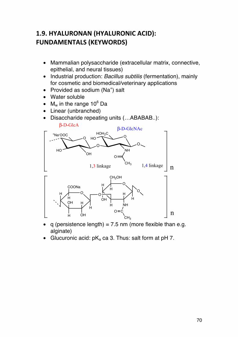
70

1.9.  HYALURONAN  (HYALURONIC  ACID):  FUNDAMENTALS  (KEYWORDS)  

• Mammalian polysaccharide (extracellular matrix, connective,

epithelial, and neural tissues) • Industrial production: Bacillus subtilis (fermentation), mainly

for cosmetic and biomedical/veterinary applications • Provided as sodium (Na+) salt • Water soluble • Mw in the range 106 Da • Linear (unbranched) • Disaccharide repeating units (…ABABAB..):

• q (persistence length) = 7.5 nm (more flexible than e.g.

alginate) • Glucuronic acid: pKa ca 3. Thus: salt form at pH 7.

O+Na-OOC

OHHO

O

OHOH2C

NH

OHO

O

CH3

O

OH HH

NHH

CH2OH

H OH

COCH3

O

HH

OHH

OH

COONa

HOH

β-D-GlcAβ-D-GlcNAc

1,3 linkage 1,4 linkage n

n

71

MHS plot hyaluronan (violet) and alginate (red). SEC with MALLS and viscosity detector. Solvent: 0.05 M Na2SO4 in 0.01 M Na2EDTA, PH 6.0.

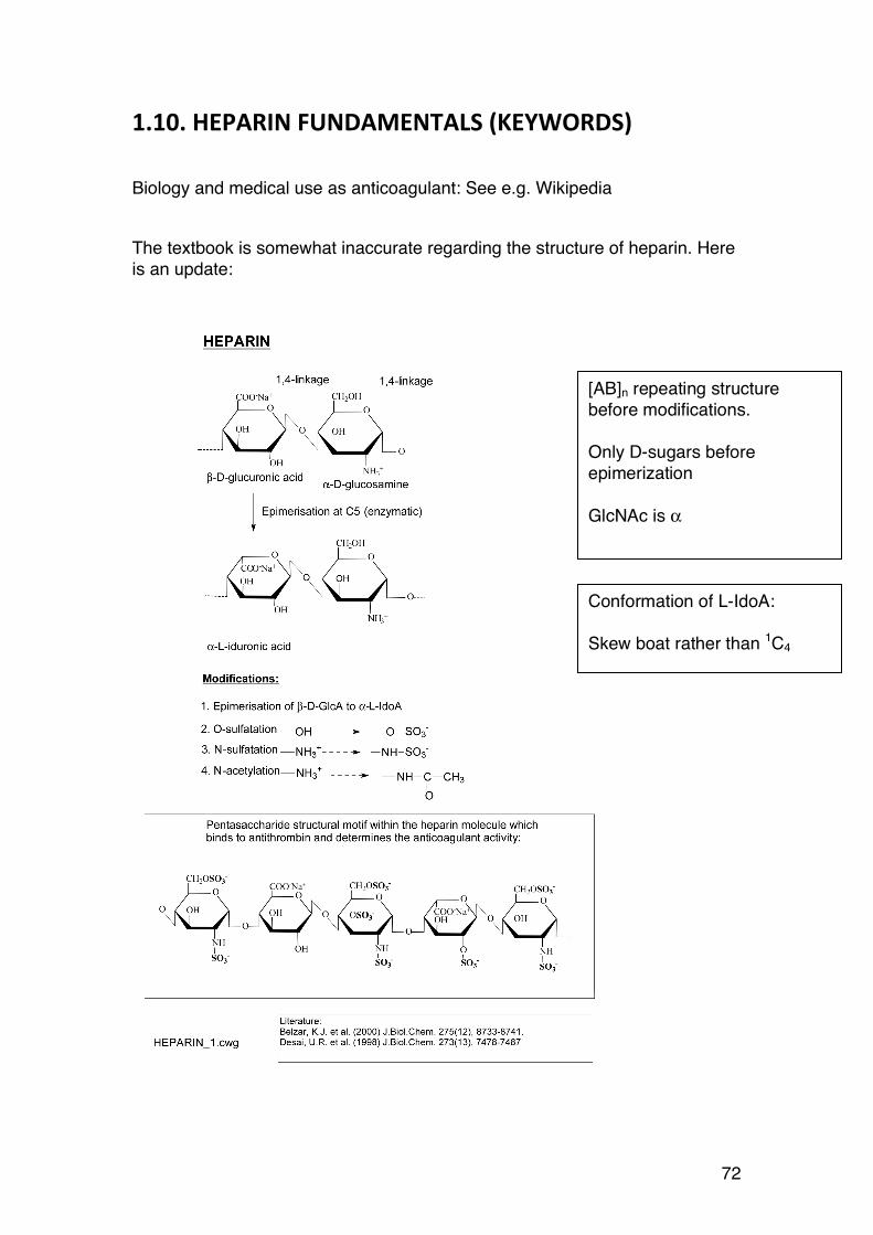
72

1.10.  HEPARIN  FUNDAMENTALS  (KEYWORDS)  

Biology and medical use as anticoagulant: See e.g. Wikipedia The textbook is somewhat inaccurate regarding the structure of heparin. Here is an update:

Conformation of L-IdoA: Skew boat rather than 1C4

[AB]n repeating structure before modifications. Only D-sugars before epimerization GlcNAc is α

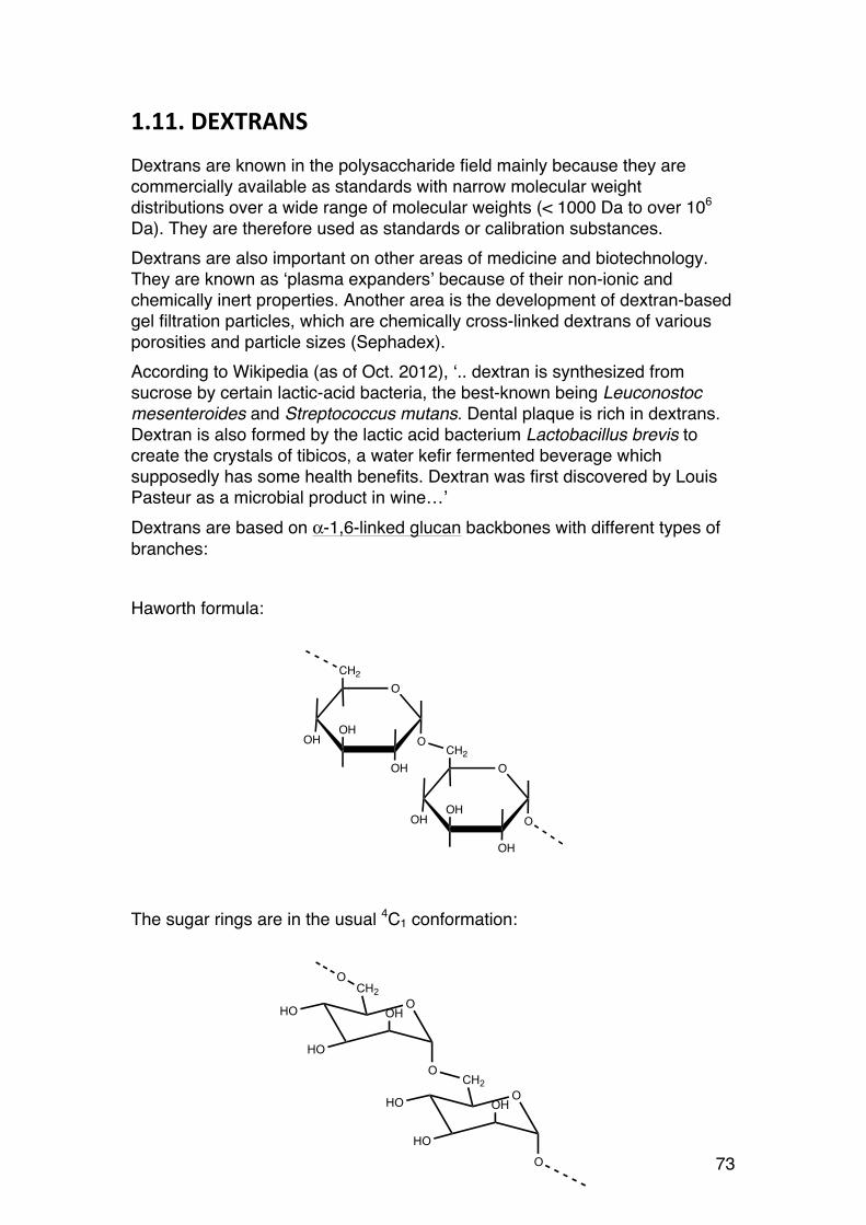
73

1.11.  DEXTRANS  

Dextrans are known in the polysaccharide field mainly because they are commercially available as standards with narrow molecular weight distributions over a wide range of molecular weights (< 1000 Da to over 106 Da). They are therefore used as standards or calibration substances. Dextrans are also important on other areas of medicine and biotechnology. They are known as ‘plasma expanders’ because of their non-ionic and chemically inert properties. Another area is the development of dextran-based gel filtration particles, which are chemically cross-linked dextrans of various porosities and particle sizes (Sephadex). According to Wikipedia (as of Oct. 2012), ‘.. dextran is synthesized from sucrose by certain lactic-acid bacteria, the best-known being Leuconostoc mesenteroides and Streptococcus mutans. Dental plaque is rich in dextrans. Dextran is also formed by the lactic acid bacterium Lactobacillus brevis to create the crystals of tibicos, a water kefir fermented beverage which supposedly has some health benefits. Dextran was first discovered by Louis Pasteur as a microbial product in wine…’ Dextrans are based on α-1,6-linked glucan backbones with different types of branches: Haworth formula: The sugar rings are in the usual 4C1 conformation:

OCH2

O

OH

OHOH

OCH2

O

OH

OHOH

OCH2

OH

HO

HO

O

O

OCH2

OH

HO

HO

O

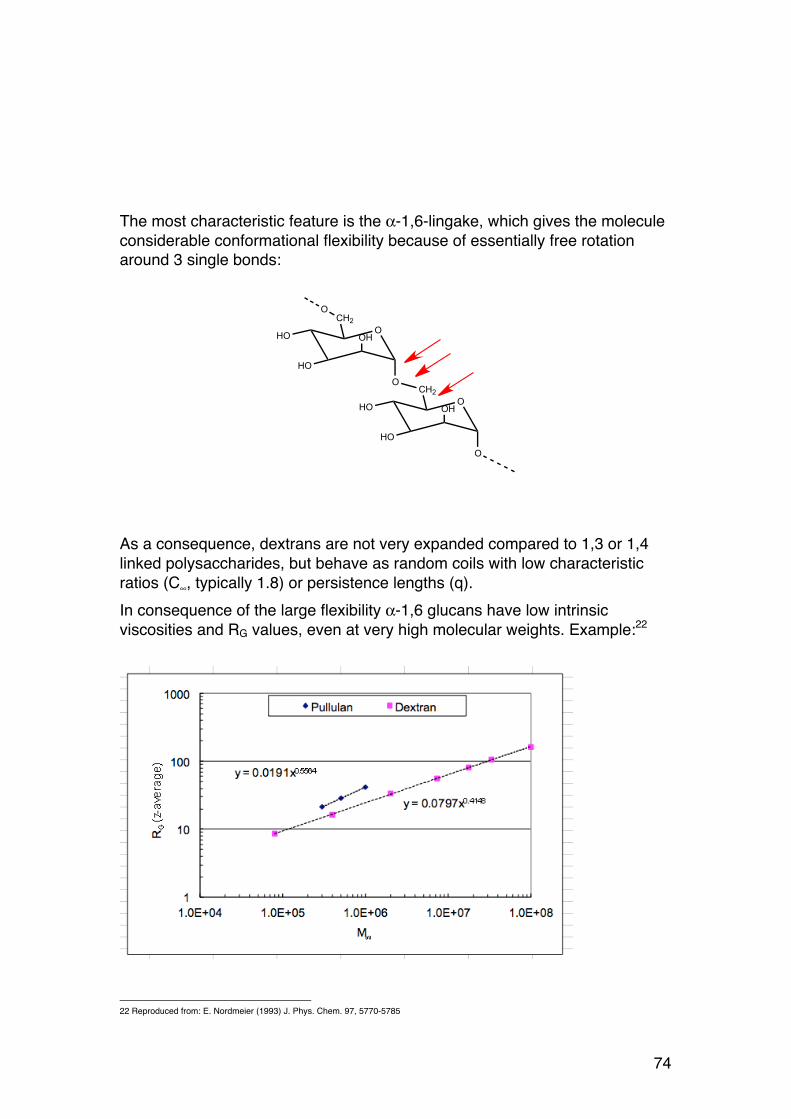
74

The most characteristic feature is the α-1,6-lingake, which gives the molecule considerable conformational flexibility because of essentially free rotation around 3 single bonds: As a consequence, dextrans are not very expanded compared to 1,3 or 1,4 linked polysaccharides, but behave as random coils with low characteristic ratios (C∞, typically 1.8) or persistence lengths (q). In consequence of the large flexibility α-1,6 glucans have low intrinsic viscosities and RG values, even at very high molecular weights. Example:22

22 Reproduced from: E. Nordmeier (1993) J. Phys. Chem. 97, 5770-5785

OCH2

OH

HO

HO

O

O

OCH2

OH

HO

HO

O

75

It may be noted that the exponent in the plot (0.41) is well below the random coil limit (0.5). This is in fact ascribed to the presence of branches, which are present at about 1 of 25 backbone residues23. Most of these branches are only one to three glucose units long, but there are also a few very long branches. The number of these long branches probably never exceeds 1% of the total number of glucose units. However, they have a great influence on the solution properties of dextran, as can be seen by comparison with the corresponding pullulan properties1. The compact nature of dextrans may cause considerable errors when they are used as calibration substances in methods like gel filtration (SEC or GPC).

 

23 Residue = sugar

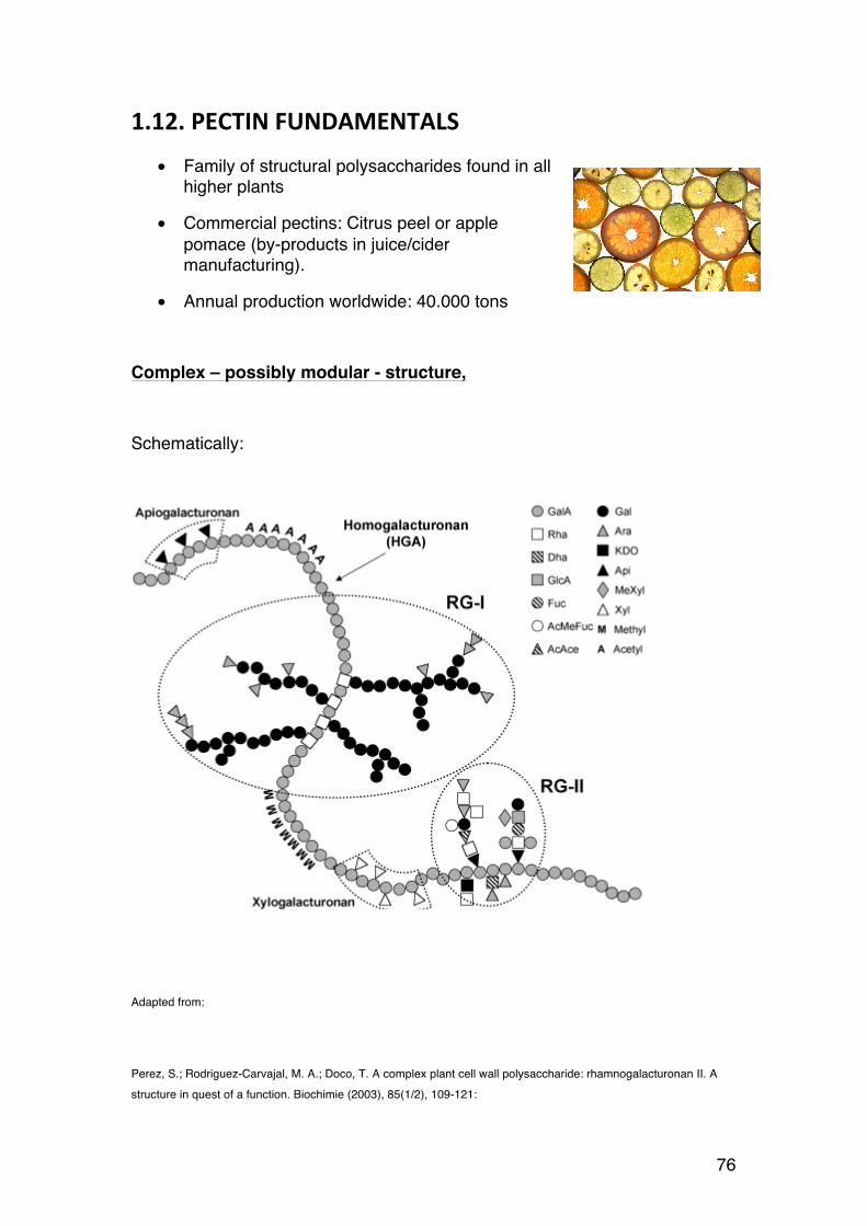
76

1.12.  PECTIN  FUNDAMENTALS  

• Family of structural polysaccharides found in all higher plants

• Commercial pectins: Citrus peel or apple pomace (by-products in juice/cider manufacturing).

• Annual production worldwide: 40.000 tons

Complex – possibly modular - structure,

Schematically:

Adapted from:

Perez, S.; Rodriguez-Carvajal, M. A.; Doco, T. A complex plant cell wall polysaccharide: rhamnogalacturonan II. A structure in quest of a function. Biochimie (2003), 85(1/2), 109-121:

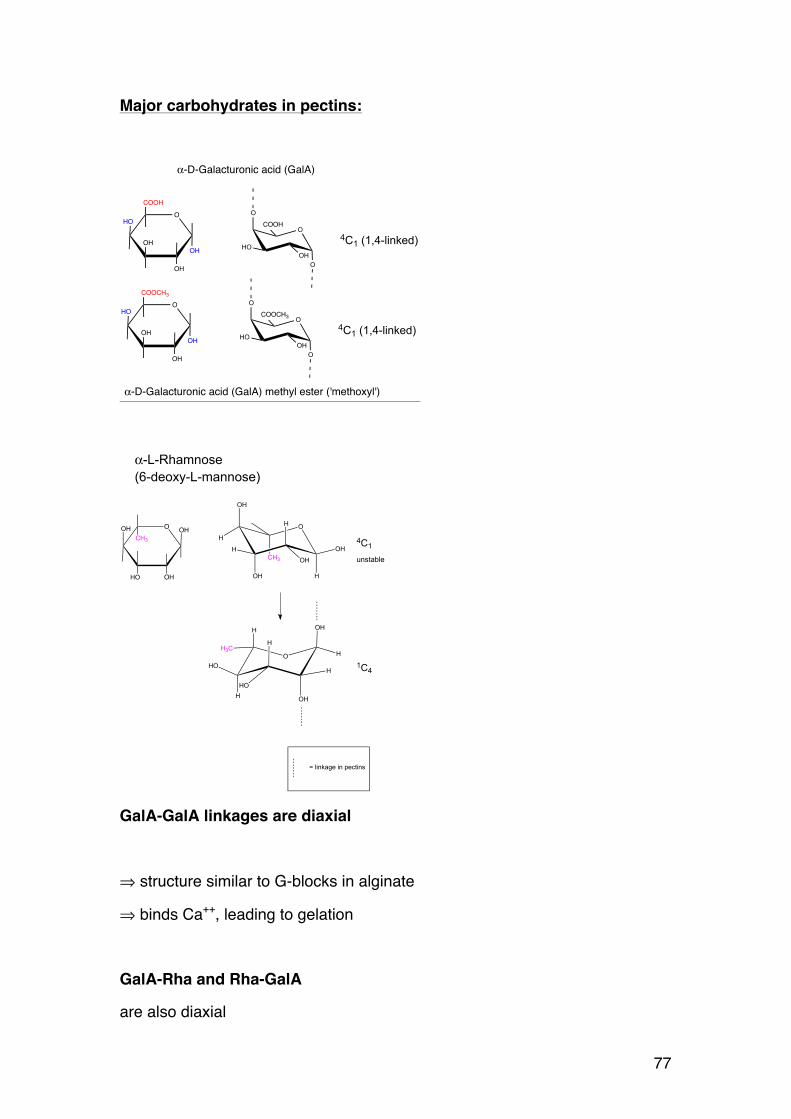
77

Major carbohydrates in pectins:

GalA-GalA linkages are diaxial

⇒ structure similar to G-blocks in alginate

⇒ binds Ca++, leading to gelation

GalA-Rha and Rha-GalA

are also diaxial

OCOOH

OH

OH

OH

HO

α-D-Galacturonic acid (GalA)

O

O

HOOH

COOH

O

4C1 (1,4-linked)

OCOOCH3

OH

OH

OH

HOO

O

HOOH

COOCH3

O

4C1 (1,4-linked)

α-D-Galacturonic acid (GalA) methyl ester ('methoxyl')

O

O

OH

H

OH

H

H

H

OHCH3

OH

OH

H

H

OH

H

HO

HO

H

H

H3C

4C1

unstable

1C4

α-L-Rhamnose

(6-deoxy-L-mannose)

O

CH3

OH

OHHO

OH

= linkage in pectins

78

Modular elements (accumulate during enzymatic degradation of pectins)

• RG-I (Rhamnogalacturonan I): Backbone: -Rha-GalA-Rha-GalA… with Gal-rich branches

• RG-II (Rhamnogalacturonan II): Backbone: - GalA-GalA-…, complex branches. Highly conserved, associated with uptake and binding of boron (borate)

• Homogalacturonan: Unbranched regions of 1→4-linked α-D-GalA. May contain O-acetyl groups (on C2 and C3). Binds Ca++ and induces gelation

• Esterified homogalacturonan regions. NOTE! Esterification ⇒ No charge. These regions associate in the presence of high concentrations of sucrose. Basis for use in jams.

Backbone

Primarily a polymer of α-D-galacturonic acid (homopolymer of (1→4)-α-D-galacturonic acid) with varying degree of carboxyl groups methyl esterified, and rhamnogalacturonan I (heteropolymer of repeating α-L-rhamnosyl (1→2) linked to α-D-galactosyluronic acid disaccharide units).

Commercial pectins

High methoxyl pectins (high degree of esterification) are used as gelling agents in foods, jams etc. Gelling requires:

a) High degree of esterification => low content of COO- (since –COOCH3 has no charge)

b) Low pH (remaining -COO- → -COOH). Citric acid often added

c) High sucrose content => influences water activity

79

The intrinsic viscosity of pectins: Role of branching

The following figure is taken from the literature24:

The dotted points (•) are experimental data for intrinsic viscosity [η] (measured at an ionic strength of 0.1 M) and weight-average molecular weight (Mw, obtained by light scattering) for different fractions of pectin from sunflower.

Note that the data follow the Mark-Houwink equation for Mw between 104 and 105 (g/mol). The authors found that [η] = 0.0955 Mw

0.73. This is within the range 0.5-0.8 which is expected for random coils in θ-solvents or good solvents, respectively.

For Mw > 100.000 the curve deviate from the expected straight line. This is attributed to branching. Adding long branches tend to increase the molecular weight, but not the specific25 hydrodynamic volume of the equivalent sphere:

24 Anger, H. and Berth, G. (1985). Carbohydrate Polymers 6 (1986) 193-202.

25 Specific => per gram, not per molecule

80

PART  2.  SHAPE  AND  SIZE  OF  BIOPOLYMERS  IN  SOLUTION  

81

2.1.  MOLECULAR  WEIGHT  DISTRIBUTIONS  AND  AVERAGES  

2.1.1.  Introduction  

Most proteins and nucleic acids are biosynthesized to obtain a specific chain length (and sequence of amino acids and nucleotides, respectively), whereas synthetic polymers, polysaccharides and a few other biopolymers (including rubbers, microbial polyesters and lignins) may have variable chain lengths. The chain length of biopolymers and synthetic polymers has a strong influence on a variety of biological and technical properties. Examples include:

• Solubility • Solution viscosity • Gel formation • Film formation and adsorption to surfaces • Crystallinity • Interactions with other molecules • Susceptibility of enzymatic degradation

2.1.2.  DP:  Degree  of  polymerization  

The term DP is much used in polymer and biopolymer science. If simply means ‘degree of polymerization’, but is used even if the chain is made by fragmentation of a longer chain.

Figure: A polymer chain with 24 residues (monomers): DP = 24

2.1.3.  Molecular  weight  (molar  mass)  

The molecular weight (M) of a homopolymer (all monomers are identical) is obviously related to DP through the simple equation:

M = DP ⋅M 0

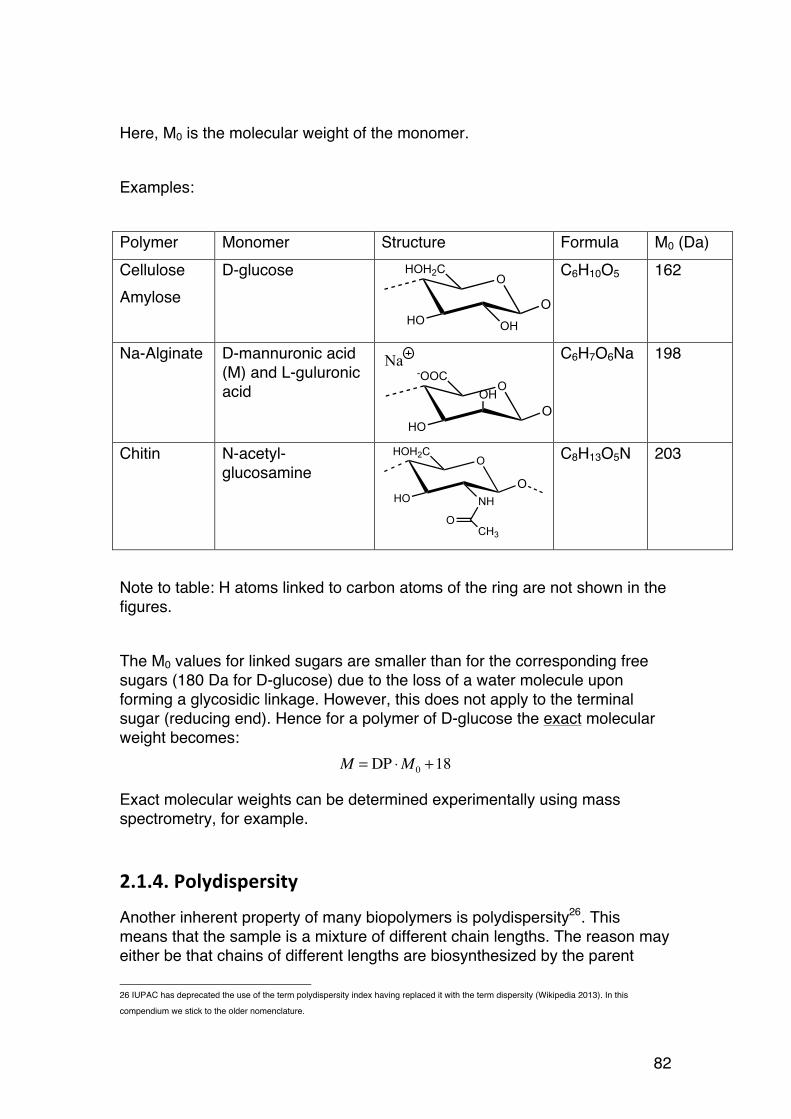
82

Here, M0 is the molecular weight of the monomer. Examples: Polymer Monomer Structure Formula M0 (Da) Cellulose Amylose

D-glucose

C6H10O5 162

Na-Alginate D-mannuronic acid (M) and L-guluronic acid

C6H7O6Na 198

Chitin N-acetyl-glucosamine

C8H13O5N 203

Note to table: H atoms linked to carbon atoms of the ring are not shown in the figures. The M0 values for linked sugars are smaller than for the corresponding free sugars (180 Da for D-glucose) due to the loss of a water molecule upon forming a glycosidic linkage. However, this does not apply to the terminal sugar (reducing end). Hence for a polymer of D-glucose the exact molecular weight becomes:

M = DP ⋅M 0 +18

Exact molecular weights can be determined experimentally using mass spectrometry, for example.

2.1.4.  Polydispersity  

Another inherent property of many biopolymers is polydispersity26. This means that the sample is a mixture of different chain lengths. The reason may either be that chains of different lengths are biosynthesized by the parent 26 IUPAC has deprecated the use of the term polydispersity index having replaced it with the term dispersity (Wikipedia 2013). In this

compendium we stick to the older nomenclature.

OHOH2C

OHHOO

O-OOC

OH

HOO

Na

OHOH2C

NHHOO

OCH3

83

cells, or that the polymers are partially and randomly degraded during isolation and purification. The polydispersity of an alginate and a xanthan sample is visualized in the figure:

Figure: Electron micrographs of alginate (top) and xanthan (bottom) molecules absorbed to a mica surface. Bar: 200 nm In contrast, many peptides proteins are strictly monodisperse. All chains are then identical. Essentially monodisperse polysaccharides may be obtained by special fractionation methods.

2.1.5.  Molecular  weight  distributions  

An accurate and complete description of the molecular weight - or equivalently the chain length distribution – would involve assigning the relative amount (weight fraction or number fraction) of each chain length in the sample. This can be illustrated in a table27 and a corresponding bar graph:

27 File: Simple distribution.xlsx

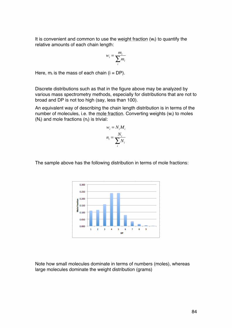
84

It is convenient and common to use the weight fraction (wi) to quantify the relative amounts of each chain length:

wi =mi

mii∑

Here, mi is the mass of each chain (i = DP). Discrete distributions such as that in the figure above may be analyzed by various mass spectrometry methods, especially for distributions that are not to broad and DP is not too high (say, less than 100). An equivalent way of describing the chain length distribution is in terms of the number of molecules, i.e. the mole fraction. Converting weights (wi) to moles (Ni) and mole fractions (ni) is trivial:

wi = NiMi

ni =Ni

Nii∑

The sample above has the following distribution in terms of mole fractions:

Note how small molecules dominate in terms of numbers (moles), whereas large molecules dominate the weight distribution (grams)

85

2.1.6.  Molecular  weight  averages:  Mn,  Mw  and  Mz  

What is the average molecular weight of the distribution discussed above? Or to simplify further: Assume you have: One molecule with M = 1000, two molecules with M = 1500, and one molecule with M = 2000. Total 4 molecules. The ‘normal ‘ average would simply be: Mave = (1000 + 1500 + 1500 + 2000)/4 = 1500 The ‘normal’ average is in fact identical to what is in polymer science defined as the number average molecular weight, with symbol Mn. The classical definition is:

Mn =NiMi

i∑

Nii∑ =

niMii∑

nii∑

Ni is as before the number of molecules, where as ni is the number of moles. Avogadro’s number cancels in the formula. It is straightforward to determine Mn in terms of masses (mi) or concentrations (ci):

ci =wi

Vwi = NiMi

ni =Ni

Nii∑

Mn =NiMi

i∑

Nii∑ =

wii∑wi

Mii∑

=ci

i∑ciMii

∑

The latter formula is very useful in practical situations where distributions are given on a mass or concentration basis. If we replace mole fractions in the expression for Mn by weight fractions we obtain another type of average called the weight average molecular weight, with symbol Mw:

86

Mw =wiMi

i∑

wii∑

Equivalent expressions are:

Mw =wiMi

i∑

wii∑ =

ciMii∑

cii∑ =

NiMi2

i∑

NiMii∑

It appears from the last expression that Mw mathematically speaking is a higher moment of the parent distribution, compared to Mn. By further extending into an even higher moment we can define the z-average molecular weight:

Mz =NiMi

3

i∑NiMi

2

i∑ =

miM i

2

i∑

miMii∑

There are several good reasons for using different types of molecular weight averages. First, a single parameter such as Mn says nothing about the distribution, whereas knowing additional averages provides simply more information. As will be discussed later (Section 5.3) common types of distributions have characteristic distributions. For example, randomly degraded polymers approach a Mw/Mn ratio of 2.0 upon prolonged degradation. The ratio between weight and number average molecular weights is often referred to as the polydispersity index (PI):

PI = Mw

Mn

Another reason for introducing different averages is that different experimental methods for determining molecular weights in case of polydispersity provides different values:

• Osmometry (Section 3.1): Provides Mn • Light scattering (Section 6.2): Provides Mw • Intrinsic viscosity (Section 6.1): May provide Mn, Mw or Mv (viscosity

average), depending on the standards used (see 6.1 for details)

87

The terms Mn, Mw and Mz are sometimes written with a bar, as in Mw . In this compendium the bar is omitted as the subscript clearly indicates a molecular weight average. Note that Mw should not be used as an abbreviation for the word ‘molecular weight’, but MW is OK.

2.1.7.  DP  averages  

DP averages (and distributions) are equivalent to molecular weight distributions. Interconversion is simple:

Mn = M 0DPnMw = M 0DPwMz = M 0DPz

2.1.8.  Continuous  distributions  

Since the number of monomers in a chain normally is an integer, and distributions hence are discrete, the size of the chains and with of the distributions makes it more practical to use continuous functions and graphical presentations:

The figure on the left shows the weight fraction as a function of the molecular weight (M). Note that a logarithmic scale is used for M. Such a figure is commonly used. The figure on the right shows the cumulative distribution. It is useful to determine the amount of material (weight fraction) above or below a certain M (or DP). For example, in the figure a M of 20.000 (arrow) corresponds to a cumulative weight fraction of 0.3, meaning that 30% of the mas has a molecular weight lower than 20.000.

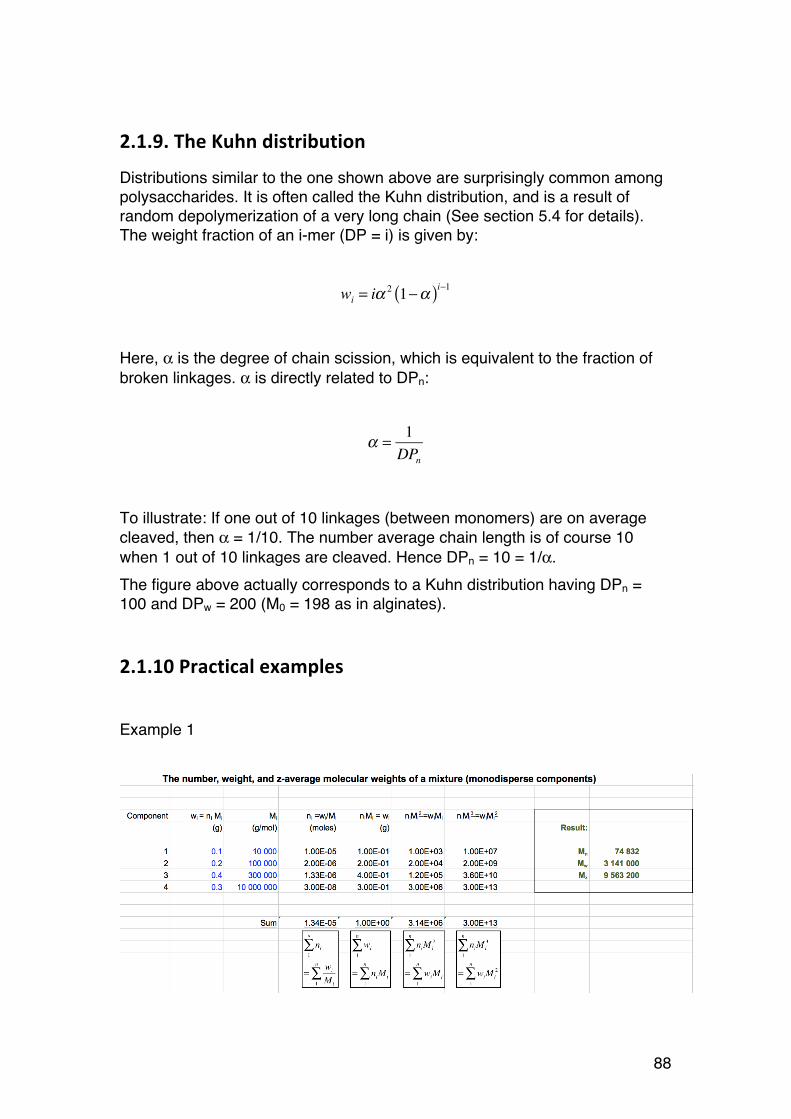
88

2.1.9.  The  Kuhn  distribution  

Distributions similar to the one shown above are surprisingly common among polysaccharides. It is often called the Kuhn distribution, and is a result of random depolymerization of a very long chain (See section 5.4 for details). The weight fraction of an i-mer (DP = i) is given by:

wi = iα2 1−α( )i−1

Here, α is the degree of chain scission, which is equivalent to the fraction of broken linkages. α is directly related to DPn:

α = 1DPn

To illustrate: If one out of 10 linkages (between monomers) are on average cleaved, then α = 1/10. The number average chain length is of course 10 when 1 out of 10 linkages are cleaved. Hence DPn = 10 = 1/α. The figure above actually corresponds to a Kuhn distribution having DPn = 100 and DPw = 200 (M0 = 198 as in alginates).

2.1.10  Practical  examples  

Example 1

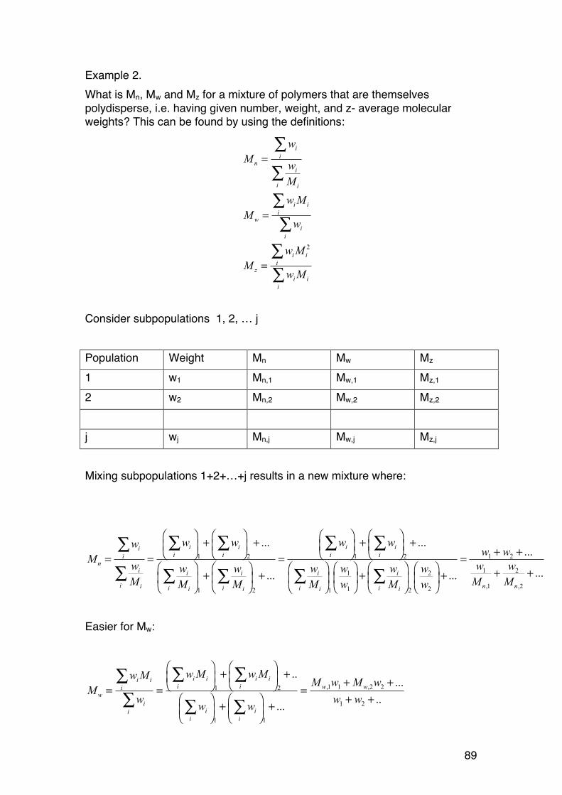
89

Example 2. What is Mn, Mw and Mz for a mixture of polymers that are themselves polydisperse, i.e. having given number, weight, and z- average molecular weights? This can be found by using the definitions:

Consider subpopulations 1, 2, … j Population Weight Mn Mw Mz

1 w1 Mn,1 Mw,1 Mz,1

2 w2 Mn,2 Mw,2 Mz,2

j wj Mn,j Mw,j Mz,j

Mixing subpopulations 1+2+…+j results in a new mixture where:

Easier for Mw:

1 21 2 1 2

1 21 2

,1 ,21 21 2 1 2

... ......

...... ...

i i i iii i i ii

ni i i i i

i i n ni i i ii i i i

w w w www wM w w ww w w w w w

M M MM M M w M w

⎛ ⎞ ⎛ ⎞ ⎛ ⎞ ⎛ ⎞+ + + +⎜ ⎟ ⎜ ⎟ ⎜ ⎟ ⎜ ⎟ + +⎝ ⎠ ⎝ ⎠ ⎝ ⎠ ⎝ ⎠= = = =⎛ ⎞ ⎛ ⎞ ⎛ ⎞ ⎛ ⎞⎛ ⎞ ⎛ ⎞ + ++ + + +⎜ ⎟ ⎜ ⎟ ⎜ ⎟ ⎜ ⎟⎜ ⎟ ⎜ ⎟

⎝ ⎠ ⎝ ⎠⎝ ⎠ ⎝ ⎠ ⎝ ⎠ ⎝ ⎠

∑ ∑ ∑ ∑∑

∑ ∑ ∑ ∑ ∑

,1 1 ,2 21 2

1 2

1 1

.....

.....

i i i ii ii i w wi

wi

i iii i

w M wMwM M w M wM

w w ww w

⎛ ⎞ ⎛ ⎞+ +⎜ ⎟ ⎜ ⎟ + +⎝ ⎠ ⎝ ⎠= = =+ +⎛ ⎞ ⎛ ⎞+ +⎜ ⎟ ⎜ ⎟⎝ ⎠ ⎝ ⎠

∑ ∑∑∑ ∑ ∑

2

ii

ni

i i

i ii

wi

i

i ii

zi i

i

wM w

MwM

Mw

wMM

wM

=

=

=

∑

∑∑∑∑∑

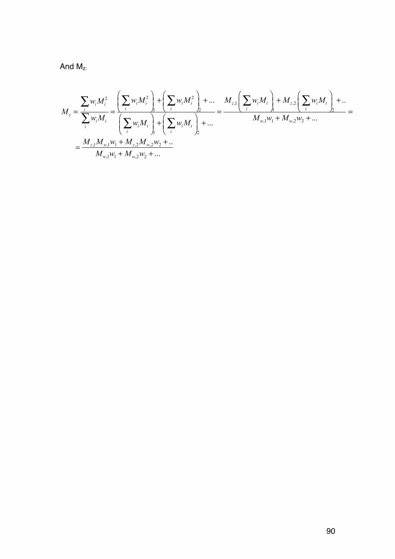
90

And Mz:

2 22,1 ,2

1 2 1 2

,1 1 ,2 2

1 2

,1 ,1 1 ,2 ,2 2

,1 1 ,2 2

... ..

......

.....

i i i i z i i z i ii ii i i ii

zi i w w

i i i iii i

z w z w

w w

wM wM M wM M wMwMM

wM M w M wwM wM

M M w M M wM w M w

⎛ ⎞ ⎛ ⎞ ⎛ ⎞ ⎛ ⎞+ + + +⎜ ⎟ ⎜ ⎟ ⎜ ⎟ ⎜ ⎟⎝ ⎠ ⎝ ⎠ ⎝ ⎠ ⎝ ⎠= = = =+ +⎛ ⎞ ⎛ ⎞+ +⎜ ⎟ ⎜ ⎟⎝ ⎠ ⎝ ⎠

+ +=

+ +

∑ ∑ ∑ ∑∑∑ ∑ ∑

91

2.2.  THE  SHAPE  OF  BIOPOLYMERS  IN  SOLUTION    

2.2.1.  Introduction  and  examples  

Figure 33. Haug's triangle illustrates the basic shapes of polymers in solution.

We will now be concerned with the properties of biopolymers when they are dissolved in a solvent, usually water. The diversity in terms of size and shape of biopolymers varies enormously, but they can roughly be categorized into three basic shapes as shown in Figure 1: solid spheres, rigid rods, and random coils. With size we usually mean the chain length, or equivalently, the molecular weight or the DP. The size has always a pronounced effect of the properties of a polymer. Generally speaking, a long chain behaves differently from a short chain having the same chemistry. However, the effect of size alone depends strongly on the basic shape, which itself plays an important role. For example, a small, compact (globular) protein behaves totally different than its denatured form, which is usually more open and randomly coiled28 Most of this chapter will focus on flexible, expanded chains, which include most polysaccharides in aqueous solution. Proteins deserve a brief comment, because many of them adopt compact shapes with little flexibility. Protein scientists take advantage of the fact that many proteins can form crystals without changing their native shape. The shape can then be determined accurately using X-ray diffraction, obtaining data with atomic resolution. Thousands of examples may be found in standard protein databases.

28 See example at the end of this document.

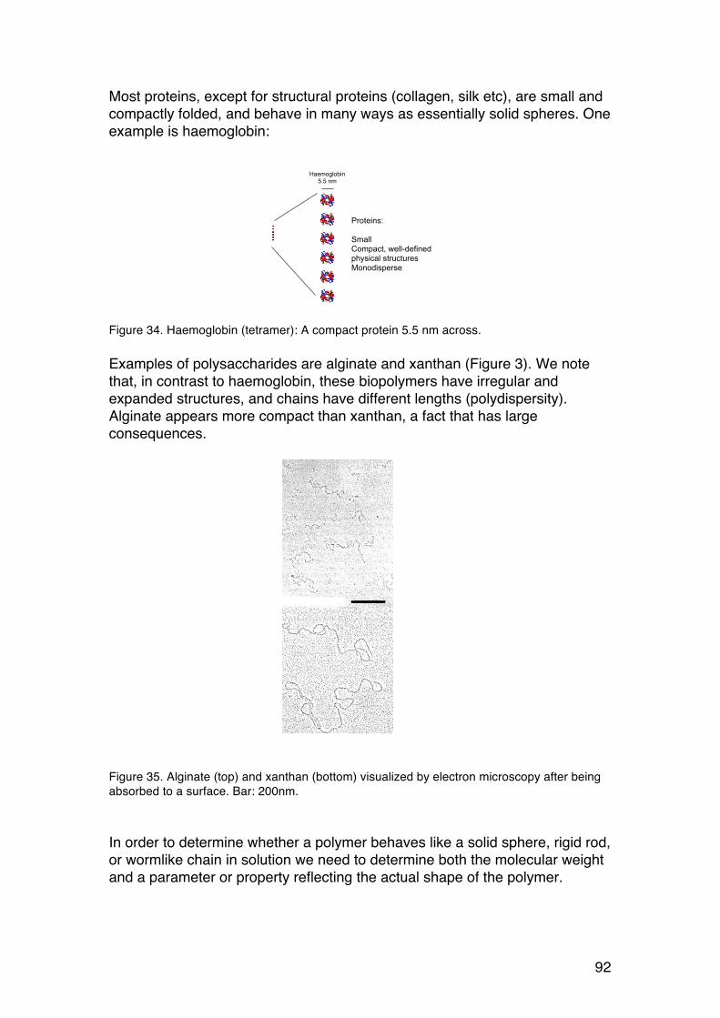
92

Most proteins, except for structural proteins (collagen, silk etc), are small and compactly folded, and behave in many ways as essentially solid spheres. One example is haemoglobin:

Figure 34. Haemoglobin (tetramer): A compact protein 5.5 nm across. Examples of polysaccharides are alginate and xanthan (Figure 3). We note that, in contrast to haemoglobin, these biopolymers have irregular and expanded structures, and chains have different lengths (polydispersity). Alginate appears more compact than xanthan, a fact that has large consequences.

Figure 35. Alginate (top) and xanthan (bottom) visualized by electron microscopy after being absorbed to a surface. Bar: 200nm. In order to determine whether a polymer behaves like a solid sphere, rigid rod, or wormlike chain in solution we need to determine both the molecular weight and a parameter or property reflecting the actual shape of the polymer.

Haemoglobin5.5 nm

Proteins:

SmallCompact, well-defined physical structuresMonodisperse

93

The molecular weight may be determined by experimental methods such as mass spectrometry (MS), light scattering or osmometry. We will study also those methods later in the course. The overall shape is usually determined indirectly by comparing experimental data reflecting the shape and the extension such as RG (radius of gyration), intrinsic viscosity (symbol [η])29 or others, and the molecular weight (M)30 with a model. The models described below are based on obtaining experimental data for the same polymer type at different molecular weights, a homologous series. Such samples may be produced by fractionating a mixture, or by controlled (partial) degradation starting with the largest molecule. Here are some examples taken from the literature (some are actually obtained in our laboratory). For each sample both the molecular weight and (in this case) the intrinsic viscosity was measured.

Figure 36. Measurements of the intrinsic viscosity for different molecular weight provides information about the shape of the polymers. Note first that the data are plotted on a double-logarithmic scale. This means straight lines correspond to an exponential equation: y = axb. Note further that both the slope (b) and the intercept (a) for the fitted straight lines in the log-log plot vary between the different biopolymers. Analysing these data gives us information about the shape of the molecules in solution. Instead of intrinsic viscosity, we could also use data for the radius of gyration (RG). Such data do indeed data exist (shown for pullulan and xanthan only), and we will start using such data first: 29 Chapter 11.1 in textbook

30 Chapter 9 in textbook

1

10

100

1 000

10 000

10 000 100 000 1 000 000 10 000 000

M (g/mol)

[h] (

ml/g

)

PullulanXanthan

Alginate

Lignosulfonate

Intrinsic viscosity (ml/g)

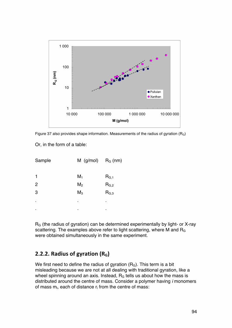
94

Figure 37 also provides shape information. Measurements of the radius of gyration (RG) Or, in the form of a table: Sample M (g/mol) RG (nm) 1 M1 RG,1 2 M2 RG,2 3 M3 RG,3

. . .

. . . RG (the radius of gyration) can be determined experimentally by light- or X-ray scattering. The examples above refer to light scattering, where M and RG were obtained simultaneously in the same experiment.

2.2.2.  Radius  of  gyration  (RG)  

We first need to define the radius of gyration (RG). This term is a bit misleading because we are not at all dealing with traditional gyration, like a wheel spinning around an axis. Instead, RG tells us about how the mass is distributed around the centre of mass. Consider a polymer having i monomers of mass mi, each of distance ri from the centre of mass:

1

10

100

1 000

10 000 100 000 1 000 000 10 000 000

M (g/mol)

RG (n

m)

PullulanXanthan

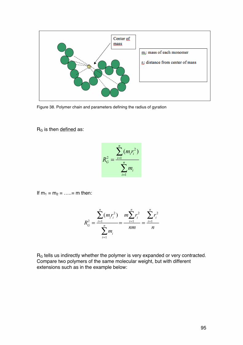
95

Figure 38. Polymer chain and parameters defining the radius of gyration RG is then defined as:

2

2 1

1

( )n

i ii

G n

ii

m rR

m

=

=

=∑

∑

If m1 = m2 = …..= m then:

RG2 =

(miri2 )

i=1

n

∑

mii=1

n

∑=

m ri2

i=1

n

∑nm

=ri

2

i=1

n

∑n

RG tells us indirectly whether the polymer is very expanded or very contracted. Compare two polymers of the same molecular weight, but with different extensions such as in the example below:

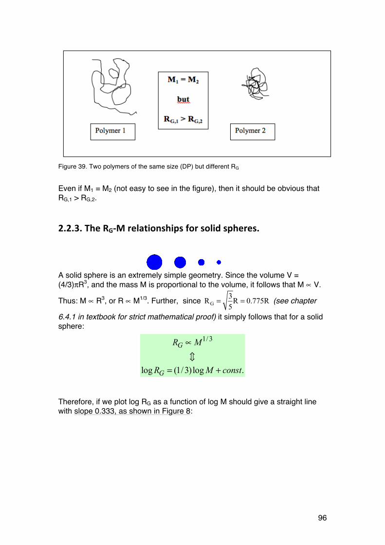
96

Figure 39. Two polymers of the same size (DP) but different RG Even if M1 = M2 (not easy to see in the figure), then it should be obvious that RG,1 > RG,2.

2.2.3.  The  RG-­‐M  relationships  for  solid  spheres.  

A solid sphere is an extremely simple geometry. Since the volume V = (4/3)πR3, and the mass M is proportional to the volume, it follows that M ∝ V.

Thus: M ∝ R3, or R ∝ M1/3. Further, since G3R R 0.775R5

= = (see chapter

6.4.1 in textbook for strict mathematical proof) it simply follows that for a solid sphere:

1/3

log (1/3)log .

G

G

R M

R M const

∝

= +

Therefore, if we plot log RG as a function of log M should give a straight line with slope 0.333, as shown in Figure 8:

97

M RG (nm)

10000 550000 8.6

250000 14.6

1

10

100

1000 10000 100000 1000000M (g/mol)

RG (n

m)

Figure 40. Data for a polymer shaped like a solid shere.

2.2.4.  The  RG-­‐M  relationships  for  rigid  rods.  

A rod is even simpler: M ∝ L, and G1R L 0.289L12

= = (see chapter 6.4.1 in

textbook for strict mathematical proof), therefore:

log log .

G

G

R M

R M const

∝

= +

If we plot log RG as a function of log M should for a rod obtain a straight line with slope 1.0. In fact, xanthan (see Figure 5) behaves like a stiff rod when the molecular weight is below 106 g/mol (Da). The slope of the dotted line in Fig. 5 is in fact 1.0.

98

2.2.5.  The  RG-­‐M  relationships  for  randomly  coiled  chains.  

Biopolymers behaving like flexible chains in solution are common: • Most denatured proteins (-S-S- bridges cleaved, high T31, 6 M urea..)

(See also Section 2.2.13) • Denatured (single-stranded) DNA, RNA (high T) • Many linear (unbranched) polysaccharides: • Pullulan (very flexible) • Alginates (Na+-form, no Ca+) • Chitosans (pH < ca. 6) • Hyaluronan • Amylose (in DMSO or alkali) • Cellulose (in special cellulose solvents)

The flexibility is caused by the properties of the linkages between monomers. In proteins, the peptide linkage has a certain freedom of rotation (Figure 9). This applies in particular to the Cα-C and N-Cα linkages, whereas the partial C=N double bond is much more rigid due to resonance:

Figure 41

In polysaccharides, the sugar rings are usually very rigid, but some rotation is allowed for the glycosidic linkages (figure 10):

Figure 42

In total, even a small amount of rotational freedom in each linkage gives rise to flexible chains. It is important to realize that flexible chains do not adopt a single, fixed shape or conformation. Due to thermal forces, the chains will constantly change 31 There are exceptions (cold denaturation)

OH

O-OOC

OH

HOO

O-OOC

HOO

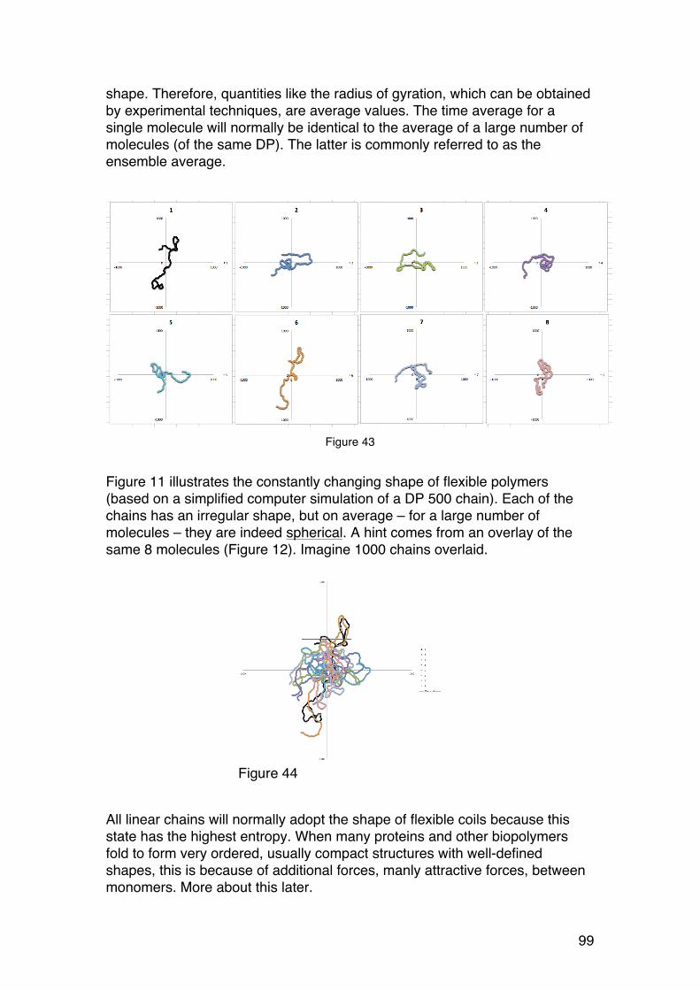
99

shape. Therefore, quantities like the radius of gyration, which can be obtained by experimental techniques, are average values. The time average for a single molecule will normally be identical to the average of a large number of molecules (of the same DP). The latter is commonly referred to as the ensemble average.

Figure 43

Figure 11 illustrates the constantly changing shape of flexible polymers (based on a simplified computer simulation of a DP 500 chain). Each of the chains has an irregular shape, but on average – for a large number of molecules – they are indeed spherical. A hint comes from an overlay of the same 8 molecules (Figure 12). Imagine 1000 chains overlaid.

All linear chains will normally adopt the shape of flexible coils because this state has the highest entropy. When many proteins and other biopolymers fold to form very ordered, usually compact structures with well-defined shapes, this is because of additional forces, manly attractive forces, between monomers. More about this later.

Figure 44

100

First, we seek a model for (the average) RG of flexible chains, similar to those of spheres and rods. The simplest case: A vector model (Figure 13) describes a freely jointed chain with no restrictions on the direction (random orientation)

Figure 45

There are n vectors (representing monomers), each of length l. (Note that n ∝ M). As a useful intermediate quantity we first determine the average square end-to-end distance: <r2> (which is not the same as <r>2). For a sufficiently high number of vectors i.e. a very long chain, the following applies:

r2 = nl2 (n→∞)

r = 0

Note the average end-to-end distance (<r>) is zero because since all end-to-end vectors cancel pairwise since they are equally probable. However, the average squared end-to-end distance (<r2>) is always positive. And represents a useful parameter for the extent of chain expansion. The relation <r2> = nl2 (for large n values) can be proven in a very elegant way, starting with recognizing that r2 must be the dot product of the end-to-end vector

r by itself, since the angle between the vectors is zero (cos φ = 0)

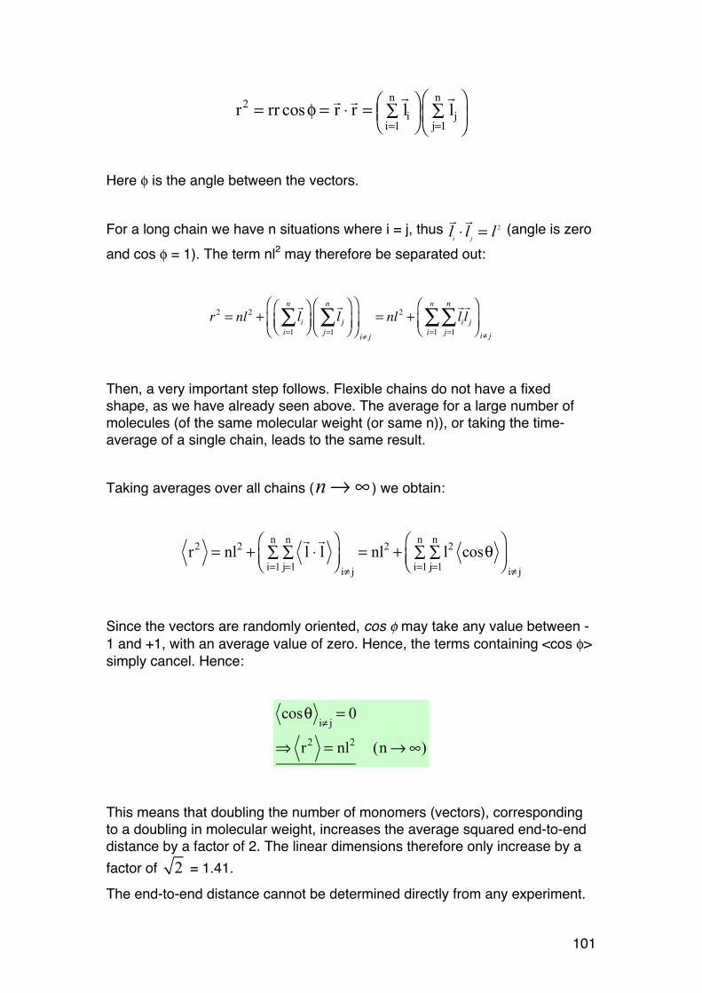
101

n n2i j

i 1 j 1r rr cos r r l l

= =

⎛ ⎞⎛ ⎞= φ = ⋅ = ∑ ∑⎜ ⎟⎜ ⎟⎝ ⎠⎝ ⎠

Here φ is the angle between the vectors. For a long chain we have n situations where i = j, thus

l l li j⋅ = 2 (angle is zero

and cos φ = 1). The term nl2 may therefore be separated out:

r2 = nl2 +li

i=1

n

∑⎛⎝⎜⎞⎠⎟

l j

j=1

n

∑⎛

⎝⎜⎞

⎠⎟⎛

⎝⎜

⎞

⎠⎟i≠ j

= nl2 +lil j

j=1

n

∑i=1

n

∑⎛

⎝⎜⎞

⎠⎟ i≠ j

Then, a very important step follows. Flexible chains do not have a fixed shape, as we have already seen above. The average for a large number of molecules (of the same molecular weight (or same n)), or taking the time-average of a single chain, leads to the same result. Taking averages over all chains (n→∞ ) we obtain:

r2 = nl2 +

l ⋅l

j=1

n∑

i=1

n∑

⎛⎝⎜

⎞⎠⎟ i≠ j

= nl2 + l2 cosθj=1

n∑

i=1

n∑

⎛⎝⎜

⎞⎠⎟ i≠ j

Since the vectors are randomly oriented, cos φ may take any value between -1 and +1, with an average value of zero. Hence, the terms containing <cos φ> simply cancel. Hence:

cosθi≠ j

= 0

⇒ r2 = nl2 (n→∞)

This means that doubling the number of monomers (vectors), corresponding to a doubling in molecular weight, increases the average squared end-to-end distance by a factor of 2. The linear dimensions therefore only increase by a factor of 2 = 1.41.

The end-to-end distance cannot be determined directly from any experiment.

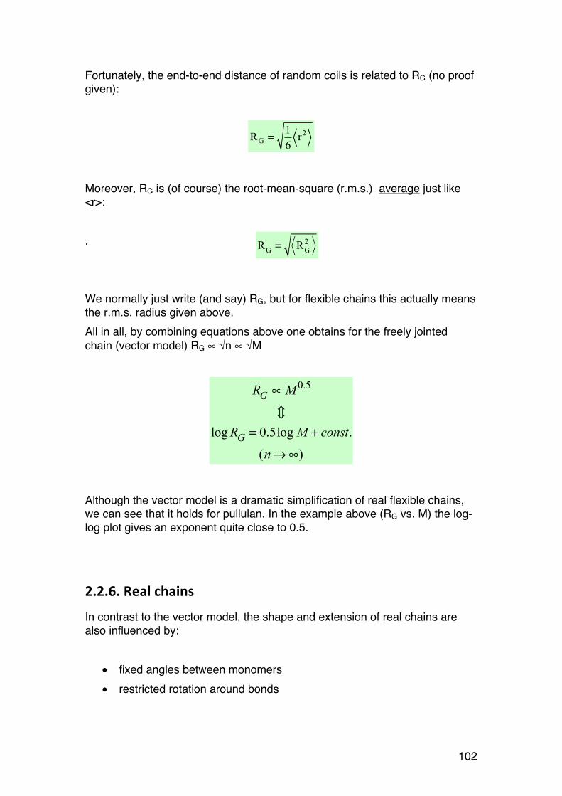
102

Fortunately, the end-to-end distance of random coils is related to RG (no proof given):

2G

1R r6

=

Moreover, RG is (of course) the root-mean-square (r.m.s.) average just like <r>: . We normally just write (and say) RG, but for flexible chains this actually means the r.m.s. radius given above. All in all, by combining equations above one obtains for the freely jointed chain (vector model) RG ∝ √n ∝ √M

RG ∝ M 0.5

log RG = 0.5log M + const.

(n→∞)

Although the vector model is a dramatic simplification of real flexible chains, we can see that it holds for pullulan. In the example above (RG vs. M) the log-log plot gives an exponent quite close to 0.5.

2.2.6.  Real  chains  

In contrast to the vector model, the shape and extension of real chains are also influenced by:

• fixed angles between monomers • restricted rotation around bonds

RG = RG

2

103

• monomers have a volume, and often charges (in polyelectrolytes), the latter leading to attraction or repulsion

Each of these is treated separately (Textbook chapter 6.1.2 – 6.1.6), but finally will be incorporated into the model, which in the end looks like this:

r2 =α 2C∞nl2 n→∞

2.2.7.  The  characteristic  ratio  (C∞):  A  stiffness  parameter  

The term C∞ is called the characteristic ratio, and combines the effects of both fixed bond angles between monomers, and restricted rotation around bonds. See Equations 6.8 and 6.11 in textbook. C∞ is hence a stiffness parameter characteristic for each polymer. It depends only on the chemistry of the polymer. Examples:

• Pullulan (Fig. 4.22, 7.12c) C∞ = 4.332 • Cereal mixed β-1,3/β-1,4 glucans, C∞ = 13-1433 • Alginates (I = ∞): C∞ = 47

The larger C∞, the more stiff and extended chain (at constant M).

2.2.8.  Excluded  volume  effects  and  θ-­‐conditions  

The term α2 refers to the excluded volume effect. The fact that monomers do have a finite volume and sometimes equally charged monomers results in a general electrostatic expansion of the chain (α2>1). The excluded volume effect is also slightly dependent on the chain length: α ∝ n0-0.1, or α ∝ M0-0.1

32 Buliga, Gregory S.; Brant, David A.. Temperature and molecular weight dependence of the unperturbed dimensions of aqueous pullulan.

Int. J. Biol. Macromol. (1987), 9(2), 71-6.

33 Gómez et al. (1997) Carbohydr. Polym. 32, 17-22

104

θ-conditions (θ-solvent or θ-temperature) refers to conditions where weak attractive forces exactly cancel the excluded volume effect, and α = 1 and independent of the chain length. When we wish to determine C∞ experiments should by conducted at θ-conditions. Alternatively, α should be known from additional investigations. How are θ-conditions found for a given polymer? Interestingly, the excluded volume effect also influences thermodynamic properties of the system, allowing the use of e.g. osmometry or light scattering to find θ-conditions. This is discussed further in Section 3. Inserting the equation α ∝ n0-0.1 in the general equation we see that:

θ-solvent:

r2 ∝ n⇔ r = r2 0.5∝ n0.5

Good solvent:

r2 ∝ n1.2 ⇔ r = r2 0.5∝ n0.6

Or, taking the square roots and combining:

r = r20.5

∝ n0.5−0.6

Note that the basic equation for a random coil is still the same, and that RG still obeys the relation: RG ∝ Ma. If we plot log RG as a function of log M should for a random coil obtain a straight line with slope 0.5 in a θ-solvent and 0.6 in a good solvent. Compare to the corresponding values for compact spheres and rods, respectively.

2.2.9.  How  to  determine  C∞  from  experiments?  

The classic way to determine C∞ consists of analysing the radius of gyration (RG) (in a θ-solvent, or knowing α2) for different molecular weights (of the same polymer). Samples with different molecular weights (M) (a homologous series) may be obtained by controlled degradation of long chains or by special fractionation methods. Once we know Mi (from e.g. light scattering) we

Figure 46. Homologous series: Same chemical composition, different chain lengths

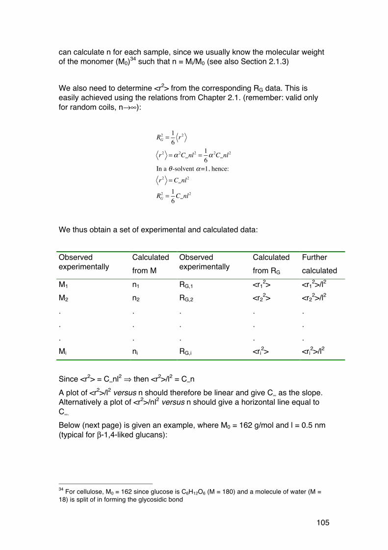
105

can calculate n for each sample, since we usually know the molecular weight of the monomer (M0)34 such that n = Mi/M0 (see also Section 2.1.3) We also need to determine <r2> from the corresponding RG data. This is easily achieved using the relations from Chapter 2.1. (remember: valid only for random coils, n→∞):

RG2 = 1

6r2

r2 =α 2C∞nl2 = 1

6α 2C∞nl

2

In a θ -solvent α=1, hence:

r2 = C∞nl2

RG2 = 1

6C∞nl

2

We thus obtain a set of experimental and calculated data:

Observed experimentally

Calculated from M

Observed experimentally

Calculated from RG

Further calculated

M1 n1 RG,1 <r12> <r1

2>/l2 M2 n2 RG,2 <r2

2> <r22>/l2

.

.

.

.

.

.

.

.

.

.

.

.

.

.

. Mi ni RG,i <ri

2> <ri2>/l2

Since <r2> = C∞nl2 ⇒ then <r2>/l2 = C∞n A plot of <r2>/l2 versus n should therefore be linear and give C∞ as the slope. Alternatively a plot of <r2>/nl2 versus n should give a horizontal line equal to C∞. Below (next page) is given an example, where M0 = 162 g/mol and l = 0.5 nm (typical for β-1,4-liked glucans):

34 For cellulose, M0 = 162 since glucose is C6H12O6 (M = 180) and a molecule of water (M = 18) is split of in forming the glycosidic bond

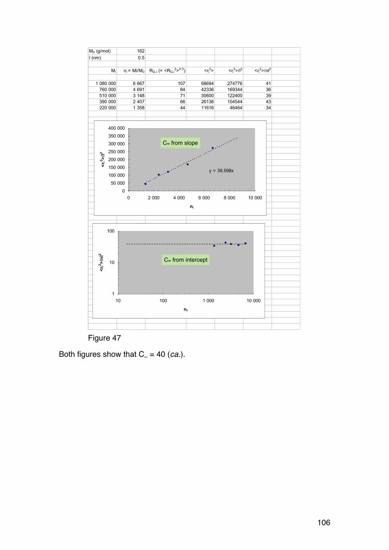
106

Both figures show that C∞ = 40 (ca.).

M0 (g/mol) 162l (nm) 0.5

Mi ni = Mi/M0 RG,i (= <RG,i2>0.5) <ri2> <ri2>/l2 <ri2>/nl2

1 080 000 6 667 107 68694 274776 41760 000 4 691 84 42336 169344 36510 000 3 148 71 30600 122400 39390 000 2 407 66 26136 104544 43220 000 1 358 44 11616 46464 34

y = 39.598x

0

50 000

100 000

150 000

200 000

250 000

300 000

350 000

400 000

0 2 000 4 000 6 000 8 000 10 000

ni

<ri2>/l2

1

10

100

10 100 1 000 10 000

ni

<ri2>/nl2

C∞ from intercept

C∞ from slope

Figure 47

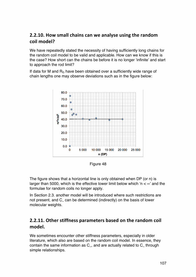
107

2.2.10.  How  small  chains  can  we  analyse  using  the  random  coil  model?  

We have repeatedly stated the necessity of having sufficiently long chains for the random coil model to be valid and applicable. How can we know if this is the case? How short can the chains be before it is no longer ‘infinite’ and start to approach the rod limit? If data for M and RG have been obtained over a sufficiently wide range of chain lengths one may observe deviations such as in the figure below:

Figure 48

The figure shows that a horizontal line is only obtained when DP (or n) is larger than 5000, which is the effective lower limit below which ‘n < ∞’ and the formulae for random coils no longer apply. In Section 2.3. another model will be introduced where such restrictions are not present, and C∞ can be determined (indirectly) on the basis of lower molecular weights.

2.2.11.  Other  stiffness  parameters  based  on  the  random  coil  model.  

We sometimes encounter other stiffness parameters, especially in older literature, which also are based on the random coil model. In essence, they contain the same information as C∞, and are actually related to C∞ through simple relationships.

108

The virtual bond length, β. We introduce a virtual bond length (β) to describe the stiffness of the random coil polymer by defining it as: <r2> = nβ2 We easily see, since <r2> = C∞nl2, that C∞ = β2/l2. The Kuhn length (lk). This is another way of creating a virtual random coil, and the ratio between the Kuhn length and the actual segment length (lk/l) expresses the chain stiffness. The Kuhn chain has nk segments of length lk, and obeys the expression for perfect random coils: <r2> = nklk2 (= C∞nl2) This means that the Kuhn chain has the same end-to-end distance as the real chain. At the same time the contour length of the Kuhn chain is the same as for the real chain: nklk = nl These equations immediately yield that: lk = C∞l nk = n/C∞

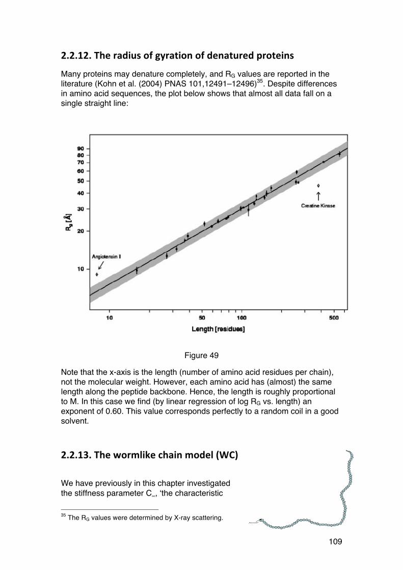
109

2.2.12.  The  radius  of  gyration  of  denatured  proteins  

Many proteins may denature completely, and RG values are reported in the literature (Kohn et al. (2004) PNAS 101,12491–12496)35. Despite differences in amino acid sequences, the plot below shows that almost all data fall on a single straight line:

Figure 49

Note that the x-axis is the length (number of amino acid residues per chain), not the molecular weight. However, each amino acid has (almost) the same length along the peptide backbone. Hence, the length is roughly proportional to M. In this case we find (by linear regression of log RG vs. length) an exponent of 0.60. This value corresponds perfectly to a random coil in a good solvent.

2.2.13.  The  wormlike  chain  model  (WC)  

We have previously in this chapter investigated the stiffness parameter C∞, ‘the characteristic

35 The RG values were determined by X-ray scattering.

110

ratio’ of a polymer. C∞ is a stiffness parameter reflecting chain stiffening due to two structural properties, namely the fixed bond angles and hindered rotation around linkages. Quantitatively, C∞ expresses quantitatively the increase in average end-to-end distance (<r2>0.5) of an otherwise randomly coiled polymer. We could determine C∞ from M-RG data using the theory of random coils (RC), provided the chains were long enough to satisfy random coil criteria. The table below shows C∞ data for a range of polysaccharides (and double-stranded DNA).

Polymer Solvent

Stiffness parameters

C∞

Persistence length estimates (nm)

Dextran Water 1.8 0.7 Pullulan Water 4.3 1.3 Amylose DMSO 5

Barley 1,3/1,4 β-glucans

Water 13-14 3.5-3.8

Hyaluronan Water, I = 0.15 M

27 7

Chitosans (F

A = 0-0.65)

pH 4.5, I = 0.1 M

19-30 5.1-7.6

Alginates Water, I = 0.17 M

55 15

Carboxymethyl cellulose

Water, I = 0.1 M

115 12-16

DNA Water, I = 0.2 M

45

Xanthan Water, I = 0.1 M

480 120

Scleroglucan 0.1 M NaOH 150 In recent years another stiffness parameter has been much used in the literature. It is called the persistence length (symbol: q or Lp). The persistence length is connected to an (abstract) alternative model for polymer chains called the wormlike chain model (WC). In contrast to the RC model, the WC model is not restricted to long chains, but is valid all the way from short rod-like chains (rigid rod limit) and across the

111

region where the polymer is long enough to satisfy the RC model (the coil limit). The figure below illustrates this for the radius of gyration RG):

In the WLC model the polymer is considered as a long, cylindrical chain with uniform thickness. The diameter (d) is negligible compared to the length of the chain (L). In addition, the chain has a constant curvature, but the direction of the curvature is random. Wikipedia (Nov. 2012) provides a good description:

The WLC model envisions an isotropic rod that is continuously flexible. This is in contrast to the freely-jointed chain model that is flexible only between discrete segments. The worm-like chain model is particularly suited for describing stiffer polymers..

log RG

log M

Rod limit: slope: 1.0

Coil limit slope: 0.5

Figure 50

112

2.2.14.  The  persistence  length  

The definition of the persistence length is in fact based on the vector model used earlier for random coils (freely jointed chains):

Mathematically, the persistence length is defined the dot product the ‘end-to-end vector’ and the unity vector of monomer one (i.e. direction of the first vector):

The persistence length is, fortunately, directly related to the characteristic ration (proof not given):

C∞ = 2ql−1

Her, l is the length of the monomer (typically in the range 0.4-0.5 nm for common monosaccharides like glucose, mannose, mannuronic acid etc.(1,3, 1,4 or 1,6 linked).

q = l

1

l1i r

= l

1

l1i li

i=1∑ n→∞( )

r = end-to-end vector

Direction of first vector

a

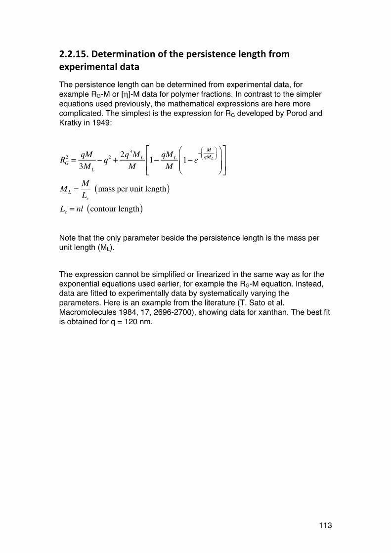
113

2.2.15.  Determination  of  the  persistence  length  from  experimental  data  

The persistence length can be determined from experimental data, for example RG-M or [η]-M data for polymer fractions. In contrast to the simpler equations used previously, the mathematical expressions are here more complicated. The simplest is the expression for RG developed by Porod and Kratky in 1949:

Note that the only parameter beside the persistence length is the mass per unit length (ML). The expression cannot be simplified or linearized in the same way as for the exponential equations used earlier, for example the RG-M equation. Instead, data are fitted to experimentally data by systematically varying the parameters. Here is an example from the literature (T. Sato et al. Macromolecules 1984, 17, 2696-2700), showing data for xanthan. The best fit is obtained for q = 120 nm.

RG2 = qM

3ML

− q2 + 2q3ML

M1− qML

M1− e

− MqML

⎛⎝⎜

⎞⎠⎟

⎛

⎝⎜⎜

⎞

⎠⎟⎟

⎡

⎣⎢⎢

⎤

⎦⎥⎥

ML =MLc

mass per unit length( )

Lc = nl contour length( )

114

In this case ML was determined from the chemical composition combined with X-ray crystallography data in the following way: The repeating unit of xanthan is given in Section 1.7. By summation of all the atoms (including the counterions) we find the repeating unit (fully pyruvated, and partially acetylated in this case) has a mass of 970 g/mol (Da) (and 848 if no pyruvate and acetate). Each glucose residue in the backbone is (from X-ray) 0.5 nm, hence ML = 970/(2*0.5) = 970 nm-1. Since xanthan is double stranded, ML becomes 1940 nm-1. This value is used in the figure above. The same type of procedure can in principle be used for [η]-M data, but the formulae are more complicated and not so convenient to process in a spreadsheet, for example. However, it is much used because [η] data are easily obtained over a larger interval of molecular weights than RG. Again, take a look at the data in the table. The range of q-values goes from less than 1 nm for the compact dextrans to 150 nm for triple-stranded scleroglucan. Do the other values make sense from what you have learned about these polymers?

 

115

PART  3.  PHYSICAL  PROPERTIES  OF  BIOPOLYMERS  IN  SOLUTION  

 

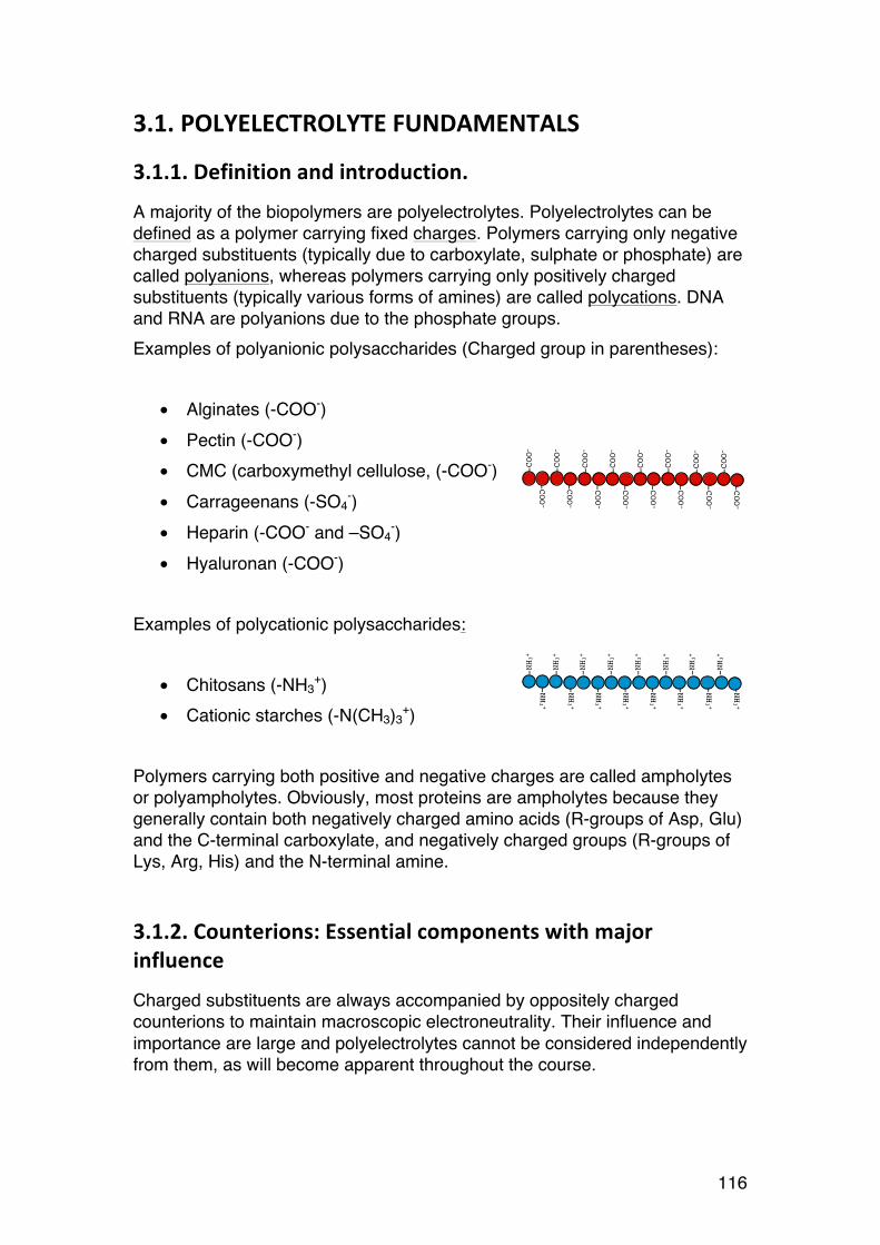
116

3.1.  POLYELECTROLYTE  FUNDAMENTALS  

3.1.1.  Definition  and  introduction.  

A majority of the biopolymers are polyelectrolytes. Polyelectrolytes can be defined as a polymer carrying fixed charges. Polymers carrying only negative charged substituents (typically due to carboxylate, sulphate or phosphate) are called polyanions, whereas polymers carrying only positively charged substituents (typically various forms of amines) are called polycations. DNA and RNA are polyanions due to the phosphate groups. Examples of polyanionic polysaccharides (Charged group in parentheses):

• Alginates (-COO-) • Pectin (-COO-) • CMC (carboxymethyl cellulose, (-COO-) • Carrageenans (-SO4

-) • Heparin (-COO- and –SO4

-) • Hyaluronan (-COO-)

Examples of polycationic polysaccharides:

• Chitosans (-NH3+)

• Cationic starches (-N(CH3)3+)

Polymers carrying both positive and negative charges are called ampholytes or polyampholytes. Obviously, most proteins are ampholytes because they generally contain both negatively charged amino acids (R-groups of Asp, Glu) and the C-terminal carboxylate, and negatively charged groups (R-groups of Lys, Arg, His) and the N-terminal amine.

3.1.2.  Counterions:  Essential  components  with  major  influence  

Charged substituents are always accompanied by oppositely charged counterions to maintain macroscopic electroneutrality. Their influence and importance are large and polyelectrolytes cannot be considered independently from them, as will become apparent throughout the course.

-COO

-

-COO-

-COO

-

-COO-

-COO

-

-COO-

-COO

-

-COO-

-COO

-

-COO-

-COO

-

-COO-

-COO

-

-COO-

-COO

-

-COO-

-NH 3

+

-NH 3

+

-NH 3

+

-NH 3

+

-NH 3

+

-NH 3

+

-NH 3

+

-NH 3

+

-NH3 +

-NH3 +

-NH3 +

-NH3 +

-NH3 +

-NH3 +

-NH3 +

-NH3 +

117

Sodium alginate is a typical example. In the dry state each carboxylate group (-COO-) is bound to a sodium ion (Na+). In other words, sodium alginate is the sodium salt of alginic acid. Upon dissolution in water the sodium ions dissociate from the polymer to become hydrated, free ions, but remain concentrated around the polymer as illustrated below.

The counterions may alternatively be any other cation such as K+, Mg++, NH4

+

or Ca++. The proton (H+) is the counterion for alginic acid, but since most of the carboxylic acids are weak acids (pKa = ca 3.5 for alginic acid) only a small fraction of the protons actually dissociates.

3.1.3.  Changing  counterions  (salt  forms)  

Interconversion between different salt forms is an important process frequently applied to obtain other salt forms. Alginates are manufactured not only as sodium alginate, but also as alginic acid, calcium alginate and ammonium acetate (see e.g. E400-E405). The conversion may be obtained by dialysis, or via the acidic form. The latter is more easily scaled up. Example (sodium alginate to potassium alginate):

1. Na-alginate is dissolved in water 2. An acid (HCl or H2SO4) is added until pH reaches 1-2 (all –COO-

protonated), forming insoluble alginic acid which is then washed with water to remove excess ions

3. pH is adjusted back to ca 7 using KOH, forming soluble K-alginate, which can be dried if necessary.

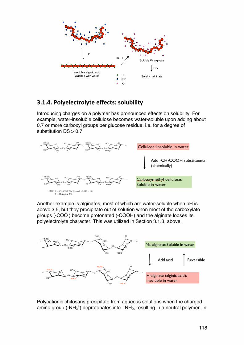
118

3.1.4.  Polyelectrolyte  effects:  solubility  

Introducing charges on a polymer has pronounced effects on solubility. For example, water-insoluble cellulose becomes water-soluble upon adding about 0.7 or more carboxyl groups per glucose residue, i.e. for a degree of substitution DS > 0.7.

Another example is alginates, most of which are water-soluble when pH is above 3.5, but they precipitate out of solution when most of the carboxylate groups (-COO-) become protonated (-COOH) and the alginate looses its polyelectrolyte character. This was utilized in Section 3.1.3. above.

Polycationic chitosans precipitate from aqueous solutions when the charged amino group (-NH3

+) deprotonates into –NH2, resulting in a neutral polymer. In

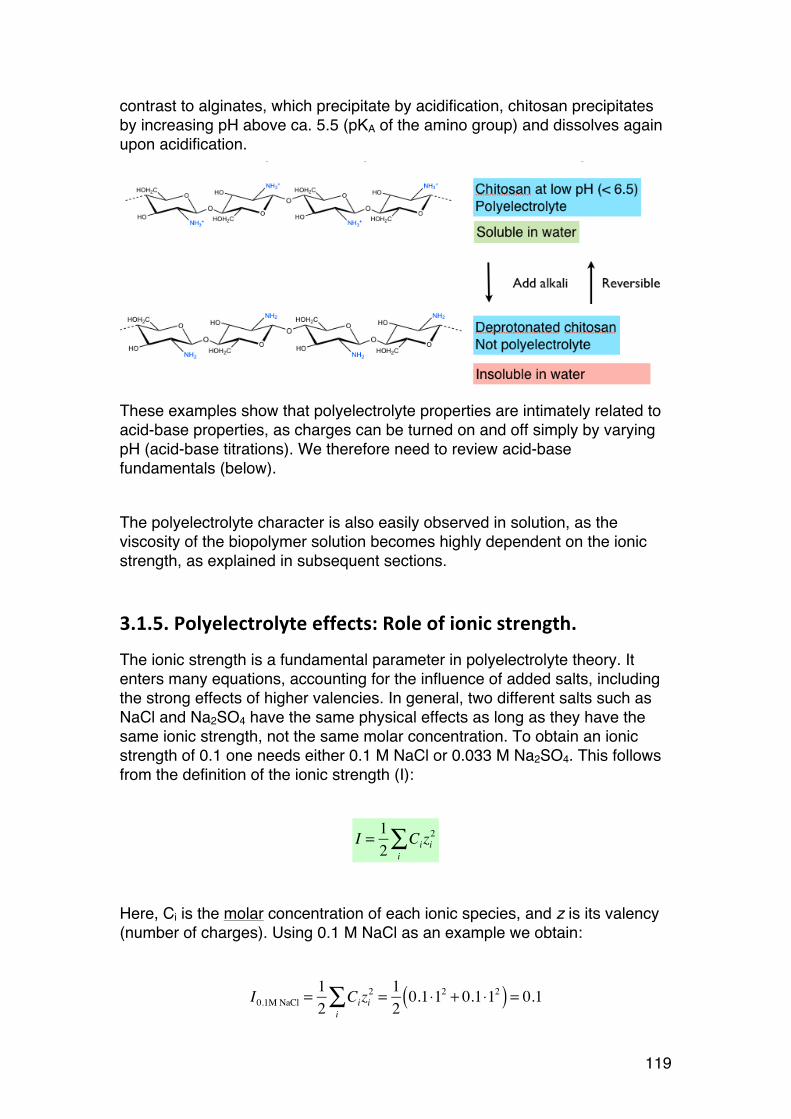
119

contrast to alginates, which precipitate by acidification, chitosan precipitates by increasing pH above ca. 5.5 (pKA of the amino group) and dissolves again upon acidification.

These examples show that polyelectrolyte properties are intimately related to acid-base properties, as charges can be turned on and off simply by varying pH (acid-base titrations). We therefore need to review acid-base fundamentals (below). The polyelectrolyte character is also easily observed in solution, as the viscosity of the biopolymer solution becomes highly dependent on the ionic strength, as explained in subsequent sections.

3.1.5.  Polyelectrolyte  effects:  Role  of  ionic  strength.  

The ionic strength is a fundamental parameter in polyelectrolyte theory. It enters many equations, accounting for the influence of added salts, including the strong effects of higher valencies. In general, two different salts such as NaCl and Na2SO4 have the same physical effects as long as they have the same ionic strength, not the same molar concentration. To obtain an ionic strength of 0.1 one needs either 0.1 M NaCl or 0.033 M Na2SO4. This follows from the definition of the ionic strength (I):

I = 12

Cizi2

i∑

Here, Ci is the molar concentration of each ionic species, and z is its valency (number of charges). Using 0.1 M NaCl as an example we obtain:

I0.1M NaCl =12

Cizi2

i∑ = 1

20.1⋅12 + 0.1⋅12( ) = 0.1

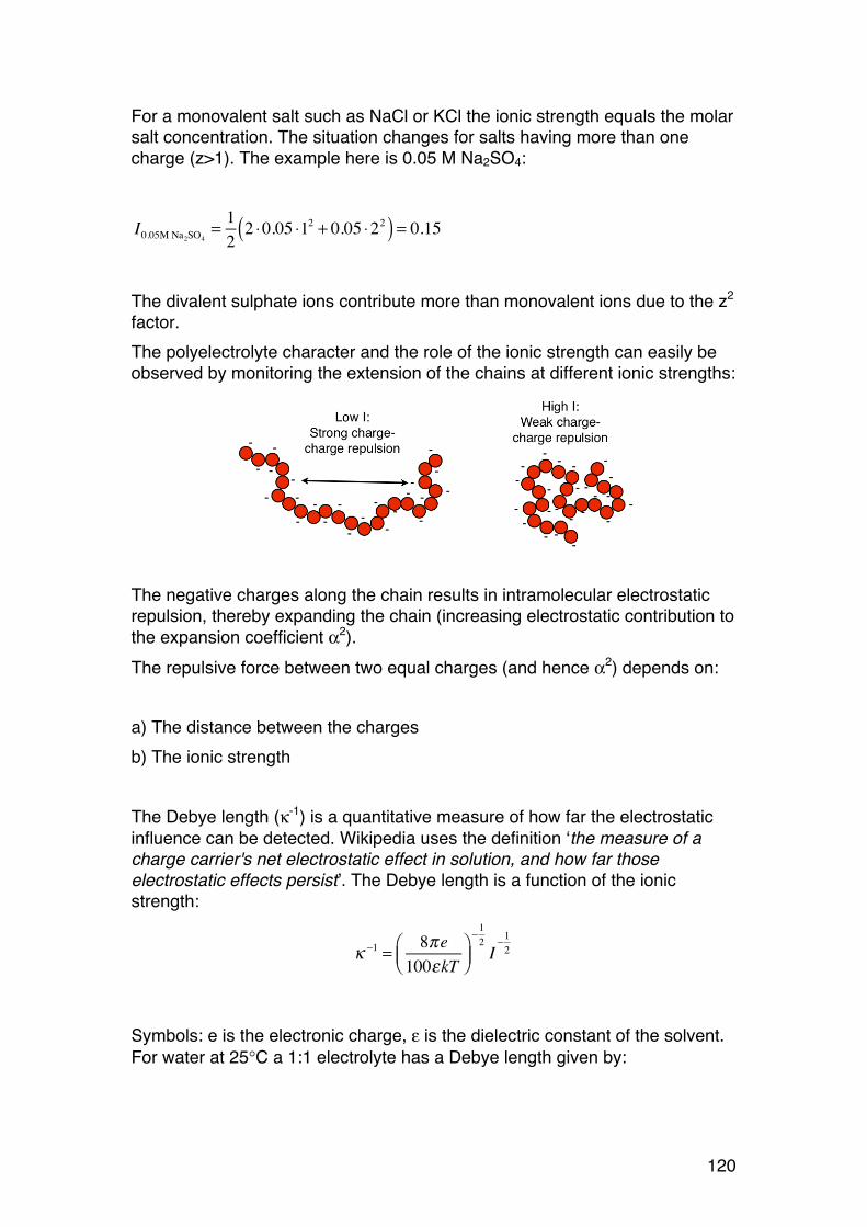
120

For a monovalent salt such as NaCl or KCl the ionic strength equals the molar salt concentration. The situation changes for salts having more than one charge (z>1). The example here is 0.05 M Na2SO4:

I0.05M Na2SO4= 1

22 ⋅0.05 ⋅12 + 0.05 ⋅22( ) = 0.15

The divalent sulphate ions contribute more than monovalent ions due to the z2 factor. The polyelectrolyte character and the role of the ionic strength can easily be observed by monitoring the extension of the chains at different ionic strengths:

The negative charges along the chain results in intramolecular electrostatic repulsion, thereby expanding the chain (increasing electrostatic contribution to the expansion coefficient α2). The repulsive force between two equal charges (and hence α2) depends on: a) The distance between the charges b) The ionic strength The Debye length (κ-1) is a quantitative measure of how far the electrostatic influence can be detected. Wikipedia uses the definition ‘the measure of a charge carrier's net electrostatic effect in solution, and how far those electrostatic effects persist’. The Debye length is a function of the ionic strength:

κ −1 = 8πe100εkT

⎛⎝⎜

⎞⎠⎟−12I−12

Symbols: e is the electronic charge, ε is the dielectric constant of the solvent. For water at 25°C a 1:1 electrolyte has a Debye length given by:

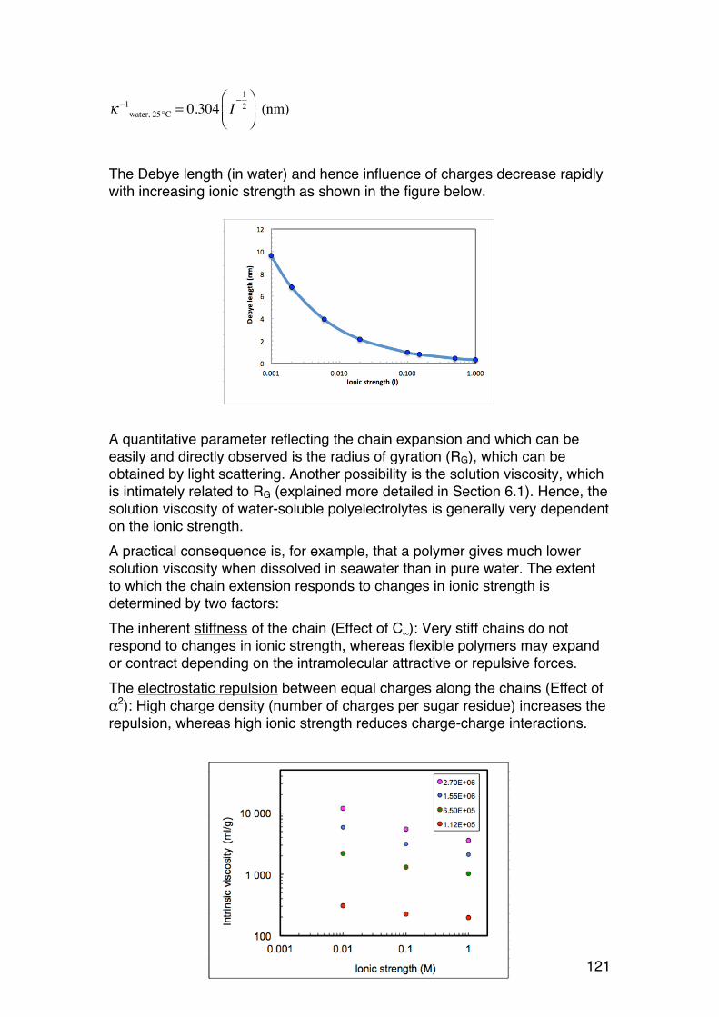
121

κ −1water, 25°C = 0.304 I

−12

⎛⎝⎜

⎞⎠⎟

(nm)

The Debye length (in water) and hence influence of charges decrease rapidly with increasing ionic strength as shown in the figure below.

A quantitative parameter reflecting the chain expansion and which can be easily and directly observed is the radius of gyration (RG), which can be obtained by light scattering. Another possibility is the solution viscosity, which is intimately related to RG (explained more detailed in Section 6.1). Hence, the solution viscosity of water-soluble polyelectrolytes is generally very dependent on the ionic strength. A practical consequence is, for example, that a polymer gives much lower solution viscosity when dissolved in seawater than in pure water. The extent to which the chain extension responds to changes in ionic strength is determined by two factors: The inherent stiffness of the chain (Effect of C∞): Very stiff chains do not respond to changes in ionic strength, whereas flexible polymers may expand or contract depending on the intramolecular attractive or repulsive forces. The electrostatic repulsion between equal charges along the chains (Effect of α2): High charge density (number of charges per sugar residue) increases the repulsion, whereas high ionic strength reduces charge-charge interactions.

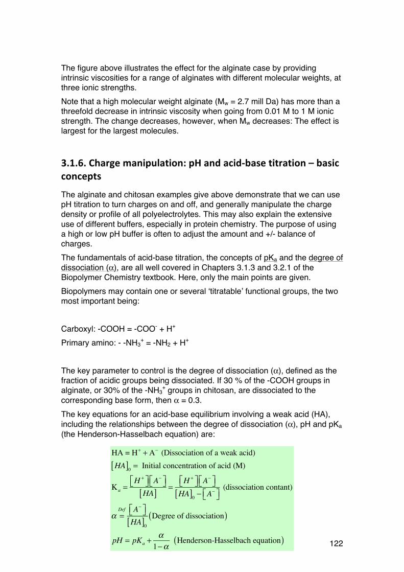
122

The figure above illustrates the effect for the alginate case by providing intrinsic viscosities for a range of alginates with different molecular weights, at three ionic strengths. Note that a high molecular weight alginate (Mw = 2.7 mill Da) has more than a threefold decrease in intrinsic viscosity when going from 0.01 M to 1 M ionic strength. The change decreases, however, when Mw decreases: The effect is largest for the largest molecules.

3.1.6.  Charge  manipulation:  pH  and  acid-­‐base  titration  –  basic  concepts  

The alginate and chitosan examples give above demonstrate that we can use pH titration to turn charges on and off, and generally manipulate the charge density or profile of all polyelectrolytes. This may also explain the extensive use of different buffers, especially in protein chemistry. The purpose of using a high or low pH buffer is often to adjust the amount and +/- balance of charges. The fundamentals of acid-base titration, the concepts of pKa and the degree of dissociation (α), are all well covered in Chapters 3.1.3 and 3.2.1 of the Biopolymer Chemistry textbook. Here, only the main points are given. Biopolymers may contain one or several ‘titratable’ functional groups, the two most important being: Carboxyl: -COOH = -COO- + H+ Primary amino: - -NH3

+ = -NH2 + H+

The key parameter to control is the degree of dissociation (α), defined as the fraction of acidic groups being dissociated. If 30 % of the -COOH groups in alginate, or 30% of the -NH3

+ groups in chitosan, are dissociated to the corresponding base form, then α = 0.3. The key equations for an acid-base equilibrium involving a weak acid (HA), including the relationships between the degree of dissociation (α), pH and pKa (the Henderson-Hasselbach equation) are:

HA = H+ + A− (Dissociation of a weak acid)HA[ ]0 = Initial concentration of acid (M)

Ka =H +⎡⎣ ⎤⎦ A−⎡⎣ ⎤⎦HA[ ] =

H +⎡⎣ ⎤⎦ A−⎡⎣ ⎤⎦HA[ ]0 − A−⎡⎣ ⎤⎦

(dissociation contant)

α =Def A−⎡⎣ ⎤⎦

HA[ ]0

Degree of dissociation( )

pH = pKa +α

1−α Henderson-Hasselbach equation( )

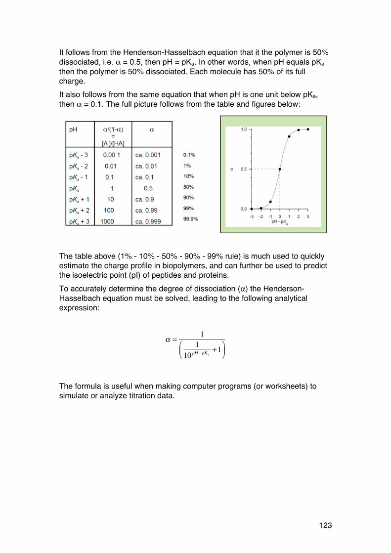
123

It follows from the Henderson-Hasselbach equation that it the polymer is 50% dissociated, i.e. α = 0.5, then pH = pKa. In other words, when pH equals pKa then the polymer is 50% dissociated. Each molecule has 50% of its full charge. It also follows from the same equation that when pH is one unit below pKa, then α = 0.1. The full picture follows from the table and figures below:

The table above (1% - 10% - 50% - 90% - 99% rule) is much used to quickly estimate the charge profile in biopolymers, and can further be used to predict the isoelectric point (pI) of peptides and proteins. To accurately determine the degree of dissociation (α) the Henderson-Hasselbach equation must be solved, leading to the following analytical expression:

α = 11

10 pH− pKa+1⎛

⎝⎜⎞⎠⎟

The formula is useful when making computer programs (or worksheets) to simulate or analyze titration data.

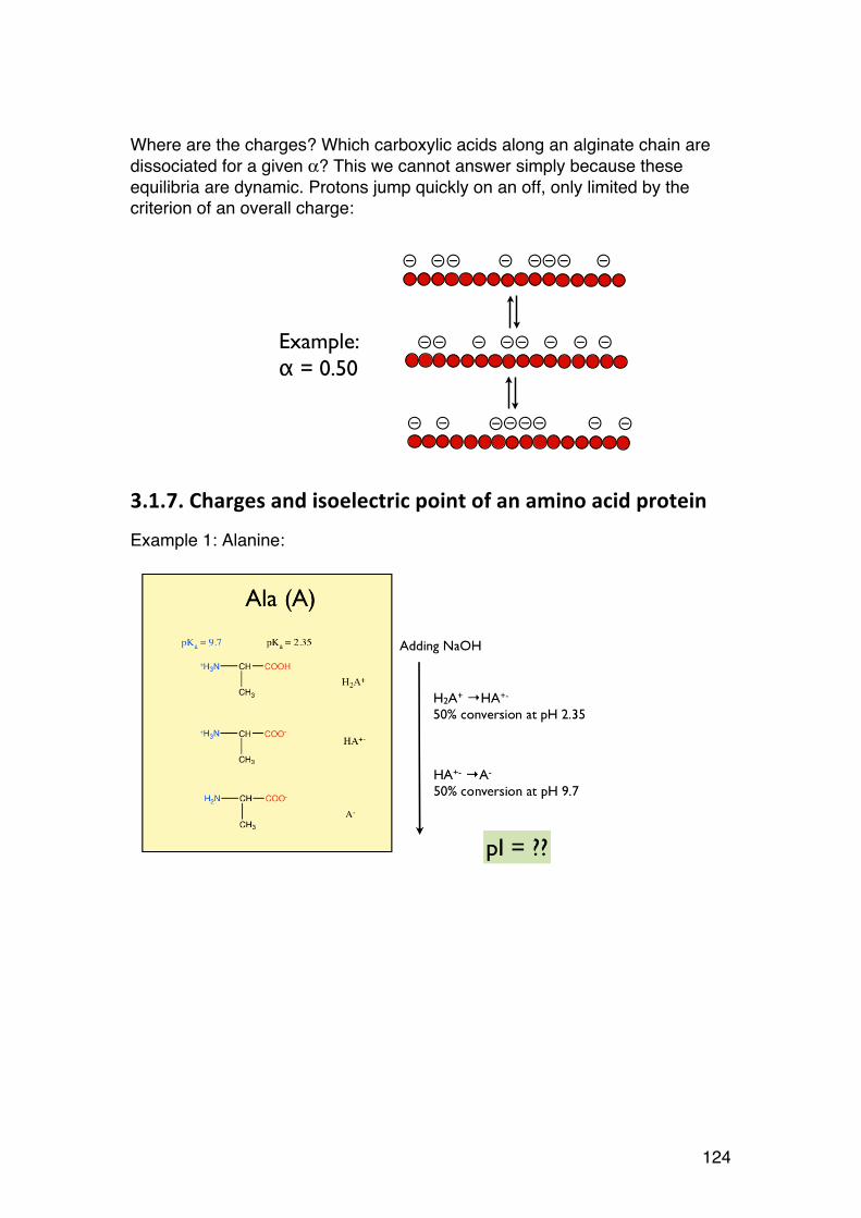
124

Where are the charges? Which carboxylic acids along an alginate chain are dissociated for a given α? This we cannot answer simply because these equilibria are dynamic. Protons jump quickly on an off, only limited by the criterion of an overall charge:

3.1.7.  Charges  and  isoelectric  point  of  an  amino  acid  protein  

Example 1: Alanine:

 

⊝ ⊝⊝ ⊝ ⊝⊝⊝ ⊝

⊝⊝ ⊝ ⊝⊝ ⊝ ⊝ ⊝

⊝ ⊝ ⊝⊝⊝⊝ ⊝ ⊝

Example: α = 0.50

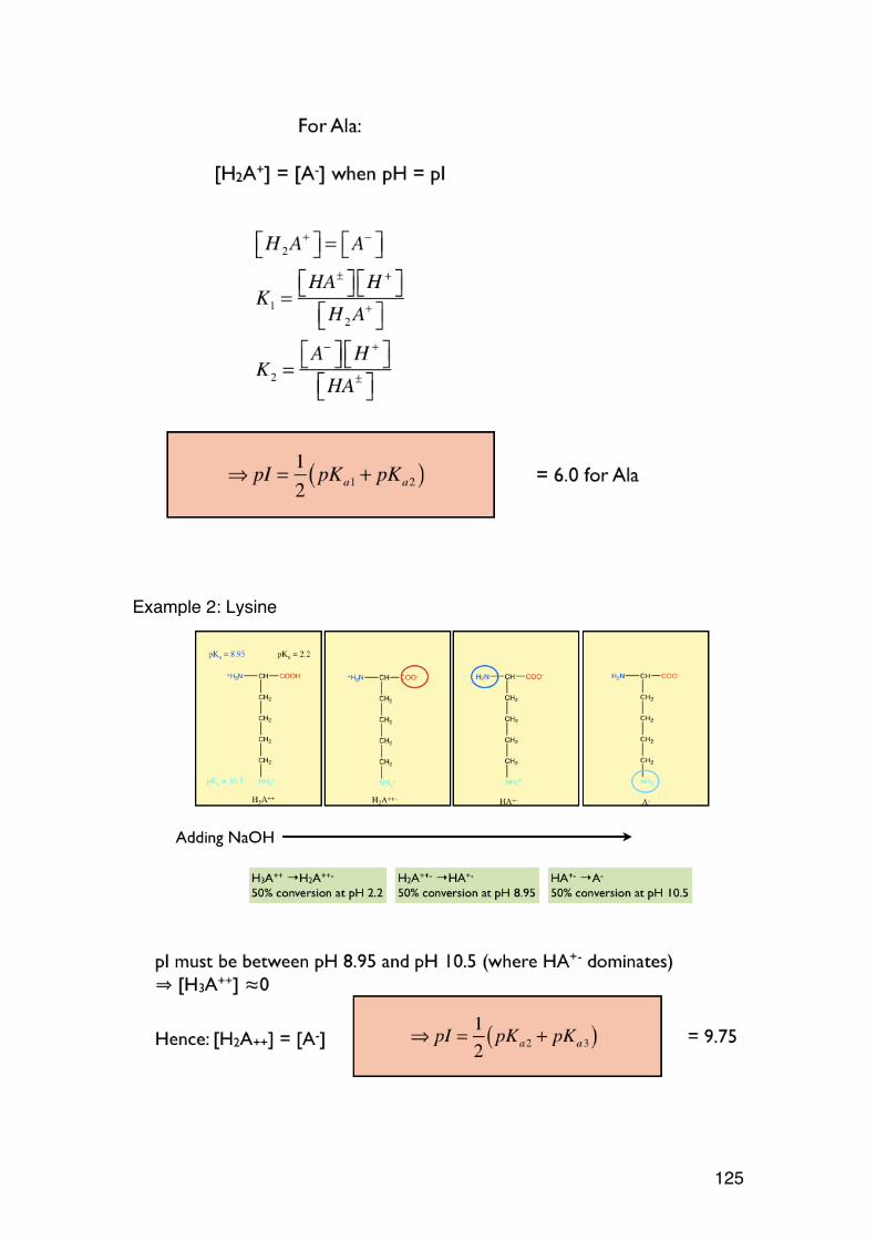
125

Example 2: Lysine

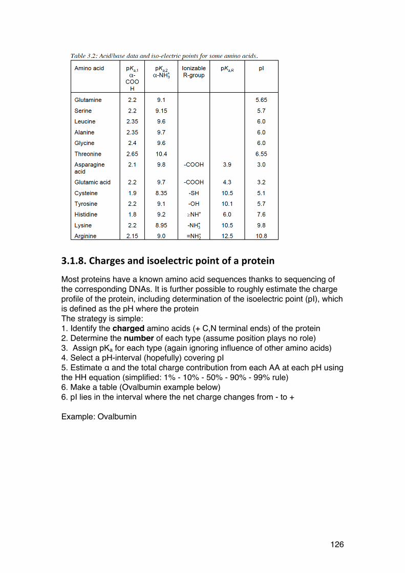
126

3.1.8.  Charges  and  isoelectric  point  of  a  protein  

Most proteins have a known amino acid sequences thanks to sequencing of the corresponding DNAs. It is further possible to roughly estimate the charge profile of the protein, including determination of the isoelectric point (pI), which is defined as the pH where the protein The strategy is simple: 1. Identify the charged amino acids (+ C,N terminal ends) of the protein 2. Determine the number of each type (assume position plays no role) 3. Assign pKa for each type (again ignoring influence of other amino acids) 4. Select a pH-interval (hopefully) covering pI 5. Estimate α and the total charge contribution from each AA at each pH using the HH equation (simplified: 1% - 10% - 50% - 90% - 99% rule) 6. Make a table (Ovalbumin example below) 6. pI lies in the interval where the net charge changes from - to + Example: Ovalbumin

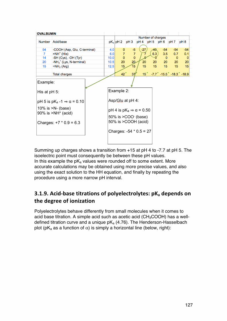
127

Summing up charges shows a transition from +15 at pH 4 to -7.7 at pH 5. The isoelectric point must consequently be between these pH values. In this example the pKa values were rounded off to some extent. More accurate calculations may be obtained using more precise values, and also using the exact solution to the HH equation, and finally by repeating the procedure using a more narrow pH interval.

3.1.9.  Acid-­‐base  titrations  of  polyelectrolytes:  pKa  depends  on  the  degree  of  ionization  

Polyelectrolytes behave differently from small molecules when it comes to acid base titration. A simple acid such as acetic acid (CH3COOH) has a well-defined titration curve and a unique pKa (4.76). The Henderson-Hasselbach plot (pKa as a function of α) is simply a horizontal line (below, right):

128

Consider then a dibasic acid such as oxalic acid:

Oxalic acid contains two chemically identical carboxyl groups. Yet, oxalic acid has two pKa values: 1.25 and 4.14 (Wikipedia). This means the first ionisation (H2A → HA-) proceeds easily (low pKa), whereas ionisation the second carboxyl is less favoured (high pKa). This can be understood by the influence of the charges. Forming a –COO-

in close proximity of an existing negative charge is thermodynamically unfavourable. The titration curve of oxalic acid clearly reveals the two pKa values.

HOOH

O

O

HOO

O

O

OO

O

O

H2A HA- A2-

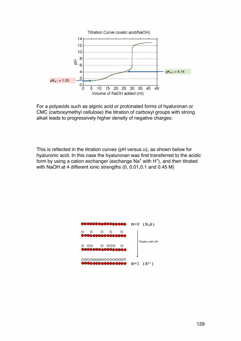
129

For a polyacids such as alginic acid or protonated forms of hyaluronan or CMC (carboxymethyl cellulose) the titration of carboxyl groups with strong alkali leads to progressively higher density of negative charges:

This is reflected in the titration curves (pH versus α), as shown below for hyaluronic acid. In this case the hyaluronan was first transferred to the acidic form by using a cation exchanger (exchange Na+ with H+), and then titrated with NaOH at 4 different ionic strengths (0, 0.01,0.1 and 0.45 M)

⊝ ⊝ ⊝ ⊝ ⊝

⊝ ⊝⊝ ⊝ ⊝⊝⊝ ⊝

⊝ ⊝⊝ ⊝ ⊝⊝⊝ ⊝⊝ ⊝⊝⊝ ⊝ ⊝⊝ ⊝

α=0 (HnA)

α=1 (An-)

Titration with OH-

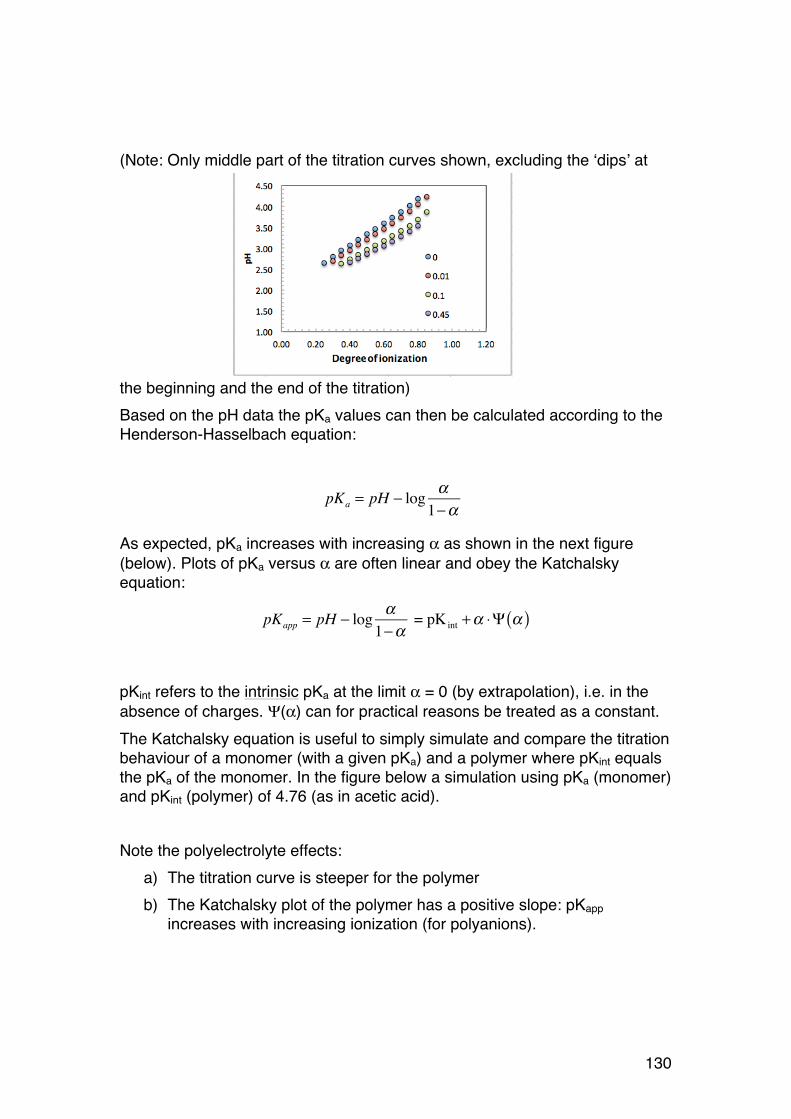
130

(Note: Only middle part of the titration curves shown, excluding the ‘dips’ at

the beginning and the end of the titration) Based on the pH data the pKa values can then be calculated according to the Henderson-Hasselbach equation:

pKa = pH − log α1−α

As expected, pKa increases with increasing α as shown in the next figure (below). Plots of pKa versus α are often linear and obey the Katchalsky equation:

pKapp = pH − log α1−α

= pKint +α ⋅Ψ α( )

pKint refers to the intrinsic pKa at the limit α = 0 (by extrapolation), i.e. in the absence of charges. Ψ(α) can for practical reasons be treated as a constant. The Katchalsky equation is useful to simply simulate and compare the titration behaviour of a monomer (with a given pKa) and a polymer where pKint equals the pKa of the monomer. In the figure below a simulation using pKa (monomer) and pKint (polymer) of 4.76 (as in acetic acid). Note the polyelectrolyte effects:

a) The titration curve is steeper for the polymer b) The Katchalsky plot of the polymer has a positive slope: pKapp

increases with increasing ionization (for polyanions).

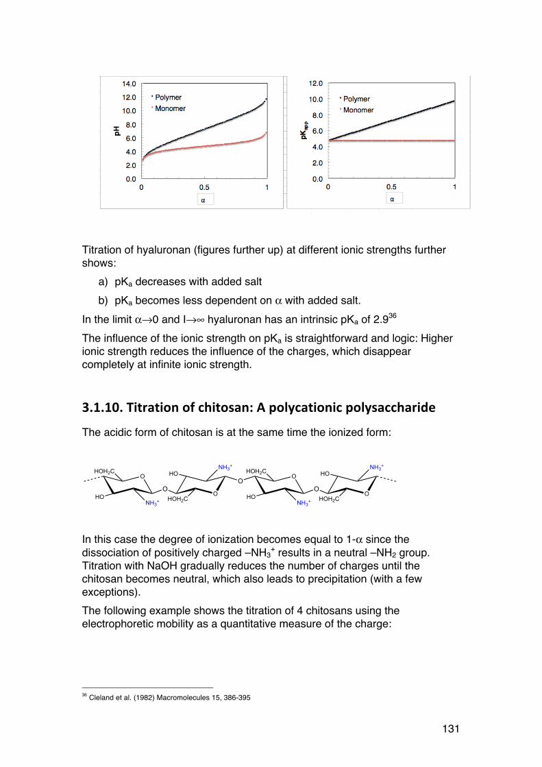
131

Titration of hyaluronan (figures further up) at different ionic strengths further shows:

a) pKa decreases with added salt b) pKa becomes less dependent on α with added salt.

In the limit α→0 and I→∞ hyaluronan has an intrinsic pKa of 2.936 The influence of the ionic strength on pKa is straightforward and logic: Higher ionic strength reduces the influence of the charges, which disappear completely at infinite ionic strength.

3.1.10.  Titration  of  chitosan:  A  polycationic  polysaccharide  

The acidic form of chitosan is at the same time the ionized form:

In this case the degree of ionization becomes equal to 1-α since the dissociation of positively charged –NH3

+ results in a neutral –NH2 group. Titration with NaOH gradually reduces the number of charges until the chitosan becomes neutral, which also leads to precipitation (with a few exceptions). The following example shows the titration of 4 chitosans using the electrophoretic mobility as a quantitative measure of the charge:

36 Cleland et al. (1982) Macromolecules 15, 386-395

NH3+

OHOH2C

NH3+HO

OO

HOH2C

HOO

NH3+

OHOH2C

NH3+HO

OO

HOH2C

HO

132

FA refers to the fraction of N-acetylated residues, i.e. neutral sugars not involved in acid-base titration (see Section 1.3 for chitosan chemistry). At pH 3, where all remaining GlcN residues are positively charged, we clearly see the electrophoretic mobility decreases as FA increases. Roughly, the mobility at FA = 0.49 is about half of that at FA = 0.01 which is reasonable as the charge density of the latter is twice the former. The pKa value is in this case taken as the midpoint of the curve since 50% of electrophoretic mobility corresponds to 50% ionization. The figure shows that pKA is the same for all chitosans at an ionic strength of 0.1 M, namely 6.5. Can you predict the situation at a much lower ionic strength? Below is titration curve for chitosan on the basis of NMR data combined with pH measurements:

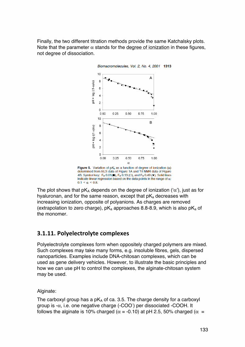
133

Finally, the two different titration methods provide the same Katchalsky plots. Note that the parameter α stands for the degree of ionization in these figures, not degree of dissociation.

The plot shows that pKA depends on the degree of ionization (‘α’), just as for hyaluronan, and for the same reason, except that pKa decreases with increasing ionization, opposite of polyanions. As charges are removed (extrapolation to zero charge), pKa approaches 8.8-8.9, which is also pKa of the monomer.

3.1.11.  Polyelectrolyte  complexes  

Polyelectrolyte complexes form when oppositely charged polymers are mixed. Such complexes may take many forms, e.g. insoluble fibres, gels, dispersed nanoparticles. Examples include DNA-chitosan complexes, which can be used as gene delivery vehicles. However, to illustrate the basic principles and how we can use pH to control the complexes, the alginate-chitosan system may be used. Alginate: The carboxyl group has a pKA of ca. 3.5. The charge density for a carboxyl group is -α, i.e. one negative charge (-COO-) per dissociated -COOH. It follows the alginate is 10% charged (α = -0.10) at pH 2.5, 50% charged (α =

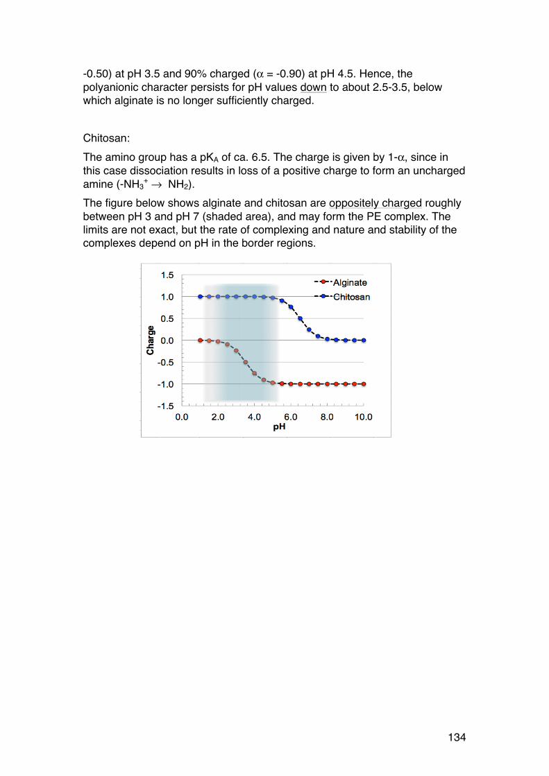
134

-0.50) at pH 3.5 and 90% charged (α = -0.90) at pH 4.5. Hence, the polyanionic character persists for pH values down to about 2.5-3.5, below which alginate is no longer sufficiently charged. Chitosan: The amino group has a pKA of ca. 6.5. The charge is given by 1-α, since in this case dissociation results in loss of a positive charge to form an uncharged amine (-NH3

+ → NH2). The figure below shows alginate and chitosan are oppositely charged roughly between pH 3 and pH 7 (shaded area), and may form the PE complex. The limits are not exact, but the rate of complexing and nature and stability of the complexes depend on pH in the border regions.

135

3.2.  THERMODYNAMICS:  IMPORTANT  TOOL  IN  BIOCHEMISTRY  

3.2.1.  General  comments  

This part of the compendium overlaps partly with chapter 10 in the textbook, but adds new examples and simplifies or omits some of the intermediate calculations. Thermodynamics is a key area in all natural sciences. For biopolymers in solution it provides a range of useful formulae allowing quantitative descriptions of key macromolecular parameters. Thermodynamic approaches are in particular relevant when studying:

• Ordered and disordered conformations • Denaturation and renaturation • Solubility, precipitation, phase behaviour, swelling • Interactions with ions • Effects of added/removed salts • Ligand binding • Osmotic effects • M, A2 • Entropy of mixing • Methods (calorimetry/ITC, osmometry..) • +++

Note that thermodynamics applies only to systems at equilibrium. In the biopolymers field we sometimes observe slow processes when changing the conditions. This may sometimes lead us to believe that equilibrium has been established when it in reality has not. Before continuing, let us briefly repeat two key formulae from your first chemistry courses

ΔG = ΔH − TΔSΔG 0 = −RTln K

Make sure you understand these equations well.

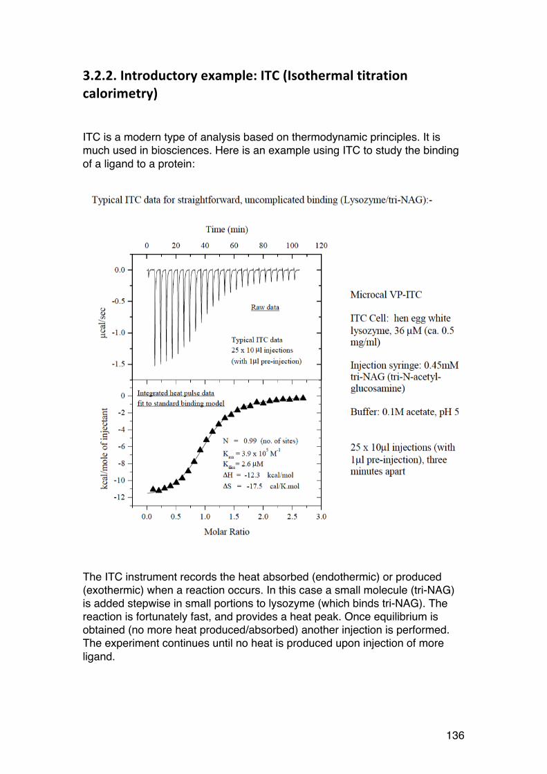
136

3.2.2.  Introductory  example:  ITC  (Isothermal  titration  calorimetry)  

ITC is a modern type of analysis based on thermodynamic principles. It is much used in biosciences. Here is an example using ITC to study the binding of a ligand to a protein:

The ITC instrument records the heat absorbed (endothermic) or produced (exothermic) when a reaction occurs. In this case a small molecule (tri-NAG) is added stepwise in small portions to lysozyme (which binds tri-NAG). The reaction is fortunately fast, and provides a heat peak. Once equilibrium is obtained (no more heat produced/absorbed) another injection is performed. The experiment continues until no heat is produced upon injection of more ligand.

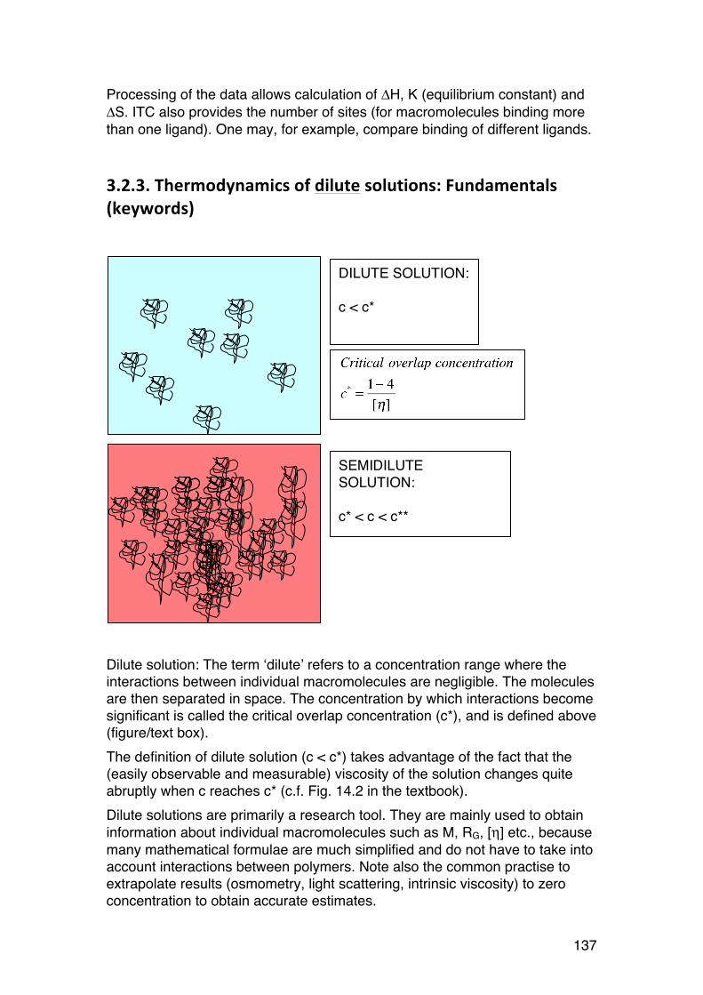
137

Processing of the data allows calculation of ΔH, K (equilibrium constant) and ΔS. ITC also provides the number of sites (for macromolecules binding more than one ligand). One may, for example, compare binding of different ligands.

3.2.3.  Thermodynamics  of  dilute  solutions:  Fundamentals  (keywords)  

Dilute solution: The term ‘dilute’ refers to a concentration range where the interactions between individual macromolecules are negligible. The molecules are then separated in space. The concentration by which interactions become significant is called the critical overlap concentration (c*), and is defined above (figure/text box). The definition of dilute solution (c < c*) takes advantage of the fact that the (easily observable and measurable) viscosity of the solution changes quite abruptly when c reaches c* (c.f. Fig. 14.2 in the textbook). Dilute solutions are primarily a research tool. They are mainly used to obtain information about individual macromolecules such as M, RG, [η] etc., because many mathematical formulae are much simplified and do not have to take into account interactions between polymers. Note also the common practise to extrapolate results (osmometry, light scattering, intrinsic viscosity) to zero concentration to obtain accurate estimates.

DILUTE SOLUTION: c < c*

SEMIDILUTE SOLUTION: c* < c < c**

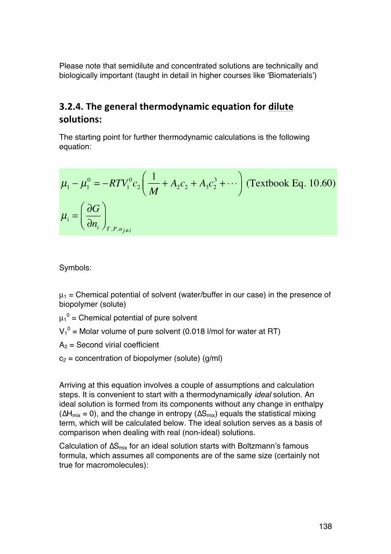
138

Please note that semidilute and concentrated solutions are technically and biologically important (taught in detail in higher courses like ‘Biomaterials’)

3.2.4.  The  general  thermodynamic  equation  for  dilute  solutions:  

The starting point for further thermodynamic calculations is the following equation:

µ1 − µ1

0= −RTV1

0c2

1

M+ A2c2 + A3c2

3+ ⋅ ⋅ ⋅⎛

⎝⎜⎞⎠⎟

(Textbook Eq. 10.60)

µi =∂G∂ni

⎛

⎝⎜⎞

⎠⎟T ,P,n j≠ i

Symbols: µ1 = Chemical potential of solvent (water/buffer in our case) in the presence of biopolymer (solute) µ1

0 = Chemical potential of pure solvent V1

0 = Molar volume of pure solvent (0.018 l/mol for water at RT) A2 = Second virial coefficient c2 = concentration of biopolymer (solute) (g/ml) Arriving at this equation involves a couple of assumptions and calculation steps. It is convenient to start with a thermodynamically ideal solution. An ideal solution is formed from its components without any change in enthalpy (∆Hmix = 0), and the change in entropy (∆Smix) equals the statistical mixing term, which will be calculated below. The ideal solution serves as a basis of comparison when dealing with real (non-ideal) solutions. Calculation of ∆Smix for an ideal solution starts with Boltzmann’s famous formula, which assumes all components are of the same size (certainly not true for macromolecules):

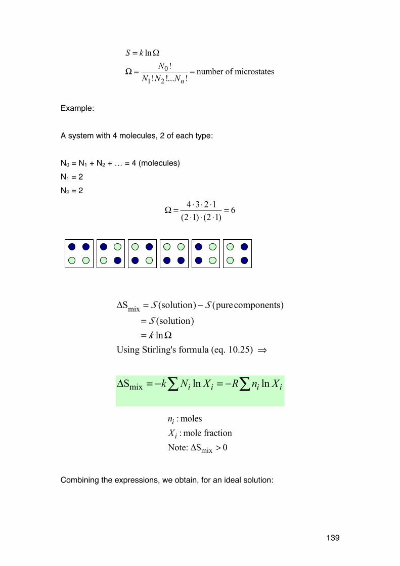
139

0

1 2

ln

!number of microstates

! !... !n

S k

N

N N N

= Ω

Ω = =

Example: A system with 4 molecules, 2 of each type: N0 = N1 + N2 + … = 4 (molecules) N1 = 2 N2 = 2

4 3 2 16

(2 1) (2 1)

⋅ ⋅ ⋅Ω = =

⋅ ⋅ ⋅

ΔSmix = S (solution) − S (purecomponents)

= S (solution)

= k lnΩ

Using Stirling's formula (eq. 10.25) ⇒

mixS ln lni i i ik N X R n XΔ = − = −∑ ∑

mix

: moles

: mole fraction

Note: S 0

i

i

n

X

Δ >

Combining the expressions, we obtain, for an ideal solution:

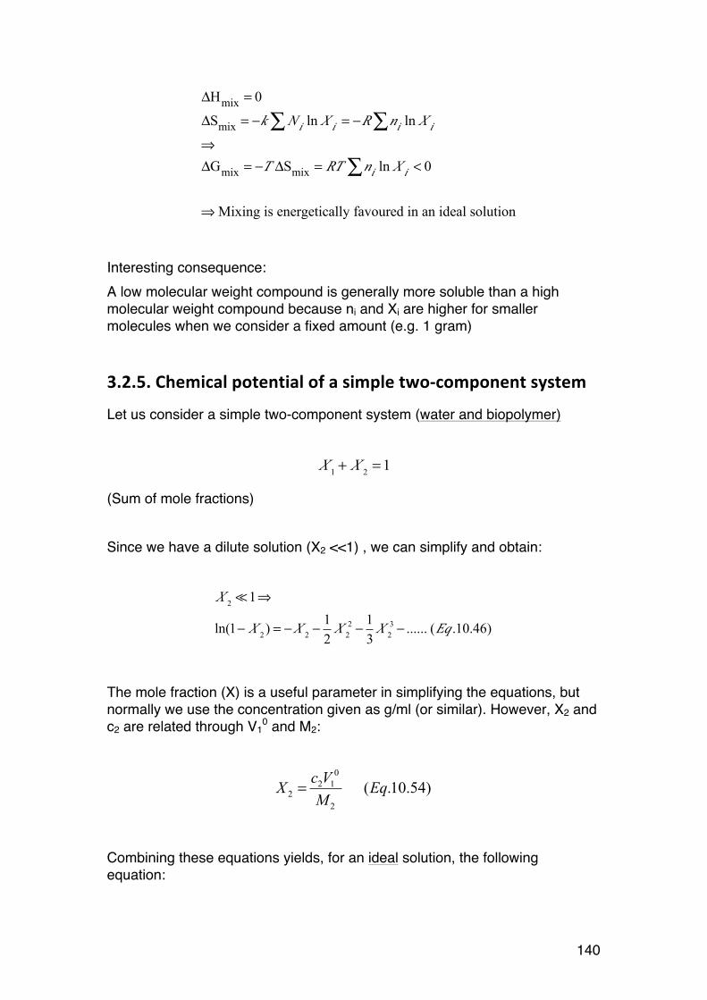
140

ΔHmix = 0

ΔSmix = −k Ni

ln Xi= −R∑ n

iln X

i∑⇒

ΔGmix = −T ΔSmix = RT ni

ln Xi∑ < 0

⇒ Mixing is energetically favoured in an ideal solution

Interesting consequence: A low molecular weight compound is generally more soluble than a high molecular weight compound because ni and Xi are higher for smaller molecules when we consider a fixed amount (e.g. 1 gram)

3.2.5.  Chemical  potential  of  a  simple  two-­‐component  system  

Let us consider a simple two-component system (water and biopolymer)

X1+ X

2=1

(Sum of mole fractions) Since we have a dilute solution (X2 <<1) , we can simplify and obtain:

X21⇒

ln(1− X2) = −X

2−1

2X2

2−1

3X2

3− ...... (Eq .10.46)

The mole fraction (X) is a useful parameter in simplifying the equations, but normally we use the concentration given as g/ml (or similar). However, X2 and c2 are related through V1

0 and M2:

0

2 12

2

( .10.54)c V

X EqM

=

Combining these equations yields, for an ideal solution, the following equation:

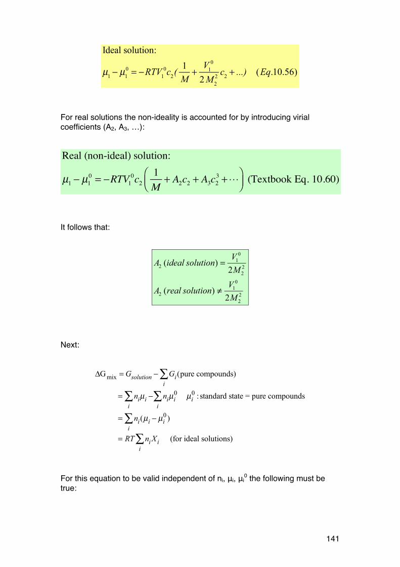
141

Ideal solution:

µ1 − µ10 = −RTV1

0c2( 1M

+V1

0

2M22 c2 + ...) (Eq.10.56)

For real solutions the non-ideality is accounted for by introducing virial coefficients (A2, A3, …):

Real (non-ideal) solution:

µ1 − µ10 = −RTV1

0c21M

+ A2c2 + A3c23 + ⋅⋅⋅⎛

⎝⎜⎞⎠⎟ (Textbook Eq. 10.60)

It follows that:

0

1

2 2

2

0

1

2 2

2

( )2

( )2

VA ideal solution

M

VA real solution

M

=

≠

Next:

ΔGmix = Gsolution − Gi(pure compounds)i∑

= niµi −i∑ niµi

0

i∑ µi

0 : standard state = pure compounds

= ni(µi − µi0)

i∑

= RT nii∑ Xi (for ideal solutions)

For this equation to be valid independent of ni, μi, μi

0 the following must be true:

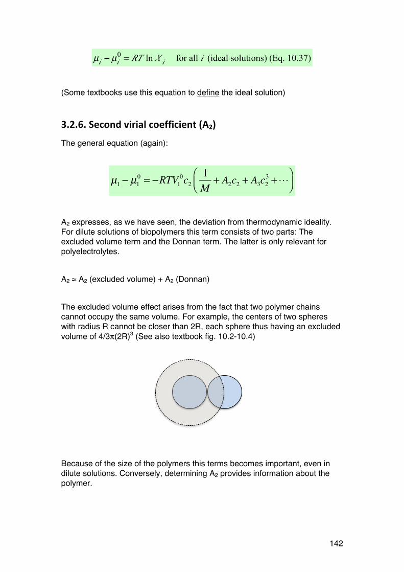
142

µi− µ

i

0= RT ln X

i for all i (ideal solutions) (Eq. 10.37)

(Some textbooks use this equation to define the ideal solution)

3.2.6.  Second  virial  coefficient  (A2)  

The general equation (again):

µ1 − µ10 = −RTV1

0c21M

+ A2c2 + A3c23 + ⋅⋅⋅⎛

⎝⎜⎞⎠⎟

A2 expresses, as we have seen, the deviation from thermodynamic ideality. For dilute solutions of biopolymers this term consists of two parts: The excluded volume term and the Donnan term. The latter is only relevant for polyelectrolytes. A2 ≈ A2 (excluded volume) + A2 (Donnan) The excluded volume effect arises from the fact that two polymer chains cannot occupy the same volume. For example, the centers of two spheres with radius R cannot be closer than 2R, each sphere thus having an excluded volume of 4/3π(2R)3 (See also textbook fig. 10.2-10.4)

Because of the size of the polymers this terms becomes important, even in dilute solutions. Conversely, determining A2 provides information about the polymer.

143

The contributions from the excluded volume for the basic shapes can be determined (no proof given):

2 2

2

3-5 22

2 2

2 2

22

2

( ) ( ) ( .10.63)2

4 16( ) Typically 3 10

3

( ) Typically

Avo

Avo

N uA general u excluded volume per macromolecule Eq

M

v R NA compact spheres ml mol g

M M

L vA rods

d M

π −

= =

= = ⋅ ⋅ ⋅

=-3 2

3 3 -4 2

2 2

2

1 10

16( ) Typically 1-5 10

3

AvoG

ml mol g

NA random coils R ml mol g

M

πγ

−

−

⋅ ⋅ ⋅

= ⋅ ⋅ ⋅

The contribution from Donnan effect (polyelectrolytes), which may in fact dominate, turns out to be:

2

2

2

1 1( ) ( .10.133)

4

, . .

BX

BX

zA Donnan Eq

M C

C molar concentration of added salt BX e g NaCl

⎛ ⎞= ⎜ ⎟

⎝ ⎠=

The Donnan effect will be discussed and explained in more detail in Section 3.4.

3.2.7.  A2:  High  or  low?  

Biopolymer scientists often refer to ‘high’ or ‘low’ A2 values. What does it mean? These are of course relative terms, and need to be considered in terms of the general equation:

µ1 − µ10 = −RTV1

0c21M

+ A2c2 + ⋅⋅⋅⎛⎝⎜

⎞⎠⎟

Low A2 means that the term A2c2 is much less than 1/M and can be ignored:

144

A2c2

1M

⇒ µ1 − µ10 = −RTV1

0c21M

In this case the A2c2 term does not contribute significantly to µ1-µ1

0. High A2 obviously means that

A2c2

1M

⇒ µ1 − µ10 = −RTV1

0c2( A2c2)

In this case the A2c2 term does contribute significantly to µ1-µ10. The effect of

A2 is consequently dependent on c2.

In practice: High values are in the range 10-3 (ml mol g-2) or higher

3.2.8.  A2:  Important  link  to  chain  statistics  

In Section 2.2.8 we introduced the concept ‘excluded volume’ for monomers in a single chain, leading to the intramolecular excluded volume factor (α2) which influences the radius of gyration and the average end-to-end distance:

We further introduced the influence of intramolecular forces on α, leading to: θ-conditions: α = 1 (excluded volume cancelled by weak attractive forces) Good solvent: α > 1 (excluded volume dominates) Bad solvent: α < 1 (attractive forces outweigh excluded volume) The argument leading to the θ-condition (balance between intramolecular excluded volume and weak attractive forces) can be applied also for the entire molecules (intermolecular attractive forces and excluded volume): θ-solvent: A2 = 0 Good solvent: A2 > 0 Bad solvent: A2 < 0

r2 =α 2C∞nl2

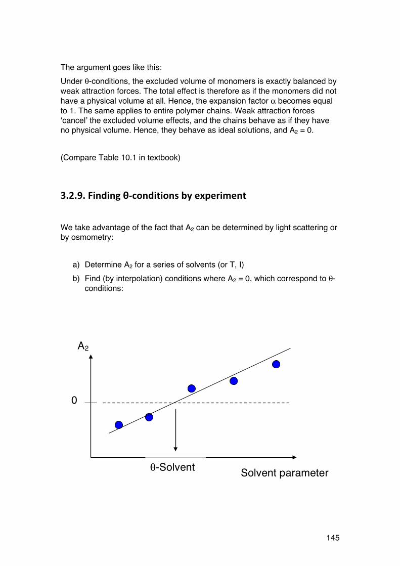
145

The argument goes like this: Under θ-conditions, the excluded volume of monomers is exactly balanced by weak attraction forces. The total effect is therefore as if the monomers did not have a physical volume at all. Hence, the expansion factor α becomes equal to 1. The same applies to entire polymer chains. Weak attraction forces ‘cancel’ the excluded volume effects, and the chains behave as if they have no physical volume. Hence, they behave as ideal solutions, and A2 = 0. (Compare Table 10.1 in textbook)

 

3.2.9.  Finding  θ-­‐conditions  by  experiment  

We take advantage of the fact that A2 can be determined by light scattering or by osmometry:

a) Determine A2 for a series of solvents (or T, I) b) Find (by interpolation) conditions where A2 = 0, which correspond to θ-

conditions:

0

Solvent parameter θ-Solvent

A2

2

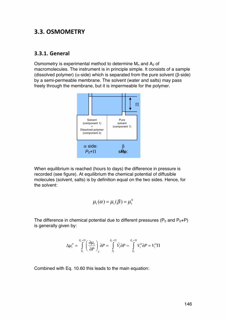
146

3.3.  OSMOMETRY  

3.3.1.  General  

Osmometry is experimental method to determine Mn and A2 of macromolecules. The instrument is in principle simple. It consists of a sample (dissolved polymer) (α-side) which is separated from the pure solvent (β-side) by a semi-permeable membrane. The solvent (water and salts) may pass freely through the membrane, but it is impermeable for the polymer.

When equilibrium is reached (hours to days) the difference in pressure is recorded (see figure). At equilibrium the chemical potential of diffusible molecules (solvent, salts) is by definition equal on the two sides. Hence, for the solvent:

0

1 1 1( ) ( )µ α µ β µ= =

The difference in chemical potential due to different pressures (P0 and P0+P) is generally given by:

Δµi

P=

∂µ1

∂P⎛⎝⎜

⎞⎠⎟

P0

P0+Π

∫T

∂P = V1

P0

P0+Π

∫ ∂P ≈ V1

0

P0

P0+Π

∫ ∂P = V1

0Π

Combined with Eq. 10.60 this leads to the main equation:

Solvent (component 1)

+ Dissolved polymer

(component 2)

Pure solvent

(component 1)

α side: P0+Π

β side: P0

Π

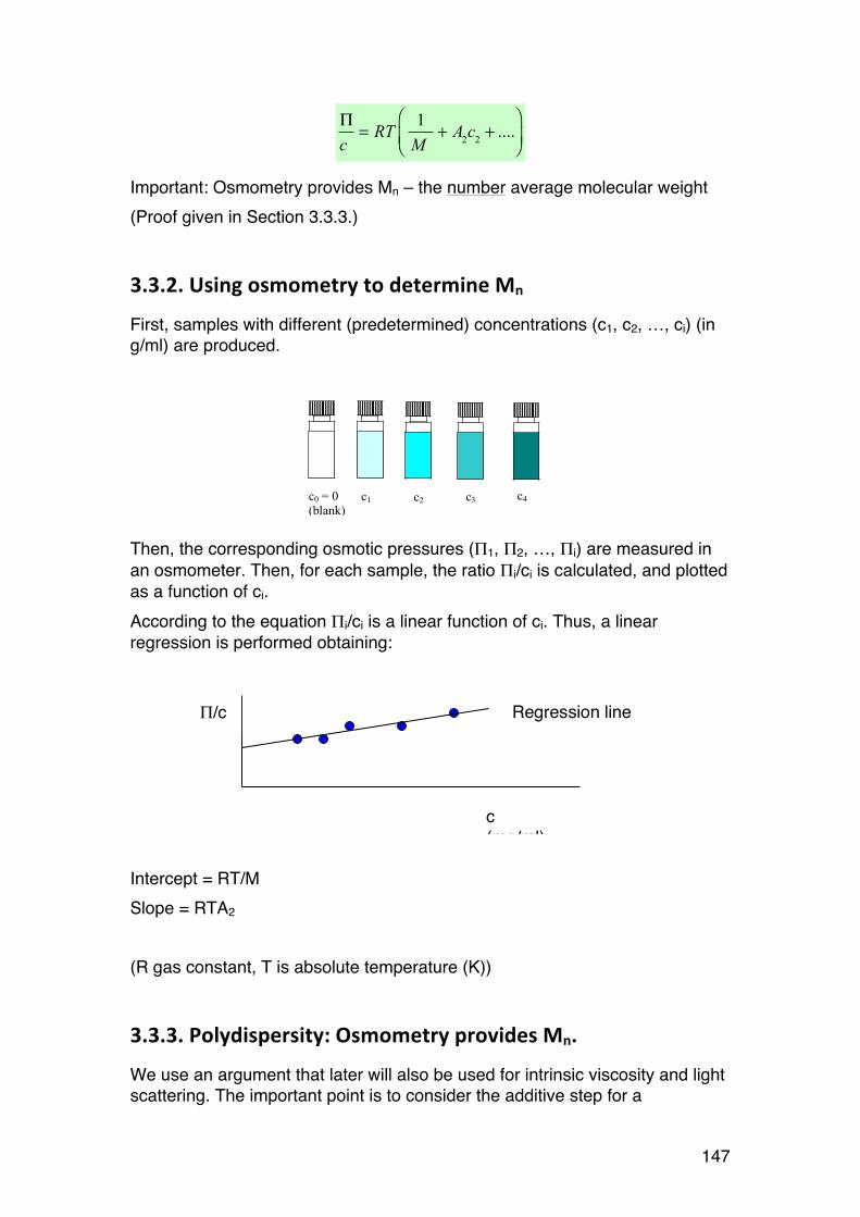
147

Πc

= RT1

M+ A

2c

2+ ....

⎛

⎝⎜⎞

⎠⎟

Important: Osmometry provides Mn – the number average molecular weight (Proof given in Section 3.3.3.)

3.3.2.  Using  osmometry  to  determine  Mn  

First, samples with different (predetermined) concentrations (c1, c2, …, ci) (in g/ml) are produced.

Then, the corresponding osmotic pressures (Π1, Π2, …, Πi) are measured in an osmometer. Then, for each sample, the ratio Πi/ci is calculated, and plotted as a function of ci. According to the equation Πi/ci is a linear function of ci. Thus, a linear regression is performed obtaining: Intercept = RT/M Slope = RTA2 (R gas constant, T is absolute temperature (K))

3.3.3.  Polydispersity:  Osmometry  provides  Mn.  

We use an argument that later will also be used for intrinsic viscosity and light scattering. The important point is to consider the additive step for a

c (mg/ml)

Π/c Regression line

c1 c2 c3 c4 c0 = 0

(blank)

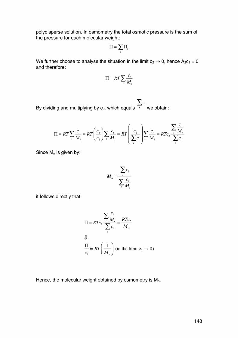
148

polydisperse solution. In osmometry the total osmotic pressure is the sum of the pressure for each molecular weight:

Π = Πi

i

∑

We further choose to analyse the situation in the limit c2 → 0, hence A2c2 = 0 and therefore:

Π = RTci

Mii

∑

By dividing and multiplying by c2, which equals c1

i

∑we obtain:

Π = RTci

Mii

∑ = RTc2

c2

⎛

⎝⎜⎞

⎠⎟ci

Mii

∑ = RTc2

ci

i

∑

⎛

⎝

⎜⎜

⎞

⎠

⎟⎟

ci

Mii

∑ = RTc2

ci

Mii

∑ci

i

∑

Since Mn is given by:

Mn=

ci

i

∑

ci

Mii

∑

it follows directly that

Π = RTc2

ci

Mii

∑ci

i

∑=RTc

2

Mn

Πc

2

= RT1

Mn

⎛

⎝⎜⎞

⎠⎟ (in the limit c

2→ 0)

Hence, the molecular weight obtained by osmometry is Mn.

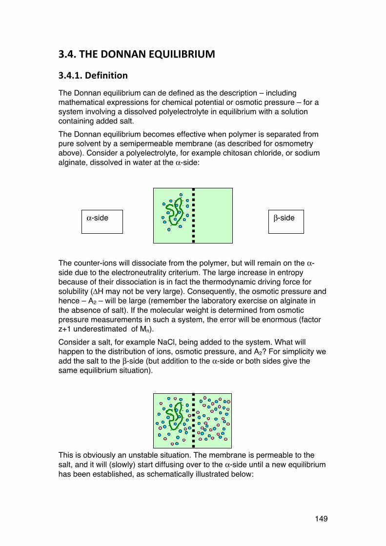
149

3.4.  THE  DONNAN  EQUILIBRIUM  

3.4.1.  Definition  

The Donnan equilibrium can de defined as the description – including mathematical expressions for chemical potential or osmotic pressure – for a system involving a dissolved polyelectrolyte in equilibrium with a solution containing added salt. The Donnan equilibrium becomes effective when polymer is separated from pure solvent by a semipermeable membrane (as described for osmometry above). Consider a polyelectrolyte, for example chitosan chloride, or sodium alginate, dissolved in water at the α-side:

The counter-ions will dissociate from the polymer, but will remain on the α-side due to the electroneutrality criterium. The large increase in entropy because of their dissociation is in fact the thermodynamic driving force for solubility (ΔH may not be very large). Consequently, the osmotic pressure and hence – A2 – will be large (remember the laboratory exercise on alginate in the absence of salt). If the molecular weight is determined from osmotic pressure measurements in such a system, the error will be enormous (factor z+1 underestimated of Mn). Consider a salt, for example NaCl, being added to the system. What will happen to the distribution of ions, osmotic pressure, and A2? For simplicity we add the salt to the β-side (but addition to the α-side or both sides give the same equilibrium situation).

This is obviously an unstable situation. The membrane is permeable to the salt, and it will (slowly) start diffusing over to the α-side until a new equilibrium has been established, as schematically illustrated below:

+

+

+ + +

+ +

+

+ +

+

+ + +

+ α-side β-side

+

+

+ + +

+ +

+

+ +

+

+ + +

+

+ - + - + - + -

+

- + - + - + - - +

-

+

+

-

+ - +

+

- + -

+ -

+ -

+ - + - + - + -

+ - + - +

- + - + - + +

- + - + - + -

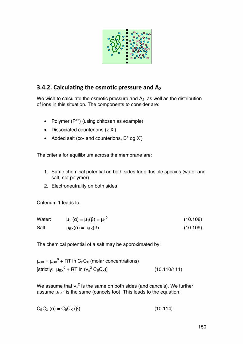
150

3.4.2.  Calculating  the  osmotic  pressure  and  A2  

We wish to calculate the osmotic pressure and A2, as well as the distribution of ions in this situation. The components to consider are:

• Polymer (Pz+) (using chitosan as example) • Dissociated counterions (z X-) • Added salt (co- and counterions, B+ og X-)

The criteria for equilibrium across the membrane are:

1. Same chemical potential on both sides for diffusible species (water and salt, not polymer)

2. Electroneutrality on both sides Criterium 1 leads to: Water: μ1 (α) = μ1(β) = μ1

0 (10.108) Salt: μBX(α) = μBX(β) (10.109) The chemical potential of a salt may be approximated by: μBX = μBX

0 + RT ln CBCX (molar concentrations) [strictly: μBX

0 + RT ln (γ±2 CBCX)] (10.110/111)

We assume that γ±

2 is the same on both sides (and cancels). We further assume μBX

0 is the same (cancels too). This leads to the equation: CBCX (α) = CBCX (β) (10.114)

+

+

+ + +

+ +

+

+ +

+

+ + +

+

+ - + - + - + - + - + - + - + - - + - + + - + - + + - + -

+ - + - + - + - + - + - + - + - + - + - + - + + - + - + - + -

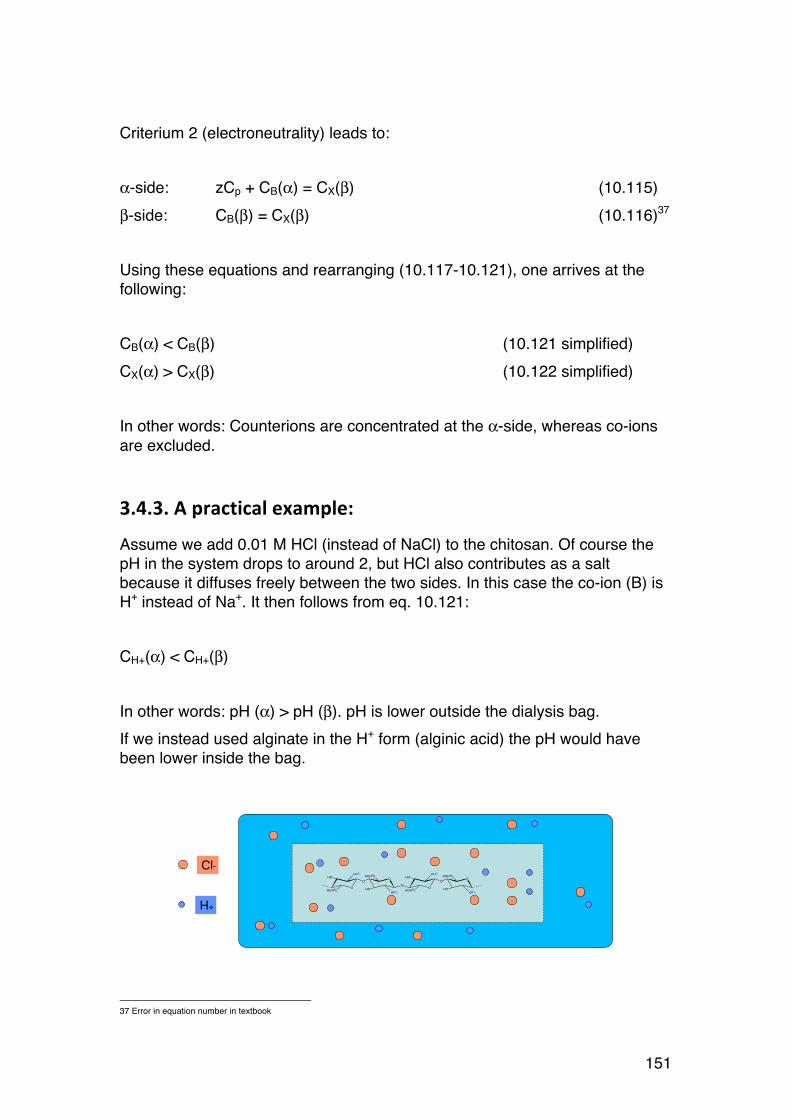
151

Criterium 2 (electroneutrality) leads to: α-side: zCp + CB(α) = CX(β) (10.115) β-side: CB(β) = CX(β) (10.116)37 Using these equations and rearranging (10.117-10.121), one arrives at the following: CB(α) < CB(β) (10.121 simplified) CX(α) > CX(β) (10.122 simplified) In other words: Counterions are concentrated at the α-side, whereas co-ions are excluded.

3.4.3.  A  practical  example:  

Assume we add 0.01 M HCl (instead of NaCl) to the chitosan. Of course the pH in the system drops to around 2, but HCl also contributes as a salt because it diffuses freely between the two sides. In this case the co-ion (B) is H+ instead of Na+. It then follows from eq. 10.121: CH+(α) < CH+(β) In other words: pH (α) > pH (β). pH is lower outside the dialysis bag. If we instead used alginate in the H+ form (alginic acid) the pH would have been lower inside the bag.

37 Error in equation number in textbook

NH3+

OHOH2C

NH3+HOO

OHOH2C

HOO

NH3+

OHOH2C

NH3+HOO

OHOH2C

HO

Cl-

H+

152

 3.4.4.  A2:  The  ideal  Donnan  term  

The redistribution of salt contributes to A2 (in addition to the excluded volume term), and may often dominate completely. This can be estimated with some simplifications. Assuming we work in dilute solutions so that A2 does not contribute (1/M >> A2c) For each species we have:

Π = RT cM

= RTC (Note C is here the molar concentration)

For the macromolecule, there is only a contribution to Π on the α side. For the salt, there is a difference in molar concentration between the α-side and the β-side. Therefore, their contribution to the osmotic pressure on the α-side is:

ΠB = RT CB(α )−CB(β )[ ]ΠX = RT CX (α )−CX (β )[ ]

The total osmotic pressure on the α-side is the sum of each term:

Π = ΠII∑ =ΠP +ΠB +ΠX = RT CP + CB (α )−CB (β )[ ]+ CX (α )−CX (β )[ ]{ } (10.128)

Assuming a large excess of salt (CBX) is added, and that the difference in salt concentration is small on the α and β sides, the equation simplifies (after a few intermediate calculations, see textbook) to:

Π = RT Cp +z2Cp

2

4CBX

⎡

⎣⎢

⎤

⎦⎥ = RT

c2M2

+ z2c22

4M22CBX

⎡

⎣⎢

⎤

⎦⎥

or

Πc2

= RT 1M2

+ z2

4M22CBX

c2⎡

⎣⎢

⎤

⎦⎥

Hence,

153

A2 (Donnan) =z2

4M22CBX

This equation shows two important features: a) The A2 for polyelectrolytes increases with the number of charges per molecule. Example: Alginate has a single charge per monomer (-COO-), i.e. one mole of charges per 198 g: z/M2 = 1/198. If we prepare an alginate where 50% of the carboxyls are COOH (acid form) and 50% are on the COOHNa form, only the Na+ ions dissociate (COOH is a weak acid, i.e. marginal dissociation), the z/M is 0.5/198, and A2 reduces 4 times. b) A2 is inversely proportional to the salt concentration (or ionic strength I). Hence increasing CNaCl from e.g. 1 mM to 1 M leads to a 1000-fold decrease in A2. This is manifested in a drastic lowering of the osmotic pressure (as you have seen in the laboratory). Sufficiently high ionic strength effectively eliminates the polyelectrolyte effect, and osmometry will give the correct molecular weight (Mn!) using the standard approach.

3.4.5.  Osmotic  pressure  of  polyelectrolytes:  Calculations  and  examples.  

(Dilute polymer solutions only) a) Uncharged polymers Uncharged polymers behave as any other uncharged molecule. Hence, the osmotic pressure is given by:

∏c= RT 1

M+ A2c

⎛⎝⎜

⎞⎠⎟

c: Polymer concentration in g/ml M: Molecular weight (Mn if polydisperse) A2: Second virial coefficient R = 8.315 J/mol K = 0.0820 L atm/mol K T = absolute temperature (K)

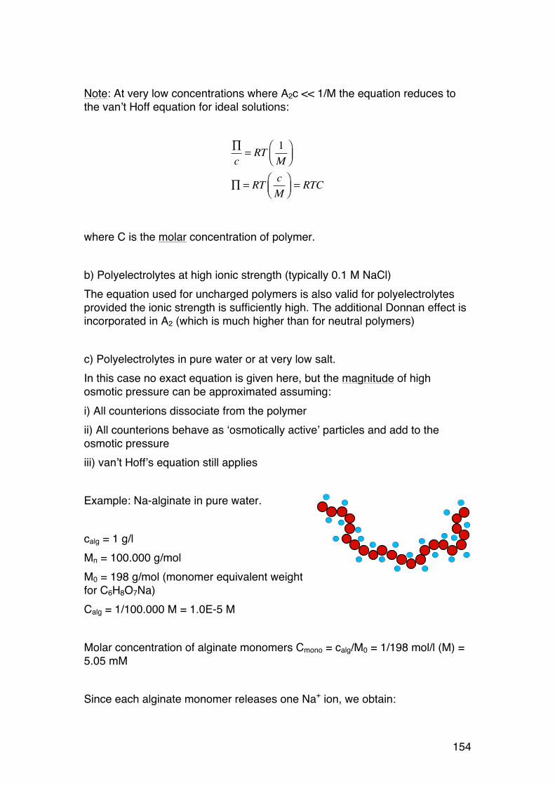
154

Note: At very low concentrations where A2c << 1/M the equation reduces to the van’t Hoff equation for ideal solutions:

∏c= RT 1

M⎛⎝⎜

⎞⎠⎟

∏ = RT cM

⎛⎝⎜

⎞⎠⎟ = RTC

where C is the molar concentration of polymer. b) Polyelectrolytes at high ionic strength (typically 0.1 M NaCl) The equation used for uncharged polymers is also valid for polyelectrolytes provided the ionic strength is sufficiently high. The additional Donnan effect is incorporated in A2 (which is much higher than for neutral polymers) c) Polyelectrolytes in pure water or at very low salt. In this case no exact equation is given here, but the magnitude of high osmotic pressure can be approximated assuming: i) All counterions dissociate from the polymer ii) All counterions behave as ‘osmotically active’ particles and add to the osmotic pressure iii) van’t Hoff’s equation still applies Example: Na-alginate in pure water. calg = 1 g/l Mn = 100.000 g/mol M0 = 198 g/mol (monomer equivalent weight for C6H8O7Na) Calg = 1/100.000 M = 1.0E-5 M Molar concentration of alginate monomers Cmono = calg/M0 = 1/198 mol/l (M) = 5.05 mM Since each alginate monomer releases one Na+ ion, we obtain:

155

CNa = Cmono = calg/M0 = 5.05 mM = 5.05E-3 M (500 x that of the polymer chains) The total molar concentration of ‘osmotically active’ particles is thus: Ctotal = Calg + CNa = 1.0E-5 M + 5.05E-3 M = 5.06E-3 M ≈ can

Hence, the number of ions totally dominates over the number of polymer molecules, which generally can be ignored in such calculations. Using the van’t Hoff equation we obtain:

Some textbooks use the (average) number of charges per molecule (z) in the equations: CNa = zCa lg

∏tot =∏a lg +∏Na = RTCa lg + RTCNa = RTCa lg + RT zCa lg( ) = 1+ z( )RTCa lg ≈ zRTCa lg By further calculation we find that the result is in fact independent of the molecular weight of the alginate:

∏tot ≈ ∏Na = RT zca lg

M⎛⎝⎜

⎞⎠⎟

Inserting z = MM0

∏tot ≈ ∏Na = RTMM0

ca lg

M⎛⎝⎜

⎞⎠⎟= RT

ca lg

M0

⎛⎝⎜

⎞⎠⎟

If no ions dissociated, Ctotal would be 1.0E-5 M, i.e. 0.2% of the value above. Hence, the osmotic pressure would be roughly 500 times lower.

∏tot =∏a lg +∏Na = RTCa lg + RTCNa = 0.12atm

156

 

3.4.  ORDER-­‐DISORDER  TRANSITIONS  

To be completed. See textbook.

157

PART  4.  PROTEINS  

   

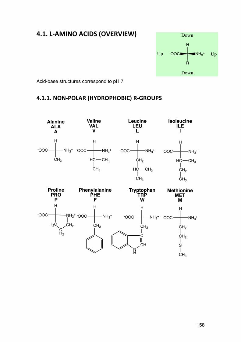
158

4.1.  L-­‐AMINO  ACIDS  (OVERVIEW)  

Acid-base structures correspond to pH 7

4.1.1.  NON-­‐POLAR  (HYDROPHOBIC)  R-­‐GROUPS  

H

NH3+-OOC

CH3

H

NH3+-OOC

HC

H

NH3+-OOC

CH2

H

NH3+-OOC

HC

CH3

CH3

HC CH3

CH3

CH2

CH3

CH3

AlanineALAA

ValineVALV

LeucineLEUL

IsoleucineILEI

H

NH2+-OOC

H2CCH2

CH2

ProlinePROP

H

NH3+-OOC

CH2

PhenylalaninePHEF

H

NH3+-OOC

CH2

C

CH

TryptophanTRPW

NH

H

NH3+-OOC

CH2

CH2

S

MethionineMETM

CH3

H

NH3+-OOC

R

Down

Down

UpUp

159

4..1.2.  POLAR  (HYDROPHILIC)  R-­‐GROUPS  

H

NH3+-OOC

H

H

NH3+-OOC

CH2

H

NH3+-OOC

HC

H

NH3+-OOC

CH2OH CH3 SH

GlycineGLYG

SerineSERS

ThreonineTHRT

CysteineCYSC

TyrosineTYRY

AsparagineASNN

GlutamineGLNQ

OH

H

NH3+-OOC

CH2

OH

H

NH3+-OOC

CH2

CO NH2

H

NH3+-OOC

CH2

CH2

CO NH2

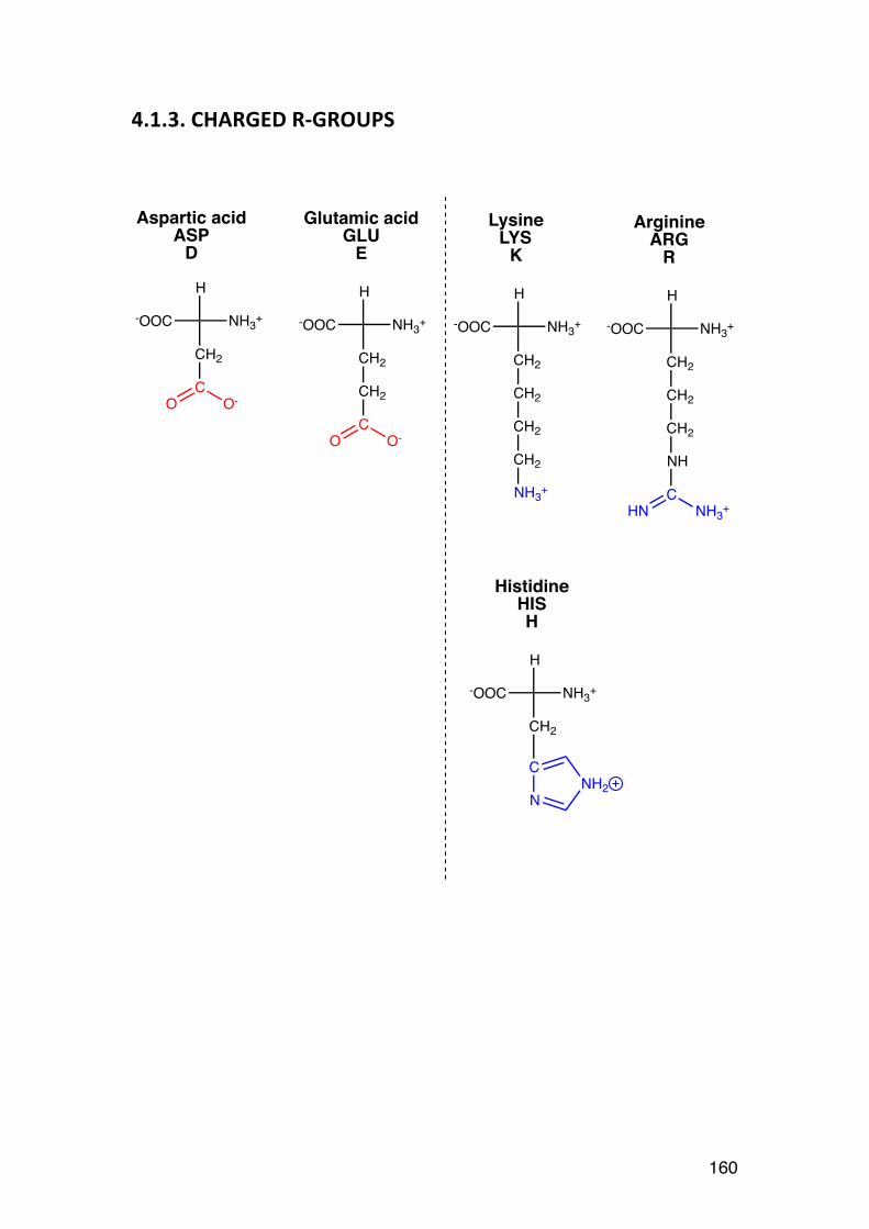
160

4.1.3.  CHARGED  R-­‐GROUPS  

   

Aspartic acidASP

D

Glutamic acidGLU

E

H

NH3+-OOC

CH2

CO O-

H

NH3+-OOC

CH2

CH2

CO O-

LysineLYS

K

H

NH3+-OOC

CH2

CH2

CH2

CH2

NH3+

ArginineARG

R

H

NH3+-OOC

CH2

CH2

CH2

NH

CHN NH3+

HistidineHISH

H

NH3+-OOC

CH2

C

NNH2

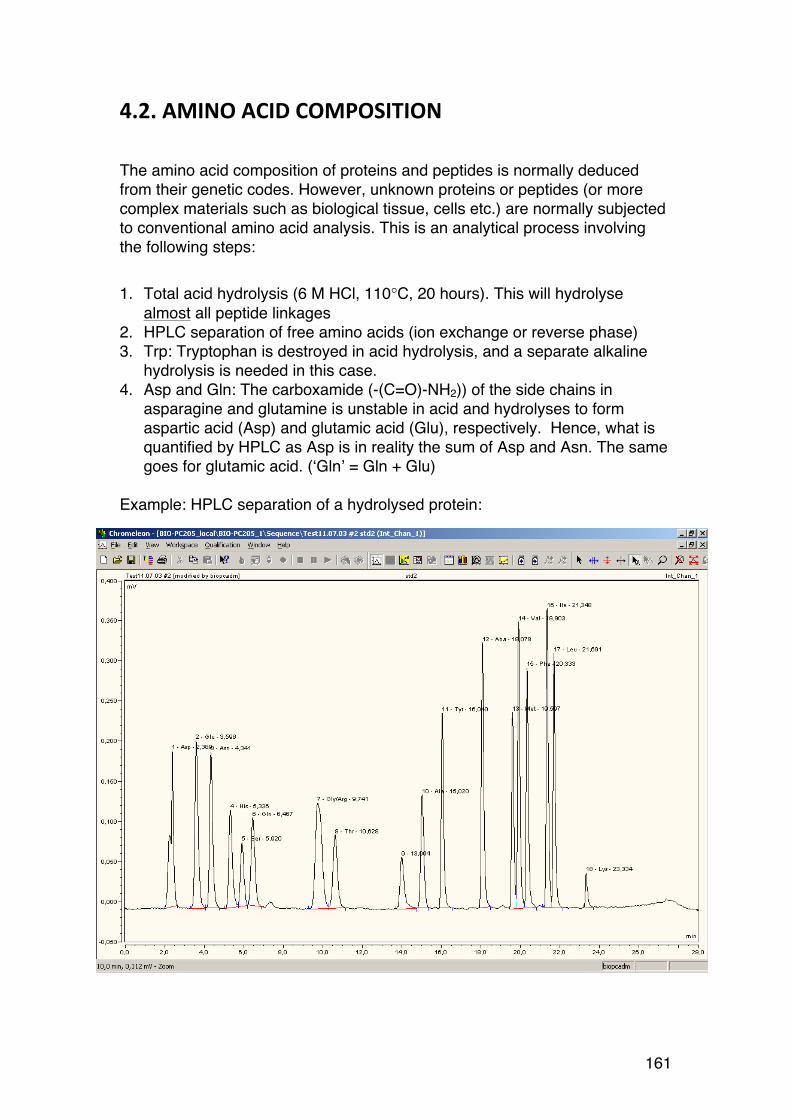
161

4.2.  AMINO  ACID  COMPOSITION  

The amino acid composition of proteins and peptides is normally deduced from their genetic codes. However, unknown proteins or peptides (or more complex materials such as biological tissue, cells etc.) are normally subjected to conventional amino acid analysis. This is an analytical process involving the following steps: 1. Total acid hydrolysis (6 M HCl, 110°C, 20 hours). This will hydrolyse

almost all peptide linkages 2. HPLC separation of free amino acids (ion exchange or reverse phase) 3. Trp: Tryptophan is destroyed in acid hydrolysis, and a separate alkaline

hydrolysis is needed in this case. 4. Asp and Gln: The carboxamide (-(C=O)-NH2)) of the side chains in

asparagine and glutamine is unstable in acid and hydrolyses to form aspartic acid (Asp) and glutamic acid (Glu), respectively. Hence, what is quantified by HPLC as Asp is in reality the sum of Asp and Asn. The same goes for glutamic acid. (‘Gln’ = Gln + Glu)

Example: HPLC separation of a hydrolysed protein:

   

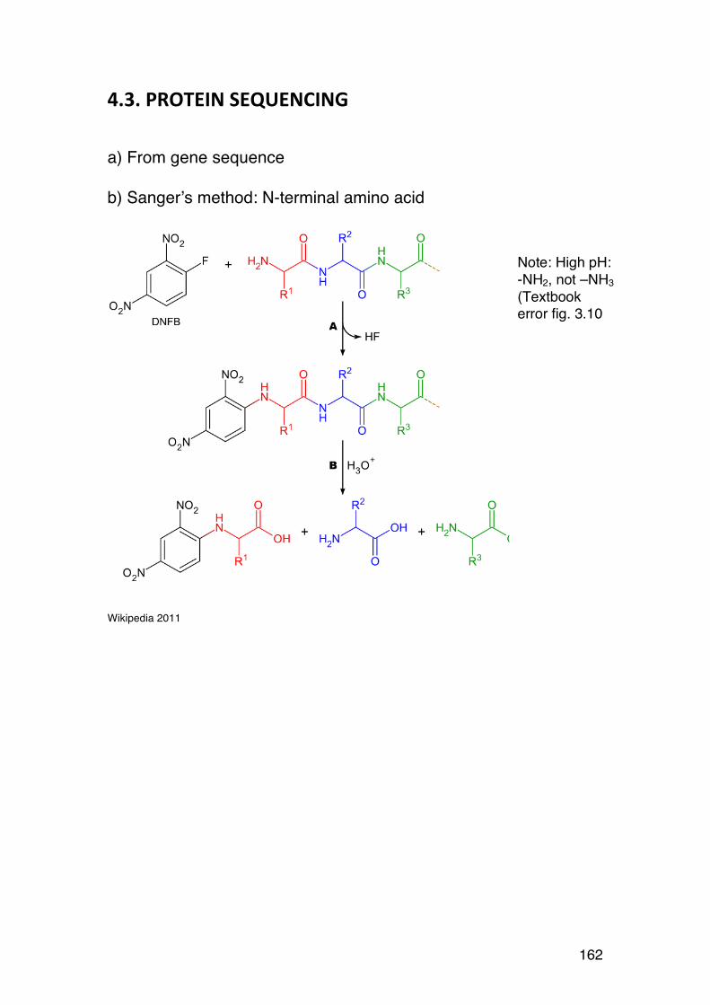
162

4.3.  PROTEIN  SEQUENCING  

a) From gene sequence b) Sanger’s method: N-terminal amino acid

Wikipedia 2011

Note: High pH: -NH2, not –NH3 (Textbook error fig. 3.10

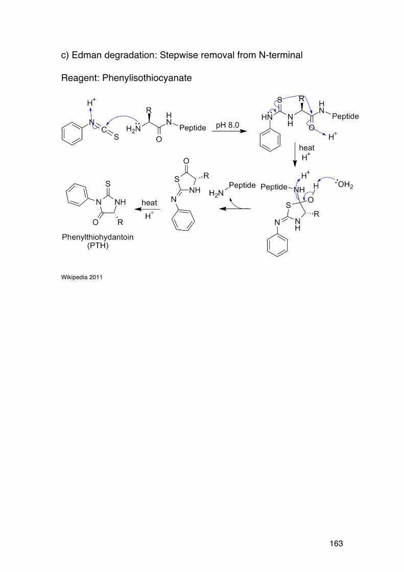
163

c) Edman degradation: Stepwise removal from N-terminal Reagent: Phenylisothiocyanate

Wikipedia 2011

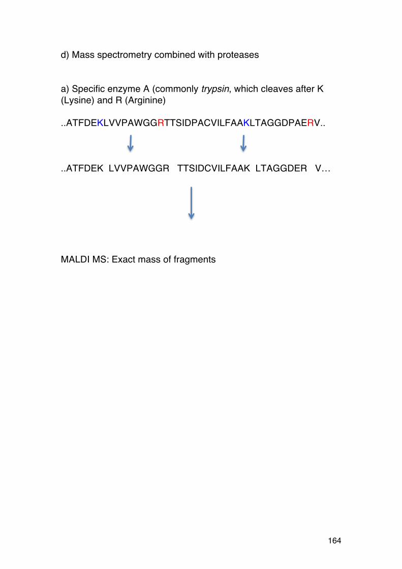
164

d) Mass spectrometry combined with proteases a) Specific enzyme A (commonly trypsin, which cleaves after K (Lysine) and R (Arginine) ..ATFDEKLVVPAWGGRTTSIDPACVILFAAKLTAGGDPAERV.. ..ATFDEK LVVPAWGGR TTSIDCVILFAAK LTAGGDER V… MALDI MS: Exact mass of fragments

 

165

4.4.  PROTEIN  STRUCTURE  

This part consists of slides prepared by Prof. A. Dikiy.

166

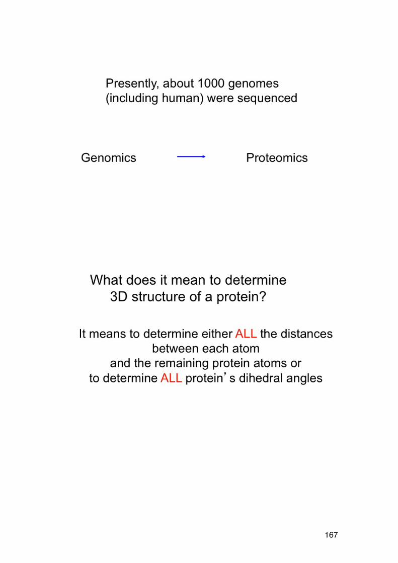
167

168

169

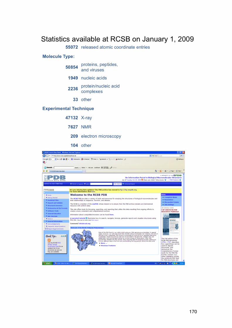
170

171

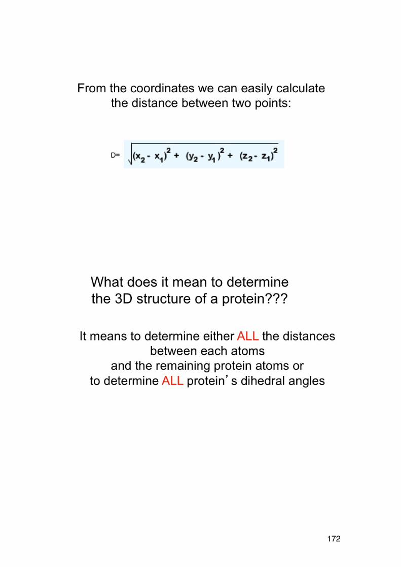
172

173

174

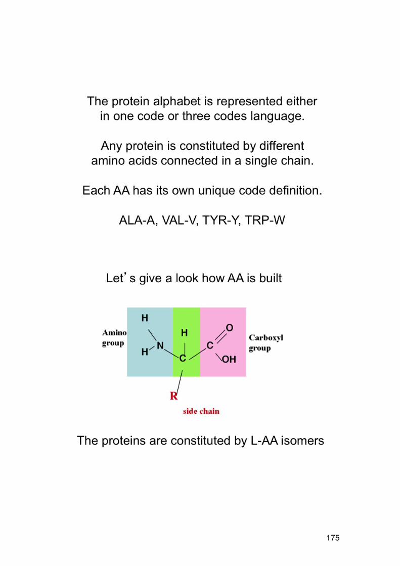
175

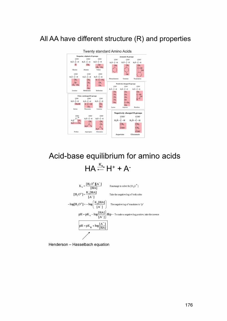
176

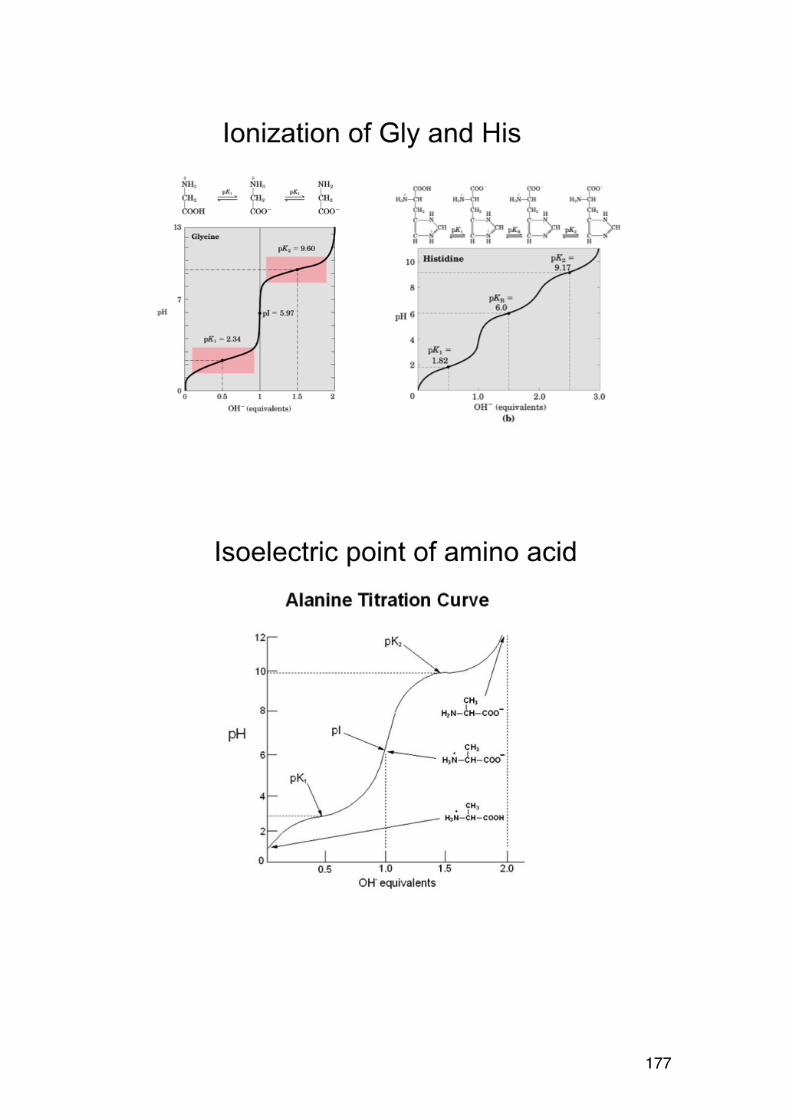
177

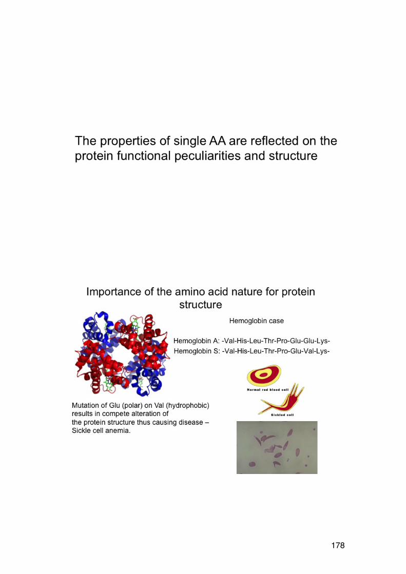
178

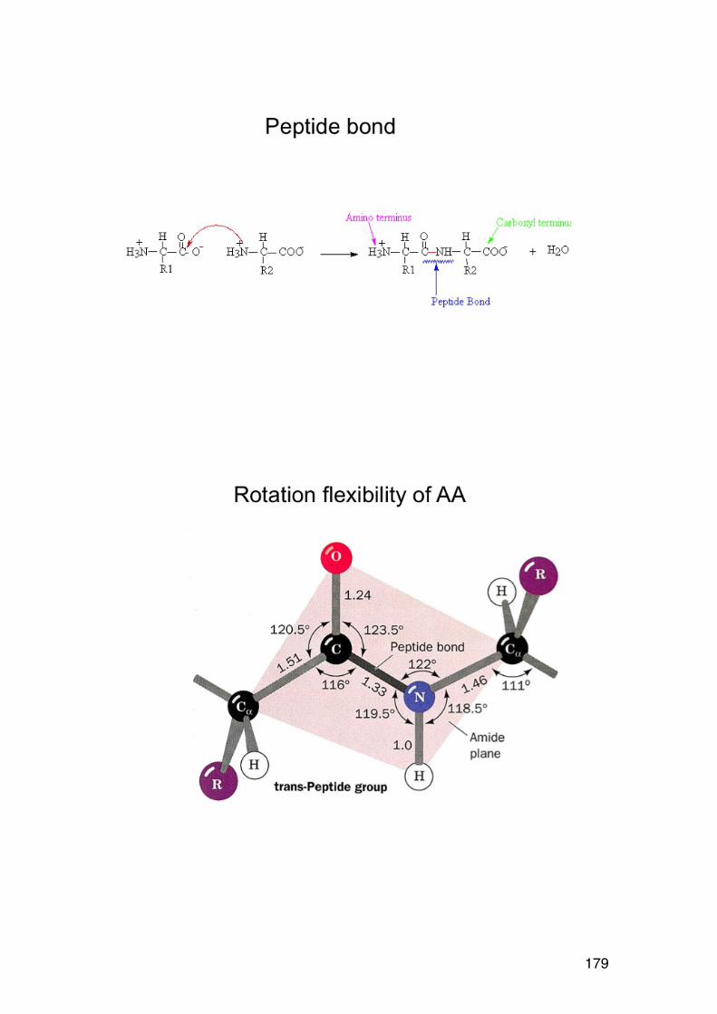
179

180

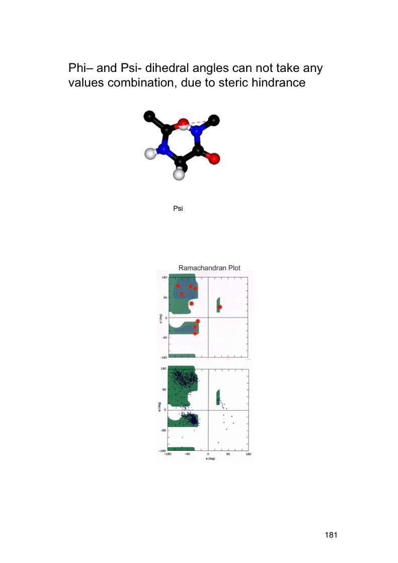
181

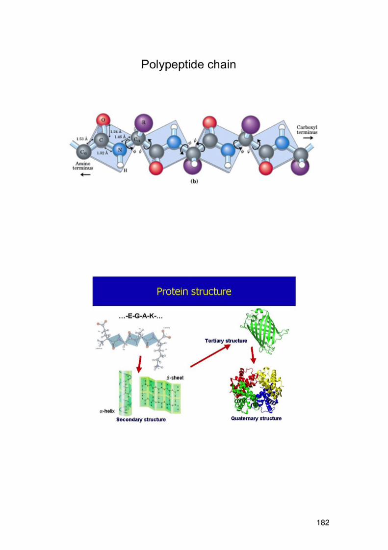
182

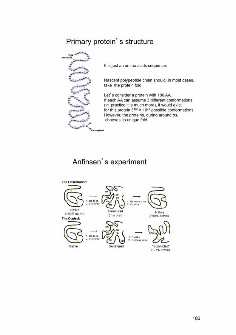
183

184

α-helix β-sheet

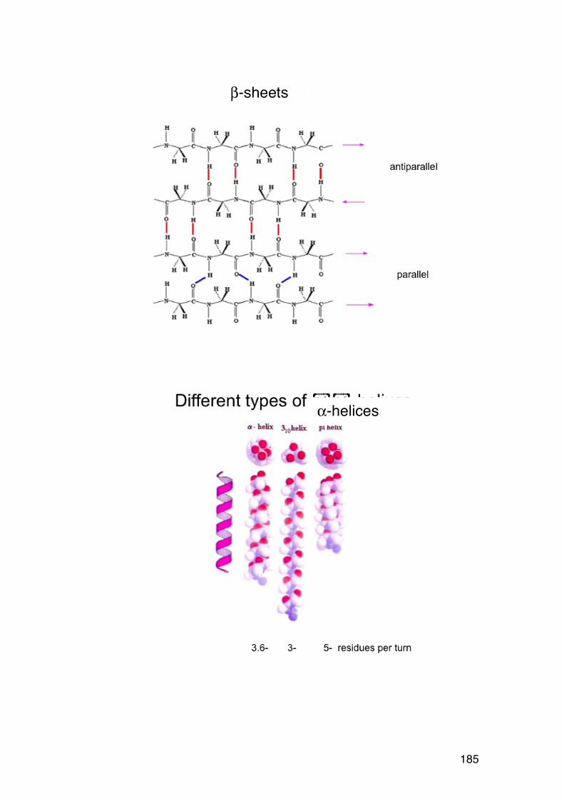
185

β-sheets

α-helices

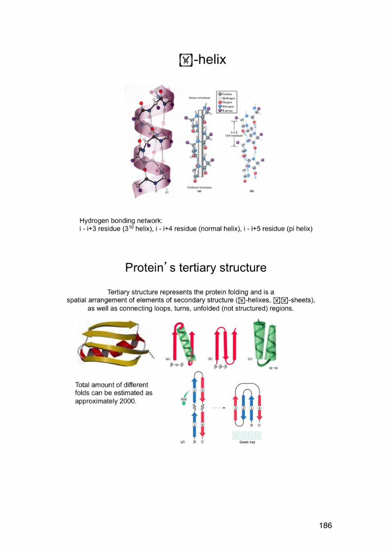
186

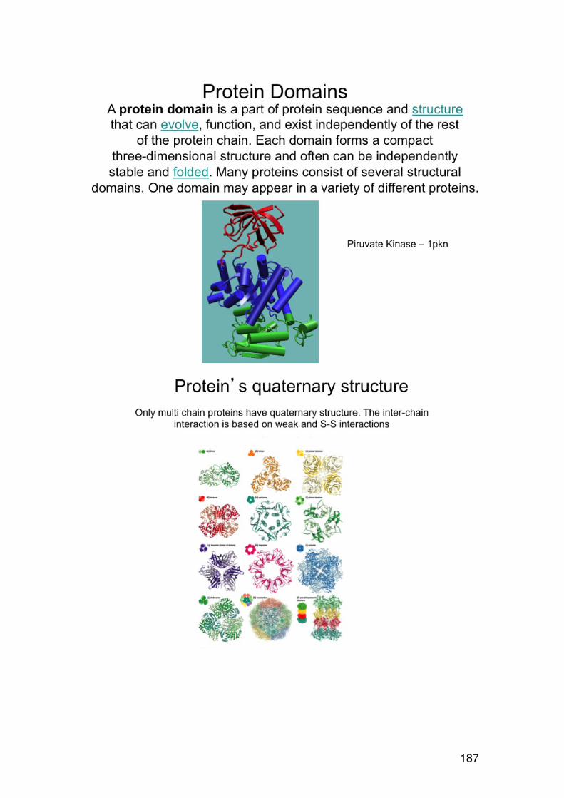
187

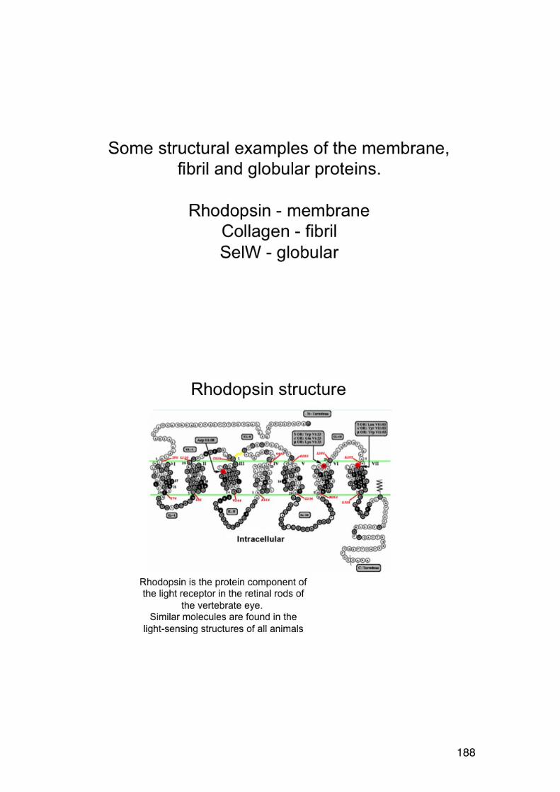
188

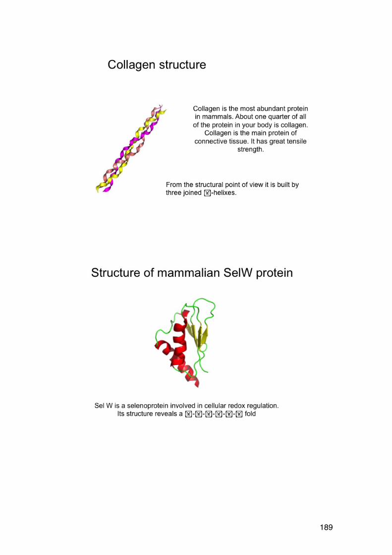
189

190

191

PART  5.  STABILITY  AND  DEGRADATION  

   

192

5.1.  DEGRADATION  OF  POLYSACCHARIDES:  CHEMISTRY  

Polysaccharides can de depolymerised (fragmented) as can any polymer (synthetic or biological). Different reaction mechanisms may be involved: chemical, physical or biological. One example is the biodegradation of cellulose by certain fungi (e.g. Trichoderma reseei) which produce cellulases – enzymes which degrade cellulose. Endocellulases break the long cellulose chains into smaller fragments, and exocellulases then cleaves off cellobiose (Glc-Glc) from the chain termini. Other enzymes cleave the cellobiose molecules to obtain glucose, which is further metabolized by the cells. Complete cleavage of all linkages in a polysaccharide is required to identify and quantify the component sugars. This is typically achieved by total hydrolysis in 2N trifluoroacetic acid (strong, volatile acid) at 120°C for 2-4 hours. The liberated monosaccharides are easily identified and quantified by GC-MS (after derivatization) or HPLC methods. The major challenge is the presence of very resistant linkages and side reactions when labile sugars are involved. Industrial polysaccharides such as alginates are sometimes subjected to mild (partial) hydrolysis to reduce the molecular weight from 3-400.000 Da to 30-40.000 Da because this molecular weight range is optimal in certain applications. In other cases it is essential to prevent degradation to preserve the highest possible molecular weight (example: special cellulose). In all cases, it becomes important to know the detailed mechanism of degradation as well as the rate of cleavage of glycosidic bonds.

5.1.1.  Glycosidic  linkages  

Most glycosidic linkages are chemically speaking acetals38, which are formed by the reaction between a hemiacetal (the sugar ring) and an alcohol. The figure illustrates hemiacetal formation in D-glucose, and subsequent acetal formation by reaction with an –OH in a second D-glucose residue:

38 For a keto sugar (e.g. fructose) the linkage will be a ketal

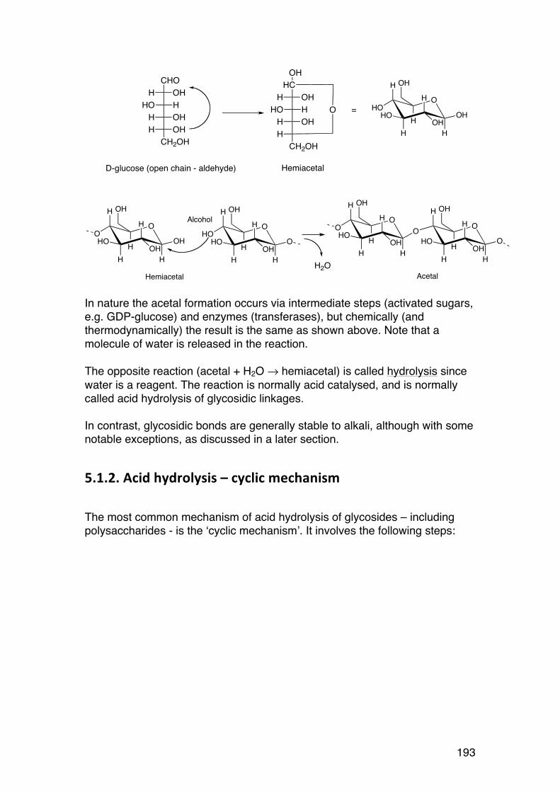
193

In nature the acetal formation occurs via intermediate steps (activated sugars, e.g. GDP-glucose) and enzymes (transferases), but chemically (and thermodynamically) the result is the same as shown above. Note that a molecule of water is released in the reaction. The opposite reaction (acetal + H2O → hemiacetal) is called hydrolysis since water is a reagent. The reaction is normally acid catalysed, and is normally called acid hydrolysis of glycosidic linkages. In contrast, glycosidic bonds are generally stable to alkali, although with some notable exceptions, as discussed in a later section.

5.1.2.  Acid  hydrolysis  –  cyclic  mechanism  

The most common mechanism of acid hydrolysis of glycosides – including polysaccharides - is the ‘cyclic mechanism’. It involves the following steps:

CHOOHHHHOOHHOHH

CH2OH

D-glucose (open chain - aldehyde)

HCOHHHHOOHH

HCH2OH

OH

O

Hemiacetal

O

H

HO

H

HO

H

HOHH OH

OH

=

O

H

O

H

HO

H

HOHH

OH

OH

Hemiacetal

O

H

HO

H

HO

H

HOHH

O

OHAlcohol O

H

O

H

HO

H

HOHH

O

OH

O

H

H

HO

H

HOHH

O

OH

AcetalH2O

194

1. Protonation of the glycosidic oxygen (weakly basic). Fast reaction 2. The linkage between C1 and the protonated oxygen atom is cleaved. This

heterolysis is the rate-limiting step (slow). The released substituent (the ‘aglycon’) (HO-R) is released.

3. As a consequence a carbocation is formed at C1. It is resonance stabilized with the ring oxygen. The partial double bond changes the ring conformation (planar ‘halfchair’ structure C1-C2-C5-O5).

4. The carbocation reacts with a molecule of water, and splits of a proton. The result is a reducing sugar (hemiacetal).

5. Note that H+ is recycled, i.e. it acts like a catalyst. Acid hydrolysis is reversible. At high concentrations of reducing sugars ‘reversion products’ may be formed by reaction between C1 and one of the OH- groups in another sugar. For analytical uses (sugar analysis) it is therefore important to use a sufficiently low concentration to avoid by-products during acid hydrolysis.

O

H

HO

H

HO

H

HOHH

O

OH

R

+ H+

O

H

HO

H

HO

H

HOHH

HO

OH

R

O

H

HO

H

HO

H

HOHH

OHHO-R

Slow(rate limiting step)

Carbocation (carbonium ion)Partial double bond to C1-O5 =>planar structure+ H2O

O

H

HO

H

HO

H

HOHH

OH2

OH

- H+ O

H

HO

H

HO

H

HOHH OH

OH

Glycoside (acetal)

195

5.1.3.  Different  sugars  are  hydrolysed  at  very  different  rates  

Certain sugars are very sensitive to acid hydrolysis, and require only (relatively) mild conditions for complete hydrolysis. Among the most sensitive sugars are the sialic acids, which are found as terminal sugars in many glycoproteins.

N-acetyl-neuraminic acid

NANA (N-acetyl-neuramic acid) can be selectively cleaved from adjacent sugars by mild conditions (0.05 M H2SO4, 80°C, 60 min). Note NANA is a 2-deoxy sugar, which are generally hydrolysed 500 to 1000 times faster than the corresponding glucose derivative. Also, NANA is a keto sugar (convince yourself by drawing the corresponding Fisher structure). Ketoses are more sensitive to acids than the corresponding aldose.

3,6-anhydro-sugars, which are found in carrageenans and agarose, are quite sensitive to acids. Hence, these polysaccharides degrade at low pH, in particular if the temperature is increased. The rate constant for degradation at pH 1 at 37°C is around 10-3 h-1 (Hjerde et al. (1996), Carbohydr. Res., 288, 175-187). Hence, carrageenans will degrade in the human stomach, producing oligosaccharides.

6-deoxyhexoses such as L-rhamnose (left) or L-fucose are hydrolysed 5-25 times more rapidly than galactose and glucose. The latter typically requires 1 M H2SO4, 6h, 100°C for complete acid hydrolysis.

Uronic acids are known to be quite resistant to acid hydrolysis. Conditions needed for complete hydrolysis also lead to destruction of the liberated uronic acids.

O

COOH

O

OH

HN

HOH2CR

H3C

O

OHH

HO H

O O

OH

HO

HO

H3C R

L-rhamnose (6-deoxy-L-mannose)

O

HO

HOOH

COOH

OR

D-glucuronic acid (GlcA)

O

H2CO

OH

H

O

R

R

3,6-anhydro-D-galactose (4 linked)

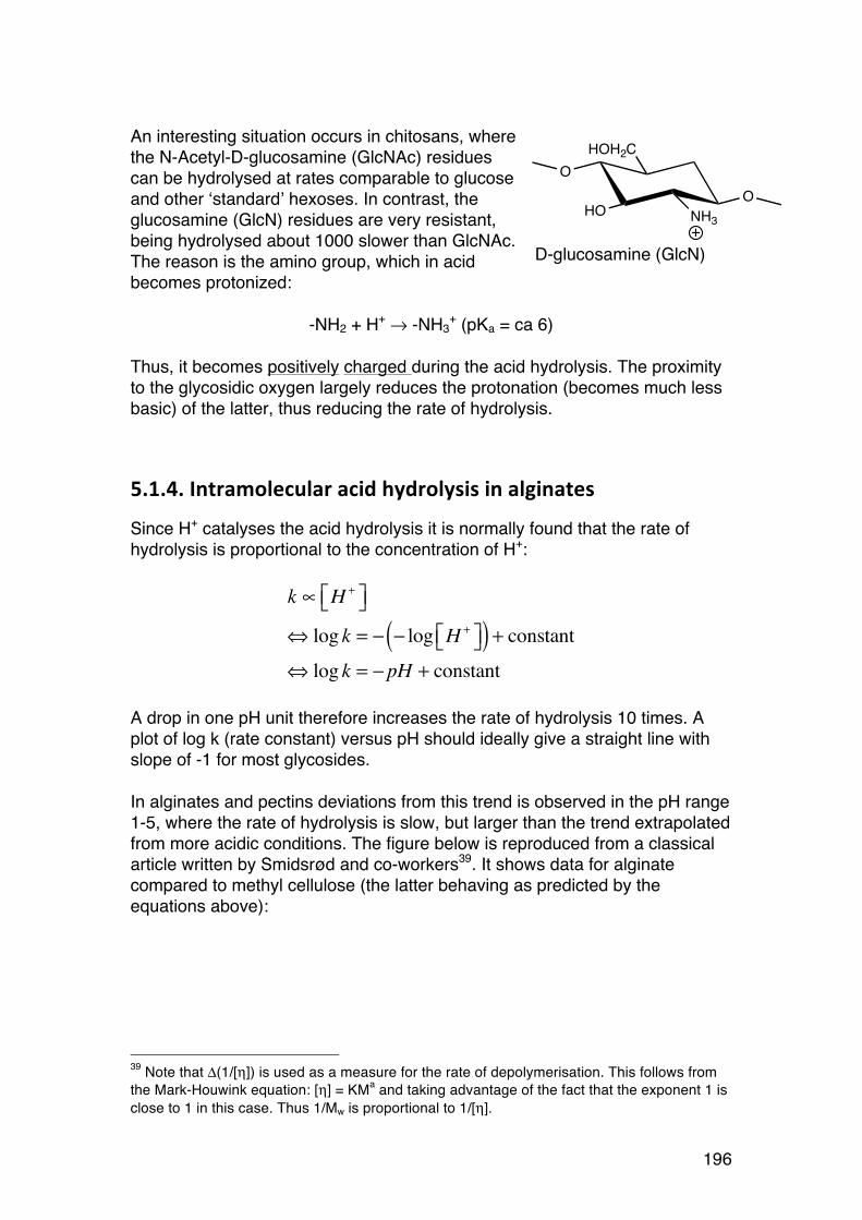
196

An interesting situation occurs in chitosans, where the N-Acetyl-D-glucosamine (GlcNAc) residues can be hydrolysed at rates comparable to glucose and other ‘standard’ hexoses. In contrast, the glucosamine (GlcN) residues are very resistant, being hydrolysed about 1000 slower than GlcNAc. The reason is the amino group, which in acid becomes protonized:

-NH2 + H+ → -NH3+ (pKa = ca 6)

Thus, it becomes positively charged during the acid hydrolysis. The proximity to the glycosidic oxygen largely reduces the protonation (becomes much less basic) of the latter, thus reducing the rate of hydrolysis.

5.1.4.  Intramolecular  acid  hydrolysis  in  alginates  

Since H+ catalyses the acid hydrolysis it is normally found that the rate of hydrolysis is proportional to the concentration of H+:

k ∝ H +⎡⎣ ⎤⎦⇔ log k = − − log H +⎡⎣ ⎤⎦( ) + constant⇔ log k = − pH + constant

A drop in one pH unit therefore increases the rate of hydrolysis 10 times. A plot of log k (rate constant) versus pH should ideally give a straight line with slope of -1 for most glycosides. In alginates and pectins deviations from this trend is observed in the pH range 1-5, where the rate of hydrolysis is slow, but larger than the trend extrapolated from more acidic conditions. The figure below is reproduced from a classical article written by Smidsrød and co-workers39. It shows data for alginate compared to methyl cellulose (the latter behaving as predicted by the equations above):

39 Note that Δ(1/[η]) is used as a measure for the rate of depolymerisation. This follows from the Mark-Houwink equation: [η] = KMa and taking advantage of the fact that the exponent 1 is close to 1 in this case. Thus 1/Mw is proportional to 1/[η].

HOH2C

NH3HOO

O

D-glucosamine (GlcN)

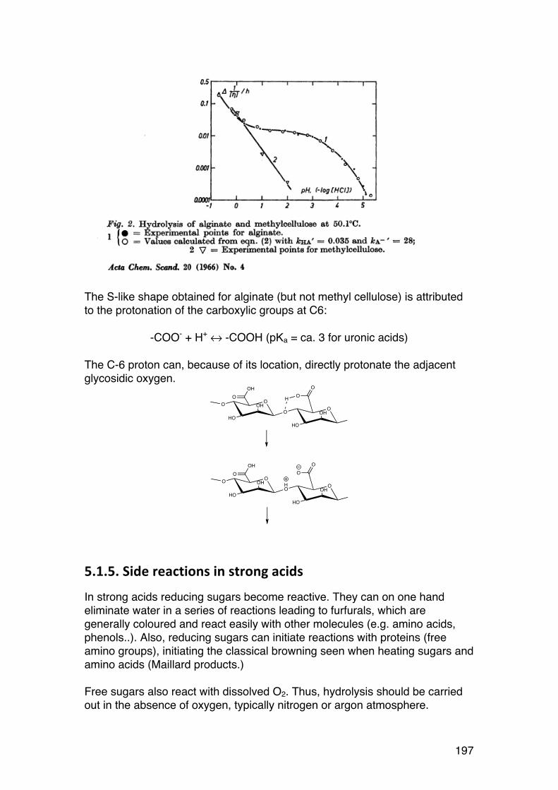
197

The S-like shape obtained for alginate (but not methyl cellulose) is attributed to the protonation of the carboxylic groups at C6:

-COO- + H+ ↔ -COOH (pKa = ca. 3 for uronic acids) The C-6 proton can, because of its location, directly protonate the adjacent glycosidic oxygen.

5.1.5.  Side  reactions  in  strong  acids  

In strong acids reducing sugars become reactive. They can on one hand eliminate water in a series of reactions leading to furfurals, which are generally coloured and react easily with other molecules (e.g. amino acids, phenols..). Also, reducing sugars can initiate reactions with proteins (free amino groups), initiating the classical browning seen when heating sugars and amino acids (Maillard products.) Free sugars also react with dissolved O2. Thus, hydrolysis should be carried out in the absence of oxygen, typically nitrogen or argon atmosphere.

OOH

HO

OHO

OO

OH

HO

OO

O

H

OOH

HO

OHO

OO

OH

HO

OO

HO

198

5.1.6.  Alkaline  hydrolysis  

As already mentioned, glycosides are generally stable under alkaline conditions. Only in strong alkali and at high temperatures can alkaline hydrolysis be observed in – for example – cellulose. However, elimination-sensitive polysaccharides are very labile to alkali as described below.

5.1.7.  Alkaline  β-­‐elimination  

4-linked polyuronides such as alginates and pectins (especially highly esterified pectins) are labile in alkaline solutions. This lability is linked to the carbonyl group at C6, which make the sugars susceptible to alkaline β-elimination. In alginates, the rate of depolymerisation is proportional to the OH- concentration when pH is above 10.5. The reaction involves the following steps:

1. The proton at C5 is much more acidic than other ring-protons because it is located in the α-position relative to the carbonyl group at C6. It reacts with OH- to produce a carbanion intermediate.

2. The linkage between C4 (β-position) and the adjacent sugar is cleaved, giving rise to a 4,5-unsaturated sugar.

If the carboxyl group at C6 is esterified (no negative charge) such as in pectins, the β-elimination reaction is orders of magnitude faster than for the corresponding un-esterified sugars.

5.1.8.  Enzymatic  degradation  

a) Hydrolases Most polysaccharide degrading enzymes work by applying an acid catalysed degradation mechanism. In such cases at –COOH group (aspartic acid or glutamic acid R-group) within the enzyme functions at proton donor. Other

Alkaline b-elimination of alginate

OOH

HO

OO

OO

OH

HO

OO

OH

H

OH

OOH

HO

OO

OO

OH

HO

OO

OH

OOH

HO

OO

OO

OH

HO

OO

OH

OOH

HO

OO

OOHH

H2O

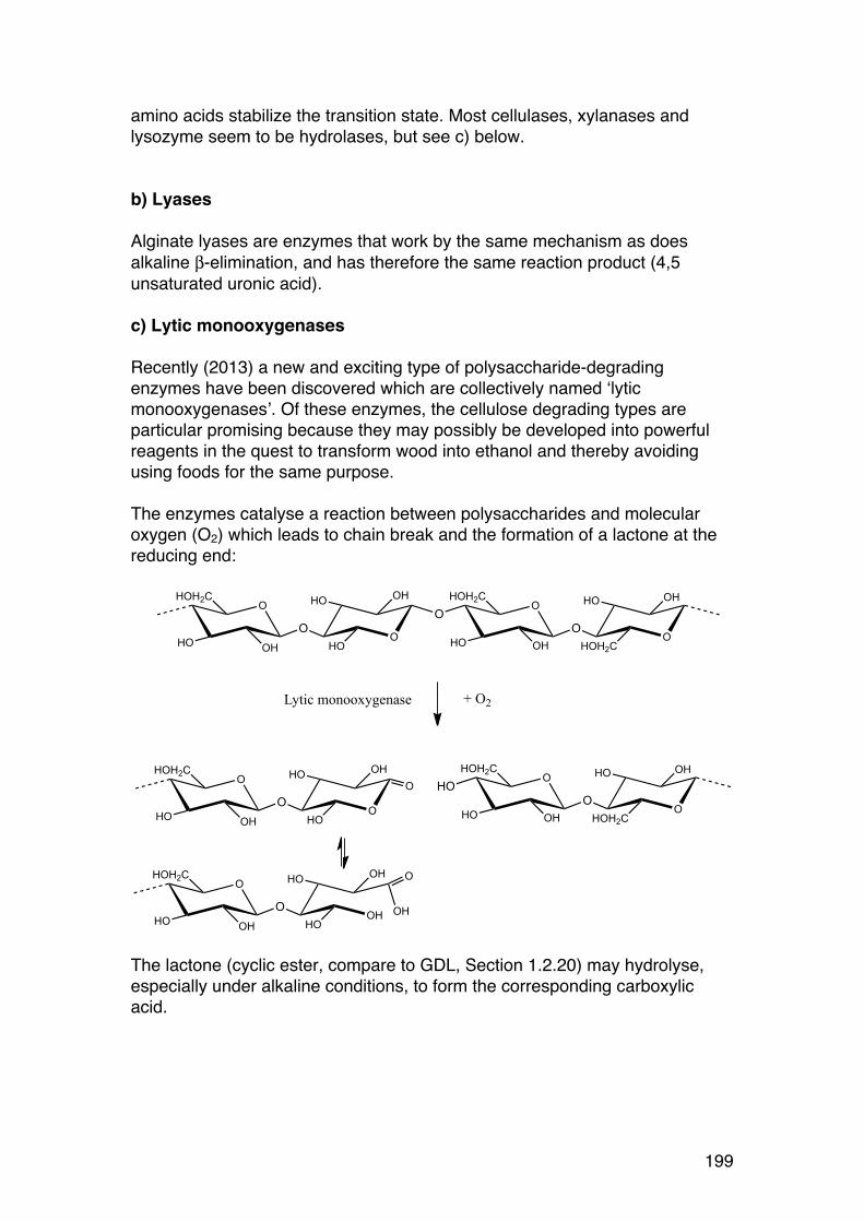
199

amino acids stabilize the transition state. Most cellulases, xylanases and lysozyme seem to be hydrolases, but see c) below. b) Lyases Alginate lyases are enzymes that work by the same mechanism as does alkaline β-elimination, and has therefore the same reaction product (4,5 unsaturated uronic acid). c) Lytic monooxygenases Recently (2013) a new and exciting type of polysaccharide-degrading enzymes have been discovered which are collectively named ‘lytic monooxygenases’. Of these enzymes, the cellulose degrading types are particular promising because they may possibly be developed into powerful reagents in the quest to transform wood into ethanol and thereby avoiding using foods for the same purpose. The enzymes catalyse a reaction between polysaccharides and molecular oxygen (O2) which leads to chain break and the formation of a lactone at the reducing end:

The lactone (cyclic ester, compare to GDL, Section 1.2.20) may hydrolyse, especially under alkaline conditions, to form the corresponding carboxylic acid.

OHO

HOH2C

OHHOO

OHO

HOO

OHO

HOH2C

OHHOO

OHOH2C

HO

+ O2Lytic monooxygenase

OHO

HOH2C

OHHOO

OHO

HOHO

OHO

HOH2C

OHHOO

OHOH2C

HOO

OHO

HOH2C

OHHOO

OHHO

HO O

OH

200

5.1.9.  Degradation  by  free  radical  mechanism  (oxidative-­‐reductive  depolymerization  –  ORD)  

Organic materials are generally degradable, also in the absence of enzymes. One example is the slow decay of plastics, which become brittle and fragmented, and eventually disappears. Such degradation is accelerated (i.e. catalysed) by light, oxygen, and transition metal ions. ORD is a general, but complicated cascade of reactions working on all kinds of polymers, including biopolymers. ORD is generally catalysed by autooxidable compounds such as ascorbic acid, sulfite, phenols and many others. Also molecular oxygen (O2) and transition metals such as Fe2+/Fe3+ function as catalysts, and the reaction seem in some cases to be catalysed by high pH. Also light catalyses ORD. Thus, optimum stability towards ORD is obtained by avoiding alkaline conditions, oxygen, light, and autooxidable compounds. The reaction cascade generally follows three steps:

1. A reducing compound (for example Cu+, F2+ or ascorbic acid, see figure) reacts with O2 (the activated singlet state is particularly reactive) to produce (directly or indirectly) a peroxide:

RH + O2 → R-O-O-H

2. The unstable peroxide decomposes in the presence of catalysts such

as Fe2+ to yield highly active radicals, including the extremely reactive hydroxyl radical (.OH):

R-O-O-H → R-O. + .OH

3. The free radicals (especially .OH) attack the polymer by abstracting a

hydrogen atom (.H):

-CH- + .OH → -C.- + H2O The polymer radical (-C.-) is unstable, and subsequent (partly unknown) reactions lead to chain scission.

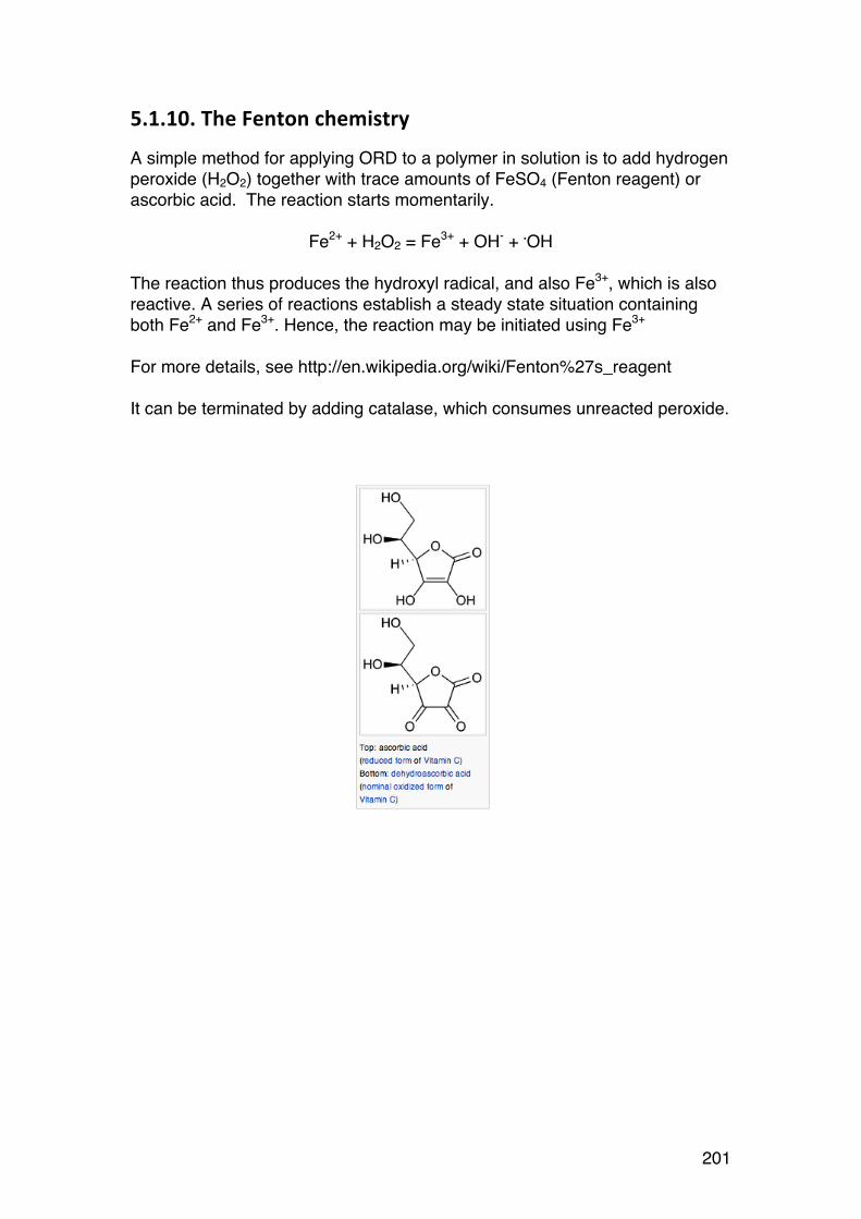
201

5.1.10.  The  Fenton  chemistry  

A simple method for applying ORD to a polymer in solution is to add hydrogen peroxide (H2O2) together with trace amounts of FeSO4 (Fenton reagent) or ascorbic acid. The reaction starts momentarily.

Fe2+ + H2O2 = Fe3+ + OH- + .OH

The reaction thus produces the hydroxyl radical, and also Fe3+, which is also reactive. A series of reactions establish a steady state situation containing both Fe2+ and Fe3+. Hence, the reaction may be initiated using Fe3+ For more details, see http://en.wikipedia.org/wiki/Fenton%27s_reagent It can be terminated by adding catalase, which consumes unreacted peroxide.  

   

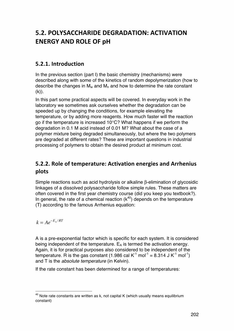
202

5.2.  POLYSACCHARIDE  DEGRADATION:  ACTIVATION  ENERGY  AND  ROLE  OF  pH  

5.2.1.  Introduction  

In the previous section (part I) the basic chemistry (mechanisms) were described along with some of the kinetics of random depolymerization (how to describe the changes in Mw and Mn and how to determine the rate constant (k)). In this part some practical aspects will be covered. In everyday work in the laboratory we sometimes ask ourselves whether the degradation can be speeded up by changing the conditions, for example elevating the temperature, or by adding more reagents. How much faster will the reaction go if the temperature is increased 10°C? What happens if we perform the degradation in 0.1 M acid instead of 0.01 M? What about the case of a polymer mixture being degraded simultaneously, but where the two polymers are degraded at different rates? These are important questions in industrial processing of polymers to obtain the desired product at minimum cost.

5.2.2.  Role  of  temperature:  Activation  energies  and  Arrhenius  plots  

Simple reactions such as acid hydrolysis or alkaline β-elimination of glycosidic linkages of a dissolved polysaccharide follow simple rules. These matters are often covered in the first year chemistry course (did you keep you textbook?). In general, the rate of a chemical reaction (k40) depends on the temperature (T) according to the famous Arrhenius equation:

k = Ae−EA /RT A is a pre-exponential factor which is specific for each system. It is considered being independent of the temperature. EA is termed the activation energy. Again, it is for practical purposes also considered to be independent of the temperature. R is the gas constant (1.986 cal K-1 mol-1 = 8.314 J K-1 mol-1) and T is the absolute temperature (in Kelvin). If the rate constant has been determined for a range of temperatures:

40 Note rate constants are written as k, not capital K (which usually means equilibrium constant)

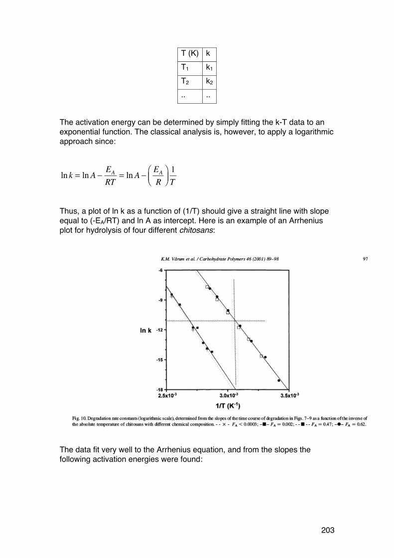
203

T (K) k T1 k1

T2 k2

.. .. The activation energy can be determined by simply fitting the k-T data to an exponential function. The classical analysis is, however, to apply a logarithmic approach since:

ln k = lnA −EART

= lnA −EAR

⎛⎝⎜

⎞⎠⎟1T

Thus, a plot of ln k as a function of (1/T) should give a straight line with slope equal to (-EA/RT) and ln A as intercept. Here is an example of an Arrhenius plot for hydrolysis of four different chitosans:

The data fit very well to the Arrhenius equation, and from the slopes the following activation energies were found:

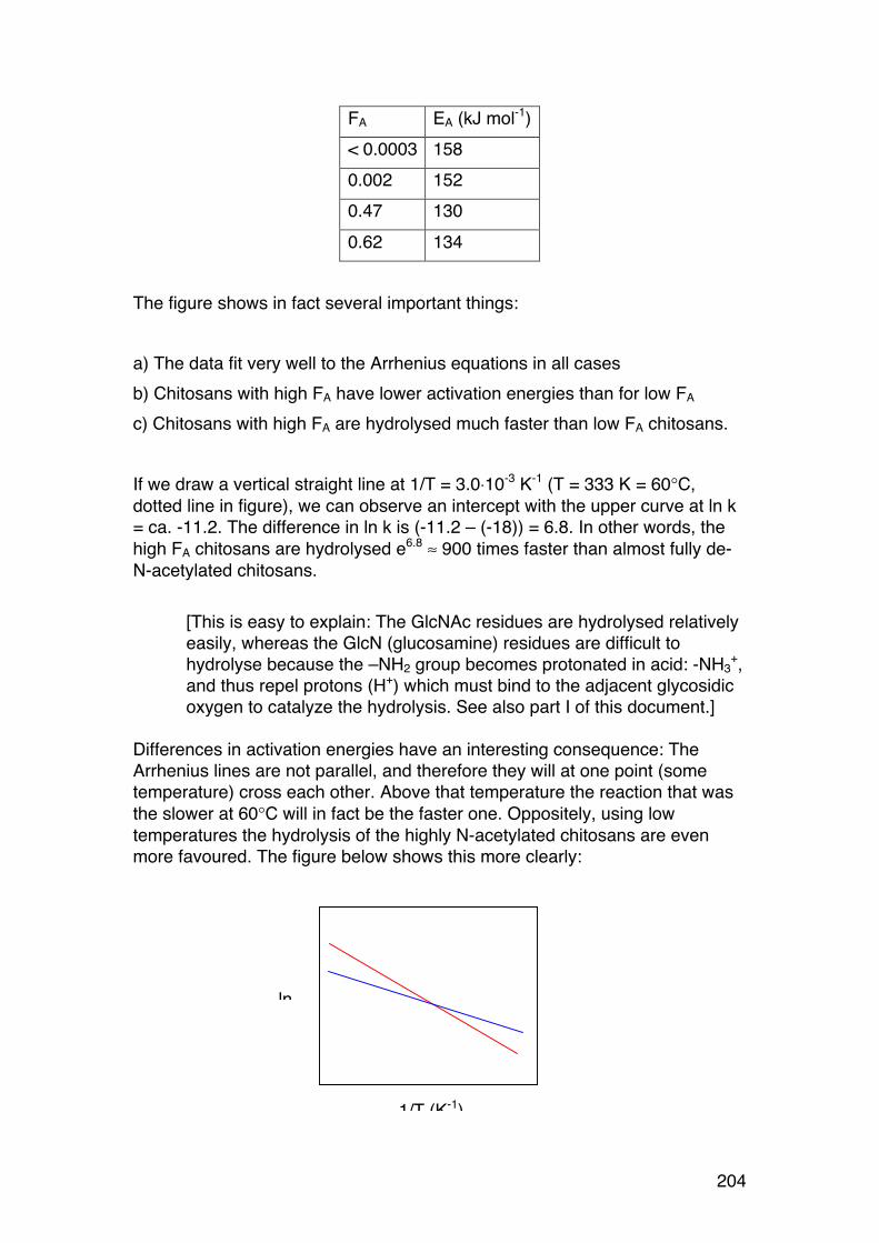
204

FA EA (kJ mol-1) < 0.0003 158 0.002 152 0.47 130 0.62 134

The figure shows in fact several important things: a) The data fit very well to the Arrhenius equations in all cases b) Chitosans with high FA have lower activation energies than for low FA c) Chitosans with high FA are hydrolysed much faster than low FA chitosans. If we draw a vertical straight line at 1/T = 3.0⋅10-3 K-1 (T = 333 K = 60°C, dotted line in figure), we can observe an intercept with the upper curve at ln k = ca. -11.2. The difference in ln k is (-11.2 – (-18)) = 6.8. In other words, the high FA chitosans are hydrolysed e6.8 ≈ 900 times faster than almost fully de-N-acetylated chitosans.

[This is easy to explain: The GlcNAc residues are hydrolysed relatively easily, whereas the GlcN (glucosamine) residues are difficult to hydrolyse because the –NH2 group becomes protonated in acid: -NH3

+, and thus repel protons (H+) which must bind to the adjacent glycosidic oxygen to catalyze the hydrolysis. See also part I of this document.]

Differences in activation energies have an interesting consequence: The Arrhenius lines are not parallel, and therefore they will at one point (some temperature) cross each other. Above that temperature the reaction that was the slower at 60°C will in fact be the faster one. Oppositely, using low temperatures the hydrolysis of the highly N-acetylated chitosans are even more favoured. The figure below shows this more clearly:

ln k

1/T (K-1)

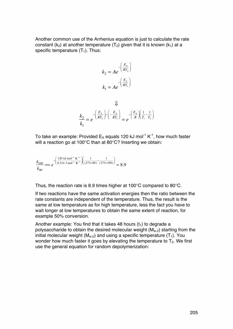
205

Another common use of the Arrhenius equation is just to calculate the rate constant (k2) at another temperature (T2) given that it is known (k1) at a specific temperature (T1). Thus:

k2 = Ae−

EA

RT2

⎛⎝⎜

⎞⎠⎟

k1 = Ae−

EA

RT1

⎛⎝⎜

⎞⎠⎟

⇓

k2k1

= e−

EA

RT2

⎛⎝⎜

⎞⎠⎟− −

EA

RT1

⎛⎝⎜

⎞⎠⎟ = e

−EA

R⎛⎝⎜

⎞⎠⎟1T1

− 1T2

⎛⎝⎜

⎞⎠⎟

To take an example: Provided EA equals 120 kJ mol-1 K-1, how much faster will a reaction go at 100°C than at 80°C? Inserting we obtain:

k100

k80== e

− 120 kJ mol−1 K−1

8.314 J mol−1 K−1

⎛⎝⎜

⎞⎠⎟

1(273+80)

− 1(273+100)

⎛⎝⎜

⎞⎠⎟ = 8.9

Thus, the reaction rate is 8.9 times higher at 100°C compared to 80°C. If two reactions have the same activation energies then the ratio between the rate constants are independent of the temperature. Thus, the result is the same at low temperature as for high temperature, less the fact you have to wait longer at low temperatures to obtain the same extent of reaction, for example 50% conversion. Another example: You find that it takes 48 hours (t1) to degrade a polysaccharide to obtain the desired molecular weight (Mw,2) starting from the initial molecular weight (Mw,0) and using a specific temperature (T1). You wonder how much faster it goes by elevating the temperature to T2. We first use the general equation for random depolymerization:

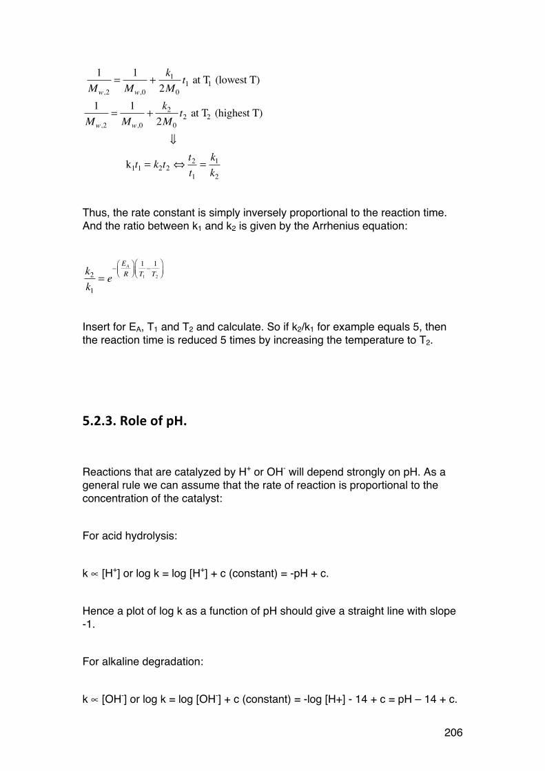
206

1Mw,2

=1

Mw,0+

k1

2M0t1 at T1 (lowest T)

1Mw,2

=1

Mw,0+

k2

2M0t2 at T2 (highest T)

⇓

k1t1 = k2t2 ⇔t2t1

=k1

k2 Thus, the rate constant is simply inversely proportional to the reaction time. And the ratio between k1 and k2 is given by the Arrhenius equation:

k2k1

= e−

EA

R⎛⎝⎜

⎞⎠⎟1T1

− 1T2

⎛⎝⎜

⎞⎠⎟

Insert for EA, T1 and T2 and calculate. So if k2/k1 for example equals 5, then the reaction time is reduced 5 times by increasing the temperature to T2.

5.2.3.  Role  of  pH.  

Reactions that are catalyzed by H+ or OH- will depend strongly on pH. As a general rule we can assume that the rate of reaction is proportional to the concentration of the catalyst: For acid hydrolysis: k ∝ [H+] or log k = log [H+] + c (constant) = -pH + c. Hence a plot of log k as a function of pH should give a straight line with slope -1. For alkaline degradation: k ∝ [OH-] or log k = log [OH-] + c (constant) = -log [H+] - 14 + c = pH – 14 + c.

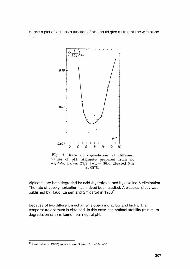
207

Hence a plot of log k as a function of pH should give a straight line with slope +1.

Alginates are both degraded by acid (hydrolysis) and by alkaline β-elimination. The rate of depolymerization has indeed been studied. A classical study was published by Haug, Larsen and Smidsrød in 196341: Because of two different mechanisms operating at low and high pH, a temperature optimum is obtained. In this case, the optimal stability (minimum degradation rate) is found near neutral pH.

41 Haug et al. (12963) Acta Chem. Scand. 5, 1466-1468

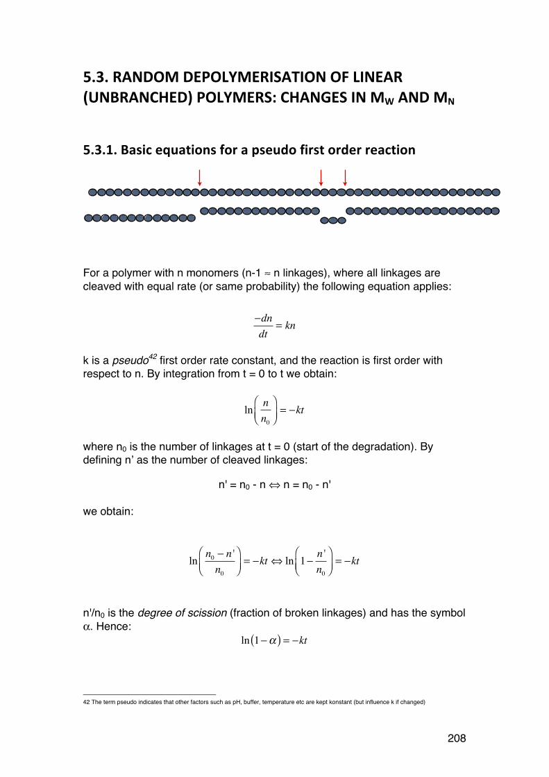
208

5.3.  RANDOM  DEPOLYMERISATION  OF  LINEAR  (UNBRANCHED)  POLYMERS:  CHANGES  IN  MW  AND  MN  

5.3.1.  Basic  equations  for  a  pseudo  first  order  reaction  

For a polymer with n monomers (n-1 ≈ n linkages), where all linkages are cleaved with equal rate (or same probability) the following equation applies:

−dndt

= kn

k is a pseudo42 first order rate constant, and the reaction is first order with respect to n. By integration from t = 0 to t we obtain:

ln nn0

⎛⎝⎜

⎞⎠⎟= −kt

where n0 is the number of linkages at t = 0 (start of the degradation). By defining n’ as the number of cleaved linkages:

n' = n0 - n ⇔ n = n0 - n' we obtain:

ln n0 − n 'n0

⎛⎝⎜

⎞⎠⎟= −kt ⇔ ln 1− n '

n0

⎛⎝⎜

⎞⎠⎟= −kt

n'/n0 is the degree of scission (fraction of broken linkages) and has the symbol α. Hence:

ln 1−α( ) = −kt

42 The term pseudo indicates that other factors such as pH, buffer, temperature etc are kept konstant (but influence k if changed)

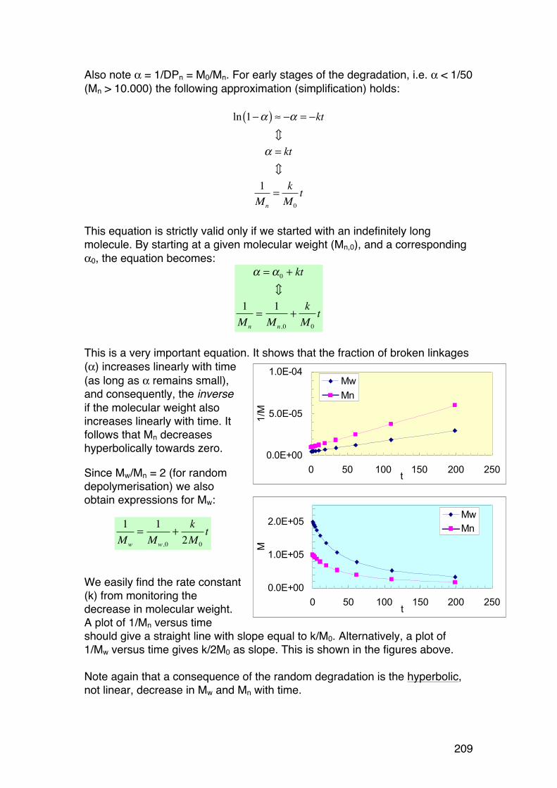
209

0.0E+00

5.0E-05

1.0E-04

0 50 100 150 200 250t

1/M

MwMn

0.0E+00

1.0E+05

2.0E+05

0 50 100 150 200 250t

M

MwMn

Also note α = 1/DPn = M0/Mn. For early stages of the degradation, i.e. α < 1/50 (Mn > 10.000) the following approximation (simplification) holds:

ln 1−α( ) ≈ −α = −kt

α = kt

1Mn

= kM0

t

This equation is strictly valid only if we started with an indefinitely long molecule. By starting at a given molecular weight (Mn,0), and a corresponding α0, the equation becomes:

α = α0 + kt

1Mn

=1

Mn,0

+kM 0

t

This is a very important equation. It shows that the fraction of broken linkages (α) increases linearly with time (as long as α remains small), and consequently, the inverse if the molecular weight also increases linearly with time. It follows that Mn decreases hyperbolically towards zero.

Since Mw/Mn = 2 (for random depolymerisation) we also obtain expressions for Mw:

1Mw

=1

Mw,0

+k2M 0

t

We easily find the rate constant (k) from monitoring the decrease in molecular weight. A plot of 1/Mn versus time should give a straight line with slope equal to k/M0. Alternatively, a plot of 1/Mw versus time gives k/2M0 as slope. This is shown in the figures above. Note again that a consequence of the random degradation is the hyperbolic, not linear, decrease in Mw and Mn with time.

210

5.3.2.  Example:  Analysis  of  a  polysaccharide  degradation  experiment:  

An alginate was hydrolysed at 100°C at pH 5.6. Samples were taken at different intervals and Mw was determined. Results:

To further analyse the data a plot of 1/Mw versus degradation time (t) is made:

The data for 1/Mw fall in a perfectly straight line according to the equations above. Hence, the degradation is random. A linear regression analysis gives a slope of 2.42E-7, corresponding to a rate constant (using M0 = 198 for alginate) of 6.1E-10 min-1.

5.3.3.  Towards  the  oligomer  range:  Higher  α  values  

If we degrade to larger α values, i.e. approaching the oligomer range, the approximation ln 1−α( ) ≈ −α no longer holds, and the ln 1−α( ) term cannot be simplified. Hence:

211

Inserting into the main equations yields the following equations:

In practise these equations do to accurately describe the degradation in the oligomer range because the linkages to terminal sugars (esp. the non-reducing end in acid hydrolysis) often are cleaved faster, leading to a higher amount of monomers than predicted by the equations above.

ln 1−α( ) = −kt ≠ −α( )α = 1− e−kt (Starting with infinitely long chain)α =α 0 + (1− e−kt ) (Starting with chain of finite length)

1DPn

= 1DPn,0

+ (1− e−kt )

1Mn

= 1Mn,0

+ (1− e−kt )

M 0

1Mw

= 1Mw,0

+ (1− e−kt )

2M 0

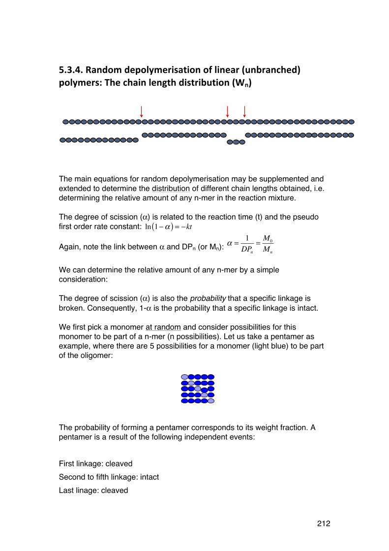
212

5.3.4.  Random  depolymerisation  of  linear  (unbranched)  polymers:  The  chain  length  distribution  (Wn)  

The main equations for random depolymerisation may be supplemented and extended to determine the distribution of different chain lengths obtained, i.e. determining the relative amount of any n-mer in the reaction mixture. The degree of scission (α) is related to the reaction time (t) and the pseudo first order rate constant: ln 1−α( ) = −kt

Again, note the link between α and DPn (or Mn): α = 1DPn

= M0

Mn

We can determine the relative amount of any n-mer by a simple consideration: The degree of scission (α) is also the probability that a specific linkage is broken. Consequently, 1-α is the probability that a specific linkage is intact. We first pick a monomer at random and consider possibilities for this monomer to be part of a n-mer (n possibilities). Let us take a pentamer as example, where there are 5 possibilities for a monomer (light blue) to be part of the oligomer:

The probability of forming a pentamer corresponds to its weight fraction. A pentamer is a result of the following independent events: First linkage: cleaved Second to fifth linkage: intact Last linage: cleaved

!

213

The probability of forming a pentamer is thus:

It follows by induction that for any n-mer, the weight fraction is:

(This is sometimes called the Kuhn distribution) Example: Assume we degrade a polymer (randomly) until α equals 0.015. According to the equation above the reaction mixture contains the following amounts of monomers, dimers.. etc.

The distribution is broad, the maximum amount being somewhere around 0.5% (calculated for n = 100). The entire distribution can be represented graphically:

w5 = 5α (1−α )(1−α )(1−α )(1−α )α = 5α 2 (1−α )4

wn = nα2 (1−α )n−1

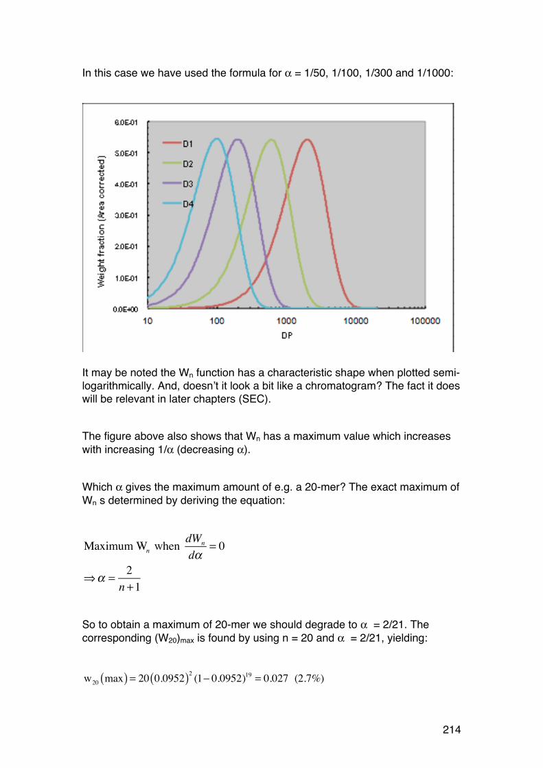
214

In this case we have used the formula for α = 1/50, 1/100, 1/300 and 1/1000:

It may be noted the Wn function has a characteristic shape when plotted semi-logarithmically. And, doesn’t it look a bit like a chromatogram? The fact it does will be relevant in later chapters (SEC). The figure above also shows that Wn has a maximum value which increases with increasing 1/α (decreasing α). Which α gives the maximum amount of e.g. a 20-mer? The exact maximum of Wn s determined by deriving the equation:

So to obtain a maximum of 20-mer we should degrade to α = 2/21. The corresponding (W20)max is found by using n = 20 and α = 2/21, yielding:

w20 max( ) = 20 0.0952( )2 (1− 0.0952)19 = 0.027 (2.7%)

Maximum Wn when dWn

dα= 0

⇒α = 2n +1

215

PART  6.  EXPERIMENTAL  METHODS  FOR  CHARACTERIZING  BIOPOLYMERS  IN  SOLUTION  

   

216

6.1.  SOLUTION  VISCOSITY  AND  INTRINSIC  VISCOSITY  

6.1.1.  Viscosity  (symbol  η)  of  dilute  solutions  

Many polysaccharides, glycoproteins and some proteins produce very thick (viscous) solutions when they are dissolved in water, even at low concentrations. Practical examples include making a sauce or a gravy. Even blood is more viscous than water because of both blood cells and dissolved proteins43. Other examples you may think of? The viscosity of solutions is both a technologically and biologically important property. In addition, measurement of the dilute solution viscosity is often a simple way to obtain information about the physical properties of the dissolved macromolecules. This includes both the molecular weight and the shape and extension of the molecules. In this course we will focus on these aspects:

a) Defining and understanding the intrinsic viscosity b) How to determine the intrinsic viscosity experimentally c) Using intrinsic viscosity measurements to determine the molecular

weight or monitor molecular weight changes of a biopolymer d) Using analysis of the intrinsic viscosity and the molecular weight to

quantify the shape and extension of a biopolymer (spherical? rodlike? C∞ or persistence length?)

First, we define the term dilute solution. It means the concentration range below which polymer-polymer interactions do not contribute to the viscosity. The concentration where such interactions emerge is called the critical overlap concentration (c*). It depends very much on the shape of the polymers, but can generally be approximated by c* ≈ 2.5/[η], where [η] is the intrinsic viscosity (defined and explained below). The viscosity of a liquid is a result of internal friction. For macromolecules in solution the viscosity depends on several factors: - The polymer concentration - The molecular weight - Flexibility, shape and extension of the polymer - The solvent properties (including pH and ionic strength) - The temperature - The type of measurement and type of viscometer

43 What is the concentration of protein in blood? Check literature or web

217

First, we will define viscosity in precise terms. Consider a liquid flowing through a narrow tube. The liquid flow is caused by an applied force (F), such as gravity, or forces applied by a pump. Forces acting in the flow direction are called shear forces. In fact, laminar flow is an example of shear deformation. We consider only laminar flow (as opposed to turbulent flow), where the liquid can be regarded as consisting of infinitely thin layers. Between adjacent layers friction forces act, leading to the characteristic flow profile with zero flow at the walls

and maximal flow in the centre of the tube. We thus have a velocity gradient perpendicular to the direction of flow. To simplify the situation we move from a tube to parallel plates, with liquid between the plates. The lower plate is stagnant, the upper is pulled by a force F in the x-direction. In result, liquid also flows in the x-direction. The flow rate (v) depends on the distance (z) from the lower plate: v = v(z). The velocity gradient is still perpendicular to the direction of flow. It is commonly called the

shear rate, and is given the symbol .γ .

.γ =

dvdz

The ratio between the force (F) and the area (A) upon which it works is given the name shear stress, and has the symbol τ:

τ = AF

Definition of viscosity (symbol: η): The viscosity (shear viscosity) of a liquid is defined as the ratio between the shear stress and the shear rate:

η =τγ=

FA

⎛⎝⎜

⎞⎠⎟

dvdz

⎛⎝⎜

⎞⎠⎟

z

x

218

The ‘dot’ in .γ indicates it is a time derivative of γ, where γ is the shear

deformation (dx/dz). This is easily demonstrated:

γ =

dvdz

=d dx

dt⎛⎝⎜

⎞⎠⎟

dz=d dx

dz⎛⎝⎜

⎞⎠⎟

dt=dγdt

In practical terms these equations are somewhat cumbersome. In a typical viscometer we generally measure the flow-through-time (t) for flowing a certain volume of liquid (V). For a capillary viscometer (or any tube where laminar flow prevails), Poiseuille’s equation applies:

Flow rate U =dVdt

=π (P1 − P2 )r4

8ηlP1 − P2 : Pressure differencer: radiusl: length of tube The flow rate (U) is inversely proportional to the flow-through-time. Hence, the viscosity is directly proportional to the flow-through-time (t): η ∝ t Therefore, the relative and specific viscosities (which we need) are easily found: Solution (with polymer) viscosity: ηSolvent viscosity: η0

Relative viscosity: ηr =ηη0

=tt0

Specific viscosity: ηsp =η −η0

η0

= ηr −1 = tt0−1

219

6.1.2.  Intrinsic  viscosity:  Definition  and  determination  

The specific viscosity depends on the concentration of dissolved molecules, but the limiting value of ηsp/c as c approaches zero is a characteristic property of the polymer/solvent system. Mathematically:

η[ ] = limc→0

ηsp

c Note that the intrinsic viscosity has the brackets [] as part of the symbol. It has further dimensions ‘inverse concentration’ such as ml/g, indicating it represents a volume per gram of polymer. In fact, it expresses the effective hydrodynamic volume, which is determined both by the physical volume of the macromolecule and its shape in solution. Since the viscosity may depend on the shear rate (non-Newtonian behaviour), also [η] will depend on the shear rate in such cases. For studies of macromolecular shape it is important to perform measurements at sufficiently low shear rate, i.e. in the Newtonian range. For this reason the symbol [η]γ→0 is used. In practise, measurements can be obtained at different shear rates, and results can be extrapolated to zero shear rate. Finding the intrinsic viscosity (experimental data) Huggins’ equation is the basis for determining the intrinsic viscosity from experimental data. It describes how the specific viscosity (of a dilute solution) depends on the concentration: ηsp

c= η[ ] + k ' η[ ]2 c

Experimental data consist of a data matrix of the following type (flow-through-times for different concentrations):

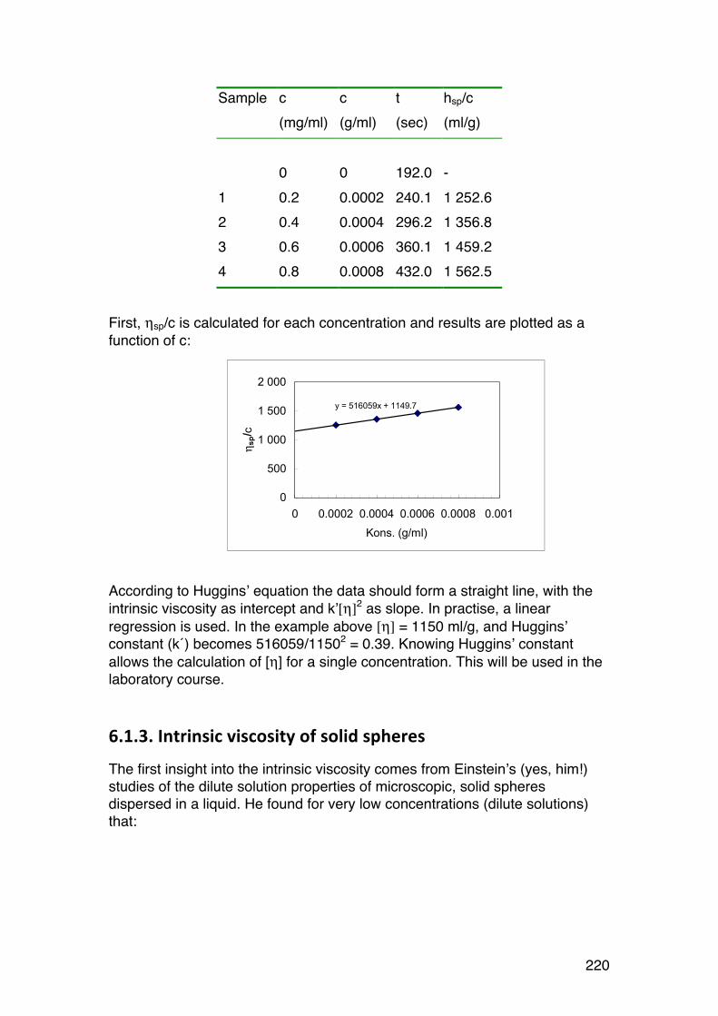
220

Sample c (mg/ml)

c (g/ml)

t (sec)

hsp/c (ml/g)

0 0 192.0 - 1 0.2 0.0002 240.1 1 252.6 2 0.4 0.0004 296.2 1 356.8 3 0.6 0.0006 360.1 1 459.2 4 0.8 0.0008 432.0 1 562.5

First, ηsp/c is calculated for each concentration and results are plotted as a function of c:

According to Huggins’ equation the data should form a straight line, with the intrinsic viscosity as intercept and k’[η]2 as slope. In practise, a linear regression is used. In the example above [η] = 1150 ml/g, and Huggins’ constant (k´) becomes 516059/11502 = 0.39. Knowing Huggins’ constant allows the calculation of [η] for a single concentration. This will be used in the laboratory course.

6.1.3.  Intrinsic  viscosity  of  solid  spheres  

The first insight into the intrinsic viscosity comes from Einstein’s (yes, him!) studies of the dilute solution properties of microscopic, solid spheres dispersed in a liquid. He found for very low concentrations (dilute solutions) that:

y = 516059x + 1149.7

0

500

1 000

1 500

2 000

0 0.0002 0.0004 0.0006 0.0008 0.001

Kons. (g/ml)

η sp/

c

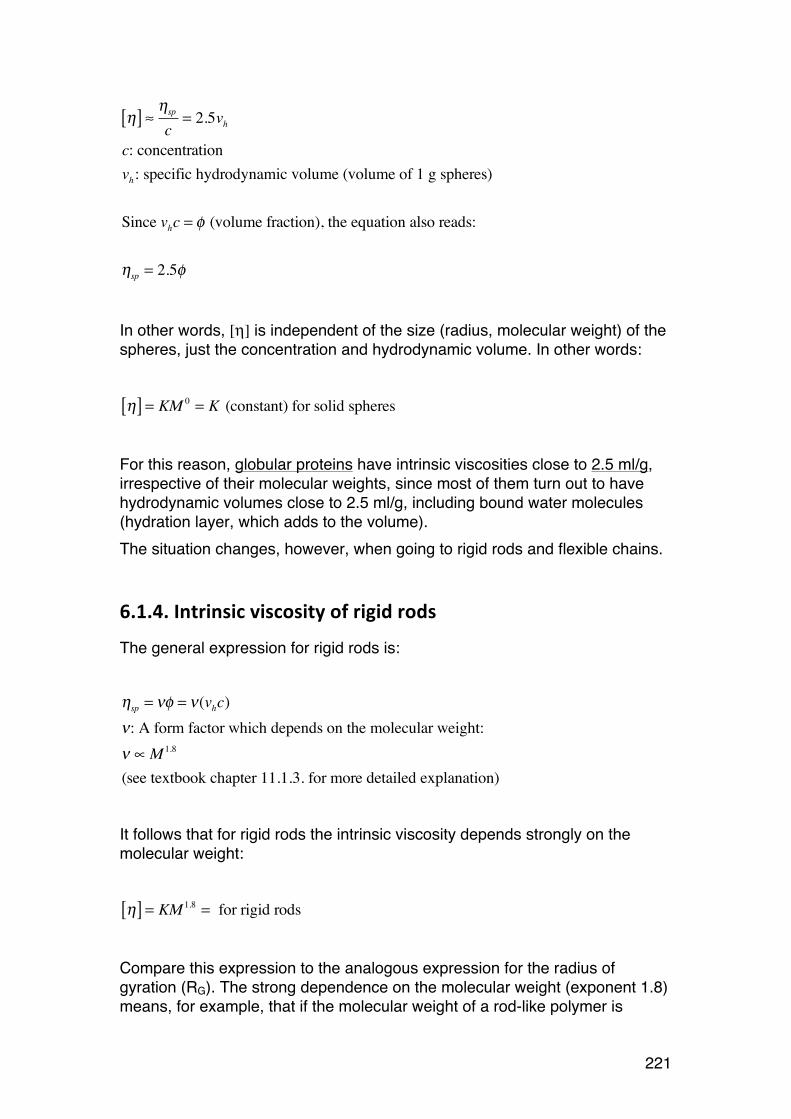
221

η[ ] ≈ ηsp

c= 2.5vh

c: concentrationvh : specific hydrodynamic volume (volume of 1 g spheres)

Since vhc = φ (volume fraction), the equation also reads:

ηsp = 2.5φ In other words, [η] is independent of the size (radius, molecular weight) of the spheres, just the concentration and hydrodynamic volume. In other words:

η[ ] = KM 0 = K (constant) for solid spheres For this reason, globular proteins have intrinsic viscosities close to 2.5 ml/g, irrespective of their molecular weights, since most of them turn out to have hydrodynamic volumes close to 2.5 ml/g, including bound water molecules (hydration layer, which adds to the volume). The situation changes, however, when going to rigid rods and flexible chains.

6.1.4.  Intrinsic  viscosity  of  rigid  rods  

The general expression for rigid rods is: ηsp = νφ = ν(vhc)ν: A form factor which depends on the molecular weight:ν ∝M 1.8

(see textbook chapter 11.1.3. for more detailed explanation) It follows that for rigid rods the intrinsic viscosity depends strongly on the molecular weight:

η[ ] = KM 1.8 = for rigid rods Compare this expression to the analogous expression for the radius of gyration (RG). The strong dependence on the molecular weight (exponent 1.8) means, for example, that if the molecular weight of a rod-like polymer is

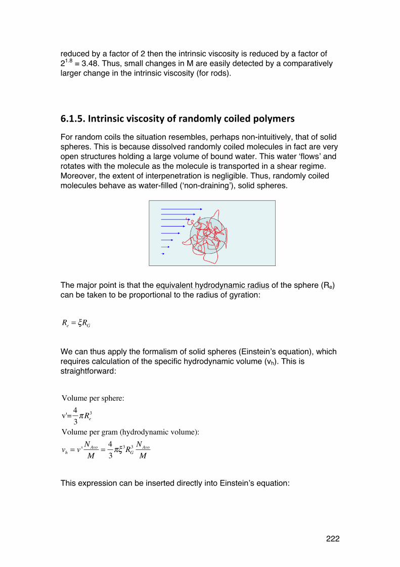
222

reduced by a factor of 2 then the intrinsic viscosity is reduced by a factor of 21.8 = 3.48. Thus, small changes in M are easily detected by a comparatively larger change in the intrinsic viscosity (for rods).

6.1.5.  Intrinsic  viscosity  of  randomly  coiled  polymers  

For random coils the situation resembles, perhaps non-intuitively, that of solid spheres. This is because dissolved randomly coiled molecules in fact are very open structures holding a large volume of bound water. This water ‘flows’ and rotates with the molecule as the molecule is transported in a shear regime. Moreover, the extent of interpenetration is negligible. Thus, randomly coiled molecules behave as water-filled (‘non-draining’), solid spheres.

The major point is that the equivalent hydrodynamic radius of the sphere (Re) can be taken to be proportional to the radius of gyration: Re = ξRG We can thus apply the formalism of solid spheres (Einstein’s equation), which requires calculation of the specific hydrodynamic volume (vh). This is straightforward: Volume per sphere:

v'= 43πRe

3

Volume per gram (hydrodynamic volume):

vh = v ' NAvo

M=

43πξ3RG

3 NAvo

M This expression can be inserted directly into Einstein’s equation:

223

η[ ] = 2.5vh =103πξ3RG

3 NAvo

M This equation shows – for randomly coiled chains – that a change in RG leads to a very large change in intrinsic viscosity. For example, a 2-fold reduction in RG leads to a 8-fold reduction in [η]. This can happen if a randomly coiled polyelectrolyte (e.g. alginate or chitosan) is transferred from low ionic strength (expanded) to high ionic strength (contracted):

Since, for random coils, the relation between RG and M is given by:

RG ∝M 0.5−0.6 (θ-solvent - good solvent) it follows by substituting for RG that (still for random coils only):

η[ ] = KM 0.5−0.8

Note the constant K is different for different systems, and different from the constants used in analogous equations for RG (RG = KMb).

6.1.6.  The  Mark-­‐Houwink-­‐Sakurada  (MHS)  equation  

The very famous - and much used – MHS equation incorporates all three basic shapes of macromolecules in solution:

η[ ] = KM a

log( η[ ]) = logK + a logM

Solid spheres (e.g. globular proteins): a = 0Rigid rods: a = 1.8

Random coils (θ-solvent): a = 0.5Random coils (good solvent): a = 0.8

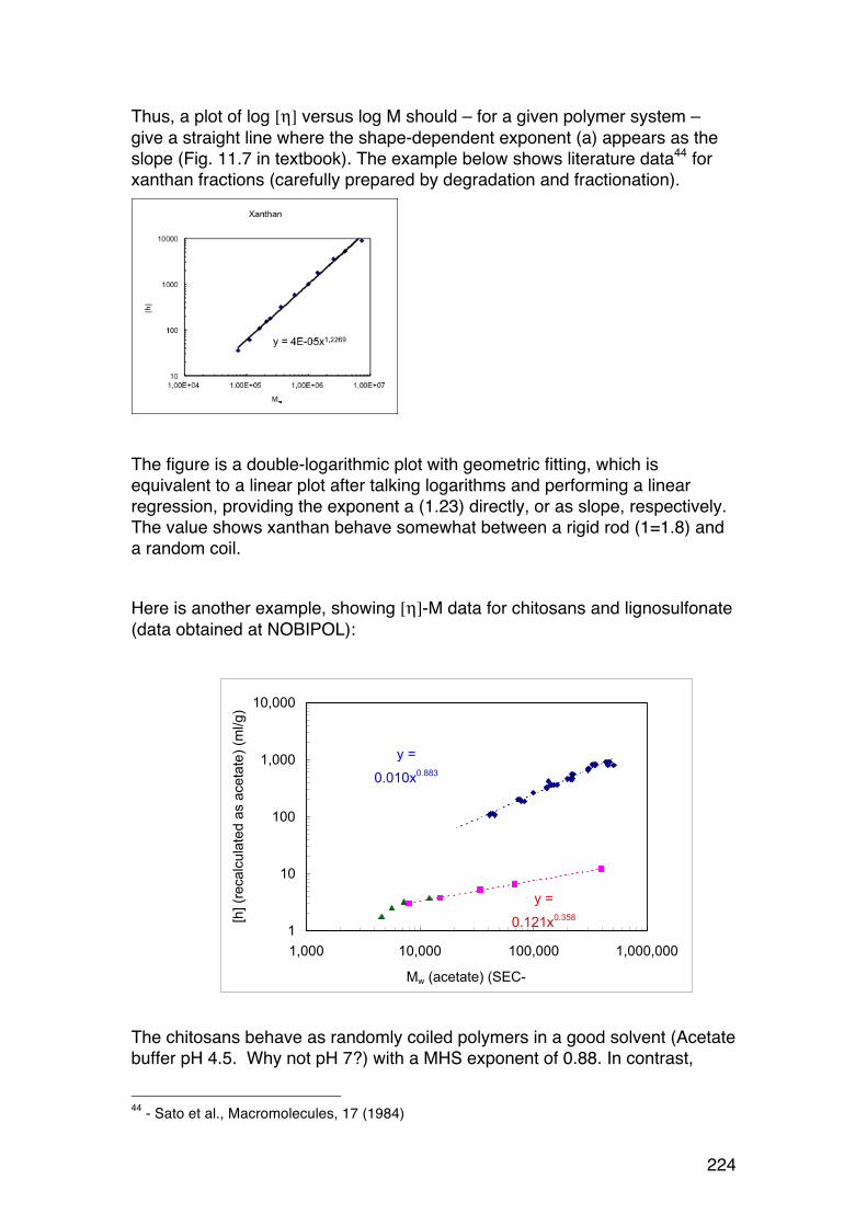
224

Thus, a plot of log [η] versus log M should – for a given polymer system – give a straight line where the shape-dependent exponent (a) appears as the slope (Fig. 11.7 in textbook). The example below shows literature data44 for xanthan fractions (carefully prepared by degradation and fractionation).

The figure is a double-logarithmic plot with geometric fitting, which is equivalent to a linear plot after talking logarithms and performing a linear regression, providing the exponent a (1.23) directly, or as slope, respectively. The value shows xanthan behave somewhat between a rigid rod (1=1.8) and a random coil. Here is another example, showing [η]-M data for chitosans and lignosulfonate (data obtained at NOBIPOL):

The chitosans behave as randomly coiled polymers in a good solvent (Acetate buffer pH 4.5. Why not pH 7?) with a MHS exponent of 0.88. In contrast,

44 - Sato et al., Macromolecules, 17 (1984)

y =

0.010x0.883

y =

0.121x0.358

1

10

100

1,000

10,000

1,000 10,000 100,000 1,000,000

Mw (acetate) (SEC-

[h] (r

ecalc

ula

ted a

s a

ceta

te)

(ml/g)

225

lignosulfonates are much more compact, having low intrinsic viscosity values (2-10 ml/g) and a very low exponent (0.36).

6.1.7.  Using  the  MHS  equation  to  find  molecular  weights  

Once the MHS parameters (K and a) have been determined for a particular macromolecule-solvent system, they can be used to find M if the (more easily accessible) intrinsic viscosity has been measured. The MHS curve then functions as a ‘standard curve’. This is a very common strategy in polymer research and development because an intrinsic viscosity measurement is so simple to perform. It is important to note that in most cases the MHS parameters are only valid for a given solvent and temperature. Changing the solvent, for example changing pH or ionic strength, may induce a change in the overall shape in the polymer, and thereby in the intrinsic viscosity. Moreover, the polydispersity plays a pivotal role here. If both standards and unknown samples are monodisperse then there is no problem, M is M. But what if the polydispersity is different in the two cases? We will illustrate this by two cases: Case 1: Monodisperse standards

Sample Mw Mn [η]

Std 1 10 000 10 000 23Std 2 50 000 50 000 52Std 3 100 000 100 000 75

Unknown ? ? 46

y = 0.2052x 0.5122

10

100

1 000 10 000 100 000 1 000 000M (g/mol)

[ η]

(ml/g

)

In this case Mw = Mn = M (of course) for the standards since they are monodisperse. The data for the standards gives the following MHS relation for this polymer (see graph above):

[ ] . .η = 0 2052 0 5122M

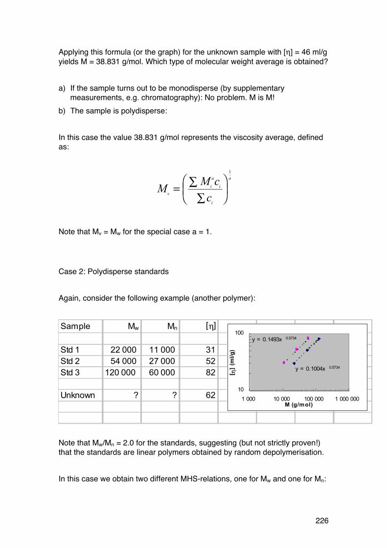
226

Applying this formula (or the graph) for the unknown sample with [η] = 46 ml/g yields M = 38.831 g/mol. Which type of molecular weight average is obtained? a) If the sample turns out to be monodisperse (by supplementary

measurements, e.g. chromatography): No problem. M is M! b) The sample is polydisperse: In this case the value 38.831 g/mol represents the viscosity average, defined as:

M M ccvi

a

i

i

a

= ∑∑

⎛⎝⎜

⎞⎠⎟

1

Note that Mv = Mw for the special case a = 1. Case 2: Polydisperse standards Again, consider the following example (another polymer):

Sample Mw Mn [η]

Std 1 22 000 11 000 31Std 2 54 000 27 000 52Std 3 120 000 60 000 82

Unknown ? ? 62

y = 0.1004x 0.5734

y = 0.1493x 0.5734

10

100

1 000 10 000 100 000 1 000 000M (g/mol)

[ η]

(ml/g

)

Note that Mw/Mn = 2.0 for the standards, suggesting (but not strictly proven!) that the standards are linear polymers obtained by random depolymerisation. In this case we obtain two different MHS-relations, one for Mw and one for Mn:

227

[ ] .[ ] .

.

.

ηη

==0100401493

0 5734

0 5734

MM

w

n

(Note: exponent a differs from example 1 ⇒ different polymer system) In order to use these equations we must assume the unknown sample has the same type of molecular weight distribution as the standards, in this case (and generally in many other cases) the distribution of a randomly degraded polymer. Applying the equations we obtain: Mw = 73.597 g/mol Mn = 36.841 g/mol This assumption is often used in practical biopolymer chemistry. Both the standards used to establish the MHS equation and the unknown samples are obtained by random degradation, for example acid hydrolysis.

6.1.8.  Using  the  intrinsic  viscosity  to  determine  the  shape  of  biopolymers  in  solution  

The simplest and possibly most common method is simply to determine the MHS parameters, especially the exponent (a), to determine the basic shape of the polymer (sphere-like, rod-like or randomly coiled) as explained in Section 6.1.6. One may also determine stiffness parameters such as the characteristic ratio (C∞) and the persistence length (q) on the basis of intrinsic viscosity measurements. The method is quite analogous to that explained for the radius of gyration (Section 2.3.3.), and is based an the same type of data as those used to establish the MHS parameters, i.e. intrinsic viscosities and molecular weights for a polymer system, covering a range of polymer sizes: Sample/fraction Molecular weight Intrinsic viscosity 1 M1 [η]1 2 M2 [η]2 . . . i Mi [η]i

228

As for RG data a model must be introduced, in this case for the intrinsic viscosity. Such models have been developed, and are based on fitting the following parameters to the data:

• ML: mass per unit length. Can be obtained from the chemistry as described in Section 2.3.3. (xanthan as example)

• Persistence length The analytical expressions are more complicated than for RG and less suited for simple worksheets and will not be discussed further here. However, a popular simplification (Bohdanecky model) is described in Section 6.2.6.

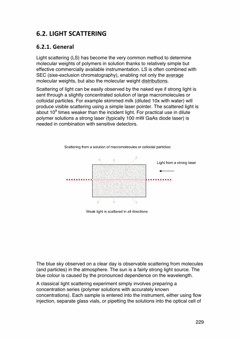
229

6.2.  LIGHT  SCATTERING  

6.2.1.  General  

Light scattering (LS) has become the very common method to determine molecular weights of polymers in solution thanks to relatively simple but effective commercially available instrumentation. LS is often combined with SEC (sixe-exclusion chromatography), enabling not only the average molecular weights, but also the molecular weight distributions. Scattering of light can be easily observed by the naked eye if strong light is sent through a slightly concentrated solution of large macromolecules or colloidal particles. For example skimmed milk (diluted 10x with water) will produce visible scattering using a simple laser pointer. The scattered light is about 109 times weaker than the incident light. For practical use in dilute polymer solutions a strong laser (typically 100 mW GaAs diode laser) is needed in combination with sensitive detectors. The blue sky observed on a clear day is observable scattering from molecules (and particles) in the atmosphere. The sun is a fairly strong light source. The blue colour is caused by the pronounced dependence on the wavelength. A classical light scattering experiment simply involves preparing a concentration series (polymer solutions with accurately known concentrations). Each sample is entered into the instrument, either using flow injection, separate glass vials, or pipetting the solutions into the optical cell of

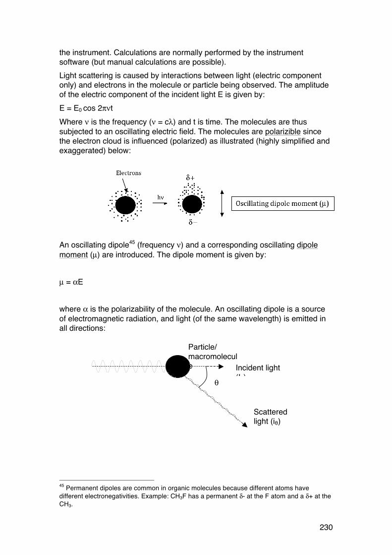
230

the instrument. Calculations are normally performed by the instrument software (but manual calculations are possible). Light scattering is caused by interactions between light (electric component only) and electrons in the molecule or particle being observed. The amplitude of the electric component of the incident light E is given by: E = E0 cos 2πνt Where ν is the frequency (ν = cλ) and t is time. The molecules are thus subjected to an oscillating electric field. The molecules are polarizible since the electron cloud is influenced (polarized) as illustrated (highly simplified and exaggerated) below: An oscillating dipole45 (frequency ν) and a corresponding oscillating dipole moment (µ) are introduced. The dipole moment is given by: µ = αE where α is the polarizability of the molecule. An oscillating dipole is a source of electromagnetic radiation, and light (of the same wavelength) is emitted in all directions:

45 Permanent dipoles are common in organic molecules because different atoms have different electronegativities. Example: CH3F has a permanent δ- at the F atom and a δ+ at the CH3.

Particle/ macromolecule

θ

Incident light (I0)

Scattered light (iθ)

231

The scattered light is – as already noted - extremely weak compared to the incident light (approx. I0 x 10-9).

6.2.2.  Scattering  from  a  single  particle  

The relationship between the intensity of the scattered light (i) and the incident light (I0) is for an isolated particle given by (for unpolarized light):

iI0

=8π 4α 2

r2λ04 (1+ cos2θ)

α: polarizabilityr: distance from scattering center to the observer (detector)λ

0: wavelength of light (in vacuo)

The scattering intensity reaches it’s maximum value at cos2θ = 1, or θ = 0°, an its minimum value at 90°. Modern instruments employ vertically polarized light. In this case:

iI0

=16π 4α 2

r2λ04 (sin2φ) φ : Angle relative to z-direction

The polarizability (α) is linked to the refractive index (n), which can be determined experimentally. The excess (solvent subtracted) polarizability is given by:

n2 − n02 = 4πNα

where N is the number of particles (macromolecules) per ml (cm3) in solution.

6.2.3.  Scattering  from  a  large  number  of  independent  particles  

Light waves scattered from a large number of particles will interfere, as waves generally do. However, for a large number of particles moving independently positive and negative interference cancel, and the total scattering intensity is simply the sum of intensities from each particle. This situation changes when

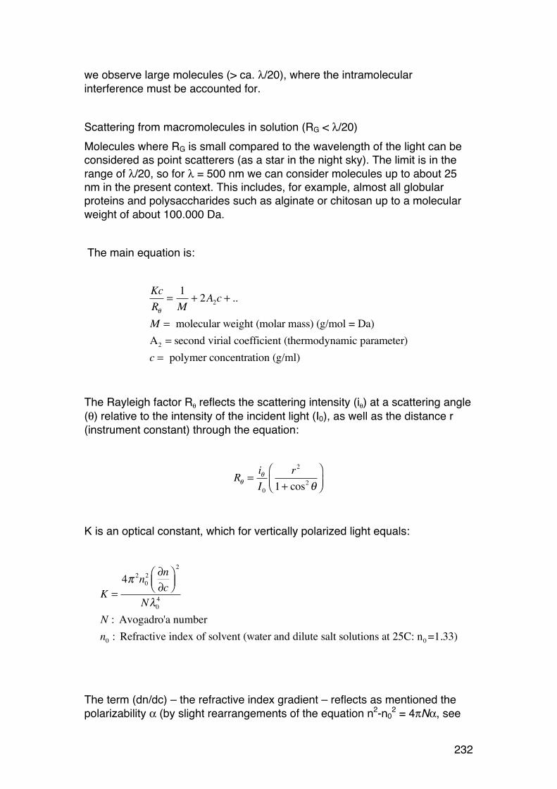
232

we observe large molecules (> ca. λ/20), where the intramolecular interference must be accounted for. Scattering from macromolecules in solution (RG < λ/20) Molecules where RG is small compared to the wavelength of the light can be considered as point scatterers (as a star in the night sky). The limit is in the range of λ/20, so for λ = 500 nm we can consider molecules up to about 25 nm in the present context. This includes, for example, almost all globular proteins and polysaccharides such as alginate or chitosan up to a molecular weight of about 100.000 Da. The main equation is:

KcRθ

=1M

+ 2A2c + ..

M = molecular weight (molar mass) (g/mol = Da)A2 = second virial coefficient (thermodynamic parameter)c = polymer concentration (g/ml)

The Rayleigh factor Rθ reflects the scattering intensity (iθ) at a scattering angle (θ) relative to the intensity of the incident light (I0), as well as the distance r (instrument constant) through the equation:

Rθ =iθI0

r2

1+ cos2θ⎛⎝⎜

⎞⎠⎟

K is an optical constant, which for vertically polarized light equals:

K =4π 2n0

2 ∂n∂c

⎛⎝⎜

⎞⎠⎟

2

Nλ04

N : Avogadro'a numbern0 : Refractive index of solvent (water and dilute salt solutions at 25C: n0 =1.33)

The term (dn/dc) – the refractive index gradient – reflects as mentioned the polarizability α (by slight rearrangements of the equation n2-n0

2 = 4πNα, see

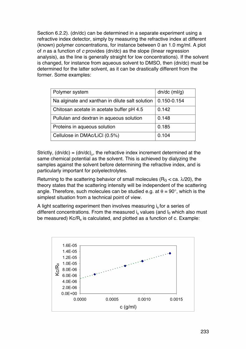
233

Section 6.2.2). (dn/dc) can be determined in a separate experiment using a refractive index detector, simply by measuring the refractive index at different (known) polymer concentrations, for instance between 0 an 1.0 mg/ml. A plot of n as a function of c provides (dn/dc) as the slope (linear regression analysis), as the line is generally straight for low concentrations). If the solvent is changed, for instance from aqueous solvent to DMSO, then (dn/dc) must be determined for the latter solvent, as it can be drastically different from the former. Some examples:

Polymer system dn/dc (ml/g) Na alginate and xanthan in dilute salt solution 0.150-0.154 Chitosan acetate in acetate buffer pH 4.5 0.142 Pullulan and dextran in aqueous solution 0.148 Proteins in aqueous solution 0.185 Cellulose in DMAc/LiCl (0.5%) 0.104

Strictly, (dn/dc) = (dn/dc)µ, the refractive index increment determined at the same chemical potential as the solvent. This is achieved by dialyzing the samples against the solvent before determining the refractive index, and is particularly important for polyelectrolytes. Returning to the scattering behavior of small molecules (RG < ca. λ/20), the theory states that the scattering intensity will be independent of the scattering angle. Therefore, such molecules can be studied e.g. at θ = 90°, which is the simplest situation from a technical point of view. A light scattering experiment then involves measuring iθ for a series of different concentrations. From the measured iθ values (and I0 which also must be measured) Kc/Rθ is calculated, and plotted as a function of c. Example:

0.0E+00

2.0E-06

4.0E-06

6.0E-06

8.0E-06

1.0E-05

1.2E-05

1.4E-05

1.6E-05

0.0000 0.0005 0.0010 0.0015

c (g/ml)

Kc/R

!

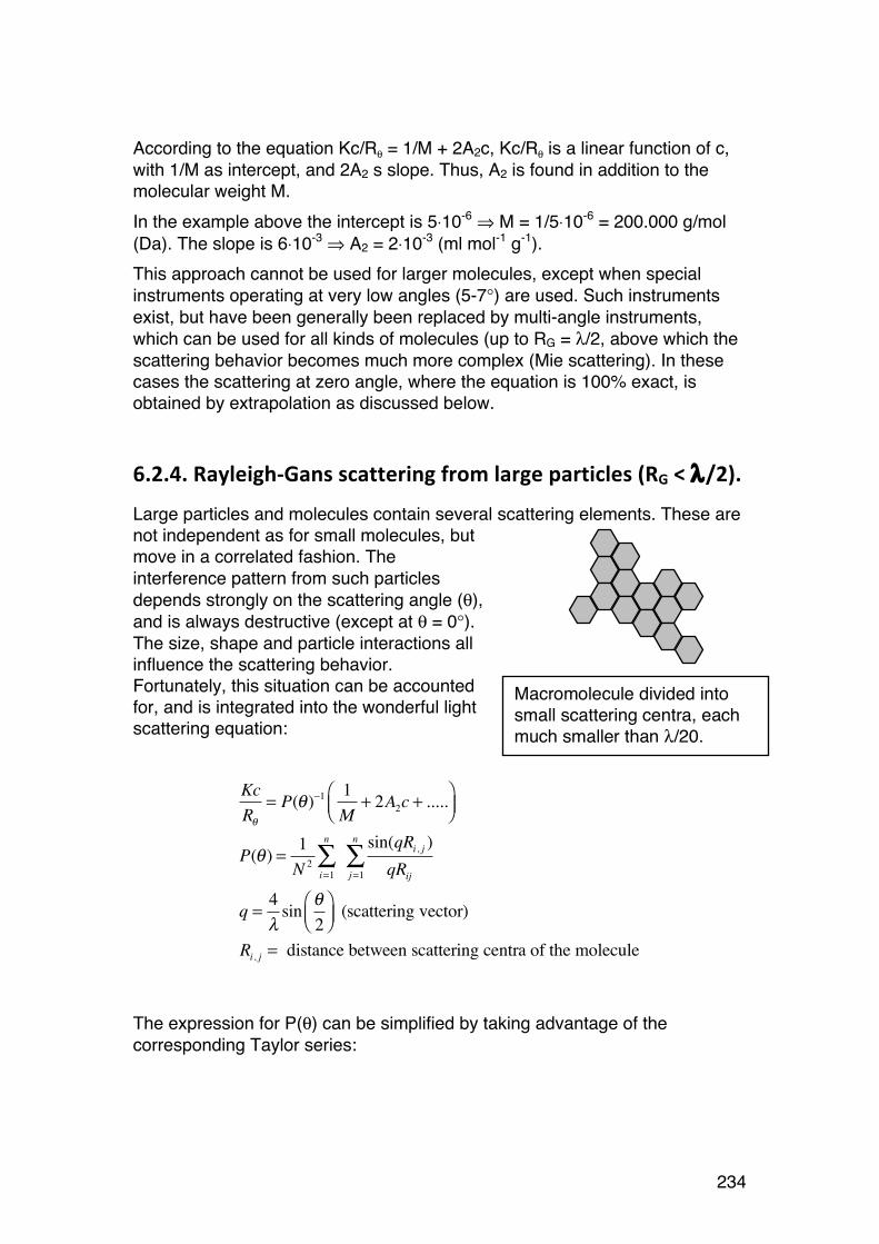
234

According to the equation Kc/Rθ = 1/M + 2A2c, Kc/Rθ is a linear function of c, with 1/M as intercept, and 2A2 s slope. Thus, A2 is found in addition to the molecular weight M. In the example above the intercept is 5⋅10-6 ⇒ M = 1/5⋅10-6 = 200.000 g/mol (Da). The slope is 6⋅10-3 ⇒ A2 = 2⋅10-3 (ml mol-1 g-1). This approach cannot be used for larger molecules, except when special instruments operating at very low angles (5-7°) are used. Such instruments exist, but have been generally been replaced by multi-angle instruments, which can be used for all kinds of molecules (up to RG = λ/2, above which the scattering behavior becomes much more complex (Mie scattering). In these cases the scattering at zero angle, where the equation is 100% exact, is obtained by extrapolation as discussed below.

6.2.4.  Rayleigh-­‐Gans  scattering  from  large  particles  (RG  <  λ/2).  

Large particles and molecules contain several scattering elements. These are not independent as for small molecules, but move in a correlated fashion. The interference pattern from such particles depends strongly on the scattering angle (θ), and is always destructive (except at θ = 0°). The size, shape and particle interactions all influence the scattering behavior. Fortunately, this situation can be accounted for, and is integrated into the wonderful light scattering equation:

KcRθ

= P(θ)−1 1M

+ 2A2c + .....⎛⎝⎜

⎞⎠⎟

P(θ) = 1N 2

i=1

n

∑ sin(qRi, j )qRijj=1

n

∑

q = 4λ

sin θ2

⎛⎝⎜

⎞⎠⎟

(scattering vector)

Ri, j = distance between scattering centra of the molecule

The expression for P(θ) can be simplified by taking advantage of the corresponding Taylor series:

Macromolecule divided into small scattering centra, each much smaller than λ/20.

235

sin(qRi, j )qRi, j

≈ 1−(qRi, j )

2

6+(qRi, j )

4

120+ .......

Keeping only the first terms (limit of low angles) and substituting for P(θ) we obtain:

P(θ) = 1− q2

6N 2 Ri, j2

j=1

N

∑i=1

N

∑

The expression looks complicated, but in fact it contains information about the radius of gyration (RG), since the latter can be defined as:

RG2 =

12N 2

i=1

N

∑ Ri, j2

j=1

N

∑

[Check the definition of RG used earlier in the course and convince yourself they are mathematically equivalent]. Taking all this into the original equation we obtain:

P(θ) = 1− q2RG

2

3+ ... = 1− 16π

2RG2

3λ2sin2 θ

2⎛⎝⎜

⎞⎠⎟+ ...

Since 1/1-x ≈ 1+x for small x, we rearrange and obtain the following expression for P(θ)-1:

P(θ)−1 = 1+ 16π2RG

2

3λ2sin2 θ

2⎛⎝⎜

⎞⎠⎟+ ...

The beauty of the equation is that with light scattering we can determine RG without any assumptions of the size or shape of the molecule. On the contrary, knowledge of RG provides valuable information of the size and shape of the molecule. For instance, denaturation of a protein changes RG, but M is the same. Alternatively, two proteins with the same molecular weight but widely differing RG must have very different shapes. It remains to state the complete light scattering equation:

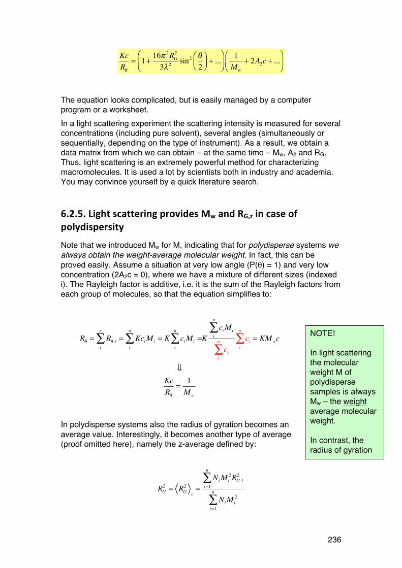
236

KcRθ

= 1+ 16π2RG

2

3λ2sin2 θ

2⎛⎝⎜

⎞⎠⎟+ ...

⎛⎝⎜

⎞⎠⎟

1Mw

+ 2A2c + ...⎛⎝⎜

⎞⎠⎟

The equation looks complicated, but is easily managed by a computer program or a worksheet. In a light scattering experiment the scattering intensity is measured for several concentrations (including pure solvent), several angles (simultaneously or sequentially, depending on the type of instrument). As a result, we obtain a data matrix from which we can obtain – at the same time – Mw, A2 and RG. Thus, light scattering is an extremely powerful method for characterizing macromolecules. It is used a lot by scientists both in industry and academia. You may convince yourself by a quick literature search.

6.2.5.  Light  scattering  provides  Mw  and  RG,z  in  case  of  polydispersity  

Note that we introduced Mw for M, indicating that for polydisperse systems we always obtain the weight-average molecular weight. In fact, this can be proved easily. Assume a situation at very low angle (P(θ) = 1) and very low concentration (2A2c = 0), where we have a mixture of different sizes (indexed i). The Rayleigh factor is additive, i.e. it is the sum of the Rayleigh factors from each group of molecules, so that the equation simplifies to:

Rθ = Rθ ,ii

n

∑ = KciMi = K ciMi =i

n

∑i

n

∑ KciMi

i

n

∑

cii

n

∑ci

i

n

∑ = KMwc

⇓KcRθ

=1Mw

In polydisperse systems also the radius of gyration becomes an average value. Interestingly, it becomes another type of average (proof omitted here), namely the z-average defined by:

RG2 = RG

2z=

NiMi2RG ,i

2

i=1

n

∑

NiMi2

i=1

n

∑

NOTE! In light scattering the molecular weight M of polydisperse samples is always Mw – the weight average molecular weight. In contrast, the radius of gyration is z-average.

237

6.2.6.  Calculations  of  Mw,  A2  and  RG  from  light  scattering  measurements.  

A classical light scattering (‘batch mode’) experiment provides Rθ values for typically 15 angles (30-150°) and 3-8 concentrations. Here is an example (Kc/Rθ values from 4 concentrations, 5 angles):

q sin2(q/2) c1 (g/ml) c2 (g/ml) c3 (g/ml) c4 (g/ml) 0.00023 0.0007 0.00097 0.0014 q1 30 0.07 6.76E-06 9.72E-06 1.14E-05 1.41E-05 q2 60 0.25 7.65E-06 1.10E-05 1.29E-05 1.60E-05 q3 90 0.50 8.88E-06 1.28E-05 1.50E-05 1.86E-05 q4 120 0.75 1.01E-05 1.45E-05 1.71E-05 2.11E-05 q5 150 0.93 1.10E-05 1.58E-05 1.86E-05 2.30E-05

How to proceed? The literature often presents data as the famous Zimm diagram, which is very elegant, but relatively complicated and less intuitive to most biochemists. The software of course produces it automatically. However, we will employ the underlying 4 steps (Zimm diagram is explained in a later section). Step. 1. We note from the main equation that Kc/Rθ is a linear function of both sin2(θ/2) and c. If we for each concentration (ci) perform a linear regression and extrapolate the Kc/R data to zero angle (sin2(θ/2) → 0) we obtain new values, Kc/Rθ=0, one for each concentration.

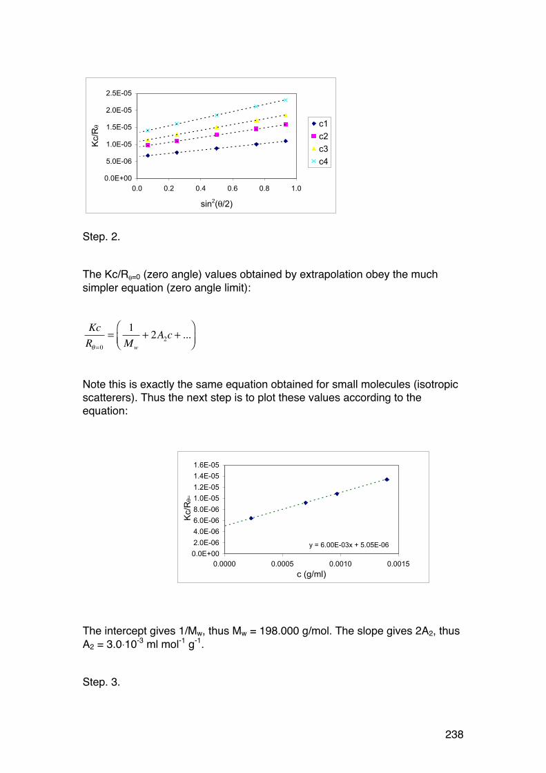
238

Step. 2. The Kc/Rθ=0 (zero angle) values obtained by extrapolation obey the much simpler equation (zero angle limit):

KcRθ=0

=1Mw

+ 2A2c + ...⎛⎝⎜

⎞⎠⎟

Note this is exactly the same equation obtained for small molecules (isotropic scatterers). Thus the next step is to plot these values according to the equation:

The intercept gives 1/Mw, thus Mw = 198.000 g/mol. The slope gives 2A2, thus A2 = 3.0⋅10-3 ml mol-1 g-1. Step. 3.

0.0E+00

5.0E-06

1.0E-05

1.5E-05

2.0E-05

2.5E-05

0.0 0.2 0.4 0.6 0.8 1.0

sin2(!/2)

Kc/R

! c1

c2

c3

c4

y = 6.00E-03x + 5.05E-06

0.0E+00

2.0E-06

4.0E-06

6.0E-06

8.0E-06

1.0E-05

1.2E-05

1.4E-05

1.6E-05

0.0000 0.0005 0.0010 0.0015

c (g/ml)

Kc/R

!=

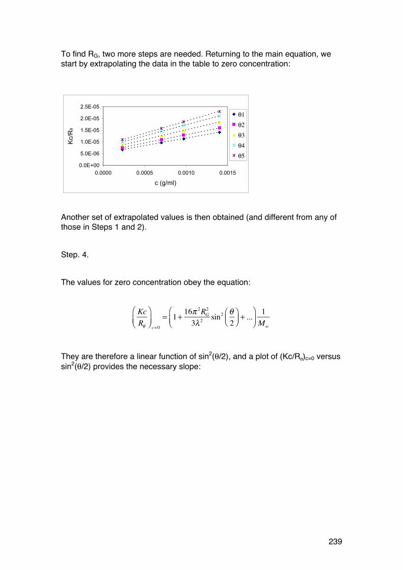
239

To find RG, two more steps are needed. Returning to the main equation, we start by extrapolating the data in the table to zero concentration:

Another set of extrapolated values is then obtained (and different from any of those in Steps 1 and 2). Step. 4. The values for zero concentration obey the equation:

KcRθ

⎛⎝⎜

⎞⎠⎟ c=0

= 1+ 16π2RG

2

3λ2sin2 θ

2⎛⎝⎜

⎞⎠⎟+ ...

⎛⎝⎜

⎞⎠⎟1Mw

They are therefore a linear function of sin2(θ/2), and a plot of (Kc/Rθ)c=0 versus sin2(θ/2) provides the necessary slope:

0.0E+00

5.0E-06

1.0E-05

1.5E-05

2.0E-05

2.5E-05

0.0000 0.0005 0.0010 0.0015

c (g/ml)

Kc/R

!

!1

!2

!3

!4

!5

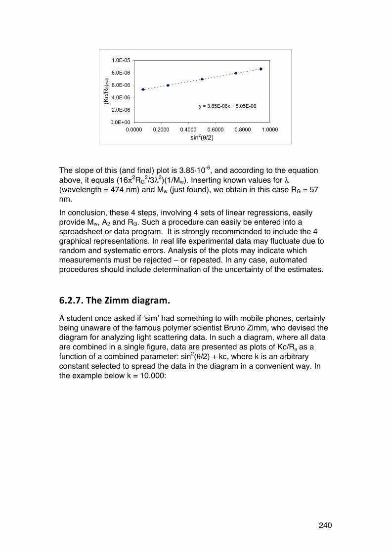
240

The slope of this (and final) plot is 3.85⋅10-6, and according to the equation above, it equals (16π2RG

2/3λ2)(1/Mw). Inserting known values for λ (wavelength = 474 nm) and Mw (just found), we obtain in this case RG = 57 nm. In conclusion, these 4 steps, involving 4 sets of linear regressions, easily provide Mw, A2 and RG. Such a procedure can easily be entered into a spreadsheet or data program. It is strongly recommended to include the 4 graphical representations. In real life experimental data may fluctuate due to random and systematic errors. Analysis of the plots may indicate which measurements must be rejected – or repeated. In any case, automated procedures should include determination of the uncertainty of the estimates.

6.2.7.  The  Zimm  diagram.  

A student once asked if ‘sim’ had something to with mobile phones, certainly being unaware of the famous polymer scientist Bruno Zimm, who devised the diagram for analyzing light scattering data. In such a diagram, where all data are combined in a single figure, data are presented as plots of Kc/Rθ as a function of a combined parameter: sin2(θ/2) + kc, where k is an arbitrary constant selected to spread the data in the diagram in a convenient way. In the example below k = 10.000:

y = 3.85E-06x + 5.05E-06

0.0E+00

2.0E-06

4.0E-06

6.0E-06

8.0E-06

1.0E-05

0.0000 0.2000 0.4000 0.6000 0.8000 1.0000

sin2(!/2)

(Kc/R

!)c=0

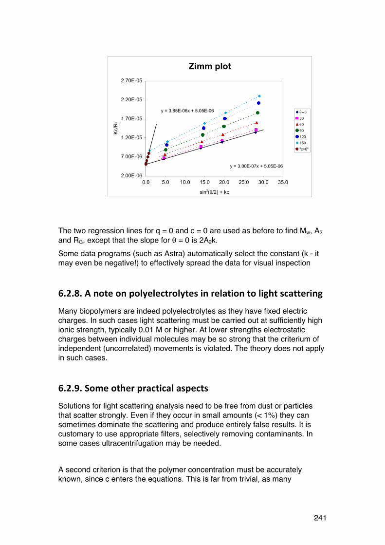
241

The two regression lines for q = 0 and c = 0 are used as before to find Mw, A2 and RG, except that the slope for θ = 0 is 2A2k. Some data programs (such as Astra) automatically select the constant (k - it may even be negative!) to effectively spread the data for visual inspection

6.2.8.  A  note  on  polyelectrolytes  in  relation  to  light  scattering  

Many biopolymers are indeed polyelectrolytes as they have fixed electric charges. In such cases light scattering must be carried out at sufficiently high ionic strength, typically 0.01 M or higher. At lower strengths electrostatic charges between individual molecules may be so strong that the criterium of independent (uncorrelated) movements is violated. The theory does not apply in such cases.

6.2.9.  Some  other  practical  aspects  

Solutions for light scattering analysis need to be free from dust or particles that scatter strongly. Even if they occur in small amounts (< 1%) they can sometimes dominate the scattering and produce entirely false results. It is customary to use appropriate filters, selectively removing contaminants. In some cases ultracentrifugation may be needed. A second criterion is that the polymer concentration must be accurately known, since c enters the equations. This is far from trivial, as many

Zimm plot

y = 3.00E-07x + 5.05E-06

y = 3.85E-06x + 5.05E-06

2.00E-06

7.00E-06

1.20E-05

1.70E-05

2.20E-05

2.70E-05

0.0 5.0 10.0 15.0 20.0 25.0 30.0 35.0

sin2(!/2) + kc

Kc/R

!

! = 0

30

60

90

120

150

"c=0"

242

biopolymers contain tightly bound water (even after drying), or other impurities. Light scattering normally requires that the samples do not absorb light at the wavelength of the laser. Any absorption of incident and scattered light must be corrected for if it cannot be avoided. Also, fluorescence may impair the measurements, as fluorescence can be much stronger than the scattering. Polymers such as lignosulfonates face this problem. Fluorescence (emission) can be eliminated by using special optical filters (‘narrow band pass’). The filters eliminate fluorescence at wavelengths other than for the scattered light itself.

6.2.10.  Light  scattering  in  practise.  

Light scattering with modern instruments is quite straightforward. Here is a brief description.

1. Prepare samples with different known concentrations, e.g. 0.2 – 1.0 mg/ml (varies with Mw and A2)

2. Samples must be free of particles and aggregates (filtration or ultracentrifugation)

3. (dn/dc) and n0 must be known (tabulated or measured separately) ⇒ K 4. Measure iθ at different angles for all concentrations, calculate the

Rayleigh factor (Rθ), and obtain a matrix of raw data. : Conc. c1 c2 cj

Angle θ1 i1,1 → Kc1/R1,1 i1,2 → Kc2/R1,2 i1,j → Kcj/R1,j θ2 i2,1 → Kc1/R2,1 i2,2 → Kc2/R2,2 i2,j → Kcj/R2,j θi ii,1 → Kc1/Ri,1 ii,2 → Kc2/Ri,2 ii,j → Kcj/Ri,j

c1 c2 c3 c4 c0 = 0 (blank)

243

The rest is software….. Good luck!

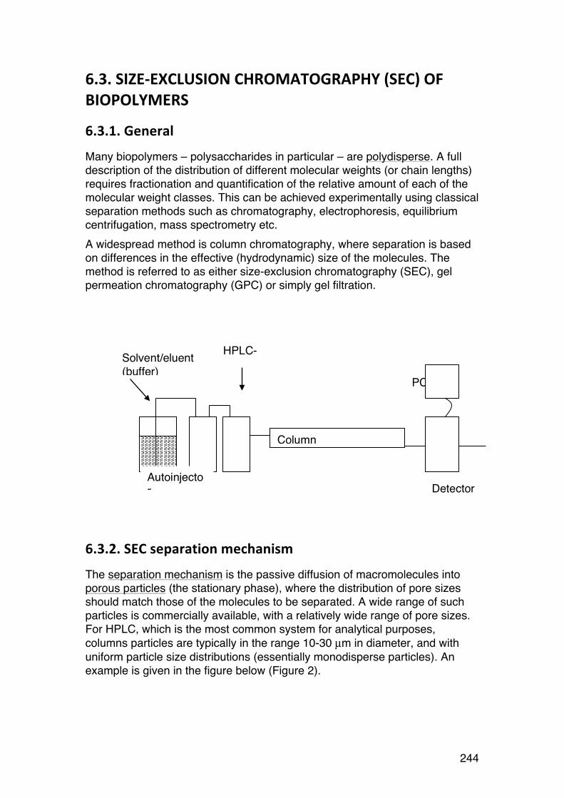
244

6.3.  SIZE-­‐EXCLUSION  CHROMATOGRAPHY  (SEC)  OF  BIOPOLYMERS  

6.3.1.  General  

Many biopolymers – polysaccharides in particular – are polydisperse. A full description of the distribution of different molecular weights (or chain lengths) requires fractionation and quantification of the relative amount of each of the molecular weight classes. This can be achieved experimentally using classical separation methods such as chromatography, electrophoresis, equilibrium centrifugation, mass spectrometry etc. A widespread method is column chromatography, where separation is based on differences in the effective (hydrodynamic) size of the molecules. The method is referred to as either size-exclusion chromatography (SEC), gel permeation chromatography (GPC) or simply gel filtration.

6.3.2.  SEC  separation  mechanism  

The separation mechanism is the passive diffusion of macromolecules into porous particles (the stationary phase), where the distribution of pore sizes should match those of the molecules to be separated. A wide range of such particles is commercially available, with a relatively wide range of pore sizes. For HPLC, which is the most common system for analytical purposes, columns particles are typically in the range 10-30 µm in diameter, and with uniform particle size distributions (essentially monodisperse particles). An example is given in the figure below (Figure 2).

PC

Column

Solvent/eluent (buffer)

HPLC-

Detector Autoinjector

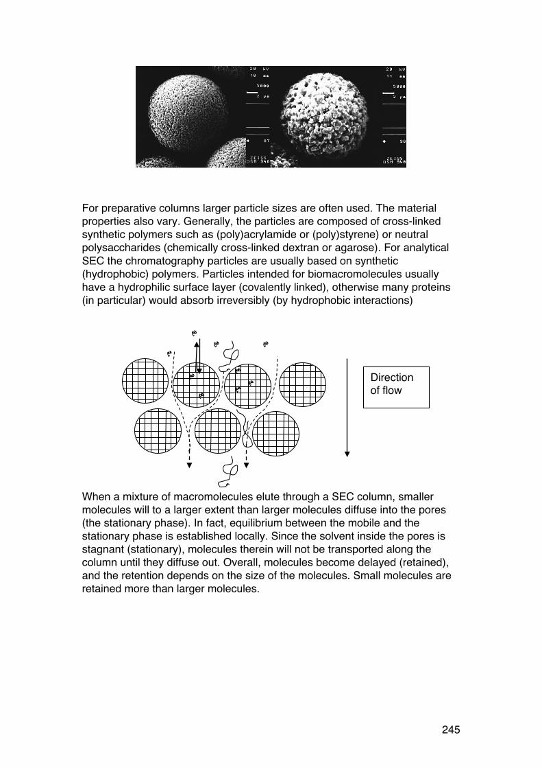
245

For preparative columns larger particle sizes are often used. The material properties also vary. Generally, the particles are composed of cross-linked synthetic polymers such as (poly)acrylamide or (poly)styrene) or neutral polysaccharides (chemically cross-linked dextran or agarose). For analytical SEC the chromatography particles are usually based on synthetic (hydrophobic) polymers. Particles intended for biomacromolecules usually have a hydrophilic surface layer (covalently linked), otherwise many proteins (in particular) would absorb irreversibly (by hydrophobic interactions)

When a mixture of macromolecules elute through a SEC column, smaller molecules will to a larger extent than larger molecules diffuse into the pores (the stationary phase). In fact, equilibrium between the mobile and the stationary phase is established locally. Since the solvent inside the pores is stagnant (stationary), molecules therein will not be transported along the column until they diffuse out. Overall, molecules become delayed (retained), and the retention depends on the size of the molecules. Small molecules are retained more than larger molecules.

Direction of flow

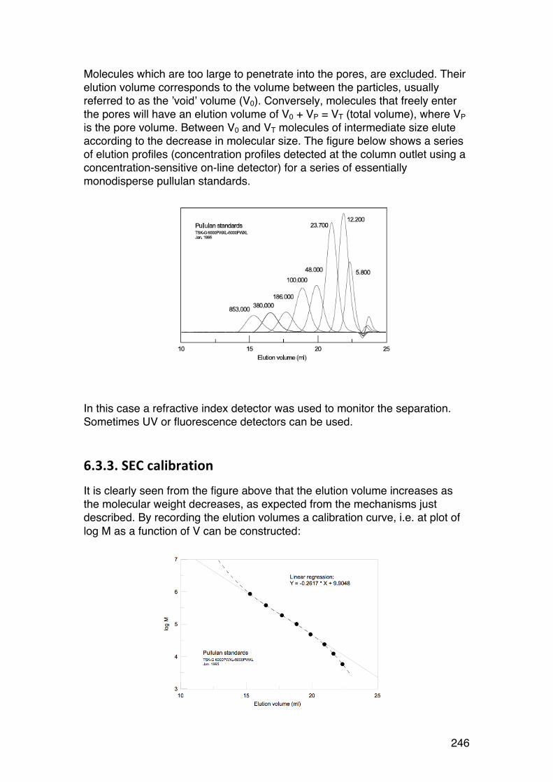
246

Molecules which are too large to penetrate into the pores, are excluded. Their elution volume corresponds to the volume between the particles, usually referred to as the ’void’ volume (V0). Conversely, molecules that freely enter the pores will have an elution volume of V0 + VP = VT (total volume), where VP is the pore volume. Between V0 and VT molecules of intermediate size elute according to the decrease in molecular size. The figure below shows a series of elution profiles (concentration profiles detected at the column outlet using a concentration-sensitive on-line detector) for a series of essentially monodisperse pullulan standards.

In this case a refractive index detector was used to monitor the separation. Sometimes UV or fluorescence detectors can be used.

6.3.3.  SEC  calibration  

It is clearly seen from the figure above that the elution volume increases as the molecular weight decreases, as expected from the mechanisms just described. By recording the elution volumes a calibration curve, i.e. at plot of log M as a function of V can be constructed:

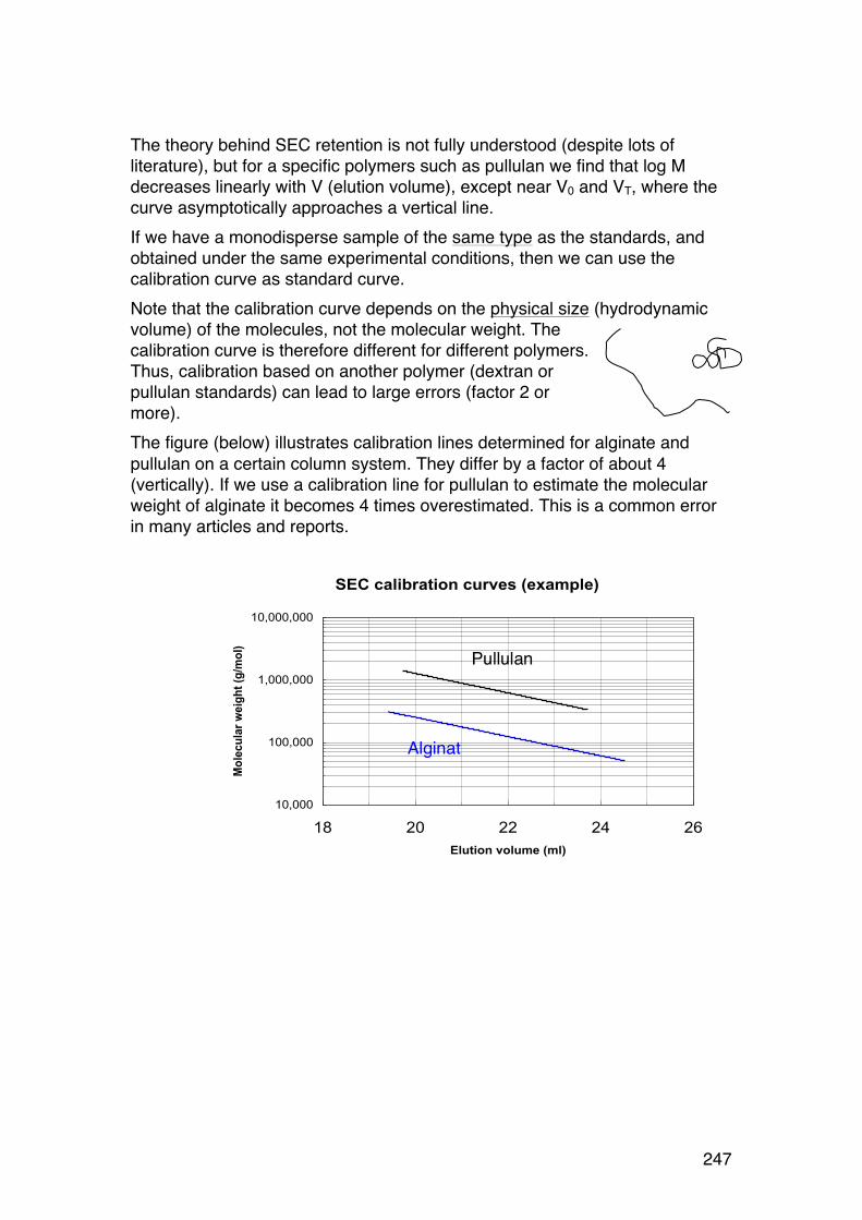
247

The theory behind SEC retention is not fully understood (despite lots of literature), but for a specific polymers such as pullulan we find that log M decreases linearly with V (elution volume), except near V0 and VT, where the curve asymptotically approaches a vertical line. If we have a monodisperse sample of the same type as the standards, and obtained under the same experimental conditions, then we can use the calibration curve as standard curve. Note that the calibration curve depends on the physical size (hydrodynamic volume) of the molecules, not the molecular weight. The calibration curve is therefore different for different polymers. Thus, calibration based on another polymer (dextran or pullulan standards) can lead to large errors (factor 2 or more). The figure (below) illustrates calibration lines determined for alginate and pullulan on a certain column system. They differ by a factor of about 4 (vertically). If we use a calibration line for pullulan to estimate the molecular weight of alginate it becomes 4 times overestimated. This is a common error in many articles and reports.

SEC calibration curves (example)

10,000

100,000

1,000,000

10,000,000

18 20 22 24 26

Elution volume (ml)

Mo

lec

ula

r w

eig

ht

(g/m

ol) Pullulan

Alginate

248

6.3.4.  SEC  ‘universal’  calibration  

The effective hydrodynamic volume (volume per particle) can be expressed as the product between the intrinsic viscosity (volume per gram) and the molecular weight (gram per mol): vh' = [η]M/NAvo

This is the basis for the so-called universal calibration. According to this theory all polymers – irrespective of shape and extension – should follow the same plot when log ([η]M) is plotted as a function of V. The theory has been shown to hold for many synthetic polymers in organic solvents. For biopolymers examples exist, but any tendency to non-specific (reversible) adsorption (non-SEC mechanisms), which are quite common, makes this a risky business and is not recommended, at least as a precise method. In cases where the ‘universal calibration’ truly applies, the calibration can be established on the basis of a single polymer system, for example dextran standards (often used by biochemists). For another polymer, the peak position (V) corresponds to a certain [η]M. If the intrinsic viscosity is measured separately, M is obtained directly.

249

6.4.  SIZE-­‐EXCLUSION  CHROMATOGRAPHY  COMBINED  WITH  ON-­‐LINE  LIGHT  SCATTERING  (SEC-­‐MALLS)  

6.4.1.  General  

SEC-MALLS is probably the most common method to determine molecular weight distributions (and averages). All components are commercially available for measurements, and software is available for all data processing. SEC-MALLS is based on the use of two on-line detectors in the chromatographic set-up:

• A concentration sensitive detector (refractive index or UV detector) • A light scattering detector, which monitors scattering at up to 18 angles

simultaneously. The figure below shows an example.

The software records raw data from the detectors at regular intervals. A single experiment is divided into 1000-5000 ‘elution slices’ (typically 0.1 ml) which

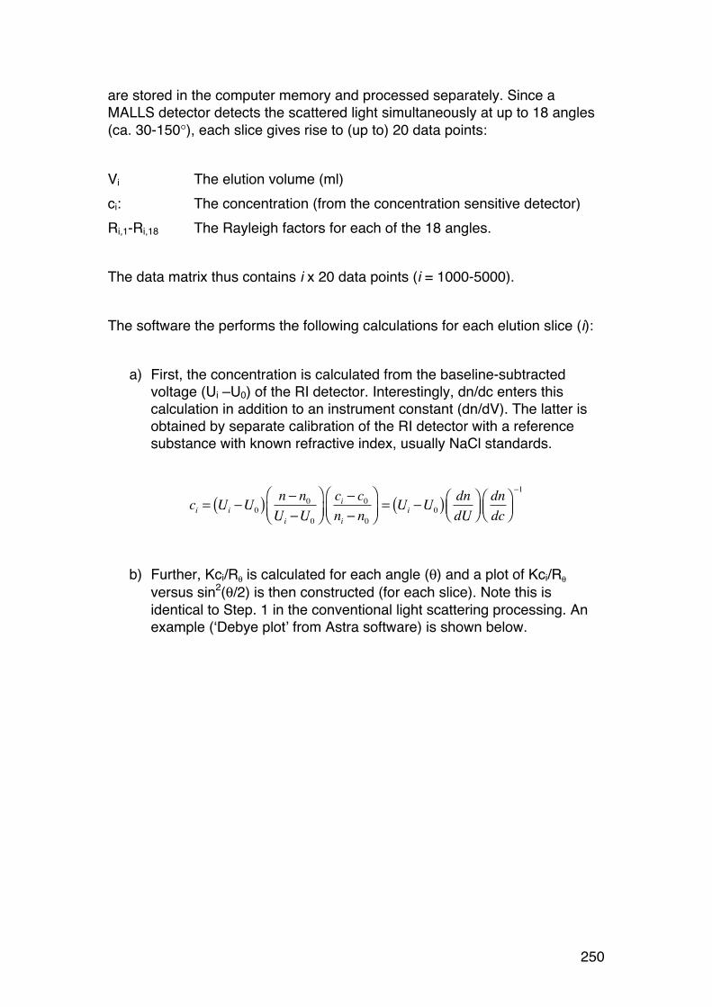
250

are stored in the computer memory and processed separately. Since a MALLS detector detects the scattered light simultaneously at up to 18 angles (ca. 30-150°), each slice gives rise to (up to) 20 data points: Vi The elution volume (ml) ci: The concentration (from the concentration sensitive detector) Ri,1-Ri,18 The Rayleigh factors for each of the 18 angles. The data matrix thus contains i x 20 data points (i = 1000-5000). The software the performs the following calculations for each elution slice (i):

a) First, the concentration is calculated from the baseline-subtracted voltage (Ui –U0) of the RI detector. Interestingly, dn/dc enters this calculation in addition to an instrument constant (dn/dV). The latter is obtained by separate calibration of the RI detector with a reference substance with known refractive index, usually NaCl standards.

ci = Ui −U0( ) n − n0Ui −U0

⎛⎝⎜

⎞⎠⎟ci − c0ni − n0

⎛⎝⎜

⎞⎠⎟= Ui −U0( ) dn

dU⎛⎝⎜

⎞⎠⎟dndc

⎛⎝⎜

⎞⎠⎟−1

b) Further, Kci/Rθ is calculated for each angle (θ) and a plot of Kci/Rθ

versus sin2(θ/2) is then constructed (for each slice). Note this is identical to Step. 1 in the conventional light scattering processing. An example (‘Debye plot’ from Astra software) is shown below.

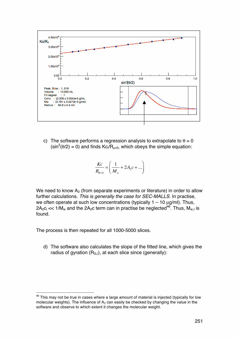
251

c) The software performs a regression analysis to extrapolate to θ = 0 (sin2(θ/2) = 0) and finds Kci/Rθ=0, which obeys the simple equation:

Kc

Rθ=0

=1

Mw

+ 2A2c + ...

⎛

⎝⎜⎞

⎠⎟

We need to know A2 (from separate experiments or literature) in order to allow further calculations. This is generally the case for SEC-MALLS. In practise, we often operate at such low concentrations (typically 1 – 10 µg/ml). Thus, 2A2ci << 1/Mw and the 2A2c term can in practise be neglected46. Thus, Mw,I is found. The process is then repeated for all 1000-5000 slices.

d) The software also calculates the slope of the fitted line, which gives the radius of gyration (RG,i), at each slice since (generally):

46 This may not be true in cases where a large amount of material is injected (typically for low molecular weights). The influence of A2 can easily be checked by changing the value in the software and observe to which extent it changes the molecular weight.

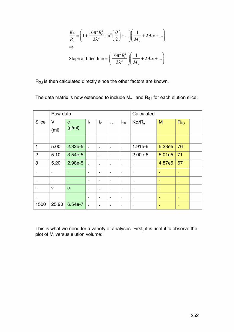
252

Kc

Rθ

= 1+16π 2

RG

2

3λ2sin2 θ

2

⎛⎝⎜

⎞⎠⎟+ ...

⎛⎝⎜

⎞⎠⎟

1

Mw

+ 2A2c + ...⎛

⎝⎜⎞

⎠⎟

⇒

Slope of fitted line = 16π 2

RG

2

3λ2

⎛⎝⎜

⎞⎠⎟

1

Mw

+ 2A2c + ...⎛

⎝⎜⎞

⎠⎟

RG,i is then calculated directly since the other factors are known. The data matrix is now extended to include Mw,I and RG,i for each elution slice: Raw data Calculated Slice V

(ml) ci (g/ml)

i1 i2 … i18 Kci/Rθ Mi RG,i

1 5.00 2.32e-5 . . . . 1.91e-6 5.23e5 76 2 5.10 3.54e-5 . . . . 2.00e-6 5.01e5 71 3 5.20 2.98e-5 . . . . . 4.87e5 67 . . . . . . . . . . . . . . . . . . . . i vi ci . . . . . . . . . . . . . . . 1500 25.90 6.54e-7 . . . . . . . This is what we need for a variety of analyses. First, it is useful to observe the plot of Mi versus elution volume:

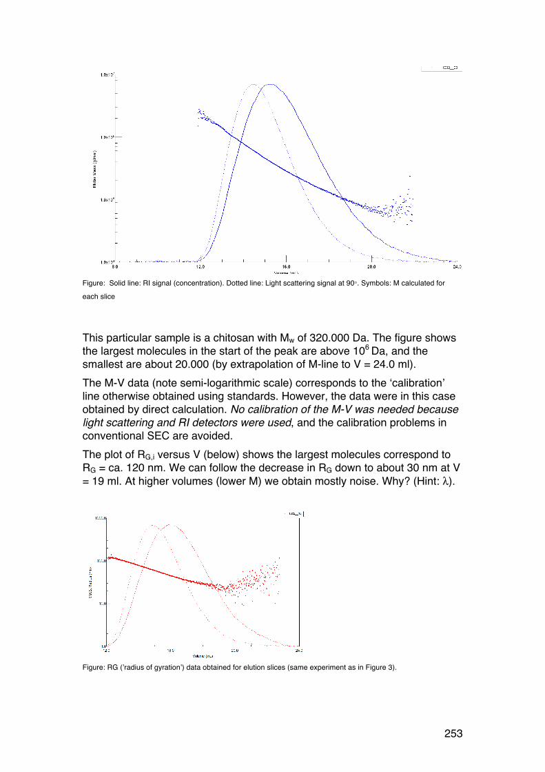
253

Figure: Solid line: RI signal (concentration). Dotted line: Light scattering signal at 90°. Symbols: M calculated for

each slice

This particular sample is a chitosan with Mw of 320.000 Da. The figure shows the largest molecules in the start of the peak are above 106

Da, and the smallest are about 20.000 (by extrapolation of M-line to V = 24.0 ml). The M-V data (note semi-logarithmic scale) corresponds to the ‘calibration’ line otherwise obtained using standards. However, the data were in this case obtained by direct calculation. No calibration of the M-V was needed because light scattering and RI detectors were used, and the calibration problems in conventional SEC are avoided. The plot of RG,i versus V (below) shows the largest molecules correspond to RG = ca. 120 nm. We can follow the decrease in RG down to about 30 nm at V = 19 ml. At higher volumes (lower M) we obtain mostly noise. Why? (Hint: λ).

Figure: RG (’radius of gyration’) data obtained for elution slices (same experiment as in Figure 3).

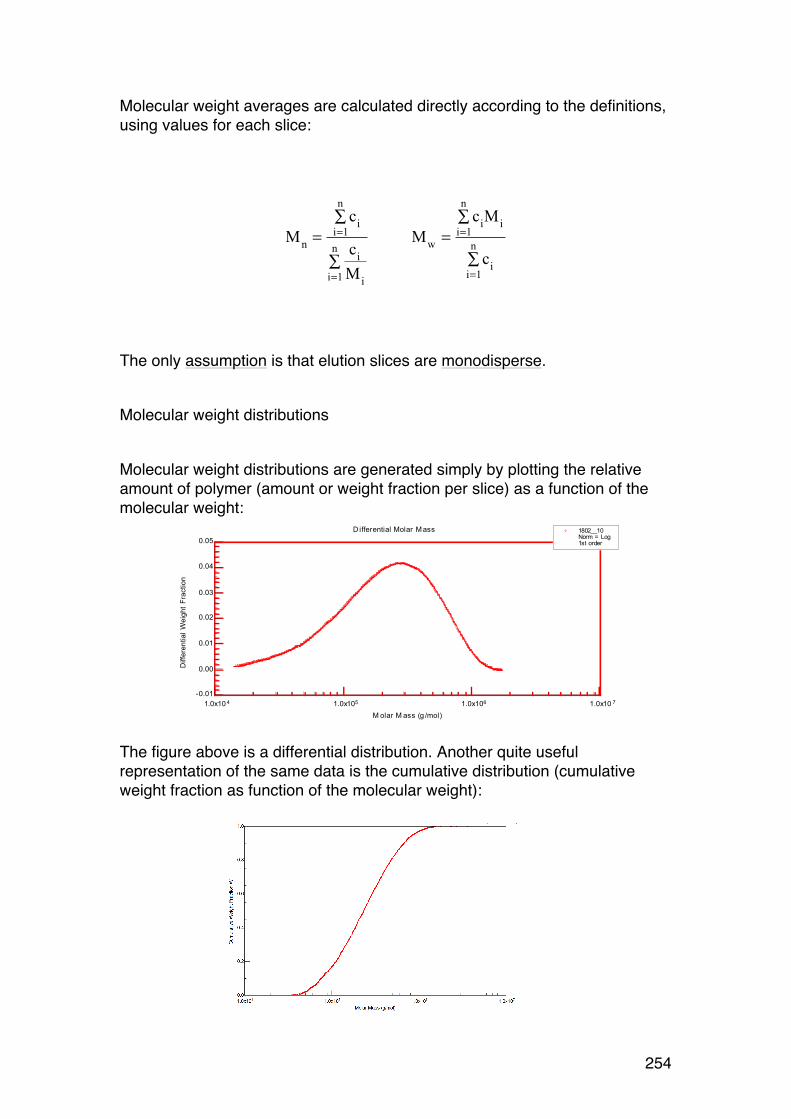
254

Molecular weight averages are calculated directly according to the definitions, using values for each slice:

Mn=

ci

i=1

n

∑

ci

Mi

i=1

n

∑

Mw=

ciM

ii=1

n

∑

ci

i=1

n

∑

The only assumption is that elution slices are monodisperse. Molecular weight distributions Molecular weight distributions are generated simply by plotting the relative amount of polymer (amount or weight fraction per slice) as a function of the molecular weight: The figure above is a differential distribution. Another quite useful representation of the same data is the cumulative distribution (cumulative weight fraction as function of the molecular weight):

-0.01

0.00

0.01

0.02

0.03

0.04

0.05

1.0x10 4 1.0x105 1.0x106 1.0x10 7

Diffe

ren

tia

l W

eig

ht

Fra

ctio

n

M olar M ass (g /mol)

D ifferential Molar M ass 1802__10Norm = Log1st order

255

If we need to find out how much of the sample has a molecular weight below 200.000 g/mol, just follow the arrows. The result is that about 45% of the sample is below 200.000. How much is above 500.000 g/mol? Such analyses are very important in biomedical uses because strict regulations may apply to the molecular weight distribution. Typically, only a certain % may be below a specified molecular weight. In the same way as for Mw and Mn, RG,n and RG,w can be calculated (after extrapolating the data to cover the whole chromatogram). Note conventional light scattering only gives RG,z.

6.4.2.  RG-­‐M  analysis  from  SEC-­‐MALLS  

Next, we can directly analyse the RG-M relationship, simply by plotting RG,i as a function of Mi (double logarithmic plot):

Except for data at very high (M > 106) and very low M (M < 105) the data follow a straight line. Thus, log RG,I is a linear function of Mi, as expected:

logRG ,i = α logM

i+ B (constant)

RG ,i = BM

α

By using SEC-MALLS we can – in a single experiment47 - study the M dependence of RG, and find the exponent (α) (after regression analysis) which provides information about the shape of the polymer. In this case we find α = 0.57. What is the shape? Let us repeat the basics for idealized shapes: 47 This is only in theory. In practise we must always optimize the experiment by choosing solvent, column (separation range), injected mass, and so on.

1.0

10.0

100.0

1000.0

1.0x10 4 1.0x10 5 1.0x106 1.0x10 7

R.M

.S.

Ra

diu

s (

nm

)

M olar M ass (g /mol)

R M S R adius vs. M olar M ass 1802__10

Figure 51

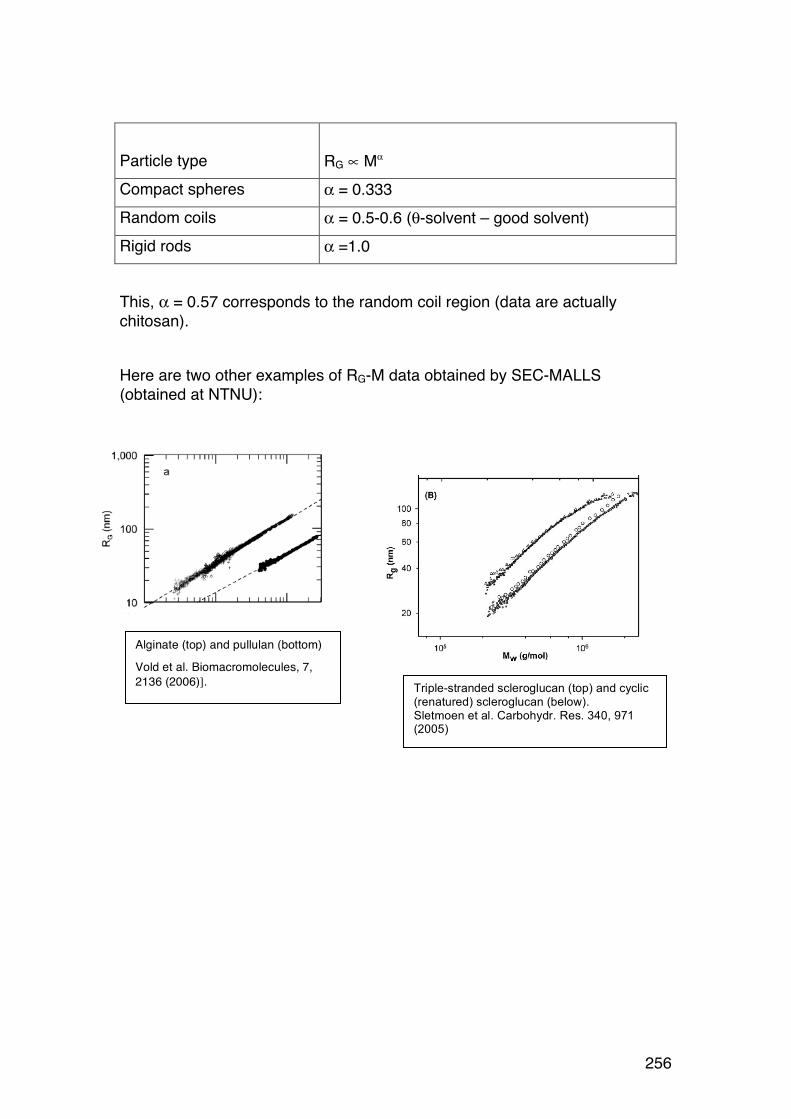
256

Particle type

RG ∝ Mα

Compact spheres α = 0.333 Random coils α = 0.5-0.6 (θ-solvent – good solvent) Rigid rods α =1.0 This, α = 0.57 corresponds to the random coil region (data are actually chitosan). Here are two other examples of RG-M data obtained by SEC-MALLS (obtained at NTNU):

Alginate (top) and pullulan (bottom)

Vold et al. Biomacromolecules, 7, 2136 (2006)].

Triple-stranded scleroglucan (top) and cyclic (renatured) scleroglucan (below). Sletmoen et al. Carbohydr. Res. 340, 971 (2005)

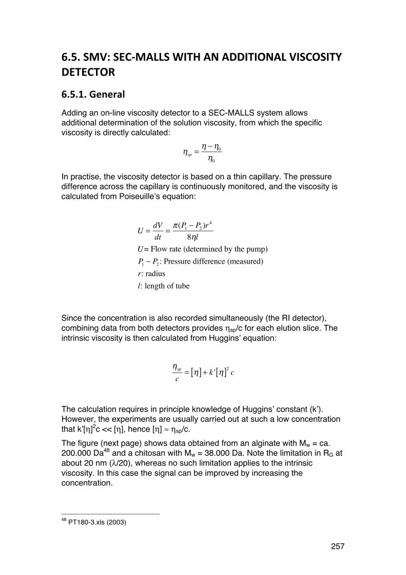
257

6.5.  SMV:  SEC-­‐MALLS  WITH  AN  ADDITIONAL  VISCOSITY  DETECTOR  

6.5.1.  General  

Adding an on-line viscosity detector to a SEC-MALLS system allows additional determination of the solution viscosity, from which the specific viscosity is directly calculated:

ηsp=η −η

0

η0

In practise, the viscosity detector is based on a thin capillary. The pressure difference across the capillary is continuously monitored, and the viscosity is calculated from Poiseuille’s equation:

U =dV

dt=π (P1 − P2 )r4

8ηl

U= Flow rate (determined by the pump)

P1 − P2 : Pressure difference (measured)

r: radius

l: length of tube

Since the concentration is also recorded simultaneously (the RI detector), combining data from both detectors provides ηsp/c for each elution slice. The intrinsic viscosity is then calculated from Huggins’ equation:

ηsp

c= η[ ] + k ' η[ ]

2

c

The calculation requires in principle knowledge of Huggins’ constant (k’). However, the experiments are usually carried out at such a low concentration that k’[η]2c << [η], hence [η] ≈ ηsp/c. The figure (next page) shows data obtained from an alginate with Mw = ca. 200.000 Da48 and a chitosan with Mw = 38.000 Da. Note the limitation in RG at about 20 nm (λ/20), whereas no such limitation applies to the intrinsic viscosity. In this case the signal can be improved by increasing the concentration.

48 PT180-3.xls (2003)

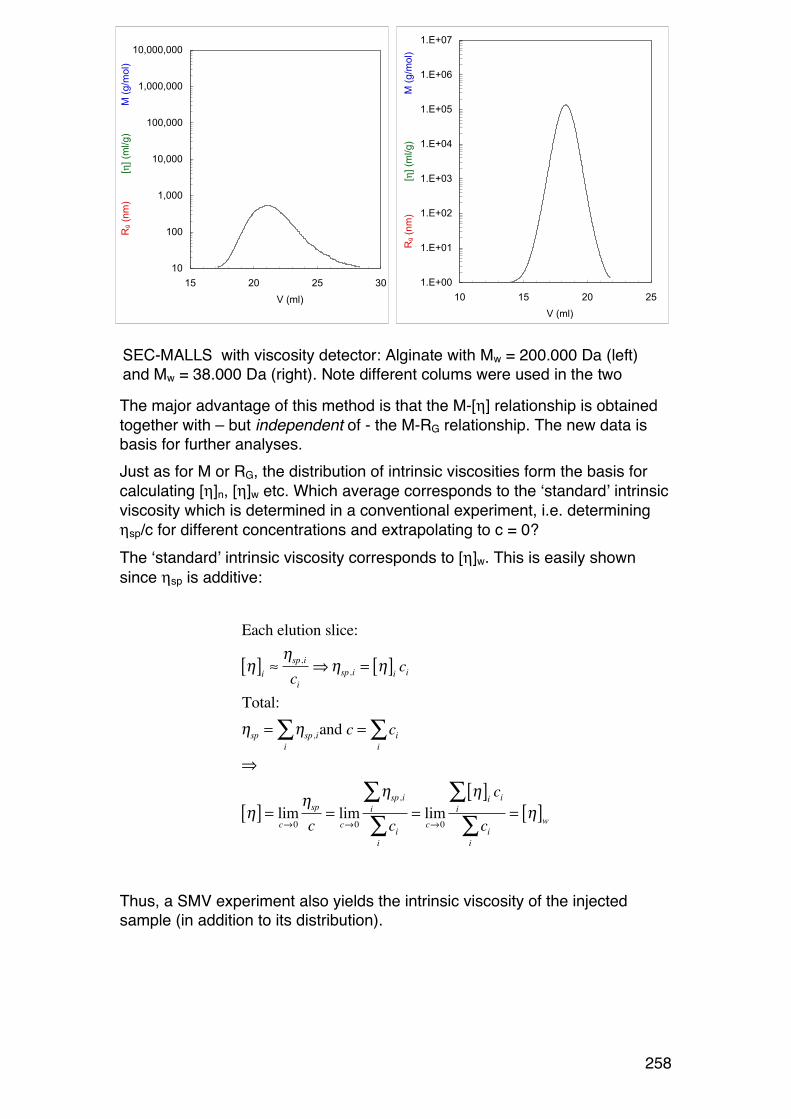
258

The major advantage of this method is that the M-[η] relationship is obtained together with – but independent of - the M-RG relationship. The new data is basis for further analyses. Just as for M or RG, the distribution of intrinsic viscosities form the basis for calculating [η]n, [η]w etc. Which average corresponds to the ‘standard’ intrinsic viscosity which is determined in a conventional experiment, i.e. determining ηsp/c for different concentrations and extrapolating to c = 0? The ‘standard’ intrinsic viscosity corresponds to [η]w. This is easily shown since ηsp is additive:

Each elution slice:

η[ ]i≈ηsp,i

ci

⇒ηsp,i

= η[ ]ici

Total:

ηsp= η

sp,i

i

∑ and c = ci

i

∑

⇒

η[ ] = limc→0

ηsp

c= lim

c→0

ηsp,i

i

∑

ci

i

∑= lim

c→0

η[ ]ici

i

∑

ci

i

∑= η[ ]

w

Thus, a SMV experiment also yields the intrinsic viscosity of the injected sample (in addition to its distribution).

10

100

1,000

10,000

100,000

1,000,000

10,000,000

15 20 25 30

V (ml)

R

g (

nm

)

[!

] (m

l/g

)

M

(g

/mo

l)

1.E+00

1.E+01

1.E+02

1.E+03

1.E+04

1.E+05

1.E+06

1.E+07

10 15 20 25

V (ml)

R

g (

nm

) [!

] (m

l/g)

M

(g/m

ol)

SEC-MALLS with viscosity detector: Alginate with Mw = 200.000 Da (left) and Mw = 38.000 Da (right). Note different colums were used in the two cases

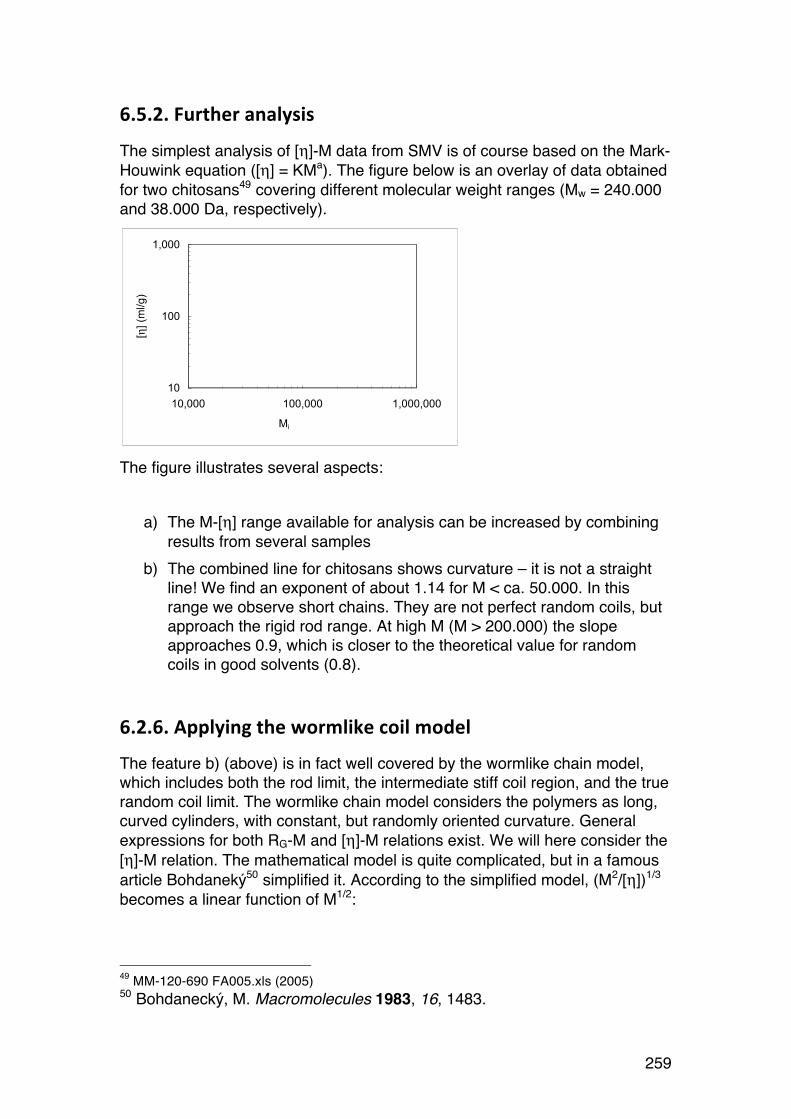
259

6.5.2.  Further  analysis  

The simplest analysis of [η]-M data from SMV is of course based on the Mark-Houwink equation ([η] = KMa). The figure below is an overlay of data obtained for two chitosans49 covering different molecular weight ranges (Mw = 240.000 and 38.000 Da, respectively).

The figure illustrates several aspects:

a) The M-[η] range available for analysis can be increased by combining results from several samples

b) The combined line for chitosans shows curvature – it is not a straight line! We find an exponent of about 1.14 for M < ca. 50.000. In this range we observe short chains. They are not perfect random coils, but approach the rigid rod range. At high M (M > 200.000) the slope approaches 0.9, which is closer to the theoretical value for random coils in good solvents (0.8).

6.2.6.  Applying  the  wormlike  coil  model  

The feature b) (above) is in fact well covered by the wormlike chain model, which includes both the rod limit, the intermediate stiff coil region, and the true random coil limit. The wormlike chain model considers the polymers as long, curved cylinders, with constant, but randomly oriented curvature. General expressions for both RG-M and [η]-M relations exist. We will here consider the [η]-M relation. The mathematical model is quite complicated, but in a famous article Bohdaneký50 simplified it. According to the simplified model, (M2/[η])1/3 becomes a linear function of M1/2:

49 MM-120-690 FA005.xls (2005) 50 Bohdanecký, M. Macromolecules 1983, 16, 1483.

10

100

1,000

10,000 100,000 1,000,000

Mi

[ !]

(ml/g

)

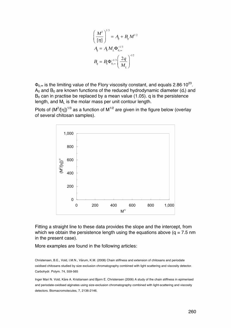
260

M2

[η]

⎛

⎝⎜⎞

⎠⎟

1/3

= Aη + Bη M1/ 2

Aη = A0M

LΦ

0,∞−1/3

Bη = B0Φ

0,∞−1/3 2q

ML

⎛

⎝⎜⎞

⎠⎟

-1/2

Φ0,∞ is the limiting value of the Flory viscosity constant, and equals 2.86⋅1023. A0 and B0 are known functions of the reduced hydrodynamic diameter (dr) and B0 can in practise be replaced by a mean value (1.05). q is the persistence length, and ML is the molar mass per unit contour length. Plots of (M2/[η])1/3 as a function of M1/2 are given in the figure below (overlay of several chitosan samples).

Fitting a straight line to these data provides the slope and the intercept, from which we obtain the persistence length using the equations above (q = 7.5 nm in the present case). More examples are found in the following articles: Christensen, B.E., Vold, I.M.N., Vårum, K.M. (2008) Chain stiffness and extension of chitosans and periodate

oxidised chitosans studied by size exclusion chromatography combined with light scattering and viscosity detector.

Carbohydr. Polym. 74, 559-565

Inger Mari N. Vold, Kåre A. Kristiansen and Bjørn E. Christensen (2006) A study of the chain stiffness in epimerised

and periodate-oxidised alginates using size-exclusion chromatography combined with light-scattering and viscosity

detectors. Biomacromolecules, 7, 2136-2146.

0

200

400

600

800

1,000

0 200 400 600 800 1,000

M1/

(M2/[!])1/

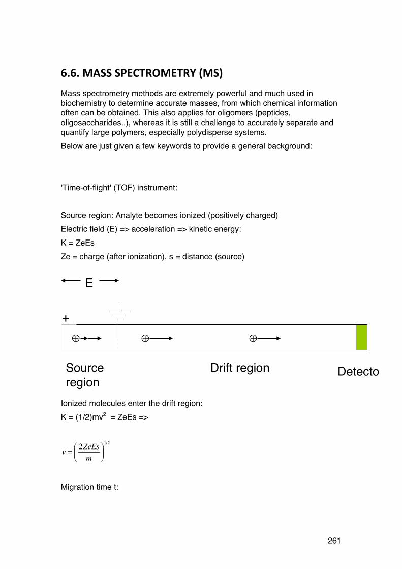
261

6.6.  MASS  SPECTROMETRY  (MS)  

Mass spectrometry methods are extremely powerful and much used in biochemistry to determine accurate masses, from which chemical information often can be obtained. This also applies for oligomers (peptides, oligosaccharides..), whereas it is still a challenge to accurately separate and quantify large polymers, especially polydisperse systems. Below are just given a few keywords to provide a general background: 'Time-of-flight' (TOF) instrument: Source region: Analyte becomes ionized (positively charged) Electric field (E) => acceleration => kinetic energy: K = ZeEs Ze = charge (after ionization), s = distance (source)

Ionized molecules enter the drift region: K = (1/2)mv2 = ZeEs =>

v = 2ZeEsm

⎛⎝⎜

⎞⎠⎟1/2

Migration time t:

⊕ ⊕ ⊕

Source region

Drift region Detector

+

E

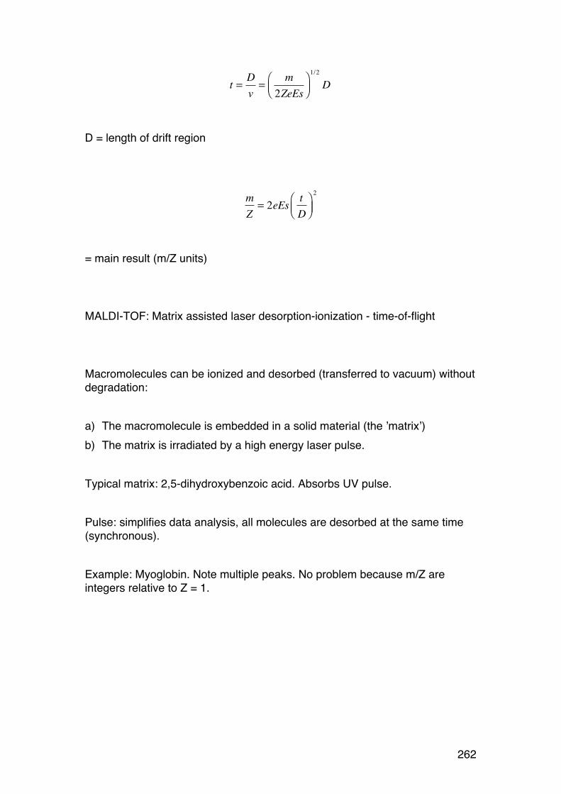
262

t = Dv=

m2ZeEs

⎛⎝⎜

⎞⎠⎟1/2

D

D = length of drift region

mZ

= 2eEs tD

⎛⎝⎜

⎞⎠⎟2

= main result (m/Z units) MALDI-TOF: Matrix assisted laser desorption-ionization - time-of-flight Macromolecules can be ionized and desorbed (transferred to vacuum) without degradation: a) The macromolecule is embedded in a solid material (the ’matrix’) b) The matrix is irradiated by a high energy laser pulse. Typical matrix: 2,5-dihydroxybenzoic acid. Absorbs UV pulse. Pulse: simplifies data analysis, all molecules are desorbed at the same time (synchronous). Example: Myoglobin. Note multiple peaks. No problem because m/Z are integers relative to Z = 1.

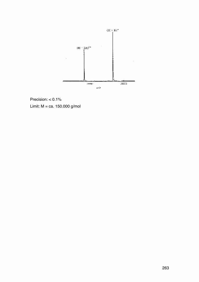
263

Precision: < 0.1% Limit: M = ca. 150.000 g/mol

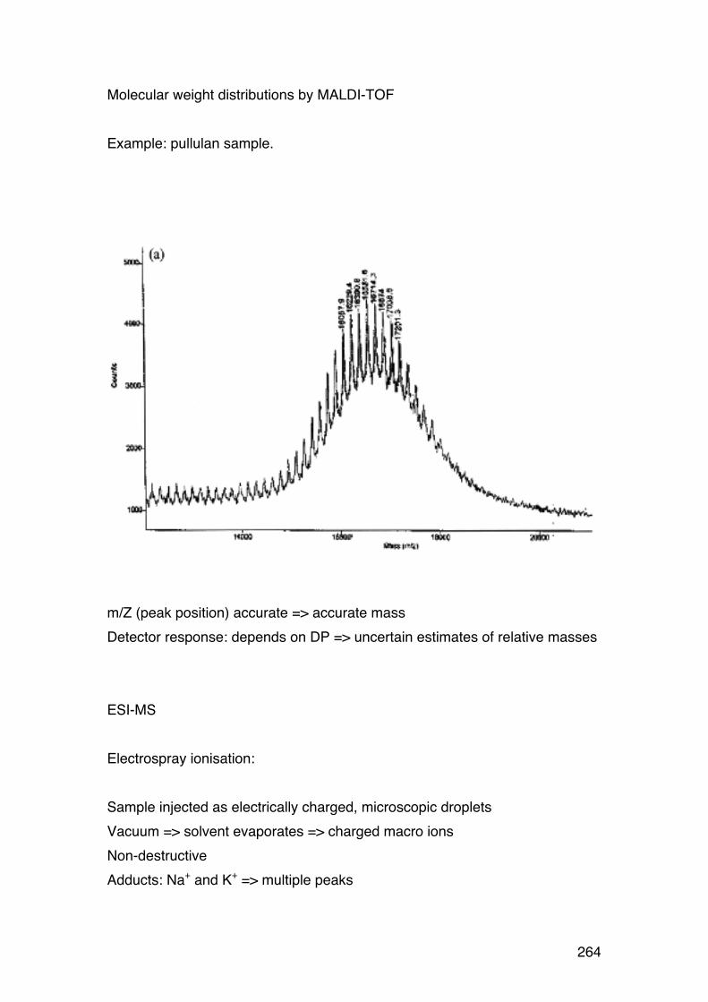
264

Molecular weight distributions by MALDI-TOF Example: pullulan sample.

m/Z (peak position) accurate => accurate mass Detector response: depends on DP => uncertain estimates of relative masses ESI-MS Electrospray ionisation: Sample injected as electrically charged, microscopic droplets Vacuum => solvent evaporates => charged macro ions Non-destructive Adducts: Na+ and K+ => multiple peaks

265

PART  7.  MISCELLANEOUS  

   

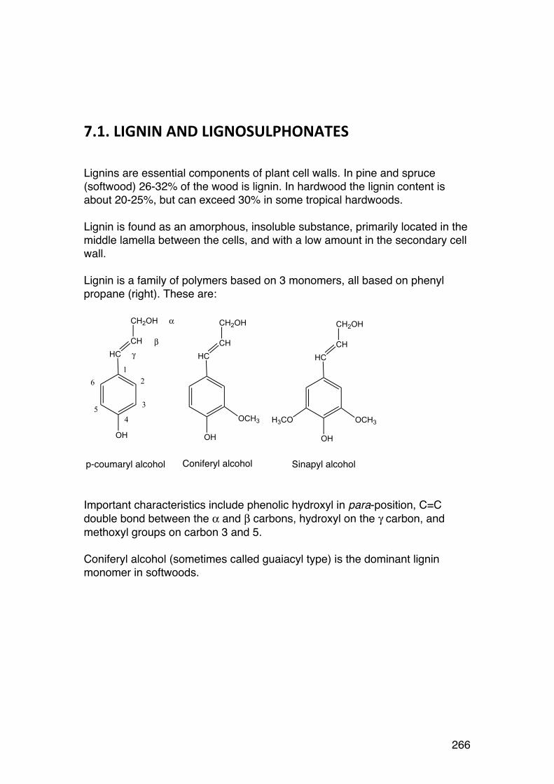
266

7.1.  LIGNIN  AND  LIGNOSULPHONATES  

Lignins are essential components of plant cell walls. In pine and spruce (softwood) 26-32% of the wood is lignin. In hardwood the lignin content is about 20-25%, but can exceed 30% in some tropical hardwoods. Lignin is found as an amorphous, insoluble substance, primarily located in the middle lamella between the cells, and with a low amount in the secondary cell wall. Lignin is a family of polymers based on 3 monomers, all based on phenyl propane (right). These are:

Important characteristics include phenolic hydroxyl in para-position, C=C double bond between the α and β carbons, hydroxyl on the γ carbon, and methoxyl groups on carbon 3 and 5. Coniferyl alcohol (sometimes called guaiacyl type) is the dominant lignin monomer in softwoods.

p-coumaryl alcohol

HCCH

CH2OH

OH

OCH3

Coniferyl alcohol

HCCH

CH2OH

OH

OCH3

Sinapyl alcohol

H3CO

HCCH

CH2OH

OH

α

βγ

12

3

45

6

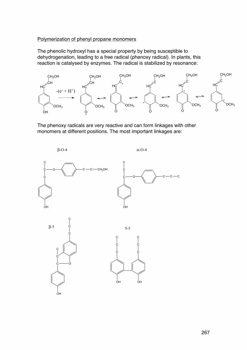
267

Polymerization of phenyl propane monomers The phenolic hydroxyl has a special property by being susceptible to dehydrogenation, leading to a free radical (phenoxy radical). In plants, this reaction is catalysed by enzymes. The radical is stabilized by resonance:

The phenoxy radicals are very reactive and can form linkages with other monomers at different positions. The most important linkages are:

HCCH

CH2OH

OH

OCH3

HCCH

CH2OH

O

OCH3

-(e- + H+)HC

C

CH2OH

O

OCH3

HCC

CH2OH

O

OCH3

HCC

CH2OH

O

OCH3

HCC

CH2OH

O

OCH3

C

C

C

OH

C C CH2OHO

β-O-4

C

C

C

OH

C C CO

α-O-4

C

C

C

OH

C

C

C

O

β-5

C

C

C

OH

C

C

C

OH

5-5

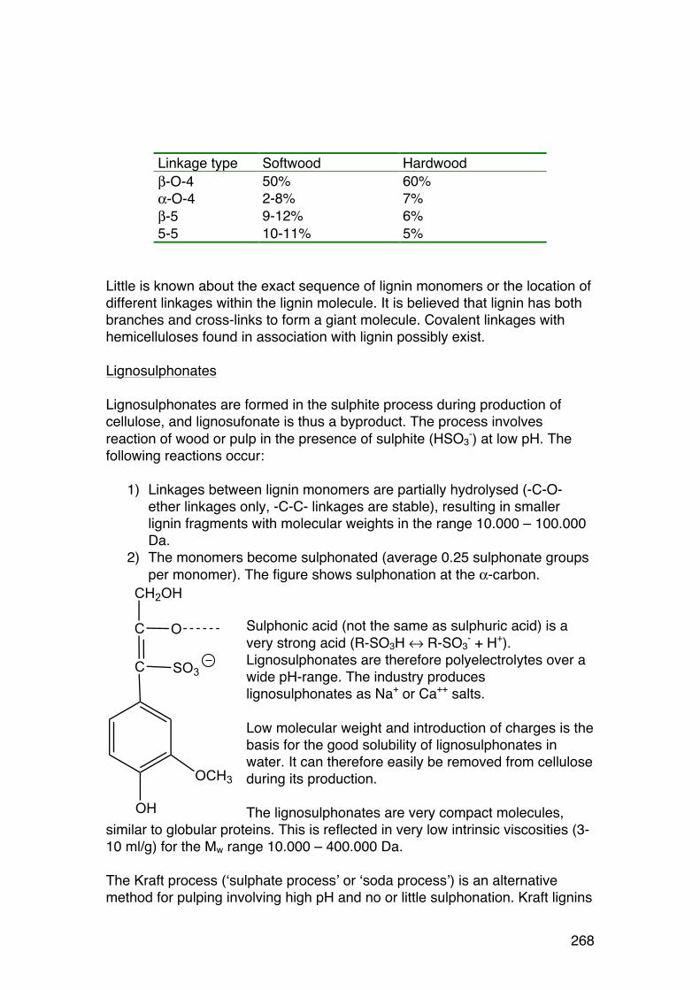
268

Linkage type Softwood Hardwood β-O-4 50% 60% α-O-4 2-8% 7% β-5 9-12% 6% 5-5 10-11% 5%

Little is known about the exact sequence of lignin monomers or the location of different linkages within the lignin molecule. It is believed that lignin has both branches and cross-links to form a giant molecule. Covalent linkages with hemicelluloses found in association with lignin possibly exist. Lignosulphonates Lignosulphonates are formed in the sulphite process during production of cellulose, and lignosufonate is thus a byproduct. The process involves reaction of wood or pulp in the presence of sulphite (HSO3

-) at low pH. The following reactions occur:

1) Linkages between lignin monomers are partially hydrolysed (-C-O- ether linkages only, -C-C- linkages are stable), resulting in smaller lignin fragments with molecular weights in the range 10.000 – 100.000 Da.

2) The monomers become sulphonated (average 0.25 sulphonate groups per monomer). The figure shows sulphonation at the α-carbon.

Sulphonic acid (not the same as sulphuric acid) is a very strong acid (R-SO3H ↔ R-SO3

- + H+). Lignosulphonates are therefore polyelectrolytes over a wide pH-range. The industry produces lignosulphonates as Na+ or Ca++ salts. Low molecular weight and introduction of charges is the basis for the good solubility of lignosulphonates in water. It can therefore easily be removed from cellulose during its production. The lignosulphonates are very compact molecules,

similar to globular proteins. This is reflected in very low intrinsic viscosities (3-10 ml/g) for the Mw range 10.000 – 400.000 Da. The Kraft process (‘sulphate process’ or ‘soda process’) is an alternative method for pulping involving high pH and no or little sulphonation. Kraft lignins

C

C

CH2OH

OH

OCH3

O

SO3

269

are only soluble at high pH due to dissociation of the weakly acidic phenolic hydroxyls (-OH → -O-).

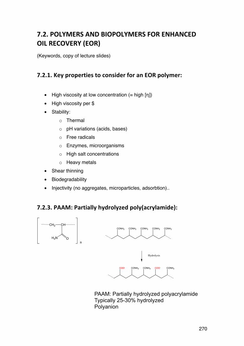
270

7.2.  POLYMERS  AND  BIOPOLYMERS  FOR  ENHANCED  OIL  RECOVERY  (EOR)  

(Keywords, copy of lecture slides)

7.2.1.  Key  properties  to  consider  for  an  EOR  polymer:  

• High viscosity at low concentration (= high [η]) • High viscosity per $ • Stability:

o Thermal o pH variations (acids, bases) o Free radicals o Enzymes, microorganisms o High salt concentrations o Heavy metals

• Shear thinning • Biodegradability • Injectivity (no aggregates, microparticles, adsorbtion)..

7.2.3.  PAAM:  Partially  hydrolyzed  poly(acrylamide):  

CH2 CH

OH2Nn

CONH2 CONH2 CONH2 CONH2 CONH2

COO- CONH2 CONH2 COO- CONH2

Hydrolysis

PAAM: Partially hydrolyzed polyacrylamideTypically 25-30% hydrolyzedPolyanion

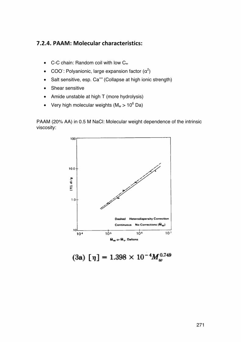
271

7.2.4.  PAAM:  Molecular  characteristics:  

• C-C chain: Random coil with low C∞ • COO-: Polyanionic, large expansion factor (α2) • Salt sensitive, esp. Ca++ (Collapse at high ionic strength) • Shear sensitive • Amide unstable at high T (more hydrolysis) • Very high molecular weights (Mw > 106 Da)

PAAM (20% AA) in 0.5 M NaCl: Molecular weight dependence of the intrinsic viscosity:

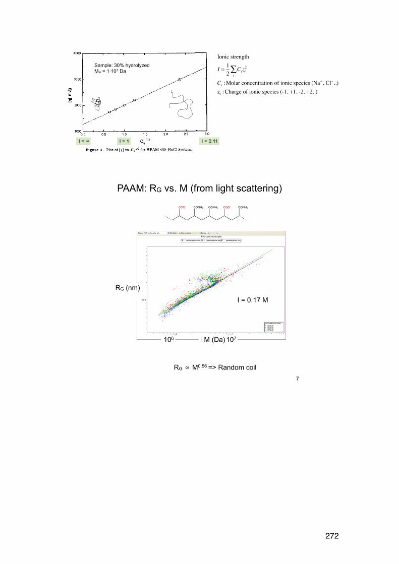
272

Ionic strength

I = 12

Cizi2

i∑

Ci :Molar concentration of ionic species (Na+ , Cl− ..)zi :Charge of ionic species (-1, +1, -2, +2..)

I = ∞ I = 1 I = 0.11

Sample: 30% hydrolyzedMw = 1·107 Da

7

COO- CONH2 CONH2 COO- CONH2

106 107M (Da)M (Da)

RG (nm)

I = 0.17 M

RG ∝ M0.56 => Random coil

PAAM: RG vs. M (from light scattering)

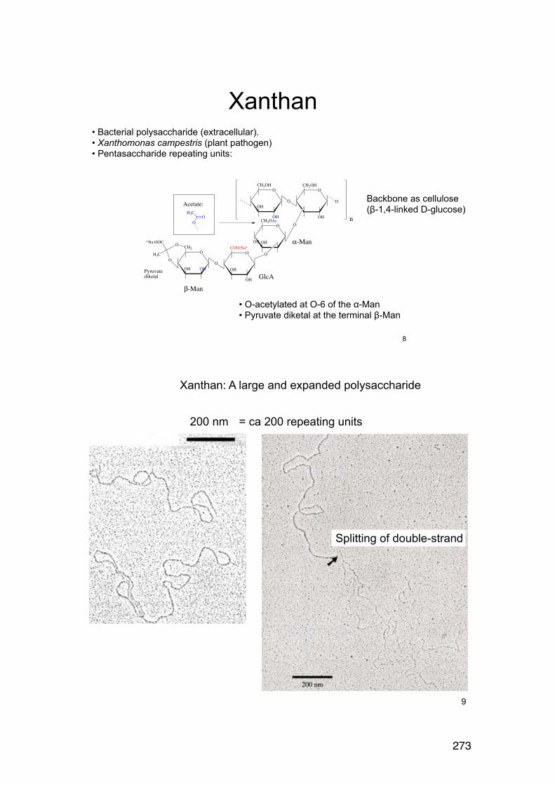
273

Xanthan

8

OCH2OH

OH

OH

OCH2OH

OH

OCH2OAc

OH OH

OCOO-Na+

OH

OH

OCH2

OH OH

O O

O

O

O

O

O

+Na-OOC

H3C

n

β-Man

GlcA

α-Man

Acetate:H3C

OO

Pyruvatediketal

• Bacterial polysaccharide (extracellular).• Xanthomonas campestris (plant pathogen)• Pentasaccharide repeating units:

Backbone as cellulose(β-1,4-linked D-glucose)

• O-acetylated at O-6 of the α-Man• Pyruvate diketal at the terminal β-Man

9

200 nm = ca 200 repeating units

Xanthan: A large and expanded polysaccharide

Splitting of double-strand

274

10

• Double-stranded, stiff structure• May dissociate into more flexible single strands at high T (depends on I (ionic strength))• Very high Mw (typically > 106 g/mol)• q (persistence length) = ca. 120 nm• Important industrial polysaccharide (E415): Viscosifyer

1,000 10,000 100,000 1,000,00010,000,000Mw

1

10

100

1,000

10,000

Intri

nsic

visc

osit y

(ml /g

)I =

0.1

M

Xanthan(double stranded)

Alginate(mannuronan)

Lignosulfonate

Xanthan: Macromolecular properties

Xanthan: Shear thinning

11Milas et al. Polymer Bulletin 14, 157 (1985)

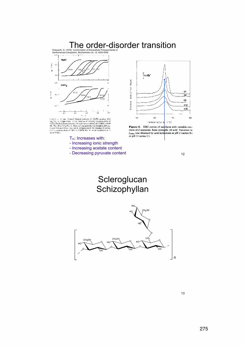
275

The order-disorder transition

12

Tm: Increases with:- Increasing ionic strength- Increasing acetate content- Decreasing pyruvate content

Holzwarth, G. (1976). Conformation of Extracellular Polysaccharide of Xanthomonas-Campestris. Biochemistry-Us, 15, 4333-4339

ScleroglucanSchizophyllan

13

276

14

The triple-strand of scleroglucan and schizophyllan

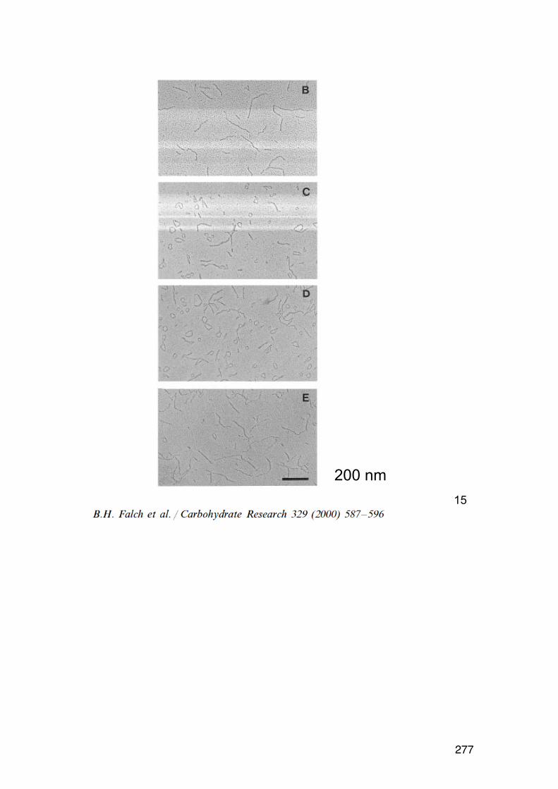
277

15

200 nm