asle natskår - ntnu open
TRANSCRIPT
Asle Natskår
Doctoral theses at N
TNU
, 2020:383
ISBN 978-82-326-5112-2 (printed ver.)ISBN 978-82-326-5113-9 (electronic ver.)
ISSN 1503-8181 (printed ver.)ISSN 2703-8084 (electronic ver.)
Doc
tora
l the
sis Doctoral theses at NTNU, 2020:383
Asle Natskår
Reliability-based assessment of marine operations with emphasis on sea transport on barges
NTN
UN
orw
egia
n U
nive
rsity
of
Scie
nce
and
Tech
nolo
gyTh
esis
for
the
degr
ee o
f Ph
iloso
phia
e D
octo
rFa
culty
of E
ngin
eeri
ng
Dep
artm
ent o
f Mar
ine
Tech
nolo
gy
Reliability-based assessment of marine operations with emphasis on sea transport on barges
Thesis for the degree of Philosophiae DoctorTrondheim, December 2020Norwegian University of Science and TechnologyFaculty of EngineeringDepartment of Marine Technology
Asle Natskår

NTNUNorwegian University of Science and Technology
Thesis for the degree of Philosophiae Doctor
Faculty of EngineeringDepartment of Marine Technology
© Asle Natskår
ISBN 978-82-326-5112-2 (printed ver.)ISBN 978-82-326-5113-9 (electronic ver.)ISSN 1503-8181 (printed ver.)ISSN 2703-8084 (electronic ver.)
Doctoral theses at NTNU, 2020:383
Printed by Skipnes Kommunikasjon AS
NO - 1598
Abstract
This thesis addresses the structural reliability assessment of marine opera-tions related to the transport of large and heavy objects. The base case hasbeen sea transportation by means of a towed barge with an emphasis onseafastening structures, considering both weather-restricted and weather-unrestricted operations. The results are, however, generic in the sense thatthey are relevant for other marine operations where environmental loadinggoverns. The reliability assessments are related to natural uncertainties andvariations. Human and organizational errors are not considered. The focusis on the structural failure of the grillage and seafastening.
While the methods for structural reliability analysis are quite mature,modeling uncertainties in loads and load effects as well as the structuralstrength are crucial and challenging. Particular efforts are directed towardsuncertainty in estimated vessel motions based on numerical and experimen-tal investigations as well as on the uncertainty in wave conditions.
The estimated motion of the transport vessel is input to calculationsof the corresponding accelerations and roll/pitch angles that are applied incalculating the load effects in the grillage and seafastening. The motion ofa typical transport barge have been studied by model tests. A model ofa North Sea barge at a scale of 1:50 was exposed to severe seas in regularand irregular waves. Roll damping tests were also performed. Barge modelswith sharp and rounded corners were tested. Based on the experiments,a model for roll damping is established. The maximum expected extremevalue of the roll angle from the experiments was 22 degrees for a stormduration of three hours. The linear analyses overestimated the maximumroll angle, while the nonlinear analysis compared well.
For most marine operations, environmental loads play an important rolein the design of the operation, and there will be a limit on the environmen-tal condition in which the operation can be performed. Weather forecastsprovide important information for marine operations with duration up tothree days and form the basis for decision making during operations. Theuncertainties in weather forecasts of the significant wave height have beenstudied, especially by shedding light on the approach used in practice toaccount for forecast uncertainty, where the so-called Alpha factor methodis used. This method was implemented in the structural reliability anal-yses performed in this thesis and was seen to effectively compensate forthe uncertainty inherent in the weather forecast. Marine operations last-ing more than three days are weather-unrestricted, and the environmentalconditions are based on long-term statistical data. Such data have been ap-
i

ii
plied in structural reliability analyses to study variations through seasonsof the year and durations of the operation. While the study of the fore-cast uncertainty did not reveal an abrupt change in forecast quality for leadtimes exceeding three days, this limitation was still used in the reliabilityassessment to be in compliance with current design standards.
The uncertainties in load effects and the resistance of the seafasten-ing structure and the corresponding failure probability are estimated. Thestructure is assumed to be designed according to current practice, and theresults provide an indication of the inherent reliability of the current prac-tice. Moreover, the sensitivity of the reliability to environmental conditions,load effects and resistance variables is investigated.
This thesis may contribute to safer sea transport on barges by providingmore knowledge on some effects that influence the structural reliability, e.g.,the time of year when transport is executed and the duration of operation.The effect has not been quantified here, but the results can provide a usefulreference for future versions of design standards for marine operations.

iii
PrefaceThis thesis is submitted to the Norwegian University of Science and Tech-nology (NTNU) for partial fulfilment of the requirements for the degree ofphilosophiae doctor.
This doctoral work has been performed at the Centre for Ships andOcean Structures (CeSOS), Department of Marine Technology, NTNU, Trond-heim, with Professor Torgeir Moan as the main supervisor and Per ØysteinAlvær, DNV GL, as the co-supervisor.
This thesis was financially supported by the Research Council of Norwaythrough the Centre for Ships and Ocean Structures (CeSOS), headed byProfessor Moan. This support is greatly appreciated.
I was partially supported by a scholarship from the Det Norske Veritas’Education Fund from DNV GL, which is also greatly appreciated.
For the sake of good order, it is mentioned that any opinions expressedin this document are mine, and they should not be construed as reflectingthe views of my employer, DNV GL.

v
Acknowledgments
During my PhD project, I have had the pleasure to meet many highlyqualified people at NTNU and Sintef Ocean in addition to my colleaguesat DNV GL. Professor Torgeir Moan has been my main supervisor. Hisknowledge, work capacity and enthusiasm towards engineering technologyand science are extraordinary, and I am very grateful for his assistance,guidance and patience. My co-supervisor has been Per Ø. Alvær at DNVGL, the company’s main expert within the area of marine operations. Hehas always been available for discussions and is a great source of inspiration.
In preparing my PhD project, I received support from many DNV GLcolleagues. I was inspired by talking to Dr. Knut O. Ronold. My line man-agers during these years have always supported me. I would in particularmention Gunnhild Laastad, who gave valuable support for initiation of theproject.
Thank you to all my professors/lecturers for their excellent lectures andsupport. I would also like to thank professors Sverre Haver, Trygve Kris-tiansen, Dag Myrhaug and Sverre Steen, as well as Dr. Amir R. Nejad atNTNU and Dr. Bjørn Abrahamsen and Torfinn Ottesen at Sintef Ocean fortheir discussions and kind support. Thank you to my fellow PhD studentsat NTNU/CeSOS for our time together and for good discussions during ourcourses in reliability and hydrodynamics. During my work in the laborato-ries, I received assistance from many employees at NTNU and Sintef Ocean.I would especially like to thank Ole Eirik Vinje and Knut Arne Hegstad atNTNU for their substantial support. I would also like to thank Dr. ZhuangKang from Harbin Engineering University in China and my family mem-bers Sigrid Olsen and Arne Natskår who assisted me during the model testsin the MC-lab. Thank you Dr. Arnt Fredriksen and Dr. Giri RajasekharGunnu for help during model testing in the Towing Tank. I would alsolike to thank Peter Sandvik at Sintef Ocean for assistance with the Simocalculations.
I have had excellent assistance from the administration at NTNU/Ce-SOS, and the Head of the IT department, Bjørn Tore Bach, which is greatlyappreciated. The University library at the Marine Technology Centre andthe DNV GL library have provided excellent support, which is also greatlyappreciated.
I am very pleased to have professor Jonas Ringsberg (Chalmers Univer-sity of Technology), professor Ove Tobias Gudmestad (University of Sta-vanger) and professor Stein Haugen (administrator, NTNU) as the doctoralcommittee. I am grateful for the editorial comments I have received to

vi
the draft version of the thesis, giving me the opportunity to improve thepresentation of my PhD-work.
I would like to thank the Research Council of Norway and the board ofthe education fund of DNV GL for their financial support.
My dear Sigrid has been extremely patient during the years of my PhDwork, for which I am very grateful.

vii
List of Appended PapersThis thesis consists of an introductory part and three papers, which areappended.
Paper 1:Barge motionsRolling of a transport barge in irregular seas, a comparison of motion anal-yses and model testsAuthors: Asle Natskår, Sverre SteenPublished in Marine Systems & Ocean Technology, Vol. 8 No. 1, pp. 05-19,June 2013
Paper 2:Uncertainty in weather forecastsUncertainty in forecasted environmental conditions for reliability analysesof marine operationsAuthors: Asle Natskår, Torgeir Moan, Per Ø. AlværPublished in Ocean Engineering, Vol. 108, pp. 636-647, 2015
Paper 3:Reliability analysisStructural reliability analysis of a seafastening structure for sea transport ofheavy objectsAuthors: Asle Natskår, Torgeir MoanSubmitted for publication in Ocean Engineering
Declaration of AuthorshipThe papers that serve as the core content of this thesis are coauthored.I was the first author and responsible for initiating the ideas, performingthe model tests, analysis and calculations, providing the results and writingthe papers. Professor Torgeir Moan has contributed by providing support,corrections and constructive comments to increase the scientific quality ofall the publications. Professor Sverre Steen has contributed by providingsupport, corrections and constructive comments to increase the scientificquality of Paper 1. For Paper 2 and 3, Per Ø. Alvær has contributed byproviding support, corrections and constructive comments, particularly re-lated to practical aspects and towards the DNV GL standards.

viii
Additional paperThe following conference paper related to the model tests has been producedas part of the doctoral work. It is not included in this thesis because theexperimental results relevant for Papers 2 and 3 are covered by Paper 1.
Paper 4:Experimental investigation of barge roll in severe beam seas.Authors: Asle Natskår, Torgeir MoanPublished in Proceedings of PRADS 2010, the 11th International Sympo-sium on Practical Design of Ships and other Floating Structures, Rio deJaneiro, Brazil
Abbreviations and terms
Alpha factor A factor to account for the uncertainty in the weather fore-cast. The design environmental condition (the operationallimiting criterion) is multiplied by the Alpha factor to ob-tain the forecasted operational criteria.
Cargo supports Structural elements with the purpose of supporting thetransported object, typically by grillage beams.
FORM First order reliability method.
Grillage A structure secured to the deck of a barge or ship, formallydesigned to support the cargo and distribute the loads be-tween the cargo and the transport vessel.
HAZID Hazard identification analysis. HAZID is used to identifyand evaluate hazards early in the project and may be auseful technique for revealing weaknesses in the design andthe preliminary operation procedures.
HAZOP Hazard and operability study. The application of a struc-tured and systematic review technique to a marine opera-tion, to identify hazards and operability problems, includ-ing causes, consequences, safeguards and remedial actionsbut also issues related to the operability of an activity oroperation, including possible improvements, to avoid ac-cidents and incidents and fulfill the zero accident/incidenttarget philosophy and increase safety during the operations.
Hindcast data Data, e.g., significant wave height and peak or mean zero-crossing wave period, reconstructed based on meteorologi-cal data registered by the meteorologist.
ix
x Abbreviations and terms
HTV Heavy transport vessel, a vessel that is designed to ballastdown to submerge its main deck and to allow self-floatingcargo to be on-loaded and off-loaded.
ISO International organization for standardization.
Lead time The period from forecast is issued until the time that theforecast is given for.
Load transfer The operation to transfer the load (i.e. the transportedobject) from or to a vessel without using cranes, i.e., byballasting or de-ballasting the vessel. A typical load trans-fer operation is load-out.
Load-out Transfer of an object (module, component, etc.) onto atransport vessel, e.g., by horizontal movement or by cranelifting.
Marine operation: Non-routine operation of a limited defined duration re-lated to handling of object(s) and/or vessel(s) in the marineenvironment during temporary phases. In this context, themarine environment is defined as construction sites, quayareas, inshore/offshore waters or sub-sea.
MWS Marine warranty surveyor, the independent third party thathas been contracted to approve marine operation. TheMWS will review the proposed procedures and equipmentand, when satisfied that they and the weather forecasts aresuitable, issue a Certificate of Approval for each relevantoperation. The MWS may also attend during the oper-ation to monitor that the procedures are followed and toagree with any necessary changes.
QRA Quantitative risk analysis
Seafastening Structural elements used to secure the transported objectfrom rotations and translations in all directions, as well asuplift at the supports. The term “Seafastening Structure”and “Seafastening System” as used here also includes ver-tical supports.
SORM Second order reliability method.
SRA Structural reliability analysis.
Abbreviations and terms xi
Standard North Sea barge: A flat top barge with a length of 91.4 m, widthof 27.4 m and depth of 6.1 m (300 by 90 by 20 feet), witha raked bow and stern.
Vessel Barge, ship, tug, or other vessel involved in marine opera-tion.
Weather-restricted operation: A marine operation with defined restrictionsto the characteristic environmental conditions planned tobe performed within the period for reliable weather fore-casts. The estimated duration is typically not more than72 hours, and the environmental design criteria are definedby the owner or his representative and confirmed by weatherforecasts prior to the start of the operation.
Weather-unrestricted operation: A marine operation with characteristic en-vironmental conditions is estimated according to long-termstatistics, normally with an estimated duration of morethan 72 hours.

xii Abbreviations and terms
Contents
1 Introduction 11.1 Marine operations . . . . . . . . . . . . . . . . . . . . . . . . 1
1.1.1 Definition . . . . . . . . . . . . . . . . . . . . . . . . . 11.1.2 History and background . . . . . . . . . . . . . . . . . 11.1.3 Sea transport of heavy objects . . . . . . . . . . . . . 2
1.2 Assumptions and limitations . . . . . . . . . . . . . . . . . . 41.3 Risk assessment of marine operations . . . . . . . . . . . . . . 4
1.3.1 Risk management . . . . . . . . . . . . . . . . . . . . 41.3.2 Risk exposure during marine operations . . . . . . . . 51.3.3 Categorization of uncertainties . . . . . . . . . . . . . 51.3.4 Effects of human factors . . . . . . . . . . . . . . . . . 61.3.5 Target reliability level . . . . . . . . . . . . . . . . . . 7
1.4 Planning and execution of marine operations . . . . . . . . . 81.4.1 General principle . . . . . . . . . . . . . . . . . . . . . 81.4.2 Rules and standards for marine operations . . . . . . . 81.4.3 Weather-restricted and -unrestricted operations . . . . 91.4.4 Capacity checks and failure modes . . . . . . . . . . . 101.4.5 Wave-induced loads and load effects . . . . . . . . . . 101.4.6 Weather forecasts . . . . . . . . . . . . . . . . . . . . . 111.4.7 Structural design of the grillage and seafastening . . . 121.4.8 Operational procedures . . . . . . . . . . . . . . . . . 141.4.9 Marine warranty surveys . . . . . . . . . . . . . . . . . 15
1.5 Aim and scope . . . . . . . . . . . . . . . . . . . . . . . . . . 151.6 Thesis outline . . . . . . . . . . . . . . . . . . . . . . . . . . . 161.7 Outline of the papers . . . . . . . . . . . . . . . . . . . . . . . 18
2 Environmental conditions for marine operations 212.1 General . . . . . . . . . . . . . . . . . . . . . . . . . . . . . . 212.2 Planning of marine operations and required environmental data 212.3 Weather forecasts . . . . . . . . . . . . . . . . . . . . . . . . . 23
xiii
xiv Contents
2.4 Hindcast data . . . . . . . . . . . . . . . . . . . . . . . . . . . 252.4.1 The use of hindcast data . . . . . . . . . . . . . . . . . 252.4.2 Long-term distribution from the hindcast data . . . . 28
2.5 Weather-restricted operations . . . . . . . . . . . . . . . . . . 302.5.1 General . . . . . . . . . . . . . . . . . . . . . . . . . . 302.5.2 Forecasted wave height . . . . . . . . . . . . . . . . . . 302.5.3 Statistical parameters . . . . . . . . . . . . . . . . . . 312.5.4 Wave period conditional upon Hs . . . . . . . . . . . . 322.5.5 Wind speed . . . . . . . . . . . . . . . . . . . . . . . . 33
2.6 Weather-unrestricted operations . . . . . . . . . . . . . . . . 332.6.1 General . . . . . . . . . . . . . . . . . . . . . . . . . . 332.6.2 Wave height obtained from the long-term distribution 342.6.3 Wave height based on the ISO standard . . . . . . . . 342.6.4 Wave height from standard return period tables . . . . 352.6.5 Wave period conditional upon Hs . . . . . . . . . . . . 352.6.6 Wind speed conditional upon Hs . . . . . . . . . . . . 362.6.7 Seasonal environmental conditions . . . . . . . . . . . 37
2.7 Weather routing . . . . . . . . . . . . . . . . . . . . . . . . . 382.8 Heading control . . . . . . . . . . . . . . . . . . . . . . . . . . 39
3 Wave-induced load effect analysis 413.1 General . . . . . . . . . . . . . . . . . . . . . . . . . . . . . . 413.2 Wave description . . . . . . . . . . . . . . . . . . . . . . . . . 42
3.2.1 Choice of the wave energy spectrum . . . . . . . . . . 423.2.2 Wave direction . . . . . . . . . . . . . . . . . . . . . . 433.2.3 Irregular waves . . . . . . . . . . . . . . . . . . . . . . 44
3.3 Numerical analyses . . . . . . . . . . . . . . . . . . . . . . . . 453.3.1 Available methods . . . . . . . . . . . . . . . . . . . . 453.3.2 Simplified motion analysis . . . . . . . . . . . . . . . . 463.3.3 Linear motion analysis in the frequency domain . . . . 463.3.4 Nonlinear analysis in the time domain . . . . . . . . . 463.3.5 Estimate of nonlinear roll damping . . . . . . . . . . . 473.3.6 The effect of sloshing in tanks . . . . . . . . . . . . . . 483.3.7 The effect of heel from the wind load . . . . . . . . . . 483.3.8 Calculation of the loads in the cargo supports . . . . . 48
3.4 Model tests . . . . . . . . . . . . . . . . . . . . . . . . . . . . 493.4.1 General . . . . . . . . . . . . . . . . . . . . . . . . . . 493.4.2 Scale effects . . . . . . . . . . . . . . . . . . . . . . . . 503.4.3 Main results . . . . . . . . . . . . . . . . . . . . . . . . 52
3.4.3.1 Roll damping . . . . . . . . . . . . . . . . . . 52
Contents xv
3.4.3.2 Barge motions and support reaction forces . 54
4 Structural reliability analysis 574.1 Introduction . . . . . . . . . . . . . . . . . . . . . . . . . . . . 574.2 Limit state design check . . . . . . . . . . . . . . . . . . . . . 58
4.2.1 Calculation of the ultimate strength . . . . . . . . . . 584.2.2 Ultimate limit state design check . . . . . . . . . . . . 594.2.3 Wave-induced load effects in the design check and in
SRA . . . . . . . . . . . . . . . . . . . . . . . . . . . . 614.3 Structural reliability analysis method . . . . . . . . . . . . . . 61
4.3.1 Formulation of the failure probability . . . . . . . . . 614.3.2 Modelling the structural capacity . . . . . . . . . . . . 624.3.3 Overview of the uncertainties in the load effects . . . . 634.3.4 Uncertainty in the forecasted wave height . . . . . . . 654.3.5 Uncertainty in the long-term significant wave height . 654.3.6 Uncertainties due to the amount of environmental data 654.3.7 Uncertainties in the gathered environmental data . . . 664.3.8 Uncertainty in the wave period . . . . . . . . . . . . . 674.3.9 Operational uncertainty . . . . . . . . . . . . . . . . . 674.3.10 Load description . . . . . . . . . . . . . . . . . . . . . 684.3.11 Basic formulation of the reliability problem . . . . . . 704.3.12 Time-independent reliability analyses with FORM/-
SORM . . . . . . . . . . . . . . . . . . . . . . . . . . . 714.3.13 Uncertainty importance factors . . . . . . . . . . . . . 72
4.4 Case studies of a seafastening structure . . . . . . . . . . . . 734.4.1 General . . . . . . . . . . . . . . . . . . . . . . . . . . 734.4.2 Input data for the structural reliability analyses . . . 73
4.4.2.1 Stochastic variables in the case studies . . . 734.4.2.2 Long-term distribution of the significant wave
height . . . . . . . . . . . . . . . . . . . . . . 734.4.2.3 Distribution of the wave period conditional
on Hs . . . . . . . . . . . . . . . . . . . . . . 734.4.3 Results from the case studies . . . . . . . . . . . . . . 74
4.4.3.1 Seafastening structure designed for weather-restricted transport . . . . . . . . . . . . . . 74
4.4.3.2 The effect of seasonal versus year-round datafor weather-unrestricted transport . . . . . . 76
4.4.3.3 Sensitivity study . . . . . . . . . . . . . . . . 784.4.4 Discussion of the results . . . . . . . . . . . . . . . . . 79
xvi Contents
5 Conclusions and recommendations for future research 835.1 General . . . . . . . . . . . . . . . . . . . . . . . . . . . . . . 835.2 Conclusions . . . . . . . . . . . . . . . . . . . . . . . . . . . . 835.3 Summary of the original contributions . . . . . . . . . . . . . 875.4 Suggestions for future research . . . . . . . . . . . . . . . . . 88
5.4.1 Additional model tests . . . . . . . . . . . . . . . . . . 885.4.2 Uncertainty assessments of wave forecasts . . . . . . . 895.4.3 Maximum duration of weather-restricted operations . 895.4.4 Ultimate strength assessment . . . . . . . . . . . . . . 895.4.5 The effect of costs . . . . . . . . . . . . . . . . . . . . 91
References 93
A Appended papers 107A.1 Paper 1 . . . . . . . . . . . . . . . . . . . . . . . . . . . . . . 109A.2 Paper 2 . . . . . . . . . . . . . . . . . . . . . . . . . . . . . . 127A.3 Paper 3 . . . . . . . . . . . . . . . . . . . . . . . . . . . . . . 141
B Structural layout of a transport barge 179B.1 Introduction . . . . . . . . . . . . . . . . . . . . . . . . . . . . 179B.2 Layout of the barge and the transported object . . . . . . . . 179
B.2.1 Positioning of the transported object . . . . . . . . . . 179B.2.2 Barge geometry . . . . . . . . . . . . . . . . . . . . . . 180B.2.3 Layout of the transported object . . . . . . . . . . . . 181B.2.4 Grillage and seafastening . . . . . . . . . . . . . . . . 181
B.3 Structural capacity . . . . . . . . . . . . . . . . . . . . . . . . 182B.3.1 Uncertainties in structural capacity . . . . . . . . . . . 182B.3.2 Structural elements in the grillage and seafastening . . 182
C Motion analysis of ships and barges 187C.1 Simplified motion analyses . . . . . . . . . . . . . . . . . . . . 187C.2 Linear analysis in frequency domain . . . . . . . . . . . . . . 188C.3 Non-linear analysis in the time domain . . . . . . . . . . . . . 189
C.3.1 Coordinate systems . . . . . . . . . . . . . . . . . . . 189C.3.2 Equations of motion . . . . . . . . . . . . . . . . . . . 190
D Model tests 197D.1 Introduction . . . . . . . . . . . . . . . . . . . . . . . . . . . . 197D.2 Model test tanks . . . . . . . . . . . . . . . . . . . . . . . . . 198D.3 Model scaling . . . . . . . . . . . . . . . . . . . . . . . . . . . 199D.4 Barge model . . . . . . . . . . . . . . . . . . . . . . . . . . . . 199

Contents xvii
D.5 Monitoring . . . . . . . . . . . . . . . . . . . . . . . . . . . . 200D.6 Free decay roll tests . . . . . . . . . . . . . . . . . . . . . . . 201D.7 Forced roll tests . . . . . . . . . . . . . . . . . . . . . . . . . . 202D.8 Tests with wave-induced motions . . . . . . . . . . . . . . . . 202
E List of previous PhD theses at Dept. of Marine Tech. 209

xviii Contents
Chapter 1
Introduction
1.1 Marine operations
1.1.1 Definition
The term Marine Operations includes many activities performed in or at sea.The marine operations considered herein are limited to specially planned,non-routine operations of limited duration related to the load transfer,transport and installation of objects.
1.1.2 History and background
For several decades, complex marine operations have been performed withinthe offshore oil and gas industry. During the construction of an offshore plat-form for drilling and petroleum production, several marine operations areperformed. Modules to be assembled into topsides for drilling and produc-tion platforms are transported from fabrication yards all over the world toassembly sites. Complete topsides and substructures are transported fromthe assembly sites to the installation locations offshore.
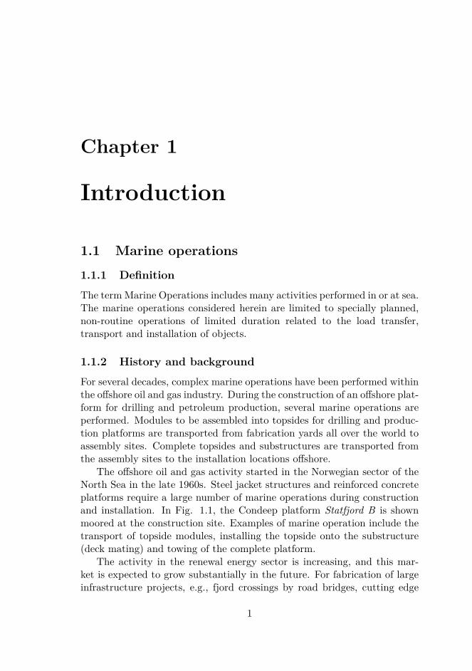
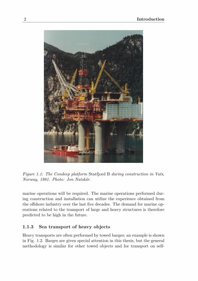
The offshore oil and gas activity started in the Norwegian sector of theNorth Sea in the late 1960s. Steel jacket structures and reinforced concreteplatforms require a large number of marine operations during constructionand installation. In Fig. 1.1, the Condeep platform Statfjord B is shownmoored at the construction site. Examples of marine operation include thetransport of topside modules, installing the topside onto the substructure(deck mating) and towing of the complete platform.
The activity in the renewal energy sector is increasing, and this mar-ket is expected to grow substantially in the future. For fabrication of largeinfrastructure projects, e.g., fjord crossings by road bridges, cutting edge
1
2 Introduction
Figure 1.1: The Condeep platform Statfjord B during construction in Vats,Norway, 1981. Photo: Jon Natskår.
marine operations will be required. The marine operations performed dur-ing construction and installation can utilize the experience obtained fromthe offshore industry over the last five decades. The demand for marine op-erations related to the transport of large and heavy structures is thereforepredicted to be high in the future.
1.1.3 Sea transport of heavy objects
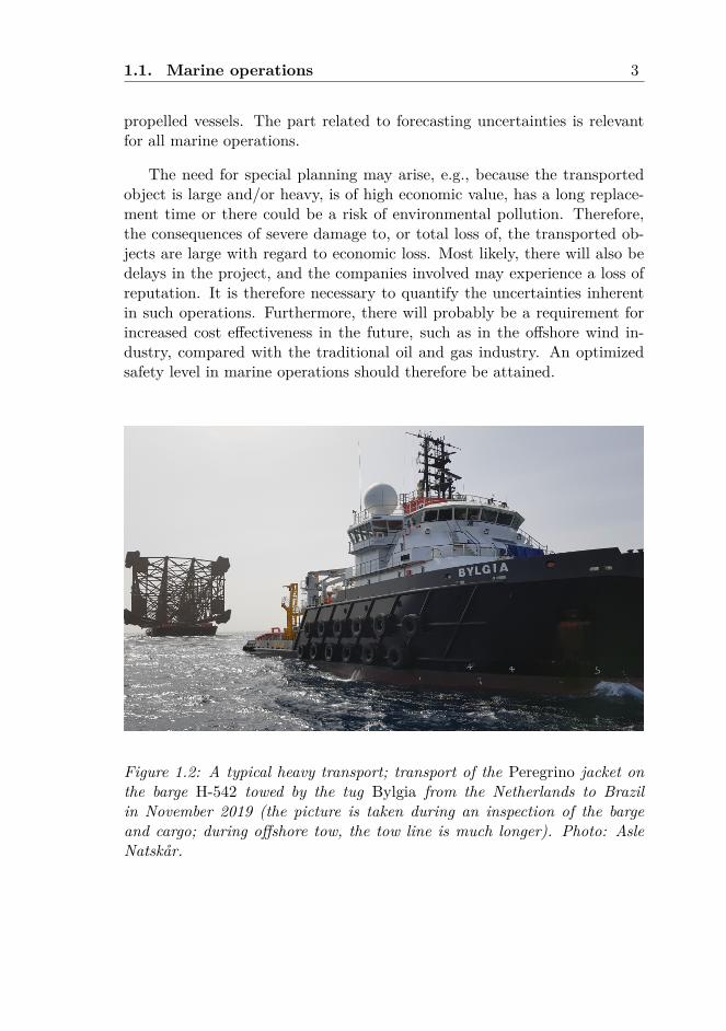
Heavy transports are often performed by towed barges; an example is shownin Fig. 1.2. Barges are given special attention in this thesis, but the generalmethodology is similar for other towed objects and for transport on self-
1.1. Marine operations 3
propelled vessels. The part related to forecasting uncertainties is relevantfor all marine operations.
The need for special planning may arise, e.g., because the transportedobject is large and/or heavy, is of high economic value, has a long replace-ment time or there could be a risk of environmental pollution. Therefore,the consequences of severe damage to, or total loss of, the transported ob-jects are large with regard to economic loss. Most likely, there will also bedelays in the project, and the companies involved may experience a loss ofreputation. It is therefore necessary to quantify the uncertainties inherentin such operations. Furthermore, there will probably be a requirement forincreased cost effectiveness in the future, such as in the offshore wind in-dustry, compared with the traditional oil and gas industry. An optimizedsafety level in marine operations should therefore be attained.
Figure 1.2: A typical heavy transport; transport of the Peregrino jacket onthe barge H-542 towed by the tug Bylgia from the Netherlands to Brazilin November 2019 (the picture is taken during an inspection of the bargeand cargo; during offshore tow, the tow line is much longer). Photo: AsleNatskår.
4 Introduction
1.2 Assumptions and limitations
Several assumptions have been made for the work performed in this thesis.Some main assumptions and limitations are listed below.r Roll motion is normally governing for the loading in the grillage and
seafastening and has been in focus in this study, and pitching is notstudiedr The structural reliability assessment focus on the cargo support struc-ture; the structural capacity of the cargo is not consideredr The forces in the cargo supports are calculated based on dynamicequilibrium of the cargor The weather forecasts and the long term statistical data in this thesisare from the Norwegian Sea and the North Sea (however, they areconsidered to be more generally representative of extratropical condi-tions)r The reliability assessments performed in this thesis are related to nat-ural uncertainties and variationsr Human and organizational errors are not considered in detail otherthan in Sec. 1.3.4, where precautions to reduce the probability ofsuch errors are discussedr Forward motion of the barge is not included, as the barge is assumedto be towed at low speed or in drift during the governing loadingcondition
1.3 Risk assessment of marine operations
1.3.1 Risk management
Active risk management is normally considered vital for the successful exe-cution of marine operations and should be an integrated part of planning.The risk management plan should cover risk assessment of the marine op-erations as well as the various construction phases [55], and human errorsshould also be analyzed in risk management work; see also Sec. 1.3.4. Riskmanagement should include risk assessment to define relevant loading con-ditions and accidental load cases [30, 71]. Robust and well-proven equip-ment, vessels and operational procedures should be used to minimize the
1.3. Risk assessment of marine operations 5
risk of failures or unacceptable delays as much as possible. The principle ofALARP, “As Low As Reasonable Practicable”, should be adhered to, mean-ing that the risk is reduced as much as found practicable during planningand execution, which is also below the formally defined acceptance levels,based on cost-benefit assessments [30, 34].
1.3.2 Risk exposure during marine operations
Marine operations involve many stages and many suboperations where thehandled object is exposed to risk. For the marine operations consideredherein, see Sec. 1.1.1, the following sub-operations are generally relevant:r Load-out of the object onto the transportation vessel by lifting with
a crane, multiwheel trailers or skiddingr Berthing of the transportation vessel after the load-out (i.e., shift thevessel from the load out position to a temporary position along thequay)r The loaded vessel moored along the quay during final preparationsr Commencement of the voyage; leaving the quay and maneuvering outof the harborr Sea voyage in open waterr Maneuvering into the harbor and berthing of the transport vessel whenarriving at the destination, or arrival at an offshore locationr Discharge of the transport vessel, typically by a reversed load-out(load-in) at a yard or by lifting with a crane or by a float-over operationfor an offshore installation
Keeping the general risk exposure and the various failure modes in mind,the focus here is on the structural failure of grillage and seafastening.
1.3.3 Categorization of uncertainties
Various categories of uncertainties are used, for example, random errors,systematic errors and gross errors (blunders) [41], human and organizationalfactors, etc.
The categorization can also be based on the type of uncertainties [96]:r fundamental or inherent uncertainties; the aleatoric uncertainties

6 Introduction
r uncertainties in mechanical or probabilistic models and statistical un-certainties; the epistemic uncertaintiesr uncertainties related to human errors that affect the resistance andload effects
An alternative categorization for structural assessment could be 1) nor-mal variability and uncertainty due to inherent variability or lack of data(also to establish analysis models) and 2) human errors, affecting both theloads and the load effects as well as the resistance [98].
The fabrication quality is one of the main design assumptions. Devia-tions in the fabrication quality contribute to the uncertainties in the struc-tural capacity. Welding of grillage and seafastening is performed on thedeck of the transport vessel, and weather sheltering can be challenging.
1.3.4 Effects of human factors
Human errors and omissions may be related to:r the planning of the operation and choice of equipmentr the fabrication of the object to be handled, grillage and seafastening,etc.r the execution of the operation
Several studies related to the human and organizational factors in marineoperations have been performed, and it is indicated that human errors ac-count for as much as 80-90% of all accidents [83, 88].
During the project phase, e.g., when performing structural design, hu-man errors may lead to under-dimensioned structures [94, 138] that maysubstantially increase the risk of structural failure.
Other studies illustrate that the probability of personnel making thewrong choice while performing a task, by pushing the wrong buttons, etc.,may become very high under unfavorable working conditions with highstress levels [66]. This approach to consider the effect of human errorscan be relevant for execution of marine operations related to control panelsfor ballasting as an example.
Human errors should not be compensated by an additional design factor.Instead, gross errors in marine operations should be eliminated by extensiveQA/QC activities (quality assurance and quality control) during design,fabrication and execution as well as utilizing defined safety barriers andredundant equipment and systems. Standard methods for risk reduction
1.3. Risk assessment of marine operations 7
during the planning of marine operations include independent (third party)design verification, Hazids, Hazops, etc. [30]. Operational errors should beeliminated by adequate training of the involved personnel [57] and by safetymeetings, toolbox talks and risk assessments [128]. Safety barriers shouldbe applied where possible to prevent one single failure from leading to severefailures [31, 65, 133].
While human factors are not directly included in this thesis, the abovementioned precautions are assumed to have been taken as relevant, sub-stantially reducing the probability of human errors leading to catastrophicfailures. Based on this assumption, the structural capacity checks are per-formed in the ultimate limit state. The corresponding target reliability levelis discussed in the following section.
1.3.5 Target reliability level
An acceptable reliability level for marine operations is presently not ac-curately defined in any design standard. However, muck work has beenperformed with respect to code calibration to obtain a specific safety levelfor offshore structures (at the offshore site) [41, 97, 99].
Offshore structures will typically be on location for twenty years or more,and the definition of the reliability level is linked to the annual probability offailure. Marine operations typically last a few days or weeks, and it is thenmore natural to define a probability of failure per operation, independent ofthe duration [84]. This approach is applied in this thesis. The target safetylevel, however, could depend on the possible progressive failure of structuralcomponents, i.e., the consequences of a component failure.
Structural reliability analyses (SRA) are used to quantify the probabilityof failure. While SRA are tools for assessing failure probability, they do notaccount for human errors. Hence, the probabilities should not be consideredas the “true”, or “real”, failure probabilities but rather than as a calibratingtool relating to the generic uncertainties included in the analysis.
Research has also been performed to combine quantitative risk analysis(QRA) with structural reliability analysis for marine operations [124, 125,142], which is an alternative to SRA. The reliability level will depend onthe type of analysis performed to some extent.
8 Introduction
1.4 Planning and execution of marine operations
1.4.1 General principle
The marine operations discussed here are based on thorough planning andpreparations. The environmental condition, wave-induced load effects, struc-tural integrity, etc., are some key elements in planning such operations. Allparts of marine operations need to be described by operational procedures,drawings, etc., collected in an operation manual. The structures and equip-ment must comply with the relevant requirements in the design standards.A few items related to the planning and execution of marine operations aredescribed below, and a short discussion and a brief review of some previousresearch are given.
1.4.2 Rules and standards for marine operations
There is a long history of standards and guidelines in marine operations.The first guidelines (to my knowledge) were given as far back as 1958, whenCaptain William David Noble introduced criteria for tow preparation forthe LeTourneau jack-up AMDP-1 to cross the Atlantic Ocean, which wasthe first drilling platform to do so [24]. Later, the Noble Denton guidelines[47] became well known in the industry. The first guidelines from DNV wereissued in the late 1970s, and the first design standard was issued in 1985,the DNV Standard for Insurance Warranty Surveys in Marine Operations.This standard was replaced by theDNV Rules for Planning and Execution ofMarine Operations in 1996 [23]. These rules were replaced by an OffshoreStandard [26] in 2011. During this period, marine operations could beplanned according to the DNV standards or the Noble Denton guidelines.
The ISO standard for Marine Operations was issued in 2009 [72]. Partsof this standard were based on the Noble Denton guidelines, and there weresome differences compared with the DNV standards [6].
Following the merger between DNV and GL in 2013, the DNV standardand the Noble Denton guidelines (Noble Denton was owned by GL at thetime) were both managed by DNV GL. The standard and guidelines bothgave technical requirements and guidance for all types of marine operations,but their structure and detailing of the requirements were quite different [7],and they were combined into one standard [31].
There are also other standards and guidelines available. London Off-shore consultants have their own Guidelines for Marine Operations [86].The International Maritime Organization, IMO, issued Guidelines for safeocean towing [70] in 1998. The US Navy issued a towing manual [110]. Ship-
1.4. Planning and execution of marine operations 9
ping and oil and gas companies have issued Guidelines for Offshore MarineOperations [48]. The API Recommended Practice for fixed platforms [8]contains a chapter with general requirements for load-out, transportation,and installation. Oil companies may also have their own specification withrequirements in addition to the standards and guidelines for the design ofmarine operations. Some of the large marine operation contractors havecompany-specific design guidelines.
The main reference standard in this thesis is the current version of theDNV GL standard for marine operations [31]1. This standard has the mostcomprehensive method for planning operations, such as accounting for un-certainty in weather forecasts.
1.4.3 Weather-restricted and -unrestricted operations
Marine operations are defined as weather-restricted or weather-unrestrictedoperations depending on the duration. The separation between these twocategories is important, as they are planned differently with respect to envi-ronmental conditions. If the duration of the operation is less than 72 hours(96 hours when the contingency time is included) or if the operation canbe halted and the handled object brought into a safe condition during thesame period, the operation can be defined as weather-restricted. The designenvironmental criteria are defined in an early phase of the project. The op-eration may commence when all preparations are finished and the weatherforecasts indicate acceptable environmental conditions. The uncertainty inthe weather forecasts and how to include this uncertainty in the planningof the operation thus become key issues [108, 107].
Operations with planned durations longer than 72 hours are weather-unrestricted. They are not planned based on environmental conditions thatcan be confirmed by weather forecasts because the duration of such opera-tions is longer than the duration for which weather forecasts are consideredreliable. In the planning of a weather-unrestricted operation, the environ-mental criteria for the design must be considered according to long-termstatistics accounting for the geographical area, the season of the year, andthe duration of the operation.
1This standard is not freely available, and access requires a subscription. However,the requirements referred to in this thesis are practically the same as those given in theprevious DNV offshore standards. Planning related to the duration and requirements forweather-restricted operations (see Sec. 2.2) are covered by DNV-OS-H101 [26], while thebarge motion criteria can be found in DNV-OS-H202 [27]. These standards are availablefor free on the Internet.
10 Introduction
1.4.4 Capacity checks and failure modes
For a typical marine operation, numerous design checks are required. Gen-erally, four types of limit states are checked (see Sec. 1.4.7), but the ul-timate limit state is the focus here. The structural strength is calculatedaccording to recognized design standards, e.g., Eurocode and Norsok stan-dards [36, 113], and adequate capacity is documented for the relevant limitstate by applying the relevant reference levels for the loads and load effects.All vessels, equipment and structures involved in marine operations need tohave documented capacity and shown to be adequate for their purpose. Thesufficient capacity of the tug (e.g., the bollard pull) and the tow line capac-ity must be verified. The hydrostatic and dynamic stability of all floatingvessels must be documented.
The design checks cover normal uncertainties due to fundamental vari-ability/uncertainty and lack of data. As mentioned in Sec. 1.3.4, humanerrors are not accounted for in the standard ultimate limit state capacitychecks.
1.4.5 Wave-induced loads and load effects
The governing load effects in the cargo supports are typically caused bythe wave-induced motions, i.e., accelerations and rolling/pitching, of thetransport vessel. Much research, both numerical and experimental, hasbeen performed on wave-induced barge motion, particularly for the rollingof barges. Early research on the rolling of ships was performed by Froude inthe 1860s [42]. In the 1960s, research on the rolling of ships and the effectof bilge keels was performed by Tanaka and Kato [80, 140]. In the 1970s,Ikeda et al. studied roll damping of ships with forward motion [68]. A bargeresearch project was also initiated by Noble Denton [37].
The rolling of ships and barges is influenced by roll damping, whichcan be split into potential damping due to wave generation and viscousdamping due to vortex shedding at the bilges. Vortex shedding and thedetails of the flow at the bilges have been studied by several researchers[49, 50, 12, 33, 126, 67], and studies are still ongoing [40, 51, 52, 101].
Handbooks based on numerical analysis and experiments, giving spe-cific values to be used for typical vessel shapes during rolling, heaving andswaying, are available [81, 144]. More recently, ITTC issued a report givinga method for roll damping estimation that can be used in the absence ofexperimental data [75]. In addition to studying viscous damping as such,research has been performed on barge motion in waves [14, 18, 135]. Ad-ditionally, studies on wave-induced motions based on real transports have
1.4. Planning and execution of marine operations 11
been performed, and full-scale measurements of barge motions have beenpublished [139], as well as model test results [79, 136].
The deformation of the transport barge in head and beam seas will have alimited effect on an object placed on four supports with a static determinateseafastening system, while there is a larger effect of deformations in obliqueseas and for the transport of structures on several supports, e.g., a jacket[20]. Then, the relative stiffness of the transported object and the transportbarge will influence the support forces.
The statistical distribution chosen to represent the responses for theanalysis of sea transport is also important. Research is performed on thestatistical distribution of the extreme value of the responses. The stan-dard approach is to assume Rayleigh or Weibull distributed individual max-ima. An alternative method was developed by Naess and Gaidai [102]; thismethod can be used for extreme value statistics of roll motions [45]. Othermethods have also been studied [105, 119].
1.4.6 Weather forecasts
The start-up of a marine operation requires forecast confirmation that theenvironmental criteria are fulfilled, and hence weather forecasts are impor-tant input for decision making during the execution of marine operations.The uncertainty in the forecasts must be accounted for in the planning ofthe operation.
The standard method to account for the forecast uncertainty is to re-duce the design criteria by an Alpha factor [31]. For example, if the designsea state is Hs,design = 4 m and α = 0.75 (the Alpha factor depends on theduration of the operation), the operation can start when the forecast pre-dicts Hs,wf ≤ 3 m throughout the operation period. The Alpha factors arebased on the uncertainty estimated based on a comparison of the measure-ments and forecasts [87, 146]. Alternative approaches exist, for example, formaking criteria for unmanning platforms during storm events [59], whereensemble weather forecasts are utilized.
Weather routing has become more available as technology has progressed.While the traditional approach for weather routing was to avoid certain ar-eas during the winter season, weather routing can now use updated weatherforecasts on board as part of the decision-making process [1]. Instead ofdefining the limit for the execution of marine operations based on the windspeed and significant wave height, the industry seems to be heading towardsa response-based approach. For several years, there has been great interestin this approach within the industry, and in 2019, DNV GL initiated a jointindustry project (JIP) to further investigate response-based methods. With
12 Introduction
the response-based approach, the wave forecasts are not limited to Hs andTp/Tz, but forecasted 2D wave energy spectra can be utilized (an exampleof a 2D spectrum is shown in Fig. 3.1). Several wave systems, e.g., windwaves and one or more swell systems, can thereby be included in the nu-merical models. Until now, this method has mostly been used in additionto the traditional approach and not as a complete decision tool for marineoperations [19]. There have also been studies related to the assessment ofoperational limits and limiting sea states based on the allowable response[54]. Such operational-based methods by means of the on board monitoringof waves and vessel motion are being developed [21]. The response-basedapproach contains various methods for improving shipping and marine op-erations in general. The methodologies are expected to be further developedover the coming years. Nevertheless, the traditional approach based on thesignificant wave height will be used for small projects and by companieswithout the resources or the need for a response-based system. To quan-tify the forecast uncertainty, the forecasts should preferably be comparedwith measured data. However, hindcast data are of high quality and can beused in comparisons instead of measured data [82]. The European Centrefor Medium-ranged Weather Forecasts, ECMWF, verifies the forecasts bycomparing the measured and forecasted environmental data [9, 147].
In areas and times of year where polar lows can occur, this phenomenonshould be included in the forecasts. The period where a reliable forecastof polar lows can be given is short, as polar lows may be predicted for aperiod of approximately 24 hours [114]. Standard weather forecasts do notinclude polar lows. Polar lows should be specially considered where relevant[118, 123].
1.4.7 Structural design of the grillage and seafastening
The grillage and seafastening are designed based on the load effects fromaccelerations and roll/pitch angles given by a motion analysis using a 3Dpanel model or from simplified motion criteria. The forces should includepossible effects of friction. Even if vessel motions used for calculating theload effects for the design of the cargo support system can be calculated bydifferent methods, the safety coefficients, e.g., the load and material factors,applied in the design do not reflect the method for calculating the motionsbut depend on the design limit state.
The transports are assumed to be planned and executed according to arecognized standard using the load and resistance factor design approach,and the structural capacity can generally be verified for four design limitstates:
1.4. Planning and execution of marine operations 13
r ultimate limit state, ULS
r accidental limit state, ALS
r fatigue limit state, FLS
r serviceability limit state, SLS
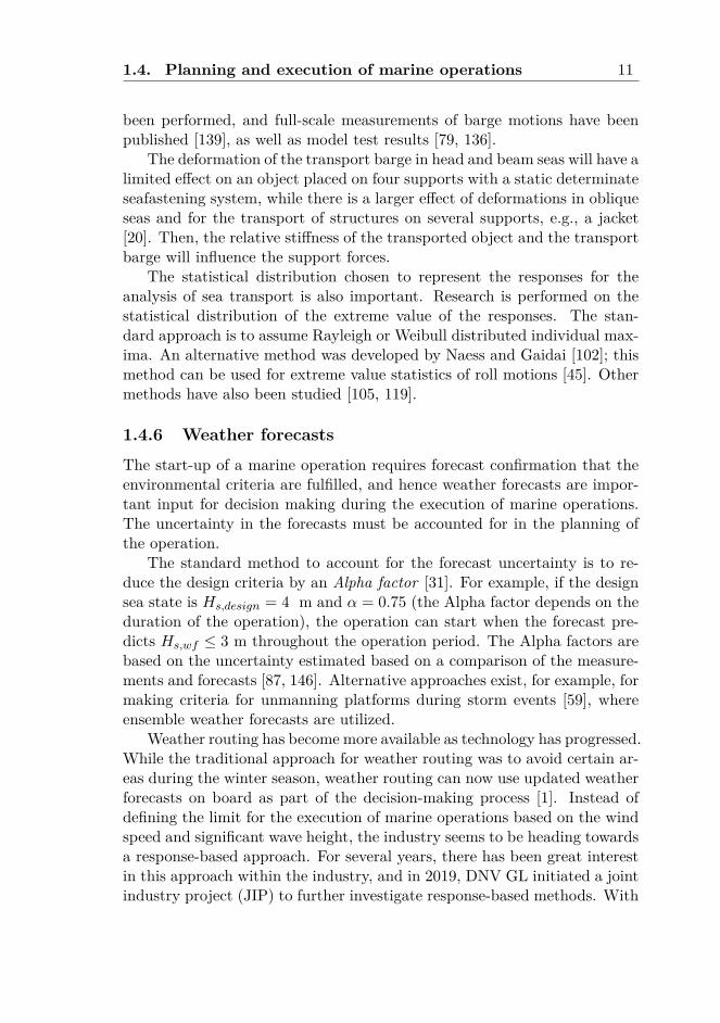
The ULS covers the normal uncertainty and variability in the loads andresistances, while the ALS is introduced to avoid progressive failure afteraccidental damage. The accidental limit state is important when there isa risk of the tanks flooding or the load shifting. For heavy cargo, shiftingof the load will lead to a total loss, but for smaller cargo, this may be arelevant ALS case. The fatigue limit state is relevant for transports with along duration, i.e., transports lasting more than a few days, and for struc-tures with poor fatigue properties (high stress concentrations). Fatigue isnot considered here. The serviceability limit state is mainly related to de-formations and is normally not of main importance for sea transports. TheSLS may be important if the transported object has equipment that is sen-sitive to relative deformations, e.g., large equipment and piping in a processmodule. The main category is the ultimate limit state, which is relevant forall transports. This category is the focus here.
The method used to calculate the structural strength can affect theoverall reliability, e.g., the use of standard capacity formulas versus linear ornonlinear finite element analyses. For example, capacity checks accordingto Eurocode 3 [36] may serve well for design purposes for plate girderswith a relevant geometry, but it is difficult to apply these checks to morecomplicated fabrications [32].
Even if there are recommendations for the general principles for seafas-tening [53], different transport vessels, e.g., a barge, a transport ship or aheavy transport vessel, may also have different characteristics, and a vessel-specific design approach may be required. For example, a module placed ongrillage beams on a barge, as shown in Fig. 4.1, cannot rely on friction atall because wet steel to steel has very little friction. On the other hand, alarge object transported on the deck of a heavy transport vessel is normallyset on wooden cribbing, and the positive effect of friction can be included[5].
As a consequence, the probability of failure will to some extent dependon the type of transport and how the load effects are calculated. Hence, thecalculated probability of failure could vary from case to case depending onthe design method.

14 Introduction
1.4.8 Operational procedures
Operational procedures and other relevant information related to organiza-tional and technical items needed during the execution of a marine opera-tion are written in a Marine Operation Manual. The operation manual iscustom-made for each operation and should include the following, as appli-cable [31]:
r reference documents
r general arrangements and references to relevant drawings
r permissible load conditions
r organization charts and lines of command
r environmental criteria
r weather forecasts and wave reporting
r specific step-by-step instructions for each phase of the operation
r references to relevant calculations, e.g., environmental loads, mooringarrangements, ballast conditions, stability, tug bollard pull
r permissible draughts, trim, and heel and corresponding ballastingplans
r contingency and emergency response plans
r vessels involvedr tow routes and ports of refuge
r towing arrangements
This information is needed for the crew to know what to to in the nor-mal operation mode and in case of emergencies. For barge transport, thisdocument is called a Towing manual and will contain the above listed infor-mation as relevant, depending on the type of transported object, geographicarea, distance, duration, etc.
1.5. Aim and scope 15
1.4.9 Marine warranty surveys
Insurance companies often require that an independent verification of theplanned operation and the execution be performed to ensure the requiredquality in the operations. A Marine warranty surveyor (MWS) is then en-gaged to verify and approve the marine operation [60]. The MWS willperform their work in accordance with a recognized standard [31, 72] andapprove the planning of the operation, which typically include drawings, de-sign calculations and operational procedures. The MWS is normally presentduring the execution of the operations, confirming that all preparations havebeen performed, that the forecasted weather conditions are within accept-able limits and that the operational procedures are being followed [46].These verification activities aim to improve the quality and hence reducethe risk inherent in the operation.
1.5 Aim and scope
The scope of this thesis is shown in Fig. 1.3, where the interconnectionbetween the research topics and papers included in Appendix A is demon-strated. The primary aim of the research is to develop a structural relia-bility model to quantify the reliability level implicit in current guidelinesand possibly calibrate the reliability level. The focus is on assessing the un-certainties of the environmental conditions, wave-induced load effects, andstructural capacity and studying the safety level and reliability of the cargosupport system for sea transport in the ultimate limit state. The main ob-jectives and scope of the research work in this thesis can be summarized asfollows:
r To study the methods for the prediction of wave-induced barge motionand related seafastening forces for cargo on a transport barge in se-vere seas and compare linear and nonlinear numerical motion analysisresults with experimental results
r To investigate the uncertainty inherent in the calculation of the wave-induced load effects
r To investigate the uncertainty in the calculated structural capacity
r To study the uncertainty in forecasted environmental conditions forweather-restricted marine operations
16 Introduction
r To quantify the forecast uncertainty of the significant wave height forweather-restricted operations and the statistical environmental datafor weather-unrestricted operationsr To develop a reliability model for the structural capacity of the cargosupportsr To perform structural reliability analyses of the support structure andcompare the implicit reliability level for various design conditions,e.g., for several forecasted significant wave heights, as a function ofthe durations of the operation, assuming that the operation occurs invarious seasons of the year
1.6 Thesis outlineThis thesis is written in the format of several briefly descriptive chaptersand appended papers related to the objective of this research. The organi-zation of this thesis is as follows:
Chapter 1:This chapter provides an introduction, the background, the motivation, abrief review of current guidelines and standards, the historic and currentdevelopments in research related to marine operations, the aim and scope,and an outline of the thesis.
Chapter 2:This chapter addresses the planning of marine operations with a focus onenvironmental conditions. The important categorization of marine opera-tions into weather-restricted and weather-unrestricted operations is furtherexplained. A brief review of the calculation methods for the design waveheights for unrestricted operations is given. Uncertainties related to thedesign wave height, e.g., due to uncertainty in the weather forecasts, anduncertainties in the background data are discussed. A simplified methodfor estimating a design wind speed for a given significant wave height ispresented. The main results from Paper 2 are included in this chapter.
Chapter 3:This chapter elaborates on the key issues related to wave-induced load ef-fects. It contains a description of the regular and irregular wave concepts.The calculation of wave-induced load effects in the frequency and time do-mains is briefly described. A description of the model tests is given. Nu-
1.6. Thesis outline 17
merical and experimental uncertainties are discussed. This chapter containsinformation from Paper 1.
Chapter 4:The structural strength in the ultimate limit state, as well as the structuralreliability method and the application for the barge transport case, are pre-sented. Capacity checks in the ultimate limit state are discussed, as well asthe uncertainties in the structural capacity and load effects. This chapteris partly related to Papers 2 and 3.
Chapter 5:Conclusions, an overview of the original contributions and recommendationsfor future research are presented in this chapter.
Appendix A:Appended papers
Paper 1:Rolling of a transport barge in irregular seas, a comparison ofmotion analyses and model testsAuthors: Asle Natskår, Sverre SteenPublished in Marine Systems & Ocean Technology, Vol. 8 No. 1, pp. 05-19,June 2013
Paper 2:Uncertainty in forecasted environmental conditions for reliabilityanalyses of marine operationsAuthors: Asle Natskår, Torgeir Moan, Per Ø. AlværPublished in Ocean Engineering, Vol. 108, pp. 636-647, 2015
Paper 3:Structural reliability analysis of a seafastening structure for seatransport of heavy objectsAuthors: Asle Natskår, Torgeir MoanSubmitted for publication in Ocean Engineering
Appendix B:Layout of a typical transport barge.
18 Introduction
Appendix C:Motion analysis of ships and barges.
Appendix D:Description of the model tests.
Appendix E:List of previous PhD theses at the Department of Marine Technology.
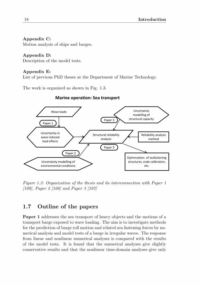
The work is organized as shown in Fig. 1.3.
Marine operation: Sea transport
Uncertainty modelling of environmental conditions
Uncertainty inwave induced load effects
Structural reliability analysis
Wave loads
Paper 2
Reliability analysis method
Uncertainty modelling of
structural capacityPaper 1
Paper 3
Optimization of seafastening structures, code calibration,
etc.
Paper 3
Figure 1.3: Organization of the thesis and its interconnection with Paper 1[109], Paper 2 [108] and Paper 3 [107]
1.7 Outline of the papersPaper 1 addresses the sea transport of heavy objects and the motions of atransport barge exposed to wave loading. The aim is to investigate methodsfor the prediction of barge roll motion and related sea fastening forces by nu-merical analysis and model tests of a barge in irregular waves. The responsefrom linear and nonlinear numerical analyses is compared with the resultsof the model tests. It is found that the numerical analyses give slightlyconservative results and that the nonlinear time-domain analyses give only
1.7. Outline of the papers 19
marginally more accurate results than the linear frequency domain method.The results from Paper 1 are used for modeling the uncertainty in the wave-induced load effect.
Paper 2 is concerned with planning marine operations with regard to en-vironmental conditions and operational limits. Operational decisions arebased on weather forecasts, and the uncertainty inherent in weather fore-casts of significant wave height is studied using data from the NorwegianSea. The results from Paper 2 form the basis for the uncertainty model ofthe environmental conditions in the reliability analyses.
Paper 3 addresses the structural capacity of the transport vessel and thecargo and discusses the uncertainty models used in the structural reliabilityanalyses. The bulkheads in the transport vessels are exposed to large ver-tical local forces from the cargo supports, and when these bulkheads havehorizontal stiffeners, the in-plane bulkhead loading acts perpendicular to thestiffeners. The modeling of the uncertainty in such structures is discussed.Furthermore, the paper presents a structural reliability analysis method toaccommodate the uncertainties affecting the design checks. The impliedprobability of structural failure by use of the relevant design standards formarine operations is studied using structural reliability analyses for twocategories of marine operations, notably weather-restricted and weather-unrestricted operations. While weather-restricted operations are designedfor a chosen limit of the significant wave height, a weather-unrestrictedoperation cannot rely on forecasts but must be designed using long-termstatistical data for the relevant season. The probability of failure is cal-culated for both categories. The probability of structural failure duringweather-restricted barge transport is calculated for various durations andseveral forecasted significant wave heights. For weather-unrestricted opera-tion, where the environmental loading is given by long-term data, the failureprobability is calculated for several operational durations and for executionin various months or seasons.

20 Introduction
Chapter 2
Environmental conditions formarine operations
2.1 General
The purpose of the marine operations studied here is to safely transport anasset from one location to another location. Environmental loads are thekey input for the design of marine operations and will often define the limitsfor the actual execution of an operation. Even if the design should aim atmaking the operation robust, most operations are sensitive to environmentalloading, and waiting on weather commonly occurs. During the planning ofweather-restricted operations, the environmental design conditions shouldbe optimized to balance the cost related to the size of the transport vessels,tugs, structural steel, equipment, etc., with the cost related to waiting onweather; see also Sec. 2.5.1.
2.2 Planning of marine operations and requiredenvironmental data
During marine operations, the handled object is brought from one definedsafe condition to another. The marine operation is over when the safedestination has been reached. A key parameter is the duration of the marineoperation. To estimate the duration, the time when the handled object is ina safe condition and the operation is finished must be clearly defined. Theduration of an operation, called the operation reference period, is definedas follows [31]:
TR = TPOP + TC (2.1)
21
22 Environmental conditions for marine operations
whereTPOP is the planned operation period andTC is the estimated maximum contingency time.The estimated maximum contingency time is normally between 50% and100% of the planned operation period. The total duration is a stochasticvariable but is assumed to be deterministic here.
Marine operations are classified as either weather-restricted or weather-unrestricted, depending on the duration of the operation. Weather-restrictedoperations are based on weather forecasts and are beneficial since the owner,or their representative, may define the environmental criteria to operate in.The operation may commence when the weather forecasts show acceptableconditions. A key issue is then the uncertainty in the weather forecastsand how to deal with that uncertainty during planning of the operation.For weather-restricted operations (i.e., operations of short duration andoperations that may be halted within a short notice), the environmentalconditions are given by weather forecasts. An ample margin must be set onthe forecasted wave height, wind speed, etc., when defining the operationalcriteria to have a sufficiently low probability of exceeding the design criteria.
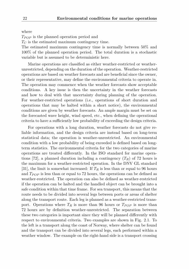
For operations with a long duration, weather forecasts do not give re-liable information, and the design criteria are instead based on long-termstatistical data; the operation is weather-unrestricted. An environmentalcondition with a low probability of being exceeded is defined based on long-term statistics. The environmental criteria for the two categories of marineoperations are treated differently. In the ISO standard for marine opera-tions [72], a planned duration including a contingency (TR) of 72 hours isthe maximum for a weather-restricted operation. In the DNV GL standard[31], the limit is somewhat increased: If TR is less than or equal to 96 hoursand TPOP is less than or equal to 72 hours, the operations can be defined asweather-restricted. The operation can also be defined as weather-restrictedif the operation can be halted and the handled object can be brought into asafe condition within that time frame. For sea transport, this means that theroute needs to be divided into several legs between ports or areas of shelteralong the transport route. Each leg is planned as a weather-restricted trans-port. Operations where TR is more than 96 hours or TPOP is more than72 hours are by definition weather-unrestricted. The separation betweenthese two categories is important since they will be planned differently withrespect to environmental criteria. Two examples are shown in Fig. 2.1. Tothe left is a transport along the coast of Norway, where shelter can be foundand the transport can be divided into several legs, each performed within aweather window. The example on the right-hand side is a transport crossing
2.3. Weather forecasts 23
the Indian Ocean. Even if there are several islands in that area, they arenot considered to provide sufficient shelter or safe haven, and the transportis weather-unrestricted. See also Sec. 2.6.
Figure 2.1: Example of weather-restricted transport with a sheltered stop(left) and weather-unrestricted transport; red lines represent transport routes(maps from www.fn.no)
In areas or seasons where weather forecasts are reliable for a shorterperiod, a shorter limit for weather-restricted operations must be applied.
2.3 Weather forecasts
Weather forecasts for marine operations are typically operation specific andspecially ordered forecasts that include a significant wave height, wave pe-riod and wind speed, among other information. The forecast can be givenfor one specific location or for a given transport route. The forecast is or-dered based on an estimated vessel speed, and an updated route is sent tothe forecaster during the operations if the actual route deviates from theplanned route.
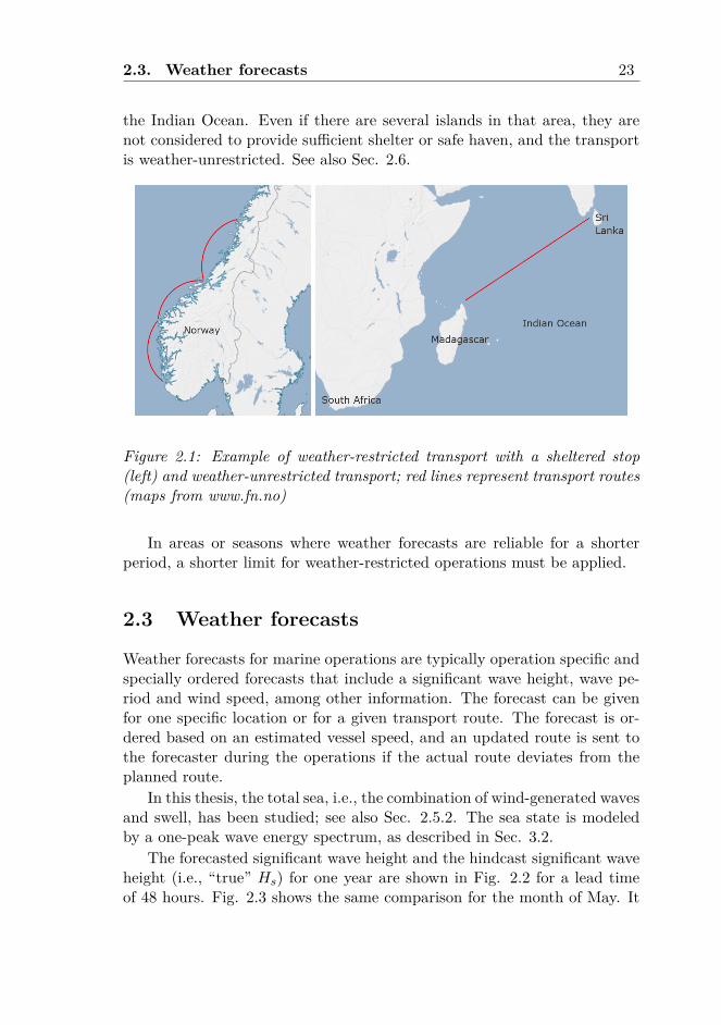
In this thesis, the total sea, i.e., the combination of wind-generated wavesand swell, has been studied; see also Sec. 2.5.2. The sea state is modeledby a one-peak wave energy spectrum, as described in Sec. 3.2.
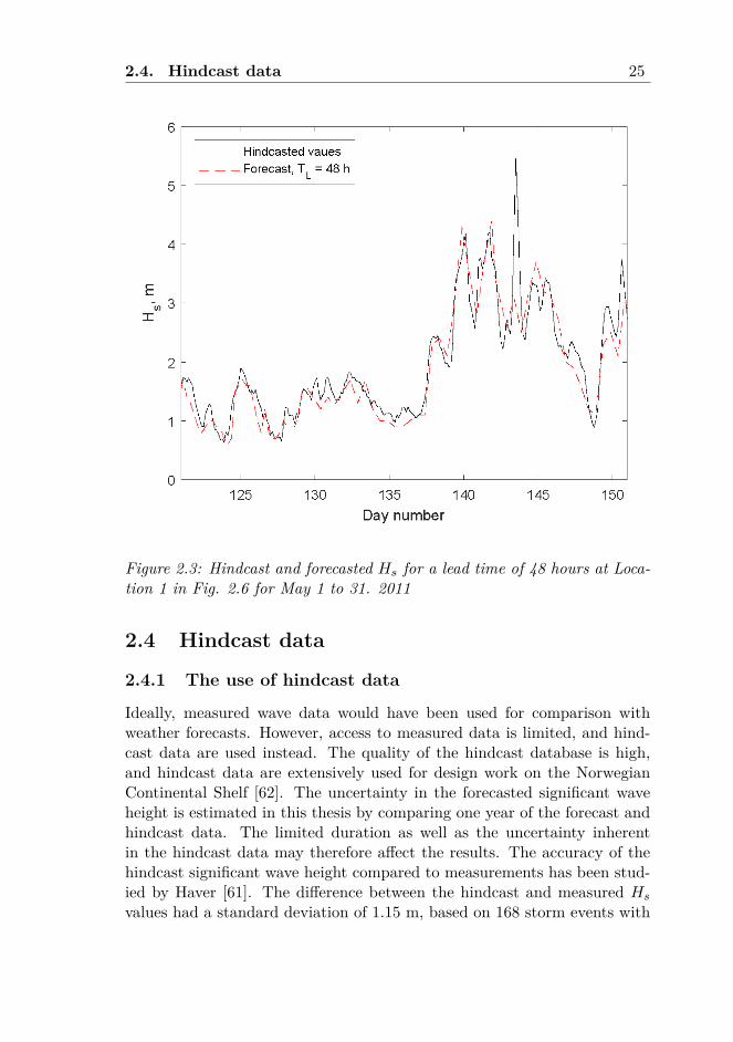
The forecasted significant wave height and the hindcast significant waveheight (i.e., “true” Hs) for one year are shown in Fig. 2.2 for a lead timeof 48 hours. Fig. 2.3 shows the same comparison for the month of May. It
24 Environmental conditions for marine operations
is evident that not all the peaks in the observed wave heights are capturedby the weather forecasts.
Figure 2.2: Hindcast and forecasted Hs for lead time of 48 hours in 2011,at Location 1 in Fig. 2.6
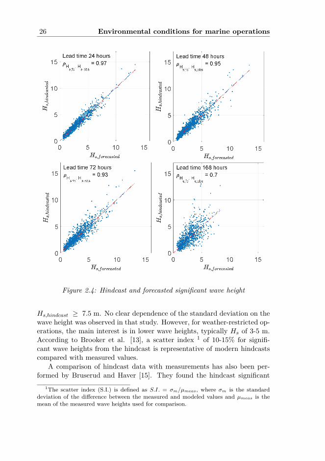
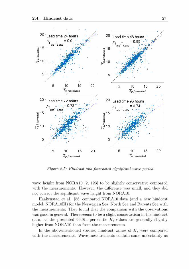
The correlation between the forecast and hindcast significant wave heightsis shown for several lead times in Fig. 2.4. The correlation decreases withincreasing lead time. In Fig. 2.5, the wave periods (spectral peak periods,Tp) are similarly shown. The correlation between the forecast and hindcastvalues is lower for peak periods than for the significant wave height for alead time less than 72 hours. The peak period appears to be more difficultto forecast than Hs. This is not limited to weather forecasts; the uncer-tainty in sea state parameters from spectral estimation has been studied byRodrigues et al. [127]. It was concluded that the use of different methodsof spectral estimation did not have a large effect on the variability of, e.g.,the significant wave height, but the peak period showed great differences asa function of the spectral method adopted.
2.4. Hindcast data 25
Figure 2.3: Hindcast and forecasted Hs for a lead time of 48 hours at Loca-tion 1 in Fig. 2.6 for May 1 to 31. 2011
2.4 Hindcast data
2.4.1 The use of hindcast data
Ideally, measured wave data would have been used for comparison withweather forecasts. However, access to measured data is limited, and hind-cast data are used instead. The quality of the hindcast database is high,and hindcast data are extensively used for design work on the NorwegianContinental Shelf [62]. The uncertainty in the forecasted significant waveheight is estimated in this thesis by comparing one year of the forecast andhindcast data. The limited duration as well as the uncertainty inherentin the hindcast data may therefore affect the results. The accuracy of thehindcast significant wave height compared to measurements has been stud-ied by Haver [61]. The difference between the hindcast and measured Hs
values had a standard deviation of 1.15 m, based on 168 storm events with
26 Environmental conditions for marine operations
Figure 2.4: Hindcast and forecasted significant wave height
Hs,hindcast ≥ 7.5 m. No clear dependence of the standard deviation on thewave height was observed in that study. However, for weather-restricted op-erations, the main interest is in lower wave heights, typically Hs of 3-5 m.According to Brooker et al. [13], a scatter index 1 of 10-15% for signifi-cant wave heights from the hindcast is representative of modern hindcastscompared with measured values.
A comparison of hindcast data with measurements has also been per-formed by Bruserud and Haver [15]. They found the hindcast significant
1The scatter index (S.I.) is defined as S.I. = σm/µmeas, where σm is the standarddeviation of the difference between the measured and modeled values and µmeas is themean of the measured wave heights used for comparison.
2.4. Hindcast data 27
Figure 2.5: Hindcast and forecasted significant wave period
wave height from NORA10 [2, 123] to be slightly conservative comparedwith the measurements. However, the difference was small, and they didnot correct the significant wave height from NORA10.
Haakenstad et al. [58] compared NORA10 data (and a new hindcastmodel, NORA10EI) for the Norwegian Sea, North Sea and Barents Sea withthe measurements. They found that the comparison with the observationswas good in general. There seems to be a slight conservatism in the hindcastdata, as the presented 99.9th percentile Hs-values are generally slightlyhigher from NORA10 than from the measurements.
In the abovementioned studies, hindcast values of Hs were comparedwith the measurements. Wave measurements contain some uncertainty as
28 Environmental conditions for marine operations
well. This was studied by Magnusson [91], comparing measurements fromwave rider buoys with radar and laser measurements. There was gener-ally a good fit between the methods, but some deviations were evident, inparticular for significant wave heights larger than 8− 10 m.
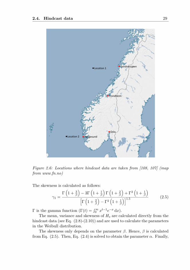
Based on the studies above, it was concluded that the measurementsand hindcasts are both suitable for a study of the uncertainty in weatherforecasts, and in this thesis, hindcast data were directly used without anycorrections. The hindcast data were used as follows:
r Hindcast significant wave heights were compared with weather fore-casts to estimate the uncertainty in the forecasted significant waveheight (Location 1 in Fig. 2.6)
r The long-term statistical distribution of the significant wave heightand the conditional distribution of the wave period were estimatedbased on the hindcast data (Location 2 in Fig. 2.6)
2.4.2 Long-term distribution from the hindcast data
In the hindcast data, the significant wave height is given every three hours.A three-parameter Weibull distribution can be fitted to the long-term distri-bution of Hs. The parameters can be estimated according to [17, Sec. 17.6].The approach is explained in detail in [62]. The probability density functionfor the Weibull distribution is defined as follows:
fHs(hs) = β
α
(hs − γα
)β−1exp
[−(hs − γα
)β](2.2)
whereα is the scale parameter (different from the Alpha factor used elsewhere),β is the shape parameter andγ is the location parameter.To estimate the three parameters, the three lowest moments are used, i.e.,the mean value, the variance and the skewness. The mean value is calculatedas follows:
µHs = γ + αΓ(
1 + 1β
)(2.3)
The variance is calculated as follows:
σ2Hs = α2
[Γ(
1 + 2β
)− Γ2
(1 + 1
β
)](2.4)
2.4. Hindcast data 29
Haugesund
Oslo
Sandnessjøen
Trondheim
Location 2
Location 1
Figure 2.6: Locations where hindcast data are taken from [108, 107] (mapfrom www.fn.no)
The skewness is calculated as follows:
γ1 =Γ(1 + 3
β
)− 3Γ
(1 + 1
β
)Γ(1 + 2
β
)+ Γ3
(1 + 1
β
)
[Γ(1 + 2
β
)− Γ2
(1 + 1
β
)]1.5 (2.5)
Γ is the gamma function (Γ(t) = ∫∞0 xt−1e−x dx).The mean, variance and skewness of Hs are calculated directly from the
hindcast data (see Eq. (2.8)-(2.10)) and are used to calculate the parametersin the Weibull distribution.
The skewness only depends on the parameter β. Hence, β is calculatedfrom Eq. (2.5). Then, Eq. (2.4) is solved to obtain the parameter α. Finally,
30 Environmental conditions for marine operations
the parameter γ is estimated from Eq. (2.3). The Weibull parameters forLocation 2 in Fig. 2.6 are given in Tables 4.4 and 4.5.
2.5 Weather-restricted operations
2.5.1 General
Marine operations, e.g., load-out operations, sea transports and installa-tion of offshore units and equipment, all need to be designed, planned andexecuted considering environmental loads.
The design environmental criteria for a weather-restricted operation areset in an early phase of the project. A low criterion may lead to extensivewaiting on weather, which is expensive. A criterion that is too high willincrease the economic cost related to the operation, e.g., due to the increasedtug size, mooring arrangements, amount of seafastening, etc. The optimumenvironmental criteria should be chosen based on an overall assessment.
The operation may commence when the weather forecasts indicate thatacceptable environmental conditions are present for the entire operation pe-riod. The uncertainty in the weather forecasts and how to include this un-certainty in the planning of the operation thus become key issues. Based onthe design environmental condition defined in the planning phase (Hs,design),the corresponding limiting environmental criteria for the execution of theoperation, i.e., the maximum allowed forecast value, (Hs,forecast), is de-fined. Hs,forecast is lower than Hs,design to account for the uncertainty inthe forecasted environmental conditions. The maximum allowed forecastedsignificant wave height can be determined by the Alpha factor method de-scribed in Sec. 1.4.6.
The uncertainty in weather forecasts was studied in Paper 2 [108]. Sec-tion 2.5 is an overview of weather-restricted operations, including a sum-mary of that paper.
2.5.2 Forecasted wave height
Wave-induced loads will normally dominate the structural load effects formarine operations where floating vessels are involved. Hence, the significantwave height is of main interest for marine operations. It is therefore vital tohave information about the level of accuracy for the forecasted wave height.The forecasts include wind-generated seas, swells and the total sea. In thestudies, the significant wave height for the total sea has been used, i.e.,Hs,total sea = (H2
s,wind waves +H2s,swell)0.5.
2.5. Weather-restricted operations 31
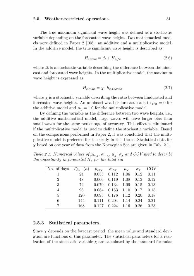
The true maximum significant wave height was defined as a stochasticvariable depending on the forecasted wave height. Two mathematical mod-els were defined in Paper 2 [108]: an additive and a multiplicative model.In the additive model, the true significant wave height is described as:
Hs,true = ∆ +Hs,fc (2.6)
where ∆ is a stochastic variable describing the difference between the hind-cast and forecasted wave heights. In the multiplicative model, the maximumwave height is expressed as:
Hs,max = χ · hs,fc,max (2.7)
where χ is a stochastic variable describing the ratio between hindcasted andforecasted wave heights. An unbiased weather forecast leads to µ∆ = 0 forthe additive model and µχ = 1.0 for the multiplicative model.
By defining the variable as the difference between two wave heights, i.e.,the additive mathematical model, large waves will have larger bias thansmall waves for the same percentage of accuracy. This effect is eliminatedif the multiplicative model is used to define the stochastic variable. Basedon the comparisons performed in Paper 2, it was concluded that the multi-plicative model is preferred for the study in this thesis. Statistical data forχ based on one year of data from the Norwegian Sea are given in Tab. 2.1.
Table 2.1: Numerical values of µlnχ, σlnχ, µχ, σχ and COV used to describethe uncertainty in forecasted Hs for the total sea
No. of days TR, (h) µlnχ σlnχ µχ σχ COV1 24 0.055 0.112 1.06 0.12 0.112 48 0.066 0.119 1.08 0.13 0.123 72 0.079 0.134 1.09 0.15 0.134 96 0.084 0.153 1.10 0.17 0.155 120 0.095 0.176 1.12 0.20 0.186 144 0.111 0.204 1.14 0.24 0.217 168 0.127 0.224 1.16 0.26 0.23
2.5.3 Statistical parameters
Since χ depends on the forecast period, the mean value and standard devi-ation are functions of this parameter. The statistical parameters for a real-ization of the stochastic variable χ are calculated by the standard formulas
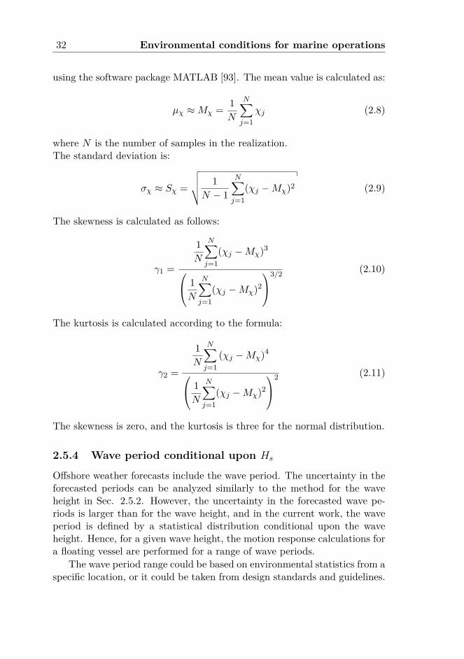
32 Environmental conditions for marine operations
using the software package MATLAB [93]. The mean value is calculated as:
µχ ≈Mχ = 1N
N∑
j=1χj (2.8)
where N is the number of samples in the realization.The standard deviation is:
σχ ≈ Sχ =
√√√√ 1N − 1
N∑
j=1(χj −Mχ)2 (2.9)
The skewness is calculated as follows:
γ1 =
1N
N∑
j=1(χj −Mχ)3
1N
N∑
j=1(χj −Mχ)2
3/2 (2.10)
The kurtosis is calculated according to the formula:
γ2 =
1N
N∑
j=1(χj −Mχ)4
1N
N∑
j=1(χj −Mχ)2
2 (2.11)
The skewness is zero, and the kurtosis is three for the normal distribution.
2.5.4 Wave period conditional upon Hs
Offshore weather forecasts include the wave period. The uncertainty in theforecasted periods can be analyzed similarly to the method for the waveheight in Sec. 2.5.2. However, the uncertainty in the forecasted wave pe-riods is larger than for the wave height, and in the current work, the waveperiod is defined by a statistical distribution conditional upon the waveheight. Hence, for a given wave height, the motion response calculations fora floating vessel are performed for a range of wave periods.
The wave period range could be based on environmental statistics from aspecific location, or it could be taken from design standards and guidelines.
2.6. Weather-unrestricted operations 33
The mean zero-crossing wave period (Tz) range can, for example, betaken as follows [31, Sec C.3.4]:
2.84H0.5s ≤ Tz ≤ max5.43H0.5
s , 13 (2.12)
where Hs is given in meters and the unit for Tz is seconds.The mean zero-crossing periods can be modeled as a lognormal distri-
bution conditional upon the significant wave height [11, 108]; see Eq. (4.13)on page 69. The parameters for the distribution can be found for the NorthAtlantic and for the Worldwide operation of ships [29] and in Table 4.6 forLocation 2 in Fig. 2.6.
2.5.5 Wind speed
The uncertainty in the forecasted wind speed may be quantified by compar-ing forecasted values with hindcast values, resulting in a statistical descrip-tion of the deviation, similar to what was done for the wave heights. Thisis particularly relevant for marine operations performed in sheltered areaswhere the wind load dominates, e.g., load-out operations where wind loadsgovern for the mooring of the transport vessel.
For typical sea transport on a large ship or transport barge, the waveload will dominate over the wind load; see Sec. 3.3.7. The uncertainty inthe wind load will therefore have a limited effect on the total load in thesupports and is not considered further for weather-restricted operations.
2.6 Weather-unrestricted operations
2.6.1 General
Marine operations with a planned duration longer than three days cannotbe designed as weather-restricted operations but need to be designed asweather-unrestricted operations; see Sections 1.4.3 and 2.2.
While for a weather-restricted operation, the environmental criteria arebased on weather forecasts accounting for the uncertainty, environmentalcriteria for weather-unrestricted operations are based on long-term envi-ronmental statistics. The design criteria are calculated for the relevantgeographical area, the season of the year and the duration of the opera-tion. The design wave heights may be calculated based on scatter diagrams[29, 64]. It should be noted that scatter diagrams based on visual observa-tions of the sea may, to some extent, include the effects of heavy weatheravoidance (i.e., the largest waves are never observed).
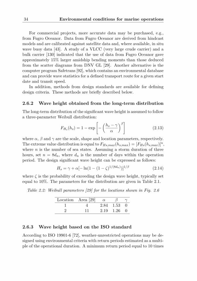
34 Environmental conditions for marine operations
For commercial projects, more accurate data may be purchased, e.g.,from Fugro Oceanor. Data from Fugro Oceanor are derived from hindcastmodels and are calibrated against satellite data and, where available, in situwave buoy data [43]. A study of a VLCC (very large crude carrier) and abulk carrier [130] indicated that the use of data from Fugro Oceanor gaveapproximately 15% larger amidship bending moments than those deducedfrom the scatter diagrams from DNV GL [29]. Another alternative is thecomputer program Safetrans [92], which contains an environmental databaseand can provide wave statistics for a defined transport route for a given startdate and transit speed.
In addition, methods from design standards are available for definingdesign criteria. These methods are briefly described below.
2.6.2 Wave height obtained from the long-term distribution
The long-term distribution of the significant wave height is assumed to followa three-parameter Weibull distribution:
FHs(hs) = 1− exp[−(hs − γα
)β](2.13)
where α, β and γ are the scale, shape and location parameters, respectively.The extreme value distribution is equal to FHs,max(hs,max) = [FHs(hs,max)]n,where n is the number of sea states. Assuming a storm duration of threehours, set n = 8dn, where dn is the number of days within the operationperiod. The design significant wave height can be expressed as follows:
Hs = γ + α[− ln(1− (1− ζ)1/(8dn))]1/β (2.14)
where ζ is the probability of exceeding the design wave height, typically setequal to 10%. The parameters for the distribution are given in Table 2.1.
Table 2.2: Weibull parameters [29] for the locations shown in Fig. 2.6
Location Area [29] α β γ
1 4 2.84 1.53 02 11 2.19 1.26 0
2.6.3 Wave height based on the ISO standard
According to ISO 19901-6 [72], weather-unrestricted operations may be de-signed using environmental criteria with return periods estimated as a multi-ple of the operational duration. A minimum return period equal to 10 times
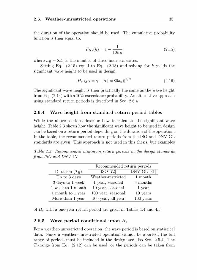
2.6. Weather-unrestricted operations 35
the duration of the operation should be used. The cumulative probabilityfunction is then equal to:
FHs(h) = 1− 110nR
(2.15)
where nR = 8dn is the number of three-hour sea states.Setting Eq. (2.15) equal to Eq. (2.13) and solving for h yields the
significant wave height to be used in design:
Hs,ISO = γ + α [ln(80dn)]1/β (2.16)
The significant wave height is then practically the same as the wave heightfrom Eq. (2.14) with a 10% exceedance probability. An alternative approachusing standard return periods is described in Sec. 2.6.4.
2.6.4 Wave height from standard return period tables
While the above sections describe how to calculate the significant waveheight, Table 2.3 shows how the significant wave height to be used in designcan be based on a return period depending on the duration of the operation.In the table, the recommended return periods from the ISO and DNV GLstandards are given. This approach is not used in this thesis, but examples
Table 2.3: Recommended minimum return periods in the design standardsfrom ISO and DNV GL
Recommended return periodsDuration (TR) ISO [72] DNV GL [31]Up to 3 days Weather-restricted 1 month
3 days to 1 week 1 year, seasonal 3 months1 week to 1 month 10 year, seasonal 1 year1 month to 1 year 100 year, seasonal 10 yearsMore than 1 year 100 year, all year 100 years
of Hs with a one-year return period are given in Tables 4.4 and 4.5.
2.6.5 Wave period conditional upon Hs
For a weather-unrestricted operation, the wave period is based on statisticaldata. Since a weather-unrestricted operation cannot be aborted, the fullrange of periods must be included in the design; see also Sec. 2.5.4. TheTz-range from Eq. (2.12) can be used, or the periods can be taken from

36 Environmental conditions for marine operations
a scatter diagram for the actual location. A statistical distribution for themean zero-crossing period conditional on the significant wave height is givenin Eq. (4.13), and the parameters for the distribution can be found in Table4.6 for Location 2 in Fig. 2.6. This conditional distribution is applied inthe structural reliability analyses.
2.6.6 Wind speed conditional upon Hs
The wind-induced loads act in addition to the wave-induced loads. Even ifthe wave-induced loads are dominant for large and heavy objects, the windspeed corresponding to the design significant wave height for sea transportmay still be needed. The relation between the wave height and the windspeed at a certain location may depend on the wind and wave directions,storm duration, fetch, water depth, etc. A simple method is proposed toestimate the wind speed from a given significant wave height. A formula forcalculating the one-minute wind speed 10 m above sea level as a functionof a specified significant wave height is presented as follows [108]:
Voneminute ≈ 10√Hs (2.17)
where Hs is given in m and the unit for the wind speed is m/s. The signifi-cant wave height representing the total sea (i.e., both wind-generated wavesand swell) is used in the comparison. The one-minute design wind speed isthus approximated as a function of the significant wave height only. Theone-minute averaged wind speed is used when the wave load dominates [31].Similarly, the one-hour wind speed can be approximated as:
Vone hour ≈ 8√Hs (2.18)
This wind speed is plotted in Fig. 2.7. It is noted that there is a largespread in the wind speed for a given Hs. The significant wave heights inEq. (2.17) and (2.18) represent the fully developed wind-generated waves.The significant wave height assumed in long-term wave distributions de-scribes the total sea, i.e., it also includes swell. This means that when thewind speed is calculated from Eq. (2.17) and the design significant waveheight includes swell, the wind speed will be overestimated. This is also il-lustrated in Fig. 2.8, where contour lines for the significant wave height andwind speed are shown for several return periods. The simplified wind speedestimate is higher than the wind speed that corresponds to the largest sig-nificant wave height for a given return period. For a typical sea transport,where the wave load dominates over the wind load, the wind load couldbe included to simulate the reaction forces in the grillage and seafastening.
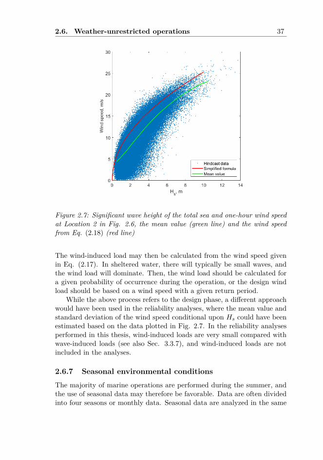
2.6. Weather-unrestricted operations 37
Figure 2.7: Significant wave height of the total sea and one-hour wind speedat Location 2 in Fig. 2.6, the mean value (green line) and the wind speedfrom Eq. (2.18) (red line)
The wind-induced load may then be calculated from the wind speed givenin Eq. (2.17). In sheltered water, there will typically be small waves, andthe wind load will dominate. Then, the wind load should be calculated fora given probability of occurrence during the operation, or the design windload should be based on a wind speed with a given return period.
While the above process refers to the design phase, a different approachwould have been used in the reliability analyses, where the mean value andstandard deviation of the wind speed conditional upon Hs could have beenestimated based on the data plotted in Fig. 2.7. In the reliability analysesperformed in this thesis, wind-induced loads are very small compared withwave-induced loads (see also Sec. 3.3.7), and wind-induced loads are notincluded in the analyses.
2.6.7 Seasonal environmental conditions
The majority of marine operations are performed during the summer, andthe use of seasonal data may therefore be favorable. Data are often dividedinto four seasons or monthly data. Seasonal data are analyzed in the same
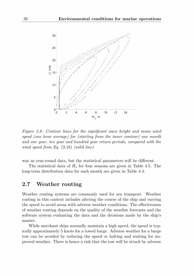
38 Environmental conditions for marine operations
Figure 2.8: Contour lines for the significant wave height and mean windspeed (one hour average) for (starting from the inner contour) one monthand one year, ten year and hundred year return periods, compared with thewind speed from Eq. (2.18) (solid line)
way as year-round data, but the statistical parameters will be different.The statistical data of Hs for four seasons are given in Table 4.5. The
long-term distribution data for each month are given in Table 4.4.
2.7 Weather routingWeather routing systems are commonly used for sea transport. Weatherrouting in this context includes altering the course of the ship and varyingthe speed to avoid areas with adverse weather conditions. The effectivenessof weather routing depends on the quality of the weather forecasts and thesoftware system evaluating the data and the decisions made by the ship’smaster.
While merchant ships normally maintain a high speed, the speed is typ-ically approximately 5 knots for a towed barge. Adverse weather for a bargetow can be avoided by reducing the speed or halting and waiting for im-proved weather. There is hence a risk that the tow will be struck by adverse
2.8. Heading control 39
weather while waiting, and the exact speed and direction of the weather sys-tem may not be accurately forecasted. Furthermore, in the case of towlinefailure, the barge will drift until the towline is reconnected. It may takequite some time before the weather calms down enough to reconnect thetowline, and weather routing is therefore not an option.
The minimum required towing speed to be able to perform effectiveweather routing has not been studied herein. It is instead concluded thatthe positive effect of weather routing cannot be utilized with respect to thestructural capacity in the ultimate limit state, e.g., for the capacity of thegrillage and seafastening. Weather routing can, however, be favorable withrespect to fatigue damage and fuel consumption.
2.8 Heading control
For sea transport on self-propelled vessels, it may under certain conditionsbe assumed that the vessel can head up against the wind/waves in adverseweather to limit the rolling. Several requirements, e.g., adequate redun-dancy in the propulsion system, need to be fulfilled to utilize heading con-trol. Heading control allows for a substantial reduction in the design waveheight, such as a 40% reduction in the design significant wave height forbeam seas [31] (hence, the significant wave height for beam seas is 60% ofthe design significant wave height for head seas). Heading control can alsobe an option for manned barges towed by multiple tugs, where after break-down of any one tug or failure of any one tow line, the remaining tug(s)have sufficient bollard pull capacity.
For barges towed by a single tug, a tow line failure or tug breakdown willleave the barge drifting until the tow line is reconnected. The probabilityfor this to happen is too high to utilize heading control [31] because adrifting barge may be exposed to beam seas. The probability of these eventsoccurring has not been quantified in this thesis. However, the dynamicloading in the tow line is high [44, 112] and may lead to failure of thetow line, as well as failure of the tow line connection [76]. Regarding tugbreakdown, ocean going tugs normally have several engines and propellers;hence, the probability of a total blackout is low. However, a fire in theengine room, for example, could result in a complete blackout even if themachinery itself is redundant. Therefore, the probability of tug breakdownshould not be neglected.
Furthermore, depending on the layout of the cargo, the wind area, etc.,it might not be possible to keep the barge heading toward the waves inadverse weather even with intact tug and tow line, and there could be a

40 Environmental conditions for marine operations
relatively large yaw angle of the barge.In the structural reliability analyses, the barge is hence assumed to be
exposed to beam seas.
Chapter 3
Wave-induced load effectanalysis
3.1 General
For sea transport, wave-induced loads are normally predominant for grillageand seafastening. Generally, wind-induced loads should also be checked, butfor heavy cargo transported on barges, the wave-induced loads dominate.For stability, however, wind loading is a main concern but is not discussedherein.
The grillage and seafastening structures are designed to sustain environ-mental loads dependent on the area, the season of the year, the durationof the transport, etc. In the ultimate limit state, structural failure occurswhen the load effect exceeds the structural capacity. Therefore, predictionof the extreme wave-induced load effects during sea transport is vital, andthe uncertainties in the characteristic wave-induced load effects must beaccounted for in the planning of marine transport.
The wave-induced motions of the transport vessel can be obtained fromformulas given in classification rules or design standards. These design cri-teria are experience-based formulas for calculating the motions based on alimited amount of input, e.g., ship length, breadth, draught, block coeffi-cient, etc. The design forces can be obtained from these design criteria.Alternatively, the wave-induced motions of the transport vessel can be ob-tained by direct calculations based on hydrodynamic software using 2Dstrip theory or 3D potential theory, and the extreme vessel motion or load-ing is then calculated based on the long-term distribution of wave heightsby means of scatter diagrams or a given design condition.
For the vessel itself, wave load analysis is performed to calculate the load
41
42 Wave-induced load effect analysis
effects for the structural design of the vessel. These analyses are performedin relation to new buildings and are normally not required for marine oper-ations as long as the vessel is used in compliance with the standard loadingconditions approved by the classification society. However, for heavy cargo,a global capacity check of the transport vessel can be relevant. The trans-ported object must also be documented to be strong enough to resist theloads caused by the vessel motion, as well as the local capacity of the trans-port vessel adjacent to the supports. Hence, the motion analysis will formthe basis for design of the support structures, in addition to capacity checksof the transported object and the vessel itself.
3.2 Wave description
3.2.1 Choice of the wave energy spectrum
A regular wave is described by the wave height (or amplitude) and waveperiod. A sea state is made up of several individual waves and is describedby the significant wave height, Hs, and the zero-crossing period, Tz, or thespectral peak period, Tp. A wave condition might consist of several wavesystems, i.e., locally generated wind-driven waves in combination with swellgenerated in remote areas. The total sea is considered in this thesis; seealso Sections 2.3 and 2.5.2.
The wave energy is distributed on frequencies (or periods) and directions,as described by a two-dimensional (2D) wave energy spectrum, as illustratedin Fig. 3.1. A simpler representation is normally used, where the waveenergy distribution on the frequency is described by a one-dimensional waveenergy spectrum with a main wave propagation direction, possibly combinedwith a wave spreading function to represent short-crested waves [29]. Aone-dimensional spectrum is used in this thesis. Long-crested waves areassumed; hence, no wave spreading function is applied. Because the caseanalyzed here is a beam sea condition and the roll response dominates, useof long-crested waves will overestimate the response if the waves are in factshort-crested (that would be different if head seas were analyzed, becauselong-crested waves would then give no roll response, and short-crested waveswould govern).
A two-peak spectrum could be applied to model the wave energy sep-arated on wind-dominated and swell-dominated sea states. Several two-peak spectra have been proposed, such as a combination of a Jonswapand a Pierson-Moskowitz spectrum to describe the two wave systems [117]or a combination of two Jonswap spectra [56]. For Norwegian waters, a
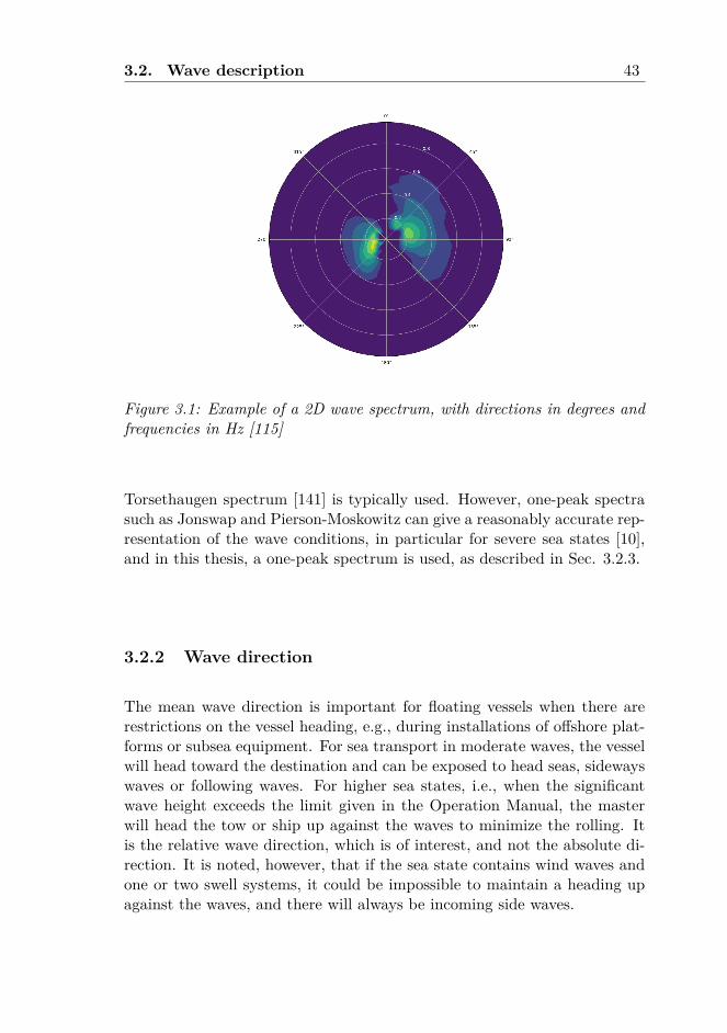
3.2. Wave description 43
Figure 3.1: Example of a 2D wave spectrum, with directions in degrees andfrequencies in Hz [115]
Torsethaugen spectrum [141] is typically used. However, one-peak spectrasuch as Jonswap and Pierson-Moskowitz can give a reasonably accurate rep-resentation of the wave conditions, in particular for severe sea states [10],and in this thesis, a one-peak spectrum is used, as described in Sec. 3.2.3.
3.2.2 Wave direction
The mean wave direction is important for floating vessels when there arerestrictions on the vessel heading, e.g., during installations of offshore plat-forms or subsea equipment. For sea transport in moderate waves, the vesselwill head toward the destination and can be exposed to head seas, sidewayswaves or following waves. For higher sea states, i.e., when the significantwave height exceeds the limit given in the Operation Manual, the masterwill head the tow or ship up against the waves to minimize the rolling. Itis the relative wave direction, which is of interest, and not the absolute di-rection. It is noted, however, that if the sea state contains wind waves andone or two swell systems, it could be impossible to maintain a heading upagainst the waves, and there will always be incoming side waves.
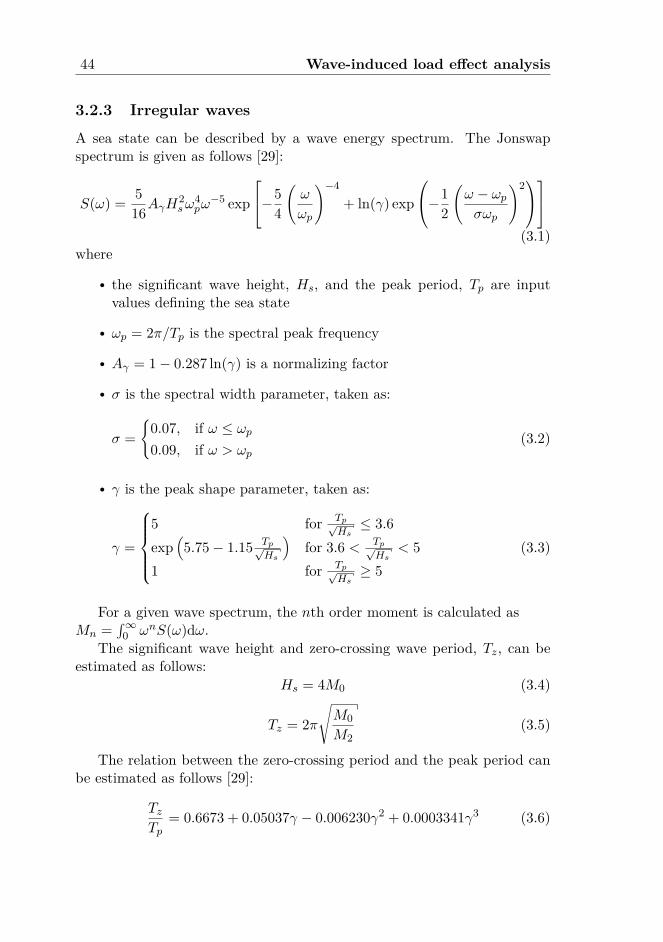
44 Wave-induced load effect analysis
3.2.3 Irregular waves
A sea state can be described by a wave energy spectrum. The Jonswapspectrum is given as follows [29]:
S(ω) = 516AγH
2sω
4pω−5 exp
−5
4
(ω
ωp
)−4
+ ln(γ) exp
−1
2
(ω − ωpσωp
)2
(3.1)wherer the significant wave height, Hs, and the peak period, Tp are input
values defining the sea stater ωp = 2π/Tp is the spectral peak frequencyr Aγ = 1− 0.287 ln(γ) is a normalizing factorr σ is the spectral width parameter, taken as:
σ =
0.07, if ω ≤ ωp0.09, if ω > ωp
(3.2)
r γ is the peak shape parameter, taken as:
γ =
5 for Tp√Hs≤ 3.6
exp(5.75− 1.15 Tp√
Hs
)for 3.6 < Tp√
Hs< 5
1 for Tp√Hs≥ 5
(3.3)
For a given wave spectrum, the nth order moment is calculated asMn =
∫∞0 ωnS(ω)dω.
The significant wave height and zero-crossing wave period, Tz, can beestimated as follows:
Hs = 4M0 (3.4)
Tz = 2π√M0M2
(3.5)
The relation between the zero-crossing period and the peak period canbe estimated as follows [29]:
TzTp
= 0.6673 + 0.05037γ − 0.006230γ2 + 0.0003341γ3 (3.6)
3.3. Numerical analyses 45
It could be noted that this relationship was previously expressed in a simplerand slightly better looking form as follows [23]:
TzTp
=√
5 + γ
11 + γ(3.7)
The results from the two expressions are, however, practically the same(maximum 2 % deviation for γ between 1 and 5).
While the Jonswap spectrum is representative of developing seas, thePierson-Moskowitz spectrum represents a fully developed sea and unlimitedfetch. The Pierson-Moskowitz spectrum is a special case of the Jonswapspectrum with γ = 1 and is expressed as follows [29]:
S(ω) = 516H
2sω
4pω−5 exp
−5
4
(ω
ωp
)−4 (3.8)
For this spectrum, the peak period can be calculated from the mean zero-crossing period as Tp ≈ 1.4Tz. The Pierson-Moskowitz spectrum was appliedin the model tests [109].
3.3 Numerical analyses
3.3.1 Available methods
Several methods are available for motion analyses. The design formulas asgiven in rules and standards and direct analyses based on potential theoryare possible tools. In practical engineering, linear analyses based on poten-tial theory dominate because they are relatively simple to perform, and theresults are easily extracted.
For barge transports, forward speed is generally not included in themotion analyses since towing speeds are low. In severe seas, the speed willbe close to zero. In small waves, however, there will be a forward speed,but this condition is not governing for the structural design in the ultimatelimit state.
The design of transports could also be based on more advanced calcu-lations, including nonlinear effects, e.g., CFD methods based on Reynolds-averaged Navier-Stokes (RANS). In practice, there is often a lack of per-sonnel, financial resources or time to perform such advanced analyses. Forpractical purposes and preliminary design, there is therefore a need forsimplified calculations for vessel motion, as given in ship rules and design
46 Wave-induced load effect analysis
standards. A simplified analysis method often used in planning marine op-erations is included in Appendix C.1; see also Sec. 3.3.2. The linear analysisapproach is discussed in Appendix C.2; see also Sec. 3.3.3. Some commentson the nonlinear method are given in Appendix C.3 and Sec. 3.3.4.
3.3.2 Simplified motion analysis
Vessel motions can be calculated by simplified methods provided by shiprules and design standards. Simplified motion criteria for ships are givenby IMO [69] and ISO [72]. Classification societies, e.g., ABS [3], BureauVeritas [16], DNV GL [25] and Lloyd’s Register [85], have class rules wherethe ship acceleration can be calculated. Motion criteria for transport bargesare given by ISO [72], DNV GL [31] and LOC [86]. Based on such criteria,the structural design can be performed. Simplified motion criteria for atransport barge are included in Appendix C.1.
3.3.3 Linear motion analysis in the frequency domain
The wave loads, added mass, linear damping and restoring force may be di-rectly calculated based on potential theory. Wamit [145] and Wadam [129]use the boundary element method to calculate the response amplitude op-erators, RAOs, i.e., the transfer functions for the six degrees of freedom.Linear analyses are performed in the frequency domain, and the statisticaltreatment of the results is then simple and robust. Irregular seas are repre-sented by energy density spectra, and the vessel response and load effectsare calculated by stochastic analysis. Since the analyses are linear, nonlin-ear effects such as viscous damping need to be linearized. Assuming narrowbanded wave spectra, the individual maxima follow a Rayleigh distribution.The most likely maximum, the expected maximum or the 90th percentilecan then easily be calculated, such as that for a three-hour storm.
3.3.4 Nonlinear analysis in the time domain
Nonlinear effects that affect the response include viscous roll damping andwater up to the instantaneous free surface elevation. The analysis has tobe performed in the time domain and is much more time consuming thanlinear analysis in the frequency domain.
A “semi” nonlinear method, where the wave loads, added mass and lineardamping are calculated based on potential theory, can be used. The dynamicequations of motion are solved in the time domain where the quadraticdamping due to vortex shedding is given as input. This approach is used
3.3. Numerical analyses 47
in Paper 1 and compared with experimental results. The purpose of thisanalysis was to study the benefits of including nonlinear effects. The waveloads, added mass, potential damping and restoring coefficients for the vesselwere calculated by Wadam [129], and the equations of motion were solvedin the time domain by Simo [131].
Wadam applied global (earth fixed) coordinates, and Simo used local(ship fixed) coordinates. The body fixed coordinate system in the timedomain analysis introduces additional terms in the equations of motions.For small waves and small ship motions, these terms are negligible, but insevere seas, they will affect the solution. This is discussed in Paper 1. Toillustrate the effect, the equations of motion are studied in more detail forthe special case of barge rolling in Appendix C.3.
3.3.5 Estimate of nonlinear roll damping
The rolling of a floating vessel is sensitive to the damping initiated fromvortex shedding at the corner/bilges. Ships are often equipped with bilgekeels to improve the roll motion characteristics. Barges, such as the Stan-dard North Sea barges, do not have bilge keels but rounded corners (bilges).Barges can also have sharp corners. Roll damping for a barge with a sharpcorner and a bilge radius was studied in Paper 1. Model test results werecompared with the results from Tanaka [140] and Ikeda [67], and nonlin-ear roll damping was estimated and given as input for the motion analyses.The damping had to be linearized to solve the equations of motion in thefrequency domain. For irregular sea states, the equivalent stochastic lin-earization is based on minimizing the expected value of the square of thedifference between the nonlinear damping force and the equivalent dampingforce [120]. The equivalent damping is then given as follows:
Beq = B1 + 2√
2πσθB2 (3.9)
wherer B1 is the linear damping coefficientr B2 is the quadratic damping coefficientr σθ is the standard deviation of the roll velocityHence, iterations are required to converge for equivalent stochastic lineardamping. (The procedure is as follows: assume (estimate) σ0
θ, calculate
B0eq from Eq. (3.9), calculate σ1
θfrom the equations of motion, calculate
B1eq and so on, until convergence.)
48 Wave-induced load effect analysis
3.3.6 The effect of sloshing in tanks
Ballast tanks should be empty or full. However, it could be necessary to haveone tank partially filled in order to achieve zero list and the predeterminedtrim. Sloshing may occur in the partially filled tank, but the effect ofsloshing is normally negligible for barge motions [78, Sec. 4.3.4].
3.3.7 The effect of heel from the wind load
The wind load on the transported object will be transferred into the trans-port vessel through grillage and seafastening. The wind load on the trans-ported object and the vessel itself will introduce a heel that also introducesforces in the seafastening system. For typical barge transport, the initialmetacentric height is large, and the initial heel from the wind load is negli-gible.
The seafastening forces from wind loads are small compared to the forcesfrom the motion of the vessel due to waves in our case. In the transport caseconsidered in Paper 1 [109], the mass of the transported object is 3500 tons,and the wind area is 600 m2. Based on the criteria shown in Table C.1, theacceleration 15 m above the water line is 0.75 g, and the wind pressure is 1.0kN/m2. The inertia force from the rolling of the barge is then 25 MN, whilethe wind load is 0.6 MN, i.e., the wind load is only 2 % of the load fromwave-induced motion. Hence, the wind load is negligible in this case. Thewind load must, however, be included when the stability is documented.
3.3.8 Calculation of the loads in the cargo supports
The wave-induced load effects in the structural members of the grillage andseafastening are calculated based on the accelerations and roll/pitch anglesderived from the motion analysis of the transport vessel. The calculationcan include the effect of elasticity in the transport vessel and the transportedobject or be based on the assumption of rigid bodies, i.e., calculate the re-action forces based on the dynamic equilibrium of the transported object.Which calculation method to use depends on the layout of the cargo and thetransport vessel. If the transported object is supported on more than threesupports, the elasticity can be important for the results. If, however, thetransported object has vertical supports at the corners, and the transverseand longitudinal directions (i.e., the roll and pitch stoppers) form a stati-cally determinate system, a simplified analysis technique may suffice. Forquartering waves, deformation of the transport vessel and the transportedobject could be important.
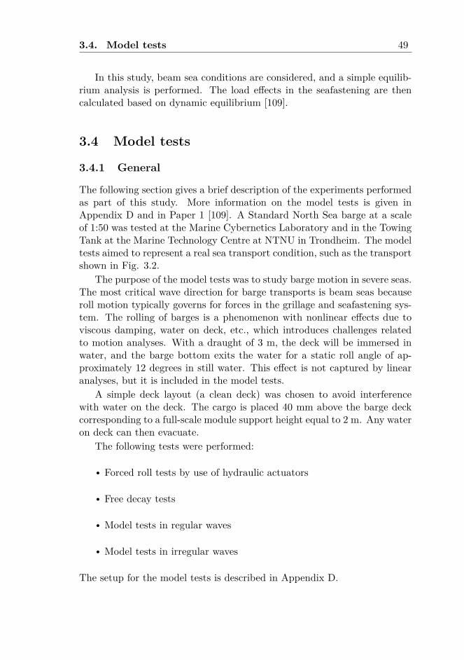
3.4. Model tests 49
In this study, beam sea conditions are considered, and a simple equilib-rium analysis is performed. The load effects in the seafastening are thencalculated based on dynamic equilibrium [109].
3.4 Model tests
3.4.1 General
The following section gives a brief description of the experiments performedas part of this study. More information on the model tests is given inAppendix D and in Paper 1 [109]. A Standard North Sea barge at a scaleof 1:50 was tested at the Marine Cybernetics Laboratory and in the TowingTank at the Marine Technology Centre at NTNU in Trondheim. The modeltests aimed to represent a real sea transport condition, such as the transportshown in Fig. 3.2.
The purpose of the model tests was to study barge motion in severe seas.The most critical wave direction for barge transports is beam seas becauseroll motion typically governs for forces in the grillage and seafastening sys-tem. The rolling of barges is a phenomenon with nonlinear effects due toviscous damping, water on deck, etc., which introduces challenges relatedto motion analyses. With a draught of 3 m, the deck will be immersed inwater, and the barge bottom exits the water for a static roll angle of ap-proximately 12 degrees in still water. This effect is not captured by linearanalyses, but it is included in the model tests.
A simple deck layout (a clean deck) was chosen to avoid interferencewith water on the deck. The cargo is placed 40 mm above the barge deckcorresponding to a full-scale module support height equal to 2 m. Any wateron deck can then evacuate.
The following tests were performed:
r Forced roll tests by use of hydraulic actuators
r Free decay tests
r Model tests in regular waves
r Model tests in irregular waves
The setup for the model tests is described in Appendix D.
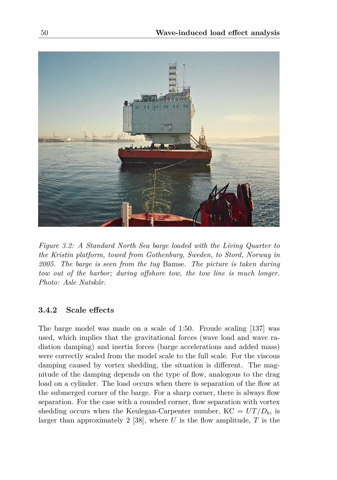
50 Wave-induced load effect analysis
Figure 3.2: A Standard North Sea barge loaded with the Living Quarter tothe Kristin platform, towed from Gothenburg, Sweden, to Stord, Norway in2005. The barge is seen from the tug Bamse. The picture is taken duringtow out of the harbor; during offshore tow, the tow line is much longer.Photo: Asle Natskår.
3.4.2 Scale effects
The barge model was made on a scale of 1:50. Froude scaling [137] wasused, which implies that the gravitational forces (wave load and wave ra-diation damping) and inertia forces (barge accelerations and added mass)were correctly scaled from the model scale to the full scale. For the viscousdamping caused by vortex shedding, the situation is different. The mag-nitude of the damping depends on the type of flow, analogous to the dragload on a cylinder. The load occurs when there is separation of the flow atthe submerged corner of the barge. For a sharp corner, there is always flowseparation. For the case with a rounded corner, flow separation with vortexshedding occurs when the Keulegan-Carpenter number, KC = UT/Db, islarger than approximately 2 [38], where U is the flow amplitude, T is the
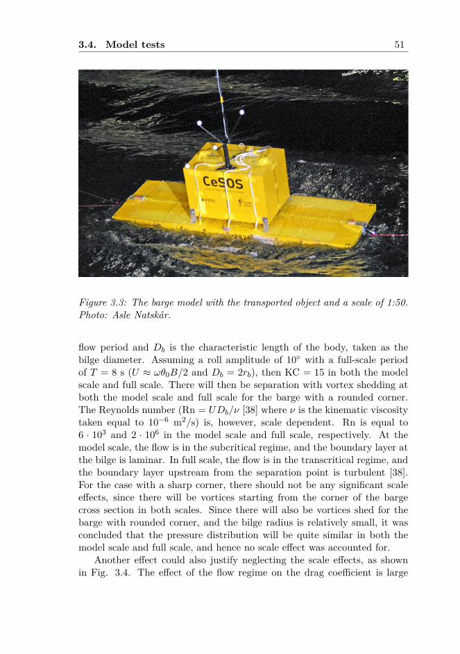
3.4. Model tests 51
Figure 3.3: The barge model with the transported object and a scale of 1:50.Photo: Asle Natskår.
flow period and Db is the characteristic length of the body, taken as thebilge diameter. Assuming a roll amplitude of 10 with a full-scale periodof T = 8 s (U ≈ ωθ0B/2 and Db = 2rb), then KC = 15 in both the modelscale and full scale. There will then be separation with vortex shedding atboth the model scale and full scale for the barge with a rounded corner.The Reynolds number (Rn = UDb/ν [38] where ν is the kinematic viscositytaken equal to 10−6 m2/s) is, however, scale dependent. Rn is equal to6 · 103 and 2 · 106 in the model scale and full scale, respectively. At themodel scale, the flow is in the subcritical regime, and the boundary layer atthe bilge is laminar. In full scale, the flow is in the transcritical regime, andthe boundary layer upstream from the separation point is turbulent [38].For the case with a sharp corner, there should not be any significant scaleeffects, since there will be vortices starting from the corner of the bargecross section in both scales. Since there will also be vortices shed for thebarge with rounded corner, and the bilge radius is relatively small, it wasconcluded that the pressure distribution will be quite similar in both themodel scale and full scale, and hence no scale effect was accounted for.
Another effect could also justify neglecting the scale effects, as shownin Fig. 3.4. The effect of the flow regime on the drag coefficient is large
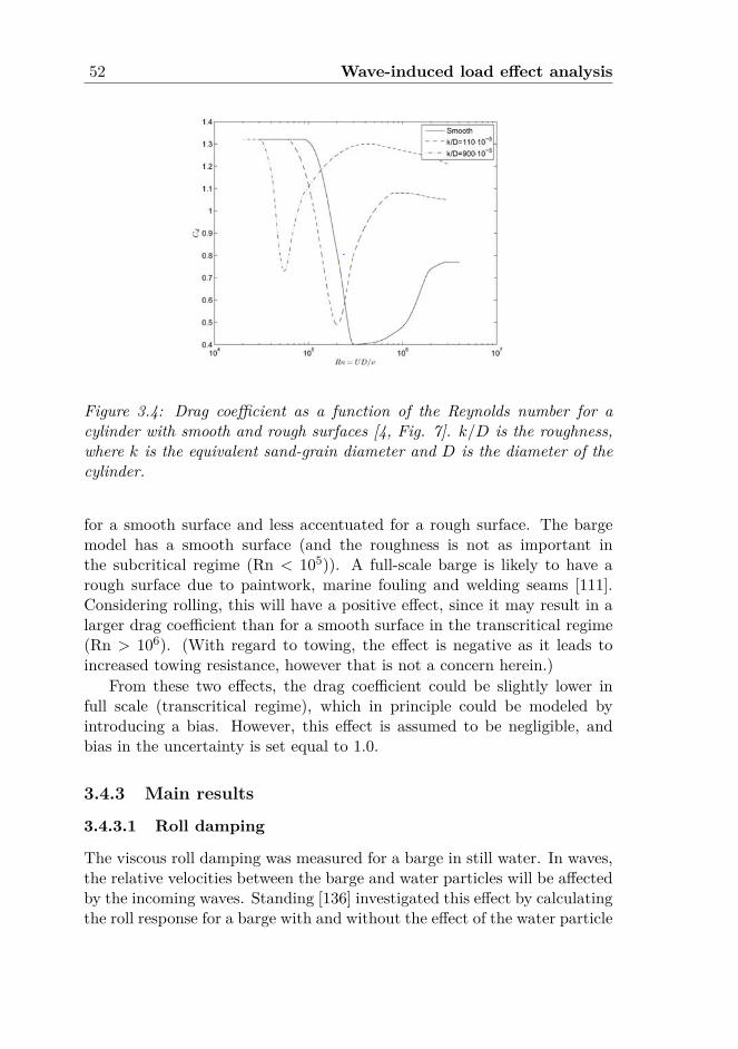
52 Wave-induced load effect analysis
Figure 3.4: Drag coefficient as a function of the Reynolds number for acylinder with smooth and rough surfaces [4, Fig. 7]. k/D is the roughness,where k is the equivalent sand-grain diameter and D is the diameter of thecylinder.
for a smooth surface and less accentuated for a rough surface. The bargemodel has a smooth surface (and the roughness is not as important inthe subcritical regime (Rn < 105)). A full-scale barge is likely to have arough surface due to paintwork, marine fouling and welding seams [111].Considering rolling, this will have a positive effect, since it may result in alarger drag coefficient than for a smooth surface in the transcritical regime(Rn > 106). (With regard to towing, the effect is negative as it leads toincreased towing resistance, however that is not a concern herein.)
From these two effects, the drag coefficient could be slightly lower infull scale (transcritical regime), which in principle could be modeled byintroducing a bias. However, this effect is assumed to be negligible, andbias in the uncertainty is set equal to 1.0.
3.4.3 Main results
3.4.3.1 Roll damping
The viscous roll damping was measured for a barge in still water. In waves,the relative velocities between the barge and water particles will be affectedby the incoming waves. Standing [136] investigated this effect by calculatingthe roll response for a barge with and without the effect of the water particle
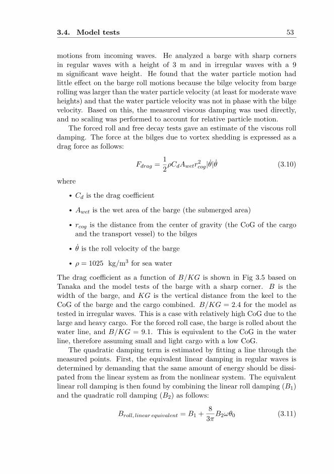
3.4. Model tests 53
motions from incoming waves. He analyzed a barge with sharp cornersin regular waves with a height of 3 m and in irregular waves with a 9m significant wave height. He found that the water particle motion hadlittle effect on the barge roll motions because the bilge velocity from bargerolling was larger than the water particle velocity (at least for moderate waveheights) and that the water particle velocity was not in phase with the bilgevelocity. Based on this, the measured viscous damping was used directly,and no scaling was performed to account for relative particle motion.
The forced roll and free decay tests gave an estimate of the viscous rolldamping. The force at the bilges due to vortex shedding is expressed as adrag force as follows:
Fdrag = 12ρCdAwetr
2cog|θ|θ (3.10)
wherer Cd is the drag coefficientr Awet is the wet area of the barge (the submerged area)r rcog is the distance from the center of gravity (the CoG of the cargoand the transport vessel) to the bilgesr θ is the roll velocity of the barger ρ = 1025 kg/m3 for sea water
The drag coefficient as a function of B/KG is shown in Fig 3.5 based onTanaka and the model tests of the barge with a sharp corner. B is thewidth of the barge, and KG is the vertical distance from the keel to theCoG of the barge and the cargo combined. B/KG = 2.4 for the model astested in irregular waves. This is a case with relatively high CoG due to thelarge and heavy cargo. For the forced roll case, the barge is rolled about thewater line, and B/KG = 9.1. This is equivalent to the CoG in the waterline, therefore assuming small and light cargo with a low CoG.
The quadratic damping term is estimated by fitting a line through themeasured points. First, the equivalent linear damping in regular waves isdetermined by demanding that the same amount of energy should be dissi-pated from the linear system as from the nonlinear system. The equivalentlinear roll damping is then found by combining the linear roll damping (B1)and the quadratic roll damping (B2) as follows:
Broll, linear equivalent = B1 + 83πB2ωθ0 (3.11)
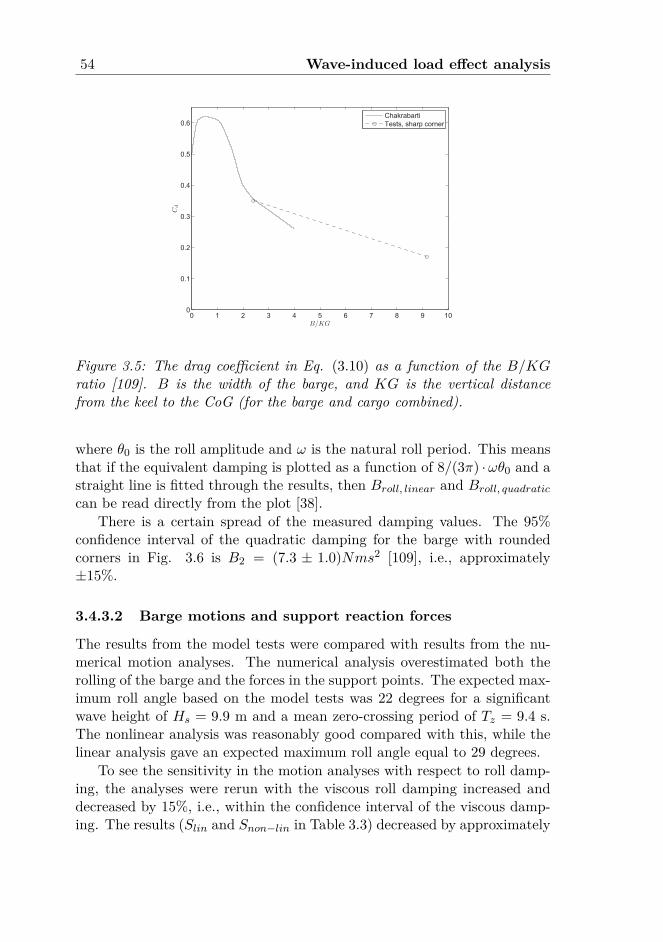
54 Wave-induced load effect analysis
0 1 2 3 4 5 6 7 8 9 100
0.1
0.2
0.3
0.4
0.5
0.6
B/KG
Cd
Chakrabarti
Tests, sharp corner
Figure 3.5: The drag coefficient in Eq. (3.10) as a function of the B/KGratio [109]. B is the width of the barge, and KG is the vertical distancefrom the keel to the CoG (for the barge and cargo combined).
where θ0 is the roll amplitude and ω is the natural roll period. This meansthat if the equivalent damping is plotted as a function of 8/(3π) ·ωθ0 and astraight line is fitted through the results, then Broll, linear and Broll, quadraticcan be read directly from the plot [38].
There is a certain spread of the measured damping values. The 95%confidence interval of the quadratic damping for the barge with roundedcorners in Fig. 3.6 is B2 = (7.3 ± 1.0)Nms2 [109], i.e., approximately±15%.
3.4.3.2 Barge motions and support reaction forces
The results from the model tests were compared with results from the nu-merical motion analyses. The numerical analysis overestimated both therolling of the barge and the forces in the support points. The expected max-imum roll angle based on the model tests was 22 degrees for a significantwave height of Hs = 9.9 m and a mean zero-crossing period of Tz = 9.4 s.The nonlinear analysis was reasonably good compared with this, while thelinear analysis gave an expected maximum roll angle equal to 29 degrees.
To see the sensitivity in the motion analyses with respect to roll damp-ing, the analyses were rerun with the viscous roll damping increased anddecreased by 15%, i.e., within the confidence interval of the viscous damp-ing. The results (Slin and Snon−lin in Table 3.3) decreased by approximately
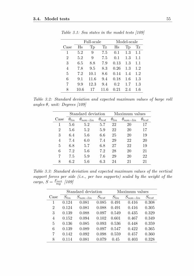
3.4. Model tests 55
Table 3.1: Sea states in the model tests [109]
Full-scale Model-scaleCase Hs Tp Tz Hs Tp Tz1 5.2 9 7.5 0.1 1.3 1.12 5.2 9 7.5 0.1 1.3 1.13 6.5 8.8 7.9 0.13 1.3 1.14 7.8 9.5 8.3 0.26 1.3 1.25 7.2 10.1 8.6 0.14 1.4 1.26 9.1 11.6 9.4 0.18 1.6 1.37 9.9 12.3 9.4 0.2 1.7 1.38 10.6 17 11.6 0.21 2.4 1.6
Table 3.2: Standard deviation and expected maximum values of barge rollangles θ, unit: Degrees [109]
Standard deviation Maximum valuesCase θlin θnon−lin θtest θlin θnon−lin θtest1 5.6 5.2 5.7 22 20 172 5.6 5.2 5.9 22 20 173 6.4 5.6 6.6 25 20 194 7.4 6.0 7.4 29 22 205 6.8 5.7 6.8 27 22 196 7.2 5.6 7.2 28 20 217 7.5 5.9 7.6 29 20 228 6.2 5.6 6.3 24 21 21
Table 3.3: Standard deviation and expected maximum values of the verticalsupport forces per side (i.e., per two supports) scaled by the weight of thecargo, S = Fvert
mg [109]
Standard deviation Maximum valuesCase Slin Snon−lin Stest Slin Snon−lin Stest1 0.124 0.081 0.085 0.491 0.416 0.3082 0.124 0.081 0.088 0.491 0.416 0.3053 0.139 0.088 0.097 0.549 0.435 0.3294 0.152 0.094 0.102 0.601 0.467 0.3495 0.136 0.085 0.093 0.536 0.448 0.3596 0.139 0.089 0.097 0.547 0.422 0.3657 0.142 0.092 0.098 0.559 0.457 0.3608 0.114 0.081 0.079 0.45 0.403 0.328
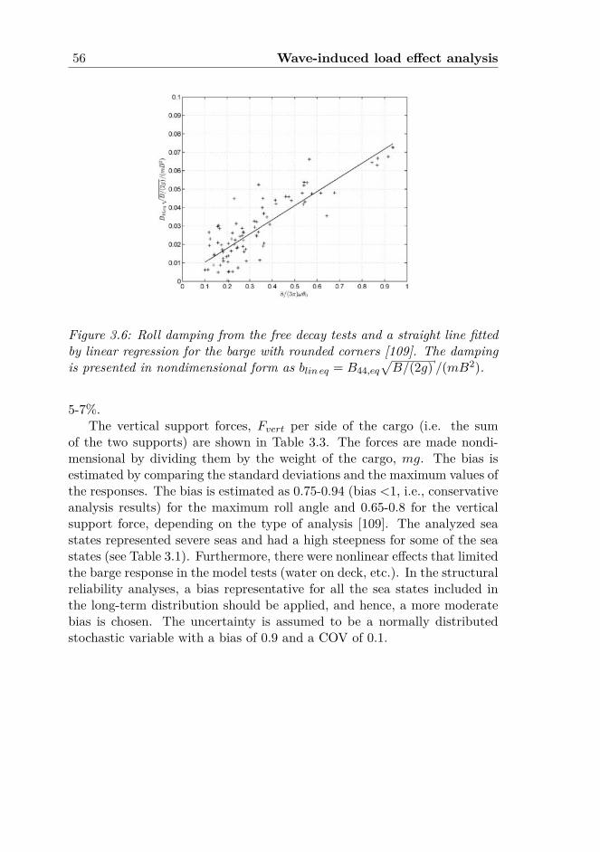
56 Wave-induced load effect analysis
Figure 3.6: Roll damping from the free decay tests and a straight line fittedby linear regression for the barge with rounded corners [109]. The dampingis presented in nondimensional form as blin eq = B44,eq
√B/(2g) /(mB2).
5-7%.The vertical support forces, Fvert per side of the cargo (i.e. the sum
of the two supports) are shown in Table 3.3. The forces are made nondi-mensional by dividing them by the weight of the cargo, mg. The bias isestimated by comparing the standard deviations and the maximum values ofthe responses. The bias is estimated as 0.75-0.94 (bias <1, i.e., conservativeanalysis results) for the maximum roll angle and 0.65-0.8 for the verticalsupport force, depending on the type of analysis [109]. The analyzed seastates represented severe seas and had a high steepness for some of the seastates (see Table 3.1). Furthermore, there were nonlinear effects that limitedthe barge response in the model tests (water on deck, etc.). In the structuralreliability analyses, a bias representative for all the sea states included inthe long-term distribution should be applied, and hence, a more moderatebias is chosen. The uncertainty is assumed to be a normally distributedstochastic variable with a bias of 0.9 and a COV of 0.1.
Chapter 4
Structural reliability analysis
4.1 Introduction
In a narrow sense, structural reliability is the probability that a structurewill not exceed any of a specified set of limit states during a specified refer-ence period. This means that the structure is in a safe set and will survive.The complementary quantity to being safe is the failure probability, Pf ,defined in a simple case with a single resistance and load effect variable,by Pf = P [R ≤ S], where R is the resistance and S represents the loadeffect. Depending on how R and especially S are related to time, the failureprobability will also depend on some reference time period. For a normaloperation, the reference period could be a year or the service lifetime. Formarine operations, the reference period is typically equal to the duration ofthe operation.
Structural design standards based on limit state formulations are typi-cally calibrated by using reliability methods [90]. Structural reliability anal-ysis (SRA) can be used to calculate the probability of failure for structuresthat have been designed for relevant limit states. The failure probabilityis calculated based on random variables describing the load effects and thestructural capacity. In this thesis, SRA is used to calculate the failure prob-ability for temporary structures designed by a semiprobabilistic method.
The concept of structural reliability analysis is briefly described in Sec.4.3.11. More details about SRA may be found in the literature, including thetext books by Ditlevsen and Madsen [22], Madsen et al. [88] and Melchersand Beck [95].
57
58 Structural reliability analysis
4.2 Limit state design check
4.2.1 Calculation of the ultimate strength
The ultimate strength is calculated for all the structural components. In ad-dition to the capacity of the grillage and seafastening, which are normallyspecifically built for each individual transport, the capacity of the trans-ported object as well as the local ship structure adjacent to the grillage andseafastening is checked. These existing structures are already given once thetransport ship is nominated, and local reinforcements for one single trans-port should be avoided. Hence, the capacity of the existing structure shouldbe checked in parallel with the design of the grillage and seafastening.
The design standards for marine operations [31, 72] describe the princi-ples for the operations and provide guidance and requirements for planningthem. They do not cover the design of structures beyond giving the princi-ples but refer to recognized codes and standards as the basis for the detaileddesign and the fabrication requirements of structural components. Many de-sign codes are thus available for calculating the ultimate structural capacity.In Norwegian waters, Eurocode and Norsok standards are typically used,e.g., [36, 113]. In other areas, ISO and API standards are widely used, e.g.,[8, 73].
A case where the load effects are caused by the self-weight and wave-induced vessel motion is considered. A typical case is shown in Fig. 4.1.An example of a support structure, the grillage beams, is shown in Fig. 4.2.This is a typical structure for the distribution of support forces for a shipor a barge. Hand calculations of the moment and sectional forces wouldnormally suffice for a design check in ULS. A finite element analysis maybe required for more complicated structures and for details. The internalbarge structure also needs to be documented. A typical barge bulkhead,i.e., a 10-20 mm thick plate with horizontal stiffeners and transverse webframes typically every 2.4 m, is shown in Fig. 4.2. More information abouta typical North Sea barge is given in Appendix B.
In short, the structural strength must be verified for the following sub-systems:r Transported objectr Grillage and seafasteningr Transport vesselThe main discussion below is related to the vertical supports (the grillagebeams). The local capacity of the transport vessel, notably the longitudinal
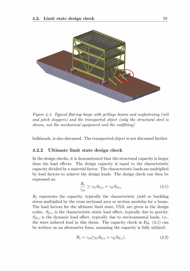
4.2. Limit state design check 59
Figure 4.1: Typical flat-top barge with grillage beams and seafastening (rolland pitch stoppers) and the transported object (only the structural steel isshown, not the mechanical equipment and the outfitting)
bulkheads, is also discussed. The transported object is not discussed further.
4.2.2 Ultimate limit state design check
In the design checks, it is demonstrated that the structural capacity is largerthan the load effects. The design capacity is equal to the characteristiccapacity divided by a material factor. The characteristic loads are multipliedby load factors to achieve the design loads. The design check can then beexpressed as:
Rcγm≥ γGSG,c + γESE,c (4.1)
Rc represents the capacity, typically the characteristic yield or bucklingstress multiplied by the cross sectional area or section modulus for a beam.The load factors for the ultimate limit state, ULS, are given in the designcodes. SG,c is the characteristic static load effect, typically due to gravity.SE,c is the dynamic load effect, typically due to environmental loads, i.e.,the wave induced load in this thesis. The capacity check in Eq. (4.1) canbe written on an alternative form, assuming the capacity is fully utilized:
Rc = γm(γGSG,c + γESE,c) (4.2)
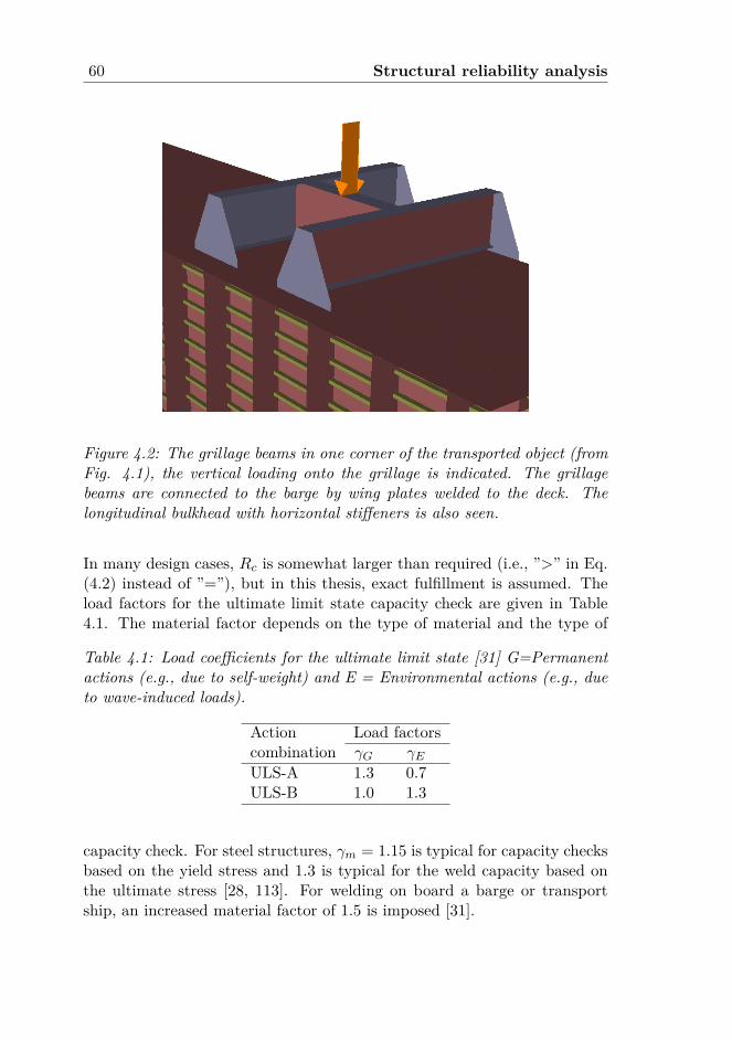
60 Structural reliability analysis
Figure 4.2: The grillage beams in one corner of the transported object (fromFig. 4.1), the vertical loading onto the grillage is indicated. The grillagebeams are connected to the barge by wing plates welded to the deck. Thelongitudinal bulkhead with horizontal stiffeners is also seen.
In many design cases, Rc is somewhat larger than required (i.e., ”>” in Eq.(4.2) instead of ”=”), but in this thesis, exact fulfillment is assumed. Theload factors for the ultimate limit state capacity check are given in Table4.1. The material factor depends on the type of material and the type of
Table 4.1: Load coefficients for the ultimate limit state [31] G=Permanentactions (e.g., due to self-weight) and E = Environmental actions (e.g., dueto wave-induced loads).
Action Load factorscombination γG γEULS-A 1.3 0.7ULS-B 1.0 1.3
capacity check. For steel structures, γm = 1.15 is typical for capacity checksbased on the yield stress and 1.3 is typical for the weld capacity based onthe ultimate stress [28, 113]. For welding on board a barge or transportship, an increased material factor of 1.5 is imposed [31].
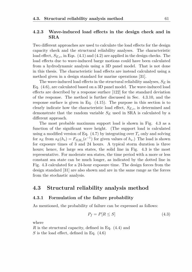
4.3. Structural reliability analysis method 61
4.2.3 Wave-induced load effects in the design check and inSRA
Two different approaches are used to calculate the load effects for the designcapacity check and the structural reliability analyses. The characteristicload effect, SE,c, in Eqs. (4.1) and (4.2) are applied in the design checks. Theload effects due to wave-induced barge motions could have been calculatedfrom a hydrodynamic analysis using a 3D panel model. That is not donein this thesis. The characteristic load effects are instead calculated using amethod given in a design standard for marine operations [31].
The wave-induced load effects in the structural reliability analyses, SE inEq. (4.6), are calculated based on a 3D panel model. The wave-induced loadeffects are described by a response surface [122] for the standard deviationof the response. The method is further discussed in Sec. 4.3.10, and theresponse surface is given in Eq. (4.15). The purpose in this section is toclearly indicate how the characteristic load effect, SE,c, is determined anddemonstrate that the random variable SE used in SRA is calculated by adifferent approach.
The most probable maximum support load is shown in Fig. 4.3 as afunction of the significant wave height. (The support load is calculatedusing a modified version of Eq. (4.7) by integrating over Tz only and solvingfor sE from sE(hs) = FS|Hs(e−1) for given values of hs.) The load is shownfor exposure times of 3 and 24 hours. A typical storm duration is threehours; hence, for large sea states, the solid line in Fig. 4.3 is the mostrepresentative. For moderate sea states, the time period with a more or lessconstant sea state can be much longer, as indicated by the dotted line inFig. 4.3 calculated for a 24-hour exposure time. The design forces from thedesign standard [31] are also shown and are in the same range as the forcesfrom the stochastic analysis.
4.3 Structural reliability analysis method
4.3.1 Formulation of the failure probability
As mentioned, the probability of failure can be expressed as follows:
Pf = P [R ≤ S] (4.3)
whereR is the structural capacity, defined in Eq. (4.4) andS is the load effect, defined in Eq. (4.6)
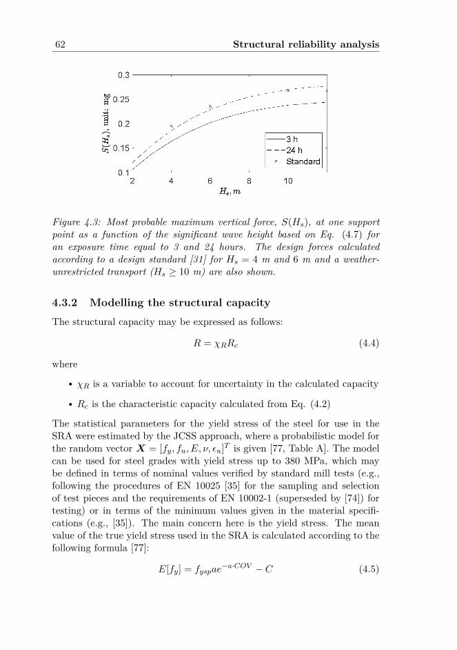
62 Structural reliability analysis
Figure 4.3: Most probable maximum vertical force, S(Hs), at one supportpoint as a function of the significant wave height based on Eq. (4.7) foran exposure time equal to 3 and 24 hours. The design forces calculatedaccording to a design standard [31] for Hs = 4 m and 6 m and a weather-unrestricted transport (Hs ≥ 10 m) are also shown.
4.3.2 Modelling the structural capacity
The structural capacity may be expressed as follows:
R = χRRc (4.4)
wherer χR is a variable to account for uncertainty in the calculated capacityr Rc is the characteristic capacity calculated from Eq. (4.2)
The statistical parameters for the yield stress of the steel for use in theSRA were estimated by the JCSS approach, where a probabilistic model forthe random vector X = [fy, fu, E, ν, εu]T is given [77, Table A]. The modelcan be used for steel grades with yield stress up to 380 MPa, which maybe defined in terms of nominal values verified by standard mill tests (e.g.,following the procedures of EN 10025 [35] for the sampling and selectionof test pieces and the requirements of EN 10002-1 (superseded by [74]) fortesting) or in terms of the minimum values given in the material specifi-cations (e.g., [35]). The main concern here is the yield stress. The meanvalue of the true yield stress used in the SRA is calculated according to thefollowing formula [77]:
E[fy] = fyspae−u·COV − C (4.5)
4.3. Structural reliability analysis method 63
wherer The COV for the yield stress is set equal to 0.07r fysp is the code specified or nominal value for the yield stress used inthe design checkr a is the spatial position factor. It is equal to 1.05 for webs of hot rolledsections and 1 otherwise; a=1 is used in this thesisr u is a factor related to the fractile of the distribution used in describingthe distance between the code specified or nominal value and the meanvalue; u is in the range of -1.5 to -2.0r C is a constant for reducing the yield strength as obtained from usualmill tests to obtain the static yield strength; a value of 20 MPa isrecommended [77]
Based on the above, the mean value and the standard deviation for the yieldstress are µ = 1.12fysp − 20 and σ = 0.07µ.
This model is combined with the random variable, which represents theuncertainty in the calculated capacity, that is assumed to follow a lognormaldistribution. The capacity of the bulkheads in the barge has a mean valueof 1.21 and a COV of 0.15, and the grillage beams have a mean value of1.0 and a COV of 0.05. [107]. When the uncertainty in the yield stress iscombined with the model uncertainty, the mean value is 1.25, and the COVis 0.17 for the vertical load acting at the bulkheads. For the grillage beams,the resulting mean value is 1.07, and the COV is 0.09.
4.3.3 Overview of the uncertainties in the load effects
The modeling of the uncertainty in the load effect will depend on the ef-fects being studied. The aleatoric and epistemic uncertainties, includingthe model uncertainties, are discussed below. The static loads from gravityand dynamic loads from waves were included in this study. Generally, windloading can also be important but is not included here because wave loadingdominates the case studied in this thesis. For this purpose, the load effectin the reliability model can be formulated as follows:
S = χS,GSG + χS,ESEBoper (4.6)
wherer SG is the static load effect
64 Structural reliability analysis
r SE is a stochastic variable representing the wave-induced load effect,accounting for the uncertainty in the significant wave height and waveperiod; see Sec. 4.3.10 (note that SE is different from the characteristicload effect in Eq. (4.1))r χS,G represents the uncertainty in the calculated static load effectr χS,E represents the uncertainty in the calculated dynamic load effectr Boper accounts for the uncertainty related to heavy weather avoidance
In the case studies, χS,G is modeled as a normal distributed variable with amean value of 0.95. The COV is set equal to 0.1.
The uncertainty in the calculated dynamic wave-induced load effect,χS,E , depends on:r the wave datar the calculated motions of the transport vessel, χS,E,1r the method for the calculation of the structural load effects due to the
vessel motions, χS,E,2
The effect of the uncertainty in the wave data is included in the calculationof the load effect, SE ; see Sec. 4.3.10. The last two items are combinedto give the resulting uncertainty estimated by χS,E = χS,E,1 · χS,E,2. Themodel uncertainty associated with the response analysis covers uncertain-ties related to the analysis of the barge motions as well as the calculationof the load effects in the supports. The prediction of the barge motions forthe structural reliability analyses is based on hydrodynamic analysis usinglinear 3D potential theory, and nonlinear effects, such as barge deck immer-sion, are not included. The viscous roll damping is linearized by stochasticlinearization. For high waves with large steepness, there may be a signifi-cant bias in the calculated barge motions [109]. However, in the structuralreliability analyses, a bias that represents all the sea states included in thelong-term distribution is needed, as discussed in Sec. 3.4.3.2. Consequently,the model uncertainty in the hydrodynamic analysis, χS,E,1, is assumed tofollow the normal distribution with a mean value of 0.9 and a COV of 0.1.The uncertainty resulting from the calculation of the dynamic load effect isassumed to be the same as that for the static load effect. Even if a sim-ple statistical model is chosen here, the uncertainty in the calculated loadeffect could in a real case depend on the ballast condition and the relativestiffness between the supports. The uncertainty χS,E,2 is assumed to follow

4.3. Structural reliability analysis method 65
a normal distribution with a mean value equal to 0.95 and a COV equal to0.1. The uncertainty in the calculated dynamic load effect is added to theuncertainty in the hydrodynamic analysis. The total model uncertainty1 isthen assumed to follow a normal distribution with a mean value of 0.86 anda COV of 0.14 [107].
For the structural reliability analysis of the supports, the extreme valuesof the support forces need to be calculated. The calculation must includethe effect of the uncertainty in the environmental conditions. For short-termanalyses based on weather forecasts, the forecast uncertainty is described inSec. 4.3.4. For long-term analyses, see Sec. 4.3.5. The load effect is furtherdescribed in Sec. 4.3.10.
4.3.4 Uncertainty in the forecasted wave height
The uncertainty in the forecasted significant wave height is assumed to fol-low a lognormal distribution [108]. The mean value and standard deviationdepend on the forecast lead time. No additional uncertainty to account forthe uncertainty in the hindcast data has been included; see also Sec. 4.3.7.
4.3.5 Uncertainty in the long-term significant wave height
Descriptions of the long-term environmental conditions are available frommany sources. Traditionally, the data from BMT [64] have been applied formarine transports. However, as BMT data are based on visual observationsof the environmental conditions from ships, they may contain the effects ofadverse weather avoidance. Another source for obtaining weather data ishindcasting [123]. The hindcast data are independent of ship observationsand are hence better suited to describe the true long-term environmentalcondition.
The long-term description of the environmental conditions used here isbased on hindcast data from the North Sea. A three-parameter Weibulldistribution is fitted to the long-term wave conditions. The long-term dis-tribution describes the fundamental variation, but the meteorological dataand the hindcast method are subjected to uncertainties; see also Sec. 4.3.7.
4.3.6 Uncertainties due to the amount of environmental data
The amount of data available for estimating the statistical parameters willaffect the uncertainty. The effect of varying amounts of data is important,
1For the product of two statistically independent variables, χ = χ1 ·χ2, the mean valueis µχ = µχ1 ·µχ2, and the coefficient of variation is COV≈
√(COVχ1 )2 + (COVχ2 )2 [95].
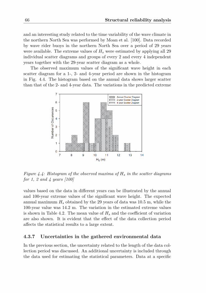
66 Structural reliability analysis
and an interesting study related to the time variability of the wave climate inthe northern North Sea was performed by Moan et al. [100]. Data recordedby wave rider buoys in the northern North Sea over a period of 29 yearswere available. The extreme values of Hs were estimated by applying all 29individual scatter diagrams and groups of every 2 and every 4 independentyears together with the 29-year scatter diagram as a whole.
The observed maximum values of the significant wave height in eachscatter diagram for a 1-, 2- and 4-year period are shown in the histogramin Fig. 4.4. The histogram based on the annual data shows larger scatterthan that of the 2- and 4-year data. The variations in the predicted extreme
Figure 4.4: Histogram of the observed maxima of Hs in the scatter diagramsfor 1, 2 and 4 years [100]
values based on the data in different years can be illustrated by the annualand 100-year extreme values of the significant wave height. The expectedannual maximum Hs obtained by the 29 years of data was 10.5 m, while the100-year value was 14.2 m. The variation in the estimated extreme valuesis shown in Table 4.2. The mean value of Hs and the coefficient of variationare also shown. It is evident that the effect of the data collection periodaffects the statistical results to a large extent.
4.3.7 Uncertainties in the gathered environmental data
In the previous section, the uncertainty related to the length of the data col-lection period was discussed. An additional uncertainty is included throughthe data used for estimating the statistical parameters. Data at a specific
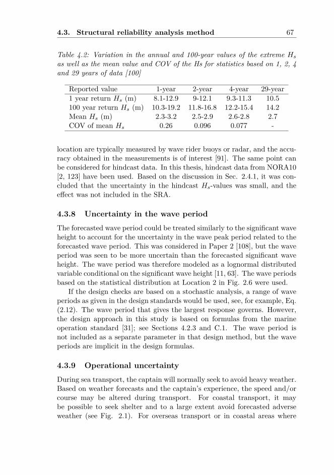
4.3. Structural reliability analysis method 67
Table 4.2: Variation in the annual and 100-year values of the extreme Hs
as well as the mean value and COV of the Hs for statistics based on 1, 2, 4and 29 years of data [100]
Reported value 1-year 2-year 4-year 29-year1 year return Hs (m) 8.1-12.9 9-12.1 9.3-11.3 10.5100 year return Hs (m) 10.3-19.2 11.8-16.8 12.2-15.4 14.2Mean Hs (m) 2.3-3.2 2.5-2.9 2.6-2.8 2.7COV of mean Hs 0.26 0.096 0.077 -
location are typically measured by wave rider buoys or radar, and the accu-racy obtained in the measurements is of interest [91]. The same point canbe considered for hindcast data. In this thesis, hindcast data from NORA10[2, 123] have been used. Based on the discussion in Sec. 2.4.1, it was con-cluded that the uncertainty in the hindcast Hs-values was small, and theeffect was not included in the SRA.
4.3.8 Uncertainty in the wave period
The forecasted wave period could be treated similarly to the significant waveheight to account for the uncertainty in the wave peak period related to theforecasted wave period. This was considered in Paper 2 [108], but the waveperiod was seen to be more uncertain than the forecasted significant waveheight. The wave period was therefore modeled as a lognormal distributedvariable conditional on the significant wave height [11, 63]. The wave periodsbased on the statistical distribution at Location 2 in Fig. 2.6 were used.
If the design checks are based on a stochastic analysis, a range of waveperiods as given in the design standards would be used, see, for example, Eq.(2.12). The wave period that gives the largest response governs. However,the design approach in this study is based on formulas from the marineoperation standard [31]; see Sections 4.2.3 and C.1. The wave period isnot included as a separate parameter in that design method, but the waveperiods are implicit in the design formulas.
4.3.9 Operational uncertainty
During sea transport, the captain will normally seek to avoid heavy weather.Based on weather forecasts and the captain’s experience, the speed and/orcourse may be altered during transport. For coastal transport, it maybe possible to seek shelter and to a large extent avoid forecasted adverseweather (see Fig. 2.1). For overseas transport or in coastal areas where
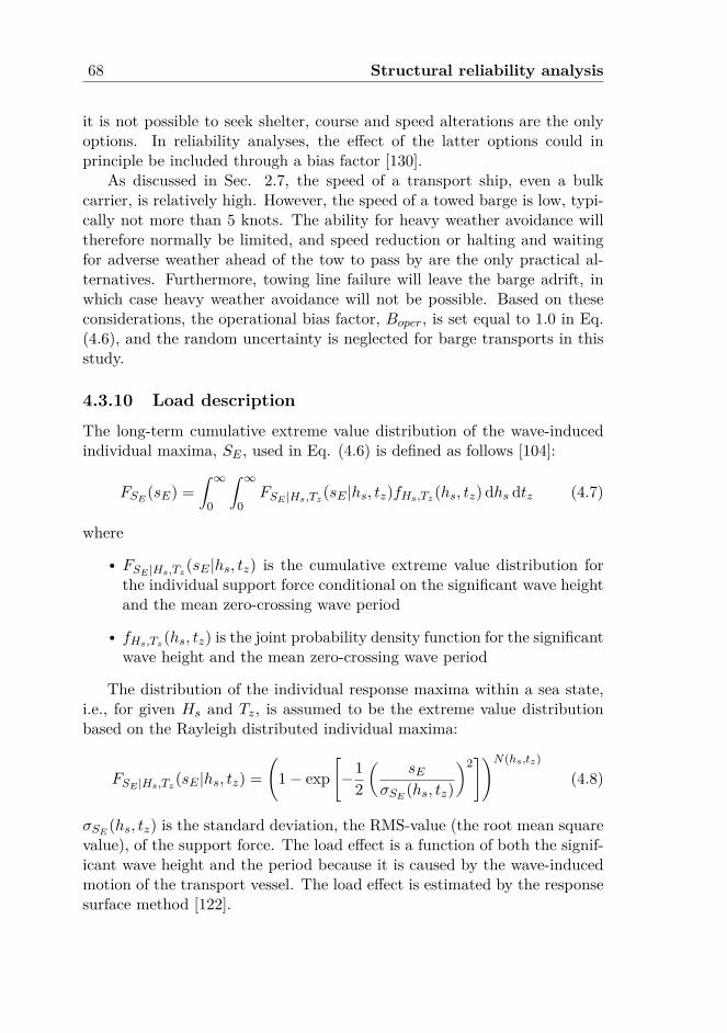
68 Structural reliability analysis
it is not possible to seek shelter, course and speed alterations are the onlyoptions. In reliability analyses, the effect of the latter options could inprinciple be included through a bias factor [130].
As discussed in Sec. 2.7, the speed of a transport ship, even a bulkcarrier, is relatively high. However, the speed of a towed barge is low, typi-cally not more than 5 knots. The ability for heavy weather avoidance willtherefore normally be limited, and speed reduction or halting and waitingfor adverse weather ahead of the tow to pass by are the only practical al-ternatives. Furthermore, towing line failure will leave the barge adrift, inwhich case heavy weather avoidance will not be possible. Based on theseconsiderations, the operational bias factor, Boper, is set equal to 1.0 in Eq.(4.6), and the random uncertainty is neglected for barge transports in thisstudy.
4.3.10 Load description
The long-term cumulative extreme value distribution of the wave-inducedindividual maxima, SE , used in Eq. (4.6) is defined as follows [104]:
FSE (sE) =∫ ∞
0
∫ ∞
0FSE |Hs,Tz(sE |hs, tz)fHs,Tz(hs, tz) dhs dtz (4.7)
wherer FSE |Hs,Tz(sE |hs, tz) is the cumulative extreme value distribution forthe individual support force conditional on the significant wave heightand the mean zero-crossing wave periodr fHs,Tz(hs, tz) is the joint probability density function for the significantwave height and the mean zero-crossing wave period
The distribution of the individual response maxima within a sea state,i.e., for given Hs and Tz, is assumed to be the extreme value distributionbased on the Rayleigh distributed individual maxima:
FSE |Hs,Tz(sE |hs, tz) =(
1− exp[−1
2
(sE
σSE (hs, tz)
)2])N(hs,tz)
(4.8)
σSE (hs, tz) is the standard deviation, the RMS-value (the root mean squarevalue), of the support force. The load effect is a function of both the signif-icant wave height and the period because it is caused by the wave-inducedmotion of the transport vessel. The load effect is estimated by the responsesurface method [122].
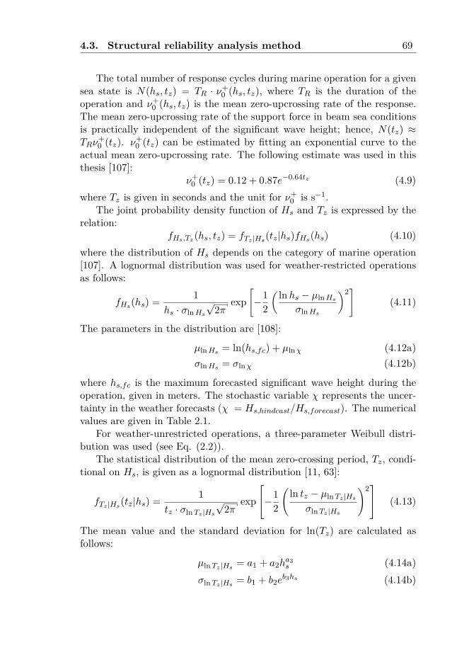
4.3. Structural reliability analysis method 69
The total number of response cycles during marine operation for a givensea state is N(hs, tz) = TR · ν+
0 (hs, tz), where TR is the duration of theoperation and ν+
0 (hs, tz) is the mean zero-upcrossing rate of the response.The mean zero-upcrossing rate of the support force in beam sea conditionsis practically independent of the significant wave height; hence, N(tz) ≈TRν
+0 (tz). ν+
0 (tz) can be estimated by fitting an exponential curve to theactual mean zero-upcrossing rate. The following estimate was used in thisthesis [107]:
ν+0 (tz) = 0.12 + 0.87e−0.64tz (4.9)
where Tz is given in seconds and the unit for ν+0 is s−1.
The joint probability density function of Hs and Tz is expressed by therelation:
fHs,Tz(hs, tz) = fTz |Hs(tz|hs)fHs(hs) (4.10)where the distribution of Hs depends on the category of marine operation[107]. A lognormal distribution was used for weather-restricted operationsas follows:
fHs(hs) = 1hs · σlnHs
√2π
exp[−1
2
( ln hs − µlnHsσlnHs
)2](4.11)
The parameters in the distribution are [108]:
µlnHs = ln(hs,fc) + µlnχ (4.12a)σlnHs = σlnχ (4.12b)
where hs,fc is the maximum forecasted significant wave height during theoperation, given in meters. The stochastic variable χ represents the uncer-tainty in the weather forecasts (χ = Hs,hindcast/Hs,forecast). The numericalvalues are given in Table 2.1.
For weather-unrestricted operations, a three-parameter Weibull distri-bution was used (see Eq. (2.2)).
The statistical distribution of the mean zero-crossing period, Tz, condi-tional on Hs, is given as a lognormal distribution [11, 63]:
fTz |Hs(tz|hs) = 1tz · σlnTz |Hs
√2π
exp
−1
2
(ln tz − µlnTz |Hs
σlnTz |Hs
)2 (4.13)
The mean value and the standard deviation for ln(Tz) are calculated asfollows:
µlnTz |Hs = a1 + a2ha3s (4.14a)
σlnTz |Hs = b1 + b2eb3hs (4.14b)
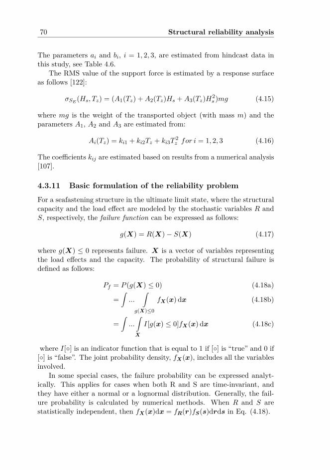
70 Structural reliability analysis
The parameters ai and bi, i = 1, 2, 3, are estimated from hindcast data inthis study, see Table 4.6.
The RMS value of the support force is estimated by a response surfaceas follows [122]:
σSE (Hs, Tz) = (A1(Tz) +A2(Tz)Hs +A3(Tz)H2s )mg (4.15)
where mg is the weight of the transported object (with mass m) and theparameters A1, A2 and A3 are estimated from:
Ai(Tz) = ki1 + ki2Tz + ki3T2z for i = 1, 2, 3 (4.16)
The coefficients kij are estimated based on results from a numerical analysis[107].
4.3.11 Basic formulation of the reliability problem
For a seafastening structure in the ultimate limit state, where the structuralcapacity and the load effect are modeled by the stochastic variables R andS, respectively, the failure function can be expressed as follows:
g(X) = R(X)− S(X) (4.17)
where g(X) ≤ 0 represents failure. X is a vector of variables representingthe load effects and the capacity. The probability of structural failure isdefined as follows:
Pf = P (g(X) ≤ 0) (4.18a)
=∫...
∫
g(X)≤0
fX(x) dx (4.18b)
=∫...
∫
X
I[g(x) ≤ 0]fX(x) dx (4.18c)
where I[] is an indicator function that is equal to 1 if [] is “true” and 0 if[] is “false”. The joint probability density, fX(x), includes all the variablesinvolved.
In some special cases, the failure probability can be expressed analyt-ically. This applies for cases when both R and S are time-invariant, andthey have either a normal or a lognormal distribution. Generally, the fail-ure probability is calculated by numerical methods. When R and S arestatistically independent, then fX(x)dx = fR(r)fS(s)drds in Eq. (4.18).
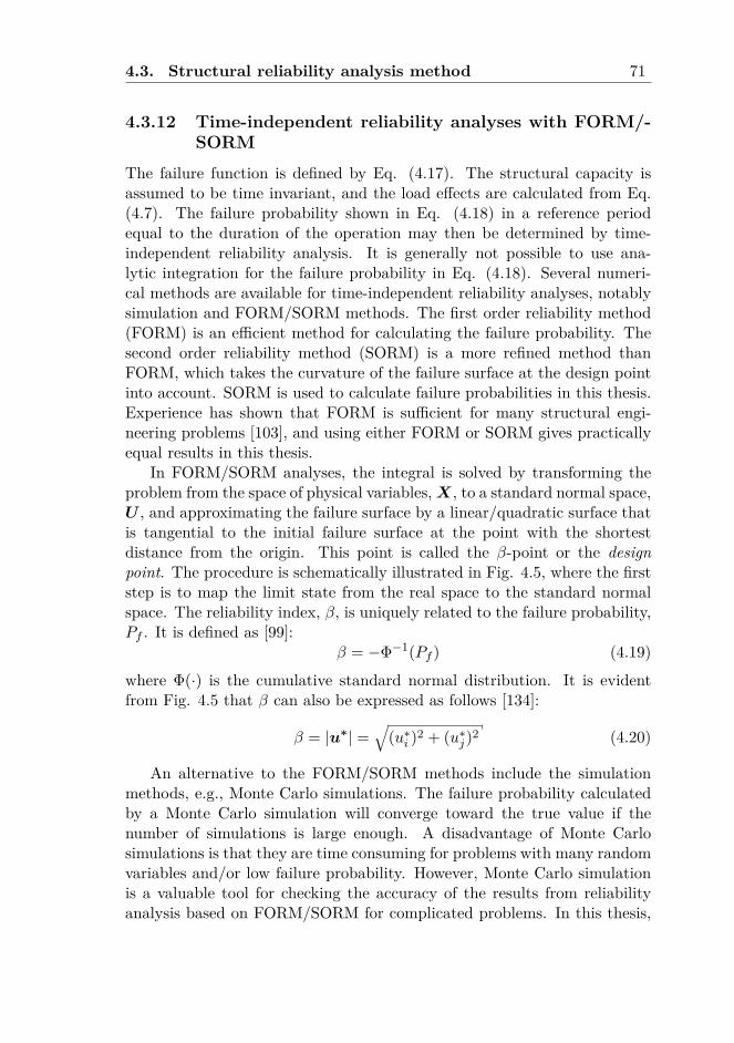
4.3. Structural reliability analysis method 71
4.3.12 Time-independent reliability analyses with FORM/-SORM
The failure function is defined by Eq. (4.17). The structural capacity isassumed to be time invariant, and the load effects are calculated from Eq.(4.7). The failure probability shown in Eq. (4.18) in a reference periodequal to the duration of the operation may then be determined by time-independent reliability analysis. It is generally not possible to use ana-lytic integration for the failure probability in Eq. (4.18). Several numeri-cal methods are available for time-independent reliability analyses, notablysimulation and FORM/SORM methods. The first order reliability method(FORM) is an efficient method for calculating the failure probability. Thesecond order reliability method (SORM) is a more refined method thanFORM, which takes the curvature of the failure surface at the design pointinto account. SORM is used to calculate failure probabilities in this thesis.Experience has shown that FORM is sufficient for many structural engi-neering problems [103], and using either FORM or SORM gives practicallyequal results in this thesis.
In FORM/SORM analyses, the integral is solved by transforming theproblem from the space of physical variables,X, to a standard normal space,U , and approximating the failure surface by a linear/quadratic surface thatis tangential to the initial failure surface at the point with the shortestdistance from the origin. This point is called the β-point or the designpoint. The procedure is schematically illustrated in Fig. 4.5, where the firststep is to map the limit state from the real space to the standard normalspace. The reliability index, β, is uniquely related to the failure probability,Pf . It is defined as [99]:
β = −Φ−1(Pf ) (4.19)where Φ(·) is the cumulative standard normal distribution. It is evidentfrom Fig. 4.5 that β can also be expressed as follows [134]:
β = |u∗| =√
(u∗i )2 + (u∗j )2 (4.20)
An alternative to the FORM/SORM methods include the simulationmethods, e.g., Monte Carlo simulations. The failure probability calculatedby a Monte Carlo simulation will converge toward the true value if thenumber of simulations is large enough. A disadvantage of Monte Carlosimulations is that they are time consuming for problems with many randomvariables and/or low failure probability. However, Monte Carlo simulationis a valuable tool for checking the accuracy of the results from reliabilityanalysis based on FORM/SORM for complicated problems. In this thesis,
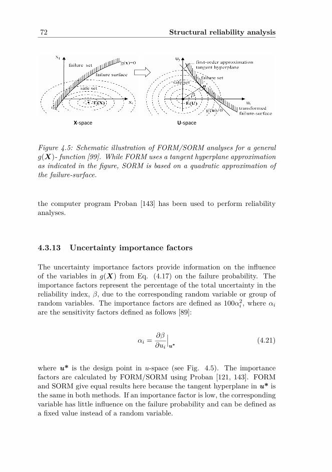
72 Structural reliability analysis
X-space U-space
Figure 4.5: Schematic illustration of FORM/SORM analyses for a generalg(X)- function [99]. While FORM uses a tangent hyperplane approximationas indicated in the figure, SORM is based on a quadratic approximation ofthe failure-surface.
the computer program Proban [143] has been used to perform reliabilityanalyses.
4.3.13 Uncertainty importance factors
The uncertainty importance factors provide information on the influenceof the variables in g(X) from Eq. (4.17) on the failure probability. Theimportance factors represent the percentage of the total uncertainty in thereliability index, β, due to the corresponding random variable or group ofrandom variables. The importance factors are defined as 100α2
i , where αiare the sensitivity factors defined as follows [89]:
αi = ∂β
∂ui
∣∣∣u∗
(4.21)
where u* is the design point in u-space (see Fig. 4.5). The importancefactors are calculated by FORM/SORM using Proban [121, 143]. FORMand SORM give equal results here because the tangent hyperplane in u* isthe same in both methods. If an importance factor is low, the correspondingvariable has little influence on the failure probability and can be defined asa fixed value instead of a random variable.
4.4. Case studies of a seafastening structure 73
4.4 Case studies of a seafastening structure in bargetransport
4.4.1 General
The barge transport of a large and heavy object was studied in this thesis.The grillage and seafastening were designed to resist the loading calculatedby a deterministic method. Based on that particular design, reliabilityanalyses were carried out, calculating the failure probability of Eq. (4.3) todemonstrate how Pf depends on various factors. This included the modeluncertainty in the load effects and structural capacity, as well as the uncer-tainty in the environmental conditions and seasonal variations.
In Sec. 4.4.2, the input to the SRA is described. Some selected resultsfrom the SRA [107] are presented in Sec. 4.4.3, and a discussion on theresults is included in Sec. 4.4.4.
4.4.2 Input data for the structural reliability analyses
4.4.2.1 Stochastic variables in the case studies
The failure probability was defined as Pf = P [R ≤ S] in Eq. (4.3). Thevariables R and S were defined in Eqs. (4.4) and (4.6), respectively. Infor-mation on the variables is given in Table 4.3.
4.4.2.2 Long-term distribution of the significant wave height
In Table 4.4, the parameters for the three-parameter Weibull distributionfor the significant wave height are given for each month and year-round.The significant wave heights with a return period equal to one year arealso shown. (This is the value of Hs with 8% probability of being exceededduring one month and 63% probability of being exceeded during 12 months).Seasonal parameters are given in Table 4.5. The data are grouped into fourseasons: winter (December - February), spring (March - May), summer(June - August) and autumn (September-November).
4.4.2.3 Distribution of the wave period conditional on Hs
The parameters in the lognormal distribution of the mean zero-crossingperiod conditional for the significant wave height (Eq. (4.13)) are given inTable 4.6.
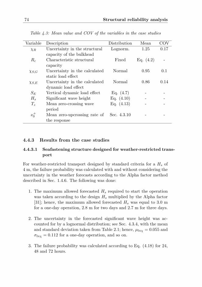
74 Structural reliability analysis
Table 4.3: Mean value and COV of the variables in the case studies
Variable Description Distribution Mean COVχR Uncertainty in the structural
capacity of the bulkheadLognorm. 1.25 0.17
Rc Characteristic structuralcapacity
Fixed Eq. (4.2) -
χS,G Uncertainty in the calculatedstatic load effect
Normal 0.95 0.1
χS,E Uncertainty in the calculateddynamic load effect
Normal 0.86 0.14
SE Vertical dynamic load effect Eq. (4.7) - -Hs Significant wave height Eq. (4.10) - -Tz Mean zero-crossing wave
periodEq. (4.13) - -
ν+0 Mean zero-upcrossing rate of
the responseSec. 4.3.10 - -
4.4.3 Results from the case studies
4.4.3.1 Seafastening structure designed for weather-restricted trans-port
For weather-restricted transport designed by standard criteria for a Hs of4 m, the failure probability was calculated with and without considering theuncertainty in the weather forecasts according to the Alpha factor methoddescribed in Sec. 1.4.6. The following was done:
1. The maximum allowed forecasted Hs required to start the operationwas taken according to the design Hs multiplied by the Alpha factor[31]; hence, the maximum allowed forecasted Hs was equal to 3.0 mfor a one-day operation, 2.8 m for two days and 2.7 m for three days.
2. The uncertainty in the forecasted significant wave height was ac-counted for by a lognormal distribution; see Sec. 4.3.4, with the meanand standard deviation taken from Table 2.1; hence, µlnχ = 0.055 andσlnχ = 0.112 for a one-day operation, and so on.
3. The failure probability was calculated according to Eq. (4.18) for 24,48 and 72 hours.
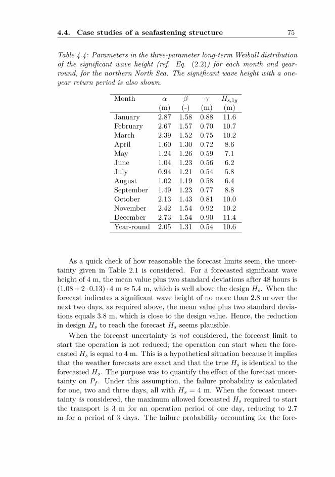
4.4. Case studies of a seafastening structure 75
Table 4.4: Parameters in the three-parameter long-term Weibull distributionof the significant wave height (ref. Eq. (2.2)) for each month and year-round, for the northern North Sea. The significant wave height with a one-year return period is also shown.
Month α β γ Hs,1y(m) (-) (m) (m)
January 2.87 1.58 0.88 11.6February 2.67 1.57 0.70 10.7March 2.39 1.52 0.75 10.2April 1.60 1.30 0.72 8.6May 1.24 1.26 0.59 7.1June 1.04 1.23 0.56 6.2July 0.94 1.21 0.54 5.8August 1.02 1.19 0.58 6.4September 1.49 1.23 0.77 8.8October 2.13 1.43 0.81 10.0November 2.42 1.54 0.92 10.2December 2.73 1.54 0.90 11.4Year-round 2.05 1.31 0.54 10.6
As a quick check of how reasonable the forecast limits seem, the uncer-tainty given in Table 2.1 is considered. For a forecasted significant waveheight of 4 m, the mean value plus two standard deviations after 48 hours is(1.08 + 2 · 0.13) · 4 m ≈ 5.4 m, which is well above the design Hs. When theforecast indicates a significant wave height of no more than 2.8 m over thenext two days, as required above, the mean value plus two standard devia-tions equals 3.8 m, which is close to the design value. Hence, the reductionin design Hs to reach the forecast Hs seems plausible.
When the forecast uncertainty is not considered, the forecast limit tostart the operation is not reduced; the operation can start when the fore-casted Hs is equal to 4 m. This is a hypothetical situation because it impliesthat the weather forecasts are exact and that the true Hs is identical to theforecasted Hs. The purpose was to quantify the effect of the forecast uncer-tainty on Pf . Under this assumption, the failure probability is calculatedfor one, two and three days, all with Hs = 4 m. When the forecast uncer-tainty is considered, the maximum allowed forecasted Hs required to startthe transport is 3 m for an operation period of one day, reducing to 2.7m for a period of 3 days. The failure probability accounting for the fore-
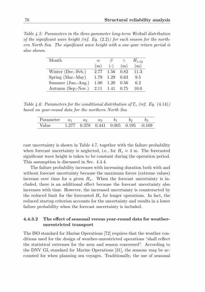
76 Structural reliability analysis
Table 4.5: Parameters in the three-parameter long-term Weibull distributionof the significant wave height (ref. Eq. (2.2)) for each season for the north-ern North Sea. The significant wave height with a one-year return period isalso shown.
Month α β γ Hs,1y(m) (-) (m) (m)
Winter (Dec.-Feb.) 2.77 1.56 0.82 11.3Spring (Mar.-May) 1.79 1.29 0.63 9.5Summer (Jun.-Aug.) 1.00 1.20 0.56 6.2Autumn (Sep.-Nov.) 2.11 1.41 0.75 10.0
Table 4.6: Parameters for the conditional distribution of Tz (ref. Eq. (4.14))based on year-round data for the northern North Sea
Parameter a1 a2 a3 b1 b2 b3Value 1.277 0.378 0.441 0.005 0.195 -0.169
cast uncertainty is shown in Table 4.7, together with the failure probabilitywhen forecast uncertainty is neglected, i.e., for Hs ≡ 4 m. The forecastedsignificant wave height is taken to be constant during the operation period.This assumption is discussed in Sec. 4.4.4.
The failure probability increases with increasing duration both with andwithout forecast uncertainty because the maximum forces (extreme values)increase over time for a given Hs. When the forecast uncertainty is in-cluded, there is an additional effect because the forecast uncertainty alsoincreases with time. However, the increased uncertainty is counteracted bythe reduced limit for the forecasted Hs for longer operations. In fact, thereduced startup criterion accounts for the uncertainty and results in a lowerfailure probability when the forecast uncertainty is included.
4.4.3.2 The effect of seasonal versus year-round data for weather-unrestricted transport
The ISO standard for Marine Operations [72] requires that the weather con-ditions used for the design of weather-unrestricted operations “shall reflectthe statistical extremes for the area and season concerned”. According tothe DNV GL standard for Marine Operations [31], the seasons may be ac-counted for when planning sea voyages. Traditionally, the use of seasonal
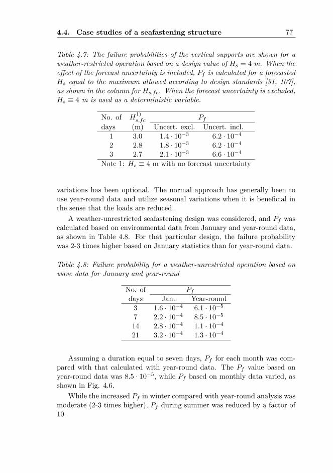
4.4. Case studies of a seafastening structure 77
Table 4.7: The failure probabilities of the vertical supports are shown for aweather-restricted operation based on a design value of Hs = 4 m. When theeffect of the forecast uncertainty is included, Pf is calculated for a forecastedHs equal to the maximum allowed according to design standards [31, 107],as shown in the column for Hs,fc. When the forecast uncertainty is excluded,Hs ≡ 4 m is used as a deterministic variable.
No. of H1)s,fc Pf
days (m) Uncert. excl. Uncert. incl.1 3.0 1.4 · 10−3 6.2 · 10−4
2 2.8 1.8 · 10−3 6.2 · 10−4
3 2.7 2.1 · 10−3 6.6 · 10−4
Note 1: Hs ≡ 4 m with no forecast uncertainty
variations has been optional. The normal approach has generally been touse year-round data and utilize seasonal variations when it is beneficial inthe sense that the loads are reduced.
A weather-unrestricted seafastening design was considered, and Pf wascalculated based on environmental data from January and year-round data,as shown in Table 4.8. For that particular design, the failure probabilitywas 2-3 times higher based on January statistics than for year-round data.
Table 4.8: Failure probability for a weather-unrestricted operation based onwave data for January and year-round
No. of Pfdays Jan. Year-round3 1.6 · 10−4 6.1 · 10−5
7 2.2 · 10−4 8.5 · 10−5
14 2.8 · 10−4 1.1 · 10−4
21 3.2 · 10−4 1.3 · 10−4
Assuming a duration equal to seven days, Pf for each month was com-pared with that calculated with year-round data. The Pf value based onyear-round data was 8.5 · 10−5, while Pf based on monthly data varied, asshown in Fig. 4.6.
While the increased Pf in winter compared with year-round analysis wasmoderate (2-3 times higher), Pf during summer was reduced by a factor of10.
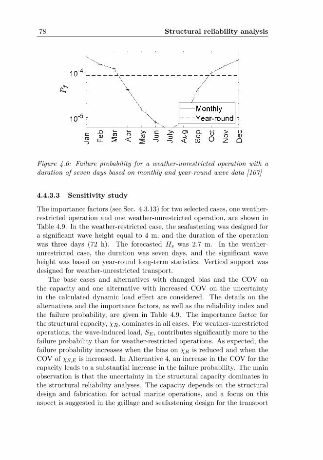
78 Structural reliability analysis
Figure 4.6: Failure probability for a weather-unrestricted operation with aduration of seven days based on monthly and year-round wave data [107]
4.4.3.3 Sensitivity study
The importance factors (see Sec. 4.3.13) for two selected cases, one weather-restricted operation and one weather-unrestricted operation, are shown inTable 4.9. In the weather-restricted case, the seafastening was designed fora significant wave height equal to 4 m, and the duration of the operationwas three days (72 h). The forecasted Hs was 2.7 m. In the weather-unrestricted case, the duration was seven days, and the significant waveheight was based on year-round long-term statistics. Vertical support wasdesigned for weather-unrestricted transport.
The base cases and alternatives with changed bias and the COV onthe capacity and one alternative with increased COV on the uncertaintyin the calculated dynamic load effect are considered. The details on thealternatives and the importance factors, as well as the reliability index andthe failure probability, are given in Table 4.9. The importance factor forthe structural capacity, χR, dominates in all cases. For weather-unrestrictedoperations, the wave-induced load, SE , contributes significantly more to thefailure probability than for weather-restricted operations. As expected, thefailure probability increases when the bias on χR is reduced and when theCOV of χS,E is increased. In Alternative 4, an increase in the COV for thecapacity leads to a substantial increase in the failure probability. The mainobservation is that the uncertainty in the structural capacity dominates inthe structural reliability analyses. The capacity depends on the structuraldesign and fabrication for actual marine operations, and a focus on thisaspect is suggested in the grillage and seafastening design for the transport
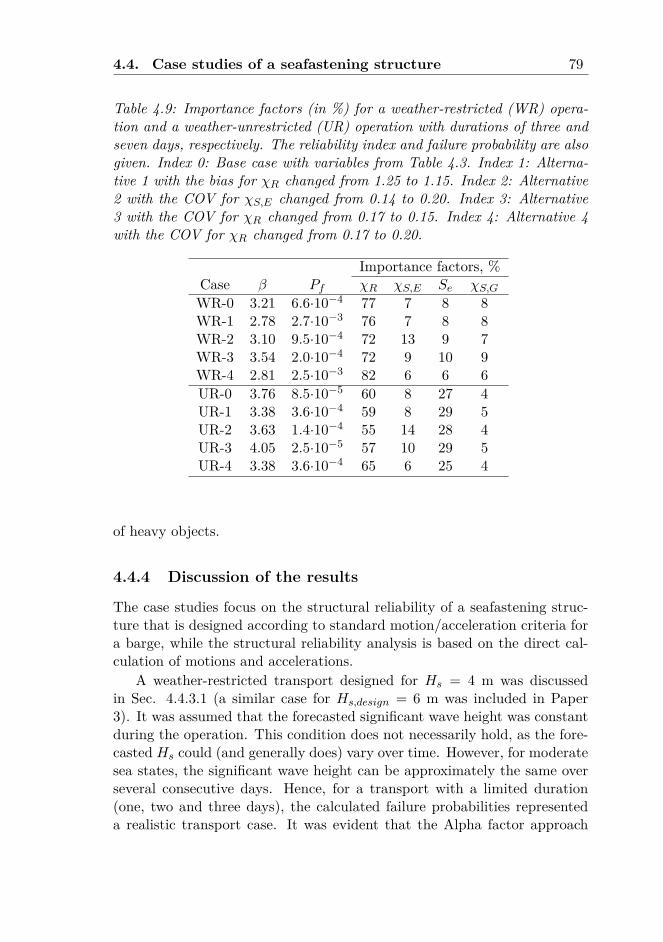
4.4. Case studies of a seafastening structure 79
Table 4.9: Importance factors (in %) for a weather-restricted (WR) opera-tion and a weather-unrestricted (UR) operation with durations of three andseven days, respectively. The reliability index and failure probability are alsogiven. Index 0: Base case with variables from Table 4.3. Index 1: Alterna-tive 1 with the bias for χR changed from 1.25 to 1.15. Index 2: Alternative2 with the COV for χS,E changed from 0.14 to 0.20. Index 3: Alternative3 with the COV for χR changed from 0.17 to 0.15. Index 4: Alternative 4with the COV for χR changed from 0.17 to 0.20.
Importance factors, %Case β Pf χR χS,E Se χS,GWR-0 3.21 6.6·10−4 77 7 8 8WR-1 2.78 2.7·10−3 76 7 8 8WR-2 3.10 9.5·10−4 72 13 9 7WR-3 3.54 2.0·10−4 72 9 10 9WR-4 2.81 2.5·10−3 82 6 6 6UR-0 3.76 8.5·10−5 60 8 27 4UR-1 3.38 3.6·10−4 59 8 29 5UR-2 3.63 1.4·10−4 55 14 28 4UR-3 4.05 2.5·10−5 57 10 29 5UR-4 3.38 3.6·10−4 65 6 25 4
of heavy objects.
4.4.4 Discussion of the results
The case studies focus on the structural reliability of a seafastening struc-ture that is designed according to standard motion/acceleration criteria fora barge, while the structural reliability analysis is based on the direct cal-culation of motions and accelerations.
A weather-restricted transport designed for Hs = 4 m was discussedin Sec. 4.4.3.1 (a similar case for Hs,design = 6 m was included in Paper3). It was assumed that the forecasted significant wave height was constantduring the operation. This condition does not necessarily hold, as the fore-casted Hs could (and generally does) vary over time. However, for moderatesea states, the significant wave height can be approximately the same overseveral consecutive days. Hence, for a transport with a limited duration(one, two and three days), the calculated failure probabilities representeda realistic transport case. It was evident that the Alpha factor approach
80 Structural reliability analysis
effectively compensated for the uncertainty of the forecasting in this case.Next, the effect of seasonal versus year-round data for weather-unrestricted
transport was studied in Sec. 4.4.3.2. For weather-unrestricted transport,the significant wave height is not constant but follows a long-term distri-bution, as discussed in Chapter 2. This distribution varies throughout theyear. From an analysis point of view, it is convenient to apply year-rounddata because that is readily available and provides flexibility in the plan-ning at an early stage before the transport date is defined. However, asindicated in Fig. 4.6, the failure probability for seafastening structuresdesigned for weather-unrestricted transports then strongly depends on thetime of the year. It is evident that Pf is very low if the transport is exe-cuted during the summer period. This is good from a safety perspective,but a too low Pf could be seen as (unnecessary) conservatism by use of theweather-unrestricted design option for the summer period and introducean (unnecessary) high cost. For practical transport, a design Hs could becalculated based on a long-term distribution or the return period approachdescribed in Sec. 2.6 (if the design Hs was below 4 or 6 m, the standardmethod in App. C.1 may be used.) It should be noted that for planningreal marine operations, it is necessary to check the capacity also using en-vironmental data for the preceding and/or succeeding month [31], but thathas not been considered in this thesis.
In reality, the duration of a marine operation is a stochastic variable,but in the analyses above, it was assumed to be a deterministic variable,estimated as described in Sec. 2.2. The duration could be modeled asa stochastic variable, and revised failure probabilities could be calculated.However, from the case studies above, it is evident that Pf is not verysensitive to the duration; hence, it is reasonable to model the duration as afixed variable.
In Sec. 4.4.3.3, a sensitivity study was performed in which importancefactors were calculated for weather-restricted and weather-unrestricted ma-rine operations. The sensitivity analyses showed that the structural capacityhad the largest importance factors of all the parameters examined. Conse-quently, the failure probabilities were sensitive to variations in the bias andCOV for the structural capacity, and the structural capacity, in particularthat of a bulkhead with horizontal stiffeners exposed to vertical loading,was an important input for the structural reliability analyses.
The above analyses are all based on the barge transport case where theseafastening structure is designed for various environmental conditions. Toobtain a further understanding of how the results from the SRA relate tothe planning of marine operations in practice, other case studies could be

4.4. Case studies of a seafastening structure 81
performed. It would also be of interest to extend the period of weather-restricted operations. The uncertainty in the forecasted value of Hs wasquantified for operations lasting up to seven days in Paper 2 (see Table 2.1above). Hence, the method for weather-restricted marine operations couldbe applied for transports with a duration of up to seven days, and the resultscould be compared with weather-unrestricted operations. This has not beendone in this thesis but is proposed as future research (see Sec. 5.4.3).

82 Structural reliability analysis
Chapter 5
Conclusions andrecommendations for futureresearch
5.1 General
The objective of the research presented in this thesis is to study the struc-tural integrity of typical support structures for sea transport of large andheavy objects in a structural reliability framework, considering both weather-restricted and weather-unrestricted operations. This thesis addresses theuncertainty assessment of wave-induced motions of a transport barge andthe capacity of the selected elements as implemented in the structural reli-ability analyses. The focus in this research work is on three topics. First,an investigation of the motion of a transport barge in severe beam seas andthe associated support loads is conducted by numerical methods supportedby the model tests. Second, the uncertainty of forecasted significant waveheight is evaluated. Finally, the structural reliability analysis of the sup-ports in the ultimate limit state is performed. The conclusions and originalcontributions of the research work in this thesis and recommendations forfuture research are presented below.
5.2 Conclusions
The main conclusions in this thesis are presented in the published papersfocusing on the three topics related to sea transports, namely, the wave-induced load effects, uncertainty in weather forecasts and structural relia-
83
84 Conclusions and recommendations for future research
bility of the cargo supports during sea transport. The main conclusions andfindings are summarized in the following.r Maximum roll angle.
For severe sea states, the model test results were compared with cal-culations in the frequency domain using stochastic linearization of theviscous roll damping. They were also compared with the results from anonlinear analysis in which the equations of motion were solved in thetime domain. The ratio between the maximum expected roll angle fora three hour storm period and the standard deviation was 3.4-3.9 forthe nonlinear analysis, i.e., close to the results from a linear analysis.The similar ratio from the model tests was between 2.7 and 3.2. Thereason for this lower ratio was concluded to be that the roll amplitudewas limited upwards by physical effects that were not captured by thenumerical analyses. The maximum expected roll amplitude from themodel tests was 22 degrees for a three hour storm period. The linearanalyses overestimated the maximum roll angle, while the nonlinearanalysis compared well.r Model uncertainty in support force.The barge motions for high sea states are calculated by linear andnonlinear analyses and compared with results from the model tests.It was found that the bias varied with the response. The bias was esti-mated to be 0.75-0.94 for the maximum roll angle and 0.65-0.8 for thevertical support force, depending on the type of analysis. Accountingfor the effect of high wave steepness and non-linearity in the modeltests, e.g., water on the deck in high sea states, the bias for the verticalsupport force from the model tests was set to 0.9 together with a COVof 0.1. The uncertainty in the calculated load effect was representedby a random variable with a mean value of 0.95 and COV of 0.1. Themodel uncertainty was then assumed to be normal distributed witha mean value of 0.86 and COV of 0.14 for long-term environmentalconditions for use in the structural reliability analysis to represent thegeneral environmental conditions.r Duration of weather-restricted operations.Operations with planned durations less than three days are designedas weather-restricted marine operations. The weather forecasts fromthe Norwegian Sea that were studied in this thesis did not reveal anyspecific increase in the forecast uncertainty that would require an exact72-h limit for weather-restricted operations, even if the uncertainty inthe forecasts increases with the lead time up to a lead time of seven
5.2. Conclusions 85
days. For example, the bias in the forecasted significant wave heightincreases from 1.09 to 1.10 from three to four days, while the coefficientof variation increases from 0.13 to 0.15.
r Forecasted wave period.A similar approach as used for the significant wave height can beenused for the forecasted wave period. However, the correlation betweenforecast and hindcast data is lower for wave periods than for signif-icant wave heights for a given lead time, indicating that forecastedwave periods are more uncertain than forecasted wave height. Thewave period for weather-restricted operations is therefore modeled bya statistical distribution similar to the distribution used for weather-unrestricted operations.
r Target reliability level.An important question in applying structural reliability analyses indecision making is to specify the target reliability level. Some designstandards recommend a certain target reliability level for the designdepending on the consequences of failure. However, in practice, itmay be difficult to relate such target levels directly to the reliabilityanalyses. However, as long as the reliability level is considered to beadequate, the target reliability level can be chosen to be the same asthat obtained by using the current design standards. The adequacy ofthe current practice is demonstrated through a low experienced failurerate and general acceptance by the industry and insurance companies.In engineering practice, the uncertainty in weather forecasts is ac-counted for by applying a risk reduction factor called the Alpha factor.This factor was implemented in the structural reliability analyses, andthe failure probability was calculated by this approach as well as byassuming perfect weather forecasts (and hence there was no forecastuncertainty to compensate for). The standard Alpha factor approachwas seen to effectively compensate for the uncertainty inherent in theweather forecast in the cases studied in this thesis.
r Structural capacity.The structural capacity was considered for the grillage beams and forthe barge bulkheads, considering the model uncertainty and the un-certainty in the material parameters. The ultimate strength of thebulkheads was found to be governing, and it was found adequate tomodel the resulting capacity by a random variable following a lognor-mal distribution with a bias of 1.25 and a COV of 0.17.
86 Conclusions and recommendations for future research
r Results from the structural reliability analysis.For a weather-unrestricted operation planned using standard all-yearcriteria for load calculation, the failure probability depends on thetime of the year in which the operation is executed. For example, itwas noticed that for a given cargo support design:
− the failure probability was 1.5 times higher using environmentaldata for November instead of seasonal data for autumn (Septem-ber - November)
− the failure probability calculated using statistical data for Jan-uary was 3 times higher than that calculated using data for theentire year
− the failure probability in July was less than 1/10 of the failureprobability in October
The differences in the failure probabilities are not dramatic in thefirst two cases. In the third case, however, the difference is ratherlarge and should be further considered. It is evident that to use theweather-unrestricted all-year criteria for summer transport introducesconservatism. This is acceptable from a safety point of view but in-creases cost. Hence, the design of grillage and seafastening shouldbe optimized by applying a reduced design sea state for weather-unrestricted summer transports based on available hindcast or mea-sured wave data.The following main conclusions are drawn from this study:
− For a weather-restricted operation, the reduction in the allowablesignificant wave height according to the so-called Alpha factormethod to account for the forecast uncertainty is a good approachwith respect to the failure probability.
− The use of seasonal data for planning weather-unrestricted opera-tions is optional according to some regulatory bodies and manda-tory according to other regulatory bodies. The use of seasonalor year-round data will affect the failure probability for a givenoperation, as seasonal data for the winter gives a higher failureprobability than year-round data.
− The calculated failure probabilities for a given operation dependon the season in which it is executed, the duration of the oper-ation, etc. However, the calculated probabilities are of the sameorder of magnitude as the target value generally accepted formarine operations, of 10−4 per operation.
5.3. Summary of the original contributions 87
The overall conclusion is that for the North Sea, the failure probabilityby use of the simplified design criteria compares well with the targetlevel. However, because the uncertainty in the strength dominatesand the strength depends on temporary solutions for each transport,a focus on this aspect is recommended in the integrity managementof the grillage and seafastening in connection with the transport ofheavy objects.
r A simple design formula for the wind speed.For a weather-unrestricted operation, the wind speed correspondingto a given design wave height needs to be determined. While thesignificant wave height can be determined based on available long-term statistics, such statistics are not always available for the designwind speed. A simple approach is proposed to estimate the designwind speed for open sea areas as a function of the design significantwave height. This easy-to-use engineering method provides a designwind speed with reasonable accuracy and could be used in planningtransports where wave-induced loading dominates and where a designsignificant wave height is given.
5.3 Summary of the original contributions
This thesis addresses the structural reliability related to the seafastening ofheavy cargo during sea transport on barges. The original contributions ofthis thesis are summarized as follows:
r Establishing a method for calculating the viscous damping for rollingof a barge.This was based on the original methods by Tanaka and Ikeda for shipsand extended to include wider vessels such as a transport barge (i.e.,increased B/KG ratios).
r Model test of the transport barge exposed to severe seas with steepwaves giving large barge motions.The purpose was to study the motions of a barge in storm conditionsduring weather-unrestricted transport. The wave periods were closeto the natural roll period to investigate the effect of resonant bargemotion in severe seas.
r Uncertainty assessment of the environmental conditions.Weather forecasts of the significant wave height were studied, and the
88 Conclusions and recommendations for future research
uncertainty was quantified. The uncertainty was implemented in thereliability analyses.
r A formula for the design wind speed.A simple formula to calculate the design wind speed correspondingto a design significant wave height was proposed. The purpose wasto provide a simple method for engineering purposes in estimatingthe wind speed and hence the wind-induced loading acting on thetransported object.
r Structural reliability analyses including modeling of uncertainties, es-pecially the uncertainty in weather forecasts.A reliability model that accounted for the uncertainty inherent in theweather forecasts was established. This model was used to study theeffect of the forecast uncertainty on the structural reliability by pro-viding a comparison with a (fictitious) condition without forecast un-certainty.
r Structural reliability analyses to study the effect of seasons, etc.A reliability model in which the long-term statistical distribution ofthe environmental conditions was modeled was used to study seasonalvariations and the failure probability as a function of the duration forweather-unrestricted operations.
5.4 Suggestions for future research
5.4.1 Additional model tests
The model tests included free decay and forced roll tests, and the barge wasexposed to beam seas. In the free decay tests, the CoG was in one position,and in the forced roll tests, the model was rolled about an axis in the watersurface.
Several additional tests could have been performed to obtain a broaderset of data to analyze the roll damping and barge motion. Additional modeltests could include:
r free decay tests with several vertical CoG positions of the cargo
r forced roll tests with the axis of rotation at several elevations
r waves from several directions in addition to the beam seas, e.g., headseas and beam quartering seas
5.4. Suggestions for future research 89
5.4.2 Uncertainty assessments of wave forecasts
In this thesis, the significant wave height for the total sea was used for com-parison of the forecast and hindcast. In the weather forecasts and hindcastdata, the significant wave height was given for the wind driven waves, swelland total sea. An alternative to the chosen approach could be to comparewind sea and swell separately, and this might be part of a future researchproject.
Many marine operations are sensitive to wave periods, e.g., vessel mo-tions close to natural periods. The maximum allowable significant waveheight for a weather-restricted operation, e.g., for an offshore crane instal-lation or sensitive sea transport, may vary as a function of the wave period(Tp or Tz) for such operations. The margin on the forecasted wave periodrequired to achieve the required safety level is not clearly defined in the de-sign standards. (For example, if the analysis has shown that the operationcan be started when Hs ≤ 2 m and Tz ≤ 9 s, the forecasted maximum Hs isα · 2 m, where Alpha is found in design standards. However, the maximumacceptable Tz in the weather forecast to start the operation is unknown.)The uncertainty in the forecasted wave period could be further addressedin future studies.
5.4.3 Maximum duration of weather-restricted operations
The maximum duration of weather-restricted operations is generally threedays according to design standards. This is often a challenge in planningmarine operations because exceeding that limit imposes design environmen-tal conditions based on long-term statistics, which is normally much moresevere than the limits defined for weather-restricted operations. It wouldtherefore be a great benefit for the industry if the limit for weather-restrictedoperations could be extended. In the study of the forecast uncertainty inthe significant wave height performed in this thesis, no clear reason to limitthe duration of a weather-restricted operation to three days was observed.However, that was an observation that was based on a limited amount ofdata, and a possible extension of the three-day limit based on a broaderdata set considering wind and waves could be a topic for future research.
5.4.4 Ultimate strength assessment
Some assumptions and simplifications regarding the strength have beenmade in this thesis. The support forces were calculated based on thedynamic equilibrium of the transported object. In future work, a refined
90 Conclusions and recommendations for future research
method could be applied for the strength assessment. The support forcescould have been calculated by finite element analysis methods, includingthe calculation of the relative stiffness of the barge and transported object.The uncertainty in the capacity of stiffened plate panels in bulkheads wasestimated based on previous experiments and analyses described in the liter-ature. More sophisticated evaluations of the bulkheads could be performedby methods such as nonlinear finite element analyses or experiments.
The event defined to represent failure in an ultimate capacity context isnot a physical collapse but a defined upper limit for the capacity. Hence,a violation of the ultimate limit state capacity will not necessarily lead tostructural failure. For the same reason, even several load cycles exceedingthe ULS capacity due to events such as rolling of the barge in heavy seasthat do not have to lead to a total loss. Following the buckling failure of abulkhead below the cargo supports, the deck plate of the barge will be ableto resist a substantial amount of loading due to membrane stresses, andhence, there is a reserve that is not accounted for in the calculated capacity.Buckling of a bulkhead would lead to local damage of the barge, but a totaldegradation of the cargo support would not occur. This reserve capacityhas not been quantified in this study. The calculated failure probabilityrefers to a defined capacity limit and not necessarily to a physical collapse.Such reserves could lead to a larger bias for the structural capacity, hencereducing the failure probability. It could also lead to lower consequencesof failure by limiting the damage and avoiding total collapse. Such effectscould be interesting to study in future work.
Another interesting subject is how conditions during fabrication couldaffect the ultimate strength. Construction work is generally performed in-doors or under cover in adverse weather conditions outdoors. Normally,fabrication is performed over a long period of time, and weld inspection caneasily be planned to comply with the required waiting time before perform-ing NDT (nondestructive testing) on the welds. The fabrication of grillageand seafastening for sea transports of offshore structures is normally per-formed under controlled conditions in a yard. However, welding of thegrillage beams and seafastening to the vessel and the transported object isperformed outdoors. Building weather shielding is time consuming and notalways done. A tight schedule may lead to a limited waiting time beforeperforming NDT. Hence, the challenges for marine operations are differ-ent than those for general fabrication. The effect of weather conditions onthe quality of welded joints and thereby the uncertainty in the structuralstrength is also relevant for future work.

5.4. Suggestions for future research 91
5.4.5 The effect of costs
In this thesis, no cost-safety benefit analysis is performed. The reliabilityanalyses do not include the effect of costs. It is then assumed that the plan-ning and execution is carried out under the ALARP regime by minimizingall the risks as much as reasonable practicable and satisfying the requiredsafety level with respect to loss of life. The application of the ALARPprinciple could be a topic for future research.

92 Conclusions and recommendations for future research
References
[1] A.B. Aalbers and C.J.G. van Dongen. Weather routing: Uncertain-ties and the effect of decision support systems. In Proceedings of theMarine Operations Specialty Symposium (MOSS), Baltimore, USA,2008.
[2] O. J. Aarnes, Ø. Breivik, and M. Reistad. Wave Extremes in theNortheast Atlantic. Journal of Climate, 25:1529–1543, 2012.
[3] ABS. Rules for Building and Classing Steel Vessels. American Bureauof Shipping, Houston, USA, July 2019.
[4] E. Achenbach. Influence of surface roughness on the cross-flow arounda circular cylinder. Journal of Fluid Mechanics, 46(2):321–335, 1971.
[5] P. Ø. Alvær. HLV transports - DNV guidelines for calculation ofcribbing friction. In Proceedings of the Royal Institution of NavalArchitects (RINA) International Conference, London, UK, 2005.
[6] P. Ø. Alvær. The VMO Standard & ISO 19001-6 Marine Operations.In Proceedings of the Second Marine Operations Specialty Symposium(MOSS), Singapore, 2012.
[7] P. Ø. Alvær. The new marine operation standard DNVGL-ST-N001.In Proceedings of the Third Marine Operations Specialty Symposium(MOSS), Singapore, 2016.
[8] API RP 2A-LRFD. Recommended practice for planning, designingand constructing fixed offshore platforms - load and resistance factordesign. American Petroleum Institute, Washington, D.C., USA., 2019.
[9] J.R. Bidlot. Twenty-one years of wave forecast verification. NewsletterNumber 150 – Winter 2016/17, European Centre for Medium-rangeWeather Forecasts (ECMW), Reading, UK, 2017.
93
94 References
[10] E. M. Bitner-Gregersen and A. Toffoli. Uncertainties of Wind Sea andSwell Prediction From the Torsethaugen Spectrum. In Proceedings ofthe 28th International Conference on Offshore Mechanics and ArcticEngineering, Hawaii, Honolulu, 2009.
[11] E.M. Bitner-Gregersen and S. Haver. Joint environmental model forreliability calculations. In ISOPE. Proc. 1st Int. Offshore and PolarEng. Conf., Edinburgh, UK, volume 1, pages 246–253, 1991.
[12] A.K. Brook and R.G. Standing. A theoretical and experimental in-vestigation of barge roll damping. In Proceedings of the Fourth inter-national conference on stability if ships and ocean vehicle, STAB ’90,Naples, Italy, 1990.
[13] D. C. Brooker, G. K. Cole, and J. D. McConochie. The influenceof hindcast modeling uncertainty on the prediction of high returnperiod wave conditions. Proceedings of the International Conferenceon Offshore Mechanics and Arctic Engineering - OMAE, Vancouver,British Columbia, Canada, 2004.
[14] D. T. Brown, R. Eatock Taylor, and M. H. Patel. Barge motions inrandom seas - a comparison of theory and experiment. Journal ofFluid Mechanics, 129:385–407, 1983.
[15] K. Bruserud and S. Haver. Comparison of wave and current measure-ments to NORA10 and NoNoCur hindcast data in the northern NorthSea. Ocean Dynamics, 66:823–838, 2016.
[16] Bureau Veritas. Rules for the Classification of Steel Ships. Part B -Hull and Stability. NR 467.B1 DT R12 E , Paris, France, January2020.
[17] K.V. Bury. Statistical Distributions in Engineering. Cambridge: Cam-bridge University Press., 1999.
[18] S. Chakrabarti. Empirical calculation of roll damping for ships andbarges. Ocean Engineering, 28(7):pages 915–932, 2001.
[19] H.S. Chan, E. Armaoglu, M. Thomson, M Garner, A Parisotto, andS. Sovilla. Response forecasts for a suspended wellbay module andflare tower during transit to shore. In Proceedings of the Twenty-ninth International Ocean and Polar Engineering Conference, ISOPE,Honolulu, Hawaii, USA, June 16-21, 2019.
References 95
[20] R.P. Dallinga, A.B. Aalbers, and J.W.W. van der Vegt. Design As-pects for Transport of Jackup Platforms on a Barge. Offshore Tech-nology Conference (OTC), Houston, 1984. Paper no. OTC1984-4733.
[21] M. Deelen and J. B. de Jonge. An operational based method fordetermining the design sea states of heavy transport vessels. MarineHeavy Transport and Lift IV, London, UK, 29-30 October, 2014.
[22] O. Ditlevsen and H.O. Madsen. Structural Reliability Methods. De-partment of Mechanical Engineering, Technical University of Den-mark, 2007. http://od-website.dk/books/OD-HOM-StrucRelMeth-Ed2.3.7.pdf [Accessed 2020-08-27].
[23] DNV. Rules for Planning and Execution of Marine Operations,1996/2000. Det Norske Veritas, Oslo, Norway.
[24] DNV GL. When Noble met Denton, 2015. https://www.dnvgl.com/oilgas/perspectives/when-noble-met-denton.html [Accessed2020-08-27].
[25] DNV GL. Rules for classification - Ships, July 2020. Oslo, Norway.
[26] DNV-OS-H101. Marine Operations, General, 2011. Det Norske Veri-tas, Oslo, Norway.
[27] DNV-OS-H202. Sea transport operations, 2015. Det Norske Veritas,Oslo, Norway.
[28] DNVGL-OS-C101. Design of offshore steel structures, general - LRFDmethod. DNVGL, Oslo, Norway, July 2019.
[29] DNVGL-RP-C205. Environmental Conditions and EnvironmentalLoads. DNV GL, Oslo, Norway, December 2019.
[30] DNVGL-RP-N101. Risk management in marine - and subsea opera-tions. DNVGL, Oslo, Norway, September 2019.
[31] DNVGL-ST-N001. Marine Operations and Marine Warranty. DNVGL, Oslo, Norway, 2020.
[32] G. Dong and T. Moan. Prediction of ultimate behaviour of plategirders in transverse frames. Proceedings of the Sixteenth InternationalOffshore and Polar Engineering Conference, ISOPE, San Francisco,California, USA, 2006.
96 References
[33] M.J. Downie, P.W. Bearman, and J.M.R Graham. Effect of vortexshedding on the coupled roll response of bodies in waves. Journal ofFluid Mechanics, 189:243–261, 1988.
[34] I.N. Dragos. Risk control - marine warranty survey. Journal of Engi-neering Studies and Research, 18(2):66–76, 2012.
[35] EN 10025-1. Hot rolled products of structural steels. Part 1: Generaltechnical delivery conditions. European Committee for Standardiza-tion, Brussels, Belgium, 2005.
[36] EN 1993-1-1. Eurocode 3. Design of steel structures - Part 1-1: Gen-eral rules and rules for buildings. European Committee for Standard-ization, Brussels, Belgium, 2005.
[37] W.A. Ewers, P.E. Freathy, K. Lindemann, and K. Børresen. BargeMotions Research Projects, Phase 2 Report, Part 3 Further workon viscous roll damping, for a consortium of companies organised byNoble Denton and Associates Ltd. Technical report, 1979. AtkinsResearch & Development, Surrey, UK, and Det Norske Veritas, Oslo,Norway.
[38] O.M. Faltinsen. Sea Loads on Ships and Offshore Structures. Cam-bridge: Cambridge University Press., 1990.
[39] O.M. Faltinsen. Hydrodynamics of High-Speed Marine Vehicles. Cam-bridge University Press, New York, USA, 2005.
[40] A.C. Fernandes and A.C. Oliveira. The roll damping assessment viadecay model testing (new ideas about an old subject). Journal ofMarine science and application, 8(2):144–150, June 2009.
[41] S. Fjeld. Reliability of Offshore Structures. Journal of PetroleumTechnology, 30(10):1486–1496, October 1978.
[42] W. Froude. On the Rolling of Ships. Parker, Son and Bourn, London,UK, 1861.
[43] FugroOceanor. http://www.oceanor.no/services/. Accessed 2020-08-27.
[44] I.J. Fylling. Analysis of towline forces in ocean towing systems. Tech-nical report, Department of Marine Technology - The Norwegian In-stitute of Technology, Nov. 1979.
References 97
[45] O. Gaidai, G. Storhaug, and A. Naess. Extreme Value Statistics ofShip Rolling. In Proceedings of PRADS 2010, the 11th InternationalSymposium on Practical Design of Ships and other Floating Struc-tures, Rio de Janeiro, Brazil, September 2010.
[46] S. Ghosh, M.A. Jacobs, and J.A. Mercier. Role of marine warrantysurveyors and their requirements for selected items. Proceedings of theInternational Conference on Offshore Mechanics and Arctic Engineer-ing - OMAE, Vancouver, British Columbia, Canada, pages 647–662,2004.
[47] GL Noble Denton. General Guidelines for Marine Projects. TechnicalStandard Committee, London, UK, 2013.
[48] GOMO. Guidelines for Offshore Marine Operations, UK/Norway.www.g-omo.info, 2020.
[49] J.M.R. Graham. The forces on sharp-edged cylinders in oscillatoryflow at low Keulegan-Carpenter numbers. Journal of Fluid Mechanics,97:331–346, 1980.
[50] J.M.R Graham. Calculation of Hydrodynamic Damping of OffshoreStructures. In Proceedings of the International Conference on Be-haviour of Offshore Structures, BOSS. Trondheim, Norway, pages579–590, 1988.
[51] J.M.R. Graham and M.J. Downie. Viscous damping of floating bodiesin waves. In Proceedings of the ASME 2015 34th International Con-ference on Ocean, Offshore and Arctic Engineering, OMAE, 2015.
[52] J.M.R. Graham and T.E. Kendon. Viscous Damping of Large Float-ing Structures. IUTAM Symposium on Fluid-Structure Interaction inOcean Engineering, © Springer Science+Business Media B.V., 8:69–78, 2008.
[53] Grillage and Seafastening Design. Guidelines No. VMO 1.2. 1989.Det Norske Veritas, Oslo, Norway.
[54] W. Guachamin Acero, L. Li, Z. Gao, and T. Moan. Methodology forassessment of the operational limits and operability of marine opera-tions. Ocean Engineering, 125:308–327, 2016.
[55] O. T. Gudmestad. Risk Assessment Tools for Use During Fabricationof Offshore Structures and in Marine Operations Projects. Journal
98 References
of Offshore Mechanics and Arctic Engineering, 124:153–161, August2002.
[56] C. Guedes Soares. Representation of double-peaked sea wave spectra.Ocean Engineering, 11(2):185–207, 1984.
[57] G.R. Gunnu. Safety and efficiency enhancement of anchor handlingoperations with particular emphasis on the stability of anchor handlingvessels. PhD thesis, Department of Marine Technology, NorwegianUniversity of Science and Technology (NTNU), Trondheim, Norway,2017.
[58] H. Haakenstad, Ø. Breivik, M. Reistad, and O. J. Aarnes. NORA10EI:A revised regional atmosphere-wave hindcast for the North Sea, theNorwegian Sea and the Barents Sea. International Journal of Clima-tology, 40(10):4347–4373, 2020.
[59] Ø. Hagen and B. Riise. Ensemble Forecasts Used for Extreme WaveWarning and Platform Unmanning Strategies. In ASME 2012 31stInternational Conference on Ocean, Offshore and Arctic EngineeringVolume 2: Structures, Safety and Reliability, Rio de Janeiro, Brazil,July 2012.
[60] A.R. Harrison. Marine warranty surveying for offshore projects andissues faced in the current market. Annual Conference of the MaritimeLaw Association of Australia & New Zeeland, 23(2), 2009.
[61] S. Haver. Uncertainties Related to Hindcast Wave Data. Proceedingsof the International Conference on Offshore Mechanics and ArcticEngineering - OMAE, Houston, Texas, USA, 1994.
[62] S. Haver. Metocean modelling and prediction of extremes. Haver &Havet, University in Stavanger (UIS), Norway, August 2020.
[63] Sverre Haver. Wave climate off northern Norway. Applied OceanResearch, 7(2):85–92, April 1985.
[64] N. Hogben, N. M. C. Da Cunha, and G. F. Olliver. Global wavestatistics. British Maritime Technology Ltd, Brown Union, London,UK, 1986.
[65] E. Hollnagel. Barriers and Accident Prevention. Ashgate PublishingLimited, Hampshire, UK, 2004. ISBN 0 7546 4301 8.
References 99
[66] D.M. Hunns and B.K. Daniels. Paired comparisons and estimates offailure likelihood. Design Studies, 2(1):9–18, Jan. 1981.
[67] Y. Ikeda, T. Fujiwara, and T. Katayama. Roll damping of a sharp-cornered barge and roll control by a new-type stabilizer. Proceedings ofthe Third International Offshore and Polar Engineering Conference,ISOPE, Singapore, 1993.
[68] Y. Ikeda, Y. Himeno, and N. Tanaka. Components of Roll Dampingof Ships at Forward Speed. Report No. 00404, Department of NavalArhitecture, University of Osaka Prefecture, August 1978.
[69] IMO. Code of Safe Practice for Cargo Stowage and Securing, Annex13. International Maritime Organization, London, UK, 1991.
[70] IMO. Guidelines for Safe Ocean Towing. International MaritimeOrganization, London, UK, 1998.
[71] ISO 17776. Petroleum and natural gas industries - Offshore productioninstallations - Major accident hazard management during the designof new installations. International Organization for Standardization,Geneva, Switzerland, 2016.
[72] ISO 19901-6. Petroleum and natural gas industries. Specific require-ments for offshore structures. Part 6: Marine Operations. Interna-tional Organization for Standardization, Geneva, Switzerland, 2009.
[73] ISO 19902. Petroleum and natural gas industries - Fixed steel offshorestructures. International Organization for Standardization, Geneva,Switzerland, 2013.
[74] ISO 6892-1. Metallic materials - Tensile testing - Part 1: Method oftest at room temperature. International Organization for Standard-ization, Geneva, Switzerland, 2016.
[75] ITTC Specialist Committee on Stability in Waves. Numerical Esti-mation of Roll Damping. In Proceedings of the 26th InternationalTowing Tank Conference, Rio de Janeiro, Brazil, 2011.
[76] R.L. Jack, D.R. Noble-Smith, and J. Huntington. Risk Reduction inTowing Offshore Structures. Journal of Petroleum Technology, Vol-ume 32, Number 1(1):21–26, January 1980.
100 References
[77] JCSS. Probabilistic model code. Part 3: Material properties.Joint Committee on Structural Safety (JCSS), https://www.jcss-lc.org, 2000.
[78] H. Jia. Structural Reliability Analysis of Intact and Damaged Shipsin a Collision Risk Analysis Perspective. PhD thesis, Department ofMarine Technology, Norwegian University of Science and Technology(NTNU), Trondheim, Norway, 2011.
[79] J. M. J. Journée. Motions of rectangular barges. In Proceedings ofthe 10th International Conference on Offshore Mechanics and ArcticEngineering, OMAE, Stavanger, Norway. Publ. by ASME, Vol 1, PartB, pages 641–650, 1991.
[80] H. Kato. Effect of Bilge Keels on the Rolling of Ships. Memories ofthe defence Academy, Japan, 4(3):369–384, 1966.
[81] J.A. Keuning and W. Beukelman. Hydrodynamic coefficients of rect-angular barges in shallow water. In Proc. Second Int. Conf. on theBehaviour of Off-Shore Structures (BOSS), London, UK, AUG. 28-31, pages 105–124, 1979.
[82] B.O. Kvamme, A.P. Orimolade, S. Haver, and O.T. Gudmestad. Ma-rine operation windows offshore norway. Proceedings of the ASME2016 35th International Conference on Ocean, Offshore and ArcticEngineering, OMAE, 2016.
[83] A. Kvitrud, G. Ersdal, and R.L. Leonhardsen. On the risk of struc-tural failure on norwegian offshore installations. In Proceedings ofthe Eleventh International Offshore and Polar Engineering Confer-ence Stavanger, Norway, June 17-22, 2001.
[84] K. Lindemann. Extreme Value Statistics and Exposure Time: A Sim-ple Method to Establish Well Defined Criteria for Marine Operations.In In proceedings of the 18th Annual Offshore Technology Conference(OTC), Houston, Texas, USA, number 5142, pages 519–525, May1986.
[85] Lloyds. Rules and Regulations for the Classification of Ships. Lloyd’sRegister Group Limited, London, UK, July 2019.
[86] LOC. Guidelines for Marine Operations. London Offshore ConsultantsLimited, Ledbury, Herefordshire, UK, 1997.
References 101
[87] Ø. Lundby. Marine operations rules, revised Alpha factor - JointIndustry Project. Report No. 2006-1756, Rev. 03. Technical report,DNV, Oslo, Norway, 2007.
[88] H. Madsen, S. Krenk, and N.C. Lind. Methods of Structural Safety.Prentice-Hall Inc., Englewood Cliffs, New Jersey, USA, 1986.
[89] H.O. Madsen. Omission sensitivity factors. Journ. of StructuralSafety, 5:35–45, 1988.
[90] M.A. Maes, S. Abelatif, and R. Frederking. Recalibration of partialload factors in the Canadian offshore structures standard CAN/CSA-S471. Can. J. Civ. Eng., 31:684–694, 2004.
[91] A.K. Magnusson. What is true sea state? 11th International Work-shop on Wave Hindcasting and Forecasting and Coastal Hazard Sym-posium, Halifax, Canada, October 18-23, 2009.
[92] Marin. Safetrans, the safe design and operation ofmarine transports. Wageningen, The Netherlands.https://www.marin.nl/storage/uploads/2375/files/SafeTrans.pdf,Accessed 2020-08-27.
[93] Matlab. Ver. 7.11. The MathWorks Inc., Natick, Massachusetts, USA,2010.
[94] R.E. Melchers. Human error in structural reliability assessments. Re-liability Engineering, 7(2):61–75, 1984.
[95] R.E. Melchers and A.T. Beck. Structural Reliability Analysis andPrediction. John Wiley & Sons Ltd, Hoboken, New Jersey, USA,third edition, 2018.
[96] T. Moan. Safety Level Across Different Types of Structural Forms andMaterials - Implicit in Codes for Offshore Structures. Technical report,SINTEF Report No. STF70 A95210. Trondheim, Norway, 1995.
[97] T. Moan. Safety of offshore structures. Technical Report No. 2005-04,Centre for Offshore Research & Engineering. National University ofSingapore, 2005.
[98] T Moan. Integrity management of offshore structures and its implica-tion on computation of structural action effects and resistance. IOPConference Series: Materials Science and Engineering, 276:012033,December 2017.
102 References
[99] T. Moan, P.K. Das, X.K. Gu, P. Friis-Hansen, L. Hovem, G. Par-mentier, E. Rizzuto, T. Shigemi, and J. Spencer. Reliability basedstructural design and code development. In 16th international shipand offshore structures congress, Southampton, UK, Aug. 2006.
[100] T. Moan, Z. Gao, and E. Ayala-Uraga. Uncertainty of wave-inducedresponse of marine structures due to long-term variation of extratrop-ical wave conditions. Marine Structures, 18(4):359–382, May 2005.
[101] B. Molin. On the frictional damping in roll of ship sections. Interna-tional Shipbuilding Progress, 51(1):59–85, 2004.
[102] A. Naess and O. Gaidai. Estimation of extreme values from sampledtime series. Structural Safety, 31(4):325–334, 2009.
[103] A. Naess and T. Moan. Probabilistic design of offshore structures.In: S. Chakrabarti (ed.), Handbook of offshore engineering, vol. 1..Elsevier, 2005.
[104] A. Naess and T. Moan. Stochastic dynamics of marine structures.Cambridge University Press, 2013.
[105] L.S. Nascimento, L.V.S. Sagrilo, and G.B. Ellwanger. On the extremevalue analysis of jack-up dynamic response parameters. Marine Sys-tems and Ocean Technology, 6(2):75–86, Dec. 2011.
[106] A. Natskår and T. Moan. An Experimental Investigation of Barge Rollin Severe Beam Seas. In Proceedings of PRADS 2010, the 11th Inter-national Symposium on Practical Design of Ships and other FloatingStructures, Rio de Janeiro, Brazil, volume 1, pages 415–425, 2010.
[107] A. Natskår and T. Moan. Structural reliability analysis of the seafas-tening structure for sea transports of heavy objects. Issued for publi-cation in Ocean Engineering, 2020.
[108] A. Natskår, T. Moan, and P. Ø. Alvær. Uncertainty in forecastedenvironmental conditions for reliability analyses of marine operations.Ocean Engineering, 108:636–647, 2015.
[109] A. Natskår and S. Steen. Rolling of a transport barge in irregular seas,a comparison of motion analyses and model tests. Marine Systems andOcean Technology, 8(1):5–19, 2013.
[110] Naval Sea Systems Command. U.S. Navy Towing Manual. SL740-AA-MAN-010, Washington, D.C., USA, 2013.
References 103
[111] J. N Newman. Marine Hydrodynamics. Cambridge: The MIT Press,1977.
[112] F. G. Nielsen. Lecture notes in marine operations. Department ofMarine Technology, Norwegian University of Science and Technology(NTNU), Trondheim, Norway, 2007.
[113] NORSOK. N-004 Design of steel structures. Norwegian TechnologyStandards, Oslo, Norway, February 2013.
[114] NORSOK. N-003, Actions and action effects. Norwegian TechnologyStandards, Oslo, Norway, 2017.
[115] Norwegian Meteorological Institute. 2D wave energy spectra. Emailreceived 2020-05-25 from Anne Hesby Palm.
[116] NTNU. https://www.ntnu.edu/imt/lab/cybernetics. Accessed 2020-09-13.
[117] M. K. Ochi and E. N. Hubble. On Six-Parameters Wave Spectra.Proceedings of the 15th Coastal Engineering Conference, 1:301–328,1976.
[118] M. Pakkan, D. Heng, and O.T. Gudmestad. Polar Lows and TheirImplications on Marine Operations: Survivability Criteria. In Pro-ceedings of the ASME 2013 32nd International Conference on Ocean,Offshore and Arctic Engineering OMAE, 2013.
[119] M. Prevosto. Distribution of Maxima of Non-Linear Barge Rollingwith Medium Damping. In Proceedings of the Eleventh InternationalOffshore and Polar Engineering Conference, ISOPE, Stavanger, Nor-way, June 17-22, volume III, pages 307–316, 2001.
[120] W. G. Price and R. E. D. Bishop. Probabilistic theory of ship dynam-ics. ISBN 0-412-12430-0. Chapman and Hall, London, UK, 1974.
[121] Proban. Theory Manual, 2004. Det Norske Veritas, Oslo, Norway.
[122] M. R. Rajashekhar and B. R. Ellingwood. A new look at the responsesurface approach for reliability analysis. Structural Safety, 12(3):205–220, 1993.
[123] M. Reistad, Ø. Breivik, H. Haakenstad, O. J. Aarnes, B. R. Furevik,and J.R. Bidlot. A high-resolution hindcast of wind and waves forthe North Sea, the Norwegian Sea, and the Barents Sea. J. Geophys.Res., 116:18, 2011.
104 References
[124] W. Rettedal and T. Aven. Integrating QRA and SRA methods withina predictive Bayesian approach: An example from offshore projects.Safety and Reliability of Industrial Products, Systems and Structures- Guedes Soares (ed), Taylor & Francis Group, London, UK, 2010.
[125] W. K. Rettedal. Quantitative Risk Analysis and Structural Relia-bility Analysis in Construction and Marine Operations of OffshoreStructures. PhD thesis, Aalborg University, Denmark and StavangerUniversity College, Norway, 1997.
[126] J. B. Roberts, J. F. Dunne, and A. Debonos. Estimation of ShipRoll Parameters in Random Waves. J. Offshore Mech. Arct. Eng,114:114–121, May 1992.
[127] G. Rodriguez, C. Guedes Soares, and U. Machado. Uncertainty of thesea state parameters resulting from the methods of spectral estima-tion. Ocean Engineering, 26:991–1002, 1999.
[128] V. Rumawas. Human Factors in Ship Design and Operation: Experi-ential Learning. PhD thesis, Department of Marine Technology, Nor-wegian University of Science and Technology (NTNU), Trondheim,Norway, 2016.
[129] SESAM. User Manual - Wadam. Wave Analysis by Diffraction andMorison Theory, January 2016. DNV GL, Oslo, Norway.
[130] Z. Shu and T. Moan. Effects of Avoidance of Heavy Weather on theWave-Induced Load on Ships. Journal of Offshore Mechanics andArctic Engineering, 130(2), 2008.
[131] SIMO. Simulation of Marine Operations. Sintef Ocean, Trondheim,Norway, https://www.sintef.no/globalassets/upload/marintek/pdf-filer/sofware/simo.pdf. Accessed 2020-08-27.
[132] Sintef Ocean. https://www.sintef.no/en/all-laboratories/towing-tanks/. Accessed 2020-09-13.
[133] S. Sklet. Safety barriers: Definition, classification, and performance.J. Loss Prev. Process Ind., 19:494–506, 2006.
[134] J.D. Sørensen. Notes in structural reliability theory and risk analysis,2004. Institute of Building Technology and Structural EngineeringAalborg University, Denmark.
References 105
[135] R. G. Standing, G. E. Jackson, and A. K. Brook. Experimental andtheoretical investigation into the roll damping of a systematic seriesof two-dimensional barge sections. In Proceedings of the 6th Interna-tional Conference on Behaviour of Offshore Structures (BOSS), Lon-don, UK, volume 2, pages 1097–1111, 1992.
[136] R.G. Standing. Prediction of viscous roll damping and response oftransportation barges in waves. In Proceedings of the First Inter-national Offshore and Polar Engineering Conference, ISOPE, Edin-burgh, UK, 11-16 August, pages 409–419, 1991.
[137] S. Steen. Experimental Methods in Marine Hydrodynamics. Faculty ofEngineering Science and Technology - Norwegian University of Scienceand Technology, NTNU, Trondheim, Norway, August 2014.
[138] M.G. Stewart and R.E. Melchers. Simulation of human error in adesign loading task. Structural safety, 5:285–297, 1988.
[139] W.P. Stewart and W.A. Ewers. Wave induced motions of marine deckcargo barges. In Proceedings of the Second International Conferenceon the Behaviour of Off-Shore Structures (BOSS79), London, UK.28-31 August, 1979.
[140] N. Tanaka. A study on the Bilge Keels. (Part 4. On the eddy makingresistance to the rolling of a ship hull). Journal of Society of NavalArchitecture, Japan, 109:205–212, 1961.
[141] K. Torsethaugen and S. Haver. Simplified Double Peak Spectral Modelfor Ocean Waves. In Proceedings of the Fourteenth International Off-shore and Polar Engineering Conference, Toulon, France, 2004.
[142] V.M. Trbojevic, O.T. Gudmestad, and W.K. Rettedal. Accountingfor management and organisational factors in risk analysis of ma-rine operations. In Proceedings of the European Safety and ReliabilityConference, ESREL - Risk, Reliability and Societal Safety, Stavanger,Norway, 25-27 June, 2007.
[143] L. Tvedt. Proban probabilistic analysis. Journal of Structural Safety,28:150–163, 2006.
[144] J. H. Vugts. The hydrodynamic coefficients for swaying heaving androlling cylinders in a free surface. Report No. 194, Laboratoriumvoor Scheepsbouwkunde, Technische Hogeschool Delft, the Nether-lands, January 1968.

106 References
[145] Wamit. User Manual, Version 7.3. Wamit Inc., Chestnut Hill, Mas-sachusetts, USA, 2019.
[146] S. Wilcken. Alpha factors for the calculation of forecasted operationallimits for marine operationsinthe barents sea. Master’s thesis, Facultyof Science and Technology, University of Stavanger, Norway, 2012.
[147] WMO Lead Centre for Wave Forecast Verication LC-WFV. Intercom-parison of operational wave forecasting systems against in-situ obser-vations, Part I: Significant wave height (SWH). European Centre forMedium-Range Weather Forecasts, ECMWF, Reading, UK, 2019.
Appendix A
Appended papers
Paper 1:Rolling of a Transport Barge in Irregular Seas, a Comparison of MotionAnalyses and Model Tests, page 109
Paper 2:Uncertainty in forecasted environmental conditions for reliability analysesof marine operations, page 127.
Paper 3:Structural reliability analysis of the seafastening structure for sea transportof heavy objects, page 141.
107

A.1. Paper 1 109
A.1 Paper 1
Paper 1:Rolling of a Transport Barge in Irregular Seas, a Comparison of Motion
Analyses and Model Tests.Authors: Asle Natskår and Sverre Steen.
Published in Marine Systems & Ocean Technology, Vol. 8 No. 1, pp.05-19, June 2013.

This paper is not included due to copyright available in Marine Systems & Ocean Technology 2013 ;Volum 8.(1) s. 5-19
https://doi.org/10.1007/BF03449266


A.2. Paper 2 127
A.2 Paper 2
Paper 2:Uncertainty in forecasted environmental conditions for reliability analyses
of marine operations.Authors: Asle Natskår, Torgeir Moan and Per Ø. Alvær.
Published in Ocean Engineering, Vol. 108, pp. 636-647, 2015.

Uncertainty in forecasted environmental conditions for reliabilityanalyses of marine operations
Asle Natskår a,n, Torgeir Moan a, Per Ø. Alvær b
a Centre for Ships and Ocean Structures (CeSOS), Norwegian University of Science and Technology (NTNU), Trondheim, Norwayb DNV GL Marine Operations, VMO, Norway
a r t i c l e i n f o
Article history:Received 3 September 2014Accepted 24 August 2015
Keywords:Marine operationsWeather forecastWeather criteriaForecast uncertainty
a b s t r a c t
Marine operations, e.g., the sea transport of heavy objects and the installation of offshore units andequipment, need to be planned and executed with proper consideration for environmental conditionsand operational limits with respect to vessel motions and structural loads. Marine operations with alimited duration, usually less than 72 h, are typically designed as weather-restricted operations. Theenvironmental design criteria are thus predefined, and the actual weather conditions are confirmed byweather forecasts issued immediately prior to the start of such an operation. Marine operations of longerduration are typically designed as weather-unrestricted operations, and the environmental conditionsare calculated based on long-term statistics, possibly depending on the season. More detailed informa-tion about uncertainties in weather forecasts could increase the feasible duration of weather-restrictedoperations. The uncertainty inherent in weather forecasts, notably that in the significant wave height, isstudied. Further, a method to assess the reliability of weather forecasts is described. Data from theNorwegian Sea are used to quantify the uncertainty in forecasted data. The probability of exceeding thedesign criteria used in the planning of a weather-unrestricted marine operation can be estimated basedon forecast statistics. The corresponding uncertainty can be incorporated into structural reliability ana-lyses.& 2015 The Authors. Published by Elsevier Ltd. This is an open access article under the CC BY-NC-ND
license (http://creativecommons.org/licenses/by-nc-nd/4.0/).
1. Introduction
The work presented in this paper is part of a research projectregarding the level of reliability inherent in marine operations. Theuncertainty in the environmental conditions, and hence in thewave- and wind-induced load effects, that are considered in theplanning of an operation is important with respect to the overallreliability level. The scope of this paper encompasses the study ofmethods to account for the uncertainty inherent in weatherforecasts for marine operations. This is of interest, e.g., with regardto structural design for sea fastening (i.e., the design of structuresto secure a transported object to the transport vessel), but theapproach is more general. The marine operations consideredherein are specially planned, non-routine operations of limitedduration related to the load transfer, transport and installation ofobjects, typically in the offshore oil and gas industry. The need forspecial planning may arise because the transported object is largeand/or heavy or has a high economic value or a long replacementtime. Therefore, the consequences of severe damage to or total loss
of such a transported object are large, involving economic loss andpossibly pollution of the environment. Most likely, there will alsobe delays in the project, and some loss of reputation may be suf-fered by the companies involved. It is therefore necessary toquantify the uncertainties inherent in such an operation. Theenvironmental conditions are important input for the planning ofmarine operations, particularly with regard to the motion analysisof floating vessels. Hence, the uncertainty in the environmentalconditions and how it is accounted for in the planning/designexert a considerable effect on the safety level of such an operation.
Marine operations can be designed in accordance with severalStandards and Guidelines. These operations are generally definedas either weather-restricted or weather-unrestricted operations,depending on their duration. For weather-restricted operationsplanned in accordance with DNV (2011) or GL Noble Denton(2013), the uncertainty inherent in the weather forecasts of thesignificant wave heights and wind speeds is accounted for by a so-called α-factor; see Eq. (2). For weather-unrestricted operations,the weather criteria cannot be based on forecasts but instead mustbe based on long-term statistical data on the environmentalconditions.
The uncertainty in the forecasting of significant wave heights isquantified by comparing the forecasted wave heights with the
Contents lists available at ScienceDirect
journal homepage: www.elsevier.com/locate/oceaneng
Ocean Engineering
http://dx.doi.org/10.1016/j.oceaneng.2015.08.0340029-8018/& 2015 The Authors. Published by Elsevier Ltd. This is an open access article under the CC BY-NC-ND license (http://creativecommons.org/licenses/by-nc-nd/4.0/).
n Corresponding author.E-mail address: [email protected] (A. Natskår).
Ocean Engineering 108 (2015) 636–647
A.2. Paper 2 129
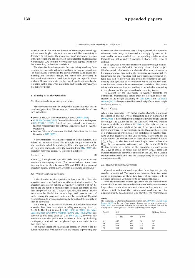
actual waves at the location. Instead of observed/measured sig-nificant wave heights, hindcast data are used. The uncertainty isdescribed by estimating the mean values and standard deviationsof the difference and ratio between the hindcasted and forecastedwave heights. Data from the Norwegian Sea are applied to quantifythe uncertainty in the forecasted data.
The objective is to incorporate the uncertainty resulting fromweather forecasts into reliability analyses for marine operations.For most marine operations, the environmental loads govern theplanning and structural design, and hence, the uncertainty inforecasted environmental conditions is important input for theseanalyses. The uncertainty in the forecasted significant wave heightis studied in this paper. The intent is to address reliability analysesin a separate paper.
2. Planning of marine operations
2.1. Design standards for marine operations
Marine operations must be designed in accordance with certainstandards/guidelines. We are aware of two such standards and twosuch guidelines:
DNV-OS-H101, Marine Operations, General, DNV (2011). GL Noble Denton (2013), General Guidelines for Marine Projects. ISO 19901-6 (2009) Petroleum and natural gas industries.
Specific requirements for offshore structures. Part 6: MarineOperations.
London Offshore Consultants Limited, Guidelines for MarineOperations, LOC (1997).
A key parameter for a marine operation is the duration. It isdefined as the best estimate plus an ample margin to account forinaccuracies in schedule and delays. This is the approach used inall referenced standards. Using the notation from DNV (2011), theoperation reference period, TR, is defined as follows:
T T T 1R POP C= + ( )
where TPOP is the planned operation period and TC is the estimatedmaximum contingency time. (The estimated maximum con-tingency time is often between 50% and 100% of the plannedoperation period, unless more accurate information is known.)
2.2. Weather-restricted operations
If the duration of the operation is less than 72 h, then theoperation can be defined as a weather-restricted operation. Anoperation can also be defined as weather restricted if it can behalted and the handled object brought into safe conditions duringthe same period. For a sea transport operation, this means that theroute must be divided into several legs, and ports or areas ofshelter along the transport route must be predefined. Updatedweather forecasts are received regularly throughout the entirety ofsuch an operation.
Traditionally, the maximum duration of a weather-restrictedoperation has been three days including contingency time, i.e.,T 72 hR ≤ . This limit is stated in ISO 19901-6 (2009), GL NobleDenton (2013), LOC (1997), NORSOK (2007). DNV (1996/2000) alsoadhered to this limit until 2011. In DNV (2011), however, themaximum operation period was increased to four days includingcontingency provided that the planned operation period is lessthan three days.
For marine operations in areas and seasons in which it can bedemonstrated that weather forecasts are capable of predicting any
extreme weather conditions over a longer period, the operationreference period may be increased accordingly. By contrast, inareas and/or seasons in which the corresponding reliable weatherforecasts are not considered realistic, a shorter limit is to beapplied.
If an operation is weather restricted, then the design environ-mental criteria are defined in an early phase of the project.Weather-restricted operations are beneficial because the owner, orhis representative, may define the necessary environmental cri-teria (with the understanding that more strict environmental cri-teria may lead to more wait time before the operation can com-mence). The operation may commence when the weather fore-casts indicate acceptable environmental conditions. The uncer-tainty in the weather forecasts and how to include this uncertaintyin the planning of the operation thus become key issues.
To account for the uncertainty in weather forecasts, theoperational environmental limits must be less than those con-sidered in the design. According to DNV (2011) and GL NobleDenton (2013), the operational limit on the significant wave heightcan be expressed as
H H 2s oper s design, ,α= ( )
where α is a parameter 1( ≤ ) that depends on both the duration ofthe operation and the level of forecasting and/or monitoring. InDNV (2011), α also depends on the significant wave height used inthe design. The parameters for the base case, with one weatherforecast available, are shown in Table 1. The α-factor can beincreased if the wave height at the site of the operation is mon-itored and if there is a meteorologist on site (because the presenceof a meteorologist will increase the confidence in weather fore-casts at that location). In the DNV method, α accounts for theuncertainty in the weather forecast based on the planned duration( T TDur POP= ), but the forecasted wave height must be less thanHs oper, for the operation reference period, TR. In the GL NobleDenton method, α is based on the operation reference periodT TDur R( = ). It should be noted that the safety formats (load andmaterial factors) are somewhat different in the DNV and GL NobleDenton formulations and that the corresponding αs may not bedirectly comparable.
2.3. Weather-unrestricted operations
Operations with durations longer than three days are typicallyweather unrestricted. The separation between these two cate-gories is important, as these two types of operations will bedesigned differently with respect to environmental loads.
Weather-unrestricted marine operations are not planned basedon weather forecasts, because the duration of such an operation islonger than the duration over which weather forecasts are con-sidered reliable. Instead, the environmental conditions used forplanning must be based on long-term statistics. The environmental
Table 1The parameter α as a function of operation duration from DNV (2011) and GL NobleDenton (2013) for the case of one weather forecast and no wave monitoring. InDNV (2011), the parameter definition is valid only for the North Sea and theNorwegian Sea and is given as a function of the design wave height.
TDur (h) DNV GL Noble Denton
H 2 ms = 4 m ≥ 6 m
12 0.76 0.79 0.8 0.6924 0.73 0.76 0.78 0.6548 0.68 0.71 0.74 0.5972 0.63 0.68 0.72 0.54
A. Natskår et al. / Ocean Engineering 108 (2015) 636–647 637
130 Appended papers
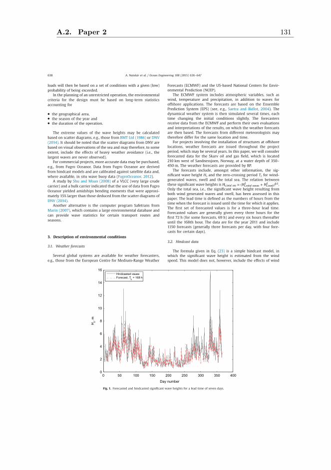
loads will then be based on a set of conditions with a given (low)probability of being exceeded.
In the planning of an unrestricted operation, the environmentalcriteria for the design must be based on long-term statisticsaccounting for
the geographical area, the season of the year and the duration of the operation.
The extreme values of the wave heights may be calculatedbased on scatter diagrams, e.g., those from BMT Ltd (1986) or DNV(2014). It should be noted that the scatter diagrams from DNV arebased on visual observations of the sea and may therefore, to someextent, include the effects of heavy weather avoidance (i.e., thelargest waves are never observed).
For commercial projects, more accurate data may be purchased,e.g., from Fugro Oceanor. Data from Fugro Oceanor are derivedfrom hindcast models and are calibrated against satellite data and,where available, in situ wave buoy data (FugroOceanor, 2012).
A study by Shu and Moan (2008) of a VLCC (very large crudecarrier) and a bulk carrier indicated that the use of data from FugroOceanor yielded amidships bending moments that were approxi-mately 15% larger than those deduced from the scatter diagrams ofDNV (2014).
Another alternative is the computer program Safetrans fromMarin (2007), which contains a large environmental database andcan provide wave statistics for certain transport routes andseasons.
3. Description of environmental conditions
3.1. Weather forecasts
Several global systems are available for weather forecasters,e.g., those from the European Centre for Medium-Range Weather
Forecasts (ECMWF) and the US-based National Centers for Envir-onmental Prediction (NCEP).
The ECMWF system includes atmospheric variables, such aswind, temperature and precipitation, in addition to waves foroffshore applications. The forecasts are based on the EnsemblePrediction System (EPS) (see, e.g., Saetra and Bidlot, 2004). Thedynamical weather system is then simulated several times, eachtime changing the initial conditions slightly. The forecastersreceive data from the ECMWF and perform their own evaluationsand interpretations of the results, on which the weather forecastsare then based. The forecasts from different meteorologists maytherefore differ for the same location and time.
For projects involving the installation of structures at offshorelocations, weather forecasts are issued throughout the projectperiod, which may be several years. In this paper, we will considerforecasted data for the Skarv oil and gas field, which is located210 km west of Sandnessjoen, Norway, at a water depth of 350–450 m. The weather forecasts are provided by BP.
The forecasts include, amongst other information, the sig-nificant wave height Hs and the zero-crossing period Tz for wind-generated waves, swell and the total sea. The relation betweenthese significant wave heights is H H Hs total sea s wind waves s swell, ,
2,
2 0.5= ( + ) .Only the total sea, i.e., the significant wave height resulting fromboth wind generated waves and swell, has been assessed in thispaper. The lead time is defined as the numbers of hours from thetime when the forecast is issued until the time for which it applies.The first set of forecasted values is for a three-hour lead time.Forecasted values are generally given every three hours for thefirst 72 h (for some forecasts, 69 h) and every six hours thereafteruntil the 168th hour. The data are for the year 2011 and include1150 forecasts (generally three forecasts per day, with four fore-casts for certain days).
3.2. Hindcast data
The formula given in Eq. (23) is a simple hindcast model, inwhich the significant wave height is estimated from the windspeed. This model does not, however, include the effects of wind
0 50 100 150 200 250 300 350 4000
2
4
6
8
10
12
14
16
Day number
H, m
Fig. 1. Forecasted and hindcasted significant wave heights for a lead time of seven days.
A. Natskår et al. / Ocean Engineering 108 (2015) 636–647638
A.2. Paper 2 131
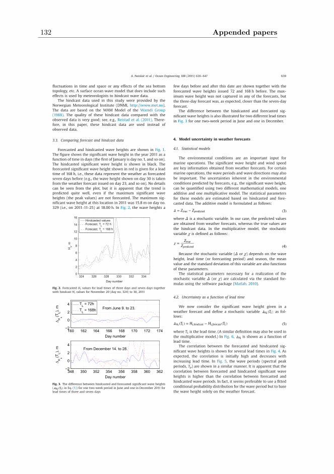
fluctuations in time and space or any effects of the sea bottomtopology, etc. A surface ocean wave model that does include sucheffects is used by meteorologists to hindcast wave data.
The hindcast data used in this study were provided by theNorwegian Meteorological Institute (DNMI, http://www.met.no).The data are based on the WAM Model of the Wamdi Group(1988). The quality of these hindcast data compared with theobserved data is very good; see, e.g., Reistad et al. (2011). There-fore, in this paper, these hindcast data are used instead ofobserved data.
3.3. Comparing forecast and hindcast data
Forecasted and hindcasted wave heights are shown in Fig. 1.The figure shows the significant wave height in the year 2011 as afunction of time in days (the first of January is day no. 1, and so on).The hindcasted significant wave height is shown in black. Theforecasted significant wave height shown in red is given for a leadtime of 168 h, i.e., these data represent the weather as forecastedseven days before (e.g., the wave height shown on day 30 is takenfrom the weather forecast issued on day 23, and so on). No detailscan be seen from the plot, but it is apparent that the trend ispredicted quite well, even if the maximum significant waveheights (the peak values) are not forecasted. The maximum sig-nificant wave height at this location in 2011 was 15.8 m on day no.329 (i.e., on 2011-11-25) at 18.00 h. In Fig. 2, the wave heights a
few days before and after this date are shown together with theforecasted wave heights issued 72 and 168 h before. The max-imum wave height was not captured in any of the forecasts, butthe three-day forecast was, as expected, closer than the seven-dayforecast.
The difference between the hindcasted and forecasted sig-nificant wave heights is also illustrated for two different lead timesin Fig. 3 for one two-week period in June and one in December.
4. Model uncertainty in weather forecasts
4.1. Statistical models
The environmental conditions are an important input formarine operations. The significant wave height and wind speedare key information obtained from weather forecasts. For certainmarine operations, the wave periods and wave directions may alsobe important. The uncertainties inherent in the environmentalconditions predicted by forecasts, e.g., the significant wave height,can be quantified using two different mathematical models, oneadditive and one multiplicative model. The statistical parametersfor these models are estimated based on hindcasted and fore-casted data. The additive model is formulated as follows:
Z Z 3true predictedΔ = − ( )
where Δ is a stochastic variable. In our case, the predicted valuesare obtained from weather forecasts, whereas the true values arethe hindcast data. In the multiplicative model, the stochasticvariable χ is defined as follows:
ZZ 4
true
predictedχ =
( )
Because the stochastic variable (Δ or χ) depends on the waveheight, lead time (or forecasting period) and season, the meanvalue and the standard deviation of this variable are also functionsof these parameters.
The statistical parameters necessary for a realization of thestochastic variable Δ (or χ) are calculated via the standard for-mulas using the software package (Matlab, 2010).
4.2. Uncertainty as a function of lead time
We now consider the significant wave height given in aweather forecast and define a stochastic variable TH LsΔ ( ) as fol-lows:
T H H T 5H L s hindcast s forecast L, ,sΔ ( ) = − ( ) ( )
where TL is the lead time. (A similar definition may also be used inthe multiplicative model.) In Fig. 6, HsΔ is shown as a function oflead time.
The correlation between the forecasted and hindcasted sig-nificant wave heights is shown for several lead times in Fig. 4. Asexpected, the correlation is initially high and decreases withincreasing lead time. In Fig. 5, the wave periods (spectral peakperiods, Tp) are shown in a similar manner. It is apparent that thecorrelation between forecasted and hindcasted significant waveheights is higher than the correlation between forecasted andhindcasted wave periods. In fact, it seems preferable to use a fittedconditional probability distribution for the wave period but to basethe wave height solely on the weather forecast.
160 162 164 166 168 170 172 174−2
0
2
4
Day number
Δ Hs(T
L), m From June 9. to 23.
348 350 352 354 356 358 360 362−2
0
2
4
Day number
Δ Hs(T
L), m From December 14. to 28.
TL = 72hTL = 168h
Fig. 3. The difference between hindcasted and forecasted significant wave heights( THs LΔ ( ) in Eq. (5)) for one two-week period in June and one in December 2011 forlead times of three and seven days
324 326 328 330 332 3340
2
4
6
8
10
12
14
16
Day number
Hs, m
Hindcasted valuesForecast, TL = 72 hForecast, TL = 168 h
Fig. 2. Forecasted Hs values for lead times of three days and seven days togetherwith hindcast Hs values for November 20 (day no. 324) to 30, 2011
A. Natskår et al. / Ocean Engineering 108 (2015) 636–647 639
132 Appended papers
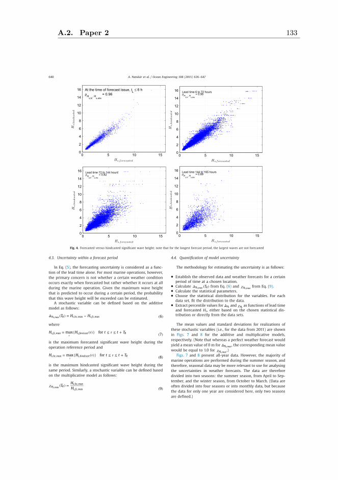
4.3. Uncertainty within a forecast period
In Eq. (5), the forecasting uncertainty is considered as a func-tion of the lead time alone. For most marine operations, however,the primary concern is not whether a certain weather conditionoccurs exactly when forecasted but rather whether it occurs at allduring the marine operation. Given the maximum wave heightthat is predicted to occur during a certain period, the probabilitythat this wave height will be exceeded can be estimated.
A stochastic variable can be defined based on the additivemodel as follows:
T H H 6H R s hc max s fc max, , , ,s max,Δ ( ) = − ( )
where
H H t t Tmax for 7s fc max s forecast R, , , τ τ= ( ) ≤ ≤ + ( )τ
is the maximum forecasted significant wave height during theoperation reference period and
H H t t Tmax for 8s hc max s hindcast R, , , τ τ= ( ) ≤ ≤ + ( )τ
is the maximum hindcasted significant wave height during thesame period. Similarly, a stochastic variable can be defined basedon the multiplicative model as follows:
THH 9H R
s hc max
s fc max
, ,
, ,s max,
χ ( ) =( )
4.4. Quantification of model uncertainty
The methodology for estimating the uncertainty is as follows:
Establish the observed data and weather forecasts for a certainperiod of time at a chosen location.
Calculate TH Rs max,Δ ( ) from Eq. (6) and Hs max,χ from Eq. (9). Calculate the statistical parameters. Choose the statistical distribution for the variables. For each
data set, fit the distribution to the data. Extract percentile values for HsΔ and Hs
χ as functions of lead timeand forecasted Hs, either based on the chosen statistical dis-tribution or directly from the data sets.
The mean values and standard deviations for realizations ofthese stochastic variables (i.e., for the data from 2011) are shownin Figs. 7 and 8 for the additive and multiplicative models,respectively. (Note that whereas a perfect weather forecast wouldyield a mean value of 0 m for Hs max,Δ , the corresponding mean valuewould be equal to 1.0 for Hs max,χ .)
Figs. 7 and 8 present all-year data. However, the majority ofmarine operations are performed during the summer season, andtherefore, seasonal data may be more relevant to use for analysingthe uncertainties in weather forecasts. The data are thereforedivided into two seasons: the summer season, from April to Sep-tember, and the winter season, from October to March. (Data areoften divided into four seasons or into monthly data, but becausethe data for only one year are considered here, only two seasonsare defined.)
Fig. 4. Forecasted versus hindcasted significant wave height; note that for the longest forecast period, the largest waves are not forecasted
A. Natskår et al. / Ocean Engineering 108 (2015) 636–647640
A.2. Paper 2 133
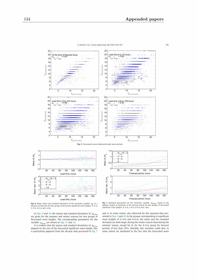
In Figs. 9 and 10, the means and standard deviations of Hs max,Δare given for the summer and winter seasons for two groups offorecasted wave heights. The corresponding parameters for thevariable Hs max,χ are shown in Figs. 11 and 12.
It is evident that the means and standard deviations of Hs max,Δdepend on the size of the forecasted significant wave height; thisis particularly apparent from the all-year data presented in Fig. 7
and is, to some extent, also observed for the seasonal data pre-sented in Figs. 9 and 10. In the groups corresponding to significantwave heights of 2–4 m and 4–6 m, the mean and the standarddeviation are both larger during the winter season than during thesummer season, except for Hs for the 4–6 m group for forecastperiods of less than 50 h. (Notably, this variation could also, tosome extent, be attributed to the fact that the forecasted wave
20 40 60 80 100 120 140 1600
0.5
1
1.5
Forecast period, hours
Mea
n of
ΔH
s
20 40 60 80 100 120 140 1600
1
2
3
Forecast period, hours
Sta
nd. d
ev. o
fΔH
s
Hs,fc=0 − 22 − 44 − 66 −
Fig. 7. Statistical parameters for the stochastic variable Hs max,Δ , based on theadditive model, as functions of the forecast period for four groups of forecastedsignificant wave heights: 0–2 m, 2–4 m, 4–6 m and 6 m>
20 40 60 80 100 120 140 160−2
−1
0
1
2
Lead time, hours
Mea
n of
ΔH
s
20 40 60 80 100 120 140 1600
1
2
3
4
Lead time, hours
Sta
nd. d
ev. o
fΔH
s
Hs,fc=0 − 2
2 − 44 − 6≥ 6
Fig. 6. Mean values and standard deviations of the stochastic variable HsΔ as afunction of lead time for four groups of forecasted significant wave heights: 0–2 m,2–4 m, 4–6 m and 6 m> .
Fig. 5. Forecasted versus hindcasted peak wave periods
A. Natskår et al. / Ocean Engineering 108 (2015) 636–647 641
134 Appended papers
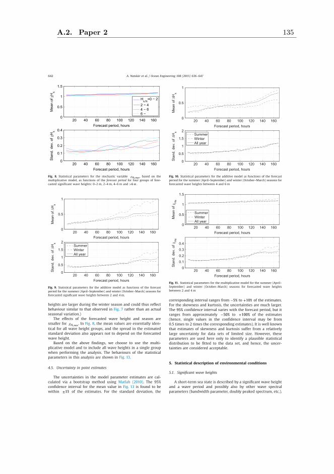
heights are larger during the winter season and could thus reflectbehaviour similar to that observed in Fig. 7 rather than an actualseasonal variation.)
The effects of the forecasted wave height and season aresmaller for Hs max,χ . In Fig. 8, the mean values are essentially iden-tical for all wave height groups, and the spread in the estimatedstandard deviation also appears not to depend on the forecastedwave height.
Based on the above findings, we choose to use the multi-plicative model and to include all wave heights in a single groupwhen performing the analysis. The behaviours of the statisticalparameters in this analysis are shown in Fig. 13.
4.5. Uncertainty in point estimates
The uncertainties in the model parameter estimates are cal-culated via a bootstrap method using Matlab (2010). The 95%confidence interval for the mean value in Fig. 13 is found to bewithin 1%± of the estimates. For the standard deviation, the
corresponding interval ranges from 5%− to 10%+ of the estimates.For the skewness and kurtosis, the uncertainties are much larger.The 95% confidence interval varies with the forecast period, but itranges from approximately 50%− to 100%+ of the estimates(hence, single values in the confidence interval may be from0.5 times to 2 times the corresponding estimates). It is well knownthat estimates of skewness and kurtosis suffer from a relativelylarge uncertainty for data sets of limited size. However, theseparameters are used here only to identify a plausible statisticaldistribution to be fitted to the data set, and hence, the uncer-tainties are considered acceptable.
5. Statistical description of environmental conditions
5.1. Significant wave heights
A short-term sea state is described by a significant wave heightand a wave period and possibly also by other wave spectralparameters (bandwidth parameter, doubly peaked spectrum, etc.).
20 40 60 80 100 120 140 1600
0.5
1
Forecast period, hours
Mea
n of
ΔH
s
20 40 60 80 100 120 140 1600
0.5
1
1.5
2
Forecast period, hours
Sta
nd. d
ev. o
fΔH
s
SummerWinterAll year
Fig. 9. Statistical parameters for the additive model as functions of the forecastperiod for the summer (April–September) and winter (October–March) seasons forforecasted significant wave heights between 2 and 4 m.
20 40 60 80 100 120 140 1600
0.5
1
Forecast period, hours
Mea
n of
ΔH
s
20 40 60 80 100 120 140 1600
0.5
1
1.5
2
Forecast period, hoursS
tand
. dev
. ofΔ
Hs
SummerWinterAll year
Fig. 10. Statistical parameters for the additive model as functions of the forecastperiod for the summer (April–September) and winter (October–March) seasons forforecasted wave heights between 4 and 6 m
20 40 60 80 100 120 140 1600
0.5
1
1.5
Forecast period, hours
Mea
n of
χH
s
20 40 60 80 100 120 140 1600
0.1
0.2
0.3
0.4
Forecast period, hours
Sta
nd. d
ev. o
fχH
s
SummerWinterAll year
Fig. 11. Statistical parameters for the multiplicative model for the summer (April–September) and winter (October–March) seasons for forecasted wave heightsbetween 2 and 4 m
20 40 60 80 100 120 140 1600
0.5
1
1.5
Forecast period, hours
Mea
n of
χH
s
20 40 60 80 100 120 140 1600
0.1
0.2
0.3
0.4
Forecast period, hours
Sta
nd. d
ev. o
fχH
s
Hs,fc=0 − 22 − 44 − 66 −
Fig. 8. Statistical parameters for the stochastic variable Hs max,χ , based on themultiplicative model, as functions of the forecast period for four groups of fore-casted significant wave heights: 0–2 m, 2–4 m, 4–6 m and 6 m> .
A. Natskår et al. / Ocean Engineering 108 (2015) 636–647642
A.2. Paper 2 135
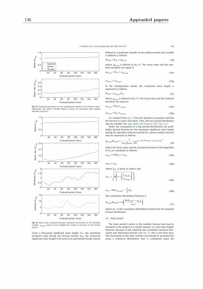
Given a forecasted significant wave height (i.e., the maximumpredicted value during the forecast period) hs fc, , the maximumsignificant wave height to be used in an operational design may be
defined as a stochastic variable. In the additive model, this variableis defined as follows:
H h 10s max s fc H, , s max,Δ= + ( )
where Hs max,Δ is defined in Eq. (6). The mean value and the stan-dard deviation are equal to
h 11aH s fc,s max Hs max, ,μ μ= + ( )Δ
11bHs max Hs max, ,σ σ= ( )Δ
In the multiplicative model, the maximum wave height isexpressed as follows:
H h 12s max H s fc, ,s max,χ= · ( )
where Hs max,χ is defined in Eq. (9). The mean value and the standarddeviation are equal to
h 13aH s fc,s max Hs max, ,μ μ= · ( )χ
h 13bH s fc,s max Hs max, ,σ σ= · ( )χ
It is evident from Fig. 13 that the skewness is positive and thatthe kurtosis is larger than three. Thus, the log-normal distributionmay be suitable (see, e.g., Hahn and Shapiro, 1967, Fig. 6-1).
Under the assumption of a log-normal distribution, the prob-ability density function for the maximum significant wave heightduring the operation reference period for a given weather forecastmay be expressed as follows:
f hh
e1
2 14H max s max
H s max
h, ,
ln ,
1/2 ln /s
s
s max Hs Hs, ln ln2
σ π( ) =
( )μ σ−( )(( − ) )
where the mean value and the standard deviation of the logarithmof Hs are calculated as follows:
hln 15aH s fcln , lnsμ μ= ( ) + ( )χ
15bHln lnsσ σ= ( )χ
where hs fc, is given in meters and
⎛
⎝⎜⎜
⎛⎝⎜⎜
⎞⎠⎟⎟
⎞
⎠⎟⎟ln 1
16aln
2Hs max
Hs max
,
,
σσ
μ= +
( )χ
χ
χ
ln12 16bln ln
2Hs max,
μ μ σ= ( ) − ( )χ χ χ
The cumulative distribution function is
⎛⎝⎜
⎞⎠⎟F h
hln
17H s max
s max H
H,
, ln
lns max
s
s, Φ
μσ
( ) =( ) −
( )
where Φ ( ) is the cumulative distribution function for the standardnormal distribution.
5.2. Wave period
The wave period is given in the weather forecast and may beincluded in the analysis in a similar manner as is the wave height.However, because of the relatively low correlation between fore-casted and hindcasted periods (see Fig. 5), this is not done here.The uncertainty in the wave periods can instead be accounted forusing a statistical distribution that is conditional upon the
20 40 60 80 100 120 140 1600
0.5
1
1.5
Forecast period, hours
Mea
n of
χH
s
20 40 60 80 100 120 140 1600.1
0.2
0.3
0.4
Forecast period, hours
Sta
nd. d
ev. o
fχH
s
20 40 60 80 100 120 140 1600
0.5
1
1.5
2
Forecast period, hours
Ske
wne
ss o
f χH
s
20 40 60 80 100 120 140 1600
5
10
15
Forecast period, hours
Kur
tosi
s of
χH
s
Fig. 13. Mean value, standard deviation, skewness and kurtosis of the stochasticvariable Hs max,χ , based on the multiplicative model, as functions of the forecastperiod.
20 40 60 80 100 120 140 1600
0.5
1
1.5
Forecast period, hours
Mea
n of
χH
s
20 40 60 80 100 120 140 1600
0.1
0.2
0.3
0.4
Forecast period, hours
Sta
nd. d
ev. o
fχH
s
SummerWinterAll year
Fig. 12. Statistical parameters for the multiplicative model for the summer (April–September) and winter (October–March) seasons for forecasted wave heightsbetween 4 and 6 m.
A. Natskår et al. / Ocean Engineering 108 (2015) 636–647 643
136 Appended papers
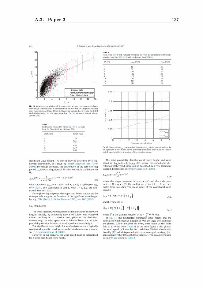
significant wave height. The period may be described by a log-normal distribution, as shown by Bitner-Gregersen and Haver(1991). For design purposes, the distribution of the zero-crossingperiod, Tz, follows a log-normal distribution that is conditional onHs:
f t ht
e1
2 18T H
T
t
ln
1/2 ln /z s
z
Tz Tzln ln2
σ π( | ) =
( )μ σ
|−( )(( − ) )
with parameters a a hTa
ln 1 2z3μ = + and b b eT
b hln 1 2z
3σ = + (see, e.g.,DNV, 2014). The coefficients ai and bi, with i 1, 2, 3= , are esti-mated from real data.
For engineering purposes, the upper and lower bounds on thewave periods are given as functions of the significant wave heightby, e.g., DNV (2011), GL Noble Denton (2013), and LOC (1997).
5.3. Wind speed
The wind speed may be treated in a similar manner as the waveheights, namely, by comparing forecasted values with observedvalues, resulting in a statistical description of the deviation.Alternatively, the wind speed can be inferred based on the jointprobability density function of wind speed and wave height.
The significant wave height for wind-driven waves is typicallyconditional upon the wind speed, as the wind creates such waves;see, e.g., Johannessen et al. (2002).
However, in our scenario, the wind speed must be determinedfor a given significant wave height.
The joint probability distribution of wave height and windspeed is f v h f h f v h,V H H V H, s s s
( ) = ( ) ( | )| , where the conditional dis-tribution of the wind speed can be described by a two-parameterWeibull distribution; see Bitner-Gregersen (2005):
f v h kvV
e19
V H
k
Ck
v V1
/s
Ck( | ) =
( )|
−−( )
where the shape parameter is k c c hc1 2 3= + and the scale para-
meter is V c c hCc
4 5 6= + . The coefficients ci, i 1, 2, , 6= … , are esti-mated from real data. The mean value of the conditional windspeed is
⎛⎝⎜
⎞⎠⎟E V H V
k1
120V H s Cs
μ Γ= [ | ] = +( )|
and the variance is
⎛⎝⎜
⎛⎝⎜
⎞⎠⎟
⎛⎝⎜
⎞⎠⎟
⎞⎠⎟V
k k1
21
121
V H C2 2 2
sσ Γ Γ= + − +( )|
where Γ is the gamma function t x e xdt x0
1∫Γ( ( ) = )∞ − − .
In Fig. 14, the hindcasted significant wave height and thehindcasted wind speed at a height of 10 m averaged over one hourare plotted. Values are given for every three hours at the Skarvfield in 2010 and 2011 (Table 3). In the same figure is also plottedthe wind speed indicated by the conditional Weibull distributionfrom Eq. (19), which is plotted with error bars equal to 2 V Hsσ± | (i.e.,approximately the 95% confidence interval). The parameters usedin Eq. (19) are given in Table 2.
Fig. 14. Wind speed at a height of 10 m averaged over one hour versus significantwave height (hindcast data) at the Skarv field for 2010 and 2011, together with thewave-wind relation obtained from Holthuijsen's formula, Eq. (24), and the fittedWeibull distribution, i.e., the mean value from Eq. (20) with error bars of 2 V Hsσ± |(see Eq. (21))
Table 2Coefficients obtained by fitting Eq. (19) to the datafrom the Skarv field for 2010 and 2011.
Coefficient Fitted value
c1 1.23c2 0.55c3 1.17c4 0.00c5 5.19c6 0.61
Table 3Mean wind speeds and standard deviations based on the conditional Weibull dis-tribution (see Eqs. (19)–(21)) with coefficients from Table 2.
Hs (m) V Hsμ | (m/s) V Hsσ | (m/s)
1 4.6 2.72 7.0 3.04 10.9 3.06 14.2 2.98 17.2 2.710 19.9 2.512 22.4 2.414 24.7 2.2
Fig. 15. Mean value lnμ( )χ and standard deviation lnσ( )χ of the logarithm of χ in themultiplicative model, based on the previously mentioned Skarv data for all fore-casted wave heights, as a function of the operation period.
A. Natskår et al. / Ocean Engineering 108 (2015) 636–647644
A.2. Paper 2 137
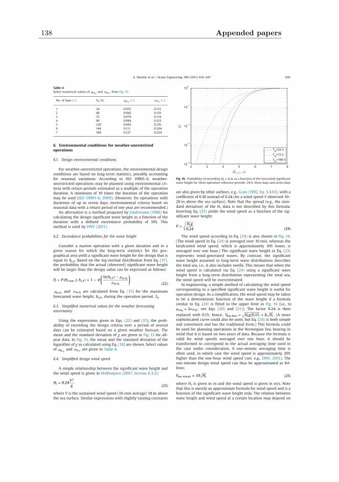
6. Environmental conditions for weather-unrestrictedoperations
6.1. Design environmental conditions
For weather-unrestricted operations, the environmental designconditions are based on long-term statistics, possibly accountingfor seasonal variations. According to ISO 19901-6, weather-unrestricted operations may be planned using environmental cri-teria with return periods estimated as a multiple of the operationduration. A minimum of 10 times the duration of the operationmay be used (ISO 19901-6, 2009). (However, for operations withdurations of up to seven days, environmental criteria based onseasonal data with a return period of one year are recommended.)
An alternative is a method proposed by Lindemann (1986) forcalculating the design significant wave height as a function of theduration with a defined exceedance probability of 10%. Thismethod is used by DNV (2011).
6.2. Exceedance probabilities for the wave height
Consider a marine operation with a given duration and in agiven season for which the long-term statistics for the geo-graphical area yield a significant wave height for the design that isequal to hs d, . Based on the log-normal distribution from Eq. (17),the probability that the actual (observed) significant wave heightwill be larger than the design value can be expressed as follows:
⎛⎝⎜
⎞⎠⎟P P H h
h1
ln
22e s max s d
s d H
H, ,
, ln
ln
s
s
Φμ
σ= ( ≥ ) = −
( ) −
( )
Hln sμ and Hln sσ are calculated from Eq. (15) for the maximumforecasted wave height, hs fc, , during the operation period, TR.
6.3. Simplified numerical values for the weather forecastinguncertainty
Using the expressions given in Eqs. (22) and (15), the prob-ability of exceeding the design criteria over a period of severaldays can be estimated based on a given weather forecast. Themean and the standard deviation of χ are given in Fig. 13 for all-year data. In Fig. 15, the mean and the standard deviation of thelogarithm of χ as calculated using Eq. (16) are shown. Select valuesof lnμ χ and lnσ χ are given in Table 4.
6.4. Simplified design wind speed
A simple relationship between the significant wave height andthe wind speed is given in Holthuijsen (2007, Section 6.3.2):
HVg
0.2423
s
2=
( )
where V is the sustained wind speed (10-min average) 10 m abovethe sea surface. Similar expressions with slightly varying constants
are also given by other authors, e.g., Gran (1992, Eq. 3.4.63), with acoefficient of 0.18 instead of 0.24 (for a wind speed V observed 10–20 m above the sea surface). Note that the spread (e.g., the stan-dard deviation) of the Hs data is not described by this formula.Inverting Eq. (23) yields the wind speed as a function of the sig-nificant wave height:
VH g0.24 24
s=( )
The wind speed according to Eq. (24) is also shown in Fig. 14.(The wind speed in Eq. (24) is averaged over 10 min, whereas thehindcasted wind speed, which is approximately 10% lower, isaveraged over one hour.) The significant wave height in Eq. (23)represents wind-generated waves. By contrast, the significantwave height assumed in long-term wave distributions describesthe total sea, i.e., it also includes swells. This means that when thewind speed is calculated via Eq. (24) using a significant waveheight from a long-term distribution representing the total sea,the wind speed will be overestimated.
In engineering, a simple method of calculating the wind speedcorresponding to a specified significant wave height is useful foroperation design. As a simplification, the wind speed may be takento be a deterministic function of the wave height if a formulasimilar to Eq. (24) is fitted to the upper limit in Fig. 14 (i.e., to
2V H V Hs sμ σ+| | ; see Eqs. (20) and (21)). The factor 0.24 is then
replaced with 0.15; hence, V H g H/0.15 8one hour s s= ≈ . (A moresophisticated curve could also be used, but Eq. (24) is both simpleand convenient and has the traditional form.) This formula couldbe used for planning operations in the Norwegian Sea, bearing inmind that it is based on two years of data. Because the formula isvalid for wind speeds averaged over one hour, it should betransformed to correspond to the actual averaging time used inthe case under consideration. A one-minute averaging time isoften used, in which case the wind speed is approximately 20%higher than the one-hour wind speed (see, e.g., DNV, 2011). Theone-minute design wind speed can thus be approximated as fol-lows:
V H10 25one minute s≈ ( )
where Hs is given in m and the wind speed is given in m/s. Notethat this is merely an approximate formula for wind speed and is afunction of the significant wave height only. The relation betweenwave height and wind speed at a certain location may depend on
Table 4Select numerical values of lnμ χ and lnσ χ , from Fig. 15.
No. of days (–) TR (h) lnμ χ (–) lnσ χ (–)
1 24 0.055 0.1122 48 0.066 0.1193 72 0.079 0.1344 96 0.084 0.1535 120 0.095 0.1766 144 0.111 0.2047 168 0.127 0.224
Fig. 16. Probability of exceeding H 6 ms = as a function of the forecasted significantwave height for three operation reference periods: 24 h, three days and seven days
A. Natskår et al. / Ocean Engineering 108 (2015) 636–647 645
138 Appended papers
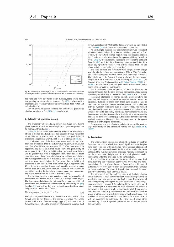
the wind and wave directions, storm duration, fetch, water depthand possibly other covariates. However, Eq. (25) can be used forengineering or feasibility studies and is valid for deep water andunlimited fetch.
For structural reliability analyses, the conditional probabilitydistribution given in Eqs. (19)–(21) may be used.
7. Reliability of a weather forecast
The probability of exceeding a certain significant wave heightgiven a certain forecasted wave height and operation period canbe estimated from Eq. (22).
In Fig. 16, the probability of exceeding a significant wave heightof 6 m is plotted as a function of the forecasted wave height forthree different operation periods. Similarly, the probability ofexceeding a significant wave height of 9 m is plotted in Fig. 17.
It is observed that if the forecasted wave height is, e.g., 4 m,then the probability that the actual wave height will be greaterthan 6 m after 24 h is approximately 103; after three days, it isapproximately 102; and after seven days, the probability ofexceedance is 101. The probability that the actual wave heightwill be greater than 9 m is negligible after either 24 h or threedays. After seven days, the probability of exceeding a wave heightof 9 m is approximately 103. It is also apparent from Fig. 17 that ifthe forecasted wave height is 6 m, then the probability ofexceeding a 9 m wave height after seven days is approximately101. Hence, the weather forecasts still provide interesting infor-mation even after one week. Because the results are sensitive tothe tail of the distribution when extreme values are considered,the values here should be taken as examples only.
The primary concern in engineering is not the probability ofexceedance but rather how to calculate a design wave height.The design wave height can be estimated for a given probability ofexceedance and a forecasted wave height. By substituting Eq. (15)into Eq. (22) and solving for Hs d, , the maximum significant waveheight can be calculated as follows:
H h Pexp 1 26s d s fc e, , ln ln1μ σ Φ= ( + ( − )) ( )χ χ
−
The probability of exceedance, Pe, should correspond to the safetyformat used in the design of the marine operation. The safetyfactors used in the structural design (typically load and materialfactors) will depend on the probability of exceeding a certain load
level. A probability of 10% that the design wave will be exceeded isused in DNV (2011) for weather-unrestricted operations.
As an example, suppose that the maximum allowed forecastedsignificant wave height for a certain marine operation is 5 m.(Hence, the operation cannot begin before the forecasts indicateH 5 ms ≤ for the entire duration of the operation.) Using the valuesfrom Table 4, the maximum significant wave heights obtainedfrom Eq. (26) are 6.4 m for a three-day operation and 7.6 m for aseven-day operation, with Pe¼0.1. (These would then be thecharacteristic values to be used in design.)
The ratio between the forecasted wave height and the designwave height for a three-day operation is 5/6.4 0.78= . This valuecan then be compared with the values from the design standards.The ratio between the forecasted wave height and the design waveheight for a 72-h operation is 0.72 according to DNV (2011) (forH 6 ms design, ≥ ) and 0.54 according to GL Noble Denton (2013); seeTable 1. Hence, these standards yield conservative results com-pared with our data set in this case.
For a seven-day operation period, no ratio is given by thedesign standards, but the ratio between the forecasted and designwave heights according to the results from Table 4 is 5/7.6 0.66= .
In general, standards for marine operations do not allow theplanning and design to be based on weather forecasts when theoperation duration is more than three days unless it can bedemonstrated that the relevant weather forecasts can predict anyextreme weather conditions over a longer period. The methoddescribed in this paper may be used to assess the reliability of suchweather forecasts, preferably based on a more extensive data set.Because only weather forecasts for a single location are included inthe data set considered in this paper, the results cannot be directlyapplied elsewhere. However, they are considered to be repre-sentative of extratropical conditions.
Because only one year of data is included, there will be a ratherlarge uncertainty in the calculated values; see, e.g., Moan et al.(2005).
8. Conclusions
The uncertainty in environmental conditions based on weatherforecasts has been studied. Forecasted significant wave heightshave been compared with hindcasted values using an additive anda multiplicative statistical model. In the additive model, the meanvalue and the standard deviation are more strongly dependent onthe forecasted wave height than in the multiplicative model,making the latter the preferred model in this study.
The uncertainty in the forecasts increases with increasing leadtime, reducing the correlation between the forecasted and hind-casted data. The correlation between forecasted and hindcasteddata is lower for wave periods than for significant wave heights forthe same lead time. Therefore, it is preferable to model the waveperiod conditionally upon the wave height.
The wind speed may be modelled using a Weibull distributionthat is conditional upon the wave height. For marine operations inwhich the governing environmental load is caused by waves andthe corresponding wind speed must be estimated, a simple engi-neering method is proposed. The relationship between wind speedand wave height was developed for wind-driven waves. Hence, ifthe waves in fact contain swells in addition to wind-driven waves,then the wind speed may be overestimated. Moreover, in shelteredwater or other cases in which there may be high wind speeds butsmall or no waves, this method is not applicable. In such cases, itwill be necessary to determine the wind speed using othermethods, e.g., the return period approach based on the duration ofthe operation.
Fig. 17. Probability of exceeding H 9 ms = as a function of the forecasted significantwave height for three operation reference periods: 24 h, three days and seven days.
A. Natskår et al. / Ocean Engineering 108 (2015) 636–647646
A.2. Paper 2 139
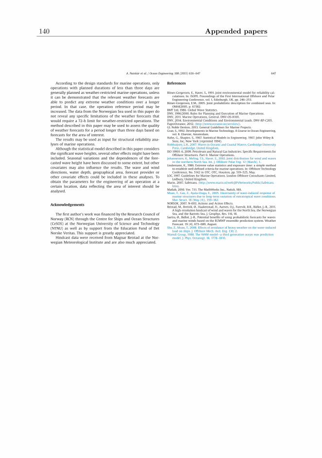
According to the design standards for marine operations, onlyoperations with planned durations of less than three days aregenerally planned as weather-restricted marine operations, unlessit can be demonstrated that the relevant weather forecasts areable to predict any extreme weather conditions over a longerperiod. In that case, the operation reference period may beincreased. The data from the Norwegian Sea used in this paper donot reveal any specific limitations of the weather forecasts thatwould require a 72-h limit for weather-restricted operations. Themethod described in this paper may be used to assess the qualityof weather forecasts for a period longer than three days based onforecasts for the area of interest.
The results may be used as input for structural reliability ana-lyses of marine operations.
Although the statistical model described in this paper considersthe significant wave heights, several other effects might have beenincluded. Seasonal variations and the dependences of the fore-casted wave height have been discussed to some extent, but othercovariates may also influence the results. The wave and winddirections, water depth, geographical area, forecast provider orother covariate effects could be included in these analyses. Toobtain the parameters for the engineering of an operation at acertain location, data reflecting the area of interest should beanalysed.
Acknowledgements
The first author's work was financed by the Research Council ofNorway (RCN) through the Centre for Ships and Ocean Structures(CeSOS) at the Norwegian University of Science and Technology(NTNU) as well as by support from the Education Fund of DetNorske Veritas. This support is greatly appreciated.
Hindcast data were received from Magnar Reistad at the Nor-wegian Meteorological Institute and are also much appreciated.
References
Bitner-Gregersen, E., Haver, S., 1991. Joint environmental model for reliability cal-culations. In: ISOPE. Proceedings of the First International Offshore and PolarEngineering Conference, vol. 1, Edinburgh, UK, pp. 246–253.
Bitner-Gregersen, E.M., 2005. Joint probabilistic description for combined seas. In:OMAE2005, p. 67382.
BMT Ltd, 1986. Global Wave Statistics.DNV, 1996/2000. Rules for Planning and Execution of Marine Operations.DNV, 2011. Marine Operations, General. DNV-OS-H101.DNV, 2014. Environmental Conditions and Environmental Loads. DNV-RP-C205.FugroOceanor, 2012. ⟨http://www.oceanor.no/services/⟩.GL Noble Denton, 2013. General Guidelines for Marine Projects.Gran, S., 1992. Developments in Marine Technology. A Course in Ocean Engineering,
vol. 8. Elsevier, Amsterdam.Hahn, G., Shapiro, S., 1967. Statistical Models in Engineering. 1967. John Wiley &
Sons, Inc, New York (reprinted 1994).Holthuijsen, L.H., 2007. Waves in Oceanic and Coastal Waters. Cambridge University
Press, Cambridge, United Kingdom.ISO 19901-6, 2009. Petroleum and Natural Gas Industries. Specific Requirements for
Offshore Structures. Part 6: Marine Operations.Johannessen, K., Meling, T.S., Haver, S., 2002. Joint distribution for wind and waves
in the northern North Sea. Int. J. Offshore Polar Eng. 12 (March), 1.Lindemann, K., 1986. Extreme value statistics and exposure time: a simple method
to establish well defined criteria for marine operations. In: Offshore TechnologyConference, No. 5142 in OTC. OTC, Houston, pp. 519–525, May.
LOC, 1997. Guidelines for Marine Operations. London Offshore Consultants Limited,Ledbury, United Kingdom.
Marin, 2007. Safetrans. ⟨http://www.marin.nl/web/JIPsNetworks/Public/Safetrans.htm⟩.
Matlab, 2010. Ver. 7.11. The MathWorks Inc., Natick, MA.Moan, T., Gao, Z., Ayala-Uraga, E., 2005. Uncertainty of wave-induced response of
marine structures due to long-term variation of extratropical wave conditions.Mar. Struct. 18 (May (4)), 359–382.
NORSOK, 2007. N-003, Actions and Action Effects.Reistad, M., Breivik, Ø., Haakenstad, H., Aarnes, O.J., Furevik, B.R., Bidlot, J.-R., 2011.
A high-resolution hindcast of wind and waves for the North Sea, the NorwegianSea, and the Barents Sea. J. Geophys. Res. 116, 18.
Saetra, Ø., Bidlot, J.-R., Potential benefits of using probabilistic forecasts for wavesand marine winds based on the ECMWF ensemble prediction system. WeatherForecast. 19 (4), 673–689, August.
Shu, Z., Moan, T., 2008. Effects of avoidance of heavy weather on the wave-inducedload on ships. J. Offshore Mech. Arct. Eng. 130, 2.
Wamdi Group, 1988. The WAM model—a third generation ocean wav predictionmodel. J. Phys. Oceanogr. 18, 1778–1810.
A. Natskår et al. / Ocean Engineering 108 (2015) 636–647 647
140 Appended papers
A.3. Paper 3 141
A.3 Paper 3
Paper 3:Structural reliability analysis of a seafastening structure for sea transport
of heavy objects.Authors: Asle Natskår and Torgeir Moan.
Issued for publication in Ocean Engineering.

This paper is awaiting publication and is not included in NTNU Open
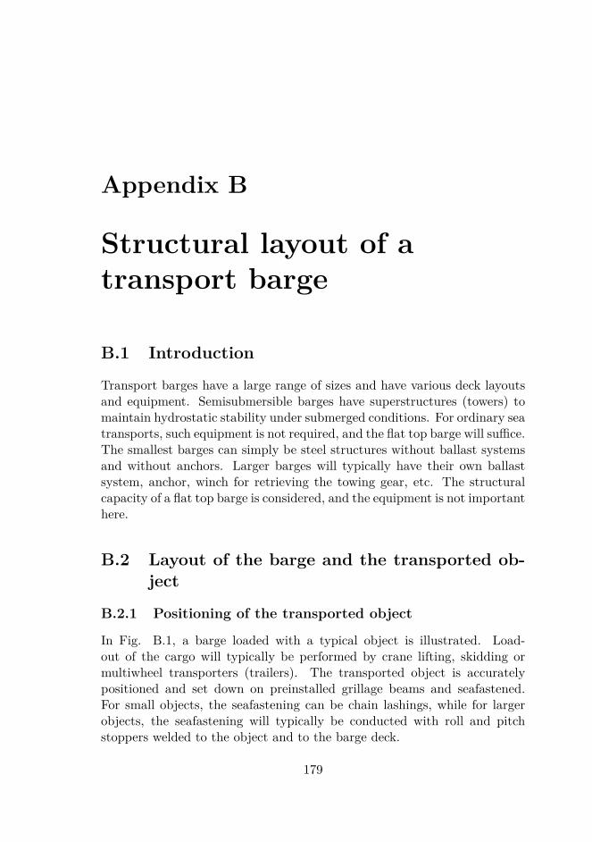
Appendix B
Structural layout of atransport barge
B.1 Introduction
Transport barges have a large range of sizes and have various deck layoutsand equipment. Semisubmersible barges have superstructures (towers) tomaintain hydrostatic stability under submerged conditions. For ordinary seatransports, such equipment is not required, and the flat top barge will suffice.The smallest barges can simply be steel structures without ballast systemsand without anchors. Larger barges will typically have their own ballastsystem, anchor, winch for retrieving the towing gear, etc. The structuralcapacity of a flat top barge is considered, and the equipment is not importanthere.
B.2 Layout of the barge and the transported ob-ject
B.2.1 Positioning of the transported object
In Fig. B.1, a barge loaded with a typical object is illustrated. Load-out of the cargo will typically be performed by crane lifting, skidding ormultiwheel transporters (trailers). The transported object is accuratelypositioned and set down on preinstalled grillage beams and seafastened.For small objects, the seafastening can be chain lashings, while for largerobjects, the seafastening will typically be conducted with roll and pitchstoppers welded to the object and to the barge deck.
179
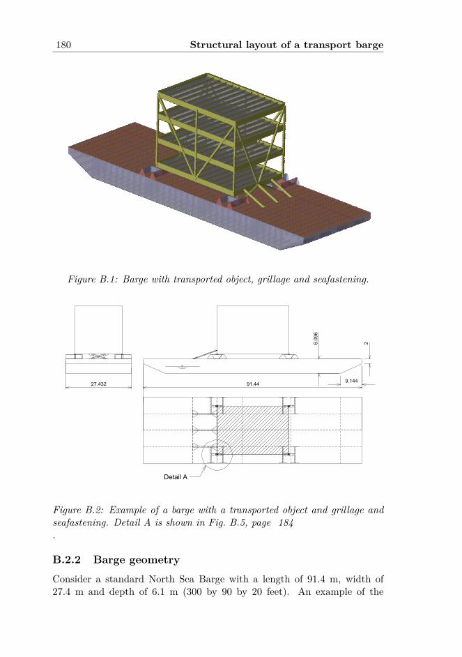
180 Structural layout of a transport barge
Figure B.1: Barge with transported object, grillage and seafastening.
[Academic use only]
Figure B.2: Example of a barge with a transported object and grillage andseafastening. Detail A is shown in Fig. B.5, page 184.
B.2.2 Barge geometry
Consider a standard North Sea Barge with a length of 91.4 m, width of27.4 m and depth of 6.1 m (300 by 90 by 20 feet). An example of the
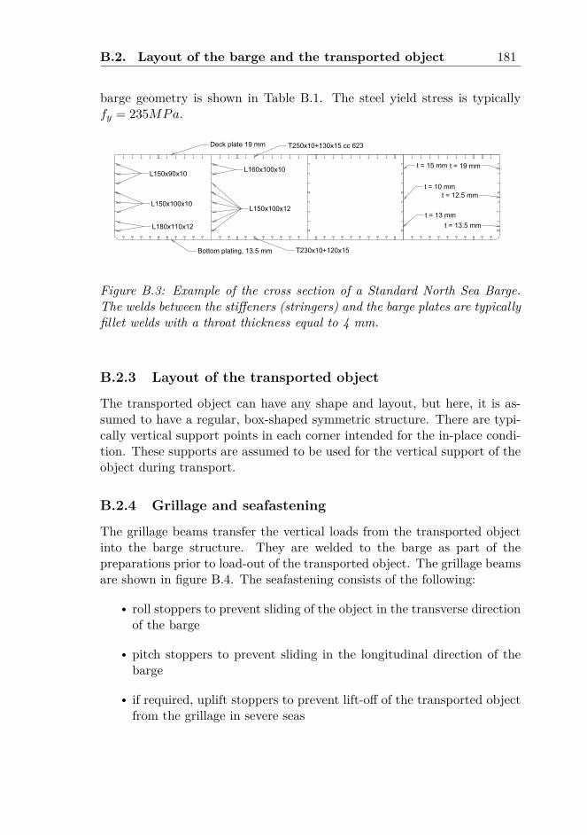
B.2. Layout of the barge and the transported object 181
barge geometry is shown in Table B.1. The steel yield stress is typicallyfy = 235MPa.
[Academic use only]
Figure B.3: Example of the cross section of a Standard North Sea Barge.The welds between the stiffeners (stringers) and the barge plates are typicallyfillet welds with a throat thickness equal to 4 mm.
B.2.3 Layout of the transported object
The transported object can have any shape and layout, but here, it is as-sumed to have a regular, box-shaped symmetric structure. There are typi-cally vertical support points in each corner intended for the in-place condi-tion. These supports are assumed to be used for the vertical support of theobject during transport.
B.2.4 Grillage and seafastening
The grillage beams transfer the vertical loads from the transported objectinto the barge structure. They are welded to the barge as part of thepreparations prior to load-out of the transported object. The grillage beamsare shown in figure B.4. The seafastening consists of the following:
r roll stoppers to prevent sliding of the object in the transverse directionof the barge
r pitch stoppers to prevent sliding in the longitudinal direction of thebarge
r if required, uplift stoppers to prevent lift-off of the transported objectfrom the grillage in severe seas
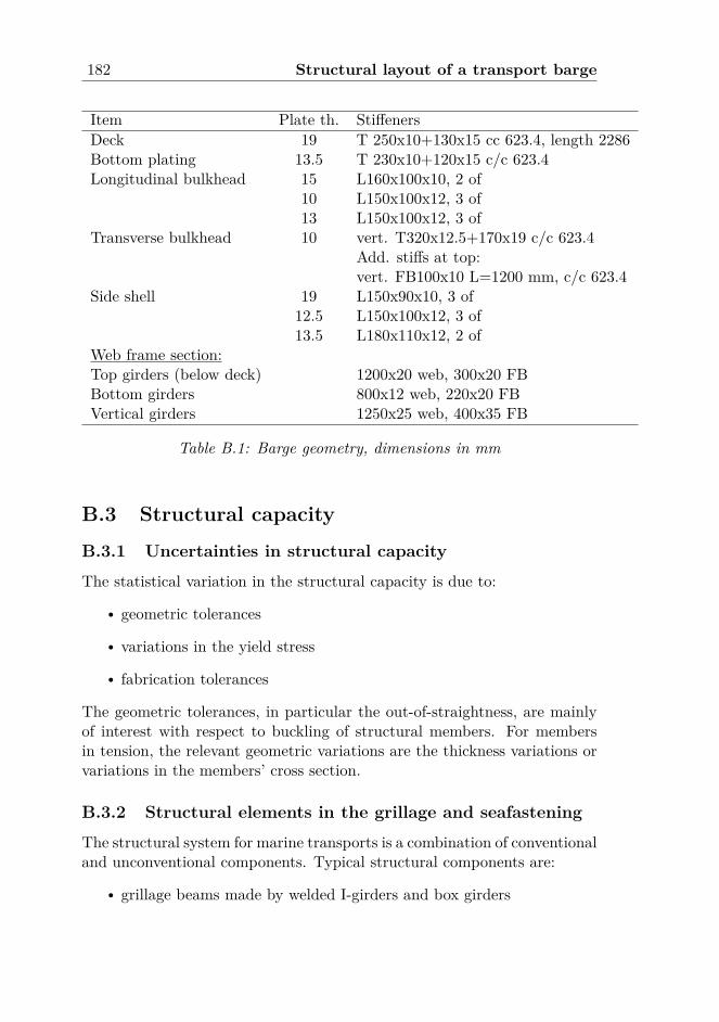
182 Structural layout of a transport barge
Item Plate th. StiffenersDeck 19 T 250x10+130x15 cc 623.4, length 2286Bottom plating 13.5 T 230x10+120x15 c/c 623.4Longitudinal bulkhead 15 L160x100x10, 2 of
10 L150x100x12, 3 of13 L150x100x12, 3 of
Transverse bulkhead 10 vert. T320x12.5+170x19 c/c 623.4Add. stiffs at top:vert. FB100x10 L=1200 mm, c/c 623.4
Side shell 19 L150x90x10, 3 of12.5 L150x100x12, 3 of13.5 L180x110x12, 2 of
Web frame section:Top girders (below deck) 1200x20 web, 300x20 FBBottom girders 800x12 web, 220x20 FBVertical girders 1250x25 web, 400x35 FB
Table B.1: Barge geometry, dimensions in mm
B.3 Structural capacity
B.3.1 Uncertainties in structural capacity
The statistical variation in the structural capacity is due to:r geometric tolerancesr variations in the yield stressr fabrication tolerances
The geometric tolerances, in particular the out-of-straightness, are mainlyof interest with respect to buckling of structural members. For membersin tension, the relevant geometric variations are the thickness variations orvariations in the members’ cross section.
B.3.2 Structural elements in the grillage and seafastening
The structural system for marine transports is a combination of conventionaland unconventional components. Typical structural components are:r grillage beams made by welded I-girders and box girders

B.3. Structural capacity 183
Figure B.4: Iso-view of grillage beams preinstalled on the barge deck
r the connection between the grillage beams and the barge, typicallymade from plates welded to the barge deck (wing plates) to distributethe load to the web frames and bulkheadsr tubular or rectangular hollow sections used as pitch and roll stoppersr roll and pitch stoppers connected to the barge deck and the trans-ported object by gusset platesr concentrated vertical loads in the stiffened panels, i.e., bulkhead andweb framesr concentrated horizontal loads in the deck (horizontal component ofthe load in the roll and pitch stoppers)
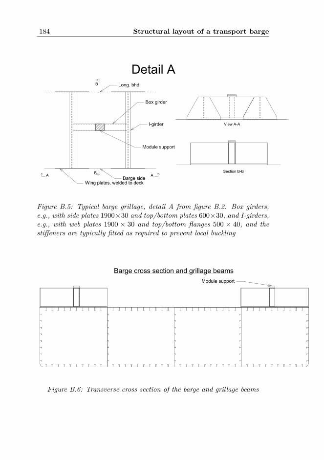
184 Structural layout of a transport barge
[Academic use only]
Figure B.5: Typical barge grillage, detail A from figure B.2. Box girders,e.g., with side plates 1900×30 and top/bottom plates 600×30, and I-girders,e.g., with web plates 1900 × 30 and top/bottom flanges 500 × 40, and thestiffeners are typically fitted as required to prevent local buckling
[Academic use only]
Figure B.6: Transverse cross section of the barge and grillage beams
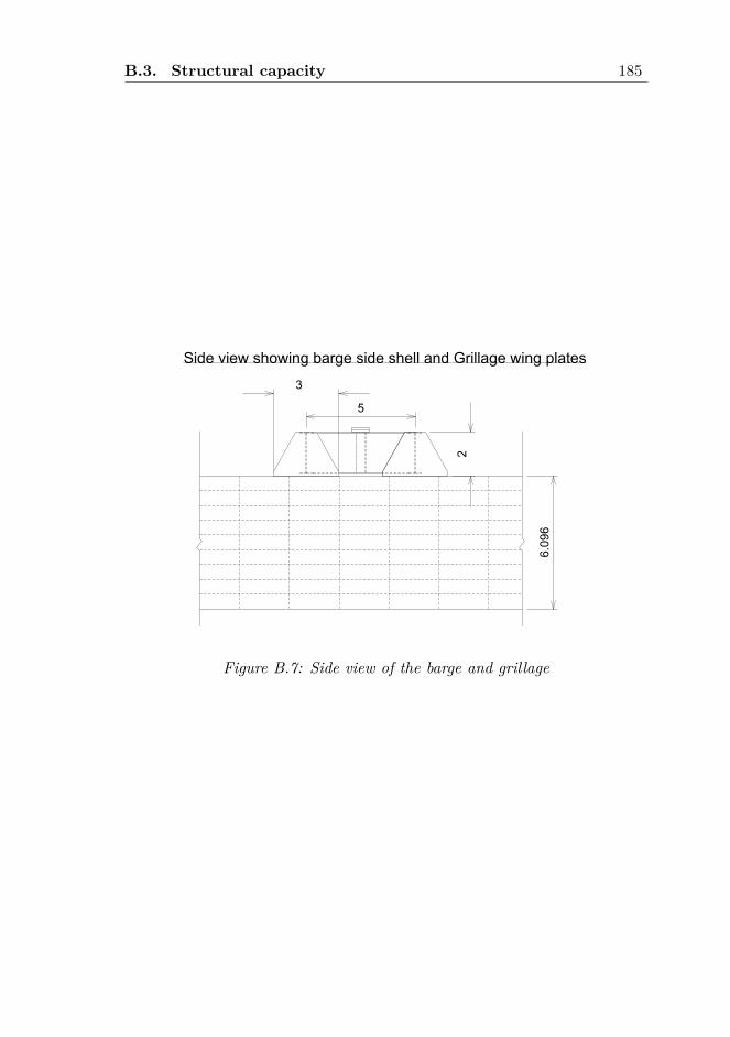
B.3. Structural capacity 185
[Academic use only]
Figure B.7: Side view of the barge and grillage

186 Structural layout of a transport barge
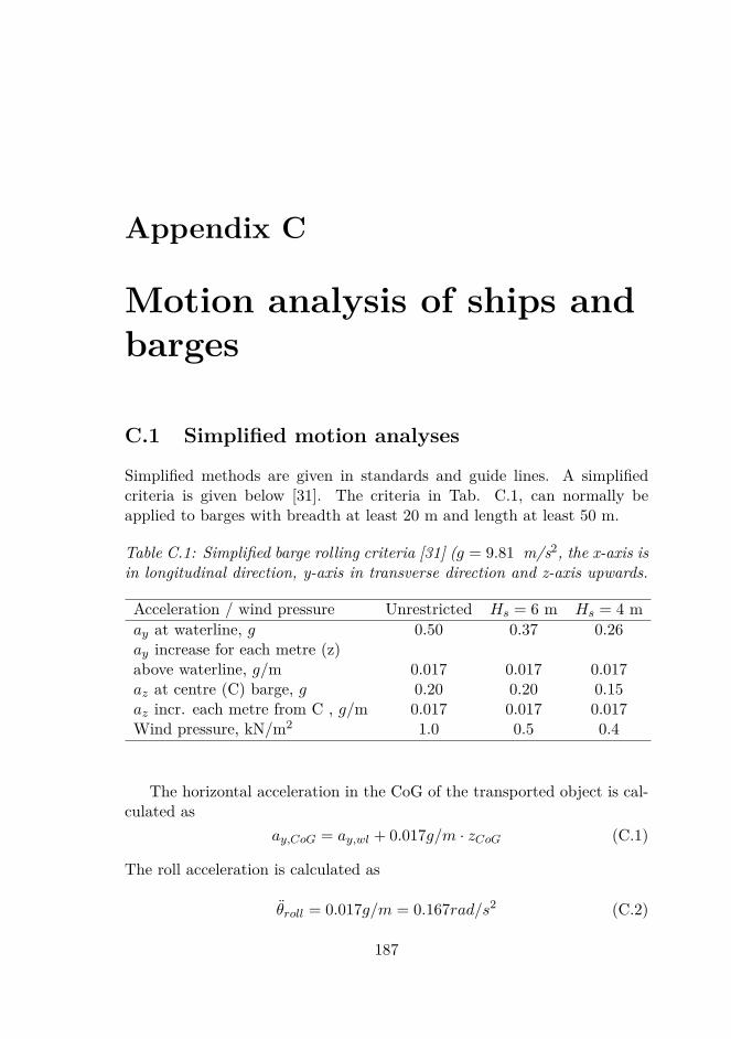
Appendix C
Motion analysis of ships andbarges
C.1 Simplified motion analyses
Simplified methods are given in standards and guide lines. A simplifiedcriteria is given below [31]. The criteria in Tab. C.1, can normally beapplied to barges with breadth at least 20 m and length at least 50 m.
Table C.1: Simplified barge rolling criteria [31] (g = 9.81 m/s2, the x-axis isin longitudinal direction, y-axis in transverse direction and z-axis upwards.
Acceleration / wind pressure Unrestricted Hs = 6 m Hs = 4 may at waterline, g 0.50 0.37 0.26ay increase for each metre (z)above waterline, g/m 0.017 0.017 0.017az at centre (C) barge, g 0.20 0.20 0.15az incr. each metre from C , g/m 0.017 0.017 0.017Wind pressure, kN/m2 1.0 0.5 0.4
The horizontal acceleration in the CoG of the transported object is cal-culated as
ay,CoG = ay,wl + 0.017g/m · zCoG (C.1)
The roll acceleration is calculated as
θroll = 0.017g/m = 0.167rad/s2 (C.2)
187
188 Motion analysis of ships and barges
The simplified accelerations for the Roll Case in Tab. C.1 are used in [107]to calculate the seafastening forces for a typical barge transport.
C.2 Linear analysis in frequency domainThe equation of motion for a floating vessel is expressed on complex formin the frequency domain as
[M +A(ω)]η + [B1(ω) +Beq]η +Cη = F0(ω)eiωt (C.3)
wherer ω is the angular frequency of the wave in rad/sr F0(ω) is the amplitude of the wave load, given on complex formr M is the mass matrix for the barge including the transported objectr A(ω) is the hydrodynamic added mass matrixr B1(ω) is the linear damping matrix from potential damping (due towave radiation)r Beq is the equivalent linear damping representing the non-linear damp-ing caused by vortex shedding at the bilges. This matrix has only onenon-zero element; B2,44 for rollr C is the restoring matrixr η = [η1 η2 η3 η4 η5 η6]T is the motion vector; index 1-6 means surge,sway, heave, roll, pitch and yaw, respectively
It is noted that even if the equation of motion is given on complex form, thesolution of interest is the real part of the mathematical solution. The waveload, F0(ω), the added mass, A(ω), and the potential damping matrix,B1(ω), are calculated from potential theory using the boundary elementmethod, and is a function of the wave frequency, see e.g., [38]. The methodis implemented in commercial software, e.g., Wadam [129].
The viscous damping is not calculated by potential theory, but it isestimated by empirical methods. The viscous damping is caused by vortexshedding at the bilges and is estimated as a quadratic damping term. Thequadratic damping is replaced by an equivalent damping term B2,44 whenthe equation of motion is solved in the frequency domain. More details aregiven in [120] and in [109].
C.3. Non-linear analysis in the time domain 189
When Eq. (C.3) is solved in the frequency domain, the transfer functionsfor the motion in six degrees of freedom is found as follows:
Hζη(ω) =(−[M +A(ω)]ω2 + [B1(ω) +Beq]iω +C
)−1F0(ω) (C.4)
The vessel motion no. j is calculated as follows:
ηj = Hζη,j(ω)eiωt (C.5)
Based on this transfer function and the power spectrum Sζ(ω) for the seaelevation, the power spectrum of the vessel motion can be calculated asfollows [104]:
Sη,j(ω) = H2ζη,j(ω)Sζ(ω) (C.6)
The expected maximum response during N cycles is estimated under theassumption that the individual response maxima follow a Rayleigh distri-bution and is calaulated as follows:
ηmax = ση,j
(√2 lnN + 0.577√
2 lnN
)(C.7)
where the variance of the response is calculated as σ2η,j =
∫∞0 Sη,j(ω)dω.
C.3 Non-linear analysis in the time domain
The non-linearity can be included in many forms in the hydrodynamic anal-yses. From a slightly non-linear to a highly non-linear model. In this thesis,the non-linear analysis in time domain is based on the wave load, the addedmass and the wave radiation damping from potential theory. The reason forrunning the analysis in the time domain is that the viscous damping do nothave to be linearized, but can be kept on a quadratic form in the equationof motion.
Below, the equation of motion as defined in a ship fixed coordinatesystem is studied, as used on the time domain analyses. It is seen thatsome additional non-linear terms are included into the equation, terms thatare negligible for small vessel motions, but will affect the solution for largermotions.
C.3.1 Coordinate systems
While the coordinate system used in the frequency domain analysis wasearth fixed, e.g., in Wadam [129], a ship fixed coordinate system is used,
190 Motion analysis of ships and barges
in accordance with Simo [131]. For large motions, the choice of coordinatesystem will affect the results, ref. Sec. 3.4. In order to describe the motion,several coordinate systems are used in Simo:r A global coordinate systemr A local, body fixed, coordinate systemr A body related coordinate system
The body related coordinate system follows the body horizontal motion,and the xy-plane is parallel to the global xy-plane
C.3.2 Equations of motion
In the following, the equations of motions are solved in local (ship fixed)coordinates. Using a body fixed coordinate system in the time domainanalysis introduce some additional terms in the equations of motions. Forsmall waves and small ship motions, these terms are negligible, but in severeseas they will affect the solution. This topic was discussed in Paper 1, butnot in much details. Therefore, the equitations are derived in more detailbelow to illustrate this interesting result of the choice of coordinate system.
The kinetics for the vessel is described by setting the time derivative ofthe momentum equal to the external forces:
PB = F (C.8)LB = M (C.9)
where the linear momentum is given as
PB = m(u+ Ω× rc) (C.10)
and the angular momentum is given as
LB = IΩ +mrc × u (C.11)
where
I =
Ix 0 00 Iy 00 0 Iz
, Ω =
pqr
, rc =
xcyczc
and u =
uvw
(C.12)
I is the rotational inertia, Ω is the rotational velocity, rc is the CoG-positionand u is the translational velocity. When the vectors are defined in the
C.3. Non-linear analysis in the time domain 191
local coordinate system, the time derivative will have to account for themotion of the local system relative to the global system. As an example,the velocity is differentiated with respect to time. The velocity can bewritten as u = ue1 + ve2 + we3, where the unit vectors ei are functions oftime. The time derivative is then:
u = ∂u
∂t= ue1 + ve2 + we3︸ ︷︷ ︸
≡u∗
+ue1 + ve2 + we3︸ ︷︷ ︸≡Ω×u
(C.13)
A derivation of this expression is given by Faltinsen [39, page 422-423].Equations (C.8) and (C.9) can now be expressed as
P∗B + Ω× PB = F (C.14)
L∗B + Ω×LB + u× PB = M (C.15)
Let us now consider beam sea exposure. Then q = r = u = 0. Further,it is assumed that the centre of gravity is located in the symmetry plane,such that xc = yc = 0.
The equations of motions will then be considerably simplified.Let us write the vector cross products used above:
Ω× rc =
∣∣∣∣∣∣∣
i j kp 0 00 0 zc
∣∣∣∣∣∣∣=
0−zcp
0
(C.16)
The linear momentum is then:
PB = m
0v − zcpw
(C.17)
Further,
rc × u =
∣∣∣∣∣∣∣
i j k0 0 zc0 v w
∣∣∣∣∣∣∣=
−zcv
00
(C.18)
The angular momentum is then:
LB =
Ixp−mzcv
00
(C.19)
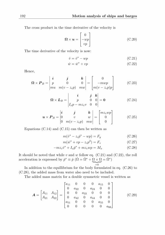
192 Motion analysis of ships and barges
The cross product in the time derivative of the velocity is
Ω× u =
0−wpvp
(C.20)
The time derivative of the velocity is now:
v = v∗ − wp (C.21)w = w∗ + vp (C.22)
Hence,
Ω× PB =
∣∣∣∣∣∣∣
i j kp 0 0mu m(v − zcp) mw
∣∣∣∣∣∣∣=
0−mwp
m(v − zcp)p
(C.23)
Ω×LB =
∣∣∣∣∣∣∣
i j kp 0 0
Ixp−mzcv 0 0
∣∣∣∣∣∣∣= 0 (C.24)
u× PB =
∣∣∣∣∣∣∣
i j k0 v w0 m(v − zcp) mw
∣∣∣∣∣∣∣=
mzcwp
00
(C.25)
Equations (C.14) and (C.15) can then be written as
m(v∗ − zcp∗ − wp) = Fy (C.26)m(w∗ + vp− zcp2) = Fz (C.27)
−mzcv∗ + Ixp∗ +mzcwp = Mx (C.28)
It should be noted that while v and w follow eq. (C.21) and (C.22), the rollacceleration is expressed by p∗ ≡ p (Ω = Ω∗ + Ω× Ω︸ ︷︷ ︸
=0
= Ω∗)
In addition to the equillibrium for the body formulated in eq. (C.26) to(C.28), the added mass from water also need to be included.
The added mass matrix for a double symmetric vessel is written as
A =[A11 A12A21 A22
]=
a11 0 0 0 a15 00 a22 0 a24 0 00 0 a33 0 0 00 a42 0 a44 0 0a51 0 0 0 a55 00 0 0 0 0 a66
(C.29)
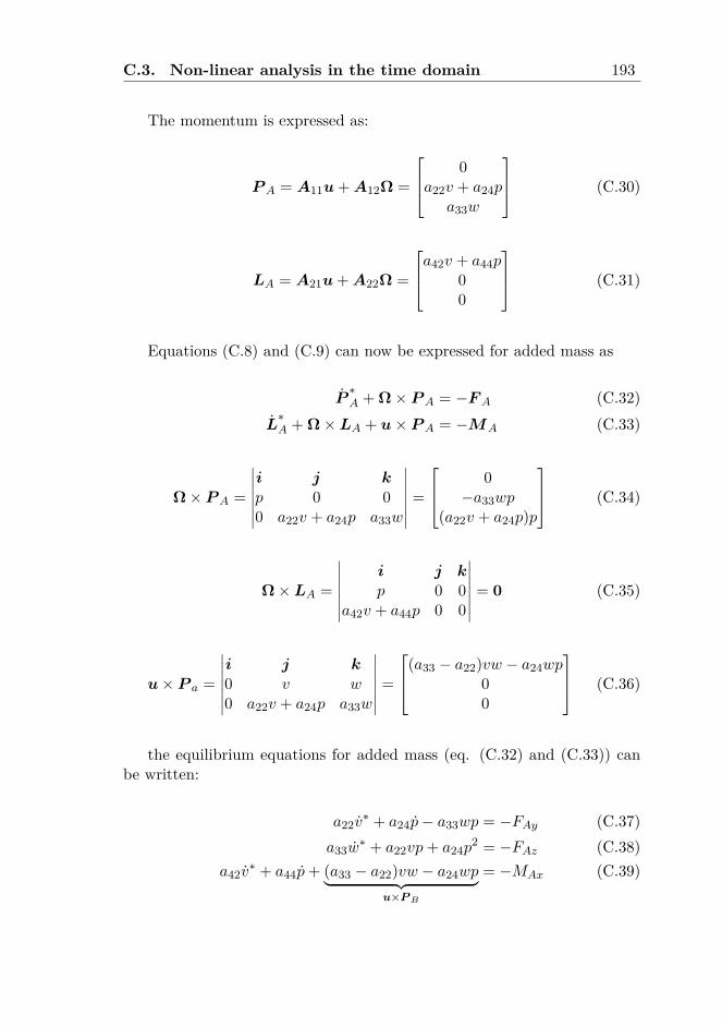
C.3. Non-linear analysis in the time domain 193
The momentum is expressed as:
PA = A11u+A12Ω =
0a22v + a24p
a33w
(C.30)
LA = A21u+A22Ω =
a42v + a44p
00
(C.31)
Equations (C.8) and (C.9) can now be expressed for added mass as
P∗A + Ω× PA = −FA (C.32)
L∗A + Ω×LA + u× PA = −MA (C.33)
Ω× PA =
∣∣∣∣∣∣∣
i j kp 0 00 a22v + a24p a33w
∣∣∣∣∣∣∣=
0−a33wp
(a22v + a24p)p
(C.34)
Ω×LA =
∣∣∣∣∣∣∣
i j kp 0 0
a42v + a44p 0 0
∣∣∣∣∣∣∣= 0 (C.35)
u× P a =
∣∣∣∣∣∣∣
i j k0 v w0 a22v + a24p a33w
∣∣∣∣∣∣∣=
(a33 − a22)vw − a24wp00
(C.36)
the equilibrium equations for added mass (eq. (C.32) and (C.33)) canbe written:
a22v∗ + a24p− a33wp = −FAy (C.37)
a33w∗ + a22vp+ a24p
2 = −FAz (C.38)a42v
∗ + a44p+ (a33 − a22)vw − a24wp︸ ︷︷ ︸u×PB
= −MAx (C.39)
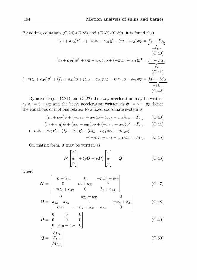
194 Motion analysis of ships and barges
By adding equations (C.26)-(C.28) and (C.37)-(C.39), it is found that
(m+ a22)v∗ + (−mzc + a24)p− (m+ a33)wp = Fy − FAy︸ ︷︷ ︸=FI,y(C.40)
(m+ a33)w∗ + (m+ a22)vp+ (−mzc + a24)p2 = Fz − FAz︸ ︷︷ ︸=FI,z(C.41)
(−mzc + a42)v∗ + (Ix + a44)p+ (a33 − a22)vw +mzcvp− a24wp = Mx −MAx︸ ︷︷ ︸=MI,x
(C.42)
By use of Eqs. (C.21) and (C.22) the sway acceleration may be writtenas v∗ = v + wp and the heave acceleration written as w∗ = w − vp, hencethe equations of motions related to a fixed coordinate system is
(m+ a22)v + (−mzc + a24)p+ (a22 − a33)wp = FI,y (C.43)(m+ a33)w + (a22 − a33)vp+ (−mzc + a24)p2 = FI,z (C.44)
(−mzc + a42)v + (Ix + a44)p+ (a33 − a22)vw +mzcvp
+(−mzc + a42 − a24)wp = MI,x (C.45)
On matrix form, it may be written as
N
vwp
+ (pO + vP )
vwp
= Q (C.46)
where
N =
m+ a22 0 −mzc + a240 m+ a33 0
−mzc + a42 0 Ix + a44
(C.47)
O =
0 a22 − a33 0a22 − a33 0 −mzc + a24mzc −mzc + a42 − a24 0
(C.48)
P =
0 0 00 0 00 a33 − a22 0
(C.49)
Q =
FI,yFI,zMI,x
(C.50)
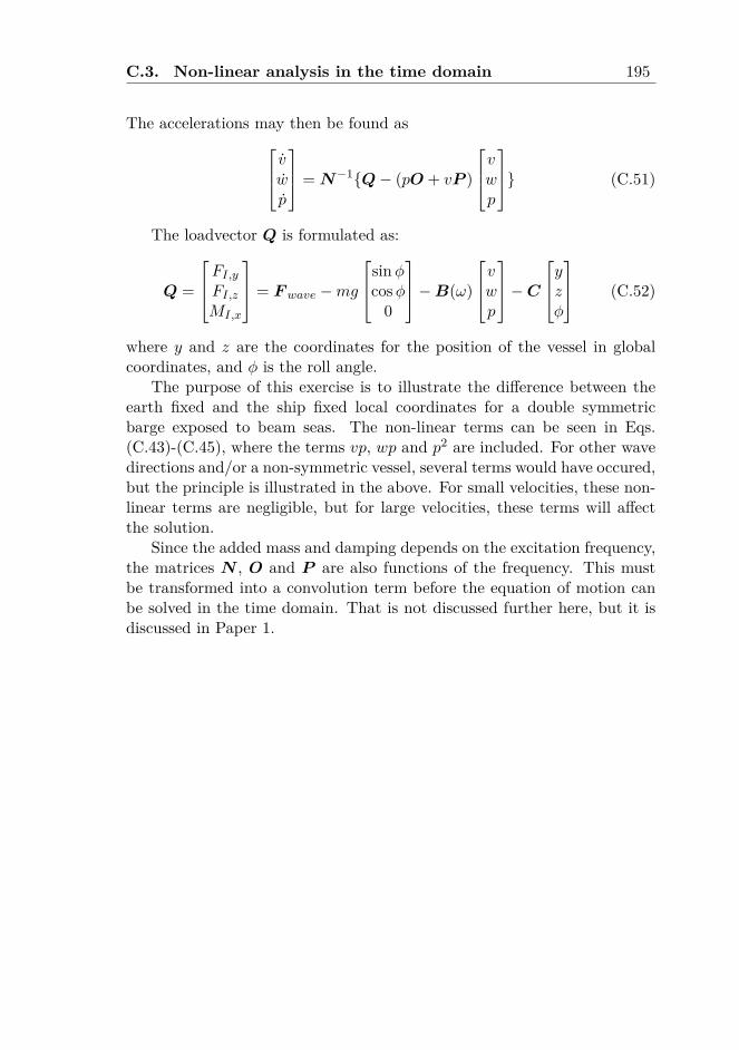
C.3. Non-linear analysis in the time domain 195
The accelerations may then be found asvwp
= N−1Q− (pO + vP )
vwp
(C.51)
The loadvector Q is formulated as:
Q =
FI,yFI,zMI,x
= Fwave −mg
sinφcosφ
0
−B(ω)
vwp
−C
yzφ
(C.52)
where y and z are the coordinates for the position of the vessel in globalcoordinates, and φ is the roll angle.
The purpose of this exercise is to illustrate the difference between theearth fixed and the ship fixed local coordinates for a double symmetricbarge exposed to beam seas. The non-linear terms can be seen in Eqs.(C.43)-(C.45), where the terms vp, wp and p2 are included. For other wavedirections and/or a non-symmetric vessel, several terms would have occured,but the principle is illustrated in the above. For small velocities, these non-linear terms are negligible, but for large velocities, these terms will affectthe solution.
Since the added mass and damping depends on the excitation frequency,the matrices N , O and P are also functions of the frequency. This mustbe transformed into a convolution term before the equation of motion canbe solved in the time domain. That is not discussed further here, but it isdiscussed in Paper 1.

196 Motion analysis of ships and barges
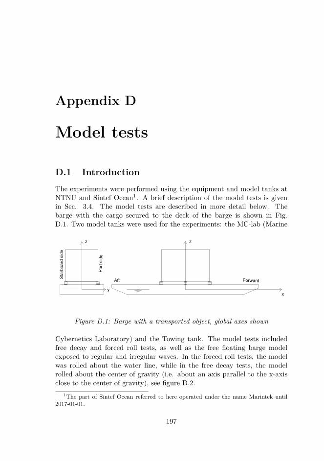
Appendix D
Model tests
D.1 IntroductionThe experiments were performed using the equipment and model tanks atNTNU and Sintef Ocean1. A brief description of the model tests is givenin Sec. 3.4. The model tests are described in more detail below. Thebarge with the cargo secured to the deck of the barge is shown in Fig.D.1. Two model tanks were used for the experiments: the MC-lab (Marine
[Academic use only]
Figure D.1: Barge with a transported object, global axes shown
Cybernetics Laboratory) and the Towing tank. The model tests includedfree decay and forced roll tests, as well as the free floating barge modelexposed to regular and irregular waves. In the forced roll tests, the modelwas rolled about the water line, while in the free decay tests, the modelrolled about the center of gravity (i.e. about an axis parallel to the x-axisclose to the center of gravity), see figure D.2.
1The part of Sintef Ocean referred to here operated under the name Marintek until2017-01-01.
197
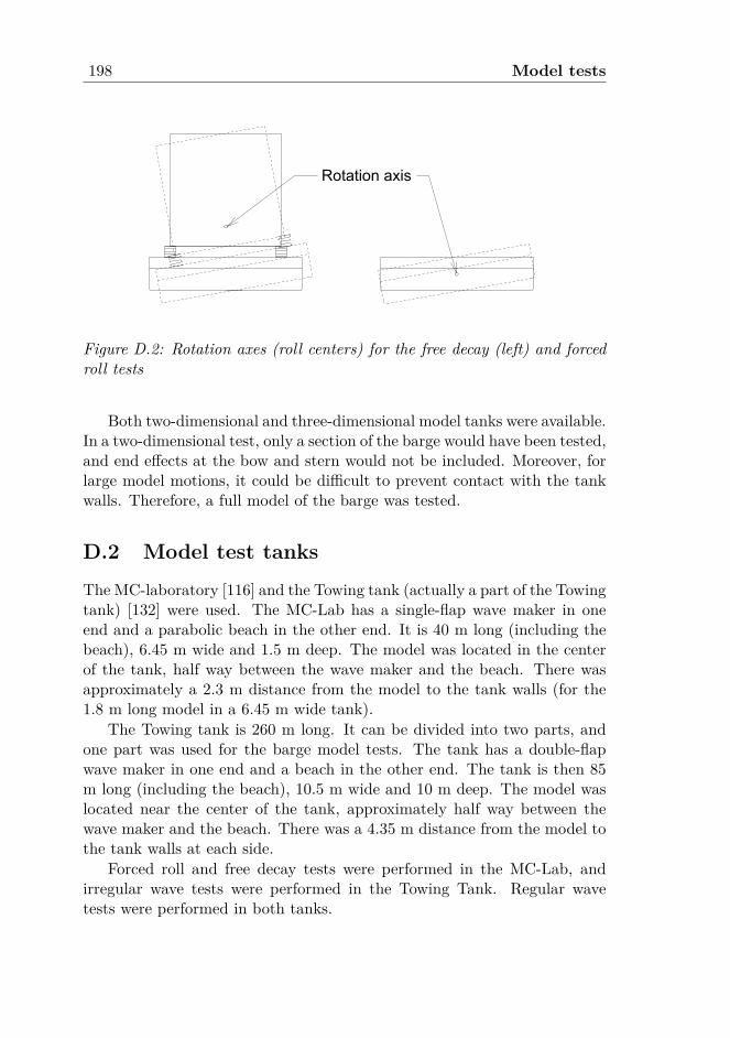
198 Model tests
[Academic use only]
Figure D.2: Rotation axes (roll centers) for the free decay (left) and forcedroll tests
Both two-dimensional and three-dimensional model tanks were available.In a two-dimensional test, only a section of the barge would have been tested,and end effects at the bow and stern would not be included. Moreover, forlarge model motions, it could be difficult to prevent contact with the tankwalls. Therefore, a full model of the barge was tested.
D.2 Model test tanks
The MC-laboratory [116] and the Towing tank (actually a part of the Towingtank) [132] were used. The MC-Lab has a single-flap wave maker in oneend and a parabolic beach in the other end. It is 40 m long (including thebeach), 6.45 m wide and 1.5 m deep. The model was located in the centerof the tank, half way between the wave maker and the beach. There wasapproximately a 2.3 m distance from the model to the tank walls (for the1.8 m long model in a 6.45 m wide tank).
The Towing tank is 260 m long. It can be divided into two parts, andone part was used for the barge model tests. The tank has a double-flapwave maker in one end and a beach in the other end. The tank is then 85m long (including the beach), 10.5 m wide and 10 m deep. The model waslocated near the center of the tank, approximately half way between thewave maker and the beach. There was a 4.35 m distance from the model tothe tank walls at each side.
Forced roll and free decay tests were performed in the MC-Lab, andirregular wave tests were performed in the Towing Tank. Regular wavetests were performed in both tanks.
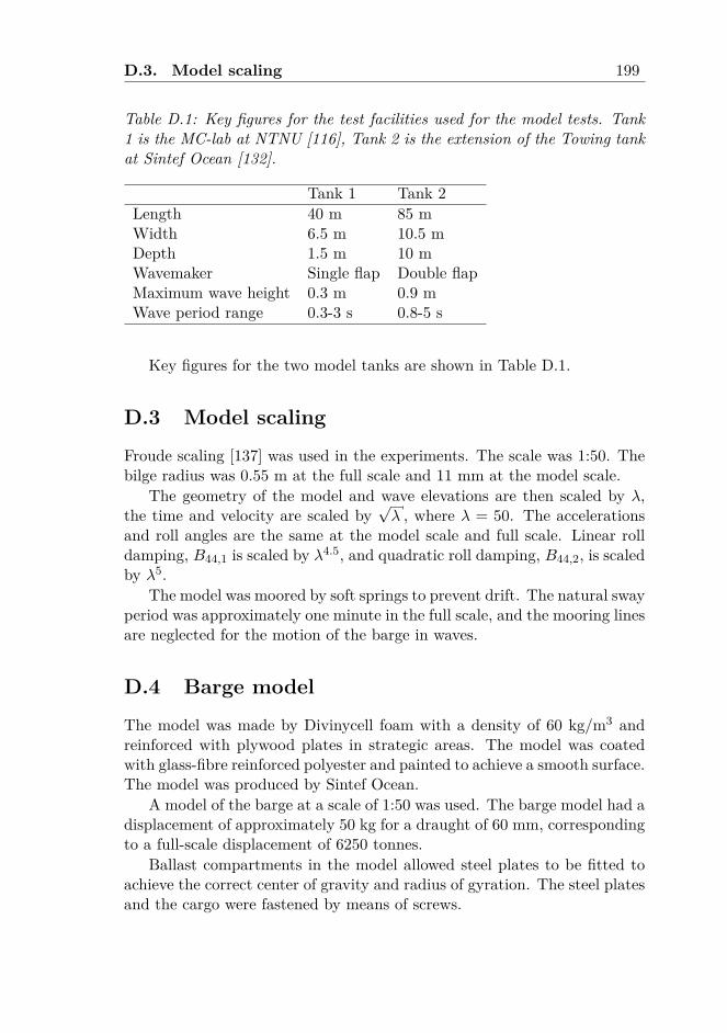
D.3. Model scaling 199
Table D.1: Key figures for the test facilities used for the model tests. Tank1 is the MC-lab at NTNU [116], Tank 2 is the extension of the Towing tankat Sintef Ocean [132].
Tank 1 Tank 2Length 40 m 85 mWidth 6.5 m 10.5 mDepth 1.5 m 10 mWavemaker Single flap Double flapMaximum wave height 0.3 m 0.9 mWave period range 0.3-3 s 0.8-5 s
Key figures for the two model tanks are shown in Table D.1.
D.3 Model scaling
Froude scaling [137] was used in the experiments. The scale was 1:50. Thebilge radius was 0.55 m at the full scale and 11 mm at the model scale.
The geometry of the model and wave elevations are then scaled by λ,the time and velocity are scaled by
√λ , where λ = 50. The accelerations
and roll angles are the same at the model scale and full scale. Linear rolldamping, B44,1 is scaled by λ4.5, and quadratic roll damping, B44,2, is scaledby λ5.
The model was moored by soft springs to prevent drift. The natural swayperiod was approximately one minute in the full scale, and the mooring linesare neglected for the motion of the barge in waves.
D.4 Barge model
The model was made by Divinycell foam with a density of 60 kg/m3 andreinforced with plywood plates in strategic areas. The model was coatedwith glass-fibre reinforced polyester and painted to achieve a smooth surface.The model was produced by Sintef Ocean.
A model of the barge at a scale of 1:50 was used. The barge model had adisplacement of approximately 50 kg for a draught of 60 mm, correspondingto a full-scale displacement of 6250 tonnes.
Ballast compartments in the model allowed steel plates to be fitted toachieve the correct center of gravity and radius of gyration. The steel platesand the cargo were fastened by means of screws.
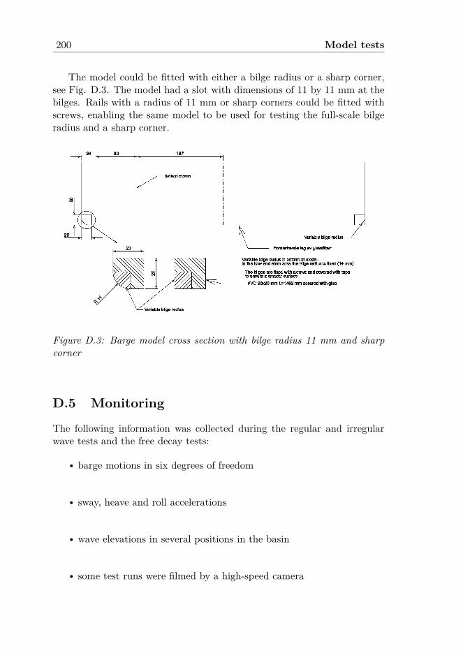
200 Model tests
The model could be fitted with either a bilge radius or a sharp corner,see Fig. D.3. The model had a slot with dimensions of 11 by 11 mm at thebilges. Rails with a radius of 11 mm or sharp corners could be fitted withscrews, enabling the same model to be used for testing the full-scale bilgeradius and a sharp corner.
Figure D.3: Barge model cross section with bilge radius 11 mm and sharpcorner
D.5 Monitoring
The following information was collected during the regular and irregularwave tests and the free decay tests:
r barge motions in six degrees of freedom
r sway, heave and roll accelerations
r wave elevations in several positions in the basin
r some test runs were filmed by a high-speed camera
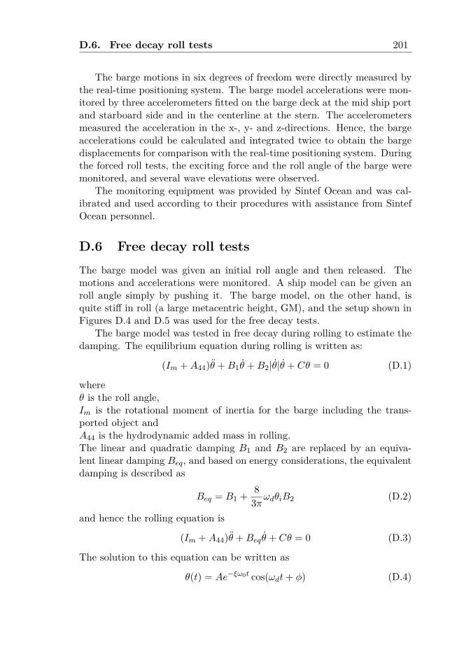
D.6. Free decay roll tests 201
The barge motions in six degrees of freedom were directly measured bythe real-time positioning system. The barge model accelerations were mon-itored by three accelerometers fitted on the barge deck at the mid ship portand starboard side and in the centerline at the stern. The accelerometersmeasured the acceleration in the x-, y- and z-directions. Hence, the bargeaccelerations could be calculated and integrated twice to obtain the bargedisplacements for comparison with the real-time positioning system. Duringthe forced roll tests, the exciting force and the roll angle of the barge weremonitored, and several wave elevations were observed.
The monitoring equipment was provided by Sintef Ocean and was cal-ibrated and used according to their procedures with assistance from SintefOcean personnel.
D.6 Free decay roll testsThe barge model was given an initial roll angle and then released. Themotions and accelerations were monitored. A ship model can be given anroll angle simply by pushing it. The barge model, on the other hand, isquite stiff in roll (a large metacentric height, GM), and the setup shown inFigures D.4 and D.5 was used for the free decay tests.
The barge model was tested in free decay during rolling to estimate thedamping. The equilibrium equation during rolling is written as:
(Im +A44)θ +B1θ +B2|θ|θ + Cθ = 0 (D.1)
whereθ is the roll angle,Im is the rotational moment of inertia for the barge including the trans-ported object andA44 is the hydrodynamic added mass in rolling.The linear and quadratic damping B1 and B2 are replaced by an equiva-lent linear damping Beq, and based on energy considerations, the equivalentdamping is described as
Beq = B1 + 83πωdθiB2 (D.2)
and hence the rolling equation is
(Im +A44)θ +Beq θ + Cθ = 0 (D.3)
The solution to this equation can be written as
θ(t) = Ae−ξω0t cos(ωdt+ φ) (D.4)
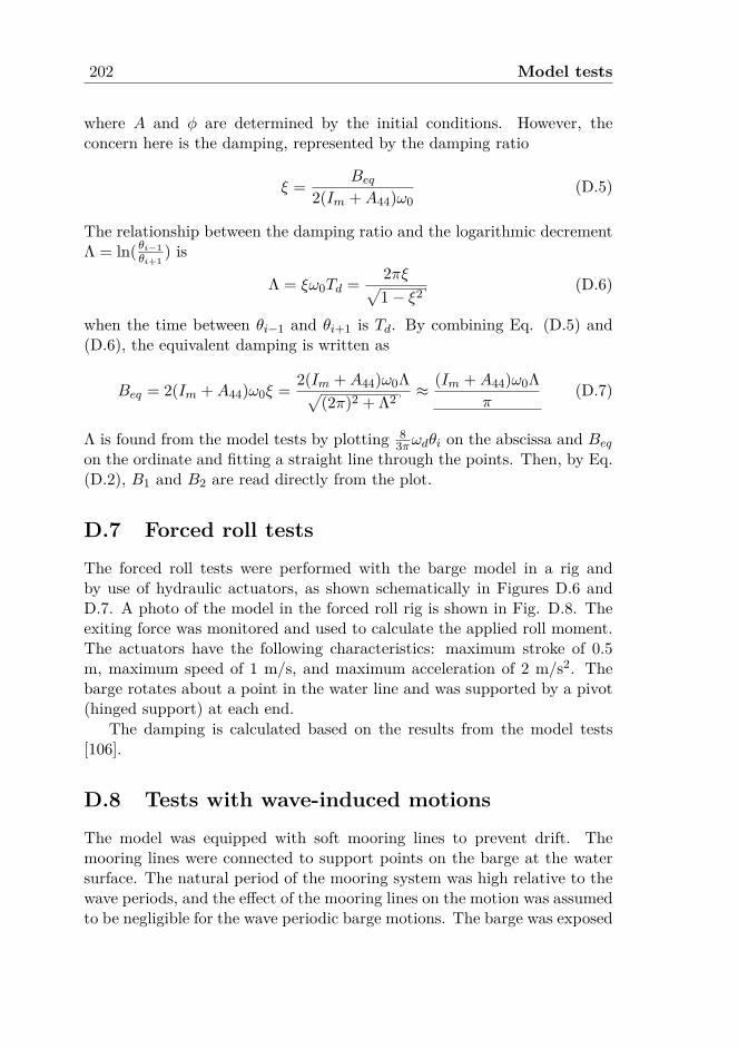
202 Model tests
where A and φ are determined by the initial conditions. However, theconcern here is the damping, represented by the damping ratio
ξ = Beq2(Im +A44)ω0
(D.5)
The relationship between the damping ratio and the logarithmic decrementΛ = ln( θi−1
θi+1) is
Λ = ξω0Td = 2πξ√1− ξ2 (D.6)
when the time between θi−1 and θi+1 is Td. By combining Eq. (D.5) and(D.6), the equivalent damping is written as
Beq = 2(Im +A44)ω0ξ = 2(Im +A44)ω0Λ√(2π)2 + Λ2 ≈ (Im +A44)ω0Λ
π(D.7)
Λ is found from the model tests by plotting 83πωdθi on the abscissa and Beq
on the ordinate and fitting a straight line through the points. Then, by Eq.(D.2), B1 and B2 are read directly from the plot.
D.7 Forced roll tests
The forced roll tests were performed with the barge model in a rig andby use of hydraulic actuators, as shown schematically in Figures D.6 andD.7. A photo of the model in the forced roll rig is shown in Fig. D.8. Theexiting force was monitored and used to calculate the applied roll moment.The actuators have the following characteristics: maximum stroke of 0.5m, maximum speed of 1 m/s, and maximum acceleration of 2 m/s2. Thebarge rotates about a point in the water line and was supported by a pivot(hinged support) at each end.
The damping is calculated based on the results from the model tests[106].
D.8 Tests with wave-induced motions
The model was equipped with soft mooring lines to prevent drift. Themooring lines were connected to support points on the barge at the watersurface. The natural period of the mooring system was high relative to thewave periods, and the effect of the mooring lines on the motion was assumedto be negligible for the wave periodic barge motions. The barge was exposed
D.8. Tests with wave-induced motions 203
[Academic use only]
Figure D.4: Barge cross section with the arrangement for the free decay testin rolling (designed to give pure roll motion)
to waves from 90 (beam sea). The setup in the MC-lab is indicated in Fig.D.9.
In the regular wave tests, the purpose was to study the barge motionas a function of the wave height and wave period. For a given wave height,a range of periods were included. The minimum wave periods (maximumwave steepness) were calculated based on recommendations given in theDNV Rules for Planning and Execution of Marine Operations. Deep waterwas assumed. In the irregular wave tests, three-hour simulations of severalsea states were tested, as described in Paper 1 [109].
204 Model tests
Figure D.5: Barge model with the arrangement for the free decay test inrolling

D.8. Tests with wave-induced motions 205
[Academic use only]
Figure D.6: Plan view (upper) and front elevation (lower) of the jig usedduring the forced roll test. The outline of the barge model is indicated onthe plan view. View A-A is shown in figure D.7.
[Academic use only]
Figure D.7: View A-A from figure D.6: The barge model with the jig (RHS60x4) and the arrangement for the forced roll test. The roll motion wasinduced by the yoke being moved up and down by electric actuators fitted onthe carriage in the model tank. See Fig. D.8 for an overview of the bargemodel.
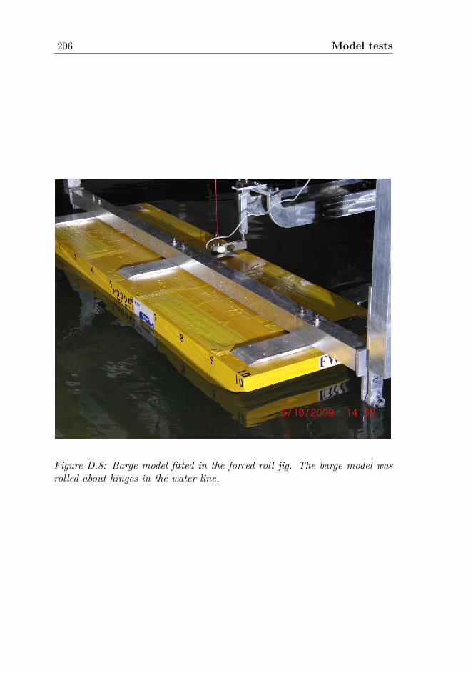
206 Model tests
Figure D.8: Barge model fitted in the forced roll jig. The barge model wasrolled about hinges in the water line.
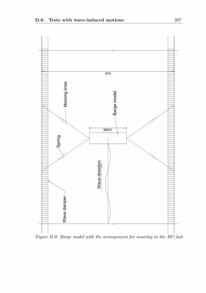
D.8. Tests with wave-induced motions 207
[Aca
dem
ic u
se o
nly]
Figure D.9: Barge model with the arrangement for mooring in the MC-Lab

208 Model tests

Appendix E
List of previous PhD thesesat Dept. of Marine Tech.

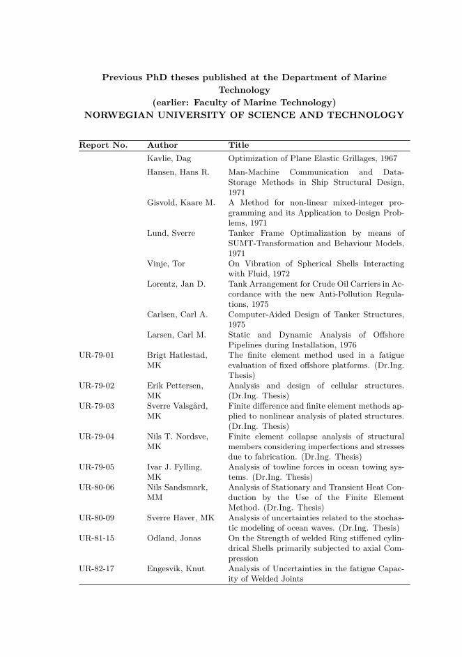
Previous PhD theses published at the Department of MarineTechnology
(earlier: Faculty of Marine Technology)NORWEGIAN UNIVERSITY OF SCIENCE AND TECHNOLOGY
Report No. Author TitleKavlie, Dag Optimization of Plane Elastic Grillages, 1967Hansen, Hans R. Man-Machine Communication and Data-
Storage Methods in Ship Structural Design,1971
Gisvold, Kaare M. A Method for non-linear mixed-integer pro-gramming and its Application to Design Prob-lems, 1971
Lund, Sverre Tanker Frame Optimalization by means ofSUMT-Transformation and Behaviour Models,1971
Vinje, Tor On Vibration of Spherical Shells Interactingwith Fluid, 1972
Lorentz, Jan D. Tank Arrangement for Crude Oil Carriers in Ac-cordance with the new Anti-Pollution Regula-tions, 1975
Carlsen, Carl A. Computer-Aided Design of Tanker Structures,1975
Larsen, Carl M. Static and Dynamic Analysis of OffshorePipelines during Installation, 1976
UR-79-01 Brigt Hatlestad,MK
The finite element method used in a fatigueevaluation of fixed offshore platforms. (Dr.Ing.Thesis)
UR-79-02 Erik Pettersen,MK
Analysis and design of cellular structures.(Dr.Ing. Thesis)
UR-79-03 Sverre Valsgård,MK
Finite difference and finite element methods ap-plied to nonlinear analysis of plated structures.(Dr.Ing. Thesis)
UR-79-04 Nils T. Nordsve,MK
Finite element collapse analysis of structuralmembers considering imperfections and stressesdue to fabrication. (Dr.Ing. Thesis)
UR-79-05 Ivar J. Fylling,MK
Analysis of towline forces in ocean towing sys-tems. (Dr.Ing. Thesis)
UR-80-06 Nils Sandsmark,MM
Analysis of Stationary and Transient Heat Con-duction by the Use of the Finite ElementMethod. (Dr.Ing. Thesis)
UR-80-09 Sverre Haver, MK Analysis of uncertainties related to the stochas-tic modeling of ocean waves. (Dr.Ing. Thesis)
UR-81-15 Odland, Jonas On the Strength of welded Ring stiffened cylin-drical Shells primarily subjected to axial Com-pression
UR-82-17 Engesvik, Knut Analysis of Uncertainties in the fatigue Capac-ity of Welded Joints

Report No. Author TitleUR-82-18 Rye, Henrik Ocean wave groupsUR-83-30 Eide, Oddvar Inge On Cumulative Fatigue Damage in Steel
Welded JointsUR-83-33 Mo, Olav Stochastic Time Domain Analysis of Slender
Offshore StructuresUR-83-34 Amdahl, Jørgen Energy absorption in Ship-platform impactsUR-84-37 Mørch, Morten Motions and mooring forces of semi sub-
mersibles as determined by full-scale measure-ments and theoretical analysis
UR-84-38 Soares, C. Guedes Probabilistic models for load effects in shipstructures
UR-84-39 Aarsnes, Jan V. Current forces on shipsUR-84-40 Czujko, Jerzy Collapse Analysis of Plates subjected to Biaxial
Compression and Lateral LoadUR-85-46 Alf G. Engseth,
MKFinite element collapse analysis of tubular steeloffshore structures. (Dr.Ing. Thesis)
UR-86-47 DengodySheshappa, MP
A Computer Design Model for Optimizing Fish-ing Vessel Designs Based on Techno-EconomicAnalysis. (Dr.Ing. Thesis)
UR-86-48 Vidar Aanesland,MH
A Theoretical and Numerical Study of ShipWave Resistance. (Dr.Ing. Thesis)
UR-86-49 Heinz-JoachimWessel, MK
Fracture Mechanics Analysis of Crack Growthin Plate Girders. (Dr.Ing. Thesis)
UR-86-50 Jon Taby, MK Ultimate and Post-ultimate Strength of DentedTubular Members. (Dr.Ing. Thesis)
UR-86-51 Walter Lian, MH A Numerical Study of Two-Dimensional Sepa-rated Flow Past Bluff Bodies at Moderate KC-Numbers. (Dr.Ing. Thesis)
UR-86-52 Bjørn Sortland,MH
Force Measurements in Oscillating Flow on ShipSections and Circular Cylinders in a U-TubeWater Tank. (Dr.Ing. Thesis)
UR-86-53 Kurt Strand, MM A System Dynamic Approach to One-dimensional Fluid Flow. (Dr.Ing. Thesis)
UR-86-54 Arne EdvinLøken, MH
Three Dimensional Second Order Hydrody-namic Effects on Ocean Structures in Waves.(Dr.Ing. Thesis)
UR-86-55 Sigurd Falch, MH A Numerical Study of Slamming of Two-Dimensional Bodies. (Dr.Ing. Thesis)
UR-87-56 Arne Braathen,MH
Application of a Vortex Tracking Method to thePrediction of Roll Damping of a Two-DimensionFloating Body. (Dr.Ing. Thesis)
UR-87-57 Bernt Leira, MK Gaussian Vector Processes for Reliability Anal-ysis involving Wave-Induced Load Effects.(Dr.Ing. Thesis)
UR-87-58 Magnus Småvik,MM
Thermal Load and Process Characteristics in aTwo-Stroke Diesel Engine with Thermal Barri-ers (in Norwegian). (Dr.Ing. Thesis)
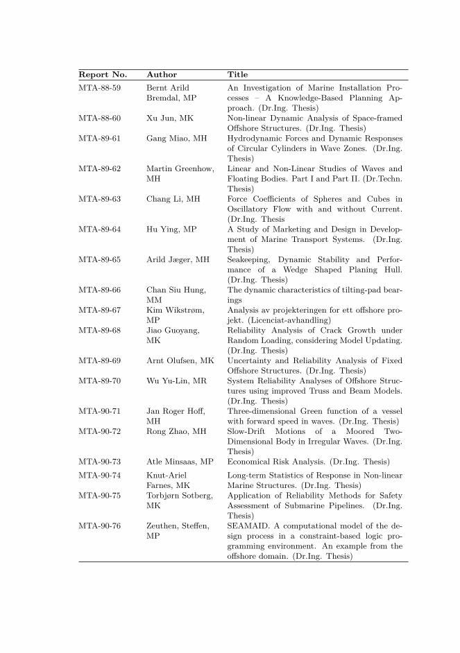
Report No. Author TitleMTA-88-59 Bernt Arild
Bremdal, MPAn Investigation of Marine Installation Pro-cesses – A Knowledge-Based Planning Ap-proach. (Dr.Ing. Thesis)
MTA-88-60 Xu Jun, MK Non-linear Dynamic Analysis of Space-framedOffshore Structures. (Dr.Ing. Thesis)
MTA-89-61 Gang Miao, MH Hydrodynamic Forces and Dynamic Responsesof Circular Cylinders in Wave Zones. (Dr.Ing.Thesis)
MTA-89-62 Martin Greenhow,MH
Linear and Non-Linear Studies of Waves andFloating Bodies. Part I and Part II. (Dr.Techn.Thesis)
MTA-89-63 Chang Li, MH Force Coefficients of Spheres and Cubes inOscillatory Flow with and without Current.(Dr.Ing. Thesis
MTA-89-64 Hu Ying, MP A Study of Marketing and Design in Develop-ment of Marine Transport Systems. (Dr.Ing.Thesis)
MTA-89-65 Arild Jæger, MH Seakeeping, Dynamic Stability and Perfor-mance of a Wedge Shaped Planing Hull.(Dr.Ing. Thesis)
MTA-89-66 Chan Siu Hung,MM
The dynamic characteristics of tilting-pad bear-ings
MTA-89-67 Kim Wikstrøm,MP
Analysis av projekteringen for ett offshore pro-jekt. (Licenciat-avhandling)
MTA-89-68 Jiao Guoyang,MK
Reliability Analysis of Crack Growth underRandom Loading, considering Model Updating.(Dr.Ing. Thesis)
MTA-89-69 Arnt Olufsen, MK Uncertainty and Reliability Analysis of FixedOffshore Structures. (Dr.Ing. Thesis)
MTA-89-70 Wu Yu-Lin, MR System Reliability Analyses of Offshore Struc-tures using improved Truss and Beam Models.(Dr.Ing. Thesis)
MTA-90-71 Jan Roger Hoff,MH
Three-dimensional Green function of a vesselwith forward speed in waves. (Dr.Ing. Thesis)
MTA-90-72 Rong Zhao, MH Slow-Drift Motions of a Moored Two-Dimensional Body in Irregular Waves. (Dr.Ing.Thesis)
MTA-90-73 Atle Minsaas, MP Economical Risk Analysis. (Dr.Ing. Thesis)MTA-90-74 Knut-Ariel
Farnes, MKLong-term Statistics of Response in Non-linearMarine Structures. (Dr.Ing. Thesis)
MTA-90-75 Torbjørn Sotberg,MK
Application of Reliability Methods for SafetyAssessment of Submarine Pipelines. (Dr.Ing.Thesis)
MTA-90-76 Zeuthen, Steffen,MP
SEAMAID. A computational model of the de-sign process in a constraint-based logic pro-gramming environment. An example from theoffshore domain. (Dr.Ing. Thesis)

Report No. Author TitleMTA-91-77 Haagensen, Sven,
MMFuel Dependant Cyclic Variability in a Spark Ig-nition Engine – An Optical Approach. (Dr.Ing.Thesis)
MTA-91-78 Løland, Geir, MH Current forces on and flow through fish farms.(Dr.Ing. Thesis)
MTA-91-79 Hoen,Christopher, MK
System Identification of Structures Excited byStochastic Load Processes. (Dr.Ing. Thesis)
MTA-91-80 Haugen, Stein,MK
Probabilistic Evaluation of Frequency of Col-lision between Ships and Offshore Platforms.(Dr.Ing. Thesis)
MTA-91-81 Sødahl, Nils, MK Methods for Design and Analysis of FlexibleRisers. (Dr.Ing. Thesis)
MTA-91-82 Ormberg, Harald,MK
Non-linear Response Analysis of Floating FishFarm Systems. (Dr.Ing. Thesis)
MTA-91-83 Marley, Mark J.,MK
Time Variant Reliability under Fatigue Degra-dation. (Dr.Ing. Thesis)
MTA-91-84 Krokstad, JørgenR., MH
Second-order Loads in Multidirectional Seas.(Dr.Ing. Thesis)
MTA-91-85 Molteberg,Gunnar A., MM
The Application of System Identification Tech-niques to Performance Monitoring of FourStroke Turbocharged Diesel Engines. (Dr.Ing.Thesis)
MTA-92-86 Mørch, HansJørgen Bjelke,MH
Aspects of Hydrofoil Design: with Emphasis onHydrofoil Interaction in Calm Water. (Dr.Ing.Thesis)
MTA-92-87 Chan Siu Hung,MM
Nonlinear Analysis of Rotordynamic Instabil-ities in Highspeed Turbomachinery. (Dr.Ing.Thesis)
MTA-92-88 Bessason, Bjarni,MK
Assessment of Earthquake Loading and Re-sponse of Seismically Isolated Bridges. (Dr.Ing.Thesis)
MTA-92-89 Langli, Geir, MP Improving Operational Safety through exploita-tion of Design Knowledge – an investigation ofoffshore platform safety. (Dr.Ing. Thesis)
MTA-92-90 Sævik, Svein, MK On Stresses and Fatigue in Flexible Pipes.(Dr.Ing. Thesis)
MTA-92-91 Ask, Tor Ø., MM Ignition and Flame Growth in Lean Gas-AirMixtures. An Experimental Study with aSchlieren System. (Dr.Ing. Thesis)
MTA-86-92 Hessen, Gunnar,MK
Fracture Mechanics Analysis of Stiffened Tubu-lar Members. (Dr.Ing. Thesis)
MTA-93-93 Steinebach,Christian, MM
Knowledge Based Systems for Diagnosis of Ro-tating Machinery. (Dr.Ing. Thesis)
MTA-93-94 Dalane, Jan Inge,MK
System Reliability in Design and Maintenanceof Fixed Offshore Structures. (Dr.Ing. Thesis)
MTA-93-95 Steen, Sverre, MH Cobblestone Effect on SES. (Dr.Ing. Thesis)
Report No. Author TitleMTA-93-96 Karunakaran,
Daniel, MKNonlinear Dynamic Response and Reliabil-ity Analysis of Drag-dominated Offshore Plat-forms. (Dr.Ing. Thesis)
MTA-93-97 Hagen, Arnulf,MP
The Framework of a Design Process Language.(Dr.Ing. Thesis)
MTA-93-98 Nordrik, Rune,MM
Investigation of Spark Ignition and Autoignitionin Methane and Air Using Computational FluidDynamics and Chemical Reaction Kinetics. ANumerical Study of Ignition Processes in Inter-nal Combustion Engines. (Dr.Ing. Thesis)
MTA-94-99 Passano,Elizabeth, MK
Efficient Analysis of Nonlinear Slender MarineStructures. (Dr.Ing. Thesis)
MTA-94-100 Kvålsvold, Jan,MH
Hydroelastic Modelling of Wetdeck Slammingon Multihull Vessels. (Dr.Ing. Thesis)
MTA-94-102 Bech, Sidsel M.,MK
Experimental and Numerical Determination ofStiffness and Strength of GRP/PVC SandwichStructures. (Dr.Ing. Thesis)
MTA-95-103 Paulsen, Hallvard,MM
A Study of Transient Jet and Spray using aSchlieren Method and Digital Image Processing.(Dr.Ing. Thesis)
MTA-95-104 Hovde, Geir Olav,MK
Fatigue and Overload Reliability of OffshoreStructural Systems, Considering the Effect ofInspection and Repair. (Dr.Ing. Thesis)
MTA-95-105 Wang, Xiaozhi,MK
Reliability Analysis of Production Ships withEmphasis on Load Combination and UltimateStrength. (Dr.Ing. Thesis)
MTA-95-106 Ulstein, Tore, MH Nonlinear Effects of a Flexible Stern Seal Bagon Cobblestone Oscillations of an SES. (Dr.Ing.Thesis)
MTA-95-107 Solaas, Frøydis,MH
Analytical and Numerical Studies of Sloshing inTanks. (Dr.Ing. Thesis)
MTA-95-108 Hellan, Øyvind,MK
Nonlinear Pushover and Cyclic Analyses in Ul-timate Limit State Design and Reassessmentof Tubular Steel Offshore Structures. (Dr.Ing.Thesis)
MTA-95-109 Hermundstad, OleA., MK
Theoretical and Experimental HydroelasticAnalysis of High Speed Vessels. (Dr.Ing. The-sis)
MTA-96-110 Bratland, AnneK., MH
Wave-Current Interaction Effects on Large-Volume Bodies in Water of Finite Depth.(Dr.Ing. Thesis)
MTA-96-111 Herfjord, Kjell,MH
A Study of Two-dimensional Separated Flow bya Combination of the Finite Element Methodand Navier-Stokes Equations. (Dr.Ing. Thesis)
MTA-96-112 AEsøy, Vilmar,MM
Hot Surface Assisted Compression Ignition in aDirect Injection Natural Gas Engine. (Dr.Ing.Thesis)

Report No. Author TitleMTA-96-113 Eknes, Monika L.,
MKEscalation Scenarios Initiated by Gas Explo-sions on Offshore Installations. (Dr.Ing. The-sis)
MTA-96-114 Erikstad, SteinO., MP
A Decision Support Model for Preliminary ShipDesign. (Dr.Ing. Thesis)
MTA-96-115 Pedersen, Egil,MH
A Nautical Study of Towed Marine SeismicStreamer Cable Configurations. (Dr.Ing. The-sis)
MTA-97-116 Moksnes, Paul O.,MM
Modelling Two-Phase Thermo-Fluid SystemsUsing Bond Graphs. (Dr.Ing. Thesis)
MTA-97-117 Halse, Karl H.,MK
On Vortex Shedding and Prediction of Vortex-Induced Vibrations of Circular Cylinders.(Dr.Ing. Thesis)
MTA-97-118 Igland, RagnarT., MK
Reliability Analysis of Pipelines during Laying,considering Ultimate Strength under CombinedLoads. (Dr.Ing. Thesis)
MTA-97-119 Pedersen,Hans-P., MP
Levendefiskteknologi for fiskefartøy. (Dr.Ing.Thesis)
MTA-98-120 Vikestad, Kyrre,MK
Multi-Frequency Response of a Cylinder Sub-jected to Vortex Shedding and Support Mo-tions. (Dr.Ing. Thesis)
MTA-98-121 Azadi,Mohammad R.E., MK
Analysis of Static and Dynamic Pile-Soil-JacketBehaviour. (Dr.Ing. Thesis)
MTA-98-122 Ulltang, Terje,MP
A Communication Model for Product Informa-tion. (Dr.Ing. Thesis)
MTA-98-123 Torbergsen, Erik,MM
Impeller/Diffuser Interaction Forces in Cen-trifugal Pumps. (Dr.Ing. Thesis)
MTA-98-124 Hansen, Edmond,MH
A Discrete Element Model to Study MarginalIce Zone Dynamics and the Behaviour of VesselsMoored in Broken Ice. (Dr.Ing. Thesis)
MTA-98-125 Videiro, PauloM., MK
Reliability Based Design of Marine Structures.(Dr.Ing. Thesis)
MTA-99-126 Mainçon,Philippe, MK
Fatigue Reliability of Long Welds Applicationto Titanium Risers. (Dr.Ing. Thesis)
MTA-99-127 Haugen, Elin M.,MH
Hydroelastic Analysis of Slamming on StiffenedPlates with Application to Catamaran Wet-decks. (Dr.Ing. Thesis)
MTA-99-128 Langhelle, NinaK., MK
Experimental Validation and Calibration ofNonlinear Finite Element Models for Use in De-sign of Aluminium Structures Exposed to Fire.(Dr.Ing. Thesis)
MTA-99-129 Berstad, Are J.,MK
Calculation of Fatigue Damage in Ship Struc-tures. (Dr.Ing. Thesis)
MTA-99-130 Andersen, TrondM., MM
Short Term Maintenance Planning. (Dr.Ing.Thesis)
MTA-99-131 Tveiten, BårdWathne, MK
Fatigue Assessment of Welded Aluminium ShipDetails. (Dr.Ing. Thesis)
Report No. Author TitleMTA-99-132 Søreide, Fredrik,
MPApplications of underwater technology in deepwater archaeology. Principles and practice.(Dr.Ing. Thesis)
MTA-99-133 Tønnessen, Rune,MH
A Finite Element Method Applied to UnsteadyViscous Flow Around 2D Blunt Bodies WithSharp Corners. (Dr.Ing. Thesis)
MTA-99-134 Elvekrok, Dag R.,MP
Engineering Integration in Field DevelopmentProjects in the Norwegian Oil and Gas Industry.The Supplier Management of Norne. (Dr.Ing.Thesis)
MTA-99-135 Fagerholt, Kjetil,MP
Optimeringsbaserte Metoder for Ruteplanleg-ging innen skipsfart. (Dr.Ing. Thesis)
MTA-99-136 Bysveen, Marie,MM
Visualization in Two Directions on a DynamicCombustion Rig for Studies of Fuel Quality.(Dr.Ing. Thesis)
MTA-2000-137 Storteig, Eskild,MM
Dynamic characteristics and leakage perfor-mance of liquid annular seals in centrifugalpumps. (Dr.Ing. Thesis)
MTA-2000-138 Sagli, Gro, MK Model uncertainty and simplified estimates oflong term extremes of hull girder loads in ships.(Dr.Ing. Thesis)
MTA-2000-139 Tronstad, Harald,MK
Nonlinear analysis and design of cable net struc-tures like fishing gear based on the finite elementmethod. (Dr.Ing. Thesis)
MTA-2000-140 Kroneberg,André, MP
Innovation in shipping by using scenarios.(Dr.Ing. Thesis)
MTA-2000-141 Haslum, HerbjørnAlf, MH
Simplified methods applied to nonlinear motionof spar platforms. (Dr.Ing. Thesis)
MTA-2001-142 Samdal, OleJohan, MM
Modelling of Degradation Mechanisms andStressor Interaction on Static MechanicalEquipment Residual Lifetime. (Dr.Ing. Thesis)
MTA-2001-143 Baarholm, RolfJarle, MH
Theoretical and experimental studies of waveimpact underneath decks of offshore platforms.(Dr.Ing. Thesis)
MTA-2001-144 Wang, Lihua, MK Probabilistic Analysis of Nonlinear Wave-induced Loads on Ships. (Dr.Ing. Thesis)
MTA-2001-145 Kristensen, OddH. Holt, MK
Ultimate Capacity of Aluminium Plates underMultiple Loads, Considering HAZ Properties.(Dr.Ing. Thesis)
MTA-2001-146 Greco, Marilena,MH
A Two-Dimensional Study of Green-WaterLoading. (Dr.Ing. Thesis)
MTA-2001-147 Heggelund, SveinE., MK
Calculation of Global Design Loads and LoadEffects in Large High Speed Catamarans.(Dr.Ing. Thesis)
MTA-2001-148 Babalola,Olusegun T., MK
Fatigue Strength of Titanium Risers – DefectSensitivity. (Dr.Ing. Thesis)
MTA-2001-149 Mohammed,Abuu K., MK
Nonlinear Shell Finite Elements for UltimateStrength and Collapse Analysis of Ship Struc-tures. (Dr.Ing. Thesis)
Report No. Author TitleMTA-2002-150 Holmedal, Lars
E., MHWave-current interactions in the vicinity of thesea bed. (Dr.Ing. Thesis)
MTA-2002-151 Rognebakke, OlavF., MH
Sloshing in rectangular tanks and interactionwith ship motions. (Dr.Ing. Thesis)
MTA-2002-152 Lader, Pål Furset,MH
Geometry and Kinematics of Breaking Waves.(Dr.Ing. Thesis)
MTA-2002-153 Yang, Qinzheng,MH
Wash and wave resistance of ships in finite waterdepth. (Dr.Ing. Thesis)
MTA-2002-154 Melhus, Øyvin,MM
Utilization of VOC in Diesel Engines. Ignitionand combustion of VOC released by crude oiltankers. (Dr.Ing. Thesis)
MTA-2002-155 Ronæss, Marit,MH
Wave Induced Motions of Two Ships Advancingon Parallel Course. (Dr.Ing. Thesis)
MTA-2002-156 Økland, Ole D.,MK
Numerical and experimental investigation ofwhipping in twin hull vessels exposed to severewet deck slamming. (Dr.Ing. Thesis)
MTA-2002-157 Ge, Chunhua,MK
Global Hydroelastic Response of Catamaransdue to Wet Deck Slamming. (Dr.Ing. Thesis)
MTA-2002-158 Byklum, Eirik,MK
Nonlinear Shell Finite Elements for UltimateStrength and Collapse Analysis of Ship Struc-tures. (Dr.Ing. Thesis)
IMT-2003-1 Chen, Haibo, MK Probabilistic Evaluation of FPSO-Tanker Colli-sion in Tandem Offloading Operation. (Dr.Ing.Thesis)
IMT-2003-2 Skaugset, KjetilBjørn, MK
On the Suppression of Vortex Induced Vibra-tions of Circular Cylinders by Radial WaterJets. (Dr.Ing. Thesis)
IMT-2003-3 Chezhian, Muthu Three-Dimensional Analysis of Slamming.(Dr.Ing. Thesis)
IMT-2003-4 Buhaug, Øyvind Deposit Formation on Cylinder Liner Surfacesin Medium Speed Engines. (Dr.Ing. Thesis)
IMT-2003-5 Tregde, Vidar Aspects of Ship Design: Optimization of AftHull with Inverse Geometry Design. (Dr.Ing.Thesis)
IMT-2003-6 Wist, HanneTherese
Statistical Properties of Successive Ocean WaveParameters. (Dr.Ing. Thesis)
IMT-2004-7 Ransau, Samuel Numerical Methods for Flows with Evolving In-terfaces. (Dr.Ing. Thesis)
IMT-2004-8 Soma, Torkel Blue-Chip or Sub-Standard. A data interroga-tion approach of identity safety characteristicsof shipping organization. (Dr.Ing. Thesis)
IMT-2004-9 Ersdal, Svein An experimental study of hydrodynamic forceson cylinders and cables in near axial flow.(Dr.Ing. Thesis)
IMT-2005-10 Brodtkorb, PerAndreas
The Probability of Occurrence of DangerousWave Situations at Sea. (Dr.Ing. Thesis)
IMT-2005-11 Yttervik, Rune Ocean current variability in relation to offshoreengineering. (Dr.Ing. Thesis)
Report No. Author TitleIMT-2005-12 Fredheim, Arne Current Forces on Net-Structures. (Dr.Ing.
Thesis)IMT-2005-13 Heggernes, Kjetil Flow around marine structures. (Dr.Ing. ThesisIMT-2005-14 Fouques,
SebastienLagrangian Modelling of Ocean Surface Wavesand Synthetic Aperture Radar Wave Measure-ments. (Dr.Ing. Thesis)
IMT-2006-15 Holm, Håvard Numerical calculation of viscous free surfaceflow around marine structures. (Dr.Ing. The-sis)
IMT-2006-16 Bjørheim, Lars G. Failure Assessment of Long Through ThicknessFatigue Cracks in Ship Hulls. (Dr.Ing. Thesis)
IMT-2006-17 Hansson, Lisbeth Safety Management for Prevention of Occupa-tional Accidents. (Dr.Ing. Thesis)
IMT-2006-18 Zhu, Xinying Application of the CIP Method to StronglyNonlinear Wave-Body Interaction Problems.(Dr.Ing. Thesis)
IMT-2006-19 Reite, Karl Johan Modelling and Control of Trawl Systems.(Dr.Ing. Thesis)
IMT-2006-20 Smogeli, ØyvindNotland
Control of Marine Propellers. From Normal toExtreme Conditions. (Dr.Ing. Thesis)
IMT-2007-21 Storhaug, Gaute Experimental Investigation of Wave Induced Vi-brations and Their Effect on the Fatigue Load-ing of Ships. (Dr.Ing. Thesis)
IMT-2007-22 Sun, Hui A Boundary Element Method Applied toStrongly Nonlinear Wave-Body InteractionProblems. (PhD Thesis, CeSOS)
IMT-2007-23 Rustad, AnneMarthine
Modelling and Control of Top Tensioned Risers.(PhD Thesis, CeSOS)
IMT-2007-24 Johansen, Vegar Modelling flexible slender system for real-timesimulations and control applications
IMT-2007-25 Wroldsen, AndersSunde
Modelling and control of tensegrity structures.(PhD Thesis, CeSOS)
IMT-2007-26 Aronsen,Kristoffer Høye
An experimental investigation of in-line andcombined inline and cross flow vortex inducedvibrations. (Dr. avhandling, IMT)
IMT-2007-27 Gao, Zhen Stochastic Response Analysis of Mooring Sys-tems with Emphasis on Frequency-domainAnalysis of Fatigue due to Wide-band ResponseProcesses (PhD Thesis, CeSOS)
IMT-2007-28 Thorstensen, TomAnders
Lifetime Profit Modelling of Ageing SystemsUtilizing Information about Technical Condi-tion. (Dr.ing. thesis, IMT)
IMT-2008-29 Berntsen, Per IvarB.
Structural Reliability Based Position Mooring.(PhD-Thesis, IMT)
IMT-2008-30 Ye, Naiquan Fatigue Assessment of Aluminium Welded Box-stiffener Joints in Ships (Dr.ing. thesis, IMT)
IMT-2008-31 Radan, Damir Integrated Control of Marine Electrical PowerSystems. (PhD-Thesis, IMT)
Report No. Author TitleIMT-2008-32 Thomassen, Paul Methods for Dynamic Response Analysis and
Fatigue Life Estimation of Floating Fish Cages.(Dr.ing. thesis, IMT)
IMT-2008-33 Pákozdi, Csaba A Smoothed Particle Hydrodynamics Study ofTwo-dimensional Nonlinear Sloshing in Rectan-gular Tanks. (Dr.ing.thesis, IMT/ CeSOS)
IMT-2008-34 Grytøyr, Guttorm A Higher-Order Boundary Element Methodand Applications to Marine Hydrodynamics.(Dr.ing.thesis, IMT)
IMT-2008-35 Drummen, Ingo Experimental and Numerical Investigation ofNonlinear Wave-Induced Load Effects in Con-tainerships considering Hydroelasticity. (PhDthesis, CeSOS)
IMT-2008-36 Skejic, Renato Maneuvering and Seakeeping of a Singel Shipand of Two Ships in Interaction. (PhD-Thesis,CeSOS)
IMT-2008-37 Harlem, Alf An Age-Based Replacement Model for Re-pairable Systems with Attention to High-SpeedMarine Diesel Engines. (PhD-Thesis, IMT)
IMT-2008-38 Alsos, Hagbart S. Ship Grounding. Analysis of Ductile Fracture,Bottom Damage and Hull Girder Response.(PhD-thesis, IMT)
IMT-2008-39 Graczyk, Mateusz Experimental Investigation of Sloshing Loadingand Load Effects in Membrane LNG Tanks Sub-jected to Random Excitation. (PhD-thesis, Ce-SOS)
IMT-2008-40 Taghipour, Reza Efficient Prediction of Dynamic Response forFlexible amd Multi-body Marine Structures.(PhD-thesis, CeSOS)
IMT-2008-41 Ruth, Eivind Propulsion control and thrust allocation on ma-rine vessels. (PhD thesis, CeSOS)
IMT-2008-42 Nystad, BentHelge
Technical Condition Indexes and RemainingUseful Life of Aggregated Systems. PhD the-sis, IMT
IMT-2008-43 Soni, PrashantKumar
Hydrodynamic Coefficients for Vortex InducedVibrations of Flexible Beams. PhD thesis, Ce-SOS
IMT-2009-43 Amlashi, HadiK.K.
Ultimate Strength and Reliability-based De-sign of Ship Hulls with Emphasis on CombinedGlobal and Local Loads. PhD Thesis, IMT
IMT-2009-44 Pedersen, TomArne
Bond Graph Modelling of Marine Power Sys-tems. PhD Thesis, IMT
IMT-2009-45 Kristiansen,Trygve
Two-Dimensional Numerical and ExperimentalStudies of Piston-Mode Resonance. PhD thesis,CeSOS
IMT-2009-46 Ong, Muk Chen Applications of a Standard High ReynoldsNumber Model and a Stochastic Scour Predic-tion Model for Marine Structures. PhD-thesis,IMT
Report No. Author TitleIMT-2009-47 Hong, Lin Simplified Analysis and Design of Ships sub-
jected to Collision and Grounding. PhD-thesis,IMT
IMT-2009-48 Koushan, Kamran Vortex Induced Vibrations of Free SpanPipelines, PhD thesis, IMT
IMT-2009-49 Korsvik, JarlEirik
Heuristic Methods for Ship Routing andScheduling. PhD-thesis, IMT
IMT-2009-50 Lee, Jihoon Experimental Investigation and Numerical inAnalyzing the Ocean Current Displacement ofLonglines. Ph.d.-Thesis, IMT.
IMT-2009-51 Vestbøstad, ToneGran
A Numerical Study of Wave-in-Deck Impactusin a Two-Dimensional Constrained Interpo-lation Profile Method, Ph.d.thesis, CeSOS.
IMT-2009-52 Bruun, Kristine Bond Graph Modelling of Fuel Cells for MarinePower Plants. Ph.d.-thesis, IMT
IMT-2009-53 Holstad, Anders Numerical Investigation of Turbulence in a Sek-wed Three-Dimensional Channel Flow, Ph.d.-thesis, IMT.
IMT-2009-54 Ayala-Uraga,Efren
Reliability-Based Assessment of DeterioratingShip-shaped Offshore Structures, Ph.d.-thesis,IMT
IMT-2009-55 Kong, Xiangjun A Numerical Study of a Damaged Ship in BeamSea Waves. Ph.d.-thesis, IMT/CeSOS.
IMT-2010-56 Kristiansen,David
Wave Induced Effects on Floaters of Aquacul-ture Plants, Ph.d.-thesis, CeSOS.
IMT-2010-57 Ludvigsen,Martin
An ROV-Toolbox for Optical and Acoustic Sci-entific Seabed Investigation. Ph.d.-thesis IMT.
IMT-2010-58 Hals, Jørgen Modelling and Phase Control of Wave-EnergyConverters. Ph.d.thesis, CeSOS.
IMT-2010-59 Shu, Zhi Uncertainty Assessment of Wave Loads and Ul-timate Strength of Tankers and Bulk Carriers ina Reliability Framework. Ph.d. Thesis, IMT/CeSOS
IMT-2010-60 Shao, Yanlin Numerical Potential-Flow Studies on Weakly-Nonlinear Wave-Body Interactions with/with-out Small Forward Speed, Ph.d.thesis, CeSOS.
IMT-2010-61 Califano, Andrea Dynamic Loads on Marine Propellers due to In-termittent Ventilation. Ph.d.thesis, IMT.
IMT-2010-62 El Khoury,George
Numerical Simulations of Massively SeparatedTurbulent Flows, Ph.d.-thesis, IMT
IMT-2010-63 Seim, KnutSponheim
Mixing Process in Dense Overflows with Em-phasis on the Faroe Bank Channel Overflow.Ph.d.thesis, IMT
IMT-2010-64 Jia, Huirong Structural Analysis of Intect and DamagedShips in a Collission Risk Analysis Perspective.Ph.d.thesis CeSoS.
IMT-2010-65 Jiao, Linlin Wave-Induced Effects on a Pontoon-type VeryLarge Floating Structures (VLFS). Ph.D.-thesis, CeSOS.
Report No. Author TitleIMT-2010-66 Abrahamsen,
Bjørn ChristianSloshing Induced Tank Roof with EntrappedAir Pocket. Ph.d.thesis, CeSOS.
IMT-2011-67 Karimirad,Madjid
Stochastic Dynamic Response Analysis of Spar-Type Wind Turbines with Catenary or TautMooring Systems. Ph.d.-thesis, CeSOS.
IMT-2011-68 Erlend Meland Condition Monitoring of Safety Critical Valves.Ph.d.-thesis, IMT.
IMT-2011-69 Yang, Limin Stochastic Dynamic System Analysis of WaveEnergy Converter with Hydraulic Power Take-Off, with Particular Reference to Wear DamageAnalysis, Ph.d. Thesis, CeSOS.
IMT-2011-70 Visscher, Jan Application of Particla Image Velocimetry onTurbulent Marine Flows, Ph.d.Thesis, IMT.
IMT-2011-71 Su, Biao Numerical Predictions of Global and Local IceLoads on Ships. Ph.d.Thesis, CeSOS.
IMT-2011-72 Liu, Zhenhui Analytical and Numerical Analysis of IcebergCollision with Ship Structures. Ph.d.Thesis,IMT.
IMT-2011-73 Aarsæther, KarlGunnar
Modeling and Analysis of Ship Traffic by Obser-vation and Numerical Simulation. Ph.d.Thesis,IMT.
IMT-2011-74 Wu, Jie Hydrodynamic Force Identification fromStochastic Vortex Induced Vibration Exper-iments with Slender Beams. Ph.d.Thesis,IMT.
IMT-2011-75 Amini, Hamid Azimuth Propulsors in Off-design Conditions.Ph.d.Thesis, IMT.
IMT-2011-76 Nguyen, Tan-Hoi Toward a System of Real-Time Prediction andMonitoring of Bottom Damage Conditions Dur-ing Ship Grounding. Ph.d.thesis, IMT.
IMT-2011-77 Tavakoli,Mohammad T.
Assessment of Oil Spill in Ship Collision andGrounding, Ph.d.thesis, IMT.
IMT-2011-78 Guo, Bingjie Numerical and Experimental Investigation ofAdded Resistance in Waves. Ph.d.Thesis, IMT.
IMT-2011-79 Chen, Qiaofeng Ultimate Strength of Aluminium Panels, con-sidering HAZ Effects, IMT
IMT-2012-80 Kota, RavikiranS.
Wave Loads on Decks of Offshore Structures inRandom Seas, CeSOS.
IMT-2012-81 Sten, Ronny Dynamic Simulation of Deep Water DrillingRisers with Heave Compensating System, IMT.
IMT-2012-82 Berle, Øyvind Risk and resilience in global maritime supplychains, IMT.
IMT-2012-83 Fang, Shaoji Fault Tolerant Position Mooring Control Basedon Structural Reliability, CeSOS.
IMT-2012-84 You, Jikun Numerical studies on wave forces and mooredship motions in intermediate and shallow water,CeSOS.
IMT-2012-85 Xiang, Xu Maneuvering of two interacting ships in waves,CeSOS
Report No. Author TitleIMT-2012-86 Dong, Wenbin Time-domain fatigue response and reliability
analysis of offshore wind turbines with emphasison welded tubular joints and gear components,CeSOS
IMT-2012-87 Zhu, Suji Investigation of Wave-Induced Nonlinear LoadEffects in Open Ships considering Hull GirderVibrations in Bending and Torsion, CeSOS
IMT-2012-88 Zhou, Li Numerical and Experimental Investigation ofStation-keeping in Level Ice, CeSOS
IMT-2012-90 Ushakov, Sergey Particulate matter emission characteristics fromdiesel enignes operating on conventional and al-ternative marine fuels, IMT
IMT-2013-1 Yin, Decao Experimental and Numerical Analysis of Com-bined In-line and Cross-flow Vortex Induced Vi-brations, CeSOS
IMT-2013-2 Kurniawan, Adi Modelling and geometry optimisation of waveenergy converters, CeSOS
IMT-2013-3 Al Ryati, Nabil Technical condition indexes doe auxiliary ma-rine diesel engines, IMT
IMT-2013-4 Firoozkoohi, Reza Experimental, numerical and analytical investi-gation of the effect of screens on sloshing, Ce-SOS
IMT-2013-5 Ommani, Babak Potential-Flow Predictions of a Semi-Displacement Vessel Including Applications toCalm Water Broaching, CeSOS
IMT-2013-6 Xing, Yihan Modelling and analysis of the gearbox in a float-ing spar-type wind turbine, CeSOS
IMT-7-2013 Balland, Océane Optimization models for reducing air emissionsfrom ships, IMT
IMT-8-2013 Yang, Dan Transitional wake flow behind an inclined flatplate – Computation and analysis, IMT
IMT-9-2013 Abdillah, Suyuthi Prediction of Extreme Loads and Fatigue Dam-age for a Ship Hull due to Ice Action, IMT
IMT-10-2013 Ramìrez, PedroAgustìn Pèrez
Ageing management and life extension of tech-nical systems. Concepts and methods appliedto oil and gas facilities, IMT
IMT-11-2013 Chuang, Zhenju Experimental and Numerical Investigation ofSpeed Loss due to Seakeeping and Maneuver-ing. IMT
IMT-12-2013 Etemaddar,Mahmoud
Load and Response Analysis of Wind Turbinesunder Atmospheric Icing and Controller SystemFaults with Emphasis on Spar Type FloatingWind Turbines, IMT
IMT-13-2013 Lindstad, Haakon Strategies and measures for reducing maritimeCO2 emissons, IMT
IMT-14-2013 Haris, Sabril Damage interaction analysis of ship collisions,IMT
Report No. Author TitleIMT-15-2013 Shainee,
MohamedConceptual Design, Numerical and Experimen-tal Investigation of a SPM Cage Concept forOffshore Mariculture, IMT
IMT-16-2013 Gansel, Lars Flow past porous cylinders and effects of bio-fouling and fish behavior on the flow in andaround Atlantic salmon net cages, IMT
IMT-17-2013 Gaspar, Henrique Handling Aspects of Complexity in ConceptualShip Design, IMT
IMT-18-2013 Thys, Maxime Theoretical and Experimental Investigation of aFree Running Fishing Vessel at Small Frequencyof Encounter, CeSOS
IMT-19-2013 Aglen, Ida VIV in Free Spanning Pipelines, CeSOSIMT-1-2014 Song, An Theoretical and experimental studies of wave
diffraction and radiation loads on a horizontallysubmerged perforated plate, CeSOS
IMT-2-2014 Rogne, ØyvindYgre
Numerical and Experimental Investigation of aHinged 5-body Wave Energy Converter, CeSOS
IMT-3-2014 Dai, Lijuan Safe and efficient operation and maintenance ofoffshore wind farms, IMT
IMT-4-2014 Bachynski, ErinElizabeth
Design and Dynamic Analysis of Tension LegPlatform Wind Turbines, CeSOS
IMT-5-2014 Wang, Jingbo Water Entry of Freefall Wedged – Wedge mo-tions and Cavity Dynamics, CeSOS
IMT-6-2014 Kim, Ekaterina Experimental and numerical studies related tothe coupled behavior of ice mass and steel struc-tures during accidental collisions, IMT
IMT-7-2014 Tan, Xiang Numerical investigation of ship’s continuous-mode icebreaking in leverl ice, CeSOS
IMT-8-2014 Muliawan, MadeJaya
Design and Analysis of Combined FloatingWave and Wind Power Facilities, with Empha-sis on Extreme Load Effects of the Mooring Sys-tem, CeSOS
IMT-9-2014 Jiang, Zhiyu Long-term response analysis of wind turbineswith an emphasis on fault and shutdown condi-tions, IMT
IMT-10-2014 Dukan, Fredrik ROV Motion Control Systems, IMTIMT-11-2014 Grimsmo, Nils I. Dynamic simulations of hydraulic cylinder for
heave compensation of deep water drilling ris-ers, IMT
IMT-12-2014 Kvittem, Marit I. Modelling and response analysis for fatigue de-sign of a semisubmersible wind turbine, CeSOS
IMT-13-2014 Akhtar, Juned The Effects of Human Fatigue on Risk at Sea,IMT
IMT-14-2014 Syahroni, Nur Fatigue Assessment of Welded Joints Takinginto Account Effects of Residual Stress, IMT
IMT-1-2015 Bøckmann, Eirik Wave Propulsion of ships, IMT
Report No. Author TitleIMT-2-2015 Wang, Kai Modelling and dynamic analysis of a semi-
submersible floating vertical axis wind turbine,CeSOS
IMT-3-2015 Fredriksen, ArntGunvald
A numerical and experimental study of a two-dimensional body with moonpool in waves andcurrent, CeSOS
IMT-4-2015 Jose PatricioGallardo Canabes
Numerical studies of viscous flow around bluffbodies, IMT
IMT-5-2015 Vegard Longva Formulation and application of finite elementtechniques for slender marine structures sub-jected to contact interactions, IMT
IMT-6-2015 Jacobus De Vaal Aerodynamic modelling of floating wind tur-bines, CeSOS
IMT-7-2015 Fachri Nasution Fatigue Performance of Copper Power Conduc-tors, IMT
IMT-8-2015 Oleh Karpa Development of bivariate extreme value distri-butions for applications in marine technology,CeSOS
IMT-9-2015 Daniel deAlmeidaFernandes
An output feedback motion control system forROVs, CeSOS/AMOS
IMT-10-2015 Bo Zhao Particle Filter for Fault Diagnosis: Applicationto Dynamic Positioning Vessel and UnderwaterRobotics, CeSOS
IMT-11-2015 Wenting Zhu Impact of emission allocation in maritime trans-portation, IMT
IMT-12-2015 Amir RasekhiNejad
Dynamic Analysis and Design of Gearboxes inOffshore Wind Turbines in a Structural Relia-bility Perspective, CeSOS
IMT-13-2015 Arturo JesùsOrtega Malca
Dynamic Response of Flexibles Risers due toUnsteady Slug Flow, CeSOS
IMT-14-2015 Dagfinn Husjord Guidance and decision-support system for safenavigation of ships operating in close proximity,IMT
IMT-15-2015 AnirbanBhattacharyya
Ducted Propellers: Behaviour in Waves andScale Effects, IMT
IMT-16-2015 Qin Zhang Image Processing for Ice Parameter Identifica-tion in Ice Management, IMT
IMT-1-2016 VincentiusRumawas
Human Factors in Ship Design and Operation:An Experiential Learning, IMT
IMT-2-2016 Martin Storheim Structural response in ship-platform and ship-ice collisions, IMT
IMT-3-2016 Mia AbrahamsenPrsic
Numerical Simulations of the Flow around sin-gle and Tandem Circular Cylinders Close to aPlane Wall, IMT
IMT-4-2016 Tufan Arslan Large-eddy simulations of cross-flow aroundship sections, IMT
IMT-5-2016 Pierre Yves-Henry Parametrisation of aquatic vegetation in hy-draulic and coastal research,IMT
Report No. Author TitleIMT-6-2016 Lin Li Dynamic Analysis of the Instalation of
Monopiles for Offshore Wind Turbines, CeSOSIMT-7-2016 Øivind Kåre
KjerstadDynamic Positioning of Marine Vessels in Ice,IMT
IMT-8-2016 Xiaopeng Wu Numerical Analysis of Anchor Handling andFish Trawling Operations in a Safety Perspec-tive, CeSOS
IMT-9-2016 Zhengshun Cheng Integrated Dynamic Analysis of Floating Verti-cal Axis Wind Turbines, CeSOS
IMT-10-2016 Ling Wan Experimental and Numerical Study of a Com-bined Offshore Wind and Wave Energy Con-verter Concept
IMT-11-2016 Wei Chai Stochastic dynamic analysis and reliability eval-uation of the roll motion for ships in randomseas, CeSOS
IMT-12-2016 Øyvind SelnesPatricksson
Decision support for conceptual ship designwith focus on a changing life cycle and futureuncertainty, IMT
IMT-13-2016 Mats JørgenThorsen
Time domain analysis of vortex-induced vibra-tions, IMT
IMT-14-2016 EdgarMcGuinness
Safety in the Norwegian Fishing Fleet - Analysisand measures for improvement, IMT
IMT-15-2016 SepidehJafarzadeh
Energy effiency and emission abatement in thefishing fleet, IMT
IMT-16-2016 Wilson IvanGuachamin Acero
Assessment of marine operations for offshorewind turbine installation with emphasis onresponse-based operational limits, IMT
IMT-17-2016 Mauro Candeloro Tools and Methods for Autonomous Operationson Seabed and Water Coumn using UnderwaterVehicles, IMT
IMT-18-2016 Valentin Chabaud Real-Time Hybrid Model Testing of FloatingWind Tubines, IMT
IMT-1-2017 Mohammad SaudAfzal
Three-dimensional streaming in a sea bedboundary layer
IMT-2-2017 Peng Li A Theoretical and Experimental Study of Wave-induced Hydroelastic Response of a CircularFloating Collar
IMT-3-2017 Martin Bergström A simulation-based design method for arcticmaritime transport systems
IMT-4-2017 Bhushan Taskar The effect of waves on marine propellers andpropulsion
IMT-5-2017 MohsenBardestani
A two-dimensional numerical and experimentalstudy of a floater with net and sinker tube inwaves and current
IMT-6-2017 Fatemeh HoseiniDadmarzi
Direct Numerical Simualtion of turbulent wakesbehind different plate configurations
IMT-7-2017 Michel R.Miyazaki
Modeling and control of hybrid marine powerplants
Report No. Author TitleIMT-8-2017 Giri Rajasekhar
GunnuSafety and effiency enhancement of anchor han-dling operations with particular emphasis onthe stability of anchor handling vessels
IMT-9-2017 Kevin KoosupYum
Transient Performance and Emissions of a Tur-bocharged Diesel Engine for Marine PowerPlants
IMT-10-2017 Zhaolong Yu Hydrodynamic and structural aspects of shipcollisions
IMT-11-2017 Martin Hassel Risk Analysis and Modelling of Allisions be-tween Passing Vessels and Offshore Installations
IMT-12-2017 Astrid H.Brodtkorb
Hybrid Control of Marine Vessels - Dynamic Po-sitioning in Varying Conditions
IMT-13-2017 Kjersti Bruserud Simultaneous stochastic model of waves andcurrent for prediction of structural design loads
IMT-14-2017 Finn-Idar GrøttaGiske
Long-Term Extreme Response Analysis of Ma-rine Structures Using Inverse Reliability Meth-ods
IMT-15-2017 Stian Skjong Modeling and Simulation of Maritime Systemsand Operations for Virtual Prototyping usingco-Simulations
IMT-1-2018 Yingguang Chu Virtual Prototyping for Marine Crane Designand Operations
IMT-2-2018 Sergey Gavrilin Validation of ship manoeuvring simulationmodels
IMT-3-2018 Jeevith Hegde Tools and methods to manage risk in au-tonomous subsea inspection,maintenance andrepair operations
IMT-4-2018 Ida M. Strand Sea Loads on Closed Flexible Fish CagesIMT-5-2018 Erlend Kvinge
JørgensenNavigation and Control of Underwater RoboticVehicles
IMT-6-2018 Bård Stovner Aided Intertial Navigation of Underwater Vehi-cles
IMT-7-2018 Erlend LiavågGrotle
Thermodynamic Response Enhanced by Slosh-ing in Marine LNG Fuel Tanks
IMT-8-2018 Børge Rokseth Safety and Verification of Advanced MaritimeVessels
IMT-9-2018 Jan VidarUlveseter
Advances in Semi-Empirical Time DomainModelling of Vortex-Induced Vibrations
IMT-10-2018 Chenyu Luan Design and analysis for a steel braceless semi-submersible hull for supporting a 5-MW hori-zontal axis wind turbine
IMT-11-2018 Carl Fredrik Rehn Ship Design under UncertaintyIMT-12-2018 Øyvind Ødegård Towards Autonomous Operations and Systems
in Marine ArchaeologyIMT-13- 2018 Stein Melvær
NornesGuidance and Control of Marine Robotics forOcean Mapping and Monitoring
Report No. Author TitleIMT-14-2018 Petter Norgren Autonomous Underwater Vehicles in Arctic Ma-
rine Operations: Arctic marine research and icemonitoring
IMT-15-2018 Minjoo Choi Modular Adaptable Ship Design for HandlingUncertainty in the Future Operating Context
MT-16-2018 Ole AlexanderEidsvik
Dynamics of Remotely Operated UnderwaterVehicle Systems
IMT-17-2018 Mahdi Ghane Fault Diagnosis of Floating Wind TurbineDrivetrain- Methodologies and Applications
IMT-18-2018 ChristophAlexanderThieme
Risk Analysis and Modelling of AutonomousMarine Systems
IMT-19-2018 Yugao Shen Operational limits for floating-collar fish farmsin waves and current, without and with well-boat presence
IMT-20-2018 Tianjiao Dai Investigations of Shear Interaction and Stressesin Flexible Pipes and Umbilicals
IMT-21-2018 Sigurd SolheimPettersen
Resilience by Latent Capabilities in Marine Sys-tems
IMT-22-2018 Thomas Sauder Fidelity of Cyber-physical Empirical Methods.Application to the Active Truncation of SlenderMarine Structures
IMT-23-2018 Jan-Tore Horn Statistical and Modelling Uncertainties in theDesign of Offshore Wind Turbines
IMT-24-2018 Anna Swider Data Mining Methods for the Analysis of PowerSystems of Vessels
IMT-1-2019 Zhao He Hydrodynamic study of a moored fish farmingcage with fish influence
IMT-2-2019 Isar Ghamari Numerical and Experimental Study on the ShipParametric Roll Resonance and the Effect ofAnti-Roll Tank
IMT-3-2019 Håkon Strandenes Turbulent Flow Simulations at Higher ReynoldsNumbers
IMT-4-2019 Siri MarianeHolen
Safety in Norwegian Fish Farming - Conceptsand Methods for Improvement
IMT-5-2019 Ping Fu Reliability Analysis of Wake-Induced Riser Col-lision
IMT-6-2019 VladimirKrivopolianskii
Experimental Investigation of Injection andCombustion Processes in Marine Gas Enginesusing Constant Volume Rig
IMT-7-2019 Anna MariaKozlowska
Hydrodynamic Loads on Marine PropellersSubject to Ventilation and out of Water Con-dition.
IMT-8-2019 Hans-MartinHeyn
Motion Sensing on Vessels Operating in Sea Ice:A Local Ice Monitoring System for Transit andStationkeeping Operations under the Influenceof Sea Ice
Report No. Author TitleIMT-9-2019 Stefan Vilsen Method for Real-Time Hybrid Model Testing
of Ocean Structures - Case on Slender MarineSystems
IMT-10-2019 Finn-ChristianW. Hanssen
Non-Linear Wave-Body Interaction in SevereWaves
IMT-11-2019 Trygve OlavFossum
Adaptive Sampling for Marine Robotics
IMT-12-2019 Jørgen BremnesNielsen
Modeling and Simulation for Design Evaluation
IMT-13-2019 Yuna Zhao Numerical modelling and dyncamic analysis ofoffshore wind turbine blade installation
IMT-14-2019 Daniela Myland Experimental and Theoretical Investigations onthe Ship Resistance in Level Ice
IMT-15-2019 Zhengru Ren Advanced control algorithms to support auto-mated offshore wind turbine installation
IMT-16-2019 Drazen Polic Ice-propeller impact analysis using an inversepropulsion machinery simulation approach
IMT-17-2019 Endre Sandvik Sea passage scenario simulation for ship systemperformance evaluation
IMT-18-2019 LoupSuja-Thauvin
Response of Monopile Wind Turbines to HigherOrder Wave Loads
IMT-19-2019 Emil Smilden Structural control of offshore wind turbines -Increasing the role of control design in offshorewind farm development
IMT-20-2019 Aleksandar-SasaMilakovic
On equivalent ice thickness and machine learn-ing in ship ice transit simulations
IMT-1-2020 Amrit ShankarVerma
Modelling, Analysis and Response-based Oper-ability Assessment of Offshore Wind TurbineBlade Installation with Emphasis on ImpactDamages
IMT-2-2020 Bent OddvarArnesenHaugaløkken
Autonomous Technology for Inspection, Main-tenance and Repair Operations in the Norwe-gian Aquaculture
IMT-3-2020 Seongpil Cho Model-based fault detection and diagnosis of ablade pitch system in floating wind turbines
IMT-4-2020 Jose Jorge GarciaAgis
Effectiveness in Decision-Making in Ship Designunder Uncertainty
IMT-5-2020 Thomas H. Viuff Uncertainty Assessment of Wave-and Current-induced Global Response of Floating Bridges
IMT-6-2020 Fredrik Mentzoni Hydrodynamic Loads on Complex Structures inthe Wave Zone
IMT-7-2020 SenthuranRavinthrakumar
Numerical and Experimental Studies of Reso-nant Flow in Moonpools in Operational Condi-tions
IMT-8-2020 Stian SkaalvikSandøy
Acoustic-based Probabilistic Localization andMapping using Unmanned Underwater Vehiclesfor Aquaculture Operations

Report No. Author TitleIMT-9-2020 Kun Xu Design and Analysis of Mooring System for
Semi-submersible Floating Wind Turbine inShallow Water
IMT-10-2020 Jianxun Zhu Cavity Flows and Wake Behind an EllipticCylinder Translating Above the Wall
IMT-11-2020 SandraHogenboom
Decision-making within Dynamic PositioningOperations in the Offshore Industry - A HumanFactors based Approach
IMT-12-2020 Woongshik Nam Structural Resistance of Ship and OffshoreStructures Exposed to the Risk of Brittle Fail-ure
IMT-13-2020 Svenn AreTutturen Værnø
Transient Performance in Dynamic Positioningof Ships: Investigation of Residual Load Modelsand Control Methods for Effective Compensa-tion
IMT-14-2020 Mohd AtifSiddiqui
Experimental and Numerical HydrodynamicsAnalysis of a Damaged Ship in Waves
IMT-15-2020 John MariusHegseth
Efficient Modelling and Design Optimization ofLarge Floating Wind Turbines
IMT-16-2020 Asle Natskår Reliability-based Assessment of Marine Oper-ations with Emphasis on Sea Transport onBarges