managed pressure cementing - ntnu open
TRANSCRIPT

Managed Pressure CementingSimulations of Pressure and Flow Dynamics
During Cementing Using Applied Back-
Pressure and Dual Gradient
Øystein Seglem BekkenErik Havnen Ullsfoss
Petroleum Geoscience and Engineering
Supervisor: John-Morten Godhavn, IGP
Department of Geoscience and Petroleum
Submission date: June 2017
Norwegian University of Science and Technology


iii
Summary
Cement operations in narrow pressure windows can be challenging, due to the increased
hydrostatic pressure caused by heavy-weight cement. Through managed pressure control,
downhole pressure fluctuations can be controlled, maintaining a relatively constant annulus
pressure profile during the entire operation. Managed Pressure Drilling (MPD) has
successfully been applied in several wells around the world to accurately control the annular
downhole pressure during drilling. In this thesis, the advantages of applying MPD techniques
while cementing, commonly known as Managed Pressure Cementing (MPC), are
investigated. The pressure and flow dynamics throughout the entire cement operation are
described by a simple hydraulic model. A Proportional-Integral (PI) controller is implemented
to control the down hole pressure fluctuations. The MPC techniques presented in this thesis
include an Applied Back-Pressure (ABP) system and a Dual Gradient (DG) system. In the
ABP system, the bottom hole pressure is managed through regulation of a topside choke
valve. In the DG system, a subsea pump module is used to manage the bottom hole pressure
by altering the riser level. The MPC models are simulated in MATLAB to demonstrate how
MPC can improve conventional cement operations. Based on the results, the ABP system was
superior to the DG system in compensating for annular downhole pressure fluctuations. The
choke regulations in the closed ABP system gave a faster pressure response in the well,
compared to the open DG system controlling the riser level. However, since the ABP system
is constantly in underbalance, the consequence of equipment failure can be severe. Compared
to a conventional cement job, MPC provides increased pressure control, allows for higher
displacement rates and the cement/spacer to be tailored outside of traditional pressure limits.
Hence, successful MPC operations are associated with reduced risk, increased efficiency and
improved cement jobs.

iv

v
Sammendrag
Under brønnsementering øker det hydrostatiske trykket i ringrommet på grunn av den høye
tettheten til sement. Denne trykkøkningen kan skape problemer i brønner med trange
trykkvindu. Ved hjelp av styrt trykkontroll kan endringer i nedihullstrykket motvirkes slik at
man kan opprettholde et relativt konstant nedihullstrykk i ringrommet under hele operasjonen.
I brønner over hele verden har Managed Pressure Drilling (MPD) blitt benyttet til å
kontrollere nedihullstrykket i ringrommet under boring. I denne masteroppgaven undersøker
vi fordelene av å benytte MPD under sementering, ofte referert til som Managed Pressure
Cementing (MPC). Vi benytter en enkel hydraulisk modell til å beskrive strømme- og
trykkdynamikken under hele sementoperasjonen. En PI (Proporsjonal-Integral) kontroller er
brukt for å kompensere for endringer i nedihullstrykket. To ulike teknikker for styrt
trykkontroll er presentert i denne oppgaven. Den ene teknikken som undersøkes, er Applied
Back-Pressure (ABP), en teknikk hvor trykket blir kontrollert ved hjelp av en strupeventil på
overflaten. Den andre teknikken heter Dual Gradient (DG) og inkluderer en
undervannspumpe som kontrollerer nedihullstrykket ved å endre væskenivået i stigerøret.
Disse to modellene vil bli simulert i MATLAB og sammen-lignet med en konvensjonell
sementoperasjon. Simuleringene vil bli brukt til å illustrere hvordan styrt trykkontroll kan
forbedre sementoperasjoner i trange trykkvindu. Resultatene fra simuleringene viste at ABP
systemet er overlegent sammenlignet med DG systemet når det gjelder å opprettholde et
konstant nedihullstrykk. Reguleringene i ventilåpningen i det lukkede ABP systemet viste seg
å gi en raskere trykkrespons, sammenlignet med trykk responsen fra justeringer av
væskenivået i det åpne DG systemet. En av ulempene med ABP systemet, er at det er i
konstant underbalanse og en utstyrsfeil kan få alvorlige følger. I forhold til en konvensjonell
sementjobb, så kan MPC sikre økt trykkontroll, tillate høyere inntrengningsrater og høyere
sement/skillevæske tetthet. Basert på teori og resultater presentert i denne oppgaven, kan man
konkludere med at en vellykket styrt trykkontrolloperasjon under brønnsementering kan
redusere risiko for formasjonstilstrømning av fluider, øke effektivitet og forbedre selve
sementjobben.

vi

vii
Preface
This Master’s thesis has been carried out during the spring 2017 at the Norwegian University
of Science and Technology (NTNU), Department of Geoscience and Petroleum. This thesis
completes our Master of Science degree in Drilling Engineering.
We would like to offer our sincere gratitude to our main supervisor Professor II John Morten
Godhavn at NTNU/Statoil ASA, for his recommendations and guidance throughout the
development of this thesis. His keen interest and engagement for the topic, together with his
ability to communicate his knowledge, have truly made this thesis better. From several
meetings with Godhavn at the Statoil office at Rotvoll, combined with our own research, we
have been able to gain the knowledge required to meet the objectives of this report. As most
of the workload in this thesis has been related to programming, his programming skills have
been invaluable in times of frustration.
We also want to express our gratitude to Professor Pål Skalle at NTNU, for helping us with
understanding the different aspect with frictional pressure losses in a wellbore.
Trondheim
June 2017
_________________ ____________________
Erik Havnen Ullsfoss Øystein Seglem Bekken

viii

ix
Table of Contents
Summary ................................................................................................................................................ iii
Sammendrag ........................................................................................................................................... v
Preface ................................................................................................................................................... vii
List of Figures ........................................................................................................................................ xi
List of Tables ....................................................................................................................................... xiii
Abbreviations ....................................................................................................................................... xv
1 Introduction .............................................................................................................................. - 1 -1.1 Motivation .............................................................................................................................. - 1 -1.2 Objectives .............................................................................................................................. - 2 -1.3 Previous Work ....................................................................................................................... - 2 -
2 Background ............................................................................................................................... - 3 -2.1 Well Cementing Fundamentals .............................................................................................. - 3 -
2.1.1 Primary Cementing Objectives ..................................................................................... - 3 -2.1.2 Primary Cementing Techniques .................................................................................... - 4 -
2.2 Cementing Challenges ........................................................................................................... - 5 -2.2.1 Bottom Hole Pressure Development ............................................................................. - 5 -2.2.2 Free-Fall Phenomenon ................................................................................................. - 7 -2.2.3 Design Limits ................................................................................................................ - 8 -
2.3 Managed Pressure Cementing ............................................................................................... - 9 -2.3.1 Applied Back-Pressure System .................................................................................... - 10 -2.3.2 Dual Gradient System ................................................................................................. - 10 -2.3.3 Advantages Using Managed Pressure Control During Cementing ............................ - 11 -
3 Modeling .................................................................................................................................. - 13 -3.1 Fundamental Fluid Dynamics .............................................................................................. - 13 -
3.1.1 Equation of State ......................................................................................................... - 14 -3.1.2 Equation of Continuity ................................................................................................ - 15 -3.1.3 Multi-Fluid Hydraulic System ..................................................................................... - 17 -3.1.4 Conservation of Momentum ........................................................................................ - 20 -
3.2 Hydraulic Friction Loss ....................................................................................................... - 21 -3.3 Simplified Hydraulic Model ................................................................................................ - 22 -
3.3.1 Model Setup ................................................................................................................. - 23 -

x
3.3.2 Model Simplifications ................................................................................................. - 24 -3.3.3 Applied Back-Pressure Modelling .............................................................................. - 25 -3.3.4 Dual Gradient Modelling ............................................................................................ - 28 -
3.4 Controller Design ................................................................................................................. - 34 -3.4.1 PI Controller ............................................................................................................... - 34 -3.4.2 Controller Implementation .......................................................................................... - 36 -
3.5 Euler Forward Method ......................................................................................................... - 38 -
4 Results and Discussion ........................................................................................................... - 41 -4.1 Simulations .......................................................................................................................... - 41 -
4.1.1 Conventional Cement Job ........................................................................................... - 42 -4.1.2 Applied-Back-Pressure Cementing Simulation ........................................................... - 46 -4.1.3 Dual Gradient Cementing Simulation ......................................................................... - 48 -4.1.4 How the MPC Systems Improve the Conventional Cement Job ................................. - 51 -4.1.5 Comparison of Applied Back-Pressure and Dual Gradient Cementing ..................... - 54 -
4.2 Model Limitations and Drawbacks ...................................................................................... - 58 -
5 Conclusions ............................................................................................................................. - 61 -
6 Further Work ......................................................................................................................... - 63 -
7 References ............................................................................................................................... - 65 -
Appendix A ...................................................................................................................................... - 67 -A.1 Simulation Parameters ......................................................................................................... - 67 -
Appendix B ...................................................................................................................................... - 69 -B.1 Conventional System ........................................................................................................... - 69 -B.2 ABP System ......................................................................................................................... - 70 -B.3 DG System ........................................................................................................................... - 71 -
Appendix C ...................................................................................................................................... - 73 -C.1 Hydraulic Friction Model .................................................................................................... - 73 -
Appendix D ...................................................................................................................................... - 79 -D.1 Conventional Cement Job MATLAB CODE ...................................................................... - 79 -D.2 ABP System MATLAB Code .............................................................................................. - 85 -D.3 DG System MATLAB Code ................................................................................................ - 92 -D.4 Hydraulic Friction Model MATLAB CODE ..................................................................... - 100 -
D.4.1 Pipe/Stinger Hydraulic Friction ....................................................................................... - 100 -D.4.2 Annulus Hydraulic Friction ............................................................................................. - 101 -

xi
List of Figures
Figure 2.1: Two plug cementing method ............................................................................... - 4 -
Figure 2.2: Simplified u-tube illustration. Heavy weight fluid causes u-tubing until
equilibrium is reached ............................................................................................. - 6 -
Figure 2.3: Green column illustrates how MPC can keep the ECD within the desired target
ECD (Russell et al., 2016) ...................................................................................... - 9 -
Figure 3.1: Fluid volumes in stinger/annulus ...................................................................... - 17 -
Figure 3.2: Flow curve of different rheology models (Skalle, 2015). ................................. - 21 -
Figure 3.3: Well schematics ................................................................................................. - 24 -
Figure 3.4: Basic sketch of the ABP system ........................................................................ - 25 -
Figure 3.5: Basic sketch of a DG system ............................................................................. - 29 -
Figure 3.6 Pump characteristics for two subsea pumps in series, top curve corresponds to a
rotational velocity of 2000 rpm, while bottom curve corresponds to 1500 rpm. The
black dashed curve represents the system curve. .................................................. - 30 -
Figure 3.7: PI controller feedback loop ............................................................................... - 34 -
Figure 4.1: Flow rates during the simulation of the conventional cement job .................... - 42 -
Figure 4.2: Compressibility effects during the simulation of the conventional cement job - 42 -
Figure 4.3: Additional bit flow and out flow caused by a fluid density increase ................ - 43 -
Figure 4.4: Pump pressure development and fluid columns in the stinger during the simulation
of the conventional cement job ............................................................................. - 44 -
Figure 4.5: Development of the BHP and the fluid columns in the annulus during the
simulation of the conventional cement job ........................................................... - 45 -
Figure 4.6: Flow rates during the simulation of the ABP system ........................................ - 46 -
Figure 4.7: Choke opening plotted against choke pressure ................................................. - 47 -
Figure 4.8: BHP during the cement operation using an ABP system .................................. - 48 -
Figure 4.9: Flow rates during simulation of the DG system ................................................ - 49 -
Figure 4.10: Rotational velocity of the subsea pumps on the left axis and air gap in the riser
on the right axis. ................................................................................................... - 50 -
Figure 4.11: BHP during simulation of the DG cement operation ...................................... - 51 -
Figure 4.12: Friction during conventional cement job using different flow rates. !"#$ and
!%&' denotes the cement pump rate and the displacing mud pump rate. ............. - 52 -

xii
Figure 4.13: BHP during simulation of ABP-system using a cement flow rate of 1000 lpm and
a displacement mud rate of 3000 lpm ................................................................... - 52 -
Figure 4.14: BHP during the simulation of the conventional cement job using two different
cement densities. A fracture pressure of 540 bar is assumed. ............................. - 53 -
Figure 4.15: Development of BHP during the simulation of the ABP cement operation ... - 54 -
Figure 4.16: Development of BHP during the simulation of the DG cement operation ..... - 55 -
Figure 4.17: Comparison of the bit flow rates during the three different simulations ......... - 56 -
Figure 4.18: Comparison of the free fall periods during the different simulations ............. - 57 -

xiii
List of Tables
Table 1: Fluid densities ........................................................................................................ - 23 -
Table 2: Proportional gain and integral time constants (ABP system) ................................ - 36 -
Table 3: Proportional gain and integral time constants (DG system) .................................. - 38 -
Table 4: Pumping periods during the simulations ............................................................... - 41 -
Table 5: BHP for the ABP and the DG simulation .............................................................. - 54 -

xiv

xv
Abbreviations
AADE American Association of Drilling Engineers
ABP Applied Back Pressure
API American Petroleum Institute
BHP Bottom Hole Pressure
DG Dual Gradient
ECD Equivalent Circulation Density
IADC International Association of Drilling Contractors
LPM Liters per Minutes
MATLAB Matrix Laboratory
MPC Managed Pressure Cementing
MPD Managed Pressure Drilling
MPV Measured Process Variable
NPT Non-Productive Time
NTNU Norwegian University of Science and Technology
ODE Ordinary Differential Equation
P&A Plug and Abandonment
PI Proportional Integral
PVT Pressure Volume Temperature
RCD Rotating Control Device
RKB Rotary Kelly Bushing
RPM Revolutions per Minute
SPM Subsea Pump Module
SPV Set Point Value

xvi

Introduction
- 1 -
1 Introduction
1.1 Motivation
As more wells are being drilled in the search of new hydrocarbons, the drilling environments
are becoming more challenging in terms of pressure control. The operators are forced to drill
deeper and often into unconventional fields or already depleted zones with narrow pressure
margins. Maintaining the pressure profile in these wells within the pressure window, i.e.
above the pore pressure and below the fracture pressure, is challenging. Numerous casing
sections might be necessary to reach target depth, making prospects less economically viable.
To enhance pressure control during the drilling of these wells, Managed Pressure Drilling
(MPD) has been developed to allow for real time pressure adjustments, reducing the number
of casing sections needed. Once target depth is reached, zones of concern should be cemented
to provide zonal isolation. Maintaining the downhole pressure within these narrow pressure
margins during the cementing operation is associated with difficulties. Applying MPD
equipment during cementing, commonly called Managed Pressure Cementing (MPC), has
proven to provide enhanced pressure control. Even though MPC is relatively new, successful
operations from around the world have been reported.
The MPC techniques presented in this thesis include an Applied Back-Pressure (ABP) system
and a Dual Gradient (DG) system. In the ABP system, the bottom hole pressure (BHP) is
managed through regulation of a topside choke valve. In the DG system, a subsea pump
module is used to manage the BHP by altering the riser level.
By implementing a simple hydraulic model into MATLAB, simulations will be performed to
describe the pressure and flow dynamics during a cement operation, using both conventional,
ABP and DG techniques. A Proportional-Integral (PI) controller will be implemented to
automatically manage the pressure during the simulation of the two MPC systems. Simulation
results will be presented, and used to investigate how MPC systems can improve conventional
cement jobs. In addition, advantages and drawbacks with the different techniques will be
highlighted.

Introduction
- 2 -
1.2 Objectives
The main objectives of this thesis are to:
• Give a brief overview of different cement job techniques, design limits and primary
cementing objectives. Provide a short introduction to MPC, and how the utilization of
MPC can improve the safety and success rate of a cement job.
• Present governing equations describing the fluid flow dynamics and pressure
development during the cement process. Based on this theory, develop models
describing a conventional cement job, an ABP system and a DG system.
• Run illustrative simulations of the fluid flow behaviours and pressure development
during the different cementing operations. Based on these results, discuss how MPC
can improve conventional cement jobs and compare the two different MPC
techniques.
1.3 Previous Work
A significant amount of literature exists on MPD. Research on MPC, on the other hand, are
more limited. However, MPC follows the exact same principles as MPD. Some of the
previous work on pressure control management in wells, are briefly introduced below.
In the work performed by Kaasa, Stamnes, Imsland, and Aamo (2012), a simplified hydraulic
model is presented, providing the derivations and assumptions necessary to develop a model
enabling downhole pressure estimation for an applied backpressure MPD control system.
Stamnes, Mjaavatten, and Falk (2012) provided a similar hydraulic model description for a
dual gradient MPD system, extended to allow for a multi-fluid operations. They also included
an implementation of a subsea pump module. Bjørkevoll, Rommetveit, Eck-Olsen, and
Rønneberg (2005) presented an innovative model developed to cement during underbalance,
by controlling the BHP with a choke. The model was used to successfully cement the first
underbalanced well drilled in Norway. Dooply et al. (2016) presented a case study, where
they provide an understanding of the cement dynamics in a dual gradient operation. Two case
studies are performed by Russell, Katz, and Pruett (2016) and they discuss how the utilization
of MPC can provide better cement jobs.

Background
- 3 -
2 Background
2.1 Well Cementing Fundamentals
There are two main cementing categories in the petroleum industry, depending on the purpose
of the cement job:
- Primary cementing
- Secondary cementing, also known as remedial cementing
Primary cementing is the process of pumping cement into the annulus between the
casing/liner and the formation. Secondary cementing is usually performed after primary
cementing, and is the process of injecting cement into specific well locations for various
purposes. Secondary cementing can be divided into squeeze cementing and plug cementing.
Squeeze cementing is often used to correct problems related to poor primary cement jobs.
During Plug and Abandonment (P&A) operations, plug cementing is applied to prevent fluids
from migrating from the formation to the surface. Since primary cementing operations is most
relevant for MPC operations, secondary cementing will not be elaborated further in this
thesis.
2.1.1 Primary Cementing Objectives
The main objective of a primary cement operation is to provide a total zonal isolation between
the formation and casing/liner, restricting fluid migration to the surface and fluid
communication between producing zones. The cement also bonds and supports the casing,
restricting vertical movements and protecting the casing from corrosive formation fluids. In
deep drilling environment, the cement can also protect the casing from shock loads during
drilling and prevent sloughing hole conditions to allow drilling even further. An effective
primary cement job is a key factor for a successful well completion. By effectively achieving
these objectives, requirements regarding economic, safety and government regulations, would
most likely be met (PetroWiki, 2015). If the objectives are not achieved, the result could be a
well that may never reach optimal production performance.

Background
- 4 -
2.1.2 Primary Cementing Techniques
2.1.2.1 Two-plug cementing
Primary cementing operations are usually carried out by employing the two-plug cement
placement method (Nelson, 2012). Figure 2.1 presents a simple sketch of the main steps of a
conventional primary cementing operation, using the two-plug method.
Figure 2.1: Two plug cementing method
After reaching the desired well depth, the drill pipe is pulled out of the hole and a casing
string is lowered into the wellbore. To prevent the cement slurry and drilling fluid from
mixing, a spacer fluid is pumped ahead of the cement, displacing the drilling fluid inside the
casing. After the spacer fluid is pumped, the bottom plug is released (Figure 2.1 A), followed
by the calculated cement volume required for the cement job. As more cement is pumped
down the interior of the casing, drilling fluid is forced out of the casing and up into the
annulus. When the required amount of cement is pumped into the casing, the top plug is
released, followed by the post-flush spacer, completely separating the cement slurry volume
from the displacing drilling fluid (B). This enclosed volume is pumped further down the
casing string, until the bottom plug lands on the bottom of the well. The bottom plug will then
rupture and the cement slurry enters the annulus. The cementing process continues until the
top plug lands on the bottom plug, creating a total seal between the annulus and the casing
interior, to prevent the cement from flowing back (C). The wiper plugs used in this technique

Background
- 5 -
enable the cement slurry to be effectively separated from the drilling- and spacer fluid and
maintain the cement slurry performance predictable.
2.1.2.2 Stinger cementing
The two-plug cement method is often used cementing smaller diameter casings, while for
larger diameter casings installed below 1000 m, a stinger or inner cementing string is
commonly used (Ng’ang’a, 2014). Cementing using a stinger involves stabbing an inner
string, often drill pipe or tubing, into the casing shoe. The inner string has a stab-in shoe at its
bottom, which is stabbed into the casing shoe. This connection creates a seal, and drilling mud
is circulated through the system, to clear the inner string and annulus for any potential debris.
The pre-flush spacer fluid is then pumped down the stinger, followed by the required amount
of cement. As in the two-plug cementing method, a post-flush spacer is pumped behind the
cement slurry.
A cement operation using a stinger does not include any wiper plugs, since the stinger
diameter is considered small, which reduces the risk of cement contamination. Except from
this, cementing through a stinger is similar to the operation shown in Figure 2.1. Cementing
through a stinger also provides reduced cement waste and decreased cement displacement
time and pressure (Ng’ang’a, 2014). The main disadvantages using this method is the amount
of time it takes to run the inner string and pull it out after cementing. In the hydraulic
cementing model presented in this thesis, a stinger is used to pump the cement into the
annulus.
2.2 Cementing Challenges
2.2.1 Bottom Hole Pressure Development
The main contributor to the bottom hole pressure in the well is the hydrostatic pressure. As
pressure is simply force divided by area, the hydrostatic pressure is given by the intuitive
equation:
()*+ =
-. =
/ℎ.1. = /1ℎ
(1)

Background
- 6 -
where - is the force acting on the area ., /is the density of the fluid, 1 is the gravity constant
and ℎ is the vertical height of the fluid. By including the frictional pressure loss, the BHP can
be expressed as:
34( = ()*+ + (678,: (2)
where()*+ denotes the hydrostatic pressure and (678,: is the frictional pressure loss in the
annulus.
To explain the pressure communication between the casing and the annulus, an open u-shaped
pipe, similar to a manometer, can be considered. Because the high-density cement induces
higher hydrostatic pressure, the cement column will fall until pressure equilibrium is reached,
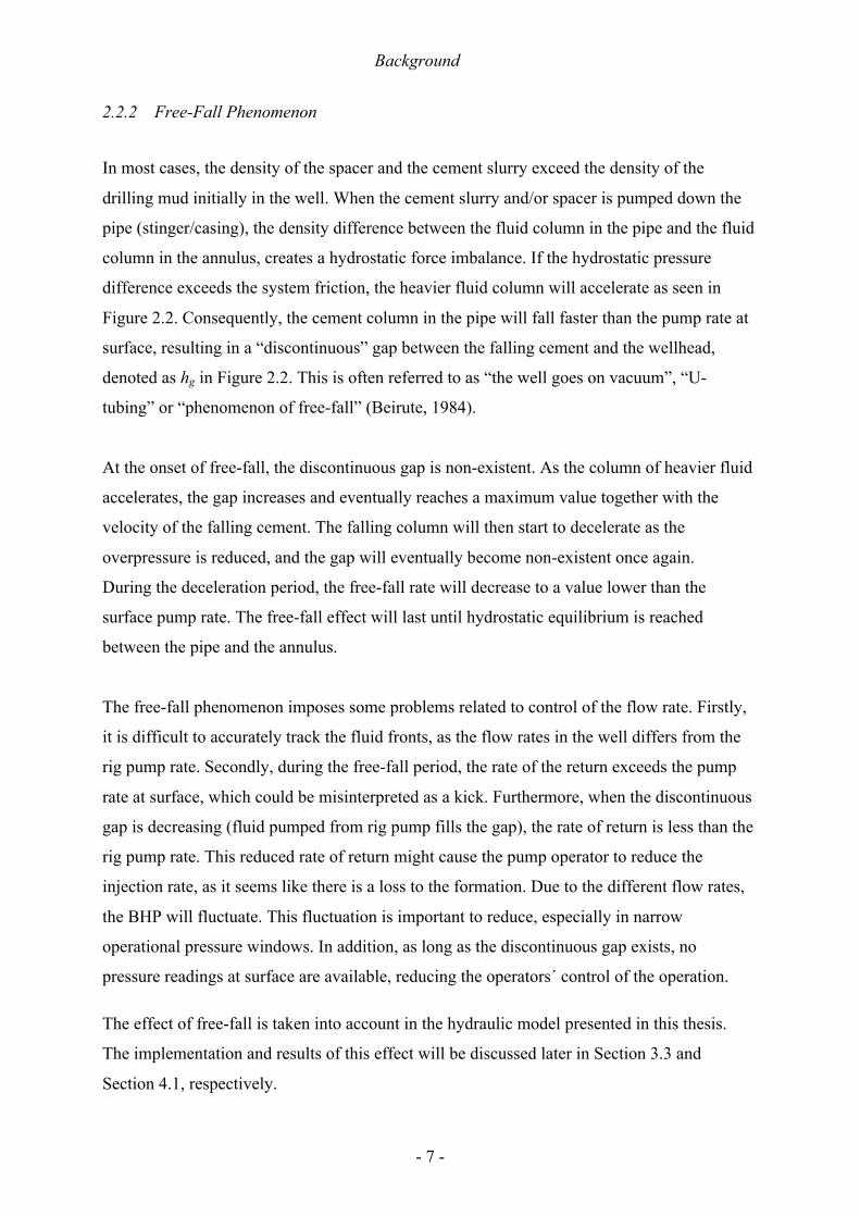
as seen in Figure 2.2.
Figure 2.2: Simplified u-tube illustration. Heavy weight fluid causes u-tubing until equilibrium is reached
Background
- 7 -
2.2.2 Free-Fall Phenomenon
In most cases, the density of the spacer and the cement slurry exceed the density of the
drilling mud initially in the well. When the cement slurry and/or spacer is pumped down the
pipe (stinger/casing), the density difference between the fluid column in the pipe and the fluid
column in the annulus, creates a hydrostatic force imbalance. If the hydrostatic pressure
difference exceeds the system friction, the heavier fluid column will accelerate as seen in
Figure 2.2. Consequently, the cement column in the pipe will fall faster than the pump rate at
surface, resulting in a “discontinuous” gap between the falling cement and the wellhead,
denoted as hg in Figure 2.2. This is often referred to as “the well goes on vacuum”, “U-
tubing” or “phenomenon of free-fall” (Beirute, 1984).
At the onset of free-fall, the discontinuous gap is non-existent. As the column of heavier fluid
accelerates, the gap increases and eventually reaches a maximum value together with the
velocity of the falling cement. The falling column will then start to decelerate as the
overpressure is reduced, and the gap will eventually become non-existent once again.
During the deceleration period, the free-fall rate will decrease to a value lower than the
surface pump rate. The free-fall effect will last until hydrostatic equilibrium is reached
between the pipe and the annulus.
The free-fall phenomenon imposes some problems related to control of the flow rate. Firstly,
it is difficult to accurately track the fluid fronts, as the flow rates in the well differs from the
rig pump rate. Secondly, during the free-fall period, the rate of the return exceeds the pump
rate at surface, which could be misinterpreted as a kick. Furthermore, when the discontinuous
gap is decreasing (fluid pumped from rig pump fills the gap), the rate of return is less than the
rig pump rate. This reduced rate of return might cause the pump operator to reduce the
injection rate, as it seems like there is a loss to the formation. Due to the different flow rates,
the BHP will fluctuate. This fluctuation is important to reduce, especially in narrow
operational pressure windows. In addition, as long as the discontinuous gap exists, no
pressure readings at surface are available, reducing the operators´ control of the operation.
The effect of free-fall is taken into account in the hydraulic model presented in this thesis.
The implementation and results of this effect will be discussed later in Section 3.3 and
Section 4.1, respectively.

Background
- 8 -
2.2.3 Design Limits
As every well is unique regarding pressure limits, formation properties, in-situ fluid
properties, bottom hole pressures, temperatures and so forth, the cement properties need to be
carefully tailored to fit the given environment. When designing the cement slurry and spacer,
a comprehensive amount of different aspects must be considered. In this section, design limits
that can be altered using MPD/MPC are included.
In general, the equivalent circulation density (ECD), must be maintained above the pore
pressure gradient to prevent influx and below the fracture pressure gradient to avoid losses to
the formation. Through downhole measurements such as negative and positive pressure tests,
downhole pressure limits and weak zones can be identified. One of the major challenges
associated with the cementing operation, is losses to the formation. Both the hydrostatic
pressure and frictional pressure loss are rapidly increased during the displacement of the
spacer and cement into the annulus, potentially fracturing the formation.
The optimal cement slurry for the downhole environment might induce an ECD higher than
allowed. To keep the ECD within the given pressure window the cement engineers have to
change the density (hydrostatic pressure) and/or the viscosity (frictional pressure). The same
ECD restrictions must be considered when designing the spacers. The spacers are designed to
minimize cement contamination and to clean the pipe and the annulus. If the optimal spacer
design is restricted to ECD control, the performance is most likely to be effected.
Balancing performance and ECD when designing spacers and cement slurry can be
challenging in narrow pressure windows. Both cement and spacer are traditionally denser and
more viscous than mud, hence the hydrostatic pressure and the frictional pressure loss will
increase as slurry and spacer enters the well. Different additives can be used to alter the
density and viscosity of the fluids, but the use of additives may be associated with declining
performance of the cement job quality.
The settling time of a cement slurry is the time of which it is capable of being pumped.
(Brechan, 2015). Obviously, it is important to match the settling time with the expected time
required to pump the cement in place. At the same time, it is desirable that the cement set as
quickly as possible after being pumped in place to reduce wait on cement (WOC) time. The

Background
- 9 -
displacement time of cement is naturally governed by the displacement rates. To improve
mud displacement efficiency and save rig time, high displacement rates is desirable.
However, as the friction pressure loss is proportional to the displacement fluid velocity
squared, the displacement rate is limited by the fracture pressure.
By introducing MPC, an extra, adjustable component to the BHP is added, altering the design
limits.
2.3 Managed Pressure Cementing
MPD/MPC is a collective term including different techniques utilized to gain improved
pressure control while drilling/cementing. According to the definition from The
Underbalanced Operations and Managed Pressure Drilling Committee of the International
Association of Drilling Contractors (IADC), MPD is “… an adaptive drilling process used to
control the annular pressure profile throughout the wellbore drilling with the objectives to
ascertain the downhole pressure environment limits and to manage the hydraulics annular
pressure accordingly” (Nas, 2011).
As previously mentioned, during conventional drilling and cementing, the fluid column must
provide hydraulic overbalance to the pore pressure to avoid formation influx. If the fracture
limit is relatively close to the pore pressure, e.g. narrow pressure window, circulation can
cause the ECD to exceed the fracture gradient, potentially resulting in losses.
Figure 2.3: Green column illustrates how MPC can keep the ECD within the desired target ECD (Russell et al., 2016)

Background
- 10 -
As seen in Figure 2.3, the narrow pressure window makes it difficult to avoid fracturing the
formation by circulating the columns providing hydrostatic overpressure. MPC allows for
hydrostatic under-pressure, as the hydrostatic pressure can be adjusted either before or during
the operation. A MPD system that is adjusted automatically based on direct system input
during cementing, is called Automated Managed Pressure Cementing (AMPC). Real time
operational data is acquired, communicated to the MPD hydraulic modelling system which
then communicates a target ECD to the MPD-equipment. As seen in Figure 2.3, the
automation of real time data interpretation provides enhanced pressure control. In this thesis,
a PI-controller is implemented to enable automatic control of the downhole pressure. It will
however be referred to as MPC, not AMPC.
Different MPC techniques are utilized in the industry to provide enhanced pressure control.
The two MPC techniques investigated and simulated in this thesis, are: 1) a system which
includes a topside choke valve to apply back-pressure, and 2) a system which includes a
subsea pump module (SPM) to reduce the fluid level in the riser. In this thesis, the two
systems used for cementing, will be referred to as Applied Back-Pressure (ABP) system and
Dual Gradient (DG) system, respectively.
2.3.1 Applied Back-Pressure System
In a standard ABP system, additional back-pressure is applied to compensate for pressure
fluctuations in the annulus. At surface the annulus is sealed off by a rotating control device
(RCD) and mudflow from the well is controlled by a choke valve. This results in an additional
and rapidly adjustable component ((;) in Equation 2, resulting in:
34( = ()*+ + (678,: + (; (3)
where (; is the choke pressure. By adjusting the choke valve opening, the pressure can be
controlled.
2.3.2 Dual Gradient System
There are many forms of DG systems available in the industry. However, in the DG system
presented in this thesis, the mud returns to the surface through a SPM, which is installed onto

Background
- 11 -
the riser. By controlling the flow rate out of the well, the subsea pump can adjust the fluid
level in the riser. The reduced mud level in the riser is either replaced with air/gas, seawater
or less dense mud, hence the name Dual Gradient.
As hydrostatic pressure is proportional to the height and density of the fluid columns, the
altering of riser level can be used to control the bottom hole pressure. The BHP is then given
by the following equation:
34( = /: ∙ 1 ∙ = − ℎ7 + /7 ∙ 1 ∙ ℎ7 + (678,: (4)
where /: is the fluid density in the annulus, = is the vertical depth of the wellbore and ℎ7 is
the height of the lower density fluid, /7, in the riser.
2.3.3 Advantages Using Managed Pressure Control During Cementing
The main advantage of using MPC is the ability to adjust the bottom hole pressure throughout
the cement process. This alters the design limits in the pre-job planning phase. During MPC,
the operator can regulate the pressure based on real time data from the well. Thus, the success
of the cement job will not depend as much on a correct pre-job planning phase, as a
conventional setup. An unanticipated well response can then potentially be counteracted by
using the MPD equipment.
In Section 2.2.3, it was recognized that density and viscosity of the cement and spacer had to
be designed so that the resulting ECD would be kept inside the pressure limits. As it is now
possible to lower the pressure profile in the well through MPD equipment, the spacer and
cement design can be tailored outside the original fracture limits. The design can be based on
performance, with less focus on keeping the ECD inside the pore pressure and fracture limits
at all stages.
The ability to control the pressure allows the operator to increase the flow rate. The higher
friction pressure caused by a higher flow rate can simply be reduced by the MPC system. By
utilizing a MPC system, the cement/spacer or displacement mud rates can be designed outside
the limits of normal principals, improving mud removal (and thus cement bond), and
minimizing fluid intermixing during the displacement. The total time of the cement job is

Background
- 12 -
reduced when the displacement rates are increased, reducing rig time and costs.
By controlling the pressure throughout the cementing process, the risk of influx and/or losses
to the formation is minimized. Both losses to the formation and formation fluid influx can be
detrimental for the cement job, but as an influx into the cement is considered more severe, it
is suggested to keep the ECD closer to the fracture gradient than the pore pressure gradient
(Russell et al., 2016).
All the abovementioned factors can improve the conventional cement job. The improved
pressure control is associated with lower risks, improved cement quality and reduced non-
producing time (NPT). By developing hydraulic models, these factors will be investigated
based on simulations performed in MATLAB.

Modeling
- 13 -
3 Modeling
3.1 Fundamental Fluid Dynamics
To model the behavior of the pressure and flow dynamics in a well, a suitable hydraulic
model is necessary. The derivation of such a hydraulic model is based on one main
assumption; the fluid in the well can be treated as a viscous fluid. The derivations in this
section is mainly based on Merritt (1967) and White (2011). By assuming a viscous fluid,
whether it is spacer, fluid or cement flowing in the well, the flow behavior can be fully
described by the following fundamental equations:
- Fluid viscosity: The fluid viscosity is a function of temperature and pressure
- Equation of state: The fluid density is a function of temperature and pressure
- Equation of continuity: Conservation of mass
- Conservation of momentum: Newton´s second law of motion or the force balance
- Equation of energy: The first law of thermodynamics or the energy balance
The hydraulic model presented in this section is a simplified hydraulic model, able to estimate
pressure and flow dynamics during a cement operation. The model is based on the work
presented by Stamnes et al. (2012) and Kaasa et al. (2012). However, some modifications are
done in order to make it suitable for the two different control systems.
One of the biggest challenges in modeling, is to make the model as simple as possible without
neglecting important factors. Only the dominating pressure and flow dynamics of the system
should be included. In addition, it is not necessary to include more details in the model, than
the control system can register.
The following assumptions were made, during the outline of this hydraulic model:
- Isothermal condition: The temperature is assumed to remain constant throughout the
operation. Consequently, the equation of energy can be neglected.
- Radially homogenous flow: Averaging properties over the cross-section of the flow
are used.
- 1D flow: Only one dimensional flow, along the well, is considered
Modeling
- 14 -
- Constant viscosity: The time variance of the viscosity is neglected
- Incompressible flow: The spatial time variance of the density is neglected in the
momentum equation. However, the main compressibility effects of the fluid are taken
into account by combining the equation of state with mass conservation.
3.1.1 Equation of State
The equation of state cannot be derived mathematically from physical principles, but rather
from empirical data. In general, the density can be described by the following equation, based
on interpolated PVT (pressure, volume and temperature) data:
/ = /((, @) (5)
where ( denotes pressure and @ denotes temperature. The density changes of a liquid as a
function of pressure and temperature, are relatively small, and are therefore often described
by a linearized equation of state:
/ = /B +C/CD D − DB +
C/C@ (@ − @B) (6)
where ρB, @B, DB is the density, temperature and pressure at the reference point of linearization.
By introducing the material properties, isothermal bulk modulus, F, and the isobaric cubical
expansion coefficient, G, Equation 6 can then be rewritten as:
/ = /B +/BF D − DB − G/B(@ − @B) (7)
where the isothermal bulk modulus and the isobaric cubical expansion coefficient is defined
respectively as:
F = /B(C(C/)H (8)

Modeling
- 15 -
G = −1/B(C/C@)J (9)
Equation 7 can be rewritten into its differential form, resulting in:
%/ = /BF %( − G/B%@ (10)
The accuracy of the presented linearization decreases with increasing temperature and
pressure. However, experimental PVT data, pressure-volume-temperature data, shows that the
linearization is quite accurate for most drilling fluids between 0 to 500 bar and temperatures
between 0 and 200 degrees Celsius (Isambourg, Anfinsen, & Marken, 1996; Kaasa et al.,
2012). As previously mentioned, the temperature changes are neglected in this model, which
simplifies the linearization even more:
%/ =/F %( (11)
Temperature gradients due exist in a well, but since the thermal expansion coefficient for
liquids,G, usually is small, the density changes in the system due to temperature changes are
often negligible with respect to transient effects. In addition, the pressure transient of a well,
range from seconds to minutes, while temperature transient could range from minutes to hours
(Kaasa et al., 2012). According to Kaasa et al. (2012), the relatively slow temperature
transients can usually be more efficiently handled by applying online calibration using
feedback in the control system, than to include these temperature effects in the hydraulic
model. Hence, the temperature effects in a wellbore system are therefore neglected in this
simplified hydraulic model.
3.1.2 Equation of Continuity
The equation of mass continuity states that the rate at which mass enters a system is equal to
the rate at which mass leaves the system plus accumulation of mass inside the system due to
compressibility effects. Assuming homogenous 1D-flow, the equation of mass continuity
becomes:

Modeling
- 16 -
C/CK +
C(/L)CM = 0 (12)
where L is the fluid velocity and M is the spatial variable defined along the flow path.
By substituting Equation 11 into the expression for the density derivative in Equation 12, and
assuming the cross-sectional area A(x) in the well to be piecewise constant, the equation of
continuity becomes:
/FC(CK = −
/.(M)
C(!)CM + L
C(/)CM (13)
where, q is the volume flow rate flowing through the cross-sectional area, A.
Furthermore, the flow is assumed to be spatially incompressible, (i.e. O(P)OQ
= 0) and Equation
12 is integrated over a homogenous control volume V, resulting in the mass balance equation
in the standard integral form:
C(/R)CK + /STU!STU − /8V!8V = 0 (14)
where / is the average density inside the control volume and /8V!8V and /STU!STU are the
mass flow rates in and out of the control volume, respectively.
In order to get the pressure as the main variable, Equation 11 is substituted into Equation 14,
creating an equation able to model the pressure variation at any location inside the drill string:
/RFC(CK + /
CRCK = /8V!8V − /STU!STU (15)
where, ( is the pressure inside the control volume.
Based on the assumption of spatially homogenous density, Equation 15 can be further
simplified, by setting / = /8V = /STU:
RFC(CK +
CRCK = !8V − !STU (16)

Modeling
- 17 -
During a cementing operation, three different fluids (spacer, cement and mud) will be present
in the pipe/ annulus at the same time. Based on the work presented by Stamnes et al. (2012),
Equation 16 can be modified and expanded to apply for a multi-fluid hydraulic system
consisting of three different fluids.
3.1.3 Multi-Fluid Hydraulic System
The pipe or annulus is modelled as shown in Figure 3.1, as a hydraulic system consisting of
three different fluids.
Figure 3.1: Fluid volumes in stinger/annulus
By creating three different control volumes, R+W, R+X and R+Y, as shown in Figure 3.1,
Equation 16 can be separated into three equations, describing the pressure dynamics inside
each fluid:
R+WF+W
C(WCK +
CR+WCK = !8V,W − !STU,W (17)

Modeling
- 18 -
R+XF+X
C(XCK +
CR+XCK = !8V,X − !STU,X (18)
R+YF+Y
C(YCK +
CR+YCK = !8V,Y − !STU,Y (19)
where the subscripts d1, d2 and d3 refers to fluid volume 1, 2 and 3 inside the pipe or annulus.
Furthermore, the pressure change at any location inside the pipe is assumed to be the same,
i.e.( = (W = (X = (Y, and !STU,Y = !8V,X and !STU,X = !8V,W. Equation 17, Equation 18 and
Equation 19 can then be added together, resulting in:
R+WF+W
+R+XF+X
+R+YF+Y
C(CK = !8V,Y − !STU,W −
CR+WCK −
CR+XCK −
CR+YCK (20)
The total volume inside the drill string is constant, which means that a positive volume
change for Fluid 3, will lead to a negative volume change, by the same amount, for Fluid 1,
i.e. R+Y = −R+W. R+X = 0, since no mass of Fluid 2 is entering or leaving the system.
Equation 20 can therefore be simplified to:
R+WF+W
+R+XF+X
+R+YF+Y
C(CK = !8V − !STU (21)
In order to implement this equation into MATLAB, a relationship is provided to calculate the
different fluid volumes. At time KB the initial volumes are set as R+WB , R+XB and R+YB . The
volumes are given as the solution to the following three differential equations:
R+W; = −!STU (22)
R+X; = 0 (23)
R+Y; = !8V (24)
These equations do not consider compressibility effects, and will not be valid during
transients, as the equations will overestimate the volumes if the pressure increases. To

Modeling
- 19 -
account for compressibility effects, the volumes can be normalized to ensure that
R+W + R+X + R+Y = RUSU:
R+W = ZR+W; (25)
R+X = ZR+X; (26)
R+Y = ZR+Y; (27)
where
Z = RUSU
(R+W; + R+X; + R+Y; ) (28)
where RUSU is the total volume inside the drill pipe/stinger. Even though Equation 25, 26 and
27 consider compressibility effects, they do not consider different compressibility of the
fluids. Since cement is less compressible than mud, the cement will be relatively less
compressed than mud. To account for different compressibility of the fluids, the bulk modulus
of each fluid is considered. The bulk modulus of Fluid 3, is defined as:
F+Y = −R+Y;∆(
R+Y − R+Y; (29)
where the volume of Fluid 3 is compressed from R+Y; to R+Y due to a given pressure difference
of ∆( and R+Y; is the solution to Equation 24. By rearranging Equation 29, the correct volume
of Fluid 3 can be calculated as:
R+Y = R+Y; (1 −∆(F+Y
) (30)
Similar for Fluid 1 and Fluid 2, the expression becomes:
R+W = R+W; (1 −∆(F+W
) (31)
R+X = R+X; (1 −∆(F+X
) (32)

Modeling
- 20 -
where R+W; and R+X; is the solution to Equation 22 and 23.
To solve the above system of equations with three unknowns, R+W, R+Y and ∆D, an additional
relationship needs to be added. R+X is known from the previous iteration, and is only changed
due to compressibility effects, since only Fluid 3 and Fluid 1 are entering and leaving the
system. By adding the expression for the known drill string volume, R+W + R+X + R+Y = RUSU,
the system consists of three independent equations and three unknowns, which makes it
solvable.
3.1.4 Conservation of Momentum
Based on Newton’s 2.law of motion, the momentum balance for 1D-flow in the x-direction
becomes:
-Q =/%L%K . M %M (33)
where -Q is the total forces acting in the x-direction and . M is the flow area.
The forces acting on the control volume in the x-direction are external fields, such as
frictional forces, pressure forces and gravitational forces. The differential momentum
equation then becomes:
/CLCK = −
C(CM −
C\CM + /1 cos(`)
(34)
where \ denotes the friction and ` denotes the wellbore inclination. Tau,\, is a lumped factor
including friction losses due to viscous effects, turbulence and flow restrictions. The frictional
pressure drop in this model is calculated and based on Zamora, Roy, and Slater (2005), see
Section 3.2. Equation 34 can be re-written as:
/
.(M)C!CK = −
C(CM −
C\CM + /1 cos(`) (35)
In general, an equation describing the average flow dynamics in a given control volume from
an arbitrary starting point x = x1 to x = x2, can be obtained by assuming that the fluid
accelerates as a homogenous stiff mass. Equation 35 can then be written as:

Modeling
- 21 -
a bW, bX%!%K = ( bW − ( bX − -(!, c, bW, bX) + G(bW, bX, /) (36)
where,
a bW, bX =/(M).(M) %M
ef
eg
(37)
- !, c, bW, bX =C\CM %M
ef
eg
(38)
G bW, bX, / = / M 1 cos ` M %M
ef
eg
(39)
where ( bW, bX is the pressure at starting point, M = bW, and end point,M = bX, respectively,
G bW, bX, / is the hydrostatic pressure difference between position M = bW and M = bX,
- !, c, bW, bX is the total frictional pressure loss along the flow path and c is the fluid
viscosity and a bW, bX is the integrated density per cross-section over the flow path.
3.2 Hydraulic Friction Loss
To predict the pressure regime in a flow-loop, accurate estimation of the friction pressure loss
is required. The key parameters impacting the friction pressure loss are flow rate, pipe
geometry, flow regime and rheological properties. Drilling fluids are generally non-
Newtonian fluids, meaning that the viscosity of the fluid is dependent on the shear rate or
shear history. As seen in Figure 3.2, different rheology models show different relationships
between shear stress and shear rate.
Figure 3.2: Flow curve of different rheology models (Skalle, 2015).
Modeling
- 22 -
Often, Newtonian fluid behavior is assumed when modeling, as the linear relationships
between shear rate and shear stress simplifies the modeling significantly. Including the non-
Newtonian properties can be challenging, even when the system parameters are well-known.
However, in this work, obtaining a fluid flow model that is as realistic as possible has been a
prioritized objective. The non-Newtonian behavior of the drilling fluid and cement has
therefore been included.
After discussions with Professor Pål Skalle at the Department of Geoscience and Petroleum,
NTNU, the Herschel-Bulkley rheology model is recognized as the model providing the most
realistic prediction of non-Newtonian drilling fluid behavior. Although the Herschel-Bulkley
is a complex rheology model, it is the choice for many drilling applications as it fits a wide
range of drilling fluids. The model also includes the yield-stress term that is used to
investigate and optimize hydraulic-related concerns like hole cleaning, suspension and barite
sag, as well as including the traditional Bingham-model and exact Power Law behavior as
special cases (Zamora et al., 2005).
Due to rising demands on accuracy from an increasing number of critical wells, several
different hydraulics software applications have been developed. Due to the increasing
deviation between the API Recommended Practice 13D-1995 and industry practice, Zamora
and Power (2002) wrote a paper on behalf of American Association of Drilling Engineers
(AADE), addressing the problems with uniformity and the increasing gap between theoretical
and practical solutions. A new model called “Unified rheological model” was introduced, to
“unify” the industry. This model proved to be sufficiently accurate both for conventional and
critical wells. As the model was a practical rheological characterization of Herschel-Bulkley,
including empirically derived flow equations expressed in a form easily recognized by field
engineers, the model gained wide acceptance. This model was extended by Zamora et al.
(2005), including pressure losses in transitional and turbulent flow regimes. Due to its
transparency and recognized level of accuracy, this model has been used to determine friction
pressure loss in the model presented in this thesis. The main ideas and equations are explained
and presented in Appendix C.
3.3 Simplified Hydraulic Model
The main objective of the simplified hydraulic model was to investigate the pressure and flow
Modeling
- 23 -
development throughout the cement operation using MPC, and to discuss how the MPC
techniques can be used to obtain better cement jobs. Consequently, it has been of high
importance to acquire descriptive and accurate pressure and flow models. The simplified
hydraulic model used in this work was based on the pressure and flow dynamics presented in
Section 3.1. Due to the complexity of the fluid dynamics, some simplifications have been
necessary. These simplifications will be further discussed in Section 3.3.2 and Section 4.2.
3.3.1 Model Setup
The simulated well consisted of a 400m long riser and a 3600m vertical open hole section
with inner diameter of 17 1/2”. The casing to be cemented had an outer diameter of 13 3/8”
and a cement stinger with inner diameter of 5” was used to place the cement column into the
annulus. One of the reasons for choosing the stinger method, was to highlight the effect of
free fall during cementing. By using a small diameter inner string, a given cement volume
will create a higher hydrostatic pressure at the bottom of the string, compared to a larger
diameter string. The pressure difference between the inner string and the annulus will increase
as the diameter of the inner string decreases. This pressure difference is, as aforementioned,
what initiates the free fall phenomenon.
For simplicity, the annulus capacity was assumed constant in the entire well, from the bottom
of the well to the rotary-kelly-bushing (RKB). The fluid densities used in the simulations are
listed in Table 1. Apart from the mud density, the same model setup and fluid properties were
used in all the three different simulations (conventional, ABP and DG systems). Other
simulations parameters can be found in Appendix A. Figure 3.3 displays a basic sketch of the
model setup.
Table 1: Fluid densities
Description Value Unit
Density mud (conventional)
Density mud (ABP)
Density mud (DG)
1300
1100
1300
[kg/m3]
[kg/m3]
[kg/m3]
Density cement
Density spacer
2000
1600
[kg/m3]
[kg/m3]

Modeling
- 24 -
Figure 3.3: Well schematics
3.3.2 Model Simplifications
The main simplification in the model setup, was the constant annulus flow area. To drill a
3600 m well in one section, with a 17 ½ inch bit, is not realistic. The open hole diameter was
assumed constant and known (neglecting diameter uncertainties) for the whole section. The
riser inner diameter was chosen identical to the open hole diameter. Preferably, different
sections should be included to make the case more realistic. In the code, this would imply to
split the annulus flow calculations into sections. This extension would not require additional
pressure and flow dynamics theory, as the already presented theory could be applied for
different sections in the annulus. However, due to time constraints, this was not prioritized
and the annulus capacity was assumed constant.
In the DG system model, the friction in the riser was neglected due to complicated flow

Modeling
- 25 -
conditions. The friction will act in different directions depending on whether the riser level
increases or decreases. This simplification is justified with the relatively small annular friction
loss in the riser compared to the length of the entire well.
The rat hole, meaning the space between the end of the casing to the bottom of the open hole,
was neglected. This means that the flow goes directly from the stinger and into the annulus. In
addition, the wellbore was assumed perfectly vertical.
3.3.3 Applied Back-Pressure Modelling
To simulate cementing using ABP, the hydraulic model presented in Section 3.1 was
integrated into a regulator, controlling the topside choke valve. The model was implemented
and simulated in MATLAB. Figure 3.4 displays a simple sketch of the ABP system.
Figure 3.4: Basic sketch of the ABP system

Modeling
- 26 -
The choke valve was set to have an operational area from 0 to 90 degrees, corresponding to
fully closed and open, respectively. The relationship between the pressure drop over the
choke, the flow rate and the choke-opening is given by the following equation:
∆(; = /!;hij;
X (40)
where ∆(; is the pressure drop over the choke valve, !; is the flow through the choke, hi
denotes the choke coefficient related to physical parameters given by the manufacturer, j; is
the choke-opening, ranging from 0 to 1, and / is the density of the fluid flowing through the
choke. The choke coefficient is defined as the number of gallons of water per minute which
will pass through a restriction resulting in a pressure drop of 1 psi at 60℉ (Fahrenheit) (King,
2017). This choke coefficient was estimated by rearranging Equation 40, and using the initial
flow rate and choke pressure, assuming a choke opening of 20 %.
The pressure drop can be written as:
∆(; = (; − (B (41)
where (; is the pressure on the inlet of the choke and(B is the outlet pressure. In this scenario,
the outlet pressure is equal to the atmospheric pressure. However, it should be mentioned that
only gauge pressure was considered in the model simulations, making ∆(; = (;.
The initial choke pressure was found by calculating the difference in BHP and set point due to
the lower-density mud used during the ABP cementing operation:
∆34( = /l;SVi − /lmno 1= = 78.48tuv (42)
where /l;SVi is the mud density used in the conventional simulation and /lmno is the mud
density used in the ABP system simulation.

Modeling
- 27 -
3.3.3.1 Pressure Dynamics
The following pressure dynamics for the ABP system was based on the discretized hydraulic
model presented in Section 3.1.
The pump pressure can simply be modelled and expressed as:
RlJ
Fl+RwJ
Fw+R;J
F;C(JCK = !J − !x (43)
where RJl/w/; , is the mud, spacer and cement volumes inside the pipe/stinger, respectively,
Fl/w/;, is the isothermal bulk modulus of mud, spacer and cement, respectively, !J denotes
the rig pump flow rate, (J is the rig pump pressure and !x is the flow rate through the bit.
Even though no bit is present during cementing, the flow out of the stinger is denoted !x and
will be referred to as “flow through the bit” in this thesis.
The BHP was modelled in the same way, resulting in:
Rl:
Fl+Rw:
Fw+R;:
F;C34(CK = !x − !; (44)
where R:l/w/; , is the mud, spacer and cement volumes inside the annulus.
3.3.3.2 Flow Dynamics
The flow through the bit was modelled by assuming it is approximately equal to the average
flow from the rig pump to the choke at surface. By applying the momentum balance,
presented in Section 3.1.4, the bit flow dynamics can be expressed as:
aJ +a:%!x%K = (J − (; − (678,J − (678,: + zJ − z: (45)
where zJ is the hydrostatic pressure in the pipe, (678,J is the frictional pressure loss inside the
stinger and aJ/: is the integrated density per cross-section over the flow path in the
Modeling
- 28 -
pipe/annulus.
The momentum balance was also used to model the flow rate through the choke. The choke
flow was assumed to be approximately equal to the average flow in the annulus, resulting in
the following expression:
aJ +a:%!;%K = 34( − (; − (678,: − z: (46)
To model the free fall phenomenon and the resulting air gap in the stinger, an if-statement
was implemented in MATLAB. At the time of free fall, the pump pressure is zero. The
hydrostatic pressure difference between the stinger and the annulus must overcome the choke
pressure and the friction in the entire well before free-fall is initiated. This scenario can be
expressed as:
zJ − z: − (678,J − (678,: − (; > 0 (47)
Since the pump pressure is zero, it was assumed that compressibility effects could be
neglected during free-fall. This assumption reduces the mass balance to a volume balance.
The flow from the pump enters the stinger, while the flow through the bit exits the stinger.
The air gap change was then incorporated into the model by introducing the following
expression:
ℎJ =1.J
!x − !J (48)
where ℎJ is the change in air gap level in the pipe and .J is the inner cross-sectional area of
the pipe. Consequently,!x > !J, will lead to a reduction in fluid level in the pipe (an increase
in air gap).
3.3.4 Dual Gradient Modelling
In the DG system model, two centrifugal subsea pumps were placed at the lower part of the
riser, to pump mud from the riser up to the rig. The riser was connected to the subsea pumps
and a mud return line connect the subsea pumps to the rig. The horizontal part of the mud
return line (MRL) was divided into a suction part (Lsuc) and discharge part (Ldisp), and the
vertical length of the MRL was denoted with the same parameter as subsea pump depth, hssp.

Modeling
- 29 -
In this model, a partially filled riser was considered. The riser was open to the atmosphere and
the riser fluid was replaced with air as the mud level decreased. The density and
compressibility of air were neglected in order to simplify the model.
Commonly a booster pump is included in a DG system, enabling pressure increase
independent of the subsea pumps. To simplify the model, such a booster pump, was not
included. To have maximum pressure reduction potential, the SPM was placed at the bottom
of the riser. Figure 3.5 shows a simple sketch of the DG system setup. SPM parameters can
be found in Appendix A. Despite a few modifications, the simulation of the DG system was
very similar to the simulation of the ABP system.
Figure 3.5: Basic sketch of a DG system
The modeled SPM consisted of two centrifugal subsea pumps in series. The modelled
centrifugal pumps were dynamic, making the flow rate, qssp, not only depending on the
Modeling
- 30 -
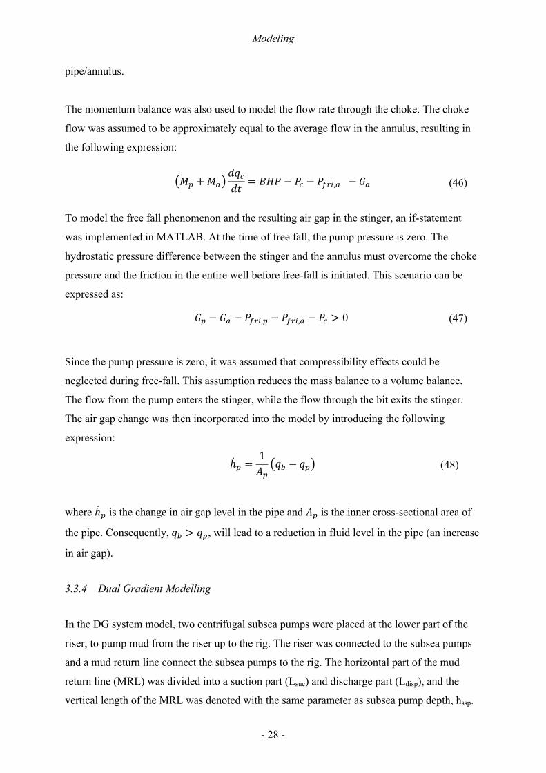
rotational velocity, wssp, but also the total head. To account for this effect, a pump model
similar to the one presented in Stamnes et al. (2012) was implemented in MATLAB. They use
the affinity laws from White (2011) to approximate the total pump head. The total head, can
then be expressed as:
ℎUSU = |J("B}wwJX − "W}wwJ!wwJ − "X!wwJX ) (49)
where |J is the number of pumps in series, }wwJ is the rotational velocity of the subsea
pumps, !wwJ is flow rate through the SPM and "B, "W,"X are fitting constants. The fitting
constants used to model the two subsea pumps were "B = 4.17 ∗ 10�Ä ,"W = 6.83 ∗ 10�X and
"X = 115 (Cohen, Stave, Hauge, & Godhavn, 2014). Equation 49 was then used to determine
the differential pressure over the SPM, given the flowrate and the rotational velocity:
∆(ÑoÖ = /l1("B}wwJX − "W}wwJ!wwJ − "X!wwJX ) (50)
Figure 3.6 Pump characteristics for two subsea pumps in series, top curve corresponds to a rotational velocity of 2000 rpm, while bottom curve corresponds to 1500 rpm. The black dashed curve represents the system curve.
Figure 3.6 displays the pump characteristics for the two subsea pumps in series, where the
pump curves were developed using Equation 49. The maximum and minimum pump velocity

Modeling
- 31 -
of the pumps were assumed to be 2000 rpm and 600 rpm, respectively. The pump curves
show that increasing flow rate, will lead to reduced total head. The operational point of the
pump is determined by the intersection between the pump curves and the system curve. The
system head (system curve) for the DG return system, consisting of hydrostatic pressure and
frictional pressure losses, neglecting friction in the riser, is expressed as:
ℎw*w =1
1/lzl7e + (678,l7e − z7 (51)
where zl7e is the hydrostatic pressure in the mud return line, (678,l7e is the frictional pressure
loss inside the mud return line and z7 is the hydrostatic pressure at the inlet of the pumps,
depending on the fluid level in the riser.
To prevent cavitation of the pumps, the riser level was restricted in the MATLAB code, and
could not be reduced to a lower level than a hydrostatic pressure corresponding to 5 bar.
3.3.4.1 Pressure and Flow Dynamics
During the DG cement operation, the pump pressure was calculated identical to ABP system,
see Equation 43. Due to the different annular conditions, the expression for the BHP becomes
slightly different:
RlFl
+RwFw+R;F;
C34(CK = !x − !7 (52)
where !7 is the flow in the riser, and is expressed as:
a:%!7%K = 34( − (678,:W − z: (53)
where (678,:W is the frictional pressure loss in the annulus below the riser. As mentioned, the
friction is the riser was neglected.

Modeling
- 32 -
The expression for the bit flow in the DG system becomes:
aJ +a:%!x%K = (J − (678,:W − (678,J + zJ − z: (54)
The flow rate dynamics through the subsea pumps were modeled using the momentum
balance. A simplifying assumption was made, assuming that the flow rate through the pumps
equals to the average flow in the mud return line. The flow rate can then be expressed as:
al7e%!wwJ%K = (ÑoÖÜá + ∆(ÑoÖ − (ÑoÖàâä − (678,l7e (55)
where (ÑoÖÜá and (ÑoÖàâä are the hydrostatic pressures at the inlet and outlet of the subsea
pumps, respectively, and al7e is the integrated density per cross-section over the flow path in
the mud return line. The integrated density per cross-section over the flow path becomes:
al7e =/(M)
.l7e(M)%M
)ããå
B (56)
where ℎwwJ is the depth of the subsea pumps and .l7e is the cross-sectional area of the mud
return line. Since the density and the cross-sectional area in the mud return line are assumed
constant, the expression becomes simply:
al7e =/lℎwwJ.l7e
(57)
During the cement operation, the flow rate through the subsea pumps might not be sufficient
for the pumps to operate properly. This can result in back-flow through the pumps, e.g.
negative flow. This scenario was not considered, and Equation 55 was modified to not allow
!wwJ to become negative:
Modeling
- 33 -
al7e
%!wwJ%K
=(ÑoÖÜá + ∆(ÑoÖ − (ÑoÖàâä − (678,l7e!wwJ > 0$uM 0, (ÑoÖÜá + ∆(ÑoÖ − (ÑoÖàâä − (678,l7e !wwJ < 0
(58)
Since friction in the riser was neglected, the inlet pressure at the subsea pumps then becomes
a function only depending on the riser level:
(ÑoÖÜá = /l1 ℎwwJ − ℎ7 (59)
The hydrostatic pressure at the subsea pump outlet is expressed as:
(ÑoÖàâä = /l1ℎwwJ (60)
To simulate the change in riser level, compressibility effects due to pressure variations in the
riser were neglected, since the riser is open to the atmosphere. Again, the mass balance
reduces to a volume balance. The flow from the annulus enters the riser, while the flow
through the subsea pumps exits the riser. The flow rate in the riser was estimated in the same
way as the bit flow rate, by applying the momentum balance. The change in riser level was
then incorporated into the model by introducing the following expression:
ℎ7 =1.7
!wwJ − !7 (61)
where ℎ7 denotes the change in riser level and .7 is the cross-sectional area of the riser. If the
flow through the subsea pumps exceeds the flow entering the riser, it will result in a reduction
in the riser level.
The free fall phenomenon happening in the stinger during the DG simulation was modeled in
the same way as for the ABP simulation.

Modeling
- 34 -
3.4 Controller Design
3.4.1 PI Controller
In order to control and maintain the BHP within the pressure window, an automatic controller
is needed. In the simulations presented in this thesis, a simple PI-controller was used.
Figure 3.7: PI controller feedback loop
PI-controllers are very common in industrial control systems due to their simplicity, low cost
and simple design (Smriti Rao & Mishra, 2014). A standard PI-controller is used to close a
feedback loop (as illustrated in Figure 3.7). The PI controller adjusts the process variable
according to a set point value. The controller calculates the error between the desired set point
value (SPV) and the measured process value (MPV). The output value is the sum of a
proportional and an integral term, often denoted as P and I, respectively.
The proportional term is simply determined by multiplying the calculated error by a gain,
called the proportional gain, denoted Kp. It is important to choose an appropriate proportional
gain, since a too high proportional gain can make the system unstable, while a too low gain
can make the controller less effective.
By only applying a proportional term to the controller, the changes will be smaller and
smaller, as the process variable approaches the set point. Eventually, the process variable
might stabilize with a constant deviation, from the desired set point. Unless the system has
naturally integrating properties, control action based only on a proportional term, will always
Modeling
- 35 -
leave an offset error between the steady state condition and the set point (Willis, 1999).
Fortunately, the integral term can be introduced to reduce the steady state error, by
accumulating previous errors.
The controller model used in this thesis, has a proportional term and an integral term. By
adding these two terms together, the output from the PI-controller can be written as:
j K = éJ# K +éJ@8
#(\)%\U
B (62)
where j K is the output value, @8 is the integral time, éJ is the proportional gain, and # K is
the error, written as:
# K = è(R −a(R(K) (63)
where SPV is constant and the desired BHP while MPV is time dependent and the measured
BHP. As there is no downhole pressure measurements available during a cementing
operation, assumptions were made to estimate this value in this model. This will be elaborated
further in Section 4.2.
éJ and @8 are parameters that should be tuned before using the controller. By optimizing
these parameters, the performance and stability of the controller can be improved. There are
several tuning techniques which can be used to tune these parameters, however, tuning by
trial and error, with some help from our supervisor, was used in this work. In practice, tuning
can be performed in safe conditions in a cased hole. Step changes in set point and flow rates
are typically used to evaluate the performance and tune the controller parameters.

Modeling
- 36 -
3.4.2 Controller Implementation
3.4.2.1 Choke Valve Controller
A simple PI controller was implemented in MATLAB to operate the opening of the choke.
The PI controller was programmed to adjust the choke opening to maintain the BHP close to
the set point. Initially, the desired BHP was set to a set point value. Further the error between
the process variable (the calculated BHP) and the set point was determined. The choke valve
position was set from 0 to 1 (0-100%), representing closed and fully open, respectively.
The output from the PI controller, the desired choke opening, was then used in Equation 40,
to determine the choke pressure corresponding to the present choke opening and flow rate.
The calculated choke pressure was then used to determine the choke flow for the next time
step. The iterations were then repeated, always using the previous choke pressure to
determine the present choke flow.
The proportional gain and the integral time used in the choke controller simulations are
presented in Table 2.
Table 2: Proportional gain and integral time constants (ABP system)
Constant Value
Kp 0.3 ∙ 10�Ä
Ti 5
For the chosen gain, a step in the error of 1 bar, e.g. 1 bar higher than set point, will give a 30
% change in choke position. The integral term will then accumulate (integrate) the error until
the error converges to zero. It was assumed that the changes in choke position were made
instantaneously.
3.4.2.2 Subsea Pump Controller
For the scenario where the BHP was controlled by adjusting the fluid level in the riser, a
mathematical model of the SPM was implemented in MATLAB. In this case, the PI controller
was implemented to control the pump speed. If the BHP increases above the set point, the PI

Modeling
- 37 -
controller will increase the pump speed to reduce the fluid level in the riser. The reduction in
fluid level will then reduce the hydrostatic pressure.
The output value from the PI controller determined the pump speed, revolutions per minute
(RPM), ranging from the minimum pump speed to the maximum pump speed. An output
value of 0, was modified to correspond to the minimum pump speed, while an output value of
1 corresponded to maximum velocity. The output value from the PI controller was then used
in the equation below, to find the desired pump speed:
}''D7ê6 = }''Dl8V + j(K)(}''Dl:Q − }''Dl8V) (64)
where }''D7ê6 denotes the new desired rotational velocity, }''Dl8V is the minimum
velocity, }''Dl:Q is the maximum velocity and j(K) is the output value, ranging from 0 to 1.
In the modeling of the choke, the changes in choke position were assumed to be
instantaneous. For the modeling of the pumps, however, a subsea pump frequency converter
was implemented, to simulate the time it takes for the impeller to adjust to the new desired
velocity. A frequency converter is typically used to maintain the pump at a given velocity. In
this model, it is assumed that the frequency converter assures that the pump velocity
converges to the reference }wwJ7ê6after a short period of time. The actuator dynamics are based
on the model presented by Stamnes et al. (2012) and expressed as:
}wwJ8 = }wwJ8�W +%K\wwJ
(}wwJ7ê6 − }wwJ8�W) (65)
where }wwJ8 is the present velocity, }wwJ8�W is the previous velocity, }wwJ7ê6 is the desired velocity
and \wwJ is the transient period it takes for the impeller to adjust to the desired }wwJ. The time
constant was set to 5 seconds.
The new pump speed was then used to estimate the flow rate through the SPM. By increasing
the pump speed, the flow rate through the SPM will increase, reducing the fluid level in the
riser.

Modeling
- 38 -
The proportional gain and the integral time used in the subsea pump controller simulations are
presented in Table 3.
Table 3: Proportional gain and integral time constants (DG system)
Constant Value
Kp 0.5 ∙ 10�ë
Ti 20
For the chosen gain, a step in the error of 1 bar, e.g. 1 bar higher than set point, will give a 0.5
% change in choke position. The integral term will then accumulate (integrate) the error until
the error converges to zero.
3.5 Euler Forward Method
The cement operation is a dynamic process that is continuous in time. However, the system
needed to be discretised to be solved it in MATLAB. The state variables will therefore be
represented by the following ordinary differential equation (Kreyszig, 2011):
í = ì(í, î) (66)
where í is the state variable, and ì(í, î) is the function that states how the state variable
changes according to the independent variable î. By inserting the definition of the derivative,
í ≡
í Z + ñK + í Z∆K
(67)
where k is the iteration number and ∆t is time step, into Equation 66, the value of the next
state variable can be given as:
íóòW = íó + ∆K ∙ ì(í, î) (68)
This is the well-known Euler equation, a straight forward first order method that estimates the
next value based on previous value and the rate of change at the current point. The error is
dependent of the size of the time step, where smaller time step reduces the error. Hence, the

Modeling
- 39 -
state variables were solved as a general initial value problem using Euler´s method, where
computational error is dependent on the time step. Although for example Runge-Kutta offers
less error when solving the ordinary differential equation (ODE), the Euler Method offers a
good balance between the order of accuracy and cost of computational time given sufficiently
small time steps.

- 40 -

Results and Discussion
- 41 -
4 Results and Discussion
In the following section the results from the simulations will be presented and discussed.
Firstly, physical explanations of the behaviours that occur in all the simulations are provided
and investigated. The conventional simulation will be used to explain general and similar
behaviours of the systems, while characteristic behaviours for the ABP and DG system will
be elaborated and discussed under Section 0 and Section 4.1.3. Then, differences with the
three systems will be analysed and reasoned. Finally, limitations and drawbacks with the
model simulations will be highlighted and briefly discussed. Additional plots from the
simulations are provided in Appendix B.
4.1 Simulations
For all the simulated models, the well is initially circulating at 1000 lpm. To investigate the
dynamic response of the well, the flow rate is ramped up twice and then reduce before starting
to pump cement. The flow rate is first ramped up to 1200 lpm, before being further increased
to 1500 lpm. Then the flow rate is reduced to 500 lpm before carrying on with the following
plan:
1. Pump 1600 kg/m3 pre-flush spacer with 500 lpm for 20 mins (10 m3)
2. Pump 2000 kg/m3 cement slurry with 500 lpm for 38.7 mins (19.4 m3)
3. Pump 1600 kg/m3 post-flush spacer with 500 lpm for 2 mins (1 m3)
4. Displace with 1300 kg/m3 with 1500 lpm for 33.6 mins (50.4 m3)
The cement volume chosen corresponds to a 300m column in the annulus. Table 4 lists the
start and stop pumping periods for the cement and spacers, equal in all the model simulations.
Table 4: Pumping periods during the simulations
Description Start [min] End [min]
Pre-flush spacer pump period 8.3 28.3
Cement pump period 28.3 67.0
Post-flush spacer pump period
Total time of operation
67.0
0.0
69.0
102.6

Results and Discussion
- 42 -
4.1.1 Conventional Cement Job
When the simulation of the conventional cement job starts, the well is entirely filled with
1300 óôlö mud and circulating at 1000 lpm. Figure 4.1 displays the flow rates throughout the
conventional cement job.
Figure 4.1: Flow rates during the simulation of the conventional cement job
Figure 4.2: Compressibility effects during the simulation of the conventional cement job
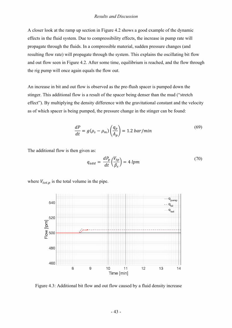
Results and Discussion
- 43 -
A closer look at the ramp up section in Figure 4.2 shows a good example of the dynamic
effects in the fluid system. Due to compressibility effects, the increase in pump rate will
propagate through the fluids. In a compressible material, sudden pressure changes (and
resulting flow rate) will propagate through the system. This explains the oscillating bit flow
and out flow seen in Figure 4.2. After some time, equilibrium is reached, and the flow through
the rig pump will once again equals the flow out.
An increase in bit and out flow is observed as the pre-flush spacer is pumped down the
stinger. This additional flow is a result of the spacer being denser than the mud (“stretch
effect”). By multiplying the density difference with the gravitational constant and the velocity
as of which spacer is being pumped, the pressure change in the stinger can be found:
%(%K = 1 /w − /l
!J.J
= 1.2tuv/$&| (69)
The additional flow is then given as:
!:++ =
%(J%K
RUJFw
= 4bD$ (70)
where RUSU,J is the total volume in the pipe.
Figure 4.3: Additional bit flow and out flow caused by a fluid density increase

Results and Discussion
- 44 -
The calculated additional flow can be verified from the simulation, as seen in Figure 4.3 .
The 1.2 bar/min increase in hydrostatic pressure leads to a corresponding decrease in pump
pressure, as seen in Figure 4.4. The fluid columns in the stinger and the pump pressure during
the simulation is plotted in Figure 4.4.
Figure 4.4: Pump pressure development and fluid columns in the stinger during the simulation of the conventional cement job
The free-fall period is initiated as the pump pressure becomes zero, at t = 21 min. As seen in
Figure 4.1, the u-tube rate1 is increased even further as the heavy-weight cement is pumped
into the stinger. During the free-fall period, the flow out of the stinger (bit flow) exceeds the
flow in, resulting in the air gap seen in Figure 4.4. After the planned cement volume is
pumped into the stinger, the post-flush spacer is pumped, reducing the u-tube rate due to its
lower density. When all the post-flush is pumped inside the stinger, the bit flow is picked up
by the increased rig pump rate.
When the front of the pre-flush spacer enters the annulus, the bit and out flow is rapidly
decreased, as seen in Figure 4.1, due to the decreasing hydrostatic difference between pipe
and annulus. A similar drop is seen as the cement is introduced to the annulus. The increased
hydrostatic pressure caused by the continuous filling of the air gap will push the cement
1 Difference in in-flow and out-flow due to hydrostatic pressure difference in stinger and annulus

Results and Discussion
- 45 -
further into the annulus. After 97.2 min, the entire air gap is filled, causing a sudden increase
in pump pressure comparable to a “water hammer” effect. As a result, the bit and out flow are
increased rapidly and later stabilize slightly below pump rate due to compressibility effects.
The BHP during the entire conventional cementing operation is plotted together with the
length of the fluid columns in the annulus in Figure 4.5.
Figure 4.5: Development of the BHP and the fluid columns in the annulus during the simulation of the conventional cement job
The changes in the BHP before the spacer and the cement is introduced to the stinger is
caused by flow rate changes induced by the rig pump and the u-tubing. They can be directly
correlated to the behaviour of the bit and out flow rate as seen in Figure 4.1 and in the annular
friction plots provided in Appendix B. As the spacer and the cement enter the annulus, the
BHP increases considerably, with a total increase of 26 bar. It is evident that the system is
dominated by the hydrostatic pressure, rather than the frictional pressure. After 102.6 minutes,
the operation is finished and the rig pump is shut off. The loss of frictional pressure when the
pump is shut off, explains the sudden drop in BHP. Compared to a static set point
(510.12bar), the BHP increases with a maximum of 37.43 bar.

Results and Discussion
- 46 -
4.1.2 Applied-Back-Pressure Cementing Simulation
During the ABP cementing operation, a lighter mud-weight (1100 kg/m3) is used. The set
point for the BHP is (núo7ê6 ≈ 510.1tuv, which corresponds to the initial hydrostatic pressure in
the conventional simulation. The lighter mud-weight enables 78.48 bar applied back-pressure
initially. This additional pressure can then later be relieved through the topside choke valve to
maintain a constant BHP as the cement enters the annulus.
Figure 4.6: Flow rates during the simulation of the ABP system
Figure 4.6 shows the flow rates during the simulation of the ABP system. After pumping all
the pre-flush spacer volume, and pumping cement for 14.5 minutes, the pump pressure
becomes zero and the free-fall period is initiated. During the conventional simulation, the
free-fall period is initiated much earlier, already while pumping the pre-flush spacer. In the
ABP system, the hydrostatic pressure difference must overcome an additional pressure, the
applied back pressure, as well as the friction in the system. Therefore, a heavier fluid column
is needed to initiate the free-fall.
During the free-fall period, the bit flow rate reaches a higher rate compared to the
conventional case. As the bit flow starts to increase, the PI controller responds by increasing
the choke opening (see Figure 4.7), compensating for the increased frictional pressure caused
by the high flow rate. The opening of the choke results in a reduction in the choke pressure,

Results and Discussion
- 47 -
increasing the pressure difference between the pipe and the annulus even further. This
explains the high u-tube rate value.
Figure 4.7: Choke opening plotted against choke pressure
By comparing Figure 4.6 and Figure 4.7, it is clear that the choke opening correlates strongly
to the choke flow rate. As the rig pump rate is ramped up, the PI controller opens the choke
valve to compensate for the increased friction in the annulus. However, in the period where
the spacer and cement is displaced into the annulus and the stinger is being filled, the choke
pressure decreases as the choke opening closes. This rather counter-intuitive correlation can
be explained by the reduction in flow through the choke. To avoid too much reduction in
choke pressure as the flow rate is reduced, the choke opening is narrowed. The correlation
between choke pressure, choke flow and choke opening is given in Equation 40, repeated
below for the readers’ convenience.
(; = /!;hij;
X
When the airgap in the pipe is filled, the pump pressure and the annular flow rate are rapidly
increased. The resulting increase in frictional pressure loss causes the rapid choke opening.
To reduce the pressure as the cement enters the annulus, the choke is opened 46 % at
maximum, meaning that this system would most likely be capable of handling higher
displacement rates, even more cement volume and denser cement.

Results and Discussion
- 48 -
During the entire simulation of the cement job, the PI controller maintains the BHP within a
pressure window of 0.62 bar (see Figure 4.8). The maximum increase in BHP as the cement
and spacer enter the annulus is 0.34 bar, and the minimum BHP is kept within 0.28 bar as the
rig pump is ramped down. Figure 4.8 will be discussed further in Section 4.1.5.
Figure 4.8: BHP during the cement operation using an ABP system
4.1.3 Dual Gradient Cementing Simulation
During the DG cement operation, the same mud weight as the conventional cement job is
used. The set point for the BHP is the same as for the ABP system, (núo7ê6 ≈ 510.1tuv. Due to
the frictional pressure loss caused by circulation, the air gap in the riser is 64m at the start of
simulation.
Figure 4.9 shows the different flow rates during the simulation of the DG system. The bit flow
rate behaviour is very similar to the bit flow rate during the conventional cementing, and will
not be explained in detail. However, it is noted that the free-fall period is initiated earlier than
in the two other model simulations. The difference in free-fall period between the three
simulations will be discussed further in Section 4.1.5.

Results and Discussion
- 49 -
Figure 4.9: Flow rates during simulation of the DG system
The parameter that is altered to adjust the BHP in a dual gradient system, is the flow rate
through the SPM, or more precisely; the velocity of the subsea pumps controls the fluid level
in the riser, which consequently affects the hydrostatic pressure profile in the annulus. This is
the reason why the qssp differs from the flow out during the conventional and ABP cement
operations.
During the ramp-up of the rig pump, the PI-controller detects the increase in BHP caused by
increased friction, communicating to the subsea pump to increase the rotational velocity. The
subsea pump velocity during the simulation and the air gap in the riser can be seen in
Figure 4.10. As the rig pump ramps up to 1500 lpm, the SPM is not able to reduce the riser
level fast enough. As a result, the BHP increases approximately 2 bars, as seen in Figure 4.11,
When the rig pump rate is later reduced from 1500 lpm to 500 lpm, the BHP reduces and the
subsea pump responds by decreasing its rotational velocity below 1000 rpm. Based on the
system curve, described in Section 3.3.4, the rotational velocity of the pumps is now no
longer sufficient to operate the pumps properly. In a realistic scenario, this would lead to
back-flow through the subsea pumps and into the riser, resulting in a negative flow rate.
However, since a back-flow scenario is not implemented into the model, the flow rate through
the subsea pumps will consequently drop to zero, as seen in Figure 4.9.

Results and Discussion
- 50 -
To maintain a constant BHP as the rig pump flow rate is reduces, the fluid level in the riser
must increase. Since there is no option implemented in the model to fill the riser from the
surface, the only solution for the system to maintain the BHP is to reduce the velocity of the
subsea pumps, and let the fluid level increase as fluid enters the annulus through the bit. Due
to insufficient riser filling, the BHP drops 5 bars below set point.
Figure 4.10: Rotational velocity of the subsea pumps on the left axis and air gap in the riser on the right axis.
At the end of the cement operation, the subsea pumps have reduced the fluid level in the riser
by approximately 250 m, as seen in Figure 4.10.
During the displacement of spacer and cement into the annulus, the flow rate through the
SPM is kept high to account for the increased hydrostatic pressure. The velocity of the subsea
pumps is raised to a maximum of 1900 rpm, and the PI controller is capable of maintaining
the BHP in a range of 4 bars above set point. Once again, due to the lack of top filling, the
system is not able to account for the lost friction as the rig pump is shut off, leading to a drop
in BHP of 11.6 bar, as seen in Figure 4.11. However, the risk of formation influx is
considered small.
It should be mentioned that there would be a delay in the top fill pump as well, so the BHP
would still decrease. To be able to close in the required pressure, a closing mechanism

Results and Discussion
- 51 -
(choke) upstream the pump could be considered. As seen in Figure 4.11 the maximum
increase in BHP during the operation is 3.96 bar above set point.
Figure 4.11: BHP during simulation of the DG cement operation
4.1.4 How the MPC Systems Improve the Conventional Cement Job
During a conventional cement operation, the choice of cement pump rate and the
displacement rate can be restricted by the given pressure window. An increase in pump rate
will lead to an increase in friction, increasing the BHP in the annulus. Figure 4.12 displays the
increase in annulus friction, as the cement/spacer pump rate and the displacement rate are
increased by a factor of two in the conventional simulation.
This additional friction could in a narrow pressure window environment fracture the
formation, causing losses to the formation. One of the advantages of utilizing MPC, is the
ability to compensate this additional friction pressure. Increased displacement rate is
associated with improved mud removal in the annulus, which further improves the quality of
the cement job. In addition, the cement job requires less rig time.
Figure 4.13 shows how the ABP system modelled in this thesis handles a cement rate and
displacement rate increased by 100%. As evident, the ABP system manages to keep a

Results and Discussion
- 52 -
relatively constant BHP, with an error of less than 0.8 bar.
Figure 4.12: Friction during conventional cement job using different flow rates. !;êl and !+8w denotes the cement pump rate and the displacing mud pump rate.
Figure 4.13: BHP during simulation of ABP-system using a cement flow rate of 1000 lpm and a displacement mud rate of 3000 lpm
Another design factor which can be limited by a narrow pressure window, is the slurry
density. A MPC system allows for a heavier spacer and cement slurry weight. From the

Results and Discussion
- 53 -
simulation of the conventional cement operation, the BHP increases 26 bar, as the cement
enters the annulus. Considering a fracture pressure of (ûüm† = 540 bar in the simulation of
the conventional case (see Figure 4.14) the BHP will exceed the fracture pressure when using
a slurry density of 2000 kg/m3.
Figure 4.14: BHP during the simulation of the conventional cement job using two different cement densities. A fracture pressure of 540 bar is assumed.
To maintain the BHP within the fracture pressure limit with a safety margin of approximately
4 bar, the slurry density needs to be reduced to 1600 kg/m3. This restriction might prevent the
ability to use the optimal cement slurry. As evident in the results in Section 0 and
Section 4.1.3, this reduction is not needed in the ABP and DG. The additional hydrostatic
pressure caused by the heavier slurry, can be reduced by adjusting the choke opening/riser
level. These results support the theory provided in Section 2.3.3; the MPC system enables the
cement engineer to be more flexible with the choice of slurry density. The increased focus on
performance and less need for ECD control while designing the spacer and cement will
potentially enhance the cement quality.

Results and Discussion
- 54 -
4.1.5 Comparison of Applied Back-Pressure and Dual Gradient Cementing
The maximum and minimum values for the BHP during the two MPC simulations are
displayed in Table 5.
Table 5: BHP for the ABP and the DG simulation
System Max BHP [bar] Min BHP [bar] Pressure Window [bar]
ABP 510.46 509.84 0.62
DG 514.08 498.59 15.5
Figure 4.15 and Figure 4.16 shows the development of the BHP during the simulations. By
comparing the BHP development during the simulation of the ABP system and the DG
system, the ABP system is clearly superior to the DG system in terms of maintaining a BHP
close to the given set point. The risk of losses or influx is in both cases considered small, but
clearly higher for the DG system.
Figure 4.15: Development of BHP during the simulation of the ABP cement operation

Results and Discussion
- 55 -
Figure 4.16: Development of BHP during the simulation of the DG cement operation
These findings do comply with the intuitive assumption that pressure adjustments in a closed,
pressurized system through a topside choke is faster than in an open system using a subsea
pump. Since fluid must be removed/added from/to the riser in order to manage the down hole
pressure, the DG system consequently becomes less efficient. An increased displacement rate
will change the pressure profile in the annulus much faster, which makes it difficult for the
DG system to maintain a constant pressure profile. This introduces a limitation with the DG
system.
The results clearly show that the ABP system is more efficient in maintaining a constant BHP.
However, an equipment failure of the ABP system (e.g. leakage through the RCD), could be
much more severe compared to the DG system, since the ABP system operates in constant
hydrostatic underbalance. Initially, during the ABP cement operation, the chosen mud weight
results in a 78.48 bar under-balanced hydrostatic environment. At the end of the cement
operation, the hydrostatic underbalance is still 32.62 bar. If the circulation stops the frictional
pressure will be lost, leading to an even more underbalanced environment. An equipment
failure could thus lead to a high influx of formation fluid, which could have detrimental effect
on the cement job and potentially result in a dangerous situation.
During the DG cement operation, the mud weight used is initially creating overbalance.
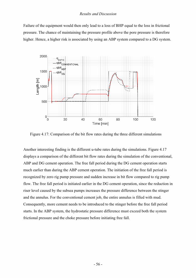
Results and Discussion
- 56 -
Failure of the equipment would then only lead to a loss of BHP equal to the loss in frictional
pressure. The chance of maintaining the pressure profile above the pore pressure is therefore
higher. Hence, a higher risk is associated by using an ABP system compared to a DG system.
Figure 4.17: Comparison of the bit flow rates during the three different simulations
Another interesting finding is the different u-tube rates during the simulations. Figure 4.17
displays a comparison of the different bit flow rates during the simulation of the conventional,
ABP and DG cement operation. The free fall period during the DG cement operation starts
much earlier than during the ABP cement operation. The initiation of the free fall period is
recognized by zero rig pump pressure and sudden increase in bit flow compared to rig pump
flow. The free fall period is initiated earlier in the DG cement operation, since the reduction in
riser level caused by the subsea pumps increases the pressure difference between the stinger
and the annulus. For the conventional cement job, the entire annulus is filled with mud.
Consequently, more cement needs to be introduced to the stinger before the free fall period
starts. In the ABP system, the hydrostatic pressure difference must exceed both the system
frictional pressure and the choke pressure before initiating free fall.

Results and Discussion
- 57 -
Figure 4.18: Comparison of the free fall periods during the different simulations
In Figure 4.18, the stinger air gaps for the different models are plotted. As seen, the free fall
period during the simulation of the DG cement operation last for approximately 84min. The
pump pressure drops to zero during the pumping of the pre-flush spacer and does not become
non-zero until the very end of the cement job. This means, that the operators are “blind”
during this entire period, making it difficult to maintain control and conduct correct pressure
adjustments if necessary. This is a drawback with the DG system.
The air gap (free fall) period for the conventional case is shorter compared to the DG system.
The ABP cementing has an even shorter air gap period, reducing the “blind” period. This is an
advantage with the ABP system, as pressure readings at the surface are available for a longer
time, improving the operators’ ability to record well responses.
In addition to the abovementioned factors, it is important to consider the well location
environment, i.e. onshore/offshore, water-depth etc, when choosing the MPC system. The
maximum pressure reduction the DG system can achieve is restricted by the length of the riser
(sea depth). In this simulation, the riser length was assumed to be 400m, which potentially, if
emptied completely, could reduce the pressure profile by 51 bar. The total pressure increase
as the spacer and cement enters the annulus is 26 bar, which implies that a 400m riser is
sufficient for this job. However, the sea depth could be the restricting factor for using the DG
system. If it is too shallow, the riser length might not be sufficient to maintain a constant

Results and Discussion
- 58 -
BHP. DG could thus naturally not be used onshore. The ABP system has no such outer
restrictions. However, the choke pressure might be restricted by equipment pressure limits.
4.2 Model Limitations and Drawbacks
It is difficult to mathematically model a physical problem without making any simplifications
or assumptions. In this section, the main limitations and drawbacks related to the models will
be discussed. The simplifications of well dimension and model setup are already presented in
Section 3.3.2.
The MPC models presented in this thesis include a standard PI-controller to adjust the
pressure profile in the well, based on BHP measurement. The problem is that during a cement
job, no downhole pressure measurement is available. In the presented model, the “measured”
BHP is estimated and assumed correct. The possibility of deviation between the simulated and
actual value is thus neglected. In a realistic scenario, estimations will rarely coincide precisely
with the real values observed in the field. For instance, inaccuracies in the friction model,
washouts in the open hole and inaccuracies during the u-tubing period, will go unnoticed by
assuming a 100 % accurate BHP-estimation. For instance, given a scenario where the open
hole diameter is larger than anticipated, the displaced spacer/cement column height in the
annulus will increase slower than estimated. The BHP will hence increase slower than
anticipated, and the result will be that the PI-controller overestimates the need to reduce BHP.
In a worst-case scenario, this can lead to formation influx, if the BHP is lowered below the
pore pressure. To overcome this problem, it should be considered to develop a better
estimator of BHP using responses from the well. By comparing simulated (assumed) pump
pressure with measured pump pressure, inaccuracies can be detected. The enlarged open hole
diameter would then be noticed by a smaller pump pressure than anticipated. BHP estimation
through back-calculations from real time pump pressure readings, possibly combined with pit
gain surveillance for better control during u-tubing, should therefore be considered to
perceive inaccuracies in the described model.
To estimate the friction in the stinger and the annulus, an average flow between two points
was used. For simplicity, the average flow in the stinger was estimated as an average of the
rig pump flow rate and bit flow rate, and the average flow in the annulus as an average of the
bit flow and the out flow. By dividing the stinger and annulus into smaller sections, the flow

Results and Discussion
- 59 -
calculations could become more accurate, increasing the overall model accuracy.
In the presented model, the temperature changes affecting the fluids were neglected, as
mentioned in Section 3.1. Consequently, the fluid properties of each fluid in the wellbore
were assumed identical in each time step. In a realistic case, the fluids would become less
viscous as the temperature increases. This would imply less friction and higher flowrates.
Increasing temperatures will also increase the fluid volume, affecting the volume calculations.
However, an extension of the model to include thermal effects was regarded as to complex
and outside of the scope of this thesis.
The intention of this thesis is to demonstrate the advantages of managed pressure control
during a cement operation. The simulation parameters used in this thesis are based on typical
values provided by Statoil. The abovementioned limitations will ultimately effect the model
accuracy. Hence, the results may not be accurate to what can be observed in the field, but is
meant as an indicator to illustrate how managed pressure control can improve conventional
cement jobs.

- 60 -

Conclusions
- 61 -
5 Conclusions
In this work, a simplified hydraulic model describing the pressure and flow dynamics during a
well cement operation has been presented. Simulations were run in MATLAB and a PI
controller was implemented to control a choke valve and a SPM in order to compensate for
downhole pressure fluctuations. Two different MPC techniques were investigated, including
an ABP system and a DG system. Advantages and drawbacks of the two techniques have
been discussed based on the presented theory and the simulation results. Based on the work
conducted in this thesis, the following conclusions can be drawn:
• During the conventional cement operation, the maximum BHP increase is 37.43 bar
above the static set point with 1300 óôlö mud. The possibility of fracturing the
formation in a narrow pressure window is considerable.
• During the ABP and DG cement operations, the maximum increase in BHP is 0.34 bar
and 3.96 bar above set point, respectively. This improved pressure control reduces risk
of losses significantly.
• The ABP system keeps the BHP within 0.28 bar below the set point as the rig pump is
shut off at the end of the operation. Due to insufficient riser filling in the DG system,
the BHP falls to a maximum of 11.6 bar below set point at shut off. The possibility of
influx is considered small in both MPC systems, but significantly higher using the DG
system compared to the ABP system.
• MPC improves conventional cement jobs in narrow pressure windows by effectively
controlling the downhole pressure throughout the entire operation. In situations with
high demands on pressure control accuracy, the ABP system is recommended.
• Accurate pressure control during cementing enables the cement operators to tailor the
cement/spacers outside traditional ECD-restrictions, potentially enhancing the cement
quality. Using MPC the displacement rates can be increased, improving mud removal
and operation efficiency.

- 62 -

Further Work
- 63 -
6 Further Work
There are aspects of this thesis that could be improved through further work.
Recommendations for further work are listed below:
• It is recognized that a downhole pressure reading is not available during the cementing
operation. In this thesis, it is assumed that the estimated BHP is correct. This
assumption eliminates one of the most significant advantages of utilizing MPC
compared to conventional cementing; the ability to correct for inaccuracies in the
model based on real time response-data from the well. It is therefore advised to
investigate different types of estimators, where BHP is back-calculated based on for
instance pump pressure and/or pit gain readings.
• It would be beneficial for the flow calculation accuracy to divide the flow sections into
smaller sections. Through iteration of the smaller flow sections, the flow calculations
and thus the overall model accuracy could be improved.
• To make the model more realistic, it is recommended to implement more realistic well
dimensions and fluid parameters. More well sections with different flow diameters,
real fluid parameters and well deviation are some suggestions. It would also be
interesting to extend the model to account temperature effects downhole.
• It is suggested to perform a thorough analysis and comparison of the economic aspects
and rig up time for the two different MPC techniques. The results could be utilized to
find the most cost effective and time efficient MPC system, which would be a natural
aspect to consider when choosing MPC technique.
• The model has not been quality-checked, as no field data has been available.
Comparing the simulations with actual readings from a case study would be a natural
step in an extension of this work.
• Another suggestion for future work, would be to simulate a hydraulic model using a
subsea pump module combined with a choke valve and compare the results to the
systems presented in this thesis.

- 64 -

References
- 65 -
7 References
Beirute, R. M. (1984). The Phenomenon of Free Fall During Primary Cementing. Society of Petroleum Engineers.
Bjørkevoll, K. S., Rommetveit, R., Eck-Olsen, J., & Rønneberg, A. (2005). Innovative Design, Operational Modelling and Lessons Learned for Pressure Management During Underbalanced Cementing with Choke Return Flow.
Blasius, H. (1950). The Boundary Layers in Fluids with Little Friction. Zeitschrift fuer Mathematik und Physik.
Brechan, B. A. (2015). Compendium - TPG4215 Drilling Engineering - Drilling, Completion, Intervention and P&A - design and operations. Department of Petroleum Engineering and Applied Geophysics.
Churchill, S. W. (1973). Empirical expressions for the shear stress in turbulent flow in commercial pipe. American Institute of Chemical Engineers.
Cohen, J. H., Stave, R., Hauge, E., & Godhavn, J. M. (2014). Dynamic Simulations of New Well Control Procedures Used to Prepare a Dual Gradient System Field Trial. Paper presented at the Offshore Technology Conference, TEXAS.
Dooply, M., DeBrujin, G., Flamant, N., Elhancha, A., Rahman, S., Duan, M., & Koons, B. (2016). Understanding Cementing Dynamics in Deepwater Dual Gradient Driling Operations. Society of Petroleum Engineers. doi:180354-MS
Isambourg, P., Anfinsen, B. T., & Marken, C. (1996). Volumetric Behaviour of Drilling Muds at High Pressure and High Temperature. Society of Petroleum Engineers. doi:36830-MS
King, G. E. (2017). Choke. Retrieved from http://gekengineering.com/Downloads/Free_Downloads/Choke.pdf
Kreyszig. (2011). Advanced Engineering Mathematics (Vol. 10th edition). Kaasa, G. O., Stamnes, Ø. N., Imsland, L., & Aamo, O. M. (2012). Simplified Hydraulics
Model Used for Intelligent Estimation of Downhole Pressure for a Managed-Pressure-Drilling Control System. Society of Petroleum Engineers.
Merritt, H. E. (1967). Hydraulic Control Systems. Nas, S. (2011). Kick Detection and Well Control in a Closed Wellbore. Society of Petroleum
Engineers. Nelson, E. B. (2012). Defining cementing: Schlumberger. Ng’ang’a, S. I. (2014). Cementing Processes in Geothermal Well Drilling: Application and
Techniques. United Nations University. PetroWiki. (2015). Cementing Operations. Retrieved from
http://petrowiki.org/Cementing_operations Russell, E., Katz, A., & Pruett, B. (2016). Achieving Zonal Isolation Using Automated
Managed Pressure Cementing. Skalle, P. (2015). Drilling Fluid Engineering. Department of Petroleum Engineering and
Applied Geophysics. Smriti Rao, K., & Mishra, R. (2014). Comparative study of P, PI and PID controller for speed
control of VSI-fed induction motor. Stamnes, Ø. N., Mjaavatten, E., & Falk, K. (2012). A Simplified Model for Multi-Fluid Dual
Gradient Drilling Operations. IFAC. White, F. M. (2011). Flud Mehcanics, Seventh Edition: McGrawe Hills. Willis, M. J. (1999). Proportional-Integral-Derivative Control. Zamora, M., & Power, D. (2002). Making a Case for AADE Hydraulics and the Unified
Rheological Model. AADE Technical Conference.

References
- 66 -
Zamora, M., Roy, S., & Slater, K. (2005). Comparing a Basic Set of Drilling Fluid Pressure-Loss Relationships to Flow_loop and Field Data AADE Technical Conference.

- 67 -
Appendix A
A.1 Simulation Parameters
Table A.1: Model parameters and fluid properties
Description Value Unit
Plastic viscosity mud 30 [cP]
Plastic viscosity cement 334.2 [cP]
Plastic viscosity spacer 62 [cP]
Yield point mud 13.5 [Pa]
Yield point cement
Yield point spacer
27
6.3
[Pa]
[Pa]
Yield stress mud 0.75 [Pa]
Yield stress cement
Yield stress spacer
0.75
0.75
[Pa]
[Pa]
Isothermal bulk modulus mud 1,5 ∙ 10° [Pa]
Isothermal bulk modulus cement
Isothermal bulk modulus spacer
40 ∙ 10°
40 ∙ 10°
[Pa]
[Pa]
Gravity constant 9.81 [lwf
]
Rig pump ramp up time 20 [s]
Table A.2: DG system parameters
Description Value Unit
MRL depth 400 [m]
MRL horizontal length, discharge part (Ldis) 5 [m]
MRL horizontal length, suction part (Lsuc) 5 [m]
MRL inner diameter 6 [in]

- 68 -

- 69 -
Appendix B
B.1 Conventional System
Figure B.1.1: Upper plot shows the frictional pressure loss in the annulus and the stinger. Lower plot shows the hydrostatic pressure inside the annulus and the stinger.
Figure B.1.2: Fluid fronts in the annulus.

- 70 -
B.2 ABP System
Figure B.2.1: Upper plot shows the frictional pressure loss in the annulus and the stinger. Lower plot shows the hydrostatic pressure inside the annulus and the stinger.
Figure B.2.2: Pump pressure development and fluid columns in the stinger.

- 71 -
Figure B.2.3: Fluid fronts in the annulus.
B.3 DG System
Figure B.3.1: Upper plot shows the frictional pressure loss in the annulus and the stinger. Lower plot shows the hydrostatic pressure inside the annulus and the stinger.

- 72 -
Figure B.3.2: Pump pressure development and fluid columns in the stinger.
Figure B.3.3: Fluid fronts in the annulus and air gap in the riser.

- 73 -
Appendix C
C.1 Hydraulic Friction Model
The following friction model is based on Zamora (2005) and was used to estimate friction
pressure loss in the model presented in this thesis.
Fluid Properties
During flow-loop testing, the density and rheological properties should be kept constant.
The Herschel-Buckley model parameters n, k [ ex¢wá
WBB6Uf] and \* in the model are found from
measurement of the traditional oilfield parameters plastic viscosity PV [cP], yield point YP
[ exWBB6Uf
], and yield stress \* [ exWBB6Uf
]:
| = 3,32 logWB
2(R + •( − \*PV + YP − \*
(C.1)
Z =
(R + •( − \*511V
(C.2)
Due to the complexity of certain relationships for Herschel-Buckley fluids, analytical
evaluation can be difficult to impossible. To take advantage of existing relationships, it is
acceptable to treat Herschel-Buckley fluids as Power Law fluids at high shear rates. The log-
log slope of the Herschel-Buckley flow equation is assumed numerically close to the Power
Law flow behavior index |J, given as:
|J = 3,32 logWB2(R + •((R + •(
(C.3)

- 74 -
Flow Velocities
The mean velocity V [ 6Ul8V
] is found from by using the known flow rate and diameters:
R =24,51©%8X
(D&D#) (C.4)
R =
24,51©%)X − %JX
(u||jbj') (C.5)
where Q [ô:el8V
] is the flow rate, %8 [in] is the inner pipe diameter, %) [in] is the open hole or
casing/riser inner diameter and %)*+ [in] is the hydraulic diameter.
Shear Rate at the Wall
To be able to calculate the shear stress at the wall í™ ['�W], calculation of the shear rate at the
wall is required. The shear rate at the wall is given by:
í™ =1,6zR%)*+
(C.6)
where z is the Newtonian geometry shear-rate correction, given in Equation C.7.
The correction factor, G, adjusts for pipe geometry, but not for oilfield viscometers, as a
closed analytical solution for Herschel-Buckley fluids does not exist and the impact is
considered insignificant. The geometry shear-rate correction is given as:
z =
3 − a | + 14 − a | 1 +
a2
(C.7)
where a equals 0 for pipes and 1 for annuli, assuming parallel-plate flow.

- 75 -
Shear Stress at the Wall
The shear stress at the wall is in the Unified model given as:
\™ = 1,066
4 − G3 − G
V
\* + Z\™V (C.8)
With no yield stress (\* = 0), Equation C.8 is reduced to the exact solution for Power Law
fluids. \* = •( gives n = 1 and Equation C.8. is reduced to the simplified Bingham-plastic
expression. By multiplying with a factor of 1,066, the units are converted to bt6/100ìKX.
Generalized Reynolds Number
The Generalized Reynolds number is the ratio of inertial to viscous forces, and is used to
determine the flow regime and friction factor:
üê¨ =
/RX
19,36\™
(C.9)
Friction Factors
When using generalized Reynolds number, the laminar friction factors are for pipes and
concentric annuli are combined:
ìe:l =16üê¨
(C.10)
In the transition between laminar and turbulent flow regime, the friction factor is difficult to
identify. Based on the Churchill method (Churchill, 1973) and the critical Reynolds number,
the friction factor in the transitional flow regime is approximated by the empirical equation:
ìU7:Vw =16 üê¨
3470 − 1370| X (C.11)

- 76 -
During turbulent flow regime, the friction factor can be approximated by using the Blasius
(Blasius, 1950) equation based on the generalized Reynolds number and the rheological
parameter np:
ìUT7x =u
üê¨x (C.12)
where a and b are based on curve fits of data taken on Power Law fluids:
u =
(logWB |J + 3,93)50
(C.13)
and
t =
1.75 − logWB |J7
(C.14)
Fanning Friction Factor
The fanning friction factor is a function of the generalized Reynolds number, flow regime and
fluid rheological properties. Using the Churchill method, the friction factor can be determined
for any flow regime and Reynolds number. The friction factor is found by first calculating an
intermediate term fint based on the transitional and turbulent flow friction factors:
ì8VU = ìU7:Vw�Æ + ìUT7x�Æ �WÆ (C.15)
which is then used to determine the friction factor:
ì = ì8VUWX + ìe:lWXWWX (C.16)
The Fanning friction factor can also be found graphically, by the knowledge of the
Generalized Reynolds Number and Power Law flow behavior index |J, illustrated in Figure
C.1.

- 77 -
Figure C.1: Fanning friction chart for non-Newtonian fluids (Zamora et al., 2005)
Frictional Pressure Loss
The Fanning equation is the most commonly used relationship to calculate the frictional
pressure loss. The pipe and annuli pressure loss is proportional to the Fanning friction factor
found above, which primarily depends on the rheological parameters, generalized Reynolds
number and flow regime:
( =
1,076/RXì=10Ä%)*+
(C.17)
where / [exØô:e
] is the drilling fluid density and L [ft] is the length of the pipe/annulus.
If the fluid temperature stays rather constant, the other parameters in the equation are easily
measured or calculated in flow-loop tests.

- 78 -

- 79 -
Appendix D
D.1 Conventional Cement Job MATLAB CODE
%% Define parameters L_SI = 4000; % length of well, [m] rho_mud = 1300; % mud density bentonite slurry, [kg/m^3] rho_cem = 2000; % Portland cement, [kg/m^3] rho_spacer = 1600; % spacer density, [kg/m^3] Cd_o = 13.375; % casing outer diameter, [in] Sd_i = 5; % stinger inner diameter, [in] Od = 17.5; % Openhole diameter, [in] PV_mud = 30; % plastic viscosity mud, [cP] PV_spacer = 62; % plastic viscosity spacer, [cP] PV_cem = 334.2; % plastic viscosity cement, [cP] YP_SI_mud = 13.5; % yield point mud, [Pa] YP_SI_spacer= 6.3; % yield point spacer, [Pa] YP_SI_cem = 27; % yield point cement, [Pa] tau_y_mud = 0.75; % yield stress mud, [lb/100ft^2] tau_y_spacer= 0.75; % yield stress spacer, [lb/100ft^2] tau_y_cem = 0.75; % yield stress cement, [lb/100ft^2] g = 9.81; % gravity constant, [m/s^2] in2m = 0.0254; % multiplier from in to m lpm2m3s = 1/60000; % multiplier from lpm to m3/s bar2Pa = 1e5; % multiplier from bar to Pa B_mud = 1.5*10^4 * bar2Pa; % isothermal bulk modulus mud [Pa] B_spacer = 1.5*10^4*bar2Pa; % isothermal bulk modulus spacer [Pa] B_cem = 40*10^4 * bar2Pa; % isothermal bulk modulus cement [Pa] Ap = pi*(Sd_i*in2m/2)^2; % inner area of stinger [m^2] Aa = pi*((Od*in2m/2)^2-(Cd_o*in2m/2)^2); % inner area of annulus [m^2] V_tp = Ap*L_SI; % total volume pipe [m^3] V_ta = Aa*L_SI; % total volume annulus [m^3] Vst1 = 10; % pre-flush-spacer [m^3] Vst2 = 1; % post-flush-spacer [m^3]
t_m = 500; % time pumping mud before cement dt = 0.01; % time step [s] T = 7200; % total duration of operation [s] t = dt:dt:T; N = length(t); qp_mud = 1000*lpm2m3s; % displacing mud rate [m^3/s] qp_cem = 500*lpm2m3s; % pumping cement rate [m^3/s] qp_mud_dis = 1500*lpm2m3s; % displacement mud rate [m^3/s] P0 = 0e5; % gauge Pressure pressure = 0 [bar] Lmp0 = L_SI; % initial length of mud in stinger [m] Lma0 = Lmp0; % initial length of mud in annulus [m] Lcem_an = 300; % length of cement in annulus [m] Vct = Lcem_an*Aa; % Total volume of cement to be pumped [m3] %% Pre-allocation of times series: a=annulus, p=pipe, c=cement, s=spacer, m=mud, f=front qp = zeros(1,N); Ga = zeros(1,N); Gp = zeros(1,N); Mp = zeros(1,N); Ma = zeros(1,N); qb = zeros(1,N); qout = zeros(1,N); qavg_pipe = zeros(1,N); Fp = zeros(1,N); Fa = zeros(1,N); Pp = zeros(1,N); Pdha = zeros(1,N); deltaP = zeros(1,N); Lcp = zeros(1,N); Lcpf = zeros(1,N); Lca = zeros(1,N); Lma = zeros(1,N); Lmp = zeros(1,N); Lsp = zeros(1,N); Lspf = zeros(1,N); Lsp1 = zeros(1,N); Lsp2 = zeros(1,N); Lsa = zeros(1,N); hd = zeros(1,N); Vcp = zeros(1,N);

- 80 -
Vcp_c = zeros(1,N); Vmp1 = zeros(1,N); Vmp2 = zeros(1,N); Vmp_c1 = zeros(1,N); Vmp_c2 = zeros(1,N); Vma_c = zeros(1,N); Vca_c = zeros(1,N); Vca = zeros(1,N); Vma = zeros(1,N); Vsp1 = zeros(1,N); Vsp_c1 = zeros(1,N); Vsp2 = zeros(1,N); Vsp_c2 = zeros(1,N); Vsa = zeros(1,N); Vsa_c = zeros(1,N); statec = zeros(1,N);
%% Initial conditions qp(1) = qp_mud; qb(1) = qp_mud; qout(1) = qp_mud; qavg_pipe(1) = qp_mud; Ga(1) = rho_mud*g*L_SI; Gp(1) = rho_mud*g*L_SI; Mp(1) = rho_mud*L_SI/((pi*(Sd_i^2)/4)*in2m^2); Ma(1) = rho_mud*L_SI/((pi*((Od^2)-(Cd_o^2))/4)*in2m^2); Fp(1) = unified_friction_pipe(Sd_i,qp_mud,L_SI,PV_mud,YP_SI_mud,tau_y_mud,rho_mud); Fa(1) = unified_friction_ann(Cd_o,Od,qp_mud,L_SI,PV_mud,YP_SI_mud,tau_y_mud,rho_mud); Pdha(1) = P0 + Fa(1) + Ga(1); Pp(1) = Pdha(1) + Fp(1) - Gp(1); r0 = Pdha(1); Lma(1) = Lma0; Lmp(1) = Lmp0; Lmp1(1) = Lmp0; Vmp1(1) = V_tp; Vma(1) = V_ta; %% Flow tramp = 20; % ramp up time rig pump headindp = true; % true/false cement head in pipe for k = 2:N if t(k) < 50 % ramping up pump pressure qp(k) = qp_mud; elseif (t(k) < 100) qp(k) = min(qp_mud*1.2 , qp(k-1)+dt*qp_mud/tramp); elseif t(k) < 150 qp(k) = min(qp_mud*1.5 , qp(k-1)+dt*qp_mud/tramp); elseif t(k) < 250 qp(k) = qp_mud*1.5; else qp(k) = max(qp_cem, qp(k-1)-dt*qp_mud/tramp); end %State machine if statec(k-1) == 0 if t(k) <= t_m % pumping mud statec(k) = 0; else statec(k) = 1; end elseif statec(k-1) == 1 if Vsp1(k-1) < Vst1 %pumping spacer statec(k) = 1; else statec(k) = 2; end elseif statec(k-1) == 2 if Vcp(k-1) < Vct %pumping cement statec(k) = 2; else statec(k) = 3; end elseif statec(k-1) == 3 if Vsp2(k-1) < Vst2 %pumping spacer statec(k) = 3; else statec(k) = 4; end elseif statec(k-1) == 4 %pumping mud if Lspf(k-1) < L_SI %
- 81 -
statec(k) = 4; else statec(k) = 5; end elseif statec(k-1) == 5 if Lcpf(k-1) < L_SI % Cement front reach bottom of well statec(k) = 5; else statec(k) = 6; end elseif statec(k-1) == 6 if Vcp(k-1) > 0.449 % Displace with mud statec(k) = 6; else statec(k) = 7; kend = N; end elseif statec(k-1) == 7 statec(k) = 7; % Ramp down rig pump end if statec(k) >= 4 % Finished pumping cement and spacer qp(k) = min(qp_mud_dis, qp(k-1)+dt*qp_mud/tramp); end if statec(k) == 0 Vmp1(k) = V_tp; Vma(k) = V_ta; Vma_c(k) = V_ta; Vmp_c1(k) = V_tp; Vcp(k) = 0; Lcp(k) = Vcp(k)/Ap; Lcpf(k) = Lcp(k); Pp(k) = max(0,Pp(k-1) + dt*(B_mud/V_tp)*(qp(k-1) - qb(k-1))); Pdha(k) = max(0,Pdha(k-1) + dt*(B_mud/V_ta)*(qb(k-1) - qout(k-1))); elseif statec(k) == 1 Vmp_c1(k) = Vmp1(k-1) - dt*(qb(k-1)); Vsp_c1(k) = Vsp1(k-1) + dt*(qp(k-1)); const_mud_pipe1 = Vmp_c1(k)/B_mud; const_spacer_pipe1 = Vsp_c1(k)/B_spacer; deltaP(k) = -(V_tp-hd(k-1)*Ap-Vmp_c1(k)-... Vsp_c1(k))/(const_mud_pipe1+const_spacer_pipe1); Vmp1(k) = Vmp_c1(k)*(1-deltaP(k)/B_mud); Vsp1(k) = Vsp_c1(k)*(1-deltaP(k)/B_spacer); Vma(k) = V_ta; Vma_c(k) = V_ta; Lsp1(k) = Vsp1(k)/Ap; Lspf(k) = Lsp(k) +hd(k-1); const_mud_pipe2 = Vmp1(k)/B_mud; const_spacer_pipe2 = Vsp1(k)/B_spacer; Pp(k) = max(0,Pp(k-1) + dt*(qp(k-1)-qb(k-... 1))/(const_mud_pipe2+const_spacer_pipe2)); Pdha(k) = max(0,Pdha(k-1) + dt*(B_mud/V_ta)*(qb(k-1) - qout(k-1))); elseif statec(k) == 2 Vmp_c1(k) = Vmp1(k-1) - dt*(qb(k-1)); Vcp_c(k) = Vcp(k-1) + dt*(qp(k-1)); Vsp_c1(k) = Vsp_c1(k-1); const_mud_pipe1 = Vmp_c1(k)/B_mud; const_cem_pipe1 = Vcp_c(k)/B_cem; const_spacer_pipe1 = Vsp_c1(k)/B_spacer; deltaP(k) = -(V_tp-hd(k-1)*Ap-Vmp_c1(k)-Vcp_c(k)-Vsp_c1(k))/... (const_mud_pipe1+const_cem_pipe1+const_spacer_pipe1); Vmp1(k) = Vmp_c1(k)*(1-deltaP(k)/B_mud); Vcp(k) = Vcp_c(k)*(1-deltaP(k)/B_cem); Vsp1(k) = Vsp_c1(k)*(1-deltaP(k)/B_spacer); Vma(k) = V_ta; Vma_c(k) = V_ta; Lcp(k) = Vcp(k)/Ap; Lcpf(k) = Lcp(k)+hd(k-1); Lsp1(k) = Vsp1(k)/Ap; Lspf(k) = Lcpf(k)+Lsp1(k); const_mud_pipe2 = Vmp1(k)/B_mud; const_cem_pipe2 = Vcp(k)/B_cem; const_spacer_pipe2 = Vsp1(k)/B_spacer; Pp(k) = max(0,Pp(k-1) + dt*(qp(k-1)-qb(k-1))/... (const_mud_pipe2+const_cem_pipe2+const_spacer_pipe2)); Pdha(k) = max(0,Pdha(k-1) + dt*(B_mud/V_ta)*(qb(k-1) - qout(k-1))); elseif statec(k) == 3 Vcp_c(k) = Vcp_c(k-1); Vsp_c1(k) = Vsp_c1(k-1); Vmp_c1(k) = max(0,Vmp1(k-1) - dt*(qb(k-1)));

- 82 -
Vsp_c2(k) = Vsp2(k-1) + dt*(qp(k-1)); Vma(k) = V_ta; Vma_c(k) = V_ta; const_mud_pipe1 = Vmp_c1(k)/B_mud; const_spacer1_pipe1 = Vsp_c1(k)/B_spacer; const_spacer2_pipe1 = Vsp_c2(k)/B_spacer; const_cem_pipe1 = Vcp_c(k)/B_cem; deltaP(k) = -(V_tp-hd(k-1)*Ap-Vmp_c1(k)-Vsp_c1(k)-Vsp_c2(k)-Vcp_c(k))/...
(const_mud_pipe1+const_spacer1_pipe1+ const_spacer2_pipe1+... const_cem_pipe1);
Vmp1(k) = Vmp_c1(k)*(1-deltaP(k)/B_mud); Vsp2 (k) = Vsp_c2(k)*(1-deltaP(k)/B_spacer); Vsp1(k) = Vsp_c1(k)*(1-deltaP(k)/B_spacer); Vcp(k) = Vcp_c(k)*(1-deltaP(k)/B_cem); Lcp(k) = (Vcp(k)/Ap); Lcpf(k) = (Vcp(k)/Ap)+(Vsp2(k)+Vmp2(k))/Ap+hd(k-1); Lsp1(k) = Vsp1(k)/Ap; Lsp2(k) = Vsp2(k)/Ap; Lspf(k) = Lcpf(k) + Lsp1(k); const_mud_pipe2 = Vmp1(k)/B_mud; const_mud2_pipe2 = Vmp2(k)/B_mud; const_spacer1_pipe2 = Vsp1(k)/B_spacer; const_spacer2_pipe2 = Vsp2(k)/B_spacer; const_cem_pipe2 = Vcp(k)/B_cem; Pp(k) = max(0,Pp(k-1) + dt*(qp(k-1)-qb(k-1))/(const_mud_pipe2+ ...
const_mud2_pipe2+... const_spacer1_pipe2+const_spacer2_pipe2+const_cem_pipe2));
Pdha(k) = Pdha(k-1) + dt*(B_mud/V_ta)*(qb(k-1)-qout(k-1)); elseif statec(k) == 4 Vcp_c(k) = Vcp_c(k-1); Vsp_c1(k) = Vsp_c1(k-1); Vsp_c2(k) = Vsp_c2(k-1); Vmp_c1(k) = max(0,Vmp1(k-1) - dt*(qb(k-1))); Vmp_c2(k) = Vmp2(k-1) + dt*(qp(k-1)); Vma(k) = V_ta; Vma_c(k) = V_ta; const_mud_pipe1 = Vmp_c1(k)/B_mud; const_mud2_pipe1 = Vmp_c2(k)/B_mud; const_spacer1_pipe1 = Vsp_c1(k)/B_spacer; const_spacer2_pipe1 = Vsp_c2(k)/B_spacer; const_cem_pipe1 = Vcp_c(k)/B_cem; deltaP(k) = -(V_tp-hd(k-1)*Ap-Vmp_c1(k)-Vsp_c1(k)-Vsp_c2(k)-Vcp_c(k)-... Vmp_c2(k))/...
(const_mud_pipe1+const_mud2_pipe1+const_spacer1_pipe1+... const_spacer2_pipe1+ const_cem_pipe1);
Vmp1(k) = Vmp_c1(k)*(1-deltaP(k)/B_mud); Vsp2 (k) = Vsp_c2(k)*(1-deltaP(k)/B_spacer); Vsp1(k) = Vsp_c1(k)*(1-deltaP(k)/B_spacer); Vmp2(k) = Vmp_c2(k)*(1-deltaP(k)/B_mud); Vcp(k) = Vcp_c(k)*(1-deltaP(k)/B_cem); Lcp(k) = (Vcp(k)/Ap); Lcpf(k) = (Vcp(k)/Ap)+(Vsp2(k)/Ap)+hd(k-1)+(Vmp2(k)/Ap); Lsp1(k) = Vsp1(k)/Ap; Lsp2(k) = Vsp2(k)/Ap; Lspf(k) = Lcpf(k) + Lsp1(k); const_mud_pipe2 = Vmp1(k)/B_mud; const_spacer1_pipe2 = Vsp1(k)/B_spacer; const_spacer2_pipe2 = Vsp2(k)/B_spacer; const_cem_pipe2 = Vcp(k)/B_cem; Pp(k) = max(0,Pp(k-1) + dt*(qp(k-1)-qb(k-1))/(const_mud_pipe2+ ... const_spacer1_pipe2+const_spacer2_pipe2+const_cem_pipe2)); Pdha(k) = Pdha(k-1) + dt*(B_mud/V_ta)*(qb(k-1)-qout(k-1)); elseif statec(k) == 5 % Pipe Vcp_c(k) = Vcp_c(k-1); Vsp_c2(k) = Vsp_c2(k-1); Vmp_c2(k) = Vmp2(k-1) + dt*(qp(k-1)); Vsp_c1(k) = max(0,Vsp1(k-1) - dt*(qb(k-1))); const_mud_pipe1 = Vmp_c2(k)/B_mud; const_spacer1_pipe1 = Vsp_c1(k)/B_spacer; const_spacer2_pipe1 = Vsp_c2(k)/B_spacer; const_cem_pipe1 = Vcp_c(k)/B_cem; deltaP(k) = -(V_tp-hd(k-1)*Ap-Vmp_c2(k)-Vcp_c(k)-Vsp_c1(k)-Vsp_c2(k))/...
(const_mud_pipe1+const_spacer1_pipe1+const_spacer2_pipe1+... const_cem_pipe1);
Vmp1(k) = 0; Vmp_c1(k) = 0; Vmp2(k) = Vmp_c2(k)*(1-deltaP(k)/B_mud); Vcp(k) = max(0,Vcp_c(k)*(1-deltaP(k)/B_cem)); Vsp1(k) = max(0,Vsp_c1(k)*(1-deltaP(k)/B_spacer)); Vsp2(k) = max(0,Vsp_c2(k)*(1-deltaP(k)/B_spacer)); Lcp(k) = (Vcp(k)/Ap);

- 83 -
Lcpf(k) = (Vcp(k)/Ap)+(Vsp2(k)/Ap)+hd(k-1)+(Vmp2(k)/Ap); Lsp1(k) = Vsp1(k)/Ap; Lsp2(k) = Vsp2(k)/Ap; Lspf(k) = Lcpf(k) + Lsp1(k); const_mud_pipe2 = Vmp2(k)/B_mud; const_spacer1_pipe2 = Vsp1(k)/B_spacer; const_spacer2_pipe2 = Vsp2(k)/B_spacer; const_cem_pipe2 = Vcp(k)/B_cem; Pp(k) = max(0,Pp(k-1) + dt*(qp(k-1)-qb(k-1))/(const_mud_pipe2+... const_cem_pipe2+const_spacer2_pipe2+const_spacer1_pipe2)); % Annulus Vma_c(k) = Vma(k-1) - dt*(qout(k-1)); Vsa_c(k) = Vsa(k-1) + dt*(qb(k-1)); const_spacer_an1 = Vsa_c(k)/B_spacer; const_mud_an1 = Vma_c(k)/B_mud; deltaP(k) = -(V_ta-Vma_c(k)-Vsa_c(k))/(const_mud_an1+const_spacer_an1); Vma(k) = Vma_c(k)*(1-deltaP(k)/B_mud); Vsa(k) = Vsa_c(k)*(1-deltaP(k)/B_spacer); Lsa(k) = Vsa(k)/Aa; const_mud_an2 = Vma(k)/B_mud; const_spacer_an2 = Vsa(k)/B_spacer; Pdha(k) = Pdha(k-1) + dt*(qb(k-1)-qout(k-1))/(const_mud_an2+const_spacer_an2); elseif statec(k) == 6 % Pipe Vcp_c(k) = max(0,Vcp(k-1)-dt*(qb(k-1))); Vsp_c2(k) = Vsp_c2(k-1); Vmp_c2(k) = Vmp2(k-1) + dt*(qp(k-1)); const_mud_pipe1 = Vmp_c2(k)/B_mud; const_spacer2_pipe1 = Vsp_c2(k)/B_spacer; const_cem_pipe1 = Vcp_c(k)/B_cem; deltaP(k) = -(V_tp-hd(k-1)*Ap-Vmp_c2(k)-Vcp_c(k)-Vsp_c1(k)-Vsp_c2(k))/... ( const_mud_pipe1+const_spacer2_pipe1+const_cem_pipe1); Vmp1(k) = 0; Vmp_c1(k) = 0; Vsp_c1(k) = 0; Vsp1(k) = 0; Vmp2(k) = Vmp_c2(k)*(1-deltaP(k)/B_mud); Vcp(k) = max(0,Vcp_c(k)*(1-deltaP(k)/B_cem)); Vsp2(k) = max(0,Vsp_c2(k)*(1-deltaP(k)/B_spacer)); Lcp(k) = (Vcp(k)/Ap); Lsp1(k) = 0; Lsp2(k) = Vsp2(k)/Ap; const_mud_pipe2 = Vmp2(k)/B_mud; const_spacer2_pipe2 = Vsp2(k)/B_spacer; const_cem_pipe2 = Vcp(k)/B_cem; Pp(k) = max(0,Pp(k-1) + dt*(qp(k-1)-qb(k-1))/(const_mud_pipe2+... const_cem_pipe2+const_spacer2_pipe2)); % Annulus Vma_c(k) = Vma(k-1) - dt*(qout(k-1)); Vsa_c(k) = Vsa_c(k-1); Vca_c(k) = Vca(k-1) + dt*(qb(k-1)); const_spacer_an1 = Vsa_c(k)/B_spacer; const_mud_an1 = Vma_c(k)/B_mud; const_cem_an1 = Vca_c(k)/B_cem; deltaP(k) = -(V_ta-Vma_c(k)-Vsa_c(k)-... Vca_c(k))/(const_mud_an1+const_spacer_an1+const_cem_an1); Vma(k) = Vma_c(k)*(1-deltaP(k)/B_mud); Vsa(k) = Vsa_c(k)*(1-deltaP(k)/B_spacer); Vca(k) = Vca_c(k)*(1-deltaP(k)/B_cem); Lsa(k) = Vsa(k)/Aa; Lca(k) = Vca(k)/Aa; const_mud_an2 = Vma(k)/B_mud; const_spacer_an2 = Vsa(k)/B_spacer; const_cem_an2 = Vca(k)/B_cem; Pdha(k) = Pdha(k-1) + dt*(qb(k-1)-qout(k-... 1))/(const_mud_an2+const_spacer_an2+const_cem_an2); else qp(k) = max(0, qp(k-1) - dt*(qp_mud/tramp)); % Pipe Vcp_c(k) = max(0,Vcp(k-1)-dt*(qb(k-1))); Vsp_c2(k) = Vsp_c2(k-1); Vmp_c2(k) = Vmp2(k-1) + dt*(qp(k-1)); const_mud_pipe1 = Vmp_c2(k)/B_mud; const_spacer2_pipe1 = Vsp_c2(k)/B_spacer; const_cem_pipe1 = Vcp_c(k)/B_cem; deltaP(k) = -(V_tp-hd(k-1)*Ap-Vmp_c2(k)-Vcp_c(k)-Vsp_c1(k)-Vsp_c2(k))/... (const_mud_pipe1+const_spacer2_pipe1+const_cem_pipe1); Vmp1(k) = 0; Vmp_c1(k) = 0; Vsp_c1(k) = 0; Vsp1(k) = 0; Vmp2(k) = Vmp_c2(k)*(1-deltaP(k)/B_mud);

- 84 -
Vcp(k) = max(0,Vcp_c(k)*(1-deltaP(k)/B_cem)); Vsp2(k) = max(0,Vsp_c2(k)*(1-deltaP(k)/B_spacer)); Lcp(k) = (Vcp(k)/Ap); Lsp1(k) = 0; Lsp2(k) = Vsp2(k)/Ap; const_mud_pipe2 = Vmp2(k)/B_mud; const_spacer2_pipe2 = Vsp2(k)/B_spacer; const_cem_pipe2 = Vcp(k)/B_cem; Pp(k) = max(0,Pp(k-1) + dt*(qp(k-1)-qb(k-1))/... (const_mud_pipe2+ const_cem_pipe2+const_spacer2_pipe2)); % Annulus Vma_c(k) = Vma(k-1) - dt*(qout(k-1)); Vsa_c(k) = Vsa_c(k-1); Vca_c(k) = Vca(k-1) + dt*(qb(k-1)); const_spacer_an1 = Vsa_c(k)/B_spacer; const_mud_an1 = Vma_c(k)/B_mud; const_cem_an1 = Vca_c(k)/B_cem; deltaP(k) = -(V_ta-Vma_c(k)-Vsa_c(k)-... Vca_c(k))/(const_mud_an1+const_spacer_an1+const_cem_an1); Vma(k) = Vma_c(k)*(1-deltaP(k)/B_mud); Vsa(k) = Vsa_c(k)*(1-deltaP(k)/B_spacer); Vca(k) = Vca_c(k)*(1-deltaP(k)/B_cem); Lsa(k) = Vsa(k)/Aa; Lca(k) = Vca(k)/Aa; const_mud_an2 = Vma(k)/B_mud; const_spacer_an2 = Vsa(k)/B_spacer; const_cem_an2 = Vca(k)/B_cem; Pdha(k) = Pdha(k-1) + dt*(qb(k-1)-qout(k-... 1))/(const_mud_an2+const_spacer_an2+const_cem_an2); end if hd(k-1) ~= 0 Pp(k) = 0; end %% Dynamics for the total wellbore
qb(k) = max(0,qb(k-1) + dt/(Mp(k-1)+Ma(k-1))*((Pp(k-1) - P0 - Fp(k-1)-Fa(k-1) +... Gp(k-1)-Ga(k-1))));
qavg_pipe(k) = max(0,qavg_pipe(k-1) + dt/Mp(k-1)*(Pp(k-1) - Fp(k-1) - Pdha(k-1) + Gp(k-1))); qout(k) = max(0,qout(k-1) + dt/(Ma(k-1))*(Pdha(k-1) - Fa(k-1) - P0 - Ga(k-1))); if Pp(k) == 0 && ((Gp(k-1)-Ga(k-1)-Fa(k-1)-Fp(k-1))) ~= 0 hd(k) = max(0,hd(k-1) + (dt/Ap)*(qb(k-1)-qp(k-1))); else hd(k) = hd(k-1); end %% Update variables Lsp(k) = Lsp1(k) + Lsp2(k); Lma(k) = L_SI - Lca(k) - Lsa(k); Lmp(k) = L_SI - Lcp(k) - hd(k)-Lsp(k); q_avgp = qavg_pipe(k); q_avga = qout(k); Mp(k) = (rho_mud*Lmp(k)/(Ap) + rho_cem*Lcp(k)/(Ap) + rho_spacer*Lsp(k)/(Ap)); Ma(k) = (rho_mud*Lma(k)/(Aa) + rho_cem*Lca(k)/(Aa) + rho_spacer*Lsa(k)/(Aa)); Gp(k) = rho_mud*g*Lmp(k) + rho_cem*g*Lcp(k) + rho_spacer*g*Lsp(k);
Ga(k) = rho_mud*g*Lma(k) + rho_cem*g*Lca(k) + rho_spacer*g*Lsa(k); Fp(k) = unified_friction_pipe(Sd_i,q_avgp,Lmp(k),PV_mud,YP_SI_mud,tau_y_mud,rho_mud) +... unified_friction_pipe(Sd_i,q_avgp,Lcp(k),PV_cem,YP_SI_cem,tau_y_cem,rho_cem) +... unified_friction_pipe(Sd_i,q_avgp,Lsp(k),PV_spacer,YP_SI_spacer,tau_y_spacer,rho_spacer); Fa(k) = unified_friction_ann(Cd_o,Od,q_avga,Lma(k),PV_mud,YP_SI_mud,tau_y_mud,rho_mud) +... unified_friction_ann(Cd_o,Od,q_avga,Lca(k),PV_cem,YP_SI_cem,tau_y_cem,rho_cem) +... unified_friction_ann(Cd_o,Od,q_avga,Lsa(k),PV_spacer,YP_SI_spacer,tau_y_spacer,rho_spacer);
if qp(k) == 0 Pp(k) = 0; end end %% The simulation is finished. The simulation results can then be plotted as desired.

- 85 -
D.2 ABP System MATLAB Code
%% Define parameters L_SI = 4000; % length of well, [m] rho_mud = 1100; % mud density bentonite slurry, [kg/m^3] rho_mud_con = 1300; % mud density conventional, [kg/m^3] rho_cem = 2000; % Portland cement, [kg/m^3] rho_spacer = 1600; % spacer density, [kg/m^3] Cd_o = 13.375; % casing outer diameter, [in] Sd_i = 5; % stinger inner diameter, [in] Od = 17.5; % Openhole diameter, [in] PV_mud = 30; % plastic viscosity mud, [cP] PV_spacer = 62; % plastic viscosity spacer, [cP] PV_cem = 334.2; % plastic viscosity cement, [cP] YP_SI_mud = 13.5; % yield point mud, [Pa] YP_SI_spacer= 6.3; % yield point spacer, [Pa] YP_SI_cem = 27; % yield point cement, [Pa] tau_y_mud = 0.75; % yield stress mud, [lb/100ft^2] tau_y_spacer= 0.75; % yield stress spacer, [lb/100ft^2] tau_y_cem = 0.75; % yield stress cement, [lb/100ft^2] g = 9.81; % gravity constant, [m/s^2] in2m = 0.0254; % multiplier from in to m lpm2m3s = 1/60000; % multiplier from lpm to m3/s bar2Pa = 1e5; % multiplier from bar to Pa B_mud = 1.5*10^4 * bar2Pa; % isothermal bulk modulus mud [Pa] B_spacer = 1.5*10^4*bar2Pa; % isothermal bulk modulus spacer [Pa] B_cem = 40*10^4 * bar2Pa; % isothermal bulk modulus cement [Pa] Ap = pi*(Sd_i*in2m/2)^2; % inner area of stinger [m^2] Aa = pi*((Od*in2m/2)^2-(Cd_o*in2m/2)^2); % inner area of annulus [m^2] V_tp = Ap*L_SI; % total volume pipe [m^3] V_ta = Aa*L_SI; % total volume annulus [m^3] Vst1 = 10; % pre-flush-spacer [m^3] Vst2 = 1; % post-flush-spacer [m^3]
t_m = 500; % time pumping mud before cement dt = 0.01; % time step [s] T = 7200; % total duration of operation [s] t = dt:dt:T; N = length(t); qp_mud = 1000*lpm2m3s; % displacing mud rate [m^3/s] qp_cem = 500*lpm2m3s; % pumping cement rate [m^3/s] qp_mud_dis = 1500*lpm2m3s; % displacement mud rate [m^3/s] P0 = 0e5; % gauge Pressure pressure = 0 [bar] Pc0 = (rho_mud_conv-rho_mud)*g*L_SI; % Initial applied back pressure [bar] u0 = 0.2; % Initial choke opening [%] Cv = qp_mud/u0/sqrt(Pc0/rho_mud); % Choke constant based on initial values Lmp0 = L_SI; % initial length of mud in stinger [m] Lma0 = Lmp0; % initial length of mud in annulus [m] Lcem_an = 300; % length of cement in annulus [m] Vct = Lcem_an*Aa; % Total volume of cement to be pumped [m3] %% Pre-allocation of times series: a=annulus, p=pipe, c=cement, s=spacer, m=mud, f=front qp = zeros(1,N); Ga = zeros(1,N); Gp = zeros(1,N); Mp = zeros(1,N); Ma = zeros(1,N); qb = zeros(1,N); qc = zeros(1,N); qavg_pipe = zeros(1,N); Fp = zeros(1,N); Fa = zeros(1,N); Pp = zeros(1,N); Pdha = zeros(1,N); Pc = zeros(1,N); deltaP = zeros(1,N); Lcp = zeros(1,N); Lcpf = zeros(1,N); Lca = zeros(1,N); Lma = zeros(1,N); Lmp = zeros(1,N); Lsp = zeros(1,N); Lspf = zeros(1,N); Lsp1 = zeros(1,N); Lsp2 = zeros(1,N); Lsa = zeros(1,N); hd = zeros(1,N); Vcp = zeros(1,N);

- 86 -
Vcp_c = zeros(1,N); Vmp1 = zeros(1,N); Vmp2 = zeros(1,N); Vmp_c1 = zeros(1,N); Vmp_c2 = zeros(1,N); Vma_c = zeros(1,N); Vca_c = zeros(1,N); Vca = zeros(1,N); Vma = zeros(1,N); Vsp1 = zeros(1,N); Vsp_c1 = zeros(1,N); Vsp2 = zeros(1,N); Vsp_c2 = zeros(1,N); Vsa = zeros(1,N); Vsa_c = zeros(1,N); e = zeros(1,N); eI = zeros(1,N); u = zeros(1,N); ref = zeros(1,N); % Set point bottom hole pressure statec = zeros(1,N); % PI Controller Constants Kp = 0.3*1e-5; Ti = 5; % [s] umin = 0.0;
%% Initial conditions qp(1) = qp_mud; qb(1) = qp_mud; qc(1) = qp_mud; qavg_pipe(1) = qp_mud; Ga(1) = rho_mud*g*L_SI; Gp(1) = rho_mud*g*L_SI; Mp(1) = rho_mud*L_SI/((pi*(Sd_i^2)/4)*in2m^2); Ma(1) = rho_mud*L_SI/((pi*((Od^2)-(Cd_o^2))/4)*in2m^2); Fp(1) = unified_friction_pipe(Sd_i,qp_mud,L_SI,PV_mud,YP_SI_mud,tau_y_mud,rho_mud); Fa(1) = unified_friction_ann(Cd_o,Od,qp_mud,L_SI,PV_mud,YP_SI_mud,tau_y_mud,rho_mud); Pc(1) = Pc0; Pdha(1) = Pc(1) + Ga(1); Pp(1) = Pdha(1) + Fp(1) - Gp(1); r0 = Pdha(1); ref(1) = r0; eI(1) = Ti/Kp*(u0 - Kp*e(1)); u(1) = u0; Lma(1) = Lma0; Lmp(1) = Lmp0; Lmp1(1) = Lmp0; Vmp1(1) = V_tp; Vma(1) = V_ta;
%% Flow tramp = 20; % ramp up time rig pump headindp = true; % true/false cement head in pipe for k = 2:N if t(k) < 50 % ramping up pump pressure qp(k) = qp_mud; elseif (t(k) < 100) qp(k) = min(qp_mud*1.2 , qp(k-1)+dt*qp_mud/tramp); elseif t(k) < 150 qp(k) = min(qp_mud*1.5 , qp(k-1)+dt*qp_mud/tramp); elseif t(k) < 250 qp(k) = qp_mud*1.5; else qp(k) = max(qp_cem, qp(k-1)-dt*qp_mud/tramp); end %State machine if statec(k-1) == 0 if t(k) <= t_m % pumping mud statec(k) = 0; else statec(k) = 1; end elseif statec(k-1) == 1 if Vsp1(k-1) < Vst1 %pumping spacer statec(k) = 1;

- 87 -
else statec(k) = 2; end elseif statec(k-1) == 2 if Vcp(k-1) < Vct %pumping cement statec(k) = 2; else statec(k) = 3; end elseif statec(k-1) == 3 if Vsp2(k-1) < Vst2 %pumping spacer statec(k) = 3; else statec(k) = 4; end elseif statec(k-1) == 4 %pumping mud if Lspf(k-1) < L_SI % statec(k) = 4; else statec(k) = 5; end elseif statec(k-1) == 5 if Lcpf(k-1) < L_SI % Cement front reach bottom of well statec(k) = 5; else statec(k) = 6; end elseif statec(k-1) == 6 if Vcp(k-1) > 0.416 % Displace with mud statec(k) = 6; else statec(k) = 7; kend = N; end elseif statec(k-1) == 7 statec(k) = 7; % Ramp down rig pump end if statec(k) >= 4 % Finished pumping cement and spacer qp(k) = min(qp_mud_dis, qp(k-1)+dt*qp_mud/tramp); end if statec(k) == 0 Vmp1(k) = V_tp; Vma(k) = V_ta; Vma_c(k) = V_ta; Vmp_c1(k) = V_tp; Vcp(k) = 0; Lcp(k) = Vcp(k)/Ap; Lcpf(k) = Lcp(k); Pp(k) = max(0,Pp(k-1) + dt*(B_mud/V_tp)*(qp(k-1) - qb(k-1))); Pdha(k) = max(0,Pdha(k-1) + dt*(B_mud/V_ta)*(qb(k-1) - qc(k-1))); elseif statec(k) == 1 Vmp_c1(k) = Vmp1(k-1) - dt*(qb(k-1)); Vsp_c1(k) = Vsp1(k-1) + dt*(qp(k-1)); const_mud_pipe1 = Vmp_c1(k)/B_mud; const_spacer_pipe1 = Vsp_c1(k)/B_spacer; deltaP(k) = -(V_tp-hd(k-1)*Ap-Vmp_c1(k)-... Vsp_c1(k))/(const_mud_pipe1+const_spacer_pipe1); Vmp1(k) = Vmp_c1(k)*(1-deltaP(k)/B_mud); Vsp1(k) = Vsp_c1(k)*(1-deltaP(k)/B_spacer); Vma(k) = V_ta; Vma_c(k) = V_ta; Lsp1(k) = Vsp1(k)/Ap; Lspf(k) = Lsp(k) +hd(k-1); const_mud_pipe2 = Vmp1(k)/B_mud; const_spacer_pipe2 = Vsp1(k)/B_spacer; Pp(k) = max(0,Pp(k-1) + dt*(qp(k-1)-... qb(k-1))/(const_mud_pipe2+const_spacer_pipe2)); Pdha(k) = max(0,Pdha(k-1) + dt*(B_mud/V_ta)*(qb(k-1) - qc(k-1))); elseif statec(k) == 2 Vmp_c1(k) = Vmp1(k-1) - dt*(qb(k-1)); Vcp_c(k) = Vcp(k-1) + dt*(qp(k-1)); Vsp_c1(k) = Vsp_c1(k-1); const_mud_pipe1 = Vmp_c1(k)/B_mud; const_cem_pipe1 = Vcp_c(k)/B_cem; const_spacer_pipe1 = Vsp_c1(k)/B_spacer; deltaP(k) = -(V_tp-hd(k-1)*Ap-Vmp_c1(k)-Vcp_c(k)-Vsp_c1(k))/... (const_mud_pipe1+const_cem_pipe1+const_spacer_pipe1); Vmp1(k) = Vmp_c1(k)*(1-deltaP(k)/B_mud); Vcp(k) = Vcp_c(k)*(1-deltaP(k)/B_cem);

- 88 -
Vsp1(k) = Vsp_c1(k)*(1-deltaP(k)/B_spacer); Vma(k) = V_ta; Vma_c(k) = V_ta; Lcp(k) = Vcp(k)/Ap; Lcpf(k) = Lcp(k)+hd(k-1); Lsp1(k) = Vsp1(k)/Ap; Lspf(k) = Lcpf(k)+Lsp1(k); const_mud_pipe2 = Vmp1(k)/B_mud; const_cem_pipe2 = Vcp(k)/B_cem; const_spacer_pipe2 = Vsp1(k)/B_spacer; Pp(k) = max(0,Pp(k-1) + dt*(qp(k-1)-qb(k-1))/... (const_mud_pipe2+const_cem_pipe2+const_spacer_pipe2)); Pdha(k) = max(0,Pdha(k-1) + dt*(B_mud/V_ta)*(qb(k-1) - qc(k-1))); elseif statec(k) == 3 Vcp_c(k) = Vcp_c(k-1); Vsp_c1(k) = Vsp_c1(k-1); Vmp_c1(k) = max(0,Vmp1(k-1) - dt*(qb(k-1))); Vsp_c2(k) = Vsp2(k-1) + dt*(qp(k-1)); Vma(k) = V_ta; Vma_c(k) = V_ta; const_mud_pipe1 = Vmp_c1(k)/B_mud; const_spacer1_pipe1 = Vsp_c1(k)/B_spacer; const_spacer2_pipe1 = Vsp_c2(k)/B_spacer; const_cem_pipe1 = Vcp_c(k)/B_cem; deltaP(k) = -(V_tp-hd(k-1)*Ap-Vmp_c1(k)-Vsp_c1(k)-Vsp_c2(k)-Vcp_c(k))/... (const_mud_pipe1+const_spacer1_pipe1+ ...
const_spacer2_pipe1+ const_cem_pipe1); Vmp1(k) = Vmp_c1(k)*(1-deltaP(k)/B_mud); Vsp2 (k) = Vsp_c2(k)*(1-deltaP(k)/B_spacer); Vsp1(k) = Vsp_c1(k)*(1-deltaP(k)/B_spacer); Vcp(k) = Vcp_c(k)*(1-deltaP(k)/B_cem); Lcp(k) = (Vcp(k)/Ap); Lcpf(k) = (Vcp(k)/Ap)+(Vsp2(k)+Vmp2(k))/Ap+hd(k-1); Lsp1(k) = Vsp1(k)/Ap; Lsp2(k) = Vsp2(k)/Ap; Lspf(k) = Lcpf(k) + Lsp1(k); const_mud_pipe2 = Vmp1(k)/B_mud; const_mud2_pipe2 = Vmp2(k)/B_mud; const_spacer1_pipe2 = Vsp1(k)/B_spacer; const_spacer2_pipe2 = Vsp2(k)/B_spacer; const_cem_pipe2 = Vcp(k)/B_cem; Pp(k) = max(0,Pp(k-1) + dt*(qp(k-1)-qb(k-1))/(const_mud_pipe2+ ...
const_mud2_pipe2+const_spacer1_pipe2...+ const_spacer2_pipe2+const_cem_pipe2));
Pdha(k) = Pdha(k-1) + dt*(B_mud/V_ta)*(qb(k-1)-qc(k-1)); elseif statec(k) == 4 Vcp_c(k) = Vcp_c(k-1); Vsp_c1(k) = Vsp_c1(k-1); Vsp_c2(k) = Vsp_c2(k-1); Vmp_c1(k) = max(0,Vmp1(k-1) - dt*(qb(k-1))); Vmp_c2(k) = Vmp2(k-1) + dt*(qp(k-1)); Vma(k) = V_ta; Vma_c(k) = V_ta; const_mud_pipe1 = Vmp_c1(k)/B_mud; const_mud2_pipe1 = Vmp_c2(k)/B_mud; const_spacer1_pipe1 = Vsp_c1(k)/B_spacer; const_spacer2_pipe1 = Vsp_c2(k)/B_spacer; const_cem_pipe1 = Vcp_c(k)/B_cem; deltaP(k) = -(V_tp-hd(k-1)*Ap-Vmp_c1(k)-Vsp_c1(k)-Vsp_c2(k)-... Vcp_c(k)-Vmp_c2(k))/(const_mud_pipe1+const_mud2_pipe1+...
const_spacer1_pipe1+ const_spacer2_pipe1+ const_cem_pipe1); Vmp1(k) = Vmp_c1(k)*(1-deltaP(k)/B_mud); Vsp2 (k) = Vsp_c2(k)*(1-deltaP(k)/B_spacer); Vsp1(k) = Vsp_c1(k)*(1-deltaP(k)/B_spacer); Vmp2(k) = Vmp_c2(k)*(1-deltaP(k)/B_mud); Vcp(k) = Vcp_c(k)*(1-deltaP(k)/B_cem); Lcp(k) = (Vcp(k)/Ap); Lcpf(k) = (Vcp(k)/Ap)+(Vsp2(k)/Ap)+hd(k-1)+(Vmp2(k)/Ap); Lsp1(k) = Vsp1(k)/Ap; Lsp2(k) = Vsp2(k)/Ap; Lspf(k) = Lcpf(k) + Lsp1(k); const_mud_pipe2 = Vmp1(k)/B_mud; const_spacer1_pipe2 = Vsp1(k)/B_spacer; const_spacer2_pipe2 = Vsp2(k)/B_spacer; const_cem_pipe2 = Vcp(k)/B_cem; Pp(k) = max(0,Pp(k-1) + dt*(qp(k-1)-qb(k-1))/(const_mud_pipe2+ ... const_spacer1_pipe2+const_spacer2_pipe2+const_cem_pipe2)); Pdha(k) = Pdha(k-1) + dt*(B_mud/V_ta)*(qb(k-1)-qc(k-1)); elseif statec(k) == 5 % Pipe Vcp_c(k) = Vcp_c(k-1);

- 89 -
Vsp_c2(k) = Vsp_c2(k-1); Vmp_c2(k) = Vmp2(k-1) + dt*(qp(k-1)); Vsp_c1(k) = max(0,Vsp1(k-1) - dt*(qb(k-1))); const_mud_pipe1 = Vmp_c2(k)/B_mud; const_spacer1_pipe1 = Vsp_c1(k)/B_spacer; const_spacer2_pipe1 = Vsp_c2(k)/B_spacer; const_cem_pipe1 = Vcp_c(k)/B_cem; deltaP(k) = -(V_tp-hd(k-1)*Ap-Vmp_c2(k)-Vcp_c(k)-Vsp_c1(k)-Vsp_c2(k))/... (const_mud_pipe1+const_spacer1_pipe1+... const_spacer2_pipe1+const_cem_pipe1); Vmp1(k) = 0; Vmp_c1(k) = 0; Vmp2(k) = Vmp_c2(k)*(1-deltaP(k)/B_mud); Vcp(k) = max(0,Vcp_c(k)*(1-deltaP(k)/B_cem)); Vsp1(k) = max(0,Vsp_c1(k)*(1-deltaP(k)/B_spacer)); Vsp2(k) = max(0,Vsp_c2(k)*(1-deltaP(k)/B_spacer)); Lcp(k) = (Vcp(k)/Ap); Lcpf(k) = (Vcp(k)/Ap)+(Vsp2(k)/Ap)+hd(k-1)+(Vmp2(k)/Ap); Lsp1(k) = Vsp1(k)/Ap; Lsp2(k) = Vsp2(k)/Ap; Lspf(k) = Lcpf(k) + Lsp1(k); const_mud_pipe2 = Vmp2(k)/B_mud; const_spacer1_pipe2 = Vsp1(k)/B_spacer; const_spacer2_pipe2 = Vsp2(k)/B_spacer; const_cem_pipe2 = Vcp(k)/B_cem; Pp(k) = max(0,Pp(k-1) + dt*(qp(k-1)-qb(k-1))/(const_mud_pipe2+... const_cem_pipe2+const_spacer2_pipe2+const_spacer1_pipe2)); % Annulus Vma_c(k) = Vma(k-1) - dt*(qc(k-1)); Vsa_c(k) = Vsa(k-1) + dt*(qb(k-1)); const_spacer_an1 = Vsa_c(k)/B_spacer; const_mud_an1 = Vma_c(k)/B_mud; deltaP(k) = -(V_ta-Vma_c(k)-Vsa_c(k))/(const_mud_an1+const_spacer_an1); Vma(k) = Vma_c(k)*(1-deltaP(k)/B_mud); Vsa(k) = Vsa_c(k)*(1-deltaP(k)/B_spacer); Lsa(k) = Vsa(k)/Aa; const_mud_an2 = Vma(k)/B_mud; const_spacer_an2 = Vsa(k)/B_spacer; Pdha(k) = Pdha(k-1) + dt*(qb(k-1)-qc(k-1))/(const_mud_an2+const_spacer_an2); elseif statec(k) == 6 % Pipe Vcp_c(k) = max(0,Vcp(k-1)-dt*(qb(k-1))); Vsp_c2(k) = Vsp_c2(k-1); Vmp_c2(k) = Vmp2(k-1) + dt*(qp(k-1)); const_mud_pipe1 = Vmp_c2(k)/B_mud; const_spacer2_pipe1 = Vsp_c2(k)/B_spacer; const_cem_pipe1 = Vcp_c(k)/B_cem; deltaP(k) = -(V_tp-hd(k-1)*Ap-Vmp_c2(k)-Vcp_c(k)-Vsp_c1(k)-Vsp_c2(k))/... ( const_mud_pipe1+const_spacer2_pipe1+const_cem_pipe1); Vmp1(k) = 0; Vmp_c1(k) = 0; Vsp_c1(k) = 0; Vsp1(k) = 0; Vmp2(k) = Vmp_c2(k)*(1-deltaP(k)/B_mud); Vcp(k) = max(0,Vcp_c(k)*(1-deltaP(k)/B_cem)); Vsp2(k) = max(0,Vsp_c2(k)*(1-deltaP(k)/B_spacer)); Lcp(k) = (Vcp(k)/Ap); Lsp1(k) = 0; Lsp2(k) = Vsp2(k)/Ap; const_mud_pipe2 = Vmp2(k)/B_mud; const_spacer2_pipe2 = Vsp2(k)/B_spacer; const_cem_pipe2 = Vcp(k)/B_cem; Pp(k) = max(0,Pp(k-1) + dt*(qp(k-1)-qb(k-1))/(const_mud_pipe2+... const_cem_pipe2+const_spacer2_pipe2)); % Annulus Vma_c(k) = Vma(k-1) - dt*(qc(k-1)); Vsa_c(k) = Vsa_c(k-1); Vca_c(k) = Vca(k-1) + dt*(qb(k-1)); const_spacer_an1 = Vsa_c(k)/B_spacer; const_mud_an1 = Vma_c(k)/B_mud; const_cem_an1 = Vca_c(k)/B_cem; deltaP(k) = -(V_ta-Vma_c(k)-Vsa_c(k)-... Vca_c(k))/(const_mud_an1+const_spacer_an1+const_cem_an1); Vma(k) = Vma_c(k)*(1-deltaP(k)/B_mud); Vsa(k) = Vsa_c(k)*(1-deltaP(k)/B_spacer); Vca(k) = Vca_c(k)*(1-deltaP(k)/B_cem); Lsa(k) = Vsa(k)/Aa; Lca(k) = Vca(k)/Aa; const_mud_an2 = Vma(k)/B_mud; const_spacer_an2 = Vsa(k)/B_spacer; const_cem_an2 = Vca(k)/B_cem; Pdha(k) = Pdha(k-1) + dt*(qb(k-1)-qc(k-... 1))/(const_mud_an2+const_spacer_an2+const_cem_an2);

- 90 -
else qp(k) = max(0, qp(k-1) - dt*(qp_mud/tramp)); % Pipe Vcp_c(k) = max(0,Vcp(k-1)-dt*(qb(k-1))); Vsp_c2(k) = Vsp_c2(k-1); Vmp_c2(k) = Vmp2(k-1) + dt*(qp(k-1)); const_mud_pipe1 = Vmp_c2(k)/B_mud; const_spacer2_pipe1 = Vsp_c2(k)/B_spacer; const_cem_pipe1 = Vcp_c(k)/B_cem; deltaP(k) = -(V_tp-hd(k-1)*Ap-Vmp_c2(k)-Vcp_c(k)-Vsp_c1(k)-Vsp_c2(k))/... (const_mud_pipe1+const_spacer2_pipe1+const_cem_pipe1); Vmp1(k) = 0; Vmp_c1(k) = 0; Vsp_c1(k) = 0; Vsp1(k) = 0; Vmp2(k) = Vmp_c2(k)*(1-deltaP(k)/B_mud); Vcp(k) = max(0,Vcp_c(k)*(1-deltaP(k)/B_cem)); Vsp2(k) = max(0,Vsp_c2(k)*(1-deltaP(k)/B_spacer)); Lcp(k) = (Vcp(k)/Ap); Lsp1(k) = 0; Lsp2(k) = Vsp2(k)/Ap; const_mud_pipe2 = Vmp2(k)/B_mud; const_spacer2_pipe2 = Vsp2(k)/B_spacer; const_cem_pipe2 = Vcp(k)/B_cem; Pp(k) = max(0,Pp(k-1) + dt*(qp(k-1)-qb(k-1))/... (const_mud_pipe2+ const_cem_pipe2+const_spacer2_pipe2)); % Annulus Vma_c(k) = Vma(k-1) - dt*(qc(k-1)); Vsa_c(k) = Vsa_c(k-1); Vca_c(k) = Vca(k-1) + dt*(qb(k-1)); const_spacer_an1 = Vsa_c(k)/B_spacer; const_mud_an1 = Vma_c(k)/B_mud; const_cem_an1 = Vca_c(k)/B_cem; deltaP(k) = -(V_ta-Vma_c(k)-Vsa_c(k)-Vca_c(k))/... (const_mud_an1+const_spacer_an1+const_cem_an1); Vma(k) = Vma_c(k)*(1-deltaP(k)/B_mud); Vsa(k) = Vsa_c(k)*(1-deltaP(k)/B_spacer); Vca(k) = Vca_c(k)*(1-deltaP(k)/B_cem); Lsa(k) = Vsa(k)/Aa; Lca(k) = Vca(k)/Aa; const_mud_an2 = Vma(k)/B_mud; const_spacer_an2 = Vsa(k)/B_spacer; const_cem_an2 = Vca(k)/B_cem; Pdha(k) = Pdha(k-1) + dt*(qb(k-1)-qc(k-1))/... (const_mud_an2+const_spacer_an2+const_cem_an2); end if hd(k-1) ~= 0 Pp(k) = 0; end
%% Dynamics for total wellbore qb(k) = max(0,qb(k-1) + dt/(Mp(k-1)+Ma(k-1))*((Pp(k-1) - Pc(k-1) - Fp(k-1)-Fa(k-1) +... Gp(k-1)-Ga(k-1))));
qavg_pipe(k) = max(0,qavg_pipe(k-1) + dt/Mp(k-1)*(Pp(k-1) - Fp(k-1) - Pdha(k-1) + Gp(k-1))); qc(k) = max(0,qc(k-1) + dt/Ma(k-1)*(Pdha(k-1) - Fa(k-1) - Pc(k-1) - Ga(k-1))); if Pp(k) == 0 && ((Gp(k-1)-Ga(k-1)-Fa(k-1)-Fp(k-1)-Pc(k-1))) ~= 0 hd(k) = max(0,hd(k-1) + (dt/Ap)*(qb(k-1)-qp(k-1))); else hd(k) = 0; end
%% PI CONTROLLER
ref(k) = r0; eI(k) = eI(k-1) + dt*e(k-1); e(k) = Pdha(k) - ref(k); u(k) = Kp*e(k) + Kp/Ti*eI(k); if u(k) < umin u(k) = umin; eI(k) = Ti/Kp*(u(k) - Kp*e(k)); elseif u(k) > 1 u(k) = 1; eI(k) = Ti/Kp*(u(k) - Kp*e(k)); end if u(k) == umin

- 91 -
qc(k) = 0; else Pc(k) = rho_mud*(qc(k)/Cv/u(k))^2; end %% Update variables Lsp(k) = Lsp1(k) + Lsp2(k); Lma(k) = L_SI - Lca(k) - Lsa(k); Lmp(k) = L_SI - Lcp(k) - hd(k)-Lsp(k); q_avgp = qavg_pipe(k); q_avga = qc(k); Mp(k) = (rho_mud*Lmp(k)/(Ap) + rho_cem*Lcp(k)/(Ap) + rho_spacer*Lsp(k)/(Ap)); Ma(k) = (rho_mud*Lma(k)/(Aa) + rho_cem*Lca(k)/(Aa) + rho_spacer*Lsa(k)/(Aa)); Gp(k) = rho_mud*g*Lmp(k) + rho_cem*g*Lcp(k) + rho_spacer*g*Lsp(k); Ga(k) = rho_mud*g*Lma(k) + rho_cem*g*Lca(k) + rho_spacer*g*Lsa(k);
Fp(k) = unified_friction_pipe(Sd_i,q_avgp,Lmp(k),PV_mud,YP_SI_mud,tau_y_mud,rho_mud) +... unified_friction_pipe(Sd_i,q_avgp,Lcp(k),PV_cem,YP_SI_cem,tau_y_cem,rho_cem) +... unified_friction_pipe(Sd_i,q_avgp,Lsp(k),PV_spacer,YP_SI_spacer,tau_y_spacer,rho_spacer); Fa(k) = unified_friction_ann(Cd_o,Od,q_avga,Lma(k),PV_mud,YP_SI_mud,tau_y_mud,rho_mud)+... unified_friction_ann(Cd_o,Od,q_avga,Lca(k),PV_cem,YP_SI_cem,tau_y_cem,rho_cem)+... unified_friction_ann(Cd_o,Od,q_avga,Lsa(k),PV_spacer,YP_SI_spacer,tau_y_spacer,rho_spacer);
if qc(k)==0 Pc(k) = max(0,Pdha(k)-Fa(k)-Ga(k)); end if qp(k) == 0 Pp(k) = 0; end end
%% The simulation is finished. The simulation results can then be plotted as desired.

- 92 -
D.3 DG System MATLAB Code
%% Define parameters L_SI = 4000; % length of well, [m] rho_mud = 1300; % mud density bentonite slurry, [kg/m^3] rho_cem = 2000; % Portland cement, [kg/m^3] rho_spacer = 1600; % spacer density, [kg/m^3] L_SI_riser = 400; % Length of riser, [m] hssp = L_SI_riser; % Depth of subsea pumps, [m] mrl_hoz = 5; % horizontal length of discharge line, [m] suc_line = 5; % horizontal length of suction line, [m] mrl_d = 6; % mud return line inner diameter, [in] Cd_o = 13.375; % casing outer diameter, [in] Sd_i = 5; % stinger inner diameter, [in] Od = 17.5; % Openhole diameter, [in] PV_mud = 30; % plastic viscosity mud, [cP] PV_spacer = 62; % plastic viscosity spacer, [cP] PV_cem = 334.2; % plastic viscosity cement, [cP] YP_SI_mud = 13.5; % yield point mud, [Pa] YP_SI_spacer= 6.3; % yield point spacer, [Pa] YP_SI_cem = 27; % yield point cement, [Pa] tau_y_mud = 0.75; % yield stress mud, [lb/100ft^2] tau_y_spacer= 0.75; % yield stress spacer, [lb/100ft^2] tau_y_cem = 0.75; % yield stress cement, [lb/100ft^2] g = 9.81; % gravity constant, [m/s^2] min_p = 5e5; % lowest pressure allowed at subsea pump module max_hr = hssp-min_p/(rho_mud*g); % lowest level allowed in riser in2m = 0.0254; % multiplier from in to m lpm2m3s = 1/60000; % multiplier from lpm to m3/s bar2Pa = 1e5; % multiplier from bar to Pa B_mud = 1.5*10^4 * bar2Pa; % isothermal bulk modulus mud [Pa] B_spacer = 1.5*10^4*bar2Pa; % isothermal bulk modulus spacer [Pa] B_cem = 40*10^4 * bar2Pa; % isothermal bulk modulus cement [Pa] Ap = pi*(Sd_i*in2m/2)^2; % inner area of stinger [m^2] Aa = pi*((Od*in2m/2)^2-(Cd_o*in2m/2)^2); % inner area of annulus [m^2] Amrl = pi*(mrl_d*in2m/2)^2; % inner area of mud return line [m^2] V_tp = Ap*L_SI; % total volume pipe [m^3] V_ta = Aa*L_SI; % total volume annulus [m^3] Vst1 = 10; % pre-flush-spacer [m^3] Vst2 = 1; % post-flush-spacer [m^3]
t_m = 500; % time pumping mud before cement dt = 0.01; % time step [s] T = 7200; % total duration of operation [s] t = dt:dt:T; N = length(t); qp_mud = 1000*lpm2m3s; % displacing mud rate [m^3/s] qp_cem = 500*lpm2m3s; % pumping cement rate [m^3/s] qp_mud_dis = 1500*lpm2m3s; % displacement mud rate [m^3/s] P0 = 0e5; % Gauge pressure 0 [bar] Lmp0 = L_SI; % initial length of mud in stinger [m] Lma0 = Lmp0; % initial length of mud in annulus [m] Lcem_an = 300; % length of cement in annulus [m] Vct = Lcem_an*Aa; % Total volume of cement to be pumped [m3]
% Subsea pump data np = 2; % number of pumps c0 = 4.17*1e-5; % pump constant c1 = 6.83*1e-2; % pump constant c2 = 115; % pump constant wssp_max = 2000; % rpm max pump speed wssp_min = 600; % rpm min pump speed %% Pre-allocation of times series: a=annulus, p=pipe, c=cement, s=spacer, m=mud, f=front qp = zeros(1,N); qb = zeros(1,N); qssp = zeros(1,N); qriser = zeros(1,N); qavg_pipe= zeros(1,N); qavg_ann = zeros(1,N); Ga = zeros(1,N); Ga2 = zeros(1,N); Gp = zeros(1,N); Grl = zeros(1,N); Mp = zeros(1,N);

- 93 -
Ma = zeros(1,N); Mrl = zeros(1,N); Fp = zeros(1,N); Fa = zeros(1,N); Frl = zeros(1,N); Pp = zeros(1,N); Pdha = zeros(1,N); DPspm = zeros(1,N); % delta pressure created by pump Pspm_in = zeros(1,N); % inlet pressure pump Pspm_out = zeros(1,N); % outlet pressure pump deltaP = zeros(1,N); Lcp = zeros(1,N); Lcpf = zeros(1,N); Lca = zeros(1,N); Lma_bp = zeros(1,N); % Length mud below pump (hssp) in annulus Lma_tot = zeros(1,N); Lmp = zeros(1,N); Lsa = zeros(1,N); Lsp = zeros(1,N); Lspf = zeros(1,N); Lsp1 = zeros(1,N); Lsp2 = zeros(1,N); hr = zeros(1,N); hd = zeros(1,N); Vcp = zeros(1,N); Vcp_c = zeros(1,N); Vmp1 = zeros(1,N); Vmp2 = zeros(1,N); Vmp_c1 = zeros(1,N); Vmp_c2 = zeros(1,N); Vma_c = zeros(1,N); Vca_c = zeros(1,N); Vca = zeros(1,N); Vma = zeros(1,N); Vap = zeros(1,N); Vsp1 = zeros(1,N); Vsp_c1 = zeros(1,N); Vsp2 = zeros(1,N); Vsp_c2 = zeros(1,N); Vsa = zeros(1,N); Vsa_c = zeros(1,N); wssp_ref = zeros(1,N); wssp = zeros(1,N); e = zeros(1,N); eI = zeros(1,N); u = zeros(1,N); ref = zeros(1,N); % Set point bottom hole pressure statec = zeros(1,N);
% PI Controller Kp = 0.7e-7; Ti = 20; % [s] umin = 0; umax = 1; tau_ssp = 5; % pump ramp-up time, 5 seconds [s]
%% Initial conditions qp(1) = qp_mud; qb(1) = qp_mud; qssp(1) = qp_mud; qriser(1) = qp_mud; qavg_pipe(1)= qp_mud; qavg_ann(1) = qp_mud; G0 = rho_mud*g*L_SI; % static pressure downhole full riser (no flow) r0 = G0; Fp(1) = unified_friction_pipe(Sd_i,qp_mud,L_SI,PV_mud,YP_SI_mud,tau_y_mud,rho_mud); Fa(1) = unified_friction_ann(Cd_o,Od,qp_mud,L_SI-hssp,PV_mud,YP_SI_mud,tau_y_mud,rho_mud); Frl(1) = unified_friction_pipe(mrl_d,qp_mud,hssp+mrl_hoz,PV_mud,YP_SI_mud,tau_y_mud,rho_mud); diff_p = G0 + Fa(1) - r0; % pressure difference between flow and no flow hr0 = diff_p/(rho_mud*g); hr(1) = hr0; Lma_bp(1) = L_SI - hssp; Lma_tot(1) = L_SI - hr0; Lmp(1) = L_SI; Vm1p_c(1) = V_tp; Ga(1) = rho_mud*g*(L_SI - hr0); Ga2(1) = rho_mud*g*(L_SI - hssp);

- 94 -
Gp(1) = rho_mud*g*L_SI; Grl(1) = rho_mud*g*hssp; Mp(1) = rho_mud*L_SI/Ap; Ma(1) = rho_mud*(L_SI-hr0)/Aa; Mrl(1) = rho_mud*(hssp)/Amrl; Pdha(1) = Ga(1) + Fa(1); Pspm_in(1) = (hssp-hr0)*rho_mud*g; Pspm_out(1) = Grl(1) + Frl(1); DPspm(1) = Pspm_out(1) - Pspm_in(1); H(1) = DPspm(1)/(np*rho_mud*g); Pp(1) = Pdha(1) + Fp(1) - Gp(1); wssp0 = (c1*qp_mud + sqrt((c1*qp_mud)^2+4*c0*(c2*qp_mud^2+H(1))))/(2*c0); wssp(1) = wssp0; wssp_ref(1) = wssp0; u0 = umin+(wssp0-wssp_min)/(wssp_max-wssp_min)*(umax-umin); u(1) = u0; ref(1) = r0; e(1) = Pdha(1) - ref(1); eI(1) = Ti/Kp*(u(1) - Kp*e(1));
%% Flow tramp = 20; % ramp up time rig pump headindp = true; % true/false cement head in pipe for k = 2:N if t(k) < 50 % ramping up pump pressure qp(k) = qp_mud; elseif (t(k) < 100) qp(k) = min(qp_mud*1.2 , qp(k-1)+dt*qp_mud/tramp); elseif t(k) < 150 qp(k) = min(qp_mud*1.5 , qp(k-1)+dt*qp_mud/tramp); elseif t(k) < 250 qp(k) = qp_mud*1.5; else qp(k) = max(qp_cem, qp(k-1)-dt*qp_mud/tramp); end %State machine if statec(k-1) == 0 if t(k) <= t_m % pumping mud statec(k) = 0; else statec(k) = 1; end elseif statec(k-1) == 1 if Vsp1(k-1) < Vst1 %pumping spacer statec(k) = 1; else statec(k) = 2; end elseif statec(k-1) == 2 if Vcp(k-1) < Vct %pumping cement statec(k) = 2; else statec(k) = 3; end elseif statec(k-1) == 3 if Vsp2(k-1) < Vst2 %pumping spacer statec(k) = 3; else statec(k) = 4; end elseif statec(k-1) == 4 %pumping mud if Lspf(k-1) < L_SI % statec(k) = 4; else statec(k) = 5; end elseif statec(k-1) == 5 if Lcpf(k-1) < L_SI % Cement front reach bottom of well statec(k) = 5; else statec(k) = 6; end elseif statec(k-1) == 6 if Vcp(k-1) > 0.416 % Displace with mud statec(k) = 6; else statec(k) = 7; kend = N; end

- 95 -
elseif statec(k-1) == 7 statec(k) = 7; % Ramp down rig pump end if statec(k) >= 4 % Finished pumping cement and spacer qp(k) = min(qp_mud_dis, qp(k-1)+dt*qp_mud/tramp); end if statec(k) == 0 Vmp1(k) = V_tp; Vma(k) = V_ta; Vma_c(k) = V_ta; Vmp_c1(k) = V_tp; Vcp(k) = 0; Lcp(k) = Vcp(k)/Ap; Lcpf(k) = Lcp(k); Pp(k) = max(0,Pp(k-1) + dt*(B_mud/V_tp)*(qp(k-1) - qb(k-1))); Pdha(k) = max(0,Pdha(k-1) + dt*(B_mud/V_ta)*(qb(k-1) - qriser(k-1))); elseif statec(k) == 1 Vmp_c1(k) = Vmp1(k-1) - dt*(qb(k-1)); Vsp_c1(k) = Vsp1(k-1) + dt*(qp(k-1)); const_mud_pipe1 = Vmp_c1(k)/B_mud; const_spacer_pipe1 = Vsp_c1(k)/B_spacer; deltaP(k) = -(V_tp-hd(k-1)*Ap-Vmp_c1(k)-... Vsp_c1(k))/(const_mud_pipe1+const_spacer_pipe1); Vmp1(k) = Vmp_c1(k)*(1-deltaP(k)/B_mud); Vsp1(k) = Vsp_c1(k)*(1-deltaP(k)/B_spacer); Vma(k) = V_ta; Vma_c(k) = V_ta; Lsp1(k) = Vsp1(k)/Ap; Lspf(k) = Lsp(k) +hd(k-1); const_mud_pipe2 = Vmp1(k)/B_mud; const_spacer_pipe2 = Vsp1(k)/B_spacer; Pp(k) = max(0,Pp(k-1) + dt*(qp(k-1)-... qb(k-1))/(const_mud_pipe2+const_spacer_pipe2)); Pdha(k) = max(0,Pdha(k-1) + dt*(B_mud/V_ta)*(qb(k-1) - qriser(k-1))); elseif statec(k) == 2 Vmp_c1(k) = Vmp1(k-1) - dt*(qb(k-1)); Vcp_c(k) = Vcp(k-1) + dt*(qp(k-1)); Vsp_c1(k) = Vsp_c1(k-1); const_mud_pipe1 = Vmp_c1(k)/B_mud; const_cem_pipe1 = Vcp_c(k)/B_cem; const_spacer_pipe1 = Vsp_c1(k)/B_spacer; deltaP(k) = -(V_tp-hd(k-1)*Ap-Vmp_c1(k)-Vcp_c(k)-Vsp_c1(k))/... (const_mud_pipe1+const_cem_pipe1+const_spacer_pipe1); Vmp1(k) = Vmp_c1(k)*(1-deltaP(k)/B_mud); Vcp(k) = Vcp_c(k)*(1-deltaP(k)/B_cem); Vsp1(k) = Vsp_c1(k)*(1-deltaP(k)/B_spacer); Vma(k) = V_ta; Vma_c(k) = V_ta; Lcp(k) = Vcp(k)/Ap; Lcpf(k) = Lcp(k)+hd(k-1); Lsp1(k) = Vsp1(k)/Ap; Lspf(k) = Lcpf(k)+Lsp1(k); const_mud_pipe2 = Vmp1(k)/B_mud; const_cem_pipe2 = Vcp(k)/B_cem; const_spacer_pipe2 = Vsp1(k)/B_spacer; Pp(k) = max(0,Pp(k-1) + dt*(qp(k-1)-qb(k-1))/... (const_mud_pipe2+const_cem_pipe2+const_spacer_pipe2)); Pdha(k) = max(0,Pdha(k-1) + dt*(B_mud/V_ta)*(qb(k-1) - qriser(k-1))); elseif statec(k) == 3 Vcp_c(k) = Vcp_c(k-1); Vsp_c1(k) = Vsp_c1(k-1); Vmp_c1(k) = max(0,Vmp1(k-1) - dt*(qb(k-1))); Vsp_c2(k) = Vsp2(k-1) + dt*(qp(k-1)); Vma(k) = V_ta; Vma_c(k) = V_ta; const_mud_pipe1 = Vmp_c1(k)/B_mud; const_spacer1_pipe1 = Vsp_c1(k)/B_spacer; const_spacer2_pipe1 = Vsp_c2(k)/B_spacer; const_cem_pipe1 = Vcp_c(k)/B_cem; deltaP(k) = -(V_tp-hd(k-1)*Ap-Vmp_c1(k)-Vsp_c1(k)-Vsp_c2(k)-Vcp_c(k))/... (const_mud_pipe1+const_spacer1_pipe1+ ...
const_spacer2_pipe1+ const_cem_pipe1); Vmp1(k) = Vmp_c1(k)*(1-deltaP(k)/B_mud); Vsp2 (k) = Vsp_c2(k)*(1-deltaP(k)/B_spacer); Vsp1(k) = Vsp_c1(k)*(1-deltaP(k)/B_spacer); Vcp(k) = Vcp_c(k)*(1-deltaP(k)/B_cem); Lcp(k) = (Vcp(k)/Ap); Lcpf(k) = (Vcp(k)/Ap)+(Vsp2(k)+Vmp2(k))/Ap+hd(k-1);

- 96 -
Lsp1(k) = Vsp1(k)/Ap; Lsp2(k) = Vsp2(k)/Ap; Lspf(k) = Lcpf(k) + Lsp1(k); const_mud_pipe2 = Vmp1(k)/B_mud; const_mud2_pipe2 = Vmp2(k)/B_mud; const_spacer1_pipe2 = Vsp1(k)/B_spacer; const_spacer2_pipe2 = Vsp2(k)/B_spacer; const_cem_pipe2 = Vcp(k)/B_cem; Pp(k) = max(0,Pp(k-1) + dt*(qp(k-1)-qb(k-1))/(const_mud_pipe2+ ...
const_mud2_pipe2+const_spacer1_pipe2+... const_spacer2_pipe2+const_cem_pipe2));
Pdha(k) = Pdha(k-1) + dt*(B_mud/V_ta)*(qb(k-1)-qriser(k-1)); elseif statec(k) == 4 Vcp_c(k) = Vcp_c(k-1); Vsp_c1(k) = Vsp_c1(k-1); Vsp_c2(k) = Vsp_c2(k-1); Vmp_c1(k) = max(0,Vmp1(k-1) - dt*(qb(k-1))); Vmp_c2(k) = Vmp2(k-1) + dt*(qp(k-1)); Vma(k) = V_ta; Vma_c(k) = V_ta; const_mud_pipe1 = Vmp_c1(k)/B_mud; const_mud2_pipe1 = Vmp_c2(k)/B_mud; const_spacer1_pipe1 = Vsp_c1(k)/B_spacer; const_spacer2_pipe1 = Vsp_c2(k)/B_spacer; const_cem_pipe1 = Vcp_c(k)/B_cem; deltaP(k) = -(V_tp-hd(k-1)*Ap-Vmp_c1(k)-Vsp_c1(k)-Vsp_c2(k)-... Vcp_c(k)-Vmp_c2(k))/(const_mud_pipe1+const_mud2_pipe1+...
const_spacer1_pipe1+ const_spacer2_pipe1+ const_cem_pipe1); Vmp1(k) = Vmp_c1(k)*(1-deltaP(k)/B_mud); Vsp2 (k) = Vsp_c2(k)*(1-deltaP(k)/B_spacer); Vsp1(k) = Vsp_c1(k)*(1-deltaP(k)/B_spacer); Vmp2(k) = Vmp_c2(k)*(1-deltaP(k)/B_mud); Vcp(k) = Vcp_c(k)*(1-deltaP(k)/B_cem); Lcp(k) = (Vcp(k)/Ap); Lcpf(k) = (Vcp(k)/Ap)+(Vsp2(k)/Ap)+hd(k-1)+(Vmp2(k)/Ap); Lsp1(k) = Vsp1(k)/Ap; Lsp2(k) = Vsp2(k)/Ap; Lspf(k) = Lcpf(k) + Lsp1(k); const_mud_pipe2 = Vmp1(k)/B_mud; const_spacer1_pipe2 = Vsp1(k)/B_spacer; const_spacer2_pipe2 = Vsp2(k)/B_spacer; const_cem_pipe2 = Vcp(k)/B_cem; Pp(k) = max(0,Pp(k-1) + dt*(qp(k-1)-qb(k-1))/(const_mud_pipe2+ ... const_spacer1_pipe2+const_spacer2_pipe2+const_cem_pipe2)); Pdha(k) = Pdha(k-1) + dt*(B_mud/V_ta)*(qb(k-1)-qriser(k-1)); elseif statec(k) == 5 % Pipe Vcp_c(k) = Vcp_c(k-1); Vsp_c2(k) = Vsp_c2(k-1); Vmp_c2(k) = Vmp2(k-1) + dt*(qp(k-1)); Vsp_c1(k) = max(0,Vsp1(k-1) - dt*(qb(k-1))); const_mud_pipe1 = Vmp_c2(k)/B_mud; const_spacer1_pipe1 = Vsp_c1(k)/B_spacer; const_spacer2_pipe1 = Vsp_c2(k)/B_spacer; const_cem_pipe1 = Vcp_c(k)/B_cem; deltaP(k) = -(V_tp-hd(k-1)*Ap-Vmp_c2(k)-Vcp_c(k)-Vsp_c1(k)-Vsp_c2(k))/... (const_mud_pipe1+const_spacer1_pipe1+... const_spacer2_pipe1+const_cem_pipe1); Vmp1(k) = 0; Vmp_c1(k) = 0; Vmp2(k) = Vmp_c2(k)*(1-deltaP(k)/B_mud); Vcp(k) = max(0,Vcp_c(k)*(1-deltaP(k)/B_cem)); Vsp1(k) = max(0,Vsp_c1(k)*(1-deltaP(k)/B_spacer)); Vsp2(k) = max(0,Vsp_c2(k)*(1-deltaP(k)/B_spacer)); Lcp(k) = (Vcp(k)/Ap); Lcpf(k) = (Vcp(k)/Ap)+(Vsp2(k)/Ap)+hd(k-1)+(Vmp2(k)/Ap); Lsp1(k) = Vsp1(k)/Ap; Lsp2(k) = Vsp2(k)/Ap; Lspf(k) = Lcpf(k) + Lsp1(k); const_mud_pipe2 = Vmp2(k)/B_mud; const_spacer1_pipe2 = Vsp1(k)/B_spacer; const_spacer2_pipe2 = Vsp2(k)/B_spacer; const_cem_pipe2 = Vcp(k)/B_cem; Pp(k) = max(0,Pp(k-1) + dt*(qp(k-1)-qb(k-1))/(const_mud_pipe2+... const_cem_pipe2+const_spacer2_pipe2+const_spacer1_pipe2)); % Annulus Vma_c(k) = Vma(k-1) - dt*(qriser(k-1)); Vsa_c(k) = Vsa(k-1) + dt*(qb(k-1)); const_spacer_an1 = Vsa_c(k)/B_spacer; const_mud_an1 = Vma_c(k)/B_mud; deltaP(k) = -(V_ta-Vma_c(k)-Vsa_c(k))/(const_mud_an1+const_spacer_an1); Vma(k) = Vma_c(k)*(1-deltaP(k)/B_mud);

- 97 -
Vsa(k) = Vsa_c(k)*(1-deltaP(k)/B_spacer); Lsa(k) = Vsa(k)/Aa; const_mud_an2 = Vma(k)/B_mud; const_spacer_an2 = Vsa(k)/B_spacer; Pdha(k) = Pdha(k-1) + dt*(qb(k-1)-qriser(k-1))/(const_mud_an2+const_spacer_an2); elseif statec(k) == 6 % Pipe Vcp_c(k) = max(0,Vcp(k-1)-dt*(qb(k-1))); Vsp_c2(k) = Vsp_c2(k-1); Vmp_c2(k) = Vmp2(k-1) + dt*(qp(k-1)); const_mud_pipe1 = Vmp_c2(k)/B_mud; const_spacer2_pipe1 = Vsp_c2(k)/B_spacer; const_cem_pipe1 = Vcp_c(k)/B_cem; deltaP(k) = -(V_tp-hd(k-1)*Ap-Vmp_c2(k)-Vcp_c(k)-Vsp_c1(k)-Vsp_c2(k))/... ( const_mud_pipe1+const_spacer2_pipe1+const_cem_pipe1); Vmp1(k) = 0; Vmp_c1(k) = 0; Vsp_c1(k) = 0; Vsp1(k) = 0; Vmp2(k) = Vmp_c2(k)*(1-deltaP(k)/B_mud); Vcp(k) = max(0,Vcp_c(k)*(1-deltaP(k)/B_cem)); Vsp2(k) = max(0,Vsp_c2(k)*(1-deltaP(k)/B_spacer)); Lcp(k) = (Vcp(k)/Ap); Lsp1(k) = 0; Lsp2(k) = Vsp2(k)/Ap; const_mud_pipe2 = Vmp2(k)/B_mud; const_spacer2_pipe2 = Vsp2(k)/B_spacer; const_cem_pipe2 = Vcp(k)/B_cem; Pp(k) = max(0,Pp(k-1) + dt*(qp(k-1)-qb(k-1))/(const_mud_pipe2+... const_cem_pipe2+const_spacer2_pipe2)); % Annulus Vma_c(k) = Vma(k-1) - dt*(qriser(k-1)); Vsa_c(k) = Vsa_c(k-1); Vca_c(k) = Vca(k-1) + dt*(qb(k-1)); const_spacer_an1 = Vsa_c(k)/B_spacer; const_mud_an1 = Vma_c(k)/B_mud; const_cem_an1 = Vca_c(k)/B_cem; deltaP(k) = -(V_ta-Vma_c(k)-Vsa_c(k)-... Vca_c(k))/(const_mud_an1+const_spacer_an1+const_cem_an1); Vma(k) = Vma_c(k)*(1-deltaP(k)/B_mud); Vsa(k) = Vsa_c(k)*(1-deltaP(k)/B_spacer); Vca(k) = Vca_c(k)*(1-deltaP(k)/B_cem); Lsa(k) = Vsa(k)/Aa; Lca(k) = Vca(k)/Aa; const_mud_an2 = Vma(k)/B_mud; const_spacer_an2 = Vsa(k)/B_spacer; const_cem_an2 = Vca(k)/B_cem; Pdha(k) = Pdha(k-1) + dt*(qb(k-1)-qriser(k-... 1))/(const_mud_an2+const_spacer_an2+const_cem_an2); else qp(k) = max(0, qp(k-1) - dt*(qp_mud/tramp)); % Pipe Vcp_c(k) = max(0,Vcp(k-1)-dt*(qb(k-1))); Vsp_c2(k) = Vsp_c2(k-1); Vmp_c2(k) = Vmp2(k-1) + dt*(qp(k-1)); const_mud_pipe1 = Vmp_c2(k)/B_mud; const_spacer2_pipe1 = Vsp_c2(k)/B_spacer; const_cem_pipe1 = Vcp_c(k)/B_cem; deltaP(k) = -(V_tp-hd(k-1)*Ap-Vmp_c2(k)-Vcp_c(k)-Vsp_c1(k)-Vsp_c2(k))/... (const_mud_pipe1+const_spacer2_pipe1+const_cem_pipe1); Vmp1(k) = 0; Vmp_c1(k) = 0; Vsp_c1(k) = 0; Vsp1(k) = 0; Vmp2(k) = Vmp_c2(k)*(1-deltaP(k)/B_mud); Vcp(k) = max(0,Vcp_c(k)*(1-deltaP(k)/B_cem)); Vsp2(k) = max(0,Vsp_c2(k)*(1-deltaP(k)/B_spacer)); Lcp(k) = (Vcp(k)/Ap); Lsp1(k) = 0; Lsp2(k) = Vsp2(k)/Ap; const_mud_pipe2 = Vmp2(k)/B_mud; const_spacer2_pipe2 = Vsp2(k)/B_spacer; const_cem_pipe2 = Vcp(k)/B_cem; Pp(k) = max(0,Pp(k-1) + dt*(qp(k-1)-qb(k-1))/... (const_mud_pipe2+ const_cem_pipe2+const_spacer2_pipe2)); % Annulus Vma_c(k) = Vma(k-1) - dt*(qriser(k-1)); Vsa_c(k) = Vsa_c(k-1); Vca_c(k) = Vca(k-1) + dt*(qb(k-1)); const_spacer_an1 = Vsa_c(k)/B_spacer; const_mud_an1 = Vma_c(k)/B_mud;

- 98 -
const_cem_an1 = Vca_c(k)/B_cem; deltaP(k) = -(V_ta-Vma_c(k)-Vsa_c(k)-Vca_c(k))/... (const_mud_an1+const_spacer_an1+const_cem_an1); Vma(k) = Vma_c(k)*(1-deltaP(k)/B_mud); Vsa(k) = Vsa_c(k)*(1-deltaP(k)/B_spacer); Vca(k) = Vca_c(k)*(1-deltaP(k)/B_cem); Lsa(k) = Vsa(k)/Aa; Lca(k) = Vca(k)/Aa; const_mud_an2 = Vma(k)/B_mud; const_spacer_an2 = Vsa(k)/B_spacer; const_cem_an2 = Vca(k)/B_cem; Pdha(k) = Pdha(k-1) + dt*(qb(k-1)-qriser(k-1))/... (const_mud_an2+const_spacer_an2+const_cem_an2); end if hd(k-1) ~= 0 Pp(k) = 0; end
%% PI CONTROLLER
ref(k) = r0; eI(k) = eI(k-1) + dt*e(k-1); e(k) = Pdha(k) - ref(k); u(k) = Kp*e(k) + Kp/Ti*eI(k); if u(k) < umin u(k) = umin; eI(k) = Ti/Kp*(u(k) - Kp*e(k)); elseif u(k) > 1 u(k) = 1; eI(k) = Ti/Kp*(u(k) - Kp*e(k)); end %Pump speed wssp_ref(k) = wssp_min+(u(k)-umin)*(wssp_max-wssp_min)/(umax-umin); wssp(k) = wssp(k-1) + dt/tau_ssp*(wssp_ref(k)-wssp(k-1));
%% Dynamics for total wellbore
qb(k) = max(0,qb(k-1) + dt/(Mp(k-1)+Ma(k-1))*(Pp(k-1) -Pspm_in(k-1)- Fp(k-1)-Fa(k-1)+... Gp(k-1)-Ga2(k-1)));
qriser(k) = max(0,qriser(k-1) + dt/Ma(k-1)*(Pdha(k-1) -Pspm_in(k-1)- Fa(k-1)-Ga2(k-1))); qssp(k) = max(0,qssp(k-1) + dt/Mrl(k-1)*(Pspm_in(k-1) + np*rho_mud*g*(c0*wssp(k)^2-... c1*wssp(k)*qssp(k-1)-c2*qssp(k-1)^2) - Pspm_out(k-1))); qavg_pipe(k)= max(0,qavg_pipe(k-1) + dt/Mp(k-1)*(Pp(k-1) - Pdha(k-1) - Fp(k-1) +... Gp(k-1)));
if qp(k) == 0
qssp(k) = 0;
qb(k) = 0;
end
% Riser level
hr(k) = min(max_hr,hr(k-1) + dt/Aa*(qssp(k-1)- qriser(k-1)));
%U-tubing drillpipe
if Pp(k) == 0 && ((Gp(k-1)-Ga(k-1)-Fa(k-1)-Fp(k-1))) ~= 0 hd(k) = max(0,hd(k-1) + (dt/Ap)*(qb(k-1)-qp(k-1))); else hd(k) = hd(k-1); end

- 99 -
%% Update variables Pspm_in(k) = rho_mud*(hssp-hr(k))*g; Lsp(k) = Lsp1(k) + Lsp2(k); Lma_bp(k) = L_SI - Lca(k) - hssp-Lsa(k); Lma_tot(k) = Lma_bp(k) + (hssp-hr(k)); Lmp(k) = L_SI - Lcp(k)-hd(k)-Lsp(k); q_avgp = qavg_pipe(k); q_avga = (qb(k)+qriser(k))/2; % Average flow in the annulus q_avgm = qssp(k); Mp(k) = (rho_mud*Lmp(k)/(Ap) + rho_cem*Lcp(k)/(Ap) + rho_spacer*Lsp(k)/(Ap)); Ma(k) = (rho_mud*Lma_bp(k)/(Aa) + rho_cem*Lca(k)/(Aa) + rho_spacer*Lsa(k)/(Aa)); Mrl(k) = (rho_mud*(hssp+mrl_hoz)/Amrl); Gp(k) = rho_mud*g*Lmp(k) + rho_cem*g*Lcp(k) + rho_spacer*g*Lsp(k); Ga(k) = rho_mud*g*Lma_tot(k) + rho_cem*g*Lca(k) + rho_spacer*g*Lsa(k); Ga2(k) = rho_mud*g*(Lma_bp(k)) + rho_cem*g*Lca(k)+rho_spacer*g*Lsa(k); Grl(k) = rho_mud*g*hssp;
Fp(k) = unified_friction_pipe(Sd_i,q_avgp,Lmp(k),PV_mud,YP_SI_mud,tau_y_mud,rho_mud) +... unified_friction_pipe(Sd_i,q_avgp,Lcp(k),PV_cem,YP_SI_cem,tau_y_cem,rho_cem) +... unified_friction_pipe(Sd_i,q_avgp,Lsp(k),PV_spacer,YP_SI_spacer,tau_y_spacer,rho_spacer);
Fa(k) =unified_friction_ann(Cd_o,Od,q_avga,Lma_bp(k),PV_mud,YP_SI_mud,tau_y_mud,rho_mud)+... unified_friction_ann(Cd_o,Od,q_avga,Lca(k),PV_cem,YP_SI_cem,tau_y_cem,rho_cem) +... unified_friction_ann(Cd_o,Od,q_avga,Lsa(k),PV_spacer,YP_SI_spacer,tau_y_spacer,rho_spacer);
Frl(k) =unified_friction_pipe(mrl_d,q_avgm,hssp+mrl_hoz,PV_mud,YP_SI_mud,tau_y_mud,rho_mud);
Pspm_out(k)= Frl(k) + Grl(k); DPspm(k) = Pspm_out(k) - Pspm_in(k);
end %% The simulation is finished. The simulation results can then be plotted as desired.

- 100 -
D.4 Hydraulic Friction Model MATLAB CODE
The friction functions are based on Zamora (2005) and the friction code was provided by our
supervisor.
D.4.1 Pipe/Stinger Hydraulic Friction
function dp = unified_friction_pipe(Dd_i,q_SI,L_SI,PV,YP_SI,tau_y,rho_SI) %% The calculations are based on Zamora2005. %% Multipliers in2m = 0.0254; % multiplier from in to m m2ft = (3.048e-1)^-1; % multiplier from m to ft %% Parameters L = L_SI*m2ft; % [ft] length q_SI = abs(q_SI); % Area in SI-units Ad_i_SI = (Dd_i*in2m)^2*pi/4; % [m2] inner area of stinger % Flow velocity v_d_SI = q_SI/Ad_i_SI; % [m/s] velocity inside drillstring V_d_m = v_d_SI*m2ft*60; % [ft/min] velocity inside drillstring % Rheology parameters rho = rho_SI/119.826427; % [kg/m3]/conv=[lb/gal] density YP = YP_SI*2.08854342; % [Pa]*conv=[lb/100 ft^2] Bingham yield point n = 3.322*log10((2*PV+YP-tau_y)/(PV+YP-tau_y)); k = (PV+YP-tau_y)/511^n; G_pipe = (3*n+1)/(4*n); gamma_w_pipe = 1.6*G_pipe*V_d_m/Dd_i; tau_w_pipe_turb = ( (4/3)^n*tau_y+k*gamma_w_pipe.^n ); % Friction calculation NReG_pipe = rho*V_d_m.^2./(19.36*tau_w_pipe_turb); f_lam_pipe = 16./NReG_pipe; f_trans_pipe = 16*NReG_pipe/(3470-1370*n)^2; n_p = 3.32*log10( (2*PV+YP)/(PV+YP) ); a = (log10(n_p)+3.93)/50; b = (1.75-log10(n_p))/7; f_turb_pipe = a./(NReG_pipe.^b); f_int_pipe = (f_trans_pipe.^-8+f_turb_pipe.^-8).^(-1/8); f_pipe = (f_int_pipe.^12+f_lam_pipe.^12).^(1/12); % Calculation of the frictional pressure drop dp = (1.076*rho*V_d_m.^2.*f_pipe*L/(Dd_i*1e5)/14.5037738)*1e5; qmin = 10/60000; if q_SI<qmin dpmin = unified_friction_pipe(Dd_i,qmin,L_SI,PV,YP_SI,tau_y,rho_SI); dp = sqrt(q_SI/qmin)*dpmin; end end

- 101 -
D.4.2 Annulus Hydraulic Friction
function dp = unified_friction_ann(Dd_o,Da,q_SI,L_SI,PV,YP_SI,tau_y,rho_SI) %% The calculations are based on Zamora2005. %% Multipliers in2m = 0.0254; % multiplier from in to m m2ft = (3.048e-1)^-1; % multiplier from m to ft %% Parameters L = L_SI*m2ft; % [ft] length q_SI = abs(q_SI); % Area in SI-units Ad_o_SI = (Dd_o*in2m)^2*pi/4; % [m2] outer area of casing Aa_SI = (Da*in2m)^2*pi/4-Ad_o_SI; % [m2] area of annulus % Flow velocity v_a_SI = q_SI/Aa_SI; % [m/s] velocity in annulus V_a_m = v_a_SI*m2ft*60; % [ft/min] velocity in annulus % Rheology parameters rho = rho_SI/119.826427; % [kg/m3]/conv=[lb/gal] density YP = YP_SI*2.08854342; % [Pa]*conv=[lb/100 ft^2] Bingham yield point n = 3.322*log10((2*PV+YP-tau_y)/(PV+YP-tau_y)); k = (PV+YP-tau_y)/511^n; G_ann = (2*n+1)/(3*n)*3/2; gamma_w_ann = 1.6*G_ann*V_a_m/(Da-Dd_o); %shear rate at the wall tau_w_ann_turb = ((3/2)^n*tau_y+k*gamma_w_ann.^n ); %shear stress at the wall % Friction calculation NReG_ann = rho*V_a_m.^2./(19.36*tau_w_ann_turb); f_lam_ann = 16./NReG_ann; f_trans_ann = 16*NReG_ann/(3470-1370*n)^2; n_p = 3.32*log10( (2*PV+YP)/(PV+YP) ); %Power law flow behaviour index a = (log10(n_p)+3.93)/50; b = (1.75-log10(n_p))/7; f_turb_ann = a./(NReG_ann.^b); f_int_ann = (f_trans_ann.^-8+f_turb_ann.^-8).^(-1/8); f_ann = (f_int_ann.^12+f_lam_ann.^12).^(1/12); % Frictional pressure drop in bar dp = (1.076*rho*V_a_m.^2.*f_ann*L/((Da-Dd_o)*1e5)/14.5037738)*1e5; %Pa qmin = 10/60000;%100 if q_SI<qmin dpmin = unified_friction_ann(Dd_o,Da,qmin,L_SI,PV,YP_SI,tau_y,rho_SI); dp = sqrt(q_SI/qmin)*dpmin; end end