user's guide - modis land - nasa
TRANSCRIPT
User’s Guide
Daily GPP and Annual NPP (MOD17A2H/A3H) and Year-end Gap-Filled (MOD17A2HGF/A3HGF) Products
NASA Earth Observing System MODIS Land Algorithm (For Collection 6.1)
Steven W. Running
Maosheng Zhao
The C61 MOD/MYD17 product is identical in format to the C6 product excepted
that we added a new data field annual total GPP (Gpp_500m) to annual
MOD/MYD17A3HG. This (C61) reprocessing does not contain any change to the
science algorithm used to make this product. Any improvement or change in the C61
product compared to the product from the prior major collection reprocessing (C6) is
from changes and enhancements to the calibration approach used in generation of the
Terra and Aqua MODIS L1B products and changes to the polarization correction used
in this collection reprocessing. For further details on C61 calibration changes and other
changes user is encouraged to refer to the Collection 6.1 specific changes that have been
summarized here:
https://landweb.modaps.eosdis.nasa.gov/QA_WWW/forPage/MODIS_C61_Land_
Proposed_Changes.pdf
. Version 1.1
Mar. 11th, 2021
Table of Contents
Synopsis .......................................................................................................................................... 1
1. The Algorithm, Background and Overview ................................................................................ 1
1.1. Relating NDVI, APAR, GPP, and NPP ............................................................................... 1
1.2. Biophysical variability of e ................................................................................................. 2
1.3. The MO[Y]D17A2H/MO[Y]D17A3H algorithm logic ...................................................... 3
1.3.1. Gross primary productivity. .......................................................................................... 3
1.3.2. Daily maintenance respiration and net photosynthesis. ................................................ 6
1.3.3. Annual maintenance respiration ................................................................................... 7
1.3.4. Annual growth respiration and net primary productivity ............................................. 8
2. Operational Details of MOD17 and Primary Uncertainties in the MOD17 Logic .................... 9
2.1. Dependence on MODIS Land Cover Classification (MCDLCHKM) ................................. 9
2.2. The BPLUT and constant biome properties ....................................................................... 10
2.3. Leaf area index and fraction of absorbed photosynthetically active radiation .................. 12
2.4. Cloud/Aerosol Screening for Year-end Gap-filled MO[Y]D17A2[3]HGF ....................... 12
2.4.1. Differences Between C6.1 and C6 MO[Y]D17 .......................................................... 13
2.4.2. C6.1 MO[Y]D17A2[3]H and Year-end Gap-filled MO[Y]D17A2[3]HGF ............... 15
2.4.3 Gap-filling FPAR/LAI for Year-end Gap-filled MO[Y]D17A2[3]HGF ..................... 15
2.5. GMAO daily meteorological data ...................................................................................... 18
3. Validation of MOD 17 GPP and NPP ..................................................................................... 20
4. Description of 500m MOD17 Date Products ........................................................................... 21
4.1. MO[Y]D17A2H (or MO[Y]D17A2HGF) ......................................................................... 21
4.2. MO[Y]D17A3H (or MO[Y]D17A3HGF) ......................................................................... 23
5. Practical Details for downloading and using MOD17 Data ..................................................... 25
6. New Science and Applications using MOD17 ......................................................................... 25
LIST OF NTSG AUTHORED/CO-AUTHORED PAPERS ........................................................ 27
REFERENCES ............................................................................................................................. 33
MOD17 Collection6 User’s Guide MODIS Land Team
Version 1.0, 02/26/2021 Page 1 of 32
Synopsis
The U.S. National Aeronautics and Space Administration (NASA) Earth Observing
System (EOS) currently “produces a regular global estimate of daily gross primary productivity
(GPP) and annual net primary productivity (NPP) of the entire terrestrial earth surface at 1-km
spatial resolution, 110 million cells, each having GPP and NPP computed individually” (Running
et al. 2004). Since the Collection6 (C6 hereafter), the spatial resolution has increased from 1km to
500m, greatly enhancing the usefulness of the data products at local scale. Starting from the
Collection6.1 (hereafter C6.1), climatology FPAR/LAI data sets, named as MCD15A2HCL,
created from MOD15A2H/MYD15A2H have been introduced as backup input when the
FPAR/LAI from MOD15A2H are contaminated. The introduction of MCD15A2HCL has greatly
enhanced the quality of C6.1 MOD17. This guide provides a description of the C6.1 Gross and
Net Primary Productivity algorithms (MO[Y]D17A2H/A3H) designed for the MODIS sensor
aboard the Aqua and Terra platforms and their year-end gap-filled data products
(MO[Y]D17A2HGF/A3HGF). The resulting 8-day products, beginning in 2000 and continuing
to the present, are archived at a NASA DAAC (Distributed Active Archive Center). This document
is intended to provide both a broad overview and sufficient detail to allow for the successful use
of the data in research and applications. 1. The Algorithm, Background and Overview
The derivation of a satellite estimate of terrestrial NPP has three theoretical components:
(1) the idea that plant NPP is directly related to absorbed solar energy, (2) the theory that a
connection exists between absorbed solar energy and satellite-derived spectral indices of
vegetation, and (3) the assumption that there are biophysical reasons why the actual conversion
efficiency of absorbed solar energy may be reduced below the theoretical potential value. We will
briefly consider each of these components.
1.1. Relating NDVI, APAR, GPP, and NPP
The original logic of John L. Monteith (1972) suggested that the NPP of well-watered and
fertilized annual crop plants was linearly related to the amount of solar energy the plants absorbed
over a growing season. This logic combined the meteorological constraint of available sunlight
reaching a site with the ecological constraint of the amount of leaf area absorbing the solar energy,
while avoiding many complexities of canopy micrometeorology and carbon balance theory.
Measures of absorbed photosynthetically active radiation (APAR) integrate the geographic and
seasonal variability of day length and potential incident radiation with daily cloud cover and
aerosol attenuation of sunlight. In addition, APAR implicitly quantifies the amount of leafy
canopy that is displayed to absorb radiation (i.e., LAI). A conversion efficiency, ε, translates
APAR (in energy units) to final tissue growth, or NPP (in biomass). GPP is the initial daily total
of photosynthesis, and daily net photosynthesis (PSNnet) subtracts leaf and fine-root respiration
over a 24-hour day. NPP is the annual sum of daily net PSN minus the cost of growth and
maintenance of living cells in permanent woody tissue. Monteith’s logic, therefore, combines the
meteorological constraint of available sunlight reaching a site with the ecological constraint of the
amount of leaf-area capable of absorbing that solar energy. Such a combination avoids many of
the complexities of carbon balance theory.
MOD17 Collection6 User’s Guide MODIS Land Team
Version 1.0, 02/26/2021 Page 2 of 32
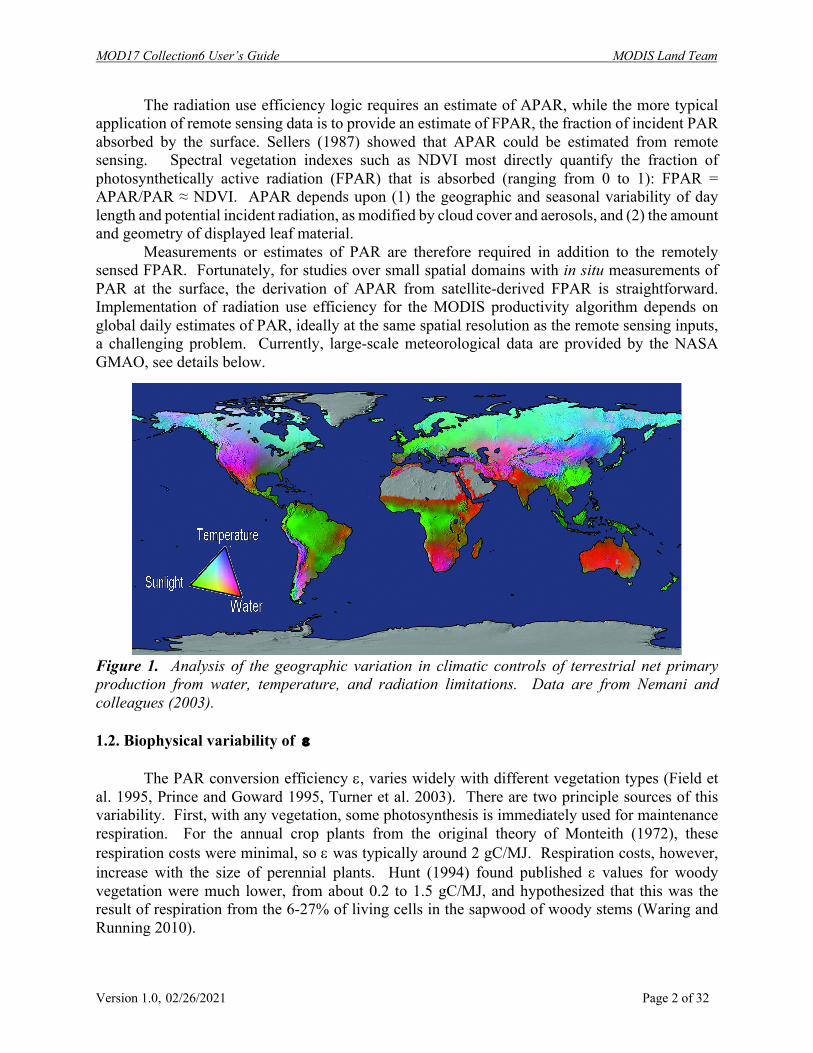
The radiation use efficiency logic requires an estimate of APAR, while the more typical
application of remote sensing data is to provide an estimate of FPAR, the fraction of incident PAR
absorbed by the surface. Sellers (1987) showed that APAR could be estimated from remote
sensing. Spectral vegetation indexes such as NDVI most directly quantify the fraction of
photosynthetically active radiation (FPAR) that is absorbed (ranging from 0 to 1): FPAR =
APAR/PAR ≈ NDVI. APAR depends upon (1) the geographic and seasonal variability of day
length and potential incident radiation, as modified by cloud cover and aerosols, and (2) the amount
and geometry of displayed leaf material.
Measurements or estimates of PAR are therefore required in addition to the remotely
sensed FPAR. Fortunately, for studies over small spatial domains with in situ measurements of
PAR at the surface, the derivation of APAR from satellite-derived FPAR is straightforward.
Implementation of radiation use efficiency for the MODIS productivity algorithm depends on
global daily estimates of PAR, ideally at the same spatial resolution as the remote sensing inputs,
a challenging problem. Currently, large-scale meteorological data are provided by the NASA
GMAO, see details below.
Figure 1. Analysis of the geographic variation in climatic controls of terrestrial net primary production from water, temperature, and radiation limitations. Data are from Nemani and colleagues (2003).
1.2. Biophysical variability of e
The PAR conversion efficiency e, varies widely with different vegetation types (Field et
al. 1995, Prince and Goward 1995, Turner et al. 2003). There are two principle sources of this
variability. First, with any vegetation, some photosynthesis is immediately used for maintenance
respiration. For the annual crop plants from the original theory of Monteith (1972), these
respiration costs were minimal, so e was typically around 2 gC/MJ. Respiration costs, however,
increase with the size of perennial plants. Hunt (1994) found published e values for woody
vegetation were much lower, from about 0.2 to 1.5 gC/MJ, and hypothesized that this was the
result of respiration from the 6-27% of living cells in the sapwood of woody stems (Waring and
Running 2010).
MOD17 Collection6 User’s Guide MODIS Land Team
Version 1.0, 02/26/2021 Page 3 of 32
The second source of variability in e is attributed to suboptimal climatic conditions. To
extrapolate Monteith’s original theory, designed for well-watered crops only during the growing
season, to perennial plants living year around, certain severe climatic constraints must be
recognized. Evergreen vegetation such as conifer trees or schlerophyllous shrubs absorb PAR all
during the non-growing season, yet sub-freezing temperatures stop photosynthesis because leaf
stomata are forced to close (Waring and Running 2010). As a global generalization, we truncate
GPP on days when the air temperature is below 0 °C. Additionally, high vapor pressure deficits, >
2000 Pa, have been shown to induce stomatal closure in many species. This level of daily
atmospheric water deficit is commonly reached in semi-arid regions of the world for much of the
growing season. So, our algorithm mimics this physiological control by progressively limiting
daily GPP by reducing e when high vapor pressure deficits are computed from the surface
meteorology. We also assume nutrient constraints on vegetation growth to be quantified by
limiting leaf area, rather than attempting to compute a constraint through e. This assumption isn’t
entirely accurate, as ranges of leaf nitrogen and photosynthetic capacity occur in all vegetation
types (Reich et al. 1994, Reich et al. 1995, Turner et al. 2003). Spectral reflectance are somewhat
sensitive to leaf chemistry, so the MODIS derived FPAR and LAI may represent some differences
in leaf nitrogen content, but in an undetermined way.
To quantify these biome- and climate-induced ranges of e, we simulated global NPP in
advance with a complex ecosystem model, BIOME-BGC, and computed the e or conversion
efficiency from APAR to final NPP. This Biome Parameter Look-Up Table or BPLUT contains
parameters for temperature and VPD limits, specific leaf area and respiration coefficients for
representative vegetation in each biome type (Running et al. 2000, White et al. 2000). The BPLUT
also defines biome differences in carbon storage and turnover rates.
Since the relationships of temperature to the processes controlling GPP and those
controlling autotrophic respiration have fundamentally different, it seems likely that the empirical
parameterization of the influence of temperature on production efficiency would be more robust if
the gross production and autotrophic respiration processes were separated. This is the approach
employed in the MOD17 algorithm.
1.3. The MO[Y]D17A2H/MO[Y]D17A3H algorithm logic
1.3.1. Gross primary productivity.
The core science of the algorithm is an application of the described radiation conversion
efficiency concept to predictions of daily GPP, using satellite-derived FPAR (from MOD15) and
independent estimates of PAR and other surface meteorological fields (from DAO data, now
renamed to GMAO/NASA), and the subsequent estimation of maintenance and growth respiration
terms that are subtracted from GPP to arrive at annual NPP. The maintenance respiration (MR)
and growth respiration (GR) components arise from allometric relationships linking daily biomass
and annual growth of plant tissues to satellite-derived estimates of leaf area index (LAI, MOD15).
These allometric relationships have been developed from an extensive literature review, and
incorporate the same parameters as those used in the BIOME-BGC ecosystem process model
(Running and Hunt 1993; White et al. 2000).
MOD17 Collection6 User’s Guide MODIS Land Team
Version 1.0, 02/26/2021 Page 4 of 32
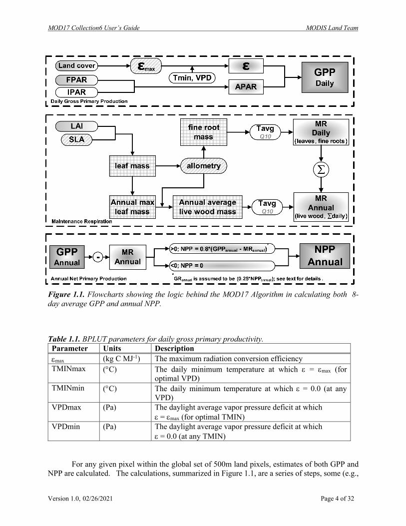
Figure 1.1. Flowcharts showing the logic behind the MOD17 Algorithm in calculating both 8-day average GPP and annual NPP.
Table 1.1. BPLUT parameters for daily gross primary productivity. Parameter Units Description emax (kg C MJ
-1) The maximum radiation conversion efficiency
TMINmax (°C) The daily minimum temperature at which e = emax (for
optimal VPD)
TMINmin (°C) The daily minimum temperature at which e = 0.0 (at any
VPD)
VPDmax (Pa) The daylight average vapor pressure deficit at which
e = emax (for optimal TMIN)
VPDmin (Pa) The daylight average vapor pressure deficit at which
e = 0.0 (at any TMIN)
For any given pixel within the global set of 500m land pixels, estimates of both GPP and
NPP are calculated. The calculations, summarized in Figure 1.1, are a series of steps, some (e.g.,
MOD17 Collection6 User’s Guide MODIS Land Team
Version 1.0, 02/26/2021 Page 5 of 32
GPP) are calculated daily, and others (e.g., NPP) on an annual basis. Calculations of daily
photosynthesis (GPP) are shown in the upper flowchart of Figure 1.1. An 8-day estimate of FPAR
from MOD15 and daily estimated PAR from GMAO/NASA are multiplied to produce daily APAR
for the pixel. Based on the at-launch landcover product (MOD12), a set of biome-specific radiation
use efficiency parameters are extracted from the Biome Properties Look-Up Table (BPLUT) for
each pixel. There are five parameters used to calculate GPP, as shown in Table 1.1. The actual
biome-specific values associated with these parameters will be discussed in Section 3, and the
entire BPLUT is shown in Table 2.1.
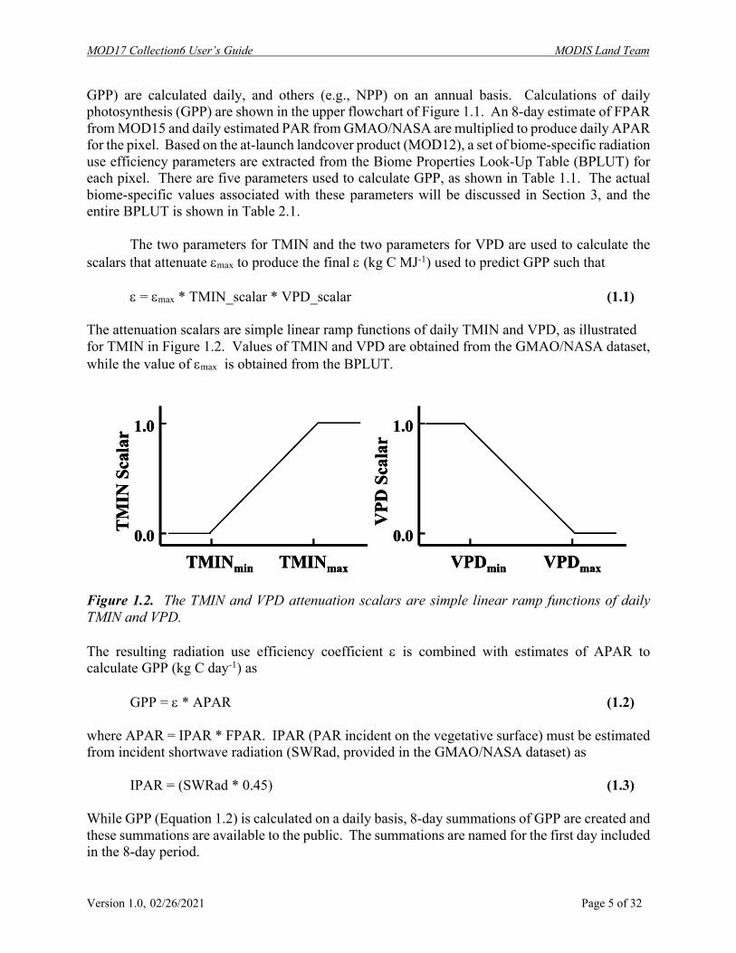
The two parameters for TMIN and the two parameters for VPD are used to calculate the
scalars that attenuate emax to produce the final e (kg C MJ-1
) used to predict GPP such that
e = emax * TMIN_scalar * VPD_scalar (1.1)
The attenuation scalars are simple linear ramp functions of daily TMIN and VPD, as illustrated
for TMIN in Figure 1.2. Values of TMIN and VPD are obtained from the GMAO/NASA dataset,
while the value of emax is obtained from the BPLUT.
Figure 1.2. The TMIN and VPD attenuation scalars are simple linear ramp functions of daily TMIN and VPD. The resulting radiation use efficiency coefficient e is combined with estimates of APAR to
calculate GPP (kg C day-1
) as
GPP = e * APAR (1.2) where APAR = IPAR * FPAR. IPAR (PAR incident on the vegetative surface) must be estimated
from incident shortwave radiation (SWRad, provided in the GMAO/NASA dataset) as
IPAR = (SWRad * 0.45) (1.3) While GPP (Equation 1.2) is calculated on a daily basis, 8-day summations of GPP are created and
these summations are available to the public. The summations are named for the first day included
in the 8-day period.
TMINmin TMINmax
TMIN
Sca
lar 1.0
0.0VPDmin VPDmax
VPD
Sca
lar
1.0
0.0TMINmin TMINmax
TMIN
Sca
lar 1.0
0.0TMINmin TMINmax
TMIN
Sca
lar 1.0
0.0VPDmin VPDmax
VPD
Sca
lar
1.0
0.0VPDmin VPDmax
VPD
Sca
lar
1.0
0.0
MOD17 Collection6 User’s Guide MODIS Land Team
Version 1.0, 02/26/2021 Page 6 of 32
~ Each summation consists of 8 consecutive days of data, and there are 46 such summations created for each calendar year of data collection. To obtain an estimate of daily GPP for this 8-day period, it is necessary to divide the value obtained during a data download by eight for the first 45 values/year and by five (or six in a leap year) for the final period. 1.3.2. Daily maintenance respiration and net photosynthesis.
Maintenance respiration costs (MR) for leaves and fine roots are summarized in the center
flowchart of Figure 1.1 and are also calculated on a daily basis. There are five parameters within
the BPLUT (Table 1.2) needed to calculate daily MR, which is dependent upon leaf or fine root
mass, base MR at 20 °C, and daily average temperature. Leaf mass (kg) is calculated as
Leaf_Mass = LAI / SLA (1.4)
where LAI, the leaf area index (m2 leaf m
-2 ground area), is obtained from MOD15 and the specific
leaf area (SLA, projected leaf area kg-1
leaf C) for a given pixel is obtained from the BPLUT.
Table 1.2. BPLUT parameters for daily maintenance respiration. Parameter Units Description SLA (m
2 kg C
-1) Projected leaf area per unit mass of leaf carbon
froot_leaf_ratio None Ratio of fine root carbon to leaf carbon
leaf_mr_base (kg C kg C-1
day-1
) Maintenance respiration per unit leaf carbon per
day at 20 °C
froot_mr_base (kg C kg C-1
day-1
) Maintenance respiration per unit fine root carbon
per day at 20 °C
Q10_mr None Exponent shape parameter controlling respiration
as a function of temperature
Fine root mass (Fine_Root_Mass, kg) is then estimated as
Fine_Root_Mass = Leaf_Mass * froot_leaf_ratio (1.5)
where froot_leaf_ratio is the ratio of fine root to leaf mass (unitless) as obtained from the BPLUT.
Leaf maintenance respiration (Leaf_MR, kg C day-1
) is calculated as
Leaf_MR = Leaf_Mass * leaf_mr_base * Q10_mr [(Tavg - 20.0) / 10.0] (1.6)
where leaf_mr_base is the maintenance respiration of leaves (kg C kg C-1
day-1
) as obtained from
the BPLUT and Tavg is the average daily temperature (°C) as estimated from the GMAO/NASA
meteorological data.
The maintenance respiration of the fine root mass (Froot_MR, kg C day-1
) is calculated as
MOD17 Collection6 User’s Guide MODIS Land Team
Version 1.0, 02/26/2021 Page 7 of 32
Froot_MR = Fine_Root_Mass * froot_mr_base * Q10_mr [(Tavg - 20.0) / 10.0] (1.7)
where froot_mr_base is the maintenance respiration per unit of fine roots (kg C kg C-1
day-1
) at 20
°C as obtained from the BPLUT.
Finally, PSNnet (kg C day-1
) can be calculated from GPP (Equation 1.2) and maintenance
respiration (Equations 1.6, 1.7) as
PSNnet = GPP – Leaf_MR - Froot_MR (1.8)
As with GPP, PSNnet is summed over an 8-day period.
~ This product does not include the maintenance respiration associated with live wood (Livewood_MR), nor does it include growth respiration (GR).
1.3.3. Annual maintenance respiration Given a calendar year’s worth of outputs from the daily algorithm, the annual algorithm
(Figure 1.1, lower flowchart) estimates annual NPP by first calculating live woody tissue
maintenance respiration, and then estimating growth respiration costs for leaves, fine roots, and
woody tissue using values defined in Table 1.3. Finally, these components are subtracted from the
accumulated daily PSNnet to produce an estimate of annual NPP.
Table 1.3. BPLUT parameters for annual maintenance and growth respiration. Parameter Units Description livewood_leaf_ratio None Ratio of live wood carbon to annual
maximum leaf carbon
livewood_mr_base (kg C kg C-1
day-1
) Maintenance respiration per unit live
wood carbon per day at 20 °C
leaf_longevity (yrs) Average leaf lifespan
leaf_gr_base (kg C kg C-1
) Respiration cost to grow a unit of leaf
carbon
froot_leaf_gr_ratio None Ratio of live wood to leaf annual growth
respiration
livewood_leaf_gr_ratio None Ratio of live wood to leaf annual growth
respiration
deadwood_leaf_gr_ratio None Ratio of dead wood to leaf annual growth
respiration
ann_turnover_proportion None Annual proportion of leaf turnover
Annual maximum leaf mass, the maximum value of daily leaf mass, is the primary input
for both live wood maintenance respiration (Livewood_MR) and whole-plant growth respiration
(GR). To account for Livewood_MR, it is assumed that the amount of live woody tissue is (1)
constant throughout the year, and (2) related to annual maximum leaf mass. Once the live woody
tissue mass has been determined, it can be used to estimate total annual livewood maintenance
respiration. This approach relies on empirical studies relating the annual growth of leaves to the
MOD17 Collection6 User’s Guide MODIS Land Team
Version 1.0, 02/26/2021 Page 8 of 32
annual growth of other plant tissues. The compilation study by Cannell (1982) is an excellent
resource, providing the basis for many of the relationships developed for this portion of the
MOD17 algorithm and tested with the BIOME-BGC ecosystem processes model. Leaf longevity
is required to estimate annual leaf growth for evergreen forests but is assumed to be less than one
year for deciduous forests, which replace all foliage annually. This logic further assumes that there
is no litterfall in deciduous forests until after maximum annual leaf mass has been attained. The
parameters relating annual leaf growth respiration costs to annual fine root, live wood, and dead
wood growth respiration were calculated directly from similar parameters developed for the
BIOME-BGC model (White et al. 2000).
To create the annual NPP term, the MOD17 algorithm maintains a series of daily pixel-
wise terms to appropriately account for plant respiration. To determine livewood maintenance
respiration, the mass of livewood (Livewood_Mass, kg C) is calculated as
Livewood_Mass = ann_leaf_mass_max * livewood_leaf_ratio (1.9)
where ann_leaf_mass_max is the annual maximum leaf mass for a given pixel (kg C) obtained
from the daily Leaf_Mass calculation (Equation 1.4). The livewood_leaf_ratio is the ratio of live
wood mass to leaf mass (unitless), and is obtained from the BPLUT.
Once the mass of live wood has been determined, it is possible to calculate the associated
maintenance respiration (Livewood_MR, kg C day-1
) as
Livewood_MR = Livewood_Mass * livewood_mr_base * annsum_mrindex (1.10)
where livewood_mr_base (kg C kg C-1
day-1
) is the maintenance respiration per unit of live wood
carbon per day from the BPLUT and annsum_mrindex is the annual sum of the maintenance
respiration term Q10_mr [(Tavg-20.0)/10.0]
.
Q10 is a constant value of 2.0 for fine root and live wood. For leaf, we adopted a temperature
acclimated Q10 equation proposed by Tjoelker et al. (2001),
Q10 = 3.22 – 0.046 * Tavg (1.11)
1.3.4. Annual growth respiration and net primary productivity
The original algorithm calculated growth respiration (Rg) as a function of annual maximum
LAI, and thus, the accuracy of Rg is determined by the accuracy of LAImax. However, when LAI
is greater than 3.0, surface reflectance have low sensitivity to LAI and the MODIS LAI is retrieved,
in most cases, under reflectance saturation conditions (Myneni et al., 2002). Generally, for forests,
annual MODIS LAImax is set to be 6.8 for pixels classified as forests. This logic can generate Rg
values that are greater than NPP. Rg is the energy cost for constructing organic compounds fixed
by photosynthesis, and it is empirically parameterized as 25% of NPP (Ryan 1991, Cannell et al.
2000). To improve the algorithm, we replaced the LAImax dependent Rg with Rg = 0.25 * NPP, and
annual MODIS NPP can be computed as
NPP = GPP – Rm – Rg = GPP – Rm – 0.25*NPP (1.12)

MOD17 Collection6 User’s Guide MODIS Land Team
Version 1.0, 02/26/2021 Page 9 of 32
where Rm is annual plant maintenance respiration, and therefore,
NPP = 0.8 * (GPP – Rm) when GPP – Rm >=0, and
NPP = 0 when GPP – Rm < 0 (1.13)
2. Operational Details of MOD17 and Primary Uncertainties in the MOD17 Logic
A number of issues are important in implementing this algorithm for a global NPP. This
section discusses some of the assumptions and special issues involved in development of the input
variables, and their influence on the final NPP.
2.1. Dependence on MODIS Land Cover Classification (MCDLCHKM)
One of the first MODIS products used in the MOD17 algorithm is the Land Cover Product,
MCDLCHKM. The importance of this product cannot be overstated as the MOD17 algorithm
relies heavily on land cover type through use of the BPLUT. While the primary product created
by MOD12 is a 17-class IGBP (International Geosphere-Biosphere Programme) landcover
classification map (Running et al. 1994, Belward et al. 1999, Friedl et al. 2010), the MOD17
algorithm employs Boston University’s UMD classification scheme (Table 2.1).
Figure 2.1. Collection5 1-km MODIS ET used land cover type 2 in 1-km Collection4 MOD12Q1 dataset. Whereas Collection6 operational 500-m MODIS ET is using land cover type 1 in Collection5.1 500-m MCDLCHKM which is a 3-year smoothed MODIS land cover data set. This figures shows land cover types from the Collection4 MOD12Q1 dataset: Evergreen Needleleaf Forest (ENF), Evergreen Broadleaf Forest (EBF), Deciduous Needleleaf Forest (DNF), Deciduous Broadleaf Forest (DBF), Mixed forests (MF), Closed Shrublands (CShrub), Open Shrublands (OShrub), Woody Savannas (WSavanna), Savannas (Savanna), grassland (Grass), and Croplands (Crop). Note that in this figure, we combined CShrub and OShrub into Shrub, and WSavanna and Savannas into Savanna. Globally, Collection5.1 500-m MCDLCHKM has a similar spatial pattern to this image.
MOD17 Collection6 User’s Guide MODIS Land Team
Version 1.0, 02/26/2021 Page 10 of 32
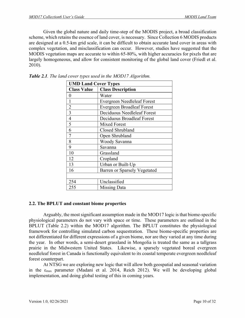
Given the global nature and daily time-step of the MODIS project, a broad classification
scheme, which retains the essence of land cover, is necessary. Since Collection 6 MODIS products
are designed at a 0.5-km grid scale, it can be difficult to obtain accurate land cover in areas with
complex vegetation, and misclassification can occur. However, studies have suggested that the
MODIS vegetation maps are accurate to within 65-80%, with higher accuracies for pixels that are
largely homogeneous, and allow for consistent monitoring of the global land cover (Friedl et al.
2010).
Table 2.1. The land cover types used in the MOD17 Algorithm.
2.2. The BPLUT and constant biome properties
Arguably, the most significant assumption made in the MOD17 logic is that biome-specific
physiological parameters do not vary with space or time. These parameters are outlined in the
BPLUT (Table 2.2) within the MOD17 algorithm. The BPLUT constitutes the physiological
framework for controlling simulated carbon sequestration. These biome-specific properties are
not differentiated for different expressions of a given biome, nor are they varied at any time during
the year. In other words, a semi-desert grassland in Mongolia is treated the same as a tallgrass
prairie in the Midwestern United States. Likewise, a sparsely vegetated boreal evergreen
needleleaf forest in Canada is functionally equivalent to its coastal temperate evergreen needleleaf
forest counterpart.
At NTSG we are exploring new logic that will allow both geospatial and seasonal variation
in the εmax parameter (Madani et al. 2014, Reich 2012). We will be developing global
implementation, and doing global testing of this in coming years.
UMD Land Cover Types Class Value Class Description 0 Water
1 Evergreen Needleleaf Forest
2 Evergreen Broadleaf Forest
3 Deciduous Needleleaf Forest
4 Deciduous Broadleaf Forest
5 Mixed Forest
6 Closed Shrubland
7 Open Shrubland
8 Woody Savanna
9 Savanna
10 Grassland
12 Cropland
13 Urban or Built-Up
16 Barren or Sparsely Vegetated
254 Unclassified
255 Missing Data
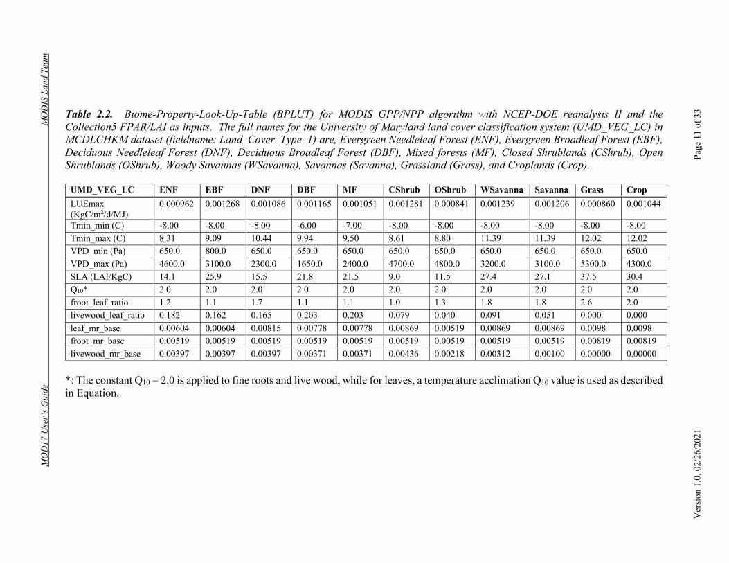
Table 2.2. Biome-Property-Look-Up-Table (BPLUT) for MODIS GPP/NPP algorithm with NCEP-DOE reanalysis II and the
Collection5 FPAR/LAI as inputs. The full names for the University of Maryland land cover classification system (UMD_VEG_LC) in
MCDLCHKM dataset (fieldname: Land_Cover_Type_1) are, Evergreen Needleleaf Forest (ENF), Evergreen Broadleaf Forest (EBF),
Deciduous Needleleaf Forest (DNF), Deciduous Broadleaf Forest (DBF), Mixed forests (MF), Closed Shrublands (CShrub), Open
Shrublands (OShrub), Woody Savannas (WSavanna), Savannas (Savanna), Grassland (Grass), and Croplands (Crop).
UMD_VEG_LC ENF EBF DNF DBF MF CShrub OShrub WSavanna Savanna Grass Crop LUEmax (KgC/m2/d/MJ)
0.000962 0.001268 0.001086 0.001165 0.001051 0.001281 0.000841 0.001239 0.001206 0.000860 0.001044
Tmin_min (C) -8.00 -8.00 -8.00 -6.00 -7.00 -8.00 -8.00 -8.00 -8.00 -8.00 -8.00 Tmin_max (C) 8.31 9.09 10.44 9.94 9.50 8.61 8.80 11.39 11.39 12.02 12.02 VPD_min (Pa) 650.0 800.0 650.0 650.0 650.0 650.0 650.0 650.0 650.0 650.0 650.0 VPD_max (Pa) 4600.0 3100.0 2300.0 1650.0 2400.0 4700.0 4800.0 3200.0 3100.0 5300.0 4300.0 SLA (LAI/KgC) 14.1 25.9 15.5 21.8 21.5 9.0 11.5 27.4 27.1 37.5 30.4 Q10* 2.0 2.0 2.0 2.0 2.0 2.0 2.0 2.0 2.0 2.0 2.0 froot_leaf_ratio 1.2 1.1 1.7 1.1 1.1 1.0 1.3 1.8 1.8 2.6 2.0 livewood_leaf_ratio 0.182 0.162 0.165 0.203 0.203 0.079 0.040 0.091 0.051 0.000 0.000 leaf_mr_base 0.00604 0.00604 0.00815 0.00778 0.00778 0.00869 0.00519 0.00869 0.00869 0.0098 0.0098 froot_mr_base 0.00519 0.00519 0.00519 0.00519 0.00519 0.00519 0.00519 0.00519 0.00519 0.00819 0.00819 livewood_mr_base 0.00397 0.00397 0.00397 0.00371 0.00371 0.00436 0.00218 0.00312 0.00100 0.00000 0.00000
*: The constant Q10 = 2.0 is applied to fine roots and live wood, while for leaves, a temperature acclimation Q10 value is used as described in Equation.
MO
D17
Use
r’s G
uide
MO
DIS
Lan
d Te
am
Ver
sion
1.0
, 02/
26/2
021
Pag
e 11
of
33
MOD17 User’s Guide MODIS Land Team
Version 1.0, 02/26/2021 Page 12 of 33
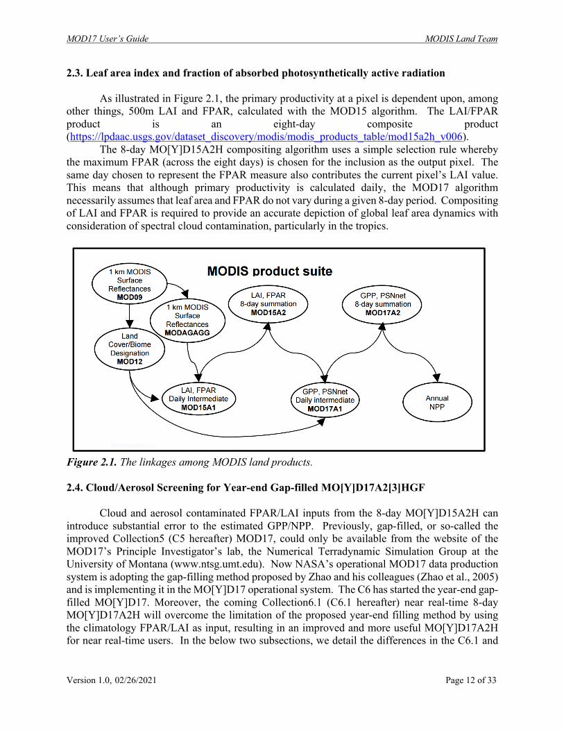
2.3. Leaf area index and fraction of absorbed photosynthetically active radiation As illustrated in Figure 2.1, the primary productivity at a pixel is dependent upon, among
other things, 500m LAI and FPAR, calculated with the MOD15 algorithm. The LAI/FPAR product is an eight-day composite product (https://lpdaac.usgs.gov/dataset_discovery/modis/modis_products_table/mod15a2h_v006).
The 8-day MO[Y]D15A2H compositing algorithm uses a simple selection rule whereby the maximum FPAR (across the eight days) is chosen for the inclusion as the output pixel. The same day chosen to represent the FPAR measure also contributes the current pixel’s LAI value. This means that although primary productivity is calculated daily, the MOD17 algorithm necessarily assumes that leaf area and FPAR do not vary during a given 8-day period. Compositing of LAI and FPAR is required to provide an accurate depiction of global leaf area dynamics with consideration of spectral cloud contamination, particularly in the tropics.
Figure 2.1. The linkages among MODIS land products. 2.4. Cloud/Aerosol Screening for Year-end Gap-filled MO[Y]D17A2[3]HGF
Cloud and aerosol contaminated FPAR/LAI inputs from the 8-day MO[Y]D15A2H can
introduce substantial error to the estimated GPP/NPP. Previously, gap-filled, or so-called the improved Collection5 (C5 hereafter) MOD17, could only be available from the website of the MOD17’s Principle Investigator’s lab, the Numerical Terradynamic Simulation Group at the University of Montana (www.ntsg.umt.edu). Now NASA’s operational MOD17 data production system is adopting the gap-filling method proposed by Zhao and his colleagues (Zhao et al., 2005) and is implementing it in the MO[Y]D17 operational system. The C6 has started the year-end gap-filled MO[Y]D17. Moreover, the coming Collection6.1 (C6.1 hereafter) near real-time 8-day MO[Y]D17A2H will overcome the limitation of the proposed year-end filling method by using the climatology FPAR/LAI as input, resulting in an improved and more useful MO[Y]D17A2H for near real-time users. In the below two subsections, we detail the differences in the C6.1 and
MOD17 User’s Guide MODIS Land Team
Version 1.0, 02/26/2021 Page 13 of 33
Gap-filled C6.1 and how the year-end gap-filling method is implemented to generate the higher quality MO[Y]D17. 2.4.1. Differences Between C6.1 and C6 MO[Y]D17
Cloud-contaminated MODIS inputs can introduce substantial errors or data gaps to the MOD17 data product, and this is the reason that NTSG had decided to improve MOD17 quality through a year-end post-processing, by cleaning these contaminated MODIS inputs (Zhao et al., 2005). The gap-filled method substantially increased the quality of MOD17, but the limitation is that the method can only be applied at the end of the year. A new branch of MOD17 data set has been introduced since C6, named as MO[Y]D17A2[3]HGF, which is year-end gap-filled MOD17 and detailed in below section 2.4.2.
Starting from C6.1 MOD1, we have introduced climatology FPAR/LAI and named it as MCD15A2HCL. The data from MCD15A2HCL are used as backup input to replace these contaminated FPAR/LAI from MOD15A2H for the corresponding 8-day periods. The 8-day MCD15A2HCL is the average of the best FPAR/LAI for a given vegetated pixel for the 8-day across the past 5 years based on the data quality from both MOD15A2H and MYD15A2H. If there is no reliable data available for an 8-day period across all 5 years, a temporally filling will be conducted to fill the gaps in climatology FPAR/LAI by following the gap-filling method proposed by Zhao et al. (2005). We chose 5-year because the time span for an interannual global scale climate fluctuation cycle, the El Niño-Southern Oscillation (ENSO), is about 5 years, and ENSO has great impacts on biosphere activities (Keeling et al., 1995; Nemani et al., 2003). A longer time span beyond 5-year may result in unrealistic climatology FPAR/LAI because averaging obscures vegetation greenness changes by ecosystem disturbances or land use cover change (Mildrexler et al., 2007; Mildrexler et al., 2009; Song et al. 2018).
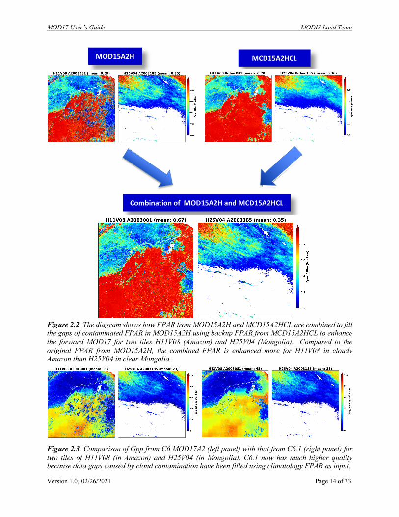
Figure 2.2 shows how the MOD17 process combines 8-day MOD15A2H with the corresponding 8-day climatology MCD15A2HCL to fill the gaps of contaminated FPAR/LAI for Gpp and PsnNet calculations. For a given vegetated pixel, if FPAR/LAI from MOD15A2H are contaminated, the corresponding climatology FPAR/LAI will be used to replace the contaminated values for calculations, resulting in enhanced estimated Gpp and PsnNet. We use two tiles: H11V08 (in Amazon) and H25V04 (in Mongolia), as examples to show in figures 2.2 and 2.3. Figure 2.2 shows that the combination of MOD15A2H and MCD15A2HCL generally results in higher FPAR values for H11V08, but almost no change of FPAR for H25V04. This is because Amazon region has high frequency of cloudiness whereas Mongolia in dry climate is clear most of time.
Figure 2.3 shows the comparison of C6 and C6.1 MOD17A2H for the two tiles. The figure clearly shows the enhanced Gpp from the C6.1 MOD17A2 than the C6 counterpart because the lower and contaminated FPAR/LAI are replaced by the climatology FPAR/LAI. The increase is much more for Amazonia H11V08 than that Mongolian H25V04 because the former has more cloudiness than the latter under a dry climate.
MOD17 User’s Guide MODIS Land Team
Version 1.0, 02/26/2021 Page 14 of 33
Figure 2.2. The diagram shows how FPAR from MOD15A2H and MCD15A2HCL are combined to fill the gaps of contaminated FPAR in MOD15A2H using backup FPAR from MCD15A2HCL to enhance the forward MOD17 for two tiles H11V08 (Amazon) and H25V04 (Mongolia). Compared to the original FPAR from MOD15A2H, the combined FPAR is enhanced more for H11V08 in cloudy Amazon than H25V04 in clear Mongolia.. Figure 2.3. Comparison of Gpp from C6 MOD17A2 (left panel) with that from C6.1 (right panel) for two tiles of H11V08 (in Amazon) and H25V04 (in Mongolia). C6.1 now has much higher quality because data gaps caused by cloud contamination have been filled using climatology FPAR as input.
MOD15A2H MCD15A2HCL
Combination of MOD15A2H and MCD15A2HCL
MOD17 User’s Guide MODIS Land Team
Version 1.0, 02/26/2021 Page 15 of 33
2.4.2. C6.1 MO[Y]D17A2[3]H and Year-end Gap-filled MO[Y]D17A2[3]HGF Though the quality of the C6.1 MO[Y]D17A2H and MO[Y]D17A3H is much better than
the C6 counterpart as because of the introduction of climatology FPAR/LAI, MOD15A2HCL, but the climatology FPAR/LAI could introduce biases because it smooths out vegetation change caused by interannual variability climate or ecosystem disturbances or recovery, such as fire, land use change, etc. The ideal high quality and consistent MOD17 still needs the application of the year-end gap-filled process as suggested by Zhao et al. (2015) to create year-end gap-filled MOD17.
The method of C6.1 gap-filled MO[Y]D17 is consistent with that to the C6 except the input MODIS data are the C6.1. Likewise, C6.1 gap-filled MO[Y]D17 have different data product names and “GF” will be added to the names of the data files, such as M*D17A2HGF and M*D17A3HGF, to distinguish from the non-gap-filled M*D17A2H and M*D17A3H.
The MO[Y]D17A2HGF and MO[Y]D17A3HGF will be generated at the end of each year when the entire yearly 8-day M*D15A2 are available, following the proposed method for improving MOD17 (Zhao et al., 2005). Hence the Gap-filled MO[Y]D17A2HGF and MO[Y]D17A3HGF are the improved MOD17 which have cleaned the contaminated inputs from 8-day FPAR/LAI. However, users cannot get MO[Y]D17A2[3]HGF in the near real-time manner because it will be generated at the end of a given year. This is the limitation of the year-end gap-filling method.
Users should maintain caution, while using these Gap-filled products from the first years of the missions, 2000 and 2002 for MODIS TERRA and AQUA respectively. This is because, the temporal gap-filling algorithm, used to produce gap-filled FPAR/LAI inputs, could not have the full 8-days data in a year for ideally gap-filling, when it came to year 2000 for TERRA and 2002 for AQUA. MOD15A2H of TERRA starts from 2000-02-28 and MYD15A2H of Aqua from 2002-07-04. Subsequently, the RANGEBEGINNINGDATE metadata value in MOD17A3HGF for these first data years is consistent with the start date of M*D15A2H not from 200X-01-01. Despite the RANGEBEGINNINGDATE metadata reflecting the start-of-mission date for TERRA (2000-02-28) and AQUA (2002-07-04) in MOD17A3HGF for years 2000 and 2002, respectively, the Gap-filled FPAR/LAI inputs were processed using a temporal gap-filling over the entire year, with missing values from the start of the year till mission start. The first available good FPAR/LAI from the start-of-mission date onward will be used for the missing values.
Therefore, users should especially be aware of using MYD17A2HGF and MYD17A3GF in 2002, when the gap from the beginning of the year to actual start of mission (2002-07-04) is too long (> 0.5 year) and hence, the gap-filled FPAR/LAI inputs have no temporal dynamics for a vegetated pixel before 2002-07-04. As a result, the 8-day MYD17A2GF and the annual MYD17A3GF are less useful for 2002. The problem is similar for MOD17A2GF and MOD17A3GF in year 2000 but much less severe because there are just about 1.5 months data gap between start of the year and actual start of mission for Gap-filled versions of MOD15.
The detailed year-end gap-filling method is described in below section.
2.4.3 Gap-filling FPAR/LAI for Year-end Gap-filled MO[Y]D17A2[3]HGF At the end of each year, we solved the issue of the contaminated FPAR/LAI inputs to
MO[Y]D17A2[3]HGF by removing poor quality FPAR and LAI data based on the QC label for every pixel. If any LAI/FPAR pixel did not meet the quality screening criteria, its value is determined through linear interpolation between the previous period’s value and that of the next
MOD17 User’s Guide MODIS Land Team
Version 1.0, 02/26/2021 Page 16 of 33
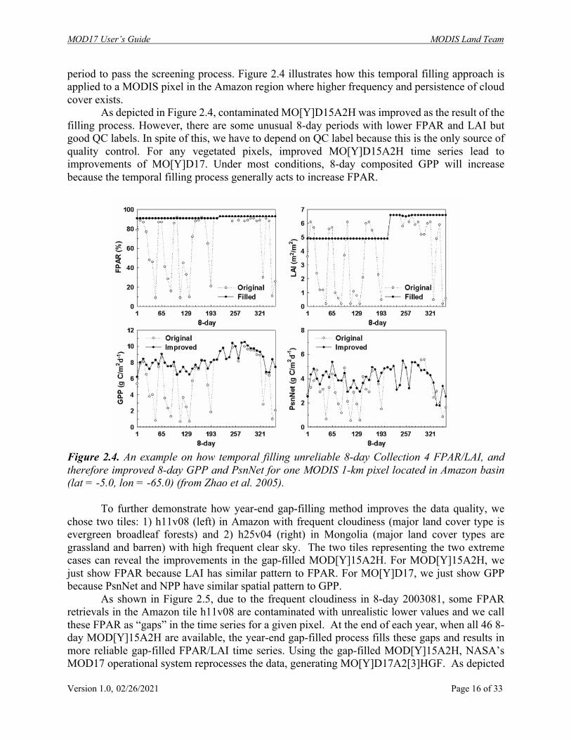
period to pass the screening process. Figure 2.4 illustrates how this temporal filling approach is applied to a MODIS pixel in the Amazon region where higher frequency and persistence of cloud cover exists.
As depicted in Figure 2.4, contaminated MO[Y]D15A2H was improved as the result of the filling process. However, there are some unusual 8-day periods with lower FPAR and LAI but good QC labels. In spite of this, we have to depend on QC label because this is the only source of quality control. For any vegetated pixels, improved MO[Y]D15A2H time series lead to improvements of MO[Y]D17. Under most conditions, 8-day composited GPP will increase because the temporal filling process generally acts to increase FPAR.
Figure 2.4. An example on how temporal filling unreliable 8-day Collection 4 FPAR/LAI, and therefore improved 8-day GPP and PsnNet for one MODIS 1-km pixel located in Amazon basin (lat = -5.0, lon = -65.0) (from Zhao et al. 2005).
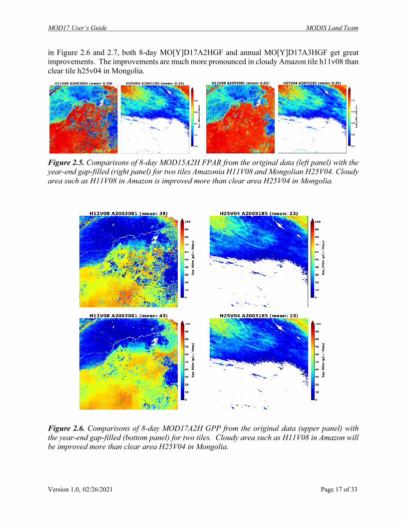
To further demonstrate how year-end gap-filling method improves the data quality, we
chose two tiles: 1) h11v08 (left) in Amazon with frequent cloudiness (major land cover type is evergreen broadleaf forests) and 2) h25v04 (right) in Mongolia (major land cover types are grassland and barren) with high frequent clear sky. The two tiles representing the two extreme cases can reveal the improvements in the gap-filled MOD[Y]15A2H. For MOD[Y]15A2H, we just show FPAR because LAI has similar pattern to FPAR. For MO[Y]D17, we just show GPP because PsnNet and NPP have similar spatial pattern to GPP.
As shown in Figure 2.5, due to the frequent cloudiness in 8-day 2003081, some FPAR retrievals in the Amazon tile h11v08 are contaminated with unrealistic lower values and we call these FPAR as “gaps” in the time series for a given pixel. At the end of each year, when all 46 8-day MOD[Y]15A2H are available, the year-end gap-filled process fills these gaps and results in more reliable gap-filled FPAR/LAI time series. Using the gap-filled MOD[Y]15A2H, NASA’s MOD17 operational system reprocesses the data, generating MO[Y]D17A2[3]HGF. As depicted
MOD17 User’s Guide MODIS Land Team
Version 1.0, 02/26/2021 Page 17 of 33
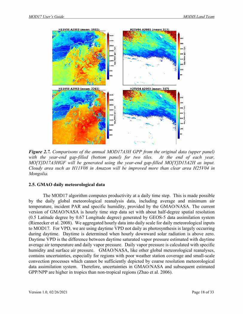
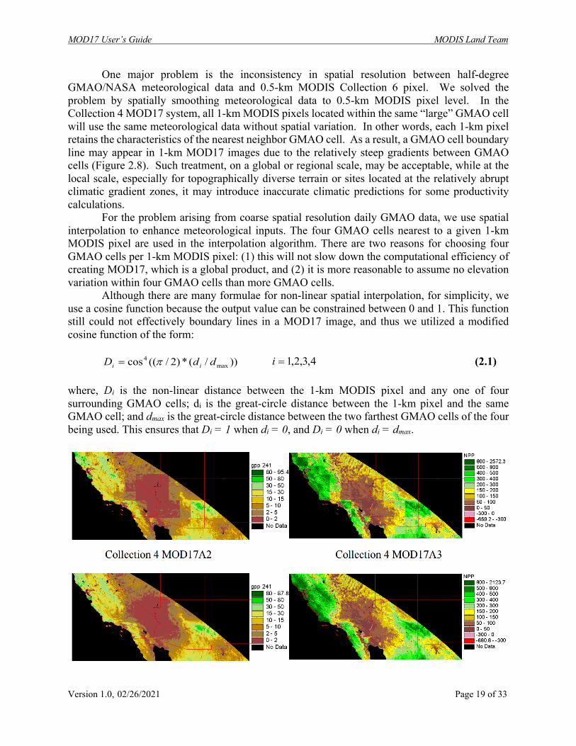
in Figure 2.6 and 2.7, both 8-day MO[Y]D17A2HGF and annual MO[Y]D17A3HGF get great improvements. The improvements are much more pronounced in cloudy Amazon tile h11v08 than clear tile h25v04 in Mongolia.
Figure 2.5. Comparisons of 8-day MOD15A2H FPAR from the original data (left panel) with the year-end gap-filled (right panel) for two tiles Amazonia H11V08 and Mongolian H25V04. Cloudy area such as H11V08 in Amazon is improved more than clear area H25V04 in Mongolia.
Figure 2.6. Comparisons of 8-day MOD17A2H GPP from the original data (upper panel) with the year-end gap-filled (bottom panel) for two tiles. Cloudy area such as H11V08 in Amazon will be improved more than clear area H25V04 in Mongolia.
MOD17 User’s Guide MODIS Land Team
Version 1.0, 02/26/2021 Page 18 of 33
Figure 2.7. Comparisons of the annual MOD17A3H GPP from the original data (upper panel) with the year-end gap-filled (bottom panel) for two tiles. At the end of each year, MO[Y]D17A3HGF will be generated using the year-end gap-filled MO[Y]D15A2H as input. Cloudy area such as H11V08 in Amazon will be improved more than clear area H25V04 in Mongolia. 2.5. GMAO daily meteorological data
The MOD17 algorithm computes productivity at a daily time step. This is made possible
by the daily global meteorological reanalysis data, including average and minimum air temperature, incident PAR and specific humidity, provided by the GMAO/NASA. The current version of GMAO/NASA is hourly time step data set with about half-degree spatial resolution (0.5 Latitude degree by 0.67 Longitude degree) generated by GEOS-5 data assimilation system (Rienecker et al. 2008). We aggregated hourly data into daily scale for daily meteorological inputs to MOD17. For VPD, we are using daytime VPD not daily as photosynthesis is largely occurring during daytime. Daytime is determined when hourly downward solar radiation is above zero. Daytime VPD is the difference between daytime saturated vapor pressure estimated with daytime average air temperature and daily vapor pressure. Daily vapor pressure is calculated with specific humidity and surface air pressure. GMAO/NASA, like other global meteorological reanalyses, contains uncertainties, especially for regions with poor weather station coverage and small-scale convection processes which cannot be sufficiently depicted by coarse resolution meteorological data assimilation system. Therefore, uncertainties in GMAO/NASA and subsequent estimated GPP/NPP are higher in tropics than non-tropical regions (Zhao et al. 2006).
MOD17 User’s Guide MODIS Land Team
Version 1.0, 02/26/2021 Page 19 of 33
One major problem is the inconsistency in spatial resolution between half-degree GMAO/NASA meteorological data and 0.5-km MODIS Collection 6 pixel. We solved the problem by spatially smoothing meteorological data to 0.5-km MODIS pixel level. In the Collection 4 MOD17 system, all 1-km MODIS pixels located within the same “large” GMAO cell will use the same meteorological data without spatial variation. In other words, each 1-km pixel retains the characteristics of the nearest neighbor GMAO cell. As a result, a GMAO cell boundary line may appear in 1-km MOD17 images due to the relatively steep gradients between GMAO cells (Figure 2.8). Such treatment, on a global or regional scale, may be acceptable, while at the local scale, especially for topographically diverse terrain or sites located at the relatively abrupt climatic gradient zones, it may introduce inaccurate climatic predictions for some productivity calculations. For the problem arising from coarse spatial resolution daily GMAO data, we use spatial interpolation to enhance meteorological inputs. The four GMAO cells nearest to a given 1-km MODIS pixel are used in the interpolation algorithm. There are two reasons for choosing four GMAO cells per 1-km MODIS pixel: (1) this will not slow down the computational efficiency of creating MOD17, which is a global product, and (2) it is more reasonable to assume no elevation variation within four GMAO cells than more GMAO cells.
Although there are many formulae for non-linear spatial interpolation, for simplicity, we use a cosine function because the output value can be constrained between 0 and 1. This function still could not effectively boundary lines in a MOD17 image, and thus we utilized a modified cosine function of the form:
(2.1)
where, Di is the non-linear distance between the 1-km MODIS pixel and any one of four surrounding GMAO cells; di is the great-circle distance between the 1-km pixel and the same GMAO cell; and dmax is the great-circle distance between the two farthest GMAO cells of the four being used. This ensures that Di = 1 when di = 0, and Di = 0 when di = dmax.
))/(*)2/((cos max4 ddD ii p= 4,3,2,1=i
MOD17 User’s Guide MODIS Land Team
Version 1.0, 02/26/2021 Page 20 of 33
Figure 2.8. Comparison of Collection 4 and Collection 4.5 MOD17A2 GPP (composite period 241) and MOD17A3 NPP for 2001.
Based on the non-linear distance (Di), the weighted value Wi can be expressed as
, (2.2)
and therefore, for a given pixel, the corresponding smoothed value (i.e., interpolated Tmin, Tavg, VPD, SWrad) is
(2.3)
Theoretically, this GMAO spatial interpolation can improve the accuracy of
meteorological data for each 1-km pixel because it is unrealistic for meteorological data to abruptly change from one side of GMAO boundary to the other, as in Collection 4. Figure 2.4 shows how this method works for MOD17A2/A3. The degree to which this interpolated GMAO will improve the accuracy of meteorological inputs, however, is largely dependent on the accuracy of GMAO data and the properties of local environmental conditions, such as elevation or weather patterns. To explore the above question, we use observed daily weather data from World Meteorological Organization (WMO) daily surface observation network (>5000 stations) to compare changes in Root Mean Squared Error (RMSE) and Correlation (COR) between the original and enhanced DAO data.
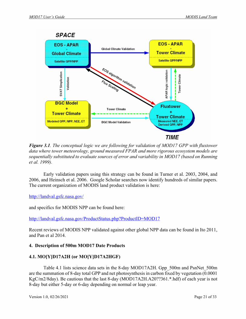
3. Validation of MOD 17 GPP and NPP The original strategy for validation of the MOD 17 GPP and NPP data can be found in Running et al. 1999. This paper, published before the first MODIS launch, developed an overall plan for integrating MODIS Land data into global terrestrial monitoring. This paper laid the foundation for the interaction between MODLAND and the eddy covariance fluxtower community, illustrating the mutual advantage of fluxtowers providing direct measurement of carbon and water fluxes, while MODIS land products provided a spatial extrapolation of the tower data. It also laid out the conceptual basis for swapping out various components of the MOD17 algorithm in order to isolate points of uncertainty and inaccuracy, shown in Figure 3.1.
å=
=4
1/i
iii DDW
V
å=
=4
1)*(
iii VWV
MOD17 User’s Guide MODIS Land Team
Version 1.0, 02/26/2021 Page 21 of 33
Figure 3.1. The conceptual logic we are following for validation of MOD17 GPP with fluxtower data where tower meteorology, ground measured FPAR and more rigorous ecosystem models are sequentially substituted to evaluate sources of error and variability in MOD17 (based on Running et al. 1999). Early validation papers using this strategy can be found in Turner et al. 2003, 2004, and 2006, and Heinsch et al. 2006. Google Scholar searches now identify hundreds of similar papers. The current organization of MODIS land product validation is here: http://landval.gsfc.nasa.gov/ and specifics for MODIS NPP can be found here: http://landval.gsfc.nasa.gov/ProductStatus.php?ProductID=MOD17 Recent reviews of MODIS NPP validated against other global NPP data can be found in Ito 2011, and Pan et al 2014. 4. Description of 500m MOD17 Date Products 4.1. MO[Y]D17A2H (or MO[Y]D17A2HGF)
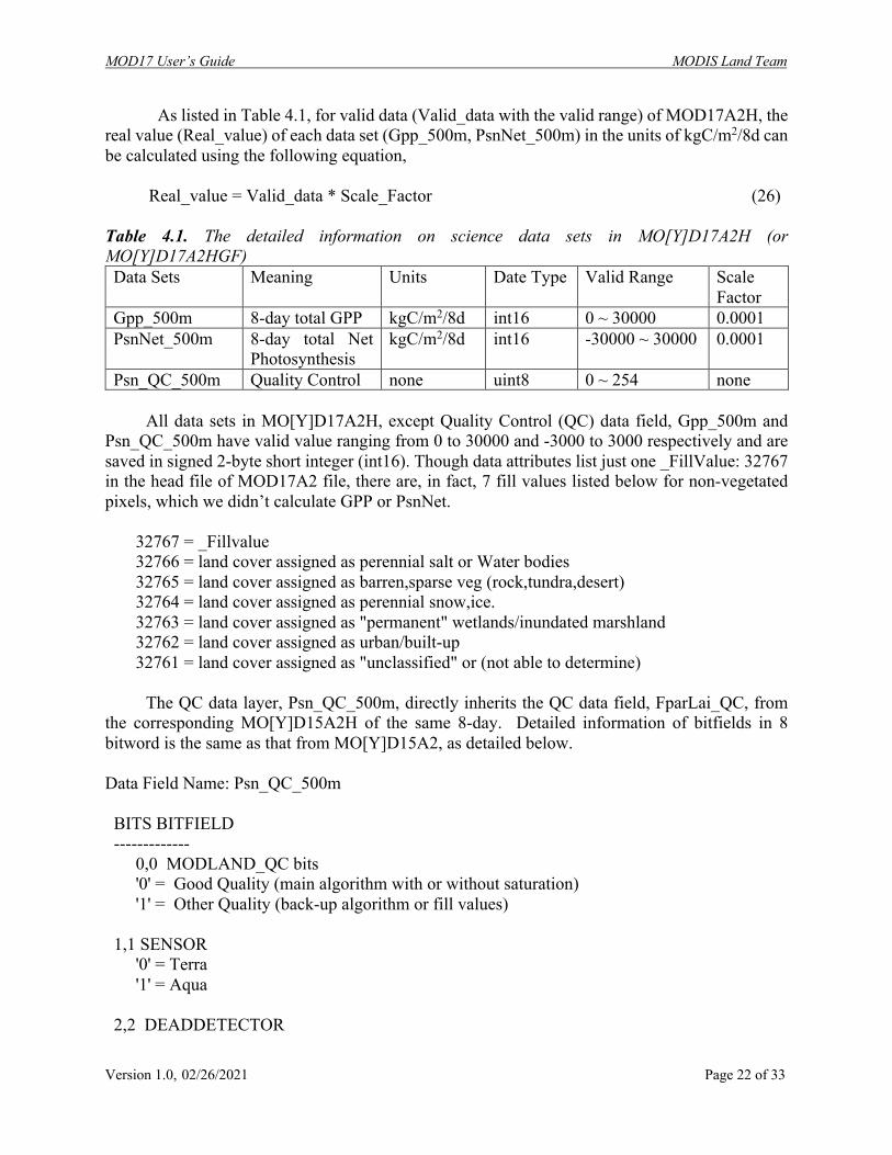
Table 4.1 lists science data sets in the 8-day MOD17A2H. Gpp_500m and PsnNet_500m are the summation of 8-day total GPP and net photosynthesis in carbon fixed by vegetation (0.0001 KgC/m2/8day). Be cautious that the last 8-day (MOD17A2H.A20??361.*.hdf) of each year is not 8-day but either 5-day or 6-day depending on normal or leap year.
MOD17 User’s Guide MODIS Land Team
Version 1.0, 02/26/2021 Page 22 of 33
As listed in Table 4.1, for valid data (Valid_data with the valid range) of MOD17A2H, the real value (Real_value) of each data set (Gpp_500m, PsnNet_500m) in the units of kgC/m2/8d can be calculated using the following equation, Real_value = Valid_data * Scale_Factor (26) Table 4.1. The detailed information on science data sets in MO[Y]D17A2H (or MO[Y]D17A2HGF) Data Sets Meaning Units Date Type Valid Range Scale
Factor Gpp_500m 8-day total GPP kgC/m2/8d int16 0 ~ 30000 0.0001 PsnNet_500m 8-day total Net
Photosynthesis kgC/m2/8d int16 -30000 ~ 30000 0.0001
Psn_QC_500m Quality Control none uint8 0 ~ 254 none All data sets in MO[Y]D17A2H, except Quality Control (QC) data field, Gpp_500m and Psn_QC_500m have valid value ranging from 0 to 30000 and -3000 to 3000 respectively and are saved in signed 2-byte short integer (int16). Though data attributes list just one _FillValue: 32767 in the head file of MOD17A2 file, there are, in fact, 7 fill values listed below for non-vegetated pixels, which we didn’t calculate GPP or PsnNet. 32767 = _Fillvalue 32766 = land cover assigned as perennial salt or Water bodies 32765 = land cover assigned as barren,sparse veg (rock,tundra,desert) 32764 = land cover assigned as perennial snow,ice. 32763 = land cover assigned as "permanent" wetlands/inundated marshland 32762 = land cover assigned as urban/built-up
32761 = land cover assigned as "unclassified" or (not able to determine)
The QC data layer, Psn_QC_500m, directly inherits the QC data field, FparLai_QC, from the corresponding MO[Y]D15A2H of the same 8-day. Detailed information of bitfields in 8 bitword is the same as that from MO[Y]D15A2, as detailed below. Data Field Name: Psn_QC_500m BITS BITFIELD ------------- 0,0 MODLAND_QC bits '0' = Good Quality (main algorithm with or without saturation) '1' = Other Quality (back-up algorithm or fill values) 1,1 SENSOR '0' = Terra '1' = Aqua 2,2 DEADDETECTOR
MOD17 User’s Guide MODIS Land Team
Version 1.0, 02/26/2021 Page 23 of 33
'0' = Detectors apparently fine for up to 50% of channels 1,2 '1' = Dead detectors caused >50% adjacent detector retrieval 3,4 CLOUDSTATE (this inherited from Aggregate_QC bits {0,1} cloud state) '00' = 0 Significant clouds NOT present (clear) '01' = 1 Significant clouds WERE present '10' = 2 Mixed cloud present on pixel '11' = 3 Cloud state not defined, assumed clear 5,7 SCF_QC (3-bit, (range '000'..100') 5 level Confidence Quality score. '000' = 0, Main (RT) method used, best result possible (no saturation) '001' = 1, Main (RT) method used with saturation. Good,very usable '010' = 2, Main (RT) method failed due to bad geometry, empirical algorithm used '011' = 3, Main (RT) method failed due to problems other than geometry, empirical algorithm used
'100' = 4, Pixel not produced at all, value couldn't be retrieved (possible reasons: bad L1B data, unusable MOD09GA data)
For the C6.1 NASA’s operational MO[Y]D17A2H, we suggest users at least exclude cloud-contaminated cells. For the year-end gap-filled MO[Y]D17A2HGF, users may ignore QC data layer because cloud-contaminated LAI/FPAR gaps have been temporally filled before calculation (also see previous section 2.4). Hence for MO[Y]D17A2HGF, QC just denotes if year-end filled LAI/FPAR were used as inputs. Users may ignore QC data layers for the year-end gap-filled MO[Y]D17A2[3]HGF but just use pixels with values within the valid range. 4.2. MO[Y]D17A3H (or MO[Y]D17A3HGF) Another difference between C6.1 and C6 is that the annual MO[Y]D17A3H and MO[Y]D17A3HGF now have a new data field called Gpp_500m, which is the total annual GPP. The addition of the Gpp_500m data field is to facilitate users who are interested in the annual total, which will provide the sum of Gpp_500m from all 46 MO[Y]D17A2H 8-day periods. Table 4.2 lists science data sets in annual MO[Y]D17A3H. Gpp_500m and Npp_500m are the summation of total daily GPP and NPP through the year (0.0001 KgC/m2/year), respectively. Gpp_500m and Npp_500m have the same unit, but different data types (unsigned and signed 2-byte short, uint16 and int16), valid range and fill values are different because of the different data types.
Similar to MO[Y]D17A2H, as listed in Table 4.2, for valid data (Valid_data with the valid range) of MO[Y]D17A3H, the real value (Real_value) in the corresponding units (kgC/m2/yr) can be calculated using the following equation,
Real_value = Valid_data * Scale_Factor (27) The annual total NPP_500m in int16, is similar to MO[Y]D17A2H, although data attributes list one _FillValue: 32767 in the HDFEOS MO[Y]D17A3H file, there are, 7 fill values listed below
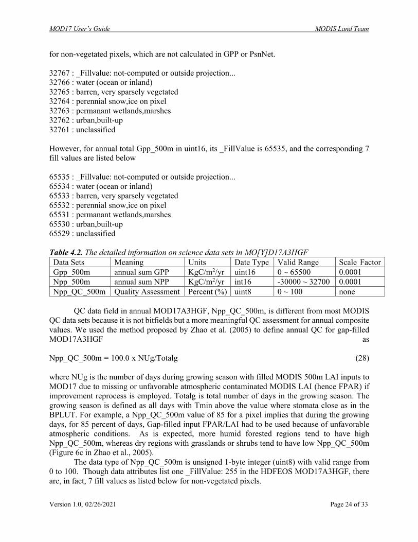
MOD17 User’s Guide MODIS Land Team
Version 1.0, 02/26/2021 Page 24 of 33
for non-vegetated pixels, which are not calculated in GPP or PsnNet. 32767 : _Fillvalue: not-computed or outside projection... 32766 : water (ocean or inland) 32765 : barren, very sparsely vegetated 32764 : perennial snow,ice on pixel 32763 : permanant wetlands,marshes 32762 : urban,built-up 32761 : unclassified However, for annual total Gpp_500m in uint16, its _FillValue is 65535, and the corresponding 7 fill values are listed below 65535 : _Fillvalue: not-computed or outside projection... 65534 : water (ocean or inland) 65533 : barren, very sparsely vegetated 65532 : perennial snow,ice on pixel 65531 : permanant wetlands,marshes 65530 : urban,built-up 65529 : unclassified Table 4.2. The detailed information on science data sets in MO[Y]D17A3HGF Data Sets Meaning Units Date Type Valid Range Scale Factor Gpp_500m annual sum GPP KgC/m2/yr uint16 0 ~ 65500 0.0001 Npp_500m annual sum NPP KgC/m2/yr int16 -30000 ~ 32700 0.0001 Npp_QC_500m Quality Assessment Percent (%) uint8 0 ~ 100 none
QC data field in annual MOD17A3HGF, Npp_QC_500m, is different from most MODIS
QC data sets because it is not bitfields but a more meaningful QC assessment for annual composite values. We used the method proposed by Zhao et al. (2005) to define annual QC for gap-filled MOD17A3HGF as Npp_QC_500m = 100.0 x NUg/Totalg (28) where NUg is the number of days during growing season with filled MODIS 500m LAI inputs to MOD17 due to missing or unfavorable atmospheric contaminated MODIS LAI (hence FPAR) if improvement reprocess is employed. Totalg is total number of days in the growing season. The growing season is defined as all days with Tmin above the value where stomata close as in the BPLUT. For example, a Npp_QC_500m value of 85 for a pixel implies that during the growing days, for 85 percent of days, Gap-filled input FPAR/LAI had to be used because of unfavorable atmospheric conditions. As is expected, more humid forested regions tend to have high Npp_QC_500m, whereas dry regions with grasslands or shrubs tend to have low Npp_QC_500m (Figure 6c in Zhao et al., 2005).
The data type of Npp_QC_500m is unsigned 1-byte integer (uint8) with valid range from 0 to 100. Though data attributes list one _FillValue: 255 in the HDFEOS MOD17A3HGF, there are, in fact, 7 fill values as listed below for non-vegetated pixels.

MOD17 User’s Guide MODIS Land Team
Version 1.0, 02/26/2021 Page 25 of 33
255 = _Fillvalue 254 = land cover assigned as perennial salt or Water bodies 253 = land cover assigned as barren,sparse veg (rock,tundra,desert) (A3/A3GF), also
used for data gaps (A3) from cloud cover and snow for vegetated pixels 252 = land cover assigned as perennial snow,ice. 251 = land cover assigned as "permanent" wetlands/inundated marshland 250 = land cover assigned as urban/built-up 249 = land cover assigned as "unclassified" or not able to determine 5. Practical Details for downloading and using MOD17 Data
All MODIS land data products are distributed to global users from the Land Processes Distributed Active Archive Center, found here: https://lpdaac.usgs.gov/ Specific details about land products, including MODIS, can be found here: https://earthdata.nasa.gov/about/daacs/lpdaac including details about sensor spectral bands, spatial/temporal resolution, platform overpass timing, datafile naming conventions, tiling formats, processing levels and more.
For users don’t know how to handle and process MODIS high-level data products, we suggest users to explore the method provided by USGS LPDAAC because their statement said that “MRT has since been retired. Users are encouraged to use NASA Earthdata Search or AppEEARS. as an alternative to MRT” (https://lpdaac.usgs.gov/news/modis-reprojection-tool-version-33-available/), or other tools such as HDF-EOS to GeoTIFF Conversion Tool (HEG) (http://hdfeos.org/software/heg.php ), or MODIS toolbox in ArcMap (https://blogs.esri.com/esri/arcgis/2011/03/21/global-evapotranspiration-data-accessible-in-arcmap-thanks-to-modis-toolbox/) to handle MOD17 though the example data is MOD16. 6. New Science and Applications using MOD17
Because NPP is the first tangible step in the transfer of carbon from the atmosphere to the biosphere, there have been a lot of applications of MOD 17 for global carbon cycle studies. While the net CO2 balance, NEE, of the land surface is of greatest interest to climate modelers, global NPP avoids the difficult problem of computing soil respiration and decomposition losses. So NPP can be more directly computed globally. Some that NTSG has been part of are looking at time trends of global NPP (Nemani et al. 2003, Zhao and Running 2010). Bastos et al. 2012, and Poulter et al. 2014 explored the causes of the maximum annual global NPP ever recorded, in 2011, and found that abundant rainfall in arid lands produced much of the anomaly. Cleveland et al. 2013 explored the role of NPP in constraining complex biogeochemical cycles globally. And Running 2012, postulated that global NPP might be a carbon cycle planetary boundary, because very little change has occurred in global NPP in the 30+ years of record.
MOD17 User’s Guide MODIS Land Team
Version 1.0, 02/26/2021 Page 26 of 33
Terrestrial NPP also has high value for evaluating human food, fibre and fuel issues. Haberl et al. 2014 has shown how MODIS NPP is used to define the Human Appropriation of NPP, or HANPP. Abdi et al. 2014 showed how regional food supply/demand balances can be analyzed with MOD 17 data. The global capacity for bioenergy done by Smith et al. 2012 used MODIS NPP. Ecosystem services and natural capital are attempts to give economic value to ecological processes. Tallis et al. 2012 illustrated how MOD17 NPP could be part of a carbon service calculation. Mora et al. 2015 analyzed global food security and agricultural growing season potentials with MOD 17 NPP. Allred et al. 2015 analyzed ecosystem plant production potential lost to industrial activity.
The year-end gap-filled C6.1 MO[Y]D17A2[3]HGF could bring more benefits than the C6.1 MO[Y]D17A2[3]H to users because the former solves the critical issue of the contaminated data or data gaps in the 8-day FPAR/LAI, inputs to MOD17. However, there is limitation for the gap-filled C6.1 MO[Y]D17A2[3]HGF because it requires the entire yearly MOD15A2H are available, making the gap-filled MOD17 data are not available for near real time users. The coming C6.1 MOD17 will address the issue by introducing the climatology FPAR/LAI as backup to replace the unreliable retrievals in the operational FPAR/LAI.
MOD17 User’s Guide MODIS Land Team
Version 1.0, 02/26/2021 Page 27 of 33
LIST OF NTSG AUTHORED/CO-AUTHORED PAPERS USING MOD 17 NPP: 2000 – 2018
[all available at https://scholarworks.umt.edu/ntsg_pubs/] He, M., Kimball, J. S., Maneta, M. P., Maxwell, B. D., Moreno, A., Beguería, S., & Wu, X. (2018).
Regional Crop Gross Primary Productivity and Yield Estimation Using Fused Landsat-MODIS Data. Remote Sensing, 10(3), 372.
Robinson, N. P., Allred, B. W., Smith, W. K., Jones, M. O., Moreno, A., Erickson, T. A., ... & Running, S. W. (2018). Terrestrial primary production for the conterminous United States derived from Landsat 30 m and MODIS 250 m. Remote Sensing in Ecology and Conservation.
Allred, B. W., Smith, W. K., Twidwell, D., Haggerty, J. H., Running, S. W., Naugle, D. E., and Fuhlendorf, S. D. (2015). Ecosystem services lost to oil and gas in North America. Science, 348(6233).
McDowell, N., Coops N. C., Beck P., Chambers J. Q., Gangodagamage C., Hicke J. A., Huang C., Kennedy R. E., Krofcheck D. J., Litvak M., Meddens A. J. H., Muss J., Litvak M., Negron-Juarez R., Peng C., Schwantes A. M., Swenson J. J., Vernon L. J., Williams A. P., Xu C., Zhao M., Running S. W., and Allen C. D. (2015). Global satellite monitoring of climate-induced vegetation disturbances. Trends in Plant Science, 20(2), 114-123.
Mora, C., Caldwell, I. R., Caldwell, J. M., Fisher, M. R., Genco, B. M., and Running S. W. (2015). Suitable Days for Plant Growth Disappear under Projected Climate Change: Potential Human and Biotic Vulnerability. PLoS Biol, 06/2015, 13(6), e1002167
Madani, N., Kimball, J. S., Affleck, D. L., Kattge, J., Graham, J., Bodegom, P. M., Reich, P. B., and Running, S. W. (2014). Improving ecosystem productivity modeling through spatially explicit estimation of optimal light use efficiency. Journal of Geophysical Research: Biogeosciences, 119(9), 1755-1769.
Pan, S., Tian, H., Dangal, S. R. S., Ouyang, Z., Tao, B., Ren, W., Lu, C., and Running, S. W. (2014). Modeling and Monitoring Terrestrial Primary Production in a Changing Global Environment: Toward a Multiscale Synthesis of Observation and Simulation. Advances in Meteorology, 2014, 1-17
Poulter, B., Frank, D., Ciais, P., Myneni, R. B., Andela, N., Bi, J., Broquet, G., Canadell, J. G., Chevallier, F., Liu, Y. Y., Running, S. W., Sitch, S., and van der Werf, G. R. (2014). Contribution of semi-arid ecosystems to interannual variability of the global carbon cycle. Nature, 509(7502), 600-603.
Smith, W. K., Cleveland, C. C., Reed, S. C., and Running, S. W. (2014). Agricultural conversion without external water and nutrient inputs reduces terrestrial vegetation productivity. Geophysical Research Letters, 41(2), 449-455.
Bastos, A., Running, S. W., Gouveia, C., and Trigo, R. M. (2013). The global NPP dependence on ENSO: La Niña and the extraordinary year of 2011. Journal of Geophysical Research: Biogeosciences, 118(3), 1247-1255.
Cleveland, C. C., Houlton, B. Z., Smith, W. K., Marklein, A. R., Reed, S. C., Parton, W., Del Grosso, S. J., and Running, S. W. (2013). Patterns of new versus recycled primary production in the terrestrial biosphere. Proceedings of the National Academy of Sciences, 110(31), 12733-12737.
Running, S. W. (2012). A measurable planetary boundary for the biosphere. Science, 337(6101), 1458-1459.Hasenauer, H., Petritsch, R., Zhao, M., Boisvenue, C., and Running, S. W.
MOD17 User’s Guide MODIS Land Team
Version 1.0, 02/26/2021 Page 28 of 33
(2012). Reconciling satellite with ground data to estimate forest productivity at national scales. Forest Ecology and Management, 276,196-208.
Smith, W. K., Cleveland, C. C., Reed, S. C., Miller, N. L., and Running S. W. (2012). Bioenergy Potential of the United States Constrained by Satellite Observations of Existing Productivity. Environmental Science and Technology, 46(6), 3536-3544.
Smith, W. K., Zhao, M., and Running, S. W. (2012). Global Bioenergy Capacity as Constrained by Observed Biospheric Productivity Rates. BioScience, 62(10), 911-922.
Tallis, H., Mooney, H., Andelman, S., Balvanera, P., Cramer, W., Karp, D., Polasky, S., Reyers, B., Ricketts,T., Running, S. W., Thonicke, K., Tietjen, B. and Walz, A. (2012). A global system for monitoring ecosystem service change. Bioscience, 62(11), 977-986.
Mu, Q., Zhao M., and Running S. W. (2011) Evolution of hydrological and carbon cycles under a changing climate. Hydrological Processes, 25(26), 4093-4102.
Zhao, M., Running, S., Heinsch, F. A., and Nemani, R. (2011). MODIS-derived terrestrial primary production. In Land Remote Sensing and Global Environmental Change (pp. 635-660). Springer New York.
Zhao, M., and Running, S. W. (2010). Drought-induced reduction in global terrestrial net primary production from 2000 through 2009. Science, 329(5994), 940-943.
Le Quéré, C., Raupach, M. R., Canadell, J. G., Marland, G., Bopp, L., Ciais, P., Conway, T. J., Doney, S.C., Feely, R.A., Foster, P.,Friedlingsten, P., Gurney, K., Houghton, R.A., House, J. I., Huntingford, C., Levy, P. E., Lomas, M. R., Majkut, J., Metzl, N., Ometto, J. P., Peters, G.P., Prentice, C., Randerson, J. T., Running, S.W., Sarmiento, J. L., Schuster, U., Sitch, S., Takahashi, T., Viovy, N., van der Werf, G.R. , and Woodward, F. I. (2009). Trends in the sources and sinks of carbon dioxide. Nature Geoscience, 2(12), 831-836.
Randerson, J. T., Hoffman, F. M., Thornton, P. E., Mahowald, N. M., Lindsay, K., LEE, Y. H., , Nevison, C.D., Doney, S.C., Bonan, G., Stockli, R., Covey, C., Running, S. W. , and Fung, I. Y. (2009). Systematic assessment of terrestrial biogeochemistry in coupled climate–carbon models. Global Change Biology, 15(10), 2462-2484.
Hashimoto, H., Dungan, J. L., White, M. A., Yang, F., Michaelis, A. R., Running, S. W., and Nemani, R. R. (2008). Satellite-based estimation of surface vapor pressure deficits using MODIS land surface temperature data. Remote Sensing of Environment, 112(1), 142-155.
Zhao, M., and Running, S. W. (2008). Remote Sensing of Terrestrial Primary Production and Carbon Cycle Advances in Land Remote Sensing: System, Modeling, Inversion and Application, S. Liang (Ed.), Springer, 423-444.
Friend, A. D., Arneth, A., Kiang, N. Y., Lomas, M., Ogee, J., Rodenbeck, C., Running, S. W, Santaren, J., Sitch, S., Viovy, N., Woodward, F. I., and Zaehle, S. (2007). FLUXNET and modelling the global carbon cycle. Global Change Biology, 13(3), 610-633.
Kimball, J. S., Zhao, M., McGuire, A. D., Heinsch, F. A., Clein, J., Calef, M., Jolly, W. M., Kang, S., Euskirchen, S. E., McDonald, K. C., and Running, S. W. (2007). Recent climate-driven increases in vegetation productivity for the western arctic: evidence of an acceleration of the northern terrestrial carbon cycle. Earth Interactions, 11(4), 1-30.
Liang, S., T. Zheng, D. Wang, K. Wang, R. Liu, S. Tsay, S. W. Running, J. Townshend. (2007) Mapping High-Resolution Incident Photosynthetically Active Radiation over Land from Polar-Orbiting and Geostationary Satellite Data. Photogrammetric Engineering and Remote Sensing 1085-1089.
MOD17 User’s Guide MODIS Land Team
Version 1.0, 02/26/2021 Page 29 of 33
Mu, Q., Zhao, M., Heinsch, F. A., Liu, M., Tian, H., and Running, S. W. (2007). Evaluating water stress controls on primary production in biogeochemical and remote sensing based models. Journal of Geophysical Research: Biogeosciences, 112(G1).
Reichstein, M., Ciais, P., Papale, D., Valentini, R., Running, S., Viovy, N., Aubinet, M., Bernhofer, Chr., Buchmann, N., Carrara, A., Grünwald, T., Heimann, M., Heinesch, B., Knohl, A., Kutsch, W., Loustau, D., Manca, G., Matteucci, G., Miglietta, F., Ourcival, J. M., Pilegaard, K., Pumpanen, J., Rambal, S., Schaphoff, S., Seufert, G., Soussana, J. F., Sanz, M. J., Vesala, T., and Zhao, M. (2007). Reduction of ecosystem productivity and respiration during the European summer 2003 climate anomaly: a joint flux tower, remote sensing and modelling analysis. Global Change Biology, 13(3), 634-651.
Zhang, K., Kimball, J. S., McDonald, K. C., Cassano, J. J., and Running, S.W. (2007). Impacts of large-scale oscillations on pan-Arctic terrestrial net primary production. Geophysical Research Letters, 34(21), L21403.
Zhang, K., Kimball, J. S., Zhao, M., Oechel, W. C., Cassano, J., and Running, S. W. (2007). Sensitivity of pan-Arctic terrestrial net primary productivity simulations to daily surface meteorology from NCEP-NCAR and ERA-40 reanalyses. Journal of Geophysical Research: Biogeosciences, 112(G1).
Chapin III, F. S., Woodwell, G. M., Randerson, J. T., Rastetter, E. B., Lovett, G. M., Baldocchi, D. D., Clark, D. A., Harmon, M. E., Schimel, D. S., Valentini, R., Wirth, C., Aber, J. D., Cole, J. J., Goulden, M. L., Harden, J. W., Heimann, M., Howarth, R. W., Matson, P. A., McGuire, A. D., Melillo, J. M., Mooney, H. A., Neff, J. C., Houghton, R. A., Pace, M. L., Ryan, M. G., Running, S. W., Sala, O. E., Schlesinger, W. H, and Schulze, E. D. (2006). Reconciling carbon-cycle concepts, terminology, and methods. Ecosystems, 9(7), 1041-1050.
Cohen, W. B., Maiersperger, T. K., Turner, D. P., Ritts, W. D., Pflugmacher, D., Kennedy, R. E., Kirschbaum, A., Running, S. W., Costas, M., and Gower, S. T. (2006). MODIS land cover and LAI collection 4 product quality across nine sites in the western hemisphere. Geoscience and Remote Sensing, IEEE Transactions on, 44(7), 1843-1857.
Heinsch, F. A., Zhao, M., Running, S. W., Kimball, J. S., Nemani, R. R., Davis, K. J., Bolstad, P. V., Cook, B. D., Desai, A. R., Ricciuto, D. M., Law, B. E., Oechel, W. C., Kwon, H., Luo, H., Wofsy, S. C., Dunn, A. L., Munger, J. W., Baldocchi, D. D., Xu, L., Hollinger, D. Y., Richardson, A. D., Stoy, P. C., Siqueira, M. B. S., Monson, R. K., Burns, S.P, and Flanagan, L. B. (2006). Evaluation of Remote Sensing Based Terrestrial Productivity from MODIS Using Regional Tower Eddy Flux Network Observations. IEEE Transactions on Geoscience and Remote Sensing, 44(7), 1908-1925.
Kang, S., Kimball, J. S., and Running, S. W. (2006). Simulating effects of fire disturbance and climate change on boreal forest productivity and evapotranspiration. Science of the Total Environment, 362(1), 85-102.
Kimball, J. S., Zhao, M., McDonald, K. C., and Running, S. W. (2006). Satellite remote sensing of terrestrial net primary production for the pan-Arctic basin and Alaska. Mitigation and Adaptation Strategies for Global Change, 11(4), 783-804.
Liang, S., Zheng, T., Liu, R., Fang, H., Tsay, S. C., & Running, S. (2006). Estimation of incident photosynthetically active radiation from Moderate Resolution Imaging Spectrometer data. Journal of Geophysical Research: Atmospheres, 111(D15).
MOD17 User’s Guide MODIS Land Team
Version 1.0, 02/26/2021 Page 30 of 33
Reeves, M. C., Zhao, M., Running, S. W. (2006). Applying Improved Estimates of MODIS Productivity to Characterize Grassland Vegetation Dynamics. Rangeland Ecology and Management, 59(1), 1-10.
Turner, D. P., Ritts, W. D., Cohen, W. B., Gower, S. T., Running, S. W., Zhao, M., Costa, M. H., Kirschbaum, A. A., Ham, J. M., Saleska, S. R., and Ahl, D. E. (2006). Evaluation of MODIS NPP and GPP products across multiple biomes. Remote Sensing of Environment, 102(3), 282-292.
Turner, D. P., Ritts, W. D., Zhao, M., Kurc, S., Dunn, A. L., Wofsy, S. C, Small, E.E., and Running, S. W. (2006). Assessing interannual variation in MODIS-based estimates of gross primary production. Geoscience and Remote Sensing, IEEE Transactions on, 44(7), 1899-1907.
White, J. D., Scott, N. A., Hirsch, A.L., and Running, S. W. (2006). 3-PG Productivity Modeling of Regeneration Amazon Forests: Climate Sensitivity and Comparison with MODIS-Derived NPP. Earth Interactions, 10(0), 1-26.
Zhao, M., Running, S. W., and Nemani, R. R. (2006). Sensitivity of Moderate Resolution Imaging Spectroradiometer (MODIS) terrestrial primary production to the accuracy of meteorological reanalyses. Journal of Geophysical Research: Biogeosciences, 111(G1).
Kang, S., Running, S. W., Zhao, M., Kimball, J. S., and Glassy, J. (2005). Improving continuity of MODIS terrestrial photosynthesis products using an interpolation scheme for cloudy pixels. International Journal of Remote Sensing, 26(8), 1659-1676.
Milesi, C., Hashimoto, H., Running, S. W., and Nemani, R. R. (2005). Climate variability, vegetation productivity and people at risk. Global and Planetary Change, 47(2), 221-231
Martel, M. C., Margolis, H. A., Coursolle, C., Bigras, F. J., Heinsch, F. A., and Running, S. W. (2005). Decreasing photosynthesis at different spatial scales during the late growing season on a boreal cutover. Tree Physiology, 25(6), 689-699.
Meyerson, L. A., Baron, J., Melillo, J. M., Naiman, R. J., O'Malley, R. I., Orians, G., Palmer, M. A., Pfaff, A. S. P., Running, S. W., and Sala, O. E. (2005). Aggregate measures of ecosystem services: can we take the pulse of nature?. Frontiers in Ecology and the Environment, 3(1), 56-59.
Reeves, M. C., Zhao, M., and Running. S. W. (2005). Usefulness and limits of MODIS GPP for estimating wheat yield. International Journal of Remote Sensing, 26(7), 1403-1421.
Turner, D. P., Ritts, W. D., Cohen, W. B., Maeirsperger, T. K., Gower, S. T., Kirschbaum, A. A., Running, S. W., Zhao, M., Wofsy, S. C., Dunn, A. L., Law, B. E., Campbell, J. L., Oechel, W. C., Kwon, H. J., Meyers, T. P., Small, E. E., Kurc, S. A., and Gamon, J. A. (2005). Site-level evaluation of satellite-based global terrestrial gross primary production and net primary production monitoring. Global Change Biology, 11(4), 666-684.
Zhao, M., Heinsch, F. A., Nemani, R. R., and Running, S. W. (2005). Improvements of the MODIS terrestrial gross and net primary production global data set. Remote sensing of Environment, 95(2), 164-176.
Hashimoto, H., Nemani, R. R., White, M. A., Jolly, W. M., Piper, S. C., Keeling, C. D., Myneni, R. R., and Running, S. W. (2004). El Nino–Southern Oscillation–induced variability in terrestrial carbon cycling. Journal of Geophysical Research: Atmospheres, 109(D23).
Running, S.W. (2004) Global Land Data Sets for Next Generation Biospheric Monitoring. American Geophysical Union Eos Transactions, 85(50), 543-545.
MOD17 User’s Guide MODIS Land Team
Version 1.0, 02/26/2021 Page 31 of 33
Running, S. W., Nemani, R. R.,Heinsch, F. A., Zhao, M., Reeves, M., and Hashimoto, H. (2004). A Continuous Satellite-Derived Measure of Global Terrestrial Primary Production. BioScience, 54(6), 547-560.
Cohen, W. B., Maiersperger, T. K., Yang, Z., Gower, S. T., Turner, D. P., Ritts, W. D., Berterretche, M., and Running, S. W. (2003). Comparisons of land cover and LAI estimates derived from ETM+ and MODIS for four sites in North America: A quality assessment of 2000/2001 provisional MODIS products. Remote Sensing of Environment, 88(3), 233-255.
Nemani, R. R., Keeling, C. D., Hashimoto, H., Jolly, W. M., Piper, S. C., Tucker, C. J., Myneni R. B., and Running, S. W. (2003). Climate-driven increases in global terrestrial net primary production from 1982 to 1999, Science, 300(5625), 1560-1563.
Milesi, C., Elvidge, C. D., Nemani, R. R., and Running, S. W (2003). Assessing the environmental impacts of human settlements using satellite data. Management of Environmental Quality, 14(1), 99-107.
Milesi, C., Elvidge, C. D, Nemani, R. R., Running, S. W. (2003). Assessing the impact of urban land development on net primary productivity in the southeastern United States. Remote Sensing of Environment, 86(3), 401-410.
Nemani, R., White, M., Pierce, L., Votava, P., Coughlan, J., Running, S. W. (2003). Biospheric Monitoring and Ecological Forecasting. Earth Observation Magazine, 12(2), 6-8.
Turner, D. P., Ritts, W. D., Cohen, W. B., Gower, S. T., Zhao, M., Running, S. W., Wofsy, S.C., Urbanski, S., Dunn, A. L., and Munger, J. W. (2003). Scaling gross primary production (GPP) over boreal and deciduous forest landscapes in support of MODIS GPP product validation. Remote Sensing of Environment, 88(3), 256-270.
Myneni, R. B., Hoffman, S., Knyazikhin, Y., Privette, J. L., Glassy, J., Tian, Y., Wang, Y., Song, X., Zhang, Y., Smith, G. R., Lotsch, A., Friedl, M., Morisette, J. T., Votava, P.,. Nemani, R. R, and Running, S. W. (2002). Global products of vegetation leaf area and fraction absorbed PAR from year one of MODIS data. Remote sensing of environment, 83(1), 214-231.
Nemani, R., White, M., Thornton, P., Nishida, K., Reddy, S., Jenkins, J., and Running, S. (2002). Recent trends in hydrologic balance have enhanced the terrestrial carbon sink in the United States. Geophysical Research Letters, 29(10), 106-1.
Pielke, R. A., Marland, G., Betts, R. A., Chase, T. N., Eastman, J. L., Niles, J. O., and Running, S. W. (2002). The influence of land-use change and landscape dynamics on the climate system: relevance to climate-change policy beyond the radiative effect of greenhouse gases. Philosophical Transactions of the Royal Society of London A: Mathematical, Physical and Engineering Sciences, 360(1797), 1705-1719.
Running, S. W. (2002). New Satellite Technologies Enhance Study of Terrestrial Biosphere. Eos, Transactions. American Geophysical Union, 83(41), 458-460.
Schimel, D., Kittel, T. G., Running, S., Monson, R., Turnipseed, A., and Anderson, D. (2002). Carbon sequestration studied in western US mountains. Eos, Transactions American Geophysical Union, 83(40), 445-449.
Baldocchi, D., Falge, E., Gu, L., Olson, R., Hollinger, D., Running, S. W., Anthoni, P., Bernhofer, C., Davis, K., Evans, R., Fuentes, J., Goldstein, A., Katul, G., Law, B., Lee, X., Malhi, Y., Meyers, T., Munger, W., Oechel, W., Paw U, K., Pilegaard, K., Schmid, H., Valentini, R., Verma, S., Vesala, T., Wilson, K., and Wofsy, S. (2001). FLUXNET: A new tool to study the temporal and spatial variability of ecosystem-scale carbon dioxide, water vapor, and energy flux densities. Bulletin of the American Meteorological Society, 82(11), 2415-2434.
MOD17 User’s Guide MODIS Land Team
Version 1.0, 02/26/2021 Page 32 of 33
Chase, T. N., Pielke Sr, R., Kittel, T. G. F., Zhao, M., Pitman, A. J., Running, S. W., and Nemani, R. R. (2001). Relative climatic effects of landcover change and elevated carbon dioxide combined with aerosols- A comparison of model results and observations. Journal of Geophysical Research. D. Atmospheres, 106, 31.
Coops, N. C., Waring, R. H., Brown, S. R., and Running, S. W. (2001). Comparisons of predictions of net primary production and seasonal patterns in water use derived with two forest growth models in Southwestern Oregon. Ecological Modelling, 142(1), 61-81.
Nemani, R. R., White, M. A., Cayan, D. R., Jones, G. V., Running, S. W., Coughlan, J. C., and Peterson, D. L. (2001). Asymmetric warming over coastal California and its impact on the premium wine industry. Climate research, 19(1), 25-34.
Reeves, M. C., Winslow, J. C., & Running, S. W. (2001). Mapping weekly rangeland vegetation productivity using MODIS algorithms. Journal of Range Management, 54(2), A90-A105.
Canadell, J. G., Mooney, H. A., Baldocchi, D. D., Berry, J. A., Ehleringer, J. R., Field, C. B., Gower, S. T., Hollinger, D. Y., Hunt, J. E., Jackson, R. B., Running, S. W., Shaver, G. R., Steffen, W., Trumbore, S. E., Valentini, R., and Bond, B. Y. (2000). Commentary: Carbon metabolism of the terrestrial biosphere: A multitechnique approach for improved understanding. Ecosystems, 3(2), 115-130.
Running, S. W. (2000). Why the earth observing system matters to all of us. The Earth Observer, 12(1), 9-10.
Running, S. W., Queen, L., Thornton, M. (2000). The Earth Observing System and Forest Management. Journal of Forestry, 98(6), 29-31.
Running, S. W., Thornton, P. E., Nemani, R., and Glassy, J. M. (2000). Global terrestrial gross and net primary productivity from the earth observing system. In Methods in ecosystem science (pp. 44-57). Springer New York.
Tian, Y., Zhang, Y., Knyazikhin, Y., Myneni, R. B., Glassy, J. M., Dedieu, G., and Running, S. W. (2000). Prototyping of MODIS LAI and FPAR algorithm with LASUR and LANDSAT data. Geoscience and Remote Sensing, IEEE Transactions on, 38(5), 2387-2401.
White, M. A., Thornton, P. E., Running, S. W., and Nemani, R. R. (2000). Parameterization and sensitivity analysis of the BIOME-BGC terrestrial ecosystem model: net primary production controls. Earth interactions, 4(3), 1-85.
MOD17 User’s Guide MODIS Land Team
Version 1.0, 02/26/2021 Page 33 of 33
REFERENCES Abdi, H., Seaquist, J., Tenenbaum, D., Eklundh, L., and Ardö, J. (2014). The supply and demand
of net primary production in the Sahel. Environmental Research Letters, 9(9), 094003-11. Allred, B. W., Smith, W. K., Twidwell, D., Haggerty, J. H., Running, S. W., Naugle, D. E., and
Fuhlendorf, S. D. (2015). Ecosystem services lost to oil and gas in North America. Science, 348(6233).
Bastos, A., Running, S. W., Gouveia, C., and Trigo, R. M. (2013). The global NPP dependence on ENSO: La Niña and the extraordinary year of 2011. Journal of Geophysical Research: Biogeosciences, 118(3), 1247-1255.
Belward, A. S., Estes, J. E., and Kline, K. D. (1999). The IGBP-DIS global 1-km land-cover data set DISCover: A project overview. Photogrammetric Engineering and Remote Sensing, 65(9), 1013-1020.
Cannell, M. (1982). World Forest Biomass and Primary Production Data. Academic Press: London.
Cannell, M. G. R., and Thornley, J. H. M. (2000). Modelling the components of plant respiration: some guiding principles. Annals of Botany, 85(1), 45-54.
Cleveland, C. C., Houlton, B. Z., Smith, W. K., Marklein, A. R., Reed, S. C., Parton, W., DelGrasso, S. J., and Running, S. W. (2013). Patterns of new versus recycled primary production in the terrestrial biosphere. Proceedings of the National Academy of Sciences, 110(31), 12733-12737.
Cleveland, C. C., Houlton, B. Z., Smith, W. K., Marklein, A. R., Reed, S. C., Parton, W., Del Grosso, S. J., and Running, S. W. (2013). Patterns of new versus recycled primary production in the terrestrial biosphere. Proceedings of the National Academy of Sciences, 110(31), 12733-12737.
Field, C. B., Randerson, J. T., and Malmstrom, C. M. (1995). Global net primary production: Combining ecology and remote sensing. Remote Sensing of Environment, 51(1), 74-88.
Friedl, M. A., Sulla-Menashe, D., Tan, B., Schneider, A., Ramankutty, N., Sibley, A., and Huang, X. (2010). MODIS Collection 5 global land cover: Algorithm refinements and characterization of new datasets. Remote Sensing of Environment, 114(1): 168-182.
Haberl, H., Erb, K. H., and Krausmann, F. (2014). Human appropriation of net primary production: patterns, trends, and planetary boundaries. Annual Review of Environment and Resources, 39, 363-391.
Heinsch, F. A., Zhao, M., Running, S. W., Kimball, J. S., Nemani, R. R., Davis, K. J., Bolstad, P. V., Cook, B. D., Desai, A. R., Ricciuto, D. M., Law, B. E., Oechel, W. C., Kwon, H., Luo, H., Wofsy, S. C.,Dunn, A. L., Munger, J. W., Baldocchi, D. D., Xu, L., Hollinger, D. Y. , Richardson, A. D., Stoy, P. C., Siqueira, M. B. S., Monson, R. K., Burns, S. P., and Flanagan, L. B. (2006). Evaluation of Remote Sensing Based Terrestrial Productivity from MODIS Using Regional Tower Eddy Flux Network Observations. IEEE Transactions on Geoscience and Remote Sensing, 44(7),1908-1925.
Hunt, E. J. (1994). Relationship between woody biomass and PAR conversion efficiency for estimating net primary production from NDVI. International Journal of Remote Sensing, 15(8), 1725-1730.
Ito, A. (2011). A historical meta-analysis of global terrestrial net primary productivity: are estimates converging?. Global Change Biology, 17(10), 3161-3175.
Keeling, C. D., Whorf, T. P., Wahlen, M., & Van der Plichtt, J. (1995). Interannual extremes in the rate of rise of atmospheric carbon dioxide since 1980. Nature, 375(6533), 666-670.
MOD17 User’s Guide MODIS Land Team
Version 1.0, 02/26/2021 Page 34 of 33
Madani, N., Kimball, J. S., Affleck, D. L., Kattge, J., Graham, J., Bodegom, P. M., Reich, P. B., and Running, S. W. (2014). Improving ecosystem productivity modeling through spatially explicit estimation of optimal light use efficiency. Journal of Geophysical Research: Biogeosciences, 119(9), 1755-1769.
Mildrexler, D. J., M. Zhao, F. A. Heinsch, S. W. Running (2007). A new satellite-based methodology for continental-scale disturbance detection. Ecological Applications, 17: 235-250.
Mildrexler, D. J., M. Zhao, S. W. Running (2009). Testing a MODIS Global Disturbance Index across North America. Remote Sensing of Environment, 113: 2103-2117.
Monteith, J. (1972). Solar radiation and productivity in tropical ecosystems. Journal of Applied Ecology, 9(3), 747-766.
Mora, C., Caldwell, I. R., Caldwell, J. M., Fisher, M. R., Genco, B. M., & Running, S. W. (2015). Suitable days for plant growth disappear under projected climate change: Potential human and biotic vulnerability. PLoS biology, 13(6), e1002167.
Myneni, R. B., Hoffman S., Knyazikhin, Y., Privette, J., Glassy, J., Tian, Y., Wang, Y., Song, X., Zhang, Y., Smith, G. R., Lotsch, A., Friedl, M., Morisette, J. T., Votava, P., Nemani, R. R., Running, S. W.. (2002). Global products of vegetation leaf area and fraction absorbed PAR from year one of MODIS data. Remote Sensing of Environment, 83(1):214-231.
Nemani R. R., Keeling, C. D., Hashimoto, H., Jolly, W.M., Piper, S. C., Tucker, C. J., Myneni, R. B., Running, S. W., (2003). Climate-Driven Increases in Global Terrestrial Net Primary Production from 1982 to 1999. Science, 300(5625):1560-1563.
Pan, S., Tian, H., Dangal, S. R. S., Ouyang, Z., Tao, B., Ren, W., Lu, C., and Running, S. W. (2014). Modeling and Monitoring Terrestrial Primary Production in a Changing Global Environment: Toward a Multiscale Synthesis of Observation and Simulation. Advances in Meteorology, 2014, 1-17.
Poulter, B., Frank, D., Ciais, P., Myneni, R. B., Andela, N., Bi, J., Broquet, G., Canadell, J. G., Chevallier, F., Liu, Y. Y., Running, S. W., Sitch, S., and van der Werf, G. R. (2014). Contribution of semi-arid ecosystems to interannual variability of the global carbon cycle. Nature, 509(7502), 600-603.
Prince, S., and Goward, S. (1995). Global primary production: a remote sensing approach. Journal of Biogeography, 22(4/5), 815-835.
Reich, P. B., Walters, M. B., Ellsworth, D. S., and Uhl, C. (1994). Photosynthesis-nitrogen relations in Amazonian tree species. Oecologia, 97(1), 62-72.
Reich, P. B., Walters, M. B., Kloeppel, B. D., and Ellsworth, D. S. (1995). Different photosynthesis-nitrogen relations in deciduous hardwood and evergreen coniferous tree species. Oecologia, 104(1), 24-30.
Reich, P. B. (2012). Key canopy traits drive forest productivity. Proceedings of the Royal Society of London B: Biological Sciences, 279(1736), 2128-2134.
Rienecker, M. M., Suarez, M. J., Todling, R., Bacmeister, J., Takacs, L., Liu, H. C., Gu, W., Sienkiewicz, M., Koster, R. D., Gelaro, R., Stajner, I., and Nielsen, J. E. (2008). The GEOS-5 data assimilation system – Documentation of versions 5.0.1, 5.1.0. Technical Report Series on Global Modeling and Data Assimilation, ed Suarez, M. J. (National Aeronautics and Space Administration, Washington, DC), 95.
Running, S. W., and Hunt, E. J. (1993). Generalization of a forest ecosystem process model for other biomes, BIOME-BGC, and an application for global-scale models. In J. R.
MOD17 User’s Guide MODIS Land Team
Version 1.0, 02/26/2021 Page 35 of 33
Ehleringer, C. Field (Eds.), Scaling Processes Between Leaf and Landscape Levels. Academic Press.
Running, S. W., Loveland, T. R., and Pierce, L. L. (1994). A vegetation classification logic based on remote sensing for use in global scale biogeochemical models. Ambio, 23, 77-81.
Running, S. W., Baldocchi, D. D., Turner, D. P., Gower, S. T., Bakwin, P. S., and Hibbard, K. A. (1999). A global terrestrial monitoring network integrating tower fluxes, flask sampling, ecosystem modeling and EOS satellite data. Remote Sensing of Environment, 70(1), 108-127.
Running, S. W., Thornton, P. E., Nemani, R. R., and Glassy, J. M. (2000). Global terrestrial gross and net primary productivity from the earth observing system. In Methods in ecosystem science (pp. 44-57). New York: Springer.
Running, S.W., Nemani, R. R., Heinsch, F. A., Zhao, M., Reeves, M., Hashimoto, H. (2004). A Continuous Satellite-Derived Measure of Global Terrestrial Primary Production. BioScience, 54(6), 547-560.
Running, S. W. (2012). A measurable planetary boundary for the biosphere. Science, 337(6101), 1458-1459.
Ryan, M. G. (1991). The effects of climate change on plant respiration. Ecological Applications, 1(2): 157-167.
Sellers, P. J. (1987). Canopy reflectance, photosynthesis, and transpiration, II. The role of biophysics in the linearity of their interdependence. Remote sensing of Environment, 21(2), 143-183.
Smith, W. K., Zhao, M., & Running, S. W. (2012). Global bioenergy capacity as constrained by observed biospheric productivity rates. BioScience, 62(10), 911-922.
Song, X. P., Hansen, M. C., Stehman, S. V., Potapov, P. V., Tyukavina, A., Vermote, E. F., & Townshend, J. R. (2018). Global land change from 1982 to 2016. Nature, 560(7720), 639-643.
Sulla-Menashe, D., Gray, J. M., Abercrombie, S. P., & Friedl, M. A. (2019). Hierarchical mapping of annual global land cover 2001 to present: The MODIS Collection 6 Land Cover product. Remote Sensing of Environment, 222, 183-194.
Tallis, H., Mooney, H., Andelman, S., Balvanera, P., Cramer, W., Karp, D., Smith, W. K., Zhao, M., and Running, S. W. (2012). A global system for monitoring ecosystem service change. Bioscience, 62(11), 977-986.
Tjoelker, M. G., Oleksyn, J., and Reich, P. (2001). Modelling respiration of vegetation: evidence for a general temperature-dependent Q10. Global Change Biology, 7(2), 223-230.
Turner, D. P., Urbanski, S., Bremer, D., Wofsy, S. C., Meyers, T., Gower, S. T., Gregory, M. (2003). Global Change Biology, 9(3), 383-395.
Turner, D. P., Ollinger, S., Smith, M. L., Krankina, O., and Gregory, M. (2004). Scaling net primary production to a MODIS footprint in support of Earth observing system product validation. International Journal of Remote Sensing, 25(10), 1961-1979.
Turner, D. P., Ritts, W. D., Cohen, W. B., Gower, S. T., Running, S. W., Zhao, M., Costa, M. H., Kirschbauma, A, Hamf, J. M., Saleskag, S. R., and Ahl, D. E. (2006). Evaluation of MODIS NPP and GPP products across multiple biomes. Remote Sensing of Environment, 102(3), 282-292.
Waring, R. H., and Running, S. W. (2010). Forest ecosystems: analysis at multiple scales. Academic Press.
MOD17 User’s Guide MODIS Land Team
Version 1.0, 02/26/2021 Page 36 of 33
White, M. A., Thornton, P. E., Running, S. W., and Nemani, R. R. (2000). Parameterization and sensitivity analysis of the BIOME-BGC terrestrial ecosystem model: net primary production controls. Earth interactions, 4(3), 1-85.
Zhao, M., Heinsch, F. A., Nemani, R. R., and Running, S. W. (2005). Improvements of the MODIS terrestrial gross and net primary production global data set. Remote Sensing of Environment, 95(2): 164–176.
Zhao, M., Running, S. W., and Nemani, R. R. (2006). Sensitivity of Moderate Resolution Imaging Spectroradiometer (MODIS) terrestrial primary production to the accuracy of meteorological reanalyses. Journal of Geophysical Research, 111, G01002.
Zhao, M., Running, S. W. (2010). Drought-induced reduction in global terrestrial net primary production from 2000 through 2009, Science, 329(5994): 940-943.