the evaluation of the tanzanian petroleum fiscal regime to projects profitability
TRANSCRIPT
THE EVALUATION OF THE TANZANIAN PETROLEUM FISCAL
REGIME TO PROJECTS PROFITABILITY
Author: Lulu Silas Olan’g
Date: 12 August 2015
A thesis presented in partial fulfilment of the requirements for the degree of MSc.
Petroleum, Energy Economics and Finance at the University of Aberdeen

i
DISCLAIMER ‘I declare that this thesis has been composed by myself, that it has not been accepted in any
previous application for a degree, that the work of which it is a record has been done by
myself, and that all quotations have been distinguished appropriately and the source of
information specifically acknowledged’
Signature:
Name:
Date:

ii
Table of Contents DISCLAIMER ............................................................................................................................................. i
LIST OF FIGURES .................................................................................................................................... iv
LIST OF TABLES ....................................................................................................................................... v
ABSTRACT .............................................................................................................................................. vi
ACKNOWLEDGEMENT .......................................................................................................................... vii
1. INTRODUCTION .............................................................................................................................. 1
1.1 United Republic of Tanzania-Background and profile .......................................................... 1
1.2 History of petroleum industry in Tanzania ............................................................................ 1
1.3 Natural gas sector and its importance to Tanzania............................................................... 2
1.4 Position of Tanzania in the competitive global market of natural gas ................................. 3
1.5 Research Overview ....................................................................................................................... 5
2. LITERATURE REVIEW ...................................................................................................................... 6
2.1 Economic rent and its measurement ........................................................................................... 6
2.2 Petroleum industry performance measurement yardsticks ................................................. 7
2.3 Rent collection Fiscal Devices .............................................................................................. 10
2.4 Current petroleum fiscal system in Tanzania ...................................................................... 19
3 DATA AND METHODOLOGY ......................................................................................................... 23
3.1 Data ....................................................................................................................................... 23
3.1.1 Costs .............................................................................................................................. 23
3.1.2 Production .................................................................................................................... 24
3.1.3 Price .............................................................................................................................. 26
3.1.4 Tax Terms ...................................................................................................................... 27
3.2 Financial Modelling .............................................................................................................. 27
3.3 Sensitivity Analysis ............................................................................................................... 28
3.4 Monte Carlo Simulation ....................................................................................................... 29
4 RESULTS ........................................................................................................................................ 30
4.1 Pre-Tax Results ..................................................................................................................... 30
4.1.1 Sensitivity analysis on pre-tax values .......................................................................... 30
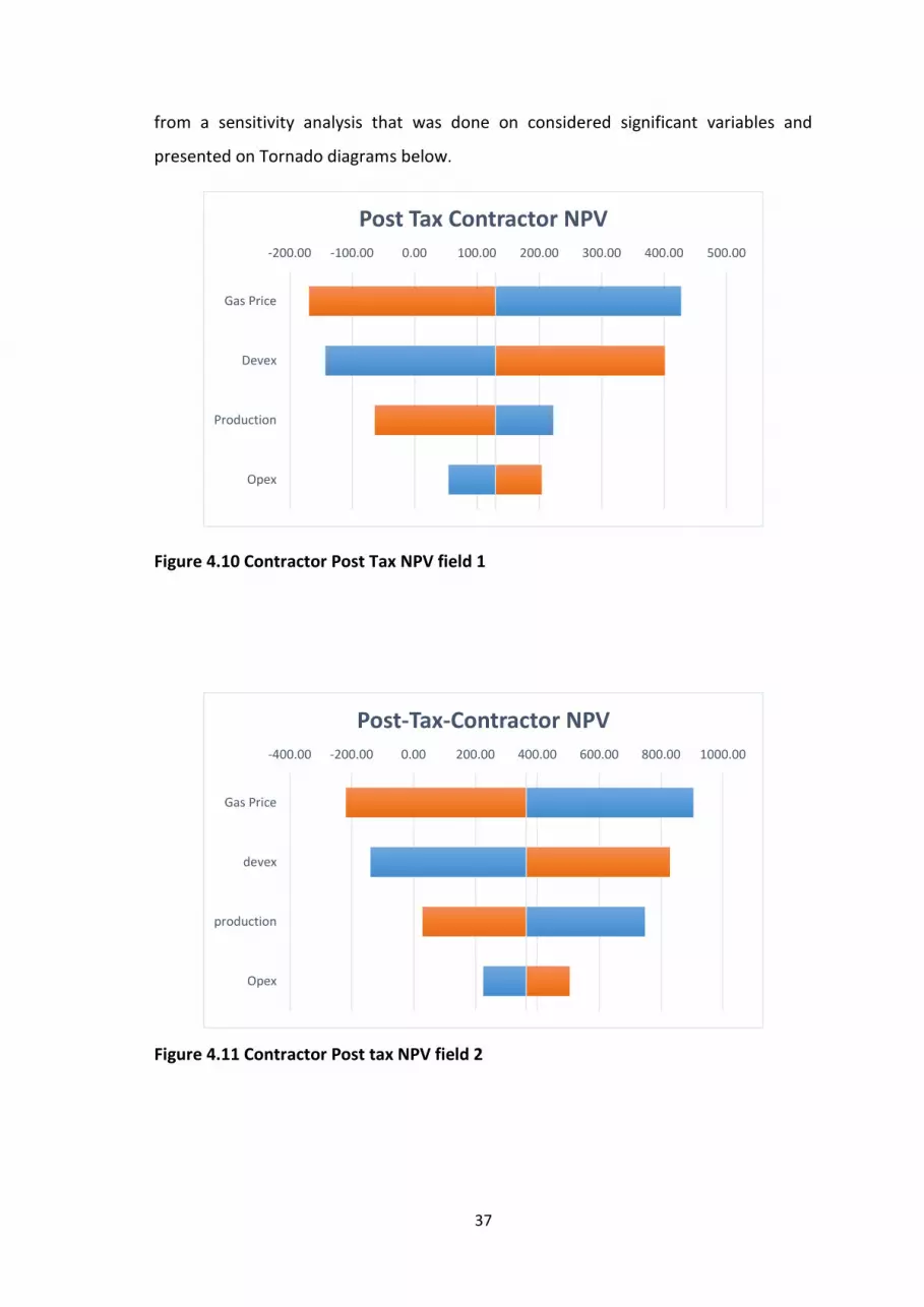
4.1.2 Pre Tax Monte Carlo results ......................................................................................... 32
4.2 Post Tax Results .................................................................................................................... 35
4.2.1 Sensitivity Analysis ....................................................................................................... 36
4.2.2 Monte Carlo Simulations.............................................................................................. 40
4.2.3 Analysis of Alternative regime ..................................................................................... 47
5 CONCLUSION ................................................................................................................................ 52
5.1 Concluding Remarks ............................................................................................................. 52

iii
5.2 Limitation of Research and Recommendation .................................................................... 53
6 BIBLIOGRAPHY .............................................................................................................................. 54
7 APPENDICES .................................................................................................................................. 56
APPENDIX A: Main formulas used in Model Calculations............................................................... 56
APPENDIX B: Conversion factors ..................................................................................................... 57

iv
LIST OF FIGURES Figure 1.1 Regional gas Prices ................................................................................................................ 4
Figure 2.1 Supply Price of Petroleum .................................................................................................... 6
Figure 2.2Progressive Tax .................................................................................................................... 11
Figure 2.3 Progressive Tax .................................................................................................................... 14
Figure 2.4 Production Sharing Agreement .......................................................................................... 18
Figure 2.5 World Petroleum Fiscal Arrangements .............................................................................. 19
Figure 3.1 Production profile field 1(small field) ................................................................................ 24
Figure 3.2 Production Profile field 2 (medium field) ........................................................................... 25
Figure 3.3 Production Profile field 3 (Large field) ............................................................................... 25
Figure 3.4 Influence Diagram ............................................................................................................... 28
Figure 4.1 Contractor Pre-tax NPV field 2 ........................................................................................... 31
Figure 4.2 Contractor Pre Tax NPV field 1 ........................................................................................... 31
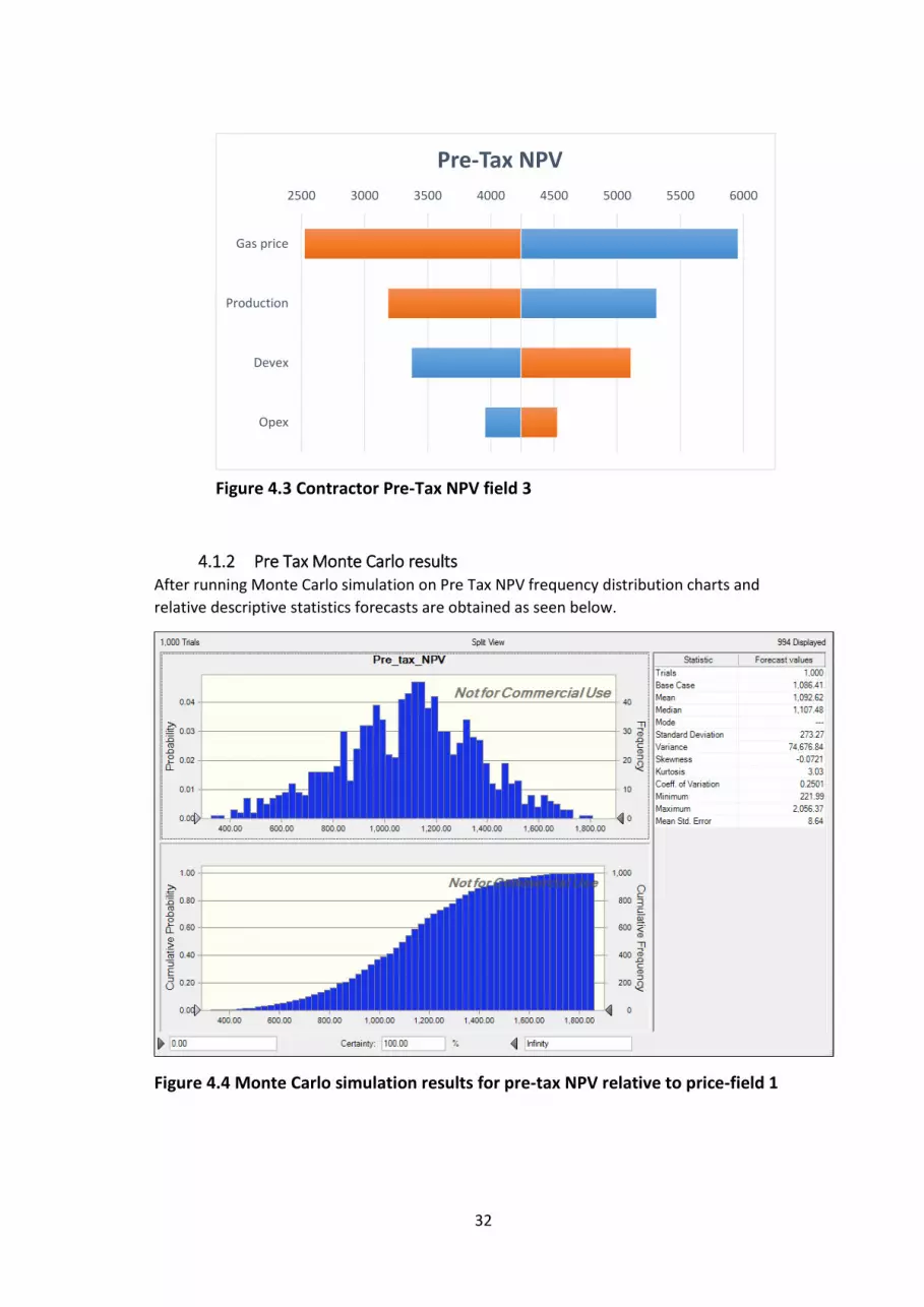
Figure 4.3 Contractor Pre-Tax NPV field 3 ........................................................................................... 32
Figure 4.4 Monte Carlo simulation results for pre-tax NPV relative to price-field 1 ......................... 32
Figure 4.5 Monte Carlo simulation results on pre-tax NPV relative to price-field 2 .......................... 33
Figure 4.6 Monte Carlo simulation results on pre-tax NPV relative to price field 3 .......................... 33
Figure 4.7 Monte Carlo simulation results on pre-tax NPV relative to devex-field 1 ........................ 34
Figure 4.8 Monte Carlo simulation results on pre-tax NPV relative to devex-field 2 ........................ 34
Figure 4.9 Monte Carlo simulation results on pre-tax NPV relative to Devex-field 3........................ 34
Figure 4.10 Contractor Post Tax NPV field 1 ....................................................................................... 37
Figure 4.11 Contractor Post tax NPV field 2 ........................................................................................ 37
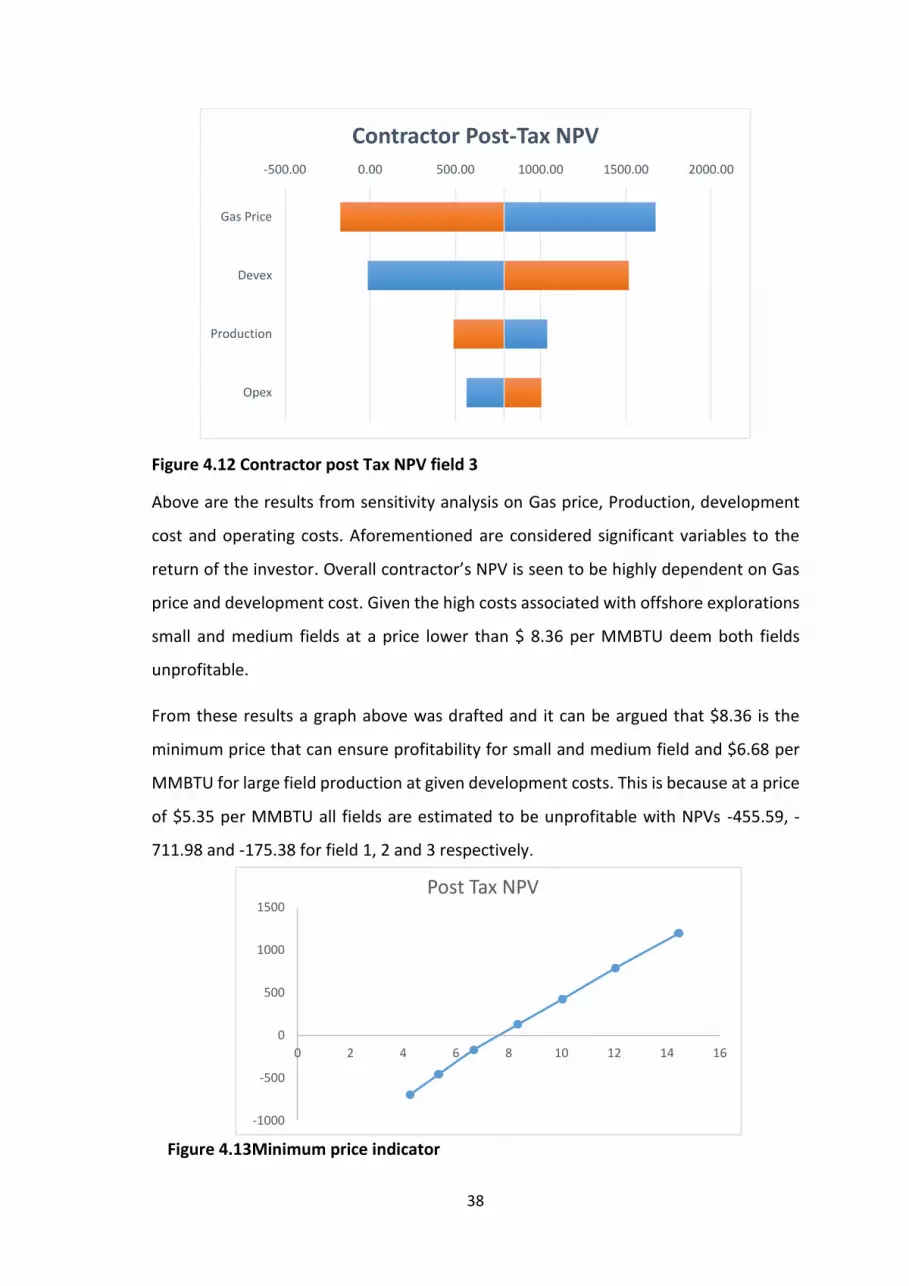
Figure 4.12 Contractor post Tax NPV field 3 ....................................................................................... 38
Figure 4.13Minimum price indicator ................................................................................................... 38
Figure 4.14 Government take field 1 ................................................................................................... 39
Figure 4.15 Government take field 2 ................................................................................................... 40
Figure 4.16 Government take field 3 ................................................................................................... 40
Figure 4.17 Monte Carlo Simulation results on post tax NPV relative to price-field 1 ...................... 41
Figure 4.18 Monte Carlo simulation results on Post Tax NPV relative to price-field 2...................... 41
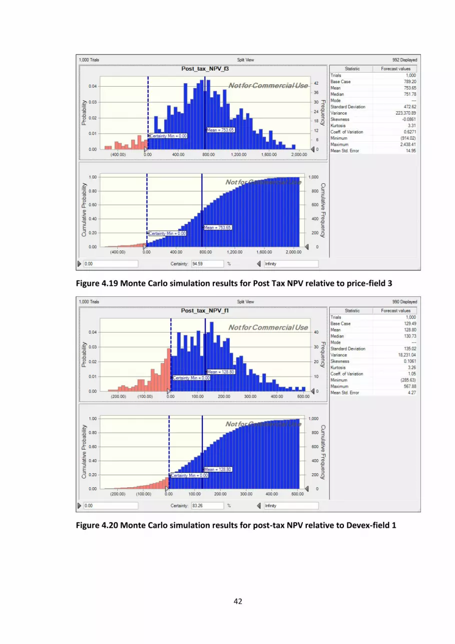
Figure 4.19 Monte Carlo simulation results for Post Tax NPV relative to price-field 3 ..................... 42
Figure 4.20 Monte Carlo simulation results for post-tax NPV relative to Devex-field 1 ................... 42
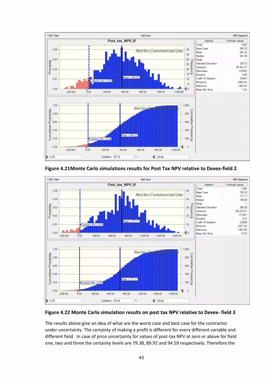
Figure 4.21Monte Carlo simulations results for Post Tax NPV relative to Devex-field 2 .................. 43
Figure 4.22 Monte Carlo simulation results on post tax NPV relative to Devex- field 3 ................... 43
Figure 4.23 Monte Carlo results on government take relative to price-field 1.................................. 44
Figure 4.24 Monte Carlo simulation results on government take relative to price-field 2 ............... 44
Figure 4.25 Monte Carlo simulation results on government take relative to price-field 3 ............... 45
Figure 4.26 Monte Carlo simulation results on government take relative to Devex-field 1 ............. 45
Figure 4.27 Monte Carlo simulation results on government take relative to devex- field 2 ............ 46
Figure 4.28 Monte Carlo simulation results on government take relative to devex-field 3 ............. 46
Figure 4.29 Tax System Comparison-contractor taker for field 1 ....................................................... 48
Figure 4.30 Tax System Comparison-Contractor take for field 2 ........................................................ 49
Figure 4.31 Tax system comparison-contractor take for field 3 ......................................................... 49
Figure 4.32 Tax System Comparison-Government take for field 1 ..................................................... 50
Figure 4.33 Tax System comparison-government take for field 2 ...................................................... 50
Figure 4.34 Tax system comparison-Government take for field 3 ..................................................... 51

v
LIST OF TABLES Table 2.1 Onshore profit gas split ........................................................................................................ 21
Table 2.2 Offshore Profit Split ............................................................................................................. 22
Table 3.1 Field Reserve and related costs ........................................................................................... 23
Table 3.2 Phasing of development expenditure ................................................................................. 24
Table 3.3 Tanzania Well reserve estimates ......................................................................................... 26
Table 3.4 Additional profit tax rates .................................................................................................... 27
Table 4.1 Pre-Tax Results ..................................................................................................................... 30
Table 4.2 Pre Tax Monte Carlo Statistics ............................................................................................. 35
Table 4.3 Post Tax Results .................................................................................................................... 36
Table 4.4 Adjusted PSA terms results .................................................................................................. 48
Table 4.5 Resource rent tax results ..................................................................................................... 48

vi
ABSTRACT Tanzania has been carrying out Petroleum exploration for over 50 years now, of which Gas
has been produced onshore and on shallow waters. The Gas produced has been used for
domestic supply. The recent discoveries of significant reserves in deep waters approximately
50 Tcf has created an opportunity for Tanzania to export. The government contracts
International companies to carry out exploration and development of gas fields. Since Gas is
a depleting resource the issue of efficient taxing system that will generate sustainable return
for the government rises. To cater for this Tanzania has been continuously updating the fiscal
system reaching to the current contractual system.
This dissertation analysed how flexible the current Tanzanian fiscal system is to guaranteeing
project’s profitability, balancing the interest of the government and the investor. The terms
of PSA (2013) ware used to analyse 3 fields of small to large size. From the analysis it was
found that pre-tax fields are profitable. Results after tax shows the system to be favourable
for large fields thus the government can continue using the current system for fields with
reserves above 1 Tcf. An adjusted system where additional profit tax is not charged is highly
recommended for smaller fields.

vii
ACKNOWLEDGEMENT This research paper would have not become complete in its nature without assistance and
guidance from other parties. First and for most I Thank God for granting me knowledge and
good health though out the period of undertaking this research.
Secondly Many Thanks to my Supervisor Dr Marc Gronwald for the assistance and guidance
received throughout the research period. Third I Thank Prof Alexander Kemp for his enormous
assistant throughout the preparation to the completion of this dissertation.
I also extend my utmost appreciation to TPDC officials for their assistance and agreeing to
meet me at such short notice, their inputs have enriched the content of this work.
I want to thank very much my Parents Mr. Silas Olan’g and Mrs. Martha Olan’g for the support
provided to enable me reach this point and finally completion of my project. Thanks to my
immediate siblings for understanding and being there for me through out. Thanks to my
friends and class mate for all the help and support provided whenever needed.
Your support and dedication is highly appreciated, May God bless you all abundantly.
1
1. INTRODUCTION 1.1 United Republic of Tanzania-Background and profile
The United Republic of Tanzania is formed of two Sovereign States. Tanganyika which
became a Sovereign State on 9th December, 1961 and a Republic in 1962 and the
People’s Republic of Zanzibar which was established after the Revolution on 12th
January, 1964 after Zanzibar became independent. In December, 1963 followed the
Union of the two states. Tanzania is in East Africa on the Indian Ocean, to the north are
Uganda and Kenya; to the west; Burundi, Rwanda, and Congo; and to the south;
Mozambique, Zambia, and Malawi. The total area in main land 883.6 and Zanzibar
2.5(“000” sq. km). The population by census of 2012 is 44.9m. (Tanzania National
Bureau of statistics, 2013)
The Tanzanian economy is heavily dependent on Agriculture which grew by 4% in 2014,
the overall economy of the country grew by 7.3% in 2013. Main sectors that contributed
to this growth include information and communication, manufacturing, construction,
mining and quarrying and other services which are supported by public investment in
infrastructure and the energy sector. Electricity production and supply in the country
has increased due to expansion in production capacity from natural gas. According to
the African economic Outlook (2015) Tanzanian economy is projected to grow by 7.5%
in 2017 this follows the expected boost of the natural gas development projects in the
country. Today, gas is used to generate electricity to feed the national grid. Further
expansions are underway including 532 km of 36 inch pipeline, which is being
constructed to transport natural gas from Mtwara and Lindi to Dar Es Salaam. A further
25km of 24 inch subsea line will connect Songo Songo Island to Somanga Fungi.
Investment in Liquefied Natural Gas (LNG) and Compressed Natural Gas (CNG)
processing plants is also being sought. (African Economic Outlook, 2015)
1.2 History of petroleum industry in Tanzania
Intermittently, Tanzania has been exploring Oil and gas since 1950s mainly onshore. The
first natural gas discovery was made in 1974 at the Songo Songo Island in Lindi Region
followed by another discovery at Mnazi Bay (Mtwara Region) in 1982. In respect to this
History of Petroleum Exploration in Tanzania has gone through five main phases to date.

2
The first phase was the year 1952-1964 where four wildcats were drilled along the coast
on Mafia Island, Zanzibar, Pemba and Onshore in the Mandawa Salt Basin. These
Operations were done by BP and Shell but significant hydrocarbons were not
discovered.
The Second phase was the year 1969-1979 where the first Production sharing
agreement was signed between Tanzania Petroleum Development Corporation (TPDC)
and AGIP on the former concessions with BP and Shell. Three onshore and two offshore
wells were drilled, in 1974 significant gas discoveries were made at SongoSongo.
Third phase is the year 1980 to 1991, this period was characterised by increase in Oil
price which stimulated exploration and production activities which led to gas discoveries
in 1982 at Mnazi Bay by AGIP. It is during this period that oil companies’ attention was
drawn to the coast of Tanzania and exploration licences were awarded to companies
including Shell and Texaco.
Then followed a fourth phase, this period was more of a regulatory finalisation period
by the government of Tanzania and TPDC there was least activities going on. These
phase was basically for development of fiscal and technical agreement for Songosongo
development, Mnazi bay field developments and acquisition of exploration licenses
which leads to the current phase.
Following the availability of new data from seismic studies done onshore and offshore
in the year starting 2000. Rights to explore the coast of Tanzania were granted to
several oil and gas companies. These exploration lead to a number of discoveries both
on shore and offshore by 2014 total onshore reserves were estimated to be 8 Tcf and
significant offshore reserves of 45.23 Tcf which totals up to 53.23Tcf.1
1.3 Natural gas sector and its importance to Tanzania
Tanzania’s recent vast discoveries of offshore natural gas strongly signal that it can
become the third-largest gas exporter in Sub-Saharan Africa, following Nigeria and
Mozambique. Based on current discoveries and estimated recoverable reserves in
Tanzania, the IMF report in 2014 projected that the government revenue would be at a
range of $ 3-6 billion annually starting 2020 or later. “Currently Tanzania is a net
1 TPDC 2014-Exploration history

3
importer of petroleum fuels that absorbs on average 55% of the country foreign
exchange earnings.” (Mkenda. A 2014). To alleviate this challenge Ongoing Oil and gas
exploration activities are currently given high priority.
Structural changes that aimed at promoting the growth of private sector led economy,
led to the first Energy policy of Tanzania (1992) to be formulated and revised in 2003.
Markets became more liberal and the government committed to bringing social
economic development. This policy has accelerated the development of energy sector
this includes increased discoveries of gas. In the study (Ebohon. O, 1996) it empirically
proven that energy consumption is complementary to Tanzania and any African country.
With the challenge of power cuts and insufficient supply of electricity in the country
given the huge reserves Tanzania can improve the domestic fuel mix. To do so the
government indicates that a minimum of 10% of gas produced in the country be
supplied in the country at a lower price and also TPDC is to pay royalty in kind (supply
gas). Also Tanzania is to take advantage of the competitive global market of natural gas.
(Ledesma, 2014)
1.4 Position of Tanzania in the competitive global market of natural gas
Natural gas has become an important source of energy in the world and its importance
is expected to continue increasing over time. Following the increase in new sources of
supply and demand in the markets of Asian countries (expected market or Tanzania gas),
where this demand is expected to be met through LNG.
In the natural gas market Tanzania is not alone, is currently competing with other
countries which have different advantages and disadvantages economical and
geographically. Currently Tanzania is competing with its neighbour Mozambique, also
with USA and Australia. Tanzania and Mozambique have almost close advantages in the
market in terms of distance and availability of clean gas2 thus lower processing and
production costs. But unlike Tanzania, Mozambique is having higher reserves. USA and
Australia are considered potential high volume suppliers because of political stability,
close proximity to the market for the case of Australia and low development cost for
USA. On the other hand USA is having a distance disadvantage being further away from
2 Gas which has no significant impurities such as carbon dioxide and sulphur oxide

4
the market and Australia has high development costs. Therefore for Tanzania it is very
crucial to distinguish it’s self in the market to be able to compete effectively in such a
concentrated market. (Ledesma, 2014)
Seeing that Tanzania is currently in a good position of securing market for its gas and
looks to contract private Oil companies mostly foreign companies it’s crucial for the
government to create an enabling environment that attracts investor’s to participate in
the exploration activities. The reason for creating an enabling environment is to reflect
on the industrial challenges of high development costs associated with gas production
and fluctuating prices. Gas pricing is a crucial component in making projects
economically viable.
For companies to secure financing for such high investment projects requires mostly by
entering into long-term contracts with customers. (Kemp, 2015) The decline in prices
and regional price segmentation in gas prices adds uncertainty to the financial outlook
of projects. In 2014 the price of natural gas in different regions dropped as seen in the
chart below while the price of LNG to japan was around $16, US henry Hub $5 and UK
NBP $8 by 2014. It is of importance the price that Tanzania is to use in the market is
competitive and reasonable that is creates enough revenues for the government and
investment incentive to contractor.
Figure 1.1 Regional gas Prices
Source: BP statistical review of world energy (2015)

5
1.5 Research Overview
Development of hydrocarbon sector to Tanzania does not only bring a number of
opportunities but also challenges. The current focus is on the development of the deep
water blocks, which are yet to be declared commercially viable. Commercializing gas is
costly, despite the active exploration activities uncertainty still prevails about gas price,
recoverable reserves and fiscal impact which will affect the design of gas projects.
Main objective of the study is to find out how the current design of the fiscal system
responds to the economic situations looking at prices and costs relative to the
profitability of the upstream petroleum project in a field of either small, medium or
large size. For this purpose 3 fields were chosen with corresponding Operating, and
development costs at given base price that will enable to analyse the risks and rewards
to companies and to the state.
This study mainly will seek:
a) To investigate how effective is the existing fiscal scheme in balancing the
government and investors interests.
b) To estimate the profitability of the selected projects (fields) under the current
hybrid system
c) Assessing project risk under the current regime relative to price and cost
uncertainties
d) Compare current PSA term with alternative fiscal tool on which benefits both
parties.
This paper is divided into 5 main chapters, Chapter one covers the introduction, chapter
2 is the literature Review which discusses the concept of economic rents and their
collection to the state, chapter 3 describes Data, Methodology used which include
financial modelling, chapter 4 discusses the results obtained from financial modelling,
sensitivity analysis and Monte Carlo Simulation, lastly are concluding remarks which
summarises the study discussions and recommendations.

6
2. LITERATURE REVIEW 2.1 Economic rent and its measurement
Tanzania just like other petroleum producing countries expect higher returns to be
generated from project investments. Host government is faced with hard decisions of
what and how will be the share of the revenue to the state since the country uses private
companies for petroleum exploration and production. In theory there are a number of
fiscal tools that can be used. Main tools that can be used for capturing economic rent
are through transfer of rights this is through bidding processes or concessions through
taxes and royalties or profit sharing agreements. (Johnston 2003)
The concept of Economic rent is very vital in the discussion of the design of an efficient
tax system. Economic rent in petroleum industry are returns acquiring to producers in
excess of supply price of the investment, this relates to the alternative investment
opportunities the company may have. In other words it is the revenue if the government
taxes the company can still get sustainable returns from the investment. (Kemp, 2015)
Figure 2.1 Supply Price of Petroleum
Source: (Kemp. A, 2015)
From the Figure above a return OMCP is required to cover production and yields normal
profits, return OMCD+P is required to cover the costs and risks involved In developing

7
new fields. The difference MCT-P is the economic rent, if the government collects any
amount in that area, development activities should be able to continue. (Kemp, 2015)
There are a number of issues that make the decision of determining how a state can
efficiently capture the share of the economic rent generated complex to most producing
countries. Considering the uniqueness of the petroleum industry. The petroleum
industry does not conform to the general definition of perfect competition,
characterised by long lead times and investment costs and especially because
petroleum is a depleting resource. (Kemp, 2015)
The size of economic rents on any projects in the petroleum industry can be determined
by the performance criteria and yardsticks as explained below. At the field development
stage the practical measure of economic rent include the net present value, rate of
return and investors weighted cost of capital. At the exploration stage the measure is
the expected monetary value.
2.2 Petroleum industry performance measurement yardsticks
2.2.1 NPV at various discount rates
Net Present Value (NPV) of an investment is computed to show the value of future
earnings at present day after initial investment costs have been compensated at a
discount rate. NPV can be calculated by the formula shown below:
Where R=revenues, O=operating cost, I=initial investment cost, r=discount rate and
i=period
The NPV decision rule is to undertake an investment whose NPV is positive and abandon
an investment with negative NPV. When comparing projects the best decision is to take
the alternative with the highest NPV, Berk and Dermazo (2007) explain the valuation
principle generally notes that an investment that adds more value is preferred

8
compared to the later not taking into account the investors’ preference to reach to this
conclusion. Thus because of the wealth measurement ability to project investments and
discounting nature it is among the mostly used Discounted cash flow investment
appraisal method.
On the other hand NPV rule is limited in its use, it does not take into account the
flexibility that an investor can have to react to new information. Considering that
flexibility in the petroleum industry is considered of high importance following the high
initial costs of investment which are irreversible. The NPV rule assumes risks to be
unchanging during the project life this is seen in its design where it deals with expected
cash flow at a constant discount rate. (Pindyck&Dixit, 1994)
2.2.2 Internal rate of return
The internal rate of return is the interest rate such that the net present value equals
zero. The calculation of IRR is done after defining the anticipated future cash flows to
be received from the investment. Its formula can be as below:
Where IRR is r in the equation
The IRR rule is based on the decision to take on an investment opportunity if the IRR is
greater than the opportunity cost of capital and turn down a project with IRR less than
the opportunity cost of capital. The IRR method just like the NPV rule are both
discounted cash flow method in that they take into account the time value of money
and shows if the project is profitable.
On the other hand the IRR rule is used when looking at stand-alone projects only if the
project’s negative cash flow precede its positive cash flow. This means that it is not a
proper method for comparing across different projects. Also the IRR rule will give
correct answers but not always that means it is to be used in line with other methods
like the NPV this is because sometimes the IRR could lead to incorrect answers for
example when the NPV is negative but the IRR is higher than the cost of capital. Making

9
a decision basing on IRR alone will in the end reduce the investor’s wealth. (Berk and
Demarzo 2007)
2.2.3 Payback period
Is the time required to recover investment costs, it is sometimes referred to as the
breakeven point. At this point money received equals money spent in Money of the Day
terms which means that it is a non-discounting appraisal method. Payback period
method seems to be insufficient in itself in investment decision since it does not show
the profitability of the investment by not taking into consideration cash flows beyond
the breakeven point. The rule of thumb for payback method is the project with the
shortest period is preferred to project with long period of payback. Whilst it’s
advantageous to use method especially in the oil and gas industry where the price of
the products are highly volatile. This method is best for comparing across projects for
this reason it’s not used in this study. (Mian. M, 2011)
2.2.4 Real profit/investment ratio
This is the ratio of Net present value to investment, this shows how much great returns
can be derived from a unit of investment made. The formula for this method is as seen
below
Where sum of NPV is divided by the sum of present value of investments
In case of limited budget this ratio is useful in ranking which investment gives a higher
return and it sometimes gives a different ranking to that of NPV. Berk and Dermazo
(2007) refer to it as profitability index which is used mostly by firms to rank projects
given constrained resources, however for this method to work there should only be one
constrained to be considered in the calculation and the set of project that maybe
undertaken should exhaust all the available resource.
NPV
PV of I
∑

10
2.2.5 Assessment at exploration stage
At the exploration stage the Expected monetary value (EMV) is considered the most
relevant measure of the project’s return. EMV is the expected Net Present Value from
development less explorations costs.
Denoted:
EMV = P(NPV) - E - P(A)
Where:
EMV = Expected Monetary Value
P = Chance of Discovery
NPV = Net Present Value
E = Initial Exploration Costs
A = Appraisal Costs
As Schuyler and Newendorp (2007) suggest following the uncertainty and risks
associated with the exploration stage risks such as chance of discovery, the EMV is
suited to give the profitability monetary value of the project and the degree of risk and
is the base parameter the decision maker should use to select investments with high
uncertainty.
The decision rule for EMV is to accept the project when EMV is positive, reject a project
when EMV is negative.
2.3 Rent collection Fiscal Devices
The economic rent generated is to be shared between the government and the
operating company(s) which can be complex and requires a design of an appropriate
tool that can be used to ensure the government equally with the company get fair
returns without causing economic distortions. A magnitude of the implied regime
matters in the sense as Bhattacharyya (2011) explains if the policy is very generous the
state will receive a low share which will be questionable by the citizens or it can be very
11
strict and deter investment because of the increased uncertainty to an investor, or
rather cause pre-mature abandonment of fields.
Generally when designing a fiscal regime there are a lot of issues to be considered, it’s
important to keep in mind the objectives of both the government and companies and
should be a function of economic rent. To be termed an efficient tax system a tax system
should be targeted on economic rents be sensitive to varying oil prices, field sizes and
costs. A progressive tax system is recommended. (Kemp, A. 2015)
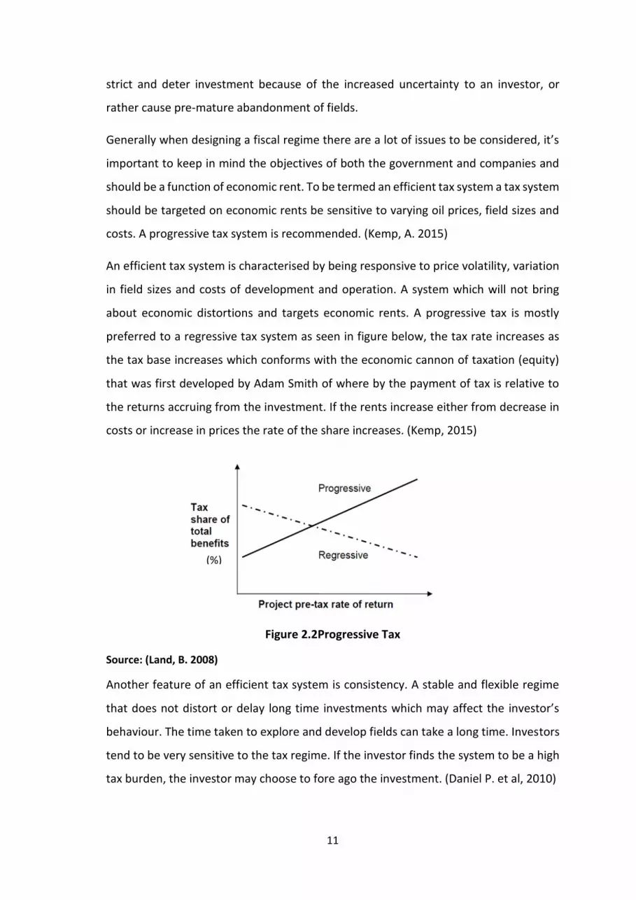
An efficient tax system is characterised by being responsive to price volatility, variation
in field sizes and costs of development and operation. A system which will not bring
about economic distortions and targets economic rents. A progressive tax is mostly
preferred to a regressive tax system as seen in figure below, the tax rate increases as
the tax base increases which conforms with the economic cannon of taxation (equity)
that was first developed by Adam Smith of where by the payment of tax is relative to
the returns accruing from the investment. If the rents increase either from decrease in
costs or increase in prices the rate of the share increases. (Kemp, 2015)
Figure 2.2Progressive Tax
Source: (Land, B. 2008)
Another feature of an efficient tax system is consistency. A stable and flexible regime
that does not distort or delay long time investments which may affect the investor’s
behaviour. The time taken to explore and develop fields can take a long time. Investors
tend to be very sensitive to the tax regime. If the investor finds the system to be a high
tax burden, the investor may choose to fore ago the investment. (Daniel P. et al, 2010)
(%)
12
A number of instruments can be used to collect rents from petroleum explorations,
most commonly used are taxes (Profit/corporate tax, resource rent tax, brown tax),
Royalties and production sharing Agreements/contracts. Below is the description of the
mostly common used instruments focusing on their characteristics, shortcomings and
their implication to the economy.
2.3.1 Corporate income tax
Income tax is levied on Oil and gas companies like any other company operating in other
economic activities which in some cases with certain provisions the charge levied on
petroleum companies may be higher than other companies. Taxes are levied on
company’s profits which is least likely to hinder field development. An effective tax is a
function of nominal tax rate and pace of write off for exploration costs. Costs are
recovered by order of first the previous unrecovered costs followed by operating,
Exploration and Appraisal then depreciation. The quicker the pace of cost write off the
better as it ensures that the rate of return is not reduced by tax. In some countries the
write off is 100% as production begins, which is less likely to take place in developing
countries such as Tanzania. (Kemp, 1992)
Among the provision that are provided under the income tax regime is project financing
where the interest rate is a deductible cost limited to a certain percentage of total
investment or by imposing a withholding tax on interest sent abroad. This is to avoid
employing a company with high debt and limit abusive transfer pricing between related
companies (Sunley et al 2003). Another provision is permitting Tax credits in countries
such as USA, it’s easier if the tax paid in producing country resembles that of home
country especially if it meets realisations, gross receipts and net income requirements.
Also loss carry forward may be considered in other countries which allows investors to
carry forward losses incurred in a year to the next year at a given level of proportions,
“Loss carry forward is important to be allowed in the petroleum exploration and
development by considering the long lead times and upfront investment” (kemp 2015).
For the above provisions to work most countries ring fence petroleum activities, this
expands the tax base by limiting the consolidation of income and deductions for tax
purposes across projects or contract area. The design of the extent of ring fencing is
13
again entirely based on the country’s fiscal regime, negotiations with IOCs and
preference of early revenues. (Keen, M. and Boadway, R. 2010)
Income tax ensures host government gets a considerable amount of rent as it targets
the profits of the company which makes them more desirable compared to royalty
which will be discussed below. Since the scheme targets the profits it is less likely to
cause disincentives to field developments. (Kemp, 2015)
A challenge with income tax comes with the present value of the depreciation
allowance. Before tax companies are provided with a depreciation allowance on
development costs. The depreciation allowance is calculated by either a rate of around
20% or 5 years on a straight line basis or 20-30% declining balance. As Kemp (2015)
elaborates on the design of depreciation allowance, in some countries depreciation
starts with expenditure while other countries it commences when production has
started. With both the present value of the depreciation allowance is lower than the
initial investment but even lesser if production starts late for countries where allowance
commences with production. (Hannesson 1998)
Another issue with corporate income tax is that it’s not targeted on economic rents. A
generally flat rate not progressively related to profits does not allow for return on equity
may leave the government with lower share or hinder development when oil prices
drop. (Kemp 2015)
2.3.2 Royalties
Royalties are traditionally rewards to landlords for use of natural resources for the right
to use property. Royalties are often not recorded in the fiscal accounts as tax but to an
investor it does not quite make a big difference since the economic impact to projects
is the same. Royalty is levied on gross revenue usually based on well- head values at a
flat rate and widely applied to mineral extraction around the world. According to most
model PSA a commonly used flat rate is 12.5% (Kemp, 2015)
To host governments royalty is more preferable revenues are yield from the very start
of production and it is easy to administer as well compared to other profit based taxes.
It also ensures to the government as a political advantage that foreign companies

14
operate project and are paying something to the state. To a contractor the risks are
shared between the government and companies to some extent (uncertainty of oil
price) while costs are borne by the investor. (Kemp, 1992) Royalties may provide fiscal
stability, predictable tax base and can be less exposed to asymmetric information
challenges (Keen, M. and Boadway, R. 2010)
Royalty has its drawbacks as well. Firstly it is not targeted on economic rents “At best
they constitute imperfect taxes on quasi rents and take no account of sunk costs of
exploration and site development” Keen, M. and Boadway, R. (2010). With a flat rate
commonly 12.5% can cause the government to leave a substantial amount of rent share
with investors when profits increase probably following oil price increase. At the same
time when the revenue after deduction of royalty falls below production cost to the
investor could make marginal fields uneconomic and will cause premature
abandonment of fields. (Kemp, 2015) The figure below elaborates the distorting effects
of royalty.
Figure 2.3 Progressive Tax
(Source; Kemp, 2015)
From above figure initial production is qo with introduction of tax t production reduces
to q1 because it is expensive for companies. With the price p1 the investor is able to
cover its marginal cost there after production q1 it becomes uneconomic to keep
operating.

15
Because most host governments prefer early revenues, to guard against the regressive
nature of the royalty some countries like Denmark and Netherlands in the years around
1973 after the major price increases introduced a sliding scale royalty scheme. Under
the sliding scale scheme the royalty rate increases as production increases. It is basically
a function of field size making more flexible but not sensitive to prices and costs. (Kemp,
1992)
2.3.3 Resource rent tax
Garnaut and Clunies Ross (1975) article is the most referred to in literature as the first
to propose the use of Resource rent tax. Lund, (2009) acknowledges system’s intent to
give a higher return to investors compared to other tax systems such as the income tax.
Resource rent tax (RRT) is the tax on the net cash flow after a specified rate of return
has been obtained from the investment. As Kemp (2015) explains the return on capital
would consist of a basic return equivalent to the rate of interest on risk free long term
borrowing plus a margin enough to cover the risks associated with the investment.
The resource rent tax is designed to target economic rent, the scheme allows the
investor to achieve a specified threshold rate of return before tax is paid. The threshold
is then used to compound the investor’s net cash flow, the cash flow is initially negative
following the exploration and appraisal costs. The cash flow is accumulated by the
threshold rate until the income becomes positive. (Kemp 2015)
A resource rent tax is stable, it varies with changes in oil prices and costs. There is no
early fiscal burden to the investor and risks are shared with the government and provide
an appropriate share of the rent to the government. The resource rent tax allows for
ring fencing, where a firm operating in one project cannot reduce the revenue of the
one project by incorporating the costs of another project otherwise revenues will be
postponed through continuous deductions. Australia resource tax system includes ring
fencing on contract area to enhance the near term revenue from resource rent tax.
(Kemp 2015)
On the other hand the Resource rent tax is faced with a problem of information
asymmetry deciding on the rate of return. The magnitude of the rate of return can either
create an incentive to invest, practice tax avoidance or give low or no return to
16
government.” if the hurdle rate is set too low, the tax may become a major deterrent to
investment, if set too high chances are it will never apply.”(sunley, et al 2003)
RRT is associated with delay of payments to the government. This can be less attractive
to some governments, also because of the high risk sharing between government and
companies. The government does not get upfront payments, due to the wait period
until the company has recovered all its costs and get the desirable rate of return which
is also unknown to the government and probably may not be desirable from the social
point of view. (Hannesson 1998). To increase the government expected revenue
Garnaut, and Ross (1975) suggest a hybrid system of imposing income tax in conjunction
with the RRT.
To cover the possibility of increased profitability in the future and ensure that the
revenue to the government increases as well. But also enable companies to recover
development costs in early years when profits are still low. The government implies a
set of tiers (where the tax rate increases as a certain rate of return has been attained by
the company) that can be imposed when a certain threshold has been met. A challenge
is on deciding the number of tiers to use, (Gaus, Ross 1975) suggest a separate tax to be
levied at more than one threshold interest rate for example a tax rate of 25% may be
levied at a real rate of return of 10 and then when the threshold rate is beyond 10 a tax
rate can increase to 35%.
The problem of gold plating also arises with such a scheme, an investor gets the
incentive to increase his expenditure to get higher returns. This is mostly common with
schemes based on the rate of return (ROR). This problem can however be avoided by
putting the ROR close to the that of the investor but is still a challenge as the IRR Is
unknown to the government. (Kemp, 2015)
2.3.4 Brown Tax
Another type of tax is Brown tax named after E.C Brown, As Kemp (2015) describes it is
a type of tax based on company’s net cash flow with no discounting. All cash flow is
taxed proportionally where the government pays subsidies when the cash flow is
negative and collects taxes when the cash flow is positive. With this scheme the rate can
be set very high but without causing disincentives except when the NPV becomes very

17
small, leaves the IRR post tax unchanged and if NPV was positive pre-tax remains
positive Post Tax.
Brown tax is proportionate in nature and considered completely neutral and effective
at targeting economic rent. But not favoured by government because of the high risk
sharing on costs, price and production. Kemp (2015)
2.3.5 Production Sharing contracts
The concept of production/profit sharing contracts is derived to explain the ownership
of resources. It was firstly used in agriculture where a tenant (rents) does not have the
title of the resources, the title is being retained by the government (land lord). In the
petroleum industry the government contracts a private company to explore and
produce oil and gas. The contractor incurs the investment costs and risks which then
gets compensated out of the production. In this case a contractor is not liable to pay
royalty but in some countries the royalty is paid as the government requires early
revenues. (Johnston, 2003)
In designing a production sharing contract it is very important to consider cost oil/gas
and profit oil/gas. Cost gas is the proportion of total production as specified by the PSC
that the contractor retains to recover investment costs. The cost recovery
conditions/process are similar to depreciation terms used in calculating income tax. A
cost recovery limit is set “a ceiling of 40% - 50% is common” (Kemp 1992) this ensures
there is profit oil as soon as production starts. The remaining gas is the profit gas which
is split between the government and the contractor following specified proportions
indicated in the contract. Because of the limit in some cases not all costs are recovered
and can also delay cost recovery in turn the post-tax rate of return gets affected which
is a great possibility of making projects less commercial. In some countries an uplift is
given to compensate for the delay. Another instance is when the actual cost for recovery
is less than the cost celling the difference goes to the state rather than becoming part
of the profit Oil which creates an incentive for companies to be less cost conscious
(Kemp, 2015)
When splitting profit gas a production sharing scheme can be progressive or at a flat
rate, although originally the scheme had a flat rate which is still is in Indonesia makes

18
the scheme inflexible as it is not responsive to increased production. The profit oil split
can as well be on an incremental basis, with the share to the state increasing as
production increases making it progressive as it responds to the field size as the seen
below where the government’s share of profit Oil increases as production increases.
(Kemp, 2015)
Source: (Kemp 2015)
Profit gas split can also be based on project’s profitability through R-factor or
contractor’s Rate of return. The R-factor can be generally be referred to as the ratio of
cumulative revenues to cumulative investment costs:
Contractor’s revenues after all royalty, tax & Government profit oil share to date
Contractor’s costs to date
The government’s take increases as the R factor/ROR increases. Usually the concept of
resource rent tax is used to determine the state’s share of profit oil/gas where the R-
factor is calculated in a given accounting period and when a certain threshold is reached
as specified in the contract another sharing rate is applied.
The profit sharing scheme is flexible to variation of oil price, field sizes and variation in
investment costs. PSA scheme considered the most efficient tool of collecting rent and
Figure 2.4 Production Sharing Agreement
19
widely used by most petroleum producing countries especially developing countries.
(Kemp, 1992) Tanzania being among countries that use PSA, the concept of PSA is going
to be further discussed and applied in this paper according to the country’s context.
2.4 Current petroleum fiscal system in Tanzania
Petroleum exploration and development activities in Tanzania are governed by the
Petroleum (Exploration and Production) Act 1980. This Act vests title to petroleum
deposits within Tanzania in the State and is designed to create a favourable legal
environment for exploration by oil companies. The Act expressly permits the
Government to enter into a petroleum agreement under which an oil company may be
granted exclusive rights to explore for and produce petroleum. According to the
Production Sharing Agreement (PSA) arrangements currently in place in Tanzania, TPDC
is granted the licences under the Act with the Government and TPDC entering into PSA's
with the oil companies. The terms of the PSA's form the basis of the licences and are
negotiable. (TPDC 2015)
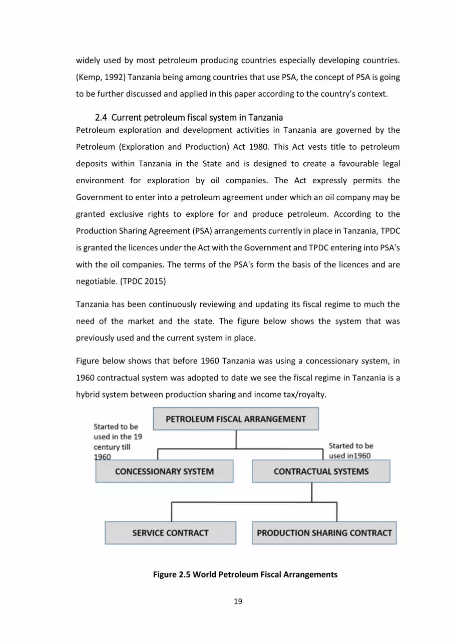
Tanzania has been continuously reviewing and updating its fiscal regime to much the
need of the market and the state. The figure below shows the system that was
previously used and the current system in place.
Figure below shows that before 1960 Tanzania was using a concessionary system, in
1960 contractual system was adopted to date we see the fiscal regime in Tanzania is a
hybrid system between production sharing and income tax/royalty.
Figure 2.5 World Petroleum Fiscal Arrangements
20
Source: TPDC presentation to Mineral and Energy Commission (2015)
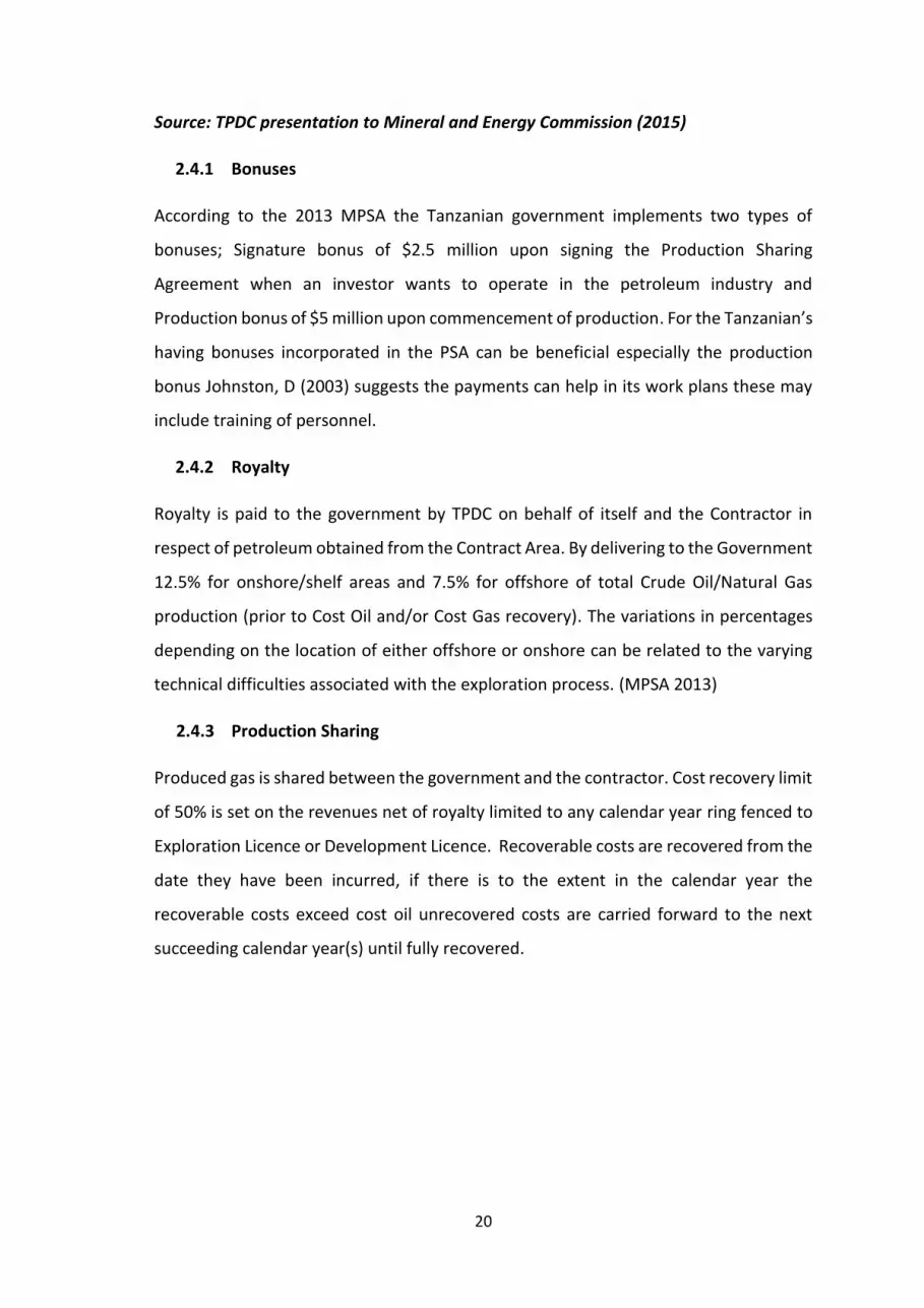
2.4.1 Bonuses
According to the 2013 MPSA the Tanzanian government implements two types of
bonuses; Signature bonus of $2.5 million upon signing the Production Sharing
Agreement when an investor wants to operate in the petroleum industry and
Production bonus of $5 million upon commencement of production. For the Tanzanian’s
having bonuses incorporated in the PSA can be beneficial especially the production
bonus Johnston, D (2003) suggests the payments can help in its work plans these may
include training of personnel.
2.4.2 Royalty
Royalty is paid to the government by TPDC on behalf of itself and the Contractor in
respect of petroleum obtained from the Contract Area. By delivering to the Government
12.5% for onshore/shelf areas and 7.5% for offshore of total Crude Oil/Natural Gas
production (prior to Cost Oil and/or Cost Gas recovery). The variations in percentages
depending on the location of either offshore or onshore can be related to the varying
technical difficulties associated with the exploration process. (MPSA 2013)
2.4.3 Production Sharing
Produced gas is shared between the government and the contractor. Cost recovery limit
of 50% is set on the revenues net of royalty limited to any calendar year ring fenced to
Exploration Licence or Development Licence. Recoverable costs are recovered from the
date they have been incurred, if there is to the extent in the calendar year the
recoverable costs exceed cost oil unrecovered costs are carried forward to the next
succeeding calendar year(s) until fully recovered.
21
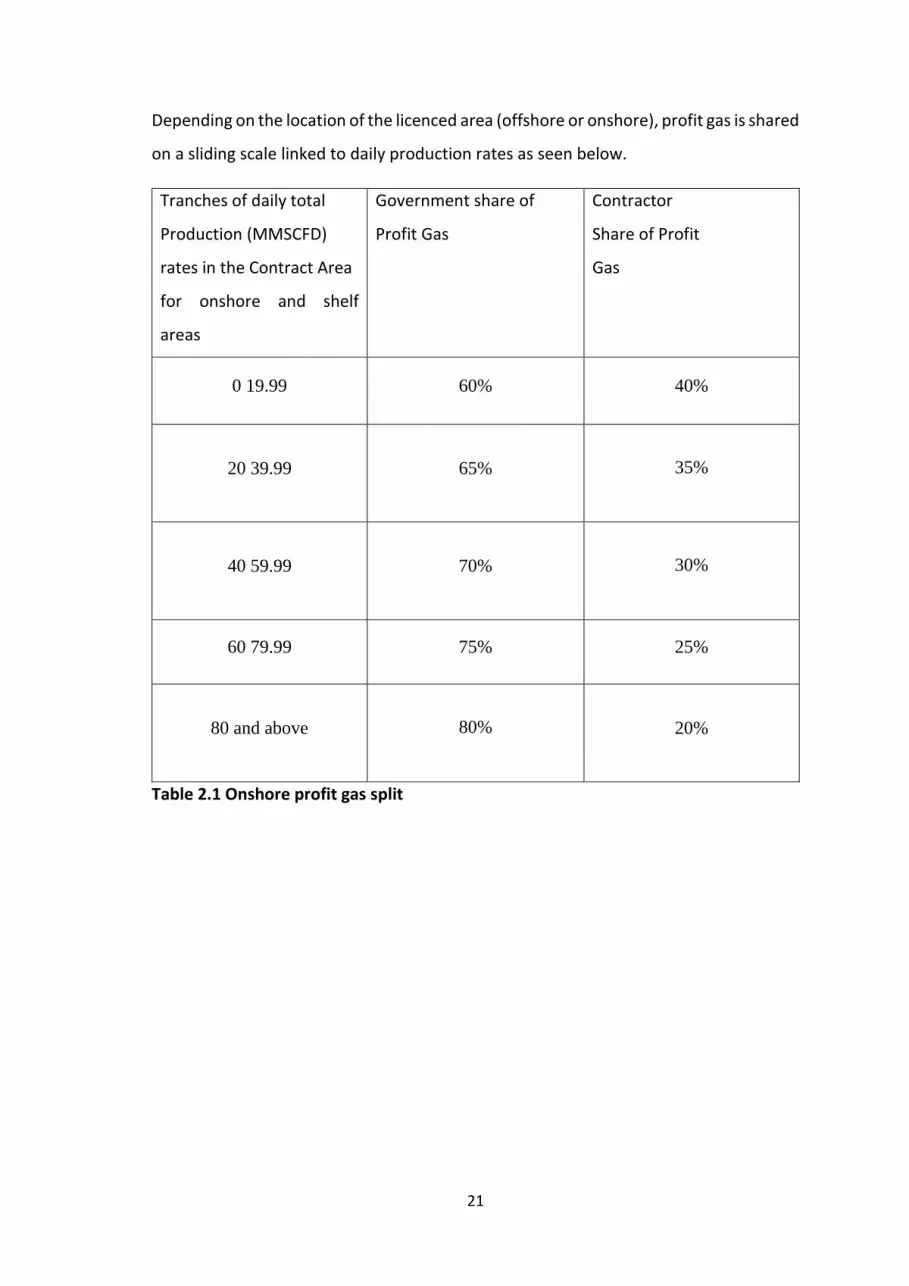
Depending on the location of the licenced area (offshore or onshore), profit gas is shared
on a sliding scale linked to daily production rates as seen below.
Tranches of daily total
Production (MMSCFD)
rates in the Contract Area
for onshore and shelf
areas
Government share of
Profit Gas
Contractor
Share of Profit
Gas
0 19.99 60% 40%
20 39.99 65%
35%
40 59.99 70%
30%
60 79.99 75% 25%
80 and above
80%
20%
Table 2.1 Onshore profit gas split
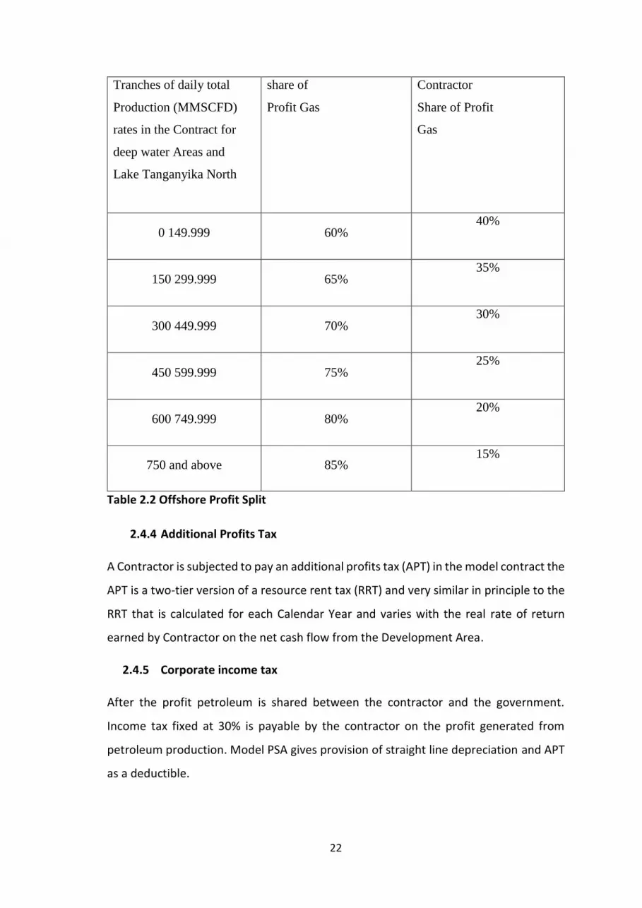
22
Tranches of daily total
Production (MMSCFD)
rates in the Contract for
deep water Areas and
Lake Tanganyika North
share of
Profit Gas
Contractor
Share of Profit
Gas
0 149.999 60% 40%
150 299.999 65% 35%
300 449.999 70% 30%
450 599.999 75% 25%
600 749.999 80% 20%
750 and above 85% 15%
Table 2.2 Offshore Profit Split
2.4.4 Additional Profits Tax
A Contractor is subjected to pay an additional profits tax (APT) in the model contract the
APT is a two-tier version of a resource rent tax (RRT) and very similar in principle to the
RRT that is calculated for each Calendar Year and varies with the real rate of return
earned by Contractor on the net cash flow from the Development Area.
2.4.5 Corporate income tax
After the profit petroleum is shared between the contractor and the government.
Income tax fixed at 30% is payable by the contractor on the profit generated from
petroleum production. Model PSA gives provision of straight line depreciation and APT
as a deductible.

23
3 DATA AND METHODOLOGY
3.1 Data Sample Gas field data has been used in this research. The choice of fields was based
upon the overall natural gas discoveries in deep waters in Tanzania that has reached
approximately 45.23 Tcf, with wells of varying sizes. To capture the variation small,
medium and large fields were selected to see whether the current fiscal system is
flexible enough in capturing economic rent and how to it affects the profitability of
different fields of varying sizes.
For the above stated purposes fields with recoverable reserves of 500 Bcf, 1000 Bcf and
2000 Bcf were chosen. Each field has associated Development costs that were chosen
with the idea of economies of scale related to field size. Field development costs
estimates are not quite certain and in the study by Ledesma, 2013 he estimates the cost
to be $3.5 per MMBTU which are quite low and argues that costs could be lowered over
time in production of gas.
3.1.1 Costs
Compared to the estimate used in this research, costs are to the contrary high in deep
water exploration. For the small field development cost is $15, medium field $12.5 and
$10 per barrels of Oil equivalency (Boe) as adopted from AUPeC report, 2009. This
information and other related costs are summarised in the table below:
Field Size
DATA 1 2 3 Units
Reserves 500 1000 2000 Billion Cubic feet
Development
costs
15 12.5 10 $ Per Barrels of Oil
equivalent
Drilling costs 50 40 35 % of development
cost
Operating costs 6.75 6.0 5.25 % of accumulated
development cost
Table 3.1 Field Reserve and related costs
24
Year
% of Total Capital expenditure
% of total Drilling expenditure
Field 1 Field 2 Field 3 Field 1 Field 2 Field 3
0 40 25 20
1 30 30 30 35 40
2 30 30 30 35 30 15
3 15 10 30 30 15
4 10 15
5 15
6 15
7 15
8 10
Table 3.2 Phasing of development expenditure
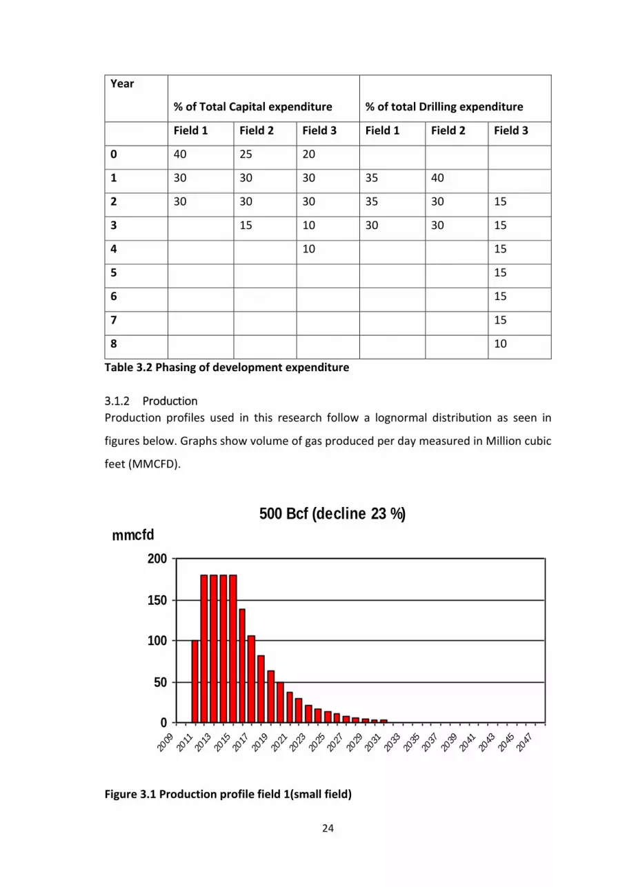
3.1.2 Production
Production profiles used in this research follow a lognormal distribution as seen in
figures below. Graphs show volume of gas produced per day measured in Million cubic
feet (MMCFD).
Figure 3.1 Production profile field 1(small field)
500 Bcf (decline 23 %)
0
50
100
150
200
2009
2011
2013
2015
2017
2019
2021
2023
2025
2027
2029
2031
2033
2035
2037
2039
2041
2043
2045
2047
mmcfd

25
Figure 3.2 Production Profile field 2 (medium fiel
Figure 3.3 Production Profile field 3 (Large field)
The above production profile were chosen to reflect Tanzania different block reserve
estimates between Chaza-1 and Papa-1 as seen in the 2013 TPDC estimates in the figure
below:
2 Tcf (decline 20 %)
0
100
200
300
400
500
2009
2011
2013
2015
2017
2019
2021
2023
2025
2027
2029
2031
2033
2035
2037
2039
2041
2043
2045
2047
mmcfd

26
Well Name Gas Reserve estimate (Tcf)
Pweza-1 1.7
Chewa-1 1.8
Papa-1 2.0
Chaza-1 0.47
Jodari-1 4.1
Mzia-1 and Mzia 2 7.8
Zafarani-1 6.0
Lavani-1 and 2 4.4
Tangawizi-1 6
Table 3.3 Tanzania Well reserve estimates
Source: (extracted from TPDC (2013) online database)
3.1.3 Price
For base year 2015 the Gas price is assumed to be $8.36 per Mmbtu as the possible
price to delivery point3. The price was chosen to reflect the price that is charged before
processing of Liquefied Natural Gas and shipping to Asian Markets. A model including
LNG processing can be model but is beyond the focus of this research which is focused
on the upstream evaluation of the project. The assumption of price comes from the
historical price of gas trades in Tanzania for onshore production which has been $5.36
per Mmbtu to delivery point. To reflect offshore activities and costs the price used in
this research was assumed and slightly increased by the researcher due to lack of
specific data of the prevailing price in Tanzania for Gas to delivery point for offshore
production. (RPS, 2015). For the purpose of this research delivery point is assumed to
be at wellhead for simplicity.
Other information used include inflation rate of 3% following the US dollar used. The
discount rate is assumed to be 10% as the prevailing rate in the industry.
3 The PSA governs upstream activity of a defined delivery point, according to the 2010 Model Addendum for Natural gas the delivery point is specified as the wellhead or other point which may be agreed between TPDC and the contractor.

27
3.1.4 Tax Terms
For the purpose of his research as a base model contract, Production contract of 2013
was used with terms as listed below.
Royalty rate of 7.5%
Corporate income tax is applied at rate of 30% adjusted for depreciation with a
rate of 20% straight line from the start of production.
Cost oil for production sharing is 50% of revenue less royalty
Profit sharing is based on the daily production of gas on a sliding scale as seen in
previous chapter (Table 2.2)
Additional profit tax is payable based on the contractors pre-tax RROR
summarised:
RROR APT rate
≤ 20 0%
20≤R≤30 25%
>30 35%
Table 3.4 Additional profit tax rates
3.2 Financial Modelling
The above data was used for financial analysis using capital budgeting tools that include
NPV, IRR and profit to investment ratio at field development stage. First by calculating
pre-tax and then post tax cash flows for both the government and the contractor to see
how much of profit gas each gets as well as how much tax is being paid. The model gives
detailed statistics and economic indicators under the model production sharing
contract.
The flow is clearly illustrated by the Influence diagram below, where the main objective
is to get the contractors Net Present value Post tax and government take as indicated
by value nodes. Government take and contractors’ Post tax NPV depend on the
revenues from production and the applied fiscal terms (PSA term) as described above
which is a hybrid including taxes and royalties. Gas price and costs subjected to inflation
are uncertain following market fluctuations. Costs include operating cost and
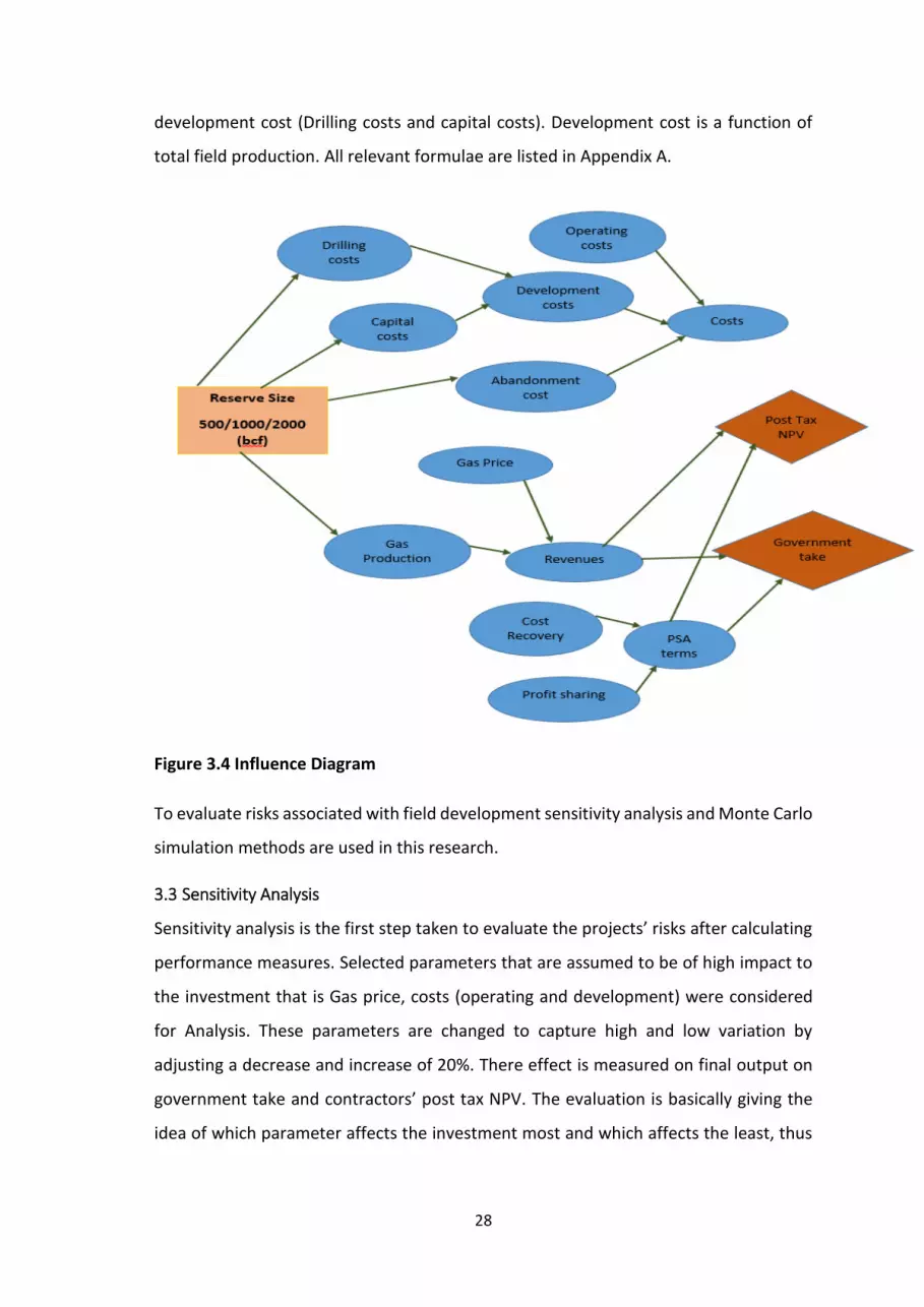
28
development cost (Drilling costs and capital costs). Development cost is a function of
total field production. All relevant formulae are listed in Appendix A.
Figure 3.4 Influence Diagram
To evaluate risks associated with field development sensitivity analysis and Monte Carlo
simulation methods are used in this research.
3.3 Sensitivity Analysis
Sensitivity analysis is the first step taken to evaluate the projects’ risks after calculating
performance measures. Selected parameters that are assumed to be of high impact to
the investment that is Gas price, costs (operating and development) were considered
for Analysis. These parameters are changed to capture high and low variation by
adjusting a decrease and increase of 20%. There effect is measured on final output on
government take and contractors’ post tax NPV. The evaluation is basically giving the
idea of which parameter affects the investment most and which affects the least, thus

29
an investment decision is likely going to be based on the parameter that affects the
project’s returns most. (Kemp, A. 2015)
3.4 Monte Carlo Simulation
Mont Carlo simulation is run on Gas price and development costs to see the effect on
Government take and contractor’s NPV. Simulations describe the uncertainty in price
and development costs in terms of probabilities. Normal distribution is used assuming
the base case variables are most likely but there is a possibility of approximately 68%
that variables will deviate from the mean especially following the trend in gas price.
When running the simulations it is important to specify a large number of trials to get
approximate accuracy in expected values and outcome. For the purpose of this research
1000 trials have been run. Monte Carlo method is argued to be very useful and since its
early recognition in 1960 most Petroleum companies have used it to make investment
decision as it illustrate the degree of riskiness in projects. (Newendorp and Schuyler
2014)

30
4 RESULTS
4.1 Pre-Tax Results
From spreadsheet modelling preliminary results are obtained and summarised below
are the contractor’s NPV at 10% discount rate, IRR and Real profit/investment ratio.
Table 4.1 below shows the metrics for each field.
Description Field 1 Field 2 Field 3 Unit
Reserves 0.5 1 2 Tcf
Pre Tax NPV 1,086 2,184 4,240 Million $
Pre Tax IRR 28 26 26 Percent
Pre Tax NPV/I 0.92 1.1 1.4
Table 4.1 Pre-Tax Results
At a base price of 8.46 dollars per Mmbtu all fields indicate higher profitability as seen
from values above. The internal rate of return is 28% for small field and 26% for medium
and large fields, these fields showing low IRR could be associated with long production
periods. Field 3 with reserves estimate of 2 Tcf has a high NPV of 4,240 and high return
derived from a unit of investment, a contractors gets a return of 1.4 this is as would be
expected because of the economies of scale where development costs for larger field is
low compared to the medium and small field.
4.1.1 Sensitivity analysis on pre-tax values
To evaluate the risk associated with each field a sensitivity analysis was done and results
are shown in tornado charts below for each respective field. All field remain quite
profitable after a decrease of 20% in Gas price and Production, increase in development
costs and operating costs, Gas price is seen to have a higher impact to contractor’s NPV
followed by production, development costs and least by operating costs as a percentage
of accumulated development cost.

31
400.00 600.00 800.00 1000.00 1200.00 1400.00 1600.00 1800.00
Gas price
Production
Devex
Opex
PRE-TAX NPV
1000.00 1500.00 2000.00 2500.00 3000.00 3500.00
Gas price
Production
Devex
Opex
Pre_Tax NPV
Figure 4.2 Contractor Pre Tax NPV field 2
Figure 4.1 Contractor Pre-tax NPV field 1
32
4.1.2 Pre Tax Monte Carlo results After running Monte Carlo simulation on Pre Tax NPV frequency distribution charts and
relative descriptive statistics forecasts are obtained as seen below.
Figure 4.4 Monte Carlo simulation results for pre-tax NPV relative to price-field 1
2500 3000 3500 4000 4500 5000 5500 6000
Gas price
Production
Devex
Opex
Pre-Tax NPV
Figure 4.3 Contractor Pre-Tax NPV field 3

33
Figure 4.5 Monte Carlo simulation results on pre-tax NPV relative to price-field 2
Figure 4.6 Monte Carlo simulation results on pre-tax NPV relative to price field 3

34
Figure 4.7 Monte Carlo simulation results on pre-tax NPV relative to devex-field 1
Figure 4.8 Monte Carlo simulation results on pre-tax NPV relative to devex-field 2
Figure 4.9 Monte Carlo simulation results on pre-tax NPV relative to Devex-field 3

35
From results above the distribution is fairly asymmetrical to the mean Indicating that
the price pulls the contractor NPV negatively and positively almost equally. There is
100% certainty of making profit before taxes for all field sizes. The table below
summarises the average, minimum and maximum profit that can be attained by the
contractor at the given price and development cost. The base case profits (NPV) for
each field fall in between the attained range from simulations as seen below.
Field 1 Field 2 Field 3
Statistics relative to Price
Mean 1,092.62 2,179.06 4,251.55
Minimum 221.99 519.18 1,257.39
Maximum 2,056.37 4,090.44 7,996.59
Statistics relative to Devex
Mean 1,086 2,178 4,231.34
Minimum 555.33 1,389.2 2,967.32
Maximum 1,682.67 3,082.11 5,862.73
Table 4.2 Pre Tax Monte Carlo Statistics
4.2 Post Tax Results
Analysis and discussion of Post Tax result section builds mainly from Pre Tax sensitivity
analysis we have seen Gas Price, production and development cost have a significant
impact to contractor’s return. Therefore after Production sharing as described in
chapter 3 and application of tax terms results on Government’s take and Contractors
NPV are presented. Uncertainty analysis results from Sensitivity analysis and Monte
Carlo simulations are also presented and analysed.
Description Field 1 Field 2 Field 3 Unit
Reserves 0.5 1 2 Tcf
Post Tax NPV 129.49 365.33 789.20 Million $
Post Tax IRR 13 14 14 Percent
Post Tax NPV/I 0.11 0.19 0.27

36
Government
present value
cash flow
956.92 1819.65 3451.35 Million $
Government
cash flow (MOD)
1,793.44 4,054.96 9,661.04 Million $
Contractor cash
flow (MOD)
952.97 2,390.85 5,543.97 Million $
Total
Government
take
65 63 64 Percent
Government
share of
economic rent
88 83 81 Percent
Royalty to the
government
379 799 1,729 Million $
Table 4.3 Post Tax Results
From table 4.3 it can be observed how statistics have changed from pre-tax results
obtained earlier. Post tax NPV obtained is 129.49, 365.33 and 789.20 million dollars for
field 1, field 2 and field 3 respectively. Total government take is (65%) for small field,
63% for medium and 64% for large field. A share of economic rent going to government
is 88% for a small field and 83% and 81% for medium and large field respectively. The
government also gets royalty (gas worth of million dollars) 379, 799 and 1,729 from
small, medium and large field respectively. Practically royalties in Tanzania are paid by
the Tanzania Petroleum Development cooperation, this could be because ideally
royalties are not meant to be incorporated in PSC’s in a place where the investor is a
contractor. It can be observed that after collection of quite a large share of economic
rent by the government all fields remain relatively profitable with positive post tax NPV
and IRR above 10%.
4.2.1 Sensitivity Analysis
Considering the base results it is of interest to measure how the above results would
change at different market situation and geological prospects. Thus below are results
37
from a sensitivity analysis that was done on considered significant variables and
presented on Tornado diagrams below.
Figure 4.10 Contractor Post Tax NPV field 1
Figure 4.11 Contractor Post tax NPV field 2
-200.00 -100.00 0.00 100.00 200.00 300.00 400.00 500.00
Gas Price
Devex
Production
Opex
Post Tax Contractor NPV
-400.00 -200.00 0.00 200.00 400.00 600.00 800.00 1000.00
Gas Price
devex
production
Opex
Post-Tax-Contractor NPV
38
Figure 4.12 Contractor post Tax NPV field 3
Above are the results from sensitivity analysis on Gas price, Production, development
cost and operating costs. Aforementioned are considered significant variables to the
return of the investor. Overall contractor’s NPV is seen to be highly dependent on Gas
price and development cost. Given the high costs associated with offshore explorations
small and medium fields at a price lower than $ 8.36 per MMBTU deem both fields
unprofitable.
From these results a graph above was drafted and it can be argued that $8.36 is the
minimum price that can ensure profitability for small and medium field and $6.68 per
MMBTU for large field production at given development costs. This is because at a price
of $5.35 per MMBTU all fields are estimated to be unprofitable with NPVs -455.59, -
711.98 and -175.38 for field 1, 2 and 3 respectively.
-500.00 0.00 500.00 1000.00 1500.00 2000.00
Gas Price
Devex
Production
Opex
Contractor Post-Tax NPV
-1000
-500
0
500
1000
1500
0 2 4 6 8 10 12 14 16
Post Tax NPV
Figure 4.13Minimum price indicator

39
Lower development costs have seen to result to higher NPV values and 20% increase of
development costs resulting to negative NPVs(-142, -139,-14.31) for field 1,2 and 3
respectively. Since development cost is an unsystematic risk, it is within the investor’s
power and interest to use minimal costs possible.
Government take
Under the current Production sharing system (2013) government take mainly includes
royalty, profit gas share, additional profit tax and corporate income tax. As seen from
figures above total government averages around 80% which indicates that the
government is able to enjoy a good return from all fields as seen in table 4.3.
Sensitivity analysis on government take relative to gas price, production, development
and operating costs was done. Results are as seen on Figures below:
800.00 900.00 1000.00 1100.00 1200.00 1300.00 1400.00 1500.00
Gas Price
production
Devex
opex
Government Present Value Take
Figure 4.14 Government take field 1

40
Figure 4.15 Government take field 2
Figure 4.16 Government take field 3
As results show the government return is highly dependent on the price that the gas
will be traded on and the level of production. A decrease in price and production
decreases the government take and vice versa is true. Development and operating
costs as observed are least significant to government revenues.
4.2.2 Monte Carlo Simulations
A simulation is run on the impact on the contractor’s Post Tax NPV and government
take if price and development costs are considered as random variable. From
sensitivity analysis above development costs and gas price affected the return of the
contractor the most and keeping in mind the high percentage take by the government
1200 1400 1600 1800 2000 2200 2400
Production
Gas Price
Devex
Opex
Government Present Value take
3000.00 3500.00 4000.00 4500.00 5000.00 5500.00
Gas Price
Production
Devex
Opex
Government Present Value

41
it crucial to see the uncertainty that results from each field. Below are figures 4.12,
4.13 and 4.14 of normal distribution charts and statistics results from a Monte Carlo
simulation for the investor. Figures 4.15, 4.16 and 4.17 are for the government.
Figure 4.17 Monte Carlo Simulation results on post tax NPV relative to price-field 1
Figure 4.18 Monte Carlo simulation results on Post Tax NPV relative to price-field 2
42
Figure 4.19 Monte Carlo simulation results for Post Tax NPV relative to price-field 3
Figure 4.20 Monte Carlo simulation results for post-tax NPV relative to Devex-field 1
43
Figure 4.21Monte Carlo simulations results for Post Tax NPV relative to Devex-field 2
Figure 4.22 Monte Carlo simulation results on post tax NPV relative to Devex- field 3
The results above give an idea of what are the worst case and best case for the contractor
under uncertainty. The certainty of making a profit is different for every different variable and
different field. In case of price uncertainty for values of post-tax NPV at zero or above for field
one, two and three the certainty levels are 79.38, 89.92 and 94.59 respectively. Therefore the

44
estimate of the probability of a loss from the simulation for field one is 20.62% field 2 with
10.08% and field three with 5.41%. For development cost again field (3) has a high possibility
of profitability at 96.84 field (2) 93.18 and field (1) 83.26. Field 1 is observed to be the least
profitable since it is a small field and more costly compared to the rest. This can be linked to
the effect of high development costs associated with small fields this could be because the
investor is not fully exploiting economies of scale
Government take
Figure 4.23 Monte Carlo results on government take relative to price-field 1
Figure 4.24 Monte Carlo simulation results on government take relative to price-field 2

45
Figure 4.25 Monte Carlo simulation results on government take relative to price-field 3
Figure 4.26 Monte Carlo simulation results on government take relative to Devex-field 1
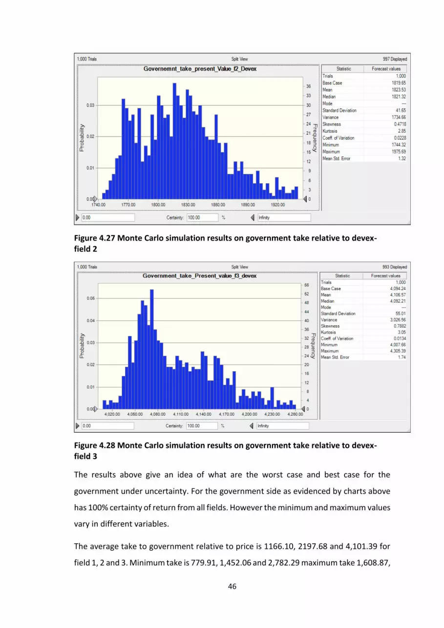
46
Figure 4.27 Monte Carlo simulation results on government take relative to devex- field 2
Figure 4.28 Monte Carlo simulation results on government take relative to devex-field 3
The results above give an idea of what are the worst case and best case for the
government under uncertainty. For the government side as evidenced by charts above
has 100% certainty of return from all fields. However the minimum and maximum values
vary in different variables.
The average take to government relative to price is 1166.10, 2197.68 and 4,101.39 for
field 1, 2 and 3. Minimum take is 779.91, 1,452.06 and 2,782.29 maximum take 1,608.87,
47
3,181.05 and 5,771.83 for field 1, 2 and 3 respectively. The average take to government
relative to development cost is 1,164.04, 1,823.53 and 4,106.57. Minimum take is
1,074.37, 1,744.32 and 4,007.66 maximum take 1,272.61, 1,975.69 and 4,305.39 for
field 1, 2 and 3 respectively. The base case profits (NPV) for each field fall in between
the attained range from simulations.
Generally, this could be translated that the riskiness of a project increases with the
decrease in reserves estimates judging by variation coefficients from figures above. On
the other hand the government is guaranteed a return from projects no matter how
unprofitable or small the field is. Looking at this from an economic and investment
analyst point of view at low gas price in world market, if the field pays the government
this high the investor is likely to make high losses to the investor it means the projects
are not profitable in the country and it will discourage investors to invest. A further
discussion below looks at alternative fiscal system/tax rates that the government may
use to collect economic rent from gas exploration.
4.2.3 Analysis of Alternative regime
For the purpose of evaluating the financial implication of the current model production
sharing contract to the maximization of investor top objective of obtaining
satisfactory/maximum profits from gas exploitation and the government to achieve high
level of tax take at the same time encourage the exploration and development of fields
which are commercially viable before tax. Thus alternative terms were implied to the
existing model and below are the results on use of Production agreement with no
Additional profits tax (APT). The reader assumes the inclusion of Additional profit tax
seems to be giving the government a high return and depriving companies of making
profits from investments especially from smaller fields, hence the choice to run another
model to see the result of exclusion of this term and results are as seen below on table
4. 3
Description Field 1 Field 2 Field 3 Unit
Reserves 0.5 1 2 Tcf
Post Tax NPV 152.57 407.89 1,388 Million $
Post Tax IRR 13 14 17 Percent

48
Post Tax NPV/I 0.13 0.21 0.48
Government
cash flow (MOD)
1,738 3,927 8,039 Million $
Contractor cash
flow (MOD)
1,008 2,518 7,165 Million $
Table 4.4 Adjusted PSA terms results
RESOURCE RENT
Resource rent tax (RRT) has been considered as a tool that provides the government
with a reasonable share of economic rent and makes the fiscal system less distorting.
This research looked at the RRT as an alternative tool for rent collection for the
government and below on table 4.5 are the results.
Field 1 Field 2 Field 3
Post Tax Net Present Value 63.93 275.35 1056.83
Post Tax Internal Rate of Return (IRR) 11% 13% 15%
Profit-to-Investment ratio (PI) 0.05 0.14 0.36
Money of Day (MOD) terms
Post Tax Net Cash flow (MoD) 846.12 2301.01 6382.29
Government tax take (MoD) 1,902.29 4144.81 8822.70
Arrival of first Tax revenue 2 2 2
Table 4.5 Resource rent tax results
Results from alternative tax term and resource rent tax from tables 4.4 and 4.5 above are
analysed in comparison to the current system and results are discussed below:
Figure 4.29 Tax System Comparison-contractor taker for field 1
0.00
0.05
0.10
0.15
Current system Adjusted System Resource Rent Tax
Contractor take
IRR Profit to Investment ratio

49
Figure 4.31 Tax system comparison-contractor take for field 3
From chats above it is generally observed that the current system is favourable to the
investor when exploration is for small and medium fields compared to resource rent tax.
Resource rent tax system and adjusted system favour the return of the investor for large
and medium fields after tax. It is also observed that the adjusted system results are
closely similar to the existing system thus making APT less a threat to investor’s return
but at the same time the absence of APT make small field more attractive after tax. The
less effect of the APT is a result of the system being based upon the real rate of return,
since the real rate of return is found to be low in this results the amount of tax paid to
government is very low.
0.1
4
0.1
4
0.1
2
0.1
9 0.2
1
0.1
4
C U R R E N T S Y S T E M A D J U S T E D S Y S T E M R E S O U R C E R E N T T A X
CONTRACTOR TAKE FIELD 2
IRR Profit to Investment ratio
0.1
4
0.1
4
0.1
5
0.2
7 0.2
9
0.3
C U R R E N T S Y S T E M A D J U S T E D S Y S T E M R E S O U R C E R E N T T A X
CONTRACTOR TAKE FIELD 3
IRR Profit to Investment ratio
Figure 4.30 Tax System Comparison-Contractor take for field 2

50
Below are charts showing results for government take at different tax system in
comparison.
Figure 4.32 Tax System Comparison-Government take for field 1
Figure 4.33 Tax System comparison-government take for field 2
956.92 933
1900.2
Current system Adjusted System Resource Rent Tax
Government take
1819
1777
1909
Current system Adjusted System Resource Rent Tax
Government take

51
Figure 4.34 Tax system comparison-Government take for field 3
From chats above it is generally observed that under resource rent tax government take
is quite a lot for small and medium field but less for the large field. The adjusted system
tends to balance between the current systems and the resource rent tax.
It is clear that the data used in this research for financial modelling are figures that
closely mimic the reserves that are available at different wells in Tanzania. In this case
though further fields could be taken to account, the considered small field could be
related to Chaza-1, medium field to Pweza-1 and large to Papa_1. Thus the following
generally conclusion may not reflect the exact situation but could be useful when
evaluating various projects.
It can be argued that for the purpose of balancing the objective of both the investor and
the government the system where the additional profit tax is not included to be used
for small fields as it is able to give the contractor a reasonable rate of return and the
government a good return. In the case of medium and large field the current PSA terms
is flexible enough to balance the interests of both parties at a given price.
3451
3395
3183
Current system Adjusted System Resource Rent Tax
Government take field 3

52
5 CONCLUSION
5.1 Concluding Remarks This research focused on looking to investigate how effective the existing fiscal
scheme is in balancing the government and investors interests, estimate the
profitability of the selected projects (fields) under the current hybrid system.
Assessing project risk under the current regime relative to price and cost
uncertainties and Comparing current PSA term with alternative fiscal tool on which
benefits both parties.
The researcher was able to measure the profitability of the selected projects by
using discounted cash flow methods through spreadsheet modelling. It was
observed that of the three fields the larger field is reasonably profitable under the
current regime. The current rent collecting system is considered to be progressive
where by the government take increases as the tax base (revenues) increase but is
rendered regressive by the combination of royalty and cost gas limit. With profit
gas sharing the system is not so flexible with fluctuating gas prices since less gas is
required for cost recovery if prices rise, and so the state gets more profit gas.
The government is able to enjoy a high return from projects and early revenues
from royalties. Since Tanzania is a new participating country in deep water natural
gas production early revenues are considered important to spear head other
regulatory activities in the government. But since the fact that TPDC meets the
royalty from its share of production in kind it might be taken to imply that the effect
of royalties does not highly affect the investor revenues which in turn from model
estimates the contractor is able to receive reasonable returns from investment. The
gas obtained from royalties is used in conjunction with the approximately 10% gas
for domestic supply.
From Monte Carlo simulations government has a 100% certainty of return unlike
the contractor simulations show great possibilities of incurring loss with low gas
prices which is not very attractive to investors. From this research it is
recommended that investments by investor to be taken when the minimum price
is $ 8.36 per MMBTU. Looking at these estimates many companies which have no

53
experience working with Tanzania before or small companies wanting to invest will
be reluctant to express their interests.
From sensitivity analysis that was done on the three fields it was found that low
prices negatively impact the returns to contractor and the government. High
investment costs were assumed for this project to reflect deep water exploration
costs which have seen to have a great impact to returns, where low development
costs increased the return and the possibility of making a loss was reduced. The fact
that high development costs reduce tax base as seen here, it is therefore argued
that this should be dealt with carefully by the government especially in collecting
APT which is based on Real rate of return to avoid gold platting problems.
In comparison to resource rent tax and a tax system suggested by the researcher
where the government does not charge additional profit tax, the adjusted system
is seen to balance the objectives of the investor and the government and is highly
recommended especially for small fields. Despite the fact that additional profit tax
is based on rate of return. The resource rent tax is also a prominent tool but since
Tanzania is a developing country and will require revenues as soon as production
begins to spear head other developmental activities in the country. Also the high
degree of risk sharing between the government and investor the resource rent tax
system is yet to be a very plausible system that the government can implement.
5.2 Limitation of Research and Recommendation
The research above focused mainly on the upstream evaluation of gas projects in
Tanzania it recommended by the researcher that further research could be done to
develop a model and build analysis on a model that incorporates the LNG
processing and transportation to the final market speculated to be Asia. Also to see
further the complete picture the research can be extended to incorporate domestic
supply take of approximately 10% from production that is sold at a lower price
compared to the stated price in this research.
54
6 BIBLIOGRAPHY Berk, J. and DeMarzo, P. (2007). Corporate finance. Boston: Pearson Addison Wesley.
Bhattacharyya, S. (2011). Energy economics. London: Springer.
Daniel, P., Keen, M. and McPherson, C. (2010). The taxation of petroleum and
minerals. USA and Canada: Routledge.
Davis, J., Fedelino, A. and Ossowski, R. (n.d.). Fiscal policy formulation and
implementation in oil-producing countries.
Ebohon, O. (1996). Energy, economic growth and causality in developing countries.
Energy Policy, 24(5), pp.447-453.
Garnaut, R. and Ross, A. (1975). Uncertainty, Risk Aversion and the Taxing of Natural
Resource Projects. The Economic Journal, 85(338), p.272.
Hannesson, R. (1998). Petroleum economics. Westport, Conn.: Quorum.
International Monetary Fund, (2014). United Republic of Tanzania: Selected Issues.
IMF Staff Country Reports, 14(121), p.1.
Johnston, D. (2003). International exploration economics, risk, and contract analysis.
Tulsa, Okla.: PennWell.
Kasriel, K. and Wood, D. (n.d.). Upstream petroleum fiscal and valuation modeling in
Excel.
Kemp, A. (1992). Petroleum policy issues in developing countries. Energy Policy,
20(2), pp.104-115.
Kemp, A. (2014). Investment Appraisal techniques.
Kemp, A. (2015). Economic rents and their collection to the state.
Ledesma, D. (2013). East Africa Gas - The Potential for Export | Oxford Institute for
Energy Studies. [online] Oxford Institute for Energy Studies. Available at:
https://www.oxfordenergy.org/2013/03/east-africa-gas-the-potential-for-export/
[Accessed 23 Jul. 2015].
Lund, D. (2009). Rent Taxation for Nonrenewable Resources. Annu. Rev. Resour.
55
Econ., 1(1), pp.287-308.
Mian, M. (2002). Project economics and decision analysis. Tusla, Okla.: PennWell
Corp.
Nbs.go.tz, (2015). Tanzania in Figures. [online] Available at:
http://www.nbs.go.tz/nbs/index.php?option=com_content&view=category&id=85
&Itemid=116 [Accessed 23 Jun. 2015].
Newendorp, P. and Schuyler, J. (2007). Decision analysis for petroleum exploration.
Aurora, Colo.: Planning Press.
Rowse, J. and Kemp, A. (1989). Petroleum Rent Collection around the World.
Canadian Public Policy / Analyse de Politiques, 15(1), p.117.
RPS Energy Canada Ltd, (2015). Mnazi bay reserve assessment. [online] Available at:
http://www.wentworthresources.com/pdf/RPS-March-2-2014-Reserves-
FINAL.pdf [Accessed 25 Jul. 2015].
Schwartz, E., Dixit, A. and Pindyck, R. (1994). Investment Under Uncertainty. The
Journal of Finance, 49(5), p.1924.
TPDC, (2015). Exploration history. [online] Available at: http://www.tpdc-
tz.com/tpdc/upstream.php [Accessed 18 Jun. 2015].

56
7 APPENDICES
APPENDIX A: Main formulas used in Model Calculations Annual Production =Daily production x 365 (Days in a year)
Revenue =Annual production x Gas Price x inflation
Drilling costs = Total recoverable reserves x Development cost per boe x
drilling cost % x drilling costs phasing x Inflation
Capex = Total recoverable reserves x Development cost per boe x
capex % x capex phasing x Inflation
Total Development cost = Drilling costs + Capex
Opex = Accumulated development cost x Opex % x inflation
Abandonment cost = Abandonment costs % x development cost p/boe x total
recoverable reserve x inflation
Total costs = Development cost + Opex + Abandonment costs
Net cashflow = Revenues – Total costs
Real Net cashflow = Net cash flow/ inflation
Net Revenue = Revenues – Royalty
Profit Oil = Net revenue – cost oil
Income Tax base = Sales- Opex – Depreciation allowance – Royalty –
government share of profit gas – additional profit gas
Post tax cashflow = Pre-tax net cash flow – Additional profit tax paid – Income
tax paid –royalty –government share of profit gas
Government take = Royalty + Additional profit tax paid + income tax paid +
royalty

57
APPENDIX B: Conversion factors
1 barrel of Oil equivalent = 5800 cubic feet
1 tcf = 1,000, 000 MMCF
1 tcf = 1000000000 MMBTU
1 boe = 5.8 MMBTU