TANZANIAN CASHEW NUT SUPPLY RESPONSE UNDER MARKET REFORMS

Godfrey Renatus Mfumu

A Research paper submitted to the school of Economics in partial

fulfillment of the requirement for the award of the degree of Masters

of Arts in Economics, University of Nairobi.

November, 2013

i

DECLARATION

Student

I hereby declare that the research project entitled “TANZANIAN CASHEW NUT SUPPLY

RESPONSE UNDER MARKET REFORMS” submitted for a Masters of Arts in Economics to the

University of Nairobi, Kenya, embodies my original work and has not been presented anywhere

for any degree award or any other academic qualification.

Signature: ______________

Godfrey Renatus Mfumu

Date: ______________________

Registration No: X50/68896/2011

Supervisor

This project has been submitted for examination with my approval as the University supervisor.

Signature: _____________

Dr. Sule Fredrick Odhiambo

Date: ______________________

Signature: _____________

Mr. Maurice Awiti

Date: ______________________

ii

DEDICATION

This research project is sincerely dedicated to my mother; Helena Kyomo, my father; Renatus

Mfumu, my two young sisters and three young brothers. I deeply appreciate the unconditional

love, care and support that I have received from family and friends throughout the whole

period of my studies. I am very much grateful and God bless you all.

iii

ACKNOWLEDGEMENT

I deeply give much appreciation to the almighty Lord, the intelligence designer and the creator

of all beings for granting me with good health and mental stability. Not because I deserve it but

simply because of his promises to all mankind.

I’m generously grateful for the support and guidance that I have received from my supervisors

Dr. Sule together with Mr. Awiti for their dedication and valuable comments that aimed at

improving my work.

My undivided appreciation goes to St. Augustine University of Tanzania for granting me the

scholarship to pursue to pursue this course. To the University of Nairobi, especially the school

of economics, I am grateful for the encouragement and cooperation that I have received from

all of you.

My sincere gratitude goes to my family for their encouragement, support and prayers through

all the trials that I have been though over the whole period of my studies. You have all been

there for me and made me understand the feeling of what it really means to be family.

Lastly but not least, I’m very grateful to have been surrounded with good friends and allies

including my classmates and work colleagues. I am very honored to have you people.

May the Lord’s blessings, guidance and protection be upon you all and let the rain of his mercy,

glory and success fall upon you all.

iv

Table of Contents Declaration……………………………………………………………………………………………………………………………………………i

Dedication…..……………………………………………………………………………………………………………………………………….ii

Acknowledgement…………………………………..………………………………………………………………………………………….iii

Table of Contents……………………………………………………………………….……………………………………………………….iv

List of Tables…………………………………………………………………………………………………………………………………………v

List of Figures………………………………………………………………………………………………………………………………………vi

Abreviations…………………….…………………………………………………………………………………….…………………………..vii

Abstract…………………………………………………………………………………………………………………………….…………………ix

`CHAPTER ONE .............................................................................................................................................. 1

1.1 Introduction ........................................................................................................................................ 1

1.1.1 Tanzanian cashew nut industry before market liberalization……………………………………………………….1

1.1.2 The social economic importance of cashew nuts…………………………………………………………….3

1.2 Research Background……………………………..…………………………………………………………………………5

1.3 Statement of the Problem…………………….……………………………………………………………………….....7

1.5 Research Objectives ............................................................................................................................ 8

1.6 Research justification…………………………………………………….……………………………….………………………………8

CHAPTER TWO ............................................................................................................................................ 10

2.0 Literature Review .............................................................................................................................. 10

2.1 The Analysis of Agricultural Supply Responses ...…………………………………………………………....10

2.2 The Theoretical Review..………………………………………………………………………………………………………………12

2.3 The Empirical Review……………………………………………………………………………………………………………………15

2.4 An Overview of Literature……………………………………………………………………………………………….……………19

CHAPTER THREE .......................................................................................................................................... 20

3.1 Theoretical Framework…………………..………………………………………………………………………………20

v

3.2 The ARDL M bounds test Approach to Co-integration…………………………………………………….23

3.3 Model Specification……………………….…………………………………………………….…………………………24

3.4 The estimation procedure………………………………………………………………………………………………25

3.5 Variables used and their expected relationships……………………….……….………………………………27

3.6 Data type and Sources…………………………………………………………………………………………………….28

3.7 Statistical diagnostic tests performed……………….…………………………………………..……………….28

CHAPTER FOUR ........................................................................................................................................... 30

4.0 Introduction…………………….…….………………………………………………………………….…………………….……………28

4.1 Summary Statistics and unit Root test results……………………………………………………………………………….28

4.2 The Co-integration Test and ECM………………………………………………………………………………………………….33

4.3 Regression results…………………………………………………………………………………………………………………………33

4.4 The ARDL co-integration test…………………………………………………………………………………………………….….34

4.5 The short run Elasticities………………………………………………………………………………………………….……………35

4.6 Stability Tests………………………………………………………………………………………………………………………………..36

4.7 The Comparison of Study Results………………………………………………………………………………………………….36

CHAPTER FIVE.....................................................................................................................................37

5.1 Conclusion……..……………………………………………..……………………………………………………..……………………….37

5.2 Policy Implications and Recommendations………………….………………………………………………………………..37

5.3 Limitations of the study…………………………………………………………………………………………………………………38

5.3 Areas for further research…………………………………………………………………………………………………………….39

REFERENCES ................................................................................................................................................ 40

Appendix 1..…………………………………………………………………………………..……………………………………………………44

Appendix 2…………………….……………………………………………………………………………………………………………………45

vi

LIST OF TABLES

Table 1: Variables used together with their expected relationships................................................27

Table 2a: 1a Descriptive Statistics.……………..……..……………………………………………………..……………………….30

Table 2b: Correlation Matrix ………………….…………………………………………………………………………....……………..31

Table 3a: Unit Root test for level variables ………………………………………………………………………………….……32

Table 3b: Unit Root test for differenced variables………………………………………………………………….…32

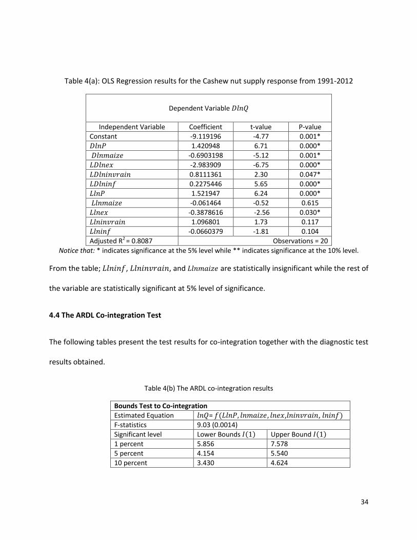
Table 4a: OLS Regression results……………………………………………………………………..…………………………34

Table 4b: The ARDL co-integration results………………….………………………………………………………………………...34

Table 4c: Diagnostic Test results……………………………….…………………………………………….………………..35

vii

LIST OF FIGURES

Figure 1: Cashew nut production trend before trade liberalization………………………….…..…..………..3

Figure 2: Cashew nut export revenue earnings.……………………………………………………………………………......4

Figure 3: Cashew nut production trend after trade liberalization………………………………………... …….6

viii

LIST OF ABBREVIATIONS

ADF

ARDLM

BoT

CATA

CBT

CPI

CUSUM

CUSUM sq

ECM

IMF

OLS

RCUs

RESET

SAPs

TCMB

US

Augmented Dickey-Fuller

Autoregressive distributed lag model

The Central Bank of Tanzania

Cashew nut Authority of Tanzania

Cashew nut Board of Tanzania

Consumer price index

Cumulative sum of residuals

Cumulative sum of squared residuals

Error Correction Mechanism

International Monetary Fund

Ordinary Least Squares

Regional Cooperative Unions

Regression Error Specification Test

Structural Adjustment Programs

Tanzanian Cashew nut Marketing Board

United States

ii

AN ABSTRACT

The title of this project is Tanzanian cashew nut supply response under market reforms. The

main objective was to assess supply responses by the Tanzanian cashew nut industry under

market reforms. The analysis employed secondary time series data from 1991-2012 using the

ARDL bounds test approach.

The results have revealed that in the short run; a 1 percent increase in price leads to 1.42

percentage increase in the quantity of cashews supplied. In addition, a 1 percent increase in

rainfall results to a 0.81 percentage increase in cashew supply. Apart from that, a 1 percent

increase in price of maize results to a 0.69 percent decrease in the cashew supply. On top of

that, a 1 percent raise in the rate of inflation forces cashews supply to increase by 0.23

percent. Lastly, a 1 percent increase in exchange rate leads to almost 3 percent reduction of

cashews supplied.

These results imply that Tanzanian cashew nut supply is elastic in the short run to both price

and non-price factors as well. However, the study failed to estimate long run elasticities due to

lack of evidence to support the presence of co-integration.

Basing on the study results, the policy recommendations includes; for the sector to bare fruitful

results, both price and non-price incentives should be a priority. Also, the BoT should avoid

delays on exercising control on exchange rate volatility in such a way that, critical and necessary

continuous intervention in the exchange rate markets must be a priority.

1

CHAPTER ONE

1.1 Introduction

Following the so called “The Elliot Berg Repor and the Model of Accumulation in Sub- Saharan

Africa” (Loxley 1983); the World Bank volunteered to offer some help for individual African

countries that were struggling from worsening economic hardships. For the assistance to be

offered, countries had to accept and implement in good faith the structural adjustment

programs (SAPs) as directed by the word Bank, Barratt (1995). The Berg report as well as other

evidences suggested that most intervention efforts by governments at that time to facilitate

economic growth were actually acting as an impediment towards growth. Such a case

therefore, had left the World Bank, IMF together with other donors with no choice other than

forcing the failing economies to adopt policy reforms, Akiyama et al (2003).

Since most African economies were heavily dependent on agriculture, it needed more than a

miracle for such reforms not to affect the sector and thus, such reforms had to be initiated with

no delays. Reforms in the agricultural sector had the aim of either reducing or eliminating

distortions within the sector through the introduction of market forces. In other words, reforms

were expected to make the sector receive world market prices for agricultural commodities

apart from eliminating rent transfers to urban population, Lunberg (2004).

1.1.1 The Tanzanian Cashew nut Industry before Market Liberalization

Cashews are among one of the major five traditional cash crops in Tanzania. It is the main back

born of the economy of the southern coastal regions estimated to employ at least 280,000

smallholder farmers, Topper et al (1998). Before the market reforms, the sector was completely

under the control of the government through the supervision of primary and secondary

2

cooperative societies which operated under the monopoly of Tanzanian cashew nut marketing

board, TCMB which replaced the cashew nut authority of Tanzania, CATA, Topper et al (1998).

In early 1970s about 68 percent of the total world cashew nut productions come from Africa,

particularly in Mozambique and Tanzania, Jaffee and Morton (1995). However, the trend

changed in 1980s with India and Vietnam emerging as the new major producers.

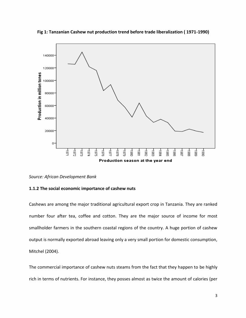
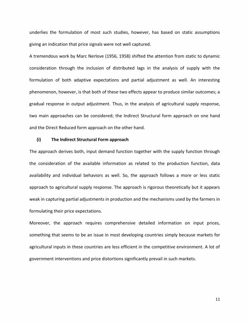
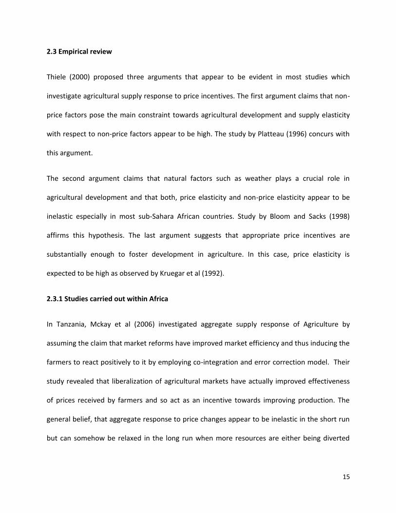
The Graph below, which depicts production trend, reveals that production continued to

increase and picked in 1973/74 with 145,000 tones of raw cashew nut being produced. Then

after, production started to decline reaching 18,490 tones in 1986/87 while the 1989/90 season

recorded the lowest level of 17,060 tones only. Throughout this period, however, Lindi, Mtwara

and Ruvuma regions accounted for more than 80 percent of the whole production.

In general, the pre-liberalization period was highly characterized by inefficiencies that acted as

distortions or disincentives to farmers. Some of these marketing as well as administrative and

procurement deficiencies include; frequent delays in the collection of the nuts from the

farmers, delays of payments to the farmers and continued accumulation of huge debts by RCUs.

3

Fig 1: Tanzanian Cashew nut production trend before trade liberalization ( 1971-1990)

Source: African Development Bank

1.1.2 The social economic importance of cashew nuts

Cashews are among the major traditional agricultural export crop in Tanzania. They are ranked

number four after tea, coffee and cotton. They are the major source of income for most

smallholder farmers in the southern coastal regions of the country. A huge portion of cashew

output is normally exported abroad leaving only a very small portion for domestic consumption,

Mitchel (2004).

The commercial importance of cashew nuts steams from the fact that they happen to be highly

rich in terms of nutrients. For instance, they posses almost as twice the amount of calories (per

4

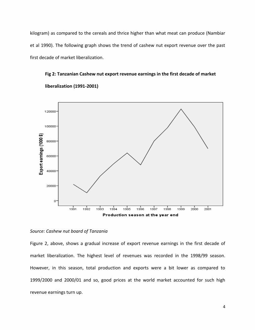
kilogram) as compared to the cereals and thrice higher than what meat can produce (Nambiar

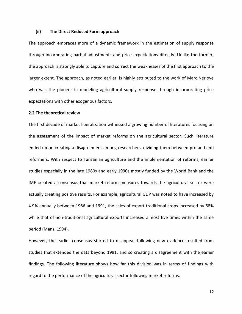
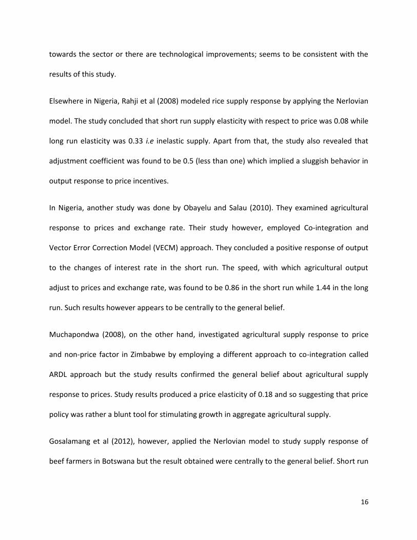
et al 1990). The following graph shows the trend of cashew nut export revenue over the past

first decade of market liberalization.

Fig 2: Tanzanian Cashew nut export revenue earnings in the first decade of market

liberalization (1991-2001)

Source: Cashew nut board of Tanzania

Figure 2, above, shows a gradual increase of export revenue earnings in the first decade of

market liberalization. The highest level of revenues was recorded in the 1998/99 season.

However, in this season, total production and exports were a bit lower as compared to

1999/2000 and 2000/01 and so, good prices at the world market accounted for such high

revenue earnings turn up.

5

1.2 Research Background

Poor pricing system and unreliability of good prices for farmers’ produce has been the main

problem of concern amongst farmers in most developing countries including Tanzania. For

almost two decades now, Tanzania has been taking several economic reforms among which

reforms in the agricultural sector stays at the centre of such efforts toward economic

liberalization.

The reforms in agricultural sector in Tanzania can be traced far back in mid and late 1980s but

with respect to the cashew nut industry, the reforms started in the early 1990s. Some of the

reforms that impacted the industry includes: government withdrawal from direct production

activities, relying on private sector for production processes as well as limiting the powers and

scope of crops marketing boards so as to allow a more active role by the private sector.

The establishment of the Warehouse Receipt System as perpetuated by the Warehouse Receipt

Act of 2006, is one among the notable reform efforts toward the sector. With this regard, the

country intends to strengthen the Warehouse Receipt regulatory system hopping to arrest

pricing and marketing agricultural produce related problems that appears to hinder farmers’

initiatives on one hand and improving the performance of export crops on the other hand;

cashew nut crop being one of them.

Under the reform period, smallholder farmers still carries out major production activities with

more involvement of the private sector in procurement and marketing activities within the

industry. During this period, the government decided to replace the TCMB with the CBT, Sijaona

(2002).

6

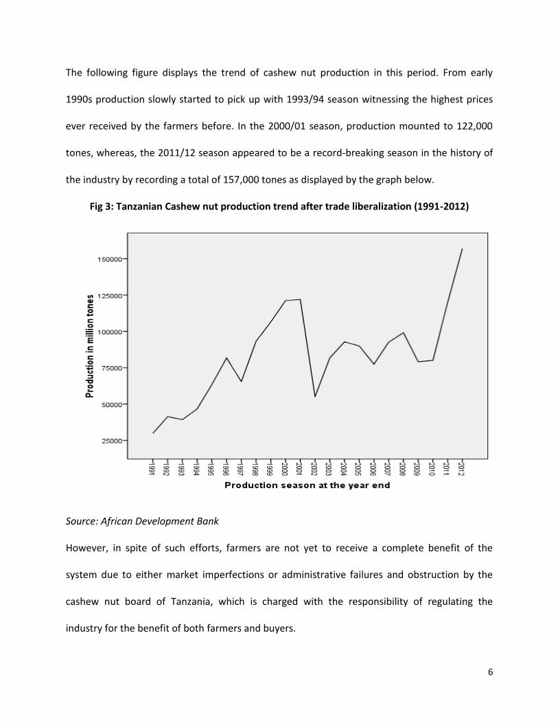
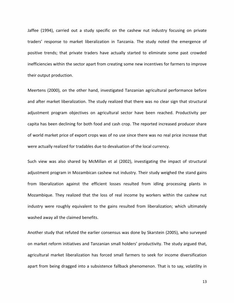
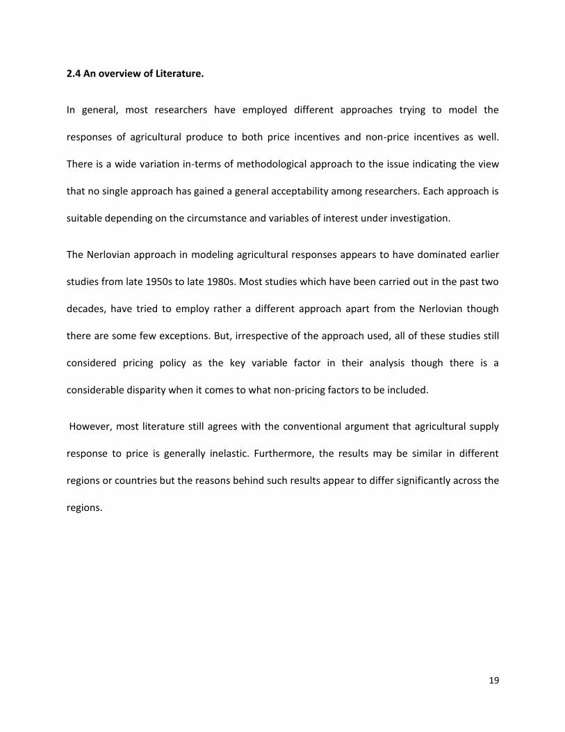
The following figure displays the trend of cashew nut production in this period. From early

1990s production slowly started to pick up with 1993/94 season witnessing the highest prices

ever received by the farmers before. In the 2000/01 season, production mounted to 122,000

tones, whereas, the 2011/12 season appeared to be a record-breaking season in the history of

the industry by recording a total of 157,000 tones as displayed by the graph below.

Fig 3: Tanzanian Cashew nut production trend after trade liberalization (1991-2012)

Source: African Development Bank

However, in spite of such efforts, farmers are not yet to receive a complete benefit of the

system due to either market imperfections or administrative failures and obstruction by the

cashew nut board of Tanzania, which is charged with the responsibility of regulating the

industry for the benefit of both farmers and buyers.

7

1.3 Statement of The Problem

Market reforms appear to possess a very promising future of success in the cashew nut industry

in Tanzania. However, the existence of divergent views by different stakeholders on the

performance of the industry since the inception of market reforms poses a very challenging

query on whether such reforms have been worthwhile taking and if they really benefits the

farmers on the ground, Rweyemamu (2002).

The sector has all potentials of growth in terms of output despite the prevalence of the pre-

existed problems such as; inefficient and untimely supply of inputs, poor or limited access to

financial facilities by the farmers, uncertainties related to good prices for the produce and

delayed payments. Altogether provides the urge for conducting a more extensive study towards

the sector and so proving the way forward.

Among the pre-supposed benefits of reforms in the agricultural sector is that we expected the

removal of government monopoly would allow a more pro-active role by private traders and

small farmers. This would result into more market competition and so creating a multiplier

effect in the form of more employment, income to the farmers and foreign exchange revenue

to the government; all from the industry. However, these authoritative, non-democratic ill-

centered reforms with “one size fits all” character have not yet produced a clear realization of

such promises.

The reforms have contributed to the stagnation of agricultural processing industry and creating

new monopolies of few cashew nut traders. For instance, before liberalization, which privatized

most processing factories, the country had twelve large cashew nut processing factories in

operation but to date we have only one active processing factory in operation. The situation

8

resulted from stiff competition faced by local processors from efficient Indian processors. This

has fueled the exportation of raw nuts, which in turn reduce foreign exchange revenues and

employment chances following the closure of such processing plants.

Thus, market reforms may be encouraging production and exportation of raw cashew nuts on

one hand, but on the other hand, they have crippled agricultural processing industry and so

restraining the benefits related from processing the nuts. Such losses include, reduced

employment opportunities, less foreign exchange earnings due to lack of value addition for the

exportable nuts and stagnation of the process of technology diffusion as related to processing

activities which ultimately reduces substantial income for the farmers.

1.4 Main Objective

Assessing supply responses by the Tanzanian cashew nut industry under market

reforms.

1.5 Specific Objectives

To determine short run and long run responses of cashew nut output supply.

To determine the rate of cashew nut output adjustment under market reforms.

To draw conclusions and make policy recommendations according to the research

findings.

1.6 Research Justification

Just like any other formerly recognized socialist state, market reforms in Tanzania was not an

easy or sweet pill to swallow. But, since such reforms were inevitable, they had to happen

gradually and still under way until today. The World Bank report of 1994 on the performance of

9

Tanzanian agriculture called into question the earlier stories of success of the sector under

market reforms which was backed by evidence from earlier studies. This argument was backed

by the fact that majority of such studies were likely to have overstated the performance of the

sector since they suffered from inadequate or unreliable information base. This reality

therefore calls upon the need of more study towards the issue.

10

CHAPTER TWO

2.0 The Literature Review

This chapter has examined different literature including the theoretical as well as empirical

works done by other researchers using either similar or different approaches, apart from

reviewing the approaches used in modeling agricultural supply responses. The chapter has then

concluded by generating an overview of the literature reviewed.

2.1 The Analysis of Agricultural Supply Responses

The interest on agricultural supply analysis has long history since it can be traced back far

before the works related to the production function, and it was generally disassociated with it.

Initially, the analysis on supply response had a lot to do with policy issues instead of application

issues or the development of formal econometric analysis. The reason accounting for this

perception is, perhaps, explained by the work of Johnson (1950) who observed that during the

great depression, both product prices and factor prices as well displayed a decreasing tendency.

However, the central focus of the influence of price in determining output has changed a lot

since then. Furthermore, there have been some notable additions and modifications on the

public agenda especially when the question with regard to the ability of expanding food supply

to meet growing demand comes into play. Thus, while the role of prices relates to the behavior

under given supply conditions on one hand, the aspect of growth can be related to the changes

within such conditions on the other hand.

Traditionally, the empirical supply function used to regress output on prices and other variables

with the aim of deducting supply responses to price incentives. Thus, most studies have

employed time series data though there are some exceptions. The theoretical framework that

11

underlies the formulation of most such studies, however, has based on static assumptions

giving an indication that price signals were not well captured.

A tremendous work by Marc Nerlove (1956, 1958) shifted the attention from static to dynamic

consideration through the inclusion of distributed lags in the analysis of supply with the

formulation of both adaptive expectations and partial adjustment as well. An interesting

phenomenon, however, is that both of these two effects appear to produce similar outcomes; a

gradual response in output adjustment. Thus, in the analysis of agricultural supply response,

two main approaches can be considered; the Indirect Structural form approach on one hand

and the Direct Reduced form approach on the other hand.

(i) The Indirect Structural Form approach

The approach derives both, input demand function together with the supply function through

the consideration of the available information as related to the production function, data

availability and individual behaviors as well. So, the approach follows a more or less static

approach to agricultural supply response. The approach is rigorous theoretically but it appears

weak in capturing partial adjustments in production and the mechanisms used by the farmers in

formulating their price expectations.

Moreover, the approach requires comprehensive detailed information on input prices,

something that seems to be an issue in most developing countries simply because markets for

agricultural inputs in these countries are less efficient in the competitive environment. A lot of

government interventions and price distortions significantly prevail in such markets.

12

(ii) The Direct Reduced Form approach

The approach embraces more of a dynamic framework in the estimation of supply response

through incorporating partial adjustments and price expectations directly. Unlike the former,

the approach is strongly able to capture and correct the weaknesses of the first approach to the

larger extent. The approach, as noted earlier, is highly attributed to the work of Marc Nerlove

who was the pioneer in modeling agricultural supply response through incorporating price

expectations with other exogenous factors.

2.2 The theoretical review

The first decade of market liberalization witnessed a growing number of literatures focusing on

the assessment of the impact of market reforms on the agricultural sector. Such literature

ended up on creating a disagreement among researchers, dividing them between pro and anti

reformers. With respect to Tanzanian agriculture and the implementation of reforms, earlier

studies especially in the late 1980s and early 1990s mostly funded by the World Bank and the

IMF created a consensus that market reform measures towards the agricultural sector were

actually creating positive results. For example, agricultural GDP was noted to have increased by

4.9% annually between 1986 and 1991, the sales of export traditional crops increased by 68%

while that of non-traditional agricultural exports increased almost five times within the same

period (Mans, 1994).

However, the earlier consensus started to disappear following new evidence resulted from

studies that extended the data beyond 1991, and so creating a disagreement with the earlier

findings. The following literature shows how far this division was in terms of findings with

regard to the performance of the agricultural sector following market reforms.

13

Jaffee (1994), carried out a study specific on the cashew nut industry focusing on private

traders’ response to market liberalization in Tanzania. The study noted the emergence of

positive trends; that private traders have actually started to eliminate some past crowded

inefficiencies within the sector apart from creating some new incentives for farmers to improve

their output production.

Meertens (2000), on the other hand, investigated Tanzanian agricultural performance before

and after market liberalization. The study realized that there was no clear sign that structural

adjustment program objectives on agricultural sector have been reached. Productivity per

capita has been declining for both food and cash crop. The reported increased producer share

of world market price of export crops was of no use since there was no real price increase that

were actually realized for tradables due to devaluation of the local currency.

Such view was also shared by McMillan et al (2002), investigating the impact of structural

adjustment program in Mozambican cashew nut industry. Their study weighed the stand gains

from liberalization against the efficient losses resulted from idling processing plants in

Mozambique. They realized that the loss of real income by workers within the cashew nut

industry were roughly equivalent to the gains resulted from liberalization; which ultimately

washed away all the claimed benefits.

Another study that refuted the earlier consensus was done by Skarstein (2005), who surveyed

on market reform initiatives and Tanzanian small holders’ productivity. The study argued that,

agricultural market liberalization has forced small farmers to seek for income diversification

apart from being dragged into a subsistence fallback phenomenon. That is to say, volatility in

14

markets and declining ratio of crop prices to input costs; has forced small farmers to produce

only for covering their basic consumption (subsistence fall back) on one hand, and seeking cash

income outside their holdings by engaging in other activities apart from agriculture (risk

spreading) on the other hand. The study therefore concluded that, instead of fueling

specialization, structural adjustment programs have resulted to opposite outcomes in Tanzania.

A recent study by Tiberti (2012), however, acknowledges a remarkable improvement of output

for the past decade in Tanzania. But more importantly, the study suggests that such effect

could not influence poverty reduction for small farmers since large share of agricultural output

growth was driven by large plantations and after all, the resulted growth was not evenly

distributed among the regions country wide. This claim is supported by the earlier study done

by Mashindano and Limbu (2002).

In spite of the sound argument presented by these studies, there’s one conspicuous weakness

that all of them share; that most of their arguments have not been formulated basing on

econometric empirical framework. Thus, we can’t rely strongly on findings of such studies to

draw general conclusions about the performance of the Tanzanian agriculture under market

reforms.

15

2.3 Empirical review

Thiele (2000) proposed three arguments that appear to be evident in most studies which

investigate agricultural supply response to price incentives. The first argument claims that non-

price factors pose the main constraint towards agricultural development and supply elasticity

with respect to non-price factors appear to be high. The study by Platteau (1996) concurs with

this argument.

The second argument claims that natural factors such as weather plays a crucial role in

agricultural development and that both, price elasticity and non-price elasticity appear to be

inelastic especially in most sub-Sahara African countries. Study by Bloom and Sacks (1998)

affirms this hypothesis. The last argument suggests that appropriate price incentives are

substantially enough to foster development in agriculture. In this case, price elasticity is

expected to be high as observed by Kruegar et al (1992).

2.3.1 Studies carried out within Africa

In Tanzania, Mckay et al (2006) investigated aggregate supply response of Agriculture by

assuming the claim that market reforms have improved market efficiency and thus inducing the

farmers to react positively to it by employing co-integration and error correction model. Their

study revealed that liberalization of agricultural markets have actually improved effectiveness

of prices received by farmers and so act as an incentive towards improving production. The

general belief, that aggregate response to price changes appear to be inelastic in the short run

but can somehow be relaxed in the long run when more resources are either being diverted

16

towards the sector or there are technological improvements; seems to be consistent with the

results of this study.

Elsewhere in Nigeria, Rahji et al (2008) modeled rice supply response by applying the Nerlovian

model. The study concluded that short run supply elasticity with respect to price was 0.08 while

long run elasticity was 0.33 i.e inelastic supply. Apart from that, the study also revealed that

adjustment coefficient was found to be 0.5 (less than one) which implied a sluggish behavior in

output response to price incentives.

In Nigeria, another study was done by Obayelu and Salau (2010). They examined agricultural

response to prices and exchange rate. Their study however, employed Co-integration and

Vector Error Correction Model (VECM) approach. They concluded a positive response of output

to the changes of interest rate in the short run. The speed, with which agricultural output

adjust to prices and exchange rate, was found to be 0.86 in the short run while 1.44 in the long

run. Such results however appears to be centrally to the general belief.

Muchapondwa (2008), on the other hand, investigated agricultural supply response to price

and non-price factor in Zimbabwe by employing a different approach to co-integration called

ARDL approach but the study results confirmed the general belief about agricultural supply

response to prices. Study results produced a price elasticity of 0.18 and so suggesting that price

policy was rather a blunt tool for stimulating growth in aggregate agricultural supply.

Gosalamang et al (2012), however, applied the Nerlovian model to study supply response of

beef farmers in Botswana but the result obtained were centrally to the general belief. Short run

17

price elasticity appeared to be 1.51 while the long run elasticity was 1.06. The study therefore,

concluded that price policies were actually effective in inducing the improvement on output.

The other related study in Africa was done by Gatete (1993), carrying out an economic analysis

of coffee supply in Kenya. The study utilized the bootstraps technique by assuming that Kenyan

government policy was to increase producer price by 15 percent as an attempt to favor

producer surplus for smallholder farmers. Although the study employed a different technique,

it ended up with the same reduced form supply function as the Nerlovian supply reduced

equation form. The study finally concluded that major coffee producers (estates) were inelastic

in terms of response to price incentives apart from suggesting that impact of price variability on

coffee producers was quite substantial.

2.3.2 Studies carried outside Africa

The evidence from Indonesia presented by Ketut and Bamang (2004), seem to clearly refute

African experience with structural adjustment program and agricultural performance as they

studied the impact of such reforms on cashew nut industry in Nusa Taggara Barat province in

Indonesia. They argued that market liberalization has made the cashew industry in Indonesia

more competitive and efficient by applying the policy analysis matrix approach.

In India, Mythili (2006) applied the Nerlovian model with panel data to study supply response

by Indian farmers to price incentives. The study supported the argument that farmers respond

slowly to price incentives in the short run and that speed of adjustment was also very slow

especially for food grains. On top of that, the study strongly rejected the hypothesis that

market liberalization has improved output or acreage response to price incentives.

18

Elsewhere in China, Yu et al (2010) studied agricultural supply response to price under

economic transformation in Henan province. Their study employed a dynamic panel data

technique and concluded that price elasticity for grains was 0.27 in the short run and 0.81 in the

long run. However, the speed or magnitude of elasticity appeared to vary significantly across

varieties of agricultural produce. The study therefore supported the conventional view that,

agricultural response to price changes in developing countries is inelastic.

Koo (1982) conducted an econometric analysis of the U.S. wheat acreage response by

evaluating farmers’ response to market prices. The study employed the Nerlovian geometric lag

model assuming that there is a tendency of price effect on agricultural produce to decline

geometrically with respect to time when measured backward from current period. The study

revealed, however, that wheat price elasticity for winter was more inelastic than in the case of

spring season. The reason accounting for the situation was that, spring wheat production was

somehow replaceable with other crops; such replacement was very limited in winter wheat

producing region.

In the U.S., another study was conducted by Lafrance and Burt (1983). They investigated

aggregate U.S. agricultural supply response using the modified partial adjustment model. Their

study results revealed a short run price elasticity of 0.1 while 0.3 price elasticity accounted for

the long run.

19

2.4 An overview of Literature.

In general, most researchers have employed different approaches trying to model the

responses of agricultural produce to both price incentives and non-price incentives as well.

There is a wide variation in-terms of methodological approach to the issue indicating the view

that no single approach has gained a general acceptability among researchers. Each approach is

suitable depending on the circumstance and variables of interest under investigation.

The Nerlovian approach in modeling agricultural responses appears to have dominated earlier

studies from late 1950s to late 1980s. Most studies which have been carried out in the past two

decades, have tried to employ rather a different approach apart from the Nerlovian though

there are some few exceptions. But, irrespective of the approach used, all of these studies still

considered pricing policy as the key variable factor in their analysis though there is a

considerable disparity when it comes to what non-pricing factors to be included.

However, most literature still agrees with the conventional argument that agricultural supply

response to price is generally inelastic. Furthermore, the results may be similar in different

regions or countries but the reasons behind such results appear to differ significantly across the

regions.

20

CHAPTER THREE

3.1 Theoretical Framework

The model originated from the pioneering work of Marc Nerlove (1958). It follows a partial

adjustment mechanism through assuming farmers’ reactions in terms of price expectations and

production adjustment. Thus, the approach encompasses the general form supply function of

partial adjustment mechanism together with the equation that captures the supply dynamics,

Askari and Commings (1977).

However, in modeling the supply response of agricultural produce, one may chose to employ

different variables such as, yield, desired area under cultivation or output, as a part of farmers’

reaction toward incentives such as prices (Yu et al 2010). Furthermore, in most empirical works,

there have been some modifications and changes applied to the model. Askari and Commings

(1977) have argued that most of such modifications can generally be categorized under the

following three groups;

The modifications on the variables used within the model

The inclusion of factors of particular interest in the situation under investigation

corresponding to variable Z.

The attempt to include some other aspects that are thought not to have been included

by the earlier steadies such as; the duration of crops to maturity and the seasonal

effects of the agricultural produce.

The basic Nerlove model however can be presented by the following three equations;

𝑄𝑡∗ = 𝑎1 + 𝑎2𝑃𝑡

∗ + 𝑎3𝑍𝑡 + 𝑈𝑡 ……………………… (1)

21

𝑄𝑡 − 𝑄𝑡−1 = β(𝑄𝑡∗ − 𝑄𝑡−1)…………………… . . (2)

𝑃𝑡∗ − 𝑃𝑡−1

∗ = α 𝑃𝑡−1 − 𝑃𝑡−1∗ …………………… (3)

Where by:

𝑄𝑡∗ is the desired output at period t

𝑄𝑡 is the actual output at period t

𝑄𝑡−1 is the actual output in the previous period

𝑃𝑡∗ is the expected price at period t

𝑃𝑡−1∗ is the expected price of the previous year

𝑍𝑡 is a set of the exogenous factors entering the supply function

β is the coefficient of output adjustment and ( o < β < 1 )

α is the coefficient of price expectations and ( 0 < α < 1 )

𝑈𝑡 is the error term

Since the model assumes adoptive expectations and that 𝑄∗ is unobservable, it is therefore

correct to conclude that 𝑄∗ = 𝑄𝑡 . Focusing on partial adjustment hypothesis, it can further be

noted that farmers make their decision basing on their knowledge about real prices (since P*

can’t be observed) that prevails immediately in the preceding year. We can be proud to assume

that 𝑃𝑡∗ = 𝑃𝑡−1 i.e. α = 1.

Taking into consideration the above assumptions, we can now substitute equation (2) into (1)

as follows:

Qt = 𝑎1 + 𝑎2Pt−1 + 𝑎3 Zt−1 + Ut …………………… 4

22

But 𝑄𝑡= 𝑄𝑡−1 + β𝑄𝑡 − β𝑄𝑡−1

Thus 𝑄𝑡 = 𝑄𝑡−1 + 𝛽 𝑎1 + 𝑎2𝑃𝑡−1 + 𝑎3𝑍𝑡 + 𝑈𝑡 − 𝛽𝑄𝑡−1

= 𝑎1𝛽 + 𝑎2𝛽𝑃𝑡−1 + 1 − 𝛽 𝑄𝑡−1 + 𝑎3𝛽𝑍𝑡 + 𝑈𝑡𝛽 ………………… (5)

Where by:

𝑎2 is the long run supply elasticity with respect to price

𝑎2𝛽 Is the short run supply elasticity with respect to price

𝛽 Is the output adjustment coefficient

Alternatively, one can also derive the model by considering the adaptive expectations and so

combining equation (1) and (3) which ultimately end up with similar structural equation as that

presented by equation (5) above. This is perhaps the main setback of the model as it becomes

uneasy to distinguish between the partial adjustment and price expectation coefficients unless

further restrictions are being put forward.

Apart from such above identification problem of the model, most literature in econometrics

argue that most time series variables are always suspicious of being non-stationary, a problem

which ultimately result into spurious regressions. This is a common phenomenon with most lagged

variable models, the Nerlovian approach in particular. The situation therefore calls upon a more

improved approach as an initiative to ratify the situation. Thus, the study resorts to the application

of co-integration analysis and error collection mechanism as a supplement to our model. Thus, the

study resorted to the application of ARDLM bounds technique to co-integration.

The ARDLM bounds technique to co-integration have thus been introduced purposefully for the

aim of overcoming spurious regression problems since the approach tends to produce

23

consistent and distinct estimates of both short run and long run elasticities which satisfies the

assumptions of classical linear regression analysis. This appears to be more general than the

partial adjustment mechanism, since it allows a wider concrete and precise way of modeling

dynamic adjustments in agricultural supply responses.

3.2 The ARDL M bounds test Approach to Co-integration.

The approach was developed by Pesaran et al (2001) through the use of bounds test to examine

the long run relationship among time series variables. The main strong hood of this approach

rests upon the fact that; it can be used regardless of whether the variables are at I(0) or I(1)

unlike most co-integration techniques. It also formulates the dynamic or unrestricted ECM

derived from ARDLM bounds test through a simple linear transformation. The approach

involves the estimation of the following general conditional version of the ECM:

ΔYt = θ0 + θ1Yt−1 + θ2Xt−1 + θ3Zt−1 + βi

p

i=1

Δ Yt−1 + σi

p

j=0

ΔXt−j + δs

p

s=0

ΔZt−s

+ ωt ………………………………………………………………… . . (6)

We can now notice that the conditional ECM from the bounds test differs from the traditional

ECM through the replacement of the error correction term with the lagged variables of the

variables under consideration. The approach estimates (𝑝 + 1)𝑘 number of regression where

as to obtain optimal of lag length for each series; 𝑝 is the maximum lag length and 𝑘 stands for

the number of variables in the respective equation.

According to Pesaran et al, therefore, for co-integration to exist, the null hypothesis of no long

run relationship i.e. 𝐻0: 𝜃1 = 𝜃2 = 𝜃3 = 0 must be rejected. The two asymptotic critical

bounds provides a test for co-integration when the independent variable 𝐼 𝑑 where by

24

(0 ≤ 𝑑 ≤ 1). The lower bound implicates that the regressors are of 𝐼 0 , where as the upper

bound implies that the regressors are of 𝐼 1 .

If the F-statistic value exceeds the upper critical value, we conclude that there is long run

relationship regardless of the order of integration. If the F-statistic falls below the lower

boundary we cannot reject the null hypothesis of no co-integration. When all variables are

known to be of 𝐼 1 the decision is made in favor of the upper boundary and when they are of

𝐼 0 , we then regard the lower boundary. If the variables appear to be co-integrated, then all

the differenced variables equals zero and thus, the long run conditional model becomes;

𝑌𝑡 = 𝛽0 + 𝛽1𝑋𝑡 + 𝛽2𝑍𝑡 + 𝑉𝑡 …………………………………………… (7)

To check for the goodness of fit in this model, both the stability test together with the

diagnostic test have to be performed. The tests checks for serial correlation, functional form of

the model, normality of the error term and heteroskedasticity as well. The stability of the

model is checked by conducting both CUSUM and CUSUMsq tests.

3.3 Model Specification

The model to be estimated can be specified by the following supply function;

𝑄𝑡 = 𝑓 𝑃𝑡 , 𝑆𝑡 , 𝑅𝑡 , 𝑊𝑡 , 𝑀𝑡 𝑎𝑛𝑑 𝑇 ………………………… . . (8)

Whereby;

𝑄𝑡 Represents the amount of cashew nut output supplied by the farmers over time

𝑃𝑡 Represents the price of the cashew nut output as given to the farmers my market

forces over time

25

𝑆𝑡 Represents the price of maize as a substitute crop for cashew nuts

𝑅𝑡 Represents market determined exchange rate between Tanzanian shilling and the US

dollar over time

𝑊𝑡 Represents average annual rainfall measured country wide over time

𝑀𝑡 Represents the rate of inflation over time

𝑇 Is the time trend variable

Setting up the Nerlovian Model;

𝑄𝑡 = 𝑎0 + 𝑎1𝛽𝑃𝑡−1 + 𝑎2𝑆𝑡−1 + 𝑎3𝛽𝑅𝑡 + 𝑎4𝛽𝑀𝑡 + 𝑎5𝛽𝑇 + 1 − 𝛽 𝑄𝑡−1 + 𝛽Ԑ𝑡 … (9)

In the reduced form;

𝑄𝑡 = 𝛿0 + 𝛿1𝑃𝑡−1 + 𝛿2𝑆𝑡−1 + 𝛿3𝑅𝑡 + 𝛿4𝑀𝑡 + 𝛿5𝑇 + 𝛿6𝑄𝑡−1 + 𝑉𝑡 ……………… (10)

Whereby;

𝛿0 = 𝑎0

𝛿1 = 𝑎1𝛽 ,

𝛿2 = 𝑎2𝛽

𝛿3 = 𝑎3𝛽

𝛿4 = 𝑎4𝛽

𝛿5 = 𝑎5𝛽

𝛿6 = (1 − 𝛽)

26

𝑉𝑡 = 𝛽Ԑ𝑡

In the log-log form, the equation appears as follows;

𝑙𝑛𝑄𝑡 = 𝛿0 + 𝛿1𝑙𝑛𝑃𝑡−1 + 𝛿2𝑙𝑛𝑆𝑡−1 + 𝛿3𝑙𝑛𝑅𝑡 + 𝛿4𝑙𝑛𝑀𝑡 + 𝛿5𝑙𝑛𝑇 + 𝛿6𝑙𝑛𝑄𝑡−1

+ 𝑉𝑡 …………………………………………………………… . (11)

3.4 The estimation procedure

As the initial step before estimation, the study had to apply the DF test to check for non-

stationarity in each of the variables represented by equation (11) above by testing the null

hypothesis of non-stationarity against the alternative hypothesis; the series are stationary,

before establishing the order of integration.

The study proceeded through the formulation of the dynamic or unrestricted ECM derived from

ARDLM bounds test with a simple linear transformation. Thus, the approach specified and

estimated the following general conditional version of the ECM containing only variables

of 𝐼 0 and 𝐼 1 since the inclusion of variables with greater than 𝐼 1 violates the underlying

foundations of the approach (Ouattara, 2004):

𝐷𝑙𝑛𝑄 = θ0 + 𝜃1𝐷𝑙𝑛𝑃 + 𝜃2𝐷𝑙𝑛𝑚𝑎𝑖𝑧𝑒 + 𝜃3𝐿𝐷𝑙𝑛𝑒𝑥 + 𝜃4𝐿𝐷𝑙𝑛𝑖𝑛𝑣𝑟𝑎𝑖𝑛 + 𝜃5𝐿𝐷𝑙𝑛𝑖𝑛𝑓 + 𝜃6𝐿𝑙𝑛𝑃

+ 𝜃7𝐿𝑙𝑛𝑒𝑥 + 𝜃8𝐿𝑙𝑛𝑖𝑛𝑣𝑟𝑎𝑖𝑛 + 𝜃9𝐿𝑙𝑛𝑖𝑛𝑓 + 𝑉𝑡 …………………………… (12)

Where by:

𝑙𝑛𝑖𝑛𝑣𝑟𝑎𝑖𝑛 = (1/𝑙𝑛𝑟𝑎𝑖𝑛)^2

𝐷 stands for the first difference of the respective variable and

𝐿 stands for the first lag of the respective variable

27

𝑉𝑡 is the residual

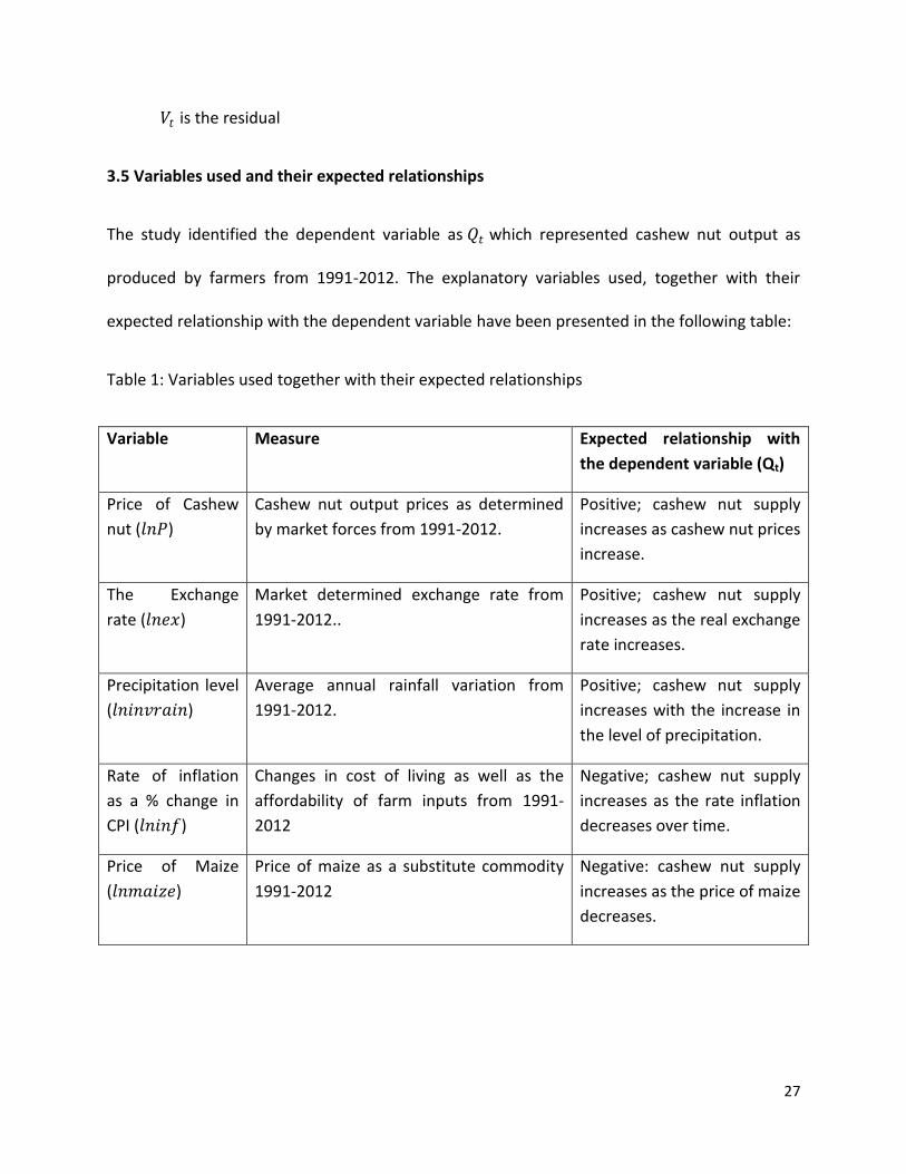
3.5 Variables used and their expected relationships

The study identified the dependent variable as 𝑄𝑡 which represented cashew nut output as

produced by farmers from 1991-2012. The explanatory variables used, together with their

expected relationship with the dependent variable have been presented in the following table:

Table 1: Variables used together with their expected relationships

Variable Measure Expected relationship with

the dependent variable (Qt)

Price of Cashew

nut (𝑙𝑛𝑃)

Cashew nut output prices as determined

by market forces from 1991-2012.

Positive; cashew nut supply

increases as cashew nut prices

increase.

The Exchange

rate (𝑙𝑛𝑒𝑥)

Market determined exchange rate from

1991-2012..

Positive; cashew nut supply

increases as the real exchange

rate increases.

Precipitation level

(𝑙𝑛𝑖𝑛𝑣𝑟𝑎𝑖𝑛)

Average annual rainfall variation from

1991-2012.

Positive; cashew nut supply

increases with the increase in

the level of precipitation.

Rate of inflation

as a % change in

CPI (𝑙𝑛𝑖𝑛𝑓)

Changes in cost of living as well as the

affordability of farm inputs from 1991-

2012

Negative; cashew nut supply

increases as the rate inflation

decreases over time.

Price of Maize

(𝑙𝑛𝑚𝑎𝑖𝑧𝑒)

Price of maize as a substitute commodity

1991-2012

Negative: cashew nut supply

increases as the price of maize

decreases.

28

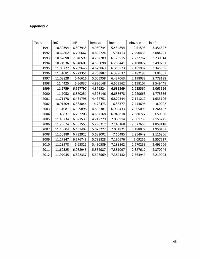
3.6 Data type and Sources

The data used by this study were mainly secondary time series data covering a period starting

from 1991 to 2012. The data were extracted from The African Development Data Bank, Bank of

Tanzania together with the Cashew nut board of Tanzania.

3.7 Statistical diagnostic tests performed

(i) The JB test for Normality

The Jarque-Bera (JB) test was employed to check for the normality of both Skewness and

kurtosis of the error term by assessing whether or not, the coefficients of skewness and excess

kurtosis are jointly equal to zero. The null hypothesis that the residuals are normally distributed

was tested against the alternative hypothesis that the residuals are not normally distributed..

(ii) The Breusch-Godfrey test for serial correlation

Breusch-Godfrey (BG) test is the valid test in the presence of higher order autocorrelation. For

first order autocorrelation, the test is asymptotically equivalent to the Durbin-Watson h

statistic, which may be considered a special case of the BG test statistic. However, Durbin-

Watson h test is not applicable for testing second or higher order autocorrelation in dynamic

models. The BG test computed Lagrange multiplier test for non-independence in the error

distribution. For a specified number of lags say (p) , it tested the null hypothesis of independent

errors against the alternative hypothesis that the errors either follows the AR(p) or MA( p) .

(iii) The Breusch –Pagan test for Heteroskedasticity

The test involved regressing the squares of the OLS residuals on a set of explanatory variables.

It was conducted by considering the Lagrange multiplier statistic: LM = 𝑛 𝑥 𝑅2 from the auxiliary

29

regression. The null hypothesis that there’s homoskedasticity was tested against its alternative

hypothesis which assumed the presence of heteroskedasticity.

(iv) Ramsey’s RESET test

This is the general test for misspecification of functional form of the model. The test for the null

hypothesis which assumes that the model is correctly specified, against the alternative

hypothesis that the model is incorrectly specified, was conducted by considering the F-test on

the powers of predicted values.

(v) The Akaike Information Criterion

The criterion has been used to test for how well our model fits the data i.e. it measured the

relative quality of the model given the available set of data. It thus deals with the trade-off

between the complexity of the model and the goodness of fit of the model. It was thus used to

determine the lag length.

30

CHAPTER FOUR

4.0 Introduction

This chapter focuses on presentation of the results of analysis. The results under consideration

include the summary statistics, the unit root test and other post estimation diagnostic tests.

The chapter also makes a comparison of obtained results with the findings of other studies.

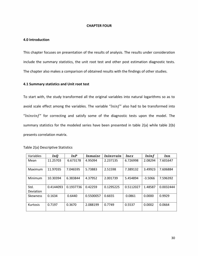
4.1 Summary statistics and Unit root test

To start with, the study transformed all the original variables into natural logarithms so as to

avoid scale effect among the variables. The variable “𝑙𝑛𝑖𝑛𝑓” also had to be transformed into

“𝑙𝑛𝑖𝑛𝑣𝑖𝑛𝑓” for correcting and satisfy some of the diagnostic tests upon the model. The

summary statistics for the modeled series have been presented in table 2(a) while table 2(b)

presents correlation matrix.

Table 2(a) Descriptive Statistics

Variables 𝒍𝒏𝑸 𝒍𝒏𝑷 𝒍𝒏𝒎𝒂𝒊𝒛𝒆 𝒍𝒏𝒊𝒏𝒗𝒓𝒂𝒊𝒏 𝒍𝒏𝒆𝒙 𝒍𝒏𝒊𝒏𝒇 𝒍𝒏𝒏 Mean 11.25703

6.673178 4.95094 2.237135 6.726998 2.08294 7.601647

Maximum 11.97035

7.046595 5.73883 2.51598 7.389132 3.49923 7.606884

Minimum 10.30394

6.383844 4.37952 2.001739 5.454894 -3.5066 7.596392

Std. Deviation

0.4144093 0.1937736 0.42259 0.1295225

0.5112027 1.48587 0.0032444

Skewness 0.1634 0.6440 0.5500057 0.6655

0.0861 0.0000 0.9929

Kurtosis 0.7197 0.3670 2.088199 0.7749

0.5537 0.0002 0.0664

31

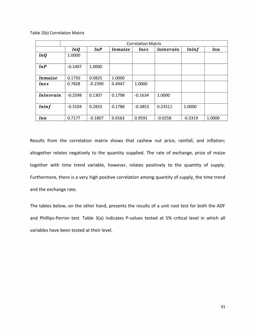
Table 2(b) Correlation Matrix

Correlation Matrix

𝒍𝒏𝑸 𝒍𝒏𝑷 𝒍𝒏𝒎𝒂𝒊𝒛𝒆 𝒍𝒏𝒆𝒙 𝒍𝒏𝒊𝒏𝒗𝒓𝒂𝒊𝒏 𝒍𝒏𝒊𝒏𝒇 𝒍𝒏𝒏

𝒍𝒏𝑸 1.0000

𝒍𝒏𝑷 -0.1407 1.0000

𝒍𝒏𝒎𝒂𝒊𝒛𝒆 0.1750 0.0825 1.0000

𝒍𝒏𝒆𝒙 0.7828 -0.2390 0.4947 1.0000

𝒍𝒏𝒊𝒏𝒗𝒓𝒂𝒊𝒏 -0.2598 0.1307 0.1798 -0.1634 1.0000

𝒍𝒏𝒊𝒏𝒇 -0.3104 0.2833 0.1788 -0.3853

0.23511 1.0000

𝒍𝒏𝒏 0.7177 -0.1807 0.6563 0.9591 -0.0258 -0.3319 1.0000

Results from the correlation matrix shows that cashew nut price, rainfall, and inflation;

altogether relates negatively to the quantity supplied. The rate of exchange, price of maize

together with time trend variable, however, relates positively to the quantity of supply.

Furthermore, there is a very high positive correlation among quantity of supply, the time trend

and the exchange rate.

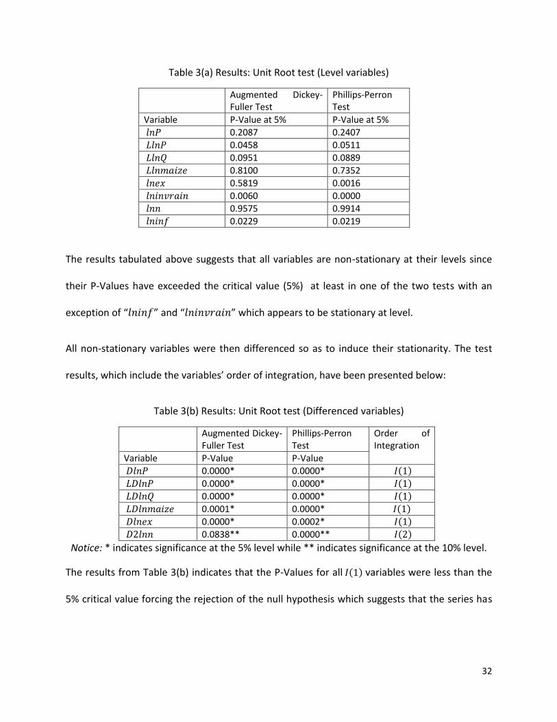
The tables below, on the other hand, presents the results of a unit root test for both the ADF

and Phillips-Perron test. Table 3(a) indicates P-values tested at 5% critical level in which all

variables have been tested at their level.

32

Table 3(a) Results: Unit Root test (Level variables)

Augmented Dickey-Fuller Test

Phillips-Perron Test

Variable P-Value at 5% P-Value at 5%

𝑙𝑛𝑃 0.2087 0.2407

𝐿𝑙𝑛𝑃 0.0458 0.0511

𝐿𝑙𝑛𝑄 0.0951 0.0889

𝐿𝑙𝑛𝑚𝑎𝑖𝑧𝑒 0.8100 0.7352

𝑙𝑛𝑒𝑥 0.5819 0.0016

𝑙𝑛𝑖𝑛𝑣𝑟𝑎𝑖𝑛 0.0060 0.0000

𝑙𝑛𝑛 0.9575 0.9914

𝑙𝑛𝑖𝑛𝑓 0.0229 0.0219

The results tabulated above suggests that all variables are non-stationary at their levels since

their P-Values have exceeded the critical value (5%) at least in one of the two tests with an

exception of “𝑙𝑛𝑖𝑛𝑓” and “𝑙𝑛𝑖𝑛𝑣𝑟𝑎𝑖𝑛” which appears to be stationary at level.

All non-stationary variables were then differenced so as to induce their stationarity. The test

results, which include the variables’ order of integration, have been presented below:

Table 3(b) Results: Unit Root test (Differenced variables)

Augmented Dickey-Fuller Test

Phillips-Perron Test

Order of Integration

Variable P-Value P-Value

𝐷𝑙𝑛𝑃 0.0000* 0.0000* 𝐼 1

𝐿𝐷𝑙𝑛𝑃 0.0000* 0.0000* 𝐼 1

𝐿𝐷𝑙𝑛𝑄 0.0000* 0.0000* 𝐼 1

𝐿𝐷𝑙𝑛𝑚𝑎𝑖𝑧𝑒 0.0001* 0.0000* 𝐼 1

𝐷𝑙𝑛𝑒𝑥 0.0000* 0.0002* 𝐼 1

𝐷2𝑙𝑛𝑛 0.0838** 0.0000** 𝐼 2

Notice: * indicates significance at the 5% level while ** indicates significance at the 10% level.

The results from Table 3(b) indicates that the P-Values for all 𝐼 1 variables were less than the

5% critical value forcing the rejection of the null hypothesis which suggests that the series has

33

unit root. However, the “D2lnn” variable had to be tested at 10% critical value since further

differencing on it would imply a significant loss of degrees of freedom.

4.2 The Co-integration Test and the ECM

The Engel and Granger (1987) test for co-integration requires all variables to be non-stationary

for their long run equilibrium to be tested. In other words, the procedure demands all variables

under consideration to be integrated of the same order i.e. order one, for their error correction

term to be formed. However, results from table 3(b) indicate otherwise since we have different

orders of integration among the variable. Such results, therefore, invalidates the test for co-

integration together with the formulation of the ECM. This is one of the reasons to why the

study resorted to the use of ARDLM bounds approach to co-integration.

4.3 Regression results

The Nerlovian model in the natural log form was estimated in Stata 12 with OLS approach. The

results have been presented in table 4. The signs of all the coefficients are as predicted in the

theory except for the exchange rate variable, which contradicted the priori assumption. Result

shows that the log of supply output increases as the log of exchange rate together with the lag

of log inflation declines. The rest of the variables appeared to exert a positive influence on the

dependent variable. All of these variables explain about 90% of the variations in Tanzanian

cashew nut supply.

34

Table 4(a): OLS Regression results for the Cashew nut supply response from 1991-2012

Dependent Variable 𝐷𝑙𝑛𝑄

Independent Variable Coefficient t-value P-value

Constant -9.119196 -4.77 0.001*

𝐷𝑙𝑛𝑃 1.420948 6.71 0.000*

𝐷𝑙𝑛𝑚𝑎𝑖𝑧𝑒 -0.6903198 -5.12 0.001*

𝐿𝐷𝑙𝑛𝑒𝑥 -2.983909 -6.75 0.000*

𝐿𝐷𝑙𝑛𝑖𝑛𝑣𝑟𝑎𝑖𝑛 0.8111361 2.30 0.047*

𝐿𝐷𝑙𝑛𝑖𝑛𝑓 0.2275446 5.65 0.000*

𝐿𝑙𝑛𝑃 1.521947 6.24 0.000*

𝐿𝑙𝑛𝑚𝑎𝑖𝑧𝑒 -0.061464 -0.52 0.615

𝐿𝑙𝑛𝑒𝑥 -0.3878616 -2.56 0.030*

𝐿𝑙𝑛𝑖𝑛𝑣𝑟𝑎𝑖𝑛 1.096801 1.73 0.117

𝐿𝑙𝑛𝑖𝑛𝑓 -0.0660379 -1.81 0.104

Adjusted R2 = 0.8087 Observations = 20

Notice that: * indicates significance at the 5% level while ** indicates significance at the 10% level.

From the table; 𝐿𝑙𝑛𝑖𝑛𝑓, 𝐿𝑙𝑛𝑖𝑛𝑣𝑟𝑎𝑖𝑛, and 𝐿𝑙𝑛𝑚𝑎𝑖𝑧𝑒 are statistically insignificant while the rest of

the variable are statistically significant at 5% level of significance.

4.4 The ARDL Co-integration Test

The following tables present the test results for co-integration together with the diagnostic test

results obtained.

Table 4(b) The ARDL co-integration results

Bounds Test to Co-integration

Estimated Equation 𝑙𝑛𝑄= 𝑓(𝐿𝑙𝑛𝑃, 𝑙𝑛𝑚𝑎𝑖𝑧𝑒, 𝑙𝑛𝑒𝑥,𝑙𝑛𝑖𝑛𝑣𝑟𝑎𝑖𝑛, 𝑙𝑛𝑖𝑛𝑓)

F-statistics 9.03 (0.0014)

Significant level Lower Bounds 𝐼 1 Upper Bound 𝐼 1

1 percent 5.856 7.578

5 percent 4.154 5.540

10 percent 3.430 4.624

35

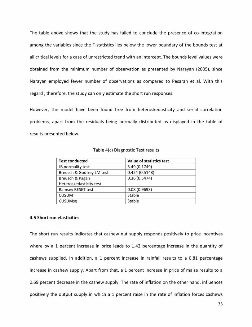
The table above shows that the study has failed to conclude the presence of co-integration

among the variables since the F-statistics lies below the lower boundary of the bounds test at

all critical levels for a case of unrestricted trend with an intercept. The bounds level values were

obtained from the minimum number of observation as presented by Narayan (2005), since

Narayan employed fewer number of observations as compared to Pesaran et al. With this

regard , therefore, the study can only estimate the short run responses.

However, the model have been found free from heteroskedasticity and serial correlation

problems, apart from the residuals being normally distributed as displayed in the table of

results presented below.

Table 4(c) Diagnostic Test results

Test conducted Value of statistics test

JB normality test 3.49 (0.1749)

Breusch & Godfrey LM test 0.424 (0.5148)

Breusch & Pagan Heteroskedasticity test

0.36 (0.5474)

Ramsey RESET test 0.08 (0.9693)

CUSUM Stable

CUSUMsq Stable

4.5 Short run elasticities

The short run results indicates that cashew nut supply responds positively to price incentives

where by a 1 percent increase in price leads to 1.42 percentage increase in the quantity of

cashews supplied. In addition, a 1 percent increase in rainfall results to a 0.81 percentage

increase in cashew supply. Apart from that, a 1 percent increase in price of maize results to a

0.69 percent decrease in the cashew supply. The rate of inflation on the other hand, influences

positively the output supply in which a 1 percent raise in the rate of inflation forces cashews

36

supply to increase by 0.23 percent. Lastly, the rate of exchange rate appears to have negative

effect on cashew supply by which a 1 percent increase in exchange rate leads to almost 3

percent reduction of cashews supplied.

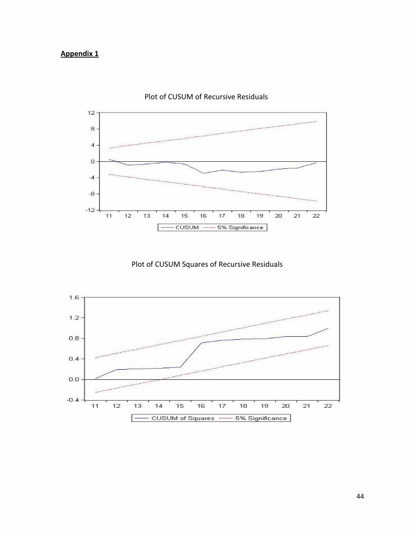
4.6 Stability Tests

Both, the CUSUM and CUSUM squared statistics do not strays out of the 95% confidence band

as indicated in figure 4 and 5; in which, the null hypothesis that the model is well specified and

the parameters are stable cannot be rejected, (Bahmani-Oskooee, M and Nasir, AM 2004).

Thus, the test results suggest that indeed, the parameters used in the model are reliable and

well fits for statistic inferences.

4.7 The Comparison of Study Results

The results from this study have suggested that pricing policy is elastic and effective towards

influencing the level of output in the short run. These results seems to share a similar, in terms

of short run responses prices, as earlier studies done by Gosalamang et al (2012) in Botswana

and Lafrance & Burt (1983) in USA. These results, therefore, refutes the conventional belief

which claims that agricultural output supply response is generally inelastic.

37

CHAPTER FIVE

5.0 Conclusion, Policy Implications and Recommendations

The chapter presents a summary result of the main findings apart from pointing out the policy

implications such obtained results together with making some policy recommendations to be

worked upon by both private and public stakeholder in making sure that the sector keeps on

improving.

5.1 Conclusion

The results from this study have clearly indicated that that farmers or suppliers of the cashew

nuts respond well to price incentives. The study reported short run price elasticity of 1.42,

which is elastic. However, the study failed to extract the long run responses since the evidence

rejected the presence of co-integration. The results indicated that price incentives, amount of

rainfall as well as the rate of inflation, altogether exerted a positive influence on the cashew nut

supplied on one hand. On the other hand, exchange rate together with price of maize had a

negative influence on the cashew supply in the short run.

5.2 Policy implications and Recommendations

In the context of policy implications, the study is helpful to both public as well as private

stakeholders involved in the cashew nut sector in Tanzania. The CBT must understand the

strength of price signals to the farmers. The announce of good indicative prices will be well

received by the farmers. However, such announcements won’t be of any use to the farmers if

they fail to benefit from it. This suggests further that there is still a need of proper supervision

38

on the sector to prevent middle traders from exploiting the farmers through collusion practices

among the buyers.

Such measures will allow price incentives to work more effective on benefiting the farmers at

the ground and improve the government revenue ripped from the sector for at least in the

short run. On the same account, for price incentives to be fruitful, the non-price incentives also

need to be incorporated at least in the short run. These two must work hand in hand with each

other for the greater good at the greatest number.

It should be also noted that, exchange rate in the floating regime still poses great challenge on

today’s economy. Any appreciation of local currency against the US dollar is more likely to hurt

harder the farmers at the ground. However, the impact may be less intense if most of the

supplied cashews would have been processed locally due to the fact that currency appreciation

would have ease the burden for the importation of spare parts for processing machines. The

results, therefore, calls upon the B0T to exercise control on exchange rate volatility in such a

way that, critical and necessary continuous intervention by the BoT in the exchange rate

markets must be a priority.

5.3 Limitations of the Study

To the reasonable extent, the study has been successful in meeting the research objectives.

However, there has been some challenges and limitations that are not worthwhile being

ignored. The main limitation in this study has to do with the reliability and availability of data.

The study could have included more variables in the analysis but most of the data are either

unavailable or need to be compiled from different sources, something which may alter the

39

authenticity of the data. In fact, one notable reason to why the study has failed to estimate long

run elasticities, is deeply embodied into the problems associated with the nature of the data

used in the analysis.

5.4 Areas for further research

Cashew nut sector in Tanzania plays a very crucial role not only to the government but also to

the farmers especially in the southern east part of the country. Despite two decades of

liberalization, still there are no clear explanations to why the private sector has failed to

significantly excelling the sector. Much work needs to be done on this area to shed enough light

on the problem and provide numerous solutions or alternatives with the aim of improving the

sector.

40

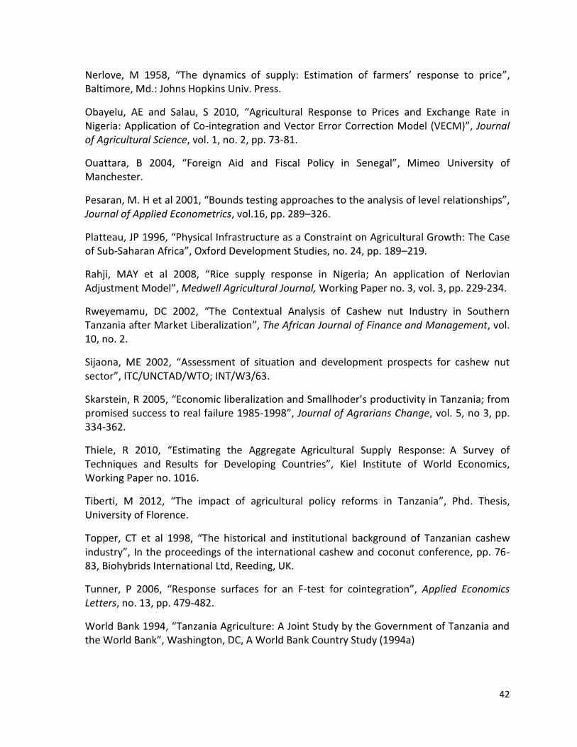
References

Akiyama, TJ et al 2001, “Commodity Market Reforms: Lessons of Two Decades”, Washington,DC, World Bank.

Askari, H and Commings, JT 1977, “Estimating Agricultural Supply Response with the Nerlove Model: A Survey”, International Economic Review, vol. 18, no. 2, pp. 257-292.

Bahmani-Oskooee, M and Nasir, AM, 2004 “ARDL Approach to test Productivity Bias Hypothesis”, Review of Development Economics, pp. 483-488.

Barratt, BM 1995, “Africa’s Choices: After Thirty Years of the World Bank”, London, Penguin Books.

Bloom, DE and Sachs, J 1998, “Geography, Demography, and Economic Growth in Africa”, Brookings Papers on Economic Activity, no. 2, pp. 207–273.

Cleaver, KM 1993, “A Strategy to Develop Agriculture in Sub-Saharan Africa and a Focus for the World Bank”, Washington, DC, World Bank Technical Paper no. 203.

Gatete, C 1993, “Economic analysis of coffee supply in Kenya”, Masters Thesis, University of British Columbia.

Gosalamang, DS et al 2012, “Supply response of beef farmers in Botswana: A Nerlovian partial adjustment model approach”, African Journal of Agricultural Research, vol. 7(31), pp. 4383-438.

Granger, CWJ and Newbold, P 1974, “Spurious Regressions in Econometrics”, Journal of Econometrics, Vol. 26.

Halcoussis, D 2005, “Understanding econometrics”, Thomson: South western.

Jafee, S and Morton, J 1995, “Marketing Africa’s high value foods; Comparative experience of emergent private sector”, The World Bank, Washington.

Johnson, DG 1950, “The nature of supply function for agricultural products”, American economic review, vol. 40(4), pp. 539-564.

Ketut, B and Bambang, D 2004, “Impact of Liberalization on Competitiveness and Efficiency of Cahew nut Industry in Nusa Taggara Barat province”, Faculty of Agriculture, Mataram University.

Koo, W 1982, “An Econometric Analysis of U.S. Wheat Acreage Response: The Impact of Changing Government Programs”, Agricultural Economics Report no. 157.

Koop, G 2002, “Parametric and Nonparametric Inference in Equilibrium Job Search Models”, Discussion Papers in Economics 04/14, Department of Economics, University of Leicester.

41

Krueger, AO et al 1992, “The Political Economy of Agricultural Pricing Policies”, A World Bank Comparative Study, Baltimore.

Lafrance, JT and Burt, OR 1983, “A Modified Partial Adjustment Model of Aggregate U.S. Agricultural Supply”, Western Journal of Agricultural Economics, vol. 8, no. 1, pp. 1-12.

Loxley, J 1983, “The Berg report and model of accumulation in sub-Saharan Africa”, Review of African Political Economy, no. 27/28, pp. 197-204.

Lunberg, M 2004, “Agricultural markets reforms; An analysis of distributional impacts of reforms”, Development economics research group and poverty reduction and economic management.

Mans, D 1994, “Tanzania: Resolute action,” in I. Husain and R. Faruqee (eds.), Adjustment in Africa, Lessons from Country Case Studies, pp. 352–426.

Mashindano, OJN and Limbu, FL 2002, “The Agricultural sector and poverty in Tanzania; the impact and future of reform process”.

McKay, A et al 2006, “Aggregate supply response in Tanzanian agriculture”, The Journal of International Trade & Economic Development, vol. 8, no.1, pp. 107-123.

McMillan, M et al 2002, “When Economic reforms goes wrong; Cashews in Mozambique”, National Bureau of Economic Research, Working Paper No. 9117.

Meerteens, B 2000, “Agricultural performance in Tanzania under structural adjustment programs: Is it really so positive?” Kluwer Academic Publishers, Journal of Agriculture and Human Values, no. 17, pp. 333–346.

Mitchell, D 2004, “Tanzania’s cashew sector; Constraints and Challenges in the global environment”, African region, Working Paper no. 70.

Muchapondwa, E 2008, “Estimation of the aggregate agricultural supply response in Zimbabwe: The ARDL approach to Co-integration”, School of Economics, University of Cape Town, Working Paper no. 90.

Mythili, G 2006, “Supply Response of Indian Farmers; Pre and Post Reforms”, Journal of Economic Literature, Working Paper no. 009.

Nambiar, MC et al 1990, “Cashew in; Bose TK, Mitra SK(eds) Fruits, Tropical and Sub-tropical, Naya Prakash, Calculta”, pp 386-414.

Narayan, PK 2005, “The saving and investment nexus for China: evidence from co-integration tests”, Applied Economics, vol. 37, no. 17, pp. 1979-1990.

Nerlove, M 1956, “Estimation of elasticities of supply of selected agricultural commodities”, Journal of farm economics, vol. 38, no.2, pp. 494-509.

42

Nerlove, M 1958, “The dynamics of supply: Estimation of farmers’ response to price”, Baltimore, Md.: Johns Hopkins Univ. Press.

Obayelu, AE and Salau, S 2010, “Agricultural Response to Prices and Exchange Rate in Nigeria: Application of Co-integration and Vector Error Correction Model (VECM)”, Journal of Agricultural Science, vol. 1, no. 2, pp. 73-81.

Ouattara, B 2004, “Foreign Aid and Fiscal Policy in Senegal”, Mimeo University of Manchester.

Pesaran, M. H et al 2001, “Bounds testing approaches to the analysis of level relationships”, Journal of Applied Econometrics, vol.16, pp. 289–326.

Platteau, JP 1996, “Physical Infrastructure as a Constraint on Agricultural Growth: The Case of Sub-Saharan Africa”, Oxford Development Studies, no. 24, pp. 189–219.

Rahji, MAY et al 2008, “Rice supply response in Nigeria; An application of Nerlovian Adjustment Model”, Medwell Agricultural Journal, Working Paper no. 3, vol. 3, pp. 229-234.

Rweyemamu, DC 2002, “The Contextual Analysis of Cashew nut Industry in Southern Tanzania after Market Liberalization”, The African Journal of Finance and Management, vol. 10, no. 2.

Sijaona, ME 2002, “Assessment of situation and development prospects for cashew nut sector”, ITC/UNCTAD/WTO; INT/W3/63.

Skarstein, R 2005, “Economic liberalization and Smallhoder’s productivity in Tanzania; from promised success to real failure 1985-1998”, Journal of Agrarians Change, vol. 5, no 3, pp. 334-362.

Thiele, R 2010, “Estimating the Aggregate Agricultural Supply Response: A Survey of Techniques and Results for Developing Countries”, Kiel Institute of World Economics, Working Paper no. 1016.

Tiberti, M 2012, “The impact of agricultural policy reforms in Tanzania”, Phd. Thesis, University of Florence.

Topper, CT et al 1998, “The historical and institutional background of Tanzanian cashew industry”, In the proceedings of the international cashew and coconut conference, pp. 76-83, Biohybrids International Ltd, Reeding, UK.

Tunner, P 2006, “Response surfaces for an F-test for cointegration”, Applied Economics Letters, no. 13, pp. 479-482.

World Bank 1994, “Tanzania Agriculture: A Joint Study by the Government of Tanzania and the World Bank”, Washington, DC, A World Bank Country Study (1994a)

43

World Bank 1983, “World Development Report”, Management in Development, New York, Oxford University Press.

Yu, B et al 2010, “Dynamic agricultural Supply response under Economic Transformation; A Case Study of Henan Province”, IFPRI Discussion Paper no. 00987.

44

Appendix 1

Plot of CUSUM of Recursive Residuals

Plot of CUSUM Squares of Recursive Residuals

45

Appendix 2

Years lnQ lnP lnmaize lnex lninvrain lninf

1991 10.30394 6.807935 4.960744 5.454894 2.51598 3.356897

1992 10.62862 6.706667 4.865224 5.81413 2.290435 3.084201

1993 10.57898 7.046595 4.767289 6.173515 2.227767 3.230014

1994 10.74936 6.948609 4.593098 6.260441 2.188077 3.499231

1995 11.05722 6.709646 4.629863 6.310573 2.151937 3.345685

1996 11.31081 6.723351 4.763882 6.389637 2.182196 3.04357

1997 11.08828 6.46616 5.005958 6.437063 2.198032 2.778198

1998 11.4425 6.66037 4.930148 6.523562 2.158107 2.549445

1999 11.5759 6.527797 4.379524 6.681269 2.235567 2.065596

2000 11.7052 6.870251 4.398146 6.688678 2.220663 1.778336

2001 11.71178 6.431798 4.436751 6.820344 2.141219 1.635106

2002 10.91509 6.383844 4.72473 6.88377 2.444696 -0.0202

2003 11.31081 6.559898 4.802381 6.969433 2.005095 1.264127

2004 11.43831 6.702206 4.607168 6.949818 2.380727 -3.50656

2005 11.40734 6.621539 4.712229 7.060914 2.001739 2.155245

2006 11.25674 6.387553 5.298317 7.140168 2.377655 1.859418

2007 11.43604 6.431492 5.023222 7.031821 2.188077 1.950187

2008 11.50388 6.732925 5.633002 7.15485 2.254649 2.116256

2009 11.27847 6.576748 5.738828 7.190676 2.09255 2.557227

2010 11.28978 6.65325 5.490589 7.288162 2.270239 2.493206

2011 11.69525 6.968945 5.562987 7.381097 2.327617 2.370244

2012 11.97035 6.892337 5.596569 7.389132 2.363949 2.219203