economic profitability of the bakken, north
TRANSCRIPT
Michigan Technological University Michigan Technological University
Digital Commons @ Michigan Tech Digital Commons @ Michigan Tech
Dissertations, Master's Theses and Master's Reports - Open
Dissertations, Master's Theses and Master's Reports
2014
ECONOMIC PROFITABILITY OF THE BAKKEN, NORTH DAKOTA ECONOMIC PROFITABILITY OF THE BAKKEN, NORTH DAKOTA
UNCONVENTIONAL OIL PLAYS BASED ON A TYPICAL WELL UNCONVENTIONAL OIL PLAYS BASED ON A TYPICAL WELL
PERFORMANCE WITH CURRENT MARKET CONDITIONS PERFORMANCE WITH CURRENT MARKET CONDITIONS
Mehmet Apaydin Michigan Technological University
Follow this and additional works at: https://digitalcommons.mtu.edu/etds
Part of the Economics Commons, Finance and Financial Management Commons, and the Petroleum
Engineering Commons
Copyright 2014 Mehmet Apaydin
Recommended Citation Recommended Citation Apaydin, Mehmet, "ECONOMIC PROFITABILITY OF THE BAKKEN, NORTH DAKOTA UNCONVENTIONAL OIL PLAYS BASED ON A TYPICAL WELL PERFORMANCE WITH CURRENT MARKET CONDITIONS", Master's Thesis, Michigan Technological University, 2014. https://doi.org/10.37099/mtu.dc.etds/866
Follow this and additional works at: https://digitalcommons.mtu.edu/etds
Part of the Economics Commons, Finance and Financial Management Commons, and the Petroleum Engineering Commons
ECONOMIC PROFITABILITY OF THE BAKKEN, NORTH DAKOTA
UNCONVENTIONAL OIL PLAYS BASED ON A TYPICAL WELL
PERFORMANCE WITH CURRENT MARKET CONDITIONS
By
Mehmet Apaydin
A THESIS
Submitted in partial fulfillment of the requirements for the degree of
MASTER OF SCIENCE
In Applied Natural Resource Economics
MICHIGAN TECHNOLOGICAL UNIVERSITY
2014
©2014 Mehmet Apaydin
This thesis has been approved in partial fulfillment of the requirements for the Degree of MASTER OF SCIENCE in Applied Natural Resource Economics.
School of Business and Economics
Thesis Co – Advisor: Dr. Mark C. Roberts
Thesis Co – Advisor: Dr. Gary A. Campbell
Committee Member: Dr. Roger Turpening
School Dean: Dr. R. Eugene Klippel

iii
Dedication
I would like to dedicate this thesis to my family and the Turkish Petroleum
Corporation.

iv
Table of Contents
List of Figures .......................................................................................................... vi
List of Tables .......................................................................................................... viii
Abstract……………………………………………………………………………..x
1. Introduction & Background ................................................................................ 1
1.1 Introduction ....................................................................................................... 1
1.2. Background ...................................................................................................... 6
2. Economic and Environmental Issues linked with Unconventional Oil
Production ............................................................................................................... 11
2.1. Unconventional Production Cost ................................................................... 12
2.2. Production Decline Rates ............................................................................... 14
2.3. Oil Price Volatility, Transportation and Refinery Issues ............................... 17
2.4. Environmental and Social Concerns .............................................................. 21
2.5. Recent Bakken Operations ............................................................................. 23
3. Methodology ........................................................................................................ 25
3.1. North Dakota Bakken Unconventional Oil Prices ......................................... 26
3.2. Total Drilling and Completion Costs ............................................................. 27
3.3. Lease Agreements and Royalty Payments ..................................................... 28
3.4. Production Rates ............................................................................................ 30
3.5. Taxation ......................................................................................................... 34
3.5.1. North Dakota State Taxes ....................................................................... 34
3.5.2. Federal Income Tax ................................................................................. 36
3.6. Lease Operating Expenses (LOE) .................................................................. 37
3.7. Tax Benefits ................................................................................................... 38
3.7.1. Tax Deductions for Intangible Drilling Cost .......................................... 38
3.7.2. Tax Deductions for Tangible Drilling Cost ............................................ 38
3.7.3. Depletion Allowance ............................................................................... 40

v
3.8. Scenarios ........................................................................................................ 40
3.8.1. Re-fracturing ........................................................................................... 41
3.9. Calculations ................................................................................................... 43
4. Scenario Analysis and Results ........................................................................... 44
4.1. Typical Bakken unconventional oil well (Simulated well) ........................... 44
4.1.1. Production Decline Curve for the First Scenario .................................... 46
4.1.2. Production Decline Curve for the Second Scenario ................................ 49
4.1.3. Production Decline Curve for the Third Scenario ................................... 51
4.1.4. Production Decline Curve for the Fourth Scenario ................................. 53
4.2. Cash Flow Statements for Scenarios ............................................................. 56
4.2.1. First Scenario (5 years production) ......................................................... 56
4.2.2. Second Scenario (10 years production) ................................................... 59
4.2.3. Third Scenario (20 years production) ..................................................... 63
4.2.4. Fourth Scenario (Another well drilled in year ten) ................................. 69
4.3. Break-even Analysis (Break-even prices) ..................................................... 75
4.4. Comparison of Results ................................................................................... 77
5. Discussion of Results .......................................................................................... 83
6. Conclusions ......................................................................................................... 89
7. References ........................................................................................................... 93

vi
List of Figures
Figure 1.1: United States Map .................................................................................... 8
Figure 1.2: Location map of the Williston Basin ....................................................... 9
Figure 2.1: Theoretical Production Curve ................................................................ 15
Figure 2.2: WTI - Bakken crude oil differential between June 2011 - May 2013 ... 19
Figure 2.3: Clearbrook crude oil prices between May 2010 - May 2014 ................. 20
Figure 4.1: Production decline curve vs. annual oil production rates for the first
scenario ..................................................................................................................... 47
Figure 4.2: Annual oil production vs. EUR for the first scenario ............................ 48
Figure 4.3: Production decline curve for the second scenario .................................. 50
Figure 4.4: Annual oil production vs. EUR for second scenario .............................. 50
Figure 4.5: 20 year production decline curve for the third scenario ........................ 51
Figure 4.6: Annual oil production vs. EUR for the third scenario ........................... 52
Figure 4.7: Production decline curve for the fourth scenario ................................... 54
Figure 4.8: Annual oil production vs. EUR for the fourth scenario ......................... 54
Figure 4.9a: Cash flow statements for the first scenario years 0 through 4 ............. 57
Figure 4.9b: Cash flow statement for the first scenario for 5 years ......................... 58
Figure 4.10a: Cash flow statement between years 0 and 4 (second scenario) ......... 60
Figure 4.10b: Year 5 through 9 (second scenario) ................................................... 61
Figure 4.10c: Cash flow statements for the second scenario covering 10 years ...... 62
Figure 4.11a: Cash flow statement between year 0 and 4 (third scenario) ............... 64
Figure 4.11b: Year 5 through 9 (third scenario) ....................................................... 65

vii
Figure 4.11c: Year 10 through 14 (third scenario) ................................................... 66
Figure 4.11d: Year 15 through 19 (third scenario) ................................................... 67
Figure 4.11e: Cash flow statements for the third scenario including 20 years ......... 68
Figure 4.12a: Cash Flow statements between year 0 and 4 (fourth scenario) .......... 70
Figure 4.12b: Year 5 through 9 ............................................................................... 71
Figure 4.12c: Year 10 through 14, new well drilled in tenth year (fourth scenario) 72
Figure 4.12d: Year 15 through 19 (fourth scenario) ................................................. 73
Figure 4.12e: Cash flow statements for the fourth scenario, including two wells ... 74
Figure 4.13:Sensitivity analysis for the best scenario (fourth scenario) .................. 81
viii
List of Tables
Table 2.1: Bakken Drilling Averages 2008 - 2013 ................................................... 13
Table 3.1: North Dakota Gross Oil Production Tax Allocation ............................... 35
Table 3.2: North Dakota Oil Extraction Tax Allocation .......................................... 35
Table 3.3: U.S. Federal Income Tax Rate Schedule ................................................. 36
Table 3.4: 7-years MACRS Depreciation ................................................................ 39
Table 4.1: Initial input values for the hyperbolic curve ........................................... 45
Table 4.2: Input values for the simulated Bakken Well ........................................... 56
Table 4.3: NPV, IRR, and EUR results for the first scenario ................................... 59
Table 4.4: NPV, IRR, and EUR results for the second scenario .............................. 63
Table 4.5: NPV, IRR, and EUR results for the third scenario .................................. 69
Table 4.6: NPV, IRR, and EUR results for the fourth scenario ............................... 75
Table 4.7: Break-even prices for the scenarios ........................................................ 76
Table 4.8: Initial input values for a simulated well .................................................. 77
Table 4.9: Comparison of results based on the cash flow statements ...................... 78
Table 4.10: Changes in NPV by drilling cost change .............................................. 79
Table 4.11: Changes in the NPV by oil price change ............................................... 80
Table 4.12: Changes in the NPV by production rate change ................................... 80
Table 4.13: Changes in the NPV by royalty rate change ......................................... 80
Table 4.14: Changes in the NPV by LOE change .................................................... 81
Table 5.1: Oil prices during the production time ..................................................... 84
Table 5.2: NPV and IRR changes with constant oil prices ...................................... 84

ix
Table 5.3: Changes in NPV and IRR with increased lease operating expenses ....... 86
Table 5.4: Nominal Annual Decline Rates for the simulated Bakken Well ............. 87
x
Abstract
Increases in oil prices after the economic recession have been surprising for
domestic oil production in the United States since the beginning of 2009. Not only
did the conventional oil extraction increase, but unconventional oil production and
exploration also improved greatly with the favorable economic conditions. This
favorable economy encourages companies to invest in new reservoirs and
technological developments. Recently, enhanced drilling techniques including
hydraulic fracturing and horizontal drilling have been supporting the domestic
economy by way of unconventional shale and tight oil from various U.S. locations.
One of the main contributors to this oil boom is the unconventional oil production
from the North Dakota Bakken field. Horizontal drilling has increased oil
production in the Bakken field, but the economic issues of unconventional oil
extraction are still debatable due to volatile oil prices, high decline rates of
production, a limited production period, high production costs, and lack of
transportation. The economic profitability and viability of the unconventional oil
play in the North Dakota Bakken was tested with an economic analysis of average
Bakken unconventional well features. Scenario analysis demonstrated that a typical
North Dakota Bakken unconventional oil well is profitable and viable as shown by
three financial metrics; net present value, internal rate of return, and break-even
prices.
1
1. Introduction & Background
1.1 Introduction
The US oil supply has been substantially rising for the last 5-6 years because
of new exploration and production from various sources such as conventional
reservoirs, tar sands, tight oil formations, and unconventional oil production from
the shale deposits that were not previously considered as the main target reservoirs.
Since the beginning of the year 2009, domestic crude oil production has been
trending upward in the United States as a result of the steady enhancements in
drilling techniques, and these developments also decrease the completion costs.
After a peak oil in 1970, the American oil production began to decline. Most
of the giant sized oil fields were discovered in the United States and production was
declining. Producers were unable to offset the rising oil demand with new
exploration and development. However, a considerable oil demand decline occurred
in the 2007-08 recession. But after the recession, oil price significantly increased
from $39 to $102 per barrel between February 2009 and May 2014 associated with
demand (Energy Information Administration 2014). High demand for oil with high
oil price motivated the American operators to focus on new fields and explore new
reservoir formations by using unconventional methods. Companies began to
concentrate on new fields such as tight oil sands and shale reservoirs because the
largest oil fields in the United States were discovered previously and oil production
was declining from these fields. Hydraulic fracturing gained importance with
technical developments. In reality, hydraulic fracturing was known from 1949.
2
However, the economic conditions did not provide a profitable environment for
fracturing until the 2000s because the cost of fracturing was much higher than
drilling a new well.
The production from new fields by fracturing horizontal holes started to
increase domestic oil production in the United States and the International Energy
Agency (IEA) forecasters emphasized that the US was on the way to surpass Russia
and Saudi Arabia to become the largest crude oil producer globally in 2020
(Bloomberg 2012). And just a few months later, IEA’s 2013 forecasts shortened this
period and pointed out the phenomenon would drive the US to become the biggest
producer 5 years before the previous IEA estimates with the help of technical
improvements and the great oil support from the unconventional oil flows,
especially from Texas and the Williston Basin, Bakken Fields (Bloomberg 2013).
Unexpectedly, a recent update has been declared by the IEA and they heralded that
the US has already surpassed other countries and producing more than 11 million
barrels of crude oil per day including liquids separated from natural gas (Smith
2014).
It is obvious that developments in oil production seem much faster now than
in the last decade, but it is still not clear that the United States will hold its
production position. Even though the annual domestic oil production has increased
year by year after 2008, annual US petroleum consumption is still much higher than
production, thus demanding oil from exporter countries. In 2012, US oil
consumption was equal to 18.49 million barrels per day, but domestic demand has
3
continued to decline year by year because the natural gas industry substituted for oil
use and decreased the oil consumption in heating and electric generation sectors.
(Annual Energy Outlook 2014). The transportation industry consumes the largest
share of oil products, accounting for 70.42 percent of the annual consumption in
2012 (Annual Energy Outlook 2014).
From the point of view of economics, high taxation and new regulations to
decrease petroleum consumption will not significantly induce consumers to give up
consuming oil in the short term. Consumer demand for crude oil is different from
and more essential than many other goods and products. High negotiated reference
prices by suppliers cannot be elastic in the short run, especially for transportation
and oil based chemical industries because it is not economic to substitute for oil
with other products. It is clear that the use of renewable energy sources will not
dominate the vehicle industry in the near future because of the infrastructural
problems and new efficient gas and diesel vehicles. Therefore, new exploration and
high production rates are very crucial to meet future demands.
As mentioned above, hydraulic fracturing gained importance in the first
decade of the 21st century as a result of developing technology and increasing oil
price. It is one of the most effective ways to produce a reservoir. Previously, it was
unprofitable to apply the unconventional drilling techniques. The cost of
unconventional drilling including hydraulic fracturing was very expensive, and did
not deliver profitable results for the investors. Then, in the early 2000s, operators
started to use hydraulic fracturing in shale reservoirs (both in oil and gas

4
operations), which were not mainly considered as profitable reservoirs. Operations
gave profitable results in unconventional shale oil and shale gas fields such as
Marcellus Shale, Eagle Ford, and Barnett Shale. This phenomenon motivated and
influenced investors in many locations. The Bakken Field – Three Forks Formation
of the Williston Basin is one of the examples for this trend.
The North Dakota Bakken Field is one of the most productive oilfields for
the US since 2007 because of unconventional operations. North Dakota drilling
operations first started in 1951, but never had a great impact on the US oil market
until 2009. High oil prices and high demand for crude oil made unconventional oil
investments more attractive in the Bakken Field and triggered local investors and
the small & medium – sized oil companies to invest in the shale deposits. EOG
Resources Company’s drilling operations is the main operator in the area. Oil
extraction from the Bakken will be an important case study associated with the
beneficial utilization of oil because it creates numerous job opportunities and
increases state income because of royalty fees and taxes from oil extraction.
Moreover, current results state that unconventional oil production makes the Bakken
field the second largest oil field in the US after Alaska’s Prudhoe Bay (Mason
2012a). In the month of April 2014, oil production reached 1,001,149 barrels per
day (Wegmann 2014).
On the other hand, the Bakken Field can still be assumed to be a new basin
for investment. Current circumstances imply that some issues associated with

5
unconventional oil economics will obstruct the investments of the major oil
companies in the future. These concerns are explained in chapter 2.
This study encompasses a comprehensive economic analysis of the North
Dakota Bakken unconventional oil plays and will determine whether or not
producers are able to produce more profitable oil with recent market conditions
(mid-2014) by using typical well profiles for 5 year, 10 year, and 20 year investment
plans. Different scenarios and well simulations were implemented to assess the
Bakken Field unconventional oil plays’ overall profitability, economic viability, the
impact of decline rates by using initial production (IP) rates, cost variables, and
other input values. To calculate the profitability of these scenarios, three decision
making financial metrics were used; Net Present Value (NPV), Internal Rate of
Return (IRR), and break-even prices. Environmental and social costs related to
hydraulic fracturing were partially avoided for the financial calculations, but
mentioned in the next chapters.
For the purpose of this analysis, previous studies are examined. James
Mason’s studies related to the North Dakota Bakken are the main reason to focus on
the area because Mason points out the huge oil potential of North Dakota and the
peak oil issues for the next years (Mason 2012a) (Mason 2012b). In addition, the
United States Geological Survey (USGS) oil assessment reports has been changing
almost every year that enhances undiscovered oil potential and increases the
curiosity on the Bakken area (USGS 2013). Also, Harvard Kennedy School’s shale
oil boom report and annual reports of the companies gave the main idea for the
6
economic analysis (Maugeri 2013). Therefore, this study focuses on the profitability
of unconventional oil investment in North Dakota with current market conditions
(mid-2014).
This analysis concentrated on the current factors, Society of Petroleum
Engineers (SPE) formulations and recommended decline curve parameters, cost
variables, taxation, and state regulations that were active in June 2014 (mid-2014)
and will be active for the next few years.
1.2. Background
Initial oil was drilled in 1859 by Edward Colonel Drake in Titusville,
Pennsylvania. Within 155 years from 1859 to 2014, numerous inventions and
innovations occurred in the oil and gas industries. Oil first gained importance when
coal steam engines converted into oil based engines in the late 1800s. The United
States began importing oil in the early 1950s. The biggest global oil crisis appeared
in the 1970s. The 1973 crisis hampered the US global oil hegemony because of the
Arab-Israeli War. Not only did production decline, but also the oil price increased
extremely between 1973 and 1985 since OPEC initiated control of the upstream
markets, which squeezed the American domestic market and hindered the US
economy with shortages of petroleum products.
US oil production was declining after the 1970s. Crude oil production
peaked in 1970 at 9.64 million barrels per day, and then fluctuated many years until
the end of 2008 (Oil and Energy Trends 2012).Until the end of the first decade of
7
the millennium century, most of the giant oil fields were already discovered in the
US; proved oil reserves of the United States and its domestic production were both
declining. The internal oil supply was not able to meet domestic consumption. In
2008, the US economy went into a big recession with the mortgage crisis, oil prices
rose from 2003 to 2008, and as a result, the United States paid additional billions of
dollars for external oil supply imported from Canada, Mexico, and other countries in
the recession period. These issues impacted the economic plans of oil management.
On the other hand, the US responded to this recession by decreasing oil
consumption, but it was not enough to decrease the prices since consumption was so
much higher than the domestic supply.
Recent statistics show that US domestic oil production has been steadily
increasing since 2009. The year 2008 was the lowest production level for the
American crude oil industry at 5.0 million barrels per day since 1946 (Oil and
Energy Trends 2012). Recently, the domestic production increase has been due to
new production from the Gulf of Mexico offshore wells and the unconventional oil
production boom from shale deposits. Unconventional drilling and shale oil
extraction are relatively new trends for the U.S., and the dynamics of the oil
industry started to change with the improvements in these techniques. These
technical improvements, high oil prices, and declining costs of production have
made investment more feasible than in the last decade, and this has been the main
reason for the oil boom around the Bakken area since 2008. Major American oil
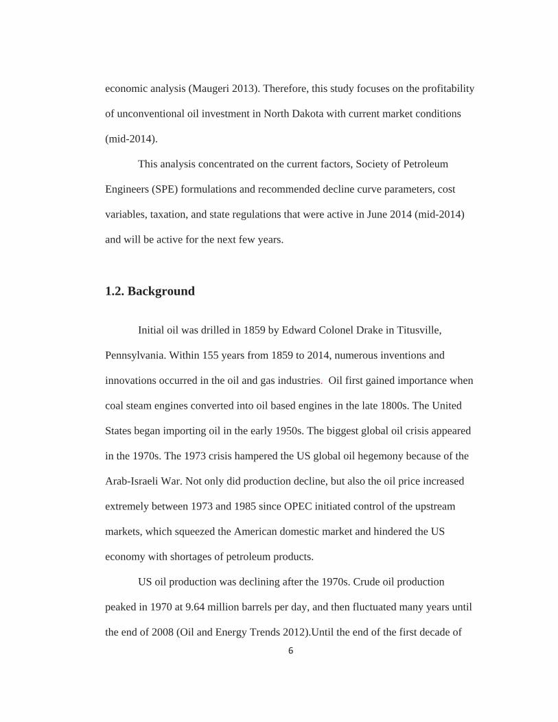
companies work in the Bakken Field, which is also known as the Williston Basin.

8
The Williston Basin is in Montana, North Dakota, South Dakota, Manitoba
(Canada), and Saskatchewan (Canada). North Dakota and Bakken Formation,
Williston Basin are shown in Figure 1.1 and Figure 1.2.
Figure 1.1: United States Map

9
Figure 1.2: Location map of the Williston Basin, Bakken Field (USGS 2013)
Hydraulic fracturing is a well-known process in drilling industry that is used
for producing oil from unconventional reservoirs. Hydraulic fracturing triggers
wells drilled into tight sands, shale formations, and coal bed methane formations
that have low permeability and poor flow rate. They started to become profitable
and affordable in North Dakota within the last decade, but previously they gave
profitable results in other fields such as Marcellus Shale, Barnett Shale, and Eagle
Ford. The combination of hydraulic fracturing and horizontal drilling made North
Dakota oil investment profitable (and almost all other unconventional plays in the
10
world). Recently, more than 70 percent of North Dakota oil is supplied by
unconventional resources (North Dakota DMR 2014).
The hydraulic fracturing or fracking is different from the previously drilled
wells, which were drilled and completed in conventional way. The fracking happens
after a well drilled and casing pipes has been settled in well bore (Earthworks 2014).
The casing is perforated in the target zones that include oil and the fracturing fluid is
injected into the target zones through the perforations. Because of the high pressure
shale rock cannot protect its own form and starts cracking. By this way, the
fracturing fluids and chemicals start to flow back to ground. The proppant materials
remain in the target zones to keep the fractured zones open (Earthworks 2014).
Extraction from shale deposits by way of fracturing methods has a
significant role in the oil market, and also help support the United States economy
with considerable earnings. Current circumstances permit companies to invest in the
basin, and high profits allure operators. After the production boom, the Bakken
Field has become the second biggest oil field in the United States.
This study covers the North Dakota lands of the Williston Basin, hereafter
called the “North Dakota Bakken”, and concentrates on the state of North Dakota,
Bakken Field unconventional oil plays by simulating a typical well, and including
the state regulations.
11
2. Economic and Environmental Issues linked with Unconventional
Oil Production
It is difficult to claim that all unconventional oil investments will be feasible
and profitable in the long run. In other words, production from unconventional
reservoirs do not always show feasible results to provide the economic viability of
investments in the long run. Especially for the Bakken shale oil play, the economic
viability is not sufficiently clear ever since shale oil operations began in 2007. Many
economic issues will remain for decades.
Currently, the cost of unconventional drilling is much higher than
conventional because the drilling operations include directional drilling and
fracturing stage, they require additional equity investment. Horizontal drilling
equipment are slightly different from the conventional ones. It requires additional
special rotational devices and control systems for horizontal / lateral drill
movements. Furthermore, hydraulic fracturing operations use large quantities of
high pressure water, and water resources are not abundant in all locations. Operators
also use fine grained sands and other chemicals to fracture and dissolve the rock.
Economic concerns are compounded by the volatility effect of oil prices, the
uncertainty of EUR (estimated or expected ultimate recovery of oil), high
production costs of directional drilling and hydraulic fracturing, sharp production
decline rates, and potential production from conventional fields that will provide
competing adequate oil into the market. These issues are all linked to each other and
will impact an investment’s profitability in the North Dakota Bakken Field. This

12
study includes the current production data (mid-2014) and indicates updated market
conditions (mid-2014) and evaluates them based on the concerns mentioned above.
2.1. Unconventional Production Cost
Production costs include drilling and well completion costs together (D & C
costs). Geological factors are the main factors for production costs, for example,
shale formations include clay materials. Clay zones are sticky and may swell with
water contact. Most of the drill string stuck problems occur in these formations.
Thus, these issues increase drilling costs.
The cost of conventional oil wells are less than unconventional oil wells
because the horizontal drilling and fracturing stages bring new operations and
additional costs into the system. Each stage of the hydraulic fracturing and
completion costs are about $95,000 in the North Dakota Bakken. Each
unconventional operations contain approximately 40 – 50 fracking stages, which
costs around $3.8 million to $4.75 million (Siegel 2013). In addition to this, a
regular unconventional drilling cost will be between $4 million and $5 million.
Horizontal drilling and hydraulic fracturing sections roughly account for half of the
total production costs. According to the Hess Oil Company, total production cost of
a well decreased to $8.6 million at the end of 2013, which was $13.4 million before
(Dukes 2013a). A $4.8 million difference is associated with the advanced drilling
technologies including high – tech equipment. In contrast to this, a simple 10-stage
fracking operation for 5,000 foot lateral drilling was around $500,000, and the total

13
well completion was equal to $1 million to $1.5 million five years ago (Siegel
2013). Recent operations cover 10 to 15 thousand feet of lateral operations;
therefore, the cost of drilling is much higher than conventional drilling.
In the last five years, the Bakken Field unconventional operations rapidly
expanded, drilling periods shortened from 32 days to 18 days, and lateral reservoir
development doubled from 5,000 feet to 10,000 feet to allow more fracking stages
(North Dakota DMR 2013). Advanced technology decreased the total cost of
production and provided significant improvements in the unconventional oil
production, increasing from 77 bbls. / day to 130 bbls. / day per well.
Table 2.1: Bakken Drilling Averages from 2008 to 2013 (North Dakota DMR 2013)
Bakken Drilling Averages End of 2008 End of 2013
Well Lateral Length 5,000 ft. 10,000 ft.
Well Total Depth (TD) 16,000 ft. 21,000 ft.
Average Prod. Per Well (bbls./day) 77 130
Drilling Period Per Well 32 days 18 days
On the other hand, other costs of production comprising labor, drilling
supplies (water, chemicals etc.), and drill strings rise each year due to inflation.
Between 2002 and 2008, average lease operating costs increased by around 60% -
65% (Annual Energy Outlook 2010). Moreover, due to drilling intensity, well
saturation will occur in the future, which has a negative impact on total production

14
and production declines will begin. For that reason, if oil price decreases in the near
future and falls under the break-even price, these production costs will obstruct
possible investments since they cannot exceed the net investment hurdle rates.
2.2. Production Decline Rates
The declining production rate of a well is one of the most important issues
for decision makers because oil is a depletable and a non – renewable resource. As
learned from previous studies and well reports, well production rates do not go
upward for a long period of time after the initial production, declines day by day
because of the formation quality such as porosity and permeability rates, well
pressure, and some other reservoir features.
Production rates are crucial for the economic evaluation of the
unconventional plays. Due to the low permeability and low porosity characteristics
of shale deposits, production rates will vary and will be relatively lower than
conventional production rates over the long term. Expected ultimate recovery
(EUR) values will change quickly from the original estimates because of changes in
the initial production (IP) rates and production decline rates. Three different
traditional decline curve analysis formulas are applicable for oil and gas wells:
exponential, harmonic, and hyperbolic curves. These formulations rely on the initial
production rates (IP) and nominal decline rates (percent per year).
15
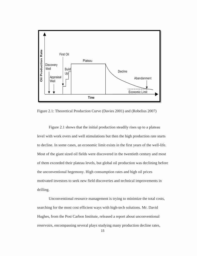
Figure 2.1: Theoretical Production Curve (Davies 2001) and (Robelius 2007)
Figure 2.1 shows that the initial production steadily rises up to a plateau
level with work overs and well stimulations but then the high production rate starts
to decline. In some cases, an economic limit exists in the first years of the well-life.
Most of the giant sized oil fields were discovered in the twentieth century and most
of them exceeded their plateau levels, but global oil production was declining before
the unconventional hegemony. High consumption rates and high oil prices
motivated investors to seek new field discoveries and technical improvements in
drilling.
Unconventional resource management is trying to minimize the total costs,
searching for the most cost efficient ways with high-tech solutions. Mr. David
Hughes, from the Post Carbon Institute, released a report about unconventional
reservoirs, encompassing several plays studying many production decline rates,
16
demonstrating that unconventional fields decline much faster than conventional
fields after the initial production (Hughes 2013).
The North Dakota Bakken Field is a new shale oil boom for the United
States, but very interestingly Deborah Rogers published an article in Energy Policy
Forum, and alleged that the daily oil production per well in the North Dakota
Bakken shale oil plays peaked in 2010 (Rogers 2013). Furthermore, James Mason
underlined the short term investment boom in the Bakken and pointed out the
drilling intensity of the region (Mason 2012b). As opposed to Rogers’s study,
Bakken oil production per well increased to 144 bbls. / day level in June 2012
(Patterson 2013). In contrast to James Mason’s approach, some companies are
planning to use re-fracking / re-stimulation technologies to improve their production
rates after 10 to 20 years of the initial well activity. Bakken Field’s oil peak issue is
still open, but February 2014 results (126 bbls. / day per well) show that the
production rate per well has been decreasing for almost two years (North Dakota
DMR 2014).
Annual production decreases impact the annual revenue for both the state
government and investors because when profits go down, royalty payments and
other taxes also decrease. The profitability of a well is basically associated with IP
rates and decline rates. Companies will shut down their production at some point
when the economic limit occurs. Therefore, most of the operators desire short term
contracts rather than long term ones and depending on the EUR values, an

17
investment will easily shift from positive to negative profitability in the long run if
production greatly decreases.
On the other hand, as mentioned before, producers are able to improve their
revenues by well maintenance and re-fracking. But, these additional operations
increase the total drilling cost by 2-4 million dollars which accounts for 40 to 60
percent of total well completion costs (Hefley et al. 2011). However, these
stimulations will not reach the initial production levels and will begin to decline
after a short time. That is why, Bakken operators generally prefer drilling new wells
instead of re-fracturing since not all the re-stimulation costs reach break-even levels.
2.3. Oil Price Volatility, Transportation and Refinery Issues
Another economic issue related to shale oil production is oil price volatility.
Oil can be assumed to be a global market because it relies on demand and supply
changes anywhere in the world. But local oil prices may easily fluctuate with
regional impacts. As opposed to other market commodities, or a single reference
price, negotiable oil prices will vary globally. For instance, in the Middle East,
economic and political conflicts will directly impact oil prices and oil supply
quickly, like the recent Iraq case. Or, unexpected oil supplies from other Canadian
fields will alter the regional contract prices in the Alberta area. Additionally, the
case of the 1973 crisis was the pioneer of the volatile prices.
Besides two well known (Brent and West Texas Intermediate (WTI)) spot
prices, Bakken Blend ex – Clearbrook and Bakken Blend ex – Guernsey are the
18
benchmark prices for the North Dakota Bakken crude oil market. These prices got
their names from their pipeline junction areas, and the Clearbrook price is the main
price indicator for this project since most of the forecasters focus on the Clearbrook
price and it is considered as the main price for Bakken shale oil by Platts, which is
the only publisher of the local oil prices.
The Clearbrook spot price is the price for Bakken crude oil including the
transportation cost between North Dakota and the pipeline junction location at
Clearbrook, MN. Thus, the price of Clearbrook crude oil can be considered as the
price at a Bakken well – head price plus transportation fees. The Clearbrook price is
a regional benchmark and slightly lower than Brent and WTI prices. The spread or
premium between these prices and Clearbrook depends on many factors. First of all,
North Dakota Bakken producers consider the transportation costs; that is why, they
discount their prices to be competitive. These discounted prices will be assumed as
an opportunity to get involved in the local oil market, but the price differential will
also limit long term investment. Lack of infrastructure for transportation and
refinery issues in North Dakota significantly affected Clearbrook prices in 2011 and
in early 2012. The spread between WTI and Clearbrook even exceeded $28 in early
2012 (Energy Information Administration 2013).
Pipelines are considered as the most cost – effective way to transport crude
oil in the United States, but it is also relatively expensive to construct them rather
than building the other shipping options; and pipeline construction may encounter
the regulation problems (Annual Energy Outlook 2013).
19
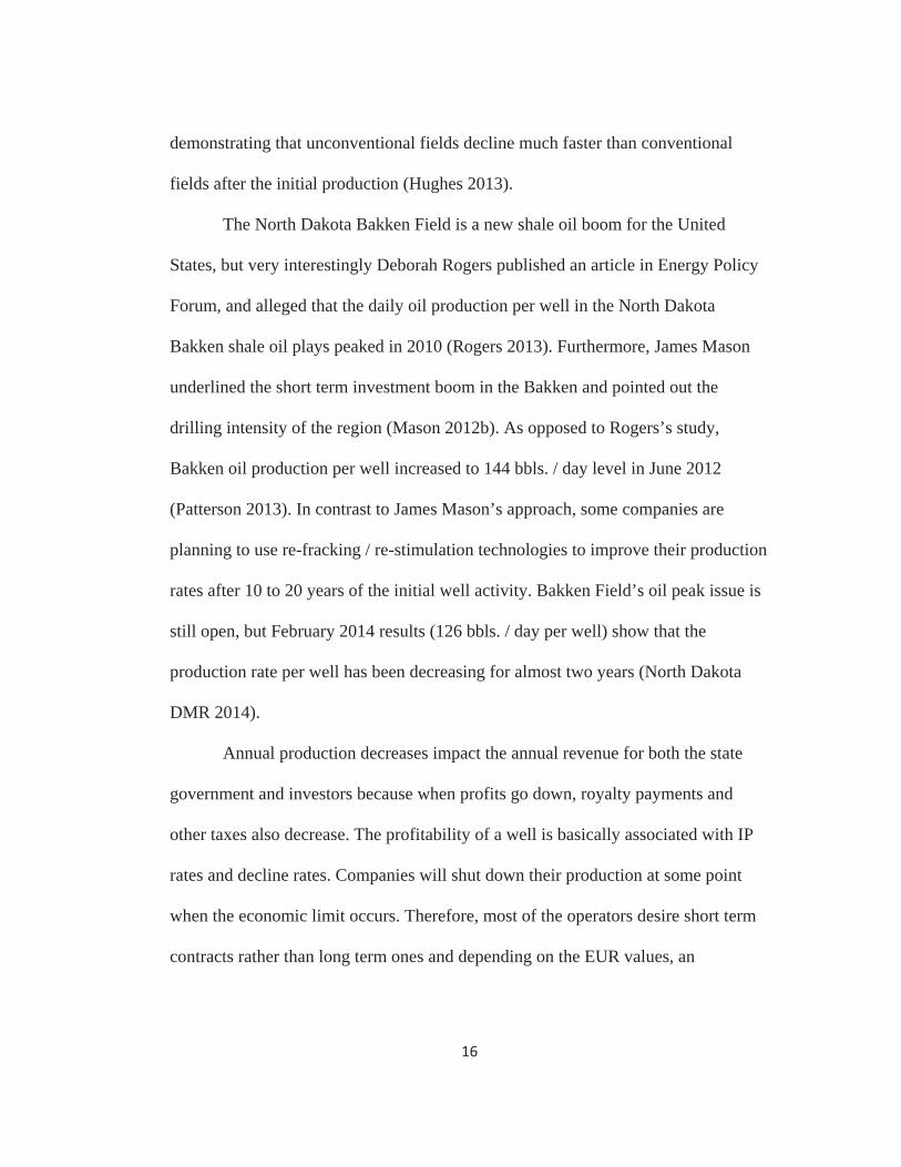
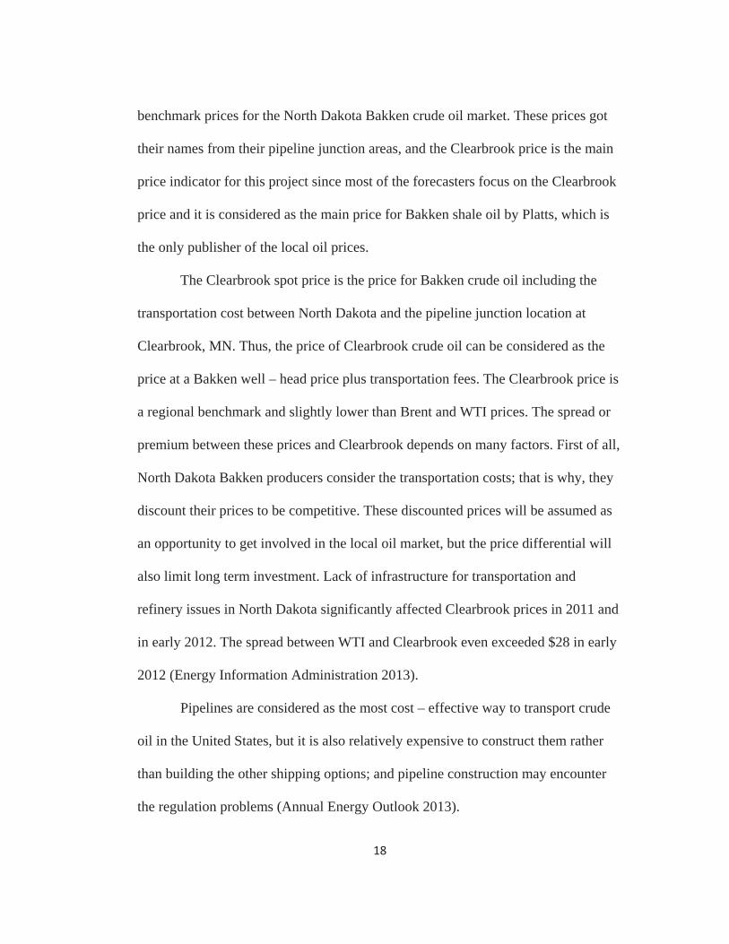
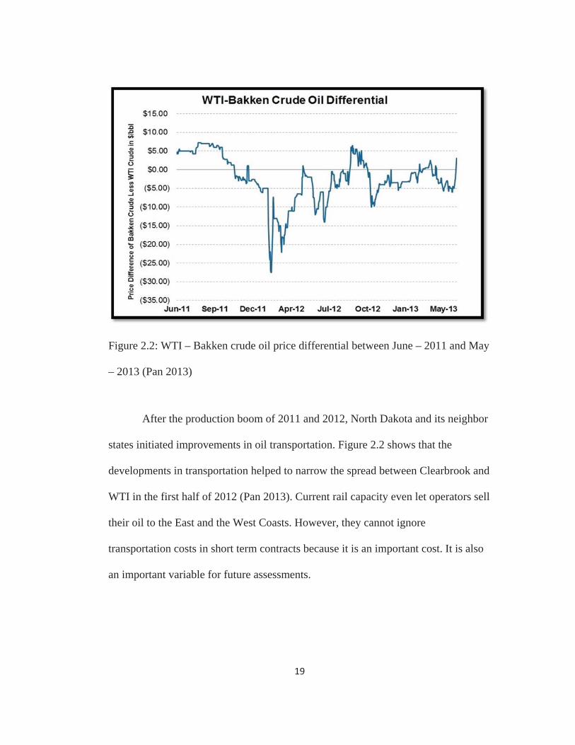
Figure 2.2: WTI – Bakken crude oil price differential between June – 2011 and May
– 2013 (Pan 2013)
After the production boom of 2011 and 2012, North Dakota and its neighbor
states initiated improvements in oil transportation. Figure 2.2 shows that the
developments in transportation helped to narrow the spread between Clearbrook and
WTI in the first half of 2012 (Pan 2013). Current rail capacity even let operators sell
their oil to the East and the West Coasts. However, they cannot ignore
transportation costs in short term contracts because it is an important cost. It is also
an important variable for future assessments.

20
Figure 2.3: Clearbrook crude oil prices between May 2010 and May 2014 (Platts)
Figure 2.3 presents the Bakken Blend ex – Clearbrook crude oil price for the
last 4 years. Not only do infrastructure and transportation influence the oil price in
North Dakota, but also some other factors determine price fluctuations. One of them
is competitive oil prices. Enhanced railroads and pipeline capacities allow North
Dakota to increase oil production, but similarly, Canadian crude oil production was
encouraged to boom. Canadians compete with Bakken oil and try to keep their
prices lower than the Bakken crude price, which will be much more attractive for
buyers. There will be a WTI – Bakken spread along with fluctuations, and
additionally this will decrease the revenues for both investors and state
governments. One other thing that will alter price is the unexpected oil supply from
0
20
40
60
80
100
120
140
5/3/2010 5/3/2011 5/3/2012 5/3/2013 5/3/2014
Daily
Oilprices
($)
Days
Bakken Blend ex - Clearbrook Crude Oil Prices
21
the Bakken Field. Unpredicted warm weather conditions will stimulate high
production and result in a seasonal oil surplus. That was one of the main reasons of
the $26.50 spread between Clearbrook and WTI prices in 2012 (Pan 2013).
Recently, the WTI – Clearbrook spread is much lower due to improvements
in transportation and enhanced pipeline capacity. However, volatility of Clearbrook
prices will remain an issue for both sellers and buyers. In addition, predicted future
declines will increase price concerns.
2.4. Environmental and Social Concerns
Unconventional oil production will have environmental costs and concerns.
These external costs may increase the total cost. Environmental issues may obstruct
the probable investments, but may also cause irrecoverable environmental damage.
Most of the Bakken operators try to minimize external costs by updating their
environmental policies with the help of advancing technical progress.
Hydraulic fracturing is a completion phase of horizontal drilling and
stimulates the largest environmental concern. Hydraulic fracturing operations may
damage water resources, including both surface supplies and underground aquifers.
In addition to this, poorly planned well construction or antiquated processes can
leak fracking materials into the casing layers and cements, which may result in
possible aquifer contamination (Gresh 2011). Water contamination hinders the
effective use of agricultural resources. Therefore, water management is a crucial
issue. Drilling operations periodically need thousands to millions of gallons of
22
water. An average North Dakota well uses about two million gallons of water (equal
to 7.6 million liters) and predicted water demand for total oil operations of the
Bakken field is 27.6 billion liters, which is for hydro-fracking (Shaver 2012). The
North Dakota Bakken is drier area than the Marcellus Shale or the Barnett Shale.
For that reason, the allocation of water resources is much more critical than in other
locations. Drilling intensity rises year by year in the North Dakota Bakken as a
result of the steep production declines of 50 % to 80 % of the initial production in
the second year. Thus, operators drill more wells to mitigate these decline rates.
Increasing drilling intensity means more water used, more environmental concerns,
and more regulations.
Waste water disposal is another concern under the issue of water
management. Approximately 10 % to 40 % of injected water flows back to the
surface during the well completion (Stepan et al. 2010) and (Galusky 2011). This
flow back water will include dissolved minerals and naturally occurring radioactive
metals (NORM) and other chemicals that are used in hydraulic fracturing. Most of
the Bakken operators can re – cycle 80 % to 90 % of waste water and inject it into
other well operations. Either storing or transporting the water will contain some risk
for North Dakota. A leakage to freshwater can substantially impact the local
ecosystem. Also, based on the Ohio case, the deep – well underground injection of
this wastewater could trigger small earthquakes (Ohio DNR 2012).
Besides these issues related to water contamination, flaring of natural gas
can occur from Bakken oil wells due to lack of gas pipeline infrastructure. North
23
Dakota is an isolated area when compared to Pennsylvania or Texas, and lack of
infrastructure prevents the storage or use of abundant quantities of natural gas. It is
too costly to store and transport natural gas without pipelines, thus operators flare
gas during drilling and work over phases, which causes air pollution.
2.5. Recent Bakken Operations
The Bakken Field unconventional oil production, including Montana and
North Dakota, reached the level of million barrels per day in April 2014. High oil
prices, profitable returns on investments, declining costs of production,
technological improvements with horizontal drilling, and taxation incentives
facilitated the production boom. On the other hand, because of the steep production
declines after the initial years, new wells are continually drilled to mitigate the
decline effect. This increases drilling intensity; affecting other uses for the land.
Although the state government updates regulations on water management, water
contamination issues remain active.
All these conditions and concerns are very important for the North Dakota
Bakken operators, landowners, and employees. Even slight changes will impact
economics of oil investments and will either increase investments or lead to shut
downs. Economic viability is the most essential issue for short term and long term
investment planning. The research question is: considering all these concerns along
with market conditions (including lease rights, oil prices, and production rates) is it
economically profitable to produce shale and tight oil from North Dakota Bakken

24
wells? Based on 5, 10, and 20 year investment plans, are these unconventional oil
wells economically viable?
25
3. Methodology
The recent unconventional boom from the North Dakota Bakken has made
an astonishing economic contribution to the United States economy (Annual Energy
Outlook 2013). But, is it viable? Most of the scholars and society do not have an
answer for how long this contribution will perpetuate. What if the oil prices go
down? When will be the oil peak occur, or has it already occurred before? Should
we consider the original oil in place (OIP), technically recoverable oil, or estimated
ultimate recovery (EUR) for effective and more accurate economic evaluations?
Which investment time span is better; short term investments of 5 years production,
or long-term investments of 10 years, or more than 10 years?
To find answers to all these questions, this study concentrates on the recent
unconventional oil production boom with the assistance of several economic
indicators. Based on these indicators and cost variables, different scenarios are
evaluated to decide whether investments are profitable or not. Production rates,
decline curves, cost variables such as leasing fees and signing bonus payments,
drilling and completion costs, and all other expenses are calculated and included in
the cash flow statements for the economic estimations of the North Dakota Bakken
unconventional oil play. Recent tax regulations were considered via North Dakota
Red Book 2012. Bakken Blend ex – Clearbrook price is used in the cash flow
statements as the reference oil price. Standard financial metrics were used in the
scenarios to judge the profitability. To determine the upstream profitability and the
feasibility; NPV, IRR, and break-even analysis (minimum return on investments)
26
methods are applied for different well simulations. Any positive or negative cash
flow statement are evaluated using the NPV method at 10 percent minimum
acceptable rate of return (MARR). For the IRR method, a minimum hurdle rate for
oil investments is 10 percent. Break-even prices are calculated to compare them
with initial scenario prices. Some assumptions are based on the decision and
financial analysts of North Dakota operator companies such as Continental
Resources, Chesapeake Energy, Whiting Petroleum, and Hess Corporation; and the
State of North Dakota, Department of Oil and Gas Division. The subsections of this
chapter elaborate the elements of this research.
3.1. North Dakota Bakken Unconventional Oil Prices
Oil price is one of the main components of any financial assessment and one
of the most essential inputs to determine profitability by comparing with break-even
prices. The Bakken blend ex-Clearbrook price is used in this analysis based on
communications with North Dakota Oil and Gas Division analysts and Platts
reports. The last four years’ average price is were used and is less than the recent
Clearbrook price since Clearbrook prices fluctuated many times between May 2010
and May 2014 period (Figure 2.3).
Clearbrook price is for the sweet and light, less sulfur content Bakken
unconventional oil, and includes the transportation fees between North Dakota and
the Clearbrook, MN pipeline junction. The May 2014 well – head price varied

27
between $88 /bbl. and $90 /bbl. (Platts 2014). The last negotiated Clearbrook price
for May 15, 2014 was $96.48. Thus, a $5 – 6 difference can be considered as the
transportation fee. The starting price of $90.78 per barrel was recorded as the
average value for the last 4 years’ Clearbrook price (May 2010 – May 2014).
The annual oil price increase is assumed to be the same as the projected
economic growth rate, which is 2.8 % per year for 2014, from the International
Monetary Fund (IMF World Economic Outlook 2014).
3.2. Total Drilling and Completion Costs
Total drilling costs comprise all drilling and well completion costs
associated with an unconventional oil well before the initial production phase. It
would be better to divide these costs into two groups as the drilling costs and the
completion costs. The drilling costs include all the possible costs that operators
spend during the drilling days such as equipment costs, additive fluid costs, mud
costs, water supply costs, horizontal drilling costs, rig rents, etc. According to
Bakken operators, this initial phase accounts for 50 to 70 percent of the total drilling
costs, which ranges from $4.0 million to $5.6 million per well (Dukes 2013b). 60
percent is assumed for this study, thus the cost of the drilling phase is $4.8 million.
The second phase is the well completion. Well completion costs consist of mainly
well stimulation works (hydraulic fracking), cementing, casing, perforation efforts,
water supply and sand costs for fracking, and include some other well tests related
to completion that must be done before the production stage. Well completion costs
28
range from $2.4 million to $4.0 million per well, and it accounts for 30 to 50 percent
of the total drilling costs. 40 percent is assumed for this analysis, so $3.2 million is
used According to Hess Corporation, Bakken Field unconventional oil drilling cost
(D) per well was equal to $8.0 million in the first quarter of 2012, and $5.4 million
was the well completion cost (C) (Hess Corporation 2013). Technological
developments, improvements in hydraulic fracturing, and water re-cycling all
diminished completion costs significantly by the end of the second quarter of 2013,
and the total drilling cost (D & C) shifted from $13.4 million to $8.4 million.
Current average cost per well is slightly less than $8.4 million. In this analysis,
annual reports and other web materials were scanned, and $8.0 million total cost
per well is used based on the costs of the big players of Bakken Field such as Hess
Corporation, Continental Resources, Whiting Petroleum, and Chesapeake Energy.
3.3. Lease Agreements and Royalty Payments
Part of the lease payments are assumed to be a sunk cost since companies do
not directly record them under their cash flow statements (Dizard 2010). As
opposed to this approach, the model used here includes all leasing costs to calculate
the most complete results for the estimation of profitability.
The leasing process starts with an initial interest in the field. After the
geological and geophysical surveys, companies decide to continue or give up their
land operations. Legally, companies must sign a lease agreement with the
29
landowners to gain access to the mineral rights before drilling begins. Furthermore,
some of these ownership agreements must be done even before the geophysical
seismic works phase that occurs after the field geology works (Anderson 2006)
Oil and gas leases are competitive. Landowners or their responsible
attorneys negotiate the lease conditions with operator companies directly. Some
residents of North Dakota such as in the western part are familiar with this process
because petroleum companies have extracted oil from their territories for more than
30 – 40 years. Interest in unconventional oil spread around the whole state and most
of the North Dakota land areas became attractive for investors, but the residents of
these new areas are not familiar with the system.
Lease costs are considered to be part of the pre – production (finding) costs
and royalties are considered as part of the production (lifting) costs (Inkpen and
Moffett 2011). Petroleum companies must offer royalty rates and lease bonus
payments together directly as an incentive. The attorneys’ or landowners’ power of
bargaining brings higher royalties and higher signing bonus payments. The royalty
rate is an agreed upon percentage that is paid based on the total oil production, paid
periodically. Royalty fees only become active after the onset of production. In North
Dakota, royalty rates usually range from 6.25 percent to 18.75 percent, in some
areas up to 20 percent. This rate is determined by negotiations as mentioned before,
and each landowners’ offer is different from others (Anderson 2006). A 12.5 percent
royalty rate is assumed these cash flow statements, and this amount is subtracted
from the gross revenue without including taxes and other costs. In addition to this,

30
companies must also negotiate the signing bonus payments with landowners. This
amount will vary depending on the estimated well productivity and the mutual
negotiability. It was impossible to determine a fixed value for these bonus
payments. For that reason, North Dakota oil and gas discussion forums were
scanned, and a range found between a few dollars (roughly $50) to $20,000 per acre
(Maugeri 2013). Thus, in this model, $3000 per acre is used as the signing bonus
payment.
Regardless of how many mineral acres are leased, any land that covers 160
acres must have its own individual lease (Anderson 2006). Additionally, 640 acres
of land (one square mile) are required for a successful well drilling operation, which
means 4 different oil leases are required for each drilling operation. But to keep this
simple, the lease and royalty rates for all parcels are assumed to be constant. In this
analysis, oil leases cover five years terms and every five years, leases will renew
with the same assumed rates. Thus $3000 per acre bonus payment ($1,920,000 for
640 acres) and 12.5 percent royalty rates remain constant for each lease period, if
the companies want to sign again.
3.4. Production Rates
To assess the economic profit and the economic viability, production rates
and oil prices are the most critical variables. High oil production rates for a long
term will reduce the payback period and increase the NPV. However, if the
production rates decline too fast, an investment can turn unprofitable in a short

31
period. Production rates cannot be flat or constant for a long period, and rates will
dramatically change after the initial production (IP).
Oil production has been the main source of income for the oil giants for the
past decades (Inkpen and Moffett 2011).Well productivity plays an important role in
the cost management. Geological factors such as rock type and rock characteristics,
depth, thickness, and properties of the hydrocarbon, and other factors such as well
density, wellbore size, production method influence the production rates. Economic,
political, and current market conditions also affect the production rate.
Tight oil and shale oil reservoirs contain less porosity and less permeability
due to their geological attributes than sandstone and limestone reservoirs. For that
reason, fracturing and horizontal drilling are essential for high production rates. The
production data for this analysis was gathered via many companies and the
probabilities of low, medium, and high well production rates are considered based
on production reports. In this study, the probabilities of these three profiles were
taken as respectively; 20 %, 60 %, and 20 %. IP rates for these profiles in the
Bakken Field are considered as respectively; 174 bbls. / day, 402 bbls. / day, and
652 bbls. / day. The expected production rate of a typical North Dakota Bakken well
will be:
32
Thus, an assumption of the initial production value of 406 bbls. / day was
considered for typical Bakken well in this study.
Decline curve analysis is an empirical statistical method of analyzing
production performance during the well life. It assumes that the current well and
reservoir conditions will remain unchanged in the future. Decline curves terminate
when net revenue of production and production costs become equal. It is known as
the economic limit or break-even and below this point, investment is unprofitable.
There are three traditional methods that developed by J. J. Arps (1944) can
be used for the decline analysis equations: exponential, harmonic, and hyperbolic
decline curve equations. These three methods are the most common ways of
forecasting future production and estimating the EUR. The hyperbolic decline curve
equation is used for the first years, then the declining trend reaches a constant
decline percentage, and a stretched exponential decline curve equation is used until
the end of the forecast. In the model of a hyperbolic decline curve, the data plots
concave upward (Petrobjects 2004).
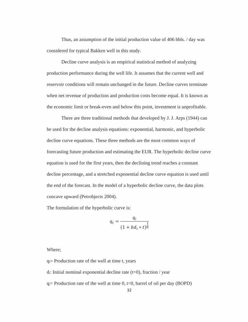
The formulation of the hyperbolic curve is:
Where;
qt= Production rate of the well at time t, years
di: Initial nominal exponential decline rate (t=0), fraction / year
qi= Production rate of the well at time 0, t=0, barrel of oil per day (BOPD)

33
b= Hyperbolic exponent of decline, b-factor, characterizes reservoir’s production
decline
t= time (years)
Apart from the initial production rate, the other input variables for the
hyperbolic curve equation were either picked from the operating company analysts
and Bakken Consultant firms or relevant data gathered by way of scanning the
previous and current forecasts. These numbers can vary for each type of study, but
hyperbolic curve serves as an approximation for the production values at any chosen
period.
After reaching the constant decline percentage, production vs. time will
become a straight line. At this point, the hyperbolic curve shifts to the exponential
curve, which assumes the b-factor zero (b=0). This continues until the economic
limit.
The formulation of the exponential decline curve is:
Referring to the EUR calculations, the economic limit can be reached at any
time (profit will decrease to zero or become negative), and companies will decide to
shut-down their operations to stop losing money or re-stimulate their wells to return
to economic profitability. Hyperbolic and exponential decline curve assumptions are

34
very important for the cash flow statements because the annual total production
multiplied by the oil price per barrel determines the annual gross revenue.
3.5. Taxation
3.5.1. North Dakota State Taxes
Not only do the producers earn revenues from the production, but also the
state government partially shares in these revenues. Taxes are the most important
way to collect revenues and circulate it under the control of the state. For example,
transportation and refinery issues have been the most crucial concerns for North
Dakota after the unconventional boom. For that reason, state government decided to
improve roads, schools, and other public infrastructure. Tax revenues funded these
solutions for emerging concerns. Also, environmental costs might be offset with an
efficient allocation of these revenues.
The North Dakota state government has different taxes on oil. The first tax
is the gross oil production tax. A 5 % flat rate is implemented on the gross value of
all oil produced at a well, separate from the royalty fees (Fong 2012).

35
Table 3.1: North Dakota Gross Oil Production Tax Allocation
Allocation of 5 % Gross Production Tax
45 % Counties (Infrastructure Funds)
35 % Schools
20 % Cities
The second one is the oil extraction tax, and it is charged on the extraction of
oil from the earth. The oil extraction tax is 6.5 % of the gross value of crude oil
produced at the well (Fong 2012). In some specific conditions, this rate may be
reduced to 4 %; but in this model, our simulated wells do not meet those
requirements and do not have exemptions, so a 6.5 % rate is applied.
Table 3.2: North Dakota Oil Extraction Tax Allocation
Allocation of the Oil Extraction Tax
30 % Legacy Fund
30 % State General Fund
20 % Education Purposes
20% Water Resources Trust Fund
Thus, a 5 % gross production tax and a 6.5 % oil extraction taxes are
charged by the North Dakota State Government.
36
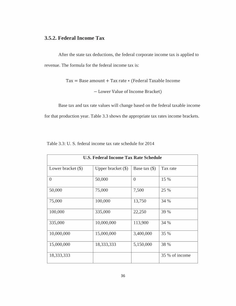
3.5.2. Federal Income Tax
After the state tax deductions, the federal corporate income tax is applied to
revenue. The formula for the federal income tax is:
Base tax and tax rate values will change based on the federal taxable income
for that production year. Table 3.3 shows the appropriate tax rates income brackets.
Table 3.3: U. S. federal income tax rate schedule for 2014
U.S. Federal Income Tax Rate Schedule
Lower bracket ($) Upper bracket ($) Base tax ($) Tax rate
0 50,000 0 15 %
50,000 75,000 7,500 25 %
75,000 100,000 13,750 34 %
100,000 335,000 22,250 39 %
335,000 10,000,000 113,900 34 %
10,000,000 15,000,000 3,400,000 35 %
15,000,000 18,333,333 5,150,000 38 %
18,333,333 35 % of income
37
3.6. Lease Operating Expenses (LOE)
Lease operating expenses (LOE) are different from the other production
costs that have been mentioned in the drilling costs section. When enumerating
these costs, LOE are additional costs that appear during the production phase. Some
costs are already included in the D & C costs (drilling and completion) section;
however, other costs that are associated with an operating lease such as labor costs,
site preparation and permitting fees including bonds and registration (initial
application) costs, power, maintenance, and material costs are not included there.
Depending on the drilling area and length of operating time, LOE will increase or
decrease. Some studies regard site preparation fees, bond fees, and initial
application fees separate from lease operating costs, however, many energy analysts
consider them all together to calculate and to find accurate unit cost per barrel
(Inkpen and Moffett 2011). In this research, these costs are considered together, and
$10 per barrel determined as the lease operating cost that was listed in SEC 10-k
filings for the operators of North Dakota. LOE’s are included in the cash flow
statements. Most of the North Dakota companies are minimizing the LOE costs
under their cost management programs.
The assumption of $10 LOE cost is hold constant for the whole life span for
any investment option.
38
3.7. Tax Benefits
Prior to implementing the state and federal income taxes for North Dakota
unconventional oil, several allowable tax deductions will occur depending on the
state and federal regulations. These include the intangible drilling costs, tangible
drilling costs, and depletion allowance.
3.7.1. Tax Deductions for Intangible Drilling Cost
Permitted intangible drilling deductions include labor costs, drilling rig
rents, chemicals, drilling fluids, and fuel costs that occur during the drilling and
completing processes of a well. These costs have no salvage value (PetroChase
2014).
Intangible drilling costs may cover 60 to 80 percent of the total drilling costs
(North Dakota Oil Boom, 2014). This study assumes 70 percent of the total drilling
costs are deductible as intangible drilling costs. Total drilling costs of a simulated
Bakken well is assumed to be $8 million and intangible costs are $5.6 million.
3.7.2. Tax Deductions for Tangible Drilling Cost
Tangible drilling costs are related to drilling and completion costs
encompassing the equipment have a salvage value in contrast to intangible drilling
costs. Investors can either use modified accelerated cost recovery system (MACRS)
or straight line depreciation system through seven years, whichever offers the best

39
option for them (North Dakota Oil Boom 2014). For this method, 7-years MACRS
depreciation was selected as the best option for an example property.
Table 3.4: 7 – years MACRS depreciation system (Internal Revenue Service 2013b)
7-years MACRS Depreciation Rates
Years Rate (%)
1 14.29
2 24.49
3 17.49
4 12.49
5 8.93
6 8.93
7 8.93
8 4.46
Since 70 percent is used as the intangible drilling costs, the remained 30
percent of the total drilling and completion costs is assumed to be the tangible
drilling costs. Thus, $2.4 million is the depreciable amount (basis) for the tangible
drilling costs.
40
3.7.3. Depletion Allowance
The depletion allowance is similar to depreciation, and is a form of cost
recovery for capital investments (Internal Revenue Service 2013a). It can be
calculated into two ways: cost depletion and percentage depletion. Investors who
have an economic interest in an oil property can get a deduction for depletion
(Internal Revenue Service 2013a). The simulated North Dakota wells in this
research are assumed to be an asset (property) of an energy company instead of
individual producers. To keep the calculation and assumption simple, a flat rate of
15 percent of the gross income is used based on the average daily production of oil
for the percentage depletion (Internal Revenue Service 2013a). Thus, cost depletion
is method is ignored.
3.8. Scenarios
Four different scenarios were are examined. Assessing the profitability and
viability of these scenarios via cash flow statements is the main purpose of this
study. These four scenarios are: first five years of production without re-stimulation;
ten years of production without re-stimulation; twenty years of production without
re-stimulation; and twenty years of production with two different well profiles, the
first well producing oil for ten years, and the second well coming into the system
after the tenth year and producing oil for ten more years.
41
Different time frames and assumptions are selected to compare their overall
profitability, feasibility, and the impact of production declines. NPV, IRR, and
break-even analysis is used to assess these four scenarios.
The first three scenarios are similar, but their time frames compare the
investment profitability over time. The EUR is calculated by using the decline curve
graphs and decline curve equations. The first three scenarios show the production
decline effect on the long run investments. All the basic assumptions remain the
same for these scenarios, and leases are renewed every five years.
The fourth scenario used the same assumptions for the first ten years and
then followed a different strategy than the first three simulations. The reason for
using a different strategy is to assess the performance of two different ten year with
two drilled wells. The first well is drilled and produced oil for the first ten years, and
then the second well with the same features is drilled and produced oil for the next
ten years. Therefore, it doubled the total drilling cost. Results will show how
profitable this is.
3.8.1. Re-fracturing
Re-fracturing is an additional assumption and completely different from the
other four scenarios. Re-fracturing operations do not always improve oil production.
There are many steps that must be analyzed and carefully studied for re-fracturing.
First, picking the target area is very important for perforations since re-fracturing
the well might result in with opening new gaps. These gaps will lower the previous
42
production via migration of the trapped oil from formation fractures. Another issue
related to re-stimulation is the economic challenges of these operations. Re-
stimulation will permit operators to boost oil production and this can be more
economic than infill drilling if the reservoir characteristics are well known and the
hydraulic fracture system is well placed (Strother et al. 2013). Each investment plan
included in this system must be examined very carefully because investments could
end up with uneconomic results.
Re-fracturing is logical because it evaluates the economics of re-fracturing
efforts. In many American fields, operators started to think about the feasibility of
re-fracturing because re-stimulation efforts may improve well performance for short
periods. According to Schlumberger, work-overs and additional fracturing is able to
increase oil production partly because of maintenance and remedial work (cleaning
or replacing the pumps and fixing the frayed cement and casings) of the well
(Schlumberger 2011). These work-overs will revitalize the well performance if re-
fracturing is successful. On the other hand, each of these bring additional costs
thereby increasing the total cost and will cause unprofitable investments.
In this analysis, re-fracturing option is not considered because the Bakken
field unconventional oil operations are still in early years of production and re-
fracturing is an active issue for the Bakken operators (based on cost &environmental
issues). Current results (mid-2014) show that companies mainly focus on drilling
new wells to mitigate the decline effect. Also, gathering data for re-fracturing was
43
unavailable because companies did not release any official report about re-fracturing
until mid-2014.
3.9. Calculations
The analysis is made using cash flow statements, and the profitability
decisions is measured using NPV, IRR, and break-even for each scenario. The first
and the most important is the NPV of each cash flow statement since it is more
reliable than IRR. To find the NPV or the present equivalent value of an investment,
all future net cash flows are discounted to the present and summed together, using
ten percent as the minimum acceptable return rate (hurdle rate). Positive NPVs for
the scenarios are considered as acceptable and profitable.
The second comparison method is the IRR, which is also known as the
economic rate of return on investment. IRR is defined as the annual average return
that is earned over the investment life. Any IRR rate that is higher than the 10
percent Minimum Acceptable Rate of Return (MARR) is acceptable as a profitable
investment.
The third method is break-even analysis. Break-even is the price of oil
needed so that the NPV is equal to zero based on 10 percent MARR. An oil price
higher than the break-even price is assumed to indicate an investible project.

44
4. Scenario Analysis and Results
As discussed in Chapter 3, the main purpose of this study is to evaluate the
economic profitability of the average (typical) Bakken unconventional oil well
under current circumstances. This chapter covers an economic analysis of four
different scenarios and considers the NPV, IRR, and break-even for each one. Cash
flow statement analysis is the most important financial tool for assessing oil and gas
investments and to pick the best alternative between the scenarios. Economic and
environmental concerns associated with unconventional oil production were
discussed in Chapter 2, and their impacts are examined in this chapter as well.
Additionally, these scenarios tested the impact of the sharp production decline rates,
and the EUR is calculated for each of the investment plans. Also, the assumed
production periods and life span of a simulated well are other concerns and the
results are analyzed to see whether five years production, ten years production, or
20 years production are more profitable in the analysis.
4.1. Typical Bakken unconventional oil well (Simulated well)
First of all, prior to calculating the cash flow statements and applying the
financial decision analysis, the production decline rates and the EUR of each
scenario were analyzed, calculated, and presented on the MS Excel spreadsheets. As
anticipated, production performances of each scenario gave different results. Each
of these scenarios began with the same IP rates and annual average decline rates.

45
Hyperbolic decline curve and exponential decline curve analyses were implemented
for the required periods. Table 4.1 presents the initial input values for the hyperbolic
decline curve equation.
Where;
qt= Production rate of the well at time t, years
di: Initial nominal exponential decline rate (t=0), fraction / year
qi= Production rate of the well at time 0, t=0, barrel of oil per day (BOPD)
b= Hyperbolic exponent of decline, b-factor, characterizes reservoir’s production
decline
t= time (years)
Table 4.1: Input values for the hyperbolic decline curve (Simulated well)
Hyperbolic decline curve equation input values
IP (initial production) rate 406 bbls. / day
Initial annual average decline rate (di) / year 68 %
b-variable (Hyperbolic exponent) 1.1
46
The hyperbolic exponent (b variable) must not be 0 or 1 to use in the
hyperbolic decline equation. It is a constant value for specific periods and is
estimated to be 1.1 for the initial year. This constant value is found by decline curve
family graphs and calculations, and since it is a confidential data for the operator
company, they did not want to share graph for this analysis. This b variable is
assumed to be 1.1 for the beginning of the petroleum production estimates even
though evaluators observed much higher numbers, approach to 2 in some cases
during the flow regime (Ryder Scott Co. 2011). 1.1 constant value is considered
based on the initial sharp declines. Indeed, the b variable is not dependent on the
initial production. It can change during the production period, but this study
assumes it will remain at 1.1 until the constant decline phase begins. Then b variable
will reach zero for the exponential curve equation. Table 4.1 shows that with the
initial production rate of 406 bbls. per day, simulated well production also declines
by a 68 percent annual average rate during the first year (12 months). If the b-value
is greater, the decline occurs more sharply (the higher the value of b, the sharper the
decline). These values remained fixed for the beginning of each scenario.
4.1.1. Production Decline Curve for the First Scenario
Oil or gas wells do not always have uniform production over their life spans.
Conventional wells usually have a longer life span than unconventional fracked
wells due to their drilling and reservoir structures. As this study concentrates on the
unconventional oil wells of the North Dakota Bakken, extremely high decline rates
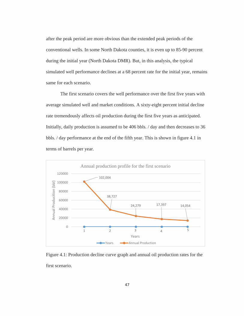
47
after the peak period are more obvious than the extended peak periods of the
conventional wells. In some North Dakota counties, it is even up to 85-90 percent
during the initial year (North Dakota DMR). But, in this analysis, the typical
simulated well performance declines at a 68 percent rate for the initial year, remains
same for each scenario.
The first scenario covers the well performance over the first five years with
average simulated well and market conditions. A sixty-eight percent initial decline
rate tremendously affects oil production during the first five years as anticipated.
Initially, daily production is assumed to be 406 bbls. / day and then decreases to 36
bbls. / day performance at the end of the fifth year. This is shown in figure 4.1 in
terms of barrels per year.
Figure 4.1: Production decline curve graph and annual oil production rates for the
first scenario.
1 2 3 4 5
102,004
38,727
24,279 17,397 14,054
0
20000
40000
60000
80000
100000
120000
Annu
alProd
ucition
(bbl)
Years
Annual production profile for the first scenario
Years Annual Production
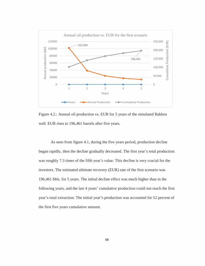
48
Figure 4.2.: Annual oil production vs. EUR for 5 years of the simulated Bakken
well. EUR rises to 196,461 barrels after five years.
As seen from figure 4.1, during the five years period, production decline
began rapidly, then the decline gradually decreased. The first year’s total production
was roughly 7.3 times of the fifth year’s value. This decline is very crucial for the
investors. The estimated ultimate recovery (EUR) rate of the first scenario was
196,461 bbls. for 5 years. The initial decline effect was much higher than in the
following years, and the last 4 years’ cumulative production could not reach the first
year’s total extraction. The initial year’s production was accounted for 52 percent of
the first five years cumulative amount.
102,004
196,461
0
50,000
100,000
150,000
200,000
250,000
0
20000
40000
60000
80000
100000
120000
1 2 3 4 5
CumulativeProd
uctio
n(EUR)
Annu
alprod
uctio
n(bbl)
Years
Annual oil production vs. EUR for the first scenario
Years Annual Production Cumulative Production
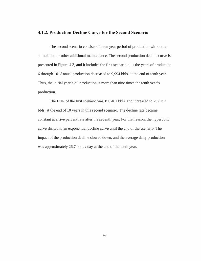
49
4.1.2. Production Decline Curve for the Second Scenario
The second scenario consists of a ten year period of production without re-
stimulation or other additional maintenance. The second production decline curve is
presented in Figure 4.3, and it includes the first scenario plus the years of production
6 through 10. Annual production decreased to 9,994 bbls. at the end of tenth year.
Thus, the initial year’s oil production is more than nine times the tenth year’s
production.
The EUR of the first scenario was 196,461 bbls. and increased to 252,252
bbls. at the end of 10 years in this second scenario. The decline rate became
constant at a five percent rate after the seventh year. For that reason, the hyperbolic
curve shifted to an exponential decline curve until the end of the scenario. The
impact of the production decline slowed down, and the average daily production
was approximately 26.7 bbls. / day at the end of the tenth year.
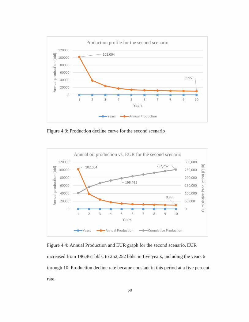
50
Figure 4.3: Production decline curve for the second scenario
Figure 4.4: Annual Production and EUR graph for the second scenario. EUR
increased from 196,461 bbls. to 252,252 bbls. in five years, including the years 6
through 10. Production decline rate became constant in this period at a five percent
rate.
102,004
9,995
0
20000
40000
60000
80000
100000
120000
1 2 3 4 5 6 7 8 9 10
Annu
alprod
uctio
n(bbl)
Years
Production profile for the second scenario
Years Annual Production
102,004
9,995
196,461
252,252
0
50,000
100,000
150,000
200,000
250,000
300,000
0
20000
40000
60000
80000
100000
120000
1 2 3 4 5 6 7 8 9 10
CumulativeProd
uctio
n(EUR)
Annu
alprod
uctio
n(bbl)
Years
Annual oil production vs. EUR for the second scenario
Years Annual Production Cumulative Production

51
4.1.3. Production Decline Curve for the Third Scenario
The previous scenarios covered five and ten year production periods without
re-stimulation and work overs. The third scenario is a continuation of the second
case, with an additional ten years. For the first two scenarios, the approximate EUR
was around 196,461 and 252,252 bbls. An additional ten year adds roughly 76,000
bbls. of oil, and the EUR of the third scenario is enhanced to 328,453 bbls. at the
end of twenty years. When compared to the first ten years, the additional ten year
production was low; it only accounted for 30 percent of the first ten years.
Figure 4.5: 20 year production decline curve for the third scenario
102,004
5,984
0
20000
40000
60000
80000
100000
120000
1 2 3 4 5 6 7 8 9 10 11 12 13 14 15 16 17 18 19 20
Annu
alprod
uctio
n(bbl.)
Years
20 year production profile for the third scenario
Years Annual Production
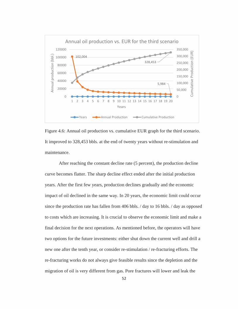
52
Figure 4.6: Annual oil production vs. cumulative EUR graph for the third scenario.
It improved to 328,453 bbls. at the end of twenty years without re-stimulation and
maintenance.
After reaching the constant decline rate (5 percent), the production decline
curve becomes flatter. The sharp decline effect ended after the initial production
years. After the first few years, production declines gradually and the economic
impact of oil declined in the same way. In 20 years, the economic limit could occur
since the production rate has fallen from 406 bbls. / day to 16 bbls. / day as opposed
to costs which are increasing. It is crucial to observe the economic limit and make a
final decision for the next operations. As mentioned before, the operators will have
two options for the future investments: either shut down the current well and drill a
new one after the tenth year, or consider re-stimulation / re-fracturing efforts. The
re-fracturing works do not always give feasible results since the depletion and the
migration of oil is very different from gas. Pore fractures will lower and leak the
102,004
5,984
328,453
0
50,000
100,000
150,000
200,000
250,000
300,000
350,000
0
20000
40000
60000
80000
100000
120000
1 2 3 4 5 6 7 8 9 10 11 12 13 14 15 16 17 18 19 20
CumulativeProd
uctio
n(EUR)
Annu
alprod
uctio
n(bbl.)
Years
Annual oil production vs. EUR for the third scenario
Years Annual Production Cumulative Production

53
trapped oil. New packing tools and hydro-fracking stages will increase the
production if the target packing zones install successfully. On the other hand, if the
operations extend beyond the target zones and all the fractured zones are re-
stimulated again, it will be costly without yielding expected oil returns.
Therefore, the third scenario leads to the fourth scenario with the idea of
drilling a replacement well with the same features at year ten, and each well would
produce for ten years.
4.1.4. Production Decline Curve for the Fourth Scenario
This scenario is different from the first three versions. A twenty year life
span is divided into two different well production sections. The initial well drilled in
year 0 is produced oil until the end of year 10. The second well is drilled at the end
of year 10 and produces oil in years 11 through 20. Both of these wells are assumed
to have the same geological and reservoir features. In other words, the second
scenario is duplicated here. If the second scenario was profitable, the duplication of
it should give better results for a 20 years life span than the third scenario because
the production rates between the end of the tenth year and the twentieth year were
extremely low in the third scenario.
On the other hand, if the second scenario did not have positive NPV,
duplicating the negative results would only make the deficit worse. The reason for
the comparing these two scenarios is to evaluate the best investment for long run
plan.

54
Figure 4.7: Production decline curve for the fourth scenario (Duplication of the
second scenario over 20 years)
Figure 4.8: Production profile vs. EUR for the fourth scenario. Expected ultimate
recovery increased to 504,505 bbls.
102,004 102,004
0
20000
40000
60000
80000
100000
120000
1 2 3 4 5 6 7 8 9 10 11 12 13 14 15 16 17 18 19 20
Annu
alProd
uctio
n(bbl)
Years
Production decline curve for the fourth scenario
Years Annual Production (bbl)
102,004 102,004
9,995
504,505
0
100,000
200,000
300,000
400,000
500,000
600,000
0
20000
40000
60000
80000
100000
120000
1 2 3 4 5 6 7 8 9 10 11 12 13 14 15 16 17 18 19 20
CumulativePR
oductio
n(EUR)
Annu
alProd
uctio
n(bbl)
Years
Annual oil production vs. EUR for the fourth scenario
Years Annual Production Cumulative Production
55
The expected ultimate recovery is highest in the fourth scenario. The highest
EUR of the previous scenarios was 328,453 bbls. and it improved to 504,505 bbls.
at the end of twenty years. In this scenario the cash flow statement analysis will
show which scenario is more profitable, but EUR results show that the maximum oil
extraction exists in the fourth scenario. The main concern of the fourth scenario was
the cost / benefit side because not only is the production doubled but the total
drilling cost is also doubled in this scenario. Therefore, a positive NPV could
improve the profitable investment and rate of return, but a negative NPV could
increase the deficit and lower the investible life span of the project.
Without the analysis in cash flow statements, interpreting the investments
based on the EUR values will give incorrect results. The highest EUR rate observed
in the fourth scenario, and the lowest EUR existed in the first one due to the shortest
production time frame. Another incorrect approach would be to link production
rates with profitability. Production rates decline significantly after the initial years.
Investors may want to stop operations due to high decline rates, but this is also
incorrect.
The analysis using cash flow statements are needed to find the best and the
worst investments.

56
4.2. Cash Flow Statements for Scenarios
4.2.1. First Scenario (5 years production)
In the previous chapter, all assumptions related to the cash flow statements
were explained and defined. These input variables are based on the current market
conditions that can be observable in the North Dakota Bakken Field. Some of these
will change or vary due to changeable conditions, regional differences, and well
characteristics. The initial cost variables are shown in Table 4.2.
Table 4.2: Simulated Bakken unconventional oil well initial input values
Initial variables for the simulated Bakken well (as of mid-2014)
D & C costs (Total Drilling Cost) $8,000,000
Intangible Drilling Cost $5,600,000
Tangible Drilling Cost $2,400,000
Clearbrook Oil Price (per barrel) $90.78
Royalty rate 12.5 %
Lease operating expenses (per barrel) $10
Signing bonus fees (per acre) $3,000
Inflation (oil price increase per year) 2.8 %
Initial annual average decline rate 68 %
State taxes (extraction and gross production) 11.5 %
Depletion Allowance 15 %
Initial production rate (IP) 406 bbls. / day
Minimum Acceptable Rate of Return (MARR) 10 %
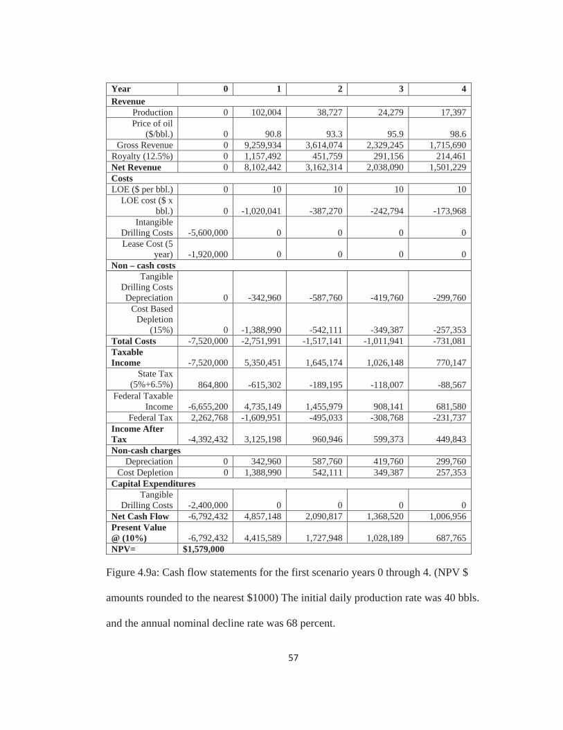
57
Year 0 1 2 3 4 Revenue
Production 0 102,004 38,727 24,279 17,397 Price of oil
($/bbl.) 0 90.8 93.3 95.9 98.6 Gross Revenue 0 9,259,934 3,614,074 2,329,245 1,715,690
Royalty (12.5%) 0 1,157,492 451,759 291,156 214,461 Net Revenue 0 8,102,442 3,162,314 2,038,090 1,501,229 Costs LOE ($ per bbl.) 0 10 10 10 10
LOE cost ($ x bbl.) 0 -1,020,041 -387,270 -242,794 -173,968
Intangible Drilling Costs -5,600,000 0 0 0 0 Lease Cost (5
year) -1,920,000 0 0 0 0 Non – cash costs
Tangible Drilling Costs Depreciation 0 -342,960 -587,760 -419,760 -299,760
Cost Based Depletion
(15%) 0 -1,388,990 -542,111 -349,387 -257,353 Total Costs -7,520,000 -2,751,991 -1,517,141 -1,011,941 -731,081 Taxable Income -7,520,000 5,350,451 1,645,174 1,026,148 770,147
State Tax (5%+6.5%) 864,800 -615,302 -189,195 -118,007 -88,567
Federal Taxable Income -6,655,200 4,735,149 1,455,979 908,141 681,580
Federal Tax 2,262,768 -1,609,951 -495,033 -308,768 -231,737 Income After Tax -4,392,432 3,125,198 960,946 599,373 449,843 Non-cash charges
Depreciation 0 342,960 587,760 419,760 299,760 Cost Depletion 0 1,388,990 542,111 349,387 257,353
Capital Expenditures Tangible
Drilling Costs -2,400,000 0 0 0 0 Net Cash Flow -6,792,432 4,857,148 2,090,817 1,368,520 1,006,956 Present Value @ (10%) -6,792,432 4,415,589 1,727,948 1,028,189 687,765 NPV= $1,579,000
Figure 4.9a: Cash flow statements for the first scenario years 0 through 4. (NPV $
amounts rounded to the nearest $1000) The initial daily production rate was 40 bbls.
and the annual nominal decline rate was 68 percent.
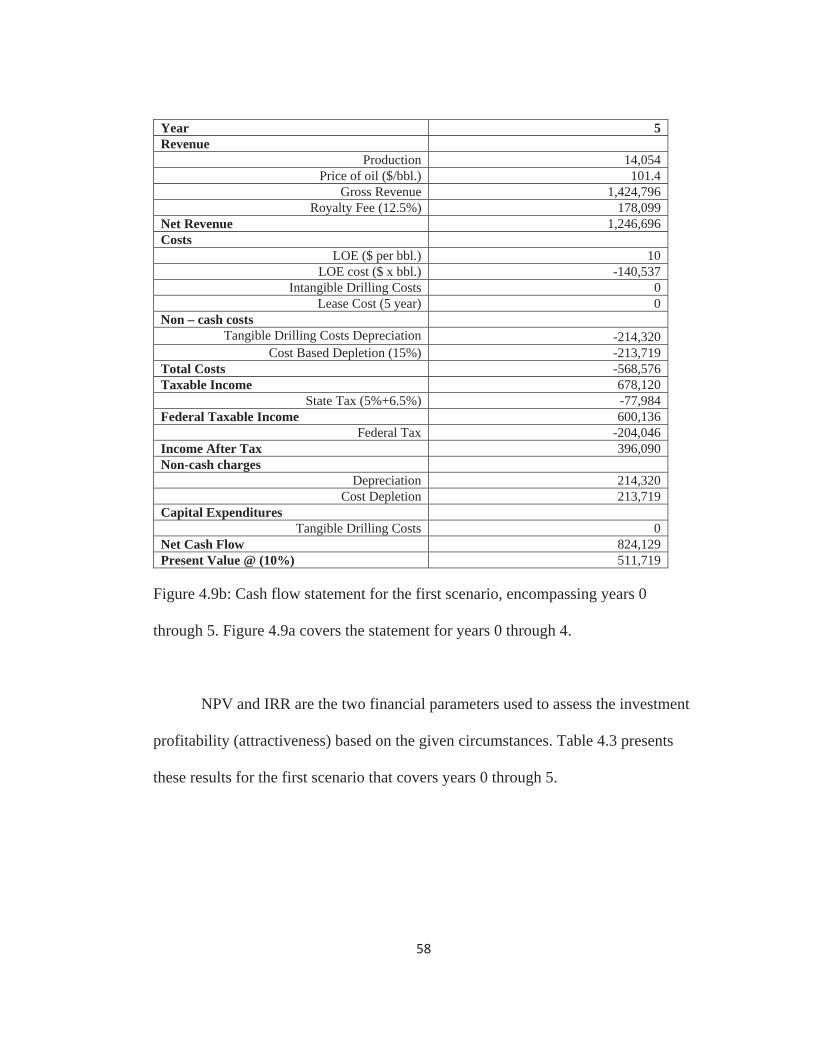
58
Year 5 Revenue
Production 14,054 Price of oil ($/bbl.) 101.4
Gross Revenue 1,424,796 Royalty Fee (12.5%) 178,099
Net Revenue 1,246,696 Costs
LOE ($ per bbl.) 10 LOE cost ($ x bbl.) -140,537
Intangible Drilling Costs 0 Lease Cost (5 year) 0
Non – cash costs Tangible Drilling Costs Depreciation -214,320
Cost Based Depletion (15%) -213,719 Total Costs -568,576 Taxable Income 678,120
State Tax (5%+6.5%) -77,984 Federal Taxable Income 600,136
Federal Tax -204,046 Income After Tax 396,090 Non-cash charges
Depreciation 214,320 Cost Depletion 213,719
Capital Expenditures Tangible Drilling Costs 0
Net Cash Flow 824,129 Present Value @ (10%) 511,719
Figure 4.9b: Cash flow statement for the first scenario, encompassing years 0
through 5. Figure 4.9a covers the statement for years 0 through 4.
NPV and IRR are the two financial parameters used to assess the investment
profitability (attractiveness) based on the given circumstances. Table 4.3 presents
these results for the first scenario that covers years 0 through 5.

59
Table 4.3: Profitably and EUR results for the first scenario
Results for years 0 through 5
NPV @ MARR = 10 % $ 1,579,000
IRR 23.1 %
EUR 196,461 bbls.
Any NPV result greater than zero means the investment is acceptable. The
NPV for the first scenario is $1,579,000 based on assumptions at current market
conditions. Thus, the first scenario is profitable based on the five year time frame.
Total costs of Bakken (D &C plus other fees) are relatively higher than some other
unconventional areas like the Marcellus Shale or the Barnett Shale. But the initial
flow rate offsets these costs and gives positive results for the 5 year investment plan.
4.2.2. Second Scenario (10 years production)
The second scenario includes ten year production profile. The initial input values
remain same as the first scenario and additional 5 year production profile increases the
cumulative production (EUR) from 196,461 bbls. to 252,252 bbls at the end of ten years.
Cash flow statement analysis for the second scenario is shown in Figure 4.10a, 4.10b, and
4.10c.
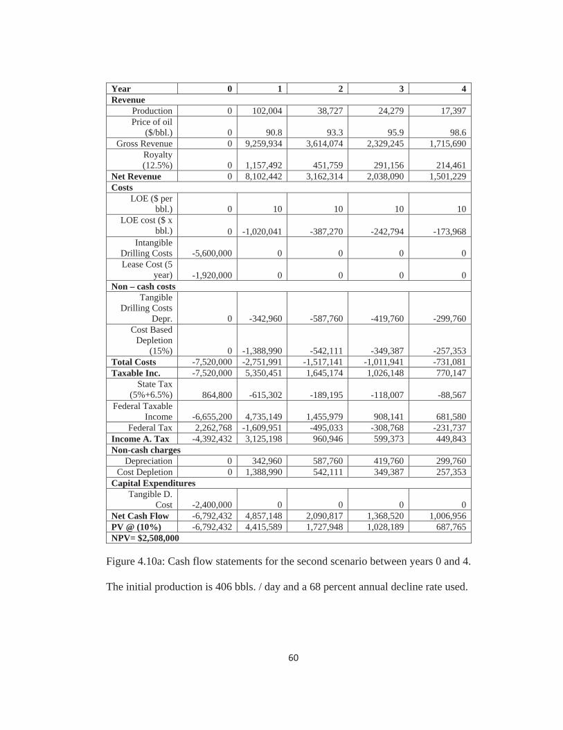
60
Year 0 1 2 3 4 Revenue
Production 0 102,004 38,727 24,279 17,397 Price of oil
($/bbl.) 0 90.8 93.3 95.9 98.6 Gross Revenue 0 9,259,934 3,614,074 2,329,245 1,715,690
Royalty (12.5%) 0 1,157,492 451,759 291,156 214,461
Net Revenue 0 8,102,442 3,162,314 2,038,090 1,501,229 Costs
LOE ($ per bbl.) 0 10 10 10 10
LOE cost ($ x bbl.) 0 -1,020,041 -387,270 -242,794 -173,968
Intangible Drilling Costs -5,600,000 0 0 0 0 Lease Cost (5
year) -1,920,000 0 0 0 0 Non – cash costs
Tangible Drilling Costs
Depr. 0 -342,960 -587,760 -419,760 -299,760 Cost Based
Depletion (15%) 0 -1,388,990 -542,111 -349,387 -257,353
Total Costs -7,520,000 -2,751,991 -1,517,141 -1,011,941 -731,081 Taxable Inc. -7,520,000 5,350,451 1,645,174 1,026,148 770,147
State Tax (5%+6.5%) 864,800 -615,302 -189,195 -118,007 -88,567
Federal Taxable Income -6,655,200 4,735,149 1,455,979 908,141 681,580
Federal Tax 2,262,768 -1,609,951 -495,033 -308,768 -231,737 Income A. Tax -4,392,432 3,125,198 960,946 599,373 449,843 Non-cash charges
Depreciation 0 342,960 587,760 419,760 299,760 Cost Depletion 0 1,388,990 542,111 349,387 257,353
Capital Expenditures Tangible D.
Cost -2,400,000 0 0 0 0 Net Cash Flow -6,792,432 4,857,148 2,090,817 1,368,520 1,006,956 PV @ (10%) -6,792,432 4,415,589 1,727,948 1,028,189 687,765 NPV= $2,508,000
Figure 4.10a: Cash flow statements for the second scenario between years 0 and 4.
The initial production is 406 bbls. / day and a 68 percent annual decline rate used.

61
Year 5 6 7 8 9 Revenue
Production 14,054 12,475 11,726 11,075 10,521 Price of oil
($/bbl.) 101.4 104.2 107.1 110.1 113.2 Gross
Revenue 1,424,796 1,300,133 1,256,345 1,219,753 1,191,211 Royalty (12.5%) 178,099 162,517 157,043 152,469 148,901
Net Revenue 1,246,696 1,137,617 1,099,302 1,067,284 1,042,309 Costs
LOE ($ per bbl.) 10 10 10 10 10
LOE cost ($ x bbl.) -140,537 -124,748 -117,263 -110,746 -105,209
Intangible Drilling
Costs 0 0 0 0 0 Lease Cost
(5 year) -1,920,000 0 0 0 Non – cash costs
Tangible Drill. Depr. -214,320 -214,320 -214,320 -107,160 0 Cost Based
Depletion -213,719 -195,020 -188,452 -182,963 -178,682 Total Costs -2,488,576 -534,088 -520,034 -400,869 -283,891 Taxable Income -1,241,880 603,529 579,267 666,414 758,419
State Tax (5%+6.5%) 142,816 -69,406 -66,616 -76,638 -87,218
Federal Taxable Income -1,099,064 534,123 512,652 589,777 671,200
Federal Tax 373,682 -181,602 -174,302 -200,524 -228,208 Income After Tax -725,382 352,521 338,350 389,253 442,992 Non-cash charges Depreciation 214,320 214,320 214,320 107,160 0
Cost Depletion 213,719 195,020 188,452 182,963 178,682
Capital Expenditures Tangible D. 0 0 0 0 0
Net Cash Flow -297,343 761,861 741,122 679,376 621,674 PV @10 % -184,626 430,051 380,313 316,934 263,650
Figure 4.10b: Years 5 through 9 for the second scenario
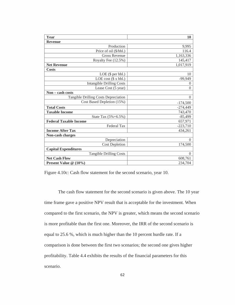
62
Year 10 Revenue
Production 9,995 Price of oil ($/bbl.) 116.4
Gross Revenue 1,163,336 Royalty Fee (12.5%) 145,417
Net Revenue 1,017,919 Costs
LOE ($ per bbl.) 10 LOE cost ($ x bbl.) -99,949
Intangible Drilling Costs 0 Lease Cost (5 year) 0
Non – cash costs Tangible Drilling Costs Depreciation 0
Cost Based Depletion (15%) -174,500 Total Costs -274,449 Taxable Income 743,470
State Tax (5%+6.5%) -85,499 Federal Taxable Income 657,971
Federal Tax -223,710 Income After Tax 434,261 Non-cash charges
Depreciation 0 Cost Depletion 174,500
Capital Expenditures Tangible Drilling Costs 0
Net Cash Flow 608,761 Present Value @ (10%) 234,704
Figure 4.10c: Cash flow statement for the second scenario, year 10.
The cash flow statement for the second scenario is given above. The 10 year
time frame gave a positive NPV result that is acceptable for the investment. When
compared to the first scenario, the NPV is greater, which means the second scenario
is more profitable than the first one. Moreover, the IRR of the second scenario is
equal to 25.6 %, which is much higher than the 10 percent hurdle rate. If a
comparison is done between the first two scenarios; the second one gives higher
profitability. Table 4.4 exhibits the results of the financial parameters for this
scenario.
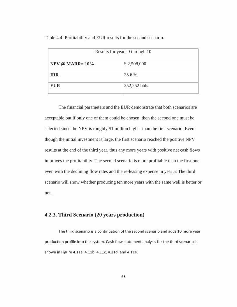
63
Table 4.4: Profitability and EUR results for the second scenario.
Results for years 0 through 10
NPV @ MARR= 10% $ 2,508,000
IRR 25.6 %
EUR 252,252 bbls.
The financial parameters and the EUR demonstrate that both scenarios are
acceptable but if only one of them could be chosen, then the second one must be
selected since the NPV is roughly $1 million higher than the first scenario. Even
though the initial investment is large, the first scenario reached the positive NPV
results at the end of the third year, thus any more years with positive net cash flows
improves the profitability. The second scenario is more profitable than the first one
even with the declining flow rates and the re-leasing expense in year 5. The third
scenario will show whether producing ten more years with the same well is better or
not.
4.2.3. Third Scenario (20 years production)
The third scenario is a continuation of the second scenario and adds 10 more year
production profile into the system. Cash flow statement analysis for the third scenario is
shown in Figure 4.11a, 4.11b, 4.11c, 4.11d, and 4.11e.
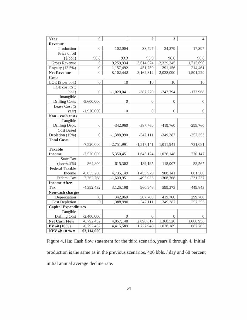
64
Year 0 1 2 3 4 Revenue
Production 0 102,004 38,727 24,279 17,397 Price of oil
($/bbl.) 90.8 93.3 95.9 98.6 90.8 Gross Revenue 0 9,259,934 3,614,074 2,329,245 1,715,690
Royalty (12.5%) 0 1,157,492 451,759 291,156 214,461 Net Revenue 0 8,102,442 3,162,314 2,038,090 1,501,229 Costs LOE ($ per bbl.) 0 10 10 10 10
LOE cost ($ x bbl.) 0 -1,020,041 -387,270 -242,794 -173,968
Intangible Drilling Costs -5,600,000 0 0 0 0 Lease Cost (5
year) -1,920,000 0 0 0 0 Non – cash costs
Tangible Drilling Depr. 0 -342,960 -587,760 -419,760 -299,760
Cost Based Depletion (15%) 0 -1,388,990 -542,111 -349,387 -257,353 Total Costs
-7,520,000 -2,751,991 -1,517,141 -
1,011,941 -731,081 Taxable Income -7,520,000 5,350,451 1,645,174 1,026,148 770,147
State Tax (5%+6.5%) 864,800 -615,302 -189,195 -118,007 -88,567
Federal Taxable Income -6,655,200 4,735,149 1,455,979 908,141 681,580
Federal Tax 2,262,768 -1,609,951 -495,033 -308,768 -231,737 Income After Tax -4,392,432 3,125,198 960,946 599,373 449,843 Non-cash charges
Depreciation 0 342,960 587,760 419,760 299,760 Cost Depletion 0 1,388,990 542,111 349,387 257,353
Capital Expenditures Tangible
Drilling Cost -2,400,000 0 0 0 0 Net Cash Flow -6,792,432 4,857,148 2,090,817 1,368,520 1,006,956 PV @ (10%) -6,792,432 4,415,589 1,727,948 1,028,189 687,765 NPV @ 10 % = $3,114,000
Figure 4.11a: Cash flow statement for the third scenario, years 0 through 4. Initial
production is the same as in the previous scenarios, 406 bbls. / day and 68 percent
initial annual average decline rate.

65
Year 5 6 7 8 9 Revenue
Production 14,054 12,475 11,726 11,075 10,521 Price of oil
($/bbl.) 101.4 104.2 107.1 110.1 113.2 Gross
Revenue 1,424,796 1,300,133 1,256,345 1,219,753 1,191,211 Royalty (12.5%) 178,099 162,517 157,043 152,469 148,901
Net Revenue 1,246,696 1,137,617 1,099,302 1,067,284 1,042,309 Costs
LOE ($ per bbl.) 10 10 10 10 10
LOE cost ($ x bbl.) -140,537 -124,748 -117,263 -110,746 -105,209
Intangible Drilling
Costs 0 0 0 0 0 Lease Cost
(5 year) -1,920,000 0 0 0 Non – cash costs
Tangible Drill. Depr. -214,320 -214,320 -214,320 -107,160 0 Cost Based
Depletion -213,719 -195,020 -188,452 -182,963 -178,682 Total Costs -2,488,576 -534,088 -520,034 -400,869 -283,891 Taxable Income -1,241,880 603,529 579,267 666,414 758,419
State Tax (5%+6.5%) 142,816 -69,406 -66,616 -76,638 -87,218
Federal Taxable Income -1,099,064 534,123 512,652 589,777 671,200
Federal Tax 373,682 -181,602 -174,302 -200,524 -228,208 Income After Tax -725,382 352,521 338,350 389,253 442,992 Non-cash charges Depreciation 214,320 214,320 214,320 107,160 0
Cost Depletion 213,719 195,020 188,452 182,963 178,682
Capital Expenditures Tangible D. 0 0 0 0 0
Net Cash Flow -297,343 761,861 741,122 679,376 621,674 PV (10 %) -184,626 430,051 380,313 316,934 263,650
Figure 4.11b: Cash flow statement for the third scenario, years 5 through 9.
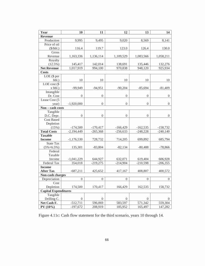
66
Year 10 11 12 13 14 Revenue
Production 9,995 9,495 9,020 8,569 8,141 Price of oil
($/bbl.) 116.4 119.7 123.0 126.4 130.0 Gross
Revenue 1,163,336 1,136,114 1,109,529 1,083,566 1,058,211 Royalty (12.5%) 145,417 142,014 138,691 135,446 132,276
Net Revenue 1,017,919 994,100 970,838 948,120 925,934 Costs
LOE ($ per bbl.) 10 10 10 10 10
LOE cost ($ x bbl.) -99,949 -94,951 -90,204 -85,694 -81,409
Intangible Dr. Cost 0 0 0 0 0
Lease Cost (5 year) -1,920,000 0 0 0 0
Non – cash costs Tangible
D.C. Depr. 0 0 0 0 0 Cost Based
Depletion (15%) -174,500 -170,417 -166,429 -162,535 -158,732
Total Costs -2,194,449 -265,368 -256,633 -248,228 -240,140 Taxable Income -1,176,530 728,732 714,205 699,892 685,794
State Tax (5%+6.5%) 135,301 -83,804 -82,134 -80,488 -78,866
Federal Taxable Income -1,041,229 644,927 632,071 619,404 606,928
Federal Tax 354,018 -219,275 -214,904 -210,598 -206,355 Income After Tax -687,211 425,652 417,167 408,807 400,572 Non-cash charges Depreciation 0 0 0 0 0
Cost Depletion 174,500 170,417 166,429 162,535 158,732
Capital Expenditures Tangible
Drilling C. 0 0 0 0 0 Net Cash F. -512,711 596,069 583,597 571,342 559,304 PV (10%) -197,672 208,919 185,952 165,497 147,282
Figure 4.11c: Cash flow statement for the third scenario, years 10 through 14.
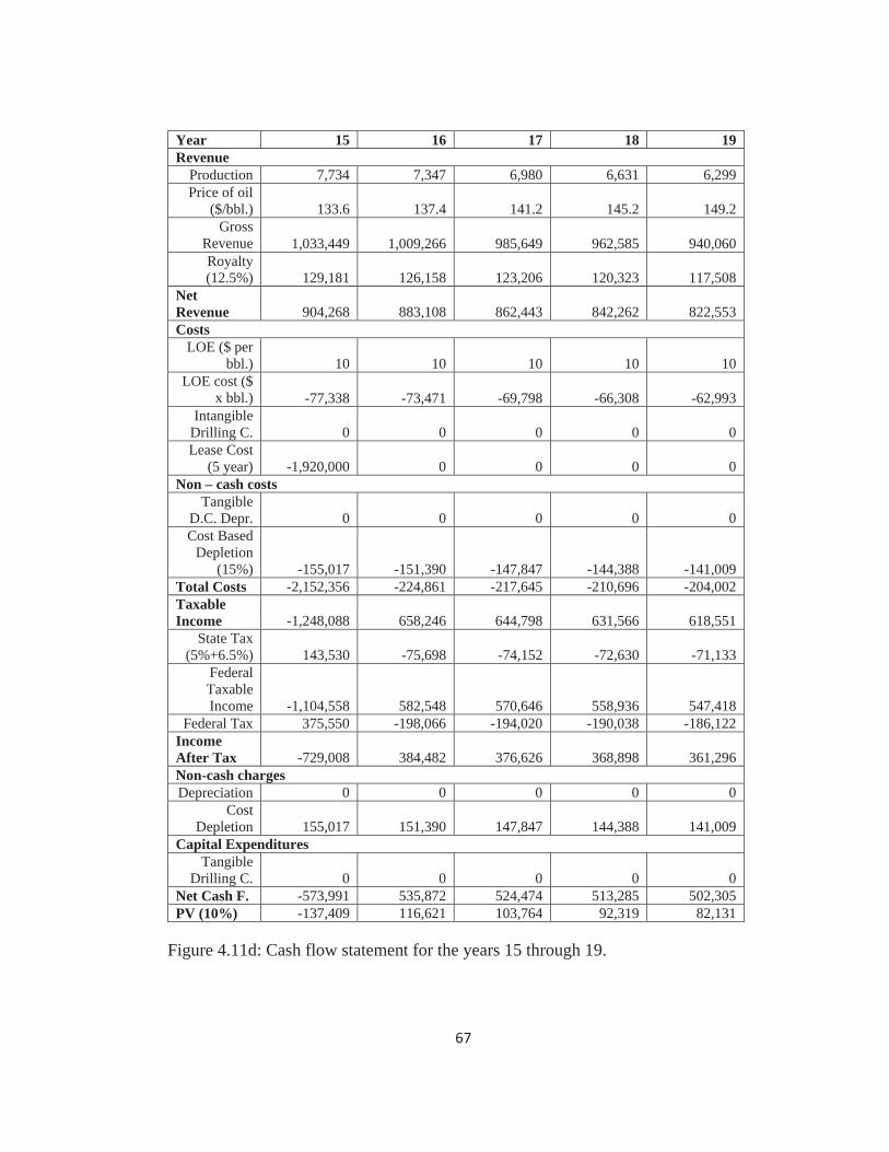
67
Year 15 16 17 18 19 Revenue
Production 7,734 7,347 6,980 6,631 6,299 Price of oil
($/bbl.) 133.6 137.4 141.2 145.2 149.2 Gross
Revenue 1,033,449 1,009,266 985,649 962,585 940,060 Royalty (12.5%) 129,181 126,158 123,206 120,323 117,508
Net Revenue 904,268 883,108 862,443 842,262 822,553 Costs
LOE ($ per bbl.) 10 10 10 10 10
LOE cost ($ x bbl.) -77,338 -73,471 -69,798 -66,308 -62,993
Intangible Drilling C. 0 0 0 0 0 Lease Cost
(5 year) -1,920,000 0 0 0 0 Non – cash costs
Tangible D.C. Depr. 0 0 0 0 0 Cost Based
Depletion (15%) -155,017 -151,390 -147,847 -144,388 -141,009
Total Costs -2,152,356 -224,861 -217,645 -210,696 -204,002 Taxable Income -1,248,088 658,246 644,798 631,566 618,551
State Tax (5%+6.5%) 143,530 -75,698 -74,152 -72,630 -71,133
Federal Taxable Income -1,104,558 582,548 570,646 558,936 547,418
Federal Tax 375,550 -198,066 -194,020 -190,038 -186,122 Income After Tax -729,008 384,482 376,626 368,898 361,296 Non-cash charges Depreciation 0 0 0 0 0
Cost Depletion 155,017 151,390 147,847 144,388 141,009
Capital Expenditures Tangible
Drilling C. 0 0 0 0 0 Net Cash F. -573,991 535,872 524,474 513,285 502,305 PV (10%) -137,409 116,621 103,764 92,319 82,131
Figure 4.11d: Cash flow statement for the years 15 through 19.

68
Figure 4.11e: Cash flow statements for the third scenario, year 20.
The third scenario considers a twenty year production period. It is a
continuation of the last two scenarios and added 10 more years beyond the second
scenario. As discussed previously, the second scenario gave better NPV and IRR
results than the first scenario, even though the production rates decline every year.
The same result occurs in the third scenario: it yields much better NPV and IRR
results than the previous scenarios. Table 4.5 shows the results.
Year 20 Revenue
Production 5,984 Price of oil ($/bbl.) 153.4
Gross Revenue 918,063 Royalty Fee (12.5%) 114,758
Net Revenue 803,305 Costs
LOE ($ per bbl.) 10 LOE cost ($ x bbl.) -59,843
Intangible Drilling Costs 0 Lease Cost (5 year) 0
Non – cash costs Tangible Drilling Costs Depreciation 0
Cost Based Depletion (15%) -137,709 Total Costs -197,552 Taxable Income 605,753
State Tax (5%+6.5%) -69,662 Federal Taxable Income 536,091
Federal Tax -182,271 Income After Tax 353,820 Non-cash charges
Depreciation 0 Cost Depletion 137,709
Capital Expenditures Tangible Drilling Costs 0
Net Cash Flow 491,530 Present Value @ (10%) 73,063
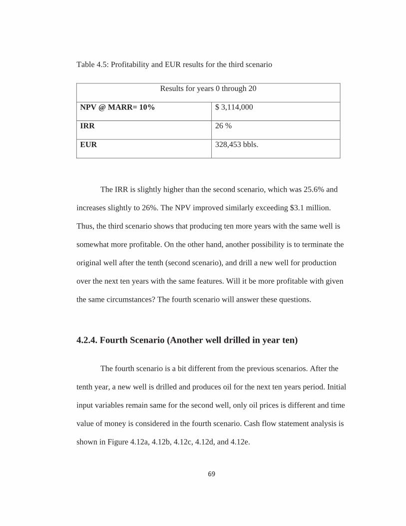
69
Table 4.5: Profitability and EUR results for the third scenario
Results for years 0 through 20
NPV @ MARR= 10% $ 3,114,000
IRR 26 %
EUR 328,453 bbls.
The IRR is slightly higher than the second scenario, which was 25.6% and
increases slightly to 26%. The NPV improved similarly exceeding $3.1 million.
Thus, the third scenario shows that producing ten more years with the same well is
somewhat more profitable. On the other hand, another possibility is to terminate the
original well after the tenth (second scenario), and drill a new well for production
over the next ten years with the same features. Will it be more profitable with given
the same circumstances? The fourth scenario will answer these questions.
4.2.4. Fourth Scenario (Another well drilled in year ten)
The fourth scenario is a bit different from the previous scenarios. After the
tenth year, a new well is drilled and produces oil for the next ten years period. Initial
input variables remain same for the second well, only oil prices is different and time
value of money is considered in the fourth scenario. Cash flow statement analysis is
shown in Figure 4.12a, 4.12b, 4.12c, 4.12d, and 4.12e.
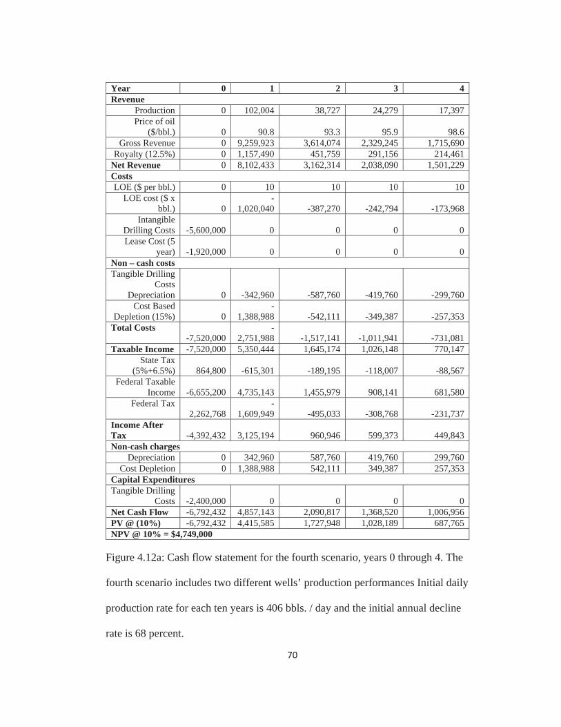
70
Year 0 1 2 3 4 Revenue
Production 0 102,004 38,727 24,279 17,397 Price of oil
($/bbl.) 0 90.8 93.3 95.9 98.6 Gross Revenue 0 9,259,923 3,614,074 2,329,245 1,715,690
Royalty (12.5%) 0 1,157,490 451,759 291,156 214,461 Net Revenue 0 8,102,433 3,162,314 2,038,090 1,501,229 Costs LOE ($ per bbl.) 0 10 10 10 10
LOE cost ($ x bbl.) 0
-1,020,040 -387,270 -242,794 -173,968
Intangible Drilling Costs -5,600,000 0 0 0 0 Lease Cost (5
year) -1,920,000 0 0 0 0 Non – cash costs Tangible Drilling
Costs Depreciation 0 -342,960 -587,760 -419,760 -299,760
Cost Based Depletion (15%) 0
-1,388,988 -542,111 -349,387 -257,353
Total Costs -7,520,000
-2,751,988 -1,517,141 -1,011,941 -731,081
Taxable Income -7,520,000 5,350,444 1,645,174 1,026,148 770,147 State Tax
(5%+6.5%) 864,800 -615,301 -189,195 -118,007 -88,567 Federal Taxable
Income -6,655,200 4,735,143 1,455,979 908,141 681,580 Federal Tax
2,262,768 -
1,609,949 -495,033 -308,768 -231,737 Income After Tax -4,392,432 3,125,194 960,946 599,373 449,843 Non-cash charges
Depreciation 0 342,960 587,760 419,760 299,760 Cost Depletion 0 1,388,988 542,111 349,387 257,353
Capital Expenditures Tangible Drilling
Costs -2,400,000 0 0 0 0 Net Cash Flow -6,792,432 4,857,143 2,090,817 1,368,520 1,006,956 PV @ (10%) -6,792,432 4,415,585 1,727,948 1,028,189 687,765 NPV @ 10% = $4,749,000
Figure 4.12a: Cash flow statement for the fourth scenario, years 0 through 4. The
fourth scenario includes two different wells’ production performances Initial daily
production rate for each ten years is 406 bbls. / day and the initial annual decline
rate is 68 percent.
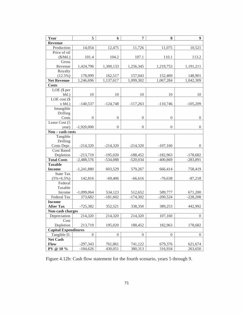
71
Year 5 6 7 8 9 Revenue
Production 14,054 12,475 11,726 11,075 10,521 Price of oil
($/bbl.) 101.4 104.2 107.1 110.1 113.2 Gross
Revenue 1,424,796 1,300,133 1,256,345 1,219,753 1,191,211 Royalty (12.5%) 178,099 162,517 157,043 152,469 148,901
Net Revenue 1,246,696 1,137,617 1,099,302 1,067,284 1,042,309 Costs
LOE ($ per bbl.) 10 10 10 10 10
LOE cost ($ x bbl.) -140,537 -124,748 -117,263 -110,746 -105,209
Intangible Drilling
Costs 0 0 0 0 0 Lease Cost (5
year) -1,920,000 0 0 0 0 Non – cash costs
Tangible Drilling
Costs Depr. -214,320 -214,320 -214,320 -107,160 0 Cost Based
Depletion -213,719 -195,020 -188,452 -182,963 -178,682 Total Costs -2,488,576 -534,088 -520,034 -400,869 -283,891 Taxable Income -1,241,880 603,529 579,267 666,414 758,419
State Tax (5%+6.5%) 142,816 -69,406 -66,616 -76,638 -87,218
Federal Taxable Income -1,099,064 534,123 512,652 589,777 671,200
Federal Tax 373,682 -181,602 -174,302 -200,524 -228,208 Income After Tax -725,382 352,521 338,350 389,253 442,992 Non-cash charges Depreciation 214,320 214,320 214,320 107,160 0
Cost Depletion 213,719 195,020 188,452 182,963 178,682
Capital Expenditures Tangible D. 0 0 0 0 0
Net Cash Flow -297,343 761,861 741,122 679,376 621,674 PV @ 10 % -184,626 430,051 380,313 316,934 263,650
Figure 4.12b: Cash flow statement for the fourth scenario, years 5 through 9.

72
Year 10 11 12 13 14 Revenue
Production 9,995 102,004 38,727 24,279 17,397 Price of oil
($/bbl.) 116.4 119.7 123.0 126.4 130.0 Gross
Revenue 1,163,336 12,205,035 4,763,522 3,070,057 2,261,361 Royalty (12.5%) 145,417 1,525,629 595,440 383,757 282,670
Net Revenue 1,017,919 10,679,406 4,168,081 2,686,300 1,978,691 Costs
LOE ($ per bbl.) 10 10 10 10 10
LOE cost ($ x bbl.) -99,949 -1,020,041 -387,270 -242,794 -173,968
Intangible Dr. Cost -5,600,000 0 0 0 0
Lease Cost (5 year) -1,920,000 0 0 0 0
Non – cash costs Tangible
D.C. Depr. 0 -342,960 -587,760 -419,760 -299,760 Cost Based
Depletion -174,500 -1,830,755 -714,528 -460,508 -339,204 Total Costs -7,794,449 -3,193,756 -1,689,558 -1,123,063 -812,932 Taxable Income -6,776,530 7,485,649 2,478,523 1,563,237 1,165,759
State Tax (5%+6.5%) 779,301 -860,850 -285,030 -179,772 -134,062
Federal Taxable Income -5,997,229 6,624,799 2,193,493 1,383,464 1,031,697
Federal Tax 2,039,058 -2,252,432 -745,788 -470,378 -350,777 Income After Tax -3,958,171 4,372,368 1,447,705 913,086 680,920 Non-cash charges Depreciation 0 342,960 587,760 419,760 299,760
Cost Dep. 174,500 1,830,755 714,528 460,508 339,204 Capital Expenditures
Tangible Drilling C. -2,400,000 0 0 0 0
Net Cash F. -6,183,671 6,546,083 2,749,994 1,793,355 1,319,884 PV (10%) -2,384,073 2,294,362 876,233 519,471 347,567
Figure 4.12c: Cash flow statement for the fourth scenario, years 10 through 14.
(New well drilled at the end of the tenth year)

73
Year 15 16 17 18 19 Revenue
Production 14,054 12,475 11,726 11,075 10,521 Price of oil
($/bbl.) 133.6 137.4 141.2 145.2 149.2 Gross
Revenue 1,877,949 1,713,638 1,655,923 1,607,693 1,570,073 Royalty (12.5%) 234,744 214,205 206,990 200,962 196,259
Net Revenue 1,643,205 1,499,433 1,448,932 1,406,731 1,373,814 Costs
LOE ($ per bbl.) 10 10 10 10 10
LOE cost ($ x bbl.) -140,537 -124,748 -117,263 -110,746 -105,209
Intangible Drilling C. 0 0 0 0 0
Lease Cost (5 year) -1,920,000 0 0 0 0
Non – cash costs Tangible
D.C. Dep. -214,320 -214,320 -214,320 -107,160 0 Cost Based
Depletion -281,692 -257,046 -248,388 -241,154 -235,511 Total Costs -2,556,549 -596,113 -579,971 -459,060 -340,720 Taxable Income -913,344 903,320 868,961 947,671 1,033,093
State Tax (5%+6.5%) 105,035 -103,882 -99,931 -108,982 -118,806
Federal Taxable Income -808,309 799,438 769,031 838,689 914,288
Federal Tax 274,825 -271,809 -261,470 -285,154 -310,858 Income After Tax -533,484 527,629 507,560 553,534 603,430 Non-cash charges Depreciation 214,320 214,320 214,320 107,160 0
Cost Depletion 281,692 257,046 248,388 241,154 235,511
Capital Expenditures Tangible
Drilling C. 0 0 0 0 0 Net Cash F. -37,472 998,995 970,269 901,848 838,941 PV (10%) -8,970 217,410 191,962 162,205 137,174
Figure 4.12d: Cash flow statement covering the years 15 through 19.

74
Figure 4.12e: Cash flow statement for the fourth scenario, year 20.
The initial well performance for the first ten years was revitalized with the
additional well’s ten year performance. The highest financial results were observed
in the fourth scenario with an NPV of $4.7 million NPV and 27.3 % IRR.
Year 20 Revenue
Production 9994,87 Price of oil ($/bbl.) 153,41
Gross Revenue 1533332,88 Royalty Fee (12.5%) 191666,61
Net Revenue 1341666,27 Costs
LOE ($ per bbl.) 10 LOE cost ($ x bbl.) -99948,69
Intangible Drilling Costs 0 Lease Cost (5 year) 0
Non – cash costs Tangible Drilling Costs Depreciation 0
Cost Based Depletion (15%) -229999,93 Total Costs -329948,61 Taxable Income 1011717,65
State Tax (5%+6.5%) -116347,53 Federal Taxable Income 895370,12
Federal Tax -304425,84 Income After Tax 590944,28 Non-cash charges
Depreciation 0 Cost Depletion 229999,93
Capital Expenditures Tangible Drilling Costs 0
Net Cash Flow 820944,21 Present Value @ (10%) 122028,12

75
Table 4.6: Profitability and EUR rate for the fourth scenario
Results for years 0 through 20
NPV @ MARR = 10% $ 4,749,000
IRR 27.3 %
EUR 504,505 bbls.
The second scenario was duplicated in the fourth one (two different wells
with the same reservoir features producing oil for ten years), but the NPV and IRR
results did not duplicate in the way that EUR did. When compared to the other
scenarios, the fourth scenario gave the most profitable results.
4.3. Break-even Analysis (Break-even prices)
There are three different financial methods used based on the cash flow
statements to analyze the investment profitability. The first two methods are the
NPV and IRR concepts. The third one is to find the break-even prices, and this
reflects the minimum oil price (per barrel) to achieve the hurdle rate that is 10
percent for the oil investments (i.e. find the price at which NPV equals to $0 using a
10 percent discount rate). In other words, the break-even price is the price that
achieves the minimum investment criteria at zero profit. In this study, the initial
break-even price was assumed to be increasing by 2.8 percent per year, the same as
the annual economic growth rate determined by the International Monetary Fund

76
(IMF). Table 4.7 shows the minimum oil prices (per barrel) to achieve the
investment hurdle rate (minimum acceptable rate of return of 10%) of the
investments.
Table 4.7: Break-even prices for different scenarios (zero NPV)
Break-even prices of oil per barrel
5 years of production (1st scenario) $74.35
10 years of production (2nd scenario) $68.81
20 years of production (3rd scenario) $66.83
20 years of production, second well drilled in year 10 (4th scenario) $63.26
Table 4.7 shows that all break-even prices for oil are lower than the initial
annual average oil price ($90.78 / bbl.). Therefore, all three methods show that these
scenarios are profitable under current market circumstances in the North Dakota
Bakken area. 20 years of production with drilling two different wells every tenth
year (4th scenario) has the lowest break-even price of $63.26. The difference
between the initial annual average oil price and the break-even price in the fourth
scenario was very significant, and the break-even is almost 30 percent lower than
the current initial price. The highest break-even price was $74.35 in the first
scenario due to short investment period and limited production time. In other words,
higher break-even prices indicate lowest profit rate. In addition, a $3.57 break-even
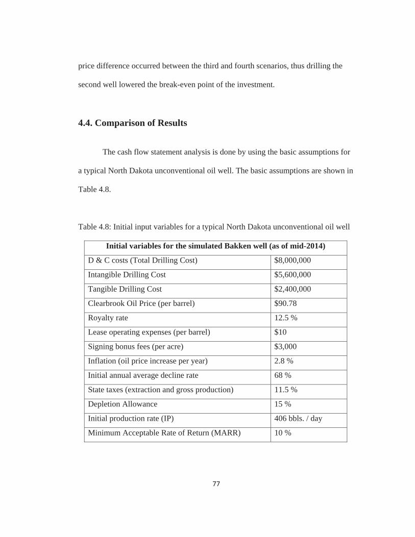
77
price difference occurred between the third and fourth scenarios, thus drilling the
second well lowered the break-even point of the investment.
4.4. Comparison of Results
The cash flow statement analysis is done by using the basic assumptions for
a typical North Dakota unconventional oil well. The basic assumptions are shown in
Table 4.8.
Table 4.8: Initial input variables for a typical North Dakota unconventional oil well
Initial variables for the simulated Bakken well (as of mid-2014)
D & C costs (Total Drilling Cost) $8,000,000
Intangible Drilling Cost $5,600,000
Tangible Drilling Cost $2,400,000
Clearbrook Oil Price (per barrel) $90.78
Royalty rate 12.5 %
Lease operating expenses (per barrel) $10
Signing bonus fees (per acre) $3,000
Inflation (oil price increase per year) 2.8 %
Initial annual average decline rate 68 %
State taxes (extraction and gross production) 11.5 %
Depletion Allowance 15 %
Initial production rate (IP) 406 bbls. / day
Minimum Acceptable Rate of Return (MARR) 10 %
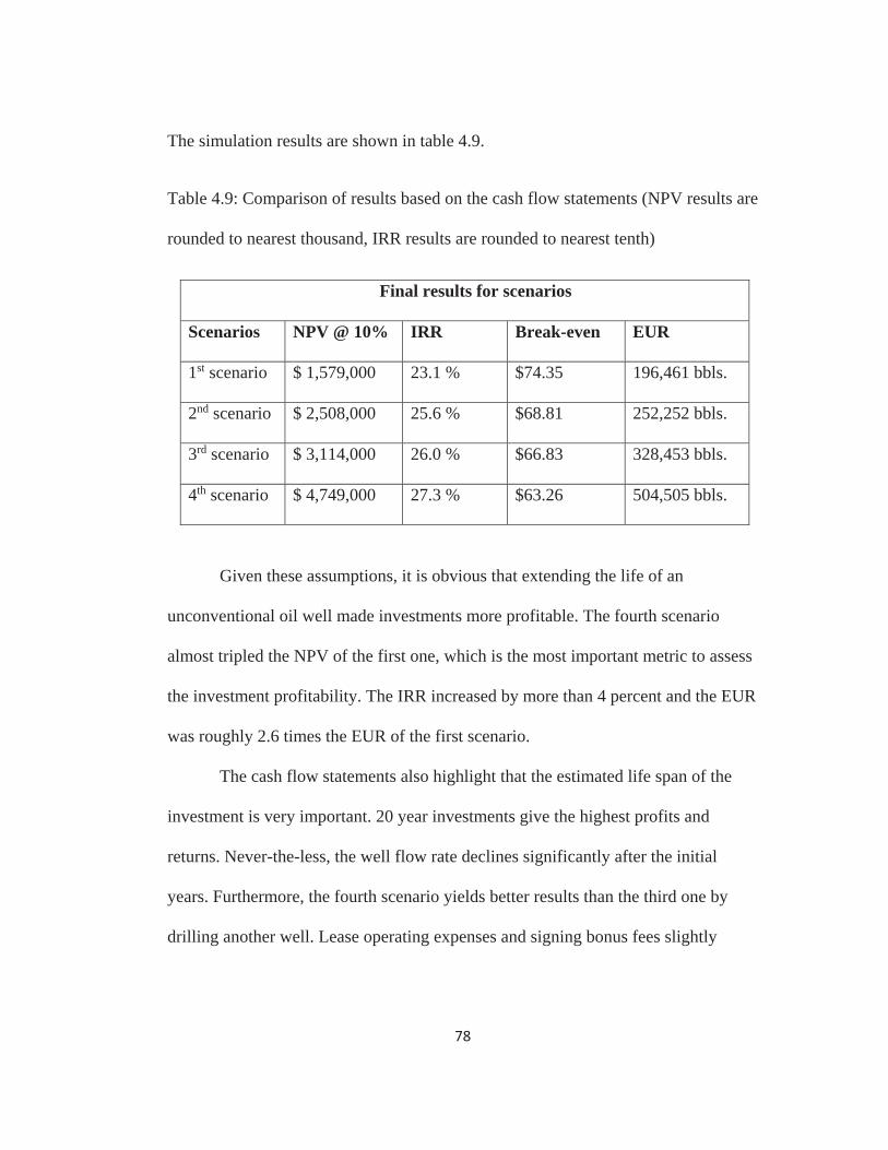
78
The simulation results are shown in table 4.9.
Table 4.9: Comparison of results based on the cash flow statements (NPV results are
rounded to nearest thousand, IRR results are rounded to nearest tenth)
Final results for scenarios
Scenarios NPV @ 10% IRR Break-even EUR
1st scenario $ 1,579,000 23.1 % $74.35 196,461 bbls.
2nd scenario $ 2,508,000 25.6 % $68.81 252,252 bbls.
3rd scenario $ 3,114,000 26.0 % $66.83 328,453 bbls.
4th scenario $ 4,749,000 27.3 % $63.26 504,505 bbls.
Given these assumptions, it is obvious that extending the life of an
unconventional oil well made investments more profitable. The fourth scenario
almost tripled the NPV of the first one, which is the most important metric to assess
the investment profitability. The IRR increased by more than 4 percent and the EUR
was roughly 2.6 times the EUR of the first scenario.
The cash flow statements also highlight that the estimated life span of the
investment is very important. 20 year investments give the highest profits and
returns. Never-the-less, the well flow rate declines significantly after the initial
years. Furthermore, the fourth scenario yields better results than the third one by
drilling another well. Lease operating expenses and signing bonus fees slightly

79
declined the profits between the year ten and twenty, but high oil prices balanced
the production costs and the system brought positive results again.
Break-even prices were also crucial for the investment viability. The average
annual oil price (mid-2014) $90.78 /bbl. was much higher than the break-even
results found via cash flow statements. $20-25 range per barrel is more than
sufficient to encourage the investments with given market conditions.
The highest NPV was achieved in the fourth scenario based on the
assumptions, but doubling the second scenario did not duplicate the NPV, IRR, and
break-even prices like EUR since the oil prices rose every year associated with the
time value of money.
Another idea for the best investment (4th scenario) can be a sensitivity
analysis to see variable over NPV sensitivity. What would be happen to the NPV if
some variables increase by 10 percent, 20 percent or decrease by 10 percent, 20
percent? Sensitivity analysis answers this question. Changes in NPV by using
different variables are shown in Table 4.10, Table 4.11, Table 4.12, Table 4.13, and
Table 4.14.
Table 4.10: Changes in NPV by increasing or decreasing drilling cost (holding all
else constant) ($ values are rounded to nearest thousand)
Variable Change in % Ex-NPV New-NPV % change in NPV Drilling cost ($8,000,000)
-20 $6,121,000 28.9 -10 45,435,000 14.4
0 (base case) $4,749,000 $4,749,000 0 +10 $4,063,000 -14.4 +20 $3,377,000 -28.9

80
Table 4.11: Changes in NPV by increasing or decreasing production rate (holding
all else constant) ($ values are rounded to nearest thousand)
Variable Change in % Ex-NPV New-NPV % change in NPV
Oil Price ($90.78/bbl.)
-20 $1,616,000 -66.0 -10 $3,182,000 -33.0
0 (base case) $4,749,000 $4,749,000 0 +10 $6,315,000 33.0 +20 $7,882,000 66.0
Table 4.12: Changes in NPV by increasing or decreasing production rate (holding
all else constant) ($ values are rounded to nearest thousand)
Variable Change in % Ex-NPV New-NPV % change in NPV
Production Rate (406 bbl./day)
-20 $1,923,000 -59.5 -10 $3,336,000 -29.8
0 (base case) $4,749,000 $4,749,000 0 +10 $6,161,000 29.7 +20 $7,574,000 59.5
Table 4.13: Changes in NPV by increasing or decreasing royalty fee (holding all
else constant) ($ values are rounded to nearest thousand)
Variable Change in % Ex-NPV New-NPV % change in NPV Royalty rate (12.5% of
gross income)
-20 $5,148,000 8.4 -10 $4,948,000 4.2
0 (base case) $4,749,000 $4,749,000 0 +10 $4,549,000 -4.2 +20 $4,350,000 -8.4
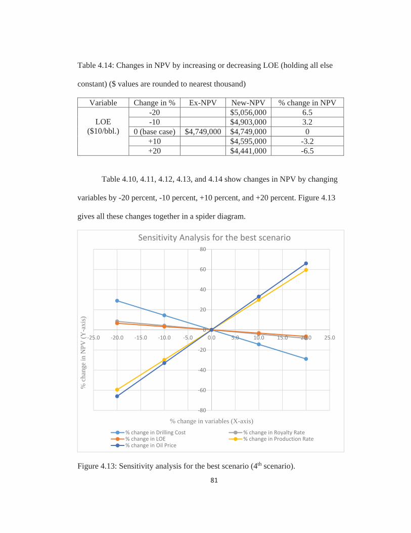
81
Table 4.14: Changes in NPV by increasing or decreasing LOE (holding all else
constant) ($ values are rounded to nearest thousand)
Variable Change in % Ex-NPV New-NPV % change in NPV
LOE ($10/bbl.)
-20 $5,056,000 6.5 -10 $4,903,000 3.2
0 (base case) $4,749,000 $4,749,000 0 +10 $4,595,000 -3.2 +20 $4,441,000 -6.5
Table 4.10, 4.11, 4.12, 4.13, and 4.14 show changes in NPV by changing
variables by -20 percent, -10 percent, +10 percent, and +20 percent. Figure 4.13
gives all these changes together in a spider diagram.
Figure 4.13: Sensitivity analysis for the best scenario (4th scenario).
80
60
40
20
0
20
40
60
80
25.0 20.0 15.0 10.0 5.0 0.0 5.0 10.0 15.0 20.0 25.0
% c
hang
e in
NPV
(Y-a
xis)
% change in variables (X-axis)
Sensitivity Analysis for the best scenario
% change in Drilling Cost % change in Royalty Rate% change in LOE % change in Production Rate% change in Oil Price
82
Figure 4.13 shows that the highest NPV changes are observed in oil price
and production rate when they increased by 20 percent (holding all else constant).
When oil price is increased by 20 percent, NPV is shifted from $4,749,000 to
$7,882,000 (66 percent increase in NPV). Similarly, when production rate is
increased by 20 percent, NPV is increased to $7,574,000 (59.5 percent increase in
NPV). Also, 20 percent decrease in oil price and production rate made significant
decreases in NPV. 20 percent decrease in oil price decreased NPV roughly $3.1
million (66 percent decrease in NPV) and 20 percent decrease in production rate
decreased NPV by $2.8 million (59.5 percent decrease in NPV).
These results additionally imply that the expected well life, EUR, and the
financial metrics moved together. When EUR and well life increased, the financial
results enhanced too.
All in all, these scenarios presented highly attractive results for the
investments in the North Dakota Bakken. Consequently, regardless of the time
frame, a typical simulated Bakken unconventional oil well presented profitable
investments and affirmative outcomes under these assumptions as of June 2014.
Comprehensive discussions, conclusions, and adverse conditions are discussed in
the following chapter (Chapter 5).
83
5. Discussion of Results
All these scenarios gave profitable results for a simulated investment. As
mentioned in the previous chapter, the most important metrics were the NPV, IRR,
EUR, and break-even prices. Based on these assumptions, all of these four scenarios
were acceptable and profitable for the given periods. Also, extending the well life
enhanced the NPVs of the investments because of the additional oil production in
the twenty year scenarios. Thus, this answers the first research question: a typical
Bakken well is economically viable under conditions in mid-2014. The second
question about the investment periods: a longer period is more profitable, with the
NPV achieving $4.75 million and the IRR reaching 27.3 percent (which almost
tripled the net investment hurdle rate of 10 percent). The fourth scenario gave the
best results, but the other scenarios were also very attractive and exceeded the
minimum acceptable rate of return. Thus, a typical North Dakota unconventional oil
well should be a profitable investment. However, in reality, these results are
variable and will easily shift from the positive to negative if the current
circumstances and assumptions change during the expected well life.
One of the main concerns is the oil price. This analysis assumes that every
year the oil price increases by 2.8 percent. Table 5.1 shows that the oil price for the
fifth, tenth, and the twentieth year respectively increased to $101.38, $116.39, and
$153.41 per barrel from $90.78 / bbl.
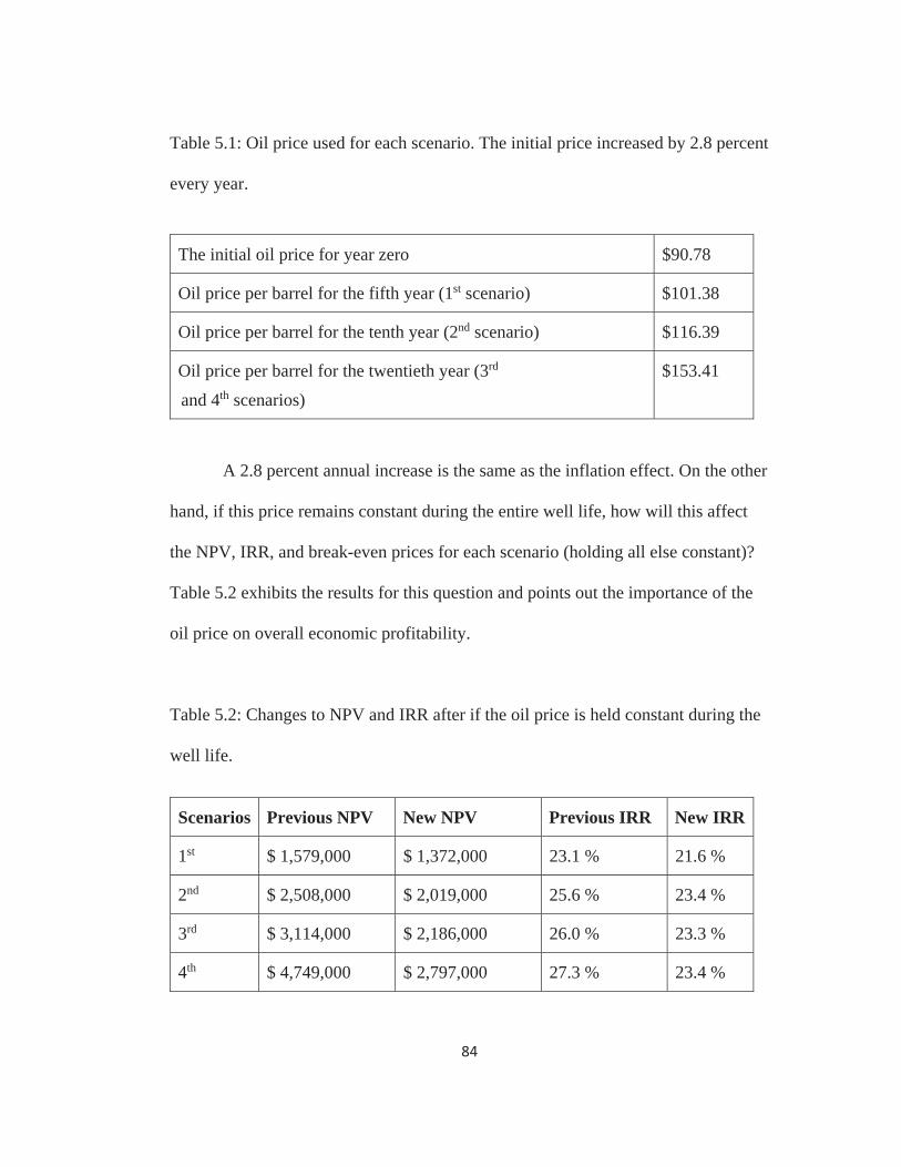
84
Table 5.1: Oil price used for each scenario. The initial price increased by 2.8 percent
every year.
The initial oil price for year zero $90.78
Oil price per barrel for the fifth year (1st scenario) $101.38
Oil price per barrel for the tenth year (2nd scenario) $116.39
Oil price per barrel for the twentieth year (3rd
and 4th scenarios)
$153.41
A 2.8 percent annual increase is the same as the inflation effect. On the other
hand, if this price remains constant during the entire well life, how will this affect
the NPV, IRR, and break-even prices for each scenario (holding all else constant)?
Table 5.2 exhibits the results for this question and points out the importance of the
oil price on overall economic profitability.
Table 5.2: Changes to NPV and IRR after if the oil price is held constant during the
well life.
Scenarios Previous NPV New NPV Previous IRR New IRR
1st $ 1,579,000 $ 1,372,000 23.1 % 21.6 %
2nd $ 2,508,000 $ 2,019,000 25.6 % 23.4 %
3rd $ 3,114,000 $ 2,186,000 26.0 % 23.3 %
4th $ 4,749,000 $ 2,797,000 27.3 % 23.4 %

85
If the initial oil price ($90.78 / bbl.) is kept constant during the whole well
life, NPV and IRR results would decrease, especially in the last two scenarios.
Based on the NPV results, a roughly two million dollar reduction would occur in the
fourth scenario, a million dollar reduction would occur in the third one, and the
others would also suffer. More interestingly, the ranking by IRR would change: the
third scenario would lose its position; the second scenario and the fourth scenario
would both have the highest IRR at 23.4%. The biggest IRR loss would occur in the
fourth scenario by 3.9 percent.
Table 5.2 shows that the impact of the price change was considerable and
lowered the profit margin. In reality, it is impossible to estimate the oil price for 20
years because many variables can be affect it such as oversupply issues, production
costs, political issues, demand changes etc. For this reason, a realistic assessment
must include many price considerations to determine the sensitivity of the project to
price.
Another concern is the lease operating expenses. As opposed to the oil
prices, in this study these expenses remained constant for the whole period ($10 per
barrel). If the same economic growth or annual increase of 2.8 percent applied to
these expenses, what would be the differences to the profitability? This question
will be important because it is basically associated with the production costs and
would have a significant increase on the cost side.
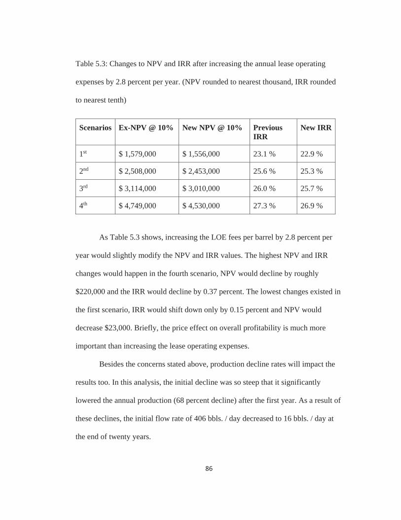
86
Table 5.3: Changes to NPV and IRR after increasing the annual lease operating
expenses by 2.8 percent per year. (NPV rounded to nearest thousand, IRR rounded
to nearest tenth)
Scenarios Ex-NPV @ 10% New NPV @ 10% Previous IRR
New IRR
1st $ 1,579,000 $ 1,556,000 23.1 % 22.9 %
2nd $ 2,508,000 $ 2,453,000 25.6 % 25.3 %
3rd $ 3,114,000 $ 3,010,000 26.0 % 25.7 %
4th $ 4,749,000 $ 4,530,000 27.3 % 26.9 %
As Table 5.3 shows, increasing the LOE fees per barrel by 2.8 percent per
year would slightly modify the NPV and IRR values. The highest NPV and IRR
changes would happen in the fourth scenario, NPV would decline by roughly
$220,000 and the IRR would decline by 0.37 percent. The lowest changes existed in
the first scenario, IRR would shift down only by 0.15 percent and NPV would
decrease $23,000. Briefly, the price effect on overall profitability is much more
important than increasing the lease operating expenses.
Besides the concerns stated above, production decline rates will impact the
results too. In this analysis, the initial decline was so steep that it significantly
lowered the annual production (68 percent decline) after the first year. As a result of
these declines, the initial flow rate of 406 bbls. / day decreased to 16 bbls. / day at
the end of twenty years.
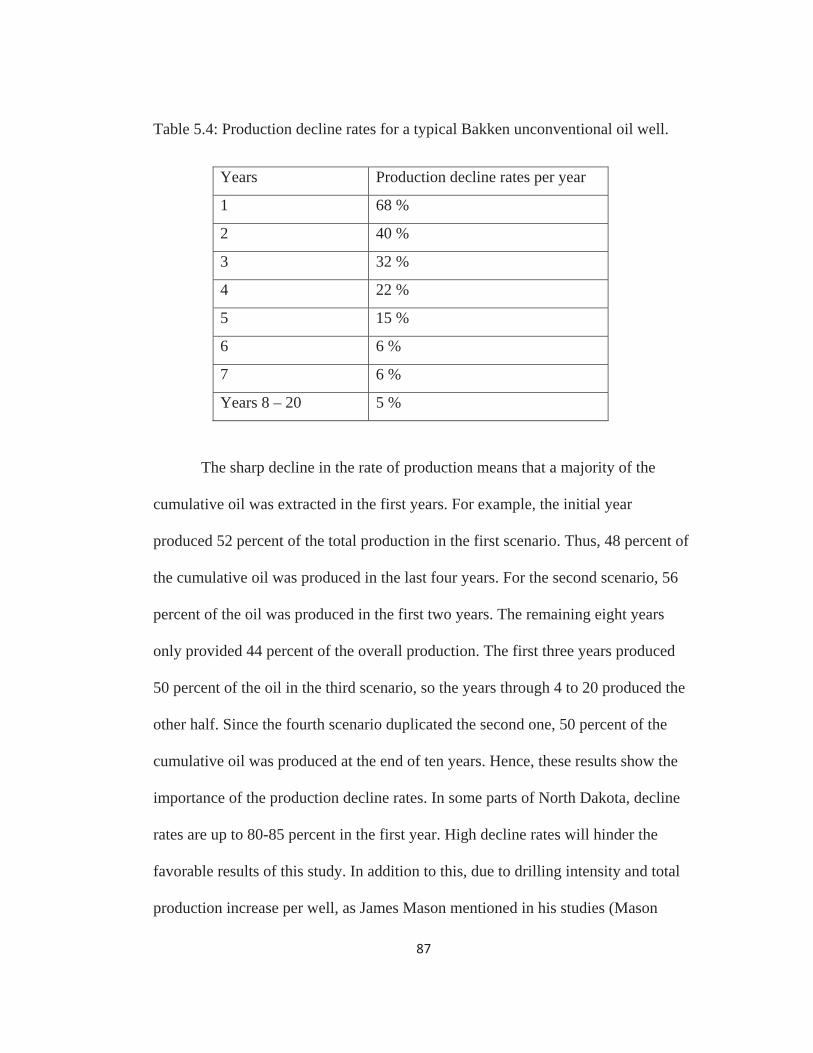
87
Table 5.4: Production decline rates for a typical Bakken unconventional oil well.
Years Production decline rates per year
1 68 %
2 40 %
3 32 %
4 22 %
5 15 %
6 6 %
7 6 %
Years 8 – 20 5 %
The sharp decline in the rate of production means that a majority of the
cumulative oil was extracted in the first years. For example, the initial year
produced 52 percent of the total production in the first scenario. Thus, 48 percent of
the cumulative oil was produced in the last four years. For the second scenario, 56
percent of the oil was produced in the first two years. The remaining eight years
only provided 44 percent of the overall production. The first three years produced
50 percent of the oil in the third scenario, so the years through 4 to 20 produced the
other half. Since the fourth scenario duplicated the second one, 50 percent of the
cumulative oil was produced at the end of ten years. Hence, these results show the
importance of the production decline rates. In some parts of North Dakota, decline
rates are up to 80-85 percent in the first year. High decline rates will hinder the
favorable results of this study. In addition to this, due to drilling intensity and total
production increase per well, as James Mason mentioned in his studies (Mason
88
2012a) (Mason 2012b), well saturation will occur much sooner than expected time
and North Dakota oil investments will cease.
To summarize, a typical North Dakota Bakken unconventional oil well
achieves positive results for all studied scenarios. The best economic results and
EUR rates were observed in the fourth scenario, but all four of them were profitable
to invest in. Under these assumptions, an oil investment in the North Dakota Bakken
will be profitable and economically viable for 5 year, 10 year, and 20 year periods.
Environmental issues were beyond the scope of this study, but if they are currently
being included in lease operating expenses, then oil investment in North Dakota
should continue to expand.

89
6. Conclusions
Advanced horizontal drilling technologies provide access to the lateral
reservoir formations. Additionally, with the support of hydraulic fracturing
operations, operators are able to increase the expected recovery rate of oil. Oil
prices increased significantly after the economic recession, which encouraged
investors and operators to explore and develop new oil fields. As a result of
enhanced drilling techniques and high oil prices, the North American tight oil sand
and shale oil formations such as the Bakken Shale gained importance and became
more economic to invest in. Recently, the Bakken field became the second largest
oilfield in the United States. Daily production reports show that production
increases day by day, and roughly 70 percent of the oil comes from unconventional
resources.
As the financial calculations and cash flow statements show, a typical North
Dakota Bakken unconventional oil well is profitable for 5, 10, and 20 year
investment periods. Surprisingly, based on the scenario analysis, operators
experienced the highest profit in the 20 year plans (the third and the fourth
scenarios). However, profitable results will change in the long run depending on the
production costs, sharp production declines and limited production periods, raising
environmental concerns associated with hydraulic fracturing, and volatile oil prices.
Oil price increases and sharp decline rates motivate Bakken operators to drill new
wells right once profit margins begin to decrease. It raises the drilling intensity and
leads to well saturation issues (Mason 2012b). Furthermore, due to lack of

90
infrastructure and potential fracturing chemical leakages, there is an increase in
environmental concerns, which may bring additional costs (external costs) into the
system. These issues might increase the production costs in the long run as opposed
to this analysis (costs held constant). Despite these concerns, based on the
assumptions used in this analysis, a typical North Dakota Bakken unconventional oil
well is profitable. In addition to this, technological developments, infrastructural
improvements, and favorable economic conditions may keep production costs low.
Thus, given the same conditions, Bakken unconventional oil well investments
should be profitable over the long run.
Outside of the operators’ point of view, unconventional oil production has
direct economic benefits to the landowners, state government, and residents of
North Dakota. Associated with the profitable unconventional oil investments in
North Dakota, oil and gas tax revenues reached the highest levels at the end of the
year 2013, at $2.9 billion. As a result of the high tax revenues, the state government
started to fix the infrastructure issues and spent money for expanding shipping
options. The state’s unemployment rate has been decreasing since 2009. Companies
create thousands of jobs every year. The unemployment rate of North Dakota was
4.2 percent in 2009, and it decreased by 1.4 percent to 2.8 percent at the end of the
August 2014 (Bureau of Labor Statistics 2014). Also, the state’s GDP increased by
9.7 percent in 2013 (Bureau of Economic Analysis 2014).
On the other hand, oil production increases bring concerns. Drilling
intensity in North Dakota will peak at some point in the future and then well
91
saturation will obstruct the possible future investments. As James Mason studied, if
daily production reaches 1.5 million bbls. per day, well saturation will occur in
2045. If daily production exceeds 2 million bbls. per day, saturation will occur 11
years before, in 2034 (Mason 2012b). Since the oil is non-renewable and limited,
oil production cannot always increase in the long run. When compared to other
states, the unconventional oil investments in North Dakota are still relatively new
and operators cannot guarantee long term success along with the increasing demand.
This analysis demonstrated high production declines after the initial years and
operators can only mitigate declines by drilling new wells. For that reason, at the
end of the tenth year in the fourth scenario, a new well was drilled and gave the
highest EUR for 20 years. It is also impossible to avoid the water supply issue.
Without 100 percent water re-cycling, a potential threat of water contamination will
remain as an important environmental issue for the state. Moreover, higher oil
production has a higher risk of pollution. Consequently, these issues will impact the
economics of unconventional oil production. Financial results of the analysis
indicates a $15 to $27 difference between break-even prices and current (mid-2014)
oil prices. Thus companies might make some modifications to their environmental
policies at a slight production cost increase to reduce the social costs of these
potential risks.
In this analysis, 5 year investments were considered as short term and 10 to
20 year investments were assumed as long term projects. The results of the analysis
highlighted the long term investment success. But in reality, market conditions and
92
the demand for oil will change in the long run. If favorable economic conditions
continue, profitable results are likely over the long - run. Also, inflation was not
considered because some production costs were held constant in the analysis and
these costs will either increase or decrease in the future.
In conclusion, considering all concerns including both recent and future
issues associated with horizontal drilling and hydraulic fracturing, a typical North
Dakota Bakken unconventional oil well is profitable and viable for short term and
long term investments. Unconventional production has been enhancing the state’s
economy along with fueling the U.S. economy with regional supply. Unless there is
a dramatic price change, or unexpected new supply source with conventional
technologies, the unconventional oil phenomenon will continue to develop for
decades because the United States Geological Survey (USGS) estimated 7.4 billion
barrel of oil in the Bakken Formation in 2013 (USGS 2013).
93
7. References
Anderson, R. (1981, last updated 2006). North Dakota Oil and Gas Leasing
Considerations (C. E. Service, Trans.). Fargo, ND.
Bloomberg. (2012). U.S. Oil Output to Overtake Saudi Arabia’s by 2020.
Retrieved 06-24, 2014, from http://www.bloomberg.com/news/2012-11-12/u-s-to-
overtake-saudi-arabia-s-oil-production-by-2020-iea-says.html
Bloomberg (2013). U.S. to Be Top Oil Producer by 2015 on Shale, IEA Says.
Retrieved 06-24, 2014, from http://www.bloomberg.com/news/2013-11-12/u-s-
nears-energy-independence-by-2035-on-shale-boom-iea-says.html
Bureau of Economic Analysis (2014, June 11, 2014). Advance 2013 and Revised
1997—2012 Statistics of GDP by State. Retrieved October, 10, 2014, from
http://www.bea.gov/newsreleases/regional/gdp_state/gsp_newsrelease.htm
Bureau of Labor Statistics (2014, September 19, 2014). Regional and State
Employment and Unemployment Summary. Economics News Release. Retrieved
October 10, 2014, from http://www.bls.gov/news.release/laus.nr0.htm
Davies, D., (2001). Production technology II. Tech. rep., Department of Petroleum
Engineering, Heriot-Watt University, Edinburgh, Scotland.
Dizard, J. (2010, March 21, 2010). The sleight of hand over shale gas costs.
Retrieved 06-11-2014, 2014, from http://www.ft.com/intl/cms/s/0/6254ec9c-33f1-
11df-8ebf-00144feabdc0.html#axzz35rPESKiV

94
Dukes, R. T. (2013a). Hess’s Bakken Drilling Days & Well Costs Down.
Retrieved 06-22, 2014, from http://bakkenshale.com/news/hesss-bakken-drilling-
days-well-costs-down/
Dukes, R. T. (2013b, October, 30, 2013). Hess’ Bakken Production Grows by 14%
& Well Costs Fall 18%. Retrieved 06-03, 2014, from
http://bakkenshale.com/news/hess-bakken-production-grows-14-well-costs-fall-18/
Duman, R. (2012). Economic Viability of Shale Gas Production in the Marcellus
Shale; Indicated by Production Rates, Costs and Current Natural Gas Prices.
Master’s Thesis, Michigan Technological University, 2012, Houghton, MI.
Retrieved from
http://services.lib.mtu.edu/etd/THESIS/2012/Business&Economics/duman/thesis.pd
f
Earthworks. (2014). Hydraulic Fracturing 101. Retrieved 11-17, 2014, from
http://www.earthworksaction.org/issues/detail/hydraulic_fracturing_101#.VGrMYv
kVgqw
Energy Information Administration. (2010). Annual Energy Outlook
Energy Information Administration (2013a, March, 19, 2013). Bakken crude oil
price differential to WTI narrows over last 14 months. Retrieved 05-04, 2014, from
http://www.eia.gov/todayinenergy/detail.cfm?id=10431
Energy Information Administration (EIA) (2013b, April, 2013). Annual Energy
Outlook 2013 (D. o. Energy, Trans.): Energy Information Administration.
95
Energy Information Administration (2014). Annual Energy Outlook 2014 (U. S. E.
I. Administration, Trans.): Energy Information Administration.
Fong, C. (2012). State and Local Taxes: An overview and Comparative Guide 2012.
Galusky, P. (2011). Feasibility Assessment of Early Flowback Water Recovery for
Reuse in Subsequent Well Completions. Illinois: Gas Technology Institute.
Hefley, W.E., et al. (August, 2011). The economic impact of the value chain of a
Marcellus Shale Well. University of Pittsburgh Katz Graduate School of Business
Hess Corporation (2013). Barclays CEO Energy-Power Conference (pp. 13).
Hughes, J. D. (2013). Drill, Baby, Drill (2nd Edition ed.). Santa Rosa, California,
USA: Post Carbon Institute.
IMF World Economic Outlook. (2014). Washington, D.C.: International Monetary
Fund. from http://www.imf.org/external/pubs/ft/weo/2014/update/01/pdf/0114.pdf
Inkpen, A. C., Moffett, H. M. (2011). Global Oil & Gas Industry: Management,
Strategy, and Finance (T. Quinn Ed.). Tulsa, Oklahoma: PennWell.
Internal Revenue Service (2013a). Publication 535, Depletion. Retrieved 05-09,
2014, from http://www.irs.gov/publications/p535/ch09.html
Internal Revenue Services (2013b). Publication 946, Table of Class Lives and
Recovery Periods. Retrieved 05-10, 2014, from
http://www.irs.gov/publications/p946/ar02.html
96
Jayakumar, R., Rai. R., Boulis, A., Araque-Martinez, A. (2013). A Systematic Study
for Refracturing Modeling under Different Scenarios in Shale Reservoirs. Paper
presented at the SPE Eastern Regional Meeting, Pittsburgh, PA.
Mason, J. (2012a). Bakken's maximum potential oil production rate explored. Oil &
Gas Journal.
Mason, J. (2012b). Oil Production Potential of the North Dakota Bakken. Oil and
Gas Journal.
Maugeri, L. (2013). The Shale Oil Boom: A U.S. Phenomenon (K. S. B. C. f. S. a. I.
Affairs, Trans.). Harvard University Kennedy School Belfer Center for Science and
International Affairs.
North Dakota Oil Boom (2014). Tax Advantages of Oil and Gas Partnerships.
Retrieved 2014, from http://northdakotaoilboom.com/tax-advantages-of-oil-and-
gas-partnerships/
Ohio Department of Natural Resources (OHDNR) 2012. “Preliminary report on the
Northstar I Class II Injection Well and the Seismic Events in the Youngstown, Ohio
Area”, from http://ohiodnr.com/downloads/northstar/UICreport.pdf ; last accessed
06-02-2014.
Oil and Energy Trends. (2012, 05-16-2012). Retrieved 05-16, 2012, from
http://onlinelibrary.wiley.com/doi/10.1111/j.1744-7992.2012.00211.x/abstract
Pan, I. (2013, 10-25-2013). Bakken crude again trading $10 below WTI, affecting
energy names. Retrieved 06-19, 2014, from
97
https://marketrealist.com/2013/10/bakken-crude-back-trading-10-wti-affecting-
continental-whiting-others/
Patterson, R. (2013, 12-13-2013). Bakken Update, Is Production Slowing Down? ,
06-14-2014, from http://peakoilbarrel.com/bakken-update-production-slowing/
Petrobjects. (2004). Petroleum Reserves Estimation Methods. From
http://large.stanford.edu/courses/2013/ph240/zaydullin2/docs/petrobjects.pdf
PetroChase. (2014). Tax Advantages. Retrieved 06-12, 2014, from
http://petrochase.com/tax-benefits/
Robelius, F. (2007). Giant Oil Fields - The Highway to Oil. (Doctor of Philosophy),
Uppsala University, Uppsala, Sweden.
Rogers, D. (2013, 04-07-2013). Is the Bakken Profitable? Retrieved 02-04, 2014,
from http://energypolicyforum.org/2013/04/07/is-the-bakken-profitable/
Ryder Scott Co. LP (2011). Promising DCA techniques emerge as widespread
public debate focuses on shale gas forecasts. 14(September - November 2011), 3.
Schlumberger. (2011). Retrieved 05-08, 2014, from
http://www.glossary.oilfield.slb.com/en/Terms.aspx?LookIn=term%20name&filter=
workover
Shaver, R. (2012). Water Management Issues Associated With Bakken Oil Shale
Development in Western North Dakota (W. A. Division, Trans.).
98
Siegel, H. (2013, 10-10-2013). Bakken 5-Year Drilling & Completion Trends.
Retrieved 10-10, 2013, from http://www.dtcenergygroup.com/bakken-5-year-
drilling-completion-trends/
Smith, G. (2014, 07-04-2014). U.S. Seen as Biggest Oil Producer after Overtaking
Saudi Arabia. Retrieved 07-09-2014, 2014, from
http://www.bloomberg.com/news/2014-07-04/u-s-seen-as-biggest-oil-producer-
after-overtaking-saudi.html
South Western College. (2001). Depletion Deductions. Retrieved 06-02, 2014,
from http://taxpoint.swcollege.com/taxpoint_2001/student/m10/m10-6.html
Stepan, D.J. and University of North Dakota Energy and Environmental Research
Center for North Dakota Industrial Commission Oil and Gas Research Council
(2010). Bakken Water Opportunities Assessment - Phase 1. In K. Fine (Ed.). Grand
Forks, ND: Energy and Environmental Research Center.
Strother, D., Valaderes, R., Nakhwa, A.D., and Pitcher, J. (2013). Challenges of
Refracturing Horizontal Wells in Unconventional and Tight Reservoirs. Society of
Petroleum Engineers.
USGS. (2013). Assessment of Undiscovered Oil Resources in the Bakken and Three
Forks Formations, Williston Basin Province, Montana, North Dakota, and South
Dakota, 2013 (B.-T. F. A. Team, Trans.) (pp. 4).
Wegmann, P. (2014). 1,000,000 Barrels a Day and Growing: Oil Production
Skyrockets in North Dakota. Retrieved 06-23, 2014, from

99
http://dailysignal.com/2014/06/23/1000000-barrels-day-growing-oil-production-
skyrockets-north-dakota/?utm_source=twitter&utm_medium=social
http://www.mapsopensource.com/usa-political-map.html