tasks for temporal graph visualisation

1

Tasks for Temporal Graph Visualisation Natalie Kerracher, Jessie Kennedy, and Kevin Chalmers

Institute for Informatics and Digital Innovation

Edinburgh Napier University, Scotland, UK

e-mail: [email protected]

In [1], we describe the design and development of a task taxonomy for temporal graph visualisation. This paper

details the full instantiation of that task taxonomy. Our task taxonomy is based on the Andrienko framework [2],

which uses a systematic approach to develop a formal task framework for visual tasks specifically associated with

Exploratory Data Analysis. The Andrienko framework is intended to be applicable to all types of data, however, it

does not consider relational (graph) data. We therefore extended both their data model and task framework for

temporal graph data, and instantiated the extended version to produce a comprehensive list of tasks of interest

during exploratory analysis of temporal graph data. As expected, our instantiation of the framework resulted in a

very large task list; with more than 144 variations of attribute based tasks alone, it is too large to fit in a standard

journal paper, hence we provide the detailed listing in this document.

This paper is organised as follows: in section 1 we give a short overview of the task categories of the taxonomy, a

more detailed explanation of which is provided in [1]. A key notion in the Andrienko framework is that of behaviours:

in section 2 we briefly summarise the partial and aspectual behaviours of interest when analysing temporal graphs.

In section 3 we provide a short guide to the formal notation used in the task definitions of the original framework.

Finally, in section 4, we give the complete task listings for both structural and attribute based graph visualisation

tasks.

1 Overview of task categories Under the Andrienko framework, there are two components to every task: the target, or unknown information to be

obtained, and the constraints, or the known conditions that information needs to fulfil. These targets and constraints

distinguish the tasks and determine the shape of the model. We provide an overview of the task categories in Figure

1, which is based on Aigner et al.’s [3] representation of the original Andrienko task model organised into a

taxonomy. We have redrawn and extended their figure to include our addition of structural tasks to the taxonomy.

A detailed description of the task categories is provided in [1].

Figure 1 The task model. Based on Aigner et al.’s drawing [2, p74] of the Andrienko task model organised into a taxonomy, redrawn and

extended to include structural tasks for graph visualisation.

2

2 Behaviours Behaviours are a key notion in the Andrienko framework: they are representative of real-world phenomena,

describing the configurations of sets of attribute values over the independent (referential) component of the data, as

determined by the data function (the mapping between the independent and dependent data components), and the

relations which exist between the elements of the independent data component e.g. distance and order. A pattern

results from an observation of a behaviour and provides a descriptive summary of its essential features. Four main

types of pattern are distinguished under the Andrienko framework: association, differentiation, arrangement and

distribution. Where there are multiple independent components of the data (as in the case of temporal graphs), they

distinguish between overall behaviours (which consider all behaviours over the entire dataset) and aspectual

behaviours (which consider only certain aspects of the overall behaviour).

In addition to the attribute based behaviours of the Andrienko framework, we introduce the notion of structural

behaviours in temporal graphs. We here outline the two partial and two aspectual attribute-based behaviours

applicable to temporal graphs, along with the four analogous structural behaviours.

2.1 Attribute based behaviours

Partial behaviours:

1. The behaviour of an attribute of a single graph element (a node, edge, or graph object) over time (the whole

time period or a subset of time) e.g. a temporal trend in the attribute of a node.

2. The behaviour of an attribute over a set of nodes (or subset of nodes/graph object) at a single time e.g. the

distribution of the attribute values over the set.

Aspectual behaviours:

1. The behaviour of the temporal trends (1, above) over the graph (i.e. the distribution of temporal behaviours

over the graph).

2. The behaviour over time of the behaviours of attribute values over the set of graph objects (2, above) (i.e.

the temporal trend in the distribution of the attribute values over the graph).

2.2 Structural behaviours

(1) The behaviour of association relations between two graph objects over time e.g. the pattern of change in

connectivity between two nodes over time.

(2) The behaviour, or configuration, of association relations within a set of nodes at a single time e.g. clusters,

cliques, motifs etc.

(3) The behaviour of the collection of patterns in (1) i.e. the aggregate pattern of all association relations between

pairs of graph objects over time, or the distribution of individual temporal behaviours over the graph.

(4) The behaviour of the configurations of association relations over the set of nodes (i.e. (2)), over time.

3 Formal Notation This section provides a brief summary of the formal notation used to represent variations in tasks in the framework.

3.1 Data function applied to temporal graphs

In the case of temporal graphs, we use the following formalism to represent the Andrienko data function which

maps a graph element at a particular time point to the corresponding values of the attributes in the data set:

f(t, g) = (y1, y2, …, yN)

3

Where:

t represents a time point

g represents a graph element (node, edge, graph object)

y1, y2, …, yN represents the N attributes in the data set

3.2 Key to formal notation

Bold a specified value (constant)

Italics an unknown value (variable)

t a time point

T′ a (sub)set of time points/a time interval

g a graph element (node, edge, graph object)

G′, G″ a (sub)set of graph elements

y the value of an unknown characteristic

c a specified characteristic C′ a subset of characteristics

Λ, Ψ, Φ, λ, ψ, φ a relation (e.g. y1 λ y2 can be read as ‘the relation between’ y1 and y2)

β(f(x1, x2) | x1∈ G′, x2 ∈ T′) the behaviour β of a data function f over the set of graph objects G′,

and time interval T′, where x1 is a graph object in the set of graph

objects (G′) and x2 is a time point in the time interval (T′)

βG{βT[f(x1, x2) | x2 ∈ T)]| x1∈ G}

βT{βG[f(x1, x2) | x1 ∈ G)]| x2∈ T}

formulae representing the two aspectual behaviours: the behaviour

of the temporal behaviours (trends) over the graph (i.e. the

distribution of temporal behaviours over the graph), and the

behaviour over time of the behaviours (distributions) of attribute

values over the set of graph elements (i.e. the temporal trend in the

distribution of the attribute values).

P a known pattern

p An unknown pattern

≈ ‘approximates’

4 Tasks In this section we list the tasks associated with analysis of temporal graph data. In order to systematically specify all

possible permutations of tasks under the framework, we used a series of task matrices when generating the tasks.

The comparison and relation seeking matrices can also be found in their complete form at

http://www.iidi.napier.ac.uk/c/downloads/downloadid/13377254 for easier reading and printing.

4.1 Attribute based tasks

4.1.1 Lookup tasks

4.1.1.1 Elementary lookup

In the temporal graph case, elementary lookup tasks involve the correspondence between a graph element (a node,

edge, or graph object) at a particular time point, and its associated attribute value. In direct lookup, given a graph

element at a given time point, we seek to find the corresponding attribute value. In inverse lookup, we seek to find

the graph element(s) and/or time point(s) associated with a given attribute value. There are a number of possible

variations of inverse lookup, depending on the additional constraints involved: we may specify just the attribute

value, or in addition specify either a time point or graph object. These variations are shown in the lookup task matrix

(Figure 3).

4

Additional task variations which are not shown in the matrix, but can be formulated based on the tasks in the matrix,

include:

• The case where the attribute value is imprecisely specified, and we allow a set of attribute values e.g. where

the value is ‘greater than 50’ or in the set {red, green, blue}: ? t, g: f(t, g) ∈ C′

• Specifying a subset of graph elements or time points (e.g. an interval) (in place of a single graph element or

time point) as an additional constraint e.g.

o Find the time(s) at which any graph object in the specified subset have the given attribute value:

? t: f(t, G′) = c

o Find the graph object(s) which have the given attribute value at any time during the given time

interval ? g: f(T′, g) = c

• Where the values of either time or graph are of no importance, we allow the whole set of time points or

graph elements to be specified:

o Find the time(s) at which any graph object had the given attribute value: ? t: f(t, G) = c

o Find the graph object(s) which had the given attribute value at any time: ? g: f(T, g) = c

4.1.1.2 Synoptic lookup

Behaviour characterisation involves finding the pattern which approximates the behaviour of an attribute over a

reference set (or subset). Pattern search is the opposite: given a pattern, we find the subset of references over

which the behaviour corresponds to the specified pattern. In the temporal graph case, these tasks involve the

aspectual and partial behaviours described in section 2, and the corresponding graph and temporal references. This

results in three task variations, depending on the referential components involved. We outline these in quadrants 2-

4 of Figure 2. Further variations in the pattern search task depend on which referential components are specified,

and these are detailed in the full lookup task matrix (Figure 3).

5

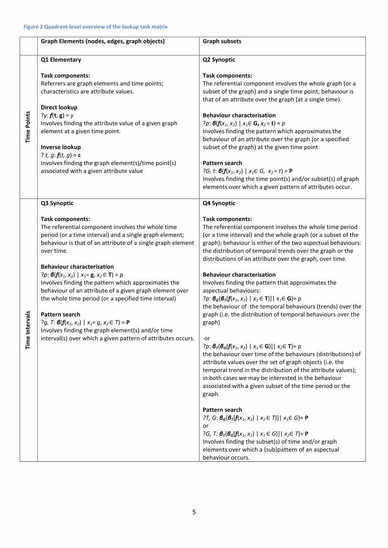
Figure 2 Quadrant-level overview of the lookup task matrix

Graph Elements (nodes, edges, graph objects) Graph subsets

Tim

e P

oin

ts

Q1 Elementary

Task components:

Referrers are graph elements and time points;

characteristics are attribute values.

Direct lookup

?y: f(t, g) = y

Involves finding the attribute value of a given graph

element at a given time point.

Inverse lookup

? t, g: f(t, g) = c

Involves finding the graph element(s)/time point(s)

associated with a given attribute value

Q2 Synoptic

Task components:

The referential component involves the whole graph (or a

subset of the graph) and a single time point; behaviour is

that of an attribute over the graph (at a single time).

Behaviour characterisation

?p: β(f(x1, x2) | x1∈ G, x2 = t) ≈ p

Involves finding the pattern which approximates the

behaviour of an attribute over the graph (or a specified

subset of the graph) at the given time point

Pattern search

?G, t: β(f(x1, x2) | x1∈ G, x2 = t) ≈ P

Involves finding the time point(s) and/or subset(s) of graph

elements over which a given pattern of attributes occur.

Tim

e I

nte

rva

ls

Q3 Synoptic

Task components:

The referential component involves the whole time

period (or a time interval) and a single graph element;

behaviour is that of an attribute of a single graph element

over time.


?p: β(f(x1, x2) | x1= g, x2 ∈ T) ≈ p

Involves finding the pattern which approximates the

behaviour of an attribute of a given graph element over

the whole time period (or a specified time interval)

Pattern search

?g, T: β(f(x1, x2) | x1= g, x2 ∈ T) ≈ P

Involves finding the graph element(s) and/or time

interval(s) over which a given pattern of attributes occurs.

Q4 Synoptic

Task components:

The referential component involves the whole time period

(or a time interval) and the whole graph (or a subset of the

graph); behaviour is either of the two aspectual behaviours:

the distribution of temporal trends over the graph or the

distributions of an attribute over the graph, over time.


Involves finding the pattern that approximates the

aspectual behaviours:

?p: βG{βT[f(x1, x2) | x2 ∈ T)]| x1∈ G}≈ p

the behaviour of the temporal behaviours (trends) over the

graph (i.e. the distribution of temporal behaviours over the

graph)

or

?p: βT{βG[f(x1, x2) | x1 ∈ G)]| x2∈ T}≈ p

the behaviour over time of the behaviours (distributions) of

attribute values over the set of graph objects (i.e. the

temporal trend in the distribution of the attribute values);

in both cases we may be interested in the behaviour

associated with a given subset of the time period or the

graph.

Pattern search

?T, G: βG{βT[f(x1, x2) | x2 ∈ T)]| x1∈ G}≈ P

or

?G, T: βT{βG[f(x1, x2) | x1 ∈ G)]| x2∈ T}≈ P

Involves finding the subset(s) of time and/or graph

elements over which a (sub)pattern of an aspectual

behaviour occurs.

6

Figure 3 Lookup task matrix

Graph Elements Graph subsets

Constraint Target Constraint Target

Tim

e p

oin

t

Ta

rge

t

Direct look up given a graph

object and time, find the

attribute value

?y: f(t, g) = y

Inverse lookup given an

attribute value and a time point,

find the graph object(s) which

have this value

? g: f(t, g) = c


Find the pattern that approximates (i.e. characterise)

the behaviour of an attribute over the graph (or a

subset of the graph) at the given time point

?p: β(f(x1, x2) | x1∈ G, x2 = t) ≈ p

Pattern search find the subset(s) of the graph over

which a particular pattern of attribute values occurs,

at the given time point

?G: β(f(x1, x2) | x1∈ G, x2 = t) ≈ P

Co

nst

rain

t

Inverse look up given a graph

object and attribute value, find

the time point(s) at which it

occurs

? t: f(t, g) = c

Inverse lookup given an attribute

value, find the graph object(s),

and the time point(s), at which

the value occurs

? t, g: f(t, g) = c

Pattern search find the time point(s) at which a

particular pattern of attributes over the graph occurs

? t: β(f(x1, x2) | x1∈ G, x2 = t) ≈ P

Pattern search find the time point(s) and subset(s) of

the graph over which a particular pattern of

attribute values occurs

?G, t: β(f(x1, x2) | x1∈ G, x2 = t) ≈ P

e.g. find (connected) subsets of the graph which

have very similar attribute values, and the time

points at which they occur

Tim

e i

nte

rva

l

Ta

rge

t


characterise the behaviour of a

attribute of a single node over

time.

?p: β(f(x1, x2) | x1= g, x2 ∈ T) ≈ p

Pattern search find the node(s)

over which a particular pattern of

attribute values occurs, over the

given time interval.

?g: β(f(x1, x2) | x1= g, x2 ∈ T) ≈ P


(i) characterise the behaviour of the temporal trends

over the graph (i.e. the distribution of temporal

behaviours over the graph)

?p: βG{βT[f(x1, x2) | x2 ∈ T)]| x1∈ G}≈ p

(ii) characterise the behaviour of the attribute values

over the graph, over time

?p: βT{βG[f(x1, x2) | x1 ∈ G)]| x2∈ T}≈ p

Pattern search

(i)Find the subset(s) of graph elements over which a

given pattern in the collection of temporal trends

occurs, over the given time interval

? G: βG{βT[f(x1, x2) | x2 ∈ T)]| x1∈ G}≈ P

(ii) find the subset(s) of the graph over which a given

(temporal) pattern in the pattern of attribute values

over the graph occurs

?G: βT{βG[f(x1, x2) | x1 ∈ G)]| x2∈ T}≈ P

Co

nst

rain

t

Pattern search find the time

interval over which a given

pattern of attribute values

occurs for a given node.

?T: β(f(x1, x2) | x1= g, x2 ∈ T) ≈ P

Pattern search find the node(s)

and time interval(s) over which

the specified pattern of attribute

values occurs

?g, T: β(f(x1, x2) | x1= g, x2 ∈ T) ≈ P

Pattern search

(i)Find the time interval(s) over which a given pattern

in the collection of temporal trends occurs

? T: βG{βT[f(x1, x2) | x2 ∈ T)]| x1∈ G}≈ P

(ii) find the time interval(s) over which a given

(temporal) pattern in the pattern of attribute values

over the graph occurs

?T: βT{βG[f(x1, x2) | x1 ∈ G)]| x2∈ T}≈ P

Pattern search

(i) Find the subset(s) of graph elements and time

interval(s) over which a given pattern in the

collection of temporal trends occurs

?T, G: βG{βT[f(x1, x2) | x2 ∈ T)]| x1∈ G}≈ P

(ii) Find the time interval(s) and subset(s) of the

graph over which a given (temporal) pattern in the

pattern of attribute values over the graph occurs

?G, T: βT{βG[f(x1, x2) | x1 ∈ G)]| x2∈ T}≈ p

7

4.1.2 Comparison

Comparison tasks are compound tasks, which consist of lookup tasks to find the elements to be

compared, and comparison of these elements to find the relation between them. Direct and

inverse comparison are distinguished based on the lookup tasks and resulting elements involved in

the comparison subtask. In the elementary case, in direct comparison, we use direct lookup and

compare the found attribute values; in inverse comparison, we use inverse lookup and compare

references (time points and/or graph elements). In the synoptic case, direct comparison involves

behaviour characterisation subtasks and comparison of patterns, while inverse comparison involves

pattern search subtasks and comparison of the associated graph subsets and/or time intervals.

4.1.2.1 Direct comparison

In both the elementary and synoptic direct comparison case, four subtasks are distinguished in the

Andrienko framework, depending on whether:

• One of the attribute values/patterns involved in the comparison is specified or two

lookup/behaviour characterisation subtasks are required

• the attributes involved in each lookup/behaviour characterisation task are the same or

different

• the references involved in each lookup task are the same or different

As temporal graphs have two referrers, “the same reference” implies the same graph element or

graph subset at the same point in time or (t1=t2, g1= g2; we use just t and g to indicate this in the task

listings); there are three possible variations of what could be meant by “different references” (note

that the same applies to subsets of the graph and time intervals):

a. The same graph object at different time points (t1≠ t2, g1= g2)

b. Different graph objects at the same time point (t1=t2, g1≠g2)

c. Two different graph objects at two different time points (t1≠t2, g1≠g2)

Task a. is the typical temporal graph scenario: we refer to this type of task as an evolutionary task, as

we are interested in how the properties of a graph element have changed or evolved between time

points. We refer to tasks b and c as contextual tasks, as we often carry out such tasks in order to put

the properties of one graph object in the context of another. Task b is also applicable to static

graphs, as this is equivalent to considering the graph at a single time point.

Note that we do not show the variations of tasks involving the same/different attributes in the

task matrix, but all tasks (with the exception of direct comparisons involving the same time

point/interval and graph element/subset) could potentially be formulated to consider comparison

involving the same attributes or two different attributes in the lookup subtask.

4.1.2.2 Inverse comparison

Three variations of the inverse comparison task are identified in the Andrienko framework based on:

• Whether two inverse lookup subtasks are involved, or one of the references (time

point/graph element) or reference subsets (time interval/graph subset) is specified.

8

• Whether the attribute involved in each subtask is the same or two different attributes

are considered

As noted above, we do not show variations of tasks involving the same/different attributes, but

these can potentially be formulated for each task. The large number of tasks in the task matrix are

derived from the permutations of references (time point/interval, graph element/subset) and to

what degree the references in the subtasks are specified.

We summarise the comparison tasks at the quadrant level, based on the references involved, in

Figure 4.

Figure 4 Quadrant-level overview of the comparison task matrix


Time

points

Q1 Elementary

Direct comparison

? y1, y2, λ: f1(t1, g1) = y1; f2(t2, g2) = y2; y1λ y2

- of attribute values associated with a given graph element

at a given time (the attribute involved in the lookup tasks

may be the same or different, hence the data functions

f1(x) and f2(x)).

Relations:

• between attribute values are domain dependent.

Inverse comparison

? t1, t2, g1, g2, λ: f(t1, g1) ∈ C′; f(t2, g2) ∈ C′′; (t1, g1) λ(t2, g2)

- of two graph elements and/or two time points associated

with given attribute values

Relations:

• between graph elements: equality

(same/different element); set relations (between

the sets of elements belonging to graph objects);

equality of configuration (in graph objects);

association (between nodes/graph objects, at a

single time point only);

• between two time points: happens before(/after),

happens at the same time [4].

Q2 Synoptic

Direct comparison

? p1, p2, λ:

β(f(x1, x2) | x1∈ G′, x2 = t1) ≈ p1;

β(f(x1, x2) | x1∈ G″, x2 = t2) ≈ p2;

p1λ p2

– of two patterns of an attribute(s)1 over the graph (or a

subset of the graph elements) at given time point(s)

Relations:

• between patterns: same(similar)/different/opposite2

Inverse comparison

? G′, G″, t1, t2, λ, ψ:

β(f(x1, x2) | x1∈ G′, x2 = t1) ≈ P1;

β(f(x1, x2) | x1∈ G″, x2 = t2) ≈ P2;

(G′, t1) λ (G″, t2);

t1ψ t2

- of the time points at which the given patterns occur

- of the graph subsets over which a given pattern occurs;

- comparison of both time points and graph subsets.

Relations:

• between two time points: happens before(/after),

happens at the same time [4];

• between two graph subsets: equality (same/different

subset); set relations (between the sets of

nodes/edges belonging to the subset); equality of

configuration (of the subset); association (between

nodes/graph objects, at a single time point only).

Time

intervals

Q3 Synoptic

Direct comparison

? p1, p2, λ: β(f(x1, x2) | x1= g1, x2 ∈ T′) ≈ p1; β(f(x1, x2) | x1= g2,

x2 ∈ T″) ≈ p2; p1λ p2

- of two (temporal) patterns associated with an

attribute(s)Error! Bookmark not defined.

of given graph element(s)

Q4 Synoptic

Direct comparison

? p1, p2, λ: βG{βT[f(x1, x2) | x2 ∈ T′)]| x1∈ G′}≈ p1; βG{βT[f(x1, x2) |

x2 ∈ T″)]| x1∈ G″}≈ p2; p1λ p2 (comparison of patterns of

distributions of temporal trends over the graph)

or

1 i.e. each pattern may correspond to a different attribute

2 In descriptive synoptic tasks (in connectional synoptic tasks, patterns of “mutual” behaviours include

correlation, dependency, and structural connection.

9


over the whole time period (or a specified time interval)

Relations:

• between patterns: same

(similar)/different/opposite

Inverse comparison

? g1 , g2 ,T′, T″, λ, ψ: β(f(x1, x2) | x1= g1, x2 ∈ T′) ≈ P1; β(f(x1,

x2) | x1= g2, x2 ∈ T″) ≈ P2; g1 λ g2 ; T′ψ T″

– of the time intervals over which given patterns occur; of

the graph elements associated with a given pattern;

comparison of both time intervals and graph elements

Relations:

• between two graph elements: equality

(same/different; set relations between the sets of

elements belonging to graph objects);

• between time intervals: happens before(/after),

happens at the same time; between two

intervals, or an instant and an interval: happens

before(/after), starts, finishes, happens during;

between intervals only: overlaps, meets [4].

? p1, p2, λ: βT{βG[f(x1, x2) | x1 ∈ G′)]| x2∈ T′}≈ p1; βT{βG[f(x1, x2) |

x1 ∈ G″)]| x2∈ T″}≈ p2; p1λ p2

(comparison of patterns of distributions of an attribute over

the graph, over time)

– of two patterns associated with a given subset of time

and/or subset of graph elements. The patterns may reflect

either of the two aspectual behaviours (the distribution of

temporal trends over the graph or the distributions of an

attribute over the graph, over time)

Relations

• between patterns: same (similar)/different/opposite

Inverse comparison

? G′, G″, T′, T″, λ, ψ: βG{βT[f(x1, x2) | x2 ∈ T′)]| x1∈ G′}≈ P1;

βG{βT[f(x1, x2) | x2 ∈ T″)]| x1∈ G″}≈ P2; T′ λ T″; G′ ψ G″;

or

? G′, G″, T′, T″, λ, ψ: βT{βG[f(x1, x2) | x1 ∈ G′)]| x2∈ T′}≈ P1;

βT{βG[f(x1, x2) | x1 ∈ G″)]| x2∈ T″}≈ P2; T′ λ T″; G′ ψ G″;

– of the time intervals and/or subsets of graph elements

associated with a given aspectual (sub)pattern

Relations:

• between two graph subsets: equality, set relations

• between time intervals: happens before(/after),

happens at the same time; between two intervals, or

an instant and an interval: happens before(/after),

starts, finishes, happens during; between intervals

only: overlaps, meets [4].

Notes on comparison task matrix:

• Due to issues of space on the printed page, we here show each quadrant of the comparison

task matrix separately. The compiled task matrix can be found at

http://www.iidi.napier.ac.uk/c/downloads/downloadid/13377254.

• In the following tasks we use (G′, t1) to specify a graph subset at a given time (as opposed to

just G′). This is due to the nature of the graph referrer: as association relations in the graph

referrer may change over time, a graph object at t1 may be quite different from “the same”

graph object at t2.

• Where both graph elements/subsets and/or both time points/intervals are unspecified, we

can add an additional constraint to the task i.e. that the components in question have a

specified relation between them e.g. in the case of the graph referrer, that they are the

same, connected, a certain distance from one another etc. or in the case of time that they

are the same, overlapping, a given distance from one another etc . Where we restrict graph

elements/subsets to being the same, and the temporal component is different, these

become evolutionary tasks e.g. compare the time intervals over which two patterns occur

over two time intervals for the same graph object:

?g, T′, T″, λ, ψ: β(f(x1, x2) | x1= g, x2 ∈ T′) ≈ P1; β(f(x1, x2) | x1= g, x2 ∈ T″) ≈ P2; T′ ψ T″

10

Figure 5 Comparison task matrix, quadrant 1: considers comparisons involving graph elements (nodes, edges, graph objects) and time points (i.e. the elementary comparison tasks)

Graph elements (nodes, edges, graph objects)

Both constraints One element specified Neither element specified

Single/same element Two different elements

Tim

e p

oin

ts Bo

th c

on

stra

ints

S

am

e t

ime

Direct comparison Compare the values of

different attributes for a given node at a

given time point.

? y1, y2, λ:

f1(t, g) = y1; f2(t, g) = y2;

y1λ y2

Direct comparison Compare the attribute

values associated with two different

nodes at the same time point.

? y1, y2, λ:

f(t, g1) = y1; f(t, g2) = y2;

y1λ y2

Inverse comparison This task reduces

to comparison with a specified

referencei . Find and compare with a

given node, the node(s) associated

with the given attribute value at the

given time.

? g2, λ:

f(t, g2) ∈ C′;

(t, g1) λ(t, g2)

Inverse comparison Find and compare

the nodes associated with two different

attribute values at the given time

? g1, g2, λ:

f(t, g1) ∈ C′; f(t, g2) ∈ C′′;

(t, g1) λ(t, g2)

Dif

fere

nt

tim

es


values associated with a single node at two

different times.

? y1, y2, λ:

f(t1, g1) = y1; f(t2, g2) = y2;

y1λ y2


values associated with two different

nodes at two different times.

? y1, y2, λ:

f(t1, g1) = y1; f(t2, g2) = y2;

y1λ y2

Inverse comparison As above but

involving two different time pointsii.

Find and compare with a given node,

the node(s) associated with the given

attribute value at the given times.

? g2, λ:

f(t2, g2) ∈ C′;

(t1, g1) λ (t2, g2)

Inverse comparison As above, but

involving two different time points. Find

and compare the nodes associated with

two different attribute values at the

given times

? g1, g2, λ:

f(t1, g1) ∈ C′; f(t2, g2) ∈ C′′;

(t1, g1) λ(t2, g2)

On

e t

ime

po

int

spe

cifi

ed

Inverse comparison This task reduces to

comparison with a specified referenceiii.

Find the time point(s) associated with the

given attribute value for the given node,

and compare it with a given time point.

? t2, λ:

f(t2, g) ∈ C′;

t1 λ t2

Inverse comparison As left, this task

reduces to comparison with a specified

referenceiv.

? t2, λ:

f(t2, g) ∈ C′;

t1 λ t2

Inverse comparison

Either:

A task reduced to comparison with a

specified referencev. Find the node(s)

and time point(s) at which it has a

given attribute value, and compare

this with a given node at a given time

point.

Inverse comparison Find the node(s)

having a specified attribute value at a

given time, and the node(s) and time

point(s) having a given attribute value,

and compare the nodes and time points.

? t2, g1, g2, λ:

f(t1, g1) ∈ C′; f(t2, g2) ∈ C′′;

(t1, g1) λ(t2, g2)

11


Both constraints One element specified Neither element specified

Single/same element Two different elements

? t2, g2, λ, Ψ:

f(t2, g2) ∈ C′;

(t1, g1) λ(t2, g2);

t1 Ψ t2

OR

Find the time point at which a given

node has a given attribute value, and

the node which has a given attribute

value at a given time, and compare

the nodes and time points.

? t1, g2, λ, Ψ:

f(t1, g1) ∈ C′; f(t2, g2) ∈ C′′;

(t1, g1) λ(t2, g2);

t1 Ψ t2

Ne

ith

er

tim

e p

oin

t

spe

cifi

ed

Inverse comparison Find and compare the

times at which the given node had the given

attribute values.

? t1, t2, λ:

f(t1, g) ∈ C′; f(t2, g) ∈ C′′;

t1 λ t2

Inverse comparison Find and compare

the times at which two given nodes had

the given attribute values.

? t1, t2, λ:

f(t1, g1) ∈ C′; f(t2, g2) ∈ C′′;

t1 λ t2

Inverse comparison Find the time

point(s) at which a given node had a

given attribute value, and the time

point(s) and node(s) having a second

given attribute value, and compare

the nodes and time points.

? t1, t2, g2, λ:

f(t1, g1) ∈ C′; f(t2, g2) ∈ C′′;

(t1, g1) λ(t2, g2)

Inverse comparison Find the time points

and nodes associated with two given

attribute values and compare them.

? t1, t2, g1, g2, λ:

f(t1, g1) ∈ C′; f(t2, g2) ∈ C′′;

(t1, g1) λ(t2, g2)

12

Figure 6 Comparison quadrant 2: considers comparisons involving the behaviour of an attribute over the graph (or a graph subset)

Graph subsets

Both constraints One constraint, one target Both are targets

Same subset Different subsets

Tim

e p

oin

ts

Bo

th c

on

stra

ints

S

am

e t

ime

Direct comparison of the attribute

patterns of two different attributes over

the same subset of the graph at the same

time point.

? p1, p2, λ:

β(f1(x1, x2) | x1∈ G′, x2 = t) ≈ p1;

β(f2(x1, x2) | x1∈ G′, x2 = 2) ≈ p2;

p1λ p2

Direct comparison of the

attribute patterns over two

different subsets of the graph at

the same time point.

? p1, p2, λ:

β(f(x1, x2) | x1∈ G′, x2 = t) ≈ p1;

β(f(x1, x2) | x1∈ G″, x2 = t) ≈ p2;

p1λ p2

Inverse comparison of a given graph subset

with the graph subset associated with a

given pattern at a given timevi.

? G′, λ:

β(f(x1, x2) | x1∈ G′, x2 = t) ≈ P;

G′, t) λ (G″, t)

Inverse comparison of two graph subsets

associated with two given patterns at the same

specified time.

? G′, G″, λ:

β(f(x1, x2) | x1∈ G′, x2 = t) ≈ P1;

β(f(x1, x2) | x1∈ G″, x2 = t) ≈ P2;

(G′, t) λ (G″, t)

Dif

fere

nt

tim

es


patterns over the same subset of the

graph at two different time points.

? p1, p2, λ:

β(f(x1, x2) | x1∈ G′, x2 = t1) ≈ p1;

β(f(x1, x2) | x1∈ G′, x2 = t2) ≈ p2;

p1λ p2


attribute patterns over two

different subsets of the graph at

two different time points.

? p1, p2, λ:

β(f(x1, x2) | x1∈ G′, x2 = t1) ≈ p1;

β(f(x1, x2) | x1∈ G″, x2 = t2) ≈ p2;

p1λ p2

Inverse comparison as above, but the

specified subset of graph elements is

associated with a different time point:

? G′, λ:

β(f(x1, x2) | x1∈ G′, x2 = t1) ≈ P;

(G′, t1) λ (G″, t2);


associated with two given patterns at two

different, specified time points.

? G′, G″, λ:

β(f(x1, x2) | x1∈ G′, x2 = t1) ≈ P1;

β(f(x1, x2) | x1∈ G″, x2 = t2) ≈ P2;

(G′, t1) λ (G″, t2)

On

e

con

stra

int,

on

e t

arg

et Inverse comparison of the time point

associated with a given pattern over a

given subset of the graph, with a given

time point3.

Inverse comparison, as left4

Inverse comparison of a given graph subset

at a given time with the graph subset

associated with a given pattern, and

comparison of a given time point with the

time point also associated with the given

Inverse comparison of the graph objects

associated with two patterns, one of them

occurring at a given time, and comparison of

the given time point with the unknown time

point at which the second pattern occurs.

3 Reduced from:? t2, λ: β(f(x1, x2) | x1∈ G′, x2 = t1) ≈ P1; β(f(x1, x2) | x1∈ G′, x2 = t2) ≈ P2; t1 λ t2 i.e. all information (the graph subset, time point and pattern) is known in the

first lookup subtask. 4NB in this case, the formula from which this task is reduced would have involved two different graph subsets.

13

Graph subsets



? t2, λ:

β(f(x1, x2) | x1∈ G′, x2 = t2) ≈ P;

t1 λ t2

pattern. This may involve only one lookup

subtask5 or two:

? G″, t2, λ, ψ:

β(f(x1, x2) | x1∈ G″, x2 = t2) ≈ P2;

(G′, t1) λ (G″, t2);

t1ψ t2

or

? G″, t1, λ, ψ:

β(f(x1, x2) | x1∈ G′, x2 = t1) ≈ P1;

β(f(x1, x2) | x1∈ G″, x2 = t2) ≈ P2;

(G′, t1) λ (G″, t2);

t1ψ t2

? G′, G″, t2, λ, ψ:

β(f(x1, x2) | x1∈ G′, x2 = t1) ≈ P1;

β(f(x1, x2) | x1∈ G″, x2 = t2) ≈ P2;

(G′, t1) λ (G″, t2);

t1ψ t2

Bo

th a

re t

arg

ets

Inverse comparison of the time points at

which two different patterns occur, over

the same graph subset.

? t1, t2, λ:

β(f(x1, x2) | x1∈ G′, x2 = t1) ≈ P1;

β(f(x1, x2) | x1∈ G′, x2 = t2) ≈ P2;

t1 λ t2

Inverse comparison of the time

points at which two different

patterns occur, over two

different graph subsets.

? t1, t2, λ:

β(f(x1, x2) | x1∈ G′, x2 = t1) ≈ P1;

β(f(x1, x2) | x1∈ G″, x2 = t2) ≈ P2;

t1 λ t2

Inverse comparison of the graph subsets

associated with given patterns, where one

of the graph subsets is specified, but the

time at which it occurs is unknown, the

other graph subset and time at which the

pattern occurs is not specified. In addition,

we may wish to compare the time points at

which the patterns occurred.

? G′, G″, t1, t2, λ, ψ:

β(f(x1, x2) | x1∈ G′, x2 = t1) ≈ P1;

β(f(x1, x2) | x1∈ G″, x2 = t2) ≈ P2;

(G′, t1) λ (G″, t2);

t1ψ t2

Inverse comparison of the graph subsets and

time points associated with two given patterns.

? G′, G″, t1, t2, λ, ψ:

β(f(x1, x2) | x1∈ G′, x2 = t1) ≈ P1;

β(f(x1, x2) | x1∈ G″, x2 = t2) ≈ P2;

(G′, t1) λ (G″, t2);

t1ψ t2

5 The first task is reduced from:? G″, t2, λ, ψ: β(f(x1, x2) | x1∈ G′, x2 = t1) ≈ P1; β(f(x1, x2) | x1∈ G″, x2 = t2) ≈ P2;(G′, t1) λ (G″, t2); t1ψ t2 i.e. all information (the graph subset,

time point and pattern) is known in the first lookup subtask.

14

Figure 7 Comparison quadrant 3: considers comparisons involving the behaviour of an attribute of a single graph element over time (i.e. a temporal trend)


Both graph elements specified One graph element specified Neither graph element specified

Single/same graph element Two different graph elements

Tim

e i

nte

rva

ls

Bo

th C

on

stra

ints

S

am

e i

nte

rva

l


patterns of two different attributes

of the same graph element over the

same time interval.

?p1, p2, λ:

β(f1(x1, x2) | x1= g, x2 ∈ T′) ≈ p1;

β(f2(x1, x2) | x1= g, x2 ∈ T′) ≈ p2;

p1λ p2


patterns of two different graph

elements over the same time

interval

?p1, p2, λ:

β(f(x1, x2) | x1= g1, x2 ∈ T′) ≈ p1;

β(f(x1, x2) | x1= g2, x2 ∈ T′) ≈ p2;

p1λ p2

Inverse comparison of a graph element

associated with a given pattern over a

given time interval, with a given graph

element.6

?g2, λ:

β(f(x1, x2) | x1= g2, x2 ∈ T′) ≈ P;

g1 λ g2

Inverse comparison of two graph elements

associated with given patterns over the same

given time interval.

?g1 ,g2, λ:

β(f(x1, x2) | x1= g1, x2 ∈ T′) ≈ P1;

β(f(x1, x2) | x1= g2, x2 ∈ T′) ≈ P2;

g1 λ g2

Dif

fere

nt

inte

rva

ls

Direct comparison of the patterns of

the same graph element over two

different time intervals.

?p1, p2, λ:

β(f(x1, x2) | x1= g, x2 ∈ T′) ≈ p1;

β(f(x1, x2) | x1= g, x2 ∈ T″) ≈ p2;

p1λ p2


patterns of two different graph

elements over two different

time intervals.

?p1, p2, λ:

β(f(x1, x2) | x1= g1, x2 ∈ T′) ≈ p1;

β(f(x1, x2) | x1= g2, x2 ∈ T″) ≈ p2;

p1λ p2

Inverse comparison as above7.


associated with given patterns over the two

different given time intervals.

?g1 ,g2, λ:

β(f(x1, x2) | x1= g1, x2 ∈ T′) ≈ P1;

β(f(x1, x2) | x1= g2, x2 ∈ T″) ≈ P2;

g1 λ g2

On

e c

on

stra

int,

on

e t

arg

et

Inverse comparison of a time

interval associated over which a

given pattern occurs for a given

graph element, with a specified time

interval.8

?T″, λ:

Inverse comparison as left9. Inverse comparison of a given graph

element with a graph element

associated with a given pattern (over a

time interval which may or may not be

specified) and comparison of a given

time interval with a time interval

associated with a given pattern (which


associated with given patterns (one of which is

a pattern over a specified time interval) and

comparison of the time intervals over which

the patterns occur.

?g1 , g2, T″, λ, ψ:

6 Reduced from: ?g2, λ: β(f(x1, x2) | x1= g1, x2 ∈ T′) ≈ P1; β(f(x1, x2) | x1= g2, x2 ∈ T′) ≈ P2; g1 λ g2

7 Reduced from ?g2, λ: β(f(x1, x2) | x1= g1, x2 ∈ T′) ≈ P1; β(f(x1, x2) | x1= g2, x2 ∈ T″) ≈ P2; g1 λ g2

8 Reduced from: ?T″, λ: β(f(x1, x2) | x1= g, x2 ∈ T′) ≈ P1; β(f(x1, x2) | x1= g, x2 ∈ T″) ≈ P2; T′ λ T″

9 Reduced from: ?T″, λ: β(f(x1, x2) | x1= g1, x2 ∈ T′) ≈ P1; β(f(x1, x2) | x1= g2, x2 ∈ T″) ≈ P2; T′ λ T″

15


Both graph elements specified One graph element specified Neither graph element specified

Single/same graph element Two different graph elements

β(f(x1, x2) | x1= g, x2 ∈ T″) ≈ P;

T′ λ T″

may or may not be associated with a

given graph element). This may involve

only one lookup subtask10

or two:

?g2, T″, λ, ψ:

β(f(x1, x2) | x1= g2, x2 ∈ T″) ≈ P;

g1 λ g2 ;

T′ ψ T″

Or

?g2 , T′, λ, ψ:

β(f(x1, x2) | x1= g1, x2 ∈ T′) ≈ P1;

β(f(x1, x2) | x1= g2, x2 ∈ T″) ≈ P2;

g1 λ g2 ;

T′ ψ T″

β(f(x1, x2) | x1= g1, x2 ∈ T′) ≈ P1;

β(f(x1, x2) | x1= g2, x2 ∈ T″) ≈ P2;

g1 λ g2 ;

T′ ψ T″

Bo

th a

re t

arg

ets


intervals over which the given

patterns occur for a single given

graph element.

?T′, T″, λ:

β(f(x1, x2) | x1= g, x2 ∈ T′) ≈ P1;

β(f(x1, x2) | x1= g, x2 ∈ T″) ≈ P2;

T′ λ T″


intervals over which the given

patterns occur for two different

graph elements.

?T′, T″, λ:

β(f(x1, x2) | x1= g1, x2 ∈ T′) ≈ P1;

β(f(x1, x2) | x1= g2, x2 ∈ T″) ≈ P2;

T′ λ T″

Inverse comparison of a specified graph

element and a graph element associated

with a given pattern (over an

unspecified time interval) and

comparison of the time intervals over

which the patterns occur.

? g2, T′, T″, λ, ψ:

β(f(x1, x2) | x1= g1, x2 ∈ T′) ≈ P1;

β(f(x1, x2) | x1= g2, x2 ∈ T″) ≈ P2;

g1 λ g2 ;

T′ ψ T″

Inverse comparison of graph elements and

time intervals associated with two given

patterns.

?g1 , g2, T′, T″, λ, ψ:

β(f(x1, x2) | x1= g1, x2 ∈ T′) ≈ P1;

β(f(x1, x2) | x1= g2, x2 ∈ T″) ≈ P2;

g1 λ g2 ;

T′ ψ T″

10

Reduced from: ?g2, T′, λ, ψ: β(f(x1, x2) | x1= g1, x2 ∈ T′) ≈ P1; β(f(x1, x2) | x1= g2, x2 ∈ T″) ≈ P2; g1 λ g2 ; T′ ψ T″

16

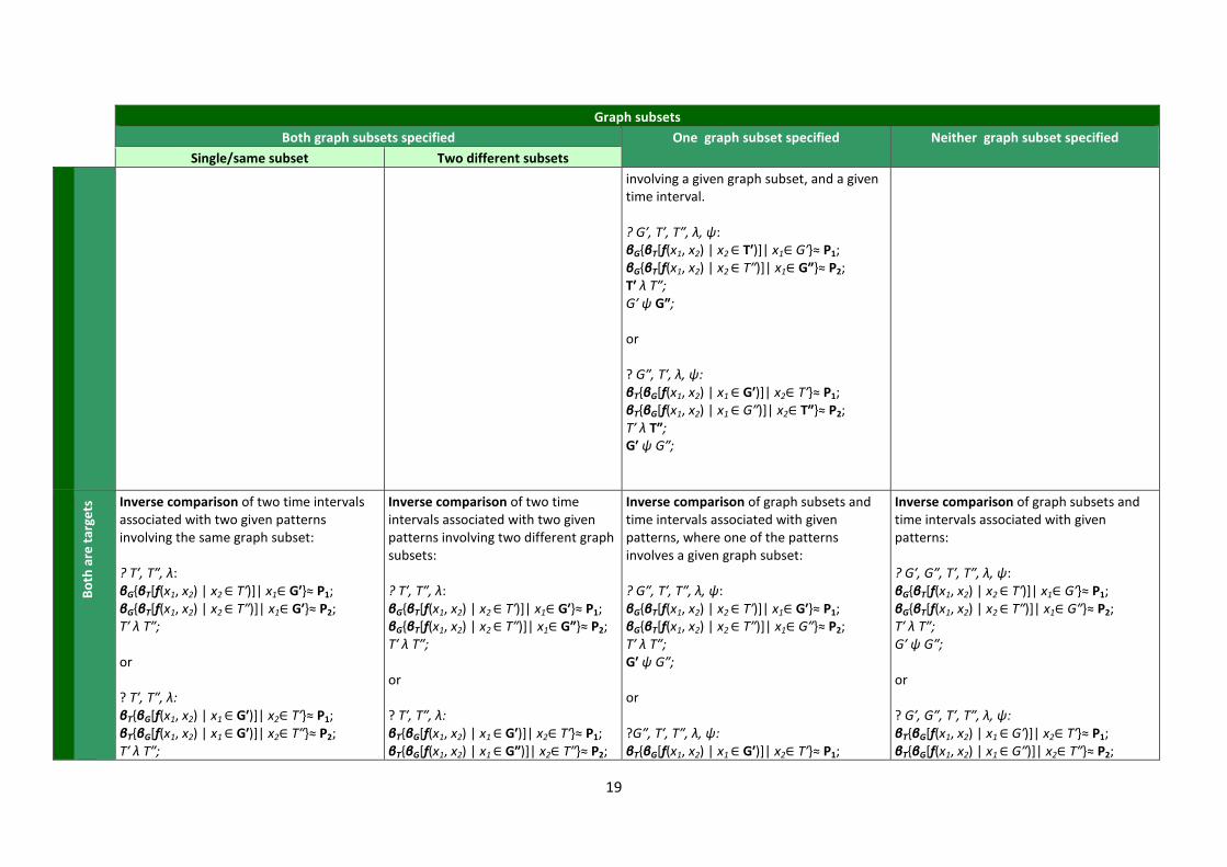
Figure 8 Comparison quadrant 4: considers comparisons involving aspectual behaviours (i) the behaviour of temporal trends for all graph elements, over the graph (ii) the behaviour of an

attribute over the graph, over time

Graph subsets

Both graph subsets specified One graph subset specified Neither graph subset specified

Single/same subset Two different subsets

Tim

e i

nte

rva

ls

Bo

th c

on

stra

ints

Sa

me

tim

e

Direct comparison of distributions of

temporal trends over the graph for two

different attributes over the same time

interval and for the same graph subset:

? p1, p2, λ:

βG{βT[f1(x1, x2) | x2 ∈ T′)]| x1∈ G′}≈ p1;

βG{βT[f2(x1, x2) | x2 ∈ T′)]| x1∈ G′}≈ p2;

p1λ p2

Or

temporal trends in distributions of an

attribute over the graph for two different

attributes for the same graph subset and

over the same time interval:

? p1, p2, λ:

βT{βG[f1(x1, x2) | x1 ∈ G′)]| x2∈ T′}≈ p1;

βT{βG[f2(x1, x2) | x1 ∈ G′)]| x2∈ T′}≈ p2;

p1λ p2


temporal trends over two different

graph subsets over the same time

interval:

? p1, p2, λ:

βG{βT[f1(x1, x2) | x2 ∈ T′)]| x1∈ G′}≈ p1;

βG{βT[f2(x1, x2) | x2 ∈ T′)]| x1∈ G″}≈ p2;

p1λ p2

Or


attribute over the graph, over two

different graph subsets over the same

time interval:

? p1, p2, λ:

βT{βG[f1(x1, x2) | x1 ∈ G′)]| x2∈ T′}≈ p1;

βT{βG[f2(x1, x2) | x1 ∈ G″)]| x2∈ T′}≈ p2;

p1λ p2

Inverse comparison of the subset of graph

elements associated with a given pattern

involving a given time interval, and a given

subset of graph elements11

:

? G″, λ:

βG{βT[f(x1, x2) | x2 ∈ T′)]| x1∈ G″}≈ P;

G′ λ G″;

or

?G″, λ:

βT{βG[f(x1, x2) | x1 ∈ G″)]| x2∈ T′}≈ P;

G′ λ G″;


associated with two given patterns

involving the same time interval:

? G′, G″, λ:

βG{βT[f(x1, x2) | x2 ∈ T′)]| x1∈ G′}≈ P1;

βG{βT[f(x1, x2) | x2 ∈ T′)]| x1∈ G″}≈ P2;

G′ λ G″;

or

? G′, G″, λ:

βT{βG[f(x1, x2) | x1 ∈ G′)]| x2∈ T′}≈ P1;

βT{βG[f(x1, x2) | x1 ∈ G″)]| x2∈ T′}≈ P2;

G′ λ G″;

11

Reduced from: ? G″, λ: βG{βT[f(x1, x2) | x2 ∈ T′)]| x1∈ G′}≈ P1; βG{βT[f(x1, x2) | x2 ∈ T′)]| x1∈ G″}≈ P2;G′ λ G″;

OR

?G″, λ: βT{βG[f(x1, x2) | x1 ∈ G′)]| x2∈ T′}≈ P1;βT{βG[f(x1, x2) | x1 ∈ G″)]| x2∈ T′}≈ P2; G′ λ G″;

17

Graph subsets



Dif

fere

nt

tim

es Direct comparison of distributions of

temporal trends over the graph for the

same graph subset during two different

time intervals:

? p1, p2, λ:

βG{βT[f1(x1, x2) | x2 ∈ T′)]| x1∈ G′}≈ p1;

βG{βT[f2(x1, x2) | x2 ∈ T″)]| x1∈ G′}≈ p2;

p1λ p2

Or


attribute over the graph, for the same

graph subset over two different time

intervals:

? p1, p2, λ:

βT{βG[f1(x1, x2) | x1 ∈ G′)]| x2∈ T′}≈ p1;

βT{βG[f2(x1, x2) | x1 ∈ G′)]| x2∈ T″}≈ p2;

p1λ p2


temporal trends over two different

graph subsets over two different time

intervals:

? p1, p2, λ:

βG{βT[f1(x1, x2) | x2 ∈ T′)]| x1∈ G′}≈ p1;

βG{βT[f2(x1, x2) | x2 ∈ T″)]| x1∈ G″}≈ p2;

p1λ p2

Or


attribute over the graph, over two

different graph subsets over two

different time intervals:

? p1, p2, λ:

βT{βG[f1(x1, x2) | x1 ∈ G′)]| x2∈ T′}≈ p1;

βT{βG[f2(x1, x2) | x1 ∈ G″)]| x2∈ T″}≈ p2;

p1λ p2

Inverse comparison as above12



involving two different time intervals

? G′, G″, λ:

βG{βT[f(x1, x2) | x2 ∈ T′)]| x1∈ G′}≈ P1;

βG{βT[f(x1, x2) | x2 ∈ T″)]| x1∈ G″}≈ P2;

G′ λ G″;

or

? G′, G″, λ:

βT{βG[f(x1, x2) | x1 ∈ G′)]| x2∈ T′}≈ P1;

βT{βG[f(x1, x2) | x1 ∈ G″)]| x2∈ T″}≈ P2;

G′ λ G″;

12

Reduced from: ? G″, λ: βG{βT[f(x1, x2) | x2 ∈ T′)]| x1∈ G′}≈ P1; βG{βT[f(x1, x2) | x2 ∈ T″)]| x1∈ G″}≈ P2; G′ λ G″;OR

? G″, λ: βT{βG[f(x1, x2) | x1 ∈ G′)]| x2∈ T′}≈ P1;βT{βG[f(x1, x2) | x1 ∈ G″)]| x2∈ T″}≈ P2; G′ λ G″;

18

Graph subsets



On

e c

on

stra

int,

on

e t

arg

et Inverse comparison of a time interval

associated with a given pattern and graph

subset, and a given time interval13

:

? T″, λ:

βG{βT[f(x1, x2) | x2 ∈ T″)]| x1∈ G′}≈ P;

T′ λ T″;

or

? T″, λ:

βT{βG[f(x1, x2) | x1 ∈ G′)]| x2∈ T″}≈ P;

T′ λ T″;

Inverse comparison as left14

.

Inverse comparison of a time interval and

graph subset associated with a given

pattern, with a given time interval and

graph subset15

? G″, T″, λ, ψ:

βG{βT[f(x1, x2) | x2 ∈ T″)]| x1∈ G″}≈ P;

T′ λ T″;

G′ ψ G″;

or

? G″, T″, λ, ψ:

βT{βG[f(x1, x2) | x1 ∈ G″)]| x2∈ T″}≈ P;

T′ λ T″;

G′ ψ G″;

OR

Inverse comparison of a graph object

associated with a pattern involving a given

time interval, and a given graph object and

a time interval associated with a pattern

Inverse comparison of graph subsets and

time intervals associated with two given

patterns, where one of the patterns

involves a given time interval:

? G′, G″, T″, λ, ψ:

βG{βT[f(x1, x2) | x2 ∈ T′)]| x1∈ G′}≈ P1;

βG{βT[f(x1, x2) | x2 ∈ T″)]| x1∈ G″}≈ P2;

T′ λ T″;

G′ ψ G″;

or

? G′, G″, T″, λ, ψ:

βT{βG[f(x1, x2) | x1 ∈ G′)]| x2∈ T′}≈ P1;

βT{βG[f(x1, x2) | x1 ∈ G″)]| x2∈ T″}≈ P2;

T′ λ T″;

G′ ψ G″;

13

Reduced from: ? T″, λ: βG{βT[f(x1, x2) | x2 ∈ T′)]| x1∈ G′}≈ P1; βG{βT[f(x1, x2) | x2 ∈ T″)]| x1∈ G′}≈ P2; T′ λ T″; or ? T″, λ: βT{βG[f(x1, x2) | x1 ∈ G′)]| x2∈ T′}≈ P1; βT{βG[f(x1, x2) | x1

∈ G′)]| x2∈ T″}≈ P2;

T′ λ T″; 14

Reduced from: ? T″, λ: βG{βT[f(x1, x2) | x2 ∈ T′)]| x1∈ G′}≈ P1; βG{βT[f(x1, x2) | x2 ∈ T″)]| x1∈ G″}≈ P2;T′ λ T″; or ? T″, λ: βT{βG[f(x1, x2) | x1 ∈ G′)]| x2∈ T′}≈ P1;βT{βG[f(x1, x2) | x1

∈ G″)]| x2∈ T″}≈P2;

T′ λ T″; 15

Reduced from: ? G″, T″, λ, ψ: βG{βT[f(x1, x2) | x2 ∈ T′)]| x1∈ G′}≈ P1; βG{βT[f(x1, x2) | x2 ∈ T″)]| x1∈ G″}≈ P2; T′ λ T″; G′ ψ G″; or ? G″, T″, λ, ψ: βT{βG[f(x1, x2) | x1 ∈ G′)]| x2∈ T′}≈

P1; βT{βG[f(x1, x2) | x1 ∈ G″)]| x2∈ T″}≈ P2; T′ λ T″; G′ ψ G″;

19

Graph subsets



involving a given graph subset, and a given

time interval.

? G′, T′, T″, λ, ψ:

βG{βT[f(x1, x2) | x2 ∈ T′)]| x1∈ G′}≈ P1;

βG{βT[f(x1, x2) | x2 ∈ T″)]| x1∈ G″}≈ P2;

T′ λ T″;

G′ ψ G″;

or

? G″, T′, λ, ψ:

βT{βG[f(x1, x2) | x1 ∈ G′)]| x2∈ T′}≈ P1;

βT{βG[f(x1, x2) | x1 ∈ G″)]| x2∈ T″}≈ P2;

T′ λ T″;

G′ ψ G″;

Bo

th a

re t

arg

ets

Inverse comparison of two time intervals


involving the same graph subset:

? T′, T″, λ:

βG{βT[f(x1, x2) | x2 ∈ T′)]| x1∈ G′}≈ P1;

βG{βT[f(x1, x2) | x2 ∈ T″)]| x1∈ G′}≈ P2;

T′ λ T″;

or

? T′, T″, λ:

βT{βG[f(x1, x2) | x1 ∈ G′)]| x2∈ T′}≈ P1;

βT{βG[f(x1, x2) | x1 ∈ G′)]| x2∈ T″}≈ P2;

T′ λ T″;

Inverse comparison of two time

intervals associated with two given

patterns involving two different graph

subsets:

? T′, T″, λ:

βG{βT[f(x1, x2) | x2 ∈ T′)]| x1∈ G′}≈ P1;

βG{βT[f(x1, x2) | x2 ∈ T″)]| x1∈ G″}≈ P2;

T′ λ T″;

or

? T′, T″, λ:

βT{βG[f(x1, x2) | x1 ∈ G′)]| x2∈ T′}≈ P1;

βT{βG[f(x1, x2) | x1 ∈ G″)]| x2∈ T″}≈ P2;


time intervals associated with given

patterns, where one of the patterns

involves a given graph subset:

? G″, T′, T″, λ, ψ:

βG{βT[f(x1, x2) | x2 ∈ T′)]| x1∈ G′}≈ P1;

βG{βT[f(x1, x2) | x2 ∈ T″)]| x1∈ G″}≈ P2;

T′ λ T″;

G′ ψ G″;

or

?G″, T′, T″, λ, ψ:

βT{βG[f(x1, x2) | x1 ∈ G′)]| x2∈ T′}≈ P1;


time intervals associated with given

patterns:

? G′, G″, T′, T″, λ, ψ:

βG{βT[f(x1, x2) | x2 ∈ T′)]| x1∈ G′}≈ P1;

βG{βT[f(x1, x2) | x2 ∈ T″)]| x1∈ G″}≈ P2;

T′ λ T″;

G′ ψ G″;

or

? G′, G″, T′, T″, λ, ψ:

βT{βG[f(x1, x2) | x1 ∈ G′)]| x2∈ T′}≈ P1;

βT{βG[f(x1, x2) | x1 ∈ G″)]| x2∈ T″}≈ P2;

20

Graph subsets



T′ λ T″;

βT{βG[f(x1, x2) | x1 ∈ G″)]| x2∈ T″}≈ P2;

T′ λ T″;

G′ ψ G″;

T′ λ T″;

G′ ψ G″;

21

4.1.3 Relation seeking

In relation seeking tasks, a relation between elements is given and the task is to find the elements

related in the specified manner. In elementary relation seeking this generally involves finding

attribute values related in a specified way, but may also involve a specified relation on time points

and/or graph elements. Similarly in synoptic tasks, this involves finding patterns related in a

specified way, but may also involve a specified relation on time intervals and/or graph subsets. The

Andrienko framework makes an additional distinction between tasks involving the same or different

attributes in the subtasks. The tasks in the matrices have been formulated to show the same

attribute, but each task could also be formulated for the case where two different attributes are

involved.

Note also that we do not show in the matrix tasks where attribute values or patterns are specified.

These tasks can be formulated to produce tasks where either:

i. Both attribute values or patterns are specified. In this case, the relation seeking task will involve

a specified relation on time points/intervals and/or graph elements/subsets. Taking an example

from quadrant 2, we could have:

Find graph subsets and time points associated with given patterns, where the graph

subsets/time points are related in the specified way.

? G′, G″, t1, t2:

β(f(x1, x2) | x1∈ G′, x2 = t1) ≈ P1;

β(f(x1, x2) | x1∈ G″, x2 = t2) ≈ P2;

t1 Ψ t2;

G′ Φ G″;

ii. One attribute value or pattern is specified. In this case, the specified relation may be between

attribute values or patterns, graph elements or subsets and/or time points or intervals (as

appropriate to the specified/unspecified elements in the task). Again, we give an example from

quadrant 2:

Find patterns related to a given pattern in the given way. Find also the graph subsets and time

points over/at which the related patterns occur. A relation between graph subsets and/or time

points may also be specified.

? G′, G″, t1, t2, P2 :

β(f(x1, x2) | x1∈ G′, x2 = t1) ≈ P1;

β(f(x1, x2) | x1∈ G″, x2 = t2) ≈ P2;

t1 Ψ t2;

G′ Φ G″;

P1 Λ P2

Note that in the case where one of the subtasks is completely specified, we reduce the task to

relation seeking involving a specified pattern or graph subset e.g.

? G″, t2, P2 :

β(f(x1, x2) | x1∈ G′, x2 = t1) ≈ P1;

β(f(x1, x2) | x1∈ G″, x2 = t2) ≈ P2;

22

t1 Ψ t2;

G′ Φ G″;

P1 Λ P2

Can be reduced to:

Find patterns/graph elements related in the given way to given patterns/graph elements. A

relation on time points may also be specified.

? G″, t2, P2 :

β(f(x1, x2) | x1∈ G″, x2 = t2) ≈ P2;

t1 Ψ t2;

G′ Φ G″;

P1 Λ P2

Again, we provide an overview of the relation seeking tasks based on the referential components

involved. The permutations of tasks involving the same/different/specified/unspecified elements are

given in the full task matrix.

Figure 9 Relation seeking quadrant-level overview

Graph elements (nodes, edges, graph objects) Graph subsets

Time

points

Elementary

? t1, t2, g1, g2, y1, y2:

f(t1, g1) = y1;

f(t2, g2) = y2;

t1 Ψ t2;

g1 Φ g2;

y1 Λ y2

Relation seeking – find the attribute values related in the

given manner (and possibly the corresponding graph

element(s)/time point(s)). In this case the possible relation

specified is domain dependent. Variations of this task

depend on the number of time points and graph elements

specified in the lookup sub tasks.

Additional constraints on the relations between graph

elements and/or time points may also be specified.

Depending on the elements involved in the lookup tasks (i.e.

whether they are specified/unspecified, same or different),

constraints may be any of the relations noted in the

comparison matrix e.g.:

• between time points: equality (same/different

time point), that time points are consecutive,

occur before/after a given time point, that a

certain distance exists between them etc.

• between graph elements: equality (same/different

element); set relations (between the sets of

elements belonging to graph objects); equality of

configuration (in graph objects); association

(where a single time point is specified in the

lookup task or a constraint of equality is added on

unspecified time points).

Synoptic

? G′, G″, t1, t2, P1, P2 :

β(f(x1, x2) | x1∈ G′, x2 = t1) ≈ P1;

β(f(x1, x2) | x1∈ G″, x2 = t2) ≈ P2;

t1 Ψ t2;

G′ Φ G″;

P1 Λ P2

Relation seeking – find patterns of attribute(s) over the graph

which are related in the given manner (and possibly the time

point(s)/subsets of graph elements at/over which they occur).

Possible specified relations between patterns are same

(similar)/different/opposite. Variations depend on the number of

time points and graph subsets specified in the lookup subtasks.

Additional constraints on relations between time points /or graph

subsets may also be included in the task specification, depending

on the elements involved in the lookup tasks. These are similar to

the relations noted in the comparison matrix e.g.

• between time points: equality (same/different time

point), that time points are consecutive, occur

before/after a given time point, that a certain distance

exists between them etc.


subset); set relations (between the sets of nodes/edges

belonging to the subset); equality of configuration of the

subset, association (between nodes/graph objects, at a

single time point only).

Time

intervals

Synoptic

? g1 , g2 ; T′, T″, P1, P2:

β(f(x1, x2) | x1= g1, x2 ∈ T′) ≈ P1;

β(f(x1, x2) | x1= g2, x2 ∈ T″) ≈ P2;

g1 Φ g2 ; T Ψ T″; P1 Λ P2

Synoptic

? G′, G″, T′, T″, P1, P2:

βG{βT[f(x1, x2) | x2 ∈ T′)]| x1∈ G′}≈ P1;

βG{βT[f(x1, x2) | x2 ∈ T″)]| x1∈ G″}≈ P2;

T′ Ψ T″; G′ Φ G″; P1 Λ P2

23

Relation seeking – find the patterns of attribute(s) over time

which are related in the given manner (and possibly find the

graph element(s) to which they correspond/the time

period(s) over which they occur). The possible specified

relations between patterns are the same

(similar)/different/opposite. Variations depend on the

number of graph elements and time intervals specified in

the lookup subtasks.

Additional constraints on relations between graph elements

and/or time intervals may also be included in the task

specification, depending on the elements involved in the

lookup tasks. These are similar to the relations noted in the

comparison matrix e.g.

• between graph elements: equality (same/different

element); set relations (between the sets of

elements belonging to graph objects); equality of

configuration (in graph objects).

• Between the time intervals (over which the

pattern occurs): happens before(/after), happens

at the same time; between two intervals, or an

instant and an interval: happens before(/after),

starts, finishes, happens during; between intervals

only: overlaps, meets [4].

or

? G′, G″, T′, T″, P1, P2:

βT{βG[f(x1, x2) | x1 ∈ G′)]| x2∈ T′}≈ P1;

βT{βG[f(x1, x2) | x1 ∈ G″)]| x2∈ T″}≈ P2;

T′ Ψ T″; G′ Φ G″; P1 Λ P2

Relation seeking – find (sub)patterns of either of the aspectual

behaviours which are related in the given manner (and possibly

find the graph subset/time interval associated with the found

patterns). The possible specified relations between patterns are

the same (similar)/different/opposite. Variations depend on the

number of graph subsets and time intervals specified in the lookup

subtasks.

Additional constraints on relations between time points /or graph

subsets may also be included in the task specification, depending

on the elements involved in the lookup tasks. These are similar to

the relations noted in the comparison matrix e.g.


subset); set relations (between the sets of nodes/edges

belonging to the subset); equality of configuration of the

subset, association (between nodes/graph objects, at a

single time point only).

• Between the time intervals (over which the pattern

occurs): happens before(/after), happens at the same

time; between two intervals, or an instant and an

interval: happens before(/after), starts, finishes,

happens during; between intervals only: overlaps, meets

[4].

24

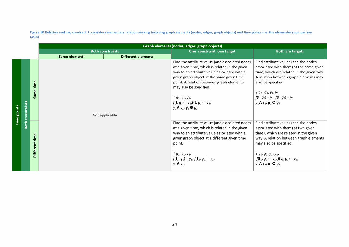
Figure 10 Relation seeking, quadrant 1: considers elementary relation seeking involving graph elements (nodes, edges, graph objects) and time points (i.e. the elementary comparison

tasks)



Same element Different elements

Tim

e p

oin

ts

Bo

th c

on

stra

ints

S

am

e t

ime

Not applicable

Find the attribute value (and associated node)

at a given time, which is related in the given

way to an attribute value associated with a

given graph object at the same given time

point. A relation between graph elements

may also be specified.

? g2, y1, y2:

f(t, g1) = y1;f(t, g2) = y2;

y1 Λ y2; g1 Φ g2

Find attribute values (and the nodes

associated with them) at the same given

time, which are related in the given way.

A relation between graph elements may

also be specified.

? g1 , g2, y1, y2:

f(t, g1) = y1; f(t, g2) = y2;

y1 Λ y2; g1 Φ g2

Dif

fere

nt

tim

e

Find the attribute value (and associated node)

at a given time, which is related in the given

way to an attribute value associated with a

given graph object at a different given time

point.

? g2, y1, y2:

f(t1, g1) = y1; f(t2, g2) = y2;

y1 Λ y2;

Find attribute values (and the nodes

associated with them) at two given

times, which are related in the given

way. A relation between graph elements


? g1, g2, y1, y2:

f(t1, g1) = y1; f(t2, g2) = y2;

y1 Λ y2; g1 Φ g2

25




On

e

con

stra

int,

on

e t

arg

et

Find an attribute value (and the

time point at which it occurs)

associated with a given graph

element, which is related in the

given way to an attribute value

associated with a the same graph

element at a given time. A relation

between time points may also be

specified.

? t2, y1, y2:

f(t1, g) = y1; f(t2, g) = y2;

y1 Λ y2

Find an attribute value (and the time

point at which it occurs) associated

with a given graph element, which is

related in the given way to an

attribute value associated with a

different given graph element at a

given time. A relation between time


? t2, y1, y2:

f(t1, g1) = y1; f(t2, g2) = y2;

t1 Ψ t2; y1 Λ y

Find an attribute value (and the time point

and graph element for which it occurs)

related in the given way to an attribute value

which is associated with a given graph

element at a given time point. Relations

between time points and/or graph elements


? t2, g2, y1, y2:

f(t1, g1) = y1; f(t2, g2) = y2;

y1 Λ y2

Or

Find attribute values related in the given way

where one of the values occurs at a given

time, and the other is associated with a given

graph element. Also find the unspecified

graph element and time point associated with

the attribute values. Relations between time

points and/or graph elements may also be

specified.

? t2, g1, y1, y2:

f(t1, g1) = y1; f(t2, g2) = y2;

t1 Ψ t2; g1 Φ g2; y1 Λ y2

Find attribute values related in the given

way where one of the values occurs at

the given time. Relations between time

points and graph elements may also be

specified.

t2, g1, g2, y1, y2:

f(t1, g1) = y1; f(t2, g2) = y2;

t1 Ψ t2; g1 Φ g2; y1 Λ y2

26




Bo

th a

re t

arg

ets

Find attribute values (and the time

points at which they occur)

associated with the same given

graph element, which are related

in the given way. A relation

between time points may also be

specified.

? t1, t2, y1, y2:

f(t1, g) = y1; f(t2, g) = y2;

y1 Λ y2; t1 Ψ t2;

Find attribute values (and the time


associated with two given graph

elements, which are related in the

given way. A relation between time


? t1, t2, y1, y2:

f(t1, g1) = y1; f(t2, g2) = y2;

t1 Ψ t2; y1 Λ y2

Find attribute values related in the given way,

where one of the attribute values is

associated with a given graph element.

Relations between time points and/or graph

elements may also be specified.

? t1, t2, g2, y1, y2:

f(t1, g1) = y1; f(t2, g2) = y2;

t1 Ψ t2; g1 Φ g2; y1 Λ y2

Find attribute values related in the given

way. Relations between time points

and/or graph elements may also be

specified.

? t1, t2, g1, g2, y1, y2:

f(t1, g1) = y1; f(t2, g2) = y2;

t1 Ψ t2; g1 Φ g2; y1 Λ y2

27

Figure 11 Relation seeking quadrant 2: considers synoptic relation seeking involving the behaviour of an attribute over the graph (or a graph subset)

Graph subsets



Tim

e p

oin

ts B

oth

co

nst

rain

ts

S

am

e t

ime

Not applicable

Find a pattern and the graph subset over which

it occurs at a given time point, which is related

in the given way to a pattern over a given graph

subset at the same time point. A relation

between graph subsets may also be specified.

? G″, P1, P2 :

β(f(x1, x2) | x1∈ G′, x2 = t) ≈ P1;

β(f(x1, x2) | x1∈ G″, x2 = t) ≈ P2;

G′ Φ G″;

P1 Λ P2

Find patterns related in the given way at the same

time point. A relation between graph subsets may

also be specified.

? G′, G″, P1, P2 :

β(f(x1, x2) | x1∈ G′, x2 = t) ≈ P1;

β(f(x1, x2) | x1∈ G″, x2 = t) ≈ P2;

G′ Φ G″;

P1 Λ P2

Dif

fere

nt

tim

es

Tasks as above, but involving two different time

points.

? G″, P1, P2 :

β(f(x1, x2) | x1∈ G′, x2 = t1) ≈ P1;

β(f(x1, x2) | x1∈ G″, x2 = t2) ≈ P2;

G′ Φ G″;

P1 Λ P2

Tasks as above, but involving two different time

points.

? G′, G″, P1, P2 :

β(f(x1, x2) | x1∈ G′, x2 = t1) ≈ P1;

β(f(x1, x2) | x1∈ G″, x2 = t2) ≈ P2;

G′ Φ G″;

P1 Λ P2

On

e c

on

stra

int,

on

e t

arg

et Find a pattern (and time

point) associated with a given

graph subset, which is related

in the given way to a pattern

associated with the same

graph subset at a given time.

A relation between time


? t2, P1, P2 :

Find a pattern (and time point)

associated with a given graph

subset, which is related in the

given way to a pattern

associated with a different

given graph subset at a given

time. A relation between time


? t2, P1, P2 :

Find a pattern and the time point and graph

subset over which it occurs related in the given

way to a pattern associated with a given graph

subset at a given time point. Relations

between time points and graph subsets may

also be specified.

? G″, t2, P1, P2 :

β(f(x1, x2) | x1∈ G′, x2 = t1) ≈ P1;

β(f(x1, x2) | x1∈ G″, x2 = t2) ≈ P2;

Find patterns related in the given way where one of

the patterns occurs at the given time. Relations

between time points and graph subsets may also

be specified.

? G′, G″, t1, P1, P2 :

β(f(x1, x2) | x1∈ G′, x2 = t1) ≈ P1;

β(f(x1, x2) | x1∈ G″, x2 = t2) ≈ P2;

t1 Ψ t2;

G′ Φ G″;

28

Graph subsets



β(f(x1, x2) | x1∈ G′, x2 = t1) ≈ P1;

β(f(x1, x2) | x1∈ G′, x2 = t2) ≈ P2;

t1 Ψ t2;

P1 Λ P2

β(f(x1, x2) | x1∈ G′, x2 = t1) ≈ P1;

β(f(x1, x2) | x1∈ G″, x2 = t2) ≈ P2;

t1 Ψ t2;

P1 Λ P2

t1 Ψ t2;

G′ Φ G″;

P1 Λ P2

Or

Find patterns related in the given way where

one of the patterns occurs at a given time, and

the other occurs over a given graph subset.

Also find the unspecified graph subset and time

point over which/at the patterns occur.

Relations between time points and graph

subsets may also be specified.

? = G″, t1, P1, P2 :

β(f(x1, x2) | x1∈ G′, x2 = t1) ≈ P1;

β(f(x1, x2) | x1∈ G″, x2 = t2) ≈ P2;

t1 Ψ t2;

G′ Φ G″;

P1 Λ P2

P1 Λ P2

Bo

th a

re t

arg

ets

Find patterns (and the time


associated with a single given

graph subset, which are

related in the given way. A

relation between time points


? t1, t2, P1, P2 :

β(f(x1, x2) | x1∈ G′, x2 = t1) ≈ P1;

β(f(x1, x2) | x1∈ G′, x2 = t2) ≈ P2;

t1 Ψ t2;

P1 Λ P2



associated with two given graph

subsets, which are related in

the given way. A relation

between time points may also

be specified.

? t1, t2, P1, P2 :

β(f(x1, x2) | x1∈ G′, x2 = t1) ≈ P1;

β(f(x1, x2) | x1∈ G″, x2 = t2) ≈ P2;

t1 Ψ t2;

P1 Λ P2

Find patterns related in the given way, where

one of the patterns is associated with a given

graph subset. Relations between time points

and graph subsets may also be specified.

? G″, t1, t2, P1, P2 :

β(f(x1, x2) | x1∈ G′, x2 = t1) ≈ P1;

β(f(x1, x2) | x1∈ G″, x2 = t2) ≈ P2;

t1 Ψ t2;

G′ Φ G″;

P1 Λ P2

Find patterns related in the given way. Relations

between time points and graph subsets may also

be specified.

? G′, G″, t1, t2, P1, P2 :

β(f(x1, x2) | x1∈ G′, x2 = t1) ≈ P1;

β(f(x1, x2) | x1∈ G″, x2 = t2) ≈ P2;

t1 Ψ t2;

G′ Φ G″;

P1 Λ P2

29

Figure 12 Relation seeking quadrant 3: considers relation seeking tasks involving the behaviour of an attribute of a single graph element over time (i.e. a temporal trend)




Tim

e i

nte

rva

ls

Bo

th c

on

stra

ints

S

am

e t

ime

Not applicable

Find a pattern (and the graph element

associated with it) which occurs over a

given time interval and is related in the

given way to a pattern associated with a

given graph element over the same time

interval. A relation between graph elements

may also be specified.16

? g2 , P1, P2:

β(f(x1, x2) | x1= g1, x2 ∈ T′) ≈ P1;

β(f(x1, x2) | x1= g2, x2 ∈ T′) ≈ P2;

P1 Λ P2;

g1 Φ g2

Find patterns (and their associated

graph elements) which occur over the

same given time interval and are related

in the given way. A relation between

graph elements may also be specified.

? g1 , g2 , P1, P2:

β(f(x1, x2) | x1= g1, x2 ∈ T′) ≈ P1;

β(f(x1, x2) | x1= g2, x2 ∈ T′) ≈ P2;

P1 Λ P2;

g1 Φ g2

Dif

fere

nt

tim

es

Find a pattern (and the graph element

associated with it) which occurs over a

given time interval and is related in the

given way to a pattern associated with a

given graph element over a given time

interval. A relation between graph elements

may also be specified

? g2 , P1, P2:

β(f(x1, x2) | x1= g1, x2 ∈ T′) ≈ P1;

β(f(x1, x2) | x1= g2, x2 ∈ T′) ≈ P2;

P1 Λ P2;

g1 Φ g2

Find patterns (and their associated

graph elements) which occur over two

given time intervals and are related in

the given way. A relation between graph

elements may also be specified

? g1 , g2, P1, P2:

β(f(x1, x2) | x1= g1, x2 ∈ T′) ≈ P1;

β(f(x1, x2) | x1= g2, x2 ∈ T″) ≈ P2;

P1 Λ P2;

g1 Φ g2

16

In all cases in this table, if we wish to specify an association relation between the graph elements, we must also specify a time at which the association relation occurs i.e.

(g1 , t) Φ (g2, t): ‘a given association relation exists between the graph elements at time t’.

30




On

e c

on

stra

int,

on

e t

arg

et

Find a pattern (and the time

interval over which it occurs) for a

given graph element, which is

related in the given way to a

pattern associated with the same

graph element over a given time

interval. A relation between time

intervals may also be specified.

? T″, P1, P2:

β(f(x1, x2) | x1= g, x2 ∈ T′) ≈ P1;

β(f(x1, x2) | x1= g, x2 ∈ T″) ≈ P2;

T′ Ψ T″;

P1 Λ P2

Find a pattern (and the time interval over

which it occurs) for a given graph

element, which is related in the given

way to a pattern associated with a given

graph element over a given time interval.

A relation between time intervals may

also be specified.

? T″, P1, P2:

β(f(x1, x2) | x1= g1, x2 ∈ T′) ≈ P1;

β(f(x1, x2) | x1= g2, x2 ∈ T″) ≈ P2;

T′ Ψ T″;

P1 Λ P2

Find a pattern, and the graph element and

time interval over which it occurs, which is

related in the given way to a pattern

associated with a given graph element over

a given time interval. A relation between

time intervals and/or graph elements may

also be specified.

? g2, T″, P1, P2:

β(f(x1, x2) | x1= g1, x2 ∈ T′) ≈ P1;

β(f(x1, x2) | x1= g2, x2 ∈ T″) ≈ P2;

T′ Ψ T″;

P1 Λ P2;

g1 Φ g2

Or

Find patterns related in the given way

where one of the patterns occurs over a

given time interval, and the other is

associated with a given graph element. Also

find the unspecified graph element and

time interval associated with the patterns).

A relation between time intervals and/or


? g2, T′, P1, P2:

β(f(x1, x2) | x1= g1, x2 ∈ T′) ≈ P1;

β(f(x1, x2) | x1= g2, x2 ∈ T″) ≈ P2;

T′ Ψ T″;

P1 Λ P2;

g1 Φ g2


where one of the patterns occurs over a

given time interval. A relation between

time intervals and/or graph elements


? g1 , g2, T″, P1, P2:

β(f(x1, x2) | x1= g1, x2 ∈ T′) ≈ P1;

β(f(x1, x2) | x1= g2, x2 ∈ T″) ≈ P2;

T′ Ψ T″;

P1 Λ P2;

g1 Φ g2

31




Bo

th a

re t

arg

ets


intervals over which they occur)

associated with a single graph

element, which are related in the

given way. A relation between time


? T′, T″, P1, P2:

β(f(x1, x2) | x1= g, x2 ∈ T′) ≈ P1;

β(f(x1, x2) | x1= g, x2 ∈ T″) ≈ P2;

T′ Ψ T″;

P1 Λ P2

Find patterns (and the time intervals over

which they occur) associated with two

given graph elements, which are related

in the given way. A relation between time


? T′, T″, P1, P2:

β(f(x1, x2) | x1= g1, x2 ∈ T′) ≈ P1;

β(f(x1, x2) | x1= g2, x2 ∈ T″) ≈ P2;

T′ Ψ T″;

P1 Λ P2

Find patterns related in the given way,

where one of the patterns is associated with

a given graph element. A relation between

time intervals and/or graph elements may

also be specified.

g2, T′, T″, P1, P2:

β(f(x1, x2) | x1= g1, x2 ∈ T′) ≈ P1;

β(f(x1, x2) | x1= g2, x2 ∈ T″) ≈ P2;

T′ Ψ T″;

P1 Λ P2;

g1 Φ g2

Find patterns related in the given way.

A relation between time intervals and/or


? g1 , g2, T′, T″, P1, P2:

β(f(x1, x2) | x1= g1, x2 ∈ T′) ≈ P1;

β(f(x1, x2) | x1= g2, x2 ∈ T″) ≈ P2;

T′ Ψ T″;

P1 Λ P2;

g1 Φ g2

32

Figure 13 Relation seeking quadrant 4: considers relation seeking tasks involving aspectual behaviours (i) the behaviour of temporal trends for all graph elements, over the graph (ii) the

behaviour of an attribute over the graph, over time

Graph subsets



Tim

e i

nte

rva

ls

Bo

th c

on

stra

ints

S

am

e t

ime

Not applicable

Find a pattern (and the graph subset associated

with it) which is associated with a given time

interval and is related in the given way to a

pattern associated with a given graph subset and

the same time interval. A relation between

graph subsets may also be specified.

? G″, P1, P2:

βG{βT[f(x1, x2) | x2 ∈ T′)]| x1∈ G′}≈ P1;

βG{βT[f(x1, x2) | x2 ∈ T′)]| x1∈ G″}≈ P2;

G′ Φ G″;

P1 Λ P2

or

? G″, P1, P2:

βT{βG[f(x1, x2) | x1 ∈ G′)]| x2∈ T′}≈ P1; βT{βG[f(x1,

x2) | x1 ∈ G″)]| x2∈ T′}≈ P2;

G′ Φ G″;

P1 Λ P2

Find patterns (and their associated graph

subsets) which are associated with a single

given time interval and are related in the

given way. A relation between graph


? G′, G″, P1, P2:

βG{βT[f(x1, x2) | x2 ∈ T′)]| x1∈ G′}≈ P1;

βG{βT[f(x1, x2) | x2 ∈ T′)]| x1∈ G″}≈ P2;

G′ Φ G″;

P1 Λ P2

or

? G′, G″, P1, P2:

βT{βG[f(x1, x2) | x1 ∈ G′)]| x2∈ T′}≈ P1;

βT{βG[f(x1, x2) | x1 ∈ G″)]| x2∈ T′}≈ P2;

G′ Φ G″;

P1 Λ P2

Dif

fere

nt

tim

es

Find a pattern (and the graph subset associated

with it) which is associated with a given time

interval and is related in the given way to a

pattern associated with a given graph subset and

a given time interval. A relation between graph


? G″, P1, P2:

βG{βT[f(x1, x2) | x2 ∈ T′)]| x1∈ G′}≈ P1;

βG{βT[f(x1, x2) | x2 ∈ T″)]| x1∈ G″}≈ P2;

Find patterns (and their associated graph

subsets) which are associated with two

given time intervals and are related in the

given way. A relation between graph


? G′, G″, P1, P2:

βG{βT[f(x1, x2) | x2 ∈ T′)]| x1∈ G′}≈ P1;

βG{βT[f(x1, x2) | x2 ∈ T″)]| x1∈ G″}≈ P2;

G′ Φ G″;

33

Graph subsets



G′ Φ G″;

P1 Λ P2

or

? G″, P1, P2:


x2) | x1 ∈ G″)]| x2∈ T″}≈ P2;

G′ Φ G″;

P1 Λ P2

P1 Λ P2

or

? G′, G″, P1, P2:

βT{βG[f(x1, x2) | x1 ∈ G′)]| x2∈ T′}≈ P1;

βT{βG[f(x1, x2) | x1 ∈ G″)]| x2∈ T″}≈ P2;

G′ Φ G″;

P1 Λ P2

On

e

con

stra

int,

on

e t

arg

et

Find a pattern (and the time interval

with which it is associated) for a

given graph subset, which is related

in the given way to a pattern

associated with the same graph

subset and a given time interval. A

relation between time intervals may

also be specified.

? T″, P1, P2:

βG{βT[f(x1, x2) | x2 ∈ T′)]| x1∈ G′}≈ P1;

βG{βT[f(x1, x2) | x2 ∈ T″)]| x1∈ G′}≈ P2;

T′ Ψ T″;

P1 Λ P2

or

? T″, P1, P2:

βT{βG[f(x1, x2) | x1 ∈ G′)]| x2∈ T′}≈ P1;

βT{βG[f(x1, x2) | x1 ∈ G′)]| x2∈ T″}≈ P2;

T′ Ψ T″;

P1 Λ P2

Find patterns (and the time intervals

over which they occur) associated

with two given graph subsets, which

are related in the given way. A relation

between time intervals may also be

specified.

? T″, P1, P2:

βG{βT[f(x1, x2) | x2 ∈ T′)]| x1∈ G′}≈ P1;

βG{βT[f(x1, x2) | x2 ∈ T″)]| x1∈ G″}≈ P2;

T′ Ψ T″;

P1 Λ P2

or

? T″, P1, P2:

βT{βG[f(x1, x2) | x1 ∈ G′)]| x2∈ T′}≈ P1;

βT{βG[f(x1, x2) | x1 ∈ G″)]| x2∈ T″}≈ P2;

T′ Ψ T″;

P1 Λ P2

Find a pattern, and the graph subset and time

interval with which it is associated, which is

related in the given way to a pattern associated

with a given graph subset and a given time

interval. Relations between time intervals

and/or graph subsets may also be specified.

? G″, T″, P1, P2:

βG{βT[f(x1, x2) | x2 ∈ T′)]| x1∈ G′}≈ P1;

βG{βT[f(x1, x2) | x2 ∈ T″)]| x1∈ G″}≈ P2;

T′ Ψ T″;

G′ Φ G″;

P1 Λ P2

or

? G″, T″, P1, P2:


x2) | x1 ∈ G″)]| x2∈ T″}≈ P2;

T′ Ψ T″;

G′ Φ G″;

P1 Λ P2


where one of the patterns involves a given

time interval. Relations between time

intervals and/or graph subsets may also be

specified.

? G′, G″, T″, P1, P2:

βG{βT[f(x1, x2) | x2 ∈ T′)]| x1∈ G′}≈ P1;

βG{βT[f(x1, x2) | x2 ∈ T″)]| x1∈ G″}≈ P2;

T′ Ψ T″;

G′ Φ G″;

P1 Λ P2

or

? G′, G″, T″, P1, P2:

βT{βG[f(x1, x2) | x1 ∈ G′)]| x2∈ T′}≈ P1;

βT{βG[f(x1, x2) | x1 ∈ G″)]| x2∈ T″}≈ P2;

T′ Ψ T″;

G′ Φ G″;

P1 Λ P2

34

Graph subsets



OR

Find patterns related in the given way where one

of the patterns is associated with a given time

interval, and the other is associated with a given

graph subset. Also find the unspecified graph

subset and time interval associated with the

patterns). Relations between time intervals

and/or graph subsets may also be specified.

? G′, T″, P1, P2:

βG{βT[f(x1, x2) | x2 ∈ T′)]| x1∈ G′}≈ P1;

βG{βT[f(x1, x2) | x2 ∈ T″)]| x1∈ G″}≈ P2;

T′ Ψ T″;

G′ Φ G″;

P1 Λ P2

or

? G″, T′, T″, P1, P2:


x2) | x1 ∈ G″)]| x2∈ T″}≈ P2;

T′ Ψ T″;

G′ Φ G″;

P1 Λ P2

Bo

th a

re t

arg

ets



with the same given graph subset,

which are related in the given way.

A relation between time intervals




with two given graph subsets, which

are related in the given way. A relation

between time intervals may also be

specified.

Find patterns related in the given way, where

one pattern is associated with a given graph

subset. Relations between time intervals and/or


? G″, T′, T″, P1, P2:

Find patterns related in the given way.

Relations between time intervals and/or


? G′, G″, T′, T″, P1, P2:

βG{βT[f(x1, x2) | x2 ∈ T′)]| x1∈ G′}≈ P1;

35

Graph subsets



? T′, T″, P1, P2:

βG{βT[f(x1, x2) | x2 ∈ T′)]| x1∈ G′}≈ P1;

βG{βT[f(x1, x2) | x2 ∈ T″)]| x1∈ G′}≈ P2;

T′ Ψ T″;

P1 Λ P2

or

? T′, T″, P1, P2:

βT{βG[f(x1, x2) | x1 ∈ G′)]| x2∈ T′}≈ P1;

βT{βG[f(x1, x2) | x1 ∈ G′)]| x2∈ T″}≈ P2;

T′ Ψ T″;

P1 Λ P2

? T′, T″, P1, P2:

βG{βT[f(x1, x2) | x2 ∈ T′)]| x1∈ G′}≈ P1;

βG{βT[f(x1, x2) | x2 ∈ T″)]| x1∈ G″}≈ P2;

T′ Ψ T″;

P1 Λ P2

or

? T′, T″, P1, P2:

βT{βG[f(x1, x2) | x1 ∈ G′)]| x2∈ T′}≈ P1;

βT{βG[f(x1, x2) | x1 ∈ G″)]| x2∈ T″}≈ P2;

T′ Ψ T″;

P1 Λ P2

βG{βT[f(x1, x2) | x2 ∈ T′)]| x1∈ G′}≈ P1;

βG{βT[f(x1, x2) | x2 ∈ T″)]| x1∈ G″}≈ P2;

T′ Ψ T″;

G′ Φ G″;

P1 Λ P2

or

? G″, T′, T″, P1, P2:


x2) | x1 ∈ G″)]| x2∈ T″}≈ P2;

T′ Ψ T″;

G′ Φ G″;

P1 Λ P2

βG{βT[f(x1, x2) | x2 ∈ T″)]| x1∈ G″}≈ P2;

T′ Ψ T″;

G′ Φ G″;

P1 Λ P2

or

? G′, G″, T′, T″, P1, P2:

βT{βG[f(x1, x2) | x1 ∈ G′)]| x2∈ T′}≈ P1;

βT{βG[f(x1, x2) | x1 ∈ G″)]| x2∈ T″}≈ P2;

T′ Ψ T″;

G′ Φ G″;

P1 Λ P2

36

4.2 Structural tasks

As for the attribute based tasks, we divide the structural task space based on the referential

components involved (Figure 14). Quadrant 1 contains the elementary tasks, while the other three

quadrants contain the synoptic tasks involving the partial and aspectual structural patterns.

Figure 14 Structural tasks based on referential components involved

4.2.1 Elementary structural tasks

We distinguish two main elementary tasks: finding association relations (connections) between

elements and finding elements connected in the given way. Note that association relations may exist

between individual graph elements (nodes) or subsets of the graph treated as individual elements

(graph objects). We may also wish to compare and find relations between association relations. We

discuss these tasks below.

4.2.1.1 Find connections between elements (comparison)

This is the “comparison” subtask: the term is rather unintuitive when dealing with questions of

connectivity between graph objects, however, its definition of ‘finding the relation between given

elements’ is exactly what we are attempting to do here. This reflects scheme 1 of Andrienko’s pure

relational tasks ([2] p.62-63) (how are the elements p and q (or the subsets P and Q) of the set S

related?):

(How) is g1 connected to g2 at the given time, t?

?λ: (g1, t) λ (g2, t)

e.g. (how) are graph objects a and b connected at time 4?

4.2.1.2 Find elements connected in the given way (relation seeking)

This is the relation seeking subtask, and there are two versions reflecting Andrienko’s pure relational

schemes 2 and 3, plus a third, hybrid version. Temporal variations of each task are also given in the

summary table, below. The association relation can be specified as generally as stating whether or

Pair of nodes Graph subsets

Tim

e P

oin

ts Q1 Elementary

Tasks involving connection between a pair of nodes at a

single time point (inverse comparison and relation seeking

only).

Q2 Synoptic

Tasks involving the behaviour, or configuration, of

association relations within a set of nodes at a single time

e.g. clusters, cliques, motifs etc.:

Tim

e I

nte

rva

ls

Q3 Synoptic

Tasks involving the behaviour of association relations

between two graph objects over time e.g. the pattern of

change in connectivity between two nodes over time.

Q4 Synoptic

Tasks involving:

The behaviour of the collection of patterns in (Q3) i.e. the

aggregate pattern of all association relations between pairs

of graph objects over time, or the distribution of individual

temporal behaviours over the graph.

OR

The behaviour of the configurations of association relations

over the set of nodes (i.e. (Q2)), over time.

37

not any connection exists between two objects, or as specifically as including the distance, direction,

and/or domain attributes.

(i) where the connection and one of the graph objects is specified (i.e. scheme 2: what element (or

subset) of the set S is related to the element p (or subset P) in the way ρ?)

Find the graph object(s) to which graph object g1 is connected in the given way at time t:

? g2 : (g1, t) Λ (g2, t)

e.g. find the node(s) directly connected to node a at time t4; find node(s)connected to node a

at a distance of less than 3 hops at time t2; find nodes with a strong direct connection to

node a; find nodes directly connected to node a with link type “friend”; find clusters

connected to cluster B at time t3.

ii) where only the connection is specified (i.e. scheme 3: what elements (or subsets) of the set S are

related in the way ρ?)

Find graph objects that are connected in the given way at the given time

? g1, g2, t:(g1, t)Λ (g2, t)

e.g. find nodes directly connected with a weight greater than 4 at time 6; find closely

connected clusters at time t3.

(iii) In addition to the tasks constructed according to the pure relational schemes, there is a hybrid

variation where we have two graph objects and a given connection relation, and we want to find the

time(s) at which the objects were connected in the given way:

Find the time points at which two given graph objects were connected in the given way

? t :(g1, t)Λ (g2, t)

e.g. find the times at which a direct connection exists between graph objects a and b

Figure 15 summary of comparison and relation seeking graph structural tasks concerning graph elements, including

variations involving specified and unspecified time points

Graph elements (nodes, graph objects)


Tim

e p

oin

ts

Bo

th c

on

stra

ints

Find connections between

elements (comparison)

(How) is graph element g1

connected to graph

element g2 at the given

time, t?

?λ: (g1, t) λ (g2, t)

Find elements connected in the

given way (relation seeking)

Find the graph element(s) to

which graph element g1 is

connected in the given way at

time t:

? g2 : (g1, t) Λ (g2, t)


given way (relation seeking) Find

graph objects which are connected

in the given way at the given time

?g1, g2 :(g1, t)Λ (g2, t)

38

Bo

th a

re t

arg

ets

Hybrid Find the time

points at which two given

graph objects were

connected in the given

way

? t :(g1, t)Λ (g2, t)



Find the graph element(s) to

which graph element g1 is

connected and the time(s) at

which the connection(s) occur

? g2, t : (g1, t) Λ (g2, t)



Find graph objects (and their

associated time points) at any time

that are connected in the given

way

? g1, g2, t :(g1, t)Λ (g2, t)

4.2.1.3 Compare and find relations between association relations (connections)

The previous tasks deal with finding association relations and finding elements connected in a given

way. It is conceivable that we may also wish to compare connections. Comparison of relations does

not exist within the original Andrienko framework, and we do not wish to add more task categories

than necessary. Therefore, while we use the tasks outlined above to find connection relations, when

comparing association relations we treat them as references: either edges in the case of direct

connection, or paths (a graph object) in indirect connection. This allows us to use the attribute

based tasks of the original Andrienko framework (see section 4.1): direct comparison to compare the

attributes associated with the edge or path (e.g. weight, domain attributes, path length), and inverse

comparison when we are interested in the (structural) equality of the graph objects themselves. We

suggest handling relation seeking tasks involving association relations in a similar manner (e.g. ‘find

dyads whose edge weight increased between times 3 and 4’ would involve relation seeking where

the edge/dyad is the reference and weight is the attribute).

4.2.2 Synoptic structural tasks

4.2.2.1 Structural pattern characterisation

Structural pattern characterisation involves describing the pattern associated with one of the four

structural behaviours outlined in section 2.2.

4.2.2.2 Structural pattern search

This is the opposite of the above task in that we seek to find the set of graph elements associated

with a given pattern or configuration of connections, and/or the time at which they occur.

4.2.2.3 Comparison and relation seeking involving structural patterns

As is the case with the attribute based tasks, we may also wish to compare or find relations between

structural patterns, and the graph elements/subsets and time points/intervals associated with these

patterns. The many possible permutations of these tasks mirror those of the original attribute based

comparison and relation seeking tasks, which are outlined in the task matrices described in section

4.1.

4.3 Connection Discovery tasks

We here discuss some examples of the three variations of relational behaviours involved in

connection discovery tasks in temporal graphs. We also discuss the possible case of connectional

behaviours between graph structural patterns.

4.3.1 Heterogeneous behaviours

(1) Relational behaviour involving two (or more) different attributes of the same reference set

39

The formal notation for this behaviour is given in the Andrienko framework as:

(3.43) ρ(f1(x), f2(x) | x ∈ R)

Where f1(x) and f2(x) are two attributes defined on the same reference set R.

Applied to temporal graphs, this task considers a relational behaviour between two different

attributes and the same graph and temporal components. Note that the Andrienko framework does

not explicitly discuss how to handle multiple referrers in relational behaviours. We therefore draw

on the partial behaviours to guide us in our discussion.

One example this relational behaviour applied to temporal graphs might be the (partial) relational

behaviour between two different attributes of the elements of the graph (nodes or edges) at a single

timepoint:

ρ(f1(g, t), f2(g, t) | g ∈ G, t = t)

We can imagine representing such a behaviour using a scatterplot, as given in the Andrienko

examples. For example, we might consider the relationship between the indegree and out degree of

all nodes in the graph at a given time point.

Further, we might consider the relational behaviour between two attribute values for the same

graph object over time:

ρ(f1(g, t), f2(g, t) | g = g, t ∈ T)

In this case we might look for some correlation or dependency in the two temporal trends, for

example, in node indegree and outdegree (e.g. an increase in outdegree followed by an increase in

indegree).

Finally, we consider such relations over all graph elements of the time points. The general formula

applied to temporal graphs could be written:

ρ(f1(g, t), f2(g, t) | g ∈ G, t ∈ T)

This would consider the relational behaviour between the two attributes for all graph objects at all

time points. Perhaps a scatterplot matrix would help us here, or a cumulative view of the temporal

trends, depending on the aspect of interest.

(2) Relational behaviour involving two (or more) different attributes of different reference sets

The formal notation for relational behaviour involving different attributes of different reference sets

is given as

(3.44) ρ(f1(x), f2(z) | x ∈ R, z∈ Z )

Where f1(x) is an attribute defined on reference set R, and f2(z) is an attribute defined on a different

reference set, Z. (However, it is noted that it is highly unlikely that the two reference sets would be

completely unrelated.)

We could apply this to temporal graphs in two ways:

1. Where the reference sets are a graph over time and external events

40

In this case, we may wish to investigate the relational behaviour between an attribute of a graph

object and external events (in time):

ρ(f1(g, t), f2(z) | g ∈ G, x2 ∈ T, z ∈ Z)

In such a case we may be looking at how the attribute values in the graph are influenced by outside

events over time. This may be of particular interest, for example where some form of external

intervention in the network is under observation, such as vaccination in a public health network.

B. Where the reference sets are two different temporal graphs

Investigate the relations between two (possibly different) attributes of two different graphs over

possibly different time periods:

ρ(f1(g1, t1), f2(g2, t2) | g1 ∈ G1, t1 ∈ T1, g2 ∈ G2, t2 ∈ T2)

This behaviour may be of interest where we are investigating two different networks which are

related in some way, for example, co-authorship networks from different domains, or the energy

grid and a computer network. Moreover, we might not only be interested in attribute based

behaviours, but also the relation between structural patterns. For example, like Gloor and Zhao [5],

we might be interested in the relationship between networks constructed to reflect different

communication mediums e.g. face-face, telephone, email. In this case we might also wish to find

some correlation between the structural patterns of the network itself, for example, we can imagine

that the times at which the email network is densely connected, the face-to-face network may be

less so.

4.3.2 Homogenous behaviours

(3) Relational behaviour involving the same attributes of different reference subsets

The formal notation is given as:

(3.44) ρ(f(x), f(x′) | x ∈ R1, x′ ∈ R2 )

Applied to temporal graphs, we might consider investigating the relations between different parts of

the graph or the graph over different subsets of time. We can formulate these to consider whether

there is some correlation or influence between attribute values of…

a. different parts of the graph over the same time interval:

ρ(f(x1, x2), f(x′1, x′2) | x1 ∈ O1, x2 ∈ T, x′1 ∈ O2, x′1 ∈ T)

b. the graph or same graph subset during different subsets of time:

ρ(f(x1, x2), f(x′1, x′2) | x1 ∈ O, x2 ∈ T1, x′1 ∈ O, x′1 ∈ T2)

c. different parts of the graph during different subsets of time:

ρ(f(x1, x2), f(x′1, x′2) | x1 ∈ O1, x2 ∈ T1, x′1 ∈ O2, x′1 ∈ T2)

In the graph case, the role of graph structure in relation to attribute values is also very much of

interest, for example, we may wish to investigate whether particular structures influence attribute

values or vice versa (e.g. Christakis and Fowler’s [6] investigation into the influence of network

structure on obesity).Moreover we may be interested in relational behaviour between graph

41

structures. To take a structural example which would reflect formulation (b) above, in social network

analysis a number of theories surround tie formation e.g. Yi et al. [7] discuss examples of these

including preferential attachment, accumulative advantage (actors with many ties gain more ties),

homophily (the theory that those with similar traits connect to one another), follow-the-trend (i.e.

the dominant choices of others), and multiconnectivity (a pursuit for diversity and multiplexity). In all

cases, we would look for how structural patterns in the graph at one point in time influence the

structural patterns at another.

4.4 Summary of temporal graph tasks

Our extension to, and instantiation of, the Andrienko task framework has resulted in two main types

of temporal graph tasks: structural tasks and attribute-based tasks (note that most attribute-based

tasks describe attributes in the context of the graph structure.) We summarise these tasks below:

Structural tasks include:

• Find connections between graph elements.

• Find graph elements connected in a given way.

• Comparison and relation seeking between connections.

• Structural pattern characterisation: describe one of four structural patterns associated with

given graph elements/subsets and time points/intervals.

• Structural pattern search: find the temporal and graph references associated with one of the

above specified patterns.

• Comparison and relation seeking involving structural patterns.

• Connection discovery tasks involving graph structure.

Attribute based tasks include:

• Elementary direct lookup: find the value of an attribute of a graph element (node, edge,

graph object) at a given time point.

• Elementary inverse lookup: find the graph element(s) and/or time point(s)

• Behaviour characterisation: find the pattern approximating a partial or aspectual behaviour.

• Pattern search: given a pattern describing one of the partial or aspectual behaviours, find

the corresponding graph element/subsets and time point/interval over which it occurs.

• Direct comparison: of attribute values associated with a given time point and graph element

(elementary) or of partial/aspectual behaviours associated with given time points/intervals

and graph elements/subsets (synoptic).

• Inverse comparison: of time points and/or graph elements associated with the occurrence of

particular attribute values (elementary), or comparison of time points/intervals and/or

graph elements/subsets over which particular patterns of attribute values occur (synoptic).

• Relation seeking: (elementary) find attribute values related in a specified way, possibly with

a specified relation on time points and/or graph elements; (synoptic) find patterns related in

a specified way, possibly with a specified relation on time intervals and/or graph subsets.

• Connection discovery tasks involving ‘mutual’ behaviours.

Further variations of attribute-based tasks involving the same or different, specified or unspecified

temporal and/or graph components are specified in the task matrices.

42

References

[1] N. Kerracher, J. Kennedy, and K. Chalmers, “A Task Taxonomy for Temporal Graph

Visualisation,” Trans. Vis. Comput. Graph., 2014 (under review).

[2] N. Andrienko and G. Andrienko, Exploratory analysis of spatial and temporal data: a

systematic approach. New York: Springer, 2006.

[3] W. Aigner, S. Miksch, H. Schumann, and C. Tominski, Visualization of Time-Oriented Data.

London: Springer, 2011.

[4] T. Lammarsch, A. Rind, W. Aigner, and S. Miksch, “Developing an Extended Task Framework

for Exploratory Data Analysis Along the Structure of Time,” in International Workshop on

Visual Analytics, 2012.

[5] P. A. Gloor and Y. Zhao, “Analyzing Actors and Their Discussion Topics by Semantic Social

Network Analysis,” Tenth Int. Conf. Inf. Vis., pp. 130–135, 2006.

[6] N. a Christakis and J. H. Fowler, “The spread of obesity in a large social network over 32

years.,” N. Engl. J. Med., vol. 357, no. 4, pp. 370–9, Jul. 2007.

[7] J. S. Yi, N. Elmqvist, and S. Lee, “TimeMatrix: Analyzing Temporal Social Networks Using

Interactive Matrix-Based Visualizations,” Int. J. Hum. Comput. Interact., vol. 26, no. 11–12, pp.

1031–1051, Nov. 2010.

i Reduced from: ? g2, λ: f(t, g1) ∈ C′; f(t, g2) ∈ C′′; (t, g1) λ(t, g2)

ii Reduced from: ? λ: f(t1, g1) ∈ C′; f(t2, g2) ∈ C′′; t1 λ t2

iii Reduced from ? t2, λ: f(t1, g) ∈ C′; f(t2, g) ∈ C′′; t1 λ t2

iv Reduced from ? t2, λ: f(t1, g1) ∈ C′; f(t2, g2) ∈ C′′; t1 λ t2

v Reduced from ? t2, g2, λ: f(t1, g1) ∈ C′; f(t2, g2) ∈ C′′; (t1, g1) λ(t2, g2)

vi This is reduced from:? G′, λ,: β(f(x1, x2) | x1∈ G′, x2 = t) ≈ P1; β(f(x1, x2) | x1∈ G″, x2 = t) ≈ P2; (G′, t) λ (G″, t); i.e.

all information (the graph subset, timepoint and pattern) is known in the second lookup subtask.

tasks for temporal graph visualisation

Documents