graph theory
TRANSCRIPT
Lecture Notes on
GRAPH THEORY
Tero HarjuDepartment of Mathematics
University of TurkuFIN-20014 Turku, Finland
e-mail: [email protected]
Contents
1 Introduction : : : : : : : : : : : : : : : : : : : : : : : : : : : : : : : : : : : : : : : : : : : : : : : : : : : : : : : : 21.1 Graphs and their plane figures . . . . . . . . . . . . . . . . . . . . . . .. . . . . . . . . . . . . . . . . . 41.2 Subgraphs . . . . . . . . . . . . . . . . . . . . . . . . . . . . . . . . . . . . . . .. . . . . . . . . . . . . . . . . . 71.3 Paths and cycles . . . . . . . . . . . . . . . . . . . . . . . . . . . . . . . . . .. . . . . . . . . . . . . . . . . . 11
2 Connectivity of Graphs : : : : : : : : : : : : : : : : : : : : : : : : : : : : : : : : : : : : : : : : : : : : : : : 162.1 Bipartite graphs and trees . . . . . . . . . . . . . . . . . . . . . . . . .. . . . . . . . . . . . . . . . . . . . 162.2 Connectivity . . . . . . . . . . . . . . . . . . . . . . . . . . . . . . . . . . . .. . . . . . . . . . . . . . . . . . . 24
3 Tours and Matchings: : : : : : : : : : : : : : : : : : : : : : : : : : : : : : : : : : : : : : : : : : : : : : : : : 303.1 Eulerian graphs . . . . . . . . . . . . . . . . . . . . . . . . . . . . . . . . . .. . . . . . . . . . . . . . . . . . . 303.2 Hamiltonian graphs. . . . . . . . . . . . . . . . . . . . . . . . . . . . . . .. . . . . . . . . . . . . . . . . . . 323.3 Matchings . . . . . . . . . . . . . . . . . . . . . . . . . . . . . . . . . . . . . . .. . . . . . . . . . . . . . . . . . 36
4 Colourings : : : : : : : : : : : : : : : : : : : : : : : : : : : : : : : : : : : : : : : : : : : : : : : : : : : : : : : : : 434.1 Edge colourings . . . . . . . . . . . . . . . . . . . . . . . . . . . . . . . . . .. . . . . . . . . . . . . . . . . . 434.2 Ramsey Theory . . . . . . . . . . . . . . . . . . . . . . . . . . . . . . . . . . . .. . . . . . . . . . . . . . . . . 474.3 Vertex colourings . . . . . . . . . . . . . . . . . . . . . . . . . . . . . . . .. . . . . . . . . . . . . . . . . . . 52
5 Graphs on Surfaces: : : : : : : : : : : : : : : : : : : : : : : : : : : : : : : : : : : : : : : : : : : : : : : : : : 605.1 Planar graphs . . . . . . . . . . . . . . . . . . . . . . . . . . . . . . . . . . . .. . . . . . . . . . . . . . . . . . . 605.2 Colouring planar graphs . . . . . . . . . . . . . . . . . . . . . . . . . . .. . . . . . . . . . . . . . . . . . . 675.3 Genus of a graph . . . . . . . . . . . . . . . . . . . . . . . . . . . . . . . . . . .. . . . . . . . . . . . . . . . . 74
6 Directed Graphs: : : : : : : : : : : : : : : : : : : : : : : : : : : : : : : : : : : : : : : : : : : : : : : : : : : : : 836.1 Digraphs. . . . . . . . . . . . . . . . . . . . . . . . . . . . . . . . . . . . . . . .. . . . . . . . . . . . . . . . . . . 836.2 Network Flows . . . . . . . . . . . . . . . . . . . . . . . . . . . . . . . . . . . .. . . . . . . . . . . . . . . . . 89
Index : : : : : : : : : : : : : : : : : : : : : : : : : : : : : : : : : : : : : : : : : : : : : : : : : : : : : : : : : : : : : : : : : : 96
1
Introduction
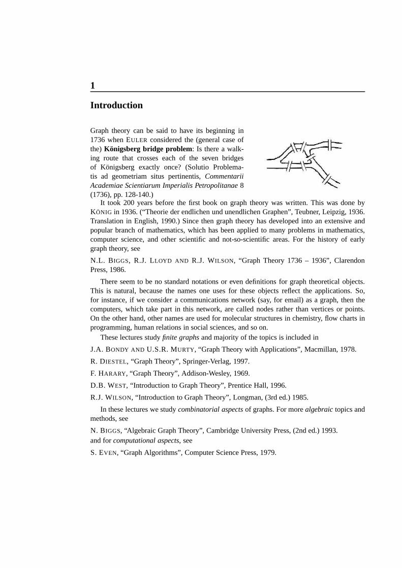
Graph theory can be said to have its beginning in1736 when EULER considered the (general case ofthe) Königsberg bridge problem: Is there a walk-ing route that crosses each of the seven bridgesof Königsberg exactly once? (Solutio Problema-tis ad geometriam situs pertinentis,CommentariiAcademiae Scientiarum Imperialis Petropolitanae8(1736), pp. 128-140.)
It took 200 years before the first book on graph theory was written. This was done byKÖNIG in 1936. (“Theorie der endlichen und unendlichen Graphen”,Teubner, Leipzig, 1936.Translation in English, 1990.) Since then graph theory has developed into an extensive andpopular branch of mathematics, which has been applied to many problems in mathematics,computer science, and other scientific and not-so-scientific areas. For the history of earlygraph theory, see
N.L. BIGGS, R.J. LLOYD AND R.J. WILSON, “Graph Theory 1736 – 1936”, ClarendonPress, 1986.
There seem to be no standard notations or even definitions forgraph theoretical objects.This is natural, because the names one uses for these objectsreflect the applications. So,for instance, if we consider a communications network (say,for email) as a graph, then thecomputers, which take part in this network, are called nodesrather than vertices or points.On the other hand, other names are used for molecular structures in chemistry, flow charts inprogramming, human relations in social sciences, and so on.
These lectures studyfinite graphsand majority of the topics is included in
J.A. BONDY AND U.S.R. MURTY, “Graph Theory with Applications”, Macmillan, 1978.
R. DIESTEL, “Graph Theory”, Springer-Verlag, 1997.
F. HARARY, “Graph Theory”, Addison-Wesley, 1969.
D.B. WEST, “Introduction to Graph Theory”, Prentice Hall, 1996.
R.J. WILSON, “Introduction to Graph Theory”, Longman, (3rd ed.) 1985.
In these lectures we studycombinatorial aspectsof graphs. For morealgebraictopics andmethods, see
N. BIGGS, “Algebraic Graph Theory”, Cambridge University Press, (2nd ed.) 1993.and forcomputational aspects, see
S. EVEN, “Graph Algorithms”, Computer Science Press, 1979.
3
In these lecture notes we mention several open problems thathave gained respect amongthe researchers. Indeed, graph theory has the advantage that it contains easily formulated openproblems that can be stated early in the theory. Finding a solution to any one of these problemsis on another layer of difficulty.
Sections with a star (�) in their heading are optional.
Notations and notions� For a finite setX, jXj denotes its size (cardinality, the number of its elements).� Let [1; n℄ = f1; 2; : : : ; ng;and in general, [i; n℄ = fi; i + 1; : : : ; ngfor integersi � n.� For a real numberx, thefloor and theceiling of x are the integersbx = maxfk 2 Z j k � xg and dxe = minfk 2 Z j x � kg:� A family fX1;X2; : : : ;Xkg of subsetsXi � X of a setX is apartition of X, ifX = [i2[1;k℄Xi and Xi \Xj = ; for all different i andj :� For two setsX andY , X � Y = f(x; y) j x 2 X; y 2 Y gis theirCartesian product.� For two setsX andY , X4Y = (X n Y ) [ (Y nX)is theirsymmetric difference. HereX n Y = fx j x 2 X;x =2 Y g.� Two numbersn; k 2 N (often n = jXj andk = jY j for setsX andY ) have thesameparity , if both are even, or both are odd, that is, ifn � k (mod 2). Otherwise, they haveopposite parity.
Graph theory has abundant examples ofNP-complete problems. Intuitively, a problem isin P 1 if there is an efficient (practical) algorithm to find a solution to it. On the other hand,a problem is in NP2, if it is first efficient to guess a solution and then efficient to check thatthis solution is correct. It is conjectured (and not known) that P 6= NP. This is one of thegreat problems in modern mathematics and theoretical computer science. If the guessing inNP-problems can be replaced by an efficient systematic search for a solution, then P=NP. Forany one NP-complete problem, if it is in P, then necessarily P=NP.1 Solvable – by an algorithm – in polynomially many steps on thesize of the problem instances.2 Solvablenondeterministicallyin polynomially many steps on the size of the problem instances.
1.1 Graphs and their plane figures 4
1.1 Graphs and their plane figures
Let V be afinite set, and denote byE(V ) = ffu; vg j u; v 2 V; u 6= vg :the subsets ofV of two distinct elements.
DEFINITION. A pairG = (V;E) with E � E(V ) is called agraph (on V ). The elementsof V are thevertices, and those ofE theedgesof the graph. The vertex set of a graphG isdenoted byVG and its edge set byEG. ThereforeG = (VG; EG).
In literature, graphs are also calledsimple graphs; vertices are callednodesorpoints; edgesare calledlinesor links. The list of alternatives is long (but still finite).
A pair fu; vg is usually written simply asuv. Notice that thenuv = vu. In order tosimplify notations, we also writev 2 G instead ofv 2 VG.
DEFINITION. For a graphG, we denote�G = jVGj and "G = jEGj :The number�G of the vertices is called theorder of G, and"G is thesizeof G. For an edgee = uv 2 EG, the verticesu andv are itsends. Verticesu andv areadjacentor neighbours,if e = uv 2 EG. Two edgese1 = uv ande2 = uw having a common end, areadjacent witheach other.
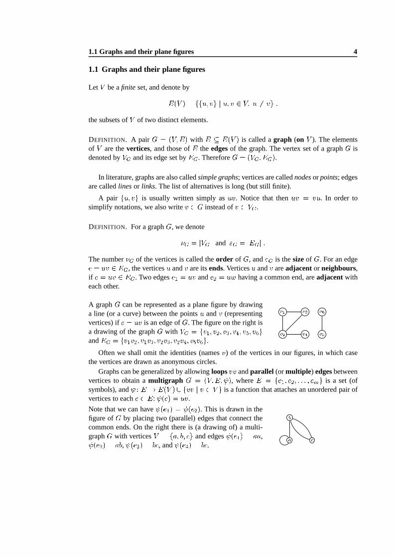
A graphG can be represented as a plane figure by drawinga line (or a curve) between the pointsu andv (representingvertices) ife = uv is an edge ofG. The figure on the right isa drawing of the graphG with VG = fv1; v2; v3; v4; v5; v6gandEG = fv1v2; v1v3; v2v3; v2v4; v5v6g. v1v2 v3v4 v5v6
Often we shall omit the identities (namesv) of the vertices in our figures, in which casethe vertices are drawn as anonymous circles.
Graphs can be generalized by allowingloopsvv andparallel (or multiple ) edgesbetweenvertices to obtain amultigraph G = (V;E; ), whereE = fe1; e2; : : : ; emg is a set (ofsymbols), and : E ! E(V ) [ fvv j v 2 V g is a function that attaches an unordered pair ofvertices to eache 2 E: (e) = uv.
Note that we can have (e1) = (e2). This is drawn in thefigure ofG by placing two (parallel) edges that connect thecommon ends. On the right there is (a drawing of) a multi-graphG with verticesV = fa; b; g and edges (e1) = aa, (e2) = ab, (e3) = b , and (e4) = b . ab
1.1 Graphs and their plane figures 5
Later we concentrate on (simple) graphs.
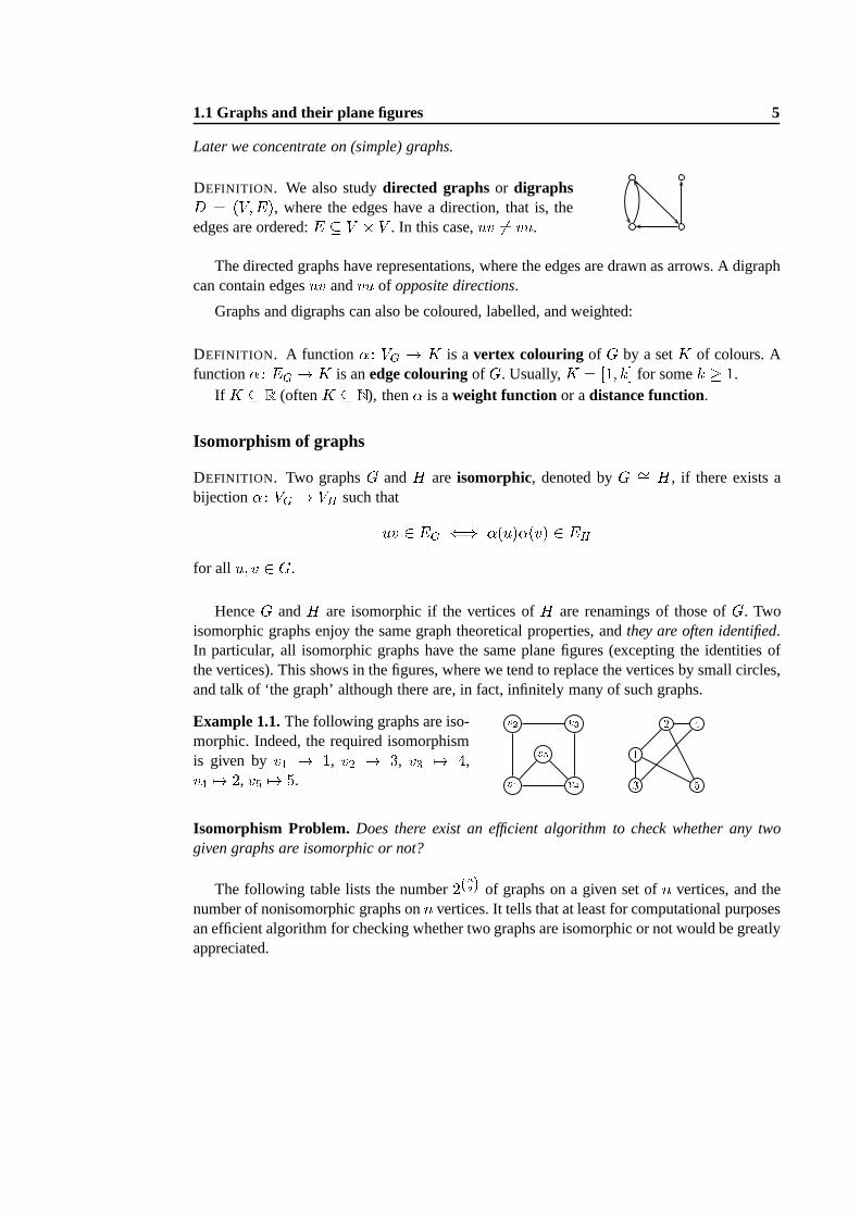
DEFINITION. We also studydirected graphs or digraphsD = (V;E), where the edges have a direction, that is, theedges are ordered:E � V � V . In this case,uv 6= vu.
The directed graphs have representations, where the edges are drawn as arrows. A digraphcan contain edgesuv andvu of opposite directions.
Graphs and digraphs can also be coloured, labelled, and weighted:
DEFINITION. A function� : VG ! K is avertex colouring of G by a setK of colours. Afunction� : EG ! K is anedge colouringof G. Usually,K = [1; k℄ for somek � 1.
If K � R (oftenK � N), then� is aweight function or adistance function.
Isomorphism of graphs
DEFINITION. Two graphsG andH are isomorphic, denoted byG �= H, if there exists abijection� : VG ! VH such thatuv 2 EG () �(u)�(v) 2 EHfor all u; v 2 G.
HenceG andH are isomorphic if the vertices ofH are renamings of those ofG. Twoisomorphic graphs enjoy the same graph theoretical properties, andthey are often identified.In particular, all isomorphic graphs have the same plane figures (excepting the identities ofthe vertices). This shows in the figures, where we tend to replace the vertices by small circles,and talk of ‘the graph’ although there are, in fact, infinitely many of such graphs.
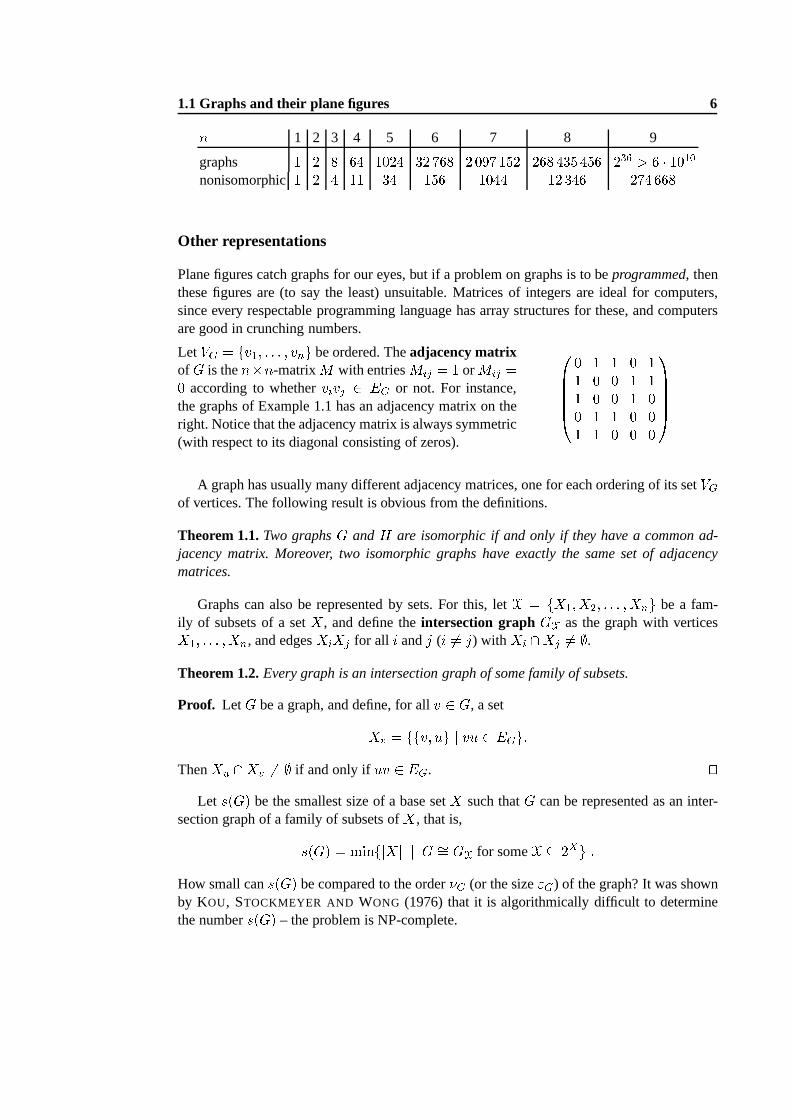
Example 1.1.The following graphs are iso-morphic. Indeed, the required isomorphismis given by v1 7! 1, v2 7! 3, v3 7! 4,v4 7! 2, v5 7! 5. v1v2 v3v4v5 13 42 5Isomorphism Problem. Does there exist an efficient algorithm to check whether any twogiven graphs are isomorphic or not?
The following table lists the number2(n2) of graphs on a given set ofn vertices, and thenumber of nonisomorphic graphs onn vertices. It tells that at least for computational purposesan efficient algorithm for checking whether two graphs are isomorphic or not would be greatlyappreciated.
1.1 Graphs and their plane figures 6n 1 2 3 4 5 6 7 8 9
graphs 1 2 8 64 1024 32 768 2 097 152 268 435 456 236 > 6 � 1010nonisomorphic1 2 4 11 34 156 1044 12 346 274 668
Other representations
Plane figures catch graphs for our eyes, but if a problem on graphs is to beprogrammed, thenthese figures are (to say the least) unsuitable. Matrices of integers are ideal for computers,since every respectable programming language has array structures for these, and computersare good in crunching numbers.
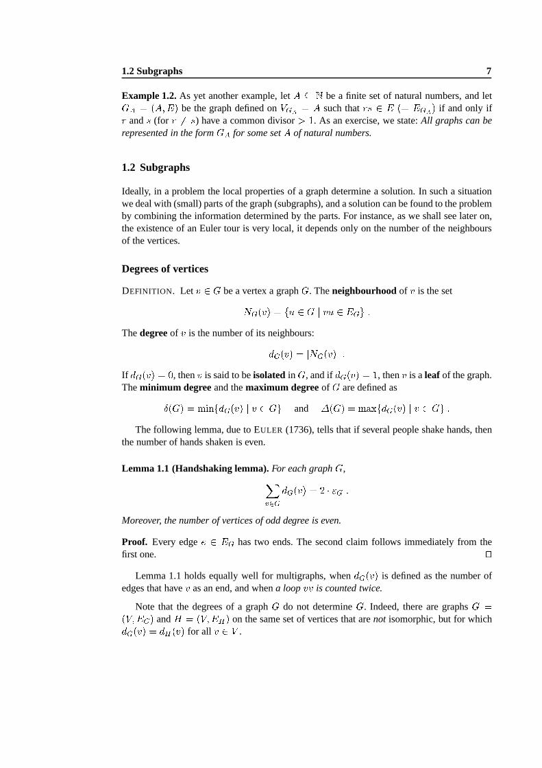
LetVG = fv1; : : : ; vng be ordered. Theadjacency matrixofG is then�n-matrixM with entriesMij = 1 orMij =0 according to whethervivj 2 EG or not. For instance,the graphs of Example 1.1 has an adjacency matrix on theright. Notice that the adjacency matrix is always symmetric(with respect to its diagonal consisting of zeros).
0BBBB� 0 1 1 0 11 0 0 1 11 0 0 1 00 1 1 0 01 1 0 0 01CCCCA
A graph has usually many different adjacency matrices, one for each ordering of its setVGof vertices. The following result is obvious from the definitions.
Theorem 1.1.Two graphsG andH are isomorphic if and only if they have a common ad-jacency matrix. Moreover, two isomorphic graphs have exactly the same set of adjacencymatrices.
Graphs can also be represented by sets. For this, letX = fX1;X2; : : : ;Xng be a fam-ily of subsets of a setX, and define theintersection graphGX as the graph with verticesX1; : : : ;Xn, and edgesXiXj for all i andj (i 6= j) with Xi \Xj 6= ;.Theorem 1.2.Every graph is an intersection graph of some family of subsets.
Proof. LetG be a graph, and define, for allv 2 G, a setXv = ffv; ug j vu 2 EGg:ThenXu \Xv 6= ; if and only if uv 2 EG. ut
Let s(G) be the smallest size of a base setX such thatG can be represented as an inter-section graph of a family of subsets ofX, that is,s(G) = minfjXj j G �= GX for someX � 2Xg :How small cans(G) be compared to the order�G (or the size"G) of the graph? It was shownby KOU, STOCKMEYER AND WONG (1976) that it is algorithmically difficult to determinethe numbers(G) – the problem is NP-complete.
1.2 Subgraphs 7
Example 1.2.As yet another example, letA � N be a finite set of natural numbers, and letGA = (A;E) be the graph defined onVGA = A such thatrs 2 E (= EGA) if and only ifr ands (for r 6= s) have a common divisor> 1. As an exercise, we state:All graphs can berepresented in the formGA for some setA of natural numbers.
1.2 Subgraphs
Ideally, in a problem the local properties of a graph determine a solution. In such a situationwe deal with (small) parts of the graph (subgraphs), and a solution can be found to the problemby combining the information determined by the parts. For instance, as we shall see later on,the existence of an Euler tour is very local, it depends only on the number of the neighboursof the vertices.
Degrees of vertices
DEFINITION. Let v 2 G be a vertex a graphG. Theneighbourhoodof v is the setNG(v) = fu 2 G j vu 2 EGg :Thedegreeof v is the number of its neighbours:dG(v) = jNG(v)j :If dG(v) = 0, thenv is said to beisolated inG, and ifdG(v) = 1, thenv is aleaf of the graph.Theminimum degreeand themaximum degreeof G are defined asÆ(G) = minfdG(v) j v 2 Gg and �(G) = maxfdG(v) j v 2 Gg :
The following lemma, due to EULER (1736), tells that if several people shake hands, thenthe number of hands shaken is even.
Lemma 1.1 (Handshaking lemma).For each graphG,Xv2G dG(v) = 2 � "G :Moreover, the number of vertices of odd degree is even.
Proof. Every edgee 2 EG has two ends. The second claim follows immediately from thefirst one. ut
Lemma 1.1 holds equally well for multigraphs, whendG(v) is defined as the number ofedges that havev as an end, and whena loopvv is counted twice.
Note that the degrees of a graphG do not determineG. Indeed, there are graphsG =(V;EG) andH = (V;EH ) on the same set of vertices that arenot isomorphic, but for whichdG(v) = dH(v) for all v 2 V .
1.2 Subgraphs 8
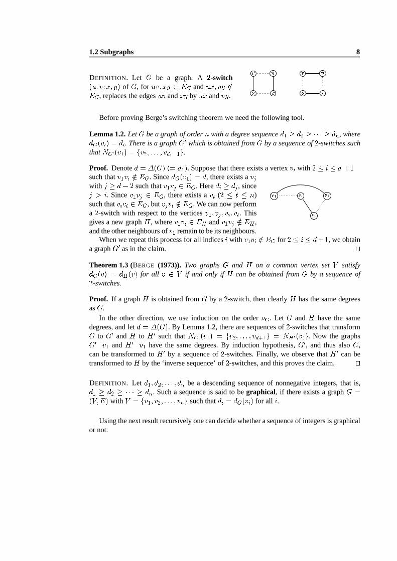
DEFINITION. Let G be a graph. A2-switch(u; v;x; y) of G, for uv; xy 2 EG andux; vy =2EG, replaces the edgesuv andxy by ux andvy. uv xy uv xyBefore proving Berge’s switching theorem we need the following tool.
Lemma 1.2.LetG be a graph of ordern with a degree sequenced1 � d2 � � � � � dn, wheredG(vi) = di. There is a graphG0 which is obtained fromG by a sequence of2-switches suchthatNG0(v1) = fv2; : : : ; vd1+1g.Proof. Denoted = �(G) (= d1). Suppose that there exists a vertexvi with 2 � i � d+ 1such thatv1vi =2 EG. SincedG(v1) = d, there exists avjwith j � d+ 2 such thatv1vj 2 EG. Heredi � dj , sincej > i. Sincev1vj 2 EG, there exists avt (2 � t � n)such thatvivt 2 EG, butvjvt =2 EG. We can now performa 2-switch with respect to the verticesv1; vj ; vi; vt. Thisgives a new graphH, wherev1vi 2 EH andv1vj =2 EH ,and the other neighbours ofv1 remain to be its neighbours.
v1 vi vjvtWhen we repeat this process for all indicesi with v1vi =2 EG for 2 � i � d+1, we obtain
a graphG0 as in the claim. utTheorem 1.3 (BERGE (1973)). Two graphsG and H on a common vertex setV satisfydG(v) = dH(v) for all v 2 V if and only ifH can be obtained fromG by a sequence of2-switches.
Proof. If a graphH is obtained fromG by a2-switch, then clearlyH has the same degreesasG.
In the other direction, we use induction on the order�G. Let G andH have the samedegrees, and letd = �(G). By Lemma 1.2, there are sequences of2-switches that transformG to G0 andH to H 0 such thatNG0(v1) = fv2; : : : ; vd+1g = NH0(v1). Now the graphsG0�v1 andH 0�v1 have the same degrees. By induction hypothesis,G0, and thus alsoG,can be transformed toH 0 by a sequence of2-switches. Finally, we observe thatH 0 can betransformed toH by the ‘inverse sequence’ of2-switches, and this proves the claim. utDEFINITION. Let d1; d2; : : : ; dn be a descending sequence of nonnegative integers, that is,d1 � d2 � � � � � dn. Such a sequence is said to begraphical, if there exists a graphG =(V;E) with V = fv1; v2; : : : ; vng such thatdi = dG(vi) for all i.
Using the next result recursively one can decide whether a sequence of integers is graphicalor not.
1.2 Subgraphs 9
Theorem 1.4 (HAVEL (1955),HAKIMI (1962)).A sequenced1; d2; : : : ; dn (with d1 � 1 andn � 2) is graphical if and only ifd2 � 1; d3 � 1; : : : ; dd1+1 � 1; dd1+2; dd1+3; : : : ; dn: (1.1)
is graphical (when put into nonincreasing order).
Proof. (() ConsiderG of ordern� 1 with vertices (and degrees)dG(v2) = d2 � 1; : : : ; dG(vd1+1) = dd1+1 � 1;dG(vd1+2) = dd1+2; : : : ; dG(vn) = dnas in (1.1). Add a new vertexv1 and the edgesv1vi for all i 2 [2; dd1+1℄. Then in this newgraphH, dH(v1) = d1, anddH(vi) = di for all i.
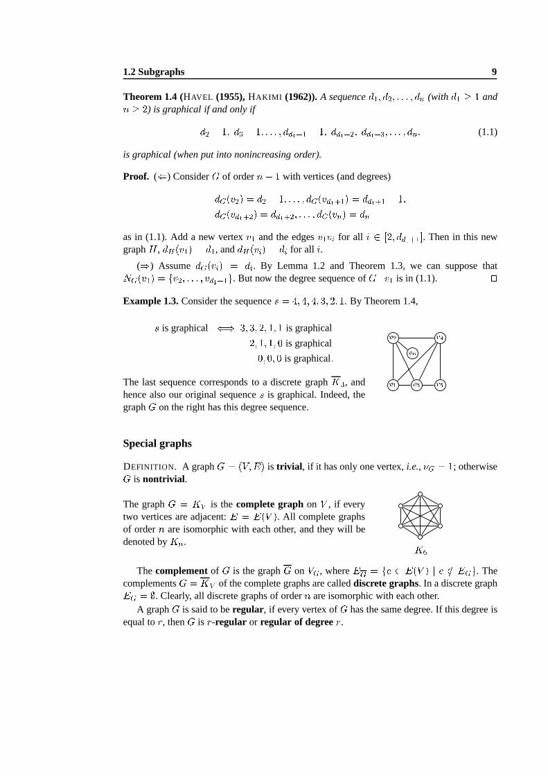
()) AssumedG(vi) = di. By Lemma 1.2 and Theorem 1.3, we can suppose thatNG(v1) = fv2; : : : ; vd1+1g. But now the degree sequence ofG�v1 is in (1.1). utExample 1.3.Consider the sequences = 4; 4; 4; 3; 2; 1. By Theorem 1.4,s is graphical () 3; 3; 2; 1; 1 is graphical2; 1; 1; 0 is graphical0; 0; 0 is graphical:The last sequence corresponds to a discrete graphK3, andhence also our original sequences is graphical. Indeed, thegraphG on the right has this degree sequence.
v1v2 v3 v4v5v6Special graphs
DEFINITION. A graphG = (V;E) is trivial , if it has only one vertex,i.e., �G = 1; otherwiseG is nontrivial .
The graphG = KV is thecomplete graphon V , if everytwo vertices are adjacent:E = E(V ). All complete graphsof ordern are isomorphic with each other, and they will bedenoted byKn. K6
Thecomplementof G is the graphG on VG, whereEG = fe 2 E(V ) j e =2 EGg. ThecomplementsG = KV of the complete graphs are calleddiscrete graphs. In a discrete graphEG = ;. Clearly, all discrete graphs of ordern are isomorphic with each other.
A graphG is said to beregular, if every vertex ofG has the same degree. If this degree isequal tor, thenG is r-regular or regular of degreer.
1.2 Subgraphs 10
Note that a discrete graph is 0-regular, and a complete graphKn is (n � 1)-regular. Inparticular,"Kn = n(n�1)=2, and therefore"G � n(n�1)=2 for all graphsG that have ordern.
Example 1.4.The graph on the right is thePetersen graphthat we will meet several times (drawn differently). It is a3-regular graph of order10.
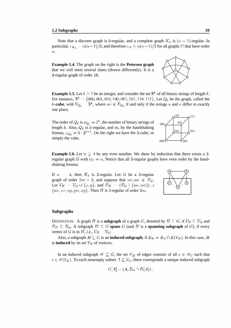
Example 1.5.Let k � 1 be an integer, and consider the setB k of all binary strings of lengthk.For instance,B 3 = f000; 001; 010; 100; 011; 101; 110; 111g. LetQk be the graph, called thek-cube, with VQk = B k , whereuv 2 EQk if and only if the stringsu andv differ in exactlyone place.
The order ofQk is �Qk = 2k, the number of binary strings oflengthk. Also,Qk is k-regular, and so, by the handshakinglemma,"Qk = k � 2k�1. On the right we have the3-cube, orsimply the cube.
000
100 101
001
010
110 111
011
Example 1.6.Let n � 4 be any even number. We show by induction that there exists a3-regular graphG with �G = n. Notice that all3-regular graphs have even order by the hand-shaking lemma.
If n = 4, then K4 is 3-regular. LetG be a 3-regulargraph of order2m � 2, and suppose thatuv; uw 2 EG.Let VH = VG [ fx; yg, andEH = (EG n fuv; uwg) [fux; xv; uy; yw; xyg: ThenH is 3-regular of order2m.
u vwx ySubgraphs
DEFINITION. A graphH is asubgraph of a graphG, denoted byH � G, if VH � VG andEH � EG. A subgraphH � G spansG (andH is a spanning subgraphof G), if everyvertex ofG is inH, i.e.,VH = VG.
Also, a subgraphH � G is aninduced subgraph, if EH = EG \E(VH). In this case,His inducedby its setVH of vertices.
In an induced subgraphH � G, the setEH of edges consists of alle 2 EG such thate 2 E(VH). To each nonempty subsetA � VG, there corresponds a unique induced subgraphG[A℄ = (A;EG \E(A)) :
1.3 Paths and cycles 11
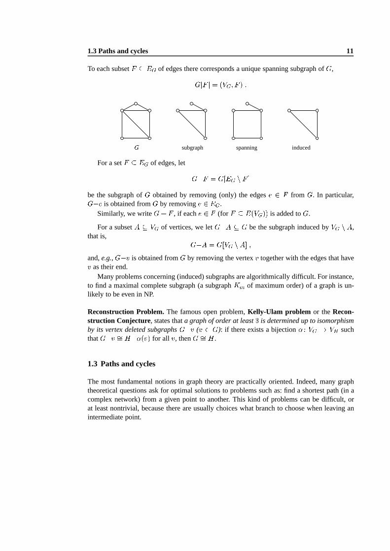
To each subsetF � EG of edges there corresponds a unique spanning subgraph ofG,G[F ℄ = (VG; F ) :G subgraph spanning induced
For a setF � EG of edges, let G�F = G[EG n F ℄be the subgraph ofG obtained by removing (only) the edgese 2 F from G. In particular,G�e is obtained fromG by removinge 2 EG.
Similarly, we writeG+ F , if eache 2 F (for F � E(VG)) is added toG.
For a subsetA � VG of vertices, we letG�A � G be the subgraph induced byVG n A,that is, G�A = G[VG n A℄ ;and,e.g.,G�v is obtained fromG by removing the vertexv together with the edges that havev as their end.
Many problems concerning (induced) subgraphs are algorithmically difficult. For instance,to find a maximal complete subgraph (a subgraphKm of maximum order) of a graph is un-likely to be even in NP.
Reconstruction Problem.The famous open problem,Kelly-Ulam problem or theRecon-struction Conjecture, states thata graph of order at least3 is determined up to isomorphismby its vertex deleted subgraphsG�v (v 2 G): if there exists a bijection� : VG ! VH suchthatG�v �= H��(v) for all v, thenG �= H.
1.3 Paths and cycles
The most fundamental notions in graph theory are practically oriented. Indeed, many graphtheoretical questions ask for optimal solutions to problems such as: find a shortest path (in acomplex network) from a given point to another. This kind of problems can be difficult, orat least nontrivial, because there are usually choices whatbranch to choose when leaving anintermediate point.

1.3 Paths and cycles 12
Walks
DEFINITION. Let ei = uiui+1 2 EG be edges ofG for i 2 [1; k℄. Hereei and ei+1 arecompatible in the sense thatei is adjacent toei+1 for all i 2 [1; k � 1℄. The sequenceW = e1e2 : : : ekis awalk of length k from u1 to uk+1.
We write, more informally,W : u1 �! u2 �! : : : �! uk �! uk+1 or W : u1 k�! uk+1 :Write u ?�! v to say that there is a walk of some length fromu to v. Here we understand thatW : u ?�! v is always a specific walk, W = e1e2 : : : ek, although we sometimes do not careto mention the edgesei it uses. The length of a walkW is denoted byjW j.DEFINITION. LetW = e1e2 : : : ek (ei = uiui+1) be a walk.W is closed, if u1 = uk+1.W is apath, if ui 6= uj for all i 6= j.W is acycle, if it is closed, andui 6= uj for i 6= j except thatu1 = uk+1.W is atrivial path , if its length is 0. A trivial path has no edges.
For a walkW : u = u1 �! : : : �! uk+1 = v, alsoW�1 : v = uk+1 �! : : : �! u1 = uis a walk inG, called theinverse walkof W .
A vertexu is anendof a pathP , if P starts or ends inu.The join of two walksW1 : u ?�! v andW2 : v ?�! w is the walkW1W2 : u ?�! w. (Here
the endv must be common to the walks.)PathsP andQ aredisjoint , if they have no vertices in common, and they areindependent,
if they can share only their ends.
Clearly, the inverse walkP�1 of a pathP is a path (theinverse pathof P ). The join oftwo paths need not be a path.
A (sub)graph, which is a path (cycle) of lengthk � 1 (k, resp.) havingk vertices is denotedby Pk (Ck, resp.). Ifk is even (odd), we saythat the path or cycle iseven (odd). Clearly,all paths of lengthk are isomorphic. The sameholds for cycles of fixed length.
P5 C6Lemma 1.3.Each walkW : u ?�! v with u 6= v contains a pathP : u ?�! v, that is, there isa pathP : u ?�! v that is obtained fromW by removing edges and vertices.
1.3 Paths and cycles 13
Proof. Let W : u = u1 �! : : : �! uk+1 = v. Let i < j be indices such thatui = uj . Ifno suchi andj exist, thenW , itself, is a path. Otherwise, inW = W1W2W3 : u ?�! ui ?�!uj ?�! v the portionU1 = W1W3 : u ?�! ui = uj ?�! v is a shorter walk. By repeating thisargument, we obtain a sequenceU1; U2; : : : ; Um of walksu ?�! v with jW j > jU1j > � � � >jUmj. When the procedure stops, we have a path as required. (Notice that in the above it mayvery well be thatW1 orW3 is a trivial walk.) utDEFINITION. If there exists a walk (and hence a path) fromu to v in G, letdG(u; v) = minfk j u k�! vgbe thedistancebetweenu andv. If there are no walksu ?�! v, let dG(u; v) =1 by conven-tion. A graphG is connected, if dG(u; v) <1 for all u; v 2 G; otherwise, it isdisconnected.The maximal connected subgraphs ofG are itsconnected components. Denote (G) = the number of connected components ofG :If (G) = 1, thenG is, of course, connected.
The maximality condition means that a subgraphH � G is a connected component if andonly if H is connected and there are no edges leavingH, i.e., for every vertexv =2 H, thesubgraphG[VH [fvg℄ is disconnected. Apparently, every connected component isan inducedsubgraph, and N�G(v) = fu j dG(v; u) <1gis theconnected component ofG that containsv 2 G. In particular, the connected componentsform a partition ofG.
Shortest paths
DEFINITION. Let G� be an edge weighted graph, that is,G� is a graphG together with aweight function� : EG ! R on its edges. ForH � G, let�(H) = Xe2EH �(e)be the (total)weight of H. In particular, ifP = e1e2 : : : ek is a path, then its weight is�(P ) =Pki=1 �(ei). Theminimum weighted distancebetween two vertices isd�G(u; v) = minf�(P ) j P : u ?�! vg :
In extremal problems we seek for optimal subgraphsH � G satisfying specific conditions.In practice we encounter situations whereG might represent� a distribution or transportation network (say, for mail), where the weights on edges are
distances, travelexpenses, or rates of flowin the network;� a system of channels in (tele)communication or computer architecture, where the weightspresent the rate ofunreliability or frequency of actionof the connections;� a model of chemical bonds, where the weights measure molecular attraction.
1.3 Paths and cycles 14
In these examples we look for a subgraph with the smallest weight, and which connectstwo given vertices, or all vertices (if we want to travel around). On the other hand, if the graphrepresents a network of pipelines, the weights are volumes or capacities, and then one wantsto find a subgraph with the maximum weight.
We consider the minimum problem. For this, letG be a graph with an integer weightfunction� : EG ! N. In this case, call�(uv) the length of uv.
Theshortest path problem: Given a connected graphGwith a weight function� : EG ! N,findd�G(u; v) for givenu; v 2 G.
Assume thatG is a connected graph. Dijkstra’s algorithm solves the problem for every pairu; v, whereu is a fixed starting point andv 2 G. Let us make the convention that�(uv) =1,if uv =2 EG.
Dijkstra’s algorithm :
(i) Setu0 = u, t(u0) = 0 andt(v) =1 for all v 6= u0.(ii) For i 2 [0; �G � 1℄: for eachv =2 fu1; : : : ; uig,
replace t(v) by minft(v); t(ui) + �(uiv)g :Let ui+1 =2 fu1; : : : ; uig beanyvertex with the least valuet(ui+1).
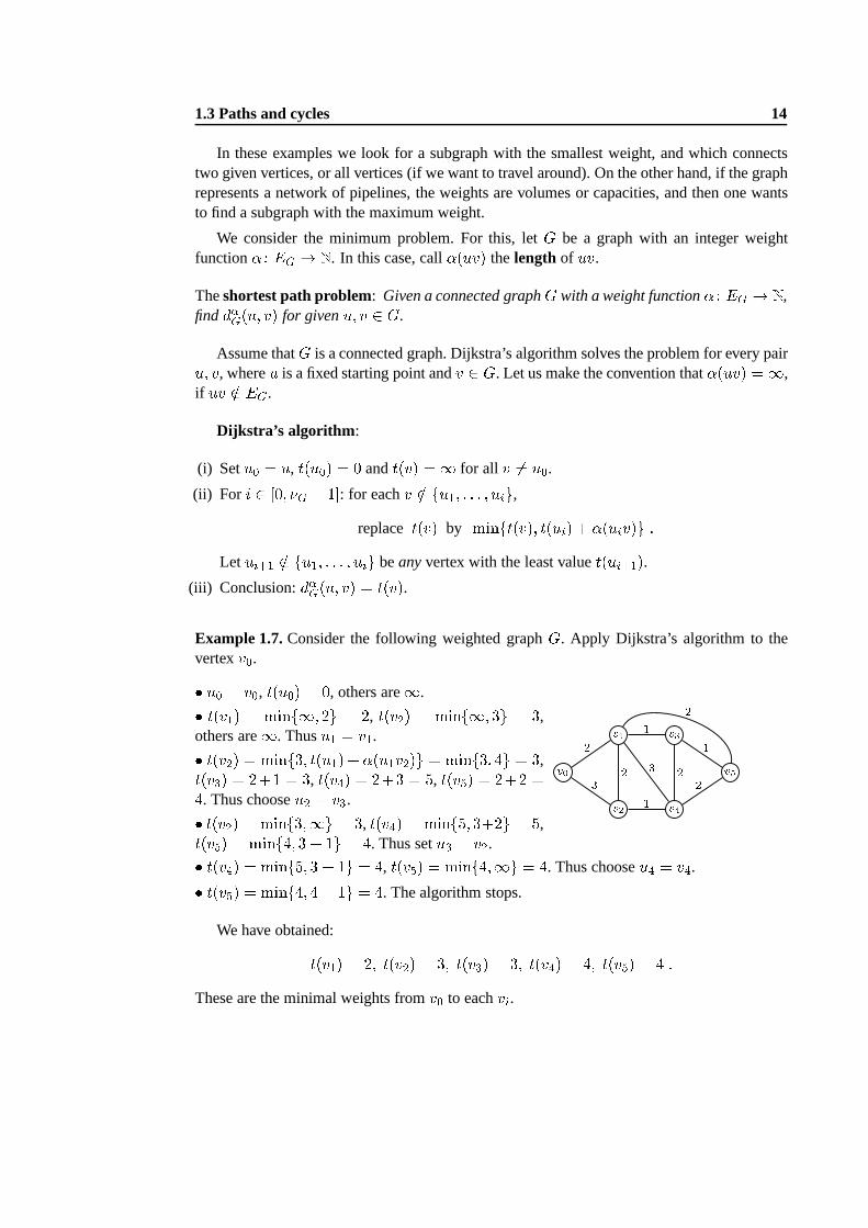
(iii) Conclusion:d�G(u; v) = t(v).Example 1.7.Consider the following weighted graphG. Apply Dijkstra’s algorithm to thevertexv0.� u0 = v0, t(u0) = 0, others are1.� t(v1) = minf1; 2g = 2, t(v2) = minf1; 3g = 3,others are1. Thusu1 = v1.� t(v2) = minf3; t(u1) +�(u1v2)g = minf3; 4g = 3,t(v3) = 2+1 = 3, t(v4) = 2+3 = 5, t(v5) = 2+2 =4. Thus chooseu2 = v3.� t(v2) = minf3;1g = 3, t(v4) = minf5; 3+2g = 5,t(v5) = minf4; 3 + 1g = 4. Thus setu3 = v2. v0 v1v2 v3v4 v523 13 2 1212 2� t(v4) = minf5; 3 + 1g = 4, t(v5) = minf4;1g = 4. Thus chooseu4 = v4.� t(v5) = minf4; 4 + 1g = 4. The algorithm stops.
We have obtained:t(v1) = 2; t(v2) = 3; t(v3) = 3; t(v4) = 4; t(v5) = 4 :These are the minimal weights fromv0 to eachvi.
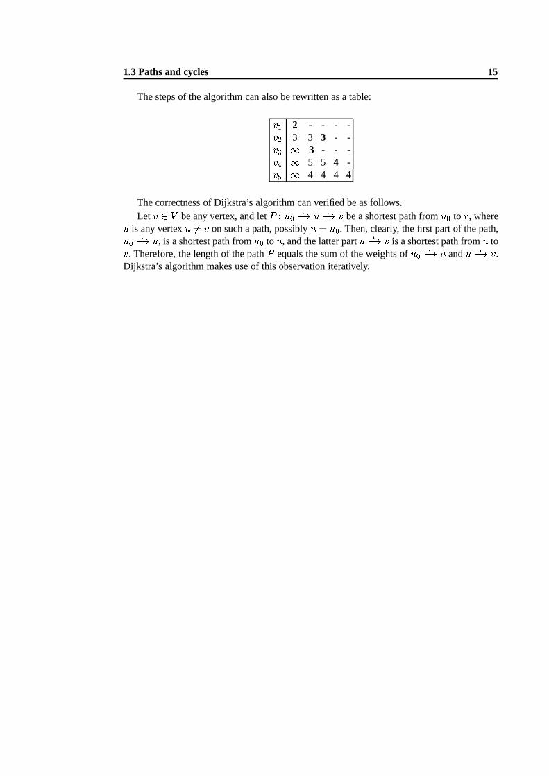
1.3 Paths and cycles 15
The steps of the algorithm can also be rewritten as a table:v1 2 - - - -v2 3 3 3 - -v3 1 3 - - -v4 1 5 5 4 -v5 1 4 4 4 4
The correctness of Dijkstra’s algorithm can verified be as follows.Let v 2 V be any vertex, and letP : u0 ?�! u ?�! v be a shortest path fromu0 to v, whereu is any vertexu 6= v on such a path, possiblyu = u0. Then, clearly, the first part of the path,u0 ?�! u, is a shortest path fromu0 to u, and the latter partu ?�! v is a shortest path fromu tov. Therefore, the length of the pathP equals the sum of the weights ofu0 ?�! u andu ?�! v.
Dijkstra’s algorithm makes use of this observation iteratively.
2
Connectivity of Graphs
2.1 Bipartite graphs and trees
In problems such as the shortest path problem we look for minimum solutions that satisfythe given requirements. The solutions in these cases are usually subgraphs without cycles.Such connected graphs will be called trees, and they are used, e.g., in search algorithms fordatabases. For concrete applications in this respect, see
T.H. CORMEN, C.E. LEISERSON AND R.L. RIVEST, “Introduction to Algorithms”, MITPress, 1993.
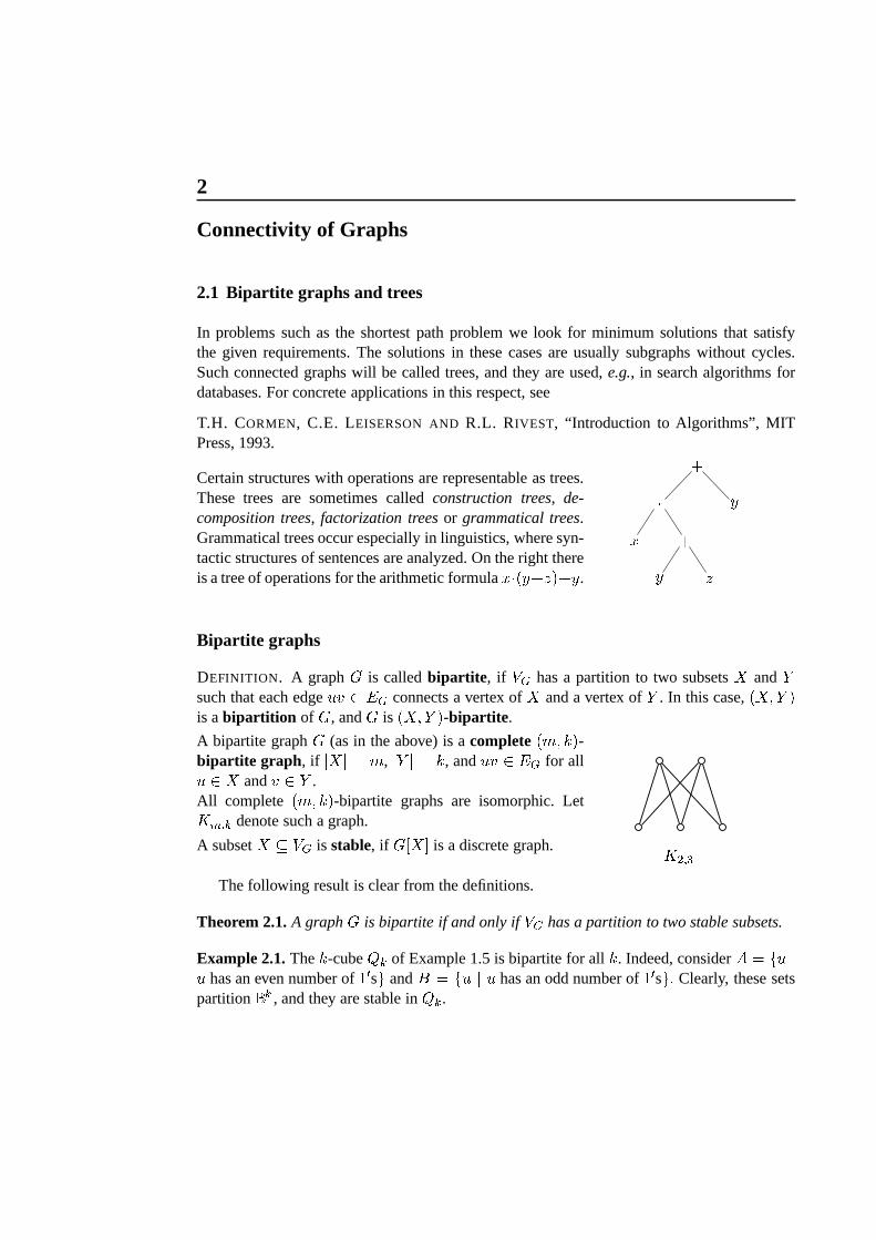
Certain structures with operations are representable as trees.These trees are sometimes calledconstruction trees, de-composition trees, factorization treesor grammatical trees.Grammatical trees occur especially in linguistics, where syn-tactic structures of sentences are analyzed. On the right thereis a tree of operations for the arithmetic formulax�(y+z)+y.
+�x +y z yBipartite graphs
DEFINITION. A graphG is calledbipartite , if VG has a partition to two subsetsX andYsuch that each edgeuv 2 EG connects a vertex ofX and a vertex ofY . In this case,(X;Y )is abipartition of G, andG is (X;Y )-bipartite .
A bipartite graphG (as in the above) is acomplete(m; k)-bipartite graph , if jXj = m, jY j = k, anduv 2 EG for allu 2 X andv 2 Y .All complete (m; k)-bipartite graphs are isomorphic. LetKm;k denote such a graph.
A subsetX � VG is stable, if G[X℄ is a discrete graph. K2;3The following result is clear from the definitions.
Theorem 2.1.A graphG is bipartite if and only ifVG has a partition to two stable subsets.
Example 2.1.Thek-cubeQk of Example 1.5 is bipartite for allk. Indeed, considerA = fu ju has an even number of10sg andB = fu j u has an odd number of10sg: Clearly, these setspartitionB k , and they are stable inQk.
2.1 Bipartite graphs and trees 17
Theorem 2.2.A graphG is bipartite if and only if it has no odd cycles.
Proof. ()) LetG be(X;Y )-bipartite. For a cycleC : v1 �! : : : �! vk+1 = v1 of lengthk,v1 2 X impliesv2 2 Y , v3 2 X, . . . ,v2i 2 Y , v2i+1 2 X. Consequently,k + 1 = 2m+ 1 isodd, andk = jCj is even.
(() Suppose that all cycles inG are even. First, we observe that it suffices to show theclaim for connected graphs. Indeed, ifG is disconnected, then each cycle ofG is contained inone of the connected components,G1; : : : ; Gp, of G. If Gi is (Xi; Yi)-bipartite, then(X1 [X2 [ � � � [Xp; Y1 [ Y2 [ � � � [ Yp) is a bipartition ofG.
Assume thus thatG is connected. Letv 2 G be a chosen vertex, and defineX = fx j dG(v; x) is eveng; Y = fy j dG(v; y) is oddg :SinceG is connected,VG = X [ Y . Also, by the definition of distance,X \ Y = ;.
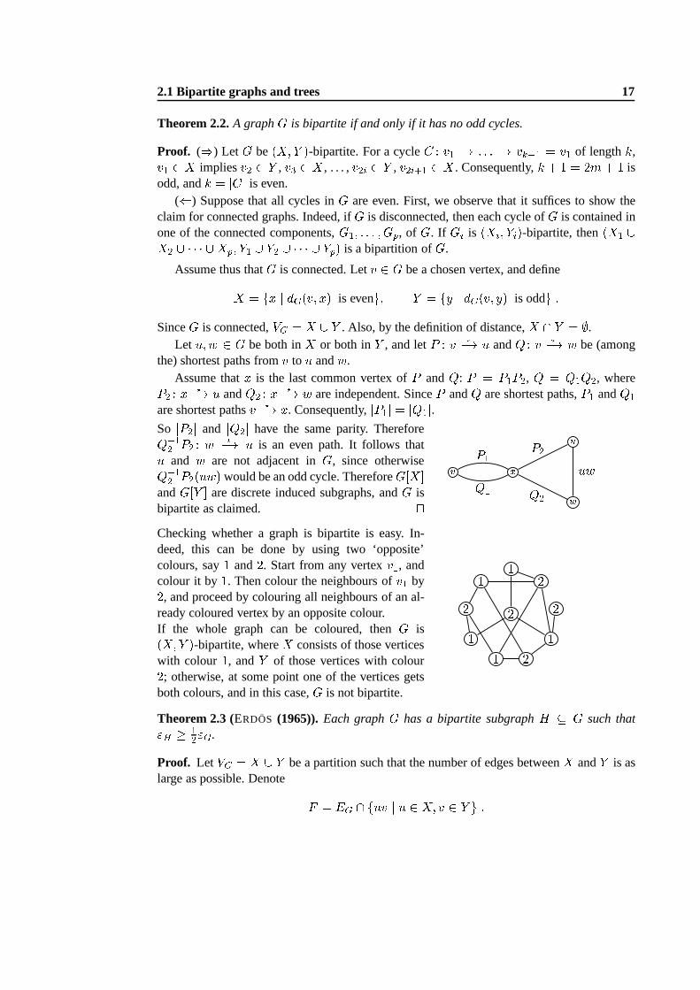
Let u;w 2 G be both inX or both inY , and letP : v ?�! u andQ : v ?�! w be (amongthe) shortest paths fromv to u andw.
Assume thatx is the last common vertex ofP andQ: P = P1P2, Q = Q1Q2, whereP2 : x ?�! u andQ2 : x ?�! w are independent. SinceP andQ are shortest paths,P1 andQ1are shortest pathsv ?�! x. Consequently,jP1j = jQ1j.So jP2j and jQ2j have the same parity. ThereforeQ�12 P2 : w ?�! u is an even path. It follows thatu and w are not adjacent inG, since otherwiseQ�12 P2(uw) would be an odd cycle. ThereforeG[X℄andG[Y ℄ are discrete induced subgraphs, andG isbipartite as claimed. ut v x uwP1Q1 P2Q2 uwChecking whether a graph is bipartite is easy. In-deed, this can be done by using two ‘opposite’colours, say1 and2. Start from any vertexv1, andcolour it by1. Then colour the neighbours ofv1 by2, and proceed by colouring all neighbours of an al-ready coloured vertex by an opposite colour.If the whole graph can be coloured, thenG is(X;Y )-bipartite, whereX consists of those verticeswith colour 1, andY of those vertices with colour2; otherwise, at some point one of the vertices getsboth colours, and in this case,G is not bipartite.
1 2 212112 1 2Theorem 2.3 (ERDÖS (1965)).Each graphG has a bipartite subgraphH � G such that"H � 12"G.
Proof. Let VG = X [ Y be a partition such that the number of edges betweenX andY is aslarge as possible. Denote F = EG \ fuv j u 2 X; v 2 Y g ;
2.1 Bipartite graphs and trees 18
and letH = G[F ℄. ObviouslyH is a spanning subgraph, and it is bipartite. By the maximumcondition, dH(v) � 12dG(v) ;since, otherwise,v is on the wrong side. (That is, ifv 2 X, then the pairX 0 = X n fvg,Y 0 = Y [ fvg does better that the pairX;Y .) Now"H = 12 Xv2H dH(v) � 12 Xv2G 12dG(v) = 12"G : utBridges
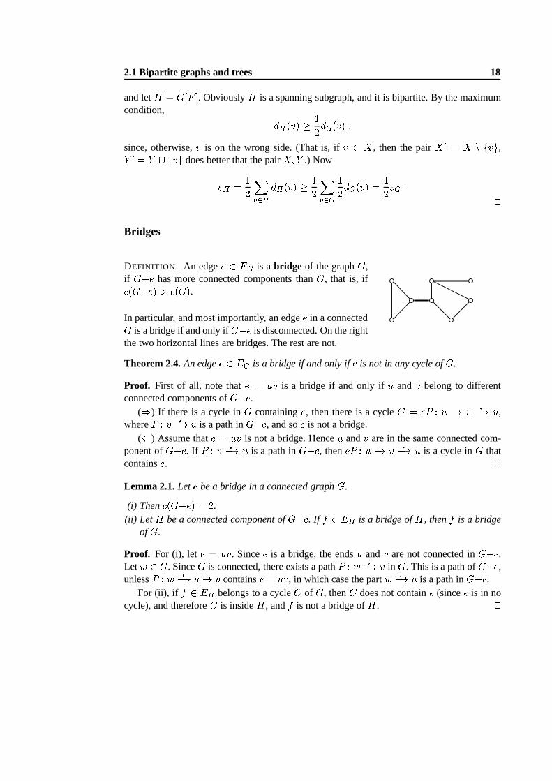
DEFINITION. An edgee 2 EG is abridge of the graphG,if G�e has more connected components thanG, that is, if (G�e) > (G).In particular, and most importantly, an edgee in a connectedG is a bridge if and only ifG�e is disconnected. On the rightthe two horizontal lines are bridges. The rest are not.
Theorem 2.4.An edgee 2 EG is a bridge if and only ife is not in any cycle ofG.
Proof. First of all, note thate = uv is a bridge if and only ifu andv belong to differentconnected components ofG�e.
()) If there is a cycle inG containinge, then there is a cycleC = eP : u �! v ?�! u,whereP : v ?�! u is a path inG�e, and soe is not a bridge.
(() Assume thate = uv is not a bridge. Henceu andv are in the same connected com-ponent ofG�e. If P : v ?�! u is a path inG�e, theneP : u �! v ?�! u is a cycle inG thatcontainse. utLemma 2.1.Lete be a bridge in a connected graphG.
(i) Then (G�e) = 2.(ii) Let H be a connected component ofG�e. If f 2 EH is a bridge ofH, thenf is a bridge
ofG.
Proof. For (i), let e = uv. Sincee is a bridge, the endsu andv are not connected inG�e.Letw 2 G. SinceG is connected, there exists a pathP : w ?�! v in G. This is a path ofG�e,unlessP : w ?�! u! v containse = uv, in which case the partw ?�! u is a path inG�e.
For (ii), if f 2 EH belongs to a cycleC of G, thenC does not containe (sincee is in nocycle), and thereforeC is insideH, andf is not a bridge ofH. ut
2.1 Bipartite graphs and trees 19
Trees
DEFINITION. A graph is calledacyclic, if it has no cycles. An acyclic graph is also called aforest. A tree is a connected acyclic graph.
By Theorem 2.4 and the definition of a tree, we have
Corollary 2.1. A connected graph is a tree if and only if all its edges are bridges.
Example 2.2.The following enumeration result for trees has many different proofs, the firstof which was given by CAYLEY in 1889:There arenn�2 trees on a vertex setV ofn elements.We omit the proof.
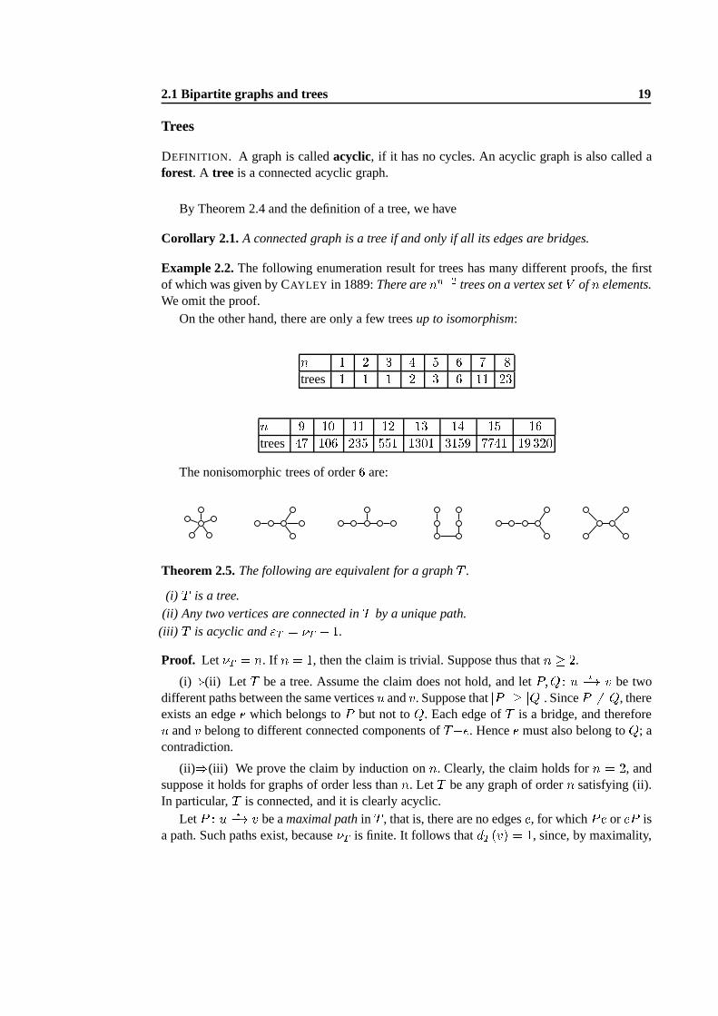
On the other hand, there are only a few treesup to isomorphism:n 1 2 3 4 5 6 7 8trees 1 1 1 2 3 6 11 23n 9 10 11 12 13 14 15 16
trees 47 106 235 551 1301 3159 7741 19 320The nonisomorphic trees of order6 are:
Theorem 2.5.The following are equivalent for a graphT .
(i) T is a tree.(ii) Any two vertices are connected inT by a unique path.(iii) T is acyclic and"T = �T � 1.
Proof. Let �T = n. If n = 1, then the claim is trivial. Suppose thus thatn � 2.
(i))(ii) Let T be a tree. Assume the claim does not hold, and letP;Q : u ?�! v be twodifferent paths between the same verticesu andv. Suppose thatjP j � jQj. SinceP 6= Q, thereexists an edgee which belongs toP but not toQ. Each edge ofT is a bridge, and thereforeu andv belong to different connected components ofT�e. Hencee must also belong toQ; acontradiction.
(ii))(iii) We prove the claim by induction onn. Clearly, the claim holds forn = 2, andsuppose it holds for graphs of order less thann. LetT be any graph of ordern satisfying (ii).In particular,T is connected, and it is clearly acyclic.
LetP : u ?�! v be amaximal pathin T , that is, there are no edgese, for whichPe or eP isa path. Such paths exist, because�T is finite. It follows thatdT (v) = 1, since, by maximality,
2.1 Bipartite graphs and trees 20
if vw 2 ET , thenw belongs toP ; otherwiseP (vw) would be a longer path. In this case,P : u ?�! w �! v, wherevw is the unique edge having an endv. The subgraphT�v isconnected, and therefore it satisfies the condition (ii). Byinduction hypothesis,"T�v = n�2,and so"T = "T�v + 1 = n� 1, and the claim follows.
(iii))(i) Assume (iii) holds forT . We need to show thatT is connected. Indeed, let theconnected components ofT beTi = (Vi; Ei), for i 2 [1; k℄. SinceT is acyclic, so are theconnected graphsTi, and hence they are trees, for which we have proved thatjEij = jVij � 1.Now, �T =Pki=1 jVij, and"T =Pki=1 jEij. Therefore,n� 1 = "T = kXi=1(jVij � 1) = kXi=1 jVij � k = n� k ;which gives thatk = 1, that is,T is connected. utExample 2.3.Consider a cup tournament ofn teams. If during a round there arek teams leftin the tournament, then these are divided intobk pairs, and from each pair only the winnercontinues. Ifk is odd, then one of the teams goes to the next round without having to play.How many plays are needed to determine the winner?
So if there are14 teams, after the first round7 teams continue, and after the second round4 teams continue, then2. So13 plays are needed in this example.The answer to our problem isn � 1, since the cup tournament is a tree, where a play
corresponds to an edge of the tree.
Spanning trees
Theorem 2.6.Each connected graph has aspanning tree, that is, a spanning graph that is atree.
Proof. LetH � G be a minimal connected spanning subgraph, that is, a connected spanningsubgraph ofG such thatH�e is disconnected for alle 2 EH . Such a subgraph is obtainedfromG by removing nonbridges:� To start with, letH0 = G.� For i � 0, letHi+1 = Hi�ei, whereei is a not a bridge ofHi. Sinceei is not a bridge,Hi+1 is a connected spanning subgraph ofHi and thus ofG.� H = Hk, when only bridges are left.
By Corollary 2.1,H is a tree. utCorollary 2.2. For each connected graphG, "G � �G � 1. Moreover, a connected graphGis a tree if and only if"G = �G � 1.
Proof. Let T be a spanning tree ofG. Then"G � "T = �T � 1 = �G � 1. The second claimis also clear. ut
2.1 Bipartite graphs and trees 21
Corollary 2.3. Each treeT with �T � 2 has at least two leaves.
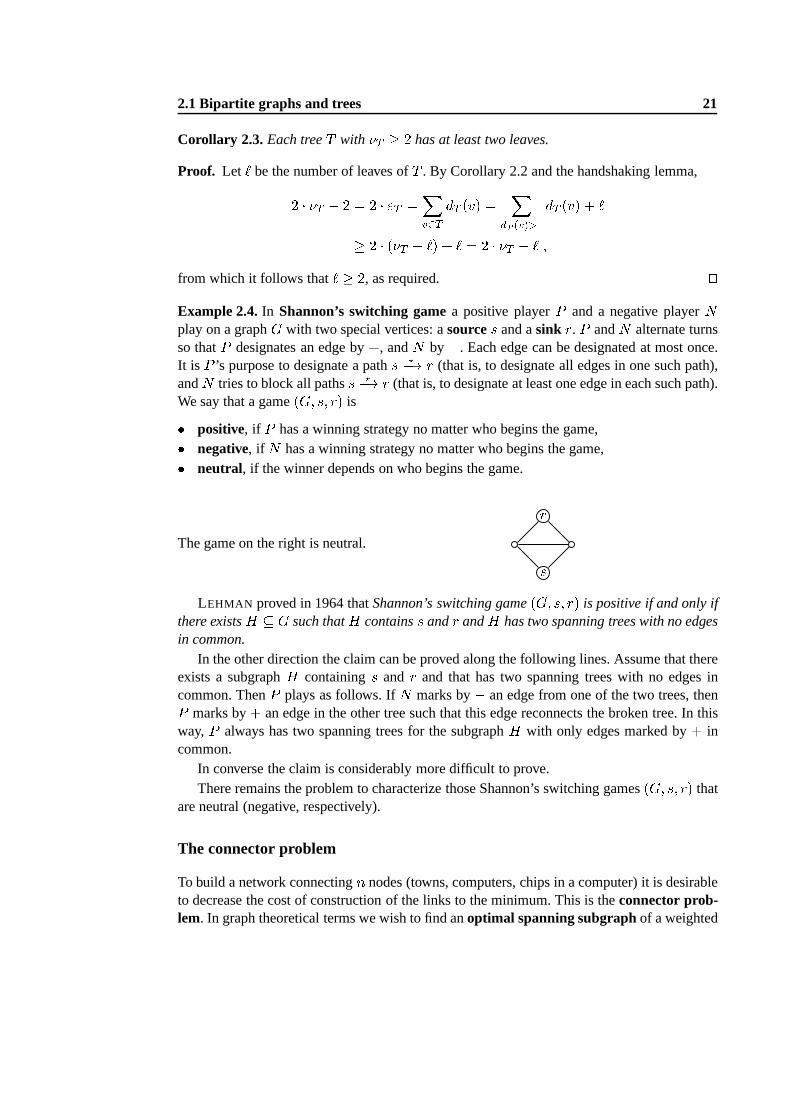
Proof. Let ` be the number of leaves ofT . By Corollary 2.2 and the handshaking lemma,2 � �T � 2 = 2 � "T =Xv2T dT (v) = XdT (v)>1 dT (v) + `� 2 � (�T � `) + ` = 2 � �T � ` ;from which it follows that̀ � 2, as required. utExample 2.4.In Shannon’s switching gamea positive playerP and a negative playerNplay on a graphG with two special vertices: asources and asink r. P andN alternate turnsso thatP designates an edge by+, andN by �. Each edge can be designated at most once.It is P ’s purpose to designate a paths ?�! r (that is, to designate all edges in one such path),andN tries to block all pathss ?�! r (that is, to designate at least one edge in each such path).We say that a game(G; s; r) is� positive, if P has a winning strategy no matter who begins the game,� negative, if N has a winning strategy no matter who begins the game,� neutral, if the winner depends on who begins the game.
The game on the right is neutral. srLEHMAN proved in 1964 thatShannon’s switching game(G; s; r) is positive if and only if
there existsH � G such thatH containss andr andH has two spanning trees with no edgesin common.
In the other direction the claim can be proved along the following lines. Assume that thereexists a subgraphH containings and r and that has two spanning trees with no edges incommon. ThenP plays as follows. IfN marks by� an edge from one of the two trees, thenP marks by+ an edge in the other tree such that this edge reconnects the broken tree. In thisway,P always has two spanning trees for the subgraphH with only edges marked by+ incommon.
In converse the claim is considerably more difficult to prove.There remains the problem to characterize those Shannon’s switching games(G; s; r) that
are neutral (negative, respectively).
The connector problem
To build a network connectingn nodes (towns, computers, chips in a computer) it is desirableto decrease the cost of construction of the links to the minimum. This is theconnector prob-lem. In graph theoretical terms we wish to find anoptimal spanning subgraphof a weighted
2.1 Bipartite graphs and trees 22
graph. Such an optimal subgraph is clearly a spanning tree, for, otherwise a deletion of anynonbridge will reduce the total weight of the subgraph.
Let thenG� be a graphG together with a weight function� : EG ! R+ (positive reals)on the edges. Kruskal’s algorithm (also known as thegreedy algorithm) provides a solutionto the connector problem.Kruskal’s algorithm : For a connected and weighted graphG� of ordern:
(i) Let e1 be an edge of smallest weight, and setE1 = fe1g.(ii) For eachi = 2; 3; : : : ; n� 1 in this order, choose an edgeei =2 Ei�1 of smallest possible
weight such thatei does not produce a cycle when added toG[Ei�1℄, and letEi = Ei�1[feig.The final outcome isT = (VG; En�1).By the construction,T = (VG; En�1) is a spanning tree ofG, because it contains no
cycles, it is connected and hasn � 1 edges. We now show thatT has the minimum totalweight among the spanning trees ofG.
SupposeT1 is any spanning tree ofG. Let ek be the first edge produced by the algorithmthat is not inT1. If we addek to T1, then a cycleC containingek is created. Also,C mustcontain an edgee that is not inT . When we replacee by ek in T1, we still have a spanningtree, sayT2. However, by the construction,�(ek) � �(e), and therefore�(T2) � �(T1). NotethatT2 has more edges in common withT thanT1.
Repeating the above procedure, we can transformT1 to T by replacing edges, one by one,such that the total weight does not increase. We deduce that�(T ) � �(T1).
The outcome of Kruskal’s algorithm need not be unique. Indeed, there may exist severaloptimal spanning trees (with the same weight, of course) fora graph.
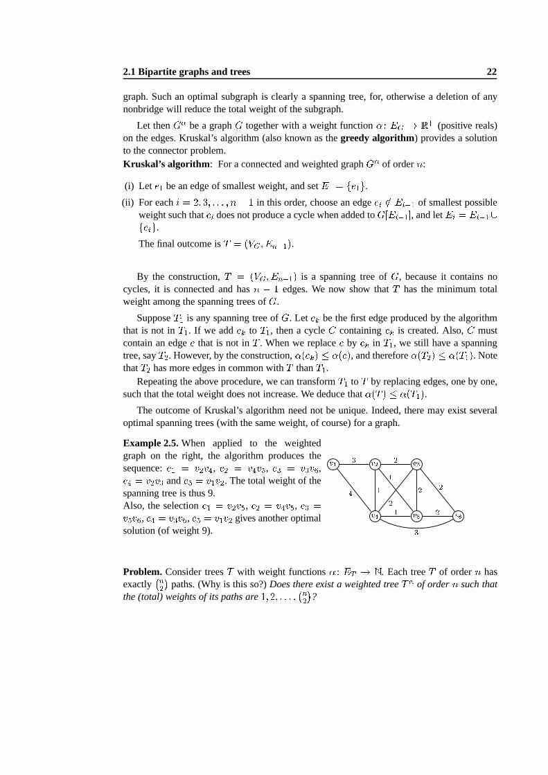
Example 2.5.When applied to the weightedgraph on the right, the algorithm produces thesequence:e1 = v2v4, e2 = v4v5, e3 = v3v6,e4 = v2v3 ande5 = v1v2. The total weight of thespanning tree is thus 9.Also, the selectione1 = v2v5, e2 = v4v5, e3 =v5v6, e4 = v3v6, e5 = v1v2 gives another optimalsolution (of weight 9).
v1 v2 v3v4 v5 v634 21 1 222 1 23
Problem. Consider treesT with weight functions� : ET ! N. Each treeT of ordern hasexactly
�n2� paths. (Why is this so?)Does there exist a weighted treeT� of ordern such thatthe (total) weights of its paths are1; 2; : : : ; �n2�?
2.1 Bipartite graphs and trees 23
In such a weighted treeT� different paths have differ-ent weights, and eachi 2 [1; �n2�℄ is a weight of onepath. Also,� must be injective.
No solutions are known for anyn � 7.2 1 5 84
TAYLOR (1977) proved:if T of ordern exists, then necessarilyn = k2 or n = k2 + 2 forsomek � 1.
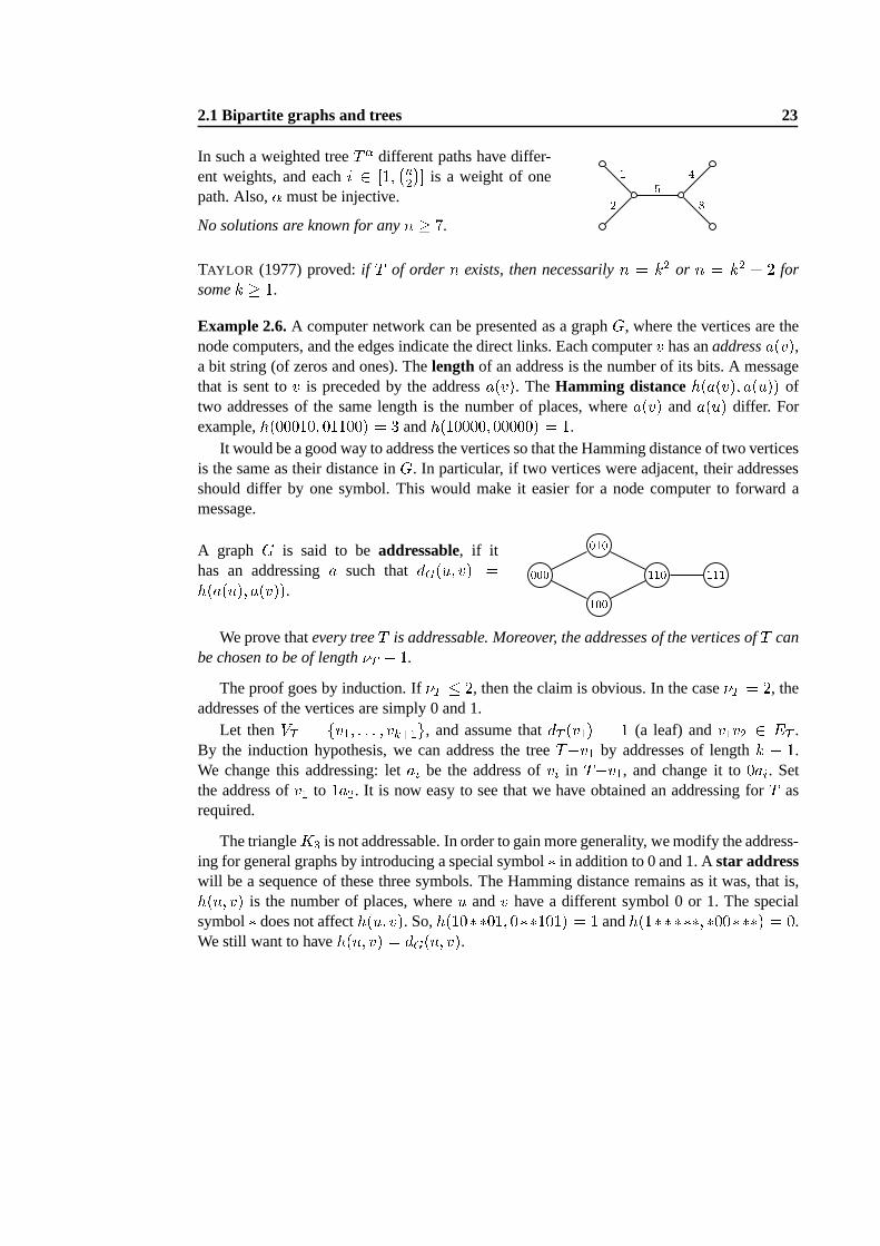
Example 2.6.A computer network can be presented as a graphG, where the vertices are thenode computers, and the edges indicate the direct links. Each computerv has anaddressa(v),a bit string (of zeros and ones). Thelength of an address is the number of its bits. A messagethat is sent tov is preceded by the addressa(v). TheHamming distanceh(a(v); a(u)) oftwo addresses of the same length is the number of places, where a(v) anda(u) differ. Forexample,h(00010; 01100) = 3 andh(10000; 00000) = 1.
It would be a good way to address the vertices so that the Hamming distance of two verticesis the same as their distance inG. In particular, if two vertices were adjacent, their addressesshould differ by one symbol. This would make it easier for a node computer to forward amessage.
A graph G is said to beaddressable, if ithas an addressinga such thatdG(u; v) =h(a(u); a(v)). 000 100010 110 111
We prove thatevery treeT is addressable. Moreover, the addresses of the vertices ofT canbe chosen to be of length�T � 1.
The proof goes by induction. If�T � 2, then the claim is obvious. In the case�T = 2, theaddresses of the vertices are simply 0 and 1.
Let thenVT = fv1; : : : ; vk+1g, and assume thatdT (v1) = 1 (a leaf) andv1v2 2 ET .By the induction hypothesis, we can address the treeT�v1 by addresses of lengthk � 1.We change this addressing: letai be the address ofvi in T�v1, and change it to0ai. Setthe address ofv1 to 1a2. It is now easy to see that we have obtained an addressing forT asrequired.
The triangleK3 is not addressable. In order to gain more generality, we modify the address-ing for general graphs by introducing a special symbol� in addition to 0 and 1. Astar addresswill be a sequence of these three symbols. The Hamming distance remains as it was, that is,h(u; v) is the number of places, whereu andv have a different symbol 0 or 1. The specialsymbol� does not affecth(u; v). So,h(10��01; 0��101) = 1 andh(1�����; �00���) = 0.We still want to haveh(u; v) = dG(u; v).
2.2 Connectivity 24
We star address this graph as follows:a(v1) = 0000, a(v2) = 10 � 0,a(v3) = 1 � 01, a(v4) = � � 11.These addresses have length 4. Can you design astar addressing with addresses of length 3?
v1 v2 v3v4WINKLER proved in 1983 a rather unexpected result:The minimum star address length of
a graphG is at most�G � 1.For the proof of this, see VAN L INT AND WILSON, “A Course in Combinatorics”.
2.2 Connectivity
Spanning trees are often optimal solutions to problems, where cost is the criterion. We mayalso wish to construct graphs that are as simple as possible,but where two vertices are alwaysconnected by at least two independent paths. These problemsoccur especially in differentaspects of fault tolerance and reliability of networks, where one has to make sure that a break-down of one connection does not affect the functionality of the network. Similarly, in a reliablenetwork we require that a break-down of a node (computer) should not result in the inactivityof the whole network.
Separating sets
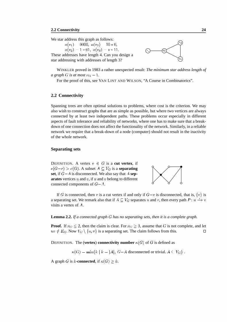
DEFINITION. A vertex v 2 G is a cut vertex, if (G�v) > (G). A subsetA � VG is aseparatingset, if G�A is disconnected. We also say thatA sep-aratesverticesu andv, if u andv belong to differentconnected components ofG�A.
If G is connected, thenv is a cut vertex if and only ifG�v is disconnected, that is,fvg isa separating set. We remark also that ifA � VG separatesu andv, then every pathP : u ?�! vvisits a vertex ofA.
Lemma 2.2.If a connected graphG has no separating sets, then it is a complete graph.
Proof. If �G � 2, then the claim is clear. For�G � 3, assume thatG is not complete, and letuv =2 EG. NowVG n fu; vg is a separating set. The claim follows from this. utDEFINITION. The (vertex) connectivity number �(G) of G is defined as�(G) = minfk j k = jAj; G�A disconnected or trivial; A � VGg :A graphG is k-connected, if �(G) � k.
2.2 Connectivity 25
In other words,� �(G) = 0, if G is disconnected,� �(G) = �G � 1, if G is a complete graph, and� otherwise�(G) equals the minimum size of a separating set ofG.
Clearly, ifG is connected, then it is 1-connected.
DEFINITION. An edge cutF of G consists of edges so thatG�F is disconnected. Let�0(G) = minfk j k = jF j; G�F disconnected; F � EGg :For trivial graphs, let�0(G) = 0. A graphG isk-edge connected, if �0(G) � k. A minimal
edge cutF � EG is abond (F n feg is not an edge cut for anye 2 F ).
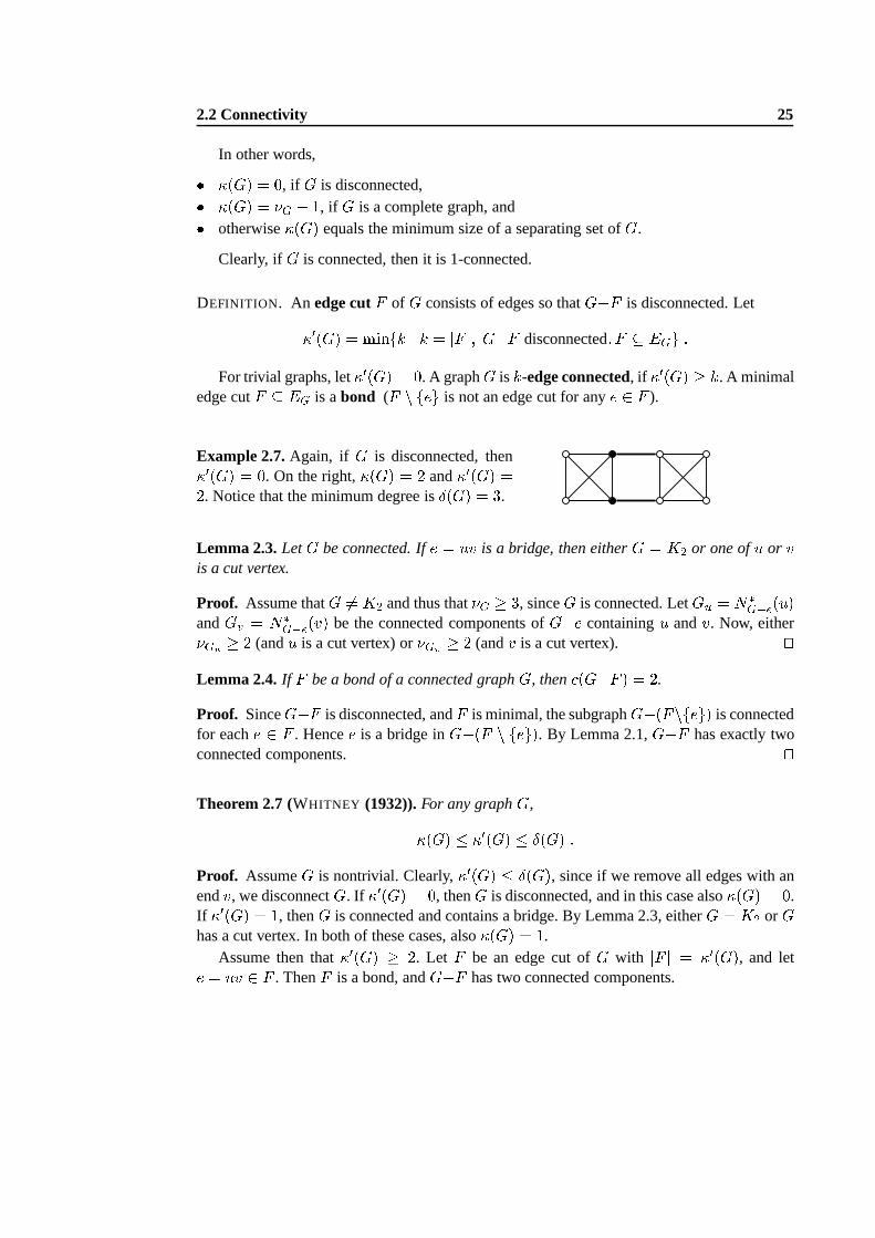
Example 2.7.Again, if G is disconnected, then�0(G) = 0. On the right,�(G) = 2 and�0(G) =2. Notice that the minimum degree isÆ(G) = 3.
Lemma 2.3.LetG be connected. Ife = uv is a bridge, then eitherG = K2 or one ofu or vis a cut vertex.
Proof. Assume thatG 6= K2 and thus that�G � 3, sinceG is connected. LetGu = N�G�e(u)andGv = N�G�e(v) be the connected components ofG�e containingu andv. Now, either�Gu � 2 (andu is a cut vertex) or�Gv � 2 (andv is a cut vertex). utLemma 2.4.If F be a bond of a connected graphG, then (G�F ) = 2.
Proof. SinceG�F is disconnected, andF is minimal, the subgraphG�(Fnfeg) is connectedfor eache 2 F . Hencee is a bridge inG�(F n feg). By Lemma 2.1,G�F has exactly twoconnected components. utTheorem 2.7 (WHITNEY (1932)).For any graphG,�(G) � �0(G) � Æ(G) :Proof. AssumeG is nontrivial. Clearly,�0(G) � Æ(G), since if we remove all edges with anendv, we disconnectG. If �0(G) = 0, thenG is disconnected, and in this case also�(G) = 0.If �0(G) = 1, thenG is connected and contains a bridge. By Lemma 2.3, eitherG = K2 orGhas a cut vertex. In both of these cases, also�(G) = 1.
Assume then that�0(G) � 2. Let F be an edge cut ofG with jF j = �0(G), and lete = uv 2 F . ThenF is a bond, andG�F has two connected components.
2.2 Connectivity 26
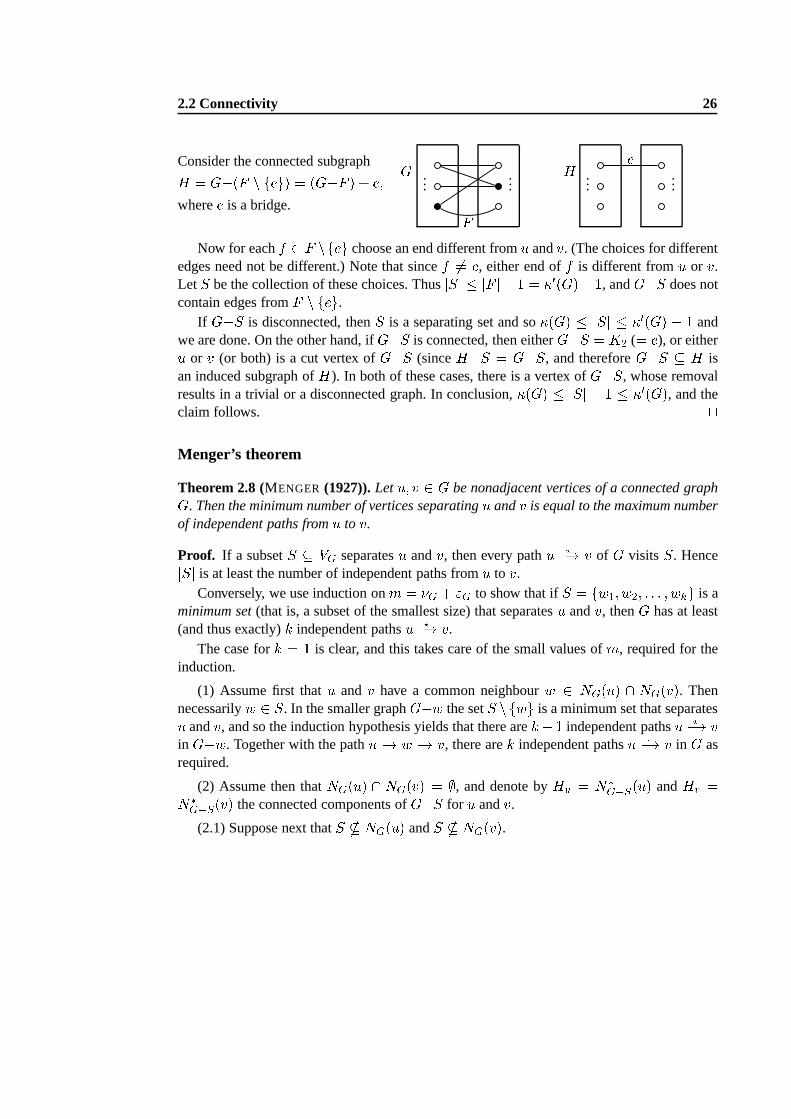
Consider the connected subgraphH = G�(F n feg) = (G�F ) + e;wheree is a bridge.
......
G F ......
H eNow for eachf 2 F nfeg choose an end different fromu andv. (The choices for different
edges need not be different.) Note that sincef 6= e, either end off is different fromu or v.LetS be the collection of these choices. ThusjSj � jF j � 1 = �0(G)� 1, andG�S does notcontain edges fromF n feg.
If G�S is disconnected, thenS is a separating set and so�(G) � jSj � �0(G) � 1 andwe are done. On the other hand, ifG�S is connected, then eitherG�S = K2 (= e), or eitheru or v (or both) is a cut vertex ofG�S (sinceH�S = G�S, and thereforeG�S � H isan induced subgraph ofH). In both of these cases, there is a vertex ofG�S, whose removalresults in a trivial or a disconnected graph. In conclusion,�(G) � jSj + 1 � �0(G), and theclaim follows. utMenger’s theorem
Theorem 2.8 (MENGER (1927)).Letu; v 2 G be nonadjacent vertices of a connected graphG. Then the minimum number of vertices separatingu andv is equal to the maximum numberof independent paths fromu to v.
Proof. If a subsetS � VG separatesu andv, then every pathu ?�! v of G visits S. HencejSj is at least the number of independent paths fromu to v.Conversely, we use induction onm = �G + "G to show that ifS = fw1; w2; : : : ; wkg is a
minimum set(that is, a subset of the smallest size) that separatesu andv, thenG has at least(and thus exactly)k independent pathsu ?�! v.
The case fork = 1 is clear, and this takes care of the small values ofm, required for theinduction.
(1) Assume first thatu and v have a common neighbourw 2 NG(u) \ NG(v). Thennecessarilyw 2 S. In the smaller graphG�w the setS n fwg is a minimum set that separatesu andv, and so the induction hypothesis yields that there arek� 1 independent pathsu ?�! vin G�w. Together with the pathu �! w �! v, there arek independent pathsu ?�! v in G asrequired.
(2) Assume then thatNG(u) \ NG(v) = ;, and denote byHu = N�G�S(u) andHv =N�G�S(v) the connected components ofG�S for u andv.
(2.1) Suppose next thatS * NG(u) andS * NG(v).
2.2 Connectivity 27
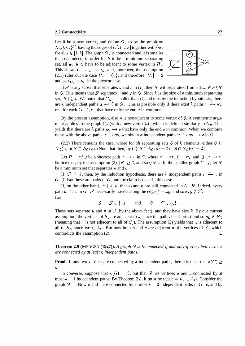
Let bv be a new vertex, and defineGu to be the graph onHu[S[fbvg having the edges ofG[Hu[S℄ together withbvwifor all i 2 [1; k℄. The graphGu is connected and it is smallerthanG. Indeed, in order forS to be a minimum separatingset, allwi 2 S have to be adjacent to some vertex inHv.This shows that"Gu � "G, and, moreover, the assumption(2.1) rules out the caseHv = fvg, and thereforejHvj � 2and so�Gu < �G in the present case.
u bvw1w2: : :wkIf S0 is any subset that separatesu andbv inGu, thenS0 will separateu from allwi 2 S nS0
in G. This means thatS0 separatesu andv in G. Sincek is the size of a minimum separatingset,jS0j � k. We noted thatGu is smaller thanG, and thus by the induction hypothesis, therearek independent pathsu ?�! bv in Gu. This is possible only if there existk pathsu ?�! wi,one for eachi 2 [1; k℄, that have only the endu in common.
By the present assumption, alsou is nonadjacent to some vertex ofS. A symmetric argu-ment applies to the graphGv (with a new vertexbu) , which is defined similarly toGu. Thisyields that there arek pathswi ?�! v that have only the endv in common. When we combinethese with the above pathsu ?�! wi, we obtaink independent pathsu ?�! wi ?�! v in G.
(2.2) There remains the case, where forall separating setsS of k elements, eitherS �NG(u) or S � NG(v). (Note that then, by (2),S \NG(v) = ; or S \NG(u) = ;.)Let P = efQ be a shortest pathu ?�! v in G, wheree = ux, f = xy, andQ : y ?�! v.
Notice that, by the assumption (2),jP j � 3, and soy 6= v. In the smaller graphG�f , let S0be a minimum set that separatesu andv.
If jS0j � k, then, by the induction hypothesis, there arek independent pathsu ?�! v inG�f . But these are paths ofG, and the claim is clear in this case.If, on the other hand,jS0j < k, thenu andv are still connected inG�S0. Indeed, every
pathu ?�! v in G�S0 necessarily travels along the edgef = xy, and sox; y =2 S0.Let Sx = S0 [ fxg and Sy = S0 [ fyg :These sets separateu andv in G (by the above fact), and they have sizek. By our currentassumption, the vertices ofSy are adjacent tov, since the pathP is shortest and souy =2 EG(meaning thatu is not adjacent to all ofSy). The assumption (2) yields thatu is adjacent toall of Sx, sinceux 2 EG. But now bothu andv are adjacent to the vertices ofS0, whichcontradicts the assumption (2). utTheorem 2.9 (MENGER (1927)).A graphG is k-connected if and only if every two verticesare connected by at leastk independent paths.
Proof. If any two vertices are connected byk independent paths, then it is clear that�(G) �k.In converse, suppose that�(G) = k, but thatG has verticesu and v connected by at
mostk � 1 independent paths. By Theorem 2.8, it must be thate = uv 2 EG. Consider thegraphG�e. Now u andv are connected by at mostk � 2 independent paths inG�e, and by
2.2 Connectivity 28
Theorem 2.8,u andv can be separated inG�e by a setS with jSj = k � 2. Since�G > k(because�(G) = k), there exists aw 2 G that is not inS [ fu; vg. The vertexw is separatedin G�e by S from u or from v; otherwise there would be a pathu ?�! v in (G�e)�S. Say,this vertex isu. The setS [ fvg hask � 1 elements, and it separatesu from w in G, whichcontradicts the assumption that�(G) = k. This proves the claim. ut
We state without a proof the corresponding separation property for edge connectivity.
DEFINITION. Let G be a graph. Auv-disconnecting setis a setF � EG such that everypathu ?�! v contains an edge fromF .
Theorem 2.10.Let u; v 2 G with u 6= v in a graphG. Then the maximum number of edge-disjoint pathsu ?�! v equals the minimum numberk of edges in auv-disconnecting set.
Corollary 2.4. A graphG is k-edge connected if and only if every two vertices are connectedby at leastk edge disjoint paths.
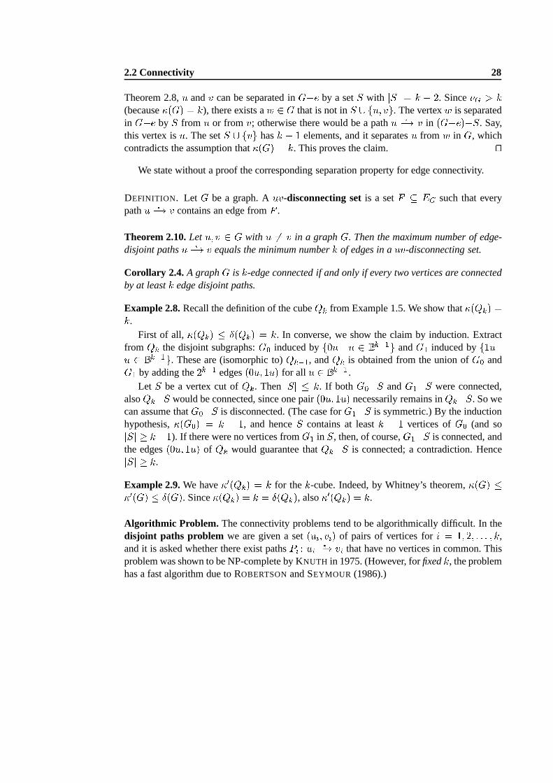
Example 2.8.Recall the definition of the cubeQk from Example 1.5. We show that�(Qk) =k.First of all, �(Qk) � Æ(Qk) = k. In converse, we show the claim by induction. Extract
from Qk the disjoint subgraphs:G0 induced byf0u j u 2 B k�1g andG1 induced byf1u ju 2 B k�1g. These are (isomorphic to)Qk�1, andQk is obtained from the union ofG0 andG1 by adding the2k�1 edges(0u; 1u) for all u 2 B k�1 .Let S be a vertex cut ofQk. Then jSj � k. If both G0�S andG1�S were connected,
alsoQk�S would be connected, since one pair(0u; 1u) necessarily remains inQk�S. So wecan assume thatG0�S is disconnected. (The case forG1�S is symmetric.) By the inductionhypothesis,�(G0) = k � 1, and henceS contains at leastk � 1 vertices ofG0 (and sojSj � k�1). If there were no vertices fromG1 in S, then, of course,G1�S is connected, andthe edges(0u; 1u) of Qk would guarantee thatQk�S is connected; a contradiction. HencejSj � k.
Example 2.9.We have�0(Qk) = k for thek-cube. Indeed, by Whitney’s theorem,�(G) ��0(G) � Æ(G). Since�(Qk) = k = Æ(Qk), also�0(Qk) = k.
Algorithmic Problem. The connectivity problems tend to be algorithmically difficult. In thedisjoint paths problem we are given a set(ui; vi) of pairs of vertices fori = 1; 2; : : : ; k,and it is asked whether there exist pathsPi : ui ?�! vi that have no vertices in common. Thisproblem was shown to be NP-complete by KNUTH in 1975. (However, forfixedk, the problemhas a fast algorithm due to ROBERTSONand SEYMOUR (1986).)
2.2 Connectivity 29
Dirac’s fans
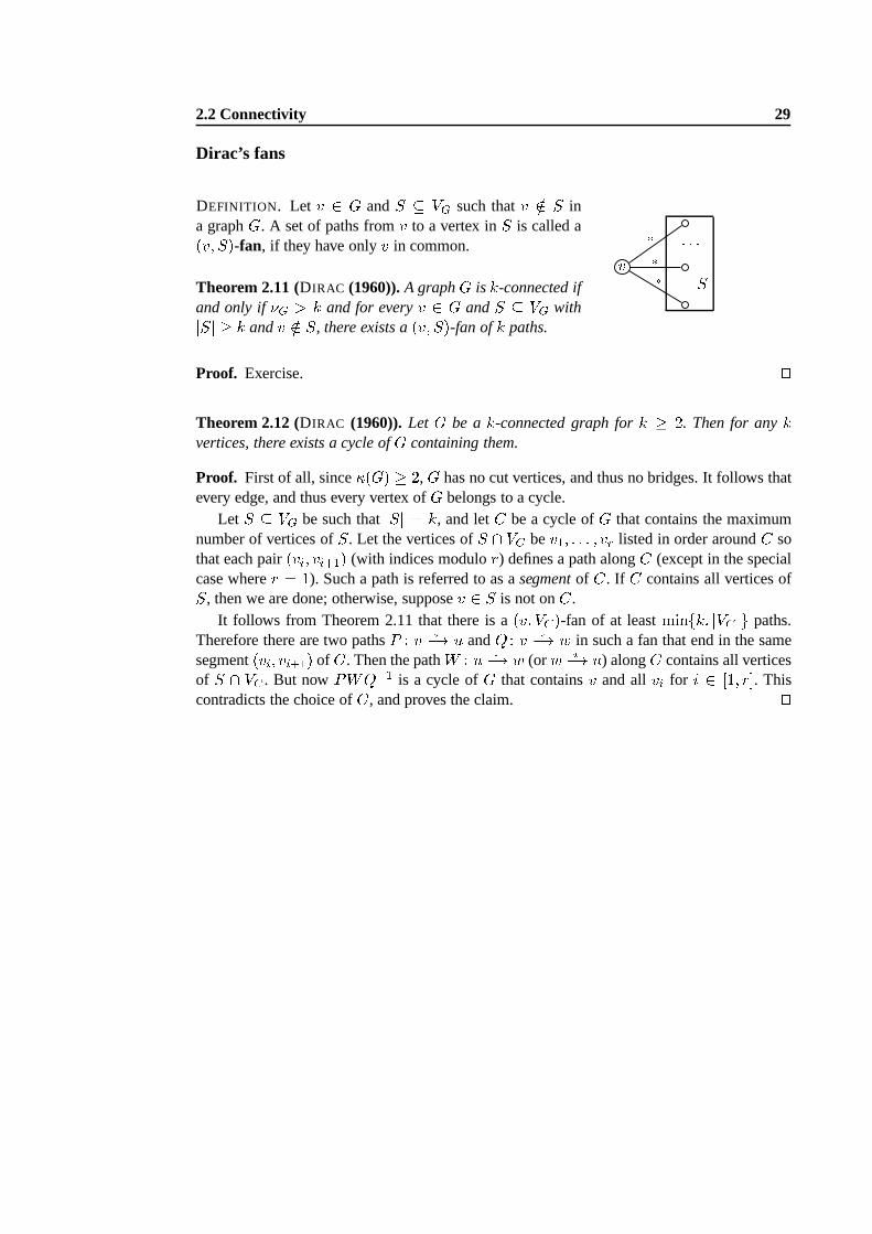
DEFINITION. Let v 2 G andS � VG such thatv =2 S ina graphG. A set of paths fromv to a vertex inS is called a(v; S)-fan, if they have onlyv in common.
Theorem 2.11 (DIRAC (1960)).A graphG is k-connected ifand only if�G > k and for everyv 2 G andS � VG withjSj � k andv =2 S, there exists a(v; S)-fan ofk paths.
v : : :��� SProof. Exercise. utTheorem 2.12 (DIRAC (1960)).Let G be ak-connected graph fork � 2. Then for anykvertices, there exists a cycle ofG containing them.
Proof. First of all, since�(G) � 2,G has no cut vertices, and thus no bridges. It follows thatevery edge, and thus every vertex ofG belongs to a cycle.
Let S � VG be such thatjSj = k, and letC be a cycle ofG that contains the maximumnumber of vertices ofS. Let the vertices ofS \ VC bev1; : : : ; vr listed in order aroundC sothat each pair(vi; vi+1) (with indices modulor) defines a path alongC (except in the specialcase wherer = 1). Such a path is referred to as asegmentof C. If C contains all vertices ofS, then we are done; otherwise, supposev 2 S is not onC.
It follows from Theorem 2.11 that there is a(v; VC)-fan of at leastminfk; jVC jg paths.Therefore there are two pathsP : v ?�! u andQ : v ?�! w in such a fan that end in the samesegment(vi; vi+1) of C. Then the pathW : u ?�! w (orw ?�! u) alongC contains all verticesof S \ VC . But nowPWQ�1 is a cycle ofG that containsv and allvi for i 2 [1; r℄. Thiscontradicts the choice ofC, and proves the claim. ut
3
Tours and Matchings
3.1 Eulerian graphs
The first proper problem in graph theory was the Königsberg bridge problem. In general, thisproblem concerns about travels around a graph such that one tries to avoid using the sameedge twice. In practice these eulerian problems occur, for instance, in optimizing distributionnetworks – such as delivering mail, where in order to save time each street should be travelledonly once. The same problem occurs in mechanical graph plotting, where one avoids liftingthe pen off the paper while drawing the lines.
Euler tours
DEFINITION. A walk W = e1e2 : : : en is a trail , if ei 6= ej for all i 6= j. An Euler trail ofa graphG is a trail that visits every edge once. A connected graphG is eulerian, if it has aclosed trail containing every edge ofG. Such a trail is called anEuler tour .
Notice that ifW = e1e2 : : : en is an Euler tour (and soEG = fe1; e2; : : : ; eng), alsoeiei+1 : : : ene1 : : : ei�1 is an Euler tour for alli 2 [1; n℄. A complete proof of the followingEuler’s Theorem was first given by HIERHOLZER in 1873.
Theorem 3.1 (EULER (1736),HIERHOLZER (1873)).A connected graphG is eulerian if andonly if every vertex has an even degree.
Proof. ()) SupposeW : u ?�! u is an Euler tour. Letv (6= u) be a vertex that occursk timesinW . Every time an edge arrives atv, another edge departs fromv, and thereforedG(v) = 2k.Also, dG(u) is even, sinceW starts and ends atu.
(() AssumeG is a nontrivial connected graph such thatdG(v) is even for allv 2 G. LetW = e1e2 : : : en : v0 ?�! vn with ei = vi�1vibe a longest trail inG. It follows that all e = vnw 2 EG are among the edges ofW , for,otherwise,W could be prolonged toWe. In particular,v0 = vn, that is,W is a closed trail.(Indeed, if it werevn 6= v0 andvn occursk times inW , thendG(vn) = 2(k� 1) + 1 and thatwould be odd.)
If W is not an Euler tour, then, sinceG is connected, there exists an edgef = viu 2 EGfor somei, which is not inW . However, nowei+1 : : : ene1 : : : eifis a trail inG, and it is longer thanW . This contradiction to the choice ofW proves the claim.ut
3.1 Eulerian graphs 31
Example 3.1.Thek-cubeQk is eulerian for even integersk, becauseQk is k-regular.
Theorem 3.2.A connected graph has an Euler trail if and only if it has at most two verticesof odd degree.
Proof. If G has an Euler trailu ?�! v, then, as in the proof of Theorem 3.1, each vertexw =2 fu; vg has an even degree.Assume then thatG is connected and has at most two vertices of odd degree. IfG has no
vertices of odd degree then, by Theorem 3.1,G has an Euler trail. Otherwise, by the hand-shaking lemma, every graph has an even number of vertices with odd degree, and thereforeG has exactly two such vertices, sayu andv. LetH be a graph obtained fromG by adding avertexw, and the edgesuw andvw. InH every vertex has an even degree, and hence it has anEuler tour, sayu ?�! v �! w �! u. Here the beginning partu ?�! v is an Euler trail ofG. utThe Chinese postman
The following problem is due to GUAN MEIGU (1962). Consider a village, where a postmanwishes to plan his route to save the legs, but still every street has to be walked through. Thisproblem is akin to Euler’s problem and to the shortest path problem.
LetG be a graph with a weight function� : EG ! R+ . TheChinese postman problemis to find a minimum weighted tour inG (starting from a given vertex, the post office).
If G is eulerian, then any Euler tour will do as a solution, because such a tourtraverseseach edge exactly once and this is the best one can do. In this case the weight of the optimaltour is the total weight of the graphG, and there is a good algorithm for finding such a tour:
Fleury’s algorithm :� Let v0 2 G be a chosen vertex, and letW0 be the trivial path onv0.� Repeat the following procedure fori = 1; 2; : : : as long as possible: suppose a trailWi =e1e2 : : : ei has been constructed, whereej = vj�1vj.Choose an edgeei+1 (6= ej for j 2 [1; i℄) so that
(i) ei+1 has an endvi, and(ii) ei+1 is not a bridge ofGi = G�fe1; : : : ; eig, unless there is no alternative.
Notice that, as is natural, the weights�(e) play no role in the eulerian case.
Theorem 3.3.If G is eulerian, then any trail ofG constructed by Fleury’s algorithm is anEuler tour ofG.
Proof. Exercise. ut
3.2 Hamiltonian graphs 32
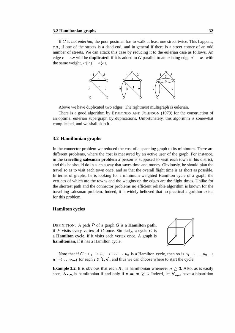
If G is not eulerian, the poor postman has to walk at least one street twice. This happens,e.g., if one of the streets is a dead end, and in general if there is astreet corner of an oddnumber of streets. We can attack this case by reducing it to the eulerian case as follows. Anedgee = uv will be duplicated, if it is added toG parallel to an existing edgee0 = uv withthe same weight,�(e0) = �(e).
2 4 13 32 2 24 13 32 2 24 133 32Above we have duplicated two edges. The rightmost multigraph is eulerian.There is a good algorithm by EDMONDS AND JOHNSON (1973) for the construction of
an optimal eulerian supergraph by duplications. Unfortunately, this algorithm is somewhatcomplicated, and we shall skip it.
3.2 Hamiltonian graphs
In the connector problem we reduced the cost of a spanning graph to its minimum. There aredifferent problems, where the cost is measured by an active user of the graph. For instance,in the travelling salesman problema person is supposed to visit each town in his district,and this he should do in such a way that saves time and money. Obviously, he should plan thetravel so as to visit each town once, and so that the overall flight time is as short as possible.In terms of graphs, he is looking for a minimum weighted Hamilton cycle of a graph, thevertices of which are the towns and the weights on the edges are the flight times. Unlike forthe shortest path and the connector problems no efficient reliable algorithm is known for thetravelling salesman problem. Indeed, it is widely believedthat no practical algorithm existsfor this problem.
Hamilton cycles
DEFINITION. A pathP of a graphG is a Hamilton path ,if P visits every vertex ofG once. Similarly, a cycleC isa Hamilton cycle, if it visits each vertex once. A graph ishamiltonian, if it has a Hamilton cycle.
Note that ifC : u1 ! u2 ! � � � ! un is a Hamilton cycle, then so isui ! : : : un !u1 ! : : : ui�1 for eachi 2 [1; n℄, and thus we can choose where to start the cycle.
Example 3.2.It is obvious that eachKn is hamiltonian whenevern � 3. Also, as is easilyseen,Kn;m is hamiltonian if and only ifn = m � 2. Indeed, letKn;m have a bipartition
3.2 Hamiltonian graphs 33(X;Y ), wherejXj = n andjY j = m. Now, each cycle inKn;m has even length as the graphis bipartite, and thus the cycle visits the setsX;Y equally many times, sinceX andY arestable subsets. But then necessarilyjXj = jY j.
Unlike for eulerian graphs (Theorem 3.1) no good characterization is known for hamilto-nian graphs. Indeed, the problem to determine ifG is hamiltonian is NP-complete. There are,however, some interesting general conditions.
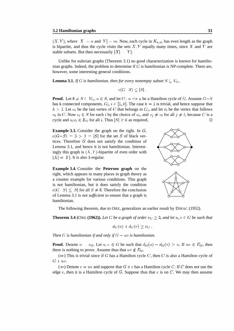
Lemma 3.1.If G is hamiltonian, then for every nonempty subsetS � VG, (G�S) � jSj :Proof. Let ; 6= S � VG, u 2 S, and letC : u ?�! u be a Hamilton cycle ofG. AssumeG�Shas k connected components,Gi, i 2 [1; k℄. The casek = 1 is trivial, and hence suppose thatk > 1. Let ui be the last vertex ofC that belongs toGi, and letvi be the vertex that followsui in C. Now vi 2 S for eachi by the choice ofui, andvj 6= vt for all j 6= t, becauseC is acycle anduivi 2 EG for all i. ThusjSj � k as required. utExample 3.3.Consider the graph on the right. InG, (G�S) = 3 > 2 = jSj for the setS of black ver-tices. ThereforeG does not satisfy the condition ofLemma 3.1, and hence it is not hamiltonian. Interest-ingly this graph is(X;Y )-bipartite of even order withjXj = jY j. It is also3-regular.
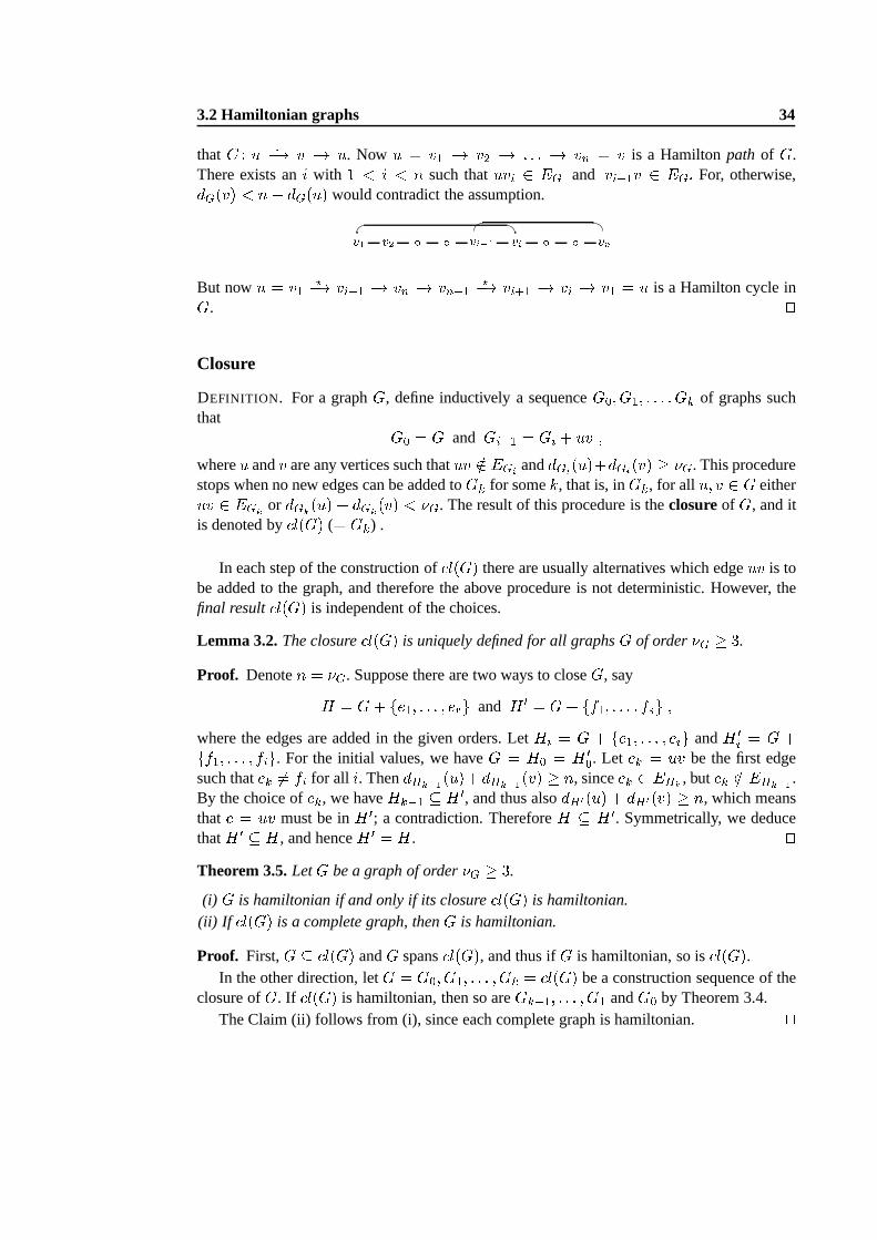
Example 3.4.Consider thePetersen graph on theright, which appears in many places in graph theory asa counter example for various conditions. This graphis not hamiltonian, but it does satisfy the condition (G�S) � jSj for all S 6= ;. Therefore the conclusionof Lemma 3.1 isnot sufficientto ensure that a graph ishamiltonian.
The following theorem, due to ORE, generalizes an earlier result by DIRAC (1952).
Theorem 3.4 (ORE (1962)).LetG be a graph of order�G � 3, and letu; v 2 G be such thatdG(u) + dG(v) � �G :ThenG is hamiltonian if and only ifG+ uv is hamiltonian.
Proof. Denoten = �G. Let u; v 2 G be such thatdG(u) + dG(v) � n. If uv 2 EG, thenthere is nothing to prove. Assume thus thatuv =2 EG.
()) This is trivial since ifG has a Hamilton cycleC, thenC is also a Hamilton cycle ofG+ uv.(() Denotee = uv and suppose thatG+ e has a Hamilton cycleC. If C does not use the
edgee, then it is a Hamilton cycle ofG. Suppose thus thate is onC. We may then assume
3.2 Hamiltonian graphs 34
thatC : u ?�! v �! u. Now u = v1 �! v2 �! : : : �! vn = v is a Hamiltonpath of G.There exists ani with 1 < i < n such thatuvi 2 EG and vi�1v 2 EG: For, otherwise,dG(v) < n� dG(u) would contradict the assumption.v1 v2 Æ Æ vi�1 vi Æ Æ vnBut nowu = v1 ?�! vi�1 �! vn �! vn�1 ?�! vi+1 �! vi �! v1 = u is a Hamilton cycle inG. utClosure
DEFINITION. For a graphG, define inductively a sequenceG0; G1; : : : ; Gk of graphs suchthat G0 = G and Gi+1 = Gi + uv ;whereu andv are any vertices such thatuv =2 EGi anddGi(u)+dGi(v) � �G. This procedurestops when no new edges can be added toGk for somek, that is, inGk, for all u; v 2 G eitheruv 2 EGk or dGk(u) + dGk(v) < �G. The result of this procedure is theclosureof G, and itis denoted by l(G) (= Gk) .
In each step of the construction of l(G) there are usually alternatives which edgeuv is tobe added to the graph, and therefore the above procedure is not deterministic. However, thefinal result l(G) is independent of the choices.
Lemma 3.2.The closure l(G) is uniquely defined for all graphsG of order�G � 3.
Proof. Denoten = �G. Suppose there are two ways to closeG, sayH = G+ fe1; : : : ; erg and H 0 = G+ ff1; : : : ; fsg ;where the edges are added in the given orders. LetHi = G + fe1; : : : ; eig andH 0i = G +ff1; : : : ; fig. For the initial values, we haveG = H0 = H 00. Let ek = uv be the first edgesuch thatek 6= fi for all i. ThendHk�1(u)+dHk�1(v) � n, sinceek 2 EHk , butek =2 EHk�1 .By the choice ofek, we haveHk�1 � H 0, and thus alsodH0(u) + dH0(v) � n, which meansthat e = uv must be inH 0; a contradiction. ThereforeH � H 0. Symmetrically, we deducethatH 0 � H, and henceH 0 = H. utTheorem 3.5.LetG be a graph of order�G � 3.
(i) G is hamiltonian if and only if its closure l(G) is hamiltonian.(ii) If l(G) is a complete graph, thenG is hamiltonian.
Proof. First,G � l(G) andG spans l(G), and thus ifG is hamiltonian, so is l(G).In the other direction, letG = G0; G1; : : : ; Gk = l(G) be a construction sequence of the
closure ofG. If l(G) is hamiltonian, then so areGk�1; : : : ; G1 andG0 by Theorem 3.4.The Claim (ii) follows from (i), since each complete graph ishamiltonian. ut
3.2 Hamiltonian graphs 35
Theorem 3.6.LetG be a graph of order�G � 3. Suppose that for all nonadjacent verticesuandv, dG(u) + dG(v) � �G. ThenG is hamiltonian. In particular, ifÆ(G) � 12�G, thenG ishamiltonian.
Proof. SincedG(u)+dG(v) � �G for all nonadjacent vertices, we have l(G) = Kn for n =�G, and thusG is hamiltonian. The second claim is immediate, since nowdG(u)+dG(v) � �Gfor all u; v 2 G whether adjacent or not. utChvátal’s condition
The hamiltonian problem of graphs has attracted much attention, at least partly because theproblem has practical significance. (Indeed, the first example where DNA computing wasapplied, was the hamiltonian problem.)
There are some general improvements of the previous resultsof this chapter, and quitemany improvements in various special cases, where the graphs are somehow restricted. Webecome satisfied by two general results.
Theorem 3.7 (CHVÁTAL (1972)).LetG be a graph withVG = fv1; v2; : : : ; vng, for n � 3,ordered so thatd1 � d2 � � � � � dn, for di = dG(vi). If for everyi < n=2,di � i =) dn�i � n� i ; (3.1)
thenG is hamiltonian.
Proof. First of all, we may suppose thatG is closed,G = l(G), becauseG is hamiltonian ifand only if l(G) is hamiltonian, and adding edges toG does not decrease any of its degrees,that is, ifG satisfies (3.1), so doesG+ e for everye. We show that, in this case,G = Kn, andthusG is hamiltonian.
Assume on the contrary thatG 6= Kn, and letuv =2 EG with dG(u) � dG(v) be such thatdG(u)+dG(v) is as large as possible. BecauseG is closed, we must havedG(u)+dG(v) < n,and thereforedG(u) = i < n=2. LetA = fw j vw =2 EG; w 6= vg. By our choice,dG(w) � ifor all w 2 A, and, moreover,jAj = (n� 1)� dG(v) � dG(u) = i :Consequently, there are at leasti verticesw with dG(w) � i, and sodi � dG(u) = i.
Similarly, for each vertex fromB = fw j uw =2 EG; w 6= ug, dG(w) � dG(v) <n� dG(u) = n� i, and jBj = (n� 1)� dG(u) = (n� 1)� i :Also dG(u) < n � i, and thus there are at leastn � i verticesw with dG(w) < n � i.Consequently,dn�i < n � i. This contradicts the obtained bounddi � i and the condition(3.1). ut
Note that the condition (3.1) is easily checkable for any given graph.
3.3 Matchings 36
3.3 Matchings
In matching problems we are given an availability relation between the elements of a set. Theproblem is then to find a pairing of the elements so that each element is paired (matched)uniquely with an available companion.
A special case of the matching problem is themarriage problem, which is stated as fol-lows. Given a setX of boys and a setY of girls, under what condition can each boy marry agirl who cares to marry him? This problem has many variations. One of them is thejob as-signment problem, where we are givenn applicants andm jobs, and we should assign eachapplicant to a job he is qualified. The problem is that an applicant may be qualified for severaljobs, and a job may be suited for several applicants.
Maximum matchings
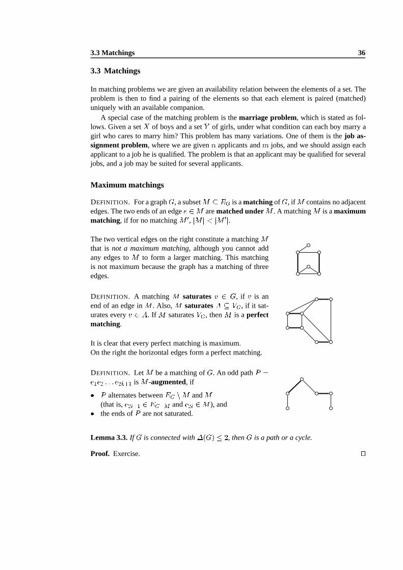
DEFINITION. For a graphG, a subsetM � EG is amatching ofG, if M contains no adjacentedges. The two ends of an edgee 2M arematched underM . A matchingM is amaximummatching, if for no matchingM 0, jM j < jM 0j.The two vertical edges on the right constitute a matchingMthat isnot a maximum matching, although you cannot addany edges toM to form a larger matching. This matchingis not maximum because the graph has a matching of threeedges.
DEFINITION. A matchingM saturates v 2 G, if v is anend of an edge inM . Also,M saturatesA � VG, if it sat-urates everyv 2 A. If M saturatesVG, thenM is aperfectmatching.
It is clear that every perfect matching is maximum.On the right the horizontal edges form a perfect matching.
DEFINITION. LetM be a matching ofG. An odd pathP =e1e2 : : : e2k+1 isM -augmented, if� P alternates betweenEG nM andM(that is,e2i+1 2 EG�M ande2i 2M ), and� the ends ofP are not saturated.
Lemma 3.3.If G is connected with�(G) � 2, thenG is a path or a cycle.
Proof. Exercise. ut
3.3 Matchings 37
We start with a result that states a necessary and sufficient condition for a matching tobe maximal. One can use the first part of the proof to constructa maximum matching in aniterative manner starting from any matchingM and from anyM -augmented path.
Theorem 3.8 (BERGE (1957)).A matchingM of G is a maximum matching if and only ifthere are noM -augmented paths inG.
Proof. ()) Let a matchingM have anM -augmented pathP = e1e2 : : : e2k+1 in G. Heree2; e4; : : : ; e2k 2M , e1; e3; : : : ; e2k+1 =2M . DefineN � EG byN = (M n fe2i j i 2 [1; k℄g) [ fe2i+1 j i 2 [0; k℄g :Now,N is a matching ofG, andjN j = jM j+ 1. ThereforeM is not a maximum matching.
(() AssumeN is a maximum matching, butM is not. HencejN j > jM j. Consider thesubgraphH = G[M4N ℄ for the symmetric differenceM4N . We havedH(v) � 2 for eachv 2 H, becausev is an end of at most one edge inM andN . By Lemma 3.3, each connectedcomponentA of H is either a path or a cycle.
Since nov 2 A can be an end of two edges fromN or fromM , each connected component(path or a cycle)A alternates betweenN andM . Now, sincejN j > jM j, there is a connectedcomponentA of H, which has more edges fromN than fromM . ThisA cannot be a cycle,because an alternating cycle is even, and it thus contains equally many edges fromN andM . HenceA : u ?�! v is a path, which starts and ends with an edge fromN . BecauseA is aconnected component ofH, the endsu andv are not saturated byM , and, consequently,A isanM -augmented path. This proves the theorem. utExample 3.5.Consider thek-cubeQk for k � 1. Each maximum matching ofQk has2k�1edges. Indeed, the matchingM = f(0u; 1u) j u 2 B k�1g, has2k�1 edges, and it is clearlyperfect.
Hall’s theorem
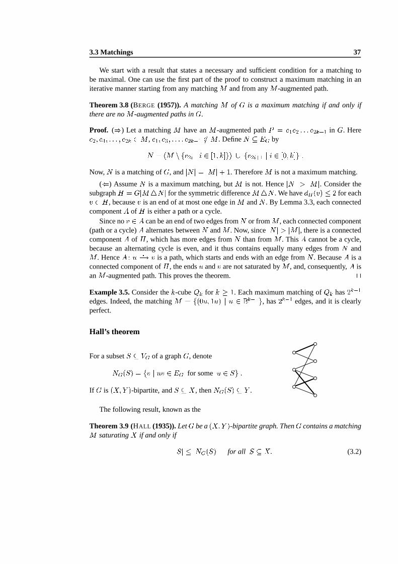
For a subsetS � VG of a graphG, denoteNG(S) = fv j uv 2 EG for some u 2 Sg :If G is (X;Y )-bipartite, andS � X, thenNG(S) � Y .
The following result, known as the
Theorem 3.9 (HALL (1935)).LetG be a(X;Y )-bipartite graph. ThenG contains a matchingM saturatingX if and only ifjSj � jNG(S)j for all S � X: (3.2)
3.3 Matchings 38
Proof. ()) LetM be a matching that saturatesX. If jSj > jNG(S)j for someS � X, thennot allx 2 S can be matched with differenty 2 NG(S).
(() LetG satisfy Hall’s condition (3.2). We prove the claim by induction on jXj.If jXj = 1, then the claim is clear. Let thenjXj � 2, and assume (3.2) implies the existence
of a matching that saturates every proper subset ofX.If jNG(S)j � jSj+ 1 for every nonemptyS � X with S 6= X, then choose an edgeuv 2EG with u 2 X, and consider the induced subgraphH = G�fu; vg. For allS � X n fug,jNH(S)j � jNG(S)j � 1 � jSj ;
and hence, by the induction hypothesis,H contains a matchingM saturatingX n fug. NowM [ fuvg is a matching saturatingX in G, as was required.Suppose then that there exists a nonempty subsetR � X with R 6= X such thatjNG(R)j = jRj. The induced subgraphH1 = G[R [ NG(R)℄ satisfies (3.2) (sinceG does),
and hence, by the induction hypothesis,H1 contains a matchingM1 that saturatesR (with theother ends inNG(R)).
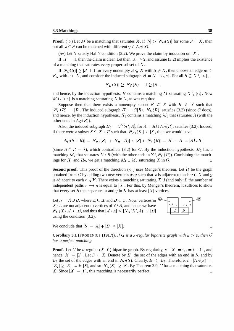
Also, the induced subgraphH2 = G[VG nA℄, forA = R[NG(R), satisfies (3.2). Indeed,if there were a subsetS � X nR such thatjNH2(S)j < jSj, then we would havejNG(S [R)j = jNH2(S)j + jNH1(R)j < jSj+ jNG(R)j = jSj+ jRj = jS [Rj(sinceS \ R = ;), which contradicts (3.2) forG. By the induction hypothesis,H2 has amatchingM2 that saturatesX nR (with the other ends inY nNG(R)). Combining the match-ings forH1 andH2, we get a matchingM1 [M2 saturatingX in G. utSecond proof. This proof of the direction(() uses Menger’s theorem. LetH be the graphobtained fromG by adding two new verticesx; y such thatx is adjacent to eachv 2 X andyis adjacent to eachv 2 Y . There exists a matching saturatingX if (and only if) the number ofindependent pathsx ?�! y is equal tojXj. For this, by Menger’s theorem, it suffices to showthat every setS that separatesx andy in H has at leastjXj vertices.
LetS = A[B, whereA � X andB � Y . Now, vertices inXnA are not adjacent to vertices ofY nB, and hence we haveNG(XnA) � B, and thus thatjXnAj � jNG(XnA)j � jBjusing the condition (3.2).
x yX n A Y n BA BWe conclude thatjSj = jAj+ jBj � jXj. utCorollary 3.1 (FROBENIUS (1917)).If G is a k-regular bipartite graph withk > 0, thenGhas a perfect matching.
Proof. LetG bek-regular(X;Y )-bipartite graph. By regularity,k � jXj = "G = k � jY j, andhencejXj = jY j. Let S � X. Denote byE1 the set of the edges with an end inS, and byE2 the set of the edges with an end inNG(S). Clearly,E1 � E2. Therefore,k � jNG(S)j =jE2j � jE1j = k �jSj, and sojNG(S)j � jSj. By Theorem 3.9,G has a matching that saturatesX. SincejXj = jY j, this matching is necessarily perfect. ut
3.3 Matchings 39
Applications of Hall’s theorem
DEFINITION. Let S = fS1; S2; : : : ; Smg be a family of finite nonempty subsets of a setS.(Si need not be distinct.) Atransversal (or a system of distinct representatives) of S is asubsetT � S of m distinct elements one from eachSi.
As an example, letS = [1; 6℄, and letS1 = S2 = f1; 2g, S3 = f2; 3g and S4 =f1; 4; 5; 6g. For S = fS1; S2; S3; S4g, the setT = f1; 2; 3; 4g is a transversal. If we addthe setS5 = f2; 3g to S, then it is impossible to find a transversal for this new family.
The connection of transversals to the Marriage Theorem is asfollows. Let S = Y andX = [1;m℄. Form an(X;Y )-bipartite graphG such that there is an edge(i; s) if and only ifs 2 Si. The possible transversalsT of S are then obtained from the matchingsM saturatingX in G by taking the ends inY of the edges ofM .
Corollary 3.2. LetS be a family of finite nonempty sets. ThenS has a transversal if and onlyif the union of anyk of the subsetsSi of S contains at leastk elements.
Example 3.6.Anm�n latin rectangle is anm�n integer matrixM with entriesMij 2 [1; n℄such that the entries in the same row and in the same column aredifferent. Moreover, ifm = n,thenM is alatin square. Note that in am�n latin rectangleM , we always have thatm � n.
We show the following:LetM be anm� n latin rectangle (withm < n). Then M can beextended to a latin square by the addition ofn�m new rows.
The claim follows when we show thatM can be extended to an(m+1)�n latin rectangle.LetAi � [1; n℄ be the set of those elements that do not occur in thei-th column ofM . Clearly,jAij = n�m for eachi, and hence
Pi2I jAij = jIj(n �m) for all subsetsI � [1; n℄. Nowj[i2IAij � jIj, since otherwise at least one element from the union would bein more thann�m of the setsAi with i 2 I. However, each row has all then elements, and therefore eachiis missing from exactlyn�m columns. By Marriage Theorem, the familyfA1; A2; : : : ; Anghas a transversal, and this transversal can be added as a new row toM . This proves the claim.
Tutte’s theorem
The next theorem is a classic characterization of perfect matchings.
DEFINITION. A connected component of a graphG is said to beodd (even), if it has an odd(even) number of vertices. Denote by odd(G) the number of odd connected components inG.
Denote bym(G) be the number of edges in a maximum matching of a graphG.
Theorem 3.10 (Tutte-Berge Formula).Each maximum matching of a graphG hasm(G) = minS�VG �G + jSj � odd(G�S)2 (3.3)
elements.
3.3 Matchings 40
Note that the condition in (ii) includes the case, whereS = ;.Proof. We prove the result for connected graphs. The result then follows for disconnectedgraphs by adding the formulas for the connected components.
We observe first that� holds in (3.3), since, for allS � VG,m(G) � jSj+m(G�S) � jSj+ jVG n Sj � odd(G�S)2 = �G + jSj � odd(G�S)2 :Indeed, each odd component ofG�S must have at least one unsaturated vertex.
The proof proceeds by induction on�G. If �G = 1, then the claim is trivial. Suppose that�G � 2.Assume first that there exists a vertexv 2 G such thatv is saturated by all maximum
matchings. Thenm(G�v) = m(G) � 1. For a subsetS0 � G�v, denoteS = S0 [ fvg. Bythe induction hypothesis, for allS0 � G�v,m(G)�1 � 12 �(�G � 1) + jS0j � odd(G�(S0 [ fvg))� = 12 ((�G + jSj � odd(G�S)))�1:The claim follows from this.
Suppose then that for each vertexv, there is a maximum matching that does not saturatev. We show that each maximum matching leaves exactly one vertex unsaturated. Suppose tothe contrary, and letM be a maximum matching having two different unsaturated verticesuandv, and chooseM so that the distancedG(u; v) is as small as possible. NowdG(u; v) � 2,since otherwiseuv 2 EG could be added toM , contradicting the maximality ofM . Let wbe an intermediate vertex on a shortest pathu ?�! v. By assumption, there exists a maximummatchingN that does not saturatew. We can chooseN such that the intersectionM \ N ismaximal. SincedG(u;w) < dG(u; v) anddG(w; v) < dG(u; v), N saturates bothu andv.The (maximum) matchingsN andM leave equally many vertices unsaturated, and hence thereexists another vertexx 6= w saturated byM but which is unsaturated byN . Let e = xy 2 EGbe the edge inM incident withx. If y is also unsaturated byN , thenN [ feg is a matching,contradicting maximality ofN . It also follows thaty 6= w. Therefore there exists an edgee0 = yz in N , wherez 6= x. But nowN 0 = N [ feg n fe0g is a maximum matching that doesnot saturatew. However,N \M � N 0 \M contradicts the choice ofN . Therefore, everymaximum matching leaves exactly one vertex unsaturated, i.e.,m(G) = (�G � 1)=2.
In this case, forS = ;, the right hand side of (3.3) gets value(�G � 1)=2, and hence, bythe beginning of the proof, this must be the minimum of the right hand side. ut
For perfect matchings we have the following corollary, since for a perfect matching wehavem(G) = (1=2)�G.
Theorem 3.11 (TUTTE (1947)).LetG be a nontrivial graph. The following are equivalent.
(i) G has a perfect matching.(ii) For every proper subsetS � VG, odd(G�S) � jSj.
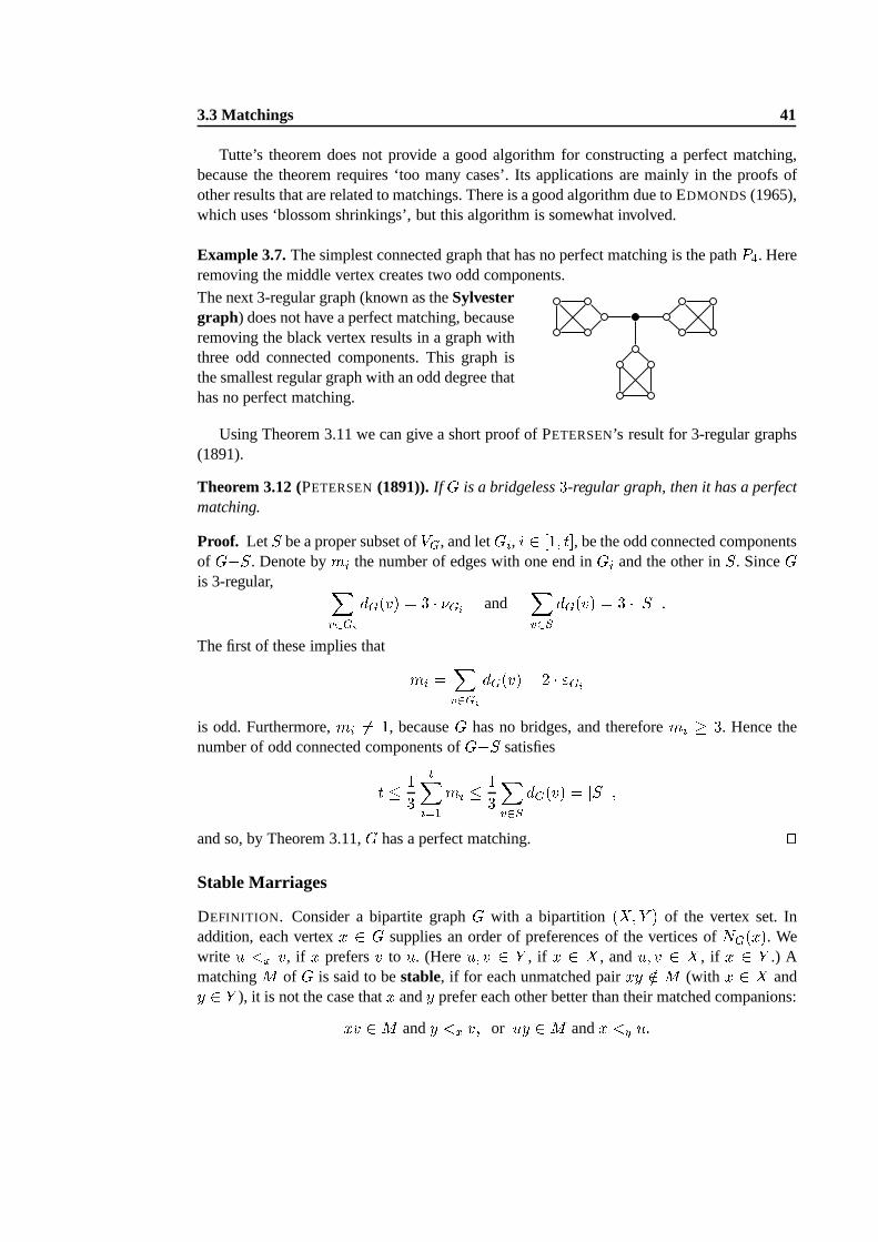
3.3 Matchings 41
Tutte’s theorem does not provide a good algorithm for constructing a perfect matching,because the theorem requires ‘too many cases’. Its applications are mainly in the proofs ofother results that are related to matchings. There is a good algorithm due to EDMONDS (1965),which uses ‘blossom shrinkings’, but this algorithm is somewhat involved.
Example 3.7.The simplest connected graph that has no perfect matching isthe pathP4. Hereremoving the middle vertex creates two odd components.
The next 3-regular graph (known as theSylvestergraph) does not have a perfect matching, becauseremoving the black vertex results in a graph withthree odd connected components. This graph isthe smallest regular graph with an odd degree thathas no perfect matching.
Using Theorem 3.11 we can give a short proof of PETERSEN’s result for 3-regular graphs(1891).
Theorem 3.12 (PETERSEN(1891)).If G is a bridgeless3-regular graph, then it has a perfectmatching.
Proof. LetS be a proper subset ofVG, and letGi, i 2 [1; t℄, be the odd connected componentsof G�S. Denote bymi the number of edges with one end inGi and the other inS. SinceGis 3-regular, Xv2Gi dG(v) = 3 � �Gi and
Xv2S dG(v) = 3 � jSj :The first of these implies that mi = Xv2Gi dG(v) � 2 � "Giis odd. Furthermore,mi 6= 1, becauseG has no bridges, and thereforemi � 3. Hence thenumber of odd connected components ofG�S satisfiest � 13 tXi=1 mi � 13Xv2S dG(v) = jSj ;and so, by Theorem 3.11,G has a perfect matching. utStable Marriages
DEFINITION. Consider a bipartite graphG with a bipartition (X;Y ) of the vertex set. Inaddition, each vertexx 2 G supplies an order of preferences of the vertices ofNG(x). Wewrite u <x v, if x prefersv to u. (Hereu; v 2 Y , if x 2 X, andu; v 2 X, if x 2 Y .) AmatchingM of G is said to bestable, if for each unmatched pairxy =2 M (with x 2 X andy 2 Y ), it is not the case thatx andy prefer each other better than their matched companions:xv 2M andy <x v; or uy 2M andx <y u:
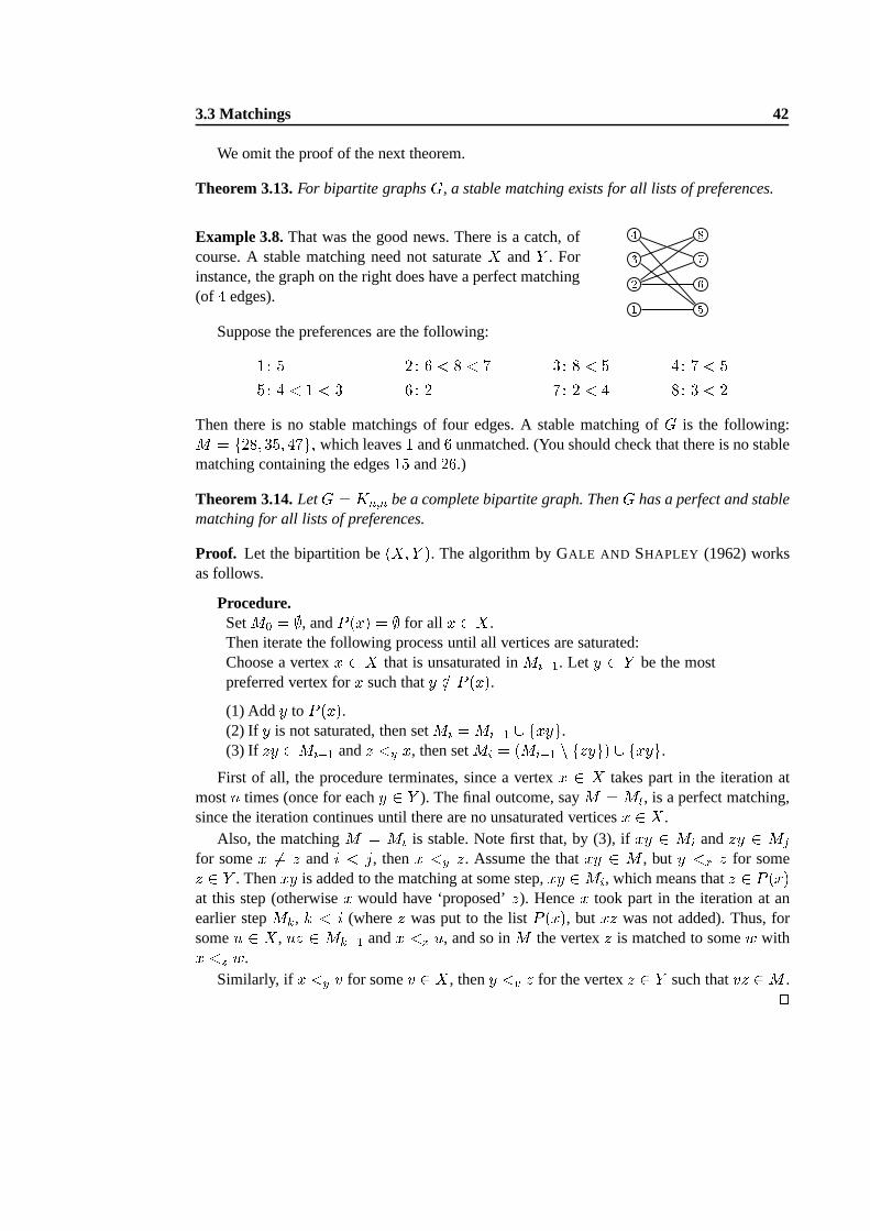
3.3 Matchings 42
We omit the proof of the next theorem.
Theorem 3.13.For bipartite graphsG, a stable matching exists for all lists of preferences.
Example 3.8.That was the good news. There is a catch, ofcourse. A stable matching need not saturateX andY . Forinstance, the graph on the right does have a perfect matching(of 4 edges).
4231 5678Suppose the preferences are the following:1: 5 2: 6 < 8 < 7 3: 8 < 5 4: 7 < 55: 4 < 1 < 3 6: 2 7: 2 < 4 8: 3 < 2
Then there is no stable matchings of four edges. A stable matching of G is the following:M = f28; 35; 47g; which leaves1 and6 unmatched. (You should check that there is no stablematching containing the edges15 and26.)
Theorem 3.14.LetG = Kn;n be a complete bipartite graph. ThenG has a perfect and stablematching for all lists of preferences.
Proof. Let the bipartition be(X;Y ). The algorithm by GALE AND SHAPLEY (1962) worksas follows.
Procedure.SetM0 = ;, andP (x) = ; for all x 2 X.Then iterate the following process until all vertices are saturated:Choose a vertexx 2 X that is unsaturated inMi�1. Let y 2 Y be the mostpreferred vertex forx such thaty =2 P (x).(1) Addy to P (x).(2) If y is not saturated, then setMi =Mi�1 [ fxyg.(3) If zy 2Mi�1 andz <y x, then setMi = (Mi�1 n fzyg) [ fxyg.
First of all, the procedure terminates, since a vertexx 2 X takes part in the iteration atmostn times (once for eachy 2 Y ). The final outcome, sayM = Mt, is a perfect matching,since the iteration continues until there are no unsaturated verticesx 2 X.
Also, the matchingM = Mt is stable. Note first that, by (3), ifxy 2 Mi andzy 2 Mjfor somex 6= z and i < j, thenx <y z. Assume the thatxy 2 M , but y <x z for somez 2 Y . Thenxy is added to the matching at some step,xy 2Mi, which means thatz 2 P (x)at this step (otherwisex would have ‘proposed’z). Hencex took part in the iteration at anearlier stepMk, k < i (wherez was put to the listP (x), but xz was not added). Thus, forsomeu 2 X, uz 2 Mk�1 andx <z u, and so inM the vertexz is matched to somew withx <z w.
Similarly, if x <y v for somev 2 X, theny <v z for the vertexz 2 Y such thatvz 2M .ut
4
Colourings
4.1 Edge colourings
Colourings of edges and vertices of a graphG are useful, when one is interested in classifyingrelations between objects.
There are two sides of colourings. In the general case, a graph G with a colouring� isgiven, and we study the properties of this pairG� = (G;�). This is the situation,e.g., intransportation networks with bus and train links, where thecolour (buss, train) of an edgetells the nature of a link.
In the chromatic theory,G is first given and then we search for a colouring that the satisfiesrequired properties. One of the important properties of colourings is ‘properness’. In a propercolouring adjacent edges or vertices are coloured differently.
Edge chromatic number
DEFINITION. A k-edge colouring� : EG ! [1; k℄ of a graphG is an assignment ofk coloursto its edges. We writeG� to indicate thatG has the edge colouring�.
A vertexv 2 G and a colouri 2 [1; k℄ areincident with each other, if�(vu) = i for somevu 2 EG. If v 2 G is not incident with a colouri, theni is available for v.The colouring� isproper, if no two adjacent edges obtain the same colour:�(e1) 6= �(e2)
for adjacente1 ande2.Theedge chromatic number�0(G) of G is defined as�0(G) = minfk j there exists a properk-edge colouring ofGg :A k-edge colouring� can be thought of as a partitionfE1; E2; : : : ; Ekg of EG, whereEi = fe j �(e) = ig. Note that it is possible thatEi = ; for somei. We adopt a simplified
notation G�[i1; i2; : : : ; it℄ = G[Ei1 [Ei2 [ � � � [Eit ℄for the subgraph ofG consisting of those edges that have a colouri1, i2, . . . , orit. That is, theedges having other colours are removed.
Lemma 4.1.Each colour setEi in a properk-edge colouring is a matching. Moreover, foreach graphG,�(G) � �0(G) � "G.
Proof. This is clear. ut
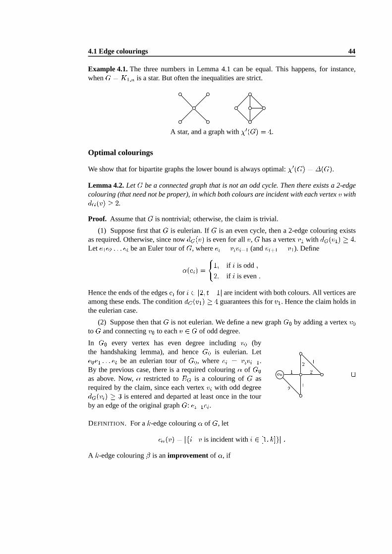
4.1 Edge colourings 44
Example 4.1.The three numbers in Lemma 4.1 can be equal. This happens, forinstance,whenG = K1;n is a star. But often the inequalities are strict.
A star, and a graph with�0(G) = 4.
Optimal colourings
We show that for bipartite graphs the lower bound is always optimal: �0(G) = �(G).Lemma 4.2.LetG be a connected graph that is not an odd cycle. Then there exists a 2-edgecolouring (that need not be proper), in which both colours are incident with each vertexv withdG(v) � 2.
Proof. Assume thatG is nontrivial; otherwise, the claim is trivial.
(1) Suppose first thatG is eulerian. IfG is an even cycle, then a 2-edge colouring existsas required. Otherwise, since nowdG(v) is even for allv,G has a vertexv1 with dG(v1) � 4.Let e1e2 : : : et be an Euler tour ofG, whereei = vivi+1 (andvt+1 = v1). Define�(ei) = (1; if i is odd;2; if i is even:Hence the ends of the edgesei for i 2 [2; t�1℄ are incident with both colours. All vertices areamong these ends. The conditiondG(v1) � 4 guarantees this forv1. Hence the claim holds inthe eulerian case.
(2) Suppose then thatG is not eulerian. We define a new graphG0 by adding a vertexv0toG and connectingv0 to eachv 2 G of odd degree.
In G0 every vertex has even degree includingv0 (bythe handshaking lemma), and henceG0 is eulerian. Lete0e1 : : : et be an eulerian tour ofG0, whereei = vivi+1.By the previous case, there is a required colouring� of G0as above. Now,� restricted toEG is a colouring ofG asrequired by the claim, since each vertexvi with odd degreedG(vi) � 3 is entered and departed at least once in the tourby an edge of the original graphG: ei�1ei. v0 12 1 212 utDEFINITION. For ak-edge colouring� of G, let �(v) = jfi j v is incident withi 2 [1; k℄gj :A k-edge colouring� is animprovement of �, if
4.1 Edge colourings 45Xv2G �(v) >Xv2G �(v) :Also,� is optimal, if it cannot be improved.
Notice that we always have �(v) � dG(v), and if� is proper, then �(v) = dG(v), andin this case� is optimal. Thus an improvement of a colouring is a change towards a propercolouring. Note also that a graphG always has an optimalk-edge colouring, but it need nothave any properk-edge colourings.
The next lemma is obvious.
Lemma 4.3.An edge colouring� ofG is proper if and only if �(v) = dG(v) for all verticesv 2 G.
Lemma 4.4.Let � be an optimalk-edge colouring ofG, and letv 2 G. Suppose that thecolour i is available forv, and the colourj is incident withv at least twice. Then the connectedcomponentH ofG�[i; j℄ that containsv, is an odd cycle.
Proof. Suppose the connected componentH is not an odd cycle. By Lemma 4.2,H has a2-edge colouring : EH ! fi; jg, in which bothi andj are incident with each vertexx withdH(x) � 2. (We have renamed the colours1 and2 to i andj.) We obtain a recolouring� ofG as follows: �(e) = ( (e); if e 2 EH ;�(e); if e =2 EH :SincedH(v) � 2 (by the assumption on the colourj) and in� both coloursi and j arenow incident withv, �(v) = �(v) + 1. Furthermore, by the construction of�, we have �(u) � �(u) for all u 6= v. Therefore
Pu2G �(u) > Pu2G �(u), which contradicts theoptimality of�. HenceH is an odd cycle. utTheorem 4.1 (KÖNIG (1916)).If G is bipartite, then�0(G) = �(G).Proof. Let � be an optimal�-edge colouring of a bipartiteG, where� = �(G). If therewere av 2 G with �(v) < dG(v), then by Lemma 4.4,G would contain an odd cycle. But abipartite graph does not contain such cycles. Therefore, for all verticesv, �(v) = dG(v). ByLemma 4.3,� is a proper colouring, and� = �0(G) as required. utVizing’s theorem
In general we can have�0(G) > �(G) as one of our examples did show. The followingimportant theorem, due to VIZING, shows that the edge chromatic number of a graphGmisses�(G) by at most one colour.
Theorem 4.2 (V IZING (1964)).For any graphG, �(G) � �0(G) � �(G) + 1.
Proof. Let� = �(G). We need only to show that�0(G) � �+ 1. Suppose on the contrarythat�0(G) > �+ 1, and let� be an optimal(�+ 1)-edge colouring ofG.
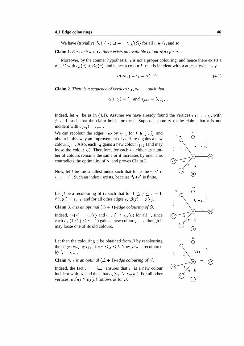
4.1 Edge colourings 46
We have (trivially)dG(u) < �+ 1 < �0(G) for all u 2 G, and so
Claim 1. For eachu 2 G, there exists an available colourb(u) for u.
Moreover, by the counter hypothesis,� is not a proper colouring, and hence there exists av 2 G with �(v) < dG(v), and hence a colouri1 that is incident withv at least twice, say�(vu1) = i1 = �(vx) : (4.1)
Claim 2. There is a sequence of verticesu1; u2; : : : such that�(vuj) = ij and ij+1 = b(uj) :Indeed, letu1 be as in (4.1). Assume we have already found the verticesu1; : : : ; uj , withj � 1, such that the claim holds for these. Suppose, contrary to the claim, thatv is notincident withb(uj) = ij+1.We can recolour the edgesvu` by i`+1 for ` 2 [1; j℄, andobtain in this way an improvement of�. Herev gains a newcolourij+1. Also, eachu` gains a new colouri`+1 (and mayloose the colouri`). Therefore, for eachu` either its num-ber of colours remains the same or it increases by one. Thiscontradicts the optimality of�, and proves Claim 2.
Now, let t be the smallest index such that for somer < t,it+1 = ir. Such an indext exists, becausedG(v) is finite.xu1u2urv ut...
. . .
ur�1i1i1i2ir�1 ir = it+1it
Let � be a recolouring ofG such that for1 � j � r � 1,�(vuj) = ij+1, and for all other edgese, �(e) = �(e).Claim 3. � is an optimal(�+ 1)-edge colouring ofG.
Indeed, �(v) = �(v) and �(u) � �(u) for all u, sinceeachuj (1 � j � r � 1) gains a new colourji+1 although itmay loose one of its old colours. xu1u2
urv ut...
. . .
ur�1i1i2i3ir ir = it+1it
Let then the colouring be obtained from� by recolouringthe edgesvuj by ij+1 for r � j � t. Now,vut is recolouredby ir = it+1.Claim 4. is an optimal(�+ 1)-edge colouring ofG.
Indeed, the factir = it+1 ensures thatir is a new colourincident withut, and thus that (ut) � �(ut). For all othervertices, (u) � �(u) follows as for�. xu1u2
urv ut...
. . .
ur�1i1i2i3ir ir+1ir
4.2 Ramsey Theory 47
By Claim 1, there is a colouri0 = b(v) that is available forv. By Lemma 4.4, the connectedcomponentsH1 of G�[i0; ir℄ andH2 of G [i0; ir℄ containing the vertexv are cycles, that is,H1 is a cycle(vur�1)P1(urv) andH2 is a cycle(vur�1)P2(utv), where bothP1 : ur�1 ?�! urandP2 : ur�1 ?�! ut are paths. However, the edges ofP1 andP2 have the same colours withrespect to� and (eitheri0 or ir). This is not possible, sinceP1 ends inur while P2 ends ina different vertexut. This contradiction proves the theorem. utExample 4.2.We show that�0(G) = 4 for the Petersen graph. Indeed, by Vizing’ theorem,�0(G) = 3 or 4. Suppose3 colours suffice. LetC : v1 �! : : : �! v5 �! v1 be the outer cycleandC 0 : u1 �! : : : �! u5 �! u1 the inner cycle ofG such thatviui 2 EG for all i.
Observe that every vertex is adjacent to all colours1; 2; 3. NowC uses one colour (say1)once and the other two twice. This can be done uniquely (up to permutations):v1 1�! v2 2�! v3 3�! v4 2�! v5 3�! v1:Hencev1 2�! u1, v2 3�! u2, v3 1�! u3, v4 1�! u4, v5 1�! u5. However, this means that1 cannotbe a colour of any edge inC 0. SinceC 0 needs three colours, the claim follows.
Edge Colouring Problem.Vizing’s theorem (nor its present proof) does not offer any char-acterization for the graphs, for which�0(G) = �(G) + 1. In fact, it is one of the famousopen problems of graph theory to find such a characterization. The answer is known (only)for some special classes of graphs. By HOLYER (1981), the problem whether�0(G) is�(G)or�(G) + 1 is NP-complete.
The proof of Vizing’s theorem can be used to obtain a proper colouring ofG with at most�(G) + 1 colours, when the word ‘optimal’ is forgotten: colour first the edges as well as youcan (if nothing better, then arbitrarily in two colours), and use the proof iteratively to improvethe colouring until no improvement is possible – then the proof says that the result is a propercolouring.
4.2 Ramsey Theory
In general, Ramsey theory studies unavoidable patterns in combinatorics. We consider aninstance of this theory mainly for edge colourings (that need not be proper). A typical exampleof a Ramsey property is the following: given 6 persons each pair of whom are either friendsor enemies, there are then 3 persons who are mutual friends ormutual enemies. In graphtheoretic terms this means that each colouring of the edges of K6 with 2 colours results in amonochromatic triangle.
Turan’s theorem for complete graphs
We shall first consider the problem of finding a general condition forKp to appear in a graph.It is clear that every graph containsK1, and that every nondiscrete graph containsK2.
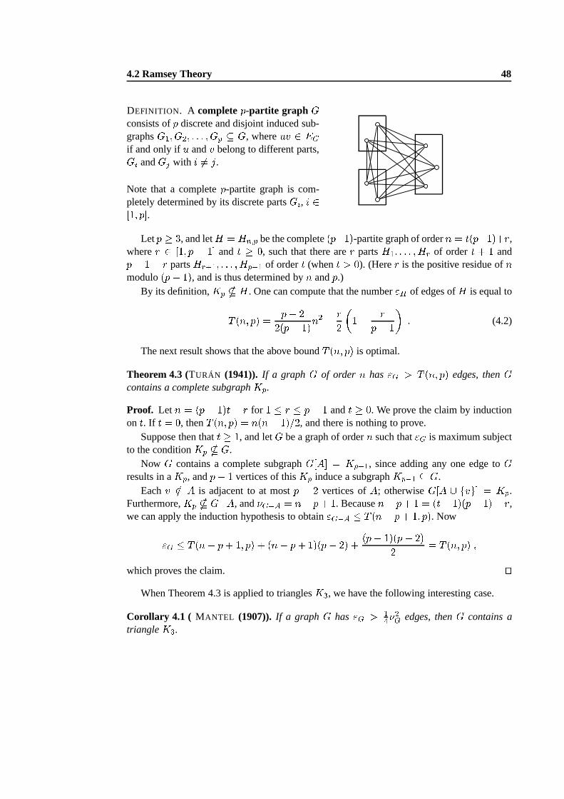
4.2 Ramsey Theory 48
DEFINITION. A completep-partite graph Gconsists ofp discrete and disjoint induced sub-graphsG1; G2; : : : ; Gp � G, whereuv 2 EGif and only if u andv belong to different parts,Gi andGj with i 6= j.Note that a completep-partite graph is com-pletely determined by its discrete partsGi, i 2[1; p℄.
Letp � 3, and letH = Hn;p be the complete(p�1)-partite graph of ordern = t(p�1)+r,wherer 2 [1; p � 1℄ and t � 0, such that there arer partsH1; : : : ;Hr of order t + 1 andp� 1 � r partsHr+1; : : : ;Hp�1 of ordert (whent > 0). (Herer is the positive residue ofnmodulo(p� 1), and is thus determined byn andp.)
By its definition,Kp * H. One can compute that the number"H of edges ofH is equal toT (n; p) = p� 22(p� 1)n2 � r2 �1� rp� 1� : (4.2)
The next result shows that the above boundT (n; p) is optimal.
Theorem 4.3 (TURÁN (1941)). If a graphG of order n has "G > T (n; p) edges, thenGcontains a complete subgraphKp.Proof. Let n = (p� 1)t+ r for 1 � r � p� 1 andt � 0. We prove the claim by inductionon t. If t = 0, thenT (n; p) = n(n� 1)=2, and there is nothing to prove.
Suppose then thatt � 1, and letG be a graph of ordern such that"G is maximum subjectto the conditionKp * G.
Now G contains a complete subgraphG[A℄ = Kp�1, since adding any one edge toGresults in aKp, andp� 1 vertices of thisKp induce a subgraphKp�1 � G.
Eachv =2 A is adjacent to at mostp � 2 vertices ofA; otherwiseG[A [ fvg℄ = Kp.Furthermore,Kp * G�A, and�G�A = n� p+ 1. Becausen� p+ 1 = (t� 1)(p� 1) + r,we can apply the induction hypothesis to obtain"G�A � T (n� p+ 1; p). Now"G � T (n� p+ 1; p) + (n� p+ 1)(p� 2) + (p� 1)(p� 2)2 = T (n; p) ;which proves the claim. ut
When Theorem 4.3 is applied to trianglesK3, we have the following interesting case.
Corollary 4.1 ( MANTEL (1907)). If a graphG has "G > 14�2G edges, thenG contains atriangleK3.
4.2 Ramsey Theory 49
Ramsey’s theorem
DEFINITION. Let � be an edge colouring ofG. A subgraphH � G is said to be (i-)monochromatic, if all edges ofH have the same colouri.
The following theorem is one of the jewels of combinatorics.
Theorem 4.4 (RAMSEY (1930)).Let p; q � 2 be any integers. Then there exists a (smallest)integerR(p; q) such that for alln � R(p; q), any 2-edge colouring ofKn ! [1; 2℄ contains a1-monochromaticKp or a 2-monochromaticKq.
Before proving this, we give an equivalent statement. Recall that a subsetX � VG isstable, ifG[X℄ is a discrete graph.
Theorem 4.5.Letp; q � 2 be any integers. Then there exists a (smallest) integerR(p; q) suchthat for all n � R(p; q), any graphG of ordern contains a complete subgraph of orderp ora stable set of orderq.
Be patient, this will follow from Theorem 4.6. The numberR(p; q) is known as theRam-sey numberfor p andq.
It is clear thatR(p; 2) = p andR(2; q) = q.Theorems 4.4 and 4.5 follow from the next result which shows (inductively) that an upper
bound exists for the Ramsey numbersR(p; q).Theorem 4.6 (ERDÖS and SZEKERES (1935)). The Ramsey numberR(p; q) exists for allp; q � 2, and R(p; q) � R(p; q � 1) +R(p� 1; q) :Proof. We use induction onp+ q. It is clear thatR(p; q) exists forp = 2 or q = 2, and it isthus exists forp+ q � 5.
It is now sufficient to show that ifG is a graph of orderR(p; q � 1) +R(p� 1; q), then ithas a complete subgraph of orderp or a stable subset of orderq.
Let v 2 G, and denote byA = VG n (NG(v) [ fvg) the set of vertices that are notadjacent tov. SinceG hasR(p; q � 1) + R(p � 1; q) � 1 vertices different fromv, eitherjNG(v)j � R(p� 1; q) or jAj � R(p; q � 1) (or both).
Assume first thatjNG(v)j � R(p�1; q). By the definition of Ramsey numbers,G[NG(v)℄contains a complete subgraphB of orderp�1 or a stable subsetS of orderq. In the first case,B [ fvg induces a complete subgraphKp in G, and in the second case the same stable set oforderq is good forG.
If jAj � R(p; q� 1), thenG[A℄ contains a complete subgraph of orderp or a stable subsetS of orderq � 1. In the first case, the same complete subgraph of orderp is good forG, andin the second case,S [ fvg is a stable subset ofG of q vertices. This proves the claim. ut
A concrete upper bound is given in the following result.
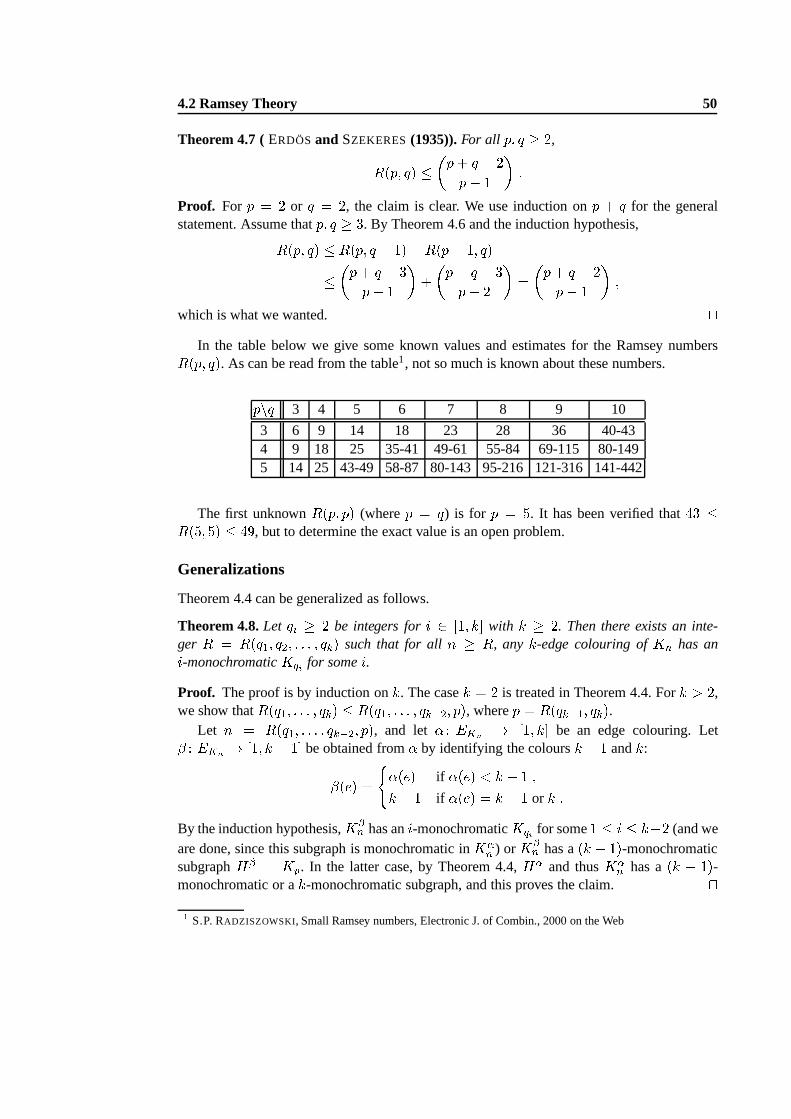
4.2 Ramsey Theory 50
Theorem 4.7 (ERDÖSand SZEKERES(1935)).For all p; q � 2,R(p; q) � �p+ q � 2p� 1 � :Proof. For p = 2 or q = 2, the claim is clear. We use induction onp + q for the generalstatement. Assume thatp; q � 3. By Theorem 4.6 and the induction hypothesis,R(p; q) � R(p; q � 1) +R(p� 1; q)� �p+ q � 3p� 1 �+�p+ q � 3p� 2 � = �p+ q � 2p� 1 � ;which is what we wanted. ut
In the table below we give some known values and estimates forthe Ramsey numbersR(p; q). As can be read from the table1, not so much is known about these numbers.pnq 3 4 5 6 7 8 9 10
3 6 9 14 18 23 28 36 40-434 9 18 25 35-41 49-61 55-84 69-115 80-1495 14 25 43-49 58-87 80-143 95-216 121-316 141-442
The first unknownR(p; p) (wherep = q) is for p = 5. It has been verified that43 �R(5; 5) � 49, but to determine the exact value is an open problem.
Generalizations
Theorem 4.4 can be generalized as follows.
Theorem 4.8.Let qi � 2 be integers fori 2 [1; k℄ with k � 2. Then there exists an inte-ger R = R(q1; q2; : : : ; qk) such that for alln � R, any k-edge colouring ofKn has ani-monochromaticKqi for somei.Proof. The proof is by induction onk. The casek = 2 is treated in Theorem 4.4. Fork > 2,we show thatR(q1; : : : ; qk) � R(q1; : : : ; qk�2; p), wherep = R(qk�1; qk).
Let n = R(q1; : : : ; qk�2; p), and let � : EKn ! [1; k℄ be an edge colouring. Let� : EKn ! [1; k � 1℄ be obtained from� by identifying the coloursk � 1 andk:�(e) = (�(e) if �(e) < k � 1 ;k � 1 if �(e) = k � 1 or k :By the induction hypothesis,K�n has ani-monochromaticKqi for some1 � i � k�2 (and weare done, since this subgraph is monochromatic inK�n ) orK�n has a(k � 1)-monochromaticsubgraphH� = Kp. In the latter case, by Theorem 4.4,H� and thusK�n has a(k � 1)-monochromatic or ak-monochromatic subgraph, and this proves the claim. ut1 S.P. RADZISZOWSKI, Small Ramsey numbers, Electronic J. of Combin., 2000 on theWeb
4.2 Ramsey Theory 51
Since for each graphH,H � Km for m = �H , we have
Corollary 4.2. Letk � 2 andH1;H2; : : : ;Hk be arbitrary graphs. Then there exists an inte-gerR(H1;H2; : : : ;Hk) such that for all complete graphsKn with n � R(H1;H2; : : : ;Hk)and for all k-edge colourings� of Kn, K�n contains ani-monochromatic subgraphHi forsomei.
This generalization is trivial from Theorem 4.8. However, the generalized Ramsey num-bersR(H1;H2; : : : ;Hk) can be much smaller than their counter parts (for complete graphs)in Theorem 4.8.
Example 4.3.We leave the following statement as an exercise: IfT is a tree of orderm, thenR(T;Kn) = (m� 1)(n� 1) + 1 ;that is, any graphG of order at leastR(T;Kn) contains a subgraph isomorphic toT , or thecomplement ofG contains a complete subgraphKn.
Examples of Ramsey numbers�Some exact values are known in Corollary 4.2, even in more general cases, for some deargraphs (see RADZISZOWSKI’s survey). Below we list some of these results for cases, wherethe graphs are equal. To this end, letRk(G) = R(G;G; : : : ; G) (k timesG):The best known lower bound ofR2(G) for connected graphs was obtained by BURR AND
ERDÖS(1976), R2(G) � �4�G � 13 � (G connected):Here is a list of some special cases:R2(Pn) = n+ jn2 k� 1;R2(Cn) = 8><>:6 if n = 3 or n = 4;2n� 1 if n � 5 andn odd ;3n=2� 1 if n � 6 andn even;R2(K1;n) = (2n� 1 if n is even;2n if n is odd;R2(K2;3) = 10; R2(K3;3) = 18:The valuesR2(K2;n) are known forn � 16, and in general,R2(K2;n) � 4n� 2. The valueR2(K2;17) is either65 or 66.
Let Wn denote thewheelonn vertices. It is a cycleCn�1, where a vertexv with degreen� 1 is attached. Note thatW4 = K4. ThenR2(W5) = 15 andR2(W6) = 17:
4.3 Vertex colourings 52
For three colours, much less is known. In fact, the only nontrivial result for completegraphs is:R3(K3) = 17. Also, 128 � R3(K4) � 235, and385 � R3(K5), but no nontrivialupper bound is known forR3(K5). For the squareC4, we know thatR3(C4) = 11.
Needless to say that no exact values are known forRk(Kn) for k � 4 andn � 3.
It follows from Theorem 4.4 that for any completeKn, thereexistsa graphG (well, anysufficiently large complete graph) such that any2-edge colouring ofG has a monochromatic(induced) subgraphKn. Note, however, that in Corollary 4.2 the monochromatic subgraphHiis not required to be induced.
The following impressive theorem improves the results we have mentioned in this chapterand it has a difficult proof.
Theorem 4.9 (DEUBER, ERDÖS, HAJNAL, PÓSA, and RÖDL (around 1973)).LetH be anygraph. Then there exists a graphG such that any2-edge colouring ofG has an monochromaticinduced subgraphH.
Example 4.4.As an application of Ramsey’s theorem, we shortly describe Schur’s theorem.For this, consider the partitionf1; 4; 10; 13g; f2; 3; 11; 12g; f5; 6; 7; 8; 9g of the setN13 =[1; 13℄. We observe that in no partition class there are three integers such thatx + y = z.However, if you try to partitionN14 into three classes, then you are bound to find a class,wherex+ y = z has a solution.
SCHUR (1916) solved this problem in a general setting. The following gives a short proofusing Ramsey’s theorem.
For eachn � 1, there exists an integerS(n) such that any partitionS1; : : : ; Sn of NS(n) hasa classSi containing two integersx; y such thatx+ y 2 Si.
Indeed, letS(n) = R(3; 3; : : : ; 3), where3 occursn times, and letK be a complete onNS(n) . For a partitionS1; : : : ; Sn of NS(n) , define an edge colouring� of K by�(ij) = k; if ji� jj 2 Sk :By Theorem 4.8,K� has a monochromatic triangle, that is, there are three vertices1 � i <j < t � S(n) such thatt � j; j � i; t � i 2 Sk for somek. But (t � j) + (j � i) = t � iproves the claim.
There are quite many interesting corollaries to Ramsey’s theorem in various parts of math-ematics including not only graph theory, but also,e.g., geometry and algebra, see
R.L. GRAHAM , B.L. ROTHSCHILD AND J.L. SPENCER, “Ramsey Theory”, Wiley, (2nd ed.)1990.
4.3 Vertex colourings
The vertices of a graphG can also be classified using colourings. These colourings tell thatcertain vertices have a common property (or that they are similar in some respect), if theyshare the same colour. In this chapter, we shall concentrateon proper vertex colourings, whereadjacent vertices get different colours.
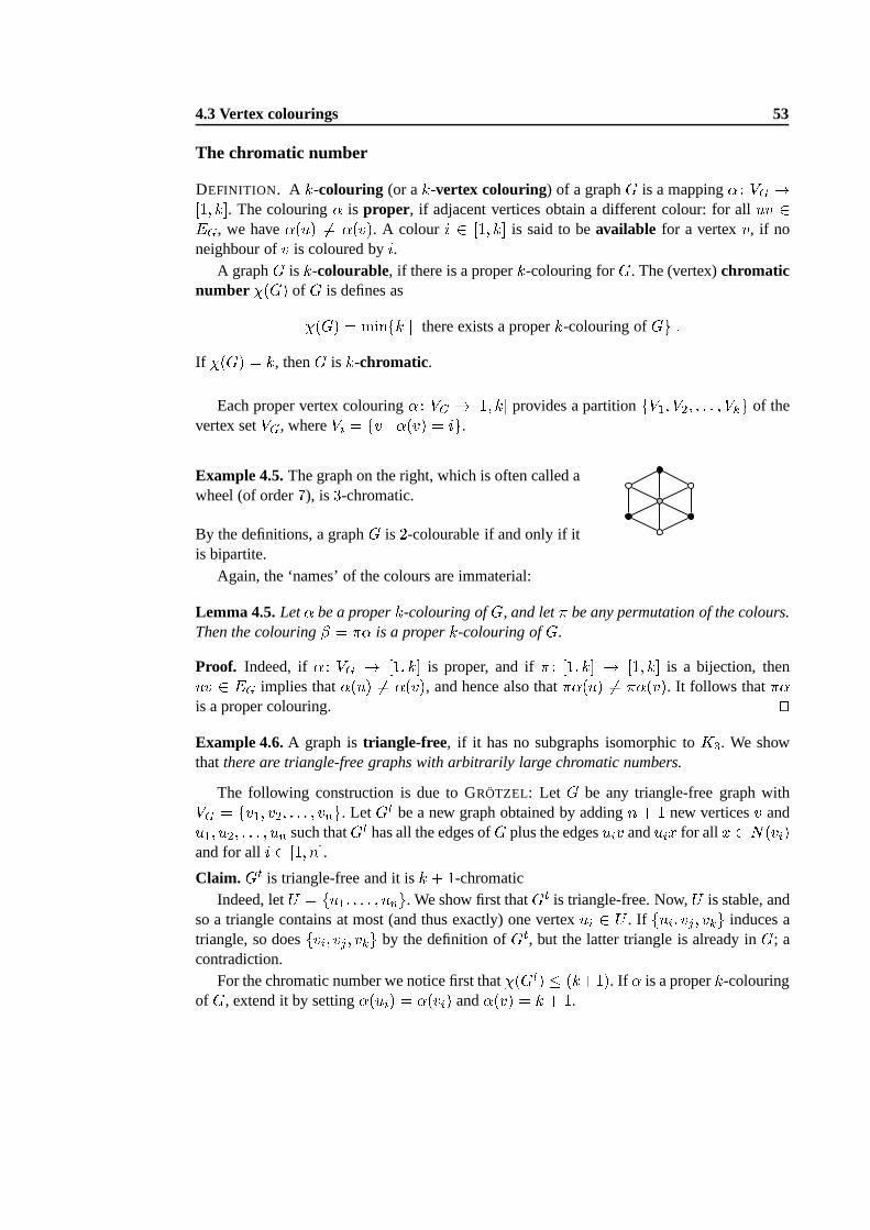
4.3 Vertex colourings 53
The chromatic number
DEFINITION. A k-colouring (or ak-vertex colouring) of a graphG is a mapping� : VG 
4.3 Vertex colourings 54
Secondly,�(Gt) > k. Assume that� is a properk-colouring ofGt, say with�(v) = k.Then�(ui) 6= k. Recolour eachvi by �(ui). This gives a proper(k � 1)-colouring toG; acontradiction. Therefore�(Gt) = k + 1.
Now using inductively the above construction starting fromthe triangle-free graphK2, weobtain larger triangle -free graphs with high chromatic numbers.
Critical graphs
DEFINITION. A k-chromatic graphG is said to bek-critical , if �(H) < k for all H � Gwith H 6= G.
In a critical graph an elimination of any edge and of any vertex will reduce the chromaticnumber:�(G�e) < �(G) and�(G�v) < �(G) for e 2 EG andv 2 G. EachKn is n-critical, since inKn�(uv) the verticesu andv can gain the same colour.
Example 4.7.The graphK2 = P2 is the only 2-critical graph. The 3-critical graphs are ex-actly the odd cyclesC2n+1 for n � 1, since a 3-chromaticG is not bipartite, and thus musthave a cycle of odd length.
Theorem 4.10.If G is k-critical for k � 2, then it is connected, andÆ(G) � k � 1.
Proof. Note that for any graphG with the connected componentsG1; G2; : : : ; Gm, �(G) =maxf�(Gi) j i 2 [1;m℄g : Connectivity claim follows from this observation.Let thenG bek-critical, butÆ(G) = dG(v) � k � 2 for v 2 G. SinceG is critical, there
is a proper(k � 1)-colouring ofG�v. Now v is adjacent to onlyÆ(G) < k � 1 vertices. Butthere arek colours, and hence there is an available colouri for v. If we recolourv by i, then aproper(k � 1)-colouring is obtained forG; a contradiction. ut
The case (iii) of the next theorem is due to SZEKERES ANDWILF (1968).
Theorem 4.11.LetG be any graph withk = �(G).(i) G has ak-critical subgraphH.(ii) G has at leastk vertices of degree� k � 1.(iii) k � 1 +maxH�G Æ(H).Proof. For (i), we observe that ak-critical subgraphH � G is obtained by removing verticesand edges fromG as long as the chromatic number remainsk.
For (ii), let H � G be k-critical. By Theorem 4.10,dH(v) � k � 1 for everyv 2 H.Of course, alsodG(v) � k � 1 for everyv 2 H. The claim follows, because, clearly, everyk-critical graphH must have at leastk vertices.
For (iii), letH � G bek-critical. By Theorem 4.10,�(G)� 1 � Æ(H), which proves thisclaim. ut
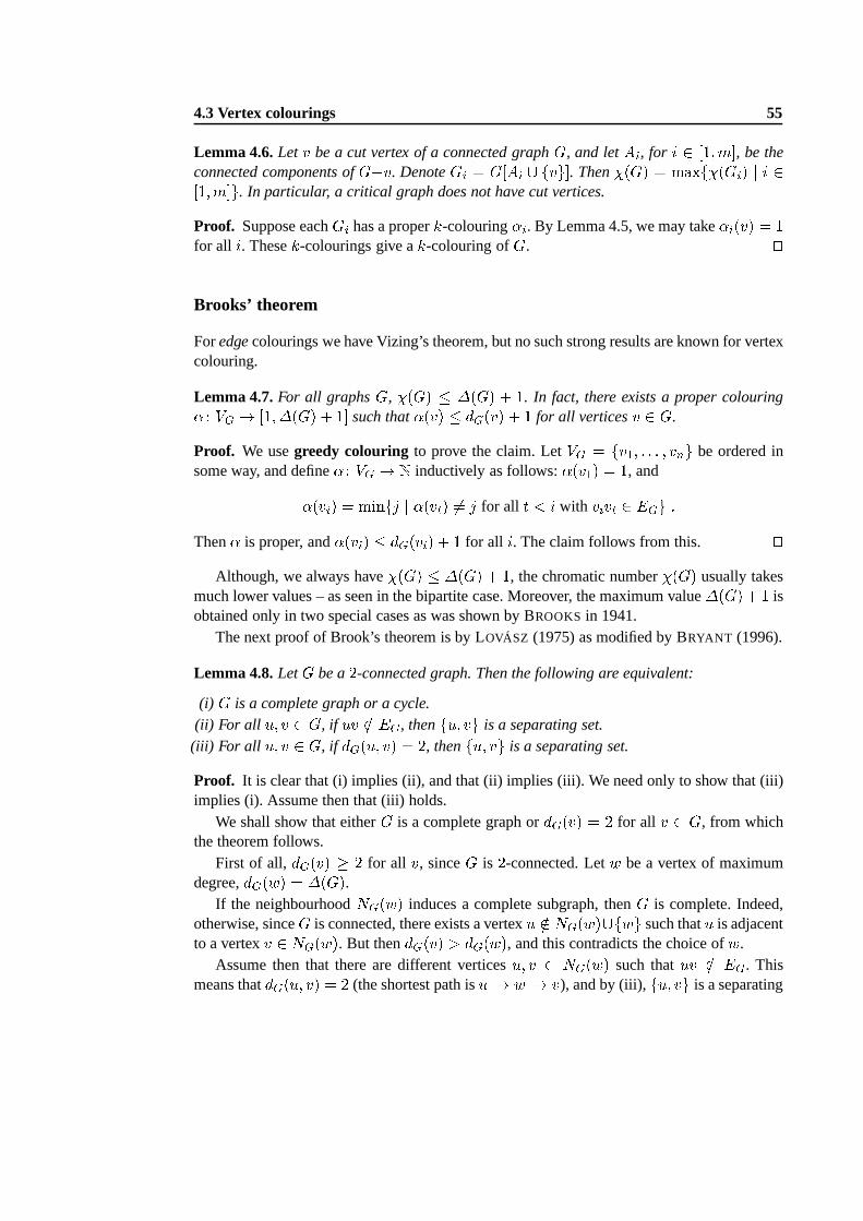
4.3 Vertex colourings 55
Lemma 4.6.Let v be a cut vertex of a connected graphG, and letAi, for i 2 [1;m℄, be theconnected components ofG�v. DenoteGi = G[Ai [ fvg℄. Then�(G) = maxf�(Gi) j i 2[1;m℄g. In particular, a critical graph does not have cut vertices.
Proof. Suppose eachGi has a properk-colouring�i. By Lemma 4.5, we may take�i(v) = 1for all i. Thesek-colourings give ak-colouring ofG. utBrooks’ theorem
Foredgecolourings we have Vizing’s theorem, but no such strong results are known for vertexcolouring.
Lemma 4.7.For all graphsG, �(G) � �(G) + 1. In fact, there exists a proper colouring� : VG ! [1;�(G) + 1℄ such that�(v) � dG(v) + 1 for all verticesv 2 G.
Proof. We usegreedy colouring to prove the claim. LetVG = fv1; : : : ; vng be ordered insome way, and define� : VG ! N inductively as follows:�(v1) = 1, and�(vi) = minfj j �(vt) 6= j for all t < i with vivt 2 EGg :Then� is proper, and�(vi) � dG(vi) + 1 for all i. The claim follows from this. ut
Although, we always have�(G) � �(G) + 1, the chromatic number�(G) usually takesmuch lower values – as seen in the bipartite case. Moreover, the maximum value�(G) + 1 isobtained only in two special cases as was shown by BROOKS in 1941.
The next proof of Brook’s theorem is by LOVÁSZ (1975) as modified by BRYANT (1996).
Lemma 4.8.LetG be a2-connected graph. Then the following are equivalent:
(i) G is a complete graph or a cycle.(ii) For all u; v 2 G, if uv =2 EG, thenfu; vg is a separating set.(iii) For all u; v 2 G, if dG(u; v) = 2, thenfu; vg is a separating set.
Proof. It is clear that (i) implies (ii), and that (ii) implies (iii). We need only to show that (iii)implies (i). Assume then that (iii) holds.
We shall show that eitherG is a complete graph ordG(v) = 2 for all v 2 G, from whichthe theorem follows.
First of all, dG(v) � 2 for all v, sinceG is 2-connected. Letw be a vertex of maximumdegree,dG(w) = �(G).
If the neighbourhoodNG(w) induces a complete subgraph, thenG is complete. Indeed,otherwise, sinceG is connected, there exists a vertexu =2 NG(w)[fwg such thatu is adjacentto a vertexv 2 NG(w). But thendG(v) > dG(w), and this contradicts the choice ofw.
Assume then that there are different verticesu; v 2 NG(w) such thatuv =2 EG. Thismeans thatdG(u; v) = 2 (the shortest path isu �! w �! v), and by (iii),fu; vg is a separating
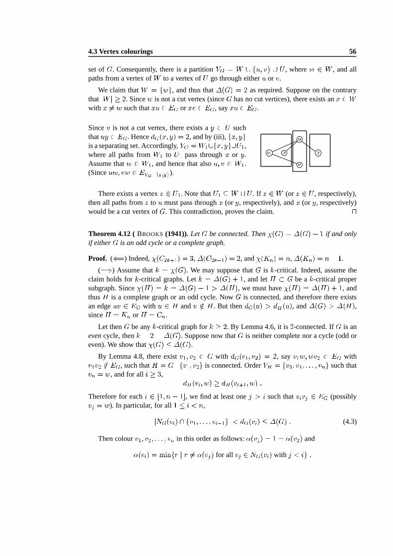
4.3 Vertex colourings 56
set ofG. Consequently, there is a partitionVG = W [ fu; vg [ U , wherew 2 W , and allpaths from a vertex ofW to a vertex ofU go through eitheru or v.
We claim thatW = fwg, and thus that�(G) = 2 as required. Suppose on the contrarythat jW j � 2. Sincew is not a cut vertex (sinceG has no cut vertices), there exists anx 2Wwith x 6= w such thatxu 2 EG or xv 2 EG, sayxu 2 EG.
Sincev is not a cut vertex, there exists ay 2 U suchthatuy 2 EG. HencedG(x; y) = 2, and by (iii),fx; ygis a separating set. Accordingly,VG =W1[fx; yg[U1,where all paths fromW1 to U1 pass throughx or y.Assume thatw 2 W1, and hence that alsou; v 2 W1.(Sinceuw; vw 2 EVG�fx;yg). w x uv y
There exists a vertexz 2 U1. Note thatU1 � W [ U . If z 2 W (or z 2 U , respectively),then all paths fromz to u must pass throughx (or y, respectively), andx (or y, respectively)would be a cut vertex ofG. This contradiction, proves the claim. utTheorem 4.12 (BROOKS (1941)).LetG be connected. Then�(G) = �(G) + 1 if and onlyif eitherG is an odd cycle or a complete graph.
Proof. ((=) Indeed,�(C2k+1) = 3,�(C2k+1) = 2, and�(Kn) = n,�(Kn) = n� 1.
(=)) Assume thatk = �(G). We may suppose thatG is k-critical. Indeed, assume theclaim holds fork-critical graphs. Letk = �(G) + 1, and letH � G be ak-critical propersubgraph. Since�(H) = k = �(G) + 1 > �(H), we must have�(H) = �(H) + 1, andthusH is a complete graph or an odd cycle. NowG is connected, and therefore there existsan edgeuv 2 EG with u 2 H andv =2 H. But thendG(u) > dH(u), and�(G) > �(H),sinceH = Kn orH = Cn.
Let thenG be anyk-critical graph fork � 2. By Lemma 4.6, it is2-connected. IfG is anevencycle, thenk = 2 = �(G). Suppose now thatG is neither complete nor a cycle (odd oreven). We show that�(G) � �(G).
By Lemma 4.8, there existv1; v2 2 G with dG(v1; v2) = 2, sayv1w;wv2 2 EG withv1v2 =2 EG, such thatH = G�fv1; v2g is connected. OrderVH = fv3; v4; : : : ; vng such thatvn = w, and for alli � 3, dH(vi; w) � dH(vi+1; w) :Therefore for eachi 2 [1; n � 1℄, we find at least onej > i such thatvivj 2 EG (possiblyvj = w). In particular, for all1 � i < n,jNG(vi) \ fv1; : : : ; vi�1gj < dG(vi) � �(G) : (4.3)
Then colourv1; v2; : : : ; vn in this order as follows:�(v1) = 1 = �(v2) and�(vi) = minfr j r 6= �(vj) for all vj 2 NG(vi) with j < ig :
4.3 Vertex colourings 57
The colouring� is proper.By (4.3),�(vi) � �(G) for all i 2 [1; n � 1℄. Also,w = vn has two neighbours,v1 andv2, of the same colour1, and sincevn has at most�(G) neighbours, there is an available
colour forvn, and so�(vn) � �(G). This shows thatG has a proper�(G)-colouring, and,consequently,�(G) � �(G). utExample 4.8.Suppose we haven objectsV = fv1; : : : ; vng, some of which are not compati-ble (like chemicals that react with each other, or worse, graph theorists who will fight during aconference). In thestorage problemwe would like to find a partition of the setV with as fewclasses as possible such that no class contains two incompatible elements. In graph theoreticalterminology we consider the graphG = (V;E), wherevivj 2 E just in casevi andvj areincompatible, and we would like to colour the vertices ofG properly using as few colours aspossible. This problem requires that we find�(G).
Unfortunately, no good algorithms are known for determining �(G), and, indeed, the chro-matic number problem is NP-complete. Already the problem if�(G) = 3 is NP-complete.(However, as we have seen, the problem whether�(G) = 2 has a fast algorithm.)
The chromatic polynomial
A given graphG has many different proper vertex colourings� : VG ! [1; k℄ for sufficientlylarge natural numbersk. Indeed, see Lemma 4.5 to be certain on this point.
DEFINITION. Thechromatic polynomial of G is the function�G : N ! N, where�G(k) = jf� j � : VG ! [1; k℄ a proper colouringgj :This notion was introduced by BIRKHOFF (1912), BIRKHOFF AND LEWIS (1946), to at-
tack the famous4-Colour Theorem, but its applications have turned out to be elsewhere.If k < �(G), then clearly�G(k) = 0, and, indeed,�(G) = minfk j �G(k) 6= 0g :
Therefore, if we can find the chromatic polynomial ofG, then we easily compute the chro-matic number�(G) just by evaluating�G(k) for k = 1; 2; : : : until we hit a nonzero value.Theorem 4.13 will give the tools for constructing�G.
Example 4.9.Consider the complete graphK4 on fv1; v2; v3; v4g. Let k � �(K4) = 4. Thevertex v1 can be first given any of thek colours, after whichk � 1 colours are availablefor v2. Thenv3 hask � 2 and finally v4 hask � 3 available colours. Therefore there arek(k � 1)(k � 2)(k � 3) different ways to properly colourK4 with k colours, and so�K4(k) = k(k � 1)(k � 2)(k � 3) :On the other hand, in the discrete graphK4 has no edges, and thus anyk-colouring is a propercolouring. Therefore �K4(k) = k4 :
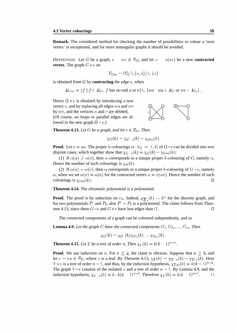
4.3 Vertex colourings 58
Remark. The considered method for checking the number of possibilities to colour a ‘nextvertex’ is exceptional, and for more nonregular graphs it should be avoided.
DEFINITION. Let G be a graph,e = uv 2 EG, and letx = x(uv) be a newcontractedvertex. The graphG � e on VG�e = (VG n fu; vg) [ fxgis obtained fromG by contracting the edgee, whenEG�e = ff j f 2 EG; f has no endu or vg [ fwx j wu 2 EG orwv 2 EGg :HenceG � e is obtained by introducing a newvertexx, and by replacing all edgeswu andwvbywx, and the verticesu andv are deleted.(Of course, no loops or parallel edges are al-lowed in the new graphG � e.) vu xeTheorem 4.13.LetG be a graph, and lete 2 EG. Then�G(k) = �G�e(k)� �G�e(k):Proof. Let e = uv. The properk-colourings� : VG ! [1; k℄ of G�e can be divided into twodisjoint cases, which together show that�G�e(k) = �G(k) + �G�e(k):
(1) If �(u) 6= �(v), then� corresponds to a unique properk-colouring ofG, namely�.Hence the number of such colourings is�G(k).
(2) If �(u) = �(v), then� corresponds to a unique properk-colouring ofG � e, namely�, when we set�(x) = �(u) for the contracted vertexx = x(uv). Hence the number of suchcolourings is�G�e(k). utTheorem 4.14.The chromatic polynomial is a polynomial.
Proof. The proof is by induction on"G. Indeed,�Kn(k) = kn for the discrete graph, andfor two polynomialsP1 andP2, alsoP1 � P2 is a polynomial. The claim follows from Theo-rem 4.13, since thereG�e andG � e have less edges thanG. ut
The connected components of a graph can be coloured independently, and so
Lemma 4.9.Let the graphG have the connected componentsG1; G2; : : : ; Gm. Then�G(k) = �G1(k)�G2(k) : : : �Gm(k) :Theorem 4.15.LetT be a tree of ordern. Then�T (k) = k(k � 1)n�1.Proof. We use induction onn. For n � 2, the claim is obvious. Suppose thatn � 3, andlet e = vu 2 ET , wherev is a leaf. By Theorem 4.13,�T (k) = �T�e(k) � �T�e(k). HereT � e is a tree of ordern� 1, and thus, by the induction hypothesis,�T�e(k) = k(k � 1)n�2.The graphT�e consists of the isolatedv and a tree of ordern � 1. By Lemma 4.9, and theinduction hypothesis,�T�e(k) = k � k(k � 1)n�2. Therefore�T (k) = k(k � 1)n�1. ut
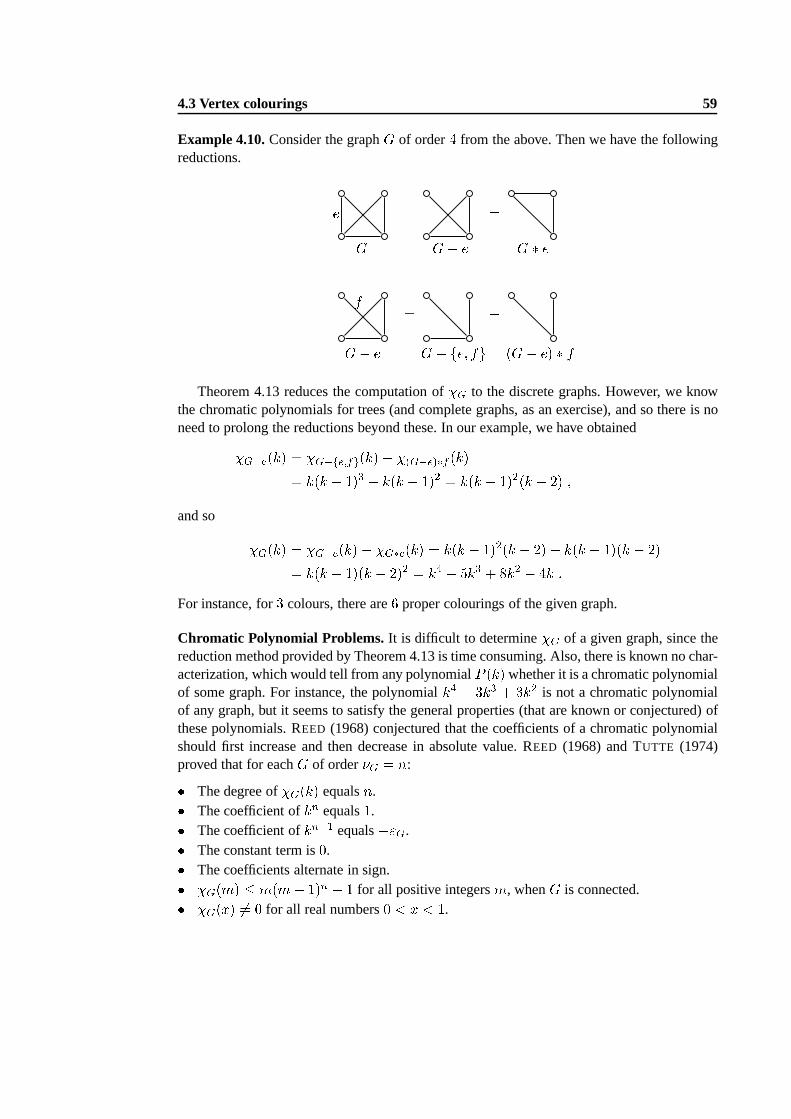
4.3 Vertex colourings 59
Example 4.10.Consider the graphG of order4 from the above. Then we have the followingreductions. = �G G� e G � ee
= �G� e G� fe; fg (G� e) � ffTheorem 4.13 reduces the computation of�G to the discrete graphs. However, we know
the chromatic polynomials for trees (and complete graphs, as an exercise), and so there is noneed to prolong the reductions beyond these. In our example,we have obtained�G�e(k) = �G�fe;fg(k)� �(G�e)�f (k)= k(k � 1)3 � k(k � 1)2 = k(k � 1)2(k � 2) ;and so �G(k) = �G�e(k)� �G�e(k) = k(k � 1)2(k � 2)� k(k � 1)(k � 2)= k(k � 1)(k � 2)2 = k4 � 5k3 + 8k2 � 4k :For instance, for3 colours, there are6 proper colourings of the given graph.
Chromatic Polynomial Problems.It is difficult to determine�G of a given graph, since thereduction method provided by Theorem 4.13 is time consuming. Also, there is known no char-acterization, which would tell from any polynomialP (k) whether it is a chromatic polynomialof some graph. For instance, the polynomialk4 � 3k3 + 3k2 is not a chromatic polynomialof any graph, but it seems to satisfy the general properties (that are known or conjectured) ofthese polynomials. REED (1968) conjectured that the coefficients of a chromatic polynomialshould first increase and then decrease in absolute value. REED (1968) and TUTTE (1974)proved that for eachG of order�G = n:� The degree of�G(k) equalsn.� The coefficient ofkn equals1.� The coefficient ofkn�1 equals�"G.� The constant term is0.� The coefficients alternate in sign.� �G(m) � m(m� 1)n � 1 for all positive integersm, whenG is connected.� �G(x) 6= 0 for all real numbers0 < x < 1.
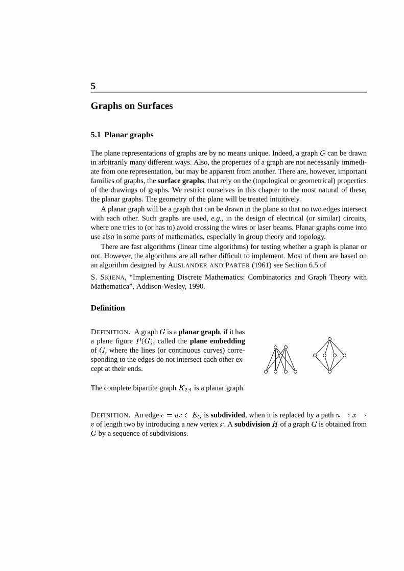
5
Graphs on Surfaces
5.1 Planar graphs
The plane representations of graphs are by no means unique. Indeed, a graphG can be drawnin arbitrarily many different ways. Also, the properties ofa graph are not necessarily immedi-ate from one representation, but may be apparent from another. There are, however, importantfamilies of graphs, thesurface graphs, that rely on the (topological or geometrical) propertiesof the drawings of graphs. We restrict ourselves in this chapter to the most natural of these,the planar graphs. The geometry of the plane will be treated intuitively.
A planar graph will be a graph that can be drawn in the plane so that no two edges intersectwith each other. Such graphs are used,e.g., in the design of electrical (or similar) circuits,where one tries to (or has to) avoid crossing the wires or laser beams. Planar graphs come intouse also in some parts of mathematics, especially in group theory and topology.
There are fast algorithms (linear time algorithms) for testing whether a graph is planar ornot. However, the algorithms are all rather difficult to implement. Most of them are based onan algorithm designed by AUSLANDER AND PARTER (1961) see Section 6.5 of
S. SKIENA , “Implementing Discrete Mathematics: Combinatorics and Graph Theory withMathematica”, Addison-Wesley, 1990.
Definition
DEFINITION. A graphG is aplanar graph, if it hasa plane figureP (G), called theplane embeddingof G, where the lines (or continuous curves) corre-sponding to the edges do not intersect each other ex-cept at their ends.
The complete bipartite graphK2;4 is a planar graph.
DEFINITION. An edgee = uv 2 EG is subdivided, when it is replaced by a pathu �! x �!v of length two by introducing anewvertexx. A subdivisionH of a graphG is obtained fromG by a sequence of subdivisions.
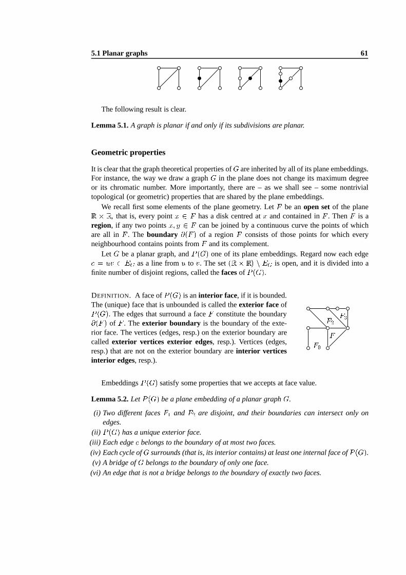
5.1 Planar graphs 61
The following result is clear.
Lemma 5.1.A graph is planar if and only if its subdivisions are planar.
Geometric properties
It is clear that the graph theoretical properties ofG are inherited by all of its plane embeddings.For instance, the way we draw a graphG in the plane does not change its maximum degreeor its chromatic number. More importantly, there are – as we shall see – some nontrivialtopological (or geometric) properties that are shared by the plane embeddings.
We recall first some elements of the plane geometry. LetF be anopen setof the planeR � R, that is, every pointx 2 F has a disk centred atx and contained inF . ThenF is aregion, if any two pointsx; y 2 F can be joined by a continuous curve the points of whichare all inF . The boundary �(F ) of a regionF consists of those points for which everyneighbourhood contains points fromF and its complement.
Let G be a planar graph, andP (G) one of its plane embeddings. Regard now each edgee = uv 2 EG as a line fromu to v. The set(R � R) n EG is open, and it is divided into afinite number of disjoint regions, called thefacesof P (G).DEFINITION. A face ofP (G) is aninterior face, if it is bounded.The (unique) face that is unbounded is called theexterior face ofP (G). The edges that surround a faceF constitute the boundary�(F ) of F . Theexterior boundary is the boundary of the exte-rior face. The vertices (edges, resp.) on the exterior boundary arecalled exterior vertices exterior edges, resp.). Vertices (edges,resp.) that are not on the exterior boundary areinterior verticesinterior edges, resp.).
F0 F1 F3F2EmbeddingsP (G) satisfy some properties that we accepts at face value.
Lemma 5.2.LetP (G) be a plane embedding of a planar graphG.
(i) Two different facesF1 and F2 are disjoint, and their boundaries can intersect only onedges.
(ii) P (G) has a unique exterior face.(iii) Each edgee belongs to the boundary of at most two faces.(iv) Each cycle ofG surrounds (that is, its interior contains) at least one internal face ofP (G).(v) A bridge ofG belongs to the boundary of only one face.(vi) An edge that is not a bridge belongs to the boundary of exactly two faces.
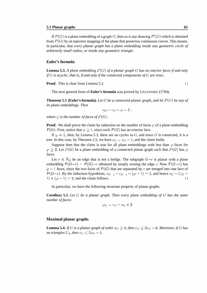
5.1 Planar graphs 62
If P (G) is a plane embedding of a graphG, then so is any drawingP 0(G)which is obtainedfromP (G) by an injective mapping of the plane that preserves continuous curves. This means,in particular, thatevery planar graph has a plane embedding inside any geometric circle ofarbitrarily small radius, or inside any geometric triangle.
Euler’s formula
Lemma 5.3.A plane embeddingP (G) of a planar graphG has no interior faces if and onlyif G is acyclic, that is, if and only if the connected components of G are trees.
Proof. This is clear from Lemma 5.2. utThe next general form ofEuler’s formula was proved by LEGENDRE(1794).
Theorem 5.1 (Euler’s formula).LetG be a connected planar graph, and letP (G) be any ofits plane embeddings. Then �G � "G + ' = 2 ;where' is the number of faces ofP (G).Proof. We shall prove the claim by induction on the number of faces' of a plane embeddingP (G). First, notice that' � 1, since eachP (G) has an exterior face.
If ' = 1, then, by Lemma 5.3, there are no cycles inG, and sinceG is connected, it is atree. In this case, by Theorem 2.5, we have"G = �G � 1, and the claim holds.
Suppose then that the claim is true for all plane embeddings with less than' faces for' � 2. Let P (G) be a plane embedding of a connected planar graph such thatP (G) has'faces.
Let e 2 EG be an edge that is not a bridge. The subgraphG�e is planar with a planeembeddingP (G�e) = P (G)�e obtained by simply erasing the edgee. Now P (G�e) has' � 1 faces, since the two faces ofP (G) that are separated bye are merged into one face ofP (G�e). By the induction hypothesis,�G�e � "G�e + ('� 1) = 2, and hence�G � ("G �1) + ('� 1) = 2, and the claim follows. ut
In particular, we have the following invariant property of planar graphs.
Corollary 5.1. Let G be a planar graph. Then every plane embedding ofG has the samenumber of faces: 'G = "G � �G + 2Maximal planar graphs
Lemma 5.4.If G is a planar graph of order�G � 3, then"G � 3�G � 6. Moreover, ifG hasno trianglesC3, then"G � 2�G � 4.
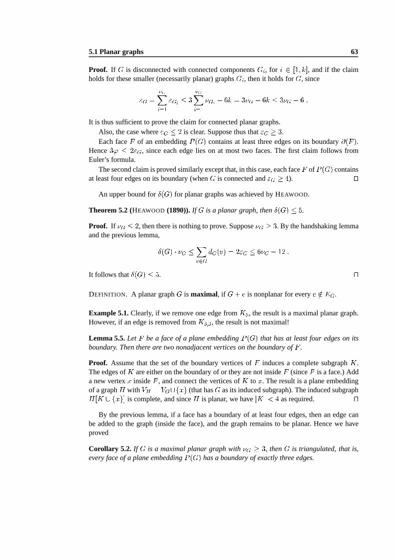
5.1 Planar graphs 63
Proof. If G is disconnected with connected componentsGi, for i 2 [1; k℄, and if the claimholds for these smaller (necessarily planar) graphsGi, then it holds forG, since"G = �GXi=1 "Gi � 3 �GXi=1 �Gi � 6k = 3�G � 6k � 3�G � 6 :It is thus sufficient to prove the claim for connected planar graphs.
Also, the case where"G � 2 is clear. Suppose thus that"G � 3.Each faceF of an embeddingP (G) contains at least three edges on its boundary�(F ).
Hence3' � 2"G, since each edge lies on at most two faces. The first claim follows fromEuler’s formula.
The second claim is proved similarly except that, in this case, each faceF of P (G) containsat least four edges on its boundary (whenG is connected and"G � 4). ut
An upper bound forÆ(G) for planar graphs was achieved by HEAWOOD.
Theorem 5.2 (HEAWOOD (1890)).If G is a planar graph, thenÆ(G) � 5.
Proof. If �G � 2, then there is nothing to prove. Suppose�G � 3. By the handshaking lemmaand the previous lemma,Æ(G) � �G �Xv2G dG(v) = 2"G � 6�G � 12 :It follows thatÆ(G) � 5. utDEFINITION. A planar graphG is maximal, if G+ e is nonplanar for everye =2 EG.
Example 5.1.Clearly, if we remove one edge fromK5, the result is a maximal planar graph.However, if an edge is removed fromK3;3, the result is not maximal!
Lemma 5.5.LetF be a face of a plane embeddingP (G) that has at least four edges on itsboundary. Then there are two nonadjacent vertices on the boundary ofF .
Proof. Assume that the set of the boundary vertices ofF induces a complete subgraphK.The edges ofK are either on the boundary of or they are not insideF (sinceF is a face.) Adda new vertexx insideF , and connect the vertices ofK to x. The result is a plane embeddingof a graphH with VH = VG[fxg (that hasG as its induced subgraph). The induced subgraphH[K [ fxg℄ is complete, and sinceH is planar, we havejKj < 4 as required. ut
By the previous lemma, if a face has a boundary of at least fouredges, then an edge canbe added to the graph (inside the face), and the graph remainsto be planar. Hence we haveproved
Corollary 5.2. If G is a maximal planar graph with�G � 3, thenG is triangulated, that is,every face of a plane embeddingP (G) has a boundary of exactly three edges.
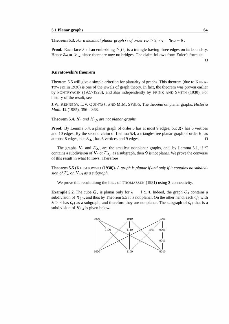
5.1 Planar graphs 64
Theorem 5.3.For a maximal planar graphG of order�G � 3, "G = 3�G � 6 :Proof. Each faceF of an embeddingP (G) is a triangle having three edges on its boundary.Hence3' = 2"G, since there are now no bridges. The claim follows from Euler’s formula.utKuratowski’s theorem
Theorem 5.5 will give a simple criterion for planarity of graphs. This theorem (due to KURA-TOWSKI in 1930) is one of the jewels of graph theory. In fact, the theorem was proven earlierby PONTRYAGIN (1927-1928), and also independently by FRINK AND SMITH (1930). Forhistory of the result, see
J.W. KENNEDY, L.V. QUINTAS, AND M.M. SYSLO, The theorem on planar graphs.HistoriaMath.12 (1985), 356 – 368.
Theorem 5.4.K5 andK3;3 are not planar graphs.
Proof. By Lemma 5.4, a planar graph of order 5 has at most 9 edges, butK5 has 5 verticesand 10 edges. By the second claim of Lemma 5.4, a triangle-free planar graph of order 6 hasat most 8 edges, butK3;3 has 6 vertices and 9 edges. ut
The graphsK5 andK3;3 are the smallest nonplanar graphs, and, by Lemma 5.1, ifGcontains a subdivision ofK5 orK3;3 as a subgraph, thenG is not planar. We prove the converseof this result in what follows. Therefore
Theorem 5.5 (KURATOWSKI (1930)).A graph is planar if and only if it contains no subdivi-sion ofK5 or K3;3 as a subgraph.
We prove this result along the lines of THOMASSEN (1981) using3-connectivity.
Example 5.2.The cubeQk is planar only fork = 1; 2; 3. Indeed, the graphQ4 contains asubdivision ofK3;3, and thus by Theorem 5.5 it is not planar. On the other hand, eachQk withk � 4 hasQ4 as a subgraph, and therefore they are nonplanar. The subgraph of Q4 that is asubdivision ofK3;3 is given below.
1000 1100 0010
0000 1010 1001
0100 1110 1101 0001
0011
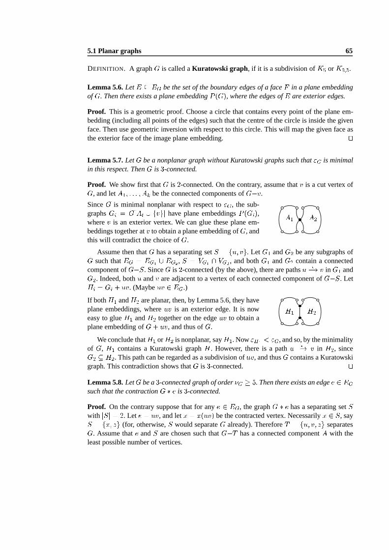
5.1 Planar graphs 65
DEFINITION. A graphG is called aKuratowski graph , if it is a subdivision ofK5 orK3;3.Lemma 5.6.LetE � EG be the set of the boundary edges of a faceF in a plane embeddingofG. Then there exists a plane embeddingP (G), where the edges ofE are exterior edges.
Proof. This is a geometric proof. Choose a circle that contains every point of the plane em-bedding (including all points of the edges) such that the centre of the circle is inside the givenface. Then use geometric inversion with respect to this circle. This will map the given face asthe exterior face of the image plane embedding. utLemma 5.7.LetG be a nonplanar graph without Kuratowski graphs such that"G is minimalin this respect. ThenG is 3-connected.
Proof. We show first thatG is 2-connected. On the contrary, assume thatv is a cut vertex ofG, and letA1; : : : ; Ak be the connected components ofG�v.
SinceG is minimal nonplanar with respect to"G, the sub-graphsGi = G[Ai [ fvg℄ have plane embeddingsP (Gi),wherev is an exterior vertex. We can glue these plane em-beddings together atv to obtain a plane embedding ofG, andthis will contradict the choice ofG.
A1 A2Assume then thatG has a separating setS = fu; vg. LetG1 andG2 be any subgraphs ofG such thatEG = EG1 [ EG2 , S = VG1 \ VG2 , and bothG1 andG2 contain a connected
component ofG�S. SinceG is 2-connected (by the above), there are pathsu ?�! v in G1 andG2. Indeed, bothu andv are adjacent to a vertex of each connected component ofG�S. LetHi = Gi + uv. (Maybeuv 2 EG.)
If bothH1 andH2 are planar, then, by Lemma 5.6, they haveplane embeddings, whereuv is an exterior edge. It is noweasy to glueH1 andH2 together on the edgeuv to obtain aplane embedding ofG+ uv, and thus ofG.
H1 H2We conclude thatH1 orH2 is nonplanar, sayH1. Now"H1 < "G, and so, by the minimality
of G, H1 contains a Kuratowski graphH. However, there is a pathu ?�! v in H2, sinceG2 � H2. This path can be regarded as a subdivision ofuv, and thusG contains a Kuratowskigraph. This contradiction shows thatG is 3-connected. utLemma 5.8.LetG be a3-connected graph of order�G � 5. Then there exists an edgee 2 EGsuch that the contractionG � e is 3-connected.
Proof. On the contrary suppose that for anye 2 EG, the graphG � e has a separating setSwith jSj = 2. Let e = uv, and letx = x(uv) be the contracted vertex. Necessarilyx 2 S, sayS = fx; zg (for, otherwise,S would separateG already). ThereforeT = fu; v; zg separatesG. Assume thate andS are chosen such thatG�T has a connected componentA with theleast possible number of vertices.
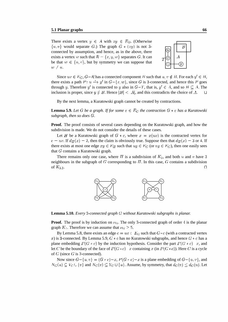
5.1 Planar graphs 66
There exists a vertexy 2 A with zy 2 EG. (Otherwisefu; vg would separateG.) The graphG � (zy) is not 3-connected by assumption, and hence, as in the above, thereexists a vertexw such thatR = fz; y; wg separatesG. It canbe thatw 2 fu; vg, but by symmetry we can suppose thatw 6= u.
uvz yBT ASinceuv 2 EG,G�R has a connected componentB such thatu; v =2 B. For eachy0 2 B,
there exists a pathP : u ?�! y0 in G�fz; wg, sinceG is 3-connected, and hence thisP goesthroughy. Thereforey0 is connected toy also inG�T , that is,y0 2 A, and soB � A. Theinclusion is proper, sincey =2 B. HencejBj < jAj, and this contradicts the choice ofA. ut
By the next lemma, a Kuratowski graph cannot be created by contractions.
Lemma 5.9.LetG be a graph. If for somee 2 EG the contractionG � e has a Kuratowskisubgraph, then so doesG.
Proof. The proof consists of several cases depending on the Kuratowski graph, and how thesubdivision is made. We do not consider the details of these cases.
Let H be a Kuratowski graph ofG � e, wherex = x(uv) is the contracted vertex fore = uv. If dH(x) = 2, then the claim is obviously true. Suppose then thatdH(x) = 3 or 4. Ifthere exists at most one edgexy 2 EH such thatuy 2 EG (or vy 2 EG), then one easily seesthatG contains a Kuratowski graph.
There remains only one case, whereH is a subdivision ofK5, and bothu andv have3neighbours in the subgraph ofG corresponding toH. In this case,G contains a subdivisionof K3;3. ut
v1v2 x v3v4 v1v2 u v v3v4Lemma 5.10.Every3-connected graphG without Kuratowski subgraphs is planar.
Proof. The proof is by induction on�G. The only3-connected graph of order4 is the planargraphK4. Therefore we can assume that�G � 5.
By Lemma 5.8, there exists an edgee = uv 2 EG such thatG�e (with a contracted vertexx) is 3-connected. By Lemma 5.9,G � e has no Kuratowski subgraphs, and henceG � e has aplane embeddingP (G � e) by the induction hypothesis. Consider the partP (G � e)�x, andletC be the boundary of the face ofP (G�e)�x containingx (in P (G�e)). HereC is a cycleof G (sinceG is 3-connected).
Now sinceG�fu; vg = (G � e)�x, P (G � e)�x is a plane embedding ofG�fu; vg, andNG(u) � VC [fvg andNG(v) � VC [fug. Assume, by symmetry, thatdG(v) � dG(u). Let
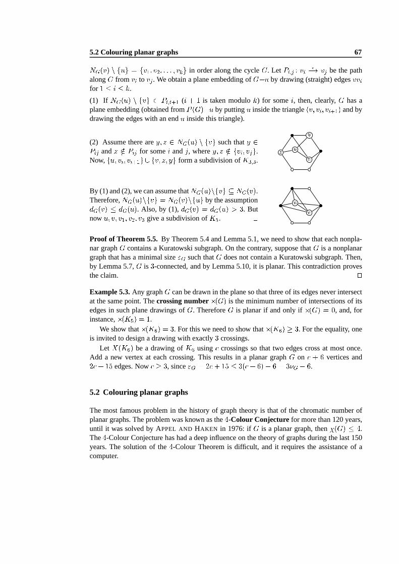
5.2 Colouring planar graphs 67NG(v) n fug = fv1; v2; : : : ; vkg in order along the cycleC. Let Pi;j : vi ?�! vj be the pathalongC from vi to vj. We obtain a plane embedding ofG�u by drawing (straight) edgesvvifor 1 � i � k.
(1) If NG(u) n fvg 2 Pi;i+1 (i + 1 is taken modulok) for somei, then, clearly,G has aplane embedding (obtained fromP (G)�u by puttingu inside the triangle(v; vi; vi+1) and bydrawing the edges with an endu inside this triangle).
(2) Assume there arey; z 2 NG(u) n fvg such thaty 2Pij andz =2 Pij for somei andj, wherey; z =2 fvi; vjg.Now, fu; vi; vi+1g [ fv; z; yg form a subdivision ofK3;3. vu yzBy (1) and (2), we can assume thatNG(u)nfvg � NG(v).Therefore,NG(u)nfvg = NG(v)nfug by the assumptiondG(v) � dG(u). Also, by (1),dG(v) = dG(u) > 3. Butnowu; v; v1; v2; v3 give a subdivision ofK5. ut vuProof of Theorem 5.5. By Theorem 5.4 and Lemma 5.1, we need to show that each nonpla-nar graphG contains a Kuratowski subgraph. On the contrary, suppose thatG is a nonplanargraph that has a minimal size"G such thatG does not contain a Kuratowski subgraph. Then,by Lemma 5.7,G is 3-connected, and by Lemma 5.10, it is planar. This contradiction provesthe claim. utExample 5.3.Any graphG can be drawn in the plane so that three of its edges never intersectat the same point. Thecrossing number�(G) is the minimum number of intersections of itsedges in such plane drawings ofG. ThereforeG is planar if and only if�(G) = 0, and, forinstance,�(K5) = 1.
We show that�(K6) = 3. For this we need to show that�(K6) � 3. For the equality, oneis invited to design a drawing with exactly3 crossings.
Let X(K6) be a drawing ofK6 using crossings so that two edges cross at most once.Add a new vertex at each crossing. This results in a planar graph G on + 6 vertices and2 + 15 edges. Now � 3, since"G = 2 + 15 � 3( + 6)� 6 = 3�G � 6.
5.2 Colouring planar graphs
The most famous problem in the history of graph theory is thatof the chromatic number ofplanar graphs. The problem was known as the4-Colour Conjecture for more than 120 years,until it was solved by APPEL AND HAKEN in 1976: ifG is a planar graph, then�(G) � 4.The4-Colour Conjecture has had a deep influence on the theory of graphs during the last 150years. The solution of the4-Colour Theorem is difficult, and it requires the assistanceof acomputer.
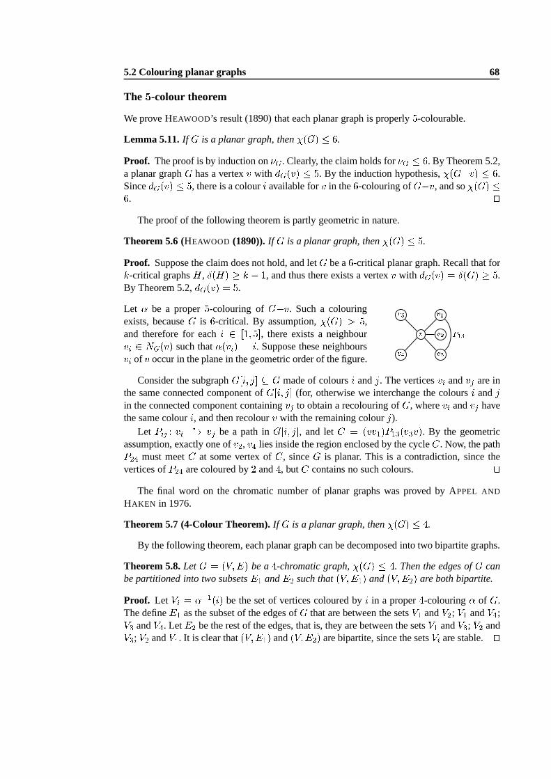
5.2 Colouring planar graphs 68
The 5-colour theorem
We prove HEAWOOD’s result (1890) that each planar graph is properly5-colourable.
Lemma 5.11.If G is a planar graph, then�(G) � 6.
Proof. The proof is by induction on�G. Clearly, the claim holds for�G � 6. By Theorem 5.2,a planar graphG has a vertexv with dG(v) � 5. By the induction hypothesis,�(G�v) � 6.SincedG(v) � 5, there is a colouri available forv in the6-colouring ofG�v, and so�(G) �6. ut
The proof of the following theorem is partly geometric in nature.
Theorem 5.6 (HEAWOOD (1890)).If G is a planar graph, then�(G) � 5.
Proof. Suppose the claim does not hold, and letG be a6-critical planar graph. Recall that fork-critical graphsH, Æ(H) � k � 1, and thus there exists a vertexv with dG(v) = Æ(G) � 5.By Theorem 5.2,dG(v) = 5.
Let � be a proper5-colouring ofG�v. Such a colouringexists, becauseG is 6-critical. By assumption,�(G) > 5,and therefore for eachi 2 [1; 5℄, there exists a neighbourvi 2 NG(v) such that�(vi) = i. Suppose these neighboursvi of v occur in the plane in the geometric order of the figure.
vv4v5 v3v2v1 P13Consider the subgraphG[i; j℄ � G made of coloursi andj. The verticesvi andvj are in
the same connected component ofG[i; j℄ (for, otherwise we interchange the coloursi andjin the connected component containingvj to obtain a recolouring ofG, wherevi andvj havethe same colouri, and then recolourv with the remaining colourj).
Let Pij : vi ?�! vj be a path inG[i; j℄, and letC = (vv1)P13(v3v). By the geometricassumption, exactly one ofv2, v4 lies inside the region enclosed by the cycleC. Now, the pathP24 must meetC at some vertex ofC, sinceG is planar. This is a contradiction, since thevertices ofP24 are coloured by2 and4, butC contains no such colours. ut
The final word on the chromatic number of planar graphs was proved by APPEL AND
HAKEN in 1976.
Theorem 5.7 (4-Colour Theorem).If G is a planar graph, then�(G) � 4.
By the following theorem, each planar graph can be decomposed into two bipartite graphs.
Theorem 5.8.LetG = (V;E) be a4-chromatic graph,�(G) � 4. Then the edges ofG canbe partitioned into two subsetsE1 andE2 such that(V;E1) and(V;E2) are both bipartite.
Proof. Let Vi = ��1(i) be the set of vertices coloured byi in a proper4-colouring� of G.The defineE1 as the subset of the edges ofG that are between the setsV1 andV2; V1 andV4;V3 andV4. LetE2 be the rest of the edges, that is, they are between the setsV1 andV3; V2 andV3; V2 andV4. It is clear that(V;E1) and(V;E2) are bipartite, since the setsVi are stable. ut
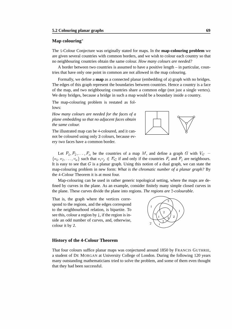
5.2 Colouring planar graphs 69
Map colouring�The4-Colour Conjecture was originally stated for maps. In themap-colouring problem weare given several countries with common borders, and we wishto colour each country so thatno neighbouring countries obtain the same colour.How many colours are needed?
A border between two countries is assumed to have a positive length – in particular, coun-tries that have only one point in common are not allowed in themap colouring.
Formally, we define amap as a connected planar (embedding of a) graph with no bridges.The edges of this graph represent the boundaries between countries. Hence a country is a faceof the map, and two neighbouring countries share a common edge (not just a single vertex).We deny bridges, because a bridge in such a map would be a boundary inside a country.
The map-colouring problem is restated as fol-lows:
How many colours are needed for the faces of aplane embedding so that no adjacent faces obtainthe same colour.
The illustrated map can be4-coloured, and it can-not be coloured using only3 colours, because ev-ery two faces have a common border.
Let F1; F2; : : : ; Fn be the countries of a mapM , and define a graphG with VG =fv1; v2; : : : ; vng such thatvivj 2 EG if and only if the countriesFi andFj are neighbours.It is easy to see thatG is a planar graph. Using this notion of a dual graph, we can state themap-colouring problem in new form:What is the chromatic number of a planar graph?Bythe4-Colour Theorem it is at most four.
Map-colouring can be used in rather generic topological setting, where the maps are de-fined by curves in the plane. As an example, consider finitely many simple closed curves inthe plane. These curves divide the plane into regions.The regions are2-colourable.
That is, the graph where the vertices corre-spond to the regions, and the edges correspondto the neighbourhood relation, is bipartite. Tosee this, colour a region by1, if the region is in-side an odd number of curves, and, otherwise,colour it by2.
21 2 1 21 2 1 2 112History of the 4-Colour Theorem
That four colours suffice planar maps was conjectured around1850 by FRANCIS GUTHRIE,a student of DE MORGAN at University College of London. During the following 120 yearsmany outstanding mathematicians tried to solve the problem, and some of them even thoughtthat they had been successful.
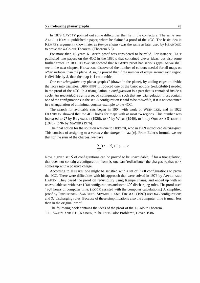
5.2 Colouring planar graphs 70
In 1879 CAYLEY pointed out some difficulties that lie in the conjecture. Thesame yearALFRED KEMPE published a paper, where he claimed a proof of the 4CC. The basic idea inKEMPE’s argument (known later asKempe chains) was the same as later used by HEAWOOD
to prove the5-Colour Theorem, (Theorem 5.6).For more than 10 years KEMPE’s proof was considered to be valid. For instance, TAIT
published two papers on the 4CC in the 1880’s that contained clever ideas, but also somefurther errors. In 1890 HEAWOOD showed that KEMPE’s proof had serious gaps. As we shallsee in the next chapter, HEAWOOD discovered the number of colours needed for all maps onothersurfaces than the plane. Also, he proved that if the number ofedges around each regionis divisible by3, then the map is4-colourable.
One cantriangulateany planar graphG (drawn in the plane), by adding edges to dividethe faces into triangles. BIRKHOFF introduced one of the basic notions (reducibility) neededin the proof of the 4CC. In a triangulation, aconfigurationis a part that is contained inside acycle. Anunavoidable setis a set of configurations such that any triangulation must containone of the configurations in the set. A configuration is said tobereducible, if it is not containedin a triangulation of a minimal counter example to the 4CC.
The search for avoidable sets began in 1904 with work of WEINICKE, and in 1922FRANKLIN showed that the 4CC holds for maps with at most25 regions. This number wasincreased to27 by REYNOLDS (1926), to35 by WINN (1940), to39 by ORE AND STEMPLE
(1970), to95 by MAYER (1976).The final notion for the solution was due to HEESCH, who in 1969 introduceddischarging.
This consists of assigning to a vertexv thecharge6 � dG(v). From Euler’s formula we seethat for the sum of the charges, we haveXv (6 � dG(v)) = 12:Now, a given setS of configurations can be proved to be unavoidable, if for a triangulation,that does not contain a configuration fromS, one can ‘redistribute’ the charges so that novcomes up with a positive charge.
According to HEESCH one might be satisfied with a set of8900 configurations to provethe 4CC. There were difficulties with his approach that were solved in 1976 by APPEL AND
HAKEN. They based the proof on reducibility using Kempe chains, and ended up with anunavoidable set with over1900 configurations and some300 discharging rules. The proof used1200 hours of computer time. (KOCH assisted with the computer calculations.) A simplifiedproof by ROBERTSON, SANDERS, SEYMOUR AND THOMAS (1997) uses633 configurationsand32 discharging rules. Because of these simplifications also the computer time is much lessthan in the original proof.
The following book contains the ideas of the proof of the4-Colour Theorem.T.L. SAATY AND P.C. KAINEN, “The Four-Color Problem”, Dover, 1986.
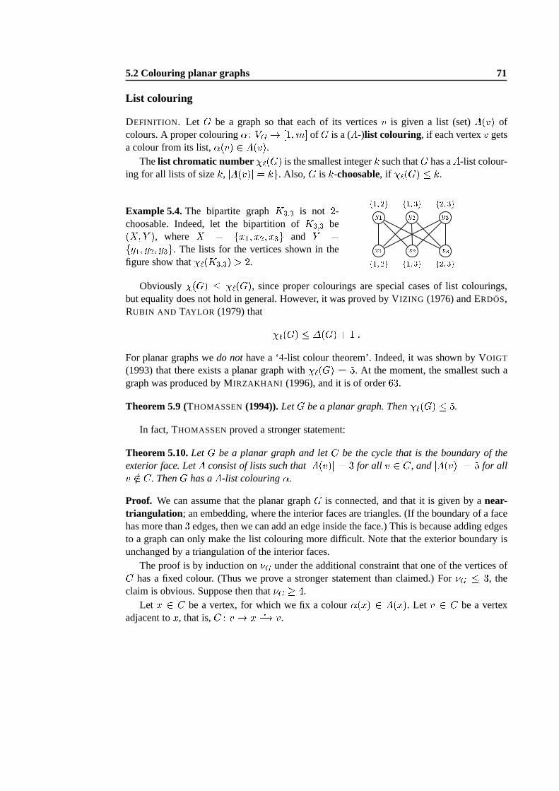
5.2 Colouring planar graphs 71
List colouring
DEFINITION. Let G be a graph so that each of its verticesv is given a list (set)�(v) ofcolours. A proper colouring� : VG ! [1;m℄ ofG is a (�-)list colouring, if each vertexv getsa colour from its list,�(v) 2 �(v).
Thelist chromatic number �`(G) is the smallest integerk such thatG has a�-list colour-ing for all lists of sizek, j�(v)j = kg. Also,G is k-choosable, if �`(G) � k.
Example 5.4.The bipartite graphK3;3 is not 2-choosable. Indeed, let the bipartition ofK3;3 be(X;Y ), where X = fx1; x2; x3g and Y =fy1; y2; y3g. The lists for the vertices shown in thefigure show that�`(K3;3) > 2.
x1f1; 2gy1f1; 2g x2f1; 3gy2f1; 3g x3f2; 3gy3f2; 3gObviously�(G) � �`(G), since proper colourings are special cases of list colourings,
but equality does not hold in general. However, it was provedby VIZING (1976) and ERDÖS,RUBIN AND TAYLOR (1979) that �`(G) � �(G) + 1 :For planar graphs wedo nothave a ‘4-list colour theorem’. Indeed, it was shown by VOIGT
(1993) that there exists a planar graph with�`(G) = 5. At the moment, the smallest such agraph was produced by MIRZAKHANI (1996), and it is of order63.
Theorem 5.9 (THOMASSEN (1994)).LetG be a planar graph. Then�`(G) � 5.
In fact, THOMASSENproved a stronger statement:
Theorem 5.10.LetG be a planar graph and letC be the cycle that is the boundary of theexterior face. Let� consist of lists such thatj�(v)j = 3 for all v 2 C, andj�(v)j = 5 for allv =2 C. ThenG has a�-list colouring�.
Proof. We can assume that the planar graphG is connected, and that it is given by anear-triangulation ; an embedding, where the interior faces are triangles. (If the boundary of a facehas more than3 edges, then we can add an edge inside the face.) This is because adding edgesto a graph can only make the list colouring more difficult. Note that the exterior boundary isunchanged by a triangulation of the interior faces.
The proof is by induction on�G under the additional constraint that one of the vertices ofC has a fixed colour. (Thus we prove a stronger statement than claimed.) For�G � 3, theclaim is obvious. Suppose then that�G � 4.
Let x 2 C be a vertex, for which we fix a colour�(x) 2 �(x). Let v 2 C be a vertexadjacent tox, that is,C : v ! x ?�! v.
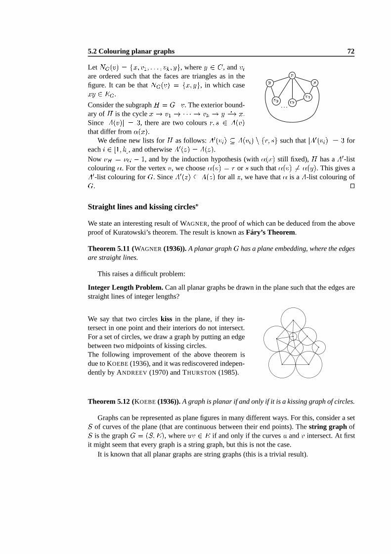
5.2 Colouring planar graphs 72
LetNG(v) = fx; v1; : : : ; vk; yg, wherey 2 C, andviare ordered such that the faces are triangles as in thefigure. It can be thatNG(v) = fx; yg, in which casexy 2 EG.
Consider the subgraphH = G�v. The exterior bound-ary ofH is the cyclex! v1 ! � � � ! vk ! y ?�! x:Sincej�(v)j = 3, there are two coloursr; s 2 �(v)that differ from�(x).
v xy v1v2vk : : :We define new lists forH as follows:�0(vi) � �(vi) n fr; sg such thatj�0(vi)j = 3 for
eachi 2 [1; k℄, and otherwise�0(z) = �(z).Now �H = �G � 1, and by the induction hypothesis (with�(x) still fixed),H has a�0-listcolouring�. For the vertexv, we choose�(v) = r or s such that�(v) 6= �(y). This gives a�0-list colouring forG. Since�0(z) � �(z) for all z, we have that� is a�-list colouring ofG. utStraight lines and kissing circles�We state an interesting result of WAGNER, the proof of which can be deduced from the aboveproof of Kuratowski’s theorem. The result is known asFáry’s Theorem.
Theorem 5.11 (WAGNER (1936)).A planar graphG has a plane embedding, where the edgesare straight lines.
This raises a difficult problem:
Integer Length Problem. Can all planar graphs be drawn in the plane such that the edgesarestraight lines of integer lengths?
We say that two circleskiss in the plane, if they in-tersect in one point and their interiors do not intersect.For a set of circles, we draw a graph by putting an edgebetween two midpoints of kissing circles.The following improvement of the above theorem isdue to KOEBE (1936), and it was rediscovered indepen-dently by ANDREEV (1970) and THURSTON (1985).
� �� ��� ��Theorem 5.12 (KOEBE (1936)).A graph is planar if and only if it is a kissing graph of circles.
Graphs can be represented as plane figures in many different ways. For this, consider a setS of curves of the plane (that are continuous between their endpoints). Thestring graph ofS is the graphG = (S;E), whereuv 2 E if and only if the curvesu andv intersect. At firstit might seem that every graph is a string graph, but this is not the case.
It is known that all planar graphs are string graphs (this is atrivial result).
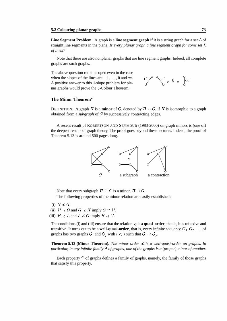
5.2 Colouring planar graphs 73
Line Segment Problem.A graph is aline segment graphif it is a string graph for a setL ofstraight line segments in the plane.Is every planar graph a line segment graph for some setLof lines?
Note that there are also nonplanar graphs that are line segment graphs. Indeed, all completegraphs are such graphs.
The above question remains open even in the casewhen the slopes of the lines are+1,�1, 0 and1.A positive answer to this4-slope problem for pla-nar graphs would prove the4-Colour Theorem.
+1 �1 0 1The Minor Theorem�DEFINITION. A graphH is aminor of G, denoted byH 4 G, if H is isomorphic to a graphobtained from asubgraphof G by successively contracting edges.
A recent result of ROBERTSON ANDSEYMOUR (1983-2000) on graph minors is (one of)the deepest results of graph theory. The proof goes beyond these lectures. Indeed, the proof ofTheorem 5.13 is around 500 pages long.
G a subgraph a contraction
eNote that every subgraphH � G is a minor,H 4 G.The following properties of the minor relation are easily established:
(i) G 4 G,(ii) H 4 G andG 4 H imply G �= H,(iii) H 4 L andL 4 G imply H 4 G.
The conditions (i) and (iii) ensure that the relation4 is aquasi-order, that is, it is reflexive andtransitive. It turns out to be awell-quasi-order, that is, every infinite sequenceG1; G2; : : : ofgraphs has two graphsGi andGj with i < j such thatGi 4 Gj.Theorem 5.13 (Minor Theorem). The minor order4 is a well-quasi-order on graphs. Inparticular, in any infinite familyF of graphs, one of the graphs is a (proper) minor of another.
Each propertyP of graphs defines a family of graphs, namely, the family of those graphsthat satisfy this property.
5.3 Genus of a graph 74
DEFINITION. A family F of graphs is said to beminor closed, if every minorH of a graphG 2 F is also inF. A propertyP of graphs is said to beinherited by minors, if all minors ofa graphG satisfyP wheneverG does.
The following families of graphs are minor closed: the family of (1) all graphs, (2) planargraphs (and their generalizations to other surfaces), (3) acyclic graphs.The acyclic graphs include all trees. However, the family oftrees is not closed under takingsubgraphs, and thus it is not minor closed. More importantly, the subgraph order of trees(T1 � T2) is not a well-quasi-order.
WAGNER proved a minor version of Kuratowski’s theorem:
Theorem 5.14 (WAGNER (1937)).A graphG is nonplanar if and only ifK5 4 G or K3;3 4G.
Proof. Exercise. utROBERTSON ANDSEYMOUR (1998) proved theWagner’s conjecture:
Theorem 5.15 (Minor Theorem 2).LetP be a property of graphs inherited by minors. Thenthere exists afinite setF of graphs such thatG satisfiesP if and only ifG does not have aminor fromF.
One of the impressive application of Theorem 5.15 concerns embeddings of graphs onsurfaces, see the next chapters. By Theorem 5.15, one can test (with a fastalgorithm) whethera graph can be embedded onto a surface.
Every graph can be drawn in the3-dimensional space without crossing edges. An oldproblem asks if there exists an algorithm that would determine whether a graph can be drawnso that its cycles do not form (nontrivial) knots. This problem is solved by the above results,since the property ‘knotless’ is inherited by minors: thereexistsa fast algorithm to do the job.However, this algorithm is not known!
Hadwiger’s Problem. HADWIGER conjectured in 1943 that for every graphG,K�(G) 4 G ;that is,if �(G) � r, thenG has a complete graphKr as its minor. The conjecture is trivialfor r = 2, and it is known to hold for allr � 6. The cases forr = 5 and6 follow from the4-Colour Theorem.
5.3 Genus of a graph
A graph is planar, if it can be drawn in the plane without crossing edges. A plane is an im-portant special case of a surface. In this section we study shortly drawing graphs in othersurfaces.
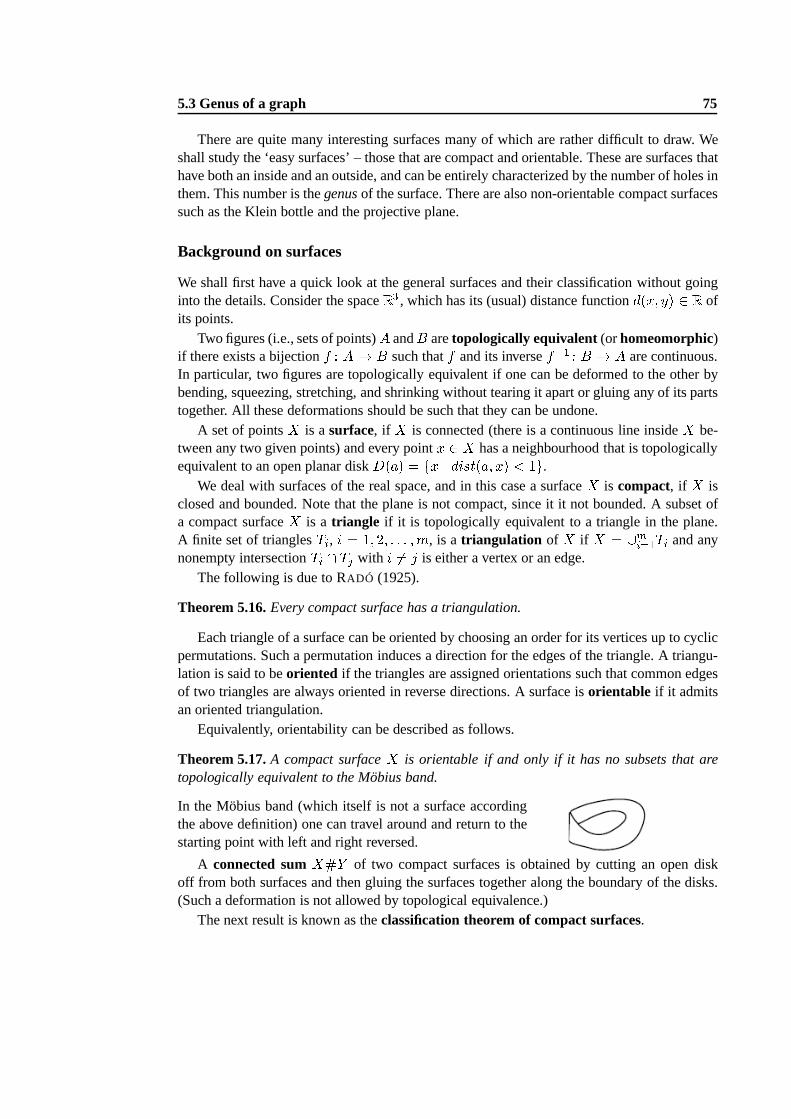
5.3 Genus of a graph 75
There are quite many interesting surfaces many of which are rather difficult to draw. Weshall study the ‘easy surfaces’ – those that are compact and orientable. These are surfaces thathave both an inside and an outside, and can be entirely characterized by the number of holes inthem. This number is thegenusof the surface. There are also non-orientable compact surfacessuch as the Klein bottle and the projective plane.
Background on surfaces
We shall first have a quick look at the general surfaces and their classification without goinginto the details. Consider the spaceR3 , which has its (usual) distance functiond(x; y) 2 R ofits points.
Two figures (i.e., sets of points)A andB aretopologically equivalent(orhomeomorphic)if there exists a bijectionf : A! B such thatf and its inversef�1 : B ! A are continuous.In particular, two figures are topologically equivalent if one can be deformed to the other bybending, squeezing, stretching, and shrinking without tearing it apart or gluing any of its partstogether. All these deformations should be such that they can be undone.
A set of pointsX is asurface, if X is connected (there is a continuous line insideX be-tween any two given points) and every pointx 2 X has a neighbourhood that is topologicallyequivalent to an open planar diskD(a) = fx j dist(a; x) < 1g.
We deal with surfaces of the real space, and in this case a surfaceX is compact, if X isclosed and bounded. Note that the plane is not compact, sinceit it not bounded. A subset ofa compact surfaceX is a triangle if it is topologically equivalent to a triangle in the plane.A finite set of trianglesTi, i = 1; 2; : : : ;m, is a triangulation of X if X = [mi=1Ti and anynonempty intersectionTi \ Tj with i 6= j is either a vertex or an edge.
The following is due to RADÓ (1925).
Theorem 5.16.Every compact surface has a triangulation.
Each triangle of a surface can be oriented by choosing an order for its vertices up to cyclicpermutations. Such a permutation induces a direction for the edges of the triangle. A triangu-lation is said to beoriented if the triangles are assigned orientations such that commonedgesof two triangles are always oriented in reverse directions.A surface isorientable if it admitsan oriented triangulation.
Equivalently, orientability can be described as follows.
Theorem 5.17.A compact surfaceX is orientable if and only if it has no subsets that aretopologically equivalent to the Möbius band.
In the Möbius band (which itself is not a surface accordingthe above definition) one can travel around and return to thestarting point with left and right reversed.
A connected sumX#Y of two compact surfaces is obtained by cutting an open diskoff from both surfaces and then gluing the surfaces togetheralong the boundary of the disks.(Such a deformation is not allowed by topological equivalence.)
The next result is known as theclassification theorem of compact surfaces.
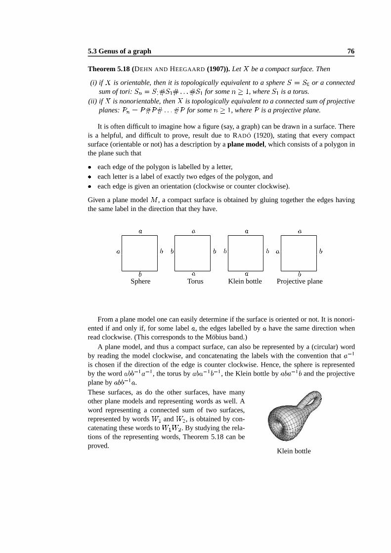
5.3 Genus of a graph 76
Theorem 5.18 (DEHN AND HEEGAARD (1907)).LetX be a compact surface. Then
(i) if X is orientable, then it is topologically equivalent to a sphere S = S0 or a connectedsum of tori:Sn = S1#S1# : : :#S1 for somen � 1, whereS1 is a torus.
(ii) if X is nonorientable, thenX is topologically equivalent to a connected sum of projectiveplanes:Pn = P#P# : : :#P for somen � 1, whereP is a projective plane.
It is often difficult to imagine how a figure (say, a graph) can be drawn in a surface. Thereis a helpful, and difficult to prove, result due to RADÓ (1920), stating that every compactsurface (orientable or not) has a description by aplane model, which consists of a polygon inthe plane such that� each edge of the polygon is labelled by a letter,� each letter is a label of exactly two edges of the polygon, and� each edge is given an orientation (clockwise or counter clockwise).
Given a plane modelM , a compact surface is obtained by gluing together the edges havingthe same label in the direction that they have.
a a bbSphere
b a baTorus
b a baKlein bottle
a a bbProjective plane
From a plane model one can easily determine if the surface is oriented or not. It is nonori-ented if and only if, for some labela, the edges labelled bya have the same direction whenread clockwise. (This corresponds to the Möbius band.)
A plane model, and thus a compact surface, can also be represented by a (circular) wordby reading the model clockwise, and concatenating the labels with the convention thata�1is chosen if the direction of the edge is counter clockwise. Hence, the sphere is representedby the wordabb�1a�1, the torus byaba�1b�1, the Klein bottle byaba�1b and the projectiveplane byabb�1a.These surfaces, as do the other surfaces, have manyother plane models and representing words as well. Aword representing a connected sum of two surfaces,represented by wordsW1 andW2, is obtained by con-catenating these words toW1W2. By studying the rela-tions of the representing words, Theorem 5.18 can beproved.
Klein bottle
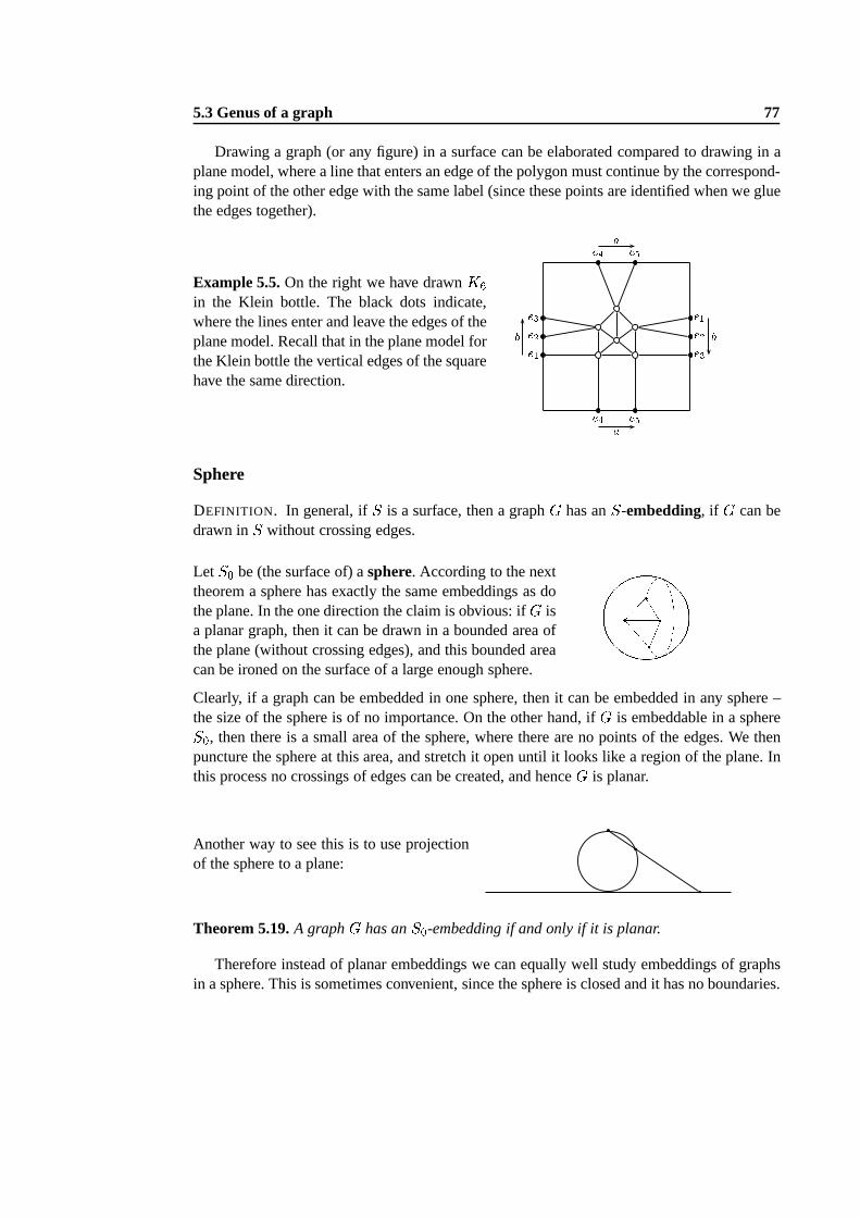
5.3 Genus of a graph 77
Drawing a graph (or any figure) in a surface can be elaborated compared to drawing in aplane model, where a line that enters an edge of the polygon must continue by the correspond-ing point of the other edge with the same label (since these points are identified when we gluethe edges together).
Example 5.5.On the right we have drawnK6in the Klein bottle. The black dots indicate,where the lines enter and leave the edges of theplane model. Recall that in the plane model forthe Klein bottle the vertical edges of the squarehave the same direction.
ba
bae1e2e3
e4 e5 e1e2e3e5e4Sphere
DEFINITION. In general, ifS is a surface, then a graphG has anS-embedding, if G can bedrawn inS without crossing edges.
LetS0 be (the surface of) asphere. According to the nexttheorem a sphere has exactly the same embeddings as dothe plane. In the one direction the claim is obvious: ifG isa planar graph, then it can be drawn in a bounded area ofthe plane (without crossing edges), and this bounded areacan be ironed on the surface of a large enough sphere.
����Clearly, if a graph can be embedded in one sphere, then it can be embedded in any sphere –the size of the sphere is of no importance. On the other hand, if G is embeddable in a sphereS0, then there is a small area of the sphere, where there are no points of the edges. We thenpuncture the sphere at this area, and stretch it open until itlooks like a region of the plane. Inthis process no crossings of edges can be created, and henceG is planar.
Another way to see this is to use projectionof the sphere to a plane:
Theorem 5.19.A graphG has anS0-embedding if and only if it is planar.
Therefore instead of planar embeddings we can equally well study embeddings of graphsin a sphere. This is sometimes convenient, since the sphere is closed and it has no boundaries.
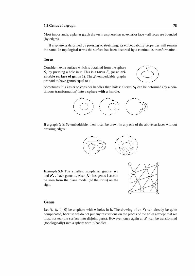
5.3 Genus of a graph 78
Most importantly, a planar graph drawn in a sphere has no exterior face – all faces are bounded(by edges).
If a sphere is deformed by pressing or stretching, its embeddability properties will remainthe same. In topological terms the surface has been distorted by a continuous transformation.
Torus
Consider next a surface which is obtained from the sphereS0 by pressing a hole in it. This is atorus S1 (or anori-entable surface of genus1). TheS1-embeddable graphsare said to havegenusequal to 1.
����Sometimes it is easier to consider handles than holes: a torusS1 can be deformed (by a con-tinuous transformation) into asphere with a handle.
���� ���� ����If a graphG is S1-embeddable, then it can be drawn in any one of the above surfaces withoutcrossing edges.
���� ����Example 5.6.The smallest nonplanar graphsK5andK3;3 have genus1. Also,K7 has genus1 as canbe seen from the plane model (of the torus) on theright. 1
1 112 3 4
5 6 7Genus
Let Sn (n � 0) be a sphere withn holes in it. The drawing of anS4 can already be quitecomplicated, because we do not put any restrictions on the places of the holes (except that wemust not tear the surface into disjoint parts). However, once again anSn can be transformed(topologically) into a sphere withn handles.
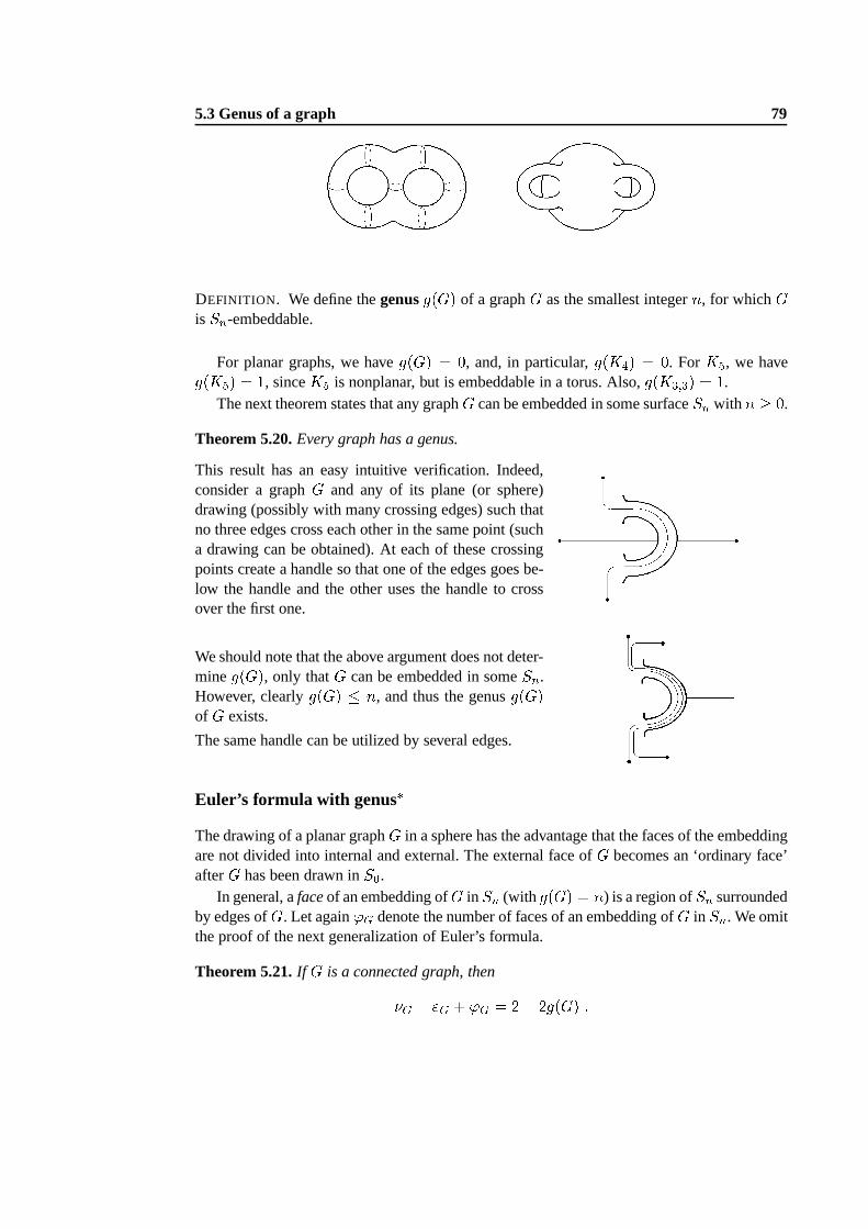
5.3 Genus of a graph 79
������ ������DEFINITION. We define thegenusg(G) of a graphG as the smallest integern, for whichGis Sn-embeddable.
For planar graphs, we haveg(G) = 0, and, in particular,g(K4) = 0. ForK5, we haveg(K5) = 1, sinceK5 is nonplanar, but is embeddable in a torus. Also,g(K3;3) = 1.The next theorem states that any graphG can be embedded in some surfaceSn with n � 0.
Theorem 5.20.Every graph has a genus.
This result has an easy intuitive verification. Indeed,consider a graphG and any of its plane (or sphere)drawing (possibly with many crossing edges) such thatno three edges cross each other in the same point (sucha drawing can be obtained). At each of these crossingpoints create a handle so that one of the edges goes be-low the handle and the other uses the handle to crossover the first one.
������We should note that the above argument does not deter-mineg(G), only thatG can be embedded in someSn.However, clearlyg(G) � n, and thus the genusg(G)of G exists.
The same handle can be utilized by several edges.
������Euler’s formula with genus�The drawing of a planar graphG in a sphere has the advantage that the faces of the embeddingare not divided into internal and external. The external face ofG becomes an ‘ordinary face’afterG has been drawn inS0.
In general, afaceof an embedding ofG in Sn (with g(G) = n) is a region ofSn surroundedby edges ofG. Let again'G denote the number of faces of an embedding ofG in Sn. We omitthe proof of the next generalization of Euler’s formula.
Theorem 5.21.If G is a connected graph, then�G � "G + 'G = 2� 2g(G) :
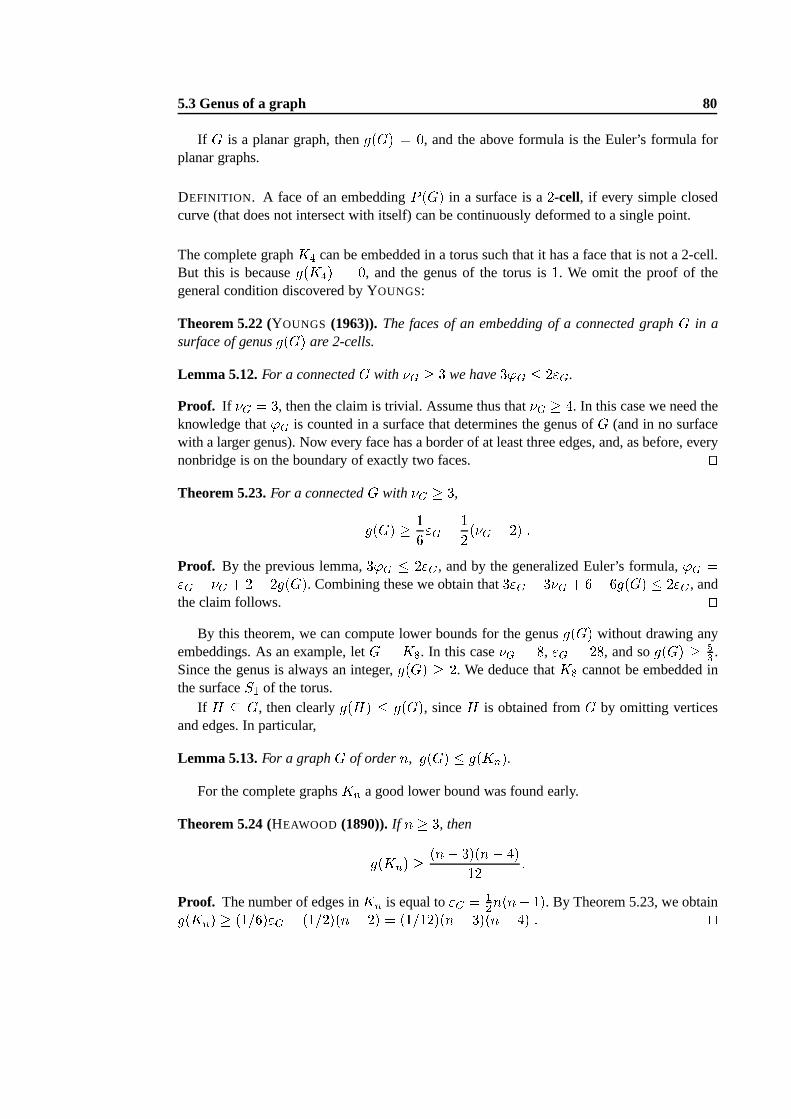
5.3 Genus of a graph 80
If G is a planar graph, theng(G) = 0, and the above formula is the Euler’s formula forplanar graphs.
DEFINITION. A face of an embeddingP (G) in a surface is a2-cell, if every simple closedcurve (that does not intersect with itself) can be continuously deformed to a single point.
The complete graphK4 can be embedded in a torus such that it has a face that is not a 2-cell.But this is becauseg(K4) = 0, and the genus of the torus is1. We omit the proof of thegeneral condition discovered by YOUNGS:
Theorem 5.22 (YOUNGS (1963)).The faces of an embedding of a connected graphG in asurface of genusg(G) are 2-cells.
Lemma 5.12.For a connectedG with �G � 3 we have3'G � 2"G.
Proof. If �G = 3, then the claim is trivial. Assume thus that�G � 4. In this case we need theknowledge that'G is counted in a surface that determines the genus ofG (and in no surfacewith a larger genus). Now every face has a border of at least three edges, and, as before, everynonbridge is on the boundary of exactly two faces. utTheorem 5.23.For a connectedG with �G � 3,g(G) � 16"G � 12(�G � 2) :Proof. By the previous lemma,3'G � 2"G, and by the generalized Euler’s formula,'G ="G � �G + 2� 2g(G). Combining these we obtain that3"G � 3�G + 6� 6g(G) � 2"G, andthe claim follows. ut
By this theorem, we can compute lower bounds for the genusg(G) without drawing anyembeddings. As an example, letG = K8. In this case�G = 8, "G = 28, and sog(G) � 53 .Since the genus is always an integer,g(G) � 2. We deduce thatK8 cannot be embedded inthe surfaceS1 of the torus.
If H � G, then clearlyg(H) � g(G), sinceH is obtained fromG by omitting verticesand edges. In particular,
Lemma 5.13.For a graphG of ordern, g(G) � g(Kn).For the complete graphsKn a good lower bound was found early.
Theorem 5.24 (HEAWOOD (1890)).If n � 3, theng(Kn) � (n� 3)(n� 4)12 :Proof. The number of edges inKn is equal to"G = 12n(n� 1). By Theorem 5.23, we obtaing(Kn) � (1=6)"G � (1=2)(n � 2) = (1=12)(n � 3)(n� 4) : ut
5.3 Genus of a graph 81
This result was dramatically improved to obtain
Theorem 5.25 (RINGEL AND YOUNGS(1968)).If n � 3, theng(Kn) = �(n� 3)(n� 4)12 � :Thereforeg(K6) = d3 � 2=12e = d1=2e = 1. Also, g(K7) = 1, butg(K8) = 2.By Theorem 5.25,
Theorem 5.26.For all graphsG of ordern � 3,g(G) � �(n� 3)(n� 4)12 � :Also, we know the exact genus for the complete bipartite graphs:
Theorem 5.27 (RINGEL (1965)).For the complete bipartite graphs,g(Km;n) = �(m� 2)(n� 2)4 � :Chromatic numbers�For the planar graphsG, the proof of the4-Colour Theorem,�(G) � 4, is extremely longand difficult. This in mind, it is surprising that the generalization of the4-Colour Theorem forgenus� 1 is much easier. HEAWOOD proved a hundred years ago:
Theorem 5.28 (HEAWOOD). If g(G) = g � 1, then�(G) � �7 +p1 + 48g2 � :Notice that forg = 0 this theorem would be the4-colour theorem. HEAWOOD proved it
‘only’ for g � 1.Using the result of RINGEL AND YOUNGS and some elementary computations we can
prove that the above theorem is the best possible.
Theorem 5.29.For eachg � 1, there exists a graphG with genusg(G) = g so that�(G) = �7 +p1 + 48g2 � :If a nonplanar graphG can be embedded in a torus, theng(G) = 1, and�(G) � b(7 +p1 + 48g)=2 = 7. Moreover, forG = K7 we have that�(K7) = 7 andg(K7) = 1.
5.3 Genus of a graph 82
Three dimensions�Every graph can be drawn without crossing edges in the3-dimensional space. Such a drawingis calledspatial embeddingof the graph. Indeed, such an embedding can be achieved byputting all vertices ofG on a line, and then drawing the edges in different planes thatcontainthe line. Alternatively, the vertices ofG can be put in a sphere, and drawing the edges asstraight lines crossing the sphere inside.
A spatial embedding of a graphG is said to havelinked cycles, if two cycles ofG form alink (they cannot be separated in the space). By CONWAY and GORDON in 1983 every spatialembedding ofK6 contains linked cycles.
It was shown by ROBERTSON, SEYMOUR AND THOMAS (1993) that there is a set of7graphs such that a graphG has a spatial embedding without linked cycles if and only ifGdoes not have a minor belonging to this set.
This family of forbidden graphs was originally found by SACHS (without proof), and itcontainsK6 and the Petersen graph. Every graph in the set has15 edges, which is curious.
For further results and proofs concerning graphs in surfaces, see
B. MOHAR AND C. THOMASSEN, “Graphs on Surfaces”, Johns Hopkins, 2001.
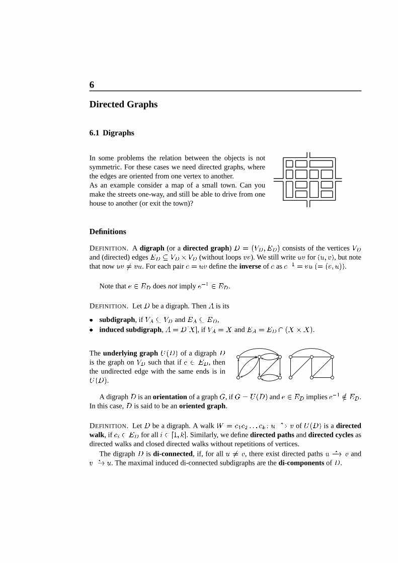
6
Directed Graphs
6.1 Digraphs
In some problems the relation between the objects is notsymmetric. For these cases we need directed graphs, wherethe edges are oriented from one vertex to another.As an example consider a map of a small town. Can youmake the streets one-way, and still be able to drive from onehouse to another (or exit the town)?
Definitions
DEFINITION. A digraph (or adirected graph) D = (VD; ED) consists of the verticesVDand (directed) edgesED � VD � VD (without loopsvv). We still writeuv for (u; v), but notethat nowuv 6= vu. For each paire = uv define theinverseof e ase�1 = vu (= (v; u)).
Note thate 2 ED doesnot imply e�1 2 ED.
DEFINITION. LetD be a digraph. ThenA is its� subdigraph, if VA � VD andEA � ED,� induced subdigraph,A = D[X℄, if VA = X andEA = ED \ (X �X).The underlying graph U(D) of a digraphDis the graph onVD such that ife 2 ED, thenthe undirected edge with the same ends is inU(D).
A digraphD is anorientation of a graphG, if G = U(D) ande 2 ED impliese�1 =2 ED.In this case,D is said to be anoriented graph.
DEFINITION. LetD be a digraph. A walkW = e1e2 : : : ek : u ?�! v of U(D) is adirectedwalk, if ei 2 ED for all i 2 [1; k℄. Similarly, we definedirected pathsanddirected cyclesasdirected walks and closed directed walks without repetitions of vertices.
The digraphD is di-connected, if, for all u 6= v, there exist directed pathsu ?�! v andv ?�! u. The maximal induced di-connected subdigraphs are thedi-componentsof D.
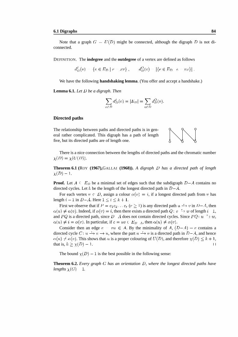
6.1 Digraphs 84
Note that a graphG = U(D) might be connected, although the digraphD is not di-connected.
DEFINITION. Theindegreeand theoutdegreeof a vertex are defined as followsdID(v) = jfe 2 ED j e = xvgj; dOD(v) = jfe 2 ED j e = vxgj :We have the followinghandshaking lemma. (You offer and accept a handshake.)
Lemma 6.1.LetD be a digraph. ThenXv2D dID(v) = jEDj = Xv2D dOD(v):Directed paths
The relationship between paths and directed paths is in gen-eral rather complicated. This digraph has a path of lengthfive, but its directed paths are of length one.
There is a nice connection between the lengths of directed paths and the chromatic number�(D) = �(U(D)).Theorem 6.1 (ROY (1967),GALLAI (1968)). A digraph D has a directed path of length�(D)� 1.
Proof. Let A � ED be a minimal set of edges such that the subdigraphD�A contains nodirected cycles. Letk be the length of the longest directed path inD�A.
For each vertexv 2 D, assign a colour�(v) = i, if a longest directed path fromv haslengthi� 1 in D�A. Here1 � i � k + 1.
First we observe that ifP = e1e2 : : : er (r � 1) is any directed pathu ?�! v in D�A, then�(u) 6= �(v). Indeed, if�(v) = i, then there exists a directed pathQ : v ?�! w of lengthi�1,andPQ is a directed path, sinceD�A does not contain directed cycles. SincePQ : u ?�! w,�(u) 6= i = �(v). In particular, ife = uv 2 ED�A, then�(u) 6= �(v).
Consider then an edgee = vu 2 A. By the minimality ofA, (D�A) + e contains adirected cycleC : u ?�! v �! u, where the partu ?�! v is a directed path inD�A, and hence�(u) 6= �(v). This shows that� is a proper colouring ofU(D), and therefore�(D) � k+ 1,that is,k � �(D)� 1. ut
The bound�(D)� 1 is the best possible in the following sense:
Theorem 6.2.Every graphG has an orientationD, where the longest directed paths havelengths�(G)� 1.
6.1 Digraphs 85
Proof. Let k = �(G) and let� be a properk-colouring ofG. As usual the set of colours is[1; k℄. We orient each edgeuv 2 EG by settinguv 2 ED, if �(u) < �(v). Clearly, the soobtained orientationD has no directed paths of length� k � 1. utDEFINITION. An orientationD of an undirected graphG is acyclic, if it has no directedcycles. Leta(G) be the number of acyclic orientations ofG.
The next result is charming, since�G(�1) measures the number of proper colourings ofG using�1 colours!
Theorem 6.3 (STANLEY (1973)).LetG be a graph of ordern. Then the number of the acyclicorientations ofG is a(G) = (�1)n�G(�1) ;where�G is the chromatic polynomial ofG.
Proof. The proof is by induction on"G. First, ifG is discrete, then�G(k) = kn, anda(G) =1 = (�1)n(�1)n = (�1)n�G(�1) as required.Now�G(k) is a polynomial that satisfies the recurrence�G(k) = �G�e(k)��G�e(k). To
prove the claim, we show thata(G) satisfies the same recurrence.
Indeed, if a(G) = a(G�e) + a(G � e) (6.1)
then, by the induction hypothesis,a(G) = (�1)n�G�e(�1) + (�1)n�1�G�e(�1) = (�1)n�G(�1) :For (6.1), we observe that every acyclic orientation ofG gives an acyclic orientation ofG�e.On the other hand, ifD is an acyclic orientation ofG�e for e = uv, it extends to an acyclicorientation ofG by putting e1 : u ! v or e2 : v ! u. Indeed, ifD has no directed pathu ?�! v, we choosee2, and ifD has no directed pathv ?�! u, we choosee1. Note that sinceD is acyclic, it cannot have both waysu ?�! v andv ?�! u.
We conclude thata(G) = a(G�e)+ b, whereb is the number of acyclic orientationsD ofG�e that extend in both wayse1 ande2. The acyclic orientationsD that extend in both waysare exactly those that contain
neitheru ?�! v nor v ?�! u as a directed path. (6.2)
Each acyclic orientation ofG � e corresponds in a natural way to an acyclic orientationDof G�e that satisfies (6.2). Thereforeb = a(G � e), and the proof is completed. utOne-way traffic
Every graph can be oriented, but the result may not be di-connected. In theone-way trafficproblem the resulting orientation should be di-connected, for otherwise someone is not ableto drive home. ROBBINS’ theorem solves this problem.
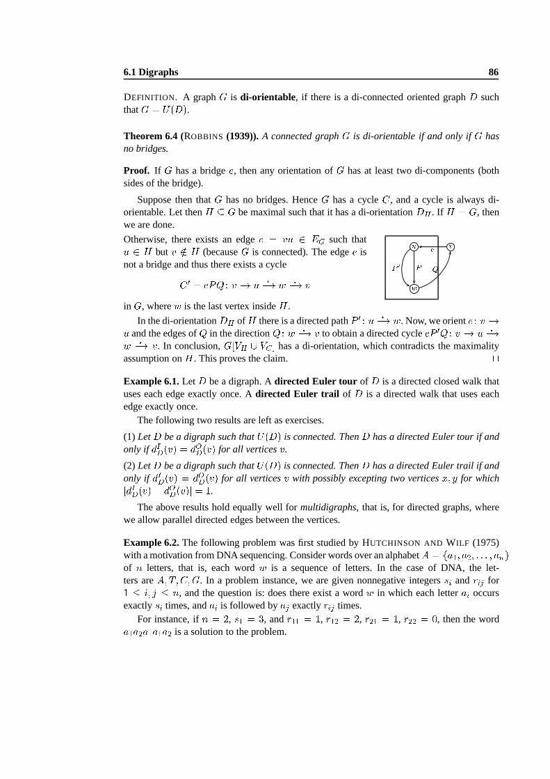
6.1 Digraphs 86
DEFINITION. A graphG is di-orientable, if there is a di-connected oriented graphD suchthatG = U(D).Theorem 6.4 (ROBBINS (1939)).A connected graphG is di-orientable if and only ifG hasno bridges.
Proof. If G has a bridgee, then any orientation ofG has at least two di-components (bothsides of the bridge).
Suppose then thatG has no bridges. HenceG has a cycleC, and a cycle is always di-orientable. Let thenH � G be maximal such that it has a di-orientationDH . If H = G, thenwe are done.
Otherwise, there exists an edgee = vu 2 EG such thatu 2 H but v =2 H (becauseG is connected). The edgee isnot a bridge and thus there exists a cycleC 0 = ePQ : v �! u ?�! w ?�! vin G, wherew is the last vertex insideH.
wu vP eQP 0In the di-orientationDH ofH there is a directed pathP 0 : u ?�! w. Now, we oriente : v �!u and the edges ofQ in the directionQ : w ?�! v to obtain a directed cycleeP 0Q : v �! u ?�!w ?�! v. In conclusion,G[VH [ VC ℄ has a di-orientation, which contradicts the maximality
assumption onH. This proves the claim. utExample 6.1.LetD be a digraph. Adirected Euler tour of D is a directed closed walk thatuses each edge exactly once. Adirected Euler trail of D is a directed walk that uses eachedge exactly once.
The following two results are left as exercises.
(1) LetD be a digraph such thatU(D) is connected. ThenD has a directed Euler tour if andonly if dID(v) = dOD(v) for all verticesv.
(2) LetD be a digraph such thatU(D) is connected. ThenD has a directed Euler trail if andonly if dID(v) = dOD(v) for all verticesv with possibly excepting two verticesx; y for whichjdID(v) � dOD(v)j = 1.
The above results hold equally well formultidigraphs, that is, for directed graphs, wherewe allow parallel directed edges between the vertices.
Example 6.2.The following problem was first studied by HUTCHINSON AND WILF (1975)with a motivation from DNA sequencing. Consider words over an alphabetA = fa1; a2; : : : ; angof n letters, that is, each wordw is a sequence of letters. In the case of DNA, the let-ters areA; T;C;G. In a problem instance, we are given nonnegative integerssi andrij for1 � i; j � n, and the question is: does there exist a wordw in which each letterai occursexactlysi times, andai is followed byaj exactlyrij times.
For instance, ifn = 2, s1 = 3, andr11 = 1, r12 = 2, r21 = 1, r22 = 0, then the worda1a2a1a1a2 is a solution to the problem.
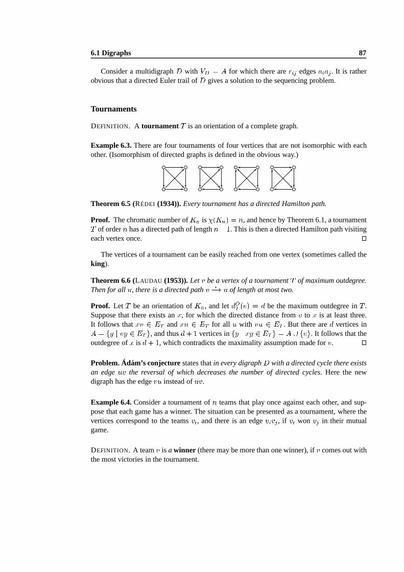
6.1 Digraphs 87
Consider a multidigraphD with VD = A for which there arerij edgesaiaj. It is ratherobvious that a directed Euler trail ofD gives a solution to the sequencing problem.
Tournaments
DEFINITION. A tournament T is an orientation of a complete graph.
Example 6.3.There are four tournaments of four vertices that are not isomorphic with eachother. (Isomorphism of directed graphs is defined in the obvious way.)
Theorem 6.5 (RÉDEI (1934)).Every tournament has a directed Hamilton path.
Proof. The chromatic number ofKn is�(Kn) = n, and hence by Theorem 6.1, a tournamentT of ordern has a directed path of lengthn� 1. This is then a directed Hamilton path visitingeach vertex once. ut
The vertices of a tournament can be easily reached from one vertex (sometimes called theking).
Theorem 6.6 (LAUDAU (1953)).Letv be a vertex of a tournamentT of maximum outdegree.Then for allu, there is a directed pathv ?�! u of length at most two.
Proof. Let T be an orientation ofKn, and letdOT (v) = d be the maximum outdegree inT .Suppose that there exists anx, for which the directed distance fromv to x is at least three.It follows thatxv 2 ET andxu 2 ET for all u with vu 2 ET . But there ared vertices inA = fy j vy 2 ET g, and thusd+ 1 vertices infy j xy 2 ET g = A [ fvg. It follows that theoutdegree ofx is d+ 1, which contradicts the maximality assumption made forv. utProblem. Ádám’s conjecturestates thatin every digraphD with a directed cycle there existsan edgeuv the reversal of which decreases the number of directed cycles. Here the newdigraph has the edgevu instead ofuv.
Example 6.4.Consider a tournament ofn teams that play once against each other, and sup-pose that each game has a winner. The situation can be presented as a tournament, where thevertices correspond to the teamsvi, and there is an edgevivj , if vi won vj in their mutualgame.
DEFINITION. A teamv is a winner (there may be more than one winner), ifv comes out withthe most victories in the tournament.
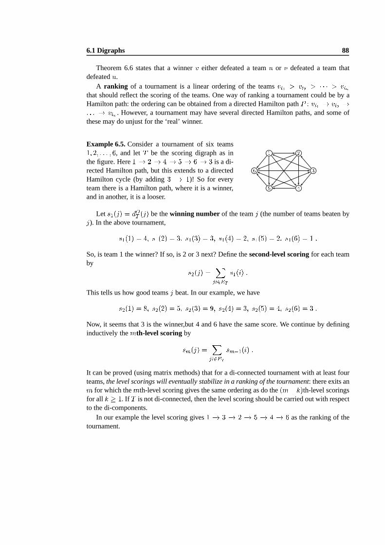
6.1 Digraphs 88
Theorem 6.6 states that a winnerv either defeated a teamu or v defeated a team thatdefeatedu.
A ranking of a tournament is a linear ordering of the teamsvi1 > vi2 > � � � > vinthat should reflect the scoring of the teams. One way of ranking a tournament could be by aHamilton path: the ordering can be obtained from a directed Hamilton pathP : vi1 �! vi2 �!: : : �! vin . However, a tournament may have several directed Hamilton paths, and some ofthese may do unjust for the ‘real’ winner.
Example 6.5.Consider a tournament of six teams1; 2; : : : ; 6, and letT be the scoring digraph as inthe figure. Here1 �! 2 �! 4 �! 5 �! 6 �! 3 is a di-rected Hamilton path, but this extends to a directedHamilton cycle (by adding3 �! 1)! So for everyteam there is a Hamilton path, where it is a winner,and in another, it is a looser.
6 51 42 3Let s1(j) = dOT (j) be thewinning number of the teamj (the number of teams beaten byj). In the above tournament,s1(1) = 4; s1(2) = 3; s1(3) = 3; s1(4) = 2; s1(5) = 2; s1(6) = 1 :
So, is team 1 the winner? If so, is 2 or 3 next? Define thesecond-level scoringfor each teamby s2(j) = Xji2ET s1(i) :This tells us how good teamsj beat. In our example, we haves2(1) = 8; s2(2) = 5; s2(3) = 9; s2(4) = 3; s2(5) = 4; s2(6) = 3 :Now, it seems that 3 is the winner,but 4 and 6 have the same score. We continue by defininginductively themth-level scoringbysm(j) = Xji2ET sm�1(i) :It can be proved (using matrix methods) that for a di-connected tournament with at least fourteams,the level scorings will eventually stabilize in a ranking ofthe tournament: there exits anm for which themth-level scoring gives the same ordering as do the(m+ k)th-level scoringsfor all k � 1. If T is not di-connected, then the level scoring should be carried out with respectto the di-components.
In our example the level scoring gives1 �! 3 �! 2 �! 5 �! 4 �! 6 as the ranking of thetournament.
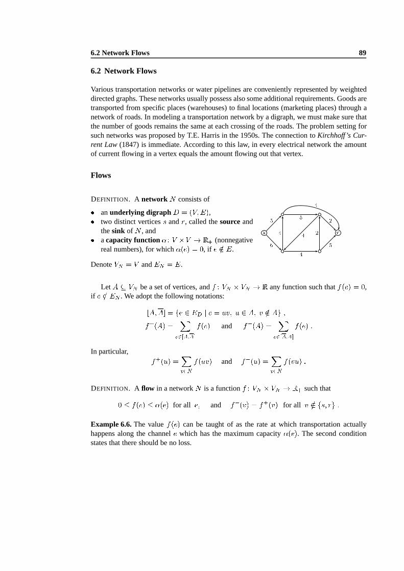
6.2 Network Flows 89
6.2 Network Flows
Various transportation networks or water pipelines are conveniently represented by weighteddirected graphs. These networks usually possess also some additional requirements. Goods aretransported from specific places (warehouses) to final locations (marketing places) through anetwork of roads. In modeling a transportation network by a digraph, we must make sure thatthe number of goods remains the same at each crossing of the roads. The problem setting forsuch networks was proposed by T.E. Harris in the 1950s. The connection toKirchhoff ’s Cur-rent Law(1847) is immediate. According to this law, in every electrical network the amountof current flowing in a vertex equals the amount flowing out that vertex.
Flows
DEFINITION. A network N consists of� anunderlying digraph D = (V;E),� two distinct verticess andr, called thesourceandthesink of N , and� acapacity function� : V �V ! R+ (nonnegativereal numbers), for which�(e) = 0, if e =2 E.
DenoteVN = V andEN = E.
s r65 4 45 2 524 4LetA � VN be a set of vertices, andf : VN � VN ! R any function such thatf(e) = 0,
if e =2 EN . We adopt the following notations:[A;A℄ = fe 2 ED j e = uv; u 2 A; v =2 Ag ;f+(A) = Xe2[A;A℄ f(e) and f�(A) = Xe2[A;A℄ f(e) :In particular, f+(u) = Xv2N f(uv) and f�(u) = Xv2N f(vu) :DEFINITION. A flow in a networkN is a functionf : VN � VN ! R+ such that0 � f(e) � �(e) for all e; and f�(v) = f+(v) for all v =2 fs; rg :Example 6.6.The valuef(e) can be taught of as the rate at which transportation actuallyhappens along the channele which has the maximum capacity�(e). The second conditionstates that there should be no loss.
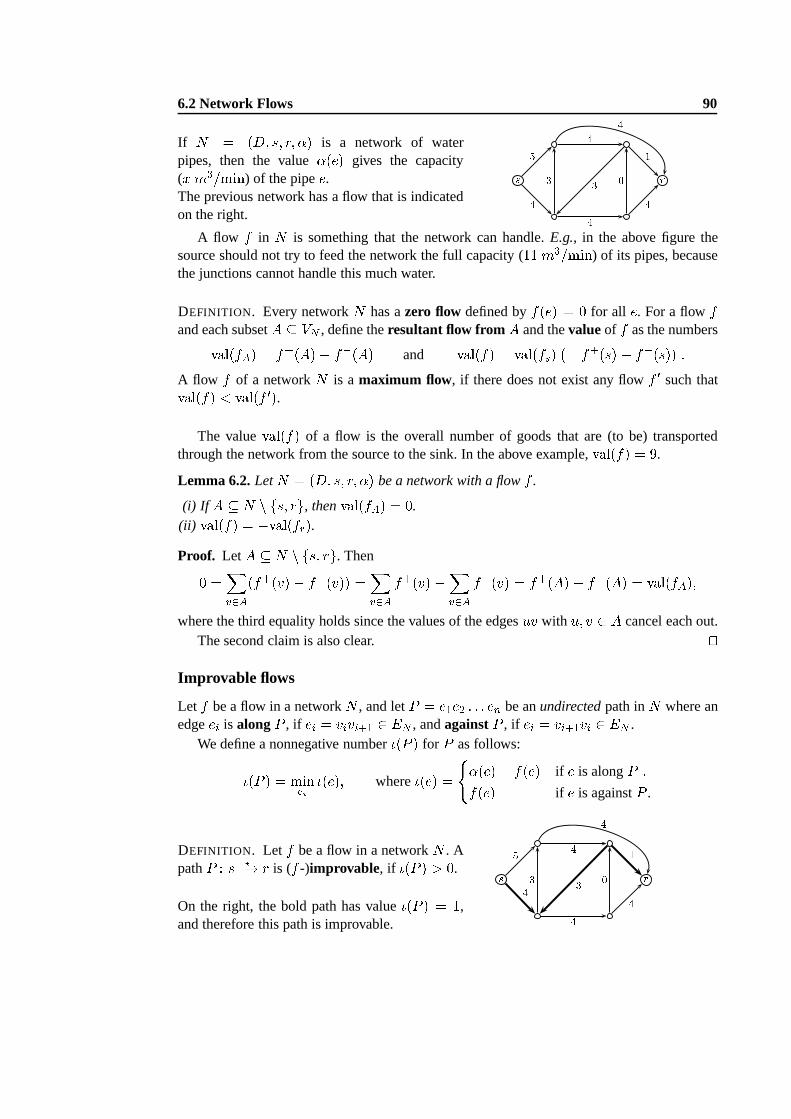
6.2 Network Flows 90
If N = (D; s; r; �) is a network of waterpipes, then the value�(e) gives the capacity(x m3=min) of the pipee.The previous network has a flow that is indicatedon the right.
s r45 3 44 0 413 4
A flow f in N is something that the network can handle.E.g., in the above figure thesource should not try to feed the network the full capacity (11 m3=min) of its pipes, becausethe junctions cannot handle this much water.
DEFINITION. Every networkN has azero flow defined byf(e) = 0 for all e. For a flowfand each subsetA � VN , define theresultant flow from A and thevalueof f as the numbersval(fA) = f+(A)� f�(A) and val(f) = val(fs) (= f+(s)� f�(s)) :A flow f of a networkN is a maximum flow, if there does not exist any flowf 0 such thatval(f) < val(f 0).
The valueval(f) of a flow is the overall number of goods that are (to be) transportedthrough the network from the source to the sink. In the above example,val(f) = 9.
Lemma 6.2.LetN = (D; s; r; �) be a network with a flowf .
(i) If A � N n fs; rg, thenval(fA) = 0.(ii) val(f) = �val(fr).Proof. LetA � N n fs; rg. Then0 =Xv2A(f+(v)� f�(v)) =Xv2A f+(v)�Xv2A f�(v) = f+(A)� f�(A) = val(fA);where the third equality holds since the values of the edgesuv with u; v 2 A cancel each out.
The second claim is also clear. utImprovable flows
Let f be a flow in a networkN , and letP = e1e2 : : : en be anundirectedpath inN where anedgeei is alongP , if ei = vivi+1 2 EN , andagainstP , if ei = vi+1vi 2 EN .
We define a nonnegative number�(P ) for P as follows:�(P ) = minei �(e); where�(e) = (�(e)� f(e) if e is alongP ;f(e) if e is againstP .
DEFINITION. Let f be a flow in a networkN . ApathP : s ?�! r is (f -)improvable, if �(P ) > 0.
On the right, the bold path has value�(P ) = 1,and therefore this path is improvable.
s r5 3 44 0 444 3 1
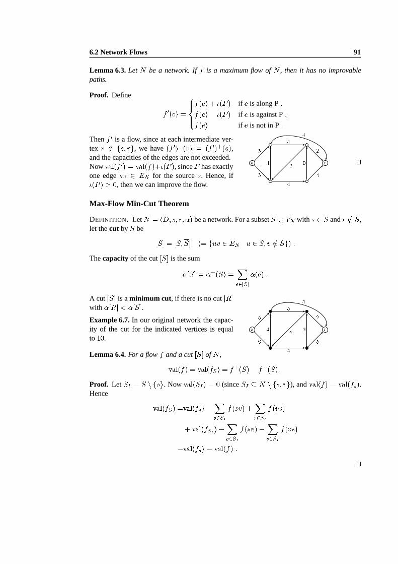
6.2 Network Flows 91
Lemma 6.3.LetN be a network. Iff is a maximum flow ofN , then it has no improvablepaths.
Proof. Define f 0(e) = 8><>:f(e) + �(P ) if e is along P;f(e)� �(P ) if e is against P;f(e) if e is not in P:Thenf 0 is a flow, since at each intermediate ver-tex v =2 fs; rg, we have(f 0)�(v) = (f 0)+(v),and the capacities of the edges are not exceeded.Nowval(f 0) = val(f)+�(P ), sinceP has exactlyone edgesv 2 EN for the sources. Hence, if�(P ) > 0, then we can improve the flow.
s r5 3 44 0 445 2 2 ut
Max-Flow Min-Cut Theorem
DEFINITION. LetN = (D; s; r; �) be a network. For a subsetS � VN with s 2 S andr =2 S,let thecut by S be [S℄ = [S; S℄ (= fuv 2 EN j u 2 S; v =2 Sg) :Thecapacity of the cut[S℄ is the sum�[S℄ = �+(S) = Xe2[S℄�(e) :A cut [S℄ is aminimum cut , if there is no cut[R℄with �[R℄ < �[S℄.Example 6.7.In our original network the capac-ity of the cut for the indicated vertices is equalto 10.
s r5 4 45 2 56 4 24
Lemma 6.4.For a flowf and a cut[S℄ ofN ,val(f) = val(fS) = f+(S)� f�(S) :Proof. Let SI = S n fsg. Now val(SI) = 0 (sinceSI � N n fs; rg), andval(f) = val(fs).Hence val(fS) =val(fs)� Xv2SI f(sv) + Xv2SI f(vs)+ val(fSI ) + Xv2SI f(sv)� Xv2SI f(vs)=val(fs) = val(f) : ut
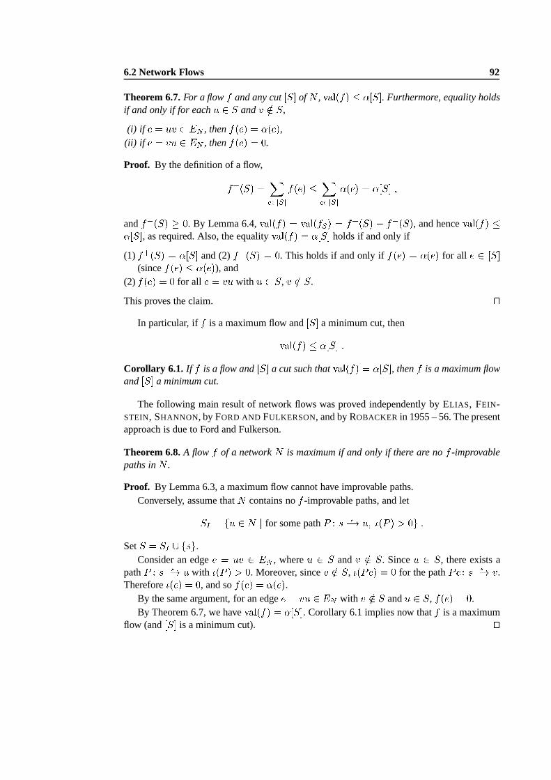
6.2 Network Flows 92
Theorem 6.7.For a flowf and any cut[S℄ ofN , val(f) � �[S℄. Furthermore, equality holdsif and only if for eachu 2 S andv =2 S,
(i) if e = uv 2 EN , thenf(e) = �(e),(ii) if e = vu 2 EN , thenf(e) = 0.
Proof. By the definition of a flow,f+(S) = Xe2[S℄ f(e) � Xe2[S℄�(e) = �[S℄ ;andf�(S) � 0. By Lemma 6.4,val(f) = val(fS) = f+(S) � f�(S), and henceval(f) ��[S℄, as required. Also, the equalityval(f) = �[S℄ holds if and only if
(1) f+(S) = �[S℄ and (2)f�(S) = 0. This holds if and only iff(e) = �(e) for all e 2 [S℄(sincef(e) � �(e)), and
(2) f(e) = 0 for all e = vu with u 2 S, v =2 S.
This proves the claim. utIn particular, iff is a maximum flow and[S℄ a minimum cut, thenval(f) � �[S℄ :
Corollary 6.1. If f is a flow and[S℄ a cut such thatval(f) = �[S℄, thenf is a maximum flowand [S℄ a minimum cut.
The following main result of network flows was proved independently by ELIAS, FEIN-STEIN, SHANNON, by FORD AND FULKERSON, and by ROBACKER in 1955 – 56. The presentapproach is due to Ford and Fulkerson.
Theorem 6.8.A flowf of a networkN is maximum if and only if there are nof -improvablepaths inN .
Proof. By Lemma 6.3, a maximum flow cannot have improvable paths.Conversely, assume thatN contains nof -improvable paths, and letSI = fu 2 N j for some pathP : s ?�! u; �(P ) > 0g :
SetS = SI [ fsg.Consider an edgee = uv 2 EN , whereu 2 S andv =2 S. Sinceu 2 S, there exists a
pathP : s ?�! u with �(P ) > 0. Moreover, sincev =2 S, �(Pe) = 0 for the pathPe : s ?�! v.Therefore�(e) = 0, and sof(e) = �(e).
By the same argument, for an edgee = vu 2 EN with v =2 S andu 2 S, f(e) = 0.By Theorem 6.7, we haveval(f) = �[S℄. Corollary 6.1 implies now thatf is a maximum
flow (and[S℄ is a minimum cut). ut
6.2 Network Flows 93
Theorem 6.9.LetN be a network, where the capacity function� : V � V ! N has integervalues. ThenN has a maximum flow with integer values.
Proof. Let f0 be the zero flow,f0(e) = 0 for all e 2 V � V . A maximum flow is constructedusing Lemma 6.3 by increasing and decreasing the values of the edges by integers only. ut
The proof of Theorem 6.8 showed also
Theorem 6.10 (Max-Flow Min-Cut). In a networkN , the valueval(f) of a maximum flowequals the capacity�[S℄ of a minimum cut.
Applications to graphs?The Max-Flow Min-Cut Theorem is a strong result, and many of our previous results followfrom it.
We mention a connection to the Marriage Theorem, Theorem 3.9. For this, letG be abipartite graph with a bipartition(X;Y ), and consider a networkN with verticesfs; rg [X [ Y . Let the edges (with their capacities) besx 2 EN (�(sx) = 1), yr 2 EN (�(yr) = 1)for all x 2 X, y 2 Y together with the edgesxy 2 EN (�(xy) = jXj + 1), if xy 2 EG forx 2 X, y 2 Y . ThenG has a matching that saturatesX if and only ifN has a maximum flowof valuejXj. Now Theorem 6.10 gives Theorem 3.9.
Next we apply the theorem tounit networks, where the capacities of the edges are equalto one (�(e) = 1 for all e 2 EN ). We obtain results for (directed) graphs.
Lemma 6.5.LetN be a unit network with sources and sinkr.(i) The valueval(f) of a maximum flow equals the maximum number of edge-disjoint directed
pathss ?�! r.(ii) The capacity of a minimum cut[S℄ equals the minimum number of edges whose removal
destroys the directed connectionss ?�! r from s to r.Proof. Exercise. utCorollary 6.2. Let u and v be two vertices of a digraphD. The maximum number of edge-disjoint directed pathsu ?�! v equals the minimum number of edges, whose removal destroysall the directed connectionsu ?�! v fromD.
Proof. A networkN with sources and sinkr is obtained by setting the capacities equal to1.The claim follows from Lemma 6.5 and Corollary 6.10. utCorollary 6.3. Let u and v be two vertices of a graphG. The maximum number of edge-disjoint pathsu ?�! v equals the minimum number of edges, whose removal destroys all theconnectionsu ?�! v fromD.
Proof. Consider the digraphD that is obtained fromG by replacing each (undirected) edgeuv 2 EG by two directed edgesuv 2 ED andvu 2 ED. The claim follows then easily fromCorollary 6.2. ut
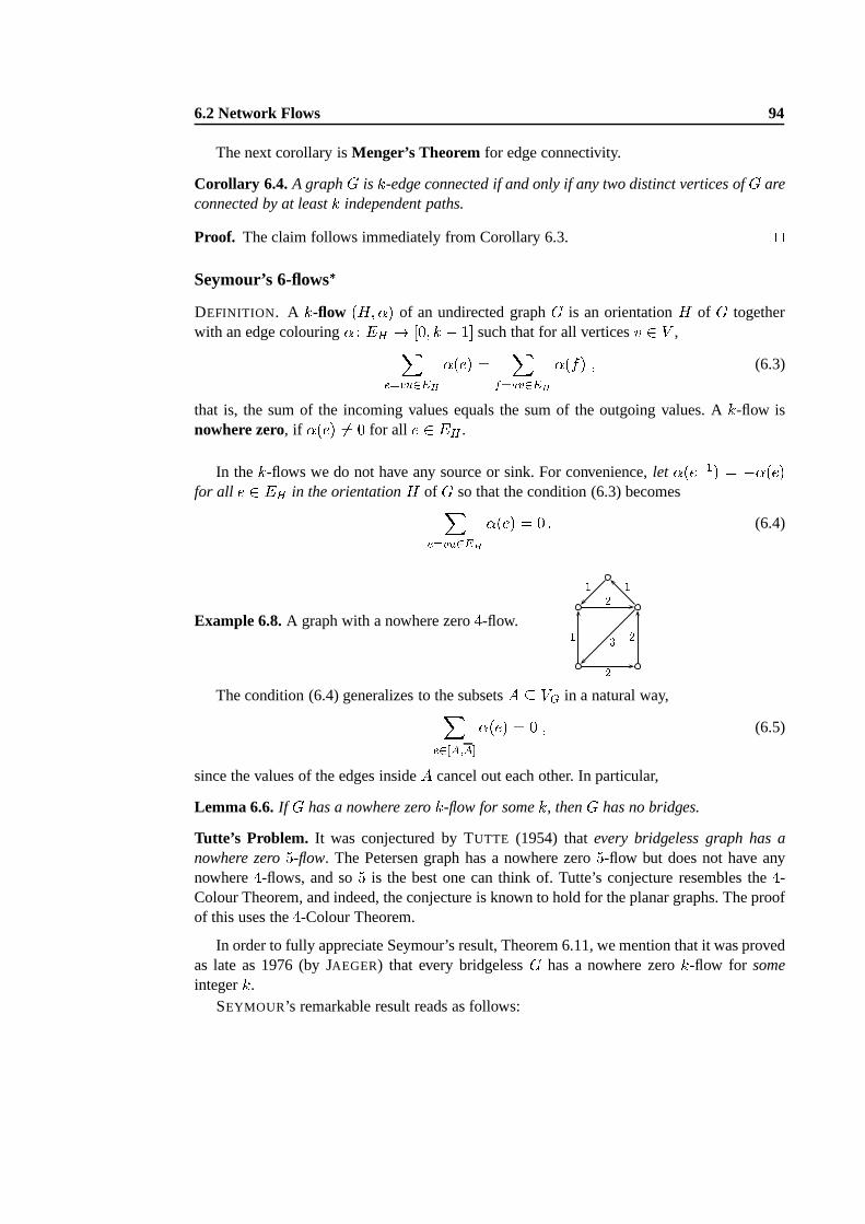
6.2 Network Flows 94
The next corollary isMenger’s Theorem for edge connectivity.
Corollary 6.4. A graphG is k-edge connected if and only if any two distinct vertices ofG areconnected by at leastk independent paths.
Proof. The claim follows immediately from Corollary 6.3. utSeymour’s 6-flows�DEFINITION. A k-flow (H;�) of an undirected graphG is an orientationH of G togetherwith an edge colouring� : EH ! [0; k � 1℄ such that for all verticesv 2 V ,Xe=vu2EH �(e) = Xf=uv2EH �(f) ; (6.3)
that is, the sum of the incoming values equals the sum of the outgoing values. Ak-flow isnowhere zero, if �(e) 6= 0 for all e 2 EH .
In thek-flows we do not have any source or sink. For convenience,let �(e�1) = ��(e)for all e 2 EH in the orientationH of G so that the condition (6.3) becomesXe=vu2EH �(e) = 0 : (6.4)
Example 6.8.A graph with a nowhere zero4-flow. 1 22 2131The condition (6.4) generalizes to the subsetsA � VG in a natural way,Xe2[A;A℄�(e) = 0 ; (6.5)
since the values of the edges insideA cancel out each other. In particular,
Lemma 6.6.If G has a nowhere zerok-flow for somek, thenG has no bridges.
Tutte’s Problem. It was conjectured by TUTTE (1954) thatevery bridgeless graph has anowhere zero5-flow. The Petersen graph has a nowhere zero5-flow but does not have anynowhere4-flows, and so5 is the best one can think of. Tutte’s conjecture resembles the 4-Colour Theorem, and indeed, the conjecture is known to hold for the planar graphs. The proofof this uses the4-Colour Theorem.
In order to fully appreciate Seymour’s result, Theorem 6.11, we mention that it was provedas late as 1976 (by JAEGER) that every bridgelessG has a nowhere zerok-flow for someintegerk.
SEYMOUR’s remarkable result reads as follows:
6.2 Network Flows 95
Theorem 6.11 (SEYMOUR’s (1981)).Every bridgeless graph has a nowhere zero6-flow.
Proof. Omitted. utDEFINITION. Theflow number f(G) of a bridgeless graphG is the least integerk for whichG has a nowhere zerok-flow.
Theorem 6.12.A connected graphG has a flow numberf(G) = 2 if and only if it is eulerian.
Proof. SupposeG is eulerian, and consider an Euler tourW of G. LetD be the orientationof G corresponding to the direction ofW . If an edgeuv 2 ED, let�(e) = 1. SinceW arrivesand leaves each vertex equally many times, the function� is a nowhere zero2-flow.
Conversely, let� be a nowhere zero2-flow of an orientationD of G. Then necessarily thedegrees of the vertices are even, and soG is eulerian. utExample 6.9.For each3-regular bipartite graphG, we havef(G) � 3. Indeed, letG be(X;Y )-biparte. By Corollary 3.1, a3-regular graph has a perfect matchingM . Orient theedgese 2 M fromX to Y , and set�(e) = 2. Orient the edgese =2 M from Y toX, and set�(e) = 1. Since eachx 2 X has exactly one neighboury1 2 Y such thatxy1 2 M , and twoneighboursy2; y3 2 Y such thatxy2; xy3 =2M , we have thatf(G) � 3.
Theorem 6.13.We havef(K4) = 4, and ifn > 4, thenf(Kn) = (2 if n is odd;3 if n is even:Proof. Exercise. ut
Index
acyclic, 17digraph, 81
addressable, 21adjacency matrix, 6adjacent, 4augmented path, 34available colour, 41, 50
bipartite, 15bond, 23boundary, 58bridge, 17
capacity, 87capacity function, 85choosable, 67chromatic number�(G), 50chromatic polynomial�G, 54closed walk, 11colouring, 50complementG, 9complete bipartiteKm;k, 15complete graphKn, 9connected, 23connected (component), 12connected sum, 72connectivity number�(G), 23contracted vertex, 55critical, 51crossing number, 64cube, 9cut (in a network), 87cut vertex, 22cycle, 11
degreedG(v), 7di-connected di-component, 80di-orientable, 82digraph, 79
directedEuler tour, trail, 82walk, path, cycle, 80
directed graphs (digraph), 4disconnected, 12disconnecting set, 25discrete graph, 9disjoint walks, 11distance, 12distance function, 5
edge, 4edge chromatic number�0(G), 41edge colouring, 5, 41edge cut, 23embedding, 73end (of a path), 11end (of an edge), 4Euler trail, tour, 28Euler’s formula, 59eulerian, 28even component, 37even cycle, 11exterior: face, boundary,vertex,edge, 58
face, 58fan, 26flow, 85flow number, 90forest, 17
genus, 75graph, 4graphical sequence, 8
Hamilton path, cycle, 30hamiltonian, 30Hamming distance, 21homeomorphic, 71
improvable (path), 86
Index 97
improvement (colouring), 42incident colours, 41indegree, 80independent paths, 11induced subdigraph, 79induced subgraph, 10interior: face, vertex, edge, 58intersection graph, 6inverse pair, 79inverse walk (path), 11isolated vertex, 7isomorphic, 5
join of walks, 11
king, 83kiss (circles), 68Kuratowski graph, 61
latin rectangle, 37latin square, 37leaf, 7line segment graph, 69linked cycles, 77list chromatic number, 67list colouring, 67loop, 4
Möbius band, 71map, 65matching, 34maximal planar graph, 60maximum
degree�(G), 7flow, 85matching, 34
minimumcut, 87degreeÆ(G), 7weighted distance, 12
minor, 69monochromatic, 46multigraph, 4
near-triangulation, 67neighbour, 4neighbourhoodNG(v), 7network, 85nontrivial graph, 9NP-complete problems, 3
odd component, 37odd cycle, 11optimal colouring, 42order�G, 4
orientable surface, 71orientation, 79oriented, 71oriented graph, 79outdegree, 80
parallel edges, 4partition, 3path, 11perfect matching, 34Petersen graph, 9, 31planar graph, 57plane embedding, 57plane model, 72proper colouring, 41, 50
Ramsey number, 47ranking, 83regular graph, 9resultant flow, 85
same parity, 3saturate (matching), 34separates, 22separating set, 22Shannon’s switching game, 19sink and source, 85size"G, 4spanning subgraph, 10spanning tree, 19spatial embedding, 77sphere, 73sphere with a handle, 74stable matching, 39stable set, 15subdigraph, 79subdivision, 57subgraph, 10surface, 71symmetric difference, 3
topologically equivalent, 71torus, 74tournament, 83trail, 28transversal, 36tree, 17triangle, 71triangle-free, 51triangulation, 71trivial graph, 9trivial path, 112-cell, 762-switch, 7
Index 98
underlying digraph, 85underlying graph, 79unit networks, 88
vertex, 4vertex colouring, 5
walk, 11weight, 12weight function, 5wheel, 49winning number, 84
zero flow, 85