Ian Robinson, Jim Webber, and Emil Eifrem

Graph Databases

Graph Databasesby Ian Robinson, Jim Webber, and Emil Eifrem

Copyright © 2013 Neo Technology, Inc.. All rights reserved.

Printed in the United States of America.

Published by O’Reilly Media, Inc., 1005 Gravenstein Highway North, Sebastopol, CA 95472.

O’Reilly books may be purchased for educational, business, or sales promotional use. Online editions arealso available for most titles (http://my.safaribooksonline.com). For more information, contact our corporate/institutional sales department: 800-998-9938 or corporate@oreilly.com.

Editors: Mike Loukides and Nathan JepsonProduction Editor: Kara EbrahimCopyeditor: Kim CoferProofreader: Kevin Broccoli

Indexer: Stephen Ingle, WordCo IndexingCover Designer: Randy ComerInterior Designer: David FutatoIllustrator: Kara Ebrahim

June 2013: First Edition

Revision History for the First Edition:

2013-05-20: First release

See http://oreilly.com/catalog/errata.csp?isbn=9781449356262 for release details.

Nutshell Handbook, the Nutshell Handbook logo, and the O’Reilly logo are registered trademarks of O’ReillyMedia, Inc. Graph Databases, the image of a European octopus, and related trade dress are trademarks ofO’Reilly Media, Inc.

Many of the designations used by manufacturers and sellers to distinguish their products are claimed astrademarks. Where those designations appear in this book, and O’Reilly Media, Inc., was aware of a trade‐mark claim, the designations have been printed in caps or initial caps.

While every precaution has been taken in the preparation of this book, the publisher and authors assumeno responsibility for errors or omissions, or for damages resulting from the use of the information containedherein.

ISBN: 978-1-449-35626-2

[LSI]

Table of Contents

Foreword. . . . . . . . . . . . . . . . . . . . . . . . . . . . . . . . . . . . . . . . . . . . . . . . . . . . . . . . . . . . . . . . . . . . . viiPreface. . . . . . . . . . . . . . . . . . . . . . . . . . . . . . . . . . . . . . . . . . . . . . . . . . . . . . . . . . . . . . . . . . . . . . . ix

1. Introduction. . . . . . . . . . . . . . . . . . . . . . . . . . . . . . . . . . . . . . . . . . . . . . . . . . . . . . . . . . . . . . . . 1What Is a Graph? 1A High-Level View of the Graph Space 4

Graph Databases 5Graph Compute Engines 6

The Power of Graph Databases 8Performance 8Flexibility 8Agility 9

Summary 9

2. Options for Storing Connected Data. . . . . . . . . . . . . . . . . . . . . . . . . . . . . . . . . . . . . . . . . . . 11Relational Databases Lack Relationships 11NOSQL Databases Also Lack Relationships 14Graph Databases Embrace Relationships 18Summary 23

3. Data Modeling with Graphs. . . . . . . . . . . . . . . . . . . . . . . . . . . . . . . . . . . . . . . . . . . . . . . . . . 25Models and Goals 25The Property Graph Model 26Querying Graphs: An Introduction to Cypher 27

Cypher Philosophy 27START 29MATCH 29RETURN 30Other Cypher Clauses 30

iii

A Comparison of Relational and Graph Modeling 31Relational Modeling in a Systems Management Domain 33Graph Modeling in a Systems Management Domain 36Testing the Model 38

Cross-Domain Models 40Creating the Shakespeare Graph 44Beginning a Query 45Declaring Information Patterns to Find 46Constraining Matches 47Processing Results 48Query Chaining 49

Common Modeling Pitfalls 50Email Provenance Problem Domain 50A Sensible First Iteration? 50Second Time’s the Charm 53Evolving the Domain 56

Avoiding Anti-Patterns 61Summary 61

4. Building a Graph Database Application. . . . . . . . . . . . . . . . . . . . . . . . . . . . . . . . . . . . . . . . 63Data Modeling 63

Describe the Model in Terms of the Application’s Needs 63Nodes for Things, Relationships for Structure 64Fine-Grained versus Generic Relationships 65Model Facts as Nodes 66Represent Complex Value Types as Nodes 69Time 70Iterative and Incremental Development 72

Application Architecture 73Embedded Versus Server 74Clustering 78Load Balancing 79

Testing 82Test-Driven Data Model Development 83Performance Testing 89

Capacity Planning 93Optimization Criteria 93Performance 94Redundancy 96Load 97

iv | Table of Contents

Summary 98

5. Graphs in the Real World. . . . . . . . . . . . . . . . . . . . . . . . . . . . . . . . . . . . . . . . . . . . . . . . . . . . 99Why Organizations Choose Graph Databases 99Common Use Cases 100

Social 100Recommendations 101Geo 102Master Data Management 103Network and Data Center Management 103Authorization and Access Control (Communications) 104

Real-World Examples 105Social Recommendations (Professional Social Network) 105Authorization and Access Control 116Geo (Logistics) 124

Summary 139

6. Graph Database Internals. . . . . . . . . . . . . . . . . . . . . . . . . . . . . . . . . . . . . . . . . . . . . . . . . . . 141Native Graph Processing 141Native Graph Storage 144Programmatic APIs 150

Kernel API 151Core (or “Beans”) API 151Traversal API 152

Nonfunctional Characteristics 154Transactions 155Recoverability 156Availability 157Scale 159

Summary 162

7. Predictive Analysis with Graph Theory. . . . . . . . . . . . . . . . . . . . . . . . . . . . . . . . . . . . . . . . 163Depth- and Breadth-First Search 163Path-Finding with Dijkstra’s Algorithm 164The A* Algorithm 173Graph Theory and Predictive Modeling 174

Triadic Closures 174Structural Balance 176

Local Bridges 180Summary 182

A. NOSQL Overview. . . . . . . . . . . . . . . . . . . . . . . . . . . . . . . . . . . . . . . . . . . . . . . . . . . . . . . . . . . 183

Table of Contents | v

Index. . . . . . . . . . . . . . . . . . . . . . . . . . . . . . . . . . . . . . . . . . . . . . . . . . . . . . . . . . . . . . . . . . . . . . . 201

vi | Table of Contents

Foreword

Graphs Are Everywhere, or the Birth of Graph Databasesas We Know ThemIt was 1999 and everyone worked 23-hour days. At least it felt that way. It seemed likeeach day brought another story about a crazy idea that just got millions of dollars infunding. All our competitors had hundreds of engineers, and we were a 20-ish persondevelopment team. As if that was not enough, 10 of our engineers spent the majority oftheir time just fighting the relational database.

It took us a while to figure out why. As we drilled deeper into the persistence layer ofour enterprise content management application, we realized that our software wasmanaging not just a lot of individual, isolated, and discrete data items, but also theconnections between them. And while we could easily fit the discrete data in relationaltables, the connected data was more challenging to store and tremendously slow toquery.

Out of pure desperation, my two Neo cofounders, Johan and Peter, and I started ex‐perimenting with other models for working with data, particularly those that were cen‐tered around graphs. We were blown away by the idea that it might be possible to replacethe tabular SQL semantic with a graph-centric model that would be much easier fordevelopers to work with when navigating connected data. We sensed that, armed witha graph data model, our development team might not waste half its time fighting thedatabase.

Surely, we said to ourselves, we can’t be unique here. Graph theory has been around fornearly 300 years and is well known for its wide applicability across a number of diversemathematical problems. Surely, there must be databases out there that embrace graphs!

vii

1. For the younger readers, it may come as a shock that there was a time in the history of mankind when Googledidn’t exist. Back then, dinosaurs ruled the earth and search engines with names like Altavista, Lycos, andExcite were used, primarily to find ecommerce portals for pet food on the Internet.

Well, we Altavistad1 around the young Web and couldn’t find any. After a few monthsof surveying, we (naively) set out to build, from scratch, a database that worked nativelywith graphs. Our vision was to keep all the proven features from the relational database(transactions, ACID, triggers, etc.) but use a data model for the 21st century. ProjectNeo was born, and with it graph databases as we know them today.

The first decade of the new millennium has seen several world-changing new businessesspring to life, including Google, Facebook, and Twitter. And there is a common threadamong them: they put connected data—graphs—at the center of their business. It’s 15years later and graphs are everywhere.

Facebook, for example, was founded on the idea that while there’s value in discreteinformation about people—their names, what they do, etc.—there’s even more value inthe relationships between them. Facebook founder Mark Zuckerberg built an empireon the insight to capture these relationships in the social graph.

Similarly, Google’s Larry Page and Sergey Brin figured out how to store and process notjust discrete web documents, but how those web documents are connected. Googlecaptured the web graph, and it made them arguably the most impactful company of theprevious decade.

Today, graphs have been successfully adopted outside the web giants. One of the biggestlogistics companies in the world uses a graph database in real time to route physicalparcels; a major airline is leveraging graphs for its media content metadata; and a top-tier financial services firm has rewritten its entire entitlements infrastructure on Neo4j.Virtually unknown a few years ago, graph databases are now used in industries as diverseas healthcare, retail, oil and gas, media, gaming, and beyond, with every indication ofaccelerating their already explosive pace.

These ideas deserve a new breed of tools: general-purpose database management tech‐nologies that embrace connected data and enable graph thinking, which are the kind oftools I wish had been available off the shelf when we were fighting the relational databaseback in 1999.

I hope this book will serve as a great introduction to this wonderful emerging world ofgraph technologies, and I hope it will inspire you to start using a graph database in yournext project so that you too can unlock the extraordinary power of graphs. Good luck!

—Emil EifremCofounder of Neo4j and CEO of Neo Technology

Menlo Park, CaliforniaMay 2013

viii | Foreword

Preface

Graph databases address one of the great macroscopic business trends of today: lever‐aging complex and dynamic relationships in highly connected data to generate insightand competitive advantage. Whether we want to understand relationships betweencustomers, elements in a telephone or data center network, entertainment producersand consumers, or genes and proteins, the ability to understand and analyze vast graphsof highly connected data will be key in determining which companies outperform theircompetitors over the coming decade.

For data of any significant size or value, graph databases are the best way to representand query connected data. Connected data is data whose interpretation and value re‐quires us first to understand the ways in which its constituent elements are related. Moreoften than not, to generate this understanding, we need to name and qualify the con‐nections between things.

Although large corporates realized this some time ago and began creating their ownproprietary graph processing technologies, we’re now in an era where that technologyhas rapidly become democratized. Today, general-purpose graph databases are a reality,enabling mainstream users to experience the benefits of connected data without havingto invest in building their own graph infrastructure.

What’s remarkable about this renaissance of graph data and graph thinking is that graphtheory itself is not new. Graph theory was pioneered by Euler in the 18th century, andhas been actively researched and improved by mathematicians, sociologists, anthro‐pologists, and others ever since. However, it is only in the past few years that graphtheory and graph thinking have been applied to information management. In that time,graph databases have helped solve important problems in the areas of social networking,master data management, geospatial, recommendations, and more. This increased fo‐cus on graph databases is driven by twin forces: by the massive commercial success ofcompanies such as Facebook, Google, and Twitter, all of whom have centered theirbusiness models around their own proprietary graph technologies; and by the intro‐duction of general-purpose graph databases into the technology landscape.

ix

About This BookThe purpose of this book is to introduce graphs and graph databases to technologypractitioners, including developers, database professionals, and technology decisionmakers. Reading this book will give you a practical understanding of graph databases.We show how the graph model “shapes” data, and how we query, reason about, under‐stand, and act upon data using a graph database. We discuss the kinds of problems thatare well aligned with graph databases, with examples drawn from actual real-world usecases, and we show how to plan and implement a graph database solution.

Conventions Used in This BookThe following typographical conventions are used in this book:Italic

Indicates new terms, URLs, email addresses, filenames, and file extensions.

Constant width

Used for program listings, as well as within paragraphs to refer to program elementssuch as variable or function names, databases, data types, environment variables,statements, and keywords.

Constant width bold

Shows commands or other text that should be typed literally by the user.

Constant width italicShows text that should be replaced with user-supplied values or by values deter‐mined by context.

This icon signifies a tip, suggestion, or general note.

This icon indicates a warning or caution.

Using Code ExamplesThis book is here to help you get your job done. In general, if this book includes codeexamples, you may use the code in this book in your programs and documentation. Youdo not need to contact us for permission unless you’re reproducing a significant portionof the code. For example, writing a program that uses several chunks of code from thisbook does not require permission. Selling or distributing a CD-ROM of examples from

x | Preface

O’Reilly books does require permission. Answering a question by citing this book andquoting example code does not require permission. Incorporating a significant amountof example code from this book into your product’s documentation does require per‐mission.

We appreciate, but do not require, attribution. An attribution usually includes the title,author, publisher, and ISBN. For example: “Graph Databases by Ian Robinson, JimWebber, and Emil Eifrem (O’Reilly). Copyright 2013 Neo Technology, Inc.,978-1-449-35626-2.”

If you feel your use of code examples falls outside fair use or the permission given above,feel free to contact us at permissions@oreilly.com.

Safari® Books OnlineSafari Books Online is an on-demand digital library that delivers ex‐pert content in both book and video form from the world’s leadingauthors in technology and business.

Technology professionals, software developers, web designers, and business and crea‐tive professionals use Safari Books Online as their primary resource for research, prob‐lem solving, learning, and certification training.

Safari Books Online offers a range of product mixes and pricing programs for organi‐zations, government agencies, and individuals. Subscribers have access to thousands ofbooks, training videos, and prepublication manuscripts in one fully searchable databasefrom publishers like O’Reilly Media, Prentice Hall Professional, Addison-Wesley Pro‐fessional, Microsoft Press, Sams, Que, Peachpit Press, Focal Press, Cisco Press, JohnWiley & Sons, Syngress, Morgan Kaufmann, IBM Redbooks, Packt, Adobe Press, FTPress, Apress, Manning, New Riders, McGraw-Hill, Jones & Bartlett, Course Technol‐ogy, and dozens more. For more information about Safari Books Online, please visit usonline.

How to Contact UsPlease address comments and questions concerning this book to the publisher:

O’Reilly Media, Inc.1005 Gravenstein Highway NorthSebastopol, CA 95472800-998-9938 (in the United States or Canada)707-829-0515 (international or local)707-829-0104 (fax)

Preface | xi

We have a web page for this book, where we list errata, examples, and any additionalinformation. You can access this page at http://oreil.ly/graph-databases.

To comment or ask technical questions about this book, send email to bookquestions@oreilly.com.

For more information about our books, courses, conferences, and news, see our websiteat http://www.oreilly.com.

Find us on Facebook: http://facebook.com/oreilly

Follow us on Twitter: http://twitter.com/oreillymedia

Watch us on YouTube: http://www.youtube.com/oreillymedia

AcknowledgmentsWe would like to thank our technical reviewers: Michael Hunger, Colin Jack, MarkNeedham, and Pramod Sadalage.

Our appreciation and thanks to our editor, Nathan Jepson.

Our colleagues at Neo Technology have contributed enormously of their time, experi‐ence, and effort throughout the writing of this book. Thanks in particular go to AndersNawroth, for his invaluable assistance with our book’s toolchain; Andrés Taylor, for hisenthusiastic help with all things Cypher; and Philip Rathle, for his advice and contri‐butions to the text.

A big thank you to everyone in the Neo4j community for your many contributions tothe graph database space over the years.

And special thanks to our families, for their love and support: Lottie, Tiger, Elliot, Kath,Billy, Madelene, and Noomi.

xii | Preface

1. For introductions to graph theory, see Richard J. Trudeau, Introduction To Graph Theory (Dover, 1993) andGary Chartrand, Introductory Graph Theory (Dover, 1985). For an excellent introduction to how graphsprovide insight into complex events and behaviors, see David Easley and Jon Kleinberg, Networks, Crowds,and Markets: Reasoning about a Highly Connected World (Cambridge University Press, 2010).

CHAPTER 1

Introduction

Although much of this book talks about graph data models, it is not a book about graphtheory.1 We don’t need much theory to take advantage of graph databases: provided weunderstand what a graph is, we’re practically there. With that in mind, let’s refresh ourmemories about graphs in general.

What Is a Graph?Formally, a graph is just a collection of vertices and edges—or, in less intimidating lan‐guage, a set of nodes and the relationships that connect them. Graphs represent entitiesas nodes and the ways in which those entities relate to the world as relationships. Thisgeneral-purpose, expressive structure allows us to model all kinds of scenarios, fromthe construction of a space rocket, to a system of roads, and from the supply-chain orprovenance of foodstuff, to medical history for populations, and beyond.

Graphs Are EverywhereGraphs are extremely useful in understanding a wide diversity of datasets in fields suchas science, government, and business. The real world—unlike the forms-based modelbehind the relational database—is rich and interrelated: uniform and rule-bound inparts, exceptional and irregular in others. Once we understand graphs, we begin to seethem in all sorts of places. Gartner, for example, identifies five graphs in the world of

1

business—social, intent, consumption, interest, and mobile—and says that the abilityto leverage these graphs provides a “sustainable competitive advantage.”

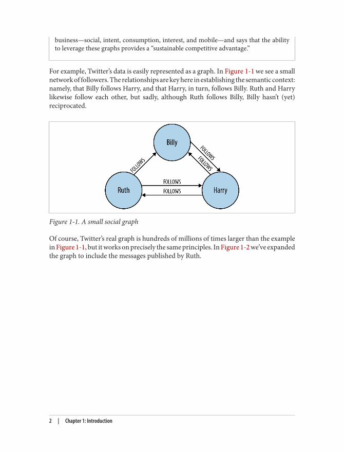
For example, Twitter’s data is easily represented as a graph. In Figure 1-1 we see a smallnetwork of followers. The relationships are key here in establishing the semantic context:namely, that Billy follows Harry, and that Harry, in turn, follows Billy. Ruth and Harrylikewise follow each other, but sadly, although Ruth follows Billy, Billy hasn’t (yet)reciprocated.

Figure 1-1. A small social graph

Of course, Twitter’s real graph is hundreds of millions of times larger than the examplein Figure 1-1, but it works on precisely the same principles. In Figure 1-2 we’ve expandedthe graph to include the messages published by Ruth.

2 | Chapter 1: Introduction

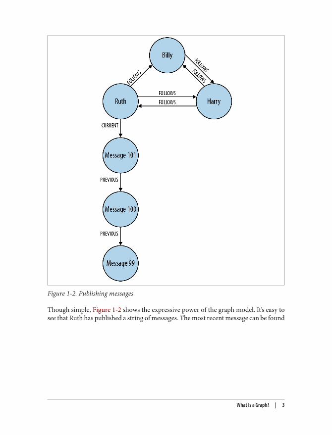
Figure 1-2. Publishing messages

Though simple, Figure 1-2 shows the expressive power of the graph model. It’s easy tosee that Ruth has published a string of messages. The most recent message can be found

What Is a Graph? | 3

by following a relationship marked CURRENT; PREVIOUS relationships then create a timeline of posts.

The Property Graph ModelIn discussing Figure 1-2 we’ve also informally introduced the most popular variant ofgraph model, the property graph (in Appendix A, we discuss alternative graph datamodels in more detail). A property graph has the following characteristics:

• It contains nodes and relationships• Nodes contain properties (key-value pairs)• Relationships are named and directed, and always have a start and end node• Relationships can also contain properties

Most people find the property graph model intuitive and easy to understand. Althoughsimple, it can be used to describe the overwhelming majority of graph use cases in waysthat yield useful insights into our data.

A High-Level View of the Graph SpaceNumerous projects and products for managing, processing, and analyzing graphs haveexploded onto the scene in recent years. The sheer number of technologies makes itdifficult to keep track of these tools and how they differ, even for those of us who areactive in the space. This section provides a high-level framework for making sense ofthe emerging graph landscape.

From 10,000 feet we can divide the graph space into two parts:Technologies used primarily for transactional online graph persistence, typically ac‐cessed directly in real time from an application

These technologies are called graph databases and are the main focus of this book.They are the equivalent of “normal” online transactional processing (OLTP) data‐bases in the relational world.

Technologies used primarily for offline graph analytics, typically performed as a seriesof batch steps

These technologies can be called graph compute engines. They can be thought of asbeing in the same category as other technologies for analysis of data in bulk, suchas data mining and online analytical processing (OLAP).

4 | Chapter 1: Introduction

2. See Rodriguez, M.A., Neubauer, P., “The Graph Traversal Pattern,” 2010.

Another way to slice the graph space is to look at the graph modelsemployed by the various technologies. There are three dominant graphdata models: the property graph, Resource Description Framework(RDF) triples, and hypergraphs. We describe these in detail in Appen‐dix A. Most of the popular graph databases on the market use the prop‐erty graph model, and in consequence, it’s the model we’ll use through‐out the remainder of this book.

Graph DatabasesA graph database management system (henceforth, a graph database) is an online da‐tabase management system with Create, Read, Update, and Delete (CRUD) methodsthat expose a graph data model. Graph databases are generally built for use with trans‐actional (OLTP) systems. Accordingly, they are normally optimized for transactionalperformance, and engineered with transactional integrity and operational availabilityin mind.

There are two properties of graph databases you should consider when investigatinggraph database technologies:The underlying storage

Some graph databases use native graph storage that is optimized and designed forstoring and managing graphs. Not all graph database technologies use native graphstorage, however. Some serialize the graph data into a relational database, an object-oriented database, or some other general-purpose data store.

The processing engineSome definitions require that a graph database use index-free adjacency, meaningthat connected nodes physically “point” to each other in the database.2 Here we takea slightly broader view: any database that from the user’s perspective behaves like agraph database (i.e., exposes a graph data model through CRUD operations) quali‐fies as a graph database. We do acknowledge, however, the significant performanceadvantages of index-free adjacency, and therefore use the term native graph pro‐cessing to describe graph databases that leverage index-free adjacency.

A High-Level View of the Graph Space | 5

It’s important to note that native graph storage and native graph pro‐cessing are neither good nor bad—they’re simply classic engineeringtrade-offs. The benefit of native graph storage is that its purpose-builtstack is engineered for performance and scalability. The benefit of non‐native graph storage, in contrast, is that it typically depends on a maturenongraph backend (such as MySQL) whose production characteristicsare well understood by operations teams. Native graph processing(index-free adjacency) benefits traversal performance, but at the ex‐pense of making some nontraversal queries difficult or memoryintensive.

Relationships are first-class citizens of the graph data model, unlike other databasemanagement systems, which require us to infer connections between entities usingcontrived properties such as foreign keys, or out-of-band processing like map-reduce.By assembling the simple abstractions of nodes and relationships into connected struc‐tures, graph databases enable us to build arbitrarily sophisticated models that mapclosely to our problem domain. The resulting models are simpler and at the same timemore expressive than those produced using traditional relational databases and theother NOSQL stores.

Figure 1-3 shows a pictorial overview of some of the graph databases on the markettoday based on their storage and processing models.

Graph Compute EnginesA graph compute engine is a technology that enables global graph computational algo‐rithms to be run against large datasets. Graph compute engines are designed to do thingslike identify clusters in your data, or answer questions such as, “how many relationships,on average, does everyone in a social network have?”

Because of their emphasis on global queries, graph compute engines are normally op‐timized for scanning and processing large amounts of information in batch, and in thatrespect they are similar to other batch analysis technologies, such as data mining andOLAP, that are familiar in the relational world. Whereas some graph compute enginesinclude a graph storage layer, others (and arguably most) concern themselves strictlywith processing data that is fed in from an external source, and returning the results.

6 | Chapter 1: Introduction

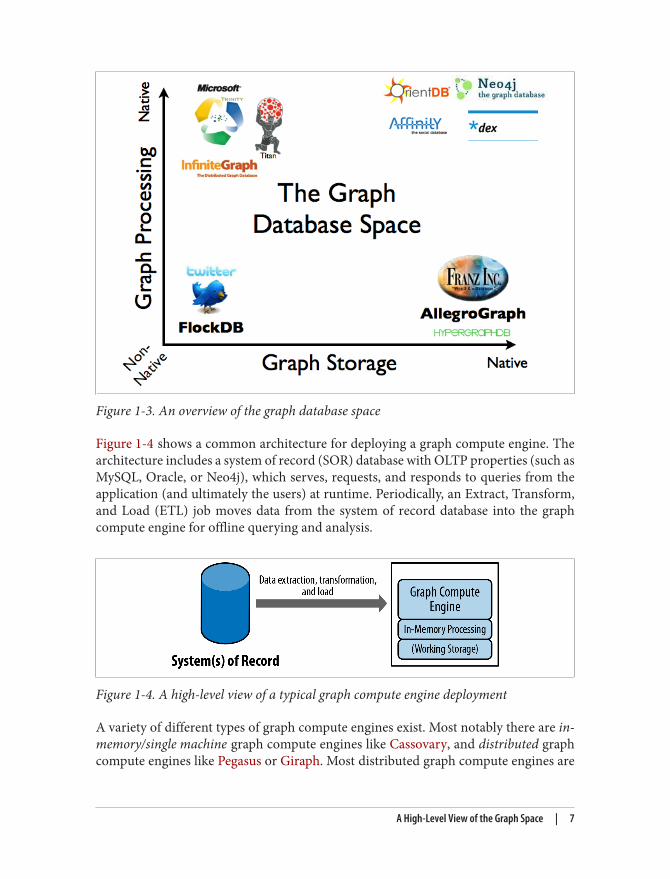
Figure 1-3. An overview of the graph database space

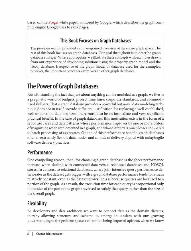
Figure 1-4 shows a common architecture for deploying a graph compute engine. Thearchitecture includes a system of record (SOR) database with OLTP properties (such asMySQL, Oracle, or Neo4j), which serves, requests, and responds to queries from theapplication (and ultimately the users) at runtime. Periodically, an Extract, Transform,and Load (ETL) job moves data from the system of record database into the graphcompute engine for offline querying and analysis.

Figure 1-4. A high-level view of a typical graph compute engine deployment

A variety of different types of graph compute engines exist. Most notably there are in-memory/single machine graph compute engines like Cassovary, and distributed graphcompute engines like Pegasus or Giraph. Most distributed graph compute engines are

A High-Level View of the Graph Space | 7

based on the Pregel white paper, authored by Google, which describes the graph com‐pute engine Google uses to rank pages.

This Book Focuses on Graph DatabasesThe previous section provided a course-grained overview of the entire graph space. Therest of this book focuses on graph databases. Our goal throughout is to describe graphdatabase concepts. Where appropriate, we illustrate these concepts with examples drawnfrom our experience of developing solutions using the property graph model and theNeo4j database. Irrespective of the graph model or database used for the examples,however, the important concepts carry over to other graph databases.

The Power of Graph DatabasesNotwithstanding the fact that just about anything can be modeled as a graph, we live ina pragmatic world of budgets, project time lines, corporate standards, and commodi‐tized skillsets. That a graph database provides a powerful but novel data modeling tech‐nique does not in itself provide sufficient justification for replacing a well-established,well-understood data platform; there must also be an immediate and very significantpractical benefit. In the case of graph databases, this motivation exists in the form of aset of use cases and data patterns whose performance improves by one or more ordersof magnitude when implemented in a graph, and whose latency is much lower comparedto batch processing of aggregates. On top of this performance benefit, graph databasesoffer an extremely flexible data model, and a mode of delivery aligned with today’s agilesoftware delivery practices.

PerformanceOne compelling reason, then, for choosing a graph database is the sheer performanceincrease when dealing with connected data versus relational databases and NOSQLstores. In contrast to relational databases, where join-intensive query performance de‐teriorates as the dataset gets bigger, with a graph database performance tends to remainrelatively constant, even as the dataset grows. This is because queries are localized to aportion of the graph. As a result, the execution time for each query is proportional onlyto the size of the part of the graph traversed to satisfy that query, rather than the size ofthe overall graph.

FlexibilityAs developers and data architects we want to connect data as the domain dictates,thereby allowing structure and schema to emerge in tandem with our growingunderstanding of the problem space, rather than being imposed upfront, when we know

8 | Chapter 1: Introduction

least about the real shape and intricacies of the data. Graph databases address this wantdirectly. As we show in Chapter 3, the graph data model expresses and accommodatesbusiness needs in a way that enables IT to move at the speed of business.

Graphs are naturally additive, meaning we can add new kinds of relationships, newnodes, and new subgraphs to an existing structure without disturbing existing queriesand application functionality. These things have generally positive implications for de‐veloper productivity and project risk. Because of the graph model’s flexibility, we don’thave to model our domain in exhaustive detail ahead of time—a practice that is all butfoolhardy in the face of changing business requirements. The additive nature of graphsalso means we tend to perform fewer migrations, thereby reducing maintenance over‐head and risk.

AgilityWe want to be able to evolve our data model in step with the rest of our application,using a technology aligned with today’s incremental and iterative software deliverypractices. Modern graph databases equip us to perform frictionless development andgraceful systems maintenance. In particular, the schema-free nature of the graph datamodel, coupled with the testable nature of a graph database’s application programminginterface (API) and query language, empower us to evolve an application in a controlledmanner.

At the same time, precisely because they are schema free, graph databases lack the kindof schema-oriented data governance mechanisms we’re familiar with in the relationalworld. But this is not a risk; rather, it calls forth a far more visible and actionable kindof governance. As we show in Chapter 4, governance is typically applied in a program‐matic fashion, using tests to drive out the data model and queries, as well as assert thebusiness rules that depend upon the graph. This is no longer a controversial practice:more so than relational development, graph database development aligns well with to‐day’s agile and test-driven software development practices, allowing graph database–backed applications to evolve in step with changing business environments.

SummaryIn this chapter we’ve reviewed the graph property model, a simple yet expressive toolfor representing connected data. Property graphs capture complex domains in an ex‐pressive and flexible fashion, while graph databases make it easy to develop applicationsthat manipulate our graph models.

Summary | 9

In the next chapter we’ll look in more detail at how several different technologies addressthe challenge of connected data, starting with relational databases, moving onto aggre‐gate NOSQL stores, and ending with graph databases. In the course of the discussion,we’ll see why graphs and graph databases provide the best means for modeling, storing,and querying connected data. Later chapters then go on to show how to design andimplement a graph database–based solution.

10 | Chapter 1: Introduction

CHAPTER 2

Options for Storing Connected Data

We live in a connected world. To thrive and progress, we need to understand and in‐fluence the web of connections that surrounds us.

How do today’s technologies deal with the challenge of connected data? In this chapterwe look at how relational databases and aggregate NOSQL stores manage graphs andconnected data, and compare their performance to that of a graph database. For readersinterested in exploring the topic of NOSQL, Appendix A describes the four major typesof NOSQL databases.

Relational Databases Lack RelationshipsFor several decades, developers have tried to accommodate connected, semi-structureddatasets inside relational databases. But whereas relational databases were initially de‐signed to codify paper forms and tabular structures—something they do exceedinglywell—they struggle when attempting to model the ad hoc, exceptional relationships thatcrop up in the real world. Ironically, relational databases deal poorly with relationships.

Relationships do exist in the vernacular of relational databases, but only as a means ofjoining tables. In our discussion of connected data in the previous chapter, we men‐tioned we often need to disambiguate the semantics of the relationships that connectentities, as well as qualify their weight or strength. Relational relations do nothing ofthe sort. Worse still, as outlier data multiplies, and the overall structure of the datasetbecomes more complex and less uniform, the relational model becomes burdened withlarge join tables, sparsely populated rows, and lots of null-checking logic. The rise inconnectedness translates in the relational world into increased joins, which impedeperformance and make it difficult for us to evolve an existing database in response tochanging business needs.

Figure 2-1 shows a relational schema for storing customer orders in a customer-centric,transactional application.

11

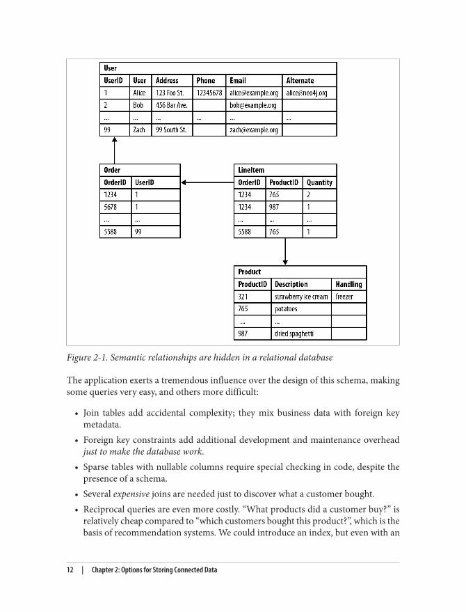
Figure 2-1. Semantic relationships are hidden in a relational database

The application exerts a tremendous influence over the design of this schema, makingsome queries very easy, and others more difficult:

• Join tables add accidental complexity; they mix business data with foreign keymetadata.

• Foreign key constraints add additional development and maintenance overheadjust to make the database work.

• Sparse tables with nullable columns require special checking in code, despite thepresence of a schema.

• Several expensive joins are needed just to discover what a customer bought.• Reciprocal queries are even more costly. “What products did a customer buy?” is

relatively cheap compared to “which customers bought this product?”, which is thebasis of recommendation systems. We could introduce an index, but even with an

12 | Chapter 2: Options for Storing Connected Data

index, recursive questions such as “which customers bought this product who alsobought that product?” quickly become prohibitively expensive as the degree of re‐cursion increases.

Relational databases struggle with highly connected domains. To understand the costof performing connected queries in a relational database, we’ll look at some simple andnot-so-simple queries in a social network domain.

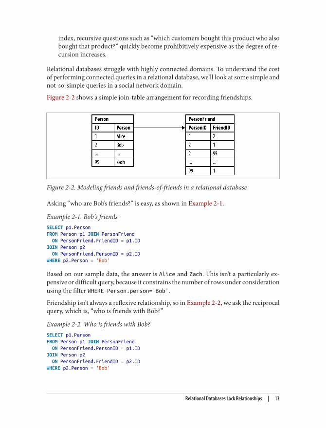
Figure 2-2 shows a simple join-table arrangement for recording friendships.

Figure 2-2. Modeling friends and friends-of-friends in a relational database

Asking “who are Bob’s friends?” is easy, as shown in Example 2-1.

Example 2-1. Bob’s friendsSELECT p1.PersonFROM Person p1 JOIN PersonFriend ON PersonFriend.FriendID = p1.IDJOIN Person p2 ON PersonFriend.PersonID = p2.IDWHERE p2.Person = 'Bob'

Based on our sample data, the answer is Alice and Zach. This isn’t a particularly ex‐pensive or difficult query, because it constrains the number of rows under considerationusing the filter WHERE Person.person='Bob'.

Friendship isn’t always a reflexive relationship, so in Example 2-2, we ask the reciprocalquery, which is, “who is friends with Bob?”

Example 2-2. Who is friends with Bob?SELECT p1.PersonFROM Person p1 JOIN PersonFriend ON PersonFriend.PersonID = p1.IDJOIN Person p2 ON PersonFriend.FriendID = p2.IDWHERE p2.Person = 'Bob'

Relational Databases Lack Relationships | 13

The answer to this query is Alice; sadly, Zach doesn’t consider Bob to be a friend. Thisreciprocal query is still easy to implement, but on the database side it’s more expensive,because the database now has to consider all the rows in the PersonFriend table.

We can add an index, but this still involves an expensive layer of indirection. Thingsbecome even more problematic when we ask, “who are the friends of my friends?”Hierarchies in SQL use recursive joins, which make the query syntactically and com‐putationally more complex, as shown in Example 2-3. (Some relational databases pro‐vide syntactic sugar for this—for instance, Oracle has a CONNECT BY function—whichsimplifies the query, but not the underlying computational complexity.)

Example 2-3. Alice’s friends-of-friendsSELECT p1.Person AS PERSON, p2.Person AS FRIEND_OF_FRIENDFROM PersonFriend pf1 JOIN Person p1 ON pf1.PersonID = p1.IDJOIN PersonFriend pf2 ON pf2.PersonID = pf1.FriendIDJOIN Person p2 ON pf2.FriendID = p2.IDWHERE p1.Person = 'Alice' AND pf2.FriendID <> p1.ID

This query is computationally complex, even though it only deals with the friends ofAlice’s friends, and goes no deeper into Alice’s social network. Things get more complexand more expensive the deeper we go into the network. Though it’s possible get ananswer to the question “who are my friends-of-friends-of-friends?” in a reasonableperiod of time, queries that extend to four, five, or six degrees of friendship deterioratesignificantly due to the computational and space complexity of recursively joiningtables.

We work against the grain whenever we try to model and query connectedness in arelational database. Besides the query and computational complexity just outlined, wealso have to deal with the double-edged sword of schema. More often than not, schemaproves to be both rigid and brittle. To subvert its rigidity we create sparsely populatedtables with many nullable columns, and code to handle the exceptional cases—all be‐cause there’s no real one-size-fits-all schema to accommodate the variety in the data weencounter. This increases coupling and all but destroys any semblance of cohesion. Itsbrittleness manifests itself as the extra effort and care required to migrate from oneschema to another as an application evolves.

NOSQL Databases Also Lack RelationshipsMost NOSQL databases—whether key-value-, document-, or column-oriented—storesets of disconnected documents/values/columns. This makes it difficult to use them forconnected data and graphs.

14 | Chapter 2: Options for Storing Connected Data

One well-known strategy for adding relationships to such stores is to embed an aggre‐gate’s identifier inside the field belonging to another aggregate—effectively introducingforeign keys. But this requires joining aggregates at the application level, which quicklybecomes prohibitively expensive.

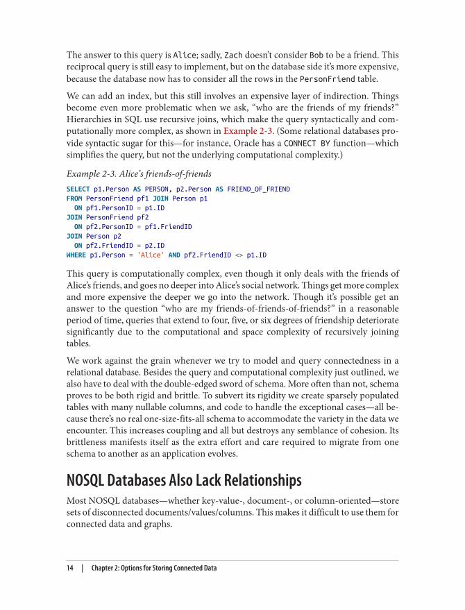
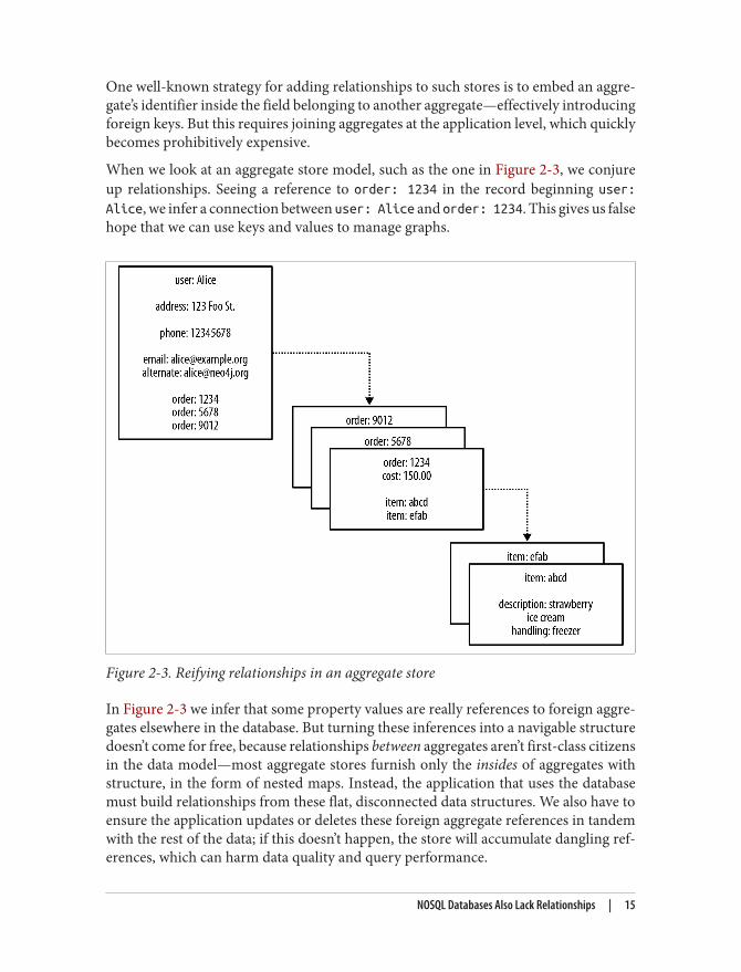
When we look at an aggregate store model, such as the one in Figure 2-3, we conjureup relationships. Seeing a reference to order: 1234 in the record beginning user:Alice, we infer a connection between user: Alice and order: 1234. This gives us falsehope that we can use keys and values to manage graphs.

Figure 2-3. Reifying relationships in an aggregate store

In Figure 2-3 we infer that some property values are really references to foreign aggre‐gates elsewhere in the database. But turning these inferences into a navigable structuredoesn’t come for free, because relationships between aggregates aren’t first-class citizensin the data model—most aggregate stores furnish only the insides of aggregates withstructure, in the form of nested maps. Instead, the application that uses the databasemust build relationships from these flat, disconnected data structures. We also have toensure the application updates or deletes these foreign aggregate references in tandemwith the rest of the data; if this doesn’t happen, the store will accumulate dangling ref‐erences, which can harm data quality and query performance.

NOSQL Databases Also Lack Relationships | 15

Links and WalkingThe Riak key-value store allows each of its stored values to be augmented with linkmetadata. Each link is one-way, pointing from one stored value to another. Riak allowsany number of these links to be walked (in Riak terminology), making the model some‐what connected. However, this link walking is powered by map-reduce, which is rela‐tively latent. Unlike a graph database, this linking is suitable only for simple graph-structured programming rather than general graph algorithms.

There’s another weak point in this scheme. Because there are no identifiers that “point”backward (the foreign aggregate “links” are not reflexive, of course), we lose the abilityto run other interesting queries on the database. For example, with the structure shownin Figure 2-3, asking the database who has bought a particular product—perhaps forthe purpose of making a recommendation based on customer profile—is an expensiveoperation. If we want to answer this kind of question, we will likely end up exportingthe dataset and processing it via some external compute infrastructure, such as Hadoop,to brute-force compute the result. Alternatively, we can retrospectively insert backward-pointing foreign aggregate references, before then querying for the result. Either way,the results will be latent.

It’s tempting to think that aggregate stores are functionally equivalent to graph databaseswith respect to connected data. But this is not the case. Aggregate stores do not maintainconsistency of connected data, nor do they support what is known as index-free adja‐cency, whereby elements contain direct links to their neighbors. As a result, for con‐nected data problems, aggregate stores must employ inherently latent methods for cre‐ating and querying relationships outside the data model.

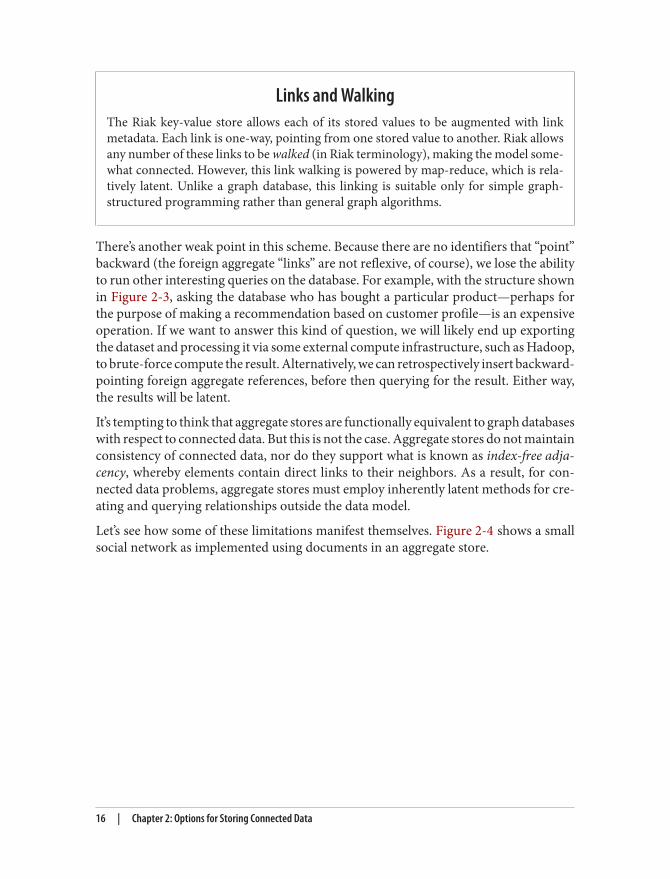
Let’s see how some of these limitations manifest themselves. Figure 2-4 shows a smallsocial network as implemented using documents in an aggregate store.

16 | Chapter 2: Options for Storing Connected Data

Figure 2-4. A small social network encoded in an aggregate store

With this structure, it’s easy to find a user’s immediate friends—assuming, of course,the application has been diligent in ensuring identifiers stored in the friends propertyare consistent with other record IDs in the database. In this case we simply look upimmediate friends by their ID, which requires numerous index lookups (one for eachfriend) but no brute-force scans of the entire dataset. Doing this, we’d find, for example,that Bob considers Alice and Zach to be friends.

But friendship isn’t always reflexive. What if we’d like to ask “who is friends with Bob?”rather than “who are Bob’s friends?” That’s a more difficult question to answer, and inthis case our only option would be to brute-force scan across the whole dataset lookingfor friends entries that contain Bob.

O-Notation and Brute-Force ProcessingWe use O-notation as a shorthand way of describing how the performance of an algo‐rithm changes with the size of the dataset. An O(1) algorithm exhibits constant-timeperformance; that is, the algorithm takes the same time to execute irrespective of thesize of the dataset. An O(n) algorithm exhibits linear performance; when the datasetdoubles, the time taken to execute the algorithm doubles. An O(log n) algorithm exhibitslogarithmic performance; when the dataset doubles, the time taken to execute the al‐gorithm increases by a fixed amount. The relative performance increase may appearcostly when a dataset is in its infancy, but it quickly tails off as the dataset gets a lot bigger.An O(m log n) algorithm is the most costly of the ones considered in this book. Withan O(m log n) algorithm, when the dataset doubles, the execution time doubles andincrements by some additional amount proportional to the number of elements in thedataset.

Brute-force computing an entire dataset is O(n) in terms of complexity because all naggregates in the data store must be considered. That’s far too costly for most

NOSQL Databases Also Lack Relationships | 17

reasonable-sized datasets, where we’d prefer an O(log n) algorithm—which is somewhatefficient because it discards half the potential workload on each iteration—or better.

Conversely, a graph database provides constant order lookup for the same query. In thiscase, we simply find the node in the graph that represents Bob, and then follow anyincoming friend relationships; these relationships lead to nodes that represent peoplewho consider Bob to be their friend. This is far cheaper than brute-forcing the resultbecause it considers far fewer members of the network; that is, it considers only thosethat are connected to Bob. Of course, if everybody is friends with Bob, we’ll still end upconsidering the entire dataset.

To avoid having to process the entire dataset, we could denormalize the storage modelby adding backward links. Adding a second property, called perhaps friended_by, toeach user, we can list the incoming friendship relations associated with that user. Butthis doesn’t come for free. For starters, we have to pay the initial and ongoing cost ofincreased write latency, plus the increased disk utilization cost for storing the additionalmetadata. On top of that, traversing the links remains expensive, because each hoprequires an index lookup. This is because aggregates have no notion of locality, unlikegraph databases, which naturally provide index-free adjacency through real—not reified—relationships. By implementing a graph structure atop a nonnative store, we get someof the benefits of partial connectedness, but at substantial cost.

This substantial cost is amplified when it comes to traversing deeper than just one hop.Friends are easy enough, but imagine trying to compute—in real time—friends-of-friends, or friends-of-friends-of-friends. That’s impractical with this kind of databasebecause traversing a fake relationship isn’t cheap. This not only limits your chances ofexpanding your social network, but it reduces profitable recommendations, missesfaulty equipment in your data center, and lets fraudulent purchasing activity slip throughthe net. Many systems try to maintain the appearance of graph-like processing, butinevitably it’s done in batches and doesn’t provide the real-time interaction that usersdemand.

Graph Databases Embrace RelationshipsThe previous examples have dealt with implicitly connected data. As users we infersemantic dependencies between entities, but the data models—and the databases them‐selves—are blind to these connections. To compensate, our applications must create anetwork out of the flat, disconnected data at hand, and then deal with any slow queriesand latent writes across denormalized stores that arise.

What we really want is a cohesive picture of the whole, including the connections be‐tween elements. In contrast to the stores we’ve just looked at, in the graph world, con‐nected data is stored as connected data. Where there are connections in the domain,

18 | Chapter 2: Options for Storing Connected Data

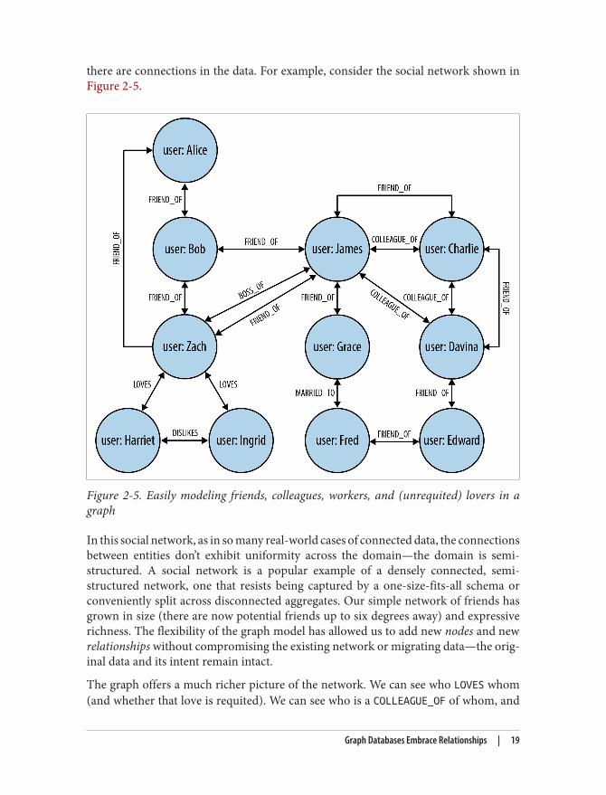
there are connections in the data. For example, consider the social network shown inFigure 2-5.

Figure 2-5. Easily modeling friends, colleagues, workers, and (unrequited) lovers in agraph

In this social network, as in so many real-world cases of connected data, the connectionsbetween entities don’t exhibit uniformity across the domain—the domain is semi-structured. A social network is a popular example of a densely connected, semi-structured network, one that resists being captured by a one-size-fits-all schema orconveniently split across disconnected aggregates. Our simple network of friends hasgrown in size (there are now potential friends up to six degrees away) and expressiverichness. The flexibility of the graph model has allowed us to add new nodes and newrelationships without compromising the existing network or migrating data—the orig‐inal data and its intent remain intact.

The graph offers a much richer picture of the network. We can see who LOVES whom(and whether that love is requited). We can see who is a COLLEAGUE_OF of whom, and

Graph Databases Embrace Relationships | 19

who is BOSS_OF them all. We can see who’s off the market, because they’re MARRIED_TOsomeone else; we can even see the antisocial elements in our otherwise social network,as represented by DISLIKES relationships. With this graph at our disposal, we can nowlook at the performance advantages of graph databases when dealing with connecteddata.

Relationships in a graph naturally form paths. Querying—or traversing—the graph in‐volves following paths. Because of the fundamentally path-oriented nature of the datamodel, the majority of path-based graph database operations are highly aligned withthe way in which the data is laid out, making them extremely efficient. In their bookNeo4j in Action, Partner and Vukotic perform an experiment using a relational storeand Neo4j. The comparison shows that the graph database is substantially quicker forconnected data than a relational store.

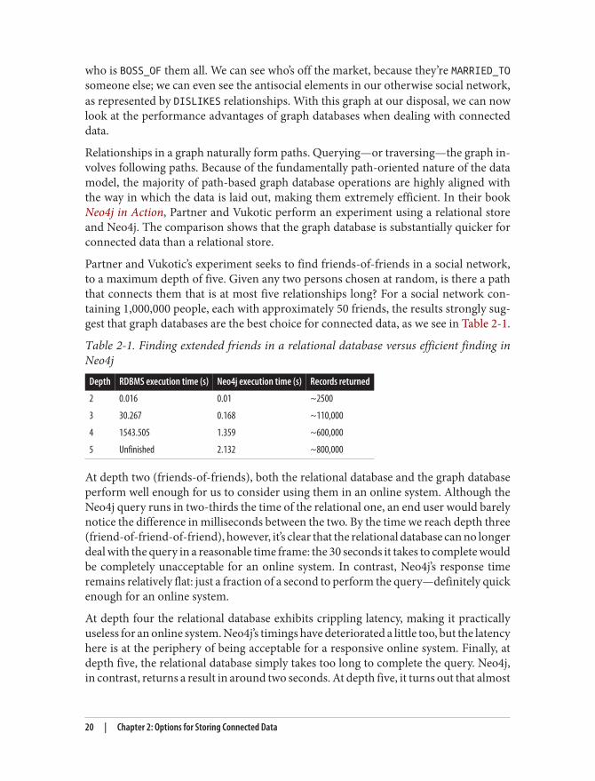
Partner and Vukotic’s experiment seeks to find friends-of-friends in a social network,to a maximum depth of five. Given any two persons chosen at random, is there a paththat connects them that is at most five relationships long? For a social network con‐taining 1,000,000 people, each with approximately 50 friends, the results strongly sug‐gest that graph databases are the best choice for connected data, as we see in Table 2-1.

Table 2-1. Finding extended friends in a relational database versus efficient finding inNeo4j

Depth RDBMS execution time (s) Neo4j execution time (s) Records returned

2 0.016 0.01 ~2500

3 30.267 0.168 ~110,000

4 1543.505 1.359 ~600,000

5 Unfinished 2.132 ~800,000

At depth two (friends-of-friends), both the relational database and the graph databaseperform well enough for us to consider using them in an online system. Although theNeo4j query runs in two-thirds the time of the relational one, an end user would barelynotice the difference in milliseconds between the two. By the time we reach depth three(friend-of-friend-of-friend), however, it’s clear that the relational database can no longerdeal with the query in a reasonable time frame: the 30 seconds it takes to complete wouldbe completely unacceptable for an online system. In contrast, Neo4j’s response timeremains relatively flat: just a fraction of a second to perform the query—definitely quickenough for an online system.

At depth four the relational database exhibits crippling latency, making it practicallyuseless for an online system. Neo4j’s timings have deteriorated a little too, but the latencyhere is at the periphery of being acceptable for a responsive online system. Finally, atdepth five, the relational database simply takes too long to complete the query. Neo4j,in contrast, returns a result in around two seconds. At depth five, it turns out that almost

20 | Chapter 2: Options for Storing Connected Data

the entire network is our friend: because of this, for many real-world use cases, we’dlikely trim the results, and the timings.

Both aggregate stores and relational databases perform poorly when wemove away from modestly sized set operations—operations that theyshould both be good at. Things slow down when we try to mine pathinformation from the graph, as with the friends-of-friends example. Wedon’t mean to unduly beat up on either aggregate stores or relationaldatabases; they have a fine technology pedigree for the things they’regood at, but they fall short when managing connected data. Anythingmore than a shallow traversal of immediate friends, or possibly friends-of-friends, will be slow because of the number of index lookups in‐volved. Graphs, on the other hand, use index-free adjacency to ensurethat traversing connected data is extremely rapid.

The social network example helps illustrate how different technologies deal with con‐nected data, but is it a valid use case? Do we really need to find such remote “friends”?Perhaps not. But substitute social networks for any other domain, and you’ll see weexperience similar performance, modeling, and maintenance benefits. Whether musicor data center management, bio-informatics or football statistics, network sensors ortime-series of trades, graphs provide powerful insight into our data. Let’s look, then, atanother contemporary application of graphs: recommending products based on a user’spurchase history and the histories of his friends, neighbors, and other people like him.With this example, we’ll bring together several independent facets of a user’s lifestyle tomake accurate and profitable recommendations.

We’ll start by modeling the purchase history of a user as connected data. In a graph, thisis as simple as linking the user to her orders, and linking orders together to provide apurchase history, as shown in Figure 2-6.

The graph shown in Figure 2-6 provides a great deal of insight into customer behavior.We can see all the orders a user has PLACED, and we can easily reason about what eachorder CONTAINS. So far so good. But on top of that, we’ve enriched the graph to supportwell-known access patterns. For example, users often want to see their order history, sowe’ve added a linked list structure to the graph that allows us to find a user’s most recentorder by following an outgoing MOST_RECENT relationship. We can then iterate throughthe list, going further back in time, by following each PREVIOUS relationship. If we wantto move forward in time, we can follow each PREVIOUS relationship in the oppositedirection, or add a reciprocal NEXT relationship.

Graph Databases Embrace Relationships | 21

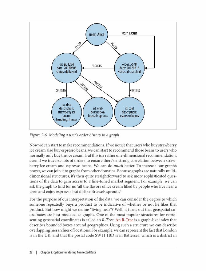
Figure 2-6. Modeling a user’s order history in a graph

Now we can start to make recommendations. If we notice that users who buy strawberryice cream also buy espresso beans, we can start to recommend those beans to users whonormally only buy the ice cream. But this is a rather one-dimensional recommendation,even if we traverse lots of orders to ensure there’s a strong correlation between straw‐berry ice cream and espresso beans. We can do much better. To increase our graph’spower, we can join it to graphs from other domains. Because graphs are naturally multi-dimensional structures, it’s then quite straightforward to ask more sophisticated ques‐tions of the data to gain access to a fine-tuned market segment. For example, we canask the graph to find for us “all the flavors of ice cream liked by people who live near auser, and enjoy espresso, but dislike Brussels sprouts.”

For the purpose of our interpretation of the data, we can consider the degree to whichsomeone repeatedly buys a product to be indicative of whether or not he likes thatproduct. But how might we define “living near”? Well, it turns out that geospatial co‐ordinates are best modeled as graphs. One of the most popular structures for repre‐senting geospatial coordinates is called an R-Tree. An R-Tree is a graph-like index thatdescribes bounded boxes around geographies. Using such a structure we can describeoverlapping hierarchies of locations. For example, we can represent the fact that Londonis in the UK, and that the postal code SW11 1BD is in Battersea, which is a district in

22 | Chapter 2: Options for Storing Connected Data

London, which is in southeastern England, which, in turn, is in Great Britain. Andbecause UK postal codes are fine-grained, we can use that boundary to target peoplewith somewhat similar tastes.

Such pattern-matching queries are extremely difficult to write in SQL,and laborious to write against aggregate stores, and in both cases theytend to perform very poorly. Graph databases, on the other hand, areoptimized for precisely these types of traversals and pattern-matchingqueries, providing in many cases millisecond responses. Moreover,most graph databases provide a query language suited to expressinggraph constructs and graph queries. In the next chapter, we’ll look at Cypher, which is a pattern-matching language tuned to the way we tendto describe graphs using diagrams.

We can use our example graph to make recommendations to the user, but we can alsouse it to benefit the seller. For example, given certain buying patterns (products, cost oftypical order, and so on), we can establish whether a particular transaction is potentiallyfraudulent. Patterns outside of the norm for a given user can easily be detected in a graphand be flagged for further attention (using well-known similarity measures from thegraph data-mining literature), thus reducing the risk for the seller.

From the data practitioner’s point of view, it’s clear that the graph database is the besttechnology for dealing with complex, semi-structured, densely connected data—that is,with datasets so sophisticated they are unwieldy when treated in any form other than agraph.

SummaryIn this chapter we’ve seen how connectedness in relational databases and NOSQL datastores requires developers to implement data processing in the application layer, andcontrasted that with graph databases, where connectedness is a first-class citizen. In thenext chapter we look in more detail at the topic of graph modeling.

Summary | 23

CHAPTER 3

Data Modeling with Graphs

In previous chapters we’ve described the substantial benefits of the graph database whencompared both with document, column family, and key-value NOSQL stores, and withtraditional relational databases. But having chosen to adopt a graph database, the ques‐tion arises: how do we model the world in graph terms?

This chapter focuses on graph modeling. Starting with a recap of the property graphmodel—the most widely adopted graph data model—we then provide an overview ofthe graph query language used for most of the code examples in this book: Cypher.Cypher is one of several languages for describing and querying property graphs. Thereis, as of today, no agreed-upon standard for graph query languages, as exists in therelational database management systems (RDBMS) world with SQL. Cypher was chosenin part because of the authors’ fluency with the language, but also because it is easy tolearn and understand, and is widely used. With these fundamentals in place, we diveinto a couple of examples of graph modeling. With our first example, that of a systemsmanagement domain, we compare relational and graph modeling techniques. With thesecond example, the production and consumption of Shakespearean literature, we usea graph to connect and query several disparate domains. We end the chapter by lookingat some common pitfalls when modeling with graphs, and highlight some goodpractices.

Models and GoalsBefore we dig deeper into modeling with graphs, a word on models in general. Modelingis an abstracting activity motivated by a particular need or goal. We model in order tobring specific facets of an unruly domain into a space where they can be structured andmanipulated. There are no natural representations of the world the way it “really is,” justmany purposeful selections, abstractions, and simplifications, some of which are moreuseful than others for satisfying a particular goal.

25

Graph representations are no different in this respect. What perhaps differentiates themfrom many other data modeling techniques, however, is the close affinity between thelogical and physical models. Relational data management techniques require us to de‐viate from our natural language representation of the domain: first by cajoling our rep‐resentation into a logical model, and then by forcing it into a physical model. Thesetransformations introduce semantic dissonance between our conceptualization of theworld and the database’s instantiation of that model. With graph databases, this gapshrinks considerably.

We Already Communicate in GraphsGraph modeling naturally fits with the way we tend to abstract the salient details froma domain using circles and boxes, and then describe the connections between thesethings by joining them with arrows. Today’s graph databases, more than any other da‐tabase technologies, are “whiteboard friendly.” The typical whiteboard view of a problemis a graph. What we sketch in our creative and analytical modes maps closely to the datamodel we implement inside the database. In terms of expressivity, graph databases re‐duce the impedance mismatch between analysis and implementation that has plaguedrelational database implementations for many years. What is particularly interestingabout such graph models is the fact that they not only communicate how we think thingsare related, but they also clearly communicate the kinds of questions we want to ask ofour domain. As we’ll see throughout this chapter, graph models and graph queries arereally just two sides of the same coin.

The Property Graph ModelWe introduced the property graph model in Chapter 1. To recap, these are its salientfeatures:

• A property graph is made up of nodes, relationships, and properties.• Nodes contain properties. Think of nodes as documents that store properties in the

form of arbitrary key-value pairs. The keys are strings and the values are arbitrarydata types.

• Relationships connect and structure nodes. A relationship always has a direction,a label, and a start node and an end node—there are no dangling relationships.Together, a relationship’s direction and label add semantic clarity to the structuringof nodes.

• Like nodes, relationships can also have properties. The ability to add properties torelationships is particularly useful for providing additional metadata for graph

26 | Chapter 3: Data Modeling with Graphs

1. The Cypher examples in the book were written using Neo4j 2.0. Most of the examples will work with versions1.8 and 1.9 of Neo4j. Where a particular language feature requires the latest version, we’ll point it out.

2. For reference documentation see http://bit.ly/15Fjjo1 and http://bit.ly/17l69Mv.

algorithms, adding additional semantics to relationships (including quality andweight), and for constraining queries at runtime.

These simple primitives are all we need to create sophisticated and semantically richmodels. So far, all our models have been in the form of diagrams. Diagrams are greatfor describing graphs outside of any technology context, but when it comes to using adatabase, we need some other mechanism for creating, manipulating, and queryingdata. We need a query language.

Querying Graphs: An Introduction to CypherCypher is an expressive (yet compact) graph database query language. Although specificto Neo4j, its close affinity with our habit of representing graphs using diagrams makesit ideal for programatically describing graphs in a precise fashion. For this reason, weuse Cypher throughout the rest of this book to illustrate graph queries and graph con‐structions. Cypher is arguably the easiest graph query language to learn, and is a greatbasis for learning about graphs. Once you understand Cypher, it becomes very easy tobranch out and learn other graph query languages.1

In the following sections we’ll take a brief tour through Cypher. This isn’t a referencedocument for Cypher, however—merely a friendly introduction so that we can exploremore interesting graph query scenarios later on.2

Other Query LanguagesOther graph databases have other means of querying data. Many, including Neo4j, sup‐port the RDF query language SPARQL and the imperative, path-based query languageGremlin. Our interest, however, is in the expressive power of a property graph combinedwith a declarative query language, and so in this book we focus almost exclusively onCypher.

Cypher PhilosophyCypher is designed to be easily read and understood by developers, database profes‐sionals, and business stakeholders. Its ease of use derives from the fact it accords withthe way we intuitively describe graphs using diagrams.

Querying Graphs: An Introduction to Cypher | 27

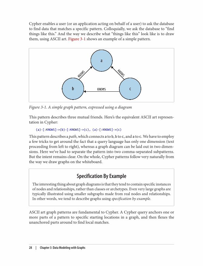
Cypher enables a user (or an application acting on behalf of a user) to ask the databaseto find data that matches a specific pattern. Colloquially, we ask the database to “findthings like this.” And the way we describe what “things like this” look like is to drawthem, using ASCII art. Figure 3-1 shows an example of a simple pattern.

Figure 3-1. A simple graph pattern, expressed using a diagram

This pattern describes three mutual friends. Here’s the equivalent ASCII art represen‐tation in Cypher:

(a)-[:KNOWS]->(b)-[:KNOWS]->(c), (a)-[:KNOWS]->(c)

This pattern describes a path, which connects a to b, b to c, and a to c. We have to employa few tricks to get around the fact that a query language has only one dimension (textproceeding from left to right), whereas a graph diagram can be laid out in two dimen‐sions. Here we’ve had to separate the pattern into two comma-separated subpatterns.But the intent remains clear. On the whole, Cypher patterns follow very naturally fromthe way we draw graphs on the whiteboard.

Specification By ExampleThe interesting thing about graph diagrams is that they tend to contain specific instancesof nodes and relationships, rather than classes or archetypes. Even very large graphs aretypically illustrated using smaller subgraphs made from real nodes and relationships.In other words, we tend to describe graphs using specification by example.

ASCII art graph patterns are fundamental to Cypher. A Cypher query anchors one ormore parts of a pattern to specific starting locations in a graph, and then flexes theunanchored parts around to find local matches.

28 | Chapter 3: Data Modeling with Graphs

The starting locations—the anchor points in the real graph, to whichsome parts of the pattern are bound—are discovered in one of two ways.The most common method is to use an index. Neo4j uses indexes asnaming services; that is, as ways of finding starting locations based onone or more indexed property values.

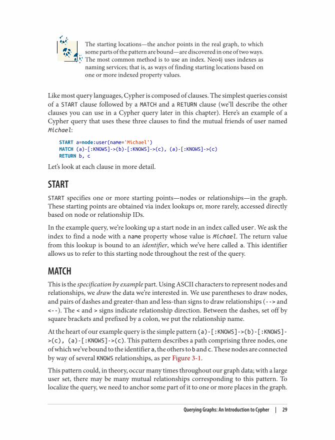
Like most query languages, Cypher is composed of clauses. The simplest queries consistof a START clause followed by a MATCH and a RETURN clause (we’ll describe the otherclauses you can use in a Cypher query later in this chapter). Here’s an example of aCypher query that uses these three clauses to find the mutual friends of user namedMichael:

START a=node:user(name='Michael')MATCH (a)-[:KNOWS]->(b)-[:KNOWS]->(c), (a)-[:KNOWS]->(c)RETURN b, c

Let’s look at each clause in more detail.

STARTSTART specifies one or more starting points—nodes or relationships—in the graph.These starting points are obtained via index lookups or, more rarely, accessed directlybased on node or relationship IDs.

In the example query, we’re looking up a start node in an index called user. We ask theindex to find a node with a name property whose value is Michael. The return valuefrom this lookup is bound to an identifier, which we’ve here called a. This identifierallows us to refer to this starting node throughout the rest of the query.

MATCHThis is the specification by example part. Using ASCII characters to represent nodes andrelationships, we draw the data we’re interested in. We use parentheses to draw nodes,and pairs of dashes and greater-than and less-than signs to draw relationships (--> and<--). The < and > signs indicate relationship direction. Between the dashes, set off bysquare brackets and prefixed by a colon, we put the relationship name.

At the heart of our example query is the simple pattern (a)-[:KNOWS]->(b)-[:KNOWS]->(c), (a)-[:KNOWS]->(c). This pattern describes a path comprising three nodes, oneof which we’ve bound to the identifier a, the others to b and c. These nodes are connectedby way of several KNOWS relationships, as per Figure 3-1.

This pattern could, in theory, occur many times throughout our graph data; with a largeuser set, there may be many mutual relationships corresponding to this pattern. Tolocalize the query, we need to anchor some part of it to one or more places in the graph.

Querying Graphs: An Introduction to Cypher | 29

What we’ve done with the START clause is look up a real node in the graph—the noderepresenting Michael. We bind this Michael node to the a identifier; a then carries overto the MATCH clause. This has the effect of anchoring our pattern to a specific point inthe graph. Cypher then matches the remainder of the pattern to the graph immediatelysurrounding the anchor point. As it does so, it discovers nodes to bind to the otheridentifiers. While a will always be anchored to Michael, b and c will be bound to asequence of nodes as the query executes.

RETURNThis clause specifies which nodes, relationships, and properties in the matched datashould be returned to the client. In our example query, we’re interested in returning thenodes bound to the b and c identifiers. Each matching node is lazily bound to its iden‐tifier as the client iterates the results.

Other Cypher ClausesThe other clauses we can use in a Cypher query include:WHERE

Provides criteria for filtering pattern matching results.

CREATE and CREATE UNIQUECreate nodes and relationships.

DELETE

Removes nodes, relationships, and properties.

SET

Sets property values.

FOREACH

Performs an updating action for each element in a list.

UNION

Merges results from two or more queries (introduced in Neo4j 2.0).

WITH

Chains subsequent query parts and forward results from one to the next. Similarto piping commands in Unix.

If these clauses look familiar—especially if you’re a SQL developer—that’s great! Cypheris intended to be familiar enough to help you move rapidly along the learning curve. Atthe same time, it’s different enough to emphasize that we’re dealing with graphs, notrelational sets.

30 | Chapter 3: Data Modeling with Graphs

We’ll see some examples of these clauses later in the chapter. Where they occur, we’lldescribe in more detail how they work.

Now that we’ve seen how we can describe and query a graph using Cypher, we can lookat some examples of graph modeling.

A Comparison of Relational and Graph ModelingTo introduce graph modeling, we’re going to look at how we model a domain using bothrelational- and graph-based techniques. Most developers and data professionals arefamiliar with RDBMS systems and the associated data modeling techniques; as a result,the comparison will highlight a few similarities, and many differences. In particular,we’ll see how easy it is to move from a conceptual graph model to a physical graphmodel, and how little the graph model distorts what we’re trying to represent versus therelational model.

To facilitate this comparison, we’ll examine a simple data center management domain.In this domain, several data centers support many applications on behalf of many cus‐tomers using different pieces of infrastructure, from virtual machines to physical loadbalancers. An example of this domain is shown in Figure 3-2.

In Figure 3-2 we see a somewhat simplified view of several applications and the datacenter infrastructure necessary to support them. The applications, represented by nodesApp 1, App 2, and App 3, depend on a cluster of databases labeled Database Server 1,2, 3. While users logically depend on the availability of an application and its data,there is additional physical infrastructure between the users and the application; thisinfrastructure includes virtual machines (Virtual Machine 10, 11, 20, 30, 31), realservers (Server 1, 2, 3), racks for the servers (Rack 1, 2 ), and load balancers (LoadBalancer 1, 2), which front the apps. In between each of the components there are,of course, many networking elements: cables, switches, patch panels, NICs, power sup‐plies, air conditioning, and so on—all of which can fail at inconvenient times. To com‐plete the picture we have a straw-man single user of application 3, represented byUser 3.

A Comparison of Relational and Graph Modeling | 31

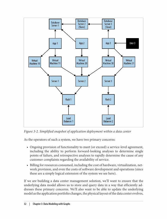
Figure 3-2. Simplified snapshot of application deployment within a data center

As the operators of such a system, we have two primary concerns:

• Ongoing provision of functionality to meet (or exceed) a service-level agreement,including the ability to perform forward-looking analyses to determine singlepoints of failure, and retrospective analyses to rapidly determine the cause of anycustomer complaints regarding the availability of service.

• Billing for resources consumed, including the cost of hardware, virtualization, net‐work provision, and even the costs of software development and operations (sincethese are a simply logical extension of the system we see here).

If we are building a data center management solution, we’ll want to ensure that theunderlying data model allows us to store and query data in a way that efficiently ad‐dresses these primary concerns. We’ll also want to be able to update the underlyingmodel as the application portfolio changes, the physical layout of the data center evolves,

32 | Chapter 3: Data Modeling with Graphs

and virtual machine instances migrate. Given these needs and constraints, let’s see howthe relational and graph models compare.

Relational Modeling in a Systems Management DomainThe initial stage of modeling in the relational world is similar to the first stage of manyother data modeling techniques: that is, we seek to understand and agree on the entitiesin the domain, how they interrelate, and the rules that govern their state transitions.Most of this tends to be done informally, often through whiteboard sketches and dis‐cussions between subject matter experts and systems and data architects. To express ourcommon understanding and agreement, we typically create a diagram such as the onein Figure 3-2, which is a graph.

The next stage captures this agreement in a more rigorous form such as an entity-relationship (E-R) diagram—another graph. This transformation of the conceptualmodel into a logical model using a more strict notation provides us with a second chanceto refine our domain vocabulary so that it can be shared with relational database spe‐cialists. (Such approaches aren’t always necessary: adept relational users often movedirectly to table design and normalization without first describing an intermediate E-R diagram.) In our example, we’ve captured the domain in the E-R diagram shown inFigure 3-3.

Despite being graphs, E-R diagrams immediately demonstrate theshortcomings of the relational model for capturing a rich domain. Al‐though they allow relationships to be named (something that graphdatabases fully embrace, but which relational stores do not), E-R dia‐grams allow only single, undirected, named relationships between en‐tities. In this respect, the relational model is a poor fit for real-worlddomains where relationships between entities are both numerous andsemantically rich and diverse.

Having arrived at a suitable logical model, we map it into tables and relations, whichare normalized to eliminate data redundancy. In many cases this step can be as simpleas transcribing the E-R diagram into a tabular form and then loading those tables viaSQL commands into the database. But even the simplest case serves to highlight theidiosyncrasies of the relational model. For example, in Figure 3-4 we see that a greatdeal of accidental complexity has crept into the model in the form of foreign key con‐straints (everything annotated [FK]), which support one-to-many relationships, andjoin tables (e.g., AppDatabase), which support many-to-many relationships—and allthis before we’ve added a single row of real user data. These constraints are model-levelmetadata that exist simply so that we can make concrete the relations between tables at

A Comparison of Relational and Graph Modeling | 33

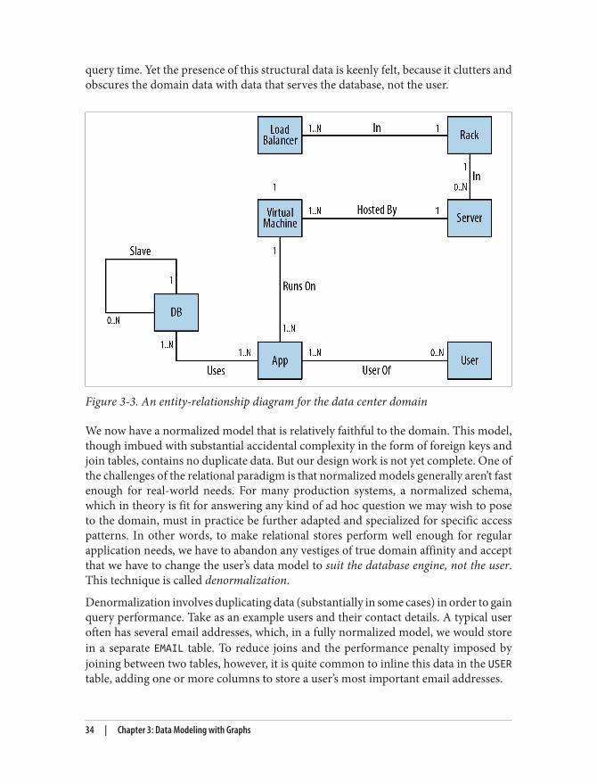
query time. Yet the presence of this structural data is keenly felt, because it clutters andobscures the domain data with data that serves the database, not the user.

Figure 3-3. An entity-relationship diagram for the data center domain

We now have a normalized model that is relatively faithful to the domain. This model,though imbued with substantial accidental complexity in the form of foreign keys andjoin tables, contains no duplicate data. But our design work is not yet complete. One ofthe challenges of the relational paradigm is that normalized models generally aren’t fastenough for real-world needs. For many production systems, a normalized schema,which in theory is fit for answering any kind of ad hoc question we may wish to poseto the domain, must in practice be further adapted and specialized for specific accesspatterns. In other words, to make relational stores perform well enough for regularapplication needs, we have to abandon any vestiges of true domain affinity and acceptthat we have to change the user’s data model to suit the database engine, not the user.This technique is called denormalization.

Denormalization involves duplicating data (substantially in some cases) in order to gainquery performance. Take as an example users and their contact details. A typical useroften has several email addresses, which, in a fully normalized model, we would storein a separate EMAIL table. To reduce joins and the performance penalty imposed byjoining between two tables, however, it is quite common to inline this data in the USERtable, adding one or more columns to store a user’s most important email addresses.

34 | Chapter 3: Data Modeling with Graphs

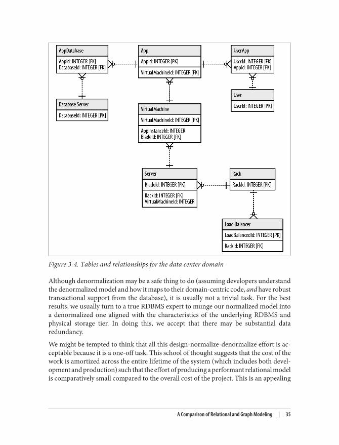
Figure 3-4. Tables and relationships for the data center domain

Although denormalization may be a safe thing to do (assuming developers understandthe denormalized model and how it maps to their domain-centric code, and have robusttransactional support from the database), it is usually not a trivial task. For the bestresults, we usually turn to a true RDBMS expert to munge our normalized model intoa denormalized one aligned with the characteristics of the underlying RDBMS andphysical storage tier. In doing this, we accept that there may be substantial dataredundancy.

We might be tempted to think that all this design-normalize-denormalize effort is ac‐ceptable because it is a one-off task. This school of thought suggests that the cost of thework is amortized across the entire lifetime of the system (which includes both devel‐opment and production) such that the effort of producing a performant relational modelis comparatively small compared to the overall cost of the project. This is an appealing

A Comparison of Relational and Graph Modeling | 35

notion, but in many cases it doesn’t match reality, because systems change not onlyduring development, but also during their production lifetimes.

The amortized view of data model change, in which costly changes during developmentare eclipsed by the long-term benefits of a stable model in production, assumes thatsystems spend the majority of their time in production environments, and that theseproduction environments are stable. Though it may be the case that most systems spendmost of their time in production environments, these environments are rarely stable.As business requirements change or regulatory requirements evolve, so must our sys‐tems and the data structures on which they are built.

Data models invariably undergo substantial revision during the design and developmentphases of a project, and in almost every case, these revisions are intended to accom‐modate the model to the needs of the applications that will consume it once it is inproduction. These initial design influences are so powerful that it becomes nearly im‐possible to modify the application and the model once they’re in production to accom‐modate things they were not originally designed to do.

The technical mechanism by which we introduce structural change into a database iscalled migration, as popularized by application development frameworks such asRails. Migrations provide a structured, step-wise approach to applying a set of databaserefactorings to a database so that it can be responsibly evolved to meet the changingneeds of the applications that use it. Unlike code refactorings, however, which we typ‐ically accomplish in a matter of seconds or minutes, database refactorings can take weeksor months to complete, with downtime for schema changes. Database refactoring isslow, risky, and expensive.

The problem, then, with the denormalized model is its resistance to the kind of rapidevolution the business demands of its systems. As we’ve seen with the data center ex‐ample, the changes imposed on the whiteboard model over the course of implementinga relational solution create a gulf between the conceptual world and the way the data isphysically laid out; this conceptual-relational dissonance all but prevents businessstakeholders from actively collaborating in the further evolution of a system. Stake‐holder participation stops at the threshold of the relational edifice. On the developmentside, the difficulties in translating changed business requirements into the underlyingand entrenched relational structure cause the evolution of the system to lag behind theevolution of the business. Without expert assistance and rigorous planning, migratinga denormalized database poses several risks. If the migrations fail to maintain storage-affinity, performance can suffer. Just as serious, if deliberately duplicated data is leftorphaned after a migration, we risk compromising the integrity of the data as a whole.

Graph Modeling in a Systems Management DomainWe’ve seen how relational modeling and its attendant implementation activities take usdown a path that divorces an application’s underlying storage model from the conceptual

36 | Chapter 3: Data Modeling with Graphs

worldview of its stakeholders. Relational databases—with their rigid schemas and com‐plex modeling characteristics—are not an especially good tool for supporting rapidchange. What we need is a model that is closely aligned with the domain, but whichdoesn’t sacrifice performance, and which supports evolution while maintaining the in‐tegrity of the data as it undergoes rapid change and growth. That model is the graphmodel. How, then, does this process differ when realized with a graph data model?

In the early stages of analysis, the work required of us is similar to the relational ap‐proach: using lo-fi methods such as whiteboard sketches, we describe and agree uponthe domain. After that, however, the methodologies diverge. Instead of transforming adomain model’s graph-like representation into tables, we enrich it, with the aim of pro‐ducing an accurate representation of the salient aspects of the domain relevant to whatwe are trying to achieve in that domain. That is, for each entity in our domain, we ensurethat we’ve captured both the properties and the connections to neighboring entitiesnecessary to support our application goals.

Remember, the domain model is not a transparent, context-free win‐dow onto reality: rather, it is a purposeful abstraction of those aspectsof our domain relevant to our application goals. There’s always somemotivation for creating a model. By enriching our first-cut domaingraph with additional properties and relationships, we effectively pro‐duce a graph model attuned to our application’s data needs; that is, weprovide for answering the kinds of questions our application will ask ofits data.

Helpfully, domain modeling is completely isomorphic to graph modeling. By ensuringthe correctness of the domain model we’re implicitly improving the graph model, be‐cause in a graph database what you sketch on the whiteboard is typically what you storein the database.

In graph terms what we’re doing is ensuring each node has the appropriate propertiesso that it can fulfil its specific data-centric domain responsibilities. But we’re also en‐suring that every node is in the correct semantic context; we do this by creating namedand directed (and often attributed) relationships between the nodes to capture thestructural aspects of the domain. For our data center scenario, the resulting graph modellooks like Figure 3-5.

A Comparison of Relational and Graph Modeling | 37

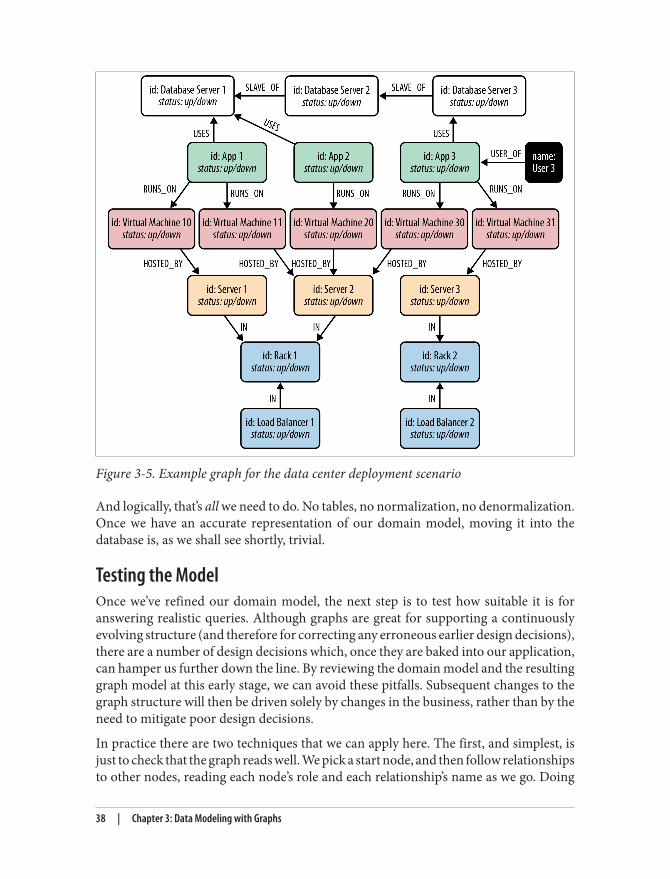
Figure 3-5. Example graph for the data center deployment scenario

And logically, that’s all we need to do. No tables, no normalization, no denormalization.Once we have an accurate representation of our domain model, moving it into thedatabase is, as we shall see shortly, trivial.

Testing the ModelOnce we’ve refined our domain model, the next step is to test how suitable it is foranswering realistic queries. Although graphs are great for supporting a continuouslyevolving structure (and therefore for correcting any erroneous earlier design decisions),there are a number of design decisions which, once they are baked into our application,can hamper us further down the line. By reviewing the domain model and the resultinggraph model at this early stage, we can avoid these pitfalls. Subsequent changes to thegraph structure will then be driven solely by changes in the business, rather than by theneed to mitigate poor design decisions.

In practice there are two techniques that we can apply here. The first, and simplest, isjust to check that the graph reads well. We pick a start node, and then follow relationshipsto other nodes, reading each node’s role and each relationship’s name as we go. Doing

38 | Chapter 3: Data Modeling with Graphs

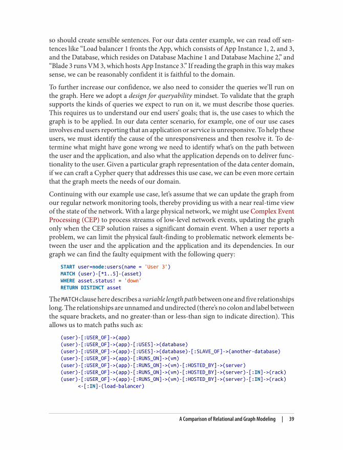
so should create sensible sentences. For our data center example, we can read off sen‐tences like “Load balancer 1 fronts the App, which consists of App Instance 1, 2, and 3,and the Database, which resides on Database Machine 1 and Database Machine 2,” and“Blade 3 runs VM 3, which hosts App Instance 3.” If reading the graph in this way makessense, we can be reasonably confident it is faithful to the domain.

To further increase our confidence, we also need to consider the queries we’ll run onthe graph. Here we adopt a design for queryability mindset. To validate that the graphsupports the kinds of queries we expect to run on it, we must describe those queries.This requires us to understand our end users’ goals; that is, the use cases to which thegraph is to be applied. In our data center scenario, for example, one of our use casesinvolves end users reporting that an application or service is unresponsive. To help theseusers, we must identify the cause of the unresponsiveness and then resolve it. To de‐termine what might have gone wrong we need to identify what’s on the path betweenthe user and the application, and also what the application depends on to deliver func‐tionality to the user. Given a particular graph representation of the data center domain,if we can craft a Cypher query that addresses this use case, we can be even more certainthat the graph meets the needs of our domain.

Continuing with our example use case, let’s assume that we can update the graph fromour regular network monitoring tools, thereby providing us with a near real-time viewof the state of the network. With a large physical network, we might use Complex EventProcessing (CEP) to process streams of low-level network events, updating the graphonly when the CEP solution raises a significant domain event. When a user reports aproblem, we can limit the physical fault-finding to problematic network elements be‐tween the user and the application and the application and its dependencies. In ourgraph we can find the faulty equipment with the following query:

START user=node:users(name = 'User 3')MATCH (user)-[*1..5]-(asset)WHERE asset.status! = 'down'RETURN DISTINCT asset

The MATCH clause here describes a variable length path between one and five relationshipslong. The relationships are unnamed and undirected (there’s no colon and label betweenthe square brackets, and no greater-than or less-than sign to indicate direction). Thisallows us to match paths such as:

(user)-[:USER_OF]->(app)(user)-[:USER_OF]->(app)-[:USES]->(database)(user)-[:USER_OF]->(app)-[:USES]->(database)-[:SLAVE_OF]->(another-database)(user)-[:USER_OF]->(app)-[:RUNS_ON]->(vm)(user)-[:USER_OF]->(app)-[:RUNS_ON]->(vm)-[:HOSTED_BY]->(server)(user)-[:USER_OF]->(app)-[:RUNS_ON]->(vm)-[:HOSTED_BY]->(server)-[:IN]->(rack)(user)-[:USER_OF]->(app)-[:RUNS_ON]->(vm)-[:HOSTED_BY]->(server)-[:IN]->(rack) <-[:IN]-(load-balancer)

A Comparison of Relational and Graph Modeling | 39

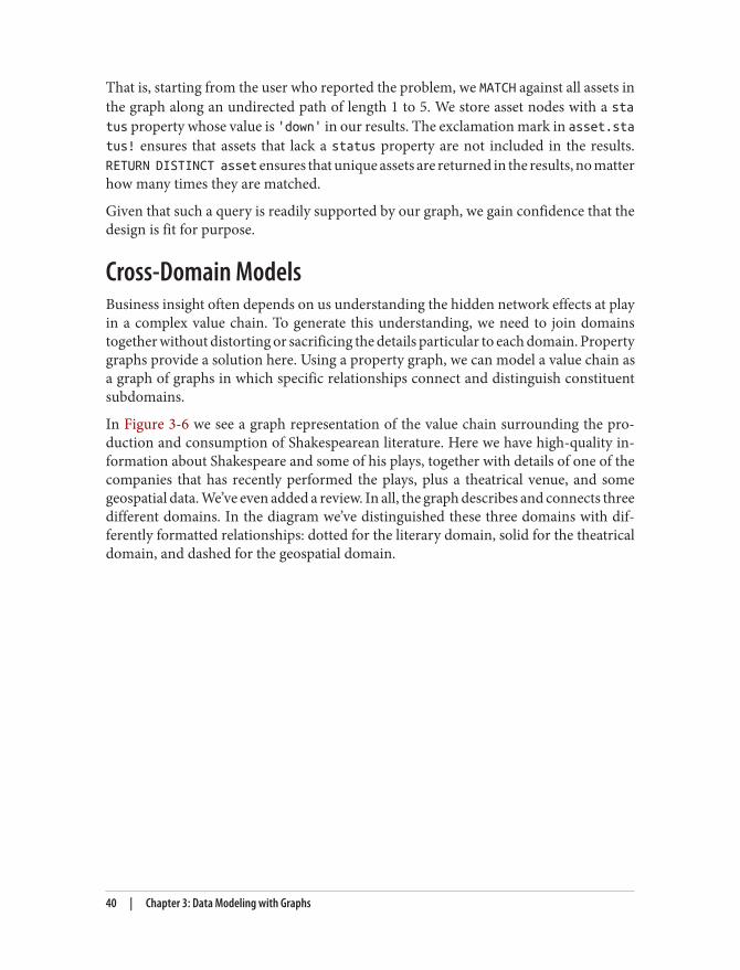
That is, starting from the user who reported the problem, we MATCH against all assets inthe graph along an undirected path of length 1 to 5. We store asset nodes with a status property whose value is 'down' in our results. The exclamation mark in asset.status! ensures that assets that lack a status property are not included in the results.RETURN DISTINCT asset ensures that unique assets are returned in the results, no matterhow many times they are matched.

Given that such a query is readily supported by our graph, we gain confidence that thedesign is fit for purpose.

Cross-Domain ModelsBusiness insight often depends on us understanding the hidden network effects at playin a complex value chain. To generate this understanding, we need to join domainstogether without distorting or sacrificing the details particular to each domain. Propertygraphs provide a solution here. Using a property graph, we can model a value chain asa graph of graphs in which specific relationships connect and distinguish constituentsubdomains.

In Figure 3-6 we see a graph representation of the value chain surrounding the pro‐duction and consumption of Shakespearean literature. Here we have high-quality in‐formation about Shakespeare and some of his plays, together with details of one of thecompanies that has recently performed the plays, plus a theatrical venue, and somegeospatial data. We’ve even added a review. In all, the graph describes and connects threedifferent domains. In the diagram we’ve distinguished these three domains with dif‐ferently formatted relationships: dotted for the literary domain, solid for the theatricaldomain, and dashed for the geospatial domain.

40 | Chapter 3: Data Modeling with Graphs

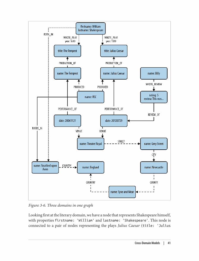
Figure 3-6. Three domains in one graph

Looking first at the literary domain, we have a node that represents Shakespeare himself,with properties firstname: 'William' and lastname: 'Shakespeare'. This node isconnected to a pair of nodes representing the plays Julius Caesar (title: 'Julius

Cross-Domain Models | 41

Caesar') and The Tempest (title: 'The Tempest') via relationships labeledWROTE_PLAY.

Reading this subgraph left-to-right, following the direction of the relationship arrows,conveys the fact that William Shakespeare wrote Julius Caesar and The Tempest. If we’reinterested in provenance, each WROTE_PLAY relationship has a date property, which tellsus that Julius Caesar was written in 1599 and The Tempest in 1610. It’s a trivial matterto see how we could add the rest of Shakespeare’s works—the plays and the poems—into the graph simply by adding more nodes to represent each work, and joining themto the Shakespeare node via WROTE_PLAY and WROTE_POEM relationships.

By tracing the WROTE_PLAY relationship arrows with our finger, we’reeffectively doing the kind of work that a graph database performs, albeitat human speed rather than computer speed. As we’ll see later, this sim‐ple traversal operation is the building block for arbitrarily sophisticatedgraph queries.

Turning next to the theatrical domain, you can see that we’ve added some informationabout the Royal Shakespeare Company (often known simply as the RSC) in the form ofa node with the key company and value RSC. The theatrical domain is, unsurprisingly,connected to the literary domain: in our graph, this is reflected by the fact that the RSChas PRODUCED versions of Julius Caesar and The Tempest; these theatrical productionsare in turn connected to their literary source, the plays in the literary domain usingPRODUCTION_OF relationships. The graph also captures details of specific performances:the RSC’s production of Julius Caesar, for example, was performed on 29 July 2012 aspart of the RSC’s summer touring season. If we’re interested in the performance venue,we simply follow the outgoing VENUE relationship from the performance node to findthat the play was performed at the Theatre Royal.

The graph also allows us to capture reviews of specific performances. In our samplegraph we’ve included just one review, for the 29 July performance, written by the userBilly. We can see this in the interplay of the performance, rating, and user nodes. Inthis case we have a node representing Billy (name: 'Billy') whose outgoing WROTE_REVIEW relationship connects to a node representing his review. The review node containsa numeric rating property and a free-text review property. The review is linked to aspecific performance through an outgoing REVIEW_OF relationship. To scale this up tomany users, many reviews, and many performances, we simply add more nodes andmore identically named relationships to the graph.

The third domain, that of geospatial data, comprises a simple hierarchical tree of places.This geospatial domain is connected to the other two domains at several points in thegraph. The town of Stratford upon Avon (with property name: 'Stratford upon

42 | Chapter 3: Data Modeling with Graphs

Avon') is connected to the literary domain as a result of its being Shakespeare’s birthplace(Shakespeare was BORN_IN Stratford). It is connected to the theatrical domain insofaras it is home to the RSC (the RSC is BASED_IN Stratford). To learn more about Stratfordupon Avon’s geography, we can follow its outgoing COUNTRY relationship to discover itis in England.

Note how the graph reduces instances of duplicated data across do‐mains. Stratford upon Avon, for example, participates in all threedomains.

The property graph makes it possible to capture more complex geospatial data. Lookingat the Theatre Royal, for example, we see that it is located on Grey Street, which is inthe CITY of Newcastle, which is in the COUNTY of Tyne and Wear, which ultimately is inthe COUNTRY of England—just like Stratford upon Avon.

Relationships help both partition a graph into separate domains and connect thosedomains. As we can see from this relatively simple example, the property graph modelmakes it easy to unite different domains—each with its own particular entities, prop‐erties, and relationships—in a way that not only makes each domain accessible, but alsogenerates insight from the connections between domains.

Labeling NodesWe’ve used relationships here to structure the graph and establish the semantic contextfor each node. By following an outgoing WROTE_REVIEW relationship, for example, weunderstand that the node at the end of that relationship represents a review. But this isa rather weak method for indicating what kind of domain abstraction a node represents.How might we improve it?

Today, to satisfy this need, many users of Neo4j add type or label properties to theirnodes. This is an ad hoc solution to the problem, with no direct support at the level ofthe query languages and APIs. Forthcoming releases of Neo4j, however, will presentusers with an enhanced property graph that incorporates labels as first-class citizens ofthe data model. Labelling allows us to attach one or more labels to a node; using theselabels we can then determine which roles or functions a node fulfills. On top of that,we’ll be able to ask the graph to find nodes labeled User, or Customer, or even nodeslabeled both User and Customer. Subsequent releases will allow us to associate con‐straints with labels, further enhancing our ability to represent and reason about ourdomain. The first release of the enhanced data model is scheduled to occur around thetime this book goes to press.

Cross-Domain Models | 43

Creating the Shakespeare GraphTo create the Shakespeare graph shown in Figure 3-6, we use CREATE to build the overallstructure. This statement is executed by the Cypher runtime within a single transactionsuch that once the statement has executed, we can be confident the graph is present inits entirety in the database. If the transaction fails, no part of the graph will be presentin the database. As we might expect, Cypher has a humane and visual way of buildinggraphs:

CREATE (shakespeare { firstname: 'William', lastname: 'Shakespeare' }), (juliusCaesar { title: 'Julius Caesar' }), (shakespeare)-[:WROTE_PLAY { year: 1599 }]->(juliusCaesar), (theTempest { title: 'The Tempest' }), (shakespeare)-[:WROTE_PLAY { year: 1610}]->(theTempest), (rsc { name: 'RSC' }), (production1 { name: 'Julius Caesar' }), (rsc)-[:PRODUCED]->(production1), (production1)-[:PRODUCTION_OF]->(juliusCaesar), (performance1 { date: 20120729 }), (performance1)-[:PERFORMANCE_OF]->(production1), (production2 { name: 'The Tempest' }), (rsc)-[:PRODUCED]->(production2), (production2)-[:PRODUCTION_OF]->(theTempest), (performance2 { date: 20061121 }), (performance2)-[:PERFORMANCE_OF]->(production2), (performance3 { date: 20120730 }), (performance3)-[:PERFORMANCE_OF]->(production1), (billy { name: 'Billy' }), (review { rating: 5, review: 'This was awesome!' }), (billy)-[:WROTE_REVIEW]->(review), (review)-[:RATED]->(performance1), (theatreRoyal { name: 'Theatre Royal' }), (performance1)-[:VENUE]->(theatreRoyal), (performance2)-[:VENUE]->(theatreRoyal), (performance3)-[:VENUE]->(theatreRoyal), (greyStreet { name: 'Grey Street' }), (theatreRoyal)-[:STREET]->(greyStreet), (newcastle { name: 'Newcastle' }), (greyStreet)-[:CITY]->(newcastle), (tyneAndWear { name: 'Tyne and Wear' }), (newcastle)-[:COUNTY]->(tyneAndWear), (england { name: 'England' }), (tyneAndWear)-[:COUNTRY]->(england), (stratford { name: 'Stratford upon Avon' }), (stratford)-[:COUNTRY]->(england), (rsc)-[:BASED_IN]->(stratford), (shakespeare)-[:BORN_IN]->stratford

The preceding Cypher code does two different things: it creates nodes (and their prop‐erties), and relates nodes (with relationship properties where necessary). For example,CREATE (shakespeare { firstname: 'William', lastname: 'Shakespeare', _la

44 | Chapter 3: Data Modeling with Graphs

bel: 'author' }) creates a node representing William Shakespeare. The newly creatednode is assigned to the identifier shakespeare. Identifiers remain available for the du‐ration of the current scope, but no longer; should we wish to give long-lived names tonodes (or relationships), we simply add them to an index. This shakespeare identifieris used later in the code to attach relationships to the underlying node. For example,(shakespeare)-[:WROTE_PLAY { year: 1599 }]->(juliusCaesar) creates a WROTErelationship from Shakespeare to the play Julius Caesar. This relationship has a yearproperty with value 1599.

Unlike the relational model, these commands don’t introduce any ac‐cidental complexity into the graph. The information meta-model—thatis, the structuring of nodes through relationships—is kept separatefrom the business data, which lives exclusively as properties. We nolonger have to worry about foreign key and cardinality constraints pol‐luting our real data, because both are explicit in the graph model in theform of nodes and the semantically rich relationships that interconnectthem.

We can modify the graph at a later point in time in two different ways. We can, of course,continue using CREATE statements to simply add to the graph. But we can also use CREATEUNIQUE, which has the semantics of ensuring that a particular subgraph structure—someof which may already exist, some of which may be missing—is in place once the com‐mand has executed. In practice, we tend to use CREATE when we’re adding to the graphand don’t mind duplication, and CREATE UNIQUE when duplication is not permitted bythe domain.

Beginning a QueryNow that we have a graph, we can start to query it. In Cypher we always begin ourqueries from one or more well-known starting points in the graph—what are calledbound nodes. (We can also start a query by binding to one or more relationships, butthis happens far less frequently than binding to nodes.) This is the purpose of the STARTclause: to give us some starting points, usually drawn from underlying indexes, forexploring the rest of the graph.

For instance, if we wanted to discover more about performances at the Theatre Royal,we’d use the Theatre Royal node as our starting point. However, if we were more inter‐ested in a person’s reviews, we’d use that person’s node as a starting point instead.

Let’s assume we want to find out about all the Shakespeare events that have taken placein the Theatre Royal in Newcastle. These three things—Shakespeare, Theatre Royal, andNewcastle—provide the starting points for our new query:

Cross-Domain Models | 45

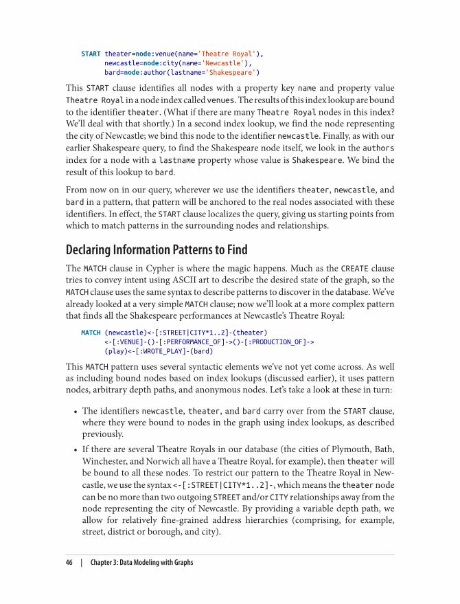
START theater=node:venue(name='Theatre Royal'), newcastle=node:city(name='Newcastle'), bard=node:author(lastname='Shakespeare')

This START clause identifies all nodes with a property key name and property valueTheatre Royal in a node index called venues. The results of this index lookup are boundto the identifier theater. (What if there are many Theatre Royal nodes in this index?We’ll deal with that shortly.) In a second index lookup, we find the node representingthe city of Newcastle; we bind this node to the identifier newcastle. Finally, as with ourearlier Shakespeare query, to find the Shakespeare node itself, we look in the authorsindex for a node with a lastname property whose value is Shakespeare. We bind theresult of this lookup to bard.

From now on in our query, wherever we use the identifiers theater, newcastle, andbard in a pattern, that pattern will be anchored to the real nodes associated with theseidentifiers. In effect, the START clause localizes the query, giving us starting points fromwhich to match patterns in the surrounding nodes and relationships.

Declaring Information Patterns to FindThe MATCH clause in Cypher is where the magic happens. Much as the CREATE clausetries to convey intent using ASCII art to describe the desired state of the graph, so theMATCH clause uses the same syntax to describe patterns to discover in the database. We’vealready looked at a very simple MATCH clause; now we’ll look at a more complex patternthat finds all the Shakespeare performances at Newcastle’s Theatre Royal:

MATCH (newcastle)<-[:STREET|CITY*1..2]-(theater) <-[:VENUE]-()-[:PERFORMANCE_OF]->()-[:PRODUCTION_OF]-> (play)<-[:WROTE_PLAY]-(bard)

This MATCH pattern uses several syntactic elements we’ve not yet come across. As wellas including bound nodes based on index lookups (discussed earlier), it uses patternnodes, arbitrary depth paths, and anonymous nodes. Let’s take a look at these in turn:

• The identifiers newcastle, theater, and bard carry over from the START clause,where they were bound to nodes in the graph using index lookups, as describedpreviously.

• If there are several Theatre Royals in our database (the cities of Plymouth, Bath,Winchester, and Norwich all have a Theatre Royal, for example), then theater willbe bound to all these nodes. To restrict our pattern to the Theatre Royal in New‐castle, we use the syntax <-[:STREET|CITY*1..2]-, which means the theater nodecan be no more than two outgoing STREET and/or CITY relationships away from thenode representing the city of Newcastle. By providing a variable depth path, weallow for relatively fine-grained address hierarchies (comprising, for example,street, district or borough, and city).

46 | Chapter 3: Data Modeling with Graphs

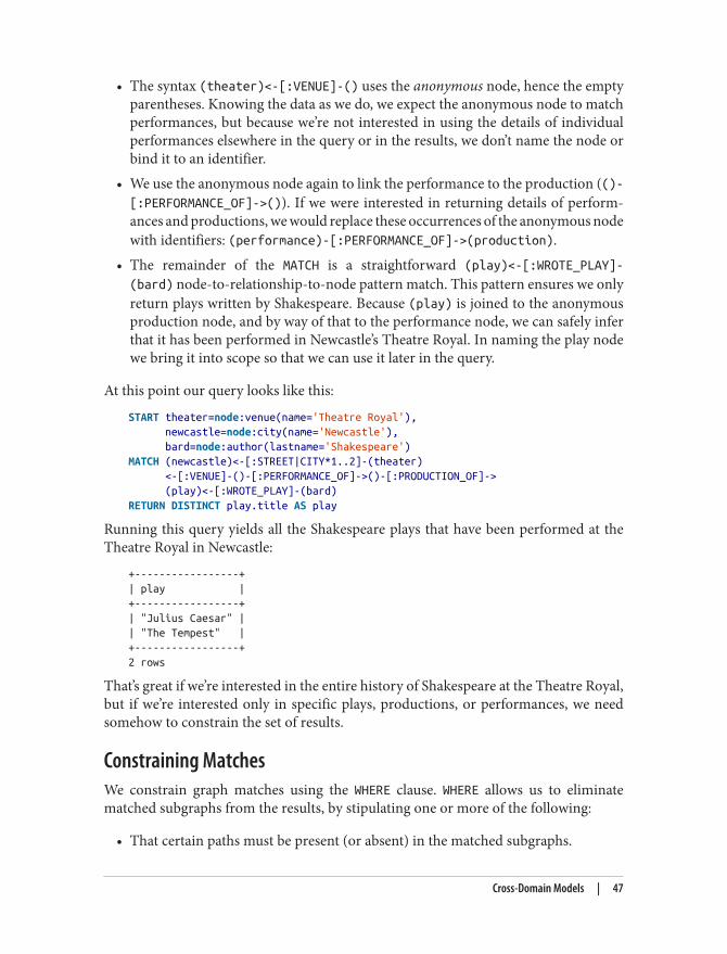
• The syntax (theater)<-[:VENUE]-() uses the anonymous node, hence the emptyparentheses. Knowing the data as we do, we expect the anonymous node to matchperformances, but because we’re not interested in using the details of individualperformances elsewhere in the query or in the results, we don’t name the node orbind it to an identifier.

• We use the anonymous node again to link the performance to the production (()-[:PERFORMANCE_OF]->()). If we were interested in returning details of perform‐ances and productions, we would replace these occurrences of the anonymous nodewith identifiers: (performance)-[:PERFORMANCE_OF]->(production).

• The remainder of the MATCH is a straightforward (play)<-[:WROTE_PLAY]-(bard) node-to-relationship-to-node pattern match. This pattern ensures we onlyreturn plays written by Shakespeare. Because (play) is joined to the anonymousproduction node, and by way of that to the performance node, we can safely inferthat it has been performed in Newcastle’s Theatre Royal. In naming the play nodewe bring it into scope so that we can use it later in the query.

At this point our query looks like this:

START theater=node:venue(name='Theatre Royal'), newcastle=node:city(name='Newcastle'), bard=node:author(lastname='Shakespeare')MATCH (newcastle)<-[:STREET|CITY*1..2]-(theater) <-[:VENUE]-()-[:PERFORMANCE_OF]->()-[:PRODUCTION_OF]-> (play)<-[:WROTE_PLAY]-(bard)RETURN DISTINCT play.title AS play

Running this query yields all the Shakespeare plays that have been performed at theTheatre Royal in Newcastle:

+-----------------+| play |+-----------------+| "Julius Caesar" || "The Tempest" |+-----------------+2 rows

That’s great if we’re interested in the entire history of Shakespeare at the Theatre Royal,but if we’re interested only in specific plays, productions, or performances, we needsomehow to constrain the set of results.

Constraining MatchesWe constrain graph matches using the WHERE clause. WHERE allows us to eliminatematched subgraphs from the results, by stipulating one or more of the following:

• That certain paths must be present (or absent) in the matched subgraphs.

Cross-Domain Models | 47

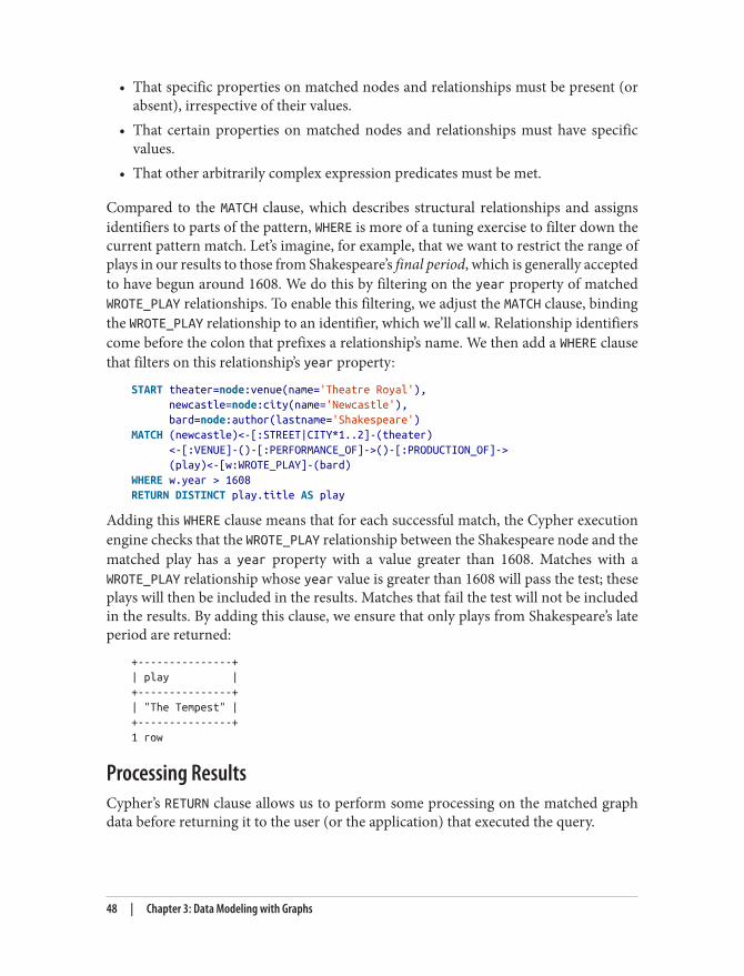
• That specific properties on matched nodes and relationships must be present (orabsent), irrespective of their values.

• That certain properties on matched nodes and relationships must have specificvalues.

• That other arbitrarily complex expression predicates must be met.

Compared to the MATCH clause, which describes structural relationships and assignsidentifiers to parts of the pattern, WHERE is more of a tuning exercise to filter down thecurrent pattern match. Let’s imagine, for example, that we want to restrict the range ofplays in our results to those from Shakespeare’s final period, which is generally acceptedto have begun around 1608. We do this by filtering on the year property of matchedWROTE_PLAY relationships. To enable this filtering, we adjust the MATCH clause, bindingthe WROTE_PLAY relationship to an identifier, which we’ll call w. Relationship identifierscome before the colon that prefixes a relationship’s name. We then add a WHERE clausethat filters on this relationship’s year property:

START theater=node:venue(name='Theatre Royal'), newcastle=node:city(name='Newcastle'), bard=node:author(lastname='Shakespeare')MATCH (newcastle)<-[:STREET|CITY*1..2]-(theater) <-[:VENUE]-()-[:PERFORMANCE_OF]->()-[:PRODUCTION_OF]-> (play)<-[w:WROTE_PLAY]-(bard)WHERE w.year > 1608RETURN DISTINCT play.title AS play

Adding this WHERE clause means that for each successful match, the Cypher executionengine checks that the WROTE_PLAY relationship between the Shakespeare node and thematched play has a year property with a value greater than 1608. Matches with aWROTE_PLAY relationship whose year value is greater than 1608 will pass the test; theseplays will then be included in the results. Matches that fail the test will not be includedin the results. By adding this clause, we ensure that only plays from Shakespeare’s lateperiod are returned:

+---------------+| play |+---------------+| "The Tempest" |+---------------+1 row

Processing ResultsCypher’s RETURN clause allows us to perform some processing on the matched graphdata before returning it to the user (or the application) that executed the query.

48 | Chapter 3: Data Modeling with Graphs

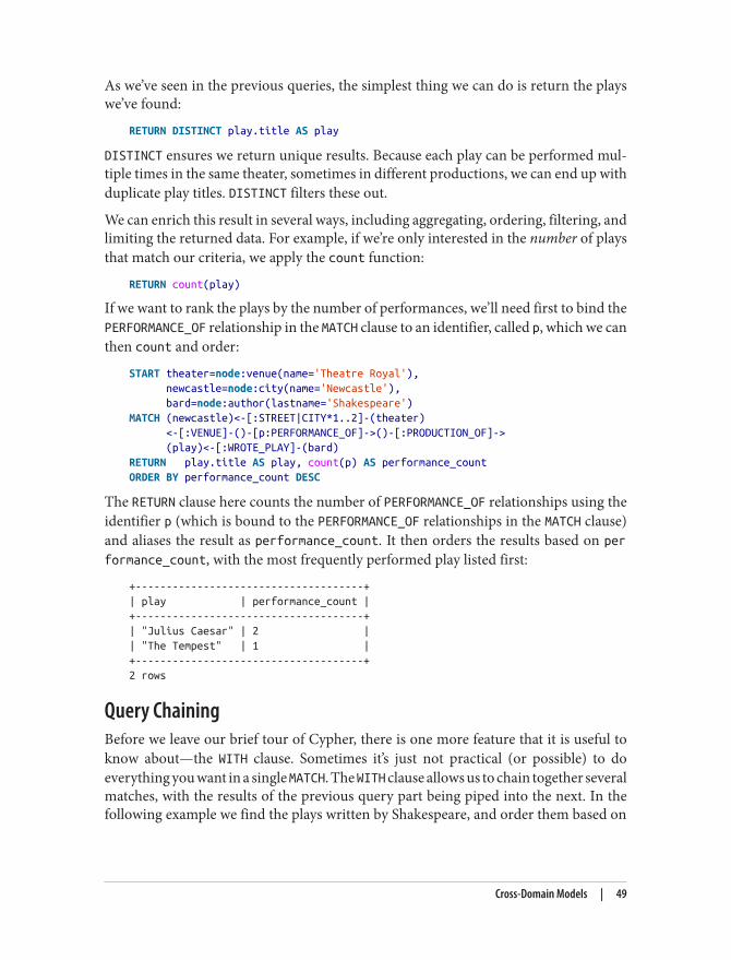
As we’ve seen in the previous queries, the simplest thing we can do is return the playswe’ve found:

RETURN DISTINCT play.title AS play

DISTINCT ensures we return unique results. Because each play can be performed mul‐tiple times in the same theater, sometimes in different productions, we can end up withduplicate play titles. DISTINCT filters these out.

We can enrich this result in several ways, including aggregating, ordering, filtering, andlimiting the returned data. For example, if we’re only interested in the number of playsthat match our criteria, we apply the count function:

RETURN count(play)

If we want to rank the plays by the number of performances, we’ll need first to bind thePERFORMANCE_OF relationship in the MATCH clause to an identifier, called p, which we canthen count and order:

START theater=node:venue(name='Theatre Royal'), newcastle=node:city(name='Newcastle'), bard=node:author(lastname='Shakespeare')MATCH (newcastle)<-[:STREET|CITY*1..2]-(theater) <-[:VENUE]-()-[p:PERFORMANCE_OF]->()-[:PRODUCTION_OF]-> (play)<-[:WROTE_PLAY]-(bard)RETURN play.title AS play, count(p) AS performance_countORDER BY performance_count DESC

The RETURN clause here counts the number of PERFORMANCE_OF relationships using theidentifier p (which is bound to the PERFORMANCE_OF relationships in the MATCH clause)and aliases the result as performance_count. It then orders the results based on performance_count, with the most frequently performed play listed first:

+-------------------------------------+| play | performance_count |+-------------------------------------+| "Julius Caesar" | 2 || "The Tempest" | 1 |+-------------------------------------+2 rows

Query ChainingBefore we leave our brief tour of Cypher, there is one more feature that it is useful toknow about—the WITH clause. Sometimes it’s just not practical (or possible) to doeverything you want in a single MATCH. The WITH clause allows us to chain together severalmatches, with the results of the previous query part being piped into the next. In thefollowing example we find the plays written by Shakespeare, and order them based on

Cross-Domain Models | 49

the year in which they were written, latest first. Using WITH, we then pipe the results tothe collect function, which produces a comma-delimited list of play titles:

START bard=node:author(lastname='Shakespeare')MATCH (bard)-[w:WROTE_PLAY]->(play)WITH playORDER BY w.year DESCRETURN collect(play.title) AS plays

Executing this query against our sample graph produces the following result:

+---------------------------------+| plays |+---------------------------------+| ["The Tempest","Julius Caesar"] |+---------------------------------+1 row

As queries become more complex, WITH instills a sense of discipline, in large part becauseit insists on separating read-only clauses from write-centric SET operations.

Common Modeling PitfallsAlthough graph modeling is a very expressive way of mastering the complexity in aproblem domain, expressivity in and of itself is no guarantee that a particular graph isfit for purpose. In fact, there have been occasions where even those of us who work withgraphs all the time make mistakes. In this section we’ll take a look at a model that wentwrong. In so doing, we’ll learn how to identify problems early in the modeling effort,and how to fix them.

Email Provenance Problem DomainThis example involves the analysis of email communications. Communication patternanalysis is a classic graph problem. Normally, we’d interrogate the graph to discoversubject matter experts, key influencers, and the communication chains through whichinformation is propagated. On this occasion, however, instead of looking for positiverole models (in the form of experts), we were searching for rogues: that is, suspiciouspatterns of email communication that fall foul of corporate governance—or even breakthe law.

A Sensible First Iteration?In analyzing the domain we learned about all the clever patterns that potential wrong-doers adopt to cover their tracks: using blind-copying (BCC), using aliases—evenconducting conversations with those aliases to mimic legitimate interactions betweenreal business stakeholders. Based on this analysis we produced a representative graphmodel that seemed to capture all the relevant entities and their activities.

50 | Chapter 3: Data Modeling with Graphs

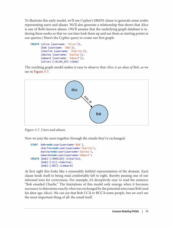
To illustrate this early model, we’ll use Cypher’s CREATE clause to generate some nodesrepresenting users and aliases. We’ll also generate a relationship that shows that Aliceis one of Bob’s known aliases. (We’ll assume that the underlying graph database is in‐dexing these nodes so that we can later look them up and use them as starting points inour queries.) Here’s the Cypher query to create our first graph:

CREATE (alice {username: 'Alice'}), (bob {username: 'Bob'}), (charlie {username: 'Charlie'}), (davina {username: 'Davina'}), (edward {username: 'Edward'}), (alice)-[:ALIAS_OF]->(bob)

The resulting graph model makes it easy to observe that Alice is an alias of Bob, as wesee in Figure 3-7.

Figure 3-7. Users and aliases

Now we join the users together through the emails they’ve exchanged:

START bob=node:user(username='Bob'), charlie=node:user(username='Charlie'), davina=node:user(username='Davina'), edward=node:user(username='Edward')CREATE (bob)-[:EMAILED]->(charlie), (bob)-[:CC]->(davina), (bob)-[:BCC]->(edward)

At first sight this looks like a reasonably faithful representation of the domain. Eachclause lends itself to being read comfortably left to right, thereby passing one of ourinformal tests for correctness. For example, it’s deceptively easy to read the sentence“Bob emailed Charlie.” The limitations of this model only emerge when it becomesnecessary to determine exactly what was exchanged by the potential miscreant Bob (andhis alter-ego Alice). We can see that Bob CC’d or BCC’d some people, but we can’t seethe most important thing of all: the email itself.

Common Modeling Pitfalls | 51

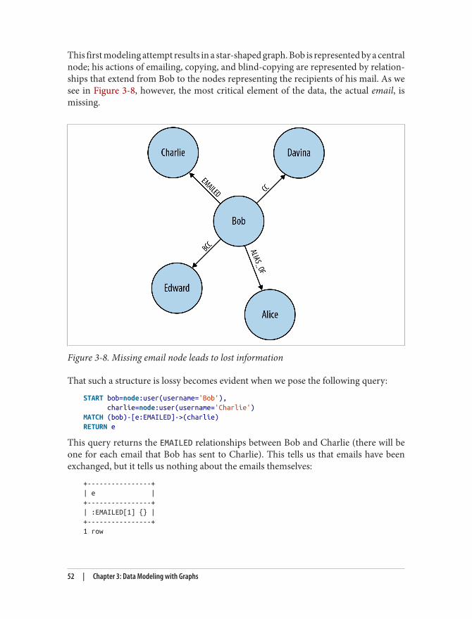
This first modeling attempt results in a star-shaped graph. Bob is represented by a centralnode; his actions of emailing, copying, and blind-copying are represented by relation‐ships that extend from Bob to the nodes representing the recipients of his mail. As wesee in Figure 3-8, however, the most critical element of the data, the actual email, ismissing.

Figure 3-8. Missing email node leads to lost information

That such a structure is lossy becomes evident when we pose the following query:

START bob=node:user(username='Bob'), charlie=node:user(username='Charlie')MATCH (bob)-[e:EMAILED]->(charlie)RETURN e

This query returns the EMAILED relationships between Bob and Charlie (there will beone for each email that Bob has sent to Charlie). This tells us that emails have beenexchanged, but it tells us nothing about the emails themselves:

+----------------+| e |+----------------+| :EMAILED[1] {} |+----------------+1 row

52 | Chapter 3: Data Modeling with Graphs

We might think we can remedy the situation by adding properties to the EMAILEDrelationship to represent an email’s attributes, but that’s just playing for time. Even withproperties attached to each EMAILED relationship, we would still be unable to correlatebetween the EMAILED, CC, and BCC relationships; that is, we would be unable to say whichemails were copied versus which were blind-copied, and to whom.

The fact is we’ve unwittingly made a simple modeling mistake, caused mostly by a laxuse of English rather than any shortcomings of graph theory. Our everyday use of lan‐guage has lead us to focus on the verb “emailed” rather than the email itself, and as aresult we’ve produced a model lacking domain insight.

In English, it’s easy and convenient to shorten the phrase “Bob sent an email to Charlie”to “Bob emailed Charlie”. In most cases that loss of a noun (the actual email) doesn’tmatter because the intent is still clear. But when it comes to our forensics scenario, theseelided statements are problematic. The intent remains the same, but the details of thenumber, contents, and recipients of the emails that Bob sent have been lost throughhaving been folded into a relationship EMAILED, rather than being modeled explicitly asnodes in their own right.

Second Time’s the CharmTo fix our lossy model, we need to insert email nodes to represent the real emails ex‐changed within the business, and expand our set of relationship names to encompassthe full set of addressing fields that email supports. Now instead of creating lossy struc‐tures like this:

CREATE (bob)-[:EMAILED]->(charlie)

we’ll instead create more detailed structures, like this:

CREATE (email_1 {id: '1', content: 'Hi Charlie, ... Kind regards, Bob'}), (bob)-[:SENT]->(email_1), (email_1)-[:TO]->(charlie), (email_1)-[:CC]->(davina), (email_1)-[:CC]->(alice), (email_1)-[:BCC]->(edward)

This results in the kind of graph structure we see in Figure 3-9.

Common Modeling Pitfalls | 53

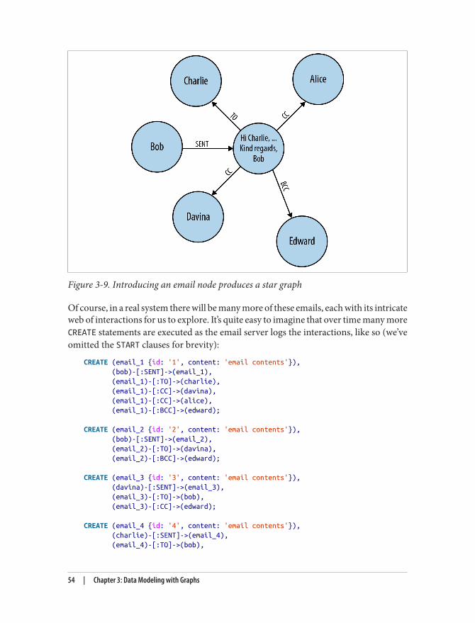
Figure 3-9. Introducing an email node produces a star graph

Of course, in a real system there will be many more of these emails, each with its intricateweb of interactions for us to explore. It’s quite easy to imagine that over time many moreCREATE statements are executed as the email server logs the interactions, like so (we’veomitted the START clauses for brevity):

CREATE (email_1 {id: '1', content: 'email contents'}), (bob)-[:SENT]->(email_1), (email_1)-[:TO]->(charlie), (email_1)-[:CC]->(davina), (email_1)-[:CC]->(alice), (email_1)-[:BCC]->(edward);

CREATE (email_2 {id: '2', content: 'email contents'}), (bob)-[:SENT]->(email_2), (email_2)-[:TO]->(davina), (email_2)-[:BCC]->(edward);

CREATE (email_3 {id: '3', content: 'email contents'}), (davina)-[:SENT]->(email_3), (email_3)-[:TO]->(bob), (email_3)-[:CC]->(edward);

CREATE (email_4 {id: '4', content: 'email contents'}), (charlie)-[:SENT]->(email_4), (email_4)-[:TO]->(bob),

54 | Chapter 3: Data Modeling with Graphs

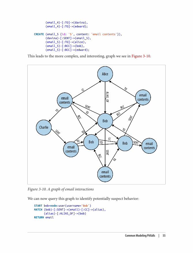
(email_4)-[:TO]->(davina), (email_4)-[:TO]->(edward);

CREATE (email_5 {id: '5', content: 'email contents'}), (davina)-[:SENT]->(email_5), (email_5)-[:TO]->(alice), (email_5)-[:BCC]->(bob), (email_5)-[:BCC]->(edward);

This leads to the more complex, and interesting, graph we see in Figure 3-10.

Figure 3-10. A graph of email interactions

We can now query this graph to identify potentially suspect behavior:

START bob=node:user(username='Bob')MATCH (bob)-[:SENT]->(email)-[:CC]->(alias), (alias)-[:ALIAS_OF]->(bob)RETURN email

Common Modeling Pitfalls | 55

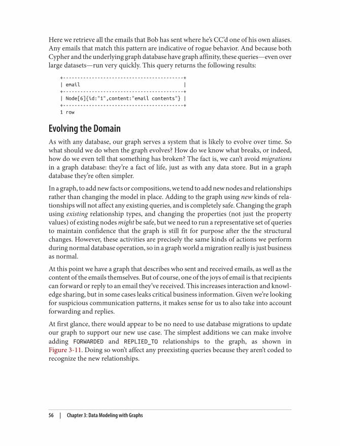
Here we retrieve all the emails that Bob has sent where he’s CC’d one of his own aliases.Any emails that match this pattern are indicative of rogue behavior. And because bothCypher and the underlying graph database have graph affinity, these queries—even overlarge datasets—run very quickly. This query returns the following results:

+------------------------------------------+| email |+------------------------------------------+| Node[6]{id:"1",content:"email contents"} |+------------------------------------------+1 row

Evolving the DomainAs with any database, our graph serves a system that is likely to evolve over time. Sowhat should we do when the graph evolves? How do we know what breaks, or indeed,how do we even tell that something has broken? The fact is, we can’t avoid migrationsin a graph database: they’re a fact of life, just as with any data store. But in a graphdatabase they’re often simpler.

In a graph, to add new facts or compositions, we tend to add new nodes and relationshipsrather than changing the model in place. Adding to the graph using new kinds of rela‐tionships will not affect any existing queries, and is completely safe. Changing the graphusing existing relationship types, and changing the properties (not just the propertyvalues) of existing nodes might be safe, but we need to run a representative set of queriesto maintain confidence that the graph is still fit for purpose after the the structuralchanges. However, these activities are precisely the same kinds of actions we performduring normal database operation, so in a graph world a migration really is just businessas normal.

At this point we have a graph that describes who sent and received emails, as well as thecontent of the emails themselves. But of course, one of the joys of email is that recipientscan forward or reply to an email they’ve received. This increases interaction and knowl‐edge sharing, but in some cases leaks critical business information. Given we’re lookingfor suspicious communication patterns, it makes sense for us to also take into accountforwarding and replies.

At first glance, there would appear to be no need to use database migrations to updateour graph to support our new use case. The simplest additions we can make involveadding FORWARDED and REPLIED_TO relationships to the graph, as shown inFigure 3-11. Doing so won’t affect any preexisting queries because they aren’t coded torecognize the new relationships.

56 | Chapter 3: Data Modeling with Graphs

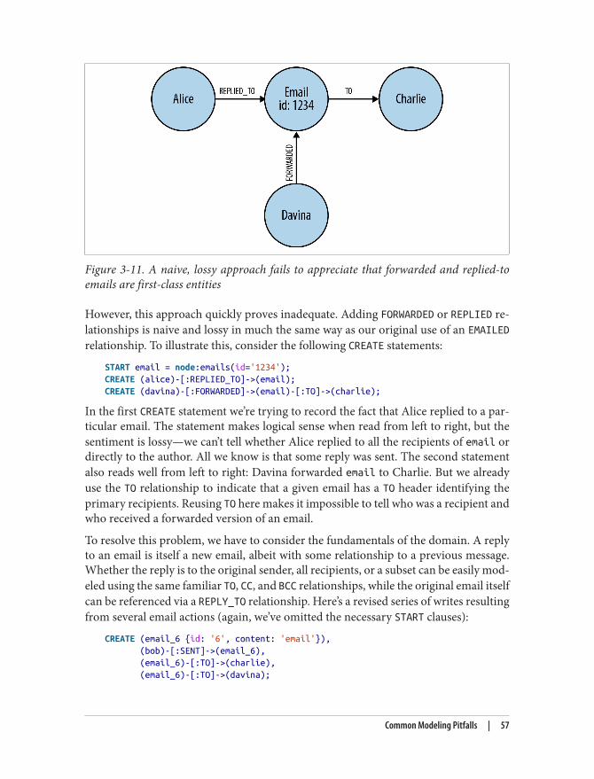
Figure 3-11. A naive, lossy approach fails to appreciate that forwarded and replied-toemails are first-class entities

However, this approach quickly proves inadequate. Adding FORWARDED or REPLIED re‐lationships is naive and lossy in much the same way as our original use of an EMAILEDrelationship. To illustrate this, consider the following CREATE statements:

START email = node:emails(id='1234');CREATE (alice)-[:REPLIED_TO]->(email);CREATE (davina)-[:FORWARDED]->(email)-[:TO]->(charlie);

In the first CREATE statement we’re trying to record the fact that Alice replied to a par‐ticular email. The statement makes logical sense when read from left to right, but thesentiment is lossy—we can’t tell whether Alice replied to all the recipients of email ordirectly to the author. All we know is that some reply was sent. The second statementalso reads well from left to right: Davina forwarded email to Charlie. But we alreadyuse the TO relationship to indicate that a given email has a TO header identifying theprimary recipients. Reusing TO here makes it impossible to tell who was a recipient andwho received a forwarded version of an email.

To resolve this problem, we have to consider the fundamentals of the domain. A replyto an email is itself a new email, albeit with some relationship to a previous message.Whether the reply is to the original sender, all recipients, or a subset can be easily mod‐eled using the same familiar TO, CC, and BCC relationships, while the original email itselfcan be referenced via a REPLY_TO relationship. Here’s a revised series of writes resultingfrom several email actions (again, we’ve omitted the necessary START clauses):

CREATE (email_6 {id: '6', content: 'email'}), (bob)-[:SENT]->(email_6), (email_6)-[:TO]->(charlie), (email_6)-[:TO]->(davina);

Common Modeling Pitfalls | 57

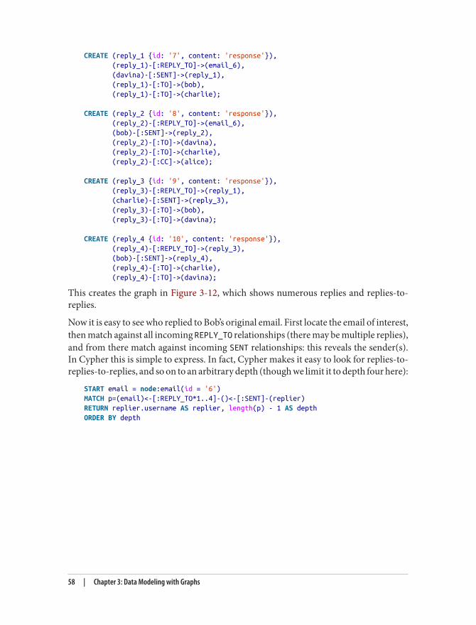
CREATE (reply_1 {id: '7', content: 'response'}), (reply_1)-[:REPLY_TO]->(email_6), (davina)-[:SENT]->(reply_1), (reply_1)-[:TO]->(bob), (reply_1)-[:TO]->(charlie);

CREATE (reply_2 {id: '8', content: 'response'}), (reply_2)-[:REPLY_TO]->(email_6), (bob)-[:SENT]->(reply_2), (reply_2)-[:TO]->(davina), (reply_2)-[:TO]->(charlie), (reply_2)-[:CC]->(alice);

CREATE (reply_3 {id: '9', content: 'response'}), (reply_3)-[:REPLY_TO]->(reply_1), (charlie)-[:SENT]->(reply_3), (reply_3)-[:TO]->(bob), (reply_3)-[:TO]->(davina);

CREATE (reply_4 {id: '10', content: 'response'}), (reply_4)-[:REPLY_TO]->(reply_3), (bob)-[:SENT]->(reply_4), (reply_4)-[:TO]->(charlie), (reply_4)-[:TO]->(davina);

This creates the graph in Figure 3-12, which shows numerous replies and replies-to-replies.

Now it is easy to see who replied to Bob’s original email. First locate the email of interest,then match against all incoming REPLY_TO relationships (there may be multiple replies),and from there match against incoming SENT relationships: this reveals the sender(s).In Cypher this is simple to express. In fact, Cypher makes it easy to look for replies-to-replies-to-replies, and so on to an arbitrary depth (though we limit it to depth four here):

START email = node:email(id = '6')MATCH p=(email)<-[:REPLY_TO*1..4]-()<-[:SENT]-(replier)RETURN replier.username AS replier, length(p) - 1 AS depthORDER BY depth

58 | Chapter 3: Data Modeling with Graphs

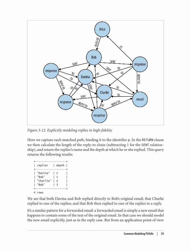
Figure 3-12. Explicitly modeling replies in high-fidelity

Here we capture each matched path, binding it to the identifier p. In the RETURN clausewe then calculate the length of the reply-to chain (subtracting 1 for the SENT relation‐ship), and return the replier’s name and the depth at which he or she replied. This queryreturns the following results:

+-------------------+| replier | depth |+-------------------+| "Davina" | 1 || "Bob" | 1 || "Charlie" | 2 || "Bob" | 3 |+-------------------+4 rows

We see that both Davina and Bob replied directly to Bob’s original email; that Charliereplied to one of the replies; and that Bob then replied to one of the replies to a reply.

It’s a similar pattern for a forwarded email: a forwarded email is simply a new email thathappens to contain some of the text of the original email. In that case we should modelthe new email explicitly, just as in the reply case. But from an application point of view

Common Modeling Pitfalls | 59

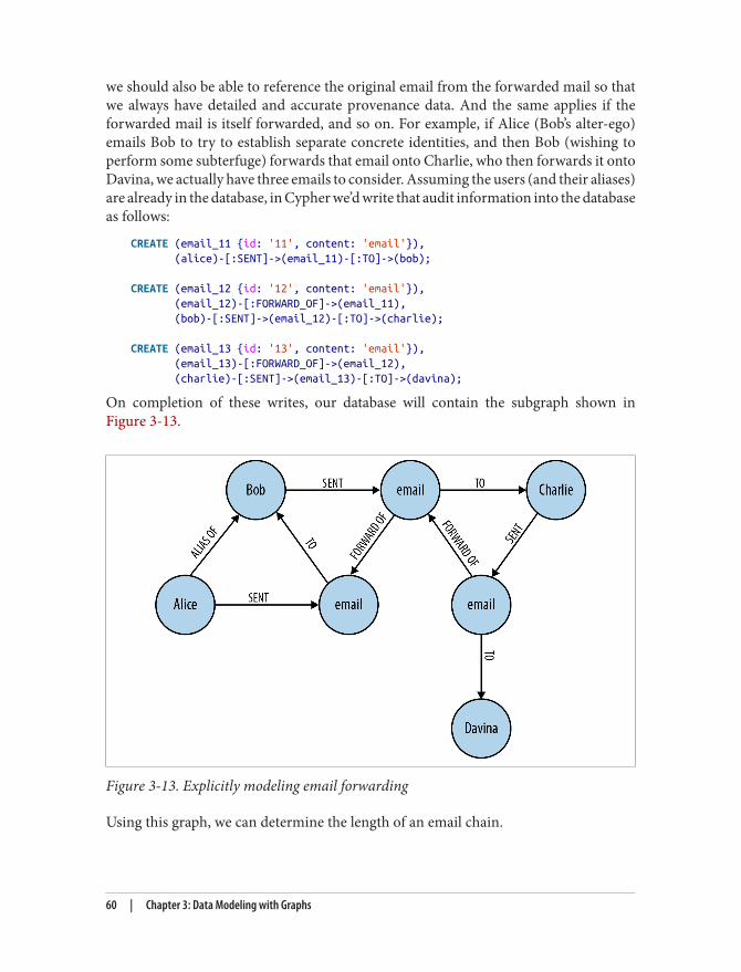
we should also be able to reference the original email from the forwarded mail so thatwe always have detailed and accurate provenance data. And the same applies if theforwarded mail is itself forwarded, and so on. For example, if Alice (Bob’s alter-ego)emails Bob to try to establish separate concrete identities, and then Bob (wishing toperform some subterfuge) forwards that email onto Charlie, who then forwards it ontoDavina, we actually have three emails to consider. Assuming the users (and their aliases)are already in the database, in Cypher we’d write that audit information into the databaseas follows:

CREATE (email_11 {id: '11', content: 'email'}), (alice)-[:SENT]->(email_11)-[:TO]->(bob);

CREATE (email_12 {id: '12', content: 'email'}), (email_12)-[:FORWARD_OF]->(email_11), (bob)-[:SENT]->(email_12)-[:TO]->(charlie);

CREATE (email_13 {id: '13', content: 'email'}), (email_13)-[:FORWARD_OF]->(email_12), (charlie)-[:SENT]->(email_13)-[:TO]->(davina);

On completion of these writes, our database will contain the subgraph shown inFigure 3-13.

Figure 3-13. Explicitly modeling email forwarding

Using this graph, we can determine the length of an email chain.

60 | Chapter 3: Data Modeling with Graphs

START email = node:email(id = '11')MATCH (email)<-[f:FORWARD_OF*]-()RETURN count(f)

This query starts at the given email and then matches against all incoming FORWARD_OF relationships to any depth. These relationships are bound to an identifier f. Tocalculate the length of the email chain, we count the number of FORWARD_OF relationshipsbound to f using Cypher’s count function. In this example, we see the original emailhas been forwarded twice:

+----------+| count(f) |+----------+| 2 |+----------+1 row

Avoiding Anti-PatternsIn the general case, don’t encode entities into relationships. Use relationships to conveysemantics about how entities are related, and the quality of those relationships. Domainentities aren’t always immediately visible in speech, so we must think carefully aboutthe nouns we’re actually dealing with.

It’s also important to realize that graphs are a naturally additive structure. It’s quitenatural to add facts in terms of domain entities and how they interrelate using newnodes and new relationships, even if it feels like we’re flooding the database with a greatdeal of painstaking data. In general, it’s bad practice to try to conflate data elements atwrite time to preserve query-time efficiency. If we model in accordance with the ques‐tions we want to ask of our data, an accurate representation of the domain will emerge.With this data model in place, we can trust the graph database to do the right thing.

Graph databases maintain fast query times even when storing vastamounts of data. Learning to trust our graph database is importantwhen learning to structure our graphs without denormalizing them.

SummaryGraph databases give software professionals the power to represent a problem domainusing a graph, and then persist and query that graph at runtime. We can use graphs toclearly describe a problem domain; graph databases then allow us to store this repre‐sentation in a way that maintains high affinity between the domain and the data. Further,graph modeling removes the need to normalize and denormalize data using complexdata management code.

Avoiding Anti-Patterns | 61

Many of us, however, will be new to modeling with graphs. The graphs we create shouldread well for queries, while avoiding conflating entities and actions—bad practices thatcan lose useful domain knowledge. Although there are no absolute rights or wrongs tograph modeling, the guidance in this chapter will help you create graph data that canserve your systems’ needs over many iterations, all the while keeping pace with codeevolution.

Armed with an understanding of graph data modeling, you may now be consideringundertaking a graph database project. In the next chapter we’ll look at what’s involvedin planning and delivering a graph database solution.

62 | Chapter 3: Data Modeling with Graphs

CHAPTER 4

Building a Graph Database Application

In this chapter we discuss some of the practical issues of working with a graph database.In previous chapters we’ve looked at graph data; in this chapter, we’ll apply that knowl‐edge in the context of developing a graph database application. We’ll look at some ofthe data modeling questions that may arise, and at some of the application architecturechoices available to us.

In our experience, graph database applications are highly amenable to being developedusing the evolutionary, incremental, and iterative software development practices inwidespread use today. A key feature of these practices is the prevalence of testingthroughout the software development life cycle. Here we’ll show how we develop ourdata model and our application in a test-driven fashion.

At the end of the chapter, we’ll look at some of the issues we’ll need to consider whenplanning for production.

Data ModelingWe covered modeling and working with graph data in detail in Chapter 3. Here wesummarize some of the more important modeling guidelines, and discuss how imple‐menting a graph data model fits with iterative and incremental software developmenttechniques.

Describe the Model in Terms of the Application’s NeedsThe questions we need to ask of the data help identify entities and relationships. Agileuser stories provide a concise means for expressing an outside-in, user-centered view

63

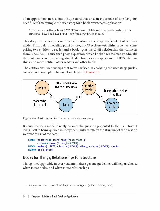
1. For agile user stories, see Mike Cohn, User Stories Applied (Addison-Wesley, 2004).

of an application’s needs, and the questions that arise in the course of satisfying thisneed.1 Here’s an example of a user story for a book review web application:

AS A reader who likes a book, I WANT to know which books other readers who like thesame book have liked, SO THAT I can find other books to read.

This story expresses a user need, which motivates the shape and content of our datamodel. From a data modeling point of view, the AS A clause establishes a context com‐prising two entities—a reader and a book—plus the LIKES relationship that connectsthem. The I WANT clause then poses a question: which books have the readers who likethe book I’m currently reading also liked? This question exposes more LIKES relation‐ships, and more entities: other readers and other books.

The entities and relationships that we’ve surfaced in analyzing the user story quicklytranslate into a simple data model, as shown in Figure 4-1.

Figure 4-1. Data model for the book reviews user story

Because this data model directly encodes the question presented by the user story, itlends itself to being queried in a way that similarly reflects the structure of the questionwe want to ask of the data:

START reader=node:users(name={readerName}) book=node:books(isbn={bookISBN})MATCH reader-[:LIKES]->book<-[:LIKES]-other_readers-[:LIKES]->booksRETURN books.title

Nodes for Things, Relationships for StructureThough not applicable in every situation, these general guidelines will help us choosewhen to use nodes, and when to use relationships:

64 | Chapter 4: Building a Graph Database Application

• Use nodes to represent entities—that is, the things that are of interest to us in ourdomain.

• Use relationships both to express the connections between entities and to establishsemantic context for each entity, thereby structuring the domain.

• Use relationship direction to further clarify relationship semantics. Many relation‐ships are asymmetrical, which is why relationships in a property graph are alwaysdirected. For bidirectional relationships, we should make our queries ignoredirection.

• Use node properties to represent entity attributes, plus any necessary entity meta‐data, such as timestamps, version numbers, etc.

• Use relationship properties to express the strength, weight, or quality of a relation‐ship, plus any necessary relationship metadata, such as timestamps, version num‐bers, etc.

It pays to be diligent about discovering and capturing domain entities. As we saw inChapter 3, it’s relatively easy to model things that really ought to be represented as nodesusing sloppily named relationships instead. If we’re tempted to use a relationship tomodel an entity—an email, or a review, for example—we must make certain that thisentity cannot be related to more than two other entities. Remember, a relationship musthave a start node and an end node—nothing more, nothing less. If we find later that weneed to connect something we’ve modeled as a relationship to more than two otherentities, we’ll have to refactor the entity inside the relationship out into a separate node.This is a breaking change to the data model, and will likely require us to make changesto any queries and application code that produce or consume the data.

Fine-Grained versus Generic RelationshipsWhen designing relationship types we should be mindful of the trade-offs between usingfine-grained relationship labels versus generic relationships qualified with properties.It’s the difference between using DELIVERY_ADDRESS and HOME_ADDRESS versus ADDRESS{type: 'delivery'} and ADDRESS {type: 'home'}.

Relationships are the royal road into the graph. Differentiating by relationship type isthe best way of eliminating large swathes of the graph from a traversal. Using one ormore property values to decide whether or not to follow a relationship incurs extra IOthe first time those properties are accessed because the properties reside in a separatestore file from the relationships (after that, however, they’re cached).

We use fine-grained relationships whenever we have a closed set of relationship types.In contrast, weightings—as required by a shortest-weighted-path algorithm—rarelycomprise a closed set, and these are usually best represented as properties onrelationships.

Data Modeling | 65

Sometimes, however, we have a closed set of relationships, but in some traversals wewant to follow specific kinds of relationships within that set, whereas in others we wantto follow all of them, irrespective of type. Addresses are a good example. Following theclosed-set principle, we might choose to create HOME_ADDRESS, WORK_ADDRESS, and DELIVERY_ADDRESS relationships. This allows us to follow specific kinds of address rela‐tionships (DELIVERY_ADDRESS, for example) while ignoring all the rest. But what do wedo if we want to find all addresses for a user? There are a couple of options here. First,we can encode knowledge of all the different relationship types in our queries: e.g.,MATCH user-[:HOME_ADDRESS|WORK_ADDRESS|DELIVERY_ADDRESS]->address. This,however, quickly becomes unwieldy when there are lots of different kinds of relation‐ships. Alternatively, we can add a more generic ADDRESS relationship to our model, inaddition to the fine-grained relationships. Every node representing an address is thenconnected to a user using two relationships: a fined-grained relationship (e.g., DELIVERY_ADDRESS) and the more generic ADDRESS {type: 'delivery'} relationship.

As we discussed in “Describe the Model in Terms of the Application’s Needs” on page63, the key here is to let the questions we want to ask of our data guide the kinds ofrelationships we introduce into the model.

Model Facts as NodesWhen two or more domain entities interact for a period of time, a fact emerges. Werepresent these facts as separate nodes, with connections to each of the entities engagedin that fact. Modeling an action in terms of its product—that is, in terms of the thingthat results from the action—produces a similar structure: an intermediate node thatrepresents the outcome of an interaction between two or more entities. We can usetimestamp properties on this intermediate node to represent start and end times.

The following examples show how we might model facts and actions using intermediatenodes.

EmploymentFigure 4-2 shows how the fact of Ian being employed by Neo Technology in the role ofengineer can be represented in the graph.

66 | Chapter 4: Building a Graph Database Application

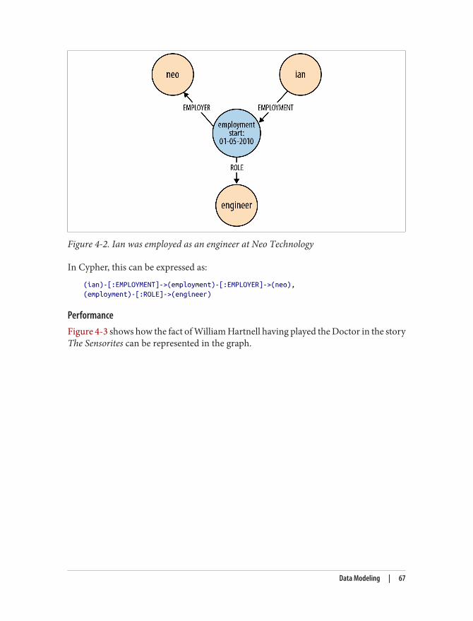
Figure 4-2. Ian was employed as an engineer at Neo Technology

In Cypher, this can be expressed as:

(ian)-[:EMPLOYMENT]->(employment)-[:EMPLOYER]->(neo),(employment)-[:ROLE]->(engineer)

PerformanceFigure 4-3 shows how the fact of William Hartnell having played the Doctor in the storyThe Sensorites can be represented in the graph.

Data Modeling | 67

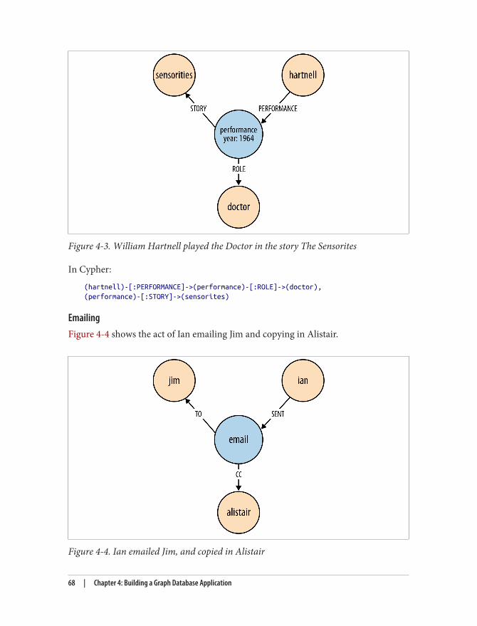
Figure 4-3. William Hartnell played the Doctor in the story The Sensorites

In Cypher:

(hartnell)-[:PERFORMANCE]->(performance)-[:ROLE]->(doctor),(performance)-[:STORY]->(sensorites)

EmailingFigure 4-4 shows the act of Ian emailing Jim and copying in Alistair.

Figure 4-4. Ian emailed Jim, and copied in Alistair

68 | Chapter 4: Building a Graph Database Application

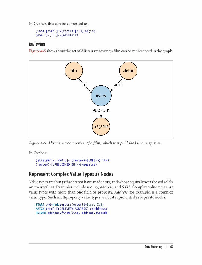
In Cypher, this can be expressed as:

(ian)-[:SENT]->(email)-[:TO]->(jim),(email)-[:CC]->(alistair)

ReviewingFigure 4-5 shows how the act of Alistair reviewing a film can be represented in the graph.

Figure 4-5. Alistair wrote a review of a film, which was published in a magazine

In Cypher:

(alistair)-[:WROTE]->(review)-[:OF]->(film),(review)-[:PUBLISHED_IN]->(magazine)

Represent Complex Value Types as NodesValue types are things that do not have an identity, and whose equivalence is based solelyon their values. Examples include money, address, and SKU. Complex value types arevalue types with more than one field or property. Address, for example, is a complexvalue type. Such multiproperty value types are best represented as separate nodes:

START ord=node:orders(orderid={orderId})MATCH (ord)-[:DELIVERY_ADDRESS]->(address)RETURN address.first_line, address.zipcode

Data Modeling | 69

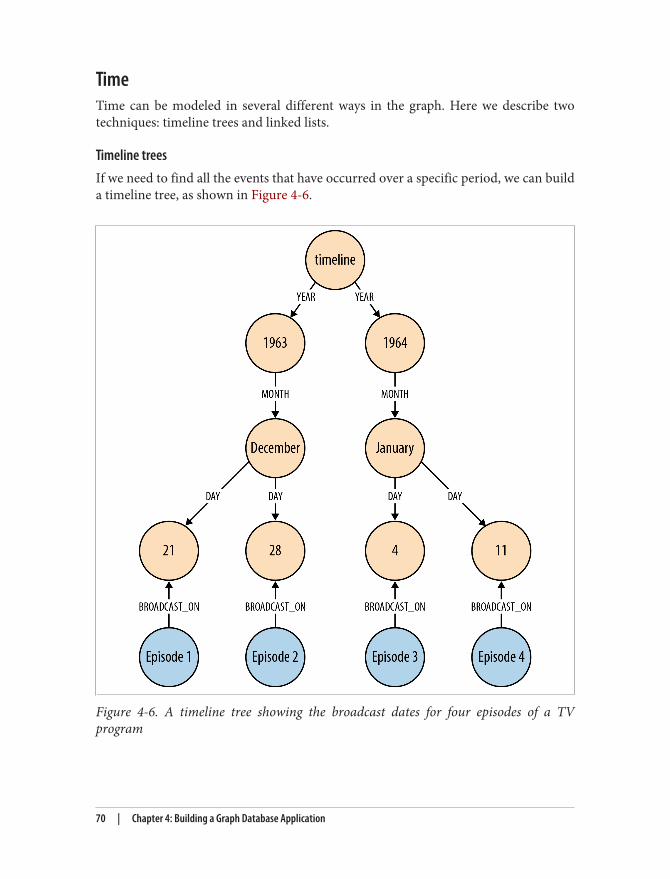
TimeTime can be modeled in several different ways in the graph. Here we describe twotechniques: timeline trees and linked lists.

Timeline treesIf we need to find all the events that have occurred over a specific period, we can builda timeline tree, as shown in Figure 4-6.

Figure 4-6. A timeline tree showing the broadcast dates for four episodes of a TVprogram

70 | Chapter 4: Building a Graph Database Application

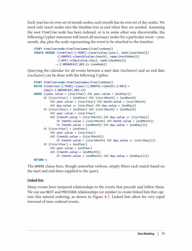
Each year has its own set of month nodes; each month has its own set of day nodes. Weneed only insert nodes into the timeline tree as and when they are needed. Assumingthe root timeline node has been indexed, or is in some other way discoverable, thefollowing Cypher statement will insert all necessary nodes for a particular event—year,month, day, plus the node representing the event to be attached to the timeline:

START timeline=node:timeline(name={timelineName})CREATE UNIQUE (timeline)-[:YEAR]->(year{value:{year}, name:{yearName}}) -[:MONTH]->(month{value:{month}, name:{monthName}}) -[:DAY]->(day{value:{day}, name:{dayName}}) <-[:BROADCAST_ON]-(n {newNode})

Querying the calendar for all events between a start date (inclusive) and an end date(exclusive) can be done with the following Cypher:

START timeline=node:timeline(name={timelineName})MATCH (timeline)-[:YEAR]->(year)-[:MONTH]->(month)-[:DAY]-> (day)<-[:BROADCAST_ON]-(n)WHERE ((year.value > {startYear} AND year.value < {endYear}) OR ({startYear} = {endYear} AND {startMonth} = {endMonth} AND year.value = {startYear} AND month.value = {startMonth} AND day.value >= {startDay} AND day.value < {endDay}) OR ({startYear} = {endYear} AND {startMonth} < {endMonth} AND year.value = {startYear} AND ((month.value = {startMonth} AND day.value >= {startDay}) OR (month.value > {startMonth} AND month.value < {endMonth}) OR (month.value = {endMonth} AND day.value < {endDay}))) OR ({startYear} < {endYear} AND year.value = {startYear} AND ((month.value > {startMonth}) OR (month.value = {startMonth} AND day.value >= {startDay}))) OR ({startYear} < {endYear} AND year.value = {endYear} AND ((month.value < {endMonth}) OR (month.value = {endMonth} AND day.value < {endDay}))))RETURN n

The WHERE clause here, though somewhat verbose, simply filters each match based onthe start and end dates supplied to the query.

Linked listsMany events have temporal relationships to the events that precede and follow them.We can use NEXT and PREVIOUS relationships (or similar) to create linked lists that cap‐ture this natural ordering, as shown in Figure 4-7. Linked lists allow for very rapidtraversal of time-ordered events.

Data Modeling | 71

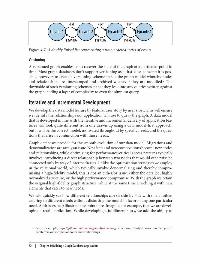
2. See, for example, https://github.com/dmontag/neo4j-versioning, which uses Neo4j’s transaction life cycle tocreate versioned copies of nodes and relationships.

Figure 4-7. A doubly linked list representing a time-ordered series of events

VersioningA versioned graph enables us to recover the state of the graph at a particular point intime. Most graph databases don’t support versioning as a first-class concept: it is pos‐sible, however, to create a versioning scheme inside the graph model whereby nodesand relationships are timestamped and archived whenever they are modified.2 Thedownside of such versioning schemes is that they leak into any queries written againstthe graph, adding a layer of complexity to even the simplest query.

Iterative and Incremental DevelopmentWe develop the data model feature by feature, user story by user story. This will ensurewe identify the relationships our application will use to query the graph. A data modelthat is developed in line with the iterative and incremental delivery of application fea‐tures will look quite different from one drawn up using a data model-first approach,but it will be the correct model, motivated throughout by specific needs, and the ques‐tions that arise in conjunction with those needs.

Graph databases provide for the smooth evolution of our data model. Migrations anddenormalization are rarely an issue. New facts and new compositions become new nodesand relationships, while optimizing for performance-critical access patterns typicallyinvolves introducing a direct relationship between two nodes that would otherwise beconnected only by way of intermediaries. Unlike the optimization strategies we employin the relational world, which typically involve denormalizing and thereby compro‐mising a high-fidelity model, this is not an either/or issue: either the detailed, highlynormalized structure, or the high performance compromise. With the graph we retainthe original high-fidelity graph structure, while at the same time enriching it with newelements that cater to new needs.

We will quickly see how different relationships can sit side-by-side with one another,catering to different needs without distorting the model in favor of any one particularneed. Addresses help illustrate the point here. Imagine, for example, that we are devel‐oping a retail application. While developing a fulfillment story, we add the ability to

72 | Chapter 4: Building a Graph Database Application

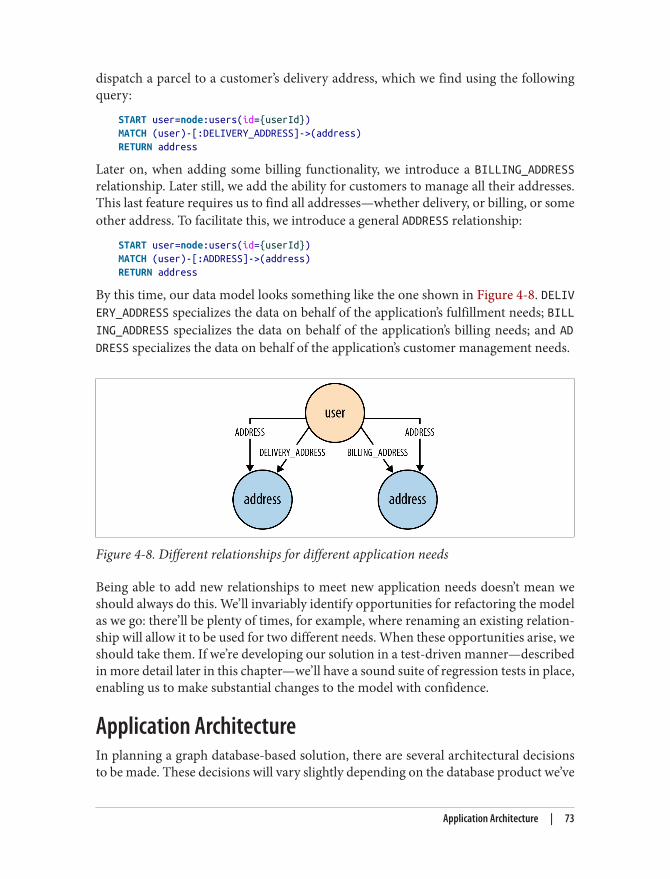
dispatch a parcel to a customer’s delivery address, which we find using the followingquery:

START user=node:users(id={userId})MATCH (user)-[:DELIVERY_ADDRESS]->(address)RETURN address

Later on, when adding some billing functionality, we introduce a BILLING_ADDRESSrelationship. Later still, we add the ability for customers to manage all their addresses.This last feature requires us to find all addresses—whether delivery, or billing, or someother address. To facilitate this, we introduce a general ADDRESS relationship:

START user=node:users(id={userId})MATCH (user)-[:ADDRESS]->(address)RETURN address

By this time, our data model looks something like the one shown in Figure 4-8. DELIVERY_ADDRESS specializes the data on behalf of the application’s fulfillment needs; BILLING_ADDRESS specializes the data on behalf of the application’s billing needs; and ADDRESS specializes the data on behalf of the application’s customer management needs.

Figure 4-8. Different relationships for different application needs

Being able to add new relationships to meet new application needs doesn’t mean weshould always do this. We’ll invariably identify opportunities for refactoring the modelas we go: there’ll be plenty of times, for example, where renaming an existing relation‐ship will allow it to be used for two different needs. When these opportunities arise, weshould take them. If we’re developing our solution in a test-driven manner—describedin more detail later in this chapter—we’ll have a sound suite of regression tests in place,enabling us to make substantial changes to the model with confidence.

Application ArchitectureIn planning a graph database-based solution, there are several architectural decisionsto be made. These decisions will vary slightly depending on the database product we’ve

Application Architecture | 73

chosen; in this section, we’ll describe some of the architectural choices, and the corre‐sponding application architectures, available to us when using Neo4j.

Embedded Versus ServerMost databases today run as a server that is accessed through a client library. Neo4j issomewhat unusual in that it can be run in embedded as well as server mode—in fact,going back nearly ten years, its origins are as an embedded graph database.

An embedded database is not the same as an in-memory database. Anembedded instance of Neo4j still makes all data durable on disk. Later,in “Testing” on page 82, we’ll discuss ImpermanentGraphDatabase, whichis an in-memory version of Neo4j designed for testing purposes.

Embedded Neo4jIn embedded mode, Neo4j runs in the same process as our application. Embedded Neo4jis ideal for hardware devices, desktop applications, and for incorporating in our ownapplication servers. Some of the advantages of embedded mode include:Low latency

Because our application speaks directly to the database, there’s no networkoverhead.

Choice of APIsWe have access to the full range of APIs for creating and querying data: the CoreAPI, traversal framework, and the Cypher query language.

Explicit transactionsUsing the Core API, we can control the transactional life cycle, executing an arbi‐trarily complex sequence of commands against the database in the context of asingle transaction. The Java APIs also expose the transaction life cycle, enabling usto plug in custom transaction event handlers that execute additional logic with eachtransaction.

Named indexesEmbedded mode gives us full control over the creation and management of namedindexes. This functionality is also available through the web-based REST interface;it is not, however, available in Cypher.

When running in embedded mode, however, we should bear in mind the following:JVM only

Neo4j is a JVM-based database. Many of its APIs are, therefore, accessible only froma JVM-based language.

74 | Chapter 4: Building a Graph Database Application

3. A list of Neo4j remote client libraries, as developed by the community, is maintained at http://bit.ly/YEHRrD.

GC behaviorsWhen running in embedded mode, Neo4j is subject to the garbage collection (GC)behaviors of the host application. Long GC pauses can affect query times. Further,when running an embedded instance as part of an HA cluster, long GC pauses cancause the cluster protocol to trigger a master reelection.

Database life cycleThe application is responsible for controlling the database life cycle, which includesstarting it, and closing it safely.

Embedded Neo4j can be clustered for high availability and horizontal read scaling justas the server version. In fact, we can run a mixed cluster of embedded and server in‐stances (clustering is performed at the database level, rather than the server level). Thisis common in enterprise integration scenarios, where regular updates from other sys‐tems are executed against an embedded instance, and then replicated out to serverinstances.

Server modeRunning Neo4j in server mode is the most common means of deploying the databasetoday. At the heart of each server is an embedded instance of Neo4j. Some of the benefitsof server mode include:REST API

The server exposes a rich REST API that allows clients to send JSON-formattedrequests over HTTP. Responses comprise JSON-formatted documents enrichedwith hypermedia links that advertise additional features of the dataset.

Platform independenceBecause access is by way of JSON-formatted documents sent over HTTP, a Neo4jserver can be accessed by a client running on practically any platform. All that’sneeded is an HTTP client library.3

Scaling independenceWith Neo4j running in server mode, we can scale our database cluster independ‐ently of our application server cluster.

Isolation from application GC behaviorsIn server mode, Neo4j is protected from any untoward GC behaviors triggered bythe rest of the application. Of course, Neo4j still produces some garbage, but itsimpact on the garbage collector has been carefully monitored and tuned duringdevelopment to mitigate any significant side effects. However, because server

Application Architecture | 75

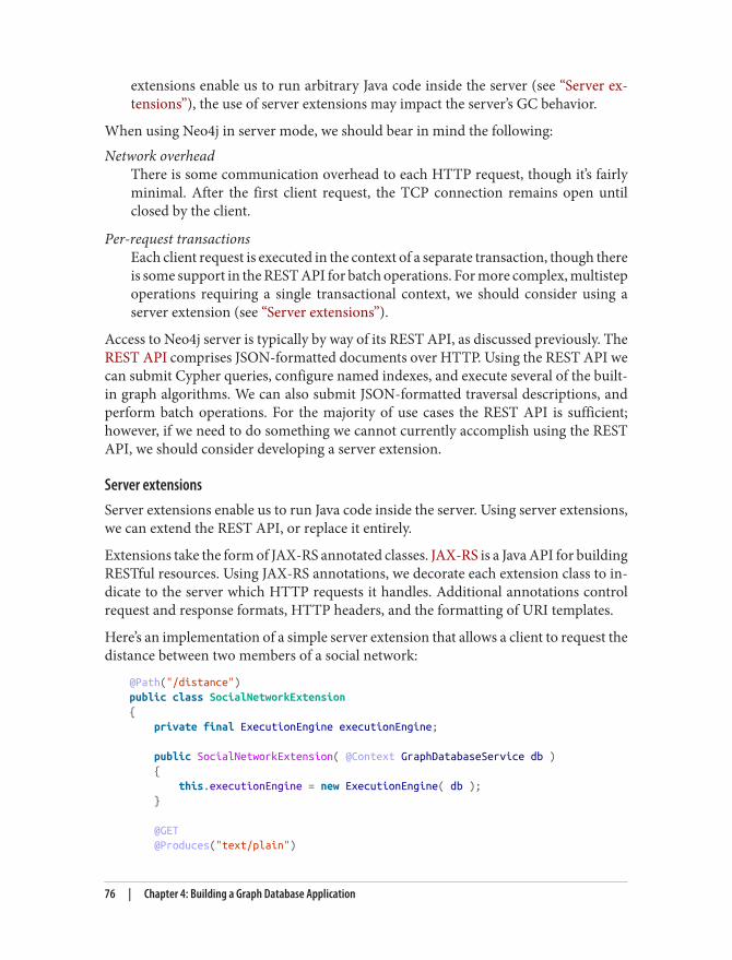
extensions enable us to run arbitrary Java code inside the server (see “Server ex‐tensions”), the use of server extensions may impact the server’s GC behavior.

When using Neo4j in server mode, we should bear in mind the following:Network overhead

There is some communication overhead to each HTTP request, though it’s fairlyminimal. After the first client request, the TCP connection remains open untilclosed by the client.

Per-request transactionsEach client request is executed in the context of a separate transaction, though thereis some support in the REST API for batch operations. For more complex, multistepoperations requiring a single transactional context, we should consider using aserver extension (see “Server extensions”).

Access to Neo4j server is typically by way of its REST API, as discussed previously. TheREST API comprises JSON-formatted documents over HTTP. Using the REST API wecan submit Cypher queries, configure named indexes, and execute several of the built-in graph algorithms. We can also submit JSON-formatted traversal descriptions, andperform batch operations. For the majority of use cases the REST API is sufficient;however, if we need to do something we cannot currently accomplish using the RESTAPI, we should consider developing a server extension.

Server extensionsServer extensions enable us to run Java code inside the server. Using server extensions,we can extend the REST API, or replace it entirely.

Extensions take the form of JAX-RS annotated classes. JAX-RS is a Java API for buildingRESTful resources. Using JAX-RS annotations, we decorate each extension class to in‐dicate to the server which HTTP requests it handles. Additional annotations controlrequest and response formats, HTTP headers, and the formatting of URI templates.

Here’s an implementation of a simple server extension that allows a client to request thedistance between two members of a social network:

@Path("/distance")public class SocialNetworkExtension{ private final ExecutionEngine executionEngine;

public SocialNetworkExtension( @Context GraphDatabaseService db ) { this.executionEngine = new ExecutionEngine( db ); }

@GET @Produces("text/plain")

76 | Chapter 4: Building a Graph Database Application

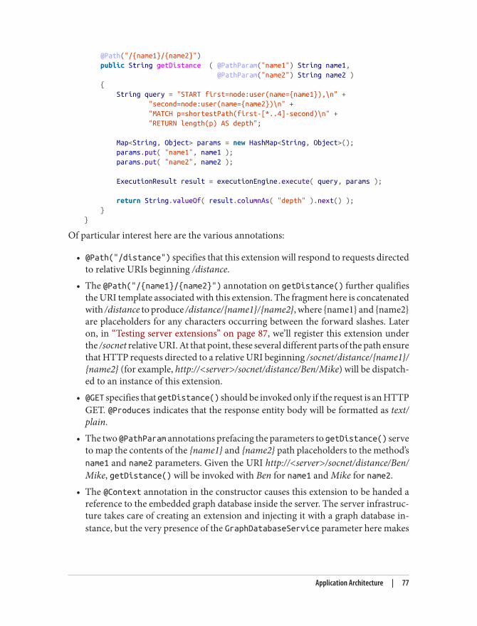
@Path("/{name1}/{name2}") public String getDistance ( @PathParam("name1") String name1, @PathParam("name2") String name2 ) { String query = "START first=node:user(name={name1}),\n" + "second=node:user(name={name2})\n" + "MATCH p=shortestPath(first-[*..4]-second)\n" + "RETURN length(p) AS depth";

Map<String, Object> params = new HashMap<String, Object>(); params.put( "name1", name1 ); params.put( "name2", name2 );

ExecutionResult result = executionEngine.execute( query, params );

return String.valueOf( result.columnAs( "depth" ).next() ); }}

Of particular interest here are the various annotations:

• @Path("/distance") specifies that this extension will respond to requests directedto relative URIs beginning /distance.

• The @Path("/{name1}/{name2}") annotation on getDistance() further qualifiesthe URI template associated with this extension. The fragment here is concatenatedwith /distance to produce /distance/{name1}/{name2}, where {name1} and {name2}are placeholders for any characters occurring between the forward slashes. Lateron, in “Testing server extensions” on page 87, we’ll register this extension underthe /socnet relative URI. At that point, these several different parts of the path ensurethat HTTP requests directed to a relative URI beginning /socnet/distance/{name1}/{name2} (for example, http://<server>/socnet/distance/Ben/Mike) will be dispatch‐ed to an instance of this extension.

• @GET specifies that getDistance() should be invoked only if the request is an HTTPGET. @Produces indicates that the response entity body will be formatted as text/plain.

• The two @PathParam annotations prefacing the parameters to getDistance() serveto map the contents of the {name1} and {name2} path placeholders to the method’sname1 and name2 parameters. Given the URI http://<server>/socnet/distance/Ben/Mike, getDistance() will be invoked with Ben for name1 and Mike for name2.

• The @Context annotation in the constructor causes this extension to be handed areference to the embedded graph database inside the server. The server infrastruc‐ture takes care of creating an extension and injecting it with a graph database in‐stance, but the very presence of the GraphDatabaseService parameter here makes

Application Architecture | 77

this extension exceedingly testable. As we’ll see later, in “Testing server exten‐sions”, we can unit test extensions without having to run them inside a server.

Server extensions can be powerful elements in our application architecture. Their chiefbenefits include:Complex transactions

Extensions enable us to execute an arbitrarily complex sequence of operations inthe context of a single transaction.

Choice of APIsEach extension is injected with a reference to the embedded graph database at theheart of the server. This gives us access to the full range of APIs—Core API, traversalframework, graph algorithm package, and Cypher—for developing our extension’sbehavior.

EncapsulationBecause each extension is hidden behind a RESTful interface, we can improve andmodify its implementation over time.

Response formatsWe control the response: both the representation format and the HTTP headers.This enables us to create response messages whose contents employ terminologyfrom our domain, rather than the graph-based terminology of the standard RESTAPI (users, products, and orders for example, rather than nodes, relationships, andproperties). Further, in controlling the HTTP headers attached to the response, wecan leverage the HTTP protocol for things such as caching and conditional requests.

When considering using server extensions, we should bear in mind the following points:JVM only

As with developing against embedded Neo4j, we’ll have to use a JVM-based lan‐guage.

GC behaviorsWe can do arbitrarily complex (and dangerous) things inside a server extension.We need to monitor garbage collection behaviors to ensure we don’t introduce anyuntoward side effects.

ClusteringAs we discuss in more detail later, in “Availability” on page 157, Neo4j clusters for highavailability and horizontal read scaling using master-slave replication. In this sectionwe discuss some of the strategies to consider when using clustered Neo4j.

78 | Chapter 4: Building a Graph Database Application

ReplicationAlthough all writes to a cluster are coordinated through the master, Neo4j does allowwriting through slaves, but even then, the slave that’s being written to syncs with themaster before returning to the client. Because of the additional network traffic andcoordination protocol, writing through slaves can be an order of magnitude slower thanwriting directly to the master. The only reasons for writing through slaves are to increasethe durability guarantees of each write (the write is made durable on two instances,rather than one) and to ensure we can read our own writes when employing cachesharding (see “Cache sharding” on page 80 and “Read your own writes” on page 82 laterin this chapter). Because newer versions of Neo4j enable us to specify that writes to themaster must be replicated out to one or more slaves, thereby increasing the durabilityguarantees of writes to the master, the case for writing through slaves is now less com‐pelling. Today it is recommended that all writes be directed to the master, and thenreplicated to slaves using the ha.tx_push_factor and ha.tx_push_strategy configu‐ration settings.

Buffer writes using queuesIn high write load scenarios, we can use queues to buffer writes and regulate load. Withthis strategy, writes to the cluster are buffered in a queue; a worker then polls the queueand executes batches of writes against the database. Not only does this regulate writetraffic, but it reduces contention, and enables us to pause write operations withoutrefusing client requests during maintenance periods.

Global clustersFor applications catering to a global audience, it is possible to install a multiregion clusterin multiple data centers and on cloud platforms such as Amazon Web Services (AWS).A multiregion cluster enables us to service reads from the portion of the cluster geo‐graphically closest to the client. In these situations, however, the latency introduced bythe physical separation of the regions can sometimes disrupt the coordination protocol;it is, therefore, often desirable to restrict master reelection to a single region. To achievethis, we create slave-only databases for the instances we don’t want to participate inmaster reelection; we do this by including the ha.slave_coordinator_up

date_mode=none configuration parameter in an instance’s configuration.

Load BalancingWhen using a clustered graph database, we should consider load balancing traffic acrossthe cluster to help maximize throughput and reduce latency. Neo4j doesn’t include anative load balancer, relying instead on the load-balancing capabilities of the networkinfrastructure.

Application Architecture | 79

Separate read traffic from write trafficGiven the recommendation to direct the majority of write traffic to the master, we shouldconsider clearly separating read requests from write requests. We should configure ourload balancer to direct write traffic to the master, while balancing the read traffic acrossthe entire cluster.

In a web-based application, the HTTP method is often sufficient to distinguish a requestwith a significant side effect—a write—from one that has no significant side effect onthe server: POST, PUT, and DELETE can modify server-side resources, whereas GETis side-effect free.

When using server extensions, it’s important to distinguish read and write operationsusing @GET and @POST annotations. If our application depends solely on server exten‐sions, this will suffice to separate the two. If we’re using the REST API to submit Cypherqueries to the database, however, the situation is not so straightforward. The REST APIuses POST as a general “process this” semantic for requests whose contents can includeCypher statements that modify the database. To separate read and write requests in thisscenario, we introduce a pair of load balancers: a write load balancer that always directsrequests to the master, and a read load balancer that balances requests across the entirecluster. In our application logic, where we know whether the operation is a read or awrite, we will then have to decide which of the two addresses we should use for anyparticular request, as illustrated in Figure 4-9.

When running in server mode, Neo4j exposes a URI that indicates whether that instanceis currently the master, and if it isn’t, which is. Load balancers can poll this URI atintervals to determine where to route traffic.

Cache shardingQueries run fastest when the portions of the graph needed to satisfy them reside in mainmemory (that is, in the filesystem cache and the object cache). A single graph databaseinstance today can hold many billions of nodes, relationships, and properties, meaningthat some graphs will be just too big to fit into main memory. Partitioning or shardinga graph is a difficult problem to solve (see “The Holy Grail of Graph Scalability” on page162). How, then, can we provide for high-performance queries over a very large graph?

One solution is to use a technique called cache sharding (Figure 4-10), which consistsof routing each request to a database instance in an HA cluster where the portion of thegraph necessary to satisfy that request is likely already in main memory (remember:every instance in the cluster will contain a full copy of the data). If the majority of anapplication’s queries are graph-local queries, meaning they start from one or more spe‐cific points in the graph, and traverse the surrounding subgraphs, then a mechanismthat consistently routes queries beginning from the same set of start points to the samedatabase instance will increase the likelihood of each query hitting a warm cache.

80 | Chapter 4: Building a Graph Database Application

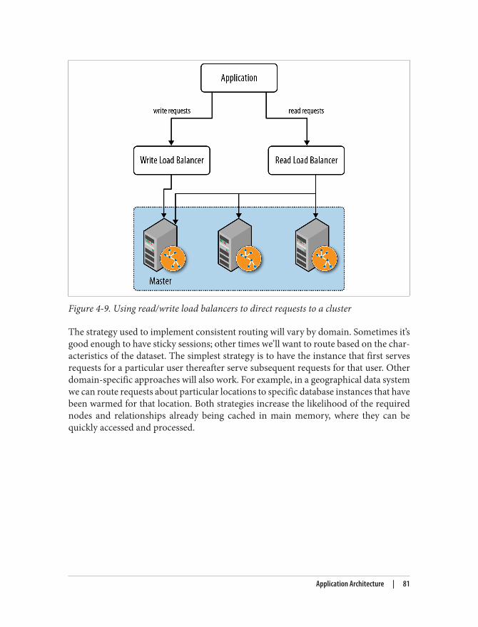
Figure 4-9. Using read/write load balancers to direct requests to a cluster

The strategy used to implement consistent routing will vary by domain. Sometimes it’sgood enough to have sticky sessions; other times we’ll want to route based on the char‐acteristics of the dataset. The simplest strategy is to have the instance that first servesrequests for a particular user thereafter serve subsequent requests for that user. Otherdomain-specific approaches will also work. For example, in a geographical data systemwe can route requests about particular locations to specific database instances that havebeen warmed for that location. Both strategies increase the likelihood of the requirednodes and relationships already being cached in main memory, where they can bequickly accessed and processed.

Application Architecture | 81

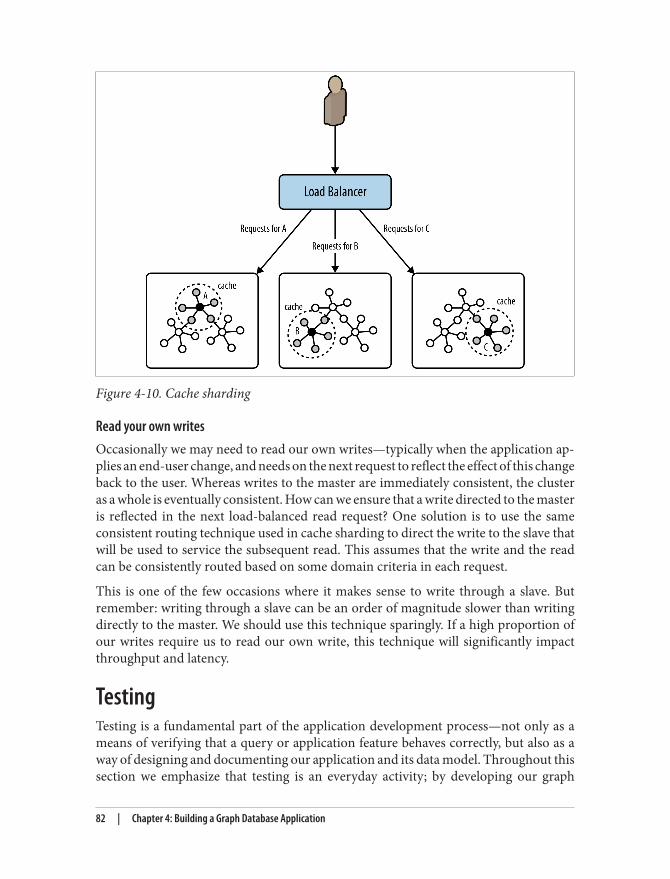
Figure 4-10. Cache sharding

Read your own writesOccasionally we may need to read our own writes—typically when the application ap‐plies an end-user change, and needs on the next request to reflect the effect of this changeback to the user. Whereas writes to the master are immediately consistent, the clusteras a whole is eventually consistent. How can we ensure that a write directed to the masteris reflected in the next load-balanced read request? One solution is to use the sameconsistent routing technique used in cache sharding to direct the write to the slave thatwill be used to service the subsequent read. This assumes that the write and the readcan be consistently routed based on some domain criteria in each request.

This is one of the few occasions where it makes sense to write through a slave. Butremember: writing through a slave can be an order of magnitude slower than writingdirectly to the master. We should use this technique sparingly. If a high proportion ofour writes require us to read our own write, this technique will significantly impactthroughput and latency.

TestingTesting is a fundamental part of the application development process—not only as ameans of verifying that a query or application feature behaves correctly, but also as away of designing and documenting our application and its data model. Throughout thissection we emphasize that testing is an everyday activity; by developing our graph

82 | Chapter 4: Building a Graph Database Application

4. Tests not only act as documentation, but they can also be used to generate documentation. All of the Cypherdocumentation in the Neo4j manual is generated automatically from the unit tests used to develop Cypher.

database solution in a test-driven manner, we provide for the rapid evolution of oursystem, and its continued responsiveness to new business needs.

Test-Driven Data Model DevelopmentIn discussing data modeling, we’ve stressed that our graph model should reflect thekinds of queries we want to run against it. By developing our data model in a test-drivenfashion we document our understanding of our domain, and validate that our queriesbehave correctly.

With test-driven data modeling, we write unit tests based on small, representative ex‐ample graphs drawn from our domain. These example graphs contain just enough datato communicate a particular feature of the domain; in many cases, they might onlycomprise 10 or so nodes, plus the relationships that connect them. We use these exam‐ples to describe what is normal for the domain, and also what is exceptional. As wediscover anomalies and corner cases in our real data, we write a test that reproduceswhat we’ve discovered.

The example graphs we create for each test comprise the setup or context for that test.Within this context we exercise a query, and assert that the query behaves as expected.Because we control the context, we, as the author of the test, know what results to expect.

Tests can act like documentation. By reading the tests, developers gain an understandingof the problems and needs the application is intended to address, and the ways in whichthe authors have gone about addressing them. With this is mind, it’s best to use eachtest to test just one aspect of our domain. It’s far easier to read lots of small tests, eachof which communicates a discrete feature of our data in a clear, simple, and concisefashion, than it is to reverse engineer a complex domain from a single large and unwieldytest. In many cases, we’ll find a particular query being exercised by several tests, someof which demonstrate the happy path through our domain, others of which exercise itin the context of some exceptional structure or set of values.4

Over time, we’ll build up a suite of tests that can act as a powerful regression test mech‐anism. As our application evolves, and we add new sources of data, or change the modelto meet new needs, our regression test suite will continue to assert that existing featurescontinue to behave as they should. Evolutionary architectures, and the incremental anditerative software development techniques that support them, depend upon a bedrockof asserted behavior. The unit-testing approach to data model development describedhere enables developers to respond to new business needs with very little risk of un‐dermining or breaking what has come before, confident in the continued quality of thesolution.

Testing | 83

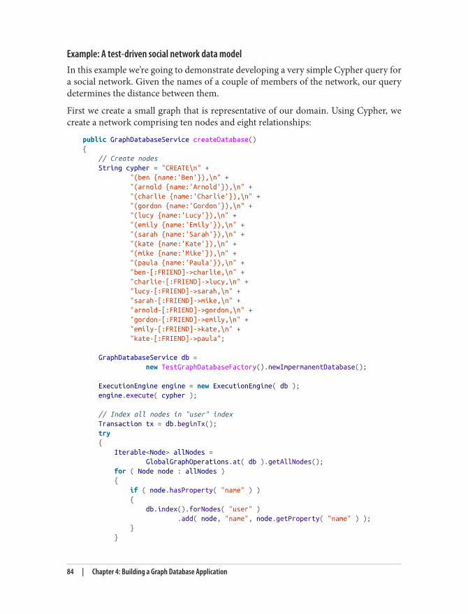
Example: A test-driven social network data modelIn this example we’re going to demonstrate developing a very simple Cypher query fora social network. Given the names of a couple of members of the network, our querydetermines the distance between them.

First we create a small graph that is representative of our domain. Using Cypher, wecreate a network comprising ten nodes and eight relationships:

public GraphDatabaseService createDatabase(){ // Create nodes String cypher = "CREATE\n" + "(ben {name:'Ben'}),\n" + "(arnold {name:'Arnold'}),\n" + "(charlie {name:'Charlie'}),\n" + "(gordon {name:'Gordon'}),\n" + "(lucy {name:'Lucy'}),\n" + "(emily {name:'Emily'}),\n" + "(sarah {name:'Sarah'}),\n" + "(kate {name:'Kate'}),\n" + "(mike {name:'Mike'}),\n" + "(paula {name:'Paula'}),\n" + "ben-[:FRIEND]->charlie,\n" + "charlie-[:FRIEND]->lucy,\n" + "lucy-[:FRIEND]->sarah,\n" + "sarah-[:FRIEND]->mike,\n" + "arnold-[:FRIEND]->gordon,\n" + "gordon-[:FRIEND]->emily,\n" + "emily-[:FRIEND]->kate,\n" + "kate-[:FRIEND]->paula";

GraphDatabaseService db = new TestGraphDatabaseFactory().newImpermanentDatabase();

ExecutionEngine engine = new ExecutionEngine( db ); engine.execute( cypher );

// Index all nodes in "user" index Transaction tx = db.beginTx(); try { Iterable<Node> allNodes = GlobalGraphOperations.at( db ).getAllNodes(); for ( Node node : allNodes ) { if ( node.hasProperty( "name" ) ) { db.index().forNodes( "user" ) .add( node, "name", node.getProperty( "name" ) ); } }

84 | Chapter 4: Building a Graph Database Application

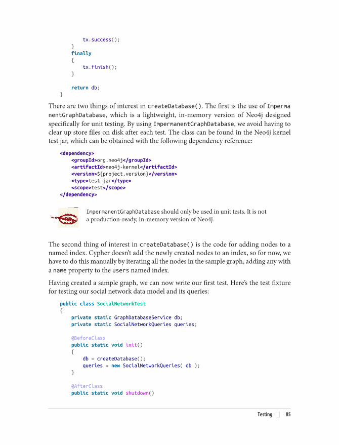
tx.success(); } finally { tx.finish(); }

return db;}

There are two things of interest in createDatabase(). The first is the use of ImpermanentGraphDatabase, which is a lightweight, in-memory version of Neo4j designedspecifically for unit testing. By using ImpermanentGraphDatabase, we avoid having toclear up store files on disk after each test. The class can be found in the Neo4j kerneltest jar, which can be obtained with the following dependency reference:

<dependency> <groupId>org.neo4j</groupId> <artifactId>neo4j-kernel</artifactId> <version>${project.version}</version> <type>test-jar</type> <scope>test</scope></dependency>

ImpermanentGraphDatabase should only be used in unit tests. It is nota production-ready, in-memory version of Neo4j.

The second thing of interest in createDatabase() is the code for adding nodes to anamed index. Cypher doesn’t add the newly created nodes to an index, so for now, wehave to do this manually by iterating all the nodes in the sample graph, adding any witha name property to the users named index.

Having created a sample graph, we can now write our first test. Here’s the test fixturefor testing our social network data model and its queries:

public class SocialNetworkTest{ private static GraphDatabaseService db; private static SocialNetworkQueries queries;

@BeforeClass public static void init() { db = createDatabase(); queries = new SocialNetworkQueries( db ); }

@AfterClass public static void shutdown()

Testing | 85

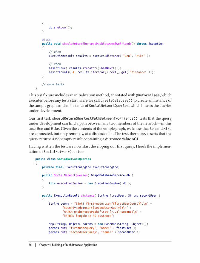
{ db.shutdown(); }

@Test public void shouldReturnShortestPathBetweenTwoFriends() throws Exception { // when ExecutionResult results = queries.distance( "Ben", "Mike" );

// then assertTrue( results.iterator().hasNext() ); assertEquals( 4, results.iterator().next().get( "distance" ) ); }

// more tests}

This test fixture includes an initialization method, annotated with @BeforeClass, whichexecutes before any tests start. Here we call createDatabase() to create an instance ofthe sample graph, and an instance of SocialNetworkQueries, which houses the queriesunder development.

Our first test, shouldReturnShortestPathBetweenTwoFriends(), tests that the queryunder development can find a path between any two members of the network—in thiscase, Ben and Mike. Given the contents of the sample graph, we know that Ben and Mikeare connected, but only remotely, at a distance of 4. The test, therefore, asserts that thequery returns a nonempty result containing a distance value of 4.

Having written the test, we now start developing our first query. Here’s the implemen‐tation of SocialNetworkQueries:

public class SocialNetworkQueries{ private final ExecutionEngine executionEngine;

public SocialNetworkQueries( GraphDatabaseService db ) { this.executionEngine = new ExecutionEngine( db ); }

public ExecutionResult distance( String firstUser, String secondUser ) { String query = "START first=node:user({firstUserQuery}),\n" + "second=node:user({secondUserQuery})\n" + "MATCH p=shortestPath(first-[*..4]-second)\n" + "RETURN length(p) AS distance";

Map<String, Object> params = new HashMap<String, Object>(); params.put( "firstUserQuery", "name:" + firstUser ); params.put( "secondUserQuery", "name:" + secondUser );

86 | Chapter 4: Building a Graph Database Application

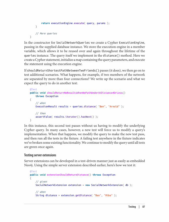
return executionEngine.execute( query, params ); }

// More queries}

In the constructor for SocialNetworkQueries we create a Cypher ExecutionEngine,passing in the supplied database instance. We store the execution engine in a membervariable, which allows it to be reused over and again throughout the lifetime of thequeries instance. The query itself we implement in the distance() method. Here wecreate a Cypher statement, initialize a map containing the query parameters, and executethe statement using the execution engine.

If shouldReturnShortestPathBetweenTwoFriends() passes (it does), we then go on totest additional scenarios. What happens, for example, if two members of the networkare separated by more than four connections? We write up the scenario and what weexpect the query to do in another test:

@Testpublic void shouldReturnNoResultsWhenNoPathUnderAtDistance4OrLess() throws Exception{ // when ExecutionResult results = queries.distance( "Ben", "Arnold" );

// then assertFalse( results.iterator().hasNext() );}

In this instance, this second test passes without us having to modify the underlyingCypher query. In many cases, however, a new test will force us to modify a query’simplementation. When that happens, we modify the query to make the new test pass,and then run all the tests in the fixture. A failing test anywhere in the fixture indicateswe’ve broken some existing functionality. We continue to modify the query until all testsare green once again.

Testing server extensionsServer extensions can be developed in a test-driven manner just as easily as embeddedNeo4j. Using the simple server extension described earlier, here’s how we test it:

@Testpublic void extensionShouldReturnDistance() throws Exception{ // given SocialNetworkExtension extension = new SocialNetworkExtension( db );

// when String distance = extension.getDistance( "Ben", "Mike" );

Testing | 87

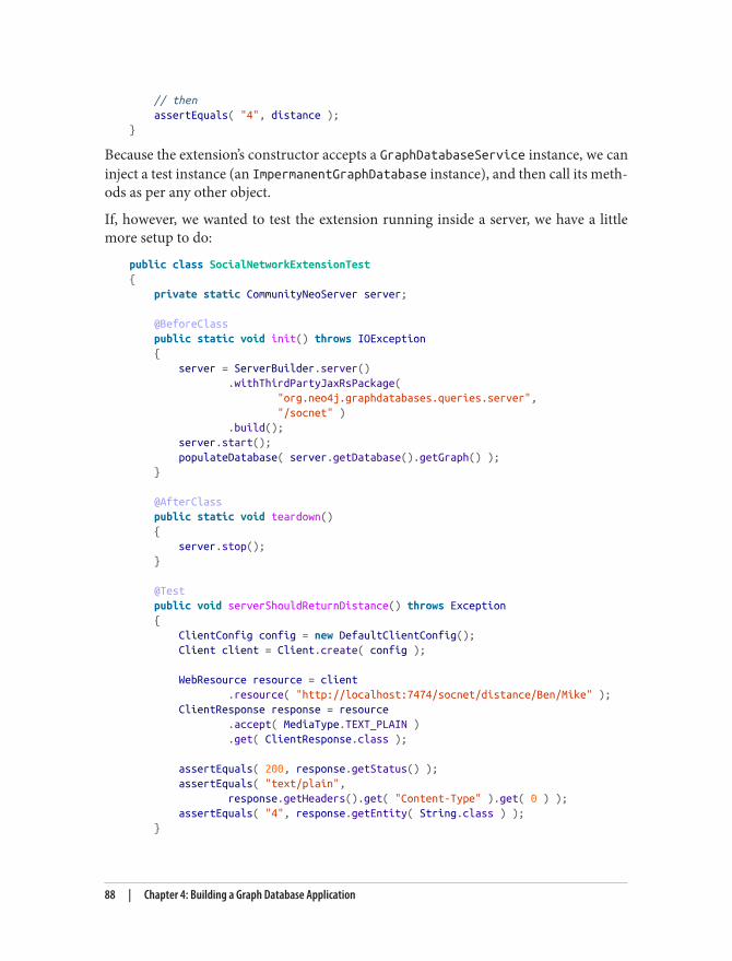
// then assertEquals( "4", distance );}

Because the extension’s constructor accepts a GraphDatabaseService instance, we caninject a test instance (an ImpermanentGraphDatabase instance), and then call its meth‐ods as per any other object.

If, however, we wanted to test the extension running inside a server, we have a littlemore setup to do:

public class SocialNetworkExtensionTest{ private static CommunityNeoServer server;

@BeforeClass public static void init() throws IOException { server = ServerBuilder.server() .withThirdPartyJaxRsPackage( "org.neo4j.graphdatabases.queries.server", "/socnet" ) .build(); server.start(); populateDatabase( server.getDatabase().getGraph() ); }

@AfterClass public static void teardown() { server.stop(); }

@Test public void serverShouldReturnDistance() throws Exception { ClientConfig config = new DefaultClientConfig(); Client client = Client.create( config );

WebResource resource = client .resource( "http://localhost:7474/socnet/distance/Ben/Mike" ); ClientResponse response = resource .accept( MediaType.TEXT_PLAIN ) .get( ClientResponse.class );

assertEquals( 200, response.getStatus() ); assertEquals( "text/plain", response.getHeaders().get( "Content-Type" ).get( 0 ) ); assertEquals( "4", response.getEntity( String.class ) ); }

88 | Chapter 4: Building a Graph Database Application

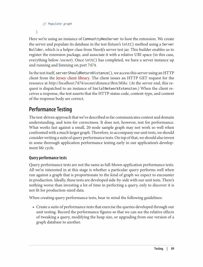
// Populate graph

}

Here we’re using an instance of CommunityNeoServer to host the extension. We createthe server and populate its database in the test fixture’s init() method using a ServerBuilder, which is a helper class from Neo4j’s server test jar. This builder enables us toregister the extension package, and associate it with a relative URI space (in this case,everything below /socnet). Once init() has completed, we have a server instance upand running and listening on port 7474.

In the test itself, serverShouldReturnDistance(), we access this server using an HTTPclient from the Jersey client library. The client issues an HTTP GET request for theresource at http://localhost:7474/socnet/distance/Ben/Mike. (At the server end, this re‐quest is dispatched to an instance of SocialNetworkExtension.) When the client re‐ceives a response, the test asserts that the HTTP status code, content-type, and contentof the response body are correct.

Performance TestingThe test-driven approach that we’ve described so far communicates context and domainunderstanding, and tests for correctness. It does not, however, test for performance.What works fast against a small, 20-node sample graph may not work so well whenconfronted with a much larger graph. Therefore, to accompany our unit tests, we shouldconsider writing a suite of query performance tests. On top of that, we should also investin some thorough application performance testing early in our application’s develop‐ment life cycle.

Query performance testsQuery performance tests are not the same as full-blown application performance tests.All we’re interested in at this stage is whether a particular query performs well whenrun against a graph that is proportionate to the kind of graph we expect to encounterin production. Ideally, these tests are developed side-by-side with our unit tests. There’snothing worse than investing a lot of time in perfecting a query, only to discover it isnot fit for production-sized data.

When creating query performance tests, bear in mind the following guidelines:

• Create a suite of performance tests that exercise the queries developed through ourunit testing. Record the performance figures so that we can see the relative effectsof tweaking a query, modifying the heap size, or upgrading from one version of agraph database to another.

Testing | 89

5. A thorough discussion of agile performance testing can be found in Alistair Jones and Patrick Kua, “ExtremePerformance Testing,” The ThoughtWorks Anthology, Volume 2 (Pragmatic Bookshelf, 2012).

• Run these tests often, so that we quickly become aware of any deterioration inperformance. We might consider incorporating these tests into a continuous de‐livery build pipeline, failing the build if the test results exceed a certain value.

• Run these tests in-process on a single thread. There’s no need to simulate multipleclients at this stage: if the performance is poor for a single client, it’s unlikely toimprove for multiple clients. Even though they are not, strictly speaking, unit tests,we can drive them using the same unit testing framework we use to develop ourunit tests.

• Run each query many times, picking starting nodes at random each time, so thatwe can see the effect of starting from a cold cache, which is then gradually warmedas multiple queries execute.

Application performance testsApplication performance tests, as distinct from query performance tests, test the per‐formance of the entire application under representative production usage scenarios.

As with query performance tests, we recommend that this kind of performance testingis done as part of everyday development, side-by-side with the development of appli‐cation features, rather than as a distinct project phase.5 To facilitate application perfor‐mance testing early in the project life cycle, it is often necessary to develop a “walkingskeleton,” an end-to-end slice through the entire system, which can be accessed andexercised by performance test clients. By developing a walking skeleton, we not onlyprovide for performance testing, but we also establish the architectural context for thegraph database part of our solution. This enables us to verify our application architec‐ture, and identify layers and abstractions that allow for discrete testing of individualcomponents.

Performance tests serve two purposes: they demonstrate how the system will performwhen used in production, and they drive out the operational affordances that make iteasier to diagnose performance issues, incorrect behavior, and bugs. What we learn increating and maintaining a performance test environment will prove invaluable whenit comes to deploying and operating the system for real.

When drawing up the criteria for a performance test, we recommend specifying per‐centiles rather than averages. Never assume a normal distribution of response times:the real world doesn’t work like that. For some applications we may want to ensure thatall requests return within a certain time period. In rare circumstances it may be im‐portant for the very first request to be as quick as when the caches have been warmed.But in the majority of cases, we will want to ensure the majority of requests return within

90 | Chapter 4: Building a Graph Database Application

6. Max De Marzi describes using Gatling to test Neo4j.

a certain time period; that, say, 98% of requests are satisfied in under 200 ms. It isimportant to keep a record of subsequent test runs so that we can compare performancefigures over time, and thereby quickly identify slowdowns and anomalous behavior.

As with unit tests and query performance tests, application performance tests provemost valuable when employed in an automated delivery pipeline, where successivebuilds of the application are automatically deployed to a testing environment, the testsexecuted, and the results automatically analyzed. Log files and test results should bestored for later retrieval, analysis, and comparison. Regressions and failures should failthe build, prompting developers to address the issues in a timely manner. One of thebig advantages of conducting performance testing over the course of an application’sdevelopment life cycle, rather than at the end, is that failures and regressions can veryoften be tied back to a recent piece of development; this enables us to diagnose, pinpoint,and remedy issues rapidly and succinctly.

For generating load, we’ll need a load-generating agent. For web applications, there areseveral open source stress and load testing tools available, including Grinder, JMeter,and Gatling.6 When testing load-balanced web applications, we should ensure our testclients are distributed across different IP addresses so that requests are balanced acrossthe cluster.

Testing with representative dataFor both query performance testing and application performance testing we will needa dataset that is representative of the data we will encounter in production. It will,therefore, be necessary to create or otherwise source such a dataset. In some cases wecan obtain a dataset from a third party, or adapt an existing dataset that we own, butunless these datasets are already in the form of a graph, we will have to write somecustom export-import code.

In many cases, however, we’re starting from scratch. If this is the case, we must dedicatesome time to creating a dataset builder. As with the rest of the software developmentlife cycle, this is best done in an iterative and incremental fashion. Whenever we intro‐duce a new element into our domain’s data model, as documented and tested in our unittests, we add the corresponding element to our performance dataset builder. That way,our performance tests will come as close to real-world usage as our current under‐standing of the domain allows.

When creating a representative dataset, we try to reproduce any domain invariants wehave identified: the minimum, maximum, and average number of relationships pernode, the spread of different relationship types, property value ranges, and so on. Ofcourse, it’s not always possible to know these things upfront, and often we’ll find

Testing | 91

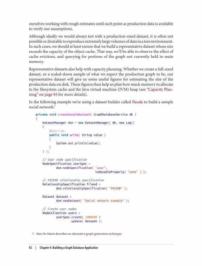
7. Max De Marzi describes an alternative graph generation technique.

ourselves working with rough estimates until such point as production data is availableto verify our assumptions.

Although ideally we would always test with a production-sized dataset, it is often notpossible or desirable to reproduce extremely large volumes of data in a test environment.In such cases, we should at least ensure that we build a representative dataset whose sizeexceeds the capacity of the object cache. That way, we’ll be able to observe the effect ofcache evictions, and querying for portions of the graph not currently held in mainmemory.

Representative datasets also help with capacity planning. Whether we create a full-sizeddataset, or a scaled-down sample of what we expect the production graph to be, ourrepresentative dataset will give us some useful figures for estimating the size of theproduction data on disk. These figures then help us plan how much memory to allocateto the filesystem cache and the Java virtual machine (JVM) heap (see “Capacity Plan‐ning” on page 93 for more details).

In the following example we’re using a dataset builder called Neode to build a samplesocial network:7

private void createSampleDataset( GraphDatabaseService db ){ DatasetManager dsm = new DatasetManager( db, new Log() { @Override public void write( String value ) { System.out.println(value); } } );

// User node specification NodeSpecification userSpec = dsm.nodeSpecification( "user", indexableProperty( "name" ) );

// FRIEND relationship specification RelationshipSpecification friend = dsm.relationshipSpecification( "FRIEND" );

Dataset dataset = dsm.newDataset( "Social network example" );

// Create user nodes NodeCollection users = userSpec.create( 1000000 ) .update( dataset );

92 | Chapter 4: Building a Graph Database Application

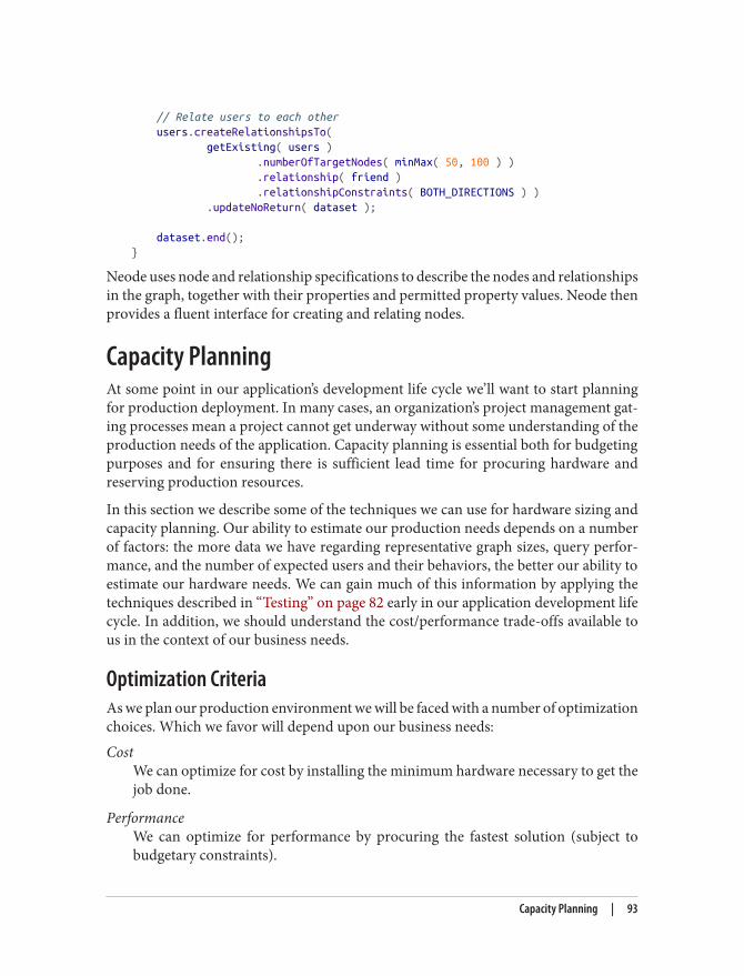
// Relate users to each other users.createRelationshipsTo( getExisting( users ) .numberOfTargetNodes( minMax( 50, 100 ) ) .relationship( friend ) .relationshipConstraints( BOTH_DIRECTIONS ) ) .updateNoReturn( dataset );

dataset.end();}

Neode uses node and relationship specifications to describe the nodes and relationshipsin the graph, together with their properties and permitted property values. Neode thenprovides a fluent interface for creating and relating nodes.

Capacity PlanningAt some point in our application’s development life cycle we’ll want to start planningfor production deployment. In many cases, an organization’s project management gat‐ing processes mean a project cannot get underway without some understanding of theproduction needs of the application. Capacity planning is essential both for budgetingpurposes and for ensuring there is sufficient lead time for procuring hardware andreserving production resources.

In this section we describe some of the techniques we can use for hardware sizing andcapacity planning. Our ability to estimate our production needs depends on a numberof factors: the more data we have regarding representative graph sizes, query perfor‐mance, and the number of expected users and their behaviors, the better our ability toestimate our hardware needs. We can gain much of this information by applying thetechniques described in “Testing” on page 82 early in our application development lifecycle. In addition, we should understand the cost/performance trade-offs available tous in the context of our business needs.

Optimization CriteriaAs we plan our production environment we will be faced with a number of optimizationchoices. Which we favor will depend upon our business needs:Cost

We can optimize for cost by installing the minimum hardware necessary to get thejob done.

PerformanceWe can optimize for performance by procuring the fastest solution (subject tobudgetary constraints).

Capacity Planning | 93

RedundancyWe can optimize for redundancy and availability by ensuring the database clusteris big enough to survive a certain number of machine failures (i.e., to survive twomachines failing, we will need a cluster comprising five instances).

LoadWith a replicated graph database solution, we can optimize for load by scalinghorizontally (for read load), and vertically (for write load).

PerformanceRedundancy and load can be costed in terms of the number of machines necessary toensure availability (five machines to provide continued availability in the face of twomachines failing, for example) and scalability (one machine per some number of con‐current requests, as per the calculations in “Load” on page 97). But what about perfor‐mance? How can we cost performance?

Calculating the cost of graph database performanceIn order to understand the cost implications of optimizing for performance, we needto understand the performance characteristics of the database stack. As we describe inmore detail later in “Native Graph Storage” on page 144, a graph database uses disk fordurable storage, and main memory for caching portions of the graph. In Neo4j, thecaching parts of main memory are further divided between the filesystem cache (whichis typically managed by the operating system) and the object cache. The filesystem cacheis a portion of off-heap RAM into which files on disk are read and cached before beingserved to the application. The object cache is an on-heap cache that stores object in‐stances of nodes, relationships, and properties.

Spinning disk is by far the slowest part of the database stack. Queries that have to reachall the way down to spinning disk will be orders of magnitude slower than queries thattouch only the object cache. Disk access can be improved by using solid-state drives(SSDs) in place of spinning disks, providing an approximate 20 times increase in per‐formance, or by using enterprise flash hardware, which can reduce latencies evenfurther.

Spinning disks and SDDs are cheap, but not very fast. Far more significant performancebenefits accrue when the database has to deal only with the caching layers. The filesystemcache offers up to 500 times the performance of spinning disk, whereas the object cachecan be up to 5,000 times faster.

For comparative purposes, graph database performance can be expressed as a functionof the percentage of data available at each level of the object cache-filesystem cache-diskhierarchy:

(% graph in object cache x 5000) * (% graph in filesystem cache * 500) * 20 (if using SSDs)

94 | Chapter 4: Building a Graph Database Application

8. Neo4j Enterprise Edition includes a cache implementation that mitigates the problems encountered withlarge heaps, and is being successfully used with heaps in the order of 200 GB.

An application in which 100% of the graph is available in the object cache (as well as inthe filesystem cache, and on disk) will be more performant than one in which 100% isavailable on disk, but only 80% in the filesystem cache and 20% in the object cache.

Performance optimization optionsThere are, then, three areas in which we can optimize for performance:

• Increase the object cache (from 2 GB, all the way up to 200 GB or more in exceptionalcircumstances)

• Increase the percentage of the store mapped into the filesystem cache• Invest in faster disks: SSDs or enterprise flash hardware

The first two options here require adding more RAM. In costing the allocation of RAM,however, there are a couple of things to bear in mind. First, whereas the size of the storefiles in the filesystem cache map one-to-one with the size on disk, graph objects in theobject cache can be up to 10 times bigger than their on-disk representations. AllocatingRAM to the object cache is, therefore, far more expensive per graph element than allo‐cating it to the filesystem cache. The second point to bear in mind relates to the locationof the object cache. If our graph database uses an on-heap cache, as does Neo4j, thenincreasing the size of the cache requires allocating more heap. Most modern JVMs donot cope well with heaps much larger than 8 GB. Once we start growing the heap beyondthis size, garbage collection can impact the performance of our application.8

As Figure 4-11 shows, the sweet spot for any cost versus performance trade-off liesaround the point where we can map our store files in their entirety into RAM, whileallowing for a healthy, but modestly sized object cache. Heaps of between 4 and 8 GBare not uncommon, though in many cases, a smaller heap can actually improve per‐formance (by mitigating expensive GC behaviors).

Calculating how much RAM to allocate to the heap and the filesystem cache dependson our knowing the projected size of our graph. Building a representative dataset earlyin our application’s development life cycle will furnish us with some of the data we needto make our calculations. If we cannot fit the entire graph into main memory (that is,at a minimum, into the filesystem cache), we should consider cache sharding (see “Cachesharding” on page 80).

Capacity Planning | 95

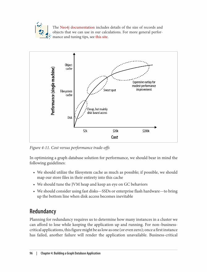
The Neo4j documentation includes details of the size of records andobjects that we can use in our calculations. For more general perfor‐mance and tuning tips, see this site.

Figure 4-11. Cost versus performance trade-offs

In optimizing a graph database solution for performance, we should bear in mind thefollowing guidelines:

• We should utilize the filesystem cache as much as possible; if possible, we shouldmap our store files in their entirety into this cache

• We should tune the JVM heap and keep an eye on GC behaviors• We should consider using fast disks—SSDs or enterprise flash hardware—to bring

up the bottom line when disk access becomes inevitable

RedundancyPlanning for redundancy requires us to determine how many instances in a cluster wecan afford to lose while keeping the application up and running. For non–business-critical applications, this figure might be as low as one (or even zero); once a first instancehas failed, another failure will render the application unavailable. Business-critical

96 | Chapter 4: Building a Graph Database Application

applications will likely require redundancy of at least two; that is, even after two ma‐chines have failed, the application continues serving requests.

For a graph database whose cluster management protocol requires a majority of coor‐dinators to be available to work properly, redundancy of one can be achieved with threeor four instances, and redundancy of two with five instances. Four is no better thanthree in this respect, because if two instances from a four-instance cluster become un‐available, the remaining coordinators will no longer be able to achieve majority.

Neo4j permits coordinators to be located on separate machines fromthe database instances in the cluster. This enables us to scale the coor‐dinators independently of the databases. With three database instancesand five coordinators located on different machines, we could lose twodatabases and two coordinators, and still achieve majority, albeit witha lone database.

LoadOptimizing for load is perhaps the trickiest part of capacity planning. As a rule of thumb:

number of concurrent requests = (1000 / average request time (in milliseconds)) * numberof cores per machine * number of machines

Actually determining what some of these figures are, or are projected to be, can some‐times be very difficult:Average request time

This covers the period from when a server receives a request, to when it sends aresponse. Performance tests can help determine average request time, assuming thetests are running on representative hardware against a representative dataset (we’llhave to hedge accordingly if not). In many cases, the “representative dataset” itselfis based on a rough estimate; we should modify our figures whenever this estimatechanges.

Number of concurrent requestsWe should distinguish here between average load and peak load. Determining thenumber of concurrent requests a new application must support is a difficult thingto do. If we’re replacing or upgrading an existing application, we may have accessto some recent production statistics we can use to refine our estimates. Someorganizations are able to extrapolate from existing application data the likely re‐quirements for a new application. Other than that, it’s down to our stakeholders toestimate the projected load on the system, but we must beware of inflatedexpectations.

Capacity Planning | 97

SummaryIn this chapter we’ve discussed the most important aspects of developing a graph data‐base application. We’ve seen how to create graph models that address an application’sneeds and an end user’s goals, and how to make those models and associated queriesexpressive and robust using unit and performance tests. We’ve looked at the pros andcons of a couple of different application architectures, and enumerated the factors weneed to consider when planning for production.

In the next chapter we’ll look at how graph databases are being used today to solve real-world problems in domains as varied as social networking, recommendations, masterdata management, data center management, access control, and logistics.

98 | Chapter 4: Building a Graph Database Application

CHAPTER 5

Graphs in the Real World

In this chapter we look at some of the common real-world use cases for graph databasesand identify the reasons why organizations choose to use a graph database rather thana relational or other NOSQL store. The bulk of the chapter comprises three in-depthuse cases, with details of the relevant data models and queries. Each of these exampleshas been drawn from a real-world production system; the names, however, have beenchanged, and the technical details simplified where necessary to hide any accidentalcomplexity, and thereby highlight key design points.

Why Organizations Choose Graph DatabasesThroughout this book, we’ve sung the praises of the graph data model, its power andflexibility, and its innate expressiveness. When it comes to applying a graph database toa real-world problem, with real-world technical and business constraints, organizationschoose graph databases for the following reasons:“Minutes to milliseconds” performance

Query performance and responsiveness are top of many organizations’ concernswith regard to their data platforms. Online transactional systems, large web appli‐cations in particular, must respond to end users in milliseconds if they are to besuccessful. In the relational world, as an application’s dataset size grows, join painsbegin to manifest themselves, and performance deteriorates. Using index-free ad‐jacency, a graph database turns complex joins into fast graph traversals, therebymaintaining millisecond performance irrespective of the overall size of the dataset.

Drastically accelerated development cyclesThe graph data model reduces the impedance mismatch that has plagued softwaredevelopment for decades, thereby reducing the development overhead of translat‐ing back and forth between an object model and a tabular relational model. Moreimportantly, the graph model reduces the impedance mismatch between the

99

1. See Nicholas Christakis and James Fowler, Connected: The Amazing Power of Social Networks and How TheyShape Our Lives (HarperPress, 2011).

technical and business domains: subject matter experts, architects, and developerscan talk about and picture the core domain using a shared model that is then in‐corporated into the application itself.

Extreme business responsivenessSuccessful applications rarely stay still; changes in business conditions, user be‐haviors, and technical and operational infrastructures drive new requirements. Inthe past, this has required organizations to undertake careful and lengthy data mi‐grations that involve modifying schemas, transforming data, and maintaining re‐dundant data to serve old and new features. The schema-free nature of a graphdatabase coupled with the ability to simultaneously relate data elements in lots ofdifferent ways allows a graph database solution to evolve as the business evolves,reducing risk and time-to-market.

Enterprise readyData is important: when employed in a business-critical application, a data tech‐nology must be robust, scalable, and more often than not, transactional. Althoughsome graph databases are fairly new and not yet fully mature, there are graph da‐tabases on the market that provide all the -ilities—ACID (Atomic, Consistent, Iso‐lated, Durable) transactionality, high-availability, horizontal read scalability, andstorage of billions of entities—needed by large enterprises today, as well as the per‐formance and flexibility characteristics discussed previously. This has been an im‐portant factor leading to the adoption of graph databases by organizations: notmerely in modest offline or departmental capacities, but in ways that can trulychange the business.

Common Use CasesIn this section we describe some of the most common graph database use cases, iden‐tifying how the graph model and the specific characteristics of the graph database canbe applied to generate competitive insight and significant business value.

SocialWe are only just beginning to discover the power of social data. In their book Connec‐ted, social scientists Nicholas Christakis and James Fowler show how, despite knowingnothing about an individual, we can better predict that person’s behavior by under‐standing who he is connected to, than we can by accumulating facts about him.1

Social applications allow organizations to gain competitive and operational advantageby leveraging information about the connections between people, together with discrete

100 | Chapter 5: Graphs in the Real World

information about individuals, to facilitate collaboration and flow of information, andpredict behavior.

As Facebook’s use of the term social graph implies, graph data models and graph data‐bases are a natural fit for this overtly relationship-centered domain. Social networkshelp us identify the direct and indirect relationships between people, groups, and thethings with which they interact, allowing users to rate, review, and discover each otherand the things they care about. By understanding who interacts with whom, how peopleare connected, and what representatives within a group are likely to do or choose basedon the aggregate behavior of the group, we generate tremendous insight into the unseenforces that influence individual behaviors. We discuss predictive modeling and its rolein social network analysis in more detail in “Graph Theory and Predictive Modeling”on page 174.

Social relations may be either explicit or implicit. Explicit relations occur wherever socialsubjects volunteer a direct link—by liking someone on Facebook, for example, or in‐dicating someone is a current or former colleague, as happens on LinkedIn. Implicitrelations emerge out of other relationships that indirectly connect two or more subjectsby way of an intermediary. We can relate subjects based on their opinions, likes, pur‐chases, and even the products of their day-to-day work. Such indirect relationships lendthemselves to being applied in multiple suggestive and inferential ways: we can say thatA is likely to know, or like, or otherwise connect to B based on some common inter‐mediaries. In so doing, we move from social network analysis into the realm of recom‐mendation engines.

RecommendationsEffective recommendations are a prime example of generating end-user value throughthe application of an inferential or suggestive capability. Whereas line-of-business ap‐plications typically apply deductive and precise algorithms—calculating payroll, apply‐ing tax, and so on—to generate end-user value, recommendation algorithms are in‐ductive and suggestive, identifying people, products, or services an individual or groupis likely to have some interest in.

Recommendation algorithms establish relationships between people and things: otherpeople, products, services, media content—whatever is relevant to the domain in whichthe recommendation is employed. Relationships are established based on users’ behav‐iors, whether purchasing, producing, consuming, rating, or reviewing the resources inquestion. The engine can then identify resources of interest to a particular individualor group, or individuals and groups likely to have some interest in a particular resource.With the first approach, identifying resources of interest to a specific user, the behaviorof the user in question—her purchasing behavior, expressed preferences, and attitudesas expressed in ratings and reviews—are correlated with those of other users in orderto identify similar users and thereafter the things with which they are connected. The

Common Use Cases | 101

2. Neo4j Spatial is an open source library of utilities that implement spatial indexes and expose Neo4j data togeotools.

second approach, identifying users and groups for a particular resource, focuses on thecharacteristics of the resource in question; the engine then identifies similar resources,and the users associated with those resources.

As in the social use case, making an effective recommendation depends on under‐standing the connections between things, as well as the quality and strength of thoseconnections—all of which are best expressed as a property graph. Queries are primarilygraph local, in that they start with one or more identifiable subjects, whether people orresources, and thereafter discover surrounding portions of the graph.

Taken together, social networks and recommendation engines provide key differenti‐ating capabilities in the areas of retail, recruitment, sentiment analysis, search, andknowledge management. Graphs are a good fit for the densely connected data structuresgermane to each of these areas; storing and querying this data using a graph databaseallows an application to surface end-user real-time results that reflect recent changes tothe data, rather than precalculated, stale results.

GeoGeospatial is the original graph use case: Euler solved the Seven Bridges of Königsbergproblem by positing a mathematical theorem that later came to form the basis of graphtheory. Geospatial applications of graph databases range from calculating routes be‐tween locations in an abstract network such as a road or rail network, airspace network,or logistical network (as illustrated by the logistics example later in this chapter) tospatial operations such as find all points of interest in a bounded area, find the centerof a region, and calculate the intersection between two or more regions.

Geospatial operations depend upon specific data structures, ranging from simpleweighted and directed relationships, through to spatial indexes, such as R-Trees, whichrepresent multidimensional properties using tree data structures. As indexes, these datastructures naturally take the form of a graph, typically hierarchical in form, and as suchthey are a good fit for a graph database. Because of the schema-free nature of graphdatabases, geospatial data can reside in the database beside other kinds of data—socialnetwork data, for example—allowing for complex multidimensional querying acrossseveral domains.2

Geospatial applications of graph databases are particularly relevant in the areas of tel‐ecommunications, logistics, travel, timetabling, and route planning.

102 | Chapter 5: Graphs in the Real World

Master Data ManagementMaster data is data that is critical to the operation of a business, but which itself is non-transactional. Master data includes data concerning users, customers, products, sup‐pliers, departments, geographies, sites, cost centers, and business units. In large organ‐izations, this data is often held in many different places, with lots of overlap and re‐dundancy, in many different formats, and with varying degrees of quality and means ofaccess. Master Data Management (MDM) is the practice of identifying, cleaning, stor‐ing, and, most importantly, governing this data. Its key concerns include managingchange over time as organizational structures change, businesses merge, and businessrules change; incorporating new sources of data; supplementing existing data with ex‐ternally sourced data; addressing the needs of reporting, compliance, and business in‐telligence consumers; and versioning data as its values and schemas change.

Graph databases don’t provide a full MDM solution; they are, however, ideally appliedto the modeling, storing, and querying of hierarchies, master data metadata, and masterdata models. Such models include type definitions, constraints, relationships betweenentities, and the mappings between the model and the underlying source systems. Agraph database’s structured yet schema-free data model provides for ad hoc, variable,and exceptional structures—schema anomalies that commonly arise when there aremultiple redundant data sources—while at the same time allowing for the rapid evolu‐tion of the master data model in line with changing business needs.

Network and Data Center ManagementIn Chapter 3 we looked at a simple data center domain model, showing how the physicaland virtual assets inside a data center can be easily modeled with a graph. Communi‐cations networks are graph structures; graph databases are, therefore, a great fit formodeling, storing, and querying this kind of domain data. The distinction betweennetwork management of a large communications network versus data center manage‐ment is largely a matter of which side of the firewall you’re working. For all intents andpurposes, these two things are one and the same.

A graph representation of a network enables us to catalogue assets, visualize how theyare deployed, and identify the dependencies between them. The graph’s connectedstructure, together with a query language like Cypher, enable us to conduct sophisticatedimpact analyses, answering questions such as:

• Which parts of the network—which applications, services, virtual machines, phys‐ical machines, data centers, routers, switches, and fibre—do important customersdepend on? (Top-down analysis)

• Conversely, which applications and services, and ultimately, customers, in the net‐work will be affected if a particular network element—a router or switch, for ex‐ample—fails? (Bottom-up analysis)

Common Use Cases | 103

• Is there redundancy throughout the network for the most important customers?

Graph database solutions complement existing network management and analysistools. As with master data management, they can be used to bring together data fromdisparate inventory systems, providing a single view of the network and its consumers,from the smallest network element all the way to application and services and the cus‐tomers who use them. A graph database representation of the network can also be usedto enrich operational intelligence based on event correlations: whenever an event cor‐relation engine [a Complex Event Processor, for example] infers a complex event froma stream of low-level network events, it can assess the impact of that event using thegraph model, and thereafter trigger any necessary compensating or mitigating actions.

Today, graph databases are being successfully employed in the areas of telecommuni‐cations, network management and analysis, cloud platform management, data centerand IT asset management, and network impact analysis, where they are reducing impactanalysis and problem resolution times from days and hours down to minutes and sec‐onds. Performance, flexibility in the face of changing network schemas, and fit for thedomain are all important factors here.

Authorization and Access Control (Communications)Authorization and access control solutions store information about parties (e.g., ad‐ministrators, organizational units, end-users) and resources (e.g., files, shares, networkdevices, products, services, agreements), together with the rules governing access tothose resources; they then apply these rules to determine who can access or manipulatea resource. Access control has traditionally been implemented either using directoryservices or by building a custom solution inside an application’s backend. Hierarchicaldirectory structures, however, cannot cope with the nonhierarchical organizational andresource dependency structures that characterize multiparty distributed supply chains.Hand-rolled solutions, particularly those developed on a relational database, suffer joinpain as the dataset size grows, becoming slow and unresponsive, and ultimately deliv‐ering a poor end-user experience.

A graph database can store complex, densely connected access control structures span‐ning billions of parties and resources. Its structured yet schema-free data model sup‐ports both hierarchical and nonhierarchical structures, while its extensible propertymodel allows for capturing rich metadata regarding every element in the system. Witha query engine that can traverse millions of relationships per second, access lookupsover large, complex structures execute in milliseconds.

As with network management and analysis, a graph database access control solutionallows for both top-down and bottom-up queries:

• Which resources—company structures, products, services, agreements, and endusers—can a particular administrator manage? (Top-down)

104 | Chapter 5: Graphs in the Real World

• Which resource can an end user access?• Given a particular resource, who can modify its access settings? (Bottom-up)

Graph database access control and authorization solutions are particularly applicablein the areas of content management, federated authorization services, social networkingpreferences, and software as a service (SaaS) offerings, where they realize minutes tomilliseconds increases in performance over their hand-rolled, relational predecessors.

Real-World ExamplesIn this section we describe three example use cases in detail: social and recommenda‐tions, authorization and access control, and logistics. Each use case is drawn from oneor more production applications of a graph database (specifically in these cases, Neo4j).Company names, context, data models, and queries have been tweaked to eliminateaccidental complexity and to highlight important design and implementation choices.

Social Recommendations (Professional Social Network)Talent.net is a social recommendations application that enables users to discover theirown professional network, and identify other users with particular skill sets. Users workfor companies, work on projects, and have one or more interests or skills. Based on thisinformation, Talent.net can describe a user’s professional network by identifying othersubscribers who share his or her interests. Searches can be restricted to the user’s currentcompany, or extended to encompass the entire subscriber base. Talent.net can alsoidentify individuals with specific skills who are directly or indirectly connected to thecurrent user; such searches are useful when looking for a subject matter expert for acurrent engagement.

Talent.net illustrates how a powerful inferential capability can be developed using agraph database. Although many line-of-business applications are deductive and precise—calculating tax or salary, or balancing debits and credits, for example—a new seamof end-user value opens up when we apply inductive algorithms to our data. This iswhat Talent.net does. Based on people’s interests and skills, and their work history, theapplication can suggest likely candidates for including in one’s professional network.These results are not precise in the way a payroll calculation must be precise, but theyare extremely useful nonetheless.

Talent.net infers connections between people. Contrast this with LinkedIn, for example,where users explicitly declare they know or have worked with someone. This is not tosay that LinkedIn is solely a precise social networking capability, because it too appliesinductive algorithms to generate further insight. But with Talent.net even the primarytie, (A)-[:KNOWS]->(B), is inferred, rather than volunteered.

Real-World Examples | 105

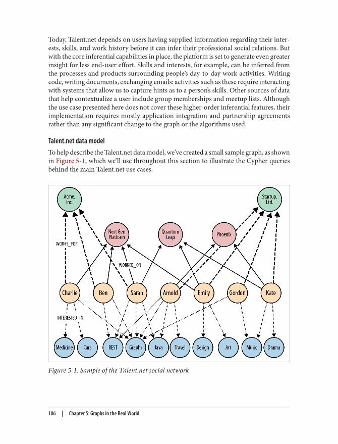
Today, Talent.net depends on users having supplied information regarding their inter‐ests, skills, and work history before it can infer their professional social relations. Butwith the core inferential capabilities in place, the platform is set to generate even greaterinsight for less end-user effort. Skills and interests, for example, can be inferred fromthe processes and products surrounding people’s day-to-day work activities. Writingcode, writing documents, exchanging emails: activities such as these require interactingwith systems that allow us to capture hints as to a person’s skills. Other sources of datathat help contextualize a user include group memberships and meetup lists. Althoughthe use case presented here does not cover these higher-order inferential features, theirimplementation requires mostly application integration and partnership agreementsrather than any significant change to the graph or the algorithms used.

Talent.net data modelTo help describe the Talent.net data model, we’ve created a small sample graph, as shownin Figure 5-1, which we’ll use throughout this section to illustrate the Cypher queriesbehind the main Talent.net use cases.

Figure 5-1. Sample of the Talent.net social network

106 | Chapter 5: Graphs in the Real World

The sample graph shown here has just two companies, each with several employees. Anemployee is connected to his employer by a WORKS_FOR relationship. Each employee isINTERESTED_IN one or more topics, and has WORKED_ON one or more projects. Occa‐sionally, employees from different companies work on the same project.

This structure addresses two important use cases:

• Given a user, inferring social relations—that is, identifying their professional socialnetwork—based on shared interests and skills.

• Given a user, recommend someone that they have worked with, or who has workedwith people they have worked with, who has a particular skill.

The first use case helps build communities around shared interests; the second helpsidentify people to fill specific project roles.

Inferring social relationsTalent.net’s graph allows it to infer a user’s professional social network by following therelationships that connect an individual’s interests to other people. The strength of therecommendation depends on the number of shared interests. If Sarah is interested inJava, graphs, and REST, Ben in graphs and REST, and Charlie in graphs, cars, and med‐icine, then there is a likely tie between Sarah and Ben based on their mutual interest ingraphs and REST, and another tie between Sarah and Charlie based on their mutualinterest in graphs, with the tie between Sarah and Ben stronger than the one betweenSarah and Charlie (two shared interests versus one).

Figure 5-2 shows the pattern representing colleagues who share a user’s interests. Thesubject node refers to the subject of the query (in the preceding example, this is Sarah).This node can be looked up in an index. The remaining nodes will be discovered oncethe pattern is anchored to the subject node and then flexed around the graph.

The Cypher to implement this query is shown here:

START subject=node:user(name={name})MATCH (subject)-[:WORKS_FOR]->(company)<-[:WORKS_FOR]-(person), (subject)-[:INTERESTED_IN]->(interest)<-[:INTERESTED_IN]-(person)RETURN person.name AS name, count(interest) AS score, collect(interest.name) AS interestsORDER BY score DESC

Real-World Examples | 107

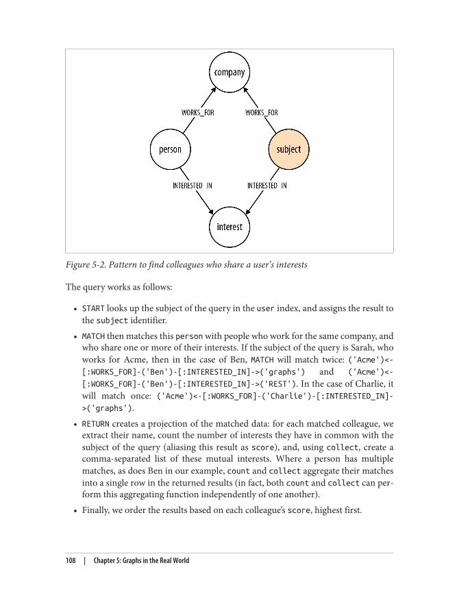
Figure 5-2. Pattern to find colleagues who share a user’s interests

The query works as follows:

• START looks up the subject of the query in the user index, and assigns the result tothe subject identifier.

• MATCH then matches this person with people who work for the same company, andwho share one or more of their interests. If the subject of the query is Sarah, whoworks for Acme, then in the case of Ben, MATCH will match twice: ('Acme')<-[:WORKS_FOR]-('Ben')-[:INTERESTED_IN]->('graphs') and ('Acme')<-

[:WORKS_FOR]-('Ben')-[:INTERESTED_IN]->('REST'). In the case of Charlie, itwill match once: ('Acme')<-[:WORKS_FOR]-('Charlie')-[:INTERESTED_IN]->('graphs').

• RETURN creates a projection of the matched data: for each matched colleague, weextract their name, count the number of interests they have in common with thesubject of the query (aliasing this result as score), and, using collect, create acomma-separated list of these mutual interests. Where a person has multiplematches, as does Ben in our example, count and collect aggregate their matchesinto a single row in the returned results (in fact, both count and collect can per‐form this aggregating function independently of one another).

• Finally, we order the results based on each colleague’s score, highest first.

108 | Chapter 5: Graphs in the Real World

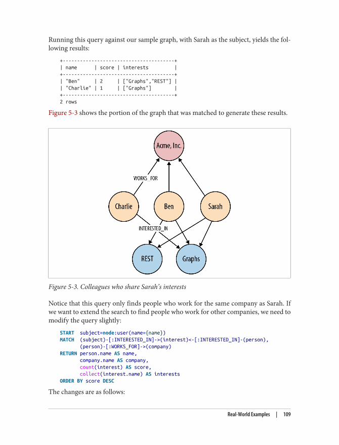
Running this query against our sample graph, with Sarah as the subject, yields the fol‐lowing results:

+---------------------------------------+| name | score | interests |+---------------------------------------+| "Ben" | 2 | ["Graphs","REST"] || "Charlie" | 1 | ["Graphs"] |+---------------------------------------+2 rows

Figure 5-3 shows the portion of the graph that was matched to generate these results.

Figure 5-3. Colleagues who share Sarah’s interests

Notice that this query only finds people who work for the same company as Sarah. Ifwe want to extend the search to find people who work for other companies, we need tomodify the query slightly:

START subject=node:user(name={name})MATCH (subject)-[:INTERESTED_IN]->(interest)<-[:INTERESTED_IN]-(person), (person)-[:WORKS_FOR]->(company)RETURN person.name AS name, company.name AS company, count(interest) AS score, collect(interest.name) AS interestsORDER BY score DESC

The changes are as follows:

Real-World Examples | 109

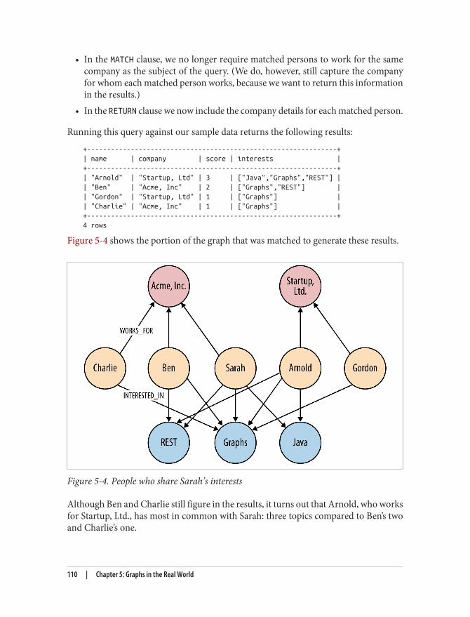
• In the MATCH clause, we no longer require matched persons to work for the samecompany as the subject of the query. (We do, however, still capture the companyfor whom each matched person works, because we want to return this informationin the results.)

• In the RETURN clause we now include the company details for each matched person.

Running this query against our sample data returns the following results:

+---------------------------------------------------------------+| name | company | score | interests |+---------------------------------------------------------------+| "Arnold" | "Startup, Ltd" | 3 | ["Java","Graphs","REST"] || "Ben" | "Acme, Inc" | 2 | ["Graphs","REST"] || "Gordon" | "Startup, Ltd" | 1 | ["Graphs"] || "Charlie" | "Acme, Inc" | 1 | ["Graphs"] |+---------------------------------------------------------------+4 rows

Figure 5-4 shows the portion of the graph that was matched to generate these results.

Figure 5-4. People who share Sarah’s interests

Although Ben and Charlie still figure in the results, it turns out that Arnold, who worksfor Startup, Ltd., has most in common with Sarah: three topics compared to Ben’s twoand Charlie’s one.

110 | Chapter 5: Graphs in the Real World

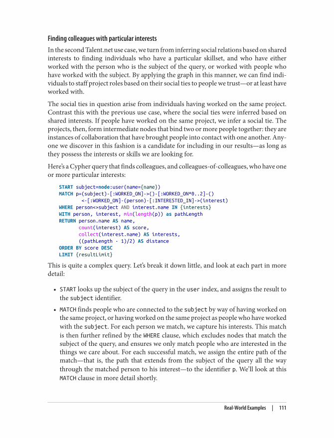
Finding colleagues with particular interestsIn the second Talent.net use case, we turn from inferring social relations based on sharedinterests to finding individuals who have a particular skillset, and who have eitherworked with the person who is the subject of the query, or worked with people whohave worked with the subject. By applying the graph in this manner, we can find indi‐viduals to staff project roles based on their social ties to people we trust—or at least haveworked with.

The social ties in question arise from individuals having worked on the same project.Contrast this with the previous use case, where the social ties were inferred based onshared interests. If people have worked on the same project, we infer a social tie. Theprojects, then, form intermediate nodes that bind two or more people together: they areinstances of collaboration that have brought people into contact with one another. Any‐one we discover in this fashion is a candidate for including in our results—as long asthey possess the interests or skills we are looking for.

Here’s a Cypher query that finds colleagues, and colleagues-of-colleagues, who have oneor more particular interests:

START subject=node:user(name={name})MATCH p=(subject)-[:WORKED_ON]->()-[:WORKED_ON*0..2]-() <-[:WORKED_ON]-(person)-[:INTERESTED_IN]->(interest)WHERE person<>subject AND interest.name IN {interests}WITH person, interest, min(length(p)) as pathLengthRETURN person.name AS name, count(interest) AS score, collect(interest.name) AS interests, ((pathLength - 1)/2) AS distanceORDER BY score DESCLIMIT {resultLimit}

This is quite a complex query. Let’s break it down little, and look at each part in moredetail:

• START looks up the subject of the query in the user index, and assigns the result tothe subject identifier.

• MATCH finds people who are connected to the subject by way of having worked onthe same project, or having worked on the same project as people who have workedwith the subject. For each person we match, we capture his interests. This matchis then further refined by the WHERE clause, which excludes nodes that match thesubject of the query, and ensures we only match people who are interested in thethings we care about. For each successful match, we assign the entire path of thematch—that is, the path that extends from the subject of the query all the waythrough the matched person to his interest—to the identifier p. We’ll look at thisMATCH clause in more detail shortly.

Real-World Examples | 111

• WITH pipes the results to the RETURN clause, filtering out redundant paths as it doesso. Redundant paths are present in the results at this point because colleagues andcolleagues-of-colleagues are often reachable through different paths, some longerthan others. We want to filter these longer paths out. That’s exactly what the WITHclause does. The WITH clause emits triples comprising a person, an interest, and thelength of the path from the subject of the query through the person to his interest.Given that any particular person/interest combination may appear more than oncein the results, but with different path lengths, we want to aggregate these multiplelines by collapsing them to a triple containing only the shortest path, which we dousing min(length(p)) as pathLength.

• RETURN creates a projection of the data, performing more aggregation as it does so.The data piped by the WITH clause to RETURN contains one entry per person perinterest: if a person matches two of the supplied interests, there will be two separatedata entries. We aggregate these entries using count and collect: count to createan overall score for a person, collect to create a comma-separated list of matchedinterests for that person. As part of the results, we also calculate how far the matchedperson is from the subject of the query: we take the pathLength for that person,subtract one (for the INTERESTED_IN relationship at the end of the path), and thendivide by two (because the person is separated from the subject by pairs ofWORKED_ON relationships). Finally, we order the results based on score, highestscore first, and limit them according to a resultLimit parameter supplied by thequery’s client.

The MATCH clause in the preceding query uses a variable-length path,[:WORKED_ON*0..2], as part of a larger pattern to match people who have worked di‐rectly with the subject of the query, as well as people who have worked on the sameproject as people who have worked with the subject. Because each person is separatedfrom the subject of the query by one or two pairs of WORKED_ON relationships, Talent.netcould have written this portion of the query as MATCH p=(subject)-

[:WORKED_ON*2..4]-(person)-[:INTERESTED_IN]->(interest), with a variable-length path of between two and four WORKED_ON relationships. However, long variable-length paths can be relatively inefficient. When writing such queries, it is advisable torestrict variable-length paths to as narrow a scope as possible. To increase the perfor‐mance of the query, Talent.net uses a fixed-length outgoing WORKED_ON relationship thatextends from the subject to her first project, and another fixed-length WORKED_ON rela‐tionship that connects the matched person to a project, with a smaller variable-lengthpath in between.

Running this query against our sample graph, and again taking Sarah as the subject ofthe query, if we look for colleagues and colleagues-of-colleagues who have interests inJava, travel, or medicine, we get the following results:

112 | Chapter 5: Graphs in the Real World

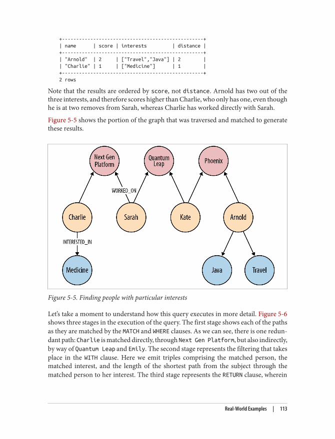
+--------------------------------------------------+| name | score | interests | distance |+--------------------------------------------------+| "Arnold" | 2 | ["Travel","Java"] | 2 || "Charlie" | 1 | ["Medicine"] | 1 |+--------------------------------------------------+2 rows

Note that the results are ordered by score, not distance. Arnold has two out of thethree interests, and therefore scores higher than Charlie, who only has one, even thoughhe is at two removes from Sarah, whereas Charlie has worked directly with Sarah.

Figure 5-5 shows the portion of the graph that was traversed and matched to generatethese results.

Figure 5-5. Finding people with particular interests

Let’s take a moment to understand how this query executes in more detail. Figure 5-6shows three stages in the execution of the query. The first stage shows each of the pathsas they are matched by the MATCH and WHERE clauses. As we can see, there is one redun‐dant path: Charlie is matched directly, through Next Gen Platform, but also indirectly,by way of Quantum Leap and Emily. The second stage represents the filtering that takesplace in the WITH clause. Here we emit triples comprising the matched person, thematched interest, and the length of the shortest path from the subject through thematched person to her interest. The third stage represents the RETURN clause, wherein

Real-World Examples | 113

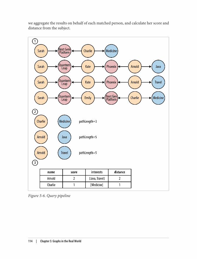
we aggregate the results on behalf of each matched person, and calculate her score anddistance from the subject.

Figure 5-6. Query pipeline

114 | Chapter 5: Graphs in the Real World

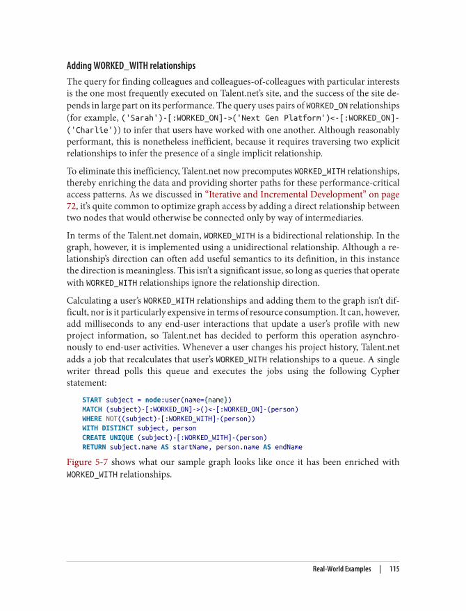
Adding WORKED_WITH relationshipsThe query for finding colleagues and colleagues-of-colleagues with particular interestsis the one most frequently executed on Talent.net’s site, and the success of the site de‐pends in large part on its performance. The query uses pairs of WORKED_ON relationships(for example, ('Sarah')-[:WORKED_ON]->('Next Gen Platform')<-[:WORKED_ON]-('Charlie')) to infer that users have worked with one another. Although reasonablyperformant, this is nonetheless inefficient, because it requires traversing two explicitrelationships to infer the presence of a single implicit relationship.

To eliminate this inefficiency, Talent.net now precomputes WORKED_WITH relationships,thereby enriching the data and providing shorter paths for these performance-criticalaccess patterns. As we discussed in “Iterative and Incremental Development” on page72, it’s quite common to optimize graph access by adding a direct relationship betweentwo nodes that would otherwise be connected only by way of intermediaries.

In terms of the Talent.net domain, WORKED_WITH is a bidirectional relationship. In thegraph, however, it is implemented using a unidirectional relationship. Although a re‐lationship’s direction can often add useful semantics to its definition, in this instancethe direction is meaningless. This isn’t a significant issue, so long as queries that operatewith WORKED_WITH relationships ignore the relationship direction.

Calculating a user’s WORKED_WITH relationships and adding them to the graph isn’t dif‐ficult, nor is it particularly expensive in terms of resource consumption. It can, however,add milliseconds to any end-user interactions that update a user’s profile with newproject information, so Talent.net has decided to perform this operation asynchro‐nously to end-user activities. Whenever a user changes his project history, Talent.netadds a job that recalculates that user’s WORKED_WITH relationships to a queue. A singlewriter thread polls this queue and executes the jobs using the following Cypherstatement:

START subject = node:user(name={name})MATCH (subject)-[:WORKED_ON]->()<-[:WORKED_ON]-(person)WHERE NOT((subject)-[:WORKED_WITH]-(person))WITH DISTINCT subject, personCREATE UNIQUE (subject)-[:WORKED_WITH]-(person)RETURN subject.name AS startName, person.name AS endName

Figure 5-7 shows what our sample graph looks like once it has been enriched withWORKED_WITH relationships.

Real-World Examples | 115

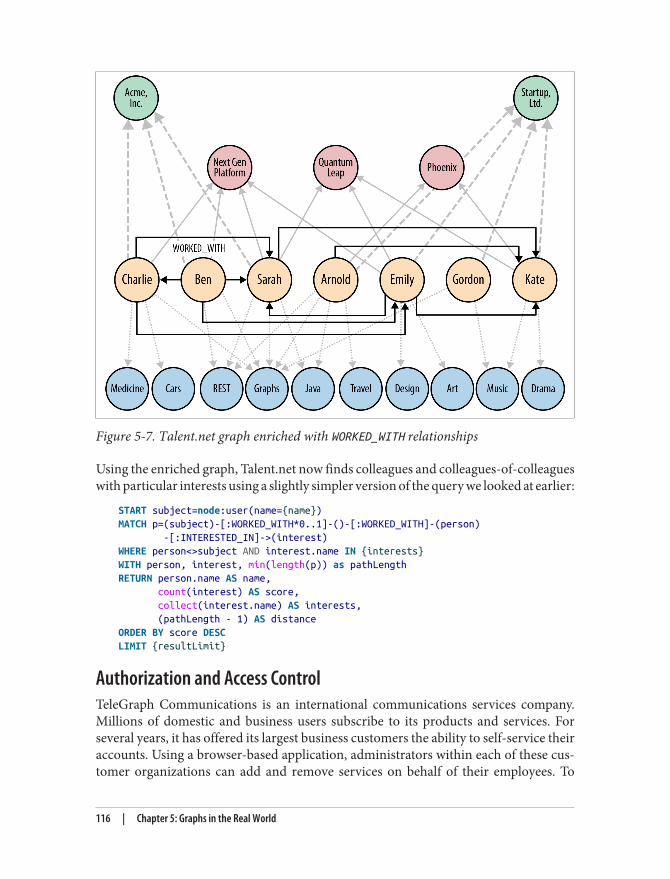
Figure 5-7. Talent.net graph enriched with WORKED_WITH relationships

Using the enriched graph, Talent.net now finds colleagues and colleagues-of-colleagueswith particular interests using a slightly simpler version of the query we looked at earlier:

START subject=node:user(name={name})MATCH p=(subject)-[:WORKED_WITH*0..1]-()-[:WORKED_WITH]-(person) -[:INTERESTED_IN]->(interest)WHERE person<>subject AND interest.name IN {interests}WITH person, interest, min(length(p)) as pathLengthRETURN person.name AS name, count(interest) AS score, collect(interest.name) AS interests, (pathLength - 1) AS distanceORDER BY score DESCLIMIT {resultLimit}

Authorization and Access ControlTeleGraph Communications is an international communications services company.Millions of domestic and business users subscribe to its products and services. Forseveral years, it has offered its largest business customers the ability to self-service theiraccounts. Using a browser-based application, administrators within each of these cus‐tomer organizations can add and remove services on behalf of their employees. To

116 | Chapter 5: Graphs in the Real World

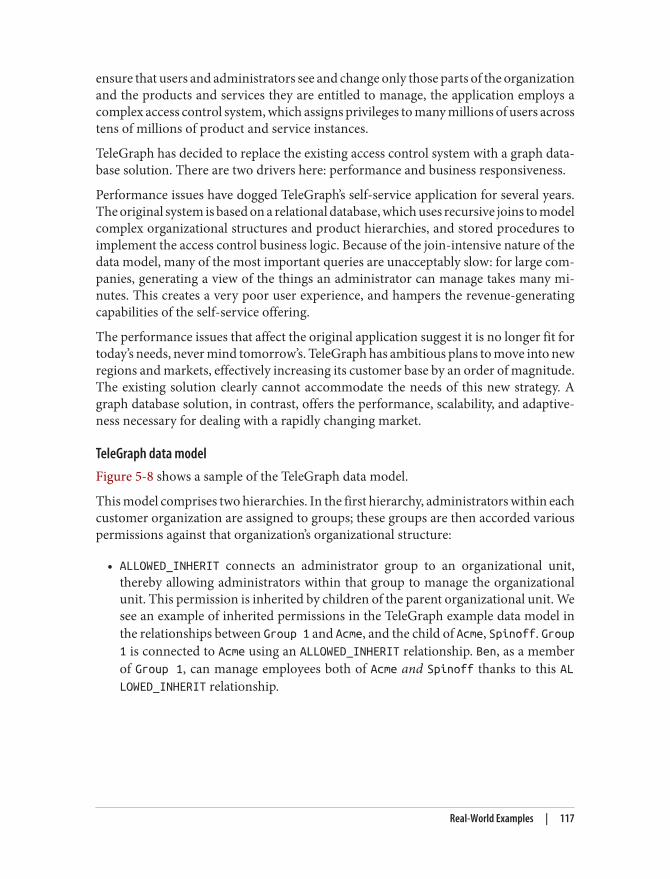
ensure that users and administrators see and change only those parts of the organizationand the products and services they are entitled to manage, the application employs acomplex access control system, which assigns privileges to many millions of users acrosstens of millions of product and service instances.

TeleGraph has decided to replace the existing access control system with a graph data‐base solution. There are two drivers here: performance and business responsiveness.

Performance issues have dogged TeleGraph’s self-service application for several years.The original system is based on a relational database, which uses recursive joins to modelcomplex organizational structures and product hierarchies, and stored procedures toimplement the access control business logic. Because of the join-intensive nature of thedata model, many of the most important queries are unacceptably slow: for large com‐panies, generating a view of the things an administrator can manage takes many mi‐nutes. This creates a very poor user experience, and hampers the revenue-generatingcapabilities of the self-service offering.

The performance issues that affect the original application suggest it is no longer fit fortoday’s needs, never mind tomorrow’s. TeleGraph has ambitious plans to move into newregions and markets, effectively increasing its customer base by an order of magnitude.The existing solution clearly cannot accommodate the needs of this new strategy. Agraph database solution, in contrast, offers the performance, scalability, and adaptive‐ness necessary for dealing with a rapidly changing market.

TeleGraph data modelFigure 5-8 shows a sample of the TeleGraph data model.

This model comprises two hierarchies. In the first hierarchy, administrators within eachcustomer organization are assigned to groups; these groups are then accorded variouspermissions against that organization’s organizational structure:

• ALLOWED_INHERIT connects an administrator group to an organizational unit,thereby allowing administrators within that group to manage the organizationalunit. This permission is inherited by children of the parent organizational unit. Wesee an example of inherited permissions in the TeleGraph example data model inthe relationships between Group 1 and Acme, and the child of Acme, Spinoff. Group1 is connected to Acme using an ALLOWED_INHERIT relationship. Ben, as a memberof Group 1, can manage employees both of Acme and Spinoff thanks to this ALLOWED_INHERIT relationship.

Real-World Examples | 117

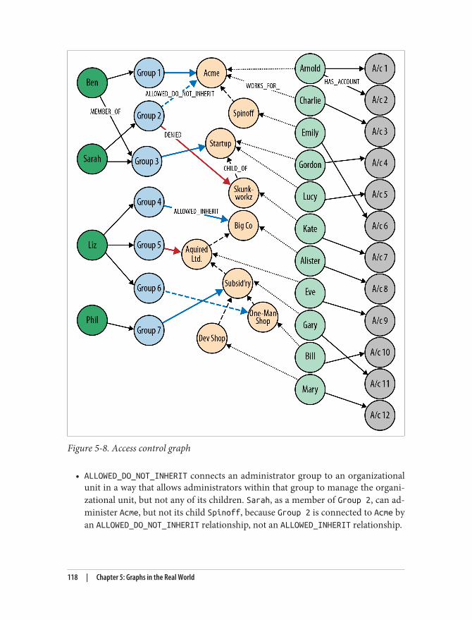
Figure 5-8. Access control graph

• ALLOWED_DO_NOT_INHERIT connects an administrator group to an organizationalunit in a way that allows administrators within that group to manage the organi‐zational unit, but not any of its children. Sarah, as a member of Group 2, can ad‐minister Acme, but not its child Spinoff, because Group 2 is connected to Acme byan ALLOWED_DO_NOT_INHERIT relationship, not an ALLOWED_INHERIT relationship.

118 | Chapter 5: Graphs in the Real World

• DENIED forbids administrators from accessing an organizational unit. This permis‐sion is inherited by children of the parent organizational unit. In the TeleGraphdiagram, this is best illustrated by Liz and her permissions with respect to BigCo, Acquired Ltd, Subsidiary, and One-Map Shop. As a result of her membershipof Group 4 and its ALLOWED_INHERIT permission on Big Co, Liz can manage BigCo. But despite this being an inheritable relationship, Liz cannot manage AcquiredLtd or Subsidiary; the reason being, Group 5, of which Liz is a member, is DENIED access to Acquired Ltd and its children (which includes Subsidiary). Lizcan, however, manage One-Map Shop, thanks to an ALLOWED_DO_NOT_INHERIT per‐mission granted to Group 6, the last group to which Liz belongs.

DENIED takes precedence over ALLOWED_INHERIT, but is subordinate to AL

LOWED_DO_NOT_INHERIT. Therefore, if an administrator is connected to a company byway of ALLOWED_DO_NOT_INHERIT and DENIED, ALLOWED_DO_NOT_INHERIT prevails.

Fine-Grained Relationships, or Relationships with Properties?Notice that the TeleGraph access control data model uses fine-grained relationships(ALLOWED_INHERIT, ALLOWED_DO_NOT_INHERIT, and DENIED) rather than a single rela‐tionship type qualified by properties—something like PERMISSION with allowed andinherited boolean properties. TeleGraph performance-tested both approaches anddetermined that the fine-grained, property-free approach was nearly twice as fast as theone using properties. For more details on designing relationships, see Chapter 4.

Finding all accessible resources for an administratorThe TeleGraph application uses many different Cypher queries; we’ll look at just a fewof them here.

First up is the ability to find all the resources an administrator can access. Whenever anonsite administrator logs in to the system, he is presented with a browser-based list ofall the employees and employee accounts he can administer. This list is generated basedon the results returned from the following query:

START admin=node:administrator(name={administratorName})MATCH paths=(admin)-[:MEMBER_OF]->()-[:ALLOWED_INHERIT]->() <-[:CHILD_OF*0..3]-(company)<-[:WORKS_FOR]-(employee) -[:HAS_ACCOUNT]->(account)WHERE NOT ((admin)-[:MEMBER_OF]->()-[:DENIED]->()<-[:CHILD_OF*0..3]-(company))RETURN employee.name AS employee, account.name AS accountUNIONSTART admin=node:administrator(name={administratorName})MATCH paths=(admin)-[:MEMBER_OF]->()-[:ALLOWED_DO_NOT_INHERIT]->()

Real-World Examples | 119

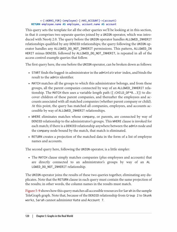
<-[:WORKS_FOR]-(employee)-[:HAS_ACCOUNT]->(account)RETURN employee.name AS employee, account.name AS account

This query sets the template for all the other queries we’ll be looking at in this section,in that it comprises two separate queries joined by a UNION operator, which was intro‐duced with Neo4j 2.0. The query before the UNION operator handles ALLOWED_INHERITrelationships qualified by any DENIED relationships; the query following the UNION op‐erator handles any ALLOWED_DO_NOT_INHERIT permissions. This pattern, ALLOWED_INHERIT minus DENIED, followed by ALLOWED_DO_NOT_INHERIT, is repeated in all of theaccess control example queries that follow.

The first query here, the one before the UNION operator, can be broken down as follows:

• START finds the logged-in administrator in the administrator index, and binds theresult to the admin identifier.

• MATCH matches all the groups to which this administrator belongs, and from thesegroups, all the parent companies connected by way of an ALLOWED_INHERIT rela‐tionship. The MATCH then uses a variable-length path ([:CHILD_OF*0..3]) to dis‐cover children of these parent companies, and thereafter the employees and ac‐counts associated with all matched companies (whether parent company or child).At this point, the query has matched all companies, employees, and accounts ac‐cessible by way of ALLOWED_INHERIT relationships.

• WHERE eliminates matches whose company, or parents, are connected by way ofDENIED relationship to the administrator’s groups. This WHERE clause is invoked foreach match; if there is a DENIED relationship anywhere between the admin node andthe company node bound by the match, that match is eliminated.

• RETURN creates a projection of the matched data in the form of a list of employeenames and accounts.

The second query here, following the UNION operator, is a little simpler:

• The MATCH clause simply matches companies (plus employees and accounts) thatare directly connected to an administrator’s groups by way of an AL

LOWED_DO_NOT_INHERIT relationship.

The UNION operator joins the results of these two queries together, eliminating any du‐plicates. Note that the RETURN clause in each query must contain the same projection ofthe results; in other words, the column names in the results must match.

Figure 5-9 shows how this query matches all accessible resources for Sarah in the sampleTeleGraph graph. Note that, because of the DENIED relationship from Group 2 to Skunkworkz, Sarah cannot administer Kate and Account 7.

120 | Chapter 5: Graphs in the Real World

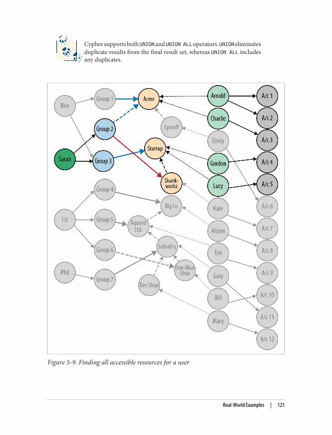
Cypher supports both UNION and UNION ALL operators. UNION eliminatesduplicate results from the final result set, whereas UNION ALL includesany duplicates.

Figure 5-9. Finding all accessible resources for a user

Real-World Examples | 121

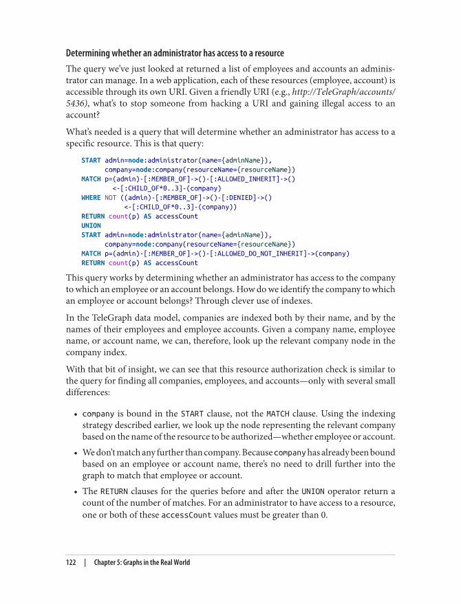
Determining whether an administrator has access to a resourceThe query we’ve just looked at returned a list of employees and accounts an adminis‐trator can manage. In a web application, each of these resources (employee, account) isaccessible through its own URI. Given a friendly URI (e.g., http://TeleGraph/accounts/5436), what’s to stop someone from hacking a URI and gaining illegal access to anaccount?

What’s needed is a query that will determine whether an administrator has access to aspecific resource. This is that query:

START admin=node:administrator(name={adminName}), company=node:company(resourceName={resourceName})MATCH p=(admin)-[:MEMBER_OF]->()-[:ALLOWED_INHERIT]->() <-[:CHILD_OF*0..3]-(company)WHERE NOT ((admin)-[:MEMBER_OF]->()-[:DENIED]->() <-[:CHILD_OF*0..3]-(company))RETURN count(p) AS accessCountUNIONSTART admin=node:administrator(name={adminName}), company=node:company(resourceName={resourceName})MATCH p=(admin)-[:MEMBER_OF]->()-[:ALLOWED_DO_NOT_INHERIT]->(company)RETURN count(p) AS accessCount

This query works by determining whether an administrator has access to the companyto which an employee or an account belongs. How do we identify the company to whichan employee or account belongs? Through clever use of indexes.

In the TeleGraph data model, companies are indexed both by their name, and by thenames of their employees and employee accounts. Given a company name, employeename, or account name, we can, therefore, look up the relevant company node in thecompany index.

With that bit of insight, we can see that this resource authorization check is similar tothe query for finding all companies, employees, and accounts—only with several smalldifferences:

• company is bound in the START clause, not the MATCH clause. Using the indexingstrategy described earlier, we look up the node representing the relevant companybased on the name of the resource to be authorized—whether employee or account.

• We don’t match any further than company. Because company has already been boundbased on an employee or account name, there’s no need to drill further into thegraph to match that employee or account.

• The RETURN clauses for the queries before and after the UNION operator return acount of the number of matches. For an administrator to have access to a resource,one or both of these accessCount values must be greater than 0.

122 | Chapter 5: Graphs in the Real World

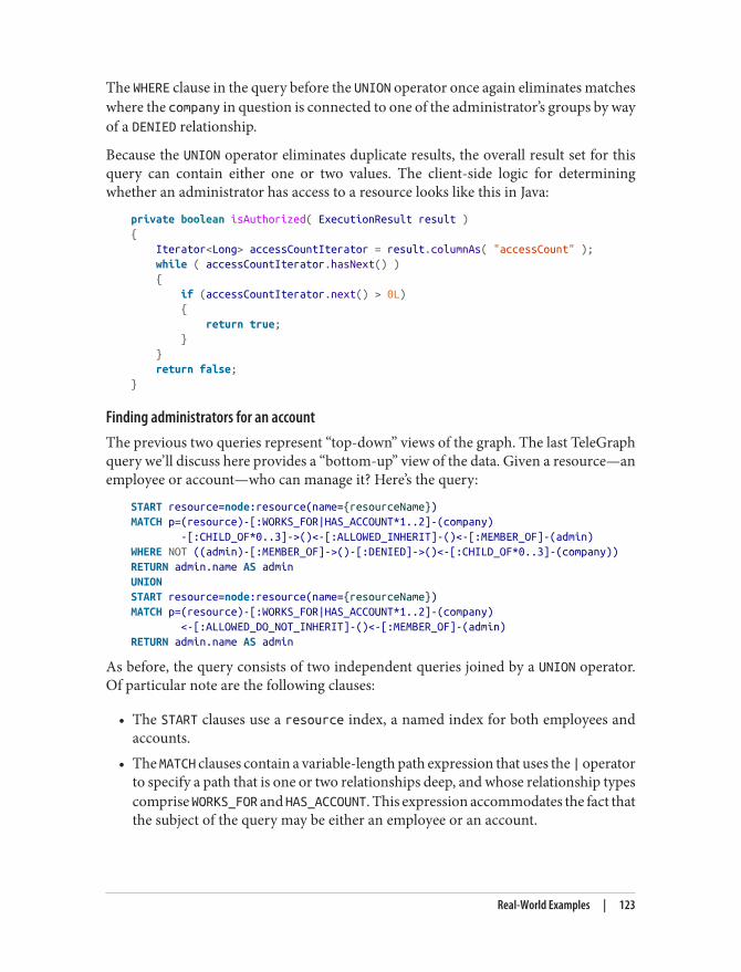
The WHERE clause in the query before the UNION operator once again eliminates matcheswhere the company in question is connected to one of the administrator’s groups by wayof a DENIED relationship.

Because the UNION operator eliminates duplicate results, the overall result set for thisquery can contain either one or two values. The client-side logic for determiningwhether an administrator has access to a resource looks like this in Java:

private boolean isAuthorized( ExecutionResult result ){ Iterator<Long> accessCountIterator = result.columnAs( "accessCount" ); while ( accessCountIterator.hasNext() ) { if (accessCountIterator.next() > 0L) { return true; } } return false;}

Finding administrators for an accountThe previous two queries represent “top-down” views of the graph. The last TeleGraphquery we’ll discuss here provides a “bottom-up” view of the data. Given a resource—anemployee or account—who can manage it? Here’s the query:

START resource=node:resource(name={resourceName})MATCH p=(resource)-[:WORKS_FOR|HAS_ACCOUNT*1..2]-(company) -[:CHILD_OF*0..3]->()<-[:ALLOWED_INHERIT]-()<-[:MEMBER_OF]-(admin)WHERE NOT ((admin)-[:MEMBER_OF]->()-[:DENIED]->()<-[:CHILD_OF*0..3]-(company))RETURN admin.name AS adminUNIONSTART resource=node:resource(name={resourceName})MATCH p=(resource)-[:WORKS_FOR|HAS_ACCOUNT*1..2]-(company) <-[:ALLOWED_DO_NOT_INHERIT]-()<-[:MEMBER_OF]-(admin)RETURN admin.name AS admin

As before, the query consists of two independent queries joined by a UNION operator.Of particular note are the following clauses:

• The START clauses use a resource index, a named index for both employees andaccounts.

• The MATCH clauses contain a variable-length path expression that uses the | operatorto specify a path that is one or two relationships deep, and whose relationship typescomprise WORKS_FOR and HAS_ACCOUNT. This expression accommodates the fact thatthe subject of the query may be either an employee or an account.

Real-World Examples | 123

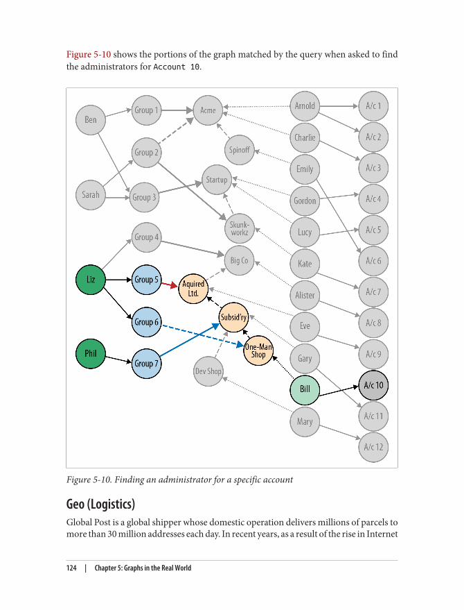
Figure 5-10 shows the portions of the graph matched by the query when asked to findthe administrators for Account 10.

Figure 5-10. Finding an administrator for a specific account

Geo (Logistics)Global Post is a global shipper whose domestic operation delivers millions of parcels tomore than 30 million addresses each day. In recent years, as a result of the rise in Internet

124 | Chapter 5: Graphs in the Real World

shopping, the number of parcels has increased significantly. Amazon and eBay deliveriesnow account for more than half the parcels routed and delivered by Global Post eachday.

With parcel volumes continuing to grow, and facing strong competition from othercourier services, Global Post has begun a large change program to upgrade all aspectsof its parcel network, including buildings, equipment, systems, and processes.

One of the most important and time-critical components in the parcel network is theroute calculation engine. Between one and three thousand parcels enter the networkeach second. As parcels enter the network they are mechanically sorted according totheir destination. To maintain a steady flow during this process, the engine must cal‐culate a parcel’s route before it reaches a point where the sorting equipment has to makea choice, which happens only seconds after the parcel has entered the network—hencethe strict time requirements on the engine.

Not only must the engine route parcels in milliseconds, but it must do so according tothe routes scheduled for a particular period. Parcel routes change throughout the year,with more trucks, delivery people, and collections over the Christmas period than dur‐ing the summer, for example. The engine must, therefore, apply its calculations usingonly those routes that are available for a particular period.

On top of accommodating different routes and levels of parcel traffic, the new parcelnetwork must also allow for significant change and evolution. The platform that GlobalPost develops today will form the business-critical basis of its operations for the next10 years or more. During that time, the company anticipates large portions of the net‐work—including equipment, premises, and transport routes—will change to matchchanges in the business environment. The data model underlying the route calculationengine must, therefore, allow for rapid and significant schema evolution.

Global Post data modelFigure 5-11 shows a simple example of the Global Post parcel network. The networkcomprises parcel centers, which are connected to delivery bases, each of which coversseveral delivery areas; these delivery areas, in turn, are subdivided into delivery segmentscovering many delivery units. There are around 25 national parcel centers and roughly2 million delivery units (corresponding to postal or zip codes).

Real-World Examples | 125

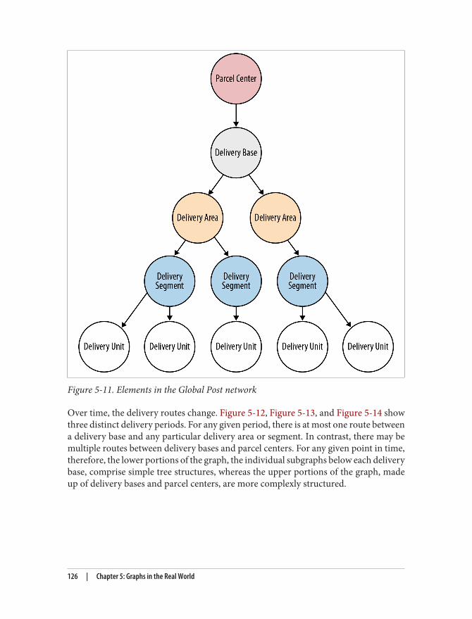
Figure 5-11. Elements in the Global Post network

Over time, the delivery routes change. Figure 5-12, Figure 5-13, and Figure 5-14 showthree distinct delivery periods. For any given period, there is at most one route betweena delivery base and any particular delivery area or segment. In contrast, there may bemultiple routes between delivery bases and parcel centers. For any given point in time,therefore, the lower portions of the graph, the individual subgraphs below each deliverybase, comprise simple tree structures, whereas the upper portions of the graph, madeup of delivery bases and parcel centers, are more complexly structured.

126 | Chapter 5: Graphs in the Real World

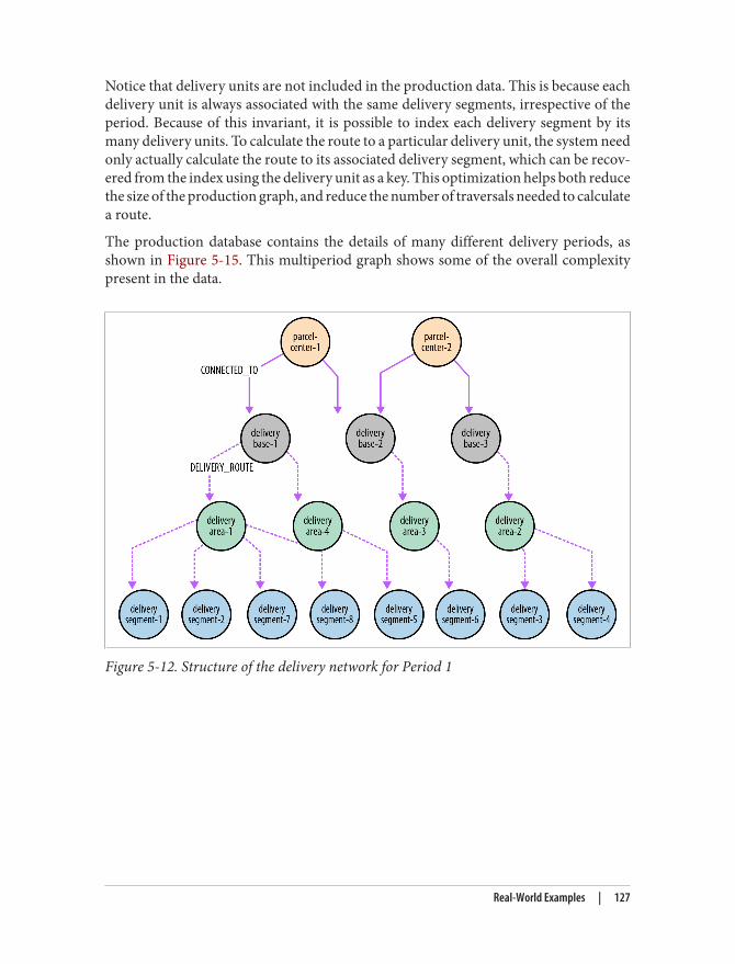
Notice that delivery units are not included in the production data. This is because eachdelivery unit is always associated with the same delivery segments, irrespective of theperiod. Because of this invariant, it is possible to index each delivery segment by itsmany delivery units. To calculate the route to a particular delivery unit, the system needonly actually calculate the route to its associated delivery segment, which can be recov‐ered from the index using the delivery unit as a key. This optimization helps both reducethe size of the production graph, and reduce the number of traversals needed to calculatea route.

The production database contains the details of many different delivery periods, asshown in Figure 5-15. This multiperiod graph shows some of the overall complexitypresent in the data.

Figure 5-12. Structure of the delivery network for Period 1

Real-World Examples | 127

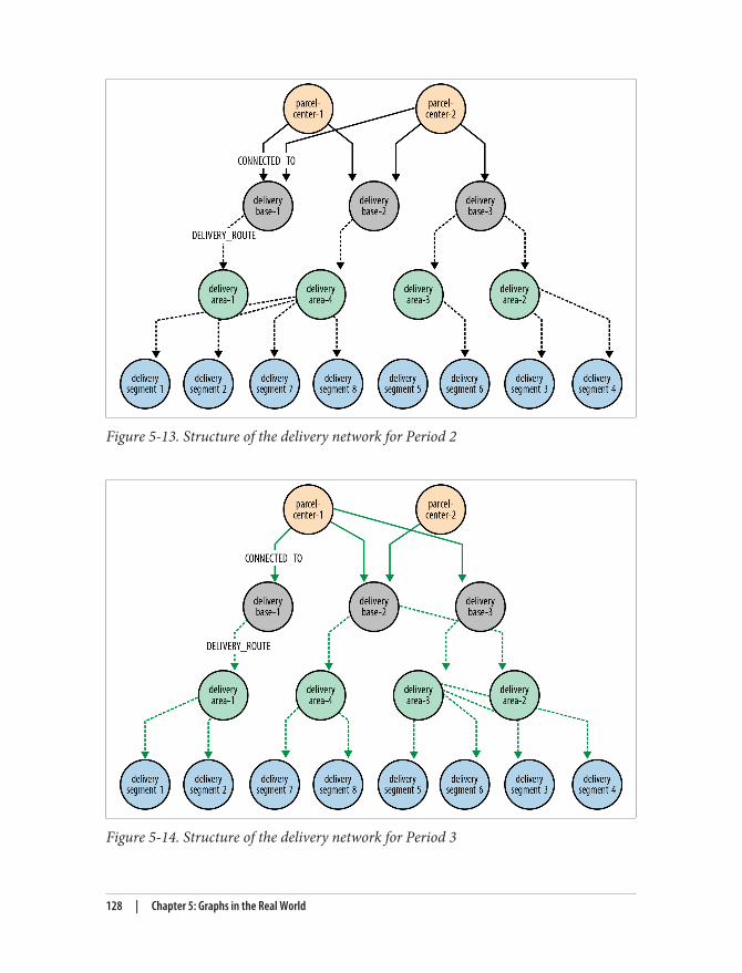
Figure 5-13. Structure of the delivery network for Period 2

Figure 5-14. Structure of the delivery network for Period 3

128 | Chapter 5: Graphs in the Real World

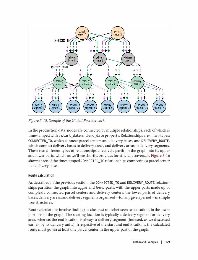
Figure 5-15. Sample of the Global Post network

In the production data, nodes are connected by multiple relationships, each of which istimestamped with a start_date and end_date property. Relationships are of two types:CONNECTED_TO, which connect parcel centers and delivery bases, and DELIVERY_ROUTE,which connect delivery bases to delivery areas, and delivery areas to delivery segments.These two different types of relationships effectively partition the graph into its upperand lower parts, which, as we’ll see shortly, provides for efficient traversals. Figure 5-16shows three of the timestamped CONNECTED_TO relationships connecting a parcel centerto a delivery base.

Route calculation

As described in the previous section, the CONNECTED_TO and DELIVERY_ROUTE relation‐ships partition the graph into upper and lower parts, with the upper parts made up ofcomplexly connected parcel centers and delivery centers, the lower parts of deliverybases, delivery areas, and delivery segments organized—for any given period—in simpletree structures.

Route calculations involve finding the cheapest route between two locations in the lowerportions of the graph. The starting location is typically a delivery segment or deliveryarea, whereas the end location is always a delivery segment (indexed, as we discussedearlier, by its delivery units). Irrespective of the start and end locations, the calculatedroute must go via at least one parcel center in the upper part of the graph.

Real-World Examples | 129

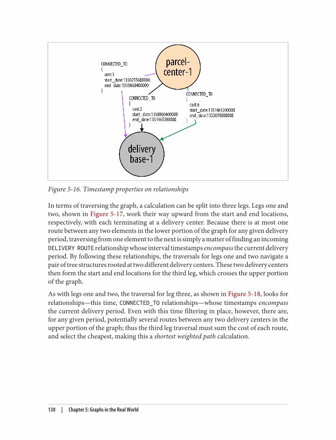
Figure 5-16. Timestamp properties on relationships

In terms of traversing the graph, a calculation can be split into three legs. Legs one andtwo, shown in Figure 5-17, work their way upward from the start and end locations,respectively, with each terminating at a delivery center. Because there is at most oneroute between any two elements in the lower portion of the graph for any given deliveryperiod, traversing from one element to the next is simply a matter of finding an incomingDELIVERY ROUTE relationship whose interval timestamps encompass the current deliveryperiod. By following these relationships, the traversals for legs one and two navigate apair of tree structures rooted at two different delivery centers. These two delivery centersthen form the start and end locations for the third leg, which crosses the upper portionof the graph.

As with legs one and two, the traversal for leg three, as shown in Figure 5-18, looks forrelationships—this time, CONNECTED_TO relationships—whose timestamps encompassthe current delivery period. Even with this time filtering in place, however, there are,for any given period, potentially several routes between any two delivery centers in theupper portion of the graph; thus the third leg traversal must sum the cost of each route,and select the cheapest, making this a shortest weighted path calculation.

130 | Chapter 5: Graphs in the Real World

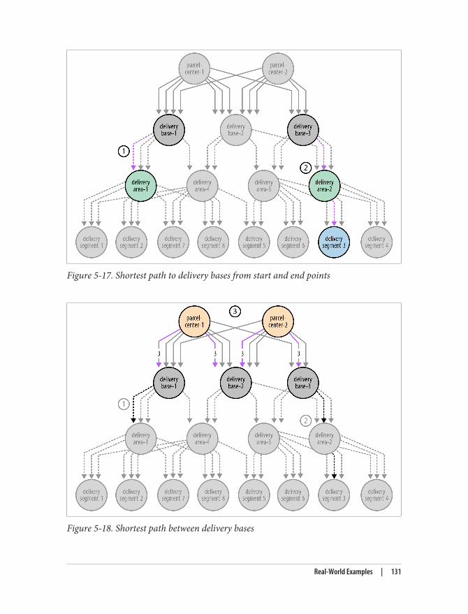
Figure 5-17. Shortest path to delivery bases from start and end points

Figure 5-18. Shortest path between delivery bases

Real-World Examples | 131

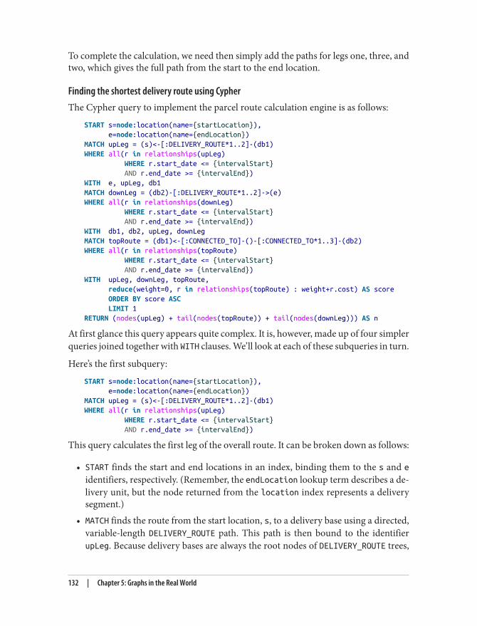
To complete the calculation, we need then simply add the paths for legs one, three, andtwo, which gives the full path from the start to the end location.

Finding the shortest delivery route using CypherThe Cypher query to implement the parcel route calculation engine is as follows:

START s=node:location(name={startLocation}), e=node:location(name={endLocation})MATCH upLeg = (s)<-[:DELIVERY_ROUTE*1..2]-(db1)WHERE all(r in relationships(upLeg) WHERE r.start_date <= {intervalStart} AND r.end_date >= {intervalEnd})WITH e, upLeg, db1MATCH downLeg = (db2)-[:DELIVERY_ROUTE*1..2]->(e)WHERE all(r in relationships(downLeg) WHERE r.start_date <= {intervalStart} AND r.end_date >= {intervalEnd})WITH db1, db2, upLeg, downLegMATCH topRoute = (db1)<-[:CONNECTED_TO]-()-[:CONNECTED_TO*1..3]-(db2)WHERE all(r in relationships(topRoute) WHERE r.start_date <= {intervalStart} AND r.end_date >= {intervalEnd})WITH upLeg, downLeg, topRoute, reduce(weight=0, r in relationships(topRoute) : weight+r.cost) AS score ORDER BY score ASC LIMIT 1RETURN (nodes(upLeg) + tail(nodes(topRoute)) + tail(nodes(downLeg))) AS n

At first glance this query appears quite complex. It is, however, made up of four simplerqueries joined together with WITH clauses. We’ll look at each of these subqueries in turn.

Here’s the first subquery:

START s=node:location(name={startLocation}), e=node:location(name={endLocation})MATCH upLeg = (s)<-[:DELIVERY_ROUTE*1..2]-(db1)WHERE all(r in relationships(upLeg) WHERE r.start_date <= {intervalStart} AND r.end_date >= {intervalEnd})

This query calculates the first leg of the overall route. It can be broken down as follows:

• START finds the start and end locations in an index, binding them to the s and eidentifiers, respectively. (Remember, the endLocation lookup term describes a de‐livery unit, but the node returned from the location index represents a deliverysegment.)

• MATCH finds the route from the start location, s, to a delivery base using a directed,variable-length DELIVERY_ROUTE path. This path is then bound to the identifierupLeg. Because delivery bases are always the root nodes of DELIVERY_ROUTE trees,

132 | Chapter 5: Graphs in the Real World

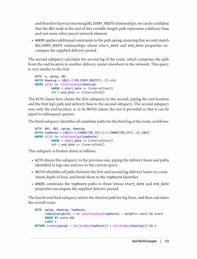
and therefore have no incoming DELIVERY_ROUTE relationships, we can be confidentthat the db1 node at the end of this variable-length path represents a delivery baseand not some other parcel network element.

• WHERE applies additional constraints to the path upLeg, ensuring that we only matchDELIVERY_ROUTE relationships whose start_date and end_date properties en‐compass the supplied delivery period.

The second subquery calculates the second leg of the route, which comprises the pathfrom the end location to another delivery center elsewhere in the network. This queryis very similar to the first:

WITH e, upLeg, db1MATCH downLeg = (db2)-[:DELIVERY_ROUTE*1..2]->(e)WHERE all(r in relationships(downLeg) WHERE r.start_date <= {intervalStart} AND r.end_date >= {intervalEnd})

The WITH clause here chains the first subquery to the second, piping the end locationand the first leg’s path and delivery base to the second subquery. The second subqueryuses only the end location, e, in its MATCH clause; the rest is provided so that it can bepiped to subsequent queries.

The third subquery identifies all candidate paths for the third leg of the route, as follows:

WITH db1, db2, upLeg, downLegMATCH topRoute = (db1)<-[:CONNECTED_TO]-()-[:CONNECTED_TO*1..3]-(db2)WHERE all(r in relationships(topRoute) WHERE r.start_date <= {intervalStart} AND r.end_date >= {intervalEnd})

This subquery is broken down as follows:

• WITH chains this subquery to the previous one, piping the delivery bases and pathsidentified in legs one and two to the current query.

• MATCH identifies all paths between the first and second leg delivery bases, to a max‐imum depth of four, and binds them to the topRoute identifier.

• WHERE constrains the topRoute paths to those whose start_date and end_dateproperties encompass the supplied delivery period.

The fourth and final subquery selects the shortest path for leg three, and then calculatesthe overall route:

WITH upLeg, downLeg, topRoute, reduce(weight=0, r in relationships(topRoute) : weight+r.cost) AS score ORDER BY score ASC LIMIT 1RETURN (nodes(upLeg) + tail(nodes(topRoute)) + tail(nodes(downLeg))) AS n

Real-World Examples | 133

This subquery works as follows:

• WITH pipes one or more triples, comprising upLeg, downLeg, and topRoute, to thecurrent query. There will be one triple for each of the paths matched by the thirdsubquery, with each path being bound to topRoute in successive triples (the pathsbound to upLeg and downLeg will stay the same, because the first and second sub‐queries matched only one path each). Each triple is accompanied by a score for thepath bound to topRoute for that triple. This score is calculated using Cypher’sreduce function, which for each triple sums the cost properties on the relationshipsin the path currently bound to topRoute; reduce was introduced with Neo4j 1.9.The triples are then ordered by this score, lowest first, and then limited to the firsttriple in the sorted list.

• RETURN sums the nodes in the paths upLeg, topRoute, and downLeg to produce thefinal results. The tail function drops the first node in each of paths topRoute anddownLeg, because that node will already be present in the preceding path.

Implementing route calculation with the traversal frameworkThe time-critical nature of the route calculation coupled with the high throughput ofthe parcel network impose strict demands on the route calculation engine. As long asthe individual query latencies are low enough, it’s always possible to scale horizontallyfor increased throughput. The Cypher-based solution is fast, but with such high sus‐tained throughput, every millisecond impacts the cluster footprint. For this reason,Global Post adopted an alternative approach: calculating routes using Neo4j’s traversalframework.

A traversal-based implementation of the route calculation engine must solve two prob‐lems: finding shortest paths, and filtering paths based on time period. We’ll look atfiltering paths based on time period first.

Traversals should follow only relationships that are valid for the specified delivery pe‐riod. In other words, as the traversal progresses through the graph, it should only bepresented with relationships whose periods of validity, as defined by their start_dateand end_date properties, contain the specified delivery period.

We implement this relationship filtering using a PathExpander. Given a path from atraversal’s start node to the node where it is currently positioned, a PathExpander’sexpand() method returns the relationships that can be used to traverse further. Thismethod is called by the traversal framework each time the framework advances anothernode into the graph. If needed, the client can supply some initial state that flows alongeach branch; expand() can then use (and even change) this state in the course of de‐ciding which relationships to return. The route calculator’s ValidPathExpander imple‐mentation uses this branch state to supply the delivery period to the expander.

134 | Chapter 5: Graphs in the Real World

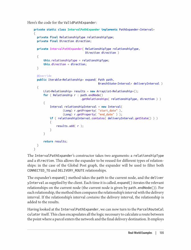
Here’s the code for the ValidPathExpander:

private static class IntervalPathExpander implements PathExpander<Interval>{ private final RelationshipType relationshipType; private final Direction direction;

private IntervalPathExpander( RelationshipType relationshipType, Direction direction ) { this.relationshipType = relationshipType; this.direction = direction; }

@Override public Iterable<Relationship> expand( Path path, BranchState<Interval> deliveryInterval ) { List<Relationship> results = new ArrayList<Relationship>(); for ( Relationship r : path.endNode() .getRelationships( relationshipType, direction ) ) { Interval relationshipInterval = new Interval( (Long) r.getProperty( "start_date" ), (Long) r.getProperty( "end_date" ) ); if ( relationshipInterval.contains( deliveryInterval.getState() ) ) { results.add( r ); } }

return results; }}

The IntervalPathExpander’s constructor takes two arguments: a relationshipTypeand a direction. This allows the expander to be reused for different types of relation‐ships: in the case of the Global Post graph, the expander will be used to filter bothCONNECTED_TO and DELIVERY_ROUTE relationships.

The expander’s expand() method takes the path to the current node, and the deliveryInterval as supplied by the client. Each time it is called, expand() iterates the relevantrelationships on the current node (the current node is given by path.endNode()). Foreach relationship, the method then compares the relationship’s interval with the deliveryinterval. If the relationship’s interval contains the delivery interval, the relationship isadded to the results.

Having looked at the IntervalPathExpander, we can now turn to the ParcelRouteCalculator itself. This class encapsulates all the logic necessary to calculate a route betweenthe point where a parcel enters the network and the final delivery destination. It employs

Real-World Examples | 135

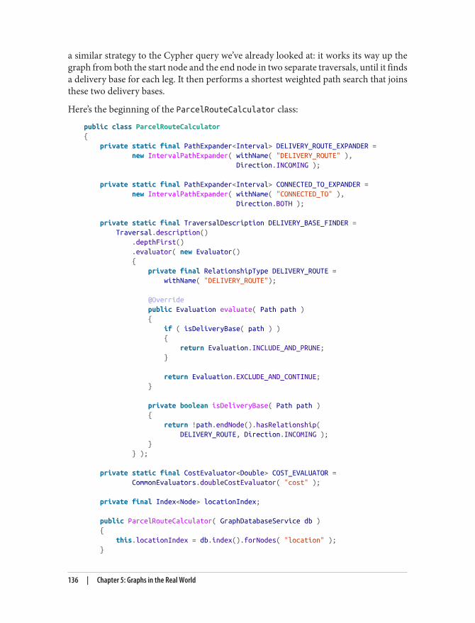
a similar strategy to the Cypher query we’ve already looked at: it works its way up thegraph from both the start node and the end node in two separate traversals, until it findsa delivery base for each leg. It then performs a shortest weighted path search that joinsthese two delivery bases.

Here’s the beginning of the ParcelRouteCalculator class:

public class ParcelRouteCalculator{ private static final PathExpander<Interval> DELIVERY_ROUTE_EXPANDER = new IntervalPathExpander( withName( "DELIVERY_ROUTE" ), Direction.INCOMING );

private static final PathExpander<Interval> CONNECTED_TO_EXPANDER = new IntervalPathExpander( withName( "CONNECTED_TO" ), Direction.BOTH );

private static final TraversalDescription DELIVERY_BASE_FINDER = Traversal.description() .depthFirst() .evaluator( new Evaluator() { private final RelationshipType DELIVERY_ROUTE = withName( "DELIVERY_ROUTE");

@Override public Evaluation evaluate( Path path ) { if ( isDeliveryBase( path ) ) { return Evaluation.INCLUDE_AND_PRUNE; }

return Evaluation.EXCLUDE_AND_CONTINUE; }

private boolean isDeliveryBase( Path path ) { return !path.endNode().hasRelationship( DELIVERY_ROUTE, Direction.INCOMING ); } } );

private static final CostEvaluator<Double> COST_EVALUATOR = CommonEvaluators.doubleCostEvaluator( "cost" );

private final Index<Node> locationIndex;

public ParcelRouteCalculator( GraphDatabaseService db ) { this.locationIndex = db.index().forNodes( "location" ); }

136 | Chapter 5: Graphs in the Real World

...}

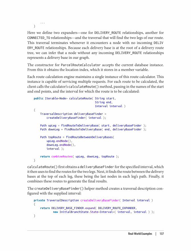
Here we define two expanders—one for DELIVERY_ROUTE relationships, another forCONNECTED_TO relationships—and the traversal that will find the two legs of our route.This traversal terminates whenever it encounters a node with no incoming DELIVERY_ROUTE relationships. Because each delivery base is at the root of a delivery routetree, we can infer that a node without any incoming DELIVERY_ROUTE relationshipsrepresents a delivery base in our graph.

The constructor for ParcelRouteCalculator accepts the current database instance.From this it obtains the location index, which it stores in a member variable.

Each route calculation engine maintains a single instance of this route calculator. Thisinstance is capable of servicing multiple requests. For each route to be calculated, theclient calls the calculator’s calculateRoute() method, passing in the names of the startand end points, and the interval for which the route is to be calculated:

public Iterable<Node> calculateRoute( String start, String end, Interval interval ){ TraversalDescription deliveryBaseFinder = createDeliveryBaseFinder( interval );

Path upLeg = findRouteToDeliveryBase( start, deliveryBaseFinder ); Path downLeg = findRouteToDeliveryBase( end, deliveryBaseFinder );

Path topRoute = findRouteBetweenDeliveryBases( upLeg.endNode(), downLeg.endNode(), interval );

return combineRoutes( upLeg, downLeg, topRoute );}

calculateRoute() first obtains a deliveryBaseFinder for the specified interval, whichit then uses to find the routes for the two legs. Next, it finds the route between the deliverybases at the top of each leg, these being the last nodes in each leg’s path. Finally, itcombines these routes to generate the final results.

The createDeliveryBaseFinder() helper method creates a traversal description con‐figured with the supplied interval:

private TraversalDescription createDeliveryBaseFinder( Interval interval ){ return DELIVERY_BASE_FINDER.expand( DELIVERY_ROUTE_EXPANDER, new InitialBranchState.State<Interval>( interval, interval ) );}

Real-World Examples | 137

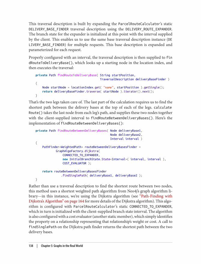
This traversal description is built by expanding the ParcelRouteCalculator’s staticDELIVERY_BASE_FINDER traversal description using the DELIVERY_ROUTE_EXPANDER.The branch state for the expander is initialized at this point with the interval suppliedby the client. This enables us to use the same base traversal description instance (DELIVERY_BASE_FINDER) for multiple requests. This base description is expanded andparameterized for each request.

Properly configured with an interval, the traversal description is then supplied to findRouteToDeliveryBase(), which looks up a starting node in the location index, andthen executes the traversal:

private Path findRouteToDeliveryBase( String startPosition, TraversalDescription deliveryBaseFinder ){ Node startNode = locationIndex.get( "name", startPosition ).getSingle(); return deliveryBaseFinder.traverse( startNode ).iterator().next();}

That’s the two legs taken care of. The last part of the calculation requires us to find theshortest path between the delivery bases at the top of each of the legs. calculateRoute() takes the last node from each leg’s path, and supplies these two nodes togetherwith the client-supplied interval to findRouteBetweenDeliveryBases(). Here’s theimplementation of findRouteBetweenDeliveryBases():

private Path findRouteBetweenDeliveryBases( Node deliveryBase1, Node deliveryBase2, Interval interval ){ PathFinder<WeightedPath> routeBetweenDeliveryBasesFinder = GraphAlgoFactory.dijkstra( CONNECTED_TO_EXPANDER, new InitialBranchState.State<Interval>( interval, interval ), COST_EVALUATOR );

return routeBetweenDeliveryBasesFinder .findSinglePath( deliveryBase1, deliveryBase2 );}

Rather than use a traversal description to find the shortest route between two nodes,this method uses a shortest weighted path algorithm from Neo4j’s graph algorithm li‐brary—in this instance, we’re using the Dijkstra algorithm (see “Path-Finding withDijkstra’s Algorithm” on page 164 for more details of the Dijkstra algorithm). This algo‐rithm is configured with ParcelRouteCalculator’s static CONNECTED_TO_EXPANDER,which in turn is initialized with the client-supplied branch state interval. The algorithmis also configured with a cost evaluator (another static member), which simply identifiesthe property on a relationship representing that relationship’s weight or cost. A call tofindSinglePath on the Dijkstra path finder returns the shortest path between the twodelivery bases.

138 | Chapter 5: Graphs in the Real World

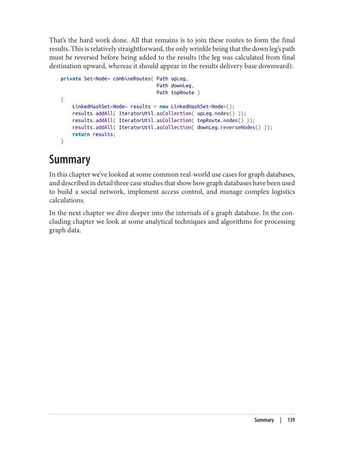
That’s the hard work done. All that remains is to join these routes to form the finalresults. This is relatively straightforward, the only wrinkle being that the down leg’s pathmust be reversed before being added to the results (the leg was calculated from finaldestination upward, whereas it should appear in the results delivery base downward):

private Set<Node> combineRoutes( Path upLeg, Path downLeg, Path topRoute ){ LinkedHashSet<Node> results = new LinkedHashSet<Node>(); results.addAll( IteratorUtil.asCollection( upLeg.nodes() )); results.addAll( IteratorUtil.asCollection( topRoute.nodes() )); results.addAll( IteratorUtil.asCollection( downLeg.reverseNodes() )); return results;}

SummaryIn this chapter we’ve looked at some common real-world use cases for graph databases,and described in detail three case studies that show how graph databases have been usedto build a social network, implement access control, and manage complex logisticscalculations.

In the next chapter we dive deeper into the internals of a graph database. In the con‐cluding chapter we look at some analytical techniques and algorithms for processinggraph data.

Summary | 139

CHAPTER 6

Graph Database Internals

In this chapter we peek under the hood and discuss the implementation of graph data‐bases, showing how they differ from other means of storing and querying complex,semi-structured, densely connected data. Although it is true that no single universalarchitecture pattern exists, even among graph databases, this chapter describes the mostcommon architecture patterns and components you can expect to find inside a graphdatabase.

We illustrate the discussion in this chapter using the Neo4j graph database, for severalreasons. Neo4j is a graph database with native processing capabilities as well as nativegraph storage (see Chapter 1 for a discussion of native graph processing and storage).In addition to being the most common graph database in use at the time of writing, ithas the transparency advantage of being open source, making it easy for the adven‐turesome reader to go a level deeper and inspect the code. Finally, it is a database theauthors know well.

Native Graph ProcessingWe’ve discussed the property graph model several times throughout this book; by nowyou should be familiar with its notion of nodes connected by way of named and directedrelationships, with both the nodes and relationships serving as containers for properties.Although the model itself is reasonably consistent across graph database implementa‐tions, there are numerous ways to encode and represent the graph in the database en‐gine’s main memory. Of the many different engine architectures, we say that a graphdatabase has native processing capabilities if it exhibits a property called index-freeadjacency.

A database engine that utilizes index-free adjacency is one in which each node maintainsdirect references to its adjacent nodes; each node, therefore acts as a micro-index ofother nearby nodes, which is much cheaper than using global indexes. It means that

141

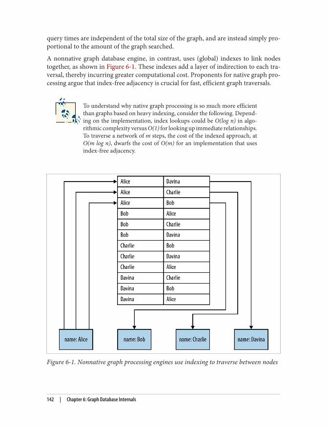
query times are independent of the total size of the graph, and are instead simply pro‐portional to the amount of the graph searched.

A nonnative graph database engine, in contrast, uses (global) indexes to link nodestogether, as shown in Figure 6-1. These indexes add a layer of indirection to each tra‐versal, thereby incurring greater computational cost. Proponents for native graph pro‐cessing argue that index-free adjacency is crucial for fast, efficient graph traversals.

To understand why native graph processing is so much more efficientthan graphs based on heavy indexing, consider the following. Depend‐ing on the implementation, index lookups could be O(log n) in algo‐rithmic complexity versus O(1) for looking up immediate relationships.To traverse a network of m steps, the cost of the indexed approach, atO(m log n), dwarfs the cost of O(m) for an implementation that usesindex-free adjacency.

Figure 6-1. Nonnative graph processing engines use indexing to traverse between nodes

142 | Chapter 6: Graph Database Internals

Figure 6-1 shows how a nonnative approach to graph processing works. To find Alice’sfriends we have first to perform an index lookup, at cost O(log n). This may be acceptablefor occasional or shallow lookups, but it quickly becomes expensive when we reversethe direction of the traversal. If, instead of finding Alice’s friends, we wanted to find outwho is friends with Alice, we would have to perform multiple index lookups, one foreach node that is potentially friends with Alice. This makes the cost far more onerous.Whereas it’s O(log n) cost to find out who are Alice’s friends, it’s O(m log n) to find outwho is friends with Alice.

Index-Free Adjacency Leads to Lower-Cost “Joins”With index-free adjacency, bidirectional joins are effectively precomputed and storedin the database as relationships. In contrast, when using indexes to fake connectionsbetween records, there is no actual relationship stored in the database. This becomesproblematic when we try to traverse in the “opposite” direction from the one for whichthe index was constructed. Because we have to perform a brute-force search throughthe index—which is an O(n) operation—joins like this are simply too costly to be of anypractical use.

Index lookups are fine for small networks, such as the one in Figure 6-1, but too costlyfor complex queries over larger graphs. Instead of using index lookups to make rela‐tionships concrete and navigable at query time, graph databases such as Neo4j withnative graph processing capabilities use index-free adjacency to ensure high-performance traversals. Figure 6-2 shows how relationships eliminate the need for indexlookups.

Figure 6-2. Neo4j uses relationships, not indexes, for fast traversals

Recall that in a general-purpose graph database relationships can be traversed in eitherdirection (tail to head, or head to tail) extremely cheaply. As we see in Figure 6-2, tofind Alice’s friends using a graph, we simply follow her outgoing FRIEND relationships,

Native Graph Processing | 143

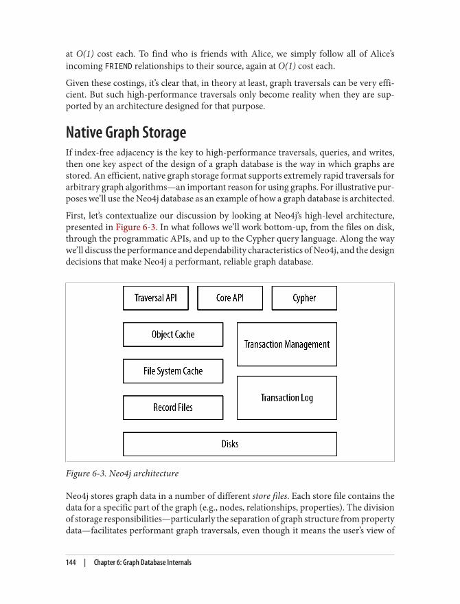
at O(1) cost each. To find who is friends with Alice, we simply follow all of Alice’sincoming FRIEND relationships to their source, again at O(1) cost each.

Given these costings, it’s clear that, in theory at least, graph traversals can be very effi‐cient. But such high-performance traversals only become reality when they are sup‐ported by an architecture designed for that purpose.

Native Graph StorageIf index-free adjacency is the key to high-performance traversals, queries, and writes,then one key aspect of the design of a graph database is the way in which graphs arestored. An efficient, native graph storage format supports extremely rapid traversals forarbitrary graph algorithms—an important reason for using graphs. For illustrative pur‐poses we’ll use the Neo4j database as an example of how a graph database is architected.

First, let’s contextualize our discussion by looking at Neo4j’s high-level architecture,presented in Figure 6-3. In what follows we’ll work bottom-up, from the files on disk,through the programmatic APIs, and up to the Cypher query language. Along the waywe’ll discuss the performance and dependability characteristics of Neo4j, and the designdecisions that make Neo4j a performant, reliable graph database.

Figure 6-3. Neo4j architecture

Neo4j stores graph data in a number of different store files. Each store file contains thedata for a specific part of the graph (e.g., nodes, relationships, properties). The divisionof storage responsibilities—particularly the separation of graph structure from propertydata—facilitates performant graph traversals, even though it means the user’s view of

144 | Chapter 6: Graph Database Internals

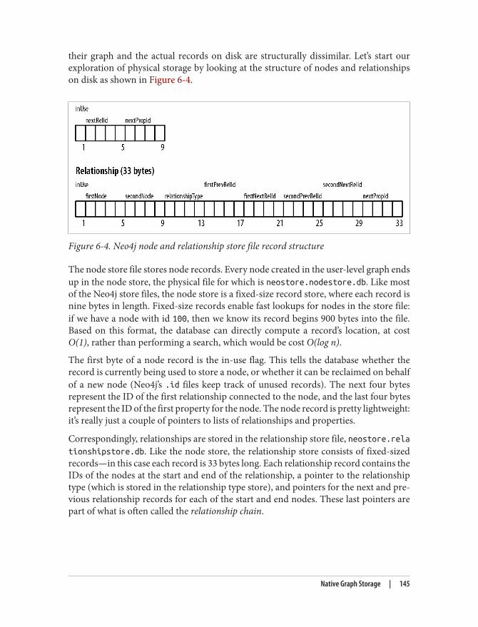
their graph and the actual records on disk are structurally dissimilar. Let’s start ourexploration of physical storage by looking at the structure of nodes and relationshipson disk as shown in Figure 6-4.

Figure 6-4. Neo4j node and relationship store file record structure

The node store file stores node records. Every node created in the user-level graph endsup in the node store, the physical file for which is neostore.nodestore.db. Like mostof the Neo4j store files, the node store is a fixed-size record store, where each record isnine bytes in length. Fixed-size records enable fast lookups for nodes in the store file:if we have a node with id 100, then we know its record begins 900 bytes into the file.Based on this format, the database can directly compute a record’s location, at costO(1), rather than performing a search, which would be cost O(log n).

The first byte of a node record is the in-use flag. This tells the database whether therecord is currently being used to store a node, or whether it can be reclaimed on behalfof a new node (Neo4j’s .id files keep track of unused records). The next four bytesrepresent the ID of the first relationship connected to the node, and the last four bytesrepresent the ID of the first property for the node. The node record is pretty lightweight:it’s really just a couple of pointers to lists of relationships and properties.

Correspondingly, relationships are stored in the relationship store file, neostore.relationshipstore.db. Like the node store, the relationship store consists of fixed-sizedrecords—in this case each record is 33 bytes long. Each relationship record contains theIDs of the nodes at the start and end of the relationship, a pointer to the relationshiptype (which is stored in the relationship type store), and pointers for the next and pre‐vious relationship records for each of the start and end nodes. These last pointers arepart of what is often called the relationship chain.

Native Graph Storage | 145

The node and relationship stores are concerned only with the structureof the graph, not its property data. Both stores use fixed-sized recordsso that any individual record’s location within a store file can be rapidlycomputed given its ID. These are critical design decisions that underlineNeo4j’s commitment to high-performance traversals.

In Figure 6-5 we see how the various store files interact on disk. Each of the two noderecords contains a pointer to that node’s first property and first relationship in a rela‐tionship chain. To read a node’s properties, we follow the singly linked list structurebeginning with the pointer to the first property. To find a relationship for a node, wefollow that node’s relationship pointer to its first relationship (the LIKES relationship inthis example). From here, we then follow the doubly linked list of relationships for thatparticular node (that is, either the start node doubly linked list, or the end node doublylinked list) until we find the relationship we’re interested in. Having found the recordfor the relationship we want, we can read that relationship’s properties (if there are any)using the same singly linked list structure as is used for node properties, or we canexamine the node records for the two nodes the relationship connects using its startnode and end node IDs. These IDs, multiplied by the node record size, give the imme‐diate offset of each node in the node store file.

Doubly Linked Lists in the Relationship StoreDon’t worry if the relationship store structure seems a little complex at first; it’s definitelynot as simple as the node store or property store.

It’s helpful to think of a relationship record as “belonging” to two nodes—the start nodeand the end node of the relationship. Clearly, however, we don’t want to store two re‐lationship records, because that would be wasteful. And yet it’s equally clear that therelationship record should somehow belong to both the start node and the end node.

That’s why there are pointers (aka record IDs) for two doubly linked lists: one is the listof relationships visible from the start node; the other is the list of relationships visiblefrom the end node. That each list is doubly linked simply enables us to rapidly iteratethrough that list in either direction, and insert and delete relationships efficiently.

Choosing to follow a different relationship involves iterating through a linked list ofrelationships until we find a good candidate (e.g., matching the correct type, or havingsome matching property value). Once we have a suitable relationship we’re back inbusiness, multiplying ID by record size, and thereafter chasing pointers.

146 | Chapter 6: Graph Database Internals

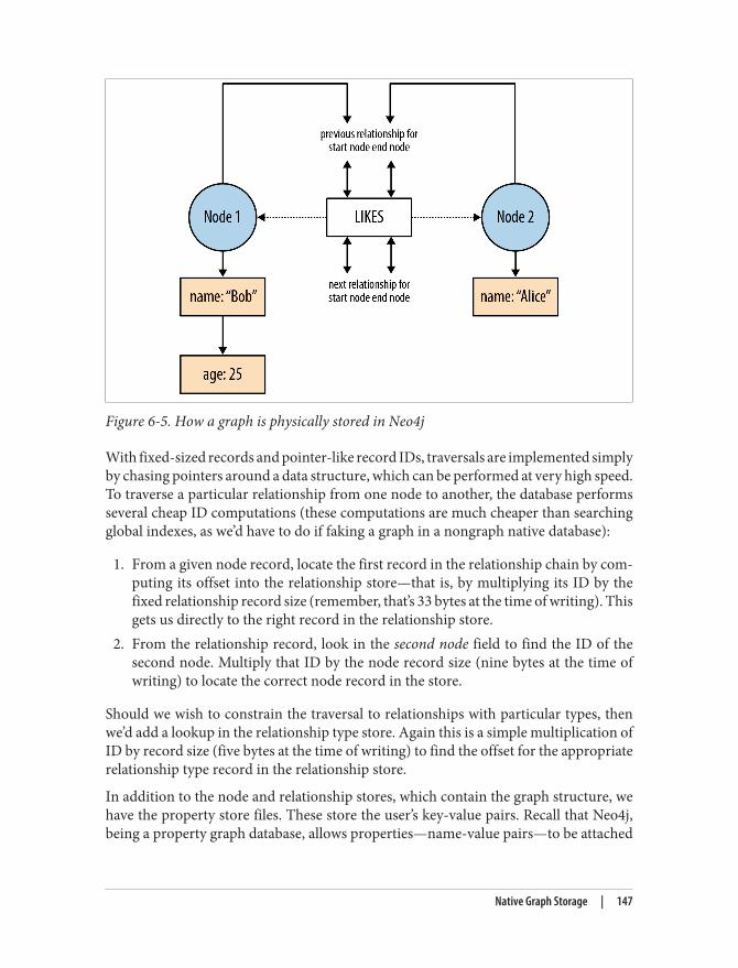
Figure 6-5. How a graph is physically stored in Neo4j

With fixed-sized records and pointer-like record IDs, traversals are implemented simplyby chasing pointers around a data structure, which can be performed at very high speed.To traverse a particular relationship from one node to another, the database performsseveral cheap ID computations (these computations are much cheaper than searchingglobal indexes, as we’d have to do if faking a graph in a nongraph native database):

1. From a given node record, locate the first record in the relationship chain by com‐puting its offset into the relationship store—that is, by multiplying its ID by thefixed relationship record size (remember, that’s 33 bytes at the time of writing). Thisgets us directly to the right record in the relationship store.

2. From the relationship record, look in the second node field to find the ID of thesecond node. Multiply that ID by the node record size (nine bytes at the time ofwriting) to locate the correct node record in the store.

Should we wish to constrain the traversal to relationships with particular types, thenwe’d add a lookup in the relationship type store. Again this is a simple multiplication ofID by record size (five bytes at the time of writing) to find the offset for the appropriaterelationship type record in the relationship store.

In addition to the node and relationship stores, which contain the graph structure, wehave the property store files. These store the user’s key-value pairs. Recall that Neo4j,being a property graph database, allows properties—name-value pairs—to be attached

Native Graph Storage | 147

to both nodes and relationships. The property stores, therefore, are referenced fromboth node and relationship records.

Records in the property store are physically stored in the neostore.propertystore.db file. As with the node and relationship stores, property records are of a fixedsize. Each property record consists of four property blocks and the ID of the next prop‐erty in the property chain (remember, properties are held as a singly linked list on diskas compared to the doubly linked list used in relationship chains). Each property oc‐cupies between one and four property blocks—a property record can, therefore, hold amaximum of four properties. A property record holds the property type (Neo4j allowsany primitive JVM type, plus strings, plus arrays of the JVM primitive types), and apointer to the property index file (neostore.propertystore.db.index), which iswhere the property name is stored. For each property’s value, the record contains eithera pointer into a dynamic store record or an inlined value. The dynamic stores allow forstoring large property values. There are two dynamic stores: a dynamic string store(neostore.propertystore.db.strings) and a dynamic array store (neostore.propertystore.db.arrays). Dynamic records comprise linked lists of fixed-sized records;a very large string, or large array, may, therefore, occupy more than one dynamic record.

Inlining and Optimizing Property Store UtilizationNeo4j supports store optimizations, whereby it inlines some properties into the propertystore file directly (neostore.propertystore.db). This happens when property data canbe encoded to fit in one or more of a record’s four property blocks. In practice this meansthat data like phone numbers and zip codes can be inlined in the property store filedirectly, rather than being pushed out to the dynamic stores. This results in reducedI/O operations and improved throughput, because only a single file access is required.

In addition to inlining certain compatible property values, Neo4j also maintains spacediscipline on property names. For example, in a social graph, there will likely be manynodes with properties like first_name and last_name. It would be wasteful if eachproperty name was written out to disk verbatim, and so instead property names areindirectly referenced from the property store through the property index file. The prop‐erty index allows all properties with the same name to share a single record, and thusfor repetitive graphs—a very common use case—Neo4j achieves considerable space andI/O savings.

Having an efficient storage layout is only half the picture. Despite the store files havingbeen optimized for rapid traversals, hardware considerations can still have a significantimpact on performance. Memory capacity has increased significantly in recent years;nonetheless, very large graphs will still exceed our ability to hold them entirely in mainmemory. Spinning disks have millisecond seek times in the order of single digits, which,

148 | Chapter 6: Graph Database Internals

though fast by human standards, are ponderously slow in computing terms. Solid StateDisks (SSDs) are far better (because there’s no significant seek penalty waiting for plat‐ters to rotate), but the path between CPU and disk is still more latent than the path toL2 cache or main memory, which is where ideally we’d like to operate on our graph.

To mitigate the performance characteristics of mechanical/electronic mass storage de‐vices, many graph databases use in-memory caching to provide probabilistic low-latency access to the graph. Neo4j uses a two-tiered caching architecture to provide thisfunctionality.

The lowest tier in the Neo4j caching stack is the filesystem cache. The filesystem cacheis a page-affined cache, meaning the cache divides each store into discrete regions, andthen holds a fixed number of regions per store file. The actual amount of memory to beused to cache the pages for each store file can be fine-tuned, though in the absence ofinput from the user, Neo4j will use sensible default values based on the capacity of theunderlying hardware. Pages are evicted from the cache based on a Least Frequently Used(LFU) cache policy. Neo4j’s default implementation leaves it up to the underlying op‐erating system’s memory-mapped filesystem to decide which pages to evict; that is, theoperating system itself determines which segments of virtual memory to hold in realmemory and which to flush out to disk.

The filesystem cache is particularly beneficial when related parts of the graph are modi‐fied at the same time such that they occupy the same page. This is a common patternfor writes, where we tend to persist whole subgraphs to disk in a single operation, ratherthan discrete nodes and relationships.

If the filesystem cache reflects the characteristics of typical write usage, the high-levelor object cache is all about optimizing for arbitrary read patterns. The high-level cachestores object representations of nodes, relationships, and properties for rapid, in-memory graph traversal. Nodes in the object cache contain both properties and refer‐ences to their relationships, making them much richer than their store file representa‐tions, and bringing them much more in line with what we expect as programmers.Conversely, relationship objects are much simpler, containing only their properties. Anode’s relationships are grouped by relationship type and direction; these groupingsprovide for fast lookups of specific relationships based on these characteristics. As withthe underlying stores, all lookups are by ID, meaning they are very performant, as wesee in Figure 6-6.

Native Graph Storage | 149

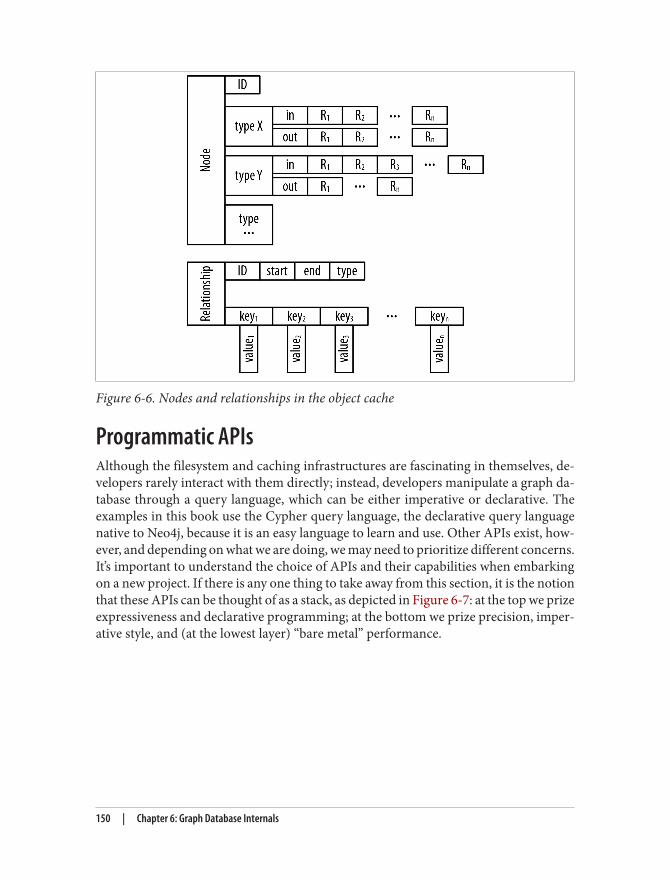
Figure 6-6. Nodes and relationships in the object cache

Programmatic APIsAlthough the filesystem and caching infrastructures are fascinating in themselves, de‐velopers rarely interact with them directly; instead, developers manipulate a graph da‐tabase through a query language, which can be either imperative or declarative. Theexamples in this book use the Cypher query language, the declarative query languagenative to Neo4j, because it is an easy language to learn and use. Other APIs exist, how‐ever, and depending on what we are doing, we may need to prioritize different concerns.It’s important to understand the choice of APIs and their capabilities when embarkingon a new project. If there is any one thing to take away from this section, it is the notionthat these APIs can be thought of as a stack, as depicted in Figure 6-7: at the top we prizeexpressiveness and declarative programming; at the bottom we prize precision, imper‐ative style, and (at the lowest layer) “bare metal” performance.

150 | Chapter 6: Graph Database Internals

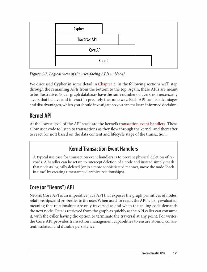
Figure 6-7. Logical view of the user-facing APIs in Neo4j

We discussed Cypher in some detail in Chapter 3. In the following sections we’ll stepthrough the remaining APIs from the bottom to the top. Again, these APIs are meantto be illustrative. Not all graph databases have the same number of layers, nor necessarilylayers that behave and interact in precisely the same way. Each API has its advantagesand disadvantages, which you should investigate so you can make an informed decision.

Kernel APIAt the lowest level of the API stack are the kernel’s transaction event handlers. Theseallow user code to listen to transactions as they flow through the kernel, and thereafterto react (or not) based on the data content and lifecycle stage of the transaction.

Kernel Transaction Event HandlersA typical use case for transaction event handlers is to prevent physical deletion of re‐cords. A handler can be set up to intercept deletion of a node and instead simply markthat node as logically deleted (or in a more sophisticated manner, move the node “backin time” by creating timestamped archive relationships).

Core (or “Beans”) APINeo4j’s Core API is an imperative Java API that exposes the graph primitives of nodes,relationships, and properties to the user. When used for reads, the API is lazily evaluated,meaning that relationships are only traversed as and when the calling code demandsthe next node. Data is retrieved from the graph as quickly as the API caller can consumeit, with the caller having the option to terminate the traversal at any point. For writes,the Core API provides transaction management capabilities to ensure atomic, consis‐tent, isolated, and durable persistence.

Programmatic APIs | 151

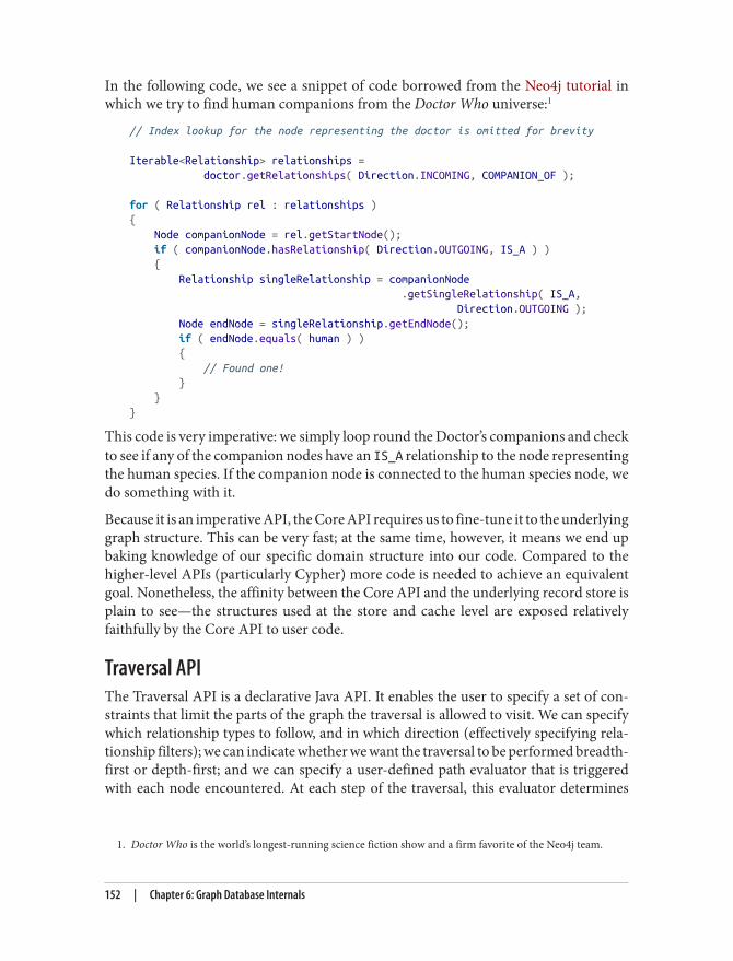
1. Doctor Who is the world’s longest-running science fiction show and a firm favorite of the Neo4j team.

In the following code, we see a snippet of code borrowed from the Neo4j tutorial inwhich we try to find human companions from the Doctor Who universe:1

// Index lookup for the node representing the doctor is omitted for brevity

Iterable<Relationship> relationships = doctor.getRelationships( Direction.INCOMING, COMPANION_OF );

for ( Relationship rel : relationships ){ Node companionNode = rel.getStartNode(); if ( companionNode.hasRelationship( Direction.OUTGOING, IS_A ) ) { Relationship singleRelationship = companionNode .getSingleRelationship( IS_A, Direction.OUTGOING ); Node endNode = singleRelationship.getEndNode(); if ( endNode.equals( human ) ) { // Found one! } }}

This code is very imperative: we simply loop round the Doctor’s companions and checkto see if any of the companion nodes have an IS_A relationship to the node representingthe human species. If the companion node is connected to the human species node, wedo something with it.

Because it is an imperative API, the Core API requires us to fine-tune it to the underlyinggraph structure. This can be very fast; at the same time, however, it means we end upbaking knowledge of our specific domain structure into our code. Compared to thehigher-level APIs (particularly Cypher) more code is needed to achieve an equivalentgoal. Nonetheless, the affinity between the Core API and the underlying record store isplain to see—the structures used at the store and cache level are exposed relativelyfaithfully by the Core API to user code.

Traversal APIThe Traversal API is a declarative Java API. It enables the user to specify a set of con‐straints that limit the parts of the graph the traversal is allowed to visit. We can specifywhich relationship types to follow, and in which direction (effectively specifying rela‐tionship filters); we can indicate whether we want the traversal to be performed breadth-first or depth-first; and we can specify a user-defined path evaluator that is triggeredwith each node encountered. At each step of the traversal, this evaluator determines

152 | Chapter 6: Graph Database Internals

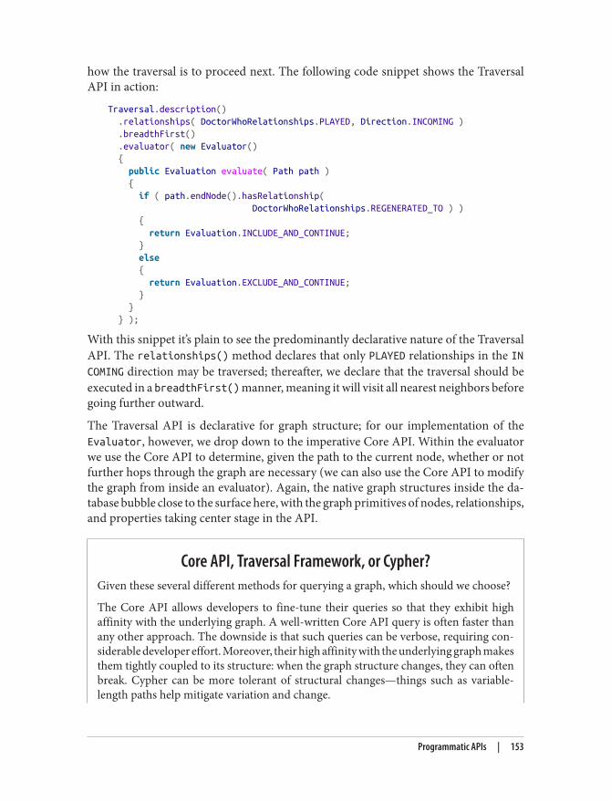
how the traversal is to proceed next. The following code snippet shows the TraversalAPI in action:

Traversal.description() .relationships( DoctorWhoRelationships.PLAYED, Direction.INCOMING ) .breadthFirst() .evaluator( new Evaluator() { public Evaluation evaluate( Path path ) { if ( path.endNode().hasRelationship( DoctorWhoRelationships.REGENERATED_TO ) ) { return Evaluation.INCLUDE_AND_CONTINUE; } else { return Evaluation.EXCLUDE_AND_CONTINUE; } } } );

With this snippet it’s plain to see the predominantly declarative nature of the TraversalAPI. The relationships() method declares that only PLAYED relationships in the INCOMING direction may be traversed; thereafter, we declare that the traversal should beexecuted in a breadthFirst() manner, meaning it will visit all nearest neighbors beforegoing further outward.

The Traversal API is declarative for graph structure; for our implementation of theEvaluator, however, we drop down to the imperative Core API. Within the evaluatorwe use the Core API to determine, given the path to the current node, whether or notfurther hops through the graph are necessary (we can also use the Core API to modifythe graph from inside an evaluator). Again, the native graph structures inside the da‐tabase bubble close to the surface here, with the graph primitives of nodes, relationships,and properties taking center stage in the API.

Core API, Traversal Framework, or Cypher?Given these several different methods for querying a graph, which should we choose?

The Core API allows developers to fine-tune their queries so that they exhibit highaffinity with the underlying graph. A well-written Core API query is often faster thanany other approach. The downside is that such queries can be verbose, requiring con‐siderable developer effort. Moreover, their high affinity with the underlying graph makesthem tightly coupled to its structure: when the graph structure changes, they can oftenbreak. Cypher can be more tolerant of structural changes—things such as variable-length paths help mitigate variation and change.

Programmatic APIs | 153

2. The formal definition of dependability is the “trustworthiness of a computing system, which allows relianceto be justifiably placed on the service it delivers” as per http://www.dependability.org/.

The Traversal Framework is both more loosely coupled than the Core API (because itallows the developer to declare informational goals), and less verbose, and as a result aquery written using the Traversal Framework typically requires less developer effortthan the equivalent written using the Core API. Because it is a general-purpose frame‐work, however, the Traversal Framework tends to perform marginally less well than awell-written Core API query.

If we find ourselves in the unusual situation of coding with the Core API or TraversalFramework (and thus eschewing Cypher and its affordances), it’s because we are work‐ing on an edge case where we need to finely craft an algorithm that cannot be expressedeffectively using Cypher’s pattern matching. Choosing between the Core API and theTraversal Framework is a matter of deciding whether the higher abstraction/lower cou‐pling of the Traversal Framework is sufficient, or whether the close-to-the-metal/highercoupling of the Core API is in fact necessary for implementing an algorithm correctlyand in accordance with our performance requirements.

This concludes our brief survey of graph programming APIs, using the native Neo4jAPIs as an example. We’ve seen how these APIs reflect the structures used in the lowerlevels of the Neo4j stack, and how this alignment permits for idiomatic and rapid graphtraversals.

It’s not enough for a database to be fast, however; it must also be dependable. This bringsus to a discussion of the nonfunctional characteristics of graph databases.

Nonfunctional CharacteristicsAt this point we’ve understood what it means to construct a native graph database, andhave seen how some of these graph-native capabilities are implemented, using Neo4j asour example. But to be considered dependable, any data storage technology must pro‐vide some level of guarantee as to the durability and accessibility of the stored data.2

One common measure by which relational databases are traditionally evaluated is thenumber of transactions per second they can process. In the relational world, it is as‐sumed that these transactions uphold the ACID properties (even in the presence offailures) such that data is consistent and recoverable. For nonstop processing and man‐aging of large volumes, a relational database is expected to scale so that many instancesare available to process queries and updates, with the loss of an individual instance notunduly affecting the running of the cluster as a whole.

At a high level at least, much the same applies to graph databases: they need to guaranteeconsistency, recover gracefully from crashes, and prevent data corruption; further, they

154 | Chapter 6: Graph Database Internals

need to scale out to provide high availability, and scale up for performance. In thefollowing sections we’ll explore what each of these requirements means for a graphdatabase architecture. Once again, we’ll expand on certain points by delving into Neo4j’sarchitecture, as a means of providing concrete examples. It should be pointed out thatnot all graph databases are fully ACID. It is important, therefore, to understand thespecifics of the transaction model of your chosen database. Neo4j’s ACID transaction‐ality shows the considerable levels of dependability that can be obtained from a graphdatabase—levels we are accustomed to obtaining from enterprise-class relational data‐base management systems.

TransactionsTransactions have been a bedrock of dependable computing systems for decades. Al‐though many NOSQL stores are not transactional, in part because there’s an unvalidatedassumption that transactional systems scale less well, transactions remain a fundamentalabstraction for dependability in contemporary graph databases—including Neo4j.(There is some truth to the claim that transactions limit scalability, insofar as distributedtwo-phase commit can exhibit unavailability problems in pathological cases, but ingeneral the effect is much less marked than is often assumed.)

Transactions in Neo4j are semantically identical to traditional database transactions.Writes occur within a transaction context, with write locks being taken for consistencypurposes on any nodes and relationships involved in the transaction. On successfulcompletion of the transaction, changes are flushed to disk for durability, and the writelocks released. These actions maintain the atomicity guarantees of the transaction.Should the transaction fail for some reason, the writes are discarded and the write locksreleased, thereby maintaining the graph in its previous consistent state.

Should two or more transactions attempt to change the same graph elements concur‐rently, Neo4j will detect a potential deadlock situation, and serialize the transactions.Writes within a single transactional context will not be visible to other transactions,thereby maintaining isolation.

How Transactions Are Implemented in Neo4jThe transaction implementation in Neo4j is conceptually straightforward. Each trans‐action is represented as an in-memory object whose state represents writes to the da‐tabase. This object is supported by a lock manager, which applies write locks to nodesand relationships as they are created, updated, and deleted. On transaction rollback, thetransaction object is simply discarded and the write locks released, whereas on successfulcompletion the transaction is committed to disk.

Committing data to disk in Neo4j uses a Write Ahead Log, whereby changes are ap‐pended as actionable entries in the active transaction log. On transaction commit

Nonfunctional Characteristics | 155

(assuming a positive response to the prepare phase) a commit entry will be written tothe log. This causes the log to be flushed to disk, thereby making the changes durable.Once the disk flush has occurred, the changes are applied to the graph itself. After allthe changes have been applied to the graph, any write locks associated with the trans‐action are released.

Once a transaction has committed, the system is in a state where changes are guaranteedto be in the database even if a fault then causes a non-pathological failure. This, as weshall now see, confers substantial advantages for recoverability, and hence for ongoingprovision of service.

RecoverabilityDatabases are no different from any other pieces of software in that they are susceptibleto bugs in their implementation, in the hardware they run on, and in that hardware’spower and cooling infrastructures. Though diligent engineers try to minimize the pos‐sibility of failure in all of these, at some point it’s inevitable that a database will crash—though the mean time between failures should be very long indeed.

In a well-designed system, a database server crash, though annoying, ought not affectavailability, though it may affect throughput. And when a failed server resumes opera‐tion, it must not serve corrupt data to its users, irrespective of the nature or timing ofthe crash.

When recovering from an unclean shutdown, perhaps caused by a fault or even anoverzealous operator, Neo4j checks in the most recently active transaction log and re‐plays any transactions it finds against the store. It’s possible that some of those trans‐actions may have already been applied to the store, but because replaying is an idem‐potent action, the net result is the same: after recovery, the store will be consistent withall transactions successfully committed prior to the failure.

Local recovery is all that is necessary in the case of a single database instance. Generally,however, we run databases in clusters (which we’ll discuss shortly) to assure high avail‐ability on behalf of client applications. Fortunately, clustering confers additional benefitsto recovering instances: not only will an instance become consistent with all transactionssuccessfully committed prior to its failure, as discussed earlier, it can also quickly catchup with other instances in the cluster, and thereby be consistent with all transactionssuccessfully committed subsequent to its failure. That is, once local recovery has com‐pleted, a replica can ask other members of the cluster—typically the master—for anynewer transactions; it can then apply these newer transactions to its own dataset viatransaction replay.

156 | Chapter 6: Graph Database Internals

Recoverability deals with the capability of the database to set things right after a faulthas arisen. In addition to recoverability, a good database needs to be highly available tomeet the increasingly sophisticated needs of data-heavy applications.

AvailabilityIn addition to being valuable in and of themselves, Neo4j’s transaction and recoverycapabilities also benefit its high-availability characteristics; its ability to recognize and,if necessary, repair an instance after crashing means that data quickly becomes availableagain without human intervention. And of course, more live instances increases theoverall availability of the database to process queries.

It’s uncommon to want individual disconnected database instances in a typical pro‐duction scenario. More often, we cluster database instances for high availability. Neo4juses a master-slave cluster arrangement to ensure a complete replica of the graph isstored on each machine. Writes are replicated out from the master to the slaves at fre‐quent intervals. At any point, the master and some slaves will have a completely up-to-date copy of the graph, while other slaves will be catching up (typically, they will be butmilliseconds behind).

For writes, the classic write-master with read-slaves is a popular topology. With thissetup, all database writes are directed at the master, and read operations are directed atslaves. This provides asymptotic scalability for writes (up to the capacity of a singlespindle) but allows for near linear scalability for reads (accounting for the modest over‐head in managing the cluster).

Although write-master with read-slaves is a classic deployment topology, Neo4j alsosupports writing through slaves. In this scenario, the slave to which a write has beendirected by the client first ensures it is consistent with the master (it “catches up”);thereafter, the write is synchronously transacted across both instances. This is usefulwhen we want immediate durability in two database instances; furthermore, because itallows writes to be directed to any instance, it offers additional deployment flexibility.It comes at the cost of higher write latency, however, owing to the forced catchup phase.It does not imply that writes are distributed around the system: all writes must still passthrough the master at some point.

Other Replication Options in Neo4jIn Neo4j version 1.8 onward it’s possible to specify that writes to the master are replicatedin a best-effort manner to an arbitrary number of replicas before a transaction is con‐sidered complete. This provides an alternative to the “at least two” level of durabilityachieved by writing through slaves. See “Replication” on page 79 for more details.

Nonfunctional Characteristics | 157

Another aspect of availability is contention for access to resources. An operation thatcontends for exclusive access (e.g., for writes) to a particular part of the graph may sufferfrom sufficiently high latency as to appear unavailable. We’ve seen similar contentionwith coarse-grained table-level locking in RDBMSs, where writes are latent even whenthere’s logically no contention.

Fortunately, in a graph access patterns tend to be more evenly spread, especially whereidiomatic graph-local queries are executed. A graph-local operation is one that starts atone or more given places in the graph and then traverses the surrounding subgraphsfrom there. The starting points for such queries tend to be things that are especiallysignificant in the domain, such as users or products. These starting points result in theoverall query load being distributed with low contention. In turn, clients perceive greaterresponsiveness and higher availability.

The Benefits of Idiomatic QueriesJackie Stewart, the Formula 1 racing driver, is reputed to have said that to drive a carwell you don’t need to be an engineer but you do need mechanical sympathy. That is,the best performance comes as a result of the driver and car working together harmo‐niously.

In much the same way, graph database queries are considered mechanically sympatheticto the database when they are framed as idiomatic, graph-local queries that begin theirtraversal from one or more start points. The underlying infrastructure, including cach‐ing and store access, is optimized to support this kind of workload.

Idiomatic queries have beneficial side effects. For example, because caching is alignedwith idiomatic searches, queries that are themselves idiomatic tend to exploit cachesbetter and run faster than nonidiomatic queries. In turn, queries that run fast free upthe database to run more of them, which means higher throughput and the sense ofbetter availability from the client’s point of view because there’s less waiting around.

Unidiomatic queries (e.g., those which pick random nodes/relationships rather thantraversing) exhibit the opposite characteristics: they disrespect the underlying cachinglayers and therefore run more slowly because more disk I/O is needed. Because thequeries run slowly, the database can process fewer of them per second, which means theavailability of the database to do useful work diminishes from the client’s point of view.

Whatever the database, understanding the underlying storage and caching infrastruc‐ture will help us construct idiomatic—and hence, mechanically sympathetic—queriesthat maximize performance.

Our final observation on availability is that scaling for cluster-wide replication has apositive impact, not just in terms of fault-tolerance, but also responsiveness. Becausethere are many machines available for a given workload, query latency is low and

158 | Chapter 6: Graph Database Internals

availability is maintained. But as we’ll now discuss, scale itself is more nuanced thansimply the number of servers we deploy.

ScaleThe topic of scale has become more important as data volumes have grown. In fact, theproblems of data at scale, which have proven difficult to solve with relational databases,have been a substantial motivation for the NOSQL movement. In some sense, graphdatabases are no different; after all, they also need to scale to meet the workload demandsof modern applications. But scale isn’t a simple value like transactions per second: it’san aggregate value that we measure across multiple axes.

For graph databases, we will decompose our broad discussion on scale into three keythemes:

1. Capacity (graph size)2. Latency (response time)3. Read and write throughput

CapacitySome graph database vendors have chosen to eschew any upper bounds in graph sizein exchange for performance and storage cost. Neo4j has taken a somewhat uniqueapproach historically, having maintained a “sweet spot” that achieves faster performanceand lower storage (and consequently diminished memory footprint and IO-ops) byoptimizing for graph sizes that lie at or below the 95th percentile of use cases. The reasonfor the trade-off lies in the use of fixed record sizes and pointers, which (as discussedin “Native Graph Storage” on page 144) it uses extensively inside of the store. At thetime of writing, the 1.9 release of Neo4j can support single graphs having tens of billionsof nodes, relationships, and properties. This allows for graphs with a social networkingdataset roughly the size of Facebook’s.

The Neo4j team has publicly expressed the intention to support 100B+nodes/relationships/properties in a single graph as part of its 2013roadmap.

How large must a dataset be to take advantage of all of the benefits a graph database hasto offer? The answer is, smaller than you might think. For queries of second or thirddegree, the performance benefits show with datasets having a few single-digit thousandnodes. The higher the degree of the query, the more extreme the delta. The ease-of-development benefits are of course unrelated to data volume, and available regardless

Nonfunctional Characteristics | 159

of the database size. The authors have seen meaningful production applications rangefrom as small as a few tens of thousands of nodes, and a few hundred thousand rela‐tionships, to billions of nodes and relationships.

LatencyGraph databases don’t suffer the same latency problems as traditional relational data‐bases, where the more data we have in tables—and in indexes—the longer the joinoperations (this simple fact of life is one of the key reasons that performance tuning isnearly always the very top issue on a relational DBA’s mind). With a graph database,most queries follow a pattern whereby an index is used simply to find a starting node(or nodes); the remainder of the traversal then uses a combination of pointer chasingand pattern matching to search the data store. What this means is that, unlike relationaldatabases, performance does not depend on the total size of the dataset, but only on thedata being queried. This leads to performance times that are nearly constant (i.e., arerelated to the size of the result set), even as the size of the dataset grows (though as wediscussed in Chapter 3, it’s still sensible to tune the structure of the graph to suit thequeries, even if we’re dealing with lower data volumes).

ThroughputWe might think a graph database would need to scale in the same way as other databases.But this isn’t the case. When we look at IO-intensive application behaviors, we see thata single complex business operation typically reads and writes a set of related data. Inother words, the application performs multiple operations on a logical subgraph withinthe overall dataset. With a graph database such multiple operations can be rolled upinto larger, more cohesive operations. Further, with a graph-native store, executing eachoperation takes less computational effort than the equivalent relational operation.Graphs scale by doing less work for the same outcome.

For example, imagine a publishing scenario in which we’d like to read the latest piecefrom an author. In a RDBMS we typically select the author’s works by joining the authorstable to a table of publications based on matching author ID, and then ordering thepublications by publication date and limiting to the newest handful. Depending on thecharacteristics of the ordering operation, that might be a O(log(n)) operation, whichisn’t so very bad.

However, as shown in Figure 6-8, the equivalent graph operation is O(1), meaning con‐stant performance irrespective of dataset size. With a graph we simply follow the out‐bound relationship called WROTE from the author to the work at the head of a list (ortree) of published articles. Should we wish to find older publications, we simply followthe PREV relationships and iterate through a linked list (or, alternatively, recurse througha tree). Writes follow suit because we always insert new publications at the head of thelist (or root of a tree), which is another constant time operation. This compares favorably

160 | Chapter 6: Graph Database Internals

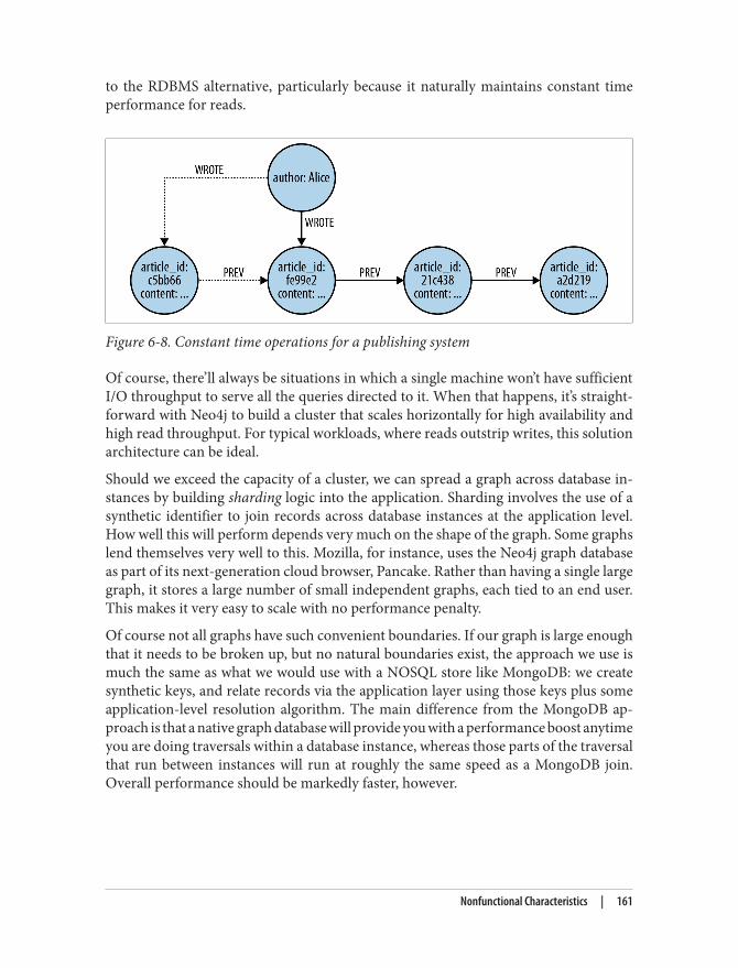
to the RDBMS alternative, particularly because it naturally maintains constant timeperformance for reads.

Figure 6-8. Constant time operations for a publishing system

Of course, there’ll always be situations in which a single machine won’t have sufficientI/O throughput to serve all the queries directed to it. When that happens, it’s straight‐forward with Neo4j to build a cluster that scales horizontally for high availability andhigh read throughput. For typical workloads, where reads outstrip writes, this solutionarchitecture can be ideal.

Should we exceed the capacity of a cluster, we can spread a graph across database in‐stances by building sharding logic into the application. Sharding involves the use of asynthetic identifier to join records across database instances at the application level.How well this will perform depends very much on the shape of the graph. Some graphslend themselves very well to this. Mozilla, for instance, uses the Neo4j graph databaseas part of its next-generation cloud browser, Pancake. Rather than having a single largegraph, it stores a large number of small independent graphs, each tied to an end user.This makes it very easy to scale with no performance penalty.

Of course not all graphs have such convenient boundaries. If our graph is large enoughthat it needs to be broken up, but no natural boundaries exist, the approach we use ismuch the same as what we would use with a NOSQL store like MongoDB: we createsynthetic keys, and relate records via the application layer using those keys plus someapplication-level resolution algorithm. The main difference from the MongoDB ap‐proach is that a native graph database will provide you with a performance boost anytimeyou are doing traversals within a database instance, whereas those parts of the traversalthat run between instances will run at roughly the same speed as a MongoDB join.Overall performance should be markedly faster, however.

Nonfunctional Characteristics | 161

The Holy Grail of Graph ScalabilityThe eventual aim of most graph databases is to be able to partition a graph across manymachines without application-level intervention so that access to the graph can be scaledhorizontally. In the general case this is known to be an NP Hard problem, and thusimpractical to solve. This manifests itself in graph databases as unpredictable querytimes as a result of traversals unexpectedly jumping between machines over a relativelyslow network. However, there is innovation happening in this space, with triple storesable to scale horizontally very well (at the expense of latency); some nonnative graphstores piggy-backing onto other databases (like Twitter’s FlockDB, which runs atopMySQL); and Neo4j’s own horizontally scalable solution. This is certainly an excitingtime to be in the data space.

SummaryIn this chapter we’ve shown how property graphs are an excellent choice for pragmaticdata modeling. We’ve explored the architecture of a graph database, with particularreference to the architecture of Neo4j, and discussed the nonfunctional characteristicsof graph database implementations and what it means for them to be dependable.

162 | Chapter 6: Graph Database Internals

CHAPTER 7

Predictive Analysis with Graph Theory

In this chapter we’re going consider analytical techniques and algorithms for processinggraph data. Both graph theory and graph algorithms are mature and well-understoodfields of computing science and we’ll demonstrate how both can can be used to minesophisticated information from graph databases. Although the reader with a back‐ground in computing science will no doubt recognize these algorithms and techniques,the discussion in this chapter is handled without recourse to mathematics, to encouragethe curious reader to dive in.

Depth- and Breadth-First SearchBefore we look at higher-order analytical techniques we need to reacquaint ourselveswith the fundamental breadth-first search algorithm, which is the basis for iterating overan entire graph. Most of the queries we’ve seen throughout this book have been depth-first rather than breadth-first in nature. That is, they traverse outward from a startingnode to some end node before repeating a similar search down a different path fromthe same start node. Depth-first is a good strategy when we’re trying to follow a path todiscover discrete pieces of information.

Informed Depth-First SearchThe classic depth-first algorithm search is uninformed in that it simply searches a pathuntil it finds the end of the graph. Once at the end, it backtracks to the start node andtries a different path. Because graph databases are semantically rich, however, we canterminate a search along a particular branch early (for example, once we’ve found a nodewith no compatible outgoing relationships, or have traversed “far enough”). Such in‐formed searches can result in lower execution times. These are exactly the kinds ofsearches performed by our Cypher matches and traversals in previous chapters.

163

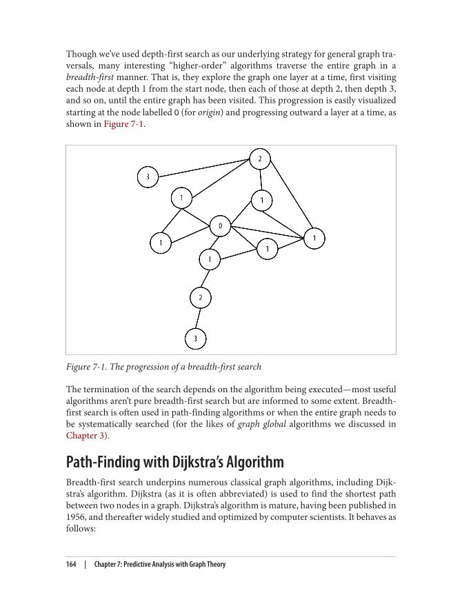
Though we’ve used depth-first search as our underlying strategy for general graph tra‐versals, many interesting “higher-order” algorithms traverse the entire graph in abreadth-first manner. That is, they explore the graph one layer at a time, first visitingeach node at depth 1 from the start node, then each of those at depth 2, then depth 3,and so on, until the entire graph has been visited. This progression is easily visualizedstarting at the node labelled O (for origin) and progressing outward a layer at a time, asshown in Figure 7-1.

Figure 7-1. The progression of a breadth-first search

The termination of the search depends on the algorithm being executed—most usefulalgorithms aren’t pure breadth-first search but are informed to some extent. Breadth-first search is often used in path-finding algorithms or when the entire graph needs tobe systematically searched (for the likes of graph global algorithms we discussed inChapter 3).

Path-Finding with Dijkstra’s AlgorithmBreadth-first search underpins numerous classical graph algorithms, including Dijk‐stra’s algorithm. Dijkstra (as it is often abbreviated) is used to find the shortest pathbetween two nodes in a graph. Dijkstra’s algorithm is mature, having been published in1956, and thereafter widely studied and optimized by computer scientists. It behaves asfollows:

164 | Chapter 7: Predictive Analysis with Graph Theory

1. Pick the start and end nodes, and add the start node to the set of solved nodes (thatis, the set of nodes with known shortest path from the start node) with value 0 (thestart node is by definition 0 path length away from itself).

2. From the starting node, traverse breadth-first to the nearest neighbors and recordthe path length against each neighbor node.

3. Take the shortest path to one of these neighbors (picking arbitrarily in the case ofties) and mark that node as solved, because we now know the shortest path fromthe start node to this neighbor.

4. From the set of solved nodes, visit the nearest neighbors (notice the breath-firstprogression) and record the path lengths from the start node against these newneighbors. Don’t visit any neighboring nodes that have already been solved, becausewe know the shortest paths to them already.

5. Repeat steps 3 and 4 until the destination node has been marked solved.

Efficiency of Dijkstra’s AlgorithmDijkstra’s algorithm is quite efficient because it computes only the lengths of a relativelysmall subset of the possible paths through the graph. When we’ve solved a node, theshortest path from the start node is then known, allowing all subsequent paths to safelybuild on that knowledge.

In fact, the fastest known worst-case implementation of Dijkstra’s algorithm has a per‐formance of O(|R| + |N| log |N|). That is, the algorithm runs in time proportional to thenumber of relationships in the graph, plus the size of the number of nodes multipliedby the log of the size of the node set. The original was O(|R|^2), meaning it ran in timeproportional to the square of the size of the number of relationships in the graph.

Dijkstra is often used to find real-world shortest paths (e.g., for navigation). Here’s anexample. In Figure 7-2 we see a logical map of Australia. Our challenge is to discoverthe shortest driving route between Sydney on the east coast (marked SYD) and Perth,marked PER, which is a continent away, on the west coast. The other major towns andcities are marked with their respective airport codes; we’ll discover many of them alongthe way.

Path-Finding with Dijkstra’s Algorithm | 165

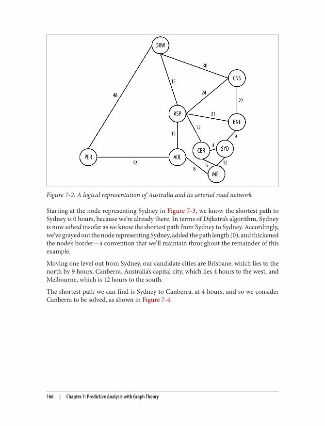
Figure 7-2. A logical representation of Australia and its arterial road network

Starting at the node representing Sydney in Figure 7-3, we know the shortest path toSydney is 0 hours, because we’re already there. In terms of Dijkstra’s algorithm, Sydneyis now solved insofar as we know the shortest path from Sydney to Sydney. Accordingly,we’ve grayed out the node representing Sydney, added the path length (0), and thickenedthe node’s border—a convention that we’ll maintain throughout the remainder of thisexample.

Moving one level out from Sydney, our candidate cities are Brisbane, which lies to thenorth by 9 hours, Canberra, Australia’s capital city, which lies 4 hours to the west, andMelbourne, which is 12 hours to the south.

The shortest path we can find is Sydney to Canberra, at 4 hours, and so we considerCanberra to be solved, as shown in Figure 7-4.

166 | Chapter 7: Predictive Analysis with Graph Theory

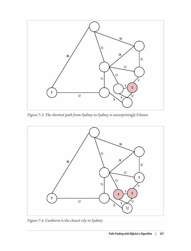
Figure 7-3. The shortest path from Sydney to Sydney is unsurprisingly 0 hours

Figure 7-4. Canberra is the closest city to Sydney

Path-Finding with Dijkstra’s Algorithm | 167

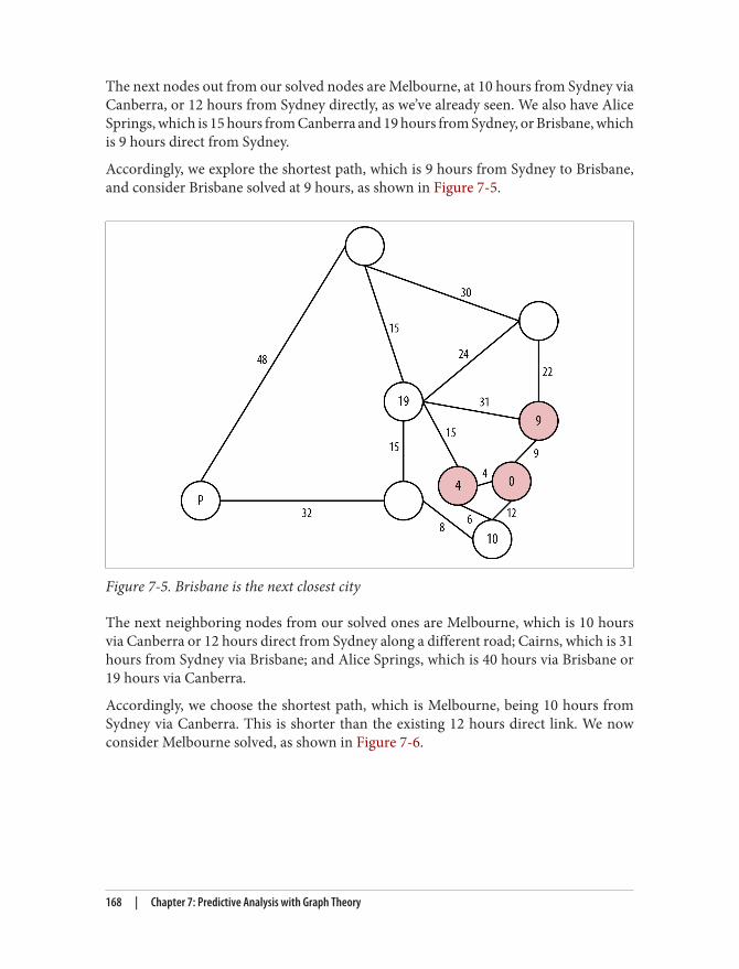
The next nodes out from our solved nodes are Melbourne, at 10 hours from Sydney viaCanberra, or 12 hours from Sydney directly, as we’ve already seen. We also have AliceSprings, which is 15 hours from Canberra and 19 hours from Sydney, or Brisbane, whichis 9 hours direct from Sydney.

Accordingly, we explore the shortest path, which is 9 hours from Sydney to Brisbane,and consider Brisbane solved at 9 hours, as shown in Figure 7-5.

Figure 7-5. Brisbane is the next closest city

The next neighboring nodes from our solved ones are Melbourne, which is 10 hoursvia Canberra or 12 hours direct from Sydney along a different road; Cairns, which is 31hours from Sydney via Brisbane; and Alice Springs, which is 40 hours via Brisbane or19 hours via Canberra.

Accordingly, we choose the shortest path, which is Melbourne, being 10 hours fromSydney via Canberra. This is shorter than the existing 12 hours direct link. We nowconsider Melbourne solved, as shown in Figure 7-6.

168 | Chapter 7: Predictive Analysis with Graph Theory

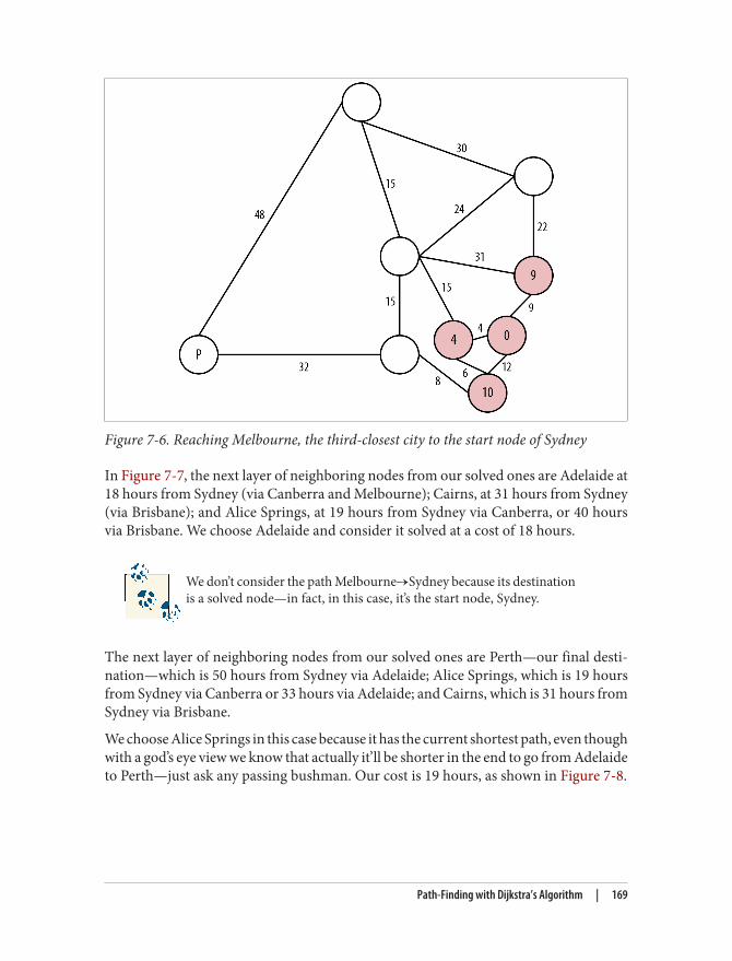
Figure 7-6. Reaching Melbourne, the third-closest city to the start node of Sydney

In Figure 7-7, the next layer of neighboring nodes from our solved ones are Adelaide at18 hours from Sydney (via Canberra and Melbourne); Cairns, at 31 hours from Sydney(via Brisbane); and Alice Springs, at 19 hours from Sydney via Canberra, or 40 hoursvia Brisbane. We choose Adelaide and consider it solved at a cost of 18 hours.

We don’t consider the path Melbourne→Sydney because its destinationis a solved node—in fact, in this case, it’s the start node, Sydney.

The next layer of neighboring nodes from our solved ones are Perth—our final desti‐nation—which is 50 hours from Sydney via Adelaide; Alice Springs, which is 19 hoursfrom Sydney via Canberra or 33 hours via Adelaide; and Cairns, which is 31 hours fromSydney via Brisbane.

We choose Alice Springs in this case because it has the current shortest path, even thoughwith a god’s eye view we know that actually it’ll be shorter in the end to go from Adelaideto Perth—just ask any passing bushman. Our cost is 19 hours, as shown in Figure 7-8.

Path-Finding with Dijkstra’s Algorithm | 169

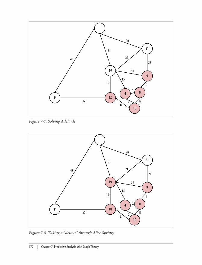
Figure 7-7. Solving Adelaide

Figure 7-8. Taking a “detour” through Alice Springs

170 | Chapter 7: Predictive Analysis with Graph Theory

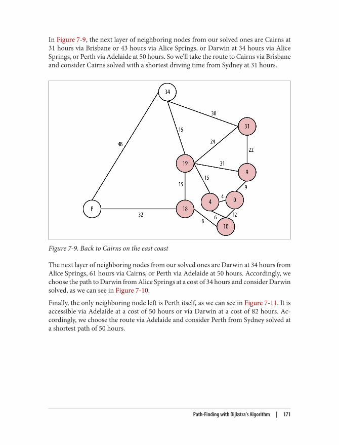
In Figure 7-9, the next layer of neighboring nodes from our solved ones are Cairns at31 hours via Brisbane or 43 hours via Alice Springs, or Darwin at 34 hours via AliceSprings, or Perth via Adelaide at 50 hours. So we’ll take the route to Cairns via Brisbaneand consider Cairns solved with a shortest driving time from Sydney at 31 hours.

Figure 7-9. Back to Cairns on the east coast

The next layer of neighboring nodes from our solved ones are Darwin at 34 hours fromAlice Springs, 61 hours via Cairns, or Perth via Adelaide at 50 hours. Accordingly, wechoose the path to Darwin from Alice Springs at a cost of 34 hours and consider Darwinsolved, as we can see in Figure 7-10.

Finally, the only neighboring node left is Perth itself, as we can see in Figure 7-11. It isaccessible via Adelaide at a cost of 50 hours or via Darwin at a cost of 82 hours. Ac‐cordingly, we choose the route via Adelaide and consider Perth from Sydney solved ata shortest path of 50 hours.

Path-Finding with Dijkstra’s Algorithm | 171

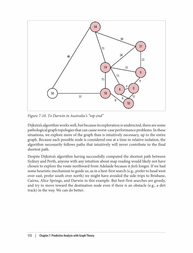
Figure 7-10. To Darwin in Australia’s “top-end”

Dijkstra’s algorithm works well, but because its exploration is undirected, there are somepathological graph topologies that can cause worst-case performance problems. In thesesituations, we explore more of the graph than is intuitively necessary, up to the entiregraph. Because each possible node is considered one at a time in relative isolation, thealgorithm necessarily follows paths that intuitively will never contribute to the finalshortest path.

Despite Dijkstra’s algorithm having successfully computed the shortest path betweenSydney and Perth, anyone with any intuition about map reading would likely not havechosen to explore the route northward from Adelaide because it feels longer. If we hadsome heuristic mechanism to guide us, as in a best-first search (e.g., prefer to head westover east, prefer south over north) we might have avoided the side-trips to Brisbane,Cairns, Alice Springs, and Darwin in this example. But best-first searches are greedy,and try to move toward the destination node even if there is an obstacle (e.g., a dirttrack) in the way. We can do better.

172 | Chapter 7: Predictive Analysis with Graph Theory

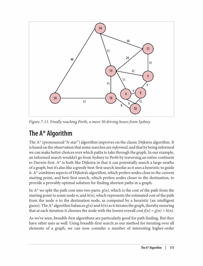
Figure 7-11. Finally reaching Perth, a mere 50 driving hours from Sydney

The A* AlgorithmThe A* (pronounced “A-star”) algorithm improves on the classic Dijkstra algorithm. Itis based on the observation that some searches are informed, and that by being informedwe can make better choices over which paths to take through the graph. In our example,an informed search wouldn’t go from Sydney to Perth by traversing an entire continentto Darwin first. A* is both like Dijkstra in that it can potentially search a large swatheof a graph, but it’s also like a greedy best-first search insofar as it uses a heuristic to guideit. A* combines aspects of Dijkstra’s algorithm, which prefers nodes close to the currentstarting point, and best-first search, which prefers nodes closer to the destination, toprovide a provably optimal solution for finding shortest paths in a graph.

In A* we split the path cost into two parts: g(n), which is the cost of the path from thestarting point to some node n; and h(n), which represents the estimated cost of the pathfrom the node n to the destination node, as computed by a heuristic (an intelligentguess). The A* algorithm balances g(n) and h(n) as it iterates the graph, thereby ensuringthat at each iteration it chooses the node with the lowest overall cost f(n) = g(n) + h(n).

As we’ve seen, breadth-first algorithms are particularly good for path finding. But theyhave other uses as well. Using breadth-first search as our method for iterating over allelements of a graph, we can now consider a number of interesting higher-order

The A* Algorithm | 173

1. In particular, see Granovetter’s pivotal work on the strength of weak ties in social communities: http://stanford.io/17XjisT. For Easley and Kleinberg, see http://bit.ly/13e0ZuZ.

algorithms from graph theory that yield predictive insight into the behavior of connec‐ted data.

Graph Theory and Predictive ModelingGraph theory is a mature and well-understood field of study concerning the nature ofnetworks (or from our point of view, connected data). The analytic techniques that havebeen developed by graph theoreticians can be brought to bear on a range of interestingproblems. Now that we understand the low-level traversal mechanisms, such as breadth-first search, we can start to consider higher-order analyses.

Graph theory techniques are broadly applicable to a wide range of problems. They areespecially useful when we first want to gain some insight into a new domain—or evenunderstand what kind of insight it’s possible to extract from a domain. In such casesthere are a range of techniques from graph theory and social sciences that we canstraightforwardly apply to gain insight.

In the next few sections we’ll introduce some of the key concepts in social graph theory.We’ll introduce these concepts in the context of a social domain based on the works ofsociologists Mark Granovetter, and Easley and Kleinberg.1

Property Graphs and Graph TheoryMuch of the work on graph theory assumes a slightly different model to the propertygraphs we’ve been using throughout this book. This work tends to ignore direction andlabeling of graphs, instead assuming undirected relationships with a single label derivedfrom the domain (e.g., friend or colleague).

We’re going to take a hybrid approach here. We’ll add names to relationships where ithelps add domain-specific meaning. In many cases, however, we will ignore relationshipdirection. This won’t impact the analysis, however: the graph structure upholds the sameprinciples irrespective of its construction.

Triadic ClosuresA triadic closure is a common property of social graphs, where we observe that if twonodes are connected via a path involving a third node, there is an increased likelihoodthat the two nodes will become directly connected at some point in the future. This isa familiar social occurrence: if we happen to be friends with two people, there’s anincreased chance that those people will become direct friends too. The very fact of their

174 | Chapter 7: Predictive Analysis with Graph Theory

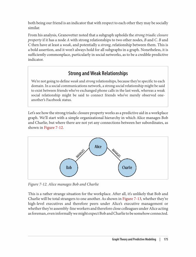
both being our friend is an indicator that with respect to each other they may be sociallysimilar.

From his analysis, Granovetter noted that a subgraph upholds the strong triadic closureproperty if it has a node A with strong relationships to two other nodes, B and C. B andC then have at least a weak, and potentially a strong, relationship between them. This isa bold assertion, and it won’t always hold for all subgraphs in a graph. Nonetheless, it issufficiently commonplace, particularly in social networks, as to be a credible predictiveindicator.

Strong and Weak RelationshipsWe’re not going to define weak and strong relationships, because they’re specific to eachdomain. In a social communications network, a strong social relationship might be saidto exist between friends who’ve exchanged phone calls in the last week, whereas a weaksocial relationship might be said to connect friends who’ve merely observed one-another’s Facebook status.

Let’s see how the strong triadic closure property works as a predictive aid in a workplacegraph. We’ll start with a simple organizational hierarchy in which Alice manages Boband Charlie, but where there are not yet any connections between her subordinates, asshown in Figure 7-12.

Figure 7-12. Alice manages Bob and Charlie

This is a rather strange situation for the workplace. After all, it’s unlikely that Bob andCharlie will be total strangers to one another. As shown in Figure 7-13, whether they’rehigh-level executives and therefore peers under Alice’s executive management orwhether they’re assembly-line workers and therefore close colleagues under Alice actingas foreman, even informally we might expect Bob and Charlie to be somehow connected.

Graph Theory and Predictive Modeling | 175

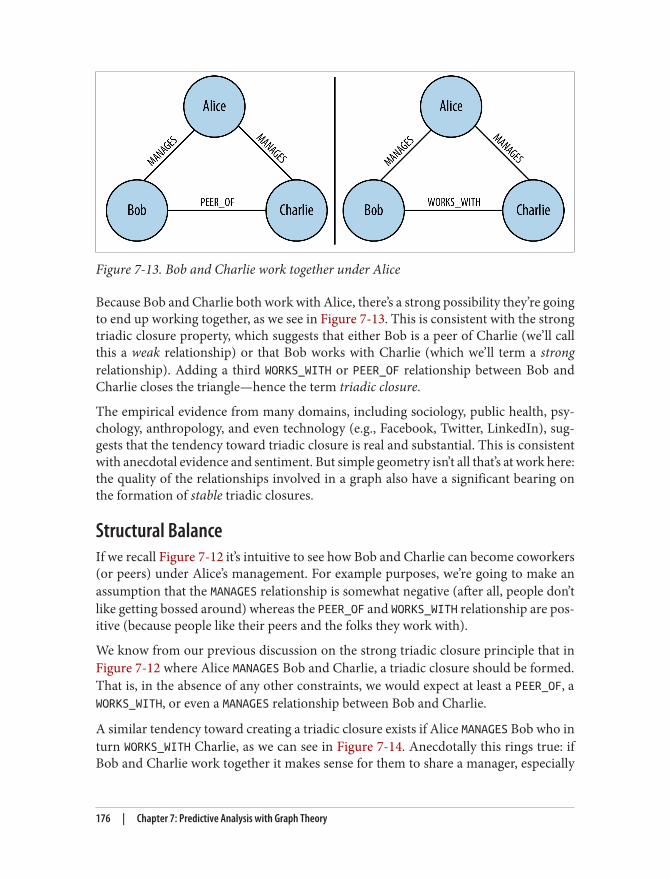
Figure 7-13. Bob and Charlie work together under Alice

Because Bob and Charlie both work with Alice, there’s a strong possibility they’re goingto end up working together, as we see in Figure 7-13. This is consistent with the strongtriadic closure property, which suggests that either Bob is a peer of Charlie (we’ll callthis a weak relationship) or that Bob works with Charlie (which we’ll term a strongrelationship). Adding a third WORKS_WITH or PEER_OF relationship between Bob andCharlie closes the triangle—hence the term triadic closure.

The empirical evidence from many domains, including sociology, public health, psy‐chology, anthropology, and even technology (e.g., Facebook, Twitter, LinkedIn), sug‐gests that the tendency toward triadic closure is real and substantial. This is consistentwith anecdotal evidence and sentiment. But simple geometry isn’t all that’s at work here:the quality of the relationships involved in a graph also have a significant bearing onthe formation of stable triadic closures.

Structural BalanceIf we recall Figure 7-12 it’s intuitive to see how Bob and Charlie can become coworkers(or peers) under Alice’s management. For example purposes, we’re going to make anassumption that the MANAGES relationship is somewhat negative (after all, people don’tlike getting bossed around) whereas the PEER_OF and WORKS_WITH relationship are pos‐itive (because people like their peers and the folks they work with).

We know from our previous discussion on the strong triadic closure principle that inFigure 7-12 where Alice MANAGES Bob and Charlie, a triadic closure should be formed.That is, in the absence of any other constraints, we would expect at least a PEER_OF, aWORKS_WITH, or even a MANAGES relationship between Bob and Charlie.

A similar tendency toward creating a triadic closure exists if Alice MANAGES Bob who inturn WORKS_WITH Charlie, as we can see in Figure 7-14. Anecdotally this rings true: ifBob and Charlie work together it makes sense for them to share a manager, especially

176 | Chapter 7: Predictive Analysis with Graph Theory

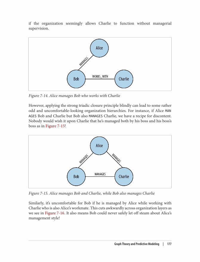
if the organization seemingly allows Charlie to function without managerialsupervision.

Figure 7-14. Alice manages Bob who works with Charlie

However, applying the strong triadic closure principle blindly can lead to some ratherodd and uncomfortable-looking organization hierarchies. For instance, if Alice MANAGES Bob and Charlie but Bob also MANAGES Charlie, we have a recipe for discontent.Nobody would wish it upon Charlie that he’s managed both by his boss and his boss’sboss as in Figure 7-15!

Figure 7-15. Alice manages Bob and Charlie, while Bob also manages Charlie

Similarly, it’s uncomfortable for Bob if he is managed by Alice while working withCharlie who is also Alice’s workmate. This cuts awkwardly across organization layers aswe see in Figure 7-16. It also means Bob could never safely let off steam about Alice’smanagement style!

Graph Theory and Predictive Modeling | 177

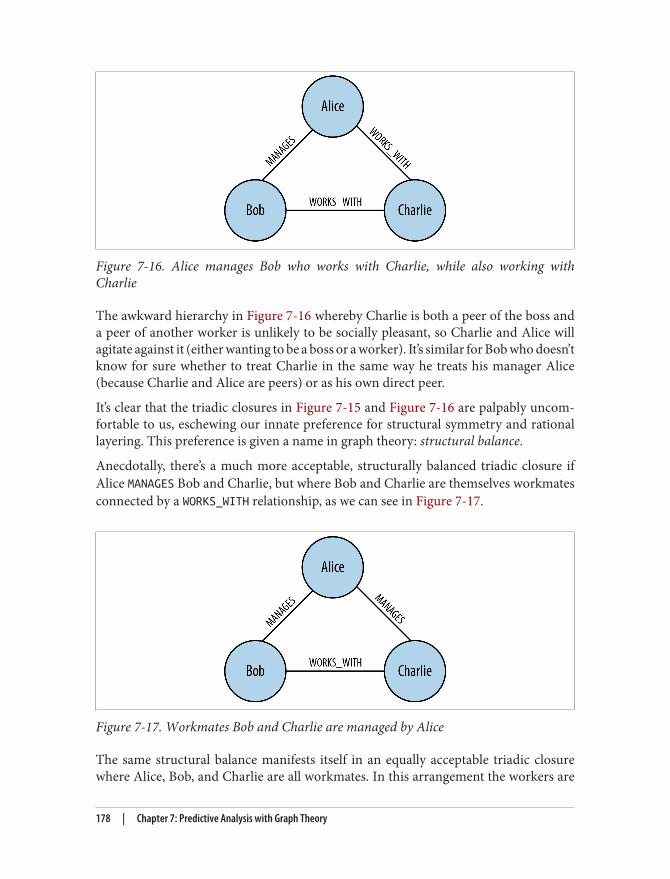
Figure 7-16. Alice manages Bob who works with Charlie, while also working withCharlie

The awkward hierarchy in Figure 7-16 whereby Charlie is both a peer of the boss anda peer of another worker is unlikely to be socially pleasant, so Charlie and Alice willagitate against it (either wanting to be a boss or a worker). It’s similar for Bob who doesn’tknow for sure whether to treat Charlie in the same way he treats his manager Alice(because Charlie and Alice are peers) or as his own direct peer.

It’s clear that the triadic closures in Figure 7-15 and Figure 7-16 are palpably uncom‐fortable to us, eschewing our innate preference for structural symmetry and rationallayering. This preference is given a name in graph theory: structural balance.

Anecdotally, there’s a much more acceptable, structurally balanced triadic closure ifAlice MANAGES Bob and Charlie, but where Bob and Charlie are themselves workmatesconnected by a WORKS_WITH relationship, as we can see in Figure 7-17.

Figure 7-17. Workmates Bob and Charlie are managed by Alice

The same structural balance manifests itself in an equally acceptable triadic closurewhere Alice, Bob, and Charlie are all workmates. In this arrangement the workers are

178 | Chapter 7: Predictive Analysis with Graph Theory

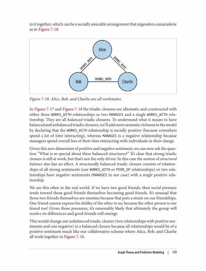
in it together, which can be a socially amicable arrangement that engenders camaraderieas in Figure 7-18.

Figure 7-18. Alice, Bob, and Charlie are all workmates

In Figure 7-17 and Figure 7-18 the triadic closures are idiomatic and constructed witheither three WORKS_WITH relationships or two MANAGES and a single WORKS_WITH rela‐tionship. They are all balanced triadic closures. To understand what it means to havebalanced and unbalanced triadic closures, we’ll add more semantic richness to the modelby declaring that the WORKS_WITH relationship is socially positive (because coworkersspend a lot of time interacting), whereas MANAGES is a negative relationship becausemanagers spend overall less of their time interacting with individuals in their charge.

Given this new dimension of positive and negative sentiment, we can now ask the ques‐tion “What is so special about these balanced structures?” It’s clear that strong triadicclosure is still at work, but that’s not the only driver. In this case the notion of structuralbalance also has an effect. A structurally balanced triadic closure consists of relation‐ships of all strong sentiments (our WORKS_WITH or PEER_OF relationships) or two rela‐tionships have negative sentiments (MANAGES in our case) with a single positive rela‐tionship.

We see this often in the real world. If we have two good friends, then social pressuretends toward those good friends themselves becoming good friends. It’s unusual thatthose two friends themselves are enemies because that puts a strain on our friendships.One friend cannot express his dislike of the other to us, because the other person is ourfriend too! Given those pressures, it’s reasonably likely that ultimately the group willresolve its differences and good friends will emerge.

This would change our unbalanced triadic closure (two relationships with positive sen‐timents and one negative) to a balanced closure because all relationships would be of apositive sentiment much like our collaborative scheme where Alice, Bob, and Charlieall work together in Figure 7-18.

Graph Theory and Predictive Modeling | 179

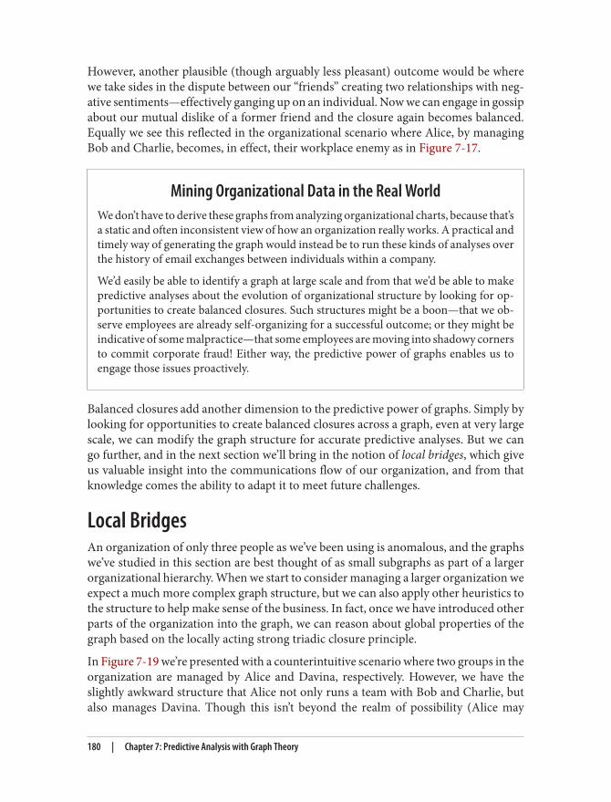
However, another plausible (though arguably less pleasant) outcome would be wherewe take sides in the dispute between our “friends” creating two relationships with neg‐ative sentiments—effectively ganging up on an individual. Now we can engage in gossipabout our mutual dislike of a former friend and the closure again becomes balanced.Equally we see this reflected in the organizational scenario where Alice, by managingBob and Charlie, becomes, in effect, their workplace enemy as in Figure 7-17.

Mining Organizational Data in the Real WorldWe don’t have to derive these graphs from analyzing organizational charts, because that’sa static and often inconsistent view of how an organization really works. A practical andtimely way of generating the graph would instead be to run these kinds of analyses overthe history of email exchanges between individuals within a company.

We’d easily be able to identify a graph at large scale and from that we’d be able to makepredictive analyses about the evolution of organizational structure by looking for op‐portunities to create balanced closures. Such structures might be a boon—that we ob‐serve employees are already self-organizing for a successful outcome; or they might beindicative of some malpractice—that some employees are moving into shadowy cornersto commit corporate fraud! Either way, the predictive power of graphs enables us toengage those issues proactively.

Balanced closures add another dimension to the predictive power of graphs. Simply bylooking for opportunities to create balanced closures across a graph, even at very largescale, we can modify the graph structure for accurate predictive analyses. But we cango further, and in the next section we’ll bring in the notion of local bridges, which giveus valuable insight into the communications flow of our organization, and from thatknowledge comes the ability to adapt it to meet future challenges.

Local BridgesAn organization of only three people as we’ve been using is anomalous, and the graphswe’ve studied in this section are best thought of as small subgraphs as part of a largerorganizational hierarchy. When we start to consider managing a larger organization weexpect a much more complex graph structure, but we can also apply other heuristics tothe structure to help make sense of the business. In fact, once we have introduced otherparts of the organization into the graph, we can reason about global properties of thegraph based on the locally acting strong triadic closure principle.

In Figure 7-19 we’re presented with a counterintuitive scenario where two groups in theorganization are managed by Alice and Davina, respectively. However, we have theslightly awkward structure that Alice not only runs a team with Bob and Charlie, butalso manages Davina. Though this isn’t beyond the realm of possibility (Alice may

180 | Chapter 7: Predictive Analysis with Graph Theory

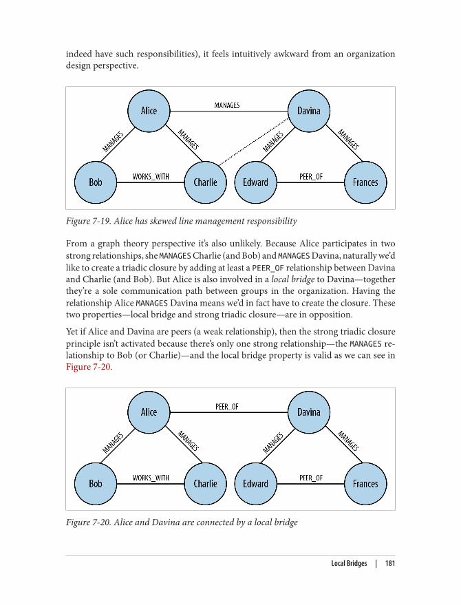
indeed have such responsibilities), it feels intuitively awkward from an organizationdesign perspective.

Figure 7-19. Alice has skewed line management responsibility

From a graph theory perspective it’s also unlikely. Because Alice participates in twostrong relationships, she MANAGES Charlie (and Bob) and MANAGES Davina, naturally we’dlike to create a triadic closure by adding at least a PEER_OF relationship between Davinaand Charlie (and Bob). But Alice is also involved in a local bridge to Davina—togetherthey’re a sole communication path between groups in the organization. Having therelationship Alice MANAGES Davina means we’d in fact have to create the closure. Thesetwo properties—local bridge and strong triadic closure—are in opposition.

Yet if Alice and Davina are peers (a weak relationship), then the strong triadic closureprinciple isn’t activated because there’s only one strong relationship—the MANAGES re‐lationship to Bob (or Charlie)—and the local bridge property is valid as we can see inFigure 7-20.

Figure 7-20. Alice and Davina are connected by a local bridge

Local Bridges | 181

What’s interesting about this local bridge is that it describes a communication channelbetween groups in our organization. Such channels are extremely important to thevitality of our enterprise. In particular, to ensure the health of our company we’d makesure that local bridge relationships are healthy and active, or equally we might keep aneye on local bridges to ensure no impropriety (embezzlement, fraud, etc.) occurs.

Finding Your Next JobThis notion of weak social links is particularly pertinent in algorithms like (social) jobsearch. The remarkable thing about job searches is that it’s rarely a close friend thatprovides the best recommendation, but a looser acquaintance.

Why should this be? Our close friends share a similar world view (they’re in the samegraph component) and have similar access to the available jobs data and hold similaropinions about those jobs. A friend across a local bridge is clearly in a different socialnetwork (a different component), with correspondingly different access to jobs and adifferent viewpoint about them. So if you’re going to find a job, look across a local bridgebecause that’s where people who have different knowledge to you and your friends hangout.

This same property of local bridges being weak links (PEER_OF in our example organi‐zation) is a property that is prevalent throughout social graphs. This means we can startto make predictive analyses of how our organization will evolve based on empiricallyderived local bridge and strong triadic closure notions. So given an arbitrary organi‐zational graph, we can see how the business structure is likely to evolve and plan forthose eventualities.

SummaryGraphs are truly remarkable structures. Our understanding of them is rooted in severalhundred years of mathematical and scientific study. And yet we’re only just beginningto understand how to apply them to our personal, social, and business lives. The tech‐nology is here, open and available to all in the form of the modern graph database; theopportunities are endless.

As we’ve seen throughout this book, graph theory algorithms and analytical techniquesare not demanding: we need only understand how to apply them to achieve our goals.We leave this book with a simple call to arms: embrace graphs and graph databases; takeall that you’ve learned about modeling with graphs, graph database architecture, de‐signing and implementing a graph database solution, and applying graph algorithms tocomplex business problems, and go build the next truly pioneering information system.

182 | Chapter 7: Predictive Analysis with Graph Theory

APPENDIX A

NOSQL Overview

Recent years have seen a meteoric rise in popularity of a family of data storage tech‐nologies known as NOSQL (a cheeky acronym for Not Only SQL, or more confronta‐tionally, No to SQL). But NOSQL as a term defines what those data stores are not—they’re not SQL-centric relational databases—rather than what they are, which is aninteresting and useful set of storage technologies whose operational, functional, andarchitectural characteristics are many and varied.

Why were these new databases created? What problems do they address? Here we’lldiscuss some of the new data challenges that have emerged in the past decade. We’llthen look at four families of NOSQL databases, including graph databases.

The Rise of NOSQLHistorically, most enterprise-level web apps ran on top of a relational database. But inthe past decade, we’ve been faced with data that is bigger in volume, changes morerapidly, and is more structurally varied than can be dealt with by traditional RDBMSdeployments. The NOSQL movement has arisen in response to these challenges.

It’s no surprise that as storage has increased dramatically, volume has become the prin‐cipal driver behind the adoption of NOSQL stores by organizations. Volume may bedefined simply as the size of the stored data.

As is well known, large datasets become unwieldy when stored in relational databases;in particular, query execution times increase as the size of tables and the number of joinsgrow (so-called join pain). This isn’t the fault of the databases themselves; rather, it isan aspect of the underlying data model, which builds a set of all possible answers to aquery before filtering to arrive at the correct solution.

In an effort to avoid joins and join pain, and thereby cope better with extremely largedatasets, the NOSQL world has adopted several alternatives to the relational model.

183

Though more adept at dealing with very large datasets, these alternative models tendto be less expressive than the relational one (with the exception of the graph model,which is actually more expressive).

But volume isn’t the only problem modern web-facing systems have to deal with. Besidesbeing big, today’s data often changes very rapidly. Velocity is the rate at which datachanges over time.

Velocity is rarely a static metric: internal and external changes to a system and thecontext in which it is employed can have considerable impact on velocity. Coupled withhigh volume, variable velocity requires data stores to not only handle sustained levelsof high write loads, but also deal with peaks.

There is another aspect to velocity, which is the rate at which the structure of the datachanges. In other words, in addition to the value of specific properties changing, theoverall structure of the elements hosting those properties can change as well. This com‐monly occurs for two reasons. The first is fast-moving business dynamics: as the busi‐ness changes, so do its data needs. The second is that data acquisition is often an ex‐perimental affair: some properties are captured “just in case,” others are introduced ata later point based on changed needs; the ones that prove valuable to the business stayaround, others fall by the wayside. Both these forms of velocity are problematic in therelational world, where high write loads translate into a high processing cost, and highschema volatility has a high operational cost.

Although commentators have later added other useful requirements to the originalquest for scale, the final key aspect is the realization that data is far more varied thanthe data we’ve dealt with in the relational world. For existential proof, think of all thosenulls in our tables and the null checks in our code. This has driven out the final widelyagreed upon facet, variety, which we define as the degree to which data is regularly orirregularly structured, dense or sparse, connected or disconnected.

ACID versus BASEWhen we first encounter NOSQL we often consider it in the context of what many ofus are already familiar with: relational databases. Although we know the data and querymodel will be different (after all, there’s no SQL!), the consistency models used byNOSQL stores can also be quite different from those employed by relational databases.Many NOSQL databases use different consistency models to support the differences involume, velocity, and variety of data discussed earlier.

184 | Appendix A: NOSQL Overview

1. The .NET-based RavenDB has bucked the trend among aggregate stores in supporting ACID transactions;as we show elsewhere in the book, ACID properties are still upheld by many graph databases.

Let’s explore what consistency features are available to help keep data safe, and whattrade-offs are involved when using (most) NOSQL stores.1

In the relational database world, we’re all familiar with ACID transactions, which havebeen the norm for some time. The ACID guarantees provide us with a safe environmentin which to operate on data:Atomic

All operations in a transaction succeed or every operation is rolled back.

ConsistentOn transaction completion, the database is structurally sound.

IsolatedTransactions do not contend with one another. Contentious access to state is mod‐erated by the database so that transactions appear to run sequentially.

DurableThe results of applying a transaction are permanent, even in the presence of failures.

These properties mean that once a transaction completes, its data is consistent (so-called write consistency) and stable on disk (or disks, or indeed in multiple distinctmemory locations). This is a wonderful abstraction for the application developer, butrequires sophisticated locking, which can cause logical unavailability, and is typicallyconsidered to be a heavyweight pattern for most use cases.

For many domains, ACID transactions are far more pessimistic than the domain ac‐tually requires. In the NOSQL world, ACID transactions have gone out of fashion asstores loosen the requirements for immediate consistency, data freshness, and accuracyin order to gain other benefits, like scale and resilience. Instead of using ACID, the termBASE has arisen as a popular way of describing the properties of a more optimisticstorage strategy.Basic availability

The store appears to work most of the time.

Soft-stateStores don’t have to be write-consistent, nor do different replicas have to be mutuallyconsistent all the time.

Eventual consistencyStores exhibit consistency at some later point (e.g., lazily at read time).

The BASE properties are considerably looser than the ACID guarantees, and there isno direct mapping between them. A BASE store values availability (because that is a

ACID versus BASE | 185

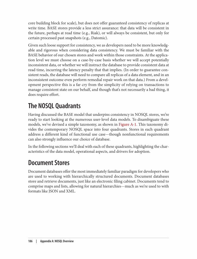
core building block for scale), but does not offer guaranteed consistency of replicas atwrite time. BASE stores provide a less strict assurance: that data will be consistent inthe future, perhaps at read time (e.g., Riak), or will always be consistent, but only forcertain processed past snapshots (e.g., Datomic).

Given such loose support for consistency, we as developers need to be more knowledg‐able and rigorous when considering data consistency. We must be familiar with theBASE behavior of our chosen stores and work within those constraints. At the applica‐tion level we must choose on a case-by-case basis whether we will accept potentiallyinconsistent data, or whether we will instruct the database to provide consistent data atread time, incurring the latency penalty that that implies. (In order to guarantee con‐sistent reads, the database will need to compare all replicas of a data element, and in aninconsistent outcome even perform remedial repair work on that data.) From a devel‐opment perspective this is a far cry from the simplicity of relying on transactions tomanage consistent state on our behalf, and though that’s not necessarily a bad thing, itdoes require effort.

The NOSQL QuadrantsHaving discussed the BASE model that underpins consistency in NOSQL stores, we’reready to start looking at the numerous user-level data models. To disambiguate thesemodels, we’ve devised a simple taxonomy, as shown in Figure A-1. This taxonomy di‐vides the contemporary NOSQL space into four quadrants. Stores in each quadrantaddress a different kind of functional use case—though nonfunctional requirementscan also strongly influence our choice of database.

In the following sections we’ll deal with each of these quadrants, highlighting the char‐acteristics of the data model, operational aspects, and drivers for adoption.

Document StoresDocument databases offer the most immediately familiar paradigm for developers whoare used to working with hierarchically structured documents. Document databasesstore and retrieve documents, just like an electronic filing cabinet. Documents tend tocomprise maps and lists, allowing for natural hierarchies—much as we’re used to withformats like JSON and XML.

186 | Appendix A: NOSQL Overview

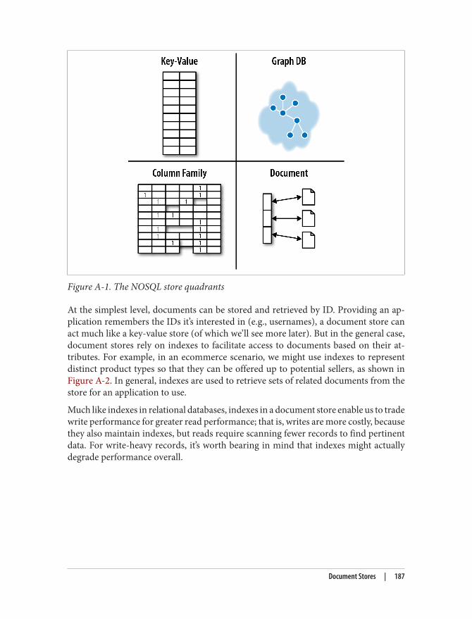
Figure A-1. The NOSQL store quadrants

At the simplest level, documents can be stored and retrieved by ID. Providing an ap‐plication remembers the IDs it’s interested in (e.g., usernames), a document store canact much like a key-value store (of which we’ll see more later). But in the general case,document stores rely on indexes to facilitate access to documents based on their at‐tributes. For example, in an ecommerce scenario, we might use indexes to representdistinct product types so that they can be offered up to potential sellers, as shown inFigure A-2. In general, indexes are used to retrieve sets of related documents from thestore for an application to use.

Much like indexes in relational databases, indexes in a document store enable us to tradewrite performance for greater read performance; that is, writes are more costly, becausethey also maintain indexes, but reads require scanning fewer records to find pertinentdata. For write-heavy records, it’s worth bearing in mind that indexes might actuallydegrade performance overall.

Document Stores | 187

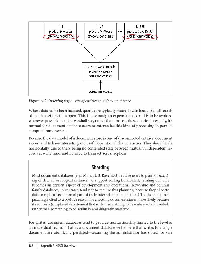
Figure A-2. Indexing reifies sets of entities in a document store

Where data hasn’t been indexed, queries are typically much slower, because a full searchof the dataset has to happen. This is obviously an expensive task and is to be avoidedwherever possible—and as we shall see, rather than process these queries internally, it’snormal for document database users to externalize this kind of processing in parallelcompute frameworks.

Because the data model of a document store is one of disconnected entities, documentstores tend to have interesting and useful operational characteristics. They should scalehorizontally, due to there being no contended state between mutually independent re‐cords at write time, and no need to transact across replicas.

ShardingMost document databases (e.g., MongoDB, RavenDB) require users to plan for shard‐ing of data across logical instances to support scaling horizontally. Scaling out thusbecomes an explicit aspect of development and operations. (Key-value and columnfamily databases, in contrast, tend not to require this planning, because they allocatedata to replicas as a normal part of their internal implementation.) This is sometimespuzzlingly cited as a positive reason for choosing document stores, most likely becauseit induces a (misplaced) excitement that scale is something to be embraced and lauded,rather than something to be skillfully and diligently mastered.

For writes, document databases tend to provide transactionality limited to the level ofan individual record. That is, a document database will ensure that writes to a singledocument are atomically persisted—assuming the administrator has opted for safe

188 | Appendix A: NOSQL Overview

levels of persistence when setting up the database. There is no locking support, however,for operating across sets of documents atomically. Such abstractions are left to appli‐cation code to implement in a domain-specific manner.

Because stored documents are not connected (save through indexes), there are numer‐ous optimistic concurrency control mechanisms that can be used to help reconcileconcurrent contending writes for a single document without having to resort to strictlocks. In fact, some document stores (like CouchDB) have made this a key point of theirvalue proposition: documents can be held in a multimaster database that automaticallyreplicates concurrently accessed, contended state across instances without undue in‐terference from the user.

In other stores, too, the database management system may be able to distinguish andreconcile writes to different parts of a document, or even use logical timestamps toreconcile several contended writes into a single logically consistent outcome. This is areasonable optimistic trade-off: it reduces the need for transactions (which we knowtend to be latent and decrease availability) by using alternative mechanisms that opti‐mistically provide greater availability, lower latency, and higher throughput.

Though optimistic concurrency control mechanisms are useful, we alsorather like transactions, and there are numerous examples of high-throughput performance transaction processing systems in theliterature.

Key-Value StoresKey-value stores are cousins of the document store family, but their lineage comesfrom Amazon’s Dynamo database. They act like large, distributed hashmap data struc‐tures that store and retrieve opaque values by key.

As shown in Figure A-3 the key space of the hashmap is spread across numerous bucketson the network. For fault-tolerance reasons, each bucket is replicated onto several ma‐chines. The formula for number of replicas required is given by R = 2F +1, where F isthe number of failures we can tolerate. The replication algorithm seeks to ensure thatmachines aren’t exact copies of each other. This allows the system to load-balance whilea machine and its buckets recover; it also helps avoid hotspots, which can cause inad‐vertent self denial-of-service.

From the client’s point of view, key-value stores are easy to use. A client stores a dataelement by hashing a domain-specific identifier (key). The hash function is crafted suchthat it provides a uniform distribution across the available buckets, which ensures thatno single machine becomes a hotspot. Given the hashed key, the client can use that

Key-Value Stores | 189

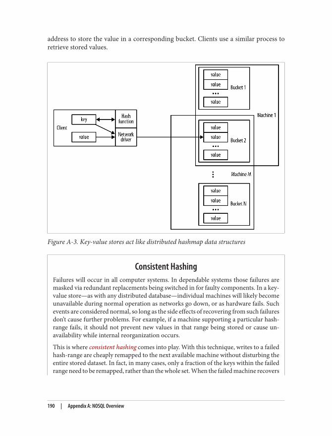
address to store the value in a corresponding bucket. Clients use a similar process toretrieve stored values.

Figure A-3. Key-value stores act like distributed hashmap data structures

Consistent HashingFailures will occur in all computer systems. In dependable systems those failures aremasked via redundant replacements being switched in for faulty components. In a key-value store—as with any distributed database—individual machines will likely becomeunavailable during normal operation as networks go down, or as hardware fails. Suchevents are considered normal, so long as the side effects of recovering from such failuresdon’t cause further problems. For example, if a machine supporting a particular hash-range fails, it should not prevent new values in that range being stored or cause un‐availability while internal reorganization occurs.

This is where consistent hashing comes into play. With this technique, writes to a failedhash-range are cheaply remapped to the next available machine without disturbing theentire stored dataset. In fact, in many cases, only a fraction of the keys within the failedrange need to be remapped, rather than the whole set. When the failed machine recovers

190 | Appendix A: NOSQL Overview

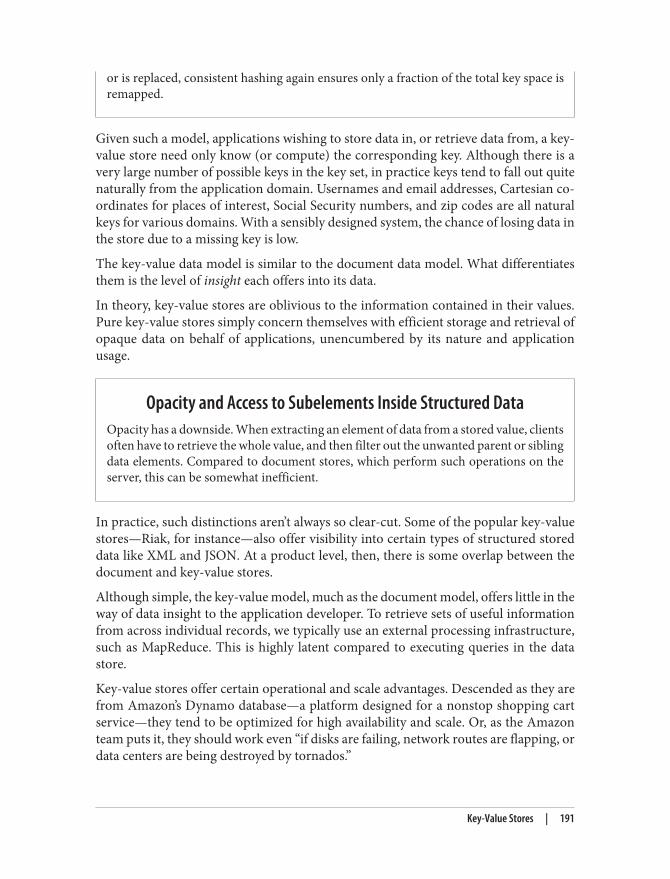
or is replaced, consistent hashing again ensures only a fraction of the total key space isremapped.

Given such a model, applications wishing to store data in, or retrieve data from, a key-value store need only know (or compute) the corresponding key. Although there is avery large number of possible keys in the key set, in practice keys tend to fall out quitenaturally from the application domain. Usernames and email addresses, Cartesian co‐ordinates for places of interest, Social Security numbers, and zip codes are all naturalkeys for various domains. With a sensibly designed system, the chance of losing data inthe store due to a missing key is low.

The key-value data model is similar to the document data model. What differentiatesthem is the level of insight each offers into its data.

In theory, key-value stores are oblivious to the information contained in their values.Pure key-value stores simply concern themselves with efficient storage and retrieval ofopaque data on behalf of applications, unencumbered by its nature and applicationusage.

Opacity and Access to Subelements Inside Structured DataOpacity has a downside. When extracting an element of data from a stored value, clientsoften have to retrieve the whole value, and then filter out the unwanted parent or siblingdata elements. Compared to document stores, which perform such operations on theserver, this can be somewhat inefficient.

In practice, such distinctions aren’t always so clear-cut. Some of the popular key-valuestores—Riak, for instance—also offer visibility into certain types of structured storeddata like XML and JSON. At a product level, then, there is some overlap between thedocument and key-value stores.

Although simple, the key-value model, much as the document model, offers little in theway of data insight to the application developer. To retrieve sets of useful informationfrom across individual records, we typically use an external processing infrastructure,such as MapReduce. This is highly latent compared to executing queries in the datastore.

Key-value stores offer certain operational and scale advantages. Descended as they arefrom Amazon’s Dynamo database—a platform designed for a nonstop shopping cartservice—they tend to be optimized for high availability and scale. Or, as the Amazonteam puts it, they should work even “if disks are failing, network routes are flapping, ordata centers are being destroyed by tornados.”

Key-Value Stores | 191

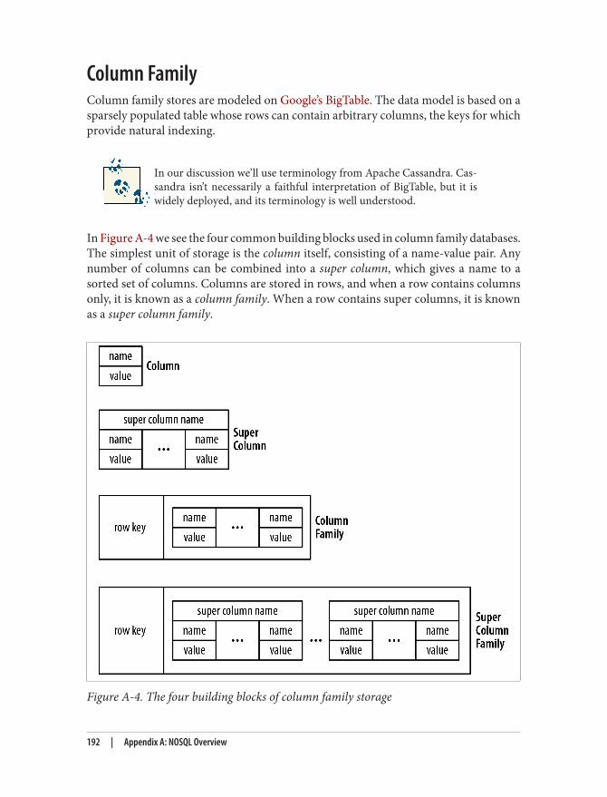
Column FamilyColumn family stores are modeled on Google’s BigTable. The data model is based on asparsely populated table whose rows can contain arbitrary columns, the keys for whichprovide natural indexing.

In our discussion we’ll use terminology from Apache Cassandra. Cas‐sandra isn’t necessarily a faithful interpretation of BigTable, but it iswidely deployed, and its terminology is well understood.

In Figure A-4 we see the four common building blocks used in column family databases.The simplest unit of storage is the column itself, consisting of a name-value pair. Anynumber of columns can be combined into a super column, which gives a name to asorted set of columns. Columns are stored in rows, and when a row contains columnsonly, it is known as a column family. When a row contains super columns, it is knownas a super column family.

Figure A-4. The four building blocks of column family storage

192 | Appendix A: NOSQL Overview

It might seem odd to focus on rows when the data model is ostensibly columnar, butindividual level rows really are important, because they provide the nested hashmapstructure into which we decompose our data. In Figure A-5 we show how we might mapa recording artist and his albums into a super column family structure—logically, it’sreally nothing more than maps of maps.

Figure A-5. Storing line-of-business data in a super column family

In a column family database, each row in the table represents a particular overarchingentity (e.g., everything about an artist). These column families are containers for relatedpieces of data, such as the artist’s name and discography. Within the column familieswe find actual key-value data, such as album release dates and the artist’s date of birth.

Helpfully, this row-oriented view can be turned through 90 degrees to arrive at acolumn-oriented view. Where each row gives a complete view of one entity, the columnview naturally indexes particular aspects across the whole dataset. For example, as wesee in Figure A-6, by “lining up” keys we are able to find all the rows where the artist isEnglish. From there it’s easy to extract complete artist data from each row. It’s not con‐nected data as we’d find in a graph, but it does at least provide some insight into a setof related entities.

Column Family | 193

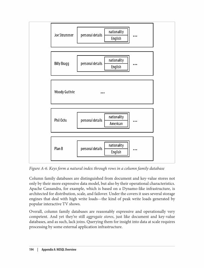
Figure A-6. Keys form a natural index through rows in a column family database

Column family databases are distinguished from document and key-value stores notonly by their more expressive data model, but also by their operational characteristics.Apache Cassandra, for example, which is based on a Dynamo-like infrastructure, isarchitected for distribution, scale, and failover. Under the covers it uses several storageengines that deal with high write loads—the kind of peak write loads generated bypopular interactive TV shows.

Overall, column family databases are reasonably expressive and operationally verycompetent. And yet they’re still aggregate stores, just like document and key-valuedatabases, and as such, lack joins. Querying them for insight into data at scale requiresprocessing by some external application infrastructure.

194 | Appendix A: NOSQL Overview

Query versus Processing in Aggregate StoresIn the preceding sections we’ve highlighted the similarities and differences between thedocument, key-value, and column family data models. On balance, the similarities havebeen greater than the differences. In fact, the similarities are so great, the three types aresometimes referred to jointly as aggregate stores. Aggregate stores persist standalonecomplex records that reflect the Domain-Driven Design notion of an aggregate.

Each aggregate store has a different storage strategy, yet they all have a great deal incommon when it comes to querying data. For simple ad hoc queries, each tends toprovide features such as indexing, simple document linking, or a query language. Formore complex queries, applications commonly identify and extract a subset of data fromthe store before piping it through some external processing infrastructure such as aMapReduce framework. This is done when the necessary deep insight cannot be gen‐erated simply by examining individual aggregates.

MapReduce, like BigTable, is another technique that comes to us from Google. The mostprevalent open source implementations of MapReduce is Apache Hadoop and its at‐tendant ecosystem.

MapReduce is a parallel programming model that splits data and operates on it in par‐allel before gathering it back together and aggregating it to provide focused information.If, for example, we wanted to use it to count how many American artists there are in arecording artists database, we’d extract all the artist records and discard the non-American ones in the map phase, and then count the remaining records in the reducephase.

Even with a lot of machines and a fast network infrastructure, MapReduce can be quitelatent. Normally, we’d use the features of the data store to provide a more focused dataset—perhaps using indexes or other ad hoc queries—and then MapReduce that smallerdataset to arrive at our answer.

Aggregate stores are not built to deal with highly connected data. We can use them forthat purpose, but we have to add code to fill in where the underlying data model leavesoff, resulting in a development experience that is far from seamless, and operationalcharacteristics that are generally speaking not very fast, particularly as the number ofhops (or “degree” of the query) increases. Aggregate stores may be good at strong datathat’s big, but they aren’t generally that great at dealing with problems that require anunderstanding of how things are connected.

Graph DatabasesA graph database is an online (“real-time”) database management system with Create,Read, Update, and Delete (CRUD) methods that expose a graph data model. Graphdatabases are generally built for use with transactional (OLTP) systems. Accordingly,

Query versus Processing in Aggregate Stores | 195

2. See Rodriguez, M.A., Neubauer, P., “The Graph Traversal Pattern,” 2010.

they are normally optimized for transactional performance, and engineered with trans‐actional integrity and operational availability in mind.

Two properties of graph databases are useful to understand when investigating graphdatabase technologies:The underlying storage

Some graph databases use native graph storage, which is optimized and designedfor storing and managing graphs. Not all graph database technologies use nativegraph storage, however. Some serialize the graph data into a relational database,object-oriented databases, or other types of general-purpose data stores.

The processing engineSome definitions of graph databases require that they be capable of index-free ad‐jacency,2 meaning that connected nodes physically “point” to each other in the da‐tabase. Here we take a slightly broader view: that any database that from the user’sperspective behaves like a graph database (i.e., exposes a graph data model throughCRUD operations), qualifies as a graph database. We do acknowledge, however, thesignificant performance advantages of index-free adjacency, and therefore use theterm native graph processing in reference to graph databases that leverage index-free adjacency.

Graph databases—in particular native ones—don’t depend heavily on indexes becausethe graph itself provides a natural adjacency index. In a native graph database, the re‐lationships attached to a node naturally provide a direct connection to other relatednodes of interest. Graph queries largely involve using this locality to traverse throughthe graph, literally chasing pointers. These operations can be carried out with extremeefficiency, traversing millions of nodes per second, in contrast to joining data througha global index, which is many orders of magnitude slower.

There are several different graph data models, including property graphs, hypergraphs,and triples.

Property GraphsA property graph has the following characteristics:

• It contains nodes and relationships• Nodes contain properties (key-value pairs)• Relationships are named and directed, and always have a start and end node• Relationships can also contain properties

196 | Appendix A: NOSQL Overview

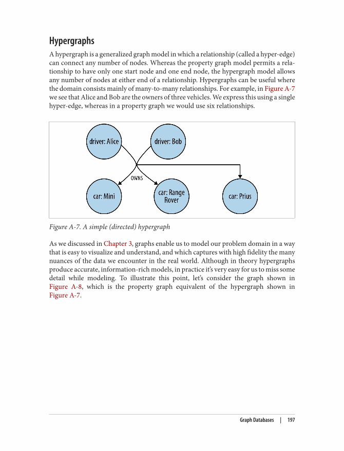
HypergraphsA hypergraph is a generalized graph model in which a relationship (called a hyper-edge)can connect any number of nodes. Whereas the property graph model permits a rela‐tionship to have only one start node and one end node, the hypergraph model allowsany number of nodes at either end of a relationship. Hypergraphs can be useful wherethe domain consists mainly of many-to-many relationships. For example, in Figure A-7we see that Alice and Bob are the owners of three vehicles. We express this using a singlehyper-edge, whereas in a property graph we would use six relationships.

Figure A-7. A simple (directed) hypergraph

As we discussed in Chapter 3, graphs enable us to model our problem domain in a waythat is easy to visualize and understand, and which captures with high fidelity the manynuances of the data we encounter in the real world. Although in theory hypergraphsproduce accurate, information-rich models, in practice it’s very easy for us to miss somedetail while modeling. To illustrate this point, let’s consider the graph shown inFigure A-8, which is the property graph equivalent of the hypergraph shown inFigure A-7.

Graph Databases | 197

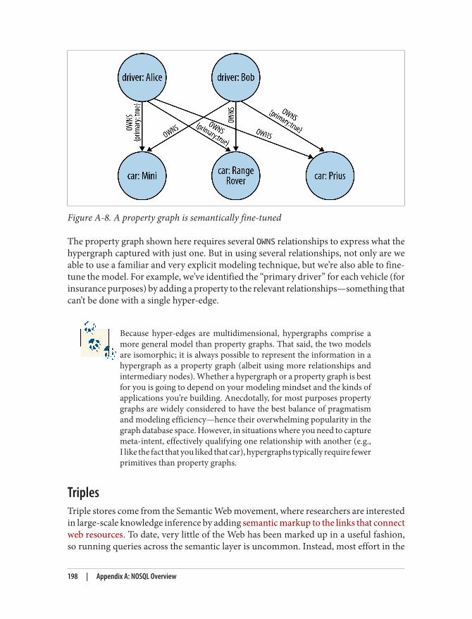
Figure A-8. A property graph is semantically fine-tuned

The property graph shown here requires several OWNS relationships to express what thehypergraph captured with just one. But in using several relationships, not only are weable to use a familiar and very explicit modeling technique, but we’re also able to fine-tune the model. For example, we’ve identified the “primary driver” for each vehicle (forinsurance purposes) by adding a property to the relevant relationships—something thatcan’t be done with a single hyper-edge.

Because hyper-edges are multidimensional, hypergraphs comprise amore general model than property graphs. That said, the two modelsare isomorphic; it is always possible to represent the information in ahypergraph as a property graph (albeit using more relationships andintermediary nodes). Whether a hypergraph or a property graph is bestfor you is going to depend on your modeling mindset and the kinds ofapplications you’re building. Anecdotally, for most purposes propertygraphs are widely considered to have the best balance of pragmatismand modeling efficiency—hence their overwhelming popularity in thegraph database space. However, in situations where you need to capturemeta-intent, effectively qualifying one relationship with another (e.g.,I like the fact that you liked that car), hypergraphs typically require fewerprimitives than property graphs.

TriplesTriple stores come from the Semantic Web movement, where researchers are interestedin large-scale knowledge inference by adding semantic markup to the links that connectweb resources. To date, very little of the Web has been marked up in a useful fashion,so running queries across the semantic layer is uncommon. Instead, most effort in the

198 | Appendix A: NOSQL Overview

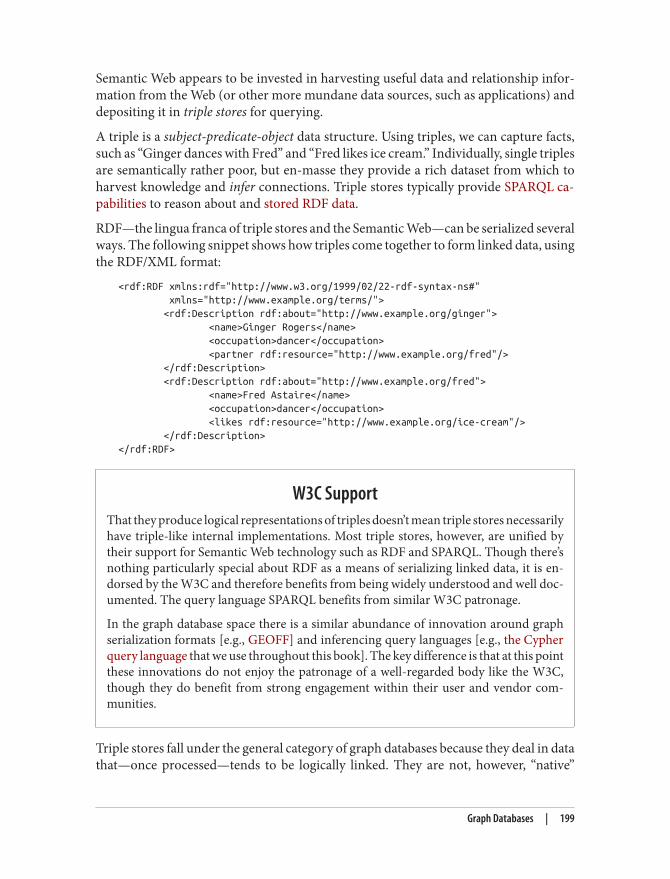
Semantic Web appears to be invested in harvesting useful data and relationship infor‐mation from the Web (or other more mundane data sources, such as applications) anddepositing it in triple stores for querying.

A triple is a subject-predicate-object data structure. Using triples, we can capture facts,such as “Ginger dances with Fred” and “Fred likes ice cream.” Individually, single triplesare semantically rather poor, but en-masse they provide a rich dataset from which toharvest knowledge and infer connections. Triple stores typically provide SPARQL ca‐pabilities to reason about and stored RDF data.

RDF—the lingua franca of triple stores and the Semantic Web—can be serialized severalways. The following snippet shows how triples come together to form linked data, usingthe RDF/XML format:

<rdf:RDF xmlns:rdf="http://www.w3.org/1999/02/22-rdf-syntax-ns#" xmlns="http://www.example.org/terms/"> <rdf:Description rdf:about="http://www.example.org/ginger"> <name>Ginger Rogers</name> <occupation>dancer</occupation> <partner rdf:resource="http://www.example.org/fred"/> </rdf:Description> <rdf:Description rdf:about="http://www.example.org/fred"> <name>Fred Astaire</name> <occupation>dancer</occupation> <likes rdf:resource="http://www.example.org/ice-cream"/> </rdf:Description></rdf:RDF>

W3C SupportThat they produce logical representations of triples doesn’t mean triple stores necessarilyhave triple-like internal implementations. Most triple stores, however, are unified bytheir support for Semantic Web technology such as RDF and SPARQL. Though there’snothing particularly special about RDF as a means of serializing linked data, it is en‐dorsed by the W3C and therefore benefits from being widely understood and well doc‐umented. The query language SPARQL benefits from similar W3C patronage.

In the graph database space there is a similar abundance of innovation around graphserialization formats [e.g., GEOFF] and inferencing query languages [e.g., the Cypherquery language that we use throughout this book]. The key difference is that at this pointthese innovations do not enjoy the patronage of a well-regarded body like the W3C,though they do benefit from strong engagement within their user and vendor com‐munities.

Triple stores fall under the general category of graph databases because they deal in datathat—once processed—tends to be logically linked. They are not, however, “native”

Graph Databases | 199

graph databases, because they do not support index-free adjacency, nor are their storageengines optimized for storing property graphs. Triple stores store triples as independentartifacts, which allows them to scale horizontally for storage, but precludes them fromrapidly traversing relationships. To perform graph queries, triple stores must createconnected structures from independent facts, which adds latency to each query. Forthese reasons, the sweet spot for a triple store is analytics, where latency is a secondaryconsideration, rather than OLTP (responsive, online transaction processing systems).

Although graph databases are designed predominantly for traversalperformance and executing graph algorithms, it is possible to use themas a backing store behind a RDF/SPARQL endpoint. For example, theBlueprints SAIL API provides an RDF interface to several graph data‐bases. In practice this implies a level of functional isomorphism betweengraph databases and triple stores. However, each store type is suited toa different kind of workload, with graph databases being optimized forgraph workloads and rapid traversals.

200 | Appendix A: NOSQL Overview

We’d like to hear your suggestions for improving our indexes. Send email to index@oreilly.com.

Index

Symbols@GET annotation, 80@POST annotation, 80@BeforeClass annotation, 86

AA* algorithm, 173access control, 104, 116–124ACID transactions, 100

BASE vs., 184–186ad hoc structures, 103aggregate store model (NOSQL databases), 15–

17column families as, 194Domain-Driven Design, 195performance with connected data, 21query vs. processing, 195

agility, 8allowed boolean property, 119Amazon, 189Amazon Web Services (AWS), 79amortized view, 36anchors, 28anonymous nodes, 46anti-patterns, 61APIs, 74, 150–154

Beans, 151Core, 151

Kernel, 151server extensions, 78Traversal, 152

applicationarchitecture, 73–82performance testing, 90server clusters, 75

application programming interface (API), 9arbitrary depth paths, 46ASCII, 46authorizations, 104

controling, 116–124availability

of data, 157–159performance and, 94

average request time, 97

Bbalanced closures, 180balanced triadic closures, 179BASE vs. ACID transactions, 184–186Beans APIs, 151best-first searches, 172bidirectional relationships, 115Big Table (Google), 192, 195Blueprints SAIL API, 200bound nodes, 45breadth-first search, 163, 174browser-based applications, 116

201

brute force processing, 17buffering writes using queues, 79building graph database applications, 63–98business responsiveness, 100

Ccache sharding, 80calculating cost, 94capacity planning, 93–97Cassandra (Apache), 192Cassovary, 7Chartrand, Gary, 1Christakis, Nicholas, 100cloud platforms, 79clustering, 75

horizontal read scaling and, 78clusters

global, 79master-slave arrangements, 157multiregion, 79recoverability and, 156

Cohn, Mike, 64collect function, 49column family stores (NOSQL), 192–194

document/key-value stores vs., 194common use cases, 100–105communication, 26

channels, 182pattern analysis, 50

Complex Event Processors, 104complex transactions, 78concurrent requests, 97CONNECT BY function (ORACLE), 14connected data

storing, 11–23walking with Riak key-values, 16

Connected: The Amazing Power of Social Net‐works and How They Shape Our Lives(Christakis and Fowler), 100

consistent hashing, 190constraining matches, 47Core API, 74, 151

Traversal framework vs., 153cost optimization criteria, 93CouchDB, 189count function, 49CREATE clauses, 30, 44CREATE UNIQUE clauses, 30, 45createDatabase() function, 85

cross-domain models, 40–50CRUD methods, 5Cypher query language, 25

as inferencing query language, 199collect function, 49Core API vs., 153count function, 49CREATE clauses, 30CREATE UNIQUE clauses, 30, 45DELETE clauses, 30DISTINCT clauses, 49embedded Neo4j and, 74FOREACH clauses, 30introduction, 27–31MATCH clauses, 29pattern-matching queries in, 23philosophy of, 27RETURN clauses, 30SET clauses, 30START clauses, 29Traversal framework vs., 153UNION clauses, 30WHERE clauses, 30WITH clauses, 30

Ddata centers, 79

managing, 103data model development, 72

test-driven, 83–89data model-first approach, 72data modeling, 25–62, 63–72databases

clusters of, 75concepts, 8life cycle of, 75refactoring, 36

dataset builders, 91Datomic, 186De Marzi, Max, 91, 92deadlocks, 155declaring information patterns to find, 46–47deductive algorithms, 101DELETE clauses, 30

server-side resources and, 80denormalization, 34, 72

of storage model, 18dependability, 154–162

availability, 157–159

202 | Index

recoverability, 156scalability, 159–162transactions, 155

depth-first search, 163designing for query-ability, 39development

cycles, 99incremental, 72iterative, 72

Dijkstra algorithm, 138efficiency, 165path-finding with, 164–172

direct relationships, 101, 115distance() method, 87DISTINCT clauses, 49distributed graph compute engine, 7Doctor Who (TV series), 152document data model, 191document stores (NOSQL), 186–189

column family stores vs., 194domain entities, 65domain model, 38Domain-Driven Design, 195domain-specific meaning, 174doubly linked lists, 146draw data, 29duplicating data, 34dynamic array store, 148dynamic stores, 148dynamic string store, 148Dynamo database (Amazon), 189

EEasley, David, 1, 174edges, 1email provenance problem, 50embedded databases, 74–78embedded Neo4j, 74encapsulation of server extensions, 78encode entities into relationships, 61encompass, 129end nodes, 4, 65end-user value, 101enterprise ready, 100entity-relationship (ER) diagram, 33ETL job, 7evolving the domain, 56–61exceptional structures, 103exclamation mark, 40

existing relationships, 56expand() functions, 135explicit transactions, 74“Extreme Performance Testing” (Jones and

Kua), 90

FFacebook, 101filesystem cache (Neo4j caching stack), 149fine-grained relationships, 119

generic vs., 65first iteration, 50first-class concepts, 72flexibility, 8, 9FlockDB (Twitter), 162FOREACH clauses, 30Fowler, James, 100

Ggarbage collection behaviors, 75

expensive, 95isolation from, 75server extensions, 78

generic vs. fine grained relationships, 65GEOFF graph serialization format, 199geospatial operations, 102

logistics and, 124–139R-tree representations of, 22

GET request, 80Giraph, 7global clusters, 79Global Post, 124

data model, 125–134goals, 25Google, 7, 192Granovetter, Mark, 174graph components, 182graph compute engines, 4, 6graph database-based solution, 73graph databases, 4, 5–6

advantages of, 8, 99APIs for, 150–154building applications with, 63–98clustered, 79connected data storage in, 18–23dependability, 154–162hypergraphs, 197internals, 141–162

Index | 203

latency, 160native processing for, 141–144NOSQL and, 195–200properties of, 5, 196property graph model, 196relationships in, 18–23scalability, 159–162triple stores, 198

graph models, 36relational databases vs., 37relational modeling compared to, 31–40vs. relational sets, 30

graph theory, 174–180predictive analysis with, 163

GraphDatabaseService instance, 88

HHA clusters, 75Hadoop (Apache), 195hardware

graph traversals and, 148sizing, 93

hashing, 190hashmap, 189heuristics, 173, 180high availability, 75high-fidelity graph structures, 72high-level cache, 149high-level view, 4–6highly connected domains, 13horizontal read scalability, 100horizontal read scaling, 75

clustering, 78horizontal scaling across clusters, 161hyper-edges, 198hypergraphs, 197

Iidentifiers, 29identifing entities/relationships, 63idiomatic queries, 158impedance mismatch, 99ImpermanentGraphDatabase instance, 85, 88in-memory caching, 149incremental development, 72index-free adjacency, 5

aggregate stores vs., 16joins and, 143

native graph processing and, 141performance advantages of, 99

indexes, named, 74indirect relationships, 101inferring social relationships, 107–110informed depth-first search, 163informed searches, 173inherited boolean property, 119init() method, 89inmemory/single machine graph compute en‐

gines, 7intermediaries, 72, 115intermediate nodes, 66Introduction to Graph Theory (Trudeau), 1Introductory Graph Theory (Chartrand), 1iterative development, 72

JJAX-RS annotated classes, 76join pain, 183join tables, 11

index-free adjacency and, 143join-intensive nature, 117Jones, Alistair, 90JSON-formatted requests, 75JVM, 74

server extensions, 78

KKernel API, 151key-value pairs, 4key-value stores (NOSQL), 189–191

column family stores vs., 194Kleinberg, Jon, 1, 174Kua, Patrick, 90

Llabel properties, 43labeling notes, 43latency, 160Least Frequently Used (LFU) cache policy, 149line-of-business applications, 101, 101linked lists, 71load balancing, 79–82, 97

optimization criteria for, 94reads/writes and, 80

local bridges, 180–182

204 | Index

local matches, 28localizing queries, 46low latency, 74low-level traversal mechanisms, 174lower parts (of graphs), 129

MMapReduce processing infrastructure, 191, 195Master Data Management (MDM), 103master-slave replication

cluster arrangements, 157clustering, 78

masters, writing to, 79MATCH clauses, 29

pattern matching with, 46route calculations and, 132variable length paths and, 39

matched path, 59migrations, 36

data modeling and, 72evolving graphs and, 56

modeling, 25data, 63–72facts as nodes, 66–69pitfalls, 50–61

MongoDB, scalability of, 161multiperiod graphs, 127multiregion clusters, 79

Nnamed indexes, 74native graph processing, 5

non-native vs., 142storage, 144–149

natural ordering, 71Neo4j, 8, 73

embedded, 74filesystem cache, 149Kernel API, 151node store file, 145property store, 147property types, 148relationship store, 145replication options in, 157storage architecture of, 144–149store files, 144sweet spot of scalability, 159transactions in, 155

Traversal API, 152Neo4j in Action (Partner and Vukotic), 20neostore.nodestore.db file (Neo4j), 145neostore.propertystore.db file (Neo4j), 148neostore.propertystore.db.arrays file (Neo4j),

148neostore.propertystore.db.index file (Neo4j),

148neostore.propertystore.db.strings file (Neo4j),

148neostore.relationshipstore.db file (Neo4j), 145network center management, 103networks, 174

elements of, 31overhead, 76

Networks, Crowds, and Markets: Reasoningabout a Highly Connected World (Easleyand Kleinberg), 1

Neubauer, P., 5, 196new relationships, 56NEXT relationships, 71No to SQL (NOSQL), 183node store file (Neo4j), 145node-to-relationship-to-node pattern match, 47nodes, 26, 64

bound, 45create, 44end, 65intermediate, 66model facts as, 66–69relate, 44represent complex value types as, 69start, 65timeline, 71

nonnative graph storage, 6normalized schemas, 34normalized structures, 72NOSQL databases, 183–200

column family stores, 192–194document stores, 186–189graph databases and, 195–200key-value stores, 189–191mimicking connected data in, 14–18quadrants of, 186stores, 25

Not Only SQL (NOSQL), 183NP Hard problem, 162number of concurrent requests, 97

Index | 205

OO-notation of performance measurements, 17object cache, 149online analytical processing (OLAP), 4online transactional processing (OLTP), 4optimization

criteria, 93performance, 95–96

organization data, 180

Ppartitioning, 80Partner, Jonas, 20path based query languages, 27pathological graph topologies, 172paths, 28

finding with Dijkstra algorithm, 164–172in graphs, 20

pattern nodes, 46Pegasus, 7per-request transactions, 76performance, 8, 94–96, 99

applications, testing, 90joins and, 117O-notation as measurement of, 17optimization criteria, 93optimization options, 95–96queries and, 89testing, 89–93

platform independence, 75POST request, 80precise algorithms, 101predictive analysis, 163predictive modeling, 174–180PREVIOUS relationships, 71processing engines, 5production deployment, 93properties, 4, 26property graph model, 26

characteristics of, 196graph theory and, 174using, 8

property index file, 148property store (Neo4j), 147purchase history, modeling with graphs, 21PUT request, 80

Qqueries

beginning, 45localizing, 46

query chaining, 49query languages, 27query performance, 99

testing, 89querying, 27–31

RR-tree (geospatial coordinate representations),

22, 102Rails, 36RAM (random access memory), 95rational layering, 178RavenDB, 185RDBMS (relational database management sys‐

tems), 25RDF (triple stores), 199read patterns, 149read vs. write traffic, 80recommendation algorithms, building, 101recovering

data, 156state of the graph, 72

redundancy, 96optimization criteria, 94

regression tests, 73relating nodes, 44relational database management systems

(RDBMS), 25relational databases

graph databases, 18–23graph model vs., 37indexes vs. document stores, 187mimicking connected data in, 11–14performance with connected data, 21

relational modeling, 33–36graphs compared to, 31–40

relational sets vs. graphs, 30relational stores, 33relationship chain, 145relationship store (Neo4j), 145

doubly linked lists in, 146relationships, 6

add new, 73building structure with, 64

206 | Index

closed sets, 65differentiating by type, 65existing, 56filtering, 134fine-grained, 65generic, 65, 66graph databases, 18–23identify, 63in NOSQL databases, 14–18in relational databases, 11–14new, 56NEXT, 71PREVIOUS, 71

relationships() method (Traversals API), 153replication, 79representative datasets, 91request

formats, 76time, 97

Resource Description Framework, 5response formats, 76

server extensions, 78response times, 90responsiveness, 99REST APIs, 75RESTful interfaces, 78RETURN clauses, 30

processing data within, 48Riak key-value store, 16

BASE properties and, 186visibility into opaque data in, 191

Rodriguez, M.A., 5, 196route calculations, 129–132

Sscalability, 159–162

capacity for, 159horizontal across a cluster, 161latency and, 160performance considerations and, 94sharding, 161throughput and, 160

scaling independence, 75scheme changes, 36Semantic Web, 198server crashes, 156server extensions, 76–78, 78, 80

APIs, 78complex transactions, 78

encapsulation, 78garbage collection behaviors, 78JVM only, 78response formats, 78testing, 87

server mode, 75, 80server vs. embedded databases, 74–78ServerBuilder, 89SET clauses, 30sharding, 161, 188

caches, 80simple directed relationships, 102simple weighted relationships, 102single named relationships, 33single relationship type, 119sizing (hardware), 93slaves, writing to, 79social cases, 100social networks as connected data, 19social recommendations, 105–116social relationships, 101Solid State Disks (SSD), 94, 149solved nodes, 165, 169SPARQI, 27spatial indexes, 102specification by example, 28, 29spinning disk, 94SQL, 23START clauses, 29

beginning queries with, 45start nodes, 4, 65Stewart, Jackie, 158storage, 100storage model, denormalizing, 18store files (Neo4j), 144storing connected data, 11–23

in NOSQL databases, 14–18mimicking with relational databases, 11–14

strong relationships, 175strong triadic closure

principle, 176property, 175

structuralbalance, 176–180change, 36symmetry, 178

subgraphs, 47, 126subject-predicate-object data structure (triple),

199

Index | 207

super columns, 192syntax, 47system of record (SOR), 7

TTalent.net, 105

data model, 106TeleGraph Communications, 116

data model, 117–119test-driven social network data model, 84–87testing, 82–93

models, 38performance, 89–93server extensions, 87with representative data, 91–93

The Graph Traversal Pattern (Rodriguez andNeubauer), 5, 196

time, 70–72timeline node, 71timeline trees, 70–71transactions, 155transactions, explicit, 74Traversal Framework, 74, 152

Core API vs., 153Cypher vs., 153

traversalsgeneric relationships and, 66hardware and, 148on fixed size records, 147operations for, 42

tree structures, 126triadic closures, 174–176triple stores, 112, 198Trudeau, Richard J., 1Twitter, 2, 162type properties, 43

Uunbalanced triadic closures, 179underlying storage, 5undirected relationships, 174

named, 33

uninformed depth-first search, 163UNION ALL, 121UNION clauses, 30, 121upper parts (of graphs), 129URI templates, 76User Stories Applied (Cohn), 64

Vvalue types, representing as nodes, 69variable

depth paths, 46length path, 39structures, 103

velocity of data, 184versioning, 72vertices, 1volume of data, 183Vukotic, Aleksa, 20

WW3C, triples support for, 199walking skeletons, 90weak relationships, 175weak social links, 182weightings, 65WHERE clauses, 30

constraining matches with, 47MATCH clauses vs., 48

whiteboard views, 26WITH clauses, 30

query chaining with, 49worst-case performance problems, 172Write Ahead Log, 155write consistency, 185writes

buffering using queues, 79read traffic vs., 80to slaves, 79to the master, 79

208 | Index

About the AuthorsIan Robinson works on research and development for future versions of the Neo4jgraph database, having previously served as Neo Technology’s Director of CustomerSuccess, where he worked with customers to design and develop graph database solu‐tions. He is a coauthor of REST in Practice (O’Reilly) and a contributor to REST: FromResearch to Practice (Springer) and Service Design Patterns (Addison-Wesley). He blogsat http://iansrobinson.com and tweets at @iansrobinson.

Dr. Jim Webber is Chief Scientist with Neo Technology, where he researches novel graphdatabases and writes open source software. Previously, Jim spent time working with biggraphs like the Web for building distributed systems, which led him to being a coauthoron the book REST in Practice (O’Reilly). Jim is active in the development community,presenting regularly around the world. His blog is located at http://jimwebber.org andhe tweets often at @jimwebber.

Emil Eifrem sketched the property graph model on a flight to Mumbai in 2000. As theCEO of Neo Technology and cofounder of the Neo4j project, he’s devoted his profes‐sional life to building and evangelizing graph databases. Committed to sustainable opensource, Emil guides Neo along a balanced path between free availability and commercialreliability. He plans to save the world with graphs and own Larry’s yacht by the end ofthe decade. Emil tweets at @emileifrem.

ColophonThe animal on the cover of Graph Databases is a European octopus (Eledone cirrhosa),also known as a lesser octopus or horned octopus. The European octopus is native tothe rocky coasts of Ireland and England, but can also be found in the Atlantic Ocean,North Sea, and Mediterranean Sea. It mainly resides in depths of 10 to 15 meters, buthas been noted as far down as 800 meters. Its identifying features include its reddish-orange color, white underside, granulations on its skin, and ovoid mantle.

The European octopus eats primarily crabs and other crustaceans. Many fisheries in theMediterranean and North Seas often unintentionally catch the European octopus. Thespecies is not subject to stock assessment or quota control, so they can be consumed.However, their population has increased in these areas in recent years due in part to theoverfishing of larger predatory fish.

The European octopus can grow to be between 12 and 40 centimeters, which it reachesin about one year. It has a relatively short life span of less than five years. Compared tothe octopus vulgaris (or common octopus), the European octopus breeds at a muchlower rate, laying on average 1,000 to 5,000 eggs.

The cover image is from Dover Pictorial Archive. The cover font is Adobe ITC Gara‐mond. The text font is Adobe Minion Pro; the heading font is Adobe Myriad Condensed;and the code font is Dalton Maag’s Ubuntu Mono.