topology-preserving mappings for data visualisation
TRANSCRIPT
5
Topology-Preserving Mappingsfor Data Visualisation
Marian Pena, Wesam Barbakh, and Colin Fyfe
Applied Computational Intelligence Research Unit,The University of Paisley, Scotland,{marian.pena,wesam.barbakh,colin.fyfe}@paisley.ac.uk
Summary. We present a family of topology preserving mappings similar to theSelf-Organizing Map (SOM) and the Generative Topographic Map (GTM) . Thesetechniques can be considered as a non-linear projection from input or data spaceto the output or latent space (usually 2D or 3D), plus a clustering technique, thatupdates the centres. A common frame based on the GTM structure can be usedwith different clustering techniques, giving new properties to the algorithms.
Thus we have the topographic product of experts (ToPoE) with the Product ofExperts substituting the Mixture of Experts of the GTM, two versions of the Har-monic Topographic Mapping (HaToM) that utilise the K-Harmonic Means (KHM)clustering, and the faster Topographic Neural Gas (ToNeGas), with the inclusionof Neural Gas in the inner loop. We also present the Inverse-weighted K-meansTopology-Preserving Map (IKToM), based on the same structure for non-linear pro-jection, that makes use of a new clustering technique called The Inverse WeightedK-Means. We apply all the algorithms to a high dimensional dataset, and compareit as well with the Self-Organizing Map, in terms of visualisation, clustering andtopology preservation.
5.1 Introduction
Topographic mappings are a class of dimensionality reduction techniques thatseek to preserve some of the structure of the data in the geometric structureof the mapping. The term “geometric structure” refers to the relationshipsbetween distances in data space and the distances in the projection to thetopographic map. In some cases all distance relationships between data pointsare important, which implies a desire for global isometry between the dataspace and the map space. Alternatively, it may only be considered importantthat local neighbourhood relationships are maintained, which is referred to astopological ordering [19]. When the topology is preserved, if the projectionsof two points are close, it is because, in the original high dimensional space,the two points were close. The closeness criterion is usually the Euclideandistance between the data patterns.
5 Topology-Preserving Mappings for Data Visualisation 133
One clear example of a topographic mapping is a Mercator projection ofthe spherical earth into two dimensions; the visualisation is improved, butsome of the distances in certain areas are distorted. These projections implya loss of some of the information which inevitably gives some inaccuracy butthey are an invaluable tool for visualisation and data analysis, e.g. for clusterdetection. Two previous works in this area have been the Self-Organizing Map(SOM) [13] and the Generative Topographic Map (GTM) [4].
Kohonen’s SOM is a neural network which creates a topology-preservingmap because there is a topological structure imposed on the nodes in thenetwork. It takes into consideration the physical arrangement of the nodes.Nodes that are “close” together are going to interact differently than nodesthat are “far” apart. The GTM was developed by Bishop et al. as a proba-bilistic version of the SOM, in order to overcome some of the problems of thismap, especially the lack of objective function.
Without taking into account the probabilistic aspects of the GTM algo-rithm, this can be considered as a projection from latent space to dataspaceto adapt the nodes to the datapoints (in this chapter called GTM structure),using K-Means with soft responsibilities as clustering technique to update theprototypes in dataspace.
In this chapter we review several topology-preserving maps that make useof the general structure of the GTM. We first review four clustering techniquesused in our algorithms in section 5.2. Then we define the common structurebased on the GTM in section 5.3.1, and develop the four topology preservingmappings in section 5.3. Finally we compare all the algorithms with the SOMin the experimental section.
5.2 Clustering Techniques
5.2.1 K-Means
K-Means clustering is an algorithm to divide or to group samples xi based onattributes/features into K groups. K is a positive integer number that has tobe given in advance. The grouping is done by minimizing the sum of squaresof distances between data and the corresponding prototypes mk.
The performance function for K-Means may be written as
J =N∑
i=1
Kmink=1
‖xi −mk‖2 , (5.1)
which we wish to minimise by moving the prototypes to the appropriate po-sitions. Note that (5.1) detects only the prototypes closest to data points andthen distributes them to give the minimum performance which determines theclustering. Any prototype which is still far from data is not utilised and does
134 M. Pena, W. Barbakh, and C. Fyfe
not enter any calculation to determine minimum performance, which may re-sult in dead prototypes, which are never appropriate for any cluster. Thusinitializing prototypes appropriately can play a big effect in K-Means.
The algorithm has the following steps:
• Step 1. Begin with a decision on the value of K = number ofclusters.
• Step 2. Put any initial partition that divides the data into Kclusters randomly.
• Step 3. Take each sample in sequence and compute its distancefrom the prototypes of each of the clusters. If a sample is notcurrently in the cluster with the closest prototype, switch thissample to that cluster and update the prototype of the clustergaining the new sample and the cluster losing the sample.
• Step 4. Repeat step 3 until convergence is achieved, that is untila pass through the training samples causes no new assignments.
Considering a general formula for the updating of the prototypes in clus-tering techniques we may write a general formula
mk ←∑N
i=1mem(mk/xi) ∗ weight(xi) ∗ xi∑Ni=1mem(mk/xi) ∗ weight(xi)
, (5.2)
where
• weight(xi) > 0 is the weighting function that defines how much influencea data point xi has in recomputing the prototype parameters mk in thenext iteration.
• mem(mk/xi) ≥ 0 with∑K
k=1mem(mk/xi) = 1 the membership functionthat decides the portion of weight(xi) ∗ xi associated with mk.
The membership and weight functions for KM are:
memKM (ml/xi) ={
1 , if l = mink ‖xi −mk‖ ,0 , otherwise ;
weightKM (xi) = 1 .(5.3)
The main problem with the K-Means algorithm is that, as with the GTM,the initialisation of the parameters can lead to a local minimum. Also thenumber of prototypes K has to be pre-determined by the user, although thisis really one of the objectives of clustering.
5.2.2 K-Harmonic Means
Harmonic Means or Harmonic Averages are defined for spaces of derivatives.For example, if you travel 1
2 of a journey at 10 km/hour and the other 12 at
20 km/hour, your total time taken is d10 + d
20 and so the average speed is
5 Topology-Preserving Mappings for Data Visualisation 135
2dd10+ d
20= 2
110 + 1
20. In general, the Harmonic Average of K values, a1, ..., aK , is
defined asHA({ai, i = 1, · · · ,K}) =
K∑Kk=1
1ak
. (5.4)
Harmonic Means were applied to the K-Means algorithm in [22] to makeK-Means a more robust algorithm. The recursive formula to update the pro-totypes is
J =N∑
i=1
K∑Kk=1
1d(xi,mk)2
; (5.5)
mk =
∑Ni=1
1d4
ik(�
Kl=1
1d2
il
)2xi∑N
i=11
d4ik(�
Kl=1
1d2
il
)2
, (5.6)
where dik is the Euclidean distance between the ith data point and the kth
prototype so that d(xi,mk) = ‖xi −mk‖.In [22] extensive simulations show that this algorithm converges to a better
solution (less prone to finding a local minimum because of poor initialisation)than both standard K-Means or a mixture of experts trained using the EMalgorithm.
Zhang subsequently developed a generalised version of the algorithm[20, 21] that includes the pth power of the L2 distance which creates a “dy-namic weighting function” that determines how data points participate in thenext iteration in the calculation of the new prototypes mk. The weight isbigger for data points further away from the prototypes, so that their partic-ipation is boosted in the next iteration. This makes the algorithm insensitiveto initialisation and also prevents one cluster from taking more than one pro-totype.
The aim of K-Harmonic Means was to improve the winner-takes-all par-titioning strategy of K-Means that gives a very strong relation between eachdatapoint and its closest prototype, so that the change in membership is notallowed until another prototype is closer. The transition of prototypes betweenareas of high density is more continuous in K- Harmonic Means due to thedistribution of associations between prototypes and datapoints.
The soft membership1 in the generalised K-Harmonic Means is
mem(mk/xi) =‖xi −mk‖−p−2∑K
k=1 ‖xi −mk‖−p−2(5.7)
allows the data points to belong partly to all prototypes.1 Soft membership means that each datapoint can belong to more than one proto-
type.
136 M. Pena, W. Barbakh, and C. Fyfe
The boosting properties for the generalised version of K-Harmonic Means(p > 2) are given by the weighting function [9]:
weight(xi) =∑K
k=1 ‖xi −mk‖−p−2
(∑K
k=1 ‖xi −mk‖−p)2, (5.8)
where the dynamic function gives a variable influence to data in clustering ina similar way to boosting [6] since the effect of any particular data point onthe re-calculation of a prototype is O(‖xi −mk‖2p−p−2), which for p > 2 hasgreatest effect for larger distances.
5.2.3 Neural Gas
Neural Gas (NG) [14] is a vector quantization technique with soft competitionbetween the units; it is called the Neural Gas algorithm because the proto-types of the clusters move around in the data space similar to the Brownianmovement of gas molecules in a closed container. In each training step, thesquared Euclidean distances
dik = ‖xi −mk‖2 = (xi −mk)T ∗ (xi −mk) (5.9)
between a randomly selected input vector xi from the training set and all pro-totypes mk are computed; the vector of these distances is d. Each prototype kis assigned a rank rk(d) = 0, ...,K − 1, where a rank of 0 indicates the closestand a rank of K-1 the most distant prototype to x. The learning rule is then
mk = mk + ε ∗ hρ[rk(d)] ∗ (x−mk) . (5.10)
The functionhρ(r) = e(−r/ρ) (5.11)
is a monotonically decreasing function of the ranking that adapts not onlythe closest prototype, but all the prototypes, with a factor exponentially de-creasing with their rank. The width of this influence is determined by theneighborhood range ρ. The learning rule is also affected by a global learningrate ε. The values of ρ and ε decrease exponentially from an initial positivevalue (ρ(0), ε(0)) to a smaller final positive value (ρ(T ), ε(T )) according to
ρ(t) = ρ(0) ∗ [ρ(T )/ρ(0)](t/T ) (5.12)
andε(t) = ε(0) ∗ [ε(T )/ε(0)](t/T ) , (5.13)
where t is the time step and T the total number of training steps, forcingmore local changes with time.
5 Topology-Preserving Mappings for Data Visualisation 137
5.2.4 Weighted K-Means
This clustering technique was introduced in [3, 2]. We might consider thefollowing performance function:
JA =N∑
i=1
K∑k=1
‖xi −mk‖2 , (5.14)
which provides a relationship between all the data points and prototypes, butit doesn’t provide useful clustering at minimum performance since
∂JA
∂mk= 0 =⇒mk =
1N
N∑i=1
xi, ∀k . (5.15)
Minimizing the performance function groups all the prototypes to the centreof the data set regardless of the initial position of the prototypes which isuseless for identification of clusters.
We wish to form a performance function with following properties:
• Minimum performance gives an intuitively ’good’ clustering.• It creates a relationship between all data points and all prototypes.
(5.14) provides an attempt to reduce the sensitivity to prototypes’ initial-ization by making a relationship between all data points and all prototypeswhile (5.1) provides an attempt to cluster data points at the minimum of theperformance function. Therefore it may seem that what we want is to combinefeatures of (5.1) and (5.14) to make a performance function such as:
J1 =N∑
i=1
[K∑
k=1
‖xi −mk‖]
Kmink=1
‖xi −mk‖2 . (5.16)
As pointed out by a reviewer, there is a potential problem with using ‖xi−mk‖rather than its square in the performance function but in practice, this hasnot been found to be a problem. We derive the clustering algorithm associatedwith this performance function by calculating the partial derivatives of (5.16)with respect to the prototypes. We call the resulting algorithm Weighted K-Means (though recognising that other weighted versions of K-Means havebeen developed in the literature). The partial derivatives are calculated as
∂J1,i
∂mr= −(xi−mr){‖xi−mr‖+2
K∑k=1
‖xi−mk‖} = −(xi−mr)air , (5.17)
when mr is the closest prototype to xi and
∂J1,i
∂mk= −(xi −mk)
‖xi −mr‖2‖xi −mk‖ = −(xi −mk)bik , (5.18)
138 M. Pena, W. Barbakh, and C. Fyfe
otherwise.We then solve this by summing over the whole data set and finding the
fixed point solution of∂J1
∂mr=
N∑i=1
∂J1,i
∂mr= 0 (5.19)
which gives a solution of
mr =
∑i∈Vr
xiair +∑
i∈Vj ,j =r xibir∑i∈Vr
air +∑
i∈Vj ,j =r bir. (5.20)
We have given extensive analysis and simulations in [3, 2] showing thatthis algorithm will cluster the data with the prototypes which are closest tothe data points being positioned in such a way that the clusters can be iden-tified. However there are some potential prototypes which are not sufficientlyresponsive to the data and so never move to identify a cluster. In fact, thesepoints move to (a weighted) prototype of the data set. This may be an advan-tage in some cases in that we can easily identify redundancy in the prototypeshowever it does waste computational resources unnecessarily.
5.2.5 The Inverse Weighted K-Means
Consider the performance algorithm
J2 =N∑
i=1
[K∑
k=1
1‖xi −mk‖p
]K
mink=1
‖xi −mk‖n . (5.21)
Let mr be the closest prototype to xi. Then
J2(xi) =
[K∑
k=1
1‖xi −mk‖p
]‖xi −mr‖n
= ‖xi −mr‖n−p +∑j =r
‖xi −mr‖n
‖xi −mk‖p. (5.22)
Therefore
∂J2(xi)∂mr
= −(n− p)(xi −mr)‖xi −mr‖n−p−2
−n(xi −mr)‖xi −mr‖n−2∑j =r
1‖xi −mk‖p
= (xi −mr)air , (5.23)∂J2(xi)∂mk
= p(xi −mk)‖xi −mr‖n
‖xi −mk‖p+2= (xi −mk)bik . (5.24)
5 Topology-Preserving Mappings for Data Visualisation 139
At convergence, E( ∂J2∂mr
) = 0 where the expectation is taken over the data set.If we denote by Vk the set of points, x for which mk is the closest, we have
∂J2
∂mr= 0 ⇐⇒
∫x∈Vr
{(n− p)(xi −mr)‖xi −mr‖n−p−2
+n(x−mr)‖x−mr‖n−2∑j =r
1‖x−mj‖p
P (x)} dx
+∑k =r
∫x∈Vk
p(x−mk)‖x−mr‖n
‖x−mk‖p+2P (x) dx = 0 , (5.25)
where P (x) is the probability measure associated with the data set. This is,in general, a very difficult set of equations to solve. However it is readilyseen that, for example, in the special case that there are the same numberof prototypes as there are data points, that one solution is to locate eachprototype at each data point (at which time ∂J2
∂mr= 0). Again solving this
over all the data set results in
mr =
∑i∈Vr
xiair +∑
i∈Vj ,j =r xibir∑i∈Vr
air +∑
i∈Vj ,j =r bir. (5.26)
From (5.25), we see that n ≥ p if the direction of the first term is to becorrect and n ≤ p + 2 to ensure stability in all parts of that equation. Inpractice, we have found that a viable algorithm may be found by using (5.24)for all prototypes (and thus never using (5.23) for the closest prototype). Wewill call this the Inverse Weighted K-Means Algorithm.
5.3 Topology Preserving Mappings
5.3.1 Generative Topographic Map
The Generative Topographic Mapping (GTM) is a non-linear latent variablemodel, intended for modeling continuous, intrinsically low-dimensional prob-ability distributions, embedded in high-dimensional spaces. It provides a prin-cipled alternative to the self-organizing map resolving many of its associatedtheoretical problems. An important, potential application of the GTM is vi-sualization of high-dimensional data. Since the GTM is non-linear, the rela-tionship between data and its visual representation may be far from trivial,but a better understanding of this relationship can be gained by computingthe so-called magnification factors [5].
There are two principal limitations of the basic GTM model. The computa-tional effort required will grow exponentially with the intrinsic dimensionalityof the density model. However, if the intended application is visualization,this will typically not be a problem. The other limitation is the initialisationof the parameters, that can lead the algorithm to a local optimum.
140 M. Pena, W. Barbakh, and C. Fyfe
The GTM defines a non-linear, parametric mapping y(x;W ) from a q-dimensional latent space to a d-dimensional data space x ∈ Rd, where nor-mally q < d. The mapping is defined to be continuous and differentiable.y(t;W ) maps every point in the latent space to a point in the data space.Since the latent space is q-dimensional, these points will be confined to aq-dimensional manifold non-linearly embedded into the d-dimensional dataspace. If we define a probability distribution over the latent space, p(t),this will induce a corresponding probability distribution into the data space.Strictly confined to the q-dimensional manifold, this distribution would be sin-gular, so it is convolved with an isotropic Gaussian noise distribution, givenby
p (x|t,W, β) =(β
2π
)d/2
exp
{−β
2
d∑d=1
(xd − yd(t,W ))2}, (5.27)
where x is a point in the data space and β denotes the noise variance. Byintegrating out the latent variable, we get the probability distribution in thedata space expressed as a function of the parameters β and W ,
p (x|W,β) =∫p (x|t,W, β) p(t) dt . (5.28)
Choosing p(t) as a set of K equally weighted delta functions on a regulargrid,
p(t) =1K
K∑k=1
δ(t− tk) , (5.29)
the integral in (5.28) becomes a sum,
p (x|W,β) =1K
K∑k=1
p (x|tk,W, β) . (5.30)
Each delta function centre maps into the centre of a Gaussian which lies in themanifold embedded in the data space. This algorithm defines a constrainedmixture of Gaussians[11, 12], since the centres of the mixture componentscan not move independently of each other, but all depend on the mappingy(t;W ). Moreover, all components of the mixture share the same variance,and the mixing coefficients are all fixed at 1/K . Given a finite set of indepen-dent and identically distributed (i.i.d.) data points, {xN
i=1}, the log-likelihoodfunction of this model is maximized by means of the Expectation Maximisa-tion algorithm with respect to the parameters of the mixture, namely W andβ. The form of the mapping y(t;w) is defined as a generalized linear regres-sion model y(t;W ) = φ(t)W where the elements of φ(t) consist of M fixedbasis functions φi(t)
Mi=1, and W is a d×M matrix.
5 Topology-Preserving Mappings for Data Visualisation 141
If we strip out the probabilistic underpinnings of the GTM method, thealgorithm can be considered as a non-linear model structure, to which a clus-tering technique is applied in data space to update the prototypes, in this casethe K-Means algorithm. In the next sections we present four algorithms thatshare this model structure.
5.3.2 Topographic Product of Experts ToPoE
Hinton [10] investigated a product of K experts with
p(xi|Θ) ∝K∏
k=1
p(xi|k) , (5.31)
where Θ is the set of current parameters in the model. Hinton notes that usingGaussians alone does not allow us to model e.g. multi-modal distributions,however the Gaussian is ideal for our purposes. Thus the base model is
p(xi|Θ) ∝K∏
k=1
(β
2π
)D2
exp(−β
2||mk − xi||2 .
). (5.32)
To fit this model to the data we can define a cost function as the negativelogarithm of the probabilities of the data so that
J =N∑
i=1
K∑k=1
β
2||mk − xi||2 . (5.33)
In [7] the Product of Gaussian model was extended by allowing latentpoints2 to have different responsibilities depending on the data point pre-sented:
p(xi|Θ) ∝K∏
k=1
(β
2π
)D2
exp(−β
2||mk − xi||2rik
), (5.34)
where rik is the responsibility of the kth expert for the data point, xi. Thusall the experts are acting in concert to create the data points but some willtake more responsibility than others. Note how crucial the responsibilities arein this model: if an expert has no responsibility for a particular data point, itis in essence saying that the data point could have a high probability as faras it is concerned. We do not allow a situation to develop where no expertaccepts responsibility for a data point; if no expert accepts responsibility fora data point, they all are given equal responsibility for that data point (seebelow).
2 The latent points, tk, generate the mk prototypes, which are the latent points’projections in data space; thus there is a bijection between the latent points andthe prototypes. mk act as prototypes of the clusters.
142 M. Pena, W. Barbakh, and C. Fyfe
We wish to maximise the likelihood of the data setX = {xi : i = 1, · · · , N}under this model. The ToPoE learning rule (5.36) is derived from the minimi-sation of − log(p(xi|Θ)) with respect to a set of parameters which generatethe mk.
We may update W either in batch mode or with online learning. To changeW in online learning, we randomly select a data point, say xi. We calculatethe current responsibility of the kth latent point for this data point,
rik =exp(−γd2ik)∑K
k=1 exp(−γd2ik), (5.35)
where dpq = ||xp −mq||, the Euclidean distance between the pth data pointand the projection of the qth latent point (through the basis functions andthen multiplied by W). If no prototypes are close to the data point (thedenominator of (5.35) is zero), we set rik = 1
K , ∀k. γ is known as the width ofthe responsibilities and is usually set to 20.
We wish to maximise (5.34) so that the data is most likely under thismodel. We do this by minimising the -log() of that probability: define m(k)
d =∑Mω=1 wωdφkω , i.e. m(k)
d is the projection of the kth latent point on the dth
dimension in data space. Similarly let x(n)d be the dth coordinate of xi. These
are used in the update rule
Δiwωd =K∑
k=1
ηφkω(x(i)d −m(k)
d )rik , (5.36)
where we have used Δi to signify the change due to the presentation of the ith
data point, xi, so that we are summing the changes due to each latent point’sresponse to the data points. Note that, for the basic model, we do not changethe Φ matrix during training at all.
5.3.3 The Harmonic Topograpic Map
The HaToM has the same structure as the GTM, withK latent points that aremapped to a feature space by M Gaussian basis functions, and then into thedata space by a matrix of weights W. In HaToM the initialisation problemsof GTM are overcomed replacing the arithmetic means of K-Means algorithmwith harmonic means, i.e. using K-Harmonic Means [22].
The basic batch algorithm often exhibited twists, such as are well-knownin the Self-organizing Map (SOM) [13], so we developed a growing methodthat prevents the mapping from developing these twists. The latent points arearranged in a square grid in a similar manner to the SOM grid.
We developed two versions of the algorithm [17]. The main structure forthe data-driven HaToM or D-HaToM is as follows:
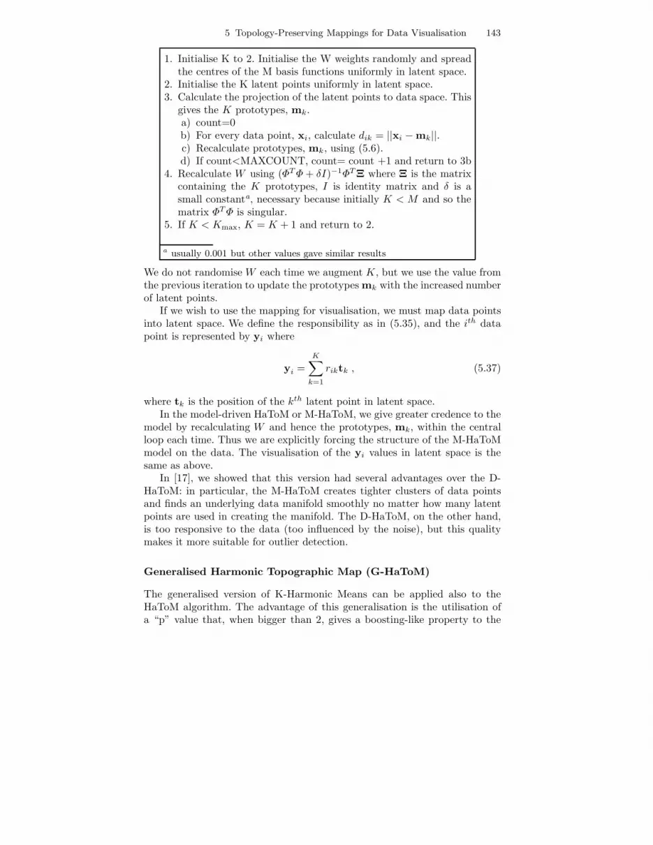
5 Topology-Preserving Mappings for Data Visualisation 143
1. Initialise K to 2. Initialise the W weights randomly and spreadthe centres of the M basis functions uniformly in latent space.
2. Initialise the K latent points uniformly in latent space.3. Calculate the projection of the latent points to data space. This
gives the K prototypes, mk.a) count=0b) For every data point, xi, calculate dik = ||xi −mk||.c) Recalculate prototypes, mk, using (5.6).d) If count<MAXCOUNT, count= count +1 and return to 3b
4. Recalculate W using (ΦTΦ+ δI)−1ΦTΞ where Ξ is the matrixcontaining the K prototypes, I is identity matrix and δ is asmall constanta, necessary because initially K < M and so thematrix ΦTΦ is singular.
5. If K < Kmax, K = K + 1 and return to 2.
a usually 0.001 but other values gave similar results
We do not randomise W each time we augment K, but we use the value fromthe previous iteration to update the prototypes mk with the increased numberof latent points.
If we wish to use the mapping for visualisation, we must map data pointsinto latent space. We define the responsibility as in (5.35), and the ith datapoint is represented by yi where
yi =K∑
k=1
riktk , (5.37)
where tk is the position of the kth latent point in latent space.In the model-driven HaToM or M-HaToM, we give greater credence to the
model by recalculating W and hence the prototypes, mk, within the centralloop each time. Thus we are explicitly forcing the structure of the M-HaToMmodel on the data. The visualisation of the yi values in latent space is thesame as above.
In [17], we showed that this version had several advantages over the D-HaToM: in particular, the M-HaToM creates tighter clusters of data pointsand finds an underlying data manifold smoothly no matter how many latentpoints are used in creating the manifold. The D-HaToM, on the other hand,is too responsive to the data (too influenced by the noise), but this qualitymakes it more suitable for outlier detection.
Generalised Harmonic Topographic Map (G-HaToM)
The generalised version of K-Harmonic Means can be applied also to theHaToM algorithm. The advantage of this generalisation is the utilisation ofa “p” value that, when bigger than 2, gives a boosting-like property to the
144 M. Pena, W. Barbakh, and C. Fyfe
updating of the prototypes. The recalculation of the prototypes in this caseis:
mk =
∑Ni=1
1dp
ik(�K
l=11
d2il
)p−2 xi∑Ni=1
1dp
ik(�
Kl=1
1d2
il
)p−2
, (5.38)
so that p determines the power of the L2 distance used in the algorithm.This generalised version of the algorithm includes the pth power of the
L2 distance which creates a “dynamic weighting function” [20] that deter-mines how data points participate in the next iteration to calculate the newprototypes mk. The weight is bigger for data points further away from theprototypes, so that their participation is boosted in the next iteration. Thismakes the algorithm insensitive to initialisation and also prevents one clusterfrom taking more than one prototype.
Some resuls for the generalised version of HaToM can be seen in [16].
5.3.4 Topographic Neural Gas
Topographic Neural Gas (ToNeGas) [18] unifies the underlying structure inGTM for topology preservation, with the technique of Neural Gas (NG). Theprototypes in data space are then clustered using the NG algorithm. Thealgorithm has been implemented based on the Neural Gas algorithm codeincluded in the SOM Toolbox for Matlab [15].
We have used the same growing method as with HaToM but have foundthat, with the NG learning, we can increment the number of latent pointsby e.g. 10 each time we augment the map whereas with HaToM, the increasecan only be one at a time to get a valid mapping. One of the advantagesof this algorithm is that the Neural Gas part is independent of the non-linear projection, thus the clustering efficiency is not limited by the topologypreservation restriction.
5.3.5 Inverse-Weighted K-Means Topology-Preserving Map
As with KHM and NG, it is possible to extend the IWKM clustering algo-rithm to provide a new algorithm for visualization and topology-preservingmappings, by using IWKM with the GTM structure. We called the new algo-rithm Inverse-weighted K-Means Topology-Preserving Map (IKToM).
5.4 Experiments
We use a dataset containing results of a high-throughput experimental tech-nology application in molecular biology (microarray data [8])3. The datasets3 http://www.ihes.fr/∼zinovyev/princmanif2006/ Dataset II - ”Three types of
bladder cancer”.
5 Topology-Preserving Mappings for Data Visualisation 145
contains only 40 observations of high-dimensional data (3036 dimensions) andthe data is drawn from three types of bladder cancer: T1, T2+ and Ta. Thedata can be used in the gene space (40 rows of 3036 variables), or in the sam-ple space (3036 rows of 40 variables), where each sample contains the profilesof the 40 genes. In these experiments we consider the first case. The datasethas been preprocessed to have zero mean; also, in the original dataset somedata was missing and these values have been filtered out.
We use the same number of neurons for all the mappings, a 12*12 grid.We used a value of p = 3 for HaToM, and p = 7 for IKToM. For several ofthe results below we have utilised the SOMtoolbox [15] with default values.
5.4.1 Projections in Latent Space
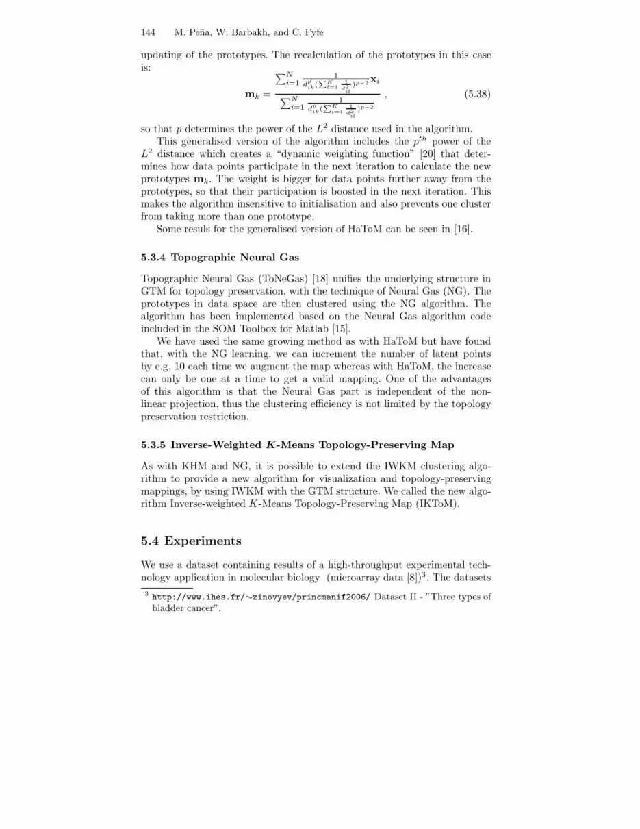
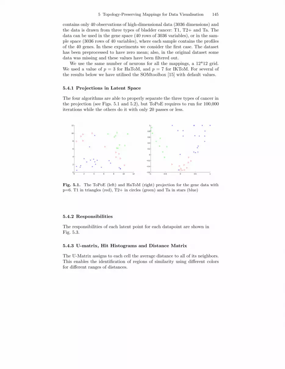
The four algorithms are able to properly separate the three types of cancer inthe projection (see Figs. 5.1 and 5.2), but ToPoE requires to run for 100,000iterations while the others do it with only 20 passes or less.
0 2 4 6 8 10 120
2
4
6
8
10
12
−1 −0.5 0 0.5 1−0.6
−0.4
−0.2
0
0.2
0.4
0.6
0.8
1
Fig. 5.1. The ToPoE (left) and HaToM (right) projection for the gene data withp=6. T1 in triangles (red), T2+ in circles (green) and Ta in stars (blue)
5.4.2 Responsibilities
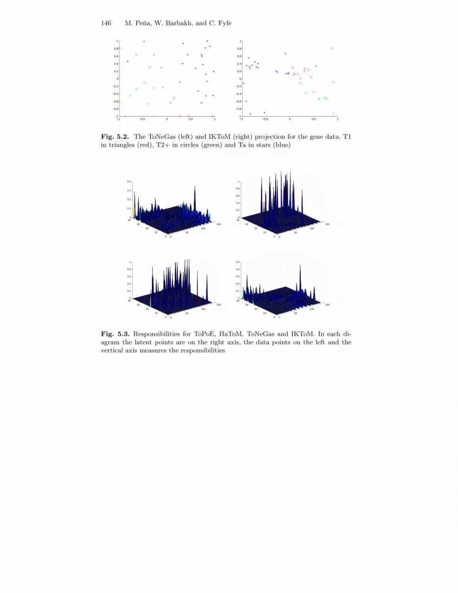
The responsibilities of each latent point for each datapoint are shown inFig. 5.3.
5.4.3 U-matrix, Hit Histograms and Distance Matrix
The U-Matrix assigns to each cell the average distance to all of its neighbors.This enables the identification of regions of similarity using different colorsfor different ranges of distances.
146 M. Pena, W. Barbakh, and C. Fyfe
−1 −0.5 0 0.5 1−1
−0.8
−0.6
−0.4
−0.2
0
0.2
0.4
0.6
0.8
1
−1 −0.5 0 0.5 1−1
−0.8
−0.6
−0.4
−0.2
0
0.2
0.4
0.6
0.8
1
Fig. 5.2. The ToNeGas (left) and IKToM (right) projection for the gene data. T1in triangles (red), T2+ in circles (green) and Ta in stars (blue)
0
50
100
150
0
10
20
30
400
0.1
0.2
0.3
0.4
0
50
100
150
0
10
20
30
400
0.2
0.4
0.6
0.8
1
0
50
100
150
0
10
20
30
400
0.2
0.4
0.6
0.8
1
0
50
100
150
0
10
20
30
400
0.1
0.2
0.3
0.4
0.5
Fig. 5.3. Responsibilities for ToPoE, HaToM, ToNeGas and IKToM. In each di-agram the latent points are on the right axis, the data points on the left and thevertical axis measures the responsibilities
5 Topology-Preserving Mappings for Data Visualisation 147
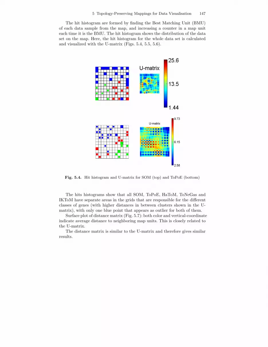
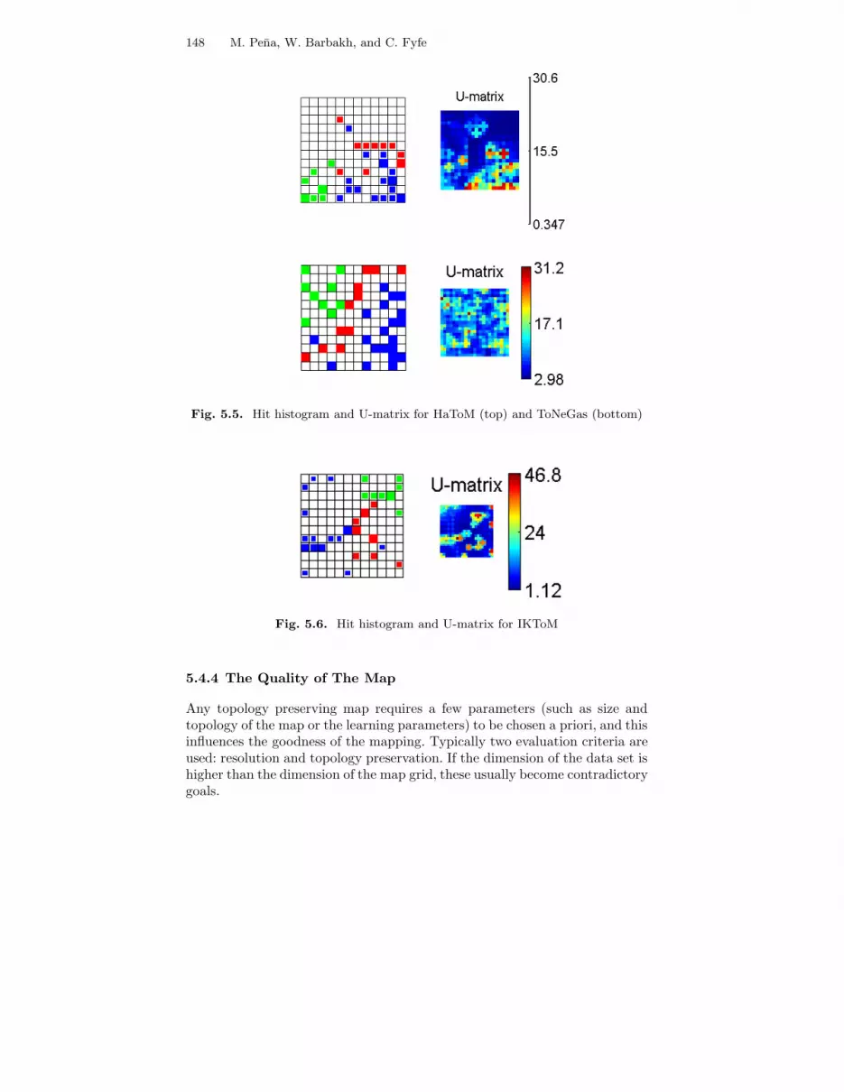
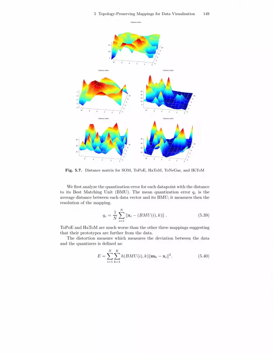
The hit histogram are formed by finding the Best Matching Unit (BMU)of each data sample from the map, and increasing a counter in a map uniteach time it is the BMU. The hit histogram shows the distribution of the dataset on the map. Here, the hit histogram for the whole data set is calculatedand visualized with the U-matrix (Figs. 5.4, 5.5, 5.6).
Fig. 5.4. Hit histogram and U-matrix for SOM (top) and ToPoE (bottom)
The hits histograms show that all SOM, ToPoE, HaToM, ToNeGas andIKToM have separate areas in the grids that are responsible for the differentclasses of genes (with higher distances in between clusters shown in the U-matrix), with only one blue point that appears as outlier for both of them.
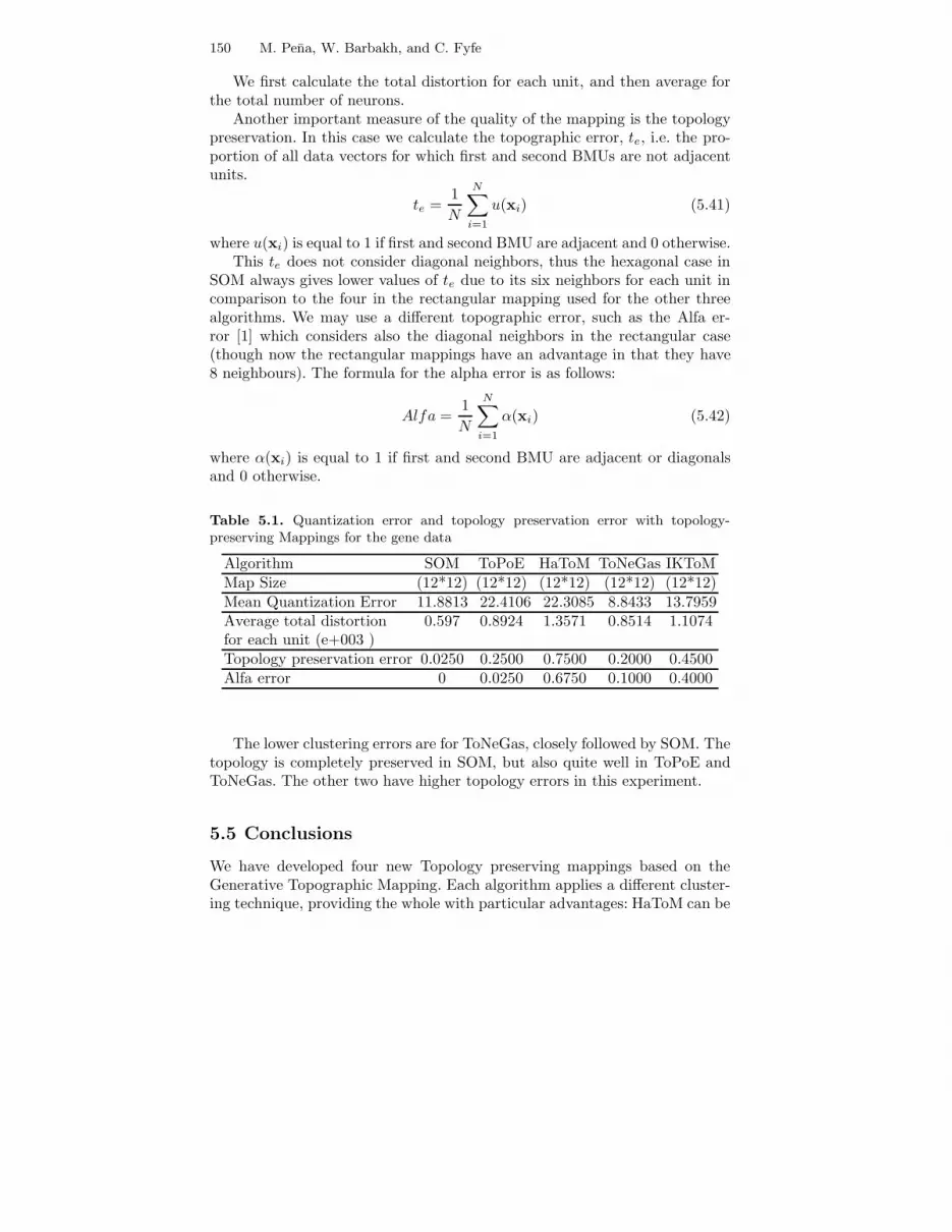
Surface plot of distance matrix (Fig. 5.7): both color and vertical-coordinateindicate average distance to neighboring map units. This is closely related tothe U-matrix.
The distance matrix is similar to the U-matrix and therefore gives similarresults.
148 M. Pena, W. Barbakh, and C. Fyfe
Fig. 5.5. Hit histogram and U-matrix for HaToM (top) and ToNeGas (bottom)
Fig. 5.6. Hit histogram and U-matrix for IKToM
5.4.4 The Quality of The Map
Any topology preserving map requires a few parameters (such as size andtopology of the map or the learning parameters) to be chosen a priori, and thisinfluences the goodness of the mapping. Typically two evaluation criteria areused: resolution and topology preservation. If the dimension of the data set ishigher than the dimension of the map grid, these usually become contradictorygoals.
5 Topology-Preserving Mappings for Data Visualisation 149
0
2
4
6
8
10
0246810
5
10
15
Distance matrix
0
2
4
6
8
10
0246810
3
4
5
6
7
Distance matrix
0
2
4
6
8
10
0246810
5
10
15
20
25
Distance matrix
0
2
4
6
8
10
02468
10
15
20
Distance matrix
0
2
4
6
8
10
0246810
10
20
30
40
Distance matrix
Fig. 5.7. Distance matrix for SOM, ToPoE, HaToM, ToNeGas, and IKToM
We first analyze the quantization error for each datapoint with the distanceto its Best Matching Unit (BMU). The mean quantization error qe is theaverage distance between each data vector and its BMU; it measures then theresolution of the mapping.
qe =1N
N∑i=1
‖xi − (BMU(i), k)‖ . (5.39)
ToPoE and HaToM are much worse than the other three mappings suggestingthat their prototypes are further from the data.
The distortion measure which measures the deviation between the dataand the quantizers is defined as:
E =N∑
i=1
K∑k=1
h(BMU(i), k)‖mk − xi‖2. (5.40)
150 M. Pena, W. Barbakh, and C. Fyfe
We first calculate the total distortion for each unit, and then average forthe total number of neurons.
Another important measure of the quality of the mapping is the topologypreservation. In this case we calculate the topographic error, te, i.e. the pro-portion of all data vectors for which first and second BMUs are not adjacentunits.
te =1N
N∑i=1
u(xi) (5.41)
where u(xi) is equal to 1 if first and second BMU are adjacent and 0 otherwise.This te does not consider diagonal neighbors, thus the hexagonal case in
SOM always gives lower values of te due to its six neighbors for each unit incomparison to the four in the rectangular mapping used for the other threealgorithms. We may use a different topographic error, such as the Alfa er-ror [1] which considers also the diagonal neighbors in the rectangular case(though now the rectangular mappings have an advantage in that they have8 neighbours). The formula for the alpha error is as follows:
Alfa =1N
N∑i=1
α(xi) (5.42)
where α(xi) is equal to 1 if first and second BMU are adjacent or diagonalsand 0 otherwise.
Table 5.1. Quantization error and topology preservation error with topology-preserving Mappings for the gene data
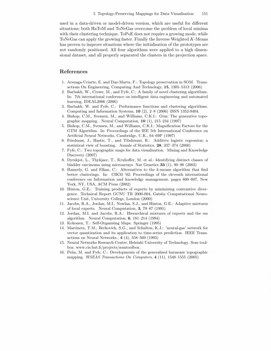
Algorithm SOM ToPoE HaToM ToNeGas IKToMMap Size (12*12) (12*12) (12*12) (12*12) (12*12)Mean Quantization Error 11.8813 22.4106 22.3085 8.8433 13.7959Average total distortion 0.597 0.8924 1.3571 0.8514 1.1074for each unit (e+003 )Topology preservation error 0.0250 0.2500 0.7500 0.2000 0.4500Alfa error 0 0.0250 0.6750 0.1000 0.4000
The lower clustering errors are for ToNeGas, closely followed by SOM. Thetopology is completely preserved in SOM, but also quite well in ToPoE andToNeGas. The other two have higher topology errors in this experiment.
5.5 Conclusions
We have developed four new Topology preserving mappings based on theGenerative Topographic Mapping. Each algorithm applies a different cluster-ing technique, providing the whole with particular advantages: HaToM can be
5 Topology-Preserving Mappings for Data Visualisation 151
used in a data-driven or model-driven version, which are useful for differentsituations; both HaToM and ToNeGas overcome the problem of local minimawith their clustering technique. ToPoE does not require a growing mode, whileToNeGas can apply the growing faster. Finally the Inverse WeightedK-Meanshas proven to improve situations where the initialisation of the prototypes arenot randomly positioned. All four algorithms were applied to a high dimen-sional dataset, and all properly separated the clusters in the projection space.
References
1. Arsuaga-Uriarte, E. and Daz-Martn, F.: Topology preservation in SOM. Trans-actions On Engineering, Computing And Technology, 15, 1305–5313 (2006)
2. Barbakh, W., Crowe, M., and Fyfe, C.: A family of novel clustering algorithms.In: 7th international conference on intelligent data engineering and automatedlearning, IDEAL2006 (2006)
3. Barbakh, W. and Fyfe, C.: Performance functions and clustering algorithms.Computing and Information Systems, 10 (2), 2–8 (2006) ISSN 1352-9404.
4. Bishop, C.M., Svensen, M., and Williams, C.K.I.: Gtm: The generative topo-graphic mapping. Neural Computation, 10 (1), 215–234 (1997)
5. Bishop, C.M., Svensen, M., and Williams, C.K.I.: Magnification Factors for theGTM Algorithm. In: Proceedings of the IEE 5th International Conference onArtificial Neural Networks, Cambridge, U.K., 64–69P (1997)
6. Friedman, J., Hastie, T., and Tibshirani, R.: Additive logistic regression: astatistical view of boosting. Annals of Statistics, 28, 337–374 (2000)
7. Fyfe, C.: Two topographic maps for data visualization. Mining and KnowledgeDiscovery (2007)
8. Dyrskjot, L., Thykjaer, T., Kruhoffer, M. et al.: Identifying distinct classes ofbladder carcinoma using microarrays. Nat Genetics 33 (1), 90–96 (2003)
9. Hamerly, G. and Elkan, C.: Alternatives to the k-means algorithm that findbetter clusterings. In: CIKM ’02: Proceedings of the eleventh internationalconference on Information and knowledge management, pages 600–607, NewYork, NY, USA, ACM Press (2002)
10. Hinton, G.E.: Training products of experts by minimizing contrastive diver-gence. Technical Report GCNU TR 2000-004, Gatsby Computational Neuro-science Unit, University College, London (2000)
11. Jacobs, R.A., Jordan, M.I., Nowlan, S.J., and Hinton, G.E.: Adaptive mixturesof local experts. Neural Computation, 3, 79–87 (1991)
12. Jordan, M.I. and Jacobs, R.A.: Hierarchical mixtures of experts and the emalgorithm. Neural Computation, 6, 181–214 (1994)
13. Kohonen, T.: Self-Organising Maps. Springer (1995)14. Martinetz, T.M., Berkovich, S.G., and Schulten, K.J.: ’neural-gas’ network for
vector quantization and its application to time-series prediction. IEEE Trans-actions on Neural Networks., 4 (4), 558–569 (1993)
15. Neural Networks Research Centre. Helsinki University of Technology. Som tool-box. www.cis.hut.fi/projects/somtoolbox.
16. Pena, M. and Fyfe, C.: Developments of the generalised harmonic topographicmapping. WSEAS Transactions On Computers, 4 (11), 1548–1555 (2005)
152 M. Pena, W. Barbakh, and C. Fyfe
17. Pena, M. and Fyfe, C.: Model- and data-driven harmonic topographic maps.WSEAS Transactions On Computers, 4 (9), 1033–1044, (2005)
18. Pena, M. and Fyfe, C.: The topographic neural gas. In: 7th International Con-ference on Intelligent Data Engineering and Automated Learning, IDEAL06.,pages 241–249 (2006)
19. Tipping, M.E.: Topographic Mappings and Feed-Forward Neural Networks.PhD thesis, The University of Aston in Birmingham (1996)
20. Zhang, B.: Generalized k-harmonic means – boosting in unsupervised learning.Technical Report HPL-2000-137, HP Laboratories, Palo Alto, October (2000)
21. Zhang, B.: Generalized k-harmonic means– dynamic weighting of data in un-supervised learning. In: First SIAM international Conference on Data Mining(2001)
22. Zhang, B., Hsu, M., and Dayal, U.: K-harmonic means - a data clustering algo-rithm. Technical Report HPL-1999-124, HP Laboratories, Palo Alto, October(1999)