HELICOPTER VIBRATION SENSOR SELECTION USING DATA VISUALISATION

Waljinder S. Gill, Ian T. Nabney

Nonlinearity and Complexity Research GroupSchool of Engineering and Applied Sciences

Aston University, Birmingham, UK

Daniel Wells

AgustaWestland Ltd.Yeovil, UK

ABSTRACTThe main objective of the project† is to enhance the alreadyeffective health-monitoring system (HUMS) for helicoptersby analysing structural vibrations to recognise different flightconditions directly from sensor information .

The goal of this paper is to develop a new method to se-lect those sensors and frequency bands that are best for de-tecting changes in flight conditions. We projected frequencyinformation to a 2-dimensional space in order to visualiseflight-condition transitions using the Generative TopographicMapping (GTM) and a variant which supports simultaneousfeature selection. We created an objective measure of theseparation between different flight conditions in the visuali-sation space by calculating the Kullback-Leibler (KL) diver-gence between Gaussian mixture models (GMMs) fitted toeach class: the higher the KL-divergence, the better the inter-class separation. To find the optimal combination of sensors,they were considered in pairs, triples and groups of four sen-sors. The sensor triples provided the best result in terms ofKL-divergence. We also found that the use of a variationaltraining algorithm for the GMMs gave more reliable results.

Index Terms— Condition monitoring, vibration, signal pro-cessing, flight condition, sensor selection, KL-divergence, data visu-alisation

1. INTRODUCTION

The main objective of the project is to enhance the HUMS forhelicopter airframes by analysing structural vibration. Pastapproaches to helicopter structural health monitoring with vi-bration data have used simple features with direct classifiersand had too many false positives to be practical. Thus thereis a necessity to develop a more sophisticated approach toachieve a significant advance in predictive maintenance forhelicopters, improving safety and reliability at less cost.

Vibration information during flight is provided by sensorslocated at different parts of the aircraft. Before structuralhealth can be inferred, features (i.e. sensors and frequency

†Thanks to EPSRC and AgustaWestland Ltd. for industrial CASE(1000239X) funding.

bands) must be chosen which provide the best informationon the state of the aircraft. These selected features will bethen used to infer the flight modes and eventually the healthand deviations from the normal state of the aircraft. The pur-pose of this paper is to propose and evaluate a novel selectionprocess. The data provided by AgustaWestland Ltd. is con-tinuously recorded vibration signals from 8 different sensorsduring flight. Each sensor measures the vibration in a partic-ular direction at chosen locations on the aircraft. During testflights, the aircraft carries out certain planned manoeuvres:our goal is to infer flight condition from the vibration dataonly, since this will be required for a practical health moni-toring system. The construction of flight state models fromvibration data is completely novel; indeed, to our knowledge,there is no prior work on models of different flight modes forhelicopters (as opposed to fixed-wing aircraft) and vibrationanalysis has mainly been used to monitor engine and trans-mission system condition, rather than airframe integrity.

Our approach is to study the (non-stationary) frequencyinformation by applying a short-time Fourier transform. Inthis way, it is possible to detect certain signatures or inten-sities at fundamental frequencies and their higher harmon-ics. Many of the key frequencies are related to the periodof either the main or tail rotor. The intensity at these fre-quencies is greater during certain periods of time and theseperiods can be associated to flight conditions and transitionperiods. Figure 1 shows the STFT and flight-state transi-tions. To understand the nature of the data and to extractmore information, the high-dimensional STFT data was pro-jected to a 2-dimensional manifold with the help of machine-learning algorithms. For this purpose we used the PrincipalComponent Analysis (PCA), Generative Topographic Map-ping (GTM) and a variant of GTM which supports simulta-neous feature selection. GTM provided better structure thanPCA in the visualisation therefore only GTM will be dis-cussed. To determine which sensors are the most useful, wecreated an objective measure of the separation between differ-ent flight conditions in the visualisation space. The remainderof this paper is structured as follows: Section 2 describes theGTM and GTM-FS (the feature-selection variant); Section 3defines the class-separation measure we have developed; Sec-

Fig. 1. STFT of sensor 7 with vertical lines at transitionsbetween flight conditions. The x and y-axis provide the time[s] and frequency [Hz] respectively.

tion 4 describes the evaluation experiments that we have per-formed; finally, Section 5 contains the conclusions of the pa-per.

2. DATA VISUALISATION ALGORITHMS

2.1. Generative Topographic Mapping

The Generative Topographic Mapping is a non-linear prob-abilistic data visualisation method that is based on a con-strained mixture of Gaussians, in which the centres of theGaussians are constrained to lie on a two-dimensional space.GTM can be viewed as an improved version of the self-organising map (SOM) algorithm [1]. In this algorithm, datavectors xn ∈ RD in the D-dimensional data space are sum-marized by a set of reference vectors in a lower-dimensionalspace (usually in a regular grid in two dimensions to aid visu-alisation). Some of the drawbacks of this algorithm are: theabsence of a cost function, lack of proof of convergence ofthe training algorithm, and the lack of density model [2].

In the GTM, a D-dimensional data point (x1, . . . , xD) isrepresented by a point in a lower-dimensional latent (hidden)-variable space t ∈ Rq (with q < D) so that it can be visualisedin a lower-dimensional space q. The mapping between the la-tent and data space is non-linear and is achieved using a for-ward mapping function x = y(t;W ) which is then invertedusing Bayes’ theorem. This function (which is usually chosento be a radial-basis function (RBF) network) is parameterisedby a network weight matrix W . The image of the latent spaceunder this function defines a q-dimensional manifold in thedata space.

To induce a density p(y|W ) in the data space, a proba-bility density p(t) is defined on the latent space. The data isnot expected to lie exactly on the q-dimensional manifold, aspherical Gaussian model with inverse variance β2 is addedin the data space so that the conditional density of the data is

given by:

p(x|t,W, β) =

{β√(2π)

}Dexp

{− (β||y(t;W )− x||)2

2

}.

(1)To get the density of the data space, the hidden space variablesmust be integrated out:

p(x|W,β) =

∫p(x|t,W, β)p(t) dt. (2)

In general, this integral would be intractable for a non-linearmodel y(t;W ). Hence p(t) is defined to be a sum of deltafunctions with centres on nodes t1, . . . , tK in the latent space:

p(t) =1

M

M∑i=1

δ(t− ti). (3)

This can be viewed as an approximation to a uniform distri-bution if the nodes are uniformly spread. Now equation (2)can be written as:

p(x|W,β) =1

K

K∑i=1

p(x|ti,W, β). (4)

This is a mixture of K Gaussians with each kernel having aconstant mixing coefficient 1/K and inverse variance β2. Theith centre is given by y(ti;W ). As these centres are depen-dent and related by the mapping, it can be viewed as a con-strained mixture model. Provided y(t;W ) defines a smoothmapping, two points t1 and t2 which are close in the latentspace are mapped to points y(t1;W ) and y(t2;W ) which areclose in the data space.

The log likelihood for a dataset containing N points thefollowing is given by:

L(W,β) =

N∑n=1

ln

{1

K

K∑i=1

p(xn|ti,W, β)

}. (5)

The parameters W and β can be found by searching forthe maximum likelihood using an expectation maximization(EM) algorithm [2]. GTM has been shown to be an effectivedata visualisation method that outperforms linear algorithmssuch as Principal Component Analysis [3].

2.2. GTM-Feature Selection

In this paper there are about 102 frequency bands for eachof the eight sensors: thus there are nearly 800 features al-together. Clearly, we would prefer to work in a lower-dimensional space while still representing all of the importantinformation in the signal so as to avoid being distracted by ir-relevant features and noise. So, to attain optimal results whilevisualizing the data, relevant features should be extractedfrom the data set. The GTM-FS model uses GTM-based

visualisation simultaneously with a measure of feature im-portance [4]. As discussed earlier in section 2, GTM uses amixture of spherical Gaussians to model the data distribution.GTM-FS associates a variation measure with each featureby using a mixture of diagonal-covariance Gaussians. Thisassumes that the features are conditionally independent. Theprobability density function is given by:

p(Xn | K, θ) =

K∑k=1

1

K

D∏d=1

p(xnd | θkd), (6)

where K is the number of mixture components, p(xnd | θkd)is the probability density function for the dth feature for thekth component, and θkd = {y(t;W ), β} with β being thecorresponding variance.

The dth feature is irrelevant if its distribution is indepen-dent of the component labels, i.e. if it follows a commondensity, denoted by q(xnd|λd) which is defined to be a diag-onal Gaussian with parameters λd. Let {Ψ = (ψ1, . . . , ψD)}be an ordered set of binary parameters such that ψd = 1 ifthe dth feature is relevant and ψd = 0 otherwise. Now themixture density is:

p(xn|Θ) =

K∑k=1

1

K

D∏d=1

[p(xnd | θkd)]ψd [q(xnd | λd)](1−ψd).

(7)where parameters: {K, θ, ψ} are summarized by Θ. Thevalue of the feature saliencies is obtained by firstly treatingthe binary values in the set Ψ as missing variables in the EMalgorithm (for structure refer to [4]) and then defining it by aprobability pd that a particular feature is relevant (ψd = 1).Cheminformatics data from was analysed in [4] using GTM,GTM-FS and SOM. In GTM and GTM-FS, the separation ofdata clusters was better while GTM-FS showed more compactresults because the irrelevant features were projected using adifferent distribution. In addition to the projection, the featuresaliency plot derived from GTM-FS showed the the featuresaliencies which gave an indication of relevant and importantfeatures whereafter it can be used in selecting features whichare above a certain high saliency.

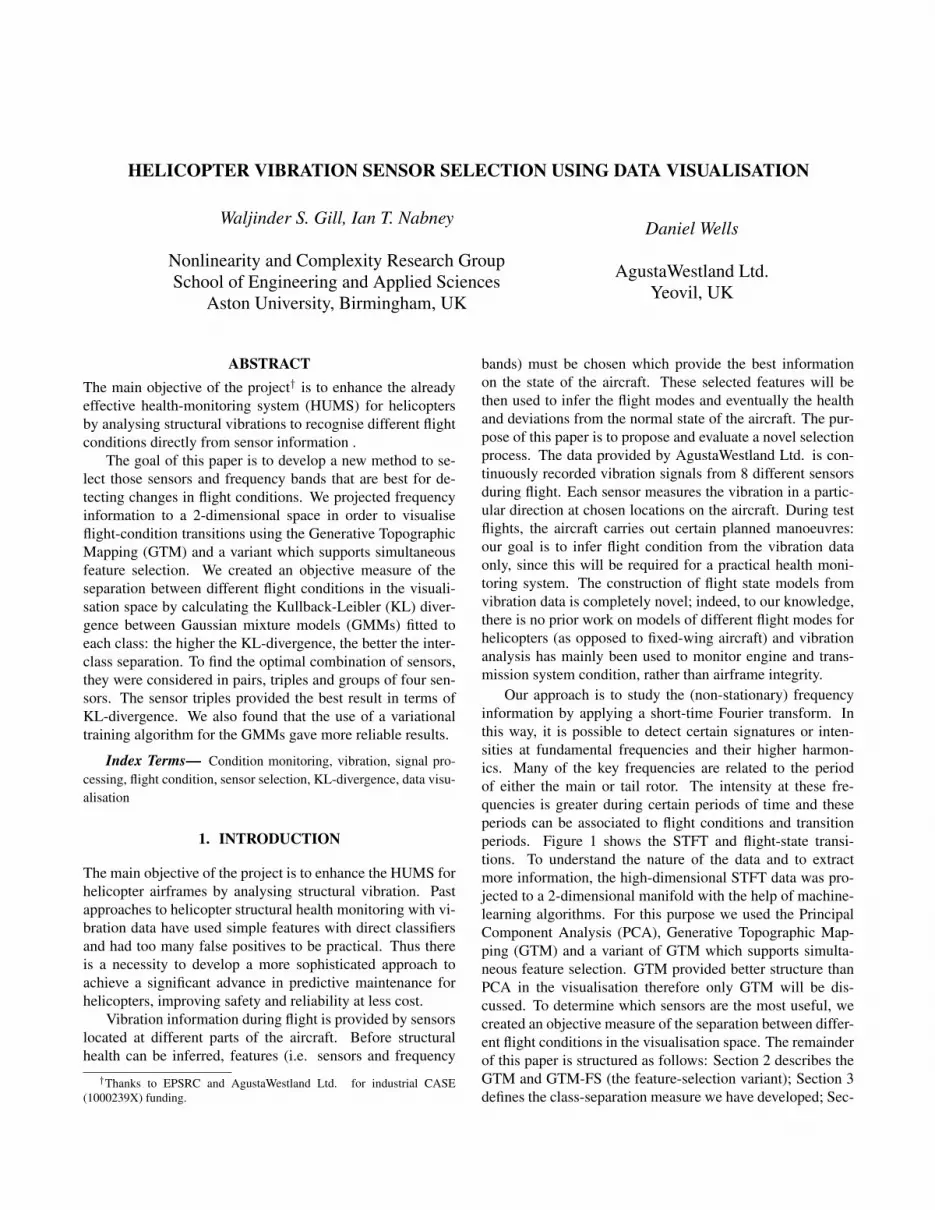
We have applied this approach to determine the most im-portant frequency bands in the STFT data. Figure 2 showsthe feature saliencies for each frequency band in the STFTdataset for a single sensor. A line is drawn at 0.7 and thefeatures which have saliencies above this line were selected.This threshold has been chosen somewhat arbitrarily, and theissue will be revisited in the future.

3. CLASS SEPARATION METRIC

The next stage of our analysis is to develop a numeric measureof the separation of classes of flight conditions. Our methodis to use the Kullback-Leibler divergence between the proba-bility distribution of each class.

Fig. 2. GTM-FS feature saliencies for frequency bands [Hz]for sensor 7 for a single flight.

3.1. Kullback-Leibler divergence

Consider visualisation plots of data drawn from several dif-ferent flight conditions. Our goal is to compare visualisa-tion plots that are based on different subsets of sensors andto choose the subset that provides the best separation (in la-tent space) between the flight conditions. We aim to do thisin latent space rather than the original data space, since theability to visualise the results helps to interpret them. In agood visualisation, each flight condition corresponds to a dis-tinct cluster of data, but to compare the plots objectively, weneed a quantitative measure of class separation. For simplic-ity, suppose that there are two clusters representing two dis-tinct classes. The Kullback-Leibler divergence is a measureof the divergence between two probability distributions P andQ [5]: P and Q can be chosen to be models of the probabil-ity density of each of the two classes. The KL-divergence isdefined as:

DKL(P ||Q) =∑n

P (xn) logP (xn)

Q(xn). (8)

If the data contains more than two classes, the KL-divergencesof all possible class pairs (in both orders, since KL-divergenceis not symmetric) are added up to calculate the overall sepa-ration. The higher the KL-divergence, the more separated theclasses are from each other.

To calculate the KL-divergence, it is necessary to fit aprobability density model to each class: we have chosen touse a mixture of Gaussians. A class label is assigned to eachpoint according to the flight condition at that time during aflight. The time points for the different conditions and thetransitions between them were provided by AgustaWestlandfor a number of test flights. We are particularly interested inthe transitions between flight conditions as these are likely toexcite unusual vibration modes. For this, a time period takenbefore and after a transition is also analysed to see if there isany transient behaviour. However, it is possible that while la-belling classes, two different labels (before or after transition)are associated with the same flight conditions data at differ-

ent time periods. To explain this, for example, suppose that atransition from 60 to 80 knots forward speed begins (class 2)at 2200 and ends at 2300 seconds and data is selected for a fewseconds before (class 1) and after (class 3). To this dataset, weadd another transition 80 to 100 kts (class 5) between 2400and 2500 seconds with a few seconds before (class 4) and af-ter (class 6) transition. So, the classes which correspond tothe same flight condition (80 kts) are 3 and 4. We want tocalculate the separation of different flight conditions ratherthan different classes with the same flight conditions. For thisreason, classes representing the same flight condition weregrouped together. We also analysed whether our results wouldgeneralise to different test flights, and so grouped togetherconditions across multiple flights. We want the members of

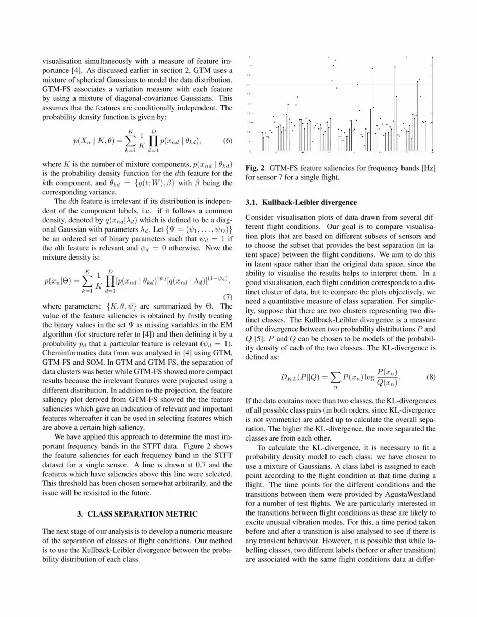
Fig. 3. GTM-FS visualisation of two flights with GMM ap-plied with a fixed number of kernels (10) for signals 1, 2 and7 (after frequency feature selection). Markers with the samecolour are drawn from a single flight condition group. Eachellipse denotes a kernel of the GMM used to fit a cluster.Ellipses with dashed boundaries have a small mixing coef-ficient. KL-Divergence was 338.

the groups to lie as close as possible to each other: Figure 3shows a typical result. The plot contains classes representing60 kts forward speed, 60–80 kts transition, 80 kts forward,80–100 kts transition, and finally 100 kts. These classes arespread across the visualisation space in a logical order (thisis easier to see with the visualisation tool than in the plots inthis paper). This figure shows that our approach can be madeto work effectively. However, there is a difficulty. We havechosen the number of kernels in the GMM arbitrarily (whichmay cause over-fitting), and also the EM algorithm is suscep-

tible to being trapped in local minima. In the next sectionwe discuss how variational Bayesian methods can be used toaddress both of these issues.

3.2. Variational mixture of Gaussians

To make the calculation of the KL-divergence more robust,we modified the algorithm that we used to fit the densitymodel to each class. A variational Bayesian Gaussian Mix-ture model automatically adjusts the number of componentsto avoid over-fitting [6]. The result of applying this model

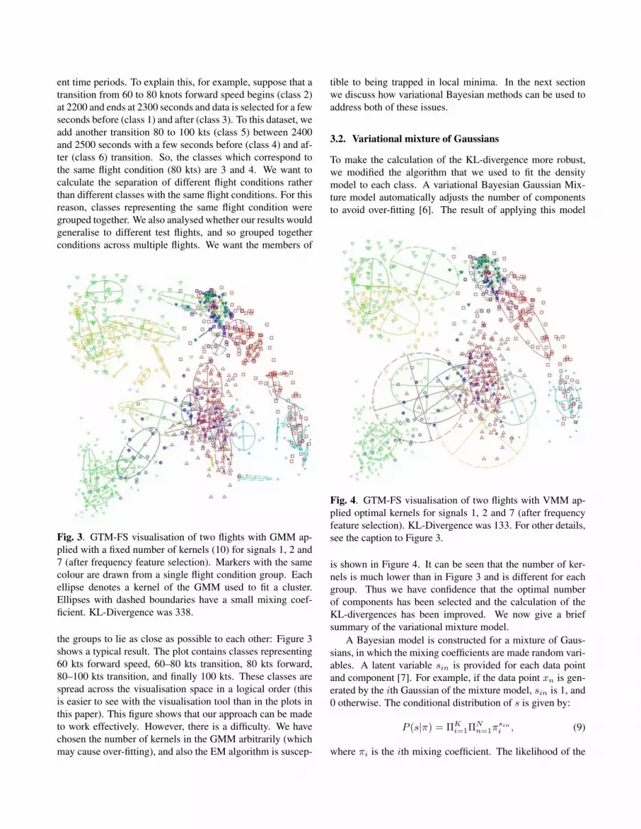
Fig. 4. GTM-FS visualisation of two flights with VMM ap-plied optimal kernels for signals 1, 2 and 7 (after frequencyfeature selection). KL-Divergence was 133. For other details,see the caption to Figure 3.

is shown in Figure 4. It can be seen that the number of ker-nels is much lower than in Figure 3 and is different for eachgroup. Thus we have confidence that the optimal numberof components has been selected and the calculation of theKL-divergences has been improved. We now give a briefsummary of the variational mixture model.

A Bayesian model is constructed for a mixture of Gaus-sians, in which the mixing coefficients are made random vari-ables. A latent variable sin is provided for each data pointand component [7]. For example, if the data point xn is gen-erated by the ith Gaussian of the mixture model, sin is 1, and0 otherwise. The conditional distribution of s is given by:

P (s|π) = ΠKi=1ΠN

n=1πsini , (9)

where πi is the ith mixing coefficient. The likelihood of the

model is given by:

P (W |µ,Σ) = ΠKi=1ΠN

n=1N (xn|µi,Σ−1i )sin , (10)

where µi, Σi are the means and inverse covariance matri-ces of the ith Gaussian component. In order to complete theBayesian model, priors are needed over the latent space vari-able s, means and inverse covariance matrices.

P (µ) = ΠKi=1N (µi|0, αI), (11)

where N is the normal distribution, α is a small valued fixedparameter which relates to prior over µ and I is identity ma-trix.

P (Σ) = ΠKi=1W(Σi|v, V −1), (12)

where W is the Wishart distribution, v is the number of de-grees of freedom and V is theD×D scale matrix for the priorover Σ.

P (s) = PiKi=1ΠNn=1π

sini . (13)

The likelihood of the dataset D is given by:

P (D, θ) = ΠNn=1P (xn|µ,Σ, s)P (s)P (µ)P (Σ). (14)

All the parameters (s, µ, Σ) are summarized as θ. In orderto select a Bayesian model, θ has to be integrated out. Thedistribution function of the data P (D) (the evidence) is thenmaximized with respect to the mixing coefficients πi. Afterthe maximization, any mixture coefficients that degenerate to0 are removed and others are kept.

Unfortunately, integrating the likelihood with respect to θis not tractable. For this reason a variational approximationapproach has been developed [7]. The assumption is madethat the variational distribution can be factorized over eachgroup of parameters.

Q(s, π, µ,Σ) = Qs(s)Qµ(µ)QΣ(Σ). (15)

Now the distribution Q that best approximates likelihoodP (D, θ) can be computed as follows:

Qs(s) = ΠKi=1ΠN

n=1psinin , (16)

where pin are the variational parameters of theQ distribution.

Qµ(µ) = ΠKi=1N (µi|m(i)

µ , |Σ(i)−1µ ), (17)

QΣ(Σ) = ΠKi=1W(Σi|v(i)

Σ , V(i)−1Σ ), (18)

Once Q has been calculated we can approximate the lowerbound of the log-likelihood. The mixing coefficients thatmaximize the lower bound are given by:

πi =1

N

N∑n=1

pin. (19)

In order to get the optimal number of components in a mix-ture, the variational approximation and the update of the mix-ing coefficients that maximize the lower bound are iteratedalternately until the lower bound converges.

4. RESULTS

We evaluated our approach to sensor selection by applying itto a dataset that combined two test flights. The aim of theexperiment was to select the best group of sensors to modelflight state and transitions. We started by computing the KL-divergences for visualisation plots based on each sensor in-dividually. We then combined the best four senors in pairsand repeated the measurement for each pair. This continuedfor triples and all four top sensors. This greedy search can

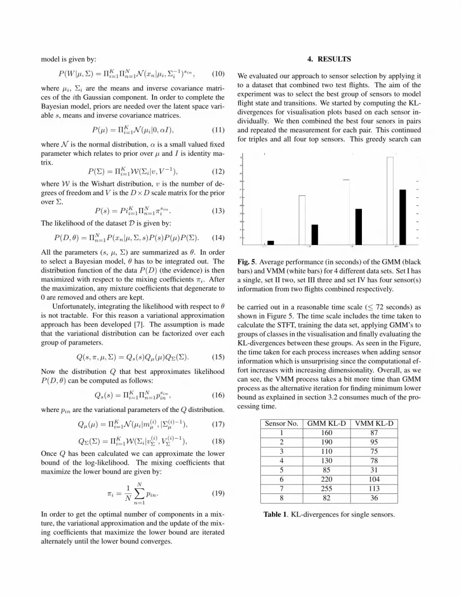
Fig. 5. Average performance (in seconds) of the GMM (blackbars) and VMM (white bars) for 4 different data sets. Set I hasa single, set II two, set III three and set IV has four sensor(s)information from two flights combined respectively.

be carried out in a reasonable time scale (≤ 72 seconds) asshown in Figure 5. The time scale includes the time taken tocalculate the STFT, training the data set, applying GMM’s togroups of classes in the visualisation and finally evaluating theKL-divergences between these groups. As seen in the Figure,the time taken for each process increases when adding sensorinformation which is unsurprising since the computational ef-fort increases with increasing dimensionality. Overall, as wecan see, the VMM process takes a bit more time than GMMprocess as the alternative iteration for finding minimum lowerbound as explained in section 3.2 consumes much of the pro-cessing time.

Sensor No. GMM KL-D VMM KL-D1 160 872 190 953 110 754 130 785 85 316 220 1047 255 1138 82 36

Table 1. KL-divergences for single sensors.

Sensor pair GMM KL-D VMM KL-D1-2 265 1201-6 225 1351-7 215 1272-6 185 1182-7 300 1226-7 198 171

Table 2. KL-divergences for sensor pairs.

Sensor triples GMM KL-D VMM KL-D1-2-6 265 1221-2-7 338 1331-6-7 288 1772-6-7 312 154

Table 3. KL-divergences for sensor triples.

Sensors GMM KL-D VMM KL-D1-2-6-7 317 173

Table 4. KL-divergences for 4 sensors together.

Table 1 shows the KL-divergences for each individualsensor. The top four sensors were: 1, 2, 6 and 7. The KL-divergences for these sensor pairs and triples are shown inTable 2 and 3 respectively. From the analysis, it has beenfound that the group of three sensors (triples) from the topselected provide the best KL-divergence when compared toindividual, pairs or 4 sensors together. The four selected sen-sors provide the best KL-divergence results as compared topairs and triples with other sensors (3, 4, 5 and 8). To confirmthis, KL-divergences of all possible sensor pairs and tripleshave been computed for single and muliple flights. It wasfound that no pair or triple had a higher KL-divergence thanthe selected four sensors.

The values of the KL-divergence computed using GMMand VMM are different: this is caused by the fact that theVMM typically uses fewer components in the mixture model.More fundamentally, it is noticeable that the sensor impor-tances using both methods for computing KL-divergence arenot the same. To investigate this, we carried out experimentsto calculate the KL-divergence with both the GMM and theVMM. For a given visualisation plot, each method was run tentimes with different initial conditions. We found that the KL-divergence values for the VMM were much more consistentover these replicates than for the GMM. The variability of theKL-divergences of Gaussian mixture model is higher (stan-dard deviation ∼ 30-50) as compared to variational Gaussianmixture (standard deviation ∼ 2-5). For this reason, the sen-sor triple 1, 6 and 7 will be used for further analysis.

5. CONCLUSIONS

We have developed a feature selection procedure that isbased on visualisation of data, feature saliency (for selectingfrequency bands for a single sensor), and a KL-divergencemetric to compare class separation. The selection proce-dure showed that sensor triples gave the best possible KL-divergences for two flights combined indicating better in-ference for flight conditions, maneuvers and health of theaircraft. This information is valuable since it enables usto work in a much lower-dimensional feature space which ismore compuational efficient than the original data (which, us-ing all frequency bands and sensors, would have been nearly800-dimensional) .

Future work on this methodology will include a more sys-tematic approach to setting the threshold for feature saliency,evaluation on a larger range of flight conditions and testflights, and consideration of generalisation to unseen flightdata.

6. REFERENCES

[1] Teuvo Kohonen, “Neurocomputing: foundations of re-search,” chapter Self-organized formation of topolog-ically correct feature maps, pp. 509–521. MIT Press,Cambridge, MA, USA, 1988.

[2] Christopher M. Bishop, Markus Svensn, and ChristopherK. I. Williams, “GTM: The generative topographic map-ping,” Neural Computation, vol. 10, pp. 215–234, 1998.

[3] Fabian Lopez-Vallejo, Adel Nefzi, Andreas Bender, JohnR. Owen, Ian T. Nabney, Richard A. Houghten, and JoseL. Medina Medina-Franco, “Increased diversity of li-braries from libraries: chemoinformatic analysis of bis-diazacyclic libraries,” Chemical biology and drug design,vol. 77, no. 5, pp. 328–342, 2011.

[4] Dharmesh M. Maniyar and Ian T. Nabney, “Data visu-alization with simultaneous feature selection,” in Com-putational Intelligence and Bioinformatics and Computa-tional Biology, 2006. CIBCB ’06. 2006 IEEE Symposiumon, Sept. 2006, pp. 1–8.

[5] Thomas M. Cover and Joy A. Thomas, Elements of In-formation Theory, Wiley-Interscience, 2006.

[6] Christopher M. Bishop, Pattern Recognition and Ma-chine Learning, Springer, 2006.

[7] Christopher M. Bishop and A. Corduneanu, “Variationalbayesian model selection for mixture distribution,” Arti-ficial Intelligence and Statistics, pp. 27–34, 2001.