Small-Scale HelicopterAutomatic Autorotation

Modeling, Guidance, and Control

Small-Scale HelicopterAutomatic Autorotation

Modeling, Guidance, and Control

Proefschrift

ter verkrijging van de graad van doctoraan de Technische Universiteit Delft,

op gezag van de Rector Magnificus prof. ir. K.C.A.M. Luyben,voorzitter van het College voor Promoties,

in het openbaar te verdedigen op vrijdag 18 september 2015 om10:00 uur

door

Skander Taamallah

Master of Science in Aeronautics & Astronautics, Stanford University, U.S.A.,Diplôme d’Ingénieur en Génie Electrique, I.N.S.A. Toulouse, France,

geboren te Tunis, Tunesië.

Dit proefschrift is goedgekeurd door de

promotor: prof. dr. ir. P.M.J. Van den Hofpromotor: prof. dr. ir. X. Bombois

Samenstelling promotiecommissie:

Rector Magnificus, voorzitterProf. dr. ir. P.M.J. Van den Hof Technische Universiteit DelftProf. dr. ir. X. Bombois CNRS, Ecole Centrale de Lyon, Frankrijk

Onafhankelijke leden:Prof. dr. R. Babuska Technische Universiteit DelftProf. dr. J. Bokor Hungarian Academy of Sciences, HongarijeProf. dr. ir. M. Mulder Technische Universiteit DelftProf. dr. H. Nijmeijer Technische Universiteit EindhovenProf. dr. G. Scorletti Ecole Centrale de Lyon, Frankrijk

The research described in this thesis has been supported by the National Aerospace Labo-ratory (NLR), Amsterdam, The Netherlands.

Keywords: Unmanned Aerial Vehicles, Small-Scale Helicopter, Automatic Autoro-tation, Trajectory Planning, Trajectory Tracking, LinearParameter Vary-ing Systems.

Printed by: Ipskamp Drukkers.

Front& Back: View of a small-scale unmanned helicopter.

Copyright c© 2015 by S. Taamallah

ISBN/EAN: 978-94-6259-831-7

An electronic version of this dissertation is available athttp://repository.tudelft.nl/.

Considerate la vostra origine: non siete nati per vivere come bruti, ma per praticare lavirtù e apprendere la conoscenza.

Dante AlighieriDivina Commedia, Inferno, Canto XXVI

Contents

Summary xi

Samenvatting xiii

Preface xv

1 Introduction 11.1 Unmanned Aerial Vehicles (UAVs). . . . . . . . . . . . . . . . . . . . . 2

1.1.1 Candidate applications. . . . . . . . . . . . . . . . . . . . . . . 31.1.2 Markets . . . . . . . . . . . . . . . . . . . . . . . . . . . . . . 31.1.3 Development and acquisition programs. . . . . . . . . . . . . . . 31.1.4 Airworthiness and safety aspects. . . . . . . . . . . . . . . . . . 4

1.2 The helicopter. . . . . . . . . . . . . . . . . . . . . . . . . . . . . . . 51.2.1 Helicopter mini-UAVs . . . . . . . . . . . . . . . . . . . . . . . 71.2.2 Helicopter main rotor hubs. . . . . . . . . . . . . . . . . . . . . 8

1.3 Helicopter autorotation. . . . . . . . . . . . . . . . . . . . . . . . . . . 81.3.1 Autorotation: a three-phases maneuver. . . . . . . . . . . . . . . 10

1.4 Problem formulation. . . . . . . . . . . . . . . . . . . . . . . . . . . . 111.5 Analysis of available options. . . . . . . . . . . . . . . . . . . . . . . . 11

1.5.1 Model-free versus model-based options. . . . . . . . . . . . . . . 121.5.2 Integrated versus segregated options. . . . . . . . . . . . . . . . 131.5.3 Summary of previous analysis. . . . . . . . . . . . . . . . . . . 16

1.6 Research objectives and limitations. . . . . . . . . . . . . . . . . . . . . 171.7 Solution strategy. . . . . . . . . . . . . . . . . . . . . . . . . . . . . . 18

1.7.1 Modeling of the nonlinear helicopter dynamics. . . . . . . . . . . 191.7.2 The Trajectory Planning (TP). . . . . . . . . . . . . . . . . . . . 211.7.3 The Trajectory Tracking (TT). . . . . . . . . . . . . . . . . . . . 24

1.8 Overview of this thesis. . . . . . . . . . . . . . . . . . . . . . . . . . . 251.8.1 Contributions. . . . . . . . . . . . . . . . . . . . . . . . . . . . 27

References. . . . . . . . . . . . . . . . . . . . . . . . . . . . . . . . . . . . 28

2 High-Order Modeling of the Helicopter Dynamics 472.1 Introduction . . . . . . . . . . . . . . . . . . . . . . . . . . . . . . . . 482.2 Helicopter modeling: general overview. . . . . . . . . . . . . . . . . . . 492.3 Model evaluation and validation. . . . . . . . . . . . . . . . . . . . . . 51

2.3.1 Trim results . . . . . . . . . . . . . . . . . . . . . . . . . . . . 522.3.2 Dynamic results. . . . . . . . . . . . . . . . . . . . . . . . . . 61

vii

viii Contents

2.4 Preliminary analysis of the rigid-body dynamics. . . . . . . . . . . . . . 642.4.1 Linearizing the nonlinear helicopter model. . . . . . . . . . . . . 652.4.2 The engine ON case. . . . . . . . . . . . . . . . . . . . . . . . 692.4.3 The engine OFF case. . . . . . . . . . . . . . . . . . . . . . . . 70

2.5 Conclusion. . . . . . . . . . . . . . . . . . . . . . . . . . . . . . . . . 702.6 Appendix A: Nomenclature. . . . . . . . . . . . . . . . . . . . . . . . . 712.7 Appendix B: Frames. . . . . . . . . . . . . . . . . . . . . . . . . . . . 742.8 Appendix C: Rigid-body equations of motion. . . . . . . . . . . . . . . . 762.9 Appendix D: Main rotor . . . . . . . . . . . . . . . . . . . . . . . . . . 782.10 Appendix E: Tail rotor. . . . . . . . . . . . . . . . . . . . . . . . . . . 952.11 Appendix F: Fuselage. . . . . . . . . . . . . . . . . . . . . . . . . . . 972.12 Appendix G: Vertical and horizontal tails. . . . . . . . . . . . . . . . . . 982.13 Appendix H: Problem data. . . . . . . . . . . . . . . . . . . . . . . . . 99References. . . . . . . . . . . . . . . . . . . . . . . . . . . . . . . . . . . . 101

3 Off-line Trajectory Planning 1073.1 Introduction . . . . . . . . . . . . . . . . . . . . . . . . . . . . . . . . 1083.2 Problem statement. . . . . . . . . . . . . . . . . . . . . . . . . . . . . 109

3.2.1 Cost functional. . . . . . . . . . . . . . . . . . . . . . . . . . . 1103.2.2 Boundary conditions and trajectory constraints. . . . . . . . . . . 111

3.3 The optimal control problem. . . . . . . . . . . . . . . . . . . . . . . . 1113.4 Direct optimal control and discretization methods. . . . . . . . . . . . . . 1133.5 Simulation results. . . . . . . . . . . . . . . . . . . . . . . . . . . . . 116

3.5.1 The Height-Velocity (H-V) diagram. . . . . . . . . . . . . . . . 1173.5.2 Evaluation of cost functionals. . . . . . . . . . . . . . . . . . . . 1183.5.3 Optimal autorotations: effect of initial conditions. . . . . . . . . . 121

3.6 Conclusion. . . . . . . . . . . . . . . . . . . . . . . . . . . . . . . . . 122References. . . . . . . . . . . . . . . . . . . . . . . . . . . . . . . . . . . . 132

4 On-line Trajectory Planning and Tracking: System Design 1414.1 Introduction . . . . . . . . . . . . . . . . . . . . . . . . . . . . . . . . 142

4.1.1 Main contributions. . . . . . . . . . . . . . . . . . . . . . . . . 1434.2 General control architecture. . . . . . . . . . . . . . . . . . . . . . . . 1444.3 Flatness-based Trajectory Planning (TP). . . . . . . . . . . . . . . . . . 144

4.3.1 Flat outputs . . . . . . . . . . . . . . . . . . . . . . . . . . . . 1464.3.2 Flat output parametrization. . . . . . . . . . . . . . . . . . . . . 1474.3.3 Optimal trajectory planning for the engine OFF case. . . . . . . . 147

4.4 Robust control based Trajectory Tracking (TT). . . . . . . . . . . . . . . 1514.4.1 Linear multivariableµ control design. . . . . . . . . . . . . . . . 1534.4.2 Controller assessment metrics. . . . . . . . . . . . . . . . . . . 155

4.5 Design of the engine OFF inner-loop controller. . . . . . . . . . . . . . . 1574.5.1 Choice of nominal plant model for the inner-loop control design . . 1574.5.2 Selection of weights. . . . . . . . . . . . . . . . . . . . . . . . 1584.5.3 Controller synthesis and analysis. . . . . . . . . . . . . . . . . . 159

Contents ix

4.6 Design of the engine OFF outer-loop controller. . . . . . . . . . . . . . . 1624.6.1 Selection of weights. . . . . . . . . . . . . . . . . . . . . . . . 1624.6.2 Controller synthesis and analysis. . . . . . . . . . . . . . . . . . 1634.6.3 Adapting the engine OFF outer-loop controller. . . . . . . . . . . 165

4.7 Conclusion. . . . . . . . . . . . . . . . . . . . . . . . . . . . . . . . . 1654.8 Appendix A: Optimal trajectory planning for the engine ON case. . . . . . 1664.9 Appendix B: Design of the inner-loop controller for the engine ON case . . 1674.10 Appendix C: Design of the outer-loop controller for the engine ON case . . 1704.11 Appendix D: Maximum roll (or pitch) angle for safe (i.e. successful) land-

ing . . . . . . . . . . . . . . . . . . . . . . . . . . . . . . . . . . . . . 1744.12 Appendix E: Proof of Lemma 1. . . . . . . . . . . . . . . . . . . . . . . 176References. . . . . . . . . . . . . . . . . . . . . . . . . . . . . . . . . . . . 178

5 On-line Trajectory Planning and Tracking: Simulation Results 1835.1 Introduction . . . . . . . . . . . . . . . . . . . . . . . . . . . . . . . . 1845.2 Setting up the trajectory planning for the engine ON cases. . . . . . . . . 1845.3 Setting up the trajectory planning for the engine OFF cases. . . . . . . . . 1875.4 Discussion of closed-loop simulation results for the engine ON cases. . . . 1895.5 Discussion of closed-loop simulation results for the engine OFF cases. . . 192

5.5.1 System energy: the engine ON versus engine OFF cases. . . . . . 1935.5.2 Closed-loop response with respect to sensors noise and winddis-

turbance. . . . . . . . . . . . . . . . . . . . . . . . . . . . . . 1945.6 Conclusion. . . . . . . . . . . . . . . . . . . . . . . . . . . . . . . . . 194References. . . . . . . . . . . . . . . . . . . . . . . . . . . . . . . . . . . . 215

6 Affine LPV Modeling 2176.1 Introduction . . . . . . . . . . . . . . . . . . . . . . . . . . . . . . . . 2186.2 Problem statement. . . . . . . . . . . . . . . . . . . . . . . . . . . . . 2216.3 Step 1: Identifying the central model (A0, B0) . . . . . . . . . . . . . . . . 2276.4 Step 2: Identifying the basis functionsLs,RsSs=1 . . . . . . . . . . . . . . 2276.5 Step 3: Identifying the basis functionsTw,ZwWw=1 . . . . . . . . . . . . . 228

6.6 Step 4.1: Identifying the parameters

ηiNi=1 . . . . . . . . . . . . . . . . . 229

6.7 Step 4.2: Obtaining the mappingη(x(t), u(t)) . . . . . . . . . . . . . . . . 231

6.8 Steps 5.1 and 5.2: Identifying the parameters

ζiNi=1 and obtaining the map-

pingζ(x(t), u(t)) . . . . . . . . . . . . . . . . . . . . . . . . . . . . . . 2316.9 Application to the modeling and control of a modified pointmass pendulum. 232

6.9.1 Building the LPV models. . . . . . . . . . . . . . . . . . . . . . 2336.9.2 Open-Loop analysis. . . . . . . . . . . . . . . . . . . . . . . . 2356.9.3 Closed-Loop analysis. . . . . . . . . . . . . . . . . . . . . . . . 238

6.10 Conclusion. . . . . . . . . . . . . . . . . . . . . . . . . . . . . . . . . 2476.11 Appendix A: Kalman-Yakubovich-Popov(KYP) Lemma with spectral mask

constraints. . . . . . . . . . . . . . . . . . . . . . . . . . . . . . . . . 2486.11.1 Preliminaries. . . . . . . . . . . . . . . . . . . . . . . . . . . . 248

x Contents

6.12 Appendix B: Identifying the set of parameters

η1(ti), ..., ηS(ti)Ni=1 for a specific case. . . . . . . . . . . . . . . . . . . . 248

6.13 Appendix C: Problem data. . . . . . . . . . . . . . . . . . . . . . . . . 250References. . . . . . . . . . . . . . . . . . . . . . . . . . . . . . . . . . . . 252

7 Conclusions and future research 2617.1 Contribution of this thesis. . . . . . . . . . . . . . . . . . . . . . . . . 2627.2 Recommendations for future research. . . . . . . . . . . . . . . . . . . . 264References. . . . . . . . . . . . . . . . . . . . . . . . . . . . . . . . . . . . 273

List of Abbreviations 281

Curriculum Vitæ 285

List of Publications 287

Summary

Over the past thirty years, significant progress related to sensors technology and minia-turized hardware has allowed for significant improvements in the fields of robotics andautomation, leading to major advancements in the area of flying robots, also known as Un-manned Aerial Vehicles (UAVs). In particular, small-scalehelicopter UAVs represent at-tractive systems, as they may be deployed and recovered fromunprepared or confined sites,such as from or above urban and natural canyons, forests, andnaval ships. Currently, one ofthe main hurdles for UAV economic expansion is the lack of clear regulations for safe oper-ations. UAVs operated in the so-called non-segregated airspace, for civilian or commercialpurpose, are only approved by airworthiness authorities ona case-by-case basis. A numberof complex issues, particularly related to UAV operationalsafety and reliability, need to beresolved, before seeing widespread use of UAVs for civilianor commercial purposes.

A failure of the power or propulsion unit, resulting in an engine OFF flight condition,represents one of the most frequent UAV failure modes. For the case considered in this the-sis, this would mean flying, and landing, a small-scale helicopter UAV without a workingengine, i.e. the autorotation flight condition. Helicopterautorotation is a highly challengingflight condition in which no power plant torque is applied to the main rotor and tail rotor,i.e. a flight condition which is somewhat comparable to gliding for a fixed-wing aircraft.During an autorotation, the main rotor is not driven by a running engine, but by air flowingthrough the rotor disk bottom-up, while the helicopter is descending. The power requiredto keep the main rotor spinning is obtained from the vehicle’s potential and kinetic ener-gies, and the task during an autorotative flight becomes mainly one of energy management.As small-scale helicopter UAVs have higher levels of dynamics coupling and instabilitywhen compared to either larger-size helicopter UAVs or full-size helicopter counterparts,performing a successful autorotation maneuver, for such small-scale vehicles, is consideredto be a great challenge.

Our research objective consists in developing a, model-based, automatic safety recov-ery system, for a small-scale helicopter UAV in autorotation, that safely flies and lands thehelicopter to a pre-specified ground location. In pursuit ofthis objective, the contributionsof this thesis are structured around three major technical avenues.

First we have developed a nonlinear, first-principles based, high-order model, used asa realistic small-scale helicopter UAV simulation. This helicopter model is applicable forhigh bandwidth control specifications, and is valid for a range of flight conditions, includ-ing (steep) descent flight and autorotation. This comprehensive model is used as-is forcontroller validation, whereas for controller design, only approximations of this nonlinearmodel are considered.

xi

xii Summary

The second technical avenue addresses the development of a guidance module, or Tra-jectory Planner (TP), which aims at generating feasible andoptimal open-loop autorotativetrajectory references, for the helicopter to follow. In this thesis, we investigate two suchTP methods. The first one is anchored within the realm of nonlinear optimal control, andallows for an off-line computation of optimal trajectories, given a cost objective, nonlinearsystem dynamics, and controls and states equality and inequality constraints. The secondapproach is based upon the concept of differential flatness and aims at retaining a high com-putational efficiency, e.g. for on-line use in a hard real-time environment.

The third technical avenue considers the Trajectory Tracker (TT), which compares cur-rent helicopter state values with the reference values produced by the TP, and formulates thecontrol inputs to ensure that the helicopter flies along these optimal trajectories. Since thehelicopter dynamics is nonlinear, the design of the TT necessitates an approach that tries torespect the system’s nonlinear structure. In this thesis wehave selected the robust controlµ

paradigm. This method consists in using a, low-order, nominal Linear Time-Invariant (LTI)plant coupled with an uncertainty, and applying a small gainapproach to design a singlerobust LTI controller. This robust LTI controller has proven to be capable of controllingand landing a helicopter UAV in autorotation. In particular, our simulations have shownthat the crucial control of vertical position and velocity exhibited outstanding behavior, interms of tracking performance. However, the tracking of horizontal position and velocitycould potentially be improved by considering some other control methods, such as LinearParameter-Varying (LPV) ones. To this end, we present an approach that approximates aknown complex nonlinear model by an affine LPV model. The practicality of this LPVmodeling method is further validated on a pointmass pendulum example, and in the futurethis LPV method could prove useful when applied to our helicopter application.

To conclude, we illustrate in this thesis—using a high-fidelity simulation of a small-scale helicopter UAV—the first, real-time feasible, model-based optimal trajectory planningand model-based robust trajectory tracking, for the case ofa small-scale helicopter UAV inautorotation.

Samenvatting

In de afgelopen dertig jaar heeft een aanzienlijke vooruitgang aan sensoren technologie engeminiaturiseerde hardware gezorgd voor belangrijke verbeteringen op het gebied van ro-botica en automatisering, wat leidt tot grote vooruitgang op het gebied van vliegende robots,ook bekend als onbemande luchtvaartuigen ’Unmanned AerialVehicles (UAV’s)’. In hetbijzonder kleinschalige helikopter UAV’s worden gezien als aantrekkelijke systemen omdatzij kunnen worden ingezet vanuit ruwe of begrensde gebieden, zoals van of boven stedelijkgebied, ravijnen, bossen en marineschepen. Op dit moment iséén van de belangrijkste hin-dernissen voor economische expansie van onbemande luchtvaartuigen het ontbreken vanduidelijke voorschriften voor veilige operaties. UAV’s bediend in een zogenaamd niet-gescheiden luchtruim, voor civiel of commercieel doel, worden alleen goedgekeurd doorluchtwaardigheid instanties op een ’case-by-case’ basis.Een aantal complexe kwesties,met name met betrekking tot operationele veiligheid en betrouwbaarheid van UAV’s, moetworden opgelost voordat er sprake zal zijn van wijdverbreidgebruik van UAV’s voor civieleof commerciële doeleinden.

Een fout in het voortstuwing systeem, wat resulteert in een ’motor uit’ vliegconditie,vertegenwoordigt één van de meest voorkomende UAV pech gevallen. In het geval be-schouwd in dit proefschrift, zou dit betekenen het vliegen en landen van een kleinschaligeonbemande helikopter zonder werkende motor, dat wil zeggende autorotatie vlucht con-ditie. Helikopter autorotatie is een zeer uitdagende vliegconditie waarbij geen krachtbronis geplaatst op de hoofd - en staartrotor, dat wil zeggen een vliegconditie die enigszinsvergelijkbaar is met zweven voor een vliegtuig. Tijdens eenautorotatie wordt de hoofd-rotor niet aangedreven door een lopende motor, maar door lucht die van onder naar bovendoor de rotor stroomt, terwijl de helikopter aan het dalen is. De kracht die nodig is omde hoofdrotor draaiende te houden wordt verkregen uit potentiële en kinetische energievan het voertuig, en de taak tijdens een autorotatie vlucht wordt er voornamelijk één vanenergie management. Aangezien kleinschalige onbemande helikopters hogere niveaus vandynamica, koppeling en instabiliteit hebben in vergelijking met grotere UAV helikoptersof grootschalige helikopter tegenhangers, is het uitvoeren van een succesvolle autorotatiemanoeuvre voor dergelijke kleinschalige voertuigen, een nog grotere uitdaging.

In dit proefschrift bestaat onze onderzoeksdoelstelling uit het ontwikkelen van een,model-gebaseerde, automatisch veiligheid herstelsysteem voor een kleinschalige onbemandehelikopter in autorotatie, dat de helikopter veilig laat vliegen naar, en landen op een voorafopgegeven locatie op de grond. Bij het nastreven van deze doelstelling zijn de bijdragenvan dit proefschrift gestructureerd rond drie belangrijketechnische domeinen.

Het eerste betreft het modelleren van de niet-lineaire dynamica van een kleinschaligehelicopter. We hebben een niet-lineaire, eerste-principes gebaseerde, hogere-orde model

xiii

xiv Samenvatting

ontwikkeld, en die wordt gebruikt als een realistische kleinschalige helikopter simulatie-omgeving. Dit helikopter model is toepasbaar voor hoge-bandbreedte regel specificaties,en is geldig voor een scala aan vliegcondities, waaronder (steile) afdaling en autorotatie.Dit uitgebreide model wordt gebruikt voor de regelaar validatie, terwijl voor de regelaarontwerp slechts benaderingen van dit niet-lineaire model worden beschouwd.

Het tweede technische domein behandelt de ontwikkeling vaneen sturings module, of’Trajectory Planner (TP)’, die gericht is op het genereren van haalbare en optimale open-lus autorotatieve traject referenties, die de helikopter dient te volgen. In dit proefschriftonderzoeken we twee van zulke TP methoden. Het eerste is verankerd in het domein vande niet-lineaire optimale controle en zorgt voor een ’off-line’ berekening van optimale tra-jecten, gegeven een doelstelling, niet-lineaire systeemdynamica en randvoorwaarden. Detweede benadering, gebaseerd op het concept van differentiële vlakheid, beoogt het behoudvan een rekenkundige doelmatigheid, bijvoorbeeld voor ’on-line’ gebruik in een harde ’real-time’ omgeving.

Het derde technische domein beschouwt het ’Trajectory Tracker (TT)’, die de huidigewaarden van de staat van de helikopter vergelijkt met de referentiewaarden geproduceerddoor de TP, en die de controle ingangen formuleert om ervoor te zorgen dat de helikopterlangs deze optimale trajecten vliegt. Aangezien de dynamica van de helikopter niet-lineairis, vereist het ontwerp van de TT een aanpak die probeert de niet-lineaire structuur vanhet systeem te behouden. Wij hebben in dit proefschrift de robuuste controleµ paradigmageselecteerd. Deze methode bestaat uit het gebruik van een,lagere-orde, nominale Line-aire Tijd-Invariant (LTI) model in combinatie met een onzekerheid en het toepassen vaneen ’small-gain’ aanpak voor het ontwerpen van een enkel robuuste LTI regelaar. Dezerobuuste LTI regelaar heeft bewezen in staat te zijn om een onbemande helikopter te kun-nen controleren en te laten landen in autorotatie. In het bijzonder blijkt uit onze simulatiesdat de cruciale controle van de verticale positie en snelheid uitstekend gedrag vertonen, intermen van het bijhouden van prestaties. Echter, het bijhouden van de horizontale positieen snelheid zou kunnen worden verbeterd door het in overweging nemen van andere con-trolemethoden, zoals ’Linear Parameter-Varying (LPV)’. Te dien einde presenteren we eenaanpak die een bekend complex niet-lineaire model door een ’affine’ LPV model wordtbenaderd. De uitvoerbaarheid van deze LPV modelleringmethode is verder gevalideerd opeen slinger voorbeeld, en in de toekomst zou deze methode nuttig kunnen blijken wanneertoegepast op onze helikopter applicatie.

Tot slot illustreren we in dit proefschrift—met behulp van een hoog betrouwbare si-mulatie van een kleinschalige onbemande helikopter—de eerste ’real-time’ haalbare auto-matische autorotatie, die gebruik maakt van een model-gebaseerde, optimale ’TrajectoryPlanner’ en robuuste ’Trajectory Tracker’.

Preface

Non saranno sempre rose e fiori:it will not always be roses and flowers, was I told by myfriend Antonio Telesca, at the start of this PhD thesis, manyyears ago. Indeed the jour-ney was not always easy, but it did provide me with much intellectual growth and reward.Hence, I would like to take this opportunity to express my sincere gratitude to the peoplewho have made this thesis possible. First, and foremost, I would like to thank my Promo-tor Professor Paul Van den Hof for giving me this unique opportunity, and privilege, to bea PhD student in a renowned academic group: the Delft Center for Systems and Control(DCSC). Dear Paul, I am extremely grateful for your criticalinput and insight, and for pro-viding me with invaluable theoretical guidance. Further, thank you so much for creating anenvironment in which I enjoyed significant academic and organizational freedom. Over theyears, I was truly touched by your unlimited patience, and above all by your generosity andwarmheartedness.

I owe also immense thanks to my Promotor Professor Xavier Bombois for sharing hisprofound insight in systems and control theory. Dear Xavier, I cannot overestimate the valueof your expert advice all along the course of this thesis. Your ability to see throughout seem-ingly complex technological problems is truly unique. Thank you also for the uncountableand inspiring discussions we have had throughout the elaboration of this project. You taughtme mathematical rigor, while guiding me towards interesting research avenues. Thank youalso for your kind friendship, you truly have a heart of Gold.

This work was funded, and therefore made possible, by my employer the NationalAerospace Laboratory (NLR) in Amsterdam. I am indebted to the NLR management forsupporting this research endeavor. In particular, my immense gratitude goes to my man-ager René Eveleens, who has been a constant support, and source of encouragement. DearRené, you have this unique ability of getting the best out of people in the workplace. This,combined with your outstanding strategic vision for our department and company, sets youin my eyes as the best leader of NLR. Thank you also for your patience and understanding,and for being such a kindhearted person.

Next, my gratitude goes also to Professor Roland Tóth for thefruitful discussions wehad, for sharing with me his great knowledge of Linear Parameter Varying (LPV) systems,and for his enthusiasm and the useful feedback that he provided during the last phase ofthis thesis. Dear Roland, your tireless effort and attention towards mathematical rigor anddetail are truly exceptional and so inspiring.

Further I also would like to thank all members of the jury for all the time and effortspent while proofreading this thesis.

xv

xvi Preface

About fifteen years ago, I was a M.Sc. graduate student in the U.S.A. in Aeronautics& Astronautics. It is there that the seeds of this thesis havebeen planted. My interest inpursuing research, by combining systems and control theory, with Unmanned Aerial Vehi-cles (UAVs), is no doubt inspired by my education at Stanford. Very exciting research wasalready taking place in this area, particularly within Professor’s Claire Tomlin laboratory(back then at Stanford, now at U.C. Berkeley). Professor’s Tomlin openness, hard-workingethic, and dedication towards research and teaching are truly exemplary, and made a tremen-dous impact on me.

I also want to thank current and former NLR colleagues for themany stimulating and in-depth discussions we had over the years, on state estimation, helicopter dynamics, avionicssystems, and general UAV matters. Special thanks are for JanBreeman, Dr. Martin Laban,Peter Faasse, Harm van Gilst, Nithin Govindarajan, Dr. Jan-Joris Roessingh, Floor Pieters,Jasper van der Vorst, Stefan van ’t Hoff, and Jan-Floris Boer.

Aside from faculty and NLR colleagues, there are several students/interns, that I (co-)supervised at NLR and with whom I had fruitful discussions,in particular Jeroen Veermanand Ferdinand Peters (modeling of quadcopter UAVs), Ludovic Tyack (UAV avionics sys-tems and sliding mode control), Floris van de Beek (UAV mechanical systems), JurriaanKerkkamp (passivity-based control), and Alexander Macintosh (robust control).

Next, I have to mention the support network of friends. Thankyou for being there mybuddy Joseph Mayer from N.Y.; further Jasper Braakhuis, Tjeerd Deinum, Professor Al-bert Menkveld, Jan-Willem Wasmann, Miriam Ryan, and Dr. Giuseppe Garcea from TheNetherlands; Dr. Daniele Corona and Dr. Marco Forgione fromItaly; Zayd Besbes andAntonio Telesca from France; and Professor Omar Besbes fromN.Y. I also have specialthoughts for my friends from Stanford with whom I shared a passion for aerospace sys-tems: Ygal Levy, Antoine Gervais, Olivier Criou, and Stéphane Micalet. Finally, to myold friends from I.N.S.A. Toulouse Hervé Walter, Laurent Turmeau, Régis Sanchez, andJean-Baptiste Saint Supery, it is finally done, James has completed it.

It is fair to say that I owe everything I am, and everything I have ever achieved, tomy parents, Latif Taamallah and Dini Bossink. They have given me unrelenting love andunconditional support, and taught me, from a young age, the values of hard work and per-severance. Thank you so very much for everything you have done and given, and for allthe sacrifices you have made. To my sister Lilia, thank you so much for your unconditionallove and support.

To my godparents Habib and Rose Skouri, and to my dear friends(as close as family)Jean-Paul and Colette Marcellin, you have helped and supported me in so many ways, andyou have showered me with care and attention. Thank you so much for everything you havegiven and done.

To my parents-in-law Wim and Anske van Hunen, and to my sister- and brother-in-lawMarinka and Patrick Ledegang, and their lovely and beautiful children Chiara, Kalle, and

Preface xvii

Felice, thank you for your constant support, thank you for all the care you have given, thankyou for your unlimited generosity, and thank you for all the sacrifices you have made overthe years.

And the best for last, to my wife and partner in life Larissa van Hunen, no words candescribe my feelings for you. Thank you for your unconditional support throughout this en-deavor, thank you for your infinite patience and love, thank you for the countless eveningsthat I spent working on the thesis, thank you for all the weekends, or parts thereof, that Ispent at NLR, or at home, working on this project, thank you for the months of parentalleave that we did not have as I used them all to work on the thesis, thank you for all theholidays that we did not have, year in year out, as I dedicatedmost of them towards thethesis, thank you for all the sacrifices you have made, and finally thank you for the twoadorable daughters you gave us, Eliana and Aurelie, the joy of our family. Without you,none of this would have been possible. I love you so very much.

I dedicate this thesis to Latif, Dini, Lilia, Larissa, Eliana, and Aurelie.

Skander TaamallahAmsterdam, April 2015

1Introduction

Begin with the End in Mind.

Stephen R. CoveyThe 7 Habits of Highly Effective People, Free Press, 1989

In this Chapter we present the background and motivation forthe research addressed in thisPhD thesis. We start by a general introduction on the subjectof Unmanned Aerial Vehicles(UAVs), helicopter mini-UAV, and helicopter autorotation. Then we formulate the centralresearch objective of this thesis. We conclude this Chapterwith the thesis roadmap, and alist of the main contributions.

Parts of this Chapter have been published in [25].

1

1

2 1. Introduction

1.1.Unmanned Aerial Vehicles (UAVs)

Over the past thirty years, significant scientific progress related to sensors technologyand computational miniaturized hardware has allowed for sustained improvements in

the fields of robotics and automation, leading to major advancement in the area of flyingrobots, also known as Unmanned Aerial Vehicles (UAVs)1 [1], see Fig.1.1. A UAV isfurther defined as a powered aerial vehicle, not carrying a human operator, that

• Uses aerodynamic forces to provide vehicle lift

• Is expendable or recoverable (in contrast to missile systems)

• May fly autonomously, or may be piloted remotely

• Carries a payload

Unmanned systems are typically associated with the so-calledDDD missions:Dull i.e.long duration,Dirty i.e. sampling for hazardous materials, andDangerousi.e. extremeexposure to hostile action [2].

Figure 1.1: Two small drones, Insitu’s Scan Eagle X200 and AeroVironment’s PUMA—both weighing less than25 kg and having a wingspans of approx. 3 m—have become the first certified UAVs, by the Federal AviationAdministration (FAA), for civilian use in the USA. They willoperate off the Alaska coast to survey ice floats andwildlife, and to conduct commercial environmental monitoring in the Arctic Circle, and further assist emergencyresponse teams in oil spill monitoring and conduct wildlifeobservations. Huffington Post, July 2013.

1Although recently industry and the regulators have adoptedUnmanned Aerial System (UAS) as the preferredterm for unmanned aircrafts, as the UAS term encompasses allaspects of deploying such vehicles, and hence notjust the vehicle platform itself.

1.1.Unmanned Aerial Vehicles (UAVs)

1

3

1.1.1.Candidate applicationsUAVs have been developed for both civilian and military missions. Examples of such ap-plications in the civilian sector include: agricultural fertilizer dissemination, animal densitydetermination, area illumination, area mapping, area pollution measurements, communica-tion relay, dam observation, flooded areas and forest fires inspection, object delivery, oilspills detection, power line and pipeline inspection, radioactivity measurement, searchingfor missed or shipwrecked persons, sports and cultural event transmission, traffic surveil-lance, video and film industry, volcano observation, and weather forecast [3].

In the military sector, UAVs have been around for a long time.Actually pilot-lessaircrafts, whether as aerial targets or for more belligerent purposes, have a history stretchingback to World War I. A multitude of candidate military missions could be performed byunmanned systems. Some could be performed by a single UAV vehicle, whereas otherscould necessitate a co-operative engagement of several UAVs. A non-exhaustive shortlistof candidate missions is given here: Battle Damage Assessment (BDA), border monitoring,Intelligence Surveillance and Reconnaissance (ISR), miniature scout helicopter (team withattack helicopter), naval gunfire support, precision strike and Suppression of Enemy AirDefenses (SEAD), range safety monitor, Search And Rescue (SAR) operations, support tospecial operations forces, and surface search and correlation [2].

1.1.2.MarketsSeveral UAV markets exist, i.e. the military market, the civilian government market, andthe civilian commercial market, with a current worldwide UAV expenditures of $5.2 billion[4]. The military and civilian government markets contain a small number of customers thatpotentially may buy a large amount of unmanned systems, whereas the civil commercialmarket is defined by a larger number of customers which are interested in buying onlya small number of systems [5]. The military market developed first due to the operationaladvantages of UAVs, the civil government market followed next as it was driven by securityneeds (law enforcement, and fire and rescue agencies), and recently the civilian commercialmarket has started to expand.

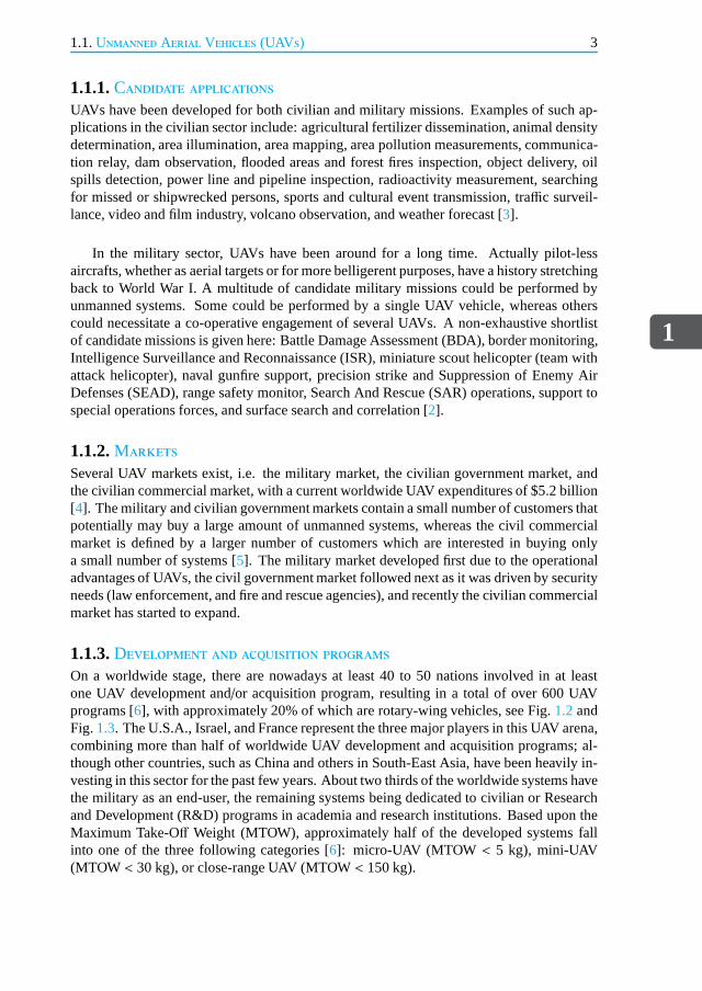
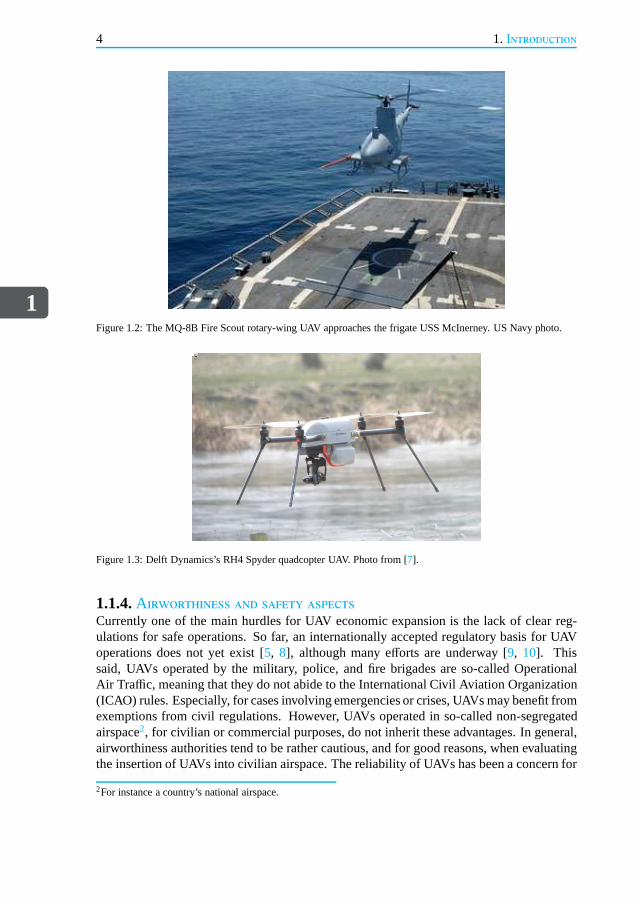
1.1.3.Development and acquisition programsOn a worldwide stage, there are nowadays at least 40 to 50 nations involved in at leastone UAV development and/or acquisition program, resulting in a total of over 600 UAVprograms [6], with approximately 20% of which are rotary-wing vehicles, see Fig.1.2andFig.1.3. The U.S.A., Israel, and France represent the three major players in this UAV arena,combining more than half of worldwide UAV development and acquisition programs; al-though other countries, such as China and others in South-East Asia, have been heavily in-vesting in this sector for the past few years. About two thirds of the worldwide systems havethe military as an end-user, the remaining systems being dedicated to civilian or Researchand Development (R&D) programs in academia and research institutions. Based upon theMaximum Take-Off Weight (MTOW), approximately half of the developed systemsfallinto one of the three following categories [6]: micro-UAV (MTOW < 5 kg), mini-UAV(MTOW < 30 kg), or close-range UAV (MTOW< 150 kg).

1

4 1. Introduction

Figure 1.2: The MQ-8B Fire Scout rotary-wing UAV approachesthe frigate USS McInerney. US Navy photo.

Figure 1.3: Delft Dynamics’s RH4 Spyder quadcopter UAV. Photo from [7].

1.1.4.Airworthiness and safety aspectsCurrently one of the main hurdles for UAV economic expansionis the lack of clear reg-ulations for safe operations. So far, an internationally accepted regulatory basis for UAVoperations does not yet exist [5, 8], although many efforts are underway [9, 10]. Thissaid, UAVs operated by the military, police, and fire brigades are so-called OperationalAir Traffic, meaning that they do not abide to the International Civil Aviation Organization(ICAO) rules. Especially, for cases involving emergenciesor crises, UAVs may benefit fromexemptions from civil regulations. However, UAVs operatedin so-called non-segregatedairspace2, for civilian or commercial purposes, do not inherit these advantages. In general,airworthiness authorities tend to be rather cautious, and for good reasons, when evaluatingthe insertion of UAVs into civilian airspace. The reliability of UAVs has been a concern for

2For instance a country’s national airspace.

1.2.The helicopter

1

5

many years, due to the high accident rates [11]. For instance, the reliability of UAVs wouldneed to improve by one to two orders of magnitude, in order to reach an equivalent generalaviation3 safety level [11, 12]. Hence, it is clear that an increase in UAV system integrity,reliability, and safety could only facilitate the introduction of UAVs into non-segregatedairspace for civilian or commercial purposes. In fact, a safety analysis would need to ad-dress each part of the UAV system, from the structural integrity of the vehicle, its engineand electronics, to the data links and embedded software.

1.2.The helicopterIn some cases, UAV deployment and recovery from unprepared or confined sites may berequired, such as when operating from or above urban and natural canyons, forests, or fromnaval ships. These specific missions would require very versatile flight modes, such asvertical takeoff/landing, hovering, and longitudinal/lateral flight. Here, a helicopter UAVcapable of flying autonomously, in and out of such restrictedareas, would represent a par-ticularly attractive asset. Hence, in the sequel, we brieflyreview some helicopter concepts.

The four forces acting on a helicopter are denoted by: thrust, drag, lift and weight,see Fig.1.4. The thrust overcomes the force of drag; the drag is a rearward force causedby the disruption of airflow by the moving rotors and vehicle;lift is produced by the dy-namic effect of the air flowing on the main rotor blades, opposing the downward force ofthe vehicle weight. On a standard helicopter configuration,the tail rotor is a small rotor,traditionally mounted vertically at the end of the tail-boom of a helicopter. The tail rotor’sthrust, multiplied by the distance from the vehicle’s center of gravity, allows it to counterthe torque effect created by the main rotor, see Fig.1.5. A typical helicopter has four sep-arate flight control inputs, which allow to control the attitude—roll, pitch, and yaw angles,see Fig.1.6—of the helicopter.

Figure 1.4: The four forces acting on a helicopter. Picturefrom [13].

Figure 1.5: Top view of a counter-clockwise rotatingmain rotor. Picture from [14].

3Roughly speaking, general aviation refers to all civil aviation operations other than scheduled air services (i.e.other than commercial airlines). General aviation flights range from gliders and powered parachutes to corporatejet flights.

1

6 1. Introduction

Figure 1.6: Attitude angles and control axis of an aerospacevehicle. Picture from [15].

The controls are known as main rotor collective, main rotor longitudinal cyclic, mainrotor lateral cyclic, and tail rotor anti-torque pedals, see Fig.1.7.

Figure 1.7: Helicopter flight controls. Picture from [16].

Some smaller helicopters have also a manual throttle neededto maintain rotor speed.The main rotor collective changes the pitch angle of all mainrotor blades collectively, andindependently of the blade rotational position. Through the collective, one can increaseor decrease the total lift derived from the main rotor. On theother hand, the main rotorcyclics change the pitch angle of the main rotor blades cyclically, i.e. the pitch angle of therotor blades changes depending upon their position, as theyrotate around the main rotorhub [16]. For example in Fig.1.7, pushing the cyclic forward results in a pitch-down ofthe helicopter, and consequently produces a thrust vector in the forward direction. If thecyclic is moved to the right, the helicopter starts rolling to the right and produces thrust in

1.2.The helicopter

1

7

that direction, causing the helicopter to move sideways [16]. The anti-torque pedals changethe pitch of the tail rotor blades. The anti-torque pedals allow to increase or decrease thethrust produced by the tail rotor, causing the nose of the vehicle to yaw. For each controlinput channel, Table1.1 summarizes the primary, and secondary, impacts on the vehicleresponse.

Table 1.1: Typical input-output coupling, for a helicopterwith a single main rotor (derived from [17]).

Input ResponseAxis Roll (φ) Pitch (θ) Yaw (ψ) Climb/Descent (w)

Main rotor Due to Due to Power change Primecollective transient transient varies response

(θ0) & steady & steady requirementlateral longitudinal for TR

flapping flapping thrust& sideslip

Main rotor Prime Due to Undesired Descentlateral cyclic response longitudinal (especially with

(θ1c) flapping in hover) roll angleMain rotor Due to Prime Negligible Desired

longitudinal cyclic lateral response in forward(θ1s) flapping flight

Tail rotor Roll due to Negligible Prime Undesired,collective TR thrust response due to

(θ0TR) & sideslip power changesin hover

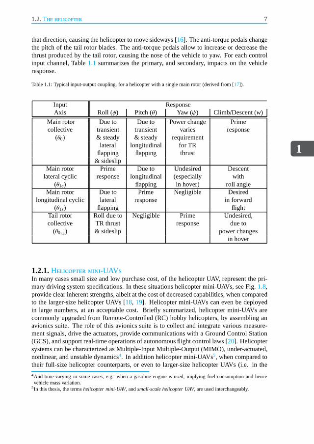
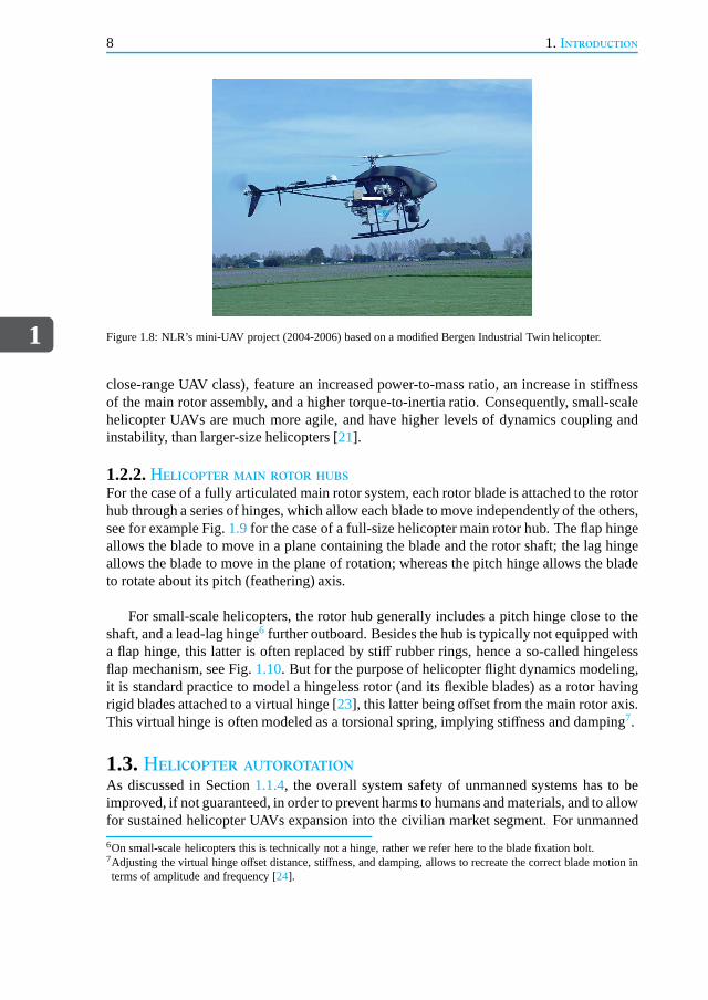
1.2.1.Helicopter mini-UAVsIn many cases small size and low purchase cost, of the helicopter UAV, represent the pri-mary driving system specifications. In these situations helicopter mini-UAVs, see Fig.1.8,provide clear inherent strengths, albeit at the cost of decreased capabilities, when comparedto the larger-size helicopter UAVs [18, 19]. Helicopter mini-UAVs can even be deployedin large numbers, at an acceptable cost. Briefly summarized,helicopter mini-UAVs arecommonly upgraded from Remote-Controlled (RC) hobby helicopters, by assembling anavionics suite. The role of this avionics suite is to collectand integrate various measure-ment signals, drive the actuators, provide communicationswith a Ground Control Station(GCS), and support real-time operations of autonomous flight control laws [20]. Helicoptersystems can be characterized as Multiple-Input Multiple-Output (MIMO), under-actuated,nonlinear, and unstable dynamics4. In addition helicopter mini-UAVs5, when compared totheir full-size helicopter counterparts, or even to larger-size helicopter UAVs (i.e. in the

4And time-varying in some cases, e.g. when a gasoline engine is used, implying fuel consumption and hencevehicle mass variation.

5In this thesis, the termshelicopter mini-UAV, andsmall-scale helicopter UAV, are used interchangeably.

1

8 1. Introduction

Figure 1.8: NLR’s mini-UAV project (2004-2006) based on a modified Bergen Industrial Twin helicopter.

close-range UAV class), feature an increased power-to-mass ratio, an increase in stiffnessof the main rotor assembly, and a higher torque-to-inertia ratio. Consequently, small-scalehelicopter UAVs are much more agile, and have higher levels of dynamics coupling andinstability, than larger-size helicopters [21].

1.2.2.Helicopter main rotor hubsFor the case of a fully articulated main rotor system, each rotor blade is attached to the rotorhub through a series of hinges, which allow each blade to moveindependently of the others,see for example Fig.1.9for the case of a full-size helicopter main rotor hub. The flaphingeallows the blade to move in a plane containing the blade and the rotor shaft; the lag hingeallows the blade to move in the plane of rotation; whereas thepitch hinge allows the bladeto rotate about its pitch (feathering) axis.

For small-scale helicopters, the rotor hub generally includes a pitch hinge close to theshaft, and a lead-lag hinge6 further outboard. Besides the hub is typically not equippedwitha flap hinge, this latter is often replaced by stiff rubber rings, hence a so-called hingelessflap mechanism, see Fig.1.10. But for the purpose of helicopter flight dynamics modeling,it is standard practice to model a hingeless rotor (and its flexible blades) as a rotor havingrigid blades attached to a virtual hinge [23], this latter being offset from the main rotor axis.This virtual hinge is often modeled as a torsional spring, implying stiffness and damping7.

1.3.Helicopter autorotationAs discussed in Section1.1.4, the overall system safety of unmanned systems has to beimproved, if not guaranteed, in order to prevent harms to humans and materials, and to allowfor sustained helicopter UAVs expansion into the civilian market segment. For unmanned

6On small-scale helicopters this is technically not a hinge,rather we refer here to the blade fixation bolt.7Adjusting the virtual hinge offset distance, stiffness, and damping, allows to recreate the correct blade motion interms of amplitude and frequency [24].

1.3.Helicopter autorotation

1

9

Figure 1.9: Agusta-109 fully articulated 4-blades main rotor. Photo from [22].

Figure 1.10: NLR’s Facility for Unmanned ROtorcraft REsearch (FURORE) project. Typical main rotor hub for a(small-scale) UAV helicopter.

1

10 1. Introduction

systems, a failure of the power or propulsion units represents currently the most frequentfailure mode of the vehicle, accounting for more than a thirdof all failure events [11]. Fora helicopter, such failures would mean flying and landing thevehicle without a workingengine, which is also known as theautorotationflight maneuver in helicopter jargon.

1.3.1.Autorotation: a three-phases maneuverHelicopter power-OFF flight, or autorotation, is a condition in which no power plant torqueis applied to the main rotor and tail rotor, i.e. a flight condition which is somewhat com-parable to gliding for a fixed-wing aircraft. During an autorotation, the main rotor is notdriven by a running engine, but by air flowing through the rotor disk bottom-up, whilethe helicopter is descending [25, 26]. In this case, the power required to keep the rotorspinning is obtained from the vehicle’s potential and kinetic energy, and the task during anautorotative flight becomes mainly one of energy management[27]. An autorotative flightis started when the engine fails on a single-engine helicopter, or when a tail rotor failurerequires engine shut-down. Unfortunately, autorotation maneuvers are known to be difficultto perform, and highly risky. From a flight maneuver standpoint, a complete autorotationgenerally contains three phases [28–32], detailed below8

• The entry. First, the tail rotor thrust needs to be reduced to account for the lossof main rotor torque (since not driven anymore by an engine).Next a reduction ofmain rotor thrust, as to prevent main rotor blade stall9 and rapid decay in main rotorRevolutions Per Minute (RPM), is often required. In addition, it is recommendedto pitch the helicopter nose down in order to gain some forward airspeed. Indeed,attaining higher airspeed avoids entering the so-called Vortex-Ring-State (VRS)10

[25], and allows for a buildup of rotor RPM while lowering the helicopter verticalsink rate.

• Steady autorotation. This is the stabilized autorotation, at a constant main rotorRPM, in which the helicopter also descends at a constant rate, which may be chosenfor minimum rate of descent, or maximum glide distance. Here, some rotor blade sta-tions on the main rotor will absorb power from the air, whereas others will consumepower, such that the net power at the main rotor shaft is zero,or sufficiently negativeto make up for losses in the tail rotor and transmission system [33, 34].

• Flare for landing . The purpose of the flare is to reduce the sink rate, reduce forwardairspeed, maintain or increase rotor RPM, and level the attitude for a proper landing,i.e. achieve appropriate tail rotor ground clearance. The helicopter flare capability isthe most important of the three autorotation phases [35, 36], and depends particularlyon a high main rotor kinetic energy, which requires a high main rotor RPM and/or alarge main rotor blade moment of inertia.

8Although the precise characteristics of the autorotation maneuver depends upon the initial flight condition, i.e.the helicopter flight condition just prior to the engine OFF situation [27].

9Stall corresponds to a sudden reduction in lift coupled witha large increase in drag.10Briefly summarized, the VRS corresponds to a condition wherethe helicopter is descending in its own wake,

resulting in a chaotic and dangerous flight condition.

1.4.Problem formulation

1

11

1.4.Problem formulationFirst, we summarize the following observations

• In order to support the economic growth of the small-scale helicopter UAV market,particularly within the civilian segment, the overall UAV system safety has to beimproved, especially when considering the case of engine failure. This requires foran autorotative flight capability of the unmanned helicopter system11.

• An autorotation maneuver is a highly challenging flight maneuver for a helicopter.For the case of manned helicopters, it is long known that a good deal of pilot trainingis required if disaster is to be avoided. In fact, quick reaction and critically timedcontrol inputs by the pilots are required for a safe autorotative landing [37–40]. Theautorotative flight maneuver is actually so risky that full touchdown autorotations(i.e. including flare and landing), as a training scenario, are nowadays very rarelypracticed by pilots. It is even reported in [41] that both the U.S. Army and U.S. AirForce have stopped practicing full autorotation flights dueto the high level of injuriesand vehicle damage.

• As pointed out in Section1.2.1, small-scale unmanned helicopters have higher lev-els of dynamics coupling and instability, when compared to larger size UAVs or tofull-size counterparts. Hence, for such small-scale unmanned systems, performing asuccessful autorotation maneuver becomes even more problematic.

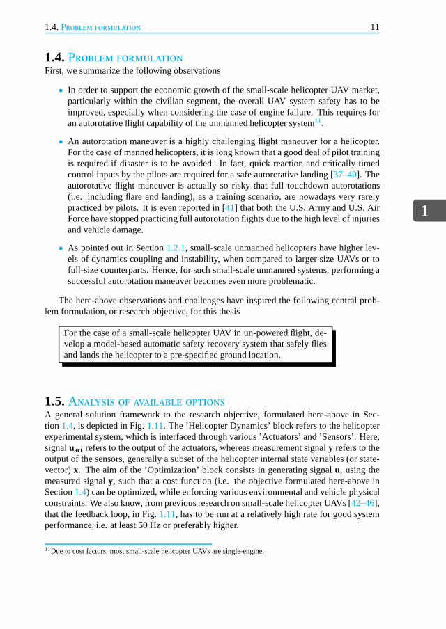
The here-above observations and challenges have inspired the following central prob-lem formulation, or research objective, for this thesis

For the case of a small-scale helicopter UAV in un-powered flight, de-velop a model-based automatic safety recovery system that safely fliesand lands the helicopter to a pre-specified ground location.

1.5.Analysis of available optionsA general solution framework to the research objective, formulated here-above in Sec-tion 1.4, is depicted in Fig.1.11. The ’Helicopter Dynamics’ block refers to the helicopterexperimental system, which is interfaced through various ’Actuators’ and ’Sensors’. Here,signaluact refers to the output of the actuators, whereas measurement signal y refers to theoutput of the sensors, generally a subset of the helicopter internal state variables (or state-vector)x. The aim of the ’Optimization’ block consists in generatingsignalu, using themeasured signaly, such that a cost function (i.e. the objective formulated here-above inSection1.4) can be optimized, while enforcing various environmental and vehicle physicalconstraints. We also know, from previous research on small-scale helicopter UAVs [42–46],that the feedback loop, in Fig.1.11, has to be run at a relatively high rate for good systemperformance, i.e. at least 50 Hz or preferably higher.

11Due to cost factors, most small-scale helicopter UAVs are single-engine.

1

12 1. Introduction

Figure 1.11: Small-scale helicopter UAV automatic autorotation: the feedback loop.

To this end, the ’Optimization’ block, in Fig.1.11, has to perform, at least, the follow-ing three tasks [47]: 1) Navigation, by determining the current position, orientation, andvelocity of the helicopter, delivering the filtered state-vectorxfilt in Fig. 1.12; 2) Guidance,by computing the trajectory or path12 to the destination point; and 3)Control by ensuringthat the helicopter stays on the computed trajectory or path. Although there is quite a bitof synergism between these three disciplines, a natural separation does exist between theNavigationtask on the one hand, and theGuidanceandControl tasks on the other.

Figure 1.12: Small-scale helicopter UAV automatic autorotation: Guidance, Navigation, and Control (GNC) feed-back loop.

1.5.1.Model-free versus model-based optionsNow, as hinted upon in Fig.1.11, the goal of this thesis is set upon the design and evaluationof the ’Optimization’ block. More specifically, the focus shall be upon theGuidanceandControl tasks, as shown in Fig.1.12. Before discussing further the content of this thesis, letus first briefly review what are, to-date, the various available options, in terms ofGuidance

12The termtrajectory denotes a route that a vehicle should traverse as a function of time, whereas apathdenotesan obstacle-free route without temporal restrictions [48].

1.5.Analysis of available options

1

13

andControl, for our UAV application. First, theGuidanceandControl tasks, in Fig.1.12,can be designed using

• A model-freeapproach. Various methods are here available, e.g. model-free fuzzylogic13 [49], with applications to UAV control in [50, 51]; model-free reinforcementlearning14 [52], with applications to UAV control in [50, 53–55]; and evolutionaryand genetic algorithms15 [56–58], with applications to UAV control in [59–63].

• A model-basedapproach, where a model of the helicopter system is made avail-able. There are three different philosophies that form the basis of modeling, namelythe white-box modeling (also known as mechanistic or first-principles models), theblack-box modeling (also known as empirical models), and the gray-box modeling(also known as hybrid models [64]) which is a mixing of the previous two [65].In the first case, a model is developed on the basis of detailedunderstandings of thegeneric underlying physical laws, that govern the system. In the second case, a modelis developed on the basis of empirical knowledge, i.e. a sufficiently large number ofconsistent observations [65, 66]. In the third case, a model is developed by combiningthe strengths of the previous two approaches. A rather wide spectrum of model-basedapproaches exists, which will be discussed in more detail inthe sequel.

1.5.2.Integrated versus segregated optionsNext, theGuidanceandControl tasks, in Fig.1.12, can be designed using

• An integratedapproach, where theGuidanceandControltasks are performed withina single optimization process. Again, either a model-free or model-based approachcan be applied. For model-free approaches, these are identical to the ones listed here-above. For model-based approaches, we distinguish betweenthe following threeoptions

1. The first one is the so-calledModel Predictive Control (MPC) theory [67,68], also known as Receding Horizon Control (RHC)16. Starting with the earlyworks in [69–73], the MPC has become one of the most popular tools for con-strained industrial control applications. Based upon a model of the system, anMPC controller generates an optimal state feedback controlsequence, by mini-mizing, at each time step, an open-loop, quadratic performance objective, whileexplicitly including input and state operating constraints [74–78]. Specifically,for each new measurement, the MPC predicts the future dynamic behavior ofthe system over a prediction horizonTp, and determines the input sequenceover a control horizonTc, with Tc ≤ Tp, such that the performance objectiveis minimized. Then the first control input of the computed optimal sequence is

13Fuzzy control is a method based upon a representation of the knowledge, and the reasoning process, of a humanoperator [49].

14Reinforcement learning is an area of machine learning, concerned with how a system ought to respond, in anenvironment, so as to maximize some notion of cumulative reward [52].

15Evolutionary and genetic algorithms use mechanisms inspired by biological evolution [56–58].16Thereceding horizonterminology corresponds to the behavior of the Earth’s horizon, i.e. as ones moves towards

it, it recedes, hence remaining a constant distance away.

1

14 1. Introduction

applied to the system, and the optimization is repeated at each subsequent timestep. Obviously, lowering the prediction horizonTp allows to lower the compu-tational time (at the cost of complications with respect to stability). This mech-anism of having a new on-line solution at each time step, results in a so-calledsampled-data feedback law [79, 80], hence bringing alongside the classical ben-efits of feedback. Now depending on the nature of the model, either linear ornonlinear, a corresponding linear or nonlinear MPC optimization problem hasto be solved. An array of applications of linear MPC to various UAVs can befound in [81–84], whereas specific applications of nonlinear MPC to helicopterUAVs can be found in [85–90], and to fixed-wing UAVs in [91–96].

2. The second option assumes that the nonlinear helicopter plant can be modeledas a Linear Parameter Varying (LPV) system. The latter can thus be used withone of the manyMPC-LPV , i.e. MPC for LPV algorithms [97–113]. ThisMPC-LPV approach, most often resulting in a Semi-Definite Program (SDP)optimization, can be seen as a middle-way between the linearand nonlinearoptimization paradigms.

3. The third option extends the framework of MPC, for the caseof infinitely longhorizonsTp and Tc, and naturally brings us to the field ofconstrained op-timal control [114–116]. Here too, based upon a model of the system, andgiven a performance objective (which need not be quadratic), and suitable in-put and state operating constraints, the solution to the optimal control problemyields the optimal input and state time histories. Again, the first control inputof the computed optimal sequence is applied to the system, and the optimiza-tion is repeated at each subsequent time step. Also, depending on the nature ofthe model, either linear or nonlinear, a corresponding linear or nonlinear con-strained optimal control problem is solved. Applications of nonlinear optimalcontrol17 to helicopter UAVs can be found in [117, 118], and to fixed-wingUAVs in [119–123].

• A segregatedapproach, in which theGuidanceandControl tasks are split into twodistinctive optimization processes. This approach separates theGuidancetask, i.e.the Trajectory Planning (TP), from theControl task, i.e. the Trajectory Tracking(TT)18. Although potentially sub-optimal, this philosophy offers the advantage ofeffectively exploiting the nonlinear nature of the system (to generate trajectories),while also making use of the linear structure of the error dynamics (to stabilize andcontrol the helicopter) [124]. This divide-and-conquer strategy is also known as theclassical two-degree of freedom Flight Control System (FCS) paradigm, as depictedin Fig. 1.13. Here, the TP shall be capable of generating open-loop, feasible, andoptimal autorotative trajectory referencesxTP, for the small-scale helicopter, subjectto system and environment constraints, and additionally though not necessarily, thefeedforward nominal control inputsuTP, needed to track these trajectories. On theother hand the TT shall compare current estimated state valuesxfilt with the reference

17Most often applied in open-loop, rather than in the closed-loop setting described here.18Within this thesis, the terms ’Trajectory Planning’ (resp.’Trajectory Tracking’) and ’Trajectory Planner’ (resp.

’Trajectory Tracker’) are used interchangeably.

1.5.Analysis of available options

1

15

Figure 1.13: Two degree of freedom Flight Control System (FCS) architecture, implemented on the true helicoptersystem.

valuesxTP produced by the TP, and shall formulate the feedback controlsuTT to en-sure that the helicopter flies along these optimal trajectories. The additional feedbackpath, denoted by a dashed line in Fig.1.13, allows for updating the generated tra-jectory based upon the current state. In Fig.1.13, the ’Helicopter Dynamics’ blockrefers to the helicopter experimental system. The role of theNavigationtask, definedas the ’Estimation Filter’ in Fig.1.13, shall be to estimate the helicopter unmeasuredstates, the wind, and low-cost sensors characteristics such as scale factors and biases.

The segregated approach: Trajectory Planning (TP)and Trajectory Tracking (TT)With regard to the segregated approach, let us now separately address the various optionsavailable for theGuidancetask, i.e. Trajectory Planning (TP), and theControl task, i.e.Trajectory Tracking (TT).

• Over the years, researchers have addressed theTrajectory Planning (TP) problemthrough several techniques, namely: cell decomposition, potential fields, roadmapsand hybrid systems, inverse dynamics and differential flatness, Mixed Integer LinearProgramming (MILP), MPC, optimal control, and finally evolutionary/genetic algo-rithms [125, 126], with specific benefits and drawbacks for each method, see also[127–129]. Some of the aforementioned planning techniques—cell decomposition,potential fields, and roadmaps—either ignore the differential constraints associatedwith the vehicle’s dynamics (i.e. are model-free approaches), or use simplified kine-matic models. With regard to the TP of a helicopter in autorotation, model-basedindirect optimal control methods have been used in [130–135], whereas model-baseddirect optimal control methods have been explored in [37, 38, 136–145]. Aside fromthese optimal control strategies, three other methods havealso been investigated forhelicopter autorotation: 1) a model-free learning-based approach in [51, 146]; 2) amodel-based parameter optimization scheme to find a backwards reachable set lead-ing to safe landing in [147, 148]; and 3) and a model-free parameter optimization

1

16 1. Introduction

scheme generating segmented routes, selecting a sequence of straight lines and curvesin [149–151].

• With respect to theTrajectory Tracking (TT) , virtually any control methods canbe applied to a helicopter UAV. For instance, for the specificcase of TT for a heli-copter with the engine ON, a vast array of technical avenues have been investigatedover the years, with the application of: classical control [152], gain-scheduling ofProportional-Integral-Derivative (PID) controllers [153], Linear Quadratic Regula-tor (LQR) [154, 155], Linear Quadratic Gaussian (LQG) [155, 156], LPV [157], H2

[158], H∞ [43, 158–160], µ [157, 161], (nonlinear) MPC [87, 89, 155], feedbacklinearization, (incremental) nonlinear dynamic inversion and nested saturated con-trol [20, 161–163], adaptive control [164–167], backstepping [166, 168–170], andmodel-based learning approaches [171–174]. For additional results relative to fuzzylogic-based controllers, artificial Neural Network (NN), or vision based controllers,refer also to [18, 175]. Conversely, very few papers have addressed the subject ofhelicopter TT with the engine OFF (i.e. autorotation), while concurrently validatingtheir results by experiments, or three-dimensional (3D) high-fidelity simulations. In[146], a model-based Differential Dynamic Programming (DDP)19 method is used;in [151] a model-based Nonlinear Dynamic Inversion (NDI) with PID loops is used;in [51] a model-free fuzzy logic method is used; and in [149, 177] a model-basedH∞method is used. Finally, none of the previous results, except for [177] which used a2D lower-fidelity model, did consider a robust TT approach.

1.5.3.Summary of previous analysisSummarizing the previous discussion, wee make the following comments.

• Although very powerful and potentially very promising, model-free (machine learn-ing) approaches have also some liabilities. First, the lackof a model makes it difficultto analyze their stability and robustness characteristics[49]. Second, the compu-tational complexity of the model-free approaches may oftenbe prohibitive for ourapplication (recall that the feedback loop in Fig.1.11 has to be run at a relativelyhigh rate, at least 50 Hz or equivalently 20 msec).

• From a conceptual viewpoint, an integrated model-based approach may potentiallyprovide the best answer to our helicopter autorotation problem. This said, it is essen-tially the linear MPC approach that has shown to be implementable on-line, even forhigh bandwidth systems [178–181]. As stated in Section1.2.1, a helicopter has anintrinsically nonlinear behavior, which renders the application of linear MPC ratherquestionable. For the case of nonlinear MPC or nonlinear constrained optimal con-trol, these methods are still time-consuming optimizationtechniques, currently un-likely to be run on-line, within a 20 msec time frame.

• Although potentially much faster than a nonlinear MPC approach, the integratedmodel-based MPC-LPV approach, with todays SDP solvers, would unlikely runwithin the 20 msec time frame. This said, this comment shouldnot be taken as

19DDP is an extension of the Linear Quadratic Regulator (LQR) formalism for non-linear systems [176].

1.6.Research objectives and limitations

1

17

conclusive on the viability of the MPC-LPV method. Indeed, agreat deal of currentMPC research is devoted to reducing the computational cost [182, 183]. In fact, aclear trend of the last ten years is to move off-line as much computational burdenas possible. One such approach is the so-called explicit MPC[184–187], which hasshown to be an attractive solution, but so-far (and to the best of our knowledge) onlyfor low-order systems. However, we do expect a bright futurefor the integrated,model-based, MPC-LPV approach.

• For the Trajectory Planning (TP), model-free approaches (or alternatively model-based approaches using a simplified kinematic model) may lead to infeasible20 plan-ning results or, at best, conservative solutions. In addition, failing to incorporate some(sufficiently) realistic vehicle dynamics, during the planning phase, will increase theon-line workload of the TT.

• For the Trajectory Tracking (TT), it is best practice to include some form of robust-ness during the controller design.

• Only four publications have addressed the aggregated planning and tracking function-alities, for a helicopter in autorotation, with validationthrough either experiments, or3D high-fidelity nonlinear simulations [51, 146, 149, 151]. The contribution in [146]has shown successful experimental demonstrations, whereas the other three contribu-tions have been validated on 3D high-fidelity simulations. The methods in [51, 146]use a model-free, learning-based TP approach. For the TT, [146] uses a model-basedDDP approach, whereas [51] uses a model-free fuzzy logic approach. The methods in[149, 151] use a model-free, (modified) Dubin procedure (i.e. a sequence of straightlines and curves), for their TP algorithms. For the TT, [151] uses a model-basedcombined NDI-PID method, whereas [149] uses a model-basedH∞ method.

• The results from [51, 151] are for the case of a full-size helicopter, whereas the resultsin [149] involve a so-called short-range/tactical size helicopter UAV (approximately200 kg). Only the results in [146] are for a small-scale helicopter UAV. As outlinedearlier, when compared to larger and heavier helicopter vehicles, the control of small-scale helicopters (i.e. under 10–20 kg) represents a much more challenging problem.

1.6.Research objectives and limitationsBased upon the previous discussion, we define the following objectives for this thesis, referalso to Fig.1.14:

1. A model-based TP approach shall be selected, allowing to compute trajectories whichare potentially less conservative than the ones originating from model-free approaches.

2. A model-based, robust, TT approach shall be selected, in order to obtain a closed-loop system which is less sensitive to modeling uncertainties.

20This is precisely the reason why nonholonomic constraints,i.e. constraints that not only involve the state butalso state derivatives, which cannot be eliminated by integration, play a crucial role in the subsequent design offeedback controllers [127].

1

18 1. Introduction

Figure 1.14: Helicopter autorotation: available options for the Guidance and Control.

3. The combined TP and TT shall be computationally tractable, i.e. to be run within a20 msec time frame.

We also limit the scope of this thesis, by adding the following boundaries:

1. The combined TP-TT shall not be validated experimentally, but rather on a 3D high-fidelity helicopter UAV simulation, serving as a proxy for the real helicopter system.

2. The effects of sensors, actuators21, and the ’Estimation Filter’, are excluded from thesimulation environment.

With this in mind, the control architecture, defined in Fig.1.13, becomes the one definedin Fig. 1.15, where the output signaly represents now a subset of the state-vectorx.

1.7.Solution strategyHere, we briefly introduce the research areas addressed within this thesis.

21The actuators are indeed not included in the simulation. However, for a realistic control design, we do includethe actuators characteristics into the control design specifications.

1.7.Solution strategy

1

19

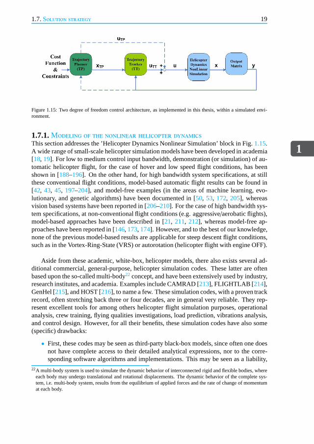
Figure 1.15: Two degree of freedom control architecture, asimplemented in this thesis, within a simulated envi-ronment.

1.7.1.Modeling of the nonlinear helicopter dynamicsThis section addresses the ’Helicopter Dynamics NonlinearSimulation’ block in Fig.1.15.A wide range of small-scale helicopter simulation models have been developed in academia[18, 19]. For low to medium control input bandwidth, demonstration(or simulation) of au-tomatic helicopter flight, for the case of hover and low speedflight conditions, has beenshown in [188–196]. On the other hand, for high bandwidth system specifications, at stillthese conventional flight conditions, model-based automatic flight results can be found in[42, 43, 45, 197–204], and model-free examples (in the areas of machine learning, evo-lutionary, and genetic algorithms) have been documented in[50, 53, 172, 205], whereasvision based systems have been reported in [206–210]. For the case of high bandwidth sys-tem specifications, at non-conventional flight conditions (e.g. aggressive/aerobatic flights),model-based approaches have been described in [21, 211, 212], whereas model-free ap-proaches have been reported in [146, 173, 174]. However, and to the best of our knowledge,none of the previous model-based results are applicable forsteep descent flight conditions,such as in the Vortex-Ring-State (VRS) or autorotation (helicopter flight with engine OFF).

Aside from these academic, white-box, helicopter models, there also exists several ad-ditional commercial, general-purpose, helicopter simulation codes. These latter are oftenbased upon the so-called multi-body22 concept, and have been extensively used by industry,research institutes, and academia. Examples include CAMRAD [213], FLIGHTLAB [ 214],GenHel [215], and HOST [216], to name a few. These simulation codes, with a proven trackrecord, often stretching back three or four decades, are in general very reliable. They rep-resent excellent tools for among others helicopter flight simulation purposes, operationalanalysis, crew training, flying qualities investigations,load prediction, vibrations analysis,and control design. However, for all their benefits, these simulation codes have also some(specific) drawbacks:

• First, these codes may be seen as third-party black-box models, since often one doesnot have complete access to their detailed analytical expressions, nor to the corre-sponding software algorithms and implementations. This may be seen as a liability,

22A multi-body system is used to simulate the dynamic behaviorof interconnected rigid and flexible bodies, whereeach body may undergo translational and rotational displacements. The dynamic behavior of the complete sys-tem, i.e. multi-body system, results from the equilibrium of applied forces and the rate of change of momentumat each body.

1

20 1. Introduction

when the end-goal is model-based control design. In addition, a physical understand-ing of the to-be controlled system is often necessary in order to be able to makejudicious structural choices during the control design (e.g. adequate model orderselection). This may become rather difficult if little is known about the system.

• Second, even when analytical expressions are available, the multi-body model struc-ture adds a huge amount of detail, resulting in very high-order dynamical systems,effectively inhibiting any further manipulation of the analytical expressions.

• Third, the black-box nature of these codes restrict the range of control techniquesthat could potentially be used. For example, these models cannot be used for con-troller design when nonlinear control techniques, that explicitly require closed-formmodeling, are sought.

• Finally, for the specific case of FLIGHTLAB, which is available at NLR, and al-though it is now possible to configure it in an autorotation mode for a small-scalehelicopter, it was unfortunately not possible to do so yearsago, at the start of thisPhD project. The problem was related to the way FLIGHTLAB dealt with the mainrotor shaft inertia, engine drive-train, and gearbox23.

Hence, these aspects have led us towards the development of our own comprehensive,white-box, flight dynamics model, particularly suited for small-scale helicopter UAVs, andvalid for a range of flight conditions, including steep descent flight and autorotation. Morespecifically, the model represents the nonlinear flight dynamics of a flybarless24 helicoptermain rotor, with rigid blades. The complete model incorporates the main rotor, tail rotor,fuselage, and tails of a modified Align T-REX helicopter, seeFig. 1.16.

In terms of dynamics, the state-vectorx given in Fig.1.15is of dimension twenty-four.The states include the twelve-states rigid-body motion, and the dynamics of the main rotor.The former include the three-states inertial position, thethree-states body linear velocities,the three-states body rotational velocities, and the three-states attitude (orientation) angles.The dynamics of the main rotor include the helicopter higher-frequency phenomena, whichexist for both the engine ON or OFF (i.e. autorotation) flightcondition. These higher-frequency phenomena include the main rotor three-states dynamic inflow [218, 219], andmain rotor blade flap-lag dynamics (each blade defined by the four-states flap/lag angles androtational velocities) [220]. Regarding the main rotor Revolutions Per Minute (RPM), itis

23To be able to run the FLIGHTLAB simulation, the combined inertia of the rotor shaft, drive-train, and gearboxhad to be set to at least one third the main rotor inertia, which represents an unrealistically high value for thecase of small-scale helicopters.

24The flybar is a mechanical component of the helicopter’s mainrotor system, and consists of a rod carrying smallaerofoils (paddles), with the Angle Of Attack (AOA) of thesepaddles being set by the main rotor cyclic control.The AOA is the angle between a reference line on a body and the velocity vector representing the relative motionbetween the body and the air [217]. It is best to think of the flybar as a gyroscope that, when notsteered, tendsto maintain its rotation axis fixed relative to the earth. A flybar on a main rotor enhances the stability of the heli-copter and hence, for a pilot using a Remote-Control (RC) device, the flybar system makes the helicopter easierto fly. This said, small-scale flybarless (i.e. without theseso-called Bell-Hiller stabilizing paddles) helicoptersare becoming increasingly popular. Most RC helicopter manufacturers are nowadays offering most of their RChelicopter kits in flybarless versions as well, since flybarless rotors allow for increased helicopter agility andperformance, and reduced rotor mechanical complexity.

1.7.Solution strategy

1

21

Figure 1.16: NLR’s mini-UAV project (2012-2014) based on a modified Align T-REX helicopter.

generally assumed fixed for the engine ON case25, whereas for the engine OFF case it is notfixed anymore. The main rotor RPM represents an essential part of the autorotative flightcondition, and this additional state is also included in thestate-vectorx when consider-ing the engine OFF case. This MATLABR©-based, nonlinear, continuous-time, High-OrderModel (HOM) is used as a realistic small-scale helicopter simulation environment, for thevalidation of the FCS.

1.7.2.The Trajectory Planning (TP)This section addresses the ’Trajectory Planner’ block in Fig. 1.15. The TP aims at gener-ating a feasible and optimal autorotative trajectory referencexTP, for the helicopter to fol-low, and additionally, though not necessarily, the feedforward nominal control inputsuTP,needed to track this trajectory. The TP computes an open-loop optimal trajectory, given acost objective, nonlinear system dynamics, and controls and states equality and inequalityconstraints. The additional feedback path, denoted by a dashed line in Fig.1.15, allowsfor updating the generated trajectory based upon the current state and, if used, would resultin a closed-loop calculation of the reference trajectory. In this thesis, we investigate twomodel-based TP options. The first is an off-line approach, whereas the second is on-linefeasible.

The off-line approachFrom our previous discussion in Section1.5.2, it became clear that the most natural frame-work for addressing TP problems was probably through optimal control theory [114].Hence, we choose to set the off-line TP approach within the continuous-time, nonlinear,constrained optimal control paradigm. Now, given that mostnonlinear constrained opti-mization problems are typically either computationally intensive (real-time computation),or memory intensive (off-line computation) [139], solving the TP optimization problem,within the MATLAB environment, in the full vehicle state space (including the higher-order main rotor modes of the helicopter HOM in Section1.7.1) has shown to be rather

25Although this is a simplification, since in the engine ON casethe main rotor RPM is being regulated by thegovernor.

1

22 1. Introduction

costly from a computational viewpoint. The two, not mutually exclusive, options to mit-igate such a problem are: 1) converting the helicopter HOM simulation, from a flexibleMATLAB code into a more constrained programming language (such as the C language),which does provide a highly optimized performance and memory environment; or 2) de-velop a Low-Order Model (LOM) better suited for nonlinear optimization problems. Thefirst option lives in the Information Technology (IT) realm,and requires some design effortat the interface of various softwares26, whereas the second option is more interesting froma system and control viewpoint, and is more in line with the personal interests of the author.Hence, in this thesis, we opted for the development of a LOM.

Low-Order Model (LOM) We discuss here the method used to construct such a small-scale helicopter LOM, which combines the required modelingaccuracy with the computa-tional tractability. In our case, the high computational cost of the HOM comes primarilyfrom the main rotor model. With this in mind, we considered two main avenues for thederivation of a simplified model.

The first, and most straightforward one, consists in adapting the HOM, by replacingall main rotor higher-order dynamics (i.e. rotor inflow, andblade flap/lag) by their corre-sponding steady-state expressions. Although this resulted in a cheaper simulation cost, thecomplex, nonlinear formulations of the main rotor forces and moments (and their corre-sponding numerical integrations) had still a detrimental effect on the overall computationalcost. Hence, we opted for an alternative approach, which consisted in retaining the low-order dynamics of the HOM, i.e. the rigid-body dynamics and the main rotor RPM dynam-ics, and then replacing the costly computations of the main rotor high-order dynamics, andmain rotor forces and moments, by closed-form ’textbook’-like expressions: i.e. a static ro-tor uniform inflow model from [218, 221] with a VRS correction from [222], a steady-staterotor Tip-Path-Plane (TPP) model from [223, 224], and rotor forces and moments expres-sions from [36]. The remaining helicopter model components, i.e. tail rotor, fuselage, andtail, are further re-used, as-is, from the HOM. To compensate for the modeling inaccura-cies introduced by the use of simpler closed-form expressions in this, so-far, white-boxmodel, we added a black-box component to it, in the form of eight empirical coefficients,set at specific ’locations’ within this simplified white-boxmodel. Subsequently, simulatedinput-output data, from the HOM, was used to fit these empirical coefficients. The latterhave also been scheduled on helicopter horizontal and vertical velocities. Compared to theHOM, the domain of validity of this gray-box model is much smaller, since the data-setused to estimate the empirical coefficients is not representative of the full helicopter flightenvelope. However, this simplified model did provide a decrease in the associated CPUtime, per model evaluation, of approximately 60 %.

Once the LOM is obtained, the solution of the continuous-time optimal control problemrequires a discretization method. Here, we apply the pseudospectral discretization numer-ical scheme [225–227] to the optimal autorotation problem. The pseudospectral method isknown to provide exponential convergence, provided the functions under considerations aresufficiently smooth. Once discretized, the problem is then transcribed into a NonLinear Pro-

26Although automatic MATLAB to C translation tools do exist.

1.7.Solution strategy

1

23

gramming problem (NLP) [228], this latter being solved numerically by a well known andefficient optimization technique, in our case a Sequential Quadratic Programming (SQP)method [229–231]. The knowledge of these optimally defined autorotative trajectories, de-fined through this off-line approach, has proved to be useful. In particular, for the case ofour Align T-REX helicopter, we found an existing bound on thetotal flight time based uponthe initial altitude and the rotor induced27 velocity in hover. Knowledge of this bound hasshown to be relevant for the subsequent on-line TP approach.

The on-line approachThe TP can either be run once, just after an engine failure hasbeen detected, or can becontinuously recomputed (see the dashed line in Fig.1.15). For both options, the TP op-timization framework of Section1.7.2, which combines an optimal control approach witha LOM, would need to see its computational cost decrease by approximately four to fiveorders of magnitude, in order to retain high computational efficiency for on-line use28.

Hence, we present here an alternative TP approach, applicable for on-line use, and basedupon the concept of differential flatness. The seminal ideas of differential flatness were in-troduced in the early 1990s in [232–234] as part of a paradigm in which certain differentialalgebraic representations of dynamical systems are equivalent. In other words, a completeparametrization of all system variables—inputs, states, and outputs—may be given in termsof a finite set of independent variables, called flat outputs,and a finite number of theirderivatives [235, 236]. This results in optimization problems with fewer variables [237],i.e. by the complete elimination of the dynamical constraints. In this case the trajectorygeneration problem is transformed from a dynamic to an algebraic one, in which the flatoutputs are parametrized over a space of basis functions. The generation of optimal trajec-tories is then reduced to a classical algebraic interpolation or collocation problem [80, 238].

It is in general difficult to determine whether a given nonlinear system is flat, althoughseveral methods for constructing flat outputs have been documented in the literature [235,239–241]. With regard to applications, it has been shown that simplified dynamics of air-craft and Vertical Take-Off and Landing (VTOL) aircraft are flat [242–247], and simplifiedhelicopter dynamics is flat [235, 248, 249], whereas more realistic vehicle models are ingeneral non-differentially flat, e.g. [235, 250]. In fact, high-fidelity helicopter models areknown to be non-differentially flat. To circumvent this difficulty, a standard approach, bythe research community, has consisted in progressively simplifying the model until it in-deed becomes flat. Rather than generating optimal trajectories based upon such simplifiedrepresentations of the helicopter dynamics, we present in this thesis an alternative approach,consisting in using only the rigid-body dynamics, with total aerodynamic forces and totalmoments as the new plant inputs. Although the relationship with the helicopter true controlinputs29 is lost, the advantage consists in having a model which does not include approx-imations, while being exactly flat. Now, since the rigid-body dynamics does not include

27The main rotor induced flow corresponds to the flow field induced by the rotation of the main rotor blades.28For on-line use in a hard real-time environment where stringent timing constraints exist (e.g. in our case the 50

Hz closed-loop update rate).29Main rotor collective, lateral and longitudinal cyclic, and tail rotor collective.

1

24 1. Introduction

the main rotor and RPM dynamics, and in order to obtain feasible autorotative trajecto-ries, we will constrain the trajectory flight time by the bound deduced using the off-line TPapproach.

Combining the off-line and on-line approachesWe summarize now the main idea behind our TP methodology:

• Step 1.Base the TP optimization on the concept of differential flatness, using a lower-complexity model (in our case the rigid-body dynamics). Combining the flatness witha lower-complexity model allows for on-line tractable computations.

• Step 2. Derive additional trajectory constraints (in our case a bound on total flighttime), obtained from the analysis of off-line optimization results, using a nonlinearoptimal control approach combined with a higher-complexity model (in our case,either the HOM helicopter of Section1.7.1, or the LOM of Section1.7.2).

• Step 3. Use the optimization framework of Step 1, combined with the additionalconstraints from Step 2 (in our case a bound on total flight time), to generate, on-line,feasible and optimal trajectories, for the original HOM helicopter.

1.7.3.The Trajectory Tracking (TT)This section addresses the ’Trajectory Tracking’ block in Fig. 1.15. The TT shall com-pare current output valuesy with the optimal reference valuesxTP produced by the TP,and shall formulate the feedback controlsuTT aimed at decreasing the tracking error, henceensuring that the helicopter flies along the optimal trajectory. The tracking error may bedue to a combination of model uncertainty (unmodeled higher-order dynamics, unmodeledstatic nonlinearities, parametric uncertainties, delays), and signal uncertainty (wind distur-bances and noise). As stated earlier, very few papers have addressed the subject of trackingan autorotative trajectory, with validation through experimental results or 3D high-fidelitysimulations [51, 146, 149, 151]. None of the previous results considered a robust TT ap-proach. Hence, we select here a model-based, robust, TT approach, in order to obtain aclosed-loop system which is less sensitive to modeling uncertainties.

Robust control based TTSince the helicopter dynamics is highly nonlinear, the design of the TT necessitates anapproach that effectively respects or exploits the system’s nonlinear structure. To this end,several control methods are available: from 1) robust control; 2) classical gain-scheduling,and Linear Parameter-Varying (LPV) approaches; to 3) trulynonlinear control methods(e.g. nonlinear MPC, Lyapunov based methods such as slidingmode and backstepping,adaptive control, or even passivity-based approaches). Inthis thesis we choose to apply arobust controlµ strategy. This method consists in using a nominal Linear Time-Invariant(LTI) plant coupled with an uncertainty, and applying a small gain approach [251, 252]to design a single robust LTI controller. This approach, when implemented on-line, iscomputationally very efficient. Now, rather than modeling the uncertainty in a detailedmanner, an input multiplicative uncertainty is added here to compensate for the unmodeled

1.8.Overview of this thesis

1

25

plant nonlinearities and unmodeled higher-order rotor dynamics30, by lumping all typesof model uncertainty together into a complex, full-block, input multiplicative uncertainty.Finally, the robust controller synthesis consists in obtaining a controller insensitive to thismultiplicative uncertainty at the plant input.

Affine LPV ModelingRather than using a robust controlµ strategy, one could also consider some other controlmethod, as listed in Section1.7.3. In particular, LPV systems have become celebrated asthey represent an attractive midway approach between LTI, and nonlinear or time-varyingstructures [253, 254]. LPV systems allow to enclose nonlinear behaviors into a linearframework, where LPV control methods can be seen as an extension of the standardH2

andH∞ LTI synthesis techniques [255–262]. The LPV method amends also the main draw-backs of classical gain-scheduling [263, 264]: 1) by eliminating the need for repeated de-signs/simulations in order to handle the global control problem; and 2) by guaranteeing bothstability and performance along all possible parameter trajectories. In addition, LPV controldesign problems are efficiently solved, by first expressing the problems as Linear Matrix In-equality (LMI) optimizations [265]—subsequently formulated as Semi-Definite Programs(SDP) [266]—for which there are several powerful numerical solutions[267, 268]. This re-sulted in a growing number of applications, such as in aerospace [269–274], wind turbines[275], wafer steppers [276, 277], Compact-Disk players [278], and robotic manipulators[279]. Now, and for all its benefits, the LPV control paradigm typically takes the exis-tence of the plant, in LPV form, as a starting point. However,a systematic formulationof a nonlinear system into a suitable LPV model remains oftenproblematic [280]. Hence,the problem of simplifying a large scale, nonlinear model, such as our helicopter HOM ofSection1.7.1, into a LPV representation is thus highly relevant.

With this in mind, and for the case where a plant’s nonlinear model already exists, wepresent in this thesis an affine LPV modeling methodology. This LPV modeling method hassubsequently been applied to a modified pointmass pendulum,and to the helicopter HOMof Section1.7.1. For the pointmass pendulum example, the LPV modeling approach wasvalidated in open- and closed-loop (using robust and LPV controllers). For the helicopterHOM case, the LPV modeling approach resulted in a LPV model having a large number of(more than thirty) scheduling parameters. Unfortunately,it became impossible to synthesizeLPV controllers with such a high-order LPV model. In fact, itis well-known that thenumerical conditioning and solvability of LMI problems play a crucial role in LPV practicaldesign methods [275–278]. A way to mitigate such problems would consist in applyingsome LPV model reduction techniques [281, 282], in order to obtain a LPV model havingfewer scheduling parameters, hence better suited for LPV controller synthesis.

1.8.Overview of this thesisThe development of an autonomous helicopter system requires for an elaborate synergybetween various engineering fields, including: 1) modeling; 2) system identification; 3)estimation and filtering; and 4) optimization and control (e.g. guidance and control). In this

30Unmodeled in the nominal LTI plant used for controller design; the higher-order dynamics are however modeledin the nonlinear HOM plant of Section1.7.1.

1

26 1. Introduction

thesis, aspects of modeling, guidance and control for a small-scale helicopter in autorotationare discussed, and new solutions are presented. This thesisis organized as follows:

• In Chapter 2 we present a helicopter flight dynamics nonlinear model for aflybar-less, articulated, Pitch-Lag-Flap (P-L-F) main rotor withrigid blades, particularlysuited for small-scale UAVs. This high-order nonlinear model incorporates the mainrotor, tail rotor, fuselage, and tails. This model is further applicable for high band-width control specifications, and is valid for a range of flight conditions, includingthe Vortex-Ring-State and autorotation. The goal of this comprehensive nonlinearmodel is twofold: 1) it serves as a nonlinear simulation environment on which theflight control system can be tested; and 2) it provides a basisfor model-based controldesign.

• In Chapter 3 optimal engine OFF (autorotative) landing trajectories are derivedthrough a model-based, direct optimal control framework. These open-loop opti-mal trajectories, generated by a trajectory planner, represent the solution to the min-imization of a cost objective, given low-order nonlinear system dynamics, controlsand states equality and inequality constraints. The optimization setting, developedin this Chapter, allows to test and evaluate various cost objectives. Once the finalcost objective and constraints have been frozen, optimal autorotative trajectories canbe computed off-line, for a range of initial conditions, and could even be stored aslookup tables on-board a flight control computer. These trajectories provide both theoptimal states to be tracked by a feedback controller, and optionally the feedforwardnominal controls.

• In Chapter 4 we present a model-based, trajectory planning and trackingframework,for a helicopter with engine OFF, anchored within the combined paradigms of dif-ferential flatness based planning and robust control based tracking. The advantage ofthis methodology is that it is model-based and real-time feasible, since: 1) it allowsfor a computationally tractable determination of the optimal trajectories; and 2) it isbased upon an easy to realize and implement LTI trajectory tracker. A similar flightcontrol system, for the engine ON condition, is also provided.

• In Chapter 5 the methodology of Chapter 4 is validated on the high-order nonlinearhelicopter model of Chapter 2. To better illustrate the various challenges encoun-tered when designing a planning and tracking system for the engine OFF condition,a comparison with some engine ON automated flight maneuvers is also provided.

• In Chapter 6 we tackle the problem of approximating a known complex nonlinearmodel by an affine LPV model. To illustrate the practicality of the presented LPVmodeling strategy, we apply it to a pointmass pendulum example, and provide exten-sive analysis in, both, open- and closed-loop simulation settings. When applied tothe high-order nonlinear helicopter model of Chapter 2, theLPV modeling approachresulted in a LPV model having an excessive number of scheduling parameters, ef-fectively impeding any LPV control design.

• Finally Chapter 7 summarizes the results of this thesis, and outlines directions for

1.8.Overview of this thesis

1

27

future research, such as the experimental validation of thehere-presented guidanceand control system.

1.8.1.Contributions• A comprehensive helicopter nonlinear high-order modelingframework, valid for a

range of flight conditions including steep descent flights and autorotation, and partic-ularly suited for small-scale helicopter UAVs has been presented in [25, 283, 284].

• The determination of optimal autorotative landing trajectories, by solving an off-linenonlinear optimal control problem, for the case of a small-scale helicopter UAV, hasbeen presented in [285–287].

• The first demonstration—using a high-fidelity, high-order,nonlinear helicopter simu-lation—of a real-time feasible, model-based optimal trajectory planning, and model-based robust trajectory tracking, for the case of a small-scale helicopter UAV in au-torotation, has been presented in [288].

• A novel affine LPV modeling framework has been presented in [289].

1

28 References

References[1] UVS-International,RPAS Remotely Piloted Aircraft Systems: The Global Perspec-

tive (Blyenburgh & Co, Paris, France, 2013).

[2] DoD, Unmanned Aircraft Systems (UAS) Roadmap 2005-2030, Tech. Rep. (U.S.A.DoD, 2005).

[3] C. Eck, Navigation Algorithms with Applications to Unmanned Helicopters, Ph.D.thesis, ETH Zurich (2001).

[4] http://tealgroup.com/index.php/about-teal-group-corporation/press-releases/94-2013-uav-press-release.

[5] M. Selier, S. Taamallah, E. J. Smit, and H. Haverdings,NLR Activities on SmallAutonomous Helicopters. Intermediate Results and LessonsLearnt Under the NIVRBasic Research Programme, Tech. Rep. NLR-CR-2005-680 (NLR, 2005).

[6] UVS-International,UAV Systems: The Global Perspective 2006/2007 (Blyenburgh& Co, Paris, France, 2006).

[7] http://www.delftdynamics.nl/ .

[8] D. B. Stringer and D. P. Schrage,Managing army airspace for integrated mannedand unmanned aviation operations,in Am. Helicopter Soc.(2004).

[9] B. Elias,Pilotless Drones: Background and Considerations for Congress RegardingUnmanned Aircraft Operations in the National Airspace System, Tech. Rep. R42718(U.S. Congressional Research Service, 2012).

[10] Anonymous,Roadmap for the integration of civil Remotely-Piloted Aircraft Systemsinto the European Aviation System, Tech. Rep. (European Commission, 2013).

[11] DoD, Unmanned Aerial Vehicle Reliability Study, Tech. Rep. (U.S.A. DoD, 2003).

[12] DoD, Defense Science Board Study on Unmanned Aerial Vehicles (UAVs) and Unin-habited Combat Aerial Vehicles (UCAVs), Tech. Rep. (U.S.A. DoD, 2004).

[13] https://www.faa.gov/regulations_policies/handbooks_manuals/aviation/helicopter_flying_handbook/media/hfh_ch02.pdf.

[14] https://en.wikipedia.org/wiki/Helicopter_rotor.

[15] http://www.novatel.com/assets/Web-Phase-2-2012/Solution-Pages/AttitudePlane.png.

[16] http://en.wikipedia.org/wiki/Helicopter_flight_controls.

[17] B. B. Blake and I. B. Alansky,Stability and control of the yuh-61a,in Am. HelicopterSoc.(1975).

[18] F. Kendoul,A survey of advances in guidance, navigation and control of unmannedrotorcraft systems,J. of Field Robotics29, 315 (2012).

References

1

29

[19] G. Cai, J. Dias, and L. Seneviratne,A survey of small-scale unmanned aerial vehi-cles: Recent advances and future development trends,Unmanned Systems2 (2014).

[20] K. Peng, G. Cai, B. M. Chen, M. Dong, K. Y. Luma, and T. H. Lee, Design andimplementation of an autonomous flight control law for a uavhelicopter,Automatica45, 2333 (2009).

[21] B. Mettler, Identification Modelling and Characteristics of MiniatureRotorcraft(Kluwer Academic Publishers, Norwell Mass, USA, 2003).

[22] http://www.b-domke.de/AviationImages/Rotorhead/14336.html.

[23] G. D. Padfield,Helicopter Flight Dynamics(Blackwell Science Ltd, Oxford, UK,1996).

[24] C. R. Brackbill,Helicopter Rotor Aeroelastic Analysis Using a Refined ElastomericDamper Model, Ph.D. thesis, Pennsylvania State University (2000).

[25] S. Taamallah,A qualitative introduction to the vortex-ring-state, autorotation, andoptimal autorotation,in Europ. Rotorcraft Forum(2010).

[26] D. Santamaria, A. Viguria, M. Bejar, K. Kondak, and A. Ollero, Towards au-tonomous autorotation landing for small size unmanned helicopters,J. Intell. RobotSyst.69, 171 (2013).

[27] A. Y. Lee, Optimal Landing of a Helicopter in Autorotation, Ph.D. thesis, StanfordUniversity (1985).

[28] http://www.metaglossary.com/mea-nings/552646/ .

[29] http://www.helipedia.com/in-dex.php?title=Autorotation.

[30] http://www.copters.com/pilot/auto-rotation.html.

[31] http://www.cybercom.net/~cop-ters/aero/autorotation.html.

[32] http://helicopterflight.net/auto-rotation.htm.

[33] R. W. Prouty,Helicopter Performance, Stability, and Control(Krieger PublishingCompany, Malabar, Florida USA, 1995).

[34] G. J. Leishman,Principles of Helicopter Aerodynamics(Cambridge UniversityPress, Cambridge, UK, 2000).

[35] S. E. Slaymaker and R. B. Gray,Power-Off Flare-up Tests of a Model HelicopterRotor in Vertical Autorotation, Tech. Rep. TN 2870 (NACA, 1953).

[36] W. Johnson,Helicopter Theory(Dover Publications Inc., NY, USA, 1994).

[37] E. N. Bachelder and B. L. Aponso,An autorotation flight director for helicoptertraining, in Am. Helicopter Soc.(2003).

1

30 References

[38] B. L. Aponso, E. N. Bachelder, and D. Lee,Automated autorotation for un-manned rotorcraft recovery,in AHS Int. Specialists’ Meeting On Unmanned Rotor-craft (2005).

[39] B. L. Aponso, D. Lee, and E. N. Bachelder,Evaluation of a rotorcraft autorotationtraining display on a commercial flight training device,J. of the Am. Helicopter Soc.(2007).

[40] S. Hart,Analysis of civil helicopter accidents,in Proceedings of the HeliExpo ’98(1998).

[41] S. P. Rogers and C. N. Asbury,A Flight Training Simulator for Instructing the Heli-copter Autorotation Maneuver (Enhanced Version), Tech. Rep. TR FR-1372 (NASAAMES, 2000).

[42] D. H. Shim,Hierarchical Control System Synthesis for Rotorcraft-based UnmannedAerial Vehicles, Ph.D. thesis, University of California at Berkeley (2000).

[43] M. L. Civita, Integrated Modeling and Robust Control for Full-Envelope Flight ofRobotic Helicopters, Ph.D. thesis, Carnegie Mellon University (2002).

[44] V. Gavrilets,Autonomous Aerobatic Maneuvering of Miniature Helicopter, Ph.D.thesis, Massachusetts Institute of Technology (2003).

[45] O. Tanner,Modeling, Identification, and Control of Autonomous Helicopters, Ph.D.thesis, ETH Zurich (2003).

[46] G. R. Drozeski,A Fault-Tolerant Control Architecture for Unmanned AerialVehicles,Ph.D. thesis, Georgia Institute of Technology (2005).

[47] M. S. Grewal, L. R. Weill, and A. P. Andrews,Global Positioning Systems, InertialNavigation, and Integration(John Wiley & Sons, U.S.A., 2001).

[48] R. M. Murray, Robust Control and nonholonomic motion planning, Ph.D. thesis,University of California at Berkeley (1990).

[49] A. Sala, T. M. Guerra, and R. Babuska,Perspectives of fuzzy systems and control,Fuzzy Sets and Systems156, 432 (2005).

[50] J. M. Engel,Reinforcement Learning Applied to UAV Helicopter Control, Tech. Rep.(Master Thesis, Delft University of Technology, 2005).

[51] Z. Sunberg and J. Rogers,A fuzzy logic-based controller for helicopter autorotation,in AIAA Aerospace Sciences Meeting and Exhibit(2013).

[52] R. S. Sutton and A. G. Barto,Reinforcement Learning: An Introduction(The MITPress, U.S.A., 1998).

[53] J. Bagnell and J. Schneider,Autonomous helicopter control using reinforcementlearning policy search methods,in Int. Conf. on Robotics and Automation(2001).

References

1

31

[54] D. J. Lee, H. Bang, and K. Baek,Autorotation of an unmanned helicopter by areinforcement learning algorithm,in AIAA Guidance, Navigation and Control Conf.(2008).

[55] D. J. Lee and H. Bang,Autonomous autorotation of an unmanned helicopter using areinforcement learning algorithm,J. Aerospace Information Systems10, 98 (2013).

[56] D. E. Goldberg,Genetic Algorithms in Search, Optimization, and Machine Learning(Addison-Wesley, Masschusetts, 1989).

[57] L. Davis,Handbook of Genetic Algorithms(Van Nostrand Reinhold, NY, 1991).

[58] Z. Michalewicz,Genetic Algorithms+ Data Structures= Evolutionary Programs(Springer-Verlag, Berlin, 1992).

[59] J. C. Rubio and S. Kragelund,The trans-pacific crossing: Long range adaptive pathplanning for uavs through variable wind fields,in 22nd Digital Avionics SystemsConf.(2003).

[60] C. Zheng, L. Li, F. Xu, F. Sun, and M. Ding,Evolutionary route planner for un-manned air vehicles,IEEE Trans. on Robotics & Automation21, 609 (2005).

[61] V. Kanakakis and N. Tsourveloudis,Evolutionary path planning and navigation ofautonomous underwater vehicles,in Mediterranean Conf. on Control and Automa-tion (2007).

[62] K. J. Obermeyer,Path planning for a uav performing reconnaissance of staticgroundtargets in terrain,in AIAA Guidance, Navigation, and Control Conf.(2009).

[63] S. L. Padula,Design of quiet rotorcraft approach trajectories: Verification phase,inAIAA/ISSMO Multidisciplinary Analysis Optimization Conf.(2010).

[64] R. Romijn, L. Ozkan, S. Weiland, J. Ludlage, and W. Marquardt,A grey-box model-ing approach for the reduction of nonlinear systems,in 8th Int. IFAC Symposium onDynamics and Control of Process Systems(2007).

[65] T. A. Johansen,Operating Regime Based Process Modeling and Identification, Ph.D.thesis, Norwegian Institute of Technology (1994).

[66] A. F. Chalmers,What is this Thing Called Science ?(Open University Press, 1982).

[67] J. M. Maciejowski,Predictive Control with Constraints(Prentice Hall, U.K., 2002).

[68] E. F. Camacho and C. Bordons,Model Predictive Control Second Edition(Springer-Verlag, London, 2007).

[69] J. Richalet, A. Rault, J. L. Testud, and J. Papon,Model predictive heuristic control:Applications to industrial processes,Automatica14, 413 (1978).

[70] C. R. Cutler and B. L. Ramaker,Dynamic matrix control - a computer control algo-rithm, in Joint Automatic Control Conf.(1980).

1

32 References

[71] D. W. Clarke, C. Mohtadi, and P. S. Tuffs, Generalized predictive control: I. thebasic algorithm,Automatica23 (1987).

[72] C. E. Garcia, D. M. Prett, and M. Morari,Model predictive control: Theory andpractice - a survey,Automatica25, 335 (1989).

[73] J. Richalet,Industrial applications of model based predictive control, Automatica29, 1251 (1993).

[74] J. B. Rawlings,Tutorial overview of model predictive control,IEEE Control SystemsMagazine , 38 (2000).

[75] D. Q. Mayne, J. B. Rawlings, C. V. Rao, and P. O. M. Scokaert, Constrained modelpredictive control: Stability and optimality,Automatica36 (2000).

[76] R. Findeisen and F. Allgower,An introduction to nonlinear model predictive control,in 21st Benelux Meeting on Systems and Control(2002).

[77] S. J. Qin and T. A. Badgwell,A survey of industrial model predictive control tech-nology,Control Engineering Practice11, 733 (2003).

[78] A. Bemporad,Model predictive control design: New trends and tools,in IEEE Conf.on Decision and Control(2006).

[79] A. Jadbabaie,Receding Horizon Control of Nonlinear Systems: A Control LyapunovFunction Approach, Ph.D. thesis, California Institute of Technology (2000).

[80] R. M. Murray, J. Hauser, A. Jadbabaie, M. B. Milam, N. Petit, W. B. Dunbar, andR. Franz,Online control customization via optimization-based control. In T. Samadand G. Balas, Editors, Software-Enabled Control: Information Technology for Dy-namical Systems(IEEE Press, 2003).

[81] M. T. Frye, C. Qian, and R. D. Colgren,Receding horizon control of a linear param-eter varying model of the raptor 50 helicopter,in AIAA Guidance, Navigation andControl Conf.(2005).

[82] C. L. Castillo, W. Moreno, and K. P. Valavanis,Unmanned helicopter waypoint tra-jectory tracking using model predictive control,in Mediterranean Conf. on Controland Automation(2007).

[83] S. Colautti and H. Haverdings,Small scale rotorcraft uas flight control using mpc,inInt. Conf. on Control, Automation and Systems(2010).

[84] M. K. Samal, M. Garratt, H. Pota, and H. T. Sangani,Model predictive attitudecontrol of vario unmanned helicopter,in 37th Annual Conf. on IEEE Industrial Elec-tronics Soc.(2011).

[85] E. A. Wan and A. A. Bogdanov,Model predictive neural control with applicationsto a 6 dof helicopter model,in Am. Control Conf.(2001).

References

1

33

[86] H. J. Kim, D. H. Shim, and S. Sastry,Nonlinear model predictive tracking controlfor rotorcraft-based unmanned aerial vehicles,in Am. Control Conf.(2002).

[87] H. J. Kim and D. H. Shim,A flight control system for aerial robots: Algorithms andexperiments,Control Engineering Practice11, 1389 (2003).

[88] D. H. Shim, H. Chung, H. J. Kim, and S. Sastry,Autonomous exploration in unknownurban environments for unmanned aerial vehicles,in AIAA Guidance, Navigation,and Control Conf.(2005).

[89] D. H. Shim and S. Sastry,A situation-aware flight control system design using real-time model predictive control for unmanned autonomous helicopters,in AIAA Guid-ance, Navigation, and Control Conf.(2006).

[90] K. Dalamagkidis, K. P. Valavanis, and L. A. Piegl,Autonomous autorotation ofunmanned rotorcraft using nonlinear model predictive control, J. Intell. Robot Syst.57, 351 (2010).

[91] L. Singh and J. Fuller,Trajectory generation for a uav in urban terrain, using non-linear mpc,in Am. Control Conf.(2001).

[92] Y. Kang and J. K. Hedrick,Design of nonlinear model predictive controller for asmall fixed-wing unmanned aerial vehicle,in AIAA Guidance, Navigation, and Con-trol Conf. (2006).

[93] N. Slegers, J. Kyle, and M. Costello,Nonlinear model predictive control techniquefor unmanned air vehicles,AIAA J. of Guidance, Control, and Dynamics29 (2006).

[94] Y. Kang and J. K. Hedrick,Linear tracking for a fixed-wing uav using nonlinearmodel predictive control,IEEE Trans. on Control Systems Technology17, 1202(2009).

[95] N. T. Depenbusch and J. W. Langelaan,Receding horizon control for atmosphericenergy harvesting by small uavs,in AIAA Guidance, Navigation and Control Conf.(2010).

[96] G. A. Garcia1 and S. Keshmiri,Nonlinear model predictive controller for naviga-tion, guidance and control of a fixed-wing uav,in AIAA Guidance, Navigation, andControl Conf.(2011).

[97] M. V. Kothare, V. Balakrishnan, and M. Morari,Robust constrained model predictivecontrol using linear matrix inequalities,Automatica32, 1361 (1996).

[98] O. Slupphaug and B. A. Foss,Bilinear matrix inequalities and robust stability ofnonlinear multi-model mpc,in Am. Control Conf.(1998).

[99] Y. Lu and Y. Arkun,Quasi-min-max mpc algorithms for lpv systems,Automatica36,527 (2000).

[100] J. Primbs and V. Nevistic,A framework for robustness analysis of finite recedinghorizon control,IEEE Trans. Autom. Control45, 1828 (2000).

1

34 References

[101] A. Casavola, M. Giannelli, and E. Mosca,Min-max predictive control strategies forinput-saturated polytopic uncertain systems,Automatica36, 125 (2000).

[102] F. A. Cuzzola, J. C. Jeromel, and M. Morari,An improved approach for contrainedrobust model predictive control,Automatica38, 1183 (2002).

[103] A. Casavola, D. Famularo, and G. Franze,A feedback minmax mpc algorithm forlpv systems subject to bounded rates of change of parameters, IEEE Trans. Autom.Control47, 1147 (2002).

[104] A. Casavola, D. Famularo, and G. Franze,Predictive control of constrained nonlin-ear system via lpv linear embeddings,Int. J. of Robust and Nonlinear Control13,281 (2003).

[105] P. Park and S. C. Jeong,Constrained rhc for lpv systems with bounded rates of pa-rameter variations,Automatica40, 865 (2004).

[106] Y. I. Lee, M. Cannon, and B. Kouvaritakis,Extended invariance and its use in modelpredictive control,Automatica , 2163 (2005).

[107] Z. Zhiqiang, X. Lihong, and Y. Meng,Quasi-min-max mpc with linear parameter-dependent state feedback law,in ICTA (2005).

[108] S. Lee and S. Won,Model predictive control for linear parameter varying systemsusing a new parameter dependent terminal weighting matrix,IEICE Trans. on Fun-damentals of Electronics, Communications and Computer SciencesE89-A, 2166(2006).

[109] A. Casavola, D. Famularo, G. Franze, and E. Garone,An improved predictive controlstrategy for polytopic lpv linear systems,in IEEE Conf. on Decision and Control(2006).

[110] L. Imsland, J. A. Rossiter, B. Pluymers, and J. Suykens, Robust triple mode mpc,inAm. Control Conf.(2006).

[111] A. Casavola, D. Famularo, G. Franze, and E. Garone,A dilated mpc control strategyfor lpv linear systems,in Europ. Control Conf.(2007).

[112] D. Angeli, A. Casavola, G. Franze, and E. Moscaa,An ellipsoidal off-line mpcscheme for uncertain polytopic discrete-time systems,Automatica44, 3113 (2008).

[113] C. Lana and M. Rotea,Desensitized model predictive control applied to a structuralbenchmark problem,in IFAC, 17th World Congress(2008).

[114] A. E. Bryson and Y. C. Ho,Applied Optimal Control(Taylor & Francis Group, NewYork, 1975).

[115] R. F. Stengel,Optimal Control and Estimation(Dover Publications, NY, 1994).

[116] J. Z. Ben-Asher,Optimal Control with Aerospace Applications(AIAA EducationSeries, Reston VA, 2010).

References

1

35

[117] A. la Cour-Harbo and M. Bisgaard,State-control trajectory generation for helicopterslung load system using optimal control,in AIAA Guidance, Navigation, and ControlConf.(2009).

[118] M. Harada and K. Bollino,Minimum-time circling flight of a triarm coaxial rotoruav,in AIAA Guidance Navigation and Control Conf.(2011).

[119] M. Harada and K. Bollino,Optimal trajectory of a glider in ground effect and windshear,in AIAA Guidance, Navigation and Control Conf.(2005).

[120] K. P. Bollino, L. R. Lewis, P. Sekhavat, and I. M. Ross,Pseudospectral optimalcontrol: A clear road for autonomous intelligent path planning, in AIAA Infotech(2007).

[121] Q. Gong, L. R. Lewis, and I. M. Ross,Pseudospectral motion planning for au-tonomous vehicles,AIAA J. of Guidance, Control, and Dynamics32 (2009).

[122] B. D. McCracken, K. L. Burzota, M. M. Ramos, and T. R. Jorris, Cooperativeunmanned air vehicle mission planning and collision avoidance,in AIAA Infotech(2011).

[123] R. Choe and N. Hovakimyan,Perching maneuver for an mav augmented with an l1adaptive controller,in AIAA Guidance, Navigation, and Control Conf.(2011).

[124] R. M. Murray,Nonlinear control of mechanical systems: A lagrangian perspective,Annual Reviews in Control21, 31 (1997).

[125] C. Goerzen, Z. Kong, and B. Mettler,A survey of motion planning algorithms fromthe perspective of autonomous uav guidance,J. Intell. Robot Syst.57, 65 (2010).

[126] N. Dadkhah and B. Mettler,Survey of motion planning literature in the presence ofuncertainty: Considerations for uav guidance,J. Intell. Robot Syst.65, 233 (2012).

[127] J. C. Latombe,Robot Motion Planning(Kluwer Int. Series in Engineering and Com-puter Science, Mass., 1991).

[128] J. C. Latombe,Motion planning: A journey of robots, molecules, digital actors, andother artifacts,Int. J. of Robotics Research18, 1119 (1999).

[129] S. M. LaValle,Planning Algorithms(Cambridge University Press, Cambridge Eng-land, 2006).

[130] M. Komoda,Prediction of height-velocity boundaries for rotorcraft by application ofoptimizing techniques,Trans. of the Japan Soc. for Aeronautical and Space Sciences15, 208 (1973).

[131] W. Johnson,Helicopter Optimal Descent and Landing After Power Loss, Tech. Rep.TM 73-244 (NASA Ames Research Center, 1977).

[132] A. Y. Lee, A. E. Bryson, and W. S. Hindson,Optimal landing of a helicopter inautorotation,AIAA J. of Guidance, Control, and Dynamics11, 7 (1988).

1

36 References

[133] Y. Okuno, K. Kawachi, A. Azuma, and S. Saito,Analytical prediction of height-velocity diagram of a helicopter using optimal control theory, AIAA J. of Guidance,Control, and Dynamics14, 453 (1991).

[134] Y. Okuno and K. Kawachi,Optimal control of helicopters following power failure,AIAA J. of Guidance, Control, and Dynamics17, 181 (1994).

[135] M. W. Floros,Descent analysis for rotorcraft survivability with power loss,in Am.Helicopter Soc.(2009).

[136] A. Lee,Engineering notes - optimal autorotational descent of a helicopter with con-trol and state inequality constraints,AIAA J. of Guidance, Control, and Dynamics13, 922 (1990).

[137] A. A. Jhemi, E. B. Carlson, Y. J. Zhao, and R. T. N. Chen,Optimization of rotorcraftflight following engine failure,J. of the Am. Helicopter Soc. (2004).

[138] B. L. Aponso, D. Lee, and E. N. Bachelder,Evaluation of a rotorcraft autorota-tion training display on a commercial flight training device, in Am. Helicopter Soc.(2005).

[139] C. L. Bottasso, A. Croce, D. Leonello, and L. Riviello,Optimization of criticaltrajectories for rotorcraft vehicles,J. of the Am. Helicopter Soc. , 165 (2005).

[140] C. L. Bottasso, C. S. Chang, A. Croce, D. Leonello, and L. Riviello, Adaptive plan-ning and tracking of trajectories for the simulation of maneuvers with multibodymodels,Computer Methods in Applied Mechanics and Engineering (2006).

[141] E. B. Carlson, S. Xue, J. Keane, and K. Burns,H-1 upgrades height-velocity diagramdevelopment through flight test and trajectory optimization, in Am. Helicopter Soc.(2006).

[142] P. Bibik and J. Narkiewicz,Helicopter optimal control after power failure using com-prehensive dynamic model,AIAA J. of Guidance, Control, and Dynamics35, 1354(2012).

[143] C. L. Bottasso, G. Maisano, and F. Luraghi,Efficient rotorcraft trajectory optimiza-tion using comprehensive vehicle models by improved shooting methods,in Europ.Rotorcraft Forum(2009).

[144] C. L. Bottasso, G. Maisano, and F. Scorcelletti,Trajectory optimization proceduresfor rotorcraft vehicles, their software implementation, and applicability to models ofincreasing complexity,J. of the Am. Helicopter Soc. (2010).

[145] M. W. Floros,Application of sequential quadratic programming to rotorcraft surviv-ability with power loss,in Am. Helicopter Soc.(2011).

[146] P. Abbeel, A. Coates, T. Hunter, and A. Y. Ng,Autonomous autorotation of an rchelicopter,in 11th Int. Symposium on Experimental Robotics (ISER)(2008).

References

1

37

[147] S. Tierney and J. W. Langelaan,Autorotation path planning using backwards reach-able set and optimal control,in Am. Helicopter Soc.(2010).

[148] N. Grande and J. W. Langelaan,Safe autonomous flare and landing during autoro-tation through wind shear,in Am. Helicopter Soc.(2013).

[149] J. Holsten, S. Loechelt, and W. Alles,Autonomous autorotation flights of helicopteruavs to known landing sites,in Am. Helicopter Soc.(2010).

[150] T. Yomchinda, J. F. Horn, and J. W. Langelaan,Flight path planning for descent-phase helicopter autorotation,in AIAA Guidance, Navigation, and Control Conf.(2011).

[151] T. Yomchinda, J. F. Horn, and J. W. Langelaan,Autonomous control and path plan-ning for autorotation of unmanned helicopters,in Am. Helicopter Soc.(2012).

[152] D. H. Shim, H. J. Kim, and S. Sastry,Hierarchical control system synthesis forrotorcraft-based unmanned aerial vehicles,in AIAA Guidance, Navigation and Con-trol Conf. (2000).

[153] M. Takahashi, G. Schulein, and M. Whalley,Flight control law design and develop-ment for an autonomous rotorcraft,in Am. Helicopter Soc.(2008).

[154] M. Bergerman, O. Amidi, J. Miller, N. Vallidis, and T. Dudek,Cascaded positionand heading control of a robotic helicopter,in Int. Conf. on Intelligent Robots andSystems(2007).

[155] K. Nonami, F. Kendoul, S. Suzuki, W. Wang, and D. Nakazawa,Autonomous FlyingRobots - Unmanned Aerial Vehicles and Micro Aerial Vehicles(Springer, New York,2010).

[156] J. Shin, K. Nonami, D. Fujiwara, and K. Hazawa,Model-based optimal attitude andpositioning control of small-scale unmanned helicopter,Robotica23, 51 (2005).

[157] G. M. Voorsluijs,Parameter-dependent robust control for a rotorcraft uav,in AIAAGuidance, Navigation and Control Conf.(2005).

[158] M. F. Weilenmann, U. Christen, and H. P. Geering,Robust helicopter position con-trol at hover,in Am. Control Conf.(1994).

[159] J. Gadewadikar, F. L. Lewis, K. Subbarao, and B. M. Chen, Structured h∞ commandand control-loop design for unmanned helicopters,AIAA J. of Guidance, Control,and Dynamics31, 1093 (2008).

[160] Y. Q. He and J. D. Han,Acceleration-feedback-enhanced robust control of an un-manned helicopter,AIAA J. of Guidance, Control, and Dynamics33, 1236 (2010).

[161] D. H. Shim, T. J. Koo, F. Hoffmann, and S. Sastry,A comprehensive study on controldesign of autonomous helicopter,in IEEE Conf. on Decision and Control(1998).

1

38 References

[162] A. Isidori, L. Marconi, and A. Serrani,Robust nonlinear motion control of a heli-copter,IEEE Trans. Autom. Control40, 413 (2003).

[163] P. Simplicio, M. D. Pave, E. vanKampen, and Q. P. Chu,An accelerationmeasurements-based approach for helicopter nonlinear flight control using incre-mental nonlinear dynamic inversion,Control Engineering Practice21, 1065 (2013).

[164] E. N. Johnson and S. K. Kannan,Adaptive trajectory control for autonomous heli-copters,AIAA J. of Guidance, Control, and Dynamics28 (2005).

[165] I. Yavrucuk, J. V. R. Prasad, and S. Unnikrishnan,Envelope protection for au-tonomous unmanned aerial vehicles,AIAA J. of Guidance, Control, and Dynamics32, 248 (2009).

[166] B. J. Guerreiro, C. Silvestre, R. Cunha, C. Cao, and N. Hovakimyan,L1 adaptivecontrol for autonomous rotorcraft,in Am. Helicopter Soc.(2009).

[167] M. Bisgaard, A. Cour-Harbo, and J. D. Bendtsen,Adaptive control system for au-tonomous helicopters slung load operations,Control Engineering Practice18, 800(2010).

[168] R. Mahony, T. Hamel, and A. Dzul,Hover control via lyapunov control for anautonomous model helicopter,in IEEE Conf. on Decision and Control(1999).

[169] E. Frazzoli, M. A. Dahleh, and E. Feron,Trajectory tracking control design for au-tonomous helicopters using a backstepping algorithm,in Am. Control Conf.(2000).

[170] R. Olfati-Saber,Nonlinear Control of Underactuated Mechanical Systems with Ap-plication to Robotics and Aerospace Vehicles, Ph.D. thesis, Massachusetts Instituteof Technology (2001).

[171] V. Gavrilets, E. Frazzoli, B. Mettler, and E. Feron,Aggressive maneuvering of smallautonomous helicopters: A human-centered approachs,Int. J. of Robotics Research20 (2001).

[172] A. Y. Ng, H. J. Kim, M. Jordan, and S. Sastry,Autonomous helicopter flight viareinforcement learning,in Neural Information Processing Systems (NIPS)(2004).

[173] A. Y. Ng, A. Coates, M. Diel, V. Ganapathi, J. Schulte, B. Tse, E. Berger, andE. Liang,Autonomous inverted helicopter flight via reinforcement learning, in Int.Symposium on Experimental Robotics(2004).

[174] P. Abbeel, A. Coates, M. Quigley, and A. Y. Ng,An application of reinforcementlearning to aerobatic helicopter flight,in NIPS 19(2007).

[175] A. Ollero and L. Merino,Control and perception techniques for aerial robotics,An-nual Reviews in Control28, 167 (2004).

[176] D. H. Jacobson and D. Q. Mayne,Differential Dynamic Programming(Elsevier,1970).

References

1

39

[177] A. A. G. Macintosh,Trajectory Tracking Control for a Small-Scale Helicopter duringAutorotation, Tech. Rep. (Master Thesis, Delft University of Technology, 2014).

[178] B. Kouvaritakis, J. A. Rossiter, and J. Schuurmans,Efficient robust predictive con-trol, IEEE Trans. Autom. Control45, 1545 (2000).

[179] H. J. Ferreau,An Online Active Set Strategy for Fast Solution of ParametricQuadratic Programs with Applications to Predictive EngineControl, Ph.D. thesis,Heidelberg University (2006).

[180] P. J. Goulart, E. C. Kerrigan, and D. Ralph,Efficient robust optimization for robustcontrol with constraints,Math. Program. Ser. A , 115 (2008).

[181] Y. Wang and S. Boyd,Fast model predictive control using online optimization,IEEETrans. on Control Systems Technology18, 267 (2010).

[182] P. Sarmah, C. Chawla, and R. Padhi,A nonlinear approach for re-entry guidanceof reusable launch vehicles using model predictive static programming,in Mediter-ranean Conf. on Control and Automation(2008).

[183] R. Padhi and M. Kothari,Model predictive static programming: A computationallyefficient technique for suboptimal control design,Int. J. of Innovative Computing,Information and Control5 (2009).

[184] A. Bemporad, M. Morari, V. Dua, and E. N. Pistikopoulos, The explicit linearquadratic regulator for constrained systems,Automatica38, 3 (2002).

[185] P. Tondel, T. A. Johansen, and A. Bemporad,Evaluation of piecewise affine controlvia binary search tree,Automatica39, 945 (2003).

[186] D. M. delaPena, A. Bemporad, and C. Filippi,Robust explicit mpc based on approx-imate multiparametric convex programming,IEEE Trans. Autom. Control51, 1399(2006).

[187] T. Besselmann, J. Lofberg, and M. Morari,Explicit mpc for lpv systems: Stabilityand optimality,IEEE Trans. Autom. Control57, 2322 (2012).

[188] M. F. Weilenmann and H. P. Geering,Test bench for rotorcraft hover control,AIAAJ. of Guidance, Control, and Dynamics17, 729 (1994).

[189] P. Bendotti and J. C. Morris,Robust hover control for a model helicopter,in Am.Control Conf.(1995).

[190] A. Conway,Autonomous Control of an Unstable Helicopter Using CarrierPhaseGPS Only, Ph.D. thesis, Stanford University (1995).

[191] E. N. Johnson and P. A. DeBitetto,Modeling and simulation for small autonomoushelicopter development,in AIAA Modeling and Simulation Technologies Conf.(1997).

1

40 References

[192] N. B. Grady, M. T. Frye, and C. Qian,The instrumentation and flight testing of arotorcraft vehicle for undergraduate flight control research, in AIAA Modeling andSimulation Technologies Conf. and Exhibit(2006).

[193] G. Cai, B. M. Chen, K. Peng, M. Dong, and T. H. Lee,Modeling and control sys-tem design for a uav helicopter,in Mediterranean Conf. on Control and Automation(2006).

[194] C. M. Velez, A. Agudelo, and J. Alvarez,Modeling, simulation and rapid prototyp-ing of an unmanned mini-helicopter,in AIAA Modeling and Simulation TechnologiesConf. and Exhibit(2006).

[195] L. Zhao and V. R. Murthy,Optimal controller for an autonomous helicopter in hov-ering and forward flight,in 47th AIAA Aerospace Sciences Meeting(2009).

[196] S. P. Khaligh, F. Fahimi, and M. Saffarian,Comprehensive aerodynamic modelingof a small autonomous helicopter rotor at all flight regimes,in AIAA Modeling andSimulation Technologies Conf.(2009).

[197] S. K. Kim and T. M. Tilbury,Mathematical modeling and experimental identificationof a model helicopter,in AIAA Modeling and Simulation Technologies Conf.(1998).

[198] C. Munzinger,Development of a Real-Time Flight Simulator for an Experimen-tal Model Helicopter, Tech. Rep. (Master Thesis, Georgia Institute of Technology,1998).

[199] R. Cunha and C. Silvestre,Dynamic modeling and stability analysis of model-scalehelicopters with bell-hiller stabilzing bar,in AIAA Guidance, Navigation, and Con-trol Conf.(2003).

[200] T. Sudiyanto, A. Budiyono, and H. Y. Sutarto,Hardware in-the-loop simulation forcontrol system designs of model helicopter,in Aerospace Indonesia Meeting, Ban-dung(2005).

[201] U. B. Hald, M. V. Hesselbaek, and M. Siegumfeldt,Nonlinear Modeling and Op-timal Control of a Miniature Autonomous Helicopter, Tech. Rep. (Master Thesis,Aalborg University, 2006).

[202] S. Bhandari and R. Colgren,6-dof dynamic model for a raptor 50 uav helicopterincluding stabilizer bar dynamics,in AIAA Modeling and Simulation TechnologiesConf.(2006).

[203] G. Cai, B. M. Chen, T. H. Lee, and K. Y. Lum,Comprehensive nonlinear modelingof a miniature unmanned helicopter,J. of the Am. Helicopter Soc.57 (2012).

[204] T. L. Andersen, D. F. Lauritzen, J. T. Madsen, M. M. Sorensen, and B. A. Mertz,Autonomous Inverted Hover of a Small Scale Helicopter, Tech. Rep. (Aalborg Uni-versity, 2008).

References

1

41

[205] G. Buskey, O. Roberts, P. Corke, P. Ridley, and G. Wyeth, Sensing and Controlfor a Small-Size Helicopter. in Experimental Robotics VIII, pp. 476-486(Springer,Berlin/Heidelberg, 2003).

[206] O. Amidi,An Autonomous Vision-Guided Helicopter, Ph.D. thesis, Carnegie MellonUniversity (1996).

[207] O. Shakernia, C. S. Sharp, R. Vidal, D. H. Shim, Y. Ma, and S. Sastry,Multiple viewmotion estimation and control for landing an unmanned aerial vehicle,in Int. Conf.on Robotics and Automation(2002).

[208] J. M. Roberts, P. I. Corke, and G. Buskey,Low-cost flight control system for a smallautonomous helicopter,in Australian Conf. on Robotics and Automation(2002).

[209] S. Saripalli, J. F. Montgomery, and G. S. Sukhatme,Visually-guided landing of anautonomous aerial vehicle,IEEE Trans. on Robotics & Automation19, 371 (2003).

[210] A. E. Barabanov, N. Y. Vazhinsky, and D. V. Romaev,Full autopilot for small elec-trical helicopter,in Europ. Rotorcraft Forum(2007).

[211] V. Gavrilets, B. Mettler, and E. Feron,Nonlinear model for a small-size acrobatichelicopter,in AIAA Guidance, Navigation and Control Conf.(2001).

[212] L. Marconi and R.Naldi,Robust nonlinear control for a miniature helicopter foraerobatic maneuvers,in Europ. Rotorcraft Forum(2006).

[213] W. Johnson,CAMRAD/JA: A Comprehensive Analytical Model of Rotorcraft Aerody-namics and Dynamics, Volume I: Theory Manual, Tech. Rep. (Johnson Aeronautics,1988).

[214] ART, (http://www.flightlab.com/, Mountain View CA., U.S.A.).

[215] J. Howlett,UH-60A Black Hawk Engineering Simulation Program: Volume I- Math-ematical Model, Tech. Rep. CR-166309 (NASA, 1981).

[216] B. Benoit, A. M. Dequin, K. Kampa, W. von Grunhagen, P. M. Basset, and B. Gi-monet,Host a general helicopter simulation tool for germany and france,in Am.Helicopter Soc.(2000).

[217] J. D. Anderson,Fundamentals of Aerodynamics. Third Ed.(McGraw-Hill HigherEducation, NY, 2001).

[218] D. A. Peters and N. HaQuang,Technical notes - dynamic inflow for practical appli-cations,J. of the Am. Helicopter Soc. , 64 (1988).

[219] D. A. Peters and C. J. He,Finite state induced flow models part ii: Three-dimensionalrotor disk,AIAA J. of Aircraft 32, 323 (1995).

[220] R. T. N. Chen,Flap-Lag Equations of Motion of Rigid, Articulated Rotor Blades withThree Hinge Sequences, Tech. Rep. NTM 100023 (NASA Ames Research Center,1987).

1

42 References

[221] D. M. Pitt and D. A. Peters,Theoretical prediction of dynamic-inflow derivatives,Vertica5, 21 (1981).

[222] D. A. Peters and C. He,Technical note: Modification of mass-flow parameter toallow smooth transition between helicopter and windmill states,J. of the Am. Heli-copter Soc. , 275 (2006).

[223] R. T. N. Chen,A Simplified Rotor System Mathematical Model for Piloted Flight Dy-namics Simulation, Tech. Rep. NTM 78575 (NASA Ames Research Center, 1979).

[224] R. T. N. Chen,Effects of Primary Rotor Parameters on Flapping Dynamics, Tech.Rep. NTP 1431 (NASA Ames Research Center, 1980).

[225] C. Canuto, M. Y. Hussaini, A. Quarteroni, and T. A. Zang, Spectral Methods inFluid Dynamics(Springer-Verlag, New York, 1988).

[226] D. A. Benson,A Gauss Pseudospectral Transcription for Optimal Control, Ph.D.thesis, Massachusetts Institute of Technology (2004).

[227] G. T. Huntington,Advancement and Analysis of a Gauss Pseudospectral Transcrip-tion for Optimal Control, Ph.D. thesis, Massachusetts Institute of Technology (2007).

[228] D. Bertsekas,Nonlinear Programming - Second Edition(Athena Scientific, Belmont,MA, 1999).

[229] P. E. Gill, W. Murray, and M. A. Saunders,Snopt: An sqp algorithm for large-scaleconstrained optimization,SIAM Reviews47, 99 (2002).

[230] P. E. Gill, W. Murray, M. A. Saunders, and M. H. Wright,User’s Guide for SNOPTVersion 7: Software for Large-Scale Nonlinear Programming, Tech. Rep. (Universityof California San Diego, 2008).

[231] SBS-Inc., (http://www.sbsi-sol-optimize.com/asp/sol_product_snopt.htm, StanfordUniversity, U.S.A.).

[232] M. Fliess,Generalized controller canonical forms for linear and nonlinear dynam-ics, IEEE Trans. Autom. Control35, 994 (1990).

[233] M. Fliess, J. Levine, P. Martin, and P. Rouchon,Sur les systemes non lineairesdifferentiellement plats,C.R. Acad. Sci. Paris315, 619 (1992).

[234] M. Fliess, J. Levine, P. Martin, and P. Rouchon,Flatness and defect of nonlinearsystems: Introductory theory and examples,Int. J. of Control61, 1327 (1995).

[235] H. Sira-Ramirez and S. K. Agrawal,Differentially Flat Systems(Marcel Dekker Inc.,2004).

[236] J. Levine,Analysis and Control of Nonlinear Systems: A Flatness-Based Approach(Springer, 2009).

References

1

43

[237] I. M. Ross and F. Fahroo,A unified computational framework for real-time optimalcontrol, in IEEE Conf. on Decision and Control(2003).

[238] P. Martin, R. M. Murray, and P. Rouchon,Flat Systems, Equivalence And TrajectoryGeneration, Tech. Rep. (CDS, California Institute of Technology, 2003).

[239] R. Murray, M. Rathinam, and W. Sluis,Differential flatness of mechanical con-trol systems: A catalog of prototype systems,in ASME Int. Mechanical EngineeringCongress(1995).

[240] M. Rathinam,Differentially Flat Nonlinear Control Systems, Ph.D. thesis, CaliforniaInstitute of Technology (1997).

[241] V. N. Chetverikov,New flatness conditions for control systems,in IFAC NonlinearControl Systems(2001).

[242] P. Martin,Contribution a l’Etude des Systemes Differentiellement Plats, Ph.D. thesis,Ecole des Mines de Paris (1992).

[243] P. Martin,Aircraft control using flatness,in Proc. CESA Lille(1996).

[244] J. Hauser and R. Hindman,Aggressive flight maneuvers,in IEEE Conf. on Decisionand Control(1997).

[245] F. Cazaurang, R. Bergeon, and L. Lavigne,Modelling of longitudinal disturbedaircraft model by flatness approach,in AIAA Guidance Navigation and Control Conf.(2003).

[246] A. Ailon, Optimal path and tracking control of an autonomous vtol aircraft, inMediterranean Conf. on Control and Automation(2006).

[247] W. C. Lu, L. Duan, F. B. Hsiao, and F. M. Camino,Neural guidance control foraircraft based on differential flatness,AIAA J. of Guidance, Control, and Dynamics31, 892 (2008).

[248] M. van Nieuwstadt and R. M. Murray,Outer flatness: Trajectory generation for amodel helicopter,in Europ. Control Conf.(1997).

[249] T. J. Koo and S. Sastry,Differential flatness based full authority helicopter controldesign,in IEEE Conf. on Decision and Control(1999).

[250] H. Sira-Ramirez, R. Castro-Linares, and E. Liceaga-Castro,A liouvillian systemsapproach for the trajectory planning-based control of helicopter models,Int. J. OfRobust And Nonlinear Control10, 301 (2000).

[251] G. Zames,On the input-output stability of time-varying nonlinear feedback systems-part i: Conditions derived using concepts of loop gain, conicity, and positivity,IEEETrans. Autom. ControlAC-11, 228 (1966).

[252] C. A. Desoer and M. Vidyasagar,Feedback Systems: Input-Output Properties(Aca-demic Press, New York, 1975).

1

44 References

[253] J. S. Shamma and M. Athans,Analysis of gain scheduled control for nonlinear plants,IEEE Trans. Autom. Control35, 898 (1990).

[254] W. Rugh and J. Shamma,Research on gain scheuling,Automatica36, 1401 (2000).

[255] A. Packard,Gain scheduling via linear fractional transformations,Systems & Con-trol Letters22, 79 (1994).

[256] P. Apkarian, P. Gahinet, and G. Becker,Self-scheduled h∞ control of linearparameter-varying systems: A design example,Automatica31, 1251 (1995).

[257] P. Apkarian and P. Gahinet,A convex characterization of gain-scheduled h∞ con-trollers, IEEE Trans. Automatic Control40, 853 (1995).

[258] W. M. Lu and J. C. Doyle,h∞ control of nonlinear systems: A convex characteriza-tion, IEEE Trans. Automatic Control40, 1668 (1995).

[259] F. Wu, X. H. Yang, A. K. Packard, and G. Becker,InducedL2 norm control for lpvsystems with bounded parameter variation rates,Int. J. Of Robust And NonlinearControl6, 983 (1996).

[260] J. Yu and A. Sideris,h∞ control with parametric lyapunov functions,Systems &Control Letters30, 57 (1997).

[261] G. Scorletti and L. ElGhaoui,Improved lmi conditions for gain scheduling and re-lated control problems,Int. J. of Robust and Nonlinear Control8, 845 (1998).

[262] C. W. Scherer,Lpv control and full block multipliers,Automatica37, 361 (2001).

[263] G. Stein,Adaptive Flight Control - A Pragmatic View. In K. S. Narendraand R.V. Monopoli (Eds), Applications of Adaptive Control(Academic Press, New York,1980).

[264] K. J. Astrom and B. Wittenmark,Adaptive Control(Addison-Wesley, Reading, MA,1989).

[265] S. Boyd, L. ElGhaoui, E. Feron, and V. Balakrishnan,Linear Matrix Inequalities inSystem and Control Theory(Soc. for Industrial and Applied Mathematics (SIAM),Philadelphia, 1994).

[266] S. Boyd and L. Vandenberghe,Convex Optimization(Cambridge University Press,Cambridge, 2004).

[267] Y. Nesterov and A. Nemirovski,Interior Point Polynomial Methods in Convex Pro-gramming(Soc. for Industrial & Applied Math, 1994).

[268] J. F. Sturm,Using sedumi 1.02, a matlab toolbox for optimization over symmetriccones,Optimization Methods and Software11-12, 625 (1999).

[269] G. J. Balas, I. Fialho, A. Packard, J. Renfrow, and C. Mullaney,On the design of lpvcontrollers for the f-14 aircraft lateral-directional axis during powered approach,inAm. Control Conf.(1997).

References

1

45

[270] G. J. Balas, J. B. Mueller, and J. M. Barker,Application of gain-scheduled, multi-variable control techniques to the f/a-18 system research aircraft,in AIAA GuidanceNavigation and Control Conf.(1999).

[271] I. Fialho, G. J. Balas, A. K. Packard, J. Renfrow, and C.Mullaney,Gain-scheduledlateral control of the f-14 aircraft during powered approach landing,AIAA J. ofGuidance, Control, and Dynamics23, 450 (2000).

[272] A. Marcos and G. J. Balas,Development of linear-parameter-varying models foraircraft, AIAA J. of Guidance, Control, and Dynamics27, 218 (2004).

[273] L. Reberga, D. Henrion, J. Bernussou, and F. Vary,Lpv modeling of a turbofanengine,in IFAC World Congress(2005).

[274] L. Giarre, D. Bausoa, P. Falugi, and B. Bamieh,Lpv model identification for gainscheduling control: An application to rotating stall and surge control problem,Con-trol Engineering Practice14, 351 (2006).

[275] K. Z. Ostergaard,Robust, Gain-Scheduled Control of Wind Turbines, Ph.D. thesis,Aalborg University (2008).

[276] M. Steinbuch, R. van de Molengraft, and A. J. van der Voort, Experimental mod-elling and lpv control of a motion system,in Am. Control Conf.(2003).

[277] M. G. Wassink, M. van de Wal, C. Scherer, and O. Bosgra,Lpv control for a waferstage: Beyond the theoretical solution,Control Engineering Practice13, 231 (2004).

[278] M. Dettori,LMI Techniques for Control, Ph.D. thesis, Delft University of Technology(2001).

[279] S. M. Hashemi, H. S. Abbas, and H. Werner,Lpv modelling and control of a 2-dof robotic manipulator using pca-based parameter set mapping, in IEEE Conf. onDecision and Control(2009).

[280] R. Toth,Identification and Modeling of Linear Parameter-Varying Systems. LectureNotes in Control and Information Sciences, Vol. 403(Springer, Heidelberg, 2010).

[281] A. Kwiatkowski and H. Werner,Pca-based parameter set mappings for lpv mod-els with fewer parameters and less overbounding,IEEE Trans. on Control SystemsTechnology16, 781 (2008).

[282] H. Abbas and H. Werner,Frequency-weighted discrete-time lpv model reduction us-ing structurally balanced truncation,IEEE Trans. on Control Systems Technology19, 140 (2011).

[283] S. Taamallah,Small-scale helicopter blade flap-lag equations of motion for a flybar-less pitch-lag-flap main rotor,in AIAA Modeling and Simulation Technologies Conf.(2011).

[284] S. Taamallah,Flight dynamics modeling for a small-scale flybarless helicopter uav,in AIAA Atmospheric Flight Mechanics Conf.(2011).

1

46 References

[285] S. Taamallah,Low-order modeling for a small-scale flybarless helicopteruav, a grey-box time-domain approach,in AIAA Atmospheric Flight Mechanics Conf.(2012).

[286] S. Taamallah,Optimal autorotation with obstacle avoidance for a small-scale flybar-less helicopter uav,in AIAA Guidance, Navigation and Control Conf.(2012).

[287] S. Taamallah, X. Bombois, and P. M. J. Van den Hof,Optimal control for power-offlanding of a small-scale helicopter a pseudospectral approach,in Am. Control Conf.(2012).

[288] S. Taamallah,Flatness based trajectory generation for a helicopter uav,in AIAAGuidance, Navigation and Control Conf.(2013).

[289] S. Taamallah, X. Bombois, and P. M. J. Van den Hof,Affine lpv modeling: An h∞based approach,in IEEE Conf. on Decision and Control(2013).

2High-OrderModeling of the

Helicopter Dynamics

All models are wrong, but some are useful.

George E. P. BoxRobustness in the strategy of scientific model building, 1979

In this Chapter we present a high-order, helicopter flight dynamics NonLinear (NL) modelfor a flybarless main rotor, with rigid blades. The model incorporates the main rotor, tailrotor, fuselage, and tails. The novel part of this Chapter istwofold. Our first contribu-tion consists in deriving the coupled flap-lag equations of motion, for a rigid, flybarless,articulated rotor, with a Pitch-Lag-Flap (P-L-F) rotor hinge sequence, particularly suitedfor small-scale Unmanned Aerial Vehicles (UAVs). The second contribution is the devel-opment of a comprehensive flight dynamics model for a small-scale helicopter UAV, forboth ClockWise (CW) or Counter-ClockWise (CCW) main rotor rotation, applicable forhigh bandwidth control specifications, and valid for a rangeof flight conditions, including(steep) descent flight into the Vortex-Ring-State (VRS)1 and autorotation. Additionally, theChapter reviews all assumptions made in deriving the model,i.e. structural, aerodynamics,and dynamical simplifications. Simulation results show that this high-order NL model is ingood agreement with an equivalent FLIGHTLAB2 model, for both static (trim) and dynamicconditions.

Parts of this Chapter have been published in [1–3].1Briefly summarized, the VRS corresponds to a condition wherethe helicopter is descending in its own wake,resulting in a chaotic and dangerous flight condition [1].

2FLIGHTLAB is a state of the art modeling, analysis and real-time simulation tool, used world-wide to simulatehelicopter flight dynamics [4].

47

2

48 2.High-Order Modeling of the Helicopter Dynamics

2.1. Introduction

I n this Chapter we develop a comprehensive, MATLAB-based, white-box3, nonlinear,continuous-time, High-Order Model (HOM), used as a realistic small-scale helicopter

simulation environment, for the validation of the Flight Control System (FCS). This heli-copter model is applicable for high bandwidth control specifications, and is valid for a rangeof flight conditions, including (steep) descent flight into the VRS and autorotation [1, 5].This HOM will, in subsequent Chapters, be used for controller validation. For controllerdesign however, and due to its complexity, only approximation of this HOM will be used inthe upcoming Chapters.

The helicopter model, developed in this Chapter, replaces the true system, and is basedupon our work presented in [2, 3]. This model aims at simulating the helicopter flight dy-namics for the case of a flybarless, articulated, Pitch-Lag-Flap (P-L-F) main rotor with rigidblades, for both ClockWise (CW) or Counter-ClockWise (CCW)main rotor rotation4. Themodel incorporates the rigid-body dynamics, main rotor, tail rotor, fuselage, and tails. Thecomplete simulation environment, i.e. including the control system, is sketched in the blockdiagram of Fig.2.1, which illustrates all internal subsystems.

Figure 2.1: Helicopter simulation environment (derived from [6]). The components of the helicopter simulationare visualized in blue, whereas in yellow we visualize the helicopter simulation components that are not relevantfor our autorotation application, and thus neglected (i.e.not modeled).

3Based upon first-principles.4A CW or CCW main rotor refers to the main rotor blade rotation when viewed from above. CCW rotation iscommon to American, British, German, Italian, and Japanesehelicopter designs, whereas CW rotation is standardon Chinese, French, Indian, Polish and Russian helicoptersdesigns.

2.2.Helicopter modeling: general overview

2

49

In Fig. 2.1, the Main Rotor (MR) determines the aerodynamic lift force that supportsthe weight of the helicopter, and the thrust that counteracts aerodynamic drag in forwardflight. It is also through the main rotor that vehicle roll angle, vehicle pitch angle, and ve-hicle vertical motion are controlled, see also Section1.2. On the other hand, the Tail Rotor(TR) provides torque balance, directional stability, and yaw angle (heading) control of thehelicopter. The role of the Vertical Tail (VT) is twofold: 1)in forward flight, it generatesa sideforce and yawing moment, hence reducing the tail rotorthrust requirement; and 2)during maneuvers, and during wind gusts, it provides yaw damping and stiffness, enhanc-ing directional stability [7]. The role of the Horizontal Tail (HT) is also twofold: 1) inforward flight, it generates a load that reduces the main rotor fore-aft flapping; and 2) dur-ing maneuvers, and during wind gusts, it provides pitch damping and stiffness, enhancingpitch stability [7]. The Ambient Conditions defines the outside air density andtemperature,whereas the Rigid-Body Equations Of Motion computes the positions, orientations, and ve-locities of the vehicle in three-dimensional (3D) inertialspace.

The remainder of this Chapter is organized as follows. In Section 2.2, our small-scalehelicopter modeling framework is outlined. In Section2.3, model validation results areanalyzed. In Section2.4, an analysis of the rigid-body dynamics, in open-loop, is presented.In Section2.5, conclusions and future directions are presented. Further, in Appendix A andB the nomenclature and frames are presented. In Appendix C, the rigid-body equations ofmotion are summarized. In Appendix D and E, main and tail rotor models are discussed.In Appendix F, the fuselage model is reviewed. In Appendix G,comments are made on thevertical and horizontal tail models.

2.2.Helicopter modeling: general overviewFrom Fig.1.15, and zooming on the ’Helicopter Dynamics Nonlinear Simulation’ block,we obtain Fig.2.2which gives additional insight into the model. We have the control input-vectoru of dimension four, and the state-vectorx of dimension twenty-four. The statesinclude the twelve-states rigid-body motion (states givenin blue), and the dynamics of themain rotor (states given in red). The former include the three-states inertial position, thethree-states body linear velocities, the three-states body rotational velocities, and the three-states attitude (orientation) angles, see Fig.2.2. The dynamics of the main rotor include thehelicopter higher frequency phenomena, which exist for both the engine ON or OFF (i.e.autorotation) flight condition. These include the main rotor three-states dynamic inflow[8, 9], and main rotor blade flap-lag dynamics, derived through the Lagrangian method [10](each blade is defined by the four-states flap/lag angles and rotational velocities) [11], seeFig. 2.2. Regarding the main rotor Revolutions Per Minute (RPM), it is generally assumedfixed for the engine ON case5, whereas for the engine OFF case it is not fixed anymore.Indeed, the main rotor RPM represents an essential part of the autorotative flight condition,and this additional state needs to be included in the state-vectorx when considering theengine OFF case, see Fig.2.2.

5Although this is a simplification, since in the engine ON casethe main rotor RPM is being regulated by thegovernor.

2

50 2.High-Order Modeling of the Helicopter Dynamics

Figure 2.2: Helicopter Inputsu (in green), Statesx (in blue the rigid-body states, in red the main rotor states), andMeasurementsy (measured states).

2.3.Model evaluation and validation

2

51

Other model components include: 1) the tail rotor, modeled as a standard Bailey typerotor [12]; 2) the fuselage, based upon aerodynamic lift and drag coefficients, which aretabulated as a function of airflow Angle Of Attack (AOA)6 and sideslip7 angles; and 3) thehorizontal and vertical tails, based upon standard flat plate models. Next, there is the vectorof measured outputsy of dimension twelve. The measurements are given byy = x(1:12),with x(1:12) a shorthand for the first twelve states ofx, i.e. the rigid-body states (see alsothe nomenclature in Appendix A). Expressing the fundamental Newtonian laws [14] in thevehicle body frameFb, we get (refer also to Appendix B and Fig.2.16)

mV .AbCG = mV.gb + Fb

CGdHb

CG

dt = MbCG

(2.1)

with AbCG the inertial (i.e. relative to frameFI , refer also to Appendix B and Fig.2.15)

acceleration of the vehicle Center of Gravity (CG) inFb, HbCG the inertial angular momen-

tum of the vehicle CG inFb, FbCG the aerodynamic forces experienced by the vehicle CG in

Fb, MbCG the moments of aerodynamic forces experienced by the vehicle CG inFb, mV the

vehicle mass,gb the acceleration due to gravity inFb (refer also to the nomenclature givenin Appendix A).

Now, HbCG is given by

HbCG = IV.Ω

bbI (2.2)

with IV the vehicle inertia matrix inFb, andΩbbI the vehicle angular velocity with respect to

FI projected inFb. Combining Eq. (2.1) and Eq. (2.2), we can express the helicopter flightdynamics model as a set of first-order, Ordinary Differential Equations (ODEs) of the form

∀t ≥ 0 x(t) = f(

x(t), u(t))

(2.3)

with f (·) a continuous-time function,x the state-vector of dimension twenty-four, andu theinput-vector of dimension four. Appendices C through G present a detailed derivation ofthe model given in Eq. (2.3).

2.3.Model evaluation and validationThe purpose of this section is to evaluate, and validate, theopen-loop behavior of our white-box helicopter mathematical model. Model validation can either be done by comparing themodel’s behavior with several recorded experimental data sets (i.e. flight tests), or by com-paring the model’s behavior with another simulation model,which is often a third-party,high-fidelity black-box model. In this thesis, since flight data is not available, we opted forthe second option, namely the use of the FLIGHTLAB [4] helicopter simulation environ-ment. For aerospace systems, the model validation task generally involves the validationof, both, the static (trim) behavior as well as the dynamic response. A trim condition sets

6The AOA is the angle between a reference line on a body and the velocity vector representing the relative motionbetween the body and the air [13].

7Sideslip flight refers to a vehicle moving somewhat sidewaysas well as forward, relative to the oncoming airflow.

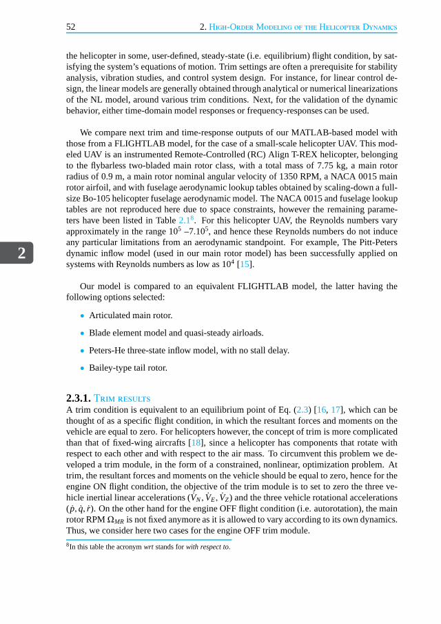
2

52 2.High-Order Modeling of the Helicopter Dynamics

the helicopter in some, user-defined, steady-state (i.e. equilibrium) flight condition, by sat-isfying the system’s equations of motion. Trim settings areoften a prerequisite for stabilityanalysis, vibration studies, and control system design. For instance, for linear control de-sign, the linear models are generally obtained through analytical or numerical linearizationsof the NL model, around various trim conditions. Next, for the validation of the dynamicbehavior, either time-domain model responses or frequency-responses can be used.

We compare next trim and time-response outputs of our MATLAB-based model withthose from a FLIGHTLAB model, for the case of a small-scale helicopter UAV. This mod-eled UAV is an instrumented Remote-Controlled (RC) Align T-REX helicopter, belongingto the flybarless two-bladed main rotor class, with a total mass of 7.75 kg, a main rotorradius of 0.9 m, a main rotor nominal angular velocity of 1350RPM, a NACA 0015 mainrotor airfoil, and with fuselage aerodynamic lookup tablesobtained by scaling-down a full-size Bo-105 helicopter fuselage aerodynamic model. The NACA 0015 and fuselage lookuptables are not reproduced here due to space constraints, however the remaining parame-ters have been listed in Table2.18. For this helicopter UAV, the Reynolds numbers varyapproximately in the range 105 –7.105, and hence these Reynolds numbers do not induceany particular limitations from an aerodynamic standpoint. For example, The Pitt-Petersdynamic inflow model (used in our main rotor model) has been successfully applied onsystems with Reynolds numbers as low as 104 [15].

Our model is compared to an equivalent FLIGHTLAB model, the latter having thefollowing options selected:

• Articulated main rotor.

• Blade element model and quasi-steady airloads.

• Peters-He three-state inflow model, with no stall delay.

• Bailey-type tail rotor.

2.3.1.Trim resultsA trim condition is equivalent to an equilibrium point of Eq.(2.3) [16, 17], which can bethought of as a specific flight condition, in which the resultant forces and moments on thevehicle are equal to zero. For helicopters however, the concept of trim is more complicatedthan that of fixed-wing aircrafts [18], since a helicopter has components that rotate withrespect to each other and with respect to the air mass. To circumvent this problem we de-veloped a trim module, in the form of a constrained, nonlinear, optimization problem. Attrim, the resultant forces and moments on the vehicle shouldbe equal to zero, hence for theengine ON flight condition, the objective of the trim module is to set to zero the three ve-hicle inertial linear accelerations (VN, VE, VZ) and the three vehicle rotational accelerations(p, q, r). On the other hand for the engine OFF flight condition (i.e. autorotation), the mainrotor RPMΩMR is not fixed anymore as it is allowed to vary according to its own dynamics.Thus, we consider here two cases for the engine OFF trim module.

8In this table the acronymwrt stands forwith respect to.

2.3.Model evaluation and validation

2

53

Table 2.1: Align T-REX physical parameters for the environment, vehicle, and actuators.

Name Parameter Value Unit

Environment

Air density ρ 1.2367 kg/m3

Static temperature T 273.15+ 15 KSpecific heat ratio (air) γ 1.4

Gas constant (air) R 287.05 J/kg.KGravity constant g 9.812 m/s2

Total mass m 7.75 kgInertia moment wrtxb A 0.2218 kg.m2

Inertia moment wrtyb B 0.5160 kg.m2

Vehicle Inertia moment wrtzb C 0.3141 kg.m2

Inertia product wrtxb D 0 kg.m2

Inertia product wrtyb E 0.0014 kg.m2

Inertia product wrtzb F 0 kg.m2

X-pos. of Fus. CG wrt total CG xFus 0 mY-pos. of Fus. CG wrt total CG yFus 0 mZ-pos. of Fus. CG wrt total CG zFus 0.017 m

MR collective θ0 [-13,13].π/180 radMR lateral cyclic θ1c [-6,6].π/180 rad

Actuators MR longitudinal cyclic θ1s [-6,6].π/180 radTR collective θTR [-20,20].π/180 rad

MR collective rate θ0 [-52,52].π/180 rad/sMR lateral cyclic rate θ1c [-52,52].π/180 rad/s

MR longitudinal cyclic rate θ1s [-52,52].π/180 rad/sTR collective rate θTR [-120,120].π/180 rad/s

1. The objective of the first engine OFF trim consists in setting to zero the previoussix accelerations, defined for the engine ON case, together with an additional ac-celeration, namely the one related to main rotor RPMΩMR. This allows to find thesteady-state autorotative flight conditions.

2. For low altitude engine OFF conditions, e.g. below 30–40 min the case of ourhelicopter, as well as during the autorotation entry phase,and flare9 phase, see Sec-tion 1.3.1, we observed, through various simulation runs, that steady-state autorota-tions was seldom reached. Rather, for those situations, thehelicopter is in a contin-uous transition from one non-equilibrium condition to the next. Hence, the objectiveof the second engine OFF trim consists in only setting to zerothe six accelerationsdefined for the engine ON case10.

9The flare refers to the landing maneuver just prior to touch-down. In the flare the nose of the vehicle is raised inorder to slow-down the descent rate, and further the proper attitude is set for touchdown.

10This second engine OFF trimming approach has shown to be feasible only for low-speed flight conditions.

2

54 2.High-Order Modeling of the Helicopter Dynamics

(Table 1 cont’d): Align T-REX physical parameters for the main rotor.

ClockWise direction of rotation Γ -1Main Number of blades Nb 2Rotor Nominal angular velocity ΩMR100% 141.37 rad/s(MR) Rotor radius from hub Rrot 0.9 m

Blade mass Mbl 0.2875 kgSpring restraint coef. due to flap KSβ

162.69 N.m/radSpring damping coef. due to flap KDβ

0 N.m.s/radSpring restraint coef. due to lag KSζ

0 N.m/radSpring damping coef. due to lag KDζ

5 N.m.s/radOffset distance eP 0.03 mOffset distance eL 0.06 mOffset distance eF 0.01 m

Distance between hub and flap hinge ∆e 0.1 mRoot cutout from flap hinge rc 0.0 m

Blade chord cbl 0.064 mBlade twist at tip θwash 0 rad

Y-pos. blade CG wrt flap hinge yGbl 0.4 mSwashplate phase angle ψPA 0 rad

Precone angle βP 0 radPitch-flap coupling ratio K(θβ) 0Pitch-lag coupling ratio K(θζ) 0

Tip loss factor B 0.97Airfoil lift coef. clbl NACA0015

Airfoil drag coef. cdbl NACA0015Airfoil pitching moment coef. cM NACA0015

X-pos. of MR hub wrt total CG xH 0.01 mY-pos. of MR hub wrt total CG yH 0 mZ-pos. of MR hub wrt total CG zH -0.213 m

Note that both of these engine OFF trim modules will be used inthe sequel. Now,the variables that the trim algorithm is allowed to manipulate include the four control in-puts (θ0, θ1c, θ1s, θTR), and the vehicle roll and pitch angles (φ, θ), since the latter two in-fluence the projection of the gravity vector on the body frame. Besides, the set-point atwhich the equilibrium is computed has to be specified in the form of additional constraints,i.e. by assigning fixed values to the three vehicle inertial linear velocities11 (VN,VE,VZ),and the three vehicle rotational velocities (p, q, r). Now regarding the dynamic inflowstates (λ0, λs, λc), and the periodic states, i.e. blade flap and lag angles and velocities(βbl, ζbl, βbl, ζbl), these states are handled by time-marching the NL helicopter model longenough until the transients have decayed. Finally, the remaining four states which include

11The three vehicle inertial linear velocities may be assigned any fixed values, hence for non-zero values thisimplies that the vehicle position is not in trim. Seen from this perspective, not all the states are in equilibrium.

2.3.Model evaluation and validation

2

55

(Table 1 cont’d): Align T-REX physical parameters for the tail rotor.

Number of blades NbTR 2Tail Nominal angular velocity ΩTR100% 612.61 rad/s

Rotor Rotor radius from rotor hub RrotTR 0.14 m(TR) Pitch-flap coupling δ3TR 0 rad

Preset collective pitch bias θbiasTR 0 radPartial coning angle wrt thrust β0TR 0 rad/N

Tail blockage constant bt1 0.927Transition velocity vbl 20 m/s

Blade chord cTR 0.0316 mTip loss factor BTR 0.92

Airfoil lift curve slope cl(0,TR) 5.92 rad−1

Blade drag coef. CDTR 0.0082X-pos. of TR hub wrt total CG xTR -1.015 mY-pos. of TR hub wrt total CG yTR -0.0575 mZ-pos. of TR hub wrt total CG zTR -0.034 m

the three vehicle Cartesian position (xN, xE, xZ) and the vehicle headingψ are left free,since the position of the helicopter does not influence12 its dynamic behavior or stability.Our trim optimization is further based upon a Newton iteration scheme, similar to that of[19], which is simple to implement and has been widely used [20]. The Newton methodguarantees quadratic local convergence, but is known to be sensitive to starting values13.

We compare next our model trim results, with those obtained from FLIGHTLAB, forthe engine ON case only. Comparison of our model with FLIGHTLAB, for the engine OFFcase, is presented within the context of dynamic results in Section2.3.2. First, Table2.2gives the maximum absolute trim deviations, as a function ofinertial linear velocities14

(VN,VE,VZ), between our model and FLIGHTLAB, for the six trim variables, i.e. the fourcontrol inputs (θ0, θ1c, θ1s, θTR) and roll and pitch angles (φ, θ). Table2.2has to be read inconjunction with Fig.2.3–Fig.2.8, where the trim results are plotted, along each motionalaxis. These motional axes are: longitudinal alongVN, lateral alongVE, vertical climb alongVZ (VZ > 0), and vertical descent alongVZ (VZ < 0). Basically, Fig.2.3–Fig. 2.8 visual-ize the trim results for each motional axis at a time, i.e. by setting to zero the velocitiesalong the remaining motional axes, whereas Table2.2 compiles the worst-case data fromFig. 2.3–Fig. 2.8 by reporting the worst-case trim deviation, for each of the six trim vari-

12Although strictly speaking this is not true in vertical flight, due to the ground effect when trimming near theground, and due to changes in air density when trimming with anon-zero vertical velocity; however for thecase of air density variations, these may be neglected when considering small-scale UAV applications, since themaximum flight altitude is generally below 150m above ground.

13Even with good starting values, it is well-known that the Newton method may at times exhibit erratic divergencedue to for example numerical corruption [20]. Hence, several other trim approaches have been researched overthe past years, for a review of helicopter trim strategies see among others [7, 16, 18, 20–24].

14With VZ positive up.

2

56 2.High-Order Modeling of the Helicopter Dynamics

Table 2.2: Trim: maximum absolute deviations between our model and FLIGHTLAB, for the engine ON case.

Name Maximum absolute deviationslongi- lateral climb descenttudinal alongVZ alongVZ

alongVN alongVE (VZ > 0) (VZ < 0)

Roll φ () 1.0 0.7 1.5 0.5Pitchθ () 0.3 0.7 0.3 0.1

MR Collectiveθ0 () 0.5 0.5 0.5 1.5TR CollectiveθTR () 0.9 0.9 1.0 2.1MR Lat. Cyclicθ1c () 0.4 0.04 0.04 0.05

MR Long. Cyclicθ1s () 0.1 0.5 0.1 0.3MR PowerPMR (W) 59 58 76 156

ables, along each motional axis. In addition, Table2.2reports the results for the main rotorpowerPMR, as this latter gives extra insight into the fidelity of our model.

We see that the maximum absolute deviations, between both models, for roll and pitchangles, are almost negligible, respectively below 1.5 and 0.7, see Table2.2. For theremaining variables, we also explore the relative deviations between both models. Regard-ing the control inputs, Table2.3gives their relative deviations in %, namely the maximumabsolute deviations divided by the full actuator ranges.

Table 2.3: Trim: maximum relative deviations between our model and FLIGHTLAB, for the control inputs in %of full actuator ranges, for the engine ON case.

Name Maximum relative deviations (in %)longi- lateral climb descenttudinal alongVZ alongVZ

alongVN alongVE (VZ > 0) (VZ < 0)

MR Collectiveθ0 1.9 1.9 1.9 5.8TR CollectiveθTR 2.2 2.2 2.5 5.2MR Lat. Cyclicθ1c 3.3 0.3 0.3 0.4

MR Long. Cyclicθ1s 0.8 4.2 0.8 2.5

Overall, we see that the differences between both models are rather small, e.g. below 6% for the Main Rotor (MR) collectiveθ0, below 5.5 % for the Tail Rotor (TR) collectiveθTR,below 3.5 % for the MR lateral cyclicθ1c, and below 4.5 % for the MR longitudinal cyclicθ1s. From Fig.2.3, Fig. 2.5, and Fig.2.7, we also see that the maximum relative trim devi-ation does not exceed 10 % for the main rotor powerPMR, for the longitudinal, lateral, andclimb motions. However, we do notice, as can also be seen in Table 2.2, some higher dis-crepancies between both models in descending flight (particularly inside the VRS), where

2.3.Model evaluation and validation

2

57

for instance the maximum relative trim deviation reaches 26% for the main rotor powerPMR. This could probably indicate that both models are implementing distinct simulationsof the induced rotor flow inside the VRS. The plot of the MR collective inputθ0, on Fig.2.4,reveals also the minimum power speed, sometimes called thebucket speed, predicted to bearound 11–13 m/s by both models. From the MR power plotPMR, in Fig. 2.5, we can alsosee that, as expected, for a CW main rotor for which the tail rotor thrust is oriented towardsport-side (i.e. to the left), it takes more power for vehiclestarboard flight (i.e. to the right)than for port-side flight. Finally, for our helicopter, the VRS region at (VN,VE) = (0, 0) m/sis approximately defined by−6 < VZ < −3 m/s (see also our discussion in [1]). Here,we clearly see form Fig.2.7 and Fig.2.8 that MR collectiveθ0 and MR powerPMR, asexpected, start to increase inside the VRS, e.g. compare their values atVZ = −4 m/svs. atVZ = −3 m/s. Hence, more engine power is required from a VRS descent thanfrom hover.

2

58 2.High-Order Modeling of the Helicopter Dynamics

−5 0 5 10 15 20−4

−2

0

2

4

Inertial Velocity VN (m/s)

Rol

l and

Pitc

h (d

eg)

−5 0 5 10 15 20400

450

500

550

600

650

Inertial Velocity VN (m/s)

Pow

er (

W)

Roll

Pitch

Figure 2.3: Trim along inertial North velocityVN: roll and pitch angles, and main rotor power (–FLIGHTLAB,∗Our Model).

−5 0 5 10 15 20−2

0

2

4

6

8

10

12

Inertial Velocity VN (m/s)

Con

trol

Inpu

ts (

deg)

Tail rotor collective

Main rotor lat. cyclic

Main rotor lon. cyclic

Main rotor collective

Figure 2.4: Trim along inertial North velocityVN: control inputs (–FLIGHTLAB,∗ Our Model).

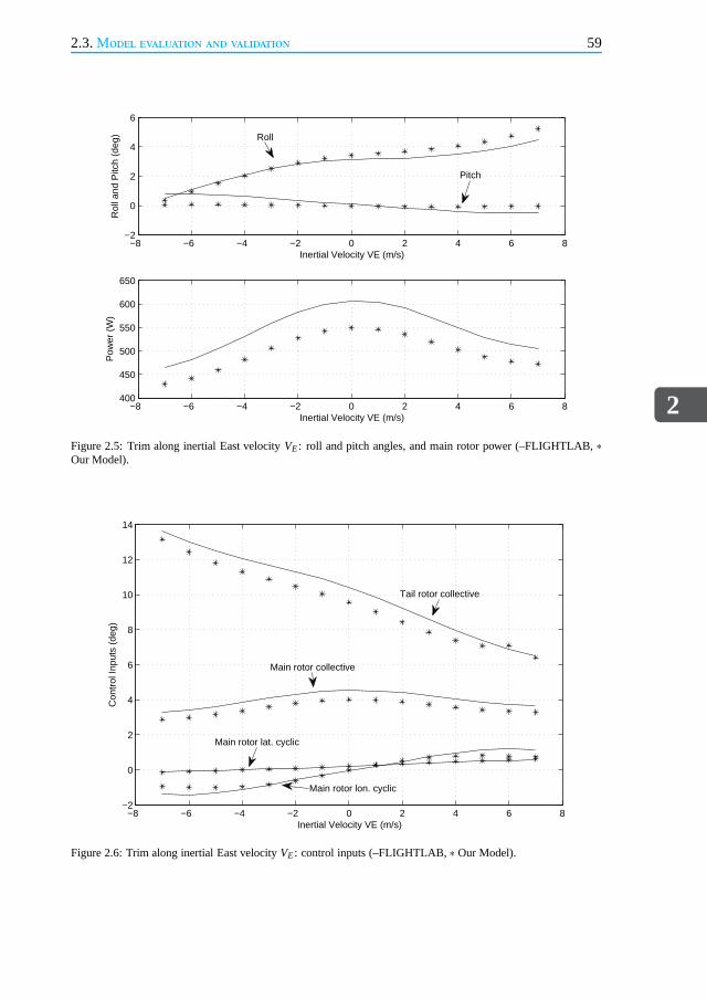
2.3.Model evaluation and validation

2

59

−8 −6 −4 −2 0 2 4 6 8−2

0

2

4

6

Inertial Velocity VE (m/s)

Rol

l and

Pitc

h (d

eg)

−8 −6 −4 −2 0 2 4 6 8400

450

500

550

600

650

Inertial Velocity VE (m/s)

Pow

er (

W)

Roll

Pitch

Figure 2.5: Trim along inertial East velocityVE: roll and pitch angles, and main rotor power (–FLIGHTLAB,∗Our Model).

−8 −6 −4 −2 0 2 4 6 8−2

0

2

4

6

8

10

12

14

Inertial Velocity VE (m/s)

Con

trol

Inpu

ts (

deg)

Tail rotor collective

Main rotor collective

Main rotor lat. cyclic

Main rotor lon. cyclic

Figure 2.6: Trim along inertial East velocityVE: control inputs (–FLIGHTLAB,∗ Our Model).

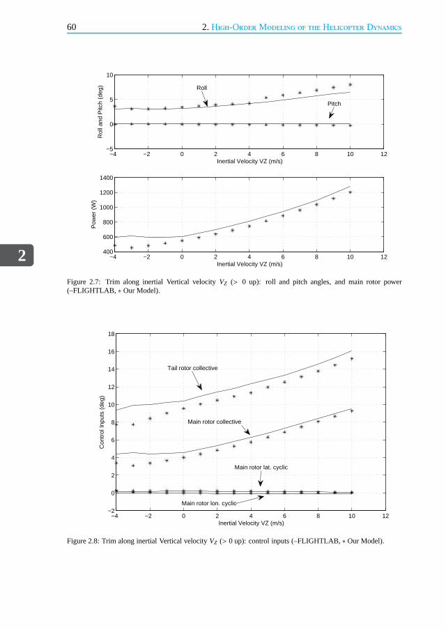
2

60 2.High-Order Modeling of the Helicopter Dynamics

−4 −2 0 2 4 6 8 10 12−5

0

5

10

Inertial Velocity VZ (m/s)

Rol

l and

Pitc

h (d

eg)

−4 −2 0 2 4 6 8 10 12400

600

800

1000

1200

1400

Inertial Velocity VZ (m/s)

Pow

er (

W)

Roll

Pitch

Figure 2.7: Trim along inertial Vertical velocityVZ (> 0 up): roll and pitch angles, and main rotor power(–FLIGHTLAB, ∗ Our Model).

−4 −2 0 2 4 6 8 10 12−2

0

2

4

6

8

10

12

14

16

18

Inertial Velocity VZ (m/s)

Con

trol

Inpu

ts (

deg)

Tail rotor collective

Main rotor collective

Main rotor lat. cyclic

Main rotor lon. cyclic

Figure 2.8: Trim along inertial Vertical velocityVZ (> 0 up): control inputs (–FLIGHTLAB,∗ Our Model).

2.3.Model evaluation and validation

2

61

2.3.2.Dynamic resultsFor the dynamic response comparison, we compare the time histories of our model withthose of FLIGHTLAB. Basically, the tests are set to evaluatethe open-loop response of ourhelicopter model. Both models have a simulation time-step set equal to 1/24th of a mainrotor revolution15. First, the rotor is allowed to reach a steady-state condition during a timeperiod of 1 s. (this is a purely software initialization matter, since the simulation starts withall states at zero). Then, for the following 3 s. we simultaneously apply sine-sweeps from0 to 2 Hz on the four input channels16, see Fig.2.9. Next, we evaluate the responses ofthe following ten states: attitude angles (φ, θ, ψ), body linear velocities (u, v,w), body rota-tional velocities (p, q, r), and MR RPMΩMR (the RPM is included for the autorotation caseonly). For a quantitative evaluation we use the Variance-Accounted-For (VAF), defined as:VAF ≔ 100%.max

(

1 − var(xk−xk)var(xk) , 0

)

with xk one of the ten states in our model, andxk its

FLIGHTLAB counterpart, see Table2.4. The VAF is a widely used metric17 in the realmof system identification18

Table 2.4: Vehicle dynamic response to sine-sweeps on the four input channels: Variance-Accounted-For (VAF)by our model with respect to FLIGHTLAB.

Name VAF (%)hover VN = steady-state autorotation

10m/s (VN,VZ) = (6,−6) m/s

Roll φ 51 76 86Pitchθ 73 84 59Yawψ 61 50 96

Long. velocityu 79 84 84Lat. velocityv 62 91 96

Vertical velocityw 93 28 92Roll ratep 67 45 76Pitch rateq 43 68 77Yaw rater 95 70 97

MR RPMΩMR N.A. N.A. 82Average over all states 69 66 85

15The default value in FLIGHTLAB.16The relatively short experiment time of 3 s. is explained by the short time-to-double amplitude, found to be

in the range of 0.9–2.3 s., this latter being derived from theeigenvalues of local LTI models. Since the totalexperiment time is rather short, we chose to focus the model validation on its low-frequency behavior, hence the2 Hz limit on the applied input signal.

17VAF values above 75 % suggest a high-quality model, whereas values in the range 50–75 % would indicate anaverage–to–good model quality.

18Note that, usually, the VAF is used in a parameter-estimation context where one tries to ’match’ the outputs of amodel with the data gathered from various experiments, or alternatively when one tries to ’match’ the outputs ofa lower-order model with those from a more complex, often higher-order, model. In our case, we simply use theVAF to compare two models, without any ’tuning’ or ’fitting’ of coefficients. Hence, in our case, the obtainedVAF values tend to be lower than VAF values typically seen in asystem identification context.

2

62 2.High-Order Modeling of the Helicopter Dynamics

Three test cases are presented, all starting at an altitude of 30 m. The first two withthe engine ON, and the third with the engine OFF. The first testcase is run from the hovertrim condition, see Fig.2.10, where it can be seen that the overall fit with FLIGHTLABis good to very good (see also Table2.4). The second test case is run to evaluate the highspeed flight condition, atVN = 10 m/s, see Fig.2.11, where we can see that the overall fitwith FLIGHTLAB is again good, except for the low VAF value (of28 %) reported forw(although the plot on thew channel is rather good, as can be seen in Fig.2.11). Indeed, ifthe to-be-compared values are close to zero (as is here the case forw), the VAF metric willtend to artificially amplify any discrepancies.

1 1.5 2 2.5 3 3.5 42

4

6

Time (s)

θ0 (

deg)

FLIGHTLABOur Model

1 1.5 2 2.5 3 3.5 4

8

10

12

Time (s)

θT

R (

deg)

1 1.5 2 2.5 3 3.5 4

−1

0

1

Time (s)

θ1s

(de

g)

1 1.5 2 2.5 3 3.5 4−1

0

1

Time (s)

θ1c

(de

g)

Figure 2.9: Vehicle dynamics: sine-sweep inputs for test cases 1, 2, & 3 (–FLIGHTLAB, – –Our Model)

The third test case is run to check the steady-state autorotative flight condition. In thistest case the helicopter is first trimmed at (VN,VZ) = (6,−6) m/s and at a MRΩMR as nearas possible to the nominal (i.e. engine ON) value of 1350 RPM,using the engine OFF trimprocedure, which also minimizes the MR RPM accelerationΩMR. The results are shown inFig. 2.12, where we can see that the overall fit with FLIGHTLAB is again good.

Naturally our model does not perfectly match FLIGHTLAB. To some extent the ob-served discrepancies, between both models, may originate from the fact that both modelsare built upon distinct modeling philosophies. For instance, for the derivation of the flap-lag dynamics as well as the computation of the rotor forces and moments, our model isbased upon a white-box, first-principles approach, i.e. a closed-form representation of thesystem’s behavior. On the contrary, FLIGHTLAB is based uponthe so-called multi-body

2.3.Model evaluation and validation

2

63

1 2 3 4

0

10

20

Time (s)

φ (d

eg)

1 2 3 4−20

−10

0

10

Time (s)

θ (d

eg)

1 2 3 4

0

50

100

Time (s)

ψ (

deg)

1 2 3 4−2

0

2

4

Time (s)

u (m

/s)

1 2 3 4

0

2

4

Time (s)

v (m

/s)

1 2 3 4−2

−1

0

Time (s)

w (

m/s

)

1 2 3 4−60−40−20

02040

Time (s)

p (d

eg/s

)

1 2 3 4−40

−20

0

20

40

Time (s)

q (d

eg/s

)

1 2 3 4

0

50

100

Time (s) r

(deg

/s)

Figure 2.10: Vehicle dynamics (test case 1): response to sine-sweep inputs (the inputs are given in Fig.2.9), froman initial condition in hover. The visualized states are: roll angleφ, pitch angleθ, yaw angleψ, body longitudinalvelocity u, body lateral velocityv, body vertical velocityw, body roll velocityp, body pitch velocityq, and bodyyaw velocityr (–FLIGHTLAB, – –Our Model).

concept19. For instance for the case of a FLIGHTLAB main rotor blade, this latter is splitinto N smaller bodies. Each body is undergoing a translational androtational displacement,with the dynamic behavior of the complete system (here the complete blade, or multi-bodysystem) resulting from the equilibrium of applied forces and the rate of change of mo-mentum at each body. This difference in modeling philosophies will inevitably result inslight differences in, for instance, the magnitude of rotor forces and moments. Further, itis well known that even small variations in the computation of forces and moments willbe integrated, over time, to large errors in velocities and positions20. Besides, this effectgets exacerbated for highly unstable systems21, which is generally the case of highly agilesmall-scale helicopters (on the one hand due to their very low inertia, and on the other due

19The multi-body concept may often be used to simulate the dynamic behavior of interconnected rigid and flexiblebodies.

20We note that the fit for test case 3 (autorotation) is better than the fit obtained for the first two test cases (withengine ON). The explanation being as follows: in autorotation, main and tail rotor collective have much lowervalues when compared to their engine ON values, and hence thegenerated aerodynamic forces are as wellsmaller in magnitude. Smaller aerodynamic forces also imply smaller discrepancies, in magnitude, between theforces computed by both models, resulting in smaller errorsin velocities and positions when integrated overtime.

21This is also why system identification of unstable systems ismost often done in closed-loop [25].

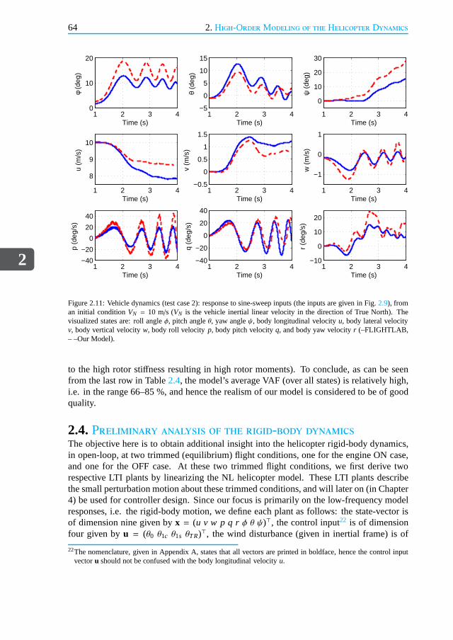
2

64 2.High-Order Modeling of the Helicopter Dynamics

1 2 3 40

10

20

Time (s)

φ (d

eg)

1 2 3 4−5

0

5

10

15

Time (s)

θ (d

eg)

1 2 3 4

0

10

20

30

Time (s)

ψ (

deg)

1 2 3 4

8

9

10

Time (s)

u (m

/s)

1 2 3 4−0.5

0

0.5

1

1.5

Time (s)

v (m

/s)

1 2 3 4

−1

0

1

Time (s)

w (

m/s

)

1 2 3 4−40

−20

0

20

40

Time (s)

p (d

eg/s

)

1 2 3 4−40

−20

0

20

40

Time (s)

q (d

eg/s

)

1 2 3 4−10

0

10

20

Time (s)

r (d

eg/s

) Figure 2.11: Vehicle dynamics (test case 2): response to sine-sweep inputs (the inputs are given in Fig.2.9), froman initial conditionVN = 10 m/s (VN is the vehicle inertial linear velocity in the direction of True North). Thevisualized states are: roll angleφ, pitch angleθ, yaw angleψ, body longitudinal velocityu, body lateral velocityv, body vertical velocityw, body roll velocityp, body pitch velocityq, and body yaw velocityr (–FLIGHTLAB,– –Our Model).

to the high rotor stiffness resulting in high rotor moments). To conclude, as can beseenfrom the last row in Table2.4, the model’s average VAF (over all states) is relatively high,i.e. in the range 66–85 %, and hence the realism of our model isconsidered to be of goodquality.

2.4.Preliminary analysis of the rigid-body dynamicsThe objective here is to obtain additional insight into the helicopter rigid-body dynamics,in open-loop, at two trimmed (equilibrium) flight conditions, one for the engine ON case,and one for the OFF case. At these two trimmed flight conditions, we first derive tworespective LTI plants by linearizing the NL helicopter model. These LTI plants describethe small perturbation motion about these trimmed conditions, and will later on (in Chapter4) be used for controller design. Since our focus is primarily on the low-frequency modelresponses, i.e. the rigid-body motion, we define each plant as follows: the state-vector isof dimension nine given byx = (u v w p q rφ θ ψ)⊤, the control input22 is of dimensionfour given byu = (θ0 θ1c θ1s θTR)⊤, the wind disturbance (given in inertial frame) is of

22The nomenclature, given in Appendix A, states that all vectors are printed in boldface, hence the control inputvectoru should not be confused with the body longitudinal velocityu.

2.4.Preliminary analysis of the rigid-body dynamics

2

65

1 2 3 40

5

10

15

Time (s)

Rol

l (de

g)

1 2 3 4−10

0

10

Time (s)

Pitc

h (d

eg)

1 2 3 40

20

40

60

Time (s)

Yaw

(de

g)

1 2 3 4

4

6

Time (s)

Long

. vel

ocity

(m

/s)

1 2 3 4−2

0

2

Time (s) La

t. ve

loci

ty (

m/s

) 1 2 3 4

4

5

6

7

Time (s) Ver

tical

vel

ocity

(m

/s)

1 2 3 4−40−20

02040

Time (s)

Rol

l rat

e (d

eg/s

)

1 2 3 4−40

−20

0

20

40

Time (s)

Pitc

h ra

te (

deg/

s)

1 2 3 4−50

0

50

Time (s)

Yaw

rat

e (d

eg/s

)

1 1.5 2 2.5 3 3.5 4126012801300132013401360

Time (s)

Mai

n R

otor

RP

M

Figure 2.12: Vehicle dynamics (test case 3): response to sine-sweep inputs (the inputs are given in Fig.2.9), froman initial condition corresponding to a steady-state autorotation at (VN,VZ) = (6,−6) m/s (VN is the vehicle inertiallinear velocity in the direction of True North, andVZ is the inertial vertical velocity). The visualized states are: rollangleφ, pitch angleθ, yaw angleψ, body longitudinal velocityu, body lateral velocityv, body vertical velocityw,body roll velocityp, body pitch velocityq, and body yaw velocityr (–FLIGHTLAB, – –Our Model).

dimension three given byd = (VNw VEw VZw)⊤, and finally the measurements vector is givenby y = x. The state-space data of these LTI models is further reported in Appendix H. Next,for these two LTI plants, we will analyze their pole maps in the complex plane, but first weaddress the NL plant linearization issue.

2.4.1.Linearizing the nonlinear helicopter modelThe NL helicopter model is subject to periodic loads, due to blades rotation, that resultin a time-varying trim condition. Linearizing the NL helicopter dynamics, around a trimcondition, can be done at each rotor position, to yield a Periodic Linear Time-Varying(PLTV) system, with a period equal to one rotation of the rotor. Now, for PLTV systems,the classical modal analysis methodologies, based upon time-invariant eigenstructures, arenot applicable anymore [26]. Hence, if one desires to apply the well-established analysisand control tools for LTI systems, then a transformation of the PLTV system into a LTI one

2

66 2.High-Order Modeling of the Helicopter Dynamics

becomes necessary. There are roughly four main methods to perform such a transformationor approximation [27]. The first, and simplest one, consists in evaluating the PLTV systemat a single rotor position (i.e. at a single blade azimuth position), and thus obtain a LTIsystem. Clearly, this approach may lead to poor results. An already better method wouldconsist in averaging the PLTV state-space matrices over oneor more rotor periods. The nexttwo methods provide LTI models with higher accuracy, but require additional mathemati-cal steps. The third method uses Floquet theory [26, 28], and the associated characteristicexponents called Floquet multipliers, to obtain constant state-space matrices. The fourthmethod uses the so-called Multi-Blade Coordinate (MBC) transformation (also known asthe Coleman transformation) [26, 29–31], i.e. by transforming quantities from rotatingblade coordinates into a non-rotating frame. Basically, the MBC describes the overall mo-tion of a rotating blade array in the inertial frame of reference. The MBC transformationresults in a weakly periodic system, which is subsequently converted into a LTI system,by averaging over one period [31]. Now, for our application, the first and fourth methodswere deemed inappropriate. For the first, it is well-known that this method may not pro-vide an LTI model of high accuracy. The fourth is particularly well-suited for rotors havingthree or more blades, and may involve significant inaccuracies for a two-bladed rotor23 [32].The third is potentially more interesting, since providingLTI models with good accuracy.However, in this thesis, we opted for the second method, since much simpler to use andimplement. Hence, the linearized models are computed usinga classical numerical pertur-bation method, resulting in a first-order Taylor series approximation of the NL model, withan averaging over several rotor periods.

Averaging: choice of the number of rotor periodsWe compare here the dynamic response, i.e. rigid-body time histories, from the NL heli-copter plant with the dynamic response from five LTI models, i.e. the latter obtained byaveraging from one to five rotor periods. Again, the rotor is first allowed to reach a steady-state condition during a time period of 1 s. Then, for the following 3 s. we simultaneouslyapply, on the four input channels, the same sine-sweep inputs that were used during themodel validation, see Fig.2.9. We further only analyze here the case for an engine ON inhover (similar results have been observed for other flight conditions), see Fig.2.13.

For a quantitative evaluation we again use the VAF, with Table 2.5 reporting the VAFvalues, accounted by each LTI model with respect to the NL model, corresponding to the 3s. long experiment depicted in Fig.2.13. Interestingly, we see that the LTI model obtainedby averaging after only one period is rather poor, particularly on the pitchθ, pitch rateq,and longitudinal velocityu axes, where these LTI outputs are moving in opposite directionswith respect to the NL ones. Increasing the number of averaged periods was thus deemednecessary. Obviously, a high number of averaged periods will tend to filter out the helicopterhigher-order dynamics, resulting in a lower-quality LTI model. Hence, some trade-offmayneed to be considered here. From the last row in Table2.5, giving the LTI model’s averageVAF (over all states), we see that averaging over three or four periods may provide thebest compromise. Now, since an LTI model should describe thesmall perturbation motionabout a trimmed condition, we also evaluated the VAF values for a shorter experiment time

23As a reminder, our Remote-Controlled (RC) Align T-REX helicopter has a two-bladed main rotor.

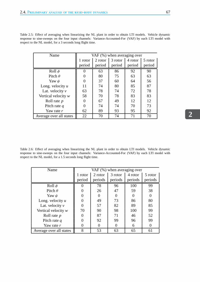
2.4.Preliminary analysis of the rigid-body dynamics

2

67

Table 2.5: Effect of averaging when linearizing the NL plant in order to obtain LTI models. Vehicle dynamicresponse to sine-sweeps on the four input channels: Variance-Accounted-For (VAF) by each LTI model withrespect to the NL model, for a 3 seconds long flight time.

Name VAF (%) when averaging over1 rotor 2 rotor 3 rotor 4 rotor 5 rotorperiod period period period period

Roll φ 0 63 86 92 90Pitchθ 0 80 75 63 63Yawψ 0 37 60 64 56

Long. velocityu 11 74 80 85 87Lat. velocityv 63 78 74 72 78

Vertical velocityw 58 70 78 83 83Roll ratep 0 67 49 12 12Pitch rateq 0 74 74 70 73Yaw rater 62 89 93 95 92

Average over all states 22 70 74 71 70

Table 2.6: Effect of averaging when linearizing the NL plant in order to obtain LTI models. Vehicle dynamicresponse to sine-sweeps on the four input channels: Variance-Accounted-For (VAF) by each LTI model withrespect to the NL model, for a 1.5 seconds long flight time.

Name VAF (%) when averaging over1 rotor 2 rotor 3 rotor 4 rotor 5 rotorperiod periods periods periods periods

Roll φ 0 78 96 100 99Pitchθ 0 26 47 59 38Yawψ 0 0 0 0 0

Long. velocityu 0 49 73 86 80Lat. velocityv 0 57 82 89 85

Vertical velocityw 70 90 98 100 99Roll ratep 0 87 71 46 52Pitch rateq 0 92 99 96 99Yaw rater 0 0 0 6 0

Average over all states 8 53 63 65 61

2

68 2.High-Order Modeling of the Helicopter Dynamics

0 2 4 6−20

0

20

40

Time (s)

φ (d

eg)

0 2 4 6−20

−10

0

10

20

Time (s)

θ (d

eg)

0 2 4 6−100

0

100

200

300

Time (s)

ψ (

deg)

0 2 4 6−2

0

2

4

Time (s)

u (m

/s)

0 2 4 6−2

0

2

4

Time (s)

v (m

/s)

0 2 4 6−2

−1

0

1

Time (s)

w (

m/s

) 0 2 4 6

−100

−50

0

50

Time (s)

p (d

eg/s

)

0 2 4 6−50

0

50

Time (s)

q (d

eg/s

)

0 2 4 6−50

0

50

100

150

Time (s)

r (d

eg/s

)

Figure 2.13: Effect of averaging when linearizing the NL plant in order to obtain LTI models. The figure comparesthe vehicle rigid-body outputs for the NL model, with those from five linearized models. The responses correspondto sine-sweep inputs from hover (black line is the NL model, red line is the LTI model by averaging over one rotorperiod, magenta line is the LTI model by averaging over two rotor periods, green line is the LTI model by averagingover three rotor periods, blue line is the LTI model by averaging over four rotor periods, and cyan line is the LTImodel by averaging over five rotor periods).

(as to better fit the helicopter linear behavior), by considering only the first 1.5 s. of theexperiment depicted in Fig.2.13. This resulted in the VAF values given in Table2.6. Basedon the last row of Table2.6, we finally settled on using four rotor periods, for the averaging,when computing LTI models from the NL helicopter model.

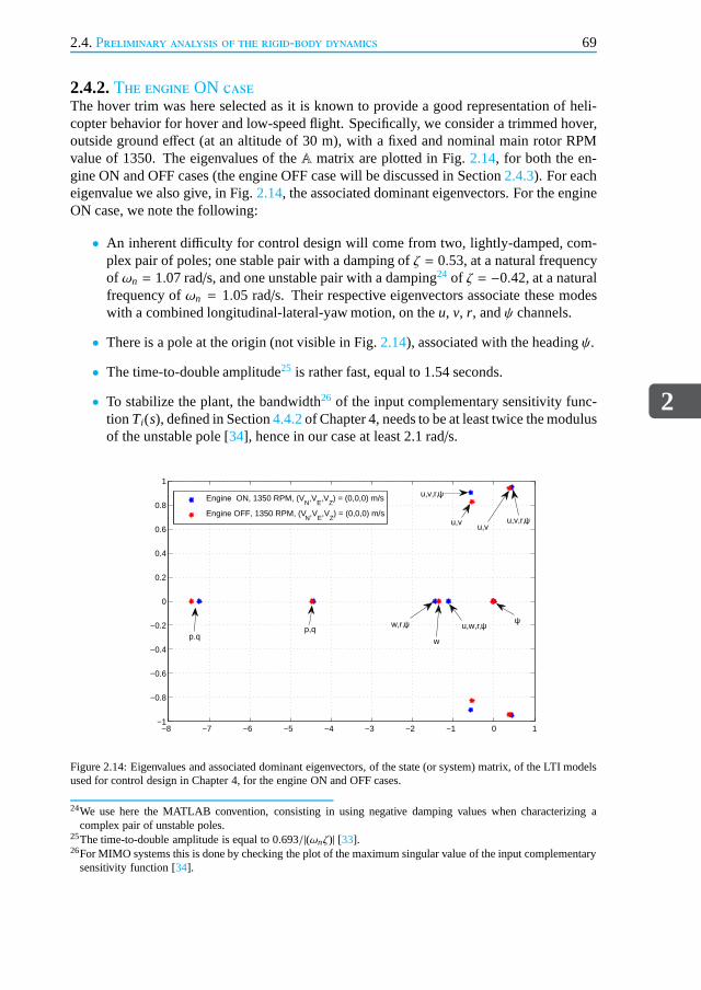
2.4.Preliminary analysis of the rigid-body dynamics

2

69

2.4.2.The engine ON caseThe hover trim was here selected as it is known to provide a good representation of heli-copter behavior for hover and low-speed flight. Specifically, we consider a trimmed hover,outside ground effect (at an altitude of 30 m), with a fixed and nominal main rotorRPMvalue of 1350. The eigenvalues of theA matrix are plotted in Fig.2.14, for both the en-gine ON and OFF cases (the engine OFF case will be discussed inSection2.4.3). For eacheigenvalue we also give, in Fig.2.14, the associated dominant eigenvectors. For the engineON case, we note the following:

• An inherent difficulty for control design will come from two, lightly-damped, com-plex pair of poles; one stable pair with a damping ofζ = 0.53, at a natural frequencyof ωn = 1.07 rad/s, and one unstable pair with a damping24 of ζ = −0.42, at a naturalfrequency ofωn = 1.05 rad/s. Their respective eigenvectors associate these modeswith a combined longitudinal-lateral-yaw motion, on theu, v, r, andψ channels.

• There is a pole at the origin (not visible in Fig.2.14), associated with the headingψ.

• The time-to-double amplitude25 is rather fast, equal to 1.54 seconds.

• To stabilize the plant, the bandwidth26 of the input complementary sensitivity func-tion Ti(s), defined in Section4.4.2of Chapter 4, needs to be at least twice the modulusof the unstable pole [34], hence in our case at least 2.1 rad/s.

−8 −7 −6 −5 −4 −3 −2 −1 0 1−1

−0.8

−0.6

−0.4

−0.2

0

0.2

0.4

0.6

0.8

1

Engine ON, 1350 RPM, (VN

,VE,V

Z) = (0,0,0) m/s

Engine OFF, 1350 RPM, (VN

,VE,V

Z) = (0,0,0) m/s

ψ

u,v,r,ψ

u,v,r,ψ

u,v

p.qp,q u,w,r,ψw,r,ψ

w

u,v

Figure 2.14: Eigenvalues and associated dominant eigenvectors, of the state (or system) matrix, of the LTI modelsused for control design in Chapter 4, for the engine ON and OFFcases.

24We use here the MATLAB convention, consisting in using negative damping values when characterizing acomplex pair of unstable poles.

25The time-to-double amplitude is equal to 0.693/|(ωnζ)| [33].26For MIMO systems this is done by checking the plot of the maximum singular value of the input complementary

sensitivity function [34].

2

70 2.High-Order Modeling of the Helicopter Dynamics

2.4.3.The engine OFFcaseIn the engine OFF case, i.e. autorotative landing, the main rotor RPM is not fixed anymore,and hence main rotor RPM dynamics will impact the overall vehicle flight dynamics. How-ever, we choose here not to include the main rotor RPMΩMR to the state-vector, and hencekeep the same state-vector that was used for the engine ON case. The advantage is that itbecomes much easier to find equilibrium points of the NL system27. Indeed, by using this"quasi-steady" modeling approach, it becomes possible to find equilibrium points outsideof steady autorotation, e.g. while transitioning between the instant of engine failure intosteady autorotation, or alternatively during flare (the maneuver just prior to landing). Ob-taining these equilibrium points allows for subsequent linearizations of the NL model, andconsequently for control design in the LTI framework.

For the trimmed flight condition, we opt for a condition in hover with engine OFF(note that now the main rotor RPM is not in equilibrium anymore). Choosing such a flightcondition, with an associated initial velocity of zero, could potentially provide the bestdescription of helicopter behavior during landing (where the helicopter velocity is also verylow). The state-space data of the LTI model is further reported in Appendix H. Again, theeigenvalues of theAmatrix are plotted in Fig.2.14, where for each eigenvalue we also givethe associated dominant eigenvectors. For the engine OFF case, we note the following:

• An inherent difficulty for control design will come from two, lightly-damped, com-plex pair of poles; one stable pair with a damping ofζ = 0.54, at a natural frequencyof ωn = 0.99 rad/s, and one unstable pair with a damping ofζ = −0.37, at a naturalfrequency ofωn = 1.02 rad/s. Their respective eigenvectors associate these modeswith a combined longitudinal-lateral motion, on theu andv channels.

• The time-to-double amplitude is also fast, equal to 1.83 seconds.

• To stabilize the plant, the bandwidth of the input complementary sensitivity functionTi(s), defined in Section4.4.2of Chapter 4, needs to be at least 2.04 rad/s.

2.5.ConclusionThis Chapter has presented the first building-block, towards the development of an au-tonomous helicopter system, that may be characterized as follows: a comprehensive model-ing framework, particularly suited for small-scale flybarless helicopters. Comparisons withan equivalent FLIGHTLAB simulation showed that our model isvalid for a range of flightconditions, and preliminary insight into the open-loop dynamics was also given. This com-prehensive helicopter nonlinear model will, in subsequentChapters, be used for controllervalidation. For controller design however, and due to its complexity, only approximation ofthis model will be used in the upcoming Chapters.

27This engine OFF trimming approach has shown to be feasible only for low-speed flight conditions.

2.6.Appendix A: Nomenclature

2

71

2.6.Appendix A: NomenclatureVectors are printed in boldfaceX. A vector is qualified by its subscript, whereas its super-script denotes the projection frame: e.g.V I

a represents the aerodynamic velocity projectedon frameFI . Matrices are written in outline typeM, and transformation matrices are de-noted asTi j , with the two suffices signifying from frameF j to frameFi . All units are in theS.I. system.

Positions and AnglesxN, xE, xZ Coordinates of vehicle CG in frameFo

φ Vehicle bank angle (roll angle)θ Vehicle inclination angle (pitch angle, or elevation)ψ Vehicle azimuth angle (yaw angle, heading)ψ f Wind heading angle

Linear velocitiesV and their componentsu, v,wVk,G Kinematic velocity of vehicle CGVa,G Aerodynamic velocity of vehicle CGuo

k = VN x component ofVk,G on Fo, North velocityvo

k = VE y component ofVk,G on Fo, East velocitywo

k = VZ zcomponent ofVk,G on Fo, Vertical velocityub

k = u x component ofVk,G on Fb

vbk = v y component ofVk,G on Fb

wbk = w zcomponent ofVk,G on Fb

uw Wind x-velocity inFE

vw Wind y-velocity inFE

ww Wind z-velocity inFE

Angular velocitiesΩ and their componentsp, q, rΩk = ΩbE Kinematic angular velocity of vehicle CG relative to the earthpb

k = p Roll velocity (roll rate) of vehicle CG wrt to the earthqb

k = q Pitch velocity (pitch rate) of vehicle CG wrt to the earthrbk = r Yaw velocity (yaw rate) of vehicle CG wrt to the earth

Main Rotor (MR) propertiesα wake angle wrt to rotor diskαbl Blade section angle of attackB Tip loss factorβbl Blade flap angleβ0 Rotor TPP coning angleβ1c Longitudinal rotor TPP tiltβ1s Lateral rotor TPP tiltβP Rotor precone angleC0 = Mbl.yGbl Blade 1st mass momentcbl Blade chord

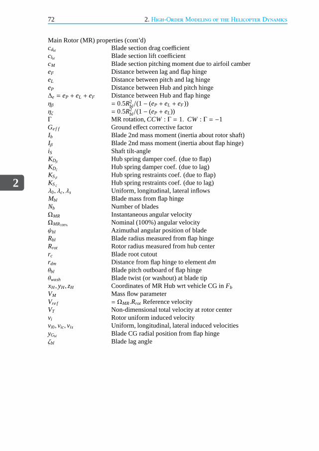
2

72 2.High-Order Modeling of the Helicopter Dynamics

Main Rotor (MR) properties (cont’d)cdbl Blade section drag coefficientclbl Blade section lift coefficientcM Blade section pitching moment due to airfoil cambereF Distance between lag and flap hingeeL Distance between pitch and lag hingeeP Distance between Hub and pitch hinge∆e = eP + eL + eF Distance between Hub and flap hingeηβ = 0.5R2

bl/(1− (eP + eL + eF))ηζ = 0.5R2

bl/(1− (eP + eL))Γ MR rotation,CCW : Γ = 1. CW : Γ = −1Ge f f Ground effect corrective factorIb Blade 2nd mass moment (inertia about rotor shaft)Iβ Blade 2nd mass moment (inertia about flap hinge)iS Shaft tilt-angleKDβ

Hub spring damper coef. (due to flap)KDζ

Hub spring damper coef. (due to lag)KSβ

Hub spring restraints coef. (due to flap)KSζ

Hub spring restraints coef. (due to lag)λ0, λc, λs Uniform, longitudinal, lateral inflowsMbl Blade mass from flap hingeNb Number of bladesΩMR Instantaneous angular velocityΩMR100% Nominal (100%) angular velocityψbl Azimuthal angular position of bladeRbl Blade radius measured from flap hingeRrot Rotor radius measured from hub centerrc Blade root cutoutrdm Distance from flap hinge to elementdmθbl Blade pitch outboard of flap hingeθwash Blade twist (or washout) at blade tipxH , yH, zH Coordinates of MR Hub wrt vehicle CG inFb

VM Mass flow parameterVre f = ΩMR.Rrot Reference velocityVT Non-dimensional total velocity at rotor centervi Rotor uniform induced velocityvi0, vic, vis Uniform, longitudinal, lateral induced velocitiesyGbl Blade CG radial position from flap hingeζbl Blade lag angle

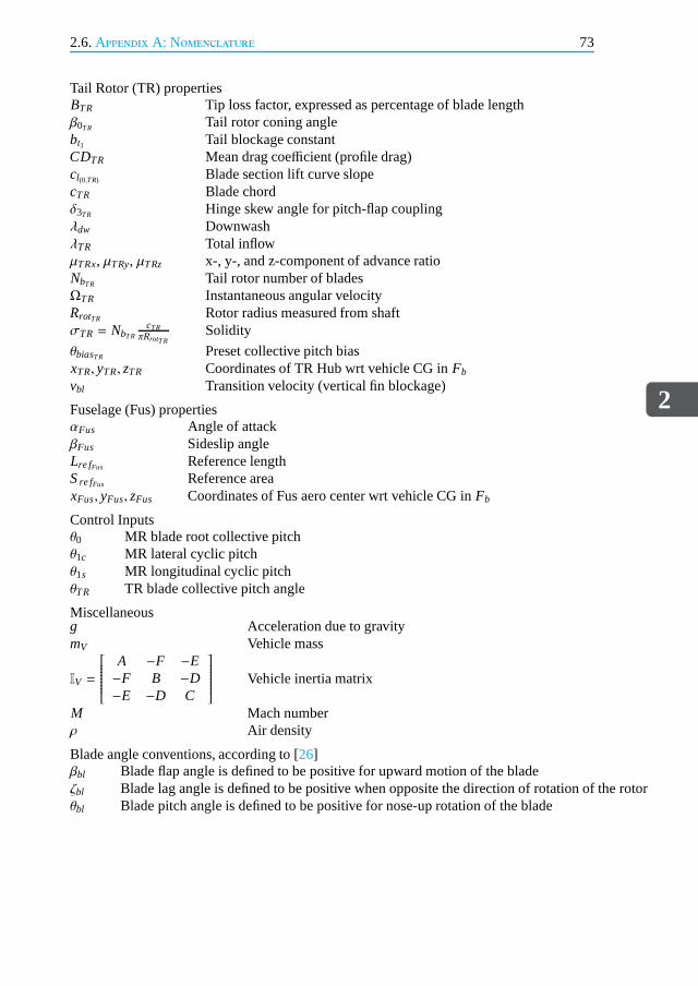
2.6.Appendix A: Nomenclature

2

73

Tail Rotor (TR) propertiesBTR Tip loss factor, expressed as percentage of blade lengthβ0TR Tail rotor coning anglebt1 Tail blockage constantCDTR Mean drag coefficient (profile drag)cl(0,TR) Blade section lift curve slopecTR Blade chordδ3TR Hinge skew angle for pitch-flap couplingλdw DownwashλTR Total inflowµTRx, µTRy, µTRz x-, y-, and z-component of advance ratioNbTR Tail rotor number of bladesΩTR Instantaneous angular velocityRrotTR Rotor radius measured from shaftσTR = NbTR

cTRπRrotTR

Solidity

θbiasTR Preset collective pitch biasxTR, yTR, zTR Coordinates of TR Hub wrt vehicle CG inFb

vbl Transition velocity (vertical fin blockage)

Fuselage (Fus) propertiesαFus Angle of attackβFus Sideslip angleLre fFus Reference lengthSre fFus Reference areaxFus, yFus, zFus Coordinates of Fus aero center wrt vehicle CG inFb

Control Inputsθ0 MR blade root collective pitchθ1c MR lateral cyclic pitchθ1s MR longitudinal cyclic pitchθTR TR blade collective pitch angle

Miscellaneousg Acceleration due to gravitymV Vehicle mass

IV =

A −F −E−F B −D−E −D C

Vehicle inertia matrix

M Mach numberρ Air density

Blade angle conventions, according to [26]βbl Blade flap angle is defined to be positive for upward motion of the bladeζbl Blade lag angle is defined to be positive when opposite the direction of rotation of the rotorθbl Blade pitch angle is defined to be positive for nose-up rotation of the blade

2

74 2.High-Order Modeling of the Helicopter Dynamics

2.7.Appendix B: FramesThe first five frames hereunder, i.e.FI –Fk, are the standard aircraft navigation frames, seefor example [14].Frame namesFI Geocentric inertial frame (see Fig.2.15)FE Normal earth fixed frameFo Vehicle carried normal earth frame (see Fig.2.16)Fb Body (vehicle) frame (see Fig.2.16)Fk Kinematic (flight path) frameFHB Hub-Body frame (see Fig.2.17and Fig.2.18)F1<i<6, Fbl Main Rotor frames (see Fig.2.17and Fig.2.18)

Frame originsA Origin of frameFI , earth centerG Origin of framesFb andFk, vehicle CGH Origin of frameFHB

O Origin of framesFE andFo

The inertial frame FI (A, xI , yI , zI )The inertial frameFI , see Fig.2.15, is a geocentric inertial axis system. The origin of theframeA being the center of the earth, the axis south-northzI is carried by the axis of theearth’s rotation, while axesxI andyI are keeping a fixed direction in space. The angularvelocity of the earth relative toFI isΩEI .

Normal earth-fixed frame FE (O, xE, yE, zE)This frame is attached to the earth. The originO is a fixed point relative to the earth andthe axiszE is oriented following the descending direction of gravitational attraction locatedonO. The plane (xE, yE) is tangent to the earth’s surface. The pointO will be placed at thesurface of the earth’s geoid and the axisxE will be directed towards the geographical north.

Vehicle-carried normal earth frame Fo (O, xo, yo, zo)The axiszo is oriented towards the descending direction of the local gravity attraction, atthe vehicle center of mass (Fo has the same originO asFE), but contrary to the latter itfollows the local gravity as seen by the vehicle. The axisxo will be directed towards thegeographical north (thusxo is not parallel toxE).

Body frame Fb (G, xb, yb, zb)This frame is linked to the vehicle’s body. The fuselage axisxb is oriented towards the frontand belongs to the symmetrical plane of the vehicle. The axiszb is in the symmetrical planeof the vehicle and oriented downwards relative to the vehicle. This definition assumes theexistence of a symmetrical plane.

Kinematic or flight-path frame Fk (G, xk, yk, zk)The axisxk is carried by the kinematic velocity of the vehicleVk,G.

2.7.Appendix B: Frames

2

75

Figure 2.15: Inertial frameFI . Figure from [14].

Figure 2.16: Vehicle carried normal earth frameFo, and body frameFb. Figure from [14].

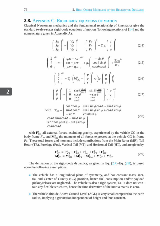
2

76 2.High-Order Modeling of the Helicopter Dynamics

2.8.Appendix C: Rigid-body equations of motionClassical Newtonian mechanics and the fundamental relationship of kinematics give thestandard twelve-states rigid-body equations of motion (following notations of [14] and thenomenclature given in Appendix A):

xN

xE

xZ

o

=

VN

VE

VZ

o

VN

VE

VZ

o

= Tob.

uvw

b

(2.4)

uvw

b

= −

q.w− r.vr.u− p.wp.v− q.u

b

+ g.

− sinθcosθ sinφcosθ cosφ

b

+FCG

mV

b

(2.5)

pqr

b

= I−1V .

(

MbCG −

pqr

b

×(

IV.

pqr

b)

)

(2.6)

φ

θ

ψ

b

=

1 sinθ. sinφcosθ sinθ. cosφ

cosθ0 cosφ − sinφ0 sinφ

cosθcosφcosθ

.

pqr

b

(2.7)

with Tob =

cosθ cosψ sinθ sinφ cosψ − sinψ cosφsinψ cosθ sinθ sinφ sinψ + cosψ cosφ− sinθ cosθ sinφ

cosψ sinθ cosφ + sinφ sinψsinθ cosφ sinψ − sinφ cosψcosθ cosφ

(2.8)

with FbCG all external forces, excluding gravity, experienced by thevehicle CG in the

body frameFb, andMbCG the moments of all forces expressed at the vehicle CG in frame

Fb. These total forces and moments include contributions fromthe Main Rotor (MR), TailRotor (TR), Fuselage (Fus), Vertical Tail (VT), and Horizontal Tail (HT), and are given by

FbCG = Fb

MR + FbTR+ Fb

Fus+ FbVT + Fb

HTMb

CG = MbMR +Mb

TR+MbFus+Mb

VT +MbHT

(2.9)

The derivation of the rigid-body dynamics, as given in Eq. (2.4)–Eq. (2.8), is basedupon the following assumptions

• The vehicle has a longitudinal plane of symmetry, and has constant mass, iner-tia, and Center of Gravity (CG) position, hence fuel consumption and/or payloadpickup/release are neglected. The vehicle is also a rigid system, i.e. it does not con-tain any flexible structures, hence the time derivative of the inertia matrix is zero.

• The vehicle altitude Above Ground Level (AGL) is very small compared to the earthradius, implying a gravitation independent of height and thus constant.

2.8.Appendix C: Rigid-body equations of motion

2

77

• The earth is assumed fixed and flat. There is thus no longer a distinction betweenthe directions of gravitational force and the force of gravity, hence the external forcebecomes the force of gravity28.

• We neglect the effect of buoyancy (Armichedes force).

28For further details on the geoid earth and gravity see [14, 35].

2

78 2.High-Order Modeling of the Helicopter Dynamics

2.9.Appendix D: Main rotorFor a single main rotor, and briefly summarized, helicopter flight dynamics includes therigid-body responses (presented in Appendix C) combined with the main rotor higher-frequency modes [36, 37]. For flight mechanics and control development purposes, thethree most important aspects of these higher-order rotor modes are: 1) blade flapping, whichallows the blade to move in a plane containing the blade and the shaft; 2) blade lead-lag,which allows the blade to move in the plane of rotation; and 3)rotor inflow which is theflow field induced by the main rotor. Now, for the purpose of modeling a generic flybarlesssmall-scale helicopter main rotor (such as the Align T-REX in Fig. 1.16), we have chosento model it as an articulated Pitch-Lag-Flap (P-L-F) hinge arrangement. This chosen hingeconfiguration is particularly well suited for the case of small-scale helicopters. It allows tokeep the pitch and lag hinge offsets at their current physical values while replacing the rub-ber O-rings, see Fig.1.10, by a virtual flap hinge (having stiffness and damping) outboardof the lag hinge. The (P-L-F) hinge arrangement is visualized in Fig.2.17and Fig.2.18.

AssumptionsThe presented assumptions are valid for stability and control investigations of helicoptersup to an advance ratio limit29 of about 0.3 [38–40].

Structural simplifications

• Rotor shaft forward and lateral tilt-angles are zero. Rotorprecone is also zero. Theblade has zero twist, constant chord, zero sweep, constant thickness ratio, and a uni-form mass distribution.

• We assume a rigid rotor blade in bending. We neglect higher modes (harmonics),since higher modes are only pronounced at high speed [7, 41]. Further, blade torsionis neglected since small-scale helicopter blades are generally relatively stiff.

• Rotor inertia inboard of the flap hinge is also neglected.

Aerodynamics simplifications

• Uniform inflow is computed through momentum theory30.

• Vehicle flies at a low altitude, hence neglecting air densityand temperature variations.Blade element theory is used to compute rotor lift and drag forces31. Radial flowalong blade span is ignored. Pitch, lag, and flap angles are assumed to be small.

• Compressibility effects are disregarded, which is a reasonable assumption consider-ing small-scale helicopter flight characteristics. Viscous flow effects are also disre-garded, which is a valid assumption for low AOA and un-separated flow [13, 42].

29The advance ratio is the ratio of forward vehicle speed to a main rotor blade tip speed. The flight envelope ofsmall-scale helicopters is well within this limit.

30Which states that the total force acting on a control volume is equal to the rate of change of momentum [26].31Blade element theory calculates the forces on the blade due to its motion through air. It is assumed that a blade

section acts as a 2D airfoil producing aerodynamic forces [26].

2.9.Appendix D: Main rotor

2

79

Figure 2.17: Main rotor frames (top-view).

Figure 2.18: Main rotor frames (side-view).

2

80 2.High-Order Modeling of the Helicopter Dynamics

• Aerodynamic interference effects between the main rotor and other helicopter mod-ules, e.g. fuselage or tail rotor, are neglected.

• The presence of the fuselage just under the main rotor acts asa so-called pseudo-ground effect [43], resulting in some thrust recovery. This phenomenon is also ne-glected.

Dynamical simplifications

• Dynamic twist32 is neglected. Hence blade CG is assumed to be colocated with bladesection quarter chord line.

• Unsteady (frequency dependent) effects for time-dependent development of blade liftand pitching moment, due to changes in local incidence, are ignored; e.g. dynamicstall, due to rapid pitch changes, is ignored.

Comments on the modeling assumptions and model simplificationsHelicopter simulation codes may be developed for a variety of applications, ranging fromflight dynamics simulation purposes, flying qualities investigations, auto-pilot design, oper-ational analysis, crew training, load prediction, and/or vibrations analysis. In our case, thedesired objectives (i.e. the application domain) for our model are: 1) flight dynamics sim-ulation, in which the model can be used in a Hardware In The loop (HITL) environment tosimulate the helicopter dynamics, hence enabling the verification and validation of a flightcontrol system (i.e. the embedded system); and 2) the model should also be useful for con-troller synthesis, i.e. the so-called modeling for controlparadigm. This sets the context ofthe model presented in this Chapter.

Now once the intended model’s application domain has been defined, we need to ad-dress the question of helicopter model fidelity. To this end,and according to [44], the levelof model sophistication, to conveniently describe a helicopter model complexity, may beformulated by two criteria, namelymodel dynamicsandmodel validity, defined as fol-lows:

1. Model dynamicsqualifies the level of detail in representing the dynamics ofthe he-licopter. This criterium determines the fidelity of the model in terms of the frequencyrange of applicability, e.g. a model consisting of only the rigid-body, actuators, andmain rotor RPM dynamics, versus a model which also includes additional main rotorhigher-frequency phenomena, such as blade flap-lag, rotor inflow dynamics, etc.

2. Model validity represents the level of sophistication in calculating the helicopterforces, moments, and main rotor inflow. This criterium determines the domain ofvalidity in the flight envelope, e.g. a model which crudely reproduces the associatedlaws of physics, versus a model which accurately simulates the vehicle (aerodynamic)forces and moments, including at high speed flight, descending in the Vortex-Ring-State (VRS), and the autorotation condition.

32Any offset in blade chordwise CG and/or blade aerodynamic center position will result in a coupling of the flapand torsion degrees-of-freedom in blade elastic modes [7].

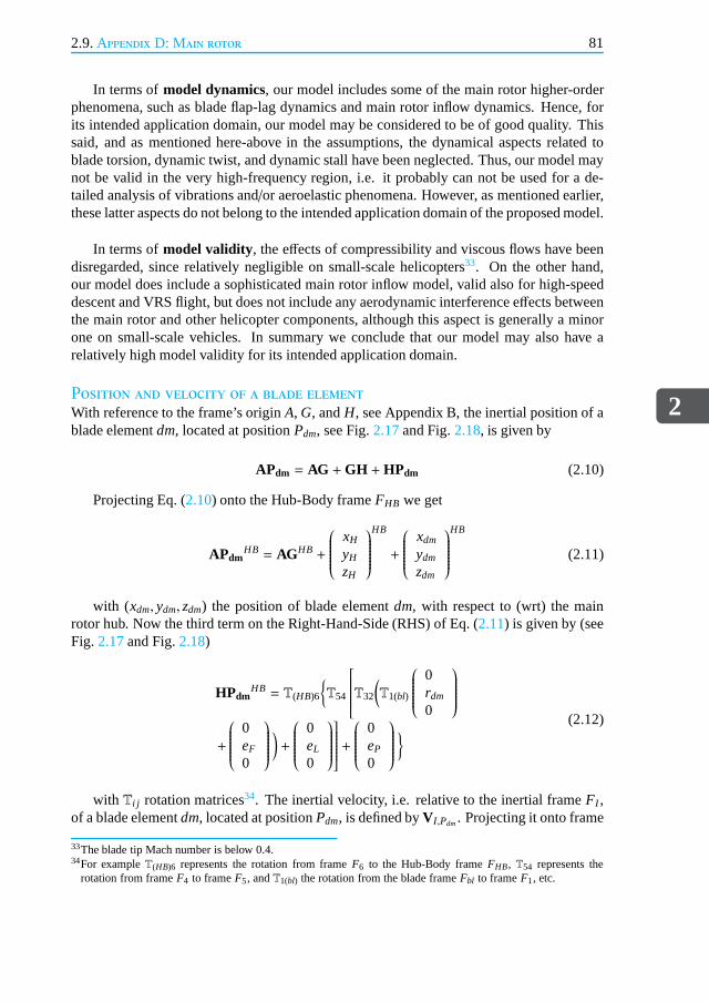
2.9.Appendix D: Main rotor

2

81

In terms ofmodel dynamics, our model includes some of the main rotor higher-orderphenomena, such as blade flap-lag dynamics and main rotor inflow dynamics. Hence, forits intended application domain, our model may be considered to be of good quality. Thissaid, and as mentioned here-above in the assumptions, the dynamical aspects related toblade torsion, dynamic twist, and dynamic stall have been neglected. Thus, our model maynot be valid in the very high-frequency region, i.e. it probably can not be used for a de-tailed analysis of vibrations and/or aeroelastic phenomena. However, as mentioned earlier,these latter aspects do not belong to the intended application domain of the proposed model.

In terms ofmodel validity, the effects of compressibility and viscous flows have beendisregarded, since relatively negligible on small-scale helicopters33. On the other hand,our model does include a sophisticated main rotor inflow model, valid also for high-speeddescent and VRS flight, but does not include any aerodynamic interference effects betweenthe main rotor and other helicopter components, although this aspect is generally a minorone on small-scale vehicles. In summary we conclude that ourmodel may also have arelatively high model validity for its intended application domain.

Position and velocity of a blade elementWith reference to the frame’s originA, G, andH, see Appendix B, the inertial position of ablade elementdm, located at positionPdm, see Fig.2.17and Fig.2.18, is given by

APdm = AG +GH + HPdm (2.10)

Projecting Eq. (2.10) onto the Hub-Body frameFHB we get

APdmHB = AGHB +

xH

yH

zH

HB

+

xdm

ydm

zdm

HB

(2.11)

with (xdm, ydm, zdm) the position of blade elementdm, with respect to (wrt) the mainrotor hub. Now the third term on the Right-Hand-Side (RHS) ofEq. (2.11) is given by (seeFig. 2.17and Fig.2.18)

HPdmHB = T(HB)6

T54

T32

(

T1(bl)

0rdm

0

+

0eF

0

)

+

0eL

0

+

0eP

0

(2.12)

with Ti j rotation matrices34. The inertial velocity, i.e. relative to the inertial frameFI ,of a blade elementdm, located at positionPdm, is defined byV I ,Pdm. Projecting it onto frame

33The blade tip Mach number is below 0.4.34For exampleT(HB)6 represents the rotation from frameF6 to the Hub-Body frameFHB, T54 represents the

rotation from frameF4 to frameF5, andT1(bl) the rotation from the blade frameFbl to frameF1, etc.

2

82 2.High-Order Modeling of the Helicopter Dynamics

FHB, and using Eq. (2.10), we obtain

VHBI ,Pdm=

(

dAG I

dt

)HB

+

(

dGH I

dt

)HB

+

(

dHPdmI

dt

)HB

(2.13)

where the superscript (·)I , such as indAG I

dt , means that the derivative is taken relative toinertial frameFI . For the first term on the RHS of Eq. (2.13), and assuming a flat and fixedearth, we get (refer also to the nomenclature)

(

dAG I

dt

)HB

= T(HB)oVok,G = T(HB)o

VN

VE

VZ

o

(2.14)

with Vok,G the vehicle kinematic velocity projected onto the vehicle carried normal earth

frameFo, andT(HB)o the rotation matrix from frameFo to frameFHB. For the second termon the RHS of Eq. (2.13) we obtain (using the kinematics rule)

(

dGH I

dt

)HB

=

(

dGHb

dt

)HB

+ΩHBbI ×GHHB (2.15)

where× denotes the cross product, andΩHBbI the angular velocity of body frameFb

relative to inertial frameFI , projected onto the Hub-Body frameFHB. Here the first termon the RHS of Eq. (2.15) is zero since the hub center H is fixed in the body frameFb. Thesecond term on the RHS of Eq. (2.15) gives

ΩHBbI ×GHHB =

(

T(HB)bΩbbI

)

×(

T(HB)bGHb)

(2.16)

Since the earth is fixed we haveΩbbI = Ω

bbE (see nomenclature), and Eq. (2.15) is now

equivalent to(

dGH I

dt

)HB

=

T(HB)b

pqr

b

×

T(HB)b

xH

yH

zH

b

(2.17)

Finally, for the third term on the RHS of Eq. (2.13) we have(

dHPdmI

dt

)HB=

(

dHPdmHB

dt

)HB+ΩHB

(HB)I × HPdmHB

= ddt

xdm

ydm

zdm

HB

+ΩHB(HB)I ×

xdm

ydm

zdm

HB(2.18)

We can also expressΩHB(HB)I as

ΩHB(HB)I = Ω

HB(HB)b +Ω

HBbI (2.19)

The first term on the RHS of Eq. (2.19) is zero since frameFHB is fixed wrt frameFb.The second term on the RHS of Eq. (2.19) can be re-written as

ΩHBbI = T(HB)bΩ

bbI = Ω

bbI = Ω

bbE =

pqr

b

(2.20)

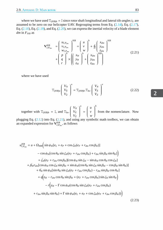
2.9.Appendix D: Main rotor

2

83

where we have usedT(HB)b = I since rotor shaft longitudinal and lateral tilt-anglesiS areassumed to be zero on our helicopter UAV. Regrouping terms from Eq. (2.14), Eq. (2.17),Eq. (2.18), Eq. (2.19), and Eq. (2.20), we can express the inertial velocity of a blade elementdm in FHB as

VHBI ,Pdm

=

uI ,Pdm

vI ,Pdm

wI ,Pdm

HB

=

uvw

b

+ ddt

xdm

ydm

zdm

HB

+

pqr

b

×

xH

yH

zH

b

+

xdm

ydm

zdm

HB

(2.21)

where we have used

T(HB)o

VN

VE

VZ

o

= T(HB)b.Tbo.

VN

VE

VZ

o

(2.22)

together withT(HB)b = I, andTbo.

VN

VE

VZ

o

=

uvw

b

from the nomenclature. Now

plugging Eq. (2.12) into Eq. (2.21), and using any symbolic math toolbox, we can obtainan expanded expression forVHB

I ,Pdm, as follows

uHBI ,Pdm= u+ ΩMR

(

sinψbl[eL + eP + cosζbl(eF + rdmcosβbl)]

− cosψbl[cosθbl sinζbl(eF + rdmcosβbl) + rdmsinβbl sinθbl])

+ ζbl(eF + rdmcosβbl)[cosψbl sinζbl − sinψbl cosθbl cosζbl]

+ βblrdm[cosψbl cosζbl sinβbl + sinψbl(cosθbl sinζbl sinβbl − cosβbl sinθbl)]

+ θbl sinψbl[sinθbl sinζbl(eF + rdmcosβbl) − rdmsinβbl cosθbl]

+ q(

zH − rdmcosθbl sinβbl + (eF + rdmcosβbl) sinζbl sinθbl

)

− r(

yH − Γ cosψbl(cosθbl sinζbl(eF + rdmcosβbl)

+ rdmsinβbl sinθbl) + Γ sinψbl(eL + eP + cosζbl(eF + rdmcosβbl)))

(2.23)

2

84 2.High-Order Modeling of the Helicopter Dynamics

vHBI ,Pdm= v+ ΩMRΓ

(

(eL + eP) cosψbl + rdmsinψbl sinβbl sinθbl

+ (eF + rdmcosβbl)(cosψbl cosζbl + sinψbl cosθbl sinζbl))

− ζblΓ(eF + rdmcosβbl)[cosψbl cosζbl cosθbl + sinψbl sinζbl]

+ βblrdmΓ(cosψbl cosθbl sinζbl sinβbl − cosψbl cosβbl sinθbl − sinψbl cosζbl sinβbl)

+ θblΓ cosψbl[sinθbl sinζbl(eF + rdmcosβbl) − rdmsinβbl cosθbl]

− p

(

zH −(

rdmcosθbl sinβbl − (eF + rdmcosβbl) sinζbl sinθbl

)

)

+ r

(

xH −(

cosψbl(eL + eP + cosζbl(eF + rdmcosβbl))

+ sinψbl(cosθbl sinζbl(eF + rdmcosβbl) + rdmsinβbl sinθbl))

)

(2.24)

wHBI ,Pdm= w+ ζbl cosζbl sinθbl(eF + rdmcosβbl)

− βblrdm(cosβbl cosθbl + sinβbl sinζbl sinθbl)

+ θbl[rdmsinθbl sinβbl + (eF + rdmcosβbl) sinζbl cosθbl]

+ p(

yH − Γ cosψbl(cosθbl sinζbl(eF + rdmcosβbl) + rdmsinβbl sinθbl)

+ Γ sinψbl(eL + eP + cosζbl(eF + rdmcosβbl)))

− q(

xH − cosψbl(eL + eP + cosζbl(eF + rdmcosβbl))

− sinψbl(cosθbl sinζbl(eF + rdmcosβbl) + rdmsinβbl sinθbl))

(2.25)

with the total blade pitch angle given by [11]

θbl = θ0 + θ1c cos(ψbl + ψPA) + θ1s sin(ψbl + ψPA) + θt,rdm − K(θblβbl)βbl − K(θblζbl)ζbl (2.26)

and the blade pitch component due to blade twist given by

θt,rdm = rdmθwash

Rbl(2.27)

Note also, as stated in the assumptions here-above, we neglect any effects due to rapidpitch changes, e.g. dynamic stall effects. Hence, we will assume thatθbl ≪ βbl, θbl ≪ ζbl,and θbl ≪ ΩMR. Consequently, in the sequel we will also assume to haveθbl ≃ 0 inEq. (2.23)–Eq. (2.25).

2.9.Appendix D: Main rotor

2

85

Flap-Lag equations of motionSince the early 1950s it is known that including flapping dynamics in a helicopter flightmodel could produce limitations in rate and attitude feedback gains [45]. Further, for heli-copter directional axis control, blade lead-lag dynamics ought to be considered for controlsystem design [46]. Indeed, it is well known that blade lead-lag produces increased phaselag at high frequency, in the same frequency range where flapping effects occur [47], andthat control rate gains are primarily limited by lead-lag-body coupling [47, 48]. Now, interms of blade flap-lag modeling, a foundational contribution was given in [11], wherederivations of the coupled flap-lag equations of motion for arigid articulated rotor, for the(F-L-P), (F-P-L), and (L-F-P) hinge sequences, was laid out. The purpose of our work isto present a model for a new hinge arrangement, i.e. the (P-L-F) sequence, which is muchmore useful for modeling the rotor dynamics of a small-scalehelicopter. The equationspresented in the sequel (obtained by the Lagrangian method [10]) are valid for a singlearticulated rotor with hinge springs and viscous dampers. Compared to [11] our approachretains all three hinges physically separated and works also for both ClockWise (CW) andCounter-ClockWise (CCW) rotating main rotors. Further, full coupling between vehicleand blade dynamics is modeled. Now from Lagrangian theory, we have

ddt

(

∂KE

∂ζbl

)

− ∂KE

∂ζbl= Qζbl (2.28a)

ddt

(

∂KE

∂βbl

)

− ∂KE

∂βbl= Qβbl (2.28b)

with KE the kinetic energy of a blade,βbl, ζbl, blade flap and lag angles, andQβbl , Qζbl ,the generalized forces. These latter include the effect of gravity, aerodynamics, and springdamping and stiffness, and are given by

Qζbl = Qζbl ,G + Qζbl ,A + Qζbl ,D + Qζbl ,S (2.29a)

Qβbl = Qβbl,G + Qβbl,A + Qβbl,D + Qβbl ,S (2.29b)

The kinetic energy of a single rotor blade is given by

KE =12

∫ Rbl

0VHB

I ,Pdm

⊤.VHB

I ,Pdmdm (2.30)

with VHBI ,Pdm

computed in Eq. (2.21), and the limits of integration are from the flap hinge,to the blade tip. The kinetic energy inboard of the flap hinge is neglected in our model sinceassumed small in the case of small-scale UAVs. We provide next the procedure for theblade lead-lag equations Eq. (2.28a), the blade flap equations Eq. (2.28b) follow a similarreasoning and are thus omitted. Now we rewrite the first term on the Left-Hand-Side (LHS)of Eq. (2.28a) as

ddt

(

∂KE

∂ζbl

)

=ddt

(

∂

∂ζbl

12

∫ Rbl

0VHB

I ,Pdm

⊤.VHB

I ,Pdmdm

)

(2.31)

And since the limits of integration are constant, Eq. (2.31) is equivalent to (using Leib-niz’s integral rule)

12

∫ Rbl

0

ddt

∂

∂ζbl

(

VHBI ,Pdm

⊤.VHB

I ,Pdm

)

dm (2.32)

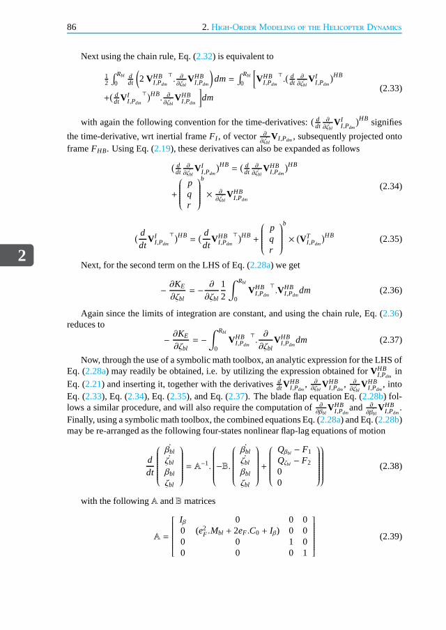
2

86 2.High-Order Modeling of the Helicopter Dynamics

Next using the chain rule, Eq. (2.32) is equivalent to

12

∫ Rbl

0ddt

(

2 VHBI ,Pdm

⊤. ∂

∂ ˙ζblVHB

I ,Pdm

)

dm=∫ Rbl

0

[

VHBI ,Pdm

⊤.( d

dt∂

∂ ˙ζblV I

I ,Pdm

)HB

+( d

dtVII ,Pdm

⊤)HB. ∂

∂ ˙ζblVHB

I ,Pdm

]

dm(2.33)

with again the following convention for the time-derivatives:( d

dt∂

∂ζblV I

I ,Pdm

)HB signifies

the time-derivative, wrt inertial frameFI , of vector ∂

∂ζblV I ,Pdm, subsequently projected onto

frameFHB. Using Eq. (2.19), these derivatives can also be expanded as follows

( ddt

∂

∂ ˙ζblV I

I ,Pdm

)HB=

( ddt

∂

∂ζblVHB

I ,Pdm

)HB

+

pqr

b

× ∂

∂ζblVHB

I ,Pdm

(2.34)

( ddt

V II ,Pdm

⊤)HB=

( ddt

VHBI ,Pdm

⊤)HB+

pqr

b

× (

VTI ,Pdm

)HB (2.35)

Next, for the second term on the LHS of Eq. (2.28a) we get

− ∂KE

∂ζbl= − ∂

∂ζbl

12

∫ Rbl

0VHB

I ,Pdm

⊤.VHB

I ,Pdmdm (2.36)

Again since the limits of integration are constant, and using the chain rule, Eq. (2.36)reduces to

− ∂KE

∂ζbl= −

∫ Rbl

0VHB

I ,Pdm

⊤.∂

∂ζblVHB

I ,Pdmdm (2.37)

Now, through the use of a symbolic math toolbox, an analytic expression for the LHS ofEq. (2.28a) may readily be obtained, i.e. by utilizing the expression obtained forVHB

I ,Pdmin

Eq. (2.21) and inserting it, together with the derivativesddtV

HBI ,Pdm

, ∂∂ζbl

VHBI ,Pdm

, ∂

∂ζblVHB

I ,Pdm, into

Eq. (2.33), Eq. (2.34), Eq. (2.35), and Eq. (2.37). The blade flap equation Eq. (2.28b) fol-lows a similar procedure, and will also require the computation of ∂

∂βblVHB

I ,Pdmand ∂

∂βblVHB

I ,Pdm.

Finally, using a symbolic math toolbox, the combined equations Eq. (2.28a) and Eq. (2.28b)may be re-arranged as the following four-states nonlinear flap-lag equations of motion

ddt

βbl

ζbl

βbl

ζbl

= A−1.

−B.

βbl

ζbl

βbl

ζbl

+

Qβbl − F1

Qζbl − F2

00

(2.38)

with the followingA andBmatrices

A =

Iβ 0 0 00 (e2

F .Mbl + 2eF .C0 + Iβ) 0 00 0 1 00 0 0 1

(2.39)

2.9.Appendix D: Main rotor

2

87

B =

0 B12 0 0B21 0 0 0−1 0 0 00 −1 0 0

(2.40)

with Mbl, C0, andIβ defined as (refer also to the nomenclature)

Mbl =∫ Rbl

0dm C0 =

∫ Rbl

0rdm.dm= Mbl.yGbl

Iβ =∫ Rbl

0r2dm.dm= Mbl.

R2bl

3

(2.41)

We stress here that Eq. (2.38) is a nonlinear representation since the scalarsB12 andB21

in Eq. (2.40), andF1, andF2 in Eq. (2.38) are (nonlinear) functions of (ζbl, βbl, ζbl). Spacerestrictions preclude a reprint of the lengthy expressionsB12, B21, F1, andF2, these can beconsulted in Appendix E of [49].

Flap angle as a Fourier seriesBlade motion is 2π periodic around the azimuth and may hence be expanded as an infiniteFourier series [26, 41]. Now for full-scale helicopters, it is well known that the magnitude ofthe flap second harmonic is less than 10 % the magnitude of the flap first harmonic [41, 50].We assume that this is also the case for small-scale helicopters and hence we neglect secondand higher harmonics in the Fourier series. This gives

βbl(ψbl) ≃ β0 + β1c cosψbl + β1s sinψbl (2.42)

with ψbl the blade azimuth angle. This harmonic representation of the blade motiondefines the rotor Tip-Path-Plane (TPP), resulting in a so-called cone-shaped rotor. Thenon-periodic termβ0 describes the coning angle, and the coefficients of the first harmonicβ1c andβ1s describe the tilting of the rotor TPP, in the longitudinal and lateral directionsrespectively. All three angles may readily be obtained through standard least-squares [51].Now in steady-state rotor operation, the flap coefficientsβ0, β1c, β1s may be consideredconstant over a 2π blade revolution. Obviously this solution would not be adequate fortransient situations such as maneuvering [52], hence in our model we compute, for eachnew blade azimuth, the instantaneous TPP angles. With regard to TPP dynamics, threenatural modes can be identified, i.e. the so-called coning, advancing, and regressing modes.In general, the regressing flapping mode is the most relevantwhen focusing on helicopterflight dynamics, as it is the lowest frequency mode of the three, and it has a tendency tocouple into the fuselage modes [40, 47, 53].

Virtual work and virtual displacementsThe determination of the generalized forcesQζbl , Qβbl in Eq. (2.29a) Eq. (2.29b) requiresthe calculation of the virtual work of each individual external force, associated with eachrespective virtual flapping and lead-lag displacements [11]. Let FXi , FYi , FZi be the compo-nents of the ith external forceFi , acting on blade elementdmin frameFHB, then the resultingelemental virtual work done by this force, due to the virtualflapping and lag displacements∂βbl and∂ζbl, is given by

dWi = FXi dxdm+ FYi dydm+ FZi dzdm (2.43)

2

88 2.High-Order Modeling of the Helicopter Dynamics

with

dxdm =∂xdm

∂βbl∂βbl +

∂xdm

∂ζbl∂ζbl (2.44a)

dydm =∂ydm

∂βbl∂βbl +

∂ydm

∂ζbl∂ζbl (2.44b)

dzdm =∂zdm

∂βbl∂βbl +

∂zdm

∂ζbl∂ζbl (2.44c)

Now summing up the elemental virtual work, over the appropriate blade span, results inthe total virtual workWi , due to external forceFi , as

Wi =∫ Rbl

0

(

FXi

∂xdm

∂βbl+ FYi

∂ydm

∂βbl+ FZi

∂zdm

∂βbl

)

∂βbl

+∫ Rbl

0

(

FXi

∂xdm

∂ζbl+ FYi

∂ydm

∂ζbl+ FZi

∂zdm

∂ζbl

)

∂ζbl

(2.45)

Which is set equivalent to

Wi = Qβbl,i .∂βbl + Qζbl ,i.∂ζbl (2.46)

The virtual displacement, in frameFHB, of a blade elementdm, located at a distancerdm outboard of the flap hinge, is obtained using Eq. (2.44) and Eq. (2.12) as follows

dxdm

dydm

dzdm

HB

= rdm.dPHBβ,r .∂βbl

+

[

dPHBζ,r + rdm.dPHB

ζ,r

]

.∂ζbl

(2.47)

with

dPHBβ,r =

cosψbl cosζbl sinβbl

Γ cosψbl

(

cosθbl sinζbl sinβbl − cosβbl sinθbl

)

− cosθbl cosβbl

+ sinψbl

(

cosθbl sinζbl sinβbl − cosβbl sinθbl

)

−Γ sinψbl cosζbl sinβbl

− sinζbl sinθbl sinβbl

(2.48)

dPHBζ,r = eF

(

cosψbl sinζbl − sinψbl cosθbl cosζbl

)

−Γ(

cosψbl cosθbl cosζbl + sinψbl sinζbl

)

cosζbl sinθbl

(2.49)

dPHBζ,r = cosβbl

dPHBζ,r

eF(2.50)

2.9.Appendix D: Main rotor

2

89

Generalized forces (gravity)The gravity force acting on a blade element with massdmcan be expressed inFHB as

FHBGbl= T(HB)o

00g.dm

o

(2.51)

with T(HB)o the transformation fromFo to FHB. Substituting Eq. (2.51) and Eq. (2.47)into Eq. (2.45), the desired generalized forces due to gravity, outboard of the flap hinge, areobtained as follows

Qζbl ,G = g.(

eF .Mbl +C0 cosβbl

)

.

(

A1 cosψbl sinζbl

−A1 sinψbl cosθbl cosζbl

−A2Γ cosψbl cosθbl cosζbl

−A2Γ sinψbl sinζbl + A3 cosζbl sinθbl

)

(2.52)

Qβbl,G = g.C0.

(

A1 cosψbl cosζbl sinβbl

+A1 sinψbl cosθbl sinζbl sinβbl

−A1 sinψbl cosβbl sinθbl

+A2Γ cosψbl cosθbl sinζbl sinβbl

−A2Γ cosψbl cosβbl sinθbl

−A2Γ sinψbl cosζbl sinβbl

−A3 cosθbl cosβbl − A3 sinζbl sinθbl sinβbl

)

(2.53)

usingA1 = − sinθA2 = cosθ sinφA3 = cosθ cosφ

(2.54)

andMbl andC0 as defined in Eq. (2.41).

Generalized forces (aerodynamic)The aerodynamic velocity, i.e. velocity relative to the air, of a blade elementdm, located atpositionPdm, is defined byVa,Pdm. Projecting it onto the blade frameFbl we get

Vbla,Pdm= T(bl)(HB).

(

VHBI ,Pdm−

00vi

HB

− T(HB)E

uw

vw

ww

E)

(2.55)

with VHBI ,Pdm

defined in Eq. (2.21), vi the rotor induced velocity35 from Eq. (2.70), (uw vw ww)⊤

the components of the wind velocity vector usually available in frameFE, andT(bl)(HB) therotation matrix from frameFHB to frameFbl. Now the section AOA of a blade elementdm

35Strictly speaking the induced velocity is perpendicular tothe Tip-Path-Plane (TPP). However since we make theassumption of small tilt angles, as to simplify the model, weconsider here an induced velocity perpendicular tothe Hub-Body frameFHB.

2

90 2.High-Order Modeling of the Helicopter Dynamics

is defined byαbl in the interval [−π,+π] rad and, for each of the four quadrants, is readilycomputed from the arctangent of the x- and z- components ofVbl

a,Pdm. Further, the elemental

lift and drag forces of a blade segment of lengthdrdm are given by

dL =12.ρ.||Vbl

a,Pdm||2.clbl .cbl.drdm (2.56)

dD =12.ρ.||Vbl

a,Pdm||2.cdbl .cbl.drdm (2.57)

with the blade section lift and drag coefficientsclbl andcdbl given as tabulated functions36

of blade section AOA and Mach numberM, and all other coefficients defined in the nomen-clature. The elemental lift and drag forces can now be expressed in the blade frameFbl, foreach of the four AOA quadrants. For example, for the case of a CCW main rotor, with theAOA quadrantαbl ∈ [0,+π/2] rad, we have

dL bl = dL.

sinαbl

0− cosαbl

(2.58)

dDbl = −dD.

cosαbl

0sinαbl

(2.59)

Coming back to the generalized aerodynamic forces, we can now express them as thesum of two contributions, one due to lift and one due to drag. For the lead-lag case inEq. (2.29a) we haveQζbl ,A = Qζbl ,AL + Qζbl ,AD . Similarly for the flap case in Eq. (2.29b) wehaveQβbl,A = Qβbl,AL + Qβbl,AD . Now keeping in mind Eq. (2.45) and Eq. (2.47), and usingEq. (2.58) and Eq. (2.59), we obtain

Qζbl ,AL =

∫ B.Rbl

rc

(

T(HB)(bl)dLbl)⊤.

(

dPHBζ,r + rdm.dPHB

ζ,r

)

.drdm (2.60)

Qζbl ,AD =

∫ Rbl

rc

(

T(HB)(bl)dDbl)⊤.

(

dPHBζ,r + rdm.dPHB

ζ,r

)

.drdm (2.61)

Qβbl,AL =

∫ B.Rbl

rc

(

T(HB)(bl)dLbl)⊤.dPHB

β,r .rdm.drdm (2.62)

Qβbl,AD =

∫ Rbl

rc

(

T(HB)(bl)dDbl)⊤.dPHB

β,r .rdm.drdm (2.63)

For the lift contributionsQζbl ,AL andQβbl,AL , the integration is performed from the bladeroot cutoutrc to a value denoted asB.Rbl, this latter accounts for blade tip loss [52]. Next byplugging Eq. (2.48), Eq. (2.50), Eq. (2.49), Eq. (2.58), and Eq. (2.59), into Eq. (2.60)–Eq. (2.63),one can derive final expressions for the generalized aerodynamic forces. Providing analyti-cal expressions for Eq. (2.60)–Eq. (2.63) represents a rather tedious task, even more so for

36Where we neglect sideslip influence.

2.9.Appendix D: Main rotor

2

91

twisted blades37 for which the blade pitch will also be function of the blade section lengthrdm. Therefore, we opted for a numerical evaluation of these expressions, as is often done inflight dynamics codes [54]. Here Gaussian quadrature integration was implemented, usinga low order (5th order) Legendre polynomial scheme [55, 56].

Generalized forces (hub damping and spring restraints)The flap and lag hinges are modeled as springs with viscous dampers. The generalizedforces corresponding to the spring dampers can be obtained directly from the potentialenergy of the dampers dissipation functions [10, 11] as

Qζbl ,D = −KDζ.ζbl Qβbl,D = −KDβ

.βbl (2.64)

Similarly the generalized forces corresponding to the spring restraints can be obtaineddirectly from the potential energy of the hub springs [10, 11] as

Qζbl ,S = −KSζ.ζbl Qβbl,S = −KSβ

.βbl (2.65)

Rotor inflowAt the heart of the helicopter aerodynamics are the induced velocities, i.e. the induced flowdue to rotor blade motion, at and near the main rotor [57]. These induced velocities con-tribute to the local blade incidence and local dynamic pressure, and can be divided into twocategories, static and dynamic inflow models. For low-bandwidth maneuvering applica-tions, such as trim calculations or flying-qualities investigations, the dynamic effects of theinteraction of the airmass with the vehicle may be deemed negligible, hence static inflowmodels may be acceptable [57]. But for high bandwidth applications, dynamic interactionsbetween the inflow dynamics and the blade motion must be considered. Conjointly dynamicinflow models can be divided into two unsteady categories: the Pitt-Peters dynamic inflow[8, 58–60], and the Peters-He finite-state wake model38 [9, 64, 65]. The finite-state wakemodel is a more comprehensive theory than dynamic inflow, notlimited in harmonics andallowing to account for nonlinear radial inflow distributions. This sophisticated model isparticularly attractive when rotor vibration and aeroelasticity need to be analyzed [66]. Butwith respect to flight dynamics applications, we assume thatit is sufficient to consider thenormal component of the inflow at the rotor, i.e. the rotor induced downwash [7]. Further,for such applications, it is reported in [66] that the Peters-He model is not remarkably betterthan the Pitt-Peters formulation. Since our primary interest is flight dynamics, we choose toimplement the more straightforward Pitt-Peters model [8, 58], with a correction39 for flightinto the Vortex-Ring-State (VRS) from [68]. The VRS corresponds to a condition wherethe helicopter is descending in its own wake. It is often associated with the following symp-toms: excessive vibrations, large unsteady blade loads, thrust/torque fluctuations, excessiveloss of altitude, and loss of control effectiveness [69]. Its boundaries, in terms of helicoptervelocities, are well-known, see Fig.2.19.

37Although in our case the helicopter UAV blades have zero twist.38Although recent advances in computing power and methodology have made it foreseeable to add a third category,

namely that of detailed free-wake models that may be run in real-time for flight dynamics applications [61–63].39Note that, if required, additional enhancements could alsobe made by including a pseudo-harmonic term to

model VRS thrust fluctuations as in [67].

2

92 2.High-Order Modeling of the Helicopter Dynamics

Figure 2.19: Vortex-Ring-State (VRS) boundaries. The x-axis represents the helicopter horizontal velocity nor-malized by the induced velocity in hover (namedvh in this figure), whereas the y-axis represents the helicoptervertical velocity normalized by the induced velocity in hover. Figure from [70].

Concerning wake bending during maneuvering flight40, we choose at first not to imple-ment it, as to lower model complexity. For the aspect of ground effect, only a static groundeffect has been accounted for, by a correction factor applied tothe non-dimensional totalvelocity at the rotor disk center.

Now, the induced inflow model implemented in this Chapter is based upon [8], andis assumed to have the following variations in the TPP wind-axis coordinates (see [8] forfurther details on TPP wind-axis coordinates)

ddt

λ0

λs

λc

= ΩMR.M−1.

−(L1.L2)−1.

λ0

λs

λc

+ Caero

(2.66)

where the main rotor RPMΩMR has been added here in front of the RHS of Eq. (2.66)

40Wake bending may significantly change the inflow distribution over the rotor, resulting in a sign reversal in theoff-axis response [71–73], for which interesting implementation results can be found in [74–76].

2.9.Appendix D: Main rotor

2

93

since the original expressions of the Pitt-Peters model arein non-dimensional time (seealso [64]). The subscript (·)aero in the forcing functionCaero indicates that only aerody-namic contributions are considered, withCaero = (CT − CL − CM)⊤aero, andCT , CL, CM ,the instantaneous main rotor thrust, roll, and pitching moment coefficients respectively, inthe TPP wind-axis system.CT is readily obtained from Eq. (2.71), whereasCL andCM

are simply derived from the forces Eq. (2.71) times their respective moment arms. NextmatricesM andL1 are defined from [8] as

M =

83π 0 00 16

45π 00 0 16

45π

(2.67)

L1 =

12 0 −15π

64

√

1−sinα1+sinα

0 41+sinα 0

15π64

√

1−sinα1+sinα 0 4 sinα

1+sinα

(2.68)

whereα represents the wake angle with respect to the rotor disk [8]. Further matrixL2

is given by

L2 =

(Ge f f.VT)−1 0 00 V−1

M 00 0 V−1

M

(2.69)

with VT the total velocity through the rotor disk,VM the momentum theory mass flowparameter, andGe f f the static ground effect factor added as a correction toVT . The expres-sions forVT andVM can be found in [68], although simpler expressions also exist in [8].However the former include a correction for flight into the VRS and hence are more attrac-tive. TheGe f f coefficient is based upon the expression found in [52]. Finally the main rotorinduced velocityvi is computed as follows [77]: 1) solve Eq. (2.66); 2) rotate the obtainedinflow from the TPP wind-axis to the TPP axis (see [8]); and 3) use these expressions tocomputevi in Eq. (2.70)

vi = Vre f .(

λ0 + λs.rdm

Rrot. sinψbl + λc.

rdm

Rrot. cosψbl

)

(2.70)

Forces and momentsFor the rotor forces, the procedure consists in simulating the forces of each individual blade.This process is repeated at each new blade azimuth position—rather than averaging theresults over one revolution—in order to recreate theNb/Revflapping vibration41. The rotorforces are subdivided into three contributions: 1) aerodynamic lift and drag; 2) inertial;and 3) centrifugal forces. The aerodynamic forcesFHB

MRaare obtained by integrating the

elementary lift and drag forces Eq. (2.58) and Eq. (2.59) over the blade span

FHBMRa=

∫ B.Rbl

rc

T(HB)(bl)dLbl.drdm+

∫ Rbl

rc

T(HB)(bl)dDbl.drdm (2.71)

41Which may be useful when validating a complete auto-pilot system in a hardware in the loop simulation envi-ronment.

2

94 2.High-Order Modeling of the Helicopter Dynamics

where the integrations are done numerically as in Eq. (2.60)–Eq. (2.63). The inertialforcesFHB

MRi, due to flap and lag, are approximated, from expressions in [26], as follows

FHBMRi=

1 0 00 1 00 0 0

.T(HB)6.

−Mblηζ ζbl

0−Mblηββbl

(2.72)

Centrifugal forcesFHBMRc

are approximated, from [26], as

FHBMRc=

1 0 00 1 00 0 0

.T(HB)6.

012 MblΩ

2MRR2

bl0

(2.73)

Finally, for the total main rotor forces we haveFbMR = Tb(HB).

(

FHBMRa+ FHB

MRi+ FHB

MRc

)

,with Tb(HB) = I, since, as mentioned earlier, rotor shaft tilt-angles are zero on our helicopterUAV. For the rotor moments, they include contributions fromsix different sources: 1) aero-dynamicsM HB

MRa; 2) inertial loadsM HB

MRi; 3) centrifugal loadsM HB

MRc; 4) flap hinge stiffness

M HBMRsti f

; 5) lag hinge dampingM HBMRdamp

; and 6) due to airfoil camberM HBMRcamber

. The lasttwo are neglected since assumed very small for small-scale helicopter rotors/blades. Thefirst three are simply computed by considering the forces Eq.(2.71)–Eq. (2.73) times theirrespective moment arms. For the flap hinge stiffness, it is derived from [26] as

M HBMRsti f

= − 1

1− eP+eL+eFRrot

.Nb.KSβ

2

Γβ1s

β1c

0

(2.74)

Rotor RPM dynamicsThe main rotor RPM dynamics is related to the available and required power by [43]

Nb.Ib.ΩMR.ΩMR = Psha f t− Preq (2.75)

with Psha f t the available shaft power, andPreq the required power to keep the vehiclealoft. This latter is the sum of main rotor induced and profilepower, tail rotor inducedand profile power, power plant transmission losses, vehicleparasite power (i.e. drag dueto fuselage, landing skids, rotor hub, etc), and finally mainrotor, tail rotor, and fuselageaerodynamic interference losses. In case of engine failure, a first-order response inPsha f t isgenerally assumed to represent the power decay, we have

Psha f t = −Psha f t

τp(2.76)

with τp a to-be-identified time constant. For the required powerPreq, we simplify themodel by only considering the contributions from the main rotor asPMR = MHB

z MRa.ΩMR,

with MHBz MRa

being the z- component of the aerodynamics momentM HBMRa

(this latter beingreferenced in the previous paragraph). Now if, at engine failure, we were to assume aninstantaneous power lossPsha f t= 0, then from Eq. (2.75) we obtain

ΩMR = −MHB

z MRa

Nb.Ib(2.77)

2.10.Appendix E: Tail rotor

2

95

2.10.Appendix E: Tail rotorThe tail rotor is a powerful design solution for torque balance, directional stability andcontrol of helicopters. We have implemented here a standardBailey type model [12], as isdone, among others, in [19, 51, 78].

AssumptionsStructural simplifications

• The blade has zero twist, constant chord, zero sweep, and hasconstant thicknessratio. The blade is also rigid, hence torsion is neglected.

Aerodynamics simplifications

• Linear lift with constant lift curve slope, and uniform induced flow over the rotor areassumed.

• Aerodynamic interference effects from the main rotor is neglected, although this maywell be an oversimplification, for some flight conditions [79, 80]. Similarly, theaerodynamic interference from the vertical tail (due to blockage) is also neglected.

• Compressibility, blade stall, and viscous flow effects are also disregarded.

Dynamical simplifications

• Blade dynamics is disregarded, and simplified inflow dynamics is considered. Un-steady effects are neglected.

Forces and momentsThe theory we apply here is based on the work done by Bailey in [12], implemented amongothers in [51, 78]. The model given here is a simplified approach of the Bailey model. First,the total tail rotor blade pitchθTR is given by

θTR = θTR− TTR∂β0TR

∂TTRtanδ3TR + θbiasTR (2.78)

with θTR the tail rotor control input, and all other coefficients defined in the nomen-clature, except forTTR defined in Eq. (2.83). The Bailey coefficients are given next by

t1 =B2

TR

2+µ2

TRxy

4(2.79a)

t2 =B3

TR

3+

BTR µ2TRxy

2(2.79b)

with BTR the tip loss factor andµTRxy defined in the sequel. Now, assuming zero twistfor the tail rotor blades, the downwash at the tail rotor is derived using momentum theoryas follows

2

96 2.High-Order Modeling of the Helicopter Dynamics

λdw =cl(0,TR)σTR

2

(

µTRzt1 + θTRt2

2√

µ2TRx+ µ

2TRy+ λ

2TR+

cl(0,TR)σTR

2 t1

)

(2.80)

with λTR the total tail rotor inflow,µTRxy =

√

µ2TRx+ µ

2TRy andµTRz non-dimensional

velocities in the tail rotor frame (see [51] for details of the tail rotor frame and the Baileymodel), and the remaining coefficients defined in the nomenclature. The total tail rotorinflow λTR is further given by

λTR = λdw− µTRz (2.81)

where it is common practice to iterate between Eqn. (2.80) and Eqn. (2.81) until con-vergence within a reasonable tolerance. Then, the tail rotor thrust is given by [51]

FbTR =

0Γ.TTR

0

(2.82)

with

TTR = 2.λdw.

√

µ2TRxy+ λ

2TR.ρ.π.

(

ΩTR.R2rotTR

)2

(2.83)

Next, the tail rotor moments are primarily due to the rotor force times the respectivemoment arms (where we neglect any sidewards rotor offset in they− direction). For com-pleteness, we also add the rotor torque acting on the pitch axis [26]

MbTR =

xTR

0zTR

b

× FbTR+

0σTR.CDTR/8.(1+ 4.6µ2

TRxy).ρ.π.Ω2TR.R

5rotTR

0

b

(2.84)

2.11.Appendix F: Fuselage

2

97

2.11.Appendix F: FuselageIn the general case, the flow around the fuselage is rather complex, and is characterizedby strong nonlinearities, unsteady separation effects, and distortions due to the influence ofthe main rotor wake [7]. For low speed sideways flight, the important fuselage character-istics are the sideforce, vertical drag, and yawing moment;whereas in forward flight, theimportant characteristics include drag, and pitching and yawing moments variations withincidence and sideslip [7]. The fuselage rolling moment is usually small, except for config-urations with deep hulls where the fuselage aerodynamic center may be significantly belowthe vehicle CG [7], see also [81, 82] for additional information.

AssumptionsAerodynamics simplifications

• Fuselage aerodynamic enter is collocated with vehicle CG. Further, only steady air-loads effects are considered.

• Effect of rotor downwash on fuselage is neglected. It can however be modeled as in[83], using a polynomial in wake skew angle, where the polynomial coefficients needto be fit from flight data [84].

Forces and momentsThe fuselage aerodynamic velocity, at its aerodynamic center, in frameFb, is given by

Vba,Fus =

u+ q.zFus− r.yFus

v− p.zFus+ r.xFus

w+ p.yFus− q.xFus

b

− T(HB)E

uw

vw

ww

E

(2.85)

Now the fuselage model is based upon aerodynamic lift and drag coefficients, which aretabulated as a function of airflow AOAαFus and sideslipβFus angles [14]. These angles arereadily computed from the x-,y-, and z- components ofVb

a,Fus. The fuselage forces in thebody frameFb are

FbFus =

qFus.CxbFus(αFus, βFus)

qFus.CybFus(αFus, βFus)

qFus.CzbFus(αFus, βFus)

(2.86)

with qFus = 1/2.ρ.Sre fFus.||Vba,Fus||2. The moments are

MbFus =

qFus.MxbFus(αFus, βFus).Lre fFus

qFus.MybFus(αFus, βFus).Lre fFus

qFus.MzbFus(αFus, βFus).Lre fFus

(2.87)

with the six aerodynamic coefficientsCxFus(·), CyFus(·), CzFus(·), MxFus(·), MyFus(·),andMzFus(·) being tabulated as a function of airflow AOAαFus, and sideslip angleβFus. Inour case, these lookup tables are obtained by scaling-down afull-size, Bo–105 helicopter,fuselage aerodynamic model.

2

98 2.High-Order Modeling of the Helicopter Dynamics

2.12.Appendix G: Vertical and horizontal tailsThe role of the vertical tail is twofold: 1) in forward flight,it generates a sideforce andyawing moment, hence reducing the tail rotor thrust requirement, in order to increase thefatigue life of the tail rotor [7, 43]; and 2) during maneuvers, and during wind gusts, itprovides yaw damping and stiffness, enhancing directional stability [7]. The role of thehorizontal tail is also twofold: 1) in forward flight, it generates a trim load that reduces themain rotor fore-aft flapping; and 2) during maneuvers, and during wind gusts, it providespitch damping and stiffness, enhancing pitch stability [7].

AssumptionsAerodynamics simplifications

• The effect of main rotor downwash on both vertical and horizontal tails is neglected.It can however be modeled by using flat vortex wake theory [85] (valid for smallsideslip angles), as presented in [54, 86], or it may be modeled as a polynomial inwake skew angle [83].

• We neglect the erratic longitudinal trim shifts that may happen when the helicopteris transitioning from hover to forward flight [7, 43] (as the main rotor wake impingeson the tail surface).

• The effect of the main rotor downwash on the tail boom is neglected, but in somecases may need to be considered during low speed flight, sinceit may influence yawdamping [7].

Forces and momentsThe vertical and horizontal tails, for the case of small-scale helicopters, can simply beviewed as flat plate representations. The force equations are omitted since very similarto those of the fuselage, and the moments are simply derived from the forces times theirrespective moment arms.

2.13.Appendix H: Problem data

2

99

2.13.Appendix H: Problem dataThe LTI state-space data used to design the inner-loop trajectory trackers is as follows: thestate-vector is of dimension nine given byx = (u v w p q rφ θ ψ)⊤, the control input isof dimension four given byu = (θ0 θ1c θ1s θTR)⊤, the wind disturbance (given in inertialframe) is of dimension three given byd = (VNw VEw VZw)⊤, and the measurement vectory = x.

For the engine ON case, we have:x = Ax + Bu + Bwindd with

A =

−0.0682 0.0480 −0.0154 −0.1718 −0.4815 0.0443 0.0188 −9.7039 0−0.0528 −0.1671 −0.0022 0.1405 −0.6382 0.0424 9.6314 −0.0010 0−0.0146 −0.0086 −1.3800 0.0308 0.0191 −0.1012 −0.4957 0.0025 0−0.4980 −0.3992 −0.1785 −4.3091 −0.9452 −0.0176 −0.8271 0.4340 00.5505 −0.6741 0.0988 0.4298 −7.4087 0.0185 −0.3565 −0.6686 0−0.0101 0.8748 −0.1435 0.0250 −0.0764 −1.0801 0.8012 0.0023 0−0.0445 −0.0868 −0.0066 0.1002 −0.4218 −0.0006 −0.0610 0.0195 00.0639 −0.0418 0.0207 0.1610 0.3185 −0.0517 −0.0158 −0.0390 00.0031 0.0777 −0.0166 0.0096 0.0118 0.8997 0.0446 −0.0024 0

B =

−2.1874 8.0268 −15.1285 0.3544−2.0942 18.8510 19.2744 −4.4702−156.7810 −0.5916 −5.7372 −1.1758−18.4143 95.7742 23.7919 −0.596910.0410 −46.1074 157.6934 −1.0295−140.8456 −1.7584 2.4157 94.8389−0.8650 14.1785 14.7893 −0.15862.7890 −10.1952 12.5716 −0.5578−13.0429 −0.7975 0.9591 8.6268

Bwind =

0.0679 −0.0514 0.01300.0443 0.1652 0.02000.0137 −0.0778 1.37450.4986 0.3890 0.1970−0.5507 0.6765 −0.05420.0101 −0.8816 0.08970.0445 0.0862 0.0119−0.0639 0.0429 −0.0179−0.0031 −0.0786 0.0118

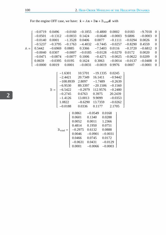
2

100 2.High-Order Modeling of the Helicopter Dynamics

For the engine OFF case, we have:x = Ax + Bu + Bwindd with

A =

−0.0719 0.0496 −0.0160 −0.1855 −0.4800 0.0002 0.0183 −9.7018 0−0.0501 −0.1312 −0.0033 0.1424 −0.6648 −0.0003 9.6806 −0.0003 0−0.0140 0.0001 −1.3528 0.0406 0.0077 −0.1111 −0.0294 0.0026 0−0.5237 −0.3795 −0.1763 −4.4032 −0.7445 −0.0257 −0.8290 0.4559 00.5442 −0.6969 0.0885 0.3366 −7.5403 0.0116 −0.3720 −0.6812 0−0.0040 0.0307 −0.0007 −0.0185 −0.0128 −0.0270 0.0172 0.0020 0−0.0471 −0.0874 −0.0077 0.1006 −0.4271 −0.0025 −0.0622 0.0209 00.0659 −0.0395 0.0195 0.1624 0.3063 −0.0014 −0.0137 −0.0408 0−0.0000 0.0019 0.0001 −0.0031 −0.0019 0.9976 0.0007 −0.0001 0

B =

−1.6301 10.5701 −19.1335 0.0245−2.4421 20.7349 16.1411 −0.9442−108.8939 2.8097 −1.7489 −0.2639−6.9530 89.3397 −20.1506 −0.1560−6.5422 −0.2979 112.9576 −0.2480−0.2745 0.6763 0.3975 20.2439−1.4126 13.0013 9.9099 −0.03531.0822 −8.6290 13.7359 −0.0262−0.0188 0.0336 0.1177 2.1705

Bwind =

0.0861 −0.0549 0.01680.0601 0.1340 0.02880.0052 0.0011 1.23660.4814 0.1950 0.0751−0.2975 0.6132 0.08880.0046 −0.0901 −0.00310.0466 0.0745 0.0172−0.0631 0.0431 −0.01290.0001 −0.0066 −0.0003

References

2

101

References[1] S. Taamallah,A qualitative introduction to the vortex-ring-state, autorotation, and

optimal autorotation,in Europ. Rotorcraft Forum(2010).

[2] S. Taamallah,Small-scale helicopter blade flap-lag equations of motion for a flybar-less pitch-lag-flap main rotor,in AIAA Modeling and Simulation Technologies Conf.(2011).

[3] S. Taamallah,Flight dynamics modeling for a small-scale flybarless helicopter uav,inAIAA Atmospheric Flight Mechanics Conf.(2011).

[4] ART, (http://www.flightlab.com/, Mountain View CA., U.S.A.).

[5] D. Santamaria, A. Viguria, M. Bejar, K. Kondak, and A. Ollero,Towards autonomousautorotation landing for small size unmanned helicopters,J. Intell. Robot Syst.69,171 (2013).

[6] M. G. Ballin, Validation of a Real-Time Engineering Simulation of the UH-60A Heli-copter, Tech. Rep. TM 88360 (NASA Ames Research Center, 1987).

[7] G. D. Padfield,Helicopter Flight Dynamics(Blackwell Science Ltd, Oxford, UK,1996).

[8] D. A. Peters and N. HaQuang,Technical notes - dynamic inflow for practical applica-tions,J. of the Am. Helicopter Soc. , 64 (1988).

[9] D. A. Peters and C. J. He,Finite state induced flow models part ii: Three-dimensionalrotor disk,AIAA J. of Aircraft 32, 323 (1995).

[10] D. A. Wells,Lagrangian Dynamics(McCraw-Hill Co., 1967).

[11] R. T. N. Chen,Flap-Lag Equations of Motion of Rigid, Articulated Rotor Blades withThree Hinge Sequences, Tech. Rep. NTM 100023 (NASA Ames Research Center,1987).

[12] F. J. Bailey,A Simplified Theoretical Method of Determining the Characteristics of aLifting Rotor in Forward Flight, Tech. Rep. RNo. 716 (NACA, 1941).

[13] J. D. Anderson,Fundamentals of Aerodynamics. Third Ed.(McGraw-Hill Higher Ed-ucation, NY, 2001).

[14] J. L. Boiffier,The Dynamics of Flight The Equations(John Wiley & Sons, Chichester,England, 1998).

[15] Email communication with Professor David Peters(Center for Computational Me-chanics, Washington University in St. Louis, USA, May 11th 2015).

[16] D. A. Peters, M. Chouchane, and M. Fulton,Helicopter trim with flap-lag-torsionand stall by an optimized controller,AIAA J. of Guidance13 (1990).

2

102 References

[17] U. B. Hald, M. V. Hesselbaek, and M. Siegumfeldt,Nonlinear Modeling and OptimalControl of a Miniature Autonomous Helicopter, Tech. Rep. (Master Thesis, AalborgUniversity, 2006).

[18] D. A. Peters and D. Barwey,A general theory of rotorcraft trim,Mathematical Prob-lems in Engineering2, 1 (1996).

[19] G. M. Voorsluijs,A Modular Generic Helicopter Model, Tech. Rep. (Master Thesis,Delft University of Technology, 2002).

[20] N. S. Achar and G. H. Gaonkar,Helicopter trim analysis by shooting and finite ele-ment methods with optimally damped newton iterations,AIAA J. 31 (1993).

[21] D. A. Peters and B. S. Kim,Control settings for a trimmed stalled rotor by an auto-matic feedback system,in AIAA (1981).

[22] D. A. Peters and A. P. Izadpanah,Helicopter trim by periodic shooting with newton-raphson iteration,in Am. Helicopter Soc.(1981).

[23] F. D. Kim, R. Celi, and M. B. Tischler,Forward flight trim and frequency responsevalidation of a helicopter simulation model,J. of Aircraft30 (1993).

[24] J. S. G. McVicar and G. Bradley,Engineering notes - robust and efficient trimmingalgorithm for application to advanced mathematical modelsof rotorcraft,AIAA J. ofAircraft 32 (1995).

[25] P. M. J. Van den Hof and R. J. P. Schrama,Identification and control - closed-loopissues,Automatica31, 1751 (1995).

[26] W. Johnson,Helicopter Theory(Dover Publications Inc., NY, USA, 1994).

[27] P. Seiler and A. Ozdemir,An optimal time-invariant approximation for wind tur-bine dynamics using the multi-blade coordinate transformation, in Am. Control Conf.(2013).

[28] K. Stol, M. Balas, and G. Bir,Floquet modal analysis of a teetered rotor wind turbine,Journal of Solar Energy Eng.124, 364 (2002).

[29] R. Coleman and A. Feingold,Theory of Self-Excited Mechanical Oscillations of He-licopter Rotors with Hinged Blades, Tech. Rep. TR 1351 (NACA, 1958).

[30] D. J. Malcolm,Modal response of 3-bladed wind turbines,Journal of Solar EnergyEng.124, 372 (2002).

[31] G. Bir, Multi-blade coordinate transformation and its applications to wind turbineanalysis,in AIAA Wind Energy Symposium(2008).

[32] K. A. Stol, H. G. Moll, G. Bir, and H. Namik,A comparison of multi-blade coordi-nate transformation and direct periodic techniques for wind turbine control design,inAIAA Aerospace Sciences Meeting(2009).

References

2

103

[33] N. K. Sinha and N. Ananthkrishnan,Elementary Flight Dynamics with an Introductionto Bifurcation and Continuation Methods(CRC Press, 2013).

[34] S. Skogestad and I. Postlethwaite,Multivariable Feedback Control: Analysis and De-sign, 2nd Ed.(Wiley-Interscience, Great Britain, 2005).

[35] P. Misra and P. Enge,Global Positioning System: Signals, Measurements and Perfor-mance, Second Edition(Ganga-Jamuna Press, Lincoln MA, USA, 2006).

[36] B. B. Blake and K. Lunn,Helicopter stability and control test methodology,in AIAAAtmospheric Flight Mechanics Conf.(1980).

[37] M. B. Tischler and R. Remple,Aircraft and Rotorcraft System Identification(Am.Institute of Aeronautics & Astronautics (AIAA), Reston VA,2006).

[38] E. Seckel and H. C. Curtiss,Aerodynamic Characteristics of Helicopter Rotors, Tech.Rep. No. 659 (Department of Aerospace and Mechanical Engineering, Princeton Uni-versity, 1962).

[39] R. T. N. Chen,A Simplified Rotor System Mathematical Model for Piloted FlightDynamics Simulation, Tech. Rep. NTM 78575 (NASA Ames Research Center, 1979).

[40] R. T. N. Chen,Effects of Primary Rotor Parameters on Flapping Dynamics, Tech.Rep. NTP 1431 (NASA Ames Research Center, 1980).

[41] A. Gessow and G. C. Myers,Aerodynamics of the Helicopter(College Park Pr, 1999).

[42] R. S. Shevell,Fundamentals of Flight(Prentice Hall, Upper Saddle River NJ, 1989).

[43] R. W. Prouty,Helicopter Performance, Stability, and Control(Krieger PublishingCompany, Malabar, Florida USA, 1995).

[44] R. T. N. Chen, J. V. Lebacqz, E. W. Aiken, and M. B. Tischler, Helicopter Mathemat-ical Models and Control Law Development for Handling Qualities Research, Tech.Rep. NCR 2495 (NASA Ames Research Center, 1988).

[45] C. W. Ellis,Effects of rotor dynamics on helicopter automatic control system require-ments,Aeronautical Engineering Review (1953).

[46] D. G. Miller and F. White,A treatment of the impact of rotor-fuselage coupling onhelicopter handling qualities,in Am. Helicopter Soc.(1987).

[47] H. C. Curtiss,Stability and control modeling,in Europ. Rotorcraft Forum(1986).

[48] M. B. Tischler,System identification requirements for high bandwidth rotorcraft flightcontrol system design,in AGARD LS-178 Rotorcraft System Identification(1991).

[49] S. Taamallah,A Flight Dynamics Helicopter UAV Model For A Single Pitch-Lag-FlapMain Rotor: Modeling& Simulations, Tech. Rep. NLR-TP-2010-286-PT-1 (NLR,2011).

2

104 References

[50] B. Mettler, Identification Modelling and Characteristics of MiniatureRotorcraft(Kluwer Academic Publishers, Norwell Mass, USA, 2003).

[51] ART, FLIGHTLAB Theory Manual (Vol. One& Two)(Advanced Rotorcraft Technol-ogy, Inc., Mountain View CA, 2006).

[52] G. J. Leishman,Principles of Helicopter Aerodynamics(Cambridge University Press,Cambridge, UK, 2000).

[53] R. T. N. Chen and W. S. Hindson,Influence of high-order dynamics on helicopterflight control system bandwidth,AIAA J. of Guidance, Control, and Dynamics9, 190(1986).

[54] M. D. Takahashi,A Flight-Dynamic Helicopter Mathematical Model with a SingleFlap-Lag-Torsion Main Rotor, Tech. Rep. TM 102267 (NASA Ames Research Center,1990).

[55] D. Kahaner, C. Moler, and S. Nash,Numerical Methods and Software(Prentice-Hall,NJ, USA, 1989).

[56] J. Stoer and R. Bulirsch,Introduction to Numerical Analysis(Springer-Verlag, 2002).

[57] R. T. N. Chen,A Survey of Nonuniform Inflow Models for Rotorcraft Flight Dynamicsand Control Applications, Tech. Rep. NTM 102219 (NASA Ames Research Center,1989).

[58] D. M. Pitt and D. A. Peters,Theoretical prediction of dynamic-inflow derivatives,inEurop. Rotorcraft Forum(1980).

[59] G. H. Gaonkar and D. A. Peters,Effectiveness of current dynamic-inflow models inhover and forward flight,J. of the Am. Helicopter Soc.31 (1986).

[60] G. H. Gaonkar and D. A. Peters,Review of dynamic inflow modeling for rotorcraftflight dynamics,Vertica , 213 (1988).

[61] B. D. Kothmann, Y. Lu, E. DeBrun, and J. Horn,Perspectives on rotorcraft aerody-namic modeling for flight dynamics applications,in 4th Decennial Specialists Conf.on Aeromechanics(2004).

[62] D. L. Kunz, Comprehensive rotorcraft analysis: Past, present, and future, inAIAA/ASME/ASCE/AHS/ASC Structures, Structural Dynamics& Materials Conf.(2005).

[63] W. R. M. van Hoydonck, H. Haverdings, and M. D. Pavel,A review of rotorcraftwake modeling methods for flight dynamics applications,in Europ. Rotorcraft Forum(2009).

[64] D. A. Peters, D. D. Boyd, and C. J. He,Finite-state induced-flow model for rotors inhover and forward flight,J. of the Am. Helicopter Soc. , 5 (1989).

References

2

105

[65] D. A. Peters and C. J. He,Correlation of measured induced velocities with a finite-state wake model,J. of the Am. Helicopter Soc.36 (1991).

[66] M. Hamers and P. M. Basset,Application of the finite state unsteady wake model inhelicopter flight dynamic simulation,in Europ. Rotorcraft Forum(2000).

[67] J. Jimenez, A. Desopper, A. Taghizad, and L. Binet,Induced velocity model in steepdescent and vortex ring state prediction,in Europ. Rotorcraft Forum(2001).

[68] D. A. Peters and C. He,Technical note: Modification of mass-flow parameter to allowsmooth transition between helicopter and windmill states,J. of the Am. HelicopterSoc. , 275 (2006).

[69] J. V. R. Prasad, C. Chen, P. M. Basset, and S. Kolb,Simplified modeling and non-linear analysis of a helicopter rotor in vortex ring state,in Europ. Rotorcraft Forum(2004).

[70] W. Johnson,Model for Vortex Ring State Influence on Rotorcraft Flight Dynamics,Tech. Rep. TP 213477 (NASA Ames Research Center, 2005).

[71] J. D. Keller, An investigation of helicopter dynamic coupling using an analyticalmodel,J. of the Am. Helicopter Soc.41, 322 (1996).

[72] H. C. Curtiss,Aerodynamic models and the off-axis response,in Am. Helicopter Soc.(1999).

[73] U. T. P. Arnold, J. D. Keller, H. C. Curtiss, and G. Reichert, The effect of inflowmodels on the predicted response of helicopters,J. of the Am. Helicopter Soc. , 25(1998).

[74] M. L. Civita, Integrated Modeling and Robust Control for Full-Envelope Flight ofRobotic Helicopters, Ph.D. thesis, Carnegie Mellon University (2002).

[75] M. Hamers and W. von Grunhagen,Nonlinear helicopter model validation applied torealtime simulations,in Am. Helicopter Soc.(1997).

[76] B. Benoit, A. M. Dequin, K. Kampa, W. von Grunhagen, P. M.Basset, and B. Gi-monet,Host a general helicopter simulation tool for germany and france,in Am. He-licopter Soc.(2000).

[77] D. M. Pitt and D. A. Peters,Theoretical prediction of dynamic-inflow derivatives,Vertica5, 21 (1981).

[78] J. A. Houck, F. L. Moore, J. J. Howlett, K. S. Pollock, andM. M. Browne,RotorSystems research Aircraft Simulation Mathematical Model, Tech. Rep. NTM 78629(NASA Langley Research Center, 1977).

[79] T. M. Fletcher and R. E. Brown,Main rotor - tail rotor wake interaction and its impli-cations for helicopter directional control,in Europ. Rotorcraft Forum(2006).

2

106 References

[80] T. M. Fletcher and R. E. Brown,Main rotor - tail rotor interaction and its implicationsfor helicopter directional control,J. of the Am. Helicopter Soc.53, 125 (2008).

[81] V. Gavrilets, B. Mettler, and E. Feron,Nonlinear model for a small-size acrobatichelicopter,in AIAA Guidance, Navigation and Control Conf.(2001).

[82] M. D. Pavel,On the Necessary Degrees of Freedom for Helicopter and Wind Tur-bine Low-Frequency Mode-Modelling, Ph.D. thesis, Delft University of Technology(2001).

[83] P. D. Talbot, B. E. Tinling, W. A. Decker, and R. T. N. Chen, A Mathematical Modelof a Single Main Rotor Helicopter for Piloted Simulation, Tech. Rep. NTM 84281(NASA Ames Research Center, 1982).

[84] J. W. Jewel and H. H. Heyson,Charts of Induced Velocities Near a Lifting Rotor,Tech. Rep. 4-15-59LY (NASA, 1959).

[85] V. E. Baskin, L. S. Vildgrube, Y. S. Vozhdayev, and C. I. Maykapar,Theory of theLifting Airscrew, Tech. Rep. TT-F-823 (NASA, 1976).

[86] X. Zhao and H. C. Curtiss,A Study of helicopter Stability and Control Including BladeDynamics, Tech. Rep. TR 1823T (NASA Ames Research Center, 1988).

3Off-line Trajectory Planning

In preparing for battle I have always found that plans are useless, but planning isindispensable.

Dwight D. EisenhowerQuoted in Six Crises, 1962

In this Chapter, we focus on the ’optimal’ nature of the autorotative trajectories, gener-ated by the guidance module, or Trajectory Planning (TP). Tothis end, we use an off-lineapproach to compute open-loop autorotative trajectories,which represent the solution tothe minimization of a cost objective, given system dynamics, controls and states equalityand inequality constraints. We further analyze and comparevarious ’optimally’ defined,power-off (i.e. autorotative), landing trajectories. The novel partof this Chapter is as fol-lows. First, we define a new optimal cost functional, for the case of helicopter autorotation,that maximizes helicopter performance and control smoothness, while minimizing roll-yawcross-coupling. Second, we include a trajectory constraint on the tail rotor blade tip, toavoid ground strike just before touch-down. Third, we applythe recently developed Pseu-doSpectral (PS) collocation discretization scheme, to solve our optimal control problemthrough a direct method. The advantage of the PS method, compared to other direct opti-mal control approaches, lies in its exponential convergence, provided the functions underconsiderations are sufficiently smooth. Finally, we conclude this Chapter by a discussion ofseveral simulation examples.

Parts of this Chapter have been published in [1–3].

107

3

108 3. Off-line Trajectory Planning

3.1. Introduction

Control over position and velocity is a primary objective of an autonomous system.An essential aspect resides in the design of an optimal route/trajectory1 planning, i.e.

a guidance system, that enables it to plan and execute a route/trajectory in a particularenvironment. Developed originally to meet the specializedneeds of the robotics commu-nity, route/trajectory planning has been an important research topic inthe field of artificialintelligence and robotics for several decades [4–9]. One typically distinguishes betweentwo route/trajectory planning paradigms, namely motion planning methods that attempt togenerate a feasible route/trajectory without accounting for obstacles explicitly, and pathplanning methods, where obstacles are included within the route/trajectory planning [10].Both can be generated in real-time, on the basis of sensor readings, or generated in advance(e.g. off-line), on the basis of a-priori knowledge.

One class of route/trajectory planning problems, which has seen considerableresearchactivity over the years, is related to the case where a UAV hasto travel from pointA to pointB, while optimizing a cost objective. This topic is also a maincomponent of our researchproject. The goal of this thesis, indeed, consists in developing a model-based automaticsafety recovery system, for a small-scale helicopter Unmanned Aerial Vehicle (UAV), inun-powered flight, that safely flies and lands the vehicle to apre-specified ground location.A conceptual design solution, for this research objective,has already been formulated inSection1.7 of Chapter 1, in the form of a guidance and control logic. Here, the philoso-phy of the chosen architectural solution decouples the guidance module from the controlmodule. The guidance module, or Trajectory Planning (TP), shall be capable of generatingopen-loop, feasible and optimal autorotative trajectories references, subject to system andenvironment constraints, whereas the control module, or Trajectory Tracking (TT), shallensure that the helicopter flies along these optimal trajectories. Over the years, researchershave addressed the TP problem through several techniques, namely: cell decomposition,potential fields, roadmaps and hybrid systems, inverse dynamics and differential flatness,Mixed Integer Linear Programming (MILP), Model PredictiveControl (MPC), optimal con-trol, and finally evolutionary/genetic algorithms [11, 12]. Perhaps the most natural frame-work for addressing TP problems is the use of optimal2 control [18]. Hence, optimal controlis the method adopted in this Chapter. We further evaluate various optimal autorotative tra-jectories for the case of a small-scale helicopter. The optimal control inputs (and optimalstates), associated with these optimal trajectories, are further obtained using a direct opti-mal control method, as follows.

First, the constrained, nonlinear, continuous-time, optimal control problem formulationis discretized, using a PseudoSpectral (PS) numerical scheme [19–21]. PS discretizationmethods exhibit a number of advantages when compared to other discretization methods,

1The termtrajectorydenotes theroute that a robot or vehicle should traverse as a function of time.2As a historical note, it is perhaps worth noting that one of the first accounts of constrained optimization datesback to theDido Problem, ca. 850 B.C. [13], where the legendary founder and first queen of Carthage, now inmodern-day Tunisia, solved the isoperimetric problem. Oneof the first publications in the field of optimizationcan be traced back to the year 1696, and the brachystochrone problem by Johann Bernoulli [14, 15], whereas thefirst numerical methods for solving optimal control problems date back to the 1950s and 1960s [15], with thework of Bellman in the United States [16], and Pontryagin in the Soviet Union [17].

3.2.Problem statement

3

109

even when compared to the popular spline parametrization [22–24]. PS methods are indeedknown to provide exponential convergence, provided the functions under considerationsare sufficiently smooth. PS methods have been extensively used for solving fluid dynamicsproblems [19, 25]. However, only recently have these methods been used for solving avariety of optimal control problems, e.g. in space and launch/reentry applications [26–43],in aircraft applications [31, 44–47], in helicopter applications [48], in fixed-wing UAV ap-plications [33, 49–52], and in helicopter UAV applications [53, 54]. This said, the workpresented in this Chapter represents the first application of the PS collocation discretizationscheme towards the helicopter optimal autorotation control problem. Second, and once dis-cretized, the optimal control problem is transcribed to a NonLinear Programming problem(NLP) [55], this latter being solved numerically by a well known and efficient optimizationtechnique, in our case a Sequential Quadratic Programming (SQP) method3 [60–63].

The remainder of this Chapter is organized as follows. In Section 3.2, the nonlinearoptimal control problem is formulated. In Section3.3 a solution strategy is presented. InSection3.4, the direct optimal control method is reviewed, together with the pseudospectraldiscretization approach. In Section3.5, simulation results are analyzed4. Finally, conclu-sions and future directions are presented in Section3.6.

3.2.Problem statementIn this Chapter, we focus upon the ’optimal’ nature of the autorotative trajectories, gener-ated by a TP. To this end, we use an off-line approach to compute open-loop autorotativetrajectories, which represent the solution to the minimization of a cost objective, given sys-tem dynamics, controls and states equality and inequality constraints. We compare various’optimally’ defined, power-off (i.e. autorotative), landing trajectories, and we presentwhatwe believe to be the ’best’ one.

To start, we need a mathematical model describing the helicopter dynamical behavior.This model (briefly addressed in the sequel) is, to a large part, derived from first-principles,and hence set-up in a nonlinear, continuous-time framework. Now, analytical solutions,through the calculus of variations [64–66], of constrained, nonlinear, continuous-time op-timal control problems, can only be derived in the realm of relatively simple mathematicalmodels. Unfortunately, this is not the case of our helicopter flight dynamics application.Consequently, our constrained optimal control problem is not solved analytically, but ratherthrough a numerical algorithm. Now it is well known that solving optimal control problems,numerically, is considered to be difficult, mainly due to the twin curses of dimensionalityand complexity. In addition, this difficulty gets exacerbated in the presence of state equal-

3Although Interior Point (IP) methods could also be used [56–59].4Note that the modeled UAV, used in the simulations of this Chapter in Section3.5, corresponds to an instrumentedRemote-Controlled (RC) Bergen Industrial Twin helicopter, belonging to the flybarless two-bladed main rotorclass. This helicopter is different from the one used in the simulations of Chapter 2 (i.e. an instrumented RCAlign T-REX helicopter), although both are very similar in terms of size and mass. The reason is here historical:the research described in this thesis started several yearsago and, over the years, the focus of the application atNLR had shifted from the larger-size 100 kg Geocopter helicopter UAV, towards the small-scale Bergen IndustrialTwin, and finally towards the small-scale Align T-REX helicopter. The latter will also be used in the simulationsof Chapters 4 and 5.

3

110 3. Off-line Trajectory Planning

ity and inequality constraints. This means that the solution to the optimal control problemmay potentially be expensive to compute, and hence selecting a suitable numerical methodbecomes primordial.

We consider now the following nonlinear optimal control problem, consisting in min-imizing the cost functionalJ(x(t), u(t),To,T f ), with the state-vectorx, and control input-vectoru, both defined on compact setsx ∈ X ⊆ Rnx, u ∈ U ⊆ Rnu, denoting the feasiblestate and control spaces respectively. Here the control input vectoru, of dimension four,has been defined in Section2.2, see Fig.2.2, as follows

u =(

θ0 θ1c θ1s θTR

)T(3.1)

with the Main Rotor (MR) blade collective pitchθ0 primarily controlling vertical helicoptermotion together with MR Revolutions Per Minute (RPM); the MRblade lateral cyclic pitchθ1c primarily controlling lateral and roll motion; the MR bladelongitudinal cyclic pitchθ1s

primarily controlling longitudinal and pitch motion; and the Tail Rotor (TR) blade collectivepitch θTR primarily controlling directional (yaw) helicopter motion. The full state-vectorx,of dimension twenty-four, has also been defined in Section2.2, see Fig.2.2 for the heli-copter High-Order Model (HOM) of Chapter 2. Unfortunately,using the HOM of chapter 2resulted in optimal control problems having a high computational cost. Hence, to lower thiscomputational cost, we developed a simplified model, also known as the Low-Order Model(LOM) see Section1.7.2of Chapter 1, which combines the required modeling accuracywith the computational tractability. The LOM uses a state-vector of dimension thirteen,containing only the lower-frequency states, i.e. the twelve rigid-body states together withthe main rotor RPM, giving

x =(

xN xE xZ u v w p q r φ θ ψ ΩMR

)T(3.2)

with the nomenclature5 given in Appendix A of Chapter 2. Here, we have removed thehigher-order MR phenomena, i.e. dynamic inflow and blade flap/lag dynamics, from thestate-vectorx. The bandwidth of the neglected dynamics is generally higher than the band-width of the vehicle flight mechanics and TP systems. Hence, and on the grounds of thistime-scale separation principle [67], the lack of high frequency modeling detail becomestypically justifiable and acceptable for vehicle guidance applications [68]. The advantagehere is in terms of computational savings, with a minimal loss in accuracy and fidelity. Wediscuss next, in more detail, the ’optimal’ nature of the autorotative trajectories generatedby our TP.

3.2.1.Cost functionalOver the last four decades, researchers have addressed the optimal autorotative flight prob-lem through several optimization techniques. We start by mentioning the successful autoro-tative flight demonstration in the case of a small-scale helicopter, through the use of rein-forcement learning method in [69, 70]. Other approaches have also focused upon reinforce-ment learning in [71, 72], and fuzzy-logic concepts in [73, 74]. Next, for the case of first

5In our nomenclature all vectors are printed in boldface, hence one should not confuse the control input-vectoru,printed in boldface, with the vehicle body longitudinal velocity u, printed in regular font.

3.3.The optimal control problem

3

111

principles based models, we briefly review the different optimization strategies that havebeen investigated. Indirect optimal control methods have been used in [75–80], whereasdirect optimal control methods have been explored in [2, 3, 68, 81–91]. Aside from theseoptimal control strategies, three other methods have also been investigated: 1) a nonlin-ear, neural-networks augmented, model-predictive control method in [92]; 2) a parameteroptimization scheme, repeatedly solved, to find a backwardsreachable set leading to safelanding in [93, 94]; and 3) a parameter optimization scheme generating segmented routes,selecting a sequence of straight lines and curves in [95–97].

For the definition of the cost functional, most of the here-above listed contributionshave focused upon the minimization of vehicle kinetic energy6 at the instant of touch-down.Some have also considered using a running cost over time, which includes criteria involvingeither: 1) the minimization of control rates [68, 84, 86, 90]; or 2) the minimization ofmain rotor RPM deviations from its nominal value, while limiting the excessive build-upof vehicle kinetic energy during the descent [80, 98]. None of the previous results haveconsidered the definition of a cost that includes all of thesecriteria, while also adding theminimization of vehicle sidewards flight, and maximizationof flight into the wind.

3.2.2.Boundary conditions and trajectory constraintsThe minimization of the cost functional has to be done while enforcing the system dynam-ics, and various additional equality and inequality constraints on the controls and states.Specifically, a final-time boundary condition, i.e. at touch-down, is being added in order to:1) set the vehicle on the ground; and 2) provide tight bounds on the vehicle kinetic energyand attitude angles, in accordance with technical specifications for safe landing. On theother hand, with regard to trajectory constraints, these are set in order to: 1) account for thevehicle’s inherent physical and flight envelope limitations (e.g. bounds on speeds, attitude,and main rotor RPM); 2) account for environmental constraints (e.g. the helicopter cannotdescend below ground); 3) check for actuators dynamic and range limitations; and finally4) avoid ground strike by the tail rotor blade tip, just before touch-down. In the sequel, weformalize our TP problem statement.

3.3.The optimal control problemIn the general optimal control problem formulation, the cost functionalJ(·) has contribu-tions from a fixed costΦ(·), and a running cost over time7

∫

ΩΨ(·)dt such that

J(x(t), u(t),To,T f ) ≔ Φ(x(To), x(T f ),T f ) +∫

Ω

Ψ(x(t), u(t), t)dt (3.3)

The solution to the optimal trajectory planning gives the optimal control inputs andassociated optimal statesu(t), x(t), which minimize this cost functionalJ(·)

u(t), x(t) ≔ arg minu(t)∈U,x(t)∈X

J(x(t), u(t),To,T f ) (3.4)

6The vehicle kinetic energy is defined as follows:12mV(u2 + v2 +w2) + 1

2 (Ap2 + Bq2 +Cr2), with A, B, andC thediagonal elements of the inertia matrixIV.

7With the independent time variablet defined over the time domainΩ = (To,T f ), where the final timeT f may befree or fixed.

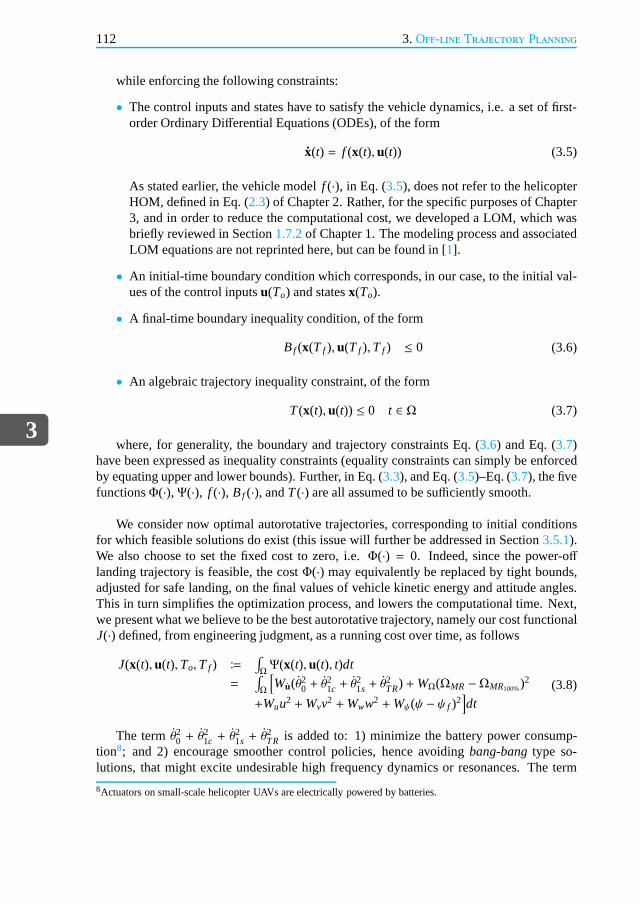
3

112 3. Off-line Trajectory Planning

while enforcing the following constraints:

• The control inputs and states have to satisfy the vehicle dynamics, i.e. a set of first-order Ordinary Differential Equations (ODEs), of the form

x(t) = f (x(t), u(t)) (3.5)

As stated earlier, the vehicle modelf (·), in Eq. (3.5), does not refer to the helicopterHOM, defined in Eq. (2.3) of Chapter 2. Rather, for the specific purposes of Chapter3, and in order to reduce the computational cost, we developed a LOM, which wasbriefly reviewed in Section1.7.2of Chapter 1. The modeling process and associatedLOM equations are not reprinted here, but can be found in [1].

• An initial-time boundary condition which corresponds, in our case, to the initial val-ues of the control inputsu(To) and statesx(To).

• A final-time boundary inequality condition, of the form

Bf (x(T f ), u(T f ),T f ) ≤ 0 (3.6)

• An algebraic trajectory inequality constraint, of the form

T(x(t), u(t)) ≤ 0 t ∈ Ω (3.7)

where, for generality, the boundary and trajectory constraints Eq. (3.6) and Eq. (3.7)have been expressed as inequality constraints (equality constraints can simply be enforcedby equating upper and lower bounds). Further, in Eq. (3.3), and Eq. (3.5)–Eq. (3.7), the fivefunctionsΦ(·),Ψ(·), f (·), Bf (·), andT(·) are all assumed to be sufficiently smooth.

We consider now optimal autorotative trajectories, corresponding to initial conditionsfor which feasible solutions do exist (this issue will further be addressed in Section3.5.1).We also choose to set the fixed cost to zero, i.e.Φ(·) = 0. Indeed, since the power-offlanding trajectory is feasible, the costΦ(·) may equivalently be replaced by tight bounds,adjusted for safe landing, on the final values of vehicle kinetic energy and attitude angles.This in turn simplifies the optimization process, and lowersthe computational time. Next,we present what we believe to be the best autorotative trajectory, namely our cost functionalJ(·) defined, from engineering judgment, as a running cost over time, as follows

J(x(t), u(t),To,T f ) ≔

∫

ΩΨ(x(t), u(t), t)dt

=∫

Ω

[

Wu(θ20 + θ

21c + θ

21s + θ

2TR) +WΩ(ΩMR −ΩMR100%)2

+Wuu2 +Wvv2 +Www2 +Wψ(ψ − ψ f )2]

dt

(3.8)

The termθ20 + θ

21c + θ

21s + θ

2TR is added to: 1) minimize the battery power consump-

tion8; and 2) encourage smoother control policies, hence avoiding bang-bangtype so-lutions, that might excite undesirable high frequency dynamics or resonances. The term

8Actuators on small-scale helicopter UAVs are electricallypowered by batteries.

3.4.Direct optimal control and discretization methods

3

113

(ΩMR − ΩMR100%)2 is added to penalize any large deviations in MR speed from itsnominal(power on) valueΩMR100%. Indeed, a rotor over-speed would increase, beyond acceptablevalues, the structural stresses on the MR hub and hinges. On the other hand, a rotor under-speed would be unsafe for the following two reasons: 1) it increases the region of bladestall9, increasing rotor drag and decreasing rotor lift, hence resulting in a higher helicoptersink rate; and 2) it lowers the stored rotor kinetic energy10, which is a crucial element for agood landing flare11 capability [99, 100]. The termu2 + w2 is added to limit the excessivebuild-up of vehicle kinetic energy during the descent. In particular, a high kinetic energycomplicates the flare maneuver, since more energy needs to bedissipated, i.e. the timing ofthe control inputs becomes increasingly critical [101]. The termv2 is added to limit vehi-cle sideslip12 flight. Large sideslip decreases the flight performance, by increasing vehicledrag, increasing roll/yaw coupling, and hence increasing the workload of any feedback TTcontroller. The termψ f refers to the wind heading angle (known through either on-boardmeasurements, or data-uplink from a ground-based wind sensor), and the term (ψ − ψ f )2

is added to encourage flight and landing into the wind. This results in better flight perfor-mance, and lowers the vehicle kinetic energy at touchdown. Finally, the additional weights,i.e. Wu, WΩ, Wu, Wv, Ww, andWψ, have been added to allow for the evaluation of varioustrade-offs within this cost objective.

Tail rotor ground clearanceHere we specifically address the constraint on the tail rotorblade tip, just before touch-down, during the flare landing maneuver. For the Tail Rotor Blade Tip (TRBT) groundclearance, we define the smallest distance between the TRBT and the ground by the distancexZTRBT in the vehicle carried normal earth frameFo, see Fig.3.1, with the TR radius givenby RrotTR. Note that both the z-axis of frameFo, and body frameFb, are oriented positivedownwards. TheFb position of the TR hub is given by (xTR, yTR, zTR), hence the lowestposition of the blade tip, for a positive vehicle pitchθ, is given inFo by

xZTRBT = xZ +

001

T

.Tob.

xTR− RrotTR. sinθyTR

zTR+ RrotTR. cosθ

(3.9)

andxZTRBT ≤ Zsa fety< 0, with Zsa fetya safety margin, andTob the transformation from bodyFb to the vehicle carried normal earth frameFo given in Eq. (2.8).

3.4.Direct optimal control and discretization methodsWe choose to solve our optimal control problem through a so-called direct method. In thiscontext, the continuous-time optimal control problem of Section 3.2 is first discretized andthe problem is transcribed to a NLP [55, 102], without formulating an alternate set of opti-mality conditions as done through indirect methods [66]. The resulting NLP can be solved

9Stall corresponds to a sudden reduction in lift.10The main rotor kinetic energy is defined as follows:1

2 NbIbΩ2MR, with Nb the number of blades, andIb the blade

inertia about the rotor shaft.11The flare refers to the landing maneuver just prior to touch-down. In the flare the nose of the vehicle is raised in

order to slow-down the descent rate, and further the proper attitude is set for touchdown.12Sideslip flight refers to a vehicle moving somewhat sidewaysas well as forward, relative to the oncoming airflow.

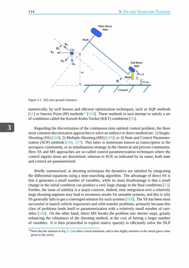
3

114 3. Off-line Trajectory Planning

Figure 3.1: Tail rotor ground clearance.

numerically, by well known and efficient optimization techniques, such as SQP methods[61] or Interior Point (IP) methods13 [103]. These methods in turn attempt to satisfy a setof conditions called the Karush-Kuhn-Tucker (KKT) conditions [55].

Regarding the discretization of the continuous-time optimal control problem, the threemost common discretization approaches to solve an indirector direct method are: 1) Single-Shooting (SS) [104]; 2) Multiple-Shooting (MS) [105]; or 3) State and Control Parameter-ization (SCP) methods [106, 107]. This latter is sometimes known as transcription in theaerospace community, or as simultaneous strategy in the chemical and process community.Here SS and MS approaches are so-called control parameterization techniques where thecontrol signals alone are discretized, whereas in SCP, as indicated by its name, both stateand control are parameterized.

Briefly summarized, in shooting techniques the dynamics aresatisfied by integratingthe differential equations using a time-marching algorithm. The advantage of direct SS isthat it generates a small number of variables, while its maindisadvantage is that a smallchange in the initial condition can produce a very large change in the final conditions [23].Further, the issue of stability is a major concern. Indeed, time integration over a relativelylarge shooting segment may lead to erroneous results for unstable systems, and this is whySS generally fails to get a converged solution for such systems [108]. The SS has been mostsuccessful in launch vehicle trajectories and orbit transfer problems, primarily because thisclass of problems lends itself to parameterization with a relatively small number of vari-ables [109]. On the other hand, direct MS breaks the problem into shorter steps, greatlyenhancing the robustness of the shooting method, at the costof having a larger numberof variables. It is then primordial to exploit matrix sparsity to efficiently solve the NLP

13Note that the solution to Eq. (3.4) is often a local minimum, and is also highly sensitive to theinitial guess valuegiven to the solver.

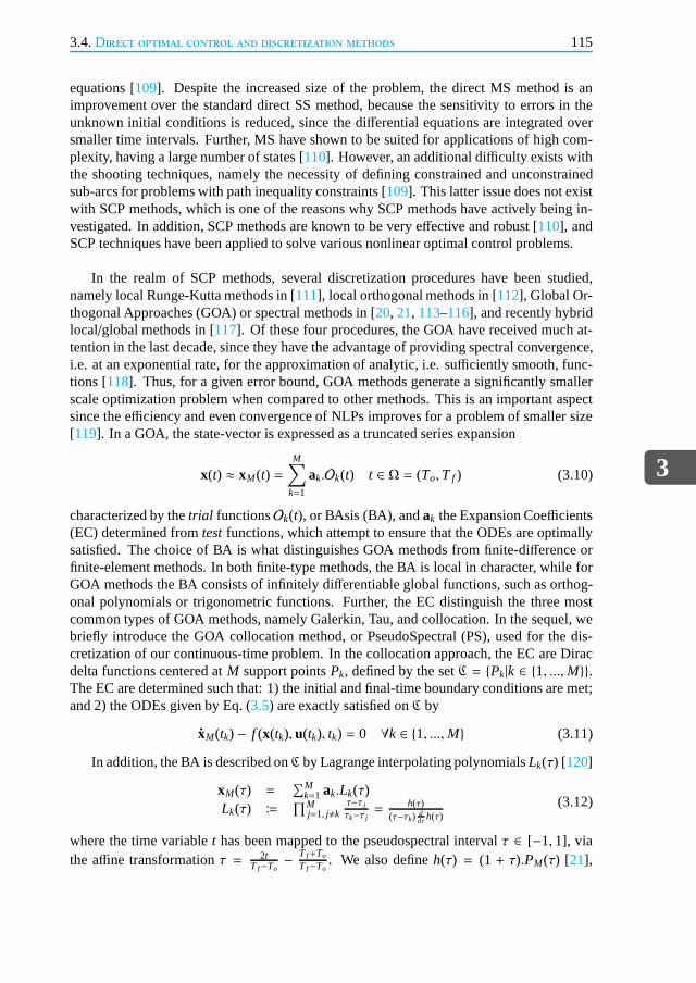
3.4.Direct optimal control and discretization methods

3

115

equations [109]. Despite the increased size of the problem, the direct MS method is animprovement over the standard direct SS method, because thesensitivity to errors in theunknown initial conditions is reduced, since the differential equations are integrated oversmaller time intervals. Further, MS have shown to be suited for applications of high com-plexity, having a large number of states [110]. However, an additional difficulty exists withthe shooting techniques, namely the necessity of defining constrained and unconstrainedsub-arcs for problems with path inequality constraints [109]. This latter issue does not existwith SCP methods, which is one of the reasons why SCP methods have actively being in-vestigated. In addition, SCP methods are known to be very effective and robust [110], andSCP techniques have been applied to solve various nonlinearoptimal control problems.

In the realm of SCP methods, several discretization procedures have been studied,namely local Runge-Kutta methods in [111], local orthogonal methods in [112], Global Or-thogonal Approaches (GOA) or spectral methods in [20, 21, 113–116], and recently hybridlocal/global methods in [117]. Of these four procedures, the GOA have received much at-tention in the last decade, since they have the advantage of providing spectral convergence,i.e. at an exponential rate, for the approximation of analytic, i.e. sufficiently smooth, func-tions [118]. Thus, for a given error bound, GOA methods generate a significantly smallerscale optimization problem when compared to other methods.This is an important aspectsince the efficiency and even convergence of NLPs improves for a problem ofsmaller size[119]. In a GOA, the state-vector is expressed as a truncated series expansion

x(t) ≈ xM(t) =M∑

k=1

ak.Ok(t) t ∈ Ω = (To,T f ) (3.10)

characterized by thetrial functionsOk(t), or BAsis (BA), andak the Expansion Coefficients(EC) determined fromtestfunctions, which attempt to ensure that the ODEs are optimallysatisfied. The choice of BA is what distinguishes GOA methodsfrom finite-difference orfinite-element methods. In both finite-type methods, the BA is local in character, while forGOA methods the BA consists of infinitely differentiable global functions, such as orthog-onal polynomials or trigonometric functions. Further, theEC distinguish the three mostcommon types of GOA methods, namely Galerkin, Tau, and collocation. In the sequel, webriefly introduce the GOA collocation method, or PseudoSpectral (PS), used for the dis-cretization of our continuous-time problem. In the collocation approach, the EC are Diracdelta functions centered atM support pointsPk, defined by the setC = Pk|k ∈ 1, ...,M.The EC are determined such that: 1) the initial and final-timeboundary conditions are met;and 2) the ODEs given by Eq. (3.5) are exactly satisfied onC by

xM(tk) − f (x(tk), u(tk), tk) = 0 ∀k ∈ 1, ...,M (3.11)

In addition, the BA is described onC by Lagrange interpolating polynomialsLk(τ) [120]

xM(τ) =∑M

k=1 ak.Lk(τ)Lk(τ) ≔

∏Mj=1, j,k

τ−τ j

τk−τ j=

h(τ)(τ−τk) d

dτh(τ)(3.12)

where the time variablet has been mapped to the pseudospectral intervalτ ∈ [−1, 1], viathe affine transformationτ = 2t

T f−To− T f+To

T f−To. We also defineh(τ) = (1 + τ).PM(τ) [21],

3

116 3. Off-line Trajectory Planning

wherePM(τ) is often related to Legendre or Chebyshev polynomials. In our case, we use aMth-degree Legendre polynomial given by

PM(τ) ≔1

2MM!dM

dτM[(τ2 − 1)M] (3.13)

Note that Lagrange polynomials are helpful for collocation; it is straightforward to showthat∀k ∈ 1, ...,M

Lk(τ j) = δk j =

1 k = j0 k , j

(3.14)

HencexM(τk) = ak onC, satisfying Eq. (3.11). In a similar way, the input control vectoris approximated with a basis of Lagrange polynomials, although not necessarily identicalto the previous ones. Besides the choice ofC, another set ofK points Qk, defined byQ = Qk|k ∈ 1, ...,K, is required for the discretization of the cost functional Eq. (3.3)and the ODEs in Eq. (3.5). HereQ is chosen such that the quadrature approximation of anintegral is minimized. We have

∫ 1

−1g(τ)dτ ≈

K∑

k=1

wk. f (τk) τ ∈ [−1, 1] (3.15)

with wk the quadrature weights. Now, it is well known that the highest accuracy quadratureapproximation, for a givenQ, is the Gauss quadrature. In this case,Q is defined by theroots of aKth-degree Legendre polynomialPK(τ), where the corresponding Gauss weightswk are given from [120] as

wk ≔2

(1− τ2k)( dPK(τk)

dτ )2∀k ∈ 1, ...,K (3.16)

PseudoSpectral methods have been extensively used for solving fluid dynamics prob-lems [19], but only recently have these methods been used for solvinga variety of optimalcontrol problems.

3.5.Simulation resultsOur MATLAB-based simulation software uses the helicopter LOM presented in Section1.7.2of Chapter 1, for the case of a small-scale helicopter UAV. The modeled UAV is an instru-mented Remote-Controlled (RC) Bergen Industrial Twin helicopter, belonging to the fly-barless two-bladed main rotor class, with a total mass of 8.35 kg, a main rotor radius of0.93 m, a main rotor nominal angular velocity of 1450 RPM, anda NACA 0015 main rotorairfoil, see Table3.1.

To solve the nonlinear control problem, the PS numerical method, as described in Sec-tion 3.4, is used. This numerical discretization framework is available in a MATLABenvironment, through the open-source General Pseudospectral OPtimal control SoftwareGPOPSR© [114, 121]. In order to use GPOPS, the optimal control problem must first bereformulated into a GPOPS format, as a set of MATLAB m-files [121]. Second, the he-licopter model must also be expressed in a vectorized structure, implying that each model

3.5.Simulation results

3

117

variable is a time-dependent vector. Third, (cubic) B-Splines interpolating functions oughtto be used, when querying lookup tables, since the spectral convergence of PS methodsonly holds when the functions under consideration are smooth [122]. Finally, it is bestpractice to non-dimensionalize and scale model variables and quantities, in order to im-prove conditioning of the numerical problem. Once the control problem is discretized, itis then transcribed into a static, finite-dimensional NLP optimization problem. An NLP isgenerally sparse, and many well-known efficient optimization techniques exist to numeri-cally solve large-scale and sparse NLPs. In our case, we use the SNOPTR© software [62],which solves finite-dimensional optimization problems through SQP. Finally, finite differ-encing has been used to estimate the objective gradient and constraint Jacobian. We presentnext simulation results for several case studies, but first we will review the Height-Velocity(H-V) diagram.

3.5.1.The Height-Velocity (H-V) diagramFor certain combinations of altitude Above Ground Level (AGL) and airspeed, the capa-bility of a helicopter to perform a safe autorotative landing is limited by the structural andaerodynamic design of the helicopter [123]. In fact, power failure within the dangerous orunsafe regions, defined by these combinations of AGL and airspeed, may result in high riskof severe damage or loss of vehicle. These limiting combinations of AGL and airspeed areoften expressed as the Height-Velocity (H-V) diagram14. Knowledge of these dangerousregions is important for safety procedures and operationalreasons15.

In Fig.3.2, a typical H-V diagram for a small-scale helicopter (of similar size to the oneconsidered in this Chapter) is shown. The H-V diagram shows two ’Avoid’ zones (in gray),namely: 1) a low-speed zone on the left, containing flight conditions where, if an enginefailure were to occur, execution of a safe landing would be unlikely, because of insufficientinitial energy; and 2) a high-speed zone on the right where, if an engine failure were to oc-cur, safe landing would also be unlikely, because the helicopter would possess insufficientaltitude to perform the flare (necessary to reduce the kinetic energy).

Now H-V diagrams can either be compiled from flight tests [132], or by solving opti-mal control problems. The latter is the approach adopted in this Chapter, where the H-Vdiagram becomes the solution of an optimization problem, similar to the general one pre-

14Also called thedeadman’szone.15Ideally, one would like to eliminate these unsafe regions altogether, or at least reduce their size. H-V studies can

be traced back to the late 1950s and early 1960s [124–126]. For example, eliminating the H-V restrictions wasdemonstrated with theKolibrie helicopter, built by theNederlandse Helikopter Industrie (NHI)in the late 1950s.It was designed by Dutch helicopter engineers and pioneers Jan M. Drees and Gerard F. Verhage. The helicopterwas ram-jet powered, these latter being positioned at the blade tips, resulting in very high main rotor inertia. TheH-V subject was also investigated in [123], where flight-test data was used to derive semi-empirical functionsof a generalized non dimensional H-V diagram, independent of density altitude and gross weight variations. In[127] it was pointed out that high rotor inertia, low disk loading, and a high maximum thrust coefficient couldreduce the size of the unsafe zone. In [128, 129], the concept of the so-called High Energy Rotor (HER) wasstudied, using blades with high rotational inertia. The goal of the HER was to eliminate the unsafe regions, butalso to allow for less demanding autorotation maneuvers, and finally use the rotor kinetic energy as a source oftransient power for better maneuverability. Additional results can also be found in [130, 131] where recent flighttests, related to the H-V subject with the Bell 430 and 407 helicopters, have been presented.

3

118 3. Off-line Trajectory Planning

Figure 3.2: Typical Height-Velocity (H-V) diagram for a small-scale helicopter UAV. Figure from [132, 133] (thenumbers on the axes are indicative only).

sented in Section3.2. To find the H-V curve, two approaches may be pursued, either:1) aminimization/maximization of altitude problem subject to safe landing; or 2) simply testinga feasibility problem in terms of safe landing. The minimization/maximization (former) ap-proach often led the solver to run into numerical difficulties. These difficulties were causedby: 1) the inclusion of highly nonlinear lookup tables which, despite B-Splines interpola-tion, have shown to have a detrimental effect on problem smoothness; and 2) the possibleexistence of a large number of solutions that all yield approximately the same value of thecost objective. In other words, the objective index is rather insensitive to the solution tra-jectory in the neighborhood of the optimal solution. On the other hand, for the feasibilityapproach, the cost objectiveJ(·) in Eq. (3.3) is set to zero, and one only requires to checkwhether a safe landing is possible, for a range of initial conditions. This method was suc-cessfully applied, based upon specific flight envelope boundaries given in Table3.2, withresults shown in Fig.3.3, for a relatively coarse grid having steps of 1 m in AGL and 1 m/sin airspeed. We found that our helicopter UAV exhibited onlythe so-called low-speed un-safe zone. We further subdivided this unsafe zone into two sub-zones: 1) one zone, shownin red, which always resulted in unsafe landings, independently of the initial guess condi-tions given to the solver; and 2) one zone, shown in magenta, which resulted in either safeor unsafe landings, depending on the initial guess conditions values given to the solver.

3.5.2.Evaluation of cost functionalsIn this section we evaluate and compare our cost functional,defined in Eq. (3.8) and ref-erenced asJ1 in Table3.3, to three other cost functionals referenced asJ2–J4 in Table3.3,

3.5.Simulation results

3

119

0 1 2 3 4 5 6 7 80

5

10

15

Horizontal Velocity (m/s)

Alti

tude

AG

L (m

)

Figure 3.3: Height-Velocity (H-V) diagram for the Bergen Industrial Twin.

which can be found in the literature. In Table3.3, J2 is a final-time only cost, which pur-pose is to minimize the vehicle kinetic energy (as well as having a horizontal attitude) atthe instant of touch-down.J3 is a running cost over time, minimizing actuators activity.J4 is also a running cost over time, which objective is to keep the main rotor RPM in theneighborhood of its nominal value, while minimizing the vehicle kinetic energies in thelongitudinal and vertical channels16.

For the comparison of these cost functionals, we consider aninitial condition, outsideof the H-V diagram, defined as follows: steady-state hover, at 40 m altitude, in a zero-windenvironment. Here for the analysis of each cost functionalJ j4j=1, we consider the following

power metricsPi j i=3, j=4i=1, j=1, of the vector-valued discrete-time signalzi(n)3i=1, defined as

z1(n) =[

θ(n)0 θ(n)TR θ(n)1c θ(n)1s

]⊤

z2(n) = [u(n) v(n) w(n)]⊤

z3(n) =[

v(n) φ(n)]⊤

Pi j =1N j‖zi(n)‖2l2 =

1N j

∑n=N j

n=1 ‖zi(n)‖22

(3.17)

with N j the number of data points of the optimization problems, corresponding to the costfunctional J j4j=1, and ‖ · ‖l2 the norm on the square-summable sequence spacel2. InEq. (3.17), the power metricP1 j , based upon signalz1, shows the control rates, i.e. thelevel of input control activity. This information is relevant, since a higher level of actuatordynamics means a higher power consumption from the batteries, and a higher likelihoodof exciting undesirable high frequency dynamics or resonances. Next, the power metricP2 j, based upon signalz2, reflects the amount of stored kinetic energy, during the flight, onthe combined three linear channels17. Finally, the power metricP3 j , based upon signalz3,

16The channels with most energies.17In general the kinetic energy, stored in the rotational channels, is much smaller than the one stored in the linear

channels.

3

120 3. Off-line Trajectory Planning

mirrors the amount of vehicle lateral motion. For each cost functional test caseJ j4j=1, thesignal power metricsPi j are reported in Table3.4. They are obtained by solving nonlinearoptimal control problems, based upon 29 nodes18 discretization, and yielding a NLP having607 variables and 506 constraints. Now, an analysis of Table3.4shows that:

• Our cost functional, defined in Eq. (3.8), considerably reduces lateral control activ-ity, e.g. compareP31 to P32, P33 andP34. The benefits of reduced lateral motion areincreased flight performance, and decreased roll-yaw coupling. This aspect is par-ticularly relevant when repositioning the current discussion within the, two-degreeof freedom, guidance and control logic, formulated in Section 1.7of Chapter 1. In-deed, the chosen flight control architectural solution decouples the guidance modulefrom the control module. The guidance module shall generateopen-loop feasibleand optimal autorotative trajectory references, whereas the control module shall en-sure that the helicopter flies along these optimal trajectories. Hence, a decrease in theamount of cross-coupling of the planned trajectories, results also in a decrease of theworkload of the feedback controller.

• J1 andJ3 display the lowest level of input control activity, confirmed by the powervaluesP11 = 0.06 andP13 = 0.008, since both costs include the input rates. Notethat excluding the control rates from the cost functional may lead to the excitation ofunmodeled or undesirable high frequency modes, potentially resulting in closed-loopinstability. This is particularly relevant when the subsequent synthesis of a feedbackcontroller is based upon low-order model representations.

• If a running cost over time is to be used, versus a final-time only cost (such asJ2),then: 1) minimization of control rates ought to be included,since we haveP14 = 1.87much higher thanP12 = 0.27; and 2) lateral motion should also be included, comparethe high values ofP33 andP34, to the lower value ofP32.

• Better performance can be achieved from the use of a final-time only cost, such asJ2, than from a poorly defined running cost over time, such asJ4.

• Finally, the last column in Table3.4 gives the total signal power∑3

i=1 Pi j , for eachcost functionalJ j4j=1, where we can see that our cost functional provides the bestautorotative trajectory. This said, this experiment, consisting in comparing variouscost functionals, was only conducted for a single initial condition, namely steady-state hover, at 40 m altitude, in a zero-wind environment. Although this conditionis representative enough of a typical initial condition fora small-scale helicopter, itwould indeed be interesting to obtain additional signal power values, correspondingto a wide spectrum of initial conditions.

18Based upon simulation results, the choice of 29 points provided a good compromise between accuracy andcomputational tractability. We do acknowledge that this isa rather empirical justification. In fact a more rigorousanalysis of the following trade-off: accuracyvs. computational tractabilityis here desirable.

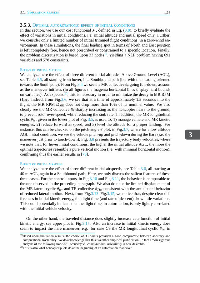
3.5.Simulation results

3

121

3.5.3.Optimal autorotations: effect of initial conditionsIn this section, we use our cost functionalJ1, defined in Eq. (3.8), to briefly evaluate theeffect of variations in initial conditions, i.e. initial altitude and initial speed only. Further,we consider only a limited number of initial trimmed flight conditions, in a zero-wind en-vironment. In these simulations, the final landing spot in terms of North and East positionis left completely free, hence not prescribed or constrained to a specific location. Finally,the problem discretization is based upon 33 nodes19, yielding a NLP problem having 691variables and 578 constraints.

Effect of initial altitudeWe analyze here the effect of three different initial altitudes Above Ground Level (AGL),see Table3.5, all starting from hover, in a Southbound path (i.e. with theheading orientedtowards the South pole). From Fig.3.4we see the MR collectiveθ0 going full-down, as soonas the maneuver initiates (in all figures the magenta horizontal lines display hard boundson variables). As expected20, this is necessary in order to minimize the decay in MR RPMΩMR. Indeed, from Fig.3.6, we see that at a time of approximately 1.5 seconds into theflight, the MR RPMΩMR does not drop more than 10% of its nominal value. We alsoclearly see the MR collectiveθ0 sharply increasing as the helicopter nears to the ground,to prevent rotor over-speed, while reducing the sink rate. In addition, the MR longitudinalcyclic θ1s, given in the lower plot of Fig.3.5, is used to: 1) manage vehicle and MR kineticenergies; 2) reduce forward airspeed; and 3) level the attitude for a proper landing. Forinstance, this can be checked on the pitch angleθ plot, in Fig.3.7, where for a low altitudeAGL initial condition, we see the vehicle pitch-up and pitch-down during the flare (i.e. themaneuver just prior to touch-down). Fig.3.8presents the trajectory body velocities, wherewe note that, for hover initial conditions, the higher the initial altitude AGL, the more theoptimal trajectories resemble a pure vertical motion (i.e.with minimal horizontal motion),confirming thus the earlier results in [76].

Effect of initial airspeedWe analyze here the effect of three different initial airspeeds, see Table3.6, all starting at40 m AGL, again in a Southbound path. Here, we only discuss thesalient features of thesethree cases. For the control inputs, in Fig.3.10and Fig.3.11, the behavior is comparable tothe one observed in the preceding paragraph. We also do note the limited displacement ofthe MR lateral cyclicθ1c, and TR collectiveθTR, consistent with the anticipated behaviorof reduced lateral motion. Next, from Fig.3.13–Fig.3.15, we notice that, despite clear dif-ferences in initial kinetic energy, the flight time (and rateof descent) show little variations.This could potentially indicate that the flight time, in autorotation, is only lightly correlatedwith the initial vehicle velocity.

On the other hand, the traveled distance does slightly increase as a function of initialkinetic energy, see upper plot in Fig.3.15. Also an increase in initial kinetic energy doesseem to impact the flare maneuver, e.g. for caseC6 the MR longitudinal cyclicθ1s, in

19Based upon simulation results, the choice of 33 points provided a good compromise between accuracy andcomputational tractability. We do acknowledge that this isa rather empirical justification. In fact a more rigorousanalysis of the following trade-off: accuracyvs. computational tractabilityis here desirable.

20This is also what helicopter pilots do at the beginning of an autorotation maneuver.

3

122 3. Off-line Trajectory Planning

Fig.3.11, and the helicopter pitchθ, in Fig.3.13, exhibit almost a ’double’ flare approachin the last two seconds of the flight. In addition, we see that if differences are to be noted,between on the one hand the hover and low-speed cases—C4 andC5—and on the otherthe high-speed caseC6, then they would tend to primarily appear on the longitudinal θ andRPMΩMR channels, during the initial flight phase21, see Fig.3.11–Fig.3.13.

3.6.ConclusionIn this Chapter, we have addressed the autorotative Trajectory Planning (TP) problem,for the case of a small-scale helicopter UAV, and we have formulated the technologi-cal/engineering TP problem into a mathematical, model-based, nonlinear optimal controlproblem. The latter was numerically solved, through a direct optimal control framework.The main benefits of this Chapter are threefold. First, we found that for fixed initial altitude,increasing the initial velocity had only a relatively limited effect on the optimal trajectoryflight time. On the other hand, the flight time showed a strong correlation with the initialaltitude. This aspect, together with the knowledge of an optimally defined autorotative tra-jectory, will prove useful in the following Chapter. Second, for a range of initial conditions,optimal autorotative trajectories could potentially be computed, off-line, by this TP, andstored as lookup tables, on-board a flight control computer.These trajectories would thenprovide, both, the optimal states to be tracked by a feedbackcontroller, and optionally thefeedforward nominal control inputs. Third, the optimization framework, developed here,could allow to study the effects of some particular factors, affecting the optimal trajectories.These factors include wind, but also some helicopter specific aspects, such as helicoptermass, number of main rotor blades, main rotor blade mass, andmain rotor inertia.

21Approximately the first second into the flight.

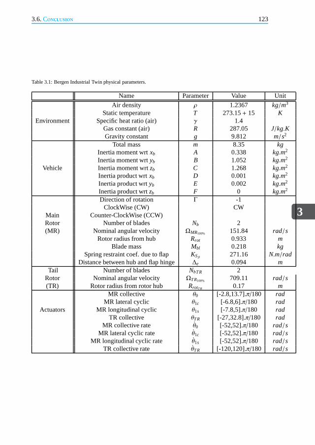
3.6.Conclusion

3

123

Table 3.1: Bergen Industrial Twin physical parameters.

Name Parameter Value Unit

Environment

Air density ρ 1.2367 kg/m3

Static temperature T 273.15+ 15 KSpecific heat ratio (air) γ 1.4

Gas constant (air) R 287.05 J/kg.KGravity constant g 9.812 m/s2

Total mass m 8.35 kgInertia moment wrtxb A 0.338 kg.m2

Inertia moment wrtyb B 1.052 kg.m2

Vehicle Inertia moment wrtzb C 1.268 kg.m2

Inertia product wrtxb D 0.001 kg.m2

Inertia product wrtyb E 0.002 kg.m2

Inertia product wrtzb F 0 kg.m2

Direction of rotation Γ -1ClockWise (CW) CW

Main Counter-ClockWise (CCW)Rotor Number of blades Nb 2(MR) Nominal angular velocity ΩMR100% 151.84 rad/s

Rotor radius from hub Rrot 0.933 mBlade mass Mbl 0.218 kg

Spring restraint coef. due to flap KSβ271.16 N.m/rad

Distance between hub and flap hinge ∆e 0.094 mTail Number of blades NbTR 2

Rotor Nominal angular velocity ΩTR100% 709.11 rad/s(TR) Rotor radius from rotor hub RrotTR 0.17 m

MR collective θ0 [-2.8,13.7].π/180 radMR lateral cyclic θ1c [-6.8,6].π/180 rad

Actuators MR longitudinal cyclic θ1s [-7.8,5].π/180 radTR collective θTR [-27,32.8].π/180 rad

MR collective rate θ0 [-52,52].π/180 rad/sMR lateral cyclic rate θ1c [-52,52].π/180 rad/s

MR longitudinal cyclic rate θ1s [-52,52].π/180 rad/sTR collective rate θTR [-120,120].π/180 rad/s

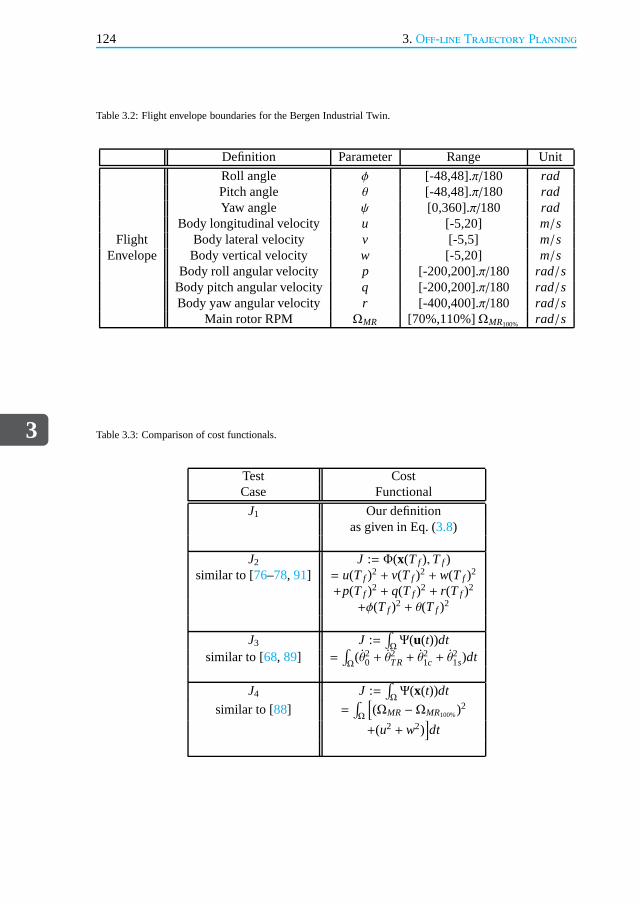
3

124 3. Off-line Trajectory Planning

Table 3.2: Flight envelope boundaries for the Bergen Industrial Twin.

Definition Parameter Range Unit

Roll angle φ [-48,48].π/180 radPitch angle θ [-48,48].π/180 radYaw angle ψ [0,360].π/180 rad

Body longitudinal velocity u [-5,20] m/sFlight Body lateral velocity v [-5,5] m/s

Envelope Body vertical velocity w [-5,20] m/sBody roll angular velocity p [-200,200].π/180 rad/s

Body pitch angular velocity q [-200,200].π/180 rad/sBody yaw angular velocity r [-400,400].π/180 rad/s

Main rotor RPM ΩMR [70%,110%]ΩMR100% rad/s

Table 3.3: Comparison of cost functionals.

Test CostCase Functional

J1 Our definitionas given in Eq. (3.8)

J2 J := Φ(x(T f ),T f )similar to [76–78, 91] = u(T f )2 + v(T f )2 + w(T f )2

+p(T f )2 + q(T f )2 + r(T f )2

+φ(T f )2 + θ(T f )2

J3 J :=∫

ΩΨ(u(t))dt

similar to [68, 89] =∫

Ω(θ2

0 + θ2TR+ θ

21c + θ

21s)dt

J4 J :=∫

ΩΨ(x(t))dt

similar to [88] =∫

Ω

[

(ΩMR −ΩMR100%)2

+(u2 + w2)]

dt

3.6.Conclusion

3

125

Table 3.4: Comparison of signal power for various cost functionals.

Test Control rates 3D linear motion Lateral motion Total powerCase P1 j P2 j P3 j

∑3i=1 Pi j

J1 0.06 50 0.06 50.12J2 0.27 62.3 1.7 64.27J3 0.008 46.2 14.9 61.108J4 1.87 46.2 16.5 63.57

Table 3.5: Initial trimmed flight conditions: autorotations with variation of initial altitude Above Ground Level(AGL).

Test Airspeed Altitude (AGL) Line ColorCase (m/s) (m) in Figures

C1 hover 25 Red (solid line)C2 hover 40 Blue (dotted line)C3 hover 110 Black (dashed line)

Table 3.6: Initial trimmed flight conditions: autorotations with variation of initial airspeed.

Test Airspeed Altitude (AGL) Line ColorCase (m/s) (m) in Figures

C4 hover 40 Red (solid line)C5 5 40 Blue (dotted line)C6 15 40 Black (dashed line)

3

126 3. Off-line Trajectory Planning

0 2 4 6 8 10 12 14 16−5

0

5

10

15

Time (s)

θ 0 (de

g)

0 2 4 6 8 10 12 14 16−40

−20

0

20

40

Time (s)

θ TR

(de

g)

Figure 3.4: MR collective control inputθ0 and TR collective control inputθTR (variation of initial altitude accord-ing to Table3.5).

0 2 4 6 8 10 12 14 16−10

−5

0

5

10

Time (s)

θ 1c (

deg)

0 2 4 6 8 10 12 14 16−10

−5

0

5

Time (s)

θ 1s (

deg)

Figure 3.5: MR lateral cyclic control inputθ1c and MR longitudinal cyclic control inputθ1s (variation of initialaltitude according to Table3.5).

3.6.Conclusion

3

127

0 2 4 6 8 10 12 14 161000

1100

1200

1300

1400

1500

1600

Time (s)

ΩM

R (

RP

M)

Figure 3.6: MR RPMΩMR (variation of initial altitude according to Table3.5).

0 2 4 6 8 10 12 14 16−50

0

50

Time (s)

φ (d

eg)

0 2 4 6 8 10 12 14 16−50

0

50

Time (s)

θ (d

eg)

0 2 4 6 8 10 12 14 160

200

400

Time (s)

ψ (

deg)

Figure 3.7: Euler angles: roll angleφ, pitch angleθ, yaw angleψ (variation of initial altitude according to Ta-ble3.5).

3

128 3. Off-line Trajectory Planning

0 2 4 6 8 10 12 14 16−10

0

10

20

Time (s)

u (m

/s)

0 2 4 6 8 10 12 14 16−5

0

5

Time (s)

v (m

/s)

0 2 4 6 8 10 12 14 16−10

0

10

20

Time (s)

w: >

0 do

wn

(m/s

)

Figure 3.8: Body linear velocities: longitudinal velocityu, lateral velocityv, vertical velocityw (variation of initialaltitude according to Table3.5).

0 2 4 6 8 10 12 14 16−4

−2

0

2

Time (s)

x N (

m)

0 2 4 6 8 10 12 14 16−10

−5

0

5

Time (s)

x E (

m)

0 2 4 6 8 10 12 14 160

50

100

150

Time (s)

x Z: >

0 up

(m

)

Figure 3.9: Inertial position: North positionxN, East positionxE, Vertical positionxZ (variation of initial altitudeaccording to Table3.5).

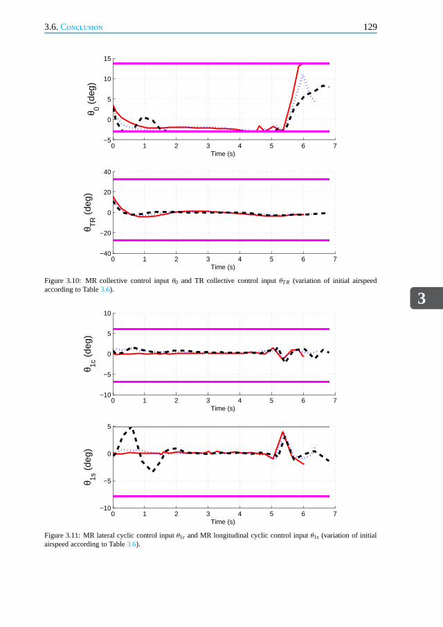
3.6.Conclusion

3

129

0 1 2 3 4 5 6 7−5

0

5

10

15

Time (s)

θ 0 (de

g)

0 1 2 3 4 5 6 7−40

−20

0

20

40

Time (s)

θ TR

(de

g)

Figure 3.10: MR collective control inputθ0 and TR collective control inputθTR (variation of initial airspeedaccording to Table3.6).

0 1 2 3 4 5 6 7−10

−5

0

5

10

Time (s)

θ 1c (

deg)

0 1 2 3 4 5 6 7−10

−5

0

5

Time (s)

θ 1s (

deg)

Figure 3.11: MR lateral cyclic control inputθ1c and MR longitudinal cyclic control inputθ1s (variation of initialairspeed according to Table3.6).

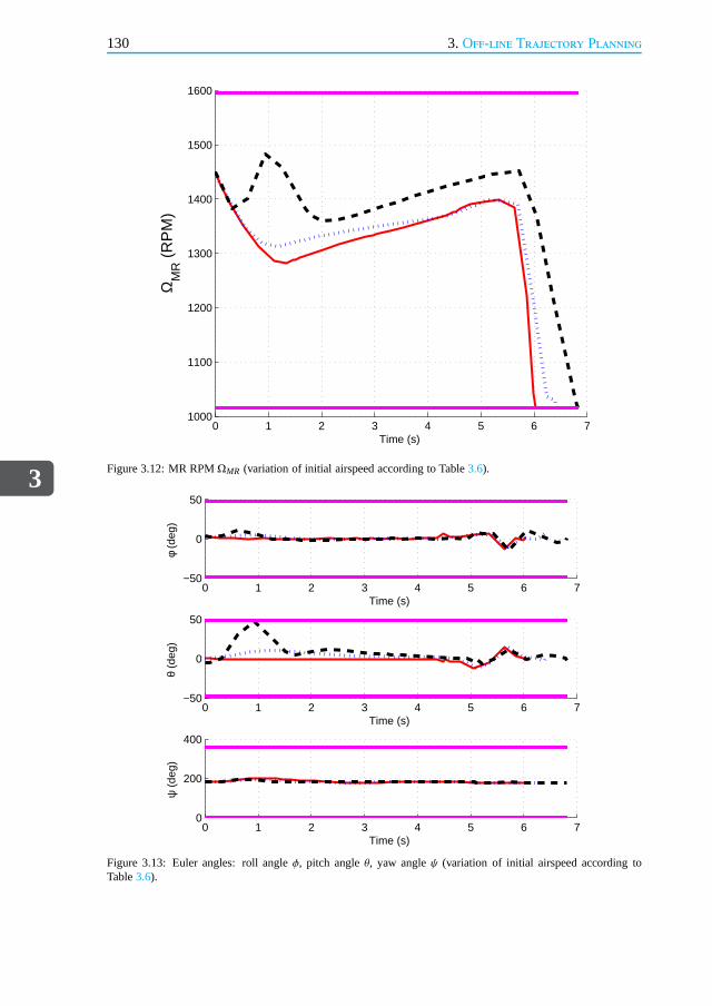
3

130 3. Off-line Trajectory Planning

0 1 2 3 4 5 6 71000

1100

1200

1300

1400

1500

1600

Time (s)

ΩM

R (

RP

M)

Figure 3.12: MR RPMΩMR (variation of initial airspeed according to Table3.6).

0 1 2 3 4 5 6 7−50

0

50

Time (s)

φ (d

eg)

0 1 2 3 4 5 6 7−50

0

50

Time (s)

θ (d

eg)

0 1 2 3 4 5 6 70

200

400

Time (s)

ψ (

deg)

Figure 3.13: Euler angles: roll angleφ, pitch angleθ, yaw angleψ (variation of initial airspeed according toTable3.6).

3.6.Conclusion

3

131

0 1 2 3 4 5 6 7−10

0

10

20

Time (s)

u (m

/s)

0 1 2 3 4 5 6 7−5

0

5

Time (s)

v (m

/s)

0 1 2 3 4 5 6 7−10

0

10

20

Time (s)

w: >

0 do

wn

(m/s

)

Figure 3.14: Body linear velocities: longitudinal velocity u, lateral velocityv, vertical velocityw (variation ofinitial airspeed according to Table3.6).

0 1 2 3 4 5 6 7−40

−20

0

20

Time (s)

x N (

m)

0 1 2 3 4 5 6 7−2

−1

0

1

Time (s)

x E (

m)

0 1 2 3 4 5 6 70

20

40

Time (s)

x Z: >

0 up

(m

)

Figure 3.15: Inertial position: North positionxN, East positionxE, Vertical positionxZ (variation of initial airspeedaccording to Table3.6).

3

132 References

References[1] S. Taamallah,Low-order modeling for a small-scale flybarless helicopteruav, a grey-

box time-domain approach,in AIAA Atmospheric Flight Mechanics Conf.(2012).

[2] S. Taamallah,Optimal autorotation with obstacle avoidance for a small-scale flybar-less helicopter uav,in AIAA Guidance, Navigation and Control Conf.(2012).

[3] S. Taamallah, X. Bombois, and P. M. J. Van den Hof,Optimal control for power-offlanding of a small-scale helicopter a pseudospectral approach,in Am. Control Conf.(2012).

[4] J. T. Schwartz and M. Sharir,A survey of motion planning and related geometricalgorithms,Artificial Intelligence37, 157 (1988).

[5] J. C. Latombe,Robot Motion Planning(Kluwer Int. Series in Engineering and Com-puter Science, Mass., 1991).

[6] Y. K. Hwang and N. Ahuja,Gross motion planning - a survey,ACM Comp. Surv.24, 219 (1992).

[7] J. C. Latombe,Motion planning: A journey of robots, molecules, digital actors, andother artifacts,Int. J. of Robotics Research18, 1119 (1999).

[8] H. Choset, K. M. Lynch, S. Hutchinson, G. Kantor, W. Burgard, L. E. Kavraki, andS. Thrun,Principles of Robot Motion: Theory, Algorithms, and Implementations(MIT Press, Cambridge, MA, 2005).

[9] S. M. LaValle,Planning Algorithms(Cambridge University Press, Cambridge Eng-land, 2006).

[10] R. M. Murray, Robust Control and nonholonomic motion planning, Ph.D. thesis,University of California at Berkeley (1990).

[11] C. Goerzen, Z. Kong, and B. Mettler,A survey of motion planning algorithms fromthe perspective of autonomous uav guidance,J. Intell. Robot Syst.57, 65 (2010).

[12] N. Dadkhah and B. Mettler,Survey of motion planning literature in the presence ofuncertainty: Considerations for uav guidance,J. Intell. Robot Syst.65, 233 (2012).

[13] R. Humphries,The Aeneid of Virgil: A Verse Translation(Macmillan, USA, 1987).

[14] A. E. Bryson,Optimal control - 1950 to 1985,IEEE Control Systems Magazine16(1996).

[15] H. J. Sussmann and J. C. Willems,300 years of optimal control: From the brachys-tochrone to the maximum principle,Control Systems, IEEE17 (1997).

[16] R. Bellman and S. E. Dreyfus,Applied Dynamic Programming(Princeton Univ.Press, Princeton New Jersey, 1971).

References

3

133

[17] L. S. Pontryagin, V. G. Boltyanskii, R. V. Gamkrelidze,E. F. Mishchenko, K. N.Trirogoff, and L. W. Neustadt,Mathematical Theory of Optimal Processes(Inter-science, NY, 1962).

[18] A. E. Bryson and Y. C. Ho,Applied Optimal Control(Taylor & Francis Group, NewYork, 1975).

[19] C. Canuto, M. Y. Hussaini, A. Quarteroni, and T. A. Zang,Spectral Methods inFluid Dynamics(Springer-Verlag, New York, 1988).

[20] D. A. Benson,A Gauss Pseudospectral Transcription for Optimal Control, Ph.D.thesis, Massachusetts Institute of Technology (2004).

[21] G. T. Huntington,Advancement and Analysis of a Gauss Pseudospectral Transcrip-tion for Optimal Control, Ph.D. thesis, Massachusetts Institute of Technology (2007).

[22] C. P. Neuman and A. Sen,A suboptimal control algorithm for constrained problemsusing cubic splines,Automatica9, 601 (1973).

[23] J. T. Betts,Practical methods for optimal control using nonlinear programming,inSIAM (2001).

[24] K. Misovec, T. Inanc, J. Wohletz, and R. M. Murray,Low-observable nonlineartrajectory generation for unmanned air vehicles,in IEEE Conf. on Decision andControl (2003).

[25] D. Gottlieb, M. Y. Hussaini, and S. A. Orszag,Theory and applications of spectralmethods,in Spectral Methods for PDE’s. Soc. of Industrial and Applied Mathematics(SIAM)(1984).

[26] P. Lu, H. Sun, and B. Tsai,Closed-loop endoatmospheric ascent guidance,AIAA J.of Guidance, Control and Dynamics26, 283 (2003).

[27] J. Rea,Launch vehicle trajectory optimization using a legendre pseudospectralmethod,in AIAA Guidance, Navigation, and Control Conf.(2003).

[28] S. Josselyn and I. M. Ross,Rapid verification method for the trajectory optimizationof reentry vehicles,AIAA J. of Guidance, Control, and Dynamics26 (2003).

[29] P. Williams, Application of pseudospectral methods for receding horizon control,AIAA J. of Guidance, Control, and Dynamics27, 310 (2004).

[30] S. I. Infeld,Optimization of Mission Design for Constrained Libration Point SpaceMissions, Ph.D. thesis, Stanford University (2005).

[31] J. P. Riehl, S. W. Paris, and W. K. Sjaw,Comparision of implicit integration methodsfor solving aerospace trajectory optimization problems,in AIAA/AAS AstrodynamicsSpecialists Conf.(2006).

[32] A. M. Hawkins, T. R. Fill, R. J. Proulx, and E. M. Feron,Constrained trajectoryoptimization for lunar landing,in AAS Spaceflight Mechanics Meeting(2006).

3

134 References

[33] K. P. Bollino, L. R. Lewis, P. Sekhavat, and I. M. Ross,Pseudospectral optimalcontrol: A clear road for autonomous intelligent path planning, in AIAA Infotech(2007).

[34] N. Bedrossian, S. Bhatt, M. Lammers, L. Nguyen, and Y. Zhang,First ever flightdemonstration of zero propellant maneuver tm attitude control concept,in AIAAGuidance, Navigation, and Control Conf.(2007).

[35] Q. Gong, K. Wei, N. S. Bedrossian, F. Fahroo, P. Sekhavat, and K. Bollino,Pseu-dospectral optimal control for military and industrial applications,in IEEE Conf. onDecision and Control(2007).

[36] I. M. Ross, P. Sekhavat, A. Fleming, and Q. Gong,Optimal feedback control: Foun-dations, examples, and experimental results for a new approach,AIAA J. of Guid-ance, Control, and Dynamics31 (2008).

[37] M. Karpenko, S. Bhatt, N. Bedrossian, A. Fleming, and I.M. Ross,Flight imple-mentation of pseudospectral optimal control for the trace space telescope,in AIAAGuidance, Navigation and Control Conf.(2011).

[38] M. Ceriotti and C. R. McInnes,Generation of optimal trajectories for earth hybridpole sitters,AIAA J. of Guidance, Control, and Dynamics34, 847 (2011).

[39] H. Yan, Q. Gong, C. D. Park, I. M. Ross, and C. N. D. Souza,High-accuracy tra-jectory optimization for a trans-earth lunar mission,AIAA J. of Guidance, Control,and Dynamics34, 1219 (2011).

[40] C. L. Darby and A. V. Rao,Minimum-fuel low-earth-orbit aeroassisted orbital trans-fer of small spacecraft,AIAA J. of Spacecraft and Rockets48 (2011).

[41] G. Boyarko, O. Yakimenko, and M. Romano,Optimal rendezvous trajectories ofa controlled spacecraft and a tumbling object,AIAA J. of Guidance, Control, andDynamics34, 1239 (2011).

[42] G. Boyarko, M. Romano, and O. Yakimenko,Time-optimal reorientation of a space-craft using an inverse dynamics optimization method,AIAA J. of Guidance, Control,and Dynamics34, 1197 (2011).

[43] K. Zhang and W. Chen,Reentry vehicle constrained trajectory optimization,in AIAAInt. Space Planes and Hypersonic Systems and Technologies(2011).

[44] S. W. Paris, J. P. Riehl, and W. K. Sjaw,Enhanced procedures for direct trajectoryoptimization using nonlinear programming and implicit integration, in AIAA/AASAstrodynamics Specialists Conf.(2006).

[45] G. C. Cottrill and F. G. Harmon,Hybrid gauss pseudospectral and generalized poly-nomial chaos algorithm to solve stochastic trajectory optimization problems,in AIAAGuidance Navigation and Control Conf.(2011).

References

3

135

[46] M. Dekel and J. Z. Ben-Asher,Pseudo-spectral-method based optimal glide in theevent of engine cut-off, in AIAA Guidance, Navigation, and Control Conf.(2011).

[47] R. Dai and J. E. Cochran,Three-dimensional trajectory optimization in constrainedairspace,AIAA J. of Aircraft 46, 627 (2009).

[48] S. Hartjes, H. G. Visser, and M. D. Pavel,Environmental optimization of rotorcraftapproach trajectories,in Europ. Rotorcraft Forum(2011).

[49] M. Harada and K. Bollino,Optimal trajectory of a glider in ground effect and windshear,in AIAA Guidance, Navigation and Control Conf.(2005).

[50] Q. Gong, L. R. Lewis, and I. M. Ross,Pseudospectral motion planning for au-tonomous vehicles,AIAA J. of Guidance, Control, and Dynamics32 (2009).

[51] B. D. McCracken, K. L. Burzota, M. M. Ramos, and T. R. Jorris, Cooperativeunmanned air vehicle mission planning and collision avoidance,in AIAA Infotech(2011).

[52] R. Choe and N. Hovakimyan,Perching maneuver for an mav augmented with an l1adaptive controller,in AIAA Guidance, Navigation, and Control Conf.(2011).

[53] A. la Cour-Harbo and M. Bisgaard,State-control trajectory generation for helicopterslung load system using optimal control,in AIAA Guidance, Navigation, and ControlConf.(2009).

[54] M. Harada and K. Bollino,Minimum-time circling flight of a triarm coaxial rotoruav,in AIAA Guidance Navigation and Control Conf.(2011).

[55] D. Bertsekas,Nonlinear Programming - Second Edition(Athena Scientific, Belmont,MA, 1999).

[56] L. T. Biegler, O. Ghattas, M. Heinkenschloss, and B. vanBloemen Waanders,Large-Scale PDE-Constrained Optimization(Springer, Berlin, 2003).

[57] R. H. Byrd, J. Nocedal, and R. A. Waltz,Knitro: An integrated package for nonlin-ear optimization,Large-Scale Nonlinear Optimization, Springer-Verlag , 35(2006).

[58] A. Wachter and L. T. Biegler,On the implementation of an interior-point filter line-search algorithm for large-scale nonlinear programming,Mathematical Program-ming106, 25 (2006).

[59] L. T. Biegler and V. M. Zavala,Large-scale nonlinear programming using ipopt: Anintegrating framework for enterprise-wide optimization,Computers and ChemicalEngineering33, 575 (2008).

[60] P. E. Gill, W. Murray, M. A. Saunders, and M. H. Wright,User’s Guide for NPSOL5.0: A Fortran Package for Nonlinear Programming, Tech. Rep. (Stanford Univer-sity, 2001).

3

136 References

[61] P. E. Gill, W. Murray, and M. A. Saunders,Snopt: An sqp algorithm for large-scaleconstrained optimization,SIAM Reviews47, 99 (2002).

[62] P. E. Gill, W. Murray, M. A. Saunders, and M. H. Wright,User’s Guide for SNOPTVersion 7: Software for Large-Scale Nonlinear Programming, Tech. Rep. (Universityof California San Diego, 2008).

[63] SBS-Inc., (http://www.sbsi-sol-optimize.com/asp/sol_product_snopt.htm, StanfordUniversity, U.S.A.).

[64] G. A. Bliss, Lectures on the Calculus of Variations(University of Chicago Press,Chicago IL, 1946).

[65] R. Weinstock,Calculus of Variations(Dover Publications, NY, 1974).

[66] B. van Brunt,The Calculus of Variations(Springer-Verlag, NY, 2004).

[67] M. D. Ardema and N. Rajan,Separation of time scales in aircraft trajectory opti-mization,AIAA J. of Guidance, Control, and Dynamics8, 275 (1985).

[68] C. L. Bottasso, A. Croce, D. Leonello, and L. Riviello,Optimization of criticaltrajectories for rotorcraft vehicles,J. of the Am. Helicopter Soc. , 165 (2005).

[69] P. Abbeel, A. Coates, M. Quigley, and A. Y. Ng,An application of reinforcementlearning to aerobatic helicopter flight,in NIPS 19(2007).

[70] P. Abbeel, A. Coates, T. Hunter, and A. Y. Ng,Autonomous autorotation of an rchelicopter,in 11th Int. Symposium on Experimental Robotics (ISER)(2008).

[71] D. J. Lee, H. Bang, and K. Baek,Autorotation of an unmanned helicopter by areinforcement learning algorithm,in AIAA Guidance, Navigation and Control Conf.(2008).

[72] D. J. Lee and H. Bang,Autonomous autorotation of an unmanned helicopter using areinforcement learning algorithm,J. Aerospace Information Systems10, 98 (2013).

[73] M. Uemura, M. Ishikawa, N. Sudo, I. Sudo, and Y. kubo,Fuzzy intelligent pilotsupport system for an autorotative flight of helicopter,in Europ. Rotorcraft Forum(1993).

[74] Z. Sunberg and J. Rogers,A fuzzy logic-based controller for helicopter autorotation,in AIAA Aerospace Sciences Meeting and Exhibit(2013).

[75] M. Komoda,Prediction of height-velocity boundaries for rotorcraft by application ofoptimizing techniques,Trans. of the Japan Soc. for Aeronautical and Space Sciences15, 208 (1973).

[76] W. Johnson,Helicopter Optimal Descent and Landing After Power Loss, Tech. Rep.TM 73-244 (NASA Ames Research Center, 1977).

References

3

137

[77] A. Y. Lee, A. E. Bryson, and W. S. Hindson,Optimal landing of a helicopter inautorotation,AIAA J. of Guidance, Control, and Dynamics11, 7 (1988).

[78] Y. Okuno, K. Kawachi, A. Azuma, and S. Saito,Analytical prediction of height-velocity diagram of a helicopter using optimal control theory, AIAA J. of Guidance,Control, and Dynamics14, 453 (1991).

[79] Y. Okuno and K. Kawachi,Optimal control of helicopters following power failure,AIAA J. of Guidance, Control, and Dynamics17, 181 (1994).

[80] M. W. Floros,Descent analysis for rotorcraft survivability with power loss,in Am.Helicopter Soc.(2009).

[81] A. Lee,Engineering notes - optimal autorotational descent of a helicopter with con-trol and state inequality constraints,AIAA J. of Guidance, Control, and Dynamics13, 922 (1990).

[82] E. N. Bachelder and B. L. Aponso,An autorotation flight director for helicoptertraining, in Am. Helicopter Soc.(2003).

[83] A. A. Jhemi, E. B. Carlson, Y. J. Zhao, and R. T. N. Chen,Optimization of rotorcraftflight following engine failure,J. of the Am. Helicopter Soc. (2004).

[84] B. L. Aponso, E. N. Bachelder, and D. Lee,Automated autorotation for un-manned rotorcraft recovery,in AHS Int. Specialists’ Meeting On Unmanned Rotor-craft (2005).

[85] B. L. Aponso, D. Lee, and E. N. Bachelder,Evaluation of a rotorcraft autorota-tion training display on a commercial flight training device, in Am. Helicopter Soc.(2005).

[86] C. L. Bottasso, C. S. Chang, A. Croce, D. Leonello, and L.Riviello, Adaptive plan-ning and tracking of trajectories for the simulation of maneuvers with multibodymodels,Computer Methods in Applied Mechanics and Engineering (2006).

[87] E. B. Carlson, S. Xue, J. Keane, and K. Burns,H-1 upgrades height-velocity diagramdevelopment through flight test and trajectory optimization, in Am. Helicopter Soc.(2006).

[88] P. Bibik and J. Narkiewicz,Helicopter optimal control after power failure using com-prehensive dynamic model,AIAA J. of Guidance, Control, and Dynamics35, 1354(2012).

[89] C. L. Bottasso, G. Maisano, and F. Luraghi,Efficient rotorcraft trajectory optimiza-tion using comprehensive vehicle models by improved shooting methods,in Europ.Rotorcraft Forum(2009).

[90] C. L. Bottasso, G. Maisano, and F. Scorcelletti,Trajectory optimization proceduresfor rotorcraft vehicles, their software implementation, and applicability to models ofincreasing complexity,J. of the Am. Helicopter Soc. (2010).

3

138 References

[91] M. W. Floros,Application of sequential quadratic programming to rotorcraft surviv-ability with power loss,in Am. Helicopter Soc.(2011).

[92] K. Dalamagkidis, K. P. Valavanis, and L. A. Piegl,Autonomous autorotation ofunmanned rotorcraft using nonlinear model predictive control, J. Intell. Robot Syst.57, 351 (2010).

[93] S. Tierney and J. W. Langelaan,Autorotation path planning using backwards reach-able set and optimal control,in Am. Helicopter Soc.(2010).

[94] N. Grande and J. W. Langelaan,Safe autonomous flare and landing during autoro-tation through wind shear,in Am. Helicopter Soc.(2013).

[95] J. Holsten, S. Loechelt, and W. Alles,Autonomous autorotation flights of helicopteruavs to known landing sites,in Am. Helicopter Soc.(2010).

[96] T. Yomchinda, J. F. Horn, and J. W. Langelaan,Flight path planning for descent-phase helicopter autorotation,in AIAA Guidance, Navigation, and Control Conf.(2011).

[97] T. Yomchinda, J. F. Horn, and J. W. Langelaan,Autonomous control and path plan-ning for autorotation of unmanned helicopters,in Am. Helicopter Soc.(2012).

[98] P. Bibik and J. Narkiewicz,Helicopter modeling and optimal control in autorotation,in Am. Helicopter Soc.(2008).

[99] R. W. Prouty,Helicopter Performance, Stability, and Control(Krieger PublishingCompany, Malabar, Florida USA, 1995).

[100] W. Johnson,Helicopter Theory(Dover Publications Inc., NY, USA, 1994).

[101] S. Taamallah,A qualitative introduction to the vortex-ring-state, autorotation, andoptimal autorotation,in Europ. Rotorcraft Forum(2010).

[102] J. Nocedal and S. Wright,Numerical Optimization(Springer, NY, 2000).

[103] R. J. Vanderbei and D. F. Shanno,An interior-point algorithm for nonconvex nonlin-ear programming,Computational Optimization and Applications13, 231 (1999).

[104] H. B. Keller, Numerical solution of two point boundary value problems,SIAM(1976).

[105] J. Stoer and R. Bulirsch,Introduction to Numerical Analysis(Springer-Verlag, 2002).

[106] D. Hull, Conversion of optimal control problems into parameter optimization prob-lems,AIAA J. of Guidance, Control, and Dynamics20, 57 (1997).

[107] L. T. Biegler, An overview of simultaneous strategies for dynamic optimization,Chemical Engineering and Processing: Process Intensification 46, 1043 (2007).

References

3

139

[108] C. J. Kim, S. K. Sung, S. H. Park, S. N. Jung, and K. Yee,Selection of rotorcraftmodels for application to optimal control problems,AIAA J. of Guidance, Control,and Dynamics31 (2008).

[109] J. T. Betts,Survey of numerical methods for trajectory optimization,AIAA J. ofGuidance, Control, and Dynamics21, 193 (1998).

[110] C. L. Bottasso, G. Maisano, and F. Scorcelletti,Trajectory optimization proceduresfor rotorcraft vehicles including pilot models, with applications to ads-33 mtes, cat-aand engine off landings,in Am. Helicopter Soc.(2009).

[111] A. L. Dontchev, W. W. Hager, and V. M. Veliov,Uniform convergence and meshindependence of newton’s method for discretized variational problems,SIAM J. onControl and Optimization39, 961 (2000).

[112] A. L. Herman and B. A. Conway,Direct optimization using collocation based onhigh-order gauss-lobatto quadrature rules,AIAA J. of Guidance, Control, and Dy-namics19, 592 (1996).

[113] F. Fahroo and I. M. Ross,Direct trajectory optimization by a chebyshev pseudospec-tral method,J. of Guidance, Control, and Dynamics25 (2002).

[114] D. A. Benson, G. T. Huntington, T. P. Thorvaldsen, and A. V. Rao,Direct trajectoryoptimization and costate estimation via an orthogonal collocation method,AIAA J.of Guidance, Control, and Dynamics29 (2006).

[115] F. Fahroo and I. M. Ross,Pseudospectral methods for infinite horizon nonlinearoptimal control problems,in AIAA Guidance, Navigation and Control Conf.(2005).

[116] D. Garg, M. A. Patterson, C. L. Darby, C. Francolin, G. T. Huntington, W. W. Hager,and A. V. Rao,Direct trajectory optimization and costate estimation of general op-timal control problems using a radau pseudospectral method, in AIAA GuidanceNavigation and Control Conf.(2009).

[117] C. L. Darby, W. W. Hager, and A. V. Rao,Direct trajectory optimization usinga variable low-order adaptive pseudospectral method,AIAA J. of Spacecraft andRockets48 (2011).

[118] A. V. Rao,A survey of numerical methods for optimal control,in Am. AstronauticalSoc.(2009).

[119] F. Fahroo and I. M. Ross,Second look at approximating differential inclusions,AIAAJ. of Guidance, Control, and Dynamics24 (2001).

[120] P. J. Davis and P. Rabinowitz,Methods of Numerical Integration(Dover Publications,2007).

[121] A. V. Rao, D. A. Benson, C. Darby, M. A. Patterson, C. Francolin, I. Sanders,and G. T. Huntington,Algorithm xxx: GPOPS, A MATLAB Software for SolvingMultiple-Phase Optimal Control Problems Using the Gauss Pseudospectral Method,Tech. Rep. (ACM Inc., 2008).

3

140 References

[122] I. M. Ross and F. Fahroo,A direct method for solving nonsmooth optimal controlproblems,in IFAC 15th Triennial World Congress(2002).

[123] R. J. Pegg,An Investigation of the Helicopter Height-Velocity Diagram ShowingEffects of Density Altitude and Gross Weight, Tech. Rep. TN D-4536 (NASA LangleyResearch Center, 1968).

[124] E. F. Katzenberger and M. J. Rich,An investigation of helicopter descent and landingcharacteristics following power failure,J. of Aeron Sci23, 345 (1956).

[125] W. D. Jepson,Some considerations of the landing and take-off characteristics oftwin engine helicopters. part i - height-velocity and part power descents,J. of theAm. Helicopter Soc.7, 33 (1962).

[126] W. J. Hanley and G. DeVore,An Analysis of the Helicopter Height-Velocity DiagramIncluding a Practical Method for Its Determination, Tech. Rep. ADS 67-23 (FAA,1967).

[127] J. M. Besse,The unsafe zone for single engine helicopters,in Europ. RotorcraftForum(1978).

[128] T. L. Wood,High energy rotor systems,in Am. Helicopter Soc.(1976).

[129] L. W. Dooley and R. D. Yeary,Flight Test Evaluation of the High Inertia RotorSystem, Tech. Rep. UARTL-TR-79-9 (U.S. Army Research and Technology Labora-tories (AVRADCOM), 1979).

[130] M. K. Szymanowski,Improving helicopter height-velocity performance,in Europ.Rotorcraft Forum(1999).

[131] J. Schillings, J. McCollough, P. Hollifield, J. Wasylyszyn, and R. Grife,Height-velocity testing of a growth rotor for the bell 407 aircraft,in Am. Helicopter Soc.(2007).

[132] D. Santamaria, A. Viguria, M. Bejar, K. Kondak, and A. Ollero, Towards au-tonomous autorotation landing for small size unmanned helicopters,J. Intell. RobotSyst.69, 171 (2013).

[133] A. A. G. Macintosh,Trajectory Tracking Control for a Small-Scale Helicopter duringAutorotation, Tech. Rep. (Master Thesis, Delft University of Technology, 2014).

4On-line Trajectory Planning and

Tracking: System Design

Linear systems are important because we can solve them and because the fundamentallaws of physics are often linear, e.g., Maxwell’s equationsfor electricity, the laws of

quantum mechanics, and the approximations when displacements are small.

Richard P. FeynmanThe Feynman Lectures on Physics, Addison-Wesley, 1963

The design of high-performance guidance and control systems for small-scale helicopterUnmanned Aerial Vehicles (UAVs) is known to be a challengingtask. In Chapter 3, wepresented a Trajectory Planning (TP) approach, for the engine OFF condition (i.e. au-torotation), for off-line use. The purpose of Chapter 4 is to present a combined TPandTrajectory Tracking (TT) system, for the engine OFF condition, having on-line computa-tional tractability. The presented system is anchored within the aggregated paradigms ofdifferential flatness based optimal planning, and robust control based trajectory tracking.A similar flight control system, for the engine ON condition,is also provided in the Appen-dices.

Parts of this Chapter have been published in [1–3].

141

4

142 4.On-line Trajectory Planning and Tracking: System Design

4.1. Introduction

Chapter 3 used an off-line approach to compute open-loop, optimal, autorotative tra-jectories. In Chapter 4, we compute these autorotative trajectories through an on-line

approach. In addition, the purpose of Chapter 4 is to presentand describe the design ofa guidance and control logic, that enables a small-scale unmanned helicopter to execute acompletely automatic landing maneuver, for an engine OFF (i.e. autorotation [4, 5]) flightcondition1. The guidance module, or Trajectory Planning (TP), shall becapable of gen-erating optimal trajectories, on-line, while effectively exploiting the rigid-body nonlineardynamics. On the other hand, the control module, or Trajectory Tracking (TT), shall havethe duty to ensure that the helicopter flies along these optimal trajectories. In Chapter 5,this complete Flight Control System (FCS) will be evaluatedon the high-fidelity helicoptersimulation model, developed in Chapter 2, for the engine OFFand ON conditions.

A full review of previous contributions, for the engine OFF TP and TT (respectivelyengine ON TP and TT), has already been presented in Sections1.5.2and 1.5.3of Chapter1, and in Section3.2.1, of Chapter 3. Most notable is that very few papers, i.e. [6–9], haveaddressed the aggregated planning and tracking functionalities, for the engine OFF case,with validation through either experiments or 3D high-fidelity nonlinear simulations. Theauthors in [8, 9] apply their FCS to the case of a full-size helicopter, whereas the applicationin [7] involves a so-called short-range/tactical size helicopter UAV (approximately 200 kg).Only the results in [6] are for a small-scale helicopter UAV. As outlined in Chapter 1, whencompared to larger and heavier helicopter vehicles, the control of small-scale helicopters(i.e. under 10–20 kg) represents a much more challenging problem.

In this Chapter we choose to base our TP on the concept of differential flatness. Thisapproach allows to exploit the rigid-body nonlinear dynamics, while retaining a high com-putational efficiency, e.g. for on-line use in a hard real-time environmentwhere stringenttiming constraints may need to be met (especially for high-bandwidth systems). Comparedto the off-line TP of Chapter 3, the advantage of the TP module presented in this Chapter,is its on-line computational tractability. The seminal ideas of differential flatness were in-troduced in the early 1990s in [10–12] as part of a paradigm in which certain differentialalgebraic representations of dynamical systems are equivalent. In other words, a com-plete parametrization of all system variables—inputs, states, and outputs—may be given interms of a finite set of independent variables, called flat outputs, and a finite number of theirderivatives [13, 14]. This results in optimization problems with fewer variables [15], i.e. bythe complete elimination of the dynamical constraints. In this case the trajectory generationproblem is transformed from a dynamic to an algebraic one, inwhich the flat outputs areparametrized over a space of basis functions, and where the generation of feasible trajecto-ries is reduced to a classical algebraic interpolation or collocation problem [16, 17].

Since the helicopter dynamics is nonlinear, the design of the TT controller shall necessi-tate an approach that effectively respects or tries to exploit the system’s nonlinear structure.To this end, several control methods are available: from 1) robust control; 2) classical gain-

1In the Appendices of this Chapter we present a guidance and control logic that allows to execute a variety ofengine ON automatic maneuvers, e.g. take-off, landing, and cruise.

4.1.Introduction

4

143

scheduling, and Linear Parameter-Varying (LPV) approaches; to 3) truly nonlinear controlmethods (e.g. nonlinear MPC, Lyapunov based methods such assliding mode and back-stepping, adaptive control, or even passivity-based approaches). In this thesis we select anapproach that combines both simplicity and computational tractability, namely a robust con-trol µ strategy. The selected strategy consists in using a single,nominal, low-order, LinearTime-Invariant (LTI) plant, coupled with an input multiplicative uncertainty, and applyinga small gain approach [18, 19] to design a single robust LTI controller. The uncertainty isadded here to compensate for the unmodeled plant nonlinearities and unmodeled higher-order rotor dynamics2.

Finally, the nomenclature is fairly standard. For appropriately dimensioned matricesK

andM, where the latter is partitioned asM =

[

M11 M12

M21 M22

]

, the lower Linear Fractional

Transformation (LFT) is defined asFl(M,K) = M11+M12K(I −M22K)−1M21, and the upperLFT is defined asFu(M,K) = M22+ M21K(I − M11K)−1M12 under the assumption that theinverses exist. ForM ∈ Cq×p, the structured singular valueµ∆(M) of M, with respect to anuncertainty set∆ ⊂ Cp×q, is defined asµ−1

∆(M) ≔ min∆∈∆σ(∆) | det(I − M∆) = 0.

4.1.1.Main contributionsThe novelty of this Chapter can be stated as follows.

• First, we design the first, real-time feasible, model-basedTP and TT system, forthe case of a small-scale helicopter UAV with an engine OFF condition. Indeed,the results in [6–9] are based upon a model-free TP. Our flatness planning approacheffectively exploits the rigid-body nonlinear dynamics, thuscomputing trajectory so-lutions which are feasible and optimal.

• Second, with regard to the TT, the method in [9] is based upon a model-free fuzzylogic approach. The method in [6] uses a model-based Differential Dynamic Pro-gramming (DDP)3 approach. The method in [8] uses a model-based combined Non-linear Dynamic Inversion (NDI) with Proportional IntegralDerivative (PID) loops,whereas the method in [7] uses a model-basedH∞ approach. For the three model-based approaches, the TT controllers are synthesized on a single nominal model, thatdoes not include uncertainties, whereas our TT controller is synthesized on the basisof a nominal model, coupled with additional uncertainties,in order to enhance therobustness properties of the closed-loop system.

The remainder of this Chapter is organized as follows. In Section 4.2, the two-degreeof freedom control architecture, as implemented in this Chapter, is first reviewed. In Sec-tion 4.3, the flatness-based trajectory planning is described. In Section4.4, the main aspectsof the robust control approach are reviewed and discussed. In Section4.5and Section4.6,the synthesis of the inner- and outer-loop controllers, forthe engine OFF case, are presented.

2Unmodeled in the low-order nominal LTI plant used for control design, these are however modeled in the high-order nonlinear plant of Chapter 2.

3DDP is an extension of the Linear Quadratic Regulator (LQR) formalism for non-linear systems [20].

4

144 4.On-line Trajectory Planning and Tracking: System Design

Conclusions and future directions are presented in Section4.7. Finally, the first three Ap-pendices present the trajectory planning and tracking system for the engine ON case (usingan architecture which is identical to the one developed for the engine OFF case).

4.2.General control architectureWe present here the conceptual FCS design solution, chosen to solve the helicopter UAVguidance and control problem. We make use of the classical two-degree of freedom con-troller design paradigm, in which the philosophy decouplesthe guidance module from thecontrol module, see Chapter 1. The guidance module, or TP, shall be capable of generatingopen-loop, feasible and optimal (autorotative) trajectory referencesxTP, for the small-scalehelicopter, subject to system and environmental constraints, see Fig.4.1. This TP com-putes open-loop optimal trajectories, given a cost objective, system dynamics, and controlsand states equality and inequality constraints. These optimal trajectories may be computedoff-line4, through the use of nonlinear optimal control methods such as in Chapter 3, oralternatively, such as in this Chapter, may be computed on-line using the concept of dif-ferential flatness. Compared to the architecture outlined in Fig. 1.15of Chapter 1, the TPof Chapter 4 does not generate any feedforward nominal control inputs, nor is there anyadditional feedback path into the TP.

On the other hand the control module, or Trajectory Tracking(TT), compares currentmeasured valuesy, i.e. a subset of the vehicle statesx, with the reference valuesxTP pro-duced by the TP, and formulates the feedback controlsu aimed at decreasing this trackingerror5. This latter may be due to a combination of model uncertainty(unmodeled higher-order dynamics, unmodeled static nonlinearities, parametric uncertainties, delays), and sig-nal uncertainty (wind disturbances and noise). In Fig.4.1, the ’Helicopter Dynamics Non-Linear Simulation’ block refers to the high-fidelity, nonlinear, High-Order Model (HOM),simulation of Chapter 2, serving as a proxy for the real helicopter system.

Figure 4.1: Two-Degree of freedom control architecture.

4.3.Flatness-based Trajectory Planning (TP)The seminal ideas of differential flatness were introduced in the early 1990s in [10–12] aspart of a paradigm in which certain differential algebraic representations of dynamical sys-

4The trajectories are stored as lookup tables, on-board a flight control computer.5The nomenclature, given in Appendix A of Chapter 2, states that all vectors are printed in boldface, hence thecontrol input vectoru should not be confused with the body longitudinal velocityu.

4.3.Flatness-based Trajectory Planning (TP)

4

145

tems are equivalent. Flatness can be seen as a a subclass of the set of controllable nonlinearsystems [21], or as a system’s geometric property [16] independent of coordinate choice,or as a Lie-Bäcklund equivalence property [14, 22], in which a complete parametrizationof all system variables—inputs, states, and outputs—may begiven in terms of a finite setof independent variables, called flat outputs, and a finite number of their derivatives [13, 14].

Flatness comes with two important benefits. First, it offers a particularly well adaptedframework for solving inverse dynamics problems [16, 23]. Indeed, flatness implies theabsence of so-called zero dynamics, allowing for a one-to-one correspondence betweentrajectories of the input-state system and trajectories ofthe flat output (in which case thenonlinear system can be feedback linearized using endogenous dynamic feedback [22]).This allows the trajectory generation and tracking for non-minimum phase systems by ex-act linearization [24, 25]. Second, and perhaps more importantly, flat parameterizationsresult in optimization problems with fewer variables [15], i.e. by the complete eliminationof the dynamical constraints. In this case, a trajectory generation problem is transformedfrom a dynamic to an algebraic one, in which the flat outputs are parametrized over a spaceof basis functions, for which the generation of feasible trajectories is reduced to a classicalalgebraic interpolation or collocation problem [16, 17]. This allows, in principle, for signif-icant computational benefits6. Seminal application of flatness towards trajectory planningcan be found in [12, 28] for the case where the motion is not subject to inequality con-straints, and in [29–31] for the case where inequality constraints have been added.

It is in general difficult to determine whether a given nonlinear system is flat, althoughseveral methods for constructing flat outputs have been documented in the literature [13,32–34]. As an example, it is known that a system’s Huygens center ofoscillations mayqualify as a flat output [11, 24, 25]. Additional rules, to find such flat outputs, includethe following: 1) all linear systems are flat; 2) all nonlinear systems which are static anddynamic feedback linearizable are flat; 3) fully actuated systems are flat; and 4) finallyunder-actuated systems may or may not be flat. With regard to applications, it was shownthat simplified dynamics of aircraft and Vertical Take-Off and Landing (VTOL) aircraft areflat [23, 35–39], simplified helicopter dynamics is flat [13, 40, 41], simplified quadrotordynamics is flat [42–46], simplified planetary lander dynamics is flat [47], and simplifiedreentry vehicle dynamics is also flat [48], whereas more realistic vehicle models are in gen-eral non-differentially flat, e.g. [13, 21] for the helicopter case.

Since high-fidelity helicopter models are known to be non-differentially flat, a standardapproach in the literature, to circumvent this difficulty, has consisted in progressively sim-plifying these models until they become flat. The drawback isthat the domain of validity,of these simplified representations of the high-order helicopter dynamics, becomes ques-tionable. Hence, rather than generating optimal trajectories based upon such questionablemodels, we choose here an alternative approach, consistingin using only the rigid-body

6Note that, in the presence of constraints, flatness parameterization implies a path constraint on the flat outputs,resulting from complex transformations of the control and/or state regions. These transformations may lead to aloss of convexity, which may be detrimental to real-time optimal control computations [15, 26, 27]. However, itis our experience that for complex, high-order, highly nonlinear plants, the benefits from the elimination of thedynamical constraints outweigh the disadvantages due to path constraints on the flat outputs.

4

146 4.On-line Trajectory Planning and Tracking: System Design

dynamics7 as the model for the TP, with total aerodynamic forces and total moments asthe plant inputs (rather than the vehicle control inputs). Obviously, this corresponds alsoto a simplification of the helicopter HOM of Chapter 2, since we are replacing the HOMwith the low-order rigid-body dynamics. However, if the bandwidth of the control inputs iskept low, then replacing the helicopter HOM with only the rigid-body dynamics becomesacceptable for planning purposes. The main drawback of using the rigid-body dynamics, asa substitute for the helicopter HOM, comes from losing the relationship between the totalaerodynamic forces/moments and the vehicle control inputs. In our case, this should notrepresent a major drawback since, as stated in Section4.2, the TP module does not feedfor-ward the control inputs. On the other hand, the advantage of using the rigid-body dynamics(as the TP model) is that it can be shown to be exactly flat.

We recall next the ideas of differential flatness in conceptual form [10–12]. We supposehere that a plant’s nonlinear model, derived from first-principles, is available and given by

∀t ≥ 0 x(t) = f(

x(t), u(t))

(4.1)

with f (·) a continuous-time, partially differentiable (sufficiently) smooth function, withx(t) ∈ Px ⊂ Rnx the plant state,u(t) ∈ Pu ⊂ Rnu the control input,t the time variable,and (Px,Pu) some compact sets. We give next the following definition from [14].

Definition 1 The system given by Eq. (4.1) is differentially flat if there exists a flat outputz(t) ∈ Pz ⊂ Rnz, nz = nu, two integers r and s, a mappingψ(·) : Rnx × (Rnu)s+1 → Rnu ofrank nu, a mappingφ0(·) : (Rnu)r+1→ Rnx of rank nx, and a mappingφ1(·) : (Rnu)r+2→ Rnu

of rank nu, with all mappings in a suitably chosen open subset, such that

z(t) ≔ ψ(x(t), u(t), u(t), · · · , u(s)(t))x(t) ≔ φ0(z(t), z(t), · · · , z(r)(t))u(t) ≔ φ1(z(t), z(t), · · · , z(r+1)(t))

(4.2)

Remark 1 If such mappings can be found then the differential equationddtφ0(·) = f (φ0(·), φ1(·))

is identically satisfied [14].

Remark 2 In some cases,z is in fact a subset of the state-vectorx. The functionψ(·) isthen obvious.

Now, simplified aircraft dynamics was shown to be flat in [35], whereas simplifiedhelicopter dynamics was also shown to be flat in [41]. In the sequel, we show that therigid-body dynamics, expressed in the body-axis frame (seeAppendix C of Chapter 2), isflat when choosing the following six specific states as flat outputs.

4.3.1.Flat outputsRecall that the twelve rigid-body states have been defined inChapter 3 as8

x =(

xN xE xZ u v w p q r φ θ ψ)T

(4.3)

Now we give the following result.7The rigid-body dynamics has been presented in Appendix C of Chapter 2.8Refer also to the nomenclature given in Appendix A of Chapter2.

4.3.Flatness-based Trajectory Planning (TP)

4

147

Lemma 1 Let real scalars nx and nu, of Definition 1, be chosen such that nx = 12 andnu = 6, then by selecting the following six body states as flat outputs

z =(

xN xE xZ φ θ ψ)⊤

(4.4)

we can express the remaining six body states

(

u v w p q r)⊤

(4.5)

together with the forces inputsFbCG = (Fb

CGXFb

CGYFb

CGZ)⊤, and moments inputsMb

CG =

(MbCGX

MbCGY

MbCGZ

)⊤, as given in Eq. (2.4)–Eq. (2.8), in terms of the flat outputsz and theirderivatives.

Proof 1 See Appendix E.

4.3.2.Flat output parametrizationTo transform the trajectory planning problem from an infinite-dimensional one to a finite

one, a parametrization of the flat outputsz =(

xN xE xZ φ θ ψ)⊤

over a spaceof basis functions is required. Here numerous alternativesare available, e.g. generic poly-nomial parameterizations have been addressed in [13, 14, 49, 50], spline parameterizationshave been applied in [30, 43, 51–55], whereas pseudospectral parameterizations have beenused in [26, 47]. In this Chapter, and with a view on using a computationallytractableapproach, we apply elementary polynomial parametrizations, as was also done in [13, 14].Using Eq. (4.4), we can express the flat outputs as

z(t) =(

xN(t) xE(t) xZ(t) φ(t) θ(t) ψ(t))⊤=

( n∑

i=0

ai,1ti ...

n∑

i=0

ai,nuti)⊤

(4.6)

with t the time variable, andai, j (i=n, j=nu)(i=0, j=1) the to-be-determined polynomial coefficients.

From this flat output definition, and from the rigid-body dynamics, we infer that integerr = 1 in Definition 19. Now, from [14] we need to choosen such thatn ≥ 2(r + 1)+ 1⇒n ≥ 5. In order to increase the likelihood of finding feasible trajectories, especially for theautorotation case, the integern should be chosen much higher than its lower bound, i.e.n ≫ 5. However, choosing a highn will inevitably increase the computational cost of theoptimization problem, hence a trade-off needs to be considered. Based upon simulation re-sults, we choosen = 7 as this provided a good compromise between trajectory smoothnessand computational cost10.

4.3.3.Optimal trajectory planning for the engine OFFcaseThe TP optimization problem, as in Chapter 3, consists of a cost functionalJ(·), with contri-butions from a fixed costΦ(·), and a running cost over time

∫

ΩΨ(·)dt, with the independent

9Here the integers in Definition 1 is not defined since the flat outputsz depend only on a subset of the statesx,and not on the model inputsu.

10We do acknowledge that this is a rather empirical justification. In fact a more rigorous analysis of the followingtrade-off: trajectory smoothnessvs. computational tractabilityis here desirable.

4

148 4.On-line Trajectory Planning and Tracking: System Design

time variablet defined over the time domainΩ = (To,T f ), where the final timeT f may befree or fixed. This cost is given by

J(x(t), u(t),To,T f ) ≔ Φ(x(To), x(T f ),T f ) +∫

Ω

Ψ(x(t), u(t), t)dt (4.7)

and from Definition 1 here-above, this cost is equivalently expressed as a function ofthe flat outputz as follows

J(φ0(z(t), z(t)), φ1(z(t), z(t), z(t)),To,T f ) ≔ Φ(φ0(z(To), z(To)), φ0(z(T f ), z(T f )),T f )+

∫

ΩΨ(φ0(z(t), z(t)), φ1(z(t), z(t), z(t)), t)dt

(4.8)with the mappingsφ0(·) andφ1(·) given by Eq. (4.39)–Eq. (4.44). The solution to the

optimal trajectory planning gives the optimal polynomial coefficientsai, j (i=n, j=nu)(i=0, j=1) which

minimize the cost functionalJ(·)

ai, j (i=n, j=nu)(i=0, j=1) ≔ arg min

ai, j ∈RJ(φ0(z(t), z(t)), φ1(z(t), z(t), z(t)),To,T f ) (4.9)

while enforcing the following constraints (which are similar to the ones of Chapter 3)

• An initial-time boundary condition which corresponds, in our case, to the initial val-ues of the control inputsφ1(z(To), z(To), z(To)) and statesφ0(z(To), z(To)).

• A final-time boundary inequality condition, of the form

Bf (φ0(z(T f ), z(T f )), φ1(z(T f ), z(T f ), z(T f )),T f ) ≤ 0 (4.10)

• An algebraic trajectory inequality constraint, of the form

T(φ0(z(t), z(t)), φ1(z(t), z(t), z(t))) ≤ 0 t ∈ Ω (4.11)

Remark 3 Notice that, contrary to the optimization problem of Chapter 3, there are here noOrdinary Differential Equations (ODEs) constraints that need to be enforced. This allowsfor significant computational benefits.

Now, computing a numerical solution to the continuous-timeproblem formulation,Eq. (4.8)–Eq. (4.11), requires first some form of problem discretization. Againwith an eyeon computational tractability, in this Chapter we choose a simple discretization scheme,involving K collocation points, evenly spaced on domainΩ (i.e. resulting in the discretizeddomainΩK = To t1... tK−2 T f ). We use here a simple rectangular discretization approach,using 16 evenly spaced points11. Obviously better discretization methods exist, however,our objective, in this Chapter, is also to keep the computational cost to a minimum. Oncediscretized, our problem is transcribed into a NonLinear Programming problem (NLP)

11Based upon simulation results with initial altitudes below100 m, the choice of 16 collocation points provideda good compromise between accuracy and computational tractability. We do acknowledge that this is a ratherempirical justification. In fact a more rigorous analysis ofthe following trade-off: accuracyvs. computationaltractability is here desirable.

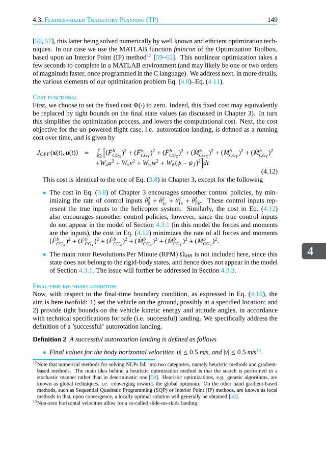
4.3.Flatness-based Trajectory Planning (TP)

4

149

[56, 57], this latter being solved numerically by well known and efficient optimization tech-niques. In our case we use the MATLAB functionfminconof the Optimization Toolbox,based upon an Interior Point (IP) method12 [59–62]. This nonlinear optimization takes afew seconds to complete in a MATLAB environment (and may likely be one or two ordersof magnitude faster, once programmed in the C language). We address next, in more details,the various elements of our optimization problem Eq. (4.8)–Eq. (4.11).

Cost functionalFirst, we choose to set the fixed costΦ(·) to zero. Indeed, this fixed cost may equivalentlybe replaced by tight bounds on the final state values (as discussed in Chapter 3). In turnthis simplifies the optimization process, and lowers the computational cost. Next, the costobjective for the un-powered flight case, i.e. autorotationlanding, is defined as a runningcost over time, and is given by

JOFF(x(t), u(t)) =∫

Ω

[

(FbCGX

)2 + (FbCGY

)2 + (FbCGZ

)2 + (MbCGX

)2 + (MbCGY

)2 + (MbCGZ

)2

+Wuu2 +Wvv2 +Www2 +Wψ(ψ − ψ f )2]

dt(4.12)

This cost is identical to the one of Eq. (3.8) in Chapter 3, except for the following

• The cost in Eq. (3.8) of Chapter 3 encourages smoother control policies, by min-imizing the rate of control inputsθ2

0 + θ21c + θ

21s + θ

2TR. These control inputs rep-

resent the true inputs to the helicopter system. Similarly,the cost in Eq. (4.12)also encourages smoother control policies, however, sincethe true control inputsdo not appear in the model of Section4.3.1(in this model the forces and momentsare the inputs), the cost in Eq. (4.12) minimizes the rate of all forces and moments(Fb

CGX)2 + (Fb

CGY)2 + (Fb

CGZ)2 + (Mb

CGX)2 + (Mb

CGY)2 + (Mb

CGZ)2.

• The main rotor Revolutions Per Minute (RPM)ΩMR is not included here, since thisstate does not belong to the rigid-body states, and hence does not appear in the modelof Section4.3.1. The issue will further be addressed in Section4.3.3.

Final-time boundary conditionNow, with respect to the final-time boundary condition, as expressed in Eq. (4.10), theaim is here twofold: 1) set the vehicle on the ground, possibly at a specified location; and2) provide tight bounds on the vehicle kinetic energy and attitude angles, in accordancewith technical specifications for safe (i.e. successful) landing. We specifically address thedefinition of a ’successful’ autorotation landing.

Definition 2 A successful autorotation landing is defined as follows

• Final values for the body horizontal velocities|u| ≤ 0.5 m/s, and|v| ≤ 0.5 m/s13.

12Note that numerical methods for solving NLPs fall into two categories, namely heuristic methods and gradient-based methods. The main idea behind a heuristic optimization method is that the search is performed in astochastic manner rather than in deterministic one [58]. Heuristic optimizations, e.g. genetic algorithms, areknown as global techniques, i.e. converging towards the global optimum. On the other hand gradient-basedmethods, such as Sequential Quadratic Programming (SQP) orInterior Point (IP) methods, are known as localmethods in that, upon convergence, a locally optimal solution will generally be obtained [58].

13Non-zero horizontal velocities allow for a so-called slide-on-skids landing.

4

150 4.On-line Trajectory Planning and Tracking: System Design

• Final value for the body vertical velocity|w| ≤ 0.25m/s.

• Final values for the roll and pitch angles|φ| ≤ 10 , and|θ| ≤ 10 .

Since roll and pitch angles will not be controlled by the TT (this issue will further be dis-cussed in Section4.4), we also derive, in Appendix D of Chapter 4, the maximum acceptableroll (or pitch) angle, for a successful landing, and hence justify the chosen attitude bounds|φ| ≤ 10 and |θ| ≤ 10 .

Bound on total flight time In Chapter 3, we found that for a fixed initial14 height aboveground, increasing the initial helicopter velocity had only a relatively limited effect on flighttime and hence stabilized rate of descent. This potentiallyindicates that the flight time,in autorotation, is only lightly correlated with the initial vehicle velocity, whereas it isprimarily influenced by the initial height above ground. This led us to consider an empiricalboundTOFF on flight timeT f , T f ≤ TOFF, with TOFF deduced from simulation experimentsas follows: LetxZI be the initial height above ground at the instant of engine failure, andrecall vih to be the helicopter induced velocity in hover, then the bound TOFF is set, afterseveral simulation experiments15, within the range:

xZI

1.75vih≤ TOFF ≤

xZI

1.50vih(4.13)

Remark 4 The reason for bounding the flight time Tf ≤ TOFF is discussed next. Althoughthe main rotor RPM dynamics is used in the helicopter nonlinear HOM, the RPM dynamicsis not included in the flat model description, i.e. in Section4.3.1, since not part of the rigid-body dynamics. By so doing, the same flat model can be used for both the engine OFF andON cases, hence simplifying the trajectory planning software. However, excluding the mainrotor RPM dynamics from the planning problem is only possible, i.e. will result in feasibleautorotative trajectories, if the trajectory flight time iskept small enough. Since the RPMdynamics is eliminated from the planning problem, the main rotor RPMΩMR signal maynot be required for the trajectory tracking system either. Thus, the standard requirementconsisting of adding a dedicated magnetic or optical RPM sensor, on the main rotor shaftor on the gear-box of a small-scale helicopter, may here be dropped.

Trajectory constraintsRegarding the trajectory constraints, as expressed in Eq. (4.11), these are conceptually iden-tical16 to the ones set in Section3.2.2of Chapter 3, except for the trajectory constraints onthe inputs, and on the main rotor RPMΩMR (see Section4.3.3). For the constraints on theinputs, these are set on total forces and moments (based uponsimulation results). Regardingthe main rotor RPMΩMR, there are no constraints, sinceΩMR is not part of the state-vector.

14By initial we mean at the start of the engine OFF flight maneuver.15The coefficients 1.50 and 1.75 in

xZI1.75vih

≤ TOFF ≤xZI

1.50vihare empirically deduced, after several simulation ex-

periments, for the case of the small-scale Align T-REX helicopter, with physical parameters as given in Table2.1of Chapter 2. A different helicopter, or even an Align T-REX helicopter with a different main rotor inertia, maylikely result in different coefficient values.

16Some numerical values of bounds and constraints may differ from the ones used in Chapter 3, in particular sinceChapter 3 and Chapter 4 do not use the same helicopter UAV (as explained in Section3.5of Chapter 3).

4.4.Robust control based Trajectory Tracking (TT)

4

151

4.4.Robust control based Trajectory Tracking (TT)The goal is to design a TT module for our small-scale helicopter UAV. This tracker shouldallow the vehicle to fly along previously planned optimal trajectories. However, with fourcontrol inputs and at least twelve measured outputs (i.e. the rigid-body states), the heli-copter is heavily under-actuated, which inevitably will limit the performance of the track-ing system. Now, since control over position and velocity isa primary objective of ourapplication, we choose to have the helicopter track the following seven references, namely3D inertial17 positions (xN xE xZ)⊤, 3D body velocities (u v w)⊤, and heading angleψ. Inaddition, based upon simulation results using the helicopter HOM, it is found that positiondynamics is much slower than velocity dynamics. This justifies a design philosophy basedupon the successive loop closure of feedback loops, where a sequential design process ofinner- and outer-loops is sought, also known as aMaster-Slavecontrol configuration seeFig. 4.2. This design approach is thus related to the well-known time-scale separation prin-ciple [63], between slow and fast dynamics of a dynamical system, and supposes that thebandwidth of the inner-loop is much higher than the bandwidth of the outer-loop18.

Figure 4.2: Master-Slave control configuration.

The outer-loop aims at tracking the planned inertial 3D position (xN xE xZ)⊤TP. On theother hand, the role of the inner-loop consists in tracking the planned headingψTP, and the

17Which is equivalent to North-East-Down (NED) position in our flight dynamics model.18Note that the control design by time-scales leads not only toa simpler and more modular control architecture,

but also to a potentially more robust one [36]. Indeed the existence of time-scales means that the systemisnumerically ill-conditioned, hence a control law ignoringthese aspects may also be ill-conditioned, thus moredifficult to implement, and potentially more sensitive to modeling errors [36].

4

152 4.On-line Trajectory Planning and Tracking: System Design

Figure 4.3: Outer-Loop, control interconnection diagram.

Figure 4.4: Inner-Loop, control interconnection diagram.

planned 3D body linear velocities (u v w)⊤TP, these latter being adjusted by the outputs ofthe outer-loop controller (u v w)⊤d to allow for position control, see Fig.4.3and Fig.4.4. Inthese figures,x represents the state-vector (with dimension twenty-four), defining the statesof the nonlinear helicopter HOM. The (u v w)⊤d can be seen as a "delta" correction to thenominal velocities (u v w)⊤TP. Hence, the to-be-tracked velocities by the inner-loop con-troller are given by (u v w)⊤TP+ (u v w)⊤d . Next, since the outputs of the outer-loop are givenin the inertial frame, i.e. North-East-Down (NED) frame, weneed a nonlinear inversion toconvert the reference velocities from NED to body frame, i.e. (u v w)⊤d = T

⊤ob(VN VE VZ)⊤d ,

with the rotation matrixTob given in Eq. (2.8) of Chapter 2. Note also that in Fig.4.4 allsignals, except position, are fed-back into the controllerto improve the closed-loop perfor-mance.

As the helicopter dynamics is nonlinear, the design of the TTcontroller necessitates anapproach that effectively respects or exploits the system’s nonlinear structure. To this end,several control methods are available, from 1) robust control; 2) classical gain-scheduling,and Linear Parameter-Varying (LPV) approaches; to 3) trulynonlinear control methods(e.g. nonlinear receding horizon control, Lyapunov based methods such as sliding modeand backstepping, adaptive control, or even passivity-based approaches). In this Chapter weselect an approach that combines simplicity and computational efficiency, i.e. we choose to

4.4.Robust control based Trajectory Tracking (TT)

4

153

apply a robust controlµ strategy. This method consists in using a nominal LTI plant coupledwith an uncertainty, and applying a small gain approach [18, 19] to design a single robustLTI controller, valid over a wide portion of the flight envelope. Now, rather than modelingthe uncertainty in a detailed or structured manner, an inputmultiplicative uncertainty isadded here to compensate for the unmodeled plant nonlinearities and unmodeled higher-order rotor dynamics19, by lumping all types of model uncertainty together into a complex,full-block, input multiplicative uncertainty. The robustcontroller synthesis consists then inobtaining a controller insensitive to this multiplicativeuncertainty at the plant input.

4.4.1.Linear multivariable µ control designBoth, the inner- and outer-loop controllers are designed according to the robust control de-sign paradigm, in a two-degrees-of-freedom control structure (i.e. using both feedback andfeedforward). Here the feedback part is used to reduce the effect of uncertainty, whereas thefeedforward part is added to improve tracking performance [64], and for optimality, bothfeedback and feedforward are designed in one step. First, a nominal plantP(s) (andPd(s)for the disturbance) is obtained by linearizing the nonlinear helicopter model at some spec-ified condition (to be discussed in the sequel). Next, we define the generalized plantGP(s)which maps the exogenous inputsw = [n⊤ r⊤ d⊤]⊤ and control inputsu, to controlledoutputsz = [zu

⊤ zp⊤]⊤ and measured outputsv = [r⊤ y⊤]⊤, see Fig.4.5.

Figure 4.5: Closed-Loop interconnection structure for robust controller synthesis.

The signals include also the sensors noisen (andno), the reference signalsr , the distur-bance signalsd, the actuators performance signal (to limit actuator deflection magnitudes

19Unmodeled in the low-order nominal LTI plant used for control design, these are however modeled in the high-order nonlinear plant of Chapter 2.

4

154 4.On-line Trajectory Planning and Tracking: System Design

and rates)zu, the desired performance in terms of closed-loop signal responseszp, and thesystem outputsy (andyo), such that

zu

rzp

y

=

0 0 0 Wu

0 I 0 00 Wp −Wp Pd Wd −Wp P (I + ∆Win)Wn 0 Pd Wd P (I + ∆Win)

nrdu

(4.14)

For the weights, which help shape the performance and robustness characteristics ofthe closed-loop system, we use the input weight Win(s), the performance weight Wp(s), theactuator weight Wu(s), the sensor noise weight Wn(s), and the disturbance weight Wd(s).Now Win(s) and∆(s), in Fig. 4.5, parametrize the uncertainty or errors in the model. TheTransfer Function (TF) Win(s) is assumed known and reflects the amount of uncertaintyin the model, whereas the TF∆(s) is assumed to be stable and unknown, except for thenorm condition||∆(s)||∞ ≤ 1. Next, the generalized plantGP(s) has a linear fractionaldependence on the input uncertainty∆(s), and is represented by the upper Linear FractionalTransformation (LFT) interconnection

(

zv

)

= GP

(

wu

)

= Fu(M,∆)

(

wu

)

(4.15)

whereM(s) is a known LTI plant, see Fig.4.6, and∆(s) some complex, full-block, four-by-four20, operator specifying how the uncertainty enters the plant dynamics.

Figure 4.6: StandardM − ∆ − K robust control framework.

The feedback structure associated with the LFT interconnection Eq. (4.15) is given by

z∆zv

= M

w∆wu

w∆ = ∆ z∆ (4.16)

with z∆, andw∆, the inputs and outputs of the operator∆(s), see Fig.4.6, and the closed-loop operator from exogenous inputsw to controlled outputsz is given by

20The helicopter plant has four control inputs.

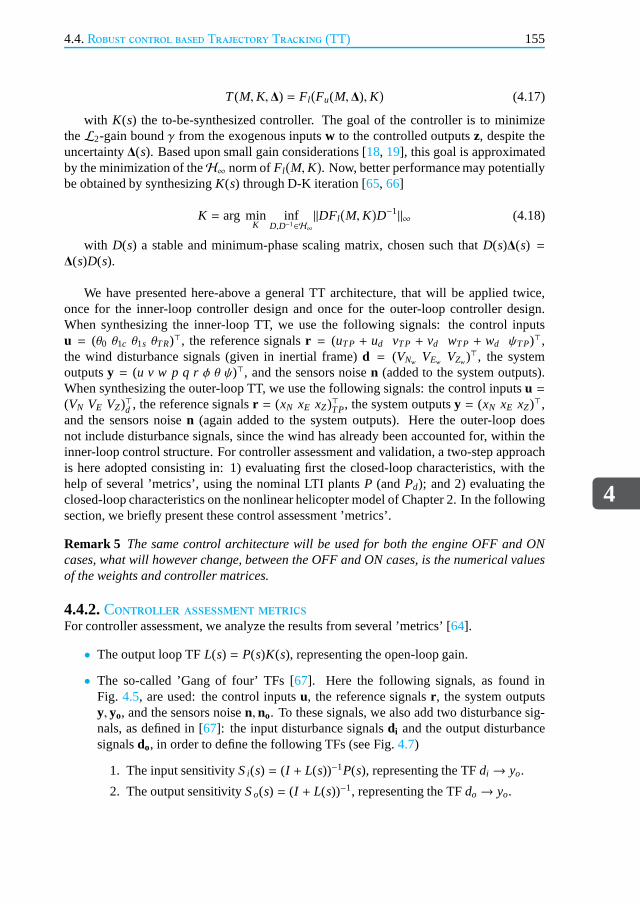
4.4.Robust control based Trajectory Tracking (TT)

4

155

T(M,K,∆) = Fl(

Fu(M,∆),K)

(4.17)

with K(s) the to-be-synthesized controller. The goal of the controller is to minimizetheL2-gain boundγ from the exogenous inputsw to the controlled outputsz, despite theuncertainty∆(s). Based upon small gain considerations [18, 19], this goal is approximatedby the minimization of theH∞ norm ofFl

(

M,K)

. Now, better performance may potentiallybe obtained by synthesizingK(s) through D-K iteration [65, 66]

K = arg minK

infD,D−1∈H∞

‖DFl(

M,K)

D−1‖∞ (4.18)

with D(s) a stable and minimum-phase scaling matrix, chosen such that D(s)∆(s) =∆(s)D(s).

We have presented here-above a general TT architecture, that will be applied twice,once for the inner-loop controller design and once for the outer-loop controller design.When synthesizing the inner-loop TT, we use the following signals: the control inputsu = (θ0 θ1c θ1s θTR)⊤, the reference signalsr = (uTP + ud vTP + vd wTP + wd ψTP)⊤,the wind disturbance signals (given in inertial frame)d = (VNw VEw VZw)⊤, the systemoutputsy = (u v w p q rφ θ ψ)⊤, and the sensors noisen (added to the system outputs).When synthesizing the outer-loop TT, we use the following signals: the control inputsu =(VN VE VZ)⊤d , the reference signalsr = (xN xE xZ)⊤TP, the system outputsy = (xN xE xZ)⊤,and the sensors noisen (again added to the system outputs). Here the outer-loop doesnot include disturbance signals, since the wind has alreadybeen accounted for, within theinner-loop control structure. For controller assessment and validation, a two-step approachis here adopted consisting in: 1) evaluating first the closed-loop characteristics, with thehelp of several ’metrics’, using the nominal LTI plantsP (andPd); and 2) evaluating theclosed-loop characteristics on the nonlinear helicopter model of Chapter 2. In the followingsection, we briefly present these control assessment ’metrics’.

Remark 5 The same control architecture will be used for both the engine OFF and ONcases, what will however change, between the OFF and ON cases, is the numerical valuesof the weights and controller matrices.

4.4.2.Controller assessment metricsFor controller assessment, we analyze the results from several ’metrics’ [64].

• The output loop TFL(s) = P(s)K(s), representing the open-loop gain.

• The so-called ’Gang of four’ TFs [67]. Here the following signals, as found inFig. 4.5, are used: the control inputsu, the reference signalsr , the system outputsy, yo, and the sensors noisen, no. To these signals, we also add two disturbance sig-nals, as defined in [67]: the input disturbance signalsdi and the output disturbancesignalsdo, in order to define the following TFs (see Fig.4.7)

1. The input sensitivitySi(s) = (I + L(s))−1P(s), representing the TFdi → yo.

2. The output sensitivitySo(s) = (I + L(s))−1, representing the TFdo→ yo.

4

156 4.On-line Trajectory Planning and Tracking: System Design

Figure 4.7: Basic feedback loop.

3. The input complementary sensitivityTi(s) = L(s)(I + L(s))−1, representing theTFsr → yo (alsono→ yo anddi → u).

4. The output complementary sensitivityTo(s) = K(s)(I + L(s))−1, representingthe TFsr → u (alsono→ u anddo→ u).

• To evaluate the frequency range over which the control is effective, we consider thefollowing bandwidths [64]

1. wC being the gain crossover frequency where|L(s)| first crosses 0 dB, fromabove.

2. wB being the lowest frequency where|Si(s)| crosses -3 dB, from below.

3. wBT being the highest frequency where|Ti(s)| crosses -3 dB, from above.

• The Robust Stability (RS) metric, defined asRS ⇔ µ∆(N11(s)) ≤ 1, with N(s) =Fl(M(s),K(s)), with N11(s) the upper left block corresponding to the full, complex,four-by-four uncertainty∆ (i.e. our plant input multiplicative uncertainty), andM(s)as given in Fig.4.6.

• The Robust Performance (RP) metric, defined asRP ⇔ µ∆(N(s)) ≤ 1, for thestructured uncertainty∆ as

∆ ≔ diag(∆,∆P) ‖∆P‖∞ ≤ 1 (4.19)

with ∆P an unstructured (complex, full-block), fictitious uncertainty of size dim(w)by dim(z), with w the exogenous inputs, andz the controlled outputs.

Remark 6 We compute both an upper and lower bound for the RS and RP, following themethod in [68]. As in [68], we have added 1% of complex perturbations to∆ in orderto improve the convergence of the lower bound, albeit at the expense of slight additionalconservatism.

In the following sections, we address the weights selectionand controller validation, forthe engine OFF case.

4.5.Design of the engine OFF inner-loop controller

4

157

4.5.Design of the engine OFF inner-loop controllerAs stated in Section4.4, with four control inputs and twelve measured outputs, the heli-copter is heavily under-actuated, which inevitably limitsthe performance of the trackingsystem. As mentioned earlier, see also Fig.4.4, we choose to have the inner-loop trackthe following four reference signals: 3D body velocities (u v w)⊤, and heading angleψ.Recall also that the goal of the controller is to minimize theL2-gain boundγ from theexogenous inputsw to the controlled outputsz, despite the uncertainty∆(s). The varioussignals are further given as follows: the exogenous inputsw = [n⊤ r⊤ d⊤]⊤, the controlledoutputsz = [zu

⊤ zp⊤]⊤, the control inputsu = (θ0 θ1c θ1s θTR)⊤, the measured outputs

v = [r⊤ y⊤]⊤, the reference signalsr = (uTP + ud vTP + vd wTP + wd ψTP)⊤, the systemoutputsy = (u v w p q rφ θ ψ)⊤, the wind disturbance signals (given in inertial frame)d = (VNw VEw VZw)⊤, and the sensors noisen (added to the system outputs), see Fig.4.5.Here the signaly contains all the available measured output signals, exceptfor the 3D po-sition, since the latter is only of interest for the outer-loop controller.

4.5.1.Choice of nominal plant model for the inner-loop control designAs mentioned in Section4.1, we do not use any gain-scheduling philosophy in this Chap-ter, rather a single LTI plant is used for controller design.Now, for an engine ON flightcondition, it is relatively easy to find equilibrium points,i.e. steady-state flight conditions,at which the nonlinear helicopter model of Chapter 2 can be linearized. The resulting LTImodels can subsequently be used for LTI control design. However, for the engine OFFflight condition, this set of equilibrium points, i.e. steady autorotative flight conditions, israther small and in certain situations even non-existent. For example, when an engine fail-ure happens at a low altitude, the helicopter does not even reach a steady-state autorotation(corresponding to a constant main rotor RPM), rather the helicopter system is continuouslyin transition from one non-equilibrium point to the next. Tomitigate this problem, theapproach used here consists in excluding the main rotor RPMΩMR from the state and mea-surement vectors, and use this "quasi-steady" modeling approach to find the equilibriumpoints. By so doing, the control architecture and control design philosophy for the engineOFF case can be made exactly identical to the engine ON case, hence simplifying the over-all control system design.

The state-space data used to design the inner-loop trajectory tracker is as follows: thestate-vector is of dimension nine given byx = (u v w p q rφ θ ψ)⊤, the control inputu (givenhere-above) is of dimension four, the wind disturbanced (given here-above) is of dimensionthree, and the measurements vectory = x. This LTI model is obtained by linearizing21

the helicopter nonlinear model of Chapter 2, at a specific trimmed flight condition. Thiscondition corresponds to hover, with the engine OFF (note that now the main rotor RPMis not in equilibrium anymore). Choosing such a flight condition, with an associated initialvelocity of zero, can potentially provide the best description of helicopter behavior duringlanding (where the helicopter velocity is also very low). The resulting state-space data givenin Appendix H22 of Chapter 2. By using the eigenvalues of theA matrix in the Popov-

21According to the linearization procedure given in Section2.4.1.22The state-space data of the LTI plants given in Appendix H of Chapter 2 are in S.I. engineering units. However,

before using the plant for control design, scalings have been used on the input and output matrices in order to

4

158 4.On-line Trajectory Planning and Tracking: System Design

Belevitch-Hautus (PBH) rank test, we found that this LTI plant was both controllable andobservable. Simulation results, presented later in Chapter 5, have shown that this nominalLTI plant is indeed suitable for the design of controllers inan engine OFF situation.

4.5.2.Selection of weightsThe robust control framework makes use of several user-defined weights, see Fig.4.5. Inthis Chapter, these weights have been chosen as follows. Themultiplicative uncertaintyweight Win(s) is of the form Win(s) = diag[win1(s),win2(s),win2(s),win2(s)], set on the fourcontrol input channelsu = (θ0 θ1c θ1s θTR)⊤, with θ0 the main rotor blade root collectivepitch,θ1c the main rotor lateral cyclic pitch,θ1s the main rotor longitudinal cyclic pitch, andθTR the tail rotor blade collective pitch. Further,win1(s) andwin2(s) are filters whose magni-tude represent the relative uncertainty at each frequency (i.e. the level of uncertainty in thebehavior of the helicopter is assumed frequency dependent). Based upon engineering judg-ment23, we choose here forwin1(s) to consider 20% uncertainty at low frequency (DC gain),100% uncertainty at the filter crossover frequency of 10 Hz (with 10 Hz being roughly theanticipated closed-loop bandwidth for the vertical velocity channel24), and 200% uncer-tainty at infinite frequency. Again, based upon engineeringjudgment, we choose forwin2(s)to consider 40% uncertainty at low frequency (DC gain), 100%uncertainty at the filtercrossover frequency of 5 Hz, and 200% uncertainty at infinitefrequency25, giving

win1(s) = (2s+ 22.21)/(s+ 111.1)win2(s) = (2s+ 23.75)/(s+ 59.37)

(4.20)

Next, the performance weight filter Wp(s) is placed on the (u, v,w, ψ) error signals, to re-flect the tracking objective for the three body linear velocities and the heading angle. HereWp(s) is a four-by-four, diagonal, frequency-varying weight Wp(s) = diag[wu(s),wv(s),ww(s),wψ(s)], with each diagonal term defined as a first-order TFs/MP+ωB

s+ωBAss. At low frequen-

cies this weighting function should be high in order to keep the error small. Beyond theanticipated bandwidth of the closed-loop system, the tracking error may be released andWp(s) rolls off [64]. After several controller design cycles, we have settled for

For wu(s) (MP, ωB,Ass) = (2, 0.5π rad/s, 0.001)For wv(s) (MP, ωB,Ass) = (2, 0.5π rad/s, 0.001)For ww(s) (MP, ωB,Ass) = (2, 90π rad/s, 0.001)For wψ(s) (MP, ωB,Ass) = (2, 4π rad/s, 0.001)

(4.21)

This means that a steady-state tracking error of 0.1% with respect to the normalizedfilter input is allowed. Further, the difference with the engine ON case is in terms of track-ing bandwidth: 1) for the engine OFF case, it is lower on the horizontal channels (u andv velocities) since the LTI model used for control design is somewhat less ’accurate’ (dueto the non-fixed main rotor RPM, and high descent rates); and 2) for the engine OFF case,the tracking bandwidth is considerably much higher on the vertical channel (w velocity)

obtain a normalized LTI plant.23The chosen uncertainty may be overly conservative, or may even be unrealistic. Alternative ways to shape the

uncertainties exist, e.g. [69]. The goal here is simply to add some robustness to the closed-loop system.24For each control input, Table1.1in Chapter 1 summarizes their primary effects on the vehicle response.25The uncertainty is large at high-frequency since we use a low-order model.

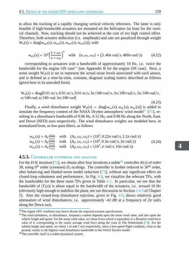
4.5.Design of the engine OFF inner-loop controller

4

159

to allow the tracking of a rapidly changing vertical velocity reference. The latter is onlyfeasible if high-bandwidth actuators are mounted on the helicopter (at least for the verti-cal channel). Now, tracking should not be achieved at the cost of too high control effort.Therefore, both actuator deflection (i.e. amplitude) and rate are penalized through weightWu(s) = diag[wact(s),wact(s),wact(s),wact(s)], with

wact(s) = 10n( s+ ω1

s+ ω2

)n

with (n, ω1, ω2) = (3, 40π rad/s, 400π rad/s) (4.22)

corresponding to actuators with a bandwidth of approximately 10 Hz, i.e. twice thebandwidth for the engine ON case26 (see Appendix B for the engine ON case). Next, anoise weight Wn(s) is set to represent the actual noise levels associated witheach sensor,and is defined as a nine-by-nine, constant, diagonal scalingmatrix described as follows(given here in its unscaled form)

Wn(s) = diag[0.01m/s, 0.01m/s, 0.01m/s, 3π/180rad/s, 3π/180rad/s, 3π/180rad/s,π/180rad, π/180rad, 3π/180rad]

(4.23)Finally, a wind disturbance weight Wd(s) = diag[wdN (s),wdE (s),wdD(s)] is added to

simulate the frequency content of the NASA Dryden atmospheric wind model27 [71], re-sulting in a disturbance bandwidth of 0.06 Hz, 0.12 Hz, and 0.96 Hz along the North, East,and Down (NED) axes respectively. The wind disturbance weights are modeled here, innormalized form, as low-pass filters, as follows

wdN (s) = Ads+ω1s+ω2

with (Ad, ω1, ω2) = (103, 0.22π rad/s, 2.2π rad/s)wdE (s) = Ad

s+ω1s+ω2

with (Ad, ω1, ω2) = (103, 0.3π rad/s, 3π rad/s)wdD (s) = Ad

s+ω1s+ω2

with (Ad, ω1, ω2) = (103, π rad/s, 10π rad/s)(4.24)

4.5.3.Controller synthesis and analysisFor the D-K iteration [72], we obtain after four iterations a stable28 controllerK(s) of order38, using 0th order (constant)Ds-scalings. The controller is further reduced to 30th order,after balancing and Hankel-norm model reduction [73], without any significant effect onclosed-loop robustness and performance. In Fig.4.8, we visualize the relevant TFs, withthe bandwidths for the three main TFs given in Table4.1. In particular, we see that thebandwidth of|Ti(s)| is about equal to the bandwidth of the actuators, i.e. around10 Hz(obviously high enough to stabilize the plant, see our discussion in Section2.4.3of Chapter2). Also the closed-loop disturbance rejection, given in Fig. 4.9, shows relatively goodattenuation of wind disturbances, i.e. approximately -43 dB at a frequency of 2π rad/salong the Down axis.26The engine OFF condition may hence dictate the required actuator specifications.27The wind turbulence, or disturbance, frequency content depends upon the mean wind value, and also upon the

vehicle height and speed. For the mean wind value, we chose 8 m/s which is equivalent to a Beaufort wind forcevalue of 4, corresponding to the yearly average wind force along the coast in The Netherlands [70]. For thevehicle height and speed, we chose 1 m and 1 m/s respectively, since a low-speed flight condition, close totheground, results in the highest wind disturbance bandwidth in the NASA Dryden model.

28The controller itself is a stable dynamical system.

4

160 4.On-line Trajectory Planning and Tracking: System Design

10−2

10−1

100

101

102

103

−100

−80

−60

−40

−20

0

20

40

60

80

100

Singular Values

Frequency (rad/s) (rad/s)

Max

imum

Sin

gula

r V

alue

(dB

) (d

B)

L

Si

So

Ti

To

0 dB

−3 dB

Figure 4.8: Singular values ofL(s), Si (s), So(s), Ti (s), andTo(s), of theinner-loop trajectory tracker (Engine OFF case).

10−5

10−4

10−3

10−2

10−1

100

101

102

103

104

−140

−120

−100

−80

−60

−40

−20

Frequency (rad/s)

Sin

gula

r V

alue

(dB

)

North wind disturbance: VN

w

−> u

East wind disturbance: VE

w

−> v

Down wind disturbance: VD

w

−> w

Figure 4.9: Closed-Loop wind disturbance rejection, for North-East-Down(NED) winds, of the inner-loop trajectory tracker (Engine OFF case).

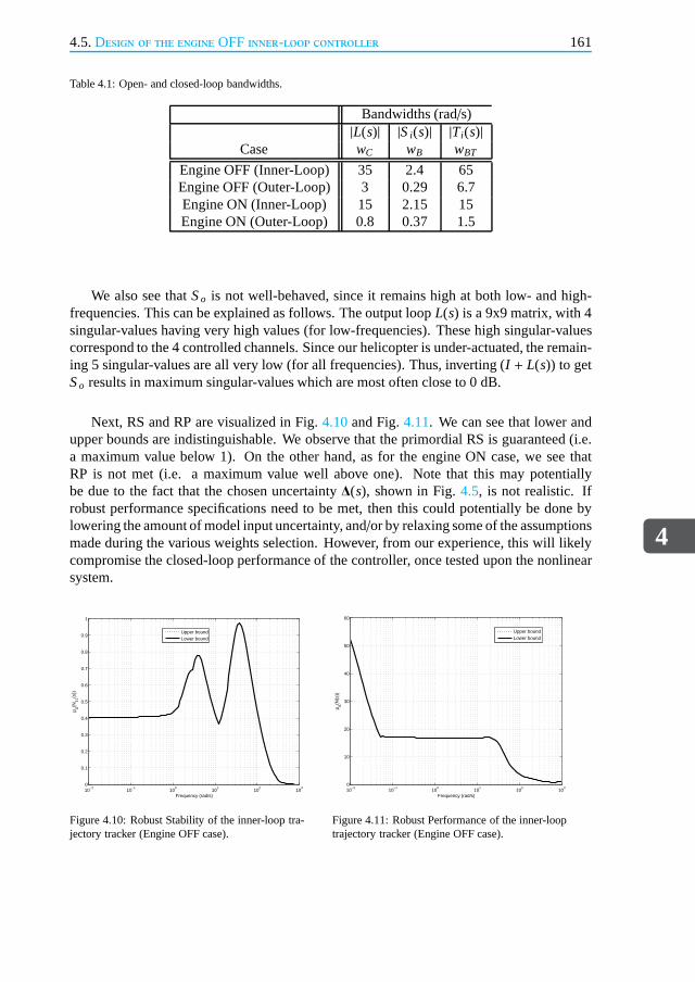
4.5.Design of the engine OFF inner-loop controller

4

161

Table 4.1: Open- and closed-loop bandwidths.

Bandwidths (rad/s)|L(s)| |Si(s)| |Ti(s)|

Case wC wB wBT

Engine OFF (Inner-Loop) 35 2.4 65Engine OFF (Outer-Loop) 3 0.29 6.7Engine ON (Inner-Loop) 15 2.15 15Engine ON (Outer-Loop) 0.8 0.37 1.5

We also see thatSo is not well-behaved, since it remains high at both low- and high-frequencies. This can be explained as follows. The output loop L(s) is a 9x9 matrix, with 4singular-values having very high values (for low-frequencies). These high singular-valuescorrespond to the 4 controlled channels. Since our helicopter is under-actuated, the remain-ing 5 singular-values are all very low (for all frequencies). Thus, inverting (I + L(s)) to getSo results in maximum singular-values which are most often close to 0 dB.

Next, RS and RP are visualized in Fig.4.10and Fig.4.11. We can see that lower andupper bounds are indistinguishable. We observe that the primordial RS is guaranteed (i.e.a maximum value below 1). On the other hand, as for the engine ON case, we see thatRP is not met (i.e. a maximum value well above one). Note that this may potentiallybe due to the fact that the chosen uncertainty∆(s), shown in Fig.4.5, is not realistic. Ifrobust performance specifications need to be met, then this could potentially be done bylowering the amount of model input uncertainty, and/or by relaxing some of the assumptionsmade during the various weights selection. However, from our experience, this will likelycompromise the closed-loop performance of the controller,once tested upon the nonlinearsystem.

10−2

10−1

100

101

102

103

0

0.1

0.2

0.3

0.4

0.5

0.6

0.7

0.8

0.9

1

Frequency (rad/s)

µ ∆(N11

(s))

Upper boundLower bound

Figure 4.10: Robust Stability of the inner-loop tra-jectory tracker (Engine OFF case).

10−2

10−1

100

101

102

103

0

10

20

30

40

50

60

Frequency (rad/s)

µ ∆(N(s

))

Upper boundLower bound

Figure 4.11: Robust Performance of the inner-looptrajectory tracker (Engine OFF case).

4

162 4.On-line Trajectory Planning and Tracking: System Design

4.6.Design of the engine OFFouter-loop controllerWe first recall that the design approach is based upon the well-known time-scale separa-tion principle [63] between slow and fast dynamics of a dynamical system, resulting in aso-calledMaster-Slaveconfiguration (see Fig.4.2), and supposes that the bandwidth of theinner-loop is much higher than the bandwidth of the outer-loop29.

As mentioned earlier, refer also to Fig.4.3, we choose to track the following threereference signals: 3D inertial30 positions (xN xE xZ)⊤. Recall also that the goal of thecontroller is to minimize theL2-gain boundγ from the exogenous inputsw to the con-trolled outputsz, despite the uncertainty∆(s). The various signals are further given asfollows: the exogenous inputsw = [n⊤ r⊤]⊤, the controlled outputsz = [zu

⊤ zp⊤]⊤, the

control inputsu = (VN VE VZ)⊤d , the measured outputsv = [r⊤ y⊤]⊤, the reference signalsr = (xN xE xZ)⊤TP, the system outputsy = (xN xE xZ)⊤, and the sensors noisen (added tothe system outputs), see Fig.4.5. Here the outer-loop does not include disturbance signals,since the wind has already been accounted for, within the inner-loop control structure.

As discussed in Section4.1, a single LTI plant is again used for controller design. Thestate-space data used to design the outer-loop trajectory tracker is obtained as follows. AnLTI dynamical system can be formed by connecting the nominalLTI model, used for theinner-loop TT, with its inner-loop controller, and subsequently adding a set of integratorson the 3D velocities to generate the 3D inertial positions (xN xE xZ)⊤. This manipulationis readily done in MATLAB, and results in the nominal LTI model needed to design theouter-loop position controller. In our case, we obtain a three-by-three input-output system,with a state-vector of dimension 55. Next a minimum realization is obtained, resulting ina state-vector of dimension 42 (the LTI model is too big to be added to the Appendix).Note that here too scalings need to be applied. Further, and except for three poles at theorigin (corresponding to the integration of the 3D velocities), all other eigenvalues of theA matrix are stable and well damped, implying easier controller design. Again, by usingthe eigenvalues of theA matrix in the PBH rank test, we found that the LTI system is bothcontrollable and observable.

The design philosophy for theµ outer-loop TT parallels that of the inner-loop.

4.6.1.Selection of weightsThe input multiplicative uncertainty weight Win(s) is of the form Win(s) = diag[win2(s),win2(s), win1(s)], with win1(s), win2(s) identical to the ones used in the engine OFF inner-loop, in Eq. (4.20). Herewin1(s) is applied to the vertical velocity channel (recall that wehaveu = (VN VE VZ)⊤d ). In the design of the inner-loop TT, in Section4.5.2, we had chosenan uncertainty weight equal towin1(s) on the collective inputθ0. Now, since the verticalvelocity channel is mostly influenced by the collective input (see Table1.1 in Chapter 1),we also assign an uncertaintywin1(s) to the vertical velocity. The same argument holds foruncertaintywin2(s) on the horizontal velocities. Obviously, this choice of the uncertainty

29Based upon simulation results, using the helicopter model of Chapter 2, it is indeed found that position dynamicsis much slower than velocity dynamics.

30Which is equivalent to North-East-Down (NED) position in our flight dynamics model.

4.6.Design of the engine OFFouter-loop controller

4

163

weight Win(s) is somewhat arbitrary. This said, the purpose here is just to add some robust-ness to the closed-loop system.

The performance weight filter Wp(s) is placed on the (xN, xE, xZ) error signals to reflectthe tracking objective for the inertial position. Here, Wp(s) is a three-by-three diagonal,frequency-varying weight. We have Wp(s) = diag[wxN(s),wxE (s),wxZ(s)], with each diag-onal term defined as a first-order transfer functions/MP+ωB

s+ωBAss. After several controller design

cycles, we have settled for

For wxN (s) (MP, ωB,Ass) = (2, 0.1π rad/s, 0.001)For wxE (s) (MP, ωB,Ass) = (2, 0.1π rad/s, 0.001)For wxZ (s) (MP, ωB,Ass) = (2, 4.5π rad/s, 0.001)

(4.25)

Again, a steady-state tracking error of 0.1% with respect tothe normalized input isallowed. The filter bandwidths, on the horizontal channels,are adjusted to be five timessmaller than the Wp(s) filter bandwidths of the inner-loop horizontal channels. For the ver-tical channel bandwidth, instead of a 1:5 ratio, we settled for a 1:20 ratio. These valueshave been obtained after several simulation experiments.

Next, tracking should not be achieved at the cost of too high control effort (i.e. resultingin much too large velocity setpointsu = (VN VE VZ)⊤d for the inner-loop). This meansthat both inertial velocities and inertial accelerations should be penalized, through weightWu(s) = diag[wact(s),wact(s),wact(s)], with wact(s) identical to the one chosen for the inner-loop, with engine OFF. Again, this choice may be interpretedas rather arbitrary, since hereWu(s) is assigned to the inner-loop setpointsu = (VN VE VZ)⊤d , whereas for the design ofthe inner-loop controller, Wu(s) was assigned to the actuators. Hence, potentially betterchoices for Wu(s) may exist, although the one selected here provided satisfactory results.Finally, a noise weight Wn(s) is also defined to scale the normalized position measurementnoise. The sensor noise model is defined as a three-by-three,constant, diagonal scalingmatrix described by (given here in its unscaled form)

Wn(s) = diag[0.1 m, 0.1 m, 0.1 m] (4.26)

4.6.2.Controller synthesis and analysisFor the D-K iteration, we obtain after four iterations a stable controllerK(s) of order 57,using 0th orderDs-scalings. The controller is further reduced to 30th order (using the sametechnique as for the inner-loop), without any effect on closed-loop robustness/performance.In Fig. 4.12, we visualize the relevant TFs (we see thatSi(s) = So(s), andTi(s) = To(s)),with the bandwidths for the three TFs given in Table4.1. In particular, we see that thebandwidth of|Ti(s)| is ten times lower its inner-loop counterpart, which is goodsince wedo not want both controllers to start interacting with each other. Further, RS is shown inFig. 4.13, whereas RP is pictured in Fig.4.14. Again, we observe that RP is not achieved,whereas RS is well guaranteed.

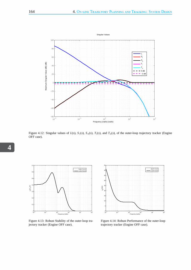
4

164 4.On-line Trajectory Planning and Tracking: System Design

10−2

10−1

100

101

102

−80

−60

−40

−20

0

20

40

60

80

100

Singular Values

Frequency (rad/s) (rad/s)

Max

imum

Sin

gula

r V

alue

(dB

) (d

B)

L

Si

So

Ti

To

0 dB

−3 dB

Figure 4.12: Singular values ofL(s), Si (s), So(s), Ti (s), andTo(s), of the outer-loop trajectory tracker (EngineOFF case).

10−2

10−1

100

101

102

103

0

0.1

0.2

0.3

0.4

0.5

0.6

0.7

Frequency (rad/s)

µ ∆(N11

(s))

Upper boundLower bound

Figure 4.13: Robust Stability of the outer-loop tra-jectory tracker (Engine OFF case).

10−2

10−1

100

101

102

103

0

5

10

15

20

25

30

35

40

45

Frequency (rad/s)

µ ∆(N(s

))

Upper boundLower bound

Figure 4.14: Robust Performance of the outer-looptrajectory tracker (Engine OFF case).

4.7.Conclusion

4

165

4.6.3.Adapting the engine OFFouter-loop controllerWhen close to the ground, it is crucial to keep the reference velocities as small as possible.To this end, we adapt the outer-loop controller as follows: the position tracking is switched-off, i.e. the values for (u v w)⊤d are set to zero, once the helicopter height descends belowa predefined threshold (keeping only velocity and heading tracking). This helps loweringthe final (touch-down) values of the 3D velocities, by givingmore time to the velocitydeceleration process. The value of this user-defined altitude threshold depends upon theinitial conditions, and depends upon whether it is an engineOFF or ON automatic landing.

4.7.ConclusionIn this Chapter we have presented a trajectory planning and tracking framework, anchoredin the combined paradigms of differential flatness based planning and robust control basedtracking. Both the engine OFF and engine ON cases are based upon the same planningand tracking system architecture. In particular, main rotor RPM is not used, neither neces-sary for the engine OFF trajectory planning, nor for the corresponding trajectory tracking,hence simplifying the overall system design. We have also presented what we believe to bea simple trajectory tracking architecture, capable of controlling a small-scale helicopter inautorotation (i.e. engine OFF flight condition). To this end, we have settled for an archi-tecture with only two nested loops, controlling position, velocity, and heading, but withoutcontrol of vehicle roll and pitch angles. Our methodology isreal-time feasible since itallows for, computationally tractable, planning and tracking solutions. In Chapter 5, weevaluate, through several simulations, the flight control control system developed in Chap-ter 4, using the nonlinear high-order helicopter model of Chapter 2.

4

166 4.On-line Trajectory Planning and Tracking: System Design

4.8.Appendix A: Optimal trajectory planning for the engineON case

The TP optimization problem, as in Chapter 3, consists of a cost functionalJ(·), with contri-butions from a fixed costΦ(·), and a running cost over time

∫

ΩΨ(·)dt, with the independent

time variablet defined over the time domainΩ = (To,T f ), where the final timeT f may befree or fixed.

Cost functionalFirst, we set the fixed cost toT f , i.e. Φ(·) = T f , to avoid obtaining trajectories with un-reasonably long flight times. Next, we define a general cost functional here, applicable forseveral types of maneuvers, including takeoff and landing, cruise flight, and hover-to-hoverflight. From engineering judgment, we use

JON(x(t), u(t),T f ) =WT f T f +∫

Ω

[

(FbCGX

)2 + (FbCGY

)2 + (FbCGZ

)2

+(MbCGX

)2 + (MbCGY

)2 + (MbCGZ

)2

+Wvv2 +Wr r2]

dt

(4.27)

For the first six terms in the running cost over time, i.e. the control derivatives, thesehave been added to: 1) minimize the battery power consumption; and 2) encourage smoothercontrol policies, hence avoidingbang-bangtype solutions, that might excite undesirablehigh frequency dynamics or resonances. Next, the termv2 is added to limit vehicle sideslip31

flight. Indeed, large sideslip decreases the flight performance, by increasing vehicle drag,increasing roll/yaw coupling, and hence increasing the workload of any feedback controller.The termr2 has been added to minimize inter-axis coupling. Finally, additional weights, i.e.WT f , Wv, andWr , have been added to evaluate various trade-offs within this cost objective.

Boundary and trajectory constraintsThe boundary conditions are used to set the initial and final (trimmed) flight conditions, andalso to set the (initial) and final vehicle accelerations to zero. Having final accelerationsequal to zero helps obtaining smooth approaches towards thefinal waypoint, or alterna-tively a gentle touch-down during an auto-land. Further themaximum flight timeT f mayalso be limited.

On the other hand, the trajectory constraints serve severalpurposes. First, they accountfor the vehicle’s inherent physical and flight envelope limitations, such as bounds on three-dimensional (3D) position, speeds, and attitude. Second, the control inputs to the rigid-body dynamics, i.e. the helicopter forces and momentsFb

CG andMbCG, are also limited,

based upon bounds obtained from simulations using the nonlinear helicopter model. Third,a tail rotor blade tip clearance has been added to avoid ground strike by the tail rotor duringa flare maneuver (see our discussion in Chapter 3). Finally, the airflow through the mainrotor, given byVrotor = w+ pyH−qxH, has been limited to half the induced velocity in hovervih, i.e. Vrotor ≤ 1

2vih, as to avoid flight into the chaotic, highly nonlinear, Vortex-Ring-State(VRS) region, refer also to Fig.2.19in Chapter 2.

31Sideslip flight refers to a vehicle moving somewhat sidewaysas well as forward, relative to the oncoming airflow.

4.9.Appendix B: Design of the inner-loop controller for the engine ON case

4

167

4.9.Appendix B: Design of the inner-loop controller for theengine ON case

As stated in Section4.4, with four control inputs and twelve measured outputs, the he-licopter is heavily under-actuated, which inevitably limits the performance of the track-ing system. As mentioned earlier for the engine OFF inner-loop, see also Fig.4.4, wechoose to have the inner-loop track the following four reference signals: 3D body ve-locities (u v w)⊤, and heading angleψ. Recall also that the goal of the controller is tominimize theL2-gain boundγ from the exogenous inputsw to the controlled outputsz,despite the uncertainty∆(s). The various signals are further given as follows: the ex-ogenous inputsw = [n⊤ r⊤ d⊤]⊤, the controlled outputsz = [zu

⊤ zp⊤]⊤, the control

inputsu = (θ0 θ1c θ1s θTR)⊤, the measured outputsv = [r⊤ y⊤]⊤, the reference signalsr = (uTP + ud vTP + vd wTP + wd ψTP)⊤, the system outputsy = (u v w p q rφ θ ψ)⊤, thewind disturbance signals (given in inertial frame)d = (VNw VEw VZw)⊤, and the sensors noisen (added to the system outputs), see Fig.4.5. Here the signaly contains all the availablemeasured output signals, except for the 3D position, since the latter is only of interest forthe outer-loop controller.

As mentioned in Section4.1, we do not use any gain-scheduling philosophy in thisChapter, rather a single LTI plant is used for controller design. The state-space data usedto design the inner-loop trajectory tracker is as follows: the state-vector is of dimensionnine given byx = (u v w p q r φ θ ψ)⊤, the control inputu (given here-above) is ofdimension four, the wind disturbanced (given here-above) is of dimension three, and themeasurements vectory = x. This LTI model is obtained by linearizing the helicopternonlinear model of Chapter 2, at a specific trimmed flight condition32, according to thelinearization procedure given in Section2.4.1, with the resulting state-space data given inAppendix H of Chapter 2. By using the eigenvalues of theAmatrix in the Popov-Belevitch-Hautus (PBH) rank test, we found that the LTI system is both controllable and observable.Simulation results have shown that this nominal LTI was verysuitable for the design ofcontrollers, capable of steering the helicopter, in an engine ON situation, from low-speedto medium-speed flight conditions.

Selection of weightsThe robust control framework makes use of several user-defined weights, see Fig.4.5. Inthis Chapter, these weights have been chosen as follows. Themultiplicative uncertaintyweight Win(s) is of the form Win(s) = diag[win1(s),win1(s),win1(s),win1(s)], with win1(s) afilter whose magnitude represents the relative uncertaintyat each frequency (i.e. the level ofuncertainty in the behavior of the helicopter is frequency dependent). Based upon engineer-ing judgment, we choose here forwin1(s) to consider 40% uncertainty at low frequency (DCgain), 100% uncertainty at the filter crossover frequency of5 Hz (roughly in the range 2.5 to5 times the anticipated closed-loop bandwidth), and 200% uncertainty at infinite frequency,giving

win1(s) = (2s+ 23.75)/(s+ 59.37) (4.28)

32The condition corresponds to hover, with engine ON (the mainrotor RPM is constant).

4

168 4.On-line Trajectory Planning and Tracking: System Design

Next, the performance weight filter Wp(s) is placed on the (u, v,w, ψ) error signals to re-flect the tracking objective for the three body linear velocities and the heading angle. HereWp(s) is a four-by-four, diagonal, frequency-varying weight Wp(s) = diag[wu(s),wv(s),ww(s),wψ(s)], with each diagonal term defined as a first-order TFs/MP+ωB

s+ωBAss. At low frequen-

cies this weighting function should be high in order to keep the error small. Beyond theanticipated bandwidth of the closed-loop system, the tracking error may be released andWp(s) rolls off [64]. After several controller design cycles, we have settled for

For wu(s) (MP, ωB,Ass) = (2, 2π rad/s, 0.001)For wv(s) (MP, ωB,Ass) = (2, 2π rad/s, 0.001)For ww(s) (MP, ωB,Ass) = (2, 4π rad/s, 0.001)For wψ(s) (MP, ωB,Ass) = (2, 4π rad/s, 0.001)

(4.29)

This means that a steady-state tracking error of 0.1% with respect to the normalizedfilter input is allowed, whereas the tracking bandwidth of these filters is set below the 5Hz actuators bandwidth (actuator data is reported in Table2.1of Chapter 2). Now, trackingshould not be achieved at the cost of too high control effort. Therefore, both actuator deflec-tion (i.e. amplitude) and rate are penalized through weightWu(s) = diag[wact(s),wact(s),wact(s),wact(s)], with

wact(s) = 10n( s+ ω1

s+ ω2

)n

with (n, ω1, ω2) = (3, 6π rad/s, 60π rad/s) (4.30)

Next, a noise weight Wn(s) is defined to represent the actual noise levels associated witheach sensor, and is defined as a nine-by-nine, constant, diagonal scaling matrix describedas follows (given here in its unscaled form)

Wn(s) = diag[0.01m/s, 0.01m/s, 0.01m/s, 3π/180rad/s, 3π/180rad/s, 3π/180rad/s,π/180rad, π/180rad, 3π/180rad]

(4.31)Finally, a wind disturbance weight Wd(s) = diag[wdN (s),wdE(s),wdD(s)] is added to

simulate the frequency content of the NASA Dryden atmospheric wind model [71], and isidentical to the one used in the engine OFF case, see Eq. (4.24).

Controller synthesis and analysisFor the D-K iteration [72], we obtain after four iterations a stable controllerK(s) of order38, using 0th order (constant)Ds-scalings. The controller is further reduced to 30th order,after balancing and Hankel-norm model reduction [73], without any significant effect onclosed-loop robustness/performance. In Fig.4.15, we visualize the relevant TFs, defined inthe previous section, with the bandwidths for the three mainTFs given in Table4.1.

In particular, we see that the bandwidth of|Ti(s)| is high enough, to stabilize the plant,i.e. above 2.1 rad/s, see our discussion in Section2.4.2. Also the closed-loop disturbancerejection, given in Fig.4.9, shows good attenuation of horizontal wind disturbances, eventhough the vertical disturbance attenuation could potentially be improved (approximately-20 dB at a frequency of 2π rad/s). We also see that theSo is not well-behaved, since it

4.9.Appendix B: Design of the inner-loop controller for the engine ON case

4

169

10−2

10−1

100

101

102

−80

−60

−40

−20

0

20

40

60

80

100

Singular Values

Frequency (rad/s) (rad/s)

Max

imum

Sin

gula

r V

alue

(dB

) (d

B)

L

Si

So

Ti

To

0 dB

−3 dB

Figure 4.15: Singular values ofL(s), Si (s), So(s), Ti (s), andTo(s), of theinner-loop trajectory tracker (Engine ON case).

10−4

10−3

10−2

10−1

100

101

102

103

104

−140

−120

−100

−80

−60

−40

−20

0

Frequency (rad/s)

Sin

gula

r V

alue

(dB

)

North wind disturbance: VN

w

−> u

East wind disturbance: VE

w

−> v

Down wind disturbance: VD

w

−> w

Figure 4.16: Closed-Loop wind disturbance rejection, for North-East-Down(NED) winds, of the inner-loop trajectory tracker (Engine ON case).

4

170 4.On-line Trajectory Planning and Tracking: System Design

remains high at both low- and high-frequencies. This can be explained as follows. Theoutput loopL(s) is a 9x9 matrix, with 4 singular-values having very high values (for low-frequencies). These high singular-values correspond to the 4 controlled channels. Sinceour helicopter is under-actuated, the remaining 5 singular-values are all very low (for allfrequencies). Thus, inverting (I + L(s)) to getSo results in maximum singular-values whichare most often close to 0 dB.

Next, RS and RP are visualized in Fig.4.10and Fig.4.11. We can see that lower andupper bounds are indistinguishable. We observe that the primordial RS is guaranteed (i.e.a maximum value below 1). On the other hand, we see that RP is not met (i.e. a maxi-mum value well above one). Again, this may potentially be dueto the fact that the chosenuncertainty∆(s), shown in Fig.4.5, is not realistic. If robust performance specificationsneed to be met, then this could potentially be done by lowering the amount of model inputuncertainty, and/or by relaxing some of the assumptions made during the various weightsselection. However, from our experience, this will likely compromise the closed-loop per-formance of the controller, once tested upon the nonlinear system.

10−2

10−1

100

101

102

103

0

0.1

0.2

0.3

0.4

0.5

0.6

0.7

0.8

0.9

Frequency (rad/s)

µ ∆(N11

(s))

Upper boundLower bound

Figure 4.17: Robust Stability of the inner-loop tra-jectory tracker (Engine ON case).

10−2

10−1

100

101

102

103

0

10

20

30

40

50

60

Frequency (rad/s)

µ ∆(N(s

))

Upper boundLower bound

Figure 4.18: Robust Performance of the inner-looptrajectory tracker (Engine ON case).

4.10.Appendix C: Design of the outer-loop controller forthe engine ON case

Again, the design approach is related to the well-known time-scale separation principle[63] between slow and fast dynamics of a dynamical system. As mentioned earlier, seeFig. 4.3, we choose to have the helicopter track the following three reference signals: 3Dinertial33 positions (xN xE xZ)⊤. Recall also that the goal of the controller is to minimizetheL2-gain boundγ from the exogenous inputsw to the controlled outputsz, despite theuncertainty∆(s). The various signals are further given as follows: the exogenous inputsw = [n⊤ r⊤]⊤, the controlled outputsz = [zu

⊤ zp⊤]⊤, the control inputsu = (VN VE VZ)⊤d ,

the measured outputsv = [r⊤ y⊤]⊤, the reference signalsr = (xN xE xZ)⊤TP, the system out-putsy = (xN xE xZ)⊤, and the sensors noisen (added to the system outputs), see Fig.4.5.

33Which is equivalent to North-East-Down (NED) position in our flight dynamics model.

4.10.Appendix C: Design of the outer-loop controller for the engine ON case

4

171

Here the outer-loop does not include disturbance signals, since the wind has already beenaccounted for, within the inner-loop control structure.

As discussed in Section4.1, a single LTI plant is used for controller design. The state-space data used to design the outer-loop trajectory trackeris obtained as follows. An LTIdynamical system can be formed by connecting the nominal LTImodel, used for the inner-loop TT, with its inner-loop controller, and subsequently adding a set of integrators to gen-erate the 3D inertial positions (xN xE xZ)⊤. This manipulation is readily done in MATLAB,and results in the nominal LTI model needed to design the outer-loop position controller. Inour case, we obtain a three-by-three input-output system, with a state-vector of dimension55. Next a minimum realization is obtained, resulting in a state-vector of dimension 42 (theLTI model is too big to be added to the Appendix). Note that here too scalings need to beapplied. Further, and except for three poles at the origin (corresponding to the integrationof the 3D velocities), all other eigenvalues of theA matrix are stable and well damped,implying easier controller design. Again, by using the eigenvalues of theA matrix in thePBH rank test, we found that the LTI system is both controllable and observable.

The design philosophy for theµ outer-loop TT parallels that of the inner-loop.

Selection of weightsThe multiplicative uncertainty weight Win(s) is of the form Win(s) = diag[win1(s), win1(s),win1(s)], with win1(s) identical to Eq. (4.28). Obviously, this choice of the uncertaintyweight Win(s) is somewhat arbitrary. This said, the purpose is here to addsome robust-ness to the closed-loop system. The performance weight Wp(s) is placed on the (xN, xE, xZ)error signals to reflect the tracking objective for the inertial position (which as a reminderis equivalent to NED position in our model). Here, Wp(s) is a three-by-three diagonal,frequency-varying weight. At low frequencies this weighting function should be high in or-der to keep the error small. Beyond the anticipated bandwidth of the position tracking sys-tem, this error may be released and Wp(s) rolls off. We have Wp(s) = diag[wxN(s),wxE(s),wxZ(s)], with each diagonal term defined as a first-order transfer function s/MP+ωB

s+ωBAss. After

several controller design cycles, we have settled for

For wxN (s) (MP, ωB,Ass) = (2, 0.2π rad/s, 0.001)For wxE (s) (MP, ωB,Ass) = (2, 0.2π rad/s, 0.001)For wxZ (s) (MP, ωB,Ass) = (2, 0.4π rad/s, 0.001)

(4.32)

This means that a steady-state tracking error of 0.1% with respect to the normalizedinput is allowed. Further, the filter bandwidths are adjusted to be ten times smaller than theWp(s) filter bandwidths for the inner-loop case.

Next, tracking should not be achieved at the cost of too high control effort (i.e. resultingin much too large velocity setpointsu = (VN VE VZ)⊤d for the inner-loop). This meansthat both inertial velocities and inertial accelerations should be penalized, through weightWu(s) = diag[wact(s),wact(s),wact(s)], with wact(s) identical to the one chosen for the inner-loop, with engine ON. Again, this choice may be interpreted as rather arbitrary, since hereWu(s) is assigned to the inner-loop setpointsu = (VN VE VZ)⊤d , whereas for the design of

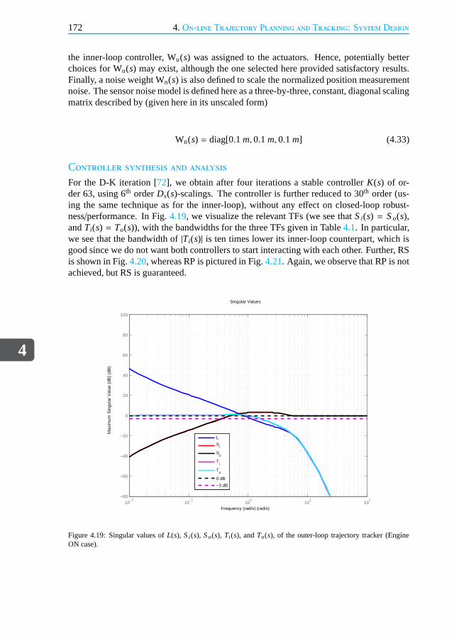
4

172 4.On-line Trajectory Planning and Tracking: System Design

the inner-loop controller, Wu(s) was assigned to the actuators. Hence, potentially betterchoices for Wu(s) may exist, although the one selected here provided satisfactory results.Finally, a noise weight Wn(s) is also defined to scale the normalized position measurementnoise. The sensor noise model is defined here as a three-by-three, constant, diagonal scalingmatrix described by (given here in its unscaled form)

Wn(s) = diag[0.1 m, 0.1 m, 0.1 m] (4.33)

Controller synthesis and analysisFor the D-K iteration [72], we obtain after four iterations a stable controllerK(s) of or-der 63, using 6th orderDs(s)-scalings. The controller is further reduced to 30th order (us-ing the same technique as for the inner-loop), without any effect on closed-loop robust-ness/performance. In Fig.4.19, we visualize the relevant TFs (we see thatSi(s) = So(s),andTi(s) = To(s)), with the bandwidths for the three TFs given in Table4.1. In particular,we see that the bandwidth of|Ti(s)| is ten times lower its inner-loop counterpart, which isgood since we do not want both controllers to start interacting with each other. Further, RSis shown in Fig.4.20, whereas RP is pictured in Fig.4.21. Again, we observe that RP is notachieved, but RS is guaranteed.

10−2

10−1

100

101

102

−80

−60

−40

−20

0

20

40

60

80

100

Singular Values

Frequency (rad/s) (rad/s)

Max

imum

Sin

gula

r V

alue

(dB

) (d

B)

L

Si

So

Ti

To

0 dB

−3 dB

Figure 4.19: Singular values ofL(s), Si (s), So(s), Ti (s), andTo(s), of the outer-loop trajectory tracker (EngineON case).

4.10.Appendix C: Design of the outer-loop controller for the engine ON case

4

173

10−2

10−1

100

101

102

103

0

0.05

0.1

0.15

0.2

0.25

0.3

0.35

0.4

0.45

Frequency (rad/s)

µ ∆(N11

(s))

Upper boundLower bound

Figure 4.20: Robust Stability of the outer-loop tra-jectory tracker (Engine ON case).

10−2

10−1

100

101

102

103

0

1

2

3

4

5

6

7

Frequency (rad/s)

µ ∆(N(s

))

Upper boundLower bound

Figure 4.21: Robust Performance of the outer-looptrajectory tracker (Engine ON case).

Adapting the engine ON outer-loop controllerFor the case of an engine ON automatic landing, and when closeto the ground, it is crucialto keep the reference velocities as small as possible. To this end, we adapt the outer-loopcontroller as follows: the position tracking is switched-off, i.e. the values for (u v w)⊤d areset to zero, once the helicopter height descends below a predefined threshold (keeping onlyvelocity and heading tracking). This helps lowering the final (touch-down) values of the 3Dvelocities, by giving more time to the velocity deceleration process.

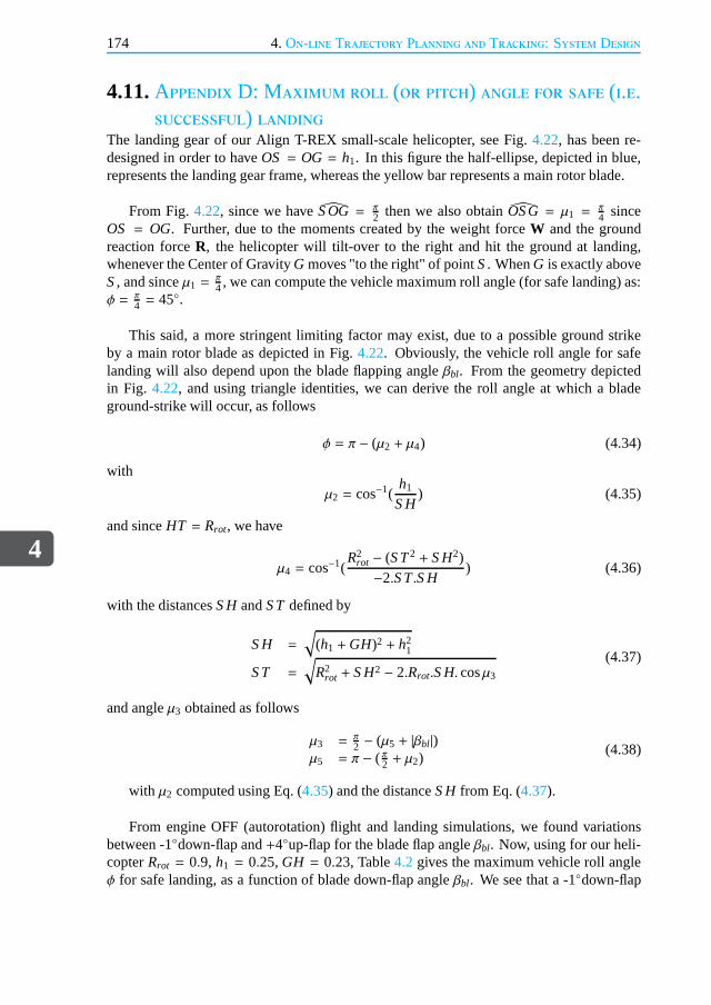
4

174 4.On-line Trajectory Planning and Tracking: System Design

4.11.Appendix D: Maximum roll (or pitch) angle for safe (i.e.successful) landing

The landing gear of our Align T-REX small-scale helicopter,see Fig.4.22, has been re-designed in order to haveOS = OG = h1. In this figure the half-ellipse, depicted in blue,represents the landing gear frame, whereas the yellow bar represents a main rotor blade.

From Fig.4.22, since we haveS OG= π2 then we also obtainOSG= µ1 =

π4 since

OS = OG. Further, due to the moments created by the weight forceW and the groundreaction forceR, the helicopter will tilt-over to the right and hit the ground at landing,whenever the Center of GravityG moves "to the right" of pointS. WhenG is exactly aboveS, and sinceµ1 =

π4 , we can compute the vehicle maximum roll angle (for safe landing) as:

φ = π4 = 45.

This said, a more stringent limiting factor may exist, due toa possible ground strikeby a main rotor blade as depicted in Fig.4.22. Obviously, the vehicle roll angle for safelanding will also depend upon the blade flapping angleβbl. From the geometry depictedin Fig. 4.22, and using triangle identities, we can derive the roll angleat which a bladeground-strike will occur, as follows

φ = π − (µ2 + µ4) (4.34)

with

µ2 = cos−1(h1

S H) (4.35)

and sinceHT = Rrot, we have

µ4 = cos−1(R2

rot − (S T2 + S H2)−2.S T.S H

) (4.36)

with the distancesS HandS Tdefined by

S H =

√

(h1 +GH)2 + h21

S T =

√

R2rot + S H2 − 2.Rrot.S H. cosµ3

(4.37)

and angleµ3 obtained as follows

µ3 = π2 − (µ5 + |βbl|)

µ5 = π − ( π2 + µ2)(4.38)

with µ2 computed using Eq. (4.35) and the distanceS H from Eq. (4.37).

From engine OFF (autorotation) flight and landing simulations, we found variationsbetween -1down-flap and+4up-flap for the blade flap angleβbl. Now, using for our heli-copterRrot = 0.9, h1 = 0.25,GH = 0.23, Table4.2 gives the maximum vehicle roll angleφ for safe landing, as a function of blade down-flap angleβbl. We see that a -1down-flap

4.11.Appendix D: Maximum roll (or pitch) angle for safe (i.e. successful) landing

4

175

Table 4.2: Maximum vehicle roll angleφ for safe landing, as a function of blade down-flap angleβbl.

Flap angleβbl () 0 -1 -5 -10 -15Roll angleφ () 36.4 35.5 31.8 27.0 21.7

Figure 4.22: Maximum vehicle roll angleφ for safe landing, for the case of a negative blade flap angleβbl.

would result in a 35.5maximum vehicle roll angle, hence way above the 10roll angle de-fined in the requirement for safe landing in Definition 4.2 of Chapter 4. Even for muchlarger down-flap angles, e.g. -15possibly due to the ground impact, we see that the maxi-mum allowable roll angle is still higher than the 10specification. A similar reasoning canalso be applied to the pitch axis which, based upon the shape of the landing gear, givescomparable results to the ones outlined for the roll axis.

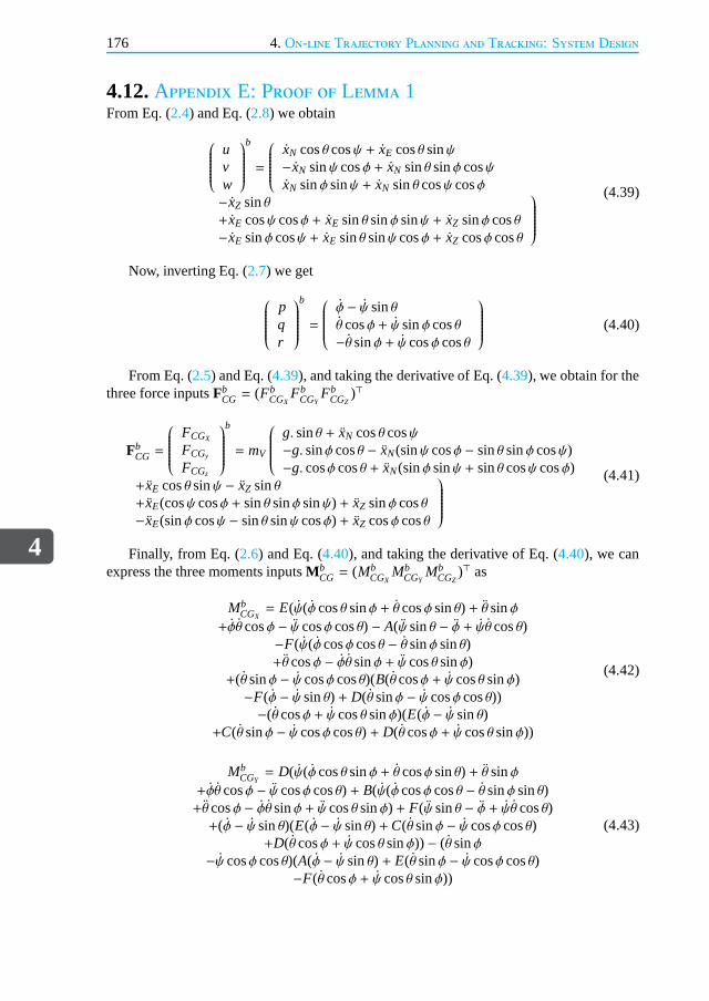
4

176 4.On-line Trajectory Planning and Tracking: System Design

4.12.Appendix E: Proof of Lemma 1From Eq. (2.4) and Eq. (2.8) we obtain

uvw

b

=

xN cosθ cosψ + xE cosθ sinψ−xN sinψ cosφ + xN sinθ sinφ cosψxN sinφ sinψ + xN sinθ cosψ cosφ

−xZ sinθ+xE cosψ cosφ + xE sinθ sinφ sinψ + xZ sinφ cosθ−xE sinφ cosψ + xE sinθ sinψ cosφ + xZ cosφ cosθ

(4.39)

Now, inverting Eq. (2.7) we get

pqr

b

=

φ − ψ sinθθ cosφ + ψ sinφ cosθ−θ sinφ + ψ cosφ cosθ

(4.40)

From Eq. (2.5) and Eq. (4.39), and taking the derivative of Eq. (4.39), we obtain for thethree force inputsFb

CG = (FbCGX

FbCGY

FbCGZ

)⊤

FbCG =

FCGX

FCGy

FCGz

b

= mV

g. sinθ + xN cosθ cosψ−g. sinφ cosθ − xN(sinψ cosφ − sinθ sinφ cosψ)−g. cosφ cosθ + xN(sinφ sinψ + sinθ cosψ cosφ)

+xE cosθ sinψ − xZ sinθ+xE(cosψ cosφ + sinθ sinφ sinψ) + xZ sinφ cosθ−xE(sinφ cosψ − sinθ sinψ cosφ) + xZ cosφ cosθ

(4.41)

Finally, from Eq. (2.6) and Eq. (4.40), and taking the derivative of Eq. (4.40), we canexpress the three moments inputsMb

CG = (MbCGX

MbCGY

MbCGZ

)⊤ as

MbCGX= E(ψ(φ cosθ sinφ + θ cosφ sinθ) + θ sinφ

+φθ cosφ − ψ cosφ cosθ) − A(ψ sinθ − φ + ψθ cosθ)−F(ψ(φ cosφ cosθ − θ sinφ sinθ)+θ cosφ − φθ sinφ + ψ cosθ sinφ)

+(θ sinφ − ψ cosφ cosθ)(B(θ cosφ + ψ cosθ sinφ)−F(φ − ψ sinθ) + D(θ sinφ − ψ cosφ cosθ))−(θ cosφ + ψ cosθ sinφ)(E(φ − ψ sinθ)

+C(θ sinφ − ψ cosφ cosθ) + D(θ cosφ + ψ cosθ sinφ))

(4.42)

MbCGY= D(ψ(φ cosθ sinφ + θ cosφ sinθ) + θ sinφ

+φθ cosφ − ψ cosφ cosθ) + B(ψ(φ cosφ cosθ − θ sinφ sinθ)+θ cosφ − φθ sinφ + ψ cosθ sinφ) + F(ψ sinθ − φ + ψθ cosθ)+(φ − ψ sinθ)(E(φ − ψ sinθ) +C(θ sinφ − ψ cosφ cosθ)

+D(θ cosφ + ψ cosθ sinφ)) − (θ sinφ−ψ cosφ cosθ)(A(φ − ψ sinθ) + E(θ sinφ − ψ cosφ cosθ)

−F(θ cosφ + ψ cosθ sinφ))

(4.43)

4.12.Appendix E: Proof of Lemma 1

4

177

MbCGZ= E(ψ sinθ − φ + ψθ cosθ) −C(ψ(φ cosθ sinφ

+θ cosφ sinθ) + θ sinφ + φθ cosφ − ψ cosφ cosθ)−D(ψ(φ cosφ cosθ − θ sinφ sinθ) + θ cosφ − φθ sinφ+ψ cosθ sinφ) + (φ − ψ sinθ)(B(θ cosφ + ψ cosθ sinφ)

−F(φ − ψ sinθ) + D(θ sinφ − ψ cosφ cosθ))−(θ cosφ + ψ cosθ sinφ)(A(φ − ψ sinθ)

+E(θ sinφ − ψ cosφ cosθ) − F(θ cosφ + ψ cosθ sinφ))

(4.44)

4

178 References

References[1] S. Taamallah,Low-order modeling for a small-scale flybarless helicopteruav, a grey-

box time-domain approach,in AIAA Atmospheric Flight Mechanics Conf.(2012).

[2] S. Taamallah,Optimal autorotation with obstacle avoidance for a small-scale flybar-less helicopter uav,in AIAA Guidance, Navigation and Control Conf.(2012).

[3] S. Taamallah, X. Bombois, and P. M. J. Van den Hof,Optimal control for power-offlanding of a small-scale helicopter a pseudospectral approach,in Am. Control Conf.(2012).

[4] S. Taamallah,A qualitative introduction to the vortex-ring-state, autorotation, andoptimal autorotation,in Europ. Rotorcraft Forum(2010).

[5] D. Santamaria, A. Viguria, M. Bejar, K. Kondak, and A. Ollero,Towards autonomousautorotation landing for small size unmanned helicopters,J. Intell. Robot Syst.69,171 (2013).

[6] P. Abbeel, A. Coates, T. Hunter, and A. Y. Ng,Autonomous autorotation of an rchelicopter,in 11th Int. Symposium on Experimental Robotics (ISER)(2008).

[7] J. Holsten, S. Loechelt, and W. Alles,Autonomous autorotation flights of helicopteruavs to known landing sites,in Am. Helicopter Soc.(2010).

[8] T. Yomchinda, J. F. Horn, and J. W. Langelaan,Autonomous control and path plan-ning for autorotation of unmanned helicopters,in Am. Helicopter Soc.(2012).

[9] Z. Sunberg and J. Rogers,A fuzzy logic-based controller for helicopter autorotation,in AIAA Aerospace Sciences Meeting and Exhibit(2013).

[10] M. Fliess,Generalized controller canonical forms for linear and nonlinear dynamics,IEEE Trans. Autom. Control35, 994 (1990).

[11] M. Fliess, J. Levine, P. Martin, and P. Rouchon,Sur les systemes non lineaires differ-entiellement plats,C.R. Acad. Sci. Paris315, 619 (1992).

[12] M. Fliess, J. Levine, P. Martin, and P. Rouchon,Flatness and defect of nonlinearsystems: Introductory theory and examples,Int. J. of Control61, 1327 (1995).

[13] H. Sira-Ramirez and S. K. Agrawal,Differentially Flat Systems(Marcel Dekker Inc.,2004).

[14] J. Levine,Analysis and Control of Nonlinear Systems: A Flatness-Based Approach(Springer, 2009).

[15] I. M. Ross and F. Fahroo,A unified computational framework for real-time optimalcontrol, in IEEE Conf. on Decision and Control(2003).

[16] P. Martin, R. M. Murray, and P. Rouchon,Flat Systems, Equivalence And TrajectoryGeneration, Tech. Rep. (CDS, California Institute of Technology, 2003).

References

4

179

[17] R. M. Murray, J. Hauser, A. Jadbabaie, M. B. Milam, N. Petit, W. B. Dunbar, andR. Franz,Online control customization via optimization-based control. In T. Samadand G. Balas, Editors, Software-Enabled Control: Information Technology for Dy-namical Systems(IEEE Press, 2003).

[18] G. Zames,On the input-output stability of time-varying nonlinear feedback systems-part i: Conditions derived using concepts of loop gain, conicity, and positivity,IEEETrans. Autom. ControlAC-11, 228 (1966).

[19] C. A. Desoer and M. Vidyasagar,Feedback Systems: Input-Output Properties(Aca-demic Press, New York, 1975).

[20] D. H. Jacobson and D. Q. Mayne,Differential Dynamic Programming(Elsevier,1970).

[21] H. Sira-Ramirez, R. Castro-Linares, and E. Liceaga-Castro, A liouvillian systemsapproach for the trajectory planning-based control of helicopter models,Int. J. OfRobust And Nonlinear Control10, 301 (2000).

[22] M. Fliess, J. Levine, P. Martin, and P. Rouchon,A lie-backlund approach to equiva-lence and flatness of nonlinear systems,IEEE Trans. Autom. Control44, 922 (1999).

[23] W. C. Lu, L. Duan, F. B. Hsiao, and F. M. Camino,Neural guidance control foraircraft based on differential flatness,AIAA J. of Guidance, Control, and Dynamics31, 892 (2008).

[24] P. Martin, S. Devasia, and B. Paden,A different look at output tracking: Control of avtol aircraft, Automatica32, 101 (1996).

[25] M. Saeki and Y. Sakaue,Flight control design for a nonlinear non-minimum phase vtolaircraft via two-step linearization,in IEEE Conf. on Decision and Control(2001).

[26] I. M. Ross and F. Fahroo,Pseudospectral methods for optimal motion planning ofdifferentially flat systems,IEEE Trans. Autom. Control49, 1410 (2004).

[27] I. M. Ross and F. Fahroo,Issues in the real time computation of optimal control,Mathematical and Computer Modelling43, 1172 (2006).

[28] M. J. van Nieuwstadt and R. M. Murray,Real time trajectory generation for differen-tially flat systems,Int. J. of Robust and Nonlinear Control18, 995 (1998).

[29] N. Faiz, S. K. Agrawal, and R. M. Murray,Trajectory planning of differentially flatsystems with dynamics and inequalities,AIAA J. of Guidance, Control, and Dynamics24, 219 (2001).

[30] M. B. Milam, K. Mushambi, and R. M. Murray,A new computational approach toreal-time trajectory generation for constrained mechanical systems,in IEEE Conf. onDecision and Control(2000).

[31] M. B. Milam, R. Franz, and R. M. Murray,Real-time constrained trajectory genera-tion applied to a flight control experiment,in IFAC World Conf.(2002).

4

180 References

[32] R. Murray, M. Rathinam, and W. Sluis,Differential flatness of mechanical control sys-tems: A catalog of prototype systems,in ASME Int. Mechanical Engineering Congress(1995).

[33] M. Rathinam,Differentially Flat Nonlinear Control Systems, Ph.D. thesis, CaliforniaInstitute of Technology (1997).

[34] V. N. Chetverikov,New flatness conditions for control systems,in IFAC NonlinearControl Systems(2001).

[35] P. Martin,Contribution a l’Etude des Systemes Differentiellement Plats, Ph.D. thesis,Ecole des Mines de Paris (1992).

[36] P. Martin,Aircraft control using flatness,in Proc. CESA Lille(1996).

[37] J. Hauser and R. Hindman,Aggressive flight maneuvers,in IEEE Conf. on Decisionand Control(1997).

[38] F. Cazaurang, R. Bergeon, and L. Lavigne,Modelling of longitudinal disturbed air-craft model by flatness approach,in AIAA Guidance Navigation and Control Conf.(2003).

[39] A. Ailon, Optimal path and tracking control of an autonomous vtol aircraft, inMediterranean Conf. on Control and Automation(2006).

[40] M. van Nieuwstadt and R. M. Murray,Outer flatness: Trajectory generation for amodel helicopter,in Europ. Control Conf.(1997).

[41] T. J. Koo and S. Sastry,Differential flatness based full authority helicopter controldesign,in IEEE Conf. on Decision and Control(1999).

[42] I. D. Cowling, O. A. Yakimenko, J. F. Whidborne, and A. K.Cook,A prototype of anautonomous controller for a quadrotor uav,in Europ. Control Conf.(2007).

[43] Y. Bouktir, M. Haddad, and T. Chettibi,Trajectory planning for a quadrotor heli-copter,in Mediterranean Conf. on Control and Automation(2008).

[44] D. Mellinger and V. Kumar,Minimum snap trajectory generation and control forquadrotors,in International Conf. on Robotics and Automation(2011).

[45] S. Formentin and M. Lovera,Flatness-based control of a quadrotor helicopter viafeedforward linearization,in IEEE Conf. on Decision and Control(2011).

[46] A. Chamseddine, Z. Youmin, C. A. Rabbath, C. Join, and D.Theilliol, Flatness-basedtrajectory planning/replanning for a quadrotor unmanned aerial vehicle,IEEE Trans.on Aerospace and Electronic Systems48, 2832 (2012).

[47] D. Desiderio and M. Lovera,Flatness-based guidance for planetary landing,in Am.Control Conf.(2010).

References

4

181

[48] V. Morio, F. Cazaurang, and P. Vernis,Flatness-based hypersonic reentry guidanceof a lifting-body vehicle,Control Engineering Practice17, 588 (2009).

[49] J. Levine and D. Nguyen,Flat output characterization for linear systems using poly-nomial matrices,Systems & Control Letters48, 69 (2003).

[50] D. Henrion and J. B. Lasserre,Lmis for constrained polynomial interpolation withapplication in trajectory planning,Systems & Control Letters55, 473 (2006).

[51] J. D. Caigny, B. Demeulenaere, J. Swevers, and J. de Schutter, Optimal design ofspline-based feedforward for trajectory tracking,in Am. Control Conf.(2007).

[52] F. Suryawan, J. A. D. Dona, and M. M. Seron,Methods for trajectory generation in amagnetic-levitation system under constraints,in Mediterranean Conf. on Control andAutomation(2010).

[53] F. Suryawan, J. A. D. Dona, and M. M. Seron,On splines and polynomial toolsfor constrained motion planning,in Mediterranean Conf. on Control and Automation(2010).

[54] R. Dai,B-splines based optimal control solution,in AIAA Guidance, Navigation andControl Conf.(2010).

[55] F. Suryawan, J. A. D. Dona, and M. M. Seron,Flatness-based minimum-time tra-jectory generation for constrained linear systems using b-splines,in IFAC WorldCongress(2011).

[56] D. Bertsekas,Nonlinear Programming - Second Edition(Athena Scientific, Belmont,MA, 1999).

[57] J. Nocedal and S. Wright,Numerical Optimization(Springer, NY, 2000).

[58] A. V. Rao,A survey of numerical methods for optimal control,in Am. AstronauticalSoc.(2009).

[59] R. J. Vanderbei and D. F. Shanno,An interior-point algorithm for nonconvex nonlinearprogramming,Computational Optimization and Applications13, 231 (1999).

[60] R. H. Byrd, M. E. Hribar, and J. Nocedal,An interior point algorithm for large-scalenonlinear programming,SIAM J. on Control and Optimization9, 877 (1999).

[61] L. T. Biegler, O. Ghattas, M. Heinkenschloss, and B. vanBloemen Waanders,Large-Scale PDE-Constrained Optimization(Springer, Berlin, 2003).

[62] R. H. Byrd, J. Nocedal, and R. A. Waltz,Knitro: An integrated package for nonlinearoptimization,Large-Scale Nonlinear Optimization, Springer-Verlag , 35(2006).

[63] M. D. Ardema and N. Rajan,Separation of time scales in aircraft trajectory optimiza-tion, AIAA J. of Guidance, Control, and Dynamics8, 275 (1985).

4

182 References

[64] S. Skogestad and I. Postlethwaite,Multivariable Feedback Control: Analysis and De-sign, 2nd Ed.(Wiley-Interscience, Great Britain, 2005).

[65] J. C. Doyle,Structured uncertainty in control system design,in IEEE Conf. on Deci-sion and Control(1985).

[66] K. Zhou, J. C. Doyle, and K. Glover,Robust and Optimal Control(Prentice Hall,New Jersey, 1996).

[67] K. J. Astrom and R. M. Murray,Feedback Systems: An Introduction for Scientists andEngineers(Princeton University Press, Princeton, NJ, 2008).

[68] D. W. Gu, P. H. Petkov, and M. M. Konstantinov,Robust Control Design with Matlab(Springer, London, 2005).

[69] A. A. G. Macintosh,Trajectory Tracking Control for a Small-Scale Helicopter duringAutorotation, Tech. Rep. (Master Thesis, Delft University of Technology, 2014).

[70] http://gemiddeldgezien.nl/meer-gemiddelden/176-gemiddelde-windkracht-nederland.

[71] Anonymous,Flying Qualities of Piloted Airplanes, Tech. Rep. MIL-F-8785C (UnitedStates DoD, 1980).

[72] G. J. Balas, J. C. Doyle, K. Glover, A. K. Packard, and R. S. Smith,µ Analysis andSynthesis Toolbox: User’s Guide(The MathWorks Inc., 1991).

[73] K. Glover,All optimal hankel-norm approximations of linear multivariable systemsand theirL∞-error bounds,Int. J. of Control39, 1115 (1984).

5On-line Trajectory Planning and

Tracking: Simulation Results

The helicopter approaches closer than any other vehicle to fulfillment of mankind’sancient dreams of the flying horse and the magic carpet.

Igor I. SikorskyDesigned the world’s first mass-produced helicopter in 1942

In Chapter 4, we presented a combined Trajectory Planning (TP) and Trajectory Tracking(TT) system, having on-line computational tractability. In Chapter 5, we demonstrate—usingthe high-fidelity, high-order, nonlinear helicopter simulation of Chapter 2—the first, real-time feasible, model-based TP and TT system, for the case of asmall-scale helicopter UAVwith an engine OFF condition (i.e. autorotation). To betterillustrate the various challengesencountered when designing a planning and tracking system for the engine OFF condition,a comparison with two engine ON automated flight maneuvers isalso provided.

183

5

184 5.On-line Trajectory Planning and Tracking: Simulation Results

5.1. Introduction

I n this Chapter, we evaluate the combined Trajectory Planning(TP) and Trajectory Track-ing (TT) functionalities, developed in Chapter 4. These aretested on the helicopter, high-

fidelity, High-Order Model (HOM) developed in Chapter 2. Five test cases are presented,two with engine ON, and three with engine OFF (autorotation), starting from various initialconditions. The modeled small-scale UAV is the instrumented Remote-Controlled (RC)Align T-REX helicopter, used also in Chapter 2, and belonging to the flybarless two-bladedmain rotor class. This vehicle has a total mass of 7.75 kg, a main rotor radius of 0.9 m, amain rotor nominal angular velocity of 1350 RPM, a NACA 0015 main rotor airfoil, andan induced velocity in hover given byvih = 3.5 m/s (see also Table2.1, of Chapter 2, foradditional helicopter parameters).

The two engine ON test cases are included to illustrate that the Flight Control System(FCS) framework, presented in the Appendices of Chapter 4, allows for a variety of auto-mated flight maneuvers. With the engine ON, we demonstrate anautomatic landing, and acruise-to-hover maneuver. The first engine ON test case starts from an initial flight condi-tion which is identical to the one used when deriving the nominal LTI model, used for TTdesign (i.e. helicopter in hover). The second test case starts from an initial condition whichis far away from the operating condition used to derive this LTI model. Both test cases areset in an ideal environment, i.e. a noise-free and disturbance-free environment.

The three engine OFF test cases are set to demonstrate the automatic autorotation land-ing capability. Here too, the first engine OFF test case is setto evaluate the FCS perfor-mance for an initial flight condition which is identical to the flight condition used to derivethe nominal LTI model, used for TT design (i.e. helicopter inhover, however with the mainrotor RPM free to vary). The second test case starts from an initial condition which is faraway from the operating condition used to derive this LTI model. These first two test casesare also set in an ideal environment, i.e. a noise-free and disturbance-free environment.The third engine OFF test case is added to illustrate the FCS performance when includingsensors measurement noise together with a wind disturbance.

5.2.Setting up the trajectory planning for the engine ONcases

Case 1.This test case involves a landing maneuver from a hover initial condition, startingat an altitude1 of -8 m, with further 2 m and -1 m displacements, in the North and East axesrespectively, together with a 90 right turn in heading. Numerically, the initial and final

1Recall that the vertical z-axis is oriented positive down.

5.2.Setting up the trajectory planning for the engine ON cases

5

185

conditions for this maneuver are given by2:

xi =(

0 m 0 m −8 m 0 m/s 0 m/s 0 m/s

0 rad/s 0 rad/s 0 rad/s π(3.4/180)rad 0 rad 0 rad)⊤

x f =(

2 m −1 m −1 m 0 m/s 0 m/s 0.2 m/s

0 rad/s 0 rad/s 0 rad/s π(3.4/180)rad 0 rad π(90/180)rad)⊤

Before proceeding, we make the following comments

• The final altitudexZ (see the third component ofx f ) is set to -1 m. This allows to adda safety margin into the planned trajectory.

• The final vertical velocityw (see the sixth component ofx f ) is set to 0.2 m/s. Whenclose to the ground, the goal is to move at a constant and slow rate of descent (untilthe skids hit the ground).

Next, the flight envelope (i.e. state constraints in the formof minimum and maximumlimits, partially based upon engineering judgment) is defined as follows:

xmin = −(

50m 50m 50m 5 m/s 1 m/s 3 m/sπ(100/180)rad/s π(100/180)rad/s π(100/180)rad/s

π(15/180)rad π(15/180)rad 2π rad)⊤

xmax=(

50m 50m −0.25m 15m/s 1 m/s 1.16m/sπ(100/180)rad/s π(100/180)rad/s π(100/180)rad/s

π(15/180)rad π(15/180)rad 2π rad)⊤

Before proceeding, we make the following comments

• When the helicopter is on the ground, the Center of Gravity (CG) height is equal to-0.25 m (see the third component ofxmax).

• The maximum helicopter velocity is limited as follows. A full-size helicopter such asthe Bell UH-1H has a main rotor radius of 7.24 m, whereas our model helicopter has amain rotor radius of 0.9 m, resulting in a scale ratioN equal toN = 7.24/0.9= 8.04.Now, a model and its full-size counterpart are said to be dynamically similar if therelative magnitudes of their governing forces are unchanged by scale [1]. Often, theso-called Froude scaling is used to study systems at a reduced size [1]. The BellUH-1H has a top speed of 60.28m/s, thus based on Froude scaling the top speed ofour RC helicopter would be 60.28/

√N = 21.26 m/s. In our case, and in order to

reduce the stresses on the airframe and main rotor hub, we do not intend to operatethe vehicle beyond 15 m/s (see the fourth component ofxmax).

2Recall also that the rigid-body dynamics, used in the flatness TP, is characterized by a state-vector of dimensiontwelvex = (xN xE xZ u v w p q rφ θ ψ)⊤, with total forces and total moments as inputs, each of dimension three,given byFb

CG = (FbCGX

FbCGY

FbCGZ

)⊤, andMbCG = (Mb

CGXMb

CGYMb

CGZ)⊤.

5

186 5.On-line Trajectory Planning and Tracking: Simulation Results

• The body lateral velocityv is constrained to± 1 m/s, as to limit vehicle sideslipmotion.

• To prevent flight into the Vortex-Ring-State (VRS)3, the body vertical velocityw islimited to a third of the induced velocity in hoverw ≤ 1

3vih, giving w ≤ 3.5/3 = 1.16m/s (see the sixth component ofxmax).

• The rollφ and pitchθ angles are limited to± 15, in order to: 1) keep the load factorn within acceptable values4, i.e. preferably below one; and 2) minimize the system’snonlinear behavior, facilitating thus the trajectory tracking5.

Next, the input constraints, i.e. on the total forces and total moments, are based uponsimulation experiments with the nonlinear helicopter HOM of Chapter 2, and have beenchosen as follows:

FbCGmin

= −(

20 N 15 N 120N)⊤

MbCGmin

= −(

5 Nm 5 Nm 5 Nm)⊤

FbCGmax

=(

20 N 15 N −30 N)⊤

MbCGmax

=(

5 Nm 5 Nm 5 Nm)⊤

Besides, additional constraints have also been included (refer also to the flatness TPin Appendix A of Chapter 4), such as: 1) a tail rotor blade tip clearance to avoid groundstrike by the tail rotor during flare; and 2) a supplementary limit on the airflow through themain rotor as to avoid flight into the VRS. The airflow through the main rotor is given byVrotor = w+ pyH − qxH , which is limited to half the induced velocity in hoverVrotor ≤ 1

2vih,see Fig.2.19in Chapter 2. In the cost functional, defined in Appendix A of Chapter 4, wehave used the following weightsWT f = Wv = 1 andWr = 100. HereWr is chosen high toreward straight flight trajectories.

Finally, we use the ’adaptation’ functionality of the engine ON outer-loop controller,as outlined in Appendix C of Chapter 4. When close to the ground, it is crucial to keepthe reference velocities as small as possible. Once the helicopter height descends below apredefined threshold (here -1 m), the position control is stopped.

Case 2.This test case involves a cruise-to-hover maneuver, starting at a North velocityVN = 10 m/s, an altitude of -20 m, and then transitioning to hover mode,at an altitude of-5 m, with further 30 m and -5 m displacements, in the North andEast axes respectively,

3Briefly summarized, the VRS corresponds to a condition wherethe helicopter is descending in its own wake,resulting in a chaotic and dangerous flight condition [2].

4For a level turning flight the load factor is given byn = 1cosφ .

5It is well known that strong coupling in longitudinal and lateral motions exists for helicopters flying in low-speed,high-g turns (i.e. high load factor), and that for helicopters with a single main rotor, the direction of turn has alsoa significant influence on the flight dynamics [3]. This coupling becomes stronger with higher roll or pitch angles,i.e. with higher-g turns [4, 5]. It was further shown in [3] that the performance of a FCS, designed using a straightflight condition, can be severely degraded when the helicopter enters a turn. Since in our case the nominal LTIplant, used for control synthesis, corresponds to a hover condition, it becomes relevant to maintain small anglesin roll and pitch.

5.3.Setting up the trajectory planning for the engine OFFcases

5

187

together with a 120 left turn in heading. Numerically, the initial and final conditions forthis maneuver are given by:

xi =(

0 m 0 m −20m 10m/s 0 m/s 0 m/s

0 rad/s 0 rad/s 0 rad/s π(2.6/180)rad −π(1.1/180)rad 0 rad)⊤

x f =(

30m −5 m −5 m 0 m/s 0 m/s 0 m/s

0 rad/s 0 rad/s 0 rad/s π(3.4/180)rad 0 rad −π(120/180)rad)⊤

Regarding the state and input constraints, and cost functional weights, these are identi-cal to the engine ON case 1.

5.3.Setting up the trajectory planning for the engine OFFcases

Three engine OFF test cases are included to demonstrate the automatic autorotation landingcapability. The first engine OFF test case is set to evaluate the FCS performance for an ini-tial flight condition which is identical to the flight condition used to derive the nominal LTImodel, used for TT design (i.e. helicopter in hover with freemain rotor RPM). The secondtest case starts from an initial condition which is far away from the operating condition usedto derive this LTI model. These first two test cases are also set in an ideal environment, i.e.a noise-free and disturbance-free environment. The third engine OFF test case is set to il-lustrate the FCS performance when including sensors measurement noise, together with awind disturbance.

Case 1.This test case involves an autorotation, starting from an engine failure in hover,at an altitude of -35 m, and then landing at 2 m North and 1 m Eastposition, without anyheading turn. Numerically, the initial and final conditionsare given by:

xi =(

0 m 0 m −35m 0 m/s 0 m/s 0 m/s

0 rad/s 0 rad/s 0 rad/s π(3.4/180)rad 0 rad 0 rad)⊤

x f =(

2 m 1 m −0.75m 0 m/s 0 m/s 0.2 m/s

0 rad/s 0 rad/s 0 rad/s 0 rad 0 rad 0 rad)⊤

Here, we make also the following comments

• Note that we also give a final value to the North and East horizontal positions (thiswas not the case in the planning of Chapter 3). This represents additional constraintson the TP. We do this with an eye on future experimental flight tests where, for safetyreasons, we want to know in advance where the helicopter willbe landing.

• The final altitudexZ (see the third component ofx f ) is set to -0.75 m. This allows toadd a safety margin into the planned trajectory6.

6This value was set to -1 m for the engine ON automatic landing.For the engine OFF case, better autorationlandings were obtained when adjusting this value to -0.75 m.

5

188 5.On-line Trajectory Planning and Tracking: Simulation Results

• Again, the final vertical velocityw (see the sixth component ofx f ) is set to 0.2 m/s.

• The final timeT f is bounded such thatT f ≤ TOFF, withxZI

1.75vih≤ TOFF ≤

xZI1.50vih

, seeour discussion in Section4.3.3, giving for this test case 5.7s ≤ TOFF ≤ 6.6s. Herewe choseTOFF = 6 s.

The constraints on states and inputs are identical to the ones used in the engine ONcases, except for the following item: we allow for a higher downwards velocity on thewchannel, up to 15 m/s. Besides, the limit on airflow through the main rotor is alsoremoved,i.e. flight through the VRS is here allowed7. In the cost functional of Section4.3.3, we haveused the following weightsWu =Wv =Ww =Wψ = 1.

Finally, we use here the ’adaptation’ functionality of the engine OFF outer-loop con-troller, as outlined in Section4.6.3of Chapter 4. When close to the ground, it is crucialto keep the reference velocities as small as possible. Once the helicopter height descendsbelow a predefined threshold (here -1 m), the position control is stopped.

Case 2.This test case involves an autorotation, starting from an engine failure atVN =

8 m/s, at an altitude of -45 m, and then landing at 30 m North and 0 m East position,together with a 30 left turn in heading. Numerically, the initial and final conditions for thismaneuver are given by:

xi =(

0 m 0 m −45m 8 m/s 0 m/s 0 m/s

0 rad/s 0 rad/s 0 rad/s π(2.6/180)rad 0 rad −π(0.8/180)rad)⊤

x f =(

30m 0 m −0.75m 0 m/s 0 m/s 0.2 m/s

0 rad/s 0 rad/s 0 rad/s 0 rad 0 rad −π(30/180)rad)⊤

We make also the following comments

• Again we give a final value to the North and East horizontal positions.

• The final timeT f is bounded such thatT f ≤ TOFF, withxZI

1.75vih≤ TOFF ≤

xZI1.50vih

,giving for this test case 7.3s≤ TOFF ≤ 8.5s. Here we choseTOFF = 7.3 s.

Regarding the state and input constraints, and cost functional weights, these are identi-cal to the engine OFF case 1.

For engine OFF flight conditions having relatively high initial velocities, we imple-mented the following ’adaptation’ functionality for the engine OFF outer-loop controller.When|xZ| ≤ 5 m is true, we stop the horizontal position tracking (xN, xE). This helps low-ering the final (touch-down) values of the 2D horizontal velocities. Further, when|xZ| ≤ 1m is true, we stop the vertical position tracking (xZ) as well.

7Indeed, and depending on the initial condition at the instant of engine failure, a brief transition through the VRSmay be unavoidable.

5.4.Discussion of closed-loop simulation results for the engine ON cases

5

189

Case 3.This test case involves an autorotation, starting from an engine failure in hover,at an altitude of -30 m, and then landing at 0 m North and 0 m Eastposition (i.e. thehorizontal position of the landing spot is identical to the horizontal position of the initialstate), without any heading turn. We also include Gaussian,white noise, on the 12 measuredstatesy = (xN xE xZ u v w p q rφ θ ψ)⊤, with the following 1-σ values:

(

0.1 m 0.1 m 0.1 m 0.05m/s 0.05m/s 0.05m/sπ(3/180)rad π(3/180)rad π(3/180)rad

π(1/180)rad π(1/180)rad π(3/180)rad)⊤

These 1-σ values correspond to the noise weight values used during controller design inChapter 4, expect for the noise on the three body velocities (the three most critical signals),where we have used a noise value which is five times higher thanthe value used duringcontroller design, in order to better visualize the response characteristics of the FCS.

We also include a headwind of 8 m/s, which is equivalent to a Beaufort wind force valueof 4, corresponding to the yearly average wind force along the coast in The Netherlands[6]. Note that this is a rather heavy wind condition for such a small-scale helicopter. Now,numerically, the initial and final conditions for this maneuver are given by:

xi =(

0 m 0 m −30m 0 m/s 0 m/s 0 m/s

0 rad/s 0 rad/s 0 rad/s π(3.4/180)rad 0 rad 0 rad)⊤

x f =(

0 m 0 m −0.75m 0 m/s 0 m/s 0.2 m/s

0 rad/s 0 rad/s 0 rad/s 0 rad 0 rad 0 rad)⊤

The final timeT f is bounded such thatT f ≤ TOFF, withxZI

1.75vih≤ TOFF ≤

xZI1.50vih

, givingfor this test case 4.9s ≤ TOFF ≤ 5.7s. Here we choseTOFF = 5 s. Regarding the state andinput constraints, and cost functional weights, together with the ’adaptation’ functionalityof the outer-loop controller, these are identical to the engine OFF case 1.

Remark 7 Before proceeding with analyzing the time-traces of the closed-loop simulationdata, we quickly compared the frequency content8 of the various inner- and outer-loop ref-erence signals (generated by the planner, for all engine ON and engine OFF test cases) withthe bandwidths of the complementary sensitivity function Ti(s), which have been reportedin Table4.1of Chapter 4. Fortunately, the frequency content of all reference signals werelower than the corresponding bandwidth of Ti(s), hence the engine ON and OFF controllersought to be able to track the reference signals.

5.4.Discussion of closed-loop simulation results for the en-gine ON cases

Fig. 5.1 and Fig.5.4 visualize the required control inputs for the engine ON testcases 1and 2, respectively. Fig.5.2 and Fig.5.5 visualize the evolution of the 3D inertial veloci-ties (VN,VE,VZ) and positions (xN, xE, xZ). Although the vertical z-axis is oriented positive8This is done by computing the single-sided amplitude spectra, obtained through Fast Fourier Transforms (FFT).

5

190 5.On-line Trajectory Planning and Tracking: Simulation Results

down, on the figuresVZ andxZ are shown positive up for better readability. Further, Fig.5.3and Fig.5.6visualize the time-histories for the body states, namely attitude angles (φ, θ, ψ),linear velocities (u, v,w), and rotational velocities (p, q, r).

In Fig.5.2, Fig.5.5, Fig.5.3, and Fig.5.6, the black lines represent the outputs from theflatness TP, these include the planned 3D inertial positions(xN xE xZ)⊤TP, defined in Fig.4.3,the planned 3D body velocities (u v w)⊤TP, defined in Fig.4.4, and the planned headingψTP,also defined in Fig.4.4. The flatness-based TP, in Section4.3of Chapter 4, computes alsoa planned trajectory for the remaining states, e.g. roll angle φ, pitch angleθ, roll ratep, etc.However, and for the sake of clarity, in Fig.5.2, Fig. 5.5, Fig. 5.3, and Fig.5.6, we haveonly visualized the TP outputs that will be tracked.

Now, in Fig.5.2and Fig.5.5, the blue lines, namedreference for outer-loop, representthe signals that need to be tracked by the outer-loop controller. Here, these signals aresimply the planned 3D inertial positions (xN xE xZ)⊤TP, i.e. black and blue lines are identical(except possibly at the end of the flight, see Section4.6.3of Chapter 4). In Fig.5.3 andFig. 5.6, the blue lines, namedreference for inner-loop, represent the signals that need tobe tracked by the inner-loop controller. Here, these signals include the planned headingψTP, where again black and blue lines are identical. However, the velocities that need to betracked by the inner-loop are given by (u v w)⊤TP + (u v w)⊤d , and here black and blue linesare not identical. Finally, the red lines represent the outputs from the nonlinear helicoptermodel of Chapter 2. From these figures, we see that:

• The combined trajectory planning and tracking system is capable of safely guidingand controlling the helicopter.

• From Fig.5.3, and Fig.5.6, we see that a single LTI controller is capable of control-ling the nonlinear helicopter system, for a relatively large variation in forward vehiclevelocity (i.e. body linear velocityu is varying between approximately -1 m/s and 10m/s).

• The specifications for a successful automatic landing, see Definition 4.2 in Sec-tion 4.3.3and Appendix D of Chapter 4, have been defined as|u| ≤ 0.5 m/s, |v| ≤ 0.5m/s, |w| ≤ 0.25 m/s, |φ| ≤ 10 , and|θ| ≤ 10 . Regarding case 1, at the instant ofground impact, we have for the body horizontal velocitiesu = 0.03 m/s, v = −0.04m/s, the body vertical velocityw = 0.22 m/s, and the roll and pitch anglesφ = 5.02,andθ = 2.04 . Hence all specifications for a successful automatic landing are met.

• From Fig.5.1, Fig. 5.4, and from the actuator data reported in Table2.1 of Chapter2, we see that the control input amplitudes never saturate, i.e. |θ0| ≤ 13, |θ1c| ≤ 6,|θ1s| ≤ 6, and|θTR| ≤ 20.

• From Fig.5.2, Fig.5.5, Fig.5.3, and Fig.5.6, better tracking performance is achievedfor the vertical motionw andxZ in (and headingψ), when compared to tracking per-formance on the horizontal channels (u, v) and (xN, xE), see our discussion in Sec-tion 2.4.2of Chapter 2.

5.4.Discussion of closed-loop simulation results for the engine ON cases

5

191

• Close to zero steady-state errors can be seen for the inner-loop reference tracking, forboth test cases.

• Position control clearly exhibit some over- and undershoot. In addition, nonzerosteady-state errors are observed for test case 1. This is partially due to the fact thatposition control is stopped when the helicopter descends below 1 m.

• Regarding test case 2, even though rollφ and pitchθ angles are not controlled, theynicely adjust, at the end of the flight, to their respective hover values.

• Although the nominal model, used for control design, was linearized at a conditionoutside the ground effect, we did not notice any significant performance deteriorationof the closed-loop system, when the helicopter was in groundeffect (i.e. below 1 mabove ground level).

In addition, Fig.5.7, Fig. 5.8, Fig. 5.9, and Fig.5.10visualize the frequency contentof the main rotor lateral Tip-Path-Plane (TPP) tilt angleβ1s, vehicle roll ratep, and con-trol inputs respectively, for the Engine ON case 1 (the engine ON case 2 is very similar).Although, in our test cases, the frequency contents of the applied control inputs are notbroadband, we are still able to identify some salient natural modes of this small-scale heli-copter system. For instance, the first two figures clearly show the main rotor TPP modes,with the lowest (the so-called regressing TPP mode) at a frequency of 5.5 Hz. The regress-ing flapping mode is the most relevant one, when focusing on helicopter flight dynamics,as it may have a tendency to couple into the fuselage modes [7–9]. Fig. 5.8 also showsthe main rotor vibrations. In the engine ON case, i.e. at a fixed main rotor RPM of 1350(equivalent to 22.5 Hz), we can clearly identify the 2/Rev9 rotor vibration at 45 Hz.

For the engine ON case, simulation tests have shown that a high-bandwidth closed-loopsystem was not required for the case of gentle and smooth flight maneuvers. This led tothe selection of low bandwidth performance weights Wp(s), during controller synthesis.Accordingly we see that the frequency content of the controlinputs is rather low, stayingbelow 0.5 Hz, see Fig.5.9–Fig.5.10, except for an interestingly large peak at 2.7 Hz. Thispeak at 2.7 Hz, clearly seen on these four figures (predominantly related to a roll-pitch-yawmotion), is an interesting aspect of these figures, and represents the interaction betweenthe Flight Control Computer (FCS) and the main rotor. Hence,we have a situation wherethe actuators are also reacting to a periodic rotor-fuselage coupling (in addition to vehiclerigid-body dynamics), as opposed to a context where the actuators are only responding tothe rigid-body dynamics. This clearly results in limit cycle oscillations.

In the experimental results obtained in [10, 11], a 3.1 Hz pendulum-like mode in rolland pitch was also observed, for the case of a two-bladed small-scale helicopter, albeithaving a teetered main rotor, but with somewhat comparable vehicle size and mass, hencecorroborating our results. This phenomenon (i.e. interaction between the FCS and the mainrotor) has only sparsely been covered in the small-scale UAVliterature. This phenomenonis well-known within the realm of wind turbines [12], and is somewhat reminiscent to the

9Since we have a two-bladed main rotor.

5

192 5.On-line Trajectory Planning and Tracking: Simulation Results

realm of Higher-Harmonic-Control (HHC) for helicopters [13]. This interaction betweenthe FCS and the main rotor is comparable to the well-known interaction between aircraftFCS and aircraft structural dynamics—i.e. aeroservoelastic effects [14]—which are knownto lead to flutter or limit cycle oscillations, and hence dynamic and fatigue loads. Asidefrom these dynamic and fatigue loads, this dynamical interaction would also result in ourcase in an increase of the electrical power consumption, andhence a lower flight time. Ageneral approach to mitigate such problems would consist in: 1) using higher-order LTImodels during the control design, possibly in combination with a reduced-order observer,in order to estimate the unmeasured main rotor states; and/or 2) use carefully selected notchfilters, see [11].

5.5.Discussion of closed-loop simulation results for the en-gine OFFcases

We discuss here the first two engine OFF cases, the third engine OFF case will be addressedin Section5.5.2. Fig.5.13and Fig.5.16visualize the required control inputs for the engineOFF test cases 1 and 2 respectively. Fig.5.14 and Fig.5.17 visualize the evolution ofthe 3D inertial velocities (VN,VE,VZ) and positions (xN, xE, xZ), whereas Fig.5.15 andFig. 5.18visualize the time-histories for the body states, namely attitude angles (φ, θ, ψ),linear velocities (u, v,w), and rotational velocities (p, q, r). Fig.5.19and Fig.5.20visualizethe time-histories for the main rotor RPMΩMR. Note also that the definition of the black,blue, and red lines, is identical to the one presented here-above, for the engine ON cases,and hence is not repeated here. From these figures, we see that:

• The combined trajectory planning and tracking system is capable of safely guidingand controlling the helicopter in autorotation.

• The specifications for a successful automatic landing, see Definition 4.2 in Sec-tion 4.3.3and Appendix D of Chapter 4, have been defined as|u| ≤ 0.5 m/s, |v| ≤ 0.5m/s, |w| ≤ 0.25 m/s, |φ| ≤ 10 , and|θ| ≤ 10 . Regarding case 1, at the instant ofground impact, we have for the body horizontal velocitiesu = 0.04 m/s, v = 0.15m/s, the body vertical velocityw = 0.25 m/s, and the roll and pitch anglesφ = 1.41, andθ = 3.39 . Regarding case 2, at the instant of ground impact, we have for thebody horizontal velocitiesu = −0.37 m/s, v = 0.13 m/s, the body vertical velocityw = 0.21 m/s, and the roll and pitch anglesφ = 6.67 , andθ = −0.54 . Regard-ing case 3, at the instant of ground impact, we have for the body horizontal velocitiesu = −0.09 m/s,v = 0.12 m/s, the body vertical velocityw = 0.24 m/s, and the roll andpitch anglesφ = −0.75 , andθ = −0.15 . Hence all specifications for a successfulautomatic landing are met.

• A single LTI controller is capable of controlling and landing the helicopter system, inautorotation, for a relatively large variation in forward and vertical vehicle velocity(at least up to approximately 8 to 10 m/s), and for relatively large variations in mainrotor RPM (approximately in the range 50% to 110% of the nominal engine ONvalue), see Fig.5.15, Fig.5.18, Fig.5.19, and Fig.5.20.

5.5.Discussion of closed-loop simulation results for the engine OFFcases

5

193

• From the actuator data, reported in Table2.1 of Chapter 2, we see that the controlinput amplitudes would never saturate, except for a brief saturation of the main rotorcollectiveθ0, that would happen just prior to touch-down.

• As expected, tracking performance is better for the vertical motionw andxZ, than thetracking of horizontal motion (u, v) and (xN, xE), see our discussion in Section2.4.3of Chapter 2.

• Some steady-state errors can be seen on the horizontal channel (see Fig.5.14 andFig. 5.17) and heading (see Fig.5.15and Fig.5.18), whereas this is not the case forthe vertical channel (refer to these same figures). This is also partially due to the factthat position control is stopped some time before the helicopter touches the ground.

• Main rotor RPMΩMR behaves as expected, see Fig.5.19 and Fig.5.20, i.e. werecognize the typical autorotative time-histories, as shown in Chapter 3. Notice that,when starting from low altitudes such as in these test cases,the helicopter does noteven reach a steady-state autorotation (main rotor RPM is not constant), rather it iscontinuously in transition from one non-equilibrium stateto the next.

• Again, although the nominal model, used for control design,was linearized at a con-dition outside the ground effect, we did not notice any significant performance dete-rioration of the closed-loop system, when the helicopter was in ground effect.

In addition, Fig.5.21, Fig.5.22, Fig.5.23, and Fig.5.24visualize the frequency contentof the main rotor lateral TPP tilt angleβ1s, vehicle roll ratep, and control inputs, respec-tively. For the engine OFF case, simulation experiments have shown that a higher closed-loop bandwidth was necessary for good tracking behavior. This resulted in a bandwidthincrease of the controller performance weights. This increase in control bandwidth has alsosome drawbacks. Indeed, we also clearly see an interaction between the FCS and the mainrotor around 5.5 Hz. This mode was identified to be the regressing flap mode of 5.5 Hz, fora constant main rotor RPM of 1350, in the figures for the engineON case. In the engineOFF case, the RPM is not constant anymore, and hence the interaction between the FCS andthe main rotor shows a frequency spread, which cannot easilybe eliminated by notch filters.

Summarizing the observed results for the engine OFF cases, we see that the crucialcontrol of vertical position and velocity exhibits outstanding behavior in terms of trackingperformance, and does not require an additional increase incontrol bandwidth. However,the tracking of horizontal positions and horizontal velocities is clearly lacking some band-width (i.e. the flown trajectories are clearly lagging the planned ones). Although a furtherincrease of the horizontal closed-loop bandwidths provided good results when evaluated onthe LTI model used for control design, this increase in closed-loop bandwidths resulted, un-fortunately, in closed-loop instabilities, when evaluated on the nonlinear helicopter modelof Chapter 2.

5.5.1.System energy: the engine ON versus engine OFFcasesWe compute here the stored energy in our helicopter system. For the following analysis, weassume that the flight time is not limited by the amount of energy stored inside the on-board

5

194 5.On-line Trajectory Planning and Tracking: Simulation Results

batteries. In other words, the electrical power supply system is omitted from this energybalance analysis. Hence, we consider only the following energy components (refer also tothe nomenclature in Appendix A of Chapter 2): the vehicle potential energymVg|xZ|; thevehicle kinetic energy12mV(u2+v2+w2)+ 1

2(Ap2+Bq2+Cr2), with A, B, andC the diagonalelements of the inertia matrixIV; the stored energy in the main rotor1

2NbIbΩ2MR; and the to-

tal energy (sum of previous three). These energies have beenplotted in Fig.5.11–Fig.5.12,and Fig.5.25–Fig.5.26, for the engine ON test cases, and for the first two engine OFF testcases, respectively. A quick scan on total energies revealsthe main difference between theengine ON and OFF cases, i.e. while the total energy for an engine ON case may evenincrease, the total energy for an engine OFF case is always decreasing. This particularityrenders the trajectory planning and tracking rather challenging for the engine OFF case.

For the engine ON case, we conjecture that the current vehicle state has only a limitedimpact (if any) on reachable states at very distant times. This is because we can always in-ject some energy back into the system, and hence compensate for any suboptimal decisionsmade at the current time. However, for the engine OFF case, since the energy of the systemis always decreasing, there is less room for error. We also conjecture that the size of thisreachable set, in the engine OFF case, is much smaller than the one for the engine ON case,and hence feasible engine OFF trajectories are much harder to find.

5.5.2.Closed-loop response with respect to sensors noise and wind distur-bance

Here we illustrate the response of the FCS, for the case of noisy measurement signals anda wind disturbance. The wind disturbance includes a constant (deterministic) headwind of8 m/s, together with a small gust (Dryden stochastic variation)on the three linear axes.Fig. 5.27visualizes the required control inputs for the engine OFF test case 3. Fig.5.28visualizes: 1) the nonlinear model time-histories for the 3D inertial velocities and positions(in red); 2) the corresponding noisy measurement positionssent to the outer-loop controller(in magenta); and 3) the wind disturbance (in green). Fig.5.29visualizes: 1) the nonlinearmodel time-histories for the nine body states (in red); and 2) the corresponding noisy mea-surements sent to the inner-loop controller (in magenta). Finally, Fig. 5.30visualizes thetime-histories for the main rotor RPM.

Again, we see that all specifications for a successful automatic landing are met, seeDefinition 4.2 in Section4.3.3and Appendix D of Chapter 4, despite the additional mea-surements noise and wind disturbance. Also Fig.5.30illustrates the benefits of a headwindlanding, namely we see that the RPM is still high (about 1100 RPM) at the end of thelanding maneuver (compare with Fig.5.19and Fig.5.20). Obviously, a higher energy inthe rotor allows for a smoother landing, and for additional control authority, which may beparticularly useful for disturbance rejection.

5.6.ConclusionIn this Chapter we have evaluated the capabilities of the Trajectory Planning (TP) and Tra-jectory Tracking (TT) framework, previously developed in Chapter 4. In particular, we have

5.6.Conclusion

5

195

demonstrated in this Chapter—using the high-fidelity, high-order, nonlinear helicopter sim-ulation of Chapter 2—the first, real-time feasible, model-based TP and TT system, for thecase of a small-scale helicopter UAV with an engine OFF condition. The main distinctivefeatures of the engine ON versus engine OFF TP and TT may be summarized as follows:

• For the engine ON case, the vehicle state at a current timeti has only a limited impact(if any) on the reachable states at a (very distant) timet f , with t f ≫ ti . If we omitthe on-board electrical power supply system from the vehicle energy balance, i.e.considering only vehicle potential, kinetic, and main rotor energies, then the totalvehicle energy may decrease or increase, depending on vehicle height above groundlevel and vehicle velocity. By contrast, the total vehicle energy in the engine OFFcase is always decreasing. Hence, we conjecture that the size of this reachable set, attime t f , is much smaller than its engine ON counterpart, and consequently feasibletrajectories are harder to find in the engine OFF case.

• For the engine ON case, helicopter operations can remain at avelocity which stays inthe neighborhood of the design-point velocity, i.e. in the neighborhood of the equilib-rium point velocity which was used to derive the LTI model forcontrol design. Thisallows to maximize the linear behavior of the system. On the other hand, helicopteroperations with the engine OFF will inevitably result in a wide range of flown veloc-ities, including high descent rates, and even flight into thechaotic Vortex-Ring-State(VRS). Indeed, a brief transition through the VRS may in somecases be required.This obviously tends to ’amplify’ the nonlinear behavior ofthe system.

• For the engine ON case, the designer can choose to keep the bandwidth of the closed-loop system rather small, by only considering gentle and smooth maneuvers in thedesign specification phase. For the engine OFF case, a higherclosed-loop bandwidthis definitely required, if proper trajectory tracking is to be performed. This maycomplicate the controller design, since higher-order LTI models (for controller de-sign) may have to be considered. This complicates also the practical implementation,since higher-bandwidth actuators may become compulsory.

• A general approach to mitigate the observed interaction problem, between the FCSand the main rotor dynamics, could be to use higher-order LTImodels, for controldesign, possibly in combination with a reduced-order observer in order to estimatethe unmeasured main rotor states.

• For the engine OFF case, our results show that the crucial control of vertical posi-tion and velocity exhibit outstanding behavior in terms of tracking performance, anddoes not require an additional increase in control bandwidth. However, the trackingof horizontal positions and horizontal velocities is clearly lacking some bandwidth.Unfortunately, a further increase of the horizontal closed-loop bandwidths resultedin closed-loop instabilities (i.e. when evaluated on the nonlinear helicopter model ofChapter 2).

• Finally, tracking performance of horizontal positions andhorizontal velocities couldpotentially be improved, by considering one of the two following options: 1) remain-ing in the framework of a single robust LTI controller, however combined with a

5

196 5.On-line Trajectory Planning and Tracking: Simulation Results

higher-order LTI plant (i.e. containing the main rotor flap-lag and inflow dynamics),instead of the low-order plant used in Section4.5.1of Chapter 4. This LTI plantcould also be derived using a more accurate linearization method, as discussed inSection2.4.1of Chapter 2; or 2) using another control method, i.e. in the realm ofnonlinear, adaptive, or Linear Parameter-Varying (LPV) methods.

5.6.Conclusion

5

197

Appendix A: Simulation results

0 1 2 3 4 5 6 7 8 92

4

6

Time (s) θ

0 (de

g)

0 1 2 3 4 5 6 7 8 9−2

0

2

Time (s)

θ1c

(de

g)

0 1 2 3 4 5 6 7 8 9−2

0

2

Time (s)

θ1s

(de

g)

0 1 2 3 4 5 6 7 8 98

10

12

Time (s)

θ0T

R (

deg)

Figure 5.1: Helicopter control inputs, for the Engine ON case 1.

0 2 4 6 8

0

0.5

1

Time (s)

VN

(m

/s)

0 2 4 6 8

−0.5

0

0.5

1

1.5

Time (s)

VE (

m/s

)

0 2 4 6 8

−1.5

−1

−0.5

0

Time (s)

VZ: U

p>0

(m/s

)

0 2 4 6 8−0.5

0

0.5

1

1.5

2

Time (s)

x N (

m)

0 2 4 6 8−1.5

−1

−0.5

0

0.5

1

1.5

Time (s)

x E (

m)

0 2 4 6 8

1

2

3

4

5

6

7

8

Time (s)

x Z: U

p>0

(m)

Figure 5.2: Inertial velocities and positions, for the Engine ON case 1. Black line: flatness planning.Blue line:references for outer-loop (identical to black line).Red line: controlled nonlinear model.

5

198 5.On-line Trajectory Planning and Tracking: Simulation Results

0 2 4 6 8−10

−5

0

5

10

Time (s)

φ (d

eg)

0 2 4 6 8

−10

0

10

Time (s)

θ (d

eg)

0 2 4 6 80

20

40

60

80

Time (s)

ψ (

deg)

0 2 4 6 8

0

1

2

Time (s)

u (m

/s)

0 2 4 6 8

−0.6

−0.4

−0.2

0

Time (s)

v (m

/s)

0 2 4 6 8−1

0

1

Time (s)

w (

m/s

)

0 2 4 6 8

−20

0

20

Time (s)

p (d

eg/s

)

0 2 4 6 8

−20

0

20

Time (s)

q (d

eg/s

)

0 2 4 6 8

0

10

20

30

Time (s)

r (d

eg/s

)

Figure 5.3: Euler angles, body linear velocities, and body rotational velocities, for the Engine ON case 1. Blackline: flatness planning.Blue line: references for inner-loop.Red line: controlled nonlinear model.

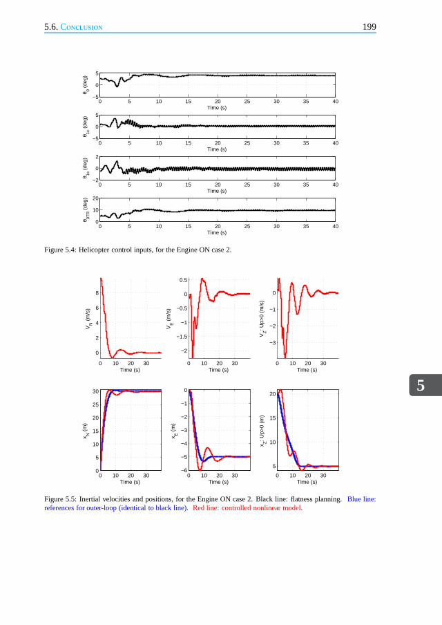
5.6.Conclusion

5

199

0 5 10 15 20 25 30 35 40−5

0

5

Time (s)

θ0 (

deg)

0 5 10 15 20 25 30 35 40−5

0

5

Time (s)

θ1c

(de

g)

0 5 10 15 20 25 30 35 40−2

0

2

Time (s)

θ1s

(de

g)

0 5 10 15 20 25 30 35 400

10

20

Time (s)

θ0T

R (

deg)

Figure 5.4: Helicopter control inputs, for the Engine ON case 2.

0 10 20 30

0

2

4

6

8

Time (s)

VN

(m

/s)

0 10 20 30

−2

−1.5

−1

−0.5

0

0.5

Time (s)

VE (

m/s

)

0 10 20 30

−3

−2

−1

0

Time (s)

VZ: U

p>0

(m/s

)

0 10 20 300

5

10

15

20

25

30

Time (s)

x N (

m)

0 10 20 30−6

−5

−4

−3

−2

−1

0

Time (s)

x E (

m)

0 10 20 30

5

10

15

20

Time (s)

x Z: U

p>0

(m)

Figure 5.5: Inertial velocities and positions, for the Engine ON case 2. Black line: flatness planning.Blue line:references for outer-loop (identical to black line).Red line: controlled nonlinear model.

5

200 5.On-line Trajectory Planning and Tracking: Simulation Results

0 20 40−20

−10

0

10

20

Time (s)

φ (d

eg)

0 20 40−10

0

10

20

Time (s)

θ (d

eg)

0 20 40−150

−100

−50

0

50

Time (s)

ψ (

deg)

0 20 40−5

0

5

10

Time (s)

u (m

/s)

0 20 40−2

−1

0

1

Time (s)

v (m

/s)

0 20 40−2

0

2

4

6

Time (s)

w (

m/s

)

0 20 40−50

0

50

100

Time (s)

p (d

eg/s

)

0 20 40−40

−20

0

20

40

Time (s)

q (d

eg/s

)

0 20 40−40

−20

0

20

Time (s)

r (d

eg/s

)

Figure 5.6: Euler angles, body linear velocities, and body rotational velocities, for the Engine ON case 2. Blackline: flatness planning.Blue line: references for inner-loop.Red line: controlled nonlinear model.

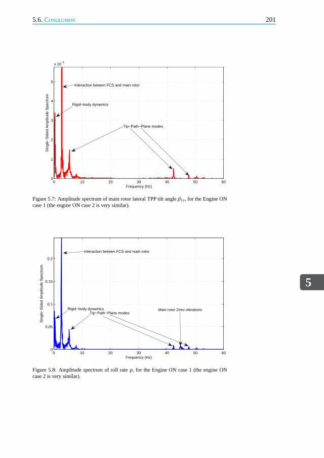
5.6.Conclusion

5

201

0 10 20 30 40 50 600

1

2

3

4

5

x 10−3

Frequency (Hz)

Sin

gle−

Sid

ed A

mpl

itude

Spe

ctru

m

Tip−Path−Plane modes

Rigid−body dynamics

Interaction betwen FCS and main rotor

Figure 5.7: Amplitude spectrum of main rotor lateral TPP tilt angleβ1s, for the Engine ONcase 1 (the engine ON case 2 is very similar).

0 10 20 30 40 50 600

0.05

0.1

0.15

0.2

Frequency (Hz)

Sin

gle−

Sid

ed A

mpl

itude

Spe

ctru

m

Interaction betwen FCS and main rotor

Rigid−body dynamicsTip−Path−Plane modes

Main rotor 2/rev vibrations

Figure 5.8: Amplitude spectrum of roll ratep, for the Engine ON case 1 (the engine ONcase 2 is very similar).

5

202 5.On-line Trajectory Planning and Tracking: Simulation Results

0 1 2 3 4 5 6 7 8 9 100

0.1

0.2

0.3

0.4

0.5

0.6

0.7

0.8

Frequency (Hz)

Sin

gle−

Sid

ed A

mpl

itude

Spe

ctru

m

MR collective θ0

MR lat. cyclic θ1c

MR lon. cyclic θ1s

TR collective θ0TR

Rigid−body dynamics

Interaction between FCS and main rotor

Figure 5.9: Amplitude spectrum of control inputs, for the Engine ON case 1.

0 1 2 3 4 5 6 7 8 9 100

0.1

0.2

0.3

0.4

0.5

0.6

0.7

0.8

Frequency (Hz)

Sin

gle−

Sid

ed A

mpl

itude

Spe

ctru

m

MR collective θ0

MR lat. cyclic θ1c

MR lon. cyclic θ1s

TR collective θ0TR

Rigid−body dynamics

Interaction between FCS and main rotor

Figure 5.10: Amplitude spectrum of control inputs, for the Engine ON case 2.

5.6.Conclusion

5

203

0 1 2 3 4 5 6 7 8 90

500

1000

1500

2000

2500

Time (s)

Veh

icle

Ene

rgie

s (J

)

TotalPotentialMain Rotor RPMKinetic

Figure 5.11: Vehicle energies, for the Engine ON case 1.

0 5 10 15 20 25 30 35 400

500

1000

1500

2000

2500

3000

3500

Time (s)

Veh

icle

Ene

rgie

s (J

)

TotalPotentialMain Rotor RPMKinetic

Figure 5.12: Vehicle energies, for the Engine ON case 2.

5

204 5.On-line Trajectory Planning and Tracking: Simulation Results

0 1 2 3 4 5 6 7−20

0

20

Time (s) θ

0 (de

g)

0 1 2 3 4 5 6 7−5

0

5

Time (s)

θ1c

(de

g)

0 1 2 3 4 5 6 7−2

0

2

Time (s)

θ1s

(de

g)

0 1 2 3 4 5 6 7−10

0

10

Time (s)

θ0T

R (

deg)

Figure 5.13: Helicopter control inputs, for the Engine OFF case 1.

0 2 4 6

0

0.5

1

Time (s)

VN

(m

/s)

0 2 4 6

0

0.1

0.2

0.3

0.4

0.5

Time (s)

VE (

m/s

)

0 2 4 6

−8

−6

−4

−2

0

Time (s)

VZ: U

p>0

(m/s

)

0 2 4 6−0.5

0

0.5

1

1.5

Time (s)

x N (

m)

0 2 4 6

0

0.2

0.4

0.6

0.8

1

Time (s)

x E (

m)

0 2 4 6

5

10

15

20

25

30

35

Time (s)

x Z: U

p>0

(m)

Figure 5.14: Inertial velocities and positions, for the Engine OFF case 1. Black line: flatness planning.Blue line:references for outer-loop (identical to black line).Red line: controlled nonlinear model.

5.6.Conclusion

5

205

0 5 10−4

−2

0

2

4

Time (s)

φ (d

eg)

0 5 10−5

0

5

10

Time (s)

θ (d

eg)

0 5 10−5

0

5

10

Time (s)

ψ (

deg)

0 5 10−0.5

0

0.5

1

1.5

Time (s)

u (m

/s)

0 5 10−0.5

0

0.5

Time (s)

v (m

/s)

0 5 10−5

0

5

10

Time (s)

w (

m/s

)

0 5 10−100

−50

0

50

100

Time (s)

p (d

eg/s

)

0 5 10−50

0

50

Time (s)

q (d

eg/s

)

0 5 10−20

0

20

40

Time (s)

r (d

eg/s

)

Figure 5.15: Euler angles, body linear velocities, and bodyrotational velocities, for the Engine OFF case 1. Blackline: flatness planning.Blue line: references for inner-loop.Red line: controlled nonlinear model.

5

206 5.On-line Trajectory Planning and Tracking: Simulation Results

0 1 2 3 4 5 6 7 8−20

0

20

Time (s) θ

0 (de

g)

0 1 2 3 4 5 6 7 8−5

0

5

Time (s)

θ1c

(de

g)

0 1 2 3 4 5 6 7 8−2

0

2

Time (s)

θ1s

(de

g)

0 1 2 3 4 5 6 7 8−10

0

10

Time (s)

θ0T

R (

deg)

Figure 5.16: Helicopter control inputs, for the Engine OFF case 2.

0 2 4 6

0

2

4

6

8

Time (s)

VN

(m

/s)

0 2 4 6

−0.5

0

0.5

Time (s)

VE (

m/s

)

0 2 4 6

−8

−6

−4

−2

0

Time (s)

VZ: U

p>0

(m/s

)

0 2 4 6

5

10

15

20

25

30

35

Time (s)

x N (

m)

0 2 4 6

0

0.2

0.4

0.6

0.8

1

1.2

Time (s)

x E (

m)

0 2 4 6

10

20

30

40

Time (s)

x Z: U

p>0

(m)

Figure 5.17: Inertial velocities and positions, for the Engine OFF case 2. Black line: flatness planning.Blue line:references for outer-loop (identical to black line).Red line: controlled nonlinear model.

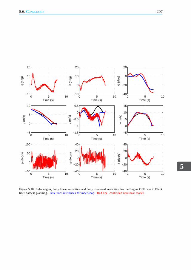
5.6.Conclusion

5

207

0 5 10−10

0

10

20

Time (s)

φ (d

eg)

0 5 10−10

0

10

20

Time (s)

θ (d

eg)

0 5 10−40

−20

0

20

Time (s)

ψ (

deg)

0 5 10−5

0

5

10

Time (s)

u (m

/s)

0 5 10−1.5

−1

−0.5

0

0.5

Time (s)

v (m

/s)

0 5 10−5

0

5

10

15

Time (s)

w (

m/s

)

0 5 10−50

0

50

100

Time (s)

p (d

eg/s

)

0 5 10−40

−20

0

20

40

Time (s)

q (d

eg/s

)

0 5 10−40

−20

0

20

40

Time (s)

r (d

eg/s

)

Figure 5.18: Euler angles, body linear velocities, and bodyrotational velocities, for the Engine OFF case 2. Blackline: flatness planning.Blue line: references for inner-loop.Red line: controlled nonlinear model.

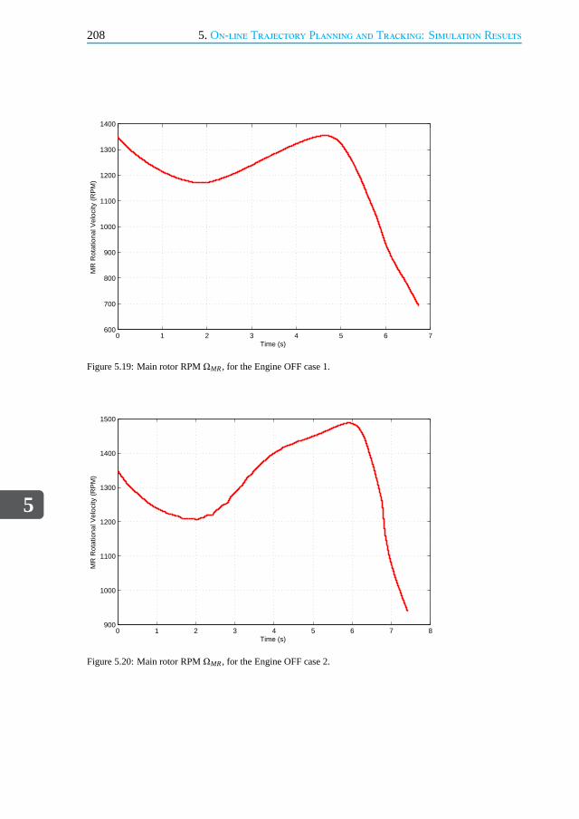
5

208 5.On-line Trajectory Planning and Tracking: Simulation Results

0 1 2 3 4 5 6 7600

700

800

900

1000

1100

1200

1300

1400

Time (s)

MR

Rot

atio

nal V

eloc

ity (

RP

M)

Figure 5.19: Main rotor RPMΩMR, for the Engine OFF case 1.

0 1 2 3 4 5 6 7 8900

1000

1100

1200

1300

1400

1500

Time (s)

MR

Rot

atio

nal V

eloc

ity (

RP

M)

Figure 5.20: Main rotor RPMΩMR, for the Engine OFF case 2.

5.6.Conclusion

5

209

0 10 20 30 40 50 600

1

2

3

4

5

x 10−3

Frequency (Hz)

Sin

gle−

Sid

ed A

mpl

itude

Spe

ctru

m

Figure 5.21: Amplitude spectrum of main rotor lateral TPP tilt angleβ1s, for the EngineOFF case 1 (the engine OFF case 2 is somewhat similar).

0 10 20 30 40 50 600

0.02

0.04

0.06

0.08

0.1

0.12

0.14

0.16

0.18

0.2

Frequency (Hz)

Sin

gle−

Sid

ed A

mpl

itude

Spe

ctru

m

Figure 5.22: Amplitude spectrum of roll ratep, for the Engine OFF case 1 (the engine OFFcase 2 is somewhat similar).

5

210 5.On-line Trajectory Planning and Tracking: Simulation Results

0 2 4 6 8 10 12 14 16 18 200

0.1

0.2

0.3

0.4

0.5

0.6

0.7

0.8

Frequency (Hz)

Sin

gle−

Sid

ed A

mpl

itude

Spe

ctru

m

MR collective θ0

MR lat. cyclic θ1c

MR lon. cyclic θ1s

TR collective θ0TR

Figure 5.23: Amplitude spectrum of control inputs, for the Engine OFF case 1.

0 2 4 6 8 10 12 14 16 18 200

0.1

0.2

0.3

0.4

0.5

0.6

0.7

0.8

Frequency (Hz)

Sin

gle−

Sid

ed A

mpl

itude

Spe

ctru

m

MR collective θ0

MR lat. cyclic θ1c

MR lon. cyclic θ1s

TR collective θ0TR

Figure 5.24: Amplitude spectrum of control inputs, for the Engine OFF case 2.

5.6.Conclusion

5

211

0 1 2 3 4 5 6 70

500

1000

1500

2000

2500

3000

3500

4000

4500

Time (s)

Veh

icle

Ene

rgie

s (J

)

TotalPotentialMain Rotor RPMKinetic

Figure 5.25: Vehicle energies, for the Engine OFF case 1.

0 1 2 3 4 5 6 7 80

1000

2000

3000

4000

5000

6000

Time (s)

Veh

icle

Ene

rgie

s (J

)

TotalPotentialMain Rotor RPMKinetic

Figure 5.26: Vehicle energies, for the Engine OFF case 2.

5

212 5.On-line Trajectory Planning and Tracking: Simulation Results

0 1 2 3 4 5 6 7−10

0

10

Time (s) θ

0 (de

g)

0 1 2 3 4 5 6 7−5

0

5

Time (s)

θ1c

(de

g)

0 1 2 3 4 5 6 7−2

0

2

Time (s)

θ1s

(de

g)

0 1 2 3 4 5 6 7−10

0

10

Time (s)

θ0T

R (

deg)

Figure 5.27: Helicopter control inputs, for the Engine OFF case 3.

0 5 10−10

−8

−6

−4

−2

0

Time (s)

VN

(m

/s)

0 5 10−1.2

−1

−0.8

−0.6

−0.4

−0.2

0

0.2

Time (s)

VE (

m/s

)

0 5 10−10

−8

−6

−4

−2

0

2

Time (s)

VZ: U

p>0

(m/s

)

0 5 10−1

−0.8

−0.6

−0.4

−0.2

0

0.2

0.4

Time (s)

x N (

m)

0 5 10−0.6

−0.4

−0.2

0

0.2

0.4

Time (s)

x E (

m)

0 5 100

5

10

15

20

25

30

35

Time (s)

x Z: U

p>0

(m)

Figure 5.28: Inertial velocities and positions, for the Engine OFF case 3. Black line: flatness planning.Blue line:references for outer-loop (identical to black line).Red line: controlled nonlinear model.Magenta line: noisymeasurements.Green line: wind disturbance.

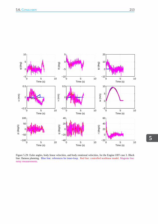
5.6.Conclusion

5

213

0 5 10−5

0

5

10

Time (s)

φ (d

eg)

0 5 10−10

−5

0

5

Time (s)

θ (d

eg)

0 5 10−10

0

10

20

Time (s)

ψ (

deg)

0 5 10−0.5

0

0.5

Time (s)

u (m

/s)

0 5 10−0.5

0

0.5

Time (s)

v (m

/s)

0 5 10−5

0

5

10

Time (s)

w (

m/s

)

0 5 10−100

−50

0

50

100

Time (s)

p (d

eg/s

)

0 5 10−40

−20

0

20

40

Time (s)

q (d

eg/s

)

0 5 10−20

0

20

40

60

Time (s)

r (d

eg/s

)

Figure 5.29: Euler angles, body linear velocities, and bodyrotational velocities, for the Engine OFF case 3. Blackline: flatness planning.Blue line: references for inner-loop.Red line: controlled nonlinear model.Magenta line:noisy measurements.

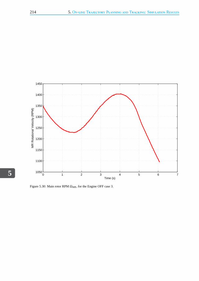
5

214 5.On-line Trajectory Planning and Tracking: Simulation Results

0 1 2 3 4 5 6 71050

1100

1150

1200

1250

1300

1350

1400

1450

Time (s)

MR

Rot

atio

nal V

eloc

ity (

RP

M)

Figure 5.30: Main rotor RPMΩMR, for the Engine OFF case 3.

References

5

215

References[1] B. Mettler, Identification Modelling and Characteristics of MiniatureRotorcraft

(Kluwer Academic Publishers, Norwell Mass, USA, 2003).

[2] S. Taamallah,A qualitative introduction to the vortex-ring-state, autorotation, andoptimal autorotation,in Europ. Rotorcraft Forum(2010).

[3] R. T. N. Chen,Flight dynamics of rotorcraft in steep high-g turns,AIAA J. of Aircraft21, 14 (1984).

[4] S. S. Houston,On the analysis of helicopter flight dynamics during maneuvers, inEurop. Rotorcraft Forum(1985).

[5] R. Celi and F. D. Kim,Trim, stability and frequency response simulation of an artic-ulated rotor helicopter in turning flight,in Europ. Rotorcraft Forum(1993).

[6] http://gemiddeldgezien.nl/meer-gemiddelden/176-gemiddelde-windkracht-nederland.

[7] R. T. N. Chen,Effects of Primary Rotor Parameters on Flapping Dynamics, Tech.Rep. NTP 1431 (NASA Ames Research Center, 1980).

[8] R. T. N. Chen and W. S. Hindson,Influence of high-order dynamics on helicopterflight control system bandwidth,AIAA J. of Guidance, Control, and Dynamics9, 190(1986).

[9] H. C. Curtiss,Stability and control modeling,in Europ. Rotorcraft Forum(1986).

[10] V. Gavrilets, A. Shterenberg, M. A. Dahleh, and E. Feron, Avionics system for a smallunmanned helicopter performing aggressive maneuvers,in Digital Avionics SystemsConf.(2000).

[11] V. Gavrilets,Autonomous Aerobatic Maneuvering of Miniature Helicopter, Ph.D. the-sis, Massachusetts Institute of Technology (2003).

[12] V. A. Riziotis, E. S. Politis, S. G. Voutsinas, and P. K. Chaviaropoulos,Stabilityanalysis of pitch-regulated, variable speed wind turbinesin closed loop operationusing a linear eigenvalue approach,Journal of Physics75 (2007).

[13] D. Patt, L. Liu, J. Chandrasekar, D. S. Bernstein, and P.P. Friedmann,Higher-harmonic-control algorithm for helicopter vibration reduction revisited,AIAA J. ofGuidance, Control and Dynamics28, 918 (2005).

[14] M. J. Patil,Nonlinear Aeroelastic Analysis, Flight Dynamics, and Control of a Com-plete Aircraft, Ph.D. thesis, Georgia Institute of Technology (1999).

6Affine LPV M odeling

There is this famous quote that the theory of nonlinear systems is like a theory ofnon-elephants. It is impossible to build a theory of nonlinear systems, because arbitrary

things can satisfy that definition.

Pablo ParilloMIT News, 2010

In Chapter 5, a single nominal Linear Time-Invariant (LTI) model was used for the designof a single robust LTI Trajectory Tracker (TT). This LTI controller was capable of landingthe helicopter in autorotation. Simulations showed that the crucial control of vertical posi-tion and velocity exhibited outstanding behavior in terms of tracking performance, althoughthe tracking of horizontal positions and velocities was lacking some bandwidth. Increasingthe horizontal closed-loop bandwidth was investigated by testing modified LTI controllerswhich, when evaluated on the nominal LTI model, showed promising results. Unfortunately,closed-loop instability was observed when evaluated on theNonLinear (NL) model of Chap-ter 2. Hence, improving the performance of the TT may necessitate an approach that betterexploits the system’s NL structure, while being computationally tractable (for on-line use).Linear Parameter-Varying (LPV) systems have become celebrated as they represent an at-tractive midway approach between LTI and NL structures, andhence LPV control couldpotentially be applied to improve the performance of the TT.However, the LPV controlparadigm takes the existence of the plant, in LPV form, as a starting point. Since a sys-tematic formulation of a NL system into a suitable LPV model remains often problematic,the purpose of this Chapter is to present an affine LPV modeling approach—for the casewhere a plant’s NL model already exists—that delivers a model suitable for control design.Our LPV modeling method was applied to the helicopter NL model of Chapter 2, and re-sulted in a LPV model having a large number of scheduling parameters. Unfortunately, itbecame impossible to synthesize LPV controllers for such a high-order model, and hencethe simulations in this Chapter have been done on a simpler pendulum system.

Parts of this Chapter have been published in [1].

217

6

218 6. Affine LPV Modeling

6.1. Introduction

I n Chapter 4, we presented a combined trajectory planning and tracking system, capableof safely landing the helicopter, in autorotation, in the vicinity of the planned North-East

landing spot. Our simulations of Chapter 5 showed that the tracking of horizontal positionsand velocities was lacking some bandwidth. Increasing the horizontal closed-loop band-width was investigated, by testing upgraded controllers. These controllers, when evaluatedon the nominal Linear Time-Invariant (LTI) model, showed promising results. Unfortu-nately, closed-loop instability was observed when tested on the helicopter, NonLinear (NL),High-Order Model (HOM) of Chapter 2. Hence, tracking performance of horizontal posi-tions and horizontal velocities could potentially be improved by considering one of the twofollowing options: i) remaining in the framework of a singlerobust LTI controller, usinga higher-order LTI plant for controller design (i.e. containing the main rotor flap-lag andinflow dynamics), instead of the low-order plant used in Section 4.5.1of Chapter 4; or ii)using another control method that better respects and exploits the system’s NL structure,while being also on-line computationally tractable. To this end, the three main alternativesare: 1) Nonlinear Dynamic Inversion (NDI) and/or Lyapunov based methods such as slid-ing mode and backstepping; 2) methods in the realm of adaptive control; or 3) methods inthe areas related to gain-scheduling and Linear Parameter-Varying (LPV) approaches.

Now the first option, i.e. option (i) here-above, with the useof a higher-order LTIplant (potentially in combination with a reduced-order observer to estimate the unmeasuredhigher-order rotor dynamics) is attractive for its simplicity, and hence is worth investigat-ing. However it was ruled out in this Chapter since, as statedin [2], it is generally notrecommended to ’hard-wire’ the higher-order main rotor dynamics into the feedback law,whenever these higher-order dynamics are insufficiently well-captured by an LTI model(which in practice may often be the case). Hence in this Chapter we have chosen to investi-gate option (ii), and in particular the third alternative, i.e. the LPV approach, since there isa plethora of mature LPV control methods, and Model Predictive Control (MPC) for LPVsystems, to choose from. This said, the first two alternatives should also be investigatedin future research projects. In particular the recent and promising developments of theL1

adaptive control [3] deserve further attention.

LPV systems allow to enclose NL behaviors into a linear framework [4, 5]. In fact,LPV control methods can be seen as an extension of the standard H2 and H∞ LTI syn-thesis techniques [6–13]. The LPV method amends also the main drawbacks of classicalgain-scheduling [14, 15] by: 1) eliminating the need for repeated designs/simulations, inorder to handle the global control problem; and 2) guaranteeing both stability and perfor-mance, along all possible parameter trajectories. In addition LPV control design problemsare efficiently solved, by first expressing the problems as Linear Matrix Inequality (LMI)optimizations [16]—subsequently formulated as Semi-Definite Programs (SDP)[17]—forwhich there are several powerful numerical solutions [18, 19]. This resulted in a growingnumber of applications [20], such as in aerospace [21–26], wind turbines [27], wafer step-pers [28, 29], CD players [30], and robotic manipulators [31], to name a few. Now, and forall its benefits, the LPV control paradigm typically takes the existence of a model of theplant, in LPV form, as a starting point. However, a systematic formulation of a NL system

6.1.Introduction

6

219

into a suitable (quasi-)LPV1 model remains often problematic [32]. Hence, the problemof simplifying a large scale, complex, NL model, such as our helicopter nonlinear HOM ofChapter 2, into a LPV representation, suitable for control design, is highly relevant. When aplant’s NL model is already available, there exists two mainmodeling avenues to transform,or approximate, its NL representation into a LPV one, namelythe so-called local and globalapproaches [32, 33]. The local approach consists in applying linearization theory of theNL system to obtain local LTI models in a state-space form, and subsequently interpolatethese models to derive a LPV approximation. Within this framework several methods havebeen developed, based upon e.g.: extended linearization [34], Jacobian linearization [35],multiple-model design procedure [36], H2 norm minimization [37], multivariable polyno-mial fitting [38], and poles, zeros, and gain interpolation [39, 40]. On the other hand theglobal approach generates a LPV model which preserves the dynamic behavior of the NLsystem. This can either be done by using a range of mathematical manipulations e.g.: statetransformation [41], velocity-based formulation [42], function substitution [43, 44], andautomated LPV model generation [32, 45], or alternatively by using a global identificationapproach of the scheduling parameters, through the use of least-squares based estimationsor Prediction Error Methods (PEM) [46].

Often it is important that the global behavior of the LPV model be similar to the globalbehavior of the NL system. This is typically the case when theLPV model is used forprediction/simulation in open-loop [47], MPC or optimal control. On the other hand, it issometimes desirable that the local (frozen) behavior of theLPV model, i.e., for constantscheduling, be representative of the local behavior of the NL system, i.e., local lineariza-tions of the NL system. For such cases, a local approach wouldbe recommended2. Thisis particularly the case when the LPV model is used for gain scheduled controller design,where controllers are synthesized on the basis of local models.

For LPV systems, the simultaneous identification3 of the LPV basis functions andscheduling parameters is a non-trivial problem, as it generally contains excessive degreesof freedom, giving rise to an ill-conditioned system identification problem [48]. Previousattempts towards such simultaneous identification problems have used nonlinear optimiza-tion methods [49, 50]. Another approach to mitigate such ill-conditioned identificationproblems requires the inclusion of additional constraintsor regularizations [47]. An evensimpler way would consist in having separate identificationsub-problems, e.g. by identi-fying first the basis functions, followed by a separate identification of the scheduling pa-rameters. We opt here for such a philosophy, i.e. by following the three-step methodologyintroduced in [36], formulated as follows: 1) identify first a central LTI model; 2) identifythe basis functions; and finally 3) identify the scheduling parameters. Now, the method in[36] generates a model which is highly effective for open-loop prediction and simulation,

1Thequasi-prefix is used to define LPV systems in which the scheduling parameters are endogenous, i.e. depen-dent of system states and/or control inputs [20].

2Note that global embedding of the behavior of a nonlinear system into an LPV representation often does notimply that the frozen aspects of the LPV models will have anything in common with the local linearizations ofthe NL system [47, 48].

3Throughout this Chapter, and since the NL system is known, weuseLPV modelingand LPV identificationinterchangeably.

6

220 6. Affine LPV Modeling

however the obtained LPV model is not truly in LPV form4, and hence can not be used forLPV control design. Since our goal is modeling for control, we present in this Chapter analternative approach that, among others, delivers a LPV model suitable for LPV controllersynthesis.

Our method is based upon local linearizations of the NL system, along a nominal tra-jectory, followed by an interpolation procedure. Specifically, our modeling method consistsin: 1) applying linearization of the NL system in order to obtain a set of local LTI modelsin state-space form, and a set of affine remainder terms resulting from (among others) lin-earizations of the NL system at non-equilibrium points; 2) finding a central model withinthis set of local LTI models; 3) using Singular Value Decompositions (SVD) tools to de-rive two sets of LPV basis functions5; 4) for the two sets of LPV basis functions, identifytwo respective sets of LPV scheduling parameters6; and 5) using a Neural Networks (NN)based approach to convert the LPV model into a quasi-LPV one,such that the schedulingparameters may be estimated on-line.

Our method is identical to theglocal7 method of [36], with respect to item 1), and withrespect to the SVD-based machinery used to obtain the first set of LPV basis functions initem 3). Our method differs from [36], as follows: a) first it generates a representation whichis truly in LPV form, as it provides a model for the affine remainder terms, and hence allowsto use the LPV model for controller design, over the completeoperating regime (hence validalso at off-equilibria points); b) the choice of the central model and the choice of the firstset of scheduling parameters are set within theH∞ norm framework, as most robustnessresults are expressed in terms ofH∞ distances; and finally c) our method allows the user tospecify an input-signal frequency range of interest, on which the local LTIs should best beapproximated8. In fact, our method is in spirit more reminiscent of the so-called Jacobianlinearization, or linearization gain-scheduled controller [5, 35], in which linearized plantsalong equilibria (or alternatively a trajectory), associated with local deviation signals, areused to design a parametrized family of linear controllers.Our modeling approach couldperhaps be seen as an extension of these methods since our approach does not rely uponlocal deviation signals and hence can be used to approximatethe NL behavior of the plantat off-equilibria points.

The LPV modeling method, presented in this Chapter, was applied to the helicopterNL model of Chapter 2 and resulted in a LPV model having a largenumber of (i.e. morethan thirty) scheduling parameters. Unfortunately it became impossible to synthesize LPVcontrollers with such a high-order LPV model. It is indeed well known that the numericalconditioning and solvability of LMI problems play a crucialrole in LPV practical design

4This aspect will be discussed later, starting with Eq. (6.7).5The first set of basis functions is used to approximate the local LTI models, whereas the second set is used toapproximate the affine remainder terms.

6The first set of scheduling parameters is obtained by minimizing theH∞ distance between the frozen-schedulingLPV models and the respective LTIs, whereas the second set isobtained by minimizing theL2 norm of a vector.

7The acronymglocal stands for the combination of bothglobal andlocal.8This is done since, for controller synthesis, design specifications are typically generated for specific frequencyranges.

6.2.Problem statement

6

221

methods [27–30]. Hence the simulation results, presented in this Chapter,have been doneon a simpler example, i.e. a modified pointmass pendulum. Although our focus is primarilyset upon LPV modeling for control, we provide extensive analysis of, both, open-loop andclosed-loop simulation results to illustrate the practicality of the method.

The remainder of this Chapter is organized as follows. In Section 6.2, the general LPVmodeling and optimization problems are defined. In Section6.3through6.8, a step by stepmodeling approach is described, and solutions to the optimization problems are derived.In Section6.9, open-loop and closed-loop simulation results are analyzed, usingH∞, µ,and two LPV controllers. Finally, conclusions and future directions are presented in Sec-tion 6.10.

The nomenclature is fairly standard. Vectors are printed inboldface. M⊤, M∗, M†

denote the transpose, the complex-conjugate transpose, and the Moore-Penrose inverse ofa real or complex matrixM, whereas He(M) (resp. Sym(M)) is shorthand forM + M∗

(resp. M + M⊤). We use⋆ as an ellipsis for terms that are induced by symmetry. Matrixinequalities are considered in the sense ofLowner. Furtherλ(M) denotes the zeros ofthe characteristic polynomial det(sI − M) = 0. L∞ is the Lebesguenormed space s.t.‖G‖∞ ≔ sup

ω∈Rσ(G( jω)) < ∞, with σ(G) the largest singular value of matrixG(·). Similarly,

H∞ ⊂ L∞ is theHardy normed space s.t.‖G‖∞ ≔ supRe(s)>0

σ(G(s)). Forω1 < ω2, ∆ω =

[ω1, ω2], we use‖G‖∆ω ≔ supω∈∆ω

σ(G( jω)). RL∞ (resp. RH∞) represent the subspace of

real rational Transfer Functions (TFs) inL∞ (resp.H∞). For appropriately dimensioned

matricesK andM, where the latter is partitioned asM =

[

M11 M12

M21 M22

]

, the lower Linear

Fractional Transformation (LFT) is defined asFl(M,K) = M11+M12K(I−M22K)−1M21, andthe upper LFT is defined asFu(M,K) = M22+M21K(I −M11K)−1M12 under the assumptionthat the inverses exist. ForM ∈ Cq×p, the structured singular valueµ∆(M) of M, with respectto an uncertainty set∆ ⊂ Cp×q, is defined asµ−1

∆(M) ≔ min∆∈∆σ(∆) | det(I − M∆) = 0.

6.2.Problem statementWe suppose that a real-life system can be described by a known, NL state-space, Continuous-Time (CT), dynamical model

∀t ≥ 0 x(t) = f(

x(t), u(t))

y(t) = f(

x(t), u(t))

(6.1)

with f (·), f (·), partially differentiable smooth functions,x(t) ∈ Px ⊂ Rnx the plant state,y(t) ∈ Py ⊂ Rny the plant output,u(t) ∈ Pu ⊂ Rnu the control input,t the time variable, andPx,Py,Pu some compact sets. In this simulation model, the simulated data is not perturbedby noise. Further, we assume that the simulation model perfectly describes the behaviorof the NL system. However, as mentioned earlier, this model is deemed too complex forcontrol design. Hence, our goal consists in approximating the NL functionsf (·), f (·), inEq. (6.1), by a quasi-LPV representation, suitable forµ or LPV control design. Next, and tosimplify the problem’s context, we consider here the approximation of functionf (·) only;indeed procedures similar to the ones presented in the sequel for f (·) may also be applied

6

222 6. Affine LPV Modeling

to approximatef (·). Hence, from now on we consider the case

∀t ≥ 0 x(t) = f(

x(t), u(t))

y(t) = x(t) (6.2)

Our procedure uses simulation data to identify a quasi-LPV model of the complex NLmodel f (·). For this purpose, we apply to simulation model Eq. (6.2) a typical input trajec-tory and store the corresponding output. This yields the following Input-Output (IO) signalsequenceZN

≔

u(ti), y(ti)Ni=1. Since in our case we considery(t) = x(t), the setZN is

refereed in the sequel asZN≔

u(ti), x(ti)Ni=1. We also assume that this sequence is infor-

mative9 enough for the identification of the quasi-LPV model, i.e. all relevant nonlinearitiesof the system given by Eq. (6.2) have been excited over the entire working area.

Remark 8 We will encompass our discussion within the CT framework since stability andperformance requirements, for controller synthesis, are generally much more convenientlyexpressed in this framework. In case an equivalent LPV Discrete-Time (DT) realizationis needed, this may be easily achieved by, either, discretizing the obtained CT LPV modelthrough one of the LPV discretization methods presented in [53] or, alternatively, by usingthe equivalent DT formulations of the machinery outlined inthis Chapter.

We denote now the affine LPV model we want to identify as

P(θ(x(t), u(t))) ≔

x(t) = A0x(t) + B0u(t)

+R∑

r=1θr (x(t), u(t))

(

Arx(t) + Bru(t)) (6.3)

with θ(x(t), u(t)) ≔ [θ1(x(t), u(t)), ..., θR(x(t), u(t))]⊤ the non-stationary scheduling pa-rameters defined on the compact setPθ, known as the scheduling space, and matricesAr , BrRr=0 of appropriate sizes, representing the basis functions. Further, we also chooseto enclose our analysis within the affine LPV setting, with static scheduling-parameter de-pendence, as dynamic dependence may lead to difficulties in terms of controller design andimplementation. There exists also a clear advantage in using the affine LPV structure. In-deed, previous work on Takagi-Sugeno (TS) fuzzy models, which exhibit similarities withLPV systems [54], has shown that, on a compact subset of the state and input space, theapproximation of the NL model Eq. (6.2) by the affine LPV model Eq. (6.3) can be madearbitrarily accurate [47, 50].

Next we consider the situation where one needs to build a CT LPV model from sampledmeasurements of the CT signalsu(t) andy(t). These DT signals, sampled with the sam-pling periodTs > 0, are denotedu(ti) = u(iTs), i ∈ Z, as illustrated here for the input signalu(·). Building a CT LPV model from samples of measured CT signalshas been addressedrecently in [55]. Our problem is here simpler since we are dealing with a noise-free NLmodel, avoiding thus the difficult question of CT random process modeling from a sam-pled CT noise source. Further, for LPV systems with static dependence, and concomitant

9Note that persistence of excitation, to ensure consistencyand convergence of the estimation as understood in theLTI case [51], is an ill-defined concept in the LPV case [52]. Signal richness, referring to the informativity of adata set w.r.t. coefficient parametrization and model order, is a more suitable LPV concept [52], but has yet to beformalized within this context, and hence is not addressed further in our LPV modeling framework.

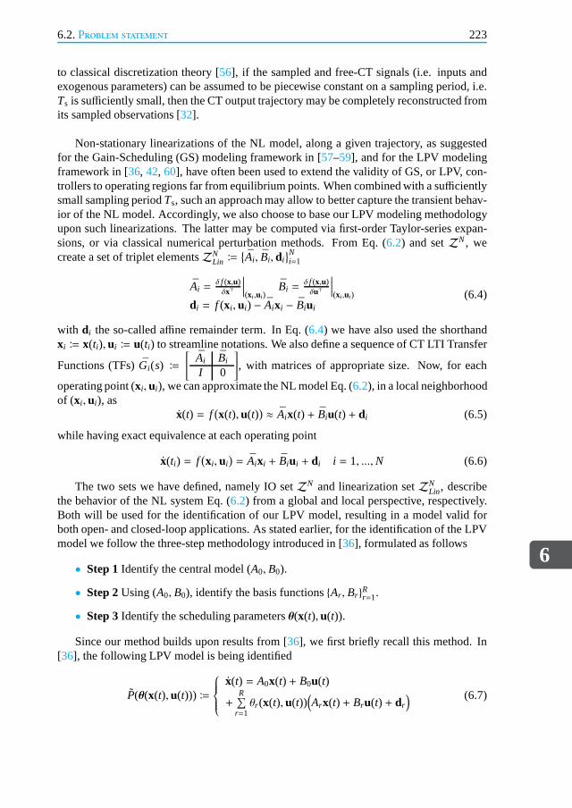
6.2.Problem statement

6

223

to classical discretization theory [56], if the sampled and free-CT signals (i.e. inputs andexogenous parameters) can be assumed to be piecewise constant on a sampling period, i.e.Ts is sufficiently small, then the CT output trajectory may be completely reconstructed fromits sampled observations [32].

Non-stationary linearizations of the NL model, along a given trajectory, as suggestedfor the Gain-Scheduling (GS) modeling framework in [57–59], and for the LPV modelingframework in [36, 42, 60], have often been used to extend the validity of GS, or LPV, con-trollers to operating regions far from equilibrium points.When combined with a sufficientlysmall sampling periodTs, such an approach may allow to better capture the transient behav-ior of the NL model. Accordingly, we also choose to base our LPV modeling methodologyupon such linearizations. The latter may be computed via first-order Taylor-series expan-sions, or via classical numerical perturbation methods. From Eq. (6.2) and setZN, wecreate a set of triplet elementsZN

Lin ≔

Ai , Bi, diNi=1

Ai =δ f (x,u)δx⊤

∣

∣

∣

∣

(xi ,ui)Bi =

δ f (x,u)δu⊤

∣

∣

∣

∣

(xi ,ui )di = f (xi , ui) − Aixi − Biui

(6.4)

with di the so-called affine remainder term. In Eq. (6.4) we have also used the shorthandxi ≔ x(ti), ui ≔ u(ti) to streamline notations. We also define a sequence of CT LTI Transfer

Functions (TFs)Gi(s) ≔

[

Ai Bi

I 0

]

, with matrices of appropriate size. Now, for each

operating point (xi, ui), we can approximate the NL model Eq. (6.2), in a local neighborhoodof (xi , ui), as

x(t) = f(

x(t), u(t)) ≈ Aix(t) + Biu(t) + di (6.5)

while having exact equivalence at each operating point

x(ti) = f(

xi, ui)

= Aixi + Biui + di i = 1, ...,N (6.6)

The two sets we have defined, namely IO setZN and linearization setZNLin, describe

the behavior of the NL system Eq. (6.2) from a global and local perspective, respectively.Both will be used for the identification of our LPV model, resulting in a model valid forboth open- and closed-loop applications. As stated earlier, for the identification of the LPVmodel we follow the three-step methodology introduced in [36], formulated as follows

• Step 1Identify the central model (A0, B0).

• Step 2Using (A0, B0), identify the basis functionsAr , BrRr=1.

• Step 3Identify the scheduling parametersθ(x(t), u(t)).

Since our method builds upon results from [36], we first briefly recall this method. In[36], the following LPV model is being identified

P(θ(x(t), u(t))) ≔

x(t) = A0x(t) + B0u(t)

+R∑

r=1θr (x(t), u(t))

(

Arx(t) + Bru(t) + dr

) (6.7)

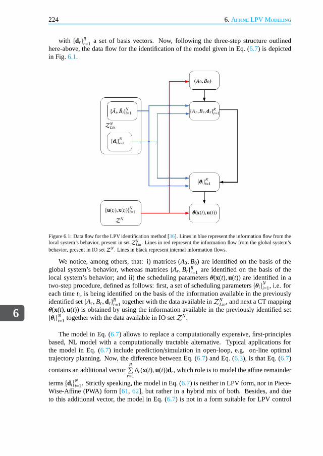
6

224 6. Affine LPV Modeling

with dr Rr=1 a set of basis vectors. Now, following the three-step structure outlinedhere-above, the data flow for the identification of the model given in Eq. (6.7) is depictedin Fig. 6.1.

Figure 6.1: Data flow for the LPV identification method [36]. Lines in blue represent the information flow from thelocal system’s behavior, present in setZN

Lin. Lines in red represent the information flow from the global system’sbehavior, present in IO setZN. Lines in black represent internal information flows.

We notice, among others, that: i) matrices (A0, B0) are identified on the basis of theglobal system’s behavior, whereas matricesAr , BrRr=1 are identified on the basis of thelocal system’s behavior; and ii) the scheduling parametersθ(x(t), u(t)) are identified in atwo-step procedure, defined as follows: first, a set of scheduling parameters

θiNi=1, i.e. for

each timeti , is being identified on the basis of the information available in the previouslyidentified setAr , Br , dr Rr=1 together with the data available inZN

Lin, and next a CT mappingθ(x(t), u(t)) is obtained by using the information available in the previously identified setθiNi=1 together with the data available in IO setZN.

The model in Eq. (6.7) allows to replace a computationally expensive, first-principlesbased, NL model with a computationally tractable alternative. Typical applications forthe model in Eq. (6.7) include prediction/simulation in open-loop, e.g. on-line optimaltrajectory planning. Now, the difference between Eq. (6.7) and Eq. (6.3), is that Eq. (6.7)

contains an additional vectorR∑

r=1θr (x(t), u(t))dr, which role is to model the affine remainder

terms

diNi=1. Strictly speaking, the model in Eq. (6.7) is neither in LPV form, nor in Piece-

Wise-Affine (PWA) form [61, 62], but rather in a hybrid mix of both. Besides, and dueto this additional vector, the model in Eq. (6.7) is not in a form suitable for LPV control

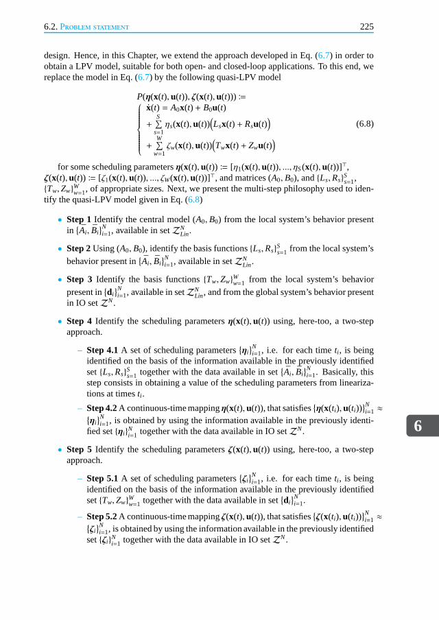
6.2.Problem statement

6

225

design. Hence, in this Chapter, we extend the approach developed in Eq. (6.7) in order toobtain a LPV model, suitable for both open- and closed-loop applications. To this end, wereplace the model in Eq. (6.7) by the following quasi-LPV model

P(η(x(t), u(t)), ζ(x(t), u(t)))≔

x(t) = A0x(t) + B0u(t)

+S∑

s=1ηs(x(t), u(t))

(

Lsx(t) + Rsu(t))

+W∑

w=1ζw(x(t), u(t))

(

Twx(t) + Zwu(t))

(6.8)

for some scheduling parametersη(x(t), u(t)) ≔ [η1(x(t), u(t)), ..., ηS(x(t), u(t))]⊤,ζ(x(t), u(t)) ≔ [ζ1(x(t), u(t)), ..., ζW(x(t), u(t))]⊤, and matrices (A0, B0), andLs,RsSs=1,Tw,ZwWw=1, of appropriate sizes. Next, we present the multi-step philosophy used to iden-tify the quasi-LPV model given in Eq. (6.8)

• Step 1Identify the central model (A0, B0) from the local system’s behavior presentin

Ai , BiNi=1, available in setZN

Lin.

• Step 2Using (A0, B0), identify the basis functionsLs,RsSs=1 from the local system’s

behavior present in

Ai , BiNi=1, available in setZN

Lin.

• Step 3 Identify the basis functionsTw,ZwWw=1 from the local system’s behavior

present in

diNi=1, available in setZN

Lin, and from the global system’s behavior presentin IO setZN.

• Step 4 Identify the scheduling parametersη(x(t), u(t)) using, here-too, a two-stepapproach.

– Step 4.1A set of scheduling parameters

ηiNi=1, i.e. for each timeti , is being

identified on the basis of the information available in the previously identifiedsetLs,RsSs=1 together with the data available in set

Ai , BiNi=1. Basically, this

step consists in obtaining a value of the scheduling parameters from lineariza-tions at timesti .

– Step 4.2A continuous-time mappingη(x(t), u(t)), that satisfies

η(x(ti), u(ti))Ni=1 ≈

ηiNi=1, is obtained by using the information available in the previously identi-

fied setηiNi=1 together with the data available in IO setZN.

• Step 5 Identify the scheduling parametersζ(x(t), u(t)) using, here-too, a two-stepapproach.

– Step 5.1A set of scheduling parameters

ζiNi=1, i.e. for each timeti , is being

identified on the basis of the information available in the previously identifiedsetTw,ZwWw=1 together with the data available in set

diNi=1.

– Step 5.2A continuous-time mappingζ(x(t), u(t)), that satisfies

ζ(x(ti), u(ti))Ni=1 ≈

ζiNi=1, is obtained by using the information available in the previously identified

setζiNi=1 together with the data available in IO setZN.

6

226 6. Affine LPV Modeling

Following this five-step structure, the data flow for the identification of the model givenin Eq. (6.8) is depicted in Fig.6.2.

Figure 6.2: Data flow for the identification of our LPV model Eq. (6.8). Lines in blue represent the informationflow from the local system’s behavior, present in setZN

Lin. Lines in red represent the information flow from theglobal system’s behavior, present in IO setZN. Lines in black represent internal information flows.

Remark 9 LPV properties cannot in general be inferred from underlying LTI properties,i.e. frozen-scheduling deductions do not generally ensurethat LPV modeling characteris-tics will be preserved with rapid parameter variations [63]. Hence, no formal proofs ofconvergence between the NL model and our LPV model may be given via this engineeringpractice.

Remark 10 Step 4.2 andStep 5.2 allow to use the model given by Eq. (6.8) for LPV controldesign. Indeed, without the knowledge of the mappingsη(x(t), u(t)), andζ(x(t), u(t)), onewould be restricted to potentially more conservativeµ control methods, since the schedulingparameters cannot be estimated on-line. Note that finding such smooth mappings is a non-trivial task, and may even require some leap of faith, which one may be willing to take incase the entire working area has been sampled with a dense enough grid.

6.3.Step 1: Identifying the central model (A0, B0)

6

227

Remark 11 We restrict our discussion to full-order modeling, i.e matricesAi and(A0, Ls,Tw)have same size (resp.Bi and(B0,Rs,Zw)).

In the sequel we discuss, in more detail, our five step methodology.

6.3.Step 1: Identifying the central model (A0, B0)As stated earlier, the model (A0, B0) is chosen within all models present in setAi , BiNi=1.A natural approach consists in finding the model which may be defined as the mostcentralone. Further, we will base this model selection within theH∞ framework10, since our pri-mary focus is on modeling for control. In addition, for controller synthesis, design specifi-cations are typically generated on various frequency ranges of interest∆ω = [ω1, ω2], ω1 <

ω2, which led us to use theH∞ norm on a frequency range of relevance, i.e. the‖ · ‖∆ω dis-tance metric defined in the introduction Section as‖G‖∆ω ≔ sup

ω∈∆ωσ(G( jω)) for a TFG( jω)

(see also Appendix A). This central model, i.e. the optimal model,G0(s) ≔

[

A0 B0

I 0

]

,

is chosen as follows: compute, for each modelGi(s) ≔

[

Ai Bi

I 0

]

i ∈ 1, ...,N, the

following meanµi and standard-deviationsi as

∀i ∈ 1, ...,N µi = (1/N)N∑

j=1‖Gi(s) − G j(s)‖∆ω

si =

[

(1/N)N∑

j=1

(

‖Gi(s) − G j(s)‖∆ω − µi

)2]1/2 (6.9)

where‖ · ‖∆ω is obtained11 by minimizing the boundγ subject to the LMI of Eq. (6.48) (seeAppendix A). Next define the following extrema

µ¯= min

iµi , µ = max

iµi , s

¯= min

isi , s= max

isi (6.10)

The optimal modelG0(s) is now designated asG0(s) ≔ Gi(s), with the optimal indexiresulting from a simple, and readily solved, mean versus standard-deviation minimizationproblem

i = arg mini∈1,...,N

(

ρ(

[µi − µ¯]/[µ − µ

¯])2+

(

[si − s¯]/[ s− s

¯])2)

(6.11)

with ρ a user-defined weighting parameter.

6.4.Step 2: Identifying the basis functions Ls,RsSs=1Whereas the role of the central modelG0(s) consists in capturing the most significant linearbehavior of the NL system, the role of the basis functionsLs,RsSs=1 (together with the

10Even though several other norms could be used, theH∞ norm provides guarantees on worst cases.11There are three ways to compute‖·‖∆ω : 1) approximately, through frequency griding of the‖·‖∞ norm; 2) exactly,

through the LMI optimization problems presented in Appendix A; or 3) approximately, through a weightedH∞norm minimization, using a strictly-proper, bandpass filter Wf , centered at∆ω, leading to‖Wf .(·)‖∞.

6

228 6. Affine LPV Modeling

scheduling parameters) consists in capturing the NL behavior of the system. We knowfrom Eq. (6.5) that the NL system may be approximated, in a local neighborhood of (xi , ui),by x(t) ≈ Aix(t)+ Biu(t)+ di . As the affine remainder termdi will be handled in the sequel,we consider here only the following local behavior of the NL systemx(t) ≈ Aix(t)+ Biu(t).Hence, the gap between the local NL behavior and the central model behavior may becharacterized, in a local neighborhood of (xi , ui), as follows

δx(t) = (Ai − A0)x(t) + (Bi − B0)u(t) (6.12)

Now from Eq. (6.12) one can build the following setAi−A0, Bi− B0Ni=1, from which wemay derive the basis functionsLs, RsSs=1, through Singular Value Decompositions (SVD).Such approaches have successfully been applied in the realmof LPV modeling in [36, 64,65]. The approach outlined in this paragraph is not based on anyH∞ norm considerations,rather it is identical to the highly efficient method presented in [36], and consists in firsttransforming the information present, in matrix form, inAi−A0, Bi−B0Ni=1 into a vectorizedform. Now, let

Υ = [1...1] (6.13)

be a row vector of lengthN. Define next the followingΦ andΩ matrices

Φ =

[

vec(A0)vec(B0)

]

⊗ Υ Ω =

[

vec(A1) , ..., vec(AN)vec(B1) , ..., vec(BN)

]

(6.14)

with vec(·) the vertical vectorization of a matrix, and⊗ the Kronecker product. It is clearthat the information contained inAi − A0, Bi − B0Ni=1 is now made available in (Ω − Φ).Next, we can obtain a proper orthogonal decomposition of (Ω−Φ) which gives the principaldirections in the space of the coefficients ofLs, RsSs=1. This is done by obtaining a SVDdecomposition of the form

Ω −Φ = UΣV∗ (6.15)

Finally, let matrixU1..S, with S ≤ nx(nx + nu), contain the firstS columns of the leftsingular vector matrixU in Eq. (6.15), then each basis function pair (Ls,Rs) is simply re-covered from the matricization12 of each column ofU1..S. The chosen value forS willdepend upon the considered application, and its ’optimal’ value represents a trade-off be-tween model accuracy and computational tractability of thecontrol synthesis.

6.5.Step 3: Identifying the basis functions Tw,ZwWw=1The idea here consists in providing a model for the affine remainder terms

diNi=1. Suppose

we can find basis functionsTw,ZwWw=1 and scheduling parametersζ(ti) ≔ [ζ1(ti), ..., ζW(ti)]⊤

such that

∀i ∈ 1, ...,N di

[

xi

ui

]†≈

[

W∑

w=1ζw(ti)Tw

W∑

w=1ζw(ti)Zw

]

(6.16)

with [·]† the left inverse, then by right-multiplying both sides with[x⊤i u⊤i ]⊤ we recover

di ≈W∑

w=1ζw(ti)

(

Twxi + Zwui

)

. To determine the basis functions, we will again use SVDs.

12The operation that turns a vector into a matrix.

6.6.Step 4.1: Identifying the parameters

ηiNi=1

6

229

First, we construct the matricesΛi andΨ such that

Λi = di

[

xi

ui

]†Ψ =

[

vec(Λ1) , ..., vec(ΛN)]

(6.17)

with vec(·) the vertical vectorization of a matrix. Next, we obtain a SVD decomposition ofthe form

Ψ = UΣV∗ (6.18)

Now let matrixU1..W, with W ≤ nx(nx + nu), contain the firstW columns of the leftsingular vector matrixU in Eq. (6.18), then each basis function pairTw,ZwWw=1 is simplyrecovered from the matricization of each column ofU1..W.

Remark 12 Note that the approach outlined inStep 3 could potentially have additionalapplications, within the LPV modeling problem, but also within the true context of systemidentification when identifying a system from noisy measurements.

6.6.Step 4.1: Identifying the parameters

ηiNi=1

We identify here the set of scheduling parameters

ηiNi=1 ≔

η1(ti), ..., ηS(ti)Ni=1 on the ba-

sis of the information available in the previously identified setLs,RsSs=1 together with the

data available in set

Ai , BiNi=1. Indeed, since our focus is mainly on modeling for control,

we choose to approximate the local behavior of the NL system Eq. (6.2). This is doneby obtaining a value of the scheduling parameters from locallinearizations, i.e. by ap-

proximating the LTI modelsGi(s) ≔

[

Ai Bi

I 0

]

with the frozen-scheduling LPV model

Gi(s) ≔

A0 +S∑

s=1ηs(ti)Ls B0 +

S∑

s=1ηs(ti)Rs

I 0

, for i = 1, ...,N. This can be formulated as

follows: for a given user defined frequency range∆ω = [ω1, ω2], find, at each timeti , theoptimal parametersη(ti)Ni=1, with η(ti) ≔ [η1(ti), ..., ηS(ti)]⊤, that minimize

J1(ti) ≔ ‖Gi(s) −Gi(s)‖∆ω i = 1, ...,N (6.19)

Minimizing J1(ti) in Eq. (6.19) is equivalent to minimizing a scalar variable, subjectto the LMI of Eq. (6.48), or to the LMI of Eq. (6.49). These LMIs are function of de-cision variablesP andQ, or F andK. Further, these LMIs are also function of matricesA and B, given hereunder in Eq. (6.22), which are dependent on the decision variables

η1(ti), ..., ηS(ti)

. Due to the product of matricesP andQ (or F andK) with matricesA andB, these LMIs become nonlinear. In such situations the projection lemma has often beenused to provide convex reformulations of the original problem. In our case, unfortunately, astraightforward application of the projection lemma is notachievable, due to the structurednature of our problem (see [66] for additional details). Hence, we choose to use an iterativeapproach to solve Eq. (6.19). The procedure has a two-stage modus operandi: an initial-ization stage, followed by a nonlinear-based refinement stage. The first stage computesreasonable guess values for ˆη(ti). The idea here consists in approximating the maximum

6

230 6. Affine LPV Modeling

gain of the LTI matrices,Ai andBi, in the following way

∀i ∈ 1, ...,N

XA(ηs(ti)) = Ai −(

A0 +S∑

s=1ηs(ti)Ls

)

XB(ηs(ti)) = Bi −(

B0 +S∑

s=1ηs(ti)Rs

)

η(ti) = arg minηs(ti )‖XA(ηs(ti))‖2 + ‖XB(ηs(ti))‖2

(6.20)

This is readily recast into the sum minimization of theL2-induced gains of two staticoperators

∀i ∈ 1, ...,N minimizeηs(ti ),γA,γB

γA + γB

subject to γA > 0 γB > 0[

γAI ⋆

XA(ηs(ti)) I

]

> 0

[

γBI ⋆

XB(ηs(ti)) I

]

> 0

(6.21)

Next, the second stage uses the initial guess values found inEq. (6.21) in order to solveEq. (6.19), through an iterative approach. Here‖ · ‖∆ω is computed via Eq. (6.49) since thelatter is convex in either the (F,K) or (A, B) matrices. These (A, B) matrices in Eq. (6.49)are given by

Gi(s) −Gi(s) ≔

[

A BC D

]

=

Ai 0 Bi

0 A0 +S∑

s=1ηs(ti)Ls B0 +

S∑

s=1ηs(ti)Rs

I −I 0

(6.22)

Our proposed approach is a simple two-step iterative LMI search, in spirit reminiscent

of D-K iteration synthesis [67]. First, partitionF andK, asF =

[

F11 F12

F21 F22

]

, andK =[

K11 K12

K21 K22

]

, with the sub-block sizes matching the partitions in Eq. (6.22). Next, the

procedure reads as follows

1. Start with the initial value ˆη(ti) obtained from Eq. (6.21)

2. In Eq. (6.49) minimizeγ with respect to (F,K)

3. Keep (F12, F22,K12,K22) from step 2 since these variables multiply the unknownsηs(ti). Next in Eq. (6.49), minimizeγ with respect to the free variables(η(ti), F11, F21,K11,K21)

4. Repeat from 2 until convergence or maximum iteration reached

Remark 13 Aside from D-K iteration, similar heuristics appear to workwell in practice,such as model order reduction [68], LPV controller with parameter-dependent scalings[69], or gain-scheduled controller with inexact scheduling parameters [70]. Analogouslyto D-K iteration convergence—for which convergence towards a global optimum, or evena local one, is not guaranteed [71, 72]—the above iterative method does not inherit anyconvergence certificates, however in practice convergencehas been achieved within a fewiterations.

6.7.Step 4.2: Obtaining the mapping η(x(t), u(t))

6

231

Remark 14 In Appendix B, we examine a specific case for which the optimalvalue of thescheduling parameters can be computed, thus avoiding any nonlinear iterative approach.

6.7.Step 4.2: Obtaining the mapping η(x(t), u(t))The aim is here to find a suitable representation, or smooth CTmappingg(·), that satis-fiesη(t) = g(x(t), u(t)) and

η(x(ti), u(ti))Ni=1 ≈

ηiNi=1. To this end, this mapping will be

obtained by using the information available in the previously identified setηiNi=1 togetherwith the data available in IO setZN.

Now, for physically-intuitive plants, one may select the required states and inputs ing(x(t), u(t)), based upon engineering judgment, and derive these mappings through popularcurve-fitting methods. For non-transparent systems, i.e. exhibiting significant dependencesamong variables, one may consider formal/systematic tools such as: orthogonal/radial ba-sis functions, principal component analysis, statisticalanalysis, fuzzy tools, or Neural Net-works (NN). Regarding NN, it is well-known that, under mild assumptions on continuityand boundedness, a network of two layers13 can be trained to approximate any IO relation-ship arbitrarily well, provided there are enough neurons inthe hidden layer [73, 74]. Hence,NN have found a wide range of applications in control theory [75]. But despite their pow-erful features, NN have only seen limited usage in the LPV field [76–78]. This said, wechoose here to base theg(·) modeling on NN. We will further illustrate the applicability ofa two-layer feedforward NN, the first being sigmoid and the second linear, withl neurons(l large enough), such that

η(t) = g(x(t), u(t)) = Cη.sη(t) (6.23)

withsη(t) =Woη .κ

(

Wxη x(t) +Wuηu(t) +Wbη)

(6.24)

andWoη ∈ RS×l , Wxη ∈ Rl×nx , Wuη ∈ Rl×nu containing the output and hidden layer weights.Further,Wbη ∈ Rl contains the sets of biases in the hidden layer,Cη ∈ RS×S contains theoutput linear maps, andκ(·) is the activation function, taken as a continuous, diagonal, dif-ferentiable, and bounded static sigmoid nonlinearity. Here, all NN models will be basedupon a classical feedforward network, with the hyperbolic tangent activation transfer func-tion in the hidden layer, and backpropagation training for the weights and biases.

6.8.Steps 5.1 and 5.2: Identifying the parameters

ζiNi=1 and

obtaining the mapping ζ(x(t), u(t))We identify here the set of scheduling parameters

ζiNi=1 ≔

ζ1(ti), ..., ζW(ti)Ni=1 on the basis

of the information available in the previously identified set Tw,ZwWw=1 together with the

data available in set

diNi=1. This problem may be formulated as follows: find, at each time

ti , the optimal parametersζ(ti)Ni=1, with ζ(ti) ≔ [ζ1(ti), ..., ζW(ti)]⊤, that minimize

J2(ti) ≔ ‖di −W∑

w=1

ζw(ti)(

Twxi + Zwui

)

‖2 i = 1, ...,N (6.25)

13The first being hidden sigmoid and the second linear.

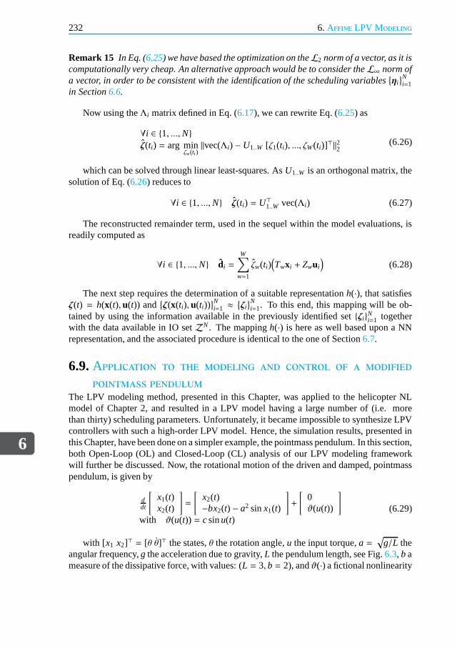
6

232 6. Affine LPV Modeling

Remark 15 In Eq. (6.25) we have based the optimization on theL2 norm of a vector, as it iscomputationally very cheap. An alternative approach wouldbe to consider theL∞ norm ofa vector, in order to be consistent with the identification ofthe scheduling variables

ηiNi=1

in Section6.6.

Now using theΛi matrix defined in Eq. (6.17), we can rewrite Eq. (6.25) as

∀i ∈ 1, ...,Nζ(ti) = arg min

ζw(ti )‖vec(Λi) − U1..W [ζ1(ti), ..., ζW(ti)]⊤‖22 (6.26)

which can be solved through linear least-squares. AsU1..W is an orthogonal matrix, thesolution of Eq. (6.26) reduces to

∀i ∈ 1, ...,N ζ(ti) = U⊤1..W vec(Λi) (6.27)

The reconstructed remainder term, used in the sequel withinthe model evaluations, isreadily computed as

∀i ∈ 1, ...,N di =

W∑

w=1

ζw(ti)(

Twxi + Zwui

)

(6.28)

The next step requires the determination of a suitable representationh(·), that satisfiesζ(t) = h(x(t), u(t)) and

ζ(x(ti), u(ti))Ni=1 ≈

ζiNi=1. To this end, this mapping will be ob-

tained by using the information available in the previouslyidentified setζiNi=1 togetherwith the data available in IO setZN. The mappingh(·) is here as well based upon a NNrepresentation, and the associated procedure is identicalto the one of Section6.7.

6.9.Application to the modeling and control of a modifiedpointmass pendulum

The LPV modeling method, presented in this Chapter, was applied to the helicopter NLmodel of Chapter 2, and resulted in a LPV model having a large number of (i.e. morethan thirty) scheduling parameters. Unfortunately, it became impossible to synthesize LPVcontrollers with such a high-order LPV model. Hence, the simulation results, presented inthis Chapter, have been done on a simpler example, the pointmass pendulum. In this section,both Open-Loop (OL) and Closed-Loop (CL) analysis of our LPVmodeling frameworkwill further be discussed. Now, the rotational motion of thedriven and damped, pointmasspendulum, is given by

ddt

[

x1(t)x2(t)

]

=

[

x2(t)−bx2(t) − a2 sinx1(t)

]

+

[

0ϑ(u(t))

]

with ϑ(u(t)) = csinu(t)(6.29)

with [x1 x2]⊤ = [θ θ]⊤ the states,θ the rotation angle,u the input torque,a =√

g/L theangular frequency,g the acceleration due to gravity,L the pendulum length, see Fig.6.3, b ameasure of the dissipative force, with values: (L = 3, b = 2), andϑ(·) a fictional nonlinearity

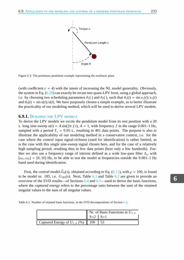
6.9.Application to the modeling and control of a modified pointmass pendulum

6

233

Figure 6.3: The pointmass pendulum example representing the nonlinear plant.

(with coefficientc = 4) with the intent of increasing the NL model generality. Obviously,the system in Eq. (6.29) can exactly be recast into quasi-LPV form, using a global approach,i.e. by choosing two scheduling parametersθ1(·) andθ2(·), such thatθ1(t) = sinx1(t)/x1(t)andθ2(t) = sinu(t)/u(t). We have purposely chosen a simple example, as to better illustratethe practicality of our modeling method, which will be used to derive several LPV models.

6.9.1.Building the LPV modelsTo derive the LPV models we excite the pendulum model from itsrest position with a 20s. long sine-sweepu(t) = Asin(2π. f .t), A = 1, with frequencyf in the range 0.001–1 Hz,sampled with a periodTs = 0.05 s., resulting in 401 data points. The purpose is also toillustrate the applicability of our modeling method in a conservative context, i.e. for thecase where the control input signal-richness (used for identification) is rather limited, asis the case with this single sine-sweep signal chosen here, and for the case of a relativelyhigh sampling period, resulting thus in few data points (here only a few hundreds). Fur-ther we also use a frequency range of interest defined as a widelow-pass filter∆ω with[ω1, ω2] = [0, 10] Hz, to be able to test the model at frequencies outside the0.001–1 Hzband used during identification.

First, thecentralmodelG0(s), obtained according to Eq. (6.11), with ρ = 100, is foundto be model nr. 185, i.e.G185(s). Next, Table6.1 and Table6.2 are given to provide anoverview of the SVD results—of Sections6.4and6.5—used to derive the basis functions,where thecaptured energyrefers to the percentage ratio between the sum of the retainedsingular values to the sum of all singular values.

Table 6.1: Number of retained basis functions, in the SVD decompositions of Section6.4.

Nr. of Basis Functions inU1..S

S=2 S=1

Captured Energy ofU1..S (%) 100 53

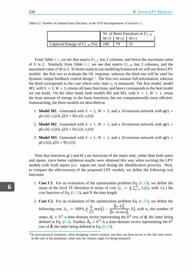
6

234 6. Affine LPV Modeling

Table 6.2: Number of retained basis functions, in the SVD decompositions of Section6.5.

Nr. of Basis Functions inU1..W

W=3 W=2 W=1

Captured Energy ofU1..W (%) 100 79 51

From Table6.1, we see that matrixU1..S has 2 columns, and hence the maximum valueof S is 2. Similarly from Table6.2, we see that matrixU1..W has 3 columns, and themaximum value ofW is 3. To better analyze our modeling framework we will use three LPVmodels: the first two to evaluate the OL response, whereas thethird one will be used fordynamic output feedback control design14. The first two assume full-information, whereasthe third corresponds to the case where only statex1 is measured. The first model, modelM1, with S = 2,W = 3, retains all basis functions, and hence corresponds to thebest modelwe can build. On the other hand, both models M2 and M3, withS = 1, W = 1, retainthe least amount of energy in the basis functions, but are computationally most efficient.Summarizing, the three models are described as

1. Model M1. Generated withS = 2, W = 3, and a 10-neurons network withη(t) =g(x1(t), x2(t)), ζ(t) = h(x1(t), x2(t))

2. Model M2. Generated withS = 1, W = 1, and a 10-neurons network withη(t) =g(x1(t), x2(t)), ζ(t) = h(x1(t), x2(t))

3. Model M3. Generated withS = 1, W = 1, and a 10-neurons network withη(t) =g(x1(t)), ζ(t) = h(x1(t))

Note that functionsg(·) andh(·) are functions of the states only, rather than both statesand inputs, since better validation results were obtained this way when exciting the LPVmodels with fresh inputs (i.e. inputs not used during the identification process). Next,to compare the effectiveness of the proposed LPV models, we define the following costfunctions

1. Cost C1. For an evaluation of the optimization problem Eq. (6.19), we define themean of the local TF deviation in terms of costJP1 ≔

1N

∑Ni=1 J1(ti), with J1(·) the

cost function of Eq. (6.19), andN the data length.

2. Cost C2. For an evaluation of the optimization problem Eq. (6.25), we define the

following cost JP2 ≔ 100%. 1nx

nx∑

k=1max

(

1 −∥

∥

∥δk−δk

∥

∥

∥

2∥

∥

∥δk−mean(δk)∥

∥

∥

2

, 0)

, with nx the number of

states,δk ∈ RN a time-domain vector representing thekth row of d, the latter beingdefined in Eq. (6.4). Further,δk ∈ RN is a time-domain vector representing thekth

row of d, the latter being defined in Eq. (6.28).

14In most practical situations, when designing control systems, one does not have access to the full state-vector.In the case of the pendulum, often only the rotation angleθ is being measured.

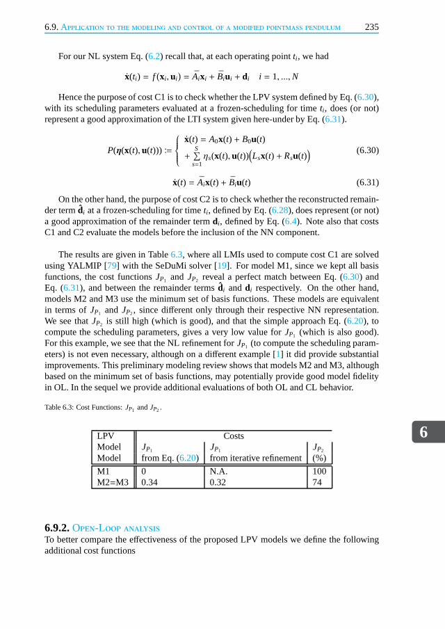
6.9.Application to the modeling and control of a modified pointmass pendulum

6

235

For our NL system Eq. (6.2) recall that, at each operating pointti , we had

x(ti) = f(

xi, ui)

= Aixi + Biui + di i = 1, ...,N

Hence the purpose of cost C1 is to check whether the LPV systemdefined by Eq. (6.30),with its scheduling parameters evaluated at a frozen-scheduling for time ti , does (or not)represent a good approximation of the LTI system given here-under by Eq. (6.31).

P(η(x(t), u(t))) ≔

x(t) = A0x(t) + B0u(t)

+S∑

s=1ηs(x(t), u(t))

(

Lsx(t) + Rsu(t)) (6.30)

x(t) = Aix(t) + Biu(t) (6.31)

On the other hand, the purpose of cost C2 is to check whether the reconstructed remain-der termdi at a frozen-scheduling for timeti , defined by Eq. (6.28), does represent (or not)a good approximation of the remainder termdi , defined by Eq. (6.4). Note also that costsC1 and C2 evaluate the models before the inclusion of the NN component.

The results are given in Table6.3, where all LMIs used to compute cost C1 are solvedusing YALMIP [79] with the SeDuMi solver [19]. For model M1, since we kept all basisfunctions, the cost functionsJP1 and JP2 reveal a perfect match between Eq. (6.30) andEq. (6.31), and between the remainder termsdi anddi respectively. On the other hand,models M2 and M3 use the minimum set of basis functions. Thesemodels are equivalentin terms ofJP1 and JP2, since different only through their respective NN representation.We see thatJP2 is still high (which is good), and that the simple approach Eq. (6.20), tocompute the scheduling parameters, gives a very low value for JP1 (which is also good).For this example, we see that the NL refinement forJP1 (to compute the scheduling param-eters) is not even necessary, although on a different example [1] it did provide substantialimprovements. This preliminary modeling review shows thatmodels M2 and M3, althoughbased on the minimum set of basis functions, may potentiallyprovide good model fidelityin OL. In the sequel we provide additional evaluations of both OL and CL behavior.

Table 6.3: Cost Functions:JP1 andJP2 .

LPV CostsModel JP1 JP1 JP2

Model from Eq. (6.20) from iterative refinement (%)

M1 0 N.A. 100M2=M3 0.34 0.32 74

6.9.2.Open-Loop analysisTo better compare the effectiveness of the proposed LPV models we define the followingadditional cost functions

6

236 6. Affine LPV Modeling

1. Cost C3. For a comparison of time-domain outputs inl2[0,∞), we use fresh datasets, namely step-inputs, and sine-inputs at varying amplitudes and frequencies, and

compute the Best-FiT (BFT)≔ 100%. 1nx

nx∑

k=1max

(

1−∥

∥

∥sk−sk

∥

∥

∥

2∥

∥

∥sk−mean(sk)∥

∥

∥

2

, 0)

with sk ∈ RN a

time-domain vector representing thekth row of x (x being the state-vector of the NLsystem), and similarlysk ∈ RN being the LPV counterpart.

2. Cost C4. Using the variables defined forC3, we compute the Variance-Accounted-For (VAF)

VAF ≔ 100%. 1nx

nx∑

k=1max

(

1− var(sk−sk)var(sk) , 0

)

. Roughly speaking the VAF tends to capture

signal closeness in terms of their respective "shapes".

In this section we have added the NN part to the LPV models (we use the NN MAT-LAB Toolbox). All models become now quasi-LPV models (also written as qLPV). Wewill compare next the behavior of the CT quasi-LPV models with that of the CT NL sys-tem. We excite the quasi-LPV models with data sets not used during the modeling build-up.First, we use sine-inputs, for several fixed amplitudes and fixed frequencies (again not usedduring identification), and present the respective BFT and VAF for each model in Table6.4through6.6.

Overall all three models exhibit very good to excellent fit with the NL model, forinput amplitudes below one (i.e. the value used during identification). The accuracy ofthese quasi-LPV models diminishes when the input amplitudeis increased above one, eventhough model M2 still retains a very good fit. We also note thatmodel M2, even thoughbased on fewer basis functions than M1, is roughly at least asgood as model M1. Thismay be explained by the fact that the NN models were trained with a very small data set.Indeed good identification data sets may be two orders of magnitude bigger, in the tens ofthousands of points rather than a few hundreds [80]. Hence, and even though there is nomeasurement noise in these simulations, a model with fewer to-be-estimated parameters,like M2, may provide, in this case, a higher quality model. The fit for model M3 is slightlyworse than that of M2, e.g. for input amplitudes above one. This may be explained by thefact that the identification of M3’s NN was based on statex1 only.

Table 6.4: Time response to sine-inputs for M1. Left value isBFT (%), Right value is VAF (%).

Input Input Frequency (Hz)Amplitude 0.25 0.5 0.75 1

0.25 93 99 94 100 96 100 97 1000.5 97 100 91 99 94 100 94 1000.75 93 100 90 99 91 99 92 1001 94 100 91 99 90 99 90 991.5 78 97 81 97 79 97 73 951.75 0 0 54 88 69 95 61 92

6.9.Application to the modeling and control of a modified pointmass pendulum

6

237

Table 6.5: Time response to sine-inputs for M2. Left value isBFT (%), Right value is VAF (%).

Input Input Frequency (Hz)Amplitude 0.25 0.5 0.75 1

0.25 93 100 87 98 90 99 91 990.5 94 100 87 98 88 99 89 990.75 96 100 90 99 90 99 90 991 94 100 94 100 93 100 91 991.5 83 97 86 98 80 98 77 971.75 80 96 77 96 68 95 63 94

Table 6.6: Time response to sine-inputs for M3. Left value isBFT (%), Right value is VAF (%).

Input Input Frequency (Hz)Amplitude 0.25 0.5 0.75 1

0.25 91 99 87 98 90 99 90 990.5 93 99 86 97 88 98 88 990.75 95 100 88 98 87 98 89 991 97 100 91 99 88 98 81 971.5 73 95 85 98 81 97 62 941.75 55 90 74 96 70 94 53 91

Finally, we also compare the model responses to a step input of amplitudeA = 0.5, withthe outcomes given in Table6.7, and Fig.6.4 through6.6, where again the respective highmodel quality is being confirmed.

Table 6.7: Time response to step input of AmplitudeA = 0.5.

Quasi-LPV CostsModel BFT (%) VAF (%)

M1 70 97M2 72 98M3 55 96

We do see that all models exhibit some steady-state error on state x1. This may po-tentially be attributed to the training of the NN models, i.e. in this case with few data. Insummary, model M2 provides good model fidelity in OL, coupledwith slightly better com-putational efficiency than model M1 (since having fewer scheduling parameters, and hencefewer NN models to evaluate), and may thus be used for OL prediction, whereas model M3has also shown to be a suitable candidate for subsequent controller design, in a dynamic

6

238 6. Affine LPV Modeling

output feedback framework (based upon measurementx1).

0 1 2 3 4 5 6 7 8 9 10−0.2

0

0.2

0.4

0.6

0.8

Time (s)

Sta

tes

Figure 6.4: M1 outputs for step input of AmplitudeA = 0.5 (legend: ’–.’ NL x1; ’– –’ NL x2; ’–’ qLPV x1; ’.’qLPV x2).

0 1 2 3 4 5 6 7 8 9 10−0.2

0

0.2

0.4

0.6

0.8

Time (s)

Sta

tes

Figure 6.5: M2 outputs for step input of AmplitudeA = 0.5 (legend: ’–.’ NL x1; ’– –’ NL x2; ’–’ qLPV x1; ’.’qLPV x2).

0 1 2 3 4 5 6 7 8 9 10−0.2

0

0.2

0.4

0.6

0.8

Time (s)

Sta

tes

Figure 6.6: M3 outputs for step input of AmplitudeA = 0.5 (legend: ’–.’ NL x1; ’– –’ NL x2; ’–’ qLPV x1; ’.’qLPV x2).

6.9.3.Closed-Loop analysisThe objective of this section is to evaluate the quasi-LPV model M3 in a CL setting. Tothis end, we define the generalized plantGP(s) which maps the exogenous inputsw =[r⊤ n⊤]⊤ and control inputsu, to controlled outputsz = [zu

⊤ zp⊤]⊤ and measured outputs

v = [r⊤ e⊤]⊤, see Fig.6.7. The signals consist further ofr the reference signals,n thesensors noise,e the tracking errors,zu the actuators performance signal (to limit actuatordeflection magnitudes and rates), andzp the desired performance in terms of closed-loopsignal responses. The plant used for control synthesis is denotedP (plantP0 and uncertaintyΘ will be addressed in the sequel), and for the weights, we use the standard robust controlweights, which include the performance weight Wp(s), the actuator weight Wu(s), and thesensor noise weight Wn(s), all given in Appendix C. The generalized plantGP(s) is further

6.9.Application to the modeling and control of a modified pointmass pendulum

6

239

Figure 6.7: Control synthesis: two degrees-of-freedom control structure.

given by

zu

zp

re

=

0 0 Wu

Wp 0 −Wp PI 0 0I −Wn −P

rnu

(6.32)

The goal of the control synthesis consists in finding a dynamic controllerK(s) thatestablishes closed-loop stability, while guaranteeing aL2-gain boundγ from the exogenousinputsw to the controlled outputsz, such that

∫ T

0z⊤(t)z(t) dτ ≤ γ2

∫ T

0w⊤(t)w(t) dτ ∀T ≥ 0 (6.33)

In the sequel, we will synthesize four controllers—oneH∞ LTI, one robustµ LTI, andtwo LPV ones—and compare their reference tracking performance to step reference in-puts. The controller synthesis is based upon a two-degrees-of-freedom control structure,see Fig.6.7. The feedback part is used to reduce the effect of uncertainty, whereas the feed-forward part is added to improve tracking performance [81], and for optimality, both willbe designed in one step. These four controllers are defined asfollows

• Controller 1: H∞ LTI controller . The purpose is here to synthesize a controllerwhich is not based on model M3, but rather based upon a nominalLTI model. Thislatter model is obtained from a single linearization, at a rest position, of the NL

model defined in Eq. (6.29). This nominal LTI modelPnom≔

[

Anom Bnom

[1 0] 0

]

, used

6

240 6. Affine LPV Modeling

for control design, is computed via a first-order Taylor-series expansion of the NLmodel, at its equilibrium point [x1 x2]⊤ = [0 0]⊤, see Appendix C. Further, for thisH∞ LTI controller, the control synthesis does not include any robustness with respectto some uncertaintyΘ, hence in Fig.6.7we have

P = P0 = Pnom (6.34)

Now, with Eq. (6.34) in mind, we can rewrite Eq. (6.32) as follows

(

zv

)

= GP

(

wu

)

(6.35)

with GP(s) the generalized plant. Obtaining here a LTI controllerK(s) that mini-mizes theL2-gain boundγ from the exogenous inputsw to the controlled outputsz,is equivalent to the minimization of theH∞ norm of a standard, weighted, mixed-sensitivity S/KS criterion. Here, the controllerK(s) is computed such that [82]

K = arg minK‖Fl

(

GP,K)‖∞ (6.36)

We will consider this controller as the benchmark controller. The next three con-trollers will be synthesized using the LPV model M3, and willalso be compared tothis benchmark controller.

• Controller 2: Robust µ LTI controller . First, the identified affine LPV model M3,as defined in Eq. (6.3), is given by

P(θ(t)) ≔

x(t) = A0x(t) + B0u(t) +R∑

r=1θr (t)

(

Arx(t) + Bru(t))

(6.37)

with R = S +W, S andW the number of basis functions retained in Section6.4and6.5, respectively, and

[θ1(t), ..., θR(t)]⊤ ≔[

η1(t), ..., ηS(t), ζ1(t), ..., ζW(t)]⊤

[A1, ...,AR] ≔ [L1, ..., LS,T1, ...,TW][B1, ..., BR] ≔ [R1, ...,RS,Z1, ...,ZW]

(6.38)

Now, it is also useful to first rescale plantP(θ(t)) in Eq. (6.37) as follows

P(α(t)) ≔

x(t) = A0x(t) + B0u(t)

+R∑

r=1αr (t)

(

Arx(t) + Bru(t)) (6.39)

such thatα(t) ≔ [α1(t), ..., αR(t)]⊤, with |αr (t)| ≤ 1. Here, the generalized plantGP(s)has a linear fractional dependence on the scheduling parameterα(t). This plantGP(s)can be represented by the upper LFT interconnection

(

zv

)

= GP

(

wu

)

= Fu(M,Θ)

(

wu

)

(6.40)

6.9.Application to the modeling and control of a modified pointmass pendulum

6

241

whereM(s) is a known LTI plant, see Fig.6.8. Further,Θ ≔ blockdiag(α1Ik1, ..., αRIkR)represents some block diagonal operator specifying how thescheduling parametersenter the plant dynamics, andIkr Rr=1 denotes identity matrices whose sizes corre-spond, in a sense, to the "complexity" of the scheduling parameter variations. Next,the feedback structure associated with the LFT interconnection Eq. (6.40) is given by

zθzv

= M

wθ

wu

wθ = Θzθ

(6.41)

with zθ, andwθ, the inputs and outputs of operatorΘ, shown in Fig.6.8.

Figure 6.8: StandardM − Θ − K robust control framework.

We further proceed by treating the scheduling parameter variations, i.e. given inΘ, asfixed uncertainties (not measured on-line). This represents an approximation of theLPV model given in Eq. (6.39), which is here considered as a set of LTI models ratherthan a time-varying model. This scheduling parameter variations is addressed herewithin the robust control framework, by consideringΘ as a time-invariant uncertainty,such that

σ(Θ) ≤ 1 (6.42)

The CL operator from exogenous inputsw to controlled outputsz is given by

T(M,K,Θ) = Fl(

Fu(M,Θ),K)

(6.43)

with K(s) the to-be-synthesized controller. Again, the goal of the controller is tominimize theL2-gain boundγ from the exogenous inputsw to the controlled outputsz, despite the uncertaintyΘ. Based upon Eq. (6.42) and small gain considerations [83,84], this goal is approximated by the minimization of theH∞ norm ofFl

(

M,K)

. Now,if Θ presents some structure, better performance may be obtained by synthesizingK(s) through D-K iteration [67, 85]

6

242 6. Affine LPV Modeling

K = arg minK

infD,D−1∈H∞

‖DFl(

M,K)

D−1‖∞ (6.44)

with D(s) a stable and minimum-phase scaling matrix, chosen such that D(s)Θ =ΘD(s). Using [86] we obtain, for our example (see Appendix C for the problem data),after five iterations, a 12th order controller based upon an 8th orderD(s)-scaling. Thecontroller is further reduced to 5th order, after balancing and Hankel-norm model re-duction [87], without any significant effect on CL robustness/performance.

In summary, we have obtained a single robust LTI controller,for a family of LTIplants. Recall however that a major approximation was made,namely the LPV modelin Eq. (6.39) is considered as a set of LTI models, by assumingΘ to be time-invariant.Clearly, such an approach is not sufficient to prove stability and performance of theoriginal, time-varying system, i.e. the LPV model in Eq. (6.39) [88]. In other words,theL2-gain from the exogenous inputsw to the controlled outputsz may be muchhigher than theH∞ norm of DFl

(

M,K)

D−1. This robust control approach shouldonly be viewed as a necessary condition to prove stability and performance of theoriginal LPV system. In other words, if the controllerK(s), obtained from Eq. (6.44),does not meet the desired stability and performance objectives, then it is pointless toconsider other controllers, such as LPV ones, that do take the time-varying aspect ofthe system into account. This said, this robust control approach, as presented here,is known to work well in practice for scheduling parameters having sufficiently slowtime-variations.

Let us now examine a more sophisticated control approach, which takes the time-varying nature of the scheduling parameters into account. To this end, we consider nowcontrollers which are also in LPV form, and hence also time-varying. The goal of anH∞-based, output-feedback, control problem for LPV systems consists in finding, for all pa-rameter trajectories15 Θ(t) ≔ blockdiag(α1(t)Ik1, ..., αR(t)IkR), a dynamic controllerK(s)that establishes closed-loop stability, while truly minimizing theL2-gain boundγ from theexogenous inputsw to the controlled outputsz.

Over the years the subject of LPV control has received much attention, resulting in aplethora of control methods. Although a full review of LPV control methods is beyond thescope of this Chapter, we briefly mention here the following classifications

• So-called polytopic—also known as quadratic—techniques [7, 89–92], versus so-called scaled small-gain—also known as Linear Fractional Representations (LFR) ornorm-bounded—approaches [6, 8, 9, 12, 13, 92–94].

• So-called Parameter-Independent Lyapunov Function (PILF) techniques (such as themethods listed in the previous alinea), versus so-called Parameter-Dependent Lya-punov Function (PDLF)—also known as griding—approaches [10, 11, 69, 70, 95–99].

15Notice that nowΘ(t) is a time-varying operator.

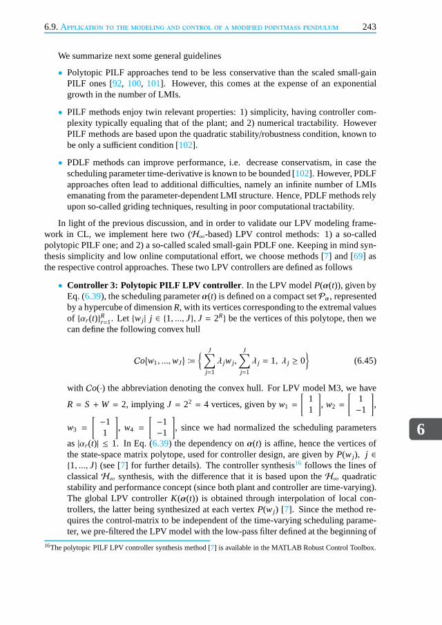
6.9.Application to the modeling and control of a modified pointmass pendulum

6

243

We summarize next some general guidelines

• Polytopic PILF approaches tend to be less conservative thanthe scaled small-gainPILF ones [92, 100, 101]. However, this comes at the expense of an exponentialgrowth in the number of LMIs.

• PILF methods enjoy twin relevant properties: 1) simplicity, having controller com-plexity typically equaling that of the plant; and 2) numerical tractability. HoweverPILF methods are based upon the quadratic stability/robustness condition, known tobe only a sufficient condition [102].

• PDLF methods can improve performance, i.e. decrease conservatism, in case thescheduling parameter time-derivative is known to be bounded [102]. However, PDLFapproaches often lead to additional difficulties, namely an infinite number of LMIsemanating from the parameter-dependent LMI structure. Hence, PDLF methods relyupon so-called griding techniques, resulting in poor computational tractability.

In light of the previous discussion, and in order to validateour LPV modeling frame-work in CL, we implement here two (H∞-based) LPV control methods: 1) a so-calledpolytopic PILF one; and 2) a so-called scaled small-gain PDLF one. Keeping in mind syn-thesis simplicity and low online computational effort, we choose methods [7] and [69] asthe respective control approaches. These two LPV controllers are defined as follows

• Controller 3: Polytopic PILF LPV controller . In the LPV modelP(α(t)), given byEq. (6.39), the scheduling parameterα(t) is defined on a compact setPα, representedby a hypercube of dimensionR, with its vertices corresponding to the extremal valuesof αr (t)Rr=1. Let w j | j ∈ 1, ..., J, J = 2R be the vertices of this polytope, then wecan define the following convex hull

Co

w1, ...,wJ

≔

J∑

j=1

λ jw j ,

J∑

j=1

λ j = 1, λ j ≥ 0

(6.45)

with Co(·) the abbreviation denoting the convex hull. For LPV model M3, we have

R = S +W = 2, implying J = 22 = 4 vertices, given byw1 =

[

11

]

, w2 =

[

1−1

]

,

w3 =

[

−11

]

, w4 =

[

−1−1

]

, since we had normalized the scheduling parameters

as |αr (t)| ≤ 1. In Eq. (6.39) the dependency onα(t) is affine, hence the vertices ofthe state-space matrix polytope, used for controller design, are given byP(w j), j ∈1, ..., J (see [7] for further details). The controller synthesis16 follows the lines ofclassicalH∞ synthesis, with the difference that it is based upon theH∞ quadraticstability and performance concept (since both plant and controller are time-varying).The global LPV controllerK(α(t)) is obtained through interpolation of local con-trollers, the latter being synthesized at each vertexP(w j) [7]. Since the method re-quires the control-matrix to be independent of the time-varying scheduling parame-ter, we pre-filtered the LPV model with the low-pass filter defined at the beginning of

16The polytopic PILF LPV controller synthesis method [7] is available in the MATLAB Robust Control Toolbox.

6

244 6. Affine LPV Modeling

Section6.9.1. A gainγ = 0.92, in Eq. (6.33), was achieved with the weights definedin Appendix C. Although the synthesized controllerK(α(t)) is time-varying—andhence represents an improvement compared to the previous LTI µ controller—thequadratic stability and performance concept assumes arbitrarily fast varying schedul-ing parametersα(t). Obviously this may result in some conservatism, in case thescheduling parameters have a bounded rate of variation.

• Controller 4: Small-gain PDLF LPV controller . This last controller is also referredin the sequel as the LPV-LFT controller. Again, both plant and controller are depen-dent on the time-varying scheduling parameterΘ(t) ≔ blockdiag(α1(t)Ik1, ..., αR(t)IkR).The CL operator from exogenous inputsw to controlled outputsz is adjusted fromEq. (6.43) to become

Tlpv(M,K,Θ(t)) = Fl(

Fu(M,Θ(t)), Fl(K,Θ(t)))

(6.46)

The to-be-designed LPV controllerK(Θ(t)) is obtained by minimizing theL2-normof operatorTlpv [69]. Moreover, the controller synthesis method also takes parametertime-derivative into account, implying a dependence on both Θ(t) and its derivativeΘ(t). This results in an infinite-dimensional LMI problem [69] which, in our case,was tackled by using a small grid, containing only the extrema ofΘ(t) andΘ(t). Sincethe method [69] is an iterative method17, good starting values for the scalings wereobtained by performing a robustµ synthesis, with constant scalings, on the (A0, B0)plant (this plant is defined in Eq. (6.39)). A gainγ = 0.51, in Eq. (6.33), was achievedwith the weights defined in Appendix C, after ten iterations.

Remark 16 The purpose of this CL experiment is not so much on specific aspects relatedto controller weight selection, but rather on highlightingany general similarities or differ-ences, obtained when synthesizing various controllers, while using two modeling options:either LTI or our LPV based method. Similarly, and although,for generality, some robust-ness with respect to signal noise was included during the controller synthesis process (withweight Wn(s)), the simulation results, presented hereunder, consider only reference trackingin a noise-free and disturbance-free environment.

Discussion of resultsThe validation of all controllers, on the NL plant, is done using step inputs on thex1 refer-ence signal, starting from a zero initial condition, i.e. pendulum at rest, see Fig.6.9–Fig.6.11.With respect to our LPV modeling method, we provide the following main conclusions andrecommendations:

• TheH∞ controller exhibits a steady-state error, which remains persistent despite sev-eral modifications of the performance weightWP(s). Compared to theH∞ controller,which is designed on a linearization of the NL plant, all other controllers designedusing our LPV modeling methodology, i.e. on model M3, do not exhibit any steady-state error, and hence achieve much better reference tracking. This is achieved eventhough model M3 has been built with the least number of basis functions.

17The small-gain PDLF LPV controller synthesis method [69] is not available in the MATLAB Robust ControlToolbox.

6.9.Application to the modeling and control of a modified pointmass pendulum

6

245

• Best practice would be to first design a robustµ controller (especially if the NN modelhas been trained with few data), and view it as a benchmark design. Then, it wouldbe interesting to implement at least one PILF LPV control method, and one PDLFLPV control method, in order to be able to compare results.

0 2 4 6 8 10 12 14 16 18 20−0.2

0

0.2

0.4

0.6

0.8

1

1.2

Time (s.)

Sta

tes

Reference

Hinfinity

Mu

LPV−Polytopic

LPV−LFT

Figure 6.9: Closed-Loop step response of NL model with controllers: re f erence→ x1. Cyan line: H∞controller. Red dotted line:µ controller. Black dash-dotted line: LPV-Polytopic controller. Blue dashedline: LPV-LFT controller.

With regard to control, we provide the following main conclusions:

• The robustµ controller and the polytopic PILF LPV controller exhibit very similartracking performance, although the control input of the latter one is much smoother,see Fig.6.11.

• Comparison of robustµ control with several LPV control methods has primarily beenaddressed in [103–107]. Except for [107], all authors have reported that LPV meth-ods were less conservative than a standardµ approach. Indeed, the distinct advantageof LPV control methods is based upon the on-line measurementof the schedulingparameters (and potentially its derivatives). However forLPV-LFT methods, thisadvantage needs to be put into perspective, since all LPV-LFT control methods (ex-cept for the most prominent contribution [94]) have been based upon static scaling,whereasµ uses dynamic scaling.

• If additional robustness is required, to account for unmodelled dynamics and NLeffects, then one may add a complex full-block input multiplicative uncertaintyΘc(s)at the input of the plant. The uncertainty structureΘ(s) in Fig. 6.8is then replaced by

a mixed, real and complex, uncertainty structure

[

Θc 00 Θ

]

, for which several LPV

control methods exist, e.g. [8, 69].

• If knowledge of the scheduling parameters is somewhat inexact, then [108] may beof interest.

6

246 6. Affine LPV Modeling

0 2 4 6 8 10 12 14 16 18 20−0.8

−0.6

−0.4

−0.2

0

0.2

0.4

0.6

0.8

Time (s.)

Sta

tes

Reference

Hinfinity

Mu

LPV−Polytopic

LPV−LFT

Figure 6.10: Closed-Loop step response of NL model with controllers: re f erence→ x2. Cyan line: H∞controller. Red dotted line:µ controller. Black dash-dotted line: LPV-Polytopic controller. Blue dashed line:LPV-LFT controller.

0 2 4 6 8 10 12 14 16 18 20−0.4

−0.2

0

0.2

0.4

0.6

0.8

1

Time (s.)

Con

trol

Inpu

t

HinfinityMu

LPV−Polytopic

LPV−LFT

Figure 6.11: Closed-Loop step response of NL model with controllers: control inputu. Cyan line: H∞controller. Red dotted line:µ controller. Black dash-dotted line: LPV-Polytopic controller. Blue dashedline: LPV-LFT controller.

6.10.Conclusion

6

247

6.10.ConclusionWe have presented a comprehensive affine quasi-LPV modeling framework, allowing to de-rive models which are suitable for open-loop and close-loopapplications such as robust andLPV controller design. In addition, the versatility of the proposed modeling framework maypotentially allow to consider other types of control analysis and synthesis avenues, providedsome form of model clustering is used, such as those in the realm of Piece-Wise-Affineand Piece-Wise-Linear methods. Since our LPV modeling approach does not incorporateany information on parameter time-derivatives, it is expected that significant enhancementscould potentially be obtained in this area.

Our modeling method was applied to the helicopter high-order nonlinear model ofChapter 2, and resulted in a LPV model having a large number of(i.e. more than thirty)scheduling parameters. Unfortunately, it became impossible to synthesize LPV controllerswith such a high-order LPV model. In fact, the numerical conditioning and solvability ofLMI problems play a crucial role in LPV practical design methods. A way to mitigatesuch problems would consist in applying some LPV model reduction techniques, in orderto obtain a LPV model having fewer scheduling parameters, hence better suited for LPVcontroller synthesis.

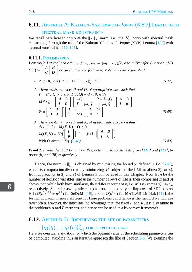
6

248 6. Affine LPV Modeling

6.11.AppendixA: Kalman-Yakubovich-Popov (KYP) Lemmawithspectral mask constraints

We recall here how to compute the‖ · ‖∆ω norm, i.e. theH∞ norm with spectral maskconstraints, through the use of the Kalman-Yakubovich-Popov (KYP) Lemma [109] withspectral constraints [110, 111].

6.11.1.PreliminariesLemma 2 Let real scalarsω1 ≤ ω2, ωc = (ω1 + ω2)/2, and a Transfer Function (TF)

G(s) ≔

[

A BC D

]

be given, then the following statements are equivalent.

1. ∀γ > 0, λ(A) ⊂ C− ∪ C+, ‖G‖2∆ω< γ2 (6.47)

2. There exists matrices P and Q, of appropriate size, such thatP = P∗, Q > 0, and L(P,Q) + Θ < 0, with

L(P,Q) =

[

A BI 0

]∗ [ −Q P+ jωcQP− jωcQ −ω1ω2Q

] [

A BI 0

]

Θ =

[

C D0 I

]∗ [I 00 −γ2I

] [

C D0 I

]

(6.48)

3. There exists matrices F and K, of appropriate size, such that∀l ∈ 1, 2 Ml(F,K) + Θ < 0

Ml(F,K) = He(

[

FK

]

[

I − jωl I]

[

A BI 0

]

)

WithΘ given in Eq. (6.48) (6.49)

Proof 2 Invoke the KYP Lemmas with spectral mask constraints, from [110] and [111], toprove (ii) and (iii) respectively.

Hence, the norm‖ · ‖2∆ω

is obtained by minimizing the boundγ2 defined in Eq. (6.47),which is computationally done by minimizingγ2 subject to the LMI in alinea 2), or 3).Both approaches in 2) and 3) of Lemma2 will be used in this Chapter. Now letn be thenumber of decision variables, andm the number of rows of LMIs, then comparing 2) and 3)shows that, while both have similarm, they differ in terms ofn, i.e. n2

x+nx versusn2x+nxnu,

respectively. Since the asymptotic computational complexity, or flop cost, of SDP solversis in O(n2m2.5 + m3.5) for SeDuMi [19], and inO(n3m) for MATLAB LMI-lab [ 112], theformer approach is more efficient for large problems, and hence is the method we will usemost often, however, the latter has the advantage that, for fixedF andK, it is also affine inthe problem’sA andB matrices, and hence can be used in a bi-convex framework.

6.12.Appendix B: Identifying the set of parameters

η1(ti), ..., ηS(ti)Ni=1 for a specific case

Here we consider a situation for which the optimal value of the scheduling parameters canbe computed, avoiding thus an iterative approach the like ofSection6.6. We examine the

6.12.Appendix B: Identifying the set of parameters

η1(ti), ..., ηS(ti)Ni=1 for a specific case

6

249

specific case where matricesLs are not identically zero, however with matricesRs identi-cally zero. Now Eq. (6.22) becomes equivalent to

Gi(s) −Gi(s) ≔

[

A BC D

]

=

Ai 0 Bi

0 A0 +S∑

s=1ηs(ti)Ls B0

I −I 0

(6.50)

Here Eq. (6.50) corresponds to a situation where the control-input matrix, of all LTImodels, is independent of the time-varying scheduling parameter (all matricesBi are iden-tical). This may be a specificity of the NL model, or alternatively, it may be achieved by(low-pass) filtering the control input of all LTI models [7]. In addition, we revert here toa standard weightedH∞ norm minimization instead of the KYP-based formalism used inSection6.6, hence replacing Eq. (6.19) by the following: find, for each timeti , the parame-tersη(ti) ≔ [η1(ti), ..., ηS(ti)]⊤ that minimize

J1(ti) ≔ ‖Wf (s)(

Gi(s) −Gi(s))‖∞ (6.51)

with Wf (s) a strictly-proper, bandpass filter, centered at∆ω. Now, if we consider the fol-lowing assumption

• A.1 In Section6.4, all basis (i.e. columns) inU1..S are retained when computingLs,RsSs=1.

then Eq. (6.51) becomes convex, and the optimal value ˆη(ti) can be found through a three-step procedure. But before solving Eq. (6.51), we give first the following result, which willprove useful in the sequel.

Lemma 3 Let Wf (s) ≔

[

Af Bf

C f 0

]

, Gi(s) ≔

[

Ai Bi

I 0

]

, Gi(s) ≔

A0 +S∑

s=1ηs(ti)Ls B0

I 0

,

be given, with matrices of appropriate size. Let

Wf (s)(

Gi(s) −Gi(s))

≔

A11 A12 B11

0 A22 B0

C11 0 0

(6.52)

with A11 =

[

Af Bf

0 Ai

]

, A12 =

[

−Bf

0

]

, B11 =

[

0Bi

]

, C11 =[

C f 0]

, and A22 = A0 +

S∑

s=1ηs(ti)Ls, then the following two statements are equivalent

1. ∀γ > 0, Wf (s) ∈ RH∞,(

Gi(s) −Gi(s)) ∈ RL∞, ‖Wf

(

Gi(s) −Gi(s))‖2∞ < γ2 (6.53)

6

250 6. Affine LPV Modeling

2. ∃(P,Q), P = P⊤, Q = Q⊤ = P−1, with matrix partitions in P and Q matching those

in Eq. (6.52), given by P=

[

P11 P12

P⊤12 P22

]

, Q =

[

Q11 Q12

Q⊤12 Q22

]

, with

Γ(

Xη,P11,P12,Q11,Q12)

≔ ...

Sym(

A11Q11 + A12Q⊤12

)

⋆ ⋆ ⋆

A⊤11+ Xη Sym(

P11A11)

⋆ ⋆

B⊤11 B⊤11P11 + B⊤0 P⊤12 −γ2I ⋆

C11Q11 C11 0 −γ2I

< 0 (6.54)

and Xη = P11A11Q11 + P11A12Q⊤12 + P12A22Q⊤12

Proof 3 The proof is a straightforward application of the Bounded Real Lemma (BRL)[113] in LMI form [ 82], with further: 1) a congruence transformation [114] with diag(J, I , I ),

J =

[

Q11 IQ⊤12 O

]

; and 2) a change of variable given by Xη . Note that for stable systems,

i.e.(

Gi(s) −Gi(s)) ∈ RH∞, one has to add the condition J⊤PJ =

[

Q11 II P11

]

> 0

Now, solving Eq. (6.51) reduces to a three-step procedure

1. First, solve∀i ∈ 1, ...,N minimizeγwith respect to Xη,P11,P12,Q11,Q12

subject to γ > 0, and the LMIs of Lemma3(6.55)

2. ComputeA22 = P†

12

(

Xη − P11A11Q11 − P11A12Q⊤12

)

Q⊤†

12, with (·)† the Moore-Penroseinverse. Note thatP12 andQ⊤12 are skinny and fat matrices, hence, by virtue of therespective left and right inverse,A22 is well-defined

3. Finally, minimize theL2-induced gain of static operator18 XA22 = A22−(

A0+S∑

s=1ηs(ti)Ls

)

,

such that∀i ∈ 1, ...,N η(ti) = arg min

ηs(ti )‖XA22‖2 (6.56)

which is solved as in Eq. (6.21)

6.13.Appendix C: Problem dataThe nominal model, corresponding to a linearization of the pendulum NL model at [x1 x2]⊤ =[0 0]⊤, used forH∞ controller design, is given by

Anom=

[

0 1−3.2667 −2

]

Bnom=

[

04

]

The data for model Eq. (6.37) is given by

A0 =

[

0 1−2.7915 −2

]

B0 =

[

03.0631

]

18Note that, thanks to assumptionA.1, the quantityA22 can exactly be recovered from(

A0 +S∑

s=1ηs(ti )Ls

)

.

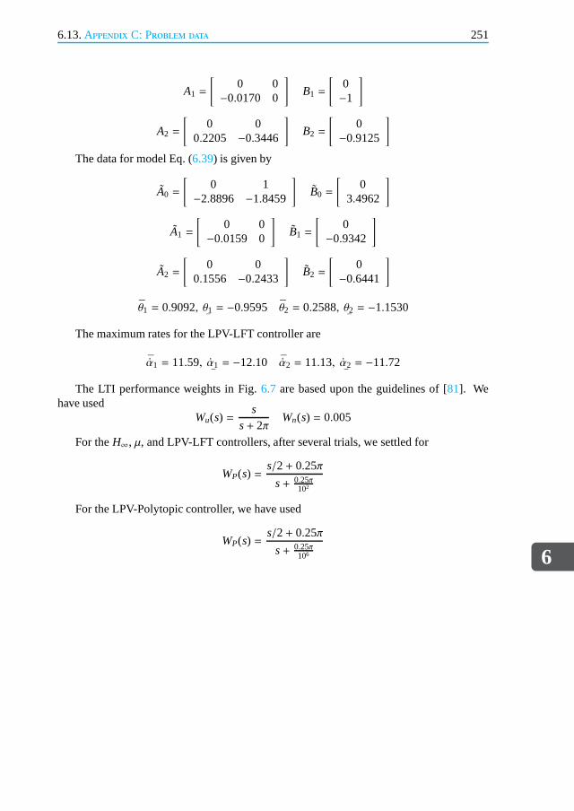
6.13.Appendix C: Problem data

6

251

A1 =

[

0 0−0.0170 0

]

B1 =

[

0−1

]

A2 =

[

0 00.2205 −0.3446

]

B2 =

[

0−0.9125

]

The data for model Eq. (6.39) is given by

A0 =

[

0 1−2.8896 −1.8459

]

B0 =

[

03.4962

]

A1 =

[

0 0−0.0159 0

]

B1 =

[

0−0.9342

]

A2 =

[

0 00.1556 −0.2433

]

B2 =

[

0−0.6441

]

θ1 = 0.9092, θ1¯= −0.9595 θ2 = 0.2588, θ2

¯= −1.1530

The maximum rates for the LPV-LFT controller are

¯α1 = 11.59, α1¯= −12.10 ¯α2 = 11.13, α2

¯= −11.72

The LTI performance weights in Fig.6.7 are based upon the guidelines of [81]. Wehave used

Wu(s) =s

s+ 2πWn(s) = 0.005

For theH∞, µ, and LPV-LFT controllers, after several trials, we settledfor

WP(s) =s/2+ 0.25π

s+ 0.25π102

For the LPV-Polytopic controller, we have used

WP(s) =s/2+ 0.25π

s+ 0.25π106

6

252 References

References[1] S. Taamallah, X. Bombois, and P. M. J. Van den Hof,Affine lpv modeling: An h∞

based approach,in IEEE Conf. on Decision and Control(2013).

[2] D. J. Walker,Multivariable control of the longitudinal and lateral dynamics of afly-by-wire helicopter,Control Engineering Practice11, 781 (2003).

[3] N. Hovakimyan and C. Cao,L1 Adaptive Control Theory: Guaranteed Robustnesswith Fast Adaptation(SIAM, 2010).

[4] J. S. Shamma and M. Athans,Analysis of gain scheduled control for nonlinear plants,IEEE Trans. Autom. Control35, 898 (1990).

[5] W. Rugh and J. Shamma,Research on gain scheuling,Automatica36, 1401 (2000).

[6] A. Packard,Gain scheduling via linear fractional transformations,Systems & Con-trol Letters22, 79 (1994).

[7] P. Apkarian, P. Gahinet, and G. Becker,Self-scheduled h∞ control of linearparameter-varying systems: A design example,Automatica31, 1251 (1995).

[8] P. Apkarian and P. Gahinet,A convex characterization of gain-scheduled h∞ con-trollers, IEEE Trans. Automatic Control40, 853 (1995).

[9] W. M. Lu and J. C. Doyle,h∞ control of nonlinear systems: A convex characteriza-tion, IEEE Trans. Automatic Control40, 1668 (1995).

[10] F. Wu, X. H. Yang, A. K. Packard, and G. Becker,InducedL2 norm control for lpvsystems with bounded parameter variation rates,Int. J. Of Robust And NonlinearControl6, 983 (1996).

[11] J. Yu and A. Sideris,h∞ control with parametric lyapunov functions,Systems &Control Letters30, 57 (1997).

[12] G. Scorletti and L. ElGhaoui,Improved lmi conditions for gain scheduling and re-lated control problems,Int. J. of Robust and Nonlinear Control8, 845 (1998).

[13] C. W. Scherer,Lpv control and full block multipliers,Automatica37, 361 (2001).

[14] G. Stein,Adaptive Flight Control - A Pragmatic View. In K. S. Narendraand R.V. Monopoli (Eds), Applications of Adaptive Control(Academic Press, New York,1980).

[15] K. J. Astrom and B. Wittenmark,Adaptive Control(Addison-Wesley, Reading, MA,1989).

[16] S. Boyd, L. ElGhaoui, E. Feron, and V. Balakrishnan,Linear Matrix Inequalities inSystem and Control Theory(Soc. for Industrial and Applied Mathematics (SIAM),Philadelphia, 1994).

References

6

253

[17] S. Boyd and L. Vandenberghe,Convex Optimization(Cambridge University Press,Cambridge, 2004).

[18] Y. Nesterov and A. Nemirovski,Interior Point Polynomial Methods in Convex Pro-gramming(Soc. for Industrial & Applied Math, 1994).

[19] J. F. Sturm,Using sedumi 1.02, a matlab toolbox for optimization over symmetriccones,Optimization Methods and Software11-12, 625 (1999).

[20] J. S. Shamma,An Overview of LPV Systems. In J. Mohammadpour and C. Scherer(Eds): Control of Linear Parameter Varying Systems with Applications (Springer,2012).

[21] G. J. Balas, I. Fialho, A. Packard, J. Renfrow, and C. Mullaney,On the design of lpvcontrollers for the f-14 aircraft lateral-directional axis during powered approach,inAm. Control Conf.(1997).

[22] G. J. Balas, J. B. Mueller, and J. M. Barker,Application of gain-scheduled, multi-variable control techniques to the f/a-18 system research aircraft,in AIAA GuidanceNavigation and Control Conf.(1999).

[23] I. Fialho, G. J. Balas, A. K. Packard, J. Renfrow, and C. Mullaney,Gain-scheduledlateral control of the f-14 aircraft during powered approach landing,AIAA J. ofGuidance, Control, and Dynamics23, 450 (2000).

[24] A. Marcos and G. J. Balas,Development of linear-parameter-varying models foraircraft, AIAA J. of Guidance, Control, and Dynamics27, 218 (2004).

[25] L. Reberga, D. Henrion, J. Bernussou, and F. Vary,Lpv modeling of a turbofanengine,in IFAC World Congress(2005).

[26] L. Giarre, D. Bausoa, P. Falugi, and B. Bamieh,Lpv model identification for gainscheduling control: An application to rotating stall and surge control problem,Con-trol Engineering Practice14, 351 (2006).

[27] K. Z. Ostergaard,Robust, Gain-Scheduled Control of Wind Turbines, Ph.D. thesis,Aalborg University (2008).

[28] M. Steinbuch, R. van de Molengraft, and A. J. van der Voort, Experimental mod-elling and lpv control of a motion system,in Am. Control Conf.(2003).

[29] M. G. Wassink, M. van de Wal, C. Scherer, and O. Bosgra,Lpv control for a waferstage: Beyond the theoretical solution,Control Engineering Practice13, 231 (2004).

[30] M. Dettori,LMI Techniques for Control, Ph.D. thesis, Delft University of Technology(2001).

[31] S. M. Hashemi, H. S. Abbas, and H. Werner,Lpv modelling and control of a 2-dof robotic manipulator using pca-based parameter set mapping, in IEEE Conf. onDecision and Control(2009).

6

254 References

[32] R. Toth,Identification and Modeling of Linear Parameter-Varying Systems. LectureNotes in Control and Information Sciences, Vol. 403(Springer, Heidelberg, 2010).

[33] R. Murray-Smith and T. Johansen (Ed),Multiple Model Approaches to Modeling andControl (CRC Press, 1997).

[34] W. Rugh,Analytical framework for gain scheduling,IEEE Control Systems Maga-zine11, 74 (1991).

[35] J. Shamma and M. Athans,Gain scheduling: Potential hazards and possible reme-dies,IEEE Control Systems Magazine12, 101 (1992).

[36] R. Bos, X. Bombois, and P. M. J. Van den Hof,Accelerating simulations of com-putationally intensive first principle models using accurate quasi-linear parametervarying models,J. of Process Control19, 1601 (2009).

[37] D. Petersson and J. Lofberg,Optimization based lpv-approximation of multi-modelsystems,in Europ. Control Conf.(2009).

[38] H. Pfifer and S. Hecker,Generation of optimal linear parametric models for lft-based robust stability analysis and control design,IEEE Trans. on Control SystemsTechnology19, 118 (2011).

[39] B. Paijmans, Interpolating Gain-Scheduling Control for Mechatronic Systemswith Parameter-Dependent Dynamics, Ph.D. thesis, Katholieke Universiteit Leuven(2007).

[40] J. DeCaigny, J. F. Camino, and J. Swevers,Interpolation-based modeling of mimolpv systems,IEEE Trans. on Control Systems Technology19, 46 (2011).

[41] J. S. Shamma and J. R. Cloutier,Gain-scheduled missile autopilot design using linearparameter varying transformations,AIAA J. of Guidance, Control, and Dynamics16, 256 (1993).

[42] D. J. Leith and W. E. Leithhead,Gain-scheduled controller design: An analyticframework directly incorporating non-equilibrium plant dynamics,Int. J. of Control70, 249 (1998).

[43] W. Tan,Applications of Linear Parameter-Varying Control Theory, Tech. Rep. (Mas-ter Thesis, University of California at Berkeley, 1997).

[44] J. Y. Shin,Quasi-Linear Parameter Varying Representation of GeneralAircraft Dy-namics Over Non-Trim Region, Tech. Rep. CR-2007-213926 (NASA Langley Re-search Center, 2007).

[45] A. Kwiatkowski, M. T. Boll, and H. Werner,Automated generation and assessmentof affine lpv models,in IEEE Conf. on Decision and Control(2006).

References

6

255

[46] R. Toth, P. S. C. Heuberger, and P. M. J. Van den Hof,Prediction Error Identificationof LPV Systems: Present and Beyond. In: J. Mohammadpour and C. W. Scherer(Eds.), Control of Linear Parameter Varying Systems with Applications(Springer,Heidelberg, 2012).

[47] T. A. Johansen, R. Shorten, and R. Murray-Smith,On the interpretation and iden-tification of dynamic takagi-sugeno fuzzy models,IEEE Trans. on Fuzzy Systems8,297 (2000).

[48] R. Shorten, R. Murray-Smith, R. Bjorgan, and H. Gollee,On the interpretation oflocal models in blended multiple model structures,Int. J. of Control72, 620 (1999).

[49] L. H. Lee and K. Poolla,Identification of linear parameter-varying systems usingnonlinear programming,J. of Dynamic Systems, Measurement and Control121, 71(1999).

[50] V. Verdult, L. Ljung, and M. Verhaegen,Identification of composite local linearstate-space models using a projected gradient search,Int. J. of Control75, 1125(2002).

[51] L. Ljung, System Identification: Theory for the User - 2nd Edition(Prentice Hall,Upper Saddle River, N.J., 1999).

[52] M. Gevers, A. Bazanella, X. Bombois, and L. Miskovic,Identification and the in-formation matrix: How to get just sufficiently rich,IEEE Trans. Autom. Control54,2828 (2009).

[53] R. Toth, P. S. C. Heuberger, and P. M. J. Van den Hof,Discretization of linearparameter-varying state-space representations,IET Control Theory & Applications4, 2082 (2010).

[54] P. Korba,A Gain Scheduled Approach to Model Based Fuzzy Control, Ph.D. thesis,University of Duisburg (2000).

[55] V. Laurain, R. Toth, M. Gilson, , and H. Garnier,Direct identification of continuous-time lpv input/output models,IET Control Theory & Applications5, 878 (2011).

[56] G. Goodwin, S. Graebe, and M. Salgado,Control System Design(Prentice Hall,2000).

[57] K. J. Hunt and T. A. Johansen,Design and analysis of gain-scheduled local con-troller networks,Int. J. of Control66, 619 (1997).

[58] T. A. Johansen, K. J. Hunt, P. J. Gawthrop, and H. Fritz,Off-equilibrium lineariza-tion and design of gain scheduled control with application to vehicle speed control,Control Engineering Practice6, 167 (1998).

[59] P. Korba and H. Werner,Counter-example to ad-hoc off-equilibrium linearisationmethods in gain-scheduling,in IEEE Conf. on Decision and Control(2001).

6

256 References

[60] C. S. Mehendale and K. M. Grigoriadis,A new approach to lpv gain-schedulingdesign and implementation,in IEEE Conf. on Decision and Control(2004).

[61] L. Rodrigues,Dynamic Output Feedback Controller Synthesis for Piecewise-AffineSystems, Ph.D. thesis, Stanford University (2002).

[62] J. Daafouz et al.,Switched and Piecewise Affine Systems. In J. Lunze and F.Lamnabhi-Lagarrigue (Eds): Handbook of Hybrid Systems Control Theory, Tools,Applications(Cambridge Univ. Press, 2009).

[63] J. S. Shamma and M. Athans,Guaranteed properties of gain scheduled control forlinear parameter-varying plants,Automatica27, 559 (1991).

[64] Z. Petres,Polytopic Decomposition of Linear Parameter-Varying Models by Tensor-Product Model Transformation, Ph.D. thesis, Budapest University of Technology andEconomics (2006).

[65] A. Kwiatkowski and H. Werner,Pca-based parameter set mappings for lpv mod-els with fewer parameters and less overbounding,IEEE Trans. on Control SystemsTechnology16, 781 (2008).

[66] E. Prempain and I. Postlethwaite,Extended lmi projection conditions,in IEEE Conf.on Decision and Control(1999).

[67] J. C. Doyle,Structured uncertainty in control system design,in IEEE Conf. on Deci-sion and Control(1985).

[68] A. Helmersson,Model reduction using lmis,in IEEE Conf. on Decision and Control(1994).

[69] P. Apkarian and R. J. Adams,Advanced gain scheduling techniques for uncertainsystems,IEEE Trans. Automatic Control6, 21 (1998).

[70] M. Sato and D. Peaucelle,Gain-Scheduled Output-Feedback Controllers with GoodImplementability and Robustness. In: J. Mohammadpour and C. W. Scherer (Eds.),Control of Linear Parameter Varying Systems with Applications(Springer, Heidel-berg, 2012).

[71] G. Stein and J. C. Doyle,Beyond singular values and loop shapes,AIAA J. of Guid-ance, Control, and Dynamics14, 5 (1991).

[72] M. A. Rotea and T. Iwasaki,An alternative to the d-k iteration ?in Am. Control Conf.(1994).

[73] K. Hornik, M. Stinchcombe, and H. White,Multilayer feedforward networks areuniversal approximators,Neural Networks2, 359 (1989).

[74] M. Norgaard, O. Ravn, N. Poulsen, and L. Hansen,Neural Networks for Modellingand Control of Dynamic Systems(Springer-Verlag, London, 2000).

References

6

257

[75] A. B. T. (Ed.), Computer Science Handbook, Second Edition(Chapman andHall/CRC, 2004).

[76] J. D. Bendtsen and K. Trangbaek,Robust quasi-lpv control based on neural state-space models,IEEE Trans. on Neural Networks13, 355 (2002).

[77] H. Abbas and H. Werner,Polytopic quasi-lpv models based on neural state-spacemodels and application to air charge control of a si engine,in IFAC 17th WorldCongress(2008).

[78] N. Lachhab, H. Abbas, and H. Werner,A neural-network based technique for mod-elling and lpv control of an arm-driven inverted pendulum,in IEEE Conf. on Deci-sion and Control(2008).

[79] J. Lofberg,Yalmip: A toolbox for modeling and optimization in matlab,in CACSDConf.(2004).

[80] M. B. Tischler, J. G. M. Leung, and D. C. Dugan,Neural network-based trajec-tory optimization for unmanned aerial vehicles,AIAA J. of Guidance, Control, andDynamics35, 548 (2012).

[81] S. Skogestad and I. Postlethwaite,Multivariable Feedback Control: Analysis andDesign, 2nd Ed.(Wiley-Interscience, Great Britain, 2005).

[82] P. Gahinet and P. Apkarian,A linear matrix inequality approach to h∞ control,Int. J.Of Robust And Nonlinear Control4, 421 (1994).

[83] G. Zames,On the input-output stability of time-varying nonlinear feedback systems-part i: Conditions derived using concepts of loop gain, conicity, and positivity,IEEETrans. Autom. ControlAC-11, 228 (1966).

[84] C. A. Desoer and M. Vidyasagar,Feedback Systems: Input-Output Properties(Aca-demic Press, New York, 1975).

[85] K. Zhou, J. C. Doyle, and K. Glover,Robust and Optimal Control(Prentice Hall,New Jersey, 1996).

[86] G. J. Balas, J. C. Doyle, K. Glover, A. K. Packard, and R. S. Smith,µ Analysis andSynthesis Toolbox: User’s Guide(The MathWorks Inc., 1991).

[87] K. Glover,All optimal hankel-norm approximations of linear multivariable systemsand theirL∞-error bounds,Int. J. of Control39, 1115 (1984).

[88] J. M. Biannic, C. Roos, and A. Knauf,Design and robustness analysis of fighteraircraft flight control laws,Europ. J. of Control12, 71 (2006).

[89] G. Becker and A. K. Packard,Robust performance of linear parametrically varyingsystems using parametrically-dependent linear feedback,Systems & Control Letters23, 205 (1994).

6

258 References

[90] I. E. Kose, F. Jabbari, and W. E. Schmitendorf,A direct characterization of l2 gaincontrollers for lpv systems,IEEE Trans. Autom. Control43, 1302 (1998).

[91] E. Prempain,Gain-scheduling h∞ loop shaping control of linear parameter-varyingsystems,in 5th IFAC Symposium on Robust Control Design(2006).

[92] M. C. de Oliveira,Explicit Controller Parametrizations for Linear Parameter-Varying Affine Systems Using Linear Matrix Inequalities. In: J. Mohammadpour andC. W. Scherer (Eds.), Control of Linear Parameter Varying Systems with Applications(Springer, Heidelberg, 2012).

[93] F. Wu,A generalized lpv system analysis and control synthesis framework,Int. J. ofControl74, 745 (2001).

[94] C. Scherer and I. E. Kose,Gain-scheduled control synthesis using dynamic d-scales,IEEE Trans. Autom. Control57, 2219 (2012).

[95] C. W. Scherer,Mixed h2 − h∞ control for time-varying and linear parametrically-varying systems,Int. J. of Robust and Nonlinear Control6, 929 (1996).

[96] P. Gahinet, P. Apkarian, and M. Chilali,Affine parameter-dependent lyapunovfunctions and real parametric uncertainty,IEEE Trans. Automatic Control41, 436(1996).

[97] S. Bennani, D. M. C. Willemsen, and C. W. Scherer,Robust control of linear para-metrically varying systems with bounded rates,AIAA J. of Guidance, Control, andDynamics21, 916 (1998).

[98] S. Lim, Analysis and Control of Linear Parameter Varying Systems, Ph.D. thesis,Stanford University (1998).

[99] C. E. deSouza and A. Trofino,Gain-scheduled h2 controller synthesis for linear pa-rameter varying systems via parameter-dependent lyapunovfunctions,Int. J. of Ro-bust and Nonlinear Control16, 243 (2006).

[100] P. Apkarian, G. Becker, P. Gahinet, and H. Kajiwara,LMI Techniques in ControlEngineering from Theory to Practice. In: Workshop notes CDCIEEE (Kobe, Japan,1996).

[101] A. Kominek, H. Werner, M. Garwon, and M. Schultalbers,Identification of Low-Complexity LPV Input-Output Models for Control of a Turbocharged CombustionEngine(Springer, Heidelberg, 2012).

[102] B. R. Barmish,Necessary and sufficient conditions for quadratic stabilizability of anuncertain system,J. of Optimization Theory and Applications46, 399 (1985).

[103] A. Helmersson,Methods for Robust Gain-Scheduling, Ph.D. thesis, Linkoping Uni-versity (1995).

References

6

259

[104] P. Apkarian, J. M. Biannic, and P. Gahinet,Self-scheduled h∞ control of missilevia linear matrix inequalities,AIAA J. of Guidance, Control and Dynamics18, 532(1995).

[105] R. J. Adams, P. Apkarian, and J. P. Chretien,Robust control approaches for a two-link flexible manipulator,in Int. Conf. Dynamics Control Structures in Space(1996).

[106] H. Kajiwara, P. Apkarian, and P. Gahinet,Lpv techniques for control of an invertedpendulum,IEEE Control Systems Magazine19, 44 (1999).

[107] T. Nagashio and T. Kida,Robust attitude controller design of linear parameter vary-ing spacecraft viaµ synthesis and gain scheduling,in IEEE Int. Conf. on ControlApplications(1999).

[108] J. Daafouz, J. Bernussou, and J. C. Geromel,On inexact lpv control design ofcontinuous-time polytopic systems,IEEE Trans. Autom. Control53, 1674 (2008).

[109] A. Rantzer,On the kalman-yakubovich-popov lemma,Systems & Control Letters28,7 (1996).

[110] T. Iwasaki, G. Meinsma, and M. Fu,Generalized s-procedure and finite frequencykyp lemma,Math. Prob. Eng.6, 305 (2000).

[111] M. R. Graham, M. C. de Oliveira, and R. A. de Callafon,An alternative kalman-yakubovich-popov lemma and some extensions,Automatica45, 1489 (2009).

[112] P. Gahinet, A. Nemirovski, A. J. Laub, and M. Chilali,LMI Control Toolbox User’sGuide(The Mathworks Partner Series, 1995).

[113] C. Scherer,The Riccati Inequality and State-Space H∞-Optimal Control, Ph.D. the-sis, Universitat Wurzburg (1990).

[114] C. W. Scherer, P. Gahinet, and M. Chilali,Multiobjective output-feedback controlvia lmi optimization,IEEE Trans. Autom. Control42, 896 (1997).

7Conclusions and future research

Perfect is the enemy of good.

Aphorism commonly attributed to Voltaire

A good enough solution that works, is immeasurably better than a perfect solution yet tobe implemented.

Justin LloydA Mastermind’s Guide to Personal Development, 2009

In this Chapter the most important results achieved in this thesis are first presented, andfurther objectives and opportunities for future research are identified and outlined.

261

7

262 7. Conclusions and future research

7.1.Contribution of this thesis

T he primary objective of this thesis was to develop a, model-based, automatic safety re-covery system that could safely fly and land a small-scale helicopter Unmanned Aerial

Vehicle (UAV) in un-powered flight (i.e. autorotation). Theflight control solution presentedin this thesis incorporates a classic guidance and control logic, in which the guidance mod-ule is decoupled from the control module. The goal of the guidance module, or TrajectoryPlanning (TP), is to generate open-loop, feasible and optimal autorotative trajectories, forthe helicopter, whereas the aim of the control module, or Trajectory Tracking (TT), consistsin comparing the current state values with the optimal reference values produced by the TP,and then formulate the feedback controls, enabling thus thehelicopter to fly along theseoptimal trajectories. The work presented in this thesis resulted in the first demonstrationof a, real-time feasible, model-based TP and model-based TT, for the case of a small-scalehelicopter UAV, with an engine OFF condition (i.e. autorotation). The validation was per-formed on a helicopter high-fidelity simulation, based upona nonlinear, High-Order Model(HOM). In the sequel we outline additional concluding remarks, relative to the varioussolutions and results presented in this thesis.

• With regard tohelicopter modeling, we developed two helicopter nonlinear models.One is a first-principles based, HOM, developed in Chapter 2,and used to validatethe Flight Control System (FCS). The second one is a gray-box1, Low-Order Model(LOM), developed and used in Chapter 3 to obtain optimal autorotative trajectories.The latter model provides a good approximation of the HOM of Chapter 2, whilehaving better computational efficiency when compared to the HOM. However, thiscomes at a price, namely a time-consuming identification of various empirical coeffi-cients, using input-output data from the HOM. In addition, each new helicopter con-figuration, or modification thereof (e.g. mass and inertia adjustments), will requirea re-identification of all empirical coefficients. By contrast, the HOM represents aflexible modeling approach, readily updated in case of new helicopter configurations,although its associated CPU time, per model evaluation, is higher.

• With respect to theoff-line TP, developed in Chapter 3, based upon the realm ofconstrained, nonlinear optimal control, we summarize herethe main findings

1. For fixed initial altitude, increasing the initial velocity has only a relatively lim-ited effect on flight time and stabilized rate of descent.

2. For fixed initial altitude, the flight time is strongly correlated with the initialaltitude and the induced velocity in hover.

3. For fixed initial altitude, increasing the initial velocity complicates somewhatthe flare maneuver.

4. For hover initial conditions, the higher the initial altitude, the more the optimalautorotative trajectory resembles a vertical flight path.

• With respect to theon-line TP and TT of Chapters 4 and 5, using the combinedparadigms of differential flatness and robust control, we summarize here the main

1Using a mix of first-principles and various empirical coefficients.

7.1.Contribution of this thesis

7

263

findings for both the engine ON (i.e. power-on) and engine OFF(i.e. power-off, alsoknown as autorotation) flight conditions, for the case of a small-scale helicopter UAV

1. The proposed TP and TT approach is validated on the high-fidelity, first-principlesbased, helicopter HOM, developed in Chapter 2, for both engine ON and en-gine OFF trajectories. The methodology is real-time feasible since it allows fora computationally tractable determination, and tracking,of the optimal trajec-tories. In addition, both the engine ON and engine OFF cases are based uponthe same planning and tracking system architecture. Further, main rotor Rev-olutions Per Minute (RPM) is not used, being neither necessary for the engineOFF trajectory planning, nor for the corresponding trajectory tracking, hencesimplifying the overall system design.

2. For the engine OFF case, a single Linear Time-Invariant (LTI) controller iscapable of controlling and landing the helicopter system, in autorotation, fora relatively large variation in forward and vertical vehicle velocity (at least upto approximately 8 to 10 m/s), and for relatively large variations in main rotorRPM (approximately in the 50% to 110% range).

3. For the engine ON case, the vehicle state at an initial timeti has only a limitedimpact (if any) on the set of reachable states for all admissible input signalsand for all time instants in an interval [0, t f ], with t f ≫ ti . If we omit theon-board electrical power supply system from the vehicle energy balance, i.e.considering only vehicle potential, kinetic, and main rotor energies, then thetotal vehicle energy may decrease or increase, depending onvehicle height andvehicle velocity. By contrast, the total vehicle energy, inthe engine OFF case,is always decreasing. Hence, we conjecture that the size of this reachable set,for the engine OFF case, is much smaller when compared to its engine ONcounterpart and, consequently, feasible trajectories aremuch harder to find inthe engine OFF case.

4. For the engine ON case, it is relatively easy to find equilibrium points, i.e.steady-state flight conditions, at which the nonlinear model can be linearized.The so-obtained LTI models can subsequently be used for LTI control design.For the engine OFF case, this set of equilibrium points, i.e.steady autorotativeflight conditions, is rather small and in certain situationseven non-existent. Forexample, when an engine failure happens at a low altitude, the helicopter doesnot even reach a steady-state autorotation, rather it is continuously in transitionfrom one non-equilibrium point to the next. To mitigate thisproblem, the ap-proach used in this thesis consists in excluding the main rotor RPM from thestate-vector, and use the resulting "quasi-steady" approach to find the equilib-rium points.

5. For the engine ON case, helicopter operations can remain at a velocity whichstays in the neighborhood of the design-point velocity, i.e. in the neighborhoodof the equilibrium point velocity which was used to derive the LTI model forcontrol design. This allows to maximize the linear behaviorof the system. Onthe other hand, helicopter operations with the engine OFF will inevitably resultin a wide range of flown velocities, including high descent rates, and even flight

7

264 7. Conclusions and future research

into the chaotic Vortex-Ring-State (VRS). Indeed, a brief transition through theVRS may in some cases be required. This obviously tends to ’amplify’ thenonlinear behavior of the system.

6. For the engine ON case, the designer can choose to keep the bandwidth of theclosed-loop system rather small, by only considering gentle and smooth ma-neuvers in the design specification phase. For the engine OFFcase, a higherclosed-loop bandwidth is definitely required (especially in the vertical channel),if proper trajectory tracking is to be performed. This may complicate the con-troller design, since higher-order LTI models (for controller design) may haveto be considered. This complicates also the practical implementation, sincehigher-bandwidth actuators may become compulsory.

7. For the engine OFF case, our results show that the crucial control of verticalposition and velocity exhibit outstanding behavior in terms of tracking perfor-mance, and does not require an additional increase in control bandwidth. How-ever, the tracking of horizontal positions and horizontal velocities is clearlylacking some bandwidth (i.e. the flown trajectories are clearly lagging theplanned ones). Although a further increase of the horizontal closed-loop band-widths provided good results when evaluated on the LTI modelused for con-trol design, this increase in closed-loop bandwidths resulted, unfortunately, inclosed-loop instabilities, when evaluated on the nonlinear helicopter model ofChapter 2.

8. For the engine OFF case, tracking performance of horizontal positions and hor-izontal velocities could potentially be improved, by considering one of the twofollowing options: i) remaining in the framework of a singlerobust LTI con-troller, using a high-order LTI plant for controller design(i.e. containing themain rotor flap-lag and inflow dynamics), instead of a low-order plant as usedin Chapter 4; or ii) using another control method that betterrespects and ex-ploits the system’s nonlinear structure, e.g. in the realm of nonlinear, adaptive,or Linear Parameter-Varying (LPV) methods.

• With respect to theaffine LPV modeling method, developed in Chapter 6, we haveshown, using a pointmass pendulum (i.e. a nonlinear example), that our LPV mod-eling strategy was capable of reproducing the open-loop behavior of the originalnonlinear dynamical system. Furthermore, we have shown that controllers (whetherrobust or LPV), designed using our LPV model, achieved better reference tracking,when compared to a controller designed using a linearization of the nonlinear system.

7.2.Recommendations for future researchIn light of the research objective of this thesis and the results achieved so far, we identifyand discuss next some stimulating opportunities for futureresearch. In particular, if thenext step is to perform flight tests and achieve an experimental validation of an automaticautorotation system, then the general control architecture, as used in this thesis, and outlinedin Fig.1.15of Chapter 1, may have to be replaced by the one given in Fig.7.1. In the sequelwe will elaborate on the new blocks of Fig.7.1, as well as several other areas that warrantfurther exploration.

7.2.Recommendations for future research

7

265

Figure 7.1: Upgraded two degree of freedom control architecture.

• For the case of an engine failure, the"engine OFF event" first needs to be recog-nized. Here the use of an engine torque sensor could prove very useful. For example,a sudden reduction in measured torque, if accompanied by fixed main rotor collectiveinput and a decelerating main rotor speed, could be indicative of an engine failure.However, a sudden reduction in engine torque if accompaniedby, either, reducedmain rotor collective input or accelerating main rotor speed, would not indicate anengine failure [1]. An additional clue for the detection of engine failure could alsocome from the yaw channel. Indeed, a jerk is generally felt onthis channel, since thetail rotor will tend to overcompensate the reduced main rotor torque [1]. As a finalpoint, it should be noted that, for the case where engine power is not lost suddenly butrather gradually, it may become much more difficult to quickly detect such a failure.

• Actuator dynamic models, with amplitude and rate constraints, ought to be in-cluded in the HOM of Chapter 2, and in any model used for control design. Indeed, itis well-known that maximum control gains and crossover frequencies may be limitedby actuator rate saturation2. Further, actuator rate saturation can have a significantdetrimental effect on the handling qualities of an aerospace vehicle [3], and directlylead into, either, degraded performance, limit cycles, or even closed-loop instability[3, 4]. For example, the crashes of the SAAB Gripen fighter jet in February 1989and August 1993 [2, 5], and the crash of the Lockheed Martin YF-22 fighter jet inApril 1992 [2, 6] are all primarily related to actuator rate saturations. These satu-rations resulted in so-called Pilot-Induced-Oscillation(PIO), and subsequent loss ofvehicle control. Several approaches could be adopted to avoid saturation problems insystems which are known to have actuator limits. The first onelives in the realm ofoptimal control. Here the control action is decided throughthe use of constrained op-

2Actuator saturation or rate limits has even been implicatedin the meltdown of the Chernobyl nuclear power plant,in April 1986 [2].

7

266 7. Conclusions and future research

timization algorithms, known as Model Predictive Control (MPC) [7]. Other optionsare related to the so-called anti-windup compensation, in which a nominal controller(that does not explicitly take the saturation constraints into account) is first designed.Then, in a second step, an anti-windup compensator is designed to handle the satura-tion constraints. Anti-windup approaches are attractive in practice because: 1) theyallow for control design in a linear framework; and 2) no restrictions are placed uponthe nominal controller design. Excellent tutorials exist in this area, see [8–10]. Re-cently, promising extensions have even considered the caseof a simultaneous designof both the nominal controller and the anti-windup compensator [11, 12].

• An estimation filter, e.g. a state estimator, is typically an integral part of a UAV FCS.Indeed, the quantities required for flight control, like position, velocity, and attitude,are not measured directly or, if measured, are noisy and often not available at the re-quired frequency. Hence, an estimation filter is often required to derive smooth, andhigh-frequency state updates, from available sensor measurements. For example, ourAlign T-REX helicopter is fitted with a flight computer featuring data logging capa-bilities, as well as a variety of low-cost sensors, such as: 1) an Inertial MeasurementUnit (IMU) containing three accelerometers and three gyroscopes that measure ac-celerations and angular velocities, respectively, in the inertial body frame; 2) a GlobalPositioning Sensor (GPS) providing a direct measurement ofthe helicopter’s inertialposition and velocity; 3) a compass measuring the vehicle’smagnetic heading; 4) abarometric pressure sensor for altitude measurement during cruise flight; and a 5)a Laser Range Finder (LRF) for altitude measurement during take-off and landing.Hence, the helicopter’s position, velocity, and attitude can be obtained through theintegration of the high-frequency, noisy, biased, and drifting IMU outputs, with thenoisy, low-frequency outputs, with bounded error characteristics, of the remainingsensors. Since in our case the vehicle’s kinematic and measurement equations arenonlinear, the nonlinear extension to the original Kalman Filter, i.e. the ExtendedKalman Filter (EKF) [13, 14], represents the most common approach for our real-time estimation problem. However, since based upon linearizations and calculationof Jacobian matrices, the EKF is also known to exhibit numerical issues and evendivergence in some situations. To mitigate such problems, the so-called UnscentedKalman Filter (UKF) [15, 16] has been developed. For all its benefits, it was reportedin [17–19] that, for the case of aerospace applications, the UKF did not offer substan-tial performance gains, when compared to the EKF. Hence, forour application, wewould recommend evaluating first the simpler EKF filter.

• Small-scale UAVs are far more sensitive to atmospheric windand gust disturbances,than their full-scale counterparts, since the mean wind magnitude is often compara-ble to the speed of the UAV, and consequently this brings upfront the relevance ofamean wind estimation capability. The knowledge of the mean wind profile mag-nitude, and direction, is indeed helpful for two reasons. First, it allows to enhancethe accuracy and feasibility of the computed trajectories during the planning phase,since knowledge of the wind can be included in the model used for planning. Sec-ond, for good trajectory tracking3, the velocities of the vehicle with respect to the

3In flight dynamics models, the aerodynamic forces are functions of the vehicle aerodynamic velocities, not of

7.2.Recommendations for future research

7

267

relative wind, i.e. the vehicle aerodynamic velocities, should be made available tothe controller. Direct wind measurement can be obtained through, either, a ground-based anemometer, or through some sort of weather balloon. The first option doesnot provide information on wind profile (as a function of altitude), whereas the sec-ond may be costly, and potentially impractical. Hence, the need for wind estimation,rather than wind measurement, becomes obvious. With regardto kinematics, the ve-hicle’s ground track velocity vector (i.e. the inertial velocity, measured with GPS)can be decomposed into the sum of a vehicle’s airspeed vectorand a wind vector.As stated earlier, GPS data is available on-board the helicopter. Hence, if the windvelocity vector is known, it can be subtracted from the GPS velocity to obtain anair-relative velocity. Alternatively, if the air-relative velocity vector is known, it canbe subtracted from the GPS velocity vector to obtain the windvelocity vector. Thedetermination of the vehicle’s air-relative velocity vector can be done through twoapproaches. The first approach, and widely used approach forfixed-wing aircrafts,consists in mounting an air-data unit, combining precise measurements of airspeedamplitude, through a pitot-static pressure sensor, and airspeed orientation, throughangle-of-attack and angle-of-sideslip vanes. The second approach is a model-basedone (often derived from relatively simple models) in which the vehicle’s air-relativevelocity vector is estimated based upon the knowledge of themodel, and based uponthe measured control inputs. Here, the first approach is generally ruled out for heli-copters, since such an air-data system needs to operate outside the main rotor down-wash and, even if placed at the front of the fuselage, may onlybe effective when thevehicle is traveling at high forward speed. Hence, the preferred approach for windand airspeed estimation, for helicopters, consists in using a model-based estimationprocedure, together with GPS and control input measurements (sometimes also incombination with heading measurements from the compass sensor). Such a strategyhas often successfully been applied to the case of autonomous guided airdrop systems(i.e. paraplanes), see also [20, 21].

• For theLow-Order Model (LOM) of Chapter 3, the empirical coefficients are es-timated in a multiple-model structure, meaning that for each point in the operatinggrid, a set of coefficients is being identified thanks to data generated from the High-Order Model (HOM). However, as stated earlier, this identification method becomesrather tedious for large grids. An alternative approach, potentially easier to imple-ment since not based upon the multiple-model concept, consists in identifying thecoefficients using the optimal control framework. Here, the empirical coefficientsconstitute the unknown control inputs of a continuous-time, nonlinear, dynamicalsystem. These inputs are obtained by solving a constrained,optimal control problem,which goal is to fit the outputs of the LOM with those of the HOM in some optimalsense. Once identified, a model defining the relation betweenthese empirical coeffi-cients and the helicopter control inputs and states, needs to be found (e.g. through aNeural Networks (NN) representation). In [22] we presented preliminary results forsuch a LOM approach.

• With regard to theoff-line Trajectory Planning of Chapter 3, we discuss several

vehicle inertial velocities.

7

268 7. Conclusions and future research

areas that may benefit from further improvements

1. As stated in Section3.4, direct optimal control methods have several advantageswhen compared to indirect methods. Specifically, the first-order necessary con-ditions do not need to be explicitly derived, and the large radii of convergenceallow for less accurate initial guess on states and control inputs. Hence, directmethods are appealing for complicated applications. Further, PseudoSpectral(PS) discretization methods have the known advantage of providing exponentialrate of convergence for the approximation of analytic functions. For all thosebenefits, the direct optimal method used in our application has also shown someinherent limitations. For example, it was in some cases uncertain whether thesolution obtained was truly optimal. Indeed, fluctuated solutions were observedas the number of discretization nodes was varied.

2. We also noticed that the use of lookup tables, within the LOM, had a negativeimpact on the exponential convergence of the method, even when queried withcubic B-Splines interpolating functions. Solving the optimal control problembecame at times computationally intractable, and at times either infeasible, orfeasible but very probably sub-optimal. This said, nonsmooth problem formu-lations are far from uncommon in aerospace. To mitigate thisknown issue,several approaches could be investigated such as: 1) a PS knotting method as in[23]; or 2) a hybrid global/local collocation method as in [24].

3. We solved the NonLinear Programming problem (NLP) via a Sequential QuadraticProgramming (SQP) approach. SQPs belong to the class of iterative, gradient-based methods, and gradient methods are known as local methods. We didnotice this sensitivity to local minima, by obtaining distinct optimal solutions,for distinct initial guesses.

4. Since in our case we did not use any mesh refinement grid (as to keep the prob-lem computationally tractable), the obtained optimal solution provided only thestate and control values at the discrete nodes. Hence, the optimal solution satis-fied only the discretized constraints (i.e. the problem is said to be discrete-timefeasible [25]). This implies that, for a small number of nodes, no guaranteesmay be given regarding the solution of the original continuous-time problem[25]. Obviously, one way to mitigate such a problem would be to increase thenumber of nodes, at the cost of higher computational time.

5. Finally a robustness analysis of the obtained trajectories4, with respect to modeland signal uncertainties, potentially within the realm of stochastic optimization,would represent an interesting avenue for future research.

• With regard to theon-line Trajectory Planning (TP) of Chapters 4 and 5, we rec-ommend considering the following aspects

1. It may be beneficial to add a feedback path into the trajectory planning, de-noted by a dashed line in Fig.7.1, which would allow to re-generate an optimalreference trajectory, based upon the current state. This functionality may, for

4This could also apply to the flatness-based trajectory planning.

7.2.Recommendations for future research

7

269

example, be of interest in the following cases: 1) within theframework of anobstacle avoidance capability; or 2) if the helicopter experiences an increasingdifficulty at tracking the current reference trajectory.

2. One could also consider adding an optical sensor, coupledwith an on-board3D map of the environment, in order to identify suitable geographical locationsfor a safe landing. If in addition the set of reachable statescould efficiently becomputed on-line, then one would be able to provide feasiblelanding positionsto the TP.

3. The optical sensor could also potentially be fused with the other sensors in orderto increase the accuracy of the estimated helicopter state-vector (computed inthe estimation filter).

• With regard to theon-line Trajectory Tracking (TT) of Chapters 4 and 5, we rec-ommend considering the following aspects

1. The NL helicopter model of Chapter 2 is subject to periodicloads, due to bladesrotation, that result in a time-varying trim condition. Linearizing the NL heli-copter dynamics, around this trim condition, can be done at each rotor position,to yield a Periodic Linear Time-Varying (PLTV) system, witha period equalto one rotation of the rotor. For PLTV systems the classical modal analysismethodologies, based upon time-invariant eigenstructures, are not applicableanymore [26]. Hence, if one wants to apply the well-established analysis andcontrol tools for LTI systems, a transformation of the PLTV system into a LTIone becomes necessary. There are roughly four main methods to perform sucha transformation or approximation [27]. The first, and simplest one, consistsin evaluating the PLTV system at a single rotor position (i.e. at a single bladeazimuth position), and obtain a LTI system. Clearly this approach may lead topoor results. An already better method would consist in averaging the PLTVstate-space matrices over one or more rotor periods. The next two methodsprovide LTI models with higher accuracy, but require additional mathematicalsteps. The third method uses Floquet theory [26, 28], and the associated char-acteristic exponents called Floquet multipliers, to obtain constant state-spacematrices. The fourth method uses the so-called Multi-BladeCoordinate (MBC)transformation (also known as the Coleman transformation)[26, 29–31], i.e.by transforming quantities from rotating blade coordinates into a non-rotatingframe. Basically the MBC describes the overall motion of a rotating blade ar-ray in the inertial frame of reference. The MBC transformation results in aweakly periodic system which is subsequently converted into a LTI system byaveraging over one period [31]. In this thesis, obtaining an LTI approximationfrom the PLTV system was done using the second method as discussed in Sec-tion 2.4.1of Chapter 2, by averaging over four rotor periods. Althoughveryeasy to implement, it is well-known that this method may not provide an LTImodel of highest accuracy. Hence, we recommend trying a moresophisticatedapproach to derive the LTI system. With regard to the MBC method, this latteris particularly well-suited for rotors having three or moreblades, and may in-

7

270 7. Conclusions and future research

volve significant inaccuracies for a two-bladed rotor5 [32]. The Floquet methodis numerically more intensive6 than the averaging method used in this thesis[35], however it may potentially provide LTI models with higheraccuracy andhence would deserve further investigations.

2. For a digital implementation of the controller, several continuous- to discrete-time transformations exist (depending on the type of control framework used[36, 37]). The goal, obviously, is to select a transformation that best preservesthe properties of the continuous-time design.

3. A general approach to mitigate the interaction problem, between the FCS andthe main rotor dynamics, could be to use higher-order LTI models (i.e. contain-ing the main rotor flap-lag and inflow dynamics), for control design, possibly incombination with a reduced-order observer in order to estimate the unmeasuredmain rotor states.

4. The addition of a roll and pitch attitude stabilization loop may potentially allowto increase the tracking bandwidth. The complete control system would theninvolve multiple nested control loops, namely: 1) the innermost-loop, whichcontrols the attitude of the vehicle; 2) the middle-loop, which controls the ve-locity; and 3) the outer-loop, which controls the position.

5. Since system delays impose severe limitations on the bandwidth of the closed-loop system [38], all hardware delays—due to actuator dead-time, sensor pro-cessing, and the effects of digital implementation on-board the embedded com-puter—need to be estimated, modeled, and added to all modelsdeveloped withinthis thesis.

6. Helicopter dynamics is highly coupled, especially during hover and low-speedflight. In order to reduce the coupling effects, and hence simplify the subsequentcontroller design, it may be worthwhile to add a decoupling module, in the formof open-loop dynamic crossfeeds, inserted in-between the controller outputs andthe plant inputs, see [39, 40].

7. It is customary to place the closed-loop poles in a suitable region of the complexplane. This is often done in order to guarantee satisfactorysystem transientsbehavior, and to indirectly enforce constraints on the controller bandwidth, andhence: 1) minimize any controller interaction with actuator dynamics, structuralmodes, or any other vehicle higher-order dynamics; and 2) allow for a digitalimplementation of the controller dynamics. This can be done, in a systematicway for LTI controllers, in the Linear Matrix Inequality (LMI) framework, see[41, 42].

8. In Chapters 4 and 5, a single nominal LTI model was used for the design ofa single robust LTI TT controller. Relatively good trackingresults have beenobtained, although the tracking of horizontal velocity andposition could poten-tially be improved, by considering one of the two following options: 1) remain-ing in the framework of a single robust LTI controller, however combined with

5As a reminder, our Remote-Controlled (RC) Align T-REX helicopter has a two-bladed main rotor.6Although some progress has been done with Fast-Floquet methods [33, 34].

7.2.Recommendations for future research

7

271

a higher-order LTI plant, instead of the low-order plant used in Section4.5.1ofChapter 4; or 2) by considering a more sophisticated controlmethod, which bet-ter exploits the system’s nonlinear structure. If the nonlinear HOM of Chapter2 could somewhat be simplified, and written in closed-form, then an additionalplethora of nonlinear control tools would become available, such as: feedbacklinearization, (incremental) nonlinear dynamic inversion, or nested saturatedcontrol in [43–46], backstepping in [47–50], adaptive control in [50–53], andeven passivity-based control approaches [54]. On the other hand, if a low-orderformulation of the LPV model of Chapter 6 could be obtained, then here tooanother array of control options may become available: obviously LPV [55],but also the application of Model Predictive Control (MPC) to LPV Systems[56, 57], or PieceWise Affine (PWA) control [58–60]. To the best of our knowl-edge, the last two control options have not even been appliedto a six degreeof freedom helicopter system, as yet. Beyond these well-known options, wealso mention the recent developments in the area of nonsmooth optimizationfor control [61–63], which allow the formulation of multiple competing objec-tives (in time- or frequency-domain), subject to additional structural constraintssuch as: controller order, and/or state/input time-domain specifications. Al-though endowed with local convergence certificates only, this newly emergingapproach is very promising, since it avoids the use of Lyapunov variables, andhence is numerically efficient for large systems. Ultimately, it would be ratherfascinating to be able to compare some, or most, of the previously mentionedTT methods, and investigate the various pros and cons of eachmethod.

9. Instead of using LTI control methods, and if blade azimuthmeasurement isavailable, one could also consider using a PLTV nominal model for control de-sign, in combination with a periodic control method [64, 65], and check whetherbetter tracking performance could so be achieved. For the case of wind tur-bines, it was shown in [32] that periodic Linear Quadratic Regulators (LQRs)performed no better than LQRs synthesized in the LTI framework. However,periodic control has also been extended toH∞ and MPC control methods [64]and it would be interesting to further evaluate these alternative control methods.

10. One could also consider adding some preview control to the current architec-ture. Indeed, since the optimal trajectory is precomputed,one could use a non-causal controller (based upon future information with regard to the referencesignals) in order to increase the overall closed-loop bandwidth [38, 66].

11. In this thesis we used a TT approach, i.e. tracking a time-parameterized refer-ence trajectory. This said, within the field of motion control for autonomous ve-hicles, the path-following approach is rather popular. Theidea of path-followingis to have the vehicle converge to, and follow, a path withouttemporal restric-tions. When compared to trajectory-tracking, path-following strategies seemto exhibit enhanced performance, smoother convergence, and reduced controleffort [67, 68].

12. Finally, a variety of robustness related topics could beconsidered. First, ournominal LTI controller designed with one linearized model could be applied to

7

272 7. Conclusions and future research

other linearized models7, as a first step towards controller validation [69, 70]. Inthis thesis, we skipped this intermediate step to go directly to the controller val-idation on the nonlinear HOM of Chapter 2. Next, we only provided a prelim-inary demonstration of the robustness of the FCS with respect to sensors noiseand wind disturbance. Hence, we do recommend a more thoroughanalysis ofthe wind disturbance rejection capability. Further, it wasalso shown in [71]that by adding an acceleration feedback loop, one could attenuate the effects ofmodel uncertainties and disturbances, and could improve tracking performance.Also, depending on the selected model-based control method, robustness guar-antees could either be provideda priori, through e.g. LPV control techniques,or a posteriorias in [72] by: 1) first applying classical gain-scheduling tech-niques in the control design process; 2) next, obtaining a Linear FractionalRepresentation (LFR) of the global closed-loop system; and3) finally analyzingthe system robustness by invoking results from Integral Quadratic Constraints(IQC) theory [73].

• With regard to theon-line Trajectory Planning and Trajectory Tracking of Chap-ters 4 and 5, one could also consider an integrated approach rather than our segregatedTP-TT approach, see our discussion in Section1.5.2of Chapter 1. In particular if thenonlinear helicopter plant can be modeled as a LPV system then one of the manyMPC-LPV algorithms, i.e. MPC for LPV systems [56, 57, 74–88], could be used.

• With regard to theaffine LPV model of Chapter 6, the method was applied to thehelicopter HOM of Chapter 2 and resulted in a LPV model havinga large numberof scheduling parameters. Unfortunately, it became impossible to synthesize LPVcontrollers with such a high-order LPV model. In fact, the numerical conditioningand solvability of LMI problems play a crucial role in LPV practical design methods[89–92]. As such, we recommend applying some LPV model reduction techniques[93, 94] in order to obtain a LPV model having fewer scheduling parameters, thusbetter suited for LPV controller synthesis. Another aspectcould be to consider re-placing theH∞ framework, used in the LPV modeling process, by the nu-gap metric[95–97]. This latter provides a measure of the separation between open-loop systems,in terms of their closed-loop behavior. Hence the nu-gap maypotentially providesome added-value, when modeling for control. Finally, our LPV modeling methodwas applied for the case of a single and simple example, i.e. the pointmass pendu-lum. Although preliminary encouraging results were obtained, definitive conclusionsmay only be drawn after some sort of Monte-Carlo type simulations performed on avariety of nonlinear plants.

7These linearized models are obtained by griding the flight envelope.

References

7

273

References[1] H. H. McIntyre,A simplified study of high speed autorotation entry characteristics, in

Am. Helicopter Soc.(1970).

[2] G. Stein,Respect the unstable,IEEE Control Systems Magazine23 (2003).

[3] M. Pachter and R. B. Miller,Manual flight control with saturating actuators,IEEEControl Systems Magazine18, 10 (1998).

[4] M. B. Tischler, C. M. Ivler, M. H. Mansur, K. K. Cheung, T. Berger, and M. Berrios,Handling-qualities optimization and trade-offs in rotorcraft flight control design,inRAeS Rotorcraft Handling-Qualities Conf.(2008).

[5] Anon.,Why the grippen crashed,Aerospace America , 11 (1994).

[6] M. A. Domheim,Report pinpoints factors leading to yf-22 crash,Aviation Week andSpace Technology , 53 (1992).

[7] J. B. Rawlings and D. Q. Mayne,Model Predictive Control: Theory and Design(NobHill Publishing, Madison, Wisconsin, 2013).

[8] S. Galeani, S. Tarbouriech, M. Turner, and L. Zaccarian,A tutorial on modern anti-windup design,Europ. J. of Control15, 418 (2009).

[9] S. Tarbouriech and M. Turner,Anti-windup design: An overview of some recent ad-vances and open problems,IET Control Theory & Applications3, 1 (2009).

[10] L. Zaccarian and A. R. Teel,Modern Anti-Windup Synthesis: Control Augmentationfor Actuator Saturation(Princeton University Press, 2011).

[11] E. F. Mulder, P. Y. Tiwari, and M. V. Kothare,Simultaneous linear and anti-windupcontroller synthesis using multiobjective convex optimization, Automatica45, 805(2009).

[12] J. M. Biannic and P. Apkarian,Anti-windup design via nonsmooth multi-objective h∞optimization,in Am. Control Conf.(2011).

[13] G. T. Schmidt,Practical Aspects of Kalman Filtering Implementation, Tech. Rep. 82(AGARD-NATO Lecture Series, 1976).

[14] A. Gelb,Applied Optimal Estimation(MIT Press, Mass., 1974).

[15] S. J. Julier and J. K. Uhlmann,Unscented filtering and nonlinear estimation,Proceed-ings of the IEEE92, 401 (2004).

[16] D. Simon,Optimal State Estimation: Kalman, H-infinity, and Nonlinear Approaches(John Wiley & Sons, 2006).

[17] J. Wendel, A. Maier, J. Metzger, and G. F. Trommer,Comparison of extended andsigma-point kalman filters for tightly coupled gps/ins integration,in AIAA Guidance,Navigation and Control Conf.(2005).

7

274 References

[18] G. Chowdhary and R. Jategaonkar,Aerodynamic parameter estimation from flightdata applying extended and unscented kalman filter,in AIAA Atmospheric Flight Me-chanics Conf.(2006).

[19] M. Rhudy, Y. Gu, J. Gross, and M. R. Napolitano,Sensitivity analysis of ekf and ukfin gps/ins sensor fusion,in AIAA Guidance, Navigation and Control Conf.(2011).

[20] M. Ward, M. Costello, and N. Slegers,On the benefits of in-flight system identificationfor autonomous airdrop systems,AIAA J. of Guidance, Control, and Dynamics33,1313 (2010).

[21] M. Ward, M. Costello, and N. Slegers,Specialized system identification for parafoiland payload systems,AIAA J. of Guidance, Control, and Dynamics35, 588 (2012).

[22] S. Taamallah,Identification of a nonlinear grey-box helicopter uav model, in AIAAAtmospheric Flight Mechanics Conf.(2013).

[23] I. M. Ross and F. Fahroo,A direct method for solving nonsmooth optimal controlproblems,in IFAC 15th Triennial World Congress(2002).

[24] C. L. Darby, W. W. Hager, and A. V. Rao,Direct trajectory optimization using a vari-able low-order adaptive pseudospectral method,AIAA J. of Spacecraft and Rockets48 (2011).

[25] I. M. Ross, P. Sekhavat, A. Fleming, and Q. Gong,Optimal feedback control: Founda-tions, examples, and experimental results for a new approach, AIAA J. of Guidance,Control, and Dynamics31 (2008).

[26] W. Johnson,Helicopter Theory(Dover Publications Inc., NY, USA, 1994).

[27] P. Seiler and A. Ozdemir,An optimal time-invariant approximation for wind tur-bine dynamics using the multi-blade coordinate transformation, in Am. Control Conf.(2013).

[28] K. Stol, M. Balas, and G. Bir,Floquet modal analysis of a teetered rotor wind turbine,Journal of Solar Energy Eng.124, 364 (2002).

[29] R. Coleman and A. Feingold,Theory of Self-Excited Mechanical Oscillations of He-licopter Rotors with Hinged Blades, Tech. Rep. TR 1351 (NACA, 1958).

[30] D. J. Malcolm,Modal response of 3-bladed wind turbines,Journal of Solar EnergyEng.124, 372 (2002).

[31] G. Bir, Multi-blade coordinate transformation and its applications to wind turbineanalysis,in AIAA Wind Energy Symposium(2008).

[32] K. A. Stol, H. G. Moll, G. Bir, and H. Namik,A comparison of multi-blade coordi-nate transformation and direct periodic techniques for wind turbine control design,inAIAA Aerospace Sciences Meeting(2009).

References

7

275

[33] D. A. Peters,Fast floquet theory and trim for multi-bladed rotorcraft,J. of the Am.Helicopter Soc.39, 82 (1994).

[34] O. A. Bauchau and Y. G. Nikishkov,An implicit floquet analysis for rotorcraft stabilityevaluation,J. of the Am. Helicopter Soc.46 (2001).

[35] O. A. Bauchau and J. Wang,Efficient and robust approaches for rotorcraft stabilityanalysis,J. of the Am. Helicopter Soc.55 (2010).

[36] G. F. Franklin, J. D. Powell, and M. L. Workman,Digital Control of Dynamic Systems(Prentice Hall, USA, 1998).

[37] R. Toth, P. S. C. Heuberger, and P. M. J. Van den Hof,Discretization of linearparameter-varying state-space representations,IET Control Theory & Applications4, 2082 (2010).

[38] S. Skogestad and I. Postlethwaite,Multivariable Feedback Control: Analysis and De-sign, 2nd Ed.(Wiley-Interscience, Great Britain, 2005).

[39] R. P. Cheng,Rotorcraft Flight Control Design Using Quantitative Feedback Theoryand Dynamic Crossfeeds, Tech. Rep. (Master Thesis, California Polytechnic StateUniversity, 1995).

[40] S. C. van ’t Hoff, Robust Decoupling of the NH90 FLIGHTLAB Model, Tech. Rep.NLR-CR-2013-556 (NLR, 2013).

[41] M. Chilali and P. Gahinet,h∞ design with pole placement constraints: an lmi ap-proach,IEEE Trans. Automatic Control41, 358 (1996).

[42] M. Chilali, P. Gahinet, and P. Apkarian,Robust pole placement in lmi regions,IEEETrans. Automatic Control44, 2257 (1999).

[43] D. H. Shim, T. J. Koo, F. Hoffmann, and S. Sastry,A comprehensive study on controldesign of autonomous helicopter,in IEEE Conf. on Decision and Control(1998).

[44] K. Peng, G. Cai, B. M. Chen, M. Dong, K. Y. Luma, and T. H. Lee, Design andimplementation of an autonomous flight control law for a uavhelicopter,Automatica45, 2333 (2009).

[45] A. Isidori, L. Marconi, and A. Serrani,Robust nonlinear motion control of a heli-copter,IEEE Trans. Autom. Control40, 413 (2003).

[46] P. Simplicio, M. D. Pave, E. vanKampen, and Q. P. Chu,An accelerationmeasurements-based approach for helicopter nonlinear flight control using incremen-tal nonlinear dynamic inversion,Control Engineering Practice21, 1065 (2013).

[47] R. Mahony, T. Hamel, and A. Dzul,Hover control via lyapunov control for an au-tonomous model helicopter,in IEEE Conf. on Decision and Control(1999).

[48] E. Frazzoli, M. A. Dahleh, and E. Feron,Trajectory tracking control design for au-tonomous helicopters using a backstepping algorithm,in Am. Control Conf.(2000).

7

276 References

[49] R. Olfati-Saber,Nonlinear Control of Underactuated Mechanical Systems with Appli-cation to Robotics and Aerospace Vehicles, Ph.D. thesis, Massachusetts Institute ofTechnology (2001).

[50] B. J. Guerreiro, C. Silvestre, R. Cunha, C. Cao, and N. Hovakimyan,L1 adaptivecontrol for autonomous rotorcraft,in Am. Helicopter Soc.(2009).

[51] E. N. Johnson and S. K. Kannan,Adaptive trajectory control for autonomous heli-copters,AIAA J. of Guidance, Control, and Dynamics28 (2005).

[52] I. Yavrucuk, J. V. R. Prasad, and S. Unnikrishnan,Envelope protection for au-tonomous unmanned aerial vehicles,AIAA J. of Guidance, Control, and Dynamics32, 248 (2009).

[53] M. Bisgaard, A. Cour-Harbo, and J. D. Bendtsen,Adaptive control system for au-tonomous helicopters slung load operations,Control Engineering Practice18, 800(2010).

[54] J. S. F. Kerkkamp,Nonlinear Control For a Small-Scale Helicopter UAV in Autorota-tion, Tech. Rep. (Master Thesis, Delft University of Technology, 2014).

[55] G. M. Voorsluijs,Parameter-dependent robust control for a rotorcraft uav,in AIAAGuidance, Navigation and Control Conf.(2005).

[56] A. Casavola, D. Famularo, and G. Franze,A feedback minmax mpc algorithm forlpv systems subject to bounded rates of change of parameters, IEEE Trans. Autom.Control47, 1147 (2002).

[57] A. Casavola, D. Famularo, G. Franze, and E. Garone,A dilated mpc control strategyfor lpv linear systems,in Europ. Control Conf.(2007).

[58] L. Rodrigues,Dynamic Output Feedback Controller Synthesis for Piecewise-AffineSystems, Ph.D. thesis, Stanford University (2002).

[59] L. Rodrigues and S. Boyd,Piecewise-affine state feedback for piecewise-affine slabsystems using convex optimization,Systems & Control Letters54, 835 (2005).

[60] W. Yue, L. Rodrigues, and B. Gordon,Piecewise-affine control of a three dof heli-copter,in Am. Control Conf.(2006).

[61] P. Apkarian and D. Noll,Nonsmooth h∞ synthesis,IEEE Trans. Automatic Control51, 71 (2006).

[62] P. Apkarian and D. Noll,Nonsmooth optimization for multidisk h∞ synthesis,Europ.J. of Control12, 229 (2006).

[63] P. Apkarian, D. Noll, and A. M. Simoes,Time-domain control design: A nonsmoothapproach,IEEE Trans. on Control Systems Technology17, 1439 (2009).

[64] S. Bittanti and P. Colaneri,Periodic Systems: Filtering and Control(Springer, 2009).

References

7

277

[65] J. Nie, R. Conway, and R. Horowitz,Optimal h∞ control for linear periodically time-varying systems in hard disk drives,IEEE/ASME Trans. on Mechatronics18, 212(2013).

[66] N. Paulino, C. Silvestre, and R. Cunha,Affine parameter-dependent preview controlfor rotorcraft terrain following flight,AIAA J. of Guidance, Control, and Dynamics29 (2006).

[67] R. Cunha and C. Silvestre,A 3d path-following velocity-tracking controller for au-tonomous vehicles,in IFAC 16th Triennial World Congress, Prague, Czech Republic(2005).

[68] R. Cunha, D. Antunes, P. Gomes, and C. Silvestre,A path-following preview con-troller for autonomous air vehicles,in AIAA Guidance, Navigation and Control Conf.(2006).

[69] A. Varga, A. Hansson, and G. P. (Eds.),Optimization Based Clearance of FlightControl Laws - A Civil Aircraft Application(Springer, Lecture Notes in Control andInformation Sciences, 2012).

[70] A. A. G. Macintosh,Trajectory Tracking Control for a Small-Scale Helicopter duringAutorotation, Tech. Rep. (Master Thesis, Delft University of Technology, 2014).

[71] Y. Q. He and J. D. Han,Acceleration-feedback-enhanced robust control of an un-manned helicopter,AIAA J. of Guidance, Control, and Dynamics33, 1236 (2010).

[72] J. M. Biannic, C. Roos, and A. Knauf,Design and robustness analysis of fighteraircraft flight control laws,Europ. J. of Control12, 71 (2006).

[73] A. Megretski and A. Rantzer,System analysis via integral quadratic constraints,IEEETrans. Automatic Control42, 819 (1997).

[74] M. V. Kothare, V. Balakrishnan, and M. Morari,Robust constrained model predictivecontrol using linear matrix inequalities,Automatica32, 1361 (1996).

[75] O. Slupphaug and B. A. Foss,Bilinear matrix inequalities and robust stability of non-linear multi-model mpc,in Am. Control Conf.(1998).

[76] Y. Lu and Y. Arkun,Quasi-min-max mpc algorithms for lpv systems,Automatica36,527 (2000).

[77] J. Primbs and V. Nevistic,A framework for robustness analysis of finite receding hori-zon control,IEEE Trans. Autom. Control45, 1828 (2000).

[78] A. Casavola, M. Giannelli, and E. Mosca,Min-max predictive control strategies forinput-saturated polytopic uncertain systems,Automatica36, 125 (2000).

[79] F. A. Cuzzola, J. C. Jeromel, and M. Morari,An improved approach for contrainedrobust model predictive control,Automatica38, 1183 (2002).

7

278 References

[80] A. Casavola, D. Famularo, and G. Franze,Predictive control of constrained nonlinearsystem via lpv linear embeddings,Int. J. of Robust and Nonlinear Control13, 281(2003).

[81] P. Park and S. C. Jeong,Constrained rhc for lpv systems with bounded rates of pa-rameter variations,Automatica40, 865 (2004).

[82] Y. I. Lee, M. Cannon, and B. Kouvaritakis,Extended invariance and its use in modelpredictive control,Automatica , 2163 (2005).

[83] Z. Zhiqiang, X. Lihong, and Y. Meng,Quasi-min-max mpc with linear parameter-dependent state feedback law,in ICTA (2005).

[84] S. Lee and S. Won,Model predictive control for linear parameter varying systemsusing a new parameter dependent terminal weighting matrix,IEICE Trans. on Funda-mentals of Electronics, Communications and Computer SciencesE89-A, 2166 (2006).

[85] A. Casavola, D. Famularo, G. Franze, and E. Garone,An improved predictive con-trol strategy for polytopic lpv linear systems,in IEEE Conf. on Decision and Control(2006).

[86] L. Imsland, J. A. Rossiter, B. Pluymers, and J. Suykens,Robust triple mode mpc,inAm. Control Conf.(2006).

[87] D. Angeli, A. Casavola, G. Franze, and E. Moscaa,An ellipsoidal off-line mpc schemefor uncertain polytopic discrete-time systems,Automatica44, 3113 (2008).

[88] C. Lana and M. Rotea,Desensitized model predictive control applied to a structuralbenchmark problem,in IFAC, 17th World Congress(2008).

[89] M. Dettori,LMI Techniques for Control, Ph.D. thesis, Delft University of Technology(2001).

[90] M. Steinbuch, R. van de Molengraft, and A. J. van der Voort, Experimental modellingand lpv control of a motion system,in Am. Control Conf.(2003).

[91] M. G. Wassink, M. van de Wal, C. Scherer, and O. Bosgra,Lpv control for a waferstage: Beyond the theoretical solution,Control Engineering Practice13, 231 (2004).

[92] K. Z. Ostergaard,Robust, Gain-Scheduled Control of Wind Turbines, Ph.D. thesis,Aalborg University (2008).

[93] A. Kwiatkowski and H. Werner,Pca-based parameter set mappings for lpv modelswith fewer parameters and less overbounding,IEEE Trans. on Control Systems Tech-nology16, 781 (2008).

[94] H. Abbas and H. Werner,Frequency-weighted discrete-time lpv model reduction usingstructurally balanced truncation,IEEE Trans. on Control Systems Technology19,140 (2011).

References

7

279

[95] G. Vinnicombe,Frequency domain uncertainty and the graph topology,IEEE Trans.Autom. Control38, 1371 (1993).

[96] G. Vinnicombe,Uncertainty and Feedback: H∞ Loop Shaping and theν-Gap Metric(Imperial College Press, MA-USA, 2001).

[97] S. Taamallah,Nu-gap metric a sum-of-squares and linear matrix inequality approach,in ICSTCC Int. Conf. on System Theory, Control and Computing (IEEE co-sponsor)(2014).

L ist of Abbreviations

The following abbreviations are used in this thesis.

AGL Above Ground LevelAOA Angle Of AttackBA BAsisBDA Battle Damage AssessmentBFT Best-FiTBRL Bounded Real LemmaCCW Counter-ClockWiseCG Center of GravityCL Closed-LoopCT Continuous-TimeCW ClockWiseDCSC Delft Center for Systems and ControlDT Discrete-TimeEC Expansion CoefficientsEKF Extended Kalman FilterFAA Federal Aviation AdministrationFCS Flight Control SystemFFT Fast Fourier TransformFus FuselageGOA Global Orthogonal ApproachesGPOPS General Pseudospectral OPtimal control SoftwareGPS Global Positioning SensorHER High Energy RotorHJB Hamilton-Jacobi-BellmanHOM High-Order ModelHT Horizontal TailH-V Height-Velocity diagramICAO International Civil Aviation OrganizationIMU Inertial Measurement UnitIO Input-OutputIP Interior PointIQC Integral Quadratic ConstraintsISR Intelligence Surveillance and ReconnaissanceKKT Karush-Kuhn-TuckerKYP Kalman-Yakubovich-PopovLFR Linear Fractional RepresentationLFT Linear Fractional Transformations

281

7

282 List of Abbreviations

LHS Left-Hand-SideLMI Linear Matrix InequalityLOM Low-Order ModelLPV Linear Parameter-VaryingLQG Linear Quadratic GaussianLQR Linear Quadratic RegulatorLRF Laser Range FinderLTI Linear Time-InvariantMILP Mixed Integer Linear ProgrammingMIMO Multiple-Input Multiple-OutputMPC Model Predictive ControlMR Main RotorMS Multiple-ShootingMTOW Maximum Take-OffWeightNACA National Advisory Committee for AeronauticsNDI Nonlinear Dynamic InversionNED North-East-DownNL Non-LinearNLP NonLinear Programming problemNLR National Aerospace LaboratoryNN Neural NetworksODEs Ordinary Differential EquationsOL Open-LoopPDLF Parameter-Dependent Lyapunov FunctionPEM Prediction Error MethodsPID Proportional Integral DerivativePILF Parameter-Independent Lyapunov FunctionPIO Pilot-Induced-OscillationP-L-F Pitch-Lag-FlapPS PseudoSpectralPWA PieceWise AffineqLPV quasi-LPVR/C Radio/Remote ControlledRHS Right-Hand-SideRPM Revolutions Per MinuteSAR Search And RescueSCP State and Control ParameterizationSDP Semi-Definite ProgramsSEAD Suppression of Enemy Air DefensesS.I. International unit SystemSQP Sequential Quadratic ProgrammingSS Single-Shootings.t. such thatSVD Singular Value DecompositionsTF Transfer Function

List of Abbreviations

7

283

TP Trajectory Planner/PlanningTPP Tip-Path-PlaneTR Tail RotorTRBT Tail Rotor Blade TipTS Takagi-SugenoTT Trajectory Tracker/TrackingUAS Unmanned Aerial SystemUAV Unmanned Aerial VehicleUKF Unscented Kalman FilterVAF Variance-Accounted-ForVD Vehicle DynamicsVRS Vortex-Ring-StateVT Vertical TailVTOL Vertical Take-Off and Landingwrt with respect to2D 2 dimensional3D 3 dimensional

Curriculum Vitæ

Skander Taamallah was born on October 30, 1971 in Tunis, Tunisia. He obtained hissecondary eduction diploma (Math and Physics French Baccalaureat), with high distinc-tion, from the Lycée Pierre Mendès France, Tunis, in 1989. Inthat year he started hisstudies at the Institut National des Sciences Appliquées (INSA), Toulouse, France, througha merit-based scholarship. In 1995, he graduated with an engineering degree (diplomed’ingenieur) in Electrical Engineering from INSA. In the summer of 1994, he interned atFoxboro, Milan, Italy, and worked on oil-refinery control system interfaces. In 1995, heinterned at Aerospatiale (now Airbus), Toulouse, for his graduation thesis, and worked onthe subject of Airbus A340 automatic pilot disconnections.In 1996, he was admitted to theone-year Young Graduate Trainee (YGT) program, of the European Space Agency (ESA),Darmstadt, Germany, and worked on the ERS-2 spacecraft electrical power simulation sys-tem. Since 1997, he is a R&D engineer within the Aircraft Systems Department, of theNational Aerospace Laboratory (NLR), Amsterdam, The Netherlands. Starting from 2000,he took a leave from NLR, and attended Stanford University, California, U.S.A., through aNetherlands-America Foundation (NAF) grant, and graduated in 2001, with a M.Sc. degreein Aeronautics & Astronautics. In the summer of 2001, he worked on navigation software,as a research assistant, within the GPS Wide Area Augmentation System (WAAS) Labo-ratory, at Stanford University. At the end of 2001 he returned to NLR where, for approx-imately the last ten years, he has been working in the field of Unmanned Aerial Vehicles(UAVs), with a multidisciplinary emphasis on flight dynamics, estimation, guidance, andcontrol topics. He is currently pursuing a part-time Ph.D. program, on the subject of small-scale helicopter automatic autorotation, in collaboration with the Delft Center for Systemsand Control (DCSC), of the Delft University of Technology, The Netherlands, under thesupervision of Professors Paul Van den Hof and Xavier Bombois. His main research inter-ests are in the areas of modeling, identification, estimation, and control, with applicationsto autonomous aerospace systems. He is further fluent in five languages, and was listed inthe Who’s Who in the World 2009.

285

L ist of Publications

Peer-reviewed journal papers

1. S. Taamallah, X. Bombois, and P. M. J. Van den Hof. Trajectory Planning and TrajectoryTracking for a Small-Scale Helicopter in Autorotation (submitted) 2015.

2. S. Taamallah, X. Bombois, R. Tóth, and P. M. J. Van den Hof. Affine LPV Modeling: A LocalH∞ Approach (in preparation) 2015.

3. S. Taamallah. A Flight Dynamics Model for a Small-Scale Flybarless Helicopter. ASME8

Journal of Dynamic Systems, Measurement, and Control (provisionally accepted) 2015.

4. S. Taamallah.L2-Gap Metric: A Convex Approach (submitted) 2015.

Peer-reviewed conference papers

1. S. Taamallah. Nu-gap metric a sum-of-squares and linear matrix inequality approach. InICSTCC International Conf. on System Theory, Control and Computing (IEEE9 co-sponsor),2014.

2. S. Taamallah, X. Bombois, and P. M. J. Van den Hof. Affine lpv modeling: AnH∞ basedapproach. InIEEE Conf. on Decision and Control, 2013.

3. S. Taamallah. Flatness based trajectory generation for ahelicopter uav. InAIAA10 Guidance,Navigation and Control Conf., 2013.

4. S. Taamallah. Identification of a nonlinear grey-box helicopter uav model. InAIAA Atmo-spheric Flight Mechanics Conf., 2013.

5. S. Taamallah. Optimal autorotation with obstacle avoidance for a small-scale flybarless heli-copter uav. InAIAA Guidance, Navigation and Control Conf., 2012.

6. S. Taamallah, X. Bombois, and P. M. J. Van den Hof. Optimal control for power-off landing ofa small-scale helicopter a pseudospectral approach. InAmerican Control Conf., 2012.

7. S. Taamallah. Low-order modeling for a small-scale flybarless helicopter uav, a greybox time-domain approach. InAIAA Atmospheric Flight Mechanics Conf., 2012.

8. S. Taamallah. Flight dynamics modeling for a small-scaleflybarless helicopter uav. InAIAAAtmospheric Flight Mechanics Conf., 2011.

9. S. Taamallah. Small-scale helicopter blade flap-lag equations of motion for a flybarless pitch-lag-flap main rotor. InAIAA Modeling and Simulation Technologies Conf., 2011.

10. S. Taamallah. A qualitative introduction to the vortex-ring-state, autorotation, and optimalautorotation. InEuropean Rotorcraft Forum, 2010.

8ASME: American Society of Mechanical Engineers.9IEEE: Institute of Electrical and Electronics Engineers.10AIAA: American Institute of Aeronautics and Astronautics.

287