·igenstructure assignment for helicopter flight control - white
TRANSCRIPT
·igenstructure Assignment for Helicopter Flight Control
Andrew J ames Pomfret
PH.D.
THE UNIVERSITY OF YORK DEPARTMENT OF ELECTRONICS
September 2006
" , I
f;
Eigenstructure Assignment for
Helicopter Flight Control
Submitted in accordance to the requirements of the University of York for the degree of Doctor of Philosophy.
Andrew James Pomfret September 2006
THE UNIVERSITY ~ork Department of Electronics
Abstract
Traditional approaches to helicopter control law design involve the iterative application of
single-input, single-output loop-at-a-time classical methods. Helicopters are typically highly
cross-coupled systems, and such approaches become very laborious under these conditions.
Modern multi variable techniques, despite their ability to solve control design problems very
efficiently, have not been embraced by practitioners. One possible reason for this is the
lack of design visibility provided by such techniques, in terms of performance and controller
structure.
This thesis presents new observations and algorithms which address this problem. Eigen
structure assignment is introduced in the context of classical control in order to illustrate
the extent to which the two methodologies share a common language of expression. The
sources of the primary dynamics of a helicopter are identified, and a new ideal eigenstructure
is derived which fulfills the UK Def.Stan.OO-970 handling qualities specification.
Dynamic compensators are investigated in detail, to identify the distribution of the design
freedom added by these structures and its possible uses in the context of eigenstructure
assignment. It is found that the manner in which the freedom is expressed does not lend
itself to eigenstructure assignrrient, and so other sources of design freedom are sought. This
leads to the development of two novel algorithms, and several extensions, for the assignment
of eigenstructure to systems with a direct transmission term and consequently to helicopters
with acceleration feedback or proportional-plus-derivative control structures.
The use of design freedom remaining after eigenstructure assignment is considered, and an
algorithm for using it to impose structure on the controller without affecting the assigned
eigenstructure is developed. Finally all of the algorithms developed in the thesis, along with
the ideal eigenstructure, are demonstrated by application to a linearised helicopter model.
3
Contents
Abstract
Acknowledgments
Declaration
Nomenclature
List of Abbreviations
1 Introduction 1.1 Control and Visibility
1.2 Controller Structure ...... 1.3 Robustness . . . . . . 1.4 Thesis Overview ... 1.5 Chapter Bibliography
2 Control and Eigenstructure Assignment 2.1 Introduction ......... . 2.2 Classical Control ...... .
2.2.1 Problem Formulation
2.2.2 Gain Determination
2.2.3 Dynamic Compensation
2.2.4 Multiple Loops ... .
2.3 Eigenstructure Assignment ..... .
2.3.1 Background..........
2.3.2 Multivariable Pole Placement
2.3.3 State Feedback EA . . . .
2.3.4 Output Feedback EA
2.3.5 Descriptor Systems . . .
2.4 Conclusions ..... .
2.5 Chapter Bibliography ........... .
3 Helicopters and Eigenstructure Assignment
3.1 Introduction ................... .
3.2 Helicopter Dynamics . . . . . . . . . . . .
4
.....
. . . . . . ......
. . . . . .....
3
10
11
12
18
19 20
20
21 22
23
25 26
26
26
33
36 38
39 40 51
53
54
61
61
62
65
66 66
Contents
3.2.1 Modelling Helicopter Flight ..... 3.2.2 Control and Stability. . . . . . . . .
3.2.3 Control Problems. . . . . . . . . . . 3.3 Handling Qualities Specification. .
3.3.1 Rotorcraft Specification ........ . 3.3.2 ADS-33D . . . . . . . .. ...... . 3.3.3 Defence Standard 00-970
3.4 An Existing Ideal Eigenstructure . . . . . . . . . 3.4.1 Eigenvalue Locations ........... . 3.4.2 Attitude Command Eigenvectors . . . . .
3.5 Rate Command Eigenvectors . . 3.5.1 Problem Definition ....
Modal Coupling Matrices
Eigenvectors ...... .
3.5.2
3.5.3 3.5.4 Complete Eigenvector Set ...........
3.6 Conclusions...:.. 3.7 Chapter Bibliography
........... .............. , ..
4 Dynamic Compensation 4.1 Introduction ..... .
4.2 Expression of Dynamic Compensators . . . 4.2.1 Augmented System Description ........ . . . . . . . . . . . . . . 4.2.2 Sub-Eigenvectors....... . . . . . . .
4.3 Dynamic Compensation in Practice. . 4.3.1 Added Poles ......... . . .......... . 4.3.2 Added Transmission Zeros . .
4.4 Freedom over Eigenvectors. . . . ...........
4.4.1 Orthogonality Conditions
4.4.2
4.4.3
Rank Conditions . . . . .
Orthogonality vs. Rank .
4.5 Dynamic Compensation for Performance . . .
4.6 Adding a Feedforward Path . . . . . . . . . .
4.6.1 Implications of the Feedforward Term
4.6.2 Feedforward Terms and Observers
4.6.3 Design Considerations ........ .
4.7 Conclusions and Further Work . . . . . . . .
4.7.1 Alternatives to Dynamic Compensation" .
4.8 Chapter Bibliography .................. .
5
67 75 78 79 80 80 80 83 84 85 85 86 87
89 95 '95
96
97 97
99
99 101 104 104 106 109 110 112
114 115
116
116 118 120
121
122
123
5 Eigenstructure Assignment in Semi-Proper Systems 125
5.1 Introduction........................ 126
5.2 Sources of Semi-Proper Systems. . . . . . . . . . . . . 127
5.2.1 Semi-Proper Systems for State Derivative Control 128
5.3 Problem Formulation. . . . . . . . . . . . . .. . . . . . . .. 129
5.3.1 Closed Loop System Structure ....... . . . . . . . . . . . . . ., 132
Contents
5.3.2 Singularities in the Closed Loop System . . 5.4 Pseudo-State Feedback ........... .
5.4.1 Excess Freedom. . . . . . . . . . . . 5.4.2 Design Procedure ............................. .
5.5 Output Feedback . . . .... . . . . . . . . . . . . . . . . . . . . . . . . 5.5.1 Generalising Multi-Stage Eigenstructure Assignment 5.5.2 Design Procedure. . . . . . . . . . . . . . . . . .
5.6 Conclusions......... . ... . 5.7 Chapter Bibliography ...... . ...................
6
132 134 136 137 138 139 146 152 152
6 Imposition of Controller Structure 154 6.1 Introduction.................... . . . . . . 154 6.2 Problem Definition . . . . . . . . . . . . . . 156
6.2.1 Extension to Pseudo-State Feedback . . . . . . . . . . . . . . . . . .. 156
6.3 Solution for Z and K . . . . . . . . . . . . . . . . . . . . . . 157 6.4 Sensitivity of the Gain Matrix. . . . . . . . 161
6.4.1 Minimum Frobenius Norm. . . . . . 162 6.4.2 Increase in Minimum Norm . . . . . . . . . . 162
6.5 Alternative Structural Constraints . . . . . . . . . . 163 6.6 Design Example ........ . . . . . . . . 164
6.6.1 Example Assignment. . . . . . . . .. . 165 6.6.2 Choosing Gains. . . . . . . . . . . . . . . . . . . 166 6.6.3 Gain Suppression . . . . . . . . . . . 167
6.7 Conclusions and Further Work . . . .. ...... 169 6.8 Chapter Bibliography .. '. . . . . . . . . . . . . . .. 170
7 Helicopter Design Examples
7.1 Introduction ... ' .................. . 7.2 Hover: A Pseudo-State Feedback Control Law ..
7.2.1 Existing State-Feedback Control Law ... 7.2.2 A Pseudo-State Feedback Equivalent . . . .
7.3 Forward Flight ............ '.' .... . 7.3.1 A State Feedback Control Law . ' ..... .
7.3.2 A Pseudo-State Feedback Control Law .. . 7.3.3 Pseudo-State Feedback and Gain Suppression .
7.4 Semi-Proper Output Feedback: Control by IMU . 7.5 Conclusions ...... .
7.6 Chapter Bibliography
171 171 173
173 178 183 184 189
195
200
205
205
8 Conclusions 207 8.1 Eigenstructure Assignment and Helicopters . . . . . . . . .. 207
8.2 Dynamic Compensators: The Problems . . . . . . . . .. 208
8.3 Alternatives to Dynamic Compensation . . . . . . . . . . .. 209
8.4 Imposing Structure . . . . . . . . . . . . . . .. 210
8.5 Applications..................................... 211
Contents
8.6 Contributions...... 8.7 Further Work ..... 8.8 Chapter Bibliography .
A Helicopter Linearisations A.l Algorithm Descriptions.
A.l.1 Trim ...... .
A.l.2 Linearisation and Normalisation . A.l.3 Model Reduction . . . .
A.2 Linearisation at Hover . . . . . A.2.1 State Space Description A.2.2 Reduced-Order Model . .
A.3 Linearisation at 60 Knots '. . .
A.3.1 State Space Description .
A.3.2 Reduced-Order Model
AA Appendix Bibliography.
B Supporting Mathematics
B.1 Introduction ................... .
B.2 Complex Eigenvector Extension to Section 404 .
B.3 Minimum Frobenius norm for Section 604.1 BA Differentiation for Section B.3 .
B.5 Appendix Bibliography. . . . . .
C Matrix Notation
C.1 Introduction ............. . C.2 Column, Row and Element Notation C.3 Definitions of Operators
C.4 Appendix Bibliography.
Bibliography
.....
7
212 213
213
215 215 216 216 217 217 217 218 220 220 221
222
223 223
223
224
226
228
229 229 229 230
231
232
List of Figures
2.1 Unity Negative Feedback ......... .
2.2 Alternative Negative Feedback .... ..
. . . . . . . . . . . . . .
. . . . . . . . . . . . 30
32
2.3 Simple Unity Negative Feedback .......................... 33
2.4 Root Locus Plot for the system of Equation 2.30 . . . . . . . . . . . . . . .. 34
2.5 Root Locus Plot With Lines of 10% Overshoot .. . . . . . . . . . . . . . .. 35
2.6 Normalised Step Response of Open and Closed Loop Systems . . . . . . . . 36
2.7 Root Locus Plot for Compensated System . . . . . . . . . . . . . . . . . . . 37
2.8 Normalised Step Response showing Compensated Closed Loop System. 37
2.9 Concentric Two-Loop Control System .. . . . . . . . . . . . . . . . 38
2.10 Multi-Input, Multi-Output Plant . . . . . . . . .. 39
2.11 Multivariable Negative Feedback . . . . . . . . . . . . 44
3.1 Blade Element Force Vectors (from Lay ton, 1984) . . . . . . . . . . . . . . . 71
3.2 Reverse Flow Region . . . . . . . . . . . . . . . . . . . . . . . . . . . . . . . 73
3.3 Tip Vortices . . . . . . . . . . . . . . . . . . . . . . . . . . . . . . . . . . . .. 75
3.4 Def.Stan.00-970 transient response (from Griffin (1997)) . . . . . . . . . . .. 82
3.5 An s-plane interpretation of the Def.Stan.00-970 short-term stability criteria {after Clar ke et al. (2003 a) ) . . . • . . . . . . . . . . . . . . . . . . . . . . .. 84
3.6 Simplified pitch channel control structure (after Griffin (1997)) ..
3.7 Example step response of ideal rate-command eigenstructure block
4.1 Dynamic Compensator . . . . . . . . . . . . . .
4.2 Dynamic Compensator with Feedforward Path
7.1 Longitudinal and lateral responses of the state feedback controller (from Grif-
86
93
98
116
fin, 1997) ....:................................. 174
7.2 On- and off-axis attitude responses to lateral and longitudinal stick (from Griffin, 1997) . . . . . . . . . . . . . . . . . . . . . . . . . . . . . . . . . . .. 175
7.3 Yaw and heave responses for the state feedback controller (from Griffin, 1997) 176
7.4 Longitudinal and lateral responses of the pseudo-state feedback controller .. 180
7.5 On- and off-axis attitude responses to lateral and longitudinal stick. . . . .. 181
7.6 Yaw and heave responses for the pseudo-state feedback controller. . . . . .. 182
8
List of Figures 9
7.7 Longitudinal and lateral responses of the state feedback controller .. 186
7.8 On- and off-axis attitude responses to lateral and longitudinal stick. . 187
7.9 Rate responses to lateral and longitudinal stick . . . . . . . . . . . . . 188
7.10 Longitudinal and lateral responses of the pseudo-state feedback controller 191
7.11 On- and off-axis attitude responses to lateral and longitudinal stick. . . . 192
7.12 Rate responses to lateral and longitudinal stick . . . . . . . . . . . . . . . 193
7.13 Longitudinal and lateral responses of the pseudo-state feedback controlller with main rotor dynamics. . . . . . . . . . . . . . . . . . . . . . . . . . . . 194
7.14 Longitudinal and lateral responses of the structured controller. . . . . 197
7.15 On- and off-axis attitude responses to lateral and longitudinal stick. . 198
7.16 Rate responses to lateral and longitudinal stick . . . . . . . . . . . . . 199
7.17 Longitudinal and lateral responses with UK Ministry of Defence Defence Stan-dard 00-970 (Def.Stan.00-970) templates . . . . . . . . . . . . . . . . 202
7.18 On- and off-axis attitude responses to lateral and longitudinal stick. 203
7.19 Rate responses to lateral and longitudinal stick . . . . . . . . . . . . 204
Acknow ledgments
Thanks are due to the University of York and to AgustaWestland (formerly GKN Westland
Helicopters) for their generous financial support.
My supervisor, Tim Clarke, provided encouragement at important times and a great deal of
knowledge and enthusiasm about helicopters and control. Paul Taylor, formerly of Westland,
also provided encouragement and useful insights into current control design practice.
Without the love and encouragement of my parents, Richard and Barbara, I doubt I'd ever
have entered the world of engineering. Thank you so much for tolerating my systematic
destruction of household objects as I developed the inquisitive mind that's helped me get this
far.
The environment in which my rese~rch was conducted was improved considerably by the
people with whom I shared it. Thanks to Alistair, Jay, Charles, Yoshi, Mark, Jon, Lee, Peter
and Andy, for whom I should add: Athwartships. Lee also kindly provided the chapterenv
and uoythesis packages used in conjunction with :g\'IEX 2£ in preparing this document.
Special thanks are due to Peter, for our conversations about work and our rants about the
world; your friendship has kept me sane, and your encouragement has kept me focussed.
Thank you.
Most of all, my thanks go to Caz. Words cannot express what you've done for me over this
time; thank you for your patience, your support, your understanding. Without you I would
not have had the strength for this.
10
Declaration
The following material, previously used by the author, is incorporated into this thesis:
Pomfret, A. J. and Clarke, T. (2003), Eigenstructure assignment for systems with acceleration feedback, in K. Burnham and O. Haas, eds, 'Proceedings of the 16th International Conference on Systems Engineering', Vol. 2, pp. 560-564.
Pomfret, A. J. and Clarke, T. (2005), Using post-eigenstructure assignment design freedom for the imposition of controller structure, in P. Horacek, M. Simandl and P. Zitek, eds, 'Proceedings of the 16th IFAC World Congress', Prague.
Pomfret, A. J., Clarke, T. and Ensor, J. (2005), Eigenstructure assignment for semi-proper systems: Pseud<rstate feedback, in P. Horacek, M. Simandl and P. Zitek, eds, 'Proceedings of the 16th IFAC World Congress', Prague.
11
Nomenclature
Classical Control (Chapter 2)
E (s ) Error signal
G(s) System transfer function
H (s ) Controller transfer function
K Controller gain
£ [x] Laplace transform of x
P(s),Pc(s) System and controller denominator polynomials
T(s) Closed-loop transfer function
U(s) System input
Y(s) System output
Z(s),Zc(s) System and controller numerator polynomials
Helicopter Modelling (Chapter 3)
A Area of rotor disc
Als , Bls Blade flapping angles
AI, BI Cyclic pitch inputs
ao Angle of attack of rotor blade
ai Angle of incidence of air on rotor disc
b Number of rotor blades
c Chord of blade element
Cdi Induced drag
Cdp Parasitic drag
q,Cd Non-dimensional lift and drag aerofoil coefficients
dD Drag from blade element
dL Lift from blade element
dQ Torque from blade element
12
Nomenclature 13
dr Width of blade element
dT Resultant force from blade element
dB Area of blade element
dT Thrust from blade element
'f/ls Lateral cyclic pitch input
Ap Eigenvalue associated with roll rate
Aq Eigenvalue associated with pitch rate
AT Eigenvalue associated with yaw rate
Au Eigenvalue associated with longitudinal velocity
Av Eigenvalue associated with lateral velocity
Aw Eigenvalue associated with heave velocity
dt Mass flow through rotor
tt Advance ratio
n . Rotor speed (rads/sec)
P Power
P Roll rate
Ps Normal atmospheric pressure
4> Roll angle
n Induced power
'Ij; Yawangle
Pn, Pt2 Total pressure far above and far below rotor
Pt Total stream pressure
q Pitch rate
qT Airflow coefficient for blade element
p Density of air
R Length of a blade
r Yaw rate
(1 Rotor disc solidity
T Thrust generated by rotor disc
() Pitch angle
()o Collective pitch input
Nomenclature 14
(h Tail rotor pitch input
u Forward speed
V Air velocity
v Lateral speed
Vi Increase in stream velocity to rotor disc (induced velocity)
Vs Velocity of free stream (far above rotor)
Voo Final increase in stream velocity
w Vertical speed (heave velocity)
Eigenstructure Assignment (Chapters 2, 4, 5 and 6)
A State-space system matrix
A, n, C Reduced system matrices for retro-assignment
Ac Compensator system matrix
Ad Closed-loop system matrix
Ad Closed-loop augmented system matrix
A Augmented system matrix
B State-space input matrix
Bc Compensator input matrix
Bel Closed-loop input matrix
BF Feedforward compensator term
:BF Augmented feedforward input matrix
a Augmented input matrix
B Augmented system external input matrix
C State-space output matrix
c Number of compensator states
Cc Compensator output matrix
Cel Closed-loop output matrix
C Augmented output matrix
C Augmented system external output matrix
~ Transmission zero test matrix
D State-space direct transmission matrix
Dc Compensator direct transmission matrix
Nomenclature
Ai
Adi
L j
A
A
Ad
Mj
m
N
n
r
S'
T'
u
v
Closed-loop direct transmission matrix
Input pre-filter matrix
Right design vector
Left design vector
MIMO transfer function matrix
Input coupling vector
Matrix of input coupling vectors
Equivalent feedback compensator gain matrix
Derivative gain matrix
Augmented gain matrix
Individual eigenvalue
Individual desired eigenvalue
Allowable subspace for the jth left eigenvector
Augmented diagonal matrix of eigenvalues
Diagonal matrix of eigenvalues
Diagonal matrix of desired eigenvalues
Subspace for the lh left gain-eigenvector product
Number of outputs
Gain term for semi-proper assignment
Number of states
Output coupling vector
Matrix of output coupling vectors
Allowable subspace for the ith right eigenvector
Subspace for the ith right gain-eigenvector product
Number of inputs
Product of partial right eigenvector set and gain matrix
Product of partial left eigenvector set and gain matrix
Input vector
Matrix of desired right eigenvectors
ith right eigenvector
Matrix of right eigenvectors
15
Nomenclature
v / w Number of assigned right/left eigenvectors
Vci,Wcj Compensator sub-eigenvectors
V c,W c Augmented compensator sub-eigenvector sets
V,W Augmented eigenvector sets
Vpi,Wpj Plant sUb-eigenvectors
Vp,Wp Augmented plant sub-eigenvector sets
W d Matrix of desired left eigenvectors
W j lh left eigenvector
W Matrix of left eigenvectors
V', W ' Partial sets of eigenvectors
K Gain matrix
x State vector
Xc Compensator state vector
y Output vector
Z Free parameter matrix
Controller Structure (Chapter 6)
8 Number of structural constraints
:3 Freedom matrix
U Structural permutation matrix
Z Free parameter matrix
Mathem,atical,Notation (See Appendix C)
At Moore-Penrose pseudo-inverse of A
adj (A) Adjoint of A
Ap. Row selection operator
Apq Element selection operator
A.q Column selection operator
A* Conjugate transpose of A
AT Transpose of A
det(A) Determinant of A
ker(A) Right nullspace of A
o Kronecker product
16

Nomenclature 17
vec{A) Column-stacked vector equivalent of A
x Complex conjugate of x
x Element-wise complex conjugate of vector x
Ilall Euclidean vector norm of a
List of Abbreviations
AFCS
ASE
Automatic Flight Control System.
Aut<rStabilisation Equipment.
Def.Stan.OO-970 UK Ministry of Defence Defence Standard 00-970.
DoF Degrees of Freedom.
EA
IFR
IMU
INS
MIMO
PD
PlO
SISO
Eigenstructure Assignment.
Instrument Flight Rules.
Inertial Measurement Unit.
Inertial Navigation System.
Multi-Input, Multi-Output.
Proportional-plus-Derivative.
Pilot-Induced Oscillation. '
Single-Input, Single-Output.
18
Chapter 1
Introduction
Contents 1.1
1.2
1.3
1.4
1.5
Control and Visibility . . . . . . . . . . . . . . . . . . . . . . . . . .
Controller Structure ..•..•••••.•••.•..•••.•••.• Robustness .'. . . . . . . . . . . . . . . . . . . . . . . . . . . . . . .
Thesis Overview • . . • . . . . . . . . . . . . . . . . . . . . . . . Chapter Bibliography . • • • • • . • • • • • • . • • • • • • • • • • • •
20
20
21
22
23
The study of control engineering can be traced back to the ancient Greeks, and examples of
mechanical control systems from the time of the Industrial Revolution are numerous (Astrom,
1999). Modern control systems usually consist of electronic sensors, controllers and actuators,
and increasingly the controllers themselves are implemented digitally. As the demands on
physical systems increase, and the systems themselves become more and more complex,
control systems become increasingly important.
Helicopters, being inherently complex systems, required the development of control system
technology before they could become useful- despite having existed as a technology for almost
as long as their fixed-wing counterparts. All high-performance aircraft, both rotary-wing and
fixed-wing, employ control systems to achieve their desired levels of performance (Blight
et al., 1994). Without feedback control, helicopters tend to be highly unstable and difficult
to fly.
This thesis is the latest in a long line of D.Phil. and Ph.D theses covering aspects of Eigen
structure Assignment (EA) and rotorcraft control at the University of York (Young, 1989;
Burrows, 1990; Lawes, 1994; Davies, 1994; Griffin, 1997; Ensor, 2000; Gee, 2000).
19
1.1. Control and Visibility 20
1.1 Control and Visibility
Traditionally, 'classical' control techniques have been used to approach helicopter control
design problems (McLean, 1990), and these techniques are still the 'most commonly used
today (Taylor, 2006). These involve forming single-input, single-output control loops, one at
a time, and iteratively adjusting their parameters until the desired performance is achieved.
Since the helicopter is a large system with many inputs and outputs, this process can be
extremely time-consuming.
Multivariable control design methodologies, such as Hoc (Kwakernaak, 1993), Linear Quad
ratic Gaussian with Loop Transfer Recovery (LQG/LTR) (Stein and Athens, 1987) and EA
(Moore, 1976) use mathematical analysis of the problem to arrive at a solution for all vari- '
abIes quickly. However, classical approaches possess the quality that changes to the design
parameters produce.a predictable change in system response, placing the control engineer in
direct contact with the system and allowing the design of a control system to become an art.
This quality is known as visibility, and is not generally shared by multivariable approaches,
wherein the design parameters are often abstracted quite considerably from the system re
sponse. It is reasonable to suggest that the lack of uptake of multivariable methods among
practitioners (Blight et al., 1994; Griffin, 1997) is partly attributable to this lack of visibility.
The gap between current theory and practice is regrettable, since the application of mod
ern multivariable control techniques could doubtless improve on the performance of current
controller designs, while simultaneously increasing the speed of arrival at a control solution
by several orders of magnitude. (Griffin, 1997) notes that EA has the potential to address
t~is problem, since the manner in which the control problem is expressed has close links
to classical control, but more work is still needed to produce algorithms which display the
visibility and flexibility required. The aim of this thesis is to attack the practice-theory gap
by promoting an understanding of EA in a classical context, and by developing algorithms
which extend the capabilities of EA towards current practice.
1.2 Controller Structure
EA, in common with other multivariable design methodologies, is inclined to use all of the
available design freedom to generate a control solution. When this design freedom is expressed
as a matrix of gains linking every plant output to every plant input, as it typically is, this is
likely to result in a fully interconnected controller. This does not fit well with classical control
1.3. Robustness 21
design practice, where the structure is designed a loop at a time and is hence generally sparse.
While the visibility of the EA process is high during the design stage, it can be difficult to
determine the roles ofthe individual gains in the final controller.
Two approaches to addressing these issues present themselves. The first is to attempt to use
EA to generate (or optimise) a set of control laws within a given structure. For example,
an existing set of helicopter controller gains and compensators could be subjected to an
EA process. This presents a challenge, since the set of available gains would have to be
represented in an unconventional form. Additionally it is restrictive in that it is possible that
EA might, if unconstrained, lead to the discovery of anew, better controller structure. The
second option therefore is that EA is used to generate a fully interconnected controller, but
a portion of the design freedom is reserved and used to impose a structure on the controller.
This imposition of structure could be guided so that the links that are removed are those
which have the least effect on the remaining controller gains; in this way the EA process
would have had an influence on the final chosen structure.
It is also important that dynamic compensators are investigated, since these could provide
a source of the design freedom needed for structuring a controller. Accordingly dynamic
compensators, other freedom-increasing methods, and structural imposition will form core
themes in this thesis.
1.3 Robustness
Robustness is a term which takes on many meanings, but it generally refers to the ability of
a closed-loop system to respond to changes in the open-loop plant in a way which conforms
to a specification - often in a way which minimises the deviation of the closed-loop system
from its nominal performance according to some measure. These changes could be the result
of nonlinearities, perturbations or uncertainties. EA has no robustness guarantees, unlike for
example Hoo; but it provides access to all the available degrees of freedom and hence ' ... may
assign a robust solution as easily as a non-robust solution' (Griffin, 1997, p176). The necessary
level of robustness must be introduced either by careful selection of the desired eigenstructure,
or through an iterative design process where the robustness of an EA design is checked
post-assignment and the design revised if necessary. Since robustness and performance are
inherently different sets of requirements, improvement of the robustness of a controller must
inevitably result in some performance degradation. However this trade-off can be performed
1.4. Thesis Overview 22
by manipulating the assigned eigenstructure, so the effects on performance can be seen and
controlled. 'Robustification' algorithms for achieving this are well-developed (Griffin, 1997;
Ensor, 2000; Ensor and Davies, 2000), and can work with any EA algorithm. Therefore
this thesis will not be concerned with issues of robustness, and will instead focus on EA for
performance on the understanding that these techniques can be applied to improve robustness
if required.
1.4 Thesis Overview
It is the author's thesis that. EA can be used as part of a visible process, sharing much of the
language of classical control, to design structured controllers for helicopter applications.
To produce an accessible, readable document, the organisation of this thesis is such that the
chapters form self-contained units. In each case a summary of the contents of the chapter
will be found at the start, and a summary and list of references at the end. A number of
appendices follow the main body of the thesis, and contain supporting material which would
otherwise break the flow of the main text.
Chapter 2 introduces EA from the perspective of traditional 'classical' control approaches.
The fundamental concepts of classical control are introduced and discussed, and the diffi
culties introduced by cross-coupled multi variable systems demonstrated. A review of the
development and types of EA algorithms demonstrates that these difficulties may be ad
dressed by EA in a way which retains as much as possible of the terminology and approach
of classical control, and that highly visible access to the available design freedom can be
obtained.
In Chapter 3, the helicopter is intro~uced from a theoretical standpoint. The understanding
of a plant is important to the generation of an effective control strategy, and several of the
characteristic helicopter dynamics are derived. The specific issues related to the application
of EA to the helicopter control problem are then considered, and a new ideal eigenstructure
for a helicopter in forward flight is developed and shown to be kinematically correct.
The application of standard state- or output-feedback EA generates a set of fixed gains link
ing the outputs of a plant to its inputs. Chapter 4 introduces the dynamic compensator,
an alternative controller structure in which the controller itself possesses dynamics. A sim
ple representation for these compensators is shown which allows the use of standard EA
techniques, by manipulating the representation of the compensator until all of its degrees of
Chapter Bibliography 23
freedom are represented by one large matrix of fixed gains. A new analysis of the effect of this
freedom on the eigenvectors is presented, and an alternative compensator structure is also
presented which carries the potential for deciding on the eventual structure of a compensator
after EA has taken place. However it is postulated that the distribution of design freedom in
a compensated system does not lend itself readily to EA, and if additional design freedom is
required, there are more suitable ways of obtaining it.
Chapter 5 contains two, separate, novel algorithms for EA. These algorithms are capable
of acting upon semi-proper (proper but not strictly proper) systems. It is shown that the
formation of semi-proper systems, by the addition of certain types of sensors or the imple
mentation of Proportional-plus-Derivative (PD) control, is a valid approach to the generation
of additional design freedom. A number of extensions are considered to the basic algorithms,
to allow the assignment of ,modal coupling vectors in the face of changes to the input and
output matrices, and to recover unused design freedom from both algorithms for use in a
retro-assignment stage or for any other purpose.
Several EA algorithms, including those developed for Chapter 5, have the potential to leave
a portion of the design freedom unused. Chapter 6 considers a new use for this freedom:
the imposition of structure on the controller through selective elimination of gains or the
establishment of known links between gain matrix entries. A novel algorithm for the achieve
ment of this aim is developed, along with tools for assessing the impact of these structural
constraints on the overall magnitude of entries in the gain matrix.
Chapter 7 puts the tools developed in the preceding chapters into context by using EA to
control two linearised helicopter models. The ideal eigenstructure from Chapter 3 is verified
by applying it to a helicopter in forward flight, which is shown to exhibit Level 1 handling
qualities. The two EA algorithms of Chapter 5 and the structural algorithm from Chapter 6
are also used and shown to work well, as expected.
Finally, overall conclusions and a summary of suggested further work can be found in Chap
ter 8.
1.5 Chapter Bibliography
Astrom, K. J. (1999), Automatic control - the hidden technology, in P. M. Frank, ed., 'Advances in Control: Highlights of ECC'99', Springer-Verlag.
Blight, J. D., Dailey, R. L. and Gangaas, D. (1994), 'Practical control law design for aircraft using multivariable techniques', International Journal of Control 59(1), 93-137.
1.5. Chapter Bibliography 24
Burrows, S. P. (1990), Robust control design techniques using eigenstructure assignment, PhD thesis, University of York.
Davies, R. (1994), Robust eigenstructure assignment for flight control applications, PhD thesis, University of York.
Ensor, J. and Davies, R. (2000), 'Assignment of reduced sensitivity eigenstructure', lEE Proceedings on Control Theory and Applications 147(1), 104-110.
Ensor, J. E. (2000), Subspace Methods for Eigenstructure Assignment, PhD thesis, University of York.
Gee, A. D. (2000), Digital Automatic Flight Control Systems for Advanced Rotorcraft: An Analysis Framework, PhD thesis, University of York.
Griffin, S. J. (1997), Helicopter Control Law Design Using Eigenstructure Assignment, PhD thesis, University of York.
Kwakernaak, H. (1993), 'Robust control and h-infinity: Tutorial paper', Automatica 29(2), 255-273.
Lawes, S. T. (1994), Real-time helicopter modelling using transputers, PhD thesis, University of York.
McLean, D. (1990), Automatic Flight Control Systems, Prentice Hall.
Moore, B. C. (1976), 'On the flexibility offered by state feedback in multivariable systems beyond closed loop eigenvalue assignment', IEEE Transactions on A utomatic Control 21, 689--692.
Stein, G. and Athens, M. (1987), 'The lqg/ltr procedure for multivariable feedback control design', IEEE Transactions on Automatic Control 32(2), 105~114.
Taylor, P. (2006), Personal communications. Technical Leader, Aircraft Dynamics (Rotary Wing), QinetiQ, Boscombe Down, UK.
Young, P. (1989), An assessment of techniques for frequency domain identification of helicopter dynamics, PhD thesis, University of York.
Chapter 2
Control and Eigenstructure
Assignment
Contents 2.1 Introduction ............................... 26 2.2 Classical Control . . . . . . . . . . . . . . . . . . . . . . . . . . . .. 26
2.2.1 Problem Formulation .......................... 26 2.2.1.1 Modelling............................ 27 2.2.1.2 2.2.1.3
Transfer Functions . Closing the Loop . .
............. " ................. , .. .. 28
. . . . . . . . . . . . . . . . . . . . .. 30 2.2.2 Gain Determination .. . . . . . . . . . . . . . . . . . . . . . 33
2.2.2.1 Root Locus Plots ....................... 33 2.2.3 Dynamic Compensation. . . . . . . . . . . . . . . . . . . . . . . .. 36 2.2.4 Multiple Loops . . . . . . . . . . . . . . . . . . . . . . . . . . . . .. 38
2.3 Eigenstructure Assignment ••..•••••.•..•••.•••.• 39 2.3.1 Background................................ 40
2.3.1.1 The Eigenstructure of a Matrix. . . . . . . . . . . . . . .. 40 2.3.1.2 2.3.1.3 2.3.1.4 2.3.1.5 2.3.1.6 2.3.1.7
The State Variable Representation. . . . . . . . . . . . .. 41 Multivariable Transfer Functions. . . . . . . . . . . . . .. 45 Eigenstructure and the State Space .. . . . . . . . . . .. 47 Controllability and Observability. . . . . . . . . . . . . .. 48 Modal Coupling Matrices . . . . . . . . . . . . . . . . . ., 50 Multivariable Zeros ....... . . . . . . . . . . . . . .. 50
2.3.2 Multivariable Pole Placement . . . . . . . . . . . . . . . . . . . . .. 51 2.3.3 State Feedback EA ........................... , 53 2.3.4 Output Feedback EA .......................... 54
2.3.4.1 Protection Methods . . . . . . . . . . . . . . . . . . . . .. 56
2.3.4.2 Parametric Methods. . . . . . . . . . . . . . . . . . . . .. 57
2.3.5 Descriptor Systems. . . . . . . . . . . . . . . . . . . . . . . . . . .. 61
2.4 Conclusions ........... '. . . . . . . . . . . . . . . . . . . .. 61 2.5 Chapter Bibliography • • • • • • • • • • • • • • • • • • • • • • • • •• 62
25 'VEAS . OF YORKIlYJ UeRARY·1
2.1. Introduction 26
2.1 Introduction
In this chapter, Eigenstructure Assignment (EA) will be introduced from the perspective of
traditional 'classical' control approaches.
Firstly, the fundamental concepts of classical control will be introduced and discussed, before
the difficulties introduced by cross-coupled multivariable systems are demonstrated. These
difficulties, it will be shown, are addressed by good EA algorithms in a way which retains as
much as possible of the terminology and approach of classical control, while providing access
to all available design freedom in a visible way.
The review of EA algorithms bears some superficial similarity to those presented by White
(1995), Griffin (1997) and Ensor (2000). However, the analysis of the algorithms presented
here is new, and has been performed in the context of the aims of this thesis. Several
assertions are made here about the nature of various existing algorithms and the manner in
which they allow a control system designer to specify the performance of the system.
In summary, this chapter is intended both to demonstrate the clear links that exist between
classical control and EA, and to provide the reader with an understanding of the language
of control and the importance of a variety of control concepts.
2.2 Classical Control
Classical control generally involves the formation of a control law to affect the behaviour of a
Single-Input, Single-Output (SISO) system whose dynamics can be described by an ordinary
differential equation. This control law is specified in terms of the dynamic response of the
system, not directly in terms of the coefficients of the differential equation. The characteristics
of such a system will be considered first, along with the way in which the system is treated
mathematically for the purposes of applying control. This will be followed by an overview of
classical techniques for calculating the parameters of a feedback controller, which typically
involve graphical tools and rules of thumb.
2.2.1 Problem Formulation
Before the approaches to control can be considered, it is important to understand the form
of the systems to which control is to be applied.
Firstly, a mathematical model of a system is formed. This model is then cast into a useful
2.2. Classical Control 21
form (the 'transfer function') for the purposes of applying control, and finally some function
of the output is fed back to the input in order to affect the behaviour of the system.
2.2.1.1 Modelling
For the purposes of mathematical analysis, continuous-time linear systems with one input
and one output are described by continuous-time linear differential equations (Jacobs, 1974;
Nise, 1995) of the form
If'/'y(t) an-1y(t) ~u(t) ~-lu(t) dtrl + an-l dtn-1 + ... + aoy(t) = dtm + bm-l dtm- 1 + ... + bou(t) (2.1)
where u(t) is the system input, y(t) is the system output and the system parameters ai and
bj serve to describe the relationship between input and output.
No real system is completely linear (Schwarzenbach and Gill, 1984), and so in order to arrive at
the form of Equation 2.1, simplifying assumptions are often made when describing the system
(Nise, 1995; Jacobs, 1974). Furthermore, even complex nonlinear systems may be described
using equations such as Equation 2.1, where such equations are approximations and are valid
only for a small region of operation or for a short period of time (Schwarzenbach and Gill,
1984; Banks, 1986; Schoukens and Pintelon, 1991; Griffin, 1997; Ogata, 1997).
The complete solution to a linear differential equation is the sum of two parts: the particular
integral (or 'forced response') and the complementary function (or 'natural response'). The
forced response is due to the input u(t), while the natural response follows only from the
initial conditions of the equation. A system is described as stable if its response to any
input decays to zero after the input is removed, and so the complementary function is of
great importance. The complementary function is found by setting the right':hand side of
Equation 2.1 to zero and solving the resulting homogeneous equation. The solution (Jacobs,
1974) will have the general form n
Ye! = L CkeBkt
k=l
(2.2)
where Ck E lR are constants determined by the initial conditions and Sk E C are the roots of
the characteristic equation
n + n-l + 0 San-IS + ... + als aO = (2.3)
The roots Sk of the characteristic equation are known as the system poles, and play a large
2.2. Classical Control 28
part in shaping the response of the system. Since the natural response is composed of the
sum of exponential terms with Sk as the exponents, it is clear that the system is stable if and
only if all system poles have negative real parts. Such poles are described as lying in the left
half plane, referring to the fact that if plotted on an Argand diagram they would lie to the
left of the imaginary axis. Also, if a pair of complex conjugate poles a + jWd and a - jWd
form part of the set, their contribution to the response can be written as
e(a+jwd)t + e(a-jwd)t = eat (eiWdt + e-jWdt ) (2.4)
= eat (cos Wdt + j sin Wdt + cos( -Wdt) + j sine -Wdt)) (2.5)
= 2eat cos Wdt (2.6)
If the system is stable, giving a < 0, the contribution of a complex pole pair is therefore
a cosinusoid that decays in magnitude exponentially. The frequency of the cosinusoid Wd is
termed the damped natural frequency.
It is worth noting also that if a subset of the poles of a system have significantly smaller
negative real parts then the rest, then the portions of the response associated with these
poles will decay much more slowly. As a result, the overall shape of the response will be
dominated by these poles. Such poles are therefore referred to as dominant; as will be seen,
the characterisation of the dominant poles affords certain simplifications when designing a
control system.
2.2.1.2 Transfer Functions
The Laplace transform' (or unilateral Laplace transform) is an integral transform capable of
converting differential equations into algebraic equations. It is defined as
.c [J(t)] = pes) = l~ J(t)e-stdt (2.7)
Applying this to both sides of Equation 2.1, and assuming that all initial conditions are zero,
yields
Rearranging,
(2.9)
2.2. Classical Control 29
Hence if the Laplace transform of the input signal is known, or can be found, Equation 2.9
can be used to find the Laplace transform of the output signal. The inverse Laplace transform
(also known as the Bromwich integral or the Fourier-Mellin integral), given as
1 l C
+iOO
£-1 [F(s)] = -2 . F(s)eBtds 7r C-}OO
(2.10)
where c is chosen such that all discontinuities in F( s) lie to the left of it in the complex plane,
can then be used to recover the time-domain version of the output signal.
Comparing Equations 2.9 and 2.3 shows that the transfer function denominator is the same
as the characteristic polynomial, and therefore that the system poles are the roots of the
denominator of the transfer function. It is also clear that the system poles are those values
{.X} where G(A) = 00.
The numerator of the transfer function is also important. From Equation 2.8, it is clear that
the numerator and denominator of the transfer function share a kind of duality of function;
were one to drive the output of the system and observe the effect on its input, the transfer
function of the observed response would be the reciprocal of that in Equation 2.9.
The numerator has no effect on the natural response however, as shown by Equation 2.3, and
its influence must therefore be over the forced response. The roots of the numerator of the
transfer function are known as zeros, and are naturally those values {z} where G(z) = O.
The location of the system zeros has no effect on stability. The effect of zeros on the system
response can be understood by considering the following example (from Nise, 1995).
Let Y (s) be the Laplace transform of the output response of a certain system, whose transfer
function G(s) has a simple constant term in the numerator. If a single zero at s = a is added
to the transfer function, it will become (s - a)G(s); the corresponding output response will
become
(s - a)Y(s) = sY(s) - aY(s) (2.11)
The output response now consists of two terms: a scaled version of the original response, and
the derivative of the original response. If a is large and negative, the derivative term will be
largely swamped and the response shape will be almost unchanged. Smaller values of a will
have larger effects. If a = 0, the zero is in fact a pure differentiator, and the response shape
will change completely.
Interestingly, if a > 0, placing the zero in the right half plane, the scaled response and the
2.2. Classical Control 30
derivative will have opposite signs. In response to a step input, the derivative of the output is
typically positive initially; if a is small enough, this will lead to the output response starting
off in the negative direction even though the final response will be positive. A system that
exhibits this behaviour is known as a nonminimum-phase system.
Clearly then, the poles and zeros of the transfer function of a system define its dynamic
response to any given input. Manipulation of the location of these poles and zeros is therefore
the aim of classical feedback control system design.
2.2.1.3 Closing the Loop
Feedback can take many forms. In each case the system output is taken, modified and used
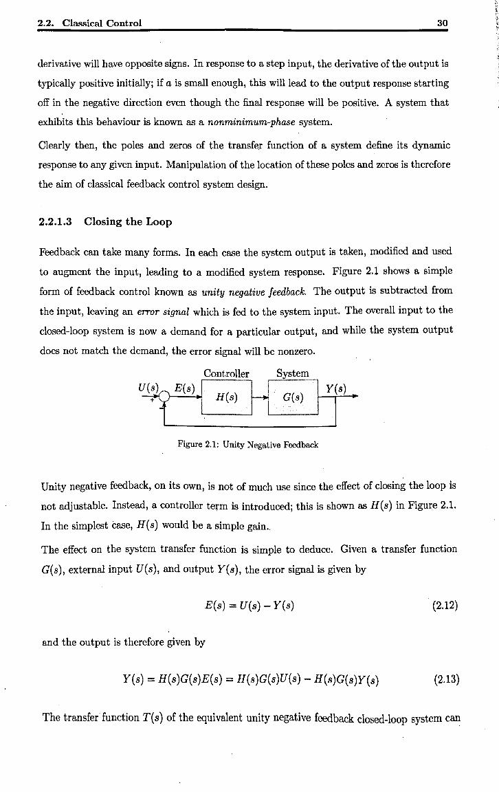
to augment the input, leading to a modified system response. Figure 2.1 shows a simple
form of feedback control known as unity negative feedback. The output is subtracted from
the input, leaving an error signal which is fed to the system input. The overall input to the
dosed-loop system is now a demand for a particular output, and while the system output
does not match the demand, the error signal will be nonzero.
Controller System ................. n ••••••••••••••••• 1-··_····_··_·········_-
U(s)( E(s) H(s)
Y(s) + : G(s)
Figure 2.1: Unity Negative Feedback
Unity negative feedback, on its own, is not of much use since the effect of dosing the loop is
not adjustable. Instead, a controller term is introduced; this is shown as H(s) in Figure 2.1.
In the simplest case, H(s) would be a simple gain ..
The effect on the system transfer function is simple to deduce. Given a transfer function
G(s), external input U(s), and output Y(s), the error signal is given by
E(s) = U(s) - Y(s) (2.12)
and the output is therefore given by
Y(s) = H(s)G(s)E(s) = H(s)G(s)U(s) - H(s)G(s)Y(s) (2.13)
The transfer'function T(s) of the equivalent unity negative feedback closed-loop system can
2.2. Classical Control
now be found:
(1 + G(s)H(s)) Yes) = G(s)H(s)U(s)
T(s) _ Yes) _ . G(s)H(s) - U(s) - 1 + G(s)H(s)
31
(2.14)
(2.15)
The poles and zeros of this closed-loop system are interesting to investigate. If the open loop
transfer function G(s) is defined as
and the controller H (s) as
then by substitution,
G( ) = Z(s) s pes)
H(s} = Ze(s) Pe(s)
~~ T(s} = PJ8)P[S)
1 + ~18) Z(~ PJ8)P[S)
Z(s)Ze(s) -~~--~~~--~
P(s}Pc(s) + Z(s}Ze(s)
(2.16)
(2.17)
(2.18)
(2.19)
Examination of Equation 2.19 shows that any' root of Z(s) is a root of the numerator of
the closed-loop transfer function T(s). This shows that the zeros of G(s) are invariant
under feedback, though any zeros present in the controller H (s) will manifest themselves
as additional zeros in T( s).
As described, the simplest type of unity negative feedback control uses a simple gain, so that
H(s) = K. Then from Equations 2.15 and 2.19, the closed loop transfer function reduces to
T s = KG(s) _ KZ(s) () 1 + KG(s) - pes) + KZ(s)
(2.20)
showing once more that the system zeros remain unchanged under feedback.
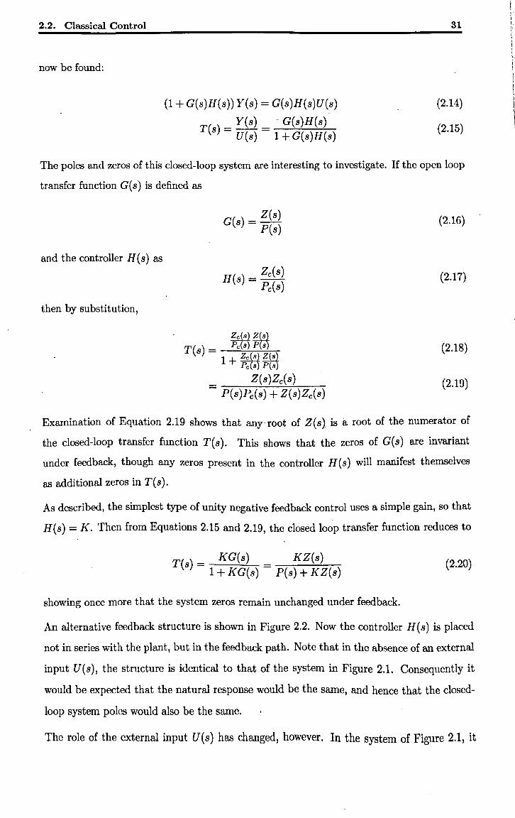
An alternative feedback structure is shown in Figure 2.2. Now the controller H(s) is placed
not in series with the plant, but in the feedback path. Note that in the absence of an external
input U(s), the structure is identical to that of the system in Figure 2.1. Consequently it
would be expected that the natural response would be the same, and hence that the closed
loop system poles would also be the same.
The role of the external input U(s) has changed, however. In the system of Figure 2.1, it
2.2. Classical Control 32
System U(s) E(s)
G(s)
tt I
+ ,/ ..:
H(s) I .... _.
Controller
Figure 2.2: Alternative Negative Feedback
acted to demand a particular output response; this is no longer the case, since the summing
junction appears after the feedback signal has been modified by the.controller H(s). For the
same reason, it is no longer strictly accurate to refer to the signal E(s) as the error signal,
though the notation will be retained for convenience.
Analysis of Figure 2.2 allows the construction of the closed loop transfer function:
E(s) = U(s) - H(s)Y(s)
yes) = G(s)E(s)
= G(s)U(s) - G(s)H(s)Y(s)
(1 + G(s)H(s)) Yes) = G(s)U(s)
T(s) _ Yes) _ G(s) - U(s) - 1 + G(s)H(s)
Substitution of Equations 2.16 and 2.17 now gives
~ T(s) = P(8j
1+~~ PTs'iPcTsJ Z(s)Pc(s)
-~~~~~~--~ P(s)Pc(s) + Z(s)Zc(s)
(2.21)
(2.22)
(2.23)
(2.24)
(2.25)
(2.26)
(2.27)
Comparison with Equation 2.19 shows that the poles are indeed identical as predicted. The
zeros of this alternative closed loop system, however, are composed not of the zeros of the
plant and controller, but of the plant zeros and the controller poles.
Once again, a simple gain H (s) = K is employed in the simplest case; the closed loop transfer
function now reduces to
Ci(s) Z(s) T(s) = 1 + KCi(s) = pes) + KZ(s) (2.28)
2.2. Classical Control 33
The manipulation of the poles of the closed loop system, by adjustment of H(s) or K, is the
aim of the classical approach to the feedback control of a linear, single-input single-output
system.
2.2.2 Gain Determination
Determining the gain, or controller transfer function, necessary to place the system poles at
the required locations is not a trivial task. Even before this, however, comes the problem of
determining suitable pole locations to satisfy a given set of design criteria.
The subject of dominance has been introduced, and this provides a mechanism for simplifying
the problem of pole placement. If a system can be considered to be dominantly first or second
order, or by the assignment of poles it can be forced to be so, then optimal locations for the
dominant poles can be found relatively easily. The response of simple first-order poles and
complex conjugate second order pole pairs was derived above, and these derivations are ex
tended to allow the determination of ideal pole locations with respect to pseudo-quantitative
time-domain measures such as settling time, rise time, time to peak overshoot, and percentage
overshoot (for details of these measures, see Nise, 1995).
Once suitable locations have been found for the dominant poles, the problem of finding the
appropriate controller transfer function can be addressed. For simplicity, this process will first
be described in the context of finding a simple gain; more complex controllers are introduced
in Section 2.2.3.
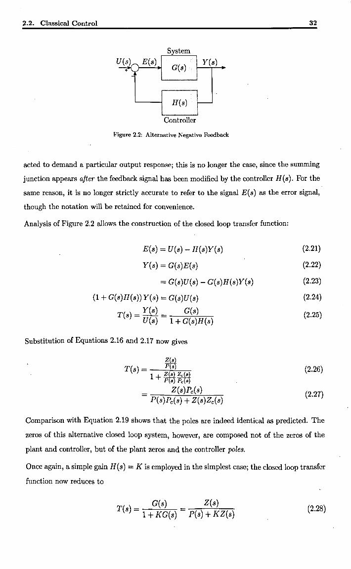
2.2.2.1 Root Locus Plots
One of the most commonly used tools for analysing the effect of changing the loop gain in a
classical feedback control system is the root locus plot. Consider the simplified unity negative
feedback system of Figure 2.3.
Gain System
~ E(s) r-~-"-H-~~:~"l Y(s)
I ·
Figure 2.3: Simple Unity Negative Feedback
As the gain K is changed, the denominator of the closed-loop transfer function will change
(via Equation 2.19) and hence so will the location of the poles. The root locus plot is a
2.2. Classical Control 34
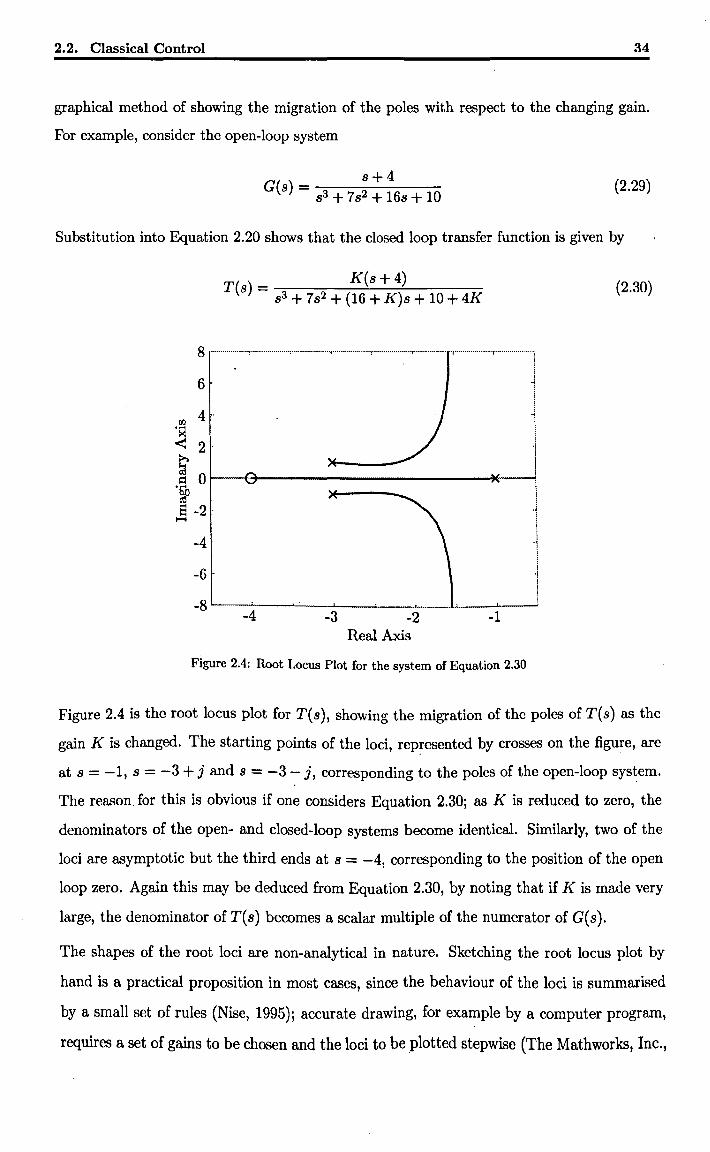
graphical method of showing the migration of the poles with respect to the changing gain.
For example, consider the open-loop system
G(s) _ 8+4 - 83 + 782 + 168 + 10
(2.29)
Substitution into Equation 2.20 shows that the closed loop transfer function is given by
T s _ K(s+4) ( ) - 83 + 782 + (16 + K)8 + 10 + 4K
8 ................... ,. ................... : .............. ······,···················'\"················ .. ·1········ ......... ·,···················,····················l ;
\ ..j :
! 6
4 · j "
.~ I ~ 2, ~
~ O~~:~-----------------------*~ 'Q I ~ J S -2" !
1-1 :
-4
-6 '
! i
"
! ! ! 'i ! , i
-8~--~--~--~----~--~--~----~~! -4 -3 -2
Real Axis -1
Figure 2.4: Root Locus Plot for the system of Equation 2.30
(2.30)
Figure 2.4 is the root locus plot for T(8), showing the migration of the poles of T(s) as the
gain K is changed. The starting points of the loci, represented by crosses on the figure, are
at 8 = -1, 8 = -3 + j and 8 = -3 - j, corresponding to the poles of the open-loop sys~em.
The reason. for this is obvious if one considers Equation 2.30; as K is reduced to zero, the
denominators of the open- and closed-loop systems become identical. Similarly, two of the
loci are asymptotic but the third ends at 8 = -4, corresponding to the position of the open
loop zero. Again this may be deduced from Equation 2.30, by noting that if K is made very
large, the denominator of T(s) becomes a scalar multiple of the numerator of G(s).
The shapes of the root loci are non-analytical in nature. Sketching the root locus plot by
hand is a practical proposition in most cases, since the behaviour of the loci is summarised
by a small set of rules (Nise, 1995); accurate drawing, for example by a computer program,
requires a set of gains to be chosen and the loci to be plotted stepwise (The Mathworks, Inc.,
2.2. Classical Control 35
2005). It is relatively easy, given a point on a root locus, to find the value of K necessary to
place a pole there.
By definition, the root locus describes those points on the complex plane at which poles can
lie; placing poles at any other point is impossible. Hence, if the system requirements can
be expressed as graphical constraints, the intersection of the root locus with the constraints
gives the solution.
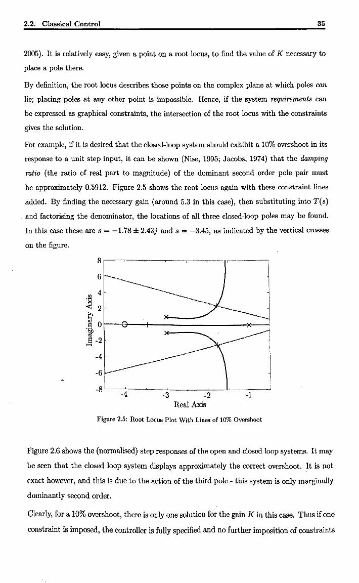
For example, if it is desired that the closed-loop system should exhibit a 10% overshoot in its
response to a unit step input, it can be shown (Nise, 1995; Jacobs, 1974) that the damping
ratio (the ratio of real part to magnitude) of the dominant second order pole pair must
be approximately 0.5912. Figure 2.5 shows the root locus again with these constraint lines
added. By finding the necessary gain (around 5.3 in this case), then substituting into T(s)
. and factorising the denominator, the locations of all three closed-loop poles may be found.
In this case these are 8 = -1.78 ± 2.43j and 8 = -3.45, as indicated by the vertical crosses
on the figure.
~~1 --- ; ...,.-- '1
~~ I .~
1
i !
-8 ................... J. •••••••••••• _ ••••• : •••••••••••••••••••• ~ •••••••••••••••••.• ;. ••••••••••••••••••• : •••• _ ••••••••••. ..I. ••••••••••••••••••• J ••••••••••••••••••• .J -4 -3 -2 -1
Real Axis
Figure 2.5: Root Locus Plot With Lines of 10% Overshoot
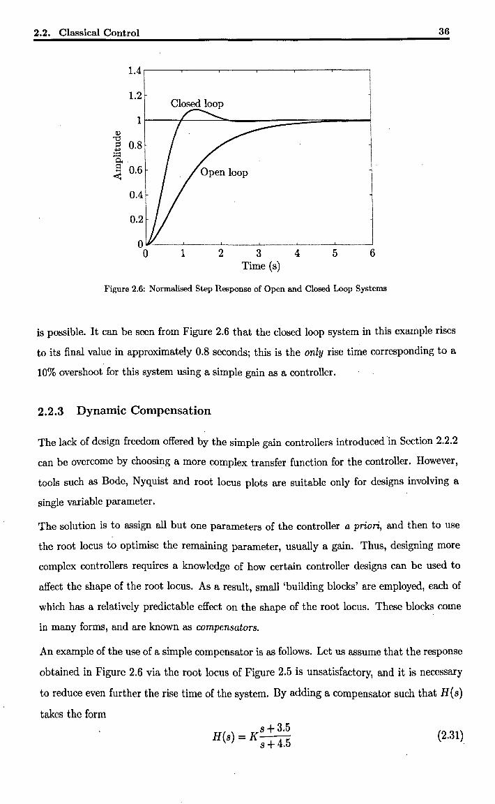
Figure 2.6 shows the (normalised) step responses of the open and closed loop systems. It may
be seen that the closed loop system displays approximately the correct overshoot. It is not
exact however, and this is due to the action of the third pole - this system is only marginally
dominantly second order.
Clearly, for a 10% overshoot, there is only one solution for the gain K in this case. Thus if one
constraint is imposed, the controller is fully specified and no further imposition of constraints
2.2. Classical Control
:
\ I 1
:
i 1r---r---~-----=======----~;
.g "'"" 0.8 ..... P.. ~ 0.6
0.4
0.2·
: ;
I ... 1
I -1 : I
J ; i i o : ....... _ ... _ ... _ ..... J •• _ •• _. ___ ••••••••••• .l .. _ ••• _ •• _ ••••••••• _ .• J. •••••••.. __ .••••••••.. .l ..• _ ..•• _ ••••. _ ...... ..J ••••••••• _ ............... j
o 1 2 3 456 Time (s)
Figure 2.6: Normalised Step Response of Open and Closed Loop Systems
36
is possible. It can be seen from Figure 2.6 that the closed loop system in this example rises
to its final value in approximately 0.8 seconds; this is the only rise time corresponding to a
10% overshoot for this system using a simple gain as a controller.
2.2.3 Dynamic Compensation
The lack of design freedom offered by the simple gain controllers introduced in Section 2.2.2
can be overcome by choosing a more complex transfer function for the controller. However,
tools such as Bode, Nyquist and root locus plots are suitable only for designs involving a
single variable parameter.
The solution is to assign all but one parameters of the controller a priori, and then to use
the root locus to optimise the remaining parameter, usually a gain. Thus, designing more
complex controllers requires a knowledge of how certain controller designs can be used to
affect the shape of the root locus. As a result, small 'building blocks' are employed, each of
which has a relatively predictable effect on the shape of the root locus. These blocks come
in many forms, and are known as compensators.
An example of the use of a simple compensator is as follows. Let us assume that the response
obtained in Figure 2.6 via the root locus of Figure 2.5 is unsatisfactory, and it is necessary
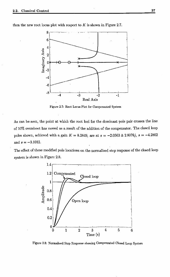
to reduce even further the rise time of the system. By adding a compensator such that H(s)
takes the form 8+3.5
H(s) = K 45 s+ . (2.31)
2.2. Classical Control
then the new root locus plot with respect to K is shown in Figure 2.7.
8.---~--~--~--~---.r---r---~--,
6 J ~~~ :
~~~, ! 4 -----~., -i
~ 2 ~- ______ ~_~ J
~ ----.~ ~ O~-+tr--~~-+----------------~~~ .,.._ J Cl) ... __ ,
cO ___ ••••• ~ i S -2 . __ ~...'j
- i ____ ~- .J
------- ! --- :
-4
......---- : -6 1 : : ;
_ 8 ............. __ .J. •••••••• _ •••••• _.: ............ _ ••••• ~ ................... ;. ••. _ ... _......... . •••••••• _ ••• _ ••• ~ ... _ ......... _ ••• J. •• _ ............. .! -4 -3 -2 -1
Real Axis
Figure 2.7: Root Locus Plot for Compensated System
37
As can be seen, the point at which the root loci for the dominant pole pair crosses the line
of 10% overshoot has moved as a result of the addition of the compensator. The closed loop
poles shown, achieved with a gain K = 8.2849, are at s = -2.0563 ± 2.8076j, s = -4.2862
and s = -3.1012.
The effect of these modified pole locations on the normalised step response of the closed loop
system is shown in Figure 2.8.
1.4 .......................... ,. .......................... , .......................... , .... -..................... ,·· .. ······· .. ·············,.···················_··· .. 1
1.2 . Comp'ensated
.lj ln ~ 0.81'
~ 0.6~ 0.4 ~ o.2f
!
.\
I ! I .j !
I ~ 1 I !
i
\
J !
O! .----'-----'----j i
--~---~---~
o 1 2 3 4 5 6 Time (s)
Figure 2.8: Normalised Step Response showing Compensated Closed Loop System

2.2. Classical Control 38
The compensator of Equation 2.31 is known as a phase lead compensator, but many different
configurations exist. Their application and design is the choice of the control engineer, and
although tools exist for assessing the likely impact of the use of a compensator, such design
decisions must ultimately come from experience.
2.2.4 Multiple Loops
If a system has more than one output, but retains a single input, standard classical approaches
can often be used to good effect. For example, Figure 2.9 shows a system wherein one output
is a function of the other.
u i1cr K2 11 Kl G1{s) Yl(S) G2(s)
Y2(S) ~
-
Figure 2.9: Concentric Two-Loop Control System
This is a common occurrence - typically one output might be the integral of another, such as
in an actuator system whose outputs are velocity and position. The design procedure in this
case is usually to close the 'innermost' loop first, and work outwards - so in this case, to find
Kl first and then K2· Clearly the selection of Kl will change the dynamics of the system
from U{s) to Yl(S), and consequently will change the shape of the root locus with respect to
Y2(S), The design process is therefore usually iterative. An initial value of Kl is selected, and
the shape of the resulting outer root locus found. Kl is then adjusted to change the shape
of the outer root locus until it passes through the site of the desired closed-loop poles, and
K2 is then selected.
If the system to be controlled has multiple outputs and multiple inputs, the process becomes
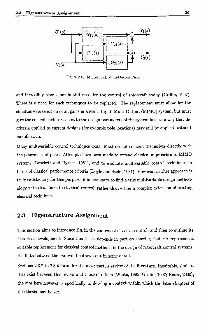
significantly more involved. Figure 2.10 shows just one possible configuration of such a
system. The figure shows only the open-loop plant, with the controller gains and feedback
loops omitted for clarity.
Clearly now there are four possible feedback paths, from Y1{s) or Y2(s) to U1(s) or U2(s).
There is no longer a logical sequence to follow when constructing a controller. Choosing,
for example, the gain K22 linking U2 to Y2 will affect not only the transfer function b~t:~
but also all the others. Hence every gain chosen has an effect on the others which must
all be recalculated to take account of the change. The process is iterative, non-intuitive
1
2.3. Eigenstructure Assignment
Gl1 {8} I i ~G))-_Y;_l~.S) ~======.~(s)
f······~~~·~~·;········II-~~·~"~I---~·· ! j Y; ( ) ! i 2 S , ; G22 (S)
i !
Figure 2.10: Multi-Input, Multi-Output Plant
39
and incredibly slow - but is still used for the control of rotorcraft today (Griffin, 1997).
There is a need for such techniques to be replaced. The replacement must allow for the
simultaneous selection of all gains in a Multi-Input, Multi-Output (MIMO) system, but must
give the control engineer access to the design parameters of the system in such a way that the
criteria applied to current designs (for example pole locations) may still be applied, without
modification.
Many multivariable control techniques exist. Most do not concern themselves directly with
the placement of poles. Attempts have been made to extend classical approaches to MIMO
systems (Brockett and Byrnes, 1981), and to evaluate multivariable control techniques in
terms of classical performance criteria (Doyle and Stein, 1981). However, neither approach is
truly satisfactory for this purpose; it is necessary to find a true multivariable design method
ology with clear links to classical control, rather than either a complex extension of existing
classical techniques .
. 2.3 Eigenstructure Assignment
This section aims to introduce EA in the context of classical control, and then to outline its
historical development. Since this thesis depends in part on showing that EA represents a
suitable replacement for classical control methods in the design of rotor craft control systems,
the links between the two will be drawn out in some detail.
Sections 2.3.2 to 2.3.4 form, for the most part, a review of the literature. Inevitably, similar
ities exist between this review and those of others (White, 1995; Griffin, 1997; Ensor, 2000);
the aim here however is specifically to develop a context within which the later chapters of
this thesis may be set.
2.3. Eigenstructure Assignment 40
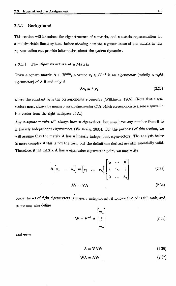
2.3.1 Background
This section will introduce the eigenstructure of a matrix, and a matrix representation for
a multivariable linear system, before showing how the eigenstructure of one matrix in this
representation can provide information about the system dynamics.
2.3.1.1 The Eigenstructure of a Matrix
Given a square matrix A E JRnxn, a vector Vi E Cnx1 is an eigenvector (strictly a right
eigenvector) of A if and only if
(2.32)
where the constant Ai is the corresponding eigenvalue (Wilkinson, 1965). (Note that eigen
vectors must always be nonzero, so an eigenvector of A which corresponds to a zero eigenvalue
is a vector from the right nullspace of A.)
Any n-square matrix will always have n eigenvalues, but may have any number from 0 to
n linearly independent eigenvectors (Weisstein, 2005). For the purposes of this section, we
will assume that the matrix A has n linearly independent eigenvectors. The analysis below
is more complex if this is not the case, but the definitions derived are still essentially valid.
Therefore, if the matrix A has n eigenvalue-eigenvector pairs, we may write
o (2.33)
o
AV=VA .(2.34)
Since the set of right eigenvectors is linearly independent, it follows that V is full rank, and
so we may also define
and write
w=V-1 =
A=VAW
WA=AW
(2.35)
(2.36)
(2.37)
2.3. Eigenstructure Assignment 41
From Equation 2.37 it can be seen that for a given eigenvalue Ai, the eigenvalue-eigenvector
relationship of Equation 2.32 has a dual:
(2.38)
The vector Wi E C1xn is therefore known as a left eigenvector of A.
Note that for a real-valued matrix A E jRnxn, the eigenvalues {Ai} of A form a self-conjugate
set and that Ai = Xi implies Vi = Vi and Wi = Vii'
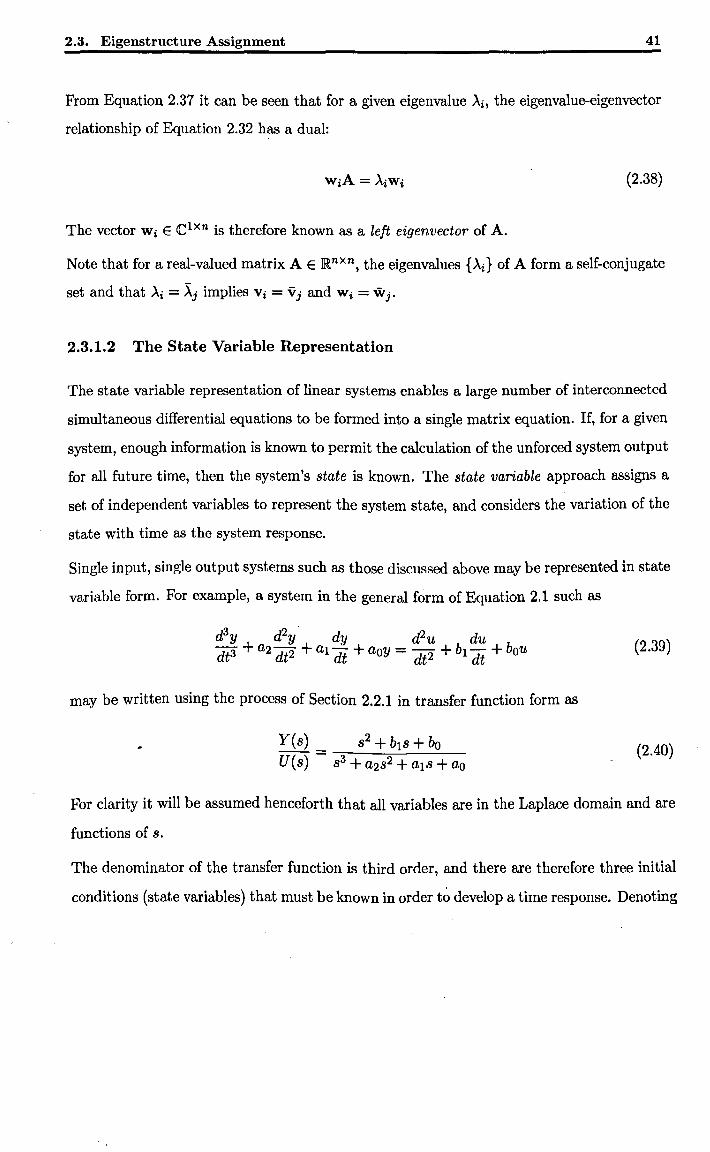
2.3.1.2 The State Variable Representation
The state variable representation of linear systems enables a large number of interconnected
simultaneous differential equations to be formed into a single matrix equation. If, for a given
system, enough information is known to permit the calculation of the unforced system output
for all future time, then the system's state is known. The state variable approach assigns a
set of independent variables to represent the system state, and considers the variation of the
state with time as the system response.
Single input, single output systems such as those discussed above may be represented in state
variable form. For example, a system in the general form of Equation 2.1 such as
(2.39)
may be written using the process of Section 2.2.1 in transfer function form as
y (s) _ 82 + bI 8 + bo U(8) - 8 3 + a2s2 + aI8 + ao
(2.40)
For clarity it will be assumed henceforth that all variables are in the Laplace domain and are
functions of 8.
The denominator of the transfer function is third order, and there are therefore three initial
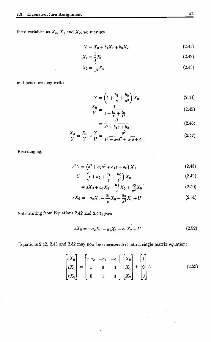
conditions (state variables) that must be known in order t~ develop a time response. Denoting
2.3. Eigenstructure Assignment
these variables as Xo, Xl and X2, we may set
and hence we may write
Rearranging,
Substituting from Equations 2.42 and 2.43 gives
42
(2.41)
(2.42)
(2.43)
(2.44)
(2.45)
(2.46)
(2.47)
(2.48)
(2.49)
(2.50)
(2.51)
(2.52)
Equations 2.42, 2.43 and 2.52 may now be concatenated into a single matrix equation:
sXo
SXI - 1
o o 1
o o
1
Xl + 0 U
o
(2.53)
2.3. Eigenstructure Assignment
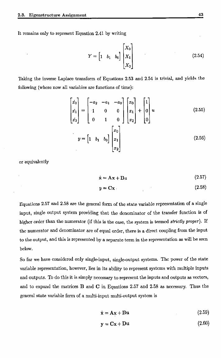
It remains only to represent Equation 2.41 by writing
Xo
y = [1 bl bo] . Xl
X2
43
(2.54)
Taking the inverse Laplace transform of Equations 2.53 and 2.54 is trivial, and yields the
following (where now all variables are functions of time):
Xo -a2 -al -aD
Xl - 1 0 0
X2 0 1 0
Xo
y= [1 bl bo] Xl
X2
or ·equivalently
x=Ax+Du
y=Cx.
Xo 1
Xl + 0
X2 0
u (2.55)
(2.56)
(2.57)
(2.58)
Equations 2.57 and 2.58 are the general form of the state variable representation of a single
input, single output system providing that the denominator of the transfer function is of
higher order than the numerator (if this is the case, the system is termed strictly proper). If
the numerator and denominator are of equal order, there is a direct coupling from the input
to the output, and this is represented by a separate term in the representation as will be seen
below.
So far we have considered only single-input, single-output systems. The power of the state
variable representation, however, lies in its ability to represent systems with multiple inputs
and outputs. To do this it is simply necessary to represent the inputs and outputs as vectors,
and to expand the matrices Band C in Equations 2.57 and 2.58 as necessary. Thus the
general state variable form of a multi-input multi-output system is
x=Ax+Bu
y = Cx+Du
(2.59)
(2.60)
2.3. Eigenstructure Assignment 44
where A E lR(nxn) is the system matrix, B E lR(nxr) is the input matrix, C E lR(mxn) is the
output matrix and D E jR(mxr) is the direct transmission matrix.
Throughout this thesis, and in the wider literature, a system might be referred to for example
as 'a state-space system (A, B)' meaning a state variable system whose direct transmission
matrix is null and whose output matrix is the identity matrix (ie. all states are measurable).
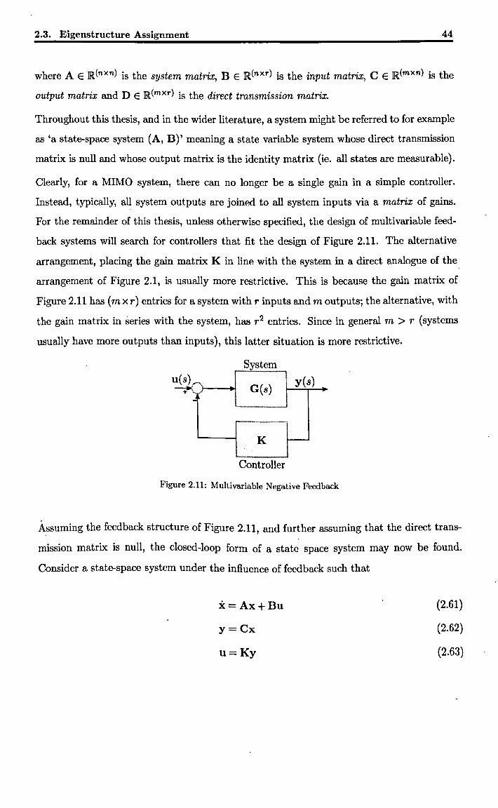
Clearly, for a MIMO system, there can no longer be a single gain in a simple controller.
Instead, typically, all system outputs are joined to all system inputs via a matrix of gains.
For the remainder of this thesis, unless otherwise specified, the design of multi variable feed
back systems will search for controllers that fit the design of Figure 2.11. The alternative
arrangement, placing the gain matrix K in line with the system in a direct analogue of the
arrangement of Figure 2.1, is usually more restrictive. This is because the gain matrix of
Figure 2.11 has (m xr) entries for a system with r inputs and m outputs; the alternative, with
the gain matrix in series with the system, has r2 entries. Since in general m > r (systems
usually have more outputs than inputs), this latter situation is more restrictive.
System
! Controller
Figure 2.11: Multivariable Negative Feedback
Assuming the feedback structure of Figure 2.11, and further assuming that the direct trans
mission matrix is null, the closed-loop form of a state space system may now be found.
Consider a state-space system under the influence of feedback such that
x=Ax+Bu
y=Cx
u=Ky
(2.61)
(2.62)
(2.63)
2.3. Eigenstructure Assignment
By substitution,
u=KCx
X= Ax+BKCx
= (A + BKC)x
45
(2.64)
(2.65)
(2.66)
Therefore Equations 2.62 and 2.66 together define the closed-loop system dynamics, and by
comparison with Equation 2.61 we may define the closed loop system matrix Ad as
Ad =A+BKC (2.67)
2.3.1.3 Multivariable Transfer Functions
Given a system in the state variable form, it is possible to recover a transfer function repre
sentation even if the system has multiple inputs and outputs. In the Laplace domain, from
Equation 2.59,
sx(s) = Ax(s) + Bu(s)
(sI - A) x(s) = Bu(s)
x(s) = (sI - A)-l Bu(s)
Substituting into Equation 2.58,
y(s) = C (sI - A)-l Bu(s) + Du(s)
= (c (sI - A)-l B + D) u(s)
A G(s)u(s)
(2.68)
(2.69)
(2.70)
(2.71)
(2.72)
(2.73)
where G(s) is the tmnsfer function matrix, containing a polynomial transfer function for each
input-output pair.
Since the inverse of a matrix X may be written in terms of its adjoint matrix and its deter
minant as
X-l _ adj(X) - det(X)
(2.74)
2.3. Eigenstructure Assignment
it is possible to write Equation 2.73 as
G(s) = Cadj(sI-A)B+D det (sI - A)
46
(2.75)
Equation 2.75 reveals that the denominator of each entry in the transfer function matrix is
the same, while the numerators differ.
Interestingly, the transfer function matrix demonstrates that state variable systems are non
unique; it is possible to transform the state vector, and the system matrices, in such a way
that the transfer function matrix remains unchanged.
Consider forming a transformed state vector x such that
x=Ex (2.76)
where E is a square, nonsingular matrix. Now Equations 2.59 and 2.60 may be written as
Ex=AEx+Bu
y=CEx+Du
and premultiplying Equation 2.77 by the inverse of E gives
i. = (E-1 AE) x + (E-IB) u
y = (CE)x+Du
If we now defin~ the tr~nsformed system matrices as
At.E-1AE
B A E-1B
CACE
D~D
then the transformed system may be written as
i=A.x+Bu
y=Cx+Du
(2.77)
(2.78)
(2.79)
(2.80)
(2.81)
(2.82)
(2.83)
(2.84)
(2.85)
(2.86)
2.3. Eigenstructure Assignment 47
The transfer function of the transformed system, from Equation 2.73, can now be seen to be
as expected.
6(s) =-C (sI - A) -1 13 + D
= (CE) (sI - E-1 AEr1 (E-1B) + D
= C (E (sI - E-1 AE) E-1)-1 B
=C(sI-A)-1 B + D
= G(s)
2.3.1.4 Eigenstructure and the State Space
(2.87)
(2.88)
(2.89)
(2.90)
(2.91)
. There exists a simple form of time-domain solution for a state-variable system in the unforced
case, a multivariable analogue of the response of Equation 2.2.
It may be shown (see Nise, 1995) that the unforced time response of a state variable system
is given by
(2.92)
where the term eAt, often denoted ~, is known as the state transition matrix. If the state
vector is considered as describing a direction in a space (or a hyperspace), then the state
transition matrix describes the trajectory of the state vector through the state space. The
term 'state space' has come to be employed to describe state variable systems, just as the
word 'state' is used to mean 'state variable'. These terms will be used interchangeably for
the remainder of this thesis . . The state transition matrix, although useful for determining a time response, is n~t partic
ularly informative. It is not clear how changing the system matrix A will affect the time
response of the resulting system. If instead a transformed system is constructed via Equa
tions 2.81 to 2.84 using a transformation matrix E = V (the matrix of right eigenvectors),
then evaluating the time response of the transformed system is instructive. From Equa
tion 2.81, the transformed system matrix is
(2.93)
via Equation 2.36, where A is the diagonal matrix of eigenvalues of A. Using Equation 2.92,
2.3. Eigenstructure Assignment
the unforced time response of the transposed system can be seen to be
Applying Equation 2.76 yields
y-Ix(t) = eAty-Ix(O)
x(t) = YeAtWx(O)
since y-I = W (from Equation 2.35).
48
(2.94)
(2.95)
(2.96)
Equation 2.96 is very informative, given that the transfer functions (and hence the poles)
of the original and transposed systems are identical. Firstly it may be seen that the only
time-variant portion of the unforced response is
o (2.97)
o
This is a diagonal matrix containing all of the exponential modes of the system (cf. Equa
tion 2.2). Hence the eigenvalues of A correspond directly to the system poles. Secondly, the
matrices Y and W of the right and left eigenvectors respectively have a physical interpre
tation as well. The initial state vector x(O) acts to excite the system modes via W, and
the modal response manifests itself in the time-varying state vector x(t) via y. Hence, for
a given mode, the associated left eigenvector describes the way in which state disturbances
excite the system modes, and the associated right eigenvector describes the coupling of the
system modes into the state vector. These facts underpin the idea of EA: If a control system
can be designed that affects the eigenstructure of A in a predictable manner, then the sys
tem poles may be placed and the coupling between the system modes and the states may be
influenced.
2.3.1.5 Controllability and Observability
Controllability and observability, as properties of a state variable system, are important
concepts in the context of control system design.
A system is s,aid to be controllable if it is possible to generate a system input that will transfer
2.3. Eigenstructure Assignment 49
the system from its initial state x{O) to any other state in a finite period of time. If this is
not the case it implies that there are uncontrollable system modes which can not be affected
by manipulation of the system input. It can be shown (Ogata, 1997) that the controllability . .
of a state space system (A, B) is equivalent to the condition that
rank ([B : AB : ... : An-1B]) = n (2.98)
Similarly, a system is said to be observable if it is possible, by observation of the system
output y(t) over a finite time, to determine the system state. If this is not the case, it implies
that there are unobservable system modes which do not manifest themselves in the system
output. It can again be shown (Ogata, 1997) that the observability of a state space system
(A, C) is equivalent to the condition that
rank
C
CA
CAn - 1
=n (2.99)
Controllability and observability are often given as preconditions for forming multi variable
control systems, as will be seen. This is not as restrictive a condition as it would at first appear
to be, however. If a system has uncontrollable modes, either these modes are important to
the system response or they are not; if they are not, a reduced model may be formed that
does not include these dynamics. Similarly, if unobservable modes are present then further
sensors should be added to the system to allow detection of these modes, lest they become
unstable under feedback.
Interestingly, it is possible for the controllability or observability test matrices to be full rank
but ill-conditioned; this implies either a nearly-uncontrollable mode, requiring large control
efforts to affect it, or a nearly-unobservable mode, whose effect is hard to detect in the
output vector. For this reason Mehrmann and Xu (2000) define the concept of 'distance to
controllability' and use it as a system analysis tool.
2.3. Eigenstructure Assignment 50
2.3.1.6 Modal Coupling Matrices
Taking the multivariable transfer function matrix from Equation 2.73
G(s) = C (sI - A)-l B + D (2.100)
it may be seen that the eigenvalue-eigenvector decomposition of A from Equation 2.36 may
be used to yield
G(s) = C(sl- VAW)-lB+D
= C (V (sl- A)W)-lB + D
= CV(sl- A)-lWB +D
(2.101)
(2.102)
(2.103)
The term (sI - A)-.l is a diagonal matrix of terms which, in the Laplace domain, describe
the exponential response of each mode. It is known that the matrices Wand V describe the
coupling from the states to the modes and the modes to the states respectively.
Hence, the terms CV and WB in Equation 2.103 describe the c~upling from the modes
to the outputs, and from the inputs to the modes. They are known respectively as the
output coupling matrix and the input coupling matrix, and collectively as the modal coupling
matrices.
Often, entries of the modal coupling matrices (particularly of the output coupling matrix) will
be of more importance to the satisfaction of design criteria than the eigenvectors themselves.
Indeed, for systems which have been obtained using system identification techniques rather
than direct modelling, the states have no physical meaning and assignment of the modal
c~upling matrices is the only satisfactory solution (Griffin, 1997).
2.3.1.7 Multivariable Zeros
It has been seen that the po~es and zeros of a SISO system are those values of s which cause
the transfer function G(s) to equal 00 or 0, respectively. It is instructive to draw a parallel
between this behaviour and that of their MIMO counterparts.
From Equation 2.73, it is clear that any eigenvalue s = A of A will cause the matrix (sI - A)
to have a zero determinant. Hence the system poles are those values {A} for which G(A) = 00.
Such a definition is possible because all the entries in the transfer function matrix share a
common denominator (from Equation 2.75).
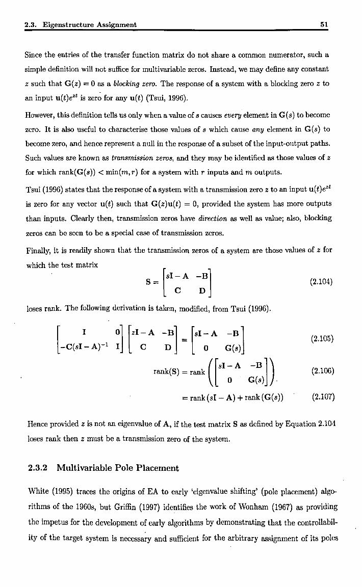
2.3. Eigenstructure Assignment 51
Since the entries of the transfer function matrix do not share a common numerator, such a
simple definition will not suffice for multivariable zeros. Instead, we may define any constant
z such that G(z) = 0 as a blocking zero. The response of a system with a blocking zero z to
an input u(t)ezt is zer~ for any u(t) (Tsui, 1996).
However, this definition tells us only when a value of s causes every element in G(s) to become
zero. It is also useful to characterise those values of s which cause any element in G(s) to
become zero, and hence represent a null in the response of a subset of the input-output paths.
Such values are known as transmission zeros, and they may be identified as those values of z
for which rank{G{s)) < min(m,r) for a system with r inputs and m outputs.
Tsui (1996) states that the response of a system with a transmission zero z to an input u(t)ezt
is zero for any vector u(t) such that G(z)u(t) = 0, provided the system has more outputs
than inputs. Clearly then, transmission zeros have direction as well as value; also, blocking
zeros can be seen to be a special case of transmission zeros.
Finally, it is readily shown that the transmission zeros of a system are those values of z for
which the test matrix
(2.104)
loses rank. The following derivation is taken, modified, from Tsui (1996).
0] [Zl-A -B] = [SI-A -B] leD . 0 G(s)
(2.105)
rank(S) = rank ([SI -A -B]) o G(s) .
(2.106)
= rank (sI - A) + rank (G(s)) (2.107)
Hence provided z is not an eigenvalue of A, if the test matrix S as defined by Equation 2.104
loses rank then z must be a transmission zero of the system.
2.3.2 Multivariable Pole Placement
White (1995) traces the origins of EA to early 'eigenvalue shifting' (pole placement) algo
rithms of the 1960s, but Griffin (1997) identifies the work of Wonham (1967) as providing
the impetus for the development of early algorithms by demonstrating that the controllabil
ity of the target system is necessary and sufficient for the arbitrary assignment of its poles
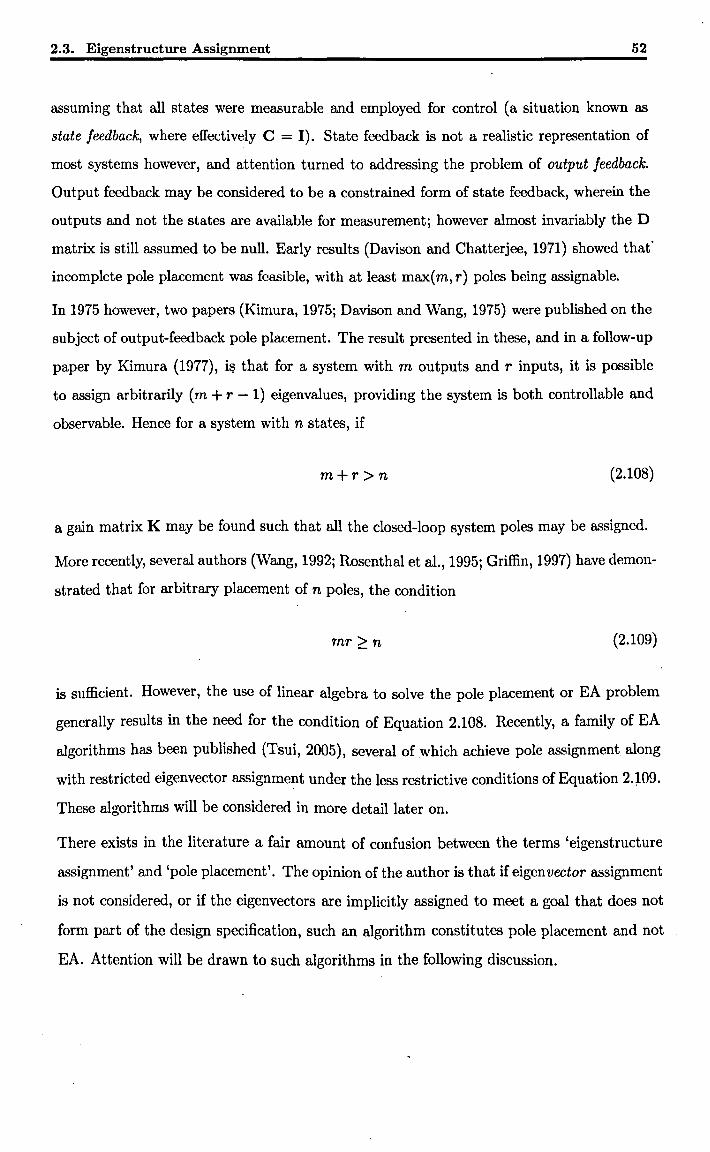
2.3. Eigenstructure Assignment 52
assuming that all states were measurable and employed for control (a situation known as
state feedback, where effectively C = I). State feedback is not a realistic representation of
most systems however, and attention turned to addressing the problem of output feedback.
Output feedback may be considered to be a constrained form of state feedback, wherein the
outputs and not the states are available for measurement; however almost invariably the D
matrix is still assumed to be null. Early results (Davison and Chatterjee, 1971) showed that'
incomplete pole placement was feasible, with at least max( m, r) poles being assignable.
In 1975 however, two papers (Kimura, 1975; Davison and Wang, 1975) were published on the
subject of output-feedback pole placement. The result presented in these, and in a follow-up
paper by Kimura (1977), i~ that for a system with m outputs and r inputs, it is possible
to assign arbitrarily (m + r - 1) eigenvalues, providing the system is both controllable and
observable. Hence for a system with n states, if
m+r>n (2.108)
a gain matrix K may be found such that all the closed-loop system poles may be assigned.
More recently, several authors (Wang, 1992; Rosenthal et al., 1995; Griffin, 1997) have demon
strated that for arbitrary placement of n poles, the condition
mr~n (2.109)
is sufficient. However, the use of linear algebra to solve the pole placement or EA problem
generally results in the need for the condition of Equation 2.108. Recently, a family of EA
algorithms has been published (Tsui, 2005), several of which achieve pole assignment along
with restricted eigenvector assignment under the less restrictive conditions of Equation 2.~09.
These algorithms will be considered in more detail later on.
There exists in the literature a fair amount of confusion between the terms 'eigenstructure
assignment' and 'pole placement'. The opinion of the author is that if eigcn vector assignment
is not considered, or if the eigenvectors are implicitly assigned to meet a goal that does not
form part of the design specification, such an algorithm constitutes pole placement and not
EA. Attention will be drawn to such algorithms in the following discussion.
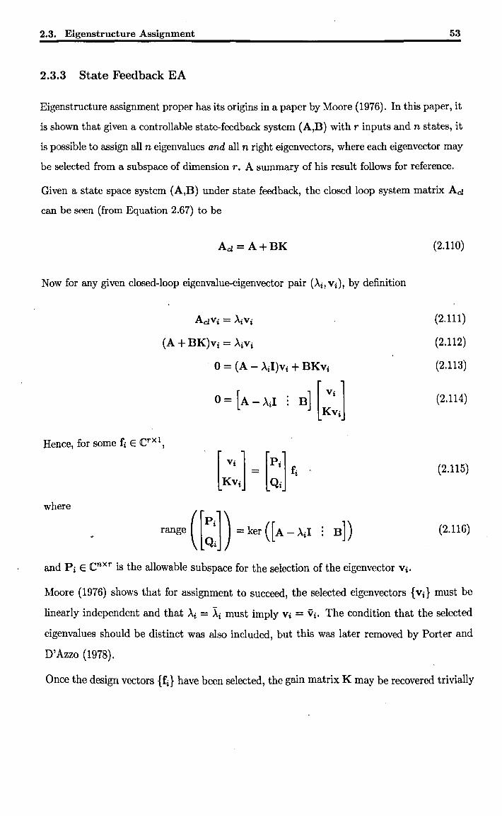
2.3. Eigenstructure Assignment 53
2.3.3 State Feedback EA
Eigenstructure assignment proper has its origins in a paper by Moore (1976). In this paper, it
is shown that given a controllable state-feedback system (A,B) with r inputs and n states, it
is possible to assign all n eigenvalues and all n right eigenvectors, where each eigenvector may
be selected from a subspace of dimension r. A summary of his result follows for reference.
Given a state space system (A,B) under state feedback, the closed loop system matrix Ad
can be seen (from Equation 2.67) to be
Ad = A+BK
Now for any given closed-loop eigenvalue-eigenvector pair P'i, Vi), by definition
(A + BK)Vi = Ai vi
0= (A - AiI)Vi + BKvi
Hence, for some fi E Crx1 ,
[;~J -[::] ~ where
and Pi E Cnxr is the allowable subspace for the selection of the eigenvector Vi.
(2.110)
(2.111)
(2.112)
(2.113)
(2.114)
(2.115)
(2.116)
Moore (1976) shows that for assignment to succeed, the selected eigenvectors {Vi} must be
linearly independent and that Ai = Xi must imply Vi = Vi. The condition that the selected
eigenvalues should be distinct was also included, but this was later removed by Porter and
D'Azzo (1978).
Once the design vectors {fi } have been selected, the gain matrix K may be recovered trivially
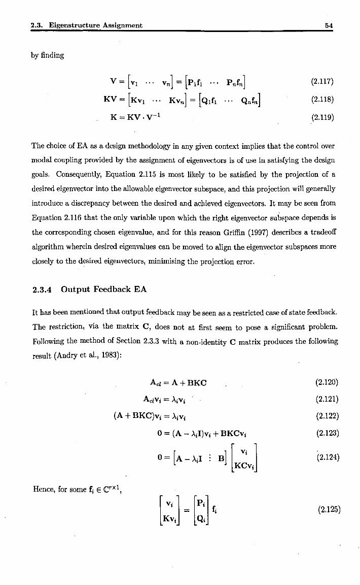
2.3. Eigenstructure Assignment
by finding
y= [VI ... Vn] = [Plfl ... Pnfn]
KY = [KVI ... KVn] = [Qlfl ... Qnfn]
K=Ky.y-1
54
(2.117)
(2.118)
(2.119)
The choice of EA as a design methodology in any given context implies that the control over
modal coupling provided by the assignment of eigenvectors is of use in satisfying the design
goals. Consequently, Equation 2.115 is most likely to be satisfied by the projection of a
desired eigenvector into the allowable eigenvector subspace, and this projection will generally
introduce a discrepancy between the desired and achieved eigenvectors. It may be seen from
Equation 2.116 that the only variable upon which the right eigenvector subspace depends is
the corresponding chosen eigenvalue, and for this reason Griffin (1997) describes a tradeoff
algorithm wherein desired eigenvalues can be moved to align the eigenvector subs paces more
closely to the desired eigenvectors, minimising the projection error.
2.3.4 Output Feedback EA
It has been mentioned that output fe~dback may be seen as a restricted case of state feedback.
The restriction, via the matrix C, does not at first seem to pose a significant problem.
Following the method of Section 2.3.3 with a non-identity C matrix produces the following
result (Andryet al., 1983):
Acl= A+BKC
(A + BKC)Vi = .AiVi
o = (A - .AiI)Vi + BKCVi
Hence for some £. E tr"rxl , ~ "-' ,
(2.120)
(2.121)
(2.122)
(2.123)
(2.124)
(2.125)
2.3. Eigenstructure Assignment 55
where Pi and Qi have meanings as before. The gain matrix may be recovered by finding .
v = [VI ... vp] = [P1f1 ... Ppfp]
KCV = [KCVI ... KCvp] ~ [Qlfl Qpfp]
K = KCV . (CV)t
(2.126)
(2.127)
(2.128)
where xt is the Moore-Penrose pseudo-inverse (Ben-Israel and Greville, 1974) of X. However,
Equation 2.128 holds only if p ::; rn, and consequently a maximum of rn poles may be
assigned using this method. The remainder are left unassigned and may become unstable.
The conditions under which a state:.feedback solution may be transformed directly into an
output-feedback one in this manner are extremely restrictive (Porter, 1977).
The output feedback problem is essentially a symmetrical one, with the matrices B and C
being duals of one another in a functional sense. Hence, assigning left eigenvectors along with
their associated eigenvalues by using subspaces generated as a function of the output matrix
C is feasible, and no more restrictive than the right eigenvector assignment described above.
Given the definition of a left eigenvector Wj,
Ad = A+B,KC
WjAd = AjWj
wj(A + BKC) = AjWj
0= wj(A - Ail) + wjBKC
0= [wJ : wjBK] [A~jI]
Hence, for some gj E C1xm,
where
and Lj E cmxn is the allowable subspace for ~he selection of the eigenvector Wj.
(2.129)
(2.130)
(2.131)
(2.132)
(2.133)
(2.134)
(2.135)
Once again, following the selection of q design vectors {gj}, the gain matrix may be recovered
2.3. Eigenstructure Assignment 56
by finding
W= (2.136)
(2.137)
K = (WB)t . WBK (2.138)
where this time K may be recovered if q ~ r.
It is therefore possible, by considering either the right or left eigenvector subspaces, to specify
max(m, r) eigenvalues and min(m, r) elements of each corresponding eigenvector, a result
found by Srinathkumar (1978). However, by imposing more stringent constraints on the
eigenvector subspaces, it is possible to assign both p ~ m eigenvalues and right eigenvectors,
and q ~ r eigenvalues and left eigcnvectors (though usually not if p"= m and q = r); hence,
if m + r > n, it is possible to assign all n eigenvalues. The algorithms which follow attempt
to do just this.
White (1995) identifies four distinct EA methods: Protection methods, parametric methods,
projection methods and orthogonal eigenvector methods. However, the latter two may be
considered to be special cases of the others, and so for clarity the only classification that will
be made here is to divide parametric methods from protection methods.
2.3.4.1 Protection Methods
Protection methods (Davison and Wang, 1975; Srinathkumar, 1978; Fletcher, 1981a, b; Fletcher
and Magni, 1987; Fahmy and O'Reilly, 1988) work by assigning a subset of the eigenvalues,
then constructing a system. with a reduced input or output vector such that the assigned
modes become uncontrollable or unobservable. If right eigenvectors have been assigned,
the reduced system has a shorter output vector than the original; if left eigenvectors were
assigned, it is the input vector that is shortened. These modes are protected since uncon
trollable or unobservable modes are invariant under output feedback. The remainder of the
eigenvalues can then be assigned to the reduced system, and the gain matrix reconstituted
by superposition at the end.
2.3. Eigenstructure Assignment 57
The algorithm of Fletcher (1981a, b) is interesting as it includes provision for a nonzero direct
transmission matrix, something that very few EA algorithms do. His algorithm assigned
eigenvalue-eigenvector pairs one at a time, each time constructing a reduced system before
continuing.
Protection methods illustrate the requirement of most EA algorithms for the condition m+r >
n to be satisfied. Consider assigning m - 1 eigenvalues to a system, together with m - 1 right
eigenvectors selected from subspaces of dimension r. The reduced system will have a single
output, and so in the second stage one may assign r eigenvalues and r left eigenvectors, each
chosen with no freedom from a subspace of dimension 1. Hence, for complete assignment,
(m - 1) + r ;::: n, or equivalently
m+r>n (2.139)
Although protection methods constitute a mathematically sound approach to the problem
of output feedback EA they are not ideal replacements for classical approaches. The main
problem is one of visibility, as described in Chapter 1. During the assignment process it is
impossible to see the effect that assigning one eigenvector will have on the allowable sub
space for the remainder, and this effectively precludes the iterative tradeoff of some design
parameters for others during the assignment process. Such iterative processes are at the core
of classical control techniques, and their use helps to reinforce an understanding of the role
that the various design parameters have in the performance of the closed loop system.
Additionally, protection methods rely heavily on the numerical accuracy of the protection
process. If the protection is not exact, assigned eigenvalues and eigenvectors can move during
the later stages of assignment, or very large gains may be generated as the a~gorithm attempts
to reassign almost-uncontrollable eigenvalues to unsuitable locations (Fahmy and Q'Reilly,
1988; White, 1991).
Finally it should be noted that Fletcher's algorithms mention eigenvectors, but do not con
sider their importance to the design solution or how they should be chosen. Consequently
these algorithms border on pole placement rather than EA.
2.3.4.2 Parametric Methods
Parametric methods constitute extensions to the original state feedback EA algorithm pre
sented by Moore (1976), which parameterised the allowable subspace for the right eigenvectors
as a means of generating a gain matrix. At the beginning of the Section it was shown that
2.3. Eigenstructure Assignment 58
merely parameterising the right or left eigenvector subspaces alone was insufficient in the
output feedback case, but the protection methods detailed above show that sufficient design
freedom does exist for the placement of n poles and the selection of n eigenvectors given
m+r > n. Hence, restrictions on the eigenvectors beyond the allowable subspace constraints
must exist in the output feedback case. Many researchers (Fahmy and O'Reilly, 1983; White,
1991; Duan, 1993; Griffin, 1997; Clarke et al., 2003; Tsui, 2005) have continued the search for
parametric EA methods on the basis that the design freedom is available in a more visible
way than is the case with protection methods.
As an aside, White (1995) describes 'projection methods' as being those which project desired
eigenvectors into their allowable subspaces. However, they can be viewed simply as parametric
methods wherein the parameters are employed for the projection of desired eigenvectors,
and consideration of these as distinct from parametric methods as a whole is not helpful.
Similarly, 'orthogonal eigenvector methods' are those which seek to assign a near-orthogonal
set of eigenvectors since analysis shows that the sensitivity of the closed-loop eigenvalues to
perturbations in the set {A, B, C, K} is at a minimum when the eigenvectors are orthogonal
(Wilkinson, 1965; Kautsky et al., 1982; Fletcher et al., 1985). These are not assignment
methods as such, but employ complex methods to determine a set of assignable eigenvectors
which are as near as possible to being mutually orthogonal prior to assignment. In general
parametric methods are used for the actual assignment, often in an iterative process in which
the eigenvector directions are adjusted gradually until the desired trade-off between nominal
performance and eigenvalue sensitivity is achieved.
For simplicity of notation let us now define the left and right allowable eigenvector subspaces
for a given eigenvalue 8 as
£( s) = ker ( [A ~ sf) (2.140)
Vt(s) = ker ([A - sI BD (2.141)
Kimura (1977) identified the restriction incumbent upon the eigenvector subspaces as a result
of the output feedback restrictions. His theorem is duplicated here for reference.
Theorem 2.3.1. (Kimura, 1977, Theorem 1) A self-conjugate set {Ai} is pole assignable if
and only if there exists Vi E Vt(Ai) and Wj E 'c(Aj) such that
Cl (Vi, i = 1 ... n) are linearly independent and"Ai = Xj implies Vi = Vj;

2.3. Eigenstructure Assignment 59
C2 (Wi' i = 1 ... n) are linearly independent and Ai = Xj implies Wi = Vlj;
C3 WjVi = 0 for all it- j;
00
Conditions Cl and C2 of Theorem 2.3.1 have already been identified in the context of state
feedback EA and the simple output feedback extensions described at the start of this Sec
tion. Condition C3 is known as the 'orthogonality condition' and encapsulates the additional
constraints on the eigenvector subspaces due to output feedback.
Once a set of eigenvectors satisfying Conditions Cl to C3 of Theorem 2.3.1 have been found,
the gain matrix may be recovered by finding
K = KCV(CV)t = (WB)tWBK (2.142)
or
(2.143)
where Ad = VAW (Fletcher et al., 1985; White, 1995; Griffin, 1997).
Finding a set of eigenvectors such that the conditions of Theorem 2.3.1 are satisfied is not
trivial. A reduced orthogonality condition, introduc~d by Griffin (1997) and published by
Clarke et al. (2003), assists greatly in this process. It is summarised in Theorem 2.3.2:
Theorem 2.3.2. (Clarke et al., 2003, Theorem 2) A self-conjugate set {Ai} is pole assignable
if and only if there exists Vi E Vl(Ai) and Wj E '£(Aj) such that
C3 WjVi = 0 for all i = 1. .. v, j = (v + 1) ... n.
00
The reduced orthogonality condition clearly shows that only n eigenvectors need be specified
for the placement of n poles, a fact made obvious by the protection methods described above.
In addition, the proof of Theorem 2.3.2 gives rise to a formula for the recovery of the gain
matrix. If the right and left subspaces are defined by Equations 2.116 and 2.135 respectively
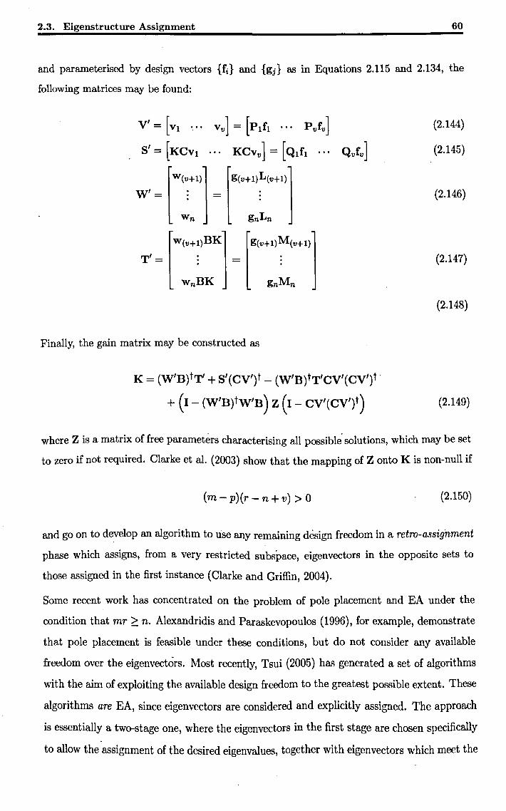
2.3. Eigenstructure Assignment 60
and parameterised by design vectors {fi } and {gj} as in Equations 2.115 and 2.134, the
following matrices may be found:
v' = [VI ... vv] = [PIfl ... Pvfv]
S' = [KCVI KCVv] = [Qlfl Qvfv]
W'= [ W(~+1) 1 = [g(v+ l)~(V+1)
Wn gnLn
T'=
Finally, the gain matrix may be constructed as
K = (W'B)tT' + S'(CV')t - (W'B)tT'CV'(CV')t'
+ (I - (W'B)tW'B) Z (I - CV'(CV')t)
(2.144)
(2.145)
(2.146)
(2.147)
(2.148)
(2.149)
where Z is a matrix of free parameters characterising all possible'solutions, which may be set
to zero if not required. Clarke et al. (2003) show that the mapping of Z onto K is non-null if
(m-p)(r-n+v) > 0 (2.150)
and go on to develop an algorithm to use any remaining design freedom in a retro-assignment
phase which assigns, from a very restricted subspace, eigenvectors in the opposite sets to
those assigned in the first instance (Clarke and Griffin, 2004).
Some recent work has concentrated on the problem of pole placement and EA under the
condition that mr ;::: n. Alexandridis and Paraskevopoulos (1996), for example, demonstrate
that pole placement is feasible under these conditions, but do not consider any available
freedom over the eigenvectors. Most recently, Tsui (2005) has generated a set of algorithms
with the aim of exploiting the available design freedom to the greatest possible extent. These
algorithms are EA, since eigenvectors are considered and explicitly assigned. The approach
is essentially a two-stage one, where the eigenvectors in the first stage are chosen specifically
to allow the assignment of the desired eigenvalues, together with eigenvectors which meet the
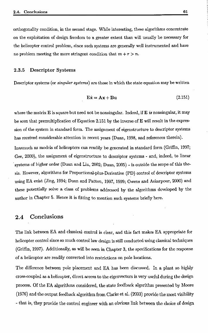
2.4. Conclusions 61
orthogonality condition, in the second stage. While interesting, these algorithms concentrate
on the exploitation of design freedom to a greater extent than will usually be necessary for
the helicopter control problem, since such systems are generally well instrumented and have
no problem meeting the more stringent condition that m + r > n.
2.3.5 Descriptor Systems
Descriptor systems (or singular systems) are those in which the state equation may be written
Ex=Ax+Bu (2.151)
where the matrix E is square but need not be nonsingular. Indeed, if E is nonsingular, it may
be seen that premultiplica~ion of Equation 2.151 by the inverse of E will result in the expres
sion of the system in standard form. The assignment of eigenstructure to descriptor systems
has received considerable attention in recent years (Duan, 1998, and references therein).
Inasmuch as models of helicopters can readily be generated in standard form (Griffin, 1997;
Gee, 2000), the assignment of eigenstructure to descriptor systems - and, indeed, to linear
'systems of higher order (Duan and Liu, 2002; Duan, 2005) - is outside the scope of this the
sis. However, algorithms for Proportional-plus-Derivative (PD) control of descriptor systems
using EA exist (Jing, 1994; Duan and Patton, 1997, 1999; Owens and Askarpour, 2000) and
these potentially solve a class of problems addressed by the algorithms developed by the
author in Chapter 5. Hence it is fitting to mention such systems briefly here.
2.4 Conclusions
The link between EA and classical control is clear, and this fact makes EA appropriate for
helicopter control since so much control law design is still conducted using classical techniques
(Griffin, 1997). Additionally, as will be seen in Chapter 3, the specifications for the response
of a helicopter are readily converted into restrictions on pole locations.
The difference between pole placement and EA has been discussed. In a plant so highly
cross-coupled as a helicopter, direct access to the eigenvectors is very useful during the design
process. Of the EA algorithms considered, the state feedback algorithm presented by Moore
(1976) and the output feedback algorithm from Clarke et al. (2003) provide the most visibility
- that is, they provide the control engineer with an obvious link between the choice of design
Chapter Bibliography 62
parameters and the closed-loop system performance.
2.5 Chapter Bibliography
Alexandridis, A. T. and Paraskevopoulos, P. N. (1996), 'A new approach to eigenstructure assignment by output feedback', IEEE Transactions on Automatic Control 41(7), 1046-1050.
Andry, A. N., Shapiro, E. Y. and Chung, J. C. (1983), 'Eigenstructure assignment for linear systems', IEEE Transactions on Aerospace and Electronic Systems 19(5), 711-727.
Banks, S. P. (1986), Control Systems Engineering, Prentice-Hall.
Ben-Israel, A. and Greville, T. N. E. (1974), Genemlised Inverses: 'Theory and Applications, John Wiley and Sons Ltd.
Brockett, R. W. and Byrnes, C. I. (1981), 'Multivariable nyquist criteria, root loci, and pole placement: A geometric viewpoint', IEEE Transactions on Automatic Control 26(1), 271-283.
Clarke, T. and Griffin, S. J. (2004), 'An addendum to output feedback eigenstructure assignment:retro-assignment', International Journal of Control 77(1), 78-85.
Clarke, T., Griffin, S. J. and Ensor, J. (2003), 'Output feedback eigenstructure assignment using a new reduced orthogonality condition', International Journal of Control 76(4), 390-402.
Davison, E. and Chatterjee, R. (1971), 'A note on pole assignment in linear systems with incomplete state feedback', IEEE Transactions on Automatic Control 16(1), 98-99.
Davison, E. J. and Wang, S. H. (1975), 'On pole assignment in linear systems with incomplete state feedback', IEEE Transactions on Automatic Control 24(3), 516-518.
Doyle, J. C. and Stein, G. (1981), 'Multivariable feedback design: Concepts for a classi. cal/modern synthesis', IEEE Transactions on Automatic Control 26(1), 4-16.
Duan, G.-R. (1993), 'Solutions of the equation AV + BW = VF and their application to eigenstructure assignment in linear systems', IEEE Transactions on Automatic Control 38(2), 276-280.
Duan, G.-R. (1998), 'Eigenstructure assignment and response analysis in descriptor linear systems with state feedback control', International Journal of Control 69(5), 663-694.
Duan, G.-R. (2005), 'Parametric approaches for eigenstructure assignment in high-order linear systems', International Journal of Control, Automation, and Systems 3(3), 419-429.
Duan, G.-R. and Liu, G.-P. (2002), 'Complete parametric approach for eigenstructure assignment in a class of second-order linear systems', Automatica 38(4), 725-729.
Duan, G.-R. and Patton, R. J. (1997), 'Eigenstructure assignment in dcscriptor systems via proportional plus derivative state feedback', International Journal of Control 68(5), 1147-1162.
2.5. Chapter Bibliography 63
Duan, G.-R. and Patton, R. J. (1999), 'Robust pole assignment in descriptor systems via proportional plus partial derivative state feedback', International Journal of Control 72(13), 1193-1203.
Ensor, J. E. (2000), Subspace Methods for Eigenstructure Assignment, PhD thesis, University of York.
Fahmy, M. M. and O'Reilly, J. (1983), 'Eigenstructure assignment in linear multivariable systems - a parametric solution', IEEE Transactions on Automatic Control 28(10), 990-994.
Fahmy, M. M. and O'Reilly, J. (1988), 'Multistage parametric eigenstructure assignment by output feedback control', International Journal of Control 48(1), 97-116.
Fletcher, L. R. (1981a), 'On pole placement in linear multivariable systems with direct feedthrough. i. theoretical considerations', International Journal of Control 33(4), 739-749.
Fletcher, L. R. (1981b), 'On pole placement in linear multivariable systems with direct feedthrough. ii. computational considerations', International Journal of Control 33(6), 1147-1154.
Fletcher, L. R., Kautsky, J., Kolka, G. K. G. and Nichols, N. K. (1985), 'Some necessary and sufficient conditions for eigenstructure assignment', International Journal of Control 42(6), 1457-1468.
Fletcher, L. R. and Magni, J. F. (1987), 'Exact pole assignment by output feedback: Part I, Part 11 and Part Ill', International Journal of Control 45(6), 1995-2033.
Gee, A. D. (2000), Digital Automatic Flight Control Systems for Advanced Rotorcraft: An Analysis Framework, PhD thesis, University of York.
Griffin, S. J. (1997), Helicopter Control Law Design Using Eigenstructure Assignment, PhD thesis, University of York.
Jacobs, O. L. R. (1974), Introduction to Control Theory, Oxford University Press.
. Jing, H. (1994), 'Eigenstructure assignment by proportional-derivative state feedback in singular systems', Systems and Control Letters 22(1), 47-52.
Kautsky, J., Nichols, N. K., Van Dooren, P. and Fletcher, L. (1982), 'Numerical methods for robust eigenstructure assignment in control system design', Contempomry Mathematics 47(3), 171-177.
Kimura, H. (1975), 'Pole assignment by gain output feedback', IEEE Transactions on Automatic Control 20, 509-516.
Kimura, H. (1977), 'A further result on the problem of pole assignment by output feedback', IEEE Transactions on Automatic Control 25(3), 458-463.
Mehrmann, V. and Xu, H. (2000), 'Numerical methods in control', Journal of Computational and Applied Mathematics 123, 371-394.
Moore, B. C. (1976), 'On the flexibility offered by state feedback in multivariable systems beyond closed loop eigenvalue assignment', IEEE Transactions on Automatic Control 21, 689--692.
2.5. Chapter Bibliography
Nise, N. S. (1995), Control Systems Engineering, 2nd edn, Benjamin Cummings.
Ogata, K. (1997), Modem Control Engineering, Prentice-Hall.
64
Owens, T. J. and Askarpour, S. (2000), 'Integrated approach to eigenstructure assignment in descriptor systems by pd and p state feedback', lEE Proceedings - Control Theory and Applications 147(4), 407-415.
Porter, B. (1977), 'Eigenvalue assignment in linear multivariable systems by output feedback'; International Journal of Control 25(3), 483-490.
Porter, B. and D'Azzo, J. J. (1978), 'Closed-loop eigenstructure assignment by state feedback in multivariable linear systems', International Journal of Control 27(3), 482-492.
Rosenthal, J., Schumacher, J. M. and Willems, J. C. (1995), 'Generic eigenvalue assignment by memoryless real outp~t feedback', Systems and Control Letters 26, 253-260.
Schoukens, J. and Pintelon, R. (1991), Identification of Linear Systems, Pergamon Press.
Schwarzenbach, J. and Gill, K. F. (1984), System Modelling and Control, 2nd edn, Edward Arnold.
Srinathkumar, S. (1978), 'Eigenvalue / eigenvector assignment using output feedback', IEEE Transactions on Automatic Control 23(1), 79-81.
The Mathworks, Inc. (2005), 'Matlab: Control system toolbox'. Accessed August 2005. URL: http://www.mathworks.com/access/helpdesk/help /toolbox/ control/ control.html
Tsui, C.-C. (1996), Robust Control System Design - Advanced State-Space Techniques, Marcel Dekker: New York.
Tsui, C.-C. (2005), 'Six-dimensional expansion of output feedback design for eigenstructure assignment', Journal of the F'ranklin Institute 342(7), 892-901.
Wang, X. (1992), 'Pole placement by static output feedback', Journal of Mathematical Systems, Estimation, and Control 2, 205-218.
Weisstein, E. W. (2005), 'Eigenvector'. From MathWorld - A Wolfram Web Resource. Accessed August 2005.' URL: http://mathworld. wolfram. com/Eigenvector.html
White, B. A. (1991), 'Eigenstructure assignment by output feedback', International Journal of Control 53(6), 1413-1429.
White, B. A. (1995), 'Eigenstructure assignment: a survey', Proceedings of the I Mech E Part I: Journal of Systems and Control Engineering 209(1), 1-11.
Wilkinson, J. H. (1965), The Algebraic Eigenvalue Problem, Clarendon Press.
Wonham, W. M. (1967), 'On pole assignment in multi-input controllable linear systems', IEEE Transactions on Automatic Control 12(6), 66D--665.
Chapter 3
Helicopters and Eigenstructure
Assignment
Contents 3.1 Introd uction ............................... 66
3.2 Helicopter Dynamics .••..•.•..•••..•••...••.•. 66
3.2.1 Modelling Helicopter Flight . . . . . . . . . . . . . . . . . . . . . .. 67
3.2.1.1 Momentum Theory . . . . . . . . . . . . . . . . . . . . .. 67
3.2.1.2 Blade Element Theory. . . . . . . . . . . . . . . . . . . .. 70
3.2.1.3 Forward Flight and Blade Hinges .............. 73
3.2.1.4 Rotor Flow Effects and Wake Analysis ........... 74
3.2.2 Control and Stability. . . . . . . . . . . ; . . . . . . . . . . . . . .. 75
3.2.2.1 The Tail ............................ 76
3.2.2.2 Pilot Controls ......................... 76
3.2.2.3 Stability Definitions . . . . . . . . . . . . . . . . . . . . .. 77
3.2.2.4 Auto-Stabilisation Equipment ................ 78
3.2.3 Control Problems. . . . . . . . . . . . . . . . . . . . . . . . . . . . .' 78
3.3 Handling Qualities Specification .•••..•••••..•••••• 79
3.3.1 Rotorcraft Specification . . . . . . . . . . . . . . . . . . . . . . . .. 80
3.3.2 ADS-33D . . . . . . . . . . . . . . . . . . . . . . . . . . . . . . . .. 80
3.3.3 Defence Standard 00-970 ........................ 80
3.4 An Existing Ideal Eigenstructure . • • • • • • • • • • • • • . • • .. 83
3.4.1 Eigenvalue Locations. . . . . . . . . . . . . . . . . . . . . . . . . .. 84
3.4.2 Attitude Command Eigenvectors . . . . . . . . . . . . . . . . . . .. 85
3.5 Rate Command Eigenvectors •.•••••••••••..•.•••. . 85
3.5.1 Problem Definition. . . . . . . . . . . . . . . . . . . . . . . . . . .. 86
3.5.2 Modal Coupling Matrices . . . . . . . . . . . . . . . . . . . . . . .. 87
3.5.3 Eigenvectors ................................ 89
3.5.3.1 A Numerical Example. . . . . . . . . . . . . . . . . . . .. 91
3.5.3.2 Second Order Tail Rotor Response . . . . . . . . . . . . .. 94
65
Chapter Bibliography 66
3.5.4 Complete Eigenvector Set . . . . . . . . . . . . . . . . . . . . . . .. 95
3.6 Conclusions................................ 95 3.7 Chapter Bibliography • . • • • . . • • • • • • • . • • • • • • • . • .• 96
3.1 Introduction
In order to effect control of a system as complex as a helicopter, it must first be understood
from a theoretical standpoint. Once the general characteristics have been identified by exam
ining the physics of the system, a controller can be developed which will specifically address
the problems found.
This chapter will introduce the helicopter as a mechanical system, and derive a sufficiently
detailed description of its operation as is required in understanding the problems faced by the
designer of a helicopter control system. Following that, the specific issues concerned with the
application of Eigenstructure Assignment (EA) to helicopters will be considered, including
the specification of closed-loop performance, and a new ideal eigenstructure for forward flight
will be developed.
It should be noted that the vast majority of helicopters currently in service are in the same
configuration - a main rotor on top of the aircraft and a tail rotor mounted vertically at the . . rear - and hence this is the configuration that will be considered here.
3.2 Helicopter Dynamics
As can be determined from observing its operation, the helicopter is supported while in flight
by a set of rotor blades, which revolve about a central hub. These blades are essentially the
same as aircraft wings, but instead of generating lift through linear motion of the aircraft
through the air, they generate lift by means of their rotational speed relative to the air.
The analysis of how these blades act to lift and propel the helicopter, and of the dynamics
of the resulting system, is complex but of enormous value. The development of a control
system for any purpose cannot be undertaken without a reasonable knowledge of the plant
to be controlled.
3.2. Helicopter Dynamics 67
3.2.1 Modelling Helicopter Flight
Helicopters are inherently extremely complex m~chines, and detailed analysis of their op
eration is consequently very involved. However, various simplifications can be made to the
flight model, allowing a variety of compromises between complexity and accuracy. There are
many texts providing full descriptions of helicopter dynamics (Bramwell, 1976; Layton, 1984;
Johnson, 1994; Padfield, 1996; Prouty, 1990; Stepniewski and Keys, 1984). In particular the
work of Layton (1984) has been consulted extensively in preparing this section.
3.2.1.1 Momentum Theory
Momentum theory is the simplest of all helicopter analysis techniques. The spinning rotor
blades are regarded as a s?lid disc, and the effect of this lifting disc on the helicopter is
considered simply in terms of Newton's laws of motion and the conservation of energy, mass
and momentum. Momentum theory is simplified by the following assumptions (Layton, 1984):
.• Air is incompressible and frictionless.
• The rotor, being a solid disc, imparts no rotation or oscillation to the wake; flow through
the disc is uniform and steady.
• Energy is added to the air by the rotor disc in the form of an instantaneous pressure
increase. The pressure both above and below the disc is constant.
• The density of air does not change with altitude.
The above assumptions will introduce errors, but the simplifications afforded are enormous
in comparison. In addition, most of the errors may be rendered negligible by the application
of a suitable correction factor to the results. The derivations below rely on the following
nomenclature:
V: Air velocity
Vs: Velocity of free stream (far above rotor)
Vi: Increase in stream velocity to rotor disc (induced velocity)
Voo: Final increase in stream velocity,·
Ptl, Pt2: Total pressure far above and far below rotor
3.2. Helicopter Dynamics 68
Ps: Normal atmospheric pressure
Pt: Total stream pressure
al: Mass flow through rotor
p: Density of air
A: Area of rotor disc
T: Thrust generated by rotor disc
The aim of momentum theory is to determine simple equations for the thrust generated by
the rotor and its efficiency, the velocity of air through the disc, and other aspects of the action
of the disc that are important in understanding the basics of helicopter flight. Starting with
Bernoulli's Equation, as the velocity of fluid in a stream tube increases, its static pressure
falls: 1 2
Pt = Ps + 2PV
Invoking this far above the rotor gives
1 2 Pt! = Ps + 2P~
(3.1)
(3.2)
Far below the rotor, when the static pressure has returned to ambient levels and the stream
has ceased to accelerate, 1 2
Pt2 = Ps + 2P (Vs + voo ) (3.3)
Subtracting Equation 3.2 from Equation 3.3 gives the difference in pressure induced by the
rotor disc:
(3.4)
Newton's second law states that F = ma, or equivalently in terms of thrust and mass flow,
T= m dV dt
Mass flow is defined as the mass of air passing through the disc per unit time:
(3.5)
,.
(3.6)
3.2. Helicopter Dynamics
The pressure change ~p acts on the area of the disc A, giving
T=A~p
Hence, by equating Equation 3.5 and Equation 3.7, and substituting Equation 3.6:
A~p = pA (Vs + Vi) dV
~p = p (Vs + Vi) dV
Over the complete stream tube, dV = voo , and equating with Equation 3.4:
~p = p (Vs + Vi) Voo = pvoo (Vs + ~Voo ) 1
Vi = 2Voo
69
(3.7)
(3.8)
(3.9)
(3.10)
(3.11)
The acceleration of air in the stream tube, then, occurs half above and half below the rotor,
with the final added velocity being double that at the disc. Developing an expression for the
thrust developed by the rotor is trivial:
T=A~p
= pA (Vs + ~Voo ) Voo
= 2pA (Vs + Vi) Vi
In the hover, this simplifies to
T= 2pAv;
or equivalently
v.= V2~A
(3.12)
(3.13)
(3.14)
(3.15)
(3.16)
Clearly, thrust is required (and therefore power is consumed) to support the helicopter in the
hover. To measure efficiency, a figure of merit FM has been defined for helicopters. This
differs from the standard definition of efficiency as the ratio of power input to power output,
because for a general propeller the power output is taken to be the product of the thrust
and the velocity, and therefore the efficiency for a stationary helicopter is undefined. Instead,
F AI describes the ratio of the hover power of an ideal rotor to a real rotor. The power output
is taken as the product of the thrust and the inflow velocity, known as the induced power,
3.2. Helicopter Dynamics 70
and is compared to the power used to turn the rotor (Pin)' So for the figure of merit:
(3.17)
1
_ T($)2 - Pin
(3.18)
T~ = 1
Pin (2pA) 2
(3.19)
3.2.1.2 Blade Element .Theory
The calculations of power above did not deduce the torque required to turn the rotor, and this
was because torque effects are to do with the drag on each rotor blade as it passes through
the air. Clearly, a slightly more detailed model is called for, and this need is fulfilled by blade
element theory.
Consider a small element of a single rotor blade, as viewed from the hub. The element is
located at a distance r from the hub; its width is dr and its chord c. The rotor is spinning at
a rate of 0 radians per second, and so the linear speed of the element through the air is Or.
Now as this element travels through the air it will generate a force dR which may be resolved
into the thrust dT and torque dQ of the element. The torque vector lies parallel to the path
of the element, while the thrust is generated perpendicular to it. However, these directions·
are not consistent with the lift and drag forces generated by a moving aerofoil, which are
referenced not to the direction of travel, but to the direction of the inflow air, Vi. Figure 3.1
shows the geometry and also defines the lift and drag forces dL and dD in terms of the angle
of attack ao and angle of incidence Ui.
From Figure 3.1, it can be seen that:
dT = dL cos ai - dD sinai
dQ = dL sin ai - dDcosai
(3.20)
(3.21)
It is standard to refer to the lift and drag of an aerofoil in terms of non-dimensional lift and
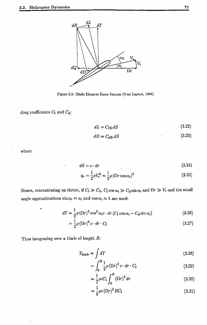
3.2. Helicopter Dynamics
Figure 3.1: Blade Element Force Vectors (from Lay ton, 1984)
drag coefficients Cz and Cd:
where
dL = CzqrdS
dD = CdqrdS
dS = c·dr
1 2 1 2 qr = "2 pVr = "2p(Orcosoi )
71
(3.22)
(3.23)
(3.24)
(3.25)
Hence, concentrating on thrust, if C, » Cd, Cz cos 0i » Cd sin 0i and Or » Vi and the small
angle approximations sin 0i ~ 0i and cos 0i ~ 1 are used:
Thus integrating over a blade of length R:
(3.26)
(3.27)
(3.28)
(3.29)
(3.30)
(3.31 )
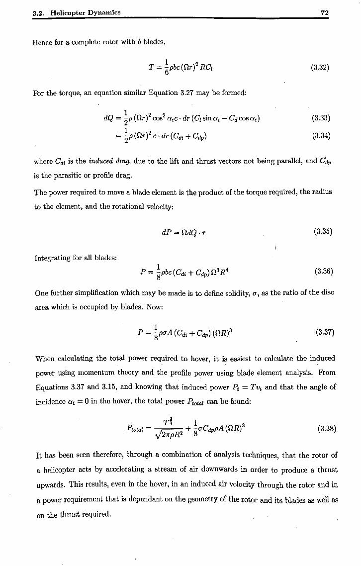
3.2. Helicopter Dynamics
Hence for a complete rotor with b blades,
For the torque, an equation similar Equation 3.27 may be formed:
dQ = ~p (Or)2 cos2 QiC' dr (Cl SinQi - Cd cos Qi)
1 2 = 2P (Or) C· dr (Cdi + Cdp)
72
(3.32)
(3.33)
(3.34)
where C di is the induced drag, due to the lift and thrust vectors not being parallel, and Cdp
is the parasitic or profile drag.
The power required to move a blade element is the product of the torque required, the radius
to the element, and the rotational velocity:
dP=OdQ·r (3.35)
Integrating for all blades:
(3.36)
One further simplification which may be made is to define solidity, u, as the ratio of the disc . . area which is occupied by blades. Now:
(3.37)
When calculating the total power required to hover, it is easiest to calculate the induced
power using momentum theory and the profile P?wer using blade element analysis. From
Equations 3.37 and 3.15, and knowing that induced power Pi = TVi and that the angle of
incidence Qi = 0 in the hover, the total power Ptotal can be found:
3 T~ 1 3
Ptotal = J + -8UCdPpA (OR) 27l"pR2
. (3.38)
It has been seen therefore, through a combination of analysis techniques, that the rotor of
a helicopter acts by accelerating a stream of air downwards in order to produce a thrust
upwards. This results, even in the hover, in an induced air velocity through the rotor and in
a power requirement that is dependant on the geometry of the rotor and its blades as well as
on the thrust required.
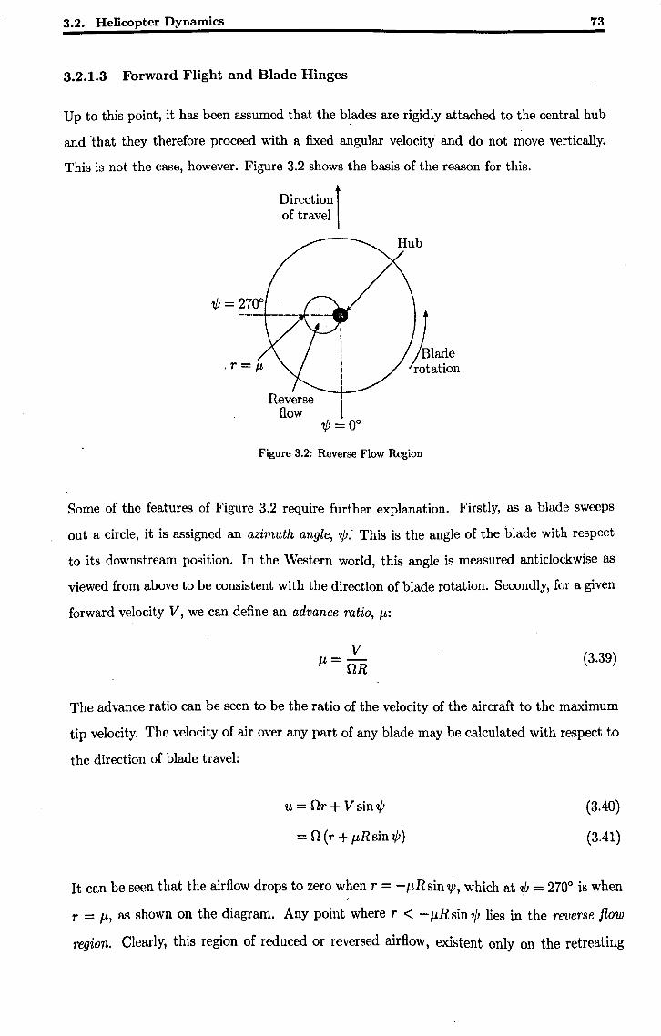
3.2. Helicopter Dynamics 73
3.2.1.3 Forward Flight and Blade Hinges
Up to this point, it has been assumed that the b~ades are rigidly attached to the central hub
and that they therefore proceed with a fixed angular velocity and do not move vertically.
This is not the case, however. Figure 3.2 shows the basis of the reason for this.
Direction 1 of travel
Reverse flow
Figure 3.2: Reverse Flow Region
Some of the features of Figure 3.2 require further explanation. Firstly, as a blade sweeps
out a circle, it is assigned an azimuth angle, 'IjJ,' This is the angle of the blade with respect
to its downstream position. In the Western world, this angle is measured anticlockwise as
viewed from above to be consistent with the direction of blade rotation. Secondly, for a given
forward velocity V, we can define an advance ratio, /L:
(3.39)
The advance ratio can be seen to be the ratio of the velocity of the aircraft to the maximum
tip velocity. The velocity of air over any part of any blade may be calculated with respect to
the direction of blade travel:
u = nr+ Vsin'IjJ
= n (r + /LRsin 'IjJ)
(3.40)
(3.41)
It can be seen that the airflow drops to zero when r = -/LRsin 'IjJ, which at 'IjJ = 2700 is when
r = Il, as shown on the diagram. Any point where r < - /LR sin 'IjJ lies in the reverse flow
region. Clearly, this region of reduced or reversed airflow, existent only on the retreating
3.2. Helicopter Dynamics 74
side of the rotor, will produce a large rolling moment on the airframe. In practice, this effect
prevented early helicopters from flying at anything but the slowest of speeds. The gyrocopter
pioneer Juan de la Cierva invented the solution to this problem, and his technique is still used
today. He introduced flapping hinges to the blade roots to allow them freedom of movement
vertically. This vertical freedom means that as a blade retreats, it generates less lift and
hence flaps downwards instead of imparting a moment on the hub. This in turn increases
the effective angle of attack of the blade and so damps the flapping movement, removing the
need for extra mechanical damping.
The vertical flapping of the blades was found to introduce great stresses at the rotor hub.
The reason for this was that the path taken by the blades caused them to be subject to
a Coriolis force that acted laterally on the blades. In addition, the cyclic variations in lift
caused by the flapping hinges induced cyclic variations in drag. Another hinge was therefore
added, the lead-Iag'hinge, to allow the blades some freedom in this axis. Unlike flapping,
however, the lead-Iag motion is not aerodynamically damped and needs mechanical dampers
and end stops.
It can be seen then that the motion of the blades through the air is a complex one. It may
be modelled reasonably accurately if enough is known about the blades and hinges, and this
modelling is important for the designer of a control system. It is useful to note that in general,
the flapping and lead-Iag modes are considerably faster than the body dynamics. For this
reason, they are often omitted from helicopter models for the purposes of control system
design. For example the helicopter model used in Chapter 7 of this thesis, and described in
Appendix A, contains flapping modes; but these are removed using a modal approximation
technique before control is attempted.
However, while this has obvious advantages for proving the design process, when a controller
designed in this way is fitted to an aircraft it may display significantly degraded handling
qualities (Ingle and Celi, 1994).
3.2.1.4 Rotor Flow Effects and Wake Analysis
Simply to state that the rotor imparts vertical movement to the air against which it works
is clearly to oversimplify reality. The interaction between the rotor and the air is extremely
complex, and an understanding of the exact nature of this interaction is not necessary for
the understanding of the control problem. It is, however, important for producing reliable
mathematical models of helicopters, such as that produced by Gee (2000). A simple summary
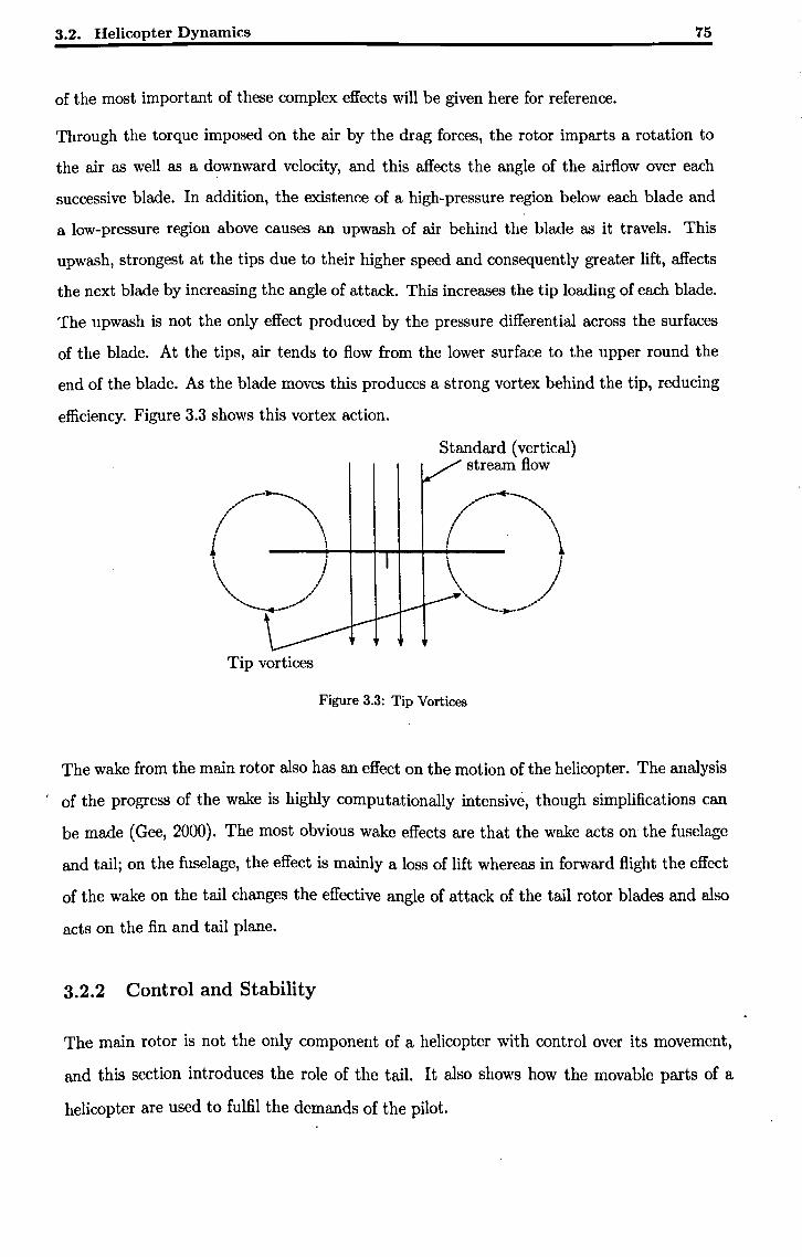
3.2. Helicopter Dynamics 75
of the most important of these complex effects will be given here for reference.
Through the torque imposed on the air by the drag forces, the rotor imparts a rotation to
the air as well as a downward velocity, and this affects the angle of the airflow over each
successive blade. In addition, the existence of a high-pressure region below each blade and
a low-pressure region above causes an upwash of air behind the blade as it travels. This
upwash, strongest at the tips due to their higher speed and consequently greater lift, affects
the next blade by increasing the angle of attack. This increases the tip loading of each blade.
The upwash is not the only effect produced by the pressure differential across the surfaces
of the blade. At the tips, air tends to flow from the lower surface to the upper round the
end of the blade. As the blade moves this produces a strong vortex behind the tip, reducing
efficiency. Figure 3.3 shows this vortex action.
Standard (vertical) stream flow
.. -... ~ ( \ L , , ) \ .' "---- .' .................
Tip vortices
Figure 3.3: Tip Vortices
The wake from the main rotor also has an effect on the motion of the helicopter. The analysis
of the progress of the wake is highly computationally intensive, though simplifications can
be made (Gee, 2000). The most obvious wake effects are that the wake acts on the fuselage
and tail; on the fuselage, the effect is mainly a loss of lift whereas in forward flight the effect
of the wake on the tail changes the effective angle of attack of the tail rotor blades and also
acts on the fin and tail plane.
3.2.2 Control and Stability
The main rotor is not the only component of a helicopter with control over its movement,
and this section introduces the role of the tail. It also shows how the movable parts of a
helicopter are used to fulfil the demands of the pilot.
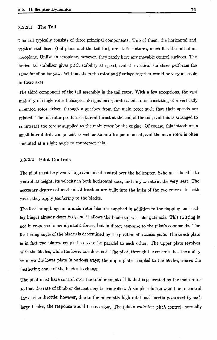
3.2. Helicopter Dynamics 76
3.2.2.1 The Tail
The tail typically consists of three principal components. Two of them, the horizontal and
vertical stabilisers (tail plane and the tail fin), are static fixtures, much like the tail of an
aeroplane. Unlike an aeroplane, however, they rarely have any movable control surfaces. The
horizontal stabiliser gives pitch stability at speed, and the vertical stabiliser performs the,
same function for yaw. Without them the rotor and fuselage together would be very unstable
in these axes.
The third component of the tail assembly is the tail rotor. With a few exceptions, the vast
majority of single-rotor helicopter designs incorporate a tail rotor consisting of a vertically
mounted rotor driven through a gearbox from the main rotor such that their speeds are
related. The tail rotor produces a lateral thrust at the end of the tail, and this is arranged to
counteract the torque supplied to the main rotor by the engine. Of course, this introduces a
small lateral drift component as well as an anti-torque moment, and the main rotor is often
mounted at a slight angle to counteract this.
3.2.2.2 Pilot Controls
The pilot must be given a large amount of control over the helicopter. 8/he must be able to
control its height, its velocity in both horizontal axes, and its yaw rate at the very least. The
necessary degrees of mechanical freedom are built into the hubs of the two rotors. In both
cases, they apply feathering to the blades.
The feathering hinge on a main rotor blade is supplied in addition to the flapping and lead
lag hinges already described, and it allows the blade t~ twist along its axis. This twis~ing is
not in response to aerodynamic forces, but in direct response to the pilot's commands. ,The
feathering angle of the blades is determined by the position of a swash plate. The swash plate
is in fact two plates, coupled so as to lie parallel to each other. The upper plate revolves
with the blades, while the lower one does not. The pilot, through the controls, has the ability
to move the lower plate in various ways; the upper plate, coupled to the blades, causes the
feathering angle of the blades to change.
The pilot must have control over the total amount of lift that is generated by the main rotor
so that the rate of climb or descent may be controlled. A simple solution would be to control
the engine throttle; however, due to the inherently high rotational inertia possessed by such
large blades, the response would be too slow. The I?ilot's collective pitch control, normally
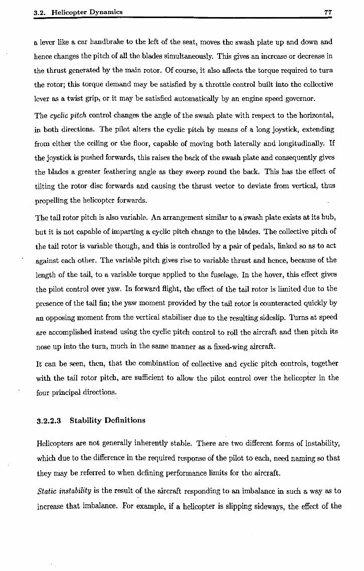
3.2. Helicopter Dynamics 77
a lever like a car handbrake to the left of the seat, moves the swash plate up and down and
hence changes the pitch of all the blades simultaneously. This gives an increase or decrease in
the thrust generated by the main rotor. Of course, it also affects the torque required to turn
the rotor; this torque demand may be satisfied by a throttle control built into the collective
lever as a twist grip, or it may be satisfied automatically by an engine speed governor.
The cyclic pitch control changes the angle of the swash plate with respect to the horizontal,
in both directions. The pilot alters the cyclic pitch by means of a long joystick, extending
from either the ceiling or the floor, capable of moving both laterally and longitudinally. If
the joystick is pushed forwards, this raises the back of the swash plate and consequently gives
the blades a greater feathering angle as they sweep round the back. This has the effect of
tilting the rotor disc forwards and causing the thrust vector to deviate from vertical, thus
propelling the helicopter forwards.
The tail rotor pitch is also variable. An arrangement similar to a'swash plate exists at its hub,
but it is not capable of imparting a cyclic pitch change to the blades. The collective pitch of
the tail rotor is variable though, and this is controlled by a pair of pedals, linked so as to act
against each other. The variable pitch gives rise to variable thrust and hence, because of the
length of the tail, to a variable torque applied to the fuselage. In the hover, this effect gives
the pilot control over yaw. In forward flight, the effect of the tail rotor is limited due to the
presence of the tail fin; the yaw moment provided by the tail rotor is counteracted quickly by
an opposing moment from the vertical stabiliser due to the resulting sideslip. Turns at speed
are accomplished instead using the cyclic pitch control to roll the aircraft and then pitch its
nose up into the turn, much in the same manner as a fixed-wing aircraft.
It can be Reen, then, that the combination of collective and cyclic pitch controls, together
with the tail rotor pitch, are sufficient to allow the pilot control over the helicopter in the
four principal directions.
3.2.2.3 Stability Definitions
Helicopters are not generally inherently stable. There are two different forms of instability,
which due to the difference in the required response of the pilot to each, need naming so that
they may be referred to when defining performance limits for the aircraft.
Static instability is the result of the aircraft responding to an imbalance in such a way as to
increase that imbalance. For example, if a helicopter is slipping sideways, the effect of the
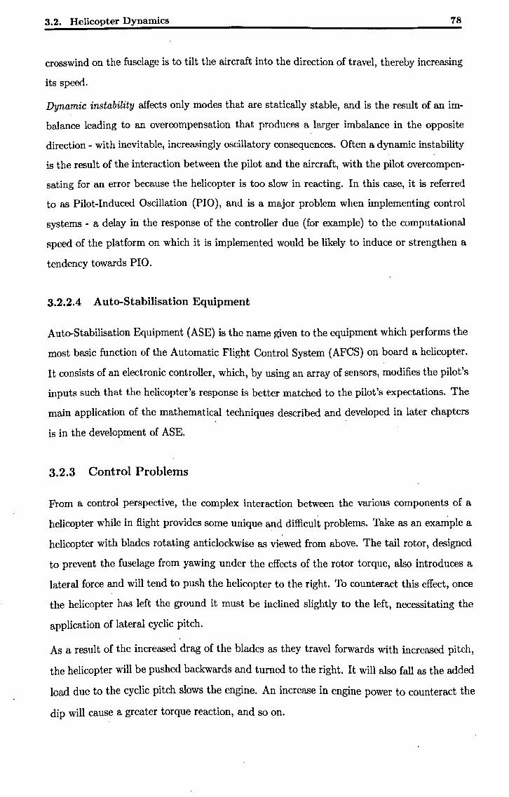
3.2. Helicopter Dynamics 78
crosswind on the fuselage is to tilt the aircraft into the direction of travel, thereby increasing
its speed.
Dynamic instability affects only modes that are statically stable, and is the result of an im
balance leading to an overcompensation that produces a larger imbalance in the opposite
direction - with inevitable, increasingly oscillatory consequences. Often a dynamic instability
is the result of the interaction between the pilot and the aircraft, with the pilot overcompen
sating for an error because the helicopter is too slow in reacting. In this case, it is referred
to as Pilot-Induced Oscillation (PlO), and is a major problem when implementing control
systems - a delay in the response of the controller due (for example) to the computational
speed of the platform on which it is implemented would be likely to induce or strengthen a
tendency towards PlO.
3.2.2.4 Auto-Stabilisation Equipment
Auto-Stabilisation Equipment (ASE) is the name given to the equipment which performs the
most basic function of the Automatic Flight Control System (AFCS) on board a helicopter.
It consists of an electronic controller, which, by using an array of sensors, modifies the pilot's
inputs such that the helicopter's response is better matched to the pilot's expectations. The
main application of the mathematical techniques described and developed in later chapters . .
is in the development of ASE.
3.2.3 Control Problems
From a control perspective, the complex interaction between the various components of a . . ' .
helicopter while in flight provides some unique and difficult problems. Take as an example a
helicopter with blades rotating anticlockwise as viewed from above. The tail rotor, designed
to prevent the fuselage from yawing under the effects of the rotor torque, also introduces a
lateral force and will tend to push the helicopter to the right. To counteract this effect, once
the helicopter has left the ground it must be inclined slightly to the left, necessitating the
application of lateral cyclic pitch.
As a result of the increased drag of the blades as they travel forwards with increased pitch,
the helicopter will be pushed backwards and turned to the right. It will also fall as the added
load due to the cyclic pitch slows the engine. An increase in engine power to counteract the
dip will cause a greater torque reaction, and so on.
3.3. Handling Qualities Specification 79
This is merely an example, but it serves to show that even in the hover, the dynamics of a
helicopter are far from simple. From a pilot's point of view, and that of the control engineer,
the biggest problem is the cross-coupling - it is not possible to al~er anything without affecting
everything else.
Additionally, helicopters are highly non-linear, and the case in the hover is vastly different
from the case at even a low forward speed. It can be shown (Bramwell, 1976; Layton, 1984;
Padfield, 1996; Stepniewski and Keys, 1984) that the efficiency of the rotor disc increases with
the flow of air through it, so as soon as the helicopter starts to move it will gain translational
lift.
The added oscillatory mode introduced by the motion of the blades around the flapping
hinges is not in phase with the blade pitch change and tends to introduce a phase shift to
the lift. Therefore the pilot must apply a coupled input to the swash plate in order to effect
a simple shift in the lift vector. This phase shift changes with forward speed.
The effect of delays in control response has already been mentioned; a helicopter is heavy
and the effect of its controls not immediate, so the potential for PlO is great even before any
additional delays due to the controller are considered. In a digital controller, the sample rate
must be high enough to avoid compounding these problems.
In summary, severe nonlinearities, time constraints and cross-~ouplings· make for a plant
which presents a unique and complex set of challenges to the designer of a control system.
3.3 Handling Qualities Specification
When designing any controller for any plant it is vitally important to have a detailed speci
fication of the desired final performance of the syst~m. In the case of a helicopter, however,
these specifications are hard to characterise. The final performance of the helicopter in a
mission role is dependent on both the machine and its pilot, and consequently the pilot's
feel for the aircraft is vital. Defining this is very subjective, however, and so over the years
a number of documents have emerged which have attempted to describe these qualitative
characteristics in a quantitative way. The intended role of the helicopter will define which
one of these applies. These documents are considered in addition to and in support of the
aircraft-specific definitions of performance laid down when a new design is proposed.
This section draws on the work of Clarke and Taylor (1999) for details of the various handling
qualities documents.
3.3. Handling Qualities Specification 80
3.3.1 Rotorcraft Specification
The aircraft-specific handling qualities are laid out in the Rotorcraft Specification for the
helicopter in question. Defined here are the operational conditions under which the aircraft
must operate, along with the levels of performance, handling and failure-tolerance that must
be met. Also defined are the roles and missions of the helicopter.
The Rotorcraft Specification is the most important document describing the desired perfor
mance of the aircraft. It is also the most detailed, as the other documents provide a much
more general set of requirements. In the case that a conflict between documents does arise,
however, the Rotorcraft Specification takes precedence.
3.3.2 ADS-33D
The ADS-33D is the'document describing the handling qualities requirements for the military
procurement of helicopters in the US (Padfield, 1996). It was introduced during the design
process of the RAH-66 Comanche, where advancing technology was meeting outdated design
documents at an impasse. The ADS-33D recognises the need for different handling qualities
during different phases of the flight mission. Handling qualities are defined as Level 1, 2 or
3 where a Level 1 response is the best, in a similar way to the Def.Stan.970 (see below).
Handling quality levels are also defined under degraded environmental conditions or failure
states.
Unusually, the handling qualities requirements in the ADS-33D are largely specified in terms
of frequency domain characteristics, principally bandwidth and phase delay. Since the fre
quency domain is a concept associated with linear systems, whereas the helicopter is highly
nonlinear, this approach has precluded the universal and c~mplete acceptance of the ADS-33D
to date.
3.3.3 Defence Standard 00-970
The UK Ministry of Defence Defence Standard 00-970 (Def.Stan.00-970)(Pitkin, 1989) is the
UK equivalent of the ADS-33D. Because it is the document most likely to be applicable to
aircraft using control systems designed using techniques in this thesis, it will be covered in
slightly more detail than the ADS-33D.
The Def.Stan.00-970 handling qualities specifications are organised according to the appro
priate operational phase. One of the four phases refers to the operations of the helicopter on
3.3. Handling Qualities Specification 81
the ground, which is of little use in this context. The other three are summarised below.
Active Flight Phase: In the Active Flight Phase, pilot involvement is intensive. This
phase may be further classified according to whether the manoeuvre is Aggressive or
Moderate.
Attentive Flight Phase: The Attentive Flight Phase demands less of the pilot, and gen
erally involves changes to the flight condition or flight under Instrument Flight Rules
(IFR).
Passive Flight Phase: Pilot involvement during the Passive Flight Phase is low. Occa
sional re-trimming of the flight condition and monitoring of the AFCS is all that is
generally required.
The Def.Stan.00-970 document also defines terms for the maximum operating envelopes in
the various flight phases, as well as tolerance of environmental conditions. Handling qualities
are rated according to a structure of Levels, which define the level of ease with which the
mission may be carried out.
Level 1: Handling qualities are clearly sufficient to allow the mission to be completed with
ease.
Level 2: The mission may be accomplished, but will require an increase in pilot workload
and this may also lead to a decrease in mission effectiveness.
Level 3: The helicopter can be controlled, but the pilot workload will be excessive and
mission effectiveness unsatisfactory.
It is the objective of the control system to ensure that the handling qualities do not fall below
Level 1 while inside the operational envelope (the flight envelope required while carrying out
a particular role) or Level 2 at other points within the service envelope (the normal operating
range of the helicopter).
The short- and long-term modes that form the responses of the helicopter to the pilot inputs
are also well defined by the Def.Stan.00-970. They are defined in terms of time-domain crite
ria, which are more intuitive than the frequency-domain criteria of the ADS-33Dj qualitative
descriptions of handling qualities tend to be described in the time domain, using words such
as speed, overshoot and sensitivity~ The derivation of an ideal eigenstructure in Section 3.4
uses these criteria directly.
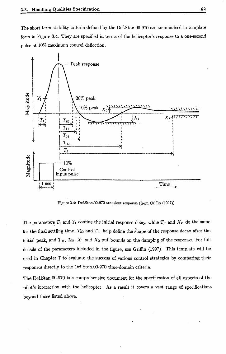
3.3. Handling Qualities Specification 82
The short term stability criteria defined by the Def.Stan.00-970 are summarised in template
form in Figure 3.4. They are specified in terms of the helicopter's response to a one-second
pulse at 10% maximum control deflection.
Peak response
~ ~ ~
JLL~l-~~~~~~~==~~~ I I
~ T30~ Tu "'
I- ?t •
~Ol :
T02 '.. :.;;;...--------~~
I ..--..---10%
Control input pulse
.
XF~7117171771 I
Time )0
Figure 3.4: Def.Stan.00-970 transient response (from Griffin (1997))
The parameter~ Tt an~ Yl confine the initial response delay, while TF and XF do the same
for the final settling time. T30 and Tu help define the shape of the response decay after the
initial peak, and TOl, T02, Xl and X2 put bounds on the damping of the response. For' full
details of the parameters included in the figure, see Griffin (1997). This template will be
used in Chapter 7 to' evaluate the success of various control strategies by comparing their
responses directly to the Def.Stan.00-970 time-domain criteria.
The Def.Stan.00-970 is a comprehensive document for the specification of all aspects of the
pilot's iJ;lteraction with the helicopter. As a result it covers a vast range of specifications
beyond those listed above.
3.4. An Existing Ideal Eigenstructure 83
3.4 An Existing Ideal Eigenstructure
The handling problems inherent to helicopters (primarily instability and cross-coupling),
combined with the close links explored in Chapter 2 between EA and the classical techniques
still so often used for the control of helicopters, render EA an ideal methodology for the
generation of controllers. However, before EA can be applied to any control problem, it is
necessary that the problem be formulated in terms of the desired closed-loop pole locations
and eigenvectors: the eigenstructure.
The formulation of an ideal eigenstructure was considered in detail by Griffin (1997) and
Clarke et al. (2003), and considered the Def.Stan.00-970 as the basis for the eigenstructure.
Eigenvalues and eigenvectors were treated separately and the eigenvectors were formulated
for the case where the cyc~ic pitch inputs control the attitude of the helicopter. Leve~ 1
handling qualities are achievable only in the hover using this type of control response.
It is at this point appropriate to introduce the naming convention for the states and inputs of
a standard helicopter model, since these will be needed to understand the ideal eigenstructure.
u: Forward speed
v: Lateral speed
w: Vertical speed (heave velocity)
p: Roll rate
q: Pitch rate
r: Yaw rate
c/>: Roll angle
(): Pitch angle
'ljJ: Yawangle
Als, B1s: Blade flapping angles
()o: Collective pitch input
Ot: Tail rotor pitch input
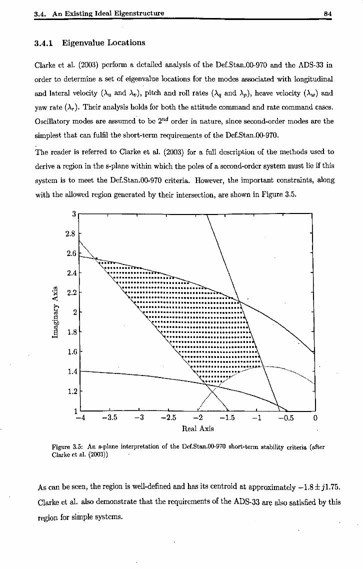
3.4. An Existing Ideal Eigenstructure 84
3.4.1 Eigenvalue Locations
Clarke et al. (2003) perform a detailed analysis of the Def.Stan.00-970 and the ADS-33 in
order to determine a set of eigenvalue locations for the modes associated with longitudinal
and lateral velocity (Au and Av), pitch and roll rates (Aq and Ap), heave velocity (Aw) and
yaw rate (Ar). Their analysis holds for both the attitude command and rate command cases.
Oscillatory modes are assumed'to be 2nd order in nature, since second-order modes are the
simplest that can fulfil the short-term requirements of the Def.Stan.00-970.
The reader is referred to Clarke et al. (2003) for a full description of the methods used to
derive a region in the s-plane within which the poles of a second-order system must lie if this
system is to meet the Def.Stan.00-970 criteria. However, the important constraints, along
with the allowed region generated by their intersection, are shown in Figure 3.5.
3
2.8
2.6
2.4
rn '>< 2.2 < » ~ 2 I=l
'So ~
S 1.8 ~
1.6
1.4
1.2
1 -4
', ... ~ •.....•.. .~ .............. . ~ ...•...........•••.. " .•••....••••.....••.•...
'\~ ...•......••.•....•••••.... " ............................. . ~ .....••........•.........•....... '~ ...... ' ............................ . " .••...•••...•..•••••.•...••......• ~ ................................ . ~ ..........•..••.....••.......•.•
''.t • •••••••••••••••••••••••••••••• ~ .............................. . " •....•..•.....•....••...•..•.. ~ ..•..••......•.••.....••..... ~ ........................... . ~ •.•...•..........•.•....•.. " ............•••....•....•.. ~ .••.•.•.•••.........•..•.
~ ....••.•••.•....•.....••
• ••• ••••• ••••••••••• !It ..... . ~ ...... -_ .... ............. ~.~ .......... ~ ............................ .......... ,,,..... ' .... ................... """
-3.5 -3 -2.5 -2 Real Axis
-1.5 -1 -0.5 o
Figure 3.5: An s-plane interpretation of the Def.Stan.00-970 short-term stability criteria (after Clarke et al. (2003))
As can be seen, the region is well-defined and has its centroid at approximately -1.8±j1.75.
Clarke et al. also demonstrate that the requirements of the ADS-33 are also satisfied by this
region for simple systems.
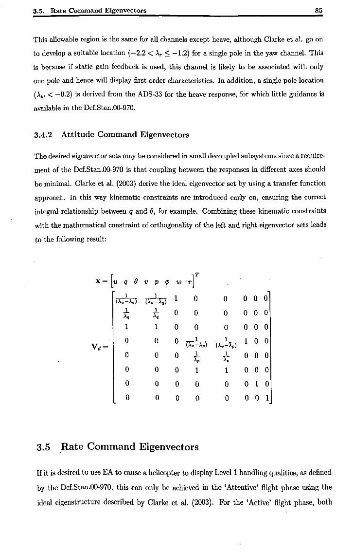
3.5. Rate Command Eigenvectors 85
This allowable region is the same for all channels except heave, although Clarke et al. go on
to develop a suitable location (-2.2 < AT ::; -1.2) for a single pole in the yaw channel. This
is because if static gain feedback is used, this channel is likely to be associated with only
one pole and hence will display first-order characteristics. In addition, a single pole location
(Aw < -0.2) is derived from the ADS-33 for the heave response, for which little guidance is
available in the Def.Stan.00-970.
3.4.2 Attitude Command Eigenvectors
The desired eigenvector sets may be considered in small decoupled subsystems since a require
ment of the Def.Stan.00-970 is that coupling between the responses in different axes should
be minimal. Clarke et al. (2003) derive the ideal eigenvector set by using a transfer function
approach. In this way kinematic constraints are introduced early on, ensuring the correct
integral relationship between q and (), for example. Combining these kinematic constraints
with the mathematical constraint of orthogonality of the left and right eigenvector sets leads
to·the following result:
X= [u q () v p </> w ·r]T 1 1 1 0 0 0 0 0 (Au -Aq) (Au -Aq)
1 1 0 0 0 0 0 0 Aq Aq
1 1 0 0 0 0 0 0
0 0 0 1 1 1 0 0 Vd= (A,,-Ap) (A,,-Ap)
0 0 0 1 1 0 0 0 Ap Ap
0 0 0 1 1 0 0 0
0 0 0 0 0 0 1 0
0 0 0 0 0 0 0 1
3.5 .Rate Command Eigenvectors
If it is desired to use EA to cause a helicopter to display Levell handling qualities, as defined
by the Def.Stan.00-970, this can only be achieved in the 'Attentive' flight phase using the
ideal eigenstructure described by Clarke et al. (2003). For the 'Active' flight phase, both
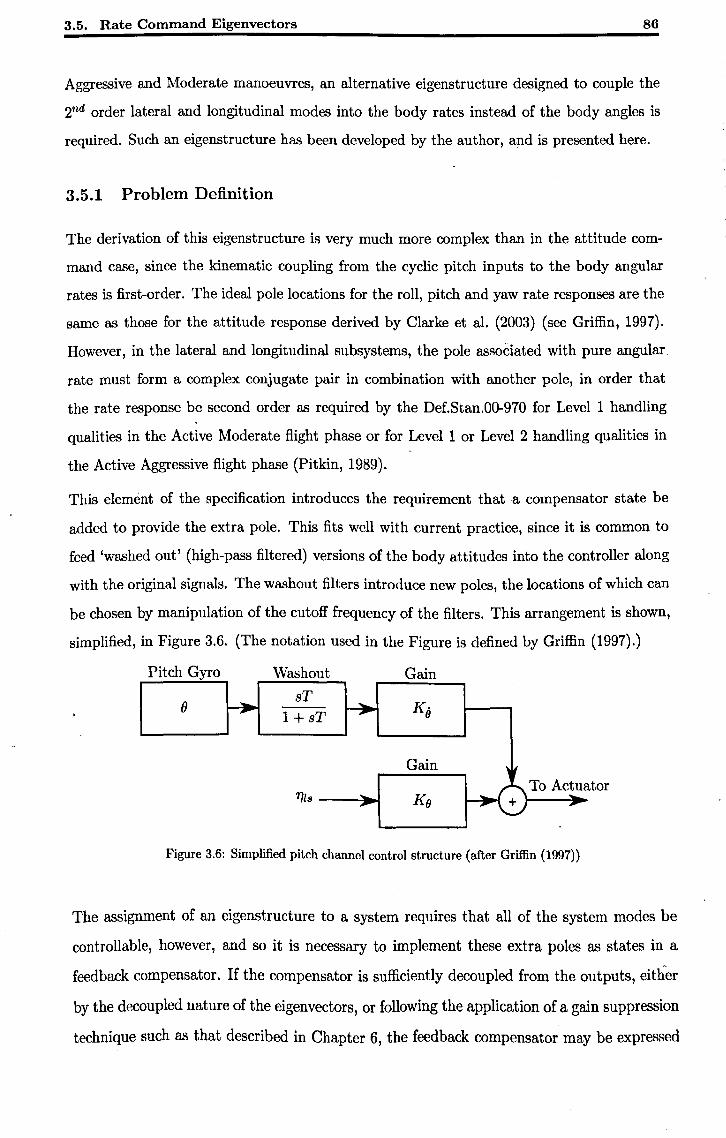
3.5. Rate Command Eigenvectors 86
Aggressive and Moderate manoeuvres, an alternative eigenstructure designed to couple the
2nd order lateral and longitudinal modes into the body rates instead of the body angles is
required. Such an eigenstructure has been developed by the author, and is presented here.
3.5.1 Problem Definition
The derivation of this eigenstructure is very much more complex than in the attitude com
mand case, since the kinematic coupling from the cyclic pitch inputs to the body angular
rates is first-order. The ideal pole locations for the roll, pitch and yaw rate responses are the
same as those for the attitude response derived by Clarke et al. (2003) (see Griffin, 1997).
However, in the lateral and longitudinal subsystems, the pole assoCiated with pure angular.
rate must form a complex conjugate pair in combination with another pole, in order that
the rate response be second order as required by the Def.Stan.00-970 for Level 1 handling
qualities in the Active Moderate flight phase or for Level 1 or Level 2 handling qualities in
the Active Aggressive flight phase (Pitkin, 1989).
This element of the specification introduces the requirement that a compensator state be
added to provide the extra pole. This fits well with current practice, since it is common to
feed 'washed out' (high-pass filtered) versions of the body attitudes into the controller along
with the original signals. The washout filters introduce new poles, the locations of which can
be chosen by manipulation of the cutoff frequency of the filters. This arrangement is shown,
simplified, in Figure 3.6. (The notation used in the Figure is defined by Griffin (1997).)
Pitch Gyro Washout Gain
() sT
1 +sT
"Ils --411 ...
K· 8
Gain To Actuator
Figure 3.6: Simplified pitch channel control structure (after Griffin (1997))
The assignment of an eigenstructure to a system requires that all of the system modes be
controllable, however, and so it is necessary to implement these extra poles as states in a
feedback compensator. If the compensator is sufficiently decoupled from the outputs, either
by the decoupled nature of the eigenvectors, or following the application of a gain suppression
technique such as that described in Chapter 6, the feedback compensator may be expressed
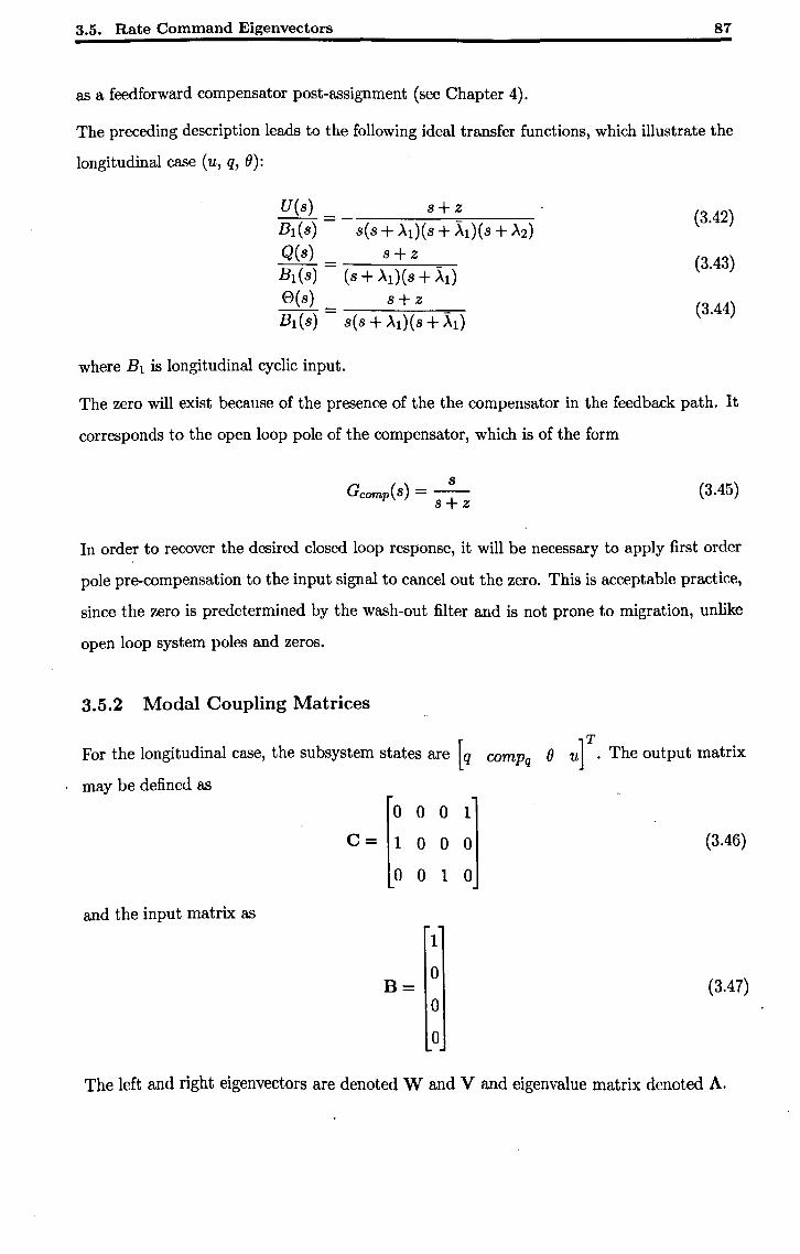
3.5. Rate Command Eigenvectors 87
as a feedforward compensator post-assignment (see Chapter 4).
The preceding description leads to the following ideal transfer functions, which illustrate the
longitudinal case (u, q, 8):
U(8) 8+Z B1(8) = 8(8 + A1)(8 + A1)(8 + A2)
(3.42)
Q(8) 8+Z - ------=--
B1(8) (8 + A1)(8 + AI) (3.43)
8(8) 8+Z B1(8) = 8(8+A1)(8+A1)
(3.44)
where B1 is longitudinal cyclic input.
The zero will exist because of the presence of the the compensator in the feedback path. It
corresponds to the open loop pole of the compensator, which is of the form
S Gcomp (8) =-
S+Z (3.45)
In order to recover the desired closed loop response, it will be necessary to apply first order
pole pre-compensation to the input signal to cancel out the zero. This is acceptable practice,
since the zero is predetermined by the wash-out filter and is not prone to migration, unlike
open loop system poles and zeros.
3.5.2 Modal Coupling Matrices
For the longitudinal case, the subsystem states are [q comPq 8 u] T. The output matrix
may be defined as
0 0 0 1
c= 1 0 0 0 (3.46)
0 0 1 0
and the input matrix as
1
0 B= (3.47)
0
0
The left and right eigenvectors are denoted Wand V and eigenvalue matrix denoted A.
3.5. Rate Command Eigenvectors 88
The subsystem transfer function matrix (G(s)) may be expressed as:
G(s) = CV (sI - A)-l WB (3.48)
For the longitudinal case, the above is expanded as follows:
1 0 0 0 t1 U [' 1'1 T4
r~l (8-'>'1)
0 1 0 0 t1 q - T2 1'2 0 (s-'>'d B1 (3.49)
0 0 ! 0 t2 8 () T3 1'3 T5
0 0 0 1 t3 (8-).2)
where Tm and tn are free parameters.
The zeros in CV exist because the mode associated with velocity is not seen in the attitude
and rate states; similarly, the attitude mode is not seen in the rate state. Equation 3.49 can
be evaluated to give:
G(s) = ..!l!L + T1t1 + W.2. + ~ 8+'>'1 8+'>'1 8 8+'>'2
.n!L + T2t1 8+'>'1 8+'>'1
.!3..h... + T3t1 + ~ 8+).1 8+'>'1 8
(3.50)
Simplifying Equation 3.50 and equa~ing numerator term leading coefficients yields the fol
lowing constraints:
For J:N8):
(3.51)
+ T1t1A2 + T1t1).1 + T6t3A1 + r1l1A1) (3.52)
1 - - - -- -s : -1 = (T4t2A1A2 + T4t2A1A1 + T1t1A1A2 + T6t3A1Al + qt1AIA2 + T4t2AIA2) (3.53)
sO : Z = (T4t2Al).lA2) (3.54)
T:' Q~L ror BiTsJ.
SI : 1 = (T2tl + r2l1)
o --s : Z = (T2hAl' + T2tlAl)
(3.55)
(3.56)
3.5. Rate Command Eigenvectors
And, finally, for :NJ):
1 - - - -s : -1 = (T3tlAl + T5t2Al + T5t2Al + T3tlAt)
o -s : -z = (T5t2AIAt)
A further important identity is
CVWB=CB
which translates to further constraints:
- 1
89
(3.57)
(3.58)
(3.59)
(3.60)
(3.61)
Eigenvectors are unique up to scaling; therefore, for convenience, let us as~ume that T2, T4
and T6 are equal to unity.
The above constraints, after considerable algebraic manipulation, yield the following results:
- 1 1 1 1 (AI-A2)Al (A1-A2)A1
CV= 1 1 0 0 (3.62)
1 1 A2 0 A1 A1
and %-Al
A1-Al Z-~1
WB= AI-AI (3.63) Z
- A1AIA2 %-A2
A2( -A1A2+A~+A1AI-AIA2)
The correctness of this result may easily be verified by substitution of Equations 3.62 and 3.63
into Equations 3.42, 3.43, 3.44 and 3.60.
3.5.3 Eigenvectors
It is now necessary to extend the algebraic manipulations to calculate the full left and right
eigenvector matrices (W & V respectively) from the input and output coupling matrices
(WB & CV respectively).
3.5. Rate Command Eigenvectors 90
Defining the full matrices as follows:
1 1 0 0
V= VI VI V3 V4
I I A2 0 >'1 >'1
(3.64)
- I I 1 1 (>'1->'2)>'1 (A1->'2)A1
and Z->'l
WI,2 WI,3 WI,4 >'1 ->'1 Z-'xl
WI,2 WI,3 WI, w= >'1 ->'1 (3.65)
Z W3,2 W3,3 W3,4 - >'1>'1>'2
z->'2 >'2 ( -AI >'2+>'1>'1 +>.~ ->'lA2) W4,2 W4,3 W4,4
From the matrix identity
VW=I (3.66)
some fundamental scalar identities ensue. These lead to some important properties of the
unknowns defined in W and V.
Starting with
WI,2 + WI,2 = 0
WI,3 + WI,3 = 0
WI,4 + Wl,4 = 0
(3.67)
(3.68)
(3.69)
These lead to the implication that the above unknowns are all purely imaginary values.
Also, the structure of the compensator' and the manner of' its c~nnection dictates that'
(3.70)
Substituting these constraints leads, after considerable algebraic manipulation, to the prop
erty
(3.71)
3.5. Rate Command Eigenvectors 91
where vte denotes the real part of a complex scalar. It follows that
1 1 . -3 0 0 "2 -~ x
1 1 • -3 0 0 "2 "~
W= x (3.72) ~t(~I) Jm(oXl) 1 0 -loXll oX2 Xl oX ll 2oX2 oX2
oX2-~t{oXl} Jm{oXl} 1 1 (-AI +A2)(Al-A2)oX2 x( -oXl +oX2)(oXl -oX2)A2 - oX2
where Jm denotes the imaginary part of a complex scalar, and finally that
1 1 0 0
xj -xj 0 0 (3.73) V=
1 1 A2 0 Al oXl
- 1 1 1 1 (oXl-oX2)Al (oXl -oX2)oXl
The real scalar value x does not affect the transfer functions resulting from V (sI - A)-l W
and may be arbitrarily set. 'It may be interpreted as a gain block applied just prior to the
waSh out filter. A second inverse gain block occurs just after the filter. A good choice for
x would be such that the modal matrix V is as well-conditioned as possible for inversion;
alternatively x could be chosen such that the projection of the set of desired eigenvectors
{Vi} into their allowable subspaces results in the least possible projection error.
Note that the eigenvector elements associated with the compensator state reflect its intended
role as a washout filter, and its consequent links only to q and not () or u. In fact, if these
structural constraints are not important, these elements may be chosen arbitrary and the
denominators of the resulting transfer functions for the states of interest will not change.
The numerators on the other hand may change, leading to migration of the zero. In practice
this is a likely outcome of the projection of the desired eigenvectors into their allowable
subspaces - see Chapter 4 for more details.
3.5.3.1 A Numerical Example
Once again an algebraic check of the correctness of Equations 3.72 and 3.73 can be made by
substitution into the original constraints.
However, in order to check that the derived eigenstructure represents an appropriate response
for a rate-commanded helicopter, a quick example will now be derived and presented.
Assume, arbitrarily, that Al = -3 + 4j, A2 = -5 and x = 1. Then using the above eigen-
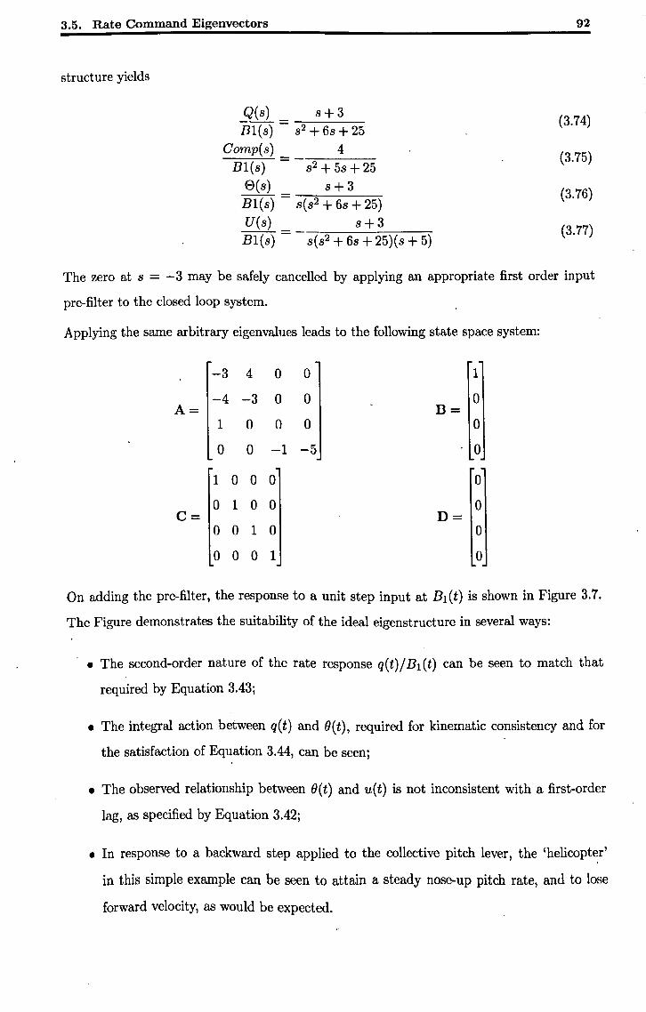
3.5. Rate Command Eigenvectors 92
structure yields
Q(8) 8+3 (3.74)
Bl(8) - 82 + 68 + 25 Comp(s) 4
(3.75) Bl(8)
-s2 + 5s + 25
8(s) s+3 (3.76) Bl(s) - 8(82 + 68 + 25) U(8) 8+3 (3.77) Bl(s) =- 8(82 + 68 + 25)(8 + 5)
The zero at 8 = -3 may be safely cancelled by applying an appropriate first order input
pre-filter to the closed loop system.
Applying the same arbitrary eigenvalues leads to the following state space system:
-3 4 0 0 1
-4 -3 0 0 0 A= B=
1 0 0 0 0
0 0 -1 -5 0
1 0 0 0 0
0 1 0 0 0 c= D=
0 0 1 0 0
0 0 0 1 0
On adding the pre-filter, the response to a unit step input at B1(t) is shown in Figure 3.7.
The Figure demonstrates the suitability of the ideal eigenstructure in several ways:
• The second-order nature of the rate response q(t)/Bl(t) can be seen to match that
required by Equation 3.43;
• The integral action between q(t) and (J(t), required for kinematic consistency and for
the satisfaction of Equation 3.44, can be seen;
• The observed relationship between (J(t) and u(t) is not inconsistent with a first-order
lag, as specified by Equation 3.42;
• In response to a backward step applied to the collective pitch lever, the 'helicopt~r'
in this simple example can be seen to attain a steady nose-up pitch rate, and to lose
forward velocity, as would be expected.
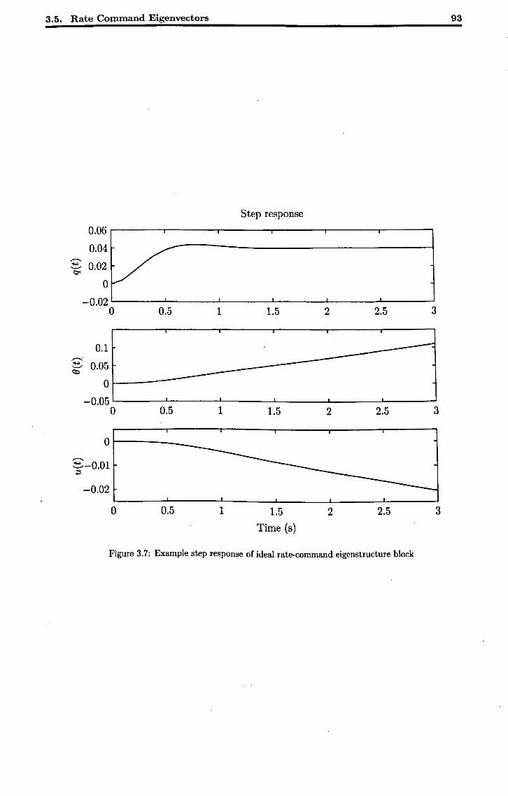
3.5. Rate Command Eigenvectors
Step response
0.06
0.04
V ,.-... -;..> 0.02 '-" ~
0
-0.02 I
0 0.5 1 1.5 2 2.5 3
0.1 ,.-....
g- 0.05 01------
-0.051..------'----""'-------..L...---....1.-----'----o 0.5
Ot-----_ ,.-... ':::--0.01 ;3
-0.02
o 0.5
1
1
1.5
1.5
Time (s)
2 2.5
2 2.5
Figure 3.7: Example step response of ideal rate-command eigenstructure block
3
3
93
3.5. Rate Command Eigenvectors 94
3.5.3.2 Second Order Tail Rotor Response
The Def.Stan.00-970 requirements for the yaw channel are specified using the same criteria
as for the cyclic channels, and with the exception of the peak response (a scaling parameter),
the requirements themselves are identical. Clarke et al. (2003) developed a first-order yaw
rate response because only static feedback controller designs were to be considered. If this.
restriction is dropped, a compensator state can instead be added in order to generate the
required second-order response in yaw.
Such a response carries no requirements on the elements of the eigenvectors associated with
the compensator state. The eigenvector subset may therefore be described using
where z is an arbitrary complex constant. The mechanics of assigning an eigenstructure
wherein a subset of the states have no specific requirements on their eigenvector elements is
investigated in Chapter 4.
Note that this yaw response, which is a rate response, is valid for achieving Level 1 handling
qualities in both the' Active' and 'Attentive' flight phases.
3.6. Conclusions 95
3.5.4 Complete Eigenvector Set
The complete set of ideal eigenvectors, constructed using four decoupled blocks and including
the first-order tail rotor subsystem, is shown below:
x = [v P comPp cp u q compq () w r]T
1 - (>.p->'v )>.p
1
j
1 >'p
o
o
o o o o
1 (>.p->.., )>'p
1
-j 1
Ap
o o
o o o o
1 1
o 0
o 0
Av 0
o 0
o 0
o 0
o 0
o 0
o 0
o
o o o
1 (>.q->. .. )>.q
1
j
1 Aq
o o
o o o o
1 (>.q-A .. ) >.q
1
-j
1 Aq
o o
o 0 0 0
o 0 0 0
o 0 0 0
o 0 0 0
1 1 0 0
o 0 0 0
o 0 0 0
Au 0 0 0
o . 0 1 0
o 0 0 1
This assumes that the arbitrary constants x for each of the cyclic pitch subsystems have been
chosen to be unity. Chapter 7 contains design examples wherein this new eigenstructure is
used to develop sets of control laws for a helicopter in forward flight, and these examples will
serve as further evidence that the eigenstructure presented here is consistent both with the
kinematics of a helicopter and with the requirements of the Def.Stan.00-970.
3.6 Conclusions
In this chapter, the complex workings of the helicopter and their effect on the manner of
its flight have been outlined, along with the means by which the pilot may exert control
over the movement of the aircraft. The sources of cross-coupling, nonlinearity and instability
which render the control of a helicopter difficult have been identified. The documents that
specify the handling qualities requirements for a helicopter have been introduced, and an ideal
eigenstructure (both eigenvalues and eigenvectors) for a helicopter in the 'Attentive' flight
phase, derived directly from the Def.Stan.00-970 by Clarke et al. (2003), has been described.
Following this review, an ideal set of eigenvectors for the achievement of Level 1 handling
qualities in the Active flight phase has been developed. This new eigenstructure requires
Chapter Bibliography 96
the use of a feedback compensator for its implementation. The eigenvector set has been
demonstrated to be kinematically consistent with the expected motion of the airframe.
Chapter 7 contains design examples which use this new eigenstructure to achieve Level 1
Def.Stan.00-970 handling qualities for a helicopter in forward flight.
3.7 Chapter Bibliography
Bramwell, A. R. S. (1976), Helicopter Dynamics, Edward Arnold.
Clarke, T., Griffin, S. J. and Ensor, J. (2003), 'Desirable eigenstructure for good short-term helicopter handling qualities: the attitude command response case', Preceedings of the I MECH E Part G Journal of Aerospace Engineering 211(1), 43-55.
Clarke, T. and Taylor, P. (1999), Helicopter design manual, Technical report, Department of Electronics, University of York / AugustaWestland.
Gee, A. D. (2000), Digital Automatic Flight Control Systems for Advanced Rotorcraft: An Analysis Framework, PhD thesis, University of York.
Griffin, S. J. (1997), Helicopter Control Law Design Using Eigenstructure Assignment, PhD thesis, University of York.
Ingle, S. J. and Celi, R. (1994), 'Effects of higher order dynamics on helicopter flight control law design', Journal of the American Helicopter Society 39(3), 12-23.
Johnson, W. (1994), Helicopter Theory, 2nd edn, Dover.
Layton, D. M. (1984), Helicopter Performance, Matrix.
Padfield, G. D. (1996), Helicopter Flight Dynamics, Blackwell Science Ltd.
Pitkin, B. (1989), 'Flight and ground handling qualities', Military Defence Specification DEFSTAN 00-970, Vol. 2, Part 6, Ministry of Defence.
Prouty, R. W. (1990), Helicopter Performance, Stability and Control, reprint edn, Rob'ert E. Krieger.
Stepniewski, W. Z. and Keys, C. N. (1984), Rotary- Wing Aerodynamics, Dover Publications.
Chapter 4
Dynamic Compensation
Contents 4.1 Introduction . . . . . . . . . . . . . . . . . . . . . . . . . . . . . . . 97
4.2 Expression of Dynamic Compensators • • • • • • • • • • • • • • •• 99
4.2.1 Augmented System Description. . . . . . . . . . . . . . . . . . . .. 99
4.2.2 Sub-Eigenvectors............................. 101
4.3 Dynamic Compensation in Practice ••••••••••••••••• 104
4.4
4.5 4.6
4.7
4.3.1 Added Poles ........................... 104
4.3.2 Added Transmission Zeros. . . . . . . . . . . . . . . . . . . . 4.3.2.1 Transmission Zero Locations . . . . . . . . . . . .. .
Freedom over Eigenvectors • • • . • • • • • • : • • • • • • • • • • • •
4.4.1 Orthogonality Conditions
106
108
109
110
4.4.2 Rank Conditions . . . . . . . . . . . . . . 112
4.4.3 Orthogonality vs. Rank . . . . . . . . . . . . . . . . . . . . . 114
4.4.3.1 Masking Poles . . . . . . . . . . . . . . . . . . . . . . . . . 114
Dynamic Compensation for Performance • • • • . . . . . . . . Adding a Feedforward Path • • • • • • • • • • '. • • • • • • • • • • •
4.6.1 Implications of the Feedforward Term ..
4.6.2 Feedforward Terms and Observers ..
.............
4.6.3 Design Considerations ................ .
Conclusions and Further Work • • • • • • • • • • • • •
4.7.1 Alternatives to Dynamic Compensation ...... .
115
116
116
118
120
121
122
4.8 Chapter Bibliography • • • • • • • • • • • • • • • • • • • • • • • • •• 123
4.1 Introduction
Standard state- or output-feedback generates a matrix of fixed gains as a controller. On
occasion, a more complex controller may be required; this could be to increase the order of
97
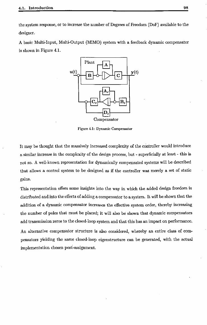
4.1. Introduction 98
the system response, or to increase the number of Degrees of Freedom (DoF) available to the
designer.
A basic Multi-Input, Multi-Output (MIMO) system with a feedback dynamic compensator
is shown in Figure 4.1.
y(t)
Compensator
Figure 4.1: Dynamic Compensator
It may be thought that the massively increased complexity of the controller would introduce
a similar increase in the complexity of the design process, but - superficially at least - this is
not so. A well-known representation for dynamically compensated systems will be described
that allows a control system to be designed as if the controller was merely a set of static
gains.
This representation offers some insights into the way in which the added design freedom is
distributed and into the effects of adding a compensator to a system. It will be shown that the
addition of a dynamic compensator increases the effective system order, thereby increasing
the number of poles that must be placed; it will also be shown that dynamic compensators
add transmission zeros to the closed-loop system and that this has an impact on performance.
An alternative compensator structure is also considered, whereby an entire class of com
pensators yielding the same closed-loop eigenstructure can be generated, with the actual
implementation chosen post-assignment.
4.2. Expression of Dynamic Compensators 99
4.2 Expression of Dynamic Compensators
4.2.1 Augmented System Description
The 'Augmented System' description for MIMO systems with dynamic compensation per
mits their representation as larger systems with static feedback. The compound system so
generated may be controlled using any standard MIMO technique.
The Augmented System Method has 'proved an expedient and popular method of achieving
dynamic compensation' (Griffin, 1997). Many researchers (Sobel and Shapiro, 1986a; Hippe
and O'Reilly, 1987; Han, 1989; Pyburn and Owens, 1990; Magni, 1999; Tsui, 1999) have
employed or developed the method, and others (Kimura, 1975; Askarpour and Owens, 1997)
have cited its use as a way to circumvent the general condition that m + r > n discussed in
Chapter 2.
The derivation of the augmented system description is straightforward. Consider a plant
under the influence of feedback via a dynamic compensator, as in Figure 4.1. The usual state
equations apply:
X= Ax+Bt
y=Cx
(4.1)
(4.2)
(4.3)
where now t is the plant input. An equivalent set of state equations apply to the compensator:
Xc = Acxc + BcY
t = Ccxc + DcY + u
(4.4)
(4.5)
where u is the external input to the system. The subscripts indicate an association with the
compensator; specifically Xc E ]RC is the compensator state vector, so the compensator is of
order c.
By substitution, we may obtain
X = Ax + BCcxc + BDcY + Bu
= (A + BDcC) x + BCcxc + Bu
(4.6)
(4.7)
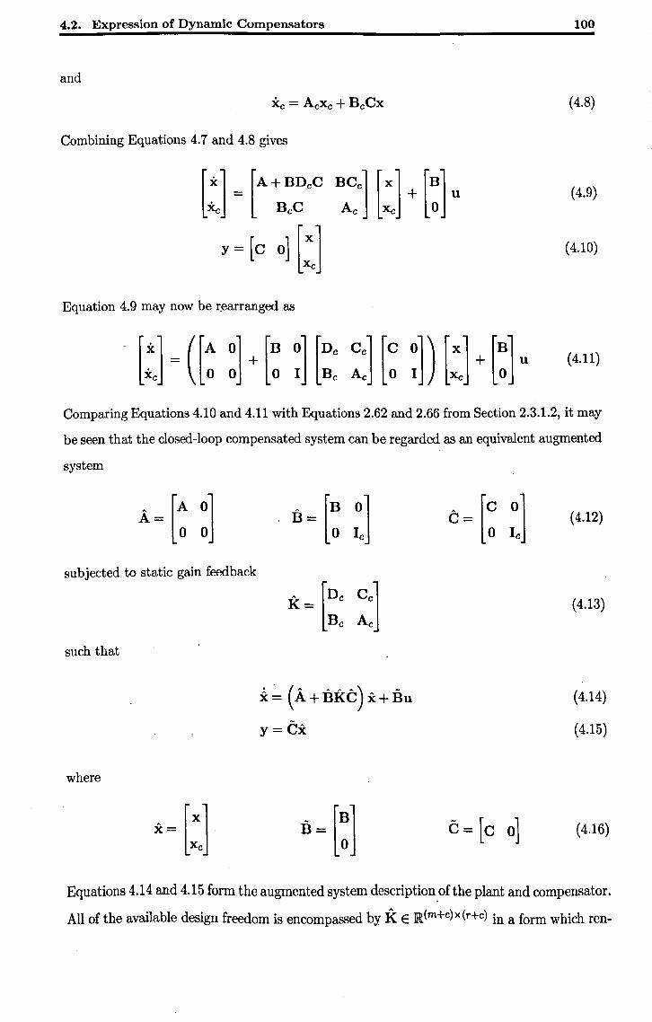
4.2. Expression of Dynamic Compensators 100
and
(4.8)
Combining Equations 4.7 and 4.8 gives
[ ~] = [A + BDeC BCe] [x] + [B] u Xc BeC Ac Xc 0 (4.9}
y= [e 0] [:] (4.10)
Equation 4.9 may now be r.earranged as
. [:J = ([~ :] + [: ~] [~: ~] [~ ~]) [:] + [:] U (4.11)
Comparing Equations 4.10 and 4.11 with Equations 2.62 and 2.66 from Section 2.3.1.2, it may
be seen that the closed-loop compensated system can be regarded as an equivalent augmented
system
subjected to static gain feedback
such that
where
i~ (A + BKC) x+Bu
y=Cx
c = [c 0]
(4.12)
(4.13)
(4.14)
(4.15)
(4.16)
Equations 4.14 and 4.15 form the augmented system description of the plant and compensator.
All of the available design freedom is encompassed by K E R(m+c)x(r+c) in a form which ren-
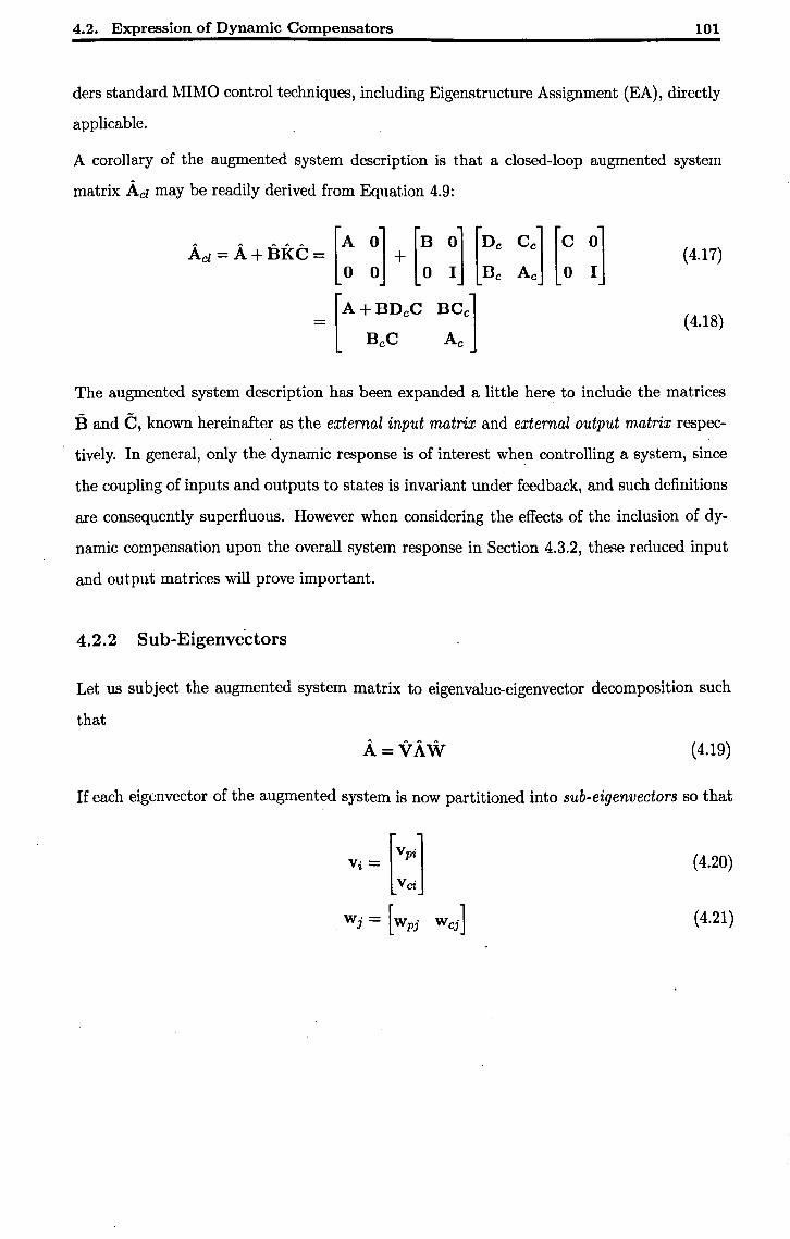
4.2. Expression of Dynamic Compensators 101
ders standard MIMO control techniques, including Eigenstructure Assignment (EA), directly
applicable.
A corollary of the augmented system description is that a closed-loop augmented system
matrix Ad may be readily derived from Equation 4.9:
(4.17)
(4.18)
The augmented system description has been expanded a little here to include the matrices
Band C, known hereinafter as the external input matrix and external output matrix respec
tively. In general, only the dynamic response is of interest when controlling a system, since
the coupling of inputs and outputs to states is invariant under feedback, and such definitions
are consequently superfluous. However when considering the effects of the inclusion of dy
namic compensation upon the overall system response in Section 4.3.2, these reduced input
and output matrices will prove important.
4.2.2 Sub-Eigenvectors
Let us subject the augmented system matrix to eigenvalue-eigenvector decomposition such
that
(4.19)
If each eigenvector of the augmented system is now partitioned into sub-eigenvectors so that
[VPi] Vi=
Vd
(4.20)
(4.21)
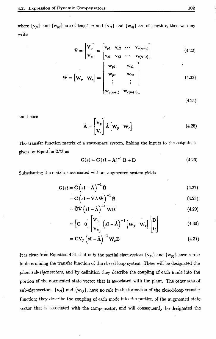
4.2. Expression of Dynamic Compensators 102
where {V pi} and {W pj} are of length n and {v ei} and {w cj} are of length c, then we may
write
v = [vp] = [V P1 Vp2 ••• VP(n+c)]
Vc Vc1 Vc2 ••• Vc(n+c)
(4.22)
Wc2 (4.23)
Wp(n+c) wc(n+c)
(4.24)
and hence
(4.25)
The transfer function matrix of a state-space system, linking the inputs to the outputs, is
given by Equation 2.73 as
G(s) = C (sI - A)-l B + D
Substituting the matrices associated with an augmented system yields
G(S)=c(sl-A)-ln =C(sI-vAW)-l iJ
= CV (sl- A)-lWB
= [e 0] [~:] (SI -At' [~p W,] [:]
= CVp (SI - A) -1 WpB
(4.26)
(4.27)
(4.28)
(4.29)
(4.30)
(4.31)
It is clear from Equation 4.31 that only the partial eigenvectors {Vpi} and {wpj} have a role
in determining the transfer function of the closed-loop system. These will be designated the
plant sub-eigenvectors, and 'by definition they describe the coupling of each mode into the
portion of the augmented state vector that is associated with the plant. The other sets of
sub-eigenvectors, {veil and {wcj}, have no role in the formation of the closed-loop transfer
function; they describe the coupling of each mode into the portion of the augmented state
vector that is associated with the compensator, and will consequently be designated the
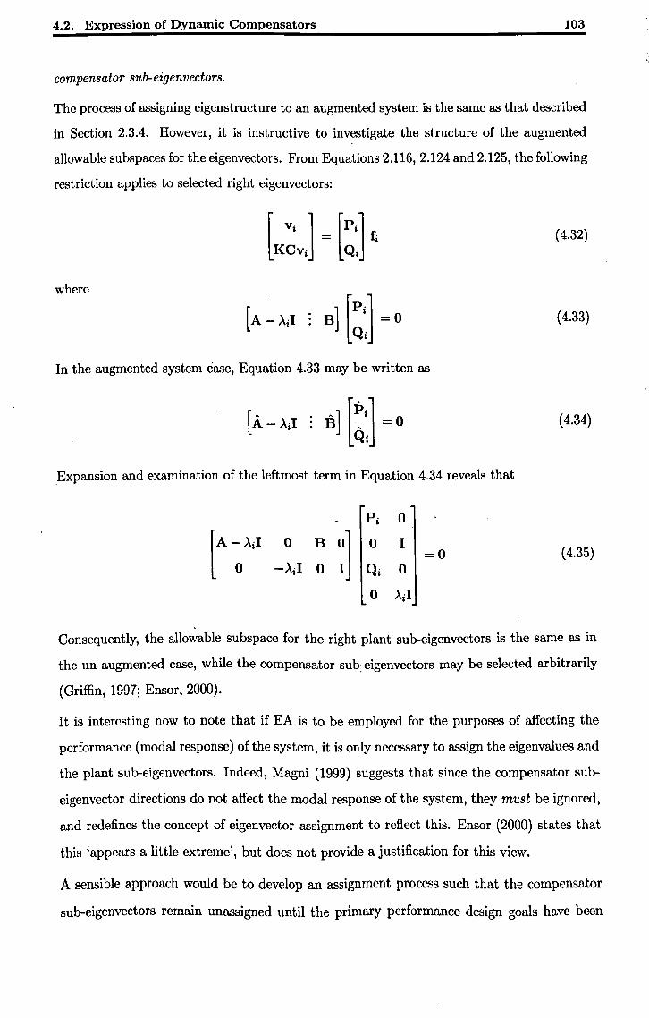
4.2. Expression of Dynamic Compensators 103
compensator sub-eigenvectors.
The process of assigning eigenstructure to an augmented system is the same as that described
in Section 2.3.4. However, it is instructive to investigate the structure of the augmented
allowable subspaces for the eigenvectors. From Equations 2.116,2.124 and 2.125, the following
restriction applies to selected right eigenvectors:
(4.32)
where
(4.33)
In the augmented system case, Equation 4.33 may be written as
[A - M : B 1 [~:] = 0 (4.34)
Expansion and examination of the leftmost term in Equation 4.34 reveals that
Pi 0
[A~M 0 B ~] 0 I (4.35) =0
-Ail 0 Qi 0
0 Ail
Consequently, the allowable subspace for the right plant sub-eigenvectors is the same as in
the un-augmented case, while the compensator suh:-eigenvectors may be selected arbitrarily
(Griffin, 1997; Ensor, 2000).
It is interesting now to note that if EA is to be employed for the purposes of affecting the
performance (modal response) of the system, it is only necessary to assign the eigenvalues and
the plant sub-eigenvectors. Indeed, Magni (1999) suggests that since the compensator sub
eigenvector directions do not affect the modal response of the system, they must be ignored,
and redefines the concept of eigenvector assignment to reflect this. Ensor (2000) states that
this 'appears a little extreme', but does not provide a justification for this view.
A sensible approach would be to develop an assignment process such that the compensator
sUb-eigenvectors remain unassigned until the primary performance design goals have been
4.3. Dynamic Compensation in Practice 104
satisfied, whereupon the design freedom they represent could be employed for other purposes
(such as gain suppression or robustness improvement).
4.3 Dynamic Compensation in Practice
Having seen how dynamic compensators may be expressed, and how the eigenstructure of an
augmented system relates to its closed-loop response, it is important to consider the impact
that these facts have on the development of dynamic control systems using EA.
If a system with n states, m outputs and r inputs is augmented with a compensator of order
c, the augmented system has m + c outputs, r + c inputs and n + c states. Consequently the
condition for pole-assignability using standard linear techniques (see Chapter 2) is
m+c+r+c>n+c
(m+r+c»ri
(4.36)
(4.37)
Hence any system which is not pole-assignable due to its dimension81ity may be rendered so
by adding a feedback compensator. Since it was first proposed (Kimura, 1975), this result
has been widely cited as justification for considering the restriction m + r > n to be a weak
one (Askarpour and Dwens, 1997, for example).
However, to assert simply that a dynamic compensator can be used to render a system pole
assignable is to evade the considerable impact that such a compensator will have upon the
form of the system's specification. The nature of EA is that the system specification is in
terms of its modal response, and the increased order of the closed-loop system must be taken
into account when specifying the required modal response.
4.3.1 Added Poles
Equation 4.31 shows that t~e closed-loop transfer function is dependent on the plant sub
eigenvectors and the entire augmented eigenvalue set La~bda. The eigenvalue set cannot
be split into plant and compensator eigenvalues, and all of the n + c closed-loop system poles
contribute to the response.
This fact has serious implications for the development of a specification for the eigenstructure
of an augmented system. If, for example, both the original system and its ideal response are
second-order, but the augmented system has three states, then three poles must be placed
4.3. Dynamic Compensation in Practice 105
and the final response will be third-order.
Placing only a subset of the poles is unlikely to yield good results, since there is no guarantee
that the unconstrained poles will be stable; even if they are, they may have a significant effect
on performance. For example, Sobel and Shapiro (1986a) assign four poles to a sixth-order
augmented system, and the unassigned poles take up a slower (and hence more dominant)
position than the assigned poles. This has the effect of causing the response of the compen
sated system to be more sluggish than its uncompensated counterpart. This effect was noted
in more detail by (Sobel and Shapiro, 1986b).
Assigning a subset of the poles such that they are an order of magnitude faster than the
natural plant modes is not a sensible approach, since attempting to force a system to respond
more quickly than its natural dynamics will allow will generally lead to large controller gains
and a solution that lacks robustness.
One possibility for placing 'extra' poles is to place multiple poles in coincident or near
coincident locations, to ensure that all modes of the closed-loop system are close in frequency
and damping to modes present in the specification. However, near-coincident eigenvalues will
have nearly co-linear eigenvector subspaces, and this is likely to result in a poorly conditioned
eigenvector set (Tsui, 1996). Systems with ill-conditioned sets of eigenvectors are sensitive
to the variation of parameters in the open-loop plant (Ensor, 2000), and are also likely to
generate large gains since the calculation of a gain matrix relies on calculating the inverse,
or pseudo-inverse, of the assigned sets of eigenvectors.
Another possibility would be to attempt to ensure that a subset of the poles of the closed-loop
system are assigned such that their associated right plant sub-eigenvectors are zero. The
mechanism for this would be that the added transmission zeros of the closed-loop system
would be assigned to the same locations as a subset of the poles. Were this possible, it is
likely that the robustness of such a system would be poor; the closed-loop poles are subject to
migration in respect of changes to the open-loop system, while the added transmission zeros
(being the poles of the compensator) are not. However, this type of assignment is not possible,
since the restrictions that are placed on the eigenvector directions make it impossible to meet
both the orthogonality condition and the rank constraints on the modal coupling matrices.
The reasons for this will be discussed more fully in Section 4.4.3.1.
In summary, attempts to hide or mask the additional system poles introduced by a dynamic
compensator are unlikely to succeed. The locations of such poles must instead be included
into the specification for the system.
4.3. Dynamic Compensation in Practice 106
4.3.2 Added Transmission Zeros
It was shown in Chapter 2, for Single-Input, Single-Output (SISO) systems, that the effect of
placing a controller with a dynamic transfer function in the feedback path of a system is to
add both poles and zeros to the resulting system. The new zeros are due entirely to the poles
of the controller. A similar phenomenon is exhibited by MIMO systems, and the following.
theorem is presented as a proof.
Patel (1978) presents a similar theorem, but considers a compensator with no direct trans
mission term. The following theorem involves a full compensator as described above.
Theorem 4.3.1. Poles of a feedback dynamic compensator manifest themselves as additional
transmission zeros in the closed loop system.
Proof. Given an augmented system under feedback, the closed-loop system matrix Ad is given
by Equation 4.18, and the external input and output matrices Band C by Equation 4.16.
Recalling Equation 2.104, transmission zero locations for the closed-loop system are given as
those values of A which cause test matrix
[
AI - Ad ~=
. C -:] (4.38)
to lose rank.
If, as is usually the case, the number of plant outputs is at least equal to the number of inputs
(m ~ r), then ~ is injective and it is sufficient to demonstrate the rank deficiency of a subset
of its columns. If m < 1', then ~ is surjective and it is sufficient instead to demonstrate the
rank deficiency of a subset of its rows. The resulting proofs are substantively identic~, so
without loss of generality it will hereafter be assumed that m ~ r.
Substituting the closed-loop matrix definitions,
AI - A - BDeC -BCe -B
~= AI - Ae 0 (4.39)
o o
It is thus sufficient to show that setting A equal to an eigenvalue of Ae causes ~ to lose rank.
4.3. Dynamic Compensation in Practice
Since it is assumed that m ~ r, tl. is injective and hence is rank deficient if
is rank deficient, or equivalently if
-BCe -B >'1 - Ae 0
o 0
rank C ([ -BC -:]) < r+c
>'1 - Ae
If >. is an eigenvalue of Ae E jRexe, then >'1 - Ae may be factorised as
>'1 - Ae = XY
where X E jRexz, Y E jRzxe and z < c. Equation 4.41 may then be written
([-BC -B]) rank XY e 0 < r + c
rank ( [ -: :] [~ ~]) < r + c
107
( 4.40)
(4.41)
( 4.42)
( 4.43)
( 4.44)
which is guaranteed to be satisfied due to the dimensionality of the matrices involved. 00
Clearly the added transmission zeros introduced by the poles of the compensator will have
an effect on the response of the closed-loop system. This effect will depend upon the placing . of the zeros, but could include 'pole masking', where the effect of a mode is diminished by
its proximity to a zero, or the creation of nonminimum-phase output responses.
Unfortunately, assignment techniques employing the augmented system method do not permit
direct manipulation of the poles of the compensator. Indeed, Tsui (1999) claims that this
fact is sufficient grounds for discarding the technique, since '[the compensator] is not even
guaranteed to be stable'. However, the stability of the compensator is not a prerequisite for
the stability (or even the performance) of the closed-loop system. If the performance and
robustness of the closed-loop system is deemed adequate, then the stability of the compensator
is of no consequence - just as the stability of the open-loop system is not a prerequisite for
successful control.
4.3. Dynamic Compensation in Practice 108
It is interesting to note, however, that if the compensator is stable it is possible to mask the
transmission zeros through the addition of an input pre-filter. The poles of the pre-filter and
the transmission zeros they mask are all products of the controller and are therefore not prone
to migration with changes in operating condition. If the compensator is not stable, however,
attempting masking in this way would be unwise since it would involve an unstable pre-filter.
If the poles of this pre-filter are not precisely coincident with those of the compensator, this
will lead to unstable modes being present in the output. Moreover, even if the matching is
precise, the condition wherein an unstable mode of the pre-filter is cancelled by a controller
zero could lead to unbounded signals within the controller, and subsequent problems with
implementation.
4.3.2.1 Transmission Zero Locations
The locations of the added transmission zeros are, as shown, given by the poles of the com
pensator. These are, in turn, given by the eigenvalues of the compensator matrix Ac which
is a partition of the static gain matrix K. Attempting to control the locations of the added
transmission zeros during assignment is, then, a problem of controlling the eigenvalues of a
square partition of the gain matrix. This is not trivial.
Alternatively, Equation 4.18 may be used to show that the matrix Ac is also a partition of the . .
closed-loop augmented system matrix Ad. Hence the zero-locations problem could be cast
as one of assigning the eigenvalues of a partition of the system matrix. This approach was
taken by Tsui (1999), who presented an algorithm for the assignment of both the transmission
zeros and the system poles in a two-stage process. However, this algorithm was not EA but
pole-placement, since the eigenvectors were not explicitly considered.
Magni (1999) chooses a priori the denominators of the compensator transfer function, hence
fixing the locations of the transmission zeros. This is done by considering the desired physical
structure of the controller. However the technique presented by Magni is not pure EA and
the design process, though powerful, is somewhat convoluted.
Yet another approach is possible. The transfer function matrix (from Equation 2.73) can be
written as
G(s) = C(sI-Ar1B+D
= CV(sI-Ar1WB + D
(4.45)
(4.46)
4.4. Freedom over Eigenvectors 109
and hence the zero locations, which may be found from the numerators of the entries in
the transfer function matrix, must be calculable given the eigenstructure of the closed-loop
system. This was demonstrated in Chapter 3 where the ideal rate-command eigenstructure
was derived. This eigenstructure, derived by considering the required mode-state couplings,
introduced a zero in a known location.
It may be thought, then, that the locations of the added transmission zeros may be fixed
by choosing the desired eigenstructure carefully. Unfortunately this is not the case. It is
extremely unlikely that all of the desired eigenvectors will lie in their associated allowable
subspaces, and hence the assigned eigenstructure will not match the desired eigenstructure
precisely. It is likely therefore that the zeros will move also. This situation is, if anything,
compounded if output-feedback EA is employed, since it is not possible to assign a complete
set of either right or left eigenvectors.
The algorithm presented by Hippe and O'Reilly (1987) effectively allows the assignment of
the compensator poles after 'assignment has taken place, but the assignment of eigenvectors
is not explicitly considered, and the approach taken relies heavily on symbolic algebra and
consequently does not lend itself to high-order systems such as helicopters.
Useful further work would be to develop a set of constraints on the assigned eigenstructure
such that the added transmission zeros are assigned, or at least constrained to a region (for
example, the left half s-plane). If these constraints were linear, they could be incorporated
as additional constraints on the eigenvector subspaces.
4.4 Freedom over Eigenvectors
It has been seen that the distribution of the additional design freedom in an augmented
system is such that the subspace from which the plant sub-eigenvectors may be selected
is the same as in the un-augmented case, while the compensator sub-eigenvectors may be
chosen arbitrarily. However, if the reduced orthogonality condition of Clarke et al. (2003)
(Theorem 2.3.2) and its associated EA algorithm are being employed, the restrictions on the
rank of the input and output coupling matrices (Conditions Cl and C2 of Theorem 2.3.2)
and on the orthogonality of the selected eigenvectors (Condition C3 of Theorem 2.3.2) are
expressed in terms of complete eigenvectors. Since the system specification is likely to be in
terms only of the plant sub-eigenvectors, it is'interesting to re-evaluate these conditions in
this context.
4.4. Freedom over Eigenvectors 110
4.4.1 Orthogonality Conditions
Condition C3 of Theorem 2.3.2, known as the orthogonality condition, requires that the sets
of assigned left and right eigenvectors must be orthogonal to one another. Thus if
(4.47)
and Wv+l
~ , W= (4.48)
Vn+c
then the orthogonality condition may be expressed as
w'v' = 0 (4.49)
If the sets of assigned eigenvectors are now partitioned into plant and compensator sub
eigenvectors, such that
and
w' = [W~ W~]
then Equation 4.49 may be written
w'v' +w'v' = 0 p p c c
w'v' = -W'V' p p c c
(4.50)
(4.51)
(4.52)
(4.53)
(4.54)
Since the compensator sub-eigenvectors may be selected arbitrarily, Equation 4.54 may be
expressed as a rank condition:
(4.55)
Hence, in the augmented system case, the orthogonality condition is equivalent to a rank
condition upon the product of the selected left and right plant sub-eigenvector sets; the
greater the compensator order, the greater t~e extent to which the orthogonality condition
4.4. Freedom over Eigenvectors 111
may be 'broken' by the selected plant sub-eigenvector sets. Indeed, if the compensator is
of very high order (c ~ max( v, n, n + c - v)), the orthogonality condition may be dismissed
entirely when constructing sets of plant sub-eigenvectors for assignment.
Assuming that plant sub-eigenvectors have been chosen according to Equation 4.55, with
rank (W~ V~) = d (4.56)
it remains necessary to find compensator sub-eigenvectors which fulfill Equation 4.54.
The following method for so doing assumes that the closed-loop system eigenvalues, and
hence the partial eigenvector subsets, are real. A simple extension to the complex case exists,
but is given in Appendix B to avoid obscuring this description.
If two matrices W x E jR(n+c-v)xd and V x E lRdxv can be found such that
(4.57)
then Equation 4.55 may be satisfied by choosing two arbitrary full-rank matrices RI E lRdxc
and R2 E lRcxd and setting
W~ = -WxRI
V~ = R2 (RIR 2)-1 V x
(4.58)
(4.59)
The inverse is guaranteed to exist due to the constraint that d ~ c, and the matrices W x
and V x, defined by Equation 4.57, may be obtained by subjecting the product W~ V~ to a
singular-value decomposition (Golub and van Loan, 1996).
If the orthogonality of W~ and V~ is pushed to its limit, such that c = d, the matrices RI
and R2 will be square, and Equation 4.59 will simplify to
V~ = R2R2 I R1I Vx
= R1IVx
(4.60)
(4.61)
and so the matrix R2 no longer carries any design freedom. It is interesting to note that
the matrix RI now has c2 DoF. In Chapter 2 it was shown that the state vector may be
transformed without affecting the transfer function matrix. Such a transformation, applied
to the compensator only, would require c2 DoF. Thus if the product W~ V~ has rank c, the
4.4. Freedom over Eigenvectors 112
freedom present in the matrix Rl acts only to transform the compensator and hence has no
effect on the locations of the transmission zeros. Indeed in general, c2 DoF have no effect on
the final transfer function for this reason (Hippe and O'Reilly, 1987); the algorithm described
by Hippe and Q'Reilly explicitly isolates the design freedom which exists only to characterise
a class of compensators.
4.4.2 Rank Conditions
Conditions Cl and C2 of Theorem 2.3.2 can also be interpreted in the context of an aug
mented system. The requirement is that the selected sets of eigenvectors must be linearly
independent, ie. that
rank CV =v (
AA ')
rank (W/13) = n + c - v
Most obviously, these conditions imply that
v:S;m+c
and
n+c-v:S;r+c
n-r$v
and therefore
.n-r:S;v$m+c
(4.62)
(4.63)
(4.64)
(4.65) .
(4.66)
(4.67)
which places lower and upper bounds upon the number of right eigenvectors that may be
selected during the assignment process.
However, the rank conditions can also be expressed as a constraint only on the selected plant
sub-eigenvectors, by re-writing Equation 4.62 as
(4.68)
If the selection of the compensator sub-eigenvectors i~ considered arbitrary, it will always be
4.4. Freedom over Eigenvectors 113
possible to obtain a set of right plant sub-eigenvectors such that
rank (V~) = min( c, v) (4.69)
Hence if v ~ c, there need be no rank conditions imposed upon the set of chosen plant
sub-eigenvectors, and Equation 4.62 can be satisfied by careful choice of the compensator
sub-eigenvectors.
If v> c however, then in order to satisfy Equation 4.62, it is necessary that
rank (CV~) ~ v - c (4.70)
The set of compensator sub-eigenvectors needs still to be full rank, but this alone is not
sufficient to ensure that Equation 4.62 is satisfied. The rows of V~ must also be linearly
independent from the rows of CV~.
Similar constraints can be derived for the left eigenvectors, by writing
rank ([ W~B W~]) = n + c - v (4.71)
The left compensator sub-eigenvector set may be chosen such that
rank (W~) = min( c, n + c -:- v) (4.72)
If n + c - v ~ c (ie. if v> n), the selected left plant sub-eigenvectors need not be subject to
a rank condition, and W~ may be chosen to ensure that the set of complete left eigenvectors
is full ranK. If v ~ n, the condition is that
rank (W~B) ~ n - v (4.73)
and the columns of W~ must be chosen to be linearly independent from those of W~B.
It is unlikely that the assignment of reduced-rank plant sub-eigenvector sets will form an
important part of the realisation of a design specification. However, a certain amount of
freedom over rank is necessary for assignment in many cases.
Consider the case where a compensator is employed to overcome the fact that m + r < n.
In this case, it is necessary either to set v > m or n + c - v > r in order to allow complete
assignment. Either the left or the right plant sub-eigenvector sets must therefore be of reduced
4.4. Freedom over Eigenvectors 114
rank with respect to m or r respectively.
4.4.3 Orthogonality vs. Rank
Equations 4.55, 4.70 and 4.73 re-express conditions Cl, C2 and C3 of Theorem 2.3.2 as
conditions on the selected plant sub-eigenvector sets. The derivation of each of these equa
tions, however, contained the assumption that the compensator sub-eigenvector sets could
be selected arbitrarily. It is unlikely that the restrictions imposed upon the compensator
sub-eigenvectors by these equations are compatible, and a compromise will have to be sought
between the rank of the selected plant sub-eigenvector sets and the rank of their product.
The interplay between these sets of constraints is extremely complex, and has thus far defied
attempts to reduce them to a linear set of simultaneous constraints or generate a logical
design procedure. Further work must be undertaken in this area to make the best use of
the insights provided here into the distribution and potential use of the design freedom in a
compensated system.
4.4.3.1 Masking Poles
In Section 4.3.1 it was claimed that placing system poles to be coincident with added trans
mission zeros by assigning zero entries into right plant sub-eigenvectors was not feasible. The
reason for this is the conflict between the rank conditions and the orthogonality condition.
Consider a subset of the assigned right eigenvectors, V H, wherein the plant sub-eigenvectors
have been assigned zero entries. The orthogonality condition requires that every assigned left
eigenvector must be orthogonal to these right eigenvectors, and hence that
(4.74)
(4.75)
W~VHc = 0 (4.76)
The rank conditions upon V' effectively force V He to be full rank. Hence if the number of
right eigenvectors in V H is given by h, a solution to Equation 4.76 for V He exists if and only
4.5. Dynamic Compensation for Performance
if W~ has a right null-space of dimension h, so
c - rank(W~) ~ h
rank(W~) ~ .. c - h
115
(4.77)
(4.78)
If W~ has zero rank (has all zero entries), then the rank conditions on W' can be satisfied
only if W~B has full rank, which is only possible for w ~ r where w is the number of assigned
left eigenvectors. As the rank of W~ increases, so the constraint on the size of W~ is relaxed,
and more left eigenvectors may be assigned.
This revised constraint on the left eigenvectors may be written as
w~r+c-h
and substituting into the constraint for pole-assignability,
m+c+r+c-h>n+c
m+r+c-h>n
(4.79)
(4.80)
(4.81 )
Hence adding compensator states will not render a system pole-assignable if the added modes
are 'hidden' in this way.
4.5 Dynamic Compensation for Performance
Using a dynamic compensator instead of a static feedback network increases the number of
DoF available for the design of a control system. It has been seen that the distribution of
this additional freedom is not simple, and its exploitation fraught with difficulties; the system
order is increased, transmission zeros are added, and no additional freedom over the coupling
of modes into the original system states is gained. Although the additional DoF can be
exploited for other means (Hippe and O'Reilly, 1987), their use for EA is very limited.
One major exception to this situation exists, and that is when the specification on a system
is already of higher order than the system itself. This is the case for a helicopter in forward
flight; its lateral and longitudinal angular rates are required to be second-order functions of
the cyclic stick position, while the open-loop dynamics are first-order. As seen in Chapter 3,
the ideal eigenstructure for this flight condition requires the introduction of two compensator
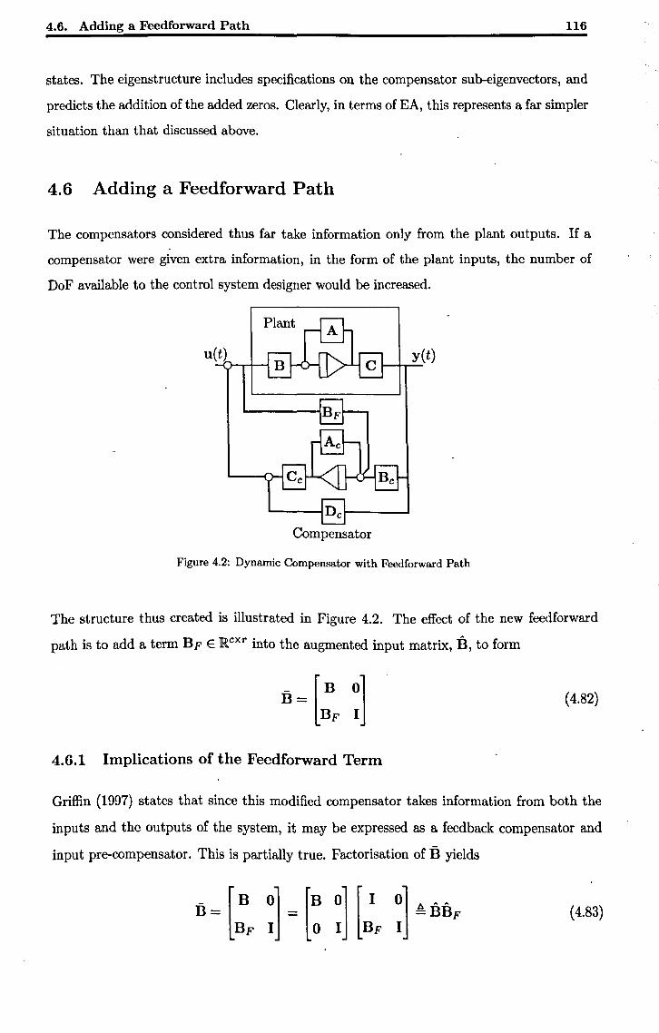
4.6. Adding a Feedforward Path 116
states. The eigenstructure includes specifications on the compensator sub-eigenvectors, and
predicts the addition of the added zeros. Clearly, in terms of EA, this represents a far simpler
situation than that discussed above.
4.6 Adding a Feedforward Path
The compensators considered thus far take information only from the plant outputs. If a
compensator were given extra information, in the form of the plant inputs, the number of
DoF available to the control system designer would be increased.
u(t) yet) I--+r;'"
'-----I Dc 1-------1
Compensator
Figure 4.2: Dynamic Compensator with Feedforward Path
The structure thus created is illustrated in Figure 4.2. The effect of the new feed forward
path is to add a term BF E jRcxr into the augmented input matrix, B, to form
B = [B 0] BF I
(4.82)
4.6.1 Implications of the Feedforward Term
Griffin (1997) states that since this modified compensator takes information from both the
inputs and the outputs of the system, it may be expressed as a feedback compensator and
input pre-compensator. This is partially true. Factorisation of B yields
A A A
=BBF (4.83)
4.6. Adding a Feedforward Path 117
Substitution into Equation 4.14 shows that the modified closed-loop system matrix is given
by
A=A+BKC
= A+BBFKC
6 A+irKC
(4.84)
(4.85)
(4.86)
In other words the dynamic response of the system (A,B,C), which includes a feedforward
term, under the influence of feedback K is the same as the dynamic response of the system
(A,B,C) under the influence of feedback K, where
(4.87)
Since the matrix :B F is full rank, the mapping between K and K is bijectivej every compen
sator in the form of Figure 4.2 has an equival~nt in the form of Figure 4.1 with the same
dynamIC response, and vice-versa.
If it is required to generate a compensator with a feedforward term from an existing feedback
compensator, this can be done simply by noting that
(4.88)
Hence, to retain the same closed-loop eigenstructure, the augmented system gain matrix can
simply be pre-multiplied by Bp! once BF has been (arbitrarily) chosen.
The input coupling is changed also. The external input matrix becomes
(4.89)
and consequently the input coupling matrix becomes
(4.90)
4.6. Adding a Feedforward Path 118
so the system response, from Equation 4.31, becomes
(4.91)
This shows that the feedforward term has pre-filtering effect upon the closed-loop system
by introducing a dependence on the compensator sub-eigenvectors that did not previously
exist. However, it is not valid to state that this effect is the same as that of an input pre
compensator. In order to achieve this effect, a pre-compensation matrix E would have to
satisfy
(4.92)
A solution for E exists (Ben-Israel and Greville, 1974) only if
(4.93)
For general W p , Wc, Band BF, this requires
(4.94)
which cannot be satisfied due to the dimensionality of the term WpB. Similarly a solution
for B F from Equation 4.92 for general W p, Wc, Band E would require
(4.95)
which again cannot g~nerally be satisfied. Hence the design freedom offered by a pre
compensator is not equivalent (but is potentially complementary) to that offered by the
feedforward term.
4.6.2 Feedforward Terms and Observers
The observer is a well-known form of dynamic compensator which, in its usual form, seeks to
estimate and synthesise the state vector through observation of the system input and output
vectors. The observer has historically been used in attempts to solve the output-feedback
problem by reconstituting the state vector and applying state-feedback control methodologies.
Observers are usually designed before a solution to the control problem is sought, due to the
separation theorem (Brogan, 1991) which guarantee$ that the characteristics of an observer
4.6. Adding a Feedforward Path 119
will not change when its outputs are used for feedback control. An observer can be designed
such that the synthesised states are guaranteed to converge to their physical counterparts,
and such that the convergence time is minimal and robust to changes in the open-loop plant
characteristics.
Unfortunately, when used for control, the robustness properties of an observer are not inher
ited by the closed-loop system (Doyle and Stein, 1979). Ideally, the controller and observer
would be designed simultaneously, such that the robust performance of the complete closed
loop system could be optimised at once.
The techniques described by Tsui (1996) provide an improvement upon this situation. The
state-feedback controller is designed taking into account the performance of the observer,
which is still designed first. For most systems[l] the robustness of the closed-loop system is
. guaranteed to be the same as that of the implementing observer. Tsui considers the use both
of optimal quadratic techniques and of EA for the design of the" controller stage.
The design process is cumbersome, however, and is a long way from exhibiting 'visibility' as
described in Chapter 1. The design of the observer uses a mixture of techniques in order to
achieve good results from an observer of minimal order, leading to a complex, decision-based
design process. Despite being state-feedback techniques, the EA algorithms presented also
suffer from a lack of visibility. They concentrate upon the assignment of eigenvectors with
specific characteristics (maximal decoupling or maximal eigenvector orthogonality) and con
sequently border on pole placement; also, for partial-state observers, they employ 'generalised
state feedback' rather than output feedback methodologies.
However, observers can be seen as compensators with feedforward terms in the form of
Figure 4.2: From Griffin (1997), a controller with a full-state observer may be written in
augmented system form as
(4.96)
It is easily verified that the closed-loop system matrix Ad = A + BKe of this arrangement
[llMost systems, in this context, means 'all open-loop systems with more outputs than inputs ~r with at least one stable transmission zero' (Tsui, 1996, p.vi)
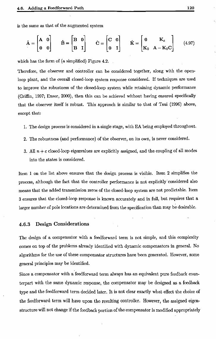
4.6. Adding a Feedforward Path 120
is the same as that of the augmented system
A = [A 0] .. 0 0
A [0 KC] K= Ko A-KoC
(4.97)
which has the form of (a simplified) Figure 4.2.
Therefore, the observer and controller can be considered together, along with the open
loop plant, and the overall closed-loop system response considered. If techniques are used
to improve the robustness of the closed-loop system while retaining dynamic performance
(Griffin, 1997; Ensor, 2000), then this can be achieved without having ensured specifically
that the observer itself is robust. This approach is similar to that of Tsui (1996) above,
except that:
1. The design process is considered in a single stage, with EA being employed throughout.
2. The robustness (and performance) of the observer, on its own, is never considered.
3. All n + c closed-loop eigenvalues are explicitly assigned, and the coupling of all modes
into the states is considered.
Item 1 on the list above ensures that the design process is visible. Item 2 simplifies the
process, although the fact that the controller performance is not explicitly· considered also
means that the added transmission zeros of the closed-loop system are not predictable. Item
3 ensures that the closed-loop response is known accurately and in full, but requires that a
larger number of pole locations are determined from the specification than may be desirable.
4.6.3 Design Considerations
The design of a compensator with a feed forward term is not simple, and this complexity
comes on top of the problems already identified with dynamic compensators in general. No
algorithms for the use of these compensator structures have been generated. However, some
general principles may be identified.
Since a compensator with a feedforward term always has an equivalent pure feedback coun
terpart with the same dynamic response, the compensator may be designed as a feedback
type and the feed forward term decided later. It is not clear exactly what effect the choice of
the feedforward term will have upon the resulting controller. However, the assigned eigen
structure will not change if the feedback portion of the compensator is modified appropriately
4.1. Conclusions and Further Work 121
through Equation 4.87. Some potential areas for research into the use of the feed forward term
could be:
• The input coupling will be affected by the addition of a feedforward term, and this
could be used to advantage to manipulate the input coupling. This could be especially
useful in situations where direct manipulation of the system input signals, as required
for a standard input pre-filter, is difficult.
• Since the lower right-hand partition of the augmented gain matrix (the compensator
A matrix) is modified when compensating for the addition of a feedforward term, it is
likely that the added transmission zeros will migrate. Hence these could be placed or
constrained, post-assignment, by a suitable algorithm.
• The introduction of a feedforward term changes entries in the B and A matrices of the
feedback compensator. This fact could potentially be exploited to reduce certain ele
ments in these matrices to zero, thereby imposing structure upon the feedback portion
of the compensator.
• The robustness of the closed-loop system to variations in the open-loop plant charac
teristics has not been studied, but it COUld,. be found that r()bustnessimprovements can
be made post-assignment by careful choice of a feedforward term.
4.7 Conclusions and Further Work
In this chapter, dynamic compensators and the augmented system description have been
introduced, and an analysis of the distribution of the design freedom added by a compensator
has been performed in the context of EA. Although no new algorithms have been presented,
it is hoped that this new exposition of the problem of applying EA to compensated systems
will form a useful contribution to the existing literature on the subject.
The idea of adding feedforward terms to feedback compensators has been introduced, and it
has been shown that it is always possible to add a feedforward term to a compensator without
changing the closed-loop eigenstructure, by means of a corresponding manipulation of the
feedback portion of the compensator. Section 4.6.3 contains several ideas for the potential
exploitation of the design freedom offered post-:assignment by this technique, and these would
form an ideal starting point for a programme of further work on this topic.
4.1. Conclusions and Further Work 122
Unless the addition of compensator states is required by the closed-loop specification, as in
Chapter 3, such an addition does not usefully increase the freedom available for EA beyond
rendering a system pole-assignable if it previously was not. The system order is increased;
transmission zeros are added and, at present, there is no method for controlling their locations
while retaining freedom over the eigenvectors; and the additional design freedom does nothing
to increase the allowable eigenvector subspaces. A method for constraining the final locations
of the added transmission zeros during assignment would be very useful further work however.
It is clear that dynamic compensation, without considerable further work, does not represent
a viable solution to the problem of increasing the available DoF when using EA to generate
a control system for a helicopter. An alternative must therefore be sought if an improvement
in performance over the static output feedback case is required.
4.7.1 Alternatives to Dynamic Compensation
If the control designer has any influence over the configuration of the plant, it is always
beneficial t·o increase the number of states that can be directly or indirectly measured. In a
linear system model this equates to an increase in rank of the C matrix. This adds design
freedom by increasing the size of the gain matrix, and could be seen as preferable to dynamic
compensation in this respect since the added freedom allows more right eigenvectors to be
assigned without increasing the system order. This benefit comes at a price - that of the
expense of the sensors themselves, including their maintenance - but the simplicity of the
resulting controller, free of dynamic compensation, may well compensate for this. It may
even be possible to convert an output-feedback problem to a state-feedback problem by
adding sensors. Unfortunately, many sensors - including. accelerometers, commonly used on
aircraft - introduce nonzero terms in the system D matrix, rendering standard approaches to
EA inapplicable.
Similarly, Proportional-plus-Derivative (PD) control also has the potential to increase the
rank of the C matrix and hence the number of available DoF. The implementation of PD con
trollers requires some care, because differentiators have a gain which increases with frequency
and hence can reduce the signal-to-noisc ratio of the signals in the controller. Bandwidth
limited differentiators (bandpass filters) may be employed instead, provided that their break
frequencies are significantly higher than the fastest system modes and can be ignored for the
purposes of modelling the controller. But again, PD control will introduce nonzero terms in
the D matrix.
Chapter Bibliography 123
Chapter 5 will introduce extensions to some standard EA techniques which are capable of
assigning eigenstructure to these types of systems, and demonstrate that the design freedom
represented by these structures is more suitable for use with visible EA algorithms than that
which is provided by dynamic compensation.
4.8 Chapter Bibliography
Askarpour, S. and Owens, T. J. (1997), 'Integrated approach to eigenstructure assignment by output feedback control', lEE Proceedings - Control Theory and Applications 144(5), 435-438.
Ben-Israel, A. and Greville, T. N. E. (1974), Generalised Inverses: Theory and Applications, John Wiley and Sons Ltd.
Brogan, W. L. (1991), Modern Control Theory, 3 edn, Prentice Hall.
Clarke, T., Griffin, S. J. and Ensor, J. (2003), 'Output feedback eigenstructure assignment using a new reduced orthogonality condition', International Journal of Control 76(4), 390-402.
Doyle, J. C. and Stein, G. (1979), 'Robustness with observers', IEEE Transactions on Automatic Control 24(4), 607-611.
Ensor, J. E. (2000), Subspace Methods for Eigenstructure Assignment, PhD thesis, University of York.
Golub, G. H. and van Loan, C. F. (1996), Matrix Computations, 3 edn, John Hopkins University Press.
Griffin, S. J. (1997), Helicopter Control Law Design Using Eigenstructure Assignment, PhD thesis, University of York.
Han, Z. (1989), 'Eigenstructure assignment using dynamical compensator', International Journal of Control 49(1), 233-245. .
Hippe, P. and O'Reilly, J. (1987), 'Parametric compensator design', International Journal of Control 45, 1455-1468.
Kimura, H. (1975), 'Pole assignment by gain output feedback', IEEE Transactions on Automatic Control 20, 509-516.
Magni, J. F. (1999), 'Multimodel eigenstructure assignment in flight-control design', Aerospace Science and Technology 3(3), 141-151.
Patel, R. V. (1978), 'On transmission zeros and dynamic output feedback', IEEE Transactions on Automatic Control 23(4), 741-742.
Pyburn, S. and Owens, T. (1990), Flight control system design by eigenstructure assignment through dynamic output feedback, in 'Proceedings of the 33rd Midwest Symposium on Circuits and Systems', Vol. 1, C~gary, Canada, pp. 50-53.

4.8. Chapter Bibliography 124
Sobel, K. and Shapiro, E. (1986a), Design of dynamic compensators via eigenstructure assignment with flight control applications, in 'Proceedings of the National Aerospace and Electronics Conference (NAECON)', Vol. 2, Dayton, OH, pp. 408-414.
Sobel, K. and Shapiro, E. (1986b), Dynamic output feedback flight control laws using eigenstructure assignment, in 'Proceedings of the 5th American Control Conference', Vol. 1, Seattle, WA, pp. 605-610.
Tsui, C.-C. (1996), Robust Control System Design - Advanced State-Space Techniques, Marcef Dekker: New York.
Tsui, C.-C. (1999), 'A new dynamic output feedback compensator design for pole placement', Journal of the Franklin Institute 336(4), 665-674.
Chapter 5
Eigenstructure Assignment in
Semi-Proper Systems
Contents 5.1 Introduction ............................... 126 5.2 Sources of Semi-Proper Systems •••••••••.••••••••• 127
5.2.1 Semi-Proper Systems for State Derivative Control .......... 128
5.2.1.1 Robustness Considerations . . . . . . . . . . . . . . . . . . 129
5.3 Problem Formulation • • • • . . • • • • . . . • • • • • • • • • • • •• 129
5.3.1 Closed Loop System Structure ...................... 132
5.3.2 Singularities in the Closed Loop System . . . . . . . . . . . . . . . . 132
5.4 Pseudo-State Feedback . • • . • • . • . • .' . • . . • • • • • . . • •. 134
5.4.1 Excess Freedom .............................. 136
5.4.2 Design Procedure ............................. 137
5.4.2.1 Choosing Eigenvectors. . . . . . . . . . . . . . . . . . . . . 137
5.4.2.2 Gain Matrix Recovery . . . . . . . . . . . . . . . . . . . . . 138
5.5 Output Feedback. • • • • • • • • • • • • • • . • • • • • • • • • • . • • ,. 138
5.5.1 Generalising Multi-Stage Eigenstructure Assignment ......... 139
5.5.1.1 Modal Coupling Vector Assignment . . . . . . . . . . . . . 140
5.5.1.2 Gain Matrix Recovery ..................... 141
5.5.2 Design Procedure. . . . . . . . . . . . . . . . . . . . . . . . . . . . . 146
5.5.2.1 Stage One ........................... 147
5.5.2.2 Stage Two ........... '. . . . . . . . . . . . . . . . 148
5.5.2.3 Gain Matrix Calculation ................... 149
5.5.2.4 A Note on Unused Freedom. . . . . . . . . . . . . . . . . . 149
5.6 Conclusions . . . . . . . . . . . . . . . . . . . . . . . . . . . . . . . . 152
5.7 Chapter Bibliography • • • • • • • . • • . . • • . . • • . • . . . • •. 152
125
5.1. Introduction 126
5.1 Introduction
As discussed in Chapter 2, standard Eigenstructure Assignment (EA) algorithms can be
divided roughly into two groups: state-feedback, where the output (C) matrix is assumed to
be an identity, and output-feedback, where assumptions are made only about the number of
inputs and outputs (White, 1995). However, both groups of algorithms generally rely on the
direct transmission (D) matrix being null. This is valid only if the system is strictly proper.
9iven the multivariable transfer function matrix G(s), a system is said to be:
• Strictly proper if G(s) --+ 0 as S --+ 00;
• Semi-proper if G(s) --+ D =I 0 as s --+ 00;
• Proper if either strictly proper or semi-proper;
• Improper if G(s) --+ 00 as s --+ 00.
Improper systems are not physically realisable Skogestad and Postlethwaite (1996).
Very few EA algorithms are compatible with semi-proper systems. A pair of papers by
Fletcher (19S1a, b), published during the formative years of EA, are concerned with output
feedback pole placement rather then EA specifically. Eigenvectors are selected but no mention
is made of their importance to the design or solution, or how they should be chosen. Moreover,
Fletcher's technique is essentially a protection method (White, 1995) and consequently suffers
from the lack of design visibility offered by these approaches. The development of the method
does not include a formulation of the complete closed-loop system, and therefore fails to
show that the input and output matrices change when the loop is closed, a fact which can
be important in the design process.
White (1997) does not assume a zero D matrix. The algorithm described by White was
developed specifically for robust EA (more accurately for robust pole placement), and used
graphical techniques with multivariable pole and zero loci to select gains in highly structured
controllers. These techniques are effective but lack any kind of design visibility.
A number of EA algorithms for descriptor systems (Le, 1992, for example) also do not make
the assumption that the open-loop system is strictly proper. Clearly any algorithm for a
descriptor system may be applied to a system in standard form, but the operation of these
algorithms in this context is in general obfuscated by their nature as algorithms for descriptor
systems.
5.2. Sources of Semi-Proper Systems 127
This chapter will introduce and develop several novel algorithms for the assignment of eigen
structure to semi-proper systems in standard form, firstly for systems with at least as many
outputs as states, and then for those with fewer outputs than states. The first algorithm rep
resents the generalisation of a standard state-feedback EA algorithm such as that of Moore
(1976), and the second a generalisation of the output-feedback algorithm presented by Clarke
et al. (2003).
5.2 Sources of Semi-Proper Systems
Although semi-proper systems are mathematically feasible, all physical systems are strictly
proper (Skogestad and Postlethwaite, 1996). However, semi-proper systems are often useful
approximations.
For example, an aircraft mathematical model will often contain several velocity states. Ve
locities are almost impossible to measure in the absence of a fixed reference frame and,
therefore, accelerometers are used to obtain state information. Incorporating the measured
accelerations into the model results in the addition of non zero entries in the D matrix. Addi
. tionally, many control structures familiar to designers of classical control systems, including
Proportional-plus-Derivative (PD) controllers a~d phase-advance networks, involve the effec
tive differentiation of states and will have the same effect. These are all approximations since
no accelerometer or controller has an infinite bandwidth. However, the realisation of these
differentiations in the form of a semi-proper system formulation is convenient and, provided
that the bandwidths of the approximated components is sufficiently high, fit for practical
purposes. A further advantage of such a semi-proper approximation is that the system order
is reduced when compared to an equivalent system with modelled sensor dynamics, meaning
that fewer Degrees of Freedom (DoF) are required for pole-assignability.
Other sources of semi-proper system descriptions exist. The reduction of a linear system
of high order to one of lower order (a process discussed in Appendix A) will often generate
a reduced-order system that is semi-proper, due the approximation of fast system modes as
direct input-output couplings. Conversion of a continuous-time model to a discrete-time form
(or vice-versa) using the bilinear (Tustin) transform (Banks, 1986) will lead to nonzero terms
in the D matrix.
5.2. Sources of Semi-Proper Systems 128
5.2.1 Semi-Proper Systems for State Derivative Control
It should be noted that although the feedback of state derivatives is a common source of semi
proper systems, other methods exist for the assignment of eig~nstructure to systems with state
derivative feedback. In particular, given a strictly proper system under proportional-plus
derivative control, the closed-loop system equation may be written
(I - BKdC)X = (A + BKC)x + Bu (5.1)
where Kd is the derivative feedback gain matrix and K the state feedback gain matrix.
Equation 5.1 is in the form of a descriptor system, and as mentioned in Chapter 2, EA
algorithms for PD control of descriptor systems exist (Duan and Patton, 1997; Duan and
Wang, 2004; Duan and Patton, 1999; Owens and Askarpour, 2000).
However, if PD or state derivative control of a system in standard form is the aim, the
algorithms to be presented here have several potential advantages over forming and controlling
a descriptor system. The feedback gains from both states and state ~erivatives are contained
in a single gain matrix, and found simultaneously; the available design freedom is presented
in the same form as in standard state feedback (or output feedback) EA. Consequently the
distribution of the design freedom is the same and this ensures that:
• The conditions for pole-assignability are simple to derive, and reflect those of a strictly
proper system;
• The formation of a semi-proper system whose outputs are composed of an arbitrary
combination of states and state derivatives is trivial, and this provides a highly flexible
mechanism for controller design;
• The controller design process is substantially identical to that of standard state-feedback
EA or of output feedback EA as proposed by Clarke et al. (2003), .and consequently
offers unprecedented levels of design visibility;
• Access to unused design freedom is available post-assignment, and may be used for
retrcrassignment (Clarke and Griffin, 2004) or gain suppression (Chapter 6). The best
(simplest and most visible) of the current algorithms (Owens and Askarpour, 2000)
considers only the minimisation of the Frobenius norm of the gain matrix.
5.3. Problem Formulation 129
5.2.1.1 Robustness Considerations
It is not the aim of this thesis to consider the robustness of control systems designed using
EA. However, it is important to note that if partial or complete state derivative feedback is
employed, the resulting open-loop C matrix will contain rows taken directly from the open
loop A matrix. Hence, if perturbations in the open-loop A matrix are to be considered for
the purposes of calculating robustness measures, their effect on the open-loop C matrix must
be borne in mind.
5.3 Problem Formulation
Consider a controllable, observable, minimal, semi-proper state-space system under the in
fluence of feedback such that
where
x=Ax+Bt
y = Cx+Dt
t=Ky+u
(5.2)
(5.3)
(5.4)
u is an exogenous input, t is the plant input, A E jRnxn, B E jRnxr, C E jRmxn, D E jRmxr
and K E Rrxm.
By substitution we may readily obtain
t = (I - KD)-l u + (I - KD)-l KCx (5.5)
under the assumption that the term 1 - KD is nonsingular (the implications of this restriction
are discussed in Section 5.3.2).
To simplify subsequent analysis, we define
N ~ (I - KD) -1 K (5.6)
giving, after substitution:
5.3. Problem Formulation
We may therefore define
x = (A + BNC) X + B (I - KD) -1 u
y = (C + DNC)x+ D(I- KD)-1 u
Ael A A+BNC
Bel ~ B (I - KD)-1
Cel A C+DNC
Del ~ D (I - KD)-1
130
(5.7)
(5.8)
(5.9)
(5.10)
(5.11)
(5.12)
The system structure derived above is accurate, but is not symmetrical in that the formula
tions of Bel and Cel appear quite different. The asymmetric nature of the structure does not
appear to originate from any inherent asymmetry in the open-loop system or the feedback
network. This observation forms the motivation for the following alternative formulation.
Consider again the system of Equations 5.2 to 5.4. By substitution once more, we may
determine that
y = (I - DK)-1 Cx + (I - DK)-1 Du
where, this time, it is assumed that the term 1- DK is nonsingular.
Substitution of Equation 5.13 into Equation 5.2 now gives:
Using the identity (Miller, 1987, 10),
Equation 5.14 becomes:
x = (A+BNC)x+ (B +BND)u
(5.13)
. (5.14)
(5.15)
(5.16)
The differences between Equations 5.13 and 5.16 and Equations 5.7 and 5.8 are due simply
5.3. Problem Formulation 131
to a difference in the order of substitution. The following is a proof of their equivalence.
From the formulation of Equation 5.16,
B + BND = B + B (I - KD)-l KD
= B (I + (I - KD) -1 KD)
= B( (I - KD)-1 (I - KD) +
(I - KD)-1 KD)
= B (I - KD)-l ((I - KD) + KD)
= B(I- KD)-1 (5.17)
which demonstrates the equivalence of Equations 5.7 and 5.16. This result could also be
obtained using Woodbury's Formula (Miller, 1987, 11). The same logic may be applied to
prove the equivalence of the Equations 5.8 and 5.13.
Consequently, we may define:
where
Ad~A+BNC
Bd ~B+BND=B(I-KD)-1
Cd ~ C + DNC = (I - DK)-1 C
Dd ~D+DND=D(I-KD)-1
= (1- DK)-1 D
(5.18)
(5.19)
(5.20)
(5.21)
(5.22)
(5.23)
It may be seen that the closed-loop matrices Ad, Bc/' C(:l, Dd all differ from the open-loop
matrices A, B, C, D if D =f O. Hence if the open-loop system is semi-proper, it is not
only the system dynamics which change when the loop is closed but also the input-state,
state-output and input-output couplings.
5.3. Problem Formulation 132
5.3.1 Closed Loop System Structure
In Fletcher's paper (Fletcher, 1981a), Equation 5.9 is stated (in expanded form) but it is not
derived. The other three closed-loop matrices are not presented. However, the effect of loop
closure on B, C and D is important.
Consider the case of right eigenvector assignment in order to control the coupling of modes
into system outputs. The closed-loop output matrix Cel (Equation 5.11) depends upon an
inverse involving the gain matrix which, at the time of assignment, is unknown. Consequently
the change from C to Cel, when the loop is closed, cannot be predicted. Therefore, the
assignment of eigenvectors to determine mode-output coupling is not appropriate.
Whether or not the change in coupling between the states and outputs is of concern depends
upon the nature of the assignment taking place. If it is necessary to ensure a specific coupling
of modes into states, then assignment of eigenvectors is appropriate. If, instead, it is desired
to control the appearance of the modes in the outputs, then techniques leading to the direct
assignment of the output-coupling vectors are required.
A secondary benefit of assigning output coupling vectors directly is that the algorithm is
immediately suitable for those systems in which the states themselves have no direct physical
interpretation. Models derived using identification techniques are likely to fall into this
category if the identification process can only approximate input-output relationships (Griffin,
1997).
5.3.2 Singularities in the Closed Loop System
Section 5.3 introduced the pre-conditions on the gain matrix that 1- KD and 1- DK must
be nonsingular.Here, we consider the reasons for this, and its implications for control system
design.
The constraint is not a curiosity of the exposition presented here. Rather, it represents
a system singularity. The feedforward Del matrix and the feedback K matrix form direct
forward and backward transmission paths, coupling the input and output through a pair of
simultaneous equations. When the constraint is not satisfied, no instantaneous solution exists
to these equations for y given u and x. Thus the constraint is somewhat pathological; it is
reasonable to assume that a control system design approach based on meeting performance
goals would never give rise to such a situation. Nevertheless, ensuring that this is the case is
a simple matter in most cases.
5.3. Problem Formulation 133
Theorem 5.3.1. If m = n, assigning a linearly independent set of output coupling vectors
is a necessary and sufficient condition for ensuring the causality of the closed loop system.
The following lemma assists with the proof.
Lemma 5.3.2. The non-singularity of anyone of the terms 1- KD, 1- DK, 1+ ND
and I + DN (where N is defined by Equation 5.6) is necessary and sufficient to ensure the
non-singularity of the remaining terms.
Proof. Consider rearranging the defined structure of N, given in Equation 5.6:
N= (I-KD)-IK
N-KDN=K
N=K+KDN
N(I+DN)-I=K
(5.24)
(5.25)
(5.26)
(5.27)
The transformation between N and K is bijective, and hence I - KD is nonsingular if and
only if I + DN is nonsingular.
Finally, 1+ DN is nonsingular if and only if I + ND is nonsingular (see Miller, 1987, Corol
lary 3, p9); it is trivial to show that the same is true for 1- KD and I - DK. 00
Proof of Theorem 5.3.1. From Equations 5.5 and 5.13, the causality of the closed-loop system
is dependent upon the terms 1- KD and 1- DK being nonsingular. Lemma 5.3.2 gives a
set of alternative necessary and sufficient conditions for this.
The term 1+ DN, implied in Equation 5.11 and listed in Lemma 5.3.2, is a factor that links
the open-loop C and closed-loop Cel matrices.
Therefore, given a set of mode-output coupling vectors
it is clear that
fl = [01 D2 On]
= Cel [VI V2 ... vn ]
= CelV
= (I + DN)CV
rank(fl) = rank ((I + DN)CV)
(5.28)
(5.29)
(5.30)
(5.31)
(5.32)
5.4. Pseudo-State Feedback 134
and since by requirement rank( C) = n and rank(V) = n,
rank(O) = min(n, rank(I + DN)) (5.33)
Since the term 1+ DN is of size m x m, if m = n Equation 5.33 reduces to
rank(O) = rank(I + DN) (5.34)
Consequently the linear independence of the set of closed-loop output coupling vectors is
necessary for term I - KD to be full rank; if the number of system outputs is the same as
the number of states, it is also sufficient. 00
5.4 Pseudo-State Feedback
There follows an algorithm, developed by the author: that forms a simple extension to stan
dard state-feedback EA. It appears in a simplified, less generic form in Pomfret and Clarke
(2003), and in this form in Pomfret et al. (2005). The term 'pseudo-state feedback' is coined
here to describe the application of output feedback to a controllable, observable system with
the same number of independent outputs as states. State feedback implies that the states
are measurable directly (ie. that C = I and D = 0), while pseudo-state feedback simply
requires that rank (C) = m = n and otherwise carries no constraints beyond those of output
feedback. Nevertheless it is not a misnomer, since the condition rank(C) = m = n allows
for the placement of all the system poles by assigning only right-eigenvectors. This is the
common characteristic of all state-feedback EA algorithms.
By definition, for any closed-loop eigenvalue-eigenvector pair P'il Vi},
and consequently
(A + BNC) Vi = ViAi
(A - Ail) Vi = BNCVi
[A-Ail Bl [N~VJ =0
(5.35)
(5.36)
(5.37)
(5.38)
5.4. Pseudo-State Feedback 135
Equation 5.38 may be parameterised by setting
(5.39)
where
(5.40)
The output-coupling vector 0i describes the distribution of a given mode into the outputs:
= (C+DNC)vi
= [c D] [ Vi ] NCVi
~= [e : ~l [~:].~
(5.41)
(5.42)
(5.43)
(5.44)
Consequently, the design vector, fi, for a given mode may used to select either an output
coupling vector Oi, or an eigenvector Vi using, for example, a least-squares projection of a
desired vector into the allowable subspace. Note that, since Cel is square and also guaranteed
to be full-rank (see Section 5.3.2), the condition that the closed-loop eigenvectors must be
linearly independent can be satisfied by ensuring instead that the selected output-coupling
vectors are linearly independent.
Having selected the design vectors {fi }, the matrix N may be recovered:
v = [Vl V2 ... V n] (5.45)
= [Plfl P2f2 Pnfn] (5.46)
S=NCV (5.47)
= [Qlfl Q2f2 ... Qnfn] (5.48)
N = 8V-1C-1 (5.49)
It only remains to rearrange N (defined at Equation 5.6) to find K (using Equation 5.27).
5.4. Pseudo-State Feedback 136
In Theorem 5.3.1 it was shown that a solution is guaranteed given a linearly independent
set of output-coupling vectors. Consequently, assigning a linearly independent set of output
vectors guarantees both a solution to Equation 5.49 and a solution to Equation 5.6.
5.4.1 Excess Freedom
If accelerometers, or other forms of derivative feedback, are used in order to increase the
number of system outputs to the point where pseudo-state feedback is practical, it is also
feasible that the number of linearly independent outputs may be made to exceed the number
of states, ie. m> n. In this case, the gain matrix solution is not unique.
If the condition that rank( C) = m = n is replaced by the new condition rank( C) = n ::; m,
the procedure of Section 5.4 may be followed until Equation 5.48. At this point, the algorithm
relies on the inversion of C and must therefore be modified.
From Equations 5.47 and 5.6, it is clear that
Simplifying,
S=NCV
= (I - KD)-l KCV
(I - KD) S = KCV
S-KDS=KCV
S=KCV+KDS
S=K(CV-tDS)
(5.50)
(5.51)
(5.52)
(5.53)
(5.54)
. (5.55)
where C, D, S and V are known. A direct solution for K by inversion from Equation 5.55 is
not possible since by hypothesis the term CV + DS is non-square. However, a solution for
K can still be found (Ben-Israel and Greville, 1974, p39):
K = S (CV + DS)t + Z (I - (CV + DS) (CV + DS)t) (5.56)
where At is the Moore-Penrose pseudo-inverse of A (see Appendix C) and Z is a matrix of
free parameters. This parameter matrix is expressed in a similar way to the matrix of free
parameters existing at the end of the output-feedback EA algorithm of Clarke et al. (2003).
5.4. Pseudo-State Feedback 137
Hence, for a system with m > n, it is possible, not only to assign n eigenvalues and right
eigenvectors, but also to recover the unused design freedom and employ it for another purpose,
for example the imposition of controller structure (see Chapter 6).
Note that Theorem 5.3.1 no longer ensures that the resulting system is causal since m f=. nj
however, there now exists the free parameter matrix Z which may be employed to avoid the
pathological condition that the term I - KD is not full-rank.
5.4.2 Design Procedure
A design procedure formalising the pseudo-state feedback EA process will now be described.
It is assumed that the system (A, B, C, D) is controllable and observable, and that rank(C) = n.
5.4.2.1 Choosing Eigenvectors
For each desired eigenvalue Ai, i = 1 ... n, form the allowable subspace
Choose a design vector fi E Crx 1 to select either the corresponding right eigenvector
or output coupling vector #
Having selected {fi}, form the matrices
v = [Vl,'''' vn] = [P1fI, ... , Pnfn]
S = [Q1f1, ... , Qnfn]
and check that n is full rank, as required by Theorem 5.3.1.
(5.57)
(5.58)
(5.59)
(5.60)
(5.61)
(5.62)
5.5. Output Feedback 138
5.4.2.2 Gain Matrix Recovery
The gain matrix formula of Equation 5.56 can be employed if there is an excess of outputs
over states:
K = S (CV + DS)t + Z (I - (CV + DS) (CV + DS)t) (5.63)
If not, Equations 5.49 and 5.27 can be employed to recover first N and then K. Alternatively,
Equation 5.56 can be modified to return K directly; if m = n, then the term (CV + DS) is
square and full rank, so
(CV + DS)t = (CV + DS)-l (5.64)
Under these conditions, Equation 5.56 reduces to
K = S(CV +DS)-l (5.65)
This concludes the design procedure.
5.5 Output Feedback
Due to the symmetrical form of the closed-loop system derived in Section 5.3, an output
feedback EA algorithm for systems 'with direct transmission te~ms is easily derived. The
multi-stage EA algorithms of Clarke et al. (2003) aim to assign eigenvalues and eigenvectors
to a closed-loop system matrix of the form
Ad = A+BKC (5.66)
where the gain matrix, K, is free and the other matrices are fixed. From Equation 5.9, the
closed-loop system matrix to which it is now desired to assign an eigenstructure is given by
Ad = A+BNC (5.67)
Consequently it may be seen that the multi-stage EA algorithms may be used without mod
ification to determine N, with Equation 5.27 used to recover K.
However, as shown by Equations 5.10 and 5.11, the coupling between the inputs and the
states, and that between the states and the outputs, is subject to change when the loop is
closed. The nature of the change is not known a priori, and if the system specification is in
5.5. Output Feedback 139
terms of, for example, output modal coupling, assignment of eigenvectors will not suffice. A
technique for specifying modal coupling vectors is desirable.
In addition, applying the multi-stage algorithms directly would yield N, not K directly;
although recovery of K via Equation 5.27 is trivial, the gain matrix equation is not returned
in a form compatible with the imposition of controller structure (see Chapter 6).
5.5.1 Generalising Multi-Stage Eigenstructure Assignment
By definition, for any closed-loop eigenvalue-right eigenvector pair P'i, Vi} or eigenvalue-Ieft
eigenvector pair {Aj, Wj},
and consequently
(A + BNC) Vi = ViAi
(A - Ail) vi = BNCVi
BJ[Vi]=O NCVi
and
Wj (A + BNC) = WjAj
Wj (A - Ajl) = wjBNC
WjBN] [A~>'jI] =0
Equations 5.72 and 5.75 may be pararneterised by setting
(5.68)
(5.69)
(5.70)
(5.71)
(5.72)
(5.73)
(5.74)
(5.75)
(5.76)
(5.77)
5.5. Output Feedback
where
range ([ ~:]) ~ ker ([A - Ail : BD
range([L; : M;n ~ker ([A~A;In
140
(5.78)
(5.79)
The right design vector, ri, or left design vector, gj, for a given mode may used to select an
eigenvector Vi or Wj using, for example, a least-squares projection of a desired vector.
5.5.1.1 Modal Coupling Vector Assignment
The output-coupling vector 0i, which describes the distribution of a given mode into the
outputs, is given by 'Equation 5.44; consequently the right design vector, ri, for a given mode
may used to select either an output-coupling vector'oi or an eigenvector Vi, Similarly the
input-coupling vector ij describing the coupling of the inputs into a given mode is given by
=Wj(B+BND)
~ [w; : wjBN] [:]
I; ~ g;- [Lj : M;] [:]
(5.80)
(5.81)
(5.82)
(5.83)
arid the left design vectors {gj} may similarly be used for the selection of either eigenvectors
or input-coupling vectors.
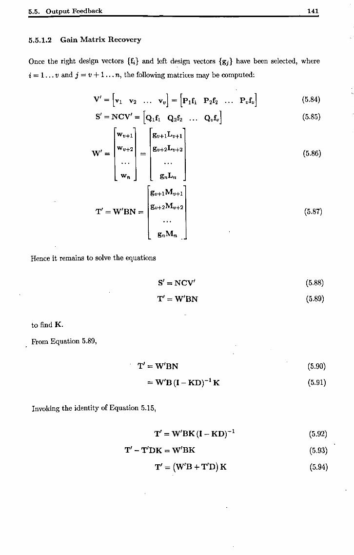
5.5. Output Feedback 141
5.5.1.2 Gain Matrix Recovery
Once the right design vectors {fi } and left design vectors {gj} have been selected, where
i = 1 ... v and j = v + 1 ... n, the following matrices may be computed:
v' = [VI V2 ... Vv] = [PIfl P2f2 ... Pvfv]
S' = NCV' = [Qlfl Q2f2 Qvfv]
W'= w v+2
gv+1M v+1
T' = W'BN = gv+2M
v+2
Hence it remains to solve the equations
to find K.
From Equation 5.89,
s' = NCV'
T' =W'BN
T' =W'BN
= W'B (I - KD)-l K
Invoking the identity of Equation 5.15,
T' = W'BK (I - KD)-l
T' - T'DK = W'BK
T' = (W'B + T/D) K
(5.84)
(5.85)
(5.86)
(5.87)
(5.88)
(5.89)
(5.90)
(5.91)
(5.92)
(5.93)
(5.94)
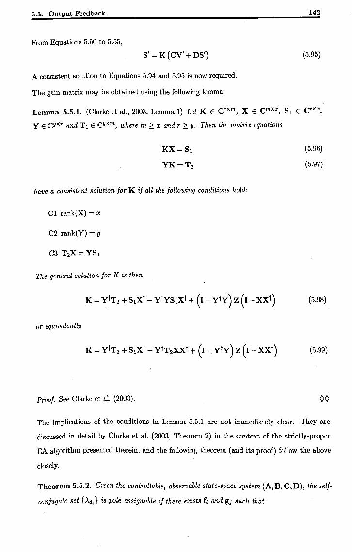
5.5. Output Feedback 142
From Equations 5.50 to 5.55,
S' = K (CV' + DS') (5.95)
A consistent solution to Equations 5.94 and 5.95 is now required.
The gain matrix may be obtained using the following lemma:
Lemma 5.5.1. (Clarke et al., 2003, Lemma 1) Let K E crxm , X E Cmxx, SI E Crxx
,
YE Cyxr and Tl E Cyxm, where m ~ x and r ~ y. Then the matrix equations
KX=Sl
YK=T2
have a consistent solution for K if all the following condit'ions hold:
Cl rank(X) = x
C2 rank(Y) = y
The general solution for K is then
(5.96)
(5.97)
K = ytT2 + SIXt - ytYS1xt + (I - yty) Z (I - xxt) (5.98)
or equivalently
(5.99)
Proof. See Clarke et al. (2003). 00
The implications of the conditions in Lemma 5.5.1 are not immediately clear. They are
discussed in detail by Clarke et al. (2003, Theorem 2) in the context of the strictly-proper
EA algorithm presented therein, and the following theorem (and its proof) follow the above
closely.
Theorem 5.5.2. Given the controllable, observable state-space system (A, D, C, D), the self
conjugate set {>'di} is pole assignable if there exists fi and gj such that
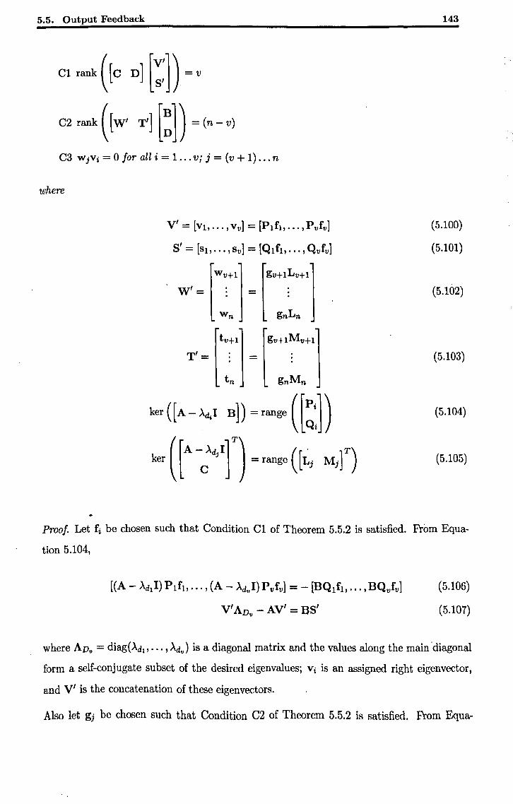
5.5. Output Feedback
Cl rank ([C D] (::1) = v
C2 rank ([w, ~] (:1) = (n - v)
C3 WjVi = 0 for all i = 1 ... Vi j = (v + 1) ... n
where
v' = [Vi, ••• , Vv] = [Plf}, ... , Pvfv]
S' = [Si, ... , sv] = [Qlfl,"" Qvfv]
W'=
T'=
ker ([A- A~I BD = range ((~:1)
ker ([A-:d,Ir) = range ([L; Mr)
143
(5.100)
(5.101)
(5.1()2)
(5.103)
(5.104)
(5.105)
Proof. Let fi be chosen such that Condition Cl of Theorem 5.5.2 is satisfied. From Equa
tion 5.104,
V'AD" - AV' = as'
(5.106)
(5.107)
where ADv = diag(>'dl' ... ,>'dv) is a diagonal matrix and the values along the main'diagonal
form a self-conjugate subset of the desired eigenvaluesj Vi is an assigned right eigenvector,
and V' is the concatenation of these eigenvectors.
Also let gj be chosen such that Condition C2 of Theorem 5.5.2 is satisfied. From Equa-
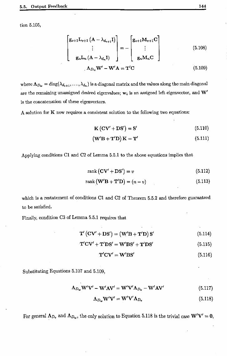
5.5. Output Feedback 144
tion 5.105,
(5.108)
A W' - W' A = T'C . Dw (5.109)
where Avw = diag(Ad"+l' ... ' Adn ) is a diagonal matrix and the values along the main diagonal
are the remaining unassigned desired eigenvalues; Wi is an assigned left eigenvector, and W'
is the concatenation of these eigenvectors.
A solution for K now requires a consistent solution to the following two equations:
K (CV' + nS') = S'
(W'B + T'n) K = T'
Applying conditions Cl and C2 of Lemma 5.5.1 to the above equations implies that
rank (CV' + ns') = v
rank(W'B + T'n) = (n - v)
(5.110)
(5.111)
(5.112)
(5.113)
which is a restatement of conditions Cl and C2 of Theorem 5.5.2 and therefore guaranteed
to be satisfied.
Finally, condition C3 of Lemma 5.5.1 requires that
T' (CV' + DS') = (W'n + T'n) S'
T'CV' + T'nS' = w'ns' + T'nS'
T' CV' = w'ns'
Substituting Equations 5.107 and 5.109,
ADw W'V' - W' AV' = W'V' Av" - W' AV'
ADw W'V' == W'V' Av"
(5.114)
(5.115)
(5.116)
(5.117)
(5.118)
For general ~DIJ and ADwl the only solution to Equation 5.118 is the trivial case W'V' = 0,
5.5. Output Feedback
or equivalently
WjVi=O for all i=1. .. v, j=(v+1) ... n
as given by condition C3 of Theorem 5.5.2.
145
(5.119)
00
Condition C3 of Theorem 5.5.2 is the same reduced orthogonality condition given by Clarke
et al. (2003), and is easily satisfied by ensuring that any selected eigenvector is orthogonal to
the set of complimentary eigenvectors already chosen.
Conditions Cl and C2, however, are somewhat different. In the strictly proper case, they serve
to restrict the selected sets of eigenvectors to be linearly independent. A similar restriction
is imposed by these revised, generalised conditions. Comparison of conditions Cl and C2 of
Theorem 5.5.2 with Equations 5.44 and 5.83 reveals that they may be written as
rank ([01, ... ,0vD = v (5.120)
rank = (n - v) (5.121)
Hence the linear independence of the selected sets of modal coupling vectors is a necessary
and sufficient condition for the satisfaction of conditions Cl and C2 of Theorem 5.5.2.
Theorem 5.3.1 showed that recovery of the gain matrix is possible only if the selected output
coupling vectors are linearly independent. However this is a sufficient condition for the
recovery of K only in the case where m = n. This theorem will therefore not suffice in
the output feedback case. The following theorem is a generalisation of Theorem 5.3.1 which
renders it applicable to the output feedback case. ..
Theorem 5.5.3. If m = v or r = n - v, the closed-loop system is guaranteed to be causal.
Proof. Lemma 5.3.2 showed that the causality of the closed loop system and the recovery of
a gain matrix is guaranteed if either 1+ DN or 1+ ND can be shown to be nonsingular.
Let us assume that all n eigenvalues have been assigned, together with v right eigenvectors and
(n - v) left eigenvectors. Consider a matrix formed from the set of assigned output-coupling
vectors:
0' = [01 02 • •• Ov] (5.122)
5.5. Output Feedback
It may be expressed in terms of the set of implicitly assigned right eigenvectors
as
0' = CclV'
= (I+DN)CV'
146
(5.123)
(5.124)
(5.125)
If 0' is full-rank, this implies not only that V' is full-rank but that rank (I + DN) ~ v. Note
that this does not, in itself, guarantee that (I + DN) is non-singular.
A dual argument can be used to show that if the selected input-coupling vectors are linearly
independent, the implication is that W' is full rank and that rank (I + ND) ~ n - v.
If now either m = v or r = n - v, it is clear that the system is causal. 00
A sufficient condition for the existence of a gain matrix in ALL circumstances has not yet been
found. However, as stated, the situation that K cannot be recovered from N is a pathological
one and very unlikely to arise given a well-posed problem and a kinematic ally consistent set
of requirements. Additionally, if m > v and r > n - v, there will exist a nonzero mapping
of the free parameter matrix Z onto K through Equation 5.98 and hence there is yet more
opportunity to avoid the pathological case that I - KD is singular.
5.5.2 Design Procedure
The design procedure is very similar to that suggested by Clarke et al. (2003). First, a set
of 81 left or right eigenvectors or modal coupling vectors are selected from their allowable
subspaces, and are chosen to meet condition Cl or C2 of Theorem 5.5.2. Next, a set of 82
dual eigenvectors or modal coupling vectors are selected; these must also be selected from
their allowable subspaces and chosen to meet condition Cl or C2 of Theorem 5.5.2, and are
subject to further restrictions via condition C3. Finally the gain matrix is calculated using
Lemma 5.5.1. In order to assign all n system poles, it is necessary that 81 + 82 = n.
The decision on whether to assign right or left eigenvectors in stage one depends upon the
design requirements, since those eigenvectors assigned in stage two are subject to more strin
gent restrictions than those assigned in stage one. On occasion there may only be one suitable
5.5. Output Feedback 141
choice for stage one (Clarke et al., 2003).
The design procedure will now be described in detail, assuming that the condition m + r > n
is satisfied for the system under consideration.-
5.5.2.1 Stage One
If right eigenvectors or output coupling vectors are to be assigned in stage one, first calculate
the allowable eigenvector subspace
for all i = 1 ... 8 1. Using design vectors fi E er XI, select eigenvectors
or output coupling vectors
Form the matrices
v' = [P1fl, ... , P 81 f81 ]
S' = [Ql fl,.:., QS1 f81 ]
0' = CV' +DS'
(5.126)
(5.127)
(5.128)
(5.129)
(5.130)
(5.131)
Check that the matrix of assigned output coupling vectors 0' is full rank as required by
condition Cl of Theorem 5.5.2.
If instead left eigenvectors or input coupling vectors are to be assigned in stage one, calculate
the allowable eigenvector subspace
[ ] [A - .xjI]
0= Lj Mj C (5.132)
for all j = 1 ... 81. Using design vectors gj E C1xm, select eigenvectors
(5.133)
5.5. Output Feedback 148
or input coupling vectors
(5.134)
Form the matrices
W'= (5.135)
T'= (5.136)
i' = W'B +T'D (5.137)
Check that the matrix of assigned input coupling vectors i' is full rank as required by
condition C2 of Theorem 5.5.2.
5.5.2.2 Stage Two
In order to meet the orthogonality condition (03 of Theorem 5.5.2), the allowable subspace
equations in stage two must be augmented as
(5.138)
if right eigenvectors were assigned in stage one, or as
(5.139)
if left eigenvectors were assigned in stage one.
Now use design vectors to select eigenvectors or modal coupling vectors and form the matrices
given in Equations 5.129 to 5.131 or Equations 5.135 to 5.137, as appropriate. Check once
again that the matrix of modal coupling vectors assigned in stage two, 0' or i', is full rank
as required by condition Cl or C2 of Theorem 5.5.2.
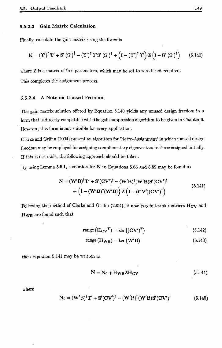
5.5. Output Feedback 149
5.5.2.3 Gain Matrix Calculation
Finally, calculate the gain matrix using the formula
K = (T') tT' + S' (0') t - (T') tT'S' (0') t + (I - (T') t T') Z (I - 0' (0') t) (5.140)
where Z is a matrix of free parameters, which may be set to zero if not required.
This completes the assignment process.
5.5.2.4 A Note on Unused Freedom
The gain matrix solution offered by Equation 5.140 yields any unused design freedom in a
form that is directly compatible with the gain suppression algorithm to be given in Chapter 6. . . However, this form is not suitable for every application.
Clarke and Griffin (2004) present an algorithm for 'Retro-Assignment' in which unused design
freedom may be employed for assigning complimentary eigenvectors to those assigned initially.
If this is desirable, the following approach should be taken.
By using Lemma 5.5.1, a solution for N to Equations 5.88 and 5.89 may be found as
N = (W'B)tT' + S'(CV')t - (W'B)t(W'B)S'(CV')t
+ (I - (W'B)t(W'B)) Z (I - (CV')(CV,)t) (5.141)
Following the method of Clarke and Griffin (2004), if now two full-rank matrices Hev and
H WB are found such that
range (lIevT) = ker ((CV')T)
range (HWB) = ker (W'B)
then Equation 5.141 may be written as
N = No + HWBZHev
where
No = (W'B)tT' + S'(CV')t - (W'B)t(W'B)S'(CV')t
(5.142)
(5.143)
(5.144)
(5.145)
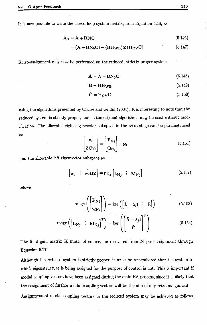
5.5. Output Feedback
It is now possible to write the closed-loop system matrix, from Equation 5.18, as
Acl = A+BNC
= (A + BNoC) + (BHwB) Z (HcvC)
Retro-assignment may now be performed on the reduced, strictly proper system
.A=A+BNoC
B=BHwB
C=HcvC
150
(5.146)
(5.147)
(5.148)
(5.149)
(5.150)
using the algorithms presented by Clarke and Griffin (2004). It is interesting to note that the
reduced system is strictly proper, and so the original algorithms may be used without mod
ification. The allowable right eigenvector subspace in the retro stage can be parameterised
as
(5.151)
and the allowable left eigenvector subspace as
(5.152)
where
(5.153)
range ([LNj (5.154)
The final gain matrix K must, of course, be recovered from N post-assignment t~rough
Equation 5.27.
Although the reduced system is strictly proper, it must be remembered that the system to
which eigenstructure is being assigned for the purpose of control is not. This is important if
modal coupling vectors have been assigned during the main EA process, since it is likely that
the assignment of further modal coupling vectors will be the aim of any retro-assignment.
Assignment of modal coupling vectors to the reduced system may be achieved as follows.
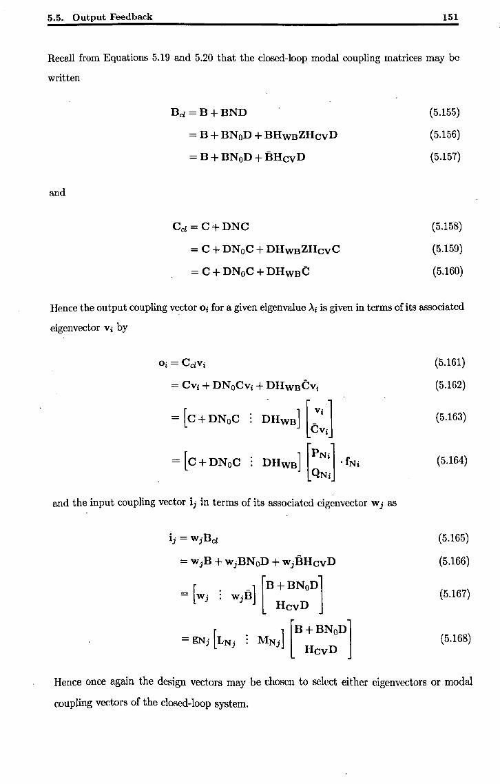
5.5. Output Feedback 151
Recall from Equations 5.19 and 5.20 that the closed-loop modal coupling matrices may be
written
and
Bel =B+BND
= B + BNoD + BHwBZHcvD
=B+BNoD+BHcvD
Cel = C+DNC
= C + DNoC + DHwBZHCVC
= C + DNoC + DHwBC
(5.155)
(5.156)
(5.157)
(5.158)
(5.159)
(5.160)
Hence the output coupling vector 0i for a given eigenvalue Ai is given in terms of its associated
eigenvector Vi by
= [C+DNoC
and the input coupling vector ij in terms of its associated eigenvector Wj as
_ [ . _] [B + BNOD] - W· : w·B
J J HcvD
[ ] [B+BNOD]
= gNj LNj : MNj HcvD
(5.161)
(5.162)
(5.163)
(5.164)
(5.165)
(5.166)
(5.167)
(5.168)
Hence once again the design vectors may be 'chosen to select either eigenvectors or modal
coupling vectors of the closed-loop system.
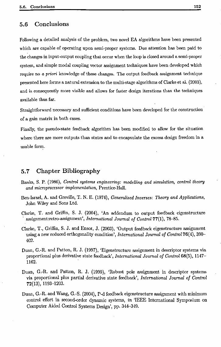
5.6. Conclusions 152
5.6 Conclusions
Following a detailed analysis of the problem, two novel EA algorithms have been presented
which are capable of operating upon semi-proper systems. Due attention has been paid to
the changes in input-output coupling that occur when the loop is closed around a semi-proper
system, and simple modal coupling vector assignment techniques have been developed which
require no a priori knowledge of these changes. The output feedback assignment technique
presented here forms a natural extension to the multi-stage algorithms of Clarke et al. (2003),
and is consequently more visible and allows for faster design iterations than the techniques
available thus far.
Straightforward necessary and sufficient conditions have been developed for the construction
of a gain matrix in both cases.
Finally, the pseudo-:state feedback algorithm has been modified to allow for the situation
where there are more outputs than states and to encapsulate the excess design freedom in a
usable form.
5.7 Chapter Bibliography
Banks, S. P. (1986), Control systems engineering: modelling and simulation, control theory and microprocessor implementation, Prentice-Hall.
Ben-Israel, A. and Greville, T. N. E. (1974), Generalised Inverses: Theory and Applications, John WHey and Sons Ltd.
Clarke, T. and Griffin, S. J. (2004), 'An addendum to output feedback eigenstructure . assignment:retro-assignment', International Journal of Control 77(1), 78-85.
Clarke, T., Griffin, S. J. and Ensor, J. (2003), 'Output feedback eigenstructure assignment using a new reduced orthogonality condition', International Journal of Control 76(4), 390-402.
Duan, G.-R. and Patton, R. J. (1997), 'Eigenstructure assignment in descriptor systems via proportional plus derivative state feedback', International Journal of Control 68(5), 1147-1162. .
Duan, G.-R. and Patton, R. J. (1999), 'Robust pole assignment in descriptor systems via proportional plus partial derivative state feedback', International Journal of Control 72(13), 1193-1203.
Duan, G.-R. and Wang, G.-S. (2004), P-d feedback eigenstructure assignment with minimum control effort in second-order dynamic systems, in 'IEEE International Symposium on Computer Aided Control Systems Design', pp. 344-349.
5.7. Chapter Bibliography 153
Fletcher, L. R. (1981a), 'On pole placement in linear multivariable systems with direct feedthrough. i. theoretical considerations', International Journal of Control 33(4), 739-749.
Fletcher, L. R. (1981 b), 'On pole placement in linear multi variable systems with direct feedthrough. ii. computational considerations', International Journal of Control 33(6), 1147-1154.
Griffin, S. J. (1997), Helicopter Control Law Design Using Eigenstructure Assignment, PhD thesis, University of York.
Le, V. X. (1992), 'Synthesis of proportional-plus-derivative feedbacks for descriptor systems', IEEE Transactions on Automatic Control 37(5), 672-675.
Miller, K. S. (1987), Some Eclectic Matrix Theory, R. E. Krieger Publishing.
Moore, B. C. (1976), 'On the flexibility offered by state feedback in multivariable systems beyond closed loop eigenvalue assignment', IEEE Transactions on Automatic Control 21, 689-692.
Owens, T. J. and Askarpour, S. (2000), 'Integrated approach to eigenstructure assignment in descriptor systems by pd and p state feedback', lEE Proceedings - Control Theory and Applications 147(4), 407-415.
Pomfret, A. J. and Clarke, T. (2003), Eigenstructure assignment for systems with acceleration feedback, in K. Burnham and O. Haas, eds, 'Proceedings of the 16th International Conference on Systems Engineering', Vol. 2, pp. 560-564.
Pomfret, A. J., Clarke, T. and Ensor, J. (2005), Eigcnstructure assignment for semi-proper systems: Pseudo-state feedback, in P. Horacek, M. Simandl and P. Zitek, eds, 'Proceedings of the 16th IFAC World Congress', Prague.
Skogestad, S. and Postlethwaite, I. (1996), Multivariable Feedback Control: Analysis and Design, John Wiley and Sons Ltd.
White, B. A. (1995), 'Eigenstructure assignment: a survey', Proceedings of the I Mech E Part I: Journal of Systems and Control Engineering 209(1), 1-11..
White, B. A. (1997), 'Robust polynomial eigenstructure assignment using dynamic feedback controllers', Proceedings of the I Mech E Part I: Journal of Systems and Control Engineering 211(1), 35-51.
Chapter 6
Imposition of Controller Structure
Contents 6.1 Introduction ............................... 154
6.2 Problem Definition ••..•••••.•..••.••••••••••• 156
6.2.1 Extension to Pseudo-State Feedback . . . . . . . . . . . . . . . . . . 156
6.3 Solution for Z and K ••••••••••••••••••••.••••. 157
6.4 Sensitivity of the Gain Matrix. • • • • • • • • • • • • • • • • • • •• 161
6.4.1 Minimum Frobenius Norm. . . . . . . . . . . . . . . . . . . . . . . . 162
6.4.2 Increase in Minimum Norm . . . . . . . . . . . . . . . . . . . . . . . 162
6.5 Alternative Structural Constraints • • • • • • • • • • • • • • • • •• 163
6.6 Design Example .. . . . . . . . . . . . . . . . . . . . . . . . . . .. 164
6.6.1 Example Assignment. . . . . . . . . . . . . . . . . . . . . . . . . . . 165
6.6.2 Choosing Gains. . . . . . . . . . . . . . . . . . . . . . . . . . . . . . 166
6.6.3 Gain Suppression. . . . . . . . . . . . . . . . . . . . . . . . . . . . . 167
6.6.3.1 Element (2,1) ......................... 167
6.6.3.2 Element (1,3). . . . . . . . . . . . . . . . . . . . . . . . . . 168
6.7 Conclusions and Further Work •••• , • • • • • • • • • • • • • •• 169
6.8 Chapter Bibliography • • • • • • • • • • • • • • • • • • . • • • • • •• 170
6.1 Introduction
The recent work of Clarke et al. (2003) detailed new algorithms for output-feedback eigen
structure assignment control for linear systems. The algorithms employ a multi-stage ap
proach, in which the available design freedom is reduced stepwise by the assignment of eigen
vectors and associated eigenvalues. Depending on the number of Degrees of Freedom (DoF)
available and the manner in which they are distributed between the design stages, it is possi
ble that some may remain unused after the assignment is complete. In other published work,
154
6.1. Introduction 155
Clarke and Griffin (2004) introduce an algorithm (the 'retro-assignment stage') that makes
use of this post-assignment freedom to assign complementary eigenvectors to those assigned
using the original algorithm.
It is likely, however, that further eigenvector assignment is not the most appropriate use for
this design freedom. Typically, only a few right eigenvectors (corresponding to dominant
modes) are crucial to the system specification, but the formation of the general nonlinear
eigenstructure assignment problem into a problem with a linear solution requires that one
eigenvector is assigned for every eigenvalue. The control of modal coupling is therefore likely
to have been satisfied by the primary assignment algorithm and the design freedom could,
instead, be employed to achieve some other objective.
One such objective is a defined controller structure. Eigenstructure Assignment (EA), in com
mon with most multi-input multi-output control system design techniques, will in general gen
erate a fully-populated matrix of feedback gains. The resulting ~omplex, fully-interconnected
controller bears little resemblance to the sparse, modular control systems achieved using clas
sical approaches. In order to impose structure upon a controller, it is necessary to reduce a
subset of the gains to zero, thereby reducing the complexity of the connections from plant
outputs to plant inputs. This chapter presents a novel method by which, after eigenstructure
assignment is completed, any remaining design freedom may be used for this purpose. It has
previously appeared in published work (Pomfret and Clarke, 2005).
To the author's knowledge, no similar method has been'developed before, although Sobel
and Shapiro (1986) use a similar mathematical approach to the problem of assigning eigen
structure to a system with structured gains. However, their method constitutes part of the
assignment process itself, and also potentially changes the assigned locations of poles.
Griffin (1997) develops a method whereby, using an iterative approach, gain matrix entries
may be suppressed without affecting the closed-loop eigenvalues. The eigenvectors are subject
to change, however, since his technique does not employ any design freedom in its operation.
Ensor (2000) presents an algorithm which does not attempt to constrain either the eigenvalues
or eigenvectors, but rather allows the effects of gain suppression on the eigenstructure to be
seen clearly.
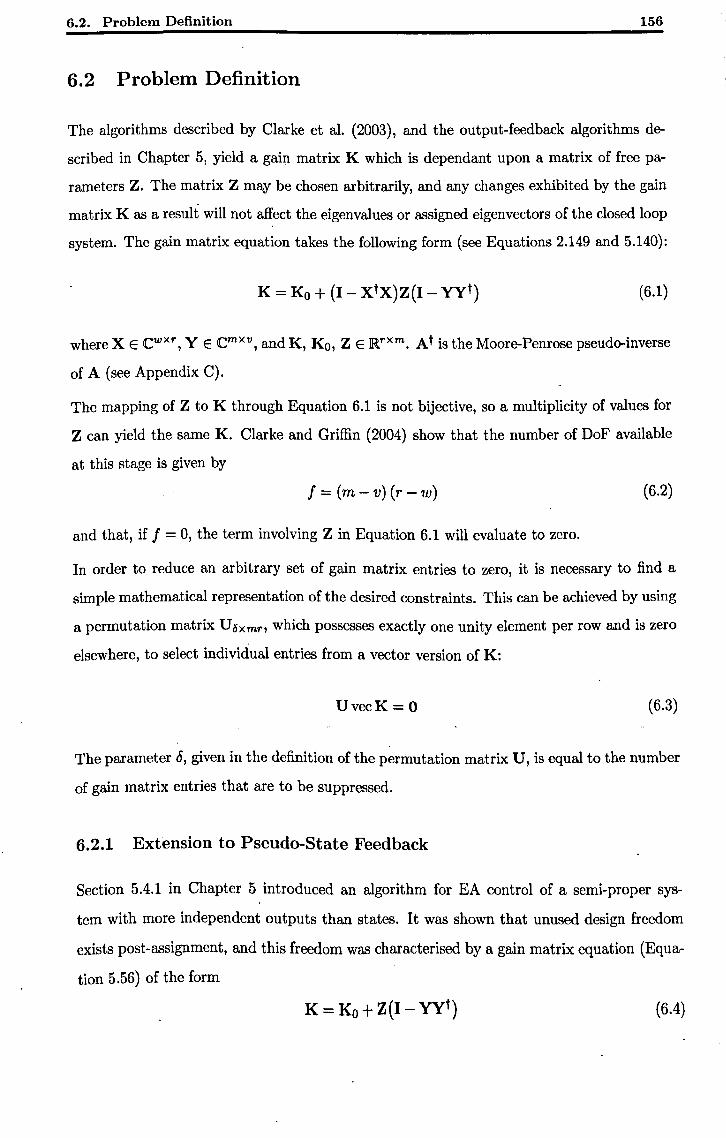
6.2. Problem Definition 156
6.2 Problem Definition
The algorithms described by Clarke et al. (2003), and the output-feedback algorithms de
scribed in Chapter 5, yield a gain matrix K which is dependant upon a matrix of free pa
rameters Z. The matrix Z may be chosen arbitrarily, and any changes exhibited by the gain
matrix K as a result will not affect the eigenvalues or assigned eigenvectors of the closed loop
system. The gain matrix equation takes the following form (see Equations 2.149 and 5.140):
K = Ko + (I - XtX)Z(I - yyt) (6.1)
where X E cwxr , YE Cmxv , and K, Ko, Z E ]Rrxm. At is the Moore-Penrose pseudo-inverse
of A (see Appendix C).
The mapping of Z to K through Equation 6.1 is not bijective, so a multiplicity of values for
Z can yield the same K. Clarke and Griffin (2004) show that the number of DoF available
at this stage is given by
f=(m-v)(r-w) (6.2)
and that, if f = 0, the term involving Z in Equation 6.1 will evaluate to zero.
In order to reduce an arbitrary set of gain matrix entries to zero, it is necessary to find a
simple mathematical representation of the desired constraints. This can be achieved by using
a permutation matrix U5xmn which possesses exactly one unity element per row and is zero
elsewhere, to select individual entries from a vector version of K:
UvecK = 0 (6.3)
The parameter 8, given in the definition of the permutation matrix U, is equal to the number
of gain matrix entries that are to be suppressed.
6.2.1 Extension to Pseudo-State Feedback
Section 5.4.1 in Chapter 5 introduced an algorithm for EA control of a semi-proper sys
tem with more independent outputs than states. It was shown that unused design freedom
exists post-assignment, and this freedom was characterised by a gain matrix equation (Equa
tion 5.56) of the form
(6.4)
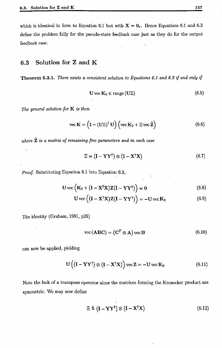
6.3. Solution for Z and K 157
which is identical in form to Equation 6.1 but with X = Or. Hence Equations 6.1 and 6.3
define the problem fully for the pseudo-state feedback case just as they do for the output
feedback case.
6.3 Solution for Z and K
Theorem 6.3.1. There exists a consistent solution to Equations 6.1 and 6.3 if and only if
U vec Ko E range (US)
The general solution for K is then
vecK = (I - (US)t U) (vecKo + Svecz)
where Z is a matrix of remaining free parameters and in each case
3 = (I - yyt) ® (I - xtX)
Proof. Substituting Equation 6.1 into Equation 6.3,
Uvec (Ko + (I - XtX)Z(1 - yyt)) = 0
Uvec ((I - XtX)Z(1 - yyt)) = -UvecKo
The identity (Graham,1981, p25)
vec (ABC) = (CT ® A) vecB
can now be applied, yielding
U ( (I - yyt) ® (I - xtX) ) vec Z = - U vec Ko
(6.5)
(6.6)
(6.7)
(6.8)
(6.9)
(6.10)
(6.11)
Note the lack of a transpose operator since the matrices forming the Kronecker product are
symmetric. We may now define
(6.12)
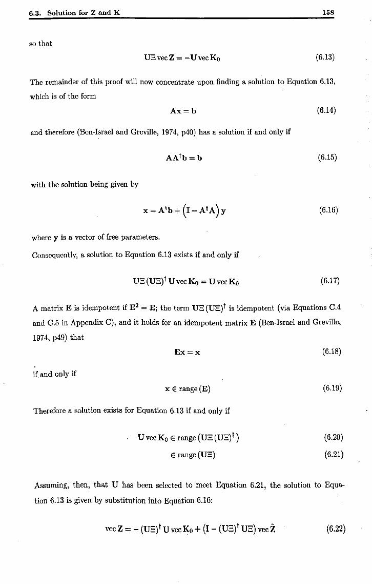
6.3. Solution for Z and K 158
so that
USvecZ = -UvecKo (6.13)
The remainder of this proof will now concentrate upon finding a solution to Equation 6.13,
which is of the form
Ax=b (6.14)
and therefore (Ben-Israel and Greville, 1974, p40) has a solution if and only if
(6.15)
with the solution being given by
(6.16)
where y is a vector of free parameters.
Consequently, a solution to Equation 6.13 exists if and only if
US(US)tUvecKo = UvecKo (6.17)
A matrix E is idempotent if E2 = Ej the term US (US)t is idempotent (via Equations C.4
and C.5 in Appendix C), and it holds for an idempotent matrix E (Ben-Israel and Greville,
1974, p49) that
Ex=x
if and only if
x E range (E)
Therefore a solution exists for Equation 6.13 if and only if
U vec Ko E range (US (US) t )
E range (US)
(6.18)
(6.19)
(6.20)
(6.21)
Assuming, then, that U has been selected to meet Equation 6.21, the solution to Equa
tion 6.13 is given by substitution into Equation 6.16:
vec Z = - (US)t Uvec~o + (I - (US)t US) vec Z (6.22)
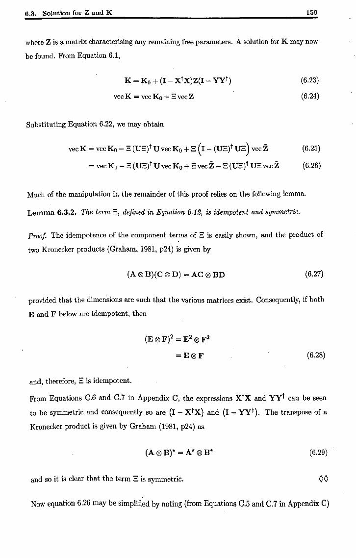
6.3. Solution for Z and K 159
where Z is a matrix characterising any remaining free parameters. A solution for K may now
be found. From Equation 6.1,
K = Ko + (I - XtX)Z(1 - yyt)
vecK = vecKo + SvecZ
Substituting Equation 6.22, we may obtain
(6.23)
(6.24)
vecK = vecKo - S (US)t UvecKo + S (I - (US)t US) vec Z (6.25)
= vecKo - S (US)t U vec Ko + SvecZ - S (US)t USvecZ (6.26)
Much of the manipulation in the remainder of this proof relies on the following lemma.
Lemma 6.3.2. The term S, defined in Equation 6.12, is idempotent and symmetric.
Proof. The idempotence of the component terms of S is easily shown, and the product of
two Kronecker products (Graham, 1981, p24) is given by
(A®B)(C0D) =AC®BD (6.27)
provided that the dimensions are such that the various matrices exist. Consequently, if both
E and F below are idempotent, then
and, therefore, S is idem potent.
(E 0 F)2 = E2 0 F2
=E0F (6.28)
From Equations C.6 and C.7 in Appendix C, the expressions xtx and yyt can be seen
to be symmetric and consequently so are (I - xtX) and (I - yyt). The transpose of a
Kronecker product is given by Graham (1981, p24) as
(A ® B)* = A * 0 B* (6.29)
and so it is clear that the term S is symmetric. 00
Now equation 6.26 may be simplified by noting (from Equations C.5 and C.7 in Appendix C)
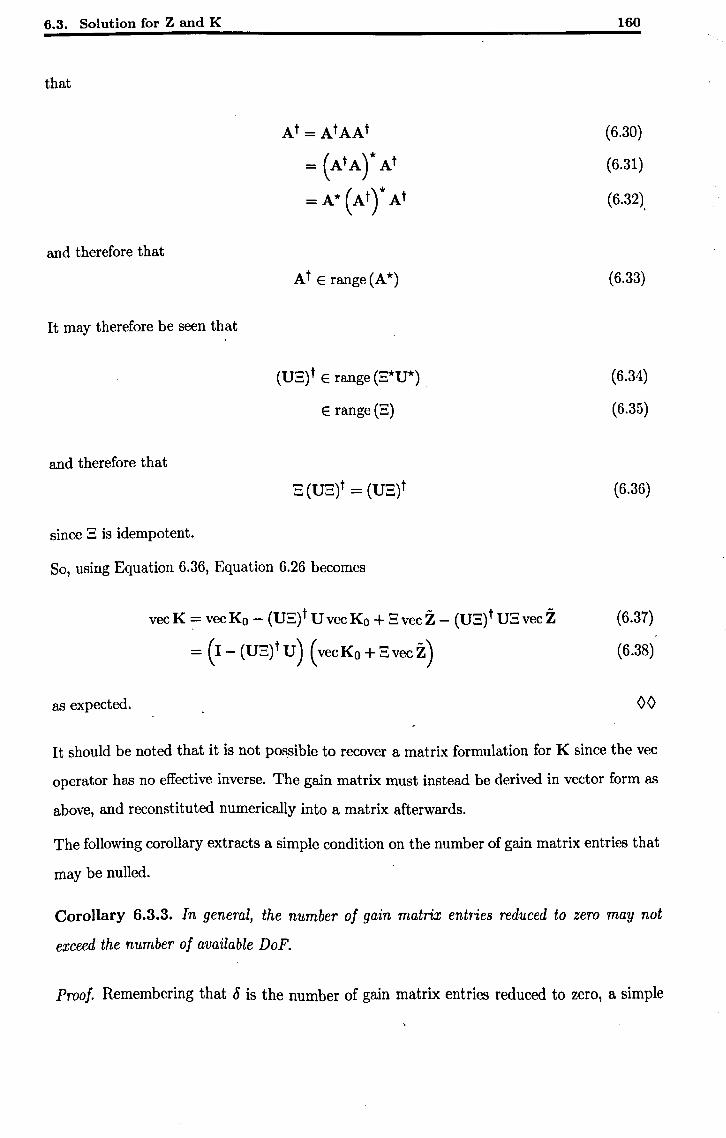
6.3. Solution for Z and K
that
and therefore that
It may therefore be seen that
and therefore that
since S is idempotent.
At = AtAAt
= (AtAr At
= A* (Atr At
At E range (A*)
(US) t E range (S*U*)
E range (S)
3 (U3)t = (U3)t
So, using Equation 6.36, Equation 6.26 becomes
as expected.
vec K = vec Ko - (US) t U vec Ko + S vec Z - (US) t US vec Z
= (I - (US) tU) (vec Ko + S vec z)
160
(6.30)
(6.31)
(6.32),
(6.33)
(6.34)
(6.35)
(6.36)
(6.37)
(6.38)
00
It should be noted that it is not possible to recover a matrix formulation for K since the vec
operator has no effective inverse. The gain matrix must instead be derived in vector form as
above, and reconstituted numerically into a matrix afterwards.
The following corollary extracts a simple condition on the number of gain matrix entries that
may be nulled.
Corollary 6.3.3. In general, the number of gain matrix entries reduced to zero may not
exceed the number of available DoF.
Proof. Remembering that 8 is the number of gain matrix entries reduced to zero, a simple
6.4. Sensitivity of the Gain Matrix 161
sufficient condition for the satisfaction of Equation 6.21 is easily seen to be
rank (U3) = 8 (6.39)
This condition, although not strictly necessary, is necessary for general Ko and S since
otherwise there is nO guarantee of the existence of a U which satisfies Equation 6.21.
A necessary (but not sufficient) condition for the fulfillment of Equation 6.39 is that
8:5 rank (3)
:5 rank ( (I - yyt) ® (I - XtX) )
:5 rank (I - yyt) . rank (I - XtX)
~ (m - rank (yyt)) (r - rank (xtX))
:5 (m-v)(r-w)
Comparison with Equation 6.2 shows that Equation 6.44 may be written as
8:5/
(6.40)
(6.41)
(6.42)
(6.43)
(6.44)
(6.45)
00
Corollary 6.3.3 demonstrates that, for general Ko and 3, the number of gain matrix entries to
be reduced to zero may not exceed the number of available degrees of freedom. Note that the
satisfaction of Equation 6.45 is not sufficient for the existence of a solution to Equation 6.13,
and that the satisfaction of Equation 6.21 is still required.
6.4 Sensitivity of the Gain Matrix
The Frobenius norm IKIF of K is the square root of the sum of squared gain matrix entries.
There exists a value of Z for which IKIF is minimal. It is safe to assume that the value of Z
found via Equation 6.6 will not equal this 'optimal' value. Therefore, nulling individual gain
matrix entries will, in general, raise IKIF'
This is important because large gain matrix entries will re.sult in proportionally greater inputs
being applied to the system by the controller. These could be in response to deviations of the
system from a required datum, leading to greater control effort; or they could be in response
6.4. Sensitivity of the Gain Matrix 162
to noise on the system outputs, resulting in poor noise rejection.
The extent to which IKIF is affected will depend upon the elements of the gain matrix selected
by the permutation matrix U. A mechanism for determining the increase in IKIF would be
a useful tool when attempting to determine which elements should be set to zero.
Since the formulation for K in Equation 6.6 contains a free parameter matrix, it is useful to
find the value of the free parameter matrix that minimises the Frobenius norm of the final
gain matrix.
6.4.1 Minimum Frobenius Norm
From the examination of the properties of B in Lemma 6.3.2, we may now determine the
value of Z that leads to the minimum IKIF. This is a complex procedure; and details may
therefore be found in Appendix B. It is shown there that the appropriate value of Z is
z=o (6.46)
Therefore, following the suppression of a subset of the allowable gains, the gain matrix with
the minimum Frobenius norm is found by setting the matrix of remaining free parameters to
zero.
6.4.2 Increase in Minimum Norm
The minimum IKIF may now be simply calculated by substituting into Equation 6.6:
min IKIF = min IIvecKII ~ 11 (I - (V~)t v) (vecKo + BvecZ) 11
= 11 (I - (VB)t v) vecKol1
(6.47)
(6.48)
The minimum IKIF achievable prior to nulling any gain matrix entries may be found by
setting V = 0:
min \K\F = min IIvecKII = IIvecKol\ = \KO\F (6.49)
Comparison of Equations 6.48 and 6.49 shows the effect of nulling a subset of the gains. This
information can be used to determine which gains may most easily be reduced to zero whilst
maintaining the lowest possible gains elsewhere.
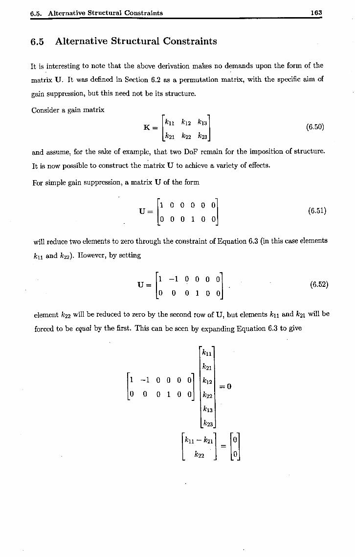
6.5. Alternative Structural Constraints 163
6.5 Alternative Structural Constraints
It is interesting to note that the above derivation makes no demands upon the form of the . .
matrix V. It was defined in Section 6.2 as a permutation matrix, with the specific aim of
gain suppression, but this need not be its structure.
Consider a gain matrix
(6.50)
and assume, for the sake of example, that two DoF remain for the imposition of structure.
It is now possible to construct the matrix V to achieve a variety of effects.
For simple gain suppression, a matrix V of the form
V=[1 0000001 o 0 0 1 0 Ij
(6.51)
will reduce two elements to zero through the constraint of Equation 6.3 (in this case elements
kll and k22 ). However, by setting
V = [1 -1 0 0 0 0] o 0 0 1 0 0
(6.52)
element k22 will be reduced to zero by the second row of V, but elements kll and k21 will be
forced to be equal by the first. This can be seen by expanding Equation 6.3 to give
kn
k21
[~ -1 0 0 0 ~] k12 =0
0 0 1 0 k22
k13
k23
[kl1 - k21] k22 [~]
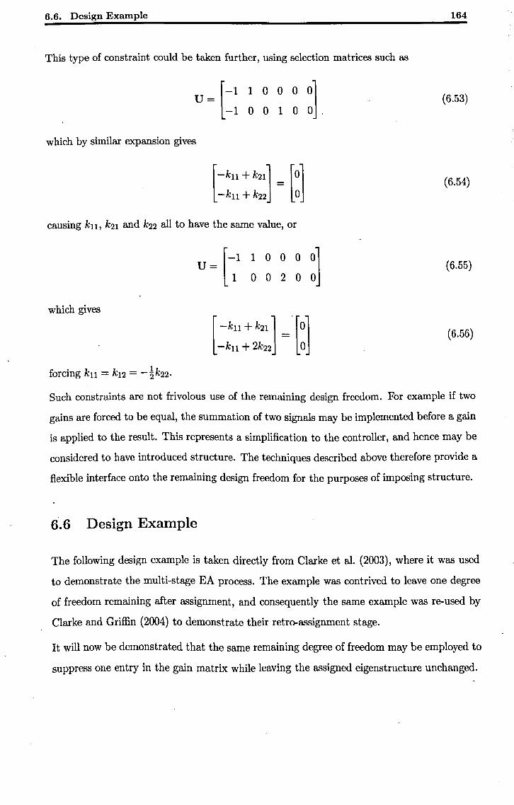
6.6. Design Example
This type of constraint could be taken further, using selection matrices such as
u = [-1 1 0 0 0 0] -1 0 0 1 0 0 ,
which by similar expansion gives
[- kll + k21] = [0] -kll + k22 0
causing kll' k21 and k22 all to have the same value, or
[-1 1 0 0 0
:] u= 1 0 0 2 0
which gives
[ -kn H2t ]
[:] --kll + 2k22
forcing kll = k12 = -!k22.
164
(6.53)
(6.54)
(6.55)
(6.56)
Such constraints are not frivolous use of the remaining design freedom. For example if two
gains are forced to be equal, the summation of two signals may be implemented before a gain
is applied to the result. This represents a simplification to the controller, and hence may be
considered to have introduced structure. The techniques described above therefore provide a
flexible interface onto the remaining design freedom for the purposes of imposing structure.
6.6 Design Example
The following design example is taken directly from Clarke et al. (2003), where it was used
to demonstrate the multi-stage EA process. The example was contrived to leave one degree
of freedom remaining after assignment, and consequently the same example was re-used by
Clarke and Griffin (2004) to demonstrate their retr~assignment stage.
It will now be demonstrated that the same remaining degree of freedom may be employed to
suppress one entry in the gain matrix while leaving the assigned eigenstructure unchanged.
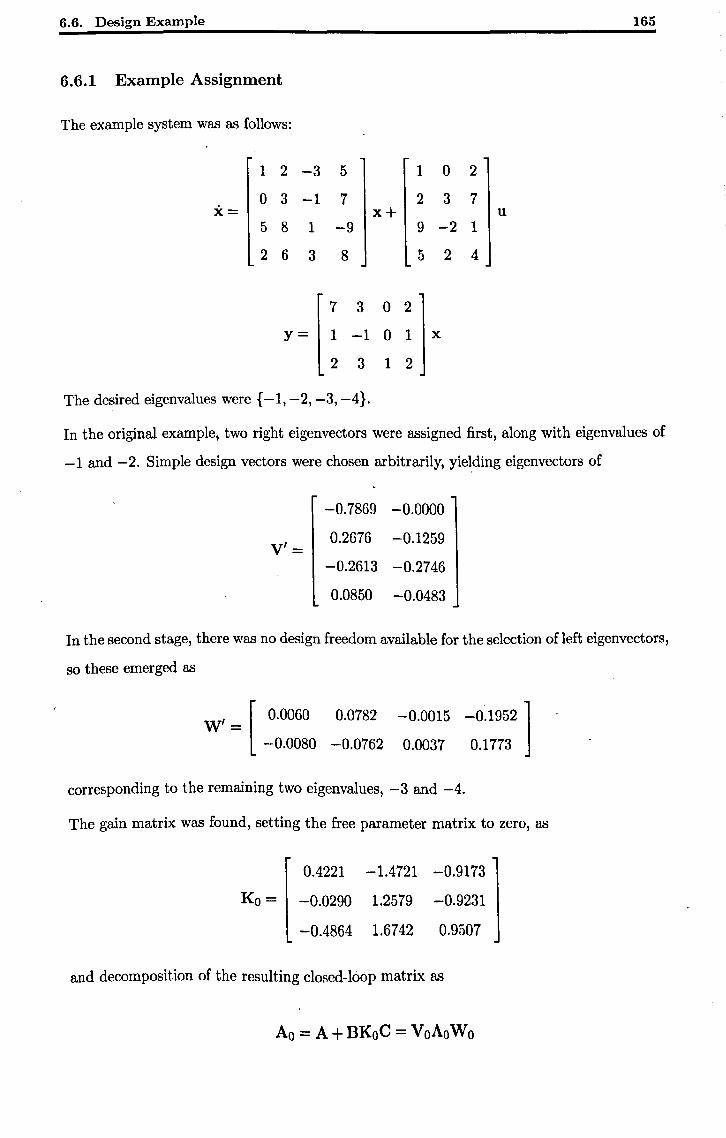
6.6. Design Example
6.6.1 Example Assignment
The example system was as follows:
1 2 -3 5 1 0
0 3 -1 7 2 3 X= x+
5 8 1 -9 9 -2
2 6 3 8 5
7 3 0 2
Y = 1 -1 0 1 x
2 3 1 2
The desired eigenvalues were {-1, -2, -3, -4}.
2
165
2
7 u
1
4
In the original example, two right eigenvectors were assigned first, along with eigenvalues of
-1 and -2. Simple design vectors were chosen arbitrarily, yielding eigenvectors of
V'=
-0.7869 -0.0000
0.2676 -0.1259
-0.2613 -0.2746
0.0850 -0.0483
In the second stage, there was no design freedom available for the selection of left eigenvectors,
so these emerged as
, [0.0060 W= -0.0080
0.0782
-0.0762
-0.0015 -0.1952]
0.0037 0.1773
corresponding to the remaining two eigenvalues, -3 and -4.
The gain matrix was found, setting the free parameter matrix to zero, as
0.4221 -1.4721 -0.9173
Ko = -0.0290 1.2579 -0.9231
-0.4864 1.6742 0.9507
and decomposition of the resulting closed-loop matrix as
Ao = A+BKoC = VoAoWo
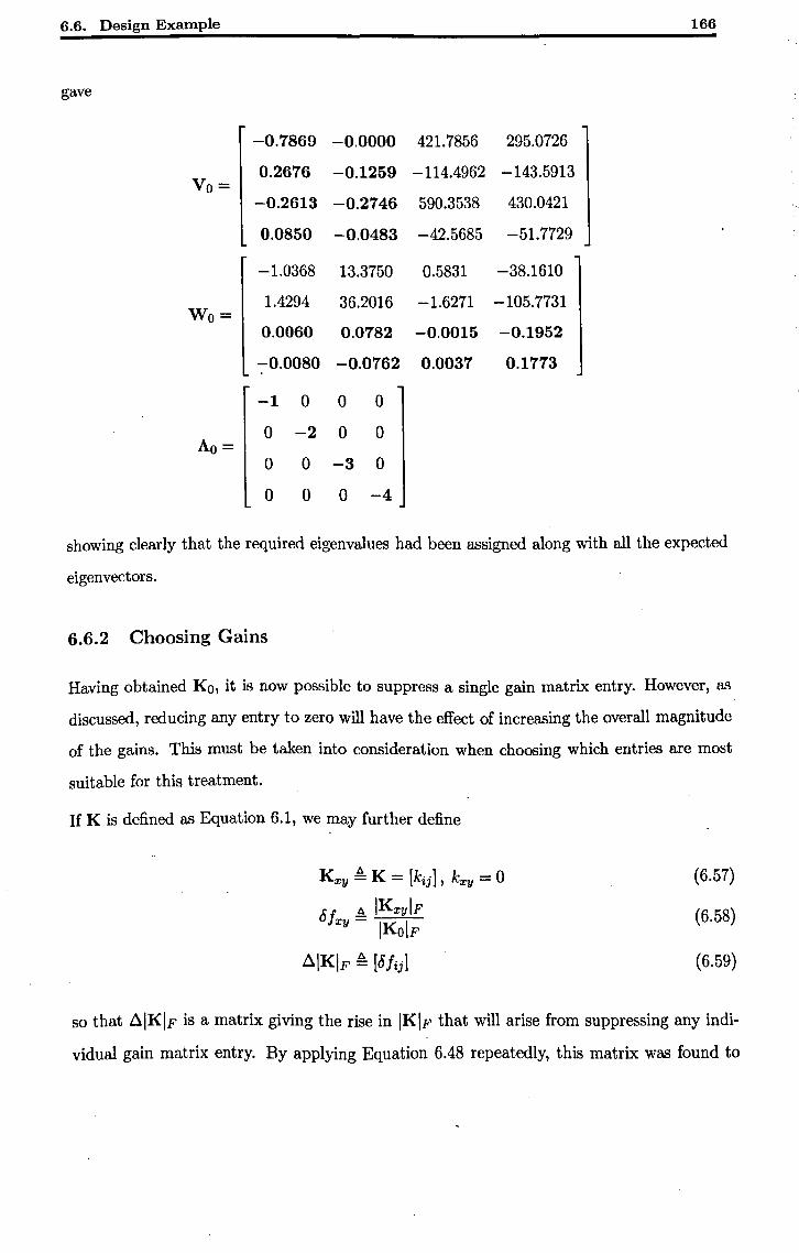
6.6. Design Example 166
gave
-0.7869 -0.0000 421.7856 295.0726
0.2676 -0.1259 -114.4962 -143.5913 Vo=
-0.2613 -0.2746 590.3538 430.0421
0.0850 -0.0483 -42.5685 -51.7729
-1.0368 13.3750 0.5831 -38.1610
1.4294 Wo=
36.2016 -1.6271 -105.7731
0.0060 0.0782 -0.0015 -0.1952
-0.0080 -0.0762 0.0037 0.1773
-1 0 0 0
0 -2 0 0 Ao=
0 0 -3 0
0 0 0 -4
showing clearly that the required eigenvalues had been assigned along with all the expected
eigenvectors.
6.6.2 Choosing Gains
Having obtained Ko, it is now possible to suppress a single gain matrix entry. However, as
discussed, reducing any entry to zero will have the effect of increasing the overall magnitude
of the gains. This must be taken into consideration when choosing which entries are most
suitable for this treatment.
If K is defined as Equation 6.1, we may further define
Kxy ~ K = [kij ] , kxy = 0
8f A IKxylF xy - IKolF
~IKIF A [8/ij]
(6.57)
(6.58)
(6.59)
so that ~IKIF is a matrix giving the rise in IKIF that will arise from suppressing any indi
vidual gain matrix entry. By applying Equation 6.48 repeatedly, this matrix was found to
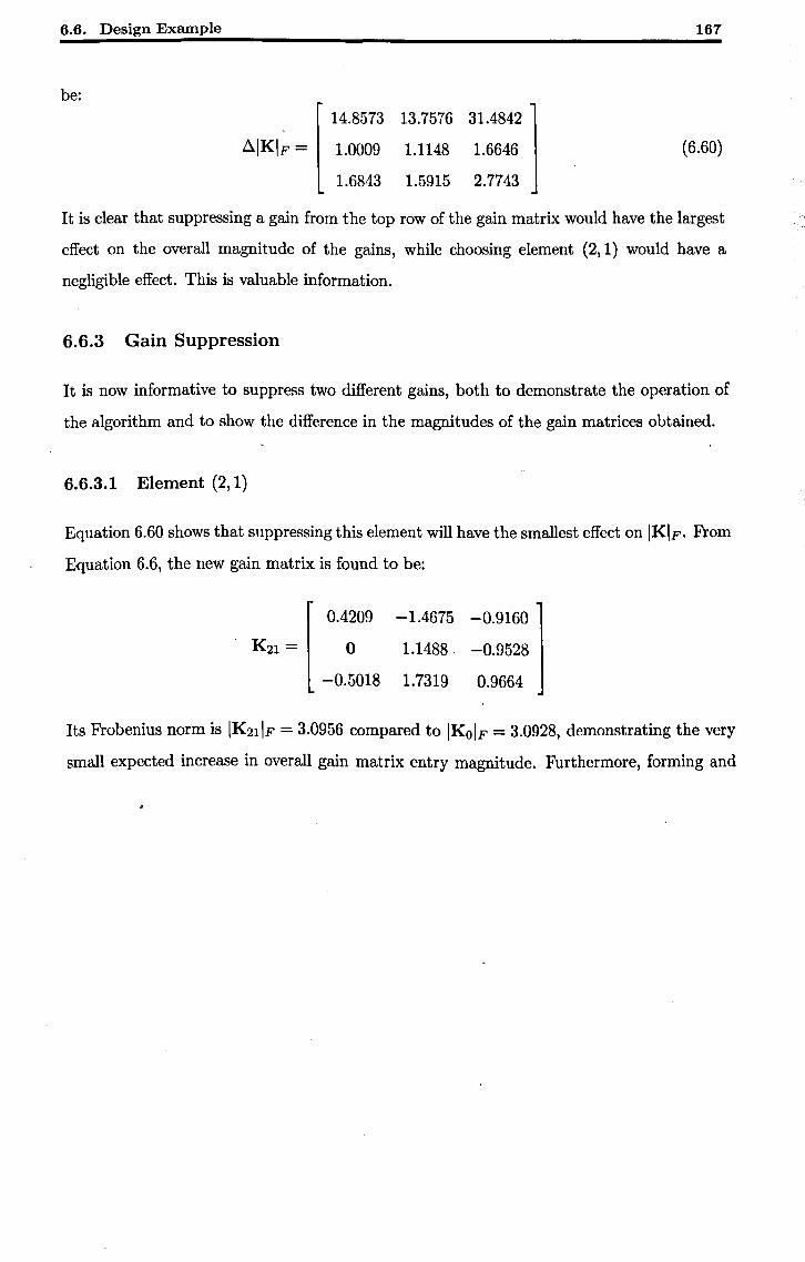
6.6. Design Example
be: 14.8573 13.7576 31.4842
~\K\F = 1.0009 1.1148 1.6646
1.6843 1.5915 2.7743
161
(6.60)
It is clear that suppressing a gain from the top row of the gain matrix would have the largest
effect on the overall magnitude of the gains, while choosing element (2,1) would have a
negligible effect. This is valuable information.
6.6.3 Gain Suppression
It is now informative to suppress two different gains, both to demonstrate the operation of
the algorithm and to show the difference in the magnitudes of the gain matrices obtained.
6.6.3.1 Element (2,1)
Equation 6.60 shows that suppressing this element will have the smallest effect on \K\F' From
Equation 6.6, the new gain matrix is found to be:
0.4209 -1.4675 -0.9160
o -0.5018
1.1488. -0.9528
1.7319 0.9664
Its Frobenius norm is \K21\F = 3.0956 compared to \KO\F = 3.0928, demonstrating the very
small expected increase in overall gain matrix entry magnitude. Furthermore, forming and
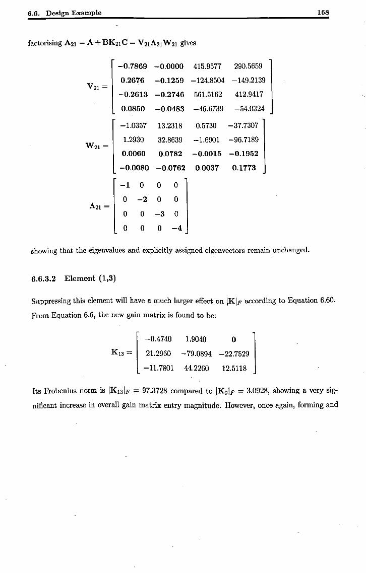
6.6. Design Example 168
factorising A21 = A + BK21 C = V 21A21 W 21 gives
-0.7869 -0.0000 415.9577 290.5659
0.2676 V21 =
-0.1259 -124.8504 -149.2139
-0.2613 -0.2746 561.5162 412.9417
0.0850 -0.0483 -46.6739 -54.0324
-1.0357 13.2318 0.5730 -37.7307
1.2930 W21 =
32.8639 -1.6901 -96.7189
0.0060 0.0782 -0.0015 -0.1952
-0.0080 -0.0762 0.0037 0.1773
-1 0 0 0
0 -2 0 0 A21 =
0 0 -3 0
0 0 0 -4
showing that the eigenvalues and explicitly assigned eigenvectors remain unchanged.
6.6.3.2 Element (1,3)
Suppressing this element will have a much larger effect on IKIF according to Equation 6.60.
From Equation 6.6, the new gain matrix is found to be:
-0.4740 1.9040 o K 13 = 21.2960 -79.0894 -22.7529
-11.7801 44.2260 12.5118
Its Frobenius norm is IK131F = 97.3728 compared to IKolF = 3.0928, showing a very sig
nificant increase in overall gain matrix entry magnitude. However, once again, forming and
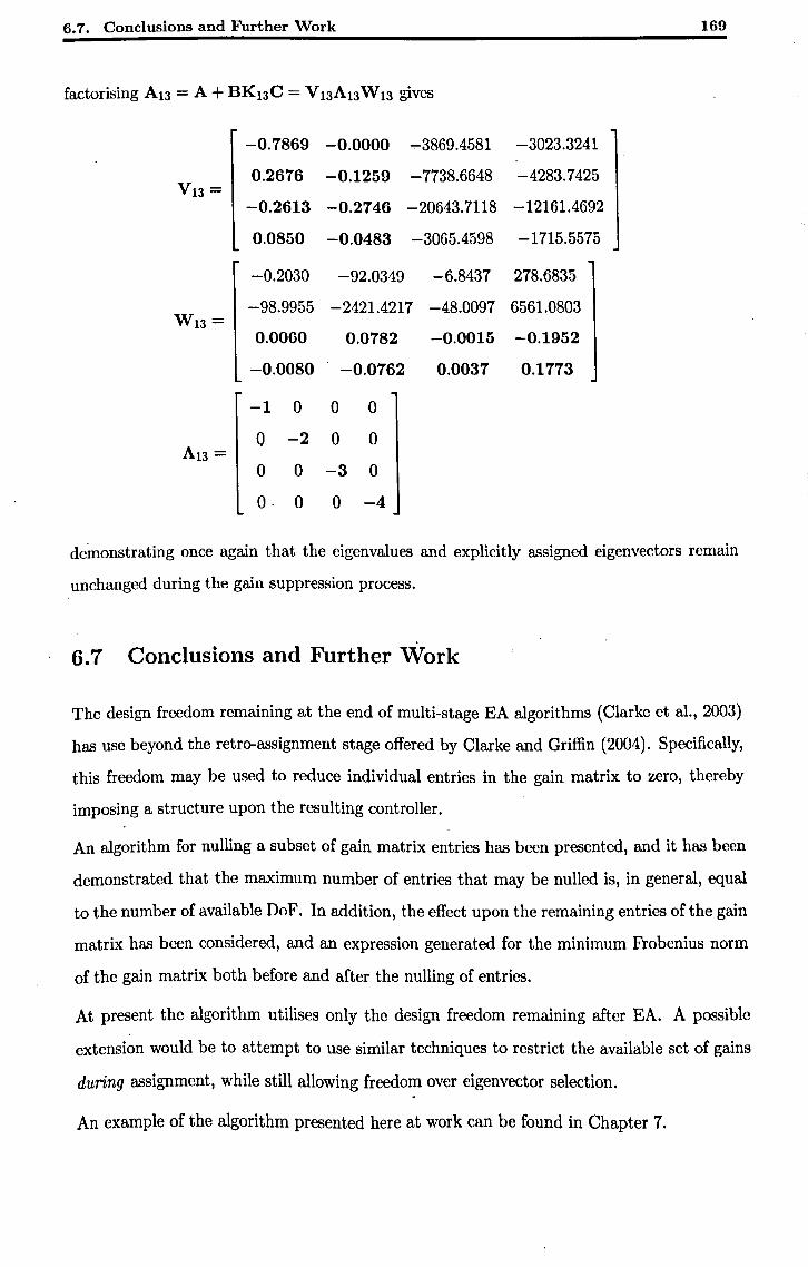
6.7. Conclusions and Further Work 169
-0.7869 -0.0000 ..,..3869.4581 -3023.3241
0.2676 -0.1259 V13 =
-7738.6648 -4283.7425
-0.2613 -0.2746 -20643.7118 -12161.4692
0.0850 -0.0483 -3065.4598 -1715.5575
-0.2030 -92.0349 -6.8437 278.6835
-98.9955 -2421.4217 -48.0097 6561.0803 W13=
0.0060 0.0782 -0.0015 -0.1952
-0.0080 -0.0762 0.0037 0.1773
-1 0 0 0
0 -2 0 0 A13 =
0 0 -3 0
O· 0 0 -4
demonstrating once again that the eigenvalues and explicitly assigned eigenvectors remain
unchanged during the gain suppression process.
6.7 Conclusions and Further Work
The design freedom remaining at the end of multi-stage EA algorithms (Clarke et al., 2003)
has use beyond the retro-assignment stage offered by Clarke and Griffin (2004). Specifically,
this freedom may be used to reduce individual entries in the gain matrix to zero, thereby
imposing a structure upon the resulting controller.
An algorithm for nulling a subset of gain matrix entries has been presented, and it has been
demonstrated that the maximum number of entries that may be nulled is, in general, equal
to the number of available DoF. In addition, the effect upon the remaining entries of the gain
matrix has been considered, and an expression generated for the minimum Frobenius norm
of the gain matrix both before and after the nulling of entries.
At present the algorithm utilises only the design freedom remaining after EA. A possible
extension would be to attempt to use similar techniques to restrict the available set of gains
during assignment, while still allowing freedom over eigenvector selection.
An example of the algorithm presented here at work can be found in Chapter 7.
Chapter Bibliography 170
6.8 Chapter Bibliography
Ben-Israel, A. and Greville, T. N. E. (1974), Generalised Inverses: Theory and Applications, John WHey and Sons Ltd.
Clarke, T. and Griffin, S. J. (2004), 'An addendum to output feedback eigenstructure assignment:retro-assignment', International Journal of Control 77(1), 78-85.
Clarke, T., Griffin, S. J. and Ensor, J. (2003), 'Output feedback eigenstructure assignment using a new reduced orthogonality condition', International Journal of Control 76(4), 390-402.
Ensor, J. E. (2000), Subspace Methods for Eigenstructure Assignment, PhD thesis, University of York.
Graham, A. (1981), Kronecker Products and Matrix Calculus With Applications, Ellis Horwood.
Griffin, S. J. (1997), Helicopter Control Law Design Using Eigenstructure Assignment, PhD thesis, University of York.
Pomfret, A. J. and Clarke, T. (2005), Using post-eigenstructure assignment design freedom for the imposition of controller structure, in P. Horacek, M. Simandl and P. Zitek, eds, 'Proceedings of the 16th IFAC World Congress', Prague.
Sobel, K. and Shapiro, E. (1986), Design of dynamic compensators via eigenstructure assignment with flight control applications, in 'Proceedings of the National Aerospace and Electronics Conference (NAECON)', Vol. 2, Day ton , OH, pp. 408-414.
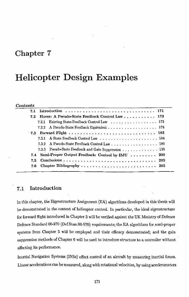
Chapter 7
Helicopter Design Examples
Contents 7.1 Introduction ............................... 171
7.2 Hover: A Pseudo-State Feedback Control Law • • • • • • • . • •• 173
7.2.1 Existing State-Feedback Control Law ................. 173
7.2.2 A Pseudo-State Feedback Equivalent. . . . . . . . . . . . . . . . . . 178
7.3 Forward Flight . . . . . . . . . . . . . . . . . . . . . . . . . . . . .. 183 7.3.1 A State Feedback Control Law ..................... 184
7.3.2 A Pseudo-State Feedback Control Law ................. 189
7.3.3 Pseudo-State Feedback and Gain Suppression ............. 195
7.4 Semi-Proper Output Feedback: Control by IMU ••••••••• 200
7.5 Conclusions................................ 205 7.6 Chapter Bibliography ••••• '.' • • • • • • . • • • • • • • • . • •• 205
7.1 Introduction
In this chapter, the Eigenstructure Assignment (EA) algorithms developed in this thesis will
be demonstrated in the context of helicopter control. In particular, the ideal eigenstructure
for forward flight introduced in Chapter 3 will be verified against the UK Ministry of Defence
Defence Standard 00-970 (Def.Stan.00-970) requirements; the EA algorithms for semi-proper
systems from Chapter 5 will be employed and their efficacy demonstrated; and the gain
suppression methods of Chapter 6 will be used to introduce structure to a controller without
affecting its performance.
Inertial Navigation Systems (INSs) effect control of an aircraft by measuring inertial forces.
Linear accelerations can be measured, along with rotational velocities, by using accelerometers
171
7.1. Introduction 172
and gyroscopes. Inertial navigation technology is mature (Lawrence, 1998; Siouris, 1993;
Titterton and Weston, 1997) having been employed as early as 1944 in the German V-2
guided rocket programme.
An INS has at its heart an Inertial Measurement Unit (IMU), responsible for the measurement
of acceleration and angular rate. Modern IMUs are of the 'strapdown' variety, wherein th~
accelerometers and gyroscopes are rigidly attached to the airframe. The resolution of the
body-relative measurements into fixed-frame readings, and the integration of the resulting
acceleration readings to generate velocity and position estimates, is performed electronically.
Using highly accurate laser-ring gyroscopes, even following the double-integration required
to estimate position, the accuracy of modern INSs can be better than 0.6 nautical miles per
hour (Titterton and Weston, 1997).
In this chapter, depending upon the aim of each design example, various of the quantities
available from the IMU will be deemed measurable. In some of the examples, it will also be
assumed that earth-relative vertical velocity can also be measured. Typically this would be
achieved using a radar altimeter (Cundy and Brown, 1997).
This chapter begins by replicating the state-feedback results of Griffin (1997) for a Lynx
helicopter in the hover. It will then be demonstrated that the same performance is achievable
using a controller which does not have access directly to state information, but instead has
access to a combination of states and state derivatives, by using the methods derived in
Chapter 5.
Forward flight is considered next, with a state-feedback example again employed to provide
a benchmark against ~hich other controllers can be compared, and to demonstrate the ideal
eigenstructure of Chapter 3. A pseudo-state feedback 'example is considered and its perfor
mance verified. A controller using' all available IMU signals and a radar altimeter is then
derived and it is shown that the excess design freedom remaining after assignment may be
employed to build a structured controller with the same performance again.
Finally, as a pedagogical exercise, control of the helicopter in hover using only the direct
inertial measurements (accelerations and angular rates) is performed. This is to demonstrate
the operation of the output-feedback algorithms from Chapter 5 and to highlight the perfor
mance problems suffered by output-feedback systems compared to their state-feedback (or
pseudo-state feedback) counterparts.
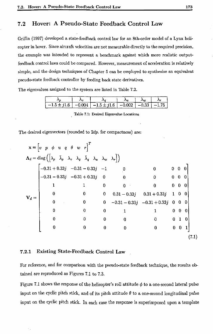
7.2. Hover: A Pseudo-State Feedback Control Law 173
7.2 Hover: A Pseudo-State Feedback Control Law
Griffin (1997) developed a state-feedback control law for an 8th-order model of a Lynx heli
copter in hover. Since aircraft velocities are not measurable directly to the required precision,
the example was intended to represent a benchmark against which more realistic output
feedback control laws could be compared. However, measurement of acceleration is relatively
simple, and the design techniques of Chapter 5 can be employed to synthesise an equivalent
pseudo-state feedback controller by feeding back state derivatives.
The eigenvalues assigned to the system are listed in Table 7.2.
Ap Av Aq Au Aw Ar -1.5 ± j1.6 -0.004 -1.5 ± j1.6 -0.002 -0.33 -1.75
Table 7.1: Desired Eigenvalue Locations
The desired eigenvectors (rounded to 2dp. for compactness) are:
x= [v p rjJ u q () w r]T
Ad = diag ([Ap ),p Av Aq ),q Au Aw Ar])
-0.31 + 0.33j -0.31 - 0.33j -1 0 0 0 0 0
-0.31 - 0.33j -0.31 + 0.33j 0 0 0 0 0 0
1 1 0 0 0 0 0 0
0 0 0 0.31- 0.33j 0.31 + 0.33j 1 0 0 Vd=
0 0 0 -0.31- 0.33j -0.31 + 0.33j 0 0 0
0 0 0 1 1 0 0 0
0 0 0 0 0 0 1 0
0 0 0 0 0 0 0 1
(7.1)
7.2.1 Existing State-Feedback Control Law
For reference, and for comparison with the pseudo-state feedback technique, the results ob
tained are reproduced as Figures 7.1 to 7.3.
Figure 7.1 shows the response of the helicopter's roll attitude rjJ to a one-second lateral pulse
input on the cyclic pitch stick, and of its pitch attitude 0 to a one-second longitudinal pulse
input on the cyclic pitch stick. In each case the response is superimposed upon a template
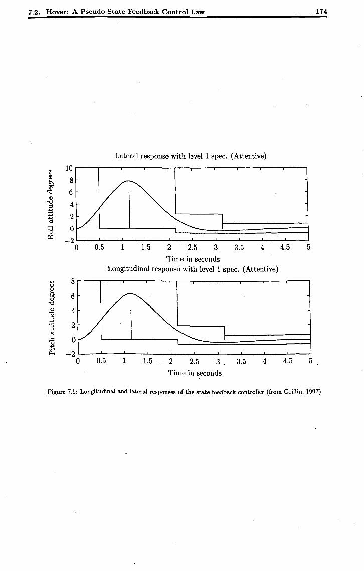
7.2. Hover: A Pseudo-State Feedback Control Law 174
Lateral response with level 1 spec. (Attentive)
CIl 10 a5 8 ~ Cl)
6 "'t:1 Cl)
"'t:1 4 ;::! 4-> .....
2 4->
1d ..... 0 ~ -2
0 0.5 1 1.5 2 2.5 3 3.5 4 4.5 5
Time in seconds Longitudinal response with level 1 spec. (Attentive)
rn 8 a5 ~ 6 Cl)
"'t:1 Cl) 4 "'t:1 ;::!
4->
2 ..... 4->
1d 13 0 4-> ..... P-4 -2
0 0.5 1 1.5 2 2.5 3, 3.5 4 4.5 5
Time in seconds
Figure 7.1: Longitudinal and lateral responses of the state feedback controller (from Griffin, 1997)
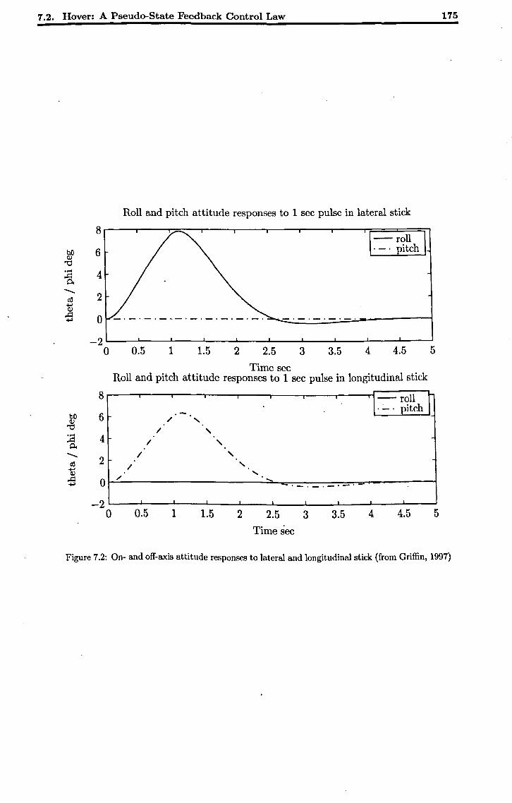
7.2. Hover: A Pseudo-State Feedback Control Law 175
Roll and pitch attitude responses to 1 sec pulse in lateral stick
8 -- roll
bO 6 Cl)
. -. pitch "0 ..... 4 ..cl 0-
.......... 2 cO
~ Cl)
..cl 0 ~
-2 0 0.5 1 1.5 2 2.5 3 3.5 4 4.5 5
Time sec Roll and pitch attitude responses to 1 scc pulse in longitudinal stick
8 1- roll I bO 6 '-. . .:..... pitch Cl) / ,
"0 / , ..... 4 ..cl / , 0-
.......... / , cO 2
/ ,
~ Cl) "-
..cl 0 / ..... ~ .-'-'
-2 0 0.5 1 1.5 2 2.5 3 3.5 4 4.5 5
Time sec Figure 7.2: On- and off-axis attitude responses to lateral and longitudinal stick (from Griffin, 1997)
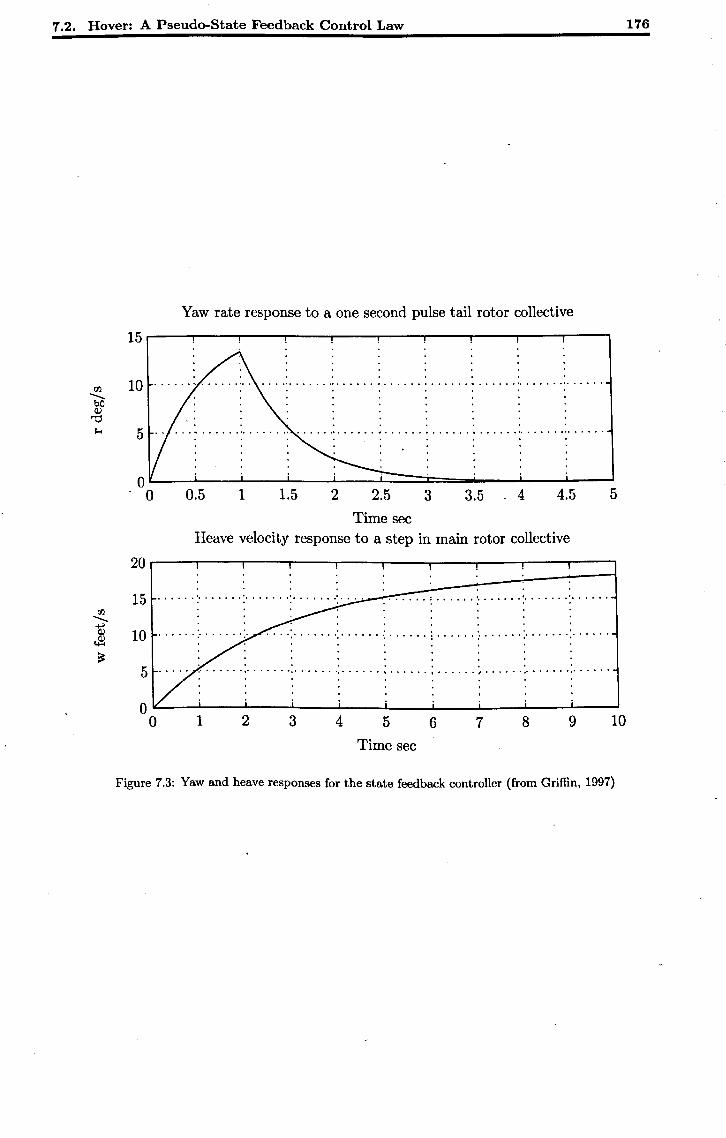
1.2. Hover: A Pseudo-State Feedback Control Law
rJl -........ b{) Q)
"0 1-4
Yaw rate response to a one second pulse tail rotor collective
15
10
5 ..
oL-~L-~--~--~--~~~==~--~--~--~ o 0.5 1 1.5 2 2.5 3 3.5 4 4.5 5
Time sec Heave velocity response to a step in main rotor collective
20r---.----r---.----.---.---~--~r_--._--_,--_,
15
. . . . . . . '" ', •••••• '.' ••••• " •••••• : •••••• ,0 ............ • '.' •••••
5 . . . . . . . . . ,' ••••• '.' ••••• ", ••••• ", ••••• \0 •••••• I •••••• , •••• • '.0 ••••• ", •••••
o~--~--~----~--~--~----~--~--~----~--~ o 1 2 3 4 5 6 7 8 9 10
Time sec
Figure 7.3: Yaw and heave responses for the state feedback controller (from Griffin, 1997)
116
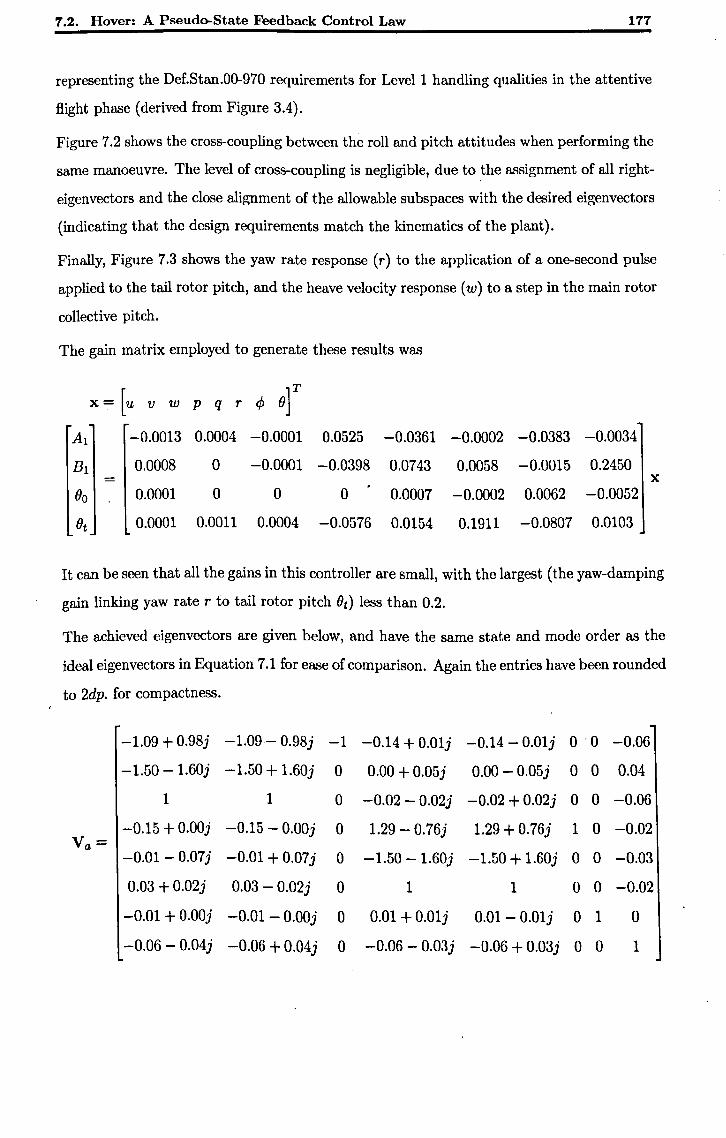
7.2. Hover: A Pseudo-State Feedback Control Law 177
representing the Def.Stan.00-970 requirements for Level 1 handling qualities in the attentive
flight phase (derived from Figure 3.4).
Figure 7.2 shows the cross-coupling between the roll and pitch attitudes when performing the
same manoeuvre. The level of cross-coupling is negligible, due to the assignment of all right
eigenvectors and the close alignment of the allowable subspaces with the desired eigenvectors
(indicating that the design requirements match the kinematics of the plant).
Finally, Figure 7.3 shows the yaw rate response (r) to the application of a one-second pulse
applied to the tail rotor pitch, and the heave velocity response (w) to a step in the main rotor
collective pitch.
The gain matrix employed to generate these results was
x= [u v w p q r ifJ O]T
Al -0.0013 0.0004 -0.0001 0.0525 -0.0361 -0.0002 -0.0383 -0.0034
Bl 0.0008 0 -0.0001 -0.0398 0.0743 0.0058 -0.0015 0.2450 - x
OD 0.0001 0 0 0 0.0007 -0.0002 0.0062 -0.0052
Ot 0.0001 0.0011 0.0004 -0.0576 0.0154 0.1911 -0.0807 0.0103
It can be seen that all the gains in this controller are small, with the largest (the yaw-damping
gain linking yaw rate r to tail rotor pitch Ot) less than 0.2.
The achieved eigenvectors are given below, and. have the same state and mode order as the
ideal eigenvectors in Equation 7.1 for ease of comparison. Again the entries have been rounded
to 2dp. for compactness.
-1.09 + 0.98j -1.09 - 0.98j -1 -0.14 + O.Olj -0.14 - 0.01j 0'0 -0.06
-1.50 - 1.60j -1.50 + 1.60j 0 0.00 + 0.05j 0.00 - 0.05j 0 0 0.04
1 1 0 -0.02 - 0.02j -0.02 + 0.02j 0 0 -0.06
Va= -0.15 + O.OOj -0.15 - O.OOj 0 1.29 - 0.76j 1.29 + 0.76j 1 0 -0.02
-0.01 - 0.07 j -0.01 + 0.07 j 0 -1.50 - 1.60j -1.50 + 1.60j 0 0 -0.03
0.03 + 0.02j 0.03 - 0.02j 0 1 1 0 0 -0.02
-0.01 + O.OOj -0.01 - O.OOj 0 0.01 +O.01j 0.01- O.01j 0 1 0
-0.06 - 0.04j -0.06 + 0.04j 0 -0.06 - 0.03j -0.06 + 0.03j 0 0 1
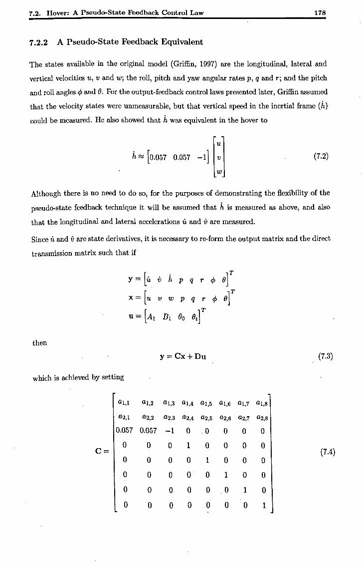
1.2. Hover: A Pseudo-State Feedback Control Law 118
7.2.2 A Pseudo-State Feedback Equivalent
The states available in the original model (Griffin, 1997) are the longitudinal, lateral and
vertical velocities u, v and Wj the roll, pitch and yaw angular rates p, q and rj and the pitch
and roll angles 4> and O. For the output-feedback control laws presented later, Griffin assumed
that the velocity states were unmeasurable, but that vertical speed in the inertial frame (h)
could be measured. He also showed that h was equivalent in the hover to
u
h ~ [0.057 0.057 -1] v
W
(7.2)
Although there is no need to do so, for the purposes of demonstrating the flexibility of the
pseudo-state feedback technique it will be assumed that h is measured as above, and also
that the longitudinal and lateral accelerations u and v are measured.
Since it and v are state derivatives, it is necessary to re-form the output matrix and the direct
transmission matrix such that if
then
Y= [it v h p q r 4> O]T
x = [u v W p q r 4> O]T
U = [AI BI 00 Ot]T
y=Cx+Du
which is achieved by setting
al,l al,2 al ,3 al,4 al,5 al,6
a2,1 a2,2 a2,3 a2,4 a2,5 a2,6
0.057 0.057 -1 0 .0 0
0 C=
0 0 1 0 0
0 0 0 0 1 0
0 0 0 O· 0 1
0 0 0 0 0 0
0 0 0 0 0 0
(7.3)
al,7 aI,S
a2,7 a2,8
0 0
0 0 (7.4)
0 0
0 0
1 0
0 1
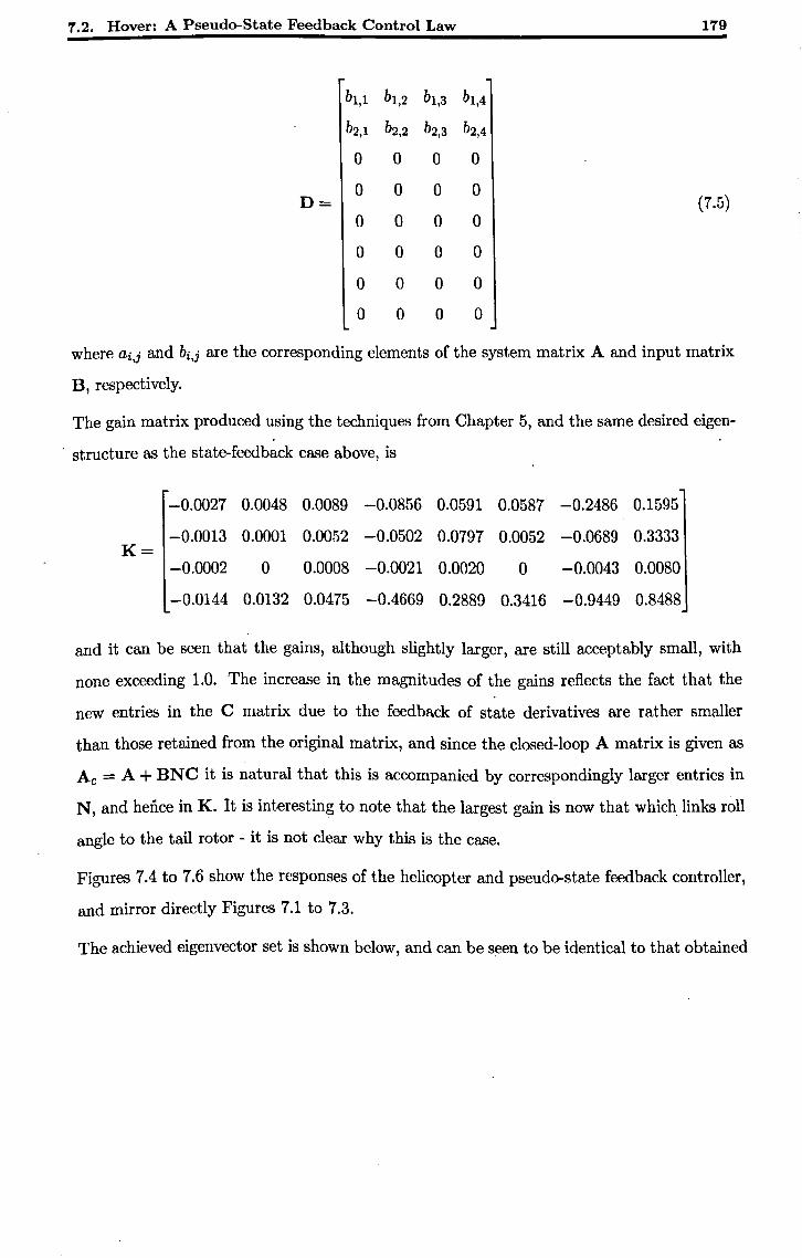
1.2. Hover: A Pseudo-State Feedback Control Law 119
bll , b12 , b1,3 b1,4
b2 1 , b22 , b23 , b2,4
0 0 0 0
0 0 0 0 (7.5) D=
0 0 0 0
0 0 0 0
0 0 0 0
0 0 0 0
where ai,j and bi,j are the corresponding elements of the system matrix A and input matrix
B, respectively.
The gain matrix produced using the techniques from Chapter 5, and the same desired eigen-
. structure as the state-feedback case above, is
-0.0027 0.0048 0.0089 -0.0856 0.0591 0.0587 -0.2486 0.1595
-0.0013 0.0001 0.0052 -0.0502 0.0797 0.0052 -0.0689 0.3333 K=
-0.0002 0 0.0008 -0.0021 0.0020 0 -0.0043 0.0080
-0.0144 0.0132 0.0475 -0.4669 0.2889 0.3416 -0.9449 0.8488
and it can be seen that the gains, although slightly larger, are still acceptably small, with
none exceeding 1.0. The increase in the magnitudes of the gains reflects the fact that the
new entries in the C matrix due to the feedback of state derivatives are rather smaller
than those retained from the original matrix, and since the closed-loop A matrix is given as
Ac = A + BNC it is natural that this is accompanied by correspondingly larger entries in
N, and hence in K. It is interesting to note that the largest gain is now that which links roll
angle to the tail rotor - it is not clear why this is the case.
Figures 7.4 to 7.6 show the responses of the helicopter and pseudo-state feedback controller,
and mirror directly Figures 7.1 to 7.3.
The achieved eigenvector set is shown below, and can be seen to be identical to that obtained
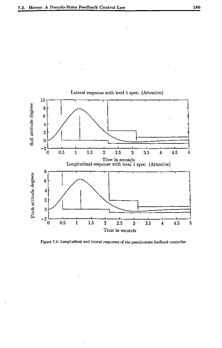
7.2. Hover: A Pseudo-State Feedback Control Law 180
Lateral response with level 1 spec. (Attentive)
10 r/l
as 8 tb Q)
6 "tl Q)
"tl 4 ;j .., ...... .., 2 1d
~ 0
-2 0 0.5 1 1.5 2 2.5 3 3.5 4 4.5 5
Time in seconds Longitudinal response with level 1 spec. (Attentive)
r/l 8 as tb 6 Q)
"tl Q) 4 "tl ;j ~ ...... 2 ~
"'id .g 0 ~ ...... p...
-2 0 0.5 1 1.5 2 2.5 3 . 3.5 4 4.5 5 .
Time in seconds
Figure 7.4: Longitudinal and lateral responses of the pseudo-state feedback controller
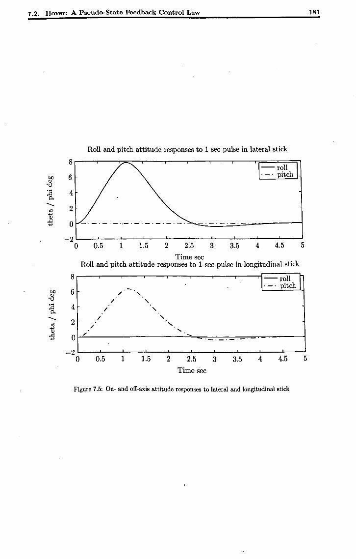
7.2. Hover: A Pseudo-State Feedback Control Law 181
Roll and pitch attitude responses to 1 sec pulse in lateral stick
8 -- roll
bO 6 <l)
. _. pitch
"0 ..... 4 A 0..
.......... 2 (Q
~ A 0 +>
-2 0 0.5 1 1.5 2 2.5 3 3.5 4 4.5 5
Time sec Roll and pitch attitude responses to 1 sec pulse in longitudinal stick
8 I roll r bO 6 .-. . _. pitch <l) / " "0 / , ..... 4 A / , 0..
.......... I " (Q 2 / " ~ .....
A 0 ,/ ......
+>
-2 0 0.5 1 1.5 2 2.5 3 3.5 4 4.5 5
Time sec
Figure 7.5: On- and off-axis attitude responses to lateral and longitudinal stick
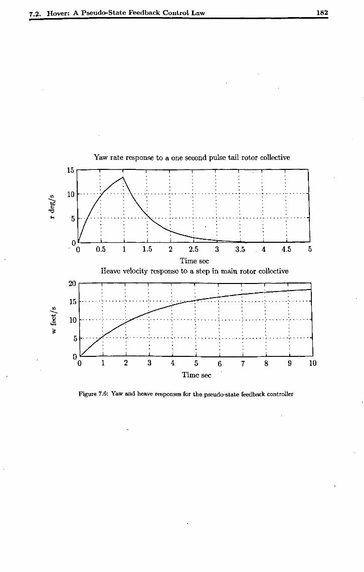
1.2. Hover: A Pseudo-State Feedback Control Law 182
Yaw rate response to a one second pulse tail rotor collective
15
rIl 10 '" ,' •••••••• 0 •••••••••••• I ..................... 00, ••••• . . -.... bj) Q)
~
'"' 5 ..
oL-~~~--~--~--~~~==~--~--~--~ . 0 0.5 1 1.5 2 2.5 3 3.5 4 4.5 5
Time sec Heave velocity response to a step in main rotor collective
20
15 ...... : ...... \ ..... ,', ...... ' ..... . . . . . rIl -.... ~
J;l 10 . . . . . . . ... ',' ..... '.' ..... ' ....... : ...... : ...... ,' ..... ',' .... .
~ 5
. . . . , . . . . .' ..... '0'····· '0'····· '0'····· '\ ......•...... , ..... ',' ..... '0'·····
0 0 1 2 3 4 5 6 7 8 9 10
Time sec
Figure 7.6: Yaw and heave responses for the pseudo-state feedback controller
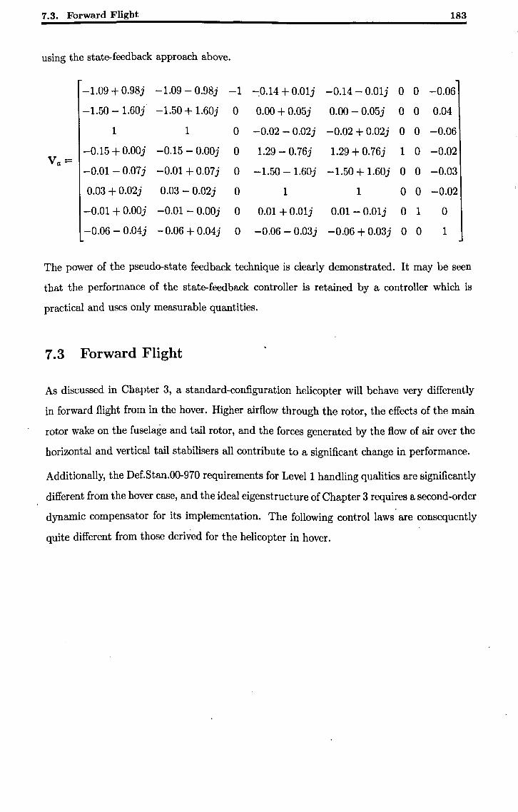
7.3. Forward Flight 183
using the state-feedback approach above.
-1.09 + 0.98j -1.09 - 0.98j -1 -:0.14 + O.01j -0.14 - O.01j 0 0 -0.06
-1.50 - 1.60j -1.50 + 1.60j 0 0.00 + 0.05j 0.00 - 0.05j 0 0 0.04
1 1 0 -0.02 - 0.02j -0.02 + 0.02j 0 0 -0.06
-0.15 + O.OOj -0.15 - O.OOj 0 1.29 - 0.76j 1.29 + 0.76j 1 0 -0.02 Va=
-0.01 - 0.07 j -0.01 + 0.07 j 0 -1.50 - 1.60j -1.50 + 1.60j 0 0 -0.03
0.03 + 0.02j 0.03 - 0.02j 0 1 1 0 0 -0.02
-0.01 + O.OOj -0.01 - O.OOj 0 0.01 + O.Olj 0.01- O.Olj 0 1 0
-0.06 - 0.04j -0.06 + 0.04j 0 -0.06 - 0.03j -0.06 + 0.03j 0 0 1
The power of the pseudo-state feedback technique is clearly demonstrated. It may be seen
that the performance of the state-feedback controller is retained by a controller which is
practical and uses only measurable quantities.
7.3 .Forward Flight
As discussed in Chapter 3, a standard-configuration helicopter will behave very differently
in forward flight from in the hover. Higher airflow through the rotor, the effects of the main
rotor wake on the fuselage and tail rotor, and the forces generated by the flow of air over the
horizontal and vertical tail stabilisers all contribute to a significant change in performance.
Additionally, the Def.Stan.00-970 requirements for Level 1 handling qualities are significantly
different from the hover case, and the ideal eigenstructure of Chapter 3 requires a second-order
dynamic compensator for its implementation. The following control laws are consequently
quite different from those derived for the helicopter in hover.
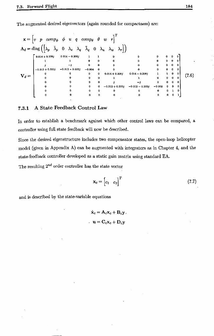
7.3. Forward Flight 184
The augmented desired eigenvectors (again rounded for compactness) are:
x= [v P comp</> </> u q comp9 () w r]T
Ad = diag ( [ Ap Xp 0 Av Aq Xq 0 Au Aw Ar]) 0.014 + 0.208; 0.014 - 0.208; 1 0 0 0 0 0 0
0 0 0 0 0 0 0 0
j -j 0 0 0 0 0 0 0 0
-0.312 + 0.333; -0.312 - 0.333; -0.004 0 0 0 0 0 0 0
Vd= 0 0 0 0 0.014 + 0.208; 0.014 - 0.208; 1 0 0 (7.6) 0 0 0 0 1 0 0 0 0
0 0 0 0 ; -; 0 0 0 0
0 0 0 0 -0.312 + 0.333; -0.312 - 0.333; -0.002 0 0 0
0 0 0 0 0 0 0 0 1 0
0 0 0 0 0 0 0 0 0 1
7.3.1 A State Feedback Control Law
In order to establish a benchmark against which other control laws can be compared, a
controller using full state feedback will now be described.
Since the desired eigenstructure includes two compensator states, the open-loop helicopter
model (given in Appendix A) can be augmented with integrators as in Chapter 4, and the
state-feedback controller developed as a static gain matrix using standard EA.
The resulting 2nd order controller has the state vector
(7.7)
and is described by the state-variable equations
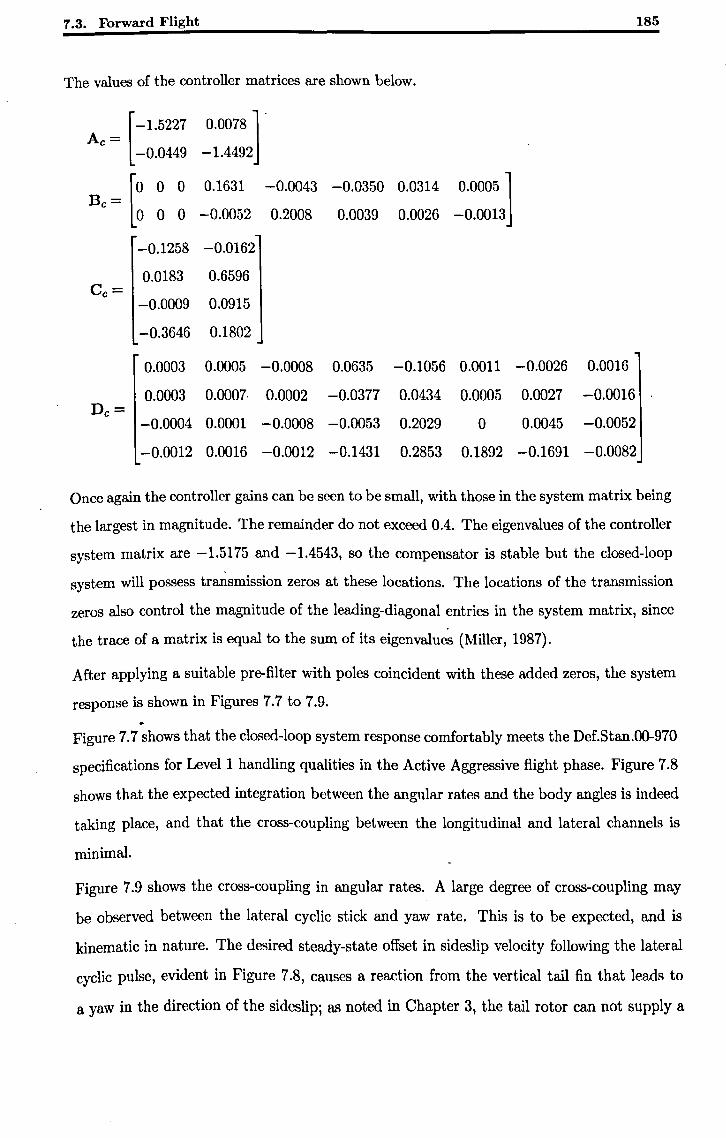
7.3. Forward Flight 185
The values of the controller matrices are shown below.
Once again the controller gains can be seen to be small, with those in the system matrix being
the largest in magnitude. The remainder do not exceed 0.4. The eigenvalues of the controller
system matrix are -1.5175 and -1.4543, so the compensator is stable but the closed-loop
system will possess transmission zeros at these locations. The locations of the transmission
zeros also control the magnitude of the leading-diagonal entries in the system matrix, since
the trace of a matrix is equal to the sum of its eigenvalucs (Miller, 1987).
After applying a suitable pre-filter with poles coincident with these added zeros, the system
response is shown in Figures 7.7 to 7.9 . ..
Figure 7.7 shows that the closed-loop system response comfortably meets the Def.Stan.OO-970
specifications for Level 1 handling qualities in the Active Aggressive flight phase. Figure 7.8
shows that the expected integration between the angular rates and the body angles is indeed
taking place, and that the cross-coupling between the longitudinal and lateral channels is
minimal.
Figure 7.9 shows the cross-coupling in angular rates. A large degree of cross-coupling may
be observed between the lateral cyclic stick and yaw rate. This is to be expected, and is
kinematic in nature. The desired steady-state offset in sideslip velocity following the lateral
cyclic pulse, evident in Figure 7.8, causes a reaction from the vertical tail fin that leads to
a yaw in the direction of the sideslip; as noted in Chapter 3, the tail rotor can not supply a
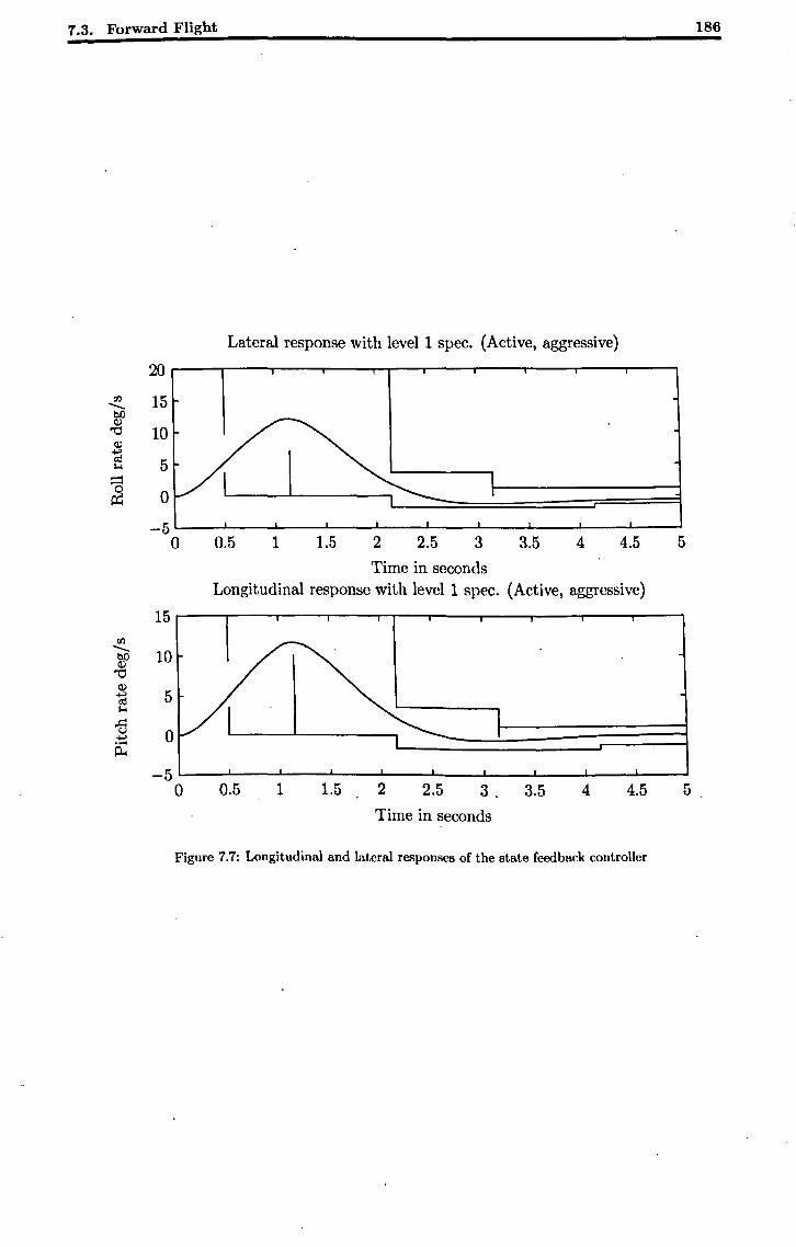
7.3. Forward Flight 186
Lateral response with level 1 spec. (Active, aggressive)
20 00 15 ........ bO Cl)
"0 10 Cl)
1d 5 '"' :::::l
~ 0
-5 0 0.5 1 1.5 2 2.5 3 3.5 4 4.5 5
Time in seconds Longitudinal response with level 1 spec. (Active, aggressive)
15 00 ........
10 bO Cl)
"0 Cl)
5 ~ '"' .g
0 ~ ..... p..
-5 0 0.5 1 1.5 2 2.5 3, 3.5 4 4.5 5
Time in seconds
Figure 7.7: Longitudinal and lateral responses of the state feedback controller
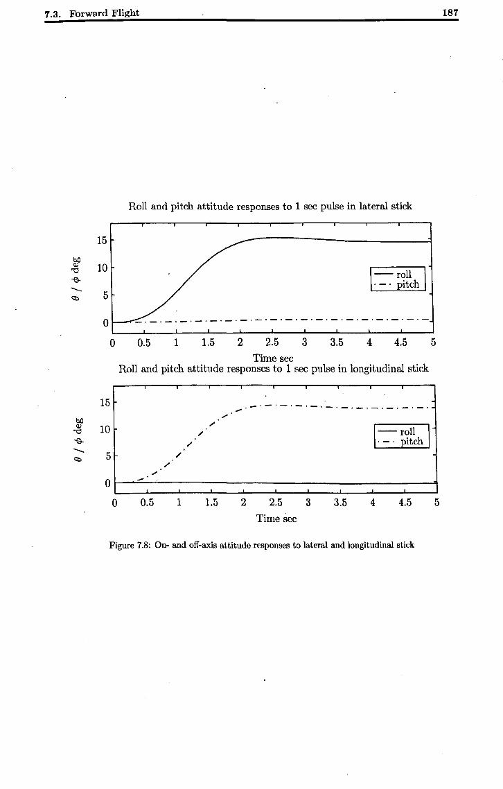
7.3. Forward Flight 187
Roll and pitch attitude responses to 1 sec pulse in lateral stick
15
10 -roll . _. pitch
5
o _._.-.-.-.-._.-._._._.-._.-._._._._._.-
o 0.5 1 1.5 2 2.5 3 3.5 4 4.5 5
Time sec Roll and pitch attitude responses to 1 sec pulse in longitudinal stick
15 .,. .~.-.-.-.-.-.-.-.-.-.-.- . "'" be ,,-
Cl) 10 "i:l " 1-roll J ~
" . _. pitch
--- 5 " c:t> ,,-
"'" 0 .,.
0 0.5 1 1.5 2 2.5 3 3.5 4 4.5 5 Time sec
Figure 7.8: On- and off-axis attitude responses to lateral and longitudinal stick
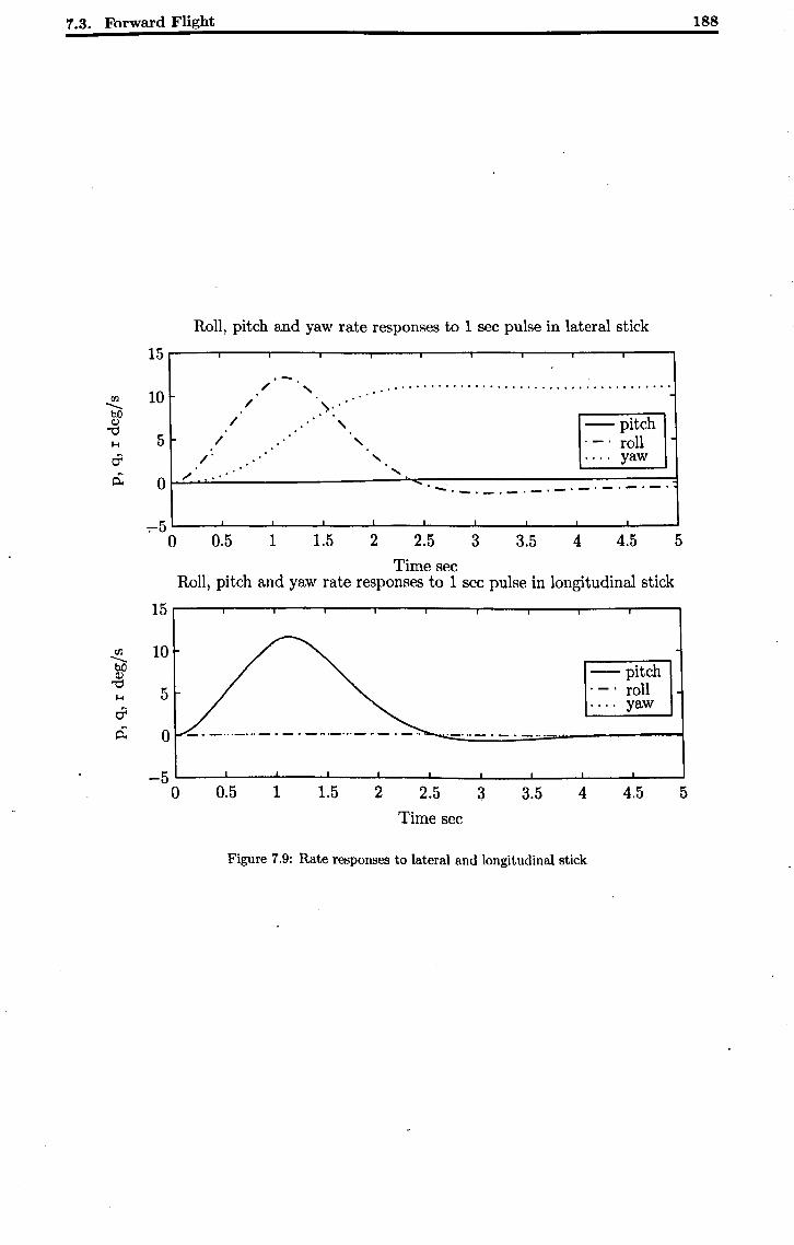
7.3. Forward Flight
rJl --bO Q)
~ I-<
a 0:
rJl --b.O Q)
~ I-<
a 0:
Roll, pitch and yaw rate responses to 1 sec pulse in lateral stick
15
/ " .' . ...................................... 10 / \.' / , -pitch
5 / , roll /. " yaw
/ .....
0 .' . - ........ _._._._._.
-:-5 0 0.5 1 1.5 2 2.5 3 3.5 4 4.5
Time sec Roll, pitch and yaw rate responses to 1 sec pulse in longitudinal stick
15
10
5
0
-5 0 0.5 1 1.5 2 2.5 3 3.5 4
Time sec
Figure 7.9: Rate responses to lateral and longitudinal stick
-pitch roll
.... yaw
4.5
188
5
5
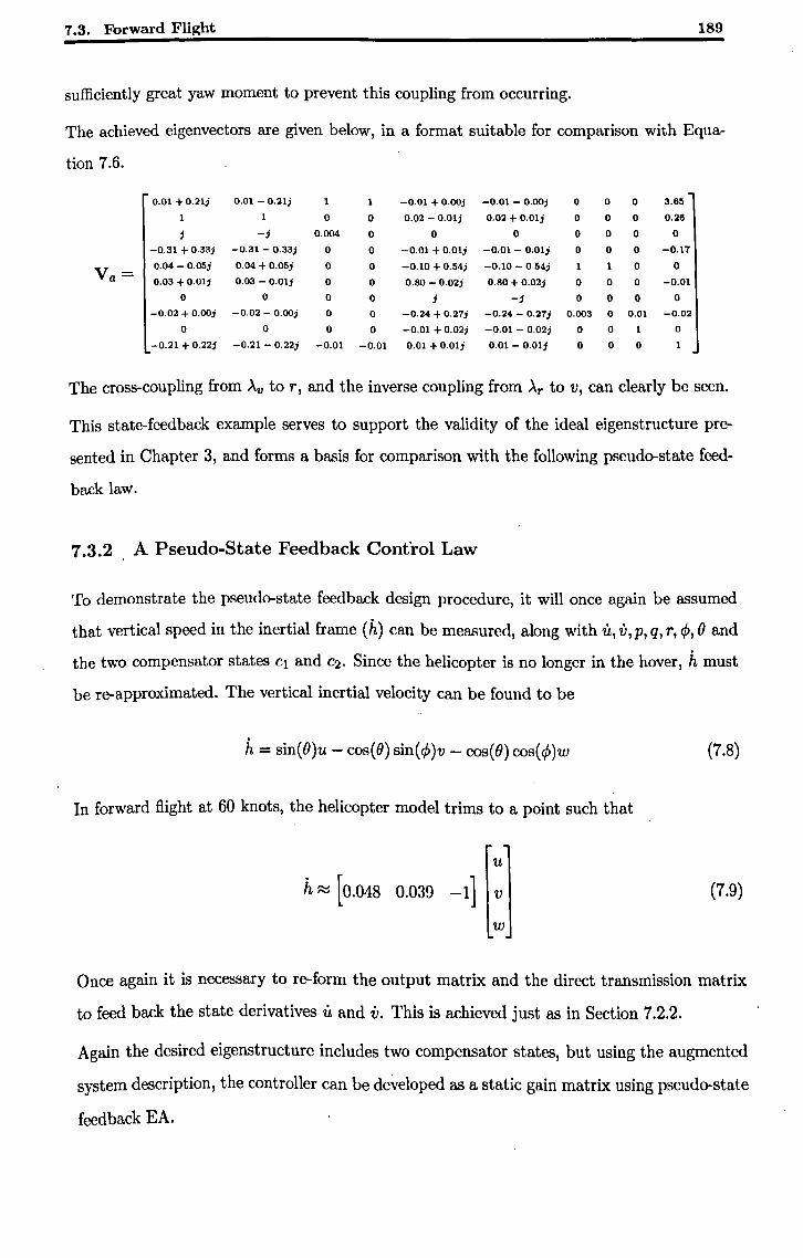
7.3. Forward Flight 189
sufficiently great yaw moment to prevent this coupling from occurring.
The achieved eigenvectors are given below, in a format suitable for comparison with Equa-
tion 7.6.
0.01 + 0.21; 0.01 - 0.21; 1 1 -0.01 + 0.00; -0.01 - 0.00; 0 0 0 3.65
1 1 0 0 0.02 - 0.01; 0.02 + 0.01; 0 0 0 0.26
-; 0.004 0 0 0 0 0 0 0
-0.31 + 0.33; -0.31 - 0.33; 0 0 -0.01 + 0.01; -0.01 - 0.Ql; 0 0 0 -0.17
Va= 0.04 - 0.05; 0.04 + 0.05; 0 0 -0.10 + 0.54; -0.10 - 0.54; 1 0 0
0.03 + 0.01; 0.03 - 0.01; 0 0 0.80 - 0.02; 0.80+0.02; 0 0 0 -0.01
0 0 0 0 ; -j 0 0 0 0
-0.02 + 0.00; -0.02 - o.ooj 0 0 -0.24 + 0.27; -0.24 - 0.27; 0.003 0 0.01 -0.02
0 0 0 0 -0.01 + 0.02; -0.01 - 0.02j 0 0 0
-0.21 + 0.22j -0.21 - 0.22; -0.01 -0.01 0.01 + 0.01; 0.01 - 0.01; 0 0 0
The cross-coupling from Av to T, and the inverse coupling from Ar to v, can clearly be seen.
This state-feedback example serves to support the validity of the ideal eigenstructure pre
sented in Chapter 3, and forms a basis for comparison with the following pseudo-state feed
back law.
7.3.2 A Pseudo-State Feedback Control Law
To demonstrate the pseudo-state feedback design procedure, it will once again be assumed
that vertical speed in the inertial frame Ch) can be measured, along with u, v, p, q, T, 4>, 0 and
the two compensator states Cl and C2. Since the helicopter is no longer in the hover, h must
be re-approximated. The vertical inertial velocity can be found to be
h = sin(O)u - cos(O) sin(4))v - cos(O) cos(4))w (7.8)
In forward flight at 60 knots, the helicopter model trims to a point such that
u
h ~ [0.048 0.039 -1] v (7.9)
w
Once again it is necessary to re-form the output matrix and the direct transmission matrix
to feed back the state derivatives u and v. This is achieved just as in Section 7.2.2.
Again the desired eigenstructure includes two compensator states, but using the augmented
system description, the controller can be developed as a static gain matrix using pseudo-state
feedback EA.
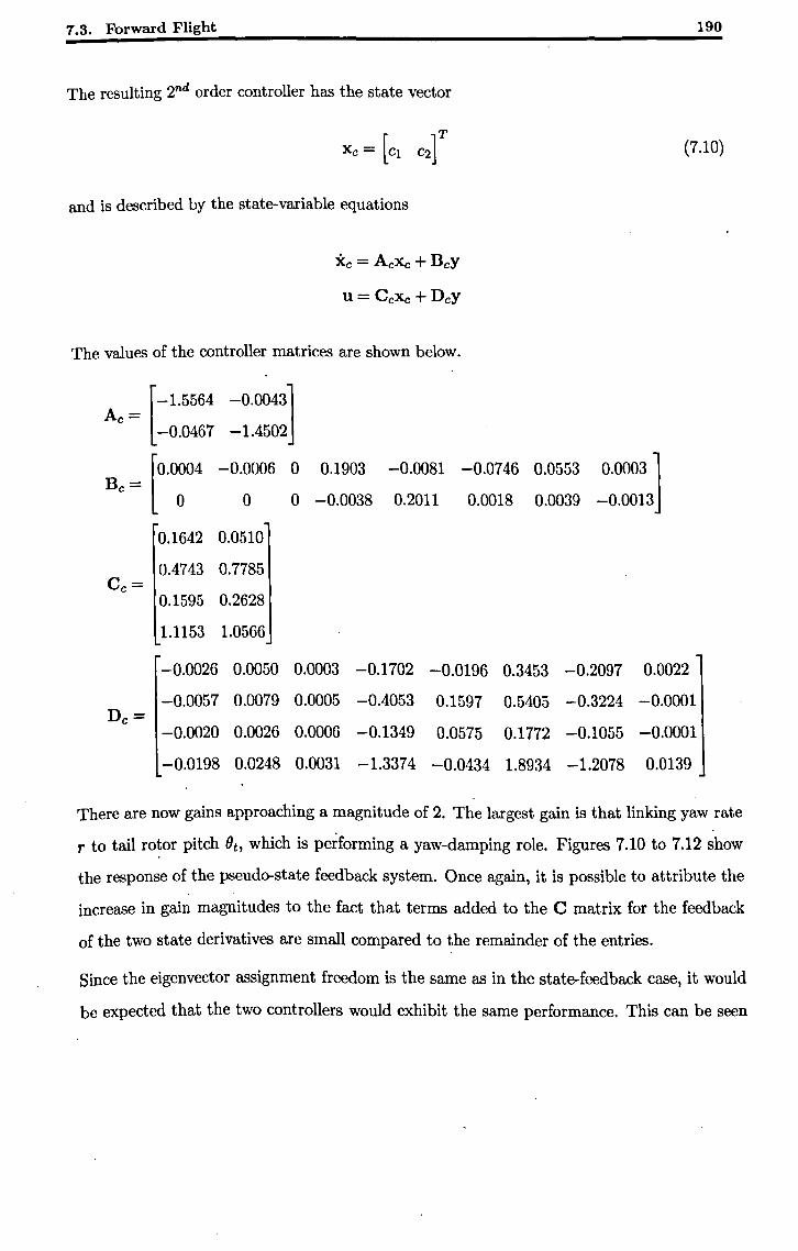
7.3. Forward Flight
The resulting 2nd order controller has the state vector
and is described by the state-variable equations
u= Ccxc + DcY
The values of the controller matrices are shown below.
[
-1.5564 -0.0043] Ac=
-0.0467 -1.4502
D, = [O.~ -O.~ ~ 0.1903
-0.0038
-0.0081 -0.0746 0.0553
0.2011 0.0018 0.0039 0.
00031 -0.0013
190
(7.10)
There are now gains approaching a magnitude of 2. The largest gain is that linking yaw rate
r to tail rotor pitch Bt , which is performing a yaw-damping role. Figures 7.10 to 7.12 show
the response of the pseudo-state feedback system. Once again, it is possible to attribute the
increase in gain magnitudes to the fact that terms added to the C matrix for the feedback
of the two state derivatives are small compared to the remainder of the entries.
Since the eigenvector assignment freedom is the same as in the state-feedback case, it would
be expected that the two controllers would exhibit the same performance. This can be seen
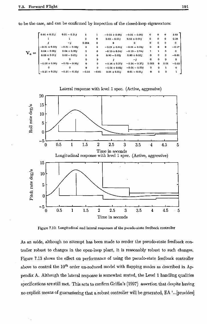
7.3. Forward Flight 191
to be the case, and can be confirmed by inspection of the closed-loop eigenvectors:
0.01 + 0.21j 0.01 - 0.21j 1 -0.01 + O.OOj -0.01 - O.OOj 0 0 0 3.65
1 1 0 0 0.02 - O.Olj 0.02 + O.Olj 0 0 0 0.26
i -j 0.004 0 0 0 0 0 0 0
-0.31 + 0.33j -0.31 - 0.33j 0 0 -0.01 + 0.01; -0.01 - O.Olj 0 0 0 -0.17
Va= 0.04 - 0.05; 0.04 + 0.05; 0 0 -0.10 + 0.54j -0.10 - 0.54j 1 1 0 0
0.03 + O.Olj 0.03 - O.Olj 0 0 0.80 - 0.02j 0.80 + 0.02j 0 0 0 -0.01
0 0 0 0 j -j 0 0 0 0
-0.02 + O.OOj -0.02 - O.OOj 0 0 -0.24 + 0.27j -0.24 - 0.27j 0.003 0 0.01 -0.02
0 0 0 0 -0.01 + 0.02j -0.01 - 0.02j 0 0 1 0
-0.21 + 0.22j -0.21 - 0.22; -0.01 -0.01 0.01 + O.Olj 0.01 - O.Olj 0 0 0
Lateral response with level 1 spec. (Active, aggressive)
20
m 15 ............ b{) Cl)
'"c:l 10 Cl)
~ 5 .... -~ 0
-5 0 0.5 1 1.5 2 2.5 3 3.5 4 4.5 5
Time in seconds Longitudinal response with level 1 spec. (Active, aggressive)
15 m
............ 10 b{)
Cl) '"c:l
Cl)
~ 5 ....
-B 0 +" ....
~
....... 5 0 0.5 1 1.5 2 2.5 3 3.5 4 4.5 5
Time in seconds
Figure 1.10: Longitudinal and lateral responses of the pseudo-state feedback controller
As an aside, although no attempt has been made to render the pseudo-state feedback con
troller robust to changes in the open-loop plant, it is reasonably robust to such changes.
Figure 7.13 shows the effect on performance of using the pseudo-state feedback controller
above to control the 10th order un-reduced model with flapping modes as described in Ap
pendix A. Although the lateral response is somewhat muted, the Level 1 handling qualities
specifications are still met. This acts to confirm Griffin's (1997) assertion that despite having
no explicit means of guaranteeing that a robust controller will be generated, EA ' ... [provides]
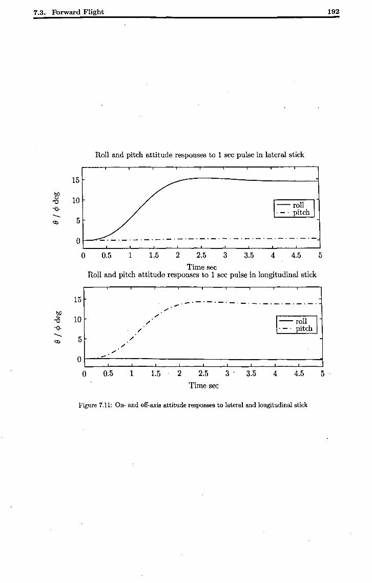
7.3. Forward Flight 192
Roll and pitch attitude responses to 1 sec pulse in lateral stick
15
10 -- roll . _. pitch
5
o _.-._._._._._.-._._.-.-._._._._._._._.-
o 0.5 1 1.5 2 2.5 3 3.5 4 4.5 5
Time sec Roll and pitch attitude responses to 1 sec pulse in longitudinal stick
15 , -'-'-'-'-'-'-'-'-'-'-'-' b.O
~
Q) 10
~
'"0 / 1- roll I ~ / . _. pitch '- 5 / ~
/ ~
0 ,
0 0.5 1 1.5 2 2.5 3 " 3.5 4 4.5 5· Time·sec
Figure 7.11: On- and off-axis attitude responses to lateral and longitudinal stick
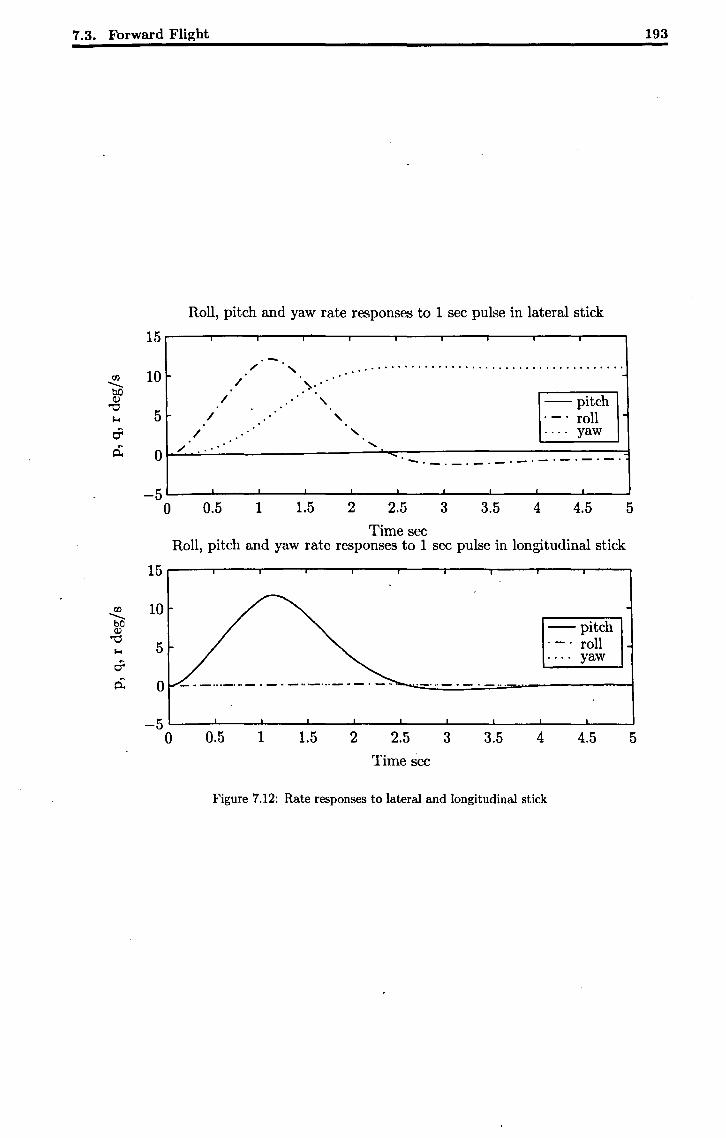
7.3. Forward Flight
15
rIJ 10 .......... bO Q)
"'0 .... 5r-a 6; 0
-5 0
15
rIJ 10 .......... bO Q)
"'0 5 ....
a p:; 0
-5 0
Roll, pitch and yaw rate responses to 1 sec pulse in lateral stick
/ , .' . ...................................... / '\ ..
I , -- pitch I , roll
/ , yaw
/ ...... .. ......._._._.-.-.
0.5 1 1.5 2 2.5 3 3.5 4 4.5 Time sec
Roll, pitch and yaw rate responses to 1 sec pulse in longitudinal stick
0.5 1 1.5 2 2.5 Time sec
3 3.5 4
Figure 7.12: Rate responses to lateral and longitudinal stick
-- pitch roll
. ... yaw
4.5
193
5
5
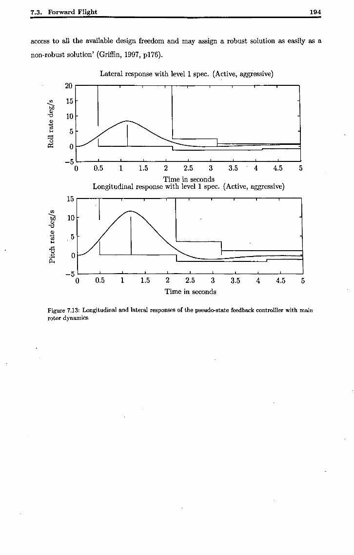
7.3. Forward Flight 194
access to all the available design freedom and may assign a robust solution as easily as a
non-robust solution' (Griffin, 1997, pI76).
Lateral response with level 1 spec. (Active, aggressive)
20
rJl 15 ""'--b.O
Cl) "'C 10
Cl)
~ 5 I-<
:::::: 0
ex:: 0
-5 0 0.5 1 1.5 2 2.5 3 3.5 4 4.5 5
Time in seconds Longitudinal response with level 1 spec. (Active, aggressive)
15
00 ""'-- 10 bO
Cl) "'C
Cl)
~ 5 I-<
oB 0 ~ .....
~
-5 0 0.5 1 1.5 2 2.5 3 3.5 4 4.5 5
Time in seconds
Figure 7.13: Longitudinal and lateral responses of the pseudo-state feedback controlller with main rotor dynamics
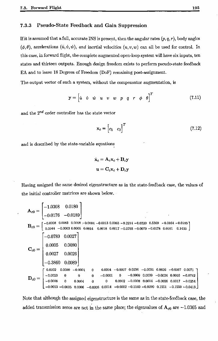
7.3. Forward Flight 195
7.3.3 Pseudo-State Feedback and Gain Suppression
If it is assumed that a full, accurate INS is prese~t, then the angular rates (p, q, r), body angles
(<p, 0), accelerations (u, v, w), and inertial velocities (u, v, w) can all be used for control. In
this case, in forward flight, the complete augmented open-loop system will have six inputs, ten
states and thirteen outputs. Enough design freedom exists to perform pseudo-state feedback
EA and to leave 18 Degrees of Freedom (DoF) remaining post-assignment.
The output vector of such a system, without the compensator augmentation, is
y = [it. v w u v w p q r <p O]T (7.11)
and the 2nd order controller has the state vector
(7.12)
and is described by the state-variable equations
Having assigned the same desired eigenstructure as in the state-feedback case, the values of
the initial controller matrices are shown below.
[
-1.0368 0.0180 ] AcO =
-0.0176 -0.0189
[-0.0008 0.0083 0.0008 :--0.0004 -0.0013 0.0065 -0.2214 -0.0320 0.5369 -0.3164 -0.0185]
BcO = 0.0044 -0.00030.0006 0.0014 0.0018 0.0017 -0.0703 -0.0079 -0.0178 0.0161 0.1433
o 0.0004 -0.0007 0.0236 -0.0031 0.0606 -0.0367 00071 ]
o -0.0001 0 -0.0009 0.0039 -0.0024 0.0016 -~.0742 o 0 0.0002 -0.0008 0.0014 -0.0026 0.0017 -0.0254
-0.0006 0.0014 -0.0002 -0.1140 -0.0090 0.1551 -0.1550 -0.0413
Note that although the assigned eigenstructure is the same as in the state-feedback case, the
added transmission zeros are not in the same place; the eigenvalues of Aeo are -1.0365 and
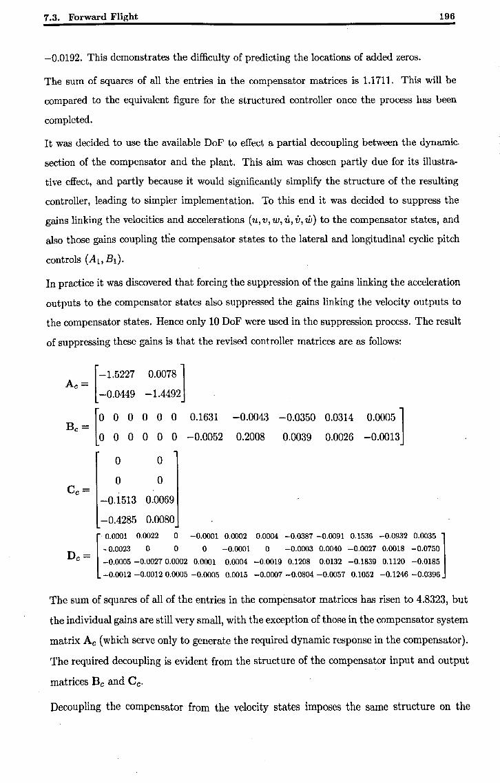
7.3. Forward Flight 196
-0.0192. This demonstrates the difficulty of predicting the locations of added zeros.
The sum of squares of all the entries in the compensator matrices is 1.1711. This will be
compared to the equivalent figure for the structured controller once the process has been
completed.
It was decided to use the available DoF to effect a partial decoupling between the dynamic"
section of the compensator and the plant. This aim was chosen partly due for its illustra
tive effect, and partly because it would significantly simplify the structure of the resulting
controller, leading to simpler implementation. To this end it was decided to suppress the
gains linking the velocities and accelerations (u, v, w, it, V, tU) to the compensator states, and
also those gains coupling the compensator states to the lateral and longitudinal cyclic pitch
controls (AI) Bd·
In practice it was discovered that forcing the suppression of the gains linking the acceleration
outputs to the compensator states also suppressed the gains linking the velocity outputs to
the compensator states. Hence only 10 DoF were used in the suppression process. The result
of suppressing these gains is that the revised controller matrices are as follows:
[-1.5227 0.0078 ] Ac=
-0.0449 -1.4492
[: 0 0 0 0 0 0.1631 -0.0043 -0.0350 0.0314 0.0005 ]
Bc= 0 0 0 0 0 -0.0052 0.2008 0.0039 0.0026 -0.0013
0 0
o 0 Cc=
-0.1513 0.0069
-0.4285 0.0080
[
. 0.0001 0.0022 0 -0.0001 0.0002 0.0004 -0.0387 -0.0091 0.1536 -0.0932 0.0035 ]
-0.0023 0 0 0 -0.0001 0 -0.0003 0.0040 -0.0027 0.0018 -0.0750
-0.0005 -0.00270.0002 0.0001 0.0004 -0.0019 0.1208 0.0132 -0.1839 0.1120 -0.0185
-0.0012 -0.00120.0005 -0.0005 0.0015 -0.0007 -0.0804 -0.0057 0.1052 -0.1246 -0.0396
The sum of squares of all of the entries in the compensator matrices has risen to 4.8323, but
the individual gains are still very small, with the exception of those in the compensator system
matrix Ac (which serve only to generate the required dynamic response in the compensator).
The required decoupling is evident from the structure of the compensator input and output
matrices Bc and Cc.
Decoupling the compensator from the velocity states imposes the same structure on the
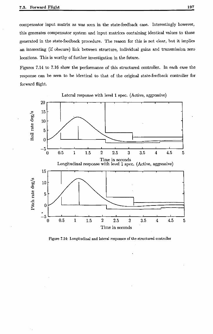
7.3. Forward Flight 197
compensator input matrix as was seen in the state-feedback case. Interestingly however,
this generates compensator system and input matrices containing identical values to those
generated in the state-feedback procedure. The reason for this is not clear, but it implies
an interesting (if obscure) link between structure, individual gains and transmission zero
locations. This is worthy of further investigation in the future.
Figures 7.14 to 7.16 show the performance of this structured controller. In each case the
response can be seen to be identical to that of the original state-feedback controller for
forward flight.
Lateral response with level 1 spec. (Active, aggressive)
20
rIl 15 ---bO
Cl)
"'0 10 Cl)
1d 5 I-<
== ~ 0
-5 0 0.5 1 1.5 2 2.5 3 3.5 4 4.5 5
Time in seconds Longitudinal response with level 1 spec. (Active, aggressive)
15 rIl
--- 10 bO Cl)
"'0 Cl)
1d 5 I-<
-B ...,. ...... Po.
-5 0 0.5 1 1.5 2 2.5 3 3.5 4 4.5 5
Time in seconds
Figure 7.14: Longitudinal and lateral responses of the structured controller
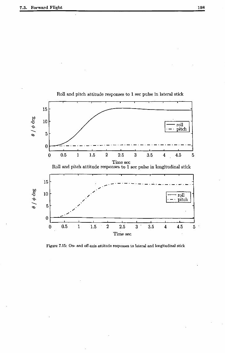
7.3. Forward Flight 198
Roll and pitch attitude responses to 1 sec pulse in lateral stick
15
10 -- roll . _. pitch
5
o -'-'-'-'-'-'-'-'-'-'-'-'-'-'-'-'-'-'-'-
o 0.5 1 1.5 2 2.5 3 3.5 4 4.5 5
Time sec Roll and pitch attitude responses to 1 sec pulse in longitudinal stick
15 -'-'-'-'-'-'~'-'-'-'-'-' ....
bO ~
Q) 10 '" "0
" I-roll I -e- " . _. pitch
.......... 5 " 'b
'" ~
0 ...
0 0.5 1 1.5 2 2.5 3 3.5 4 4.5 5 Time 'sec
Figure 7.15: On- and off-axis attitude responses to lateral and longitudinal stick
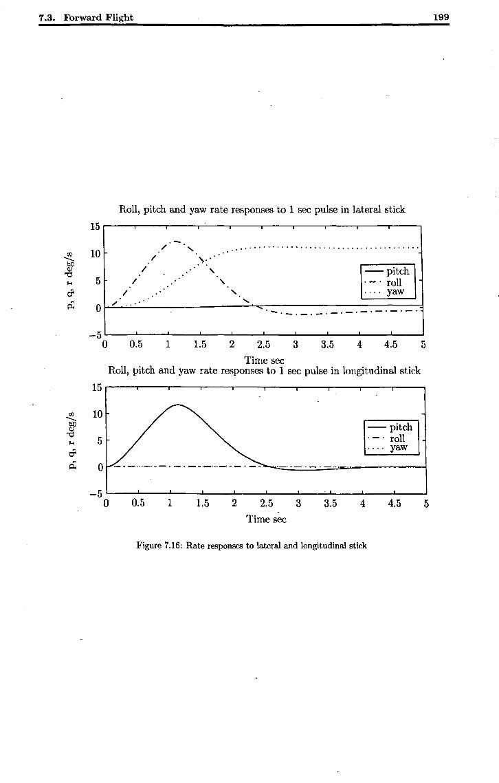
7.3. Forward Flight
r/l -..... bO Cl)
"'C ... a 0..
r/l -..... bO Cl)
"'C ... a 0:
Roll, pitch and yaw rate responses to 1 sec pulse in lateral stick
15
/ ...... .' . ....................................... 10 / '\ .. / , -pitch
5 / , roll / ...... .... yaw
/ ...... 0 .' .
' ...... _._._.-._._.
-5 0 0.5 1 1.5 2 2.5 3 3.5 4 4.5
Time sec Roll, pitch and yaw rate responses to 1 sec pulse in longitudinal stick
15
10
5
0
-5 0 0.5 1 1.5 2 2.5 3 3.5 4
Time sec
Figure 7.16: Rate responses to lateral and longitudinal stick
-- pitch roll
. ... yaw
4.5
199
5
5
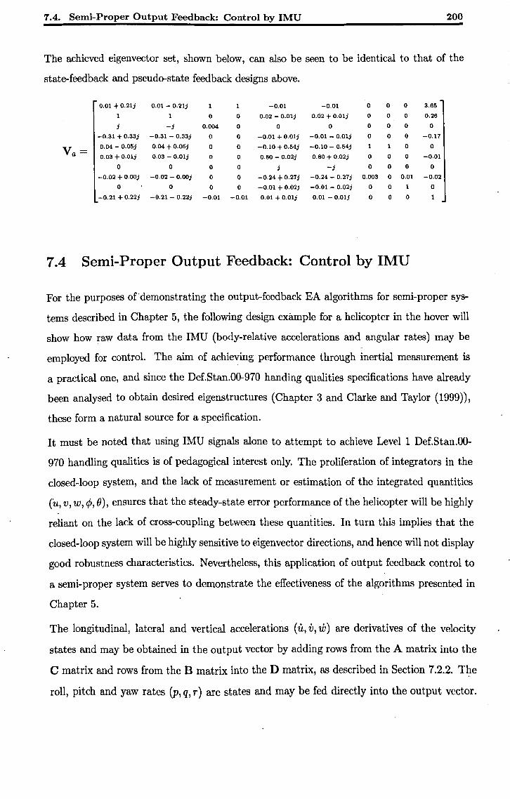
1.4. Semi-Proper Output Feedback: Control by IMU 200
The achieved eigenvector set, shown below, can also be seen to be identical to that of the
state-feedback and pseud~state feedback designs above.
0.01 + 0.21j 0.01 - 0.21j 1 1 -0.01 -0.01 0 0 0 3.65
0 0 0.02 - O.Olj 0.02 + O.Olj 0 0 0 0.26
j -j 0.004 0 0 0 0 0 0 0
-0.31 + 0.33j -0.31 - 0.33j 0 0 -0.01 + O.Olj -0.01 - 0.01; 0 0 0 -0.17
Va= 0.04 - 0.05j 0.04 + 0.05; 0 0 -0.10 + O.54j -0.10 - 0.54j 0 0
0.03 + O.Olj 0.03 - 0.01; 0 0 0.80 - 0.02; 0.80 + 0.02j 0 0 0 -0.01
0 0 0 0 ; -; 0 0 0 0
-0.02 + O.OOj -0.02 - 0.00; 0 0 -0.24 + 0.27j -0.24 - 0.27j 0.003 0 0.01 -0.02
0 0 0 0 -0.01 + 0.02; -0.01 - 0.02j 0 0 1 0
-0.21 + 0.22; -0.21 - 0.22; -0.01 -0.01 0.01 + 0.01; 0.01 - 0.01; 0 0 0 1
7.4 Semi-Proper Output Feedback: Control by IMU
For the purposes of demonstrating the output-feedback EA algorithms for semi-proper sys
tems described in Chapter 5, the following design example for a helicopter in the hover will
show how raw data from the IMU (body-relative accelerations and angular rates) may be
employed for control. The aim of achieving performance through inertial measurement is
a practical one, and since the Def.Stan.00-970 handing qualities specifications have already
been analysed to obtain desired eigenstructures (Chapter 3 and Clarke and Taylor (1999)),
these form a natural source for a specification.
It must be noted that using IMU signals alone to attempt to achieve Level 1 Def.Stan.OO-
970 handling qualities is of pedagogical interest only. The proliferation of integrators in the
closed-loop system, and the lack of measurement or estimation of the integrated quantities
(u, v, w, 4>, e), ensures that the steady-state error performance of the helicopter will be highly
reliant on the lack of cross-coupling between these quantities. In turn this implies that the
closed-loop system will be highly sensitive to eigenvector directions, and hence will not display
good robustness characteristics. Nevertheless, this application of output feedback control to
a semi-proper system serves to demonstrate the effectiveness of the algorithms presented in
Chapter 5.
The longitudinal, lateral and vertical accelerations (it, V, w) are derivatives of the velocity
states and may be obtained in the output vector by adding rows from the A matrix into the
C matrix and rows from the B matrix into the D matrix, as described in Section 7.2.2. Th.e
roll, pitch and yaw rates (p, q, r) are states and may be fed directly into the output vector.
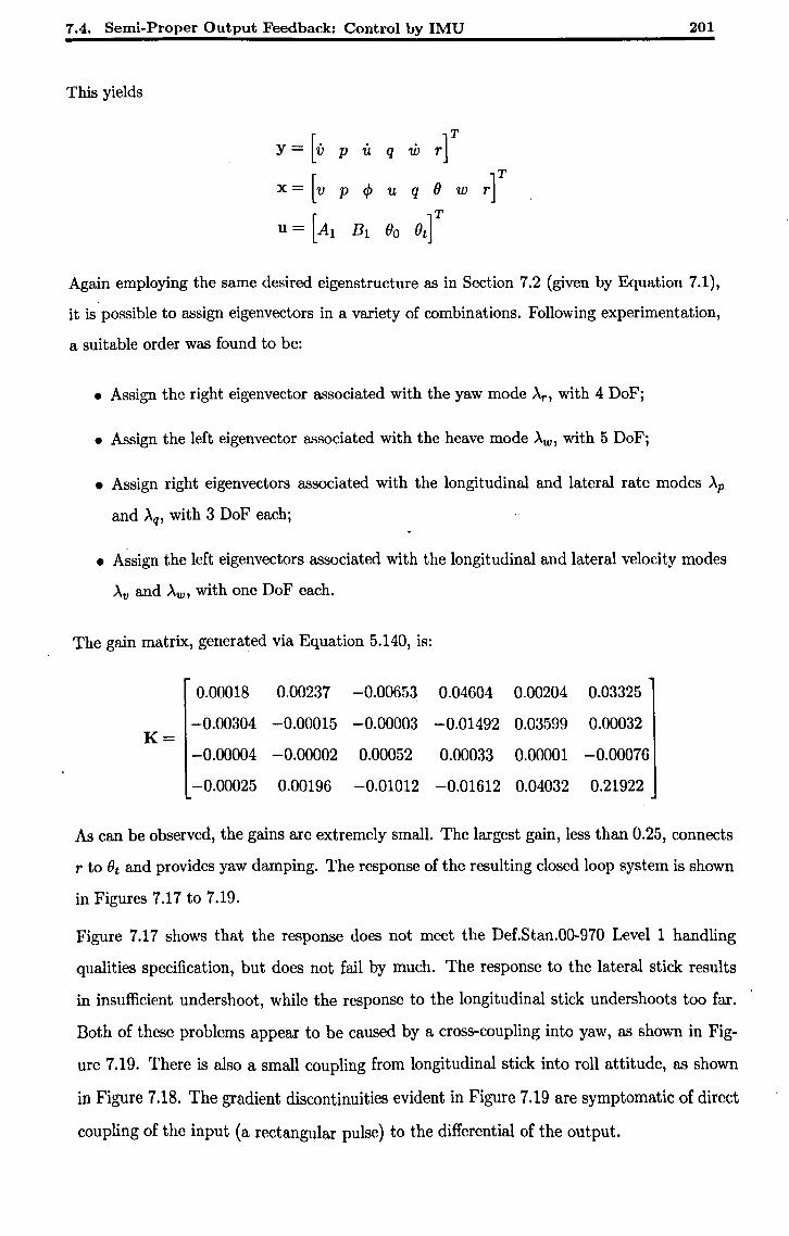
1.4. Semi-Proper Output Feedback: Control by IMU
This yields
y = [v p u q w r]T x = [v p </> u q () w r]T U = [AI BI ()O ()t]T
201
Again employing the same desired eigenstructure as in Section 7.2 (given by Equation 7.1),
it is possible to assign eigenvectors in a variety of combinations. Following experimentation,
a suitable order was found to be:
• Assign the right eigenvector associated with the yaw mode Ar, with 4 DoFj
• Assign the left eigenvector associated with the heave mode Aw , with 5 DoFj
• Assign right eigenvectors associated with the longitudinal and lateral rate modes Ap
and Aq, with 3 DoF each;
• A~sign the left eigenvectors associated with the longitudinal and lateral velocity modes
Av and Aw, with one DoF each.
The gain matrix, generated via Equation 5.140, is:
0.00018 0.00237 -0.00653 0.04604 0.00204 0.03325
-0.00304 -0.00015 -0.00003 -0.01492 0.03599 0.00032 K=
-0.00004 -0.00002 0.00052 0.00033 0.00001 -0.00076
-0.00025 0.00196 -0.01012 -0.01612 0.04032 0.21922
As can be observed, the gains are extremely small. The largest gain, less than 0.25, connects
r to ()t and provides yaw damping. The response of the resulting closed loop system is shown
in Figures 7.17 to 7.19.
Figure 7.17 shows that the response does not meet the Def.Stan.00-970 Level 1 handling
qualities specification, but does not fail by much. The response to the lateral stick results
in insufficient undershoot, while the response to the longitudinal stick undershoots too far.
Both of these problems appear to be caused by a cross-coupling into yaw, as shown in Fig
ure 7.19. There is also a small coupling from longitudinal stick into roll attitude, as shown
in Figure 7.18. The gradient discontinuities evident in Figure 7.19 are symptomatic of direct
coupling of the input (a rectangular pulse) to the differential of the output.
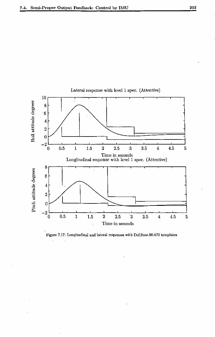
7.4. Semi-Proper Output Feedback: Control by IMU 202
Lateral response with level 1 spec. (Attentive)
10 00
&l 8 6b CD
"6 '"0 CD
'"0 4 ;:j +" ..... +" 2 1d -....... 0 ~
-2 0 0.5 1 1.5 2 2.5 3 3.5 4 4.5 5
Time in seconds Longitudinal response with level 1 spec. (Attentive)
00 8 &l ~ 6 CD
'"0 CD 4 '"0 ::l +" ...... 2 +"
1d "fi 0 +" ...... ~ -2
0 0.5 1 1.5 2 2.5 "3 3.5 4 4.5 5
Time in seconds
Figure 7.17: Longitudinal and lateral responses with Def.Stan.00-970 templates
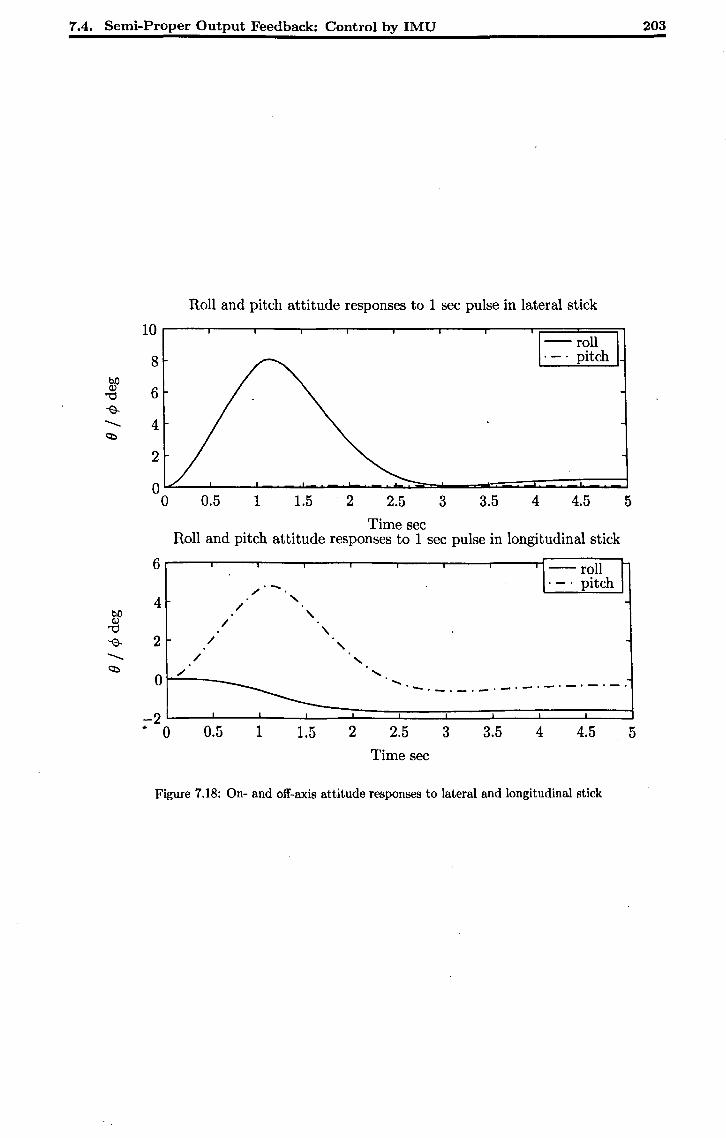
7.4. Semi-Proper Output Feedback: Control by IMU 203
Roll and pitch attitude responses to 1 sec pulse in lateral stick
Time sec Roll and pitch attitude responses to 1 sec pulse in longitudinal stick
6 I roll r /,.-.. . _. pitch
4 ,
b.O / ,
(l) / "0 , -e- 2 / , -.... / , <::b /' .......
0 ..... '~'-.-'-'-'-'-'-.-.-'
-2 .. 0 0.5 1 1.5 2 2.5 3 3.5 4 4.5 5 Time sec
Figure 7.18: On- and off-axis attitude responses to lateral and longitudinal stick
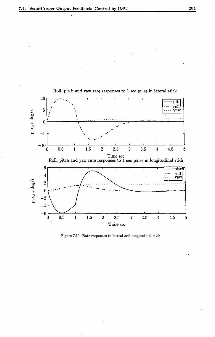
7.4. Semi-Proper Output Feedback: Control by IMU 204
00 -bO Q)
"0 ... 0< 0;
00 -bO Q)
"0 ... 0< 0:
Roll, pitch and yaw rate responses to 1 sec pulse in lateral stick
10 .... '-/ -pitch.
" I .-. roll 5 \ .... yaw
I \ I ........ . .........................................
0 . . . . ' . -.... , ,;
-5 \ ,;
.... '-.-
-10 0 0.5 1 1.5 2 2.5 3 3.5 4 4.5 5
Time sec Roll, pitch and yaw rate responses to 1 sec pulse in longitudinal stick
6
4
2
0
-2
-4
-6 0 0.5 1 1.5 2
--pite 1 . _. roll ... ' ya
.................................
2.5 3' 3.5 4 4.5 Time-sec
Figure 7.19: Rate responses to lateral and longitudinal stick
5'
1.5. Conclusions 205
It is likely that all of these problems could be mitigated by the use of alternative projection
schemes such as iterative projection (Griffin, 1997) or projection with eigenvalue tradeoff
(Clarke et al., 2003); retro-assignment could even be employed (see Section 5.5.2.4), though
with only one available degree of freedom, it is unlikely to offer a tangible benefit.
7.5 Conclusions
It has been seen that the algorithms presented in this thesis provide a suitable mechanism
for the design of controllers for helicopters. In particular, by feeding back state derivatives
via accelerometers, a helicopter has been controlled in the hover using pseudo-state feedback
techniques; without this acceleration feedback, Griffin (1997) resorted to output feedback,
with inevitably inferior results. The output-feedback techniques of Chapter 5 have also been
verified, through the design of a control system to stabilise a hovering helicopter using only
inertial measurements.
EA for forward flight has also been performed, utilising and verifying the ideal eigenstructure
derived in Chapter 3. A state feedback solution, provided for reference, has been matched
'in performance by a pseudo-state feedback solution; a further pseudo-state feedback design,
having more DoFthan required for complete pole placement, has been subjected to the struc
tural imposition techniques of Chapter 6. These techniques have been found to perform
well.
7.6 Chapter Bibliography
Clarke,' T., Griffin, S. J. and Ensor, J. (2003), 'A polynomial approach to eigenstructure assignment using projection with eigenvalue trade-off', International Journal of Control 76(4), 403-413.
Clarke, T. and Taylor, P. (1999), Helicopter design manual, Technical report, Department of Electronics, University of York / Augusta Westland.
Cundy, D. R. and Brown, R. S. (1997), Introduction to avionics, Prentice Hall.
Griffin, S. J. (1997), Helicopter Control Law Design Using Eigenstructure Assignment, PhD thesis, University of York.
Lawrence, A. (1998), Modern inertial technology: Navigation, Guidance, and Control, 2 ecln, Springer, New York.
Miller, K. S. (1987), Some Eclectic Matrix Theory, R. E. Krieger Publishing.

1.6. Chapter Bibliography 206
Siouris, G. M. (1993), Aerospace Avionics Systems: A Modern Synthesis, Academic Press, San Diego.
Titterton, D. H. and Weston, J. L. (1997), Strapdown Inertial Navigation Technology, Peter Peregrinus Ltd., London. '
Chapter 8
Conclusions
Contents 8.1 Eigenstructure Assignment and Helicopters •••.•••..••• 207
8.2 Dynamic Compensators: The Problems . • . • . • • • • . • • . •• 208
8.3 Alternatives to Dynamic Compensation • • • • • • • • • • • • • •• 209
8.4 Imposing Structure •••••• '. . . . • • • • . • . . • • • . • • • •• 210
. 8.5 Applications ............................... 211
8.6 Contributions............................... 212
8.7 F'tlrther Work. . . . . . . . . . . . . . . . . . . . . . . . . . . . . .. 213
8.8 Chapter Bibliography. • • • • • . • • • • • • • • • • • • . • • • • •• 213
In Chapter 1 it was stated that the aim of this thesis was to attack the practice-theory gap
by promoting an understanding of Eigenstructure Assignment (EA) in a classical context,
and by developing algorithms which extend the capabilities of EA towards current practice.
The author asserts that this aim has been met, although further work must be undertaken
to close the gap completely.
8.1 Eigenstructure Assignment and Helicopters
The link between EA and classical control is clear and was drawn to the reader's attention in
Chapter 2. This link is important because the techniques generally used by control engineers
working on helicopters are still Single-Input, Single-Output (SI80) loop-at-a-time techniques
(Taylor, 2006).
The difference between pole placement and EA was discussed, and is highly relevant. The
helicopter is a highly cross-coupled plant, and the ability explicitly to control the coupling
of modes into states by manipulation of the eigenvectors is of great importance. It was seen
207
8.2. Dynamic Compensators: The Problems 208
that true EA, along with sufficient design visibility, is provided only by a small number of
the algorithms currently available.
In Chapter 3, the physical characteristics of the helicopter were investigated in sufficient
detail to gain an understanding of the problems facing the designer of a control system. In
particular, cross-coupling and instability were identified as important issues; the helicopter,
is also highly non-linear, but when working with linear models this is only of significance
inasmuch as it indicates the degree to which the controller gains will need to be 'scheduled'
across the operating envelope - a practice which, although problematic, is commonplace (and
necessary, when the performance specification demands a change in the nature of the pilot
control between hover and forward flight).
The specifications for the response of a helicopter, as given in the UK Ministry of Defence
Defence Standard 00-970 (Def.Stan.00-970) (Pitkin, 1989) are readily converted into restric
tions on pole locations, as demonstrated by Clarke et al. (2003a). This work also involved
the creation of a set of ideal eigenvectors for a helicopter in the hover.
This thesis has introduced a new set of ideal eigenvectors for the case where the movement of
the cyclic pitch stick is expected to generate a response in angular rate rather than attitude.
This is not a trivial problem, and requires the use of a feedback compensator to raise the
order of the open-loop system such· that the coupling from the cyclic pitch inputs to the
body rates is second-order. It has been shown that this process naturally introduces zeros
into the transfer function matrix of the closed-loop system. The eigenvector set has been
demonstrated to be kinematically consistent with the expected motion of the airframe.
8.2 Dynamic Compensators: The Problems
The original aim of this thesis was to investigate the practicability of using dynamic com
pensators to increase the design freedom available for the use of EA. It rapidly became
obvious that the practical problems involved in the successful implementation of dynamic
compensators, and the efficient exploitation of the design freedom they carry, are not trivial.
In Chapter 4, an analysis of the distribution of the design freedom added by a compensator
was performed in the context of EA. It was shown that the introduction of a compensator
increases the order of the system, adds transmission zeros in potentially unpredictable loca
tions, and provides no additional freedom over eigenvector directions. The additional freedom
is available for pole placement, if the system was not pole-assignable before the addition of the
8.3. Alternatives to Dynamic Compensation 209
compensator. The remainder of the freedom is tied up in the compensator sub-eigenvectors,
the directions of which have no effect on the plant outputs.
No available algorithms currently address the issues of dynamic compensation and EA effi
ciently and holistically. Algorithms which place the added transmission zeros (Magni, 1999;
Tsui, 1999) exist, but while these ensure that the zero locations are known, the effective
need for the determination of the poles of the open-loop compensator a priori seems overly
restrictive. Hippe and O'Reilly's (1987) design methodology allows placement of these poles
post-assignment, but does not consider eigenvector assignment explicitly and relies heavily
on symbolic algebra.
In summary, unless the dynamic compensator is required and explicitly defined by the closed
loop system specification, such structures do not currently represent a flexible way of increas-
.. ing the design freedom available for EA.
8.3 Alternatives to Dynamic Compensation
At the end of Chapter 4 it was argued that any technique which increases the rank of the
open-loop output (C) matrix would increase the number of available degrees of freedom,
and do so in a manner that was preferable to the way in which dynamic compensators
do the same. This is because an increase in rank of the C matrix increases the number
of explicitly assignable right eigenvectors without increaSing the system order. This could
render a system pole-assignable, or even allow state-feedback techniques to be used instead of
output feedback techniques. Even if none of these advantages apply, the ability to assign more
right eigenvectors is useful since the mode-input coupling can be influenced by the addition
of a pre-filter if required, while the mode-output coupling cannot be similarly influenced and
is controlled solely by the right eigenvectors; the allowable subspace for any assigned left
eigenvectors is also inflated by an increased rank C matrix.
Increasing the rank of the C matrix can be achieved by adding more sensors to the plant.
There is no reason to suppose the plant will not be well-instrumented already, but any sensor
which measures a state derivative - accelerometers, for example - were heretofore generally
not suited to EA because the appearance of state derivatives in the output vector introduces
nonzero terms into the direct transmission (D) matrix. For example, the helicopter model
considered by Griffin (1997) is controlled using output-feedback techniques because the linear
velocity states were considered to be unmeasurable. If the derivatives of these states could
8.4. Imposing Structure 210
be fed back, the problem would revert to one in which the numbers of outputs and states
were the same.
Chapter 5 was therefore dedicated to the development and description of two novel algorithms
for EA in semi-proper systems. Changes occur to both the input (B) and output (C) matrices
in addition to the system (A) matrix when the loop is closed, and these have been dealt with in
an elegant way. Techniques for assigning the eigenvectors or the modal coupling vectors have
been developed, and the modal coupling vector assignment requires no a priori knowledge of
the inevitable changes to the Band C matrices.
The first of the assignment techniques bears large similarities to the classic state-feedback
EA algorithm of Moore (1976), but cannot be described as state-feedback because the output
and state vectors are different and the D matrix. is nonzero. Hence the term 'pseudo-state
feedback' has been coined to describe this new algorithm. In common with state-feedback
algorithms, it is possible using this technique to assign all the eigenvalues and all of the right
eigenvectors of a system.
The second technique forms a natural extension to the output-feedback EA algorithms of
Clarke et aI. (2003b), and provides access to the eigenvalues and a subset of each of the left
and right eigenvectors in a highly visible parametric form.
Each algorithm has the potential to leave design freedom unused post-assignment. In the case
of the pseudo-state feedback algorithm, this is because the number of outputs may potentially
exceed the number of states. The manner in which this unused freedom is expressed is
essentially consistent between the two systems. In the case of the output-feedback algorithm,
an extension has been presented to allow retro-assignment (Clarke and Griffin, 2004) to take
place. However, in the opinion of the author, it is likely 'that the main performance 'goals
will have been satisfied by the primary assignment of important right eigenvectors, and it
is unlikely that any further manipulation of complimentary eigenvectors will improve the
situation.
8.4 Imposing Structure
The freedom left by the two algorithms described in Chapter 5 has use beyond EA, and
Chapter 6 presented a novel algorithm which used the freedom remaining after the application
of either algorithm, or indeed that of Clarke et aI. (2003b), for imposing structure upon the
gain matrix.. This could be by reducing gain matrix entries to zero, thus severing paths
8.5. Applications 211
between the system outputs and inputs, or by forcing certain sets of entries to be equal or to
be 'geared' in a given ratio.
The effect of the imposition of structure upon the ov:erall magnitude of the entries in the gain
matrix has been considered, and expressions for the minimum Frobenius norm of the gain
matrix both before and after the process have been generated. These should assist in the
choice of structural constraints. It is interesting to note that some structural constraints will
have more effect on the overall gains than others, and so to some extent the final structure
of the controller is governed (or at least influenced) by the initial EA process.
8.5 Applications
Chapter 7 provided design examples to support the algorithmic development described above.
The hover case was considered first, and it was shown that by using feedback from accelerom
eters, the pseudo-state feedback algorithm of Chapter 5 was able to retain the performance
of a state-feedback solution while using only measurable information. In the same context,
Griffin (1997) had resorted to output feedback, and the results were inevitably inferior.
Forward flight required the use of the ideal eigenstructure derived in Chapter 3. Using this
eigenstructure, Level 1 handling qualities were obtained at 60 knots using both state-feedback
and pseudo-state feedback algorithms, demonstrating that the eigenstructure is correct both
kinematic ally and in terms of the Def.Stan.00-970 specification.
A pseudo-state feedback controller was also designed for forward flight that had excessive
Degrees of Freedom (DoF), and the remaining DoF after EA were used to impose structure
on the controller. This demonstrated well the operation of the algorithm of Chapter 6.
In addition, a pedagogical case was presented wherein it was attempted to control a helicopter
in forward flight using only the signals from an Inertial Measurement Unit (IMU) - that is,
the roll, pitch and yaw rates and the body accelerations. The output feedback algorithm
from Chapter 5 was used and the responses generated were not far from meeting Level 1
Def.Stan.00-970 specifications despite the lack of feedback from the body angle states and a
consequent inability to control steady-state errors.
8.6. Contributions 212
8.6 Contributions
To the best of the author's knowledge, the list below describes the novel contributions of this
work:
• Derivation of a new ideal eigenstructure that meets the Def.Stan.00-970 response criteria
for Level 1 handling qualities in forward flight, and demonstration that it is appropriate.
• Derivation of all ideal second-order yaw response eigenstructure.
• Characterisation of the design freedom offered by dynamic compensators in terms of the
effect solely on the plant sub-eigenvectors, namely the rank and mutual orthogonality
of the assigned eigenvector subsets.
• Analysis of the design freedom offered by a feedforward compensator term, and how
this freedom may be exploited.
• Analysis of the effects on the modal coupling matrices of the change to the input and
output matrices of a semi-proper system under feedback.
• Development of a novel algorithm to effect 'pseudo-state feedback' control for semi
proper systems, offering a substantially identical design procedure to that of standard
state-feedback EA.
• Characterisation of the design freedom remaining after the assignment of eigenstructure
to a system with more outputs than states.
• Development of a novel algorithm to allow output-feedback EA to be conducted on
semi-proper systems.
• Characterisation of any remaining design freedom from the semi-proper output-feedback
EA process in a form which allows a retro-assignment stage to be performed, and the
development of this technique to reflect the change to the system input and output
matrices in the closed loop.
• Implementation of Proportional-plus-Derivative (PD) controllers using semi-proper sys
tem descriptions, allowing EA to be conducted in a single, visible stage.
• A new analysis of the design freedom remaining after EA, and the resulting discovery
of a method by which it may be used to impose structure upon the controller.
8.7. Further Work 213
• Design of an algorithm to allow the freedom remaining after output-feedback EA, semi
proper output-feedback EA or pseudo-state feedback EA to be used for this purpose.
• Development of tools for the analysis of the effect of the imposition of structure on the
overall magnitude of the gain matrix elements.
8.7 Further Work
Several areas have been identified in this thesis which warrant further work.
Chapter 4 revealed some problems with the available algorithms for performing EA on com
pensated systems. The ideal algorithm for the purposes of EA would constrain the trans
mission zeros, allow full control of eigenvalue locations and plant sub-eigenvector directions,
and present the unused design freedom in a usable form. This would allow the EA process
to inform the design of a controller structure, rather than vice-versa.
The idea of adding feedforward terms to feedback compensators was introduced. Section 4.6.3
contains several ideas for the potential exploitation of the design freedom offered post
assignment by this technique, and these would form an ideal starting point for a programme
of further work on this topic. Structural constraints, transmission zero placement and ro
bustness improvement are just a few of the potential applications for this extra freedom.
The algorithm for introducing structural constraints in Chapter 6, at present, utilises only the
design freedom remaining after EA. If similar techniques could be used to restrict the available
set of gains during assignment, while still allowing freedom over eigenvector selection, this
could potentially provide an algorithm for using EA to optimise the gains of existing control
structures. This would be an interesting new application area for EA.
8.8 Chapter Bibliography
Clarke, T. and Griffin, S. J. (2004), 'An addendum to output feedback eigenstructure assignment:retro-assignment', International Journal of Control 77(1), 78-85.
Clarke, T., Griffin, S. J. and Ensor, J. (2003 a) , 'Desirable eigenstructure for good shortterm helicopter handling qualities: the attitude command response case', Preceedings of the I MECH E Part G Journal of Aerospace Engineering 217(1), 43-55.
Clarke, T., Griffin, S. J. and Ensor, J. (2003b), 'Output feedback eigenstructure assignment using a new reduced orthogonality condition', International Journal of Control 76(4), 390-402.
8.8. Chapter Bibliography 214
Griffin, S. J. (1997), Helicopter Control Law Design Using Eigenstructure Assignment, PhD thesis, University of York.
Hippe, P. and Q'Reilly, J. (1987), 'Parametric compensator design', International Journal of Control 45, 1455-1468.
Magni, J. F. (1999), 'Multimodel eigenstructure assignment in flight-control design', Aerospace Science and Technology 3(3), 141-15l.
Moore, B. C. (1976), 'On the flexibility offered by state feedback in multivariable systems beyond closed loop eigenvalue assignment', IEEE Transactions on A utomatic Control 21, 689-692.
Pitkin, B. (1989), 'Flight and ground handling qualities', Military Defence Specification DEFSTAN 00-970, Vol. 2, Part 6, Ministry of Defence.
Taylor, P. (2006), Personal communications. Technical Leader, Aircraft Dynamics (Rotary Wing), QinetiQ, Boscombe Down, UK.
Tsui, C.-C. (1999), 'A new dynamic output feedback compensator design for pole placement', Journal of the F'ranklin Institute 336(4), 665-674.
Appendix A
Helicopter Linearisations
Contents A.l Algorithm Descriptions •••.••••••.••• '. • • • • • • • • •• 215
A.Ll '!'rim.................................... 216 A.L2 Linearisation and Normalisation ............... ; .... 216 A.L3 Model Reduction ............................. 217
A.2 Linearisation at Hover ••••••.•••••••••••••••.•• 217
A.2.1 State Space Description . . . . . . . . . . . . . . . . . . . . . . . . . 217 A.2.2 Reduced-Order Model .......................... 218
A.3 Linearisation at 60 Knots ••••••••••••••••••••••. 220
A.3.1 State Space Description ......................... 220 A.3.2 Reduced-Order Model . . . . . . . . . . . . . . . . . . . . . . . . . . 221
A.4 Appendix Bibliography • . • • • . • • • • ~ • • • • • • • • • • • • •• 222
For the design examples presented in Chapter 7, simplified linear approximations to a non
linear 11 tit.. order model of a Lynx helicopter were employed. This Appendix provides an
overview of the algorithms used to obtain the linear models, together with the state-variable
descriptions of the models so obtained. For the sake of allowing direct comparison, the pr~
cedure used for generating the linear models was the same as that used by Griffin (1997),
and is simply summarised here for reference.
A.I Algorithm Descriptions
In order to extract a linear model from a non-linear one, it is first necessary to obtain an
operating point about which a linear approximation can be formed. This process is known
as trimming. In the case of the design examples of Chapter 7, two trim points {hover and
215
A.!. Algorithm Descriptions 216
forward flight at 60 knots) were chosen. Secondly, a linear approximation to the system at
these points must be found; and thirdly, the model must be reduced in complexity to remove
the near-uncontrollable blade flapping modes.
A.1.1 Trim
Before the model can be linearised, an operating point must be found where the system is in
equilibrium.
In the case of the hover, this point is with zero body velocities and accelerations, zero angular
rates and angular rate derivatives, and zero blade flapping angle derivatives. The body angles
are not constrained. At 60 knots, the trim point is with zero angular rates and angular rate
derivatives, zero body accelerations and heave velocity, and a zero roll angle with the pilot
tolerating (and expecting) a small sideslip angle (Griffin, 1997). Once again the flapping
angle derivatives are required to be zero, but the pitch angle is unconstrained, as is lateral
velocity.
For the purposes of the design examples in this thesis, trimming was .conducted using a
Newton-Raphson nonlinear equation solver, after Griffin (1997) who achieved success with
the same method on the same model.
A.1.2 Linearisation and Normalisation
The linearisation of a nonlinear function around a given point is a first-order Taylor approx
imation about that point. Such an approximation is easily calculated by perturbing each
state and input in turn an observing its effect on the state derivatives to form entries in the
A and B matriCes. For the work in this thesis, an algorithm to adjust the perturbation sizes
automatically (Clarke and Griffin, 2003) was employed in order to generate a model that was
valid over as wide a range of operating conditions as possible.
Griffin (1997) also developed a set of normalisations for the model such that two eigenvector
elements of equal magnitude would result in a perceived equal coupling of the mode into the
two states. The normalisation values are given in Table A.1.2.
These normalisations have not been applied to the linear models as given below, but were
instead applied (in inverse form) to the desired eigenstructure before assignment.
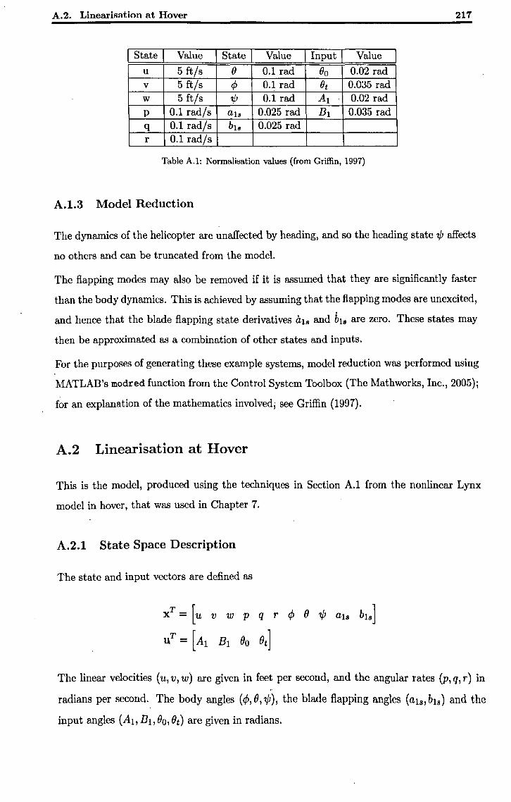
A.2. Linearisation at Hover 217
I State I Value I State I Value I Input I Value u 5 ft/s () 0.1 rad ()o 0.02 rad v 5 ft/s </> 0.1 rad (h 0.035 rad w 5 ft/s 'IjJ 0.1 rad A1 0.02 rad p 0.1 rad/s als 0.025 rad B1 0.035 rad q 0.1 rad/s b1s 0.025 rad r 0.1 rad/s
Table A.l: Normalisation values (from Griffin, 1997)
A.1.3 Model Reduction
The dynamics of the helicopter are unaffected by heading, and so the heading state 'I/J affects
no others and can be truncated from the model.
The flapping modes may also be removed if it is assumed that they are significantly faster
than the body dynamics. This is achieved by assuming that the flapping modes are unexcited,
and hence that the blade flapping state derivatives a1s and b1s are zero. These states may
then be approximated as a combination of other states and inputs.
For the purposes of generating these example systems, model reduction was performed using
MATLAB's modred function from the Control System Toolbox (The Mathworks, Inc., 2005);
for an explanation of the mathematics involved; see Griffin (1997).
A.2 Linearisation at Hover
This is the model, produced using the techniques in Section A.l from the nonlinear Lynx
model in hover, that was used in Chapter 7.
A.2.1 State Space Description
The state and input vectors are defined as
xT = [u v w p q r </> () 'I/J als bls]
UT = [AI BI eo et]
The linear velocities (u,v,w) are given in feet per second, and the angular rates (p,q,r) in ..
radians per second. The body angles (</>, e, 'I/J), the blade flapping angles (aI s, bls) and the
input angles (Ab BI, 00 , ()t) are given in radians.
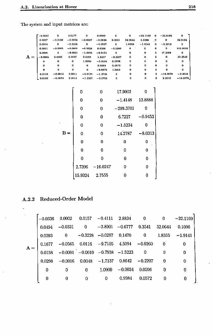
A.2. Linearisation at Hover 218
The system and input matrices are:
-0.0043 0 0.0177 0 0.0089 0 0 -32.1169 0 -32.8194 0
0.0007 -0.0169 -0.0034 -0.0697 -0.0626 0.3541 32.0644 0.1096 0 0 32.8194
0.0314 0 -0.3226 0 -0.0537 0 1.8355 -1.9141 0 -2.2912 0
0.0001 -0.0005 -0.0001 -0.0028 6.6266 -0.0260 0 0 0 0 112.9618
0.0005 0 -0.0021 -1.0094 -0.0153 0 0 0 0 17.2069 0
A= -0.0004 0.0085 0.0027 0.0355 1.2457 -0.2207 0 0 0 0 20.3546
0 0 0 1.0000 -0.0034 0.0596 0 0 0 0 0
0 0 0 0 0.9984 0.0572 0 0 0 0 0
0 0 0 0 -0.0573 1.0001 0 0 0 0 0
0.0158 -0.0012 0.0011 -0.0131 -1.2725 0 0 0 0 -14.0578 -2.2016
0.0189 -0.0070 0.0013 -1.2357 -0.0706 0 0 0 0 2.2016 -14.0578
0 0 17.9002 0
0 0 -1.4148 12.8888
0 0 -299.3701 0
0 0 6.7227 -0.9453
0 0 -1.5234 0
B= 0 0 14:2787 -8.0313
0 0 0 0
0 0 0 0
0 0 0 0
2.7396 -16.0247 0 0
15.9324 2.7555 0 0
A.2.2 Reduced-Order Model
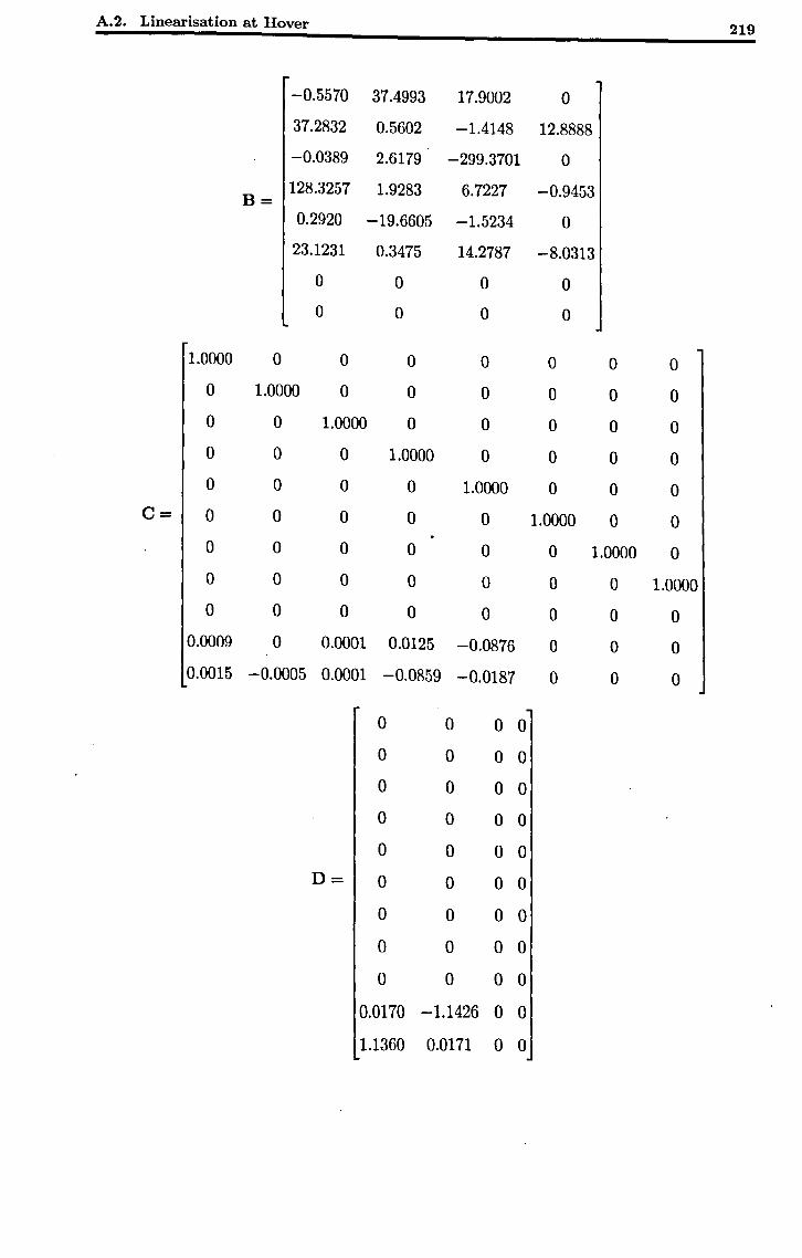
A.2. Linearisation at Hover 219
-0.5570 37.4993 17.9002 0
37.2832 0.5602 -1.4148 12.8888
-0.0389 2.6179 -299.3701 0
B= 128.3257 1.9283 6.7227 -0.9453
0.2920 -19.6605 -1.5234 0
23.1231 0.3475 14.2787 -8.0313
0 0 0 0
0 0 0 0
1.0000 0 0 0 0 0 0 0
0 1.0000 0 0 0 0 0 0
0 0 1.0000 0 0 0 0 0
0 0 0 1.0000 0 0 0 0
0 0 0 0 1.0000 0 0 0
c= 0 0 0 0 0 1.0000 0 0
0 0 0 0 0 0 1.0000 0
0 0 0 0 0 0 0 1.0000
0 0 0 0 0 0 0 0
0.0009 0 0.0001 0.0125 -0.0876 0 0 0
0.0015 -0.0005 0.0001 -0.0859 -0.0187 0 0 0
0 0 0 0
0 0 0 0
0 0 0 0
0 0 0 0
0 0 0 0
D= 0 0 0 0
0 0 0 0
0 0 0 0
0 0 0 0
0.0170 -1.1426 0 0
1.1360 0.0171 0 0
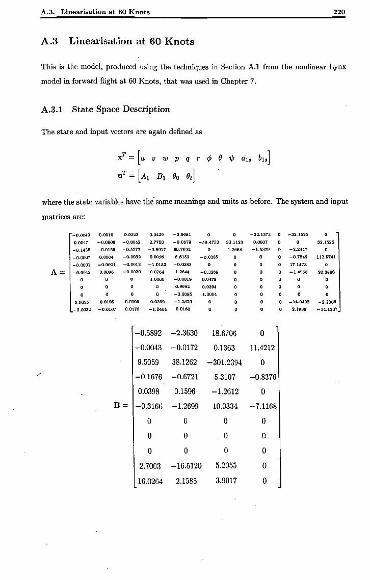
A.3. Linearisation at 60 Knots 220
A.3 Linearisation at 60 Knots
This is the model, produced using the techniques in Section A.l from the nonlinear Lynx
model in forward flight at 60 Knots, that was used in Chapter 7.
A.3.1 State Space Description
The state and input vectors are again defined as
xT = [u v w p q r 4> () 'I/J aIs bIs]
uT ,,; [AI RI 00 (}t]
where the state variables have the' same meanings and units as before. The system and input
matrices are:
-0.0040 0.0010 0.0322 0.0429 -2.9081 0 0 -32.1373 0 -32.1525 0
0.0047 -0.0806 -0.0042 2.7750 -0.0879 -59.4753 32.1123 0.0607 0 0 32.1525
-0.1435 -0.0159 -0.5577 -0.6917 60.7602 0 1.2664 -1.5379 0 -2.2447 0
-0.0007 0.0034 -0.0032 0.0096 6.6152 -0.0385 0 0 0 -0.7849 112.5741
-0.0001 -0.0001 -0.0013 -1.0153 -0.0383 0 0 0 0 17.1473 0
A= -0.0042 0.0098 -0.0020 0.0764 1.2644 -0.3269 0 0 0 -1.4968 20.2886
0 0 0 1.0000 -0.0019 0.0479 0 0 0 0 0
0 0 0 0 0.9992 0.0394 0 0 0 0 0
0 0 0 0 -0.0395 1.0004 0 0 0 0 0
0.0055 0.0105 0.0105 0.0399 -1.2329 0 0 0 0 -14.0402 -2.2306
-0.0032 -0.0107 0.0170 -1.2404 0.0160 0 0 0 0 2.1939 -14.1237
-0.5892 -2.3630 18.6706 0
-0.0043 -0.0172 0.1363 11.4212
9.5059 38.1262 -301.2394 0 / -0.1676 -0.6721 5.3107 -0.8376
0.0398 0.1596 -1.2612 0
B= -0.3166 -1.2699 10.0334 -7.1168
0 0 0 0
0 0 0 0
0 0 0 0
2.7003 -16.5120 5.2055 0
16.0264 2.1585 3.9017 0
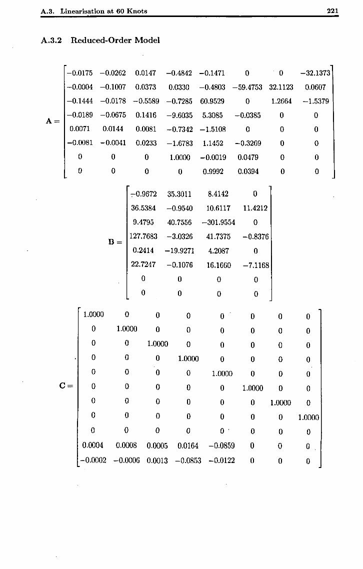
A.3. Linearisation at 60 Knots 221
A.3.2 Reduced-Order Model
-0.0175 -0.0262 0.0147 -0.4842 -0.1471 0 ·0 -32.1373
-0.0004 -0.1007 0.0373 0.0330 -0.4803 -59.4753 32.1123 0.0607
-0.1444 -0.0178 -0.5589 -0.7285 60.9529 0 1.2664 -1.5379
-0.0189 -0.0675 A=
0.1416 -9.6035 5.3085 -0.0385 0 0
0.0071 0.0144 0.0081 -0.7342 -1.5108 0 0 0
-0.0081 -0.0041 0.0233 -1.6783 1.1452 -0.3269 0 0
0 0 0 1.0000 -0.0019 0.0479 0 0
0 0 0 0 0.9992 0.0394 0 0
7"0.9672 35.3011 8.4142 0
36.5384 -0.9540 10.6117 11.4212
9.4795 40.7556 -301.9554 0
B= 127.7683 -3.0326 41.7375 -0.8376
0.2414 -19.9271 4.2087 0
22.7247 -0.1076 16.1660 -7.1168
0 0 0 0
0 0 0 0
1.0000 0 0 0 0 0 0 0
0 1.0000 0 0 0 0 0 0
0 0 1.0000 0 0 0 0 0
0 0 0 1.0000 0 0 0 0
0 0 0 0 1.0000 0 0 0
c= 0 0 0 0 0 1.0000 0 0
0 0 0 0 0 0 1.0000 0
0 0 0 0 0 0 0 1.0000
0 0 0 0 O· 0 0 0
0.0004 0.0008 0.0005 0.0164 -0.0859 0 0 0
-0.0002 -0.0006 0.0013 -0.0853 -0.0122 0 0 0
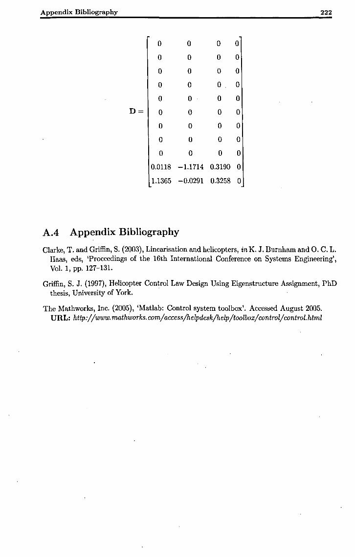
Appendix Bibliography 222
0 0 0 0
0 0 0 0
0 0 0 0
0 0 0 0
0 0 0 0
D= 0 0 0 0
0 0 0 0
0 0 0 0
0 0 0 0
0.0118 -1.1714 0.3190 0
1.1365 -0.0291 0.3258 0
A.4 Appendix Bibliography
Clarke, T. and Griffin, S. (2003), Linearisation and helicopters, in K. J.llurnham and O. C. L. Haas, eds, 'Proceedings of the 16th International Conference on Systems Engineering', Vol. 1, pp. 127-131.
Griffin, S. J. (1997), Helicopter Control Law Design Using Eigenstructure Assignment, PhD thesis, University of York.' .
The Mathworks, Inc. (2005), 'Matlab: Control system toolbox'. Accessed August 2005. URL: http://www.rnathworks.com/access/helpdesk/help /toolbox/ control! control. htrnl
Appendix B
Supporting Mathematics
Contents B.l Introduction . . . . . . . . . . . . . . . . . . . . . . . . . . . . . . . 223
B.2 Complex Eigenvector Extension to Section 4.4 • • • • • • • • • •• 223
B.3 Minimum Frobenius norm for Section 6.4.1 • • • • • • • • • • • •• 224
B.4 Differentiation for Section B.3. . • • • . • • • • • • • • • • • • • •• 226
B.5 Appendix Bibliography • • . • • • • . • • • • • • • • • • • • • • • •• 228
B.1 Introduction
This Appendix contains mathematical derivations which support the derivations in the main
body of this thesis, but which would act as a distraction if placed therein.
B.2 . Complex Eigenvector Extension to Section 4.4
The assigned eigenvector subsets in Equation 4.57 must form self-conjugate sets. Assuming
that the rows of W~ and the columns of V~ are arranged such that conjugate pairs are next
to each other, two matrices r wE c(n+c-v)x(n+c-v) and r v E CVXV may be formed with block
diagonal structures. The blocks on the leading diagonal of r ware:
• A '1' corresponding to any real row in W~;
• A block [1 j.] corresponding to any conjugate pair of rows in W~. 1 -J
Similarly the blocks on the leading diagonal of r v are:
223
B.3. Minimum Frobenius norm for Section 6.4.1
• A '1' corresponding to any real column in V~j
. A block [~ 1.] corresponding to any conjugate pair of columns in V~. J -J .
It is easily verified that it is therefore possible to write
where W~ and V~r are real-valued.
w~=rwW~r
V~ = V~rrv
224
(B.l)
(B.2)
The nature and order of the conjugate rows and columns in W~ and V~ must be the same
as those of W~ and V~. Hence the terms W x and V x can be formed by setting
WxVx = W~rV~r (B.3)
in place of Equation 4.57. The compensator sub-eigenvector sets may then be chosen using
where RI and R2 are still real-valued.
B.3 Minimum Frobenius norm for Section 6.4.1
Because vec K is simply a rearrangement of entries,
IKIF = IIvecKII
and therefore
IKIF= 11(1-(US)t U) (vecKo + SvecZ) 11
= 11 (I - (US)t U) vecKo + (I - (US)t U) BvecZl1
(BA)
(B.5)
(B.6)
(B.7)
(B.S)
B.3. Minimum Frobenius norm for Section 6.4.1 225
The problem is now one of solving an equation of the form
d dx IIAx+yll = 0 (B.9)
to find a minimum. It may be shown (see Section B.4 of this Appendix) that
d AT (Ax+y) dx IIAx + yll = IIAx + yll (B.lO)
and therefore we must solve
d~ 11 (I - (US)t U) vecKo + (I - (US)t U) Svec Zll = 0 (B.11)
i.e.
(S - (US)t US) T ((I - (US)t U) vecKo + (I - (US)t U)3 vec Z) = 0 (B.12)
so,
(s-(US)tus) ((I-(US)tU)vecKo+ (1-(US)tU)SvecZ) =0 (B.13)
since At A and 8 are both symmetric.
Equation B.l3 may be simplified further:
(8 - (UB)tUB) (vecKo - (UB)tUvecKo+ 8vecZ - (US)tusvecZ) = 0 (B.14)
8 vec Ko - 8 (US) t U vec Ko + S2 vec Z - B (UB) t UB vec Z
- (US) t US vec Ko + (US) t UB (US) t U vec Ko .
+ (UB)tUB2vecZ - (US)tUBvecZ ~ 0 (B.15)
B vec Ko - (US) t U vec Ko + S vec Z - (US) t UB vec Z
- (US) t US vec Ko + (US) t U vec Ko
+ (US) t US vec Z - (US) t US vec Z = 0 (B.16)
S vec Ko - (US) t US vec Ko + B vec Z - (US) t US vec Z = 0 (B.17)
since S is idempotent (the identity of Equation 6.36 is employed). Hence
(I - (US)t U) S vec Ko + (I - (UB)t U) Bvec Z = 0 (B.18)
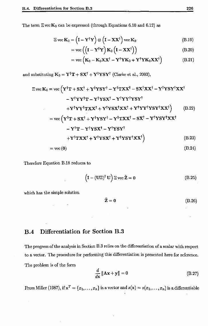
B.4. Differentiation for Section B.3
The term BvecKo can be expressed (through Equations 6.10 and 6.12) as
B vec Ko = (I - yty ) ® (I - xxt) vecKo
= vec ( (I - yty ) Ko (I - XXt) )
= vec (Ko - KoXXt - ytYKo + ytYKoxxt)
and substituting Ko = ytT + SXt + ytYSyt (Clarke et al., 2003),
226
(B.19)
(B.20)
(B.21),
B vec Ko = vec (ytT + SXt + ytYSyt - ytTXXt - SXtxxt - ytYSytxxt
- ytyytT _ ytYSxt _ ytyytYSyt
+ ytyytTXXt + ytYSxtxxt + ytyytYSytxxt) (D.22)
= vec (ytT + SXt + ytYSyt - ytTXXt - SXt - ytYSytxxt
- ytT - ytYSxt - ytYSyt
+ ytTXXt + ytYSxt + ytYSytXXt)
= vec (0)
Therefore Equation B.18 reduces to
(I - (UB) tu) B vec Z = 0
which has the simple solution
z=o
B.4 Differentiation for Section B.3
(D.23)
(B.24)
(B.25)
(B.26)
The progress of the analysis in Section B.3 relies on the differentiation of a scalar with respect
to a vector. The procedure for performing this differentiation is presented here for reference.
The problem is of the form d ' -I\Ax+yl\ = 0 dx
(D.27)
From Miller (1987), ifxT = {Xl, •.• ! Xn} is a vector and s(x) = S(XI! •.. ! xn) is a differentiable

B.4. Differentiation for Section B.3
scalar function of x,
So:
For each element:
Evaluating the square gives
as 8x1
d t:. dxS(X) =
as &n
221
(B.28)
(0.29)
(0.30)
(0.31)
(0.32)
(D.33)
The terms in parentheses have no dependency on Xk. This is demonstrated by expanding the
summations over j to give
n
L (aijXj) - aikXk + Yi = ai1 Xl + ai2X2 + ... + ainXn - aikxk + Yi
j=1
(B.35)
(B.36)
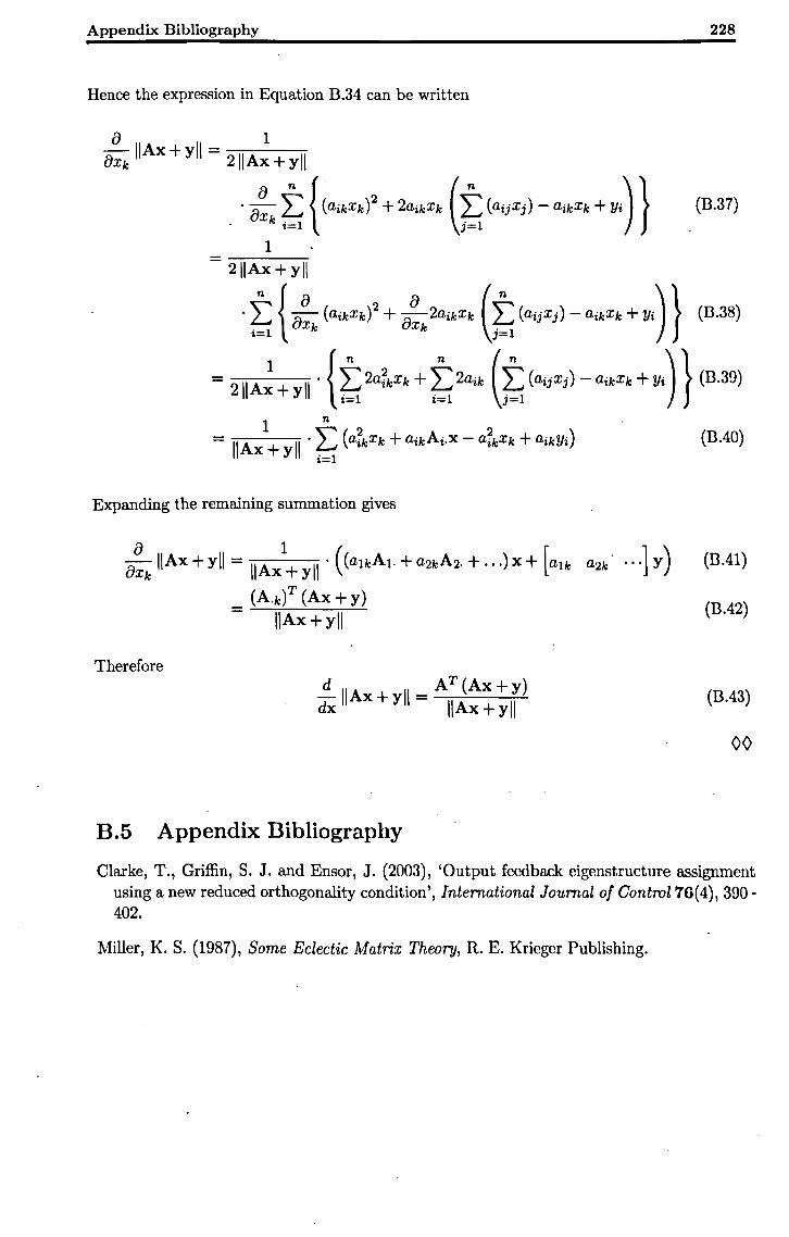
Appendix Bibliography
Hence the expression in Equation B.34 can be written
Expanding the remaining summation gives
a~k IIAx + y\\ = 1\ Ax1+ yll . (alkA1. + a2k A 2. + ... ) x + [a1k a2k
(A.kf (Ax + y) -
IIAx + yll
Therefore d A AT(Ax+y) dx 11 x+yl\ = IIAx+yll
B.5 Appendix Bibliography
228
(B.37)
(DAO)
(llA1)
(llA2)
(DA3)
00
Clarke, T., Griffin, S. J. and Ensor, J. (2003), 'Output feedback eigenstructure assignment using a new reduced orthogonality condition', International Journal of Control 76(4), 390-402.
Miller, K. S. (1987), Some Eclectic Matrix Theory, R. E. Krieger Publishing.
Appendix C
Matrix Notation
Contents C.1 Introduction . . . . . . . . . . . . . . . . . . . . . . . . . . . . . . . 229
C.2 Column, Row and Element Notation. • • • • • • • • • • • • • • •• 229
C.3 Definitions of Operators •••••••••••••••••••••••• 230
C.4 Appendix Bibliography • • • • • • • • • • • • • • • • • • • • • • • •• 231
C.l Introduction
The nature of this thesis dictates that much of the content is presented in mathematical form.
This Appendix contains details, for reference, of some of the more important (and obscure)
aspects of the matrix notation used.
C.2 . Column, Row and Element Notation
Matrix subscripts identify individual elements, rows or columns.
229
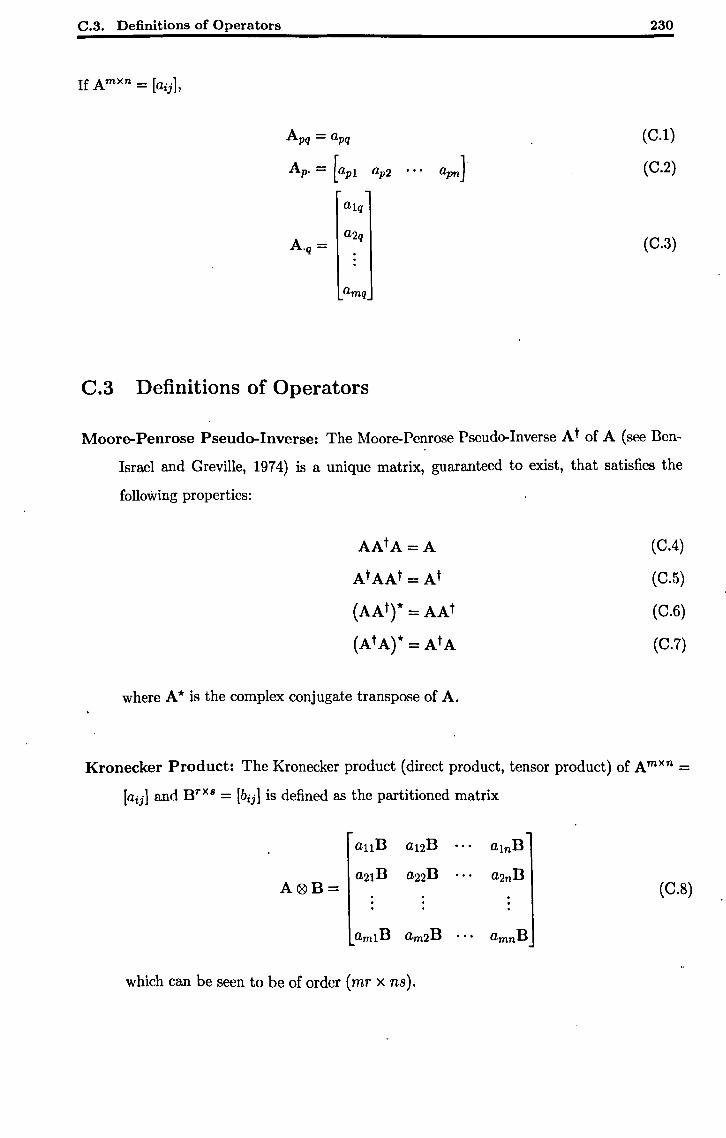
C.3. Definitions of Operators
Apq = apq
Ap. = rap! ap2 ••• apn ]
C.3 Definitions of Operators
230
(c.1)
(C.2)
(C.3)
Moore-Penrose Pseudo-Inverse: The Moore-Penrose Pseudo-Inverse At of A (see llen
Israel and Greville, 1974) is a unique matrix, guaranteed to exist, that satisfies the
following properties:
AAtA=A
AtAAt = At
(AAt)* = AAt
(AtAr = AtA
where A * is the complex conjugate transpose of A.
(C.4)
(C.5)
(C.6)
(C.7)
Kronecker Product: The Kronecker product (direct product, tensor product) of Amxn = [aij] and BrxB = [bij ] is defined as the partitioned matrix
(C.8)
which can be seen to be of order (mr x ns).
Appendix Bibliography 231
Vec Operator: The vec operator converts a matrix of order (m x n) into a vector of length
mn and is defined as
(C.9)
C.4 Appendix Bibliography
Ben-Israel, A. and Greville, T. N. E. (1974), Generalised Inverses: Theory and Applications, John WHey and Sons Ltd.
Bibliography
Alexandridis, A. T. and Paraskevopoulos, P. N. (1996), 'A new approach to eigenstructure
assignment by output feedback', IEEE Transactions on Automatic Control 41(7), 1046-
1050.
Andry, A. N., Shapiro, E. Y. and Chung, J. C. (1983), 'Eigenstructure assignment for linear
systems', IEEE Transactions on Aerospace and Electronic Systems 19(5), 711-727.
Askarpour, S. and Dwens, T. J. (1997), 'Integrated approach to eigenstructure assignment by
output feedback control', lEE Proceedings - Control Theory and Applications 144(5), 435-
438.
Astrom, K. J. (1999), Automatic control - the hidden technology, in P. M. Frank, ed., 'Ad
vances in Control: Highlights of ECC'99', Springer-Verlag.
Banks, S. P. (1986a), Control Systems Engineering, Prentice-Hall.
Banks, S. P. (1986b), Control systems engineering: modelling and simulation, control theory
and microprocessor implementation, Prentice-Hall.
Den-Israel, A. and Greville, T. N. E .. (1974), Generalised Inverses: Theory and Applications,
John WHey and Sons Ltd.
Blight, J. D., Dailey, R. L. and Gangaas, D. (1994), 'Practical control law design for aircraft
using multivariable techniques', International Journal of Control 59(1), 93-137.
Dramwell, A. R. S. (1976), Helicopter Dynamics, Edward Arnold.
Drockett, R. W. and Byrnes, C. I. (1981), 'Multivariable nyquist criteria, root loci, and pole
placement: A geometric viewpoint', IEEE Transactions on Automatic Control 26(1), 271-
283.
Brogan, W. L. (1991), Modern Control Theory, 3 edn, Prentice Hall.
232
Bibliography 233
Burrows, S. P. (1990), Robust control design techniques using eigenstructure assignment,
PhD thesis, University of York.
Clarke, T. and Griffin, S. (2003), Linearisation and helicopters, in K. J. Burnham and O. C. L.
Haas, eds, 'Proceedings of the 16th International Conference on Systems Engineering',
Vol. 1, pp. 127-131.
Clarke, T. and Griffin, S. J. (2004), 'An addendum to output feedback eigenstructure
assignment:retro-assignment', International Journal of Control 77(1), 78-85.
Clarke, T., Griffin, S. J. and Ensor, J. (2003 a), 'Desirable eigenstructure for good short
term helicopter handling qualities: the attitude command response case', Preceedings of
the I MECH E Part G Journal of Aerospace Engineering 217(1), 43-55.
Clarke, T., Griffin, S. J. and Ensor, J. (2003b), 'Output feedback eigenstructure assignment
using a new reduced orthogonality condition', International Journal of Control 76(4), 390-
402.
Clarke, T., Griffin, S. J. and Ensor, J. (2003 c) , 'A polynomial approach to eigenstructure
assignment using projection with eigenvalue trade-off', International Journal of Control
76( 4), 403-413.
Clarke, T. and Taylor, P. (1999), Helicopter design manual, Technical report, Department of
Electronics, University of York / AugustaWestland.
Cundy, D. R. and Brown, R. S. (1997), Introduction to avionics, Prentice Hall.
Davies, R, (1994), Robust eigenstructure assignment for flight control applications, PhD
thesis, University of York.
Davison, E. and Chatterjee, R. (1971), 'A note on pole assignment in linear systems with
incomplete state feedback', IEEE Transactions on Automatic Control 16(1), 98-99.
Davison, E. J. and Wang, S. H. (1975), 'On pole assignment in linear systems with incomplete
state feedback', IEEE Transactions on Automatic Control 24(3), 516-518.
Doyle, J. C. and Stein, G. (1979), 'Robustness with observers', IEEE Transactions on Auto
matic Control 24(4), 607-611.
Doyle, J. C. and Stein, G. (1981), 'Multivariable feedback design: Concepts for a classi
cal/modern synthesis', IEEE Transactions on Automatic Control 26(1), 4-16.
Bibliography 234
Duan, G.-R. (1993), 'Solutions of the equation AV + BW = VF and their application to
eigenstructure assignment in linear systems', IEEE Transactions on Automatic Control
38(2), 276-280.
Duan, G.-R. (1998), 'Eigenstructure assignment and response analysis in descriptor linear
systems with state feedback control', International Journal of Control 69(5), 663-694.
Duan, G.-R. (2005), 'Parametric approaches for eigenstructure assignment in high-order lin
ear systems', International Journal of Control, Automation, and Systems 3(3), 419-429.
Duan, G.-R. and Liu, G.-P. (2002), 'Complete parametric approach for eigenstructure assign
ment in a class of second-order linear systems', Automatica 38(4), 725-729.
Duan, G.-R. and Patton, R. J. (1997), 'Eigenstructure assignment in descriptor systems via
proportional plus derivative state feedback', International Journal of Control 68(5), 1147-
1162.
Duan, G.-R. and Patton, R. J. (1999), 'Robust pole assignment in descriptor systems
via proportional plus partial derivative state feedback', International Journal of Control
72(13), 1193-1203.
Duan, G.-R. and Wang, G.-S. (2004), P-d feedback eigenstructure assignment with minimum
control effort in second-order dynamic systems, in 'IEEE International Symposium on
Computer Aided Control Systems Design', pp. 344-349.
Ensor, J. and Davies, R. (2000), 'Assignment of reduced sensitivity eigcnstructure', lEE
Proceedings on Control Theory and Applications 147(1), 104-110.
Ensor, J. E. (2000), Subspace Methods for Eigenstructure Assignment, PhD thesis, University
of York.
Fahmy, M. M. and O'Reilly, J. (1983), 'Eigenstructure assignment in linear multivariable
systems - a parametric solution', IEEE Transactions on Automatic Control 28(10), 990-
994.
Fahmy, M. M. and O'Reilly; J. (1988), 'Multistage parametric eigenstructure assignment by
output feedback control', International Journal of Control 48(1), 97-116.
Fletcher, L. R. (1981a), 'On pole placement in linear multivariable systems with direct
feedthrou~h. i. theoretical considerations', International Journal of Control 33(4), 739-
749.
Bibliography 235
Fletcher, L. R (1981b), 'On pole placement in linear multivariable systems with di
rect feedthrough. ii. computational considerations', International Journal of Control
33(6), 1147-1154.
Fletcher, L. R, Kautsky, J., Kolka, G. K. G. and Nichols, N. K. (1985), 'Some necessary
and sufficient conditions for eigenstructure assignment', International Journal of Control
42(6), 1457-1468.
Fletcher, L. R. and Magni, J. F. (1987), 'Exact pole assignment by output feedback: Part I,
Part 11 and Part Ill', International Journal of Control 45(6), 1995-2033.
Gee, A. D. (2000), Digital Automatic Flight Control Systems for Advanced Rotorcraft: An
Analysis Framework, PhD thesis, University of York.
Golub, G. H. and van Loan, C. F. (1996), Matrix Computations, 3 edn, John Hopkins Uni
versity Press.
Graham, A. (1981), Kronecker Products and Matrix Calculus With Applications, Ellis Hor
wood.
Griffin, S. J. (1997), Helicopter Control Law Design Using Eigenstructure Assignment, PhD
thesis, University of York.
Han, Z. (1989), 'Eigenstructure assignment using dynamical compensator', International
Journal of Control 49(1), 233-245.
Hippe, P. and O'Reilly, J. (1987), 'Parametric compensator design', International Journal of
Control 45, 1455-1468.
Ingle, S. J. and Celi, R. (1994), 'Effects of higher order dynamics on helicopter flight control
law design', Journal of the American Helicopter Society 39(3), 12-23.
Jacobs, O. L. R. (1974), Introduction to Control Theory, Oxford University Press.
Jing, H. (1994), 'Eigenstructure assignment by proportional-derivative state feedback in sin
gular systems', Systems and Control Letters 22(1), 47-52.
Johnson, W. (1994), Helicopter Theory, 2nd edn, Dover.
Kautsky, J., Nichols, N. K., Van Dooren, P. a~d Fletcher, L. (1982), 'Numerical methods for
robust eigenstructure assignment in control system design', Contemporary Mathematics
47(3), 171-177.
Bibliography 236
Kimura, H. (1975), 'Pole assignment by gain output feedback', IEEE Transactions on Auto
matic Control 20, 509-516.
Kimura, H. (1977), 'A further result on the problem of pole assignment by output feedback',
IEEE Transactions on Automatic Control 25(3), 458-463.
Kwakernaak, H. (1993), 'Robust control and h-infinity: Tutorial paper', Automatica
29(2), 255-273.
Lawes, S. T. (1994), Real-time helicopter modelling using transputers, PhD thesis, University
of York.
Lawrence, A. (1998), Modem inertial technology: Navigation, Guidance, and Control, 2 edn,
Springer, New York.
Layton, D. M. (1984), Helicopter Performance, Matrix.
Le, V. X. (1992), 'Synthesis of proportional-plus-derivative feedbacks for descriptor systems',
IEEE Transactions on Automatic Control 37(5), 672-675.
Magni, J. F. (1999), 'Multimodel eigenstructure assignment in flight-control design',
Aerospace Science and Technology 3(3), 141-151.
McLean, D. (1990), Automatic Flight Control Systems, Prentice Hall.
Mehrmann, V. and Xu, H. (2000), 'Numerical methods in control', Journal of Computational
and Applied Mathematics 123, 371-394.
Miller, K. S. (1987), Some Eclectic Matrix Theory, R. E. Krieger Publishing.
Moore, B. C. (1976), 'On the flexibility offered by state feedback in multivariable sys
tems beyond closed loop eigenvalue assignment', IEEE Transactions on Automatic Control
21, 689--692.
Nise, N. S. (1995), Control Systems Engineering, 2nd edn, Benjamin Cummings.
Ogata, K. (1997), Modem Control Engineering, Prentice-Hall.
Owens, T. J. and Askarpour, S. (2000), 'Integrated approach to eigenstructure assignment
in descriptor systems by pd and p state feedback', lEE Proceedings - Control Theory and
Applications 147(4), 407-415.
Padfield, G. D. (1996), Helicopter Flight Dynamics, Blackwell Science Ltd.
Bibliography 237
Patel, R. V. (1978), 'On transmission zeros and dynamic output feedback', IEEE Transactions
on Automatic Control 23(4), 741-742.
Pitkin, B. (1989), 'Flight and ground handling qualities', Military Defence Specification DEF
STAN 00-970, Vol. 2, Part 6, Ministry of Defence.
Pomfret, A. J. and Clarke, T. (2003), Eigenstructure assignment for systems with acceler
ation feedback, in K. Burnham and O. Haas, eds, 'Proceedings of the 16th International
Conference on Systems Engineering', Vol. 2, pp. 560-564.
Pomfret, A. J. and Clarke, T. (2005), Using post-eigenstructure assignment design freedom
for the imposition of controller structure, in P. Horacek, M. Simandl and P. Zitek, eds,
'Proceedings of the 16th IFAC World Congress', Prague.
Pomfret, A. J., Clarke, T. and Ensor, J. (2005), Eigenstructure assignment for semi-proper
systems: Pseudo-state feedback, in P. Horacek, M. Simandl and P. Zitek, eds, 'Proceedings
of the 16th IFAC World Congress', Prague.
Porter, 'n. (1977), 'Eigenvalue assignment in linear multivariable systems by output feedback',
International Journal of Control 25(3), 483-490.
Porter, B. and D'Azzo, J. J. (1978), 'Closed-loop eigenstructure assignment by state feedback
in multivariable linear systems', International Journal of Control 27(3), 482-492.
Prouty, R. W. (1990), Helicopter Performance, Stability and Control, reprint edn, Robert E.
Krieger.
Pyburn, S. and Owens, T. (1990), Flight control system design by eigenstructure assignment
through dynamic output feedback, in 'Proceedings of the 33rd Midwest Symposium on
Circuits and Systems', Vol. 1, Calgary, Canada, pp. 50-53.
Rosenthal, J., Schumacher, J. M. and Willems, J. C. (1995), 'Generic eigenvalue assignment
by memoryless real output feedback', Systems and Control Letters 26, 253-260.
Schoukens, J. and Pintelon, R. (1991), Identification of Linear Systems, Pergamon Press.
Schwarzenbach, J. and Gill, K. F. (1984), System Modelling and Control, 2nd edn, Edward
Arnold.
Siouris, G. M. (1993), Aerospace Avionics Systems: A Modern Synthesis, Academic Press,
San Diego.
Bibliography 238
Skogestad, S. and Postlethwaite, I. (1996), Multivariable Feedback Control: Analysis and
Design, John Wiley and Sons Ltd.
Sobel, K. and Shapiro, E. (1986a), Design of dynamic compensators via eigenstructure as
signment with flight control applications, in 'Proceedings of the National Aerospace and
Electronics Conference (NAECON)', Vol. 2, Dayton, OH, pp. 408-414.
Sobel, K. and Shapiro, E. (1986b), Dynamic output feedback flight control laws using eigen
structure assignment, in 'Proceedings of the 5th American Control Conference', Vol. 1,
Seattle, WA, pp. 605-610.
Srinathkumar, S. (1978), 'Eigenvalue / eigenvector assignment using output feedback', IEEE
Transactions on Automatic Control 23(1), 79-81.
Stein, G. and Athens, M. (1987), 'The lqg/ltr procedure for multivariable feedback control
design', IEEE Transactions on Automatic Control 32(2), 105-114.
Stepniewski, W. Z. and Keys, C. N. (1984), Rotary- Wing Aerodynamics, Dover Publications.
Taylor, P. (2006), Personal communications. Technical Leader, Aircraft Dynamics (Rotary
Wing), QinetiQ, Boscombe Down, UK.
The Mathworks, Inc. (2005), 'Matlab: Control system toolbox'. Accessed August 2005.
URL: http://www.mathworks.com/access/helpdesk/help /toolbox/ control/ control.html
Titterton, D. H. and Weston, J. L. (1997), Strapdown Inertial Navigation Technology, Peter
Peregrinus Ltd., London.
Tsui, C.-C. (1996), Robust Control System Design - Advanced State-Space Techniques, Marcel
Dekker: New York.
Tsui, C.-C. (1999), 'A new dynamic output feedback compensator design for pole placement',
Journal of the Franklin Institute 336(4), 665-674.
Tsui, C.-C. (2005), 'Six-dimensional expansion of output feedback design for eigenstructure
assignment', Journal of the F'ranklin Institute 342(7), 892-901.
Wang, X. (1992), 'Pole placement by static output feedback', Journal of Mathematical Sys
tems, Estimation, and Control 2, 205-218.
Bibliography 239
Weisstein, E. W. (2005), 'Eigenvector'. From Math World - A Wolfram Web Resource. Ac
cessed August 2005.
URL: http://mathworld. wolfram. com/Eigenvector.html
White, B. A. (1991), 'Eigenstructure assignment by output feedback', International Journal
of Control 53(6), 1413-1429.
White, B. A. (1995), 'Eigenstructure assignment: a survey', Proceedings of the I Mech E Part
I: Journal of Systems and Control Engineering 209(1), 1-11.
White, B. A. (1997), 'Robust polynomial eigenstructure assignment using dynamic feedback
controllers', Proceedings of the I Mech E Part I: Journal of Systems and Control Engineer
ing 211(1), 35-51.
Wilkinson, J. H. (1965), The Algebraic Eigenvalue Problem, Clarendon Press.
Wonham, W. M. (1967), 'On pole assignment in multi-input controllable linear systems',
IEEE Transactions on Automatic Control 12(6), 660-665.
Young, P. (1989), An assessment of techniques for frequency domain identification of heli
copter dynamics, PhD thesis, University of York.