1

Optimal Tracking Controller Design for A SmallScale HelicopterA. Budiyono† and S.S. Wibowo‡

Abstract–A model helicopter is more difficult to controlthan its full scale counterparts. This is due to its greater sen-sitivity to control inputs and disturbances as well as higherbandwidth of dynamics. This works is focused on designingpractical tracking controller for a small scale helicopter fol-lowing predefined trajectories. A tracking controller basedon optimal control theory is synthesized as part of the devel-opment of an autonomous helicopter. Some issues in regardsto control contraints are addressed. The weighting betweenstate tracking performance and control power expenditureis analyzed. Overall performance of the control design isevaluated based on its time domain histories of trajectoriesas well as control inputs.

Keywords–tracking control, optimal control theory, rotorunmanned aerial vehicle, helicopter control

Nomenclature

u, v, w velocity components in x, y and z-bodyaxes system, fps

u0, v0, w0 values of u, v, w at trim condition, fpsp, q, r roll, pitch and yaw rates, rad/sφ, θ,ψ roll, pitch and yaw angles, rad

δlat lateral deflection of main rotor, radδlon longitudinal deflection of main rotor, radδped pitch deflection of tail rotor blade, radδcol pitch deflection of main rotor blade, rada, b main rotor longitudinal and lateral flap-

ping motions, radc, d stabilizer bar longitudinal and lateral

flapping motions, radτs, τf stabilizer and main rotor time constants

Alon, Blon longitudinal input derivativesAlat, Blat lateral input derivatives

tf final timen number of state variables

d(.)dt derivative with respect to timepT Lagrange multiplier

K(t) gain matrix of co-state equation

Superscripts∗ optimal conditione unbounded− lower bound+ upper boundT transpose

†Lecturer, Department of Aeronautics and Astronautics, BandungInstitute of Technology‡Graduate Research Assistant, Department of Aeronautics and As-

tronautics, Bandung Institute of Technology

I. Introduction

THE period of 1990s has witnessed the pervasive use ofclassical control systems for a small scale helicopter[1].

A single-input-single-output SISO proportional-derivative(PD) feedback control systems have been primarily used inwhich their controller parameters were usually tuned em-pirically. The approach is based on performance measuresdefined in the frequency and time domain such as gain andphase margin, bandwidth, peak overshoot, rise time andsettling time. This trial-and-error approach to design an”acceptable” control system however is not agreeable witha more general complex multi-input multi-output MIMOsystems with sophisticated performance criteria. To con-trol a model helicopter as a complex MIMO system, anapproach that can synthesize a control algorithm to makethe helicopter meet performance criteria while satisfyingsome physical constraints is required. Recent develop-ments in this line of research include the use of optimalcontrol (Linear Quadratic Regulator) implemented on asmall aerobatic helicopter designed at MIT[2][3]. Similarapproach has been also independently developed for a rotorunmanned aerial vehicle at UC Berkeley [1]. An adaptivehigh-bandwidth controller for helicopter was synthesized atGeorgia Technology Research Institute[4].The current paper addresses this challenge using optimal

control theory and reports encouraging preliminary resultsamenable to its application to multivariable control synthe-sis for high bandwidth dynamics of a small scale helicopter.The practical tracking controller is intended to be imple-mented on the on-board computer of the model helicopteras part of its autonomous system design.

II. Dynamics of a Small Scale Helicopter

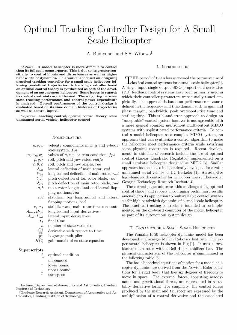
The Yamaha R-50 helicopter dynamics model has beendeveloped at Carnegie Mellon Robotics Institute. The ex-perimental helicopter is shown in Fig.[1]. It uses a two-bladed main rotor with a Bell-Hiller stabilizer bar. Thephysical characteristic of the helicopter is summarized inthe following table [5].The basic linearized equations of motion for a model heli-

copter dynamics are derived from the Newton-Euler equa-tions for a rigid body that has six degrees of freedom tomove in space. The external forces, consisting aerody-namic and gravitational forces, are represented in a sta-bility derivative form. For simplicity, the control forcesproduced by the main and tail rotor are expressed by themultiplication of a control derivative and the associated

2

Fig. 1. The experimental R-50 helicopter

TABLE I

Physical Parameters of the Yamaha R-50.

Rotor Speed 850 rpmTip speed 449 ft/sDry weight 97 lbInstrumented weight 150 lbEngine Single cylinder, 2-strokeFlight autonomy 30 minutes

control input. Following Ref.[5], the equations of motionof the model helicopter are derived and categorized intothe following groups.

A. Lateral and longitudinal fuselage dynamics

Using the Newton-Euler equations, the translational andangular fuselage motions of the helicopter can be derivedas the following set of equations:

.u = (−w0q + v0r)− gθ +Xuu+ ...+Xaa (1).v = (−u0r + w0p)− gφ+ Yvv + ...+ Ybb (2).p = Luu+ Lvv + ...+ Lbb (3).q = Muu+Mvv + ...+Maa (4)

The stability derivatives are used to express the exter-nal aerodynamic and gravitational forces and moments.Xa, Yb denotes rotor derivatives and Lb,Ma the flappingspring-derivatives. They are all used to describe the ro-tor forces and moments respectively. General aerody-namic effects are expressed by speed derivatives given asXu, Yv, Lu, Lv,Mu,Mv.

B. Heaving(vertical) dynamics

The Newton-Euler rigid body equations for the heavingdynamics is represented by

.w= (−v0p+ u0q) + Zww + Zcolδcol (5)

In the hovering flight, v0 and u0 are obviously zero.Thus, the centrifugal forces represented by the terms inparentheses are relevant only in cruise flight.

C. Yaw dynamics

The augmented yaw dynamics is approximated as a first-order bare airframe dynamics with a yaw rate feedbackrepresented by a simple first-order low-pass filter. The cor-responding differential equations used in the state-spacemodel are also given in appropriate stability derivatives asfollows

r = Nrr +Nped(δped − rfb) (6).rfb = Krr −Krfbrfb (7)

D. Coupled Rotor-stabilizer bar dynamics

The simplified rotor dynamics is represented by twofirst-order differential equations for the lateral(b) andlongitudinal(a) flapping motion. In the state-space model,the rotor model are given as:

b =Baa+Blatδlat +Bdd+Blonδlon − b

τf− p (8)

.a =

Abb+Alatδlat +Acc+Alonδlon − aτf

− q (9)

where the following derivatives related to the gearing of theBell-mixer are introduced:

Kd =BdBlat

(10)

Kc =AcAlat

(11)

The stabilizer bar receives cyclic inputs from the swash-plate in a similar way as do the main blades. The equationsfor the lateral(d) and longitudinal(c) flapping motions are:

.

d =1

τ s(−d− τsp+Dlatδlat) (12)

.c =

1

τ s(−c− τ sq + Clonδlon) (13)

E. The state-space model of the R-50 dynamics

The state-space model of the helicopter can be assembledfrom the above set of differential equations in a matrixform:

.x= Ax+Bu (14)

where x= {u, v, p, q,φ, θ, a, b, w, r, rfb, c, d}T is the statevector and u = {δlat, δlon, δped, δcol}T the input vector.The dynamic matrix A contains the stability derivativesand the control matrix B contains the input derivatives.The complete description the elements of these matricesare presented in the Appendix.

III. Tracking Control Design

A. Linear Regulator Problem

A Linear Regulator problem in the optimal control the-ory represents a class of problem where the plant dynamics

3

is linear and the quadratic form of performance criteria isused. The linear dynamics (which can be time-varying)are: ·

x (t) = A(t)x(t) +B(t)u(t) (15)

and the cost is quadratic:

J =1

2x(tf )

THx(tf ) + (16)

1

2

Z tf

t0

[x(t)TQ(t)x(t) + u(t)TR(t)u(t)]dt

where the requirements of the weighting matrices are givenas

H = HT ≥ 0 (17)

Q(t) = Q(t)T ≥ 0R(t) = R(t)T > 0 (18)

Also, there is no other constraints and tf is fixed i.e. noterminal constraints and no constraints on u. Note thatthere is a terminal weighting of the states x. The physicalinterpretation of the problem statement is: it is desired tomaintain the state vector close to the origin without anexcessive expenditure of control effort[6].The optimal feedback control law can be derived by

identifying the Hamiltonian of the system and using theHamilton-Jacoby-Bellman (HJB) equation to ensure theoptimality[7]. The Hamiltonian H = H[x(t), u∗(t), J∗x , t]for the above problem is defined as:

H =1

2x(t)TQ(t)x(t) +

1

2u(t)TR(t)u(t)

+J∗x(x, t).[A(t)x(t) +B(t)u(t)] (19)

minimizing with respect to u, it reads:

dH

du= u(t)TR(t) + J∗x(x, t).B(t) = 0

d2H

du2= R(t) > 0

(20)

Note that the above stationary condition defines a globalminimum because the function H depends quadraticallyonly on u.The optimal control is obtained by using the stationary

condition and solving for u,

u∗[t] = −R(t)−1B(t)TJ∗x(x, t)T (21)

The Hamiltonian in Eq.[19] can then be written as:

H = J∗x(x, t).A(t)x(t) +1

2x(t)TQ(t)x(t)

−12J∗x(x, t).B(t)R(t)

−1B(t)TJ∗x(x, t)T (22)

Now, in order to ensure the optimality the HJB equationmust be satisfied. The complete HJB equation is:

J∗t (x, t). = J∗x(x, t).A(t)x(t) +1

2x(t)TQ(t)x(t)

−12J∗x(x, t).B(t)R(t)

−1B(t)TJ∗x(x, t)T(23)

where the boundary condition (in this case, with fixed tf )is

J∗(x(tf ), tf ). =1

2x(tf )

THx(tf ) (24)

A quadratic form for the cost is used to verify its validityusing the HJB equation. Letting:

J∗(x(t), t). =1

2x(t)TK(t)x(t) (25)

Thus, the partial derivatives appearing in Eq.[23], can bewritten as

J∗x(x, t). = x(t)TK(t) (26)

J∗t (x, t). =1

2x(t)T

dK(t)

dtx(t) (27)

and the HJB equation becomes:

1

2x(t)T

.

K (t)x(t) =1

2x(t)TQ(t)x(t) + x(t)TK(t)A(t)x(t)

−12x(t)TK(t)B(t)x(t)×

R(t)−1B(t)TK(t)Tx(t) (28)

The terms appearing in the above equation are scalar. Thetranspose of a scalar term is the same as the term. Sinceonly scalar terms are dealt with the following relation ap-plies:

x(t)TK(t)A(t)x(t) =1

2x(t)TK(t)A(t)x(t)

+1

2x(t)TA(t)TK(t)Tx(t) (29)

And thus the HJB equation becomes:

0 =1

2x(t)T [

.K (t) +Q(t) +K(t)A(t) + (30)

A(t)TK(t)T −K(t)B(t)R(t)−1B(t)TK(t)T ]x(t)Now, letting K(tf ) = H = HT (symmetric), K(t) will besymmetric from above and thus symmetry of K(tf ) will beretained ∀t, i.e. K(t) = K(t)T (symmetric). K(tf ) = H isthe boundary condition for K(t). Since the above equationmust be satisfied ∀x(t), the following matrix differentialequation is obtained:

− .

K (t) = Q(t) +K(t)A(t) +A(t)TK(t)T (31)

−K(t)B(t)R(t)−1B(t)TK(t)T

With a finite terminal time specified the entire solutionis a transient and K(t) will be time varying. However ifthe terminal time is taken far enough out, the solutionfor K and the corresponding feedback gain might tend toa constant. To get the invariant asymptotic solution thedifferential equation for

.

K can be integrated to a steadystate solution or the time derivative term is set to zero i.e..

K= 0. This leads to Algebraic Riccati equation (ARE)[6]:

Q+KA+ATKT −KBR−1BTKT = 0 (32)

4

For K(t) satisfying the above Riccati form matrixquadratic equation, it is required that Eq.[25] is optimal,and the optimal control in Eq.[21] is now given by

u∗(t). = R−1BTKx(t) (33)

This is the state feedback control law for the continuoustime LQR problem. Note that both forms of Riccati equa-tion given in Eqs.[31] and [32] do not depend on x or uand thus the solution for K can be obtained in advanceand finally the gain matrix −R−1BTK can be stored. Thecontrol can then be obtained in real time by multiplyingthe stored gain with x(t).

B. Path tracking problem formulation

To use the LQR design for path tracking control, theregulator problem must be recast as a tracking problem. Ina tracking problem, the output y is compared to a referencesignal r. The goal is to drive the error between the referenceand the output to zero. It is common to add an integratorto the error signal and then minimize it. An alternativeapproach would be using the derivative of the error signal.Assuming perfect measurements i.e. the sensor matrix isof identity form:

yerror

= xerror(t) = xref (t)− x(t) (34)

Taking the time derivative of the equation yields:

xerror(t) = xref (t)− x(t) (35)

When the reference is predefined as constant, thenxref (t) = 0, and

xerror(t) = −x(t) (36)

A path tracking control law can be designed by using thefollowing general relation:

xerror(t) = −ηx(t) (37)

where η is an arbitrary constant representing the weightof the tracking performance in the cost function. In thematrix form, the above relation can written as:

xerror(t) =

xerror(t)yerror(t)zerror(t)

= −ηx(t)−ηy(t)−ηz(t)

(38)

Substituting x = u, y = v and z = w, the above equationcan be expressed as

xerror(t) =

−ηu(t)−ηv(t)−ηw(t)

(39)

To accommodate the tracking term in the cost function,the state-space model is augmented as the following:

xaug(t) = Aaugxaug(t) +Baugu(t) (40)

where:

xaug(t) = {xerror, yerror, zerror, x}T (41)

Aaug =

·03×3 −η.I3 03×11014×3 A

¸(42)

Baug =

·03×4B

¸(43)

The size of the matrix is associated with the matrix ap-pearing in Eq.[14] with the addition of three augmentedstates. When the terminal weighting is not considered, theperformance measure is now

J =1

2

Z tf

t0

[xaug(t)TQ(t)xaug(t) + u(t)

TR(t)u(t)]dt (44)

where the determination of the weighting matrices η, Q andR are empirical.

C. Control synthesis in the presence of input constraints

In a real system, the control inputs are always limited byhard constraints. The limitation of the control inputs for atypical aircraft, for instance, is governed by the maximumallowable deflection of its control surfaces. In the case ofhelicopters, the control hard limits are imposed on theirlateral and longitudinal cyclic, pedal and collective pitch.The control input limits for the helicopter used in this studyare:

−5o ≤ δlat ≤ 5o (45)

−5o ≤ δlong ≤ 5o (46)

−22o ≤ δped ≤ 22o (47)

−10o ≤ δcol ≤ 10o (48)

To incorporate control input constraints into the controlsynthesis, the Pontryagin’s minimum principle is employed.Essentially, the Hamiltonian of the system is re-derived toexpress the presence of input constraints. The stationarycondition is applied to the modified Hamiltonian to ob-tained the optimal bounded control[8].The Hamiltonian for the above tracking problem is

H =1

2xaug(t)

TQ(t)xaug(t) +1

2u(t)TR(t)u(t)

+pT (Axaug +Bu) (49)

and its derivative with respect to u is

Hu = u(t)TR(t) + pTB (50)

The optimal control can be solved by imposing Hu = 0.This yields

u∗ = −R(t)−1BT p (51)

When the control is constrained or bounded, the optimalcontrol is

u∗ = argminu(t) ∈ U(t)

·1

2u(t)TR(t)u(t) + pTBu

¸(52)

5

In practice, the control elements are penalized individu-ally. It does not make any sense to minimize the productbetween u1 and u2,for example. Thus the weighting ma-trix R is not usually a full matrix. The diagonal matrixR was used in this work which simplified the optimizationconsiderably. For a diagonal R,

u∗ = argminu(t) ∈ U(t)

"mXi=1

1

2Riiu

2i + p

T biui

#(53)

u∗i =argminui(t) ∈ Ui(t)

·1

2Riiu

2i + p

T biui

¸(54)

The unbounded solution can thus be written as

ui = −R−1ii pT bi (55)

and the bounded control requirement, −M−i ≤ ui ≤ M+i ,

can be implemented in the following logic:

If ui ≤M−i u∗i =M−i

−M−i ≤ ui ≤M+i u∗i = ui

ui ≥M+i u∗i =M

+i

(56)

Note that the solution of the bounded control is not thesame as the solution obtained by imposing the constraintsto the unbounded solution. The optimal control history ofthe bounded control case can not be determined by calcu-lating the optimal control history for the unbounded caseand then allowing it to saturate whenever there is a viola-tion of the stipulated boundaries.

IV. Numerical Simulation

To evaluate the performance of the tracking controllerdesign, numerical simulation is conducted for a variety ofreference trajectories and for different values of weightingmatrices. The simulation is carried out using Matlab withthe data presented in the Appendix. Since the focus ofthe design is on the tracking performance, only the datacorresponding to cruise is applicable. The effects of theweighting matrices are analyzed based on the evident trade-off between tracking performance and control expenditure.The effect of the weighting matrix to the states will beobserved by comparing the tracking performance betweentwo highly separated values of Q, Q = 0.01I17 and Q = I17.Similar effects will be observed for position tracking andcontrol weighting matrices.Note that in order to be able to physically interpret

the result of the simulation, a coordinate transformationis needed between body coordinate and local horizon coor-dinate system. The transformation matrix between thesetwo coordinates is given as the following:

T bI =

cθcψ cθsψ −sθsφsθcψ − cφsψ sφsθsψ + cφcψ sφcθcφsθcψ + sφsψ cφsθsψ − sφcψ cφcθ

(57)

where c(.) = cos(.), and s(.) = sin(.)With this transformation, the final results of the simu-

lation are presented in the local horizon coordinate. The

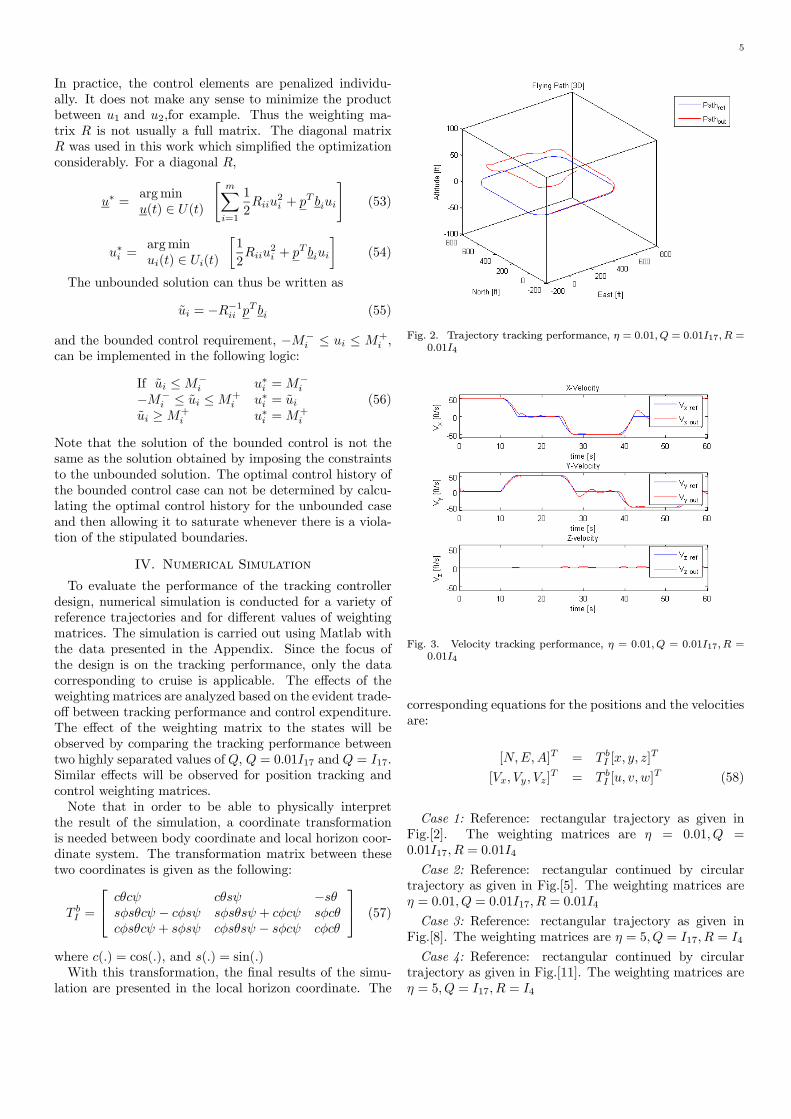
Fig. 2. Trajectory tracking performance, η = 0.01, Q = 0.01I17, R =0.01I4

Fig. 3. Velocity tracking performance, η = 0.01, Q = 0.01I17, R =0.01I4

corresponding equations for the positions and the velocitiesare:

[N,E,A]T = T bI [x, y, z]T

[Vx, Vy, Vz]T = T bI [u, v, w]

T (58)

Case 1: Reference: rectangular trajectory as given inFig.[2]. The weighting matrices are η = 0.01, Q =0.01I17, R = 0.01I4

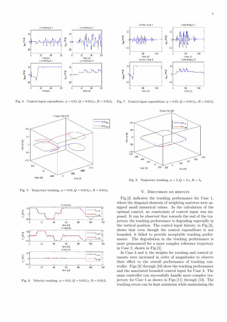
Case 2: Reference: rectangular continued by circulartrajectory as given in Fig.[5]. The weighting matrices areη = 0.01, Q = 0.01I17, R = 0.01I4

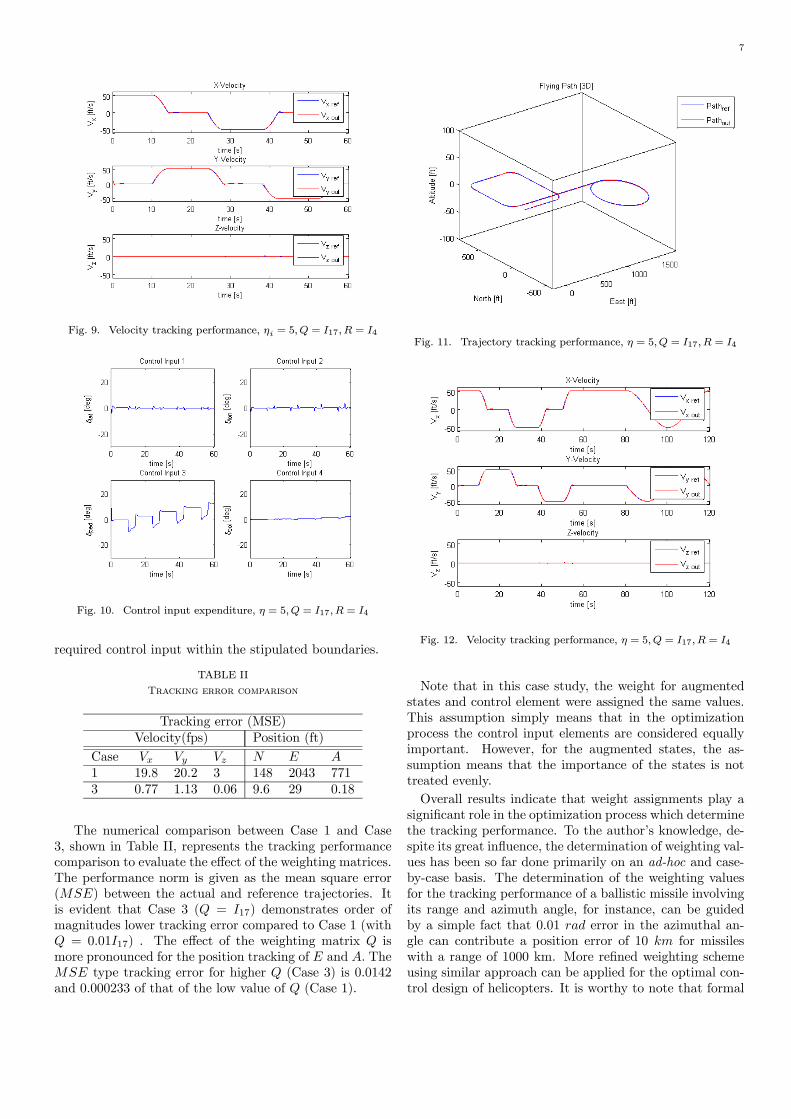
Case 3: Reference: rectangular trajectory as given inFig.[8]. The weighting matrices are η = 5, Q = I17, R = I4

Case 4: Reference: rectangular continued by circulartrajectory as given in Fig.[11]. The weighting matrices areη = 5, Q = I17, R = I4

6

Fig. 4. Control input expenditure, η = 0.01, Q = 0.01I17, R = 0.01I4

Fig. 5. Trajectory tracking, η = 0.01, Q = 0.01I17, R = 0.01I4

Fig. 6. Velocity tracking, η = 0.01, Q = 0.01I17, R = 0.01I4

Fig. 7. Control input expenditure, η = 0.01,Q = 0.01I17, R = 0.01I4

Fig. 8. Trajectory tracking, η = 5, Q = I17, R = I4

V. Discussion on results

Fig.[2] indicates the tracking performance for Case 1,where the diagonal elements of weighting matrices were as-signed small numerical values. In the calculation of theoptimal control, no constraints of control input was im-posed. It can be observed that towards the end of the tra-jectory the tracking performance is degrading especially inthe vertical position. The control input history, in Fig.[4],shows that even though the control expenditure is notbounded, it failed to provide acceptable tracking perfor-mance. The degradation in the tracking performance ismore pronounced for a more complex reference trajectoryin Case 2, shown in Fig.[5].In Case 3 and 4, the weights for tracking and control el-

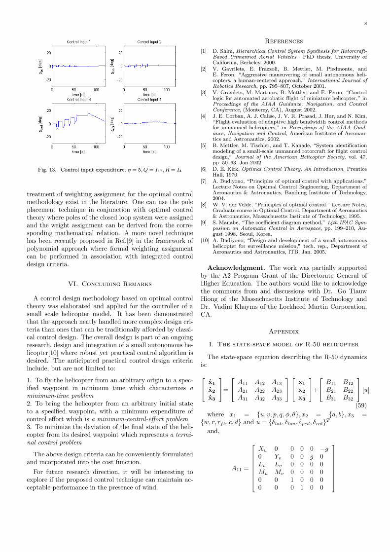
ements were increased in order of magnitudes to observetheir effect to the overall performance of tracking con-troller. Figs.[8] through [10] show the tracking performanceand the associated bounded control input for Case 3. Thesame controller can successfully handle more complex tra-jectory for Case 4 as shown in Figs.[11] through [13]. Thetracking errors can be kept minimum while maintaining the

7

Fig. 9. Velocity tracking performance, ηi = 5, Q = I17, R = I4

Fig. 10. Control input expenditure, η = 5,Q = I17, R = I4

required control input within the stipulated boundaries.

TABLE II

Tracking error comparison

Tracking error (MSE)Velocity(fps) Position (ft)

Case Vx Vy Vz N E A1 19.8 20.2 3 148 2043 7713 0.77 1.13 0.06 9.6 29 0.18

The numerical comparison between Case 1 and Case3, shown in Table II, represents the tracking performancecomparison to evaluate the effect of the weighting matrices.The performance norm is given as the mean square error(MSE) between the actual and reference trajectories. Itis evident that Case 3 (Q = I17) demonstrates order ofmagnitudes lower tracking error compared to Case 1 (withQ = 0.01I17) . The effect of the weighting matrix Q ismore pronounced for the position tracking of E and A. TheMSE type tracking error for higher Q (Case 3) is 0.0142and 0.000233 of that of the low value of Q (Case 1).

Fig. 11. Trajectory tracking performance, η = 5,Q = I17, R = I4

Fig. 12. Velocity tracking performance, η = 5, Q = I17, R = I4

Note that in this case study, the weight for augmentedstates and control element were assigned the same values.This assumption simply means that in the optimizationprocess the control input elements are considered equallyimportant. However, for the augmented states, the as-sumption means that the importance of the states is nottreated evenly.

Overall results indicate that weight assignments play asignificant role in the optimization process which determinethe tracking performance. To the author’s knowledge, de-spite its great influence, the determination of weighting val-ues has been so far done primarily on an ad-hoc and case-by-case basis. The determination of the weighting valuesfor the tracking performance of a ballistic missile involvingits range and azimuth angle, for instance, can be guidedby a simple fact that 0.01 rad error in the azimuthal an-gle can contribute a position error of 10 km for missileswith a range of 1000 km. More refined weighting schemeusing similar approach can be applied for the optimal con-trol design of helicopters. It is worthy to note that formal

8

Fig. 13. Control input expenditure, η = 5,Q = I17, R = I4

treatment of weighting assignment for the optimal controlmethodology exist in the literature. One can use the poleplacement technique in conjunction with optimal controltheory where poles of the closed loop system were assignedand the weight assignment can be derived from the corre-sponding mathematical relation. A more novel techniquehas been recently proposed in Ref.[9] in the framework ofpolynomial approach where formal weighting assignmentcan be performed in association with integrated controldesign criteria.

VI. Concluding Remarks

A control design methodology based on optimal controltheory was elaborated and applied for the controller of asmall scale helicopter model. It has been demonstratedthat the approach neatly handled more complex design cri-teria than ones that can be traditionally afforded by classi-cal control design. The overall design is part of an ongoingresearch, design and integration of a small autonomous he-licopter[10] where robust yet practical control algorithm isdesired. The anticipated practical control design criteriainclude, but are not limited to:

1. To fly the helicopter from an arbitrary origin to a spec-ified waypoint in minimum time which characterizes aminimum-time problem2. To bring the helicopter from an arbitrary initial stateto a specified waypoint, with a minimum expenditure ofcontrol effort which is a minimum-control-effort problem3. To minimize the deviation of the final state of the heli-copter from its desired waypoint which represents a termi-nal control problem

The above design criteria can be conveniently formulatedand incorporated into the cost function.

For future research direction, it will be interesting toexplore if the proposed control technique can maintain ac-ceptable performance in the presence of wind.

References

[1] D. Shim, Hierarchical Control System Synthesis for Rotorcraft-Based Unmanned Aerial Vehicles. PhD thesis, University ofCalifornia, Berkeley, 2000.

[2] V. Gavrilets, E. Frazzoli, B. Mettler, M. Piedmonte, andE. Feron, “Aggressive maneuvering of small autonomous heli-copters. a human-centered approach,” International Journal ofRobotics Research, pp. 795—807, October 2001.

[3] V. Gravilets, M. Martinos, B. Mettler, and E. Feron, “Controllogic for automated aerobatic flight of miniature helicopter,” inProceedings of the AIAA Guidance, Navigation, and ControlConference, (Monterey, CA), August 2002.

[4] J. E. Corban, A. J. Calise, J. V. R. Prasad, J. Hur, and N. Kim,“Flight evaluation of adaptive high bandwidth control methodsfor unmanned helicopters,” in Proceedings of the AIAA Guid-ance, Navigation and Control, American Institute of Aeronau-tics and Astronautics, 2002.

[5] B. Mettler, M. Tischler, and T. Kanade, “System identificationmodeling of a small-scale unmanned rotorcraft for flight controldesign,” Journal of the American Helicopter Society, vol. 47,pp. 50—63, Jan 2002.

[6] D. E. Kirk, Optimal Control Theory. An Introduction. PrenticeHall, 1970.

[7] A. Budiyono, “Principles of optimal control with applications.”Lecture Notes on Optimal Control Engineering, Department ofAeronautics & Astronautics, Bandung Institute of Technology,2004.

[8] W. V. der Velde, “Principles of optimal control.” Lecture Notes,Graduate course in Optimal Control, Department of Aeronautics& Astronautics, Massachusetts Institute of Technology, 1995.

[9] S. Manabe, “The coefficient diagram method,” 14th IFAC Sym-posium on Automatic Control in Aerospace, pp. 199—210, Au-gust 1998. Seoul, Korea.

[10] A. Budiyono, “Design and development of a small autonomoushelicopter for surveillance mission,” tech. rep., Department ofAeronautics and Astronautics, ITB, Jan. 2005.

Acknowledgment. The work was partially supportedby the A2 Program Grant of the Directorate General ofHigher Education. The authors would like to acknowledgethe comments from and discussions with Dr. Go TiauwHiong of the Massachusetts Institute of Technology andDr. Vadim Khayms of the Lockheed Martin Corporation,CA.

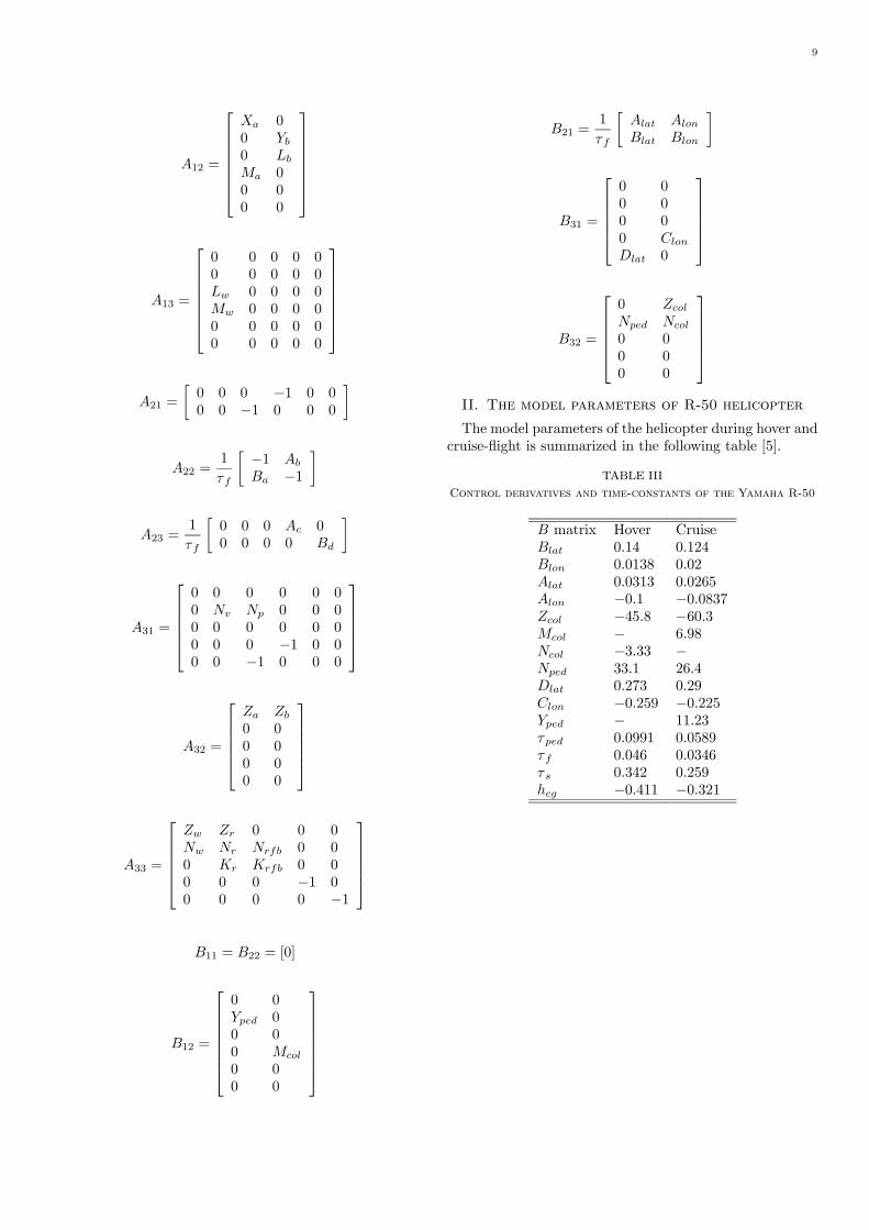
Appendix

I. The state-space model of R-50 helicopter

The state-space equation describing the R-50 dynamicsis: x1x2x3

= A11 A12 A13A21 A22 A23A31 A32 A33

x1x2x3

+ B11 B12B21 B22B31 B32

[u](59)

where x1 = {u, v, p, q,φ, θ}, x2 = {a, b}, x3 ={w, r, rfb, c, d} and u = {δlat, δlon, δped, δcol}Tand,

A11 =

Xu 0 0 0 0 −g0 Yv 0 0 g 0Lu Lv 0 0 0 0Mu Mv 0 0 0 00 0 1 0 0 00 0 0 1 0 0

9

A12 =

Xa 00 Yb0 LbMa 00 00 0

A13 =

0 0 0 0 00 0 0 0 0Lw 0 0 0 0Mw 0 0 0 00 0 0 0 00 0 0 0 0

A21 =

·0 0 0 −1 0 00 0 −1 0 0 0

¸

A22 =1

τf

· −1 AbBa −1

¸

A23 =1

τf

·0 0 0 Ac 00 0 0 0 Bd

¸

A31 =

0 0 0 0 0 00 Nv Np 0 0 00 0 0 0 0 00 0 0 −1 0 00 0 −1 0 0 0

A32 =

Za Zb0 00 00 00 0

A33 =

Zw Zr 0 0 0Nw Nr Nrfb 0 00 Kr Krfb 0 00 0 0 −1 00 0 0 0 −1

B11 = B22 = [0]

B12 =

0 0Yped 00 00 Mcol

0 00 0

B21 =1

τf

·Alat AlonBlat Blon

¸

B31 =

0 00 00 00 ClonDlat 0

B32 =

0 ZcolNped Ncol0 00 00 0

II. The model parameters of R-50 helicopter

The model parameters of the helicopter during hover andcruise-flight is summarized in the following table [5].

TABLE III

Control derivatives and time-constants of the Yamaha R-50

B matrix HoverBlat 0.14Blon 0.0138Alat 0.0313Alon −0.1Zcol −45.8Mcol −Ncol −3.33Nped 33.1Dlat 0.273Clon −0.259Yped −τped 0.0991τf 0.046τs 0.342hcg −0.411

Cruise0.1240.020.0265−0.0837−60.36.98−26.40.29−0.22511.230.05890.03460.259−0.321

10

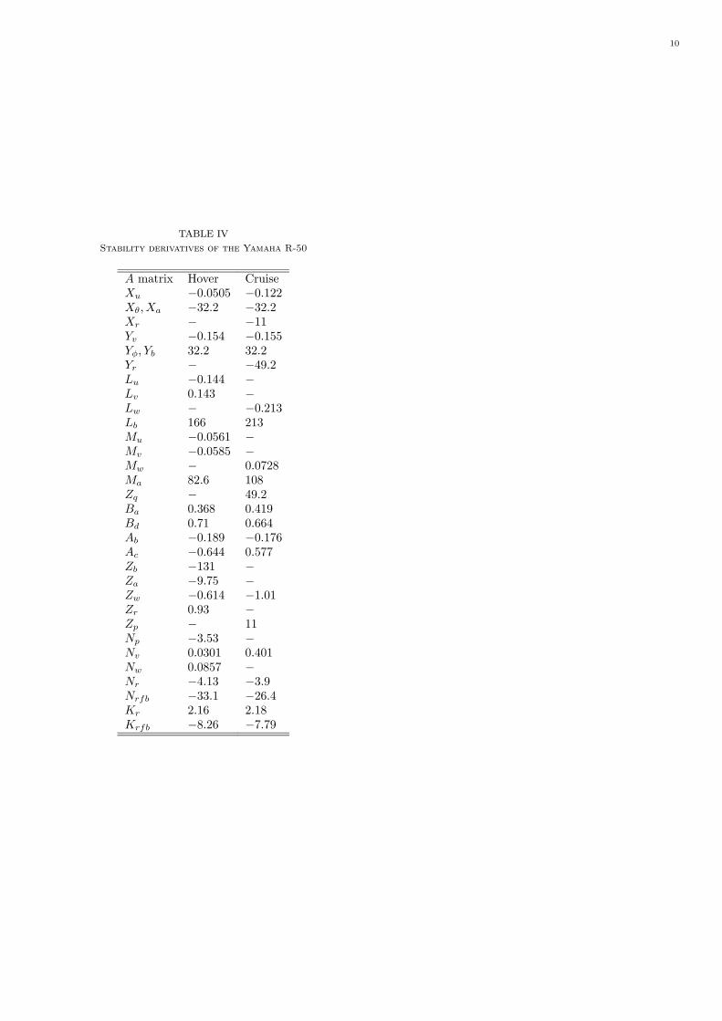
TABLE IV

Stability derivatives of the Yamaha R-50

A matrix HoverXu −0.0505Xθ,Xa −32.2Xr −Yv −0.154Yφ, Yb 32.2Yr −Lu −0.144Lv 0.143Lw −Lb 166Mu −0.0561Mv −0.0585Mw −Ma 82.6Zq −Ba 0.368Bd 0.71Ab −0.189Ac −0.644Zb −131Za −9.75Zw −0.614Zr 0.93Zp −Np −3.53Nv 0.0301Nw 0.0857Nr −4.13Nrfb −33.1Kr 2.16Krfb −8.26

Cruise−0.122−32.2−11−0.15532.2−49.2−−−0.213213−−0.072810849.20.4190.664−0.1760.577−−−1.01−11−0.401−−3.9−26.42.18−7.79