striatal network modeling in huntington's disease - plos

RESEARCH ARTICLE

Striatal network modeling in Huntington’s

Disease

Adam PonziID1¤*, Scott J. Barton2, Kendra D. BunnerID

2, Claudia Rangel-Barajas2, Emily

S. ZhangID2, Benjamin R. Miller2, George V. Rebec2☯‡, James KozloskiID

1☯‡

1 IBM Research, Computational Biology Center, Thomas J. Watson Research Laboratories, Yorktown

Heights, New York, United States of America, 2 Program in Neuroscience, Department of Psychological and

Brain Sciences, Indiana University, Bloomington, Indiana, United States of America

☯ These authors contributed equally to this work.

¤ Current address: Institute of Biology, Otto-von-Guericke University, Magdeburg, Germany

‡ These authors are joint senior authors on this work.

* [email protected]

Abstract

Medium spiny neurons (MSNs) comprise over 90% of cells in the striatum. In vivo MSNs dis-

play coherent burst firing cell assembly activity patterns, even though isolated MSNs do not

burst fire intrinsically. This activity is important for the learning and execution of action

sequences and is characteristically dysregulated in Huntington’s Disease (HD). However,

how dysregulation is caused by the various neural pathologies affecting MSNs in HD is

unknown. Previous modeling work using simple cell models has shown that cell assembly

activity patterns can emerge as a result of MSN inhibitory network interactions. Here, by

directly estimating MSN network model parameters from single unit spiking data, we show

that a network composed of much more physiologically detailed MSNs provides an excellent

quantitative fit to wild type (WT) mouse spiking data, but only when network parameters are

appropriate for the striatum. We find the WT MSN network is situated in a regime close to a

transition from stable to strongly fluctuating network dynamics. This regime facilitates the

generation of low-dimensional slowly varying coherent activity patterns and confers high

sensitivity to variations in cortical driving. By re-estimating the model on HD spiking data we

discover network parameter modifications are consistent across three very different types of

HD mutant mouse models (YAC128, Q175, R6/2). In striking agreement with the known

pathophysiology we find feedforward excitatory drive is reduced in HD compared to WT

mice, while recurrent inhibition also shows phenotype dependency. We show that these

modifications shift the HD MSN network to a sub-optimal regime where higher dimensional

incoherent rapidly fluctuating activity predominates. Our results provide insight into a

diverse range of experimental findings in HD, including cognitive and motor symptoms, and

may suggest new avenues for treatment.

PLOS COMPUTATIONAL BIOLOGY

PLOS Computational Biology | https://doi.org/10.1371/journal.pcbi.1007648 April 17, 2020 1 / 44

a1111111111

a1111111111

a1111111111

a1111111111

a1111111111

OPEN ACCESS

Citation: Ponzi A, Barton SJ, Bunner KD, Rangel-

Barajas C, Zhang ES, Miller BR, et al. (2020) Striatal

network modeling in Huntington’s Disease. PLoS

Comput Biol 16(4): e1007648. https://doi.org/

10.1371/journal.pcbi.1007648

Editor: Srdjan Ostojic, Ecole Normale Superieure,

FRANCE

Received: July 2, 2019

Accepted: January 9, 2020

Published: April 17, 2020

Peer Review History: PLOS recognizes the

benefits of transparency in the peer review

process; therefore, we enable the publication of

all of the content of peer review and author

responses alongside final, published articles. The

editorial history of this article is available here:

https://doi.org/10.1371/journal.pcbi.1007648

Copyright: © 2020 Ponzi et al. This is an open

access article distributed under the terms of the

Creative Commons Attribution License, which

permits unrestricted use, distribution, and

reproduction in any medium, provided the original

author and source are credited.

Data Availability Statement: The data are available

at https://github.com/adampdp/plosCB-ponzi-HD.

Funding: Portions of each authors’ work reported

here were funded by CHDI. AP’s work was also

funded in part by NSF grant DMS-1555237. The

http://orcid.org/0000-0001-8712-5911

http://orcid.org/0000-0002-3001-0264

http://orcid.org/0000-0003-4188-5063

http://orcid.org/0000-0003-3420-4688


http://crossmark.crossref.org/dialog/?doi=10.1371/journal.pcbi.1007648&domain=pdf&date_stamp=2020-05-04









http://creativecommons.org/licenses/by/4.0/

https://github.com/adampdp/plosCB-ponzi-HD

Author summary

Huntington’s Disease (HD) is an inherited neurodegenerative disease with devastating

symptoms including progressive motor dysfunction and disturbances to normal cogni-

tion. The age of disease onset is roughly related to the length of abnormally expanded

CAG repeats in the mutant huntingtin gene, but how this produces HD is not well under-

stood. Several transgenic mouse models have been created to investigate the stages of dis-

ease progression. HD is found to be primarily associated with pathology of medium spiny

neurons (MSNs) in the striatum, the main input stage of the basal ganglia. In wild type

(WT) animals MSNs display cell-assembly activation patterns which are known to play a

crucial role in striatal cognitive and motor information processing. These activity patterns

are lost in HD mice. Here we use computational modeling to probe the role of striatal net-

work dynamics in HD. We fit the parameters of an MSN network model to spiking data

from WT mice and three different types of transgenic mice. In agreement with the known

pathophysiology, we find cortical feedforward excitation is consistently reduced in all

three HD mice. We show how this produces the characteristic dysregulation of MSN

activity and explain why it may underlie the motor symptoms of HD.

Introduction

Huntington’s Disease (HD) is an inherited condition caused by an abnormal expansion of

CAG trinucleotide repeats in the mutant huntingtin (mHTT) gene (The Huntington’s Disease

Collaborative Research Group, 1993). HD is a devastating neurodegenerative disease charac-

terized by progressive motor dysfunction and disturbances to normal cognition. In early stages

chorea is prominent, while akinesia dominates at later stages [1]. Cognitive symptoms include

depression, apathy and anxiety, as well as irritability and agression [2, 3]. The age of disease

onset is roughly related to the length of the CAG repeat [4–6]

Several transgenic rodent models of HD have been created [7–9] to investigate the stages of

HD progression [10]. Striatal medium spiny neuron (MSN) dysfunction is a prominent find-

ing and may be a pathophysiological cause of HD symptoms. It is well established that MSNs

gradually degenerate and eventually die [11] however HD symptoms also occur in the absence

of obvious cell loss [12, 13]. Indeed neuronal and synaptic dysfunction precedes cell death by

many years in humans [14–16] and occurs before, or even in the absence of, cell death in HD

animal models [17–20]. The fact that the Huntingtin protein (Htt) is involved in synaptic func-

tion [9, 21] also suggests that HD may primarily be a synaptopathology [22]. Similar alterations

of striatal synaptic activity have been demonstrated in multiple different HD mouse models

[23]. Progressive changes in spontaneous corticostriatal excitatory synaptic activity [24–27]

have been associated with pre- and postsynaptic alterations including reductions in synaptic

proteins, loss of dendritic spines, and loss of synapses [1, 9, 24, 28–31]. A progressive discon-

nection between cortex and striatum seems to be a general characteristic of HD.

In contrast, studies of GABAergic synaptic activity in HD are less conclusive. There are two

main types of GABAergic inhibition affecting MSNs in the striatum; feedback via the MSN

axon collaterals and feedforward inhibition generated by GABAergic fast spiking interneurons

[32]. Although the two types of inhibition have been extensively characterized in WT animals

[33–37], little is known about the role of collateral MSN interactions in HD mouse models.

GABAergic synaptic activity was found to be modified among a subset of MSNs in HD [4, 38–

40] but its source is unknown.

PLOS COMPUTATIONAL BIOLOGY Striatal network modeling in Huntington’s Disease


funders had no role in study design, data collection

and analysis, decision to publish, or preparation of

the manuscript.

Competing interests: The authors have declared

that no competing interests exist.


In vivo striatal MSNs show strong firing irregularity characterised by very high inter-spike-

interval (ISI) coefficients of variation (CV) [41]. Further examination reveals that spike trains

are composed of irregularly timed, but comparitively short, bursting episodes of fairly high fre-

quency spiking, usually lasting a few seconds, separated by much longer periods of quiescence

or sporadic spiking, lasting tens of seconds [42]. Importantly spiking bursts do not occur in

isolation but coherently across multiple MSNs which form cell assemblies in vivo [42] and invitro [43]. Because bursting is both coherent across many cells and also occurs on slow beha-

vioural timescales, it is thought to be crucial for striatal cognitive and motor processing. The

encoding of movement sequences [44–48], the execution of learned motor programs and

sequence learning [49–62] and the representation of time [63–65] all rely on coherent MSN

population activity.

Dysregulation of striatal coherent bursting activity is found in various pathological states

[66] and in particular is a key component of HD pathophysiology regardless of the severity of

HD symptoms, genetic construct, and background strain of the mouse models [42, 67, 68].

WT MSNs do not show intrinsic bursting or subthreshold oscillations when isolated [41, 45,

69–72]. Therefore burst firing in WT mice must be caused by slowly varying fluctuations in

input current when the cell is close to spiking threshold. We hypothesized that changes in

input current properties may therefore be responsible for the changes in spiking burstiness

found in HD.

Previous modeling of the MSN network [73–78] using simple cell models demonstrated

that realistic WT spiking characteristics can be reproduced when input current fluctuations

are generated by recurrent feedback through the inhibitory collaterals connecting MSN’s to

each other. Although a rigorous quantitative comparison between model generated and exper-

imental spiking data has never been attempted, a very good qualitative match was obtained,

but only when network parameters, such as the IPSP size and MSN to MSN connection proba-

bility, were in the vicinity of their physiological measured values [73]. Interestingly, it was

found that the MSN network was poised in a critical transition regime [74]. Coherently burst-

ing cell assemblies were shown to reflect an underlying fairly low dimensional dynamical

structure which also endowed the MSN network with optimal information processing capabil-

ities, such as the ability to faithfully represent elapsed time, a faculty crucial for the correct

sequencing of actions. However outside the physiologically correct parameter regime, coher-

ent bursting cell assemblies were lost, and information processing properties declined.

We wondered if putative synaptic and network alterations underlying the dysregulation of

burst firing found in HD could be disambiguated through computational modeling with

parameters estimated directly from HD and WT mouse spiking data. In order to make detailed

comparisons with data, we studied a large 2500 cell network and used a well-validated special-

ized single compartment MSN cell model [79, 80]. We employed spiking data from three dif-

ferent transgencic models: R6/2, YAC128 and Q175. The R6/2 mouse model displays a rapidly

progressing phenotype, while Q175 and YAC128 progress much more slowly and better repre-

sent the stages of the human disease [7, 13, 81–86]. Despite these strong differences in genetic

makeup, we find remarkable similarities in spiking dysregulation in the different HD mouse

models and in how this dysregulation occurs through synaptic modifications in the estimated

MSN network model. In the latter two mouse models, we also investigated age dependency in

the spiking data and how this translates into age variation in network model parameters.

Again our findings are consistent across the mouse models, despite their different genetic

constructs.

The only drug which has been approved for use in HD, tetrabenazine (TBZ), primarily

alters corticostriatal synaptic transmission. We hope new insight this modeling provides into




the complex interplay of network and synaptic dysfunctions that take place in HD will stimu-

late discovery of effective novel drug combinations.

Results

Data analysis

Before making detailed quantitative comparison between model generated and experimental

data, we first describe salient features of the MSN spiking recordings which vary between WT

and HD mice. These quantities are calculated to estimate the fit of the network model to exper-

imental data; however the data analysis also reveals interesting new findings. We investigated

spiking data from three different transgenic models: R6/2, YAC128 and Q175. From each

model we also investigated data from WT mice of the same background strain, housed in the

same environment and of similar age as the HD variants.

R6/2 mice contain a fragment of human mHTT with a large number of CAG repeats (150),

and are rapidly progressing. They show motor hyperactivity within 5-7 weeks of birth, akinesia

at 8 weeks and die around 12–16 weeks [87–89]. Although some striatal atrophy is found at

around 5 weeks [90], MSNs do not die until later [91]. The WT R6/2 mice (R62WT) investi-

gated here were aged between 6 and 9 weeks, while the HD R6/2 mice (R62HD) varied

between 8 and 11.5 weeks and were therefore all in the symptomatic stage.

YAC128 mice were created using a yeast artificial chromosome containing the entire full

length human mHTT with 128 repeats. The phenotype shows features of the human disease

including cognitive and motor dysfunction [81, 92]. Progression is much slower than R6/2

and biphasic with impaired learning at 2 months, motor hyperactivity from 3 months, brady-

kinesia from 7 months and hypoactivity at 12 months. Modest striatal atrophy is found at 9

months and a small decrease in the quantity of MSNs at 12 months. The YAC128 mice investi-

gated here, both WT (YACWT) and HD (YACHD), vary between 10 and 90 weeks of age and

thus extend throughout the symptomatic period.

The recently introduced Q175 knockin mouse [28, 93–95] carries the human mHTT gene

in the mouse genomic context [95, 96]. Q175 come in heterozygote and homozygote varieties.

Motor, cognitive, and circadian deficits occur in both [94, 97]. In homozygotes, motor symp-

toms start to develop around 5 months and by 10-12 months they are hypokinetic with mild

tremor. By 8 months 10% of striatal volume is lost in heterozygotes and 20% in homozygotes

[98]. We analyse data from Q175 WT (Q175WT) mice between the ages of 30 and 60 weeks

and Q175 heterozygote (Q175Het) mice between 30 and 90 weeks. We also investigate Q175

homozygote (Q175Hom) data but this dataset is mostly limited to around 30 weeks.

To estimate the model parameters, we only used single unit spiking data. Thirteen of the fif-

teen quantities used to fit the model to WT and HD data are indicated by the asterisks in Fig 1,

which shows spiking characteristics for the seven different mouse types for all ages combined.

We find that spiking activity shows consistent changes between WT and HD mice across the

three types of HD mutant mice, despite the fact that these mice are very different genetic

constructs.

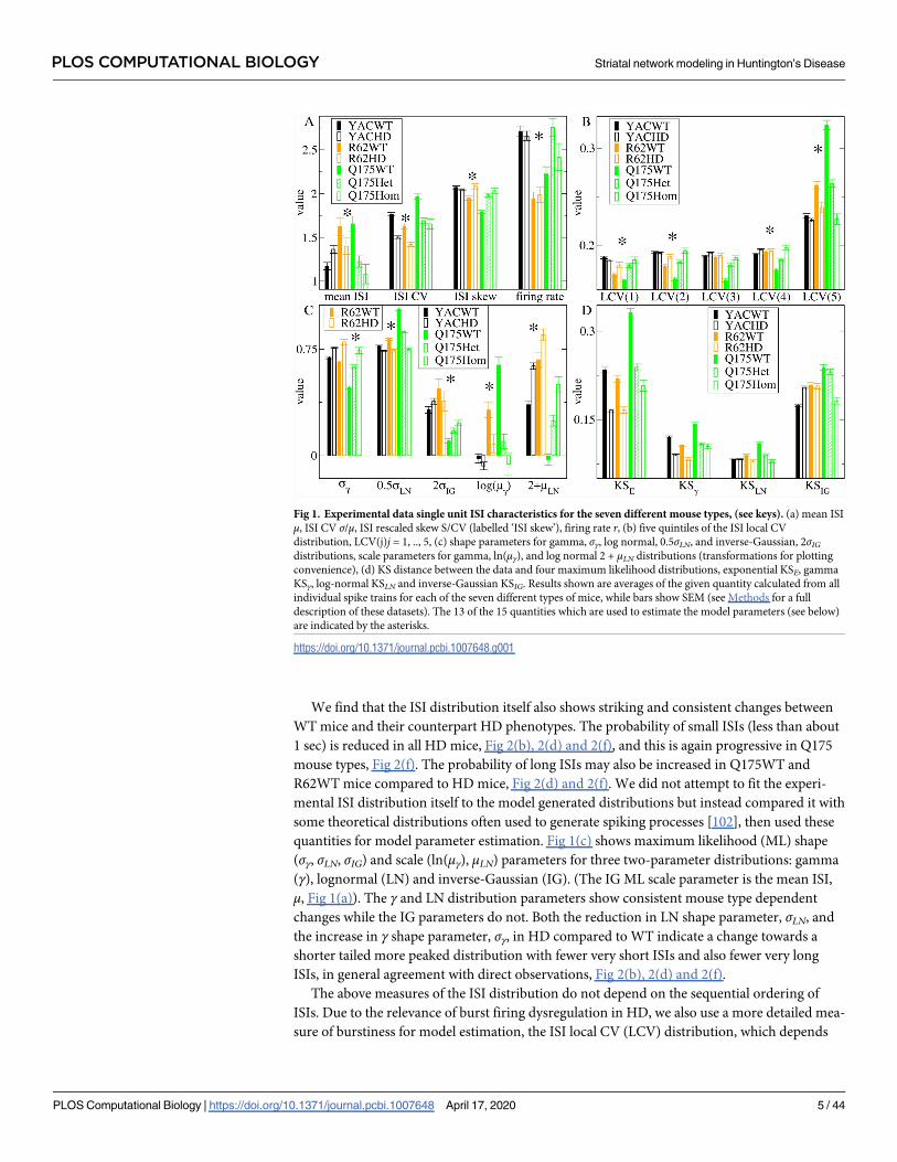
Scaled moments of the ISI distribution are shown in Fig 1(a). In agreement with previous

findings [42, 99, 100] we do not find a consistent change in firing rate r, mean ISI μ, or ISI

rescaled skew, Fig 1(a), between WT and HD mice, while YAC and R6/2 mice do not show

any change in r at all. On the other hand, the ISI CV, Fig 1(a), which is the ISI standard devia-

tion σ normalized by μ, is very high in all three WT mice and consistently reduced in all three

transgenic mice. Spiking much more irregular than Poisson (CV>1) is a well-known salient

feature of MSN activity, and its loss is characteristic of HD [42, 67, 68, 101].




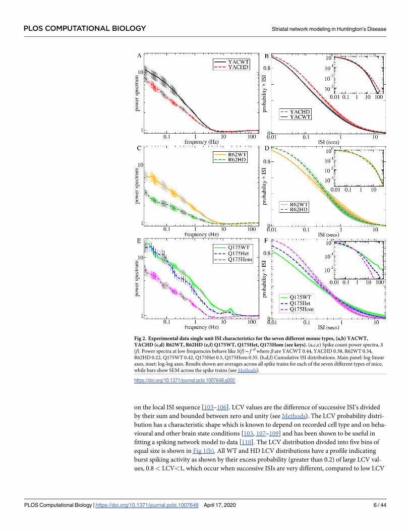
We find that the ISI distribution itself also shows striking and consistent changes between

WT mice and their counterpart HD phenotypes. The probability of small ISIs (less than about

1 sec) is reduced in all HD mice, Fig 2(b), 2(d) and 2(f), and this is again progressive in Q175

mouse types, Fig 2(f). The probability of long ISIs may also be increased in Q175WT and

R62WT mice compared to HD mice, Fig 2(d) and 2(f). We did not attempt to fit the experi-

mental ISI distribution itself to the model generated distributions but instead compared it with

some theoretical distributions often used to generate spiking processes [102], then used these

quantities for model parameter estimation. Fig 1(c) shows maximum likelihood (ML) shape

(σγ, σLN, σIG) and scale (ln(μγ), μLN) parameters for three two-parameter distributions: gamma

(γ), lognormal (LN) and inverse-Gaussian (IG). (The IG ML scale parameter is the mean ISI,

μ, Fig 1(a)). The γ and LN distribution parameters show consistent mouse type dependent

changes while the IG parameters do not. Both the reduction in LN shape parameter, σLN, and

the increase in γ shape parameter, σγ, in HD compared to WT indicate a change towards a

shorter tailed more peaked distribution with fewer very short ISIs and also fewer very long

ISIs, in general agreement with direct observations, Fig 2(b), 2(d) and 2(f).

The above measures of the ISI distribution do not depend on the sequential ordering of

ISIs. Due to the relevance of burst firing dysregulation in HD, we also use a more detailed mea-

sure of burstiness for model estimation, the ISI local CV (LCV) distribution, which depends

Fig 1. Experimental data single unit ISI characteristics for the seven different mouse types, (see keys). (a) mean ISI

μ, ISI CV σ/μ, ISI rescaled skew S/CV (labelled ‘ISI skew’), firing rate r, (b) five quintiles of the ISI local CV

distribution, LCV(j)j = 1, .., 5, (c) shape parameters for gamma, σγ, log normal, 0.5σLN, and inverse-Gaussian, 2σIGdistributions, scale parameters for gamma, ln(μγ), and log normal 2 + μLN distributions (transformations for plotting

convenience), (d) KS distance between the data and four maximum likelihood distributions, exponential KSE, gamma

KSγ, log-normal KSLN and inverse-Gaussian KSIG. Results shown are averages of the given quantity calculated from all

individual spike trains for each of the seven different types of mice, while bars show SEM (see Methods for a full

description of these datasets). The 13 of the 15 quantities which are used to estimate the model parameters (see below)

are indicated by the asterisks.

https://doi.org/10.1371/journal.pcbi.1007648.g001





on the local ISI sequence [103–106]. LCV values are the difference of successive ISI’s divided

by their sum and bounded between zero and unity (see Methods). The LCV probability distri-

bution has a characteristic shape which is known to depend on recorded cell type and on beha-

vioural and other brain state conditions [103, 107–109] and has been shown to be useful in

fitting a spiking network model to data [110]. The LCV distribution divided into five bins of

equal size is shown in Fig 1(b). All WT and HD LCV distributions have a profile indicating

burst spiking activity as shown by their excess probability (greater than 0.2) of large LCV val-

ues, 0.8< LCV<1, which occur when successive ISIs are very different, compared to low LCV

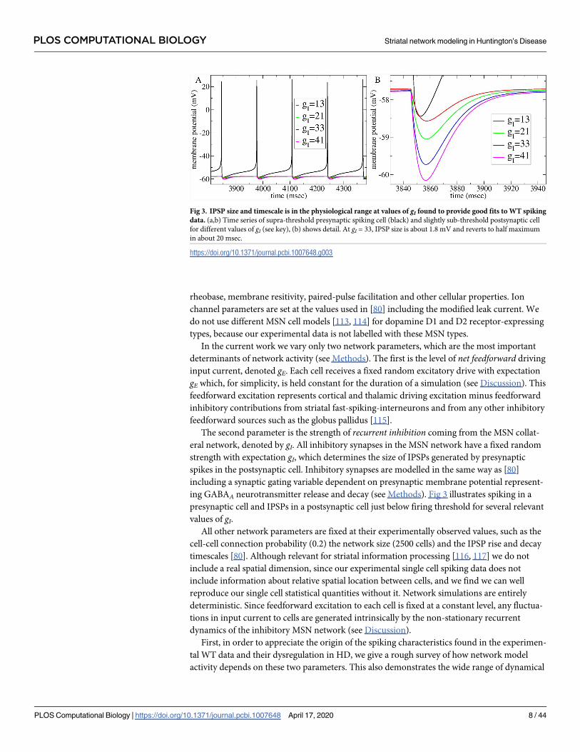
Fig 2. Experimental data single unit ISI characteristics for the seven different mouse types, (a,b) YACWT,

YACHD (c,d) R62WT, R62HD (e,f) Q175WT, Q175Het, Q175Hom (see keys). (a,c,e) Spike count power spectra, S(f). Power spectra at low frequencies behave like S(f)*f−β where β are YACWT 0.44, YACHD 0.38, R62WT 0.34,

R62HD 0.22, Q175WT 0.42, Q175Het 0.5, Q175Hom 0.35. (b,d,f) Cumulative ISI distributions. Main panel: log-linear

axes, inset: log-log axes. Results shown are averages across all spike trains for each of the seven different types of mice,

while bars show SEM across the spike trains (see Methods).






values, LCV<0.8 (with probability less than 0.2) which occur when successive ISIs are more

similar. This bursty profile is consistently attenuated in all three types of HD mice compared

to WTs, and the loss is progressive in Q175 types. Finally, we also used two closely related

quantities for model estimation: the first two serial lagged ISI autocorrelations (see Methods

and below).

Besides these quantities used to fit the model, we also calculated some other partially inde-

pendent auxiliary quantities to provide a demonstration of how well the estimated best fit

model actually predicts other characteristics of the experimental data. The normalized spike

train power spectrum, S(f), is shown in Fig 2(a), 2(c) and 2(e) (see Methods). While not

completely independent, the power spectrum is not equivalent to the ISI distribution, since the

spiking processes we investigate here are not renewal processes, and in fact ISIs show strong

long range serial autocorrelations (see below). All power spectra have a characteristic shape

dominated by high power at low frequencies, f, with a S(f)*f−β type ‘power-law’ decay up to

about 10 Hz and a minimum somewhere between 10 and 100 Hz (this dip is less pronounced

in the Q175WT). The WT power spectra are not identical because the three cohorts of mice

differ in strain and age as well as in other respects. Slowly varying activity, with frequency

below about 10Hz, is reduced in a very similar way in all three HD mice compared with their

WT controls (see β values in Fig 2, caption). This reduction also occurs progressively from

Q175WT to Q175Het to Q175Hom mice, (though for very low frequencies, <0.1 Hz, the dis-

tinction between Q175WT and Q175Het breaks down).

Calculation of the ISI ML quantities described above is always possible and does not suggest

the particular theoretical distribution is actually a good fit to the data. We found that the Kol-

mogorov-Smirnov (KS) distances between the experimental data and the theoretical ML ISI

distributions, Fig 1(d), (see Methods), which provide some indication of which distribution is

a better fit, also provide a useful, partially independent, measure of how well our estimated

best fit model predicts the experimental data, as the KS distances vary strongly with both the

experimental data and the model generated data (see below). The LN distribution is clearly the

best fit (lowest KS distance) for the three WT mice while the γ distribution and LN distribution

are almost equally good fits in all three of the HD mutant mice. The IG distribution always has

the largest KS distance of the three two parameter distributions. Like the scale and shape

parameters themselves, WT/HD dependent changes in KSLN and KSγ are consistent across all

three mouse models and progressive in Q175, while KSIG variations are not. The KS distance

from the one-parameter exponential distribution, KSE, is also shown. This is clearly the worst

fit for the WT animals, but comparable to the IG distribution in HD mice.

Network model

We find various spiking statistical quantities are consistent across different strains of WT mice

and also consistent across three different types of HD mutant mice, but many of these quanti-

ties also show strong variations between WT and HD mice. We wondered if the particular WT

spiking statistics could be quantitatively fit to an MSN network model with physiologically

realistic parameter settings and whether modifications to synaptic parameters could account

for the changes found in our measures of spiking activity in HD.

In order to make detailed comparisons with data, we employ a well-validated specialized

single compartment MSN cell model [79, 80]. This model includes most of the ion-channels

thought to be relevant for determining MSN spiking. It captures MSN characteristics [41, 45,

70–72, 111, 112] such as ‘up-down’ states, whereby a large 20 mV step separates a hyperpolar-

ized resting state from a depolarized state close to firing threshold. It also captures the charac-

teristic long latency to first spike after current injection and provides realistic values for




rheobase, membrane resitivity, paired-pulse facilitation and other cellular properties. Ion

channel parameters are set at the values used in [80] including the modified leak current. We

do not use different MSN cell models [113, 114] for dopamine D1 and D2 receptor-expressing

types, because our experimental data is not labelled with these MSN types.

In the current work we vary only two network parameters, which are the most important

determinants of network activity (see Methods). The first is the level of net feedforward driving

input current, denoted gE. Each cell receives a fixed random excitatory drive with expectation

gE which, for simplicity, is held constant for the duration of a simulation (see Discussion). This

feedforward excitation represents cortical and thalamic driving excitation minus feedforward

inhibitory contributions from striatal fast-spiking-interneurons and from any other inhibitory

feedforward sources such as the globus pallidus [115].

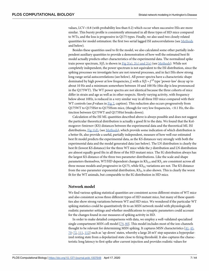
The second parameter is the strength of recurrent inhibition coming from the MSN collat-

eral network, denoted by gI. All inhibitory synapses in the MSN network have a fixed random

strength with expectation gI, which determines the size of IPSPs generated by presynaptic

spikes in the postsynaptic cell. Inhibitory synapses are modelled in the same way as [80]

including a synaptic gating variable dependent on presynaptic membrane potential represent-

ing GABAA neurotransmitter release and decay (see Methods). Fig 3 illustrates spiking in a

presynaptic cell and IPSPs in a postsynaptic cell just below firing threshold for several relevant

values of gI.All other network parameters are fixed at their experimentally observed values, such as the

cell-cell connection probability (0.2) the network size (2500 cells) and the IPSP rise and decay

timescales [80]. Although relevant for striatal information processing [116, 117] we do not

include a real spatial dimension, since our experimental single cell spiking data does not

include information about relative spatial location between cells, and we find we can well

reproduce our single cell statistical quantities without it. Network simulations are entirely

deterministic. Since feedforward excitation to each cell is fixed at a constant level, any fluctua-

tions in input current to cells are generated intrinsically by the non-stationary recurrent

dynamics of the inhibitory MSN network (see Discussion).

First, in order to appreciate the origin of the spiking characteristics found in the experimen-

tal WT data and their dysregulation in HD, we give a rough survey of how network model

activity depends on these two parameters. This also demonstrates the wide range of dynamical

Fig 3. IPSP size and timescale is in the physiological range at values of gI found to provide good fits to WT spiking

data. (a,b) Time series of supra-threshold presynaptic spiking cell (black) and slightly sub-threshold postsynaptic cell

for different values of gI (see key), (b) shows detail. At gI = 33, IPSP size is about 1.8 mV and reverts to half maximum

in about 20 msec.






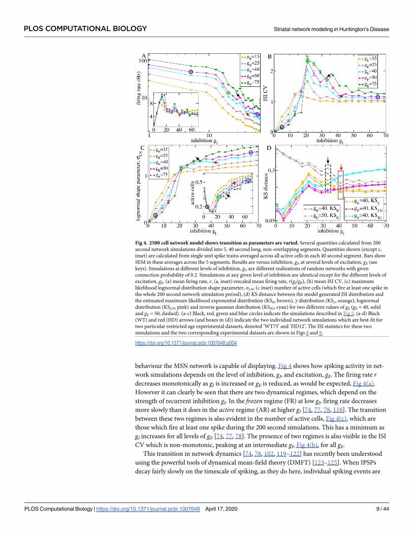
behaviour the MSN network is capable of displaying. Fig 4 shows how spiking activity in net-

work simulations depends on the level of inhibition, gI, and excitation, gE. The firing rate rdecreases monotonically as gI is increased or gE is reduced, as would be expected, Fig 4(a).

However it can clearly be seen that there are two dynamical regimes, which depend on the

strength of recurrent inhibition gI. In the frozen regime (FR) at low gI, firing rate decreases

more slowly than it does in the active regime (AR) at higher gI [74, 77, 78, 118]. The transition

between these two regimes is also evident in the number of active cells, Fig 4(c), which are

those which fire at least one spike during the 200 second simulations. This has a minimum as

gI increases for all levels of gE [74, 77, 78]. The presence of two regimes is also visible in the ISI

CV which is non-monotonic, peaking at an intermediate gI, Fig 4(b), for all gE.

This transition in network dynamics [74, 78, 102, 119–122] has recently been understood

using the powerful tools of dynamical mean-field theory (DMFT) [123–125]. When IPSPs

decay fairly slowly on the timescale of spiking, as they do here, individual spiking events are

Fig 4. 2500 cell network model shows transition as parameters are varied. Several quantities calculated from 200

second network simulations divided into 5, 40 second long, non-overlapping segments. Quantities shown (except c,

inset) are calculated from single unit spike trains averaged across all active cells in each 40 second segment. Bars show

SEM in these averages across the 5 segments. Results are versus inhibition, gI, at several levels of excitation, gE (see

keys). Simulations at different levels of inhibition, gI, are different realizations of random networks with given

connection probability of 0.2. Simulations at any given level of inhibition are identical except for the different levels of

excitation, gE. (a) mean firing rate, r, (a, inset) rescaled mean firing rate, r(gI/gE), (b) mean ISI CV, (c) maximum

likelihood lognormal distribution shape parameter, σLN, (c inset) number of active cells (which fire at least one spike in

the whole 200 second network simulation period), (d) KS distance between the model generated ISI distribution and

the estimated maximum likelihood exponential distribution (KSE, brown), γ distribution (KSγ, orange), lognormal

distribution (KSLN, pink) and inverse gaussian distribution (KSIG, cyan) for two different values of gE (gE = 40, solid

and gE = 50, dashed). (a-c) Black, red, green and blue circles indicate the simulations described in Fig 5. (a-d) Black

(WT) and red (HD) arrows (and boxes in (d)) indicate the two individual network simulations which are best-fit for

two particular restricted age experimental datasets, denoted ‘WT75’ and ‘HD12’. The ISI statistics for these two

simulations and the two corresponding experimental datasets are shown in Figs 8 and 9.






averaged out and network dynamical behaviour is determined by the associated dynamics of

the mean input current to cells. In the FR, mean input currents are stationary and unvarying

[123, 124]. As inhibition, gI, is increased, at some point this stable fixed point state becomes

unstable and a non-stationary state, the AR, with chaotically varying input currents appears

[74, 78, 123, 124]. Just above the transition, input current fluctuations are ‘critical’ and while

small in magnitude their autocorrelation decays exceedingly slowly [123, 124]. Further into

the AR, fluctuations increase in size dramatically, but also decay more rapidly.

The DMFT approximation to the spiking network dynamics is relevant even when synaptic

decay timescales are as small as 20 ms and cells have biologically reasonable firing rates [123].

However the presence of spiking modifies the predictions of DMFT somewhat. Even in the

FR, small fluctuations arise from spiking events which decorate the fixed point state, and these

fluctuations can be non-linearly amplified as gI is increased and the transition to the AR is

approached. In the critical regime, spiking noise prevents full divergence of the autocorrelation

timescale. Thus spiking smoothes the transition [124]. The DMFT predicts that due to the

dynamical balance between recurrent inhibition and feedforward excitation, firing rates

should be proportional to gE/gI [123, 124]. Network simulation firing rates rescaled by this

quantity are shown in Fig 4(a, inset). While there are substantial deviations, the approximate

independence of the rescaled firing rate from gE and gI demonstrates the relevance of the

DMFT theory, even in this spiking network model of fairly physiologically detailed MSN cells.

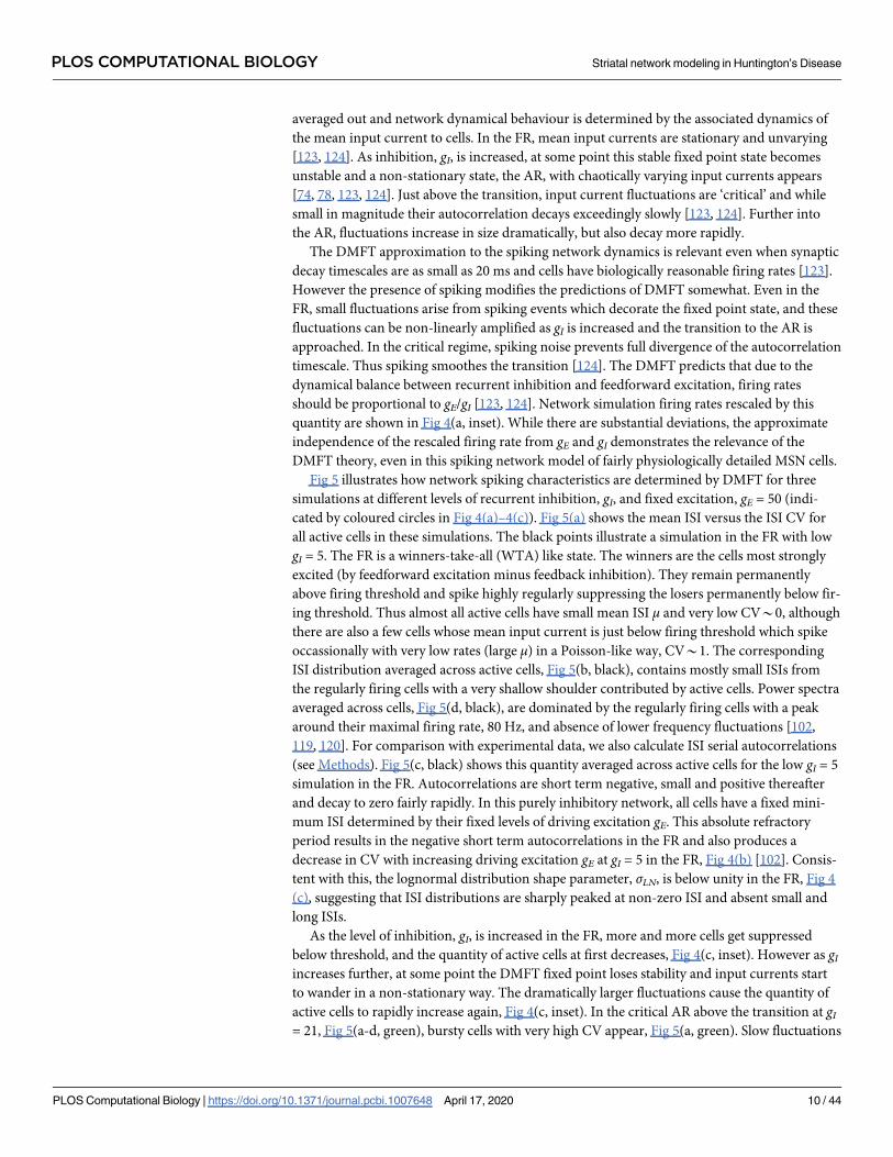
Fig 5 illustrates how network spiking characteristics are determined by DMFT for three

simulations at different levels of recurrent inhibition, gI, and fixed excitation, gE = 50 (indi-

cated by coloured circles in Fig 4(a)–4(c)). Fig 5(a) shows the mean ISI versus the ISI CV for

all active cells in these simulations. The black points illustrate a simulation in the FR with low

gI = 5. The FR is a winners-take-all (WTA) like state. The winners are the cells most strongly

excited (by feedforward excitation minus feedback inhibition). They remain permanently

above firing threshold and spike highly regularly suppressing the losers permanently below fir-

ing threshold. Thus almost all active cells have small mean ISI μ and very low CV*0, although

there are also a few cells whose mean input current is just below firing threshold which spike

occassionally with very low rates (large μ) in a Poisson-like way, CV*1. The corresponding

ISI distribution averaged across active cells, Fig 5(b, black), contains mostly small ISIs from

the regularly firing cells with a very shallow shoulder contributed by active cells. Power spectra

averaged across cells, Fig 5(d, black), are dominated by the regularly firing cells with a peak

around their maximal firing rate, 80 Hz, and absence of lower frequency fluctuations [102,

119, 120]. For comparison with experimental data, we also calculate ISI serial autocorrelations

(see Methods). Fig 5(c, black) shows this quantity averaged across active cells for the low gI = 5

simulation in the FR. Autocorrelations are short term negative, small and positive thereafter

and decay to zero fairly rapidly. In this purely inhibitory network, all cells have a fixed mini-

mum ISI determined by their fixed levels of driving excitation gE. This absolute refractory

period results in the negative short term autocorrelations in the FR and also produces a

decrease in CV with increasing driving excitation gE at gI = 5 in the FR, Fig 4(b) [102]. Consis-

tent with this, the lognormal distribution shape parameter, σLN, is below unity in the FR, Fig 4

(c), suggesting that ISI distributions are sharply peaked at non-zero ISI and absent small and

long ISIs.

As the level of inhibition, gI, is increased in the FR, more and more cells get suppressed

below threshold, and the quantity of active cells at first decreases, Fig 4(c, inset). However as gIincreases further, at some point the DMFT fixed point loses stability and input currents start

to wander in a non-stationary way. The dramatically larger fluctuations cause the quantity of

active cells to rapidly increase again, Fig 4(c, inset). In the critical AR above the transition at gI= 21, Fig 5(a-d, green), bursty cells with very high CV appear, Fig 5(a, green). Slow fluctuations




in inhibitory input current cause cells to irregularly switch between regularly spiking and qui-

escent states. The ISI distribution, Fig 5(b, green), contains a broad exponential shoulder

reflecting the long interburst intervals and a peak at small ISI from the intraburst ISIs. ISI serial

autocorrelation, Fig 5(c, green), is positive for all lags and decays very slowly due to the long

bursts of spikes while spectral power, S(f), at low frequencies increases dramatically, Fig 5(d,

green) and displays a power-law form, S(f)*f−β reflecting the very long timescales which

appear. In the AR, the lognormal distribution shape parameter, σLN, Fig 4(c), shows a transi-

tion to a value exceeding unity, indicating the presence of arbitrarily small ISIs and a long tail.

In contrast to the FR, now increasing the driving excitation gE increases the CV, Fig 4(b). In

the AR, input current fluctuations vary on a much longer timescale than the spiking itself.

Increasing excitation results in an increase in the amount of spikes within a burst without a

large effect on the interburst intervals, which increases the CV. In the critical regime, the effect

of a small change in gE on CV can be substantial.

Finally as recurrent inhibition increases further to gI = 65, Fig 5(a-d, blue), mean-field input

current fluctuations increase in magnitude but their autocorrelation decays more rapidly [123,

124]. All cells fluctuate rapidly between activity and quiescence. Spiking therefore approaches

Poisson for almost all cells as demonstrated by the fact that CV values are close to unity, Figs 4

(b) and 5(a, blue), the ISI distribution Fig 5(b, blue), is almost exponential, ISI serial autocorre-

lation, Fig 5(c, blue), is absent and the power spectrum, S(f), Fig 5(d, blue), flattens out.

Fig 5. Model generated single unit ISI characteristics for three illustrative simulations with different levels of

inhibition, gI (see keys) at a fixed level of excitation, gE = 50, indicated by the coloured circles in Fig 4(a)–4(c). (a)

Mean ISI, μ, versus ISI CV for all individual active cells in each simulation, (b) Cumulative ISI distribution, (c) ISI

serial lagged autocorrelation, (d) Spike power spectra, S(f). (b-d) Results are averages across the given quantity

calculated from all individual single cell spike trains with more than 10 spikes in each 200 second simulation and bars

show SEM across these observations (see Methods).






We also investigated how the KS distances between model generated ISI distributions and

the theoretical ML exponential, gamma (γ), log-normal (LN) and inverse-Gaussian (IG) distri-

butions, as described above, vary with the model parameters. Fig 4(d) shows the KS distances

versus model recurrent inhibition, gI, for two values of driving excitation, gE = 40 and gE = 50.

The KS distances demonstrate interesting crossovers close to the transition from FR to AR. At

very low gI in the FR for any given gE, the LN distribution (pink) is definitely the best fit (lowest

KS distance) while the γ (orange) and IG (cyan) distributions are similar, KSLN< KSγ� KSIG.

Increasing gI, in particular for higher gE, we find a regime where KSLN< KSIG< KSγ, while as

gI is increased further a regime with KSLN< KSγ< KSIG appears. Finally in the AR the γ distri-

bution becomes definitely the best fit, KSγ< KSLN< KSIG.

Model estimation

We find various differences between WT and HD data. Many of these differences are consis-

tent across phenotypes. The above observations of network model transitions suggested to us

that differences between WT and HD data might be explained by changes in network model

parameters, gE and gI. However the non-monotonic dependence of ISI statistical quantities on

model parameters means multivariate measures must be used for estimation.

Here we take a very direct approach. We calculate several (N) statistical measures, termed

features, from each of the single spike trains in a particular dataset, for example the YACHD

dataset. This results in a multivariate distribution where each N–dimensional observation cor-

responds to one spike train. We also calculate the exact same set of features from each of the

spike trains generated from a 2500 cell network model simulation with some given parameter

values, gE and gI. This results in another N–dimensional multivariate distribution characteris-

ing the given model. We then use the Kullback-Leibler (KL) distance between these two distri-

butions as a measure of how far the given model simulation is from the particular

experimental dataset (see Methods). The fifteen features used in this calculation are the thir-

teen indicated by asterisks in Fig 1 and the first two lagged ISI serial autocorrelations (see

Methods).

Heat maps of the natural logarithm of the KL distance, log KL, for the seven experimental

datasets with all animals of a given type of all ages combined, as well as two restricted age data-

sets (see below), are shown in Fig 6. Here each large coloured matrix corresponds to a particu-

lar experimental dataset and each small square in each matrix shows the KL distance from the

experimental dataset to a network model simulation parameterised by gI and gE. Note that the

gE (vertical) axis is not regularly spaced. Similarities and differences are evident in these heat

maps, reflecting the similarities and differences we found in the original data. The first column,

Fig 6(a), 6(d) and 6(g), shows the WT datasets, (a) Q175WT, (d) YACWT, (g) R62WT while

the second column Fig 6(b), 6(e) and 6(h), shows the HD datasets, (b) Q175Het, (e) YACHD,

(h) R62HD and the top of the third column Fig 6(c) shows Q175Hom. The three WT heat-

maps Fig 6(a), 6(d) and 6(g) are very similar to each other with a minimum (best fit of the KL

distance) around gI = 25* 41 and gE = 50 * 75. These gI values place the WT datasets close to

the transition, but definitely in the AR in Fig 4, as previously suggested [73, 74, 77, 78] based

on qualitative observations. However, models only provide good fits to WT datasets at higher

levels of gE, even though the FR-AR transition is found at all gE levels.

HD datasets Fig 6(b), 6(e), 6(h) and 6(c) on the other hand display a different but consistent

profile. In all cases the best fit area of minimum KL moves to lower values of gE and this change

is progressive in the Q175 mouse types, Fig 6(a), 6(b) and 6(c). The area of best fit inhibition

also becomes more diffuse and spread over a wider range gI = 33* 57. That consistent

changes in these heat maps are found across different strains of wild type mice and different




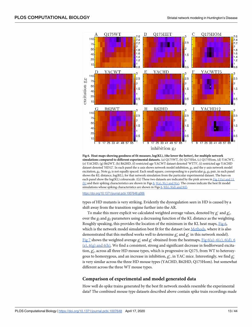
types of HD mutants is very striking. Evidently the dysregulation seen in HD is caused by a

shift away from the transition regime further into the AR.

To make this more explicit we calculated weighted average values, denoted by g�I and g�E,

over the gI and gE parameters using a decreasing function of the KL distance as the weighting.

Roughly speaking, this provides the location of the minimum in the KL heat maps, Fig 6,

which is the network model simulation best fit for the dataset (see Methods, where it is also

demonstrated that this method works well to determine g�E and g�I in this network model).

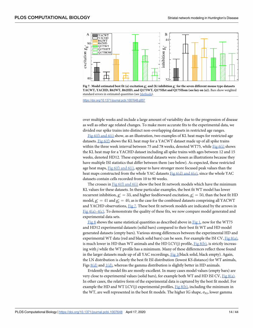
Fig 7 shows the weighted average g�E and g�I obtained from the heatmaps, Fig 6(a)–6(c), 6(d), 6

(e), 6(g) and 6(h). We find a consistent, strong and significant decrease in feedforward excita-

tion, g�E, across all three HD mouse types, which is progressive in Q175, from WT to heterozy-

gous to homozygous, and an increase in inhibition, g�I , in YAC mice. Interestingly, we find g�Eis very similar across the three HD mouse types (YACHD, R62HD, Q175Hom). but somewhat

different across the three WT mouse types.

Comparison of experimental and model generated data

How well do spike trains generated by the best fit network models resemble the experimental

data? The combined mouse type datasets described above contain spike train recordings made

Fig 6. Heat maps showing goodness of fit measure, log(KL), (the lower the better), for multiple network

simulations compared to different experimental datasets. (a) Q175WT, (b) Q175Het, (c) Q175Hom, (d) YACWT,

(e) YACHD, (g) R62WT, (h) R62HD, (f) restricted age YACWT dataset denoted ‘WT75’, (i) restricted age YACHD

dataset denoted ‘HD12’. In each panel the x-axis shows network model inhibition, gI, and the y-axis network model

excitation, gE. Note gE is not equally spaced. Each small square, corresponding to a particular gI, gE pair, in each panel

shows the KL distance, log(KL), for that network simulation from the particular experimental dataset. The bars on

each panel show the log(KL) colourscale. (f,i) These two datasets are indicated by the pink arrows in Fig 11(a) and 11

(b) and their spiking characteristics are shown in Figs 8, 9(a), 9(c) and 9(e). The crosses indicate the best fit model

simulations whose spiking characteristics are shown in Figs 8, 9(b), 9(d) and 9(f).






over multiple weeks and include a large amount of variability due to the progression of disease

as well as other age related changes. To make more accurate fits to the experimental data, we

divided our spike trains into distinct non-overlapping datasets in restricted age ranges.

Fig 6(f) and 6(i) show, as an illustration, two examples of KL heat maps for restricted age

datasets. Fig 6(f) shows the KL heat map for a YACWT dataset made up of all spike trains

within the three week interval between 75 and 78 weeks, denoted WT75, while Fig 6(i) shows

the KL heat map for a YACHD dataset including all spike trains with ages between 12 and 15

weeks, denoted HD12. These experimental datasets were chosen as illustrations because they

have multiple ISI statistics that differ between them (see below). As expected, these restricted

age heat maps, Fig 6(f) and 6(i), appear to have stronger more focused peak values than the

heat maps constructed from the whole YAC datasets Fig 6(d) and 6(e), since the whole YAC

datasets contain cells recorded from 10 to 90 weeks.

The crosses in Fig 6(f) and 6(i) show the best fit network models which have the minimum

KL values for these datasets. In these particular examples, the best fit WT model has lower

recurrent inhibition, g�I ¼ 33, and higher feedforward excitation, g�E ¼ 50, than the best fit HD

model, g�I ¼ 41 and g�E ¼ 40, as is the case for the combined datasets comprising all YACWT

and YACHD observations, Fig 7. These best fit network models are indicated by the arrows in

Fig 4(a)–4(c). To demonstrate the quality of these fits, we now compare model generated and

experimental data sets.

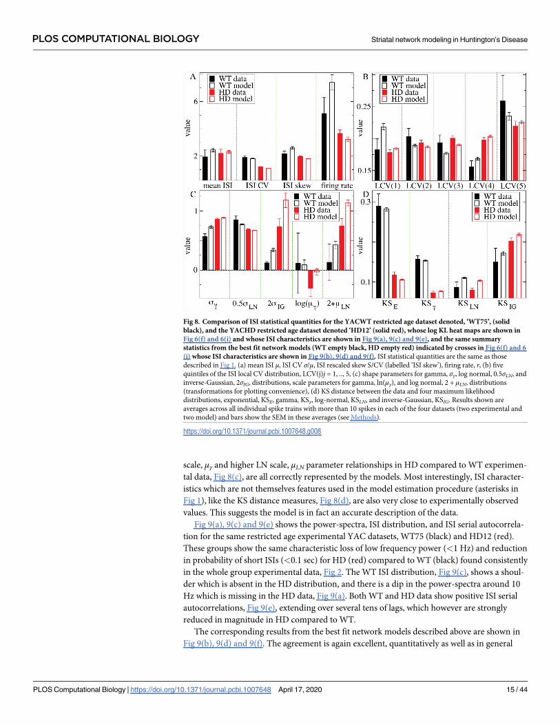
Fig 8 shows the same statistical quantities as described above in Fig 1, now for the WT75

and HD12 experimental datasets (solid bars) compared to their best fit WT and HD model

generated datasets (empty bars). Various strong differences between the experimental HD and

experimental WT data (red and black solid bars) can be seen. For example the ISI CV, Fig 8(a),

is much lower in HD than WT animals and the HD LCV(j) profile, Fig 8(b), is strictly increas-

ing with j while the WT profile has a minimum. Many of these differences reflect those found

in the larger datasets made up of all YAC recordings, Fig 1(black solid, black empty). Again,

the LN distribution is clearly the best fit ISI distribution (lowest KS distance) for WT animals,

Figs 8(d) and 1(d), whereas the gamma distribution is slightly better in HD animals.

Evidently the model fits are mostly excellent. In many cases model values (empty bars) are

very close to experimental values (solid bars), for example both WT and HD ISI CV, Fig 8(a).

In other cases, the relative form of the experimental data is captured by the best fit model. For

example the HD and WT LCV(j) experimental profiles, Fig 8(b), including the minimum in

the WT, are well represented in the best fit models. The higher IG shape, σIG, lower gamma

Fig 7. Model estimated best fit (a) excitation g�E and (b) inhibition g�I for the seven different mouse type datasets

YACWT, YACHD, R62WT, R62HD, and Q175WT, Q175Het and Q175Hom (see key on (a)). Bars show weighted

standard errors in estimated quantities (see Methods).






scale, μγ and higher LN scale, μLN parameter relationships in HD compared to WT experimen-

tal data, Fig 8(c), are all correctly represented by the models. Most interestingly, ISI character-

istics which are not themselves features used in the model estimation procedure (asterisks in

Fig 1), like the KS distance measures, Fig 8(d), are also very close to experimentally observed

values. This suggests the model is in fact an accurate description of the data.

Fig 9(a), 9(c) and 9(e) shows the power-spectra, ISI distribution, and ISI serial autocorrela-

tion for the same restricted age experimental YAC datasets, WT75 (black) and HD12 (red).

These groups show the same characteristic loss of low frequency power (<1 Hz) and reduction

in probability of short ISIs (<0.1 sec) for HD (red) compared to WT (black) found consistently

in the whole group experimental data, Fig 2. The WT ISI distribution, Fig 9(c), shows a shoul-

der which is absent in the HD distribution, and there is a dip in the power-spectra around 10

Hz which is missing in the HD data, Fig 9(a). Both WT and HD data show positive ISI serial

autocorrelations, Fig 9(e), extending over several tens of lags, which however are strongly

reduced in magnitude in HD compared to WT.

The corresponding results from the best fit network models described above are shown in

Fig 9(b), 9(d) and 9(f). The agreement is again excellent, quantitatively as well as in general

Fig 8. Comparison of ISI statistical quantities for the YACWT restricted age dataset denoted, ‘WT75’, (solid

black), and the YACHD restricted age dataset denoted ‘HD12’ (solid red), whose log KL heat maps are shown in

Fig 6(f) and 6(i) and whose ISI characteristics are shown in Fig 9(a), 9(c) and 9(e), and the same summary

statistics from the best fit network models (WT empty black, HD empty red) indicated by crosses in Fig 6(f) and 6

(i) whose ISI characteristics are shown in Fig 9(b), 9(d) and 9(f). ISI statistical quantities are the same as those

described in Fig 1. (a) mean ISI μ, ISI CV σ/μ, ISI rescaled skew S/CV (labelled ‘ISI skew’), firing rate, r, (b) five

quintiles of the ISI local CV distribution, LCV(j)j = 1, .., 5, (c) shape parameters for gamma, σγ, log normal, 0.5σLN, and

inverse-Gaussian, 2σIG, distributions, scale parameters for gamma, ln(μγ), and log normal, 2 + μLN, distributions

(transformations for plotting convenience), (d) KS distance between the data and four maximum likelihood

distributions, exponential, KSE, gamma, KSγ, log-normal, KSLN, and inverse-Gaussian, KSIG. Results shown are

averages across all individual spike trains with more than 10 spikes in each of the four datasets (two experimental and

two model) and bars show the SEM in these averages (see Methods).






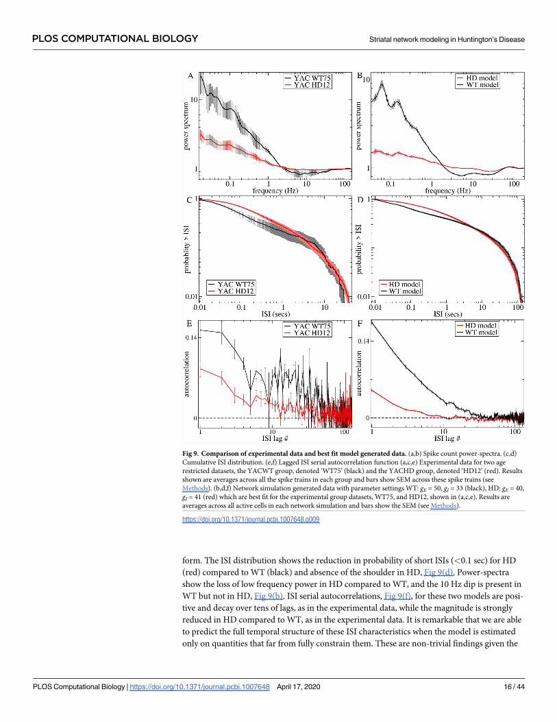
form. The ISI distribution shows the reduction in probability of short ISIs (<0.1 sec) for HD

(red) compared to WT (black) and absence of the shoulder in HD, Fig 9(d). Power-spectra

show the loss of low frequency power in HD compared to WT, and the 10 Hz dip is present in

WT but not in HD, Fig 9(b). ISI serial autocorrelations, Fig 9(f), for these two models are posi-

tive and decay over tens of lags, as in the experimental data, while the magnitude is strongly

reduced in HD compared to WT, as in the experimental data. It is remarkable that we are able

to predict the full temporal structure of these ISI characteristics when the model is estimated

only on quantities that far from fully constrain them. These are non-trivial findings given the

Fig 9. Comparison of experimental data and best fit model generated data. (a,b) Spike count power-spectra. (c,d)

Cumulative ISI distribution. (e,f) Lagged ISI serial autocorrelation function (a,c,e) Experimental data for two age

restricted datasets, the YACWT group, denoted ‘WT75’ (black) and the YACHD group, denoted ‘HD12’ (red). Results

shown are averages across all the spike trains in each group and bars show SEM across these spike trains (see

Methods). (b,d,f) Network simulation generated data with parameter settings WT: gE = 50, gI = 33 (black), HD: gE = 40,

gI = 41 (red) which are best fit for the experimental group datasets, WT75, and HD12, shown in (a,c,e). Results are

averages across all active cells in each network simulation and bars show the SEM (see Methods).






large range of possible profiles these quantities can take up in this network model, as demon-

strated in Fig 5, and again suggest that the model is correct.

These two WT and HD best fit models are quite close in parameter space, only separated by

ΔgE = 10 and ΔgI = 8. The small difference between IPSPs at gI = 33 (WT) and gI = 41 (HD) is

illustrated in Fig 3(b). How does such a striking change in spiking dynamics occur? Fig 4 illus-

trates that a small change in parameters can have a large effect when parameters are modified

in the vicinity of the network transition. The arrows, Fig 4(a)–4(c), and rectangles, Fig 4(d),

indicate the best fit WT (black) and HD (red) models.

Close to the transition, ISI CV falls dramatically from a very bursty WT value of about 1.7

to a minimal Poisson-like HD value about 1.1, as gE is reduced and gI increased, Fig 4(b). On

the other hand, the drop in firing rate, Fig 4(a), from about 7Hz for the WT model to about

3Hz for the HD model is rather modest considering the large range possible within the gE and

gI models explored. The ISI distribution KS measures, Fig 4(d), reveal the effect of the transi-

tion particularly clearly. The KS distance measures for the WT best fit model (gE = 50, gI = 33),

Fig 4(d, dashed lines within black dashed rectangle), show that the LN KS distance is a clear

minimum, indicating that the WT model is in the transition regime. Increasing gI and decreas-

ing gE just a small amount to the HD best fit model parameter values (gE = 40, gI = 41), Fig 4(d,

solid lines with solid red rectangle), causes a transition to a state where the γ distribution is the

minimum.

Age dependency

YAC and Q175 HD mice display a slowly progressing phenotype with behavioural changes

across the age range from 10 to 100 weeks [13, 81, 86, 92, 94, 97]. We next wondered if we

could find a progressive variation in statistical quantities with age, which might possibly be

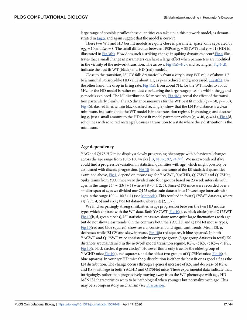
associated with disease progression. Fig 10 shows how some of the ISI statistical quantities

examined above, Fig 1, depend on mouse age for YACWT, YACHD, Q175WT and Q175Het.

Spike trains from YAC mice were divided into four groups based on 23 week intervals with

ages in the range 23i* 23(i + 1) where i 2 {0, 1, 2, 3}. Since Q175 mice were recorded over a

smaller span of ages we divided our Q175 spike train dataset into 10 week age intervals with

ages in the range 10i* 10(i + 1) (see Methods). This resulted in four Q175WT datasets, where

i 2 {2, 3, 4, 5} and six Q175Het datasets, where i 2 {2, .., 7}.

We find surprisingly strong similarities in age progression between the two HD mouse

types which contrast with the WT data. Both YACWT, Fig 10(a, c, black circles) and Q175WT

Fig 10(b, d, green circles), ISI statistical measures show some quite large fluctuations with age

but do not show clear trends. On the contrary both the YACHD and Q175Het mouse types,

Fig 10(red and blue squares), show several consistent and significant trends. Mean ISI, μ,

decreases while ISI CV and skew increase, Fig 10(a red squares, b blue squares). In both

YACWT and Q175WT mice consistently in every age group (8 age group datasets in total) KS

distances are maintained in the network model transition regime, KSLN< KSγ< KSIG< KSE,

Fig 10(c black circles, d green circles). However this is only true for the oldest group of

YACHD mice Fig 10(c, red squares), and the oldest two groups of Q175Het mice, Fig 10(d,

blue squares). In younger HD mice the γ distribution is either the best fit or as good a fit as the

LN distribution. The change occurs through a general increase of KSγ and decrease of KSLN

and KSIG with age in both YACHD and Q175Het mice. These experimental data indicate that,

intriguingly, rather than progressively moving away from the WT phenotype with age, HD

MSN ISI characteristics seem to be pathological when younger but normalize with age. This

may be a compensatory mechanism (see Discussion).




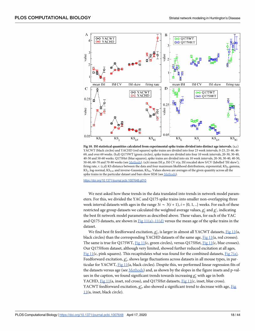
We next asked how these trends in the data translated into trends in network model param-

eters. For this, we divided the YAC and Q175 spike trains into smaller non-overlapping three

week interval datasets with ages in the range 3i* 3(i + 1), i = {0, 1, ..} weeks. For each of these

restricted age group datasets we calculated the weighted average values, g�E and g�I , indicating

the best fit network model parameters as described above. These values, for each of the YAC

and Q175 datasets, are shown in Fig 11(a)–11(d) versus the mean age of the spike trains in the

dataset.

We find best fit feedforward excitation, g�E, is larger in almost all YACWT datasets, Fig 11(a,

black circles) than the corresponding YACHD datasets of the same age, Fig 11(a, red crosses).

The same is true for Q175WT, Fig 11(c, green circles), versus Q175Het, Fig 11(c, blue crosses).

Our Q175Hom dataset, although very limited, showed further reduced excitation at all ages,

Fig 11(c, pink squares). This recapitulates what was found for the combined datasets, Fig 7(a).

Feedforward excitation, g�E, shows large fluctuations across datasets in all mouse types, in par-

ticular for YACWT, Fig 11(a, black circles). Despite this, we performed linear regression fits of

the datasets versus age (see Methods) and, as shown by the slopes in the figure insets and p-val-

ues in the caption, we found significant trends towards increasing g�E with age in both

YACHD, Fig 11(a, inset, red cross), and Q175Het datasets, Fig 11(c, inset, blue cross).

YACWT feedforward excitation, g�E, also showed a significant trend to decrease with age, Fig

11(a, inset, black circle).

Fig 10. ISI statistical quantities calculated from experimental spike trains divided into distinct age intervals. (a,c)

YACWT (black circles) and YACHD (red squares) spike trains are divided into four 23 week intervals, 0-23, 23-46, 46-

69, and over 69 weeks. (b,d) Q175WT (green circles), spike trains are divided into four 10 week intervals, 20-30, 30-40,

40-50 and 50-60 weeks. Q175Het (blue squares), spike trains are divided into six 10 week intervals, 20-30, 30-40, 40-50,

50-60, 60-70 and 70-80 weeks (see Methods). (a,b) mean ISI μ, ISI CV σ/μ, ISI rescaled skew S/CV (labelled ‘ISI skew’),

firing rate, r. (c,d) KS distance between the data and four maximum likelihood distributions, exponential, KSE, gamma,

KSγ, log-normal, KSLN, and inverse-Gaussian, KSIG. Values shown are averages of the given quantity across all the

spike trains in the particular dataset and bars show SEM (see Methods).






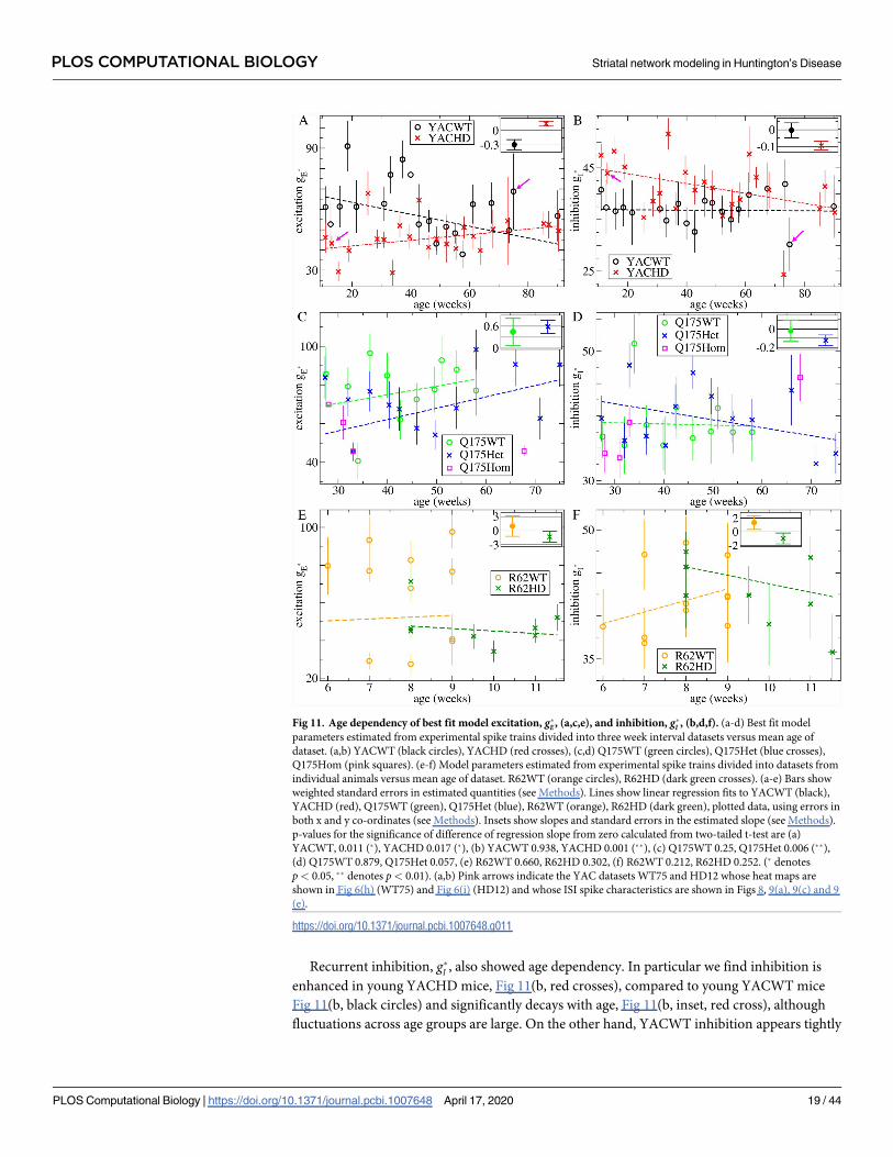
Recurrent inhibition, g�I , also showed age dependency. In particular we find inhibition is

enhanced in young YACHD mice, Fig 11(b, red crosses), compared to young YACWT mice

Fig 11(b, black circles) and significantly decays with age, Fig 11(b, inset, red cross), although

fluctuations across age groups are large. On the other hand, YACWT inhibition appears tightly

Fig 11. Age dependency of best fit model excitation, g�E , (a,c,e), and inhibition, g�I , (b,d,f). (a-d) Best fit model

parameters estimated from experimental spike trains divided into three week interval datasets versus mean age of

dataset. (a,b) YACWT (black circles), YACHD (red crosses), (c,d) Q175WT (green circles), Q175Het (blue crosses),

Q175Hom (pink squares). (e-f) Model parameters estimated from experimental spike trains divided into datasets from

individual animals versus mean age of dataset. R62WT (orange circles), R62HD (dark green crosses). (a-e) Bars show

weighted standard errors in estimated quantities (see Methods). Lines show linear regression fits to YACWT (black),

YACHD (red), Q175WT (green), Q175Het (blue), R62WT (orange), R62HD (dark green), plotted data, using errors in

both x and y co-ordinates (see Methods). Insets show slopes and standard errors in the estimated slope (see Methods).

p-values for the significance of difference of regression slope from zero calculated from two-tailed t-test are (a)

YACWT, 0.011 (�), YACHD 0.017 (�), (b) YACWT 0.938, YACHD 0.001 (��), (c) Q175WT 0.25, Q175Het 0.006 (��),

(d) Q175WT 0.879, Q175Het 0.057, (e) R62WT 0.660, R62HD 0.302, (f) R62WT 0.212, R62HD 0.252. (� denotes

p< 0.05, �� denotes p< 0.01). (a,b) Pink arrows indicate the YAC datasets WT75 and HD12 whose heat maps are

shown in Fig 6(h) (WT75) and Fig 6(i) (HD12) and whose ISI spike characteristics are shown in Figs 8, 9(a), 9(c) and 9

(e).






regulated with age, Fig 11(b, black circles, inset black circle), around g�I ¼ 35 � 40. Interest-

ingly, we find very similar behaviour in Q175 animals. Except for one outlier around 35 weeks,

Q175WT inhibition appears tightly regulated, again around g�I ¼ 35 � 40, Fig 11(d, green cir-

cles, inset green circle), while Q175Het inhibition, Fig 11(d, blue crosses), decays with age with

a similar slope, Fig 11(d, inset blue cross), to the YACHD data, albeit with much weaker

significance.

Thus the transition we found in the YACHD and Q175Het experimental data, Fig 10,

mainly translates into a gradual decay of recurrent inhibition in HD compared to WT, starting

from a state of enhanced inhibition. On the other hand feedforward excitation is reduced from

the outset in HD and continues to be reduced across all age ranges. The tightly regulated inhi-

bition around g�I ¼ 35 � 40 found in WT animals places them in the AR just above the transi-

tion regime, Fig 4, at all ages, while HD animals are found deeper in the AR.

Due to the rapidly progressing nature of the R6/2 phenotype our data did not include much

age variation. However in Fig 11(e) and 11(f) we plot estimated g�I;E for R62WT and R62HD

individual animals versus the mean age of their spike trains. Again we find excitation, g�E, is

generally reduced in R62HD, Fig 11(e, dark green crosses), compared to R62WT, Fig 11(e,

orange circles), while fluctuations in g�E across R62WT datasets, Fig 11(e, orange circles), are

again large, as they were in the YACWT datasets, Fig 11(a, black circles). Recurrent inhibition,

g�I , does not show much phenotype dependency Fig 11(f), and none of the linear regression

slopes, Fig 11(e,f insets), are significantly different from zero.

Dynamical complexity

Our experimental data set was limited to single unit recordings. We did not have access to any

multi-unit data and therefore did not use any multivariate information, such as cross-correla-

tions, to estimate network model parameters. However, it is known that coherent burst firing

and slowly varying cell-assembly activity is present in WT MSN multi-unit recordings and

that this coherent activity is lost in HD mice [42]. Remarkably, this is also an emergent finding

of the present analysis.

Fig 12 shows spike time series raster plots from the two network simulations best fit to the

restricted age YAC datasets, WT75, and HD12, whose ISI statistics are shown in Fig 8, indi-

cated by the arrows in Fig 4(a)–4(c). Evidently the WT best fit model with gI = 33, gE = 50 dis-

plays coherent bursting cell assembly activity, Fig 12(a), while this activity is lost in the HD

best fit model with gI = 41 and gE = 40, Fig 12(b), despite the rather small change in parameters.

These raster plots are very similar in appearance to the ones shown in [42] for WT and HD

mice.

To quantify this finding, we calculate the principal components of the network activity

based on the firing rate covariance matrix using a 100 ms sliding window to estimate firing

rates from the spiking data. A large proportion of the variance is explained by fewer compo-

nents in the WT model compared to the HD model, Fig 12(c). Fig 12(d) shows how the

entropy of the explained variance distribution varies with gI and gE in multiple simulations. It

has a minimum close to the transition from FR to AR at all levels of gE, which is stronger for

higher gE. The minimum suggests that the network is generating low dimensional rate fluctua-

tions in the transition regime. Entropy is high in the FR because although the mean-field input

current dynamics has a stable fixed point, spiking generates white noise like fluctuations in the

measured rate dynamics. On the other hand entropy is high at high gI because mean-field

input currents fluctuate strongly. The squares indicate that the WT best fit model network

(black) generates lower dimensional dynamics than the best fit HD model (red). The low

dimensional rate activity shows up as coherent cell assemblies in the spiking activity, Fig 12(a).




Discussion

MSNs in the striatum of WT mice display slowly varying coherent burst firing activity which is

diminished in HD mice [42, 67, 68]. We hypothesized that this patterned activity is generated

by the recurrent inhibitory MSN network and that its loss in HD occurs as a result of changes

in parameters local to individual cells. To investigate this hypothesis we fit an MSN recurrent

network model to mouse spiking data. To fit the model we varied only two parameters, the

mean level of feedforward excitation and the mean level of recurrent inhibition. Other param-

eters, synaptic and cellular, were set at their physiological values and we used a fairly detailed

cell model which faithfully represents MSN properties [79, 80]. In particular we demonstrate

that it is neither necessary to vary any model timescale parameters nor is it necessary to rely on

putative temporally varying cortical driving to reproduce slowly varying striatal burst firing

activity or its reduction in HD. Given this simple model and its simplest possible parameter

variation, the fits we obtain to both the WT and HD, as demonstrated by Figs 8 and 9, are sur-

prisingly good. These fits are not just qualitative. Detailed properties of the autocorrelation

function, as represented by the shape of the power-spectrum, and its decomposition into ISI

distribution and serial ISI autocorrelation, are quantitatively captured. Fluctuations generated

by recurrent inhibition in the MSN network are therefore sufficient to generate the correct ISI

autocorrelation properties. That the WT can be so well represented and the HD phenotype

recovered by just small parameter changes suggests that our hypothesis is correct.

Fig 12. (a,b) Sections of raster plots from the (a) WT and (b) HD best fit network simulations depicted by crosses in

Fig 6(f) (WT) and Fig 6(i) (HD) whose ISI statistics are also shown in Figs 8, 9(b), 9(d) and 9(f). (c) Explained variance

of the principal components of ensemble rate fluctuations of all active cells for simulations shown in (a, black) and (b,

red). (d) Entropy of explained variance distributions for principal components of ensemble rate fluctuations for

multiple network simulations at different levels of inhibition gI and excitation gE. Network simulations described in (a,

b,c) are indicated by the black (WT) and red (HD) arrows.






By demonstrating the broad range of activity the recurrent inhibitory network model can

generate as parameters are varied, Figs 4 and 5, we showed coherent bursting emerged as a

property of a transition regime from stable to strongly fluctuating recurrent network dynam-

ics. Most interestingly, we found WT empirical data was best fit by network models with levels

of recurrent inhibition which placed them in the critical regime, just above this transition.

This finding was consistent across the WT strains as shown by the KL distance plots, Fig 6(a),

6(d) and 6(g), and best fit values, Fig 7(b). It was also consistent across different ages in

YACWT, Fig 11(b), and Q175WT mice, Fig 11(d), and across different individual R62WT ani-

mals, Fig 11(f). WT feedforward excitation, gE, was more variable than recurrent inhibition, gI,but also restricted to a given intermediate range.

Are the best fit values of inhibition and excitation we found physiologically plausible? The

network simulation used to illustrate the fit to WT spiking data, Figs 6(f) and 8 (black), has

recurrent inhibition level gI = 33. This is about 1/3 the value used in [80]. The discrepancy

probably originates from the larger network size we are using which allows us to reduce the

IPSP size closer to observed values. Indeed at this gI level, IPSPs generated in postsynaptic cells

with membrane potentials close to firing threshold are about 2 mV (see Fig 3). This is in the

physiological regime, but slightly larger than typically observed [10, 126, 127]. Typical values

are around 0.5* 1 mV for cells close to firing threshold (IPSPs actually shown in [10, 126,

127] are much larger, but this is because the cells are voltage clamped and the chloride reversal

potential is manipulated). The slightly larger size may be because we have fewer incoming

inhibitory connections than in reality, which requires slightly larger IPSPs to provide the cor-

rect total recurrent inhibitory input to the postsynaptic cell. In our 2500 cell networks, with

connection probabilites of 0.2, each cell receives connections from approximately 500 presyn-

aptic cells. However experimental studies [10, 126] often find connection probabilities of

around 0.35 (0.35 is the connection probability used in [80] model). Another possibility is that

the IPSP decay timescale, although appropriate for GABAA synapses in the striatum, and close

to the value used in [80], is a bit too small. Indeed while IPSPs are highly variable, IPSP areas

shown in [126] often range between 100 and 300 μVs. Adjusting for the experimental protocol

conditions results in areas between about 30 and 100 μVs for IPSPs in cells close to firing

threshold. The IPSPs shown in Fig 3 have areas around 60 or 70 μVs well within the acceptable

range, and close to the midpoint, in fact. Synaptic facilitation and suppression, which we have

not included in this model, are also known to occur at these synapses [127], and would be

expected to generate a larger range of IPSP sizes.

Furthermore, provided recurrent inhibition, gI, has roughly the correct value, as we suggest

it does, then feedforward excitation, gE, should also have roughly the correct value if network

activity is physiologically reasonable. As shown in Fig 8(a, solid black), the WT empirical

mean ISI is around 2 secs. Since the best fit network generates an almost identical mean ISI,

Fig 8(a, empty black), we can conclude that the level of feedforward excitation, gE, we find is

also reasonable. The fact that spiking characteristics matching WT data occur when the IPSP

size, gI, is physiologically reasonable, but, crucially, do not match when gI is outside this range,

as demonstrated by Figs 4 and 5, futher supports our hypothesis that the empirically observed

coherent bursting is generated by the MSN recurrent network.

We found that MSNs in the best fit WT model did not simply burst fire, but that their firing

rates varied coherently across multiple cells, as shown by the spiking raster and eigenvalue

spectrum, Fig 12. While the WT raster plot, Fig 12(a), does display switching activity resem-

bling up-down state transitions in certain subsets of cells, we have not investigated if the mem-

brane potential for these cells shows the bimodal distribution associated with up-down states

in the striatum [70]. This coherent bursting activity was reduced in best fit HD models. Since

our model estimation procedure utilized only single cell spiking characteristics, without




multivariate measures, this is an emergent finding. It is important to point out that the tacit

assumption underlying this is that the model is correct. That is to say, the experimental data is

actually drawn from the model with the network and cellular parameters we have set at their

physiological values and within the explored range of gI and gE. Given this, we have demon-

strated in Methods that gI and gE, can be uniquely determined from the single unit ISI statis-

tics. Furthermore, network simulations show that at these parameter settings, coherent

bursting is prevalent, Fig 12. Thus, we infer the presence of coherent activity from single unit

ISI statistics by assuming the model is correct. This does not mean that this is the only model

that could in principle reproduce the correct single cell ISI statistics or that they cannot be well

reproduced at some other cellular or network parameter settings in the current model. In par-

ticular, it does not rule out the possibility that at some other parameter settings, single cell ISI

statistics could be captured but without the cross-cell firing rate coherence. However, we have

not observed such regimes in the current model, and they would have to be far outside the

physiologically acceptable range. Furthermore, it is difficult to imagine a mechanism in the

current model which could reproduce slowly varying burst firing, except by the coherent activ-

ity of afferent cells. Conversely, while we did not find it necessary to include a spatial dimen-

sion in the network structure, or network hubs, or to impose cortical driving activity which

varied coherently across cells to reproduce coherent bursting, this does not mean that such

mechanisms do not also operate in the striatum. However, it is highly likely that this is the sim-

plest and most parsimonious model which accounts for coherent bursting in the striatum.

We investigated three different genetic models of Huntington’s Disease. We found consis-

tent changes in ISI statistics between the HD transgenics and the corresponding WT strains.

In particular, low frequency spectral power and ISI CVs were reduced in the HD mice com-

pared to WT mice, while the best fit ISI distribution, which was log-normal in WT mice, was

much closer to gamma in HD mice. Due to the slowly progressing nature of the YAC and

Q175 phenotypes we were also able to investigate changes in ISI statistics with age. Our

YAC128 data ranged from 10 to 90 weeks, while our Q175 data ranged from about 30 to 75

weeks. In both cases we found that HD ISI statistics were most different from WT when

young, but approached WT values with greater ages (to some extent). This was most evident in

the HD best fit ISI distribution, which changed progressively from gamma to lognormal with

age.

From the network model fit, we established that while the WT mice were poised in the net-

work critical regime, strikingly, all three HD mouse types were found to be supercritical in the

active regime. This change was mainly caused by a significant reduction in feedforward excita-

tion, gE, in all HD mouse types compared to their WT controls at all ages. Feedforward excita-

tion did increase with age in YAC128 and Q175Het mice, but this effect was fairly weak. We

also found changes in recurrent inhibition: gI was higher in young YAC128 mice, and to a

lesser extent young Q175Het mice, than their age matched WT controls, and this was followed

by a decline with increasing age. In WT mice inhibition, was much more tightly regulated,

with no age dependency. R6/2 mice showed no age related changes however. Is there any

empirical evidence for these model pathologies?

The large number of neuronal and glial dysfunctions associated with HD in the striatum

complicate conclusions which can be drawn about the underlying mechanisms for dysregula-

tion of burst firing. The two parameters we varied, gE and gI, are simplifications of a much

more complex reality. In our model gI controls the impact of slowly varying inhibitory input

current from the MSN network on individual cells, while gE is a constant offset current which

must be net excitatory. Many physiogically measured quantities that are pathological in HD

can actually affect both of these parameters. Moreover, variations in both of these parameters

affect the properties of the MSN network-generated fluctuations, as described in Fig 4, in a




non-linear way, such that it need not be immediately obvious which of them may underlie any

particular empirically observed variation. For example, increasing gE increases the excitatory

input to a cell and its firing rate, Fig 4(a). However, whether it increases or decreases the size

or timescale of inhibitory input current fluctuations coming from the MSN network, resulting

in an increase or a decrease of burstiness, CV, depends on the value of gI, Fig 4(b).

HD pathologies, which may be represented by variations in gE in this model, include not

only changes in presynaptic glutamatergic cortical and thalamic input and changes in feedfor-

ward inhibition, like FSI GABA input, but also alterations in glia or neuromodulators, like

dopamine and endocannabinoids, which regulate the effects of these neurotransmitters on

MSNs. Changes in postsynaptic dendritic structure or its intergrative properties and even

MSN cellular changes, which may change rheobase current may also account for our variation

in gE. Similarly, changes in neuromodulators, glia, cellular or synaptic properties may also pro-

duce changes in gI if they alter synaptic transmission between MSNs. Furthermore, in this

work we have not varied the network size or the MSN-MSN connection probability. However

if the network is sufficiently large (which it is here) a change in the quantity of inhibitory syn-

apses may produce very similar effects on network dynamics as a change in their mean

strength gI [78, 102, 119, 123, 124].

Multiple studies [100, 128] have found cortical dysfunction in HD, that lead to changes in

feedforward excitation to the striatum. In R6/2 mice, alterations in the corticostriatal pathway

preceed symptomatology and MSN cell death. Spontaneous glutamatergic EPSC frequency

was similar in 3-4 week old HD mice compared to controls, but significantly reduced by 5-7

weeks, when behavioural symptoms appear, and severely reduced by 11-15 weeks [24]. Corti-

costriatal AMPA and NMDA receptor-mediated evoked responses were reduced in size in

symptomatic mice [129, 130] and the density of excitatory synaptic contacts onto MSNs, as

well as MSN spine size, were found to be reduced [130]. All the R6/2 HD mice in our study

were in this late symptomatic stage between 8 and 11 week and our primary result of reduced

gE, Figs 11(e) and 7(a), is thus strongly consistent with these experimental findings.

Studies of YAC128 mice have focused on three age groups, around 1.5 months (6 weeks),

around 6-7 months (28 weeks) and around 12 months (52 weeks). We do not have 6 week

data. However, at both 28 and 52 weeks, we find feedforward excitation, gE, is reduced in WT

compared to HD, Figs 11(a) and 7(a). This is also in good agreement with multiple studies.

Cortically evoked EPSCs are smaller in HD than WT YAC128 at 7 months [26, 27]. Evoked

postsynaptic receptor mediated NMDA currents in presymptomatic YAC128 mice decrease

with advanced disease progression [26]. Spontaneous EPSCs are reduced in frequency and

decay slightly faster in YAC128 compared to WT at 6 and 12 months [1, 40]. Evoked EPSCs

were also much smaller in symptomatic HD mice compared to WT in D1 cells, although simi-

lar in D2 cells [1]. The authors therefore suggested that late stage HD is characterized by a loss

of presynaptic and postsynaptic glutamate function in D1 cells in particular.

The 3-4 month and 6-9 month age groups of Q175 heterozygous and homozygous mice

also demonstrate significant reduction in cortically evoked EPSC amplitudes compared to age

matched WTs [98]. Although we do not have 3-4 month Q175 data, our analysis of 25-40 week

data agrees with this. The same study also found that evoked EPSP amplitudes decreased pro-

gressively from Q175WT to Q175Het to Q175Hom in both age groups [98], in good agree-

ment with our findings. Spontaneous EPSC frequency was also significantly decreased in

MSNs from Q175 mice at 7 and 12 months and was more pronounced in Q175Hom than

Q175Het mice [28]. This was associated with a reduction in spine density. Also in good agree-

ment with our results, a recent study found dendritic excitability of indirect pathway MSNs in

Q175Het mice was depressed at around 24 weeks when mice became symptomatic [131].




Interestingly, selective suppression of the mutant huntingtin gene in cortical efferents par-

tially restores a healthy pattern of MSN activity in symptomatic HD mice [100], further sup-

porting a role for aberrant cortico-striatal communication in HD.

Mechanisms responsible for decreased excitation may be further complicated by local

homeostatic response by glia to changes in cortical inputs. GLT-1, the transporter responsible

for regulating the extracellular level of striatal glutamate [132, 133] and for controlling gluta-

mate-mediated long-term synaptic plasticity [134], is down-regulated in HD [135, 136].

Manipulations that increase striatal GLT-1 expression in HD mice improve both the motor

phenotype [137] and striatal gamma band activity [138], however the decline in glutamate

uptake was not reflected in an increase in extracellular glutamate [137]. The authors suggested

that glutamate transmission in these mice may adapt to the loss of uptake with a compensatory

decrease in glutamate release [137]. Downregulation of GLT-1 also increases astrocytic GABA

release [139] which would contribute to the reduction in feedforward excitation, gE. Our find-

ings are therefore consistent with a decrease in glutamate release caused by downregulation in

glutamate uptake and the concomittant increase in astrocytic GABA release. In addition,

because GLT-1 is dysfunctional, AMPA receptor desensitization may also play a role in our

findings of decreased excitation [140, 141].

Reduced feedforward excitation, gE, may also reflect an increase in feedforward inhibition.

The heterogeneous population of striatal interneurons exerts different inhibitory and modula-

tory control of MSN activity [142]. Growing evidence from HD model animals suggests

changes in intra-striatal synaptic coupling related to interneuron dysfunction [23, 143]. Fast-

spiking interneurons, for example, are likely drivers of the increase in striatal gamma-band

power reported for Q175 mice [144] and this may also result in increased feedforward inhibi-

tion of MSNs.

Various MSN cellular neurodegenerative changes are also widespread in HD [86, 129, 145].

MSNs show increases in cell membrane input resistance, depolarized resting membrane

potentials and reductions in rheobase current [40, 129, 146, 147]. The primary effect on cellu-

lar excitability is equivalent to an increased level of driving excitation in HD compared to WT.

Thus the reduced feedforward excitation, gE, we find in young HD compared to WT mice sug-

gests that the well established reduction in synaptic efficacy plays a stronger role than the

increase in cellular excitability at this age, which may represent a compensatory mechanism.

We also found a gradual decrease of excitation with age in YACWT mice while age related

changes in excitation were not found in our R62WT or Q175WT mice, possibly due to greatly

reduced age variation in our data for these latter two mice. While studies in mice appear to be

lacking, in agreement with our model observation, decreased excitation in aged rats compared

to young ones has been found [148–150].

While the reduction in cortical excitation in multiple transgenic HD mice is well estab-

lished, experimental findings on recurrent inhibition are more complicated and less conclu-

sive. Spontaneous and evoked IPSCs in R6/2 MSNs were found to be significantly larger and

spontaneous ones more frequent than WT [10, 38]. These IPSCs may have originated from

FSIs, so the authors also investigated MSN-MSN connections directly [10]. They found

reduced connection probability between D2 cells and between D2 and D1 cells, but increased

connection probability between D1 cells in R6/2 mice compared to controls. On the other

hand success rates were higher in R6/2 mice in all connection types, while IPSP areas were

smaller. A study of YAC128 mice found spontaneous IPSCs were more frequent, but had

smaller area, in some MSNs compared to WT MSNs, and this difference increased with age

between 6 and 12 months [40]. Spontaneous IPSC frequency was strongly increased in D2 but

not D1 cells in symptomatic 12 month YAC128 mice [151]. In Q175 mice the frequency and

amplitude of spontaneous IPSCs increased progressively from WT to Het to Hom at 7 and 12




months [28]. However, other studies [4] have found smaller evoked IPSCs in Q175 and R6/2

compared to WT mice.

Unfortunately most studies of IPSCs do not distinguish FSI feedforward inhibition from

MSN feedback inhibition [86]. Increased feedforward inhibition is equivalent to reduced gE in

our model. Furthermore, observed changes in the frequency of spontaneous IPSCs may be due

to higher firing rates in presynaptic neurons [4] rather than any changes in synaptic strength

per se. Progressive MSN cell death is well established however, and in some agreement with

our results, would manifest as a gradual reduction in our parameter gI at advancing symptom-

atic ages, as would the general reduction in MSN-MSN connection probability found in [10].

Our model assumes a random network; asymmetric connectivity patterns [10, 152] and spatial

distortions of dendritic trees [153–155] found in HD should be investigated in future

modeling.

Both YAC128 and Q175Het mice were more similar to their WT controls when old than

when when young. This was clear in both the raw experimental data and the fitted model. This

finding is somewhat surprising because spiking activity might be expected to become more

dissimilar between HD and WT as age and symptoms progress. However this need not be the

case. In fact, it is possible that mutant mice start off in a pathological state, which normalizes

with age through compensatory mechanisms, but which still results in behavioural symptoms.

There are multiple possible scenarios consistent with this. Our data did not distinguish D1 and

D2 type cells. One possibility is that reduced excitation, gE, in young HD animals affects pri-

marily one or other of these cell types, through abnormal corticostriatal synaptic structure, or

dopamine or plasticity pathology for example [86]. As a result of this, these cells then gradually

die or their connectivity changes [10] and in the process this reduces network inhibition, gI.The weaker age dependent increase in excitation, gE, could also occur through a number of

mechanisms, for example related to glutamate reuptake mechansims or cellular excitability

changes. Such processes could create an imbalance in D1 and D2 cell activity resulting in

motor symptoms. Since D1 and D2 cells anchor the direct and indirect basal ganglia pathways,

this might also produce the commonly observed biphasic HD motor symptom profile of

hyperkinesia followed by hypokinesia at later stages [86].

We found WT model spiking displayed coherent bursting cell assembly dynamics while

HD models did not, Fig 12. This was associated with a lower dimensional dynamical state cre-

ated by the recurrent MSN network. Striatal cell assembly dynamics has been implicated in

cognitive processing [43, 59, 60, 73, 74, 156, 157], including activation of particular cue-selec-

tive cell assemblies in primate response tasks [60]. Loss of appropriate switching between cell

assemblies is found in disease pathology [42, 66, 67]. Dysregulation of coherent bursting was

associated with motor symptoms in HD [42] while in Parkinsonian MSN networks, cell assem-

blies were found to be locked into a dominant state under dopamine depletion [66]. Therefore

under pathological conditions, proper transitions between different cell assembly states that

are required for locomotion may be prevented. It is possible that downstream structures in the

BG [158, 159] utilize average signals from sequentially switching cell assemblies to control

movement, which may be further divided into D1 and D2 dominant cell assemblies [156] for

initiation and termination of sequence elements respectively. MSN activity clearly modulates

movement parameters such as velocity and acceleration [160–162] such that any disruption of

normal slowly varying patterned activity will have consequences for motor control.

The loss of coherently bursting cell assemblies is also closely related to the loss of low fre-

quency power we observed in the HD power spectra. Our experimental power spectra show

no sign of saturating up to the lowest frequency we investigated, Fig 2(a), 2(c) and 2(e). For a

renewal spiking process, where individual ISIs are independently drawn from a given distribu-

tion, the power spectrum is fully determined by the ISI distribution. Renewal processes (with




finite variance) cannot generate diverging power spectra. This is possible only if ISIs have suffi-

ciently slowly decaying serial autocorrelations [163–165]. Here the power-law diverging power

spectrum, S(f)*f−β, where 0< β< 1, is equivalent to a power-law decaying spike count auto-

correlation function of the form C(τ)*τ−α, where α = 1 − β [163]. Stochastic processes with

such autocorrelation functions are also known as ‘long memory’ processes because they decay

much slower than the more typical exponentially decaying autocorrelation functions. Long

timescales in MSN cell assembly dynamics have been observed [63–65] and a strong role for

the striatum has been found in timing tasks. MSNs were found to activate sequentially in

bursts across very long delay periods on the order of seconds [63, 64] and this activity pattern

was stronger in the striatum than the cortex [65]. The reduction in β we found may indicate a

reduction in memory timescales in the striatum of HD animals, resulting in deficits in move-

ment sequence planning on behavioural timescales.

Best fit WT models were found to be in a critical regime close to a dynamical transition.

Network activity, in particular the quantity of burst firing, is highly responsive (i.e. susceptible)

to small changes in cortical driving, gE, in this regime, Fig 4(b). Thus WT networks may oper-

ate at a point where transfer of information from cortex through cortico-BG motor control

loops occurs optimally. In contrast, although best fit HD networks were only a little further

from the transition, variations in gE would have a much weaker effect on MSN network activ-

ity. This cortical-striatal disconnect may underlie the range of cognitive and motor symptoms

found in HD.

Pharmacological interventions targeting early pathophysiological disturbances in HD

mouse models can reverse neuronal dysfunction [14, 166] and delay progression to neurode-

generation [167]. Tetrabenazine (TBZ) has been found to provide significant benefit in the

treatment of chorea associated with HD [168–170] while PDE10 inhibitors have also been

invesigated [171]. The reduction in feedforward excitation, gE, we found probably reflects

changes in cortico-striatal synapses. It is possible that TBZ, by altering dopamine, normalizes

corticostriatal transmission, and the effect of this could be tested in this network model in

future work. Since recurrent inhibition, gI, is also altered in the best fit HD model, it is not

clear that striatal activity would be normalized, and coherent burst firing recovered, simply by

agents that increase gE however. Such a strategy may even make matters worse. Moreover, it

can be seen that the most appropropriate pharmacological manipulations will depend on the

stage of disease progression. In future studies, detailed models estimated from data could be

used to test drug cocktails. This is particulary important in neural systems, since they are likely

to exhibit criticality [172] and to be in the vicinity of dynamical regime transitions where com-

plex feedbacks work non-linearly to complicate the effects of pharmacological manipulations,

producing results not easily predicted from simple ‘block and arrow’ linear models. We hope

that new insights provided by this modeling of the network and synaptic dysfunctions that

take place in HD will stimulate further investigation of pathophysiological changes in this and

other neurodegenerative disorders, and lead to the development of more effective drug

combinations.

Methods

Animals

Data were obtained from three transgenic mouse models of HD and their corresponding wild-

type (WT) controls: R6/2 (Bl6xCBA); YAC128 (FVB/N), and Q175 knock-in (C57Bl/6).

Because robust neurological signs have a relatively early onset in R6/2s, this model was tested

between 6 and 11 weeks of age. YAC128s and Q175s were tested beginning at 10 and 30 weeks

of age, respectively, and continuing for several months over the course of symptom




development. The number of animals in each group was: YAC (WT) 30, YAC (HD) 35, R6/2

(WT) 11, R6/2 (HD) 8, Q175 (WT) 8, Q175 (Heterozygote) 15, Q175 (Homozygote) 4. All ani-

mals were housed in the departmental animal colony on a 12-h light/dark cycle (lights on at

07:30 h) with free access to food and water. All procedures followed the National Institutes of

Health Guidelines for the Care and Use of Laboratory Animals and were approved by the

Institutional Animal Care and Use Committee. All datasets were archival when shared with

researchers from IBM, and no new experiments were suggested, designed, or performed based

on the analyses reported here.

Surgical procedures

Stereotaxic surgery for placement of electrode bundles in striatum followed established proce-

dures for chronic electrophysiological recording (e.g., [42]). Briefly, mice were anesthetized

with a mixture of chloral hydrate and sodium pentobarbital (chloropent, 0.4 ml/100 g, admin-

istered intraperitoneally) and were mounted in a stereotaxic frame. After an incision was

made at the midline and the skull exposed, holes were drilled for bilateral recording in most

cases, and multi-wire bundle electrodes were set in place (+0.5 mm anterior and ±1.6 mm lat-

eral to bregma and 3.0 mm ventral to skull surface [173]. Two additional skull holes accommo-

dated stainless steel anchor screws. Dental acrylic permanently attached the electrode

assembly to the skull. After receiving standard postsurgical preparation, all mice were moni-

tored for at least a week of recovery to ensure they were free from signs of pain and other

health complications.

Electrophysiological recording

Each electrode bundle was constructed in house and consisted of four, 25 or 50 μm Formvar-

insulated stainless steel recording wires (California Fine Wire, Grover Beach, CA) and one 50

μm uninsulated stainless steel ground wire twisted together. Bundles were friction-fitted to

gold pin connectors in a custom nylon hub (6-mm diameter). For recording, the electrode

assembly was connected to a lightweight flexible-wire recording system equipped with field-

effect transistors that provide unity-gain current amplification for each micro-wire. Neuronal

discharges were acquired by a Multichannel Acquisition Processor, which allows for direct

computer control of signal amplification, filtering, discrimination, and storage. To detect spik-

ing activity, signals were bandpass filtered (154 Hz to 8.8 kHz) and digitized at a rate of 40

kHz. All spike sorting occurred before the animal was placed in the behavioural chamber for

data collection. Sort Client software (Plexon) was used in conjunction with oscilloscope track-

ing to isolate each unit (matching the analog signal with the digitized template) and to elimi-

nate the need for post hoc offline sorting. Voltage threshold >2.5-fold background noise was

established, and a template waveform was created via principal component analysis. Autocor-

relation and inter-spike interval analyses were applied to each unit to avoid recording the

same unit on multiple channels. The recording system was connected to a swiveling commuta-

tor, which allowed the mice to behave freely.

Mice were placed in an open-field arena (26 x 18 cm) housed inside a sound-attenuating

and electrically shielded recording chamber. Mice were behaviourally active during all open-

field recording sessions. All mice participated in multiple recording sessions, typically at a rate

of one session per week or every other week. Recorded units were treated as independent enti-

ties in each recording session because electrode drift and subtle changes in behavioural state

cannot guarantee positive detection of the same neuron over multiple sessions [174]. All exper-

iments were conducted during the light phase of the diurnal cycle. Individual recording ses-

sions were 20-30 min in duration.




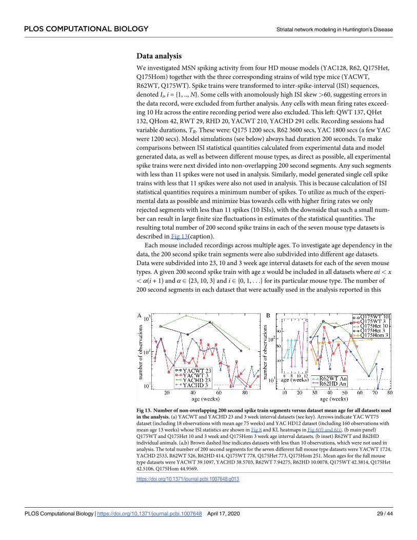
Data analysis

We investigated MSN spiking activity from four HD mouse models (YAC128, R62, Q175Het,

Q175Hom) together with the three corresponding strains of wild type mice (YACWT,

R62WT, Q175WT). Spike trains were transformed to inter-spike-interval (ISI) sequences,

denoted Ii, i = {1, .., N}. Some cells with anomolously high ISI skew >60, suggesting errors in

the data record, were excluded from further analysis. Any cells with mean firing rates exceed-

ing 10 Hz across the entire recording period were also excluded. This left: QWT 137, QHet

132, QHom 42, RWT 29, RHD 20, YACWT 210, YACHD 291 cells. Recording sessions had

variable durations, TR. These were: Q175 1200 secs, R62 3600 secs, YAC 1800 secs (a few YAC

were 1200 secs). Model simulations (see below) always had duration 200 seconds. To make

comparisons between ISI statistical quantities calculated from experimental data and model

generated data, as well as between different mouse types, as direct as possible, all experimental

spike trains were next divided into non-overlapping 200 second segments. Any such segments

with less than 11 spikes were not used in analysis. Similarly, model generated single cell spike

trains with less that 11 spikes were also not used in analysis. This is because calculation of ISI

statistical quantities requires a minimum number of spikes. To utilize as much of the experi-

mental data as possible and minimize bias towards cells with higher firing rates we only

rejected segments with less than 11 spikes (10 ISIs), with the downside that such a small num-

ber can result in large finite size fluctuations in estimates of the statistical quantities. The

resulting total number of 200 second spike trains in each of the seven mouse type datasets is

described in Fig 13(caption).

Each mouse included recordings across multiple ages. To investigate age dependency in the

data, the 200 second spike train segments were also subdivided into different age datasets.

Data were subdivided into 23, 10 and 3 week age interval datasets for each of the seven mouse

types. A given 200 second spike train with age x would be included in all datasets where αi< x< α(i + 1) and α 2 {23, 10, 3} and i 2 {0, 1, . . .} for its particular mouse type. The number of

200 second segments in each dataset that were actually used in the analysis reported in this

Fig 13. Number of non-overlapping 200 second spike train segments versus dataset mean age for all datasets used

in the analysis. (a) YACWT and YACHD 23 and 3 week interval datasets (see key). Arrows indicate YAC WT75

dataset (including 18 observations with mean age 75 weeks) and YAC HD12 dataset (including 160 observations with

mean age 13 weeks) whose ISI statistics are shown in Fig 8 and KL heatmaps in Fig 6(f) and 6(i). (b main panel)

Q175WT and Q175Het 10 and 3 week and Q175Hom 3 week age interval datasets. (b inset) R62WT and R62HD

individual animals. (a,b) Brown dashed line indicates datasets with less than 10 observations, which were not used in

analysis. The total number of 200 second segments for the seven different full mouse type datasets were YACWT 1724,

YACHD 2533, R62WT 526, R62HD 414, Q175WT 778, Q175Het 773, Q175Hom 251. Mean ages for the full mouse

type datasets were YACWT 39.1097, YACHD 38.5703, R62WT 7.94275, R62HD 10.0078, Q175WT 42.3814, Q175Het

42.5106, Q175Hom 44.9569.






paper are plotted against the dataset average age in Fig 13. Only 23 and 3 week datasets were

utilized for YAC mice, Fig 13(a), and only 10 and 3 week datasets were utilized for Q175Het

and Q175WT mice, Fig 13(b). We only had enough Q175Hom mouse data to investigate 3

week interval (i.e. α = 3) datasets, Fig 13(b), and we did not have enough data from R6/2 mice

to subdivide them into different age datasets at all, however individual animals were investi-

gated, Fig 13(b, inset). Any datasets with less than ten 200 second spike trains were not used in

the analysis.

ISI statistical quantities shown in Figs 1, 8 and 10 are averages of the given quantity calcu-

lated for each of the 200 second spike train segments in the given dataset. The bars show the

SEM over these calculated quantities for each given dataset.

Power spectra, S(f), shown in Figs 2, 9 and 5 were calculated on each individual spike train

in a given experimental dataset or model simulation dataset using a Morlet wavelet transform

and then averaged across the spike trains in the dataset. More specifically spike count time

series were created for each individual spike train by sliding a non-overlapping 4 ms window

along the entire spike train and counting spikes in each window (almost always zero or one).

Normalized Morlet wavelets w(t, f) were constructed with frequencies starting from 1/64 Hz

and increasing in multiples of 21/8 Hz. The wavelets had temporal standard deviation σt = 6/

2πf and temporal widths 3σt. Count time series were convolved with w(t, f) to obtain complex

time frequency representations TFR(t, f) and the power spectra S(f) = h|TFR(t, f)|2i obtained

where h..i denotes the time average. Before averaging them, S(f) were normalized by the mean

firing rate of the particular spike train so that S(f =1) = 1. Figs 2, 9 and 5 show these normal-

ized S(f) averaged across all spike trains in an experimental dataset or simulation dataset to

give dataset mean power spectra, where bars show SEM across observations in this dataset.

Cumulative ISI distributions Q(n) shown in Figs 2, 9 and 5 were calculated from QðnÞ ¼P1

i¼n PðiÞ=P1

i¼0PðiÞ and PðnÞ ¼

PNi¼1

HðIi � nDtÞHððnþ 1ÞDt � IiÞð200=ð200 � IiÞÞ,where the binsize Δτ = 10 ms and the factor (200/(200 − Ii)) accounts for censorship of the ISI

distribution by the recording period 200 secs. Q(n) were calculated for each spike train in an

experimental or simulation dataset, then averaged across the dataset, where bars show SEM in

this dataset. In the same way serial ISI autocorrelations of lag n shown in Figs 9 and 5 were cal-

culated from ρ(n) = (hIi+nIii − μ)/σ2 and averaged across all spike trains in the particular exper-

imental or simulation dataset, where bars show SEM in this dataset.

In order to demonstrate the size of fluctuations which can be expected in model network

average mean quantites, model network simulation results shown in Fig 4 were calculated by

dividing the 200 second simulations into 5 non-overlapping 40 second segments. For each 40

second segment, the given quantity was calculated for each active cell (those with more than

10 spikes in the 40 seconds) and then averaged across all active cells to generate network aver-

age quantities. The bars show the SEM across these five observations of network average

quantities.

When estimating model parameters by comparing ISI quantities calculated from experi-

mental data with the same quantities calculated from model generated data using the KL dis-

tance metric (see below) 200 second spike train segments were generated slightly differently.

Instead of dividing a given experimental spike train of length TR into non-overlapping 200 sec-

ond segments, we randomly drew a number, 10TR/200, of potentially overlapping 200 second

segments to generate a larger number of samples. The resultant number of observations in

each dataset was roughly ten times that shown in Fig 13. The quantity is not exactly ten fold

because again any spike trains with less than 11 spikes were discarded. Groups with less than

100 spike train segments (which turned out to be the same as those with less than 10 non-over-

lapping segments shown in Fig 13) were not included in model fitting. Model generated data




always had length 200 seconds, and all single cell spikes trains with more 10 spikes were used

in the calculation of KL distances.

From each of the obtained 200 second spike time series segments, experimental and model,

the following statistical quantities are calculated.

• The firing rate r (number of spikes per second in the 200 second interval).

• The mean ISI, m ¼ hIi ¼ ð1=NÞPN

i¼1Ii, where Ii is the ith ISI.

• The ISI coefficient of variation (CV), σ/μ, where σ2 = hI2i − μ2 is the ISI variance.

• The rescaled ISI skew, S/CV, where the skew is S = (hI3i − 3μσ2 − μ3)/σ3.

• The first two lagged ISI autocorrelations, ρ(n) = (hIi+nIii − μ)/σ2, where n = 1, 2.

• Five intervals of the probability distribution of local CV which is bounded between 0 and 1.

If Xi = |Ii+1 − Ii|/(Ii+1 + Ii), where |x| denotes the absolute value of x, these are defined by

LCVðjþ 1Þ ¼PN� 1

i¼1HðXi � j=5ÞHððjþ 1Þ=5 � XiÞ=ðN � 1Þ, where j = 0, 1, 2, 3, 4 and H

(x) = 1 if x� 0 and H(x) = 0 otherwise [103, 107].

• Maximum likelihood parameters (ML) for the log-normal distribution: scale μLN = hln(I)i;

shape sLN ¼

ffiffiffiffiffiffiffiffiffiffiffiffiffiffiffiffiffiffiffiffiffiffiffiffiffiffiffiffiffiffiffiffiffi

hð ln ðIÞ � mLNÞ2i

q

.

• ML parameters for a gamma distribution: shape parameter

sg ¼ ð3 � z þffiffiffiffiffiffiffiffiffiffiffiffiffiffiffiffiffiffiffiffiffiffiffiffiffiffiffiffiffi

ð3 � zÞ2 þ 24zq

Þ=12z, where z = ln(μ) − μLN; log scale parameter ln(μγ),where μγ = μ/σγ [175].

• ML parameters for an inverse-Gaussian distribution: shape σIG = (hI−1i − μ−1)−1. (The scale

parameter is μ.)

To calculate KS distance from various ML distributions D(n) we first obtain the censorhip

corrected cumulative ISI distribution as described above, except now the binsize Δτ = 0.1 ms.

Fits are performed using Q(n) for n = {1, . . ., M}, and M is the largest integer such that Q(M)>

10−8. KS distance is the maximum value of |1 − D(n) − Q(n)| over n, where |x| denotes absolute

value.

• KS Distance from ML gamma distribution: D(n) = γ(σγ, nΔτ/μγ)/Γ(σγ), where Γ(.) is the

gamma function and γ(.,.) is the incomplete gamma function.

• KS Distance from ML log normal distribution:

DðnÞ ¼ 1=2ð1þ erfðð ln ðnDtÞ � mLNÞ=ffiffiffi2p

sLNÞÞ, where erf(.) is the error function.

• KS Distance from ML inverse-Gaussian distribution: D(n) = F(ax/μ − a) + bF(− ax/μ − a),

where a ¼ffiffið

psIG=nDtÞ, b = exp(2σIG/μ) and F(.) is the standard Gaussian cumulative dis-

tribution function.

Fifteen of these quantities, which we term ‘features’, are used to estimate the parameters of

the network model. The features used were the n = 1 and n = 2 lagged autocorrelations, ρ(n),

the mean ISI, μ, the ISI CV, the ISI rescaled skew, the firing rate, four of the quintiles of the

local CV, LCV (1, 2, 4, 5), the two ML parameters from the gamma distribution, ln(μγ), σγ, the

two ML parameters from the lognormal distribution, μLN, σLN, and the shape parameter from

the inverse-Gaussian distribution, σIG. The KS distance measures were not used in the model

fitting procedure. These features are far from independent. In fact some are simply functions

and combinations of others. However since our estimation method is based on comparison of




feature distributions, this redundancy does not pose a problem. Futhermore the finite time

length of our spike time series (model and experimental) affects different statistics in different

ways. For example, N spikes distributed over T = 200 seconds have a firing rate r = N/T, but

the mean ISI may be far from 1/r if all the spikes occur in a small sub-interval of T. Further-

more, we noticed that some feature quantities appear to show much larger fluctuations across

network simulations nearby in parameter space than others, in particular those involving

higher moments such as the skew. Relatively large fluctuations in CV, Fig 4(b), across network

simulations compared to much smaller fluctuations in the KS distances, Fig 4(d), and in the

lognormal distribution shape parameter, σLN, Fig 4(c), can be seen in Fig 4. We found distribu-

tion maximum likelihood fit parameters were more stable than moments. The use of multiple

different features in our model estimation procedure acts to reduce these fluctuations, to some

extent.

Network simulation parameters are estimated from experimental data by comparing fea-

tures calculated from the data, termed ‘experimental features’ with the same features calculated

from the model, termed ‘model features’, using the KL distance of their joint distributions.

More specifically, we choose a random set, R, of n of the 15 features. For all the observations, i= {1, .., ND}, in an experimental dataset, D, we calculate the experimental feature values, FD

ij , for

each of the features, j = {1, .., n}. For each feature, j, we find its median value, FDj , such that

ProbðFDij > FD

j Þ ¼ 1=2. We compute the n–dimensional joint distribution,

PD;R ¼ ProbðFDi1 > FD

1; FD

i2 > FD2; :::; FD

in > FDn Þ, over the ND observations, i. Similarly, for each

observation, k = {1, .., NM}, in a model dataset, M, we calculate the model feature values, FMkj .

We obtain the n–dimensional joint distribution,

PM;R ¼ ProbðFMk1> FD

1; FM

k2> FD

2; :::; FM

kn > FDn Þ, over the NM observations, k. Finally we calcu-

late the KL distance, KM,D,R = ∑PD,R ln (PD,R/(PM,R + �)), where the sum runs over the 2n bins

and � = 10−7 is a small number, in case PM,R contains bins with zero observations.

To determine best fit model parameters, xD,R, to dataset, D, for the set of features, R, we

first calculate model weights, aM;D;R ¼ K � bM;D;R=P

mK� bm;D;R, which describes a normalized soft

minimum over KM,D,R, where the sum runs over all models m, and we used β = 3. xD,R is then

obtained as the weighted average, xD,R = ∑mxmαm,D,R, where xm is the parameter x value for

model m and the standard error, σ(xD,R), is given by σ(xD,R)2 = ∑m(xm − xD,R)2 αm,D,R.

This provides one observation of xD,R for the randomly chosen set of features R. To obtain a

better estimate, the process is repeated for many (here 30) randomly chosen sets, R, of n fea-

tures from the full 15. For each set R we define ϕD,R = σ(xD,R)−1/∑r σ(xD,r)−1 as a measure of

goodness of fit. Finally we obtain the estimated parameter xD as the weighted average, xD = ∑r

xD,rϕD,r, with standard error, σ(xD), given by σ(xD)2 = ∑r(xD − xD,r)2 ϕD,r. These quantities, the

weighted average and its weighted standard error, are the quantities shown in Figs 7 and 11 by

the points and the error bars. Here we set n = 7, although n = 5 provides similar results, while

results become noisy when n is reduced further. Slopes shown in Fig 11 are obtained via stan-

dard linear regression of xD versus the mean age for observations in dataset D using σ(xD) for

the error in xD and the standard error in the age in dataset D [176]. Error bars shown are the

standard error in the slopes obtained from the linear regression in the usual way, [176] and p-

values calculated using the two-tailed t-test on the slope normalized by its standard error with

appropriate degrees of freedom are reported in the caption of Fig 11.

Fig 14 demonstrates this method for calculation of xD, where experimental datasets, D,

were generated from the network model simulations themselves. To make these results, each

200 second network simulation at given gE and gI is divided into two non-overlapping 100 sec-

ond segments. The first set of segments are used as the experimental datasets, while the second

set are used as the model datasets. Fig 14(a) shows that the estimated inhibition, g�I , is quite




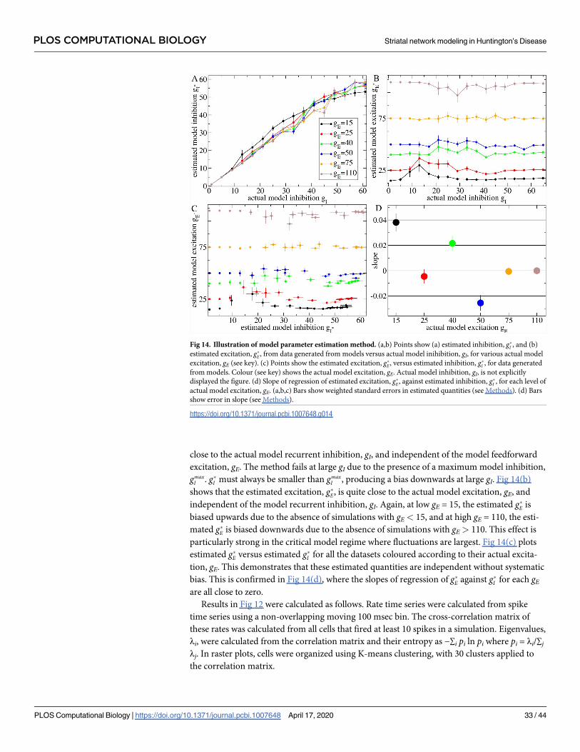
close to the actual model recurrent inhibition, gI, and independent of the model feedforward

excitation, gE. The method fails at large gI due to the presence of a maximum model inhibition,

gmaxI . g�I must always be smaller than gmax

I , producing a bias downwards at large gI. Fig 14(b)

shows that the estimated excitation, g�E, is quite close to the actual model excitation, gE, and

independent of the model recurrent inhibition, gI. Again, at low gE = 15, the estimated g�E is

biased upwards due to the absence of simulations with gE< 15, and at high gE = 110, the esti-

mated g�E is biased downwards due to the absence of simulations with gE> 110. This effect is

particularly strong in the critical model regime where fluctuations are largest. Fig 14(c) plots

estimated g�E versus estimated g�I for all the datasets coloured according to their actual excita-

tion, gE. This demonstrates that these estimated quantities are independent without systematic

bias. This is confirmed in Fig 14(d), where the slopes of regression of g�E against g�I for each gEare all close to zero.

Results in Fig 12 were calculated as follows. Rate time series were calculated from spike

time series using a non-overlapping moving 100 msec bin. The cross-correlation matrix of

these rates was calculated from all cells that fired at least 10 spikes in a simulation. Eigenvalues,

λi, were calculated from the correlation matrix and their entropy as −∑i pi ln pi where pi = λi/∑j

λj. In raster plots, cells were organized using K-means clustering, with 30 clusters applied to

the correlation matrix.

Fig 14. Illustration of model parameter estimation method. (a,b) Points show (a) estimated inhibition, g�I , and (b)

estimated excitation, g�E , from data generated from models versus actual model inihibition, gI, for various actual model

excitation, gE (see key). (c) Points show the estimated excitation, g�E , versus estimated inhibition, g�I , for data generated

from models. Colour (see key) shows the actual model excitation, gE. Actual model inhibition, gI, is not explicitly

displayed the figure. (d) Slope of regression of estimated excitation, g�E , against estimated inhibition, g�I , for each level of

actual model excitation, gE. (a,b,c) Bars show weighted standard errors in estimated quantities (see Methods). (d) Bars

show error in slope (see Methods).






Network model

We use the MSN cell model [79] exactly as in [80] including the modified leak current reversal

potential of -90 mV based on more recent experimental findings [177]. All simulations include

2500 cells connected through inhibitory collaterals randomly with probability 0.2 [10, 126,

178–182]. The network degree distribution is therefore binomial. Each cell receives input from

approximately 500 others with standard deviation of 20. Inhibitory synaptic currents are given

by

Isyn ¼ GsynsðV � VClÞ; ð1Þ

where VCl = −80 mV is the chloride reversal potential. Gsyn, the maximal synaptic conductance,

is the parameter varied in network simulations governing the IPSP size. In a network simula-

tion with given parameter gI, connections are made with random strengths, Gsyn, drawn from

a uniform distribution on [0.001gI, 0.001gI + 0.001]. s is a voltage dependent synaptic gating

variable given by

dsdt¼ aHðVÞð1 � sÞ � Bs: ð2Þ

We use parameters similar to those adopted in [80]: a = 2 and B is a uniform random vari-

able drawn from [0.08, 0.09] for each presynaptic cell. [80] used a = 2 and B = 0.1. H(V) is the

Heaviside function applied to the membrane potential of the presynaptic cell. This is unity

when the presynaptic cell spikes, and zero otherwise.

Feedforward excitation to MSNs is given by

Iex ¼ GexðV � VcatÞ; ð3Þ

where V is the membrane potential of the postsynaptic MSN, and Vcat = 0 mV is the cation

reversal potential. For a network simulation with excitation gE, Gex is a random variable drawn

uniformly from [0.04381, 0.04381 + 0.002gE] for each postsynaptic cell and held constant for

the duration of the simulation. 0.04318 is the conductance at firing threshold. All cells in all

simulations are driven above firing threshold by the feedforward excitation. Therefore all sim-

ulations are generated by varying only the two parameters gE and gI. Simulations at different

levels of gI were initialized with different random seeds, providing different realizations of the

network structure and conductances Gsyn and Gex. On the other hand, simulations at any given

gI are identical, save for the variation in the parameter gE.

The network model was implemented in IBM Model Graph Simulator, which is the core

parallel processing architecture for model description (using the Model Description Language,

MDL) and resource allocation (using the Graph Specification Language, GSL) of the Neural

Tissue Simulator [183]. The Model Graph Simulator software is experimental. Readers are

therefore encouraged to contact the authors if interested in using the tool.

Ethics statement

All procedures followed the National Institutes of Health Guidelines for the Care and Use of

Laboratory Animals and were approved by the Institutional Animal Care and Use Committee.

All animal experiments were approved by the Bloomington Institutional Animal Care and Use

Committee (approval numbers 13-002 and 16-001). All datasets were archival when shared

with researchers from IBM, and no new experiments were suggested, designed, or performed

based on the analyses reported here.

For histological verification of electrode placements, mice were deeply anesthetized with

chloropent (at more than double the surgical dose) a current pulse (30μA for 10 s) was passed




through each active micro-wire to mark recording sites. Mice were then transcardially per-

fused with saline followed by 10% potassium ferrocyanide [K4Fe(CN)6] in 10% paraformalde-

hyde to produce small blue deposits at the site of the recording electrode (“Prussian blue”

reaction). Brains were removed, postfixed in 10% paraformaldehyde for 1 h, and cryoprotected

in 30% phosphate-buffered sucrose. The brains were then frozen; coronal sections (60μM)

were then cut on a sliding microtome and mounted on gelatin-subbed slides. The sections

were stained with cresyl violet and examined under a light microscope to confirm micro-wire

location.

Acknowledgments

We are grateful for the support of Casey Diekman and his lab at New Jersey Institute of Tech-

nology, where part of this research was conducted while AP was a visiting scholar.

Author Contributions

Conceptualization: Adam Ponzi, George V. Rebec, James Kozloski.

Data curation: Scott J. Barton.

Formal analysis: Adam Ponzi.

Funding acquisition: George V. Rebec, James Kozloski.

Investigation: Adam Ponzi, Scott J. Barton, Kendra D. Bunner, Claudia Rangel-Barajas, Emily

S. Zhang, Benjamin R. Miller.

Methodology: Adam Ponzi, George V. Rebec.

Project administration: George V. Rebec, James Kozloski.

Resources: James Kozloski.

Software: Adam Ponzi, James Kozloski.

Supervision: George V. Rebec, James Kozloski.

Validation: Adam Ponzi.

Visualization: Adam Ponzi.

Writing – original draft: Adam Ponzi.

Writing – review & editing: Adam Ponzi, George V. Rebec, James Kozloski.

References1. Andre VM, Cepeda C, Fisher YE, Huynh M, Bardakjian N, Singh S, et al. Differential electrophysiologi-

cal changes in striatal output neurons in Huntington’s disease. Journal of Neuroscience. 2011; 31

(4):1170–82. https://doi.org/10.1523/JNEUROSCI.3539-10.2011 PMID: 21273402

2. Bird ED, Spokes EG, Iversen LL. Dopamine and noradrenaline in postmortem brain in Huntington’s

disease and schizophrenic illness. Acta Psychiatrica Scandinavica. 1980; 61(S280):63–73. https://doi.

org/10.1111/acps.1980.61.s280.63 PMID: 28678367

3. Bonelli RM, Hofmann P. A systematic review of the treatment studies in Huntington’s disease since

1990. Expert opinion on pharmacotherapy. 2007; 8(2):141–53. https://doi.org/10.1517/14656566.8.2.

141 PMID: 17257085

4. Dvorzhak A, Semtner M, Faber DS, Grantyn R. Tonic mGluR5/CB1 dependent suppression of inhibi-

tion as a pathophysiological hallmark in the striatum of mice carrying a mutant form of huntingtin. The

Journal of physiology. 2013; 591(4):1145–66. https://doi.org/10.1113/jphysiol.2012.241018 PMID:

23230231



https://doi.org/10.1523/JNEUROSCI.3539-10.2011

http://www.ncbi.nlm.nih.gov/pubmed/21273402

https://doi.org/10.1111/acps.1980.61.s280.63

https://doi.org/10.1111/acps.1980.61.s280.63


https://doi.org/10.1517/14656566.8.2.141

https://doi.org/10.1517/14656566.8.2.141


https://doi.org/10.1113/jphysiol.2012.241018



5. Kremer B, Squitieri F, Telenius H, Andrew SE, Theilmann J, Spence N, et al. Molecular analysis of late

onset Huntington’s disease. Journal of medical genetics. 1993; 30(12):991–5. https://doi.org/10.1136/

jmg.30.12.991 PMID: 8133510

6. Snell RG, MacMillan JC, Cheadle JP, Fenton I, Lazarou LP, Davies P, et al. Relationship between tri-

nucleotide repeat expansion and phenotypic variation in Huntington’s disease. Nature genetics. 1993;

4(4):393–7. https://doi.org/10.1038/ng0893-393 PMID: 8401588

7. Mangiarini L, Sathasivam K, Seller M, Cozens B, Harper A, Hetherington C, et al. Exon 1 of the HD

gene with an expanded CAG repeat is sufficient to cause a progressive neurological phenotype in

transgenic mice. Cell. 1996; 87(3):493–506. https://doi.org/10.1016/s0092-8674(00)81369-0 PMID:

8898202

8. Hodgson JG, Agopyan N, Gutekunst CA, Leavitt BR, LePiane F, Singaraja R, et al. A YAC mouse

model for Huntington’s disease with full-length mutant huntingtin, cytoplasmic toxicity, and selective

striatal neurodegeneration. Neuron. 1999; 23(1):181–92. https://doi.org/10.1016/s0896-6273(00)

80764-3 PMID: 10402204

9. Raymond LA, Andre VM, Cepeda C, Gladding CM, Milnerwood AJ, Levine MS. Pathophysiology of

Huntington’s disease: time-dependent alterations in synaptic and receptor function. Neuroscience.

2011; 198:252–73. https://doi.org/10.1016/j.neuroscience.2011.08.052 PMID: 21907762

10. Cepeda C, Galvan L, Holley SM, Rao SP, Andre VM, Botelho EP, et al. Multiple sources of striatal inhi-

bition are differentially affected in Huntington’s disease mouse models. Journal of Neuroscience.

2013; 33(17):7393–406. https://doi.org/10.1523/JNEUROSCI.2137-12.2013 PMID: 23616545

11. Vonsattel JP, DiFiglia M. Huntington disease. Journal of neuropathology and experimental neurology.

1998; 57(5):369. https://doi.org/10.1097/00005072-199805000-00001 PMID: 9596408

12. Tobin AJ, Signer ER. Huntington’s disease: the challenge for cell biologists. Trends in cell biology.

2000; 10(12):531–6. https://doi.org/10.1016/s0962-8924(00)01853-5 PMID: 11121745

13. Levine MS, Cepeda C, Hickey MA, Fleming SM, Chesselet MF. Genetic mouse models of Hunting-

ton’s and Parkinson’s diseases: illuminating but imperfect. Trends in neurosciences. 2004; 27

(11):691–7. https://doi.org/10.1016/j.tins.2004.08.008 PMID: 15474170

14. Milnerwood AJ, Raymond LA. Early synaptic pathophysiology in neurodegeneration: insights from

Huntington’s disease. Trends in neurosciences. 2010; 33(11):513–23. https://doi.org/10.1016/j.tins.

2010.08.002 PMID: 20850189

15. Orth M, Schippling S, Schneider SA, Bhatia KP, Talelli P, Tabrizi SJ, et al. Abnormal motor cortex plas-

ticity in premanifest and very early manifest Huntington disease. Journal of Neurology, Neurosurgery

& Psychiatry. 2010; 81(3):267–70. https://doi.org/10.1136/jnnp.2009.171926

16. Schippling S, Schneider SA, Bhatia KP, Munchau A, Rothwell JC, Tabrizi SJ, et al. Abnormal motor

cortex excitability in preclinical and very early Huntington’s disease. Biological psychiatry. 2009; 65

(11):959–65. https://doi.org/10.1016/j.biopsych.2008.12.026 PMID: 19200948

17. Cummings DM, Milnerwood AJ, Dallerac GM, Waights V, Brown JY, Vatsavayai SC, et al. Aberrant

cortical synaptic plasticity and dopaminergic dysfunction in a mouse model of Huntington’s disease.

Human molecular genetics. 2006; 15(19):2856–68. https://doi.org/10.1093/hmg/ddl224 PMID:

16905556

18. Milnerwood AJ, Cummings DM, Dallerac GM, Brown JY, Vatsavayai SC, Hirst MC, et al. Early devel-

opment of aberrant synaptic plasticity in a mouse model of Huntington’s disease. Human molecular

genetics. 2006; 15(10):1690–703. https://doi.org/10.1093/hmg/ddl092 PMID: 16600988

19. Usdin MT, Shelbourne PF, Myers RM, Madison DV. Impaired synaptic plasticity in mice carrying the

Huntington’s disease mutation. Human molecular genetics. 1999; 8(5):839–46. https://doi.org/10.

1093/hmg/8.5.839 PMID: 10196373

20. Lynch G, Kramar EA, Rex CS, Jia Y, Chappas D, Gall CM, et al. Brain-derived neurotrophic factor

restores synaptic plasticity in a knock-in mouse model of Huntington’s disease. Journal of Neurosci-

ence. 2007; 27(16):4424–34. https://doi.org/10.1523/JNEUROSCI.5113-06.2007 PMID: 17442827

21. Wood JD, MacMillan JC, Harper PS, Lowenstein PR, Jones AL. Partial characterisation of murine hun-

tingtin and apparent variations in the subcellular localisation of huntingtin in human, mouse and rat brain.

Human molecular genetics. 1996; 5(4):481–7. https://doi.org/10.1093/hmg/5.4.481 PMID: 8845840

22. Li JY, Plomann M, Brundin P. Huntington’s disease: a synaptopathy?. Trends in molecular medicine.

2003; 9(10):414–20. https://doi.org/10.1016/j.molmed.2003.08.006 PMID: 14557053

23. Cepeda C, Wu N, Andre VM, Cummings DM, Levine MS. The corticostriatal pathway in Huntington’s

disease. Progress in neurobiology. 2007; 81(5-6):253–71. https://doi.org/10.1016/j.pneurobio.2006.

11.001 PMID: 17169479

24. Cepeda C, Hurst RS, Calvert CR, Hernandez-Echeagaray E, Nguyen OK, Jocoy E, et al. Transient

and progressive electrophysiological alterations in the corticostriatal pathway in a mouse model of



https://doi.org/10.1136/jmg.30.12.991

https://doi.org/10.1136/jmg.30.12.991


https://doi.org/10.1038/ng0893-393


https://doi.org/10.1016/s0092-8674(00)81369-0


https://doi.org/10.1016/s0896-6273(00)80764-3

https://doi.org/10.1016/s0896-6273(00)80764-3


https://doi.org/10.1016/j.neuroscience.2011.08.052




https://doi.org/10.1097/00005072-199805000-00001


https://doi.org/10.1016/s0962-8924(00)01853-5


https://doi.org/10.1016/j.tins.2004.08.008





https://doi.org/10.1136/jnnp.2009.171926

https://doi.org/10.1016/j.biopsych.2008.12.026


https://doi.org/10.1093/hmg/ddl224


https://doi.org/10.1093/hmg/ddl092


https://doi.org/10.1093/hmg/8.5.839







https://doi.org/10.1016/j.molmed.2003.08.006


https://doi.org/10.1016/j.pneurobio.2006.11.001

https://doi.org/10.1016/j.pneurobio.2006.11.001



Huntington’s disease. Journal of Neuroscience. 2003; 23(3):961–9. https://doi.org/10.1523/

JNEUROSCI.23-03-00961.2003 PMID: 12574425

25. Cummings DM, Andre VM, Uzgil BO, Gee SM, Fisher YE, Cepeda C, et al. Alterations in cortical exci-

tation and inhibition in genetic mouse models of Huntington’s disease. Journal of Neuroscience. 2009;

29(33):10371–86. https://doi.org/10.1523/JNEUROSCI.1592-09.2009 PMID: 19692612

26. Graham RK, Pouladi MA, Joshi P, Lu G, Deng Y, Wu NP, et al. Differential susceptibility to excitotoxic

stress in YAC128 mouse models of Huntington disease between initiation and progression of disease.

Journal of Neuroscience. 2009; 29(7):2193–204. https://doi.org/10.1523/JNEUROSCI.5473-08.2009

PMID: 19228972

27. Joshi PR, Wu NP, Andre VM, Cummings DM, Cepeda C, Joyce JA, et al. Age-dependent alterations

of corticostriatal activity in the YAC128 mouse model of Huntington disease. Journal of Neuroscience.


28. Indersmitten T, Tran CH, Cepeda C, Levine MS. Altered excitatory and inhibitory inputs to striatal

medium-sized spiny neurons and cortical pyramidal neurons in the Q175 mouse model of Huntington’s

disease. Journal of neurophysiology. 2015; 113(7):2953–66. https://doi.org/10.1152/jn.01056.2014

PMID: 25673747

29. Gray M, Shirasaki DI, Cepeda C, Andre VM, Wilburn B, Lu XH, et al. Full-length human mutant hun-

tingtin with a stable polyglutamine repeat can elicit progressive and selective neuropathogenesis in

BACHD mice. Journal of Neuroscience. 2008; 28(24):6182–95. https://doi.org/10.1523/JNEUROSCI.

0857-08.2008 PMID: 18550760

30. Milnerwood AJ, Raymond LA. Corticostriatal synaptic function in mouse models of Huntington’s dis-

ease: early effects of huntingtin repeat length and protein load. The Journal of physiology. 2007; 585

(3):817–31. https://doi.org/10.1113/jphysiol.2007.142448 PMID: 17947312

31. Wang N, Gray M, Lu XH, Cantle JP, Holley SM, Greiner E, et al. Neuronal targets for reducing mutant

huntingtin expression to ameliorate disease in a mouse model of Huntington’s disease. Nature medi-

cine. 2014; 20(5):536. https://doi.org/10.1038/nm.3514 PMID: 24784230

32. Tepper JM, Bolam JP. Functional diversity and specificity of neostriatal interneurons. Current opinion

in neurobiology. 2004; 14(6):685–92. https://doi.org/10.1016/j.conb.2004.10.003 PMID: 15582369

33. Kawaguchi Y, Wilson CJ, Augood SJ, Emson PC. Striatal interneurones: chemical, physiological and

morphological characterization. Trends in neurosciences. 1995; 18(12):527–35. https://doi.org/10.

1016/0166-2236(95)98374-8 PMID: 8638293

34. Czubayko U, Plenz D. Fast synaptic transmission between striatal spiny projection neurons. Proceedings

of the National Academy of Sciences. 2002; 99(24):15764–9. https://doi.org/10.1073/pnas.242428599

35. Tunstall MJ, Oorschot DE, Kean A, Wickens JR. Inhibitory interactions between spiny projection neu-

rons in the rat striatum. Journal of neurophysiology. 2002; 88(3):1263–9. https://doi.org/10.1152/jn.

2002.88.3.1263 PMID: 12205147

36. Plotkin JL, Wu N, Chesselet MF, Levine MS. Functional and molecular development of striatal fast–

spiking GABAergic interneurons and their cortical inputs. European Journal of Neuroscience. 2005; 22

(5):1097–108. https://doi.org/10.1111/j.1460-9568.2005.04303.x PMID: 16176351

37. Kreitzer AC. Physiology and pharmacology of striatal neurons. Annual review of neuroscience. 2009;

32:127–47. https://doi.org/10.1146/annurev.neuro.051508.135422 PMID: 19400717

38. Cepeda C, Starling AJ, Wu N, Nguyen OK, Uzgil B, Soda T, et al. Increased GABAergic function in

mouse models of Huntington’s disease: reversal by BDNF. Journal of neuroscience research. 2004;

78(6):855–67. https://doi.org/10.1002/jnr.20344 PMID: 15505789

39. Centonze D, Rossi S, Prosperetti C, Tscherter A, Bernardi G, Maccarrone M, et al. Abnormal sensitiv-

ity to cannabinoid receptor stimulation might contribute to altered gamma-aminobutyric acid transmis-

sion in the striatum of R6/2 Huntington’s disease mice. Biological psychiatry. 2005; 57(12):1583–9.

https://doi.org/10.1016/j.biopsych.2005.03.008 PMID: 15953496

40. Cummings DM, Cepeda C, Levine MS. Alterations in striatal synaptic transmission are consistent

across genetic mouse models of Huntington’s disease. ASN neuro. 2010; 2(3):AN20100007. https://

doi.org/10.1042/AN20100007

41. Wilson CJ. The generation of natural firing patterns in neostriatal neurons. In Progress in brain

research 1993 Jan 1 ( Vol. 99, pp. 277–297). Elsevier.

42. Miller BR, Walker AG, Shah AS, Barton SJ, Rebec GV. Dysregulated information processing by

medium spiny neurons in striatum of freely behaving mouse models of Huntington’s disease. Journal

of neurophysiology. 2008; 100(4):2205–16. https://doi.org/10.1152/jn.90606.2008 PMID: 18667541

43. Carrillo-Reid L, Tecuapetla F, Tapia D, Hernandez-Cruz A, Galarraga E, Drucker-Colin R, et al. Encod-

ing network states by striatal cell assemblies. Journal of neurophysiology. 2008; 99(3):1435–50.

https://doi.org/10.1152/jn.01131.2007 PMID: 18184883



https://doi.org/10.1523/JNEUROSCI.23-03-00961.2003









https://doi.org/10.1152/jn.01056.2014







https://doi.org/10.1038/nm.3514


https://doi.org/10.1016/j.conb.2004.10.003


https://doi.org/10.1016/0166-2236(95)98374-8

https://doi.org/10.1016/0166-2236(95)98374-8


https://doi.org/10.1073/pnas.242428599

https://doi.org/10.1152/jn.2002.88.3.1263

https://doi.org/10.1152/jn.2002.88.3.1263


https://doi.org/10.1111/j.1460-9568.2005.04303.x


https://doi.org/10.1146/annurev.neuro.051508.135422


https://doi.org/10.1002/jnr.20344


https://doi.org/10.1016/j.biopsych.2005.03.008


https://doi.org/10.1042/AN20100007

https://doi.org/10.1042/AN20100007

https://doi.org/10.1152/jn.90606.2008


https://doi.org/10.1152/jn.01131.2007



44. DeLong MR. Putamen: activity of single units during slow and rapid arm movements. Science. 1973;

179(4079):1240–2. https://doi.org/10.1126/science.179.4079.1240 PMID: 4631890

45. Hikosaka O, Sakamoto M, Usui S. Functional properties of monkey caudate neurons. I. Activities

related to saccadic eye movements. Journal of neurophysiology. 1989; 61(4):780–98. https://doi.org/

10.1152/jn.1989.61.4.780 PMID: 2723720

46. Hikosaka O, Takikawa Y, Kawagoe R. Role of the basal ganglia in the control of purposive saccadic

eye movements. Physiological reviews. 2000; 80(3):953–78. https://doi.org/10.1152/physrev.2000.80.

3.953 PMID: 10893428

47. Jaeger D, Gilman S, Aldridge JW. Neuronal activity in the striatum and pallidum of primates related to

the execution of externally cued reaching movements. Brain research. 1995; 694(1-2):111–27. https://

doi.org/10.1016/0006-8993(95)00780-t PMID: 8974634

48. Kasanetz F, Riquelme LA, O’Donnell P, Murer MG. Turning off cortical ensembles stops striatal Up

states and elicits phase perturbations in cortical and striatal slow oscillations in rat in vivo. The Journal

of physiology. 2006; 577(1):97–113. https://doi.org/10.1113/jphysiol.2006.113050 PMID: 16931555

49. Kimura M. Behaviorally contingent property of movement-related activity of the primate putamen. Jour-

nal of neurophysiology. 1990; 63(6):1277–96. https://doi.org/10.1152/jn.1990.63.6.1277 PMID: 2358877

50. West MO, Carelli RM, Pomerantz MI, Cohen SM, Gardner JP, Chapin JK, et al. A region in the dorso-

lateral striatum of the rat exhibiting single-unit correlations with specific locomotor limb movements.

Journal of Neurophysiology. 1990; 64(4):1233–46. https://doi.org/10.1152/jn.1990.64.4.1233 PMID:

2258744

51. Brotchie P, Iansek R, Horne MK. Motor function of the monkey globus pallidus: 2. Cognitive aspects of

movement and phasic neuronal activity. Brain. 1991; 114(4):1685–702. https://doi.org/10.1093/brain/

114.4.1685 PMID: 1884173

52. Gardiner TW, Kitai ST. Single-unit activity in the globus pallidus and neostriatum of the rat during per-

formance of a trained head movement. Experimental Brain Research. 1992; 88(3):517–30. https://doi.

org/10.1007/bf00228181 PMID: 1587313

53. Kimura M, Aosaki T, Hu Y, Ishida A, Watanabe K. Activity of primate putamen neurons is selective to

the mode of voluntary movement: visually guided, self-initiated or memory-guided. Experimental Brain

Research. 1992; 89(3):473–7. https://doi.org/10.1007/bf00229870 PMID: 1644114

54. Kermadi I, Joseph JP. Activity in the caudate nucleus of monkey during spatial sequencing. Journal of

Neurophysiology. 1995; 74(3):911–33. https://doi.org/10.1152/jn.1995.74.3.911 PMID: 7500161

55. Mushiake H, Strick PL. Pallidal neuron activity during sequential arm movements. Journal of Neuro-

physiology. 1995; 74(6):2754–8. https://doi.org/10.1152/jn.1995.74.6.2754 PMID: 8747231

56. Aldridge JW, Berridge KC. Coding of serial order by neostriatal neurons: a “natural action” approach to

movement sequence. Journal of Neuroscience. 1998; 18(7):2777–87. https://doi.org/10.1523/

JNEUROSCI.18-07-02777.1998 PMID: 9502834

57. Jog MS, Kubota Y, Connolly CI, Hillegaart V, Graybiel AM. Building neural representations of habits.

Science. 1999; 286(5445):1745–9. https://doi.org/10.1126/science.286.5445.1745 PMID: 10576743

58. Barnes TD, Kubota Y, Hu D, Jin DZ, Graybiel AM. Activity of striatal neurons reflects dynamic encoding

and recoding of procedural memories. Nature. 2005; 437(7062):1158–61. https://doi.org/10.1038/

nature04053 PMID: 16237445

59. Bakhurin KI, Mac V, Golshani P, Masmanidis SC. Temporal correlations among functionally special-

ized striatal neural ensembles in reward-conditioned mice. Journal of neurophysiology. 2016; 115

(3):1521–32. https://doi.org/10.1152/jn.01037.2015 PMID: 26763779

60. Adler A, Katabi S, Finkes I, Israel Z, Prut Y, Bergman H. Temporal convergence of dynamic cell

assemblies in the striato-pallidal network. Journal of Neuroscience. 2012; 32(7):2473–84. https://doi.

org/10.1523/JNEUROSCI.4830-11.2012 PMID: 22396421

61. Lopez-Huerta VG, Carrillo-Reid L, Galarraga E, Tapia D, Fiordelisio T, Drucker-Colin R, et al. The bal-

ance of striatal feedback transmission is disrupted in a model of parkinsonism. Journal of Neurosci-


62. Yin HH. The sensorimotor striatum is necessary for serial order learning. Journal of Neuroscience.


63. Mello GB, Soares S, Paton JJ. A scalable population code for time in the striatum. Current Biology.

2015; 25(9):1113–22. https://doi.org/10.1016/j.cub.2015.02.036 PMID: 25913405

64. Gouvêa TS, Monteiro T, Motiwala A, Soares S, Machens C, Paton JJ. Striatal dynamics explain dura-

tion judgments. Elife. 2015; 4:e11386. https://doi.org/10.7554/eLife.11386 PMID: 26641377

65. Bakhurin KI, Goudar V, Shobe JL, Claar LD, Buonomano DV, Masmanidis SC. Differential encoding of

time by prefrontal and striatal network dynamics. Journal of Neuroscience. 2017; 37(4):854–70.

https://doi.org/10.1523/JNEUROSCI.1789-16.2016 PMID: 28123021



https://doi.org/10.1126/science.179.4079.1240


https://doi.org/10.1152/jn.1989.61.4.780

https://doi.org/10.1152/jn.1989.61.4.780


https://doi.org/10.1152/physrev.2000.80.3.953

https://doi.org/10.1152/physrev.2000.80.3.953


https://doi.org/10.1016/0006-8993(95)00780-t

https://doi.org/10.1016/0006-8993(95)00780-t




https://doi.org/10.1152/jn.1990.63.6.1277


https://doi.org/10.1152/jn.1990.64.4.1233


https://doi.org/10.1093/brain/114.4.1685

https://doi.org/10.1093/brain/114.4.1685


https://doi.org/10.1007/bf00228181

https://doi.org/10.1007/bf00228181


https://doi.org/10.1007/bf00229870


https://doi.org/10.1152/jn.1995.74.3.911


https://doi.org/10.1152/jn.1995.74.6.2754





https://doi.org/10.1126/science.286.5445.1745


https://doi.org/10.1038/nature04053

https://doi.org/10.1038/nature04053


https://doi.org/10.1152/jn.01037.2015









https://doi.org/10.1016/j.cub.2015.02.036


https://doi.org/10.7554/eLife.11386





66. Jaidar O, Carrillo-Reid L, Hernandez A, Drucker-Colın R, Bargas J, Hernandez-Cruz A. Dynamics of

the Parkinsonian striatal microcircuit: entrainment into a dominant network state. Journal of Neurosci-


67. Miller BR, Walker AG, Fowler SC, von Horsten S, Riess O, Johnson MA, et al. Dysregulation of coordi-

nated neuronal firing patterns in striatum of freely behaving transgenic rats that model Huntington’s

disease. Neurobiology of disease. 2010; 37(1):106–13. https://doi.org/10.1016/j.nbd.2009.09.013

PMID: 19818852

68. Miller BR, Walker AG, Barton SJ, Rebec GV. Dysregulated neuronal activity patterns implicate corti-

costriatal circuit dysfunction in multiple rodent models of Huntington’s disease. Frontiers in systems

neuroscience. 2011; 5:26. https://doi.org/10.3389/fnsys.2011.00026 PMID: 21629717

69. Beatty JA, Song SC, Wilson CJ. Cell-type-specific resonances shape the responses of striatal neurons

to synaptic input. Journal of neurophysiology. 2015; 113(3):688–700. https://doi.org/10.1152/jn.00827.

2014 PMID: 25411465

70. Wilson CJ, Kawaguchi Y. The origins of two-state spontaneous membrane potential fluctuations of

neostriatal spiny neurons. Journal of neuroscience. 1996; 16(7):2397–410. https://doi.org/10.1523/

JNEUROSCI.16-07-02397.1996 PMID: 8601819

71. Wickens JR, Wilson CJ. Regulation of action-potential firing in spiny neurons of the rat neostriatum in

vivo. Journal of neurophysiology. 1998; 79(5):2358–64. https://doi.org/10.1152/jn.1998.79.5.2358

PMID: 9582211

72. Kitano K, Cateau H, Kaneda K, Nambu A, Takada M, Fukai T. Two-state membrane potential transi-

tions of striatal spiny neurons as evidenced by numerical simulations and electrophysiological record-

ings in awake monkeys. Journal of Neuroscience. 2002; 22(12):RC230-. https://doi.org/10.1523/

JNEUROSCI.22-12-j0003.2002 PMID: 12045235

73. Ponzi A, Wickens J. Sequentially switching cell assemblies in random inhibitory networks of spiking

neurons in the striatum. Journal of Neuroscience. 2010; 30(17):5894–911. https://doi.org/10.1523/

JNEUROSCI.5540-09.2010 PMID: 20427650

74. Ponzi A, Wickens JR. Optimal balance of the striatal medium spiny neuron network. PLoS computa-

tional biology. 2013; 9(4). https://doi.org/10.1371/journal.pcbi.1002954 PMID: 23592954

75. Ponzi A, Wickens JR. Input dependent cell assembly dynamics in a model of the striatal medium spiny

neuron network. Frontiers in systems neuroscience. 2012; 6:6. https://doi.org/10.3389/fnsys.2012.

00006 PMID: 22438838

76. Ponzi A, Wickens J. Cell assemblies in large sparse inhibitory networks of biologically realistic spiking

neurons. InAdvances in Neural Information Processing Systems 2009 (pp. 1273-1280).

77. Angulo-Garcia D, Berke JD, Torcini A. Cell assembly dynamics of sparsely-connected inhibitory net-

works: a simple model for the collective activity of striatal projection neurons. PLoS computational biol-

ogy. 2016; 12(2). https://doi.org/10.1371/journal.pcbi.1004778 PMID: 26915024

78. Angulo-Garcia D, Luccioli S, Olmi S, Torcini A. Death and rebirth of neural activity in sparse inhibitory

networks. New Journal of Physics. 2017; 19(5):053011. https://doi.org/10.1088/1367-2630/aa69ff

79. Mahon S, Deniau JM, Charpier S, Delord B. Role of a striatal slowly inactivating potassium current in

short-term facilitation of corticostriatal inputs: a computer simulation study. Learning & Memory. 2000;

7(5):357–62. https://doi.org/10.1101/lm.34800

80. Corbit VL, Whalen TC, Zitelli KT, Crilly SY, Rubin JE, Gittis AH. Pallidostriatal projections promote βoscillations in a dopamine-depleted biophysical network model. Journal of Neuroscience. 2016; 36

(20):5556–71. https://doi.org/10.1523/JNEUROSCI.0339-16.2016 PMID: 27194335

81. Van Raamsdonk JM, Murphy Z, Slow EJ, Leavitt BR, Hayden MR. Selective degeneration and nuclear

localization of mutant huntingtin in the YAC128 mouse model of Huntington disease. Human molecular

genetics. 2005; 14(24):3823–35. https://doi.org/10.1093/hmg/ddi407 PMID: 16278236

82. Menalled L, El-Khodor BF, Patry M, Suarez-Fariñas M, Orenstein SJ, Zahasky B, et al. Systematic

behavioral evaluation of Huntington’s disease transgenic and knock-in mouse models. Neurobiology

of disease. 2009; 35(3):319–36. https://doi.org/10.1016/j.nbd.2009.05.007 PMID: 19464370

83. Lu XH. BAC to Degeneration: Bacterial Artificial Chromosome (BAC)-Mediated Transgenesis for

Modeling Basal Ganglia Neurodegenerative Disorders. International review of neurobiology. 2009;

89:37–56. https://doi.org/10.1016/S0074-7742(09)89002-8 PMID: 19900614

84. Cepeda C, Cummings DM, Andre VM, Holley SM, Levine MS. Genetic mouse models of Huntington’s

disease: focus on electrophysiological mechanisms. ASN neuro. 2010; 2(2):AN20090058. https://doi.

org/10.1042/AN20090058

85. Rozas JL, Gomez-Sanchez L, Tomas-Zapico C, Lucas JJ, Fernandez-Chacon R. Presynaptic dys-

function in Huntington’s disease. Biochemical Society Transactions. 2010: 488–492. https://doi.org/

10.1042/BST0380488 PMID: 20298208





https://doi.org/10.1016/j.nbd.2009.09.013


https://doi.org/10.3389/fnsys.2011.00026


https://doi.org/10.1152/jn.00827.2014

https://doi.org/10.1152/jn.00827.2014





https://doi.org/10.1152/jn.1998.79.5.2358


https://doi.org/10.1523/JNEUROSCI.22-12-j0003.2002

https://doi.org/10.1523/JNEUROSCI.22-12-j0003.2002












https://doi.org/10.1088/1367-2630/aa69ff

https://doi.org/10.1101/lm.34800



https://doi.org/10.1093/hmg/ddi407




https://doi.org/10.1016/S0074-7742(09)89002-8


https://doi.org/10.1042/AN20090058

https://doi.org/10.1042/AN20090058

https://doi.org/10.1042/BST0380488

https://doi.org/10.1042/BST0380488



86. Plotkin JL, Surmeier DJ. Corticostriatal synaptic adaptations in Huntington’s disease. Current opinion

in neurobiology. 2015; 33:53–62. https://doi.org/10.1016/j.conb.2015.01.020 PMID: 25700146

87. Carter RJ, Lione LA, Humby T, Mangiarini L, Mahal A, Bates GP, et al. Characterization of progressive

motor deficits in mice transgenic for the human Huntington’s disease mutation. Journal of Neurosci-

ence. 1999; 19(8):3248–57. https://doi.org/10.1523/JNEUROSCI.19-08-03248.1999 PMID: 10191337

88. Lione LA, Carter RJ, Hunt MJ, Bates GP, Morton AJ, Dunnett SB. Selective discrimination learning

impairments in mice expressing the human Huntington’s disease mutation. Journal of Neuroscience.

1999; 19(23):10428–37. https://doi.org/10.1523/JNEUROSCI.19-23-10428.1999 PMID: 10575040

89. Murphy KP, Carter RJ, Lione LA, Mangiarini L, Mahal A, Bates GP, et al. Abnormal synaptic plasticity

and impaired spatial cognition in mice transgenic for exon 1 of the human Huntington’s disease muta-

tion. Journal of Neuroscience. 2000; 20(13):5115–23. https://doi.org/10.1523/JNEUROSCI.20-13-

05115.2000 PMID: 10864968

90. Davies SW, Turmaine M, Cozens BA, DiFiglia M, Sharp AH, Ross CA, et al. Formation of neuronal

intranuclear inclusions underlies the neurological dysfunction in mice transgenic for the HD mutation.

Cell. 1997; 90(3):537–48. https://doi.org/10.1016/s0092-8674(00)80513-9 PMID: 9267033

91. Turmaine M, Raza A, Mahal A, Mangiarini L, Bates GP, Davies SW. Nonapoptotic neurodegeneration

in a transgenic mouse model of Huntington’s disease. Proceedings of the National Academy of Sci-

ences. 2000; 97(14):8093–7. https://doi.org/10.1073/pnas.110078997

92. Slow EJ, Van Raamsdonk J, Rogers D, Coleman SH, Graham RK, Deng Y, et al. Selective striatal neu-

ronal loss in a YAC128 mouse model of Huntington disease. Human molecular genetics. 2003; 12

(13):1555–67. https://doi.org/10.1093/hmg/ddg169 PMID: 12812983

93. Heikkinen T, Lehtimaki K, Vartiainen N, Puolivali J, Hendricks SJ, Glaser JR, et al. Characterization of

neurophysiological and behavioral changes, MRI brain volumetry and 1H MRS in zQ175 knock-in

mouse model of Huntington’s disease. PloS one. 2012; 7(12). https://doi.org/10.1371/journal.pone.

0050717

94. Menalled LB, Kudwa AE, Miller S, Fitzpatrick J, Watson-Johnson J, Keating N, et al. Comprehensive

behavioral and molecular characterization of a new knock-in mouse model of Huntington’s disease:

zQ175. PloS one. 2012; 7(12). https://doi.org/10.1371/journal.pone.0049838 PMID: 23284626

95. Menalled LB. Knock-in mouse models of Huntington’s disease. NeuroRx. 2005; 2(3):465–70. https://

doi.org/10.1602/neurorx.2.3.465 PMID: 16389309

96. Heng MY, Tallaksen-Greene SJ, Detloff PJ, Albin RL. Longitudinal evaluation of the Hdh (CAG) 150

knock-in murine model of Huntington’s disease. Journal of Neuroscience. 2007; 27(34):8989–98.


97. Loh DH, Kudo T, Truong D, Wu Y, Colwell CS. The Q175 mouse model of Huntington’s disease shows

gene dosage-and age-related decline in circadian rhythms of activity and sleep. PloS one. 2013; 8(7).

https://doi.org/10.1371/journal.pone.0069993

98. Heikkinen T, Lehtimaki K, Vartiainen N, Puolivali J, Hendricks SJ, Glaser JR, et al. Characterization of

neurophysiological and behavioral changes, MRI brain volumetry and 1H MRS in zQ175 knock-in

mouse model of Huntington’s disease. PloS one. 2012; 7(12). https://doi.org/10.1371/journal.pone.

0050717

99. Rebec GV, Conroy SK, Barton SJ. Hyperactive striatal neurons in symptomatic Huntington R6/2 mice:

variations with behavioral state and repeated ascorbate treatment. Neuroscience. 2006; 137(1):327–

36. https://doi.org/10.1016/j.neuroscience.2005.08.062 PMID: 16257492

100. Estrada-Sanchez AM, Burroughs CL, Cavaliere S, Barton SJ, Chen S, Yang XW, et al. Cortical effer-

ents lacking mutant huntingtin improve striatal neuronal activity and behavior in a conditional mouse

model of Huntington’s disease. Journal of Neuroscience. 2015; 35(10):4440–51. https://doi.org/10.

1523/JNEUROSCI.2812-14.2015 PMID: 25762686

101. Hong SL, Cossyleon D, Hussain WA, Walker LJ, Barton SJ, Rebec GV. Dysfunctional behavioral mod-

ulation of corticostriatal communication in the R6/2 mouse model of Huntington’s disease. PLoS One.

2012; 7(10). https://doi.org/10.1371/journal.pone.0047026

102. Schwalger T, Droste F, Lindner B. Statistical structure of neural spiking under non-Poissonian or other

non-white stimulation. Journal of computational neuroscience. 2015; 39(1):29–51. https://doi.org/10.

1007/s10827-015-0560-x PMID: 25936628

103. Holt GR, Softky WR, Koch C, Douglas RJ. Comparison of discharge variability in vitro and in vivo in cat

visual cortex neurons. Journal of neurophysiology. 1996; 75(5):1806–14. https://doi.org/10.1152/jn.

1996.75.5.1806 PMID: 8734581

104. Shinomoto S, Miyazaki Y, Tamura H, Fujita I. Regional and laminar differences in in vivo firing patterns

of primate cortical neurons. Journal of Neurophysiology. 2005; 94(1):567–75. https://doi.org/10.1152/

jn.00896.2004 PMID: 15758054



https://doi.org/10.1016/j.conb.2015.01.020









https://doi.org/10.1016/s0092-8674(00)80513-9



https://doi.org/10.1093/hmg/ddg169






https://doi.org/10.1602/neurorx.2.3.465

https://doi.org/10.1602/neurorx.2.3.465













https://doi.org/10.1007/s10827-015-0560-x

https://doi.org/10.1007/s10827-015-0560-x


https://doi.org/10.1152/jn.1996.75.5.1806

https://doi.org/10.1152/jn.1996.75.5.1806


https://doi.org/10.1152/jn.00896.2004

https://doi.org/10.1152/jn.00896.2004



105. Davies RM, Gerstein GL, Baker SN. Measurement of time-dependent changes in the irregularity of

neural spiking. Journal of Neurophysiology. 2006; 96(2):906–18. https://doi.org/10.1152/jn.01030.

2005 PMID: 16554511

106. Miura K, Okada M, Amari SI. Estimating spiking irregularities under changing environments. Neural

Computation. 2006; 18(10):2359–86. https://doi.org/10.1162/neco.2006.18.10.2359 PMID: 16907630

107. Ponce-Alvarez A, Kilavik BE, Riehle A. Comparison of local measures of spike time irregularity and

relating variability to firing rate in motor cortical neurons. Journal of Computational Neuroscience.

2010; 29(1-2):351–65. https://doi.org/10.1007/s10827-009-0158-2 PMID: 19449094

108. Shinomoto S, Kim H, Shimokawa T, Matsuno N, Funahashi S, Shima K, et al. Relating neuronal firing

patterns to functional differentiation of cerebral cortex. PLoS computational biology. 2009; 5(7). https://

doi.org/10.1371/journal.pcbi.1000433 PMID: 19593378

109. Compte A, Constantinidis C, Tegner J, Raghavachari S, Chafee MV, Goldman-Rakic PS, et al. Tem-

porally irregular mnemonic persistent activity in prefrontal neurons of monkeys during a delayed

response task. Journal of neurophysiology. 2003; 90(5):3441–54. https://doi.org/10.1152/jn.00949.

2002 PMID: 12773500

110. Hamaguchi K, Riehle A, Brunel N. Estimating network parameters from combined dynamics of firing

rate and irregularity of single neurons. Journal of neurophysiology. 2011; 105(1):487–500. https://doi.

org/10.1152/jn.00858.2009 PMID: 20719928

111. Nisenbaum ES, Wilson CJ. Potassium currents responsible for inward and outward rectification in rat

neostriatal spiny projection neurons. Journal of Neuroscience. 1995; 15(6):4449–63. https://doi.org/

10.1523/JNEUROSCI.15-06-04449.1995 PMID: 7790919

112. Plenz D, Aertsen A. Neural dynamics in cortex-striatum co-cultures—II. Spatiotemporal characteristics

of neuronal activity. Neuroscience. 1996; 70(4):893–924. https://doi.org/10.1016/0306-4522(95)

00405-x PMID: 8848173

113. Wu Z, Guo A, Fu X. Generation of low-gamma oscillations in a GABAergic network model of the stria-

tum. Neural Networks. 2017; 95:72–90. https://doi.org/10.1016/j.neunet.2017.08.004 PMID:

28910740

114. Damodaran S, Cressman JR, Jedrzejewski-Szmek Z, Blackwell KT. Desynchronization of fast-spiking

interneurons reduces β-band oscillations and imbalance in firing in the dopamine-depleted striatum.


PMID: 25609629

115. Mallet N, Micklem BR, Henny P, Brown MT, Williams C, Bolam JP, et al. Dichotomous organization of

the external globus pallidus. Neuron. 2012; 74(6):1075–86. https://doi.org/10.1016/j.neuron.2012.04.

027 PMID: 22726837

116. Humphries MD, Wood R, Gurney K. Reconstructing the three-dimensional GABAergic microcircuit of

the striatum. PLoS computational biology. 2010; 6(11). https://doi.org/10.1371/journal.pcbi.1001011

PMID: 21124867

117. Moyer JT, Halterman BL, Finkel LH, Wolf JA. Lateral and feedforward inhibition suppress asynchro-

nous activity in a large, biophysically-detailed computational model of the striatal network. Frontiers in

computational neuroscience. 2014; 8:152. https://doi.org/10.3389/fncom.2014.00152 PMID:

25505406

118. Renart A, Moreno-Bote R, Wang XJ, Parga N. Mean-driven and fluctuation-driven persistent activity in

recurrent networks. Neural computation. 2007; 19(1):1–46. https://doi.org/10.1162/neco.2007.19.1.1

PMID: 17134316

119. Wieland S, Bernardi D, Schwalger T, Lindner B. Slow fluctuations in recurrent networks of spiking neu-

rons. Physical Review E. 2015; 92(4):040901. https://doi.org/10.1103/PhysRevE.92.040901

120. Dummer B, Wieland S, Lindner B. Self-consistent determination of the spike-train power spectrum in a

neural network with sparse connectivity. Frontiers in computational neuroscience. 2014; 8:104. https://

doi.org/10.3389/fncom.2014.00104 PMID: 25278869

121. Ostojic S. Two types of asynchronous activity in networks of excitatory and inhibitory spiking neurons.

Nature neuroscience. 2014; 17(4):594. https://doi.org/10.1038/nn.3658 PMID: 24561997

122. Mastrogiuseppe F, Ostojic S. Intrinsically-generated fluctuating activity in excitatory-inhibitory net-

works. PLoS computational biology. 2017; 13(4):e1005498. https://doi.org/10.1371/journal.pcbi.

1005498 PMID: 28437436

123. Harish O, Hansel D. Asynchronous rate chaos in spiking neuronal circuits. PLoS computational biol-

ogy. 2015; 11(7). https://doi.org/10.1371/journal.pcbi.1004266 PMID: 26230679

124. Kadmon J, Sompolinsky H. Transition to chaos in random neuronal networks. Physical Review X.

2015; 5(4):041030. https://doi.org/10.1103/PhysRevX.5.041030



https://doi.org/10.1152/jn.01030.2005

https://doi.org/10.1152/jn.01030.2005


https://doi.org/10.1162/neco.2006.18.10.2359


https://doi.org/10.1007/s10827-009-0158-2





https://doi.org/10.1152/jn.00949.2002

https://doi.org/10.1152/jn.00949.2002


https://doi.org/10.1152/jn.00858.2009

https://doi.org/10.1152/jn.00858.2009





https://doi.org/10.1016/0306-4522(95)00405-x

https://doi.org/10.1016/0306-4522(95)00405-x


https://doi.org/10.1016/j.neunet.2017.08.004




https://doi.org/10.1016/j.neuron.2012.04.027





https://doi.org/10.3389/fncom.2014.00152


https://doi.org/10.1162/neco.2007.19.1.1


https://doi.org/10.1103/PhysRevE.92.040901




https://doi.org/10.1038/nn.3658







https://doi.org/10.1103/PhysRevX.5.041030


125. Sompolinsky H, Crisanti A, Sommers HJ. Chaos in random neural networks. Physical review letters.

1988; 61(3):259. https://doi.org/10.1103/PhysRevLett.61.259 PMID: 10039285

126. Taverna S, Ilijic E, Surmeier DJ. Recurrent collateral connections of striatal medium spiny neurons are

disrupted in models of Parkinson’s disease. Journal of Neuroscience. 2008; 28(21):5504–12. https://

doi.org/10.1523/JNEUROSCI.5493-07.2008 PMID: 18495884

127. Planert H, Szydlowski SN, Hjorth JJ, Grillner S, Silberberg G. Dynamics of synaptic transmission

between fast-spiking interneurons and striatal projection neurons of the direct and indirect pathways.


PMID: 20203210

128. Walker AG, Miller BR, Fritsch JN, Barton SJ, Rebec GV. Altered information processing in the prefron-

tal cortex of Huntington’s disease mouse models. Journal of Neuroscience. 2008; 28(36):8973–82.


129. Klapstein GJ, Fisher RS, Zanjani H, Cepeda C, Jokel ES, Chesselet MF, et al. Electrophysiological

and morphological changes in striatal spiny neurons in R6/2 Huntington’s disease transgenic mice.

Journal of neurophysiology. 2001; 86(6):2667–77. https://doi.org/10.1152/jn.2001.86.6.2667 PMID:

11731527

130. Parievsky A, Moore C, Kamdjou T, Cepeda C, Meshul CK, Levine MS. Differential electrophysiological

and morphological alterations of thalamostriatal and corticostriatal projections in the R6/2 mouse

model of Huntington’s disease. Neurobiology of disease. 2017; 108:29–44. https://doi.org/10.1016/j.

nbd.2017.07.020 PMID: 28757327

131. Carrillo-Reid L, Day M, Xie Z, Melendez AE, Kondapalli J, Plotkin JL, et al. Mutant huntingtin enhances

activation of dendritic Kv4 K+ channels in striatal spiny projection neurons. Elife. 2019; 8:e40818.

https://doi.org/10.7554/eLife.40818 PMID: 31017573

132. Danbolt NC. Glutamate uptake. Progress in neurobiology. 2001; 65(1):1–05. https://doi.org/10.1016/

s0301-0082(00)00067-8 PMID: 11369436

133. Dvorzhak A, Helassa N, Torok K, Schmitz D, Grantyn R. Single synapse indicators of impaired gluta-

mate clearance derived from fast iGluu imaging of cortical afferents in the striatum of normal and Hun-

tington (Q175) mice. Journal of Neuroscience. 2019; 39(20):3970–82. https://doi.org/10.1523/

JNEUROSCI.2865-18.2019 PMID: 30819797

134. Valtcheva S, Venance L. Control of long-term plasticity by glutamate transporters. Frontiers in synaptic

neuroscience. 2019; 11. https://doi.org/10.3389/fnsyn.2019.00010 PMID: 31024287

135. Behrens PF, Franz P, Woodman B, Lindenberg KS, Landwehrmeyer GB. Impaired glutamate trans-

port and glutamate–glutamine cycling: downstream effects of the Huntington mutation. Brain. 2002;

125(8):1908–22. https://doi.org/10.1093/brain/awf180 PMID: 12135980

136. Lievens JC, Woodman B, Mahal A, Spasic-Boscovic O, Samuel D, Kerkerian-Le Goff L, et al. Impaired

glutamate uptake in the R6 Huntington’s disease transgenic mice. Neurobiology of disease. 2001; 8

(5):807–21. https://doi.org/10.1006/nbdi.2001.0430 PMID: 11592850

137. Miller BR, Dorner JL, Shou M, Sari Y, Barton SJ, Sengelaub DR, et al. Up-regulation of GLT1 expres-

sion increases glutamate uptake and attenuates the Huntington’s disease phenotype in the R6/2

mouse. Neuroscience. 2008; 153(1):329–37. https://doi.org/10.1016/j.neuroscience.2008.02.004

PMID: 18353560

138. Rangel-Barajas C, Coronel I, Rebec GV. Up-regulation of EAAT2/GLT1 normalizes multiple compo-

nents of striatal glutamate transmission in the Q175 model of Huntington’s disease. Abstr Soc Neu-

rosci. 2017: 388.05.

139. Wojtowicz AM, Dvorzhak A, Semtner M, Grantyn R. Reduced tonic inhibition in striatal output neurons

from Huntington mice due to loss of astrocytic GABA release through GAT-3. Frontiers in neural cir-

cuits. 2013; 7:188. https://doi.org/10.3389/fncir.2013.00188 PMID: 24324407

140. Estrada-Sanchez AM, Rebec GV. Corticostriatal dysfunction and glutamate transporter 1 (GLT1) in

Huntington’s disease: interactions between neurons and astrocytes. Basal ganglia. 2012; 2(2):57–66.

https://doi.org/10.1016/j.baga.2012.04.029 PMID: 22905336

141. Andre VM, Cepeda C, Venegas A, Gomez Y, Levine MS. Altered cortical glutamate receptor function

in the R6/2 model of Huntington’s disease. Journal of neurophysiology. 2006; 95(4):2108–19. https://

doi.org/10.1152/jn.01118.2005 PMID: 16381805

142. Tepper JM, Tecuapetla F, Koos T, Ibañez-Sandoval O. Heterogeneity and diversity of striatal GABAer-

gic interneurons. Frontiers in neuroanatomy. 2010; 4:150. https://doi.org/10.3389/fnana.2010.00150

PMID: 21228905

143. Ghiglieri V, Bagetta V, Calabresi P, Picconi B. Functional interactions within striatal microcircuit in ani-

mal models of Huntington’s disease. Neuroscience. 2012; 211:165–84. https://doi.org/10.1016/j.

neuroscience.2011.06.075 PMID: 21756979



https://doi.org/10.1103/PhysRevLett.61.259









https://doi.org/10.1152/jn.2001.86.6.2667





https://doi.org/10.7554/eLife.40818


https://doi.org/10.1016/s0301-0082(00)00067-8

https://doi.org/10.1016/s0301-0082(00)00067-8





https://doi.org/10.3389/fnsyn.2019.00010


https://doi.org/10.1093/brain/awf180


https://doi.org/10.1006/nbdi.2001.0430




https://doi.org/10.3389/fncir.2013.00188


https://doi.org/10.1016/j.baga.2012.04.029


https://doi.org/10.1152/jn.01118.2005

https://doi.org/10.1152/jn.01118.2005


https://doi.org/10.3389/fnana.2010.00150






144. Naze S, Humble J, Zheng P, Barton S, Rangel-Barajas C, Rebec GV, et al. Cortico-striatal cross-fre-

quency coupling and gamma genesis disruptions in Huntington’s disease mouse and computational

models. eNeuro. 2018; 5(6). https://doi.org/10.1523/ENEURO.0210-18.2018 PMID: 30627632

145. Laforet GA, Sapp E, Chase K, McIntyre C, Boyce FM, Campbell M, et al. Changes in cortical and stria-

tal neurons predict behavioral and electrophysiological abnormalities in a transgenic murine model of

Huntington’s disease. Journal of Neuroscience. 2001; 21(23):9112–23. https://doi.org/10.1523/

JNEUROSCI.21-23-09112.2001 PMID: 11717344

146. Levine MS, Klapstein GJ, Koppel A, Gruen E, Cepeda C, Vargas ME, et al. Enhanced sensitivity to N–

methyl–D−aspartate receptor activation in transgenic and knockin mouse models of Huntington’s dis-

ease. Journal of neuroscience research. 1999; 58(4):515–32. https://doi.org/10.1002/(SICI)1097-

4547(19991115)58:4%3C515::AID-JNR5%3E3.0.CO;2-F PMID: 10533044

147. Ariano MA, Cepeda C, Calvert CR, Flores-Hernandez J, Hernandez-Echeagaray E, Klapstein GJ,

et al. Striatal potassium channel dysfunction in Huntington’s disease transgenic mice. Journal of

neurophysiology. 2005; 93(5):2565–74. https://doi.org/10.1152/jn.00791.2004 PMID: 15625098

148. Cepeda C, Walsh JP, Hull CD, Buchwald NA, Levine MS. Intracellular neurophysiological analysis

reveals alterations in excitation in striatal neurons in aged rats. Brain research. 1989; 494(2):215–26.

https://doi.org/10.1016/0006-8993(89)90589-1 PMID: 2776015

149. Cepeda C, Lee N, Buchwald NA, Radisavljevic Z, Levine MS. Age-induced changes in electrophysio-

logical responses of neostriatal neurons recorded in vitro. Neuroscience. 1992; 51(2):411–23. https://

doi.org/10.1016/0306-4522(92)90325-v PMID: 1465200

150. Walsh JP, Ou X. Loss of paired–pulse facilitation at the corticostriatal synapse of the aged rat. Syn-

apse. 1994; 17(1):36–42. https://doi.org/10.1002/syn.890170105 PMID: 8042145

151. Andre VM, Fisher YE, Levine MS. Altered balance of activity in the striatal direct and indirect pathways

in mouse models of Huntington’s disease. Frontiers in systems neuroscience. 2011; 5:46. https://doi.

org/10.3389/fnsys.2011.00046 PMID: 21720523

152. Zheng P, Kozloski J. Striatal Network Models of Huntington’s Disease Dysfunction Phenotypes. Fron-

tiers in computational neuroscience. 2017; 11:70. https://doi.org/10.3389/fncom.2017.00070 PMID:

28798680

153. Ferrante RJ, Kowall NW, Richardson EP. Proliferative and degenerative changes in striatal spiny neu-

rons in Huntington’s disease: a combined study using the section-Golgi method and calbindin D28k

immunocytochemistry. Journal of Neuroscience. 1991; 11(12):3877–87. https://doi.org/10.1523/

JNEUROSCI.11-12-03877.1991 PMID: 1836019

154. Graveland GA, Williams RS, DiFiglia M. Evidence for degenerative and regenerative changes in neos-

triatal spiny neurons in Huntington’s disease. Science. 1985; 227(4688):770–3.

155. Wickens JR, Kotter R, Alexander ME. Effects of local connectivity on striatal function: Simulation and

analysis of a model. Synapse. 1995; 20(4):281–98. https://doi.org/10.1002/syn.890200402 PMID:

7482288

156. Barbera G, Liang B, Zhang L, Gerfen CR, Culurciello E, Chen R, et al. Spatially compact neural clus-

ters in the dorsal striatum encode locomotion relevant information. Neuron. 2016; 92(1):202–13.

https://doi.org/10.1016/j.neuron.2016.08.037 PMID: 27667003

157. Humphries MD, Wood R, Gurney K. Dopamine-modulated dynamic cell assemblies generated by the

GABAergic striatal microcircuit. Neural Networks. 2009; 22(8):1174–88. https://doi.org/10.1016/j.

neunet.2009.07.018 PMID: 19646846

158. Oorschot DE. Cell types in the different nuclei of the basal ganglia. In Handbook of Behavioral Neuro-

science, Elsevier. 2016; 24:99–117. https://doi.org/10.1016/B978-0-12-802206-1.00005-2

159. Wickens JR. A Theory of the Striatum. Pergamon, Oxford. 1993.

160. Bartholomew RA, Li H, Gaidis EJ, Stackmann M, Shoemaker CT, Rossi MA, et al. Striatonigral control

of movement velocity in mice. European Journal of Neuroscience. 2016; 43(8):1097–110. https://doi.

org/10.1111/ejn.13187 PMID: 27091436

161. Yin HH. The role of opponent basal ganglia outputs in behavior. Future Neurology. 2016; 11(2):149–

69. https://doi.org/10.2217/fnl.16.6

162. Kim N, Barter JW, Sukharnikova T, Yin HH. Striatal firing rate reflects head movement velocity. Euro-

pean Journal of Neuroscience. 2014; 40(10):3481–90. https://doi.org/10.1111/ejn.12722 PMID:

25209171

163. Lowen SB, Teich MC. Fractal-based point processes. John Wiley & Sons; 2005;366.

164. Nawrot MP, Boucsein C, Molina VR, Riehle A, Aertsen A, Rotter S. Measurement of variability dynam-

ics in cortical spike trains. Journal of neuroscience methods. 2008; 169(2):374–90. https://doi.org/10.

1016/j.jneumeth.2007.10.013 PMID: 18155774

165. Cox D.R., Lewis P.A.W. The statistical analysis of series of events. Methuen, London (1966).



https://doi.org/10.1523/ENEURO.0210-18.2018





https://doi.org/10.1002/(SICI)1097-4547(19991115)58:4%3C515::AID-JNR5%3E3.0.CO;2-F

https://doi.org/10.1002/(SICI)1097-4547(19991115)58:4%3C515::AID-JNR5%3E3.0.CO;2-F


https://doi.org/10.1152/jn.00791.2004


https://doi.org/10.1016/0006-8993(89)90589-1


https://doi.org/10.1016/0306-4522(92)90325-v

https://doi.org/10.1016/0306-4522(92)90325-v


https://doi.org/10.1002/syn.890170105










https://doi.org/10.1002/syn.890200402







https://doi.org/10.1016/B978-0-12-802206-1.00005-2

https://doi.org/10.1111/ejn.13187



https://doi.org/10.2217/fnl.16.6



https://doi.org/10.1016/j.jneumeth.2007.10.013

https://doi.org/10.1016/j.jneumeth.2007.10.013



166. Simmons DA, Rex CS, Palmer L, Pandyarajan V, Fedulov V, Gall CM, et al. Up-regulating BDNF with

an ampakine rescues synaptic plasticity and memory in Huntington’s disease knockin mice. Proceed-

ings of the National Academy of Sciences. 2009; 106(12):4906–11. https://doi.org/10.1073/pnas.

0811228106

167. Okamoto SI, Pouladi MA, Talantova M, Yao D, Xia P, Ehrnhoefer DE, et al. Balance between synaptic

versus extrasynaptic NMDA receptor activity influences inclusions and neurotoxicity of mutant hunting-

tin. Nature medicine. 2009; 15(12):1407. https://doi.org/10.1038/nm.2056 PMID: 19915593

168. Ondo WG, Tintner R, Thomas M, Jankovic J. Tetrabenazine treatment for Huntington’s disease-asso-

ciated chorea. Clinical neuropharmacology. 2002; 25(6):300–2. https://doi.org/10.1097/00002826-

200211000-00003 PMID: 12469001

169. Huntington Study Group. Tetrabenazine as antichorea therapy in Huntington disease: a randomized

controlled trial. Neurology. 2006; 66(3):366–72. https://doi.org/10.1212/01.wnl.0000198586.85250.13

PMID: 16476934

170. Brusa L, Orlacchio A, Moschella V, Iani C, Bernardi G, Mercuri NB. Treatment of the symptoms of Hun-

tington’s disease: preliminary results comparing aripiprazole and tetrabenazine. Movement disorders.

2009; 24(1):126–9. https://doi.org/10.1002/mds.22376 PMID: 19170197

171. Beaumont V, Zhong S, Lin H, Xu W, Bradaia A, Steidl E, et al. Phosphodiesterase 10A inhibition

improves cortico-basal ganglia function in Huntington’s disease models. Neuron. 2016; 92(6):1220–

37. https://doi.org/10.1016/j.neuron.2016.10.064 PMID: 27916455

172. Ma Z, Turrigiano GG, Wessel R, Hengen KB. Cortical circuit dynamics are homeostatically tuned to

criticality in vivo. Neuron. 2019; 104(4):655–64. https://doi.org/10.1016/j.neuron.2019.08.031 PMID:

31601510

173. Paxinos G, Franklin K. The Mouse Brain in Stereotaxic Coordinates ( 2nd ed). 2001. New York: Aca-

demic Press.

174. Lewicki MS. A review of methods for spike sorting: the detection and classification of neural action

potentials. Network: Computation in Neural Systems. 1998; 9(4):R53–78. https://doi.org/10.1088/

0954-898X_9_4_001

175. Minka TP. Estimating a Gamma distribution. Microsoft Research, Cambridge, UK, Tech. Rep. 2002.

176. Press WH. Teukolsky SA, Vetterling WT, and Flannery BP. Numerical Recipes in C 3rd edition: The

art of scientific computing. Cambridge university press.

177. Gertler TS, Chan CS, Surmeier DJ. Dichotomous anatomical properties of adult striatal medium spiny

neurons. Journal of Neuroscience. 2008; 28(43):10814–24. https://doi.org/10.1523/JNEUROSCI.

2660-08.2008 PMID: 18945889

178. Oorschot DE, Tunstall MJ, Wickens JR. Local connectivity between striatal spiny projection neurons: a

re-evaluation. In The basal ganglia VII 2002 (pp. 421–434). Springer, Boston, MA.

179. Plenz D. When inhibition goes incognito: feedback interaction between spiny projection neurons in

striatal function. Trends in neurosciences. 2003; 26(8):436–43. https://doi.org/10.1016/S0166-2236

(03)00196-6 PMID: 12900175

180. Koos T, Tepper JM, Wilson CJ. Comparison of IPSCs evoked by spiny and fast-spiking neurons in the

neostriatum. Journal of Neuroscience. 2004; 24(36):7916–22. https://doi.org/10.1523/JNEUROSCI.

2163-04.2004 PMID: 15356204

181. Tepper JM, Koos T, Wilson CJ. GABAergic microcircuits in the neostriatum. Trends in neurosciences.

2004; 27(11):662–9. https://doi.org/10.1016/j.tins.2004.08.007 PMID: 15474166

182. Wickens JR, Arbuthnott GW, Shindou T. Simulation of GABA function in the basal ganglia: computa-

tional models of GABAergic mechanisms in basal ganglia function. Progress in brain research. 2007;

160:313–29. https://doi.org/10.1016/S0079-6123(06)60018-6 PMID: 17499122

183. Kozloski J, Wagner J. An ultrascalable solution to large-scale neural tissue simulation. Frontiers in

neuroinformatics. 2011; 5:15. https://doi.org/10.3389/fninf.2011.00015 PMID: 21954383





https://doi.org/10.1038/nm.2056


https://doi.org/10.1097/00002826-200211000-00003

https://doi.org/10.1097/00002826-200211000-00003


https://doi.org/10.1212/01.wnl.0000198586.85250.13


https://doi.org/10.1002/mds.22376






https://doi.org/10.1088/0954-898X_9_4_001

https://doi.org/10.1088/0954-898X_9_4_001




https://doi.org/10.1016/S0166-2236(03)00196-6

https://doi.org/10.1016/S0166-2236(03)00196-6







https://doi.org/10.1016/S0079-6123(06)60018-6


https://doi.org/10.3389/fninf.2011.00015



striatal network modeling in huntington's disease - plos

Documents