stochastic modeling of temporal ultrasound data for prostate
TRANSCRIPT

Stochastic Modeling of Temporal Ultrasound
Data for Prostate Cancer Diagnostics
by
Layan Imad Nahlawi
A thesis submitted to the
School of Computing
in conformity with the requirements for
the degree of Doctor of Philosophy
Queen’s University
Kingston, Ontario, Canada
September 2017
Copyright c© Layan Imad Nahlawi, 2017

Abstract
Despite recent advances in clinical oncology, prostate cancer remains a major health
concern in men, where current detection techniques still lead to both over- and under-
diagnosis. More accurate prediction and detection of prostate cancer can improve
disease management and treatment outcome.
Temporal Enhanced Ultrasound (TeUS) is a promising imaging approach that can
help identify tissue-specific patterns in time-series of ultrasound data and, in turn,
differentiate between benign and malignant tissues. We introduce a probabilistic-
temporal framework, based on hidden Markov models, for modeling ultrasound time-
series data obtained from prostate cancer patients. The proposed models capture the
temporal signatures of tissue-specific responses to prolonged sonication. Our results
show improved prediction of malignancy compared to previously reported results,
where we identify cancerous regions with over 85.6% accuracy.
However, adopting this approach in diagnostic procedures requires understanding
of the physical properties of TeUS and its interactions with tissues. We therefore uti-
lize our probabilistic modeling approach to examine two properties of TeUS signals
– temporal order and length – and present a new framework to assess their impact
on tissue information. Our results strongly indicate that temporal order has signifi-
cant impact on TeUS performance, and it thus plays a important role in conveying
i

tissue-specific information. Additionally, we demonstrate the feasibility of reducing
the duration of data collection to shorten the sequences while maintaining sufficient
information for tissue typing.
To investigate the tissue characteristics interrogated by TeUS, we compare the
predictions of our models with malignancy markings on multi-parametric magnetic
resonance images. Our findings show that the proposed models have the highest
agreement in detecting cancer with Dynamic Contrast-Enhanced (DCE) sequences as
compared to Apparent Diffusion Coefficient (ADC) maps and T2-Weighted (T2W)
images. Hence, this agreement suggests that the effect of agiogenesis, visualized on
DCE images, may also be detected using TeUS, and, in turn, paving the way for
further investigation about tissue characteristics captured by TeUS.
ii

iii

Dedication
For my lovely parents, Imad Nahlawi and Zeina Chebaro ...
You never stop to impress me with your wisdom.
I love you.
iv

Acknowledgments
With utmost humility and humbleness, I praise Allah, the mighty Creator, for all
the bounties He bestowed upon me. I thank God, the most gracious and the most
merciful for blessing me with patience and perseverance to endure this journey and
to realize my dream.
To my supervisors Dr. Parvin Mousavi and Dr. Hagit Shatkay, I would like to
thank you for the effort and time you invested in teaching, correcting and guiding
me through out the years of my PhD studies. The long meetings and countless
discussions have taught me a lot both personally and professionally. I will forever be
indebted to you.
To Dr. Purang Abolmeasumi, I would like to express my sincere gratitude for the
fruitful long discussions we had about my research as well as your generous feedback
on my presentations and papers.
To Dr. Dorothea Blostein, your advice and encouragement helped me go over
the toughest times of my PhD studies. I will never forget your motivating emails
and discussions that restored my confidence in my research and boosted me to push
through until the completion of the degree.
To my mentors and source of strength, my parents, Imad Nahlawi and Zeina
Chebaro, thank you for always being there for me through the roughest and happiest
v

times. Our everyday calls were the fuel I live on away from home. Thank you for
believing in me and always reminding me about it. It wouldn’t have been possible to
go through this journey without your constant guidance and encouragement. I am
what I am because of what you taught me and keep teaching me every time I come
to you with a problem. Your wise words and happy demeanor protect me and always
put me back on the right path. I love you beyond what can be described in words.
To my other half, the love of my life, my husband Sharief Oteafy, thank you for
every time you helped me out of my dark places, throughout my doctorate studies,
with your kindness, love, and wisdom. Thank you for every smile you put on my face
even during the lows of research. Thank you for always helping me see things from a
different perspective. Shifo, life would have been tasteless without you.
To my sunshine, my source of joy, my daughter Reem, thank you for adding colors
to my life and making me realize that your tiny hands and soft voice can wipe away
any sorrow. What I feel for you is way larger than love. May you grow-up and be
inspired by this journey to always aim higher.
To the source of my pride, my siblings Adnan, Acile and Mohammad, thank you
for always reminding me to raise the bar higher and encouraging me. Thank you for
the laughs we shared in our silly moments and tears we shed to console each others.
Because of you, I know I’m not alone. I love you.
To my lab mates, Dr. Lili Wang, Dr. Andrew Dinckinson, Melissa tresize, Nathan
Braniff, Amir Khojaste, Dr. Farhad Imani, Dr. Mostafa Mostafavi, Sinthu Sivanesan,
Sahar Ghavidel, Alireza Sedghi, Kyle MacNeil , Si Jia li and Tal Shapira, thank you
for all the engaging discussions we had and all the Eureka moments and research dis-
appointment we shared throughout the years in the Medical Informatics Laboratory.
vi

To my squash mates, Umme Hunny and Dr. Elodie Lugez, thank you for all the
games we played and all the fun we had.
I would also like to thank my friends, Rana Ramadan and Dr. Hisham - the
Farhatz, Noha Ali and Dr. Fady - the Badranz, Dr. Maha Othman and Dr. Hisham
Elbarney, Hanin Al Saadi, Dr. Mervat Abulkheir, Wissam Khashogji and Dr. Ashraf
Elfaqih, Dr. Gehan Selim and Dr. Mohamad Hosney, Dr. Shereen Abd el Hameed,
Mariam Elazab and Dr. Rami Atawia, Dr. Enass Elthaghafi, and Ghadeer Sabhan
for making Kingston a second home. The fun we had in our gatherings and outings
made my time at Queen’s much easier. I will always cherish all the memories we
made in our hikes, BBQs, shopping sprees and late night laughs.
May the work put in this dissertation be a witness of my aspiration to make a
difference in this life and to contribute to the fight against cancer.
vii

Statement of Originality
I, Layan Imad Nahlawi, hereby certify that the research described within this thesis
is the original work of the author. The work was conducted under the supervision
of Dr. Parvin Mousavi and Dr. Hagit Shatkay. All ideas and research work of other
researchers are cited according to the standard referencing practices.
Layan Imad Nahlawi
August, 2017
viii

Glossary
ADC Apparent Diffusion Coefficient imaging.
adenocarcinoma Cancerous growth in glandular cells.
angiogenesis is the development of new blood vessels from existing vasculature.
ANN Artificial Neural Network.
apoptosis is the controlled cell death in an organism as part of its growth and
development.
AUC Area Under the ROC Curve.
B-mode Brightness-mode images are generated using post-processed echointensity
values collected from the scanned tissue.
BPH Benign Prostatic Hyperplasia is a prostate disease causing the gland to get
enlarged. It is often diagnosed in older men.
CDUS Color Doppler Ultrasound.
cellularity reflects the number, quality, and condition of cells present in a specific
tissue.
ix

CEUS Color Enhanced Ultrasound.
CT Computed Tomography.
DBN Deep Belief Network.
DCE Dynamic Contrast-Enhanced imaging.
DRE Digital Rectal Examination.
DWI Diffusion Weighted Imaging.
ex vivo a process is described as ex vivo if it takes place outside of a living body
similar to experiments on tissues taken outside of their living organism with
minimal changes to their natural conditions.
fiducial A fiducial is an object placed in the visual field of an imaging system and
it is visible in the generated images. Fiducials are used as points of reference.
Gd Gadolinium is a contrast agent that is injected intravenously for DCE imaging.
HMM Hidden Markov Model.
ICA Independent Component Analysis.
in vivo a process is described to be in vivo when it happens inside a living organism
such as imaging of human organs inside the body.
Ktrans The forward volume transfer constant of the contrast agent Gd between blood
plasma and the extravascular extracellular space expressed in unit min-1.
x

kNN k-Nearest Neighbor method.
Mann-Whitney-Wilcoxon test A non parametric hypothesis testing that does not
require the assumption of normal distributions.
metastasis The spread of cancerous cells outside the organ where the original ma-
lignant growth started.
mp-MR Multi-Parametric Magnetic Resonance imaging modalities.
MR Magnetic Resonance is a medical imaging modality that allows the visualization
of the anatomy and physiological processes of the body.
necrosis is cell death caused by the lack of blood flow, injury or disease.
PET Positron Emission Tomography.
PIN Prostatic Intraepithelial Neoplasia is an abnormality in the epithelial cells that
line the sacs and ducts in the prostate. This abnormality is often considered a
pre-cancerous condition.
PK Pharmaco-Kinetic modeling is used to measure different aspect of the uptake
and release of contrast agent Gd during DCE imaging. PK parameters include
Ktrans, ve, and kep.
PSA Prostate Specific Antigen is a protein produced by the prostate gland. Its level
in the blood serum is often elevated in BPH and prostate cancer patients.
resection surgical removal of an organ or tissue from the body.
xi

RF Radio Frequency.
RF frame RF frame is composed of echointensities collected form the scanned tissue.
After post-processing these frames are used to form B-mode images. TeUS
consists of a time series of RF frames corresponding to the same location in the
tissue.
RNN Recurrent Neural Network.
ROC Receiver Operator Characteristic curve shows the diagnostic power of a binary
classifier by illustrating the trade-off between sensitivity and false positive rate.
ROI Region of Interest.
RP Radical Prostatectomy is a procedure where the prostate gland and sometimes
nearby lymph nodes are surgically removed from the body.
SVM Support Vector Machine.
T2W T2-weighted imaging is one of the basic protocols in MR imaging that is based
on “spin-spin” relaxation time of scanned tissues..
TeUS Temporal Enhanced Ultrasound.
TRUS TransRectal Ultrasound images are collected using an ultrasound probe in-
serted in the rectum. It is usually used to image the prostate.
vasculature Vascular system and its arrangement in/around an organ or part of a
body.
voxel volumetric pixel.
xii

whole-mount In histopathology, a whole mount analysis is done when a whole or-
ganism or specimen is placed on a slide for microscopic examination. For whole-
mount analysis of resected organs like prostate, cross-section slices of the whole
organ are cut then microscopically analyzed.
xiii

xiv

Contents
Abstract i
Dedication iv
Acknowledgments v
Statement of Originality viii
Glossary ix
Contents xv
List of Figures xx
List of Tables xxvii
Chapter 1: Introduction 1
1.1 Motivation . . . . . . . . . . . . . . . . . . . . . . . . . . . . . . . . . 2
1.2 Objectives . . . . . . . . . . . . . . . . . . . . . . . . . . . . . . . . . 4
1.3 Contributions . . . . . . . . . . . . . . . . . . . . . . . . . . . . . . . 5
1.4 Thesis Organization . . . . . . . . . . . . . . . . . . . . . . . . . . . . 7
Chapter 2: Background 9
xv

2.1 Prostate Cancer: Medical Background . . . . . . . . . . . . . . . . . 10
2.1.1 Anatomical factors and Disease Description . . . . . . . . . . 10
2.1.2 Epidemiology . . . . . . . . . . . . . . . . . . . . . . . . . . . 12
2.1.3 Risk Factors and Symptoms . . . . . . . . . . . . . . . . . . . 12
2.1.4 Diagnosis and Treatment . . . . . . . . . . . . . . . . . . . . . 13
2.2 Imaging modalities for Prostate Biopsy . . . . . . . . . . . . . . . . . 17
2.2.1 Ultrasound . . . . . . . . . . . . . . . . . . . . . . . . . . . . 18
2.2.1.A Sonography with Color Enhancement . . . . . . . . . 19
2.2.1.B Elastography . . . . . . . . . . . . . . . . . . . . . . 20
2.2.1.C Temporal Enhanced Ultrasound . . . . . . . . . . . . 21
2.2.1.D Ultrasound-based Features . . . . . . . . . . . . . . . 22
2.2.2 Magnetic Resonance Imaging . . . . . . . . . . . . . . . . . . 24
2.3 Machine Learning Approaches for Prostate Cancer Diagnosis . . . . . 27
2.3.1 Feature Generation Approaches . . . . . . . . . . . . . . . . . 28
2.3.1.A Linear Regression . . . . . . . . . . . . . . . . . . . . 29
2.3.1.B Deep Belief Networks . . . . . . . . . . . . . . . . . . 29
2.3.1.C Independent Component Analysis . . . . . . . . . . . 30
2.3.2 Classification Approaches . . . . . . . . . . . . . . . . . . . . 31
2.3.2.A k-Nearest Neighbor . . . . . . . . . . . . . . . . . . . 31
2.3.2.B Support Vector Machines . . . . . . . . . . . . . . . 32
2.3.2.C Artificial Neural Networks . . . . . . . . . . . . . . . 33
2.3.3 Hidden Markov Models . . . . . . . . . . . . . . . . . . . . . . 34
2.4 Conclusion . . . . . . . . . . . . . . . . . . . . . . . . . . . . . . . . . 35
Chapter 3: Temporal Enhanced Ultrasound Data 37
xvi

3.1 Data Acquisition . . . . . . . . . . . . . . . . . . . . . . . . . . . . . 38
3.2 Ground Truth . . . . . . . . . . . . . . . . . . . . . . . . . . . . . . . 40
3.3 Temporal Enhanced Ultrasound Data Description . . . . . . . . . . . 42
3.4 Regions of Interest Selection . . . . . . . . . . . . . . . . . . . . . . . 45
3.5 Time-domain Representation of TeUS Data . . . . . . . . . . . . . . . 46
Chapter 4: Sequential Stochastic Modeling of Temporal Enhanced
Ultrasound for Prostate Cancer Diagnosis 49
4.1 Motivation and Objectives . . . . . . . . . . . . . . . . . . . . . . . . 50
4.2 Temporal Ultrasound Data . . . . . . . . . . . . . . . . . . . . . . . . 51
4.2.1 Noise Injection . . . . . . . . . . . . . . . . . . . . . . . . . . 53
4.3 Definition and Learning Process of HMMs for TeUS Signals . . . . . . 55
4.3.1 HMM Learning . . . . . . . . . . . . . . . . . . . . . . . . . . 56
4.3.2 Model Initialization via Clustering . . . . . . . . . . . . . . . 57
4.4 Model Design Decisions . . . . . . . . . . . . . . . . . . . . . . . . . . 58
4.4.1 Model Topology and Number of states . . . . . . . . . . . . . 59
4.4.2 Model Alphabet and its Size . . . . . . . . . . . . . . . . . . . 60
4.5 HMM-based Tissue Classification Framework . . . . . . . . . . . . . . 62
4.5.1 Cross-validation and Performance Evaluation . . . . . . . . . 63
4.6 Experiments . . . . . . . . . . . . . . . . . . . . . . . . . . . . . . . . 67
4.7 Results and Discussion . . . . . . . . . . . . . . . . . . . . . . . . . . 68
4.7.1 Effect of Number of States and Alphabet Size . . . . . . . . . 68
4.7.2 Results of Noise Injection . . . . . . . . . . . . . . . . . . . . 71
4.7.3 Tissue Classification Results . . . . . . . . . . . . . . . . . . . 73
4.8 Conclusion . . . . . . . . . . . . . . . . . . . . . . . . . . . . . . . . . 81
xvii

Chapter 5: Assessing the Impact of TeUS Temporal Properties Us-
ing Stochastic Models 84
5.1 Motivation and Objectives . . . . . . . . . . . . . . . . . . . . . . . . 85
5.2 TeUS Data . . . . . . . . . . . . . . . . . . . . . . . . . . . . . . . . 86
5.2.1 Order Rearrangement . . . . . . . . . . . . . . . . . . . . . . . 87
5.2.2 Signal-length Cropping . . . . . . . . . . . . . . . . . . . . . . 89
5.3 Modeling and Comparison Methods . . . . . . . . . . . . . . . . . . . 90
5.3.1 Stochastic Models of TeUS Data . . . . . . . . . . . . . . . . . 90
5.3.2 Kullback-Leibler Divergence for HMM Comparison . . . . . . 92
5.3.3 Assessing HMM Performance for Tissue Typing . . . . . . . . 93
5.3.4 Experiments . . . . . . . . . . . . . . . . . . . . . . . . . . . . 95
5.4 Results and Discussion . . . . . . . . . . . . . . . . . . . . . . . . . . 96
5.4.1 KL-Divergence Results . . . . . . . . . . . . . . . . . . . . . . 96
5.4.2 Effect of Rearranged-Block Length . . . . . . . . . . . . . . . 98
5.4.3 Effect of Rearranged-Block Position . . . . . . . . . . . . . . . 104
5.4.4 Effect of TeUS Signal Duration . . . . . . . . . . . . . . . . . 106
5.5 Conclusion . . . . . . . . . . . . . . . . . . . . . . . . . . . . . . . . . 107
Chapter 6: A Comparison between Malignancy Prediction of TeUS
Stochastic Models and Multi-Parametric MR Markings 109
6.1 Motivation and Objectives . . . . . . . . . . . . . . . . . . . . . . . . 110
6.2 Data . . . . . . . . . . . . . . . . . . . . . . . . . . . . . . . . . . . . 112
6.3 mp-MR Label Prediction Framework . . . . . . . . . . . . . . . . . . 114
6.4 Results and Discussion . . . . . . . . . . . . . . . . . . . . . . . . . . 116
6.5 Conclusions . . . . . . . . . . . . . . . . . . . . . . . . . . . . . . . . 124
xviii

Chapter 7: Conclusions and Future Work 127
7.1 Summary and Conclusions . . . . . . . . . . . . . . . . . . . . . . . . 128
7.2 Future Work . . . . . . . . . . . . . . . . . . . . . . . . . . . . . . . . 133
Bibliography 135
xix

List of Figures
2.1 The prostate gland alongside its surrounding organs: blad-
der, rectum, penis, urethra, and testis (Figure taken from
https://commons.wikimedia.org/wiki/ - accessed June 2017). 10
2.2 The anatomical zones of the prostate: transitional, central,
and peripheral zones . . . . . . . . . . . . . . . . . . . . . . . . . 11
2.3 An illustration of a TRUS-guided biopsy showing the tran-
srectal ultrasound-probe along with the biopsy needle (from
http://www.webmd.com/prostate-cancer/transrectal-prostate-biopsy – figure by Health-
wise Staff – Primary Medical Reviewer E. Gregory Thompson, MD - Internal Medicine
– Specialist Medical Reviewer Christopher G. Wood, MD, FACS - Urology, Oncology
– current as of November 2015). . . . . . . . . . . . . . . . . . . . . . . . . 14
3.1 Fiducial placement. Top: Reconstructed 3D MR volume
showing the fiducials on prostate surface. Bottom: Prescribed
fiducial layout. Figure reproduced with permission from Imani
et al.’s work [85] . . . . . . . . . . . . . . . . . . . . . . . . . . . . 39
xx

3.2 A 3D representation of the prostate volume along with a
parasagital ultrasound image, acquired using a transrectal
probe, in addition to a histopahology image. The figure shows
the intersection of both imaging planes, a line where ground
truth annotations are used to label ROIs. . . . . . . . . . . . . 41
3.3 A Sequence of ultrasound images corresponding to RF frames
of a patient’s prostate along with its respective TeUS time
series.The sequence contains 128 frames, each corresponding
to a single point in time . . . . . . . . . . . . . . . . . . . . . . . 42
3.4 An example of an RF frame, consisting of 1276 samples in
the axial direction and 64 in the lateral direction. The grid
divides each RF frame into ROIs. The white circle shows the
boundaries of the prostate. The solid red lines point to ROIs
labeled as malignant, while the dashed green arrows point to
ROIs labeled as benign. . . . . . . . . . . . . . . . . . . . . . . . . 43
3.5 Histology cross-section on segmented ultrasound images. Se-
lected ROIs are marked on the images with blue stars for
benign ROIs and red stars for malignant ROIs. . . . . . . . . 46
4.1 An example of a first-order-difference sequence shown as the
signal in green with diamond markers and its two different
quantized versions. The signal in blue with star markers is
the outcome of quantizing using 10 bins, whereas the signal
in red with circle markers was generated using 50 bins. . . . 61
xxi

4.2 Tissue characterization framework. The process starts with
learning two HMMs from the training set of ROIs. For each
ROI in the test set, two log likelihood are calculated reflecting
how likely the ROI is to be generated by each of the learned
models. A label is assign to test-ROI depending on the ratio
of the log likelihoods. . . . . . . . . . . . . . . . . . . . . . . . . 62
4.3 Color spectrum used to map the log odds ratio values to dif-
ferent colors, which are then used to color-code the ROIs
according to the tissue-characterization outcome. . . . . . . . 66
4.4 Average classification accuracy of three pairs of models as a
function of the number of points that undergoes value changes
along with the standard deviation over 50 repeats. . . . . . . 72
4.5 A graphical representation of the HMMs that have 6 states,
10 observations, and an accuracy of 85.15%. A) The model
learned from malignant ROIs, and B) the HMM trained on
benign ROIs. Nodes represent states. Edges are labeled by
transition probabilities; Emission probabilities are shown to
the right of each model. Edges with probability < 0.2 are not
shown. . . . . . . . . . . . . . . . . . . . . . . . . . . . . . . . . . . 74
4.6 Maximum emission probabilities per observation for each of
the malignant and benign HMMs. . . . . . . . . . . . . . . . . 76
xxii

4.7 ROC Curves of the eight patients that have benign and ma-
lignant ROIs used for training the HMMs, along with the
overall ROC showing the performance over all ROIs of these
eight patients. . . . . . . . . . . . . . . . . . . . . . . . . . . . . . 78
4.8 Colormaps of the RF frames overlaid with malignant/be-
nign pathology labels. For each patient, the image to the
left shows the histopathology cross-sections and the selected
ROIs, whereas the image to right shows our color-maps. . . 79
5.1 A) A sequence of ultrasound images corresponding to TeUS
data illustrating order rearrangement in a block of length 3
(top). The order of the three frames – I, J and K – is per-
muted at random (middle), while the whole permuted block
is placed at its original position in the sequence (bottom).
B-D) A TeUS signal from a sample ROI, shown along with
a rearranged block of varying lengths (L) and starting posi-
tions (f), where L = 32, 64 and 128 (B, C, D respectively) and
f = 33 in C, and 1 in B and D. . . . . . . . . . . . . . . . . . . . 88
5.2 The tissue characterization framework, which consists of train-
ing and testing HMMs based on order-preserving and order-
altered signals. The labeling of test-ROI sequences is done
according to log of the probability ratio. . . . . . . . . . . . . . 93
xxiii

5.3 Average KL-divergence values for divergence calculated be-
tween HMMs learned from ordered signals and those trained
on rearranged signals. The solid-red line shows the average
KL-divergence between models trained on malignant ROI sig-
nals, whereas the dashed-blue line shows the KL divergence
between models learned from benign ROI sequences. . . . . . 97
5.4 A comparison between the average performance of HMMs
learned from ROIs in their original order (a rearranged-block
of length 0) and HMMs trained/tested on ROIs that have
a permuted block of length L∈ {32,64,96,128}. Performance
is measured in terms of average accuracy, sensitivity and
specificity. Average performance is calculated for all HMMs
trained on rearranged sequences sharing the same block-length
L regardless of the block starting-position (see Section 5.2.1
for details). . . . . . . . . . . . . . . . . . . . . . . . . . . . . . . . 99
5.5 A comparison of the transition and emission probabilities of malignant-
tissue vs. benign-tissue HMMs. A-B) State-transition diagrams
for models trained/tested on the original time-series data (A) and
for models trained/tested on temporally-rearranged time-series
data with a rearranged-block size of 128 (B). Transition probabil-
ities lower than 0.2 are not shown. C-D) State-emission probabil-
ity distributions for models learned from original unaltered data
(C) and for models learned from completely rearranged data (D).
Emission probabilities greater than 0.1 are shown. . . . . . . . . 101
xxiv

5.6 Average performance resulting from models trained/tested
over rearranged ROI sequences that share the same permuted
block-length, as a function of the block’s starting-point. The
standard deviation at the top of the bars shows the variations
in the results due to the change in the random permutations
used to rearrange the order in the blocks. Parts A-C show
the accuracy, sensitivity and specificity for models of ROIs
whose rearranged-block length is 32, 64 and 96, respectively. . 103
5.7 Average performance (accuracy, sensitivity, and specificity) of
HMMs trained on cropped ROI signals, as a function of the
signal duration, along with the results obtained from models
trained on the complete signal of length 128. The standard
deviation at the top of each of the bars shows the variation
in performance due to change in the starting-point index, i,
of the sliding window used to generate the cropped signals. . 105
6.1 Framework of label prediction for ROIs located inside the
mp-MR contours registered to ultrasound images using the
previously trained HMMs. The table, at the bottom left of
the figure, shows the color coding of the contours according
to the mp-MR sequence and either union or intersection of
observers’ markings. . . . . . . . . . . . . . . . . . . . . . . . . . 115
xxv

6.2 Average percentage in prediction agreement of ROIs within
each of mp-MR contours as shown on the X-axis. The bars
are color coded according to their respective mp-MR ROI set
as shown in Figure 6.1, whereas the last two bars in blue are
results of the ROI set spanning all three mp-MR sequence. . 117
6.3 Patient specific accuracy of ROI label assignment. Images A)
and B) show the performance results over ROI sets inside the
T2W contours; whereas panels C) and D) show the accuracy
for sets of ROIs selected from the ADC contours, while E)
and F) for ROIs in DCEs markings. Graphs G) and H) show
accuracy obtained over the sets of union and intersection of
ROIs marked as cancerous by all four observers regardless of
the mp-MR sequence. . . . . . . . . . . . . . . . . . . . . . . . . 119
6.4 Examples of color-maps for the ROI sets, R∪T2W , R∩T2W , R∪ADC,
and R∩ADC selected from T2W and ADC contours. . . . . . . . 121
6.5 Examples of color-maps for ROIs inside the DCE contours,
R∪DCE and R∩DCE in addition to the ROI sets denoted by R∪ of ∩
and R∩ of ∩. . . . . . . . . . . . . . . . . . . . . . . . . . . . . . . . . 122
xxvi

List of Tables
3.1 Details of equipment and imaging parameters used for TeUS
data collection . . . . . . . . . . . . . . . . . . . . . . . . . . . . . 38
3.2 Primary and secondary Gleason grades for all fourteen patients 44
3.3 The distribution of malignant and benign ROIs over patients. 47
4.1 The distribution of malignant and benign ROIs over patients. 53
4.2 The values of tissue-classification accuracy for the HMMs that
have different number of states and alphabet size. . . . . . . . 69
4.3 Classification performance using 6-state HMMs with an al-
phabet size of 10. . . . . . . . . . . . . . . . . . . . . . . . . . . . 77
6.1 Number of ROIs per patient for each of the eight mp-MR
ROI sets. . . . . . . . . . . . . . . . . . . . . . . . . . . . . . . . . . 114
xxvii

1
Chapter 1
Introduction
Medicine is a science of uncertainty
and an art of probability.
William Osler
For more than a century stochastic modeling has been extensively used as an anal-
ysis tool for time-varying processes in multiple domains including finance, speech syn-
thesis, medicine and many others. Diagnostic and prognostic procedures in medicine
are enshrouded with uncertainty. Therefore, stochastic modeling is regarded as a
suitable analysis approach that takes advantage of past and current knowledge to
enhance our prediction of the unseen. Medical diagnostic imaging is a more spe-
cific application where such a modeling approach is poised to assist in enhancing the
information gathered from the visualization techniques of the body.
In this dissertation, we propose to use stochastic models for assisting clinicians dur-
ing prostate biopsy procedures, currently employed for definitive diagnosis of prostate
cancer. We build probabilistic models of Temporal Enhanced Ultrasound (TeUS)
data, which is the time-varying tissue response to prolonged sonication. Our goal is
to capture the contrast between different tissue types and offer a risk map that can be

1.1. MOTIVATION 2
used to guide specimen collection during biopsies. TeUS is a novel ultrasound-based
approach; its mechanism of action and the physical interpretation of the informa-
tion relayed by its signals are still under investigation. We demonstrate the use of
our probabilistic models as a tool to study the temporal properties of TeUS and to
compare their predictions with malignancy markings on Multi Parametric-Magentic
Resonance(mp-MR) sequences with the goal of gaining insight into tissue character-
istics captured by TeUS.
The rest of the chapter is organized as follows. Section 1.1 presents our motiva-
tion, and in Section 1.2 we discuss our goals and objectives. The contributions are
summarized in Section 1.3. Finally, Section 1.4 describes the organization of this
dissertation.
1.1 Motivation
Prostate cancer is the most commonly diagnosed non cutaneous cancer in men in
North-America [8,30]. The American Cancer Society predicts that one in seven men
will be diagnosed with prostate cancer during their lifetime [8]. Current standards
in prostate cancer diagnosis begin with measuring Prostate Specific Antigen (PSA)
levels in blood serum and performing a Digital Rectal Examination (DRE). If either
test is abnormal, definitive diagnosis is made using core needle biopsy of the prostate
under Trans-Rectal Ultrasound (TRUS) guidance.
Prostatic malignancy is characterized by a wide range of echogenecity in TRUS
images depending on its location and the level of cancerous-cell infiltration [9]. There-
fore, TRUS suffers from low sensitivity and specificity in detecting malignant regions

1.1. MOTIVATION 3
in the prostate. As a result TRUS-guided biopsies lead to a high rate of false nega-
tives (about 30%) for cancer diagnosis in addition to over- and under-estimation of
cancer severity (i.e., cancer grading) [58, 109,161].
While improved prostate-cancer screening has reduced mortality rates by 45%
over the past two decades [49], inaccurate diagnosis and grading have resulted in
a surge in over-treatment [168]. Notably, radical or over-aggressive treatment of
prostate-cancer patients leads to a decline in their quality of life [168]. Accurate
identification and grading of lesions and their extent especially using low-cost readily-
accessible technologies such as ultrasound – can, therefore, significantly contribute
to appropriate and effective treatment. To do so, computational methods must be
developed to guide TRUS biopsies to target regions more likely to be malignant.
The task of computational differentiation of malignant tissue from its surrounding
tissue is referred to in the literature as tissue characterization or tissue-typing or
characterization. Most research on ultrasound-based tissue characterization focuses
on the analysis of texture- [63] and spectral-features [50] of single ultrasound frames.
Elastography [100], another ultrasound-based technique, aims to distinguish tissue
types using their measured stiffness in response to external vibrations. A different
way of utilizing ultrasound is by acquiring TeUS, which is a sequence of ultrasound
frames captured from the sonication of tissue over a short period of time, without
intentionally moving the tissue or the ultrasound probe. TeUS signal of a specific
region records the echo intensities received by the ultrasound transducer as a response
to repetitive sonication over a short period of time. In this dissertation, we propose a
computational framework for tissue characterization using TeUS to augment TRUS-
guided biopsies with tissue-specific information.

1.2. OBJECTIVES 4
1.2 Objectives
The extensive heterogeneity in morphology and pathology of prostate adenocarci-
noma are challenging factors in obtaining accurate diagnosis. Providing tissue-specific
information during TRUS-guided biopsies assist in targeting regions with high prob-
ability of malignancy. In prostate cancer, the analysis of TeUS time-series reveals a
difference in response between benign and malignant tissues as reported by several
previous studies [85, 120]. The objectives of the work presented here is to explicitly
model the temporal aspect of the time-series data and to utilize the models for tissue
characterization.
Since TeUS sequences are time-varying signals, we aim to use Hidden Markov
Models (HMMs) [149] to model the variability of these time series in malignant versus
benign prostate tissue. HMMs are often used to model time series where the gen-
erating process is unknown or prone to noise and variations. The process is viewed
as a sequence of stochastic transitions between unobservable (hidden) states; some
aspects of each state are observed and recorded. In this work, a tissue response value
recorded in an RF frame at certain time-point is viewed as an observation. Employing
the Markov property, we assume each value depends only on the response recorded
at the frame directly preceding it, independent of any earlier responses.
The learned models serve as building blocks for our tissue-characterization frame-
work used to differentiate between malignant and benign tissue types. We assess the
impact of various design decisions related to model structure on classification per-
formance. Tissue-specific information is then used to build the risk maps that can
be employed for diagnostic guidance during prostate biopsies. Moreover, we aim to
investigate the impact of signal properties, namely temporal-order and length, on the

1.3. CONTRIBUTIONS 5
ability of TeUS to differentiate between tissue types by employing the same modeling
approach. We model signals that went through either different levels of permutations
to their order or length cropping. We then compare the performance of these models
in classifying the TeUS signals. With the purpose of revealing the tissue character-
istics captured by TeUS, we compare the predictions of our stochastic models and
malignancy markings in mp-MR imaging, which is a well established technique.
1.3 Contributions
The contributions of this dissertation are as follows:
1. Stochastic tissue characterization for prostate cancer: We introduce the
use of HMMs to build a stochastic tissue-characterization framework through
time-domain analysis of TeUS data in prostate cancer. Our proposed models
facilitate more accurate prostate-cancer diagnosis and can be easily interpreted
in the context of ultrasound echoes since the model’s alphabet is identified using
the intensity changes. Using stochastic models that capture the temporal aspect
of RF time series, we model the responses of malignant and of benign prostatic-
regions. These models are then used in a stochastic tissue-characterization
framework.
Contributions
(a) Proposed a time-domain analysis approach that, for the first time, explic-
itly models the temporal aspect of TeUS signals.
(b) Introduced the application of HMMs for modeling TeUS sequences. The

1.3. CONTRIBUTIONS 6
temporal signatures of malignant and benign tissues reflecting typical re-
sponses to prolonged sonication are represented as HMMs.
(c) Proposed a stochastic tissue characterization framework for TeUS signals
based on HMMs.
(d) Statistically significantly improved the accuracy of tissue characterization
for TeUS signals as compared to Imani et al.’s previously published study.
2. The impact of TeUS temporal properties on tissue-characterization:
We propose a comparative framework that utilizes our stochastic models to
assess the influence of signal properties, namely temporal order and length, on
the tissue-specific information recorded by TeUS. We model TeUS signals that
went through alteration to either their order or length. We then compare the
ability of the learned models to differentiate between malignant and benign
tissue types.
Contributions
(a) Proposed a comparative framework based on HMMs to assess the impact
of temporal order and signal length of TeUS signals on the differentiation
between tissue types.
(b) Demonstrated that the temporal order of the signal carries tissue-specific
information and alteration to this order leads to less accurate tissue char-
acterization.
(c) Showed the feasibility of reducing the duration of TeUS data collection
while maintaining high accuracy in tissue classification.

1.4. THESIS ORGANIZATION 7
3. Diagnostic agreement between TeUS stochastic models and multi-
parametric magnetic resonance (mp-MR) markings: To uncover the
physical interpretation of tissue-specific information captured by TeUS, we com-
pare the predictions of TeUS models with the malignancy markings on mp-MR
sequences. The prediction agreement between the labels assigned by the models
and mp-MR markings facilitates further investigation about tissue characteris-
tics captured by TeUS.
Contributions
(a) Proposed a framework to assess the prediction agreement between TeUS
models and mp-MR markings.
(b) Demonstrated that TeUS models learned from signals with histophology
annotations are able to detect, with high accuracy, malignancy that was
marked on DCE images and less accurately on ADC maps.
1.4 Thesis Organization
Chapter 2 provides the medical background related to prostate cancer, its epidemiol-
ogy, diagnosis and treatment. We also discuss imaging techniques and machine learn-
ing approaches used for computer-aided diagnosis. Chapter 3 describes the TeUS
data analyzed in this work. It explains the process of data acquisition and of estab-
lishing ground truth for the analysis described in this thesis. Moreover, we present
our time-domain representation of TeUS signals.
The three main components of the work are presented in chapters 4, 5, and 6.
Each chapter explains specific motivation and goals, then describes the methods used.

1.4. THESIS ORGANIZATION 8
These chapters also include a detailed description of respective results and a discussion
of the findings. In Chapter 4, we explain TeUS modeling approach and describe our
stochastic tissue-characterization framework. In addition, we explain design-decisions
and their impact on the performance in tissue typing. The method of generating
risk maps is also presented in this chapter. Our proposed framework for assessing
the impact of signal temporal-properties on tissue differentiability is described in
Chapter 5. Studying the agreement between mp-MR markings and malignancy labels
assigned by TeUS models is discussed in Chapter 6. Finally, Chapter 7 provides the
conclusions and presents directions for future work.

9
Chapter 2
Background
If I have seen further, it is by
standing on ye sholders of Giants.
Isaac Newton
This chapter presents the medical and computational background related to this
thesis. In Section 2.1, we provide an overview of the definition, etiology and epi-
demiology of prostate cancer. We also review current guidelines for diagnosis and
treatment of this disease. Section 2.2 surveys the literature of computer-aided diag-
nosis discussing state-of-the-art imaging modalities used for the detection of prostatic
malignancy along with a summary of their limitations. A plethora of methods used
in diagnostics are based on supervised learning where classifiers are trained on data
labeled by domain experts. Here, we are interested in differentiating between malig-
nant and benign tissues, a process known as tissue characterization or tissue typing.
Section 2.3 reviews machine-learning approaches previously used in computer-aided
procedures for prostate cancer diagnosis. We focus on ultrasound-based approaches
especially those using Temporal Enhanced Ultrasound (TeUS), which are typically
based on spectral-domain analysis, in contrast to our proposed approach, which relies

2.1. PROSTATE CANCER: MEDICAL BACKGROUND 10
Figure 2.1: The prostate gland alongside its surrounding organs: blad-der, rectum, penis, urethra, and testis (Figure taken fromhttps://commons.wikimedia.org/wiki/ - accessed June 2017).
on time-domain analysis. In Section 2.4, we summarize the literature survey and
conclude.
2.1 Prostate Cancer: Medical Background
Prostate cancer is one of the major health concerns for men despite recent advances in
diagnostic procedures and treatment options. We briefly define prostate cancer and
provide related risk factors and some epidemiological statistics. We also summarize
available options for diagnosis and treatment.
2.1.1 Anatomical factors and Disease Description
The prostate is an organ in the male reproductive system. It is a walnut-shaped gland
situated below the bladder close to the rectum, and surrounds the urethra, as shown
in Figure 2.1. Its most important function is the secretion of the seminal fluid that

2.1. PROSTATE CANCER: MEDICAL BACKGROUND 11
Figure 2.2: The anatomical zones of the prostate: transitional, central, andperipheral zones
nourishes and protects the male gametes (sperms) [44, 90, 97]. The Glandular ducts
of the prostate flow in the urethra through which the secreted fluid is pushed by the
muscular part of the gland [90, 97]. The prostate specific antigen (PSA) is a protein
produced by the cells of the prostate gland. PSA level in the blood serum is used for
the detection and screening of prostate cancer and other diseases of the prostate such
as Benign Prostatic Hyperplasia (BPH) [26, 142, 183]. This organ consists of three
major zones (peripheral, central, and transitional) in addition to a fibromuscular area
as illustrated in Figure 2.2 [115,160].
Prostate cancer is a malignant growth that starts in the prostate cells. In later
stages of the disease, cancerous cells migrate to nearby organs and lymph nodes, a
process known as metastasis [21, 90, 114]. This type of cancer is multi-focal where
malignant cells are found in different parts of the organ. The most common prostate
malignancy is adenocarcinoma, which is carcinoma stemming from glandular cells.
More than 75% of prostate cancer arise in the peripheral zone whereas ∼20% appear

2.1. PROSTATE CANCER: MEDICAL BACKGROUND 12
in the transitional zone and only 5-8% in the central zone [146,156].
2.1.2 Epidemiology
Prostate cancer is the most commonly diagnosed non-cutaneous cancer in men af-
fecting more than 2.9 million patients in North America [8, 30, 79, 171]. It has the
highest number of new estimated cases in the developed-world and the second highest
incidence rate worldwide [7]. According to the Canadian Cancer Society, one in seven
men is expected to develop prostate cancer during their lifetime [30]. Despite the
increased awareness and advances in prostate oncology, the disease remains a promi-
nent health concern for men where more than 26, 000 deaths are expected for 2017
in the United States and Canada [8,30]. Nonetheless, prostate cancer can be treated
and managed properly if diagnosed early, where the 5-year survival rates are more
than 95% [30,79].
2.1.3 Risk Factors and Symptoms
Incidence and mortality rates are significantly affected by multiple risk factors, mainly
age, family history, ethnicity, and geography [10,156,184]. Prostate cancer is very rare
in men younger than 40 years. The chances rapidly increase as men get older than 50
years, where 60% of the cases are diagnosed in men older than 65 [184]. Family history
of prostate cancer has been established in the literature to be associated with at least
a two-fold increase in the probability of being diagnosed with the disease [6,156,175].
Aside from the history of prostate cancer in close-family members, men who have
incidences in their distant relatives have higher probability of developing prostate
cancer [6, 45]. African-American men are more likely to be diagnosed with prostate

2.1. PROSTATE CANCER: MEDICAL BACKGROUND 13
cancer than other ethnicities [184, 192]. Moreover, worldwide cancer statistics have
shown that geographic and socioeconomic status have also been linked to a higher
risk of prostate cancer [184, 192]. Men in developed countries are more prone to get
prostate malignancy as opposed to men elsewhere [33,192].
In the early stages of the disease, prostate cancer is asymptomatic and often dis-
covered either during routine exams or while screening for other diseases [8, 75, 125].
More aggressive tumors may result in symptoms similar to other prostate conditions,
such as BPH, and Prostatic Intraepithelial Neoplasia (PIN). These symptoms include
urinary incontinence or obstruction, lower-abdomen pain, hematuria (blood in the
urine or semen) and erectile dysfunction, in addition to more sever manifestations of
metastasized cancer [39, 75, 102]. Multiple diagnostic procedures are used for discov-
ering prostate malignancy and are summarized next.
2.1.4 Diagnosis and Treatment
Screening procedures facilitates the early detection of prostate cancer, in high risk
men who have no symptoms or signs of the disease. These procedures include the
following tests: Digital Rectal Examination (DRE), measuring serum biomarkers
(such as PSA level, PSA velocity, and PSA doubling time, ...), and biopsy guided
by Trans-Rectal Ultrasound(TRUS) [32, 75, 142, 183]. DRE is used to assess the size
and stiffness of the prostate gland [40, 78]. TRUS is performed using a transrectal
ultrasound-probe of central frequency 6–10 MHz [150] (Figure 2.3). However, TRUS
can only provide anatomical guidance, not pathological one, as prostatic malignancy
may present as hypo-echoic (lower intensity than surrounding) or hyper-echoic (higher
intensity) lesions in the sonograms of the prostate [9, 27, 183].

2.1. PROSTATE CANCER: MEDICAL BACKGROUND 14
Figure 2.3: An illustration of a TRUS-guided biopsy showing thetransrectal ultrasound-probe along with the biopsy needle(from http://www.webmd.com/prostate-cancer/transrectal-prostate-biopsy – figure by
Healthwise Staff – Primary Medical Reviewer E. Gregory Thompson, MD - Internal
Medicine – Specialist Medical Reviewer Christopher G. Wood, MD, FACS - Urology,
Oncology – current as of November 2015).
Although prostate cancer screening has led to a 45% decrease in mortality rates,
over-treatment has risen as a critical concern due to the inability of current screening
standards to accurately differentiate between indolent and aggressive cancers [49,
74, 95, 168]. Moreover, a high level of PSA in the serum is not specific to prostate
cancer since other conditions such as BPH also lead to an increase in the PSA level.
Nowadays, PSA screening is rarely performed in men younger than 45 [45,163].
Suspicion of prostate cancer often arises following an abnormal DRE or an el-
evated PSA level (≥ 4 ng/ml) [27, 82, 195]. A definitive diagnosis is made using
the histopathology analysis of specimens collected during core needle biopsy of the

2.1. PROSTATE CANCER: MEDICAL BACKGROUND 15
prostate under TRUS guidance [31, 127], as illustrated in Figure 2.3. Originally,
TRUS-guided biopsy was performed using the sextant systematic approach where six
cores were collected from the left and right sides of the base, mid and apex of the
prostate [169]. To increase the biopsy yield, an extended technique is adopted where
8–12 cores are collected instead of just 6 specimens [169]. Biopsy cores are analyzed by
pathologists using microscopic high-resolution imaging where cells and cell networks
are examined for cancerous infiltration. Histopathology analysis is a labor intensive
process that is subjective to the expertise and skills of the pathologist [61].
Prostate cancer is heterogeneous, where malignant cells usually reside in between
normal cells along different locations of the organ. As a consequence, TRUS-guided
biopsies result in more than 30% false negatives, where cancer lesions are missed,
and repeat biopsies are needed for accurate diagnosis [32, 109, 161, 162]. In addition,
cancer grades are underestimated in about 48% of patients and overestimated in
up to 67% of cases [28, 60, 109, 161]. In order to reduce inaccurate diagnostic rates,
TRUS-guided biopsies are required to be transformed into targeted procedures, where
high risk areas are sampled. Recent approaches have been proposed to guide biopsy
procedures using Magnetic Resonance (MR) imaging [181, 182] or MR-TRUS fusion
[41, 143, 172]. However, the ability to obtain accurate diagnosis using ultrasound
remains a priority due to the wide availability and relatively low cost of this modality
[152]. In Section 2.2, we review the literature concerning methods for guided prostate
biopsies.
For the detection of metastasized cancer, multiple imaging modalities are used
such as Computed Tomography (CT), bone scan, and Positron Emission Tomography
(PET) [91,92, 187]. The choice of imaging modality is often directed by the location

2.1. PROSTATE CANCER: MEDICAL BACKGROUND 16
of the suspected metastasis, for example CT is used to detect metastasized lymph
nodes since this modality provides detailed visualization of the anatomical structures
in the body [91].
Disease prognosis and treatment decisions highly depend on grading of biopsy
cores and on disease staging. Grading determines the cancer aggressiveness in the
cores through histopathology analysis using the Gleason system. A grade between
1-5 is assigned for the dominant cancer pattern (primary) and the second dominant
pattern (secondary) [48,58]. A Gleason score is then calculated by calculating the sum
of the primary and secondary grades. Disease staging depends on the Gleason scores
of the biopsy cores, the PSA levels and other tests used for metastasis detection.
One of the most prominent staging systems is the American Joint Committee on
Cancer (AJCC) TNM system [187]. The T category describes the extent of the
primary tumor, whereas the N category relays if the cancer has spread to nearby
lymph nodes. The M category reports whether the cancer has metastasized to other
parts of the body [187].
Once prostate cancer is diagnosed, determining the appropriate treatment is a
complex process that depends on the disease stage and the life expectancy of the
patient [91, 92]. For indolent cancer, active surveillance and watchful waiting have
emerged as better alternatives, where PSA level measurement, DRE exam, MR imag-
ing, and TRUS-guided biopsy are performed regularly according to a predefined sched-
ule [91, 168]. It should be noted that most of the diagnosed malignancies in the
prostate are indolent [5]. More aggressive treatment options include external-beam
radiation therapy, brachytherapy, cryotherapy, chemotherapy, Radical Prostatectomy
(RP), and androgen deprivation therapy [91,113,145,165,179].

2.2. IMAGING MODALITIES FOR PROSTATE BIOPSY 17
2.2 Imaging modalities for Prostate Biopsy
This section reviews the literature of image-guided approaches for prostate-biopsy
procedures using different imaging modalities. As mentioned earlier, current practice
in ultrasound-guided prostate biopsies is predominantly blind to the pathology of
patients. Malignant lesions can be easily missed leading to a high rate of false neg-
atives [32, 109, 161, 162]. Advances in imaging technologies have geared the research
efforts towards developing image-guidance systems. The goal of guiding biopsy pro-
cedures is to increase the biopsy yield and decrease the number of unwanted biopsies.
Augmenting these procedures with tissue-specific information facilitates targeting
high-risk areas during specimen collection. Here, we summarize the state-of-the-art
in ultrasound- and MR-based approaches used for guiding prostate biopsies.
As mentioned in Section 2.1.1, prostate cancer is a multi-focal heterogeneous ma-
lignancy [25]. Multiple cancerous loci are usually found in the gland where normal
cells are infiltrated by malignant cells. Biopsy detection rates are therefore greatly
affected [28, 60, 109]. Cancer lesions are not always detectable on TRUS images as
cancerous tissues in the prostate are characterized with a wide range of echogenesity.
Patient-specific biopsy guidance cannot be achieved using TRUS imaging only. Cur-
rent practice in TRUS guidance of prostate biopsies is considered as an anatomical
guidance more than a pathological one.
The overarching goal of biopsy guidance is to equip practitioners with sufficient
tissue-information in order to detect clinically-significant malignancy. A worldwide
postmortem study has shown that more than 40% of men over the age of 50 had
undiagnosed prostate cancer [62]. Therefore, reducing the rate of over-diagnosing
slow-growing asymptomatic disease is a significant challenge in diagnostic oncology [3,

2.2. IMAGING MODALITIES FOR PROSTATE BIOPSY 18
77].
Advancements in imaging technologies facilitate the extraction of tissue specific
information that can be used to inform physicians about high risk areas during biop-
sies. The two most prominent imaging modalities for prostate biopsy guidance are
ultrasound and MR imaging [169, 180]. Some research-focused centers also use CT
for guiding prostate biopsies [54, 180]. Currently, prostate-cancer research focused
on imaging technologies is oriented toward improving diagnostic standards, mainly
biopsies. The aim is not to replace these standards since changing such procedures is
a non-trivial task that requires strong reproducible evidence for the alternatives.
2.2.1 Ultrasound
For over five decades, ultrasound has been utilized as a medical imaging modality
to generate visual representations of internal organs and tissues in the human body
[34]. Ultrasound images are generated based on acoustic-wave reflection from scanned
tissues. A transducer sends repeated pulses of sound waves and receives the echoes
(reflections and backscattered signals) from the organs and tissues in the sonicated
area. Complex post-processing of Radio-Frequency (RF) echo signals received by
the transducer is performed to generate the conventional Brightness-mode (B-mode)
images visualized on the screen of ultrasound machines [71]. After its advent in
1970s, trans-rectal ultrasound probes enabled the visualization of prostate and have
been since used to qualitatively-guide biopsy procedures by providing information on
size and boundaries to detect malignant lesions in the gland [66,181].
Ultrasound has become one the most prominent imaging modality in the medical
field and it has been accepted as a standard imaging and guiding technique for many

2.2. IMAGING MODALITIES FOR PROSTATE BIOPSY 19
diagnostic procedures in oncology, especially in prostate cancer [37, 119]. Multiple
factors played a role in the prevalence of this technology. These factors include
its ability to generate real-time images that facilitate medical procedures and its
relatively low cost in comparison with other modalities such as MR and CT [66].
Moreover, sonography is one of the least harmful imaging techniques as it is non-
ionizing and has no known side effects [29]. This modality is highly portable and
accessible, where it can be easily used in remote areas. Yet, it suffers from lack of
contrast due to low signal-to-noise ratio and the presence of speckle in images leading
to difficulties in accurately differentiating tissue types on sonograms [123].
2.2.1.A Sonography with Color Enhancement
Color Doppler Ultrasound (CDUS) and Color Enhanced Ultrasound (CEUS) were
introduced to allow the visualization of perfusion in order to gain contrast between
malignant and benign tissue based on tumor neovascularity [37]. Multiple studies
have been published to describe the utility of CDUS and CEUS in characterizing
cancerous tissue for prostate cancer [43, 89,154,155].
A fundamental problem in doppler-based cancer detection is that the signals
backscattered from moving red blood-cells are weaker than those of surrounding tis-
sue. A significant frequency shift is, therefore, needed to separate the signals of blood
vessels from others. Consequently, doppler-based approaches have higher accuracy for
visualizing blood flow in larger vessels and less accurate for micro-vascularization re-
lated to malignant angiogenesis [123]. As such, the use of doppler-based approaches
is not common for the detection of prostate cancer. An ultrasonic contrast agent
is employed in CEUS to increase the intensity of the signals scattered from blood

2.2. IMAGING MODALITIES FOR PROSTATE BIOPSY 20
cells; and, in turn, ensures a better contrast for visualizing micro-vascularization
than CDUS [37,123]. However, legal and technical difficulties have limited the use of
the contrast agent for prostate-cancer detection [123].
2.2.1.B Elastography
Elastography is another ultrasound-based imaging technique that is used to depict
tissue elasticity, which was originally detected using DRE [37, 59]. Malignant tissue
are usually stiffer than normal ones due to the changes in tissue microstructures such
as the increase of cellular density and decrease in glandular tissues. Two types of
elastography have been used to detect elastic difference between malignant tissue and
its benign surrounding [37].
The first type is strain elastography where a compression of the scanned tissue is
performed using the ultrasound probe. This type of elastography has a reproducibility
issue since it is operator dependent [37]. The second elastography approach uses
acoustic radiation force to generate a shear wave that propagates through the tissue
instead of mechanical tissue-compression. Both elastography approaches were used
for tissue characterization in prostate cancer [24, 42,100,122,133].
One of the main disadvantages of elastography is the complexity of computations
needed for cross-correlation analysis performed to compare the signals before and
after compression. Moreover, prostate cancer characteristics such as its multi-focal
disposition and its heterogeneity limit the use of elastography in everyday’s clinical
procedures [37, 123].

2.2. IMAGING MODALITIES FOR PROSTATE BIOPSY 21
2.2.1.C Temporal Enhanced Ultrasound
A more recent ultrasound-based imaging technique is Temporal Enhanced Ultrasound
(TeUS) also known as RF echo time-series. It has been introduced by Moradi et al. to
differentiate between tissue types [121]. Analyzing temporal sequences of ultrasound
is a promising technique to augment biopsy procedures with tissue-specific informa-
tion for guiding specimen collection to areas that are highly likely to be malignant.
A TeUS signal is a sequence of ultrasound frames collected during sonication of a
stationary tissue over a short period of time - approximately two seconds. These
temporal sequences capture ultrasound echoes of scanned tissue in response to pro-
longed sonication. During scanning, tissue responses vary from one time point to
another and variation patterns have been shown to be tissue specific [121]. Two the-
ories have been proposed to explain the physical phenomenon causing the change in
echointensity during TeUS collection.
The first is an increase in tissue temperature, induced by the acoustic radiation
force of ultrasound, which leads to a change in the speed of sound in different tis-
sue types. Daoud et al. proposed a simulation to estimate the ultrasound induced
increase in tissue temperature. They also demonstrated that a change in the temper-
ature causes the acoustic waves to travel faster in the scanned medium causing the
echointensities to vary as well [46].
The second theory is micro-vibrations in acoustic scatterer caused by low-frequency,
low-amplitude external vibrations or pulsation and perfusion. Azizi et al. captured
a low frequency component in TeUS signals that played a key role in tissue charac-
terization. Their findings suggested that this component may be the frequency of an
internal or external vibration picked up by TeUS [12]. In a recent publication Bayat

2.2. IMAGING MODALITIES FOR PROSTATE BIOPSY 22
et al. presented finite element models and TeUS simulations to inspect the role of
micro-vibrations relayed by TeUS in revealing the difference between tissue types [19].
Since its introduction, TeUS has been used for tissue characterization in the
prostate, breast and for ablation [2, 12, 85, 87, 120, 130, 191]. For the work presented
in this dissertation, TeUS is the imaging modality used for data collection in prostate
cancer-patients.
2.2.1.D Ultrasound-based Features
Feature-based tissue typing techniques have gained a significant amount of attention
by researchers in the field of diagnostic oncology. These approaches use features,
such as spectral-based parameters and texture-based features, extracted from either
B-mode images, RF echo signals, or RF echo time-series (TeUS) to increase the
contrast between different tissue types [37, 121, 123, 135]. Characterization of tissues
using such features is rooted in the premise that echo signals, backscattered from the
imaged area, depend on the micro-structure of tissues. From histopathology, we also
know that malignant and benign tissue have different microscopic structures [135].
These features are therefore used to supplement ultrasound-guided prostate biopsies
with tissue-specific information to assist in targeting the regions that are most likely
to be malignant.
Spectral Features: Since the 1970s, scattering related parameters, such as
backscattering coefficients, acoustic attenuation and scatterer properties, have been
estimated using multiple parameters extracted from the spectrum of RF echo sig-
nals (single RF lines) [107, 123, 135]. Feleppa et al. were the first to use spectral

2.2. IMAGING MODALITIES FOR PROSTATE BIOPSY 23
features, namely intercept, slope and midband of the linear-regression fit of the spec-
trum, for tissue typing in prostate cancer [50,52]. In a later study, they demonstrated
an increase of 20% in the Area Under the Receiver Operating characteristics (ROC)
Curve (AUC) for tissue classification in 64 prostate cancer patients using spectral
features [51]. Additionally, high order spectral features were used for tissue charac-
terization in TRUS images of 144 patients [137].
For TeUS data, spectral features were extracted from ex vivo RF time series
(not single RF lines) along with the fractal dimension to characterize prostate cancer
tissues [120]. Imani et al. used wavelet and mean central frequency features extracted
from in vivo TeUS signals for tissue typing in prostate cancer [85]. More recently,
automatic spectral feature extraction was proposed by Azizi et al. for the detection
of prostate malignancy in TeUS signals of 158 patients [12]. A fundamental problem
with using spectral domain analysis is the lack of a practical implementation for
calibration and the proper compensation for the attenuation of acoustic signals [135].
In addition, the features extracted from TeUS signals in the spectral domain do not
have information about the temporal-order of the time-series.
Texture Features: Texture-based features are extracted from B-mode images
after boundary detection and were also used for tissue typing in prostate. These
features are used to inspect the speckle patterns that reflect structural information
about scanned tissues [35, 63, 117, 123]. Some features are derived from first and
second order statistics of pixel intensities in a Region of Interest (ROI), for example
standard deviation, kurtosis and angular second moment. Speckle signal-to-noise
ratio is another example of texture features [123].
For tissue characterization, texture features are usually used along other spectral

2.2. IMAGING MODALITIES FOR PROSTATE BIOPSY 24
or clinical features. Han et al. combined a group of texture (brightness and multi-
resolution autocorrelation coefficients) and clinical features (location and shape of
tumor) to characterize tissues in 51 prostate-cancer patients [63]. Texture-based
statistical features are dependent on the imaging system and on the spatial scale
used [132]. Hence, results reproducibility is a key challenge for tissue-characterization
using texture-based features.
2.2.2 Magnetic Resonance Imaging
Over the last decade, the interest in MR as an imaging modality for prostate biopsy
guidance has increased, fueled by the technological advances that introduced quali-
tative and quantitative improvements such as faster data collection, and higher reso-
lution [153]. MR imaging is a non-invasive diagnostic technique that uses a magnetic
field and radio waves to generate 2-D and 3-D images of internal organs and tissue
in the body. This imaging modality has a superior quality in the anatomical details
revealed and it is most suitable for imaging soft-tissue.
Cross-sectional MR images are produced based on the nuclear magnetic resonance
of hydrogen atoms in the body induced by radio waves. The magnetic field causes
protons in the water molecules of the scanned tissue to get realigned (magnetized).
A radio wave is then used to perturb this realignment. The atoms go back to their
resting alignment through multiple relaxation processes and emit radio-frequency
signals throughout the process. Depending on the timing of signal measurement,
different MR images are generated, namely T1- and T2-weighted images [67]. Multi-
Parametric MR (mp-MR) is a functional imaging used to supplement the original
anatomical modalities (T1 and T2). Three different mp-MR imaging sequences are

2.2. IMAGING MODALITIES FOR PROSTATE BIOPSY 25
currently utilized for prostate cancer detection: Dynamic Contrast-Enhanced (DCE),
Diffusion Weighted Imaging (DWI) and Apparent Diffusion Coefficient (ADC). In
addition, MR spectroscopy is another less eminent functional MR approach for ma-
lignancy detection in the prostate [14, 72,104].
The National Comprehensive Cancer Network (NCCN) guidelines for prostate
cancer recommends the use of MRI after initial diagnosis in high-risk patients mainly
to determine the extent of the disease and to detect potential metastasis [91, 118].
MR imaging is also used for active surveillance in low-risk patients [168]. Recent
publications have shown a increased interest, supported by evidence, to include MR
imaging in the guidelines of prostate cancer diagnosis before referring the patient
to a biopsy [4, 136]. This adoption of this imaging modality for prostate cancer
diagnosis is still arguable due to multiple factors including the heterogeneity of image
quality among centers, patient specific challenges such as hip metalwork, subjective
interpretation of radiologists, and tumor sparsity, size and grade [14]. Furthermore,
the cost and availability of this modality are other challenges facing MR imaging
especially in remote centers. Standardization efforts such as the Prostate Imaging
Reporting and Data System (PI-RADS) [13] facilitate the inclusion of this imaging
modality in the procedural standards for early prostate cancer detection.
Many research and clinical centers have oriented their efforts towards the develop-
ment of biopsy-guidance systems using MR imaging. Anatomical and functional MR
sequences were used to assist in identifying cancer lesions through three different guid-
ance approaches [53, 65, 118]. First approach is an in-bore specimen collection where
the biopsy procedure is performed within the MR magnet [147, 157, 182, 188]. Intra-
operative MR images are co-registered with pre-operative ones that were acquired

2.2. IMAGING MODALITIES FOR PROSTATE BIOPSY 26
for the detection of lesions. Second way is a cognitive targeting where physicians
are informed by pre-operative MR images and mentally locate the MR-identified le-
sions on TRUS images. Then, they attempt to target these areas during biopsy
[118, 126, 144, 181]. The third approach is the fusion of MR and TRUS images in
order to register the MR-identified lesions on TRUS scans used for biopsy guid-
ance [11, 93, 143, 166] . Several MR-TRUS fusions systems have been commercial-
ized such as Urostation1, Uronav2, Artemis3, and Biopsee4 [110]. In a recent study,
Wegelin el al. have shown that in-bore MR-guided biopsy had a better yield in
clinically significant cancer over cognitive guidance and had comparable results with
fusion approach [194]. TRUS-MR fusion suffer from registration problems between
the two modalities. Pre-operative alignment between MR and TRUS images often
gets distorted after a biopsy or when a patient moves.
It is important to note that MR as an imaging modality is considered expen-
sive, time consuming; moreover it is not as widely available for prostate guidance as
ultrasound-based approaches. In addition, radiologists acceptance and understanding
of this modality are another challenge for MR [138]. For prostate cancer diagnosis,
small lesions with low grade malignancy are less likely to be detected using MR
imaging [14,72]. Therefore, the ability to obtain accurate diagnosis using ultrasound
remains a priority due to the wide availability and relatively low cost of this modal-
ity. TeUS as an ultrasound-based technique has a great potential to improve the
caner yield of prostate biopsy. Furthermore, TeUS-based guidance approach that
provide color-maps of high risk areas assists in compensating for registration errors
1Koelis, Grenoble, France2In Vivo, USA3Eigen Inc., California, USA4Pi Medical, Athens, Greece

2.3. MACHINE LEARNING APPROACHES FOR PROSTATECANCER DIAGNOSIS 27
in TRUS-MR fusion techniques.
2.3 Machine Learning Approaches for Prostate Cancer Diagnosis
Machine Learning (ML) is the automation of data analysis and model building needed
to perform a specific task such as classification and clustering. Disease prediction is
often done using a classifier that learns patterns, structures or features from a set of
data labeled to reflect the existence of a disease or its absence. The learned infor-
mation is then used to provide a label for not-previously-seen data. Dimensionality
reduction approaches are utilized to produce an adequate set of features that sum-
marize the information relayed by the data. Regression approaches and modeling
techniques are also used to provide a description (model) of the training data.
For prostate cancer diagnosis using imaging data, the task of differentiating be-
tween types of tissue, known as tissue characterization or typing, is essential. Machine-
learning methods are employed to automate the process of tissue typing, as well as,
to derive tissue-specific features informed by the available imaging data. In this sec-
tion, we focus our discussion on two complementary categories of machine-learning
approaches: feature generation and classification used for prostate cancer diagnosis
using ultrasound imaging data. The detection of cancer is based on classifying the
generated features as either malignant or benign.
In diagnostic oncology, imaging data is often scarce and expensive to collect. Its
scarcity is due to multiple factors including disease heterogeneity and the significant
amount of time required for data acquisition/patient recruitment. Various ethical
and legal approvals are also needed for using such data in research. Moreover, this
type of data is usually highly imbalanced due to the lack of healthy people willing and

2.3. MACHINE LEARNING APPROACHES FOR PROSTATECANCER DIAGNOSIS 28
allowed to take part in data collection that is sometimes invasive, such as biopsies.
Consequently, generalizing and reproducing the findings of published work on tissue
characterization using machine learning approaches remain as pressing challenges for
researchers. To cope with these challenges, different approaches are proposed in the
literature. To adjust the balance of imaging data, bootstrapping, over- and under-
sampling approaches were used, such as synthetic minority oversampling technique
(SMOTE) [36, 56]. One way of addressing the lack of generalizability, is the use of
regularization approaches, such as the injection of noise into the training data to
account for the under-represented variations [23, 55,174].
Next, we discuss the machine learning methods employed for prostate cancer di-
agnosis either as feature generation techniques or classifiers. The list of explained
methods is not a comprehensive one as there is a plethora of approaches adopted for
computer-aided diagnosis. We focus on the methods that were repeatedly used with
ultrasound data and mainly TeUS signals for the detection of prostate cancer. We
also discuss, in more detail, Hidden Markov models, since in this dissertation, we
introduce their application on TeUS data.
2.3.1 Feature Generation Approaches
Feature generation is the process of constructing a set of attributes to represent a
dataset using either modeling, matrix decomposition, or other manual or automatic
techniques mostly based on domain knowledge. In this section, we discuss three fea-
ture generation approaches used in the literature of prostate-cancer detection: two
modeling techniques, linear regression and deep belief networks, and a matrix decom-
position approach, independent component analysis .

2.3. MACHINE LEARNING APPROACHES FOR PROSTATECANCER DIAGNOSIS 29
2.3.1.A Linear Regression
Linear Regression is a modeling technique that finds the relationship between a de-
pendent variable and another explanatory independent variable [159]. It generates a
linear combination of the predictor variables weighted by regressive coefficients that
can be used as a predictive model [159]. It is not suitable for modeling non-linear
relationships and is limited for prediction of numeric output.
Feleppa et al. extracted the spectral-features, discussed in Section 2.2.1.D, from
the line fit to the power spectrum of RF echo signals (single RF lines) obtained
by sonicating the tissue of interest [50, 51]. After using Fourier transform to map
the RF signals into the spectral domain, they used a linear regression to explain
the relationship between frequency bandwidth and amplitude in the power spectrum.
Parameters of the line fit generated by the regression, such as the intercept and slope,
are then used as features of RF signals to be modeled for tissue characterization.
Feleppa et al. were the first to use such features calculated from regression fit for
tissue typing in prostate cancer [50, 51]. Moradi et al. extracted features from the
line fit of the power spectrum calculated for ex vivo TeUS signals along with fractal
dimension and employed them for tissue typing in prostate cancer [124]. Imani et al.
utilized similar spectral features Moradi et al. to generate features from their in vivo
TeUS signals collected from prostate cancer patients [85].
2.3.1.B Deep Belief Networks
Deep Belief Networks (DBN) are probabilistic generative models [76,164]. These net-
works are made of multiple connected hidden layers and an observed one. Each layer
is trained as a restricted Boltzmann machine (with undirected connections between

2.3. MACHINE LEARNING APPROACHES FOR PROSTATECANCER DIAGNOSIS 30
layers) [76]. DBNs are usually used to detect features in the input data.
Recently, DBN gained a significant attention from medical-imaging researchers
and has been applied for modeling different types of data. The main advantage of
DBNs is their ability to discover informative representation of data, and, in turn, con-
tributing to feature engineering originally performed solely by human experts [164].
Besides being computationally expensive, large scale data is required for effective deep
learning and to ensure proper generalizability. Azizi et al. proposed training DBNs
on TeUS signals in the spectral domain to automatically generate a set of descriptive
features which will be then used to build a classifier for the data [12]. DBNs were also
used to model histopathology images of colon cancer where automatically generated
features were used to detect malignant tissue [196].
2.3.1.C Independent Component Analysis
Independent Component Analysis (ICA) is a dimensionality reduction approach. It
uses a matrix decomposition technique to generate a set of statistically independent
variables from a set of signals or features [84]. For feature generation, it expresses the
set of features as a linear combination of uncorrelated and statistically independent
components which can be further used to train a classifier. This method requires
significant computational time and resources especially when analyzing large-scale
data. A fundamental assumption imposed in ICA is the non-Guassianity of data
distributions. One of the problem of this appraoch is over-fitting [83].
The utility of ICA for differentiating tissue types was shown by Lai et al. using
simulated ultrasound images [103]. Imani et al. used a joint ICA algorithm to select
the most informative and independent combination of features extracted from in vivo

2.3. MACHINE LEARNING APPROACHES FOR PROSTATECANCER DIAGNOSIS 31
TeUS signals. The independent components were selected out of a mixed group
of three sets of spectral features, fractal dimension features and wavelet transform
coefficients of RF time-series. They then trained a classifier for characterizing TeUS
signals of prostate tissues using the independent components [86].
2.3.2 Classification Approaches
Classification is a supervised learning task where the differentiation between two or
more classes (categories) is learned from a training set of labeled data then it is used
to predict the class of unlabeled instances. Here, we discuss two types of classifiers
employed for tissue typing: two distance-based approaches, k-nearest neighbors and
support vector machines, and a modeling approach, artificial neural networks. None
of these classification methods model temporality in the data, unlike our proposed
stochastic classifier based on hidden Markov models.
2.3.2.A k-Nearest Neighbor
The k-Nearest Neighbor (kNN) method was introduced in the early 50s and has been
since used for classification tasks [140]. It is based on measuring the distance (com-
monly Eucledian distance) between data instances using their features. To assign a
label for a test instance, its distances from labeled data items are calculated. The
instance is then classified according to the class (label) of a number (K) of neighbors
with the closest distance to the tested data. The learning process of this classifier is
computationally expensive when large datasets are used. In addition, kNN’s perfor-
mance depends on the number and informativeness of the features used for distance
calculation.

2.3. MACHINE LEARNING APPROACHES FOR PROSTATECANCER DIAGNOSIS 32
kNN has been employed in multiple application domains including tissue charac-
terization in imaging data of prostate cancer. Llobet et al. proposed the adoption of
a kNN classifier to detect malignant regions in TRUS images of the prostate [108].
They utilized texture-based feature extracted from the ultrasound images to train
their classifier. kNN was also used to find metastatic gastric cancer using spectroscopy
images [105].
2.3.2.B Support Vector Machines
Support Vector Machine (SVM) is a widely-used classification method in multiple ap-
plication fields including tissue typing in cancer using ultrasound and MR data [158].
Training an SVM entails searching for a hyperplane capable of separating the data
in two classes using different kernels. The data points are mapped to a higher di-
mensional space where such a hyperplane can be found [176]. A kernel function is
used for the mapping process. This method is more suitable for a binary classifi-
cation tasks than one with multiple classes as there is no consensus on a optimal
design for multi-class approach [80]. SVMs are sensitive to the selection of the ker-
nel function and its parameters. In addition, this classifier is characterized with a
high algorithmic complexity and has expensive memory requirements especially for
large-scale datasets.
For prostate cancer, SVMs have been used to separate data from different imaging
modalities, such as histopathology, ultrasound and MR imaging [85,99,111,120,178].
Lopes et al. employed SVMs to detect prostate cancer using fractal features extracted
from T2W MR-images [111]. Sung et al. characterized tissues utilizing SVMs to
differentiate between kinetic features calculated from DCE images. For TeUS data,

2.3. MACHINE LEARNING APPROACHES FOR PROSTATECANCER DIAGNOSIS 33
Moradi et al. extracted spectral features and fractal dimension from ex vivo temporal
ultrasound data to train an SVM for tissue typing in prostate cancer [120]. Wavelet
transform and mean central frequency were utilized to build and SVM classifier for
in vivo TeUS signals collected from prostate cancer patients [85]. In another TeUS
characterization study, Azizi et al. used SVM to classify automatically-extracted
features of TeUS signals. Their ground truth was obtained from biopsy histopathology
analysis unlike previous studies, which used whole-mount analysis [12].
2.3.2.C Artificial Neural Networks
In the computer-aided diagnosis literature, Artificial Neural Networks (ANN) are
another type of classifier adopted to differentiate between data classes such as tissue
type or disease absence/presence learned from a variety of data types. An ANN
represents a non-linear function that maps a set of inputs to set of outputs [15].
Different network structures were proposed in the literature such as single preceptron,
feedforward, and Hopefield networks. ANNs demonstrated great success due to their
tolerance to noisy or faulty data and to find a linear or non-linear mapping between
input and output even with the absence of physical relations [70]. Their performance
however highly depends on the quality and quantity of the data analyzed as well as
on the chosen network structure [15].
Feleppa et al. proposed the use of ANN to differentiate between spectral and
clinical features of RF echo signals collected during TRUS imaging of the prostate [50].
The RF signals were labeled using biopsy histophathology analysis. Moradi et al. have
employed a feedforward neural network structure to map spectral features calculated
from ex vivo TeUS time-series data collected from prostate tissue to malignant/benign

2.3. MACHINE LEARNING APPROACHES FOR PROSTATECANCER DIAGNOSIS 34
classes [124]. They used whole-mount histopathology analysis as their ground truth
for labeling prostate tissue.
2.3.3 Hidden Markov Models
Hidden Markov models (HMM) represent sequential data, especially time series, as
stochastic processes through capturing repetitive patterns and motifs in the data
[20, 148, 149]. They belong to the family of graphical models similar to DBN and
bayesian networks [170]. HMMs are based on probabilistic dependency and hence are
well suited for describing time-varying sequences. We use HMMs for modeling TeUS
data and the work is presented in Chapter 4. Therefore, we are going to expand
our discussion on the applications of HMMs beyond oncological tissue characteriza-
tion. HMMs are modeling tools so they are intrinsically an unsupervised approach.
Yet, they may be informed by data labels and the learned HMMs can be used in a
classification framework.
One of the attractive properties of HMMs is their ability to model complex non-
stationary processes. They are often used when the modeled data is generated by
an unobservable or unknown process which can be estimated using HMMs [148].
Training HMMs generates descriptive data models and is based on maximizing the
log likelihood of the data given the model parameters. As classifiers, HMMs can be
used to label data either according to the likelihood of being generated by the model
of each data class or by using HMM’s hidden variables and the path each test data
takes to pass through model’s states. Their learning process is sensitive to the initial
parameters and is prone to getting trapped in local optima.
HMMs have been applied to a wide range of clinical data. They are typically used

2.4. CONCLUSION 35
to model time-dependent physiological processes (e.g. heartbeats [38, 141]), or the
progression of disease-risk over time [68]. HMMs are also used within and outside the
biomedical domain to model sequence-data such as text [106], proteins [173], DNA
sequences [69] and others [116,186]. In this dissertation, we use them to model TeUS
signals, where echointensity values recorded in these sequences change over one time
point to another during sonication.
Llobet et al. proposed the use of HMMs for tissue characterization in TRUS im-
ages collected during prostate biopsies. They modeled the echo intensity values along
the biopsy-needle path inside of the scanned tissue [108]. The modeled sequences
in this case are position-dependent rather than time-dependent. They defined two
different model topologies for malignant and benign tissue types.
To the best of our knowledge, there is no previously published studies that report
the application of HMMs to model TeUS signals. RF time-series are time-varying
processes, where echointensities change over the duration of sonication. In addition,
the reason for these changes is still under investigation. Therefore, we assume that
the generating process of these echointensity values is unobservable and we estimate
it using the observations (values) in TeUS signals.
2.4 Conclusion
In this chapter, we presented an overview of the medical background related to
prostate cancer. In addition, we summarized the most prominent imaging modalities
and features proposed for oncological tissue-characterization. Finally, we reviewed
machine-learning methods employed for detecting malignancy mainly in the prostate.
We also provided a discussion about HMMs as a modeling technique and a classi-
fier since it is our adopted methodology. The work carried out for this dissertation

2.4. CONCLUSION 36
aims to complement previous studies on tissue characterization using TeUS by ex-
plicitly modeling the temporal signature of TeUS. We then use it as a tool for further
investigations about TeUS signals and their temporal properties.

37
Chapter 3
Temporal Enhanced Ultrasound Data
In God we trust, all others must
bring data.
William Edwards Deming
This chapter presents the Temporal Enhanced Ultrasound (TeUS) data used for
the evaluation of our stochastic tissue characterization approach, which is described
in Chapter 4, for the study of the impact of TeUS temporal-properties, discussed
in Chapter 5 and for training the models whose malignancy prediction is compared
with mp-MR markings in Chapter 6. In section 3.1, we describe the data acquisition
process followed by a summary of the method used to establish a ground truth for
characterizing prostate cancer tissue1 in Section 3.2. Section 3.3 provides a descrip-
tion of the data to be analyzed, whereas Section 3.4 explains the process of Region
of Interest (ROI) selection. Finally, we describe our proposed time-domain represen-
tation of TeUS data in Section 3.5.
1The data collection process was originally performed by Imani et al. and published in [85]

3.1. DATA ACQUISITION 38
Table 3.1: Details of equipment and imaging parameters used for TeUS datacollection
Ultrasound Machine SonixTouchUltrasound Probe BPL9-5/55Probe Array LinearCentral Frequency 6.67 MHzDepth 5 cmNumber of Scan-lines 64Beam-forming Delay & Sum
3.1 Data Acquisition
A cohort of fourteen prostate cancer patients was recruited, following institutional
ethics board approval. All fourteen patients provided informed consent to participate
in the study. Radical Prostatectomy (RP) was selected as the treatment option for
this cohort of patients. Two sets of ultrasound images were collected from each
participant, a fan of B-mode images and another fan of RF frames.
Pre-operatively, in vivo ultrasound images were acquired from the prostates of all
participating patients. A SonixTouch ultrasound machine 2 [190] was used to scan
the patients using the side-firing transducer of BPL9-5/55 trans-rectal probe at a
frequency of 6.67 MHz (Table 3.1). A clinician was holding a cradle, where the probe
was mounted [85]. For each patient, the radiologist collected a fan of parasagittal
B-mode images at intervals of 0.5◦, where the size of each pixel was 0.12 × 0.12
mm. The collected ultrasound images were then reconstructed into a 3D image with
0.12 mm isotropic voxels to be used later during the multi-step registration process
performed to establish the ground truth (see Section 3.2). Afterwards, a fan of 2-D
RF frames was acquired with a rotational interval of 2◦ and a 0.85 mm lateral by
2Analogic Ultrasound, Massachusetts, United States of America

3.1. DATA ACQUISITION 39
Figure 3.1: Fiducial placement. Top: Reconstructed 3D MR volume show-ing the fiducials on prostate surface. Bottom: Prescribed fidu-cial layout. Figure reproduced with permission from Imani etal.’s work [85]
0.04 mm axial pixel size. For each imaging location, the probe was kept stationary
for slightly less than 3 seconds to collect a TeUS sequence (RF time series) with a
rate of 77 frame/sec. The collected TeUS sequences consisted of 128 RF frames.
After resection, extracted prostate specimens were processed according to a pro-
tocol that facilitates 3-D reconstruction of whole-mount histopathology [57]. The
prostate glands were fixed in a 10% buffered formalin solution. Strand-like fiducials
that are visible during MR and histopathology imaging were implanted inside and
around the specimens according to a prescribed layout, shown in Figure 3.1 [57]. Next,
ex vivo MR images were collected from the fixed prostate specimens with fiducials
using Discorvery MR750 scanner3 at 3 Tesla. A T1-weighted protocol was adopted
3GE Healthcare, Waukesha, USA

3.2. GROUND TRUTH 40
for image acquisition, where the voxel size was 0.3 mm3. After MR imaging, the spec-
imens were cut into three to five 4.4 mm thick sections and embedded with paraffin
in preparation for histopathology analysis. Slices of 4 µm thick, cut out of each sec-
tion, were then placed on positively charged slides and stained with hematoxylin and
eosin. High resolution histology images of the stained tissue were acquired using a
ScanScope GL4, where pixel size was 0.5 µm. Finally, a clinician contoured areas
with Gleason grade ≥ 3 as well as regions with BPH, PIN and atrophy. Contoured
areas were confirmed by a genitourinary pathologist.
3.2 Ground Truth
To obtain a ground truth for tissue-characterization, the echo-intensities correspond-
ing to malignant and to benign regions in the prostate, were identified using demarca-
tions from postoperative-histopathology analysis of tissues [22, 85]. The registration
of ultrasound images and high-resolution histopathology images is a challenging pro-
cedure. Figure 3.2 shows the intersection (line) of a histopathology cross-section and
TeUS imaging plane along with a three-dimensional representation of the prostate.
Thus, MR was used as an intermediary modality, where registration was performed
over two steps [85]:
1. Histopathology to ex vivo MR Registration: this process was performed
through a fiducial-based algorithm using a 2D-3D affine transformation of each
histopathology image and its corresponding MR image [57].
2. Ex vivo MR to in vivo Ultrasound Registration: Following manual
and automatic segmentation of the prostate on images of both modalities, the
4Aperio Tech., Vista, USA

3.2. GROUND TRUTH 41
Figure 3.2: A 3D representation of the prostate volume along with aparasagital ultrasound image, acquired using a transrectalprobe, in addition to a histopahology image. The figure showsthe intersection of both imaging planes, a line where groundtruth annotations are used to label ROIs.

3.3. TEMPORAL ENHANCED ULTRASOUND DATADESCRIPTION 42
Figure 3.3: A Sequence of ultrasound images corresponding to RF framesof a patient’s prostate along with its respective TeUS time se-ries.The sequence contains 128 frames, each corresponding to asingle point in time
boundaries of the organ, on MR and ultrasound, were rigidly aligned. Then, an
intensity-based affine registration was performed [85,94].
3.3 Temporal Enhanced Ultrasound Data Description
TeUS data comprises time series of ultrasound echo-intensities reflected from a scanned
tissue over time. The echo-intensities collected to be used in forming the ultrasound
image of the scanned tissue at each time point are referred to as a Radio-Frequency
(RF frame).
Figure 3.3 shows a sequence of 128 ultrasound images corresponding to RF frames
during sonography from a prostate, along with the time-series representation of a
typical TeUS signal. In our data, each RF frame consists of 1276×64 intensity values
(i.e. RF values), which imply 1276 samples in the axial direction and 64 in the lateral

3.3. TEMPORAL ENHANCED ULTRASOUND DATADESCRIPTION 43
Figure 3.4: An example of an RF frame, consisting of 1276 samples in theaxial direction and 64 in the lateral direction. The grid divideseach RF frame into ROIs. The white circle shows the boundariesof the prostate. The solid red lines point to ROIs labeled asmalignant, while the dashed green arrows point to ROIs labeledas benign.
direction as shown in Figure 3.4 and its corresponding TeUS time series is 128 frames
long. By applying image segmentation to the ultrasound image, the boundaries of
the prostate are delineated and the echo-intensities corresponding to the organ are
located. Figure 3.4 shows the boundaries of the prostate encircled in white.
Ultrasound imaging techniques do not provide accurate information about the
location of very small objects, due to the scattering phenomenon: the echoes reflected
from such small objects in soft tissues are scattered in all directions rather than solely
in the direction back to the transducer [71]. Thus, the annotation of ultrasound
images is based on groups of RF values, not a single value, corresponding to areas
known as ROIs, which can be easily visualized by clinicians. Imani et al. proposed
the use of an ROI size of 1.7×1.7mm [85], which we also use for the work presented

3.3. TEMPORAL ENHANCED ULTRASOUND DATADESCRIPTION 44
Table 3.2: Primary and secondary Gleason grades for all fourteen patients
Patient Gleason Score
1 3+3, 3+4, 4+42 3+3, 3+4, 4+3, 4+43 3+3, 3+4, 4+3, 4+44 3+3, 3+4, 4+45 3+3, 3+4, 4+3, 4+46 3+3, 3+4, 4+47 3+3, 3+4, 4+48 3+3, 3+4, 4+3, 4+49 3+3, 4+310 3+3, 3+411 3+312 3+313 3+3, 3+4, 4+3, 4+414 3+3,3+4, 4+3, 4+4, 3+5, 4+5, 5+5
in this dissertation. A grid of 1.7×1.7mm squares is overlaid on each RF frame. The
grid divides each frame into ROIs of 44 values in the axial direction and 2 values in
the lateral direction. The ROI grid is depicted in Figure 3.4. The ROIs are labeled
according to the histopathology annotations registered to the ultrasound. The solid
red arrows point to ROIs labeled as malignant, while the dashed green arrows point
to ROIs labeled as benign.
The 14 patients participating in this study had prostate cancer (stage II) as con-
firmed by histopathology analysis of specimens collected during biopsy. Therefore,
radical prostatectomy was the proper treatment for these patients. Primary and
secondary Gleason grade obtained from post-operative histopathology analysis are
reported in Table 3.2 for all of the participants. Patients 1-8, 13, and 14 had domi-
nant lesions with an average size of 19 mm and a maximum of 4 cm. The Gleason
scores for patients 1-8 and 13 ranged from 6 to 8, whereas patient 14 had malignant

3.4. REGIONS OF INTEREST SELECTION 45
regions with up to 10 in Gleason score. For patients 9-12, the average size of cancer-
ous lesions was 7mm (smaller than the rest of the patients) and their Gleason scores
were less than 8, yet they had multiple regions labeled as PIN. Small lesions that did
not appear in consecutive slices were not selected since the size of clinically significant
malignant lesions is ≥ 0.5 cubic centimeters.
3.4 Regions of Interest Selection
Malignant and benign ROIs were selected from the annotated ultrasound images of
patients and their corresponding TeUS signals were used in the tissue characterization
framework. The ROIs were selected from within the prostate boundaries and those
at the edge were not considered for further analysis to avoid getting affected by
the registration error. Patients 1-8 and 13 contributed malignant and benign ROIs
to the dataset, whereas only benign regions were selected from patients 9-12 as their
cancerous lesions were very small. Patient 14 has Gleason scores higher than all other
patients, therefore, no ROIs where selected from this patient to keep the homogeneity
of Gleason Scores in our training dataset.
To select ROIs, histopathology images are transformed to the coordinates of ultra-
sound RF frames, where selection is performed. Due to difference in imaging planes,
the intersection between an ultrasound image and a contoured histopathology image
is a line. Figure 3.5 shows the histology cross-sections in light-gray lines that are
approximately parallel. It should be noted that the number of lines on the images
depends on the number of cross-section cuts performed for histopathology. Malig-
nant ROIs were only selected where cancer appears in consecutive histology slices
and where the lesion size is ≥ 7 mm. As for benign ROIs, they were selected with a

3.5. TIME-DOMAIN REPRESENTATION OF TEUS DATA 46
Figure 3.5: Histology cross-section on segmented ultrasound images. Se-lected ROIs are marked on the images with blue stars for benignROIs and red stars for malignant ROIs.
safe margin of ≥ 5 mm away from malignancy, PIN, BPH and atrophy.
Data from patients 1-8 and 9-12 were used for the analysis presented in Chapter 4
to directly compare our findings with those of a previous study [85] on the same data.
As the number of malignant and benign ROIs is the same for patients 1-8 and 13,
these ROIs were utilized for the analysis in Chapter 5. The data used in Chapter 6
was collected from patients 1-8 due to the availability of annotated mp-MR images
for these patients (see Section 6.2).
3.5 Time-domain Representation of TeUS Data
Each patient data consists of a set of annotated ROIs, where each ROI is a 128-long
series, defined as:
ROIx = 〈ROIx1 , . . . , ROIx128〉, (3.1)
and x is the ROI number ranging from 1 to 286 for malignant ROIs and to 860 for be-
nign ROIs. The total available data thus consists of 1146 selected ROIs. Each ROIxi

3.5. TIME-DOMAIN REPRESENTATION OF TEUS DATA 47
Table 3.3: The distribution of malignant and benign ROIs over patients.
PatientNumber
Number of ROIsMalignant Benign
1 42 422 17 173 64 614 29 295 35 356 18 187 28 298 30 309 0 7110 0 25411 0 6212 0 18913 23 23
Total 286 860
value is the mean intensity of all 44×2 RF values at the ith time point as mentioned
above. Due to the scattering phenomenon, a single RF value can be attributed to
noise or may be generated by multiple scatterers [71]. Therefore, averaging the infor-
mation of 88 (44×2) RF values into a single mean value reduces the impact of noise
in the TeUS time series without significant loss of information, and helps reduce the
data dimensionality. TeUS Data from the 13 subjects, whose benign and malignant
ROIs are clearly labeled, are used in the analysis described in this dissertation.
As mentioned in Chapter 2, malignant and benign tissues demonstrate different
patterns of echointensity variation during the sonication period. As such, patterns
of echointensity variations can serve as a source of tissue-specific information carried
by TeUS data. To focus the analysis on the variation in values, we calculate the
first-order difference series of each ROIx, transforming the 128-long time series into

3.5. TIME-DOMAIN REPRESENTATION OF TEUS DATA 48
a 127-long series of differences ROI ′x, where:
ROI ′xi = ROIxi+1−ROIxi , (3.2)
and 1 ≤ i ≤ 127. Since the first-order difference values ROI ′xi are real numbers while
we use discrete observations in our HMMs representation, (see Chapter 4 for details),
we discretize these values into M equally spaced bins of difference subranges. Since
more than 99% of difference-values in our dataset fall in the range between -9 and
9, this range is divided into M subranges (bins). The ordinal number, O, of each
bin is used to represent the values falling in its respective sub-range. As such, the
discretized signal, ROIdx , is defined as follows:
ROIdx = 〈Ok1 , . . . , O
k127〉, (3.3)
where Ok1 is the kth bin number, which is used to represent the value of the first
time-point in the difference signal ROI ′x, 1 ≤ k ≤ M , and M is the total number of
bins. We experimented with different numbers of bins (10, 20, . . . , 50) for the tissue
characterization framework discussed in Chapter 4. For our studies on the temporal
properties of TeUS and the prediction agreement with mp-MR markings, we adopted
10 bins for the discretization of signals as our experiments suggested that M = 10 is
sufficient for effective tissue characterization (see chapters 5 and 6). The discretized-
representations of ROIs, from all patients, are partitioned into two groups: malignant
ROIs – represented as a (286 × 127) matrix, GM, and benign ROIs – represented as
a (860 × 127) matrix, GB. These representations are used to train our models, as
discussed in Chapter 4.

49
Chapter 4
Sequential Stochastic Modeling of Temporal
Enhanced Ultrasound for Prostate Cancer
Diagnosis
The algorithm will see you now.
Siddhartha Mukherjee
In this chapter, we introduce our stochastic tissue-characterization approach based
on hidden Markov models (HMMs) for malignancy detection in the prostate. Parts
of this chapters were presented in a study, co-authored by L. Nahlawi, F. Imani, M.
Gaed, J. A. Gomez, M. Moussa, E. Gibson, A. Fenster, A. D. Ward, P. Abolmaesumi,
H. Shatkay, and P. Mousavi:
1. “Prostate cancer: Improved tissue characterization by temporal modeling of
radio-frequency ultrasound echo data”, published in the proceedings of the in-
ternational conference on Medical Image Computing and Computer-Assisted
Intervention (MICCAI), 2016 [130].
Section 4.1 presents the motivation and objectives of our proposed characterization

4.1. MOTIVATION AND OBJECTIVES 50
(i.e. classification) approach. In Section 4.2, we provide a summary of the temporal
ultrasound data used for training and testing the tissue-classifier. We formally define
hidden Markov models and explain the learning approach in Section 4.3. We discuss
our design decisions related to model structure and we investigate their effect on
tissue-specific information relayed by temporal ultrasound sequences in Section 4.4.
The probabilistic tissue characterization approach is presented in Section 4.5. In
Section 4.7, we present our classification results and discuss their implications as
well as demonstrate the influence of different model-structures on capturing sufficient
tissue-information for accurate classification. Finally, Section 4.8 summarizes and
concludes the work presented in this chapter.
4.1 Motivation and Objectives
Research on ultrasound-based tissue characterization focuses on analyzing features
extracted from single ultrasound frames. As discussed in Chapters 2 and 3, a dif-
ferent way of utilizing ultrasound is by acquiring TeUS data, which is a sequence of
ultrasound frames captured from sonicating tissue over a short period of time, without
intentionally moving the tissue or the ultrasound probe. Frequency domain analysis
of TeUS data has shown promising results for tissue characterization in breast [191]
and prostate cancer [12, 85, 119, 130]. Neither of these lines of work have explicitly
modeled the temporal aspect of TeUS and utilized it for tissue characterization. The
temporal aspect of the data carry useful information if directly captured and employed
for tissue typing [129].
Here we present a new approach for analyzing TeUS data, using a probabilistic
temporal model, namely, hidden Markov models, (HMMs) [148]. Specifically, we

4.2. TEMPORAL ULTRASOUND DATA 51
represent and make use of the temporal aspect of the data. We apply the method to
differentiate between malignant and benign prostate tissue and demonstrate its utility,
showing an improved performance compared to previous methods. In addition, we
discuss design decisions related to modeling TeUS signals via HMMs and assess their
impact on tissue characterization. As discusssed in Chapter 2, probabilistic temporal
modeling, and HMMs in particular, have been applied to a wide range of clinical data.
In this work, we use them to model TeUS signals, where echointensities change over
the time of data collection; we will demonstrate that this change has an impact on
the information relayed by the ultrasound sequences.
4.2 Temporal Ultrasound Data
As defined in Chapters 2 and 3, TeUS data consists of time-varying sequences of
RF frames collected form tissue over a short period of time. The data we use for
the evaluation of our proposed HMM-based tissue classifier has been introduced in
Chapter 3. We analyze the same ROI time-series acquired from 12 patients as Imani
et al. used in their study [85]. The reason for this choice of data is to have the ability
to perform a direct comparison of our findings with previous results on the same
data. We also aim to demonstrate the ability of time-domain analysis and specifically
HMMs to capture sufficient information from TeUS sequences leading to an improved
differentiating between tissues.
Table 4.1 shows the ROI distribution of the 12 patients. The number of malignant
and of benign ROIs, selected form patients 1-8, is approximately the same. However,
for patients 9-12, only 576 benign ROIs were selected for analysis due to lack of
dominant malignant regions. To simplify the explanation, we summarize the formal

4.2. TEMPORAL ULTRASOUND DATA 52
data definition and time domain-representation (see Chapter 3, for details). For each
ROI, Rx, a 128-long time series is created as follows:
Rx = 〈Rx1, . . . , Rx128〉 (4.1)
where 1 ≤ x ≤ X and X = 263 for malignant ROIs, whereas X = 837 for benign
ROIs. Each point Rxt in the series corresponds to the average intensity of that ROI
in the RF frame recorded at time t, where 1 ≤ t ≤ 128. While the number of
patients is relatively low, the total number of ROIs per patient is quite high (see
Table 4.1), thus providing sufficient data to support effective model-learning. As
discussed in Section 3.5, each ROI sequence, Rx, is represented using a time-domain
representation. We calculate the first-order-difference , R′x, for each series, and
quantize (discretize) the values into M bins, giving rise to the discretized sequence
R′dx, to enable modeling the sequences using discrete HMMs.
To assess the effect of quantizing R′x, we generate multiple representations of
the quantized series, R′dx, varying the bin number, M ∈ {10, 20, 30, 40, 50}. The
quantization of data sequences is closely related to one of the elements of HMM-
structure, namely its alpahbet size (see Section 4.3). A detailed discussion about the
level of quantization and its influence on tissue-specific information is provided in
Section 4.4.2. As explained in Section 3.2, the ROIs are annotated as malignant or
benign. The TeUS signals associated with the labeled ROIs are utilized as training
and test data for building a probabilistic model used for tissue typing, as described
in the Section 4.5. The set of malignant TeUS signals, GM, is used to train malignant
HMMs, whereas the set of benign signals, GB is employed to train benign HMMs.

4.2. TEMPORAL ULTRASOUND DATA 53
Table 4.1: The distribution of malignant and benign ROIs over patients.
PatientNumber
Number of ROIsMalignant Benign
1 42 422 17 173 64 614 29 295 35 356 18 187 28 298 30 309 0 7110 0 25411 0 6212 0 189
Total 263 837
4.2.1 Noise Injection
Since the number of ROIs is different among the patients, tissue-characterization
performance varies from one cross-validation iteration to another depending on the
training-set variability. We, therefore, use noise injection to introduce variations
into the training datasets for improving the generalizability (avoid over-fitting) when
predicting the label of test signals. Noise injection is done in various ways in the
machine learning literature. Introducing noise/changes to the training data was shown
to be equivalent to regularization approaches used for neural networks and other
methods since it avoids over-fitting [23, 55, 174]. One way of injecting noise is to
randomly add Gaussian noise to the training data.
Due to the quantization of the TeUS signals, a white Guassian noise added to
the values of the un-discretized signal might not always be reflected in the values
of the discretized sequence. Binning the values in the first-order-difference signal

4.2. TEMPORAL ULTRASOUND DATA 54
entails representing a group of values falling in a certain range by one bin number.
Therefore, a value with added Gaussian noise might still fall in the same range of
values as the original one (without noise) and hence both (original and with noise)
would take on the same representation. We, thus, adopted a different noise injection
approach for TeUS since we want to ensure that the injected noise is in fact not only
reflected in the mean-intensity signal but also in the discretized version of the it.
We change the values of the discretized first-order-difference signals for ROIs in the
training set instead of introducing the noise to mean-intensity signals. As mentioned
in Section 3.5, each value in a first-order-difference signal, R′k, is substituted by the
ordinal number of the bin, whose range encompasses the value being substituted.
To start, we determine the amount of noise, which we define as the number, Y ,
of time points, whose values are going to be slightly changed. We then randomly
select those Y points and choose at random between either changing the bin number
(O) at a certain time point to the bin directly preceding the current (O − 1) or the
one following it (O + 1). For example, we have 10 bins to discretize an ROI signal,
whose values are going to be substituted by either of the following {1, . . . , 10}. To
inject noise into a time-point that have a discretized value of “5”, we randomly choose
between either adding one to the value, for it to become “6”, or subtracting one from
it, which makes it “4”. In this way, we ensure that at every time we inject noise, the
values in the discretized signals are actually changed.

4.3. DEFINITION AND LEARNING PROCESS OF HMMS FORTEUS SIGNALS 55
4.3 Definition and Learning Process of HMMs for TeUS Signals
HMMs are often used to model time series, where the generating process is unknown
or prone to variation and noise. The process is viewed as a sequence of stochas-
tic transitions between unobservable (hidden) states; some aspects of each state are
observed and recorded. As such, the states may be estimated from the observation-
sequence [148]. A simplifying assumption underlying the use of these models is the
Markov property, namely, that the state at a given time-point depends only on the
state at the preceding point, conditionally independent of all other time points. In
this work, we consider a tissue response value recorded in an RF frame and quantized
using the approach discussed above, as an observation. Employing the Markov prop-
erty, we assume each such value depends only on the response recorded at the frame
directly preceding it, independent of any earlier responses. Formally, an HMM, λ,
consists of five components:
1. A set of N states, S = {s1, . . . , sN}.
2. An alphabet containing a set of M observations,
V = {v1, . . . , vM}.
3. An N × N stochastic matrix, A, governing the state-transition probability,
whose elements are:
Aij = Pr(statet+1 = si|statet = sj), (4.2)
where 1 ≤ i, j ≤ N , and statet is the state at time t.

4.3. DEFINITION AND LEARNING PROCESS OF HMMS FORTEUS SIGNALS 56
4. An N ×M stochastic-emission matrix, B, whose elements:
Bim = Pr(Ot = vm|statet = si), (4.3)
where Ot is the observation at time t, 1 ≤ i ≤ N and 1 ≤ m ≤ M , denote the
probability of observing vm at state si.
5. An N -dimensional stochastic vector, Π, where for each state si, the elements of
this vector:
πi = Pr(state1 = si) (4.4)
determine the probability to start the process at state si.
4.3.1 HMM Learning
Given a sequence of observations, O = o1, o2, . . . , o128, a model λ is learned from the
sequence, by optimizing the model parameters (namely, the state-transition matrix
A and state-emission matrix B), to maximize log[Pr(O|λ)], the probability of the
observations O given the model λ whose set of parameters are denoted as θ. Given
a training set of discretized ROI signals, (R′d), the learning process finds the set of
parameters θ∗ that maximizes the conditional probability of the training set, such
that:
P (R′d|θ∗) = arg maxθ
(∏
1≤x≤X
P (R′dx|θ)), (4.5)

4.3. DEFINITION AND LEARNING PROCESS OF HMMS FORTEUS SIGNALS 57
where X is the total number of ROIs in the training set. The optimization is done
using an Expectation Maximization (EM) approach known as the Baum-Welch algo-
rithm. In practice, Π is fixed such that:
π1 = Pr(state1 = s1) = 1, and πj = 0, ∀j 6= 1.
Hence, s1 is always the first state in our models. Training an HMMs entails tuning
the parameters of the model to ensure a maximum log likelihood of the data given
the model. T
4.3.2 Model Initialization via Clustering
Model optimization starts with an initial model that is usually estimated either based
on the data or from domain knowledge. To initialize the HMM parameters, we use
estimates based on clustering the values of the first-order difference signals of ROIs
(namely, R′xi as defined in equation 3.2) into N clusters 〈C1, . . . , CN〉, which are
centered around randomly initialized centroids cj, where 1 ≤ j ≤ N1. The number
of clusters is determined by the number of states in the models. Each point-value
within the ROIs is assigned to one of the clusters according to the squared difference
between the R′xi value (see equation 3.2) and each cluster centroid cj. The outcome
of clustering the values in the malignant ROI matrix GM is a 286 × 127 matrix,
CM, where CMij holds the cluster number (between 1-N) to which the jth value of
the ith ROI sequence was assigned. Similarly, clustering the values of the benign
ROI matrix GB results in a 284 × 127 matrix, CB, where each entry in the matrix
holds the cluster-number of the cluster into which the respective ROI sequence value
1We use the MATLAB implementation of the K-means algorithm.

4.4. MODEL DESIGN DECISIONS 58
was assigned. The parameters of the initial model are estimated based on the values
within these matrices. The initial values of the transition matrix A (see Equation 4.2)
and of the observation matrix B (see Equation 4.3) are thus estimated as:
Aij =# of times Cj at (t+ 1) & Ci at t occurs
# of times Cj occurs, (4.6)
Bik =# of times vk & Ci occurs
# of times Ci occurs, (4.7)
where Ci and Cj are the ith and jth clusters respectively, 1 ≤ i, j ≤ N , t is the time
point, 1 ≤ t ≤ (T − 1), vk is the kth observation symbol in the disretized ROI signal
R′dx, and 1 ≤ k ≤ M . Recall that we fix the initial vector Π such that state s1 is
always the initial state in the model, thus π1 = 1 and πi = 0 for all i 6= 1.
We used our own C++ implementation of HMM related algorithms, classes and
functions required to perform the experiments described here.
4.4 Model Design Decisions
Designing the structure of an HMM entails deciding on the model’s topology in terms
of transitions between states (ergodic or only left-to-right transitions, or other forms),
the number of states, the alphabet and its size. It also involves determining if the
model has discrete or continuous probability-distribution for the observations. The
HMMs strongly depend on the aforementioned design decisions and on the initial
model from which parameter optimization (learning) starts. It should be noted that
a small number of states in a model is favorable as it allows for a computationally ef-
ficient learning while typically leading to good generalization beyond the training set.
Model structure is determined based on either domain knowledge or experimentation.

4.4. MODEL DESIGN DECISIONS 59
In our study, we experimented with multiple model structures. Our goal was to find
HMMs capable of capturing the tissue-specific patterns of change in echointensities
from TeUS signals in the training set to accurately predict the labels of sequences in
the test set.
4.4.1 Model Topology and Number of states
We initially experimented with a strictly left-to-right model-structure, where each
time point in TeUS signals corresponds to a state in the HMM [129]. The only state
transitions allowed were from the state at time point t to the state at time point t+ 1
for all time points t = {1, ...T − 1}. Such models do not generalize well on test data
and do not provide an accurate explanation of the phenomenon. We then adopted a
more flexible ergodic topology and a smaller number of states, where transitions are
allowed between any two states.
The states constitute the estimated hidden stochastic-process that emit the ob-
served values in the modeled sequences. An adequate number of states is important
to capture the periodicity and patterns of change in the time series. A model that
has a sufficient number of states captures the information relayed by the sequences
without duplication. The states are, therefore, associated with distinct emission prob-
ability distributions. Here, we experiment with different number of states, N , where
N ∈ {2, 3, . . . , 8}. We assess the effect of the number of states on performance in
tissue classification. For each value of N , benign and malignant HMMs are trained
using labeled TeUS signals and employed for tissue characterization.

4.4. MODEL DESIGN DECISIONS 60
4.4.2 Model Alphabet and its Size
An HMM alphabet consists of the observation symbols emitted by the states of the
model’s hidden process. The alphabet size is the number of these symbols. The
emitted symbols are set based on the domain, where they can be either discrete or
continuous. For example the alphabet of HMM modeling DNA sequences may be
represented using 4 discrete observation symbols corresponding to the nucleotides
(A, C, G, and T). In other application domains, the set of observation symbols is
continuous, such as in TeUS signals, where a different approach is needed to determine
the model alphabet and its size. A common method is vector quantization, where the
range of values observed in the sequences is quantized (discretized) into M bins that
contain subranges of observation values. The ordinal number of the M bins are used
as the symbols in the model alphabet. Each observation is then represented using
the ordinal number of the subrange that includes the value of the observation. In the
work presented here, we utilize this discretization approach to represent TeUS signals
(for details see Section 3.5).
As explained in Chapter 3, we hypothesize that the patterns of change in echoin-
tensity over time are the source of tissue-specific information carried by TeUS. We
derived the set of observation symbols from quantizing the values in the first-order-
difference sequences of each ROI since we are interested in the patterns of changes.
In an earlier work [129], we experimented with observation symbols derived from the
mean-echointensity values of the ROIs rather than first-order-difference values, which
resulted in a relatively poor performance. Hence, we chose an alphabet based on dis-
cretizing the values of first-order-difference signals for the analysis presented in this
dissertation.

4.4. MODEL DESIGN DECISIONS 61
Figure 4.1: An example of a first-order-difference sequence shown as the sig-nal in green with diamond markers and its two different quan-tized versions. The signal in blue with star markers is the out-come of quantizing using 10 bins, whereas the signal in red withcircle markers was generated using 50 bins.
The number of symbols (bins), M , reflects the level of detail the data represen-
tation preserves. The smaller the number of bins the less detail the representation
has about the echointensity-difference values and the more lossy is the representation.
With a large M , the subrange of values in each bin is smaller than the subrange of
values with a smaller M , and thus fewer values are represented using each bin number.
Figure 4.1 provides an example of a first-order difference signal, R′x along with its
representations using 10 and 50 bins (observation symbols). The signal shown in green
with diamond markers corresponds to the difference series, whereas the one shown
in blue with star-markers illustrates the quantized representation using 10 bins and
the signal in red with circular markers depicts the discretized signal with 50 bins. As
shown in Figure 4.1, the quantized representation of the signal using 50 bins preserves

4.5. HMM-BASED TISSUE CLASSIFICATION FRAMEWORK 62
Figure 4.2: Tissue characterization framework. The process starts withlearning two HMMs from the training set of ROIs. For eachROI in the test set, two log likelihood are calculated reflectinghow likely the ROI is to be generated by each of the learnedmodels. A label is assign to test-ROI depending on the ratio ofthe log likelihoods.
a larger amount of detail about the changes in the difference series over time than
the representation with 10 bins. To compare the classification performance of HMMs
as a function of the number of bins used for the quantization, we performed multiple
experiments, where different alphabet size, M , was utilized (M ∈ {10, 20, . . . , 50}).
4.5 HMM-based Tissue Classification Framework
For tissue classification, we learn two HMMs – one for representing series obtained
from malignant tissue, denoted λM , and the other for benign tissue, denoted λB.
We use supervised learning approach to optimize the models’ parameters, where the
training and test data consist of the TeUS signals corresponding to the ROIs that

4.5. HMM-BASED TISSUE CLASSIFICATION FRAMEWORK 63
were labeled as malignant and benign (described in Section 3). The classification
framework is shown in Figure 4.2. Using the training set of Malignant ROIs, we learn
λM , while λB is built using the training set of benign ROIs. For every test-sequence,
ROItesti , a log likelihood, LH, is assigned by each of the two models, λM and λB
using the forward pass of the forward-backward algorithm2 [148], where:
LH = log(Pr(ROItesti |λcl)), and cl ∈ {M,B}. (4.8)
This probability is a measure indicating how likely the model is to have generated
the time-series. The class label assigned to ROItesti , Cltesti , is the one, whose model
maximizes the log probability, that is:
Cltesti = arg maxcl∈{M,B}
(log(Pr(ROItesti |λcl))), (4.9)
where 1 ≤ i ≤ L, and L is the number of test-ROIs. Practically, the log Odds-Ratio,
log(OR) is employed for deciding on a class label, where:
log(OR) = logPr(ROItesti |λB)
Pr(ROItesti|λM)(4.10)
When log(OR) is positive, ROItesti is classified as malignant, otherwise it is classified
as benign.
4.5.1 Cross-validation and Performance Evaluation
To train each model, we use a leave-one-patient-out cross-validation strategy. We
partition each of the groups of malignant ROIs (GM) and benign ROIs (GB) into
2This algorithm is polynomial in both the number of states and the length of the sequence.

4.5. HMM-BASED TISSUE CLASSIFICATION FRAMEWORK 64
training and test sets. In each cross-validation iteration, the ROIs of one of the 12
patients are left-out as a test-set, while the ROIs of the other 11 patients are used
to train the HMMs. This cross-validation provides a patient-specific performance
evaluation.
To assess our method’s performance, we employ each of the trained models (trained
over ROI time-series obtained from 11 patients) to assign labels for the test data (the
ROIs of the left-out patient). We then calculate the average standard measures accu-
racy, sensitivity and specificity of the assigned labels with respect to the ground-truth
according to the following definitions:
Accuracy =# of correctly classified ROIs
Total # of ROIs;
Sensitivity =# of correctly classified malignantROIs
Total # of malignant ROIs; (4.11)
Specificity =# of correctly classified benign ROIs
Total # of benign ROIs.
Precision and recall are another two measures used for evaluating the performance
of binary classification. Sensitivity is the same measure as recall, where both are the
ratio of the number of correctly classified positives over the sum of true positives and
false negatives. However, precision is the number of true positives over the sum of
true positives and false positives [47]. Hence, the true negative rate is not included
in the precision and recall measures unlike sensitivity and specificity. In clinical re-
search, sensitivity and specificity are typically used as performance measures, whereas
precision and recall are usually used in information retrieval and machine learning.
To report the diagnostic ability of our classifier, we also plot Receiver Operating

4.5. HMM-BASED TISSUE CLASSIFICATION FRAMEWORK 65
Characteristic (ROC) curves and calculate the Area Under the Curve (AUC)3 for
each of the 8 patients, who contributed malignant and benign ROIs to our dataset.
An ROC curve shows the trade-off between a classifier’s true positive rate and its
false positive rate; its trend is strongly correlated with the precision-recall curve as
shown by Davis et al. [47]. We also plotted the ROC curve to show the overall per-
formance over all ROIs of these 8 patients. A classifier that has a better performance
than random classification is expected to have an ROC curve that lies to the north
of the diagonal line (connecting the two points with coordinates (0,0) and (1,1), re-
spectively)4. The AUC value is equivalent to the probability of a random positive
instance getting a test result (log(OR) in our case) indicating a greater suspicion of
the condition (here prostate cancer) than that of a random negative instance [64].
A classifier randomly labeling the test cases has an AUC of 0.5 and an ROC curve
overlapping with the diagonal line connecting the origin of the plot and the point
at (1,1). However, an AUC value of 1 would be assigned to a classifier that always
predicts the correct labels. We note that we use the same performance measures
(accuracy, sensitivity (recall), specificity, and AUC) as used by Imani et al., [85], to
be able to perform a proper scientific comparison between our findings and the state
of the art.
Log Likelihood Colormaps: The learned HMMs provides a summary of the
course of changes in RF values that each of the tissue types goes through in response
to prolonged sonication. As mentioned earlier in Section 4.1, we aim to provide
physicians with color-maps overlaid on ultrasound images, highlighting high risk areas
3We use the MATLAB function perfcurve to generate the ROC curves and calculate their AUCvalues.
4It should be noted that all ROC curves should start with coordinates (0,0) and end with (1,1).

4.5. HMM-BASED TISSUE CLASSIFICATION FRAMEWORK 66
Figure 4.3: Color spectrum used to map the log odds ratio values to differentcolors, which are then used to color-code the ROIs according tothe tissue-characterization outcome.
to be targeted during biopsies. The ROIs in the prostate are color-coded to relay how
likely an area is to be malignant or benign.
Using the HMMs leading to the best performance in tissue characterization, we
generate colormaps for all the ROIs inside the prostate boundaries for all the patients.
For each ROI, the trained models calculate a log odds ratio log(OR), which is then
employed to color-code the respective area on the ultrasound image. The range of
log(OR) values (see equation 4.10) is mapped to a spectrum of colors, shown in
Figure 4.3, starting with shades of blue for the negative values, going through shades
of green/yellow for values close to zero and ending with various shades of orange/red
for the positive ones. The colors at the boundaries of the spectrum are used to
reflect a higher confidence in the predicted class label of the ROIs than those colors
lying in the middle.
We adopt a multi-step mapping-approach to associate the log(OR) values with
colors in the spectrum, shown in Figure 4.3. First, we calculate the mean value
(µ) and standard deviation(σ) of all log(OR) values calculated for the whole set of
ROIs selected from all patients. We consider that the values at the boundaries of the
log(OR) range (values < µ − σ and values > µ + σ) provide higher confidence in
the label assigned to the corresponding ROIs than other log(OR) values. Therefore,
we map the log(OR) values that are less than one standard deviation away from the

4.6. EXPERIMENTS 67
mean to the first color in the spectrum (dark blue). The values that are greater
than one standard deviation away from the mean are associated with the last color
in the spectrum (dark red). We then perform a patient-wise min-max normalization
for the remaining log(OR) values ( ∀ log(OR) values, where µ − σ ≤ log(OR) ≤
µ + σ). The normalized values of log-odds ratio are then automatically mapped to
colors from the spectrum5. In Section 4.7, we use the log(OR) as a basis for the
color-maps to visualize the tissue characterization outcome according to the above
explained mapping approach.
4.6 Experiments
In this section, we summarize the experiments performed for tissue characterization
and for the assessment of the effect of model-design decisions on the classification
outcome.
We carried out different experiments to assess the effect of model structures –
namely, number of states and alphabet size – on the classification ability of the
HMMs. We experimented with 5 values for the number of states and 7 values for
the alphabet size. In each experiment, we trained 12 pairs of HMMs – one malignant
and one benign – where for each pair, the training is done on data obtained from
11 of the 12 patients. Each pair of HMMs was then used for classifying the ROIs of
the left-out 12th (test) patient. The performance measures accuracy, sensitivity and
specificity were averaged over the 12 cross-validation iterations and then reported as
percentages. Moreover, we generated ROC curves and calculated the AUC values
to evaluate the trade-off between the sensitivity and specificity of classifying the
5We use the MATLAB functions (mat2gray, grary2ind, and ind2rgb) to automatically maplog(OR) values to colors in the “JET” color spectrum.

4.7. RESULTS AND DISCUSSION 68
ROIs per patient. We also generated color-maps based on the log probability values
calculated by the HMMs.
For each of the aforementioned experiments, the HMMs were trained on the TeUS
signals without noise injection as well as with various levels of noise (number of time
points where noise will be added). We experimented with 8 different noise levels
injected to training data. For every noise level, we repeated each experiment for 50
times to avoid any bias caused by the randomness of selecting the time points where
noise is injected. We then averaged the accuracy values over the 50 iterations to
assess the impact of noise injection on the performance of HMMs learned from the
signals with noise.
4.7 Results and Discussion
4.7.1 Effect of Number of States and Alphabet Size
We experimented with different number of states, N , and alphabet size, M , for the
structure of the HMMs trained according to the cross-validation approach explained
above. Seven different values were used for N and five values for M , where 12 pairs of
models are trained for each combination of N and M . We compared the performance
outcome of the 35 experiments (with 5 possible values for the number of the states
and 7 possible values for the alphabet size) to decide on the best HMMs that are
parsimonious, (i.e. models with smaller number of parameters that accomplishes a
desired level of differentiation between tissue types). The parameters of an HMM
with N states and M observation symbols are N × N state-transition probabilities
and N ×M state emission probabilities. Therefore, HMM complexity is determined
by identifying the number of states and the alphabet size.

4.7. RESULTS AND DISCUSSION 69
Table 4.2: The values of tissue-classification accuracy for the HMMs thathave different number of states and alphabet size.
Number of States
2 3 4 5 6 7 8
Alp
hab
et
Siz
e 10 82.28 82.62 82.81 83.67 85.15 84.67 83.11
20 83.23 83.63 83.52 83.26 83.08 84.92 84.12
30 84.45 84.90 83.07 82.73 84.57 84.32 84.80
40 84.64 84.63 85.35 84.35 83.74 84.45 84.78
50 83.54 83.72 82.72 85.06 83.34 83.26 84.00
Table 4.2 shows the percentage accuracy values for all of these experiments. The
top three highest accuracies were reached by the pair of HMMs that have 4 states and
40 observations (85.35%) followed by the models with 6 states and 10 observations
(85.15%), then those with 5 states and 50 observations (85.06%). These three values
are not statistically significantly different. However the parsimony of the models used
to reach these top three values is not the same. The models with 6 states and 10
observations are the most parsimonious models, which we used for generating the
color-maps and ROC curves shown in Section 4.7.3.
It should be noted that the accuracy values obtained from these 35 experiments
do not have very large differences among them. The lowest accuracy was 82.28%,
which was the classification outcome of HMMs with 2 states and 10 observations.
The difference between highest and lowest accuracy values is 3.07%.
For models with 2, 3 and 8 states, the highest accuracy was achieved when we used
an alphabet size of 30. Yet, the best accuracy for HMMs with 4 states was when 40
observation symbols were utilized; and for models with 5 states, the best performance
was with an alphabet size of 50. 6-state models had highest accuracy value when only

4.7. RESULTS AND DISCUSSION 70
10 observations were used, whereas for 7 state models, the best performance was with
an alphabet size of 20. As mentioned above, the differences between accuracy values
are not large but it is important to be able to measure the effect of the change in
model structure on the classification outcome. For models with an alphabet size = 10,
the performance appears to increase as we use more states in the models until they
reach their best performance at 6 states, then the accuracy values decrease as the
number of states increases to 7 and 8. This pattern of performance change is not
apparent for other alphabet sizes, where accuracy values fluctuates up and down as
the number of states increases.
In comparison with the previously published results on the same data, the values
in Table 4.2 are all greater than the average accuracy of 80% reported by Imani et al.
[85]. However, they are not all statistically significantly higher than the classification
accuracy achieved by Imani et al. due to the variation in performance among the
different patients. The models that had statistical increase in the accuracy values in
comparison with Imani et al.’s values are 3-state models with 30 and 40 observations,
4-state HMMs with 40 observations and 7-state models with 10 observation according
to the one tailed Mann-Whitney-Wilcoxon test with p-values < 0.05.
The adequate number of states and alphabet is specific to the data being modeled,
since the structure of an HMM is related to the patterns and motifs available in the
training sequences. To generalize these findings beyond our data, the HMMs need to
be trained on TeUS signals from more patients.

4.7. RESULTS AND DISCUSSION 71
4.7.2 Results of Noise Injection
To improve the performance of the top three pairs of models whose accuracy values
are shown in Table 4.2, we introduced noise to the training signals as explained in
Section 4.2.1. For each model, we experimented with different amount of noise defined
as the number of time points whose values will be slightly changed (for details, see
Section 4.2.1). Eight different number of time points (Y) were used for the experi-
ments, where Y ∈ {5, 10, 20, 30, 40, 50, 61, 127}. To avoid bias due to the randomness
in selecting the time points and how their values are changed, we repeated the ex-
periments with each value of Y for 50 times. We then averaged the performance
over 50 repeats and reported them as shown in Figure 4.4 along with their standard
deviation values.
In Figure 4.4, accuracy reported at zero as the number of time points with changed
values is for the HMMs trained without noise injection. The performance changes
are shown in this figure for the following three pairs of models: 4-state, 5-state and
6-state models with an alphabet size of 40, 50, and 10 respectively. The accuracy
values of 6-state and 4-state models do not improve with the addition of noise. How-
ever, the performance of the 5-state model improved from 85.35% without noise to
85.64% ± 0.34, when 5 randomly selected time points had their values changed ac-
cording to the method explained in Section 4.2.1. This 5-state model trained on data
with regularization has a significantly higher accuracy (85.64%) than the average ac-
curacy of 80% reported by Imani et al. [85], with a p-value < 0.04 calculated using
the Mann-Whitney-Wilcoxon test. Noise injection for this model has improved its
classification outcome to a statistically significantly better performance than Imani
et al.’s unlike the results of the same model trained without regularization.

4.7. RESULTS AND DISCUSSION 72
Figure 4.4: Average classification accuracy of three pairs of models as afunction of the number of points that undergoes value changesalong with the standard deviation over 50 repeats.
As evident from Figure 4.4, the effect of noise is larger on the 6-state models since
their performance deteriorated from 85.15% without noise to 78.4% ± 1.14 when all
the points in the signals (127 points) had their values randomly changed according to
our method (a difference of 6.75%). The 4-state models had a performance difference
of 1.2% between the models trained without noise and the worst performance with
noise added to 127 time-points. Yet, the 5-state models had a overall performance
difference of 0.58% between the model with zero noise and the models trained with

4.7. RESULTS AND DISCUSSION 73
signals that had 30 time-points with changed values (worst accuracy value with noise).
The patterns of change in classification accuracy due to noise injection reflect how
fitted is the model to the data. Slight deterioration in performance relays that the
models are more generalizable to data that is different from the one used for training.
However, in our experiments the amount of change introduced on the training signals
highly depend on the alphabet and its size. The larger the alphabet size the smaller
is the range of values represented using each observation symbol. The changes we
introduced by changing the symbol O to either O + 1 or O − 1 thus cause a smaller
change in the values when the alphabet size is larger similar to models with 40 and
50 observation symbols. The changes in time-point values are greater when the al-
phabet size is smaller (10 observations) since the range of values represented by a
single symbol is 4 and 5 times larger than symbols of alphabets with size 40 and
50 respectively. As a consequence, these experiments are not suitable for comparing
the patterns of change across different model structures. Yet, this noise injection
approach is useful as a way to improve the generalization of models with a specific
structure and provides an idea on how the model would behave with data similar to
the one with noise.
4.7.3 Tissue Classification Results
The Models As shown from the results in Table 4.2, the pair of HMMs with
6 states and an alphabet size of 10 are the most parsimonious models between those
achieving the top three accuracies in the design decision experiments. We therefore
show the details of tissue classification performance for this model as well as we use
it to generate the color-maps. Figure 4.5 shows the pair of 6-state HMMs, where the

4.7. RESULTS AND DISCUSSION 74
Figure 4.5: A graphical representation of the HMMs that have 6 states, 10observations, and an accuracy of 85.15%. A) The model learnedfrom malignant ROIs, and B) the HMM trained on benign ROIs.Nodes represent states. Edges are labeled by transition prob-abilities; Emission probabilities are shown to the right of eachmodel. Edges with probability < 0.2 are not shown.

4.7. RESULTS AND DISCUSSION 75
left one was trained on time-series obtained from malignant ROIs while the one on
the right was trained on benign signals. The transition probabilities are shown on the
edges while emission probabilities for each state are shown as histograms. The figure
shows that in both models, each state is characterized by its own markedly distinct
observation distribution. Moreover, the most likely path transitioning through the
malignant model alternates primarily between the states s1 and s6 possibly via s5,
where s5 is the most central state, that is, the one most likely to be visited. In contrast,
the benign model alternates primarily between two paths with similar likelihood, the
path between states s1 and s6 as well as the one going from s1 to s2 through s4. The
most central state from the benign model is s4. Notably the emission distribution
associated with s5 in the malignant model is very different from that associated with
s4 in the benign one, hence these two states are not equivalent. The clear distinction
between the two models means that time series obtained from malignant ROIs form
a certain typical pattern of changing values, while time series obtained from benign
ROIs form a different typical pattern, and our models do capture the difference.
To compare the emission probabilities of the malignant HMM with those of the
benign model, we plot the maximum emission probabilities of both HMMs for each
observation symbol, regardless of the emitting state. Figure 4.6 shows the maximum
emission probability per observation for the malignant model (solid red bars) and
those of the benign model (diagonally stripped blue bars). This plot reveals which
observations are more likely to happen in malignant and benign models. It shows
that the benign model has higher probabilities for the first 4 observations and the
eighth one (negative echointensity differences ≤ −3 and positive values between 5 and
7, see Section 3.5 for more details) than the malignant HMM. Observations 5-8 and

4.7. RESULTS AND DISCUSSION 76
Figure 4.6: Maximum emission probabilities per observation for each of themalignant and benign HMMs.
10 (−3 < echointensity difference ≤ 5 and values > 7) have higher probabilities in
the malignant model than values in the benign HMM. These findings are specific to
the echointensities in our data and are dependent on the machines used for acquiring
the TeUS signals.
HMM Performance in Tissue Characterization The classification results
for all test patients are shown in Table 4.3. The average accuracy is 85.15%, whereas
the average sensitivity and specificity are 83% and 88.4%, respectively. The last
4 patients do not have sensitivity and AUC values since no malignant ROIs were
selected from their TeUS data. The AUC values ranged from 0.83 (lowest) to 1
(highest). In addition, the overall AUC is 0.95, which shows that the learned models
are more likely to assign a higher log(OR) values to malignant ROIs than to benign
ones. The results clearly indicate that for the majority of ROIs, our trained models
can correctly distinguish between ROIs obtained from malignant tissue and those

4.7. RESULTS AND DISCUSSION 77
Table 4.3: Classification performance using 6-state HMMs with an alphabetsize of 10.
Accuracy Sensitivity Specificity AUC
P1 92.9 100 85.7 0.99
P2 82.4 70.6 94.1 0.96
P3 89.6 79.7 100 0.98
P4 96.6 93.1 100 0.99
P5 91.4 100 82.9 0.99
P6 94.4 88.9 100 1
P7 84.2 78.6 89.7 0.92
P8 71.7 53.3 90 0.83
P9 97.2 0 97.2 -
P10 85.4 0 85.4 -
P11 74.2 0 74.2 -
P12 61.9 0 61.9 -
Average 85.15 83 88.4 0.95
obtained from benign tissue. An exception to the high level of performance is clearly
observed for patients P8, P11 and P12, for whom the classification performance is
significantly lower than that obtained for all other patients. Possible reasons for this
poorer performance are ROI mislabeling, higher registration errors, or overfitting the
training, where test data exhibits different patterns of changes than the training set.
The fact that mis-labeled ROIs are not well-distinguished based on the models learned
from other patient data serves as further evidence for the fact that the models indeed
capture the salient differences between RF echos emitted by benign vs malignant
tissue. As explained in Chapter 3, patients P11 and P12 have a lot of areas with
PIN, BPH and atrophy, which might have led to mislabeling some ROIs. Figure 4.7

4.7. RESULTS AND DISCUSSION 78
Figure 4.7: ROC Curves of the eight patients that have benign and malig-nant ROIs used for training the HMMs, along with the overallROC showing the performance over all ROIs of these eight pa-tients.
shows the ROC curves of 8 patients from whom we selected malignant and benign
ROIs. All of the curves lie to the north side of the diagonal line, the fact that indicates
a balanced trade-off between true positives and true negatives. The curve closer to the
diagonal belongs to patient P8, who has the worst sensitivity among the 8 patients.
Color-maps Figure 4.8 shows examples of RF frames obtained from the 12
patients. Two versions of the same RF frame are displayed, the one to the left
shows histopathology cross-sections and labeled ROIs selected for analysis, whereas
the other version to the right correspond to color-maps based on our results. Each

4.7. RESULTS AND DISCUSSION 79
Figure 4.8: Colormaps of the RF frames overlaid with malignant/benignpathology labels. For each patient, the image to the leftshows the histopathology cross-sections and the selected ROIs,whereas the image to right shows our color-maps.
.

4.7. RESULTS AND DISCUSSION 80
ROI, is assigned a color reflecting the log-odds ratio calculated for its respective time-
series, as explained in Section 4.5.1. Only few ROIs have ground truth labels shown
in their corresponding images to the left. We predicted the labels of all the ROIs
with the boundaries of the prostate (with or without annotation) and assigned them
colors accordingly. The color-maps are therefore used to inspect the overall patterns
of prediction for ROIs without true labels.
The RF frames of patients P1-P7 have color-maps that match the true-annotations
almost perfectly. More false negatives appear in color-maps of patients P8 as also
reflected in the performance measures shown in Table 4.3. Despite the fact that there
was no malignant ROIs selected from patients P9-P12, their color-maps still show
few false positives as per the true labels shown in to the left of each color-map. It
should be, however, noted that these patients went through prostatectomy due to
cancerous samples in their biopsies. It is possible that some of these false positives
are not entirely erroneous as TeUS might have relayed information about malignancy
outside of the histophathology cross-sections.
It is important to note that the color-maps, shown in Figure 4.8, reveal a color
pattern, where colors encoding malignancy is often present at the top of the RF
frames and colors representing benign regions appear at the bottom. This pattern
may be attributed to multiple factors. The top of the images are in the periph-
eral zone of the prostate, closer to the rectum, where there is much higher chance
of having cancerous lesions as mentioned in Chapter 2. In addition, the approach
adopted for ROI selection dictated to leave a large margin between malignant and
benign ROIs. This led to cancerous regions being selected mostly from the top and
the benign from the bottom. Furthermore, it was drawn to our attention after the

4.8. CONCLUSION 81
data collection process that a uniform time-gain compensation was used to mitigate
signal attenuation, whereas a depth-dependent compensation would have been more
appropriate for this data. Therefore, the power of the acoustic signal as well as the
received echointensities are believed to be affected by this depth attenuation that
most likely have contributed to the depth-dependent pattern in the color-maps.
We performed extensive experiments to overcome the depth-related bias in the
data, yet the results were not promising. We tried to re-select the ROIs and use a
minority oversampling technique to mitigate the small number of canceous regions in
comparison with the normal ones. We also experimented with modeling and classi-
fication approach, where we allowed the HMMs of each class to train on some ROIs
of the other class. Moreover, we segragated the selected ROIs in groups according
to their depth and generated malignant and benign models per depth level. None of
these models were able to accurately differentiate between tissue types. Other mod-
eling techniques, such as transfer learning using HMMs, may be useful to overcome
this depth-related issue. In this technique, parameter optimization is initialized using
a model that has been trained on a dataset that does not have the depth-bias in order
to include domain knowledge that would steer the learning process away from getting
affected by the bias.
4.8 Conclusion
We introduced a new approach for tissue-classification using HMMs in prostate can-
cer, based on modeling temporal aspects of tissue-response to prolonged sonica-
tion. Representing the two tissue types (malignant/benign), each as a probabilistic-
temporal model learned from patients’ data (training-set) allows for accurate labeling

4.8. CONCLUSION 82
of test-data obtained from another patient. The models capture the patterns of echo-
intensity changes that are specific to the corresponding tissue type, and thus effec-
tively represent the different time-domain signatures of malignant vs benign tissue.
We also have demonstrated the effect of various model-design decisions on the
classification outcome of HMMs by comparing the performance of models with dif-
ferent structures. Model topology, number of states and alphabet size were shown
to have an impact on tissue-specific information captured by the HMMs and used
for tissue typing. In addition, we discussed the impact of noise injection as a regu-
larization approach for the training data and demonstrated an improvement in the
differentiation between tissue types over the state of the art after models were trained
on signals with noise injection. We evaluated our proposed approach using different
performance measures and generated color-maps based on log likelihood values cal-
culated by the models. Using the Mann-Whitney-Wilcoxon test, we compared our
classification results with previously published performance on the same data.
Our results indicate that temporal patterns, captured by our models, help differ-
entiate between TeUS time series obtained from malignant vs. benign tissues, where
the best achieved accuracy was 85.64%. This performance is an improvement to
the previously published results, since our accuracy is statistically significantly larger
than the one reported by Imani et al. (p-value < 0.04). These findings are in con-
cordance with Bayat et al.’s study reporting that TeUS captures the micro-stucture
of tissues. They also identified the dominant phenomenon governing the interactions
between TeUS and the scanned tissue as micro-vibrations of 1-2Hz frequency (related
to pulsation) [19]. Hence incorporating the temporality of the signals in TeUS models

4.8. CONCLUSION 83
enables the HMMs to capture the periodicity of micro-vibrations affecting the micro-
structure of tissues, and in turn, causing changes in echointensity. We have also shown
that noise injection to the training data improved the generalizability of the model
with 5 states and 50 observations. Furthermore, our generated color-map reflected
high match between the predicted labels of annotated ROIs and the ground truth.
However, these color-maps revealed a depth-dependent color pattern, where colors
encoding malignancy mostly appeared at the top of RF frames. We provided possi-
ble interpretation of these results, where we believe that the disposition of prostate
malignancy, ROI selection approach and uniform time-gain compensation are likely
causes of the depth dependency in color patterns. Our findings show that modeling
TeUS signals in the time domain using HMMs allowed us to improve classification
outcome on this data. Previously published methods for the analysis of RF time
series in the spectral domain do not explicitly incorporate the temporal aspect of the
sequences in their models.
This study takes a first step using such models, and is limited by a relatively small
number of patients for which we have reliably annotated whole-mount tissue images.
It is also worth noting that our models were only trained on TeUS signals of tissue
with Gleason grades 3 and 4. A dataset containing signals of tissue with Gleason
grades > 4 is needed to ensure that our classifier can detect malignant regions with
a broader spectrum of Gleason scores. In the future we shall increase the number
of patients, and include anatomical-data indicating the zones from which ROIs are
selected. Beyond prostate cancer, we expect our method to be applicable to other
types of cancer such as breast and liver.

84
Chapter 5
Assessing the Impact of TeUS Temporal
Properties Using Stochastic Models
Divide each difficulty into as many
parts as is feasible and necessary to
resolve it.
Rene Descartes
This chapter presents our study about the impact of TeUS temporal-properties on
the tissue-specific information captured in tissue responses to prolonged sonication.
This chapter is based on three papers:
1. “Using hidden markov models to capture temporal aspects of ultrasound data
in prostate cancer”, published in the proceedings of the IEEE international
Conference on Bioinformatics and Biomedicine (BIBM), 2015 [129].
2. “Models of Temporal Enhanced Ultrasound Data for Prostate Cancer Diagno-
sis: The Impact of Time-Series Order”, published in the proceedings of SPIE
Medical Imaging conference, 2017 [128].

5.1. MOTIVATION AND OBJECTIVES 85
3. “Stochastic Modeling of Temporal Enhanced Ultrasound: Impact of Tempo-
ral Properties on Prostate Cancer Characterization”, submitted and under-
review in the IEEE Transactions on Biomedical Engineering (TBME), 2017.
In Section 5.1, we discuss the motivation and goals of the study presented in this
chapter. Section 5.2 provides a summary about TeUS data, ROI distribution and
representation used in the analysis. We also explain the process of order rearrange-
ment and signal cropping of ROI time series performed for the experiments of this
study. In Section 5.3, we present our HMM-based framework for assessing the impact
of temporal order and signal length on the tissue-specific information needed for ac-
curate differentiating between tissue-types. Section 5.4 provides the experiments and
results of the work. We then summarize and conclude our analysis in Section 5.5.
5.1 Motivation and Objectives
Understanding the properties of TeUS is essential for improving data collection and
for clinical translation of the technology. In this study, we build on the stochas-
tic tissue characterization framework presented in Chapter 4 to study the temporal
properties of TeUS [129, 130]. We use HMMs to directly investigate the impact of
TeUS temporal properties on differentiating tissue types. The temporal order is an
important characteristic that demonstrates how tissue-specific information is relayed
by TeUS data. Specifically, it is likely to reflect cumulative or repetitive effect (or a
combination of both) exerted on the scanned tissue whose response to sonication is
recorded. The number of time points in the signal (i.e. the signal length) is another
important factor. The impact of change in signal length on TeUS properties can
help determine the duration of sonication needed to collect a TeUS signal that carries

5.2. TEUS DATA 86
sufficient information for tissue characterization. The shorter the scanning time, the
easier it is to incorporate TeUS-data collection into diagnostic procedures.
As explained in Chapters 4 and 2, HMMs are probabilistic models typically used
to detect motifs and patterns in noisy time series [149]. To examine the significance of
temporal order, we build HMMs of TeUS signals while conserving their original order,
as well as under various permutations to their order in time. We use the Kullback-
Leiber (KL) divergence [96] to measure the difference between models trained on
ordered signals and models trained on signals whose order has been altered. We
then compare the performance of the respective models on the target task of tissue-
characterization. To assess the impact of signal length, we train HMMs using signal
prefixes, where we vary the number of time points included within each prefix (here-
inafter referred to as cropped signals), and compare the resulting models performance
when distinguishing between malignant and benign tissues. We demonstrate that the
information carried by the temporal order of TeUS signals is in fact related to tissue
malignancy. We also show that accurate differentiation between tissue types can be
achieved with shorter TeUS signals, that is, shorter scanning-duration.
5.2 TeUS Data
As described in Chapter 3, TeUS data is a time-dependent sequence of ultrasound
echo-intensities reflected from a scanned tissue over time. We use in vivo TeUS
data collected during pre-operative procedures from prostate cancer patients (see
Section 3.1). The data contains TeUS signals from a cohort of 14 patients. We only
used data from 9 patients (participants 1-8 and 13 as shown in Table 3.3) who have an
approximately the same numbers of malignant and benign ROIs, selected for analysis.

5.2. TEUS DATA 87
The total number of ROIs analyzed for the study presented here is 570 ROIs of which
286 are malignant and 284 are benign.
The data is represented using the time-domain representation explained in Sec-
tion 3.5. For each ROI, we calculate the spatial-average of the 44 × 2 RF values at
each time point of the 128-long sequence. Since we are interested in the patterns of
change in echointensity over time, we compute the first-order-difference of the mean-
intensity time series for all ROIs. Furthermore, the echointensity values at each time
point in the ROI signals are discretized into M bins as described in Section 3.5. For
the analysis of the impact of TeUS temporal properties, we use 10 bins (M = 10)
as our earlier experiments [130] have shown that this number of bins is adequate to
capture sufficient tissue-specific information that is used for accurate tissue typing.
The discretized-representations of ROIs, from all patients, are segregated into two
groups: malignant ROIs – represented as a (286× 127) matrix, GM, and benign ROIs
– represented as a (284 × 127) matrix, GB. These two groups are used to train the
HMM models, as discussed in Section 5.3.1.
5.2.1 Order Rearrangement
To assess the significance of order in TeUS signals, we generate collections of order-
altered (rearranged) ROIs, where we select a block within the sequence (block length
ranges between 32 and 128 – the latter being the entire sequence), and permute at
random the order of all values within the block. The permutations are performed on
the original signals before calculating and discretizing the first-order difference. We
experimented with blocks of different lengths (32, 64, 96, and 128), and with different
starting positions for the block along the sequence (1, 33, 65, or 97). We denote the

5.2. TEUS DATA 88
Figure 5.1: A) A sequence of ultrasound images corresponding to TeUSdata illustrating order rearrangement in a block of length 3(top). The order of the three frames – I, J and K – is per-muted at random (middle), while the whole permuted block isplaced at its original position in the sequence (bottom). B-D) ATeUS signal from a sample ROI, shown along with a rearrangedblock of varying lengths (L) and starting positions (f), whereL = 32, 64 and 128 (B, C, D respectively) and f = 33 in C, and 1in B and D.
starting point by f , and the block length by L.
For each of the 10 viable combinations of f and L (that is, the combinations in
which f+L≤128) we generate two rearranged groups of signals: one for malignant

5.2. TEUS DATA 89
ROIs G(f,L)M and the other for benign ROIs G
(f,L)B . Figure 5.1.A illustrates a simple
case where the block-length is 3, the block starting point is I and the end point is K.
The values within the rearranged block are permuted at random. Figure 5.1.B, 5.1.C
and 5.1.D show example ROIs in their original order along with a rearranged block of
different lengths (L), as well as different starting positions (f). For each rearranged
group of ROIs G(f,L)M and G
(f,L)B , we generate 100 versions, each has a different random
permutation of the time points in the rearranged block. We then calculate the first-
order difference series then discretize each signal to be used for training and testing
the models of rearranged signals (denoted HMMRe). In total, we generated 2000 ROI
groups: 1000 the malignant ROI groups, G(f,L)M , and 1000 benign ROI groups, G
(f,L)B .
5.2.2 Signal-length Cropping
To determine the effect of the temporal-duration of TeUS signals on tissue characteri-
zation, we generated data for collections of cropped ROIs while varying signal length.
For each signal length, we employed a sliding window of length, z, and a starting-
point index, i. The sliding window determines the time points from the original
signal to be included in the cropped version of the signal. We experimented with 9
values for the length z, z∈{20, 30, . . . , 100}, and 10 values for the starting-point index
i, i ∈ {10, 20, . . . , 100}. Combinations of z and i were restricted to those resulting
in a window that is fully contained in the original signal. We generated a total of
63 collections of cropped signals. In each collection, the group of malignant ROIs,
G(z,i)M , and the group of benign ROIs, G
(z,i)B , are used to train and test the respective
malignant-characteristic and benign-characteristic HMM.

5.3. MODELING AND COMPARISON METHODS 90
5.3 Modeling and Comparison Methods
In this section, we briefly describe the HMMs employed in the analysis as they were
discussed in detail in Chapter 4. We emphasize on the specifics of the HMM-based
framework proposed for investigating the impact of TeUS temporal-properties.
5.3.1 Stochastic Models of TeUS Data
An HMM represents a pair of two stochastic processes, where the first process con-
sists of transitions among states that are not directly observable; the states can only
be estimated through a second process that generates a sequence of observed sym-
bols [148]. The underlying Markov property assumption implies that the state at time
t depends only on the state directly preceding it, that is, the state at time t− 1, con-
ditionally independent of earlier states. Hidden Markov models and their parameters
are formally defined in Chapter 4.
The proposed HMM is ergodic, where transitions between states are expected
to capture the pattern of tissue response to prolonged sonication. Based on our
experiments, five states (N=5) and ten observation symbols (M=10) have shown to
be sufficient for the tissue characterization task at hand. Hence, the HMM model
λ consists of 5 states and 10 observation symbols (see Section 3.5 for details on
discretization). As mentioned in Chapter 3, the length of the observation sequence is
T=127. To train (learn) the model λ using observation sequences O=〈o1, . . . , o127〉, we
estimate the model parameters (namely the transition matrix A and the observation
matrix B) to maximize the log(Pr(O|λ)), which is the log probability of observing
sequence O given model λ. An initial model is estimated followed by iterative updates
of its parameters until convergence is reached to a locally-optimal model.

5.3. MODELING AND COMPARISON METHODS 91
To initialize the parameters of the HMMs, we use estimates based on clustering
the values of the first-order difference signals of ROIs (namely, ROI ′xi as defined
in equation 3.2). The details of model initialization via clustering are explained in
Chapter 4. We determine the appropriate number of clusters as described in our
published study [130]. Accordingly, we use five clusters 〈C1, . . . , C5〉. Each cluster is
centered around a randomly initialized centroids cj, where 1 ≤ j ≤ 51. The outcome
of clustering the values in the malignant ROI matrix GM is a 286× 127 matrix, CM,
where CMij holds the cluster number (between 1-5) to which the jth value of the ith ROI
sequence was assigned. Similarly, clustering the values of the benign ROI matrix GB
results in a 284× 127 matrix, CB, where each entry in the matrix holds the cluster-
number of the cluster into which the respective ROI sequence value was assigned.
The parameters of the initial model are estimated based on the values within these
matrices.
We utilize the group of malignant ROIs GM to learn an HMM λM aiming to cap-
ture the temporal pattern of signals stemming from malignant tissues, while the group
of benign ROIs GB is used to learn the HMM λB capturing the pattern of signals
stemming from benign signals, (we refer to the models as malignant HMM and be-
nign HMM, respectively). The trained models represent the patterns of echointensity
variation of tissues as a response to prolonged sonication. To assess the impact of
order in the TeUS data, we also train HMMs based on each of the rearranged groups
of ROIs, G(f,L)M and G
(f,L)B (see Section 5.2.1). Moreover, to assess the effect of signal
duration on tissue characterization, we train HMMs using the sets of cropped-ROIs
we have generated, both malignant and benign, G(z,i)M and G
(z,i)B , respectively.
1We used the MATLAB implementation of the K-means algorithm.

5.3. MODELING AND COMPARISON METHODS 92
5.3.2 Kullback-Leibler Divergence for HMM Comparison
To assess the impact of the order of points within the TeUS data on the result-
ing models, we compare the transition and emission probability distributions of the
corresponding models built in Section 5.3.1. We expect that if the temporal order
within the TeUS data carries no information, HMMs learned from ROI sequences in
their original order and models learned from rearranged signals will generate similar
sequences with similar governing probability distributions. The similarity in distri-
bution can be measured using the Kullback-Leibler (KL) Divergence [101]. Thus
two highly similar models give rise to very small KL-divergence values. Two HMMs
are equivalent when the probability assigned by the two models to any observation
sequence is the same, and the KL divergence is zero. When two HMMs are not equiv-
alent, the divergence is a positive real number; as the difference between the models
increases, the KL-divergence between them increases as well.
To compare two models, λi and λj, we calculate the symmetric version of the
KL-divergence between them [96,101] utilizing sampled sequences in the calculation.
Monte-Carlo sampling is employed to obtain pairs of observation sequences generated
from both models. For each pair, a sequence Seqi is sampled from model λi (which was
trained on ROIs in their original order), while another sequence of the same length,
Seqj, is sampled from λj (the HMM trained on ROIs with permuted order). The
symmetric KL-divergence measure, Ds between two models λi and λj is calculated
as:
Ds(λi, λj) =D(λi, λj) +D(λj, λi)
2, (5.1)
where:
D(λi, λj) = log(Pr(Seqi|λi))− log(Pr(Seqi|λj)). (5.2)

5.3. MODELING AND COMPARISON METHODS 93
Figure 5.2: The tissue characterization framework, which consists of train-ing and testing HMMs based on order-preserving and order-altered signals. The labeling of test-ROI sequences is done ac-cording to log of the probability ratio.
5.3.3 Assessing HMM Performance for Tissue Typing
We use the tissue characterization framework, described in Chapter 4, that employ
HMMs [130], as depicted in Figure 5.2. Supervised learning is utilized to train and
test the HMMs, through a leave-one-patient-out cross-validation. In each cross-
validation run, the malignant and the benign ROIs of eight out the nine patients
serve to train the HMMs and the ROIs of the ninth patient are used for testing. For
each test-ROI ROI testx , (where 1 ≤ x ≤ # of test-ROIs), the malignant HMM, λM,
and the benign HMM, λB, generate log likelihood values, log(Pr(ROI testx |λM)) and

5.3. MODELING AND COMPARISON METHODS 94
log(Pr(ROI testx |λB)), respectively, reflecting how likely each test-ROI is to be gener-
ated by each of the HMMs. The ROI test sequence ROI testx is then assigned the class
label Cltestx based on the log of the probability ratio according to the following:
Cltestx =
M if log
(Pr(ROI testx |λM)
Pr(ROI testx |λB)
)> 0
B if log
(Pr(ROI testx |λM)
Pr(ROI testx |λB)
)≤ 0
(5.3)
If the log ratio is greater than 0, the ROI is labeled malignant (M), otherwise it is
labeled benign (B) (see Figure 5.2). The HMMs performance in tissue characteriza-
tion is evaluated by calculating the accuracy, sensitivity and specificity in predicting
the class label of each tissue-type in the test set, defined as:
Accuracy =TP + TN
Total # of ROIs, Sensitivity =
TP
TP + FN, Specificity =
TN
TN + FP,
where TP is the number of true positives (i.e. the number of malignant ROIs that
were correctly classified), TN is the number of true negatives (i.e. benign ROIs that
were correctly classified), FN is the number of false negatives, and FP is the number of
false positives. We report the average performance over all cross-validation iterations.
To assess the impact of order on tissue-specific information, we compare the per-
formance of HMMs trained on ROIs in their original order (HMMOr) to that of HMMs
trained on ROIS with rearranged order (HMMRe). A better performance of the model
trained on the original signals than that obtained by a model trained on permuted
sequences, demonstrates that the temporal order is indeed important for capturing
tissue-specific patterns. Similarly, we compare the performance of HMMs trained
on cropped ROIs of different durations in order to determine the effect of the signal

5.3. MODELING AND COMPARISON METHODS 95
duration (series length) on the ability to distinguish between malignant and benign
ROI signals.
5.3.4 Experiments
Using ROI sequences in their original temporal order, we have trained two HMMs,
one over the sequences originating from malignant tissue (referred to as a malignant
HMM) and one over those originating from benign tissue (referred to as a benign
HMM). We then used the groups of rearranged ROI sequences of each type (malignant
or benign, described in Section 5.2.1), to train a large set of malignant and benign
HMMs, as described below. For each of the 10 viable pairs of block-length L and
block starting-position f , (see Section 5.2.1), we generated 100 different random order-
permutations of length L, and applied each of these permutations starting at position
f to all the malignant originally-ordered sequences. This gives rise to 100 groups
of permuted malignant-ROI sequences. Each of these groups is then used to train
a respective malignant HMM. Notably, this process is repeated 10 times, once for
each combination of block-length and starting-point. Through the same permutation
process we similarly train benign HMM s, each stemming from a set of rearranged
benign ROI sequences, under varying permutation block-length and starting point.
We have also generated groups of malignant and benign cropped-ROIs, G(z,i)M and
G(z,i)B , where z is the length (duration) of the cropped ROI sequence starting at
position i (see Section 5.2.2). For each of the 63 viable pairs of duration and starting-
position of the sliding window2, The respective group of cropped ROI sequences are
used to train 63 malignant HMMs and 63 benign HMMs.
2The possible values of the cropped-ROI length, z, are {20, 30, . . . , 100}, whereas the startingposition, i, takes on one the values in {10, 20, . . . , 100}

5.4. RESULTS AND DISCUSSION 96
Using a process of leave-one-patient-out cross validation, we trained malignant
HMMs and benign HMMs over the order-preserved ROI sequences, obtained from
malignant and from benign tissue regions, as well as over the order-rearranged ROI
sequences and the cropped sequences. For each cross-validation run two HMMs – one
for malignant and one for benign – were trained over the respective ROIs obtained
from eight of the patients and tested on the ROIs obtained from the ninth patient.
Using the trained HMMs, we assigned class labels to ROIs in the corresponding test
dataset. We evaluated the performance of each pair of malignant and benign HMMs
by calculating its accuracy, sensitivity and specificity. The performance measures are
averaged over the 9 pairs of malignant and benign HMMs.
5.4 Results and Discussion
Two sets of experiments were performed to investigate the influence of temporal order
and signal length of TeUS sequences. We describe the results,followed by a discussion.
5.4.1 KL-Divergence Results
To compare HMMs trained over the original sequences with those trained over per-
muted sequences, for each pair 〈L, f〉 we selected from the respective set of 100
HMMs (be it malignant or benign), the HMM that shows the highest performance
in tissue characterization. This selection results in 10 HMMs learned from permuted
malignant-ROIs and 10 HMMs learned from benign ones. As mentioned in Sec-
tion 5.3.2, we calculated the symmetric-sampled KL-divergence Ds(λm, λmj), between
the HMM learned from the malignant ROI sequences in their original order, λm and

5.4. RESULTS AND DISCUSSION 97
Figure 5.3: Average KL-divergence values for divergence calculated betweenHMMs learned from ordered signals and those trained on re-arranged signals. The solid-red line shows the average KL-divergence between models trained on malignant ROI signals,whereas the dashed-blue line shows the KL divergence betweenmodels learned from benign ROI sequences.
each of the 10 selected models, λmj, (1≤j≤10), learned from rearranged malignant-
ROIs. Similarly, we also calculated the KL-divergence Ds(λb, λbj) between the re-
spective benign models.
For each of the KL-divergence calculations we employed Monte-Carlo sampling to
generate sequences, each of length 127, from the respective HMM (see Section 5.3.2).
KL-divergence values that were obtained from all HMMs learned from permuted ROI
sequences sharing the same permutation block-length L (regardless of the block’s
position f) are averaged. We thus obtain 4 KL-divergence values comparing models
of malignant ROIs and 4 values comparing models of benign ROIs.
Figure 5.3 shows the mean KL-divergence values, as calculated between the models
learned from ordered ROIs and each of the models trained on rearranged ROIs, as a
function of the rearranged block length L. The red solid-line plots results obtained

5.4. RESULTS AND DISCUSSION 98
when the training sequences stem from malignant regions, while the blue dashed-line
corresponds to models trained over sequences stemming from benign tissue. The
figure clearly shows that the KL-divergence between models learned from the original
sequences and those learned from the permuted ones increases as the number of
permutation points increases, indicating that the specific order within the sequences
forms an essential component of the signal pattern that is captured by the HMMs.
The increase in KL-divergence is consistent for both models that are trained on
malignant ROI sequences and those trained on signals reflected from benign tissue.
However, the KL-divergence mean values for malignant models are higher than those
obtained from benign models. That is, malignant models appear more sensitive to
random rearrangement up to the point where more than 50% of the time points
are substituted and none of the original order is retained any more. These results
suggest that malignant tissues may be more sensitive to the effect induced by the
acoustic waves during sonication, corresponding to a stronger temporal signal in the
TeUS sequences. The models compared using KL-divergence are used in our tissue
characterization framework. We thus expect that prediction performance of models
learned from rearranged sequences stemming from malignant ROIs will be affected
more than the performance of models learned from benign ROI sequences, as shown
and validated in the next section.
5.4.2 Effect of Rearranged-Block Length
During the cross-validation iterations, a total of 18 HMMs were trained (9 models
from malignant ROIs and 9 models from benign ROIs) for each of the ordered and
permuted ROI groups. We then averaged the performance measures of all HMMs

5.4. RESULTS AND DISCUSSION 99
Figure 5.4: A comparison between the average performance of HMMslearned from ROIs in their original order (a rearranged-blockof length 0) and HMMs trained/tested on ROIs that have apermuted block of length L∈{32,64,96,128}. Performance is mea-sured in terms of average accuracy, sensitivity and specificity.Average performance is calculated for all HMMs trained on re-arranged sequences sharing the same block-length L regardlessof the block starting-position (see Section 5.2.1 for details).
trained on permuted ROIs that share the same rearranged-block length L (regardless
of the block’s starting position) and used them in assessing the effect of the block
length, L, on tissue characterization.
Figure 5.4 shows the performance measures of the models trained on order-preserved
and order-altered signals as a function of the length of rearranged-blocks. The models
of order-preserved signals has zero rearranged frames. The accuracy, sensitivity and
specificity decrease as the length of the rearranged-block increases. The accuracy of
tissue characterization is 85.01% when using the models trained and tested on ROIs
in their original order, whereas it decreases to 62.35% when using the models trained
and tested on completely rearranged ROIs (L=128 and f=1) as shown in Figure 5.4.A.

5.4. RESULTS AND DISCUSSION 100
This decrease indicates that the temporal order is essential for accurate differentia-
tion between malignant and benign ROIs. The sensitivity decreases from 83.86% for
models of ordered signals to 45.12% using models of permuted ROIs (L=128, f=1),
whereas the specificity decreases from 86.2% for HMMs of ordered ROIs to 79.6%
using the HMMs of the completely rearranged ROIs, as shown in Figure 5.4.B and
Figure 5.4.C respectively.
Figure 5.5 provides a comparison between HMM parameters, state-transition and
state-emission probabilities, of two different models. Figures 5.5.A and 5.5.C show
the parameters of models trained/tested on the original time-series data that lead to
85% accuracy. Figures 5.5.B and 5.5.D depict the parameters of the models learned
from completely rearranged time-series data (block of 128 points) resulting in 62%
accuracy.
In Figure 5.5.A-B, the nodes in the graphs represent the HMM states while the
directed edges represent the transitions between states. The number next to each edge
indicates the corresponding transition-probability. Transitions whose probability is
lower than 0.2 are not shown. The states, shown in Figure 5.5, were relabeled so that
states with the same label have the same (or approximately the same) observation-
distribution. The topology of the transition-graphs are different between the two
models. For example, in the transition graph of the malignant-tissue HMM learned
from the rearranged signals, there are edges from S4 to S1 as well as from S3 to
S1 that do not exist in the transition graph on the malignant-tissue HMM learned
from the original signals. In addition, the transition graph of the benign-tissue HMM
trained/tested using original signals has edges from S1 to S3 that are not present in
the transition graph of benign-tissue HMM trained/tested using rearranged signals.

5.4. RESULTS AND DISCUSSION 101
Figure 5.5: A comparison of the transition and emission probabilities of
malignant-tissue vs. benign-tissue HMMs. A-B) State-transition di-
agrams for models trained/tested on the original time-series data (A)
and for models trained/tested on temporally-rearranged time-series
data with a rearranged-block size of 128 (B). Transition probabilities
lower than 0.2 are not shown. C-D) State-emission probability dis-
tributions for models learned from original unaltered data (C) and
for models learned from completely rearranged data (D). Emission
probabilities greater than 0.1 are shown.

5.4. RESULTS AND DISCUSSION 102
In Figures 5.5.C-D, state-emission probabilities greater than 0.1 are shown. The
emission probability distributions are different between the models learned from the
original data and those learned from temporally-rearranged time series. The emission
probabilities of the former have higher values for the observations ranging between
3 and 8 and lower values for observations 1, 2, 9 and 10. In contrast, the emis-
sion probability distribution of models learned from temporally-rearranged signals is
close to uniform. The comparison between model-parameters, transition and emis-
sion probability distributions, show that there is a difference between the original
order-conserving signals and the rearranged signals.
The results show that order-permutation leads to higher degradation in sensitivity
(∼39%) than in specificity (∼7%), which suggests that signal-rearrangement has more
impact within the echointensity patterns of malignant ROI sequences than in benign
ones. That is, the ordered pattern within the signal is more significant for identifying
malignant ROIs than benign ones. These results thus suggest that the mechanism
captured by TeUS may be more pronounced in malignant regions than in benign ones.
The specificity levels, which do not fall below 79%, indicate that benign ROIs
are correctly identified in the majority of cases even when the signals are completely
rearranged. This result indicates that the tissue-specific information characterizing
benign regions is not solely reflected by the temporal order of the signal. In con-
trast, the sensitivity drops to 45% for models of rearranged signals, indicating that
temporal-order of sequences, emanating from malignant regions, is likely to carry
tissue-specific information, which is significant for malignancy detection.

5.4. RESULTS AND DISCUSSION 103
Figure 5.6: Average performance resulting from models trained/tested overrearranged ROI sequences that share the same permuted block-length, as a function of the block’s starting-point. The standarddeviation at the top of the bars shows the variations in theresults due to the change in the random permutations used torearrange the order in the blocks. Parts A-C show the accuracy,sensitivity and specificity for models of ROIs whose rearranged-block length is 32, 64 and 96, respectively.

5.4. RESULTS AND DISCUSSION 104
5.4.3 Effect of Rearranged-Block Position
For each of the permuted-ROI groups, both malignant and benign, we also compared
the performance among HMMs trained and tested on ROI sequences that have un-
dergone block-permutation for blocks of the same length, L, while varying the block
starting position, f , along the ROI sequence. Figure 5.6 A-C shows the performance
measures obtained from HMMs learned from ROI sequences in which the rearranged
block length (L) takes on three different values (32, 64 and 96), while varying the block
starting point f along the sequence (f=1, 33, 65, and 97). The figure demonstrates
the impact of the starting position of the rearranged block on performance. Specifi-
cally, for all block lengths, both the accuracy and the specificity (A1-C1; A3-C3) are
lower when the rearrangement is introduced early in the sequence (e.g. position 1)
than when it is introduced toward the end of the sequence (e.g. position 65).
The accuracy and specificity of the model trained on ROIs containing a rearranged
block of length 32 at the beginning of the signal is statistically significantly lower
than those of models trained on ROI sequences of the same length (L=32) but with
different starting points (f = 33, 65 and 97) (p-value � 10−12, calculated using a
one-tail 2-sample t-test). Moreover, the accuracy and specificity of HMMs learned
from ROIs where the rearranged block length was 64 starting at the first point in
the signal is statistically-significantly lower than of models learned from ROIs where
the permuted block of the same length started at different positions (f = 33 and 65)
(p-value� 10−8). The differences in sensitivity across models learned from permuted
signals, where the permuted block is of length L= 32, or 64, but starts at a different
position along the ROI sequence are not statistically significant. As for the models
trained on ROIs containing rearranged-blocks of 96 time-points, the accuracy and

5.4. RESULTS AND DISCUSSION 105
Figure 5.7: Average performance (accuracy, sensitivity, and specificity) ofHMMs trained on cropped ROI signals, as a function of thesignal duration, along with the results obtained from modelstrained on the complete signal of length 128. The standarddeviation at the top of each of the bars shows the variation inperformance due to change in the starting-point index, i, of thesliding window used to generate the cropped signals.
sensitivity are slightly lower when the starting point of the block f=33, unlike the
specificity which is lower when f=1 as shown in Figure 5.6.C.
These results indicate that the benign ROIs are more sensitive to rearrangement at
the beginning of the signal unlike the malignant ROIs since the decrease in specificity
is greater than the decrease in sensitivity when the permuted ROIs have a permuted-
block starting at f = 1. Hence, the temporal order in the beginning of the signal
carries tissue-specific information about the ROIs, in comparison with other parts of
the signal.

5.4. RESULTS AND DISCUSSION 106
5.4.4 Effect of TeUS Signal Duration
For each of the 63 pairs of malignant and benign models trained on cropped-ROIs,
we calculated the average accuracy, sensitivity and specificity, over all HMMs trained
on ROIs sequences sharing the same duration, z, regardless of the starting-position,
i. Figure 5.7 shows the average accuracy, sensitivity and specificity of the resulting
HMMs. Standard deviations shown at the top of the bars, indicate variation in
performance due to change in the window-starting position i.
As the figure shows, the best performance was attained by HMMs trained on
cropped ROIs of length 80, where accuracy was 85.4%. This is almost the same accu-
racy attained by HMMs trained over the original ordered signals (85.01%, where the
signal length is 128). Moreover, the difference in performance between HMMs trained
over cropped signals of lengths 80, 90, 100, and 128 are not statistically significant
(p-value � 0.05, using 2-sample t-test). Although the performance decreases as the
duration of the signal is truncated, the difference in performance is only statistically
significant when the length of the signal is ≤ 70. As such, we conclude that HMMs
trained over shorter sequences retain a level of performance comparable to that at-
tained by HMMs trained on the original longer sequences. However, below a certain
threshold (z ≤ 70) performance drops significantly (p-value < 7 × 10⁻⁵, according
to the one-tailed 2-sample t-test). These results show that shorter signals (up to a
certain threshold) relay sufficient information about the sequence pattern, to train
HMMs that are as effective for tissue typing as models trained over longer sequences.
Thus, the time required for TeUS data collection can be reduced while the resulting
sequence can still be used to train effective models for differentiating between ma-
lignant and benign signals. It is important to note that showing the feasibility of

5.5. CONCLUSION 107
decreasing the duration of TeUS acquisition enables the clinical translational as it
warrants shorter interruption for the current flow of diagnostic procedures.
5.5 Conclusion
We have proposed a stochastic temporal tissue characterization framework for assess-
ing the influence of temporal-order and signal duration on tissue-specific information
relayed by TeUS signals. We utilized HMMs to model TeUS data of malignant and of
benign regions obtained from nine prostate cancer patients. Application of HMMs to
model the TeUS data (in the time domain), allows us to capture temporal patterns
in the signals, and to assess their impact on tissue characterization.
We compared HMMs trained and tested on TeUS data in their original order to
those obtained from sequences with permuted order using the symmetric sampled KL-
divergence. KL-divergence increases as a function of increased permutation, which
indicates that the order of values within the time-domain sequence carries significant
information that enables modeling the variability in prostate tissue and the respective
variation in tissue response to ultrasound sonication.
To assess the actual impact of TeUS temporal order on tissue characterization
in prostate cancer, we compared the performance of HMMs learned from signals in
their original temporal order, to that of models learned from order-altered signals.
Our results show that the model performance in distinguishing between malignant
and benign prostate ROIs decreases as the amount of permutation increases. That is,
change in the original order corrupts the tissue-specific pattern of response, reducing
the amount of tissue specific information carried by the TeUS signal, and making
it harder to distinguish between malignant and benign tissue based on this signal.

5.5. CONCLUSION 108
Moreover, we investigated the effect of the position of permutation along the ROI
signals. Our findings demonstrate that HMMs trained on ROIs that undergo per-
mutations at the beginning of their sequences have significantly worse performance
than models learned from ROIs containing permuted blocks along other parts of the
signals.
We also examined the impact of signal duration on tissue-characterization perfor-
mance, by comparing HMMs trained on cropped TeUS-signals, thus varying signal
duration. Our results indicate that even when sequence duration is reduced down to
a certain limit (in our dataset, almost 40% reduction in length from 128 to 80), the
temporal signal still supports differentiation between malignant and benign tissue. As
such, the sonication time needed for gathering sufficient TeUS data can be shortened
while retaining a desirable level of tissue-characterization performance as obtained
using longer sequences.
These results indicate that the earlier time points in the ROI signals are more
informative for tissue characterization, since order-alterations happening later down
the signal have a lower impact on the performance than alterations at the beginning,
and shorter sequences have comparable effectiveness to longer ones in differentiating
between tissue types. To summarize, our findings validate the value of explicitly
exploiting temporal order when modeling TeUS signals, and the robustness of such
temporal models in distinguishing between malignant and benign tissue.

109
Chapter 6
A Comparison between Malignancy Prediction of
TeUS Stochastic Models and Multi-Parametric
MR Markings
This chapter provides a comparison between label prediction based on HMMs learned
from TeUS signals and malignancy markings on multi-parametric Magnetic Resonance
(mp-MR) images. Our goal is to contribute to the research on TeUS’s mechanisms
of action by investigating whether regions with malignant manifestations on mp-MR
images can also be detected by analyzing their respective TeUS signals. In Section 6.1,
we present the motivation and objectives of this study. Section 6.2 briefly summarizes
the mp-MR data used in the comparison framework in addition to the TeUS data on
which the HMMs are trained and tested. We then describe the framework of label
prediction for TeUS signals that emanate from ROIs within the mp-MR contours,
in Section 6.3. The results and discussion are provided in Section 6.4. Finally, we
summarize and conclude in Section 6.5.

6.1. MOTIVATION AND OBJECTIVES 110
6.1 Motivation and Objectives
As mentioned in Chapter 3, the analysis of TeUS signals has been shown to provide
useful guidance for the diagnostic procedure such as biopsies of prostate and breast
cancer [12, 85, 120, 130, 191]. RF time series carry tissue-specific information that is
utilized to detect malignancy in the affected organs. However, TeUS’s mechanism of
action and the reason for echointensity changes over the short period of sonication
are still under investigation. Our goal, in the work presented here, is to assist in un-
covering the physical interpretation of the information relayed by TeUS. We use the
models trained on the the temporal ultrasound data labeled using histopathology in-
formation (described in Chapter 3). The mp-MR markings (contours) are transferred
into the ultrasound coordinates. Using our trained HMMs, we predict the labels of
the ROIs located inside the mp-MR contours.
As explained in Chapter 2, MR imaging is currently used in high-risk patients
after initial-diagnosis for grading/staging of the disease. It is also employed in active
surveillance procedures for low-risk patients. Aggressive malignancy (Gleason grade
more than 3) with significantly large lesions have a high detection rates using MR
imaging, unlike smaller low grade ones [14, 72].
Despite the advantages in diagnostic and prognostic abilities of MR imaging, this
modality is costly and time consuming [72]. It causes claustrophobic reactions, pain,
and discomfort in some patients, due to imaging arrangements such as the use of en-
dorectal coil [73,185]. The agreement in malignancy prediction between TeUS models
and mp-MR markings helps in furthering our knowledge on the tissue characteristics
captured by TeUS. In addition, this accordance demonstrates the potential of tem-
poral ultrasound in achieving similar diagnostic rates as mp-MR. A recent study by

6.1. MOTIVATION AND OBJECTIVES 111
Ahmed et al. discussed the role of mp-MR imaging as a triage test for prostate
biopsy [3]. They demonstrated that using mp-MR imaging (for triage) leads to an
increase in the detection of high risk malignancy and a reduction in the number of
unnecessary biopsies when cancer is indolent [3].
Besides the superior resolution of anatomic MR imaging, mp-MR provides func-
tional information about the scanned tissue. MR imaging is a well-established tech-
nique, there is a rich literature about functional and molecular characteristics of tissue,
visualized by each mp-MR sequence (here: T2-Weighted (T2W), Diffusion Weighted
Imaging (DWI), and Dynamic Contrast Enhanced (DCE), see Section 2.2.2 for se-
quence definitions) [14,72,110,143,189]. Malignancy features inspected by DWI imag-
ing are cellularity, necrosis, and apoptosis, whereas DCE sequence is used for identi-
fying angiogenesis, and T2W for anatomical features [112,189]. DWI reflects the mi-
croscopic movement of protons in water molecules inside the scanned tissues [72,189].
Apparent Diffusion Coefficient (ADC) images, known as ADC maps are generated
using the information about water diffusion collected from DWI. In these maps, ma-
lignant regions are hypo-echoic (lower intensity than surrounding) as they have re-
stricted movement of water molecules compared to normal areas. Pharmaco-Kinetic
(PK) modeling of the data collected during DCE imaging is used to measure the flow
of Gadolinium (Gd) into and out of the plasma of vasculature and the interstitial
space between prostate cells [72, 189]. Cancerous lesions have higher concentrations
of Gd as they are characterized with higher vascularity due to pathologic angiogen-
esis [189]. Therefore these lesions appear as darker red regions on DCE images and
get color-enhanced faster than normal tissue.

6.2. DATA 112
In the work presented here, we investigate the agreement between the predic-
tions of TeUS’s probabilistic models and the malignancy markings of radiologists on
mp-MR images. To the best of our knowledge, this is the first study that attempts
such an investigation. Our stochastic models, learned from signals annotated through
histopathology analysis, allowed us to study the impact of TeUS’s temporal proper-
ties (see Chapter 5). In this study, we aim to use the trained HMMs to further our
understanding of the information relayed by the modeled signals. We propose to
demonstrate that TeUS stochastic models are able to predict malignancy of RF time
series originating from the ROIs within the mp-MR contours. The agreement between
HMM label-prediction and the mp-MR markings suggest that the tissue characteris-
tics visualized in mp-MR sequences are also detectable using TeUS signals.
6.2 Data
As explained in Chapter 3, in vivo TeUS data was collected pre-operatively from the
cohort of patients in addition to mp-MR images. A Discovery MR750 scanner1 was
utilized for mp-MR data acquisition at 3T with an endo-rectal coil2. Three mp-MR
sequences were generated: T2W, ADC, and DCE (Ktrans). For each image, regions
suspected to be malignant were demarcated by four observers from the department
of Radiology. To overlay the mp-MR contours on the ultrasound frames, ex vivo
MR images were first manually registered to high-resolution in vivo T2W images,
then a thin-plate-spline deformation was applied on the images [88]. Subsequently,
the ex vivo MR images were mapped to the ultrasound coordinates according to the
registration process explained in Section 3.2.
1GE Healthcare, Waukesha, US2Prostate eCoil, Medrad, Warrendale, US

6.2. DATA 113
The HMMs used for label prediction here were trained on the same TeUS dataset
of malignant and benign ROIs, as in the analysis presented in Chapter 5. These
models achieved the highest tissue-characterization accuracy on this dataset as eval-
uated through a leave-one-patient-out cross-validation approach described in Sec-
tion 4.5.1 [130]. A total of 570 ROIs were selected from 9 patients with approxi-
mately equal number of malignant (286) and benign (284) ROIs. For details on the
description of TeUS data, see sections 3.3 and 5.2. To predict the labels of the ROIs
annotated on mp-MR images, we selected all the ROIs inside the mp-MR contours
that were registered to ultrasound images. It should be noted that two out of the nine
patients (P7 and P8, see Table 3.3) did not have mp-MR data. We generated two sets
of ROIs from each of the mp-MR sequences (T2W, ADC, and DCE). The first set
corresponds to the union of malignancy markings of four observers and the second set
is the intersection of observers’ markings. We also took the union of the intersection
of observers’ markings in all sequences where each ROI is marked as malignant in
at least one mp-MR sequence by the four observers. In addition, we generated the
set of ROIs that were labeled as cancerous by all observers in all mp-MR sequences.
Hence, we have eight sets of ROIs selected from malignancy contours registered to
ultrasound images as follows:
• from T2W contours: R∪T2W , and R∩T2W ,
• from ADC contours: R∪ADC , and R∩ADC ,
• from DCE contours: R∪DCE, and R∩DCE,
• from all mp-MR contours: R∪ of ∩, and R∩ of ∩,
where ∪ and ∩ denote the union and intersection of markings, respectively. The

6.3. MP-MR LABEL PREDICTION FRAMEWORK 114
Table 6.1: Number of ROIs per patient for each of the eight mp-MR ROIsets.
P1 P2 P3 P4 P5 P6 P9 Total
R∪T2W 22 105 429 40 0 367 27 990R∩T2W 0 35 91 0 0 10 5 141R∪ADC 9 98 0 20 0 310 0 437R∩ADC 0 14 0 0 0 15 0 29R∪DCE 19 101 486 17 6 394 12 1035R∩DCE 0 22 24 0 0 0 0 46R∪ of ∩ 0 52 108 0 0 28 5 193R∩ of ∩ 0 0 11 0 0 0 0 11
number of ROIs selected from each patient’s data for these eight sets of ROIs is
shown in Table 6.1. The labels of all ROIs in each set are predicted using our trained
HMMs. Thus, each ROI signal was put in the time domain representation explained
in section 3.5 and 5.2 to be tested with the HMMs.
6.3 mp-MR Label Prediction Framework
Using our previously trained HMMs, we predict the labels of ROIs selected from
the mp-MR contours following the framework illustrated in Figure 6.1. The malig-
nant and benign models were trained using TeUS signals of ROIs annotated using
histopathology markings (for details see Section 5.3).
The models consist of 5 states and 10 observation symbols. They were initialized
via clustering the values in the discretized first-order-difference signals as explained in
Section 4.3.1. The HMM performance was validated through a leave-one-patient-out
cross-validation. All TeUS signals from ROIs of one patient are left out for testing
and the remaining ROIs are utilized for training the models. We used these previously

6.3. MP-MR LABEL PREDICTION FRAMEWORK 115
Figure 6.1: Framework of label prediction for ROIs located inside the mp-MR contours registered to ultrasound images using the pre-viously trained HMMs. The table, at the bottom left of thefigure, shows the color coding of the contours according to themp-MR sequence and either union or intersection of observers’markings.
trained HMMs as they were able to accurately predict the class of test ROIs result-
ing in an average accuracy of more than 88%, which was reported in our published
work [130]. The models employed for label prediction in the work presented here are
the HMMs that had the best performance among all cross-validation iterations [130].
As mentioned in chapters 4 and 5, an ROI label is assigned according to the
class of the model that generates the greater log likelihood between both malignant
and benign HMMs. To avoid testing on training data, all ROIs with histopathology
annotations were removed from ROI sets with the mp-MR contours as they were used
for training the HMMs. To evaluate our mp-MR label prediction approach, we report

6.4. RESULTS AND DISCUSSION 116
the agreement between TeUS and mp-MR markings, defined as follows:
Prediction agreement =# of correctly labeled ROIs inRTotal # of ROIs in ROI set,R
, (6.1)
where R ∈ {R∪T2W ,R∩T2W ,R∪ADC ,R∩ADC ,R∪DCE,R∩DCE,R∪ of ∩,R∩ of ∩}. The predic-
tion agreement is the number of correctly classified ROIs, which were labeled as
malignant on mp-MR sequences. This agreement reflects the degree at which TeUS’s
models capture malignant-tissue characteristics3 that enable correct labeling of TeUS
signals from regions marked as malignant in one of the mp-MR sequences. For each
ROI set we report prediction-agreement averaged over all ROIs in the set as well as
per patient.
Using the log likelihoods generated by the HMMs, we color-code the ROIs in-
side the mp-MR contours through an approach similar to the one explained in Sec-
tion 4.5.1. First we calculate the log odds ratio, log(OR), for each ROIs (see equa-
tion 4.10). We then map all the values of log(OR) to colors in the jet color-spectrum
shown in Figure 4.3. We skip the first step of color-map generation, presented in Sec-
tion 4.5.1, since we are interested here in visualizing all the levels of malignancy sus-
picion (i.e. likelihood of an ROI to be malignant) reflected by the values of log(OR).
6.4 Results and Discussion
The average prediction agreement for each of the eight ROI sets is shown in Figure 6.2.
The top three values for prediction agreement are 89.4%, 85.5% and 82.41%, for ROIs
inside the DCE and ADC contours in the respective ROI sets R∩DCE, R∪ADC , and
3The functional and molecular tissue-characteristics visualized in each of the mp-MR sequencesare explained in Section 6.1.
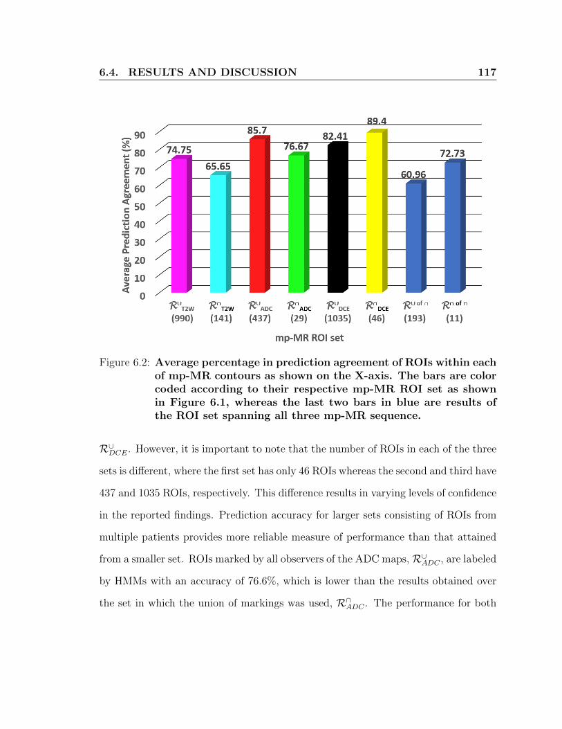
6.4. RESULTS AND DISCUSSION 117
Figure 6.2: Average percentage in prediction agreement of ROIs within eachof mp-MR contours as shown on the X-axis. The bars are colorcoded according to their respective mp-MR ROI set as shownin Figure 6.1, whereas the last two bars in blue are results ofthe ROI set spanning all three mp-MR sequence.
R∪DCE. However, it is important to note that the number of ROIs in each of the three
sets is different, where the first set has only 46 ROIs whereas the second and third have
437 and 1035 ROIs, respectively. This difference results in varying levels of confidence
in the reported findings. Prediction accuracy for larger sets consisting of ROIs from
multiple patients provides more reliable measure of performance than that attained
from a smaller set. ROIs marked by all observers of the ADC maps, R∪ADC , are labeled
by HMMs with an accuracy of 76.6%, which is lower than the results obtained over
the set in which the union of markings was used, R∩ADC . The performance for both

6.4. RESULTS AND DISCUSSION 118
ROI sets selected from the T2W contours is lower than that attained over other mp-
MR sequences, with 74.4% for the union set, R∪T2W , and 65.6% for the intersection,
R∩T2W . The lowest performance, namely 60.9%, was obtained over the ROI set where
malignancy was marked by all observers in at least one of the mp-MR sequences.
The prediction agreement is higher for ROIs in R∩ of ∩, the set of malignant regions
marked by all observers in all mp-MR sequences as compared to those in R∪ of ∩.
These results demonstrate that our HMMs are more likely to correctly identify a
malignancy that is detectable by consensus in all mp-MR sequences.
Figure 6.3 shows the performance per patient. Parts A), C), and E) show the re-
sults per patient for the union of markings in T2W, ADC, DCE, respectively, whereas
G) is for the intersection of observers’ markings in all modalities. Plots B), D), F)
show results using the intersection of markings in the three mp-MR sequences and H)
is for the the intersection of observers in all mp-MR sequences. This figure demon-
strates the variability in the number of patients whose ROIs are included in each
of the eight ROI sets. For example, set R∪DCE contains ROIs from all of the seven
patients, while R∩ of ∩ has ROIs from one patient only. Patient P2 has ROIs in all
of the eight sets and the prediction agreement on these ROIs is higher than 91% for
ROIs inside each of the mp-MR contours. The poor performance on ROIs of patients
P3 and P9 inside the T2W and DCE contours can be attributed to the uncertainty
about the tissue malignancy, which is reflected in the lack of consensus among ob-
servers. This uncertainly is manifested by the large difference in the size of ROI sets
containing union of markings and the sets of markings’ intersection. We also note
that the number of ROIs varies from one patient to another, causing a skew in the
results towards patients with higher number of ROIs.

6.4. RESULTS AND DISCUSSION 119
Figure 6.3: Patient specific accuracy of ROI label assignment. Images A)and B) show the performance results over ROI sets inside theT2W contours; whereas panels C) and D) show the accuracy forsets of ROIs selected from the ADC contours, while E) and F)for ROIs in DCEs markings. Graphs G) and H) show accuracyobtained over the sets of union and intersection of ROIs markedas cancerous by all four observers regardless of the mp-MR se-quence.

6.4. RESULTS AND DISCUSSION 120
Figures 6.4 and 6.5, show three examples of ROI color-maps overlaid on mp-
MR contours in the ultrasound coordinates, where contours are depicted as white
areas. Figure 6.4 shows ROIs within the T2W and ADC contours, whereas Figure 6.5
visualize the results of ROI sets selected from the DCE contours and the union and
intersection of markings by all observers in the different modalities. The colors shown
in each color-map correspond to various malignancy levels, where shades of orange
and red indicate high probability of being cancerous and shades of blue indicate
low probability of being cancerous. By inspecting the color-maps, especially those
corresponding to patient P3, we can detect a depth bias similar to the one discussed
in Section 4.7.3, where ROIs located in the top of the images are typically color-coded
in shades of red and while those at the bottom appear in blue. Potential sources of
this bias are explained in Section 4.7.3. However since most of the cancerous lesions
appear at the top of the images in the peripheral zone closer to the rectum, the bias
is not as apparent as it is in the images of patient P3 where cancerous lesions span
larger regions in the prostate.
In terms of the agreement between HMM predictions and the mp-MR markings,
shown in Figure 6.3, accuracy values for label prediction of ROI set annotated as
cancerous by all observers are more conclusive than the values of the sets containing
the union of markings. In the intersection of markings, the consensus among the four
observers reflects higher malignancy suspicion for the corresponding region. The mp-
MR sequence whose markings were best predicted is DCE, followed by ADC, then
T2W. Despite the low scale of this study which was affected by the large inter-observer
marking-variance, the high agreement with the DCE sequence is concordant with the
theory that pulsation is one of the most important factors providing tissue contrast

6.4. RESULTS AND DISCUSSION 121
in TeUS signals as shown in the simulation results of Bayat et al. [19]. As mentioned
earlier, the DCE sequence reflects the movement of Gd from the vasculature to the
interstitial space. The prediction agreement with the ADC maps is also informative
Figure 6.4: Examples of color-maps for the ROI sets, R∪T2W , R∩T2W , R∪ADC,and R∩ADC selected from T2W and ADC contours.

6.4. RESULTS AND DISCUSSION 122
Figure 6.5: Examples of color-maps for ROIs inside the DCE contours, R∪DCEand R∩DCE in addition to the ROI sets denoted by R∪ of ∩ andR∩ of ∩.

6.4. RESULTS AND DISCUSSION 123
as perfusion is another factor believed to contribute to tissue contrast in TeUS [19],
since it is known that metabolic characteristics relayed by the movement of water
molecules is captured in the ADC maps. The lower agreement with the T2W markings
is expected as the anatomical detail visualized by T2W imaging are superior to what
is captured by ultrasound.
These results provide insight into the physical meaning of the information cap-
tured by TeUS. The prediction agreement between TeUS models and malignancy
markings on DCE images and ADC maps suggest that the tissue contrast gained
in TeUS maybe related to the same functional and molecular characteristics visu-
alized in the aforementioned mp-MR sequences. In a recent publication, Bayat et
al. demonstrated that micro-vibration is the dominant physical phenomenon gov-
erning the interaction between TeUS and the scanned tissue. The high agreement
between TeUS models’ malignancy prediction and the markings on DCE and ADC
sequences implies that blood and fluid circulation has an effect on tissue contrast in
TeUS. In addition, difference in the micro-structure between malignant and benign
tissues lead to a difference in responses to the acoustic waves over the duration of
sonication. Malignant angiogenesis not only changes the micro-structure of tissue but
also amplifies the circulatory activities around cancerous regions. These results are
along the same lines of Bayat et al.’s findings stating that TeUS is affected by tissue
micro-structure and micro-vibration from internal (pulsation and perfusion) or exter-
nal environmental sources. The micro-structure of cells are different between benign
and malignant tissues in histopathology analysis. Malignant cells differ in their size,
shape and development from benign cells, which are well differentiated and have clear
cellular compartments [48]. A recent publication by Bayat et al. showed that TeUS

6.5. CONCLUSIONS 124
captures the difference in benign and malignant micro-structure from the changes
in the speckle pattern of ultrasound which is modulated by low frequency micro-
vibrations due to environmental or physiological sources [19]. They demonstrated
that in fact frequencies of 1-2 Hz (heart beat) were most important in distinguishing
tissue types. The nuclei of cells are the main scattering source of ultrasound and
TeUS captures differences between the distribution and size of cells through the scat-
tering function [19]. Our results from the malignancy-prediction agreement between
TeUS and DCE images indicates that TeUS may be affected by the cellularity of the
tissue (i.e. number and quality). Malignancy-prediction agreement with ADC may
indicate that TeUS is affected by angiogenesis as well but more experiments and data
are required to explore this further.
6.5 Conclusions
We introduced a new framework to study the physical interpretation of the infor-
mation relayed by TeUS. This study is based on the premise that malignancy is
detectable in mp-MR sequences (here T2W, ADC, and DCE modalities) by visual-
izing functional and molecular characteristics that are tissue specific. We therefore
assessed the agreement between mp-MR malignancy-markings and label predictions
by TeUS models. This agreement in label prediction for ROIs inside the mp-MR con-
tours implicates that TeUS captured some of the tissue-specific characteristics that
enabled detecting malignancy in the corresponding mp-MR sequence.
We utilized in-vivo mp-MR images, where malignancy was marked by multiple
observers and subsequently registered to ultrasound images. We predicted the labels
of ROIs inside the mp-MR contours using HMMs previously trained on TeUS signals

6.5. CONCLUSIONS 125
annotated using histopathology information. The models calculated log likelihoods
for each ROI marked as malignant either in the intersection or union of observers in
each of the mp-MR sequences separately or in all of them together. The ROIs were
then labeled by the class of the model (malignant or benign HMMs) that generated
the larger log probability. We limited our prediction to malignant areas since our
aim is to identify malignancy characteristics captured by TeUS and relate them to
the physical phenomenon governing the interaction between TeUS and the scanned
tissue. Our comparison does not take in consideration the areas that were not within
the mp-MR contours. It should be noted that our predictions are meant to detect
the malignancy suspicion as marked on the mp-MR sequences by the radiologists and
not malignancy that is verified through histopathology. We, however, experimented
with extending our prediction to areas outside of the contours to make sure that
the models does not assign a malignant label to all regions (inside and outside the
contours). The results of these experiments demonstrated a lower level of agreement
between TeUS and mp-MR than the malignancy predictions. Using an agreement
measure that incorporates a penalty for false positives provides a better estimation of
the agreement between TeUS and mp-MR especially when predictions are extended
beyond the malignancy markings.
Our findings show that TeUS models are more likely to predict malignancy marked
on DCE sequences than those annotated on the ADC maps. The results reveal a
much lower agreement between TeUS labels predicted by HMMs and T2W markings.
Angiogenesis and metabolic characteristics of tissues are reflected by DCE images
and ADC maps, respectively. The prediction outcome demonstrates that malignancy
detected on DCE images due to the visualization of tissue characteristics related to

6.5. CONCLUSIONS 126
angiogenesis, is also partly reflected by analyzing TeUS signals. Therefore, these
findings support the argument that pulsation is an important factor contributing
to tissue contrast in TeUS signals. Furthermore, the concordance with ADC maps
implies that the information about water-molecule movement relayed in DWI is also
captured by TeUS, hence, supporting the theory stating perfusion as another source
of tissue contrast in TeUS.
It is worth noting that these findings are limited by the scale of the data. A larger
study is required to replicate these results and ensure a better generalizability. In
addition, this data’s depth bias due to uniform time-gain compensation might have
also affected the outcome and a more reliable data is needed to guarantee robust
conclusions. The investigation presented here serves as a feasibility study, where we
demonstrate that the proposed framework is a helpful tool to discover the physical
characteristics of tissues captured by TeUS. Extending the prediction to areas beyond
the mp-MR contours would provide more evidence for the agreement between TeUS
and mp-MR modalities.

127
Chapter 7
Conclusions and Future Work
In this dissertation, we demonstrated the use of stochastic modeling in building a
classifier for TeUS signals and using the classification framework to investigate the
source and influence of the tissue-specific information relayed by the sequences. We
modeled TeUS time-series, which are histopathologically labeled, using HMMs and
proposed a stochastic tissue-characterization framework using the learned models. In
addition, we studied the impact of TeUS temporal-properties on the outcome of the
HMM-based classifier that was trained on signals. We also demonstrated that our
classifier can predict mp-MR malignancy-markings, demarcated according to tissue-
contrast obtained by capturing functional and molecular tissue-characteristics.
The work aims to help increase the detection rates of prostate biopsy and reduce
the need for repeat biopsies. The proposed new application of HMMs assist in guiding
specimen collection from the prostate by providing maps of high risk areas to be
targeted during the biopsy procedure.

7.1. SUMMARY AND CONCLUSIONS 128
7.1 Summary and Conclusions
HMM-based tissue classifier We introduced a stochastic modeling approach
for TeUS signals of prostate tissues to directly represent the temporal signatures of
benign vs. malignant tissue responses to prolonged sonication. We also demonstrated
the utility of using time-domain modeling of TeUS signals in a stochastic tissue char-
acterization framework based on HMMs. In contrast previous analysis of TeUS was
based on features extracted from the spectral domain of the signals then used for
tissue characterization in prostate and breast cancer [12,85,120,191].
The performance of our HMM-based classifier in tissue typing was evaluated for
models with different structures (topology, number of states, and alphabet size) in
order to assess the impact of model topology and alphabet size on the ability to dis-
tinguish malignant tissues from benign ones. We showed the trade-off in performance
between the number of states in the model and the size of the alphabet, where in
most cases a larger alphabet is needed to accurately model the data using HMMs
with fewer states.
Utilizing a non-parametric statistical test, we compared our classification results
with those of a previous study on the same TeUS data. We demonstrated a statis-
tically significantly improved differentiation between TeUS signals of malignant and
benign tissue. This improvement was achieved due to explicitly integrating the tempo-
ral order of the signal in our models, unlike the previous study that employed spectral
domain analysis, where information about signal temporal-order is not available.
These results demonstrate that HMMs capture the contrast between TeUS signals
of malignant and benign prostatic tissues. We used the log odds ratio of the likelihood
values calculated by the HMMs to generate the maps of high risk areas that can be

7.1. SUMMARY AND CONCLUSIONS 129
used to guide physicians during prostate biopsy-procedures. We color-coded the ROIs
on each ultrasound frame by mapping the values of the log odds ratio to colors in the
jet color-spectrum. Dark red was used to color-code the areas with high risk, while
the dark blue utilized for very low risk areas. Despite the high agreement between our
HMMs label prediction and the histopathology ground truth, the color-maps showed
a depth dependent pattern where areas of red/orange shades dominated the locations
at the top of the frames and shades of blue were mostly available at the bottom.
This depth bias may be attributed to the constant time-gain compensation used to
overcome the attenuation of the acoustic power as the signals travel in the depth of
the tissues. Another reason might be the ROI-selection approach that maintained a
large margin between malignant and benign regions, knowing that cancerous lesions
were mostly at top of the frames. It should be noted that the top of the frame
correspond to the areas closer to the rectum in the peripheral zone which has a much
higher probability of developing cancerous. We tried different approaches to rectify
the bias in the data (for details, see Section 4.7), yet none of them were successful.
We thus believe that another dataset is needed to duplicate our findings and show
the robustness of the modeling approach.
Impact of TeUS Temporal Properties TeUS is considered a novel ultrasound-
based imaging technique, whose mechanisms of action and the physical interpretation
of the information captured by its signals are still under investigation. The aim of
studying TeUS temporal properties is to acquire more knowledge about the signals
and to assist in uncovering the reasons behind the change in echointensities over the
short period of sonication. Using the same classification framework, we assessed the

7.1. SUMMARY AND CONCLUSIONS 130
impact of TeUS properties, namely temporal order and signal length, on the perfor-
mance of HMMs in tissue characterization.
We compared the classification outcome of models learned from signals, where
groups of time points (blocks) have been rearranged at random to alter their temporal
order. We generated multiple datasets of rearranged signals, where in each dataset,
the signals had a different rearranged-block size as well as a different block location.
The signals in each of the datasets were then utilized to train a pair of malignant and
benign HMMs. The performance measures of each of the models were compared to
reveal the impact of the block size and its location on the tissue-specific information
captured by the HMMs and used for classification. Our results showed that tissue-
characterization accuracy deteriorated as the size of the rearranged block increased.
The accuracy of 85.01% obtained by the models trained on signals in their original
order decreased to 62.35% for models learned from completely rearranged signals.
Moreover, order rearrangement at the beginning of the signal caused a larger decrease
in the performance as compared to rearrangement elsewhere in the signal.
To assess the impact of signal length on HMMs’ performance, we generated an-
other group of datasets, where signals were cropped to different lengths. The signals
were then modeled and the performance of the learned models in differentiating be-
tween tissue types was evaluated. Subsequently, the accuracy values obtained by the
HMMs trained on signals of different lengths were also compared. The outcome of
these experiments demonstrated that shorter sequences are less informative for tissue
characterization in comparison with longer sequences. Yet, there is a length cut-off,
where longer sequences do not lead to a significant improvement in the classification.
For this dataset, we showed that signals acquired for almost one second (80 frames)

7.1. SUMMARY AND CONCLUSIONS 131
have statistically significantly similar classification performance as signals collected
for more than 2.7 seconds (128 frames).
We demonstrated that the order of TeUS signals carries tissue-specific information
required for accurate differentiation between tissue types. The repetitive patterns
captured by the HMMs of TeUS signals highly depend on the temporal order of the
signals. Moreover, our findings demonstrate that shorter sequences (acquired for less
than 2 seconds and more than a certain threshold) carry sufficient amount of tissue-
specific information that can be used to accurately identify malignancy in prostatic
tissues. Shorter duration for TeUS data collection is one of the implication of these
results.
Comparison between Label Prediction of TeUS models and mp-MR
Markings Tissue characteristics visualized by each of the mp-MR sequences are
reported in the literature. Malignant regions are detectable by expert observers due
to the tissue-contrast gained by the visualization of functional and molecular char-
acteristics that are exhibited differently according to tissue types. Therefore, we
proposed a framework to investigate whether TeUS models can predict the label
of malignant regions demarcated in T2W, ADC and DCE images. In case HMM
malignancy-prediction match the markings in one of the mp-MR sequence, then the
tissue contrast captured by the TeUS models is similar to that provided by the visu-
alized tissue characteristics in mp-MR.
Malignancy was contoured on images of each mp-MR sequence by four observers.
These contours were transformed to the ultrasound coordinates. ROIs within the

7.1. SUMMARY AND CONCLUSIONS 132
contours were used to generate eight datasets of TeUS signals whose labels were pre-
dicted using the same models trained and tested on signals of ROIs with histopathol-
ogy annotation. For each mp-MR sequence, we utilized the union and intersection of
markings by all observers. We also used the intersection of ROIs inside the contours
that were demarcated in consensus among observers in all three mp-MR sequences
along with their union. The highest agreement was achieved between the predictions
of TeUS’ HMMs and the malignancy markings on DCE images, then with the ADC
maps, and the worst agreement was with the T2W images. These results demonstrate
that angiogenesis characteristics visualized on DCE images may also be detectable
with TeUS signals. In addition, the metabolic tissue characteristics reflected in the
ADC maps can be captured to an extent using TeUS signals. Both sets of tissue
characteristics are related to pulsation and perfusion which were two sources of micro-
vibrations suggested to play a role in changing the echointensity values during TeUS
imaging.
Our findings show that TeUS is a promising imaging technique. It visualizes tissue
contrast better than conventional ultrasound and comparable to mp-MR sequences
with the advantage of lower costs, wide availability and more convenient imaging
set-up. It should however be noted that the datasets used for this study have large
difference in their sizes and the number of patients from which ROIs are selected.
Therefore, the study needs to be repeated on a larger scale to replicate our findings
and to offer more significant conclusions.

7.2. FUTURE WORK 133
7.2 Future Work
We have proposed a framework to differentiate between malignant and benign tissue,
where it can be used to improve the yield of prostate biopsy as a diagnostic procedure.
The prognosis of prostate cancer is a pressing issue in oncology. For indolent prostate-
cancer, aggressive treatment-options should be avoided since active surveillance has
proven to be an effective course for disease management and provides an improved
quality of life [168]. Malignant tissues may respond differently to prolonged sonication
depending on their cancer grades. In addition, non-malignant-tissue responses also
vary based on anatomical prostatic-zones. When modeling the temporal responses
of malignant tissues, it is important to be able to differentiate between subgroups of
these responses as well as investigate their connection with the anatomical structure.
The probabilistic tissue-characterization framework can be extended to utilize
grading information and predict grades. The dataset, used in this work, only included
regions with Gleason grades 3 and 4. Therefore, a dataset annotated with a broader
variety of Gleason scores is is likely to enable the development of an HMM-based
grading classifier.
The learning approach adopted here supports accurate tissue typing, where pa-
rameter tuning maximizes the log probability of the data given the model’s param-
eters. With a larger scale dataset, an additional parameter optimization step that
maximizes the differentiation between the classes would improve classification per-
formance. At each step of the expectation maximization, besides ensuring that the
log likelihood is maximized, we could also update the parameters to maximize the
accuracy of tissue differentiation. Furthermore, on a larger dataset, training HMMs

7.2. FUTURE WORK 134
with continuous observations may improve generalizability and classification accu-
racy. Our learned models reflect the typical response of malignant vs benign tissue
to prolonged sonication. They can extended to uncover different subgroups of tissue
responses by clustering the state sequences of TeUS signals.
Our results in tissue classification are promising as they demonstrate an improve-
ment over previous tissue characterization studies. The trained HMMs have effectively
distinguished between malignant and benign tissue. With a more comprehensive set
of TeUS signals collected from a larger cohort, these models can be retrained to in-
corporate a wider spectrum of variability. A transfer learning scheme may be used
where our HMMs can serve as the initial models to be optimized using the new
dataset. One of the issues in implementing such a scheme, is the time-domain repre-
sentation of TeUS signals, used in this dissertation. The binning method is specific to
the range of values available in the data and is not applicable for a dataset collected
on a another platform with a different range of values. An approach that includes
standardization or normalization of the data would provide a platform- and data-
independent representation that can be used for data collected on different platforms
across multiple centers.
One of the main advantages of temporal ultrasound is its use of a technology that
is already integrated in clinical procedures and widely accessible even on portable
platforms. The stochastic tissue-characterization method we have presented is likely
to be extandable to tissue types in other organs such as breast and liver, where
ultrasound is currently used to assist in cancer diagnosis.

BIBLIOGRAPHY 135
Bibliography
[1] Hamidreza Abdi and P Black. Evolving use of multi parametric MRI in prostate
cancer detection, 2015.
[2] Mohammad Aboofazeli, Purang Abolmaesumi, Gabor Fichtinger, and Parvin
Mousavi. Tissue characterization using multiscale products of wavelet trans-
form of ultrasound radio frequency echoes. In the proceedings of the IEEE In-
ternational Conference of Engineering in Medicine and Biology Society, pages
479–482. IEEE, 2009.
[3] Hashim U Ahmed, Ahmed El-Shater Bosaily, Louise C Brown, Rhian Gabe,
Richard Kaplan, Mahesh K Parmar, Yolanda Collaco-Moraes, Katie Ward,
Richard G Hindley, Alex Freeman, Alex kirkham, Robert Oldroyd, Chris
Parker, Mark Emberton, and PROMIS study Group. Diagnostic accuracy of
multi-parametric mri and trus biopsy in prostate cancer (promis): a paired
validating confirmatory study. The Lancet, 389(10071):815–822, 2017.
[4] Hashim U Ahmed, Alex Kirkham, Manit Arya, Rowland Illing, Alex Freeman,
Clare Allen, and Mark Emberton. Is it time to consider a role for MRI before
prostate biopsy? Nature reviews Clinical oncology, 6(4):197–206, 2009.

BIBLIOGRAPHY 136
[5] Peter C Albertsen, James A Hanley, and Judith Fine. 20-year outcomes fol-
lowing conservative management of clinically localized prostate cancer. Jama,
293(17):2095–2101, 2005.
[6] Frederick Albright, Robert A Stephenson, Neeraj Agarwal, Craig C Teerlink,
William T Lowrance, James M Farnham, and Lisa A Cannon Albright. Prostate
cancer risk prediction based on complete prostate cancer family history. The
Prostate, 75(4):390–398, 2015.
[7] American Cancer Society. Global cancer facts & figures 3rd edition. atlanta:
American cancer society; 2015., 2015.
[8] American Cancer Society. Cancer facts & figures 2017. Atlanta, 2017.
[9] Jeffrey C Applewhite, BR Matlaga, DL McCullough, and MC Hall. Transrectal
ultrasound and biopsy in the early diagnosis of prostate cancer. Cancer control:
journal of the Moffitt Cancer Center, 8(2):141–150, 2000.
[10] Gerhardt Attard, Chris Parker, Ros A. Eeles, Fritz Schroder, Scott A. Tomlins,
Ian Tannock, Charles G. Drake, and Johann S. de Bono. Prostate cancer. The
Lancet, 387(10013):70–82, 2016.
[11] Hannes CashEmail authorAndreas MaxeinerCarsten StephanThomas Fischer-
Tahir DurmusJosephine HolzmannPatrick AsbachMatthias HaasStefan HinzJrg
NeymeyerKurt MillerKarsten GnzelCarsten Kempkensteffen. The detection of
significant prostate cancer is correlated with the prostate imaging reporting and
data system (PI-RADS) in MRI/transrectal ultrasound fusion biopsy. World
journal of urology, 34(4):525–532, 2016.

BIBLIOGRAPHY 137
[12] Shekoofeh Azizi, Farhad Imani, Sahar Ghavidel, Amir Tahmasebi, Jin Tae
Kwak, Sheng Xu, Baris Turkbey, Peter Choyke, Peter Pinto, Bradford Wood,
et al. Detection of prostate cancer using temporal sequences of ultrasound data:
a large clinical feasibility study. International journal of computer assisted ra-
diology and surgery, 11(6):947–956, 2016.
[13] Jelle O Barentsz, Jonathan Richenberg, Richard Clements, Peter Choyke,
Sadhna Verma, Geert Villeirs, Olivier Rouviere, Vibeke Logager, and Jurgen J
Futterer. ESUR prostate MR guidelines 2012. European radiology, 22(4):746–
757, 2012.
[14] Tristan Barrett. What is multiparametric-MRI of the prostate and why do we
need it? Imaging in Medicine, 7(1):13–17, 2015.
[15] IA Basheer and M Hajmeer. Artificial neural networks: fundamentals, comput-
ing, design, and application. Journal of microbiological methods, 43(1):3–31,
2000.
[16] I Batal, H Valizadegan, GF Cooper, and M Hauskrecht. A temporal pattern
mining approach for classifying electronic health record data. ACM Transac-
tions on Intelligent Systems and Technology (TIST), 4(4):63, 2013.
[17] GE Batista, EJ Keogh, OM Tataw, and VMA de Souza. Cid: an efficient
complexity-invariant distance for time series. Data Mining and Knowledge Dis-
covery, 28(3):634–669, 2014.

BIBLIOGRAPHY 138
[18] GE Batista, X Wang, and EJ Keogh. A complexity-invariant distance measure
for time series. In SIAM International Conference on Data Mining, volume 11,
pages 699–710. SIAM, 2011.
[19] S Bayat, F Imani, CD Gerardo, G Nir, S Azizi, P Yan, A Tahmasebi, S Wilson,
KA Iczkowski, MS Lucia, L Goldenberg, SE Salcudean, P Mousavi, and P Abol-
maesumi. Tissue mimicking simulations for temporal enhanced ultrasound-
based tissue typing. In Proceeding of SPIE Medical Imaging, pages 101390D–
101390D, 2017.
[20] Yoshua Bengio. Markovian models for sequential data. Neural computing sur-
veys, 2(199):129–162, 1999.
[21] Giles Rottenberg Benjamin J. Challacombe. The staging of prostate cancer. In
Ashutosh Tewari, editor, Prostate Cancer: A Comprehensive Perspective, pages
525–536. Springer London, 2013.
[22] Fernando J Bianco, Peter T Scardino, and James A Eastham. Radical prosta-
tectomy: long-term cancer control and recovery of sexual and urinary function
(”trifecta”). Urology, 66(5):83–94, 2005.
[23] Chris M Bishop. Training with noise is equivalent to tikhonov regularization.
Neural computation, 7(1):108–116, 1995.
[24] K Boehm, G Salomon, B Beyer, J Schiffmann, K Simonis, M Graefen, and
L Budaeus. Shear wave elastography for localization of prostate cancer lesions
and assessment of elasticity thresholds: implications for targeted biopsies and
active surveillance protocols. The Journal of urology, 193(3):794–800, 2015.

BIBLIOGRAPHY 139
[25] LK Boyd, X Mao, and Y Lu. The complexity of prostate cancer: genomic
alterations and heterogeneity. Nature Reviews Urology, 9(11):652–664, 2012.
[26] Michael K Brawer, Roger S Kirby, and Claus G Roehrborn. Prostate specific
antigen. Marcel Dekker New York, NY, 2001.
[27] M Brock, C von Bodman, J Palisaar, W Becker, P Martin-Seidel, and J Noldus.
Detecting prostate cancer: a prospective comparison of systematic prostate
biopsy with targeted biopsy guided by fused mri and transrectal ultrasound.
Deutsches Arzteblatt International, 112(37):605, 2015.
[28] Miguel C Cabarrus and Antonio C Westphalen. Multiparametric magnetic
resonance imaging of the prostate: a basic tutorial. Translational Andrology
and Urology, 2017.
[29] Canadian Cancer Society. Transrectal ultrasound (TRUS). online
(http://www.cancer.ca/en/cancer-information/diagnosis-and-treatment/tests-
and-procedures/transrectal-ultrasound-trus), Accessed on 2017-06-09.
[30] Canadian Cancer Society and National Cancer Institute of Canada. Advisory
Committee on Records and Registries. Canadian cancer statistics. Canadian
Cancer Society, 2017.
[31] Peter Carroll, Christopher Coley, David McLeod, Paul Schellhammer, Greg
Sweat, John Wasson, Anthony Zietman, and Ian Thompson. Prostate-specific
antigen best practice policy part i: early detection and diagnosis of prostate
cancer. Urology, 57(2):217–224, 2001.

BIBLIOGRAPHY 140
[32] HB Carter, PC Albertsen, MJ Barry, R Etzioni, SJ Freedland, KL Greene,
L Holmberg, P Kantoff, BR Konety, MH Murad, DF Penson, and AL Zietman.
Early detection of prostate cancer: AUA guideline. The Journal of urology,
190(2):419–426, 2013.
[33] Melissa M Center, Ahmedin Jemal, Joannie Lortet-Tieulent, Elizabeth Ward,
Jacques Ferlay, Otis Brawley, and Freddie Bray. International variation in
prostate cancer incidence and mortality rates. European urology, 61(6):1079–
1092, 2012.
[34] Vincent Chan and Anahi Perlas. Basics of ultrasound imaging. In Atlas of
ultrasound-guided procedures in interventional pain management, pages 13–19.
Springer, 2011.
[35] Chuan-Yu Chang, Meng-Yu Tu, and Yuh-Shyan Tsai. Prostate tumor identifi-
cation in ultrasound images. In Intelligent Data analysis and its Applications,
Volume II, pages 15–24. Springer, 2014.
[36] Nitesh V Chawla, Kevin W Bowyer, Lawrence O Hall, and W Philip
Kegelmeyer. Smote: synthetic minority over-sampling technique. Journal of
artificial intelligence research, 16:321–357, 2002.
[37] Frank K Chen, Andre Luis de Castro Abreu, and Suzanne L Palmer. Utility of
ultrasound in the diagnosis, treatment, and follow-up of prostate cancer: State
of the art. Journal of Nuclear Medicine, 57(Supplement 3):13S–18S, 2016.

BIBLIOGRAPHY 141
[38] Douglas A Coast, Richard M Stern, Gerald G Cano, and Stanley A Briller. An
approach to cardiac arrhythmia analysis using hidden markov models. Biomed-
ical Eng, IEEE Trans on, 37(9):826–836, 1990.
[39] Simon M Collin, Chris Metcalfe, Jenny Donovan, J Lane, Michael Davis, David
Neal, Freddie Hamdy, and Richard M Martin. Associations of lower urinary
tract symptoms with prostate-specific antigen levels, and screen-detected lo-
calized and advanced prostate cancer: a case-control study nested within the
uk population-based protect (prostate testing for cancer and treatment) study.
BJU international, 102(10):1400–1406, 2008.
[40] Elise D Cook and Ana C Nelson. Prostate cancer screening. Current oncology
reports, 13(1):57–62, 2011.
[41] Derek W Cool, Jeff Bax, Cesare Romagnoli, Aaron D Ward, Lori Gardi, Vaishali
Karnik, Jonathan Izawa, Joseph Chin, and Aaron Fenster. Fusion of MRI to
3D TRUS for mechanically-assisted targeted prostate biopsy: system design
and initial clinical experience. In International Workshop on Prostate Cancer
Imaging, pages 121–133. Springer, 2011.
[42] Jean-Michel Correas, Anne-Marie Tissier, Ahmed Khairoune, Viorel Vassiliu,
Arnaud Mejean, Olivier Helenon, Richard Memo, and Richard G Barr. Prostate
cancer: diagnostic performance of real-time shear-wave elastography. Radiology,
275(1):280–289, 2014.
[43] D Cosgrove. Angiogenesis imaging–ultrasound. The British Journal of Radiol-
ogy, 2014.

BIBLIOGRAPHY 142
[44] Anthony J. Costello and Niall M. Corcoran. Development, applied, and surgical
anatomy of the prostate. In Ashutosh Tewari, editor, Prostate Cancer: A
Comprehensive Perspective, pages 3–17. Springer London, 2013.
[45] Jack Cuzick, Mangesh A. Thorat, Gerald Andriole, Otis W. Brawley, Powel H.
Brown, Zoran Culig, Rosalind A. Eeles, Leslie G. Ford, Freddie C. Hamdy, Lars
Holmberg, Dragan Ilic, Timothy J. Key, Carlo La Vecchia, Hans Lilja, Michael
Marberger, Frank L. Meyskens, Lori M. Minasian, Chris Parker, Howard L.
Parnes, Sven Perner, Harry Rittenhouse, Jack Schalken, Hans-Peter Schmid,
Bernd J. Schmitz-Drager, Fritz H. Schroder, Arnulf Stenzl, Bertrand Tombal,
Timothy J. Wilt, and Alicja Wolk. Prevention and early detection of prostate
cancer. Lancet Oncology, 15(11):e484–e492, 2014.
[46] Mohammad I Daoud, Parvin Mousavi, Farhad Imani, Robert Rohling, and Pu-
rang Abolmaesumi. Tissue classification using ultrasound-induced variations in
acoustic backscattering features. IEEE Transactions on Biomedical Engineer-
ing, 60(2):310–320, 2013.
[47] Jesse Davis and Mark Goadrich. The relationship between precision-recall and
roc curves. In Proceedings of the 23rd international conference on Machine
learning, pages 233–240. ACM, 2006.
[48] Jonathan I Epstein, Lars Egevad, Mahul B Amin, Brett Delahunt, John R
Srigley, Peter A Humphrey, and Grading Committee. The 2014 international
society of urological pathology (isup) consensus conference on gleason grading
of prostatic carcinoma: definition of grading patterns and proposal for a new

BIBLIOGRAPHY 143
grading system. The American journal of surgical pathology, 40(2):244–252,
2016.
[49] R. Etzioni, A. Tsodikov, A. Mariotto, A. Szabo, S. Falcon, J. Wegelin,
K. Karnofski, R. Gulati, D. F Penson, and E. Feuer. Quantifying the role
of PSA screening in the us prostate cancer mortality decline. Cancer Causes &
Control, 19(2):175–181, 2008.
[50] E. J Feleppa, C. R Porter, J. Ketterling, P. Lee, Sh. Dasgupta, S. Urban, and
A. Kalisz. Recent developments in tissue-type imaging (tti) for planning and
monitoring treatment of prostate cancer. Ultrasonic imaging, 26(3):163–172,
2004.
[51] Ernest J Feleppa. Ultrasonic tissue-type imaging of the prostate: implications
for biopsy and treatment guidance. Cancer Biomarkers, 4(4, 5):201–212, 2008.
[52] Ernest J Feleppa, Andrew Kalisz, Joan B Sokil-Melgar, Frederic L Lizzi, Tian
Liu, Angel L Rosado, Mary C Shao, William R Fair, Yu Wang, Michael S
Cookson, V.E. Reuter, and W.D.W. Heston. Typing of prostate tissue by ul-
trasonic spectrum analysis. IEEE Transactions on Ultrasonics, Ferroelectrics,
and Frequency Control, 43(4):609–619, 1996.
[53] Fiona M Fennessy, Kemal Tuncali, Paul R Morrison, and Clare M Tempany. Mr
imaging–guided interventions in the genitourinary tract: An evolving concept.
Radiologic Clinics of North America, 46(1):149–166, 2008.
[54] Gabor Fichtinger, Theodore L DeWeese, Alexandru Patriciu, Attila Tanacs,
Dumitru Mazilu, James H Anderson, Ken Masamune, Russell H Taylor, and

BIBLIOGRAPHY 144
Dan Stoianovici. System for robotically assisted prostate biopsy and therapy
with intraoperative ct guidance. Academic Radiology, 9(1):60–74, 2002.
[55] Zoubin Ghahramani. An introduction to hidden markov models and bayesian
networks. International journal of pattern recognition and artificial intelligence,
15(01):9–42, 2001.
[56] Sahar Ghavidel, Farhad Imani, Siavash Khallaghi, Eli Gibson, Amir Khojaste,
Mena Gaed, Madeleine Moussa, Jose A Gomez, D Robert Siemens, Michael
Leveridge, Silvi Chang, Aaron Fenster, Aaron D. Ward, Purang Abolmaesumi,
and Parvin Mousavi. Classification of prostate cancer grade using temporal
ultrasound: in vivo feasibility study. In SPIE Medical Imaging, pages 97860K–
97860K. International Society for Optics and Photonics, 2016.
[57] Eli Gibson, Cathie Crukley, Mena Gaed, Jose A Gomez, Madeleine Moussa,
Joseph L Chin, Glenn S Bauman, Aaron Fenster, and Aaron D Ward. Regis-
tration of prostate histology images to ex vivo MR images via strand-shaped
fiducials. Journal of Magnetic Resonance Imaging, 36(6):1402–1412, 2012.
[58] Donald F Gleason. Histologic grading of prostate cancer: a perspective. Human
pathology, 23(3):273–279, 1992.
[59] Daniel W Good, Grant D Stewart, Steven Hammer, Paul Scanlan, Wen-
miao Shu, Simon Phipps, Robert Reuben, and Alan S McNeill. Elasticity
as a biomarker for prostate cancer: a systematic review. BJU international,
113(4):523–534, 2014.

BIBLIOGRAPHY 145
[60] Theresa Graif, Stacy Loeb, Kimberly A Roehl, Sara N Gashti, Christopher Grif-
fin, Xiaoying Yu, and William J Catalona. Under diagnosis and over diagnosis
of prostate cancer. The Journal of urology, 178(1):88–92, 2007.
[61] Metin N Gurcan, Laura E Boucheron, Ali Can, Anant Madabhushi, Nasir M
Rajpoot, and Bulent Yener. Histopathological image analysis: A review. IEEE
reviews in biomedical engineering, 2:147–171, 2009.
[62] Gabriel P Haas, Nicolas Delongchamps, Otis W Brawley, Ching Y Wang, and
Gustavo de la Roza. The worldwide epidemiology of prostate cancer: perspec-
tives from autopsy studies. The Canadian journal of urology, 15(1):3866, 2008.
[63] S. M. Han, H. J. Lee, and J. Y. Choi. Computer-aided prostate cancer detection
using texture features and clinical features in ultrasound image. Journal of
digital imaging, 21(1):121–133, 2008.
[64] James A Hanley and Barbara J McNeil. The meaning and use of the area under
a receiver operating characteristic (roc) curve. Radiology, 143(1):29–36, 1982.
[65] Noboru Hara, Mina Okuizumi, Hiroshi Koike, Makoto Kawaguchi, and Vladimir
Bilim. Dynamic contrast-enhanced magnetic resonance imaging (DCE-MRI) is
a useful modality for the precise detection and staging of early prostate cancer.
The Prostate, 62(2):140–147, 2005.
[66] CJ Harvey, J Pilcher, J Richenberg, U Patel, and F Frauscher. Applications
of transrectal ultrasound in prostate cancer. The British journal of radiology,
2014.

BIBLIOGRAPHY 146
[67] Ray Hashman Hashemi, William G Bradley, and Christopher J Lisanti. MRI:
the basics. Lippincott Williams & Wilkins, 2012.
[68] Milos Hauskrecht and Hamish Fraser. Planning treatment of ischemic heart
disease with partially observable markov decision processes. A. I. in Medicine,
18(3):221–244, 2000.
[69] David Kulp David Haussler and Martin G Reese Frank H Eeckman. A gen-
eralized hidden markov model for the recognition of human genes in dna. In
Proc. Int. Conf. on Intelligent Systems for Molecular Biology, St. Louis, pages
134–142, 1996.
[70] Simon S Haykin. Neural networks and learning machines. Pearson Upper Saddle
River, NJ, USA:, 3 edition, 2009.
[71] Wayne R Hedrick, David L Hykes, and Dale E Starchman. Ultrasound physics
and instrumentation. Elsevier Mosby, 2005.
[72] John V Hegde, Robert V Mulkern, Lawrence P Panych, Fiona M Fennessy,
Andriy Fedorov, Stephan E Maier, and Clare Tempany. Multiparametric MRI
of prostate cancer: An update on state-of-the-art techniques and their perfor-
mance in detecting and localizing prostate cancer. Journal of Magnetic Reso-
nance Imaging, 37(5):1035–1054, 2013.
[73] Stijn WTPJ Heijmink, Tom WJ Scheenen, Emile NJT van Lin, Andries G
Visser, Lambertus ALM Kiemeney, J Alfred Witjes, and Jelle O Barentsz.

BIBLIOGRAPHY 147
Changes in prostate shape and volume and their implications for radiother-
apy after introduction of endorectal balloon as determined by mri at 3t. In-
ternational Journal of Radiation Oncology* Biology* Physics, 73(5):1446–1453,
2009.
[74] Jan Herden, Dietrich Schnell, Axel Heidenreich, and Lothar Weissbach. MP43-
09 ”active surveillance” in the everyday care: Results from harow-a prospective,
non-interventional study with a mean follow-up of 66.7 months. The Journal
of Urology, 197(4):e557, 2017.
[75] T Hermanns, C Kuk, and AR Zlotta. Clinical presentation, diagnosis and
staging. In VH Nargund, D Raghavan, and HM Sandler, editors, Urological
Oncology, pages 697–718. Springer, 2015.
[76] Geoffrey E Hinton. Deep belief networks. Scholarpedia, 4(5):5947, 2009.
[77] Bruce L. Jacobs; Yun Zhang; Florian R. Schroeck; Ted A. Skolarus; John T.
Wei; James E. Montie; Scott M. Gilbert; Seth A. Strope; Rodney L. Dunn;
David C. Miller; Brent K. Hollenbeck. Use of advanced treatment technologies
among men at low risk of dying from prostate cancer. JAMA, 309(24):2587–
2595, 2013.
[78] RM Hostetler, IG Mandel, and J Marshburn. Prostate cancer screening. The
Medical clinics of North America, 80(1):83, 1996.
[79] N Howlader, AM Noone, M Krapcho, D Miller, K Bishop, CL Kosary, M Yu,
J Ruhl, Z Tatalovich, A Mariotto, DR Lewis, HS Chen, EJ Feuer, and

BIBLIOGRAPHY 148
KA Cronin. Seer cancer statistics review, 1975-2014. National Cancer In-
stitute, Bethesda, MD, 2017. based on November 2016 SEER data submission,
posted to the SEER web site, April 2017.
[80] Chih-Wei Hsu and Chih-Jen Lin. A comparison of methods for multiclass sup-
port vector machines. IEEE transactions on Neural Networks, 13(2):415–425,
2002.
[81] R. Hughey and A. Krogh. Hidden markov models for sequence analysis: exten-
sion and analysis of the basic method. Computer applications in the biosciences
: CABIOS, 12(2):95–107, Apr 1996.
[82] Hartwig Huland and Markus Graefen. Changing trends in surgical management
of prostate cancer: the end of overtreatment? European urology, 68(2):175–178,
2015.
[83] Aapo Hyvarinen. Survey on independent component analysis. Neural computing
surveys, 2(4):94–128, 1999.
[84] Aapo Hyvarinen, Juha Karhunen, and Erkki Oja. Independent component anal-
ysis, volume 46 of The Wiley Series on Adaptive and Learning Systems for
Signal Processing, Communications, and Control. John Wiley & Sons, 2004.
[85] Farhad Imani, Purang Abolmaesumi, Eli Gibson, Amir Khojaste, Mena Gaed,
Madeleine Moussa, Jose A Gomez, Cesare Romagnoli, Michael Leveridge, Sil-
via Chang, D. Robert Siemens, Aaron Fenster, Aaron D. Ward, and Parvin
Mousavi. Computer-aided prostate cancer detection using ultrasound RF time

BIBLIOGRAPHY 149
series: In vivo feasibility study. IEEE Transactions on Medical Imaging,
34(11):2248–2257, 2015.
[86] Farhad Imani, Mahdi Ramezani, Saman Nouranian, Eli Gibson, Amir Khojaste,
Mena Gaed, Madeleine Moussa, Jose A Gomez, Cesare Romagnoli, Michael
Leveridge, Silvia Chang, Aaron Fenster, D. Robert Siemens, Aaron D. Ward,
Parvin Mousavi, and Purang Abolmaesumi. Ultrasound-based characterization
of prostate cancer using joint independent component analysis. IEEE Transac-
tions on Biomedical Engineering, 62(7):1796–1804, 2015.
[87] Farhad Imani, Mark Z Wu, Andras Lasso, Everett C Burdette, Mohammad
Daoud, Gabor Fitchinger, Purang Abolmaesumi, and Parvin Mousavi. Monitor-
ing of tissue ablation using time series of ultrasound RF data. In International
Conference on Medical Image Computing and Computer-Assisted Intervention,
pages 379–386. Springer, 2011.
[88] Farhad Imania, Sahar Ghavidelb, Purang Abolmaesumia, Siavash Khallaghia,
Eli Gibsonc, Amir Khojasteb, Mena Gaedd, Madeleine Moussae, Jose A
Gomeze, Cesare Romagnolid, et al. Fusion of multi-parametric MRI and tempo-
ral ultrasound for characterization of prostate cancer: in vivo feasibility study.
In SPIE Medical Imaging, pages 97851K–97851K. International Society for Op-
tics and Photonics, 2016.
[89] H Ito, K Kamoi, K Yokoyama, K Yamada, and T Nishimura. Visualization of
prostate cancer using dynamic contrast-enhanced mri: comparison with tran-
srectal power doppler ultrasound. The British journal of radiology, 2014.
[90] Nicholas James. Primer on Prostate Cancer. Springer Healthcare Ltd., 2014.

BIBLIOGRAPHY 150
[91] Andrew J. Armstrong ScM Robert R. Bahnson Michael Cohen Anthony Victor
DAmico James A. Eastham Charles A. Enke Thomas A. Farrington Celestia
S. Higano Eric Mark Horwitz Christopher J. Kane Mark H. Kawachi Michael
Kuettel Timothy M. Kuzel Richard J. Lee Arnold W. Malcolm David Miller
Elizabeth R. Plimack-Julio M. Pow-Sang David Raben Sylvia Richey Mack
Roach III Eric Rohren Stan Rosenfeld Edward Schaeffer Eric J. Small Guru
Sonpavde Sandy Srinivas Cy Stein Seth A. Strope Jonathan Tward Dorothy A.
Shead Maria Ho James L. Mohler, Philip W. Kantoff. Prostate cancer, version
2.2014. Journal of the National Comprehensive Cancer Network, 12(5):686–718,
2014.
[92] Robert R. Bahnson Anthony Victor D’Amico Brian J. Davis James A. East-
ham Charles A. Enke Thomas A. Farrington Celestia S. Higano Eric M. Hor-
witz Michael Hurwitz Christopher J. Kane Mark H. Kawachi Michael Kuettel
Richard J. Lee Joshua J. Meeks David F. Penson Elizabeth R. Plimack Julio M.
Pow-Sang David Raben-Sylvia Richey Mack Roach III Stan Rosenfeld Edward
Schaeffer Ted A. Skolarus Eric J. Small Guru Sonpavde Sandy Srinivas Seth A.
Strope Jonathan Tward Dorothy A. Shead Deborah A. Freedman-Cass James
L. Mohler, Andrew J. Armstrong. Prostate cancer, version 1.2016. Journal of
the National Comprehensive Cancer Network, 14(1):19–30, 2016.
[93] Amina Jelidi, Mickael Ohana, Aıssam Labani, Guillaume Alemann, Herve Lang,
and Catherine Roy. Prostate cancer diagnosis: Efficacy of a simple electro-
magnetic MRI-TRUS fusion method to target biopsies. European Journal of
Radiology, 86:127–134, 2017.

BIBLIOGRAPHY 151
[94] Mark Jenkinson and Stephen Smith. A global optimisation method for robust
affine registration of brain images. Medical image analysis, 5(2):143–156, 2001.
[95] J Stephen Jones. Prostate Cancer Diagnosis: PSA, Biopsy and Beyond.
Springer Science & Business Media, 2012.
[96] Biing-Hwang Fred Juang and Lawrence R Rabiner. A probabilistic distance
measure for hidden markov models. AT&T technical journal, 64(2):391–408,
1985.
[97] Philip Kantoff, Peter R. Carroll, Anthony V. D’Amico, and Inc Ovid Technolo-
gies. Prostate cancer: principles and practice. Lippincott Williams & Wilkins,
Philadelphia, 2002.
[98] Deborah R Kaye, Dan Stoianovici, and Misop Han. Robotic ultrasound and
needle guidance for prostate cancer management: review of the contemporary
literature. Current opinion in urology, 24(1):75, 2014.
[99] Parmeshwar Khurd, Claus Bahlmann, Peter Maday, Ali Kamen, Summer
Gibbs-Strauss, Elizabeth M Genega, and John V Frangioni. Computer-aided
gleason grading of prostate cancer histopathological images using texton forests.
In Biomedical Imaging: From Nano to Macro, 2010 IEEE International Sym-
posium on, pages 636–639. IEEE, 2010.
[100] Thomas A Krouskop, Thomas M Wheeler, Faouzi Kallel, Brian S Garra, and
Timothy Hall. Elastic moduli of breast and prostate tissues under compression.
Ultrasonic imaging, 20(4):260–274, 1998.

BIBLIOGRAPHY 152
[101] Solomon Kullback and Richard A Leibler. On information and sufficiency. The
annals of mathematical statistics, 22(1):79–86, 1951.
[102] Fernand Labrie. Psa screening for prostate cancer: why so much controversy?
Asian journal of andrology, 15(5):603, 2013.
[103] Di Lai, Navalgund Rao, Chung-hui Kuo, Shweta Bhatt, and Vikram Dogra.
Independent component analysis applied to ultrasound speckle texture analysis
and tissue characterization. In Engineering in Medicine and Biology Society,
2007. EMBS 2007. 29th Annual International Conference of the IEEE, pages
6523–6526. IEEE, 2007.
[104] A Latifoltojar, N Dikaios, A Ridout, C Moore, R Illing, A Kirkham, S Tay-
lor, S Halligan, D Atkinson, C Allen, M Emberton, and S Punwani. Evo-
lution of multi-parametric MRI quantitative parameters following transrectal
ultrasound-guided biopsy of the prostate. Prostate cancer and prostatic dis-
eases, 18(4):343–351, 2015.
[105] Chao Li, Shuheng Zhang, Huan Zhang, Lifang Pang, Kinman Lam, Chun Hui,
and Su Zhang. Using the k-nearest neighbor algorithm for the classification
of lymph node metastasis in gastric cancer. Computational and mathematical
methods in medicine, 2012, 2012.
[106] Ying Li, Sharon Lipsky Gorman, and Noemie Elhadad. Section classification
in clinical notes using supervised hidden markov model. In Proceedings of the
1st ACM International Health Informatics Symposium, pages 744–750. ACM,
2010.

BIBLIOGRAPHY 153
[107] Frederic L Lizzi, Michael Greenebaum, Ernest J Feleppa, Marek Elbaum, and
D Jackson Coleman. Theoretical framework for spectrum analysis in ultra-
sonic tissue characterization. The Journal of the Acoustical Society of America,
73(4):1366–1373, 1983.
[108] Rafael Llobet, Juan C Perez-Cortes, Alejandro H Toselli, and Alfons Juan.
Computer-aided detection of prostate cancer. International Journal of Medical
Informatics, 76(7):547–556, 2007.
[109] Stacy Loeb, Marc A Bjurlin, Joseph Nicholson, Teuvo L Tammela, David F
Penson, H Ballentine Carter, Peter Carroll, and Ruth Etzioni. Overdiagnosis
and overtreatment of prostate cancer. European urology, 65(6):1046–1055, 2014.
[110] JK Logan, S Rais-Bahrami, B Turkbey, A Gomella, H Amalou, P Choyke,
BJ Wood, and P Pinto. Current status of MRI and ultrasound fusion software
platforms for guidance of prostate biopsies. BJU International, 114(5):614–652,
2014.
[111] R Lopes, A Ayache, N Makni, P Puech, A Villers, S Mordon, and N Betrouni.
Prostate cancer characterization on MR images using fractal features. Medical
physics, 38(1):83–95, 2011.
[112] Antonio Luna, Shivani Pahwa, Claudio Bonini, Lidia Alcala-Mata, Katherine L
Wright, and Vikas Gulani. Multiparametric mr imaging in abdominal malig-
nancies. Magnetic resonance imaging clinics of North America, 24(1):157–186,
2016.

BIBLIOGRAPHY 154
[113] Donna L. Berry Celestia S. Higano E. David Crawford Glenn Liu George Wild-
ing Stephen Prescott Subramanian Kanaga Sundaram Eric Jay Small Nancy
Ann Dawson Bryan J. Donnelly Peter M. Venner Ulka N. Vaishampayan Paul
F. Schellhammer David I. Quinn Derek Raghavan Benjamin Ely Carol M. Moin-
pour Nicholas J. Vogelzang Maha Hussain, Catherine M. Tangen and Ian M.
Thompson. Intermittent versus continuous androgen deprivation in prostate
cancer. New England Journal of Medicine, 368(14):1314–1325, 2013.
[114] Elizabeth Martin. Concise Medical Dictionary. Oxford University Press, 2015.
[115] John E McNeal. The zonal anatomy of the prostate. The prostate, 2(1):35–49,
1981.
[116] Petra Menn, Reiner Leidl, and Rolf Holle. A lifetime markov model for the
economic evaluation of chronic obstructive pulmonary disease. Pharmacoeco-
nomics, 30(9):825–840, 2012.
[117] MM Mohamed, TK Abdel-Galil, EF El-Saadany, A Fenster, DB Downey,
K Rizkalla, EF El-saadany, and M kame1. Prostate cancer diagnosis based on
gabor filter texture segmentation of ultrasound image. In IEEE Canadian Con-
ference on Electrical and Computer Engineering, volume 3, pages 1485–1488,
2003.
[118] Caroline M Moore, Nicola L Robertson, Nasr Arsanious, Thomas Middleton,
Arnauld Villers, Laurence Klotz, Samir S Taneja, and Mark Emberton. Image-
guided prostate biopsy using magnetic resonance imaging–derived targets: a
systematic review. European urology, 63(1):125–140, 2013.

BIBLIOGRAPHY 155
[119] Mehdi Moradi. A new paradigm for ultrasound-based tissue typing in prostate
cancer. PhD thesis, School of Computing, Queen’s University, 2008.
[120] Mehdi Moradi, Purang Abolmaesumi, Alexander Boag, Eric Sauerbrei, Robert
Siemens, and Parvin Mousavi. Augmenting detection of prostate cancer in
transrectal ultrasound images using svm and rf time series. IEEE Transactions
on Biomedical Engineering, 56(9):2214–2224, 2009.
[121] Mehdi Moradi, Purang Abolmaesumi, Parvin Mousavi, Eric Sauerbrei, Robert
Siemens, and Phillip Isotalo. Method for improved ultrasonic detection, May 25
2007. US Patent App. 12/227,697.
[122] Mehdi Moradi, S Sara Mahdavi, G Nir, O Mohareri, A Koupparis, L Gagnon,
L Fazli, R Casey, J Ischia, E Jones, S Goldenberg, and S Salcudean. Multi-
parametric 3D in vivo ultrasound vibroelastography imaging of prostate cancer:
Preliminary results. Medical physics, 41(7):073505, 2014.
[123] Mehdi Moradi, Parvin Mousavi, and Purang Abolmaesumi. Computer-aided
diagnosis of prostate cancer with emphasis on ultrasound-based approaches: a
review. Ultrasound in medicine & biology, 33(7):1010–1028, 2007.
[124] Mehdi Moradi, Parvin Mousavi, and Purang Abolmaesumi. Tissue character-
ization using fractal dimension of high frequency ultrasound rf time series. In
International Conference on Medical Image Computing and Computer-Assisted
Intervention, pages 900–908. Springer Berlin Heidelberg, 2007.

BIBLIOGRAPHY 156
[125] Virginia A. Moyer. Screening for prostate cancer: US preventive services task
force recommendation statement. Annals of Internal Medicine, 157(2):120–134,
2012.
[126] Ian G Murphy, Elaine NiMhurchu, Robert G Gibney, and Colm J McMahon.
MRI-directed cognitive fusion-guided biopsy of the anterior prostate tumors.
Diagnostic and Interventional Radiology, 23(2):87, 2017.
[127] J. Bellmunt R.C.N. van den Bergh M. Bolla N.J. van Casteren P. Cornford S.
Joniau M.D. Mason V. Matveev T.H. van der Kwast H. van der Poel O. Rouvire
T. Wiegel N. Mottet, P.J. Bastian. Guidelines on prostate cancer. European
Urology, 65(1):124–37, 2014.
[128] Layan Nahlawi, Caroline Goncalves, Farhad Imani, Mena Gaed, Jose A Gomez,
Madeleine Moussa, Eli Gibson, Aaron Fenster, Aaron D. Ward, Purang Abol-
maesumi, Parvin Mousavi, and Hagit Shatkay. Models of temporal enhanced
ultrasound data for prostate cancer diagnosis: the impact of time-series order.
In Proceedings of SPIE Medical Imaging, volume 10135, pages 101351D–1, 2017.
[129] Layan Nahlawi, Farhad Imani, Mena Gaed, Jose A Gomez, Madeleine Moussa,
Eli Gibson, Aaron Fenster, Aaron D Ward, Purang Abolmaesumi, Parvin
Mousavi, and Hagit Shatkay. Using hidden markov models to capture temporal
aspects of ultrasound data in prostate cancer. In Proceedings of the IEEE in-
ternatinal conference on Bioinformatics and Biomediciene (BIBM), pages 446–
449. IEEE, 2015.
[130] Layan Nahlawi, Farhad Imani, Mena Gaed, Jose A Gomez, Madeleine Moussa,
Eli Gibson, Aaron Fenster, Aaron D Ward, Purang Abolmaesumi, Hagit

BIBLIOGRAPHY 157
Shatkay, and Parvin Mousavi. Prostate cancer: Improved tissue characteriza-
tion by temporal modeling of radio-frequency ultrasound echo data. In Proceed-
ings of international conference on Medical Image Computing and Computer-
Assisted Intervention (MICCAI), pages 644–652. Springer, 2016.
[131] Nima Nassiri, Daniel J Margolis, Shyam Natarajan, Devi S Sharma, Jiaoti
Huang, Frederick J Dorey, and Leonard S Marks. Targeted biopsy to detect
gleason score upgrading during active surveillance for men with low versus in-
termediate risk prostate cancer. The Journal of urology, 197(3):632–639, 2017.
[132] J Alison Noble. Ultrasound image segmentation and tissue characterization.
Proceedings of the Institution of Mechanical Engineers, Part H: Journal of En-
gineering in Medicine, 224(2):307–316, 2010.
[133] Yngve Nygard, Svein A Haukaas, Ole J Halvorsen, Karsten Gravdal, Jannicke
Frugard, Lars A Akslen, and Christian Beisland. A positive real-time elastog-
raphy is an independent marker for detection of high-risk prostate cancers in
the primary biopsy setting. BJU international, 113(5b):E90–E97, 2014.
[134] Can Obek, Tunkut Doganca, Sinan Erdal, Sarper Erdogan, and Haydar Du-
rak. Core length in prostate biopsy: size matters. The Journal of urology,
187(6):2051–2055, 2012.
[135] Michael L Oelze and Jonathan Mamou. Review of quantitative ultrasound:
Envelope statistics and backscatter coefficient imaging and contributions to
diagnostic ultrasound. IEEE transactions on ultrasonics, ferroelectrics, and
frequency control, 63(2):336–351, 2016.

BIBLIOGRAPHY 158
[136] Anwar R Padhani, Giuseppe Petralia, and Francesco Sanguedolce. Magnetic
resonance imaging before prostate biopsy: Time to talk. European Urology,
1(69):1–3, 2016.
[137] Gyan Pareek, U Rajendra Acharya, S Vinitha Sree, G Swapna, Ratna Yantri,
Roshan Joy Martis, Luca Saba, Ganapathy Krishnamurthi, Giorgio Mallarini,
Ayman El-Baz, Shadi Al Ekish, Beland Michael, and Jasjit S Suri. Prostate tis-
sue characterization/classification in 144 patient population using wavelet and
higher order spectra features from transrectal ultrasound images. Technology
in cancer research & treatment, 12(6):545–557, 2013.
[138] Tobias Penzkofer and Clare M Tempany-Afdhal. Prostate cancer detection and
diagnosis: the role of mr and its comparison with other diagnostic modalities–a
radiologist’s perspective. NMR in Biomedicine, 27(1):3–15, 2014.
[139] Fernando R Pereira, Joao C Machado, and F Stuart Foster. Ultrasound char-
acterization of coronary artery wall in vitro using temperature-dependent wave
speed. IEEE transactions on ultrasonics, ferroelectrics, and frequency control,
50(11):1474–1485, 2003.
[140] Leif E Peterson. K-nearest neighbor. Scholarpedia, 4(2):1883, 2009.
[141] Marco AF Pimentel, Mauro D Santos, David B Springer, and Gari D Clif-
ford. Heart beat detection in multimodal physiological data using a hidden
semi-markov model and signal quality indices. Physiological measurement,
36(8):1717, 2015.

BIBLIOGRAPHY 159
[142] Jehonathan H Pinthus, Dalibor Pacik, and Jacob Ramon. Diagnosis of prostate
cancer. In Prostate Cancer, pages 83–99. Springer, 2007.
[143] Peter A Pinto, Paul H Chung, Ardeshir R Rastinehad, Angelo A Baccala,
Jochen Kruecker, Compton J Benjamin, Sheng Xu, Pingkun Yan, Samuel
Kadoury, Celene Chua, Julia K Locklin, Baris Turkbey, Joanna H Shih,
Stacey P Gates, Carey Buckner, Gennady Bratslavsky, W. Marston Linehan,
Peter L Glossop, Neil D and Choyke, and Bradford J Wood. Magnetic reso-
nance imaging/ultrasound fusion guided prostate biopsy improves cancer detec-
tion following transrectal ultrasound biopsy and correlates with multiparametric
magnetic resonance imaging. The Journal of urology, 186(4):1281–1285, 2011.
[144] Morgan R Pokorny, Maarten De Rooij, Earl Duncan, Fritz H Schroder, Robert
Parkinson, Jelle O Barentsz, and Leslie C Thompson. Prospective study of diag-
nostic accuracy comparing prostate cancer detection by transrectal ultrasound–
guided biopsy versus magnetic resonance (MR) imaging with subsequent MR-
guided biopsy in men without previous prostate biopsies. European urology,
66(1):22–29, 2014.
[145] Alan Pollack, Alexandra L Hanlon, Eric M Horwitz, Steven J Feigenberg,
Robert G Uzzo, and Gerald E Hanks. Prostate cancer radiotherapy dose
response: an update of the fox chase experience. The Journal of urology,
171(3):1132–1136, 2004.
[146] Ben Pullar and Nimish Shah. Prostate cancer. Surgery (Oxford), 34(10):505–
511, 2016.

BIBLIOGRAPHY 160
[147] Michael Quentin, Dirk Blondin, Christian Arsov, Lars Schimmoller, Andreas
Hiester, Erhard Godehardt, Peter Albers, Gerald Antoch, and Robert Rabenalt.
Prospective evaluation of magnetic resonance imaging guided in-bore prostate
biopsy versus systematic transrectal ultrasound guided prostate biopsy in biopsy
naıve men with elevated prostate specific antigen. The Journal of urology,
192(5):1374–1379, 2014.
[148] Lawrence Rabiner. A tutorial on hidden markov models and selected applica-
tions in speech recognition. Proceedings of the IEEE, 77(2):257–286, 1989.
[149] Lawrence R Rabiner and Biing-Hwang Juang. An introduction to hidden
markov models. ASSP Magazine, IEEE, 3(1):4–16, 1986.
[150] JR Ramey. Ultrasonography and biopsy of the prostate. Campbell-Walsh Urol-
ogy, pages 2883–2895, 2007.
[151] Mahdi Ramezani, Purang Abolmaesumi, Kris Marble, Heather Trang, and In-
grid Johnsrude. Fusion analysis of functional MRI data for classification of indi-
viduals based on patterns of activation. Brain imaging and behavior, 9(2):149–
161, 2015.
[152] Charles Roehrig, George Miller, Craig Lake, and Jenny Bryant. National health
spending by medical condition, 1996–2005. Health Affairs, 28(2):w358–w367,
2009.
[153] Val M Runge. Current technological advances in magnetic resonance with criti-
cal impact for clinical diagnosis and therapy. Investigative radiology, 48(12):869–
877, 2013.

BIBLIOGRAPHY 161
[154] Futoshi Sano and Hiroji Uemura. The utility and limitations of contrast-
enhanced ultrasound for the diagnosis and treatment of prostate cancer. Sen-
sors, 15(3):4947–4957, 2015.
[155] J-L Sauvain, E Sauvain, P Rohmer, D Louis, N Nader, R Papavero, J-M Bre-
mon, and J Jehl. Value of transrectal power doppler sonography in the detection
of low-risk prostate cancers. Diagnostic and interventional imaging, 94(1):60–
67, 2013.
[156] Howard I Scher, SA Leibel, Z Fuks, C Cordon-Cardo, and PT Scardino. Cancer
of the prostate. In Vincent DeVita, Theodore Hellman, and Steven Rosenberg,
editors, DeVita, Hellman, and Rosenbergs Cancer: Principles and Practice of
Oncology, pages 932–980. Pa: Lippincott Williams & Wilkins, Philadephia, 10th
ed edition, 2015.
[157] Lars Schimmoller, Dirk Blondin, Christian Arsov, Robert Rabenalt, Peter Al-
bers, Gerald Antoch, and Michael Quentin. MRI-guided in-bore biopsy: differ-
ences between prostate cancer detection and localization in primary and sec-
ondary biopsy settings. American Journal of Roentgenology, 206(1):92–99, 2016.
[158] Bernhard Scholkopf and Alexander J Smola. Learning with kernels: support
vector machines, regularization, optimization, and beyond. MIT press, 2001.
[159] George AF Seber and Alan J Lee. Linear regression analysis, volume 936. John
Wiley & Sons, 2012.
[160] Steven H Selman. The McNeal prostate: a review. Urology, 78(6):1224–1228,
2011.

BIBLIOGRAPHY 162
[161] Ege Can Serefoglu, Serkan Altinova, Nevzat Serdar Ugras, Egemen Akincioglu,
Erem Asil, and Derya Balbay. How reliable is 12-core prostate biopsy procedure
in the detection of prostate cancer? Canadian Urological Association Journal,
7(5-6):293–8, 2013.
[162] Shahrokh F Shariat and Claus G Roehrborn. Using biopsy to detect prostate
cancer. Rev Urol, 10(4):262–280, 2008.
[163] P R. Carroll; JK Parsons; G Andriole; RR Bahnson; DA Barocas ; WJ Cat-
alona; DM Dahl; JW Davis ; JI Epstein; RB Etzioni; V N Giri; GP Hemstreet;
MH Kawachi; PH Lange; KR Loughlin; W Lowrance; P Maroni; J Mohler; TM
Morgan; RB Nadler; M Poch; C Scales; TM Shanefelt; AJ. Vickers; R Wake; DA
Shead; and M Ho. Prostate cancer early detection, version 1.2014. Journal of
the National Comprehensive Cancer Network, 12(9):1211–1219, 2014.
[164] Dinggang Shen, Guorong Wu, and Heung-Il Suk. Deep learning in medical
image analysis. Annual Review of Biomedical Engineering, (0), 2017.
[165] Katsuto Shinohara. Prostate cancer: cryotherapy. Urologic Clinics of North
America, 30(4):725–736, 2003.
[166] M Minhaj Siddiqui, Soroush Rais-Bahrami, Baris Turkbey, Arvin K George, Ja-
son Rothwax, Nabeel Shakir, Chinonyerem Okoro, Dima Raskolnikov, Howard L
Parnes, W Marston Linehan, Maria J Merino, Richard M Simon, Peter L
Choyke, Bradford J Wood, and Peter A Pinto. Comparison of MR/ultrasound
fusion–guided biopsy with ultrasound-guided biopsy for the diagnosis of prostate
cancer. Jama, 313(4):390–397, 2015.

BIBLIOGRAPHY 163
[167] Rebecca L Siegel, Kimberly D Miller, and Ahmedin Jemal. Cancer statistics,
2016. CA: A cancer journal for clinicians, 2015.
[168] Eric A Singer, Aradhana Kaushal, Baris Turkbey, Anna Couvillon, Peter A
Pinto, and Howard L Parnes. Active surveillance for prostate cancer: past,
present and future. Current opinion in oncology, 24(3):243–250, 2012.
[169] Paras B Singh, Caroline M Moore, and Mark Emberton. Prostate biopsy. In
Prostate Cancer: A Comprehensive Perspective, pages 511–524. Springer, 2013.
[170] Padhraic Smyth. Belief networks, hidden markov models, and markov random
fields: a unifying view. Pattern recognition letters, 18(11):1261–1268, 1997.
[171] American Cancer Society. Cancer facts & figures 2015. atlanta: American cancer
society. 2015.
[172] Geoffrey A Sonn, Shyam Natarajan, Daniel JA Margolis, Malu MacAiran, Pa-
tricia Lieu, Jiaoti Huang, Frederick J Dorey, and Leonard S Marks. Targeted
biopsy in the detection of prostate cancer using an office based magnetic reso-
nance ultrasound fusion device. The Journal of urology, 189(1):86–92, 2013.
[173] Erik LL Sonnhammer, Gunnar Von Heijne, and Anders Krogh. A hidden
markov model for predicting transmembrane helices in protein sequences. In
ISMB, volume 6, pages 175–182, 1998.
[174] Nitish Srivastava, Geoffrey Hinton, Alex Krizhevsky, Ilya Sutskever, and Rus-
lan Salakhutdinov. Dropout: A simple way to prevent neural networks from
overfitting. The Journal of Machine Learning Research, 15(1):1929–1958, 2014.

BIBLIOGRAPHY 164
[175] Gary D Steinberg, Bob S Carter, Terri H Beaty, Barton Childs, and Patrick C
Walsh. Family history and the risk of prostate cancer. The prostate, 17(4):337–
347, 1990.
[176] Ingo Steinwart and Andreas Christmann. Support vector machines. Springer
Science & Business Media, 2008.
[177] Yu Sub Sung, Heon-Ju Kwon, Bum-Woo Park, Gyunggoo Cho, Chang Kyung
Lee, Kyoung-Sik Cho, and Jeong Kon Kim. Prostate cancer detection on dy-
namic contrast-enhanced MRI: computer-aided diagnosis versus single perfusion
parameter maps. American Journal of Roentgenology, 197(5):1122–1129, 2011.
[178] Ali Tabesh, Mikhail Teverovskiy, Ho-Yuen Pang, Vinay P Kumar, David Ver-
bel, Angeliki Kotsianti, and Olivier Saidi. Multifeature prostate cancer diag-
nosis and gleason grading of histological images. IEEE transactions on medical
imaging, 26(10):1366–1378, 2007.
[179] James A Talcott, Judith Manola, Ronald C Chen, Jack A Clark, Irving Ka-
plan, Anthony V D’amico, and Anthony L Zietman. Using patient-reported
outcomes to assess and improve prostate cancer brachytherapy. BJU interna-
tional, 114(4):511–516, 2014.
[180] Samir S Taneja. Imaging in the diagnosis and management of prostate cancer.
Reviews in urology, 6(3):101, 2004.
[181] Clare Tempany, Jagadeesan Jayender, Tina Kapur, Raphael Bueno, Alexandra
Golby, Nathalie Agar, and Ferenc A Jolesz. Multimodal imaging for improved
diagnosis and treatment of cancers. Cancer, 121(6):817–827, 2015.

BIBLIOGRAPHY 165
[182] Clare Tempany, Sarah Straus, Nobuhiko Hata, and Steven Haker. MR-guided
prostate interventions. Journal of Magnetic Resonance Imaging, 27(2):356–367,
2008.
[183] P Tenke, J Horti, P Balint, and B Kovacs. Prostate cancer screening. In
Prostate Cancer, pages 65–81. Springer, 2007.
[184] The American Cancer Society medical and editorial content team. Prostate
cancer risk factors. Online, March 2016.
[185] Susan Thorpe, Paul M Salkovskis, and Antonia Dittner. Claustrophobia in mri:
the role of cognitions. Magnetic resonance imaging, 26(8):1081–1088, 2008.
[186] Keiichi Tokuda, Yoshihiko Nankaku, Tomoki Toda, Heiga Zen, Junichi Yam-
agishi, and Keiichiro Oura. Speech synthesis based on hidden markov models.
Proceedings of the IEEE, 101(5):1234–1252, 2013.
[187] Jeffrey J Tosoian, Meera Chappidi, Zhaoyong Feng, Elizabeth B Humphreys,
Misop Han, Christian P Pavlovich, Jonathan I Epstein, Alan W Partin, and
Bruce J Trock. Prediction of pathological stage based on clinical stage, serum
prostate-specific antigen, and biopsy gleason score: Partin tables in the con-
temporary era. BJU international, 2016.
[188] Igor Trilisky, Aytekin Oto, and Scott Eggener. In-bore magnetic resonance
imaging-targeted prostate biopsy. In Imaging and Focal Therapy of Early
Prostate Cancer, pages 205–218. Springer, 2017.

BIBLIOGRAPHY 166
[189] Baris Turkbey and Peter L Choyke. Multiparametric mri and prostate cancer
diagnosis and risk stratification. Current opinion in urology, 22(4):310–315,
2012.
[190] Ultrasonix. Research documentation, http://www.ultrasonix.com/wikisonix.
[191] Nishant Uniyal, Hani Eskandari, Purang Abolmaesumi, Samira Sojoudi, Paula
Gordon, Linda Warren, Robert N Rohling, Septimiu E Salcudean, and Mehdi
Moradi. Ultrasound RF time series for classification of breast lesions. Medical
Imaging, IEEE Trans on, 34(2):652–661, 2015.
[192] Elizabeth Ward, Ahmedin Jemal, Vilma Cokkinides, Gopal K Singh, Cheryll
Cardinez, Asma Ghafoor, and Michael Thun. Cancer disparities by race/ethnic-
ity and socioeconomic status. CA: a cancer journal for clinicians, 54(2):78–93,
2004.
[193] McKenzie CA Montreuil J Gibson E Romagnoli C Gomez JA Moussa M Chin
J Bauman G Fenster A. Ward AD, Crukley C. Prostate: registration of digital
histopathologic images to in vivo mr images acquired by using endorectal receive
coil. Radiology, 263(3):856–864, 2012.
[194] Olivier Wegelin, Harm HE van Melick, Lotty Hooft, JLH Ruud Bosch, Hans B
Reitsma, Jelle O Barentsz, and Diederik M Somford. Comparing three dif-
ferent techniques for magnetic resonance imaging-targeted prostate biopsies:
a systematic review of in-bore versus magnetic resonance imaging-transrectal
ultrasound fusion versus cognitive registration. is there a preferred technique?
European urology, 71(4):517–531, 2017.

BIBLIOGRAPHY 167
[195] A Wolf, R C Wender, R B Etzioni, I M Thompson, A V D’Amico, RJ Volk, D D
Brooks, C Dash, I Guessous, K Andrews, C DeSantis, RA Smith, and American
Cancer Society Prostate Cancer Advisory Committee. American cancer society
guideline for the early detection of prostate cancer: update 2010. CA: a cancer
journal for clinicians, 60(2):70–98, 2010.
[196] Yan Xu, Tao Mo, Qiwei Feng, Peilin Zhong, Maode Lai, I Eric, and Chao
Chang. Deep learning of feature representation with multiple instance learning
for medical image analysis. In IEEE International Conference on Acoustics,
Speech and Signal Processing (ICASSP), pages 1626–1630, 2014.