Seediscussions,stats,andauthorprofilesforthispublicationat:https://www.researchgate.net/publication/228699264

RobustStochasticApproximationApproachtoStochasticProgramming

ARTICLEinSIAMJOURNALONOPTIMIZATION·JANUARY2009

ImpactFactor:1.83·DOI:10.1137/070704277·Source:DBLP

CITATIONS

311

READS

179

4AUTHORS,INCLUDING:

ArkadiNemirovski

GeorgiaInstituteofTechnology

148PUBLICATIONS8,527CITATIONS

SEEPROFILE

GuanghuiLan

UniversityofFlorida

38PUBLICATIONS766CITATIONS

SEEPROFILE

Availablefrom:ArkadiNemirovski

Retrievedon:05February2016

Stochastic Approximation Approach to Stochastic

Programming

Anatoli Juditsky∗ Guanghui Lan† Arkadi Nemirovski‡ Alexander Shapiro §

Abstract. In this paper we consider optimization problems where the objective function isgiven in a form of the expectation. A basic difficulty of solving such stochastic optimizationproblems is that the involved multidimensional integrals (expectations) cannot be computed withhigh accuracy. The aim of this paper is to compare two computational approaches based onMonte Carlo sampling techniques, namely, the Stochastic Approximation (SA) and the SampleAverage Approximation (SAA) methods. Both approaches, the SA and SAA methods, have along history. Current opinion is that the SAA method can efficiently use a specific (say linear)structure of the considered problem, while the SA approach is a crude subgradient method whichoften performs poorly in practice. We intend to demonstrate that a properly modified SA approachcan be competitive and even significantly outperform the SAA method for a certain class of convexstochastic problems. We extend the analysis to the case of convex-concave stochastic saddle pointproblems, and present (in our opinion highly encouraging) results of numerical experiments.

Key words: stochastic approximation, sample average approximation method, stochastic pro-gramming, Monte Carlo sampling, complexity, saddle point, minimax problems, mirror descentalgorithm

∗LJK, Universite J. Fourier, B.P. 53, 38041 Grenoble Cedex 9, France, Anatoli.Juditsky@imag.fr†Georgia Institute of Technology, Atlanta, Georgia 30332, USA, glan@isye.gatech.edu,

research of this author was partially supported by NSF award CCF-0430644 and ONR award

N00014-05-1-0183.‡Georgia Institute of Technology, Atlanta, Georgia 30332, USA, nemirovs@isye.gatech.edu,

research of this author was partly supported by the NSF award DMI-0619977.§Georgia Institute of Technology, Atlanta, Georgia 30332, USA, ashapiro@isye.gatech.edu,

research of this author was partly supported by the NSF awards DMS-0510324 and DMI-0619977.

1

1 Introduction

In this paper we consider the following optimization problem

minx∈X

f(x) := E[F (x, ξ)]

. (1.1)

Here X ⊂ Rn is a nonempty bounded closed convex set, ξ is a random vector whose probabilitydistribution P is supported on set Ξ ⊂ Rd and F : X × Ξ → R. We assume that for every ξ ∈ Ξthe function F (·, ξ) is convex on X, and that the expectation

E[F (x, ξ)] =∫Ξ F (x, ξ)dP (ξ) (1.2)

is well defined and finite valued for every x ∈ X. It follows that function f(·) is convex and finitevalued on X. Moreover, we assume that f(·) is continuous on X. Of course, continuity of f(·)follows from convexity if f(·) is finite valued and convex on a neighborhood of X. With theseassumptions, (1.1) becomes a convex programming problem.

A basic difficulty of solving stochastic optimization problem (1.1) is that the multidimensionalintegral (expectation) (1.2) cannot be computed with a high accuracy for dimension d, say, greaterthan 5. The aim of this paper is to compare two computational approaches based on MonteCarlo sampling techniques, namely, the Stochastic Approximation (SA) and the Sample AverageApproximation (SAA) methods. To this end we make the following assumptions.

(A1) It is possible to generate an iid sample ξ1, ξ2, ..., of realizations of random vector ξ.

(A2) There is a mechanism (an oracle) which for every given x ∈ X and ξ ∈ Ξ returns value F (x, ξ)and a stochastic subgradient – a vector G(x, ξ) such that g(x) := E[G(x, ξ)] is well definedand is a subgradient of f(·) at x, i.e., g(x) ∈ ∂f(x).

Recall that if F (·, ξ), ξ ∈ Ξ, is convex and f(·) is finite valued in a neighborhood of a point x,then (cf., Strassen [18])

∂f(x) = E [∂xF (x, ξ)] . (1.3)

In that case we can employ a measurable selection G(x, ξ) ∈ ∂xF (x, ξ) as a stochastic subgradient.At this stage, however, this is not important, we shall see later other relevant ways for constructingstochastic subgradients.

Both approaches, the SA and SAA methods, have a long history. The SA method is goingback to the pioneering paper by Robbins and Monro [13]. Since then stochastic approximationalgorithms became widely used in stochastic optimization and, due to especially low demand forcomputer memory, in signal processing (cf., [3] and references therein). In the classical analysis ofthe SA algorithm (it apparently goes back to the works [4] and [14]) it is assumed that f is twicecontinuously differentiable and strongly convex, and in the case when the minimizer of f belongsto the interior of X, exhibits asymptotically optimal rate of convergence E[f(xt) − f∗] = O(1/t)(here xt is t-th iterate and f∗ is the minimal value of f(x) over x ∈ X). This algorithm, however,is very sensitive to a choice of the respective stepsizes. The difficult to implement “asymptoticallyoptimal” stepsize policy can be very bad in the beginning, so that the algorithm often performspoorly in practice.

An important improvement of the SA method was developed by B. Polyak [11, 12], where longerstepsizes were suggested with consequent averaging of the obtained iterates. Under the outlined

1

“classical” assumptions, the resulting algorithm exhibits the same optimal O(1/t) asymptoticalconvergence rate, while using an easy to implement and “robust” stepsize policy. It should bementioned that the main ingredients of Polyak’s scheme – long steps and averaging – were, in adifferent form, proposed already in [9] for the case of problems (1.1) with general type Lipschitzcontinuous convex objectives and for convex-concave saddle point problems. The algorithms from[9] exhibit, in a non-asymptotical fashion, the unimprovable in the general convex case O(1/

√t)-rate

of convergence. For a summary of early results in this direction, see [10].The SAA approach was used by many authors in various contexts under different names. Its

basic idea is rather simple: generate a (random) sample ξ1, ..., ξN , of size N , and approximate the“true” problem (1.1) by the sample average problem

minx∈X

fN (x) := N−1

∑Nj=1 F (x, ξj)

. (1.4)

Note that the SAA method is not an algorithm, the obtained SAA problem (1.4) still has to besolved by an appropriate numerical procedure. Recent theoretical studies (cf., [6, 16, 17]) andnumerical experiments (see, e.g., [7, 8, 19]) show that the SAA method coupled with a good (deter-ministic) algorithm could be reasonably efficient for solving certain classes of two stage stochasticprogramming problems. On the other hand classical SA type numerical procedures typically per-formed poorly for such problems. We intend to demonstrate in this paper that a properly modifiedSA approach can be competitive and even significantly outperform the SAA method for a certainclass of stochastic problems.

The rest of this paper is organized as follows. In Section 2 we focus on the theory of SA asapplied to problem (1.1). We start with outlining the (relevant to our goals part of the) classical“O(1/t) SA theory” (Section 2.1) along with its “O(1/

√t)” modifications (Section 2.2). Well known

and simple results presented in these sections pave road to our main developments carried out inSection 2.3. In Section 3 we extend the constructions and results of Section 2.3 to the case ofconvex-concave stochastic saddle point problem. In concluding Section 4 we present results (in ouropinion, highly encouraging) of numerical experiments with the SA algorithm (Sections 2.3 and3) applied to large-scale stochastic convex minimization and saddle point problems. Finally, sometechnical proofs are given in the Appendix.

Throughout the paper, we use the following notation. By ‖x‖p we denote the `p norm of vectorx ∈ Rn, in particular, ‖x‖2 =

√xT x denotes the Euclidean norm. By ΠX we denote the metric

projection operator onto the set X, that is ΠX(x) = arg minx′∈X ‖x − x′‖2. Note that ΠX is acontraction operator, i.e.,

‖ΠX(x′)−ΠX(x)‖2 ≤ ‖x′ − x‖2, ∀x′, x ∈ Rn. (1.5)

By O(1) we denote a generic constant independent of the data. The notation bac stands for thelargest integer less than or equal to a ∈ R. Unless stated otherwise all relations between randomvariables are supposed to hold almost surely.

2 Stochastic Approximation, Basic Theory

In this section we discuss theory and implementations of the stochastic approximation (SA) ap-proach to the minimization problem (1.1).

2

2.1 Classical SA Algorithm

The classical SA algorithm solves problem (1.1) by mimicking the simplest subgradient descentmethod. That is, for chosen x1 ∈ X and a sequence γj > 0, j = 1, ..., of stepsizes, it generates theiterates by the formula

xj+1 := ΠX

(xj − γjG(xj , ξj)

). (2.1)

Of course, the crucial question of that approach is how to choose the stepsizes γj . Let x be anoptimal solution of problem (1.1). Note that since the set X is compact and f(x) is continuous,problem (1.1) has an optimal solution. Note also that the iterate xj = xj(ξ[j−1]) is a function ofthe history ξ[j−1] := (ξ1, ..., ξj−1) of the generated random process and hence is random.

Denote Aj := 12‖xj − x‖2

2 and aj := E[Aj ] = 12E

[‖xj − x‖22

]. By using (1.5) and since x ∈ X

and hence ΠX(x) = x, we can write

Aj+1 = 12

∥∥ΠX

(xj − γjG(xj , ξj)

)− x∥∥2

2

= 12

∥∥ΠX

(xj − γjG(xj , ξj)

)−ΠX(x)∥∥2

2

≤ 12

∥∥xj − γjG(xj , ξj)− x∥∥2

2= Aj + 1

2γ2j ‖G(xj , ξj)‖2

2 − γj(xj − x)T G(xj , ξj).

(2.2)

We also haveE

[(xj − x)T G(xj , ξj)

]= Eξ[j−1]

Eξj

[(xj − x)T G(xj , ξj)

]

= Eξ[j−1]

(xj − x)TE

[G(xj , ξj)

]

= E[(xj − x)T g(xj)

].

(2.3)

Therefore, by taking expectation of both sides of (2.2) we obtain

aj+1 ≤ aj − γjE[(xj − x)T g(xj)

]+ 1

2γ2j M2, (2.4)

whereM2 := sup

x∈XE

[‖G(x, ξ)‖22

]. (2.5)

We assume that the above constant M is finite.Suppose, further, that the expectation function f(x) is differentiable and strongly convex on

X, i.e., there is constant c > 0 such that

f(x′) ≥ f(x) + (x′ − x)T∇f(x) + 12c‖x′ − x‖2

2, ∀x′, x ∈ X,

or equivalently that

(x′ − x)T (∇f(x′)−∇f(x)) ≥ c‖x′ − x‖22, ∀x′, x ∈ X. (2.6)

Note that strong convexity of f(x) implies that the minimizer x is unique. By optimality of x wehave that

(x− x)T∇f(x) ≥ 0, ∀x ∈ X,

which together with (2.6) implies that

E[(xj − x)T∇f(xj)

] ≥ E [(xj − x)T (∇f(xj)−∇f(x))

] ≥ cE[‖xj − x‖2

2

]= 2caj .

3

Therefore it follows from (2.4) that

aj+1 ≤ (1− 2cγj)aj + 12γ

2j M2. (2.7)

Let us take stepsizes γj = θ/j for some constant θ > 1/(2c). Then by (2.7) we have

aj+1 ≤ (1− 2cθ/j)aj + 12θ

2M2/j2,

and by inductionaj ≤ κ/j, (2.8)

where

κ := max

12θ

2M2(2cθ − 1)−1, a1

.

Suppose, further, that x is an interior point of X and ∇f(x) is Lipschitz continuous, i.e., there isconstant L > 0 such that

‖∇f(x′)−∇f(x)‖2 ≤ L‖x′ − x‖2, ∀x′, x ∈ X. (2.9)

Thenf(x) ≤ f(x) + 1

2L‖x− x‖22, ∀x ∈ X, (2.10)

and henceE

[f(xj)− f(x)

] ≤ Laj ≤ Lκ/j. (2.11)

Under the specified assumptions, it follows from (2.10) and (2.11), respectively, that after titerations the expected error of the current solution is of order O(t−1/2) and the expected error ofthe corresponding objective value is of order O(t−1), provided that θ > 1/(2c). We have arrivedat the O(t−1)-rate of convergence mentioned in the Introduction. Note, however, that the result ishighly sensitive to our a priori information on c. What would happen if the parameter c of strongconvexity is overestimated? As a simple example consider f(x) = x2/10, X = [−1, 1] ⊂ R andassume that there is no noise, i.e., F (x, ξ) ≡ f(x). Suppose, further, that we take θ = 1 (i.e.,γj = 1/j), which will be the optimal choice for c = 1, while actually here c = 0.2. Then theiteration process becomes

xj+1 = xj − f ′(xj)/j =(1− 1

5j

)xj ,

and hence starting with x1 = 1,

xj =∏j−1

s=1

(1− 1

5s

)= exp

−∑j−1

s=1 ln(1 + 1

5s−1

)> exp

−∑j−1

s=11

5s−1

> exp−

(0.25 +

∫ j−11

15t−1dt

)> exp

−0.25 + 0.2 ln 1.25− 15 ln j

> 0.8j−1/5.

That is, the convergence is extremely slow. For example for j = 109 the error of the iteratedsolution is greater than 0.015. On the other hand for the optimal stepsize factor of γ = 1/c = 5,the optimal solution x = 0 is found in one iteration.

4

2.2 Robust SA Approach

The results of this section go back to [9] and [10].Let us look again at the basic estimate (2.4). By convexity of f(x) we have that for any x,

f(x) ≥ f(xj) + (x− xj)T g(xj), and hence

E[(xj − x)T g(xj)

] ≥ E[f(xj)− f(x)

]= E

[f(xj)

]− f(x).

Together with (2.4) this implies

γjE[f(xj)− f(x)

] ≤ aj − aj+1 + 12γ

2j M2.

It follows thatj∑

t=1

γtE[f(xt)− f(x)

] ≤j∑

t=1

[at − at+1] + 12M

2j∑

t=1

γ2t ≤ a1 + 1

2M2

j∑

t=1

γ2t , (2.12)

and hence

E

[j∑

t=1

νtf(xt)− f(x)

]≤ a1 + 1

2M2∑j

t=1 γ2t∑j

t=1 γt

, (2.13)

where νt := γt∑ji=1 γi

(note that∑j

t=1 νt = 1). Consider points

xj :=j∑

t=1

νtxt. (2.14)

By convexity of f(x) we have f(xj) ≤∑j

t=1 νtf(xt), and since xj ∈ X, by optimality of x we havethat f(xj) ≥ f(x). Thus, by (2.13),

0 ≤ E [f(xj)− f(x)] ≤ a1 + 12M

2∑j

t=1 γ2t∑j

t=1 γt

. (2.15)

Let us suppose for the moment that the number of iterations of the method is fixed in advance, sayequal to N . In this case one can use a constant stepsize strategy, i.e., choose γt ≡ γ for t = 1, ..., N .For this choice of γt we obtain immediately from (2.15) that the obtained approximate solution

xN = N−1N∑

t=1

xt, (2.16)

satisfies:

E [f(xN )− f(x)] ≤ a1

γN+

M2γ

2. (2.17)

Let us denote DX := maxx∈X ‖x− x1‖2. Then a1 ≤ D2X/2, and taking

γ :=DX

M√

N, (2.18)

we achieveE [f(xN )− f(x)] ≤ DXM√

N. (2.19)

5

Discussion. We conclude that the expected error of Robust SA algorithm (2.1),(2.16), with con-stant stepsize strategy (2.18), after N iterations is O(N−1/2) in our setting. Of course, this is worsethan the rate O(N−1) for the classical SA algorithm when the objective function f(x) is stronglyconvex. However, the error bound (2.19) is guaranteed wether the function f(x) is strongly convexon X or not. Note also that it follows from (2.17) that the rate O(N−1/2) is guaranteed for theconstant stepsize of the form γ := θ/

√N for any choice of the constant θ > 0. This explains the

adjective Robust in the name of the algorithm.

In applications it can be convenient to construct an approximate solution xN which is theaverage of only part of the trajectory x1, ..., xN . For instance, let for some integer ` ∈ 1, ..., N,

xj :=1

bN/`cN∑

t=N−bN/`c+1

xt. (2.20)

If we sum in (2.12) between N − bN/`c and N (instead of summing from 1 to N) we easily get

E [f(xN )− f(x)] ≤ DXM(` + 1)2√

N, (2.21)

where DX := maxx′,x∈X ‖x′ − x‖2.Of course, the constant stepsize strategy is not the only possible one. For instance, let γj =

θj−1/2, j = 1, 2, ..., with θ > 0 and let xj be defined as follows:

xj =

j∑

t=j−bj/`cγt

−1

j∑

t=j−bj/`cγtxt,

for some integer 2 ≤ ` ≤ j and j ≥ 2. Then

E [f(xj)− f(x)] ≤ O(1)`[D2

X + M2θ2]θ√

j. (2.22)

Note that (D2X + M2θ2)/θ attains its minimum at θ = DX/M . For that choice of θ the estimate

(2.22) becomes

E [f(xj)− f(x)] ≤ O(1)`DXM√

j. (2.23)

2.3 Mirror Descent SA Method

In this section we develop a substantial generalization of the robust SA approach (a very rudimen-tary form of this generalization can be found in [10], from where, in particular, the name “MirrorDescent” originates). Let ‖ · ‖ be a (general) norm on Rn and ‖x‖∗ = sup‖y‖≤1 yT x be its dualnorm. We say that a function ω : X → R is a distance generating function modulus α > 0 withrespect to ‖ · ‖, if ω is convex and continuous on X, the set

Xo :=x ∈ X : there exists p ∈ Rn such that x ∈ arg minu∈X [pT u + ω(u)]

6

is convex (note that Xo always contains the relative interior of X), and restricted to Xo, ω iscontinuously differentiable and strongly convex with parameter α with respect to ‖ · ‖, i.e.,

(x′ − x)T (∇ω(x′)−∇ω(x)) ≥ α‖x′ − x‖2, ∀x′, x ∈ Xo. (2.24)

An example of distance generating function (modulus 1 with respect to ‖ · ‖2 ) is ω(x) := 12‖x‖2

2.For that choice of ω(·) we have that Xo = X,

ΠX(x− y) = arg minz∈X

‖z − x‖22

2+ yT (z − x)

and‖z − x‖2

2

2= ω(z)− [ω(x) +∇ω(x)T (z − x)].

Let us define function V : Xo ×X → R+ as follows

V (x, z) := ω(z)− [ω(x) +∇ω(x)T (z − x)]. (2.25)

In what follows we shall refer to V (·, ·) as prox-function associated with distance generating functionω(x). Note that V (x, ·) is nonnegative and is strongly convex modulus α with respect to the norm‖ · ‖. Let us define prox mapping Px : Rn → Xo, associated with ω and a point x ∈ Xo, viewed asa parameter, as follows:

Px(y) := arg minz∈X

yT (z − x) + V (x, z)

. (2.26)

For ω(x) = 12‖x‖2

2 we have that Px(y) = ΠX(x− y). Let us observe that the minimum in the righthand side of (2.26) is attained since ω is continuous on X and X is compact, and all the minimizersbelong to Xo, whence the minimizer is unique, since V (x, ·) is strongly convex on Xo, and hencethe prox-mapping is well defined. Using the definition of the prox-mapping for ω(x) = 1

2‖x‖22, the

iterative formula (2.1) can be written as

xj+1 = Pxj (γjG(xj , ξj)), x1 ∈ Xo. (2.27)

We discuss now the recursion (2.27) for general distance generating function ω(x). As it wasmentioned above, if ω(x) = 1

2‖x‖22, then formula (2.27) coincides with (2.1). In that case we refer

to the procedure as Euclidean SA algorithm.The following statement is a simple consequence of the optimality conditions of the right hand

side of (2.26).

Lemma 2.1 For any u ∈ X,x ∈ Xo and y the following inequality holds

V (Px(y), u) ≤ V (x, u) + yT (u− x) +‖y‖2∗2α

. (2.28)

Proof of this lemma is given in the Appendix.

Using (2.28) with x = xj , y = γjG(xj , ξj) and u = x, we get

γj(xj − x)T G(xj , ξj) ≤ V (xj , x)− V (xj+1, x) +γ2

j

2α‖G(xj , ξj)‖2

∗. (2.29)

7

If we compare inequality (2.29) with (2.2) we see that values of the prox-function V (xj , x) alongthe iterations of the Mirror Descent SA satisfy exactly the same relations as values Aj = 1

2‖xj− x‖22

along the trajectory of the Euclidean SA. The proposed construction of the prox-function V (·, ·)allows us to act in the general case exactly in the same way as we have done in the Euclideansituation of the previous section. Setting

∆j := G(xj , ξj)− g(xj), (2.30)

we can rewrite (2.29), with j replaced by t, as

γt(xt − x)T g(xt) ≤ V (xt, x)− V (xt+1, x)− γt∆Tt (xt − x) +

γ2t

2α‖G(xt, ξt)‖2

∗. (2.31)

Summing up over t = 1, ..., j, and taking into account that V (xj+1, u) ≥ 0, u ∈ X, we get

j∑

t=1

γt(xt − x)T g(xt) ≤ V (x1, x) +j∑

t=1

γ2t

2α‖G(xt, ξt)‖2

∗ −j∑

t=1

γt∆Tt (xt − x). (2.32)

Now let νt := γt∑ji=1 γi

, t = 1, ..., j, and

xj :=j∑

t=1

νtxt. (2.33)

By convexity of f(·) we have that

∑jt=1 γt(xt − x)T g(xt) ≥ ∑j

t=1 γt [f(xt)− f(x)] =(∑j

t=1 γt

) [∑jt=1 νtf(xt)− f(x)

]

≥(∑j

t=1 γt

)[f(xj)− f(x)] .

Together with (2.32) this implies that

f(xj)− f(x) ≤ V (x1, x) +∑j

t=1γ2

t2α‖G(xt, ξt)‖2∗ −

∑jt=1 γt∆T

t (xt − x)∑jt=1 γt

. (2.34)

Let us suppose, as in the previous section (cf., (2.5)), that there is a constant M2∗ > 0 such that

E[‖G(x, ξ)‖2

∗] ≤ M2

∗ , ∀x ∈ X. (2.35)

Taking expectations of both sides of (2.34) and noting that: (i) xt is a deterministic function ofξ[t−1] = (ξ1, ..., ξt−1), (ii) conditional on ξ[t−1] the expectation of ∆t is 0, and (iii) the expectationof ‖G(xt, ξt)‖2∗ does not exceed M2∗ , we obtain

E [f(xj)− f(x)] ≤ h1 + (2α)−1M2∗∑j

t=1 γ2t∑j

t=1 γt

, (2.36)

where h1 := maxu∈X V (x1, u).To design the stepsize strategy let us start with the situation when the number j of iterations

of the method is fixed in advance, say equals to N . Then the constant stepsize strategy γt ≡ γ,

8

t = 1, ..., N , can be implemented. Let us suppose from now on that the initial point x1 is exactlythe minimizer of ω(x) on X. Then V (x1, z) ≤ D2

ω,X , where

Dω,X := [maxz∈X ω(z)−minz∈X ω(z)]1/2 , (2.37)

and thus h1 ≤ D2ω,X . Then the approximate solution xN satisfies:

E [f(xN )− f(x)] ≤ D2ω,X

γN+

M2∗γ2α

, (2.38)

where

xN =1N

N∑

t=1

xt. (2.39)

If we set

γ :=Dω,X

M∗

√2α

N, (2.40)

we get

E [f(xN )− f(x)] ≤ Dω,XM∗

√2

αN. (2.41)

We refer to the method (2.27), (2.33) and (2.40) as Robust Mirror Descent SA algorithm withconstant stepsize policy.

By Markov inequality it follows from (2.41) that for any ε > 0,

Prob f(xN )− f(x) > ε ≤√

2Dω,XM∗ε√

αN. (2.42)

It is possible, however, to obtain much finer bounds for those probabilities when imposing morerestrictive assumptions on the distribution of G(x, ξ). Let us assume that

E[exp

‖G(x, ξ)‖2

∗ /M2∗]

≤ exp1, ∀x ∈ X. (2.43)

Note that condition (2.43) is stronger than condition (2.35). Indeed, if a random variable Y satisfiesE[expY/a] ≤ exp1 for some a > 0, then by Jensen inequality expE[Y/a] ≤ E[expY/a] ≤exp1, and therefore E[Y ] ≤ a. Of course, condition (2.43) holds if ‖G(x, ξ)‖∗ ≤ M∗ for all(x, ξ) ∈ X × Ξ.

Proposition 2.1 Suppose that condition (2.43) holds. Then for the constant stepsizes (2.40) thefollowing inequality holds for any Ω ≥ 1:

Prob

f(xN )− f(x) > M∗Dω,X

√2

αN(12 + 2Ω)

≤ 2 exp−Ω. (2.44)

Proof of this proposition is given in the Appendix.

9

Discussion. The confidence bound (2.44) can be written as

Prob f(xN )− f(x) > ε ≤ O(1) exp− κε

√N

, (2.45)

where κ :=√

α√8M∗Dω,X

and ε > 0. (Condition Ω ≥ 1 means here that N ≥ 49κ−2ε−2.) It follows

that for chosen accuracy ε and confidence level δ ∈ (0, 1), the sample size

N ≥ O(1)M2∗D2ω,X ln2(δ−1)

αε2(2.46)

guarantees that xN is an ε-optimal solution of the true problem with probability at least 1 − δ.This can be compared with a similar estimate for an optimal solution of the SAA problem (1.4)(cf., [16]). In both cases the estimated sample size N , considered as a function of the accuracy ε,is of order O(ε−2) and depends logarithmically on the confidence level δ.

We can modify Robust Mirror Descent SA algorithm so that the approximate solution xN isobtained by averaging over a part of trajectory, namely, let for some integer `, 1 ≤ ` ≤ N ,

xN :=1

bN/`cN∑

t=N−bN/`c+1

xt.

In this case we have for the constant stepsize strategy with γ := Dω,X

M∗ ,

E [f(xN )− f(x)] ≤ Dω,XM∗(` + 1)2√

αN,

where the quantity

Dω,X :=[2 supx∈Xo,z∈X V (x, z)

]1/2

is assumed to be finite (which definitely is the case when ω is continuously differentiable on theentire X). Note that in the case of Euclidean SA, when ω(x) = 1

2‖x‖22, Dω,X coincides with the

Euclidean diameter DX of X.A decreasing stepsize strategy with

γt :=θ√t, t = 1, 2, ..., (2.47)

can be also used in the Robust Mirror Descent algorithm. One can easily verify that when θ :=Dω,X/M∗, the approximate solution xj ,

xj =

j∑

t=j−bj/`cγt

−1

j∑

t=j−bj/`cγtxt,

satisfies for j ≥ 2 and 2 ≤ ` ≤ j:

[f(xj)− f(x)] ≤ O(1)`Dω,XM∗√

αj. (2.48)

10

We see that for both methods, (Euclidean) Robust SA and Robust Mirror Descent SA, the expectedvalue of the error of the last iterate after t steps is of order O(t−1/2). A potential benefit of theMirror Descent over the Euclidean algorithm is that the norm ‖ · ‖ and the distance generatingfunction ω(·) can be adjusted to the geometry of the set X.

Example 2.1 Let X := x ∈ Rn :∑n

i=1 xi = 1, x ≥ 0 be a standard simplex. Suppose thatthe initial solution is the barycenter x1 = n−1(1, 1, ..., 1) of the simplex. In that case it is notdifficult to find the exact Euclidean projection ΠX(x). The estimate (2.19) suggests an error oforder DXMN−1/2 of obtained solution for a sample of size N , with the constant M defined in(2.5). Here the (Euclidean) characteristics DX of the set X, DX = maxx∈X ‖x − x1‖2 ≤

√2 for

any n ≥ 1.Now let us consider the `1 norm ‖x‖1 =

∑ni=1 |xi|. Its dual norm is the `∞ norm ‖x‖∞ =

max|x1|, ..., |xn|. For ω(x) = 12‖x‖2

2 the corresponding estimate (2.41) suggests an error of orderα−1/2Dω,XM∗N−1/2, where the constants α and M∗ are computed with respect to the norms ‖ · ‖1

and ‖ · ‖∞, respectively. We have that for any x ∈ Rn,

‖x‖∞ ≤ ‖x‖2 ≤√

n‖x‖∞ and ‖x‖2 ≤ ‖x‖1 ≤√

n‖x‖2,

and these inequalities are sharp. This indicates that the constant M∗ might be up to√

n-timessmaller than the constant M . However, the constant α, taken with respect to the `1 norm is also√

n-times smaller than the corresponding constant of ω taken with respect to the `2 norm. In otherwords, we do not gain anything in terms of the estimate (2.41) as compared with the estimate(2.23). This, of course, should be not surprising since the algorithm depends on a chosen normonly through the choice (2.40) of stepsizes.

Consider now the entropy distance generating function

ω(x) :=n∑

i=1

xi ln xi. (2.49)

Here Xo = x ∈ X : x > 0, Dω,X =√

ln n, x1 := argmin Xω = n−1(1, ..., 1)T is the barycenter ofX, and α = 1 (see the Appendix). The corresponding prox-function V (x, z) is

V (x, z) =n∑

i=1

zi lnzi

xi.

Note that we can easily compute the prox mapping Px(y) of (2.26) in this case:

[Px(y)]i =xie

−yi

∑nk=1 xke−yk

, i = 1, ..., n.

We can compare the Mirror Descent SA algorithm associated with the above choice of “entropy like”distance generating function coupled with the `1 norm and its dual `∞ norm, with the Euclidean

SA algorithm. The error estimate (2.41) suggests that we lose a factor lnn in the ratioD2

ω,X

α as

compared with D2X

α . On the other hand, we have a potential gain of factor of order√

n in M∗(which is computed with respect to the norm `∞) as compared with M (computed with respect tothe Euclidean norm).

11

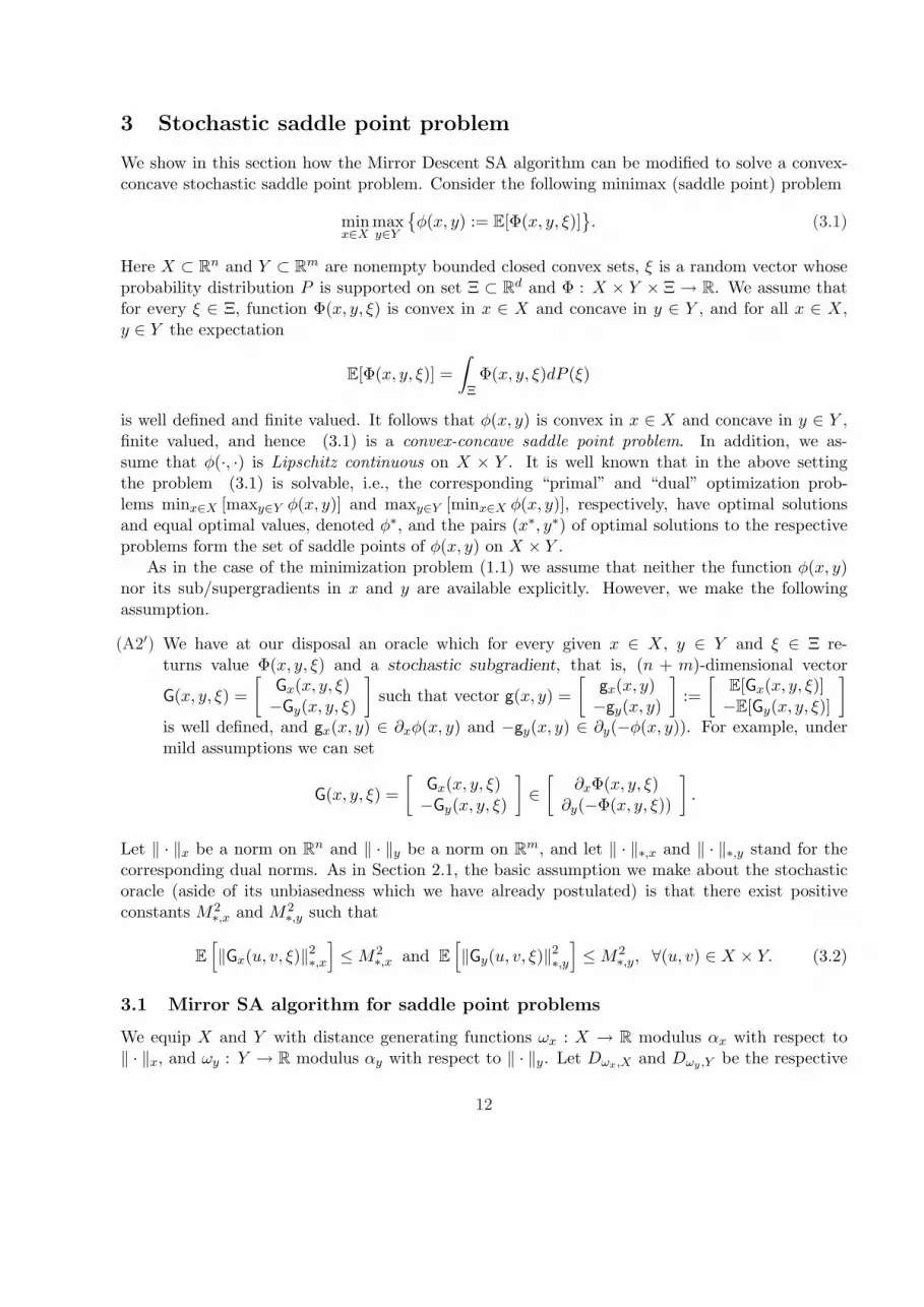
3 Stochastic saddle point problem

We show in this section how the Mirror Descent SA algorithm can be modified to solve a convex-concave stochastic saddle point problem. Consider the following minimax (saddle point) problem

minx∈X

maxy∈Y

φ(x, y) := E[Φ(x, y, ξ)]

. (3.1)

Here X ⊂ Rn and Y ⊂ Rm are nonempty bounded closed convex sets, ξ is a random vector whoseprobability distribution P is supported on set Ξ ⊂ Rd and Φ : X × Y × Ξ → R. We assume thatfor every ξ ∈ Ξ, function Φ(x, y, ξ) is convex in x ∈ X and concave in y ∈ Y , and for all x ∈ X,y ∈ Y the expectation

E[Φ(x, y, ξ)] =∫

ΞΦ(x, y, ξ)dP (ξ)

is well defined and finite valued. It follows that φ(x, y) is convex in x ∈ X and concave in y ∈ Y ,finite valued, and hence (3.1) is a convex-concave saddle point problem. In addition, we as-sume that φ(·, ·) is Lipschitz continuous on X × Y . It is well known that in the above settingthe problem (3.1) is solvable, i.e., the corresponding “primal” and “dual” optimization prob-lems minx∈X [maxy∈Y φ(x, y)] and maxy∈Y [minx∈X φ(x, y)], respectively, have optimal solutionsand equal optimal values, denoted φ∗, and the pairs (x∗, y∗) of optimal solutions to the respectiveproblems form the set of saddle points of φ(x, y) on X × Y .

As in the case of the minimization problem (1.1) we assume that neither the function φ(x, y)nor its sub/supergradients in x and y are available explicitly. However, we make the followingassumption.

(A2′) We have at our disposal an oracle which for every given x ∈ X, y ∈ Y and ξ ∈ Ξ re-turns value Φ(x, y, ξ) and a stochastic subgradient, that is, (n + m)-dimensional vector

G(x, y, ξ) =[

Gx(x, y, ξ)−Gy(x, y, ξ)

]such that vector g(x, y) =

[gx(x, y)−gy(x, y)

]:=

[E[Gx(x, y, ξ)]−E[Gy(x, y, ξ)]

]

is well defined, and gx(x, y) ∈ ∂xφ(x, y) and −gy(x, y) ∈ ∂y(−φ(x, y)). For example, undermild assumptions we can set

G(x, y, ξ) =[

Gx(x, y, ξ)−Gy(x, y, ξ)

]∈

[∂xΦ(x, y, ξ)

∂y(−Φ(x, y, ξ))

].

Let ‖ · ‖x be a norm on Rn and ‖ · ‖y be a norm on Rm, and let ‖ · ‖∗,x and ‖ · ‖∗,y stand for thecorresponding dual norms. As in Section 2.1, the basic assumption we make about the stochasticoracle (aside of its unbiasedness which we have already postulated) is that there exist positiveconstants M2∗,x and M2∗,y such that

E[‖Gx(u, v, ξ)‖2

∗,x]≤ M2

∗,x and E[‖Gy(u, v, ξ)‖2

∗,y]≤ M2

∗,y, ∀(u, v) ∈ X × Y. (3.2)

3.1 Mirror SA algorithm for saddle point problems

We equip X and Y with distance generating functions ωx : X → R modulus αx with respect to‖ · ‖x, and ωy : Y → R modulus αy with respect to ‖ · ‖y. Let Dωx,X and Dωy,Y be the respective

12

constants (see definition (2.37)). We equip Rn × Rm with the norm

‖(x, y)‖ :=√

αx

2D2ωx,X

‖x‖2x +

αy

2D2ωy,Y

‖y‖2y, (3.3)

so that the dual norm is

‖(ζ, η)‖∗ =

√2D2

ωx,X

αx‖ζ‖2∗,x +

2D2ωy ,Y

αy‖η‖2∗,y. (3.4)

It follows by (3.2) that

E[‖G(x, y, ξ)‖2

∗] ≤ 2D2

ωx,X

αxM2∗,x +

2D2ωy,Y

αyM2∗,y =: M2

∗ . (3.5)

We use notation z = (x, y) and equip Z := X ×Y with the distance generating function as follows:

ω(z) :=ωx(x)

2D2ωx,X

+ωy(y)

2D2ωy ,Y

.

It is immediately seen that ω indeed is a distance generating function for Z modulus α = 1 withrespect to the norm ‖·‖, and that Zo = Xo×Y o and Dω,Z = 1. In what follows, V (z, u) : Zo×Z → Rand Pz(ζ) : Rn+m → Zo are the prox-function and prox-mapping associated with ω and Z, see(2.25), (2.26).

We are ready now to present the Mirror SA algorithm for saddle point problems. This is theiterative procedure

zj+1 := Pzj (G(zj , ξj)), (3.6)

where the initial point z1 ∈ Z is chosen to be the minimizer of ω(z) on Z. As before (cf., (2.39)),we define the approximate solution zj of (3.1) after j iterations as

zj = (xj , yj) :=

(j∑

t=1

γt

)−1 j∑

t=1

γtzt. (3.7)

We refer to the procedure (3.6), (3.7) as Saddle Point Mirror SA algorithm.Let us analyze the convergence properties of the algorithm. We measure quality of an approxi-

mate solution z = (x, y) by the error

εφ(z) :=[maxy∈Y

φ(x, y)− φ∗

]+

[φ∗ −min

x∈Xφ(x, y)

]= max

y∈Yφ(x, y)−min

x∈Xφ(x, y).

By convexity of φ(·, y) we have

φ(xt, yt)− φ(x, yt) ≤ gx(xt, yt)T (xt − x), ∀x ∈ X,

and by concavity of φ(x, ·),φ(xt, y)− φ(xt, yt) ≤ gy(xt, yt)T (y − yt), ∀y ∈ Y,

13

so that for all z = (x, y) ∈ Z,

φ(xt, y)− φ(x, yt) ≤ gx(xt, yt)T (xt − x) + gy(xt, yt)T (y − yt) = g(zt)T (zt − z).

Using once again the convexity-concavity of φ we write

εφ(zj) = maxy∈Y

φ(xj , y)−minx∈X

φ(x, yj)

≤[

j∑

t=1

γt

]−1 [maxy∈Y

j∑

t=1

γtφ(xt, y)−minx∈X

j∑

t=1

γtφ(x, yt)

]

≤(

j∑

t=1

γt

)−1

maxz∈Z

j∑

t=1

γtg(zt)T (zt − z). (3.8)

To bound the right-hand side of (3.8) we use the following result.

Lemma 3.1 In the above setting, for any j ≥ 1 the following inequality holds

E

[maxz∈Z

j∑

t=1

γtg(zt)T (zt − z)

]≤ 2 +

52M2∗

j∑

t=1

γ2t . (3.9)

Proof of this lemma is given in the Appendix.Now to get an error bound for the solution zj it suffices to substitute inequality (3.9) into (3.8)

to obtain

E[εφ(zj)] ≤(

j∑

t=1

γt

)−1 [2 +

52M2∗

j∑

t=1

γ2t

].

Let us use the constant stepsize strategy

γt =2

M∗√

5N, t = 1, ..., N. (3.10)

Then εφ(zN ) ≤ 2M∗√

5N , and hence (see definition (3.5) of M∗) we obtain

εφ(zN ) ≤ 2

√√√√10[αyD2

ωx,XM2∗,x + αxD2ωy,Y M2∗,y

]

αxαyN. (3.11)

Same as in the minimization case, we can pass from constant stepsizes on a fixed “time horizon”to decreasing stepsize policy (2.47) with θ = 1/M∗ and from averaging of all iterates to the “slidingaveraging”

zj =

j∑

t=j−bj/`cγt

−1

j∑

t=j−bj/`cγtzt,

arriving at the efficiency estimate

ε(zj) ≤ O(1)`Dω,ZM∗√

j, (3.12)

14

where the quantity Dω,Z =[2 supz∈Zo,w∈Z V (z, w)

]1/2 is assumed to be finite.

We give below a bound on the probabilities of large deviations of the error εφ(zN ).

Proposition 3.1 Suppose that conditions of the bound (3.11) are verified and, further, it holds forall (u, v) ∈ Z that

E[exp

‖Gx(u, v, ξ)‖2

∗,x /M2∗,x

]≤ exp1, E

[exp

‖Gy(x, y, ξ)‖2

∗,y /M2∗,y

]≤ exp1. (3.13)

Then for the stepsizes (3.10) one has for any Ω ≥ 1 that

Prob

εφ(zN ) >

(8 + 2Ω)√

5M∗√N

≤ 2 exp−Ω. (3.14)

Proof of this proposition is given in the Appendix.

3.2 Application to minimax stochastic problems

Consider the following minimax stochastic problem

minx∈X

max1≤i≤m

fi(x) := E[Fi(x, ξ)]

, (3.15)

where X ⊂ Rn is a nonempty bounded closed convex set, ξ is a random vector whose probabilitydistribution P is supported on set Ξ ⊂ Rd and Fi : X × Ξ → R, i = 1, ..., m. We assume thatfor a.e. ξ the functions Fi(·, ξ) are convex and for every x ∈ Rn, Fi(x, ·) are integrable, i.e., theexpectations

E[Fi(x, ξ)] =∫

ΞFi(x, ξ)dP (ξ), i = 1, ...,m, (3.16)

are well defined and finite valued. To find a solution to the minimax problem (3.15) is exactly thesame as to solve the saddle point problem

minx∈X

maxy∈Y

φ(x, y) :=

m∑

i=1

yifi(x)

, (3.17)

with Y := y ∈ Rm : y ≥ 0,∑m

i=1 yi = 1.Similarly to assumptions (A1) and (A2), assume that we cannot compute fi(x) (and thus φ(x, y))

explicitly, but are able to generate independent realizations ξ1, ξ2, ... distributed according to P ,and for given x ∈ X and ξ ∈ Ξ we can compute Fi(x, ξ) and its stochastic subgradient Gi(x, ξ), i.e.,such that gi(x) = E[Gi(x, ξ)] is well defined and gi(x) ∈ ∂fi(x), x ∈ X, i = 1, ..., m. In other wordswe have a stochastic oracle for the problem (3.17) such that assumption (A2′) holds, with

G(x, y, ξ) :=[ ∑m

i=1 yiGi(x, ξ)(− F1(x, ξ), ...,−Fm(x, ξ))

], (3.18)

and

g(x, y) := E[G(x, y, ξ)] =[ ∑m

i=1 yigi(x)(−f1(x), ...,−fm(x))

]∈

[∂xφ(x, y)

−∂yφ(x, y)

]. (3.19)

15

Suppose that the set X is equipped with norm ‖ · ‖x, whose dual norm is ‖ · ‖∗,x, and a distance

generating function ω modulus αx with respect to ‖ · ‖x, and let R2x :=

D2ωx,X

αx. We equip the set Y

with norm ‖ · ‖y := ‖ · ‖1, so that ‖ · ‖∗,y = ‖ · ‖∞, and with the distance generating function

ωy(y) :=m∑

i=1

yi ln yi,

and set R2y :=

D2ωy,Y

αy= ln m. Next, following (3.3) we set

‖(x, y)‖ :=

√‖x‖2

x

2R2x

+‖y‖2

1

2R2y

,

and hence‖(ζ, η)‖∗ =

√2R2

x‖ζ‖2∗,x + 2R2y‖η‖2∞.

Let us assume uniform bounds:

E[

max1≤i≤m

‖Gi(x, ξ)‖2∗,x

]≤ M2

∗,x, E[

max1≤i≤m

|Fi(x, ξ)|2]≤ M2

∗,y, i = 1, ...,m.

Note that

E[‖G(x, y, ξ)‖2

∗]

= 2R2x E

[∥∥

m∑

i=1

yiGi(x, ξ)∥∥2

∗,x

]+ 2R2

y E[‖F (x, ξ)‖2

∞]

(3.20)

≤ 2R2xM2

∗,x + 2R2yM

2∗,y = 2R2

xM2∗,x + 2M2

∗,y ln m =: M2∗ . (3.21)

Let us now use the Saddle Point Mirror SA algorithm (3.6), (3.7) with the constant stepsizestrategy

γt =2

M∗√

5N, t = 1, 2, ..., N.

When substituting the value of M∗, we obtain from (3.11):

E [εφ(zN )] = E[maxy∈Y

φ(xN , y)−minx∈X

φ(x, yN )]≤ 2M∗

√5N

≤ 2

√10

[R2

xM2∗,x + M2∗,x ln m]

N. (3.22)

Discussion. Looking at the bound (3.22) one can make the following important observation.The error of the Saddle Point Mirror SA algorithm in this case is “almost independent” of thenumber m of constraints (it grows as O(

√lnm) as m increases). The interested reader can easily

verify that if an Euclidean SA algorithm were used in the same setting (i.e., the algorithm tunedto the norm ‖ · ‖y := ‖ · ‖2), the corresponding bound would grow with m much faster (in fact, ourerror bound would be O(

√m) in that case).

Note that properties of the Saddle Point Mirror SA can be used to reduce significantly thearithmetic cost of the algorithm implementation. To this end let us look at the definition (3.18)

16

of the stochastic oracle: in order to obtain a realization G(x, y, ξ) one has to compute m randomsubgradients Gi(x, ξ), i = 1, ..., m, and then the convex combination

∑mi=1 yiGi(x, ξ). Now let η be

an independent of ξ and uniformly distributed in [0, 1] random variable, and let ı(η, y) : [0, 1]×Y →1, ...,m equals to i when

∑i−1s=1 ys < η ≤ ∑i

s=1 ys. That is, random variable ı = ı(η, y) takes values1, ..., m with probabilities y1, ..., ym. Consider random vector

G(x, y, (ξ, η)) :=[

Gı(η,y)(x, ξ)(−F1(x, ξ), ...,−Fm(x, ξ))

]. (3.23)

We refer to G(x, y, (ξ, η)) as a randomized oracle for problem (3.17), the corresponding randomparameter being (ξ, η). By construction we still have E

[G(x, y, (ξ, η))

]= g(x, y), where g is defined

in (3.19), and, moreover, the same bound (3.20) holds for E[‖G(x, y, (ξ, η))‖2∗

]. We conclude

that the accuracy bound (3.22) holds for the error of the Saddle Point Mirror SA algorithm withrandomized oracle. On the other hand, in the latter procedure only one randomized subgradientGı(x, ξ) per iteration is to be computed. This simple idea is further developed in another interestingapplication of the Saddle Point Mirror SA algorithm to bilinear matrix games which we discussnext.

3.3 Application to bilinear matrix games

Consider the standard matrix game problem, that is, problem (3.1) with

φ(x, y) := yT Ax + bT x + cT y,

where A ∈ Rm×n, and X and Y are the standard simplices, i.e.,

X :=x ∈ Rn : x ≥ 0,

∑nj=1 xj = 1

, Y :=

y ∈ Rm : y ≥ 0,

∑mi=1 yi = 1

.

In the case in question it is natural to equip X (respectively, Y ) with the usual ‖ · ‖1-norm on Rn

(respectively, Rm). We choose entropies as the corresponding distance generating functions:

ωx(x) :=n∑

i=1

xi ln xi, ωy(x) :=m∑

i=1

yi ln yi.

As we already have seen, this choice results inD2

ωx,X

αx= lnn and

D2ωy,Y

αy= ln m. According to

(3.3) we set

‖(x, y)‖ :=

√‖x‖2

1

2 ln n+‖y‖2

1

2 lnm,

and thus

‖(ζ, η)‖∗ =√

2‖ζ‖2∞ ln n + 2‖η‖2∞ lnm. (3.24)

In order to compute the estimates Φ(x, y, ξ) of φ(x, y) and G(x, y, ξ) of g(x, y) = (b+AT y,−c−Ax)to be used in the Saddle Point Mirror SA iterations (3.6), we use the randomized oracle

Φ(x, y, ξ) = cT x + bT y + Aı(ξ1,y)ı(ξ2,x),

G(x, y, ξ) =[

c + Aı(ξ1,y)

−b−Aı(ξ2,x)

],

17

where ξ1 and ξ2 are independent uniformly distributed on [0, 1] random variables, j = ı(ξ1, y) andi = ı(ξ2, x) are defined as in (3.23), i.e., j can take values 1, ...,m with probabilities y1, ..., ym and ican take values 1, ..., n with probabilities x1, ..., xn, and Aj , [Ai]T are j-th column and i-th row inA, respectively.

Note that g(x, y) := E[G(x, y, (j, i))

] ∈[

∂xφ(x, y)∂y(−φ(x, y))

]. Besides this,

|G(x, y, ξ)i| ≤ max1≤j≤m

‖Aj + b‖∞, for i = 1, ..., n,

and|G(x, y, ξ)i| ≤ max

1≤j≤n‖Aj + c‖∞, for i = n + 1, ..., n + m.

Hence, by the definition (3.24) of ‖ · ‖∗,E‖G(x, y, ξ)‖2

∗ ≤ M2∗ := 2 lnn max

1≤j≤m‖Aj + b‖2

∞ + 2 lnm max1≤j≤n

‖Aj + c‖2∞.

The bottom line is that inputs of the randomized Mirror Saddle Point SA satisfy the conditions ofvalidity of the bound (3.11) with M∗ as above. Using the constant stepsize strategy with

γt =2

M∗√

5N, t = 1, ..., N,

we obtain from (3.11):

E[εφ(zN )

]= E

[maxy∈Y

φ(xN , y)−minx∈X

φ(x, yN )]≤ 2M∗

√5N

. (3.25)

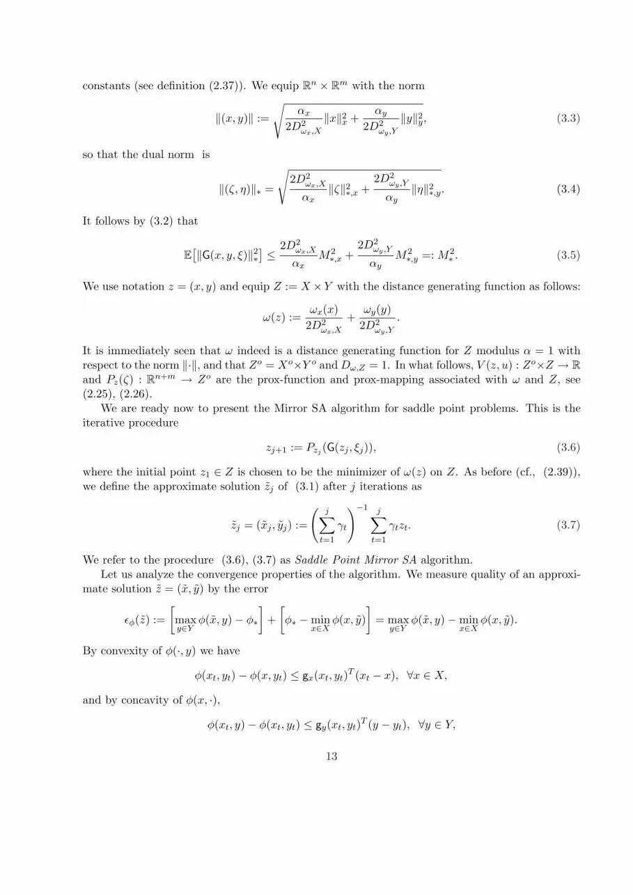
We continue with the counterpart of Proposition 3.1 for the Saddle Point Mirror SA in the settingof bilinear matrix games.

Proposition 3.2 For any Ω ≥ 1 it holds that

Prob

εφ(zN ) > 2M∗

√5N

+4M√

NΩ

≤ exp

−Ω2/2

, (3.26)

whereM := max

1≤j≤m‖Aj + b‖∞ + max

1≤j≤n‖Aj + c‖∞. (3.27)

Discussion. Consider a bilinear matrix game with m = n and b = c = 0. Suppose that we areinterested to solve it within a fixed relative accuracy ρ, that is, to ensure that a (perhaps random)approximate solution zN , we get after N iterations, satisfies the error bound

εφ(zN ) ≤ ρ max1≤i, j≤n

|Aij |

with probability at least 1−δ. According to (3.26), to this end one can use the randomized SaddlePoint Mirror SA algorithm (3.6), (3.7) with

N = O(1)ln n + ln(δ−1)

ρ2. (3.28)

18

The computational cost of building zN with this approach is

C(ρ) = O(1)

[lnn + ln(δ−1)

]Rρ2

arithmetic operations, where R is the arithmetic cost of extracting a column/row from A, giventhe index of this column/row. The total number of rows and columns visited by the algorithmdoes not exceed the sample size N , given in (3.28), so that the total number of entries in A usedin course of the entire computation does not exceed

M = O(1)n(lnn + ln(δ−1))

ρ2.

When ρ is fixed and n is large, this is incomparably less that the total number n2 of entries ofA. Thus, the algorithm in question produces reliable solutions of prescribed quality to large-scalematrix games by inspecting a negligible, as n → ∞, part of randomly selected data. Note thatrandomization here is critical. It is easily seen that a deterministic algorithm which is capable tofind a solution with (deterministic) relative accuracy ρ ≤ 0.1, has to “see” in the worst case at leastO(1)n rows/columns of A.

4 Numerical results

In this section, we report the results of our computational experiments where we compare theperformance of the Robust Mirror Descent SA method and the SAA method applied to threestochastic programming problems, namely: a stochastic utility problem, a stochastic max-flowproblem and network planning problem with random demand. We also present a small simulationstudy of performance of randomized Mirror SA algorithm for bilinear matrix games.

4.1 A stochastic utility problem

Our first experiment was carried out with the utility model

minx∈X

f(x) := E

[φ(∑n

i=1(ai + ξi)xi

)] . (4.1)

Here X = x ∈ Rn :∑n

i=1 xi = 1, x ≥ 0, ξi ∼ N(0, 1) are independent random variables havingstandard normal distribution, ai = i/n are constants, and φ(·) is a piecewise linear convex functiongiven by φ(t) = maxv1 + s1t, ..., vm + smt, where vk and sk are certain constants.

Two variants of the Robust Mirror Descent SA method have been used for solving problem (4.1).The first variant, the Euclidean SA (E-SA), employs the Euclidean distance generating functionω(x) = 1

2‖x‖22, and its iterates coincide with those of the classic SA as discussed in Section 2.3.

The other distance generating function used in the following experiments is the entropy functiondefined in (2.49). The resulting variant of the Robust Mirror Descent SA is referred to as theNon-Euclidean SA (N-SA) method.

These two variants of SA method are compared with the SAA approach in the following way:fixing an i.i.d. sample (of size N) for the random variable ξ, we apply the three afore-mentionedmethods to obtain approximate solutions for problem (4.1), and then the quality of the solutions

19

Table 1: the selection of step-sizes[method: N-SA, N:2,000, K:10,000, instance: L1]

ηpolicy 0.1 1 5 10

variable -7.4733 -7.8865 -7.8789 -7.8547constant -6.9371 -7.8637 -7.9037 -7.8971

yielded by these algorithms is evaluated using another i.i.d. sample of size K >> N . It should benoted that SAA itself is not an algorithm and in our experiments it is coupled with the so-calledNon-Euclidean Restricted Memory Level (NERML) deterministic algorithm (see [2]), for solvingthe sample average problem (1.4).

In our experiment, the function φ(·) in problem (4.1) was set to be a piecewise linear functionwith 10 breakpoints (m = 10) over the interval [0, 1] and four instances (namely: L1, L2, L3 andL4) with different dimensions ranging from n = 500 to 5, 000 were randomly generated. Note thateach of these instances assumes a different function φ(·), i.e., has different values of vk and sk fork = 1, ..., m. All the algorithms were coded in ANSI C and the experiments were conducted on aIntel PIV 1.6GHz machine with Microsoft Windows XP professional.

The first step of our experimentation is to determine the step-sizes γt used by both variantsof SA method. Note that in our situation, either a constant stepsize policy (2.40) or a variablestep-size policy (2.47) can be applied. Observe however that the quantity M∗ appearing in bothstepsize policies is usually unknown and requires an estimation. In our implementation, an estimateof M∗ is obtained by taking the maxima of ‖G(·, ·)‖∗ over a certain number (for example, 100) ofrandom feasible solutions x and realizations of the random variable ξ. To account for the errorinherited by this estimation procedure, the stepsizes are set to ηγt for t = 1, ..., N , where γt aredefined as in (2.40) or (2.47), and η > 0 is a user-defined parameter that can be fine-tuned, forexample, by a trial-and-error procedure.

Some results of our experiments for determining the step-sizes are presented in Table 1. Specifi-cally, Table 1 compares the solution quality obtained by the Non-Euclidean SA method (N = 2,000and K = 10,000) applied for solving the instance L1 (n = 500) with different stepsize polices anddifferent values of η. In this table, column 1 gives the name of the two policies and column 2 throughcolumn 5 report the objective values for η = 0.1, 1, 5 and 10 respectively. The results given in Table1 show that the constant step-size policy with a properly chosen parameter η slightly outperformsthe variable stepsize policy and the same phenomenon has also been observed for the EuclideanSA method. Based on these observations, the constant step-size was chosen for both variants ofSA method. To set the parameter η, we run each variant of SA method in which different valuesof η ∈ 0.1, 1, 5, 10 are applied, and the best selection of η in terms of the solution quality waschosen. More specifically, the parameter η was set to 0.1 and 5, respectively, for the Euclidean SAmethod and Non-Euclidean throughout our computation.

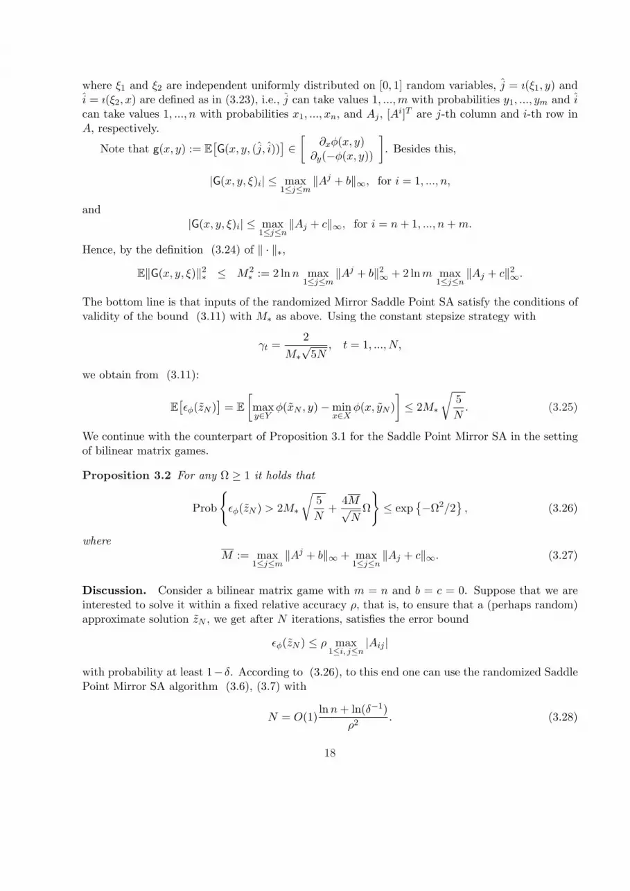
We then run each of the three afore-mentioned methods with various sample-sizes for each testinstance and the computational results are reported in Table 2, where n is the dimension of problem,N denotes the sample-size, ‘OBJ’ and ‘DEV’ represents mean and deviation, respectively, of theobjective values of problem (4.1) as evaluated over a sample of size K = 10, 000 for the solutionsgenerated by the algorithms, ‘TIME’ is the CPU seconds for obtaining the solutions, and ‘ORC’stands for the number of calls to the stochastic oracle.

20

Table 2: SA vs. SAA on the stochastic utility model- L1: n = 500 L2: n = 1000

alg. N obj dev time orc obj dev time orcN-SA 100 -7.7599 0.5615 0.00 200 -5.8340 0.1962 0.00 200

1,000 -7.8781 0.3988 2.00 1,100 -5.9152 0.1663 2.00 1,1002,000 -7.8987 0.3589 2.00 2,100 -5.9243 0.1668 5.00 2,1004,000 -7.9075 0.3716 5.00 4,100 -5.9365 0.1627 12.00 4,100

E-SA 100 -7.6895 0.3702 0.00 200 -5.7988 0.1046 1.00 2001,000 -7.8559 0.3153 2.00 1,100 -5.8919 0.0998 4.00 1,1002,000 -7.8737 0.3101 3.00 2,100 -5.9067 0.1017 7.00 2,1004,000 -7.8948 0.3084 7.00 4,100 -5.9193 0.1060 13.00 4,100

SAA 100 -7.6571 0.9343 7.00 4,000 -5.6346 0.9333 8.00 4,0001,000 -7.8821 0.4015 31.00 40,000 -5.9221 0.2314 68.00 400002,000 -7.9100 0.3545 72.00 80,000 -5.9313 0.2100 128.00 80,0004,000 -7.9087 0.3696 113.00 160,000 -5.9384 0.1944 253.00 160,000

- L3: n = 2000 L4: n = 5000alg. N obj dev time orc obj dev time orcN-SA 100 -7.1419 0.2394 1.00 200 -5.4688 0.2719 3.00 200

1,000 -7.2312 0.1822 6.00 1,100 -5.5716 0.1762 13.00 1,1002,000 -7.2513 0.1691 10.00 2,100 -5.5847 0.1506 25.00 2,1004,000 -7.2595 0.1685 20.00 4,100 -5.5935 0.1498 49.00 4,100

E-SA 100 -7.0165 0.1547 1.00 200 -4.9364 0.1111 4.00 2001,000 -7.2029 0.1301 7.00 1,100 -5.3895 0.1416 20.00 1,1002,000 -7.2306 0.1256 15.00 2,100 -5.4870 0.1238 39.00 2,1004,000 -7.2441 0.1282 29.00 4,100 -5.5354 0.1195 77.00 4,100

SAA 100 -6.9748 0.8685 19.00 4,000 -5.3360 0.7188 44.00 4,0001,000 -7.2393 0.2469 134.00 40,000 -5.5656 0.2181 337.00 40,0002,000 -7.2583 0.2030 261.00 80,000 -5.5878 0.1747 656.00 80,0004,000 -7.2664 0.1838 515.00 160,000 -5.5967 0.1538 1283.00 160,000

In order to evaluate variability of these algorithms, we run each method 100 times and computethe resulting statistics as shown in Table 3. Note that the instance L2 is chosen as a representativeand only two different sample-sizes (N = 1000 and 2000) are applied since this test is more time-consuming. In Table 3, column 1 and column 2 give the instance name and the sample-size usedfor each run of the method. The objective value of the approximate solution yielded by each runof the algorithm was evaluated over K = 104 sample size, and the mean and standard deviationof these objective values over 100 runs are given in columns 3-4, columns 6-7, and columns 9-10,respectively, for N-SA, E-SA and SAA method. The average solution time of these three methodsover 100 runs are also reported in column 5, 8, and 11 respectively.

The experiment demonstrates that the solution quality is improved for all three methods withthe increase of the sample size N . Moreover, for a given sample size, the solution time for N-SA issignificantly smaller than that for SAA, while the solution quality for N-SA is close to that for thelatter one.

21

Table 3: The variability for the stochastic utility problem- N-SA E-SA SAA

obj avg. obj avg. obj avg.inst N mean dev time mean dev time mean dev timeL2 1,000 -5.9159 0.0025 2.63 -5.8925 0.0024 4.99 -5.9219 0.0047 67.31L2 2,000 -5.9258 0.0022 5.03 -5.9063 0.0019 7.09 -5.9328 0.0028 131.25

4.2 Stochastic max-flow problem

In the second experiment, we consider a simple two-stage stochastic linear programming, namely, astochastic max-flow problem. The problem is to investigate the capacity expansion over a stochasticnetwork. Let G = (N,A) be a diagraph with a source node s and a sink node t. Each arc (i, j) ∈ Ahas an existing capacity pij ≥ 0, and a random implementing/operating level ξij . Moreover, thereis a common random degrading factor denoted by θ for all arcs in A. The goal is to determine howmuch capacity to add to the arcs subject to a budget constraint, such that the expected maximumflow from s to t is maximized. Let xij denote the capacity to be added to arc (i, j). The problemcan be formulated as

maxx

f(x) := E[F (x, ξ)]

s.t.∑

(i,j)∈A

cijxij ≤ b, xij ≥ 0, ∀(i, j) ∈ A, (4.2)

where cij is unit cost for the capacity to be added, b is the total available budget, and F (x, ξ)denotes the maximum s − t flow in the network when the capacity of an arc (i, j) is given byθξij(pij + xij). Note that the above is a maximization rather than minimization problem.

For our purpose, we assume that the random variables ξij and θ are independent and uniformlydistributed over (0, 1) and (0.5, 1), respectively. Also let pij = 0 and cij = 1 for all (i, j) ∈ E,and b = 1. We randomly generated 4 network instances (referred to as F1, F2, F3 and F4) usingthe network generator GRIDGEN, which is available on DIMACS challenge. The push-relabelalgorithm (see [5]) was used to solve the second stage max-flow problem.

The three methods, namely: N-SA, E-SA and SAA, and the same stepsize policy as discussed inSubsection 4.1, were applied for solving these stochastic max-flow instances. In the first test, eachalgorithm was run once for each test instance and the computational results are reported in Table4, where m and n denote the number of nodes and arcs in G, respectively, N denotes the numberof samples, ‘OBJ’ and ‘DEV’ represent the mean and standard deviation, respectively, of objectivevalues of problem (4.2) as evaluated over K = 104 sample size at the approximated solutions yieldedby the algorithms, ‘TIME’ is CPU seconds for obtaining the approximated solution, and ‘ORC’stands for the number of calls to the stochastic oracle. Similar to the stochastic utility problem,we investigate the variability of these three methods by running each method for 100 times andcomputing the statistical results as shown in Table 5 whose columns have exactly the same meaningas in Table 3.

This experiment, once more, shows that for a given sample size N , the solution quality for N-SAis close to or even in some cases is better than that for SAA, meanwhile, the solution time of N-SAis much smaller than the latter one.

22

Table 4: SA vs. SAA on the stochastic max-flow model- F1: m = 50, n = 500 F2: m = 100, n = 1000

alg. N obj dev time orc obj dev time orcN-SA 100 0.1140 0.0786 0.00 200 0.0637 0.0302 0.00 200

1000 0.1254 0.0943 1.00 1,100 0.0686 0.0300 3.00 1,1002000 0.1249 0.0947 3.00 2,100 0.0697 0.0289 6.00 2,1004000 0.1246 0.0930 5.00 4,100 0.0698 0.0268 11.00 4,100

E-SA 100 0.0840 0.0362 0.00 200 0.0618 0.0257 1.00 2001000 0.1253 0.0944 3.00 1,100 0.0670 0.0248 6.00 1,1002000 0.1246 0.0947 5.00 2,100 0.0695 0.0263 13.00 2,1004000 0.1247 0.0929 9.00 4,100 0.0696 0.0264 24.00 4,100

SAA 100 0.1212 0.0878 5.00 4,000 0.0653 0.0340 12.00 4,0001000 0.1223 0.0896 35.00 40,000 0.0694 0.0296 84.00 40,0002000 0.1223 0.0895 70.00 80,000 0.0693 0.0274 170.00 80,0004000 0.1221 0.0893 140.00 160,000 0.0693 0.0264 323.00 160,000

- F3: m = 100, n = 2000 F4: m = 250, n = 5000alg. N obj dev time orc obj dev time orcN-SA 100 0.1296 0.0735 1.00 200 0.1278 0.0800 3.00 200

1000 0.1305 0.0709 6.00 1,100 0.1329 0.0808 15.00 1,1002000 0.1318 0.0812 11.00 2,100 0.1338 0.0834 29.00 2,1004000 0.1331 0.0834 21.00 4,100 0.1334 0.0831 56.00 4,100

E-SA 100 0.1277 0.0588 2.00 200 0.1153 0.0603 7.00 2001000 0.1281 0.0565 16.00 1,100 0.1312 0.0659 39.00 1,1002000 0.1287 0.0589 28.00 2,100 0.1312 0.0656 72.00 2,1004000 0.1303 0.0627 53.00 4,100 0.1310 0.0683 127.00 4,100

SAA 100 0.1310 0.0773 20.00 4,000 0.1253 0.0625 60.00 4,0001000 0.1294 0.0588 157.00 40,000 0.1291 0.0667 466.00 40,0002000 0.1304 0.0621 311.00 80,000 0.1284 0.0642 986.00 80,0004000 0.1301 0.0636 636.00 160,000 0.1293 0.0659 1885.00 160,000

4.3 A network planning problem with random demand

In the last experiment, we consider the so-called SSN problem of Sen, Doverspike, and Cosares [15].This problem arises in telecommunications network design where the owner of the network sellsprivate-line services between pairs of nodes in the network, and the demands are treated as randomvariables based on the historical demand patterns. The optimization problem is to decide whereto add capacity to the network to minimize the expected rate of unsatisfied demands. Since thisproblem has been studied by several authors (see, e.g., [7, 15]), it could be interesting to comparethe results. Another purpose of this experiment is to investigate the behavior of the SA methodwhen one variance reduction technique, namely, the Latin Hyperplane Sampling (LHS), is applied.

The problem has been formulated as a two-stage stochastic linear programming as follows:

minx

f(x) := E[Q(x, ξ)]

s.t.∑

j xj = b, xj ≥ 0,(4.3)

where x is the vector of capacities to be added to the arcs of the network, b (the budget) is thetotal amount of capacity to be added, ξ denotes the random demand, and Q(x, ξ) represents the

23

Table 5: The variability for the stochastic max-flow problem- N-SA E-SA SAA

obj avg. obj avg. obj avg.inst N mean dev time mean dev time mean dev timeF2 1,000 0.0691 0.0004 3.11 0.0688 0.0006 4.62 0.0694 0.0003 90.15F2 2,000 0.0694 0.0003 6.07 0.0692 0.0002 6.91 0.0695 0.0003 170.45

number of unserved requests. We have

Q(x, ξ) = mins,f

∑i si

s.t.∑

i

∑r∈R(i) Airfir ≤ x + c,∑

r∈R(i) fir + si = ξi, ∀i,fir ≥ 0, si ≥ 0, ∀i, r ∈ R(i).

(4.4)

Here, R(i) denotes a set of routes that can be used for connections associated with the node-pairi (Note that a static network-flow model is used in the formulation to simplify the problem); ξ isa realization of the random variable ξ; the vectors Air are incidence vectors whose jth componentairj is 1 if the link j belongs to the route r and is 0 otherwise; c is the vector of current capacities;fir is the number of connections associated with pair i using route r ∈ R(i); s is the vector ofunsatisfied demands for each request.

In the data set for SSN, there are total of 89 arcs and 86 point-to-point pairs; that is, thedimension of x is 89 and of ξ is 86. Each component of ξ is an independent random variable witha known discrete distribution. Specifically, there are between three and seven possible values foreach component of ξ, giving a total of approximately 1070 possible complete demand scenarios.

The three methods, namely: N-SA, E-SA and SAA, and the same stepsize policy as discussedin Subsection 4.1, were applied for solving the SSN problem. Moreover, we compare these methodswith or without using the Latin Hyperplane Sampling (LHS) technique. In the first test, eachalgorithm was run once for each test instance and the computational results are reported in Table6, where N denotes the number of samples, ‘OBJ’ and ‘DEV’ represent the mean and standarddeviation, respectively, of objective values of problem (4.3) as evaluated over K = 104 sample sizeat the approximated solutions yielded by the algorithms, ‘TIME’ is CPU seconds for obtaining theapproximated solution, and ‘ORC’ stands for the number of calls to the stochastic oracle. Similarto the stochastic utility problem, we investigate the variability of these three methods by runningeach method for 100 times and computing the statistical results as shown in Table 7. Note thatthese tests for the SSN problem were conducted on a more powerful computer: Intel Xeon 1.86GHzwith Red Hat Enterprize Linux.

This experiment shows that for a given sample size N , the solution quality for N-SA is close tothat for SAA, meanwhile, the solution time of N-SA is much smaller than the latter one. However,for this particular instance, the improvement on the solution quality by using the Latin Hyperplanesampling is not significant, especially when a larger sample-size is applied. This result seems to beconsistent with the observation in [7].

24

Table 6: SA vs. SAA on the SSN problem- Without LHS With LHS

alg. N obj dev time orc obj dev time orcN-SA 100 11.0984 19.2898 1.00 200 10.1024 18.7742 1.00 200

1,000 10.0821 18.3557 6.00 1100 10.0313 18.0926 7.00 11002,000 9.9812 18.0206 12.00 2100 9.9936 17.9069 12.00 21004,000 9.9151 17.9446 23.00 4100 9.9428 17.9934 22.00 4100

E-SA 100 10.9027 19.1640 1.00 200 10.3860 19.1116 1.00 2001,000 10.1268 18.6424 6.00 1100 10.0984 18.3513 6.00 11002,000 10.0304 18.5600 12.00 2100 10.0552 18.4294 12.00 21004,000 9.9662 18.6180 23.00 4100 9.9862 18.4541 23.00 4100

SAA 100 11.8915 19.4606 24.00 4,000 11.0561 20.4907 23.00 40001,000 10.0939 19.3332 215.00 40,000 10.0488 19.4696 216.00 40,0002,000 9.9769 19.0010 431.00 80,000 9.9872 18.9073 426.00 80,0004,000 9.8773 18.9184 849.00 160,000 9.9051 18.3441 853.00 160,000

Table 7: The variability for the SSN problem- N-SA E-SA SAA

obj avg. obj avg. obj avg.N LHS mean dev time mean dev time mean dev time

1,000 no 10.0624 0.1867 6.03 10.1730 0.1826 6.12 10.1460 0.2825 215.061,000 yes 10.0573 0.1830 6.16 10.1237 0.1867 6.14 10.0135 0.2579 216.102,000 no 9.9965 0.2058 11.61 10.0853 0.1887 11.68 9.9943 0.2038 432.932,000 yes 9.9978 0.2579 11.71 10.0486 0.2066 11.74 9.9830 0.1872 436.94

4.4 N-SA vs. E-SA

The data in Tables 3, 4, 6 demonstrate that with the same sample size N , the N-SA somehowoutperforms the E-SA in terms of both the quality of approximate solutions and the running time.The difference, at the first glance, seems slim, and one could think that adjusting the SA algorithmto the “geometry” of the problem in question (in our case, to minimization over a standard simplex)is of minor importance. We, however, do believe that such a conclusion would be wrong. In orderto get a better insight, let us come back to the stochastic utility problem. This test problem has animportant advantage – we can easily compute the value of the objective f(x) at a given candidatesolution x analytically1. Moreover, it is easy to minimize f(x) over the simplex – on a closestinspection, this problem reduces to minimizing an easy-to-compute univariate convex function, sothat we can approximate the true optimal value f∗ to high accuracy by Bisection. Thus, in thecase in question we can compare solutions x generated by various algorithms in terms of their “trueinaccuracy” f(x)− f∗, and this is the rationale behind our “Gaussian setup”. We can now exploitthe just outlined advantage of the stochastic utility problem for comparing properly N-SA andE-SA. In Table 8, we present the true values of the objective f(x∗) at the approximate solutions x∗generated by N-SA and E-SA as applied to the instances L1 and L4 of the stochastic utility problem(cf. Table 3) along with the inaccuracies f(x∗)− f∗ and the Monte Carlo estimates f(x∗) of f(x∗)

1Indeed, (ξ1, ..., ξn) ∼ N(0, In), so that the random variable ξx =∑

i(ai + ξi)xi is normal with easily computablemean and variance, and since φ is piecewise linear, the expectation f(x) = E[φ(ξx)] can be immediately expressedvia the error function.

25

Table 8: N-SA vs. E-SAMethod Problem f(x∗), f(x∗) f(x∗)− f∗ Time

N-SA, N = 2, 000 L2: n = 1000 -5.9232/-5.9326 0.0113 2.00E-SA, N = 2, 000 L2 -5.8796/-5.8864 0.0575 7.00E-SA, N = 10, 000 L2 -5.9059/-5.9058 0.0381 13.00E-SA, N = 20, 000 L2 -5.9151/-5.9158 0.0281 27.00N-SA, N = 2, 000 L4: n = 5000 -5.5855/-5.5867 0.0199 6.00E-SA, N = 2, 000 L4 -5.5467/-5.5469 0.0597 10.00E-SA, N = 10, 000 L4 -5.5810/-5.5812 0.0254 36.00E-SA, N = 20, 000 L4 -5.5901/-5.5902 0.0164 84.00

obtained via 50,000-element samples. We see that the difference in the inaccuracy f(x∗)−f∗ of thesolutions produced by the algorithms is much more significant than it is suggested by the data inTable 3 (where the actual inaccuracy is “obscured” by the estimation error and summation withf∗). Specifically, at the common for both algorithms sample size N = 2, 000, the inaccuracy yieldedby N-SA is 3 – 5 times less than the one for E-SA, and in order to compensate for this difference,one should increase the sample size for E-SA (and hence the running time) by factor 5 – 10. Itshould be added that in light of theoretical complexity analysis carried out in Example 2.1, theoutlined significant difference in performances of N-SA and E-SA is not surprising; the surprisingfact is that E-SA works at all.

4.5 Bilinear matrix game

We consider here a bilinear matrix game

minx∈X

maxy∈Y

yT Ax,

where both feasible sets are the standard simplices in Rn, i.e., Y = X = x ∈ Rn :∑n

i=1 xi = 1, x ≥0. We consider two versions of the randomized Mirror SA algorithm (3.6), (3.7) for the saddlepoint problem: Euclidean Saddle Point SA (E-SA) which uses as ωx and ωy Euclidean distancegenerating function ωx(x) = 1

2‖x‖22. The other version of the method, which is referred to as the

Non-Euclidean Saddle Point SA (N-SA), employs the entropy distance generating function definedin (2.49). To compare the two procedures we compute the corresponding approximate solutionstzN after N iterations and compute the exact values of the error:

ε(zN ) := maxy∈Y

yT AxN −minx∈X

yTNAx, i = 1, 2.

In our experiments we consider symmetric matrices A of two kinds. The matrices of the first family,parameterized by α > 0, have the elements which obey the formula

Aij :=(

i + j − 12n− 1

)α

, 1 ≤ i, j ≤ n.

The second family of matrices, which is also parameterized by α > 0, contains the matrices withgeneric element

Aij :=( |i− j|+ 1

2n− 1

)α

, 1 ≤ i, j ≤ n.

26

Table 9: SA for bilinear matrix gamesE2(2), ε(z1) = 0.500 E2(1), ε(z1) = 0.500 E2(0.5), ε(z1) = 0.390

N-SA ε(zN ) avg. ε(zN ) avg. ε(zN ) avg.N mean dev time mean dev time mean dev time

100 0.0121 3.9 e-4 0.58 0.0127 1.9 e-4 0.69 0.0122 4.3 e-4 0.811,000 0.00228 3.7 e-5 5.8 0.00257 2.2 e-5 7.3 0.00271 4.5 e-5 8.52,000 0.00145 2.1 e-5 11.6 0.00166 1.0 e-5 13.8 0.00179 2.7 e-5 16.4E-SA ε(zN ) avg. ε(zN ) avg. ε(zN ) avg.N mean dev time mean dev time mean dev time

100 0.00952 1.0 e-4 1.27 0.0102 5.1 e-5 1.77 0.00891 1.1 e-4 1.941,000 0.00274 1.3 e-5 11.3 0.00328 7.8 e-6 17.6 0.00309 1.6 e-5 20.92,000 0.00210 7.4 e-6 39.7 0.00256 4.6 e-6 36.7 0.00245 7.8 e-6 39.2

E1(2), ε(z1) = 0.0625 E1(1), ε(z1) = 0.125 E1(0.5), ε(z1) = 0.138N-SA ε(zN ) avg. ε(zN ) avg. ε(zN ) avg.

N mean dev time mean dev time mean dev time100 0.00817 0.0016 0.58 0.0368 0.0068 0.66 0.0529 0.0091 0.78

1,000 0.00130 2.7 e-4 6.2 0.0115 0.0024 6.5 0.0191 0.0033 7.62,000 0.00076 1.6 e-4 11.4 0.00840 0.0014 11.7 0.0136 0.0018 13.8E-SA ε(zN ) avg. ε(zN ) avg. ε(zN ) avg.N mean dev time mean dev time mean dev time

100 0.00768 0.0012 1.75 0.0377 0.0062 2.05 0.0546 0.0064 2.741,000 0.00127 2.2 e-4 17.2 0.0125 0.0022 19.9 0.0207 0.0020 18.42,000 0.00079 1.6 e-4 35.0 0.00885 0.0015 36.3 0.0149 0.0020 36.7

We use the notations E1(α) and E2(α) to refer to the experiences with the matrices of the first andsecond kind with parameter α. We present in Table 9 the results of experiments conducted for thematrices A of size 104 × 104. We have done 100 simulation runs in each experiment, we presentthe average error (column MEAN), standard deviation (column Dav) and the average runningtime (time which is necessary to compute the error of the solution is not taken into account). Forcomparison we also present the error of the initial solution z1 = (x1, y1).

Our basic observation is as follows: both Non-Euclidean SA (N-SA) and Euclidean SA (E-SA)algorithms succeed to reduce the error of solution reasonably fast. The mirror implementationis preferable as it is more efficient in terms of running time. For comparison, it takes Matlabfrom 10 (for the simplest problem) to 35 seconds (for the hardest one) to compute just one answer

g(x, y) =[

AT y−Ax

]of the deterministic oracle.

References

[1] Azuma, K. Weighted sums of certain dependent random variables. Tokuku Math. J., 19, 357-367 (1967).

[2] Ben-Tal, A. and Nemirovski, A., Non-euclidean restricted memory level method for large-scaleconvex optimization, Mathematical Programming, 102, 407-456 (2005).

27

[3] Benveniste, A., Metivier, M., Priouret, P., Algorithmes adaptatifs et approximations stochas-tiques , Masson, (1987). English trans. Adaptive Algorithms and Stochastic Approximations,Springer Verlag (1993).

[4] Chung, K.L., On a stochastic approximation method, Ann. Math. Stat. 25, 463-483 (1954).

[5] Goldberg, A.V. and Tarjan, R.E., A New Approach to the Maximum Flow Problem, Journalof ACM, 35, 921-940 (1988).

[6] Kleywegt, A. J., Shapiro, A. and Homem-de-Mello, T., The sample average approximationmethod for stochastic discrete optimization, SIAM J. Optimization, 12, 479-502 (2001).

[7] Linderoth, J., Shapiro, A. and Wright, S., The empirical behavior of sampling methods forstochastic programming, Annals of Operations Research, 142, 215-241 (2006).

[8] Mak, W.K., Morton, D.P. and Wood, R.K., Monte Carlo bounding techniques for determiningsolution quality in stochastic programs, Operations Research Letters, 24, 47–56 (1999).

[9] Nemirovskii, A., and Yudin, D. ”On Cezari’s convergence of the steepest descent method forapproximating saddle point of convex-concave functions.” (in Russian) - Doklady AkademiiNauk SSSR, v. 239 (1978) No. 5 (English translation: Soviet Math. Dokl. v. 19 (1978) No. 2)

[10] Nemirovski, A., Yudin, D., Problem complexity and method efficiency in optimization, Wiley-Interscience Series in Discrete Mathematics, John Wiley, XV, 1983.

[11] Polyak, B.T., New stochastic approximation type procedures, Automat. i Telemekh., 7 (1990),98-107.

[12] Polyak, B.T. and Juditsky, A.B., Acceleration of stochastic approximation by averaging, SIAMJ. Control and Optimization, 30 (1992), 838-855.

[13] Robbins, H. and Monro, S., A stochastic spproximation method, Annals of Math. Stat., 22(1951), 400-407.

[14] Sacks, J., Asymptotic distribution of stochastic approximation, Ann. Math. Stat., 29, 373-409(1958).

[15] Sen, S., Doverspike, R.D. and Cosares, S., Network Planning with Random Demand, Telecom-munication Systems, 3, 11-30 (1994).

[16] Shapiro, A., Monte Carlo sampling methods, in: Ruszczynski, A. and Shapiro, A., (Eds.),Stochastic Programming, Handbook in OR & MS, Vol. 10, North-Holland Publishing Company,Amsterdam, 2003.

[17] Shapiro, A. and Nemirovski, A., On complexity of stochastic programming problems, in: Con-tinuous Optimization: Current Trends and Applications, pp. 111-144, V. Jeyakumar and A.M.Rubinov (Eds.), Springer, 2005.

[18] Strassen, V., The existence of probability measures with given marginals, Annals of Mathe-matical Statistics, 38, 423–439 (1965).

28

[19] Verweij, B., Ahmed, S., Kleywegt, A.J., Nemhauser, G. and Shapiro, A., The sample aver-age approximation method applied to stochastic routing problems: a computational study,Computational Optimization and Applications, 24, 289–333 (2003).

5 Appendix

Proof of Lemma 2.1. Let x ∈ Xo and v = Px(y); note that v is of the form argmin z∈X [ω(z) +pT z] and thus v ∈ Xo, so that ω is differentiable at v. As ∇vV (x, v) = ∇ω(v) − ∇ω(x), theoptimality conditions for (2.26) imply that

(∇ω(v)−∇ω(x) + y)T (v − u) ≤ 0 ∀u ∈ X. (5.1)

For u ∈ X we therefore have

V (v, u)− V (x, u) = [ω(u)−∇ω(v)T (u− v)− ω(v)]− [ω(u)−∇ω(x)T (u− x)− ω(x)]= (∇ω(v)−∇ω(x) + y)T (v − u) + yT (u− v)

−[ω(v)−∇ω(x)T (v − x)− ω(x)][due to (5.1)] ≤ yT (u− v)− V (x, v).

By Young’s inequality2 we have

yT (x− v) ≤ ‖y‖2∗2α

+α

2‖x− v‖2,

while V (x, v) ≥ α2 ‖x− v‖2, due to the strong convexity of V (x, ·). We get

V (v, u)− V (x, u) ≤ yT (u− v)− V (x, v) = yT (u− x) + yT (x− v)− V (x, v) ≤ yT (u− x) +‖y‖2∗2α

,

as required in (2.28).

Entropy as a distance-generating function on the standard simplex. The only propertywhich is not immediately evident is that the entropy w(x) :=

∑ni=1 xi ln xi is strongly convex,

modulus 1 with respect to ‖ · ‖1-norm, on the standard simplex X :=x ∈ Rn : x ≥ 0,

∑ni=1 xi

.

We are in the situation where Xo = x ∈ X : x > 0, and in order to establish the property inquestion it suffices to verify that hT∇2ω(x)h ≥ ‖h‖2

1 for every x ∈ Xo. Here is the computation:

[∑

i

|hi|]2

=

[∑

i

(x−1/2i |hi|)x1/2

i

]2

≤[∑

i

h2i x−1i

][∑

i

xi

]=

∑

i

h2i x−1i = hT∇2ω(x)h,

where the inequality follows by Cauchy inequality.2For any u, v ∈ Rn we have by the definition of the dual norm that ‖u‖∗‖v‖ ≥ uT v and hence (‖u‖2∗/α+α‖v‖2)/2 ≥

‖u‖∗‖v‖ ≥ uT v.

29

Proof of Lemma 3.1. By (2.28) we have for any u ∈ Z that

γt(zt − u)T G(zt, ξt) ≤ V (zt, u)− V (zt+1, u) +γ2

t

2‖G(zt, ξt)‖2

∗ (5.2)

(recall that we are in the situation of α = 1). This relation implies that for every u ∈ Z one has

γt(zt − u)T g(zt) ≤ V (zt, u)− V (zt+1, u) +γ2

t

2‖G(zt, ξt)‖2

∗ − γt(zt − u)T ∆t, (5.3)

where ∆t := G(zt, ξt)− g(zt). Summing up these inequalities over t = 1, ..., j, we get

j∑

t=1

γt(zt − u)T g(zt) ≤ V (z1, u)− V (zt+1, u) +j∑

t=1

γ2t

2‖G(zt, ξt)‖2

∗ −j∑

t=1

γt(zt − u)T ∆t.

Now we need the following simple lemma.

Lemma 5.1 Let ζ1, ..., ζj be a sequence of elements of Rn+m. Define the sequence vt, t = 1, 2, ...in Zo as follows: v1 ∈ Zo and

vt+1 = Pvt(ζt), 1 ≤ t ≤ j.

Then for any u ∈ Z the following holds

j∑

t=1

ζTt (vt − u) ≤ V (v1, u) + 1

2

j∑

t=1

‖ζt‖2∗. (5.4)

Proof. Using the bound (2.28) of Lemma 2.1 with y = ζt and x = vt (so that vt+1 = Pvt(ζt)) andrecalling that we are in the situation of α = 1, we obtain for any u ∈ Z:

V (vt+1, u) ≤ V (vt, u) + ζTt (u− vt) +

‖ζt‖2∗2

.

Summing up from t = 1 to t = j we conclude that

V (vj+1, u) ≤ V (v1, u) +j∑

t=1

ζTt (u− vt) +

j∑

t=1

‖ζt‖2∗2

,

which implies (5.4) due to V (v, u) ≥ 0 for any v ∈ Zo, u ∈ Z.

Applying Lemma 5.1 with v1 = z1, ζt = −γt∆t:

∀u ∈ Z :j∑

t=1

γt∆Tt (u− vt) ≤ V (z1, u) +

12

j∑

t=1

γ2t ‖∆t‖2

∗. (5.5)

Observe that

E‖∆t‖2∗ ≤ 4E‖G(zt, ξt)‖2

∗ ≤ 4

(2D2

ωx,X

αxM2∗,x +

2D2ωy ,Y

αyM2∗,y

)= 4M2

∗ ,

30

so that when taking the expectation of both sides of (5.5) we get

E supu∈Z

(j∑

t=1

γt∆Tt (u− vt)

)≤ 1 + 2M2

∗j∑

t=1

γ2t (5.6)

(recall that V (z1, ·) is bounded by 1 on Z). Now we proceed exactly as in Section 2.2: we sum up(5.3) from t = 1 to j to obtain

j∑

t=1

γt(zt − u)T g(zt) ≤ V (z1, u) +j∑

t=1

γ2t

2‖G(zt, ξt)‖2

∗ −j∑

t=1

γt(zt − u)T ∆t

= V (z1, u) +j∑

t=1

γ2t

2‖G(zt, ξt)‖2

∗ −j∑

t=1

γt(zt − vt)T ∆t +j∑

t=1

γt(u− vt)T ∆t. (5.7)

When taking into account that zt and vt are deterministic functions of ξ[t−1] = (ξ1, ..., ξt−1) and thatthe conditional expectation of ∆t, ξ[t−1] being given, vanishes, we conclude that E[(zt−vt)T ∆t] = 0.We take now suprema in u ∈ Z and then expectations on both sides of (5.7):

E

[supu∈Z

j∑

t=1

γt(zt − u)T g(zt)

]≤ sup

u∈ZV (z1, u) +

j∑

t=1

γ2t

2E‖G(zt, ξt)‖2

∗ + supu∈Z

j∑

t=1

γt(u− vt)T ∆t

[by (5.6)] ≤ 1 +M2∗2

j∑

t=1

γ2t +

[1 + 2M2

∗j∑

t=1

γ2t

]= 2 +

52M2∗

j∑

t=1

γ2t .

and we arrive at (3.9).

Proof of Propositions 2.1 and 3.1. We provide here the proof of Proposition 3.1 only. Theproof of Proposition 2.1 follows the same lines and can be easily reconstructed using the bound(2.34) instead of the relations (5.5) and (5.7) in the proof below.

First of all, with M∗ given by (3.5) one has

∀(z ∈ Z) : E[exp‖G(z, ξ)‖2

∗/M2∗

] ≤ exp1. (5.8)

Indeed, setting px =2D2

ωx,XM2∗,x

αxM2∗, py =

2D2ωy,Y M2

∗,y

αyM2∗we have px + py = 1, whence, invoking (3.4),

E[exp‖G(z, ξ)‖2∗/M2

∗]

= E[exppx‖Gx(z, ξ)‖2∗,x/M2

∗,x + py‖Gy(z, ξ)‖2∗,y/M2∗,y

],

and (5.8) follows from (3.13) by the Holder inequality.

Setting ΓN =∑N

t=1 γt and using the notation from the proof of Lemma 3.1, relations (3.8),(5.5), (5.7) combined with the fact that V (z1, u) ≤ 1 for u ∈ Z, imply that

ΓN εφ(zN ) ≤ 2 +N∑

t=1

γ2t

2[‖G(zt, ξt)‖2

∗ + ‖∆t‖2∗]

︸ ︷︷ ︸αN

+N∑

t=1

γt(vt − zt)T ∆t

︸ ︷︷ ︸βN

. (5.9)

Now, from (5.8) it follows straightforwardly that

E[exp‖∆t‖2∗/(2M∗)2] ≤ exp1, E[exp‖G(zt, ξt)‖2

∗/M2∗ ] ≤ exp1, (5.10)

31

which in turn implies that

E[expαN/σα] ≤ exp1, σα =52M2∗

N∑

t=1

γ2t , (5.11)

and therefore, by Markov inequality,

∀(Ω > 0) : ProbαN ≥ (1 + Ω)σα ≤ exp−Ω. (5.12)

Indeed, we have by (5.8)

‖g(zt)‖∗ = ‖E[G(zt, ξt)|ξ[t−1]]‖∗ ≤√E(‖G(zt, ξt)‖2∗|ξ[t−1]) ≤ M∗,

and‖∆t‖2∗ = ‖G(zt, ξt)− g(zt)‖2∗ ≤ (‖G(zt, ξt)‖∗ + ‖g(zt)‖∗)2 ≤ 2‖G(zt, ξt)‖2∗ + 2M2

∗ ,

what implies that

αN ≤N∑

t=1

γ2t

2

[3‖G(zt, ξt)‖2∗ + 2M2

∗].

Further, by the Holder inequality we have from (5.8):

E

[exp

γ2

t

[32‖G(zt, ξt)‖2∗ + M2

∗]

52γ2

t M2∗

]≤ exp(1).

Observe that if r1, ..., ri are nonnegative random variables such that E[exprt/σt] ≤ exp1 for some deterministicσt > 0, then, by convexity of the exponent, w(s) = exps,

E

[exp

∑t≤i rt∑t≤i σt

]≤ E

∑

t≤i

σt∑τ≤i στ

exprt/σt ≤ exp1. (5.13)

Now applying (5.13) with rt = γ2t

[32‖G(zt, ξt)‖2∗ + M2

∗]

and σt = 52γ2

t M2∗ we obtain (5.11).

Now let ζt = γt(vt − zt)T ∆t. Observing that vt, zt are deterministic functions of ξ[t−1], whileE[∆t|ξ[t−1]] = 0, we see that the sequence ζtN

t=1 of random real variables forms a martingale-difference. Besides this, by strong convexity of ω with modulus 1 w.r.t. ‖ · ‖ and due to Dω,Z ≤ 1we have

u ∈ Z ⇒ 1 ≥ V (z1, u) ≥ 12‖u− z1‖2,

whence the ‖ · ‖-diameter of Z does not exceed 2√

2, so that |ζt| ≤ 2√

2γt‖∆t‖∗, and therefore

E[exp|ζt|2/(32γ2t M2

∗ )|ξ[t−1]] ≤ exp1by (5.10). Applying Cramer’s deviation bound, we arrive at

∀Ω > 0 : Prob

βN > 4ΩM∗√∑N

t=1 γ2t

≤ exp−Ω2/4. (5.14)

Indeed, for 0 ≤ γ, setting σt = 4√

2γtM∗ and taking into account that ζt is a deterministic function of ξ[t] withE[ζt|ξ[t−1]] = 0 and E[expζ2

t /σ2t |ξ[t−1]] ≤ exp1, we have

0 < γσt ≤ 1 ⇒ (as ex ≤ x + ex2)

E[expγζt|ξ[t−1]] ≤ E[expγ2ζ2t |ξ[t−1]] ≤ E[(expζ2

t /σ2t )γ2σ2

t |ξ[t−1]] ≤ expγ2σ2t ;

γσt > 1 ⇒E[expγζt|ξ[t−1]] ≤ E[exp[ 12γ2σ2

t + 12ζ2

t /σ2t |ξ[t−1]] ≤ exp 1

2γ2σ2t + 1

2 ≤ expγ2σ2t

32

that is, in both cases E[expγζt|ξ[t−1]] ≤ expγ2σ2t . Therefore

E[expγβi] = E[expγβi−1E[expγζi|ξ[i−1]]

] ≤ expγ2σ2i E[expγβi−1],

whence

E[expγβN] ≤ expγ2N∑

t=1

σ2t ,

and thus by Markov inequality for every Ω > 0 it holds

Prob

βN > Ω

√√√√N∑

t=1

σ2t

≤ exp

γ2

N∑t=1

σ2t

exp

−γΩ

√√√√N∑

t=1

σ2t

.

When choosing γ = 12Ω

(∑Nt=1 σ2

t

)−1/2

we arrive at (5.14).

Combining (5.9), (5.10) and (5.14), we get for any positive Ω and Θ:

Prob

ΓN εφ(zt) > 2 +

52(1 + Ω)M2

∗N∑

t=1

γ2t + 4

√2ΘM∗

√√√√N∑

t=1

γ2t

≤ exp−Ω+ exp−Θ2/4.

When setting Θ = 2√

Ω and substituting (3.10) we obtain (3.14).

Proof of Proposition 3.2 As in the proof of Proposition 3.1, when setting ΓN =∑N

t=1 γt andusing the relations (3.8), (5.5), (5.7), combined with the fact that ‖G(z, ξy)‖∗ ≤ M∗, we obtain

ΓN εφ(zN ) ≤ 2 +N∑

t=1

γ2t

2[‖G(zt, ξt)‖2

∗ + ‖∆t‖2∗]+

N∑

t=1

γt(vt − zt)T ∆t

≤ 2 +52M2∗

N∑

t=1

γ2t +

N∑

t=1

γt(vt − zt)T ∆t

︸ ︷︷ ︸αN

. (5.15)

Recall that by definition of ∆t, ‖∆t‖∗ = ‖G(zt, ξt)− g(zt)‖∗ ≤ ‖G(zt, ξt)‖+ ‖g(zt)‖∗ ≤ 2M∗.

Note that ζt = γt(vt − zt)T ∆t is a bounded martingale-difference, i.e., E(ζt|ξ[t−1]) = 0, and|ζt| ≤ 4γtM (here M is defined in (3.27)). Then by Azuma-Hoeffding’s inequality [1] for anyΩ ≥ 0:

Prob

αN > 4ΩM

√√√√N∑

t=1

γ2t

≤ e−Ω2/2. (5.16)

Indeed, let us denote vt = (v(x)t , v

(y)t ) and ∆t = (∆

(x)t , ∆

(y)t ). When taking into account that ‖v(x)

t ‖1 ≤ 1, ‖v(y)t ‖1 ≤ 1,

and ‖xt‖1 ≤ 1, ‖yt‖1 ≤ 1, we conclude that

|(vt − zt)T ∆t| ≤ |(v(x)

t − xt)T ∆

(x)t |+ |(v(y)

t − yt)T ∆

(y)t |

≤ 2‖∆(x)t ‖∞ + 2‖∆(y)

t ‖∞ ≤ 4 max1≤j≤m

‖Aj + b‖∞ + 4 max1≤j≤n

‖Aj + c‖∞ = 4M.

We conclude from (5.15) and (5.16) that

Prob

ΓN εφ(zN ) > 2 +

52M2∗

N∑

t=1

γ2t + 4ΩM

√√√√N∑

t=1

γ2t

≤ e−Ω2/2,

33

and the bound (3.26) of the proposition can be easily obtained by substituting the constantstepsizes γt as defined in (3.10).

34