robust design optimization in aeronautics using stochastic analysis and evolutionary algorithms

Robust design optimization in aeronautics usingstochastic analysis and evolutionary algorithmsJ Pons-Prats1*, G Bugeda2,3, F Zarate3, and E Onate3

1International Center for Numerical Methods in Engineering, Castelldefels, Spain2Universitat Politecnica de Catalunya, Barcelona, Spain3International Center for Numerical Methods in Engineering Barcelona, Spain

The manuscript was received on 14 September 2010 and was accepted after revision for publication on 11 May 2011.

DOI: 10.1177/0954410011412131

Abstract: Uncertainties are a daily issue to deal with in aerospace engineering and applica-tions. Robust optimization methods commonly use a random generation of the inputs andtake advantage of multi-point criteria to look for robust solutions accounting with uncertaintydefinition. From the computational point of view, the application to coupled problems, likecomputational fluid dynamics (CFD) or fluid–structure interaction (FSI), can be extremelyexpensive. This study presents a coupling between stochastic analysis techniques and evolu-tionary optimization algorithms for the definition of a stochastic robust optimization proce-dure. At first, a stochastic procedure is proposed to be applied into optimization problems.The proposed method has been applied to both CFD and FSI problems for the reduction ofdrag and flutter, respectively.

Keywords: uncertainties, optimization, robust optimization, airfoil, aero-elastics

1 INTRODUCTION

Optimization problems are a meeting point of several

disciplines. Thanks to the improvements in computer

sciences, which enable fast computations, computa-

tional fluid dynamics (CFD) and aero-elastic prob-

lems have become a daily topic for analysis

engineers. The trend on the design process is now

focussed on dealing with uncertainties, which can

greatly affect the final performance of the system.

Uncertainty is an important concept to be taken

into consideration for simulation and optimization

processes. Accounting with the management of

uncertainties produces better results regarding the

robustness of the design. Uncertainties related to

the quality of the analysis processes, like approxima-

tion of the modelling analytical equations, quality of

the discretization, etc. can be taken into account, but

here the focus will be on the uncertainties related

with the definition of the real problem to be analysed.

These uncertainties are usually related with the input

variables for the analysis, which represents some nat-

ural behaviour, or some manufacturing parameters

and tolerances. Uncertainties can be classified in

two categories, as described by Helton and Davis [1].

The first one is the so-called random uncertainty:

the behaviour of natural systems, with its inherent

variability, is the best example. Thanks to empiric

observation, random uncertainties can be accurately

modelled and represented through the use of prob-

abilistic methods.

The second category is the so-called epistemic

uncertainty, which comes from a lack of knowledge

of the system behaviour. Usually, it is not well repre-

sented nor modelled using classical probabilistic

*Corresponding author: International Center for Numerical

Methods in engineering (CIMNE), c/Esteve Terrades 5, 08860

Castelldefels, Spain.

email: [email protected]

SPECIAL ISSUE PAPER 1131

Proc. IMechE Vol. 225 Part G: J. Aerospace Engineering

approaches and it leads to non-probabilistic methods

based on interval specifications [2].

The aim of this study is to define a new methodol-

ogy to be applied to optimization problems in aero-

dynamics, or coupled problems, enabling the

stochastic definition of the input parameters for a

better representation of uncertainties associated to

input values. This methodology should be efficient,

so it should reduce the number of needed calcula-

tions to a small amount compared with the dimen-

sions of the search space. It should also be robust, and

it should find the optimum value under a complex

topology of the search space. It must be taken into

consideration that engineering problems, and also

those related to aerodynamics, or coupled problems,

require a robust solution to ensure the optimal per-

formance across the larger range of operation condi-

tions as possible.

This article is organized in four sections. After this

section, the second section focuses on the definition

of the used stochastic procedure. The third section is

devoted to the analysis of the integration of the sto-

chastic procedure into optimization methods based

on evolutionary algorithms and presents an illustra-

tive example. Finally, the fourth section points out the

conclusions and planned further work in the devel-

opment of the presented methodology.

2 STOCHASTIC PROCEDURE

Engineering problems face a great number of uncer-

tainties. From lack of information or knowledge of the

analysed phenomena about intrinsic errors during

tests, or numerical simulations, the parameters are

always dealing with uncertainties. At the end, they

can produce a big variability on the results. Not to

take into account the possible variability of the differ-

ent phenomena considered in the analysis can pro-

duce completely wrong conclusions. It is really

important to ensure the best understanding of the

phenomena, but also of the associated uncertainties

and variability.

Stochastic procedures are based on the coupling

between a generator of random values for those

inputs with uncertainties and the analysis tool.

Input variables with uncertainties, like flow boundary

conditions, are defined using a probabilistic density

function (PDF). Gaussian or uniform PDFs are the

most commonly used. Then, a set of random values

are generated for each random input variable follow-

ing the corresponding PDF. Each of the randomly

generated values represents a configuration of the

problem to be analysed. The analyses of all the

defined configurations produce a set of results that,

at the end of the process, are analysed using statistical

tools.

This section presents different examples of sto-

chastic analysis taking into account the variability of

different parameters of the problem, and the corre-

sponding conclusions that can be extracted from the

results.

Next tests are mainly intended to check if the sto-

chastic procedure leads to meaningful results that

can be used in further development of a stochastic

robust design optimization method. Results will also

be evaluated in comparison with real and known

physical behaviour. It will provide a confirmation

and validation of the whole procedure in two ways:

regarding not only the procedure but also the mean-

ing of the results.

In this study, the STAC code has been used for the

generation of all random values. STAC is a stochastic

analysis management tool. Thanks to the develop-

ments by Hurtado and Barbat [3] regarding the

random generation of samples using Monte-Carlo

and Latin Hypercube techniques, STAC tool provides

a very friendly and easy to use user interface with pre-

and post-processing capabilities. Several PDFs, both

continuous and discrete, can be applied to the input

variables.

When different variables with uncertainties are

present, the combination of several random cases is

used to generate comparison information that helps

to identify the most relevant parameters regarding

variability of the output.

A CFD and aero-elastic stochastic analyses are

shown in next sub-sections. The main aim of the

CFD analysis is to analyse the variability of the lift

and drag coefficients when angle of attack (AoA)

and Mach number (M) present uncertainties. The

aero-elastic problem is defined to capture the vari-

ability of aerodynamic and structural values that

can help to understand flutter phenomena, like lift

(Cl) and pressure drag (Cdp) coefficients, as well as

angular spin and vertical deformations of the wing,

when defining uncertainties for M, AoA, x-coordinate

of the elastic axis position, the damping coefficients

of wing, both angular and vertical movements, and

the mass ratio. From an engineering point of view, the

CFD problem can help to determine the best config-

uration regarding drag reduction and lift maximiza-

tion, while the aero-elastic problem helps to analyse

the flutter phenomena, which is of major importance

due to safety reasons.

2.1 Example of a stochastic CFD analysis

In order to illustrate the main characteristics of a sto-

chastic analysis, the analysis of a RAE2822 profile [4]

1132 J Pons-Prats, G Bugeda, F Zarate, and E Onate


using stochastically defined input parameters has

been performed. The considered stochastic input

parameters have been selected from the most rele-

vant CFD values. Different probabilistic definitions

have been applied to each of them in order to analyse

the behaviour of the output data against the variabil-

ity of the input data. The combination of those cases

has enabled to detect the influence on the outputs of

the modification of different input values.

Eight different stochastic analyses have been per-

formed. Table 1 shows the characteristics of each of

them. The first one has only considered the Mach

number (M) as a stochastic input variable, whereas

the angle of attack (AoA) has been considered as fixed.

On the other side, the second case has only consid-

ered the stochastic nature of AoA, whereas M has

been considered as fixed. Cases 3–8 have considered

a stochastic nature for both the AoA and the M, but

using different PDF definitions.

For all eight cases, STAC has defined a probabilistic

set of values, 250 shots defined using Monte-Carlo

method, according with the PDFs of each studied

case. For each pair of input values, the corresponding

CFD analysis has been performed. The CFD code

used in this study has been PUMI, which is a code

developed at CIMNE by Flores and Ortega [5]. It is

based on the use of Euler equations and uses a stabi-

lization technique added to the Galerkin scheme in

order to avoid non-physical solutions. An explicit

multi-stage Runge–Kutta scheme is used as the time

integration scheme in order to get robustness in the

solution. Special care has been taken in the code effi-

ciency in order to deal with complex geometrical

problems avoiding high computational demands,

i.e. minimum memory requirements, fast single-

treaded performance, and a good parallel scaling.

Other CFD tools could also be coupled into the pro-

cedure, like XFOIL [6], which deals with low subsonic

problems, and which has been used for other tests not

included in this article.

Outputs that have been obtained and statisti-

cally analysed are lift and pressure drag coefficients

(Cl and Cdp). The solution has focussed on the mean

and standard deviation (SD) of both coefficients in

order to capture their behaviour and correlation

with the input parameters. The numerical analysis

has been defined through the use of GiD pre-proces-

sor tool [7]. An unstructured mesh has been created

which enables a proper calculation of the lift and drag

values through the definition of finer elements on the

profile lines and a surrounding areas. The conver-

gence has been ensured defining a proper amount

of time steps. The numerical solver has been set up

according to its internal definition; more detail can be

obtained from reference [5].

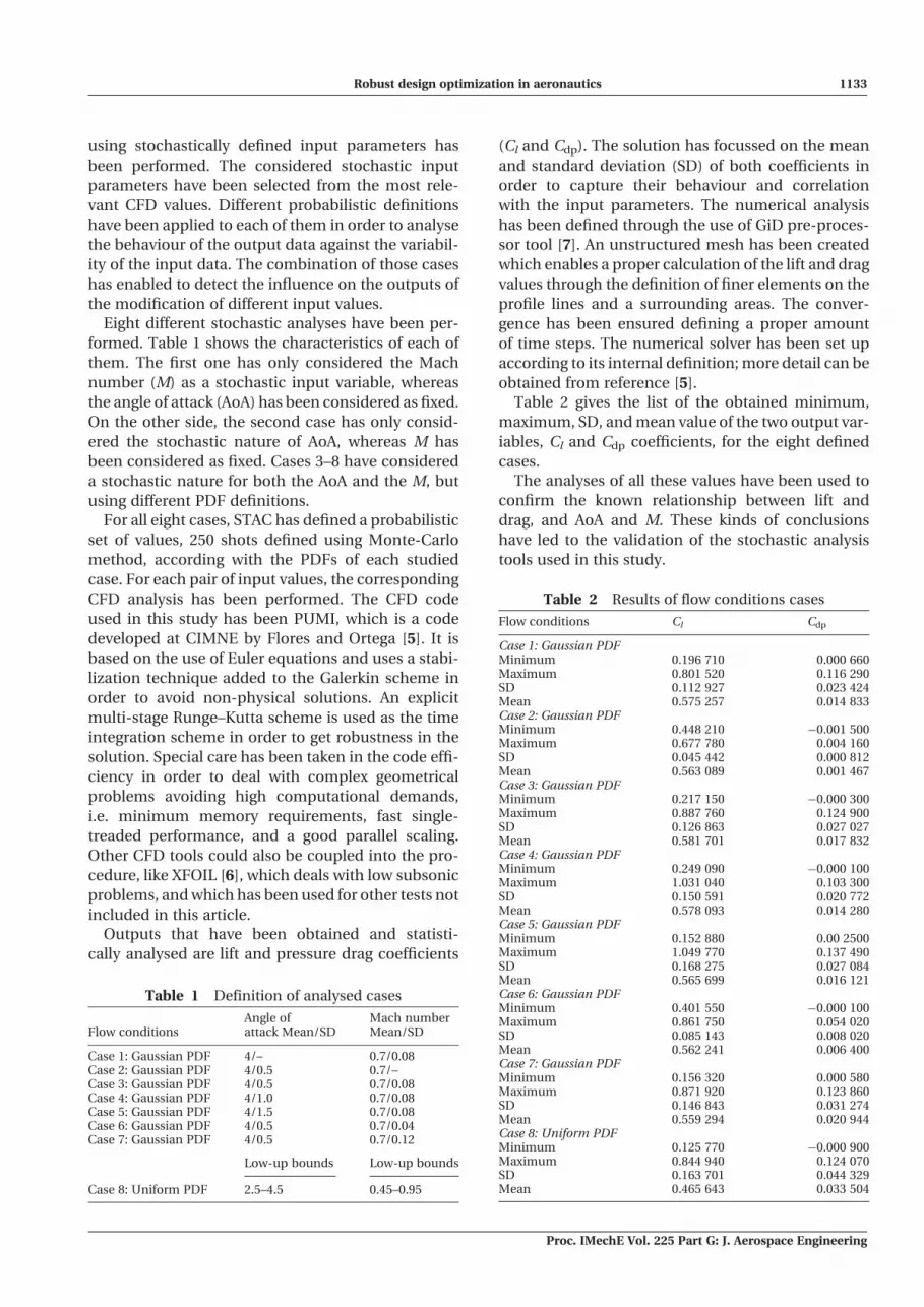
Table 2 gives the list of the obtained minimum,

maximum, SD, and mean value of the two output var-

iables, Cl and Cdp coefficients, for the eight defined

cases.

The analyses of all these values have been used to

confirm the known relationship between lift and

drag, and AoA and M. These kinds of conclusions

have led to the validation of the stochastic analysis

tools used in this study.

Table 2 Results of flow conditions cases

Flow conditions Cl Cdp

Case 1: Gaussian PDFMinimum 0.196 710 0.000 660Maximum 0.801 520 0.116 290SD 0.112 927 0.023 424Mean 0.575 257 0.014 833Case 2: Gaussian PDFMinimum 0.448 210 �0.001 500Maximum 0.677 780 0.004 160SD 0.045 442 0.000 812Mean 0.563 089 0.001 467Case 3: Gaussian PDFMinimum 0.217 150 �0.000 300Maximum 0.887 760 0.124 900SD 0.126 863 0.027 027Mean 0.581 701 0.017 832Case 4: Gaussian PDFMinimum 0.249 090 �0.000 100Maximum 1.031 040 0.103 300SD 0.150 591 0.020 772Mean 0.578 093 0.014 280Case 5: Gaussian PDFMinimum 0.152 880 0.00 2500Maximum 1.049 770 0.137 490SD 0.168 275 0.027 084Mean 0.565 699 0.016 121Case 6: Gaussian PDFMinimum 0.401 550 �0.000 100Maximum 0.861 750 0.054 020SD 0.085 143 0.008 020Mean 0.562 241 0.006 400Case 7: Gaussian PDFMinimum 0.156 320 0.000 580Maximum 0.871 920 0.123 860SD 0.146 843 0.031 274Mean 0.559 294 0.020 944Case 8: Uniform PDFMinimum 0.125 770 �0.000 900Maximum 0.844 940 0.124 070SD 0.163 701 0.044 329Mean 0.465 643 0.033 504

Table 1 Definition of analysed cases

Flow conditionsAngle ofattack Mean/SD

Mach numberMean/SD

Case 1: Gaussian PDF 4/– 0.7/0.08Case 2: Gaussian PDF 4/0.5 0.7/–Case 3: Gaussian PDF 4/0.5 0.7/0.08Case 4: Gaussian PDF 4/1.0 0.7/0.08Case 5: Gaussian PDF 4/1.5 0.7/0.08Case 6: Gaussian PDF 4/0.5 0.7/0.04Case 7: Gaussian PDF 4/0.5 0.7/0.12

Low-up bounds Low-up bounds

Case 8: Uniform PDF 2.5–4.5 0.45–0.95

Robust design optimization in aeronautics 1133


Figures 1 and 2 show, respectively, the mean values

of Cl and Cdp for each case, together with their corre-

sponding �3r range. A result with a wide �3r range

means a big dispersion in the results obtained from

the stochastic analysis and, consequently, a big

dependence with respect to the corresponding sto-

chastic input variable. On the other side, a short

�3r range shows an almost insensitive output with

respect the stochastic input value.

In Figs 1 and 2, the sensitivity of each output value

can be analysed for each defined case. From these

plots, one can immediately identify which one of

the two coefficients is more affected by the variability

of each input.

The comparison between the coefficient of varia-

tion of the input and the output values can also be

used for the measurement of the dispersion in the

obtained results. The coefficient of variation is

defined as the ration between the mean deviation

(r) and the mean value. Lower values of this coeffi-

cient mean lower dispersion in the stochastic vari-

able. On the other side, if both the input and the

output variables have the same coefficient of varia-

tion, it means that the output has exactly the same

variability (dispersion of values) as the input. This

implies that the variability of the input is directly

transferred to the output neither without adding

additional dispersion nor without reducing it.

In Table 3, coefficients of variation for both inputs,

AoA and M, and for both outputs, Cl and Cdp, are tab-

ulated. It is easy to realize that Cdp distribution is

more sensitive to input variability than Cl.

Comparing coefficients of variation obtained when

M or AoA are constant (cases 1 and 2). M produces

bigger effect than AoA, which in both Cl and Cdp dis-

tributions present lower coefficients of variation.

Fig. 1 Mean values and SD ranges for Cl

Fig. 2 Mean values and SD ranges for Cdp



Other cases present a clear difference between coef-

ficient values for Cl and Cdp, while coefficient values

for Cl cases are lower than 1, around 0.25 as mean.

Values for Cdp case are usually higher than 1, around

1.4 as mean. One can realize how far are coefficients

of variation of input values and those obtained for

output values. Coefficient of variation for Cl is pretty

close to the original ones for AoA and M, but Cdp does

not present the same behaviour with a higher coeffi-

cient of variation compared with original ones for

input variables.

In addition to the previous analysis, which uses

coefficient of variation as the main comparing crite-

ria, the following figures provide a graphical analysis

of the variability. They present the behaviour of each

output compared with the input. Figures 3 and 4

show Cl and Cdp versus M. The results of all the anal-

yses performed for all eight stochastic defined cases

are plotted. In the same way, in Fig. 5, Cl is plotted

versus AoA.

In Fig. 3, it can be realized how Cl increases with M,

up to a limit, where shock waves begin to appear. It

follows the typical shape of a polar curve but, in this

case, M is following a Gaussian distribution. Values

are spread around the mean value, with a bigger den-

sity at this value and reducing it as values are far from

Fig. 3 Cl vs M with several distributions of AoA

Fig. 4 Cdp vs M with several distributions of AoA

Table 3 Coefficients of variation

Flow conditions AoA M Cl Cdp

Case 1: Gaussian PDF 0 0.114 0.196 1.579Case 2: Gaussian PDF 0.125 0 0.081 0.553Case 3: Gaussian PDF 0.125 0.114 0.218 1.516Case 4: Gaussian PDF 0.25 0.114 0.260 1.455Case 5: Gaussian PDF 0.375 0.114 0.297 1.680Case 6: Gaussian PDF 0.125 0.057 0.151 1.253Case 7: Gaussian PDF 0.125 0.171 0.263 1.493Case 8: Uniform PDF 0.048 0.060 0.352 1.323



the mean value. In addition, it shows a clear depen-

dency between Cl and the AoA: on one hand, in sub-

sonic regime, M < 0.8, the plot presents a big

variability of Cl while increasing the SD of the AoA,

even considering the effect of doubling and multiply-

ing by 3 this value, or considering a uniform distribu-

tion. On the other hand, in transonic regime, the

variability (dispersion of values) of Cl is lower, and

the plot is a thinner line of points.

In Fig. 4, pressure drag coefficient, Cdp, shows a

quite constant behaviour until transonic values of M

start to increase. The CFD solver used, PUMI, only

provides pressure drag values, because it is based

on Euler equations, without calculating boundary

layer effects. Then, the value provided for Cdp is neg-

ligible up to transonic values, when a shock pressure

appears and Cdp produces significant values.

Figure 4 presents a lower variability of Cdp due to

the variability of the AoA. In opposite to what hap-

pens with Cl, Cdp variability increases in transonic

regime due to the presence of shock waves.

Variability in subsonic regime is mainly due to

numerical errors of the solver more than to Cdp

variance.

In Fig. 5, a straight line portion of the polar line can

be shown because the values of the AoA are low

enough. Figure 5 shows a linear relationship between

the angle of attack and Cl, as it is expected. The var-

iability induced by M is regularly spread along the

curve without breaking the linear relationship

between Cl and AoA.

In all the above figures, the effect of the statistical

distributions applied to M or AoA can be detected. In

Figs 3 and 4, the density of values is bigger around

M ¼ 0.734, which is the mean value of the M. On the

other side, Fig. 5 shows that the variability of the AoA

produces thicker plots that increase their thickness

when increasing the SD of this angle.

Output variability has been analysed for the

RAE2822 airfoil case. The obtained results follow the

expected trends. It can be concluded that the input

variable producing the biggest dispersion of values in

the output parameters is the Mach number.

These analyses provide information of how lift and

drag are affected by variability in the flow conditions;

namely angle of attack and Mach number. Not only

can the well-known relationship between them be

identified on the plots, but also the combined effect

of both variables at the same time, and for several

statistical distributions. Obviously, the best represen-

tation of this relationship can be seen when one of the

variables remains constant, but it can also be identi-

fied when the variability effects appear in the plot,

even if the plot becomes thicker (disperse) due to

the representation of variability.

The stochastic procedure has performed well in a

CFD environment. The use of the coefficient of vari-

ation has been demonstrated as mandatory in order

to compare the dispersion of results with the disper-

sion in the input values. Due to the fact that the values

of lift and drag coefficients have a one order of mag-

nitude difference, their mean and SD values are not

comparable. The simplest way to compare the

obtained Gaussian distributions is to normalize SD

values through the use of the coefficient of variation.

The fact that PUMI CFD solver is based on Euler

equations must be taken into consideration. Hence,

the calculation of drag is an approximation that can

affect the final behaviour of the results. This fact dem-

onstrates the need of knowing the solver and under-

standing its use. If not, it can easily lead to wrong

conclusions.

Fig. 5 Cl vs AoA with several distributions of M



STAC enables the definition of samples using both

Monte-Carlo and Latin Hypercube techniques.

Several tests have been performed and they lead to

the conclusion that both sampling techniques pro-

vide similar results. This conclusion is due to the

fact that the comparison analysis uses mean values

as its main target, and it is well known that Latin

Hypercube improves the covariance convergence

compared to Monte-Carlo method, but not necessar-

ily the mean value.

2.2 Example of a stochastic aero-elastic analysis

In a similar way in the stochastic CFD analysis, an

aero-elastic problem has been defined. The

RAE2822 profile is, again, the baseline geometry. An

uncertainty definition of both flow and structural

input parameters has been used. The flow field

parameters are the Mach number and the angle of

attack. The structural parameters are the damping

coefficients for the vertical and the angular move-

ments, and the x-coordinate of the elastic axis. All of

them have been stochastically defined using a

Gaussian statistical distribution (Table 4). For each

stochastic analysis, a set of 200 samples or shots

have been calculated using the Latin Hypercube sam-

pling technique.

Three different types of analysis have been defined;

the first one is a deterministic analysis that uses the

mean values of all parameters as input values without

considering their stochastic nature. This first analysis

has been defined to be used as a reference (case 0).

The second analysis considers a simultaneous sto-

chastic behaviour of all input parameters (case 1).

The third analysis is, in fact, a set of separate stochas-

tic cases. In each of these cases, only one of the five

input parameters has been considered as stochastic

(cases 2a–e), whereas the rest have been maintained

as in the deterministic case. The total number of cases

is equal to the number of input parameters for which

a stochastic nature has been considered (Table 4).

An in-house aero-elastic code based on particle

finite-element method [8, 9] has been used as the

main analysis tool. It takes advantage of Euler equa-

tions for flow calculations, coupled with a two-

degrees–of-freedom (pitch and plunge) structural

model for the elasticity model. The selected output

is theta, �, which is the angular oscillation of the flut-

ter phenomena.

Figures 6 to 12 show a comparison between the

results obtained for each of the defined analyses

and cases. All the figures show the evolution of the

angular spin angle of the profile through time. The

figures are used to compare the effects when intro-

ducing variability to some of the design variables.

Figure 6 shows the results for the deterministic case.

In this case, the elastic behaviour of the wing pro-

duces a first oscillation, which decreases in 0.45� the

Fig. 6 Time evolution of angular oscillation applying nominal deterministic values

Table 4 Analysed cases for the ensitivity study

AoA M x-EA

Mean SD Mean SD Mean SD

Case 1 2.79 0.279 0.734 0.01 0.4 0.04Case 2a 2.79 0.279 0.734 – 0.4 –Case 2b 2.79 – 0.734 0.01 0.4 –Case 2c 2.79 – 0.734 – 0.4 0.04Case 2d 2.79 – 0.734 – 0.4 –Case 2e 2.79 – 0.734 – 0.4 –

a-dp z-dp

Mean SD Mean SD

Case 1 0.25 0.025 0.25 0.025Case 2a 0.25 – 0.25 –Case 2b 0.25 – 0.25 –Case 2c 0.25 – 0.25 –Case 2d 0.25 0.025 0.25 –Case 2e 0.25 – 0.25 0.025



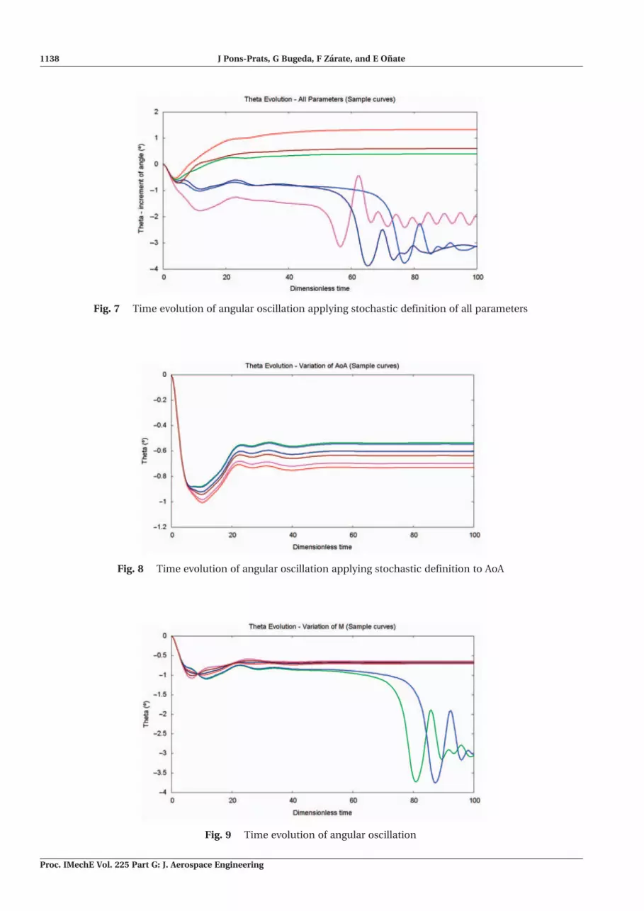
Fig. 7 Time evolution of angular oscillation applying stochastic definition of all parameters

Fig. 8 Time evolution of angular oscillation applying stochastic definition to AoA

Fig. 9 Time evolution of angular oscillation



Fig. 11 Time evolution of angular oscillation applying stochastic definition to z-dp

Fig. 10 Time evolution of angular oscillation applying stochastic definition to x-EA

Fig. 12 Time evolution of angular oscillation applying stochastic definition to a-dp



actual angle of attack, but after that point the flow

stabilizes around the profile and one can consider

that the actual angle of attack remains constant at

0.021� below the nominal value. Figure 7 shows

some samples among the whole set of curves from

the profiles corresponding to the second analysis,

when all the parameters are stochastically defined

in a simultaneous way. It shows a set of plots that

represent all the analysed cases. The first important

point to remark in the new set of results is that this

plot follows a similar pattern to the deterministic

case. The shape and behaviour of the curves in Fig.

7 are similar to those shown in Fig. 6. The second

important remark to be done is the flutter phenome-

non that appears in some cases. After an apparent

trend leading to convergence, some values of the sto-

chastic parameters make the convergence loose and

oscillation grows with time. This flutter phenome-

non, which is an undesired structural effect, is pro-

duced by some of the combinations of values of input

parameters.

In order to detect which of the stochastic parame-

ters induces the flutter, a separate stochastic analysis

for each input variable has been performed. Figure 8

shows some sample curves of the time evolution of

the oscillation when only angle of attack is stochasti-

cally defined. The first oscillation is bigger than that

obtained in the deterministic case. However, the final

convergence value is lower. Anyway, it can be easily

realized that all the analysed cases converge to a

stable value of �.

On the other hand, Fig. 9 shows some of the results

corresponding when the Mach number is stochasti-

cally defined. Now, the lack of convergence of some

samples is easily detected. The time evolution does

not follow the same pattern of other analyses.

Figures 10 to 12 show some of the results corre-

sponding to the stochastic definition of x-EA, z-dp,

and a-dp, respectively. In all the cases, the evolution

of the angular oscillation converges to a stable value.

Figure 11 shows how the vertical damping coefficient

produces a very small variability value, even plotting

only few samples. The stochastic range of values of

this coefficient is small enough to ensure a tight var-

iability range of the oscillation angle. It is easily

understandable that the damping coefficient of the

vertical movement does not directly affect the oscil-

lation angle.

Both damping coefficients present a very narrow

set of curves (Figs 11 and 12). In the first case, the

vertical movement damping has a low effect on the

variability of theta angle (�), as it could be guessed a

priori. What was hard to predict is that angular damp-

ing coefficient has also a tight variability effect. SDs of

both damping coefficients are about 10 per cent of the

mean value, which are similar values to those defined

for other parameters. However, in Table 6, one can

realize their low effects in the variability of the output.

Table 4 gives a brief summary of all analysed cases

and the applied values in each one. Both damping

coefficients have smaller SD, which leads to the

obtained results.

Each of these cases has been used to analyse the

behaviour of additional output parameters, like the

vertical movement of the profile, and the aerody-

namic coefficients of lift, drag, and momentum.

Other output variables, like aerodynamic coeffi-

cients (lift, drag, and momentum), or structural

parameters like vertical deformation of the wing can

be analysed in the same way as it has been done with

�, the angular spin of the profile. The description of

the results has been focused on � in order to simplify

the presentation. However, similar conclusions can

be taken from other output parameters.

Results can be summarized using the coefficient of

variation obtained for all the analyses. In Table 5, the

obtained coefficients are listed.

3 STOCHASTIC CFD OPTIMIZATION

Stochastic CFD is the basis of the defined stochastic

evolutionary optimization procedure. A traditional

evolutionary optimization method is now coupled

with the stochastic tool enabling the stochastic anal-

ysis of each individual within the optimization pro-

cess. In this approach, the classical deterministic

analysis of each individual is substituted by a com-

plete stochastic analysis. The stochastic analysis of a

given individual provides now a cloud of points, and

the fitness function is computed through the mean

value of the output, which is used as the stochastic

fitness. The mean deviation of the output can also

be used as a measure of the robustness of the

Table 5 Coefficients of variation

AoA M x-EA a-dp z-dp

Case 1 0.0927 0.0133 0.0980 0.0960 0.0930Case 2 0.0972 0.0 0.0 0.0 0.0Case 3 0.0 0.0130 0.0 0.0 0.0Case 4 0.0 0.0 0.1084 0.0 0.0Case 5 0.0 0.0 0.0 0.1069 0.0Case 6 0.0 0.0 0.0 0.0 0.0981

Th (min) h/c (max) Cd (min) Cl (min) Cm (min)

Case 1 �0.6952 0.1332 �0.7412 10.2331 �0.6719Case 2 �0.0487 0.0502 �0.2456 0.0602 �0.0376Case 3 �0.6854 0.0120 �0.3253 7.0153 �0.6480Case 4 �0.3362 0.1583 �0.4269 0.1032 �0.3340Case 5 �0.0077 0.0223 �0.0103 0.0094 �0.0061Case 6 �0.0018 0.0026 �0.0633 0.0041 �0.0038



design compared with the variability of the input

value [10, 11].

A traditional CFD stochastic analysis requires a

significant amount of different analysis, and the cor-

responding global computational cost can be very

expensive. This cost can be much more prohibitive

when a stochastic analysis is performed for each of

the different designs obtained during an evolution-

ary optimization process. This justifies the use of a

surrogate model. In this study, the use of artificial

neural networks (ANN) have been selected because

of its capability to deal with a vast type of different

problems [12–15]. It will be integrated in the evolu-

tionary algorithm in parallel with the stochastic

CFD tool.

Based on a proved evolutionary algorithm, like

NSGA-II [16–18], some tests have been performed

in order to show the capabilities of the proposed

methodology. The parameters used to set up the

genetic algorithm are as follows:

(a) population size: 16;

(b) number of generations: 100;

(c) probability of cross-over: 0.99;

(d) probability of mutation: 0.25;

3.1 Deterministic optimization problem

As an illustration example, the results corresponding

to a deterministic multi-objective optimization prob-

lem are first shown. The problem is defined as

Minimize

f1 ¼1

Cl

f2 ¼ Cdp ð1Þ

For a profile defined using Bezier curves, which takes

RAE2822 coordinates as starting point (Fig. 13).

Table 6 shows the constraints applied to the coor-

dinates of the knot points of the Bezier curves used for

the geometrical parametrization of the problem.

In order to compare the solutions obtained by a

deterministic optimization problem and a stochastic

one, the deterministic problem has been first solved

using the following values for the Angle of attack

(AoA) and the Mach number (M)

Angle of attack, AoA ¼ 2.79

Mach number, M ¼ 0.734

The NSGA-II optimizer and ANN surrogate model

have been used. The following parameters have been

defined to set up the algorithm:

(a) population size: 24;

(b) number of generations: 300;

(c) probability of cross-over: 0.95;

(d) probability of mutation: 0.166 667;

Figure 14 shows the obtained population and

Pareto front as the solution of the deterministic opti-

mization problem.

3.2 Integrating stochastic CFD andevolutionary algorithms

The deterministic example has been transformed into

a stochastic one, coupling the stochastic CFD analysis

and the evolutionary algorithm. The problem now

becomes

Minimize

f1 ¼mean1

Cl

� �f2 ¼mean Cdp

� �ð2Þ

Fig. 13 Bezier curves and knot points under EA control



For a profile defined using Bezier curves, which

takes RAE2822 coordinates as starting point, and

same as Fig. 13. The values of Table 6 are still used

for the constraints applied to the coordinates of the

knot points of the Bezier curves used for the geomet-

rical parametrization of the problem.

Table 7 shows the mean values and the SD corre-

sponding to a Gaussian PDF definition for AoA and M.

Mean values are the same as the deterministic values

previously defined. Using Monte-Carlo method, a

single set of 250 samples have been generated to

model the input parameters, and it has been used

for the analysis of all individuals.

The proposed integration of the stochastic analysis

and the evolutionary algorithms is defined as follows.

1. Initial population:

(a) define individuals using geometrical variables;

(b) calculation of the fitness of each individual using

a stochastic analysis; obtain a set of samples to

calculate mean and variance of the fitness.

2. Evolutionary algorithm; main loop:

(a) generate new populations of geometries; selec-

tion, cross-over, and mutation of individuals;

(b) calculation of the fitness of each individual using

the stochastic analysis.

3. End of iterations:

(a) reach of convergence criteria;

(b) reach of maximum time or number of

populations.

The use of a surrogate model is almost mandatory

to reduce the computational cost of the whole pro-

cess. The used ANN has been trained in order to pro-

vide results with less than 1 per cent of error.

In order to ensure ANN feasibility, the Pareto fronts

obtained using the direct analysis tool and the ANN

have been compared. Figure 15(a) shows the differ-

ence between the whole populations obtained in both

cases. Figure 15(b) shows both Pareto fronts and the

difference existing between them. This difference

remains below a 3 per cent which has been consid-

ered as acceptable.

Figure 16 shows a comparison between the deter-

ministic and the stochastic optimization solutions.

Both of them use the same problem definition

except for AoA and M, which are the stochastic vari-

ables. Both use ANN coupled with the optimizer.

One should notice that the shapes of both fronts are

similar, but one front is displaced with respect to the

other one. The stochastic front is clearly forwarded, as

it can be seen in the amplified picture (Fig. 16).

Solutions are different because the stochastic solu-

tion is dealing with the mean of a cloud of evaluations

instead of a single value as the deterministic case is.

Some of these points are affected by the presence of a

shock wave, whereas the deterministic optimization

does not take into account the possibility of hav-

ing this shock wave. From this point of view, stochas-

tic definition produces a more robust solution.

Fig. 14 Deterministic multi-objective optimization

Table 6 Geometrical constraints

Xcoordinate

Ycoordinate

Lowerbound

Upperbound

Knot x1s, y1s 0 0 – –Knot x2s, y2s 0 0.05 – –Knot x3s, y3s 0.25 Variable 0.05 0.085Knot x4s, y4s 0.5 Variable 0.03 0.06Knot x5s, y5s 0.75 Variable 0.01 0.02Knot x6s, y6s 1 0 – –Knot x2l, y2l 0 �0.05 – –Knot x3l, y3l 0.25 Variable �0.06 �0.03Knot x4l, y4l 0.5 Variable �0.035 �0.02Knot x5l, y5l 0.75 Variable �0.015 �0.005



Closest Pareto fronts could be obtained in low sub-

sonic situations, but when work with transonic flow

fields the differences are relevant.

3.3 Applying statistical input behaviour to the

optimization process

In order to simplify the process, the previous stochas-

tic optimization process was defined using the same

set of stochastic values for AoA and M for all the ana-

lysed individuals. This is, in fact, an extreme case of a

multi-point optimization problem with a very high

number of points. Anyway, a multi-point evaluation

of all the individuals is not really representative of the

statistical representation of the input variables and

the next step has been to really consider the genera-

tion of a different set of random input variables for

the analysis of each individual.

It could be considered that using a single random

input definition for the individuals analysed during

the whole optimization process is enough (multi-

point approach). Nevertheless, the statistical defini-

tion of the input variables mainly intends to capture

its random behaviour. A different sampling for each

individual introduces an additional variability that

increases the robustness of the result. Hence,

random samples are now generated for each genera-

tion and individual, it is the so-called variable random

definition.

Figure 17 shows the comparison between the

results obtained with the fixed random definition

and those obtained with a different random defini-

tion for each individual. It can be detected how the

fixed definition also fixes the front of the solution,

clearly defining a linear trend, while the variable def-

inition breaks this regularity. It means that the vari-

able definition affects the evaluation of the fitness

function enabling to capture better results.

If attention is focused only in the shape of the

Pareto fronts, Fig. 18 shows how optimal results for

the fixed definition lead to a poor number of individ-

uals compared with those existing in the Pareto front

Table 7 Stochastic constraints

Mean SD

Angle of attack 2.79 0.279Mach number 0.734 0.05

Fig. 16 Comparison between deterministic and stochastic results

Fig. 15 Solution of the optimization using the analysis tool and ANN: (a) whole population and (b)Pareto front



obtained with the variable definition. The variable

definition leads to a narrower front, producing results

with lower values for f1.

A comparison of two different types of PDF has also

been done. Gaussian and Uniform PDF have been

used and applied to the analysis of each individual

during the optimization loop and the authors have

not detected any relevant difference between them.

4 STOCHASTIC AERO-ELASTIC DESIGN

OPTIMIZATION

4.1 Multi-objective deterministic optimization

A deterministic aero-elastic optimization problem is

now used as a basis of a multi-objective optimization.

The solution of this case has been used as a reference

to be compared with the stochastic optimization pre-

sented in a later subsection. The problem is based on

a RAE2822 profile, which is the baseline design to

solve a problem which is mainly intended to look

for the smoother behaviour of the time evolution of

the angular displacement (�i(t)) and the time evolu-

tion of the drag coefficient (Cdp(t)); smoother in the

sense to reduce the total integral of the curvature, the

second derivative of each time function. The problem

can be formulated as

Minimize

f1 ¼XNt

i¼0

@2�i tð Þ

@t 2

f2 ¼XNt

i¼0

@2Cd i tð Þ

@t 2ð3Þ

Fig. 17 Comparison between random variable and fixed definition and detail on random variabledefinition effects on the front

Fig. 18 Comparison between Pareto fronts for random variable and fixed definition



Being Nt the number of time steps used to calculate

both time-dependant variables; so, the total sum of

the curvature values is obtained and used as fitness

function.

Considering the following bounds for the design

variables:

(a) range of the x-coordinate of the elastic axis; x-EA:

[0.25 0.65];

(b) range of the x-coordinate of the centre of gravity;

x-CG: [0.35 0.60];

(c) range of the mass ratio, �: [30.0 65.0];

(d) range of the damping coefficient for the vertical

deformation, �h: [0.15 0.35];

(e) range of the damping coefficient for the angular

spin, ��: [0.15 0.45].

Finally, angle of attack and Mach number are defined

as constant values at:

(a) angle of attack: 2.79;

(b) Mach number: 0.734.

The optimization method will look for a shape of

�i(t) and Cdp(t) curves that should look similar to that

shown in Fig. 19(b), which is smoother that the one

shown in Fig. 19(a). Optimal results should reach

smooth shapes for both fitness functions.

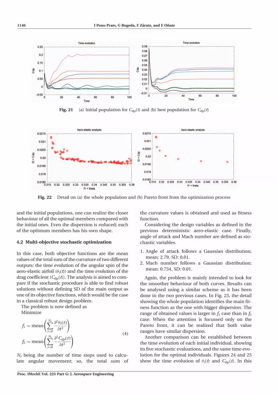
The optimization procedure has defined initial

populations that present a wide variability, as

shown in Figs 20(a) and 21(a). After the optimization

process, the best populations that fulfil the optimiza-

tion criteria are obtained. Figures 20(b) and 21(b)

show a set of curves with a smoother time evolution.

However, not only the smoothness of the curves is

improved, but also the dispersion is reduced. Both

�i(t) and Cdp(t) initial populations present a large var-

iability: a large dispersion between members of the

population, but also a significant difference between

the behaviour of each member. Some of them present

an early converge in time, but others converge after a

larger amount of time steps. On the other hand, the

behaviour of the best populations is much homoge-

neous, as it can be seen in Figs 20(b) and 21(b).

The integration of the aero-elastic problem with a

multi-objective optimizer provides a whole popula-

tion and a Pareto front that follow the usual behav-

iour of this kind of analysis. Initial population has a

poor behaviour, but it continuously improves on each

iteration up to the optimal one as Fig. 22 shows.

The analysed deterministic optimization has been

performed as a validation of the problem definition. It

defines a comparison point with the next analyses to

be done. Comparing the obtained results for the best

Fig. 20 (a) Initial population for �i(t) and (b) best population for �i(t)

Fig. 19 Examples of (a) non-smooth and (b) smoother curves



and the initial populations, one can realize the closer

behaviour of all the optimal members compared with

the initial ones. Even the dispersion is reduced; each

of the optimum members has his own shape.

4.2 Multi-objective stochastic optimization

In this case, both objective functions are the mean

values of the total sum of the curvature of two different

outputs: the time evolution of the angular spin of the

aero-elastic airfoil (�i(t)) and the time evolution of the

drag coefficient (Cdp(t)). The analysis is aimed to com-

pare if the stochastic procedure is able to find robust

solutions without defining SD of the main output as

one of its objective functions, which would be the case

in a classical robust design problem.

The problem is now defined as

Minimize

f1 ¼meanXNt

i¼0

@2�i tð Þ

@t 2

!

f2 ¼meanXNt

i¼0

@2Cdp tð Þ

@t 2

! ð4Þ

Nt being the number of time steps used to calcu-

late angular movement; so, the total sum of

the curvature values is obtained and used as fitness

function.

Considering the design variables as defined in the

previous deterministic aero-elastic case. Finally,

angle of attack and Mach number are defined as sto-

chastic variables.

1. Angle of attack follows a Gaussian distribution;

mean: 2.79, SD: 0.01.

2. Mach number follows a Gaussian distribution;

mean: 0.734, SD: 0.01.

Again, the problem is mainly intended to look for

the smoother behaviour of both curves. Results can

be analysed using a similar scheme as it has been

done in the two previous cases. In Fig. 23, the detail

showing the whole population identifies the main fit-

ness function as the one with bigger dispersion. The

range of obtained values is larger in f1 case than in f2

case. When the attention is focussed only on the

Pareto front, it can be realized that both value

ranges have similar dispersion.

Another comparison can be established between

the time evolution of each initial individual, showing

its five stochastic evaluations, and the same time evo-

lution for the optimal individuals. Figures 24 and 25

show the time evolution of �i(t) and Cdp(t). In this

Fig. 22 Detail on (a) the whole population and (b) Pareto front from the optimization process

Fig. 21 (a) Initial population for Cdp(t) and (b) best population for Cdp(t)



case, even not defining the SD as one of the objective

functions, the final aim is reached. Both �i(t) and

Cdp(t) curves became smoother after the

optimization.

Similar conclusions can be taken from Figs 24 and

25, as it has been done in the previous test case.

Comparing initial and best populations, one can real-

ize how the optimization process tends to look for the

fittest individuals. Compared with the deterministic

results, the dispersion between optimal members is

reduced and the shapes of all the optimal members

tend to be pretty similar.

Fig. 23 Whole population and Pareto front for an aero-elastic stochastic analysis

Fig. 25 (a) Initial and (b) best populations of Cdp(t) evolution

Fig. 24 (a) Initial and (b) best populations of theta, �, evolution



4.3 Multi-objective stochastic robust

design optimization

Same aero-elastic problem is now used as the basis of

the stochastic optimization, based on the same prob-

lem definition already used in previous section.

The problem is now defined as

Minimize

f1 ¼meanXNt

i¼0

@2�i tð Þ

@t 2

!

f2 ¼ �XNt

i¼0

@2�i tð Þ

@t 2

!ð5Þ

Considering the design variables and bounds as

defined in the stochastic case.

The problem is mainly intended to look for the

smoother and robust behaviour of �i(t). Not only the

curvature of each single individual is considered, but

also the behaviour of all the stochastic set of gener-

ated individuals. As it is shown in Fig. 26, significantly

different behaviours could be obtained with slightly

different values of the input values.

The main difference with the deterministic optimi-

zation problem, regarding the definition of the objec-

tive functions, is the fact that now mean and SD are

the selected functions. Regarding the problem defini-

tion, it is clear that the stochastic definition of the

angle and Mach number are the main issue.

Results can be analysed using a similar scheme as it

has been done in the deterministic case. First of all, a

comparison between the initial population and the

optimal one has been done. The plots in Fig. 27,

showing the whole population, and Fig. 28, showing

the physical meaning of these individuals, demon-

strate that the initial individuals are far from the opti-

mal values. Again, the optimization process is able to

tend to the optimum.

The coupling between the stochastic procedure

and the aero-elastic analysis tool does work as

expected, without any problem. In Fig. 27, both the

obtained Pareto front and the whole population are

shown.

Fig. 27 Whole population and Pareto front for an aero-elastic robust analysis

Fig. 26 ((a) and (b)) Examples of the angular movement for a set of stochastic samples



Another comparison can be established between

the time evolution of each initial individual, showing

its five stochastic evaluations, and the same time evo-

lution for the optimal individuals. It is easy to realize

how the initial population is more disperse, in all the

senses. Each individual differs a lot from the other

ones, but also each stochastic evaluation of individ-

uals also presents a bigger variability. On the other

hand, the set of best solutions tends to the same

shape, with lower variability comparing both individ-

uals and stochastic evaluations.

Additional information taken from the plot in

Fig. 28(a) and (b) of the time evolutions of theta �i(t)

is of great interest to validate the final results of this

test case.

Plots in Fig. 28 showing the �i(t) fitness function

shapes clearly identify how the optimization process

behaves. Figure 28(a) shows the initial individuals

and how they do not follow any trend. Figure 28(b),

where only the extreme bounds of the whole set of

obtained curves are shown to simplify, demonstrates

how the optimization procedure leads to soft shapes

(decrease the curvature as defined), and standardizes

the optimized shape to the whole set of optimal

values. In this particular case, where the fitness func-

tion is strongly related to a time-dependant function,

it is also important to confirm that the results adjust

to the desired behaviour, as shown in Fig. 28.

Comparing the results with the deterministic or

stochastic cases, the robust case increases the disper-

sion of the optimal values because of the change on

the objective functions from the deterministic values

to the mean values, and finally the mean and the SD.

A perfect coupling between aero-elastic problem

and stochastic procedure has been performed. The

test case does not use any geometrical information;

it only uses a fixed geometry of a RAE2822 profile.

The evolutionary algorithm controls other kinds of

input parameters like mass ratio or damping coeffi-

cient, which are directly related with this type of

problem.

An additional contribution from this test case is the

use of mean and SD as fitness functions. The robust-

ness of the solution has been reinforced by these two

facts; namely the stochastic definition of the input

variables, which introduces uncertainty concept

into the analysis, but also using the variability as an

objective of the optimization, which ensures the min-

imization of this variability.

5 CONCLUSIONS

A new stochastic optimization procedure has been

defined and analysed. The integration of an evolu-

tionary algorithm and a stochastic analysis tool has

been compared with the first issues of the methodol-

ogy [19, 20]. Several options had been evaluated

related to the stochastic definition of the parameters

and how the uncertainty could be spread across the

numerical analysis.

Three cases have been defined; the classical deter-

ministic solution, which does not define any uncer-

tainty at all, the stochastic one, which defines the

mean values of the functional as fitness function of

the optimization, and the robust one, which defines

both the mean and the SD of the functional as the two

fitness function to deal with during the optimization.

The comparison between the deterministic, the sto-

chastic, and the robust design cases shows how the

solution deals with the uncertainty of the inputs and

how a robust solution is obtained. Comparing the

deterministic solutions with the stochastic and

robust ones, one can realize how the introduction of

the stochastic definition leads to completely new

results. The stochastic and robust cases are able to

reduce the dispersion of the results, while ensuring

the robustness of the solution.

Monte-Carlo techniques, as well as Latin

Hypercube, are computationally expensive. The use

of a surrogate model, like ANN, is mandatory. If it is

well trained and validated, it has been demonstrated

that the approximation error of the surrogate model

Fig. 28 (a) Initial and (b) best populations



remains low enough. The intrinsic variability of the

stochastic method, due to its statistical definition of

the variables, is added to the error of the surrogate

model. It is important, then, to keep both under con-

trol and below a desirable limit in order not to lead to

wrong results. The amount of random samples

defined for the stochastic definition of the input

values is of big importance. A big amount of samples

produces a bigger variability and a better representa-

tion of the random nature of input variables.

Nevertheless, the higher the amount of samples is,

the higher the computational cost is.

In order to obtain a competitive method, further

work in parallelization is urgently required. In addi-

tion, new developments on collocation methods are

under analysis to check if the reduction of evaluations

compensates the multi-point character of these

methods.

The stochastic definition has demonstrated its

robustness in front of the two main cases regarding

the type of objective functions, namely the stochastic

case and the robust case. The first one uses the mean,

while the second one uses both the mean and the SD

values. Both cases have led to optimal solutions that

fulfil the requirements. Due to the fact that the uncer-

tainty propagation method is completely coupled

with the evolutionary algorithm, the definition of

the SD as a fitness function does not require a great

effort. Robustness is ensured by the input stochastic

definition, and SD provides additional information.

FUNDING

This study has been supported by the EC Commission

under FP6 project NODESIM-CFD (contract number

030959) and by the Spanish Ministerio de Ciencia e

Innovacion through project DPI2008-05250.

� Authors 2011

REFERENCES

1 Helton, J. C. and Davis, F. J. Latin Hypercube sam-pling and the propagation of uncertainty in analysesof complex systems. Reliabil. Eng. Syst. Safety, 2003,81(1), 23–69.

2 Durga Rao, K., Kushwaha, H. S., Verma, A. K., andSrividya, A. Quantification of epistemic and aleatoryuncertainties in level-1 probabilistic safety assess-ment studies. Reliabil. Eng. Syst. Safety, 2007, 92(7),947–956.

3 Hurtado, J. E. and Barbat, A. H. Monte-Carlo tech-niques in computational stochastics mechanics. Ed.Springer, Arch. Comput. Methods Eng., 1998, 5(1),3–29.

4 Cook, P. H., McDonald, M. A., and Firmin, M. C. P.Aerofoil RAE 2822 - pressure distributions, andboundary layer and wake measurements, experi-mental data base for computer program assessment,AGARD Report AR 138, 1979.

5 Flores, R. and Ortega, E. PUMI: an explicit 3Dunstructured finite element solver for Euler equa-tions. CIMNE, 2007.

6 Drela, M. XFOIL – an analysis and design system forlow Reynolds number airfoils, low Reynolds numberaerodynamics. Proceedings of the Conference, NotreDame, Indiana, Germany, 5–7 June, 1989, 1–12.

7 GiD. The pre and post-processor tool. CIMNE, avail-able from www.gid.cimne.com (accessed April 2011).

8 Ortega, E., Onate, E., and Idelshon, S. An improvedfinite point method for a three dimensional potentialflows. Comput. Mech., 2007, 40, 949–963.

9 Ortega, E., Onate, E., and Idelshon, S. A finite pointmethod for adaptive three-dimensional compress-ible flow calculations. Int. J. Numer. MethodsFluids, 2009, 60, 937–971.

10 Tang, Z., Periaux, J., Bugeda, G., and Onate, E. Liftmaximization with uncertainties for the optimiza-tion of high-lift devices. Int. J. Numer. MethodsFluids, Early View, 2010, 64, 119–135.

11 Tang, Z., Periaux, J., Bugeda, G., and Onate, E. Liftmaximization with uncertainties for the optimiza-tion of high lift devices using multi-criterion evolu-tionary algorithms, CEC2009. 2009 IEEE Congress onEvolutionary Computation, Tronheim (Norway),18–21 June 2009.

12 Lopez, R. Flood A1. An open source neuralnetworks Cþþ library, User Guide, CIMNE, 2007,[Department RMEE (Resistencia de Materials iEstructures a l’Enginyeria), University UPC(Universitat Politecnica de Catalunya)].

13 Lopez, R. Neural networks for variational problems inengineering. PhD Thesis, Department RMEE(Resistencia de Materials i Estructures a l’Enginyeria),University UPC (Universitat Politecnica de Catalunya),2008.

14 Lopez, R. and Onate, E. A variational formulationfor the multilayer perceptron, Artificial NeuralNetworks, ICANN 2006. Lecture Notes Comput. Sci.,2006, 4132(I), 159–168.

15 Lopez, R., Balsa-Canto, E., and Onate, E. Neuralnetworks for variational problems in engineering.Int. J. Numer. Methods Eng, Early View, 2008,75(11), 1341–1360.

16 Deb, K., Pratap, A., Agarwal, S., and Meyarivan, T.A fast and elitist multi-objective genetic algorithm:NSGA-II. IEEE Trans. Evolut. Comput., 2002, 6(2),182–197.

17 Papadrakakis, M., Lagaros, N. D., andTsompanakis, Y. Structural optimization using evo-lution strategies and neural networks. Comput.Methods Applic. Mech. Eng., 1998, 156, 309–333.

18 Quagliarella, D. and Vicini, A. Designing high-liftairfoils using genetic algorithms. Proceedingsof EUROGEN, Jyvaskyla, Finland, 30 May–3 June1999.



19 Pons-Prats, J., Onate, E., Zarate, F., Bugeda,G., and Hurtado, J. Non-deterministic shapeoptimization in aeronautics. In Proceedings of MAOAIAA-ISSMO Conference, Victoria, Canada, AIAA, 10–12 September 2009.

20 Pons-Prats, J., Bugeda, G., Onate, E., Zarate,F., and Hurtado, J. Robust shape optimizationin aeronautics. In Proceedings of WCSMO-8Conference, Lisbon, Portugal, 2009, 1–5 June2008.

APPENDIX

Notation

AoA angle of attack

Cdp airfoil pressure drag coefficient

Cl airfoil lift coefficient

f1 objective function 1

f2 objective function 2

M Mach number

Nt number of time steps

� theta angle; angular deformation during

flutter phenomena

r SD



robust design optimization in aeronautics using stochastic analysis and evolutionary algorithms

Documents