This article has been accepted for inclusion in a future issue.

820 IEEE TRANSACTIONS ON SYSTEMS, MAN, AND CYBERNETICS—PART B: CYBERNETICS, VOL. 36, NO. 4, AUGUST 2006

Parameter Learning From Stochastic Teachers andStochastic Compulsive Liars

B. John Oommen, Fellow, IEEE, Govindachari Raghunath, and Benjamin Kuipers, Fellow, IEEE

Abstract—This paper considers a general learning problem akinto the field of learning automata (LA) in which the learning mech-anism attempts to learn from a stochastic teacher or a stochasticcompulsive liar. More specifically, unlike the traditional LA modelin which LA attempts to learn the optimal action offered by theEnvironment (also here called the “Oracle”), this paper considersthe problem of the learning mechanism (robot, an LA, or ingeneral, an algorithm) attempting to learn a “parameter” withina closed interval. The problem is modeled as follows: The learningmechanism is trying to locate an unknown point on a real intervalby interacting with a stochastic Environment through a seriesof informed guesses. For each guess, the Environment essentiallyinforms the mechanism, possibly erroneously (i.e., with probabilityp), which way it should move to reach the unknown point. Whenthe probability of a correct response is p > 0.5, the Environmentis said to be informative, and thus the case of learning from astochastic teacher. When this probability p < 0.5, the Environ-ment is deemed deceptive, and is called a stochastic compulsiveliar. This paper describes a novel learning strategy by which theunknown parameter can be learned in both environments. Theseresults are the first reported results, which are applicable to thelatter scenario. The most significant contribution of this paperis that the proposed scheme is shown to operate equally well,even when the learning mechanism is unaware of whether theEnvironment (“Oracle”) is informative or deceptive. The learningstrategy proposed herein, called CPL-AdS, partitions the searchinterval into d subintervals, evaluates the location of the unknownpoint with respect to these subintervals using fast-convergingε-optimal LRI LA, and prunes the search space in each iterationby eliminating at least one partition. The CPL-AdS algorithmis shown to provably converge to the unknown point with anarbitrary degree of accuracy with probability as close to unity asdesired. Comprehensive experimental results confirm the fast andaccurate convergence of the search for a wide range of values forthe Environment’s feedback accuracy parameter p, and thus hasnumerous potential applications.

Index Terms—Learning automata (LA), pattern recognition,statistical parameter learning, stochastic optimization.

I. INTRODUCTION

THE GENERAL and most traditional model used in thefield of learning automata (LA) [11], [15]–[17], [28], [34]

Manuscript received June 3, 2005. This work was supported in part by theNatural Sciences and Engineering Research Council of Canada. Some verypreliminary results found in this paper were presented at AI’03, the 2003Australian AI Conference. The paper was presented as a Plenary Talk at theConference. This paper was recommended by Associate Editor Q. Zhao. Thefirst author (B. J. Oommen) dedicates this paper to the memory of his parents.His father’s centenary was on February 25, 2005. Thanks Dad and Mom.

B. J. Oommen and G. Raghunath are with the School of Computer Sci-ence, Carleton University, Ottawa, ON K1S 5B6, Canada (e-mail: oommen@scs.carleton.ca; raghunathg@mindtree.com).

B. Kuipers is with the Department of Computer Sciences, University ofTexas, Austin, TX 78712 USA (e-mail: kuipers@cs.utexas.edu).

Digital Object Identifier 10.1109/TSMCB.2005.863379

and stochastic learning is one in which the learning mecha-nism, modeled by an LA, interacts with an Environment or“Oracle,” which (unfortunately) is stochastic. The latter servesas a teacher, and the aim of the learning exercise is for theLA to learn the action, which penalizes it with the minimumprobability. In this paper, we generalize the learning paradigmin two ways. First of all, we do not merely seek for the “bestaction” offered by the Environment. Rather, we seek for thebest (according to a criterion function described at present)value in a continuous domain, which we call the “parameter.”Secondly, and more importantly, we consider the scenario whenthe “Oracle,” could also be a stochastic compulsive liar, who istrying to deceive the LA. We intend to devise a scheme wherebythe mechanism can learn the optimal parameter, even though itis unaware of the identity of the Oracle, namely, whether it is ateacher or a liar.

To view our problem in the right perspective, consider theproblem of a robot (algorithm, learning mechanism) movingalong the real line attempting to locate a particular point λ∗. Toassist the mechanism, we assume that it can communicate withan Environment (“Oracle”), which guides it with informationregarding the direction in which it should go. If the Environ-ment is deterministic, the problem is the “deterministic point-location problem,” which has been studied rather thoroughly.In its pioneering version, Baeza-Yates et al. [6] presented theproblem in a setting such that the Environment could chargethe robot a cost that is proportional to the distance it is fromthe point sought for. The question of having multiple commu-nicating robots locate a point on the line has also been studiedby Baeza-Yates et al. [6], [7]. In the stochastic version of thisproblem [23], [24], the learning mechanism attempts to locate apoint in an interval with stochastic (i.e., possibly erroneous),instead of deterministic, responses from the Environment.Thus, when it should really be moving to the “right” it maybe advised to move to the “left” and vice versa, with a nonzeroprobability. A brief discussion of how this problem fits into thegeneral field of LA and stochastic learning is given below.

To motivate the problem, we present some of its straight-forward applications. First of all, the entire field of LA andstochastic learning has had a myriad of applications [11], [15],[16], [28], [34], which (apart from the many applications listedin these books) include solutions for problems in network andcommunications [14], [19], [22], [26], network call admis-sion, traffic control, quality of service routing, [4], [5], [36]distributed scheduling [33], training hidden Markov models[9], neural network adaptation [13], intelligent vehicle control[35], and even graph partitioning [21]. We believe that oursolutions will be applicable, with minor problem-dependant

1083-4419/$20.00 © 2006 IEEE

This article has been accepted for inclusion in a future issue.

OOMMEN et al.: PARAMETER LEARNING FROM STOCHASTIC TEACHERS AND STOCHASTIC COMPULSIVE LIARS 821

modifications, to any of these application domains. Otherwise,we believe that our solution will also be applicable in a varietyof areas where LA, which in their virgin form seek for thebest action from a finite set of actions, has not found directapplications. Indeed, this is because the results involving LA,which can learn from an infinite action set, is scanty [31]. Tobe specific, in many optimization solutions, for example inimage processing, pattern recognition, and neural computing[10], [23], [25], [27], [29], [30], [37], [38], the algorithm worksits way iteratively from its current solution to the optimalsolution. Such algorithms, typically, have a key parameter thatdetermines the convergence of the algorithm to the optimum.The choice of the value for this parameter is therefore criticalto the algorithm. In many cases, the parameter of the scheme isrelated to the second derivative of the criterion function, whichresults in a technique analogous to a Newton’s root solvingscheme. The disadvantages of the latter are well known—if thestarting point of the algorithm is not well chosen, the schemecan diverge; in addition, if the second derivative is small,the scheme is ill defined. Finally, such a scheme requires theadditional computation involved in evaluating the (matrix of)second derivatives [29], [30], [37]. We suggest that our strategyto solve the stochastic point-location problem can be invokedto learn the best parameter to be used in any given optimizationalgorithm.

The paper organization is as follows. We first present,in Section I-A, a brief literature survey of the field of LAand the stochastic point-location problem. The specific ex-isting solutions to the latter are discussed in more detail inSection I-B. We proceed in Section I-C to describe an interest-ing age-old puzzle that deals with truth-tellers and liars whoseresponses can lead a distressed prisoner to either death or life.We state, without much ado, that the solution to the latter puzzlecan be utilized, quite directly, to solve our present problem ifwe are permitted to ask double-negative queries, and to use theresponses as input to the currently available solutions to thestochastic point-location problem. But as far as we know, thisstrategy is inadequate if the model of computation is as statedhere. After this, we proceed to Section I-D, which crystallizesthe contributions of the paper. Sections II and III present a ker-nel solution (with the formal proofs) for the scenario when theOracle is a stochastic teacher. We then proceed to Section IV,where the latter results are generalized to also support learningfrom a stochastic compulsive liar. The implementation detailsof the scheme are described in Section V, where we also presentthe results obtained from experimentally testing the scheme ona variety of Oracles. Section VI concludes the paper.

A. LA and the Stochastic Point-Location Problem

LA [11], [15]–[17], [28], [34] have been used to modelbiological learning systems and to find the optimal action thatis offered by a random Environment. Learning is accomplishedby explicitly interacting with the Environment and processingits responses to the actions that are chosen, while graduallyconverging toward an ultimate goal. LA have found variousapplications in the past two decades. The learning loop involvestwo entities, the random environment and a learning automaton.

A complete study of the theory and applications of LA canbe found in excellent books by Lakshmivarahan [11], Narendaand Thathachar [16], Najim and Poznyak [15], and Poznyakand Najim [28]. Besides these, a recent issue of the IEEETRANSACTIONS ON SYSTEMS, MAN AND CYBERNETICS [17](also see [18]) has been dedicated entirely to the study of LA,and a more recent book [34] describes the state of the art whenit concerns networks and games of LA. Some of the fastestreported LA belong to the estimator families of algorithms(initiated by Thathachar and Sastry), a detailed study of whichcan be found in [1]–[3], [12], [17], [20].

In the generalized setting considered in this paper, the goalof the learning mechanism is to determine the optimal value ofsome parameter λ ∈ [0, 1). Although the mechanism does notknow the value of λ∗, we assume that it has responses from theEnvironment E, which is capable of informing it whether thecurrent estimate λ is too small or too big. To render the problemboth meaningful and distinct from its deterministic version, weemphasize that the response from this Environment is assumed“faulty.” Thus, E may tell us to increase λ when it shouldbe decreased, and vice versa with a fixed nonzero probability1− p. Note that the quantity p reflects the “effectiveness” of theEnvironment E. Thus, whenever λ < λ, E correctly suggeststhat we increase λ with probability p. It could as well haveincorrectly recommended that we decrease λ with probability1− p. Similarly, whenever λ > λ, E tells us to decrease λ withprobability p, and to increase it with probability (1− p).

We further distinguish between two types of Environ-ments—informative and deceptive. An Environment is said tobe “informative” if the probability p of it, giving a correctfeedback, is greater than 0.5. If p < 0.5, the Environment issaid to be “deceptive,” which means that it is more likely togive erroneous feedback than a correct feedback. When theprobability of a correct feedback p of the Environment tendsto 0, the Environment clearly represents a compulsive liar.

B. Related Work

Oommen [23] proposed and analyzed an algorithm thatoperates on a discretized search space while interacting withan informative Environment. This algorithm takes advantage ofthe limited precision available in practical implementations torestrict the probability of choosing an action to only finitelymany values from the interval [0,1). Its main drawback isthat the steps are always very conservative. If the step sizeis increased, the scheme converges faster, but the accuracyis correspondingly decreased. Bentley and Yao [8] solved thedeterministic point-location problem of searching in an un-bounded space by examining points f(i) and f(i + 1) at twosuccessive iterations between which the unknown point lies,and by doing a binary search between these points. Althoughit may appear that a similar binary search can be applied inthe stochastic point-location problem, the faulty nature of thefeedback from the Environment may affect the certainty ofconvergence of the search, and hence a more sophisticatedsearch strategy is called for. Thus, whereas in Bentley and Yao’salgorithm we could confidently discard regions of the searchspace, we now have to resort to stochastic methods, and work

This article has been accepted for inclusion in a future issue.

822 IEEE TRANSACTIONS ON SYSTEMS, MAN, AND CYBERNETICS—PART B: CYBERNETICS, VOL. 36, NO. 4, AUGUST 2006

so that we minimize the probability of rejecting an interval ofinterest. This is even more significant and sensitive when thelearning mechanism is unaware of whether the Environmentis informative or deceptive. A novel strategy combining LAand pruning was used in [24], which aims to search for theparameter in the continuous space when interacting with aninformative Environment.

Santharam et al. [31] presented an alternative solution tofind the optimal action from an infinite number of actions ina continuous space. This can be used to locate a point in a con-tinuous space, but not by merely discretizing it. Alternatively,the problem could probably also be solved by a Chernoff–Hoeffding estimation approach,1 and this is currently beinginvestigated.

C. Truth-Tellers/Liars and Life/Death Puzzle

There is an age-old puzzle that can throw some light on theproblem we are studying. A traveler is stranded on an islandthat has two tribes of people—the members of the first alwaystell the truth, and the members of the second always tell lies.He also has before him two gates, one that leads to life andthe second that leads to death. The traveler, unfortunately, doesnot know the identity of the person he is communicating with,and neither does he know the gate to life. He is allowed to ask asingle question, and based on the response he gets, he is allowedto choose a gate. We shall refer to this puzzle as the Deter-ministic Saint–Liar/Life–Death (SL-LD) puzzle.

Rather than be a “spoil it all” to the curious puzzle solver,we believe that it is best to not disclose the solution to thepuzzle here. But the following hint could be useful to thedistressed traveler: “Try asking a double-negative question, anddo the opposite of what you are advised to do!” We also state,in passing, that such double-negative questions can be usefulin resolving an ensemble of similar deterministic puzzles, inwhich natives always tell the truth or lies.

If we are dealing with stochastic teachers or stochastic com-pulsive liars, it is an easy exercise to see that the solution tothe Deterministic SL-LD puzzle can be enhanced to solve theproblem we are currently studying. The solution is the follow-ing: The LA asks a double-negative question to the Oracle (ofthe same flavor as the traveler would ask in the SL-LD puzzle),and then do the opposite of what it was advised to do, andin doing so, it would invoke one of the reported ε-optimalsolutions to the stochastic point-location problem [23], [24].Again, rather than labor the point, we leave it as an exerciseto the reader to show that such a strategy will also be ε-optimalin the case when the identity of the Oracle is unknown, thus“closing the chapter.”

Unfortunately, the chapter is not closed if we are workingwith the model of computation that the LA cannot ask double-negative questions. The learning mechanism is merely allowedto choose a value of λ at time “n,” and propose this value tothe Oracle. The Oracle, in return, responds with a direction to

1The case of learning from a stochastic teacher can clearly be solved usingboth of these methods. But the question of whether these methods can be used ifthe identity of the stochastic teacher/liar is unknown is still under investigation.

either go left or right. The problem of ε-optimally convergingto the value of λ∗, with this model of computation, is still, toour knowledge, an unsolved problem.

D. Contribution of the Paper

The main contribution of this paper is that we demonstratehow we can divide the region of interest into d subintervals, andcan prune away as many as d− 1 of these subintervals in eachepoch when the Oracle is a stochastic teacher. The differencebetween this result and the result given in [24] is that, firstof all, the value of d needs not be 3. But more importantly,unlike the work of Oommen and Raghunath [24], we formallyand rigorously derive the values of the penalty probabilities ofthe underlying Environment. Such a rigorous treatment wasnot given earlier. But most importantly, we then proceed toshow that the same philosophy can be used for learning fromthe stochastic liar, if the responses of the Oracle are negated.Finally, we shall show that by intelligently proposing valuesof λ, LA can learn the identity of the teacher/liar in a singleepoch, and can then proceed to learn the value λ∗ ε-optimally.As mentioned earlier, we believe that this is the first reportedsolution to this problem. All these concepts have also beenrigorously tested in a variety of Environments.

II. CONTINUOUS POINT LOCATION WITH ADAPTIVE

d-ARY SEARCH (CPL-AdS)

The first solution presented in this paper is based on a so-called CPL-AdS strategy. It is a generalization of a portion ofthe work in [24], where the value of d was 3. But, more im-portantly, unlike the work of Oommen and Raghunath [24], weformally and rigorously derive the values of the penalty/rewardprobabilities of the underlying Environment. The basic idea be-hind this solution is to systematically explore a current intervalfor the parameter. This exploration is a series of estimates, eachone more accurate than the previous one.

In CPL-AdS, the given search interval is divided into dpartitions representing d disjoint subintervals. In each interval,initially, we take the midpoint of the given interval to be our es-timate. Each of the d partitions of the interval is independentlyexplored using an ε-optimal fast converging two-action LA,where the two actions are those of selecting a point from theleft or right half of the partition under consideration. We theneliminate at least one of the subintervals from being searchedfurther, and recursively search the remaining pruned contigu-ous interval until the search interval is at least as small asthe required resolution of estimation. This elimination processessentially utilizes the ε-optimality property of the underlyingautomata and the monotonicity of the intervals to guarantee theconvergence.

In the interest of simplicity, we shall assume that the individ-ual LA used is the well-known LRI scheme with parameter θ,although any other ε-optimal scheme (including those belong-ing to the estimator families) can be used just as effectively.Also, to simplify matters, we shall derive most of the resultsfor the general case of any d, but for the ease of explanation,

This article has been accepted for inclusion in a future issue.

OOMMEN et al.: PARAMETER LEARNING FROM STOCHASTIC TEACHERS AND STOCHASTIC COMPULSIVE LIARS 823

some of the algorithmic aspects are specified for the casewhen d is 3.

A. Notations and Definitions

Let ∆ = [σ, γ) s.t. σ ≤ λ < γ be the current search intervalcontaining λ whose left and right (smaller and greater) bound-aries on the real line are σ and γ, respectively. We partition ∆into d equisized disjoint partitions2 ∆j , j ∈ 1, 2, . . . , d, suchthat ∆j = [σj , γj). To formally describe the relative locationsof intervals, we define an interval relational operator ≺ suchthat ∆j ≺ ∆k iff γj < σk. Since the points on the real intervalare monotonically increasing, we have ∆1 ≺ ∆2 · · · ≺ ∆d. Forevery partition ∆j , we define Lj and Rj as its left half and righthalf, respectively, as

Lj =x|σj ≤ x < mid(∆j)

Rj =

x|mid(∆j) ≤ x < γj

where mid(∆j) is the midpoint of the partition ∆j . A pointx ∈ Lj will be denoted by xj

L, and a point x ∈ Rj by xjR.

To relate the various intervals to λ, we introduce the rela-tional operators, shown at the bottom of the page.

These operators can trivially be shown to satisfy the usuallaws of transitivity.

B. Construction of the LA

In the CPL-AdS strategy, with each partition ∆j , we asso-ciate a 2-action LRI automatonAj , (Σj ,Πj ,Γj ,Υj ,Ωj), whereΣj is the set of actions, Πj is the set of action probabilities, Γj

is the set of feedback inputs from the Environment, Υj is theset of action probability updating rules, and Ωj is the set ofpossible decision outputs of the automata at the end of eachepoch. The Environment E is characterized by the probabilityof a correct response p, which we shall later, analytically,map to the penalty probabilities c j

k for the two actions ofthe automaton Aj . The overall search strategy CPL-AdS, inaddition uses, a decision table3 Λ to prune the search intervalby comparing the output decisions Ωj for the d partitions. Thus,Aj , j ∈ 1, . . . d, together with E and Λ, completely define theCPL-AdS strategy.

1) The set of actions of the automaton (Σj). The two actionsof the automaton are αj

k, for k ∈ 0, 1, where αj0 cor-

responds to selecting the left half Lj of the partition ∆j ,and αj

1 corresponds to selecting the right half Rj .

2The equipartitioning is really not a restriction. It can easily be generalized.3This table is also referred to as the “Pruning” table.

2) The action probabilities (Πj). P jk (n) represents the prob-

abilities of selecting the action αjk, for k ∈ 0, 1, at step

n. Initially, P jk (0) = 0.5, for k = 0, 1.

3) The feedback inputs from the Environment to eachautomaton (Γj). It is important to recognize a subtle, butcrucial point in the construction of the LA in CPL-AdS.From the automaton’s point of view, the two actions arethose of selecting either the left or the right half of itspartition. However, from the Environment’s point of view,the automaton presents a current estimate λ for the truevalue of λ, and it gives a feedback based on the relativeposition (or direction) of λ with respect to λ. Thus, thereis a need to map the intervals to a point value, and thefeedback on the point value to the feedback on the choiceof the intervals.

Let the automaton select either the left or right halfof the partition, and then pick a point randomly (usinga continuous uniform probability distribution) from thissubinterval, which is presented as the current estimate forλ. Then, the feedbacks β(n) at step n are defined by theconditional probabilities

Pr[β(n) = 0|xj

L ∈ Lj and xjL ≥ λ

]= p

Pr[β(n) = 1|xj

L ∈ Lj and xjL < λ

]= p

Pr[β(n) = 0|xj

R ∈ Rj and xjR < λ

]= p

Pr[β(n) = 1|xj

R ∈ Rj and xjR ≥ λ

]= p. (1)

Note that, the condition xjL ∈ Lj indicates that the ac-

tion αj0 was selected, and the condition xj

R ∈ Rj indicatesthat the other action αj

1 was selected. The reader willalso observe that we have tried to be consistent with theexisting literature in which the response β = 0 is treatedas a “reward,” and the response β = 1 is treated as a“penalty.”

A brief explanation about the above equation could bebeneficial. The LA system is rewarded if it chooses apoint in the left half of the region, which is to the rightof λ, in which case the Environment advises it to go tothe left. This occurs with a probability of p. Alternatively,it is rewarded if it chooses a point in the right half ofthe region, which is to the left of λ, in which case theEnvironment advises it to go to the right. This too occurswith a probability of p. The penalty scenarios are thereversed ones.

λ©≺ ∆j iff λ < σj , i.e., λ is to the left of the interval ∆j

λ© ∆j iff λ > γj , i.e., λ is to the right of the interval ∆j

λ©= ∆j iff σj ≤ λ < γj , i.e., λ is contained in the interval ∆j

λ© ∆j iff λ©≺ ∆j or λ©= ∆j , i.e., λ is either to the left of or inside the interval ∆j

λ© ∆j iff λ© ∆j or λ©= ∆j , i.e., λ is either to the right of or inside the interval ∆j

This article has been accepted for inclusion in a future issue.

824 IEEE TRANSACTIONS ON SYSTEMS, MAN, AND CYBERNETICS—PART B: CYBERNETICS, VOL. 36, NO. 4, AUGUST 2006

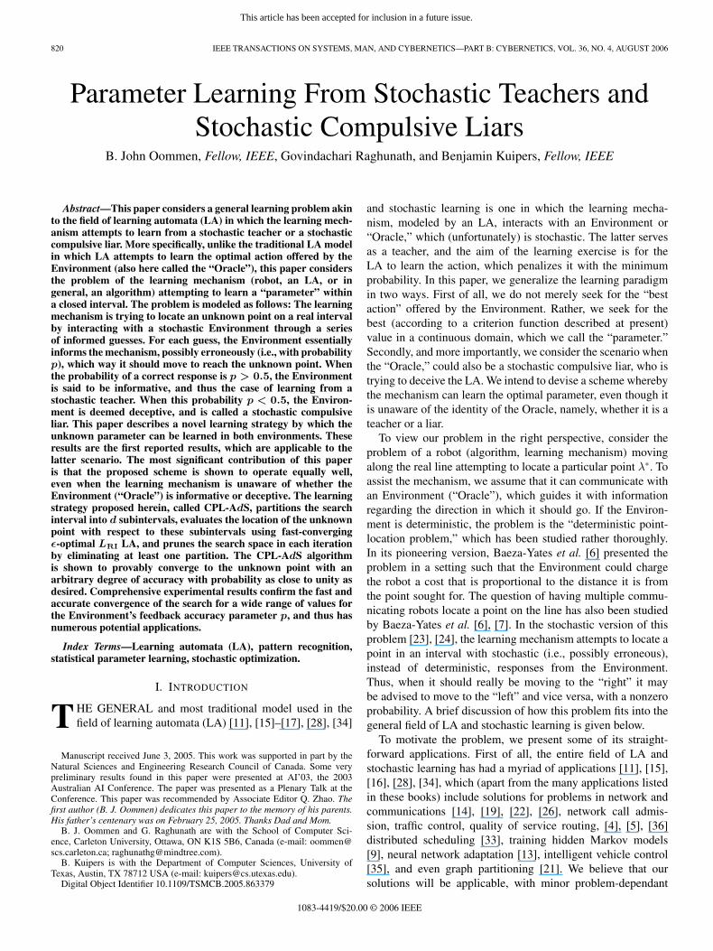
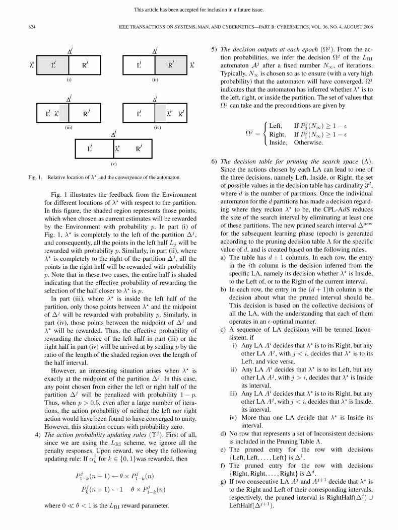
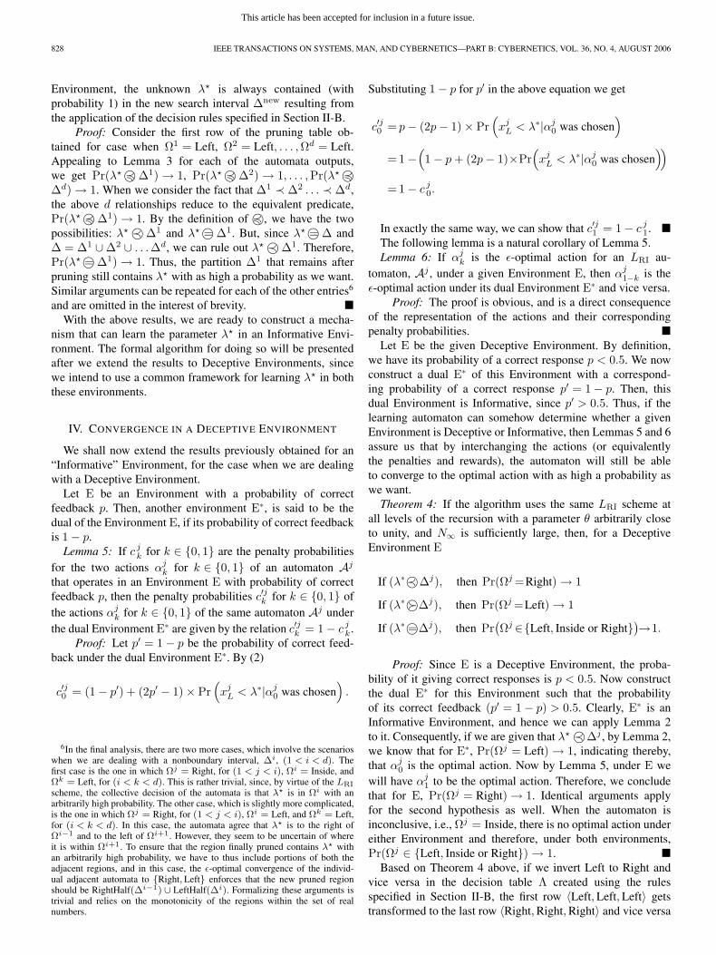
Fig. 1. Relative location of λ and the convergence of the automaton.

Fig. 1 illustrates the feedback from the Environmentfor different locations of λ with respect to the partition.In this figure, the shaded region represents those points,which when chosen as current estimates will be rewardedby the Environment with probability p. In part (i) ofFig. 1, λ is completely to the left of the partition ∆j ,and consequently, all the points in the left half Lj will berewarded with probability p. Similarly, in part (ii), whereλ is completely to the right of the partition ∆j , all thepoints in the right half will be rewarded with probabilityp. Note that in these two cases, the entire half is shadedindicating that the effective probability of rewarding theselection of the half closer to λ is p.

In part (iii), where λ is inside the left half of thepartition, only those points between λ and the midpointof ∆j will be rewarded with probability p. Similarly, inpart (iv), those points between the midpoint of ∆j andλ will be rewarded. Thus, the effective probability ofrewarding the choice of the left half in part (iii) or theright half in part (iv) will be arrived at by scaling p by theratio of the length of the shaded region over the length ofthe half interval.

However, an interesting situation arises when λ isexactly at the midpoint of the partition ∆j . In this case,any point chosen from either the left or right half of thepartition ∆j will be penalized with probability 1− p.Thus, when p > 0.5, even after a large number of itera-tions, the action probability of neither the left nor rightaction would have been found to have converged to unity.However, this situation occurs with probability zero.

4) The action probability updating rules (Υj). First of all,since we are using the LRI scheme, we ignore all thepenalty responses. Upon reward, we obey the followingupdating rule: If αj

k for k ∈ 0, 1was rewarded, then

P j1−k(n + 1)← θ × P j

1−k(n)

P jk (n + 1)← 1− θ × P j

1−k(n)

where 0 θ < 1 is the LRI reward parameter.

5) The decision outputs at each epoch (Ωj). From the ac-tion probabilities, we infer the decision Ωj of the LRI

automaton Aj after a fixed number N∞, of iterations.Typically, N∞ is chosen so as to ensure (with a very highprobability) that the automaton will have converged. Ωj

indicates that the automaton has inferred whether λ is tothe left, right, or inside the partition. The set of values thatΩj can take and the preconditions are given by

Ωj =

Left, If P j0 (N∞) ≥ 1− ε

Right, If P j1 (N∞) ≥ 1− ε

Inside, Otherwise.

6) The decision table for pruning the search space (Λ).Since the actions chosen by each LA can lead to one ofthe three decisions, namely Left, Inside, or Right, the setof possible values in the decision table has cardinality 3d,where d is the number of partitions. Once the individualautomaton for the d partitions has made a decision regard-ing where they reckon λ to be, the CPL-AdS reducesthe size of the search interval by eliminating at least oneof these partitions. The new pruned search interval ∆new

for the subsequent learning phase (epoch) is generatedaccording to the pruning decision table Λ for the specificvalue of d, and is created based on the following rules.a) The table has d + 1 columns. In each row, the entry

in the ith column is the decision inferred from thespecific LA, namely its decision whether λ is Inside,to the Left of, or to the Right of the current interval.

b) In each row, the entry in the (d + 1)th column is thedecision about what the pruned interval should be.This decision is based on the collective decisions ofall the LA, with the understanding that each of themoperates in an ε-optimal manner.

c) A sequence of LA decisions will be termed Incon-sistent, if

i) Any LA Ai decides that λ is to its Right, but anyother LA Aj , with j < i, decides that λ is to itsLeft, and vice versa.

ii) Any LA Ai decides that λ is to its Left, but anyother LA Aj , with j > i, decides that λ is Insideits interval.

iii) Any LA Ai decides that λ is to its Right, but anyother LA Aj , with j < i, decides that λ is Inside,its interval.

iv) More than one LA decide that λ is Inside itsinterval.

d) No row that represents a set of Inconsistent decisionsis included in the Pruning Table Λ.

e) The pruned entry for the row with decisionsLeft, Left, . . . , Left is ∆1.

f) The pruned entry for the row with decisionsRight, Right, . . . , Right is ∆d.

g) If two consecutive LA Aj and Aj+1 decide that λ isto the Right and Left of their corresponding intervals,respectively, the pruned interval is RightHalf(∆j) ∪LeftHalf(∆j+1).

This article has been accepted for inclusion in a future issue.

OOMMEN et al.: PARAMETER LEARNING FROM STOCHASTIC TEACHERS AND STOCHASTIC COMPULSIVE LIARS 825

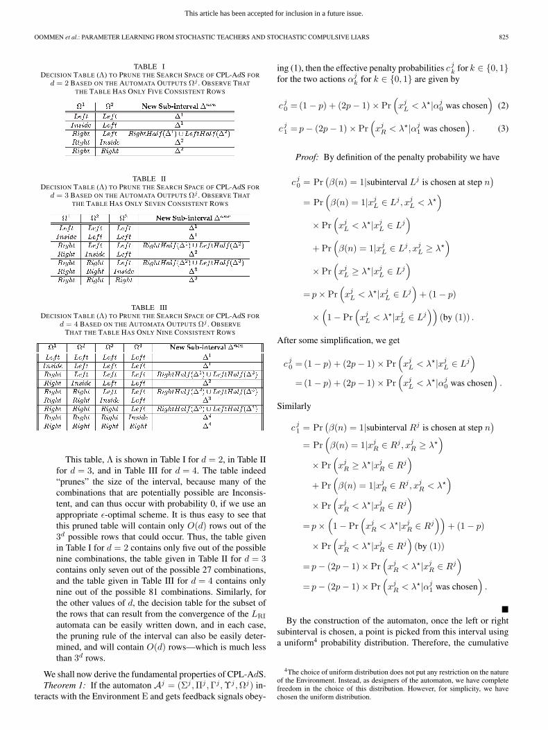
TABLE IDECISION TABLE (Λ) TO PRUNE THE SEARCH SPACE OF CPL-AdS FOR

d = 2 BASED ON THE AUTOMATA OUTPUTS Ωj . OBSERVE THAT

THE TABLE HAS ONLY FIVE CONSISTENT ROWS

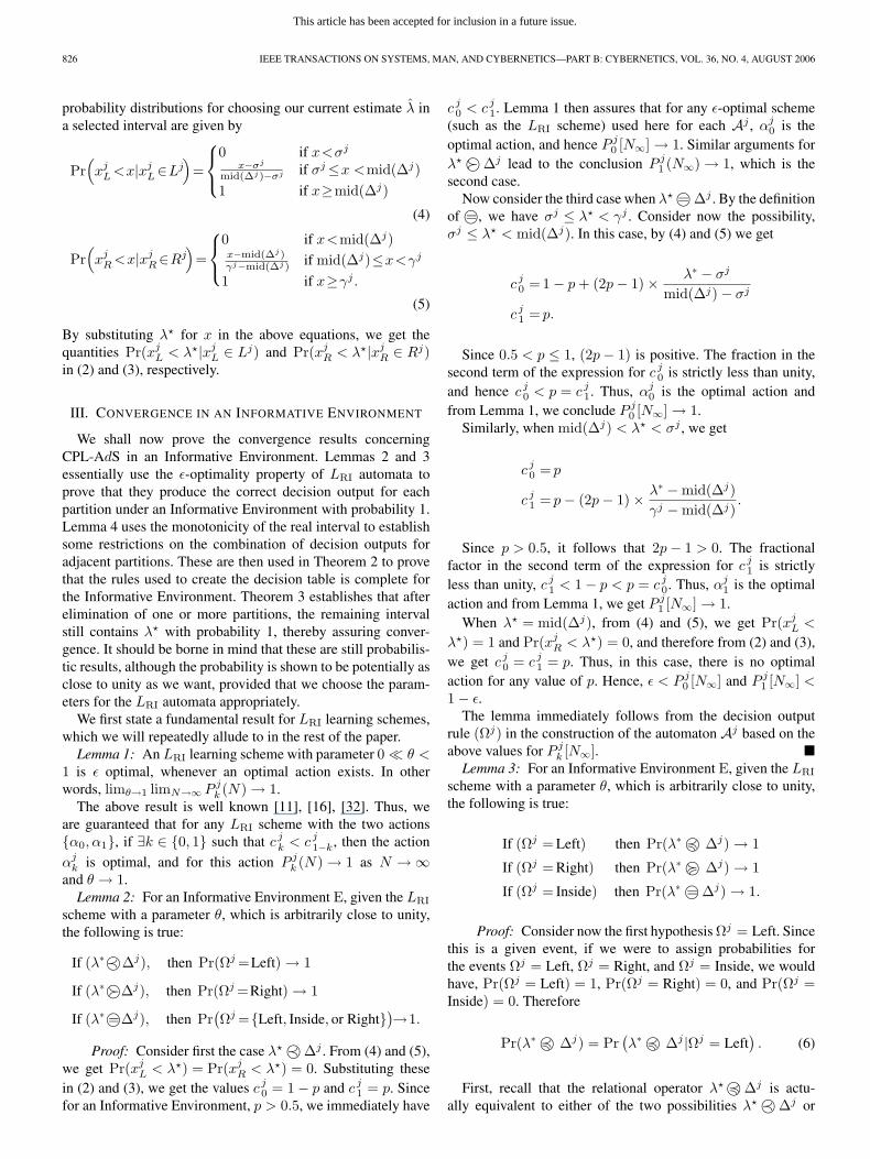
TABLE IIDECISION TABLE (Λ) TO PRUNE THE SEARCH SPACE OF CPL-AdS FOR

d = 3 BASED ON THE AUTOMATA OUTPUTS Ωj . OBSERVE THAT

THE TABLE HAS ONLY SEVEN CONSISTENT ROWS

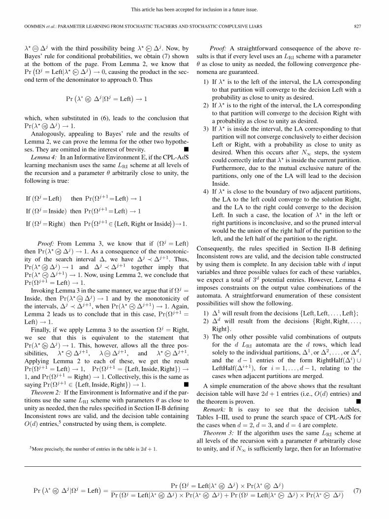
TABLE IIIDECISION TABLE (Λ) TO PRUNE THE SEARCH SPACE OF CPL-AdS FOR

d = 4 BASED ON THE AUTOMATA OUTPUTS Ωj . OBSERVE

THAT THE TABLE HAS ONLY NINE CONSISTENT ROWS

This table, Λ is shown in Table I for d = 2, in Table IIfor d = 3, and in Table III for d = 4. The table indeed“prunes” the size of the interval, because many of thecombinations that are potentially possible are Inconsis-tent, and can thus occur with probability 0, if we use anappropriate ε-optimal scheme. It is thus easy to see thatthis pruned table will contain only O(d) rows out of the3d possible rows that could occur. Thus, the table givenin Table I for d = 2 contains only five out of the possiblenine combinations, the table given in Table II for d = 3contains only seven out of the possible 27 combinations,and the table given in Table III for d = 4 contains onlynine out of the possible 81 combinations. Similarly, forthe other values of d, the decision table for the subset ofthe rows that can result from the convergence of the LRI

automata can be easily written down, and in each case,the pruning rule of the interval can also be easily deter-mined, and will contain O(d) rows—which is much lessthan 3d rows.

We shall now derive the fundamental properties of CPL-AdS.Theorem 1: If the automaton Aj = (Σj ,Πj ,Γj ,Υj ,Ωj) in-

teracts with the Environment E and gets feedback signals obey-

ing (1), then the effective penalty probabilities c jk for k ∈ 0, 1

for the two actions αjk for k ∈ 0, 1 are given by

c j0 =(1− p) + (2p− 1)× Pr

(xj

L < λ|αj0 was chosen

)(2)

c j1 = p− (2p− 1)× Pr

(xj

R < λ|αj1 was chosen

). (3)

Proof: By definition of the penalty probability we have

c j0 = Pr

(β(n) = 1|subinterval Lj is chosen at step n

)

= Pr(β(n) = 1|xj

L ∈ Lj , xjL < λ

)

× Pr(xj

L < λ|xjL ∈ Lj

)

+ Pr(β(n) = 1|xj

L ∈ Lj , xjL ≥ λ

)

× Pr(xj

L ≥ λ|xjL ∈ Lj

)

= p× Pr(xj

L < λ|xjL ∈ Lj

)+ (1− p)

×(1− Pr

(xj

L < λ|xjL ∈ Lj

))(by (1)) .

After some simplification, we get

c j0 =(1− p) + (2p− 1)× Pr

(xj

L < λ|xjL ∈ Lj

)

=(1− p) + (2p− 1)× Pr(xj

L < λ|αj0 was chosen

).

Similarly

c j1 = Pr

(β(n) = 1|subinterval Rj is chosen at step n

)= Pr

(β(n) = 1|xj

R ∈ Rj , xjR ≥ λ

)

× Pr(xj

R ≥ λ|xjR ∈ Rj

)

+ Pr(β(n) = 1|xj

R ∈ Rj , xjR < λ

)

× Pr(xj

R < λ|xjR ∈ Rj

)

= p×(1− Pr

(xj

R < λ|xjR ∈ Rj

))+ (1− p)

× Pr(xj

R < λ|xjR ∈ Rj

)(by (1))

= p− (2p− 1)× Pr(xj

R < λ|xjR ∈ Rj

)

= p− (2p− 1)× Pr(xj

R < λ|αj1 was chosen

).

By the construction of the automaton, once the left or right

subinterval is chosen, a point is picked from this interval usinga uniform4 probability distribution. Therefore, the cumulative

4The choice of uniform distribution does not put any restriction on the natureof the Environment. Instead, as designers of the automaton, we have completefreedom in the choice of this distribution. However, for simplicity, we havechosen the uniform distribution.

This article has been accepted for inclusion in a future issue.

826 IEEE TRANSACTIONS ON SYSTEMS, MAN, AND CYBERNETICS—PART B: CYBERNETICS, VOL. 36, NO. 4, AUGUST 2006

probability distributions for choosing our current estimate λ ina selected interval are given by

Pr(xj

L <x|xjL∈Lj

)=

0 if x<σj

x−σj

mid(∆j)−σj if σj≤x <mid(∆j)1 if x≥mid(∆j)

(4)

Pr(xj

R <x|xjR∈Rj

)=

0 if x<mid(∆j)x−mid(∆j)γj−mid(∆j) if mid(∆j)≤x<γj

1 if x≥γj .

(5)

By substituting λ for x in the above equations, we get thequantities Pr(xj

L < λ|xjL ∈ Lj) and Pr(xj

R < λ|xjR ∈ Rj)

in (2) and (3), respectively.

III. CONVERGENCE IN AN INFORMATIVE ENVIRONMENT

We shall now prove the convergence results concerningCPL-AdS in an Informative Environment. Lemmas 2 and 3essentially use the ε-optimality property of LRI automata toprove that they produce the correct decision output for eachpartition under an Informative Environment with probability 1.Lemma 4 uses the monotonicity of the real interval to establishsome restrictions on the combination of decision outputs foradjacent partitions. These are then used in Theorem 2 to provethat the rules used to create the decision table is complete forthe Informative Environment. Theorem 3 establishes that afterelimination of one or more partitions, the remaining intervalstill contains λ with probability 1, thereby assuring conver-gence. It should be borne in mind that these are still probabilis-tic results, although the probability is shown to be potentially asclose to unity as we want, provided that we choose the param-eters for the LRI automata appropriately.

We first state a fundamental result for LRI learning schemes,which we will repeatedly allude to in the rest of the paper.

Lemma 1: An LRI learning scheme with parameter 0 θ <1 is ε optimal, whenever an optimal action exists. In otherwords, limθ→1 limN→∞ P j

k (N)→ 1.The above result is well known [11], [16], [32]. Thus, we

are guaranteed that for any LRI scheme with the two actionsα0, α1, if ∃k ∈ 0, 1 such that c j

k < c j1−k, then the action

αjk is optimal, and for this action P j

k (N)→ 1 as N →∞and θ → 1.

Lemma 2: For an Informative Environment E, given the LRI

scheme with a parameter θ, which is arbitrarily close to unity,the following is true:

If (λ∗©≺ ∆j), then Pr(Ωj =Left)→ 1

If (λ∗© ∆j), then Pr(Ωj =Right)→ 1

If (λ∗©=∆j), then Pr(Ωj =Left, Inside, or Right)→1.

Proof: Consider first the case λ ≺©∆j . From (4) and (5),we get Pr(xj

L < λ) = Pr(xjR < λ) = 0. Substituting these

in (2) and (3), we get the values c j0 = 1− p and c j

1 = p. Sincefor an Informative Environment, p > 0.5, we immediately have

c j0 < c j

1. Lemma 1 then assures that for any ε-optimal scheme(such as the LRI scheme) used here for each Aj , αj

0 is theoptimal action, and hence P j

0 [N∞]→ 1. Similar arguments forλ ©∆j lead to the conclusion P j

1 (N∞)→ 1, which is thesecond case.

Now consider the third case when λ =©∆j . By the definitionof =©, we have σj ≤ λ < γj . Consider now the possibility,σj ≤ λ < mid(∆j). In this case, by (4) and (5) we get

c j0 =1− p + (2p− 1)× λ∗ − σj

mid(∆j)− σj

c j1 = p.

Since 0.5 < p ≤ 1, (2p− 1) is positive. The fraction in thesecond term of the expression for c j

0 is strictly less than unity,and hence c j

0 < p = c j1. Thus, αj

0 is the optimal action andfrom Lemma 1, we conclude P j

0 [N∞]→ 1.Similarly, when mid(∆j) < λ < σj , we get

c j0 = p

c j1 = p− (2p− 1)× λ∗ −mid(∆j)

γj −mid(∆j).

Since p > 0.5, it follows that 2p− 1 > 0. The fractionalfactor in the second term of the expression for c j

1 is strictlyless than unity, c j

1 < 1− p < p = c j0. Thus, αj

1 is the optimalaction and from Lemma 1, we get P j

1 [N∞]→ 1.When λ = mid(∆j), from (4) and (5), we get Pr(xj

L <

λ) = 1 and Pr(xjR < λ) = 0, and therefore from (2) and (3),

we get c j0 = c j

1 = p. Thus, in this case, there is no optimalaction for any value of p. Hence, ε < P j

0 [N∞] and P j1 [N∞] <

1− ε.The lemma immediately follows from the decision output

rule (Ωj) in the construction of the automaton Aj based on theabove values for P j

k [N∞]. Lemma 3: For an Informative Environment E, given the LRI

scheme with a parameter θ, which is arbitrarily close to unity,the following is true:

If (Ωj = Left) then Pr(λ∗ © ∆j)→ 1

If (Ωj = Right) then Pr(λ∗ © ∆j)→ 1

If (Ωj = Inside) then Pr(λ∗ ©= ∆j)→ 1.

Proof: Consider now the first hypothesis Ωj = Left. Sincethis is a given event, if we were to assign probabilities forthe events Ωj = Left, Ωj = Right, and Ωj = Inside, we wouldhave, Pr(Ωj = Left) = 1, Pr(Ωj = Right) = 0, and Pr(Ωj =Inside) = 0. Therefore

Pr(λ∗ © ∆j) = Pr(λ∗ © ∆j |Ωj = Left

). (6)

First, recall that the relational operator λ ©∆j is actu-ally equivalent to either of the two possibilities λ ≺©∆j or

This article has been accepted for inclusion in a future issue.

OOMMEN et al.: PARAMETER LEARNING FROM STOCHASTIC TEACHERS AND STOCHASTIC COMPULSIVE LIARS 827

λ =©∆j with the third possibility being λ ©∆j . Now, byBayes’ rule for conditional probabilities, we obtain (7) shownat the bottom of the page. From Lemma 2, we know thatPr

(Ωj = Left|λ ©∆j

)→ 0, causing the product in the sec-ond term of the denominator to approach 0. Thus

Pr(λ∗ © ∆j |Ωj = Left

)→ 1

which, when substituted in (6), leads to the conclusion thatPr(λ ©∆j)→ 1.

Analogously, appealing to Bayes’ rule and the results ofLemma 2, we can prove the lemma for the other two hypothe-ses. They are omitted in the interest of brevity.

Lemma 4: In an Informative Environment E, if the CPL-AdSlearning mechanism uses the same LRI scheme at all levels ofthe recursion and a parameter θ arbitrarily close to unity, thefollowing is true:

If (Ωj =Left) then Pr(Ωj+1 =Left)→ 1

If (Ωj = Inside) then Pr(Ωj+1 =Left)→ 1

If (Ωj =Right) then Pr(Ωj+1∈Left, Right or Inside)→1.

Proof: From Lemma 3, we know that if (Ωj = Left)then Pr(λ ©∆j)→ 1. As a consequence of the monotonic-ity of the search interval ∆, we have ∆j ≺ ∆j+1. Thus,Pr(λ ©∆j)→ 1 and ∆j ≺ ∆j+1 together imply thatPr(λ ≺©∆j+1)→ 1. Now, using Lemma 2, we conclude thatPr(Ωj+1 = Left)→ 1.

Invoking Lemma 3 in the same manner, we argue that if Ωj =Inside, then Pr(λ =©∆j)→ 1 and by the monotonicity ofthe intervals, ∆j ≺ ∆j+1, when Pr(λ ≺©∆j+1)→ 1. Again,Lemma 2 leads us to conclude that in this case, Pr(Ωj+1 =Left)→ 1.

Finally, if we apply Lemma 3 to the assertion Ωj = Right,we see that this is equivalent to the statement thatPr(λ ©∆j)→ 1. This, however, allows all the three pos-sibilities, λ ≺©∆j+1, λ =©∆j+1, and λ ©∆j+1.Applying Lemma 2 to each of these, we get the resultPr(Ωj+1 = Left)→ 1, Pr(Ωj+1 = Left, Inside, Right)→1, and Pr(Ωj+1 = Right)→ 1. Collectively, this is the same assaying Pr(Ωj+1 ∈ Left, Inside, Right)→ 1.

Theorem 2: If the Environment is Informative and if the par-titions use the same LRI scheme with parameters θ as close tounity as needed, then the rules specified in Section II-B definingInconsistent rows are valid, and the decision table containingO(d) entries,5 constructed by using them, is complete.

5More precisely, the number of entries in the table is 2d + 1.

Proof: A straightforward consequence of the above re-sults is that if every level uses an LRI scheme with a parameterθ as close to unity as needed, the following convergence phe-nomena are guaranteed.

1) If λ is to the left of the interval, the LA correspondingto that partition will converge to the decision Left with aprobability as close to unity as desired.

2) If λ is to the right of the interval, the LA correspondingto that partition will converge to the decision Right witha probability as close to unity as desired.

3) If λ is inside the interval, the LA corresponding to thatpartition will not converge conclusively to either decisionLeft or Right, with a probability as close to unity asdesired. When this occurs after N∞ steps, the systemcould correctly infer that λ is inside the current partition.Furthermore, due to the mutual exclusive nature of thepartitions, only one of the LA will lead to the decisionInside.

4) If λ is close to the boundary of two adjacent partitions,the LA to the left could converge to the solution Right,and the LA to the right could converge to the decisionLeft. In such a case, the location of λ in the left orright partitions is inconclusive, and so the pruned intervalwould be the union of the right half of the partition to theleft, and the left half of the partition to the right.

Consequently, the rules specified in Section II-B definingInconsistent rows are valid, and the decision table constructedby using them is complete. In any decision table with d inputvariables and three possible values for each of these variables,we expect a total of 3d potential entries. However, Lemma 4imposes constraints on the output value combinations of theautomata. A straightforward enumeration of these consistentpossibilities will show the following.

1) ∆1 will result from the decisions Left, Left, . . . , Left;2) ∆d will result from the decisions Right, Right, . . . ,

Right.3) The only other possible valid combinations of outputs

for the d LRI automata are the d rows, which leadsolely to the individual partitions, ∆1, or ∆2, . . . , or ∆d,and the d− 1 entries of the form RightHalf(∆i) ∪LeftHalf(∆i+1), for i = 1, . . . , d− 1, relating to thecases when adjacent partitions are merged.

A simple enumeration of the above shows that the resultantdecision table will have 2d + 1 entries (i.e., O(d) entries) andthe theorem is proven.

Remark: It is easy to see that the decision tables,Tables I–III, used to prune the search space of CPL-AdS forthe cases when d = 2, d = 3, and d = 4 are complete.

Theorem 3: If the algorithm uses the same LRI scheme atall levels of the recursion with a parameter θ arbitrarily closeto unity, and if N∞ is sufficiently large, then for an Informative

Pr(λ∗ © ∆j |Ωj = Left

)=

Pr(Ωj = Left|λ∗ © ∆j

)× Pr(λ∗ © ∆j)Pr (Ωj = Left|λ∗ © ∆j)× Pr(λ∗ © ∆j) + Pr (Ωj = Left|λ∗ © ∆j)× Pr(λ∗ © ∆j)

(7)

This article has been accepted for inclusion in a future issue.

828 IEEE TRANSACTIONS ON SYSTEMS, MAN, AND CYBERNETICS—PART B: CYBERNETICS, VOL. 36, NO. 4, AUGUST 2006

Environment, the unknown λ is always contained (withprobability 1) in the new search interval ∆new resulting fromthe application of the decision rules specified in Section II-B.

Proof: Consider the first row of the pruning table ob-tained for case when Ω1 = Left, Ω2 = Left, . . . ,Ωd = Left.Appealing to Lemma 3 for each of the automata outputs,we get Pr(λ ©∆1)→ 1, Pr(λ ©∆2)→ 1, . . . ,Pr(λ ©∆d)→ 1. When we consider the fact that ∆1 ≺ ∆2 . . . ≺ ∆d,the above d relationships reduce to the equivalent predicate,Pr(λ ©∆1)→ 1. By the definition of ©, we have the twopossibilities: λ ≺©∆1 and λ =©∆1. But, since λ =©∆ and∆ = ∆1 ∪∆2 ∪ . . . ∆d, we can rule out λ ≺©∆1. Therefore,Pr(λ =©∆1)→ 1. Thus, the partition ∆1 that remains afterpruning still contains λ with as high a probability as we want.Similar arguments can be repeated for each of the other entries6

and are omitted in the interest of brevity. With the above results, we are ready to construct a mecha-

nism that can learn the parameter λ in an Informative Envi-ronment. The formal algorithm for doing so will be presentedafter we extend the results to Deceptive Environments, sincewe intend to use a common framework for learning λ in boththese environments.

IV. CONVERGENCE IN A DECEPTIVE ENVIRONMENT

We shall now extend the results previously obtained for an“Informative” Environment, for the case when we are dealingwith a Deceptive Environment.

Let E be an Environment with a probability of correctfeedback p. Then, another environment E∗, is said to be thedual of the Environment E, if its probability of correct feedbackis 1− p.

Lemma 5: If c jk for k ∈ 0, 1 are the penalty probabilities

for the two actions αjk for k ∈ 0, 1 of an automaton Aj

that operates in an Environment E with probability of correctfeedback p, then the penalty probabilities c′jk for k ∈ 0, 1 ofthe actions αj

k for k ∈ 0, 1 of the same automaton Aj underthe dual Environment E∗ are given by the relation c′jk = 1− c j

k.Proof: Let p′ = 1− p be the probability of correct feed-

back under the dual Environment E∗. By (2)

c′j0 = (1− p′) + (2p′ − 1)× Pr(xj

L < λ∗|αj0 was chosen

).

6In the final analysis, there are two more cases, which involve the scenarioswhen we are dealing with a nonboundary interval, ∆i, (1 < i < d). Thefirst case is the one in which Ωj = Right, for (1 < j < i), Ωi = Inside, andΩk = Left, for (i < k < d). This is rather trivial, since, by virtue of the LRI

scheme, the collective decision of the automata is that λ is in Ωi with anarbitrarily high probability. The other case, which is slightly more complicated,is the one in which Ωj = Right, for (1 < j < i), Ωi = Left, and Ωk = Left,for (i < k < d). In this case, the automata agree that λ is to the right ofΩi−1 and to the left of Ωi+1. However, they seem to be uncertain of whereit is within Ωi+1. To ensure that the region finally pruned contains λ withan arbitrarily high probability, we have to thus include portions of both theadjacent regions, and in this case, the ε-optimal convergence of the individ-ual adjacent automata to Right, Left enforces that the new pruned regionshould be RightHalf(∆i−1) ∪ LeftHalf(∆i). Formalizing these arguments istrivial and relies on the monotonicity of the regions within the set of realnumbers.

Substituting 1− p for p′ in the above equation we get

c′j0 = p− (2p− 1)× Pr(xj

L < λ∗|αj0 was chosen

)

=1−(1− p + (2p− 1)×Pr

(xj

L < λ∗|αj0 was chosen

))

=1− c j0.

In exactly the same way, we can show that c′j1 = 1− c j1.

The following lemma is a natural corollary of Lemma 5.Lemma 6: If αj

k is the ε-optimal action for an LRI au-tomaton, Aj , under a given Environment E, then αj

1−k is theε-optimal action under its dual Environment E∗ and vice versa.

Proof: The proof is obvious, and is a direct consequenceof the representation of the actions and their correspondingpenalty probabilities.

Let E be the given Deceptive Environment. By definition,we have its probability of a correct response p < 0.5. We nowconstruct a dual E∗ of this Environment with a correspond-ing probability of a correct response p′ = 1− p. Then, thisdual Environment is Informative, since p′ > 0.5. Thus, if thelearning automaton can somehow determine whether a givenEnvironment is Deceptive or Informative, then Lemmas 5 and 6assure us that by interchanging the actions (or equivalentlythe penalties and rewards), the automaton will still be ableto converge to the optimal action with as high a probability aswe want.

Theorem 4: If the algorithm uses the same LRI scheme atall levels of the recursion with a parameter θ arbitrarily closeto unity, and N∞ is sufficiently large, then, for a DeceptiveEnvironment E

If (λ∗©≺ ∆j), then Pr(Ωj =Right)→ 1

If (λ∗© ∆j), then Pr(Ωj =Left)→ 1

If (λ∗©=∆j), then Pr(Ωj ∈Left, Inside or Right)→1.

Proof: Since E is a Deceptive Environment, the proba-bility of it giving correct responses is p < 0.5. Now constructthe dual E∗ for this Environment such that the probabilityof its correct feedback (p′ = 1− p) > 0.5. Clearly, E∗ is anInformative Environment, and hence we can apply Lemma 2to it. Consequently, if we are given that λ©≺ ∆j , by Lemma 2,we know that for E∗, Pr(Ωj = Left)→ 1, indicating thereby,that αj

0 is the optimal action. Now by Lemma 5, under E wewill have αj

1 to be the optimal action. Therefore, we concludethat for E, Pr(Ωj = Right)→ 1. Identical arguments applyfor the second hypothesis as well. When the automaton isinconclusive, i.e., Ωj = Inside, there is no optimal action undereither Environment and therefore, under both environments,Pr(Ωj ∈ Left, Inside or Right)→ 1.

Based on Theorem 4 above, if we invert Left to Right andvice versa in the decision table Λ created using the rulesspecified in Section II-B, the first row 〈Left, Left, Left〉 getstransformed to the last row 〈Right, Right, Right〉 and vice versa

This article has been accepted for inclusion in a future issue.

OOMMEN et al.: PARAMETER LEARNING FROM STOCHASTIC TEACHERS AND STOCHASTIC COMPULSIVE LIARS 829

and the rest of the rows will get transformed to one of theimpossible entries. Thus, except for the two cases where theautomata outputs are all Left or all Right, we can directly detecta Deceptive Environment. We now provide a mechanism fordealing with the two extreme cases as well.

Theorem 5: Suppose it is given that for 1 < i < d, λ =©∆i,λ ©∆j , for all j < i, and λ©≺ ∆j , for all j > i. Then,under a Deceptive Environment, the decision outputs givenby the vector Ω for the d automata Aj , j ∈ 1, 2, . . . , d,will be inconsistent with the decision table created using therules specified in Section II-B. Conversely, if for any givenEnvironment and λ as above, the decision outputs given bythe vector Ω of the automata is inconsistent with the decisiontable, then the Environment is Deceptive.

Proof: In the interest of simplicity, we shall prove theresult for the case when d = 3, since these arguments can beextended for other values of d in quite a straightforward manner.Consider the case when λ is in ∆2. Applying Theorem 4 toeach of λ ©∆1, λ =©∆2, and λ ≺©∆3, we have

Pr(Ω1 = Left)→ 1

Pr(Ω2 = Left, Inside or Right)→ 1

Pr(Ω3 = Right)→ 1.

By inspecting the decision table Λ (Table II), we see that thereare no entries for the outputs given by the vector

Ω = [Left, Left, Inside or Right, Right]

and hence the entry is inconsistent with Table II. The converseis proved by contradiction by alluding to the completenessresult of Theorem 2 for an Informative Environment. Therefore,whenever the decision outputs given by the vector Ω is inconsis-tent with Table II, we can safely conclude that the Environmentis Deceptive.

Generalizing this, if it is given that λ =©∆i, λ ©∆j forall j < i, and λ ≺©∆j for all j > i, then, we can applyTheorem 4 to each of these constraints to yield (for a DeceptiveEnvironment)

Pr(Ωj = Left)→ 1 for j < i

Pr(Ωi = Left, Inside or Right)→ 1

Pr(Ωj = Right)→ 1 for j > i.

By inspecting the decision table Λ resulting from the applica-tion of the decision rules specified in Section II-B, we see thatthere are no entries for the outputs given by the vector

Ω = [Left, . . . ,Left,Left, Inside or Right,Right, . . . ,Right]

and hence the entry is inconsistent with the correspondingdecision table Λ. Again, the converse is proved by contradictionby alluding to the completeness result of Theorem 2 for an

Informative Environment. Therefore, whenever the decisionoutputs given by the vector Ω is inconsistent with the cor-responding decision table Λ we can safely conclude that theEnvironment is Deceptive.

Remark: Utilizing this test for the case when d = 2 is trivial.There are essentially two scenarios, namely: 1) the first LAconverges to the Left and the second converges to the Right,or 2) both LA converge to the decision that λ is Inside theirrespective region. In both these cases, we quickly decide thatthe Environment is Deceptive. In what follows, we assumethat d > 2.

Theorem 6: Let I = [0, 1) be the original search interval inwhich λ is to be found. For any d > 2, let I′ = [−1/(d− 2),1 + (1/(d− 2))) be the initial search interval used byCPL-AdS. Then, CPL-AdS always determines whether or notan Environment is Deceptive after a single epoch.

Proof: First of all, we can see that λ ∈ I′ because, I ⊂I′. We further see that I′ is of length d/(d− 2), and thus, ifwe divide I′ into d equal partitions, each partition will be oflength 1/(d− 2). When we divide I′ into d equal partitions∆1,∆2, . . . ,∆d, we get

∆1 =[− 1

d− 2, 0

)

∆2 =[0,

1d− 2

)

∆3 =[

1d− 2

,2

d− 2

), . . .

∆i =[

i− 2d− 2

,i− 1d− 2

), . . .

∆d−1 =[1− 1

d− 2, 1

)

∆d =[1, 1 +

1d− 2

).

Since λ ∈ I, we know that λ ∈ ∆i for some 1 < i < d,where the latter inequalities are strict. Thus, for this value ofi, λ ©∆j for all 1 < j < i, λ =©∆i, and λ©≺ ∆j for alld > j > i, which is the precondition for Theorem 5. Hence, byappealing to Theorem 5, we see that if the Environment wasDeceptive, we would get an inconsistent decision vector. If not,by Theorem 2, we would get a consistent decision vector. Thus,after a single epoch, we conclude decisively about the nature ofthe Environment.

Theorem 6 gives us a simple mechanism for detectingDeceptive Environments. Thus, we start with an initial searchinterval I′ = [−(1/(d− 2)), 1 + (1/(d− 2))), partition it intod subintervals, and run the d LRI automata Aj , j = 1, 2, . . . , dfor exactly one epoch. At the end of the epoch, we use thecorresponding decision table Λ created using the rules spec-ified in Section II-B, to check if the decision vector Ω hasa valid entry or not, and accordingly conclude whether theEnvironment is Informative or Deceptive. If the Environmentis found to be Deceptive, we flip the probability update rules,

This article has been accepted for inclusion in a future issue.

830 IEEE TRANSACTIONS ON SYSTEMS, MAN, AND CYBERNETICS—PART B: CYBERNETICS, VOL. 36, NO. 4, AUGUST 2006

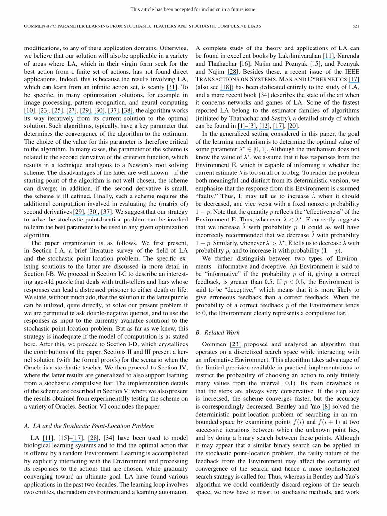
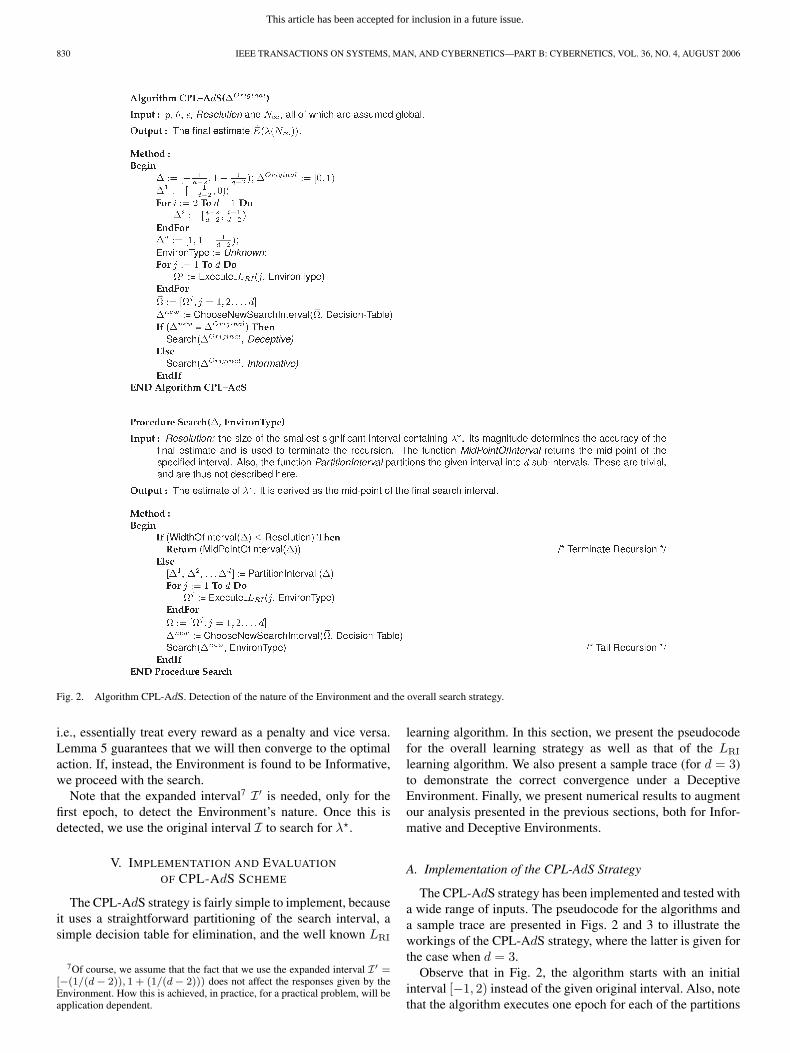
Fig. 2. Algorithm CPL-AdS. Detection of the nature of the Environment and the overall search strategy.

i.e., essentially treat every reward as a penalty and vice versa.Lemma 5 guarantees that we will then converge to the optimalaction. If, instead, the Environment is found to be Informative,we proceed with the search.

Note that the expanded interval7 I′ is needed, only for thefirst epoch, to detect the Environment’s nature. Once this isdetected, we use the original interval I to search for λ.

V. IMPLEMENTATION AND EVALUATION

OF CPL-AdS SCHEME

The CPL-AdS strategy is fairly simple to implement, becauseit uses a straightforward partitioning of the search interval, asimple decision table for elimination, and the well known LRI

7Of course, we assume that the fact that we use the expanded interval I′ =[−(1/(d − 2)), 1 + (1/(d − 2))) does not affect the responses given by theEnvironment. How this is achieved, in practice, for a practical problem, will beapplication dependent.

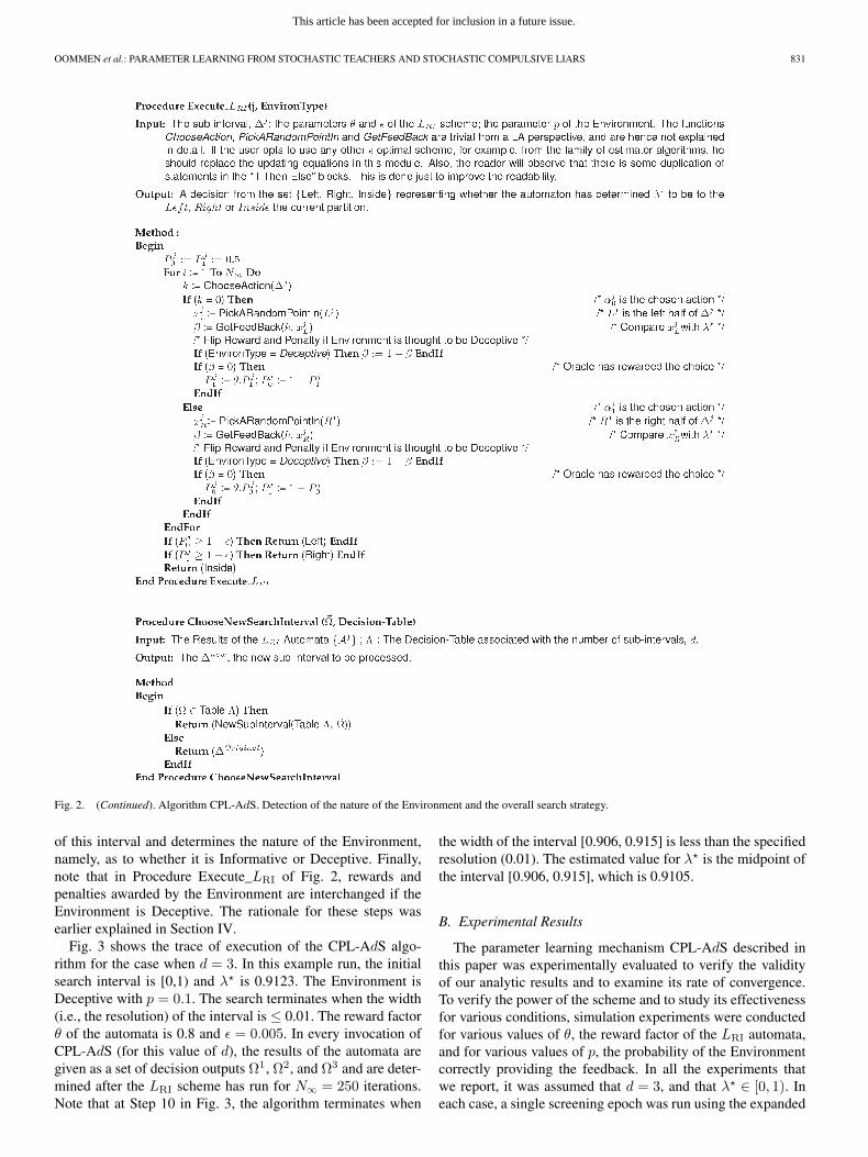
learning algorithm. In this section, we present the pseudocodefor the overall learning strategy as well as that of the LRI

learning algorithm. We also present a sample trace (for d = 3)to demonstrate the correct convergence under a DeceptiveEnvironment. Finally, we present numerical results to augmentour analysis presented in the previous sections, both for Infor-mative and Deceptive Environments.

A. Implementation of the CPL-AdS Strategy

The CPL-AdS strategy has been implemented and tested witha wide range of inputs. The pseudocode for the algorithms anda sample trace are presented in Figs. 2 and 3 to illustrate theworkings of the CPL-AdS strategy, where the latter is given forthe case when d = 3.

Observe that in Fig. 2, the algorithm starts with an initialinterval [−1, 2) instead of the given original interval. Also, notethat the algorithm executes one epoch for each of the partitions

This article has been accepted for inclusion in a future issue.

OOMMEN et al.: PARAMETER LEARNING FROM STOCHASTIC TEACHERS AND STOCHASTIC COMPULSIVE LIARS 831

Fig. 2. (Continued). Algorithm CPL-AdS. Detection of the nature of the Environment and the overall search strategy.

of this interval and determines the nature of the Environment,namely, as to whether it is Informative or Deceptive. Finally,note that in Procedure Execute_LRI of Fig. 2, rewards andpenalties awarded by the Environment are interchanged if theEnvironment is Deceptive. The rationale for these steps wasearlier explained in Section IV.

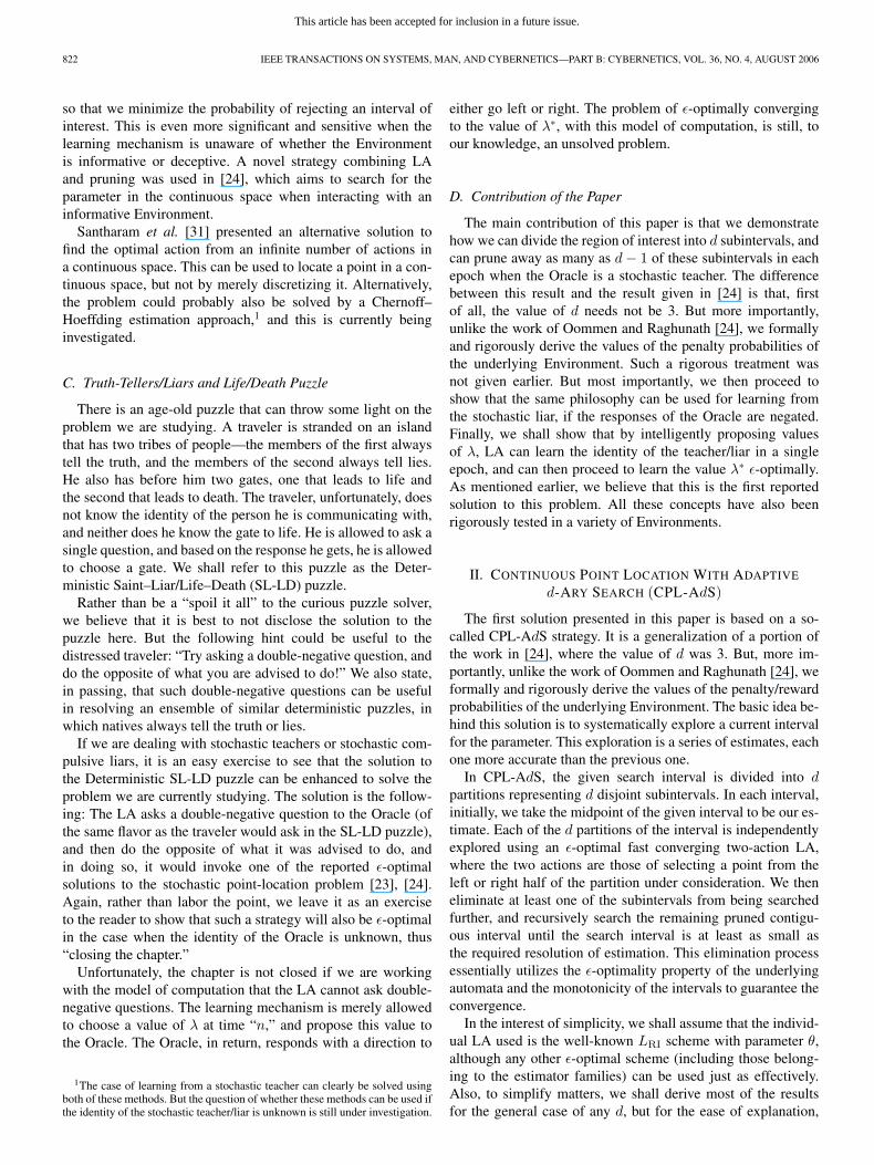
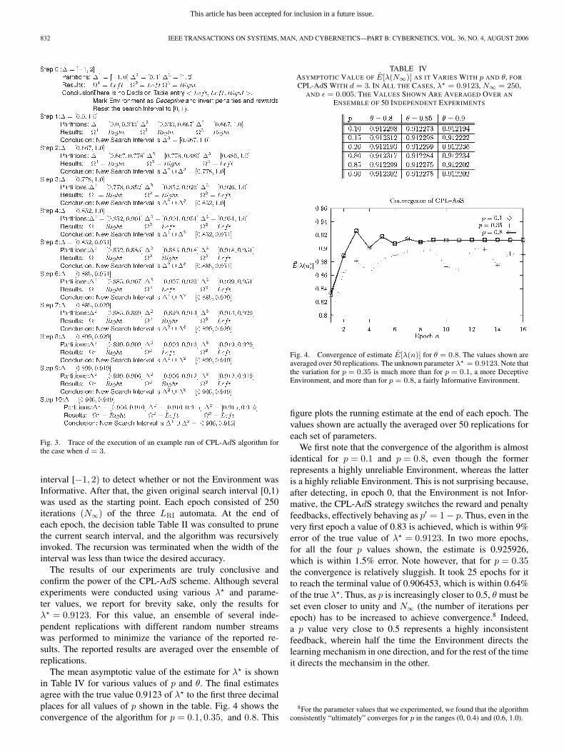
Fig. 3 shows the trace of execution of the CPL-AdS algo-rithm for the case when d = 3. In this example run, the initialsearch interval is [0,1) and λ is 0.9123. The Environment isDeceptive with p = 0.1. The search terminates when the width(i.e., the resolution) of the interval is ≤ 0.01. The reward factorθ of the automata is 0.8 and ε = 0.005. In every invocation ofCPL-AdS (for this value of d), the results of the automata aregiven as a set of decision outputs Ω1, Ω2, and Ω3 and are deter-mined after the LRI scheme has run for N∞ = 250 iterations.Note that at Step 10 in Fig. 3, the algorithm terminates when

the width of the interval [0.906, 0.915] is less than the specifiedresolution (0.01). The estimated value for λ is the midpoint ofthe interval [0.906, 0.915], which is 0.9105.

B. Experimental Results

The parameter learning mechanism CPL-AdS described inthis paper was experimentally evaluated to verify the validityof our analytic results and to examine its rate of convergence.To verify the power of the scheme and to study its effectivenessfor various conditions, simulation experiments were conductedfor various values of θ, the reward factor of the LRI automata,and for various values of p, the probability of the Environmentcorrectly providing the feedback. In all the experiments thatwe report, it was assumed that d = 3, and that λ ∈ [0, 1). Ineach case, a single screening epoch was run using the expanded

This article has been accepted for inclusion in a future issue.

832 IEEE TRANSACTIONS ON SYSTEMS, MAN, AND CYBERNETICS—PART B: CYBERNETICS, VOL. 36, NO. 4, AUGUST 2006

Fig. 3. Trace of the execution of an example run of CPL-AdS algorithm forthe case when d = 3.

interval [−1, 2) to detect whether or not the Environment wasInformative. After that, the given original search interval [0,1)was used as the starting point. Each epoch consisted of 250iterations (N∞) of the three LRI automata. At the end ofeach epoch, the decision table Table II was consulted to prunethe current search interval, and the algorithm was recursivelyinvoked. The recursion was terminated when the width of theinterval was less than twice the desired accuracy.

The results of our experiments are truly conclusive andconfirm the power of the CPL-AdS scheme. Although severalexperiments were conducted using various λ and parame-ter values, we report for brevity sake, only the results forλ = 0.9123. For this value, an ensemble of several inde-pendent replications with different random number streamswas performed to minimize the variance of the reported re-sults. The reported results are averaged over the ensemble ofreplications.

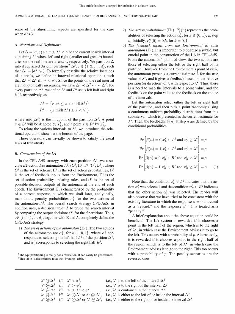
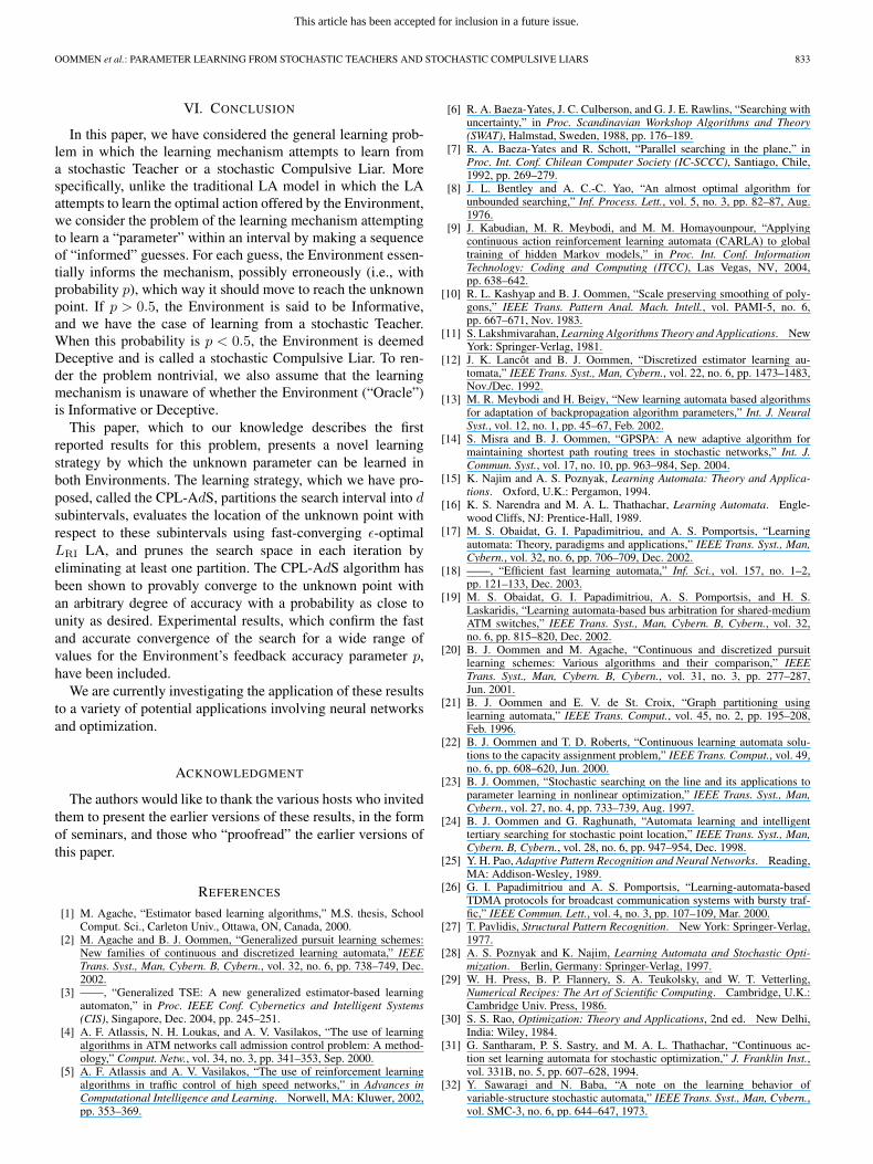
The mean asymptotic value of the estimate for λ is shownin Table IV for various values of p and θ. The final estimatesagree with the true value 0.9123 of λ to the first three decimalplaces for all values of p shown in the table. Fig. 4 shows theconvergence of the algorithm for p = 0.1, 0.35, and 0.8. This

TABLE IVASYMPTOTIC VALUE OF E[λ(N∞)] AS IT VARIES WITH p AND θ, FOR

CPL-AdS WITH d = 3. IN ALL THE CASES, λ = 0.9123, N∞ = 250,AND ε = 0.005. THE VALUES SHOWN ARE AVERAGED OVER AN

ENSEMBLE OF 50 INDEPENDENT EXPERIMENTS

Fig. 4. Convergence of estimate E[λ(n)] for θ = 0.8. The values shown areaveraged over 50 replications. The unknown parameter λ = 0.9123. Note thatthe variation for p = 0.35 is much more than for p = 0.1, a more DeceptiveEnvironment, and more than for p = 0.8, a fairly Informative Environment.

figure plots the running estimate at the end of each epoch. Thevalues shown are actually the averaged over 50 replications foreach set of parameters.

We first note that the convergence of the algorithm is almostidentical for p = 0.1 and p = 0.8, even though the formerrepresents a highly unreliable Environment, whereas the latteris a highly reliable Environment. This is not surprising because,after detecting, in epoch 0, that the Environment is not Infor-mative, the CPL-AdS strategy switches the reward and penaltyfeedbacks, effectively behaving as p′ = 1− p. Thus, even in thevery first epoch a value of 0.83 is achieved, which is within 9%error of the true value of λ = 0.9123. In two more epochs,for all the four p values shown, the estimate is 0.925926,which is within 1.5% error. Note however, that for p = 0.35the convergence is relatively sluggish. It took 25 epochs for itto reach the terminal value of 0.906453, which is within 0.64%of the true λ. Thus, as p is increasingly closer to 0.5, θ must beset even closer to unity and N∞ (the number of iterations perepoch) has to be increased to achieve convergence.8 Indeed,a p value very close to 0.5 represents a highly inconsistentfeedback, wherein half the time the Environment directs thelearning mechanism in one direction, and for the rest of the timeit directs the mechansim in the other.

8For the parameter values that we experimented, we found that the algorithmconsistently “ultimately” converges for p in the ranges (0, 0.4) and (0.6, 1.0).

This article has been accepted for inclusion in a future issue.

OOMMEN et al.: PARAMETER LEARNING FROM STOCHASTIC TEACHERS AND STOCHASTIC COMPULSIVE LIARS 833

VI. CONCLUSION

In this paper, we have considered the general learning prob-lem in which the learning mechanism attempts to learn froma stochastic Teacher or a stochastic Compulsive Liar. Morespecifically, unlike the traditional LA model in which the LAattempts to learn the optimal action offered by the Environment,we consider the problem of the learning mechanism attemptingto learn a “parameter” within an interval by making a sequenceof “informed” guesses. For each guess, the Environment essen-tially informs the mechanism, possibly erroneously (i.e., withprobability p), which way it should move to reach the unknownpoint. If p > 0.5, the Environment is said to be Informative,and we have the case of learning from a stochastic Teacher.When this probability is p < 0.5, the Environment is deemedDeceptive and is called a stochastic Compulsive Liar. To ren-der the problem nontrivial, we also assume that the learningmechanism is unaware of whether the Environment (“Oracle”)is Informative or Deceptive.

This paper, which to our knowledge describes the firstreported results for this problem, presents a novel learningstrategy by which the unknown parameter can be learned inboth Environments. The learning strategy, which we have pro-posed, called the CPL-AdS, partitions the search interval into dsubintervals, evaluates the location of the unknown point withrespect to these subintervals using fast-converging ε-optimalLRI LA, and prunes the search space in each iteration byeliminating at least one partition. The CPL-AdS algorithm hasbeen shown to provably converge to the unknown point withan arbitrary degree of accuracy with a probability as close tounity as desired. Experimental results, which confirm the fastand accurate convergence of the search for a wide range ofvalues for the Environment’s feedback accuracy parameter p,have been included.

We are currently investigating the application of these resultsto a variety of potential applications involving neural networksand optimization.

ACKNOWLEDGMENT

The authors would like to thank the various hosts who invitedthem to present the earlier versions of these results, in the formof seminars, and those who “proofread” the earlier versions ofthis paper.

REFERENCES

[1] M. Agache, “Estimator based learning algorithms,” M.S. thesis, SchoolComput. Sci., Carleton Univ., Ottawa, ON, Canada, 2000.

[2] M. Agache and B. J. Oommen, “Generalized pursuit learning schemes:New families of continuous and discretized learning automata,” IEEETrans. Syst., Man, Cybern. B, Cybern., vol. 32, no. 6, pp. 738–749, Dec.2002.

[3] ——, “Generalized TSE: A new generalized estimator-based learningautomaton,” in Proc. IEEE Conf. Cybernetics and Intelligent Systems(CIS), Singapore, Dec. 2004, pp. 245–251.

[4] A. F. Atlassis, N. H. Loukas, and A. V. Vasilakos, “The use of learningalgorithms in ATM networks call admission control problem: A method-ology,” Comput. Netw., vol. 34, no. 3, pp. 341–353, Sep. 2000.

[5] A. F. Atlassis and A. V. Vasilakos, “The use of reinforcement learningalgorithms in traffic control of high speed networks,” in Advances inComputational Intelligence and Learning. Norwell, MA: Kluwer, 2002,pp. 353–369.

[6] R. A. Baeza-Yates, J. C. Culberson, and G. J. E. Rawlins, “Searching withuncertainty,” in Proc. Scandinavian Workshop Algorithms and Theory(SWAT), Halmstad, Sweden, 1988, pp. 176–189.

[7] R. A. Baeza-Yates and R. Schott, “Parallel searching in the plane,” inProc. Int. Conf. Chilean Computer Society (IC-SCCC), Santiago, Chile,1992, pp. 269–279.

[8] J. L. Bentley and A. C.-C. Yao, “An almost optimal algorithm forunbounded searching,” Inf. Process. Lett., vol. 5, no. 3, pp. 82–87, Aug.1976.

[9] J. Kabudian, M. R. Meybodi, and M. M. Homayounpour, “Applyingcontinuous action reinforcement learning automata (CARLA) to globaltraining of hidden Markov models,” in Proc. Int. Conf. InformationTechnology: Coding and Computing (ITCC), Las Vegas, NV, 2004,pp. 638–642.

[10] R. L. Kashyap and B. J. Oommen, “Scale preserving smoothing of poly-gons,” IEEE Trans. Pattern Anal. Mach. Intell., vol. PAMI-5, no. 6,pp. 667–671, Nov. 1983.

[11] S. Lakshmivarahan, Learning Algorithms Theory and Applications. NewYork: Springer-Verlag, 1981.

[12] J. K. Lancôt and B. J. Oommen, “Discretized estimator learning au-tomata,” IEEE Trans. Syst., Man, Cybern., vol. 22, no. 6, pp. 1473–1483,Nov./Dec. 1992.

[13] M. R. Meybodi and H. Beigy, “New learning automata based algorithmsfor adaptation of backpropagation algorithm parameters,” Int. J. NeuralSyst., vol. 12, no. 1, pp. 45–67, Feb. 2002.

[14] S. Misra and B. J. Oommen, “GPSPA: A new adaptive algorithm formaintaining shortest path routing trees in stochastic networks,” Int. J.Commun. Syst., vol. 17, no. 10, pp. 963–984, Sep. 2004.

[15] K. Najim and A. S. Poznyak, Learning Automata: Theory and Applica-tions. Oxford, U.K.: Pergamon, 1994.

[16] K. S. Narendra and M. A. L. Thathachar, Learning Automata. Engle-wood Cliffs, NJ: Prentice-Hall, 1989.

[17] M. S. Obaidat, G. I. Papadimitriou, and A. S. Pomportsis, “Learningautomata: Theory, paradigms and applications,” IEEE Trans. Syst., Man,Cybern., vol. 32, no. 6, pp. 706–709, Dec. 2002.

[18] ——, “Efficient fast learning automata,” Inf. Sci., vol. 157, no. 1–2,pp. 121–133, Dec. 2003.

[19] M. S. Obaidat, G. I. Papadimitriou, A. S. Pomportsis, and H. S.Laskaridis, “Learning automata-based bus arbitration for shared-mediumATM switches,” IEEE Trans. Syst., Man, Cybern. B, Cybern., vol. 32,no. 6, pp. 815–820, Dec. 2002.

[20] B. J. Oommen and M. Agache, “Continuous and discretized pursuitlearning schemes: Various algorithms and their comparison,” IEEETrans. Syst., Man, Cybern. B, Cybern., vol. 31, no. 3, pp. 277–287,Jun. 2001.

[21] B. J. Oommen and E. V. de St. Croix, “Graph partitioning usinglearning automata,” IEEE Trans. Comput., vol. 45, no. 2, pp. 195–208,Feb. 1996.

[22] B. J. Oommen and T. D. Roberts, “Continuous learning automata solu-tions to the capacity assignment problem,” IEEE Trans. Comput., vol. 49,no. 6, pp. 608–620, Jun. 2000.

[23] B. J. Oommen, “Stochastic searching on the line and its applications toparameter learning in nonlinear optimization,” IEEE Trans. Syst., Man,Cybern., vol. 27, no. 4, pp. 733–739, Aug. 1997.

[24] B. J. Oommen and G. Raghunath, “Automata learning and intelligenttertiary searching for stochastic point location,” IEEE Trans. Syst., Man,Cybern. B, Cybern., vol. 28, no. 6, pp. 947–954, Dec. 1998.

[25] Y. H. Pao, Adaptive Pattern Recognition and Neural Networks. Reading,MA: Addison-Wesley, 1989.

[26] G. I. Papadimitriou and A. S. Pomportsis, “Learning-automata-basedTDMA protocols for broadcast communication systems with bursty traf-fic,” IEEE Commun. Lett., vol. 4, no. 3, pp. 107–109, Mar. 2000.

[27] T. Pavlidis, Structural Pattern Recognition. New York: Springer-Verlag,1977.

[28] A. S. Poznyak and K. Najim, Learning Automata and Stochastic Opti-mization. Berlin, Germany: Springer-Verlag, 1997.

[29] W. H. Press, B. P. Flannery, S. A. Teukolsky, and W. T. Vetterling,Numerical Recipes: The Art of Scientific Computing. Cambridge, U.K.:Cambridge Univ. Press, 1986.

[30] S. S. Rao, Optimization: Theory and Applications, 2nd ed. New Delhi,India: Wiley, 1984.

[31] G. Santharam, P. S. Sastry, and M. A. L. Thathachar, “Continuous ac-tion set learning automata for stochastic optimization,” J. Franklin Inst.,vol. 331B, no. 5, pp. 607–628, 1994.

[32] Y. Sawaragi and N. Baba, “A note on the learning behavior ofvariable-structure stochastic automata,” IEEE Trans. Syst., Man, Cybern.,vol. SMC-3, no. 6, pp. 644–647, 1973.

This article has been accepted for inclusion in a future issue.

834 IEEE TRANSACTIONS ON SYSTEMS, MAN, AND CYBERNETICS—PART B: CYBERNETICS, VOL. 36, NO. 4, AUGUST 2006

[33] F. Seredynski, “Distributed scheduling using simple learning machines,”Eur. J. Oper. Res., vol. 107, no. 2, pp. 401–413, 1998.

[34] M. A. L. Thathachar and P. S. Sastry, Networks of Learning Automata:Techniques for Online Stochastic Optimization. Boston, MA: Kluwer,2003.

[35] C. Unsal, P. Kachroo, and J. S. Bay, “Simulation study of multiple in-telligent vehicle control using stochastic learning automata,” Trans. Soc.Comput. Simul. Int., vol. 14, no. 4, pp. 193–210, Dec. 1997.

[36] A. V. Vasilakos, M. P. Saltouros, A. F. Atlassis, and W. Pedrycz, “Opti-mizing QoS routing in hierarchical ATM networks using computationalintelligence techniques,” IEEE Trans. Syst., Man, Cybern. C, Appl. Rev.,vol. 33, no. 3, pp. 297–312, Aug. 2003.

[37] P. D. Wasserman, Neural Computing: Theory and Practice. New York:Van Nostrand Reinhold, 1989.

[38] R. J. Williams, “Simple statistical gradient-following algorithms forconnectioninst reinforcement learning,” Mach. Learn., vol. 8, no. 3–4,pp. 229–256, May 1992.

B. John Oommen (S’79–M’83–SM’88–F’03) wasborn in Coonoor, India, on September 9, 1953. Hereceived the B.Tech. degree from the Indian Instituteof Technology, Madras, India, in 1975, the M.E.degree from the Indian Institute of Science in Banga-lore, India, in 1977, and the M.S. and Ph.D. degreesfrom Purdue University, West Lafayettte, IN, in 1979and 1982, respectively, all in electrical engineering.

He joined the School of Computer Science,Carleton University, Ottawa, ON, Canada, in the1981–1982 academic year. He is currently at Car-

leton University, and holds the rank of a Full Professor. He also holds theHonorary rank of Chancellor’s Professor of Carleton University. His researchinterests include automata learning, adaptive data structures, statistical and syn-tactic pattern recognition, stochastic algorithms, and partitioning algorithms.He is the author of more than 255 refereed journal and conference publications.He is an editor for Pattern Recognition.

Dr. Oommen is on the Editorial Board of the IEEE TRANSACTIONS ON

SYSTEMS, MAN, AND CYBERNETICS.

Govindachari Raghunath received the Ph.D. de-gree in computer science from Carleton University,Ottawa, ON, Canada, in 1997.

He has 19 years of industry experience in engi-neering of embedded systems for military and com-mercial applications, including command controlsystems, call processing platforms for mobile switch-ing centers, and embedded consumer appliances.His research interests are in systems engineering,performance analysis, and high-speed protocol engi-neering. He is Director of Engineering in MindTree

and in that capacity is heading MindTree Research, a group responsible fordeveloping short-range wireless communications technologies.

Benjamin Kuipers (M’89–SM’97–F’99) receivedthe B.A. degree in mathematics from SwarthmoreCollege, Swarthmore, PA, in 1970 and the Ph.D. de-gree in mathematics from the Massachusetts Instituteof Technology (MIT), Cambridge, in 1977.

He has held research or faculty appointments atMIT, Tufts University, and the University of Texas.He holds an Endowed Professorship in computersciences at the University of Texas at Austin. He hasserved as Department Chairman. He investigates therepresentation of commonsense and expert knowl-

edge, with particular emphasis on the effective use of incomplete knowledge.His research accomplishments include developing the TOUR model of spatialknowledge in the cognitive map, the QSIM algorithm for qualitative simulation,the Algernon system for knowledge representation, and the spatial semantichierarchy model of knowledge for robot exploration and mapping.

Dr. Kuipers is a Fellow of the AAAI.