A tabu search procedure for generating robust projectbaseline schedules under stochastic resource availabilities

O. Lambrechts, Erik Demeulemeester and Willy Herroelen

DEPARTMENT OF DECISION SCIENCES AND INFORMATION MANAGEMENT (KBI)

Faculty of Economics and Applied Economics

KBI 0604

A tabu search procedure for generating robust

project baseline schedules under stochastic

resource availabilities

Olivier Lambrechts Erik Demeulemeester

Willy Herroelen

Research Center for Operations Management

Department of Decision Sciences and Information Management

Faculty of Economics and Applied Economics

Katholieke Universiteit Leuven (Belgium)

Abstract

The majority of research efforts in project scheduling assume a static

and deterministic environment with complete information. In practice,

however, these assumptions will hardly, if ever, be satisfied. Proactive

scheduling aims at the generation of robust baseline schedules that are as

much as possible protected against anticipated disruptions that may oc-

cur during project execution. In this paper, we focus on disruptions that

may be caused by stochastic resource availabilities and aim at generat-

ing stable baseline schedules, where the solution robustness (stability) of

the baseline schedule is measured by the weighted deviation between the

planned and the actually realized activity starting times during project

execution. We present a tabu search procedure that operates on a surro-

gate free slack based objective function. The effectiveness of the procedure

is demonstrated by extensive computational results obtained on a set of

randomly generated test instances.

1 Introduction

In traditional scheduling it is common practice to assume that the environmentin which the production or project schedule will be executed is determinis-

1

tic and static so that all parameter values are known in advance and do notchange during schedule execution. The literature on the construction of (op-timal) schedules in such an environment is vast (excellent machine schedulingreferences are Pinedo (1995) and Brucker (2004); for project scheduling we re-fer the interested reader to Herroelen et al. (1998), Brucker et al. (1999) andDemeulemeester & Herroelen (2002)). Unfortunately, these underlying assump-tions simply do not hold in practice. In the real world, a plant or projectmanager has to deal with a stochastic and dynamic scheduling environment.Construction projects, for instance, are amongst others subject to disruptionscaused by accidents, resource breakdowns, bad weather conditions, unreliabledeliveries and unreliable subcontractors. Therefore, in practice, the probabilitythat a pre-computed schedule will be executed exactly as planned is very smalland the so-called ’optimal’ schedule will seldom be feasible, let alone be optimal,in practice.

Stochastic scheduling, on the other hand, uses all information that is avail-able regarding potential uncertainties while building and/or executing the sched-ule. In their excellent overview paper on scheduling under uncertainty, Dav-enport & Beck (2002) distinguish between proactive and reactive scheduling.Proactive scheduling focuses on the construction of predictive schedules thatuse statistical knowledge of the uncertainties with the aim of increasing sched-ule robustness. A schedule is considered to be robust if it can absorb anticipateddisruptions without affecting planned external activities while maintaining highshop performance (O’Donovan et al. 1999). Approaches to build such a robustschedule can be based on redundancy, probabilistic techniques or contingentscheduling. In this paper we focus on the construction of robust project sched-ules based on redundancy. This implies the reservation of extra time and/orresource capacity so that unexpected events during execution can be absorbedby these time and/or resource buffers. Unfortunately, no matter how much careis taken in constructing a proactive schedule, disruptions can never be totallyprevented.

In case an activity is delayed due to an unforeseen resource breakdown ora duration increase of one of its predecessors, for example, the schedule maybecome infeasible. A reactive procedure must then be used to repair the sched-ule. Reactive scheduling can either be combined with a baseline schedule that isconstructed before the project starts and repaired as indicated by the reactivestrategy when a disruption occurs (predictive (proactive)-reactive scheduling),or it can be used as a stand-alone strategy. In the latter case, one forgoes

2

the construction of a baseline schedule and uses scheduling policies to decidedynamically over time which activity to execute next (see Pinedo (1995) formachine scheduling and Stork (2001) for project scheduling).

In this paper, we focus on predictive-reactive scheduling because of the highimportance adhered to the baseline schedule in real-life applications. The base-line schedule’s core use is to allocate resources to competing activities to op-timize some performance measure. Besides that, it is invaluable for verifyingthe feasibility of executing the given tasks within a certain timeframe, provid-ing visibility of future actions for internal and external parties, offering degreesof freedom for reactive scheduling, evaluating performance, providing visibilityof potential future problems so they can be avoided and determining whetherpromises to customers can be met (for an extensive justification of baselinescheduling, we refer to Aytug et al. (2005), Mehta & Uzsoy (1998), Vieira et al.(2003) and O’Donovan et al. (1999)).

The objective of this paper is to develop a proactive/reactive schedulingmetaheuristic for generating stable baseline schedules in the presence of uncer-tain renewable resource availabilities. The paper is organized as follows. Insection 2, we present a mathematical formulation of the problem. Section 3 isdevoted to the development of a new free slack based robustness measure. Insection 4, we describe a tabu search procedure for generating stable baselineschedules that are protected against resource disruptions. In section 5, the effi-ciency and effectiveness of the procedure are demonstrated through the resultsof an extensive computational experiment performed on a set of test problems.Finally, we present our conclusions and some ideas for further research in section6.

2 Problem statement

This paper deals with the generation of robust project baseline schedules. Vande Vonder et al. (2005) distinguish between quality robustness and solution ro-bustness. Quality robustness is defined as the probability that the project endswithin the projected deadline, whereas solution robustness (or stability) is mea-sured as

∑i∈N

wi|E(si)−si|, the sum of the weighted absolute deviations between

the expected real activity starting times si and the planned activity start timessi. A comparable definition of solution robustness has been used by O’Donovanet al. (1999), Abumaizar & Svestka (1997) and Leus & Herroelen (2002). The

3

weight wi, allocated to each activity i, denotes the marginal cost of deviatingthe starting time of activity i during project execution from its planned start-ing in the baseline schedule. The weights can be seen as a penalty incurredfor having subcontractors start later than originally agreed or as an extra in-ventory holding cost for storing raw material longer than originally planned.Minimizing instability then means that we are looking for the schedule that isleast likely to get severely disrupted, i.e. a solution robust schedule that satisfiesthe precedence and resource constraints and does not exceed the due date setby the project’s client. Not exceeding this due date during project execution isencouraged by giving the last activity, signaling the end of the project, a heavyinstability weight.

Recent research (Leus & Herroelen (2004) and Van de Vonder et al. (2005))study the solution robustness objective function for the case of project schedul-ing with stochastic activity durations. We focus on schedule disruptions causedby resource unavailabilities. In predictive machine scheduling, coping with ran-dom machine breakdowns has been well studied for the single machine (Mehta& Uzsoy 1999) and the job shop case (Mehta & Uzsoy (1998) and Leon et al.(1994)). The literature on proactive project scheduling under resource uncer-tainties is virtually void. Drezet (2005) considers the problem of project plan-ning subject to human resource constraints which have to do with job compe-tences, working hour limits, vacation periods and unavailability of employees.A mathematical model as well as dedicated algorithms are presented for ro-bust schedule generation and schedule repair. Yu & Qi (2004) present an ILPmodel for a multi-mode resource-constrained project scheduling problem whereresource availabilities in certain time periods may decrease by a known amount.They report on computational results obtained with a hybrid mixed integer pro-gramming/constraint propagation approach for a disruption in the duration ofa single activity.

The problem studied in this paper can be formulated as follows:

4

minimize∑

i∈N

wi|E(si)− si| (2.1)

subject to

si + di 6 sj ∀(i, j) ∈ A (2.2)∑

i:i∈St

rik 6 ak ∀t, ∀k (2.3)

sn 6 δn (2.4)

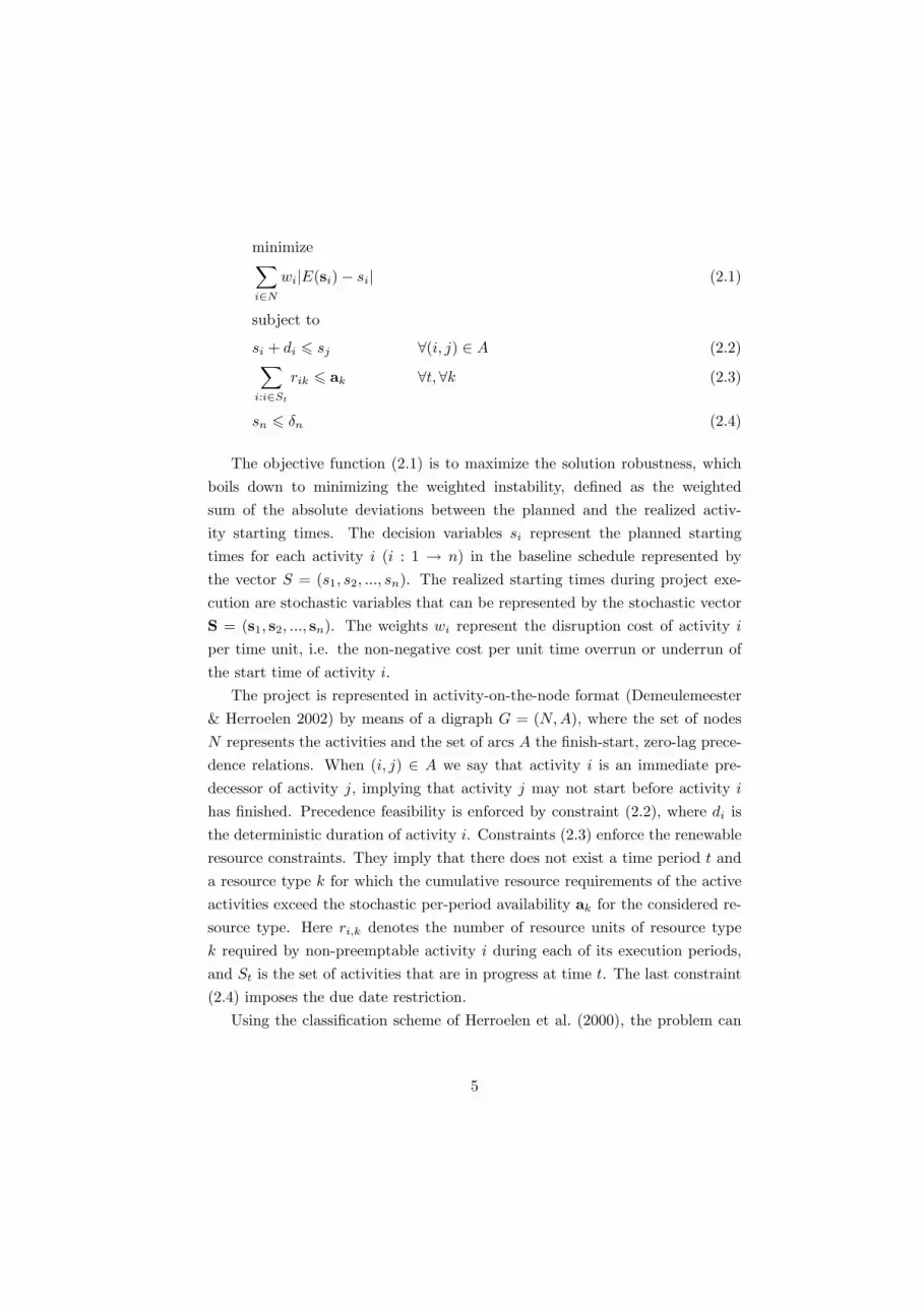
The objective function (2.1) is to maximize the solution robustness, whichboils down to minimizing the weighted instability, defined as the weightedsum of the absolute deviations between the planned and the realized activ-ity starting times. The decision variables si represent the planned startingtimes for each activity i (i : 1 → n) in the baseline schedule represented bythe vector S = (s1, s2, ..., sn). The realized starting times during project exe-cution are stochastic variables that can be represented by the stochastic vectorS = (s1, s2, ..., sn). The weights wi represent the disruption cost of activity i

per time unit, i.e. the non-negative cost per unit time overrun or underrun ofthe start time of activity i.

The project is represented in activity-on-the-node format (Demeulemeester& Herroelen 2002) by means of a digraph G = (N, A), where the set of nodesN represents the activities and the set of arcs A the finish-start, zero-lag prece-dence relations. When (i, j) ∈ A we say that activity i is an immediate pre-decessor of activity j, implying that activity j may not start before activity i

has finished. Precedence feasibility is enforced by constraint (2.2), where di isthe deterministic duration of activity i. Constraints (2.3) enforce the renewableresource constraints. They imply that there does not exist a time period t anda resource type k for which the cumulative resource requirements of the activeactivities exceed the stochastic per-period availability ak for the considered re-source type. Here ri,k denotes the number of resource units of resource typek required by non-preemptable activity i during each of its execution periods,and St is the set of activities that are in progress at time t. The last constraint(2.4) imposes the due date restriction.

Using the classification scheme of Herroelen et al. (2000), the problem can

5

be classified as m, 1,va|cpm, δn|∑

wi|E(si) − si|. The field m, 1,va specifiesthe resource characteristics: an arbitrary number of renewable resource types,each with stochastic availability ak that varies over time. The second fieldindicates the use of finish-start, zero-lag precedence constraints and a deter-ministic project due date. The last field shows the objective function, herethe expected weighted instability cost. The deterministic resource-constrainedproject scheduling problem under the minimum makespan objective is known tobe strongly NP-hard (Blazewicz et al. 1983). Allowing for stochastic resourceavailabilities complicates the problem. Assuming that during project execu-tion activities are never started before their planned starting time, Lambrechtset al. (2006) develop and evaluate eight proactive and three reactive schedulingprocedures for the problem described above.

The analytic evaluation of the objective function is computationally verycumbersome so that Lambrechts et al. (2006) rely on simulation. Furthermore,as argued by Leon et al. (1994), the performance measure is affected by boththe initial baseline schedule, the disruption scenario and the reactive policythat is used to resolve infeasibilities. One way to make the problem workableis to replace the objective function with a surrogate measure that gives a goodestimate of the magnitude of the corresponding instability performance measurebut is easy and quick to calculate. Such a surrogate measure will be presentedin section 3.

3 Surrogate robustness measures

3.1 Sum of free activity slacks

Al-Fawzan & Haouari (2005) have developed a bi-objective model for robustresource-constrained project scheduling when no information regarding the na-ture or size of the uncertain events is available. Their model differs from theone proposed in section 2 insofar that a different objective function is used, nodue date constraint is imposed, resource availabilities are fixed and protection issought against disturbances caused by activity duration variability. Whereas wetry to maximize schedule robustness within a certain given due date, Al-Fawzan& Haouari (2005) aim at the generation of a set of schedules with a high robust-ness zR and a low makespan zM . An aggregation function zλ = λzM−(1−λ)zR,

0 ≤ λ ≤ 1, is introduced to allow the user to trade-off between robustness andmakespan. The authors run a single-objective tabu search procedure for dif-

6

ferent values of λ allowing them to generate an approximate set of efficientsolutions for the bi-objective problem.

The authors measure schedule robustness zR as the sum of the free slacksover all activities. The free slack FSi of activity i is defined as the total amountof time activity i can be delayed without causing any precedence or resourceconstraint violations.

The computation of the free slack for a given schedule can then go as in-dicated in algorithm 1. We assume that an activity can never start before itsbaseline starting time. Therefore, the earliest allowable starting time of activityi, se

i , is equal to its baseline starting time si and likewise, the earliest allowablecompletion time, ce

i , is equal to the baseline completion time ci = si + di. Letsl

i and cli respectively be the latest allowable start time and the latest allowable

completion time of activity i given the due date, the precedence constraints andthe resource constraints and let L′ be the list of activities ordered according tonon-increasing earliest completion times ci (tiebreaker is highest activity num-ber). The free slack of activity i can then be calculated as FSi = sl

i − si. Thelatest allowable completion times cl

i are computed in such a way that duringthe time interval between the earliest possible starting time of activity i, si, andits latest possible completion time, cl

i, the required amount of resource units iscontinuously available. Furthermore, it should be possible to complete activ-ity i up to its latest feasible completion time cl

i without delaying the plannedstart of the immediate successors. This basically means that the start time ofan activity can be shifted within the interval [si, s

li] without jeopardizing the

feasibility of the schedule.Based on the desired properties of the latest feasible activity completion

times, the following backward procedure is introduced in which activities arescheduled in the order of list Ll while respecting both properties as well asthe precedence and resource constraints. The superscript l refers to ’latest’,subscript Ll

(i) denotes the activity in position i of the ordered list Ll, SLl(i)

denotes the immediate successors of the activity in position i of the list, and St

denotes the activities in progress at time t.Consider the example network in figure 1. Above each of the 10 activity

nodes, we indicate the activity’s duration, its resource requirement of a singlerenewable resource type with a per period availability of 8 units and its insta-bility weight. Activities 1 and 10 are dummy activities (with a duration and aresource usage of 0) that are used to indicate the start and end of the project.The instability weight for activity 10 is much larger than the other instability

7

Algorithm 1 Free slack calculation1: sl

n = cln = sn

2: for i = 2 to n do3: cl

L′(i)= min{se

j | j ∈ SL′(i)}

4: slL′(i)

= clL′(i)

− dL′(i)

5: while ∃k, t :∑

j∈St

rj,k > ak (k = 1, ...,m and t = seL′(i)

, ..., clL′(i)

) do

6: slL′(i)

− 1 , clL′(i)

− 1

7: FSL′(i) = slL′(i) − sL′(i)

weights in order to reflect the fact that in practice meeting the project due date isoften deemed far more important than meeting planned activity starting times.In this example we assume a project due date of 18. The baseline starting timeof the dummy start activity is then set to the release date of the project (timeperiod 0) whereas the dummy end activity is assumed to end at the project duedate. Note that for ease of notation and illustration only one resource type isconsidered, but an extension to multiple types is straightforward.

Figure 1: Example project network

Imagine that we calculate the minimal makespan schedule, depicted in figure2, for this project. Given a project deadline of 18, it is easy to see that thisschedule has a total free slack of 6. None of the activities can be shifted to theright except for activities 6 and 9. Of these two, each can be postponed for atmost 3 time units, yielding a total free slack equal to 6. However, this valuecan easily be improved. If we take the schedule in figure 3 we see that activity

8

6 has a free slack of 5, activity 7 a free slack of 7 and activity 9 a free slack of 1time unit. This sums up to an improvement of 7 over the total free slack of theminimal makespan schedule.

Figure 2: Minimal makespan schedule

Figure 3: Improved Schedule

3.2 A new free slack based objective function

In the next section we will describe a tabu search procedure for building robustproject baseline schedules that avoids the use of simulation by using a surrogateobjective function instead of the objective function of equation 2.1. We wouldlike to obtain a schedule in which the start times of activities with a high impacton the total weighted instability are protected as well as possible. This meansthat we want idle times in front of activities with the potential to affect activitieswith a high instability weight when they are postponed.

9

Simply minimizing the sum of free activity slacks as a surrogate stabilityobjective function would assume the contribution of free slack values to theobjective function to be equivalent for each activity whereas our real objec-tive function consists of a weighted sum. Therefore, we suggest the followingsurrogate objective function:

maximize (n∑

i=1

CIWi

FSi∑j=1

e−j)− itnoimprove×max(0, sn − δn)

Instead of taking the sum of free slacks over all activities, we use a free slackutility function for each activity with diminishing returns per extra unit of freeslack that is allocated to that activity. If for example the solution procedurehas the choice between allocating a unit of free slack to activity a, having afree slack of 3 units, or to activity b, having a free slack of 0, it would selectb since this would correspond to an increase in the transformed free slack ofe−1 = 0.36788 whereas this would only be e−4 = 0.018316 for activity a.

Furthermore, we multiply the modified free slack values of each activity i

with its cumulative instability weight CIWi which is calculated by adding theinstability weight of activity i to the instability weights of all of its immediateand transitive successors: CIWi = wi +

∑j:j∈S∗i

wj , where S∗i denotes the set of

direct and indirect successors of activity i. The idea is that if activity i getsdelayed by one time unit, we will for sure experience a cost of wi. The impactof such a delay on the rest of the schedule is harder to predict but it can beapproximated by assuming that all of its successors will also be postponed withone time unit (this would indeed be the case if we assume right-shift reschedulingand if there would be no idle-time between any of the successors).

Finally, we penalize the objective function for the extent to which the duedate constraint is violated, weighted with the number of iterations itnoimprove

used by the tabu search procedure since the last major improvement was found.The reason for this is that temporarily allowing infeasible moves allows for theexploration of a far larger search space. Also note that we decided to assume agiven due date δn instead of generating a set of schedules with a high robustnessand a low makespan. The reason is that in practice the project’s client willusually set a due date the project manager has to stick to.

4 Solution procedure

We use tabu search (Glover & Laguna 1993) as the basis for our solution ap-proach. The reasons are twofold. First of all, tabu search has been applied with

10

success for solving the deterministic RCPSP (Pinson et al. (1994) ,Nonobe &Ibaraki (2002)). Secondly, it is a metaheuristic that is relatively straightforwardto implement and for which not too much parameter-tweaking is needed in orderto obtain good results.

Tabu search is a metaheuristic that aims at overcoming the limitations oftraditional local search techniques. Tabu search as well as local search areboth improvement heuristics that start from an initial solution that is theniteratively improved by performing moves defined on the level of the solutionrepresentation. The main difference is that local search only allows improvingmoves whereas tabu search contains a mechanism for exploring a wider area ofthe search space. Because local search does not try to reach other regions ofthe search space for which non-improving moves would be necessary, it usuallyends up in a local optimum from which it will be impossible to escape, forcingthe procedure to terminate prematurely. Various methods have been proposedto avoid getting stuck in such a local optimum. First of all, one can use severaldifferent starting solutions (iterative local search). Another possibility is to allownon-improving moves with a certain probability that gradually decreases as theprocedure comes to its end (simulated annealing) or to use a pool of solutionsthat are combined so that new solutions are formed (genetic algorithms). Tabusearch, on the other hand, tries to overcome the traditional drawback of localsearch by systematically imposing and releasing constraints in order to allowfor the exploration of regions in the search space that would otherwise notbe explored. More specifically, a tabu list is used in which moves are storedthat are forbidden for a number of iterations. The underlying idea is that onewishes to avoid cycling in order to guide the search process to explore otherwisedifficult regions and this can be realized by forbidding moves that revert toprior solutions for a certain time period. In this section we will give the exactdetails of our tabu search algorithm and illustrate the procedure by means ofpseudocode and an example.

4.1 Solution Representation

As we stated in section 2, a solution for the robustness problem can be repre-sented by means of a vector S = (s1, s2, ..., sn) containing the starting times si

for each activity i. However, such a representation suffers from the drawbackthat every time the starting time of one or more activities is changed, we willneed to check the feasibility of the schedule by evaluating each individual prece-

11

dence and resource constraint. This would lead to a computationally very costlymove evaluation. A better alternative would be to use a shift vector (Sampson& Weiss 1993) , indicating how many time units an activity is started beyondits earliest precedence feasible starting time. Unfortunately, while avoiding theprecedence constraint checking, we are still stuck with the resource constraints.Therefore we use the well-known priority list representation.

In the priority list representation a solution is represented by means of anordered list of activities L. This ordering has to be precedence feasible, whichmeans that no activity appears earlier in the list than its predecessors. Thelist can be decoded into a feasible schedule by means of a schedule generationscheme. Usually the serial schedule generation scheme is used (Kelley 1963).This implies that activities are scheduled in time according to the order dictatedby the priority list. Each activity is scheduled at its earliest possible startingtime so that no resource or precedence constraints are violated. However, thisapproach greatly restricts the search space because only active schedules canbe considered. Active schedules are schedules in which no local or global leftshift can be performed (Demeulemeester & Herroelen 2002). Local left shiftsare possible when we can schedule an activity a number of periods earlier intime and if every intermediate schedule (obtained by repetitively decreasingthe starting time of the considered activity with one time unit) is feasible.Global left shifts, on the other hand, are comparable but here at least oneintermediate schedule violates the resource constraints. All of this implies thata serial schedule generation scheme based on a priority list representation doesnot allow for the generation of schedules with inserted idle time.

Inserting slack into a baseline schedule offers protection against anticipateddisruptions during project execution such as resource breakdowns (Lambrechtset al. 2006). Therefore, we present a new approach extending the traditionalpriority list representation by including a buffer list representation. The bufferlist B indicates which activities should be buffered and by how much theirstarting times should be extended beyond their earliest starting time as dictatedby the serial schedule generation scheme. The decoding approach to transforma solution represented by the combination of a priority list and a buffer list intoa feasible schedule is an extension of the serial schedule generation scheme andis described in algorithm 2 in which the subscript L(p) denotes the activity inthe pth position of list L, and PL(p) represents the set of immediate predecessorsof the activity in the pth position of list L.

12

Algorithm 2 Decoding procedure1: sL(1) = s0 = 02: for p = 2 to n do3: sL(p) = maxj∈PL(p)

(sj + dj)4: while ∃k, t :

∑j∈St

rj,k > ak do

5: sL(p) + 16: sL(p) + BL(p)

7: while ∃k, t :∑

j∈St

rj,k > ak do

8: sL(p) + 19: sn = max(sn, δn)

4.2 Solution space

The neighbourhood N(x, σ) of a solution x can be defined as the set of solutionsthat can be reached from x by means of an operation σ, called a move. Intraditional steepest-descent local search, the neighbour with the best objectivefunction value will be chosen. In case no neighbour can be found with an ob-jective function value that is better than the current solution x, we call x alocal optimum with respect to the neighbourhood structure N(x, σ) (Glover &Laguna 1993). Of course, the moves that can be performed on a solution, andtherefore the neighbourhood structure, will depend on the solution representa-tion.

As we stated in section 4.1, we use a priority list L coupled with a bufferlist B. Two neighbourhoods will be defined, one for each list representation.For the priority list we use the commonly used precedence feasible swap. Theprecedence feasible swap will evaluate the interchange of any two positions i andj in list L (i < j) while respecting the precedence feasibility of the list. For thebuffer list, we consider an increase of the buffer length Bi for each activity witha discrete value between −∆ and +∆. Because we cannot buffer an activitywith a negative length, we require that Bi > 0. Note that we allow ∆ to varyas the procedure evolves. Normally, we set ∆ = 1 but after a large number ofiterations with no improvement, it might be better to use a higher value for ∆.Therefore, we set ∆ = 3 after 5 iterations without an improvement and ∆ = 5after 10 iterations in which no better solution was found.

Because it would be computationally very cumbersome to analyze everycombination of each priority list move and each buffer list move in each iteration,we work with separate iterations. In iteration type I we consider moves in the

13

priority list neighbourhood whereas in iteration type II we consider moves inthe buffer list neighbourhood. We alternate the iterations in which we considereach iteration type. First, we consider nI iterations of type I, then nII iterationsof type II. When the set of nI + nII iterations is finished, we start again withan iteration of type I.

4.3 Selection scheme

In each iteration we select the neighbour solution with the best objective func-tion value. Note that in case the move leading to this solution would belongto the tabu list, this move will be overridden. An exception is made when theimproving move is tabu but would lead to a better solution than the best solu-tion that has been found so far. This exception is called the aspiration criterionand results in overriding the tabu classification for the considered move. Af-ter performing the chosen move, we will label it as tabu, our aim being thatthe solution procedure does not return too quickly to the last visited solution.Therefore, when considering an iteration of type I, we classify those moves astabu that result in starting activity i at time si and activity j at time sj . Morespecifically, this means that if we just executed the precedence feasible swap ofactivity in position i in list L (denoted as L(i)) with the activity in position j oflist L (L(j)) then we store the iteration up to which moves resulting in activityL(i) starting at time sL(i) and activity L(j) starting at time sL(j) are forbiddenin the variables tabuL(i),sL(i)

and tabuL(j),sL(j). On the other hand, when con-

sidering an iteration of type II, we add the move that returns to a buffer lengthBi for activity i to the tabu list represented by the variables tabui,Bi .

Note that in order not to overly restrict the search space, the due dateconstraint is transformed into a soft constraint that penalizes the objectivefunction for the amount by which the due date is exceeded, multiplied with afactor accounting for the number of iterations that no improving solution wasfound (see section 3). Therefore, all precedence feasible, non-tabu swaps as wellas all non-tabu buffer size changes that correspond to positive buffer values canbe considered without constantly having to check due date feasibility.

4.4 Pseudocode

In algorithm 3 we give the pseudocode for our tabu search algorithm. Note thatwe use the minimal makespan schedule as the starting solution. This scheduleis then encoded using the priority list representation and stored in list L. L

14

is obtained by sorting the activities according to increasing starting times, asa tie-breaker we use the lowest activity number. The corresponding buffer listB is set equal to the minimal buffer list, implying a zero buffer length forevery activity. The corresponding value of the objective function is obtainedby using the function f(L,B) and is stored in O. The vectors L∗and B∗ areused to indicate the solution leading to the best objective function value O∗

obtained so far. L′ and B′, on the other hand, correspond to the solutionyielding the best objective function value O′ found in the current iteration. Thetabu tenure T , the current iteration it and the number of iterations since thelast improvement of O∗ are initialized at the beginning of the algorithm. Theprocedure sequentially searches in neighbourhoods of type I and type II asindicated by the user-defined values nI and nII , it is terminated after havingbeen executed for a preset time period tMAX .

4.5 Example

It might be illustrative to look at two iterations (one of each type) of thealgorithm applied to the problem instance we introduced in figure ??. Thestarting schedule depicted in figure 4 was constructed using the priority listL=(1,2,3,5,4,6,7,8,9,10) and an empty buffer list.

Figure 4: L=(1,2,3,5,4,6,7,8,9,10) & B=(0,0,0,0,0,0,0,0,0,0)

The corresponding objective function value is equal to 41.1 and was calcu-lated as shown in table 1.

15

Algorithm 3 TS heuristic for generating robust baseline schedules1: set L∗ = L , B∗ = B , O∗ = O , T = n , it = 0 , itnoimprove = 02: while (duration < tMAX) do3: for n = 1 to nI do4: set O′ = −999999, it + 15: for i = 2 to n− 2 , for j = i + 1 to n− 1 do6: swap L(i) and L(j) if precedence feasible7: if O = f(B, L) > O′ then8: if (O > O∗ & sn 6 δn) OR (it > tabuL(i),sL(i)

& it > tabuL(j),sL(j))

then9: store i → i′ , j → j′ , O → O′

10: undo swap11: if ∃i′ & ∃j′ then12: swap L(i′) and L(j′)13: tabuL(i′),sL(i′)

= tabuL(j′),sL(j′)= it + T

14: if O′ > O∗ & sn < δn then15: O∗ = O′ , L∗ = L , itnoimprove = 016: else17: itnoimprove + 118: for n = 1 to nII do19: set O′ = −999999, it + 120: set ∆ based on itnoimprove21: for i = 2 to n− 1 , for b = −∆ to ∆ do22: increase Bi with b if Bi + b > 023: if O = f(B, L) > O′ then24: if (O > O∗ & sn 6 δn) OR it > tabui,Bi then25: store i → i′ , b → b′ ,O → O′

26: undo move27: if ∃i′ & ∃b′ then28: Bi = Bi + b′

29: tabui′,Bi = it + T30: if O′ > O∗ & sn < δn then31: O∗ = O′ , B∗ = B , itnoimprove = 032: else33: itnoimprove + 1

16

Table 1: Calculation of the modified objective function

activity FS∑

e−FS CIW CIW ∗∑e−FS

1 0 0 102 02 0 0 73 03 0 0 54 04 0 0 58 05 0 0 57 06 1 0.37 47 17.37 0 0 39 08 0 0 44 09 3 0.55 43 23.810 0 0 38 0

41.1

In iteration I we try to find out if there exists a non-tabu precedence feasibleswap in list L resulting in an improvement of the objective function. Apparentlyswapping activities 4 and 5 allows us to obtain this improvement resulting in theschedule in figure 5 with an objective function value equal to 59.5 (calculatedas above).

Figure 5: L=(1,2,3,4,5,6,7,8,9,10) & B=(0,0,0,0,0,0,0,0,0,0)

Besides swapping activities in the priority list L it is also possible to manipu-late the buffer list. This is exactly what happens in iteration type II. Considerfor example an increase of the buffer length assigned to activity 4 with one unit.We obtain the schedule in figure 6 with an improved solution value of 78.5.

17

Figure 6: L =(1,2,3,4,5,6,7,8,9,10) & B=(0,0,0,1,0,0,0,0,0,0)

5 Results

5.1 Experiment

We implemented the algorithms in Microsoft Visual C++ 6.0 and executedthem on a Dell Optiplex GX270 workstation. Simulation was used in order toevaluate the weighted instability objective function

∑i∈N

wi|E(si)− si|. The aim

of our experiment is not only to compare the impact of the surrogate objectivefunctions - i.e., the sum of free activity slacks and the modified sum of freeactivity slacks - and the impact of the solution solution representation - i.e., thepriority list and the priority and buffer list -, but also to validate the performanceof the metaheuristic approach developed in this paper against the dedicatedalgorithms developed by Lambrechts et al. (2006).

The dedicated algorithms of Lambrechts et al. (2006) are based on a proac-tive baseline generation process in which three choices need to be made. Firstof all, one has to decide whether to start from a minimal makespan schedulethat is short but usually also very dense and therefore prone to disruption oralternatively, from a schedule in which activities with a high impact on totalproject instability are scheduled as early as possible in time (’largest CIW first ’)in order to decrease the probability that these activities get disrupted due to thedisruption of an activity earlier in the schedule. Secondly, it has to be decidedwhether to apply resource buffering to this initial schedule. Resource bufferingboils down to planning the project using a resource availability that is lower thanthe actual resource availability. Since we assume that uncertainty is modeled bymeans of resources that are subject to random breakdowns, using less resources

18

per time unit than the maximal availability can prevent the negative impactof these breakdowns. Finally, time buffering can be added. This implies thatwe explicitly insert idle time into the schedule based on the estimated size andimpact of activity disturbances on the objective function. In the end, this givesus a total of 23 different strategies. It can be expected that resource bufferingand time buffering will outperform our metaheuristic because both approachesuse specific information regarding uncertainties that can be encountered duringproject execution. More specifically, they exploit the information that resourcebreakdowns are modeled using exponential distributions for the time betweenfailures and the time between resource repairs. Using exponential distributionsfor resource breakdowns is correct (Lambrechts et al. 2006) but also practicalbecause the distributions are fully specified for each resource type k by meansof respectively the mean time to failure (MTTFk) and the mean time to repair(MTTRk).

As we indicated in section 1, we also need to specify the type of reactive pol-icy used when the schedule breaks. Three reactive strategies are suggested thatrely on activity lists that are decoded into feasible schedules using an adaptedversion of the serial scheduling scheme that takes non-constant resource avail-abilities into account. The first reactive strategy is based on a random list, thesecond one is based on the list that corresponds to the initial baseline sched-ule and the third is based on the same list after applying a tabu search basedimprovement heuristic to it in order to obtain a schedule that is closer to thebaseline schedule. For a detailed explanation of these reactive strategies, weagain refer the reader to Lambrechts et al. (2006). It is also important to ob-serve that we assume railway-scheduling in our experiment. This means thatan activity is never started earlier than its planned baseline start time, evenwhen the possibility to do so surfaces. This decision can be justified becauseschedule stability is often very important in practice. Starting activities earlierthan planned complicates agreements that were made in advance with suppli-ers or subcontractors and decreases insight in the execution of the project byemployees.

As a test set for assessing the effectiveness of all these strategies, we usethe 480 30-activity RCPSP instances of the well-known PSPLIB set of testproblems (Kolisch & Sprecher 1997). Each combination of a proactive policy anda reactive policy was tested using 10 replications for each problem instance. Weset the maximum search length of the tabu search procedure used for generatinga robust schedule to 10 seconds. The instability weights wi for all non-dummy

19

activities are drawn from a discrete, triangularly shaped distribution between 1and 10 with P (wi = x) = 0.21−0.02x. Corresponding to what can be expectedin real-life projects, most activities will have a low instability weight whereasonly a minority are more heavily penalized for being started later than planned.The instability weight of the dummy end activity represents the importance ofmeeting the projected due date and is set equal to β times the average of theinstability weight distribution function, which is 3.85 for P (wi = x). Becauseusually meeting the project due date is far more critical than starting eachactivity at the planned starting time, we set β = 10 for our experiment. Theproject due date is derived from the minimal makespan schedule obtained usingthe branch-and-bound algorithm developed by Demeulemeester and Herroelen(1992), (1997). In a static and deterministic environment, this lower bound onthe makespan (CRCPSP

max ) corresponds to the length of the minimum durationschedule obtained when optimally solving the RCPSP. It seems reasonable toassume that the project manager will prefer a makespan that does not deviatetoo much from this lower bound. Therefore, we set the due date of the robustschedule at CRCPSP

max (1+α), where the due date factor α is a parameter chosen bythe project manager that constitutes the trade-off between project stability andproject duration (Van de Vonder et al. 2005). Finally, we draw the MTTRk

values from a uniform discrete distribution between 1 and 5. The values forMTTFk are drawn from a uniform discrete distribution between 50% and 150%of CRCPSP

max .

5.2 Computational Results

The results in table 2 provide an overview of the relative performance of thealgorithms. The results were obtained for a due date setting α = 30% andterminating the tabu search procedure for generating robust schedules after 10seconds. We list the median values of the weighted instability objective functionvalues obtained over all projects and MTTF-MTTR scenarios for the proac-tive scheduling strategies (time buffering or not, resource buffering or not, incombination with a minimum makespan schedule or a schedule obtained usingthe ’largest CIW first ’ rule, or alternatively the algorithms based on surrogatemeasures that were proposed in this paper) in combination with the three re-active procedures (random list scheduling, scheduled order list scheduling andtabu search). The numbers shown in italic in the last column give the averageweighted instability cost values for each of the proactive scheduling rules, the

20

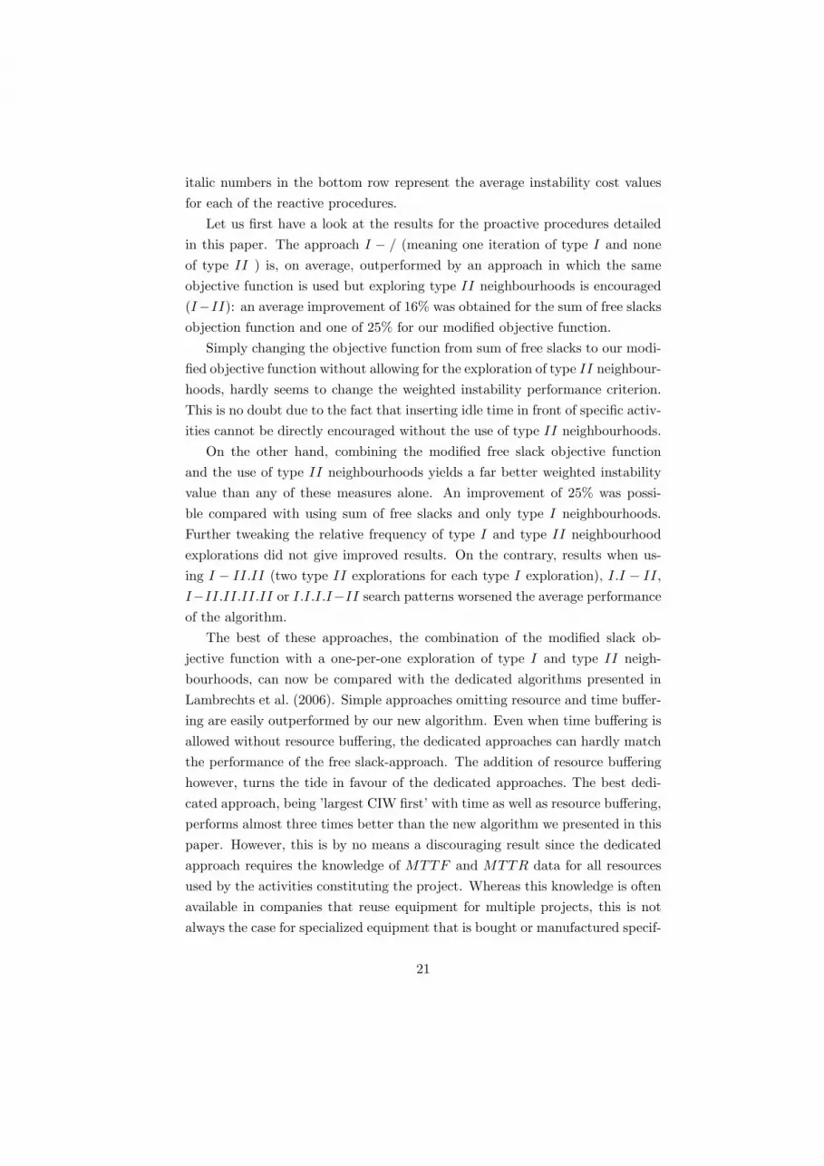
italic numbers in the bottom row represent the average instability cost valuesfor each of the reactive procedures.

Let us first have a look at the results for the proactive procedures detailedin this paper. The approach I − / (meaning one iteration of type I and noneof type II ) is, on average, outperformed by an approach in which the sameobjective function is used but exploring type II neighbourhoods is encouraged(I−II): an average improvement of 16% was obtained for the sum of free slacksobjection function and one of 25% for our modified objective function.

Simply changing the objective function from sum of free slacks to our modi-fied objective function without allowing for the exploration of type II neighbour-hoods, hardly seems to change the weighted instability performance criterion.This is no doubt due to the fact that inserting idle time in front of specific activ-ities cannot be directly encouraged without the use of type II neighbourhoods.

On the other hand, combining the modified free slack objective functionand the use of type II neighbourhoods yields a far better weighted instabilityvalue than any of these measures alone. An improvement of 25% was possi-ble compared with using sum of free slacks and only type I neighbourhoods.Further tweaking the relative frequency of type I and type II neighbourhoodexplorations did not give improved results. On the contrary, results when us-ing I − II.II (two type II explorations for each type I exploration), I.I − II,I−II.II.II.II or I.I.I.I−II search patterns worsened the average performanceof the algorithm.

The best of these approaches, the combination of the modified slack ob-jective function with a one-per-one exploration of type I and type II neigh-bourhoods, can now be compared with the dedicated algorithms presented inLambrechts et al. (2006). Simple approaches omitting resource and time buffer-ing are easily outperformed by our new algorithm. Even when time buffering isallowed without resource buffering, the dedicated approaches can hardly matchthe performance of the free slack-approach. The addition of resource bufferinghowever, turns the tide in favour of the dedicated approaches. The best dedi-cated approach, being ’largest CIW first’ with time as well as resource buffering,performs almost three times better than the new algorithm we presented in thispaper. However, this is by no means a discouraging result since the dedicatedapproach requires the knowledge of MTTF and MTTR data for all resourcesused by the activities constituting the project. Whereas this knowledge is oftenavailable in companies that reuse equipment for multiple projects, this is notalways the case for specialized equipment that is bought or manufactured specif-

21

ically for a certain project. For those project settings, dedicated approachescannot be used and the algorithm we present in this paper can offer a good basefor constructing a robust schedule.

When looking at the impact of the reactive strategies, the results are hardlysurprising. As Lambrechts et al. (2006) already concluded, a significant per-formance gain is possible when using the more intelligent scheduled order ruleinstead of the random list strategy. These results can be further improved bysuperimposing a tabu search on the scheduled ordered list.

Table 2: Average weighted instability values

random

list

schedule

dorder

tabu

search

no timebuffering

no resourcebuffering

min Cmax 1109.46 286.85 241.20 545.84

CIW ↘ 1025.76 244.30 194.80 488.29

resourcebuffering

min Cmax 483.73 102.40 89.70 225.28

CIW ↘ 416.95 81.30 66.80 188.35

timebuffering

no resourcebuffering

min Cmax 812.51 115.20 100.70 342.80

CIW ↘ 759.96 112.10 99.50 323.85

resourcebuffering

min Cmax 325.91 41.95 36.60 134.82

CIW ↘ 308.71 45.70 42.50 132.30

surrogatemeasures

sum of freeslacks

I-/ 869.55 237.60 166.45 424.53

I-II 792.85 156.90 118.40 356.05

modifiedobjectivefunction

I-/ 899.70 217.55 158.85 425.37

I-II 761.35 109.55 88.75 319.88

I-II.II 806.30 112.30 90.80 336.47

I.I-II 785.20 101.40 88.70 325.10

I-II.II.II.II 773.15 103.55 90.75 322.48

I.I.I.I-II 829.90 101.55 84.80 338.75

735.06 135.64 109.96

6 Conclusion

In this paper we presented an approach for building robust project baselineschedules when information regarding the nature and size of uncertain occur-rences during project execution is costly or impossible to obtain. Constructingrobust schedules is critical in a practical setting because often work is subcon-

22

tracted or promises towards clients need to be met implying that it is importantthat the realized schedule does not differ too much from the originally plannedschedule.

Our procedure is based on the tabu search framework and uses a doubleneighbourhood structure to allow for the generation of feasible project sched-ules that respect precedence, resource and due date constraints and includeexplicitly inserted idle time for protecting activities that have a high impact onthe weighted sum of absolute deviations between planned and observed activitystarting times.

By means of a computational simulation experiment it was shown that ourprocedure performs very well for the weighted instability objective function.A comparable approach using a more traditional objective function and notallowing explicitly inserted idle time is easily outperformed. Furthermore, evenwhen compared with dedicated approaches that use a simple time bufferingheuristic, our procedure seems to hold up solidly.

An interesting direction for further research would be the development of anexact algorithm for proactive/reactive project scheduling under resource uncer-tainties.

7 Acknowledgement

This research has been partially supported by project OT/03/14 of the ResearchFund of K.U.Leuven and project G.0109.04 of the Research Programme of theFund for Scientific Research - Flanders (Belgium) (F.W.O.-Vlaanderen)

References

Abumaizar, R. & Svestka, J. (1997). Rescheduling job shops under randomdisruptions. International Journal of Production Research, 35(7), pp 2065–2082.

Al-Fawzan, M. A. & Haouari, M. (2005). A bi-objective model for robustresource-constrained project scheduling. International Journal of Produc-tion Economics, 96, pp 175–187.

23

Aytug, H., Lawley, M., McKay, K., Mohan, S. & Uzoy, R. (2005). Executingproduction schedules in the face of uncertainties: A review and some futuredirections. European Journal of Operational Research, 161, pp 86–110.

Blazewicz, J., Lenstra, J. & Rinnooy, A. (1983). Scheduling subject to resourceconstraints - Classification and complexity. Discrete Applied Mathematics,5, pp 11–24.

Brucker, P. (2004). Scheduling Algorithms - 4th edition. Springer, Berlin.

Brucker, P., Drexl, A., Mohring, R., Neumann, K. & Pesch, E. (1999). Resource-constrained project scheduling: Notation, classification, models and meth-ods. European Journal of Operational Research, 112, pp 3–41.

Davenport, A. & Beck, J. (2002). A survey of techniques for scheduling withuncertainty. Unpublished manuscript.

Demeulemeester, E. & Herroelen, W. (1992). A branch-and-bound procedure forthe multiple resource-constrained project scheduling problem. ManagementScience, 38, pp 1803–1818.

Demeulemeester, E. & Herroelen, W. (1997). New benchmark results forthe resource-constrained project scheduling problem. Management Science,43, pp 1485–1492.

Demeulemeester, E. & Herroelen, W. (2002). Project scheduling - A researchhandbook. Vol. 49 of International Series in Operations Research & Man-agement Science. Kluwer Academic Publishers, Boston.

Drezet, L.-E. (2005). Resolution d’un probleme de gestion de projets souscontraintes de ressources humaines: De l’approche predictive l’approchereactive. PhD thesis. Universite Francois Rabelais Tours, France.

Glover, F. & Laguna, M. (1993). Tabu Search. Blackwell Scientific, Oxford.pp 70–141. In C. Reeves (Editor): Modern Heuristic Techniques for Com-binatorial Problems.

Herroelen, W., De Reyck, B. & Demeulemeester, E. (1998). Resource-constrained scheduling: A survey of recent developments. Computers andOperations Research, 25, pp 279–302.

24

Herroelen, W., De Reyck, B. & Demeulemeester, E. (2000). On the paper”Resource-constrained project scheduling: Notation, classification, modelsand methods” by Brucker et al.. European Journal of Operations Research,128(3), pp 221–230.

Kelley, J. J. (1963). The Critical-Path Method: Resources Planning and Schedul-ing. Prentice Hall, Englewood Cliffs. pp 347–365. In Muth, J.F. and G.L.Thompson (Eds): Industrial Scheduling.

Kolisch, R. & Sprecher, A. (1997). PSPLIB - A project scheduling library.European Journal of Operational Research, 96, pp 205–216.

Lambrechts, O., Demeulemeester, E. & Herroelen, W. (2006). Proactive andreactive strategies for the resource-constrained project scheduling problemwith uncertain resource availabilities. Working paper, to appear.

Leon, V., Wu, S. & Storer, R. (1994). Robustness measures and robust schedul-ing for job shops. IIE Transactions, 26(5), pp 32–43.

Leus, R. & Herroelen, W. (2002). The complexity of generating robust resource-constrained baseline schedules. Research Report 0250. Department of ap-plied economics, Katholieke Universiteit Leuven.

Leus, R. & Herroelen, W. (2004). Stability and resource allocation in projectplanning. IIE transactions, 36(7), pp 1–16.

Mehta, S. & Uzsoy, R. (1998). Predictive scheduling of a job shop subject tobreakdowns. IEEE Transactions on Robotics and Automation, 14, pp 365–378.

Mehta, S. & Uzsoy, R. (1999). Predictable scheduling of a single machine subjectto breakdowns. International Jounal of Computer Integrated Manufactur-ing, 12, pp 15–38.

Nonobe, K. & Ibaraki, T. (2002). Formulation and tabu search algorithm for theresource constrained project scheduling problem. Kluwer Academic Publish-ers, Dordrecht. pp 557–588. In Ribeiro, C., Hansen, P. (Eds.), Essays andsurveys in metaheuristics.

O’Donovan, R., Uzsoy, R. & McKay, K. (1999). Predictable scheduling of asingle machine with breakdowns and sensitive jobs. International Journalof Production Research, 37, pp 4217–4233.

25

Pinedo, M. (1995). Scheduling - Theory, Algorithms and Systems. Prentice Hall,Englewood Cliffs, New Jersey.

Pinson, E., Prins, C. & Rullier, F. (1994). Using tabu search for solvingthe resource-constrained project scheduling problem. Fourth InternationalWorkshop on Project Management and Scheduling. Euro Working Groupon Project Management and Scheduling. pp 102–106.

Sampson, S. & Weiss, E. (1993). Local search techniques for the generalizedresource constrained project scheduling problem. Naval Research Logistics,40, pp 665–675.

Stork, F. (2001). Stochastic Resource-Constrained Project Scheduling. PhD the-sis. Technical University of Berlin, School of Mathematics and NaturalSciences.

Van de Vonder, S., Demeulemeester, E., Herroelen, W. & Leus, R. (2005). Theuse of buffers in project management: The trade-off between stability andmakespan. International Journal of Production Economics, 97, pp 227–240.

Vieira, G., Herrmann, J. & Lin, E. (2003). Rescheduling manufacturing systems:A framework of strategies, policies, and methods. Journal of Scheduling,6(1), pp 39–62.

Yu, G. & Qi, X. (2004). Disruption Management. World Scientific, New Jersey.

26