A

Ss

Sa

b

a

ARRAA

KPSMG

1

mirtWtgmdab

1d

ARTICLE IN PRESSG ModelSOC-958; No. of Pages 14

Applied Soft Computing xxx (2010) xxx–xxx

Contents lists available at ScienceDirect

Applied Soft Computing

journa l homepage: www.e lsev ier .com/ locate /asoc

tochastic approximation driven particle swarm optimization withimultaneous perturbation – Who will guide the guide?

erkan Kiranyaza,∗, Turker Inceb, Moncef Gabbouja

Tampere University of Technology, Department of Signal Processing, P.O. Box 553, FIN-33101, Tampere, FinlandIzmir University of Economics, Department of Electronics and Telecommunications Engineering, TR-35330, Izmir, Turkey

r t i c l e i n f o

rticle history:eceived 19 February 2010eceived in revised form 10 May 2010ccepted 12 July 2010vailable online xxx

eywords:article swarm optimizationtochastic approximationulti-dimensional searchradient descent

a b s t r a c t

The need for solving multi-modal optimization problems in high dimensions is pervasive in many prac-tical applications. Particle swarm optimization (PSO) is attracting an ever-growing attention and morethan ever it has found many application areas for many challenging optimization problems. It is, however,a known fact that PSO has a severe drawback in the update of its global best (gbest) particle, which has acrucial role of guiding the rest of the swarm. In this paper, we propose two efficient solutions to remedythis problem using a stochastic approximation (SA) technique. In the first approach, gbest is updated(moved) with respect to a global estimation of the gradient of the underlying (error) surface or functionand hence can avoid getting trapped into a local optimum. The second approach is based on the formationof an alternative or artificial global best particle, the so-called aGB, which can replace the native gbestparticle for a better guidance, the decision of which is held by a fair competition between the two. Forthis purpose we use simultaneous perturbation stochastic approximation (SPSA) for its low cost. SinceSPSA is applied only to the gbest (not to the entire swarm), both approaches result thus in a negligibleoverhead cost for the entire PSO process. Both approaches are shown to significantly improve the perfor-mance of PSO over a wide range of non-linear functions, especially if SPSA parameters are well selectedto fit the problem at hand. A major finding of the paper is that even if the SPSA parameters are not tuned

well, results of SA-driven (SAD) PSO are still better than the best of PSO and SPSA. Since the problemof poor gbest update persists in the recently proposed extension of PSO, called multi-dimensional PSO(MD-PSO), both approaches are also integrated into MD-PSO and tested over a set of unsupervised dataclustering applications. As in the basic PSO application, experimental results show that the proposedapproaches significantly improved the quality of the MD-PSO clustering as measured by a validity index

e prorange

function. Furthermore, thand applicable to a wide

. Introduction

The Merriam Webster dictionary defines optimization as theathematical procedures (as finding the maximum of a function)

nvolved in this. More specifically, consider the problem of finding aoot �* (either minimum or maximum point) of the gradient equa-ion: g(�) ≡ ∂ L(�)/∂ � = 0 for some differentiable function L : Rp → R1.

hen g is present and L is a differentiable and uni-modal func-ion, there are powerful deterministic methods for finding thelobal �*such as traditional steepest descent and Newton-Raphson

Please cite this article in press as: S. Kiranyaz, et al., Stochastic approperturbation – Who will guide the guide?, Appl. Soft Comput. J. (2010),

ethods. However, in many real problems g cannot be observedirectly and/or L is multi-modal, in which case the aforementionedpproaches may be trapped into some deceiving local optima. Thisrought the era of the stochastic optimization algorithms, which

∗ Corresponding author.E-mail address: serkan@cs.tut.fi (S. Kiranyaz).

568-4946/$ – see front matter © 2010 Elsevier B.V. All rights reserved.oi:10.1016/j.asoc.2010.07.022

posed approaches are generic as they can be used with other PSO variantsof problems.

© 2010 Elsevier B.V. All rights reserved.

can estimate the gradient and may avoid being trapped into a localoptimum due to their stochastic nature. One of the most popu-lar stochastic optimization techniques is stochastic approximation(SA), in particular the form that is called “gradient free” SA. Amongmany SA variants proposed by several researchers such as Styblin-ski and Tang [37], Kushner [25], Gelfand and Mitter [13], and Chin[6], the one and somewhat different SA application is called simul-taneous perturbation SA (SPSA) proposed by Spall in 1992 [35]. Themain advantage of SPSA is that it often achieves a much more eco-nomical operation in terms of loss function evaluations, which areusually the most computationally intensive part of an optimizationprocess.

Particle swarm optimization (PSO) was introduced by Kennedy

ximation driven particle swarm optimization with simultaneousdoi:10.1016/j.asoc.2010.07.022

and Eberhart [20] in 1995 as a population based stochastic searchand optimization process. It is originated from the computer simu-lation of the individuals (particles or living organisms) in a bird flockor fish school [42], which basically show a natural behavior whenthey search for some target (e.g. food). Henceforth, PSO exhibits

INA

2 ft Com

c[[(mhpttsatpcbSopacBp

sastpTmtgiHicd[iipnsetabtrngchtnrT

sofettdi

ARTICLEG ModelSOC-958; No. of Pages 14

S. Kiranyaz et al. / Applied So

ertain similarities with the other evolutionary algorithms (EAs)4] such as genetic algorithm (GA) [14], genetic programming (GP)24], evolution strategies (ES) [5], and evolutionary programmingEP) [11]. The common point of all is that EAs are population based

ethods and they may avoid being trapped in a local optimum;owever, this is never guaranteed. In a PSO process, a swarm ofarticles (or agents), each of which represent a potential solutiono an optimization problem; navigate through the search (or solu-ion) space. The particles are initially distributed randomly over theearch space and the goal is to converge to the global optimum offunction or a system. Each particle keeps track of its position in

he search space and its best solution so far achieved. This is theersonal best position (the so-called pbest in [20]) and the PSO pro-ess also keeps track of the global best (GB) solution so far achievedy the swarm with its particle index (the so-called gbest in [20]).o during their journey with discrete time iterations, the velocityf each particle in the next iteration is computed by using the bestosition of the swarm (personal best position of the particle gbests the social component), its personal best position (pbest as theognitive component), and its current velocity (the memory term).oth social and cognitive components contribute randomly to theosition of the particle in the next iteration.

As a stochastic search algorithm in multi-dimensional (MD)earch space, PSO exhibits some major problems similar to theforementioned EAs. The first one is due to the fact that anytochastic optimization technique depends on the parameters ofhe optimization problem where it is applied and variation of thesearameters significantly affects the performance of the algorithm.his problem is a crucial one for PSO where parameter variationsay result in large performance shifts [26]. The second one is due

o the direct link of the information flow between particles andbest, which then “guides” the rest of the swarm and thus result-ng in the creation of similar particles with some loss of diversity.ence this phenomenon increases the likelihood of being trapped

n local optima [32] and it is the main cause of the prematureonvergence problem especially when the search space is of highimensions [40] and the problem to be optimized is multi-modal32]. Therefore, at any iteration of a PSO process, gbest is the mostmportant particle; however, it has the poorest update equation,.e. when a particle becomes gbest, it resides on its personal bestosition (pbest) and thus both social and cognitive components areullified in the velocity update equation. Although it guides thewarm during the following iterations, ironically it lacks the nec-ssary guidance to do so effectively. In that, if gbest is (likely to get)rapped in a local optimum, so is the rest of the swarm due to theforementioned direct link of information flow. This deficiency haseen raised in a recent work [22] where an artificial GB particle,he aGB, is created at each iteration as an alternative to gbest, andeplaces the native gbest particle as long as it achieves a better fit-ess score. In that study, it has been shown that such an enhanceduidance alone is indeed sufficient in most cases to achieve globalonvergence performance on multi-modal functions and even inigh dimensions. However, the underlying mechanism for creatinghe aGB particle, the so-called fractional GB formation (FGBF), isot generic in the sense that it is rather problem dependent, whichequires (the estimate of) individual dimensional fitness scores.his may be quite hard or infeasible for certain problems.

In order to address this drawback efficiently, in this paper wehall propose two approaches. The first one moves gbest efficientlyr simply put, guides it with respect to the function (or error sur-ace). The idea behind this is quite simple: since the velocity update

Please cite this article in press as: S. Kiranyaz, et al., Stochastic approperturbation – Who will guide the guide?, Appl. Soft Comput. J. (2010),

quation of gbest is quite poor, SPSA as a simple yet powerful searchechnique is used to drive it instead. Due to its stochastic naturehe likelihood of getting trapped into a local optimum is furtherecreased and with the SA, gbest is driven according to (an approx-

mation of) the gradient of the function. The second approach has

PRESSputing xxx (2010) xxx–xxx

a similar idea with the FGBF proposed in [22], i.e. an aGB particleis created by SPSA this time, which is applied over the personalbest (pbest) position of the gbest particle. The aGB particle will thenguide the swarm instead of gbest if and only if it achieves a betterfitness score than the (personal best position of) gbest. Note thatboth approaches only deal with the gbest particle and hence theinternal PSO process remains as is. That is, neither of the proposedapproaches is a PSO variant by itself; rather a solution for the prob-lem of the original PSO caused by poor gbest update. Furthermore,we shall demonstrate that the proposed approaches have a negligi-ble computational cost overhead, e.g. only few percent increase ofthe computational complexity, which can be easily compensatedwith a slight reduction either in the swarm size or in the iterationnumber. Both approaches of SA-driven PSO (SAD PSO) will be testedand evaluated against the basic PSO (bPSO) over several benchmarkuni- and multi-modal functions in high dimensions. Moreover, theyare also applied to the multi-dimensional extension of PSO, theMD-PSO technique proposed in [22], which can find the optimumdimension of the solution space and hence voids the need of fixingthe dimension of the solution space in advance. SAD MD-PSO is thentested and evaluated against the standalone MD-PSO applicationover several data clustering problems where both complexity andthe dimension of the solution space (the true number of clusters)are varied significantly.

The rest of the paper is organized as follows. Section 2 surveysthe basic PSO (bPSO), MD-PSO methods with the related work indata clustering. The proposed techniques applied over both PSOand MD-PSO are presented in Section 3. Section 4 presents theexperimental results over two problem domains, non-linear func-tion minimization and data clustering. Finally, Section 5 concludesthe paper.

2. Related work

2.1. The basic PSO technique

In the basic PSO method, (bPSO), a swarm of particles fliesthrough an N-dimensional search space where the position of eachparticle represents a potential solution to the optimization prob-lem. Each particle a in the swarm with S particles, � ={x1, . . ., xa, . . .,xS}, is represented by the following characteristics:

• xa,j(t): jth dimensional component of the position of particle a, attime t

• va,j(t) : jth dimensional component of the velocity ofparticle a, at time t

• ya,j(t): jth dimensional component of the personal best (pbest)position of particle a, at time t

• yj(t) : jth dimensional component of the global bestposition of swarm, at time t

Let f denote the fitness function to be optimized. Without lossof generality assume that the objective is to find the minimum of fin N-dimensional space. Then the personal best of particle a can beupdated in iteration t + 1 as,

ya,j(t + 1) ={

ya,j(t) if f (xa(t + 1)) > f (ya(t))xa,j(t + 1) else

}∀j ∈ [1, N]

(1)

ximation driven particle swarm optimization with simultaneousdoi:10.1016/j.asoc.2010.07.022

Since gbest is the index of the GB particle, then y(t) = ygbest(t) =arg min

∀i ∈ [1,S](f (yi(t))). Then for each iteration in a PSO process, posi-

tional updates are performed for each particle, a ∈ [1, S] and along

ARTICLE ING ModelASOC-958; No. of Pages 14

S. Kiranyaz et al. / Applied Soft Com

Table 1Pseudo-code for bPSO algorithm.

bPSO (termination criteria: {IterNo, εC , . . .}, Vmax)1. For ∀a ∈ [1, S] do:

1.1. Randomize xa(1), va(1)1.2. Let ya(0) = xa(1)1.3. Let y(0) = xa(1)

2. End For.3. For ∀t ∈ [1, IterNo] do:

3.1. For ∀a ∈ [1, S] do:3.1.1. Compute ya(t) using Eq. (1)

3.1.2. If

(f (ya(t)) < min

(f (y(t − 1)), f (yi(t)

1≤i<a

)

))then gbest = a

and y(t) = ya(t)3.2. End For.3.3. If any termination criterion is met, then Stop.3.4. For ∀a ∈ [1, S] do:

3.4.1. For ∀j ∈ [1, N] do:3.4.1.1. Compute va,j(t + 1) using Eq. (2)3.4.1.2. If (|va,j(t + 1)| > Vmax) then clamp it to |va,j(t + 1)| = Vmax

e

ws1tmvsctivtswvpooonp

m3ltdTiwglioplwo

3.4.1.3. Compute xa,j(t + 1) using Eq. (2)3.4.2. End For.

3.5. End For.4. End For.

ach dimensional component, j ∈ [1, N], as follows:

va,j(t + 1) = w(t)va,j(t) + c1r1,j(t)(ya,j(t) − xa,j(t))

+ c2r2,j(t)(yj(t) − xa,j(t))

xa,j(t + 1) = xa,j(t) + va,j(t + 1)

(2)

here w is the inertia weight [34], and c1, c2 are acceleration con-tants which are usually set to 1.49 or 2. r1,j ∼ U(0, 1) and r2,j ∼ U(0,) are random variables with a uniform distribution. Recall fromhe earlier discussion that the first term in the summation is theemory term, which represents the contribution of the previous

elocity, the second term is the cognitive component, which repre-ents the particle’s own experience and the third term is the socialomponent through which the particle is “guided” by the gbest par-icle towards the GB solution so far obtained. Although the use ofnertia weight, w, was later added by Shi and Eberhart [34], into theelocity update equation, it is widely accepted as the basic form ofhe PSO algorithm. A larger value of w favors exploration while amall inertia weight favors exploitation. As originally introduced,

is often linearly decreased from a high value (e.g. 0.9) to a lowalue (e.g. 0.4) during the iterations of a PSO run, which updates theositions of the particles using (2). Depending on the problem to beptimized, PSO iterations can be repeated until a specified numberf iterations, say IterNo, is exceeded, velocity updates become zero,r the desired fitness score is achieved (i.e. f < εC where f is the fit-ess function and εC is the cut-off error). Accordingly, the generalseudo-code of the bPSO is presented in Table 1.

Velocity clamping, also called “dampening” with a user-definedaximum range Vmax (and −Vmax for the minimum) as in step

.4.1.2 is one of the earliest attempts to control or prevent oscil-ations [9]. Such oscillations are indeed crucial since they broadenhe search capability of the swarm; however, they have a potentialrawback of oscillating continuously around the optimum point.herefore, such oscillations should be dampened and convergences achieved with the proper use of velocity clamping and the inertia

eight. Furthermore, this is the bPSO algorithm where the particlebest is determined within the entire swarm. Another major topo-ogical approach, the so-called lbest, also exists where the swarms divided into overlapping neighborhoods of particles and instead

Please cite this article in press as: S. Kiranyaz, et al., Stochastic approperturbation – Who will guide the guide?, Appl. Soft Comput. J. (2010),

f defining gbest and y(t) = ygbest(t) over the entire swarm, for aarticular neighborhood Ni, the (local) best particle is referred as

best with the position yi(t) = ylbest(t). Neighbors can be definedith respect to particle indices (i.e. i ∈{j − l, j + l} or by using some

ther topological forms) [38]. It is obvious that gbest is a special

PRESSputing xxx (2010) xxx–xxx 3

case of lbest scheme where the neighborhood is defined as theentire swarm. The lbest approach is one of the earlier attempts,which usually improves the diversity; however, it is slower thanthe gbest approach [21] and requires more parameters and settingof a suitable neighborhood topology. Even in [15], gbest approachis found to be superior than several lbest topologies and thereforeis preferred in this context.

2.2. MD-PSO algorithm

Instead of operating at a fixed dimension N, the MD-PSO algo-rithm [22] is designed to seek both positional and dimensionaloptima within a dimension range, (Dmin ≤ N ≤ Dmax). In order toaccomplish this, each particle has two sets of components, each ofwhich has been subjected to two independent and consecutive pro-cesses. The first one is a regular positional PSO, i.e. the traditionalvelocity updates and following positional moves in N-dimensionalsearch (solution) space. The second one is a dimensional PSO, whichallows the particle to navigate through dimensions. Accordingly,each particle keeps track of its last position, velocity and personalbest position (pbest) in a particular dimension so that when itre-visits the same dimension at a later time, it can perform its reg-ular “positional” fly using this information. The dimensional PSOprocess of each particle may then move the particle to anotherdimension where it will remember its positional status and keep“flying” within the positional PSO process in this dimension, and soon. The swarm, on the other hand, keeps track of the gbest parti-cles in all dimensions, each of which respectively indicates the best(global) position so far achieved and can thus be used in the regularvelocity update equation for that dimension. Similarly, the dimen-sional PSO process of each particle uses its personal best dimensionin which the personal best fitness score has so far been achieved.Finally, the swarm keeps track of the global best dimension, dbest,among all the personal best dimensions. The gbest particle in dbestdimension represents the optimum solution (and the optimumdimension).

In a MD-PSO process and at time (iteration) t, each particle a inthe swarm, � ={x1, . . ., xa, . . ., xS}, is represented by the followingcharacteristics:

• xxxda(t)a,j

(t) : jth component (dimension) of the velocity ofparticle a, in dimension xda(t)

• vxxda(t)a,j

(t) : jth component (dimension) of the velocity ofparticle a, in dimension xda(t)

• xyxda(t)a,j

(t) : jth component (dimension) of the personalbest (pbest) position of particle a, in dimension xda(t)

• gbest(d): global best particle index in dimension d• xyd

j(t) : jth component (dimension) of the global best

position of swarm, in dimension d• xda(t): dimension component of particle a• vda(t) : velocity component of dimension of particle a• xda(t) : personal best dimension component of particle a

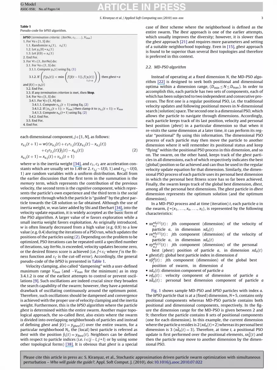
Fig. 1 shows sample MD-PSO and bPSO particles with index a.The bPSO particle that is at a (fixed) dimension, N = 5, contains onlypositional components whereas MD-PSO particle contains bothpositional and dimensional components, respectively. In the fig-ure the dimension range for the MD-PSO is given between 2 and9; therefore the particle contains 8 sets of positional components(one for each dimension). In this example, the current dimension

ximation driven particle swarm optimization with simultaneousdoi:10.1016/j.asoc.2010.07.022

where the particle a resides is 2 (xda(t) = 2) whereas its personal bestdimension is 3 (xda(t) = 3). Therefore, at time t, a positional PSOupdate is first performed over the positional elements, xx2

a(t) andthen the particle may move to another dimension by the dimen-sional PSO.

ARTICLE IN PRESSG ModelASOC-958; No. of Pages 14

4 S. Kiranyaz et al. / Applied Soft Computing xxx (2010) xxx–xxx

[Dmin =

oWmdttl

x

u

x

p

a

ptppj

btu

Fig. 1. Sample MD-PSO (right) vs. bPSO (left) particle structures. For MD-PSO

Let f denote the dimensional fitness function that is to beptimized within a certain dimension range, (Dmin ≤ N ≤ Dmax).ithout loss of generality assume that the objective is to find theinimum (position) of f at the optimum dimension within a multi-

imensional search space. Assume that the particle a visits (back)he same dimension after T iterations (i.e. xda(t) = xda(t + T)), thenhe personal best position can be updated in iteration t + T as fol-ows:

yxda(t+T)a,j (t + T)

={

xyxda(t)a,j

(t) if f (xxxda(t+T)a (t + T)) > f (xyxda(t)

a (t))

xxda(t+T)a,j

(t + T) else

}

∀j ∈ [1, xda(t)] (3)

Furthermore, the personal best dimension of particle a can bepdated in iteration t + 1 as follows:

da(t + 1) ={

xda(t) if f (xxxda(t+1)a (t + 1)) > f (xyxda(t)

a (t))xda(t + 1) else

}(4)

Recall that gbest(d) is the index of the global bestarticle at dimension d then xydbest(t) = xydbest

gbest(dbest)(t) =rg min

∀i ∈ [1,S](f (xydbest

i(t)). For a particular iteration t, and for a

article a ∈ [1, S], first the positional components are updated inhe current dimension, xda(t), and then the dimensional update iserformed to determine the next (t + 1st) dimension, xda(t + 1). Theositional update is performed for each dimension component,∈ [1, xda(t)] as follows:

vxxda(t)a,j

(t + 1) = w(t)vxxda(t)a,j

(t) + c1r1,j(t)(xyxda(t)a,j

(t) − xxxda(t)a,j

(t))

+ c2r2,j(t)(xyxda(t)j

(t) − xxxda(t)a,j

(t))

xxxda(t)a,j

(t + 1) = xxxda(t)a,j

(t) + vxxda(t)a,j

(t + 1)

(5)

Note that the particle’s new position, xxxda(t)a (t + 1), will still

e in the same dimension, xda(t); however, the particle may flyo another dimension afterwards with the following dimensional

Please cite this article in press as: S. Kiranyaz, et al., Stochastic approperturbation – Who will guide the guide?, Appl. Soft Comput. J. (2010),

pdate equations:

vda(t + 1) =⌊vda(t) + c1r1(t)(xda(t) − xda(t))

+ c2r2(t)(dbest − xda(t))⌋

xda(t + 1) = xda(t) + vda(t + 1)(6)

2, Dmax = 9] and at the current time t, xda(t) = 2 and xda(t) = 3. For bPSO N = 5.

where · is the floor operator. Unlike in Eq. (2), an inertia weightis not used for positional velocity update, since no benefit wasobtained experimentally for dimensional PSO. To avoid exploding,along with the positional velocity limit Vmax, two more clampingoperations are applied for dimensional PSO components, such as|vda,j(t + 1)| < VDmax and the initial dimension range set by theuser, Dmin ≤ xda(t) ≤ Dmax. Once the MD-PSO process terminates,the optimum solution will be xydbest at the optimum dimension,dbest, achieved by the particle gbest(dbest) and finally the best (fit-ness) score achieved will naturally be f (xydbest). Accordingly, thegeneral pseudo-code of the MD-PSO technique is given in Table 2.

More detailed information of MD-PSO can be found in [22].

2.3. Data clustering by MD-PSO

As the process of identifying natural groupings in a multi-dimensional data based on some distance metric (e.g. Euclidean),data clustering can be divided into two main categories: hierar-chical and partitional [12]. Each category then has a wealth ofsub-categories and different algorithmic approaches for finding theclusters where extensive survey can be found in [19,31].

A hard clustering technique based on the basic PSO (bPSO) wasfirst introduced by Omran et al. in [29] and this work showedthat the bPSO can outperform K-means, Fuzzy C-means (FCM), K-harmonic means (KHM) and some other state-of-the-art clusteringmethods in any (evaluation) criteria. This is indeed an expectedoutcome due to the PSO’s aforementioned ability to cope up withthe local optima by maintaining a guided random search opera-tion through the swarm particles. In clustering, similar to other PSOapplications, each particle represents a potential solution at a par-ticular time t, i.e. the particle a in the swarm, � ={x1, . . ., xa, . . ., xS}, isformed as xa(t) ={ca,1, . . ., ca,j, . . ., ca,K}⇒ xa,j(t) = ca,j where ca,j is thejth (potential) cluster centroid in N-dimensional data space and Kis the number of clusters fixed in advance. Note that the data spacedimension, N, is now different from the solution space dimension,K. Furthermore, the fitness (validity index) function, f that is to beoptimized, is formed with respect to two widely used criteria inclustering:

ximation driven particle swarm optimization with simultaneousdoi:10.1016/j.asoc.2010.07.022

• Compactness: Data items in one cluster should be similar or closeto each other in N-dimensional space and different or far awayfrom the others when belonging to different clusters.

• Separation: Clusters and their respective centroids should be dis-tinct and well separated from each other.

ARTICLE ING ModelASOC-958; No. of Pages 14

S. Kiranyaz et al. / Applied Soft Com

Table 2Pseudo-code of MD-PSO algorithm.

MD-PSO (termination criteria: {IterNo, εC , . . .}, Vmax, VDmax, Dmin, Dmax)1. For ∀a ∈ [1, S] do:

1.1. Randomize xda(0)1.2. Initialize xda(0) = xda(0)1.3. For ∀d ∈ [Dmin, Dmax] do:

1.3.1. Randomize xxda(0)

1.3.2. Initialize xyda(0) = xxd

a(0)1.4. End For.

2. End For.3. For ∀t ∈ [1, IterNo] do:

3.1. For ∀a ∈ [1, S] do:

3.1.1. If

(f (xxxda(t)

a (t)) < min

(f (xyxda(t)

a (t − 1)), minp ∈ S−{a}

(f (xxxda(t)p (t)))

))then do:

3.1.1.1. xyxda(t)a (t) = xxxda(t)

a (t)

3.1.1.2. If (f (xxxda(t)a (t)) < f (xyxda(t)

gbest(xda(t))(t − 1))) then gbest(xda(t)) = a

3.1.1.3. If (f (xxxda(t)a (t)) < f (xyxda(t−1)

a (t − 1))) then xda(t) = xda(t)

3.1.1.4. If (f (xxxda(t)a (t)) < f (xydbest(t − 1))) then dbest = xda(t)

3.1.2. End If.3.2. End For.3.3. If the termination criteria are met, then Stop.

3.4. For ∀a ∈ [1, S] do:3.4.1. For ∀j ∈ [1, xda(t)] do:

3.4.1.1. Compute vxxda(t)a,j

(t + 1) using Eq. (5)3.4.1.2. If (|vxxda(t)

a,j(t + 1)| > Vmax) then clamp it to |vxxda(t)

a,j(t + 1)| = Vmax

3.4.1.3. Compute xxxda(t)a,j

(t + 1) using Eq. (5)3.4.2. End For.3.4.3. Compute vda(t + 1) using Eq. (6)3.4.4. If (|vda(t + 1)| > VDmax) then clamp it to |vda(t + 1)| = VDmax

3.4.5. Compute xda(t + 1) using Eq. (6)3.4.6. If (xd (t + 1) < D ) then (xd (t + 1) = D )

lait

wtpvicuftddvawtnwvHMcs[

a min a min

3.4.7. If (xda(t + 1) > Dmax) then (xda(t + 1) = Dmax)3.5. End For.

4. End For.

The fitness functions for clustering are then formed as a regu-arization function fusing both Compactness and Separation criteriand in this problem domain they are known as clustering validityndices. Omran et al. in [29] used the following validity index inheir work,

f (xa, Z) = w1dmax(xa, Z) + w2(Zmax − dmin(xa)) + w3Qe(xa)

where Qe(xa) = 1K

K∑j=1

∑∀zp ∈ xa,j

||xa,j − zp||||xa,j||

(7)

here Qe is the quantization error (or the average intra-cluster dis-ance), dmax is the maximum average Euclidean distance of dataoints, Z ={zp, zp ∈ xa,j}, to their centroids, xa. Zmax is a constantalue for theoretical maximum inter-cluster distance, and dmins the minimum centroid (inter-cluster) distance in the clusterentroid set xa. The weights, w1, w2, w3 are user-defined reg-larization coefficients. So the minimization of the validity index

(xa, Z) will simultaneously try to minimize the intra-cluster dis-ances (for better Compactness) and maximize the inter-clusteristance (for better Separation). In such a regularization approach,ifferent priorities (weights) can be assigned to both sub-objectivesia proper setting of weight coefficients; however, this makes thepproach strictly parameter dependent. Another traditional andell-known validity index is Dunn’s index [8], which suffers from

wo drawbacks: It is computationally expensive and sensitive tooise [16]. Several variants of Dunn’s index were proposed in [31]here robustness against noise is improved. There are many other

alidity indices, i.e. proposed by Turi [39], Davies and Bouldin [7],

Please cite this article in press as: S. Kiranyaz, et al., Stochastic approperturbation – Who will guide the guide?, Appl. Soft Comput. J. (2010),

alkidi et al. [16], etc. A throughout survey can be found in [16].ost of them presented promising results; however, none of them

an guarantee the “optimum” number of clusters in every clusteringcheme. Especially for the aforementioned PSO-based clustering in29], the clustering scheme further depends on weight coefficients

PRESSputing xxx (2010) xxx–xxx 5

and may, therefore, result in over- or under-clustering particularlyin complex data distributions.

Although PSO-based clustering outperforms many well-knownclustering methods, it still suffers from two major drawbacks. Thenumber of clusters, K (being the solution space dimension) muststill be specified in advance and similar to other bPSO applications,the method tends to trap in local optima particularly when thecomplexity of the clustering scheme increases. This is also true fordynamic clustering schemes, DCPSO [30] and MEPSO [1], both ofwhich eventually presented results only in low dimensions and forsimple data distributions.

Based on the earlier discussion it is obvious that the clus-tering problem requires the determination of the solution spacedimension (i.e. number of clusters, K) where in a recent work [22]MD-PSO technique has been successfully used. At time t, the par-ticle a in the swarm, � ={x1, . . ., xa, . . ., xS}, has the positionalcomponent formed as, xxxda(t)

a (t) = {ca,1, . . . , ca,j, . . . , ca,xda(t)} ⇒xxxda(t)

a,j(t) = ca,j meaning that it represents a potential solution (i.e.

the cluster centroids) for the xda(t) number of clusters whilst jthcomponent being the jth cluster centroid. Apart from the regularlimits such as (spatial) velocity, Vmax, dimensional velocity, VDmax

and dimension range Dmin ≤ xda(t) ≤ Dmax, the N-dimensional dataspace is also limited with some practical spatial range, i.e. Xmin <xxxda(t)

a (t) < Xmax. In case this range is exceeded even for a singledimension j, xxxda(t)

a,j(t), then all positional components of the par-

ticle for the respective dimension xda(t) are initialized randomlywithin the range (i.e. refer to step 1.3.1 in MD-PSO pseudo-codein Table 2) and this further contributes to the overall diversity. Inthis work as well as in [22], the following validity index is usedto obtain computational simplicity with minimal or no parameterdependency,

f (xxxda(t)a , Z) = Qe(xxxda(t)

a )(xda(t))˛ where

Qe(xxxda(t)a ) = 1

xda(t)

xda(t)∑j=1

∑∀zp ∈ xxxda(t)

a,j||xxxda(t)

a,j− zp||

||xxxda(t)a ||

(8)

where Qe is the quantization error (or the average intra-cluster dis-tance) as the Compactness term and (xda(t))˛ is the Separation term,by simply penalizing higher cluster numbers with an exponential,˛ > 0. Using ˛ = 1, the validity index yields the simplest form (i.e.only the nominator of Qe) and becomes entirely parameter-free.

On the other hand, (hard) clustering has some constraints. LetCj = {xxxda(t)

a,j(t)} = {ca,j} be the set of data points assigned to a

(potential) cluster centroid xxxda(t)a,j

(t) for a particle a at time t. Thepartitions Cj, ∀ j ∈ [1, xda(t)] should maintain the following con-straints:

1. Each data point should be assigned to one cluster set, i.e.⋃xda(t)j=1 Cj = Z.

2. Each cluster should contain at least one data point, i.e. Cj /= {�},∀ j ∈ [1, xda(t)].

3. Two clusters should have no common data points, i.e. Ci ∩ Cj ={�},i /= j and ∀ i, j ∈ [1, xda(t)].

In order to satisfy the 1st and 3rd (hard) clustering constraints,before computing the clustering fitness score via the validity indexfunction in (8), all data points are first assigned to the closestcentroid. Yet there is no guarantee for the fulfillment of the 2ndconstraint since xxxda(t)

a (t) is set (updated) by the internal dynam-ics of the MD-PSO process and hence any dimensional component

ximation driven particle swarm optimization with simultaneousdoi:10.1016/j.asoc.2010.07.022

(i.e. a potential cluster candidate), xxxda(t)a,j

(t), can be in an abun-dant position (i.e. no closest data point exists). To avoid this, a highpenalty is set for the fitness score of the particle, i.e. f (xxxda(t)

a , Z) ≈∞, if {xxxda(t)

a,j} = {�} for any j.

ARTICLE ING ModelASOC-958; No. of Pages 14

6 S. Kiranyaz et al. / Applied Soft Com

Table 3Pseudo-code for SPSA technique.

SPSA (IterNo, a, c, A, ˛, �)1. Initialize

��1

2. For ∀k ∈ [1, IterNo] do:2.1. Generate zero-mean, p-dimensional perturbation vector: k

2.2. Let ak = a/(A + k)˛ and ck = c/k�

2.3. Compute L(��k + ckk) and L(

��k − ckk)

3

3

aag

g

srpa��

waTsKvfsa

�g

wBicci2at

o6“tociw

b

given (dimension) range, d ∈ [Dmin, Dmax]. The main difference isthat in each dimension, there is a distinct gbest particle, gbest(d).So SPSA is applied individually over the position of each gbest(d) ifit (re-) visits the dimension d (i.e. d = xdgbest(t)). Therefore, there

2.4. Compute �gk(��k) using (11)

2.5. Compute��k+1 using (10)

3. End For.

. The proposed techniques: SAD PSO and SAD MD-PSO

.1. SPSA overview

The goal of deterministic optimization methods is to minimizeloss function L : Rp → R1, which is a differentiable function of �

nd the minimum (or maximum) point �* corresponds to the zero-radient point, i.e.

(�) ≡ ∂L(�)∂�

∣∣∣∣�=�∗

= 0 (9)

As mentioned earlier, in cases where more than one pointatisfies this equation (e.g. a multi-modal problem), then such algo-ithms may only converge to a local minimum. Moreover, in manyractical problems, g is not readily available. This makes the SAlgorithms quite popular and they are in the general SA form:

k+1 = ��k − ak

�gk(��k) (10)

here �gk(��k) is the estimate of the gradient g(�) at iteration k

nd ak is a scalar gain sequence satisfying certain conditions [35].here are two common SA methods: finite difference SA (FDSA) andimultaneous perturbation SA (SPSA). FDSA adopts the traditionaliefer-Wolfowitz approach to approximate gradient vectors as aector of p partial derivatives where p is the dimension of the lossunction. On the other hand, SPSA has all elements of

��k perturbed

imultaneously using only two measurements of the loss functions,

k(��k) = L(

��k + ckk) − L(

��k − ckk)

2ck

⎡⎢⎢⎢⎣

−1k1

−1k2...

−1kp

⎤⎥⎥⎥⎦ (11)

here the p-dimensional random variable k is usually chosen asernoulli ±1 distribution and ck is a scalar gain sequence satisfy-

ng certain conditions [35]. Spall in [35] presents conditions foronvergence of SPSA (i.e.

��k → �∗) and show that under certain

onditions both SPSA and FDSA have the same convergence abil-ty – yet SPSA needs only 2 measurements whereas FDSA needsp. This makes SPSA our natural choice for driving gbest in bothpproaches. Table 3 presents the general pseudo-code of the SPSAechnique.

SPSA has five parameters as given in Table 3. Spall in [36] rec-mmended to use values for A (the stability constant), ˛, and � as0, 0.602 and 0.101, respectively. However, he also concluded thatthe choice of both gain sequences is critical to the performance ofhe SPSA as with all stochastic optimization algorithms and the choicef their respective algorithm coefficients”. This especially makes the

Please cite this article in press as: S. Kiranyaz, et al., Stochastic approperturbation – Who will guide the guide?, Appl. Soft Comput. J. (2010),

hoice of gain parameters a and c critical for a particular problem,.e. Maryak and Chin in [27] varied them with respect to the problem

hilst keeping the other three (A, ˛, and �) as recommended.Recently Maeda and Kuratani in [28] has used SPSA with the

PSO in a hybrid algorithm called Simultaneous Perturbation PSO

PRESSputing xxx (2010) xxx–xxx

(SP-PSO) over a limited set of problems and reported some slightimprovements over the bPSO. Both SP-PSO variants they proposedinvolved the insertion of the �gk(

��k) directly over the velocity equa-

tions of all swarm particles with the intention of improving theirlocal search capability. This may, however, present some draw-backs. First of all, performing SPSA at each iteration and for allparticles will double the computational cost of the PSO since SPSAwill require an additional function evaluation at each iteration.1

Secondly, such an abrupt adding of SPSA’s �gk(��k) term directly into

the bPSO may degrade the original PSO workout, i.e. the collectiveswarm updates and interactions, and require an accurate scalingbetween the parameters of the two methods, PSO’s and SPSA. Oth-erwise, one can dominant the other, and hence their combinationmay turn out to be a noisy variant of either method. This is perhapsthe reason of the limited success, if any, achieved by SP-PSO. As wediscuss next and demonstrate its elegant performance experimen-tally, SPSA should not be mixed up with PSO as such, rather shouldonly be used to guide it if SPSA can drive the PSO’s native guide, thegbest, better than PSO.

3.2. SAD PSO

In this work two distinct SAD PSO approaches are proposed,each of which is only applied to gbest whilst keeping the inter-nal PSO process intact. Since both SPSA and PSO are iterativeprocesses, in both approaches SPSA can thus easily be inte-grated into PSO by using the same iteration count (i.e. t ≡ k).In other words, at a particular iteration t in the PSO process,only the SPSA steps 2.1–2.5 in Table 3 are inserted accordinglyinto the PSO process. The following sub-sections will detail eachapproach.

A1) First SAD PSO approach: gbest update by SPSA

In this approach, at each iteration gbest particle is updated usingSPSA. This requires the adaptation of the SPSA elements (parame-ters and variables) and integration of the internal SPSA part (withinthe loop) appropriately into the PSO pseudo-code, as shown inTable 4. Note that such a “plug-in” approach will not change theinternal PSO structure and only affects the gbest particle’s move-ment. It only costs two extra function evaluations and hence ateach iteration the total number of evaluations is increased from Sto S + 2 (recall that S is the swarm size).

Since the fitness of each particle’s current position is computedwithin the PSO process, it is possible to further diminish this cost toonly one extra fitness evaluation per iteration. Let

��k + ckk = xa(t)

in step 3.4.1.1. and thus L(��k + ckk) is known a priori. Then nat-

urally,��k − ckk = xa(t) − 2ckk, which is the only (new) location

where the (extra) fitness evaluation (L(��k − ckk)) has to be com-

puted. Once the gradient (�gk(��k)) is estimated in step 3.4.1.4, then

the next (updated) location of the gbest will be: xa(t + 1) = ��k+1.

Note that the difference of this “low-cost” SPSA update is thatxa(t + 1) is updated (estimated) not from xa(t), but instead fromxa(t) − ckk.

This approach can easily be extended for MD-PSO, which is anatural extension of PSO for multi-dimensional search within a

ximation driven particle swarm optimization with simultaneousdoi:10.1016/j.asoc.2010.07.022

1 In [28] the function evaluations are given with respect to the iteration number;however, it should have been noted that SP-PSO performs twice more evaluationsthan bPSO per iteration. Considering this fact, the plots therein show little or noperformance improvement at all.

ARTICLE IN PRESSG ModelASOC-958; No. of Pages 14

S. Kiranyaz et al. / Applied Soft Computing xxx (2010) xxx–xxx 7

Table 4Pseudo-code for the first SAD PSO approach.

A1) SAD PSO Plug-in (termination criteria: {IterNo, εC , . . .}, Vmax, a, c, A, ˛, �)1. See Line 1 in Table 12. See Line 2 in Table 13. For ∀t ∈ [1, IterNo] do:

3.4. For ∀a ∈ [1, S] do:3.4.1. If (a = gbest) then do:

3.4.1.1. Let k = t,��k = xa(t) and L = f

3.4.1.2. Let ak = a/(A + k)˛ and ck = c/k�

3.4.1.3. Compute L(��k + ckk) and L(

��k − ckk)

3.4.1.4. Compute �gk(��k) using Eq. (11)

3.4.1.5. Compute xa(t + 1) = ��k+1 using Eq. (10)

3.4.2. Else do:3.4.2.1. For ∀j ∈ [1, N] do:

3.4.2.1.1. Compute va,j(t + 1) using Eq. (2)3.4.2.1.2. If (|va,j(t + 1)| > Vmax) then clamp it to |va,j(t + 1)| = Vmax

3.4.2.1.3. Compute xa,j(t + 1) using Eq. (2)

ciuia(svttotis

A

iatagi

qaigtb

TP

Table 6MD-PSO Plug-in for the second approach.

A2) SAD MD-PSO Plug-in (�, a, c, A, ˛, �)1. Create a new aGB particle, {xxd

aGB(t + 1), xyd

aGB(t + 1)} for ∀d ∈ [Dmin, Dmax]

2. For ∀d ∈ [Dmin, Dmax] do:

2.1. Let k = t,��k = xyd(t) and L = f

2.2. Let ak = a/(A + k)˛ and ck = c/k�

2.3. Compute L(��k + ckk) and L(

��k − ckk)

2.4. Compute �gk(��k) using Eq. (11)

2.5. Compute xxdaGB

(t + 1) = ��k+1 using Eq. (10)

2.6. If (f (xxdaGB

(t + 1)) < f (xydaGB

(t))) then xydaGB

(t + 1) = xxdaGB

(t + 1)

2.7. Else xydaGB

(t + 1) = xydaGB

(t)d d d d

3.4.2.2. End For.3.5. End For.

4. End For.

an be 2(Dmax − Dmin) number of function evaluations, indicat-ng a significant cost especially if a wide dimensional range issed. However, this is a theoretical limit, which can only happen

f gbest(i) /= gbest(j) for ∀ i, j ∈ [Dmin, Dmax], i /= j and all particlesltogether visit the particular dimensions in which they are gbesti.e. xdgbest(d)(t) = d, ∀ t ∈ [1, iterNo]). Especially in a wide dimen-ional range, note that this is highly unlikely due to the dimensionalelocity, which makes particles move (jump) from one dimensiono another at each iteration. It is straightforward to see that underhe assumption of a uniform distribution for particles’ movementsver all dimensions within the dimensional range, SAD MD-PSOoo, would have the same cost overhead as the SAD PSO. Exper-mental results indicate that the practical overhead cost is onlylightly higher than this.

2) Second SAD PSO approach: aGB formation by SPSA

The second approach replaces the FGBF operation proposedn [22] with the SPSA to create an aGB particle. SPSA is basicallypplied over the pbest position of the gbest particle. The aGB par-icle will then guide the swarm instead of gbest if and only if itchieves a better fitness score than the (personal best position of)best. SAD PSO pseudo-code as given in Table 5 can then be pluggedn between steps 3.3 and 3.4 of bPSO pseudo-code.

The extension of the second approach to MD-PSO is alsouite straightforward. In order to create an aGB particle, forll dimensions in the given range (i.e. ∀d ∈ [Dmin, Dmax]) SPSA

Please cite this article in press as: S. Kiranyaz, et al., Stochastic approperturbation – Who will guide the guide?, Appl. Soft Comput. J. (2010),

s applied individually over the personal best position of eachbest(d) particle and furthermore, the aforementioned competi-ive selection ensures that xyd

aGB(t), ∀d ∈ [Dmin, Dmax] is set to theest of the xxd

aGB(t + 1) and xydaGB(t). As a result, the SPSA cre-

able 5SO Plug-in for the second approach.

A2) SAD PSO Plug-in (�, a, c, A, ˛, �)1. Create a new aGB particle, {xaGB(t + 1), yaGB(t + 1)}2. Let k = t,

��k = y(t) and L = f

3. Let ak = a/(A + k)˛ and ck = c/k�

4. Compute L(��k + ckk) and L(

��k − ckk)

5. Compute �gk(��k) using Eq. (11)

6. Compute xaGB(t) = ��k+1 using Eq. (10)

7. Compute f (xaGB(t + 1)) = L(��k+1)

8. If (f(xaGB(t + 1)) < f(yaGB(t))) then yaGB(t + 1) = xaGB(t + 1)9. Else yaGB(t + 1) = yaGB(t)10. If (f (yaGB(t + 1)) < f (y(t))) then y(t) = yaGB(t + 1)

2.8. If (f (xyaGB

(t + 1)) < f (xygbest(d)

(t))) then xygbest(d)

(t) = xyaGB

(t + 1)

3. End For.4. Re-assign dbest: dbest = arg min

d ∈ [Dmin,Dmax](f (xyd

gbest(d)(t)))

ates one aGB particle providing (potential) GB solutions (xydaGB(t +

1), ∀d ∈ [Dmin, Dmax]) for all dimensions in the given dimensionrange. The pseudo-code of the second approach as given in Table 6can then be plugged in between steps 3.2 and 3.3 of the MD-PSOpseudo-code, given in Table 2.

Note that in the second SAD PSO approach, there are three extrafitness evaluations (as opposed to two in the first one) at each iter-ation. Yet as in the first approach, it is possible to further decreasethe cost of SAD PSO by one (from three to two fitness evaluationsper iteration). Let

��k + ckk = y(t) in step 2 and thus L(

��k + ckk) is

known a priori. Then it follows the same analogy as before and theonly difference is that the aGB particle is formed not from

��k = y(t)

but from��k = y(t) − ckk. However, in this approach a major dif-

ference in the computational cost may occur since in each iterationthere are inevitably 3(Dmax − Dmin) (or 2(Dmax − Dmin) for low-costapplication) fitness evaluations, which can be significant.

4. Experimental results

Two problem domains are considered in this paper over whichthe proposed techniques are evaluated. The first one is non-linearfunction minimization where several benchmark functions areused. This allows us to test the performance of SAD PSO againstbPSO over both uni- and multi-modal functions. The second domainis data clustering, which provides certain constraints in multi-dimensional solution space and allows the performance evaluationin the presence of significant variation in data distribution with animpure validity index. This problem domain can efficiently validatethe performance of SAD MD-PSO regarding the convergence to theglobal solution in the right dimension. In this way, we can trulyevaluate the contribution and the significance of both approaches(A1 and A2) especially over multi-modal optimization problems inhigh dimensions.

4.1. Non-linear function minimization

We used seven benchmark functions given in Table 7 to providea good mixture of complexity and modality. They have been widelystudied by several researchers, e.g. see [3,10,17,26,33,34]. Sphere,De Jong and Rosenbrock are uni-modal functions and the rest aremulti-modal, meaning that they have many local minima. On themacroscopic level Griewank demonstrates certain similarities withuni-modal functions especially when the dimensionality is above20; however, in low dimensions it bears a significant noise, which

ximation driven particle swarm optimization with simultaneousdoi:10.1016/j.asoc.2010.07.022

creates many local minima due to the second multiplication termwith cosine components.

Both approaches of the proposed SAD PSO along with the “low-cost” application are tested over seven benchmark functions givenin Table 7 and compared with the bPSO and standalone SPSA appli-

ARTICLE IN PRESSG ModelASOC-958; No. of Pages 14

8 S. Kiranyaz et al. / Applied Soft Computing xxx (2010) xxx–xxx

Table 7Benchmark functions with dimensional bias.

Function Formula Initial range Dimension set: {d}

Sphere F1(x, d) =

(d∑

i=1

x2i

)[−150, 75] 20, 50, 80

De Jong F2(x, d) =

(d∑

i=1

ix4i

)[−50, 25] 20, 50, 80

Rosenbrock F3(x, d) =

(d∑

i=1

100(xi+1 − x2i)2 + (xi − 1)2

)[−50, 25] 20, 50, 80

Rastrigin F4(x, d) =

(d∑

i=1

10 + x2i

− 10 cos(2xi)

)[−500, 250] 20, 50, 80

Griewank F5(x, d) =

(1

4000

d∑i=1

x2i

−d∏

i=1

cos

(xi√i+1

))[−500, 250] 20, 50, 80

Schwefel F6(x, d) =

(418.9829d +

d∑i=1

xi sin

(√|xi|))

[−500, 250] 20, 50, 80(in(

4

)

cot8e(dafSpiaSe

r

TS

Giunta F7(x, d) =d∑

i=1

sin(

1615 xi − 1

)+ sin2

(1615 xi − 1

)+ 1

50 s

ation. We used the same termination criteria as the combinationf the maximum number of iterations allowed (iterNo = 10,000) andhe cut-off error (εC = 10−5). We used three dimensions (20, 50 and0) for the sample functions in order to test the performance ofach technique in such varying dimensions individually. For PSObPSO and SAD PSO) we used the swarm size, S = 40, and w is linearlyecreased from 0.9 to 0.2. We used the recommended values for A, ˛nd � as 60, 0.602 and 0.101 as well as set a and c to 1 that are fixedor all functions. We purposefully made no parameter tuning forPSA since this may not be feasible for many practical applications,articularly the ones where the underlying fitness (error) surface

s unknown. In order to make a fair comparison among SPSA, bPSO

Please cite this article in press as: S. Kiranyaz, et al., Stochastic approperturbation – Who will guide the guide?, Appl. Soft Comput. J. (2010),

nd SAD PSO, the number of evaluations is kept equal (so S = 38 and= 37 are used for both SAD PSO approaches and the number ofvaluations is set to 40 × 10,000 = 4E+5 for SPSA).

For each setting (for each function and each dimension), 100uns are performed and the 1st and 2nd order statistics (mean,

able 8tatistical results from 100 runs over 7 benchmark functions.

Functions d SPSA bPSO

� � �

Sphere 20 0 0 050 0 0 080 0 0 135.272

De Jong 20 0.013 0.0275 050 0.0218 0.03 9.044580 0.418 0.267 998.737

Rosenbrock 20 1.14422 0.2692 1.2646250 3.5942 0.7485 15.905380 5.3928 0.7961 170.9547

Rastrigin 20 204.9169 51.2863 0.042950 513.3888 75.7015 0.052880 832.9218 102.1792 0.7943

Griewank 20 0 0 050 1.0631E+007 3.3726E+006 50.731780 2.8251E+007 5.7896E+006 24,978

Schwefel 20 0.3584 0.0794 1.747450 0.8906 0.1006 10.202780 1.4352 0.1465 21.8269

Giunta 20 42,743 667.2494 495.077750 10,724 1027.6 425780 17,283 1247.9 9873.6

(1615 xi − 1

))+ 268

1000 [−500, 250] 20, 50, 80

� and standard deviation, �) of the fitness scores are reported inTable 8 whilst the best statistics are highlighted. During each run,the operation terminates when the fitness score drops below thecut-off error and it is assumed that the global minimum of the func-tion is reached, henceforth; the score is set to 0. Therefore, for anysetting yielding � = 0 as the average score means that the methodconverges to the global minimum at every run.

As the entire statistics in the right side of Table 8 indicate, eitherSAD PSO approach achieves an equal or superior average perfor-mance statistics over all functions regardless of the dimension,modality, and without any exception. In other words, SAD PSO per-forms equal or better than the best of bPSO and SPSA – even though

ximation driven particle swarm optimization with simultaneousdoi:10.1016/j.asoc.2010.07.022

either of them might have a quite poor performance for a partic-ular function. Note especially that if SPSA performs well enough(meaning that the setting of the critical parameters, e.g. a and c isappropriate), then a significant performance improvement can beachieved by SAD PSO, i.e. see for instance De Jong, Rosenbrock and

SAD PSO (A2) SAD PSO (A1)

� � � � �

0 0 0 0 00 0 0 0 0276.185 0 0 0 00 0 0 0 026.9962 0.0075 0.0091 0.2189 0.6491832.1993 0.2584 0.4706 13,546.02 4305.040.4382 1.29941 0.4658 0.4089 0.21305.21491 12.35141 2.67731 2.5472 0.3696231.9113 28.1527 5.1699 5.2919 0.81770.0383 0.0383 0.0369 0.0326 0.03000.0688 0.0381 0.0436 0.0353 0.05030.9517 0.2363 0.6552 0.1240 0.16940 0 0 0 0191.1558 0 0 3074.02 13,98923,257 20,733 24,160 378,210 137,4100.3915 0.3076 0.0758 0.3991 0.07962.2145 0.8278 0.1093 0.9791 0.12325.1809 1.3633 0.1402 1.5528 0.1544245.1220 445.1360 264.1160 445.1356 249.5412713.1723 3938.9 626.9194 3916.2 758.32901313 8838.2 1357 8454.2 1285.3

ARTICLE IN PRESSG ModelASOC-958; No. of Pages 14

S. Kiranyaz et al. / Applied Soft Computing xxx (2010) xxx–xxx 9

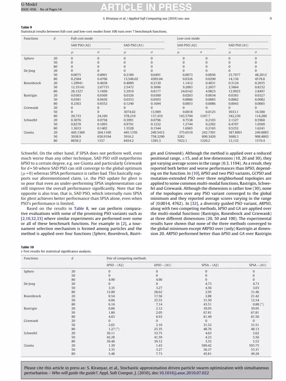
Table 9Statistical results between full-cost and low-cost modes from 100 runs over 7 benchmark functions.

Functions d Full-cost mode Low-cost mode

SAD PSO (A2) SAD PSO (A1) SAD PSO (A2) SAD PSO (A1)

� � � � � � � �

Sphere 20 0 0 0 0 0 0 0 050 0 0 0 0 0 0 0 080 0 0 0 0 0 0 0 0

De Jong 20 0 0 0 0 0 0 0 050 0.0075 0.0091 0.2189 0.6491 0.0073 0.0036 23.7977 48.201280 0.2584 0.4706 13,546.02 4305.04 0.0326 0.0290 14,136 4578.8

Rosenbrock 20 1.29941 0.4658 0.4089 0.2130 1.1412 0.4031 0.3124 0.203550 12.35141 2.67731 2.5472 0.3696 9.2063 2.2657 2.5864 0.823280 28.1527 5.1699 5.2919 0.8177 24.0142 4.9823 12.9923 2.8497

Rastrigin 20 0.0383 0.0369 0.0326 0.0300 0.0263 0.0634 0.0383 0.032750 0.0381 0.0436 0.0353 0.0503 0.0066 0.0083 0.0062 0.008280 0.2363 0.6552 0.1240 0.1694 0.0053 0.0086 0.0043 0.0065

Griewank 20 0 0 0 0 0 0 0 050 0 0 3074.02 13,989 0.0018 0.0125 3033.1 16,58880 20,733 24,160 378,210 137,410 143.5794 1247.7 342,230 114,280

Schwefel 20 0.3076 0.0758 0.3991 0.0796 0.7538 0.2103 2.1327 0.596050 0.8278 0.1093 0.9791 0.1232 1.2744 0.2282 6.4797 1.0569

Smbf(pssofP

t[onm

Tt

80 1.3633 0.1402 1.5528Giunta 20 445.1360 264.1160 445.1356

50 3938.9 626.9194 3916.280 8838.2 1357 8454.2

chwefel. On the other hand, if SPSA does not perform well, evenuch worse than any other technique, SAD PSO still outperforms

PSO to a certain degree, e.g. see Giunta and particularly Griewankor d = 50 where SAD PSO can still converge to the global optimum� = 0) whereas SPSA performance is rather bad. This basically sup-orts our aforementioned claim, i.e. the PSO update for gbest iso poor that even an under-performing SPSA implementation cantill improve the overall performance significantly. Note that thepposite is also true, that is, SAD PSO, which internally runs SPSAor gbest achieves better performance than SPSA alone, even whenSO’s performance is limited.

Based on the results in Table 8, we can perform compara-

Please cite this article in press as: S. Kiranyaz, et al., Stochastic approperturbation – Who will guide the guide?, Appl. Soft Comput. J. (2010),

ive evaluations with some of the promising PSO variants such as2,10,32,33] where similar experiments are performed over somer all of these benchmark functions. For example in [2], a tour-ament selection mechanism is formed among particles and theethod is applied over four functions (Sphere, Rosenbrock, Rastri-

able 10-Test results for statistical significance analysis.

Functions d Pair of competing methods

bPSO – (A2)

Sphere 20 050 080 4.90

De Jong 20 050 3.3580 12.00

Rosenbrock 20 0.5450 6.0680 6.16

Rastrigin 20 0.8650 1.8080 4.83

Griewank 20 050 2.6580 1.27 (*)

Schwefel 20 36.1150 42.2880 39.48

Giunta 20 1.3950 3.3580 5.48

0.1544 1.6965 0.2165 9.5252 1.6241249.5412 375.6510 242.7301 387.8901 249.8883758.3290 3282 890.3426 3688.3 908.48031285.3 7922.1 1320.2 12,132 1579.4

gin and Griewank). Although the method is applied over a reducedpositional range, ±15, and at low dimensions (10, 20 and 30), theygot varying average scores in the range {0.3, 1194}. As a result, theyreported both better and worse performances than bPSO, depend-ing on the function. In [10], bPSO and two PSO variants, GCPSO andmutation-extended PSO over three neighborhood topologies areapplied to some common multi-modal functions, Rastrigin, Schwe-fel and Griewank. Although the dimension is rather low (30), noneof the topologies over any PSO variant converged to the globalminimum and they reported average scores varying in the rangeof {0.0014, 4762}. In [32], a diversity guided PSO variant, ARPSO,along with two competing methods, bPSO and GA are applied over

ximation driven particle swarm optimization with simultaneousdoi:10.1016/j.asoc.2010.07.022

the multi-modal functions (Rastrigin, Rosenbrock and Griewank)at three different dimensions (20, 50 and 100). The experimentalresults have shown that none of the three methods converged tothe global minimum except ARPSO over (only) Rastrigin at dimen-sion 20. ARPSO performed better than bPSO and GA over Rastrigin

bPSO – (A1) SPSA – (A2) SPSA – (A1)

0 0 00 0 04.90 0 00 4.73 4.733.27 4.56 3.03

28.62 2.95 31.4617.56 2.88 21.4225.55 31.50 12.54

7.14 43.51 0.88 (*)2.12 39.95 39.952.05 67.81 67.816.93 81.49 81.500 0 02.16 31.52 31.51

25.35 48.76 48.1333.75 4.63 3.6241.59 4.23 5.5639.12 3.55 5.53

1.43 589.42 593.753.27 56.37 53.317.73 45.81 49.28

IN PRESSA

1 ft Computing xxx (2010) xxx–xxx

a[Rt8rasSc(aoG

iisFfGt

sadtttv(wpti

t

wsvwaHc

Table 11t-Table presenting degrees of freedom vs. probability.

Degrees of freedom P: probability

ARTICLEG ModelSOC-958; No. of Pages 14

0 S. Kiranyaz et al. / Applied So

nd Rosenbrock but worse for Griewank. The CPSO proposed in41] was applied over five functions including Sphere, Rastrigin,osenbrock and Griewank. The dimension of all functions is fixedo 30 and in this dimension, CPSO performed better than bPSO in0% of the experiments. Finally in [33] dynamic sociometries viaing and star have been introduced among the swarm particlesnd the performance of various combinations of swarm size andociometry over six functions (the ones used in this paper exceptchwefel) has been reported. Although the tests are performed overomparatively reduced positional ranges and at a low dimension30), the experimental results indicate that none of the sociometrynd swarm size combinations converged to the global minimumf multi-modal functions except only for some dimensions of theriewank function.

The statistical comparison between low-cost mode and the orig-nal (full-cost) are reported in Table 9. The statistics in the tablendicate that both modes within both approaches usually obtain aimilar performance but occasionally a significant gap is visible.or instance, low-cost mode achieves a significantly better per-ormance within the second SAD PSO approach for De Jong andriewank functions at d = 80. The opposite is true for Schwefel par-

icularly at d = 20.In order to verify if the results are statistically significant, we

hall now apply statistical significance test between each SAD PSOpproach and each technique (bPSO and SPSA) using the statisticalata given in Table 9. Let H0 be the null hypothesis, which stateshat there is no difference between the proposed and competingechniques (i.e. the statistical results occur by chance). We shallhen define two common threshold values for P, 5% and 1%. If the Palue, which is the probability of observing such a large differenceor larger) between the statistics, is less than either threshold, thene can reject H0 with that confidence level. To accomplish this, weerformed the standard t-test and compute the t values betweenhe pair of competing methods. Recall that the formula for the t-tests as follows:

= �1 − �2√((n1 − 1)�2

1 + (n2 − 1)�22 )/(n1 + n2 − 2)((n1 + n2)/n1n2)

(12)

here n1 = n2 = 100 is the number of runs. Using the first andecond order statistics presented in Table 8, the overall t-test

Please cite this article in press as: S. Kiranyaz, et al., Stochastic approperturbation – Who will guide the guide?, Appl. Soft Comput. J. (2010),

alues are computed and enlisted in Table 10. In those entriesith 0 value, both methods have a zero mean and zero vari-

nce, indicating convergence to the global optimum. In such cases,0 cannot be rejected. In those non-zero entries, t-test valuesorresponding to the best approach are highlighted. In those t-

Fig. 2. 2D synthetic data spaces carryi

0.1 0.05 0.01 0.001

100 1.29 1.66 2.364 3.174∞ 1.282 1.645 2.325 3.090

tests the degrees of freedom is simply, n1 + n2 − 2 = 198. Table 11presents two corresponding entries of t-test values required toreject H0 at several levels of confidence (one-tailed test). Accord-ingly, H0 can be rejected and hence all results are statisticallysignificant beyond the confidence level of 0.01 except the twoentries shown with a (*) in Table 10. Note that the majority ofthe results are statistically significant beyond the 0.001 level ofconfidence (e.g. the likelihood to occur by chance is less than 1 in1000 times).

4.2. Data clustering

In order to test each approach of the proposed SAD MD-PSOtechnique over (data) clustering, we created 8 synthetic data spacesas shown in Fig. 2 where white dots (pixels) represent data points.For illustration purposes each data space is formed in 2D; however,clusters are formed with different shapes, densities, sizes and inter-cluster distances to test the robustness of clustering applicationof the proposed approaches against such variations. Furthermore,recall that the number of clusters determines the (true) dimensionof the solution space in a PSO application and hence it is also keptvarying among data spaces to test the convergence accuracy to thetrue (solution space) dimension. As a result, significantly varyingcomplexity levels are established among all data spaces to performa general-purpose evaluation of each approach.

Unless stated otherwise, the maximum number of iterations isset to 10,000 as before; however, the use of cut-off error as a ter-mination criterion is avoided since it is not feasible to set a uniqueεC value for all clustering schemes. The same range values given inSection 4.1 are also used in all experiments except the positionalrange, since it can now be set simply as the natural boundaries ofthe 2D data space. For MD-PSO, we used the swarm size, S = 200and for both SAD MD-PSO approaches, a reduced number is used

ximation driven particle swarm optimization with simultaneousdoi:10.1016/j.asoc.2010.07.022

in order to ensure the same number of evaluation among all com-peting techniques. w is linearly decreased from 0.75 to 0.2 and weagain used the recommended values for A, ˛ and � as 60, 0.602 and0.101, whereas a and c are set to 0.4 and 10, respectively. For eachdataset, 20 clustering runs are performed and the 1st and 2nd order

ng different clustering schemes.

Please cite this article in press as: S. Kiranyaz, et al., Stochastic approximation driven particle swarm optimization with simultaneousperturbation – Who will guide the guide?, Appl. Soft Comput. J. (2010), doi:10.1016/j.asoc.2010.07.022

ARTICLE IN PRESSG ModelASOC-958; No. of Pages 14

S. Kiranyaz et al. / Applied Soft Computing xxx (2010) xxx–xxx 11

Table 12Statistical results from 20 runs over 8 2D data spaces.

Clusters No. d MD-PSO SAD MD-PSO (A2) SAD MD-PSO (A1)

Score dbest Score dbest Score dbest

� � � � � � � � � � � �

C1 6 6 1456.5 108.07 6.4 0.78 1455.2 103.43 6.3 0.67 1473.8 109 6.2 1.15C2 10 12 1243.2 72.12 10.95 2.28 1158.3 44.13 12.65 2.08 1170.8 64.88 11.65 1.56C3 10 11 3833.7 215.48 10.4 3.23 3799.7 163.5 11.3 2.57 3884.8 194.03 11.55 2.66C4 13 14 1894.5 321.3 20.2 3.55 1649.8 243.38 19.75 2.88 1676.2 295.8 19.6 2.32C5 16 17 5756 1439.8 19 7.96 5120.4 1076.3 22.85 4.17 4118.3 330.31 21.8 2.87C6 19 28 21,533 4220.8 19.95 10.16 18,323 1687.6 26.45 2.41 20,016 3382 22.3 6.97C7 22 22 3243 1133.3 21.95 2.8 2748.2 871.1 23 2.51 2380.5 1059.2 22.55 2.8C8 22 25 6508.85 1014 17.25 10.44 6045.1 412.78 26.45 3.01 5870.25 788.6 23.5 5.55

Fig. 3. Fitness score (top) and dimension (bottom) plots vs. iteration number for a clustering operation over C2. Three clustering snapshots at iterations 105, 1050 and 1850,are presented below.

Fig. 4. Some clustering runs with the corresponding fitness scores (f).

ARTICLE IN PRESSG ModelASOC-958; No. of Pages 14

12 S. Kiranyaz et al. / Applied Soft Computing xxx (2010) xxx–xxx

lts usi

sab

biptsamwvdbct

Fig. 5. The worst and the best clustering resu

tatistics (mean, � and standard deviation, �) of the fitness scoresnd dbest values converged are presented in Table 12 whilst theest statistics are highlighted.

According to the statistics in Table 12, similar comments cane made as in the PSO application on non-linear function min-

mization, i.e. either SAD MD-PSO approach achieves a superiorerformance over all data spaces regardless of the number of clus-ers and cluster complexity (modality) without any exception. Theuperiority hereby is visible on the average fitness scores achieveds well as the proximity of the average dbest statistics to the opti-al dimension. Note that d in the table is the optimal dimension,hich may be different than the true number of clusters due to the

Please cite this article in press as: S. Kiranyaz, et al., Stochastic approperturbation – Who will guide the guide?, Appl. Soft Comput. J. (2010),

alidity index function used. A sample clustering operation (overata space C2) illustrating this case is shown in Fig. 3 where in theottom part, each cluster is represented in one of the three colorodes (red, green and blue) for illustration purposes and each clus-er centroid (each dimensional component of the gbest particle) is

ng standalone (left) and SAD (right) MD-PSO.

shown with a white ‘+’. Note that the (true) number of clusters is10, which is eventually reached at the beginning of the operation,yet the minimum score achieved with 10 clusters (∼1100) remainshigher than the one with 11 (∼710) and than the final (and opti-mal) outcome with 12 clusters (∼570) too. The main reason forthis is that the validity index in Eq. (8) over long (and loose) clus-ters such as ‘C’ and ‘S’ in the figure, yields a much higher fitnessscore with one centroid than two or perhaps more and therefore,over all data spaces with such long and loose clusters (e.g. C3–C6and C8), the proposed method yields a slight over-clustering butnever under-clustering. Improving the validity index or adoptinga more sophisticated one such as Dunn’s index [8] or any other,

ximation driven particle swarm optimization with simultaneousdoi:10.1016/j.asoc.2010.07.022

might improve the clustering accuracy; however, this is beyondthe scope of this paper. Note that under-clustering, if it occurs, is amajor error in a clustering operation, which means that the opti-mization method got trapped in a local optimum during the earlystages.

INA

ft Com

tirfsftsdcTwsfdoomcohTtrpnt

tMsbaqtalo2sossiPaPtto

5

Plgttwwigdf

ARTICLEG ModelSOC-958; No. of Pages 14

S. Kiranyaz et al. / Applied So

Some further important conclusions can be drawn from the sta-istical results in Table 12. First of all, the performance gap tends toncrease as the cluster number (dimension of the solution space)ises. For instance all methods have fitness scores in a close vicinityor the data space C1 whilst both SAD MD-PSO approaches performignificantly better for C7. Note, however, that the performance gapor C8 is not as high as in C7, indicating SPSA parameters are notoo appropriate for C8 (as a consequence of fixed SPSA parameteretting). On the other hand, in some particular clustering runs, theifference in the average fitness scores in Table 12 does not reallyorrespond to the actual improvement in the clustering quality.ake for instance the two clustering runs over C1 and C2 in Fig. 4here some clustering instances with the corresponding fitness

cores are shown. The first (left-most) instances in both rows arerom severely erroneous clustering operation although only a mereifference in fitness scores occurs with the instances in the sec-nd column, which have significantly less clustering errors. On thether hand the proximity of the average dbest statistics to the opti-al dimension may be another alternative for the evaluation of the

lustering performance; however, it is fairly probable that two runs,ne with severely under- and another with over-clustering, mayave an average dbest that is quite close to the optimal dimension.herefore, the standard deviation should play an important role inhe evaluation and in this aspect; one can see from the statisticalesults in Table 12 that the second SAD MD-PSO approach (A2) inarticular achieves the best performance (i.e. converging to the trueumber of clusters and correct localization of the centroids) whilsthe performance of the standalone MD-PSO is the poorest.

For visual evaluation, Fig. 5 presents the worst and the best clus-ering results of the two competing techniques, standalone vs. SAD

D-PSO, based on the highest (worst) and lowest (best) fitnesscores achieved among the 20 runs. The clustering results of theest performing SAD MD-PSO approach, as highlighted in Table 12,re shown whilst excluding C1 since results of all techniques areuite close for this data space due to its simplicity. Note first of allhat the results of the (standalone) MD-PSO deteriorate severelys the complexity and/or the number of clusters increases. Particu-arly in the worst results, the critical errors such as under-clusteringften occur with dislocated cluster centroids. For instance 4 out of0 runs for C6 results in severe under-clustering with 3 clusters,imilar to the one shown in the figure whereas this goes up to 10ut of 20 runs for C8. Although the clusters are the simplest inhape and in density for C7, due to the high solution space dimen-ion (e.g. number of clusters = 22), even the best MD-PSO run is notmmune to under-clustering errors. In some of the worst SAD MD-SO runs too, one or few under-clusterings do occur; however, theyre minority cases in general and definitely not as severe as in MD-SO runs. It is quite evident from the worst and the best results inhe figure that SAD MD-PSO achieves a significantly superior clus-ering quality and usually converges to a close vicinity of the globalptimum solution.

. Conclusions

In this paper, we draw the focus on a major drawback of theSO algorithm: the poor gbest update. This can be a severe prob-em, which may cause premature convergence to local optima sincebest as the common term in the update equation of all particles, ishe primary guide of the swarm. Therefore, we basically seek a solu-ion for the social problem in PSO, i.e. “Who will guide the guide?”hich resembles the rhetoric question posed by Plato in his famous

Please cite this article in press as: S. Kiranyaz, et al., Stochastic approperturbation – Who will guide the guide?, Appl. Soft Comput. J. (2010),

ork on government: “Who will guard the guards?” (Quis custodietpsos custodes?). SA is purposefully adopted to guide (or drive) thebest particle (with simultaneous perturbation) towards the “right”irection with the gradient estimate of the underlying surface (orunction) whilst avoiding local traps due to its stochastic nature. In

PRESSputing xxx (2010) xxx–xxx 13

that, the proposed SAD PSO is not a new PSO variant or extension,rather a “guided PSO” algorithm, which has an identical processwith the basic PSO as guidance is only provided to gbest particle –of the whole swarm.

In SAD PSO, we have proposed two approaches where SPSA isexplicitly used. The first approach replaces the PSO update of gbestwith the SPSA whereas the second one forms an alternative (or arti-ficial) GB particle (the aGB), which can replace gbest if it proves itssuperiority. Both SAD PSO approaches are tested over seven non-linear functions and the experimental results demonstrated thatthey achieved a superior performance over all functions regardlessof the dimension, modality, and without any exception. Especiallyif the setting of the critical parameters, e.g. a and c is appropri-ate, then a significant performance gain can be achieved by SADPSO. If not, SAD PSO still outperforms bPSO. This shows that SPSA,even without proper parameter setting still performs better thanthe PSO’s native gbest update. The complexity overhead in SAD PSOis negligible, i.e. only two (or three in the second approach) extrafitness evaluations per iteration and with the proposed low-costmode, it is further reduced by one. The experimental results showthat the low-cost mode does not cause a noticeable performanceloss; on the contrary, it occasionally may perform even better.

Both approaches are also integrated into MD-PSO, which definesa new particle formation and integrates the ability of dimensionalnavigation into the core of the PSO process. Recall that such flexi-bility negates the requirement of setting the dimension in advancesince swarm particles can now converge to the global solution atthe optimum dimension, in a simultaneous manner. SAD MD-PSO isthen applied to the unsupervised clustering problem within whichthe (clustering) complexity can be thought of as synonymous to(function) modality and tested over eight synthetic data spaces in2D with ground truth clusters. The statistical results obtained fromthe clustering runs approve the superiority of SAD MD-PSO in termsof global convergence. As in SAD PSO application for non-linearfunction minimization, we have applied a fixed set of SPSA param-eters and hence we can make the same conclusion as before aboutthe effect of the SPSA parameters over the performance. Further-more, we have noticed that the performance gap widens especiallywhen the clustering complexity increases since the performance ofthe standalone MD-PSO operation, without any proper guidance,severely deteriorates. One observation worth mentioning is thatthe second approach on SAD MD-PSO has a significant overheadcost, which is anyway balanced by using a reduced number of par-ticles in the experiments; therefore, the low-cost mode should beused with a limited dimensional range for those applications withhigh computational complexity.

Encouraged by the results, current plans for future work includethe application of SAD (MD-)PSO to other problem domains. Sincethe SPSA only “estimates” the gradient of the error surface withoutimposing any continuity, the proposed technique can be used fordiscrete (and even binary) problems. Particularly, we can foreseethat those problems where a proper guidance mechanism such asFGBF is needed but cannot be applied due to infeasibility problems(e.g. evolutionary ANN applications by the standalone MD-PSO asin [18] and [23]), SAD MD-PSO would be a promising solution tofurther improve the performance. For those multi-objective prob-lems (MOPs), the application of SAD PSO can be crucial since thegoal is to search for a set of Pareto-optimal solutions and hence,the particles must follow (a set of) best guide(s) that will lead themtoward the optimal solutions. This will thus be the subject of ourfuture research.

ximation driven particle swarm optimization with simultaneousdoi:10.1016/j.asoc.2010.07.022

References

[1] A. Abraham, S. Das, S. Roy, Swarm intelligence algorithms for data clustering,in: Soft Computing for Knowledge Discovery and Data Mining Book, 2007, PartIV, pp. 279–313, October 25.

INA

1 ft Com

[

[

[

[

[

[

[

[

[

[

[

[

[

[

[

[

[

[

[

[

[

[

[

[

[

[

[

[

[

[

[

ARTICLEG ModelSOC-958; No. of Pages 14

4 S. Kiranyaz et al. / Applied So

[2] P.J. Angeline, Using selection to improve particle swarm optimization, in: Pro-ceedings of the IEEE Congress on Evolutionary Computation, IEEE Press, 1998,pp. 84–89.

[3] P.I. Angeline, Evolutionary optimization versus particle swarm optimization:Philosophy and performance differences, in: Evolutionary Programming VII,Conference EP’98, Springer Verlag, Lecture Notes in Computer Science No. 1447,California, USA, March 1998, pp. 601–410.

[4] T. Back, H.P. Schwefel, An overview of evolutionary algorithm for parameteroptimization, Evolutionary Computation 1 (1993) 1–23.

[5] T. Back, F. Kursawe, Evolutionary algorithms for fuzzy logic: a brief overview,in: Fuzzy Logic and Soft Computing, World Scientific, Singapore, 1995,pp. 3–10.

[6] D.C. Chin, A more efficient global optimization algorithm based on Styblinskiand Tang, Neural Networks 7 (1994) 573–574.

[7] D.L. Davies, D.W. Bouldin, A cluster separation measure, IEEE Transactions onPattern Analysis and Machine Intelligence 1 (1979) 224–227.

[8] J.C. Dunn, Well separated clusters and optimal fuzzy partitions, Journal ofCybernetics 4 (1974) 95–104.

[9] R. Eberhart, P. Simpson, R. Dobbins, Computational Intelligence. PC Tools, Aca-demic Press, Inc., Boston, MA, USA, 1996.

10] S.C. Esquivel, C.A. Coello Coello, On the use of particle swarm optimizationwith multimodal functions, IEEE Transactions on Evolutionary Computation 2(2003) 1130–1136.

11] U.M. Fayyad, G.P. Shapire, P. Smyth, R. Uthurusamy, Advances in KnowledgeDiscovery and Data Mining, MIT Press, Cambridge, MA, 1996.

12] H. Frigui, R. Krishnapuram, Clustering by competitive agglomeration, PatternRecognition 30 (1997) 1109–1119.

13] S.B. Gelfand, S.K. Mitter, Recursive stochastic algorithms for global optimiza-tion, Rd, SIAM Journal on Control and Optimization 29 (September(5)) (1991)999–1018.

14] D. Goldberg, Genetic Algorithms in Search, Optimization and Machine Learning,Addison-Wesley, Reading, MA, 1989, pp. 1–25.

15] M. Gunther, V. Nissen, a comparison of neighbourhood topologies for staffscheduling with particle swarm optimisation, Advances in Artificial Intelli-gence, Lecture Notes in Computer Science 5803 (2009) 185–192.

16] M. Halkidi, Y. Batistakis, M. Vazirgiannis, On cluster validation techniques, Jour-nal of Intelligent Information Systems 17 (2–3) (2001) 107–145.

17] H. Higashi, H. Iba, Particle swarm optimization with Gaussian mutation,in: Proceedings of the IEEE Swarm Intelligence Symposium, 2003, pp. 72–79.

18] T. Ince, S. Kiranyaz, M. Gabbouj, A generic and robust system for automatedpatient-specific classification of electrocardiogram signals, IEEE Transactionson Biomedical Engineering 56 (May(5)) (2009) 1415–1426.

19] A.K. Jain, M.N. Murthy, P.J. Flynn, Data clustering: a review, ACM ComputingReviews 31 (1999) 264–323.

20] J. Kennedy, R. Eberhart, Particle swarm optimization, in: Proceedings of IEEEInternational Conference on Neural Networks, vol. 4, Perth, Australia, 1995, pp.

Please cite this article in press as: S. Kiranyaz, et al., Stochastic approperturbation – Who will guide the guide?, Appl. Soft Comput. J. (2010),

1942–1948.21] J. Kennedy, R. Eberhart, Y. Shi, Swarm Intelligence, Kaufmann, San Francisco,

2001.22] S. Kiranyaz, T. Ince, A. Yildirim, M. Gabbouj, Fractional particle swarm optimiza-

tion in multi-dimensional search space, IEEE Transactions on Systems, Man, andCybernetics – Part B 40 (2010) 298–319.

[

[

PRESSputing xxx (2010) xxx–xxx

23] S. Kiranyaz, T. Ince, A. Yildirim, M. Gabbouj, Evolutionary artificial neural net-works by multi-dimensional particle swarm optimization, Neural Networks 22(2009) 1448–1462.

24] J. Koza, Genetic Programming: On the Programming of Computers by means ofNatural Selection, MIT Press, Cambridge, MA, 1992.

25] H.J. Kushner, G.G. Yin, Stochastic Approximation Algorithms and Applications,Springer, New York, 1997.

26] M. Lovberg, T. Krink, Extending particle swarm optimisers with self-organizedcriticality, in: Proceedings of the IEEE Congress on Evolutionary Computation,vol. 2, 2002, pp. 1588–1593.

27] J.L. Maryak, D.C. Chin, Global random optimization by simultaneous pertur-bation stochastic approximation, in: Proceedings of the 33rd Conference onWinter Simulation, Washington, DC, December 09–12, 2001, pp. 307–312.

28] Y. Maeda, T. Kuratani, Simultaneous perturbation particle swarm optimization,in: IEEE Congress on Evolutionary Computation, CEC’06, 2006, pp. 672–676.

29] M. Omran, A. Salman, A.P. Engelbrecht, Image classification using particleswarm optimization, in: Conference on Simulated Evolution and Learning, vol.1, 2002, pp. 370–374.

30] M.G. Omran, A. Salman, A.P. Engelbrecht, Dynamic clustering using particleswarm optimization with application in image segmentation, Pattern Analysisand Applications 8 (2006) 332–344.

31] N.R. Pal, J. Biswas, Cluster validation using graph theoretic concepts, PatternRecognition 30 (1997) 847–857.

32] J. Riget, J.S. Vesterstrom, A Diversity-Guided Particle Swarm Optimizer – TheARPSO, Technical Report, Department of Computer Science, University ofAarhus, 2002.

33] M. Richards, D. Ventura, Dynamic sociometry in particle swarm optimiza-tion, in: Proceedings of the Sixth International Conference on ComputationalIntelligence and Natural Computing, North Carolina, September, 2003, pp.1557–1560.

34] Y. Shi, R.C. Eberhart, A modified particle swarm optimizer, in: Proceedings ofthe IEEE Congress on Evolutionary Computation, 1998, pp. 69–73.

35] J.C. Spall, Multivariate stochastic approximation using a simultaneous pertur-bation gradient approximation, IEEE Transactions on Automatic Control 37(1992) 332–341.

36] J.C. Spall, Implementation of the simultaneous perturbation algorithm forstochastic optimization, IEEE Transactions on Aerospace and Electronic Sys-tems 34 (July) (1998) 817–823.

37] M.A. Styblinski, T.-S. Tang, Experiments in nonconvex optimization: stochas-tic approximation with function smoothing and simulated annealing, NeuralNetworks 3 (4) (1990) 467–483.

38] P.N. Suganthan, Particle swarm optimiser with neighborhood operator, in: Pro-ceedings of the IEEE Congress on Evolutionary Computation, IEEE Press, 1999,pp. 1958–1962.

39] R.H. Turi, Clustering-based colour image segmentation, PhD Thesis, MonashUniversity, Australia, 2001.

40] F. Van den Bergh, An analysis of particle swarm optimizers, PhD thesis, Depart-

ximation driven particle swarm optimization with simultaneousdoi:10.1016/j.asoc.2010.07.022

ment of Computer Science, University of Pretoria, Pretoria, South Africa, 2002.41] F. van den Bergh, A.P. Engelbrecht, A cooperative approach to particle swarm

optimization, IEEE Transactions on Evolutionary Computation 3 (June) (2004)225–239.

42] E.O. Wilson, Sociobiology: The New Synthesis, Belknap Press, Cambridge, MA,1975.