higher order numerical methods for singular perturbation
TRANSCRIPT

Higher Order Numerical Methods
for
Singular Perturbation Problems
Justin Bazimaziki Munyakazi
A thesis submitted in partial fulfilment of the requirements for
the degree of Doctor of Philosophy in the Department of Mathematics
and Applied Mathematics, University of the Western Cape.
Supervisor: Prof. Kailash C. Patidar
May 2009

Higher Order Numerical Methods
for Singular Perturbation Problems
Justin B. Munyakazi
KEYWORDS
Singular perturbation problems
Fitted finite difference methods
Higher order numerical methods
Richardson extrapolation
Self-adjoint problems
Turning point problems
Parabolic problems
Elliptic problems
Maximum and minimum principles
Convergence analysis
i

Abstract
Higher Order Numerical Methods for Singular Perturbation Problems
J.B.Munyakazi
PhD Thesis, Department of Mathematics and Applied Mathematics, University of the
Western Cape.
In recent years, there has been a great interest towards the higher order nu-
merical methods for singularly perturbed problems. As compared to their
lower order counterparts, they provide better accuracy with fewer mesh points.
Construction and/or implementation of direct higher order methods is usually
very complicated. Thus a natural choice is to use some convergence accel-
eration techniques, e.g., Richardson extrapolation, defect correction, etc. In
this thesis, we will consider various classes of problems described by singularly
perturbed ordinary and partial differential equations. For these problems, we
design some novel numerical methods and attempt to increase their accuracy
as well as the order of convergence. We also do the same for existing numer-
ical methods in some instances. We find that, even though the Richardson
extrapolation technique always improves the accuracy, it does not perform
equally well when applied to different methods for certain classes of problems.
Moreover, while in some cases it improves the order of convergence, in other
ii

cases it does not. These issues are discussed in this thesis for linear and non-
linear singularly perturbed ODEs as well as PDEs. Extrapolation techniques
are analyzed thoroughly in all the cases, whereas the limitations of the defect
correction approach for certain problems is indicated at the end of the thesis.
May 2009.
iii

Declaration
I declare that Higher Order Numerical Methods for Singular Perturbation Prob-
lems is my own work, that it has not been submitted before for any degree or examination
in any other university, and that all the sources I have used or quoted have been indicated
and acknowledged as complete references.
Justin Bazimaziki Munyakazi May 2009
Signed:..........................................
iv

Acknowledgement
The preparation of this thesis would not have been possible without the support, hard
work, and endless efforts of a large number of individuals and institutions, by the grace
of our Lord Jesus Christ.
I am deeply indebted to my supervisor for his commitment, encouragements and valu-
able advices throughout my PhD studies. Professor K.C. Patidar, without your persistent
guidance and constant rigor, I could have lost the confidence and courage of pursuing my
dream of becoming a great computational mathematician.
I express my gratitude to the Department of Mathematics and Applied Mathematics
and the Four Year Programme of the Faculty of Natural Science of the University of the
Western Cape (UWC) for their invaluable financial assistance through the tutorship and
part time lectureship position they offered me.
A special thanks is due to the African Institute for Mathematical Sciences (AIMS)
for introducing me to computational mathematics, awakening and revitalizing my inter-
ests towards further studies thus strengthening my research abilities. The South African
Winery Trust (SAWIT) is also acknowledged for the half Prestige Scholarship that they
granted me via the University of the Western Cape Social Transformation Programme.
I would like to acknowledge Prof. P. Witbooi, Prof. R. Fray and Dr. L. Holtaman for
their contribution at different stages of my stay at UWC.
I thank you, Dr E. Mwambene, for being that kind person that God put on my path.
Never think that your many inputs in my life are ever forgotten. Allow me to remind you
v

that “mema hayaozake”.
Ma vive reconnaissance est adressee aux familles Philippe Balibuno, Francois Bapolisi
ainsi qu’a madame Odyle Lukanga pour les tendres soins qu’ils ont prodigues a ma famille
lorsque, a cause de mes etudes, j’etais physiquement separe d’elle.
My gratitude is also expressed to my friend and the best colleague I ever had. Mrs E.
Williams would never refrain from adding up my duties to hers just to help me get more
time to work towards the completion of this thesis, sacrificing her time to accommodate
her other needs. May she be reminded that “God kan alleenlik vir haar beloon”.
I am gratefull to Mrs G. Hendricks, Mr A. Prins, Mr. E. Bashier, Mr. P. Okito and
all the PhD students of the Department of Mathematics for the warm atmosphere and
the many opportunities of chatting during our busy working days.
I finally wish to express my love to all my family and friends. I would particularly like
to thank my parents Francois de Paul and Julienne for not opposing me to fly to South
Africa to further my studies. My wife and children deserve big thanks for the emotional
support and for accepting that “daddy has got a lot of work to do, we can’t go out”. Prof
Patidar’s family experienced long waiting hours for their husband and dad, because so
much effort had to be put forward for the completion of this work. My sincere thanks
are conveyed to them. Pascal Borauzima, Malawi Shamavu, Bora-Amani, Josaphat, P.A.
Mulamba, C. Bayingana, Olivier, Gaspard, and J. C. Chishimbi are to be thanked for their
encouragements and ongoing social support.“Vos messages telephoniques et electroniques
ont contribue a garder mon moral haut”.
vi
A Adeline,
Julia,
Joelle.
Vous etes ce pourquoi je vis.
A tous ceux qui,
de pres ou de loin,
souffrent les affres des guerres
recurrentes et injustes
imposees a mon pays,
la R.D.Congo.
“There’s no honorable way to kill, no gentle way to destroy.
There is nothing good in war except its ending.”
-Abraham Lincoln
“Never think that war, no matter how necessary,
nor how justified, is not a crime.”
-Ernest Hemingway
vii

Contents
Keywords i
Abstract iii
Declaration iv
Aknowledgement vi
Dedication vii
List of Tables xvi
List of Figures xvii
List of Publications xix
1 General Introduction 1
1.1 Introduction . . . . . . . . . . . . . . . . . . . . . . . . . . . . . . . . . . . 1
1.2 Some models of singular perturbation problems (SPPs) . . . . . . . . . . . 6
1.3 A brief survey of some numerical techniques for solving SPPs . . . . . . . . 11
1.4 Literature review on higher order numerical methods for SPPs . . . . . . . 17
1.5 Summary of the thesis . . . . . . . . . . . . . . . . . . . . . . . . . . . . . 30
viii

2 Higher Order Fitted Mesh Finite Difference Scheme for a Singularly
Perturbed Self-adjoint Problem 33
2.1 Introduction . . . . . . . . . . . . . . . . . . . . . . . . . . . . . . . . . . . 34
2.2 Reduction to normal form and some theoretical estimates . . . . . . . . . . 36
2.3 The numerical method . . . . . . . . . . . . . . . . . . . . . . . . . . . . . 40
2.4 Convergence analysis of the method . . . . . . . . . . . . . . . . . . . . . . 44
2.5 Extrapolation . . . . . . . . . . . . . . . . . . . . . . . . . . . . . . . . . . 45
2.5.1 Extrapolation formula . . . . . . . . . . . . . . . . . . . . . . . . . 45
2.5.2 Error estimates after extrapolation . . . . . . . . . . . . . . . . . . 46
2.6 Numerical results . . . . . . . . . . . . . . . . . . . . . . . . . . . . . . . . 52
2.7 Discussion . . . . . . . . . . . . . . . . . . . . . . . . . . . . . . . . . . . . 53
3 Higher Order Fitted Operator Finite Difference Scheme for a Singularly
Perturbed Self-adjoint Problem 59
3.1 Introduction . . . . . . . . . . . . . . . . . . . . . . . . . . . . . . . . . . . 60
3.2 Two fitted operator finite difference methods . . . . . . . . . . . . . . . . . 62
3.2.1 FOFDM-I . . . . . . . . . . . . . . . . . . . . . . . . . . . . . . . . 63
3.2.2 FOFDM-II . . . . . . . . . . . . . . . . . . . . . . . . . . . . . . . . 64
3.3 Analysis of the numerical methods . . . . . . . . . . . . . . . . . . . . . . 65
3.3.1 Analysis of FOFDM-I . . . . . . . . . . . . . . . . . . . . . . . . . 66
Error estimates before extrapolation . . . . . . . . . . . . . . . . . 66
Extrapolation formula . . . . . . . . . . . . . . . . . . . . . . . . . 66
Error estimates after extrapolation . . . . . . . . . . . . . . . . . . 68
3.3.2 Analysis of FOFDM-II . . . . . . . . . . . . . . . . . . . . . . . . . 74
Error estimates before extrapolation . . . . . . . . . . . . . . . . . 74
Extrapolation formula . . . . . . . . . . . . . . . . . . . . . . . . . 75
Error estimates after extrapolation . . . . . . . . . . . . . . . . . . 76
3.4 Numerical results . . . . . . . . . . . . . . . . . . . . . . . . . . . . . . . . 77
ix

3.5 Discussion . . . . . . . . . . . . . . . . . . . . . . . . . . . . . . . . . . . . 86
4 Performance of Richardson Extrapolation on Various Numerical Meth-
ods for a Singularly Perturbed Turning Point Problem whose Solution
has Boundary Layers 87
4.1 Introduction . . . . . . . . . . . . . . . . . . . . . . . . . . . . . . . . . . . 88
4.2 Some a priori estimates for the bounds of the solution and its derivatives . 90
4.3 Richardson extrapolation on fitted operator finite difference method . . . . 92
4.3.1 The fitted operator finite difference method (FOFDM) . . . . . . . 92
4.3.2 Richardson extrapolation for FOFDM . . . . . . . . . . . . . . . . . 97
4.4 Richardson extrapolation on fitted mesh finite difference method . . . . . . 99
4.4.1 The fitted mesh finite difference method (FMFDM) . . . . . . . . . 99
4.4.2 Richardson extrapolation for FMFDM . . . . . . . . . . . . . . . . 106
4.5 Numerical results . . . . . . . . . . . . . . . . . . . . . . . . . . . . . . . . 111
4.6 Discussion . . . . . . . . . . . . . . . . . . . . . . . . . . . . . . . . . . . . 119
5 A High Accuracy Fitted Operator Finite Difference Method for a Non-
linear Singularly Perturbed Two-point Boundary Value Problem 120
5.1 Introduction . . . . . . . . . . . . . . . . . . . . . . . . . . . . . . . . . . . 121
5.2 Quasilinearization process and its convergence . . . . . . . . . . . . . . . . 122
5.2.1 Quasilinearization . . . . . . . . . . . . . . . . . . . . . . . . . . . . 122
5.2.2 Convergence of the quasilinearization process . . . . . . . . . . . . . 123
5.3 Fitted operator finite difference method (FOFDM) for the sequence of lin-
ear problems . . . . . . . . . . . . . . . . . . . . . . . . . . . . . . . . . . . 125
5.4 Convergence analysis of FOFDM . . . . . . . . . . . . . . . . . . . . . . . 127
5.5 Richardson extrapolation . . . . . . . . . . . . . . . . . . . . . . . . . . . . 128
5.5.1 Extrapolation formula for linear problems . . . . . . . . . . . . . . 129
5.5.2 Error estimates for the linear problems after extrapolation . . . . . 129
x

5.6 The case a(x) ≡ 0, b(x) > 0, for all x ∈ (0, 1) . . . . . . . . . . . . . . . . . 131
5.6.1 The method . . . . . . . . . . . . . . . . . . . . . . . . . . . . . . . 131
5.6.2 Convergence analysis of the method . . . . . . . . . . . . . . . . . . 132
5.6.3 Richardson extrapolation . . . . . . . . . . . . . . . . . . . . . . . . 133
Extrapolation formula . . . . . . . . . . . . . . . . . . . . . . . . . 133
Error estimates after extrapolation . . . . . . . . . . . . . . . . . . 134
5.7 Numerical results . . . . . . . . . . . . . . . . . . . . . . . . . . . . . . . . 135
5.8 Discussion . . . . . . . . . . . . . . . . . . . . . . . . . . . . . . . . . . . . 144
6 Higher Order Numerical Method for Singularly Perturbed Parabolic
Problems in One Dimension 145
6.1 Introduction . . . . . . . . . . . . . . . . . . . . . . . . . . . . . . . . . . . 145
6.2 Quasilinearization and time semidiscretization . . . . . . . . . . . . . . . . 148
6.2.1 Quasilinearization . . . . . . . . . . . . . . . . . . . . . . . . . . . . 148
6.2.2 Time semidiscretization . . . . . . . . . . . . . . . . . . . . . . . . 149
6.3 A fitted operator finite difference method for the solution of Burgers’ equation151
6.3.1 The method . . . . . . . . . . . . . . . . . . . . . . . . . . . . . . . 151
6.3.2 Convergence analysis . . . . . . . . . . . . . . . . . . . . . . . . . . 152
6.4 Richardson extrapolation . . . . . . . . . . . . . . . . . . . . . . . . . . . . 157
6.5 Numerical results . . . . . . . . . . . . . . . . . . . . . . . . . . . . . . . . 157
6.6 Discussion . . . . . . . . . . . . . . . . . . . . . . . . . . . . . . . . . . . . 158
7 Higher Order Numerical Methods for Singularly Perturbed Elliptic Prob-
lems 160
7.1 Introduction . . . . . . . . . . . . . . . . . . . . . . . . . . . . . . . . . . . 160
7.2 Bounds on the solution and its derivatives . . . . . . . . . . . . . . . . . . 162
7.3 Construction and analysis of the fitted operator finite difference method . . 166
7.3.1 Error estimate before extrapolation . . . . . . . . . . . . . . . . . . 169
xi
7.4 Extrapolation on the fitted operator finite difference method . . . . . . . . 170
7.4.1 Extrapolation formula . . . . . . . . . . . . . . . . . . . . . . . . . 170
7.4.2 Analysis of the extrapolation process . . . . . . . . . . . . . . . . . 171
7.5 Numerical results . . . . . . . . . . . . . . . . . . . . . . . . . . . . . . . . 172
7.6 Concluding remarks . . . . . . . . . . . . . . . . . . . . . . . . . . . . . . . 176
8 Concluding remarks and scope for future research 177
Bibliography 180
xii

List of Tables
1.1 The reduction of the maximum error by higher order methods. . . . . . . . 18
2.1 Results for Example 2.6.1 before extrapolation (Maximum errors) . . . . . 54
2.2 Results for Example 2.6.1 after extrapolation (Maximum errors) . . . . . . 54
2.3 Results for Example 2.6.2 before extrapolation (Maximum errors) . . . . . 55
2.4 Results for Example 2.6.2 after extrapolation (Maximum errors) . . . . . . 55
2.5 Results for Example 2.6.1 before extrapolation (Rates of convergence)
nk = 64, 128, 256, 512, 1024 . . . . . . . . . . . . . . . . . . . . . . . . . . . 56
2.6 Results for Example 2.6.1 after extrapolation (Rates of convergence) nk =
64, 128, 256, 512, 1024 . . . . . . . . . . . . . . . . . . . . . . . . . . . . . . 56
2.7 Results for Example 2.6.2 before extrapolation (Rates of convergence)
nk = 64, 128, 256, 512, 1024 . . . . . . . . . . . . . . . . . . . . . . . . . . . 57
2.8 Results for Example 2.6.2 after extrapolation (Rates of convergence) nk =
64, 128, 256, 512, 1024 . . . . . . . . . . . . . . . . . . . . . . . . . . . . . . 57
3.1 Results for example 3.4.1 before extrapolation (maximum errors using
FOFDM-I) . . . . . . . . . . . . . . . . . . . . . . . . . . . . . . . . . . . . 80
3.2 Results for example 3.4.1 after extrapolation (maximum errors using FOFDM-
I) . . . . . . . . . . . . . . . . . . . . . . . . . . . . . . . . . . . . . . . . . 80
3.3 Results for example 3.4.1 before extrapolation (rates of convergence using
FOFDM-I) nk = 20× 2k−1, k = 1(1)5 . . . . . . . . . . . . . . . . . . . . . 81
xiii

3.4 Results for example 3.4.1 after extrapolation (rates of convergence using
FOFDM-I) nk = 20× 2k−1, k = 1(1)5 . . . . . . . . . . . . . . . . . . . . . 81
3.5 Results for example 3.4.2 before extrapolation (maximum errors using
FOFDM-I) . . . . . . . . . . . . . . . . . . . . . . . . . . . . . . . . . . . . 82
3.6 Results for example 3.4.2 after extrapolation (maximum errors using FOFDM-
I) . . . . . . . . . . . . . . . . . . . . . . . . . . . . . . . . . . . . . . . . . 82
3.7 Results for example 3.4.2 before extrapolation (rates of convergence using
FOFDM-I) nk = 20× 2k−1, k = 1(1)5 . . . . . . . . . . . . . . . . . . . . . 83
3.8 Results for example 3.4.2 after extrapolation (rates of convergence using
FOFDM-I) nk = 20× 2k−1, k = 1(1)5 . . . . . . . . . . . . . . . . . . . . . 83
3.9 Results for example 3.4.2 before extrapolation (maximum errors using
FOFDM-II) . . . . . . . . . . . . . . . . . . . . . . . . . . . . . . . . . . . 84
3.10 Results for example 3.4.2 after extrapolation (maximum errors using FOFDM-
II) . . . . . . . . . . . . . . . . . . . . . . . . . . . . . . . . . . . . . . . . 84
3.11 Results for example 3.4.2 before extrapolation (rate of convergence using
FOFDM-II), nk = 8× 2k−1, k = 1(1)6 . . . . . . . . . . . . . . . . . . . . . 85
3.12 Results for example 3.4.2 after extrapolation (rate of convergence using
FOFDM-II), nk = 8× 2k−1, k = 1(1)6 . . . . . . . . . . . . . . . . . . . . . 85
4.1 Results for Example 4.5.2: Maximum errors via FOFDM (4.3.6) along with
(4.3.5) before extrapolation. . . . . . . . . . . . . . . . . . . . . . . . . . . 113
4.2 Results for Example 4.5.2: Maximum errors via FOFDM (4.3.6) along with
(4.3.5) after extrapolation. . . . . . . . . . . . . . . . . . . . . . . . . . . . 113
4.3 Results for Example 4.5.2: Rates of convergence via FOFDM (4.3.6) along
with (4.3.5) before extrapolation . . . . . . . . . . . . . . . . . . . . . . . 114
4.4 Results for Example 4.5.2: Rates of convergence via FOFDM (4.3.6) along
with (4.3.5) after extrapolation . . . . . . . . . . . . . . . . . . . . . . . . 114
xiv

4.5 Results for Example 4.5.1: Maximum errors via FMFDM (4.4.17) along
with (4.4.16) before extrapolation. . . . . . . . . . . . . . . . . . . . . . . 115
4.6 Results for Example 4.5.1: Maximum errors via FMFDM (4.4.17) along
with (4.4.16) after extrapolation. . . . . . . . . . . . . . . . . . . . . . . . 115
4.7 Results for Example 4.5.1: Rates of convergence via FMFDM (4.4.17) along
with (4.4.16) before extrapolation . . . . . . . . . . . . . . . . . . . . . . 116
4.8 Results for Example 4.5.1: Rates of convergence via FMFDM (4.4.17) along
with (4.4.16) after extrapolation . . . . . . . . . . . . . . . . . . . . . . . 116
4.9 Results for Example 4.5.2: Maximum errors via FMFDM (4.4.17) along
with (4.4.16) before extrapolation. . . . . . . . . . . . . . . . . . . . . . . 117
4.10 Results for Example 4.5.2: Maximum errors via FMFDM (4.4.17) along
with (4.4.16) after extrapolation. . . . . . . . . . . . . . . . . . . . . . . . 117
4.11 Results for Example 4.5.1: Rates of convergence via FMFDM (4.4.17) along
with (4.4.16) before extrapolation . . . . . . . . . . . . . . . . . . . . . . 118
4.12 Results for Example 4.5.1: Rates of convergence via FMFDM (4.4.17) along
with (4.4.16) after extrapolation . . . . . . . . . . . . . . . . . . . . . . . 118
5.1 Results for Example 5.7.1: Maximum errors via FOFDM before extrapo-
lation . . . . . . . . . . . . . . . . . . . . . . . . . . . . . . . . . . . . . . . 138
5.2 Results for Example 5.7.1: Maximum errors via FOFDM after extrapolation138
5.3 Results for Example 5.7.1: Rates of convergence via FOFDM before ex-
trapolation nk = 16, 32, 64, 128, 256, 512. . . . . . . . . . . . . . . . . . . . 139
5.4 Results for Example 5.7.1: Rates of convergence via FOFDM after extrap-
olation nk = 16, 32, 64, 128, 256, 512. . . . . . . . . . . . . . . . . . . . . . . 139
5.5 Results for Example 5.7.2: Maximum errors via FOFDM before extrapo-
lation . . . . . . . . . . . . . . . . . . . . . . . . . . . . . . . . . . . . . . . 140
5.6 Results for Example 5.7.2: Maximum errors via FOFDM after extrapolation140
xv

5.7 Results for Example 5.7.2: Rates of convergence via FOFDM before ex-
trapolation, nk = 16, 32, 64, 128, 256, 512. . . . . . . . . . . . . . . . . . . . 141
5.8 Results for Example 5.7.2: Rates of convergence via FOFDM after extrap-
olation, nk = 16, 32, 64, 128, 256, 512. . . . . . . . . . . . . . . . . . . . . . 141
5.9 Results for Example 5.7.3: Maximum errors vi FOFDM before extrapolation142
5.10 Results for Example 5.7.3: Maximum errors via FOFDM after extrapolation142
5.11 Results for Example 5.7.3: Rates of convergence via FOFDM before ex-
trapolation, nk = 16, 32, 64, 128, 256, 512. . . . . . . . . . . . . . . . . . . . 143
5.12 Results for Example 5.7.3: Rates of convergence via FOFDM after extrap-
olation, nk = 16, 32, 64, 128, 256, 512. . . . . . . . . . . . . . . . . . . . . . 143
7.1 Maximum errors before extrapolation . . . . . . . . . . . . . . . . . . . . 174
7.2 Maximum errors after extrapolation . . . . . . . . . . . . . . . . . . . . . 174
7.3 Rates of convergence before extrapolation, ns = 8, 16, 32. . . . . . . . . . 175
7.4 Rates of convergence after extrapolation, ns = 8, 16 . . . . . . . . . . . . 175
xvi

List of Figures
1.1 Exact solution of Example 1.1.2 for ε = 10−3 . . . . . . . . . . . . . . . . 3
1.2 The exact solution of the Burger’s problem and the two reduced solutions
v+0 and v−0 . . . . . . . . . . . . . . . . . . . . . . . . . . . . . . . . . . . . 5
1.3 The profile of a viscous flow for Euler and Navier-Stokes models . . . . . . 8
1.4 A presentation of a Bakhvalov mesh . . . . . . . . . . . . . . . . . . . . . . 14
1.5 A presentation of a Shishkin mesh . . . . . . . . . . . . . . . . . . . . . . . 16
6.1 Profile of the numerical solution of the problem in Example 6.5.1 for various
values of ε. . . . . . . . . . . . . . . . . . . . . . . . . . . . . . . . . . . . . 159
xvii
List of Publications
Part of this thesis has already been published/submitted in form of the following research
papers:
1. Justin B. Munyakazi and Kailash C. Patidar, On Richardson extrapolation for fit-
ted operator finite difference methods, Applied Mathematics and Computation 201
(2008) 465-480.
2. Justin B. Munyakazi and Kailash C. Patidar, Limitations of Richardson’s Extrapo-
lation for a High Order Fitted Mesh Method for Self-adjoint Singularly Perturbed
Problems, Journal of Applied Mathematics and Computing, in press.
3. Justin B. Munyakazi and Kailash C. Patidar, A fitted operator finite difference
method for a singularly perturbed turning point problem whose solution has bound-
ary layers, submitted for publication.
4. Justin B. Munyakazi and Kailash C. Patidar, Performance of convergence acceler-
ation techniques on various numerical methods for a singularly perturbed turning
point problem whose solution has boundary layers, submitted for publication.
5. Justin B. Munyakazi and Kailash C. Patidar, A high accuracy fitted operator finite
difference method for a nonlinear singularly perturbed two-point boundary value
problem, submitted for publication.
xviii

6. Justin B. Munyakazi and Kailash C. Patidar, Higher order numerical method for
singularly perturbed parabolic problems in one dimension, submitted for publica-
tion.
7. Justin B. Munyakazi and Kailash C. Patidar, Higher order numerical methods for
singularly perturbed elliptic problems, submitted for publication.
xix

Chapter 1
General Introduction
In this chapter, we provide a state-of-the-art on some works on higher order methods
developed in recent years for singular perturbation problems (SPPs). To motivate the
works, firstly we present some singularly perturbed models and briefly review the methods
of solving them with a particular attention to the fitted methods. Two popular meshes
(Bakhvalov mesh and Shishkin mesh) for resolving the difficulties associated with the
layer(s) in the solutions of SPPs are also discussed. Finally, we present the summary of
this thesis at the end of this chapter.
1.1 Introduction
In real life we often encounter many problems which are described by parameter depen-
dent differential equations. The behaviour of the solutions of these differential equations
depend on the magnitude of the parameters. If the parameter is small and multiplies the
highest derivative term in such an equation, then the problem is said to be singularly
perturbed and the small parameter is referred to as the singular perturbation parameter.
More precisely, consider a problem depending on a small parameter ε (the singular pertur-
bation parameter) which we denote by Pε where ε is multiplied to the highest derivative
1

CHAPTER 1. GENERAL INTRODUCTION
term(s). Setting ε = 0 in Pε, we obtain a reduced problem which we denote by P0. Let us
assume further that u(x, ε) is a solution of Pε, and u(x, 0) is the solution of the reduced
problem.
Now, if
limε→0
u(x, ε) = u(x, 0)
then Pε is a regular perturbation problem (RPP); otherwise Pε is a singular perturbation
problem (SPP). Notice that the solutions of this type of differential equations typically
contain layers [124]. We explain the layer behaviour of the solutions through the following
examples.
Example 1.1.1. Consider the following initial value problem [102]
εu′(x, ε) + u(x, ε) = 0
u(0, ε) = u0.
The exact solution of the above problem is u(x, ε) = u(0, ε)e−x/ε. The reduced problem
has the trivial solution v(x, 0) = 0, which does not agree with the initial condition unless
u0 = 0. This explains that there is a boundary layer in the neighbourhood of x = 0.
Example 1.1.2. Consider the reaction-diffusion problem [102]
−εu′′(x, ε) + u(x, ε) = 0, x ∈ [0, 1],
u(0, ε) = u0, u(1, ε) = u1.
When u0 = u1 = 1, the exact solution of the above problem will be
u(x, ε) =e−x/
√ε + e−(1−x)/
√ε
1 + e−1/√
ε.
2

CHAPTER 1. GENERAL INTRODUCTION
0 0.1 0.2 0.3 0.4 0.5 0.6 0.7 0.8 0.9 10
0.1
0.2
0.3
0.4
0.5
0.6
0.7
0.8
0.9
1
x
u ε(x)
Figure 1.1: Exact solution of Example 1.1.2 for ε = 10−3
The solution to the reduced problem of this reaction-diffusion problem is again the trivial
function v(x, 0) = 0. It does not agree with the boundary values u0 and u1, unless these
values vanish. Thus, the solution possesses two boundary layers: one in the neighourhood
of x = 0 and the other in the neighbourhood of x = 1.
Example 1.1.3. Consider the linear convection-diffusion problem [102]
−εu′′(x, ε) + u′(x, ε) = 0
u(0, ε) = u0, u(1, ε) = u1.
The exact solution is of the form
u(x, ε) = A + Be−(1−x)/ε
The solution of the reduced problem solves the first order ordinary differential equation
3

CHAPTER 1. GENERAL INTRODUCTION
v′0(x) = 0 in which only one integration parameter is allowed. Therefore only one boundary
condition can be used to determine the solution of the reduced problem. Since the problem
does not agree with the other boundary condition, a layer will occur. It is clear from the
form of u(x, ε) that, unless u0 = u1, a boundary layer arises in the neighbourhood of
x = 1.
Example 1.1.4. Consider the following two-point boundary value problem for the Burger’s
equation on the interval Ω = (−1, 1) [102]
−εu′′(x, ε) + u(x, ε)u′(x, ε) + u(x, ε) = 0
u(−1, ε) = u−1, u(1, ε) = u1.
The reduced equation v(x, 0)v′(x, 0)+v(x, 0) = 0 has two families of solutions, namely
v(x, 0) = 0 and the solutions of v′(x, 0) = −1 which are v+(x, 0) = −(x + 1) + u−1 and
v−(x, 0) = −(x− 1) + u1.
The layer occurs at:
xs =u−1 + u1
2
The terminology boundary layers was introduced by Ludwig Prandtl at the Third
International Congress of Mathematicians in Heidelberg [124]. In his paper, Prandtl
explained the boundary layer phenomenon which occurs in fluid and gas dynamics. It
is however believed that the idea of boundary layer has its roots in the early nineteenth
century [36]. The great natural philosophers of that era such as Laplace and Lorenz
applied this idea first to the static liquid drop of meniscus, and then to elasticity, creeping
viscous flow, electrostatics and acoustics.
Singular perturbation problems arise in many other areas of applied mathematics.
Fluid mechanics, quantum mechanics, plasticity, chemical-reaction theory, aerodynamics,
rarefied-gas dynamics, oceanography, meteorology, modelling of semiconductor devices,
diffraction theory and reaction-diffusion processes are some of these areas. The singularly
4

CHAPTER 1. GENERAL INTRODUCTION
u
u
xs
v
v0
0+
interior layer
−1
1
_
1−1
Figure 1.2: The exact solution of the Burger’s problem and the two reduced solutions v+0
and v−0
5

CHAPTER 1. GENERAL INTRODUCTION
perturbed differential equations have a variety of features depending on the situations
that they describe. These features may be taken into account in the selection of the
methods for solutions.
Asymptotic methods can be used to give qualitative information about the solutions,
for instance the width and the location of layers. When analytical solutions are not
available, SPPs can be solved by means of numerical methods (finite difference methods,
finite elements methods, spline approximation methods, etc). However, these standard
methods fail to resolve the layer(s) for all values of the parameter ε, unless a very fine grid
is considered, which unfortunately raises up the computational complexities. Therefore,
methods providing reliable numerical results on a mesh with a reasonable number of grid
points are to be sought.
The rest of this chapter is organized as follows. Section 1.2 presents some models
describing singularly perturbed problems. Methods for solution of SPPs are discussed in
Section 1.3. Two mesh selection strategies for resolving the layer difficulties occurring in
the solution of SPPs, namely the Bakhvalov-type and the Shiskhin-type meshes are also
dealt within this section. The focus of Section 1.4 is to provide a brief account of works
on higher order methods which are applied so far to solve SPPs, and finally in Section
1.5, we give a short discussion about different issues presented in this chapter.
1.2 Some models of singular perturbation problems
(SPPs)
Several real life situations are described by singularly perturbed differential equations.
Below, we give some models describing these situations.
1. Fluid and gas dynamics are described by Navier-Stokes equations [102]. In two di-
mensions, these are made of the following system of four nonlinear partial differential
6

CHAPTER 1. GENERAL INTRODUCTION
equations for the conservation of mass, momentum, and energy.
∂ρ
∂t+
∂ρu
∂x+
∂ρv
∂y= 0,
∂ρu
∂t+
∂(ρu2 + p)
∂x+
∂(ρvu)
∂y− µ
(∂τxx
∂x+
∂τxy
∂y
)= 0,
∂ρv
∂t+
∂(ρuv)
∂x+
∂(ρv2 + p)
∂y− µ
(∂τyx
∂x+
∂τyy
∂y
)= 0,
∂ρe
∂t+
∂
∂x
(ρu
(e +
p
ρ
))+
∂
∂y
(ρv
(e +
p
ρ
))
−µ
(∂
∂x(uτxx + vτxy) +
∂
∂y(uτyx + vτyy)
)− k
(∂2T
∂x2+
∂2T
∂y2
)= 0,
where ρ, u, v and e are the dependent variables; ρ is density of the material (fluid),
u and v, the components of the velocity of the fluid, and e the internal energy. The
coefficient µ and k are respectively the inverse of the Reynolds number Re and that
of the Prandtl number Pr. The component τxx, τxy, τyx and τyy of the viscous stress
tensor τ are expressed in terms of the rate of change in space of the velocities by
the relations:
τxx =4
3
∂u
∂x− 2
3
∂v
∂y; τyy = −2
3
∂u
∂x+
4
3
∂v
∂y; τxy = τyx =
∂v
∂x+
∂u
∂y.
Notice that last three of the above mentioned Navier-Stokes equations are of second
order. When µ = 0 and k = 0 in these equations, their orders drops to first
order. The equations thus obtained are the Euler equations. The solutions of the
Navier-Stokes equations contain more integration parameters than those of the Euler
equations and, consequently, more boundary conditions are required to specify the
solution of the Navier-Stokes equations. For instance, the imposition of a condition
of zero velocity (the ‘no-slip’ condition) at the surface of the plate, in the case
of steady incompressible laminar flow over an infinite flat plate is allowed for the
Navier-Stokes equations and not for the Euler equations. In this case the ‘no-slip’
7

CHAPTER 1. GENERAL INTRODUCTION
condition creates a layer near the surface of the infinite flat plate.
boundary layer
Figure 1.3: The profile of a viscous flow for Euler and Navier-Stokes models
2. Consider the free motion of the undamped linear spring mass system with a very
resistant spring [114]. Let the prescribed specific displacement be at times t = 0
and 1. Then one can obtain the two-point problem
ε2x + x = 0, 0 ≤ t ≤ 1, x(0) = 0, x(1) = 1
where ε2 (the ratio of the mass to the spring constant) is small. For non-exceptional
small positive values of ε the exact solution oscillates rapidly, so no pointwise limit
exists as ε → 0.
3. Consider the Dirichlet problem [113, 152]:
εx + xx = 0 on 0 ≤ t ≤ 1,
where x(0) and x(1) are prescribed. It could describe the motion of a mass moving
in a medium with damping proportional to the displacement, where either the mass
is small or the damping is large. Depending on the particular end values x(0) and
x(1), the solution may have initial/shock/boundary layers.
8

CHAPTER 1. GENERAL INTRODUCTION
4. The example:
εx−(
t− 1
2
)x = 0, 0 ≤ t ≤ 1, x(0) and x(1) are prescribed
relates to an exit time problem for randomly perturbed dynamical systems [127].
5. Consider the swirling flow between two rotating, coaxial disks, located at x = 0 and
at x = 1 [13]. The BVP is
εf ′′′′ + f ′′′ + g′ = 0,
εg′′ + fg′ − f ′g = 0,
f(0) = f(1) = f ′(0) = f ′(1) = 0,
g(0) = Ω0, g(1) = Ω1,
where Ω0 and Ω1 are the angular velocities of the infinite disks, |Ω0| + |Ω1| 6= 0,
and ε is a velocity parameter, 0 < ε ¿ 1. For this BVP, multiple solutions are
possible. Taking, e.g., Ω1 = 1, one can obtain different cases for different values
of Ω0. If Ω0 < 0 (with a special symmetry when Ω0 = −1), then the disks are
counter-rotating; if Ω0 = 0 then one disk is at rest, while if Ω0 > 0 then the disks
are co-rotating.
6. The mathematical model describing the motion of the sunflower is [120]
εx′′(t) + ax′(t) + b sin x(t− ε) = 0, ε > 0, t ∈ [−ε, 0],
with x′(0) prescribed. Here the function x′(t) is the angle of the plant with the
vertical, the time lag say ε is geotropic reaction, and a and b are positive parameters
which can be obtained experimentally.
7. In the modelling of a semiconductor device, the model equations [101] governing the
9

CHAPTER 1. GENERAL INTRODUCTION
static one-dimensional case are
ψ′′ =q
ε(n− p− C(z)) Poisson’s equation,
n′ =µn
Dn
nψ′ +I
qDn
Jn electron current relation,
p′ = − µp
Dp
pψ′ − I
qDp
Jp hole current relation,
J ′n = qR(n, p) continuity equation for electron,
J ′p = −qR(n, p) continuity equation for holes, for− l ≤ z ≤ l
subject to the boundary conditions
ψ(−l) = UT lnni
p(−l)+ UA (anode),
ψ(l) = UT lnn(l)
n(i)+ UC (cathode),
n(±l)p(±l) = n2i ,
n(±l)− p(±l)− C(±l) = 0,
where ψ is potential, Jn is electron current density, Jp is hole current density, n is
electron density, p is hole density, q is electron charge, ε is permittivity constant, µn
is electron mobility, µp is hole mobility, Dn is electron diffusion constant, Dp is hole
diffusion constant, ni is intrinsic number, UT ≡ Dn/µn ≡ Dp/µp is thermal voltage,
C(z) = N+D (z)−N−
A (z) is impurity distribution, N+D is the donor density, N−
A is the
accepter density and R(n, p) is the recombination rate.
8. A model of an armature controlled DC-motor [79] is
x = az,
Lz = bx−Rz + u
10

CHAPTER 1. GENERAL INTRODUCTION
where x, z and u are, respectively, speed, current, and voltage, R and L are ar-
mature resistance and inductance, and a and b are some motor constants. In most
DC-motors L is small parameter which we consider as the singular perturbation
parameter ε.
9. The point mass equations of motion for two-dimensional flight using the sum of
kinetic and potential energy
E = h +v2
2g(1.2.1)
as a state variable, can be written as [79]
x = v cos γ, v =√
(E − h)/2g,
εE =(T −D)v
W,
ε2h = v sin γ,
ε3h = gL−W cos γ
Wv,
where T is thrust, D is drag, L is lift, W is weight, γ is the flight path angle, x is
down range position, h is altitude, g is the gravitation constant and v is velocity, in
this case not a state variable.
More models can be found in the standard texts on singular perturbation problems. We
refer the readers to Kadalbajoo and Patidar ([66]) for an exhaustive list of related works
on some of these models.
1.3 A brief survey of some numerical techniques for
solving SPPs
The main difficulty lies in resolving the boundary and/or interior layers. The use of Stan-
dard Finite Difference like methods fail to resolve the layers when ε → 0. The truncation
11

CHAPTER 1. GENERAL INTRODUCTION
error is reduced in refining the mesh more and more. A better level of accuracy may be
achieved with a large number of mesh points and this makes the methods expensive. A
very fine mesh may resolve the layers but if considered on the whole interval, then it may
increase the round off errors and therefore such a solution is not really appreciable.
Asymptotic methods (Matched Asymptotic Expansion (MAE), Method of Multiple
Scales (MMS), etc.) are used to analyze the qualitative behavior of solutions to singu-
lar perturbation problems. Finite Difference Methods (FDM), Finite Element Methods
(FEM), Spline Approximation Methods are some of the numerical methods that can be
modified in order to capture the difficulties arising in the layers. Two families of FDM are
commonly used in this respect: the Fitted Mesh Finite Difference Methods (FMFDM)
and the Fitted Operator Finite Difference Methods (FOFDM).
The use of FMFDM requires the knowledge of the location of the layer(s). The method
aims at designing a mesh which is more refined in the layers. However, it is not always easy
to detect the location of the layers, even for some simple singularly perturbed ordinary
differential equations, e.g., turning point problems. In this case, FOFDM is a possible
approach. In these methods, a fitting factor is sought. The fitting factor is then utilized
to construct the finite difference operator for approximating the differential operator of
the concerned problem.
The FMFDMs are easily extendable to higher dimensional and nonlinear problems
(provided a suitable mesh selection strategy is chosen). However, they require some a
priori knowledge of the location and the width of the layer(s). On the other hand, the
FOFDMs give reliable results on a uniform mesh. The only major disadvantage of this
later class of methods is that they are sometimes difficult to extend to higher dimensional
problems.
Fitted (also called “layer adapted”) meshes lie under two classes: graded and piecewise
uniform meshes. The most successful and popular ones are those of Bakhvalov-type and
Shishkin-type [72]. A Bakhvalov mesh is designed in such a way that in the layer region
12

CHAPTER 1. GENERAL INTRODUCTION
the mesh is fine at one end and gradually becomes coarse and outside the layer region
the mesh is uniform. A Shishkin mesh is a union of two or more uniform meshes with
different discretization parameters. Below we explain these two meshes briefly.
Bakhvalov-type meshes
The basic tool for the construction of a layer adapted mesh is the mesh generating function.
It is a strictly monotone function ϕ : [0, 1] → [0, 1] that maps a uniform mesh in ξ onto a
layer-adapted mesh in x by x = ϕ(ξ). We now discuss how this tool is used to generate
meshes of Bakhvalov-type [87].
Bakhvalov’s idea is to use an equidistant ξ-grid near x = 0, then to map this grid back
onto the x-axis by means of the (scaled) boundary layer function. That is, grid points xi
near x = 0 are defined by
q(1− e−
βxiσε
)= ξi =
i
Nfor i = 0, 1, . . . , (1.3.2)
where the scaling parameters q ∈ (0, 1] and σ > 0 are user chosen: q is the ratio of mesh
points used to resolve the layer, while σ determines the grading of the mesh inside the
layer. Away from the layer a uniform mesh in x is used with the transition point τ such
that the resulting mesh generating function is C1[0, 1], i.e.,
ϕ(ξ) =
χ(ξ) := −σεβ
ln (1− ξq) for ξ ∈ [0, τ ],
π(ξ) := χ(τ) + χ′(τ)(ξ − τ) for ξ ∈ [τ, 1],
where the point τ satisfies
χ(τ) + χ′(τ)(1− τ) = 1. (1.3.3)
Geometrically this means that (τ, χ(τ)) is the contact point of the tangent π to x = χ(ξ)
that passes through the point (1,1).
13

CHAPTER 1. GENERAL INTRODUCTION
Equation (1.3.2) gives
xi = χ(ξi) = −σε
βln
(1− ξi
q
). (1.3.4)
The transition point τ is chosen such that
χ(τ) = γε
β| ln ε|. (1.3.5)
Using (1.3.5) in (1.3.3), we obtain
χ′(τ) =1− γ ε
β| ln ε|
1− τ.
Therefore
xi = π(ξi) = γε
β| ln ε|+
(1− γ
ε
β| ln ε|
)ξi − τ
1− τ. (1.3.6)
Equations (1.3.4) and (1.3.6) serve to determine the mesh points inside and outside the
layer region, respectively.
0 1χ(τ)
Figure 1.4: A presentation of a Bakhvalov mesh
Shishkin-type meshes
Another frequently studied mesh is the so-called Shishkin mesh. We describe this mesh
for the problem
−εu′′ − bu′ + cu = f in (0, 1), u(0) = u(1) = 0,
14
CHAPTER 1. GENERAL INTRODUCTION
where ε is a small positive parameter, b(x) ≥ β > 0 and c(x) ≥ 0 for x ∈ [0, 1]. Let
q ∈ (0, 1) and σ > 0 be two mesh parameters.
We define a mesh transition point τ by
τ = min
q,
σε
βln N
.
Then the intervals [0, τ ] and [τ, 1] are divided into qN and (1−q)N equidistant subintervals
(assuming that qN is an integer). This mesh may be regarded as generated by the mesh
generating function
ϕ(ξ) =
σεβ
ln N ξq
for ξ ∈ [0, q],
1−(1− σε
βln N
)1−ξ1−q
for ξ ∈ [q, 1],
if q ≥ τ . The mesh points are therefore the xi’s such that xi = ϕ(ξi), ξi = i/N, i =
0, 1, . . .
Again the parameter q is the amount of mesh points used to resolve the layer. The mesh
transition point τ has been chosen such that the layer term eβx/ε in
|u(k)(x)| ≤ C1 + ε−ke−βx/ε for k = 0, 1, . . . , q and x ∈ [0, 1],
is smaller than N−σ on [τ, 1]. Typically σ will be chosen equal to the formal order of the
method or sufficiently large to accommodate the error analysis.
Note that unlike the Bakhvalov mesh (and Vulanovic modification of it) the underlying
mesh generating function is only piecewise C1[0, 1] and depends on N, the number of mesh
elements. For simplicity, it is assumed that q ≥ τ as otherwise N is exponentially large
compared to 1/ε and a uniform mesh is sufficient to cope with the problem.
A Shishkin-type mesh can be constructed on (0, 1) for the initial value problem of
Example 1.1.1 as follows: Choose τ such that 0 < τ ≤ 1/2 and assume N = 2r, r ≥ 2.
The transition point τ divides (0, 1) into (0, τ) and (τ, 1). Divide each of these subintervals
15
CHAPTER 1. GENERAL INTRODUCTION
into N/2 equal subintervals. The transition point is located at τ = min1/2, ε ln N. For
N sufficiently large, ε ln N ≥ 1/2, therefore the mesh is uniform.
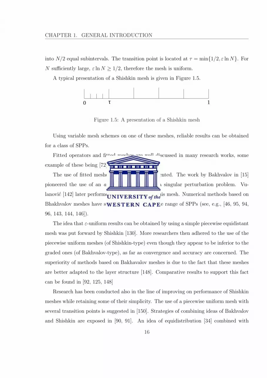
A typical presentation of a Shishkin mesh is given in Figure 1.5.
τ 0 1
Figure 1.5: A presentation of a Shishkin mesh
Using variable mesh schemes on one of these meshes, reliable results can be obtained
for a class of SPPs.
Fitted operators and fitted meshes are well discussed in many research works, some
example of these being [72], [87] and [102].
The use of fitted meshes is immensely documented. The work by Bakhvalov in [15]
pioneered the use of an a priori mesh to solve a singular perturbation problem. Vu-
lanovic [142] later performed a generalization of this mesh. Numerical methods based on
Bhakhvalov meshes have successfully solved a wide range of SPPs (see, e.g., [46, 95, 94,
96, 143, 144, 146]).
The idea that ε-uniform results can be obtained by using a simple piecewise equidistant
mesh was put forward by Shishkin [130]. More researchers then adhered to the use of the
piecewise uniform meshes (of Shishkin-type) even though they appear to be inferior to the
graded ones (of Bakhvalov-type), as far as convergence and accuracy are concerned. The
superiority of methods based on Bakhavalov meshes is due to the fact that these meshes
are better adapted to the layer structure [148]. Comparative results to support this fact
can be found in [92, 125, 148]
Research has been conducted also in the line of improving on performance of Shishkin
meshes while retaining some of their simplicity. The use of a piecewise uniform mesh with
several transition points is suggested in [150]. Strategies of combining ideas of Bakhvalov
and Shishkin are exposed in [90, 91]. An idea of equidistribution [34] combined with
16

CHAPTER 1. GENERAL INTRODUCTION
Shishkin type transition point is presented in [17].
The extendability of the methods using meshes of Shishkin type to higher dimensional
problem explains why people are interested in using them. Another advantage of Shishkin
meshes over Bakhvalov ones, pointed out in [150], is the convenience to handle complicated
higher order methods. Since, in this thesis, we aim at constructing higher order methods,
we will rather use Shishkin type meshes.
The fitted operator methods were introduced by Allen and Southwell [10] to solve the
problem of viscous fluid pass a cylinder. Subsequently, Doolan et al. [33] studied one type
of exponentially fitted methods considered by Liniger and Willoughby [89] which is in fact
a special class of the θ-method of Lambert [83]. The discussion about the construction of
a suitable fitting factor in the above methods is provided in [33].
The research is ongoing in this field and hence there is no end to the literature ac-
countable to this topic.
1.4 Literature review on higher order numerical meth-
ods for SPPs
In this section, we survey some of the works done so far on higher order methods for
singular perturbation problems in recent years, some of which are found in [66]. The
works are presented in the chronological order.
Fitted methods have been shown to be superior to standard methods in solving singular
perturbation problems because they attempt to capture the singular behaviour of the
solution in the layers. However, higher order methods can be used to obtain an expected
degree of accuracy with fewer mesh points as compared to lower order methods. Table 1.1
shows that the maximum error is reduced by a factor of 1/16 if the number of subintervals
of a mesh is multiplied by 16 for a first order method. The same degree of accuracy is
attained when the number of subintervals of the mesh is only doubled for a fourth order
17

CHAPTER 1. GENERAL INTRODUCTION
method. Another comparison can be made as follows: if one multiplies the number of
subintervals of a mesh by 16, the maximum error is only divided by 16 for a first order
method whereas this error is divided by 65536 for a fourth order method. This explains
our interest in designing higher order methods.
Vulanovic [145] solved the singularly perturbed problem
−εu′′ − b(x)u′ + c(x)u = f(x),
subject to one of the following boundary conditions
u(0) = γ0, u(1) = γ1,
or
−εu′(0) = γ0, u(1) = γ1.
The functions b, c, f are sufficiently smooth and b(x) > β > 0, c(x) ≥ 0, while 0 < ε ¿1. He obtained the second-order convergence uniform in ε due to the treatment of the
boundary layer function, to a special non-equidistant mesh (dense in the layer), and to
the use of a combination of central and mid-point finite difference schemes.
Stynes and O’Riordan [137] examined the problem
εu′′ + a(x)u′ − b(x)u = f(x),
Table 1.1: The reduction of the maximum error by higher order methods.
Order 10 20 40 80 1601 1/2 1/4 1/8 1/162 1/4 1/16 1/64 1/2563 1/8 1/64 1/512 1/40964 1/16 1/256 1/4096 1/65536
18

CHAPTER 1. GENERAL INTRODUCTION
for 0 < x < 1, a(x) ≥ α > 0, b(x) ≥ β, α2 + 4αβ > 0; a, b and f in C2[0, 1], ε in (0, 1],
u(0) and u(1) given. Using finite elements and a discretized Green’s function, they showed
that the El-Mistikawy and Werle difference scheme on an equidistant mesh of width h is
uniformly second order accurate for this problem. With a natural choice of trial functions,
they obtained uniform first order accuracy in L∞(0, 1) norm. Choosing piecewise linear
trial functions (“hat” functions) they obtained the same accuracy in the L1(0, 1) norm.
O’Riordan and Stynes [115] considered the numerical solutions of the differential equa-
tion
ε(p(x)u′)′ + (q(x)u)′ − r(x)u = f(x),
0 < x < 1; u(0) = u0; u(1) = u1,
where p > 0, q > 0, r ≥ 0, 0 < ε ≤ 1, and p, q, r and f ∈ C2[0, 1]. Using finite
elements with uniform mesh h, they generated a tridiagonal difference scheme which
has uniform O(h2) nodal accuracy. Using piecewise linear trial functions, they obtained
uniform O(h) accuracy in the L1(0, 1) norm. Using certain other trial functions (L-
splines), they obtained uniform O(h) accuracy in the L∞(0, 1) norm.
Farell [38] gave some results which characterize the behavior of a linear nonselfad-
joint singular perturbation problem. He also gave criteria for uniform convergence of a
nonturning, simple turning point and one multiple turning point case and indicated the
uniform methods for higher-order cases. Then he discussed the consequences for quasi-
linear problems.
Using a finite difference framework of Doedel [32] and Lynch and Rice [99], Gartland
[45] constructed a family of uniformly accurate finite difference schemes for the problem
−εu′′(x) + a(x)u′ + b(x)u = f(x),
0 < x < 1 ; u(0) = g0 , u(1) = g1.
with the assumptions that a, b and f are bounded continuous functions and a(x) ≥ a > 0
19

CHAPTER 1. GENERAL INTRODUCTION
on [0,1]. A scheme of order hp (uniform in ε) is constructed to be exact on a collocation
of functions of the type
1, x, · · · · · · , xp, exp
(∫ 1
x
a
), x exp
(∫ 1
x
a
), · · · · · · ,
xp−1 exp
(∫ 1
x
a
).
The high order is achieved through extra evaluations of f . He also presented some nu-
merical experiments which exhibit uniform orders hp, p = 1, 2, 3 and 4.
Sklyar [134] constructed a conservative difference scheme for singularly perturbed dif-
ferential problems. In the construction a suitable decomposition of a symmetric bilinear
form is applied. The method is presented for the model problem
εu′′ + au′ = f, x ∈ (0, 1); u(0) = α0, u(1) = α1.
The coefficients of the scheme are obtained by recursion; the number of iterations depends
on ε. The order of convergence is proved to be O(h2) and is independent of ε.
Herceg et al. [56] considered singularly perturbed semilinear selfadjoint two-point
boundary value problems, with Dirichlet boundary conditions. Using a Bakhvalov-type
mesh, they gave a difference scheme for numerically solving such problems. It is shown
that the solution of this difference scheme is amenable to Richardson extrapolation, and
that one can thereby obtain sixth-order convergence at each node, uniformly in the sin-
gular perturbation parameter.
Herceg [57] used the Hermitian approximation of the second order derivative for a
linear singularly perturbed nonlocal problem
ε2u′′ + b(x)u = f(x) , 0 ≤ x ≤ 1,
20

CHAPTER 1. GENERAL INTRODUCTION
u(0) = 0, u(1) =m∑
i=1
ciu(si) + d,
d, ci ∈ R,
si ∈ (0, 1), i = 1, 2, · · · ,m,
0 < ε << 1, b ∈ Ck[0, 1],
k ∈ N, b(x) ≥ β2 > 0,
for some positive constant β. He proved that the technique is fourth order uniformly
convergent.
Stojanovic [136] considered a linear, self-adjoint, singularly perturbed, two-point bound-
ary value problem. She generated a difference scheme for this problem by approximating
the forcing term with a piecewise cubic polynomial, and approximating the coefficient
of the zero-order term with a piecewise constant function. This scheme is shown to be
second-order accurate, uniformly in the singular perturbation parameter.
Schmitt [126] constructed a symmetric difference scheme for linear, stiff, or singularly
perturbed boundary value problems of first-order with constant coefficients. His scheme
is based on a stability function containing a matrix square root. Its essential feature
is the unconditional stability function in the absence of purely imaginary eigenvalues of
the coefficient matrix. He proved local damping of errors, uniform stability, and uniform
second-order convergence. He also discussed the computation of the specific matrix square
root by a well-known stable variant of Newton’s method.
Based on the coupling of the central difference scheme with the Abrahamsson-Keller-
Kreiss box scheme on a special nonuniform mesh, Sun and Wu [138] proposed a scheme
for the numerical solution of the singular boundary value problem
εu′′ + b(x)u′ − c(x)u = f(x), u(0) = α, u(1) = β.
21

CHAPTER 1. GENERAL INTRODUCTION
They proved that this scheme is uniformly second-order convergent.
Kadalbajoo and Bawa [65] presented a variable-mesh method based on cubic spline
approximation for nonlinear singularly perturbed boundary-value problems of the form
εy′′ = f(x, y) , y(a) = α , y(b) = β.
They gave convergence analysis and the method is shown to have third-order convergence.
In [151], Wang solved a nonlinear singular perturbation problem numerically on non-
equidistant meshes which are dense in the boundary layers. The method is based on the
numerical solution of integral equations. He proved the fourth-order uniform accuracy of
the scheme.
Grekov and Krasnikov [51] examined a linear singularly perturbed reaction-diffusion
problem in one dimension. Assuming that its coefficients are piecewise smooth, they con-
sidered any mesh whose nodes include the points of discontinuity of these coefficients.
The solution u is expressed as a series, each term of which can be computed by numer-
ically solving a singularly perturbed reaction-diffusion problem with piecewise constant
coefficients. They proved that by truncating this series, u can be approximated in the
L∞-norm, uniformly in the singular perturbation parameter, up to O(hm), where h is the
mesh diameter and m is an arbitrary positive integer.
Hu et al. [62] developed a discretization method for one-dimensional singular pertur-
bation problems based on Petrov-Galerkin finite element, or an equivalent finite volume,
scheme. The model one-dimensional problem which they considered was
−εu′′ + βu′ + σu = f in (a, b),
u(a) = ua, u(b) = ub.
22

CHAPTER 1. GENERAL INTRODUCTION
This problem has its origin in the physical conservation law
q′ + (σ − β′)u = f,
and Fick’s diffusion law
q = −εu′ + βu,
where q is the flux, ε the diffusivity, β the velocity, and σ the absorbing coefficient (or
reactivity). The scheme that they developed is not only O(h2) accurate uniformly in
ε, but also satisfies certain discrete versions of both the conservative law and maximum
principle.
Beckett and Mackenzie [18] studied the numerical approximation of a singularly per-
turbed reaction-diffusion equation using a p-th order Galerkin finite element method on a
non-uniform grid. The grid was constructed by equidistributing a strictly positive moni-
tor function which is a linear combination of a constant floor and a power of the second
derivative of a representation of the boundary layers-obtained using a suitable decom-
position of the analytical solution. By the appropriate selection of the monitor function
parameters they proved that the numerical solution is insensitive to the size of the singu-
lar perturbation parameter and achieves the optimal rate of convergence with respect to
the mesh density.
In [43], a defect correction method based on finite difference schemes is considered
for a singularly perturbed boundary value problem on a Shishkin mesh. The method
combines the stability of the upwind difference scheme and the higher-order convergence
of the central difference scheme. The almost second-order convergence of the scheme
with respect to the discrete maximum norm, uniformly in the perturbation parameter, is
proved.
A boundary value problem for a singularly perturbed parabolic equation of convection
diffusion type on an interval is studied. For the approximation of the boundary value prob-
23

CHAPTER 1. GENERAL INTRODUCTION
lem, Hemker et al. [53] use earlier developed finite difference schemes, epsilon-uniformly
of a high order of accuracy with respect to time, based on defect correction.
Vulanovic [150] solved numerically a class of singularly perturbed quasilinear boundary
value problems with two small parameters by finite differences on a Shishkin-type mesh.
The discretization combined a four-point third-order scheme inside the boundary layers
with the standard central scheme outside the layers. This results in an almost third-order
accuracy which is uniform with respect to the perturbation parameters. The paper also
showed that the Shishkin meshes are more suitable for higher-order schemes than the
Bakhvalov meshes, since complicated non-equidistant schemes can be avoided.
Hemker et al. [54] used a defect correction technique to construct ε-uniformly con-
vergent schemes of high-order time-accuracy. The efficiency of the new defect-correction
schemes is confirmed with numerical experiments. An original technique for an experi-
mental study of convergence orders is developed for cases when the orders of convergence
in the x-direction and in the t-direction can be essentially different.
Until an approach by Roos (in one of his technical reports in 2005: complete cita-
tion details are not available), the best way to construct high order uniformly convergent
schemes for singular perturbation problems was to apply exponentially fitted compact
difference schemes. His approach consists of the following steps: firstly solve an auxil-
iary problem with piecewise or nearly piecewise constant coefficients, secondly improve
the approximation iteratively using the defect correction idea and piecewise polynomial
approximations of higher order. An important advantage of this approach lies in the
fact that it is possible to start from a classical or weak formulation of a boundary value
problem. Therefore, the approach is useful for singular perturbations related to ordinary
as well as partial differential equations.
Patidar [118] considered the self-adjoint singularly perturbed two-point boundary
value problems
−ε(a(x)y′)′ + b(x)y = f(x), x ∈ [0, 1],
24

CHAPTER 1. GENERAL INTRODUCTION
y(0) = η0, y(1) = η1.
Highest possible order of uniform convergence for such problems achieved so far via fitted
operator methods, was one. Reducing the original problem into the normal form and then
using the theory of inverse monotone matrices, he derived a FOFDM via the standard
Numerov’s method. His scheme is fourth order accurate for moderate values of ε and
ε-uniformly convergent with order two for very small values of ε.
A one-dimensional singularly perturbed problem of mixed type is considered by
Brayanov [24]. The domain under consideration is partitioned into two subdomains. In
the first subdomain a parabolic reaction-diffusion problem is given and in the second one
an elliptic convection-diffusion-reaction problem. The solution is decomposed into regular
and singular components. The problem is discretized using an inverse-monotone finite
volume method on condensed Shishkin meshes. He establishes an almost second-order
global pointwise convergence in the space variable.
Gracia et al. [49] constructed a second order monotone numerical method for a sin-
gularly perturbed ordinary differential equation with two small parameters affecting the
convection and diffusion terms. The monotone operator is combined with a piecewise-
uniform Shishkin mesh. An asymptotic error bound in the maximum norm is established
theoretically whose error constants are shown to be independent of both singular pertur-
bation parameters.
A numerical study is made in [71] to examine a singularly perturbed parabolic initial-
boundary value problem in one space dimension on a rectangular domain. The solution of
this problem exhibits the boundary layer on the right side of the domain. They constructed
a Crank-Nicolson finite difference method consisting of an upwind finite difference operator
on a fitted piecewise uniform mesh. The resulting method has been shown to be almost
first order accurate in space and second order in time. Numerical experiments have been
carried out, which validate the theoretical results. It is also shown that a numerical
method consisting of same finite difference operator on uniform mesh does not converge
25

CHAPTER 1. GENERAL INTRODUCTION
uniformly with respect to the singular perturbation parameter.
Mohanthy and Singh [108] derived a difference method of O(h4), so called, arithmetic
average discretization for the solution of two dimensional non-linear singularly perturbed
elliptic partial differential equation of the form
ε(uxx + uyy) = f(x, y, u, ux, uy),
0 < x, y < 1,
subject to appropriate Dirichlet boundary conditions where ε > 0 is a small parameter.
They also derived new methods of higher order for the estimates of ∂u/∂n, which are
quite often of interest in many physical problems. In all cases, only 9-grid points and a
single computational cell were required. The main advantage of the proposed methods is
that the methods are directly applicable to singular problems.
In [12], a high-order (second and fourth of convergence, but with first and third-order
local truncation error, respectively) compact finite difference schemes for elliptic equa-
tions with intersecting interfaces is derived. The approach uses the differential equation
and the jump (interface) relations as additional identities which can be differentiated to
eliminate higher order local truncation errors. Numerical experiments are carried out to
demonstrate the high-order accuracy and to show that our method is effective to sharp
contrast in the diffusion coefficients of the problems.
Rao and Kumar [122] present a B-spline collocation method of higher order for a class
of self-adjoint singularly perturbed boundary value problems. The essential idea in this
method is to divide the domain of the differential equation into three non-overlapping
subdomains and solve the regular problems obtained by transforming the differential
equation with respective boundary conditions on these subdomains using the present
higher order B-spline collocation method. The boundary conditions at the transition
points are obtained by the asymptotic approximation of order zero to the solution of the
26

CHAPTER 1. GENERAL INTRODUCTION
problem. The convergence analysis is given and the method is shown to have optimal
order convergence; by collocating the perturbed differential equation, which is satisfied
by a special cubic spline interpolate of the true solution.
Franz [42] analyzed a continuous interior penalty (CIP) method for elliptic convection-
diffusion problems with characteristic layers on a Shishkin mesh. The method penalizes
jumps of the normal derivative across interior edges. He shows that it is of the same order
of convergence as the streamline diffusion finite-element method and is superclose in the
CIP norm induced by its bilinear form for the difference between the FEM solution and
the bilinear nodal interpolant of the exact solution. Furthermore, he studies numerically
the behaviour of the method for different choices of the stabilization parameter.
A fourth-order finite-difference method for singularly perturbed one-dimensional
reaction-diffusion problem is presented by Herceg and Herceg in [58]. The problem is
discretized using a Bakhvalov-type mesh. They gave a uniform convergence with respect
to the perturbation parameter.
Kadalbajoo and Kumar [73] develop a method which deals with the singularly per-
turbed boundary value problem for a linear second order differential-difference equation
of the convection-diffusion type with small delay parameter τ of O(ε) whose solution has
a boundary layer. The fitted mesh technique is employed to generate a piecewise-uniform
mesh condensed in the neighborhood of the boundary layers. B-spline collocation method
is used with fitted mesh. Parameter-uniform convergence analysis of the method is dis-
cussed. The method is shown to have almost second order parameter-uniform convergence.
The effect of small delay τ on boundary layer has also been discussed.
Kadalbajoo and Yadaw [74] presented a B-spline collocation method for solving a class
of two-parameter singularly perturbed boundary value problems. They used B-spline
collocation method on piecewise-uniform Shishkin mesh, which leads to a tridiagonal
linear system. They analyzed the method for convergence and showed that it is uniformly
convergent of second order.
27

CHAPTER 1. GENERAL INTRODUCTION
Lin et al. [88] developed a new method by detecting the boundary layer of the solution
of a singular perturbation problem. On the non-boundary layer domain, the singular
perturbation problem is dominated by the reduced equation which is solved with standard
techniques for initial value problems. While on the boundary layer domain, it is controlled
by the singular perturbation. Its numerical solution is obtained using finite difference
methods. The numerical error is maintained at the same level with a constant number of
mesh points for a family of singular perturbation problems.
Shahraki and Hosseini [128] presented a new scheme for discretization of singularly
perturbed boundary value problems based on finite difference methods. This method is
a combination of simple upwind scheme and central difference method on a special non-
uniform mesh (Shishkin mesh) for the space discretization. Numerical results show that
the convergence of method is uniform with respect to singular perturbation parameter
and has a higher order of convergence.
In the paper, Solin and Avila [135] present a new piecewise-linear finite element mesh
suitable for the discretization of the one-dimensional convection-diffusion equation
−εu′′ − bu′ = 0, u(0) = 0, u(1) = 1.
The solution to this equation exhibits an exponential boundary layer which occurs also
in more complicated convection-diffusion problems of the form
−ε∆u− b∂u
∂x+ cu = f.
Their new mesh is based on the equidistribution of the interpolation error and it takes
into account finite computer arithmetic. It is demonstrated numerically that for the above
problem, the new previous mesh has remarkably better convergence properties than the
well-known previous shishkin and Bakhvalov meshes.
Xie et al. [154] presented a novel approach for solving parameterized singularly per-
28

CHAPTER 1. GENERAL INTRODUCTION
turbed two-point boundary value problems with a boundary layer. By the boundary layer
correction technique, the original problem is converted into two non-singularly perturbed
problems which can be solved using traditional numerical methods, such as Runge-Kutta
methods. Several non-linear problems are solved to demonstrate the applicability of the
method.
The bilinear finite element methods on appropriately graded meshes are considered in
Zhu and Chen [155] both for solving singular and semisingular perturbation problems. In
each case, the quasi-optimal order error estimates are proved in the ε-weighted H1-norm
uniformly in singular perturbation parameter ε, up to a logarithmic factor. By using
the interpolation postprocessing technique, the global superconvergent error estimates in
ε-weighted H1-norm are obtained.
Kadalbajoo and Gupta [75] designed a numerical scheme to solve a singularly per-
turbed convection-diffusion problem. The scheme involves B-spline collocation method
and appropriate piecewise-uniform Shishkin mesh. Bounds were established for the deriva-
tive of the analytical solution. Moreover, the method is boundary layer resolving as well
as second-order uniformly convergent in the maximum norm. They give a comprehensive
analysis to prove the uniform convergence with respect to singular perturbation parame-
ter.
Surla et al. [139] considered finite difference approximation of a singularly perturbed
one-dimensional convection-diffusion two-point boundary value problem. The problem
is numerically treated by a quadratic spline collocation method on a piecewise uniform
slightly modified Shishkin mesh. The position of collocation points is chosen so that
the obtained scheme satisfies the discrete minimum principle. They prove pointwise con-
vergence of order O(N−2 ln2 N) inside the boundary layer and second order convergence
elsewhere. Further, they approximate normalized flux and give estimates of the error at
the mesh points and between them.
They determine the conditions under which the difference schemes, applied indepen-
29

CHAPTER 1. GENERAL INTRODUCTION
dently on subdomains may accelerate (epsilon-uniformly) the solution of the boundary
value problem without losing the accuracy of the original schemes. Hence, the simulta-
neous solution on subdomains can in principle be used for parallelization of the compu-
tational method.
Ilicasu and Schultz [63] developed a high-order finite-difference technique for the
second-order, singularly perturbed linear BVP in one dimension. Taylor series expan-
sions and error conversions are used for the development of the techniques. Convergence
and stability conditions of these techniques are proved.
Liu and Shen [97] proposed a new spectral Galerkin method for the convection-
dominated convection-diffusion equation. This method employs a new class of trial func-
tion spaces. The available error bounds provide a clear theoretical interpretation for the
higher accuracy of the new method compared to the conventional spectral methods when
applied to problems with this boundary layers.
Some of the works that are more specific for the problems considered in the individual
chapters are described further in the introduction sections of those chapters. There might
be little repetitions but we do so in order for the chapters to be self contained.
1.5 Summary of the thesis
The order of the various numerical methods that we mentioned in previous section vary
from less that one to three or four. Quite often a numerical analyst prefers a higher
order method due to the fact that it offers the opportunity to attain a better degree of
accuracy with fewer mesh points as compared to lower order methods. Since in most cases,
techniques of constructing directly higher order methods are tedious, we will rather focus
on Richardson’s extrapolation which is one of the convergence acceleration techniques. It
consists of taking a linear combination of k solutions (k ≥ 2) corresponding to different
but nested meshes on the intersection of these meshes which is in fact the coarsest mesh
[41]. Due to time limitation the other convergence technique, the defect correction is not
30

CHAPTER 1. GENERAL INTRODUCTION
considered in this thesis. While we will investigate the effect of Richardson extrapolation
on some existing fitted methods in some instances, we will use this technique on some
novel fitted methods in other instances.
In Chapter 2, we investigate the effect of Richardson extrapolation on the fitted mesh
finite difference method (FMFDM) of [119] for a self-adjoint problem. We note that even
though the accuracy is improved, the order of convergence remains unchanged. This unex-
pected fact contradicts the assertion met in the literature about Richardson extapolation
that “A numerical solution of required accuracy can be obtained by using Richardson
extrapolation method [11, 133] and it can be used to improve the ε-uniform rates of
convergence of computed solutions [133].
We go on investigating what impact the extrapolation technique will have on other
methods to solve the above mentioned self-adjoint problem in Chapter 3. We consider
two fitted operator finite difference methods (FOFDMs) which we denote by FOFDM-I
and FOFDM-II, presented in [118] and [98], respectively. In the first case, Richardon
extrapolation does not improve the convergence which is of order four and two for some
moderate and smaller values of ε. In the latter case, the second order accuracy is improved
up to four, irrespective of the value of ε.
Chapter 4 deals with construction and analysis of a FMFDM and a FOFDM to solve
a singularly perturbed turning point problem whose solution has boundary layers. We
study the performance of Richardson extrapolation on these methods.
In Chapter 5, we consider a singularly perturbed nonlinear two-point boundary value
problem. We first apply the quasilinearization process [19] to linearize the problem. Then
the resulting sequence of linear problems is solved by a FOFDM.
A time-dependent nonlinear Burgers’ equation is considered in Chap 6. We again lin-
earize the problem using the quasilinearization process. The process results in a sequence
of linear problems at each time level which we solve using a FOFDM.
The FOFDM-II of Chapter 3 is extended to singularly perturbed elliptic problems in
31

CHAPTER 1. GENERAL INTRODUCTION
2-dimensions in Chapter 7. This method is of order 2 in both x- and y-direction. The
fourth order convergence is achieved after applying Richardson extrapolation.
Due to the space limitations, we give only necessary details in the latter chapters.
Finally, some concluding remarks and directions for further research are provided in
Chapter 8.
32
Chapter 2
Higher Order Fitted Mesh Finite
Difference Scheme for a Singularly
Perturbed Self-adjoint Problem
Numerous methods have been developed for singularly perturbed self-adjoint boundary
value problems in past three decades. The order of these methods vary from less than
one to three or four. Quite often a numerical analyst prefers a higher order method due
to the fact that it offers the opportunity to attain a better degree of accuracy with fewer
mesh points as compared to lower order methods. Motivated by this fact, we would like to
investigate in this chapter whether we can accelerate the order of convergence of existing
high order methods.
We consider the fitted mesh finite difference method of Patidar [119] applied on a
Shishkin-type mesh for the solution of self-adjoint problem which is ε-uniform convergent
of order four. We attempt to increase the order of convergence by Richardson’s ex-
trapolation and notice that this well-known convergence acceleration technique has some
limitations. We observe that even though Richardson extrapolation improves the accu-
racy slightly, this technique does not increase the rate of convergence which is originally
33

CHAPTER 2. HIGHER ORDER FITTED MESH FINITE DIFFERENCE SCHEMEFOR A SINGULARLY PERTURBED SELF-ADJOINT PROBLEM
four for the underlying method for the problem above. This fact was unexpected and
contradicts the assertion met in the literature so far about Richardson extrapolation.
2.1 Introduction
Solutions of singular perturbation problems (SPPs) present large gradients when the per-
turbation parameter approaches zero. The solution of these SPPs typically contains layers.
This behavior lowers the order of convergence of the underlying numerical method and
results in low accuracy. Standard methods have failed to resolve the layer(s) for all values
of ε (the singular perturbation parameter), unless a very fine mesh is considered, which
unfortunately increases the computational complexities. To overcome this difficulty, fitted
methods have been considered by various authors since they provide reliable numerical
results on a mesh with a reasonable number of grid points and hence make the method
practically applicable. However, some fitted methods perform better than others.
Various numerical methods have been developed so far to solve such problems, some
of which we will mention below. The order of these methods vary from less than one to
three or four. Since quite often a numerical analyst prefers a higher order method due
to the fact that it offers the opportunity to attain a better degree of accuracy with fewer
mesh points as compared to lower order methods, we would like to investigate in this
paper whether we can accelerate the order of convergence of existing high order methods.
Direct techniques to obtain high order methods for singularly perturbed problems are
well documented. We provide few examples. For a one-dimensional convection-diffusion
problem, a second order ε-uniformly convergent method was designed in [145]. In [137],
the same order of convergence was obtained using finite elements and discretized Green’s
functions and applying the El-Mistikawy and Werle difference scheme on an equidistant
mesh. This problem was also examined in [45] where a scheme of order p (p = 1, 2, 3, 4)
was constructed using collocation approach.
By using Hermitian approximation of the second order derivative, a fourth order uni-
34

CHAPTER 2. HIGHER ORDER FITTED MESH FINITE DIFFERENCE SCHEMEFOR A SINGULARLY PERTURBED SELF-ADJOINT PROBLEM
formly convergent scheme for a reaction-diffusion problem was presented in [57].
For a self-adjoint problem, a second-order nodal accuracy using finite elements with
uniform mesh is obtained in [115], whereas in [118] a fitted operator finite difference
method (FOFDM) was derived via Numerov’s method that showed to be fourth order
accurate for moderate value of ε and second order uniformly convergent for small values
of ε. On the other hand in [119] a fitted mesh finite difference method (FMFDM) was
shown to be fourth order ε-uniformly convergent. The third order of convergence was
found for quasilinear problems in [149] and [150]. The third and fourth order of conver-
gence was obtained for a nonlinear problem [151] by using numerical solution of integral
equations. While none of these methods is of order higher than four, there exist methods
of arbitrary order (see, e.g., [51]). However, because designing and implementing such
methods appears not to be an easy task, no numerical experiment has supported this
assertion.
Beside the various techniques of constructing directly higher order methods (which are
tedious in most cases), one would rather use a convergence acceleration strategy. Several
methods for improvement of solutions have been designed (see, e.g., [11, 47, 64, 123, 132,
133] and the references therein). One of these methods, which was subsequently termed as
the Richardson extrapolation, is a post-processing procedure where a linear combination
of two computed solutions approximating a particular quantity gives a third and better
approximation. It was implemented in [77] for a system of first order linear ordinary
differential equation, in [93] and [111] for a one-dimensional linear convection-diffusion
problem and in [133] for a quasilinear parabolic singularly perturbed convection-diffusion
equations.
Our aim in this Chapter is to investigate the limitations of the Richardson’s extrap-
olation when it is applied for a method which is already of high order. To this end, we
consider the following problem (2.1.1) for which Patidar [119] constructed a fourth order
35

CHAPTER 2. HIGHER ORDER FITTED MESH FINITE DIFFERENCE SCHEMEFOR A SINGULARLY PERTURBED SELF-ADJOINT PROBLEM
ε-uniformly convergent FMFDM (on a mesh of Shishkin-type):
Ly ≡ −ε(a(x)y′)′ + b(x)y = f(x), x ∈ (0, 1), y(0) = η0, y(1) = η1, (2.1.1)
where η0 and η1 are given constants and ε ∈ (0, 1]. The functions f(x), a(x) and b(x) are
assumed to be sufficiently smooth and to satisfy the conditions
a(x) ≥ a > 0, b(x) ≥ b > 0.
The rest of this chapter is organized as follows. Some theoretical estimates are provided
in Section 2.2. For the sake of completeness, we present the FMFDM of [119] in Section
2.3. We establish the extrapolation formula in Section 2.5. This section deals also with the
error analysis of the FMFDM after extrapolation where analysis before extrapolation is
reviewed. Two numerical examples are considered in section 2.5 to confirm our theoretical
results. Section 2.7 is devoted to the conclusions and further research plans.
2.2 Reduction to normal form and some theoretical
estimates
The following lemmas [119] are necessary for the existence and uniqueness of the solution
and for the problem to be well-posed.
Lemma 2.2.1. (Maximum Principle) Let L be the operator as in (2.1.1) such that
B0y(0) ≡ y(0) = η0, B1y(1) ≡ y(1) = η1. Suppose φ(x) is any smooth function satis-
fying B0y(0) ≥ 0, B1y(1) ≥ 0 and let Lφ(x) ≥ 0, ∀ 0 < x < 1 then φ(x) ≥ 0,∀ 0 ≤ x ≤ 1.
Proof. The proof is by contradiction. Let x∗ be such that φ(x∗) = minx∈[0,1] φ(x) and
assume that φ(x∗) < 0. Clearly, x∗ /∈ 0, 1 and therefore φ′(x∗) = 0 and φ′′(x∗) ≥ 0.
36

CHAPTER 2. HIGHER ORDER FITTED MESH FINITE DIFFERENCE SCHEMEFOR A SINGULARLY PERTURBED SELF-ADJOINT PROBLEM
Further,
Lφ(x∗) = −ε(a(x∗)φ′(x∗))′ + b(x∗)φ(x∗) < 0,
which is a contradiction. It follows that φ(x∗) ≥ 0 and thus φ(x) ≥ 0∀ x ∈ [0, 1].
The uniqueness of the solution is implied by this maximum principle. Its existence fol-
lows trivially (as for linear problems, the uniqueness of the solution implies its existence).
This principle is now applied to prove that the solution of (2.1.1) is bounded.
Lemma 2.2.2. Let y(x) be the solution of the problem (2.1.1), then we have
||y|| ≤ b−1||f ||+ max(η0, η1).
Proof. We construct two barrier functions Π± defined by
Π±(x) = b−1||f ||+ max(η0, η1)± y(x).
Then we have
Π±(0) = b−1||f ||+ max(η0, η1)± y(0)
= b−1||f ||+ max(η0, η1)± η0
≥ 0,
Π±(1) = b−1||f ||+ max(η0, η1)± y(1)
= b−1||f ||+ max(η0, η1)± η1
≥ 0,
and we have
LΠ±(x) = −ε(a(x)(Π±(x))′)′ + b(x)Π±(x)
= b(x)(b−1||f ||+ max(η0, η1))± Ly(x)
37
CHAPTER 2. HIGHER ORDER FITTED MESH FINITE DIFFERENCE SCHEMEFOR A SINGULARLY PERTURBED SELF-ADJOINT PROBLEM
= b(x)[b−1||f ||+ max(η0, η1)]± f(x)
≥ 0, since ||f || ≥ f(x).
Therefore, by the maximum principle (Lemma 2.2.1), we obtain Π±(x) ≥ 0, for all x ∈[0, 1], which gives the required estimate.
Now, let
P (x) =a′(x)
a(x), Q(x) = − b(x)
εa(x)and R(x) = − f(x)
εa(x).
Equation (2.1.1) therefore becomes
y′′ + P (x)y′ + Q(x)y = R(x). (2.2.2)
Via the substitutions
U(x) = exp(− 1
2
∫ x
0
P (ζ)dζ)
and
y(x) = U(x)V (x), (2.2.3)
into equation (2.2.2), the problem (2.1.1) is transformed into the normal form
LV ≡ −εV ′′ + W (x)V = Z(x), (2.2.4)
V (0) = α0
(≡ y(0)
U(0)
), V (1) = α1
(≡ y(1)
U(1)
), α0, α1 ∈ R
where
W (x) = −ε
(Q(x)− 1
2P ′(x)− 1
4(P (x))2
),
Z(x) = −ε
(R(x) exp
(1
2
∫ x
0
P (ζ)dζ))
.
It is worthwhile noting that the operator L also satisfies the maximum principle:
38
CHAPTER 2. HIGHER ORDER FITTED MESH FINITE DIFFERENCE SCHEMEFOR A SINGULARLY PERTURBED SELF-ADJOINT PROBLEM
Lemma 2.2.3. Let ψ(x) be any sufficiently smooth function such that ψ(0) ≥ 0 and
ψ(1) ≥ 0. Then Lψ(x) ≥ 0,∀ x ∈ (0, 1) implies that ψ(x) ≥ 0,∀x ∈ [0, 1].
In the error analysis of problem (2.2.4), it is convenient to decompose the solution Vε
into a smooth (regular) component Vε,r and a singular component Vε,s. Bounds on these
components and on their derivatives are provided in the following Lemma [105]:
Lemma 2.2.4. The solution Vε of the problem (2.2.4) can be decomposed into the form
Vε := Vε,r + Vε,s
where for all k ∈ 0, 1, 2, · · · , 6 and x ∈ [0, 1], the regular component Vε,r satisfies
|V (k)ε,r | ≤ M [1 + ε−(k−2)/2E(x, β)],
and the singular component Vε,s satisfies
|V (k)ε,s | ≤ Mε−k/2E(x, β),
where
0 < β ≤ W (x)
and
E(x, β) =
exp(− x/
√β/ε
)+ exp
(− (1− x)
√β/ε
)
.
Lemma 2.2.5. For a fixed mesh and for all integers k, we have
limε→0
max1≤j≤n−1
exp(−Mxj/√
ε)
εk/2= 0,
39

CHAPTER 2. HIGHER ORDER FITTED MESH FINITE DIFFERENCE SCHEMEFOR A SINGULARLY PERTURBED SELF-ADJOINT PROBLEM
and
limε→0
max1≤j≤n−1
exp(−M(1− xj)/√
ε)
εk/2= 0,
where xj = jh, h = 1/n, ∀j = 1(1)n− 1.
Proof. Consider the partition
[0, 1] := 0 = x0 < x1 < x2 < · · · < xn−1 < xn = 1.
It is clear that, for the interior grid points, we have
max1≤j≤n−1
exp(−Mxj/√
ε)
εk/2≤ exp(−Mx1/
√ε)
εk/2=
exp(−Mh/√
ε)
εk/2
and
max1≤j≤n−1
exp(−M(1− xj)/√
ε)
εk/2≤ exp(−M(1− xn)/
√ε)
εk/2= M
exp(−Mh/√
ε)
εk/2
(as x1 = h, 1− xn−1 = 1− (n− 1)h = h). An application of L’Hospital’s rule the gives
limε→0
exp(−Mh/√
ε)
εk/2= lim
p(=1/√
ε)→∞pk
exp(Mhp)≡ lim
p→∞k!
(Mh)k exp(Mhp)= 0,
which completes the proof.
2.3 The numerical method
The FMFDM that we use in Chapter has been derived in Patidar [119] on the Shishkin
mesh described below.
The interval [0, 1] is divided into three sub-intervals:
[0, 1] := [0, δ] ∪ [δ, 1− δ] ∪ [1− δ, 1],
40

CHAPTER 2. HIGHER ORDER FITTED MESH FINITE DIFFERENCE SCHEMEFOR A SINGULARLY PERTURBED SELF-ADJOINT PROBLEM
where δ is the width of the boundary layer. Let n be a positive integer such that n = 2m
with m ≥ 5. The intervals (0, δ) and (1 − δ, 1) are each divided into n/4 equal mesh
elements, while the interval (δ, 1− δ) is divided into n/2 equal mesh elements. Therefore,
we have n/4 + 1 equidistant grid points in the intervals [0, δ] and [1 − δ, 1] and n/2 − 1
equidistant grid points in (δ, 1− δ). The parameter δ is defined by
δ = min
1/4, 4(√
ε/β)
ln(n/16)
(2.3.5)
where 0 < β ≤ W (x), ∀x ∈ [0, 1]. Assuming that j0 = n/4, xj0 = δ, xn−j0 = 1− δ and
[0, 1] := 0 = x0 < x1 < · · · < xj0 < · · · < xn−j0 < · · · < xn = 1,
we have hj = xj − xj−1 where the mesh spacing is given by
hj =
4δn−1, j = 1, . . . , j0, n− j0 + 1, . . . , n,
2(1− 2δ)n−1, j = j0 + 1, . . . , n− j0.
(2.3.6)
We denote this mesh by µn,δ and assume that
δ = 4(√
ε/β)
ln(n/16), (2.3.7)
since if δ = 1/4, i.e, 1/4 < 4(√
ε/β)
ln(n/16), then n−1 is very small relative to ε. (This
is very unlikely in practice and in such a case the method can be analyzed using the
standard techniques).
We use the notation Vj = V (xj),Wj = W (xj), and Zj = Z(xj), the approximations
of Vj at the grid points are denoted by the unknowns νj. The scheme of [119] is given by
the tridiagonal system
Aν = F, (2.3.8)
41
CHAPTER 2. HIGHER ORDER FITTED MESH FINITE DIFFERENCE SCHEMEFOR A SINGULARLY PERTURBED SELF-ADJOINT PROBLEM
where A is the matrix of the system and ν and F are corresponding vectors. The various
entries of this matrix and the components of the right-hand-side vector are given by
(diag(A))j = rcj , j = 1, 2, . . . , n− 1,
(subdiag(A))j = r−j , j = 2, 3, . . . , n− 1,
(supdiag(A))j = r+j , j = 1, 2, . . . , n− 2,
F1 = q−1 Z0 + qc1Z1 + q+
1 Z2 − r−1 ν0,
Fj = q−j Zj−1 + qcjZj + q+
j Zj+1, j = 2, 3, . . . , n− 2,
Fn−1 = q−n−1Zn−2 + qcn−1Zn−1 + q+
n−1Zn − r+n−1νn,
ν0 = α0, νn = α1,
(2.3.9)
42

CHAPTER 2. HIGHER ORDER FITTED MESH FINITE DIFFERENCE SCHEMEFOR A SINGULARLY PERTURBED SELF-ADJOINT PROBLEM
where
q−j =hj+1
hj(hj+hj+1)
(h3
j−h3j+1
6+
h4j+h4
j+1
12hj+1
),
q+j = − hj
hj+1(hj+hj+1)
(h3
j−h3j+1
6− h4
j+h4j+1
12hj
),
qcj =
h2j+h2
j+1
2+
2(hj−hj+1)(h3j−h3
j+1)−(h4j+h4
j+1)
12hjhj+1,
r−j = −ε
1− hj+1(hj−hj+1)
hj(hj+hj+1)
+ q−j Wj−1,
r+j = −ε
1 +
hj(hj−hj+1)
hj+1(hj+hj+1)
+ q+
j Wj+1,
rcj = ε
2 +
(hj−hj+1)2
hjhj+1
+ qc
jWj.
(2.3.10)
If hj = hj+1 = h (i.e, uniform mesh throughout the region), then (2.3.10) reduces to
r−j = −ε + h2Wj−1/12, r+j = −ε + h2Wj+1/12, rc
j = 2ε + 5h2Wj/6,
q±j = h2
12, qc
j = 5h2
6.
(2.3.11)
Using equations (2.3.8)-(2.3.10) or (2.3.11), we get the approximate solution of V (x) at
the grid points xj. The solution of the original problem (2.1.1) at these grid points is
obtained using (2.2.3) since U(x) is known.
The method consisting of (2.3.8)-(2.3.10) is referred to as the Fitted Mesh Finite Dif-
ference Method (FMFDM) whereas the method consisting of (2.3.8), (2.3.9), and (2.3.11)
is the Standard Numerov’s Finite Difference Method (SNFDM).
In the rest of the chapter, M denotes various positive constants independent of the
mesh spacing hj and of ε and may take different values in different equations and inequal-
ities.
The discrete operator in the FMFDM, which we denote by Lh, satisfies the following
43
CHAPTER 2. HIGHER ORDER FITTED MESH FINITE DIFFERENCE SCHEMEFOR A SINGULARLY PERTURBED SELF-ADJOINT PROBLEM
Lemmas (see [105] for proofs).
Lemma 2.3.1. (Discrete maximum principle) For any mesh function φi satisfying φ0 ≥0, φn ≥ 0 and Lhφi ≥ 0, ∀ 0 < i < n, we have φi ≥ 0,∀ 0 ≤ i ≤ n.
Lemma 2.3.2. (Uniformly stability estimate) If ζi is any mesh function such that ζ0 =
ζn = 0, then
|ζi| ≤ 1
βmax
1≤j≤n−1|Lhζj| for 0 ≤ i ≤ n.
2.4 Convergence analysis of the method
In this section, we succinctly present the relevant results of [119] and then we provide
convergence analysis.
Error estimates before extrapolation
The main result of [119] which is mentioned in (2.5.12) is stated in the following theorem.
Theorem 2.4.1. Let W (x), Z(x) be sufficiently smooth so that V (x) ∈ C6[0, 1] and
W (x) ≥ β > 0. Let νj, j = 0(1)n, be the approximate solution of (2.2.4), obtained using
(2.3.8)-(2.3.10) with ν0 = V (0), νn = V (1). Then, there is a constant M independent of
ε and h such that
sup0<ε≤1
max0<j≤n
|Vj − νj| ≤ Mn−6 ln6(n/16) ≤ Mn−4,
since ln3(n/16) ≤ Mn, ∀ n.
Next, we derive the extrapolation formula that will be used in the extrapolation tech-
nique.
44
CHAPTER 2. HIGHER ORDER FITTED MESH FINITE DIFFERENCE SCHEMEFOR A SINGULARLY PERTURBED SELF-ADJOINT PROBLEM
2.5 Extrapolation
Richardson extrapolation is a convergence acceleration technique where a linear combi-
nation of two computed solutions approximating a particular quantity gives a third and
better approximation. These solutions are calculated on two different but nested meshes.
This method is used to increase the accuracy of computed approximations of the solutions
of classical boundary value problems and to improve the ε-uniform rates of convergence
of computed solutions for linear singularly perturbed problems ([133] and some of the
references therein).
2.5.1 Extrapolation formula
We outline below how we implement this procedure to the solution of FMFDM (2.3.8)-
(2.3.10).
Consider the mesh µ2n,δ where δ is given by (2.3.7), and µ2n,δ is obtained from µn,δ by
bisecting each mesh sub-interval. Thus,
µn,δ = xj ⊂ µ2n,δ = xj
and xj − xj−1 = hj = hj/2.
Solving the discrete analogue of (2.2.4) on µn,δ, the following estimate was established
in [119]:
sup0<ε≤1
max0<j≤n
|Vj − νj| ≤ Mn−6 ln6(n/16) ≤ Mn−4, since ln3(n/16) ≤ Mn, ∀ n. (2.5.12)
Denoting by ν the numerical solution computed on the mesh µ2n,δ, (2.5.12) reads:
sup0<ε≤1
max0<j≤n
|Vj − νj| ≤ M(2n)−6 ln6(n/16) ≤ M(2n)−4. (2.5.13)
It is to be noted that the factor ln(n/16) in both (2.5.12) and (2.5.13) comes from equation
45

CHAPTER 2. HIGHER ORDER FITTED MESH FINITE DIFFERENCE SCHEMEFOR A SINGULARLY PERTURBED SELF-ADJOINT PROBLEM
(2.3.7) and one need not substitute n by 2n in this factor on the mesh µ2n,δ, since the two
meshes use the same mesh transition parameter δ. It follows that
V (xj)− ν(xj) = Mn−6 ln6(n/16) + Rn(xj), ∀ xj ∈ µn,δ
and
V (xj)− ν(x)j = M(2n)−6 ln6(n/16) + R2n(xj), ∀ xj ∈ µ2n,δ,
where the remainders Rn(xj) and R2n(xj) are of o(n−6 ln6(n/16)).
A combination of the two equations above gives
(V (xj)− ν(xj)
)− 64
(V (xj)− ν(xj
)= Rn(xj)− 64R2n(xj) = o(n−6 ln6(n/16)),
∀ xj ∈ µn,δ.
Hence,
V (xj)− 64νj(xj)− ν(xj)
63= o(n−6 ln6(n/16)), ∀ xj ∈ µn,δ
and therefore we set
νextj :=
64νj(xj)− ν(xj)
63, ∀ xj ∈ µn,δ. (2.5.14)
as the extrapolation formula which we shall use in next section.
2.5.2 Error estimates after extrapolation
For any j ∈ 1, 2, . . . , n−1, the local truncation error of the scheme (2.3.8)-(2.3.10) after
extrapolation is
[Lh
(V − νext
)]j=
64
63
(Lh(V − ν)
)j− 1
63
(Lh(V − ν)
)j. (2.5.15)
46

CHAPTER 2. HIGHER ORDER FITTED MESH FINITE DIFFERENCE SCHEMEFOR A SINGULARLY PERTURBED SELF-ADJOINT PROBLEM
Now
(Lh(V − ν)
)j
= (r−j − q−j Wj−1)Vj−1 + (rcj − qc
jWj)Vj + (r+j − q+
j Wj+1)Vj+1
+ε(q−j V ′′j−1 + qc
jV′′j + q+
j V ′′j+1) (2.5.16)
and
(Lh(V − ν)
)j
= (r−j − q−j Wj−1)Vj−1 + (rcj − qc
jWj)Vj + (r+j − q+
j Wj+1)Vj+1
+ε(q−j V ′′j−1 + qc
jV′′j + q+
j V ′′j+1). (2.5.17)
The quantities r−j , rcj , r
+j , q−j , qc
j and q+j are given in (2.3.10) while the quantities r−j , rc
j , r+j , q−j , qc
j
and q+j , are obtained by substituting hj by hj in the expressions for r−j , rc
j , r+j , q−j , qc
j , and q+j ,
respectively.
We will use two versions of the expansions of Vj−1, Vj+1 and their derivatives depending
on whether we want to apply them in (2.5.16) or in (2.5.17).
Expansions to be used in (2.5.16):
Vj−1 = Vj − hjV′j +
h2j
2V ′′
j −h3
j
6V ′′′
j +h4
j
24V
(4)j − h5
j
120V
(5)j +
h6j
720V (6)(ξ1,j),
Vj+1 = Vj + hj+1V′j +
h2j+1
2V ′′
j +h3
j+1
6V ′′′
j +h4
j+1
24V
(4)j +
h5j+1
120V
(5)j +
h6j+1
720V (6)(ξ2,j),
V ′′j−1 = V ′′
j − hjV′′′j +
h2j
2V
(4)j − h3
j
6V
(5)j +
h4j
24V (6)(ξ3,j),
V ′′j+1 = V ′′
j + hj+1V′′′j +
h2j+1
2V (4)j +
h3j+1
6V
(5)j +
h4j+1
24V (6)(ξ4,j),
where
ξ1,j ∈ (xj−1, xj), ξ3,j ∈ (xj−1, xj)
47

CHAPTER 2. HIGHER ORDER FITTED MESH FINITE DIFFERENCE SCHEMEFOR A SINGULARLY PERTURBED SELF-ADJOINT PROBLEM
and
ξ2,j ∈ (xj, xj+1), ξ4,j ∈ (xj, xj+1).
Expansions to be used in (2.5.17):
Vj−1 = Vj − hjV′j +
h2j
2V ′′
j −h3
j
6V ′′′
j +h4
j
24V
(4)j − h5
j
120V
(5)j +
h6j
720V (6)(ξ1,j),
Vj+1 = Vj + hj+1V′j +
h2j+1
2V ′′
j +h3
j+1
6V ′′′
j +h4
j+1
24V
(4)j +
h5j+1
120V
(5)j +
h6j+1
720V (6)(ξ2,j),
V ′′j−1 = V ′′
j − hjV′′′j +
h2j
2V
(4)j − h3
j
6V
(5)j +
h4j
24V (6)(ξ3,j),
V ′′j+1 = V ′′
j + hj+1V′′′j +
h2j+1
2V (4)j +
h3j+1
6V
(5)j +
h4j+1
24V (6)(ξ4,j),
where
ξ1,j ∈(xj−1 + xj
2, xj
), ξ3,j ∈
(xj−1 + xj
2, xj
)
and
ξ2,j ∈(xj,
xj + xj+1
2
), ξ4,j ∈
(xj,
xj + xj+1
2
).
Equations (2.5.16) and (2.5.17), respectively, become
(Lh(V − ν)
)j
= T0Vj + T1V′j + T2V
′′j + T3V
′′′j + T4V (4)j + T5V
(5)j + T6,1V
(6)(ξ1,j)
+T6,2V(6)(ξ2,j) + T6,3V
(6)(ξ3,j) + T6,4V(6)(ξ4,j) (2.5.18)
48

CHAPTER 2. HIGHER ORDER FITTED MESH FINITE DIFFERENCE SCHEMEFOR A SINGULARLY PERTURBED SELF-ADJOINT PROBLEM
and
(Lh(V − ν)
)j
= T0Vj + T1V′j + T2V
′′j + T3V
′′′j + T4V (4)j + T5V
(5)j + T6,1V
(6)(ξ1,j)
+T6,2V(6)(ξ2,j) + T6,3V
(6)(ξ3,j) + T6,4V(6)(ξ4,j) (2.5.19)
where
ξ1,j, ξ3,j ∈ (xj−1, xj), ξ2,j, ξ4,j ∈ (xj, xj+1)
and
ξ1,j, ξ3,j ∈(
xj−1 + xj
2, xj
), ξ2,j, ξ4,j ∈
(xj,
xj + xj+1
2
).
In the above
T0 = (r−j + rcj + r+
j )− (q−j Wj−1 + qcjWj + q+
j Wj+1),
T1 = hj+1(r+j − q+
j Wj+1)− hj(r−j − q−j Wj−1),
T2 =h2
j
2(r−j − q−j Wj−1) +
h2j+1
2(r+
j − q+j Wj+1) + ε(q−j + qc
j + q+j ),
T3 = −h3j
6(r−j − q−j Wj−1) +
h3j+1
6(r+
j − q+j Wj+1) + ε(hj+1q
+j − hjq
−j ),
(2.5.20)
T4 =h4
j
24(r−j − q−j Wj−1) +
h4j+1
24(r+
j − q+j Wj+1) +
ε
2(h2
j+1q+j + h2
jq−j ),
T5 = − h5j
120(r−j − q−j Wj−1) +
h5j+1
120(r+
j − q+j Wj+1) +
ε
6(h3
j+1q+j − h3
jq−j ),
T6,1 =h6
j
720(r−j − q−j Wj−1), T6,2 =
h6j+1
720(r+
j − q+j Wj+1)
49

CHAPTER 2. HIGHER ORDER FITTED MESH FINITE DIFFERENCE SCHEMEFOR A SINGULARLY PERTURBED SELF-ADJOINT PROBLEM
T6,3 =εh4
jq−j
24, T6,4 =
εh4j+1q
+j
24.
The expressions for T0, T1, T2, T3, T4, T5, T6,1, T6,2, T6,3, and T6,4 can similarly be found as
in (3.3.19) by replacing hj by hj.
Now two cases are to be considered:
Either
j ∈ 1, . . . , j0 − 1 ∪ n− j0 + 1, . . . , n− 1 (2.5.21)
(i.e, the grid point xj lies in the fine mesh),
or
j ∈ j0, . . . , n− j0 (2.5.22)
(i.e, the point lies in the coarse mesh).
Using (2.3.6), (2.3.7) and (2.3.10), we see that in both cases, all T ’s and T ’s vanish
except T6,1, . . . , T6,4, each of which being equal to Mεh6j and T6,1, . . . , T6,4 each of which
being equal to Mεh6j .
It follows from (2.5.18) and (2.5.19) that
∣∣∣(Lh(V − ν)
)j
∣∣∣ ≤ Mεh6j
∣∣∣V (6)(ξ)∣∣∣ and
∣∣∣(Lh(V − ν)
)j
∣∣∣ ≤ Mεh6j
∣∣∣V (6)(ξ)∣∣∣,
where
ξ ∈ (xj−1, xj+1) and ξ ∈(xj−1 + xj
2,xj + xj+1
2
).
Therefore, (2.5.15) leads to
∣∣∣[Lh
(V − νext
j
)]j
∣∣∣ ≤ Mεh6j
∣∣∣V (6)(ξ)∣∣∣, (2.5.23)
50

CHAPTER 2. HIGHER ORDER FITTED MESH FINITE DIFFERENCE SCHEMEFOR A SINGULARLY PERTURBED SELF-ADJOINT PROBLEM
where
ξ ∈ (xj−1, xj+1).
We denote νextε,r and νext
ε,s , respectively, the regular and the singular components of νext.
By virtue of Lemma (2.2.4), we have,
∣∣∣[Lh
(Vε,r − νext
ε,r
)]j
∣∣∣ ≤ Mεh6j
∣∣∣V (6)ε,r (ξ)
∣∣∣ ≤ Mεh6j
(1 + ε−2E(xj, β)
)(2.5.24)
which finally leads to the estimate
∣∣∣[Lh
(Vε,r − νext
ε,r
)]j
∣∣∣ ≤ M
n−6 ln6(n/16), in case of (2.5.21),
n−6(
ε−xj0
√β/ε
+e−(1−xj0
)√
β/ε
ε
), in case of (2.5.22).
(2.5.25)
Likewise, ∣∣∣[Lh
(Vε,s − νext
ε,s
)]j
∣∣∣ ≤ Mεh6j
∣∣∣V (6)ε,s (ξ)
∣∣∣ ≤ Mεh6jε−3E(xj, β) (2.5.26)
leads to
∣∣∣[Lh
(Vε,s − νext
ε,s
)]j
∣∣∣ ≤ M
n−6 ln6(n/16), in case of (2.5.21),
n−6(
e−xj0
√β/ε
+ε−(1−xj0
)√
β/ε
ε
), in case of (2.5.22).
(2.5.27)
Combining (2.5.25) and (2.5.27), and using Lemma (2.2.5) along with Lemma (2.3.2)
(uniform stability estimate), we obtain our main result stated in the following theorem.
Theorem 2.5.1. Let W (x), Z(x) be sufficiently smooth so that V (x) ∈ C6[0, 1] and
W (x) ≥ β > 0. Let νextj , j = 0(1)n be the approximate solution of (2.2.4) after using the
51

CHAPTER 2. HIGHER ORDER FITTED MESH FINITE DIFFERENCE SCHEMEFOR A SINGULARLY PERTURBED SELF-ADJOINT PROBLEM
Richardson extrapolation. Then, there is a constant M independent of ε and h such that
sup0<ε≤1
max0<j≤n
∣∣∣Vj − νextj
∣∣∣ ≤ Mn−6 ln6(n/16) ≤ Mn−4.
2.6 Numerical results
To demonstrate the theoretical outcomes, we consider the following examples and present
the results before and after extrapolation.
Example 2.6.1. [119] Consider problem (2.1.1) with
a(x) = 1 + x2, b(x) = 1 + x(1− x),
f(x) = 1 + x(1− x)− exp(−x/√
ε)[x(2x2 − 3x + 1)− 2√
ε(2x2 − x(1 +√
ε) + 1)]
+ exp(−(1− x)/√
ε)[x2(2x− 1) + 2√
ε(2x2 + x√
ε + 1)].
Its exact solution is given by
y(x) = 1 + (x− 1) exp[−x/√
ε]− x exp[−(1− x)/√
ε].
Example 2.6.2. [119] Consider problem (2.1.1) with
a(x) = 1, b(x) = 1, f(x) = −(cos2 πx + 2επ2 cos 2πx).
Its exact solution is given by
y(x) =(exp[−(1− x)/
√ε] + exp[−x/
√ε]
)/(1 + exp[−1/
√ε]
)− cos2 πx.
Maximum errors at all the mesh points are evaluated using the formulae:
En,ε := max0≤j≤n
|y(xj)− vj|, before extrapolation,
52
CHAPTER 2. HIGHER ORDER FITTED MESH FINITE DIFFERENCE SCHEMEFOR A SINGULARLY PERTURBED SELF-ADJOINT PROBLEM
and
Eextn,ε := max
0≤j≤n|y(xj)− vext
j |, after extrapolation,
where νj is the solutions of (2.1.1) obtained using (2.2.3) and (2.2.4) and νextj is the
solution after extrapolation of νj.
The numerical rates of convergence are computed using the formula [33]:
rk ≡ rε,k := log2(Enk/E2nk
), k = 1, 2, . . .
where E stands for En,ε and Eextn,ε , respectively. Further, we compute
En = max0<ε≤1
En,ε
and
Eextn = max
0<ε≤1Eext
n,ε
whereas the numerical rate of uniform convergence is computed as
Rn := log2(En/E2n)
and
Rextn := log2(E
extn /Eext
2n ).
2.7 Discussion
In this chapter we have investigated whether Richardson extrapolation improves the ac-
curacy of the numerical solution obtained through a high order method applied to a
self-adjoint singular perturbation problem.
We observe that even though Richardson extrapolation improves the accuracy slightly,
53

CHAPTER 2. HIGHER ORDER FITTED MESH FINITE DIFFERENCE SCHEMEFOR A SINGULARLY PERTURBED SELF-ADJOINT PROBLEM
Table 2.1: Results for Example 2.6.1 before extrapolation (Maximum errors)ε n=64 n=128 n=256 n=512 n=1024
1.00E-02 1.10E-06 6.87E-08 4.30E-09 2.69E-10 1.68E-111.00E-03 4.57E-05 4.75E-06 2.99E-07 1.87E-08 1.17E-091.00E-04 6.26E-04 8.41E-06 1.01E-06 1.55E-07 2.01E-081.00E-05 4.46E-03 9.06E-05 1.13E-06 1.48E-07 1.92E-081.00E-06 1.00E-02 3.98E-04 1.13E-05 1.87E-07 1.90E-081.00E-07 1.31E-02 6.73E-04 3.07E-05 1.14E-06 2.80E-081.00E-08 1.43E-02 7.98E-04 4.29E-05 2.18E-06 9.70E-081.00E-09 1.47E-02 8.42E-04 4.77E-05 2.68E-06 1.47E-071.00E-10 1.48E-02 8.56E-04 4.93E-05 2.87E-06 1.68E-071.00E-11 1.49E-02 8.61E-04 4.98E-05 2.93E-06 1.75E-071.00E-12 1.49E-02 8.62E-04 5.00E-05 2.95E-06 1.77E-071.00E-13 1.49E-02 8.63E-04 5.00E-05 2.96E-06 1.78E-07
En 1.49E-02 8.63E-04 5.00E-05 2.96E-06 1.78E-07
Table 2.2: Results for Example 2.6.1 after extrapolation (Maximum errors)ε n=64 n=128 n=256 n=512 n=1024
1.00E-02 5.24E-08 3.27E-09 2.05E-10 1.28E-11 7.54E-131.00E-03 1.08E-05 2.27E-07 1.42E-08 8.89E-10 5.56E-111.00E-04 1.06E-04 1.82E-06 4.83E-08 7.38E-09 9.56E-101.00E-05 1.30E-03 1.55E-05 1.78E-07 7.07E-09 9.16E-101.00E-06 5.90E-03 1.71E-04 2.78E-06 2.58E-08 9.02E-101.00E-07 9.98E-03 4.72E-04 1.77E-05 4.33E-07 5.52E-091.00E-08 1.18E-02 6.59E-04 3.41E-05 1.53E-06 5.17E-081.00E-09 1.25E-02 7.33E-04 4.21E-05 2.32E-06 1.18E-071.00E-10 1.27E-02 7.58E-04 4.50E-05 2.65E-06 1.53E-071.00E-11 1.27E-02 7.67E-04 4.60E-05 2.77E-06 1.67E-071.00E-12 1.28E-02 7.69E-04 4.63E-05 2.81E-06 1.71E-071.00E-13 1.28E-02 7.70E-04 4.64E-05 2.82E-06 1.73E-07
En 1.28E-02 7.70E-04 4.64E-05 2.82E-06 1.73E-07
54

CHAPTER 2. HIGHER ORDER FITTED MESH FINITE DIFFERENCE SCHEMEFOR A SINGULARLY PERTURBED SELF-ADJOINT PROBLEM
Table 2.3: Results for Example 2.6.2 before extrapolation (Maximum errors)ε n=64 n=128 n=256 n=512 n=1024
1.00E-02 4.81E-07 3.01E-08 1.88E-09 1.18E-10 7.42E-121.00E-03 7.41E-05 2.85E-06 1.78E-07 1.12E-08 6.97E-101.00E-04 4.10E-04 7.94E-06 6.93E-07 1.81E-07 4.56E-081.00E-05 2.10E-03 5.05E-05 7.78E-07 1.05E-07 1.37E-081.00E-06 4.03E-03 1.70E-04 5.37E-06 1.07E-07 1.37E-081.00E-07 5.00E-03 2.60E-04 1.22E-05 4.85E-07 1.37E-081.00E-08 5.35E-03 2.97E-04 1.60E-05 8.27E-07 3.86E-081.00E-09 5.47E-03 3.10E-04 1.74E-05 9.82E-07 5.43E-081.00E-10 5.51E-03 3.15E-04 1.79E-05 1.04E-06 6.05E-081.00E-11 5.52E-03 3.16E-04 1.81E-05 1.06E-06 6.27E-081.00E-12 5.52E-03 3.16E-04 1.81E-05 1.07E-06 6.45E-081.00E-13 5.52E-03 3.17E-04 1.82E-05 1.10E-06 7.10E-08
En 5.52E-03 3.17E-04 1.82E-05 1.10E-06 7.10E-08
Table 2.4: Results for Example 2.6.2 after extrapolation (Maximum errors)ε n=64 n=128 n=256 n=512 n=1024
1.00E-02 2.29E-08 1.43E-09 8.97E-11 5.67E-12 3.62E-131.00E-03 1.77E-05 1.36E-07 8.50E-09 5.31E-10 3.32E-111.00E-04 7.76E-05 1.81E-06 1.67E-07 4.32E-08 1.09E-081.00E-05 7.05E-04 1.03E-05 1.38E-07 5.02E-09 9.21E-101.00E-06 2.47E-03 8.06E-05 1.59E-06 1.79E-08 6.50E-101.00E-07 3.79E-03 1.86E-04 7.52E-06 2.12E-07 3.34E-091.00E-08 4.35E-03 2.44E-04 1.29E-05 6.07E-07 2.26E-081.00E-09 4.54E-03 2.67E-04 1.53E-05 8.57E-07 4.47E-081.00E-10 4.60E-03 2.74E-04 1.62E-05 9.56E-07 5.56E-081.00E-11 4.62E-03 2.76E-04 1.65E-05 9.90E-07 5.99E-081.00E-12 4.63E-03 2.77E-04 1.66E-05 1.00E-06 6.09E-081.00E-13 4.63E-03 2.77E-04 1.66E-05 1.00E-06 6.13E-08
En 4.63E-03 2.77E-04 1.66E-05 1.00E-06 6.13E-08
55

CHAPTER 2. HIGHER ORDER FITTED MESH FINITE DIFFERENCE SCHEMEFOR A SINGULARLY PERTURBED SELF-ADJOINT PROBLEM
Table 2.5: Results for Example 2.6.1 before extrapolation (Rates of convergence) nk =64, 128, 256, 512, 1024
ε r1 r2 r3 r4 r5
1.0E-02 4.00 4.00 4.00 4.00 4.071.0E-03 3.27 3.99 4.00 4.00 4.001.0E-04 6.22 3.05 2.71 2.95 3.111.0E-05 5.62 6.33 2.93 2.95 3.111.0E-06 4.65 5.15 5.91 3.30 3.111.0E-07 4.28 4.45 4.76 5.34 3.671.0E-08 4.16 4.22 4.30 4.49 4.881.0E-09 4.12 4.14 4.15 4.19 4.311.0E-10 4.11 4.12 4.10 4.10 4.121.0E-11 4.11 4.11 4.09 4.07 4.061.0E-12 4.11 4.11 4.08 4.06 4.041.0E-13 4.11 4.11 4.08 4.05 3.34
Rn 4.11 4.11 4.08 4.05 3.34
Table 2.6: Results for Example 2.6.1 after extrapolation (Rates of convergence) nk =64, 128, 256, 512, 1024
ε r1 r2 r3 r4 r5
1.0E-02 4.00 4.00 4.00 4.08 -0.291.0E-03 5.57 4.00 4.00 4.00 3.991.0E-04 5.86 5.23 2.71 2.95 3.111.0E-05 6.39 6.44 4.66 2.95 3.111.0E-06 5.11 5.94 6.75 4.84 3.091.0E-07 4.40 4.74 5.35 6.29 5.621.0E-08 4.16 4.27 4.48 4.89 5.631.0E-09 4.09 4.12 4.18 4.30 4.571.0E-10 4.06 4.07 4.08 4.11 4.191.0E-11 4.06 4.06 4.05 4.05 4.071.0E-12 4.05 4.05 4.04 4.04 4.031.0E-13 4.05 4.05 4.04 4.03 3.30
Rn 4.05 4.05 4.04 4.03 3.30
56

CHAPTER 2. HIGHER ORDER FITTED MESH FINITE DIFFERENCE SCHEMEFOR A SINGULARLY PERTURBED SELF-ADJOINT PROBLEM
Table 2.7: Results for Example 2.6.2 before extrapolation (Rates of convergence) nk =64, 128, 256, 512, 1024
ε r1 r2 r3 r4 r5
1.0E-02 4.00 4.00 4.00 3.99 4.011.0E-03 4.70 4.00 4.00 4.00 4.001.0E-04 5.69 3.52 1.94 1.99 2.281.0E-05 5.38 6.02 2.88 2.95 3.111.0E-06 4.57 4.98 5.65 2.97 3.111.0E-07 4.27 4.41 4.65 5.14 3.111.0E-08 4.17 4.22 4.27 4.42 4.611.0E-09 4.14 4.15 4.15 4.18 4.271.0E-10 4.13 4.13 4.11 4.10 4.111.0E-11 4.13 4.13 4.10 4.07 4.061.0E-12 4.13 4.12 4.08 4.05 3.721.0E-13 4.12 4.12 4.05 3.95 2.02
Rn 4.12 4.12 4.05 3.95 2.02
Table 2.8: Results for Example 2.6.2 after extrapolation (Rates of convergence) nk =64, 128, 256, 512, 1024
ε r1 r2 r3 r4 r5
1.0E-02 4.00 4.00 3.98 3.97 0.231.0E-03 7.02 4.00 4.00 4.00 3.161.0E-04 5.42 3.44 1.95 1.99 2.281.0E-05 6.10 6.23 4.78 2.45 1.671.0E-06 4.94 5.66 6.47 4.78 3.091.0E-07 4.35 4.63 5.15 5.99 5.351.0E-08 4.15 4.24 4.41 4.75 5.391.0E-09 4.09 4.12 4.16 4.26 4.481.0E-10 4.07 4.08 4.08 4.10 4.161.0E-11 4.06 4.07 4.06 4.05 4.071.0E-12 4.06 4.06 4.05 4.04 3.641.0E-13 4.06 4.06 4.05 4.03 1.81
Rn 4.06 4.06 4.05 4.03 1.81
57

CHAPTER 2. HIGHER ORDER FITTED MESH FINITE DIFFERENCE SCHEMEFOR A SINGULARLY PERTURBED SELF-ADJOINT PROBLEM
this technique does not increase the rate of convergence which is originally four. This
fact was unexpected and contradicts the assertion met in the literature so far about
Richardson extrapolation that “A numerical solution of required accuracy is obtained by
using Richardson extrapolation method to increase the accuracy of the difference solution
[11, 133] and to improve the ε-uniform rates of convergence of computed solutions [133].”
Since the ε-uniform rate of convergence of the FMFDM remains unimproved after
applying Richardson extrapolation to a method of order four for a self-adjoint SPP, it is
natural to check up to which extent this technique improves the order of convergence for
a particular class of SPPs. We are also interested in investigating the limitations of the
technique as applied to methods for high-dimensional SPPs.
58

Chapter 3
Higher Order Fitted Operator Finite
Difference Scheme for a Singularly
Perturbed Self-adjoint Problem
Recently, there has been a great interest towards the higher order methods for singu-
larly perturbed problems. As compared to their lower order counterparts, they provide
better accuracy with fewer mesh points. Construction and/or implementation of direct
higher order methods is usually very complicated. Thus a natural choice is to use some
convergence acceleration techniques, e.g., Richardson extrapolation, etc. However, as we
see in this chapter, such techniques do not perform equally well on all type of methods.
To investigate this, we consider two fitted operator finite difference methods (FOFDMs)
developed by Patidar [118] and Lubuma and Patidar [98], referred to as FOFDM-I and
FOFDM-II, respectively. The FOFDM-I is fourth and second order accurate for mod-
erate and smaller values of ε, respectively. Unfortunately, the Richardson extrapolation
does not improve the order of this method. The FOFDM-II is second order uniformly
convergent and we show that its order can be improved up to four by using Richardson
extrapolation. Both the methods are analyzed for convergence and comparative numerical
59

CHAPTER 3. HIGHER ORDER FITTED OPERATOR FINITE DIFFERENCESCHEME FOR A SINGULARLY PERTURBED SELF-ADJOINT PROBLEM
results supporting theoretical estimates are provided.
3.1 Introduction
The main aim of this chapter is to investigate the performance of Richardson extrapolation
when applied to various FOFDMs for Singular Perturbation Problems (SPPs).
It is known that the solutions of SPPs have large gradients when the singular pertur-
bation parameter ε approaches zero. In such limiting cases, boundary/interior layers are
developed. The layer behavior of the solution lowers the order of convergence of the under-
lying numerical method. Standard methods have failed to resolve these problems unless a
very fine mesh is considered, which unfortunately raises the computational complexities.
To overcome this difficulty, fitted mesh methods have been considered by various authors
(see, e.g., [68, 111, 105, 119]) since they provide reliable numerical results on a mesh with
a reasonable number of grid points and hence make the method practically applicable.
However, there are certain limitations of these fitted mesh methods (when one intend to
design a direct higher order method) and therefore we consider in this paper the fitted
operator type of methods.
Direct techniques to obtain high order methods for singularly perturbed problems are
well documented. We provide here some of those works.
Gartland [45] examined a one-dimensional convection-diffusion problem where he con-
structed a scheme of order p (p = 1, 2, 3, 4) using collocation approach whereas a fourth
order uniformly convergent scheme for a reaction-diffusion problem was presented in [57]
where the Hermitian approximation of the second order derivative was used.
For a self-adjoint problem, O’Riordan and Stynes [115] gave a method using finite
elements with uniform mesh. This method is second order accurate in L∞-norm. In [118]
a fitted operator finite difference method (FOFDM) was derived via Numerov’s method
and shown to be fourth order accurate for moderate value of ε and second order accurate
for very small values of ε. On the other hand, in [119] a fitted mesh finite difference
60
CHAPTER 3. HIGHER ORDER FITTED OPERATOR FINITE DIFFERENCESCHEME FOR A SINGULARLY PERTURBED SELF-ADJOINT PROBLEM
method (FMFDM) was shown to be fourth order ε-uniformly convergent.
On the other hand, Vulanovic presented a second order ε-uniformly convergent method
in [145] for a nonlinear problem. The same author gave a third order method for quasi-
linear problems in [149] and [150] whereas Wang [151] achieved third and fourth order
convergence for a nonlinear problem.
While none of the methods above is of order higher than four, there exist methods of
arbitrary order (see, e.g., [51]) for certain class of problems.
Since the aim is to achieve a better accuracy, one would rather use a convergence
acceleration strategy than any of the direct methods (which are tedious in most cases).
Several methods for improving the accuracy have been designed in the past (see for ex-
ample [11, 47, 64, 123, 132, 133] and the references therein). One of these convergence
acceleration techniques (presented in [64]) was subsequently termed as the Richardson ex-
trapolation. It is a postprocessing procedure where a linear combination of two computed
solutions approximating a particular quantity gives a third and better approximation
([111]). It was implemented in [77] for a system of first order linear ordinary differential
equation, in [93] and [111] for a one-dimensional linear convection-diffusion problem, and
in [133] for a quasilinear parabolic singularly perturbed convection-diffusion equations.
In this paper, we consider two FOFDMs for the solution of the self-adjoint problem
Ly ≡ −ε(a(x)y′)′ + b(x)y = f(x), x ∈ [0, 1], y(0) = η0, y(1) = η1, (3.1.1)
where η0 and η1 are given constants and ε ∈ (0, 1]. The functions f(x), a(x) and b(x) are
assumed to be sufficiently smooth that satisfy the conditions
a(x) ≥ a > 0, b(x) ≥ b > 0.
The existence and uniqueness of a solution of the above problem can be obtained by
using the following two results (both of which are proved in Patidar [118]):
61
CHAPTER 3. HIGHER ORDER FITTED OPERATOR FINITE DIFFERENCESCHEME FOR A SINGULARLY PERTURBED SELF-ADJOINT PROBLEM
Lemma 3.1.1. Let Ψ(x) be any sufficiently smooth function that satisfies Ψ(0) ≥ 0 and
Ψ(1) ≥ 0. Then LΨ(x) ≥ 0 for all x ∈ (0, 1) implies that Ψ(x) ≥ 0 for all x ∈ [0, 1].
Lemma 3.1.2. Let y(x) be the solution of the problem (3.1.1), then we have
||y|| ≤ b−1||f ||+ max(η0, η1),
where ‖.‖ is the usual maximum norm.
The rest of this chapter is organized as follows. We present two FOFDMs in Section
3.2 which are analyzed in Section 3.3. Comparative numerical results (before and after
extrapolation) for these two methods are presented in Section 3.4. Finally, we conclude
the chapter in Section 3.5.
3.2 Two fitted operator finite difference methods
Now, let n be a positive integer. Consider the following partition of the interval [0, 1]:
x0 = 0, xj = x0 + jh, j = 1(1)n, h = xj − xj−1, xn = 1.
We denote the above mesh by µn whereas the mesh µ2n is obtained by bisecting each
mesh interval in µn , i.e.,
µ2n = xj with x0 = 0, xn = 1 and xj − xj−1 = h = h/2, j = 1(1)2n.
These two meshes will be used to derive the extrapolation formulae in the next section.
Furthermore, we use the notations Vj = V (xj), Wj = W (xj) and Zj = Z(xj) and we
denote the approximations of Vj at the grid points xj by the unknowns νj.
62

CHAPTER 3. HIGHER ORDER FITTED OPERATOR FINITE DIFFERENCESCHEME FOR A SINGULARLY PERTURBED SELF-ADJOINT PROBLEM
3.2.1 FOFDM-I
Using the theory of inverse monotone matrices, Patidar [118] designed a high order
FOFDM to solve (3.1.1) via (2.2.4) and (2.2.3) as follows:
He defined the fitting comparison problem associated with (2.2.4) by
−σ(x, ε)V ′′ + W (x)V = Z(x), V (0) = α0, V (1) = α1, (3.2.2)
where σ(x, ε) is a fitting factor. Then the approximate solution of the problem (3.2.2) is
sought by the Numerov’s method:
−[σ−j −
h2
12Wj−1
]νj−1 +
[2σc
j +5h2
6Wj
]νj −
[σ+
j −h2
12Wj+1
]νj+1
=h2
12[Zj−1 + 10Zj + Zj+1], (3.2.3)
where σ±j and σcj are given by
σ±j =h2Wj±1
12
(1 +
3
sinh2(ρjh
2)
)and σc
j =h2Wj
12
(1 +
3
sinh2(ρjh
2)
). (3.2.4)
In matrix notation, the scheme (3.2.3) can be written as the following tridiagonal system
Aν = F. (3.2.5)
The entries corresponding to A and F in this case are
Aij = r−j , i = j + 1; j = 1, 2, · · · , n− 2;
Aij = rcj , i = j; j = 1, 2, · · · , n− 1;
Aij = r+j , i = j − 1; j = 2, 3, · · · , n− 1;
63

CHAPTER 3. HIGHER ORDER FITTED OPERATOR FINITE DIFFERENCESCHEME FOR A SINGULARLY PERTURBED SELF-ADJOINT PROBLEM
F1 = q−1 Z0 + qc1Z1 + q+
1 Z2 − r−1 α0,
Fj = q−j Zj−1 + qcjZj + q+
j + Zj+1, j = 2, 3, . . . , n− 2,
Fn−1 = q−n−1Zn−2 + qcn−1Zj + q+
n−1Zn − r+n−1α1,
where
r−j = −[σ−j − h2
12Wj−1
],
rcj =
[2σc
j + 5h2
6Wj
],
r+j = −
[σ+
j − h2
12Wj+1
],
q−j = q+j = h2
12, qc
j = 5h2
6; j = 1, 2, . . . , n− 1.
(3.2.6)
3.2.2 FOFDM-II
Subsequent to Patidar [118], Lubuma and Patidar [98] developed the following FOFDM
(using the nonstandard finite difference modeling rules of Mickens [103]) to solve (2.2.4):
−ενj−1 − 2νj + νj+1
φ2j
+ Wjνj = Zj, (3.2.7)
where
Wj =Wj−1 + Wj + Wj+1
3, ρj =
√Wj
ε, and φj ≡ 2
ρj
sinh
(ρjh
2
).
This leads to a tridiagonal system of linear equations
Aν = F. (3.2.8)
64

CHAPTER 3. HIGHER ORDER FITTED OPERATOR FINITE DIFFERENCESCHEME FOR A SINGULARLY PERTURBED SELF-ADJOINT PROBLEM
Corresponding entries of A and F in this case are
Aij = r−j , i = j + 1; j = 1, 2, · · · , n− 2,
Aij = rcj , i = j; j = 1, 2, · · · , n− 1,
Aij = r+j , i = j − 1; j = 2, 3, · · · , n− 1,
F1 = Z1 − r−1 α0, Fn−1 = Zn−1 − r+n−1α1,
Fj = Zj; j = 2, 3, · · · , n− 2,
where
r−j = − ε
φ2j
, r+j = − ε
φ2j
, and rcj =
2ε
φ2j
+ Wj. (3.2.9)
We analyze the above FOFDMs in next section whereas the comparative numerical results
obtained via these methods are presented in Section 4.
3.3 Analysis of the numerical methods
FOFDM-I was analyzed for convergence (before extrapolation) in [118]. Here we provide
additional analysis, that is, the one after the extrapolation. Regarding FOFDM-II, we
revisit the analysis (before extrapolation) presented in [98] and then present the analysis
after extrapolation.
The analysis for each of the methods is divided into three parts. Firstly, we provide the
error estimates where the approximate solution is the one obtained before extrapolation.
These estimates are then used to derive the extrapolation formula. Finally, we provide the
error estimates in which the approximate solution obtained after extrapolation is used.
65

CHAPTER 3. HIGHER ORDER FITTED OPERATOR FINITE DIFFERENCESCHEME FOR A SINGULARLY PERTURBED SELF-ADJOINT PROBLEM
3.3.1 Analysis of FOFDM-I
Error estimates before extrapolation
The following estimates are obtained in [118]:
max1≤j≤n−1
|V (xj)− νj| ≤
Mh4
ε
[1 + max1≤j≤n−1
E(xj ,β)
ε2
], when Ch ≤ ε,
Mh2[1 + h2 max1≤j≤n−1
E(xj ,β)
ε
], when Ch ≥ ε.
(3.3.10)
where
E(x, β) =
exp(− x/
√β/ε
)+ exp
(− (1− x)
√β/ε
), and 0 < β ≤ W (x).
Here and after, M and C denote positive constants which may take different values in
different equations and inequalities but are always independent of h and ε.
Extrapolation formula
The FOFDM-I on the mesh µn satisfies (3.3.10). Denoting by ν the numerical solution
computed on the mesh µ2n, the estimate (3.3.10) reads
max1≤ j≤2n−1
|V (xj)− νj| ≤
Mε(h
2)4
[1 + max1≤ j≤2n−1
E(xj ,β)
ε2
], when Ch ≤ ε,
M(h2)2
[1 + (h
2)2 max1≤ j≤2n−1
E(xj ,β)
ε
], when Ch ≥ ε.
(3.3.11)
To establish the suitable extrapolation formula, it is important to consider the two cases
separately.
We start with the case in which Ch ≤ ε.
66

CHAPTER 3. HIGHER ORDER FITTED OPERATOR FINITE DIFFERENCESCHEME FOR A SINGULARLY PERTURBED SELF-ADJOINT PROBLEM
It follows, from (3.3.10) and (3.3.11), that
V (xj)− νj =Mh4
ε
[1 +
E(xj, β)
ε2
]+ Rn(xj), 1 ≤ j ≤ n− 1,
and
V (xj)− νj =M
ε
(h
2
)4 [1 +
E(xj, β)
ε2
]+ R2n(xj), 1 ≤ j ≤ 2n− 1,
where both the remainders, Rn(xj) and R2n(xj), are of O(h4).
Therefore,
(V (xj)− νj)− 16 (V (xj)− νj) = Rn(xj)− 16R2n(xj) = o(h4), ∀ xj ∈ µn.
Hence,
V (xj)− 16νj − νj
15= O(h4), ∀ xj ∈ µn. (3.3.12)
In the case when Ch ≥ ε, estimates (3.3.10) and (3.3.11), respectively, give
V (xj)− νj = Mh2
[1 + h2E(xj, β)
ε
]+ R∗
n(xj), 1 ≤ j ≤ n− 1,
and
V (xj)− νj = M
(h
2
)2[1 +
(h
2
)2E(xj, β)
ε
]+ R∗
2n(xj), 1 ≤ j ≤ 2n− 1,
where both the remainders, R∗n(xj) and R∗
2n(xj) are of O(h2).
Thus,
(V (xj)− νj)− 16 (V (xj)− νj) = O(h2), ∀ xj ∈ µn
67
CHAPTER 3. HIGHER ORDER FITTED OPERATOR FINITE DIFFERENCESCHEME FOR A SINGULARLY PERTURBED SELF-ADJOINT PROBLEM
and consequently,
V (xj)− 16νj − νj
15= O(h2), ∀ xj ∈ µn. (3.3.13)
In view of equations (3.3.12) and (3.3.13), it is natural to use the formula
νextj :=
16νj − νj
15, j = 1(1)n− 1 (3.3.14)
in the extrapolation process, irrespective of the cases Ch ≤ ε or Ch ≥ ε.
Error estimates after extrapolation
Unless indicated otherwise, in what follows, the functions with a symbol ‘˜’ means that
they are evaluated at the mesh µ2n. The only exceptions to this notation are with the
denominator functions used in FOFDM-II and the functions W used in (3.3.47) where we
use ‘ − ’ with the denominator function evaluated at the mesh µ2n whereas the one at
the mesh µn has a ‘˜’ on top of it.
The local truncation error of the scheme (3.2.5) and (3.2.6) after extrapolation is
[Lh
(V − 16ν − ν
15
)]
j
=16
15
[A(V − ν)
]j− 1
15[A(V − ν)]j , (3.3.15)
j = 1(1)n− 1.
Here
(A(V − ν))j = (r−j − q−j Wj−1)Vj−1 + (rcj − qc
jWj)Vj + (r+j − q+
j Wj+1)Vj+1
+ε(q−j V ′′j−1 + qc
jV′′j + q+
j V ′′j+1), (3.3.16)
and
(A(V − ν))j = (r−j − q−j Wj−1)Vj−1 + (rcj − qc
jWj)Vj + (r+j − q+
j Wj+1)Vj+1
68

CHAPTER 3. HIGHER ORDER FITTED OPERATOR FINITE DIFFERENCESCHEME FOR A SINGULARLY PERTURBED SELF-ADJOINT PROBLEM
+ε(q−j V ′′j−1 + qc
jV′′j + q+
j V ′′j+1). (3.3.17)
Using the Taylor series expansions, we obtain (when Ch ≤ ε)
(A(V − ν))j = T0Vj + T1V′j + T2V
′′j + T3V
′′′j
+T4V(4)(ξ1,j) + T4V
(4)(ξ2,j), (3.3.18)
and
(A(V − ν)
)j
= T0Vj + T1V′j + T2V
′′j + T3V
′′′j
+T4V(4)(ξ1,j) + T4V
(4)(ξ2,j), (3.3.19)
where
ξ1,j ∈ (xj−1, xj), ξ2,j ∈ (xj, xj+1),
and
ξ1,j ∈(
xj−1 + xj
2, xj
), ξ2,j ∈
(xj,
xj + xj+1
2
).
Also
T0 = −σ−j + 2σcj − σ+
j ,
T1 = h(σ−j − σ+j ),
T2 = −h2[
12(σ−j + σ+
j )− ε],
T3 =h3
j
6(σ−j − σ+
j ),
T4 = −h4j
24[σ−j + σ+
j − 2ε].
(3.3.20)
69

CHAPTER 3. HIGHER ORDER FITTED OPERATOR FINITE DIFFERENCESCHEME FOR A SINGULARLY PERTURBED SELF-ADJOINT PROBLEM
The different expressions for T0, T1, T2, T3, and T4, are equivalently found as in (3.3.20)
by replacing h by h and σ by σ.
Some algebraic manipulations yield
|T0| ≤ Mh6
ε, |T0| ≤ Mh6
ε; |T1| ≤ Mh6
ε, |T1| ≤ Mh6
ε;
|T2| ≤ Mh6
ε, |T2| ≤ Mh6
ε;
|T3| ≤ Mh8
ε, |T3| ≤ Mh8
ε; |T4| ≤ Mh8
ε, |T4| ≤ Mh8
ε.
(3.3.21)
On the other hand, the following lemma (proved in [105]) provides bounds on the deriva-
tives of solution:
Lemma 3.3.1. For all k ∈ 0, 1, 2, 3, 4 and x ∈ [0, 1], the solution V (x) of (2.2.4)
satisfies
|V (k)(x)| ≤ M [1 + ε−k/2E(x, β)],
where
0 < β ≤ W (x) and E(x, β) =
exp(−x/
√β/ε
)+ exp
(−(1− x)
√β/ε
).
Using the above lemma, relations (3.3.18)-(3.3.19), and the fact that h < h, we obtain
max1≤j≤n−1
∣∣∣(A(V − ν))j
∣∣∣ ≤ Mh6
ε
[1 + max
1≤j≤n−1
E(xj, β)
ε2
], (3.3.22)
and
max1≤j≤n−1
∣∣∣∣(A(V − ν)
)j
∣∣∣∣ ≤Mh6
ε
[1 + max
1≤j≤n−1
E(xj, β)
ε2
]. (3.3.23)
Furthermore, the matrices A and A are diagonally dominant by rows, therefore, we
have the following result (due to Varah [140]) to estimate the norm of the associated
70

CHAPTER 3. HIGHER ORDER FITTED OPERATOR FINITE DIFFERENCESCHEME FOR A SINGULARLY PERTURBED SELF-ADJOINT PROBLEM
matrix:
||A−1|| ≤ maxj|rc
j | − (|r−j |+ |r+j |)−1. (3.3.24)
Using (3.2.6), we get
|rcj | − (|r−j |+ |r+
j |) ≥ Mh2.
Hence from the inequality (3.3.24), we have
||A−1|| ≤ M
h2, (3.3.25)
and similarly
||A−1|| ≤ M
h2. (3.3.26)
Now, using the inequality
maxj
∣∣∣∣V (xj)− 16νj − νj
15
∣∣∣∣ ≤16
15max
j|V (xj)− νj|+ 1
15max
j|V (xj)− νj|,
along with (3.3.22)-(3.3.23) and (3.3.25)-(3.3.26) into
maxj|Vj − νj| ≤ ||A−1||max
j
∣∣∣(A(V − ν))j
∣∣∣ , (3.3.27)
and
maxj|Vj − νj| ≤ ||A−1||max
j
∣∣∣∣(A(V − ν)
)j
∣∣∣∣ , (3.3.28)
we obtain
maxj
∣∣V (xj)− νextj
∣∣ ≤ Mh4
ε
(1 + max
j
E(xj, β)
ε2
). (3.3.29)
On the other hand, when Ch ≥ ε, we introduce some new notations
r−j = r−j (Wj−1), r+j = r+
j (Wj+1), rcj = rc
j(Wj),
R−j = r−j (W0), R+
j = r+j (W0), Rc
j = rcj(W0),
71

CHAPTER 3. HIGHER ORDER FITTED OPERATOR FINITE DIFFERENCESCHEME FOR A SINGULARLY PERTURBED SELF-ADJOINT PROBLEM
r−j = r−j (Wj−1), r+j = r+
j (Wj+1), rcj = rc
j(Wj),
R−j = r−j (W0), R+
j = r+j (W0), Rc
j = rcj(W0),
and since qj’s and qj’s are independent of Wj’s, we will have Qj = qj, Qj = qj, etc.
In this case, then we have
(A(V − ν))j = [(r−j − q−j Wj−1)Vj−1 + (rcj − qc
jWj)Vj + (r+j − q+
j Wj+1)Vj+1
+ε(q−j V ′′j−1 + qc
jV′′j + q+
j V ′′j+1)]
−[(R−j −Q−
j W0)Vj−1 + (Rcj −Qc
jW0)Vj + (R+j −Q+
j W0)Vj+1
+ε(Q−j V ′′
j−1 + QcjV
′′j + Q+
j V ′′j+1)]
and
(A(V − ν)
)j
= [(r−j − q−j Wj−1)Vj−1 + (rcj − qc
jWj)Vj + (r+j − q+
j Wj+1)Vj+1
+ε(q−j V ′′j−1 + qc
jV′′j + q+
j V ′′j+1)]
−[(R−j − Q−
j W0)Vj−1 + (Rcj − Qc
jW0)Vj + (R+j − Q+
j W0)Vj+1
+ε(Q−j V ′′
j−1 + QcjV
′′j + Q+
j V ′′j+1)],
which when simplified, reduce to
(A(V − ν))j = [(r−j −R−j )− q−j (Wj−1 −W0)]Vj−1 + [(rc
j −Rcj)− qc
j(Wj −W0)]Vj
+[(r+j −R+
j )− q+j (Wj+1 −W0)]Vj+1 (3.3.30)
and
(A(V − ν)
)j
= [(r−j − R−j )− q−j (Wj−1 −W0)]Vj−1 + [(rc
j − Rcj)− qc
j(Wj −W0)]Vj
+[(r+j − R+
j )− q+j (Wj+1 −W0)]Vj+1, j = 1(1)n− 1. (3.3.31)
72

CHAPTER 3. HIGHER ORDER FITTED OPERATOR FINITE DIFFERENCESCHEME FOR A SINGULARLY PERTURBED SELF-ADJOINT PROBLEM
Simplifying (3.3.30), we obtain
∣∣∣[A(V − ν)]j
∣∣∣ ≤ Mh4
[3Vj + h2V ′′
j +h4
24
(V (4)(ξ1,j) + V (4)(ξ2,j)
)]. (3.3.32)
Applying Lemma 3.3.1, we get
max1≤j≤n−1
∣∣∣[A(V − ν)]j
∣∣∣ ≤ Mh4
[1 + h2 max
1≤j≤n−1
E(xj, β)
ε
]. (3.3.33)
Similarly, Eq. (3.3.31) yields
max1≤j≤n−1
∣∣∣[A(V − ν)]j
∣∣∣ ≤ Mh4
[1 + h2 max
1≤j≤n−1
E(xj, β)
ε
]. (3.3.34)
Hence, from (3.3.25)-(3.3.28) and (3.3.33)-(3.3.34), we obtain
max0<j≤n
∣∣Vj − νextj
∣∣ ≤ Mh2
[1 + h2 max
0<j≤n
E(xj, β)
ε
]. (3.3.35)
We have therefore established that
max1<j≤n−1
∣∣Vj − νextj
∣∣ ≤
Mh4
ε
[1 + max1≤j≤n−1
E(xj ,β)
ε2
], when Ch ≤ ε,
Mh2[1 + h2 max1≤j≤n−1
E(xj ,β)
ε
], when Ch ≥ ε.
(3.3.36)
which means that the Richardson extrapolation does not improve the order of convergence
of FOFDM-I.
73

CHAPTER 3. HIGHER ORDER FITTED OPERATOR FINITE DIFFERENCESCHEME FOR A SINGULARLY PERTURBED SELF-ADJOINT PROBLEM
3.3.2 Analysis of FOFDM-II
Error estimates before extrapolation
The local truncation error of the scheme (3.2.8) and (3.2.9) is given by
τj(V ) = T0Vj + T1V′j + T2V
′′j + T3V
′′′j + T4V
(4)(ξj); ξj ∈ (xj−1, xj+1), (3.3.37)
where
T0 = r−j + rcj + r+
j − Wj,
T1 = h(r+j − r−j ),
T2 = h2
2(r+
j + r−j ) + ε,
T3 = h3
6(r+
j − r−j ),
and T4 = h4
24(r+
j + r−j ).
(3.3.38)
Further simplifications yield
T0 = T1 = T3 = 0, |T2| ≤ Mh2, and |T4| ≤ Mh2. (3.3.39)
Finally using Lemma 3.3.1 we obtain
max1≤j≤n−1
|τj(V )| ≤ Mh2
[1 + max
1≤j≤n−1
E(xj, β)
ε2
]. (3.3.40)
74

CHAPTER 3. HIGHER ORDER FITTED OPERATOR FINITE DIFFERENCESCHEME FOR A SINGULARLY PERTURBED SELF-ADJOINT PROBLEM
Now since A is diagonally dominant by rows, we can estimate ||A−1|| by the relation
(3.3.24). Since, |rcj | − (|r−j |+ |r+
j |) ≥ M , we conclude that,
‖A−1‖ ≤ M. (3.3.41)
But the relation
τj(V ) = (AV )j −(LV
)j= (A(V − ν))j (3.3.42)
implies that
maxj|Vj − νj| ≤ ‖A‖−1 max
j
∣∣∣(A(V − ν))j
∣∣∣ . (3.3.43)
Hence, using (3.3.40) and (3.3.41), we obtain
max1≤j≤n−1
|Vj − νj| ≤ Mh2
[1 + max
1≤j≤n−1
E(xj, β)
ε2
]. (3.3.44)
Now using the lemma (see, [118] for details) on exponential behavior of the solution, we
find that
sup0<ε≤1
max1≤j≤n−1
|Vj − νj| ≤ Mh2. (3.3.45)
Extrapolation formula
In this case, ν and ν denote the computed solutions of problem (2.2.4) by the scheme
(3.2.8) and (3.2.9) on the meshes µn and µ2n, respectively. This implies that
|Vj − νj| ≤ Mh2
[1 +
E(xj, β)
ε2
], j = 1(1)n− 1
and
|Vj − νj| ≤ M(h/2)2
[1 +
E(xj, β)
ε2
], j = 1(1)2n− 1.
75
CHAPTER 3. HIGHER ORDER FITTED OPERATOR FINITE DIFFERENCESCHEME FOR A SINGULARLY PERTURBED SELF-ADJOINT PROBLEM
Therefore,
Vj − νj = Mh2
[1 +
E(xj, β)
ε2
]+ Rn(xj),∀ xj ∈ µn
and
Vj − νj = M(h/2)2
[1 +
E(xj, β)
ε2
]+ R2n(xj), ∀ xj ∈ µ2n.
where both the remainders, Rn(xj) and R2n(xj) are o(h2).
Hence,
(Vj − νj)− 4(Vj − νj) = Rn(xj)− 4R2n(xj) = o(h2),∀ xj ∈ µn
indicates that in the extrapolation process, we should use the formula
νextj :=
4νj − νj
3, j = 1(1)n− 1. (3.3.46)
Error estimates after extrapolation
An analogue of (3.3.15) implies that the local truncation error of the scheme (3.2.8) and
(3.2.9) after extrapolation should be given by
(Lh∗(V − νext))j =
4
3(Lh
∗(V − ν))j − 1
3(Lh
∗(V − ν))j
=4
3
[(−εV ′′
j + WjVj
)
−(−ε
Vj+1 − 2Vj + Vj−1
φ2j
+ WjVj
)]
−1
3
[(−εV ′′
j + WjVj
)
−(−ε
Vj+1 − 2Vj + Vj−1
φ2j
+ WjVj
)], (3.3.47)
76

CHAPTER 3. HIGHER ORDER FITTED OPERATOR FINITE DIFFERENCESCHEME FOR A SINGULARLY PERTURBED SELF-ADJOINT PROBLEM
where Lh∗ and Lh
∗ denote the discrete operators associated with FOFDM-II (i.e., relations
(3.2.8) and (3.2.9)) when considered on meshes µn and µ2n, respectively. (Note that φj is
obtained from φj by replacing h by h).
Some algebraic manipulations yield
(Lh∗(V − νext))j ≤ Mh4V (vi)(ξj), ξj ∈ (xj−1, xj+1). (3.3.48)
Using Lemma 3.3.1, we obtain
max1≤j≤n−1
|Lh∗(V − νext)|j ≤ Mh4
[1 + max
1≤j≤n−1
E(xj, β)
ε3
]. (3.3.49)
Finally, using the lemma (see, [118] for details) on exponential behavior of the solution,
we find that
sup0<ε≤1
max0<j≤n
∣∣Vj − νextj
∣∣ ≤ Mh4.
In summary, we have the following main result:
Theorem 3.3.1. Let W (x), Z(x) be sufficiently smooth so that V (x) ∈ C4[0, 1]. Let
νextj , j = 0(1)n be the approximate solutions of (2.2.4) obtained after extrapolation, with
ν0 = νext0 = V (0), and νn = νext
n = V (1). Then, there is a constant M independent of ε
and h such that
sup0<ε≤1
max0<j≤n
∣∣Vj − νextj
∣∣ ≤ Mh2 for FOFDM-I.
sup0<ε≤1
max0<j≤n
∣∣Vj − νextj
∣∣ ≤ Mh4 for FOFDM-II.
3.4 Numerical results
In this section we present some comparative numerical results for two test problems
considered in [118].
77

CHAPTER 3. HIGHER ORDER FITTED OPERATOR FINITE DIFFERENCESCHEME FOR A SINGULARLY PERTURBED SELF-ADJOINT PROBLEM
Example 3.4.1. Consider problem (3.1.1) with
a(x) = 1 + x2, b(x) = (cos x)/(3− x)3, f(x) = 4(3x2 − 3x + 1)[(x− 1/2)2 + 2
];
y(0) = −1, y(1) = 0.
The exact solution for this problem is not available.
Example 3.4.2. Consider problem (3.1.1) with
a(x) = 1, b(x) = 1 + x(1− x),
f(x) = 1 + x(1− x) +[2√
ε− x2(1− x)]exp
[−(1− x)/√
ε)]
+[2√
ε− x(1− x)2]exp
[−x/√
ε].
Its exact solution is given by
y(x) = 1 + (x− 1) exp[−x/
√ε]− x exp
[−(1− x)/√
ε].
Since the exact solution is available for Example 3.4.2, the maximum errors at all the
mesh points are calculated using the formula
eε,n := max0≤j≤n
|y(xj)− νj|, before extrapolation,
and
eextε,n := max
0≤j≤n|y(xj)− νext
j |, after extrapolation,
where νj is the solution of (3.1.1) obtained by using (2.2.4) and (2.2.3), and νextj is the
solution after extrapolation.
For Example 3.4.1, the exact solution is not available and therefore we use the double
78

CHAPTER 3. HIGHER ORDER FITTED OPERATOR FINITE DIFFERENCESCHEME FOR A SINGULARLY PERTURBED SELF-ADJOINT PROBLEM
mesh principle [33] to evaluate the maximum errors at all the mesh points:
eε,n := max0≤j≤n
|νnj − ν2n
2j |, before extrapolation,
and
eextε,n := max
0≤j≤n|νext
j − νext2j |, after extrapolation,
where ν2n2j is the numerical solution of (3.1.1) obtained by using (2.2.4) and (2.2.3) on
the mesh µ2n. The numerical rates of convergence are computed using the formula [33]:
rk ≡ rε,k := log2(enk/e2nk
), k = 1, 2, . . . where e stands for eε,n and eextε,n, respectively.
Furthermore, we compute en := max0<ε≤1 eε,n and eextn = max0<ε≤1 eext
ε,n whereas the
numerical rate of uniform convergence is computed as rn := log2(en/e2n) and rextn :=
log2(eextn /eext
2n ). (Note that the negative entries in some of the tables for rates of conver-
gence are due to the fact that the round-off errors propagate which can be seen from the
corresponding entries in the error tables).
79

CHAPTER 3. HIGHER ORDER FITTED OPERATOR FINITE DIFFERENCESCHEME FOR A SINGULARLY PERTURBED SELF-ADJOINT PROBLEM
Table 3.1: Results for example 3.4.1 before extrapolation (maximum errors usingFOFDM-I)
ε n=20 n=40 n=80 n=160 n=320 n=640 n=12801.0e-01 3.62e-06 2.26e-07 1.41e-08 8.84e-10 5.59e-11 1.55e-12 8.33e-121.0e-02 3.79e-05 2.37e-06 1.48e-07 9.23e-09 5.84e-10 2.24e-11 9.42e-111.0e-04 1.29e-02 8.94e-04 5.78e-05 3.67e-06 2.30e-07 1.44e-08 8.86e-101.0e-06 2.67e-01 3.56e-02 1.89e-02 3.17e-03 2.25e-04 1.48e-05 9.35e-071.0e-08 2.99e-01 7.79e-02 1.99e-02 4.77e-03 7.15e-04 2.56e-03 6.54e-041.0e-10 2.99e-01 7.79e-02 1.99e-02 5.02e-03 1.26e-03 3.16e-04 7.80e-051.0e-11 2.99e-01 7.79e-02 1.99e-02 5.02e-03 1.26e-03 3.16e-04 7.92e-051.0e-12 2.99e-01 7.79e-02 1.99e-02 5.02e-03 1.26e-03 3.16e-04 7.92e-05
en 2.99e-01 7.79e-02 1.99e-02 5.02e-03 1.26e-03 3.16e-04 7.92e-05
Table 3.2: Results for example 3.4.1 after extrapolation (maximum errors using FOFDM-I)
ε n=20 n=40 n=80 n=160 n=320 n=640 n=12801.0e-01 3.64e-10 5.86e-12 3.89e-13 7.31e-13 2.68e-12 8.81e-12 4.15e-111.0e-02 6.99e-09 1.10e-10 4.07e-12 7.99e-12 1.62e-11 9.91e-11 3.26e-101.0e-04 9.68e-05 1.64e-06 2.61e-08 4.10e-10 1.03e-11 3.68e-11 9.51e-111.0e-06 2.34e-02 2.91e-03 7.28e-04 2.91e-05 5.19e-07 8.49e-09 1.36e-101.0e-08 5.97e-02 1.56e-02 3.73e-03 4.97e-04 2.06e-04 1.38e-04 9.11e-061.0e-10 5.97e-02 1.56e-02 3.98e-03 1.00e-03 2.52e-04 6.21e-05 1.01e-051.0e-11 5.97e-02 1.56e-02 3.98e-03 1.00e-03 2.52e-04 6.33e-05 1.58e-051.0e-12 5.97e-02 1.56e-02 3.98e-03 1.00e-03 2.52e-04 6.33e-05 1.58e-05
eextn 5.97e-02 1.56e-02 3.98e-03 1.00e-03 2.52e-04 6.33e-05 1.58e-05
80

CHAPTER 3. HIGHER ORDER FITTED OPERATOR FINITE DIFFERENCESCHEME FOR A SINGULARLY PERTURBED SELF-ADJOINT PROBLEM
Table 3.3: Results for example 3.4.1 before extrapolation (rates of convergence usingFOFDM-I) nk = 20× 2k−1, k = 1(1)5
ε r1 r2 r3 r4 r5
1.0e-01 4.00e+00 4.00e+00 4.00e+00 3.98e+00 5.17e+001.0e-02 4.00e+00 4.00e+00 4.00e+00 3.98e+00 4.70e+001.0e-04 3.85e+00 3.95e+00 3.98e+00 4.00e+00 4.00e+001.0e-06 2.91e+00 9.18e-01 2.57e+00 3.81e+00 3.93e+001.0e-08 1.94e+00 1.97e+00 2.06e+00 2.74e+00 -1.84e+001.0e-10 1.94e+00 1.97e+00 1.98e+00 1.99e+00 2.00e+001.0e-11 1.94e+00 1.97e+00 1.98e+00 1.99e+00 2.00e+001.0e-12 1.94e+00 1.97e+00 1.98e+00 1.99e+00 2.00e+00
rn 1.94e+00 1.97e+00 1.98e+00 1.99e+00 2.00e+00
Table 3.4: Results for example 3.4.1 after extrapolation (rates of convergence usingFOFDM-I) nk = 20× 2k−1, k = 1(1)5
ε r1 r2 r3 r4 r5
1.0e-01 5.96e+00 3.91e+00 -9.08e-01 -1.87e+00 -1.72e+001.0e-02 5.99e+00 4.75e+00 -9.71e-01 -1.02e+00 -2.62e+001.0e-04 5.89e+00 5.97e+00 5.99e+00 5.32e+00 -1.84e+001.0e-06 3.01e+00 2.00e+00 4.64e+00 5.81e+00 5.93e+001.0e-08 1.94e+00 2.06e+00 2.91e+00 1.27e+00 5.81e-011.0e-10 1.94e+00 1.97e+00 1.98e+00 1.99e+00 2.02e+001.0e-11 1.94e+00 1.97e+00 1.98e+00 1.99e+00 2.00e+001.0e-12 1.94e+00 1.97e+00 1.98e+00 1.99e+00 2.00e+00
rextn 1.94e+00 1.97e+00 1.98e+00 1.99e+00 2.00e+00
81

CHAPTER 3. HIGHER ORDER FITTED OPERATOR FINITE DIFFERENCESCHEME FOR A SINGULARLY PERTURBED SELF-ADJOINT PROBLEM
Table 3.5: Results for example 3.4.2 before extrapolation (maximum errors usingFOFDM-I)
ε n=20 n=40 n=80 n=160 n=320 n=640 n=12801.0e-01 5.19e-07 3.27e-08 2.05e-09 1.28e-10 8.00e-12 5.38e-13 1.14e-121.0e-02 2.14e-05 1.43e-06 8.99e-08 5.63e-09 3.52e-10 2.21e-11 1.32e-121.0e-04 1.08e-03 6.00e-04 9.44e-05 6.53e-06 4.31e-07 2.71e-08 1.70e-091.0e-06 3.82e-04 9.94e-05 1.39e-04 1.52e-04 9.33e-05 1.98e-05 1.67e-061.0e-08 3.82e-04 9.94e-05 2.54e-05 1.01e-05 1.50e-05 1.62e-05 1.63e-051.0e-10 3.96e-04 1.00e-04 2.54e-05 6.43e-06 1.62e-06 1.26e-06 1.56e-061.0e-11 3.97e-04 1.01e-04 2.54e-05 6.43e-06 1.62e-06 4.06e-07 4.25e-071.0e-12 3.98e-04 1.02e-04 2.56e-05 6.43e-06 1.62e-06 4.06e-07 1.02e-07
en 3.98e-04 1.02e-04 2.57e-05 6.43e-06 1.62e-06 4.06e-07 1.02e-07
Table 3.6: Results for example 3.4.2 after extrapolation (maximum errors using FOFDM-I)
ε n=20 n=40 n=80 n=160 n=320 n=640 n=12801.0e-01 3.86e-11 6.13e-13 1.61e-14 2.50e-14 1.12e-13 1.25e-12 7.47e-131.0e-02 1.61e-08 2.79e-10 4.41e-12 7.47e-14 6.35e-14 4.34e-13 6.75e-131.0e-04 5.56e-05 3.11e-06 3.51e-07 7.25e-09 1.25e-10 2.43e-12 2.37e-121.0e-06 9.02e-05 3.12e-05 1.58e-05 8.13e-06 8.54e-08 9.81e-08 2.78e-091.0e-08 8.06e-05 2.14e-05 6.24e-06 2.40e-06 1.43e-06 1.20e-06 1.06e-061.0e-10 7.97e-05 2.04e-05 5.25e-06 1.40e-06 4.35e-07 1.92e-07 1.31e-071.0e-11 7.96e-05 2.04e-05 5.18e-06 1.33e-06 3.60e-07 1.16e-07 5.54e-081.0e-12 7.96e-05 2.03e-05 5.16e-06 1.31e-06 3.36e-07 9.23e-08 3.14e-08
eextn 7.96e-05 2.03e-05 5.15e-06 1.30e-06 3.28e-07 8.48e-08 7.41e-08
82

CHAPTER 3. HIGHER ORDER FITTED OPERATOR FINITE DIFFERENCESCHEME FOR A SINGULARLY PERTURBED SELF-ADJOINT PROBLEM
Table 3.7: Results for example 3.4.2 before extrapolation (rates of convergence usingFOFDM-I) nk = 20× 2k−1, k = 1(1)5
ε r1 r2 r3 r4 r5
1.0e-01 3.99e+00 4.00e+00 4.00e+00 4.00e+00 3.89e+001.0e-02 3.90e+00 4.00e+00 4.00e+00 4.00e+00 4.00e+001.0e-04 8.49e-01 2.67e+00 3.85e+00 3.92e+00 3.99e+001.0e-06 1.94e+00 -4.82e-01 -1.33e-01 7.06e-01 2.23e+001.0e-08 1.94e+00 1.97e+00 1.33e+00 -5.71e-01 -1.15e-011.0e-10 1.99e+00 1.98e+00 1.98e+00 1.99e+00 3.63e-011.0e-11 1.97e+00 1.99e+00 1.98e+00 1.99e+00 2.00e+001.0e-12 1.97e+00 1.99e+00 1.99e+00 1.99e+00 2.00e+00
rn 1.97e+00 1.99e+00 2.00e+00 1.99e+00 2.00e+00
Table 3.8: Results for example 3.4.2 after extrapolation (rates of convergence usingFOFDM-I) nk = 20× 2k−1, k = 1(1)5
ε r1 r2 r3 r4 r5
1.0e-01 5.98e+00 5.25e+00 -6.34e-01 -2.16e+00 -3.48e+001.0e-02 5.85e+00 5.98e+00 5.88e+00 2.35e-01 -2.77e+001.0e-04 4.16e+00 3.15e+00 5.60e+00 5.86e+00 5.69e+001.0e-06 1.53e+00 9.84e-01 9.55e-01 6.57e+00 -1.99e-011.0e-08 1.91e+00 1.78e+00 1.38e+00 7.44e-01 2.55e-011.0e-10 1.96e+00 1.96e+00 1.90e+00 1.69e+00 1.18e+001.0e-11 1.97e+00 1.98e+00 1.96e+00 1.89e+00 1.63e+001.0e-12 1.97e+00 1.98e+00 1.98e+00 1.96e+00 1.86e+00
rextn 1.97e+00 1.98e+00 1.99e+00 1.98e+00 1.95e+00
83
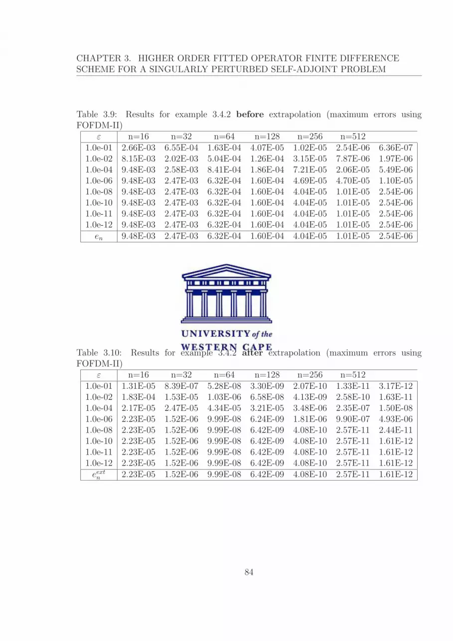
CHAPTER 3. HIGHER ORDER FITTED OPERATOR FINITE DIFFERENCESCHEME FOR A SINGULARLY PERTURBED SELF-ADJOINT PROBLEM
Table 3.9: Results for example 3.4.2 before extrapolation (maximum errors usingFOFDM-II)
ε n=16 n=32 n=64 n=128 n=256 n=5121.0e-01 2.66E-03 6.55E-04 1.63E-04 4.07E-05 1.02E-05 2.54E-06 6.36E-071.0e-02 8.15E-03 2.02E-03 5.04E-04 1.26E-04 3.15E-05 7.87E-06 1.97E-061.0e-04 9.48E-03 2.58E-03 8.41E-04 1.86E-04 7.21E-05 2.06E-05 5.49E-061.0e-06 9.48E-03 2.47E-03 6.32E-04 1.60E-04 4.69E-05 4.70E-05 1.10E-051.0e-08 9.48E-03 2.47E-03 6.32E-04 1.60E-04 4.04E-05 1.01E-05 2.54E-061.0e-10 9.48E-03 2.47E-03 6.32E-04 1.60E-04 4.04E-05 1.01E-05 2.54E-061.0e-11 9.48E-03 2.47E-03 6.32E-04 1.60E-04 4.04E-05 1.01E-05 2.54E-061.0e-12 9.48E-03 2.47E-03 6.32E-04 1.60E-04 4.04E-05 1.01E-05 2.54E-06
en 9.48E-03 2.47E-03 6.32E-04 1.60E-04 4.04E-05 1.01E-05 2.54E-06
Table 3.10: Results for example 3.4.2 after extrapolation (maximum errors usingFOFDM-II)
ε n=16 n=32 n=64 n=128 n=256 n=5121.0e-01 1.31E-05 8.39E-07 5.28E-08 3.30E-09 2.07E-10 1.33E-11 3.17E-121.0e-02 1.83E-04 1.53E-05 1.03E-06 6.58E-08 4.13E-09 2.58E-10 1.63E-111.0e-04 2.17E-05 2.47E-05 4.34E-05 3.21E-05 3.48E-06 2.35E-07 1.50E-081.0e-06 2.23E-05 1.52E-06 9.99E-08 6.24E-09 1.81E-06 9.90E-07 4.93E-061.0e-08 2.23E-05 1.52E-06 9.99E-08 6.42E-09 4.08E-10 2.57E-11 2.44E-111.0e-10 2.23E-05 1.52E-06 9.99E-08 6.42E-09 4.08E-10 2.57E-11 1.61E-121.0e-11 2.23E-05 1.52E-06 9.99E-08 6.42E-09 4.08E-10 2.57E-11 1.61E-121.0e-12 2.23E-05 1.52E-06 9.99E-08 6.42E-09 4.08E-10 2.57E-11 1.61E-12
eextn 2.23E-05 1.52E-06 9.99E-08 6.42E-09 4.08E-10 2.57E-11 1.61E-12
84

CHAPTER 3. HIGHER ORDER FITTED OPERATOR FINITE DIFFERENCESCHEME FOR A SINGULARLY PERTURBED SELF-ADJOINT PROBLEM
Table 3.11: Results for example 3.4.2 before extrapolation (rate of convergence usingFOFDM-II), nk = 8× 2k−1, k = 1(1)6
ε r2 r3 r4 r5 r6
1.0e-01 2.02E+00 2.01E+00 2.00E+00 2.00E+00 2.00E+00 2.00E+001.0e-02 2.01E+00 2.00E+00 2.00E+00 2.00E+00 2.00E+00 2.00E+001.0e-04 1.88E+00 1.62E+00 2.17E+00 1.37E+00 1.80E+00 1.91E+001.0e-06 1.94E+00 1.96E+00 1.98E+00 1.77E+00 -3.53E-03 2.09E+001.0e-08 1.94E+00 1.96E+00 1.98E+00 1.99E+00 1.99E+00 2.00E+001.0e-10 1.94E+00 1.96E+00 1.98E+00 1.99E+00 1.99E+00 2.00E+001.0e-11 1.94E+00 1.96E+00 1.98E+00 1.99E+00 1.99E+00 2.00E+001.0e-12 1.94E+00 1.96E+00 1.98E+00 1.99E+00 1.99E+00 2.00E+00
rn 1.94E+00 1.96E+00 1.98E+00 1.99E+00 1.99E+00 2.00E+00
Table 3.12: Results for example 3.4.2 after extrapolation (rate of convergence usingFOFDM-II), nk = 8× 2k−1, k = 1(1)6
ε r2 r3 r4 r5 r6
1.0e-01 3.96E+00 3.99E+00 4.00E+00 4.00E+00 3.96E+00 2.06E+001.0e-02 3.58E+00 3.89E+00 3.96E+00 3.99E+00 4.00E+00 3.98E+001.0e-04 -1.86E-01 -8.14E-01 4.38E-01 3.20E+00 3.89E+00 3.97E+001.0e-06 3.88E+00 3.93E+00 4.00E+00 -8.18E+00 8.74E-01 -2.32E+001.0e-08 3.88E+00 3.93E+00 3.96E+00 3.98E+00 3.99E+00 7.26E-021.0e-10 3.88E+00 3.93E+00 3.96E+00 3.98E+00 3.99E+00 3.99E+001.0e-11 3.88E+00 3.93E+00 3.96E+00 3.98E+00 3.99E+00 3.99E+001.0e-12 3.88E+00 3.93E+00 3.96E+00 3.98E+00 3.99E+00 3.99E+00
rextn 3.88E+00 3.93E+00 3.96E+00 3.98E+00 3.99E+00 3.99E+00
85

CHAPTER 3. HIGHER ORDER FITTED OPERATOR FINITE DIFFERENCESCHEME FOR A SINGULARLY PERTURBED SELF-ADJOINT PROBLEM
3.5 Discussion
In this Chapter, we have investigated the performance of the Richardson extrapolation on
some fitted operator finite difference methods. We considered two FOFDMs referred to
as FOFDM-I and FOFDM-II which were designed to solve a class of self-adjoint problems
in [119] and [98], respectively. These methods are analyzed for convergence (where the
solution before and after extrapolation is used to derive the error estimates).
Richardson extrapolation does not improve the convergence of FOFDM-I which is of
order four and two for some moderate and smaller values of ε respectively. In the case
of FOFDM-II, its second order accuracy is improved up to four, irrespective of the value
of ε. The observations (made through tables 3.1-3.12) and the associated analysis show
that the performance of Richardson extrapolation is scheme dependent.
86

Chapter 4
Performance of Richardson
Extrapolation on Various Numerical
Methods for a Singularly Perturbed
Turning Point Problem whose
Solution has Boundary Layers
In this chapter, we consider singularly perturbed turning point problems. There exist two
classes of such type of problems: the one whose solution possesses boundary layer(s) and
the one whose solution possesses interior layer(s). After we design some fitted methods,
the performance of the Richardson extrapolation is studied here for the problems of the
former class. The same for the later class of problems is being considered elsewhere.
87
CHAPTER 4. PERFORMANCE OF RICHARDSON EXTRAPOLATION ONVARIOUS NUMERICAL METHODS FOR A SINGULARLY PERTURBEDTURNING POINT PROBLEM WHOSE SOLUTION HAS BOUNDARY LAYERS
4.1 Introduction
In this Chapter we develop a fitted operator finite difference method (FOFDM) and a
fitted mesh finite difference method (FMFDM) to solve a singularly perturbed turning
point problem (TPP) whose solution displays boundary layers. Since we aim at achieving
high order of convergence, we investigate the performance of Richardson extrapolation on
these methods.
Several authors have attempted to solve singularly perturbed TPPs, but up to the
best of our knowledge, the acceleration techniques such as the one above have not yet
been explored.
Abrahamsson [4] and Berger et al. [21] derived a number of a priori estimates for
solutions of singularly perturbed TPPs. Adzic in [5], [6] and [8] developed modified
standard spectral methods for singularly perturbed problems without turning points, with
turning point with boundary layers and with turning point with interior layer, respectively.
The same author used a domain decomposition method (in [7]) to solve some turning point
problems via the asymptotic behavior of the exact solution.
We consider the problem
Lu := εu′′ + a(x)u′ − b(x)u = f(x), x ∈ Ω = (−1, 1), (4.1.1)
u(−1) = A, u(1) = B. (4.1.2)
where A and B are given constants and ε ∈ (0, 1], and the coefficients a(x), b(x) and f(x)
are sufficiently smooth functions in Ω.
The distinct zeros αi, i = 1, 2, · · · , r of a(x) in the interval Ω, if they exist, are called
the turning points of (4.1.1)-(4.1.2), provided that a(−1)a(1) 6= 0.
Berger et al. [21] showed that the bounds of the solution u(x) near a given turning
point αi depend on ε and the constant βi = b(αi)/a′(αi). For βi < 0, u(x) is “smooth”
near x = αi whereas βi > 0 indicates that u(x) has a large gradient at x = αi resulting
88

CHAPTER 4. PERFORMANCE OF RICHARDSON EXTRAPOLATION ONVARIOUS NUMERICAL METHODS FOR A SINGULARLY PERTURBEDTURNING POINT PROBLEM WHOSE SOLUTION HAS BOUNDARY LAYERS
in an “interior layer”. Moreover, u(x) has a boundary layer at x = −1 and x = 1 if and
only if a(−1) > 0 and a(1) < 0, respectively.
In the rest of this chapter, we assume that
a(0) = 0, a′(0) ≤ 0, a(−1) > 0, a(1) < 0, and |a(x)| ≥ a0 > 0, for 0 < |x| ≤ 1,
thus ensuring that the solution to (4.1.1)-(4.1.2) has two boundary layers. Also it is
required that b(x) ≥ b0 > 0 so as to ensure that the solution of (4.1.1)-(4.1.2) satisfies
a minimum principle. The condition |a′(x)| ≥ |a′(0)/2|, −1 ≤ x ≤ 1 guarantees the
uniqueness of the turning point in the interval [-1,1].
Under the requirements mentioned above, the operator L admits the following contin-
uous minimum principle
Lemma 4.1.1. Let ξ be a smooth function satisfying ξ(−1) ≥ 0, ξ(1) ≥ 0 and Lξ(x) ≤0, ∀x ∈ (−1, 1). Then ξ(x) ≥ 0, ∀x ∈ [−1, 1].
Proof Let x∗ ∈ [−1, 1] such that ξ(x∗) = minx∈[−1,1] ξ(x) and assume ξ(x∗) < 0. Then,
obviously, x∗ /∈ −1, 1, ξ′(x∗) = 0 and ξ′′(x∗) ≥ 0. We have
Lξ(x∗) = εξ′′(x∗) + a(x∗)ξ′(x∗)− b(x∗)ξ(x∗) > 0,
which is a contradiction. It follows that, ξ(x∗) ≥ 0 and thus, ξ(x) ≥ 0, ∀x ∈ [−1, 1].
The minimum principle implies the existence and unicity of the solution. We use this
principle to prove the following results which states that the solution depends continuously
on the data.
Lemma 4.1.2. Let u(x) be the solution of (4.1.1)-(4.1.2). Then, we have
||u|| ≤ C(b−10 ||f ||+ max|A|, |B|) ,∀x ∈ [−1, 1].
89

CHAPTER 4. PERFORMANCE OF RICHARDSON EXTRAPOLATION ONVARIOUS NUMERICAL METHODS FOR A SINGULARLY PERTURBEDTURNING POINT PROBLEM WHOSE SOLUTION HAS BOUNDARY LAYERS
Proof Consider the comparison function
Π±(x) = b−10 ||f ||+ max|A|, |B| ± u(x).
Then we have
LΠ±(x) = ±f(x)− b(x)
b0
||f || − b(x) max|A|, |B| ≤ 0.
implying that Π±(x) ≥ 0, ∀x ∈ [−1, 1], which completes the proof.
The rest of this chapter is organized as follows. In section 4.2, we state some a
priori estimates of the bounds of the solution and its derivatives, the use of which will
be apparent in the analysis of the numerical methods. The construction and analysis
of FOFDM and FMFDM are presented in sections 4.3 and 4.4. In these sections, the
performance of extrapolation on the underlying methods is studied. Numerical results to
support our theoretical findings are displayed in section 4.5. A short discussion on these
results is provided in section 4.6.
4.2 Some a priori estimates for the bounds of the
solution and its derivatives
In this section, we present the bounds on the solution of the problem (4.1.1)-(4.1.2) and
its derivatives.
We shall denote by Ωl = [−1,−δ], Ωc = [−δ, δ], Ωr = [δ, 1], where 0 < δ ≤ 12; the
left, central and right part of the domain, respectively. Note that β = b(0)/a′(0) < 0.
Let k be a positive integer. We define
S1(k) = ||a||k, ||b||k, ||f ||k, a0, 1− δ, |B|, u(δ), k,
90
CHAPTER 4. PERFORMANCE OF RICHARDSON EXTRAPOLATION ONVARIOUS NUMERICAL METHODS FOR A SINGULARLY PERTURBEDTURNING POINT PROBLEM WHOSE SOLUTION HAS BOUNDARY LAYERS
S2(k) = ||a||k, ||b||k, ||f ||k, a0, 1− δ, |A|, u(−δ), k
and
S3(k) = ||a||k, ||b||k, ||f ||k, βs, b0, |A|, |B|, k.
Depending on whether x belongs to Ωl, Ωc or Ωr, the appropriate bounds are provided in
the following lemmas.
Lemma 4.2.1. [21] If u(x) is the solution of the TPP (4.1.1)-(4.1.2) and a, b and f ∈Ck(Ω), k > 0, then there exist positive constants η and C depending only on S1(k) such
that
|u(j)(x)| ≤ C[1 + ε−j exp(−a0(1− x)/ε)], j = 1(1)k + 1, x ∈ Ωr.
Proof. See [21].
Lemma 4.2.2. [21] If u(x) is the solution of the TPP (4.1.1)-(4.1.2) and a, b and f ∈Ck(Ω), k > 0, then there exist positive constants η and C depending only on S2(k) such
that
|u(j)(x)| ≤ C[1 + ε−j exp(−a0(1 + x)/ε)], j = 1(1)k + 1, x ∈ Ωl.
Proof. See [21].
Lemma 4.2.3. [21] If u(x) is the solution of the TPP (4.1.1)-(4.1.2) and a, b and f ∈Ck(Ω), k > 0, then there exists a positive constant C depending only on S3(k) such that
|u(j)| ≤ C, ∀x ∈ Ωc, j = 0(1)k.
Proof. See [21].
91
CHAPTER 4. PERFORMANCE OF RICHARDSON EXTRAPOLATION ONVARIOUS NUMERICAL METHODS FOR A SINGULARLY PERTURBEDTURNING POINT PROBLEM WHOSE SOLUTION HAS BOUNDARY LAYERS
Lemma 4.2.4. [105] The solution u of the TPP (4.1.1)-(4.1.2) can be decomposed as
u = v + w,
where, for all j, 0 ≤ j ≤ k, and all x ∈ [−1, 1], the smooth component v satisfies
∣∣v(j)(x)∣∣ ≤ C(1 + ε−(k−2) exp(−a0(1 + x)/ε), x ∈ [−1, 0],
∣∣v(j)(x)∣∣ ≤ C(1 + ε−(k−2) exp(−a0(1− x)/ε), x ∈ [0, 1],
and the singular component w satisfies
∣∣w(j)(x)∣∣ ≤ Cε−k exp(−a0(1 + x)/ε), x ∈ [−1, 0],
∣∣w(j)(x)∣∣ ≤ Cε−k exp(−a0(1− x)/ε), x ∈ [0, 1],
for some constant C independent of ε.
Proof. See [105].
4.3 Richardson extrapolation on fitted operator fi-
nite difference method
Here we first present the FOFDM which is developed in [110] and the associated error
estimates. Then we analyze the effect of Richardson extrapolation on this scheme.
4.3.1 The fitted operator finite difference method (FOFDM)
Let n be any positive integer. Consider the following partition of the interval [−1, 1]:
µn = xj = x0 + jh, x0 = −1, xn = 1, j = 1(1)n, h = xj − xj−1.
92

CHAPTER 4. PERFORMANCE OF RICHARDSON EXTRAPOLATION ONVARIOUS NUMERICAL METHODS FOR A SINGULARLY PERTURBEDTURNING POINT PROBLEM WHOSE SOLUTION HAS BOUNDARY LAYERS
The denominator function φ2j appearing in the discrete form of the approximation of
the second derivative term of the differential equation (4.1.1) is considered as
φ2j =
hεaj
(exp
(ajh
ε
)− 1
), j = 0(1)n
2− 1,
hεaj
(1− exp
(−ajh
ε
)), j = n
2+ 1(1)n,
h2, j = n2.
(4.3.3)
The above is normally obtained by using the theory of difference equations (see, e.g.,
[103]).
Hence, the problem (4.1.1)-(4.1.2) is discretized as follows
LhUj ≡
εUj+1−2Uj+Uj−1
φ2j
+ ajUj+1−Uj
h− bjUj = fj, j = 1(1)n
2− 1,
εUj+1−2Uj+Uj−1
φ2j
+ ajUj−Uj−1
h− bjUj = fj, j = n
2(1)n− 1,
(4.3.4)
U0 = A, Un = B. (4.3.5)
where
aj =aj + aj+1
2,
bj =bj−1 + bj + bj+1
3,
fj =fj−1 + fj + fj+1
3,
and φj is obtained as in (4.3.3) by substituting aj by aj.
Equations (4.3.4) can be written in the form
r−j Uj−1 + rcjUj + r+
j Uj+1 = fj, j = 1(1)n− 1. (4.3.6)
93

CHAPTER 4. PERFORMANCE OF RICHARDSON EXTRAPOLATION ONVARIOUS NUMERICAL METHODS FOR A SINGULARLY PERTURBEDTURNING POINT PROBLEM WHOSE SOLUTION HAS BOUNDARY LAYERS
where
r+j =
ε
φ2j
+aj
h, rc
j = −2ε
φ2j
− aj
h− b, r−j =
ε
φ2j
, for j = 1, 2, · · · , n
2− 1,
and
r+j =
ε
φ2j
, rcj = −2ε
φ2j
+aj
h− b, r−j =
ε
φ2j
− aj
h, for j =
n
2,n
2+ 1, · · · , n− 1.
In view of the scheme above, we now prove the following Lemma which states that
the discrete problem LhUj = fj, 1 ≤ j ≤ n− 1, U0 = A, Un = B, satisfies the discrete
minimum principle.
Lemma 4.3.1. For any mesh function ξj such that Lhξj ≤ 0, ∀j = 1(1)n−1, ξ0 ≥ 0 and
ξn ≥ 0, we have ξj ≥ 0, ∀j = 0(1)n.
Proof
Let k be such that ξk = min0≤j≤n ξj and suppose that ξk < 0. It’s clear that k /∈ 0, n.Also ξk+1 − ξk ≥ 0, ξk − ξk−1 ≤ 0.
On one hand we have
Lhξk = εξk+1 − 2ξk + ξk−1
φ2k
+ akξk+1 − ξk
h− bkξk > 0, for 1 ≤ k ≤ n/2− 1.
On the other hand
Lhξk = εξk+1 − 2ξk + ξk−1
φ2k
+ akξk − ξk−1
h− bkξk > 0, for n/2 ≤ k ≤ n− 1.
Thus Lhξk > 0, 1 ≤ k ≤ n− 1, which is a contradiction. It follows that ξk ≥ 0 and thus
ξj ≥ 0, 0 ≤ j ≤ n.
This minimum principle is used to prove the following lemma.
94

CHAPTER 4. PERFORMANCE OF RICHARDSON EXTRAPOLATION ONVARIOUS NUMERICAL METHODS FOR A SINGULARLY PERTURBEDTURNING POINT PROBLEM WHOSE SOLUTION HAS BOUNDARY LAYERS
Lemma 4.3.2. If Zi is any mesh function such that Z0 = Zn = 0, then
|Zi| ≤ 1
a∗max
1≤j≤n−1|LhZj| for 0 ≤ i ≤ n.
where
a∗ =
−a0 if 0 ≤ i ≤ n/2− 1,
a0 if n/2 ≤ i ≤ n.
Proof Let us define two comparison functions Y ±i by
Y ±i =
xi
a∗max
1≤j≤n−1|LhZj| ± Zi, 0 ≤ i ≤ n.
It is clear that Y ±0 ≥ 0 and Y ±
n ≥ 0. Also, observe that
LhY ±i =
ai − bixi
a∗max
1≤j≤n−1|LhZj|+ LhZi, 0 ≤ i ≤ n.
If 0 ≤ i ≤ n/2 − 1, then ai > 0, ai > a0 and since bi > 0 and xi < 0, we have (ai −bixi)/(−a0)) < −1. Likewise, if n/2 ≤ i ≤ n, then ai < 0, |ai| > a0 and since bi > 0 and
xi > 0, we have (ai− bixi)/a0 < −1. In either case, LhY ±i ≤ 0. By the discrete minimum
principle (Lemma 4.3.1), we conclude that Yi ≥ 0, ∀0 ≤ i ≤ n and this completes the
proof.
We will be requiring the following lemma in the analysis below.
Lemma 4.3.3. For a fixed mesh and for all integers k, we have
limε→0
max1≤j≤n/2−1
exp(−M(1 + xj)/ε)
εk= 0
and
limε→0
maxn/2≤j≤n−1
exp(−M(1− xj)/ε)
εk= 0,
95

CHAPTER 4. PERFORMANCE OF RICHARDSON EXTRAPOLATION ONVARIOUS NUMERICAL METHODS FOR A SINGULARLY PERTURBEDTURNING POINT PROBLEM WHOSE SOLUTION HAS BOUNDARY LAYERS
where xj = jh− 1, h = 2/n, ∀j = 1(1)n− 1.
Proof
We extend the proof provided in [118] to cater for the turning point problems here. In fact,
to prove the second limit above we consider the partition [0, 1] := 0 = xn2
< xn2+1 < · · · <
xn−1 < xn = 1. The first limit is established by replacing xj by −xj in the second limit.
In this case, we use the partition [−1, 0] := −1 = x0 < x1 < x2 < · · · < xn2−1 < xn
2= 0.
Now, the truncation error of our method is calculated as follows.
For j = 1(1)n/2− 1 we have
Lh(uj − Uj) =(r−j uj−1 + rc
juj + r+j uj+1
)− fj
= T0uj + T1u′j + T2u
′′j + T3u
′′′j + T4u
(iv)(ξj), (4.3.7)
where ξj ∈ (xj−1, xj+1) and
T0 = r−j + rcj + r+
j + bj +1
3h2b′′j ,
T1 = h(r+j − r−j
)− aj − 1
3h2
(a′′j − 2b′j
),
T2 =h2
2
(r+j + r−j
)− ε− 1
3h2
(2a′j − bj − h2
2b′′j
),
T3 =h3
6
(r+j − r−j
)− 1
3h2
(aj +
h2
2a′′j
),
T4 =h4
24
(r+j + r−j
)− 1
3h2ε.
We note that T0 = 0, |T1| ≤ Mh, |T2| ≤ Mh, |T3| ≤ Mh2, and |T4| ≤ Mh2.
(Hereinafter, M denotes a positive constant which may take different values in different
equations and inequalities but is always independent of h and ε.) Therefore, (4.3.7) leads
to
|Lh(uj − Uj)| ≤ Mh
[1 +
exp (−a0(1 + xj)/ε)
ε
], (4.3.8)
96

CHAPTER 4. PERFORMANCE OF RICHARDSON EXTRAPOLATION ONVARIOUS NUMERICAL METHODS FOR A SINGULARLY PERTURBEDTURNING POINT PROBLEM WHOSE SOLUTION HAS BOUNDARY LAYERS
where we have used Lemma 4.2.2 and considered only dominating terms.
Following the same procedure, and using both lemmas 4.2.2 and 4.2.3, we establish
that for j = n/2(1)n− 1,
|Lh(uj − Uj)| ≤ Mh
[1 +
exp (−a0(1− xj)/ε)
ε
]. (4.3.9)
Finally, using lemmas 4.3.2 and 4.3.3, we have the following result.
Theorem 4.3.1. Let a(x), b(x) and f(x) be sufficiently smooth functions in the problem
(4.1.1)-(4.1.2) and so that u(x) ∈ C4([−1, 1]). The numerical solution U obtained via the
FOFDM (4.3.6)-(4.3.5) satisfy the following estimate:
sup0<ε≤1
max0≤j≤n
|uj − Uj| ≤ Mh. (4.3.10)
4.3.2 Richardson extrapolation for FOFDM
Let us denote by µ2n the mesh obtained by bisecting each mesh interval in µn, i.e,
µ2n = xj with x0 = −1, xn = 1 and xj − xj−1 = h = h/2, j = 1(1)2n.
We denote the analytical and numerical solutions on the mesh µ2n by uj and Uj, respec-
tively.
From estimate (4.3.10), we have on one hand
uj − Uj = Mh + Rn(xj), 1 ≤ j ≤ n− 1.
On the other hand, we have
uj − Uj = Mh + R2n(xj), 1 ≤ j ≤ 2n− 1.
97
CHAPTER 4. PERFORMANCE OF RICHARDSON EXTRAPOLATION ONVARIOUS NUMERICAL METHODS FOR A SINGULARLY PERTURBEDTURNING POINT PROBLEM WHOSE SOLUTION HAS BOUNDARY LAYERS
Therefore,
uj − (2Uj − Uj) = O(h), ∀1 ≤ j ≤ n− 1.
Let
U extj := 2Uj − Uj.
Thus U ext is another numerical approximation of uj.
Using some algebraic manipulations, we established that
∣∣Lh(uj − Uj)∣∣ ≤ Mh.
Therefore, ∣∣∣Lh(uj − Uj)∣∣∣ ≤ Mh
and consequently
max1≤j≤n−1
|uj − Uj| ≤ Mh
and
max1≤j≤n−1
∣∣uj − Uj
∣∣ ≤ Mh.
Finally, the inequality
max1≤j≤n−1
∣∣uj − U extj
∣∣ ≤ 2 max1≤j≤n−1
∣∣uj − Uj
∣∣ + max1≤j≤n−1
|uj − Uj| (4.3.11)
leads to
Theorem 4.3.2. Let a(x), b(x) and f(x) be sufficiently smooth functions in the problem
(4.1.1)-(4.1.2) and so that u(x) ∈ C4([−1, 1]). Then the numerical solution U ext obtained
via Richardson extrapolation based on FOFDM (4.3.6) along with (4.3.5) satisfies the
following estimate:
sup0<ε≤1
max1≤j≤n−1
|uj − U extj | ≤ Mh. (4.3.12)
98

CHAPTER 4. PERFORMANCE OF RICHARDSON EXTRAPOLATION ONVARIOUS NUMERICAL METHODS FOR A SINGULARLY PERTURBEDTURNING POINT PROBLEM WHOSE SOLUTION HAS BOUNDARY LAYERS
4.4 Richardson extrapolation on fitted mesh finite
difference method
The idea from Chapter 8 of Miller et al. [105] is used in this section to develop a fitted mesh
finite difference scheme. The convergence of the scheme is analyzed before embarking on
the study of the effect of Richardson extrapolation on its accuracy and rate of convergence.
4.4.1 The fitted mesh finite difference method (FMFDM)
It is assumed that there are two boundary layers, one at each end, and let the interval
[−1, 1] be partitioned as
[−1, 1] := [−1,−1 + τ ] ∪ [−1 + τ, 1− τ ] ∪ [1− τ, 1],
where τ is a parameter denoting the width of the boundary layer.
Let n be a positive integer such that n = 2m with m ≥ 3.
To construct the piece-wise mesh (of Shishkin type), we subdivide both the intervals
[−1,−1 + τ ] and [1− τ, 1] into n/4 equal mesh elements while we subdivide the interval
[−1 + τ, 1− τ ] into n/2 equal mesh elements. This gives
[−1, 1] := −1 = x0 < x1 < · · · < xn/4 < · · · < xn/2 = 0 < · · · < x3n/4 < · · · < xn = 1.
The parameter τ is defined by
τ = min
1
4,
ε
a0
ln(n
4
). (4.4.13)
99

CHAPTER 4. PERFORMANCE OF RICHARDSON EXTRAPOLATION ONVARIOUS NUMERICAL METHODS FOR A SINGULARLY PERTURBEDTURNING POINT PROBLEM WHOSE SOLUTION HAS BOUNDARY LAYERS
The mesh spacing hj = xj − xj−1 is given by
hj =
4τn−1 j = 1, 2, · · · , n/2, 3n/4 + 1, 3n/4 + 2, · · · , n− 1, n
4(1− τ)n−1 j = n/2 + 1, n/2 + 2, · · · , 3n/4.(4.4.14)
We denote this mesh by µn,τ .
Using the above conventions, we discretize the problem (4.1.1)-(4.1.2) on µn,τ as
εDUj + ajD+Uj − bjUj = fj, aj > 0;
εDUj + ajD−Uj − bjUj = fj, aj ≤ 0;
(4.4.15)
U0 = A, Un = B, (4.4.16)
where
D+Uj =Uj+1 − Uj
hj+1
,
D−Uj =Uj − Uj−1
hj
,
and
DUj =2
hj + hj+1
(D+Uj −D−Uj
).
Equations (4.4.15) can be written in the form
r−j Uj−1 + rcjUj + r+
j Uj+1 = fj, j = 1(1)n− 1, (4.4.17)
where, for j = 1, 2, · · · , n2− 1, we have
r+j =
2ε
hj+1(hj+1 + hj)+
aj
hj+1
,
rcj = − 2ε
hjhj+1
− aj
hj+1
− bj,
100

CHAPTER 4. PERFORMANCE OF RICHARDSON EXTRAPOLATION ONVARIOUS NUMERICAL METHODS FOR A SINGULARLY PERTURBEDTURNING POINT PROBLEM WHOSE SOLUTION HAS BOUNDARY LAYERS
r−j =2ε
hj(hj + hj+1),
and for j = n2, n
2+ 1, · · · , n− 1, we have
r+j =
2ε
hj+1(hj+1 + hj),
rcj = − 2ε
hjhj+1
+aj
hj
− bj,
r−j =2ε
hj(hj + hj+1)− aj
hj
.
Convergence analysis of FMFDM
The restrictions of problem (4.1.1)-(4.1.2) to the intervals [0, 1] and [−1, 0] feature like the
convection-diffusion problem of Chapter 8 in [105]. In our analysis, we will implement the
ideas provided in this work, for the interval [0, 1]. The analysis on [−1, 0] follows similar
steps.
We decompose the solution U of the discrete problem (4.4.15)-(4.4.16) in its regular
part V and singular part W . The components V and W of U are solutions of the problems
LnV = f, V (−1) = v(−1), V (1) = v(1)
and
LnW = 0, W (−1) = w(−1),W (1) = w(1),
respectively, where Ln denotes the discrete operator associated with (4.4.17).
101

CHAPTER 4. PERFORMANCE OF RICHARDSON EXTRAPOLATION ONVARIOUS NUMERICAL METHODS FOR A SINGULARLY PERTURBEDTURNING POINT PROBLEM WHOSE SOLUTION HAS BOUNDARY LAYERS
We can write the error in the form
U − u = (V − v) + (W − w) (4.4.18)
and estimate the components of the error separately.
We start with the regular component.
The local truncation error is given by
Ln(V − v) = ε
(d2
dx2− D
)v + a
(d
dx−D−
)v. (4.4.19)
Using Lemma 4.1 ([105]), we obtain
|Ln(Vj − vj)| ≤ ε
3(xj+1 − xj−1) |v′′′j |+
aj
2(xj − xj−1) |v′′j |, for
n
2≤ j ≤ n− 1. (4.4.20)
Since hj = xj − xj−1 ≤ 4n−1 for any j, therefore using lemma 4.2.4,we obtain
|Ln(Vj − vj)| ≤ Mn−1. (4.4.21)
Hence, by Lemma 4.3.2,
|Vj − vj| ≤ Mn−1. (4.4.22)
The estimate on Ln(W − w) depends on whether τ = 1/4 or τ = (ε/a0) ln(n/4).
If τ = 1/4, the mesh is uniform and 1/4 ≤ (ε/a0) ln(n/4). The local truncation error
Ln(W − w) is given by
|Ln(Wj − wj)| ≤ ε
3(xj+1 − xj−1)|w′′′
j |+aj
2(xj − xj−1)|w′′
j |, forn
2≤ j ≤ n− 1. (4.4.23)
By Lemma 4.2.4 and the fact that hj = xj − xj−1 = 4n−1, the above inequality gives
|Ln(Wj − wj)| ≤ Mε−2n−1. (4.4.24)
102
CHAPTER 4. PERFORMANCE OF RICHARDSON EXTRAPOLATION ONVARIOUS NUMERICAL METHODS FOR A SINGULARLY PERTURBEDTURNING POINT PROBLEM WHOSE SOLUTION HAS BOUNDARY LAYERS
Now since ε−1 is less than (4/a0) ln(n/4), we have
|Ln(Wj − wj)| ≤ Mn−1(ln(n/4))2 (4.4.25)
Using Lemma 4.3.2 then we obtain
|Wj − wj| ≤ Mn−1(ln(n/4))2. (4.4.26)
If τ = (ε/a0) ln(n/4), then the mesh is piecewise uniform. In each of the subintervals
[0, 1− τ ] and [1− τ, 1], a different argument is used to bound W − w.
Both W and w are small on the subinterval with no boundary layer, namely [0, 1− τ ].
Therefore, since |W − w| ≤ |W | + |w|, we will bound W and w separately. Before we
move any further, let us note that w can also be decomposed as w = w0 + εw1 (see [105],
p.59). Introducing the function ϕ by
ϕ(x) =
∫ 1
xexp(−A(t)/ε)dt∫ 1
0exp(−A(t)/ε)dt
, A(t) =
∫ 1
x
a(s)ds.
It can be shown that w0 can be written in the form
w0(x) = w0(0)ϕ(x) + w0(1)(1− ϕ(x))
and therefore
w′0(x) = (w0(0)− w0(1))ϕ′(x).
But w0(0) = w0(1) exp(−a0/ε) and hence
w′0(x)
w0(1)= −(1− exp(−a0/ε)ϕ
′(x) > 0.
It follows that w0(x)/w0(1) is positive and increasing in the interval [0, 1].
103

CHAPTER 4. PERFORMANCE OF RICHARDSON EXTRAPOLATION ONVARIOUS NUMERICAL METHODS FOR A SINGULARLY PERTURBEDTURNING POINT PROBLEM WHOSE SOLUTION HAS BOUNDARY LAYERS
Thus
0 ≤ w0(x)
w0(1)≤ w0(1− τ)
w0(1)
and hence
|w0(x)| ≤ |w0(1− τ)|, ∀x ∈ [0, 1− τ ].
The same is true for w1(x) and since w = w0 + εw1, it follows that
|w(x)| ≤ |w(1− τ)|, ∀x ∈ [0, 1− τ ].
Using the estimate for |w| and the fact that τ = (ε/a0) ln(n/4), we obtain
|w(x)| ≤ M exp(−a0τ/ε) = Mn−1. (4.4.27)
Now we define an auxiliary mesh function W analogous to W except that the coefficient
a in the difference operator Ln is replaced by a0. Then Lemma 7.5 on page 53 of [105]
suggests that
|Wj| ≤ |Wj|, ∀0 ≤ j ≤ n.
Thus by Lemma 7.3(p.51 of [105]) , we conclude that
|Wj| ≤ Mn−1, for n/2 ≤ j ≤ 3n/4. (4.4.28)
Hence, from inequalities (4.4.27) and (4.4.28) , we have
|Wj − wj| ≤ Mn−1, for n/2 ≤ j ≤ 3n/4. (4.4.29)
In the subinterval [1− τ, 1], the classical argument leads to
|Ln(Wj − wj)| ≤ Mε−2|xj+1 − xj−1| = 8Mε−2τn−1.
104

CHAPTER 4. PERFORMANCE OF RICHARDSON EXTRAPOLATION ONVARIOUS NUMERICAL METHODS FOR A SINGULARLY PERTURBEDTURNING POINT PROBLEM WHOSE SOLUTION HAS BOUNDARY LAYERS
But also from the (4.4.29), we have
|Wn − wn| = 0
and
|W3n/4 − w3n/4| ≤ |W3n/4|+ |w3n/4| ≤ Mn−1.
By introducing the barrier function
Φj = (xj − (1− τ))M1ε−2τn−1 + M2n
−1,
we see that the mesh functions
Ψ±j = Φj ± (Wj − wj)
satisfy
Ψ±3n/4 ≥ 0, Ψ±
n = 0,
provided that the constants M1 and M2 are chosen suitably.
Note that
LnΨ±j ≤ 0, 3n/4 + 1 ≤ j ≤ n− 1.
By the discrete minimum principle (Lemma 4.3.1), on [1− τ, 1] we get
Ψ±j ≥ 0, 3n/4 ≤ j ≤ n.
Consequently,
|Wj − wj| ≤ Φj ≤ M1ε−2τ 2n−1 + M2n
−1,
105
CHAPTER 4. PERFORMANCE OF RICHARDSON EXTRAPOLATION ONVARIOUS NUMERICAL METHODS FOR A SINGULARLY PERTURBEDTURNING POINT PROBLEM WHOSE SOLUTION HAS BOUNDARY LAYERS
and making use of the inequality τ ≤ (ε/a0) ln(n/4), we obtain
|Wj − wj| ≤ Mn−1(ln(n/4))2. (4.4.30)
Combining (4.4.29) and (4.4.30), we obtain the following estimate on the singular com-
ponent of the error over the interval [0,1]:
|Wj − wj| ≤ Mn−1(ln(n/4))2, n/2 ≤ j ≤ n. (4.4.31)
Estimates (4.4.22) and (4.4.31) along with the inequality (4.4.18) immediately gives
|Uj − uj| ≤ Mn−1(ln(n/4))2, n/2 ≤ j ≤ n. (4.4.32)
Similarly,
|Uj − uj| ≤ Mn−1(ln(n/4))2, 0 ≤ j ≤ n/2− 1. (4.4.33)
We therefore have the following result.
Theorem 4.4.1. Let a(x), b(x) and f(x) be sufficiently smooth functions in the problem
(4.1.1)-(4.1.2) and so that u(x) ∈ C4([−1, 1]). The numerical solution U obtained via
FMFDM (4.4.17) along with (4.4.16) satisfies
sup0<ε≤1
max0≤j≤n
|uj − Uj| ≤ Mn−1(ln(n/4))2. (4.4.34)
4.4.2 Richardson extrapolation for FMFDM
We bisect each mesh sub-interval of µn,τ and obtain a new mesh which we denote by µ2n,τ .
µ2n,τ = xj, 0 ≤ j ≤ 2n + 1 ⊃ µn,τ and xj − xj−1 = hj = hj/2.
We denote the numerical solution computed on the mesh µ2n,τ by U .
106

CHAPTER 4. PERFORMANCE OF RICHARDSON EXTRAPOLATION ONVARIOUS NUMERICAL METHODS FOR A SINGULARLY PERTURBEDTURNING POINT PROBLEM WHOSE SOLUTION HAS BOUNDARY LAYERS
From the estimate (4.4.34), we have
uj − Uj = Mn−1(ln(n/4))2 + Rn(xj), ∀xj ∈ µn,τ (4.4.35)
and
uj − Uj = M(2n)−1(ln(n/4))2 + R2n(xj), ∀xj ∈ µ2n,τ . (4.4.36)
The remainders Rn(xj) and R2n(xj) are of O(n−1(ln(n/4))2). It is to be noted that in
practice, we assume
τ =ε
a0
ln(n
4
), (4.4.37)
because the possibility τ = 1/4 suggested in equation (4.4.13) means that
1/4 < (ε/a0) ln(n/4), and so n−1 is very small relative to ε. This unlikely situation can
be dealt with using the standard techniques.
The presence of the factor ln(n/4) in both (4.4.35) and (4.4.36) explains the fact that
the two meshes µn,τ and µ2n,τ use the same parameter τ given by (4.4.37).
A combination of equations (4.4.35) and (4.4.36) suggests that
uj − (2Uj − Uj) = O(n−1(ln(n/4))2), ∀j = 1, · · · , n− 1
and therefore we set
U extj := 2Uj − Uj, ∀j = 1, · · · , n− 1 (4.4.38)
as the numerical approximation of u at the grid point xj ∈ µn,τ resulting from the extrap-
olation process.
The decomposition of the error after extrapolation in a similar manner as in (4.4.18)
gives
U ext − u =(V ext − v
)+
(W ext − w
), (4.4.39)
where V ext and W ext are the regular and singular components of U ext, respectively. We
107

CHAPTER 4. PERFORMANCE OF RICHARDSON EXTRAPOLATION ONVARIOUS NUMERICAL METHODS FOR A SINGULARLY PERTURBEDTURNING POINT PROBLEM WHOSE SOLUTION HAS BOUNDARY LAYERS
will estimate the components of the error separately.
For similar reasons as mentioned in the previous subsection, we will provide the anal-
ysis only on the interval [0, 1].
The local truncation error of the scheme (4.4.17) along with (4.4.16) at the grid point
xj after extrapolation is given by
Ln(u− U ext) =[2Ln
∗ (vj − Vj)− Ln(vj − Vj)]
+[2Ln
∗ (wj − Wj)− Ln(wj −Wj)], (4.4.40)
where, like Ln, Ln∗ is a discrete operator associated with (4.4.17) along with (4.4.16) but
on the mesh µ2n,τ .
For the regular part of the local truncation after extrapolation, we use Lemma 4.1
([105]). An analogous result as in (4.4.20) is
∣∣2Ln∗ (vj − Vj)− Ln(vj − V j)
∣∣ ≤ 2ε
3(xj+1/2 − xj−1/2)|v′′j |+ aj(xj − xj−1/2)|v′j|
+ε
3(xj+1 − xj−1)|v′′′j |+
aj
2(xj − xj−1)|v′′j |,
forn
2≤ j ≤ n− 1.
Using Lemma 4.3.2, we therefore have
∣∣vj − V extj
∣∣ ≤ Mn−1, forn
2≤ j ≤ n− 1. (4.4.41)
For the estimates on wj −W extj , we discuss two different cases.
If τ = 1/4, the mesh is uniform and we have ε−1 ≤ (4/a0) ln(n/4). Therefore, by
Lemma (4.4.17), we have
∣∣2Ln∗ (wj − Wj)− Ln(wj −Wj)
∣∣ ≤ Mn−1ε−2 ≤ Mn−1(ln(n/4))2.
108

CHAPTER 4. PERFORMANCE OF RICHARDSON EXTRAPOLATION ONVARIOUS NUMERICAL METHODS FOR A SINGULARLY PERTURBEDTURNING POINT PROBLEM WHOSE SOLUTION HAS BOUNDARY LAYERS
An application of Lemma 4.3.2 then gives
∣∣wj −W extj
∣∣ ≤ Mn−1(ln(n/4))2, forn
2≤ j ≤ n− 1. (4.4.42)
If τ = (ε/a0) ln(n/4), the mesh is piecewise uniform with mesh spacing of 4(1 − τ)/n in
the interval [0, 1− τ ] and 4τ/n in the interval [1− τ, 1].
In the subinterval [0, 1 − τ ], the functions w, W and W are small and therefore we
have∣∣wj −W ext
j
∣∣ ≤ |w|+ 2|W |+ |W |.
The bounds on |w| and |W | are obtained in the previous subsection. Also, bounds of |W |are those of |W |. Hence,
∣∣wj −W extj
∣∣ ≤ Mn−1, forn
2≤ j ≤ 3n
4. (4.4.43)
In the subinterval [1 − τ, 1], we use the discrete minimum principle (Lemma 4.3.1) to
bound∣∣wj −W ext
j
∣∣. For 3n/4 + 1 ≤ j ≤ n− 1, we have
Ln(wj −W extj ) ≤ Mε−2|xj+1 − xj−1| = Mε−2τn−1.
Furthermore,∣∣∣w3n/4 −W ext
3n/4
∣∣∣ ≤ Mn−1 and |wn −W extn | = 0.
Defining the barrier function
Φj = (xj − (1− τ))M1ε−2τn−1 + M2n
−1,
we notice that, for a suitable choice of M1 and M2, the mesh function
Ψ±j = Φj ± (wj −W ext
j )
109
CHAPTER 4. PERFORMANCE OF RICHARDSON EXTRAPOLATION ONVARIOUS NUMERICAL METHODS FOR A SINGULARLY PERTURBEDTURNING POINT PROBLEM WHOSE SOLUTION HAS BOUNDARY LAYERS
satisfies
Ψ±3n/4 ≥ 0, Ψ±
n = 0
and
LnΨ±j ≤ 0, for
3n
4+ 1 ≤ j ≤ n− 1.
It follows, by the discrete minimum principle (Lemma 4.3.1) that on the interval [1− τ, 1]
Ψ±j ≥ 0, for
3n
4+ 1 ≤ j ≤ n− 1.
Therefore
|wj −W extj | ≤ Φj ≤ M1ε
−2τ 2n−1 + M2n−1.
Hence
|wj −W extj | ≤ Mn−1(ln(n/4))2, for
3n
4+ 1 ≤ j ≤ n− 1. (4.4.44)
Combining estimates (4.4.43) and (4.4.44), we obtain
|wj −W extj | ≤ Mn−1(ln(n/4))2, for
n
2≤ j ≤ n. (4.4.45)
By virtue of (4.4.39), estimates (4.4.41) and (4.4.45) lead to
|uj − U extj | ≤ Mn−1(ln(n/4))2, for
n
2≤ j ≤ n. (4.4.46)
Following the similar lines on the interval [−1, 0], i.e, when a > 0, we obtain the same
estimate.
Combining the two, we have
Theorem 4.4.2. Let a(x), b(x) and f(x) be sufficiently smooth functions in the problem
(4.1.1)-(4.1.2) and so that u(x) ∈ C4([−1, 1]). The numerical solution U ext obtained via
110

CHAPTER 4. PERFORMANCE OF RICHARDSON EXTRAPOLATION ONVARIOUS NUMERICAL METHODS FOR A SINGULARLY PERTURBEDTURNING POINT PROBLEM WHOSE SOLUTION HAS BOUNDARY LAYERS
FMFDM (4.4.17) along with (4.4.16) after extrapolation satisfies
sup0<ε≤1
max0≤j≤n
|uj − U extj | ≤ Mn−1(ln(n/4))2. (4.4.47)
In next section, we provide test examples to support these theoretical estimates.
4.5 Numerical results
For the following two test examples we provide comparative numerical results before and
after extrapolation using the two fitted methods.
Example 4.5.1. [82] Consider problem (4.1.1)-(4.1.2) with
a(x) = 2(1− 2x), b(x) = 4, f(x) = 0
for 0 < x < 1.
The exact solution is
u(x) = exp
(−2x
1− x
ε
).
The solution to this problem has a turning point at x = 0.5.
Example 4.5.2. Consider problem (4.1.1)-(4.1.2) with
a(x) = −2x3, b(x) = exp(x2),
f(x) =
[2
(1 +
2x2
ε− 2x4
ε
)− exp(x2)
]exp
[x2 − 1
ε
].
Its exact solution is given by
u(x) = exp
[−(1− x)(1 + x)
ε
].
The solution has a turning point at x = 0.
111

CHAPTER 4. PERFORMANCE OF RICHARDSON EXTRAPOLATION ONVARIOUS NUMERICAL METHODS FOR A SINGULARLY PERTURBEDTURNING POINT PROBLEM WHOSE SOLUTION HAS BOUNDARY LAYERS
The maximum errors before extrapolation at all mesh points are evaluated using the
fomulae
eε,n := max0≤j≤n
|uj − Uj|, (4.5.48)
for both FOFDM (4.3.6) along with (4.3.5) and FMFDM (4.4.17) along with (4.4.16).
After extrapolation, the maximum errors are calculated as
eextε,n := max
0≤j≤n|uj − U ext
j |. (4.5.49)
The numerical rates of convergence are computed by using the formula [33]:
rk ≡ rε,k := log2(enk/e2nk
), k = 1, 2, ...
where e stands for eε,n, and eextε,n, respectively.
112

CHAPTER 4. PERFORMANCE OF RICHARDSON EXTRAPOLATION ONVARIOUS NUMERICAL METHODS FOR A SINGULARLY PERTURBEDTURNING POINT PROBLEM WHOSE SOLUTION HAS BOUNDARY LAYERS
Table 4.1: Results for Example 4.5.2: Maximum errors via FOFDM (4.3.6) along with(4.3.5) before extrapolation.
ε n=16 n=32 n=64 n=128 n=256 n=512 n=10241.0E-02 3.62E-02 1.46E-02 8.06E-03 9.07E-03 7.21E-03 3.17E-03 1.34E-031.0E-04 3.60E-02 1.45E-02 6.37E-03 2.99E-03 1.45E-03 7.12E-04 3.53E-041.0E-05 3.60E-02 1.45E-02 6.37E-03 2.99E-03 1.45E-03 7.12E-04 3.53E-041.0E-06 3.60E-02 1.45E-02 6.37E-03 2.99E-03 1.45E-03 7.12E-04 3.53E-041.0E-07 3.60E-02 1.45E-02 6.37E-03 2.99E-03 1.45E-03 7.12E-04 3.53E-041.0E-08 3.60E-02 1.45E-02 6.37E-03 2.99E-03 1.45E-03 7.12E-04 3.53E-041.0E-09 3.60E-02 1.45E-02 6.37E-03 2.99E-03 1.45E-03 7.12E-04 3.53E-041.0E-10 3.60E-02 1.45E-02 6.37E-03 2.99E-03 1.45E-03 7.12E-04 3.53E-041.0E-11 3.60E-02 1.45E-02 6.37E-03 2.99E-03 1.45E-03 7.12E-04 3.53E-04
en 3.60E-02 1.45E-02 6.37E-03 2.99E-03 1.45E-03 7.12E-04 3.53E-04
Table 4.2: Results for Example 4.5.2: Maximum errors via FOFDM (4.3.6) along with(4.3.5) after extrapolation.
ε n=16 n=32 n=64 n=128 n=256 n=512 n=10241.0E-02 2.43E-02 1.01E-02 6.24E-03 3.86E-03 1.54E-03 5.05E-04 1.49E-041.0E-04 2.42E-02 9.78E-03 4.28E-03 2.00E-03 9.67E-04 4.75E-04 2.36E-041.0E-05 2.42E-02 9.78E-03 4.28E-03 2.00E-03 9.67E-04 4.75E-04 2.36E-041.0E-06 2.42E-02 9.78E-03 4.28E-03 2.00E-03 9.67E-04 4.75E-04 2.36E-041.0E-07 2.42E-02 9.78E-03 4.28E-03 2.00E-03 9.67E-04 4.75E-04 2.36E-041.0E-08 2.42E-02 9.78E-03 4.28E-03 2.00E-03 9.67E-04 4.75E-04 2.36E-041.0E-09 2.42E-02 9.78E-03 4.28E-03 2.00E-03 9.67E-04 4.75E-04 2.36E-041.0E-10 2.42E-02 9.78E-03 4.28E-03 2.00E-03 9.67E-04 4.75E-04 2.36E-041.0E-11 2.42E-02 9.78E-03 4.28E-03 2.00E-03 9.67E-04 4.75E-04 2.36E-04
eextn 2.42E-02 9.78E-03 4.28E-03 2.00E-03 9.67E-04 4.75E-04 2.36E-04
113

CHAPTER 4. PERFORMANCE OF RICHARDSON EXTRAPOLATION ONVARIOUS NUMERICAL METHODS FOR A SINGULARLY PERTURBEDTURNING POINT PROBLEM WHOSE SOLUTION HAS BOUNDARY LAYERS
Table 4.3: Results for Example 4.5.2: Rates of convergence via FOFDM (4.3.6) alongwith (4.3.5) before extrapolation
ε r1 r2 r3 r4 r5 r6
1.0E-02 1.31 0.85 -0.17 0.33 1.19 1.241.0E-04 1.32 1.18 1.09 1.05 1.02 1.011.0E-05 1.32 1.18 1.09 1.05 1.02 1.011.0E-06 1.32 1.18 1.09 1.05 1.02 1.011.0E-07 1.32 1.18 1.09 1.05 1.02 1.011.0E-08 1.32 1.18 1.09 1.05 1.02 1.011.0E-09 1.32 1.18 1.09 1.05 1.02 1.011.0E-10 1.32 1.18 1.09 1.05 1.02 1.011.0E-11 1.32 1.18 1.09 1.05 1.02 1.01
Rn 1.32 1.18 1.09 1.05 1.02 1.01
Table 4.4: Results for Example 4.5.2: Rates of convergence via FOFDM (4.3.6) alongwith (4.3.5) after extrapolation
ε r1 r2 r3 r4 r5 r6
1.0E-02 1.27 0.69 0.69 1.33 1.61 1.761.0E-04 1.31 1.19 1.10 1.05 1.02 1.011.0E-05 1.31 1.19 1.10 1.05 1.02 1.011.0E-06 1.31 1.19 1.10 1.05 1.02 1.011.0E-07 1.31 1.19 1.10 1.05 1.02 1.011.0E-08 1.31 1.19 1.10 1.05 1.02 1.011.0E-09 1.31 1.19 1.10 1.05 1.02 1.011.0E-10 1.31 1.19 1.10 1.05 1.02 1.011.0E-11 1.31 1.19 1.10 1.05 1.02 1.01
Rextn 1.31 1.19 1.10 1.05 1.02 1.01
114

CHAPTER 4. PERFORMANCE OF RICHARDSON EXTRAPOLATION ONVARIOUS NUMERICAL METHODS FOR A SINGULARLY PERTURBEDTURNING POINT PROBLEM WHOSE SOLUTION HAS BOUNDARY LAYERS
Table 4.5: Results for Example 4.5.1: Maximum errors via FMFDM (4.4.17) along with(4.4.16) before extrapolation.
ε n=16 n=32 n=64 n=128 n=256 n=512 n=10241.0E-02 1.36E-01 9.02E-02 5.83E-02 3.67E-02 2.25E-02 1.33E-02 7.71E-031.0E-04 1.43E-01 9.44E-02 6.04E-02 3.77E-02 2.29E-02 1.36E-02 7.84E-031.0E-05 1.43E-01 9.44E-02 6.04E-02 3.77E-02 2.29E-02 1.36E-02 7.84E-031.0E-06 1.43E-01 9.44E-02 6.04E-02 3.77E-02 2.29E-02 1.36E-02 7.84E-031.0E-07 1.43E-01 9.44E-02 6.04E-02 3.77E-02 2.29E-02 1.36E-02 7.84E-031.0E-08 1.43E-01 9.44E-02 6.04E-02 3.77E-02 2.29E-02 1.36E-02 7.84E-031.0E-09 1.43E-01 9.44E-02 6.04E-02 3.77E-02 2.29E-02 1.36E-02 7.84E-031.0E-10 1.43E-01 9.44E-02 6.04E-02 3.77E-02 2.29E-02 1.36E-02 7.84E-031.0E-11 1.43E-01 9.44E-02 6.04E-02 3.77E-02 2.29E-02 1.36E-02 7.84E-03
en 1.43E-01 9.44E-02 6.04E-02 3.77E-02 2.29E-02 1.36E-02 7.84E-03
Table 4.6: Results for Example 4.5.1: Maximum errors via FMFDM (4.4.17) along with(4.4.16) after extrapolation.
ε n=16 n=32 n=64 n=128 n=256 n=512 n=10241.0E-02 6.61E-02 4.23E-02 2.46E-02 1.56E-02 1.11E-02 8.37E-03 6.60E-031.0E-04 6.46E-02 4.35E-02 2.56E-02 1.61E-02 1.13E-02 8.51E-03 6.69E-031.0E-05 6.45E-02 4.35E-02 2.56E-02 1.61E-02 1.13E-02 8.51E-03 6.69E-031.0E-06 6.45E-02 4.35E-02 2.56E-02 1.61E-02 1.13E-02 8.51E-03 6.69E-031.0E-07 6.45E-02 4.35E-02 2.56E-02 1.61E-02 1.13E-02 8.51E-03 6.69E-031.0E-08 6.45E-02 4.35E-02 2.56E-02 1.61E-02 1.13E-02 8.51E-03 6.69E-031.0E-09 6.45E-02 4.35E-02 2.56E-02 1.61E-02 1.13E-02 8.51E-03 6.69E-031.0E-10 6.45E-02 4.35E-02 2.56E-02 1.61E-02 1.13E-02 8.51E-03 6.69E-031.0E-11 6.46E-02 4.35E-02 2.56E-02 1.61E-02 1.14E-02 8.51E-03 6.75E-03
eextn 6.45E-02 4.35E-02 2.56E-02 1.61E-02 1.14E-02 8.51E-03 6.69E-03
115

CHAPTER 4. PERFORMANCE OF RICHARDSON EXTRAPOLATION ONVARIOUS NUMERICAL METHODS FOR A SINGULARLY PERTURBEDTURNING POINT PROBLEM WHOSE SOLUTION HAS BOUNDARY LAYERS
Table 4.7: Results for Example 4.5.1: Rates of convergence via FMFDM (4.4.17) alongwith (4.4.16) before extrapolation
ε r1 r2 r3 r4 r5 r6
1.0E-02 0.59 0.63 0.67 0.71 0.75 0.791.0E-04 0.60 0.64 0.68 0.72 0.76 0.791.0E-05 0.60 0.64 0.68 0.72 0.76 0.791.0E-06 0.60 0.64 0.68 0.72 0.76 0.791.0E-07 0.60 0.64 0.68 0.72 0.76 0.791.0E-08 0.60 0.64 0.68 0.72 0.76 0.791.0E-09 0.60 0.64 0.68 0.72 0.76 0.791.0E-10 0.60 0.64 0.68 0.72 0.76 0.791.0E-11 0.60 0.64 0.68 0.72 0.76 0.79
Rn 0.60 0.64 0.67 0.72 0.76 0.79
Table 4.8: Results for Example 4.5.1: Rates of convergence via FMFDM (4.4.17) alongwith (4.4.16) after extrapolation
ε r1 r2 r3 r4 r5 r6
1.0E-02 0.64 0.78 0.66 0.50 0.40 0.341.0E-04 0.57 0.77 0.67 0.51 0.41 0.351.0E-05 0.57 0.77 0.67 0.51 0.41 0.351.0E-06 0.57 0.77 0.67 0.51 0.41 0.351.0E-07 0.57 0.77 0.67 0.51 0.41 0.351.0E-08 0.57 0.77 0.67 0.51 0.41 0.351.0E-09 0.57 0.77 0.67 0.51 0.41 0.351.0E-10 0.57 0.77 0.67 0.51 0.41 0.351.0E-11 0.57 0.77 0.67 0.50 0.42 0.33
Rextn 0.57 0.77 0.67 0.50 0.42 0.33
116
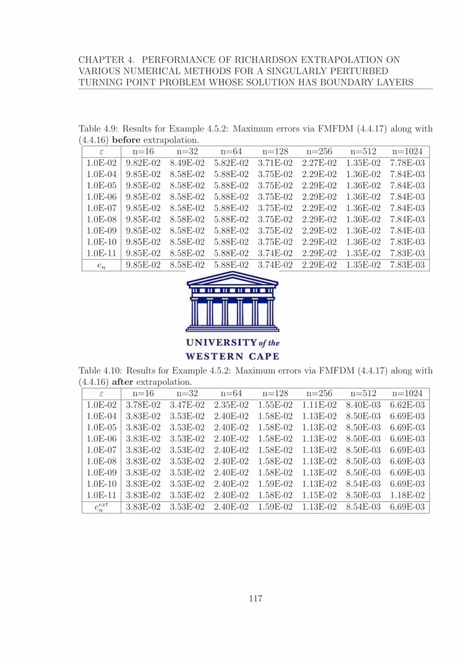
CHAPTER 4. PERFORMANCE OF RICHARDSON EXTRAPOLATION ONVARIOUS NUMERICAL METHODS FOR A SINGULARLY PERTURBEDTURNING POINT PROBLEM WHOSE SOLUTION HAS BOUNDARY LAYERS
Table 4.9: Results for Example 4.5.2: Maximum errors via FMFDM (4.4.17) along with(4.4.16) before extrapolation.
ε n=16 n=32 n=64 n=128 n=256 n=512 n=10241.0E-02 9.82E-02 8.49E-02 5.82E-02 3.71E-02 2.27E-02 1.35E-02 7.78E-031.0E-04 9.85E-02 8.58E-02 5.88E-02 3.75E-02 2.29E-02 1.36E-02 7.84E-031.0E-05 9.85E-02 8.58E-02 5.88E-02 3.75E-02 2.29E-02 1.36E-02 7.84E-031.0E-06 9.85E-02 8.58E-02 5.88E-02 3.75E-02 2.29E-02 1.36E-02 7.84E-031.0E-07 9.85E-02 8.58E-02 5.88E-02 3.75E-02 2.29E-02 1.36E-02 7.84E-031.0E-08 9.85E-02 8.58E-02 5.88E-02 3.75E-02 2.29E-02 1.36E-02 7.84E-031.0E-09 9.85E-02 8.58E-02 5.88E-02 3.75E-02 2.29E-02 1.36E-02 7.84E-031.0E-10 9.85E-02 8.58E-02 5.88E-02 3.75E-02 2.29E-02 1.36E-02 7.83E-031.0E-11 9.85E-02 8.58E-02 5.88E-02 3.74E-02 2.29E-02 1.35E-02 7.83E-03
en 9.85E-02 8.58E-02 5.88E-02 3.74E-02 2.29E-02 1.35E-02 7.83E-03
Table 4.10: Results for Example 4.5.2: Maximum errors via FMFDM (4.4.17) along with(4.4.16) after extrapolation.
ε n=16 n=32 n=64 n=128 n=256 n=512 n=10241.0E-02 3.78E-02 3.47E-02 2.35E-02 1.55E-02 1.11E-02 8.40E-03 6.62E-031.0E-04 3.83E-02 3.53E-02 2.40E-02 1.58E-02 1.13E-02 8.50E-03 6.69E-031.0E-05 3.83E-02 3.53E-02 2.40E-02 1.58E-02 1.13E-02 8.50E-03 6.69E-031.0E-06 3.83E-02 3.53E-02 2.40E-02 1.58E-02 1.13E-02 8.50E-03 6.69E-031.0E-07 3.83E-02 3.53E-02 2.40E-02 1.58E-02 1.13E-02 8.50E-03 6.69E-031.0E-08 3.83E-02 3.53E-02 2.40E-02 1.58E-02 1.13E-02 8.50E-03 6.69E-031.0E-09 3.83E-02 3.53E-02 2.40E-02 1.58E-02 1.13E-02 8.50E-03 6.69E-031.0E-10 3.83E-02 3.53E-02 2.40E-02 1.59E-02 1.13E-02 8.54E-03 6.69E-031.0E-11 3.83E-02 3.53E-02 2.40E-02 1.58E-02 1.15E-02 8.50E-03 1.18E-02
eextn 3.83E-02 3.53E-02 2.40E-02 1.59E-02 1.13E-02 8.54E-03 6.69E-03
117

CHAPTER 4. PERFORMANCE OF RICHARDSON EXTRAPOLATION ONVARIOUS NUMERICAL METHODS FOR A SINGULARLY PERTURBEDTURNING POINT PROBLEM WHOSE SOLUTION HAS BOUNDARY LAYERS
Table 4.11: Results for Example 4.5.1: Rates of convergence via FMFDM (4.4.17) alongwith (4.4.16) before extrapolation
ε r1 r2 r3 r4 r5 r6
1.0E-02 0.75 0.86 0.92 0.96 0.98 0.991.0E-04 0.27 0.54 0.63 0.75 0.97 0.981.0E-05 0.24 0.55 0.64 0.70 0.75 0.791.0E-06 0.22 0.54 0.65 0.71 0.75 0.791.0E-07 0.21 0.54 0.65 0.71 0.75 0.791.0E-08 0.20 0.54 0.65 0.71 0.76 0.791.0E-09 0.20 0.54 0.65 0.71 0.76 0.791.0E-10 0.20 0.54 0.65 0.71 0.76 0.791.0E-11 0.20 0.54 0.65 0.71 0.76 0.79
Rn 0.20 0.54 0.65 0.71 0.76 0.79
Table 4.12: Results for Example 4.5.1: Rates of convergence via FMFDM (4.4.17) alongwith (4.4.16) after extrapolation
ε r1 r2 r3 r4 r5 r6
1.0E-02 0.12 0.56 0.60 0.49 0.40 0.341.0E-04 0.12 0.56 0.60 0.49 0.41 0.351.0E-05 0.12 0.56 0.60 0.49 0.41 0.351.0E-06 0.12 0.56 0.60 0.49 0.41 0.351.0E-07 0.12 0.56 0.60 0.49 0.41 0.351.0E-08 0.12 0.56 0.60 0.49 0.41 0.351.0E-09 0.12 0.56 0.60 0.49 0.41 0.351.0E-10 0.12 0.56 0.60 0.49 0.40 0.351.0E-11 0.12 0.56 0.60 0.47 0.43 -0.48
Rextn 0.12 0.56 0.60 0.49 0.40 0.35
118

CHAPTER 4. PERFORMANCE OF RICHARDSON EXTRAPOLATION ONVARIOUS NUMERICAL METHODS FOR A SINGULARLY PERTURBEDTURNING POINT PROBLEM WHOSE SOLUTION HAS BOUNDARY LAYERS
4.6 Discussion
In this chapter, we have constructed two fitted finite difference methods to solve the
singularly perturbed turning point problem (4.1.1)-(4.1.2): a FOFDM and a FMFDM.
The former is first order convergent and the latter is almost first order. These theoretical
results are confirmed by our numerics presented in Table 4.3 in the case of FOFDM and
tables 4.7 and 4.11 in the case of FMFDM. We have also investigated the performance
of the Richardson extrapolation when applied on these methods and noticed that this
convergence acceleration technique does not improve the order of convergence of either
of the methods above as seen in tables 4.4, 4.8 and 4.12. However, the Richardson
extrapolation improves the accuracy of the methods as supported by the comparative
results before and after extrapolation in tables 4.1 and 4.2, 4.5 and 4.6 and 4.9 and 4.10.
119

Chapter 5
A High Accuracy Fitted Operator
Finite Difference Method for a
Nonlinear Singularly Perturbed
Two-point Boundary Value Problem
In this chapter, we extend the ideas developed for the singularly perturbed linear two-
point boundary value problems to solve a class of singularly perturbed nonlinear two-
point boundary value problems. The original nonlinear problem is linearized and each
of the linear problems is then solved using an appropriate FOFDM. The Richardson
extrapolation is then carried out to find whether we can achieve higher accuracy. Error
estimates before and after extrapolation are also provided.
120

CHAPTER 5. A HIGH ACCURACY FITTED OPERATOR FINITE DIFFERENCEMETHOD FOR A NONLINEAR SINGULARLY PERTURBED TWO-POINTBOUNDARY VALUE PROBLEM
5.1 Introduction
We consider the following class of singularly perturbed nonlinear two-point boundary
value problems ([33])
Ly ≡ εy′′ = F (x, y, y′), (5.1.1)
y(0) = η0, y(1) = η1, (5.1.2)
where y(0) = η0, y(1) = η1 ∈ R and x ∈ (0, 1) and ε is a small positive parameter. We
assume that F is a smooth function satisfying the following conditions:
• (∂/∂z)F (x, y, z) ≤ 0,
• (∂/∂y)F (x, y, z) ≥ 0,
• (∂/∂y − ∂/∂z)F (x, y, z) ≥ α > 0,
• the growth condition F (x, y, z) = O(|z|2), as z →∞, for all x ∈ [0, 1] and all real y
and z.
Under the above assumptions, a unique solution exists for the problem (5.1.1)-(5.1.2).
The details can be found in [29, 61].
The solution to the above problem is sought in two steps: The first step is the quasi-
linearization and the second one is to solve the sequence of linear problems.
In general, one linearizes the equation (5.1.1) around a nominal solution, which satisfies
the specified boundary conditions [19]. This process leads to a sequence of linear two-
point boundary-value problems in which the solution of the k-th linear problem satisfies
the specified boundary conditions and is taken as the nominal profile for the (k + 1)-th
linear problem. Each of the linear problems in this sequence is then solved by using an
appropriate method for a linear problem. The iterative procedure is continued until the
desired convergence is achieved.
121

CHAPTER 5. A HIGH ACCURACY FITTED OPERATOR FINITE DIFFERENCEMETHOD FOR A NONLINEAR SINGULARLY PERTURBED TWO-POINTBOUNDARY VALUE PROBLEM
The readers are referred to chapter 1 for some of the works found in the literature
regarding the numerical solutions of nonlinear two-point boundary value problems. How-
ever, we are not aware of the use of the convergence acceleration techniques for such
problems and hence, the present work is an attempt to fill this gap.
The rest of this chapter is organized as follows. We linearize the nonlinear problem
above via quasilinearization and prove the convergence of this process in Section 5.2.
The sequence of linear boundary value problems obtained via quasilinearization is solved
using a fitted operator finite difference method (FOFDM) which we introduce in Section
5.3. In Section 5.4, the analysis of this FOFDM is presented. Section 5.5 provides the
error estimate of the extrapolation of this FOFDM. Numerical results which validate our
findings are displayed in Section 5.7. Finally, a brief discussion of our results is given in
Section 5.8.
5.2 Quasilinearization process and its convergence
Following some of the works, for example, [19, 67], in this section we discuss the quasilin-
earization process and its convergence.
5.2.1 Quasilinearization
Let(y(k)(x), (y′)(k)(x)
)be the kth nominal solution to problem (5.1.1)-(5.1.2) over the
interval [0, 1]. This means that the profiles y(k)(x) and (y′)(k)(x) satisfy the boundary
conditions exactly and the differential equation (5.1.1) approximately.
Taking the Taylor expansion of the right-hand side of (5.1.1) up to first-order terms
around the above nominal solution, we get
ε(y′′)(k+1) ≈ F(y(k), (y′)(k)
)+ Fy
[y(k+1) − y(k)
]+ Fy′
[(y′)(k+1) − (y′)(k)
], (5.2.3)
122
CHAPTER 5. A HIGH ACCURACY FITTED OPERATOR FINITE DIFFERENCEMETHOD FOR A NONLINEAR SINGULARLY PERTURBED TWO-POINTBOUNDARY VALUE PROBLEM
and therefore
ε(y′′)(k+1) − Fy′(y′)(k+1) − Fy(y)(k+1) = F
(y(k), (y′)(k)
)− Fyy(k) − Fy′(y
′)(k), (5.2.4)
which is linear in yk+1(x).
Now, instead of solving the nonlinear problem (5.1.1)-(5.1.2), we will solve a sequence
of linear problems (5.2.4) for k = 0, 1, 2, · · · along with the boundary conditions
y(k)(0) = y(0) = η0, y(k)(1) = y(1) = η1. (5.2.5)
Theoretically, for a solution to the nonlinear problem, we require that
limk→∞
y(k)(x) = y∗(x), 0 ≤ x ≤ 1,
where y∗(x) is the solution of the nonlinear problem. Numerically, we require that
∣∣y(k+1)(x)− y(k)(x)∣∣ ≤ Tol, 0 ≤ x ≤ 1.
where Tol is a small tolerance prescribed by us.
5.2.2 Convergence of the quasilinearization process
For the sake of simplicity, in this subsection we will denote F (x, y, y′) by F (y). Consider
the problem
εy′′ = F (y), (5.2.6)
y(x0) = 0, y(xn) = 0. (5.2.7)
We recall that x0 and xn are respectively 0 and 1 in this chapter. However, to keep the
exposition wider, we present the analysis in this section by considering the general values.
123

CHAPTER 5. A HIGH ACCURACY FITTED OPERATOR FINITE DIFFERENCEMETHOD FOR A NONLINEAR SINGULARLY PERTURBED TWO-POINTBOUNDARY VALUE PROBLEM
Let y0(x) be some initial approximation and consider the sequence yk determined
by the recurrence relation
εy′′k = F (yk−1) + (yk − yk−1)F′(yk−1), (5.2.8)
yk(x0) = 0, yk(xn) = 0. (5.2.9)
Equation (5.2.8) implies that
ε(yk+1 − yk)′′ = F (yk)− F (yk−1) + (yk+1 − yk)F
′(yk)− (yk − yk−1)F′(yk−1). (5.2.10)
This equation can be regarded as a differential equation in yk+1 − yk. We convert it into
the following integral equation
ε (yk+1 − yk) =
∫ xn
x0
G(x, s) [F (yk)− F (yk−1) + (yk+1 − yk)F′(yk)
−(yk − yk−1)F′(yk−1)] ds, (5.2.11)
where the Green function G(x, s) is given by
G(x, s) =
(xn−x)(s−x0)xn−x0
, x0 ≤ s ≤ x,
(x−x0)(xn−s)xn−x0
, x ≤ s ≤ xn.(5.2.12)
It is to be noted that the function G(x, s) reaches its maximum value (xn − x0)/4 at
s = (x0 + xn)/2. Also, we note from the mean value theorem that
F (yk)− F (yk−1)− (yk − yk−1)F′(yk−1) = (yk − yk−1)F
′′(θ), yk−1 < θ < yk.
Define
K = max|y|≤1
|F ′′(y)|, and M = max|y|≤1
|F ′(y)|.
124

CHAPTER 5. A HIGH ACCURACY FITTED OPERATOR FINITE DIFFERENCEMETHOD FOR A NONLINEAR SINGULARLY PERTURBED TWO-POINTBOUNDARY VALUE PROBLEM
It follows from equation (5.2.11) that
|yk+1 − yk| ≤ xn − x0
4ε
∫ xn
x0
[K
2(yk − yk−1)
2 + M |yk+1 − yk|]
ds.
Taking maximum over x after rearranging the terms, we get
maxx
(yk+1 − yk) ≤[
K(xn − x0)2
8ε
/(1− M(xn − x0)
2
4ε
)]max
x(yk − yk−1)
2 . (5.2.13)
This shows a quadratic convergence, provided that
[K(xn − x0)
2
8ε
/ (1− M(xn − x0)
2
4ε
)]< 1.
If xn − x0 is small enough, the above inequality holds. If xn − x0 is large, an adequate
choice of the initial approximation y0(x) will keep |y1(x) − y0(x)| sufficiently small. It
follows that max |yk+1 − yk| is small enough for all x ∈ (x0, xn), which is sufficient for
convergence.
5.3 Fitted operator finite difference method (FOFDM)
for the sequence of linear problems
At each iteration, equation (5.2.4) can be written as
Lu ≡ −εu′′ + a(x)u′ + b(x)u = f, for x ∈ (0, 1), (5.3.14)
where
a(x) = Fy′ , b(x) = Fy, f(x) = Fyy(k) + Fy′(y
(k))′ − F (y(k), (y(k))′),
and
u = y(k+1).
125
CHAPTER 5. A HIGH ACCURACY FITTED OPERATOR FINITE DIFFERENCEMETHOD FOR A NONLINEAR SINGULARLY PERTURBED TWO-POINTBOUNDARY VALUE PROBLEM
The boundary conditions at each iteration are given by
u(0) = η0, and u(1) = η1. (5.3.15)
It is to be noted that the solution profile of problem (5.3.14)-(5.3.15) depends on the sign
patterns of the coefficient functions a(x) and b(x).
• If a(x) 6= 0 for 0 ≤ x ≤ 1, then the solution has a boundary layer at x = 0 for
a(x) < 0 and at x = 1 for a(x) > 0.
• If a(x) ≡ 0 for 0 ≤ x ≤ 1, then the solution may have boundary layers at x = 0 and
x = 1 for b(x) > 0 and may oscillate rapidly for b(x) < 0.
We will develop a FOFDM for one of the above cases, namely, the case where a(x) ≥ α > 0.
We discretize problem (5.3.14)-(5.3.15) as in Chapter 4 and obtain the following
FOFDM (note that the notation U used below denotes the approximations for u):
LhUj ≡ −εUj+1 − 2Uj + Uj−1
φ2j
+ ajUj − Uj−1
h+ bjUj = fj,
where
aj =aj + aj+1
2,
bj =bj−1 + bj + bj+1
3,
fj =fj−1 + fj + fj+1
3,
and
φ2j =
hε
aj
(exp
(ajh
ε
)− 1
).
126

CHAPTER 5. A HIGH ACCURACY FITTED OPERATOR FINITE DIFFERENCEMETHOD FOR A NONLINEAR SINGULARLY PERTURBED TWO-POINTBOUNDARY VALUE PROBLEM
In the above, Lh is the discrete operator associated with the linear operator L. This
discretization results in the following tridiagonal system
AU = G. (5.3.16)
The corresponding entries of A and G are
Aij = r−j , i = j + 1; j = 1, 2, . . . , n− 2,
Aij = rcj , i = j; j = 1, 2, . . . , n− 1,
Aij = r+j , i = j − 1; j = 2, 3, . . . , n− 1,
G1 = f1 − r−1 η0, Fn−1 = fn−1 − r+n−1η1,
Gj = fj, j = 2, 3, . . . , n− 1,
where
r−j = − ε
φ2j
− aj
h, rc
j =2ε
φ2j
+aj
h+ bj, and r+
j = − ε
φ2j
. (5.3.17)
If the form of the linear equation is different from the one considered in this chapter,
then the above process can be suitably adjusted.
In next section, we analyze this method for convergence.
5.4 Convergence analysis of FOFDM
The local truncation error of the scheme (5.3.16) and (5.3.17) is given by
Lh(uj − Uj) = T0uj + T1u′j + T2u
′′j + T3u
′′′j + T4u
(iv)(ξj), (5.4.18)
where ξj ∈ (xj−1, xj+1) and
T0 = r−j + rcj + r+
j − bj − h2
3b′′j ,
127

CHAPTER 5. A HIGH ACCURACY FITTED OPERATOR FINITE DIFFERENCEMETHOD FOR A NONLINEAR SINGULARLY PERTURBED TWO-POINTBOUNDARY VALUE PROBLEM
T1 = h(r+j − r−j )− aj − 1
3h2
(a′′j + 2b′j
),
T2 =h2
2
(r+j + r−j
)+ ε− h2
3
(2a′j + bj +
1
2b′′j h
2
), (5.4.19)
T3 =h3
6
(r+j − r−j
)− h2
3
(aj +
1
2a′′j h
2
),
T4 =h3
24
(r+j + r−j
)+
1
3εh2.
After some algebraic manipulations, we obtain
T0 = 0, |T1| ≤ Mh, |T2| ≤ Mh + Mh2/ε, |T3| ≤ Mh2, |T4| ≤ Mh2. (5.4.20)
Considering the dominating terms and using Lemma 4.2.2 we obtain
|Lh(uj − Uj)| ≤ Mh
(1 +
h
ε
) [1 +
exp(−α(1− xj)/ε)
ε2
], for j = 1, 2, · · · , n− 1.
(5.4.21)
where α is such that a(x) ≥ α > 0, ∀x ∈ [0, 1].
Finally, using lemmas (4.3.2) and (2.2.5), we have the following result.
Theorem 5.4.1. Let U be the numerical approximation to u of (5.3.14)-(5.3.15) obtained
by using (5.3.16)-(5.3.17). Then there is a positive constant M , independent of h and ε,
such that
max0≤j≤n
|uj − Uj| ≤ Mh
(1 +
h
ε
), (5.4.22)
where M is a constant independent of h and ε.
5.5 Richardson extrapolation
We have used the FOFDM presented in an earlier section to solve the sequence of linear
problems. The extrapolation formula as well as the error estimates after extrapolation
are derived in this section.
128

CHAPTER 5. A HIGH ACCURACY FITTED OPERATOR FINITE DIFFERENCEMETHOD FOR A NONLINEAR SINGULARLY PERTURBED TWO-POINTBOUNDARY VALUE PROBLEM
5.5.1 Extrapolation formula for linear problems
Let µ2n be the mesh obtained by bisecting each mesh interval in µn. We have
µ2n = xj, with x0 = 0, xn = 1, and xj − xj−1 = h = h/2, j = 1(1)2n.
Denoting by U the numerical approximation of u computed using (5.3.16)-(5.3.17) on the
mesh µ2n, the estimate in Theorem 5.4.1 suggests that
uj − Uj = Mh + O(h2/ε), j = 0(1)n.
Similarly,
uj − Uj = Mh + O(h2/ε), j = 0(1)2n.
A straightforward calculation therefore shows that
uj − (2Uj − Uj) = O(h2/ε), j = 0(1)n.
Thus, we will use
U extj := 2Uj − Uj, j = 0(1)n. (5.5.23)
as the approximation of u after extrapolation.
5.5.2 Error estimates for the linear problems after extrapolation
The local truncation error of the scheme (5.3.16)-(5.3.17) after extrapolation is
Lh(uj − U ext
j
)= 2Lh(uj − Uj)− Lh(uj − Uj), j = 1(1)n− 1. (5.5.24)
129

CHAPTER 5. A HIGH ACCURACY FITTED OPERATOR FINITE DIFFERENCEMETHOD FOR A NONLINEAR SINGULARLY PERTURBED TWO-POINTBOUNDARY VALUE PROBLEM
The quantity Lh(uj − Uj) is given by equation (5.4.18) and
Lh(uj − Uj) = T0uj + T1u′j + T2u
′′j + T3u
′′′j + T4u
(iv)(ξj), (5.5.25)
where ξj ∈ (xj − h, xj + h) and
T0 = r−j + rcj + r+
j − bj − h2
3b′′j ,
T1 = h(r+j − r−j )− aj − 1
3h2
(a′′j + 2b′j
),
T2 =h2
2
(r+j + r−j
)+ ε− h2
3
(2a′j + bj +
1
2b′′j h
2
), (5.5.26)
T3 =h3
6
(r+j − r−j
)− h2
3
(aj +
1
2a′′j h
2
),
T4 =h3
24
(r+j + r−j
)+
1
3εh2,
and the r’s are obtained from the r’s by substituting h by h. It follows that
Lh(uj − U ext
j
)= (2T0−T0)uj+(2T1−T1)u
′j+(2T2−T2)u
′′j +(2T3−T3)u
′′′j +(2T4−T4)u
(iv)(ξj),
(5.5.27)
where ξj ∈ (xj − h, xj + h). We note that
2T0 − T0 = 0, |2T1 − T1| ≤ Mh2, |2T2 − T2| ≤ Mh2/ε,
|2T3 − T3| ≤ Mh2, |2T4 − T4| ≤ Mh2. (5.5.28)
Thus, from (5.5.27), we obtain
∣∣∣Lh(uj − U ext
j
)∣∣∣ ≤ Mh2|u′j|+ Mh2
ε|u′′j |+ Mh2|u′′′j |+ Mh2|uiv
j |.
130

CHAPTER 5. A HIGH ACCURACY FITTED OPERATOR FINITE DIFFERENCEMETHOD FOR A NONLINEAR SINGULARLY PERTURBED TWO-POINTBOUNDARY VALUE PROBLEM
Using Lemma 4.2.2, we get
∣∣∣Lh(uj − U ext
j
)∣∣∣ ≤ Mh2
(1 +
1
ε
)[1 +
exp(−α(1− xj)/ε)
ε2
](5.5.29)
Finally, using lemmas (4.3.2) and (2.2.5) we obtain the following result
Theorem 5.5.1. Let U ext be the numerical approximation of the solution u of problem
(5.3.14)-(5.3.15) obtained after extrapolation of (5.3.16)-(5.3.17). Then there exists a
positive constant M independent of h and ε, such that
max0≤j≤n
|uj − U extj | ≤ Mh2
(1 +
1
ε
), (5.5.30)
where M is a constant independent of h and ε.
5.6 The case a(x) ≡ 0, b(x) > 0, for all x ∈ (0, 1)
For this case, we briefly describe the method, give the basic steps of its analysis then we
embark in Richardson extrapolation.
5.6.1 The method
The continuous problem (5.3.14)-(5.3.15) is discretized on the mesh µn as follows.
LhUj ≡ −εUj+1 − 2Uj + Uj−1
ψ2j
+ bjUj = fj,
where
bj =bj−1 + bj + bj+1
3,
fj =fj−1 + fj + fj+1
3,
131

CHAPTER 5. A HIGH ACCURACY FITTED OPERATOR FINITE DIFFERENCEMETHOD FOR A NONLINEAR SINGULARLY PERTURBED TWO-POINTBOUNDARY VALUE PROBLEM
and
ψj ≡ 2
ρj
sinh
(ρjh
2
), ρj =
√bj
ε.
The tridiagonal system resulting from this discretization is
AU = G, (5.6.31)
where the corresponding entries of A and G are
Aij = r−j , i = j + 1; j = 1, 2, . . . , n− 2,
Aij = rcj , i = j; j = 1, 2, . . . , n− 1,
Aij = r+j , i = j − 1; j = 2, 3, . . . , n− 1,
G1 = f1 − r−1 η0, Fn−1 = fn−1 − r+n−1η1,
Gj = fj, j = 2, 3, . . . , n− 1,
and
r−j = − ε
φ2j
, rcj =
2ε
φ2j
+ bj, and r+j = − ε
φ2j
. (5.6.32)
5.6.2 Convergence analysis of the method
The local truncation error of the scheme above is calculated as in (5.4.18). Note that in
this case, in the expressions for the Tjs, all the ajs vanish and the φjs are substituted by
ψj as necessary. We obtain
T0 = T3 = 0; |T1| ≤ Mh2; |T2| ≤ Mh2(1 + h2/ε); |T4| ≤ Mh2.
The following lemmas will be used below.
Lemma 5.6.1. If u(x) is the solution of the problem (5.3.14)-(5.3.15), and b, f ∈
132

CHAPTER 5. A HIGH ACCURACY FITTED OPERATOR FINITE DIFFERENCEMETHOD FOR A NONLINEAR SINGULARLY PERTURBED TWO-POINTBOUNDARY VALUE PROBLEM
Ck(Ω), k > 0, with a(x) ≡ 0, then there exists a constant C such that
|u(k)| ≤ C[1 + ε−k/2
(exp(−x
√β/ε) + exp(−(1− x)
√β/ε)
)],
where 0 < β ≤ b(x), x ∈ [0, 1].
Proof. See [105].
Lemma 5.6.2. If Zi is any mesh function such that Z0 = Zn = 0, then
|Zi| ≤ 1
βmax
1≤j≤n−1|LhZj| for 0 ≤ i ≤ n.
Proof. See [105].
Using lemmas (4.3.2), (2.2.5) and (5.6.1), we obtain the following result.
Theorem 5.6.1. Assume that a(x) ≡ 0, and b(x) and f(x) are sufficiently smooth func-
tions in equation (5.3.14) for x ∈ [0, 1]. Let Uj, j = 0(1)n, be the approximate solution
of (5.3.14)-(5.3.15) obtained using the method (5.6.31)-(5.6.32). Then we have
max0≤j≤n
|uj − Uj| ≤ Mh2
(1 +
h2
ε
). (5.6.33)
5.6.3 Richardson extrapolation
Extrapolation formula
In this section, U and U denote the computed solutions of problem (5.3.14) by the scheme
(5.6.31)-(5.6.32) on the meshes µn and µ2n, respectively. This implies that
uj − Uj = Mh2
(1 +
h2
ε
)+ Rn(xj), xj ∈ µn
and
uj − Uj = M
(h
2
)2(
1 +1
ε
(h
2
)2)
+ R2n(xj), xj ∈ µ2n
133

CHAPTER 5. A HIGH ACCURACY FITTED OPERATOR FINITE DIFFERENCEMETHOD FOR A NONLINEAR SINGULARLY PERTURBED TWO-POINTBOUNDARY VALUE PROBLEM
where both the remainders Rn(xj) and R2n(xj) are 0(h4). The linear combination
4(uj − Uj)− (uj − Uj) = O(h4/ε)
suggests that we should use
U extj :=
4Uj − Uj
3, j = 1(1)n− 1,
as the approximation of uj after extrapolation.
Error estimates after extrapolation
The local truncation error of the scheme (5.6.31)-(5.6.32) after extrapolation is
Lh(uj − U ext
j
)=
4
3Lh(uj − Uj)− 1
3Lh(uj − Uj), j = 1(1)n− 1. (5.6.34)
An analogous of (5.5.27) is then obtained in the form
Lh(uj − U ext
j
)=
(4
3T0 − 1
3T0
)uj +
(4
3T1 − 1
3T1
)u′j +
(4
3T2 − 1
3T2
)u′′j
+
(4
3T3 − 1
3T3
)u′′′j +
(4
3T4 − 1
3T4
)u(iv)(ξj), (5.6.35)
where ξj ∈ (xj − h, xj + h).
The T s are obtained from the T s by substituting h by h. Straightforward calculations
show that4
3T0 − 1
3T0 =
4
3T1 − 1
3T1 =
4
3T3 − 1
3T3 = 0
and ∣∣∣∣4
3T2 − 1
3T2
∣∣∣∣ ≤ Mh4
(1 +
1
ε
),
∣∣∣∣4
3T4 − 1
3T4
∣∣∣∣ ≤ Mh4.
With these bounds, applying lemmas (4.3.2), (2.2.5) and (5.6.1) to equation (5.6.35),
134

CHAPTER 5. A HIGH ACCURACY FITTED OPERATOR FINITE DIFFERENCEMETHOD FOR A NONLINEAR SINGULARLY PERTURBED TWO-POINTBOUNDARY VALUE PROBLEM
we obtain the following result.
Theorem 5.6.2. Assume that a(x) ≡ 0, and b(x) and f(x) are sufficiently smooth func-
tions in equation (5.3.14) for x ∈ [0, 1]. Let U extj , j = 0(1)n, be the approximate solution
of (5.3.14)-(5.3.15) obtained using the method (5.6.31)-(5.6.32) after extrapolation. Then
we have
max0≤j≤n
∣∣uj − U extj
∣∣ ≤ Mh4
(1 +
1
ε
). (5.6.36)
5.7 Numerical results
In this section we solve the following singularly perturbed nonlinear problems in order to
illustrate our theoretical results.
Example 5.7.1. ([112]) Consider the problem
εy′′ − yy′ − y = 0, y(0) = 1, y(1) = 1.
Its exact solution is not available.
The quasilinear process equations are
−ε(y′′)(k+1)(x) + y(k)(x)(y′)(k+1)(x) +(1 + (y′)(k)(x)
)y(k+1)(x) = y(k)(x)(y′)(k)(x),
y(k)(0) = 1, y(k)(1) = 1.
Example 5.7.2. ([28]) Consider the problem
εy′′ − y − y2 = − exp(−2x/√
ε), y(0) = 1, y(1) = exp(−1/√
ε).
The exact solution of this problem is
y(x) = exp(−x/√
ε).
135

CHAPTER 5. A HIGH ACCURACY FITTED OPERATOR FINITE DIFFERENCEMETHOD FOR A NONLINEAR SINGULARLY PERTURBED TWO-POINTBOUNDARY VALUE PROBLEM
The quasilinear process equations are
ε(y′′)(k+1)(x)− [1 + 2y(k)(x)
]y(k+1) = − [
y(k)(x)]2 − exp(−2x/
√(ε)),
y(k)(0) = 1, y(k)(1) = exp(−1/√
ε).
Example 5.7.3. ([20]) Consider the problem
εy′′ − xy − y2 = 0; y(0) = 1, y(1) = 0. (5.7.37)
Its exact solution is not available.
The quasilinear process equations are
−ε(y′′)(k+1)(x) +[x + 2y(k)(x)
]y(k+1)(x) =
(y(k)(x)
)2,
y(k)(0) = 1, y(k)(1) = 0.
The maximum errors as tabulated in tables 5.1 and 5.2 at all mesh points are calculated
using the formula
Eε,n := max |uj − Uj| and Eextε,n := max |uj − U ext
j |
before and after extrapolation, respectively for Example 5.7.2 since its exact solution is
available. For examples 5.7.1 and 5.7.3, the exact solutions are not available. Therefore,
we use the formula
Eε,n := max |Unj − U2n
2j | and Eextε,n := max |U ext
j − U ext2j |
before and after extrapolation, respectively, where U2n2j and U ext
2j are the computed solu-
tions before and after extrapolation on the mesh µ2n, respectively. The maximum errors
for these examples are presented in tables 5.5, 5.6, 5.9 and 5.10.
136

CHAPTER 5. A HIGH ACCURACY FITTED OPERATOR FINITE DIFFERENCEMETHOD FOR A NONLINEAR SINGULARLY PERTURBED TWO-POINTBOUNDARY VALUE PROBLEM
The numerical rates of convergence are calculated using the formula [33]:
rk ≡ rε,k := log2(Enk/E2nk
), k = 1, 2, . . .
where E stands for E and Eext, respectively. These rates are given in tables 5.3, 5.4, 5.7,
5.8, 5.11 and 5.12.
137

CHAPTER 5. A HIGH ACCURACY FITTED OPERATOR FINITE DIFFERENCEMETHOD FOR A NONLINEAR SINGULARLY PERTURBED TWO-POINTBOUNDARY VALUE PROBLEM
Table 5.1: Results for Example 5.7.1: Maximum errors via FOFDM before extrapolationε n=16 n=32 n=64 n=128 n=256 n=512 n=1024
2−1 5.83E-04 2.36E-04 1.02E-04 4.66E-05 2.22E-05 1.08E-05 5.35E-062−2 2.64E-03 1.10E-03 4.73E-04 2.14E-04 1.01E-04 4.90E-05 2.41E-052−3 9.38E-03 3.95E-03 1.69E-03 7.48E-04 3.45E-04 1.65E-04 8.04E-052−4 2.65E-02 1.15E-02 4.87E-03 2.10E-03 9.40E-04 4.38E-04 2.10E-042−5 6.07E-02 2.83E-02 1.24E-02 5.31E-03 2.31E-03 1.04E-03 4.86E-042−6 1.08E-01 6.38E-02 2.89E-02 1.28E-02 5.52E-03 2.41E-03 1.09E-032−7 1.59E-01 1.13E-01 6.49E-02 2.91E-02 1.30E-02 5.59E-03 2.44E-032−8 2.03E-01 1.65E-01 1.15E-01 6.50E-02 2.93E-02 1.30E-02 5.59E-032−9 2.29E-01 2.08E-01 1.67E-01 1.15E-01 6.49E-02 2.92E-02 1.29E-02
Table 5.2: Results for Example 5.7.1: Maximum errors via FOFDM after extrapolationε n=16 n=32 n=64 n=128 n=256 n=512 n=1024
2−1 1.15E-04 3.23E-05 8.76E-06 2.30E-06 5.91E-07 1.50E-07 3.78E-082−2 4.73E-04 1.52E-04 4.52E-05 1.26E-05 3.32E-06 8.55E-07 2.17E-072−3 1.57E-03 5.82E-04 1.94E-04 5.81E-05 1.61E-05 4.24E-06 1.09E-062−4 3.97E-03 1.75E-03 6.68E-04 2.21E-04 6.54E-05 1.80E-05 4.73E-062−5 8.38E-03 4.55E-03 1.90E-03 7.04E-04 2.30E-04 6.77E-05 1.85E-052−6 1.56E-02 1.01E-02 4.75E-03 1.95E-03 7.13E-04 2.31E-04 6.75E-052−7 2.68E-02 1.98E-02 1.07E-02 4.78E-03 1.95E-03 7.08E-04 2.28E-042−8 4.17E-02 3.56E-02 2.10E-02 1.08E-02 4.74E-03 1.93E-03 6.99E-042−9 5.19E-02 5.89E-02 3.75E-02 2.13E-02 1.08E-02 4.71E-03 1.91E-03
138
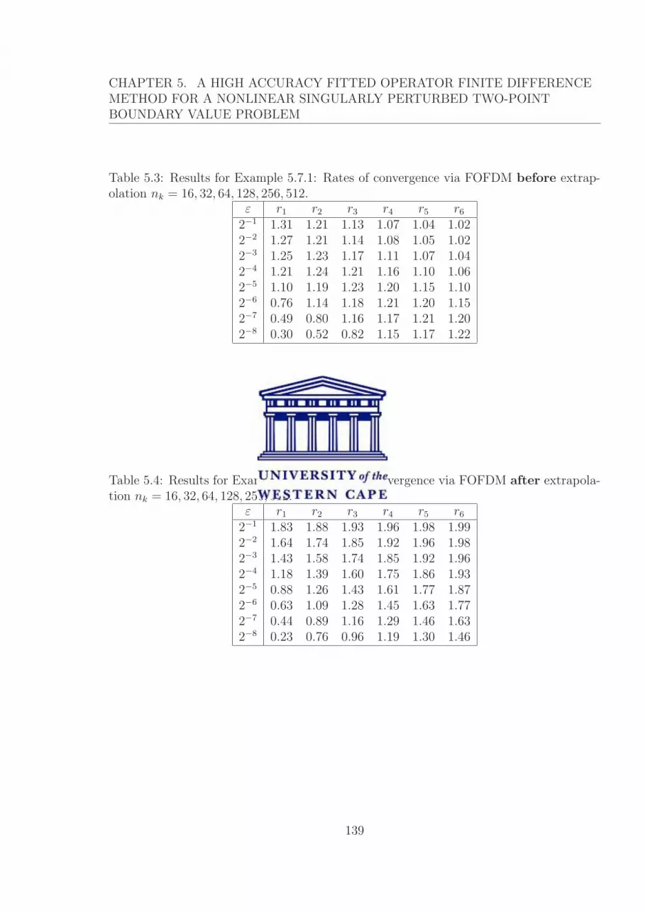
CHAPTER 5. A HIGH ACCURACY FITTED OPERATOR FINITE DIFFERENCEMETHOD FOR A NONLINEAR SINGULARLY PERTURBED TWO-POINTBOUNDARY VALUE PROBLEM
Table 5.3: Results for Example 5.7.1: Rates of convergence via FOFDM before extrap-olation nk = 16, 32, 64, 128, 256, 512.
ε r1 r2 r3 r4 r5 r6
2−1 1.31 1.21 1.13 1.07 1.04 1.022−2 1.27 1.21 1.14 1.08 1.05 1.022−3 1.25 1.23 1.17 1.11 1.07 1.042−4 1.21 1.24 1.21 1.16 1.10 1.062−5 1.10 1.19 1.23 1.20 1.15 1.102−6 0.76 1.14 1.18 1.21 1.20 1.152−7 0.49 0.80 1.16 1.17 1.21 1.202−8 0.30 0.52 0.82 1.15 1.17 1.22
Table 5.4: Results for Example 5.7.1: Rates of convergence via FOFDM after extrapola-tion nk = 16, 32, 64, 128, 256, 512.
ε r1 r2 r3 r4 r5 r6
2−1 1.83 1.88 1.93 1.96 1.98 1.992−2 1.64 1.74 1.85 1.92 1.96 1.982−3 1.43 1.58 1.74 1.85 1.92 1.962−4 1.18 1.39 1.60 1.75 1.86 1.932−5 0.88 1.26 1.43 1.61 1.77 1.872−6 0.63 1.09 1.28 1.45 1.63 1.772−7 0.44 0.89 1.16 1.29 1.46 1.632−8 0.23 0.76 0.96 1.19 1.30 1.46
139

CHAPTER 5. A HIGH ACCURACY FITTED OPERATOR FINITE DIFFERENCEMETHOD FOR A NONLINEAR SINGULARLY PERTURBED TWO-POINTBOUNDARY VALUE PROBLEM
Table 5.5: Results for Example 5.7.2: Maximum errors via FOFDM before extrapolationε n=16 n=32 n=64 n=128 n=256 n=512 n=1024
2−1 2.21E-03 5.10E-04 1.23E-04 3.02E-05 7.48E-06 1.86E-06 4.65E-072−2 3.39E-03 8.03E-04 1.94E-04 4.77E-05 1.18E-05 2.94E-06 7.33E-072−3 6.50E-03 1.57E-03 3.79E-04 9.25E-05 2.28E-05 5.67E-06 1.41E-062−4 1.28E-02 3.17E-03 7.65E-04 1.86E-04 4.57E-05 1.13E-05 2.81E-062−5 2.42E-02 6.44E-03 1.56E-03 3.76E-04 9.19E-05 2.27E-05 5.64E-062−6 4.54E-02 1.28E-02 3.17E-03 7.64E-04 1.86E-04 4.56E-05 1.13E-052−7 7.64E-02 2.42E-02 6.44E-03 1.56E-03 3.76E-04 9.19E-05 2.27E-052−8 1.18E-01 4.54E-02 1.28E-02 3.17E-03 7.64E-04 1.86E-04 4.56E-052−9 1.82E-01 7.64E-02 2.42E-02 6.44E-03 1.56E-03 3.76E-04 9.19E-05
Table 5.6: Results for Example 5.7.2: Maximum errors via FOFDM after extrapolationε n=16 n=32 n=64 n=128 n=256 n=512 n=1024
2−1 9.36E-05 2.80E-05 7.49E-06 1.93E-06 4.89E-07 1.23E-07 3.09E-082−2 1.04E-04 3.00E-05 8.22E-06 2.13E-06 5.42E-07 1.37E-07 3.44E-082−3 1.52E-04 2.45E-05 7.02E-06 1.85E-06 4.72E-07 1.19E-07 3.00E-082−4 3.67E-04 5.47E-05 7.88E-06 1.13E-06 2.91E-07 7.37E-08 1.86E-082−5 1.18E-03 1.38E-04 2.10E-05 2.91E-06 3.84E-07 4.94E-08 7.13E-092−6 3.49E-03 3.68E-04 5.45E-05 7.87E-06 1.06E-06 1.38E-07 1.76E-082−7 9.22E-03 1.18E-03 1.38E-04 2.09E-05 2.91E-06 3.84E-07 4.94E-082−8 2.11E-02 3.49E-03 3.68E-04 5.45E-05 7.87E-06 1.06E-06 1.38E-072−9 4.10E-02 9.22E-03 1.18E-03 1.38E-04 2.09E-05 2.91E-06 3.84E-07
140

CHAPTER 5. A HIGH ACCURACY FITTED OPERATOR FINITE DIFFERENCEMETHOD FOR A NONLINEAR SINGULARLY PERTURBED TWO-POINTBOUNDARY VALUE PROBLEM
Table 5.7: Results for Example 5.7.2: Rates of convergence via FOFDM before extrap-olation, nk = 16, 32, 64, 128, 256, 512.
ε r1 r2 r3 r4 r5 r6
2−1 2.11 2.05 2.03 2.01 2.01 2.002−2 2.08 2.05 2.03 2.01 2.01 2.002−3 2.05 2.05 2.03 2.02 2.01 2.002−4 2.01 2.05 2.04 2.02 2.01 2.012−5 1.91 2.05 2.05 2.03 2.02 2.012−6 1.83 2.01 2.05 2.04 2.02 2.012−7 1.66 1.91 2.05 2.05 2.03 2.022−8 1.38 1.83 2.01 2.05 2.04 2.022−9 1.26 1.66 1.91 2.05 2.05 2.03
Table 5.8: Results for Example 5.7.2: Rates of convergence via FOFDM after extrapola-tion, nk = 16, 32, 64, 128, 256, 512.
ε r1 r2 r3 r4 r5 r6
2−1 1.74 1.90 1.96 1.98 1.99 1.992−2 1.79 1.87 1.95 1.98 1.99 1.992−3 2.63 1.80 1.93 1.97 1.98 1.992−4 2.75 2.79 2.81 1.96 1.98 1.982−5 3.10 2.72 2.85 2.92 2.96 2.792−6 3.25 2.76 2.79 2.89 2.94 2.972−7 2.96 3.10 2.72 2.85 2.92 2.962−8 2.60 3.25 2.76 2.79 2.89 2.942−9 2.15 2.96 3.10 2.72 2.85 2.92
141
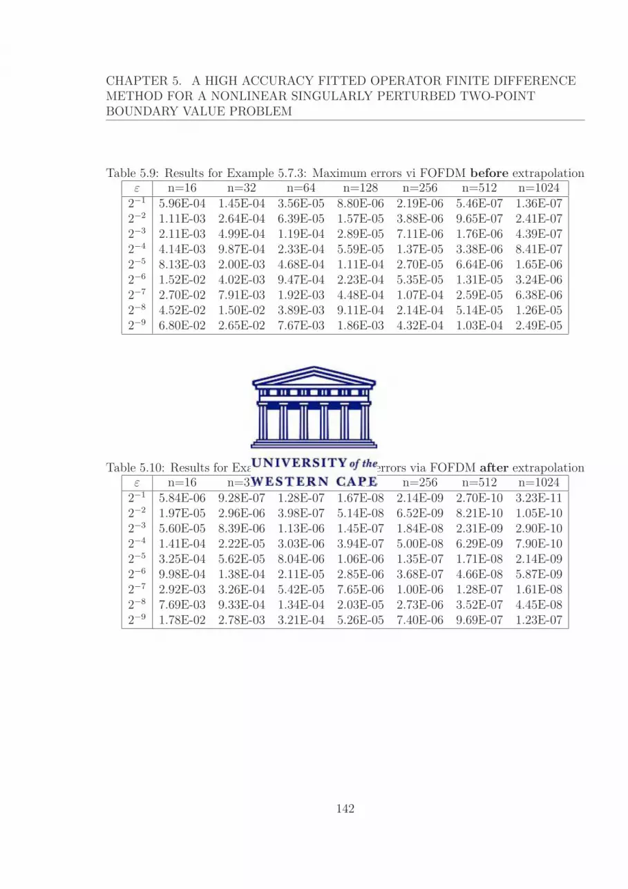
CHAPTER 5. A HIGH ACCURACY FITTED OPERATOR FINITE DIFFERENCEMETHOD FOR A NONLINEAR SINGULARLY PERTURBED TWO-POINTBOUNDARY VALUE PROBLEM
Table 5.9: Results for Example 5.7.3: Maximum errors vi FOFDM before extrapolationε n=16 n=32 n=64 n=128 n=256 n=512 n=1024
2−1 5.96E-04 1.45E-04 3.56E-05 8.80E-06 2.19E-06 5.46E-07 1.36E-072−2 1.11E-03 2.64E-04 6.39E-05 1.57E-05 3.88E-06 9.65E-07 2.41E-072−3 2.11E-03 4.99E-04 1.19E-04 2.89E-05 7.11E-06 1.76E-06 4.39E-072−4 4.14E-03 9.87E-04 2.33E-04 5.59E-05 1.37E-05 3.38E-06 8.41E-072−5 8.13E-03 2.00E-03 4.68E-04 1.11E-04 2.70E-05 6.64E-06 1.65E-062−6 1.52E-02 4.02E-03 9.47E-04 2.23E-04 5.35E-05 1.31E-05 3.24E-062−7 2.70E-02 7.91E-03 1.92E-03 4.48E-04 1.07E-04 2.59E-05 6.38E-062−8 4.52E-02 1.50E-02 3.89E-03 9.11E-04 2.14E-04 5.14E-05 1.26E-052−9 6.80E-02 2.65E-02 7.67E-03 1.86E-03 4.32E-04 1.03E-04 2.49E-05
Table 5.10: Results for Example 5.7.3: Maximum errors via FOFDM after extrapolationε n=16 n=32 n=64 n=128 n=256 n=512 n=1024
2−1 5.84E-06 9.28E-07 1.28E-07 1.67E-08 2.14E-09 2.70E-10 3.23E-112−2 1.97E-05 2.96E-06 3.98E-07 5.14E-08 6.52E-09 8.21E-10 1.05E-102−3 5.60E-05 8.39E-06 1.13E-06 1.45E-07 1.84E-08 2.31E-09 2.90E-102−4 1.41E-04 2.22E-05 3.03E-06 3.94E-07 5.00E-08 6.29E-09 7.90E-102−5 3.25E-04 5.62E-05 8.04E-06 1.06E-06 1.35E-07 1.71E-08 2.14E-092−6 9.98E-04 1.38E-04 2.11E-05 2.85E-06 3.68E-07 4.66E-08 5.87E-092−7 2.92E-03 3.26E-04 5.42E-05 7.65E-06 1.00E-06 1.28E-07 1.61E-082−8 7.69E-03 9.33E-04 1.34E-04 2.03E-05 2.73E-06 3.52E-07 4.45E-082−9 1.78E-02 2.78E-03 3.21E-04 5.26E-05 7.40E-06 9.69E-07 1.23E-07
142
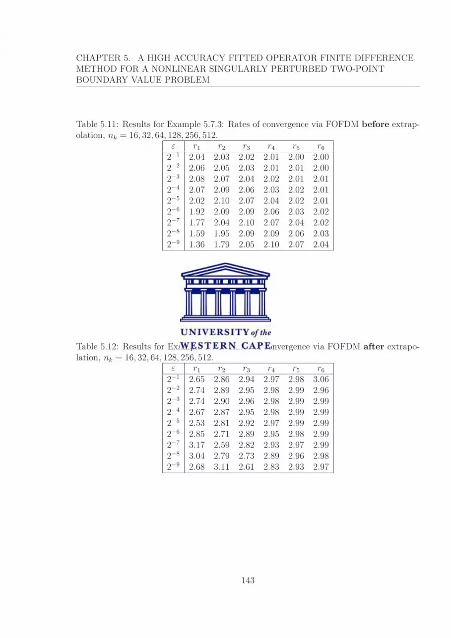
CHAPTER 5. A HIGH ACCURACY FITTED OPERATOR FINITE DIFFERENCEMETHOD FOR A NONLINEAR SINGULARLY PERTURBED TWO-POINTBOUNDARY VALUE PROBLEM
Table 5.11: Results for Example 5.7.3: Rates of convergence via FOFDM before extrap-olation, nk = 16, 32, 64, 128, 256, 512.
ε r1 r2 r3 r4 r5 r6
2−1 2.04 2.03 2.02 2.01 2.00 2.002−2 2.06 2.05 2.03 2.01 2.01 2.002−3 2.08 2.07 2.04 2.02 2.01 2.012−4 2.07 2.09 2.06 2.03 2.02 2.012−5 2.02 2.10 2.07 2.04 2.02 2.012−6 1.92 2.09 2.09 2.06 2.03 2.022−7 1.77 2.04 2.10 2.07 2.04 2.022−8 1.59 1.95 2.09 2.09 2.06 2.032−9 1.36 1.79 2.05 2.10 2.07 2.04
Table 5.12: Results for Example 5.7.3: Rates of convergence via FOFDM after extrapo-lation, nk = 16, 32, 64, 128, 256, 512.
ε r1 r2 r3 r4 r5 r6
2−1 2.65 2.86 2.94 2.97 2.98 3.062−2 2.74 2.89 2.95 2.98 2.99 2.962−3 2.74 2.90 2.96 2.98 2.99 2.992−4 2.67 2.87 2.95 2.98 2.99 2.992−5 2.53 2.81 2.92 2.97 2.99 2.992−6 2.85 2.71 2.89 2.95 2.98 2.992−7 3.17 2.59 2.82 2.93 2.97 2.992−8 3.04 2.79 2.73 2.89 2.96 2.982−9 2.68 3.11 2.61 2.83 2.93 2.97
143

CHAPTER 5. A HIGH ACCURACY FITTED OPERATOR FINITE DIFFERENCEMETHOD FOR A NONLINEAR SINGULARLY PERTURBED TWO-POINTBOUNDARY VALUE PROBLEM
5.8 Discussion
In this chapter, we considered a singularly perturbed nonlinear two point boundary value
problem. We first linearized the problem via the quasilinearization method. This process
led to a sequence of linear problems. For the case where the functional F of equation
(5.1.1) contains the argument y′, we developed and analyzed a fitted operator method
designed for the resulting sequence of linear problems. We noted that the method is first
order convergent. Richardson extrapolation was then carried out and both the accuracy
and order of convergence were improved.
Similar steps are also taken for the case where the functional F does not contain the
argument y′. However this is done with less details. The second order convergence of the
underlying fitted operator finite difference method is improved to four.
Some numerical results are not of higher order as expected but this is due to the con-
vergence properties of the sequence of linear problems. This is issue is being investigated
further.
144
Chapter 6
Higher Order Numerical Method for
Singularly Perturbed Parabolic
Problems in One Dimension
This chapter deals with singularly perturbed parabolic problems. Our basic aim is to
extend the ideas generated in chapters 4 and 5 to solve this class of problems. After
we linearize the problem, each of the linear problems is discretized as follows: the time
derivative is approximated by a forward Euler approximation and then the stationary
problem is solved using a fitted operator finited difference method (FOFDM). The overall
method is analyzed for convergence. We also discuss why the extrapolation process can
not improve the order of convergence of the proposed FOFDM.
6.1 Introduction
We consider the problem
∂u
∂t= ε
∂2u
∂x2− u
∂u
∂x, (x, t) ∈ Ω× (0, T ], (6.1.1)
145

CHAPTER 6. HIGHER ORDER NUMERICAL METHOD FOR SINGULARLYPERTURBED PARABOLIC PROBLEMS IN ONE DIMENSION
where Ω = (0, 1).
The initial and boundary conditions are respectively given by
u(x, 0) = f(x), for 0 ≤ x ≤ 1, (6.1.2)
u(0, t) = 0 u(1, t) = 0 for 0 ≤ t ≤ T. (6.1.3)
Equation (6.1.1) is a one-dimensional quasi-linear parabolic partial differential equa-
tion, which is referred to in the literature as Burgers’ equation (see [25, 26, 40]).
The parameter ε ∈ (0, 1] is the coefficient of kinematic viscosity and the function f(x)
is sufficiently smooth. In order for the data to match at the two corners (0, 0) and (1, 0)
of the domain Ω× [0, T ], we impose the compatibility conditions
f(0) = 0, f(1) = 0. (6.1.4)
In [22], it was proved that there exists a constant C such that
|u(x, t)− f(x)| ≤ Ct, t ∈ (0, T ), (6.1.5)
|u(x, t)− 0| ≤ Cx, x ∈ (0, 1), (6.1.6)
with (x, t) ∈ Ω× [0, T ].
Equation (6.1.1) was introduced by Bateman [16], presenting its steady state solutions.
It was after Burgers who studied this model for turbulent flows in [26], that it is referred
to as Burgers’ equation. Several researchers have studied this important fluid dynamic
model whose use was subsequently extended to other fields such as gas dynamics, heat
conduction, elasticity, turbulence and shock wave theory [26, 31, 60]. These references,
amongst others, provide the exact solutions (in the form of infinite series) to Burgers’
equations for given initial and boundary conditions.
One important fact presented by Miller [104] is that these exact solutions have no prac-
146

CHAPTER 6. HIGHER ORDER NUMERICAL METHOD FOR SINGULARLYPERTURBED PARABOLIC PROBLEMS IN ONE DIMENSION
tical meaning when ε is very small due to the occurrence of slow convergence. Numerous
numerical schemes are available in the literature to circumvent this difficulty.
Abbasbandy and Darvishi [1] used the modified Adomian’s decomposition method
for calculating a numerical solution of problem (6.1.1)-(6.1.3) without recourse to any
transformation in the above equation such as Hopf-Cole transformation. Kutluay et al.
[80] presented the exact-explicit finite difference scheme to achieve a reliable accuracy. A
variational method built on the method of time discretization was suggested by Aksan and
Odzes [9]. Subsequently, Kadalbajoo et al. [70] semidiscretized the equation in time by
backward Euler scheme with uniform time step and then used the quasilinerization process
[19] to linearize the stationary Burgers’ equation. There are other numerical methods to
solve the Burgers’ equation that are based on finite differences [37, 80, 117, 141], on
finite element approaches [27, 81, 76] and on splines [3]. Other notable works include
[2, 59, 106, 107].
In this chapter, we intend to extend the FOFDM developed in Chapter 5 to solve the
Burgers’ equation. The quasilinearization of the original problem gives us a sequence of
linear parabolic problems. After the time semi-discretization for these parabolic problems,
the stationary problems are solved using this FOFDM.
The rest of this chapter is organized as follows. Section 6.2 deals with quasilineariza-
tion and time semi-discretization. Section 6.3 is concerned with the FOFDM and its error
analysis. A result of Richardson extrapolation on this FOFDM is presented in Section
6.4. Some numerical illustrations are given in Section 6.5 and these results are discussed
in Section 6.6.
147

CHAPTER 6. HIGHER ORDER NUMERICAL METHOD FOR SINGULARLYPERTURBED PARABOLIC PROBLEMS IN ONE DIMENSION
6.2 Quasilinearization and time semidiscretization
6.2.1 Quasilinearization
Writing Eq. (6.1.1) in the form
ut = εuxx − uux on Ω× (0, T ], (6.2.7)
and setting
g(u, ux) = −uux,
we have gu = −ux and gux = −u.
Assuming that (un, unx) is the n-th nominal solution to problem (6.1.1) along with the
initial and boundary conditions (6.1.2)-(6.1.3) and taking the Taylor expansion of g up
to first-order terms around this nominal function, we get
g(un+1, un+1x ) = g(un, un
x) + gu(un+1 − un) + gux(u
n+1x − un
x).
Hence the quasilinearization process for equation (6.2.7) (see [19]) gives
un+1t = εun+1
xx − un+1x un − un
xun+1 + unxun, (6.2.8)
along with
un+1(0, t) = 0, un+1(1, t) = 0 for 0 ≤ t ≤ T (6.2.9)
and
un+1(x, 0) = f(x) for 0 ≤ x ≤ 1. (6.2.10)
Letting un+1 = U , we get the quasilinear process equations
Ut = εUxx − unUx − unxU + un
xun. (6.2.11)
148

CHAPTER 6. HIGHER ORDER NUMERICAL METHOD FOR SINGULARLYPERTURBED PARABOLIC PROBLEMS IN ONE DIMENSION
With this new notation, the boundary and initial conditions take the form
U(0, t) = 0, U(1, t) = 0 for 0 ≤ t ≤ T (6.2.12)
and
U(x, 0) = f(x) for 0 ≤ x ≤ 1. (6.2.13)
6.2.2 Time semidiscretization
We discretize the time variable by means of the implicit Euler method (IEM). To do so,
firstly we partition the time interval [0, T ] into M subintervals such that the time step ∆t
is given by ∆t = T/M .
Then the IEM reads:
Uj+1 − Uj
∆t= ε(Uj+1)xx − un
j+1(Uj+1)x − (unj+1)xUj+1 + (un
j+1)xunj+1. (6.2.14)
Rearranging this equation and using the notation
unj+1 = an(x),
1
∆t+ (un
j+1)x = bn(x),
Uj
∆t+ (un
j+1)xunj+1 = F n(x),
we obtain from equation (6.2.14)
−ε (Uj+1(x))xx + an(x) (Uj+1(x))x + bn(x)Uj+1 = F n(x), (6.2.15)
with j = 0(1)M − 1.
149
CHAPTER 6. HIGHER ORDER NUMERICAL METHOD FOR SINGULARLYPERTURBED PARABOLIC PROBLEMS IN ONE DIMENSION
Finally, equations (6.2.10) and (6.2.15) can be written in the form
U0 = f(x),
LUj+1(x) = F n(x), 0 ≤ j ≤ M − 1, (6.2.16)
where
LUj+1(x) ≡ −ε (Uj+1(x))xx + an(x) (Uj+1(x))x + bn(x)Uj+1(x),
and the boundary conditions are
Uj+1(0) = 0, Uj+1(1) = 0.
Letting
k = max|Uj+1|≤1
|HUj+1Uj+1(Uj+1)| and m = max
|Uj+1|≤1|HUj+1
(Uj+1)|,
the following result was proved in [70].
maxx
∣∣∣(U
(n+2)j+1 − U
(n+1)j+1
)∣∣∣ ≤(
k8
1− m4
)max
x
(U
(n+1)j+1 − U
(n)j+1
)2
. (6.2.17)
This inequality shows that the quasilinearization process enjoys a quadratic convergence.
The linear operator L satisfies the following maximum principle.
Lemma 6.2.1. Let ψ ∈ C2(Ω) be any function satisfying ψ(0) ≥ 0, ψ(1) ≥ 0 and
Lψ(x) ≥ 0 for all x ∈ Ω. Then ψ(x) ≥ 0 for all x ∈ Ω.
Proof. See [105].
150

CHAPTER 6. HIGHER ORDER NUMERICAL METHOD FOR SINGULARLYPERTURBED PARABOLIC PROBLEMS IN ONE DIMENSION
6.3 A fitted operator finite difference method for the
solution of Burgers’ equation
6.3.1 The method
Let N be a positive integer. The interval [0, 1] is partitioned as follows.
x0 = 0, h = 1/N, xi = x0 + ih, i = 1(1)N.
For the sake of simplicity, we assume that an(x) ≥ α > 0, for all x ∈ (0, 1).
At each iteration n, and each time level j = 1, 2, . . . , M − 1, we discretize (6.2.16) as
LhU(i, j) := −εUi+1,j − 2Ui,j + Ui+1,j
φ2i
+ ani
Ui,j − Ui−1,j
h+ bn
i Ui,j = F ni,j (6.3.18)
where the function φ is given by
φ2i =
hε
ani
(exp
(an
i h
ε
)− 1
).
where
ani =
ani + an
i+1
2,
bni =
bni−1 + bn
i + bni+1
3,
and
F ni =
F ni−1 + F n
i + F ni+1
3.
Equation (6.3.18) leads to a tridiagonal system of linear equation
AU = G. (6.3.19)
151

CHAPTER 6. HIGHER ORDER NUMERICAL METHOD FOR SINGULARLYPERTURBED PARABOLIC PROBLEMS IN ONE DIMENSION
Corresponding entries of A and G in this case are
Aik = r−k , i = k + 1; k = 1, 2, . . . , N − 2,
Aik = rck, i = k; k = 1, 2, . . . , N − 1,
Aik = r+k , i = k − 1; k = 2, 3, . . . , N − 1,
G1 = F n1 − r−1 U(0),
GN−1 = F nN−1 − r+
N−1U(1),
Gk = F nk , k = 2, 3, . . . , N − 1,
where
r−k = − ε
φ2k
− ank
h, r+
k = − ε
φ2k
, and rck = 2
ε
φ2k
+an
k
h+ bn
k . (6.3.20)
6.3.2 Convergence analysis
Below we present the bounds on the solution of Burgers’ equation. Then we provide the
error analysis of both the time discretization (see [70]) and the FOFDM introduced above.
Finally we will summarize the two results at the end of this subsection.
Lemma 6.3.1. The solution u(x, t) of (6.1.1) enjoys the following bound
|u(x, t)| ≤ C, for all (x, t) ∈ Ω× [0, T ].
Proof. Inequality (6.1.5) implies that
|u| ≤ Ct + |f |.
The proof follows using the fact that f(x) is sufficiently smooth and x and t lie in bounded
intervals.
Lemma 6.3.2. By keeping x fixed along the line (x, t) : 0 ≤ t ≤ T, the bound of ut is
152

CHAPTER 6. HIGHER ORDER NUMERICAL METHOD FOR SINGULARLYPERTURBED PARABOLIC PROBLEMS IN ONE DIMENSION
given by
∣∣∣∣∂iu(x, t)
∂ti
∣∣∣∣ ≤ C, for i = 0, 1, 2, 3. (6.3.21)
Proof. Assuming that the solution u(x, t) is sufficiently smooth in the domain Ω× [0, T ],
the mean value theorem suggests that there exists t∗ ∈ (t, t + k) along the line (x, t) :
0 ≤ t ≤ T such that
ut(x, t∗) =u(x, t + k)− u(x, t)
k
thus implying that
|ut(x, t∗)| ≤ 2|u(x, t)|k
.
By Lemma 6.3.1, we get
ut(x, t) ≤ C.
We get the bounds on utt(x, t) and uttt(x, t) along the line (x, t) : 0 ≤ t ≤ T in a similar
manner.
It follows from this lemma that, by keeping x fixed along the line (x, t), 0 ≤ t ≤ T,the solution U of equation (6.2.11) satisfies
U(tj) = U(tj+1)−∆t∂U(tj+1)
∂t+
∫ tj
tj+1
(tj − s)∂2U
∂t2(s)ds, (6.3.22)
i.e.,
U(tj) = U(tj+1)−∆t (εUxx − unUx − unxU + un
xun) (tj+1)
+
∫ tj
tj+1
(tj − s)∂2U
∂t2(s)ds. (6.3.23)
Subtracting (6.2.14) from (6.3.23) and denoting the local truncation error U(tj+1)−Uj+1
by ej+1, we obtain
maxj|∆tLej+1| ≤ C(∆t)2 (6.3.24)
153

CHAPTER 6. HIGHER ORDER NUMERICAL METHOD FOR SINGULARLYPERTURBED PARABOLIC PROBLEMS IN ONE DIMENSION
and since the operator ∆tL satisfies the maximum principle (Lemma 6.2.1), we deduce
that
maxj|ej+1| ≤ C(∆t)2. (6.3.25)
We now derive the estimate of the global error at the (j + 1)th time step, Ej+1 as follows
maxj|Ej+1| = max
j
∣∣∣∣∣j∑
l=1
el
∣∣∣∣∣ , j ≤ T/∆t,
≤j∑
l=1
maxj|el|,
≤ jC(∆t)2,
≤ CT∆t,
≤ C∆t. (6.3.26)
We have thus proved that
Theorem 6.3.1. If
∣∣∣∣∂ku(x, t)
∂kt
∣∣∣∣ ≤ C, (x, t) ∈ Ω× [0, T ], 0 ≤ k ≤ 2
then the local and global error estimates of the time discretization satisfy the following
estimates
maxj|ej+1| ≤ C(∆t)2,
maxj|Ej+1| ≤ C∆t, for all j ≤ T/∆t.
In other words, the time discretization process is uniformly convergent of first order.
For the solution Uj+1 of (6.2.16) and its derivatives, the estimates contained in the
following lemma hold (see [70, 105]).
154

CHAPTER 6. HIGHER ORDER NUMERICAL METHOD FOR SINGULARLYPERTURBED PARABOLIC PROBLEMS IN ONE DIMENSION
Lemma 6.3.3. If Uj+1 is the solution of (6.2.16) then there exists a constant C such that
|Uj+1(x)| ≤ C, for all x ∈ Ω.
Lemma 6.3.4. If Uj+1 is the solution of (6.2.16), then the bounds on its derivatives are
given by
∣∣∣U (k)j+1
∣∣∣ ≤ C(1 + ε−k exp (−α(1− x)/ε) ; for all x ∈ Ω, k = 1, 2, 3. (6.3.27)
For the sake of notational simplicity, we drop the index j + 1. Therefore, at each grid
point xi, i = 0, 1, . . . , N , U(xi) and Ui represent the solution of (6.2.16) and (6.3.19)
respectively.
The local truncation error of FOFDM (6.3.19)-(6.3.20) is therefore given by
Lh (Ui − U(xi)) =− [r+i U(xi+1) + rc
iU(xi) + r−i U(xi−1)]
− [−εU ′′(xi) + an(xi)U′(xi) + bn(xi)U(xi)] .
This equation implies that
ÃLh (U(xi)− Ui)) = T0U(xi) + T1U′(xi) + T2U
′′(xi) + T3U′′′(xi) + T4U
iv(ξi), (6.3.28)
where ξi ∈ (xi−1, xi+1) and
T0 = r−i + rci + r+
i − bni −
h2
3b′′i ,
T1 = h(r+i − r−i )− an
i −1
3h2 ((an
i )′′ + 2(bni )′) ,
T2 =h2
2
(r+i + r−i
)+ ε− h2
3
(2(an
i )′ + bni +
1
2(bn
i )′′h2
), (6.3.29)
T3 =h3
6
(r+i − r−i
)− h2
3
(an
i +1
2(an
i )′′h2
),
155

CHAPTER 6. HIGHER ORDER NUMERICAL METHOD FOR SINGULARLYPERTURBED PARABOLIC PROBLEMS IN ONE DIMENSION
T4 =h3
24
(r+i + r−i
)+
1
3εh2.
Further simplifications yield
T0 = 0, |T1| ≤ Mh, |T2| ≤ Mh + Mh2/ε, |T3| ≤ Mh2, |T4| ≤ Mh2. (6.3.30)
Considering the dominating terms and using lemmas 4.2.2 and 6.3.3 we obtain
|Lh(Ui − U(xi))| ≤ Mh
(1 +
h
ε
)[1 +
exp(−α(1− xi)/ε)
ε2
], for i = 1, 2, · · · , n− 1.
(6.3.31)
where α is such that an(x) ≥ α > 0, ∀x ∈ [0, 1].
Finally, using Lemma 4.3.2 and re-instating the dropped time indice j + 1, we obtain
|Ui,j+1 − Uj+1(xi)| ≤ Mh
(1 +
h
ε
)[1 +
exp(−α(1− xi)/ε)
ε2
], for i = 1, 2, · · · , n− 1.
and therefore applying Lemma 2.2.5, we get
Theorem 6.3.2. If Uj+1(xi) is the solution of problem (6.2.16) and Ui,j+1 the solution
of the discrete problem (6.3.18) at the point xi and the (j + 1)-th time level, there is a
constant C such that
maxi|Ui,j+1 − Uj+1(xi)| ≤ Mh
(1 +
h
ε
).
The results of theorems 6.3.1 and 6.3.2 are now combined to give an estimate of the
fully discrete scheme.
Theorem 6.3.3. Let U(xi, tj+1) be the solution of the linearized problem (6.2.11) of equa-
tion (6.1.1), and Ui,j+1 be the solution of the totally discrete equation (6.3.18). Then, there
156

CHAPTER 6. HIGHER ORDER NUMERICAL METHOD FOR SINGULARLYPERTURBED PARABOLIC PROBLEMS IN ONE DIMENSION
exists a constant M such that
maxi,j
|Ui,j+1 − Uj+1(xi, tj+1)| ≤ M
(∆t + h
(1 +
h
ε
)),
where i = 0, 1, . . . , N and j = 0, 1, . . . ,M − 1.
6.4 Richardson extrapolation
In this section, we adapt the Richardson extrapolation of Section 5.5 to FOFDM 6.3.18.
Denoting by Ui,j+1 and U exti,j+1 the solutions of equation (6.3.19) on the mesh µ2N and
after extrapolation, respectively, we have
U exti,j+1 := 2Ui,j+1 − Ui,j, i = 1(1)N − 1.
Following the same lines as in Section 5.5, we obtain the following result.
Theorem 6.4.1. Let U(xi, tj+1) be the solution of the linearized equation (6.2.11) of
equation (6.1.1) and U exti,j+1 the solution of the totally discrete equation (6.3.18). Then,
there exists a constant M such that:
maxi,j
∣∣U exti,j+1 − U(xi, tj+1)
∣∣ ≤ M
(∆t + h2
(1 +
1
ε
)). (6.4.32)
6.5 Numerical results
Example 6.5.1. We consider the equation
ut + uux = εuxx, (x, t) ∈ (0, 1)× (0, T )
with initial condition
u(x, 0) = sin(πx), 0 ≤ t ≤ T,
157

CHAPTER 6. HIGHER ORDER NUMERICAL METHOD FOR SINGULARLYPERTURBED PARABOLIC PROBLEMS IN ONE DIMENSION
and boundary conditions
u(0, t) = 0, u(1, t) = 0, 0 ≤ x ≤ 1.
The exact (Fourier) solution is given by ([31])
u(x, t) = 2πε
∑∞n=1 an exp(−n2π2εt)n sin(nπx)
a0 +∑∞
n=1 an exp(−n2π2εt) cos(nπx),
where a0 and an(n = 1, 2, . . .) are the following Fourier coefficients
a0 =
∫ 1
0
exp−(2πε)−1[1− cos(πx)]dx,
an = 2
∫ 1
0
exp−(2πε)−1[1− cos(πx)] cos(nπx)dx, n = 1, 2, 3, . . . .
Many researchers have used the above solution to evaluate the errors in their approxima-
tions.
6.6 Discussion
We have considered viscous Burgers’ equation which is a nonlinear parabolic PDE and
shown the quasilinearization for this equation. The set of quasilinear process equations
are then solved at each time level by a novel FOFDM. Each of the quasilinear process
equation is time dependent linear SPP for which it is known that the standard methods
do not perform well.
The profile of the numerical solution is shown in Figure 6.1.
One remarkable issue here is the use of extrapolation with respect to the spatial
variable x. We noted that the order of convergence (in x-direction) after extrapolation
has improved. Due to the convergence properties of the quasilinearization, the FOFDM
appears not to be ε-uniform. This aspect is under investigation.
158

CHAPTER 6. HIGHER ORDER NUMERICAL METHOD FOR SINGULARLYPERTURBED PARABOLIC PROBLEMS IN ONE DIMENSION
0 0.2 0.4 0.6 0.8 10
0.1
0.2
0.3
0.4
x
U(x
,t)
0 0.2 0.4 0.6 0.8 10
0.2
0.4
0.6
0.8
1
x
U(x
,t)
0 0.2 0.4 0.6 0.8 10
0.2
0.4
0.6
0.8
1
x
U(x
,t)
0 0.2 0.4 0.6 0.8 10
0.2
0.4
0.6
0.8
1
x
U(x
,t)
eps=1 eps=0.1
eps=0.01 eps=0.0001
Figure 6.1: Profile of the numerical solution of the problem in Example 6.5.1 for variousvalues of ε.
159

Chapter 7
Higher Order Numerical Methods
for Singularly Perturbed Elliptic
Problems
This chapter is devoted to a family of singularly perturbed elliptic problems in two di-
mensions. We extend FOFDM-II (p.64) to solve such problems. Through a rigorous
convergence analysis, we show that the method is second order in both variables. This
order of convergence is improved to four through extrapolation.
7.1 Introduction
We consider the problem
Lu := −ε∆u + b(x, y)u = f(x, y), in Ω = (0, 1)2, (7.1.1)
u = 0, on ∂Ω. (7.1.2)
160

CHAPTER 7. HIGHER ORDER NUMERICAL METHODS FOR SINGULARLYPERTURBED ELLIPTIC PROBLEMS
where ε ∈ (0, 1] and b and f are sufficiently smooth functions in Ω. It is assumed
that b(x, y) ≥ α2 > 0, in Ω. Also, we impose the following compatibility conditions
[116, 124] which guarantee that the solution u(x, y) to problem (7.1.1)-(7.1.2) is a member
of C4(Ω) ∩ C2(Ω), where Ω = ∂Ω ∪ Ω:
f(0, 0) = f(0, 1) = f(1, 0) = f(1, 1) = 0.
While singularly perturbed two-point boundary value problems are well studied from
different angles, their higher dimensional counterparts are not tackled sufficiently, as far
as FOFDMs are concerned. There were some attempts made to extend the approaches
developed for singularly perturbed ordinary differential equation but the success was very
limited.
On the other hand, some researchers tried to solve these higher dimensional problems
directly. Some notable works include [39, 52, 86, 124, 129, 131, 147].
A careful reading of the work of Kadalbajoo and Patidar [69] indicates that there are
no extensions of any fitted operator methods developed for singularly perturbed ODEs
that can solve the singularly perturbed PDEs, in particular the elliptic ones. To fill this
gap, the first aim of this chapter is to extend a FOFDM (which is developed for singularly
perturbed ODEs) to solve the elliptic singular perturbation problem. Then, in order to
achieve a higher order convergence, we perform the Richardson extrapolation.
The rest of this chapter is organized as follows. In Section 7.2, we presents some
qualitative features of the solution and its derivatives. Section 7.3 is concerned with the
construction and analysis of the numerical method Section 7.4 deals with the extrapolation
of the method developed in Section 7.3. Numerical results to support the theory are
provided in Section 7.5. We end the chapter with a discussion of the results and related
issues in Section 7.6.
161
CHAPTER 7. HIGHER ORDER NUMERICAL METHODS FOR SINGULARLYPERTURBED ELLIPTIC PROBLEMS
7.2 Bounds on the solution and its derivatives
Lemma 7.2.1. [48] (Continuous maximum principle)
Let ξ(x, y) be any sufficiently smooth function such that ξ(x, y) ≥ 0 on ∂Ω. Then
Lξ(x, y) ≥ 0 on Ω implies that ξ(x, y) ≥ 0, ∀(x, y) ∈ Ω = ∂Ω ∪ Ω.
Proof. Let (x∗, y∗) be such that
ξ(x∗, y∗) = min(x,y)∈Ω
ξ(x, y)
and assume that ξ(x∗, y∗) < 0. Clearly, (x∗, y∗) /∈ ∂Ω. We have
∂
∂xξ(x, y)
∣∣∣(x∗,y∗)
= 0,
∂
∂yξ(x, y)
∣∣∣(x∗,y∗)
= 0,
∂2
∂x2ξ(x, y)
∣∣∣(x∗,y∗)
≥ 0,
and∂2
∂y2ξ(x, y)
∣∣∣(x∗,y∗)
≥ 0.
Therefore
Lξ(x∗, y∗) = −ε∆ξ(x∗, y∗) + b(x∗, y∗)ξ(x∗, y∗) < 0,
which is a contradiction.
The following lemmas provide bounds on the solution of the problem (7.1.1)-(7.1.1)
as well as those of its derivatives [85]. A suitable choice of barrier functions [84, 153] may
be made in the proofs.
Lemma 7.2.2. Let u(x, y) be the solution of problem (7.1.1)-(7.1.2). Then we have
(a). |u(x, y)| ≤ C(1− e−αx/
√ε)
on Ω,
162

CHAPTER 7. HIGHER ORDER NUMERICAL METHODS FOR SINGULARLYPERTURBED ELLIPTIC PROBLEMS
(b). |u(x, y)| ≤ C(1− e−α(1−x)/
√ε)
on Ω,
(c). |u(x, y)| ≤ C(1− e−αy/
√ε)
on Ω,
(d). |u(x, y)| ≤ C(1− e−α(1−y)/
√ε)
on Ω.
Proof. (a). Using the barrier function
φ(x, y) = C(1− e(−αx/√
ε)),
we see that
L(φ± u) = −ε∆(φ± u) + b(φ± u),
= Cα2e(−αx/√
ε) + bC(1− e(−αx/√
ε))± f,
= C(α2 − b)(e(−αx/
√ε) − 1
)+ Cα2 ± f.
Since
(α2 − b)(e(−αx/
√ε) − 1
)≥ 0,
we have
L(φ± u) ≥ Cα2 ± f ≥ 0.
Using the maximum principle and the fact that (φ± u)|∂Ω ≥ 0, we get
|u| ≤ φ.
The proof of part (b), (c) and (d) is done in a similar way by choosing the barrier functions
φ(x, y) =(1− e−α(1−x)/
√ε)
,
φ(x, y) =(1− e−αy/
√ε)
,
163
CHAPTER 7. HIGHER ORDER NUMERICAL METHODS FOR SINGULARLYPERTURBED ELLIPTIC PROBLEMS
and
φ(x, y) =(1− e−α(1−y)/
√ε)
,
respectively.
Now we have
Lemma 7.2.3. Let u(x, y) be the solution of problem (7.1.1)-(7.1.2). Then we have
(a). |ux(x, y)| ≤ Cε−1/2 on ∂Ω,
(b). |uy(x, y)| ≤ Cε−1/2 on ∂Ω.
Proof
By Lemma 7.2.2, we have
|ux(0, y)| =
∣∣∣∣ limx→0+
u(x, y)− u(0, y)
x
∣∣∣∣
≤ limx→0+
C(1− e(−αx/√
ε))
x= C
α
ε1/2
≤ Cε−1/2.
Similarly, applying the estimate in part (b) of Lemma 7.2.2, we get the estimate for
ux(1, y).
Differentiating the given boundary conditions u(x, y) = 0 at y = 0 and y = 1 with respect
to x gives us ux(x, 0) = ux(x, 1) = 0 and this finishes the proof.
Similarly,
|uy(x, 0)| =
∣∣∣∣ limy→0+
u(x, y)− u(x, 0)
y
∣∣∣∣
≤ limy→0+
C(1− e(−αy/√
ε))
y
≤ Cε−1/2.
164

CHAPTER 7. HIGHER ORDER NUMERICAL METHODS FOR SINGULARLYPERTURBED ELLIPTIC PROBLEMS
We get the estimate of uy(x, 1) by applying the estimate in part (d) of Lemma 7.2.2.
Differentiating the given boundary conditions u(x, y) = 0 at x = 0 and x = 1 with respect
to y we get uy(0, y) = uy(1, y) = 0. This completes the proof.
Lemma 7.2.4. Let u(x, y) be the solution of problem (7.1.1)-(7.1.2). Then we have
(a). |ux(x, y)| ≤ C(1− ε−1/2e−αx/
√ε + ε−1/2e−α(1−x)/
√ε)
on Ω,
(b). |uy(x, y)| ≤ C(1− ε−1/2e−αy/
√ε + ε−1/2e−α(1−y)/
√ε)
on Ω.
Proof. By choosing the barrier function
φ(x, y) = C(1− ε−1/2e−αx/
√ε + ε−1/2e−α(1−x)/
√ε)
,
we obtain
L(φ± ux) ≥ bC ± (fx − bxu) ≥ 0,
and since (φ±ux)|∂Ω ≥ 0, the proof is completed by making use of the maximum principle
(Lemma [48]).
For the proof of the estimate in part (b), we can use the barrier function
φ(x, y) = C(1− ε−1/2e−αy/
√ε + ε−1/2e−α(1−y)/
√ε)
.
Now, the following results for the bounds on the second derivatives hold.
Lemma 7.2.5. Let u(x, y) be the solution of problem (7.1.1)-(7.1.2). Then we have
(a). |uxx(x, y)| ≤ Cε−1 on ∂Ω,
(b). |uyy(x, y)| ≤ Cε−1 on ∂Ω. %endLemma
(c). |uxx(x, y)| ≤ C(1 + ε−1e−αx/
√ε + ε−1e−α(1−x)/
√ε)
on Ω,
165
CHAPTER 7. HIGHER ORDER NUMERICAL METHODS FOR SINGULARLYPERTURBED ELLIPTIC PROBLEMS
(d). |uyy(x, y)| ≤ C(1 + ε−1e−αy/
√ε + ε−1e−α(1−y)/
√ε)
on Ω.
Proof. See [85].
7.3 Construction and analysis of the fitted operator
finite difference method
Let n and m be positive integers.
We consider the following partitions of the interval [0,1]:
x0 = 0, xi = x0 + ih, i = 1(1)n, h = xi − xi−1, xn = 1.
y0 = 0, yj = y0 + jk, j = 1(1)m, k = yj − yj−1, ym = 1.
The tensor product of these two partitions gives the mesh grid
µ(n,m) = (xi, yj), i = 0(1)n, j = 0(1)m.
In the rest of this chapter, we adopt the notation W ji = W (xi, yj) and denote the approx-
imations of uji at the grid point (xi, yj) by the unknown vj
i .
Using the theory of difference equations for problems in one dimension, we construct
the following FOFDM (looking at the one dimension at a time):
−ε
[vj
i+1 − 2vji + vj
i−1
(φji )
2h
+vj+1
i − 2vji + vj−1
i
(φji )
2k
]+ bj
ivji = f j
i , (7.3.3)
with the discrete boundary conditions
v0i = vj
0 = vmi = vj
n = 0, i = 0(1)n, j = 0(1)m, (7.3.4)
166

CHAPTER 7. HIGHER ORDER NUMERICAL METHODS FOR SINGULARLYPERTURBED ELLIPTIC PROBLEMS
where
(φji )h ≡ φj
i (h, ε) :=2
ρji
sinh
(ρj
ih
2
)(7.3.5)
and
(φji )k ≡ φj
i (k, ε) :=2
ρji
sinh
(ρj
ik
2
), (7.3.6)
with ρji =
√bji/ε.
Note that
φji (h, ε) = h + O
(h3
ε
),
and
φji (k, ε) = k + O
(k3
ε
).
For the sake of simplicity, we assume that h = k, and hence the common denominator
will then be φji (= (φj
i )h = (φji )k). Thus equation (7.3.3) becomes
−ε
[vj
i+1 − 2vji + vj
i−1
(φji )
2+
vj+1i − 2vj
i + vj−1i
(φji )
2
]+ bj
ivji = f j
i , (7.3.7)
which we rewrite as
− ε
(φji )
2
[vj
i+1 + vji−1 + vj+1
i + vj−1i − 4vj
i
]+ bj
ivji = f j
i . (7.3.8)
One should note that, in the above we have considered h = k merely for the sake of
simplicity. However, in the analysis below, we keep the general set up.
We start with stating the following two lemmas whose roles are primordial in the
analysis of the method developed in previous section.
Lemma 7.3.1. (Discrete maximum principle) Let ξji be any mesh function satisfying
ξ0i ≥ 0, i = 1(1)n− 1,
ξmi ≥ 0, i = 1(1)n− 1,
ξj0 ≥ 0, i = 1(1)m− 1,
167

CHAPTER 7. HIGHER ORDER NUMERICAL METHODS FOR SINGULARLYPERTURBED ELLIPTIC PROBLEMS
ξjn ≥ 0, i = 1(1)m− 1,
ξ00 ≥ 0, ξ0
n ≥ 0, ξm0 ≥ 0, ξn
m ≥ 0,
and Lkhξ
ji ≥ 0, i = 1(1)n− 1; j = 1(1)m− 1.
Then ξji ≥ 0, ∀i = 0(1)n, j = 0(1)m.
Proof Let (s, t) be indices such that
ξts = min
(i,j)ξji , ∀ (i, j) ∈ 0, 1, . . . , n × 0, 1, . . . , m.
Assume that ξts < 0. It is clear that
(s, t) ∈ 1, 2, . . . , n− 1 × 1, 2, . . . , m− 1
or else, ξts ≥ 0.
We observe that
ξts+1 − ξt
s > 0,
ξts−1 − ξt
s > 0,
ξt+1s − ξt
s > 0,
ξts − ξt−1
s > 0.
Therefore
Lkhξ
ts < 0,
which is a contradiction.
Lemma 7.3.2. If Zji is any mesh function such that Zj
i = 0 on (∂Ω)ji , then there exists
a constant C such that
|Zsl | ≤ C max
1≤i≤n−1;1≤j≤m−1|Lk
hZji |, for 0 ≤ l ≤ n; 0 ≤ s ≤ m.
168

CHAPTER 7. HIGHER ORDER NUMERICAL METHODS FOR SINGULARLYPERTURBED ELLIPTIC PROBLEMS
Proof. The proof follows similar lines as those for the FOFDMs developed for singularly
perturbed linear two-point boundary value problems.
7.3.1 Error estimate before extrapolation
The local truncation error of the FOFDM (7.3.3)-(7.3.4) is
Lkh(u
ji − vj
i ) =−ε(∆u)j
i + bjiu
ji
−−ε
[uj
i+1 − 2uji + uj
i−1
(φji )
2h
+uj+1
i − 2uji + uj−1
i
(φji )
2k
]+ bj
iuji
= −ε(uxx)ji − ε(uyy)
ji
+ε
(φji )
2h
[h2(uxx)
ji +
h4
12(uxxxx)
ji + · · ·
]
+ε
(φji )
2k
[k2(uyy)
ji +
k4
12(uyyyy)
ji + · · ·
]
= −ε(uxx)ji − ε(uyy)
ji
+
(ε
h2− bj
i
12+
h2(bji )
2
240ε+ · · ·
)[h2(uxx)
ji +
h4
12(uxxxx)
ji + · · ·
]
+
(ε
k2− bj
i
12+
k2(bji )
2
240ε+ · · ·
)[h2(uyy)
ji +
k4
12(uyyyy)
ji · · ·
]
This implies that
Lkh(u
ji − vj
i ) =εh2
12(uxxxx)
ji −
h2(bji )
2
12(uxx)
ji −
h4(bji )
144(uxxxx)
ji +
h4(bji )
2
240ε(uxx)
ji
+εk2
12(uyyyy)
ji −
k2(bji )
2
12(uyy)
ji −
k4(bji )
144(uyyyy)
ji +
k4(bji )
2
240ε(uyy)
ji + · · ·
Using Lemma 7.2.5 we obtain
|Lkh(u
ji − vj
i )| ≤ M
[h2
(1 +
h2
ε
)+ k2
(1 +
k2
ε
)].
169

CHAPTER 7. HIGHER ORDER NUMERICAL METHODS FOR SINGULARLYPERTURBED ELLIPTIC PROBLEMS
Then by Lemma 7.3.2, we have
max0≤i≤n
max0≤j≤m
|uji − vj
i | ≤ M
[h2
(1 +
h2
ε
)+ k2
(1 +
k2
ε
)]. (7.3.9)
Note that, if h = k, then we have the estimate
max0≤i≤n
max0≤j≤n
|uji − vj
i | ≤ Mh2
(1 +
h2
ε
). (7.3.10)
7.4 Extrapolation on the fitted operator finite differ-
ence method
7.4.1 Extrapolation formula
Let µ(2n,2m) = (xi, yj) be the mesh with x0 = 0, xn = 1, y0 = 0, ym = 1, and
xi − xi−1 = h = h/2, j = 1(1)2n, and yj − yj−1 = k = k/2, j = 1(1)2m, and vji denote
the numerical solution computed on the mesh µ(2n,2m).
On one hand, we have from (7.3.9),
uji − vj
i = M(h2 + k2) + Rn(xi) + Rm(yj),
1 ≤ i ≤ n− 1, 1 ≤ j ≤ m− 1.
On the other hand, we have
uji − vj
i = M(h2 + k2) + R2n(xi) + R2m(yj),
1 ≤ i ≤ 2n− 1, 1 ≤ j ≤ 2m− 1.
Therefore,
uji −
4vji − vj
i
3= O(h2 + k2), ∀(xi, yj) ∈ µ(2n,2m).
170

CHAPTER 7. HIGHER ORDER NUMERICAL METHODS FOR SINGULARLYPERTURBED ELLIPTIC PROBLEMS
We therefore set
(vji )
ext :=4vj
i − vji
3
as the extrapolation formula.
7.4.2 Analysis of the extrapolation process
The local truncation error after extrapolation is
Lkh
(uj
i − (vji )
ext)
=4
3Lk
h(uji − vj
i )−1
3Lk
h(uji − vj
i ). (7.4.11)
While Lkh(u
ji − vj
i ) is given by equation (7.3.9), Lkh(uj
i − vji ) is obtained from Lk
h(uji − vj
i )
by substituting h and k by h and k, respectively. It follows that
Lkh
(uj
i − (vji )
ext)
=4
3
[εh2
12(uxxxx)
ji −
h2(bji )
2
12(uxx)
ji −
h4(bji )
144(uxxxx)
ji +
h4(bji )
2
240ε(uxx)
ji
+εk2
12(uyyyy)
ji −
k2(bji )
2
12(uyy)
ji −
k4(bji )
144(uyyyy)
ji +
k4(bji )
2
240ε(uyy)
ji + · · ·
]
−1
3
[εh2
12(uxxxx)
ji −
h2(bji )
2
12(uxx)
ji −
h4(bji )
144(uxxxx)
ji +
h4(bji )
2
240ε(uxx)
ji
+εk2
12(uyyyy)
ji −
k2(bji )
2
12(uyy)
ji −
k4(bji )
144(uyyyy)
ji +
k4(bji )
2
240ε(uyy)
ji + · · ·
].
A simplification leads to
Lkh
(uj
i − (vji )
ext)
:=bjih
4
576(uxxxxx)
ji −
(bji )
2h4
960ε(uxx)
ji +
bjik
4
576(uxxxxx)
ji −
(bji )
2k4
960ε(uxx)
ji + · · · .
Using Lemma 7.2.5 and its analogues for fourth order derivative terms we obtain
∣∣Lkh
(uj
i − (vji )
ext)∣∣ ≤ M(h4 + k4)
(1 +
1
ε
). (7.4.12)
171

CHAPTER 7. HIGHER ORDER NUMERICAL METHODS FOR SINGULARLYPERTURBED ELLIPTIC PROBLEMS
By Lemma 7.3.2, we obtain
∣∣uji − (vj
i )ext
∣∣ ≤ M(h4 + k4)
(1 +
1
ε
). (7.4.13)
We summarize the results in the following theorem
Theorem 7.4.1. Let b(x, y) and f(x, y) be sufficiently smooth functions in the problem
(7.1.1)-(7.1.2) so that u(x, y) ∈ C4([0, 1]2). Then the numerical solutions v and vext
obtained via the FOFDM (7.3.3)-(7.3.4) before and after extrapolation, respectively, satisfy
the following estimates
max0≤i≤n
max0≤j≤m
|uji − vj
i | ≤ M
[h2
(1 +
h2
ε
)+ k2
(1 +
k2
ε
)]. (7.4.14)
max0≤i≤n
max0≤j≤m
|uji − (vj
i )ext| ≤ M(h4 + k4)
(1 +
1
ε
). (7.4.15)
7.5 Numerical results
In this section, we give some numerical results for a test example corresponding to the
problem (7.1.1)-(7.1.2). In the implementation of the FOFDM (7.3.3)-(7.3.4) before and
after extrapolation, we assume that the step-sizes h and k in x- and y-directions, respec-
tively, are equal.
Example 7.5.1. Consider problem (7.1.1)-(7.1.2) with b = 2,
f(x, y) = −e−x/√
ε + e−(1−x)/√
ε
1 + e−1/√
ε− e−y/
√ε + e−(1−y)/
√ε
1 + e−1/√
ε
+2 [1 + ε (x(1− x) + y(1− y) + xy(1− x)(1− y))] .
172
CHAPTER 7. HIGHER ORDER NUMERICAL METHODS FOR SINGULARLYPERTURBED ELLIPTIC PROBLEMS
The exact solution is
u(x, y) =
(1− e−x/
√ε + e−(1−x)/
√ε
1 + e−1/√
ε
) (1− e−y/
√ε + e−(1−y)/
√ε
1 + e−1/√
ε
)
+xy(1− x)(1− y).
The maximum errors at all mesh points are calculated using the formulas
Eε,n := max0≤i,j≤m
|uji − vj
i |, before extrapolation
and
Eextε,n := max
0≤i,j≤m|uj
i − (vji )
ext|, after extrapolation.
The numerical rates of convergence are computed using the formula [33]
rε,s := log2(Ens/E2ns), s = 1, 2, . . .
where E stands for Eε,n and Eextε,n , respectively.
173

CHAPTER 7. HIGHER ORDER NUMERICAL METHODS FOR SINGULARLYPERTURBED ELLIPTIC PROBLEMS
Table 7.1: Maximum errors before extrapolationε n=8 n=16 n=32 n=641 1.62E-04 4.05E-05 1.01E-05 2.53E-06
2−1 3.59E-04 8.98E-05 2.25E-05 5.62E-062−2 8.98E-04 2.25E-04 5.64E-05 1.41E-052−3 2.26E-03 5.68E-04 1.42E-04 3.56E-052−4 4.52E-03 1.15E-03 2.89E-04 7.24E-052−5 6.71E-03 1.76E-03 4.46E-04 1.12E-042−6 1.10E-02 3.07E-03 7.88E-04 1.99E-042−7 1.95E-02 5.76E-03 1.51E-03 3.83E-042−8 2.65E-02 1.04E-02 2.91E-03 7.53E-042−9 2.30E-02 1.91E-02 5.67E-03 1.49E-03
Table 7.2: Maximum errors after extrapolationε n=8 n=16 n=321 1.12E-07 7.06E-09 4.43E-10
2−1 8.71E-07 5.49E-08 3.44E-092−2 6.01E-06 3.80E-07 2.38E-082−3 2.96E-05 1.90E-06 1.19E-072−4 1.02E-04 6.78E-06 4.30E-072−5 3.51E-04 2.48E-05 1.60E-062−6 1.19E-03 9.31E-05 6.19E-062−7 3.18E-03 3.40E-04 2.40E-052−8 5.14E-03 1.18E-03 9.19E-052−9 4.31E-03 3.15E-03 3.38E-04
174

CHAPTER 7. HIGHER ORDER NUMERICAL METHODS FOR SINGULARLYPERTURBED ELLIPTIC PROBLEMS
Table 7.3: Rates of convergence before extrapolation, ns = 8, 16, 32.ε r1 r2 r3
1 2.00 2.00 2.002−1 2.00 2.00 2.002−2 2.00 2.00 2.002−3 1.99 2.00 2.002−4 1.97 1.99 2.002−5 1.93 1.98 2.002−6 1.84 1.96 1.992−7 1.76 1.93 1.982−8 1.35 1.84 1.95
Table 7.4: Rates of convergence after extrapolation, ns = 8, 16ε r1 r2
1 3.98 3.992−1 3.99 4.002−2 3.99 4.002−3 3.98 4.002−4 3.96 3.992−5 3.91 3.982−6 3.82 3.952−7 3.68 3.912−8 3.23 3.82
175

CHAPTER 7. HIGHER ORDER NUMERICAL METHODS FOR SINGULARLYPERTURBED ELLIPTIC PROBLEMS
7.6 Concluding remarks
This chapter was concerned with singularly perturbed elliptic problems in two dimen-
sions. Our aim was to design a fitted operator finite difference method for these problems
and to investigate the effect of extrapolation on the convergence of this novel method.
The method showed to be second order convergent. The extrapolation improves this con-
vergence up to fourth order. Numerical results presented in tables 7.1-7.4 confirm the
theoretical estimates given in (7.4.14)-(7.4.15).
176

Chapter 8
Concluding remarks and scope for
future research
In this thesis, we have considered many classes of singularly perturbed problems. This
include, linear and non-linear two-point boundary value problems, turning point problems,
time dependent parabolic problems and elliptic problems. Our aim was to construct
some higher order methods for these problems. This could be done either by designing
direct methods or by making use of the convergence acceleration techniques (for example,
Richardson extrapolation, defect corrections, etc.). Due to the fact that the convergence
acceleration techniques can cater for the large class of problems, we have decided to choose
this later option.
The main observation that we have made through the work in this thesis is that if a
singular perturbation model involves the first derivative term(s) of the solution, then the
extrapolation technique improves the accuracy of the underlying fitted method, while the
rate of convergence remains intact in many cases. However, if the model does not involve
the first derivative term(s), the rate of convergence can also be improved. This depends
on the fitted method utilized.
In Chapter 2, we investigated the effect of Richardson extrapolation on the fitted mesh
177

CHAPTER 8. CONCLUDING REMARKS AND SCOPE FOR FUTURE RESEARCH
finite difference method (FMFDM) for a self-adjoint problem. We noted that even though
the accuracy is improved, the order of convergence remains unchanged. This unexpected
fact contradicts the assertion met in the literature about Richardson extrapolation. This
motivated us to investigate, for the same class of problems, which impact the extrapolation
technique will have on other methods to solve the above mentioned self-adjoint problem
in Chapter 3. We considered two fitted operator finite difference methods (FOFDMs)
which we denoted by FOFDM-I and FOFDM-II. In the first case, the extrapolation does
not improve the convergence which is of order four and two for some moderate and
smaller values of ε. In the latter case, the second order accuracy is improved up to four,
irrespective of the value of ε. We are investigating this issue in more details.
Chapter 4 dealt with the construction and analysis of a FMFDM and a FOFDM to
solve a singularly perturbed turning point problem whose solution has boundary layers.
We studied the performance of Richardson extrapolation on these methods. The conclu-
sions drawn after analysis are in line with the observations made earlier: The turning
point problem involves a first order derivative term and therefore, the rate of convergence
is not increased even though the accuracy is improved in both cases. As a scope of future
work, we intend to explore the proposed method in this chapter to solve multiple turning
point problems.
In Chapter 5, we considered a singularly perturbed nonlinear two-point boundary value
problem. We first applied the quasilinearization process to linearize the problem. Then
the resulting sequence of linear problems was solved by a FOFDM. The ideas developed
here are extended in Chapter 6 to solve a time-dependent nonlinear Burgers’ equation.
Currently we are investigating whether we can use a direct approach to solve these types
of nonlinear problems.
The FOFDM-II of Chapter 3 is extended for solving singularly perturbed elliptic
problems of reaction-diffusion type in 2-dimensions in Chapter 7. This method is of order
2 in both x- and y-directions. A remarkable fact is that the fourth order convergence is
178

CHAPTER 8. CONCLUDING REMARKS AND SCOPE FOR FUTURE RESEARCH
achieved after applying Richardson extrapolation.
Due to the space limitations, we did not include the impact of defect correction tech-
nique on the various classes of problems mentioned in this thesis. Some work has been
done in this regard (see, e.g., [43]) on a singularly perturbed problem of the convection-
diffusion type in one dimension. We would like to deepen this study to various classes of
singular perturbation problems and come up with general conclusions. Currently, we are
also studying the singularly perturbed turning point problems whose solution has interior
layers.
179

Bibliography
[1] S. Abbasbandy, M.T. Darvishi, A numerical solution of Burgers’ equation by mod-
ified Adomian method, Appl. Math. Comput. 163 (2005) 1265-1272.
[2] M.B. Abd-el-Malek, S.M.A. El-Mansi, Group theoretic methods applied to Burgers
equation, J. Comput. Appl. Math. 115 (2000) 112.
[3] A.H.A. Ali, G.A. Gardner, L.R.T. Gardner, A collocation solution for Burgers equa-
tion using cubic B-spline finite elements, Comput. Methods Appl. Mech. Engrg. 100
(1992) 325337.
[4] L.R. Abrahamsson, A priori estimates for solutions of singular perturbations with
a turning point, Stud. Appl. Math. 56 (1977) 51-69.
[5] N. Adzic , Spectral approximation for single turning point problem, Z. Angew.
Math. Mech. 72(6) (1992) 621-624.
[6] N. Adzic, Jacobi approximate solution of the boundary layer problem, Univ. u
Novom Sadu, Zb. Rad. Prirod.-Mat. Fak. Ser. Math. 23(1) (1993) 347-359.
[7] N. Adzic N., Domain decomposition for spectral approximation of the layer solution.
Univ. u Novom Sadu, Zb. Rad. Prirod.-Mat. Fak. Ser. Math. 24(1) (1994) 347-357.
[8] N. Adzic , Jacobi polynomials in spectral approximation for shock layer problems,
Univ. u Novom Sadu, Zb. Rad. Prirod.-Mat. Fak. Ser. Math. 25(1) (1995), 53-65.
180

BIBLIOGRAPHY
[9] E.N. Aksan, A. Ozdes, A numerical solution of Burgers’ equation, Appl. Math.
Comput. 156 (2004) 395-402.
[10] D. Allen, R.V. Southwell, Relaxation methods applied to determine the motion in
2-D of a viscous fluid past a fixed cylinder, Quart. J. Mech. Appl. Math. VIII(2)
(1955) 129-145.
[11] V.F. Andreev, A.M. Popov, Using Richardson’s Method to construct high-order
accurate adaptive grids, Comput. Math. Model 10(3) (1999), 227-238.
[12] I. T. Angelova, L.G. Vulkov, High-order finite difference schemes for elliptic prob-
lems with intersecting interfaces, Appl. Math. Comput. 187(2) (2007) 824-843.
[13] U.M. Ascher, R.M.M. Mattheij, R.D. Russel, Numerical Solution of Boundary Value
Problems for Ordinary Differential Equations, Prentice-Hall, Englewood Cliffs, NJ,
1988.
[14] O. Axellson, On the numerical solutions of convection-diffusion equations, Compu-
tational mathematics 13 (1984) 165-184.
[15] N.S. Bakhvalov, Towards optimization of methods for solving boundary value prob-
lems in the presence of a boundary layer, Zh. Vychsl. Mat. Fiz. 9 (1969) 841-859
(in Russian).
[16] H. Bateman, Some recent researches on the motion of fluids, Monthly Weather Rev.
43 (1915) 163-170.
[17] G. Beckett, J.A. Mckenzie, Convergence analysis of finite difference approximations
on equidistributed grids to a singularly perturbed boundary value problem, Appl.
Numer. Math. 35(2) (2000) 87-109.
181

BIBLIOGRAPHY
[18] G. Beckett, J. A. Mackenzie, Uniformly convergent high order finite element solu-
tions of a singularly perturbed reaction-diffusion equation using mesh equidistribu-
tion, Appl. Num. Math. 39(1) ( 2001) 31-45.
[19] R.E. Bellman, R.E. Kalaba, Quasilinearization and Nonlinear Boundary-Value
Problems, American Elsevier Publishing Company, Inc., New York, 1965.
[20] C.M. Bender, S.A. Orszag, Advanced Mathematical Methods for Scientists and En-
gineers, McGraw-Hill, New York, 1978.
[21] AE. Berger, H. Han, RB. Kellogg, A priori estimates and analysis of a numerical
method for a turning point problem, Math. Comput. 42(166) (1984) 465-492.
[22] L. Bobisud, Second-order linear parabolic equation with a small parameter, Arch.
Ration. Mech. Anal. 27 (1967) 385-397.
[23] K. Bohmer, P. Hemker, H.J. Stetter, The defect correction approach, Computing 5
(1984) 1-32.
[24] I. A. Brayanov, Numerical solution of a mixed singularly perturbed parabolic-elliptic
problem, J. Math. Anal. Appl. 320 (1) (2006) 361-380.
[25] J.M. Burgers, Mathematical examples illustrating relations occurring in the theory
of turbulent fluid motion, Tran. Roy. Neth. Acad. Sci. Amesterdam 17 (1939) 1-53.
[26] J.M. Burgers, A mathematical model illustrating the theory of turbulence, in: R.
Von Mises, T. Von Karman (Eds.), Advances in Applied Mechanics, Vol. 1, Aca-
demic Press, New York, 1948, 171-199.
[27] J. Caldwell, P. Wanless, A.E. Cook, A finite element approach to Burgers’ equation,
Appl. Math. Modelling 5 (1981) 189-193.
182

BIBLIOGRAPHY
[28] J.R. Cash, M.H. Wright, A Deferred Correction Method for Nonlinear Two-Point
Boundary-Value Problems: Implementation and Numerical Evaluation, SIAM Jour-
nal on Scientific and Statistical Computing 12 (1991) 971-989.
[29] K.W. Chang, F.A. Howes, Nonlinear Singular Perturbation Phenomena: Theory
and Applications, Springer, Berlin, 1984.
[30] C. Clavero, J.L. Gracia, E. O’Riordan, The defect-correction technique applied to
singularly perturbed elliptic problems of convection-diffusion type, Monografıas del
Seminario Matematico Garcıa de Galdeano 33, (2006) 411-418.
[31] J.D. Cole, On a quasilinear parabolic equations occurring in aerodynamics, Quart.
Appl. Math. 9 (1951) 225-236.
[32] E.J. Doedel, The construction of finite-difference approximations to ordinary differ-
ential equations, em SIAM J. Numer. Anal. 15 (1978) 450-465.
[33] E.P. Doolan, J.J.H. Miller, W.H.A. Schilders, Uniform Numerical Methods for Prob-
lems with Initial and Boundary Layers, Boole Press, Dublin, 1980.
[34] E.A. Dorfi, L.O’C. Drury, Simple adaptive grids in 1-D initial value problems, J.
Comput. Phys. 69 (1987) 175-195.
[35] R.G. Duran, A.L. Lombardi, Finite element approximation of convection diffusion
problems using graded meshes, Appl. Numer. Math. 56 (2006) 1314-1325.
[36] M.V. Dyke, Nineteenth-century roots of the boundary-layer idea, SIAM Review
36(3) (1994) 415-424.
[37] D.J. Evans, A.R. Abdullah, The group explicit method for the solution of Burger’s
equation, Computing 32 (1984) 239253.
[38] P.A. Farell, Criteria for uniform convergence, in: BAIL IV (Novosibirsk), Boole,
Dun Laoghaire, 1986, 286-291.
183

BIBLIOGRAPHY
[39] P.A. Farrell, A.F. Hegarty, J.J.H. Miller, E. ORiordan and G.I. Shishkin, Robust
Computational Techniques for Boundary Layers, Chapman & Hall/CRC Press, Boca
Raton, USA 2000.
[40] C.A. Fletcher, Burgers equation: a model for all reasons, in: J. Noye (Ed.), Nu-
merical Solutions for Partial Differential Equations, North-Holland, Amsterdam,
1982.
[41] R Foßmeier, On Richardson extrapolation for finite difference methods on regular
grids, Numer. Math. 55 (1989) 451-462.
[42] S. Franz, Continuous interior penalty method on a Shishkin mesh for convection-
diffusion problems with characteristic boundary layers, Comput. Meth. Appl. Mech.
Eng. 197 (45-48) (2008) 3679-3686.
[43] A Frohner, H.-G. Roos, The ε-uniform convergence of a defect correction method
on a Shishkin mesh, Appl. Num. Math 37 (2001) 79-94.
[44] A Frohner, T. Linß, H.-G. Roos, Defect correction on Shishkin-type meshes, Num.
Algor. 26 (2001) 281-299.
[45] E.C. Gartland, Uniform high-order difference schemes for a singularly perturbed
two-point boundary value problem, Math. Comp. 178(48) (1987) 551-564.
[46] E.C. Gartland, Graded-mesh difference schemes for singularly perturbed two-point
boundary value problems, Math. Comput. 51(184) (1988) 631-657.
[47] J.A. Gaunt, The deferred approach limit. II: Interpenetrating lattices, Philos. Trans.
R. Soc. Lond. Ser. A Math. Phys. Eng. Sci. 226 (1927) 350-361.
[48] D. Gilberg, N. Trudinger, Elliptic Partial Differential Equations of Second Order,
Springer-Verlag, 1977.
184

BIBLIOGRAPHY
[49] J.L. Gracia, E. O’Riordan, M.L. Pickett, A parameter robust second order numerical
method for a singularly perturbed two-parameter problem, Appl. Num. Math. 56(7)
(2006) 962-980.
[50] J.L. Gracia, E. O’Riordan, A defect-correction parameter-uniform numerical
method for a singularly perturbed convection-diffusion problem in one dimension,
Numerical Algorithms 41 (2006) 359-385.
[51] L.D. Grekov, V.M. Krasnikov, FD method of arbitrary uniform order accuracy for
solving singularly perturbed boundary problems for second-order ordinary differen-
tial equations, J. Math. Sci. 77(5) (1995) 3420-3425.
[52] P.W. Hemker, An accurate method without directional bias for the numerical solu-
tion of a 2-D elliptic singular perturbation problem. In: W. Eckhaus and E.M. de
Jager (Eds.), Theory and Applications of Singular Perturbations Lecture Notes in
Mathematics 942, Springer, Berlin, 1982, 192-206.
[53] P.W. Hemker, G.I. Shiskin, L.P. Shiskina, High-order time-accurate parallel schemes
for parabolic singularly perturbed problems with convection, Computing 66(2)
(2001) 139-161.
[54] P.W. Hemker, G.I. Shishkin, L.P. Shishkina, High-order time-accurate schemes for
singularly perturbed parabolic convection-diffusion problems with Robin boundary
conditions, Comput. Meth. Appl. Math. 2(1) (2002) 3-25.
[55] P.W. Hemker, G.I. Shishkin, L.P. Shishkina, High-order accurate decomposition of
Richardson’s method for a singularly perturbed elliptic reaction-diffusion equation,
Comp. Math. Math. Phys. 44 (2004) 309-316.
[56] D. Herceg, R. Vulanovic, N. Petrovic, Higher order schemes and Richardson extrap-
olation for singular perturbation problems, Bull. Austral. Math. Soc. 39(1) (1989)
129-139.
185
BIBLIOGRAPHY
[57] D. Herceg, On the numerical solution of a singularly perturbed nonlocal problem,
Zb.-Rad.-Prirod.-Mat.-Fak.-Ser.-Mat. 20(2) (1990) 1-10.
[58] D. Herceg, D. Herceg, On a fourth-order finite-difference method for singularly
perturbed boundary value problems, Appl. Math. Comput. 203(2) (2008) 828-837.
[59] Y.C. Hon, X.Z. Mao, An efficient numerical scheme for Burgers’ equation, Appl.
Math. Comput. 95 (1998) 37-50.
[60] E. Hopf, The partial differential equation ut + uux = µuxx, Commun. Pure Appl.
Math. 3 (1950) 201-230.
[61] F.A. Howes, Singular Perturbations and Differential Inequalities, Memoirs AMS
168, 1976.
[62] X.C. Hu, T.A. Manteuffel, S. McCormick, T.F. Russell, Accurate discretization for
singular perturbations: the one-dimensional case, SIAM J. Numer. Anal. 32(1)
(1995) 83-109.
[63] F.O. Ilicasu, D.H. Schultz, High-Order Finite-Difference Techniques for Linear Sin-
gular Perturbation, Comp. Math. Appl. 47(2-3) (2004) 391-417.
[64] D.C. Joyce, Survey of extrapolation process in numerical analysis, SIAM Rev. 13
(4) (1971) 435-490.
[65] M.K. Kadalbajoo, R.K. Bawa, Third-order variable-mesh cubic spline methods for
singularly-perturbed boundary-value problems, Appl. Math. Comp. 59 (2-3) (1993)
117-129.
[66] M.K. Kadalbajoo, K.C. Patidar, A survey of numerical techniques for solving sin-
gularly perturbed ordinary differential equations, Appl. Math. Comp. 130 (2002)
457-510.
186

BIBLIOGRAPHY
[67] M.K. Kadalbajoo, K.C. Patidar, Spline techniques for solving singularly perturbed
nonlinear problems on nonuniform grids, J. Opt. Theory Appl. 114(3) (2002) 573-
591.
[68] M.K. Kadalbajoo, K.C. Patidar, spline approximation method for solving self-
adjoint singular perturbation problems on non-uniform grids, J. Comput. Anal.
Appl. 5(4) (2003) 425-451.
[69] M.K. Kadalbajoo, K.C. Patidar, Singularly perturbed problems in partial differen-
tial equations: a survey, Applied Mathematics and Computation 134 (2-3) (2003)
371-429.
[70] M.K. Kadalbajoo, K.K. Sharma, A. Awasthi, A parameter-uniform implicit differ-
ence scheme for solving time-dependent Burgers’ equations, Appl. Math. Comput.
170 (2005) 1365-1393.
[71] M. K. Kadalbajoo, A. Awasthi, A parameter uniform difference scheme for singu-
larly perturbed parabolic problem in one space dimension, Appl. Math. Comput.
183(1) (2006) 42-60.
[72] M.K. Kadalbajoo, K.C. Patidar, ε-Uniformly convergent fitted mesh finite difference
methods for general singular perturbation problems, Appl. Math. Comp. 179 (2006)
248-266.
[73] M.K. Kadalbajoo, D. Kumar, Fitted mesh B-spline collocation method for singularly
perturbed differential-difference equations with small delay, Appl. Math. Comput.
204 (1) (2008) 90-98.
[74] M.K. Kadalbajoo, A. S. Yadav, B-Spline collocation method for a two-parameter
singularly perturbed convection-diffusion boundary value problems, Appl. Math.
Comput. 201(1-2)( 2008) 504-513.
187
BIBLIOGRAPHY
[75] M. K. Kadalbajoo, V. Gupta, Numerical solution of singularly perturbed convection-
diffusion problem using parameter uniform B-spline collocation method, J. Math.
Anal. Appl. 355(1) (2009) 439-452.
[76] K. Kakuda, N. Tosaka, The generalized boundary element approach to Burgers
equation, Internat. J. Numer. Methods Engrg. 29 (1990) 245-261.
[77] H.B. Keller, Accurate difference methods for linear ordinary differential systems
subject to linear constraints, SIAM J. Numer. Anal. 6 (1969) 8-30.
[78] B. Kellogg, Some simple boundary value problems with corner singularities and
boundary layers, Comp. Math. Appl. 51 (2006) 783-792.
[79] P.V. Kokotovic, Applications of singular perturbation techniques to control prob-
lems, SIAM Rev. 26(4) (1984) 501-550.
[80] S. Kutluay, A.R. Bahadir, A. Ozdes, Numerical solution of one-dimensional Burgers
equation: explicit and exact-explicit finite difference methods, J. Comput. Appl.
Math. 103 (1999) 251-261.
[81] S. Kutluay, A. Esena, I. Dagb, Numerical solutions of the Burgers equation by the
least-squares quadratic B-spline finite element method, J. Comput. Appl. Math. 167
(1) (2004) 21-33.
[82] P.A. Lagerstrom, Matched Assymptotic Expansions, Springer Verlag, New York,
1988.
[83] J.D. Lambert, Computational Methods in Ordinary Differential Equations, John
Wiley & Sons, New York, 1973.
[84] J. Li, Quasi-optimal uniformly convergent finite element methods for the elliptic
boundary layer problem, Computers Math. Applic. 33(10) (1997) 11-22.
188
BIBLIOGRAPHY
[85] J. Li, I.M. Navon, Uniformly convergent finite element methods for singularly per-
turbed elliptic boundary value problems I: Reaction-Diffusion Type, Computers
Math. Applic. 35(3) (1998) 57-70.
[86] T. Linss and M. Stynes, Asymptotic analysis and Shishkin-type decomposition for
an elliptic convectiondiffusion problem, J. Math. Anal. Appl. 261 (2001) 604-632.
[87] T. Linß, Layer-adapted meshes for convection-diffusion problems, Comput. Meth.
Appl. Mech. Engrg. 192 (2003) 1061-1105.
[88] T.-C. Lin, D. H. Schultz, W. Zhang, Numerical solutions of linear and nonlinear
singular perturbation problems, Comput. Math. Appl. 55(11) (2008) 2574-2592.
[89] W. Liniger, R.A. Willoughby, Efficient numerical integration methods for stiff sys-
tem of differential equations, IBM Research Report RC-1970, 1967.
[90] T. Linß, An upwind difference scheme on a novel Shishkin-type mesh for a linear
convection-diffusion problem, J. Comput. Appl. Math. 110(1) (1999) 93-104.
[91] T. Linß, Analysis of a Galerkin finite element method on a Bakhvalov-Shishkin
mesh for a linear convection-diffusion problem, IMA J. Numer. Anal. 20(4) (2000)
621-632.
[92] T. Linß, H.-G. Roos, R. Vulanovic, Uniform pointwise convergence on Shishkin
type meshes for quasilinear convection diffusion problems, SIAM J. Numer. Anal.
38 (2000) 897-912.
[93] T. Linß, Error expansion for a first-order upwind difference scheme applied to a
model convection-diffusion problem, IMA J. Numer. Anal. 24 (2004) 239-253.
[94] V.D. Liseikin, N.N. Yanenko, On the numerical solution of equations with interior
and exterior boundary layers on a nonuniform mesh, in: BAIL III, Proceedings of
189

BIBLIOGRAPHY
the 3rd International Conference on Boundary and Interior layers, Dublin/Ireland,
1984, 68-80.
[95] V.D. Liseikin, The use of special transformations in the numerical solution of bound-
ary layer problems, Comput. Math. Math. Phys. 30(1) (1990) 43-53.
[96] V.D. Liseikin, Layer resolving grids and transormations for singular perturbation
problems, VSP BV, Utrecht, 2001.
[97] W.B. Liu and J. Shen, A new efficient spectral Galerkin method for singular per-
burbation problems, J. Sci. Comp. 11 (1996) 411-437.
[98] J. Lubuma, K.C. Patidar, Uniformly convergent non-standard finite difference meth-
odsfor self-adjoint singular perturbation problems, J. Comput. Appl. Math. 191
(2006) 228-238.
[99] R.E. Lynch, J.R. Rice, A high-order difference method for differential equations,
Math. Comput. 34 (1980) 333-372.
[100] G.I. Marchuk, V.V. Shaidurov, Difference Methods and their Extrapolations,
Springer, New York, 1983.
[101] P.A. Markowich, C.A. Ringhofer, A singularly perturbed boundary value problem
modelling a semiconductor device, SIAM J. Appl. Math. 44(2) (1984) 231-256.
[102] J.J.H. Miller, E. O’Riordan, G.I. Shishkin, Fitted Numerical Methods for Singular
Perturbation Problems - Error Estimates in the Maximum Norm for Linear Prob-
lems in One and Two Dimensions, World Scientific, Singapore, 1996.
[103] R.E. Mickens, Nonstandard Finite Difference Models of Differential Equations,
World Scientific, Singapore, 1994.
[104] E.L. Miller, Predictor-corrector studies of Burgers’ model of turbulent flow, M.S.
Thesis, University of Delaware, Newark, DE, 1966.
190

BIBLIOGRAPHY
[105] J.J.H. Miller, E. O’Riordan, G.I. Shishkin, Fitted Numerical Methods for Singular
Perturbation Problems, Word Scientific, Singapore, 1996.
[106] R.C. Mittal, P. Singhal, Numerical solution of Burger’s Equation, Comm. Numer.
Methods Engrg. 9 (1993) 397-406.
[107] R.C. Mittal, P. Singhal, Numerical solution of periodic Burger equation, Indian J.
Pure Appl. Math. 27(7) (1996) 689-700.
[108] R.K. Mohanty, S. Singh, A new fourth order discretization for singularly perturbed
two dimensional non-linear elliptic boundary value problems Appl. Math. Comput.
175(2) (2006) 1400-1414.
[109] J.B. Munyakazi, K.C. Patidar, On Richardson extrapolation for fitted operator finite
difference methods, Appl. Math. Comput. 201 (2008) 465-480.
[110] J.B. Munyakazi, K.C. Patidar, A fitted operator finite difference method for a sin-
gularly perturbed turning point problem whose solution has boundary layers, sub-
mitted.
[111] M.C. Natividad, M. Stynes, Richardson extrapolation for a convection-diffusion
problem using a Shishkin mesh, Appl. Numer. Math. 45 (2003) 315-329.
[112] A.H. Nayfeh, Introduction to Perturbation Techniques, Academic Press, John Wiley
& Sons, New York, 1981.
[113] R.E. O’Malley, Introduction to Singular Perturbations, Academic Press, New York,
1974.
[114] R.E. O’Malley, Singular Perturbation Methods for Ordinary Differential Equations,
Springer-Verlag, New York, 1991.
[115] E. O’Riordan, M. Stynes, A uniform finite element method for a conservative sin-
gularly perturbed problem, J. Comput. Appl. Math. 18(2) (1987) 163-174.
191

BIBLIOGRAPHY
[116] E. O’Riordan, M. Stynes, A globally convergent finite element method for a singu-
larly perturbed elliptic problem in two dimensions, Math. Comp. 57 (1991) 47-62.
[117] T. Ozis, A. Ozdes, A direct variational methods applied to Burgers equation, J.
Comput. Appl. Math. 71 (1996) 163-175.
[118] K.C. Patidar, High order fitted operator numerical method for self-adjoint singular
perturbation problems, Appl. Math. Comp. 171(1) (2005) 547-566.
[119] K.C. Patidar, High order parameter uniform numerical method for singular pertur-
bation problems, Appl. Math. Comput. 188 (2007) 720-733.
[120] M.L. Pean, Asymptotic expansion for the initial value problem of the sunflower
equation, J. Math. Anal. Appl. 142(2) (1989) 471-479.
[121] M.H. Protter, H.F. Weinberger, Maximum Principles in Differential Equations,
Prentice-Hall, Englewood Cliffs, N. J., 1967.
[122] S.C.S. Rao, M. Kumar Optimal B-spline collocation method for self-adjoint sin-
gularly perturbed boundary value problems, Appl. Math. Comput. 188(1) (2007)
749-761.
[123] L.F. Richardson, The deferred approach to the limit. I: Single lattice., Philos. Trans.
R. Soc. Lond. Ser A Math. Phys. Eng. Sci. 226 (1927) 299-349.
[124] H.-G. Roos, M. Stynes, L. Tobiska, Numerical Methods for Singularly Perturbed
Differential Equations, Springer-Verlag, Berlin, 1996.
[125] H.-G. Roos, T. Linß, Sufficient conditions for uniform convergence on layer adapted
grids, Computing 64 (1999) 27-45.
[126] B.A. Schmitt, An algebraic approximation for the matrix exponential in singularly
perturbed boundary value problems, SIAM J. Numer. Anal. 27(1) (1990) 51-66.
192

BIBLIOGRAPHY
[127] Z. Schuss, Theory and Applications of Stochastic Differential Equations, Wiley, New
York, 1980.
[128] M. M. Shahraki, S. M. Hosseini, Comparison of a higher order method and the
simple upwind and non-monotone methods for singularly perturbed boundary value
problems, Appl. Math. Comput. 182 (1) (2006) 460-473.
[129] G.I. Shishkin, Solution of a boundary value problem for an elliptic equation with a
small parameter for the leading derivatives, USSR Comput. Math. Math. Phys. 26
(1986) 38-46.
[130] G.I. Shishkin, A difference scheme for a singularly perturbed parabolic equation
with a discontinuous boundary condition, Zh. Vychisl. Math. Fiz. 28 (1988) 1679-
1692 (in Russian).
[131] G.I. Shishkin, Grid approximation of elliptic convectiondiffusion equations in an
unbounded domain with various types of boundary layers, Dokl. Akad. Nauk 392
(4) (2003) 452-456.
[132] G.I. Shishkin, Robust novel high-order accurate numerical methods for singularly
perturbed convection-diffusion problems, Math. Model. Anal. 10(4) (2005) 393-412.
[133] G.I. Shishkin, L.P. Shishkina, The Richardson extrapolation technique for quasi-
linear parabolic singularly perturbed convection-diffusion equations, J. Phys. 55
(2006) 203-213.
[134] S.N. Sklyar, Decomposition of a bilinear form and its use in the discretization of sin-
gularly perturbed boundary value problems, Izv. Akad. Nauk Kirgiz. SSR 1 (1988)
180-189.
[135] P. Solin, J. Avila, Equidistributed error mesh for problems with exponential bound-
ary layers, J. Comput. Appl. Math. 218 (1) (2008) 157-166.
193

BIBLIOGRAPHY
[136] M. Stojanovic, A uniformly accurate spline collocation method for a singular per-
turbation problem, Calcolo 27(1/2) (1990) 81-88.
[137] M. Stynes, E. O’Riordan, A finite element method for a singularly perturbed bound-
ary value problem, Numer. Math. 50 (1986) 1-15.
[138] X.D. Sun, Q.G. Wu, A coupling difference scheme for the numerical solution of a sin-
gular perturbation problem, Appl. Math. Mech. 13(11) (1992) 1009-1016 (English
edition).
[139] K. Surla, L. Teofanov, Z. Uzelac, A robust layer-resolving spline collocation method
for a convection-diffusion problem, Appl. Math. Comput. 208( 1) (2009) 76-89.
[140] J.M. Varah, A lower bound for the smallest singular value of a matrix, Linear Alg.
Appl. 11(1975) 3-5.
[141] E. Varoglu, W.D.L. Finn, Space time finite elements incorporating characteristics
for the Burgers equations, Internat. J. Numer. Methods Engrg. 16 (1980) 171-184.
[142] R. Vulanovic, On a numerical solution of a type of singularly perturbed boundary
value problem by using a special discretization mesh, Univ. Novom. Sadu Zb. Rad.
Prirod. Mat. Fak. Ser. Mat. 13 (1983) 187-201.
[143] R. Vulanovic, Mesh construction for discretization of singularly perturbed problems,
Ph.D. thesis, University of Novi Sad, 1986.
[144] R. Vulanovic, Non-equidistant generalizations of the Gushchin-Shchennikov scheme,
Z. Angew. Math. Mech. 67 (1987) 625-632.
[145] R. Vulanovic, Higher-order monotone schemes for a nonlinear singular perturbation
problem, J. Angew. Math. Mech. 68(5) (1988) 428-430.
[146] R. Vulanovic, A uniform method for quasilinear singular perturbation problem with-
out turning points, Computing 41 (1989) 97-106.
194

BIBLIOGRAPHY
[147] R. Vulanovic, Non-equidistant finite difference methods for elliptic singular pertur-
bation problems. In: J.J.H. Miller, Editor, Computational Methods for Boundary
and Interior Layers in Several Dimensions, Bool Press, Dublin (1991) 203-223.
[148] R. Vulanovic, Fourth order algorithm for a semilinear singular perturbation problem,
Numer. Algorith. 16 (1997) 117-128.
[149] R. Vulanovic, A higher-order method for stationary shock problems, Appl. Math.
Comput. 108 (2000) 139-152.
[150] R. Vulanovic, A higher-order scheme for quasilinear boundary value problems with
two small parameters, Computing 67 (2001) 287-303.
[151] G.Y. Wang, the application of integral equations to the numerical solution of non-
linear singular perturbation problems, J. Comp. Math 12(1) (1994), 36-45.
[152] W. Wasow, On boundary layer problems in the theory of ordinary differential equa-
tions, Ph.D. Thesis, 1941, New York University, New York.
[153] Q. Wu, J. Li, Numerical solutions for singularly perturbed semi-linear parabolic
equations, Appl. Math. Mech. 14 (1993) 793-801.
[154] F. Xie, J. Wang, W. Zhang, M. He, A novel method for a class of parameterized
singularly perturbed boundary value problems, J. Comp. Appl. Math. 213(1) (2008)
258-267.
[155] G. Zhu, S. Chen, Convergence and superconvergence analysis of finite element meth-
ods on graded meshes for singularly and semisingularly perturbed reaction-diffusion
problems, J. Comput. Appl. Math. 220(1-2) (2008) 373-393.
195