on the erm formulation and a stochastic approximation algorithm of the stochastic- $$r_0$$ r 0 evlcp

1 23

Annals of Operations Research ISSN 0254-5330Volume 217Number 1 Ann Oper Res (2014) 217:513-534DOI 10.1007/s10479-014-1575-9

On the ERM formulation and a stochasticapproximation algorithm of the stochastic-$$R_0$$ R 0 EVLCP

Ming-Zheng Wang & M. Montaz Ali

1 23

Your article is protected by copyright and all

rights are held exclusively by Springer Science

+Business Media New York. This e-offprint is

for personal use only and shall not be self-

archived in electronic repositories. If you wish

to self-archive your article, please use the

accepted manuscript version for posting on

your own website. You may further deposit

the accepted manuscript version in any

repository, provided it is only made publicly

available 12 months after official publication

or later and provided acknowledgement is

given to the original source of publication

and a link is inserted to the published article

on Springer's website. The link must be

accompanied by the following text: "The final

publication is available at link.springer.com”.

Ann Oper Res (2014) 217:513–534DOI 10.1007/s10479-014-1575-9

On the ERM formulation and a stochastic approximationalgorithm of the stochastic-R0 EVLCP

Ming-Zheng Wang · M. Montaz Ali

Published online: 17 March 2014© Springer Science+Business Media New York 2014

Abstract In this paper, a class of stochastic extended vertical linear complementarity prob-lems is studied as an extension of the stochastic linear complementarity problem. Theexpected residual minimization (ERM) formulation of this stochastic extended vertical com-plementarity problem is proposed based on an NCP function. We study the correspondingproperties of the ERM problem, such as existence of solutions, coercive property and differ-entiability. Finally, we propose a descent stochastic approximation method for solving thisproblem. A comprehensive convergence analysis is given. A number of test examples areconstructed and the numerical results are presented.

Keywords Stochastic programming · Stochastic R0-property · Existence of solution ·Stochastic approximation algorithm · ERM reformulation

1 Introduction

The deterministic extended vertical linear complementarity problem (in short, the determin-istic EVLCP), that is, to find x ∈ �n such that

0 ≤ Mx + p ⊥ N x + q ≥ 0, (1)

has been extensively studied in the literature, see Cottle and Dantzig (1970), Gowda andSznajder (1994, 1996), Mohan et al. (1996), Sznajder and Gowda (1995). A number ofpapers have studied the theoretical aspects including the existence and uniqueness of solution,

M.-Z. WangSchool of Management Science and Engineering, Dalian University of Technology, Dalian 116024, Chinae-mail: [email protected]

M. M. Ali (B)School of Computational and Applied mathematics, University of the Witwatersrand,Wits-2050, Johannesburg, South Africae-mail: [email protected]

123

Author's personal copy

514 Ann Oper Res (2014) 217:513–534

the boundedness of the solution set, and extended the basic properties of linearcomplementarity problems to their counterparts in the deterministic EVLCPs, see Cottleand Dantzig (1970), Gowda and Sznajder (1994), Mohan et al. (1996), Sznajder and Gowda(1995). Other papers have studied the methods for solving the deterministic EVLCPs, seeQi and Liao (1999), Sun (1995). The deterministic EVLCP has many applications in controltheory, see Sun (1995), in generalized bimatrix game, see Gowda and Sznajder (1996), ingeneralized Leontief input-output model, see Ebiefung and Kostreva (1993), and in nonlinearnetwork, see Fujisawa and Kuh (1972).

However, in many applications, problems contain uncertain data and these problems canbe modeled as the following stochastic EVLCP: to find x ∈ �n such that

0 ≤ M(ω)x + p(ω) ⊥ N (ω)x + q(ω) ≥ 0, a.e. ω ∈ �, (2)

where ω is a random variable defined in the probability space (�, F, Pr), notation ‘a.e.’denotes almost surely, and for each ω, M(ω) ∈ �n×n , N (ω) ∈ �n×n , q(ω) ∈ �n , andp(ω) ∈ �n .

If N (ω) ≡ In(identity matrix) and q(ω) ≡ 0, problem (2) is reduced to the standardstochastic linear complementarity problem (SLCP), see Chen and Fukushima (2005); Fanget al. (2007), and the survey paper by Lin and Fukushima (2010). As in the case of SLCP,(2) also has no solution in general. The stochastic complementarity problems have beenreceiving much attention in the recent literature. Chen and Fukushima (2005) formulatedthe SLCP as a problem of minimizing an expected residual defined by an NCP function,which is referred to as the ERM method. Then, they employed a quasi-Monte Carlo methodand gave some convergence results under suitable assumptions on the associated matrices.Further research works can be found in Chen et al. (2009) and Fang et al. (2007). Zhang andChen (2008) generalized the ERM method of Chen and Fukushima (2005) to the nonlinearcomplementary problem. Lin et al. (2007) proposed new restricted NCP functions and errorbounds for stochastic nonlinear complementarity problems. As a further extension, Chenet al. (2012) proposed the residual minimization smoothing/sample average approximationsfor stochastic variational inequalities. Lin and Fukushima (2006) proposed the stochasticmathematical programming with equilibrium constraints reformulation for the stochasticnonlinear complementarity problem. They also designed an algorithm to solve the problem forthe case of discrete random variables. They however did not deal with the continuous randomvariable case. Lin (2009) proposed another new stochastic mathematical programming withequilibrium constraints reformulation for the stochastic nonlinear complementarity problemand presented a penalty-based Monte Carlo algorithm. In this paper, we study the stochasticextended vertical complementarity problem in the linear case (2), which to the best of ourknowledge has not been studied.

We will derive some properties of the stochastic EVLCP as an extension of the stan-dard SLCP. In order to solve problem (2), we will establish its unconstrained optimizationequivalence by using the expected residual minimization formulation.

The rest of this paper is organized as follows. In the next section, we investigate thestochastic R0-property of the stochastic EVLCP. In Sect. 3, we will study the boundednessproperties of the solution set of the stochastic EVLCP. In Sect. 4, we discuss the differ-entiability property of the ERM objective function. In Sect. 5, we construct a stochasticapproximation algorithm for solving the stochastic EVLCP and prove its convergence. In thesame section, we present the numerical results. Throughout this paper, the norm ‖ · ‖ denotesthe Euclidean norm.

123


Ann Oper Res (2014) 217:513–534 515

2 Stochastic R0-property

Define M(ω) = (M(ω), N (ω)), q(ω) = (p(ω), q(ω)).

Definition 2.1 The matrix M(ω) has the stochastic R0-property if

min {M(ω)x, N (ω)x} = 0 a.e. ⇒ x = 0.

If M(ω) ≡ M , p(ω) ≡ p, N (ω) ≡ N and q(ω) ≡ q , where M and N are two deterministicmatrixes and both the vectors p and q are two deterministic vectors, Definition 2.1 is reducedto the R0-property of the deterministic EVLCP in Qi and Liao (1999). So Definition 2.1 isan extension of R0-property of the deterministic EVLCP. If N (ω) ≡ In(the identity matrix)and q(ω) ≡ 0, Definition 2.1 is reduced to the stochastic R0-property of the standard SLCP,see Fang et al. (2007). Clearly, Definition 2.1 is also an extension of stochastic R0-propertyof the standard SLCP.

DefineG(x, ω) = min {M(ω)x + p(ω), N (ω)x + q(ω)} , and

g(x) = E[‖G(x, ω)‖2] =∫

�

‖G(x, ω)‖2d F(ω), (3)

where notation ‘E’ stands for the mathematical expectation and F(·) stands for the distributionof the random variable ω.Note that 4(min{a, b})2 = 2a[1− sign(a −b)]a +2b[1+ sign(a −b)]b, where the function

sign(a − b) =⎧⎨⎩

1 if a > b,

0 if a = b,

−1 if a < b.

We use the above NCP to construct the ERM formulation of (3). We can write

2‖G(x, ω)‖2 = (M(ω)x + p(ω))T (In − D(x, ω))(M(ω)x + p(ω))

+ (N (ω)x + q(ω))T (In + D(x, ω))(N (ω)x + q(ω)),

where the diagonal matrix D(x, ω)

=⎛⎜⎝

sign(M1(ω)x + p1(ω) − N1(ω)x − q1(ω))

. . .

sign(Mn(ω)x + pn(ω) − Nn(ω)x − qn(ω))

⎞⎟⎠

with Mi (ω) (respectively Ni (ω)) being the i th row of M(ω) (respectively N (ω)).The expected residual minimization formulation of the stochastic EVLCP, denoted byERM(M(·), N (·), p(·), q(·)) or ERM(M(·), q(·)), is now defined as the following deter-ministic formulation:

minx∈�n

g(x), (4)

where

g(x) =∫

�

‖G(x, ω)‖2dF(ω) = 1

2

∫

�

(M(ω)x + p(ω))T (In − D(x, ω))(M(ω)x

+ p(ω))dF(ω) + 1

2

∫

�

(N (ω)x + q(ω))T (In + D(x, ω))(N (ω)x + q(ω))dF(ω).

123


516 Ann Oper Res (2014) 217:513–534

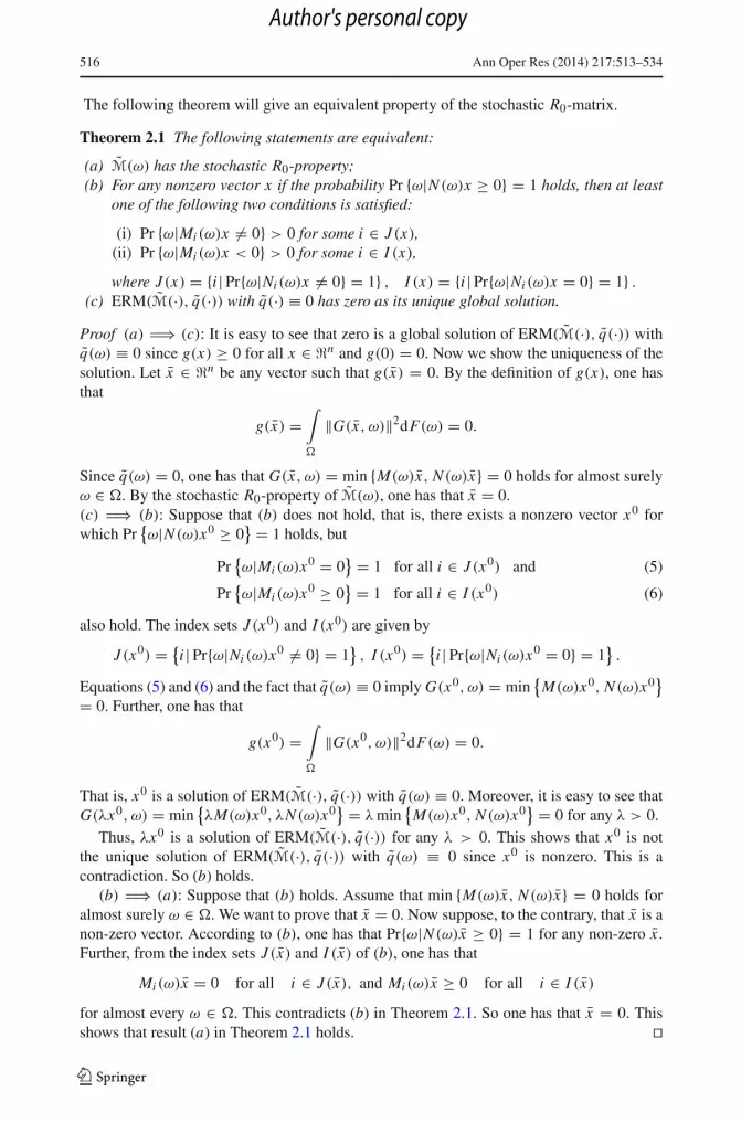
The following theorem will give an equivalent property of the stochastic R0-matrix.

Theorem 2.1 The following statements are equivalent:

(a) M(ω) has the stochastic R0-property;(b) For any nonzero vector x if the probability Pr {ω|N (ω)x ≥ 0} = 1 holds, then at least

one of the following two conditions is satisfied:

(i) Pr {ω|Mi (ω)x �= 0} > 0 for some i ∈ J (x),(ii) Pr {ω|Mi (ω)x < 0} > 0 for some i ∈ I (x),

where J (x) = {i | Pr{ω|Ni (ω)x �= 0} = 1} , I (x) = {i | Pr{ω|Ni (ω)x = 0} = 1} .

(c) ERM(M(·), q(·)) with q(·) ≡ 0 has zero as its unique global solution.

Proof (a) ⇒ (c): It is easy to see that zero is a global solution of ERM(M(·), q(·)) withq(ω) ≡ 0 since g(x) ≥ 0 for all x ∈ �n and g(0) = 0. Now we show the uniqueness of thesolution. Let x ∈ �n be any vector such that g(x) = 0. By the definition of g(x), one hasthat

g(x) =∫

�

‖G(x, ω)‖2dF(ω) = 0.

Since q(ω) = 0, one has that G(x, ω) = min {M(ω)x, N (ω)x} = 0 holds for almost surelyω ∈ �. By the stochastic R0-property of M(ω), one has that x = 0.(c) ⇒ (b): Suppose that (b) does not hold, that is, there exists a nonzero vector x0 forwhich Pr

{ω|N (ω)x0 ≥ 0

} = 1 holds, but

Pr{ω|Mi (ω)x0 = 0

} = 1 for all i ∈ J (x0) and (5)

Pr{ω|Mi (ω)x0 ≥ 0

} = 1 for all i ∈ I (x0) (6)

also hold. The index sets J (x0) and I (x0) are given by

J (x0) = {i | Pr{ω|Ni (ω)x0 �= 0} = 1

}, I (x0) = {

i | Pr{ω|Ni (ω)x0 = 0} = 1}.

Equations (5) and (6) and the fact that q(ω) ≡ 0 imply G(x0, ω) = min{

M(ω)x0, N (ω)x0}

= 0. Further, one has that

g(x0) =∫

�

‖G(x0, ω)‖2dF(ω) = 0.

That is, x0 is a solution of ERM(M(·), q(·)) with q(ω) ≡ 0. Moreover, it is easy to see thatG(λx0, ω) = min

{λM(ω)x0, λN (ω)x0

} = λ min{

M(ω)x0, N (ω)x0} = 0 for any λ > 0.

Thus, λx0 is a solution of ERM(M(·), q(·)) for any λ > 0. This shows that x0 is notthe unique solution of ERM(M(·), q(·)) with q(ω) ≡ 0 since x0 is nonzero. This is acontradiction. So (b) holds.

(b) ⇒ (a): Suppose that (b) holds. Assume that min {M(ω)x, N (ω)x} = 0 holds foralmost surely ω ∈ �. We want to prove that x = 0. Now suppose, to the contrary, that x is anon-zero vector. According to (b), one has that Pr{ω|N (ω)x ≥ 0} = 1 for any non-zero x .Further, from the index sets J (x) and I (x) of (b), one has that

Mi (ω)x = 0 for all i ∈ J (x), and Mi (ω)x ≥ 0 for all i ∈ I (x)

for almost every ω ∈ �. This contradicts (b) in Theorem 2.1. So one has that x = 0. Thisshows that result (a) in Theorem 2.1 holds. �

123


Ann Oper Res (2014) 217:513–534 517

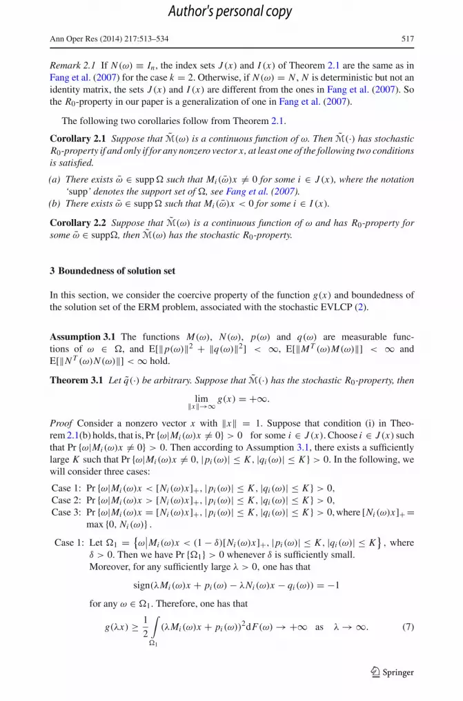
Remark 2.1 If N (ω) ≡ In , the index sets J (x) and I (x) of Theorem 2.1 are the same as inFang et al. (2007) for the case k = 2. Otherwise, if N (ω) = N , N is deterministic but not anidentity matrix, the sets J (x) and I (x) are different from the ones in Fang et al. (2007). Sothe R0-property in our paper is a generalization of one in Fang et al. (2007).

The following two corollaries follow from Theorem 2.1.

Corollary 2.1 Suppose that M(ω) is a continuous function of ω. Then M(·) has stochasticR0-property if and only if for any nonzero vector x, at least one of the following two conditionsis satisfied.

(a) There exists ω ∈ supp � such that Mi (ω)x �= 0 for some i ∈ J (x), where the notation‘supp’ denotes the support set of �, see Fang et al. (2007).

(b) There exists ω ∈ supp � such that Mi (ω)x < 0 for some i ∈ I (x).

Corollary 2.2 Suppose that M(ω) is a continuous function of ω and has R0-property forsome ω ∈ supp�, then M(ω) has the stochastic R0-property.

3 Boundedness of solution set

In this section, we consider the coercive property of the function g(x) and boundedness ofthe solution set of the ERM problem, associated with the stochastic EVLCP (2).

Assumption 3.1 The functions M(ω), N (ω), p(ω) and q(ω) are measurable func-tions of ω ∈ �, and E[‖p(ω)‖2 + ‖q(ω)‖2] < ∞, E[‖MT (ω)M(ω)‖] < ∞ andE[‖N T (ω)N (ω)‖] < ∞ hold.

Theorem 3.1 Let q(·) be arbitrary. Suppose that M(·) has the stochastic R0-property, then

lim‖x‖→∞ g(x) = +∞.

Proof Consider a nonzero vector x with ‖x‖ = 1. Suppose that condition (i) in Theo-rem 2.1(b) holds, that is, Pr {ω|Mi (ω)x �= 0} > 0 for some i ∈ J (x). Choose i ∈ J (x) suchthat Pr {ω|Mi (ω)x �= 0} > 0. Then according to Assumption 3.1, there exists a sufficientlylarge K such that Pr {ω|Mi (ω)x �= 0, |pi (ω)| ≤ K , |qi (ω)| ≤ K } > 0. In the following, wewill consider three cases:

Case 1: Pr {ω|Mi (ω)x < [Ni (ω)x]+, |pi (ω)| ≤ K , |qi (ω)| ≤ K } > 0,

Case 2: Pr {ω|Mi (ω)x > [Ni (ω)x]+, |pi (ω)| ≤ K , |qi (ω)| ≤ K } > 0,

Case 3: Pr {ω|Mi (ω)x = [Ni (ω)x]+, |pi (ω)| ≤ K , |qi (ω)| ≤ K } > 0, where [Ni (ω)x]+ =max {0, Ni (ω)} .

Case 1: Let �1 = {ω

∣∣Mi (ω)x < (1 − δ)[Ni (ω)x]+, |pi (ω)| ≤ K , |qi (ω)| ≤ K}, where

δ > 0. Then we have Pr {�1} > 0 whenever δ is sufficiently small.Moreover, for any sufficiently large λ > 0, one has that

sign(λMi (ω)x + pi (ω) − λNi (ω)x − qi (ω)) = −1

for any ω ∈ �1. Therefore, one has that

g(λx) ≥ 1

2

∫

�1

(λMi (ω)x + pi (ω))2dF(ω) → +∞ as λ → ∞. (7)

123


518 Ann Oper Res (2014) 217:513–534

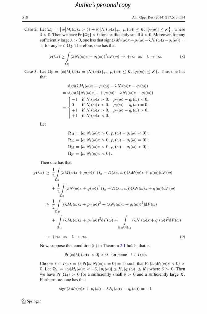
Case 2: Let �2 = {ω

∣∣Mi (ω)x > (1 + δ)[Ni (ω)x]+, |pi (ω)| ≤ K , |qi (ω)| ≤ K}, where

δ > 0. Then we have Pr {�2} > 0 for a sufficiently small δ > 0. Moreover, for anysufficiently large λ > 0, one has that sign(λMi (ω)x + pi (ω)−λNi (ω)x −qi (ω)) =1, for any ω ∈ �2. Therefore, one has that

g(λx) ≥∫

�2

(λNi (ω)x + qi (ω))2dF(ω) → +∞ as λ → ∞. (8)

Case 3: Let �3 = {ω|Mi (ω)x = [Ni (ω)x]+, |pi (ω)| ≤ K , |qi (ω)| ≤ K } . Thus one hasthat

sign(λMi (ω)x + pi (ω) − λNi (ω)x − qi (ω))

= sign(λ[Ni (ω)x]+ + pi (ω) − λNi (ω)x − qi (ω))

=

⎧⎪⎪⎨⎪⎪⎩

−1 if Ni (ω)x > 0, pi (ω) − qi (ω) < 0,

0 if Ni (ω)x > 0, pi (ω) − qi (ω) = 0,

+1 if Ni (ω)x > 0, pi (ω) − qi (ω) > 0,

+1 if Ni (ω)x < 0.

Let

�31 = {ω|Ni (ω)x > 0, pi (ω) − qi (ω) < 0} ;�32 = {ω|Ni (ω)x > 0, pi (ω) − qi (ω) = 0} ;�33 = {ω|Ni (ω)x > 0, pi (ω) − qi (ω) > 0} ;�34 = {ω|Ni (ω)x < 0} .

Then one has that

g(λx) ≥ 1

2

∫

�3

(λM(ω)x + p(ω))T (In − D(λx, ω))(λM(ω)x + p(ω))dF(ω)

+ 1

2

∫

�3

(λN (ω)x + q(ω))T (In + D(λx, ω))(λN (ω)x + q(ω))dF(ω)

≥ 1

2

∫

�32

[(λMi (ω)x + pi (ω))2 + (λNi (ω)x + qi (ω))2]dF(ω)

+∫

�31

(λMi (ω)x + pi (ω))2dF(ω) +∫

�33∪�34

(λNi (ω)x + qi (ω))2dF(ω)

→ +∞ as λ → ∞. (9)

Now, suppose that condition (ii) in Theorem 2.1 holds, that is,

Pr {ω|Mi (ω)x < 0} > 0 for some i ∈ I (x).

Choose i ∈ I (x) = {i |Pr{ω|Ni (ω)x = 0} = 1} such that Pr {ω|Mi (ω)x < 0} >

0. Let �4 = {ω|Mi (ω)x < −δ, |pi (ω)| ≤ K , |qi (ω)| ≤ K } where δ > 0. Thenwe have Pr {�4} > 0 for a sufficiently small δ > 0 and a sufficiently large K .Furthermore, one has that

sign(λMi (ω)x + pi (ω) − λNi (ω)x − qi (ω)) = −1.

123


Ann Oper Res (2014) 217:513–534 519

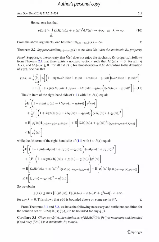
Hence, one has that

g(λx) ≥∫

�4

(λMi (ω)x + pi (ω))2dF(ω) → +∞ as λ → ∞. (10)

From the above arguments, one has that lim‖x‖→∞ g(x) = ∞. � Theorem 3.2 Suppose that lim‖x‖→∞ g(x) = ∞, then M(·) has the stochastic R0-property.

Proof Suppose, to the contrary, that M(·) does not enjoy the stochastic R0-property. It followsfrom Theorem 2.1 that there exists a nonzero vector x such that Mi (ω)x = 0 for all i ∈J (x), and Mi (ω)x ≥ 0 for all i ∈ I (x) for almost every ω ∈ �. According to the definitionof g(x), one has that

g(λx) = 1

2

n∑i=1

{E

[(1 − sign(λMi (ω)x + pi (ω) − λNi (ω)x − qi (ω))

)(λMi (ω)x + pi (ω))2

]

+ E

[(1 + sign(λMi (ω)x + pi (ω) − λNi (ω)x − qi (ω))

)(λNi (ω)x + qi (ω))2

]}. (11)

The i th item of the right-hand side of (11) with i ∈ J (x) equals

1

2E

[(1 − sign(pi (ω) − λNi (ω)x − qi (ω))

)p2

i (ω)

]

+ 1

2E

[(1 + sign(pi (ω) − λNi (ω)x − qi (ω))

)(λNi (ω)x + qi (ω))2

]

= E

[p2

i (ω)1{pi (ω)−qi (ω)≤λNi (ω)}]

+ E

[(λNi (ω)x + qi (ω))21{pi (ω)−qi (ω)>λNi (ω)}

]

≤ E

[p2

i (ω)

].

while the i th term of the right-hand side of (11) with i ∈ I (x) equals

1

2E

[(1 − sign(λMi (ω)x + pi (ω) − qi (ω))

)(λMi (ω)x + pi (ω))2

]

+ 1

2E

[(1 + sign(λMi (ω)x + pi (ω) − qi (ω))

)q2

i (ω)

]

= E

[(λMi (ω)x + pi (ω))21{λMi (ω)x+pi (ω)≤qi (ω)}

]+ E

[q2

i (ω)1{λMi (ω)x+pi (ω)≥qi (ω)}]

≤ E

[(pi (ω) − qi (ω))2 + q2

i (ω)

].

So we obtain

g(λx) ≤ max{E[p2

i (ω)], E[(pi (ω) − qi (ω))2 + q2i (ω)]} < +∞,

for any λ > 0. This shows that g(·) is bounded above on some ray in �n . � From Theorems 3.1 and 3.2, we have the following necessary and sufficient condition for

the solution set of ERM(M(·); q(·))) to be bounded for any q(·).Corollary 3.1 Given any q(·)), the solution set of ERM(M(·); q(·)) is nonempty and boundedif and only if M(·) is a stochastic R0 matrix.

123


520 Ann Oper Res (2014) 217:513–534

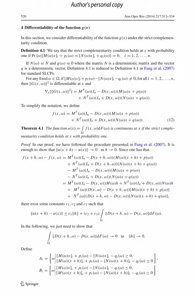
4 Differentiability of the function g(x)

In this section, we consider differentiability of the function g(x) under the strict complemen-tarity condition.

Definition 4.1 We say that the strict complementarity condition holds at x with probabilityone if Pr {ω|[M(ω)x]i + pi (ω) = [N (ω)x]i + qi (ω)} = 0, i = 1, 2, . . . , n.

If N (ω) ≡ N and q(ω) ≡ 0 where the matrix N is a deterministic matrix and the vectorq is a deterministic vector, Definition 4.1 is reduced to Definition 4.1 in Fang et al. (2007)for standard SLCPs.

For any fixed ω ∈ �, if [M(ω)x]i + pi (ω)−[N (ω)x]i −qi (ω) �= 0, for all i = 1, 2, . . . , n,then ‖G(x, ω)‖2 is differentiable at x and

∇x [‖G(x, ω)‖2] = MT (ω)(In − D(x, ω))(M(ω)x + p(ω))

+ N T (ω)(In + D(x, ω))(N (ω)x + q(ω)).

To simplify the notation, we define

f (x, ω) = MT (ω)(In − D(x, ω))(M(ω)x + p(ω))

+ N T (ω)(In + D(x, ω))(N (ω)x + q(ω)). (12)

Theorem 4.1 The function u(x) = ∫�

f (x, ω)dF(ω) is continuous at x if the strict comple-

mentarity condition holds at x with probability one.

Proof In our proof, we have followed the procedure presented in Fang et al. (2007). It isenough to show that ‖u(x + h) − u(x)‖ → 0 as h → 0. Since one has that

f (x + h, ω) − f (x, ω) = MT (ω)(In − D(x + h, ω))(M(ω)(x + h) + p(ω))

+ N T (ω)(In + D(x + h, ω))(N (ω)(x + h) + q(ω))

− MT (ω)(In − D(x, ω))(M(ω)x + p(ω))

− N T (ω)(In + D(x, ω))(N (ω)x + q(ω))

= MT (ω)(In − D(x, ω))M(ω)h + N T (ω)(In + D(x, ω))N (ω)h

+ MT (ω)(D(x, ω) − D(x + h, ω))[M(ω)(x + h) + p(ω)]+ N T (ω)(D(x + h, ω) − D(x, ω))[N (ω)(x + h) + q(ω)],

there exist some constants c1, c2 and c3 such that

‖u(x + h) − u(x)‖ ≤ c1‖h‖ + (c2 + c3)

∫

�

‖D(x + h, ω) − D(x, ω)‖dF(ω).

In the following, we just need to show that∫

�

‖D(x + h, ω) − D(x, ω)‖dF(ω) → 0 as ‖h‖ → 0.

Define

Ai ={ω

∣∣∣∣ [M(ω)x]i + pi (ω) − [N (ω)x]i − qi (ω) ≥ 0,

[M(ω)(x + h)]i + pi (ω) − [N (ω)(x + h)]i − qi (ω) ≤ 0

},

Bi ={ω

∣∣∣∣ [M(ω)x]i + pi (ω) − [N (ω)x]i − qi (ω) ≤ 0,

[M(ω)(x + h)]i + pi (ω) − [N (ω)(x + h)]i − qi (ω) ≥ 0

}.

123


Ann Oper Res (2014) 217:513–534 521

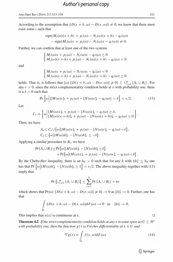
According to the assumption that ‖D(x + h, ω) − D(x, ω)‖ �= 0, we know that there mustexist some i such that

sign(Mi (ω)(x + h) + pi (ω) − Ni (ω)(x + h) − qi (ω))

− sign(Mi (ω)x + pi (ω) − Ni (ω)x − qi (ω)) �= 0.

Further, we can confirm that at least one of the two systems{Mi (ω)x + pi (ω) − Ni (ω)x − qi (ω) ≥ 0Mi (ω)(x + h) + pi (ω) − Ni (ω)(x + h) − qi (ω) < 0

and {Mi (ω)x + pi (ω) − Ni (ω)x − qi (ω) < 0Mi (ω)(x + h) + pi (ω) − Ni (ω)(x + h) − qi (ω) ≥ 0

holds. That is, it follows that {ω| ‖D(x + h, ω) − D(x, ω)‖ �= 0} ⊂ ∪ni=1 {Ai ∪ Bi } . For

any ε > 0, since the strict complementarity condition holds at x with probability one, thereis a δ > 0 such that

Pr{ω

∣∣∣|[M(ω)x]i + pi (ω) − [N (ω)x]i − qi (ω)| < δ}

< ε/2. (13)

Let

Ci ={ω

∣∣∣∣ [M(ω)x]i + pi (ω) − [N (ω)x]i − qi (ω) ≥ δ,

[M(ω)(x + h)]i + pi (ω) − [N (ω)(x + h)]i − qi (ω) ≤ 0

}.

Then, we have

Ai ⊂ Ci ∪{ω

∣∣[M(ω)x]i + pi (ω) − [N (ω)x]i − qi (ω)<δ},

Ci ⊂ {ω

∣∣[M(ω)h]i − [N (ω)h]i ≤ −δ}.

Applying a similar procedure to Bi , we have

Pr{Ai ∪Bi }≤ Pr{ω

∣∣[M(ω)h]i − [N (ω)h]i ≥δ}

+ Pr{ω

∣∣[M(ω)x]i + pi (ω) − [N (ω)x]i − qi (ω)<δ}.

By the Chebychev inequality, there is an h0 > 0 such that for any h with ‖h‖ ≤ h0 one

has that Pr{ω

∣∣∣[M(ω)h]i − [N (ω)h]i ≥ δ}

< ε/2. The above inequality together with (13)

imply that

Pr{∪n

i=1 {Ai ∪ Bi }} ≤

n∑i=1

Pr {Ai ∪ Bi } < nε

which shows that Pr{ω| ‖D(x + h, ω) − D(x, ω)‖ �= 0} → 0 as ‖h‖ → 0. Further, one hasthat ∫

�

‖D(x + h, ω) − D(x, ω)‖dF(ω) → 0 as ‖h‖ → 0.

This implies that u(x) is continuous at x . � Theorem 4.2 If the strict complementarity condition holds at any x in some open set U ⊂ �n

with probability one, then the function g(·) is Frechet differentiable at x ∈ U and

∇g(x) =∫

�

f (x, ω)dF(ω) (14)

123


522 Ann Oper Res (2014) 217:513–534

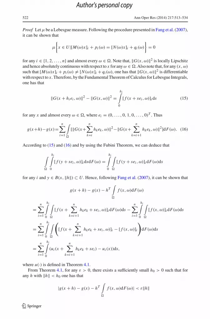
Proof Let μ be a Lebesgue measure. Following the procedure presented in Fang et al. (2007),it can be shown that

μ

{x ∈ U |[M(ω)x]i + pi (ω) = [N (ω)x]i + qi (ω)

}= 0

for any i ∈ {1, 2, . . . , n} and almost every ω ∈ �. Note that, ‖G(x, ω)‖2 is locally Lipschitzand hence absolutely continuous with respect to x for any ω ∈ �. Also note that, for any (x, ω)

such that [M(ω)x]i + pi (ω) �= [N (ω)x]i + qi (ω), one has that ‖G(x, ω)‖2 is differentiablewith respect to x . Therefore, by the Fundamental Theorem of Calculus for Lebesgue Integrals,one has that

‖G(x + hi ei , ω)‖2 − ‖G(x, ω)‖2 =hi∫

0

[ f (x + sei , ω)]i ds (15)

for any x and almost every ω ∈ �, where ei = (0, . . . , 0, 1, 0, . . . , 0)T . Thus

g(x+h)−g(x)=n∑

i=1

∫

�

[‖G(x+n∑

k=i

hkek, ω)‖2−‖G(x+n∑

k=i+1

hkek, ω)‖2]dF(ω). (16)

According to (15) and (16) and by using the Fubini Theorem, we can deduce that

∫

�

hi∫

0

[ f (y + sei , ω)]i dsdF(ω) =hi∫

0

∫

�

[ f (y + sei , ω)]i dF(ω)ds

for any i and y ∈ B(x, ‖h‖) ⊂ U . Hence, following Fang et al. (2007), it can be shown that

g(x + h) − g(x) − hT∫

�

f (x, ω)dF(ω)

=n∑

i=1

hi∫

0

∫

�

[ f (x +n∑

k=i+1

hkek + sei , ω)]i dF(ω)ds −n∑

i=1

hi∫

0

∫

�

[ f (x, ω)]i dF(ω)ds

=n∑

i=1

hi∫

0

∫

�

([ f (x +

n∑k=i+1

hkek + sei , ω)]i − [ f (x, ω)]i

)dF(ω)ds

=n∑

i=1

hi∫

0

(ui (x +n∑

k=i+1

hkek + sei ) − ui (x))ds,

where u(·) is defined in Theorem 4.1.From Theorem 4.1, for any ε > 0, there exists a sufficiently small h0 > 0 such that for

any h with ‖h‖ < h0 one has that

|g(x + h) − g(x) − hT∫

�

f (x, ω)dF(ω)| < ε‖h‖

123


Ann Oper Res (2014) 217:513–534 523

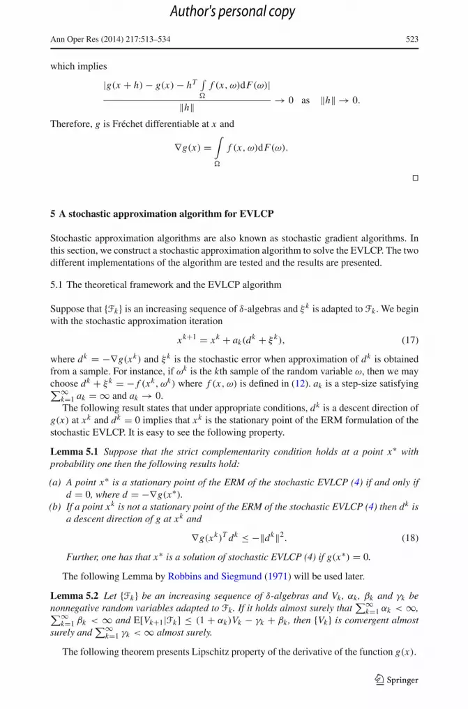
which implies

|g(x + h) − g(x) − hT∫�

f (x, ω)dF(ω)|‖h‖ → 0 as ‖h‖ → 0.

Therefore, g is Fréchet differentiable at x and

∇g(x) =∫

�

f (x, ω)dF(ω).

�

5 A stochastic approximation algorithm for EVLCP

Stochastic approximation algorithms are also known as stochastic gradient algorithms. Inthis section, we construct a stochastic approximation algorithm to solve the EVLCP. The twodifferent implementations of the algorithm are tested and the results are presented.

5.1 The theoretical framework and the EVLCP algorithm

Suppose that {Fk} is an increasing sequence of δ-algebras and ξ k is adapted to Fk . We beginwith the stochastic approximation iteration

xk+1 = xk + ak(dk + ξ k), (17)

where dk = −∇g(xk) and ξ k is the stochastic error when approximation of dk is obtainedfrom a sample. For instance, if ωk is the kth sample of the random variable ω, then we maychoose dk + ξ k = − f (xk, ωk) where f (x, ω) is defined in (12). ak is a step-size satisfying∑∞

k=1 ak = ∞ and ak → 0.The following result states that under appropriate conditions, dk is a descent direction of

g(x) at xk and dk = 0 implies that xk is the stationary point of the ERM formulation of thestochastic EVLCP. It is easy to see the following property.

Lemma 5.1 Suppose that the strict complementarity condition holds at a point x∗ withprobability one then the following results hold:

(a) A point x∗ is a stationary point of the ERM of the stochastic EVLCP (4) if and only ifd = 0, where d = −∇g(x∗).

(b) If a point xk is not a stationary point of the ERM of the stochastic EVLCP (4) then dk isa descent direction of g at xk and

∇g(xk)T dk ≤ −‖dk‖2. (18)

Further, one has that x∗ is a solution of stochastic EVLCP (4) if g(x∗) = 0.

The following Lemma by Robbins and Siegmund (1971) will be used later.

Lemma 5.2 Let {Fk} be an increasing sequence of δ-algebras and Vk, αk , βk and γk benonnegative random variables adapted to Fk . If it holds almost surely that

∑∞k=1 αk < ∞,∑∞

k=1 βk < ∞ and E[Vk+1|Fk] ≤ (1 + αk)Vk − γk + βk , then {Vk} is convergent almostsurely and

∑∞k=1 γk < ∞ almost surely.

The following theorem presents Lipschitz property of the derivative of the function g(x).

123


524 Ann Oper Res (2014) 217:513–534

Theorem 5.1 Assume that the strict complementarity condition holds at any x in some openset U ⊂ �n with probability one, and the sequence

{xk

}∞k=0 ⊂ U are generated by the

iterative scheme (17), then one has that

‖∇g(y) − ∇g(xk)‖ ≤ L‖y − xk‖holds for all y enough close to xk , where L = 2E[‖M(ω)‖2 + ‖N (ω)‖2] < ∞.

Proof According to the definition of f (x, ω) and proof of Theorem 4.1, we know that

‖ f (y, ω) − f (xk, ω)‖‖h‖

= ∥∥MT (ω)(In − D(xk, ω))M(ω)h + N T (ω)(In + D(xk, ω))N (ω)h

+ MT (ω)(D(xk, ω) − D(xk + h, ω))[M(ω)(xk + h) + p(ω)]+ N T (ω)(D(xk, ω) − D(xk + h, ω))[N (ω)(xk + h) + q(ω)]∥∥/‖h‖,

where y = xk + h. Since we know that the strict complementarity condition holds at any xin some open set U ⊂ �n with probability one, one has that

D(xk, ω) − D(y, ω) = 0,

for all y close enough to xk and for a. e. ω. It follows that there exists a constant y > 0 suchthat

‖ f (y, ω) − f (xk, ω)‖‖y − xk‖

= ∥∥MT (ω)(In − D(xk, ω))M(ω)(y − xk)

+N T (ω)(In + D(xk, ω))N (ω)(y − xk)}‖/‖y − xk‖≤ 2[‖M(ω)‖2 + ‖N (ω)‖2]

for all y ∈ B(xk, ¯‖y‖) and every ω ∈ �. Thus one has that

‖ f (y, ω) − f (xk, ω)‖ ≤ 2[‖M(ω)‖2 + ‖N (ω)‖2]‖y − xk‖.Further, one has that

‖∇g(y) − ∇g(xk)‖ = ‖∫

ω∈�

[ f (y, ω) − f (xk, ω))]Pr(dω)‖

≤∫

ω∈�

‖ f (y, ω) − f (xk, ω)‖Pr(dω)

≤ 2E[‖M(ω)‖2 + ‖N (ω)‖2]‖y − xk‖ = L‖y − xk‖where L = 2E[‖M(ω)‖2 + ‖N (ω)‖2]. �

Suppose that the set U is some open set containing the solution set of problem (4). LetF denote an increasing sequence of σ -algebras such that xk is Fk measurable. We have thefollowing convergent theorem.

Theorem 5.2 Assume that M(·) has stochastic R0-property. Assume that it holds almostsurely that both

∑∞k=1 ak = ∞ and

∑∞k=1 a2

k < ∞. Assume also that it holds almost surelythat

∑∞k=0 E[‖ξ k‖2|Fk] < ∞. If the strict complementarity condition holds at any x in some

open set U ⊂ �n with probability one, then the sequence{

xk}

generated by the iterativescheme (17) is convergent to the solution set of problem (4).

123


Ann Oper Res (2014) 217:513–534 525

Proof By using Lemma 5.1 and assumptions in our paper, we have, for some yk ∈ (xk, xk+1),

E[g(xk+1)|Fk] = E[g(xk) + ∇g(yk)T (xk+1 − xk)|Fk]= E

[g(xk) + ∇g(xk)T (xk+1 − xk)

+[(

∇g(yk) − ∇g(xk))T

(xk+1 − xk)|Fk

]]

≤ g(xk) + ak∇g(xk)T dk + LE[‖xk+1 − xk‖2|Fk]= g(xk) − ak‖∇g(xk)‖2 + La2

k E[‖dk + ξ k‖2|Fk]≤ g(xk) − ak‖∇g(xk)‖2 + La2

k E[‖dk‖2 + ‖ξ k‖2|Fk]= g(xk) − ak(1 − ak L)‖∇g(xk)‖2 + La2

k E[‖ξ k‖2|Fk].According to the assumptions and Lemma 5.2, we see that the sequence

{g(xk)

}∞k=1 is

convergent almost surely and it holds that∑∞

k=0 ak(1−ak L)‖∇g(xk)‖2 < ∞ almost surely.In the following, we will show that ‖∇g(xk)‖ is convergent to 0 for every sample path

corresponding to convergence of g(xk). Let the sample path be fixed.First, we prove that the sequence

{xk

}is bounded. Assume for the sake of contradiction

that limk→∞ ‖xk‖ = ∞ for the sample path at which g(xk) is convergent. Since M(·) hasstochastic R0-property, according to Theorem 3.1, we obtain that limk→∞ g(xk) = ∞, whichcontradicts the convergence of the sequence

{g(xk)

}∞k=0. So the sequence

{xk

}is bounded.

Since∑∞

k=0 ak(1 − ak L)‖∇g(xk)‖2 < ∞ holds almost surely, we have

∞∑k=0

ak‖∇g(xk)‖2 < ∞

almost surely. We now prove that limk→∞ ‖∇g(xk)‖ = 0 for the bounded sequence{

xk}.

Assume, to the contrary, that there exists a subsequence{

xkp}∞

1 converging to x such that

limkp→∞ ‖∇g(xkp )‖ = ‖∇g(x)‖ > 0.

It follows that for some ε > 0 there exists K > 0 such that ‖∇g(xkp ) − ∇g(x)‖ < ε for allkp > K . Further, one has that

‖∇g(xkp )‖ > ‖∇g(x)‖ − ε

for all kp > K .Define C = min

{‖∇g(xkp )‖ | kp = 1, 2, . . . , K}

and C = min {C, ‖∇g(x)‖ − ε}, onehas that

∞ = C2 ·∞∑

k=0

ak <

∞∑k=0

ak‖∇g(xkp )‖2 < ∞

This is a contradiction. This shows it must hold that limk→∞ ‖∇g(xk)‖ = 0. Since thesequence {xk}∞1 is bounded, there must exist a convergent subsequence. Without loss of gen-erality, we denote this subsequence by {xk}∞1 . This shows that the sequence {xk} is convergentto the solution set of the ERM of the stochastic EVLCP. The convergence follows from thefact that the above arguments hold for every sample path corresponding to convergence ofg(xk). �

123


526 Ann Oper Res (2014) 217:513–534

We now present an algorithm for solving the stochastic EVLCP via ERM formulationbased on the step-size parameter ak satisfying

∑∞k=1 ak = +∞ and

∑∞n=1 a2

n < +∞.

Algorithm: An approximation algorithm for the stochastic EVLCPStep 0: Given sampling size N and an arbitrary small ε > 0. Initialize the starting point

x0. Set initial value: β ∈ ( 12 , 1], a1, a, b. Let k = 1, 2, . . . .

Step 1: Randomly sampling ωk from �.Step 2: Computing the kth iteration:

xk = xk−1 + ak−1[− f (xk−1, ωk)] (19)

where ak = a1(bk +a

bk +a+kβ

), see Powell (2007).

Step 3: Stop if ‖ 1k

∑kj=1 f (xk, ω j )‖ < ε or k > N , otherwise set k = k + 1 and go to

Step 2.

Remark 5.1 A different implementation of the above algorithm can be carried by replacingthe equation (19) with

xk = xk−1 + ak−1

(−1

k

k−1∑i=1

f (xk−1, ωi )

). (20)

We denote the two implementations as implementations I and II respectively.

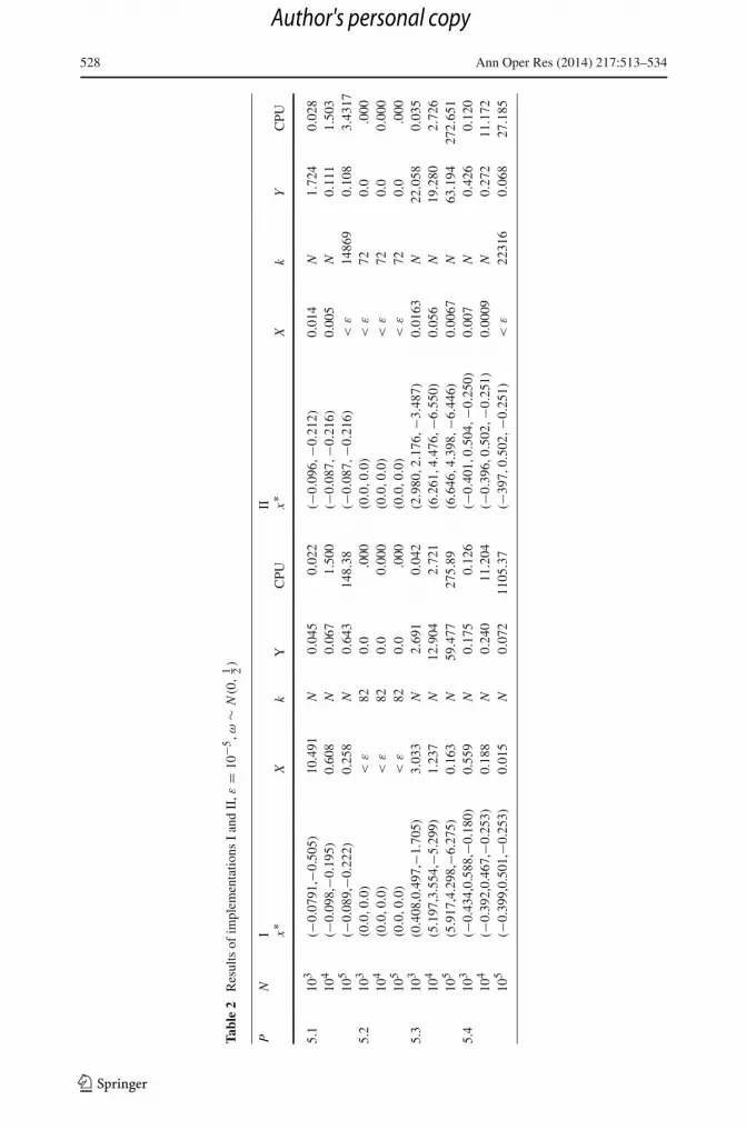
5.2 Numerical results

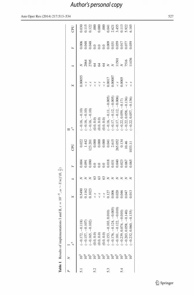
In this subsection, we present the numerical results of the EVLCP algorithm. Program waswritten in Pascal. The algorithm is coded in Pascal language and implemented on a PC with3–20 GHz processor Intel i5 E650 and 4G of RAM. The random number generator wasinitialized with seed 1000. We have constructed four test examples for the implementation ofthe algorithm. The examples are given in Appendix. The examples are constructed with ω ∈�. Hence, g(x) cannot be given explicitly. We have however presented g(x) for example 5.1assuming ω ∼ Uni f (�). Results of the implementation I and II are presented using (19) and(20) respectively. We have initialized the parameters as β = 0.6, a1 = 0.1 and a = b = 10.We have conducted a series of runs with various values of β, a and b and found that they aresuitable values to choose. Both implementations also work for other choice of β, a and b. Forexample, β = 0.5, a = b = 5 also produce suitable results. First, we present results obtainedby the implementations I & II using ω ∼ Uni f (0, 1

2 ), i.e. using uniform distribution. Resultsof the EVLCP algorithm are summarized in Table 1, where P is the problem number, x∗is the optimal solution, k is the number of iterations and ‖ ∑k

j=1 f (xk, ω j )/k‖ (=X ) is theapproximate gradient of the objective function. The objective function value is approximatedwith

∑kj=1 ‖G(xk, ω j )‖2/k (=Y ). CPU times are in seconds. We present the results for three

values of N . The results using ω ∼ N (0, 12 ) for both the implementations are summarized in

Table 2. In both tables when k=N the algorithm stopped after reaching the maximum numberof iterations, N . For other cases the algorithm stopped based on the gradient values, i.e.before iteration k reaching N . The summarized results show that the implementation II of theEVLCP algorithm produces much better results than the implementation I. This paradigmalso holds true for other choice of values for β, a and b.

123


Ann Oper Res (2014) 217:513–534 527

Tabl

e1

Res

ults

ofim

plem

enta

tions

Ian

dII

,ε=

10−5

,ω∼

Uni

f(0,

1 2)

PN

III

x∗X

kY

CPU

x∗X

kY

CPU

5.1

103

(−0.

172,

−0.1

18)

0.54

90N

0.00

40.

022

(−0.

16,−0

.10)

0.00

055

N0.

006

0.03

010

4(−

0.15

7,−0

.107

)0.

1162

N0.

091

1.44

2(−

0.16

,−0

.10)

<ε

2064

0.04

80.

115

105

(−0.

165,

−0.1

02)

0.10

23N

0.09

012

3.20

1(−

0.16

,−0

.10)

<ε

2705

0.04

80.

122

5.2

103

(0.0

,0.

0)<

ε63

0.0

0.00

0(0

.0,0.

0)<

ε64

0.0

.000

104

(0.0

,0.

0)<

ε63

0.0

0.00

0(0

.0,0.

0)<

ε64

0.0

0.00

010

5(0

.0,0.

0)<

ε63

0.0

0.00

0(0

.0,0.

0)<

ε64

0.0

.000

5.3

103

(−0.

153,

−0.1

03,0.

010)

0.12

7N

0.01

80.

041

(−0.

16,−0

.11,

−0.0

05)

0.00

17N

0.00

90.

041

104

(−0.

176,

−0.1

24,−0

.005

)0.

006

N0.

031

2.61

5(−

0.17

,−0

.12,

−0.0

05)

0.00

007

N0.

031

2.62

110

5(−

0.18

1,−0

.122

,−0

.010

)0.

020

N0.

040

265.

052

(−0.

17,−0

.12,

−0.0

06)

<ε

1150

10.

059

3.45

55.

410

3(−

0.23

9,0.

074,

−0.0

10)

0.04

6N

0.02

30.

134

(−0.

22,0.

059,

−0.1

7)0.

0005

N0.

017

0.11

310

4(−

0.20

3,0.

058,

−0.1

40)

0.04

7N

0.06

710

.46

(−0.

22,0.

058,

−0.1

36)

<ε

7516

0.07

75.

922

105

(−0.

232,

0.06

0,−0

.135

)0.

013

N0.

065

1033

.11

(−0.

22,0.

057,

−0.1

36)

<ε

1143

60.

059

6.18

5

123


528 Ann Oper Res (2014) 217:513–534

Tabl

e2

Res

ults

ofim

plem

enta

tions

Ian

dII

,ε=

10−5

,ω∼

N(0

,1 2)

PN

III

x∗X

kY

CPU

x∗X

kY

CPU

5.1

103

(−0.

0791

,−0.

505)

10.4

91N

0.04

50.

022

(−0.

096,

−0.2

12)

0.01

4N

1.72

40.

028

104

(−0.

098,

−0.1

95)

0.60

8N

0.06

71.

500

(−0.

087,

−0.2

16)

0.00

5N

0.11

11.

503

105

(−0.

089,

−0.2

22)

0.25

8N

0.64

314

8.38

(−0.

087,

−0.2

16)

<ε

1486

90.

108

3.43

175.

210

3(0

.0,0.

0)<

ε82

0.0

.000

(0.0

,0.

0)<

ε72

0.0

.000

104

(0.0

,0.

0)<

ε82

0.0

0.00

0(0

.0,0.

0)<

ε72

0.0

0.00

010

5(0

.0,0.

0)<

ε82

0.0

.000

(0.0

,0.

0)<

ε72

0.0

.000

5.3

103

(0.4

08,0

.497

,−1.

705)

3.03

3N

2.69

10.

042

(2.9

80,2.

176,

−3.4

87)

0.01

63N

22.0

580.

035

104

(5.1

97,3

.554

,−5.

299)

1.23

7N

12.9

042.

721

(6.2

61,4.

476,

−6.5

50)

0.05

6N

19.2

802.

726

105

(5.9

17,4

.298

,−6.

275)

0.16

3N

59.4

7727

5.89

(6.6

46,4.

398,

−6.4

46)

0.00

67N

63.1

9427

2.65

15.

410

3(−

0.43

4,0.

588,

−0.1

80)

0.55

9N

0.17

50.

126

(−0.

401,

0.50

4,−0

.250

)0.

007

N0.

426

0.12

010

4(−

0.39

2,0.

467,

−0.2

53)

0.18

8N

0.24

011

.204

(−0.

396,

0.50

2,−0

.251

)0.

0009

N0.

272

11.1

7210

5(−

0.39

9,0.

501,

−0.2

53)

0.01

5N

0.07

211

05.3

7(−

397,

0.50

2,−0

.251

)<

ε22

316

0.06

827

.185

123


Ann Oper Res (2014) 217:513–534 529

Conclusion

In this paper, we have discussed the existence of the solution of the stochastic EVLCP. Areformulation of the stochastic EVLCP as an unconstrained minimization problem is alsopresented. Finally, we have also constructed a descent stochastic approximation method forsolving this stochastic extended vertical linear complementarity problem. Results obtainedshow that the algorithm achieves considerable success in solving the test problems, andtherefore has a role to play in stochastic complementarity optimization.

Acknowledgments This work is partially supported by the NSFC (No. 71171027 and No. 71031002), NCET-12-0081 and LNET (No. LJQ2012004), and the Fundamental Research Funds for the Central Universities (No.DUT12ZD208).

Appendix

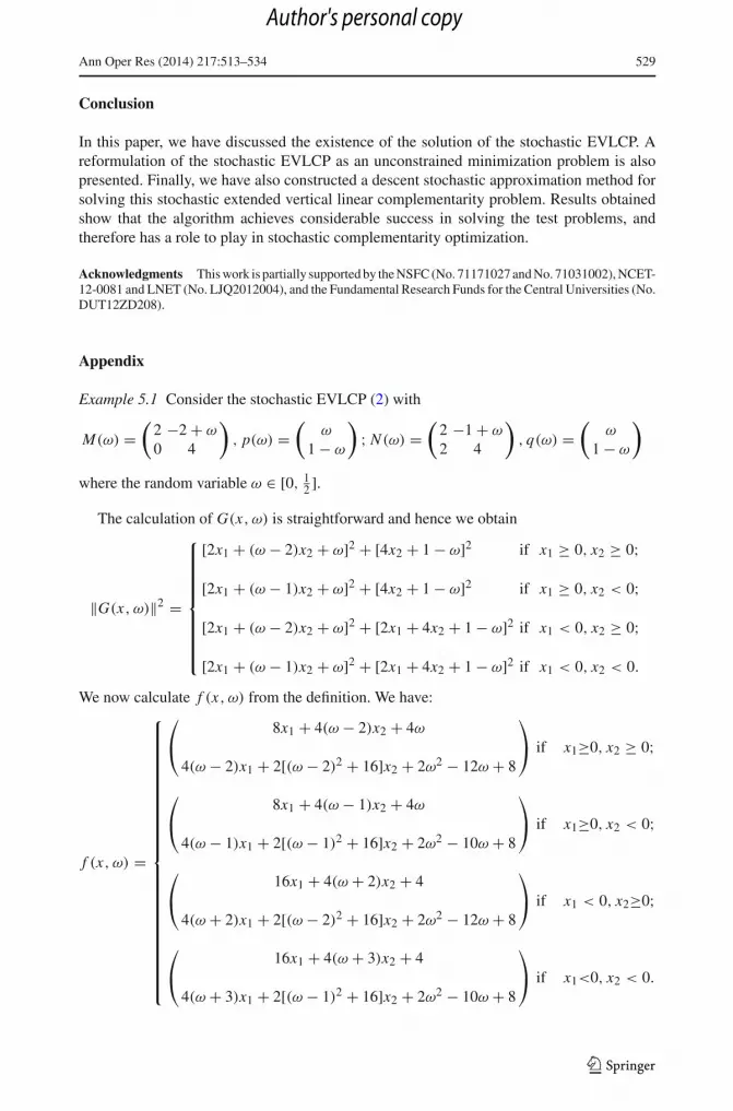
Example 5.1 Consider the stochastic EVLCP (2) with

M(ω) =(

2 −2 + ω

0 4

), p(ω) =

(ω

1 − ω

); N (ω) =

(2 −1 + ω

2 4

), q(ω) =

(ω

1 − ω

)

where the random variable ω ∈ [0, 12 ].

The calculation of G(x, ω) is straightforward and hence we obtain

‖G(x, ω)‖2 =

⎧⎪⎪⎪⎪⎪⎪⎪⎪⎨⎪⎪⎪⎪⎪⎪⎪⎪⎩

[2x1 + (ω − 2)x2 + ω]2 + [4x2 + 1 − ω]2 if x1 ≥ 0, x2 ≥ 0;

[2x1 + (ω − 1)x2 + ω]2 + [4x2 + 1 − ω]2 if x1 ≥ 0, x2 < 0;

[2x1 + (ω − 2)x2 + ω]2 + [2x1 + 4x2 + 1 − ω]2 if x1 < 0, x2 ≥ 0;

[2x1 + (ω − 1)x2 + ω]2 + [2x1 + 4x2 + 1 − ω]2 if x1 < 0, x2 < 0.

We now calculate f (x, ω) from the definition. We have:

f (x, ω) =

⎧⎪⎪⎪⎪⎪⎪⎪⎪⎪⎪⎪⎪⎪⎪⎪⎪⎪⎪⎪⎪⎪⎪⎪⎪⎨⎪⎪⎪⎪⎪⎪⎪⎪⎪⎪⎪⎪⎪⎪⎪⎪⎪⎪⎪⎪⎪⎪⎪⎪⎩

⎛⎝ 8x1 + 4(ω − 2)x2 + 4ω

4(ω − 2)x1 + 2[(ω − 2)2 + 16]x2 + 2ω2 − 12ω + 8

⎞⎠ if x1≥0, x2 ≥ 0;

⎛⎝ 8x1 + 4(ω − 1)x2 + 4ω

4(ω − 1)x1 + 2[(ω − 1)2 + 16]x2 + 2ω2 − 10ω + 8

⎞⎠ if x1≥0, x2 < 0;

⎛⎝ 16x1 + 4(ω + 2)x2 + 4

4(ω + 2)x1 + 2[(ω − 2)2 + 16]x2 + 2ω2 − 12ω + 8

⎞⎠ if x1 < 0, x2≥0;

⎛⎝ 16x1 + 4(ω + 3)x2 + 4

4(ω + 3)x1 + 2[(ω − 1)2 + 16]x2 + 2ω2 − 10ω + 8

⎞⎠ if x1<0, x2 < 0.

123


530 Ann Oper Res (2014) 217:513–534

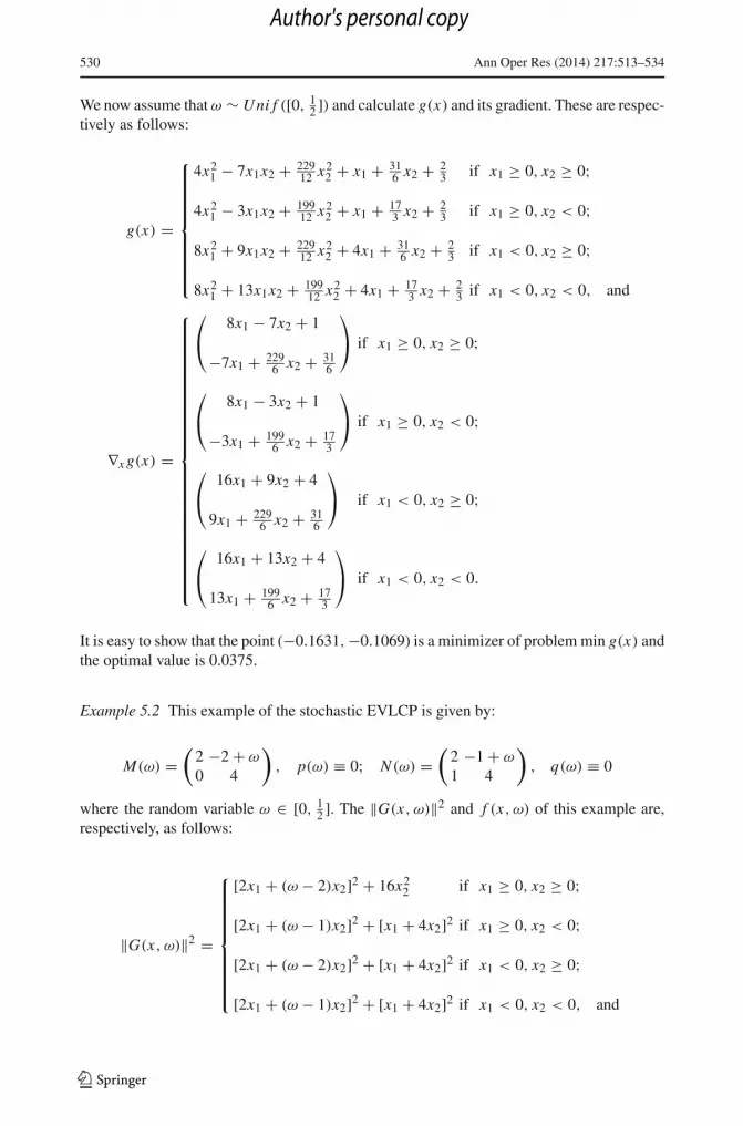
We now assume that ω ∼ Uni f ([0, 12 ]) and calculate g(x) and its gradient. These are respec-

tively as follows:

g(x) =

⎧⎪⎪⎪⎪⎪⎪⎪⎪⎨⎪⎪⎪⎪⎪⎪⎪⎪⎩

4x21 − 7x1x2 + 229

12 x22 + x1 + 31

6 x2 + 23 if x1 ≥ 0, x2 ≥ 0;

4x21 − 3x1x2 + 199

12 x22 + x1 + 17

3 x2 + 23 if x1 ≥ 0, x2 < 0;

8x21 + 9x1x2 + 229

12 x22 + 4x1 + 31

6 x2 + 23 if x1 < 0, x2 ≥ 0;

8x21 + 13x1x2 + 199

12 x22 + 4x1 + 17

3 x2 + 23 if x1 < 0, x2 < 0, and

∇x g(x) =

⎧⎪⎪⎪⎪⎪⎪⎪⎪⎪⎪⎪⎪⎪⎪⎪⎪⎪⎪⎪⎪⎪⎪⎪⎪⎨⎪⎪⎪⎪⎪⎪⎪⎪⎪⎪⎪⎪⎪⎪⎪⎪⎪⎪⎪⎪⎪⎪⎪⎪⎩

⎛⎝ 8x1 − 7x2 + 1

−7x1 + 2296 x2 + 31

6

⎞⎠ if x1 ≥ 0, x2 ≥ 0;

⎛⎝ 8x1 − 3x2 + 1

−3x1 + 1996 x2 + 17

3

⎞⎠ if x1 ≥ 0, x2 < 0;

⎛⎝ 16x1 + 9x2 + 4

9x1 + 2296 x2 + 31

6

⎞⎠ if x1 < 0, x2 ≥ 0;

⎛⎝ 16x1 + 13x2 + 4

13x1 + 1996 x2 + 17

3

⎞⎠ if x1 < 0, x2 < 0.

It is easy to show that the point (−0.1631,−0.1069) is a minimizer of problem min g(x) andthe optimal value is 0.0375.

Example 5.2 This example of the stochastic EVLCP is given by:

M(ω) =(

2 −2 + ω

0 4

), p(ω) ≡ 0; N (ω) =

(2 −1 + ω

1 4

), q(ω) ≡ 0

where the random variable ω ∈ [0, 12 ]. The ‖G(x, ω)‖2 and f (x, ω) of this example are,

respectively, as follows:

‖G(x, ω)‖2 =

⎧⎪⎪⎪⎪⎪⎪⎪⎪⎨⎪⎪⎪⎪⎪⎪⎪⎪⎩

[2x1 + (ω − 2)x2]2 + 16x22 if x1 ≥ 0, x2 ≥ 0;

[2x1 + (ω − 1)x2]2 + [x1 + 4x2]2 if x1 ≥ 0, x2 < 0;

[2x1 + (ω − 2)x2]2 + [x1 + 4x2]2 if x1 < 0, x2 ≥ 0;

[2x1 + (ω − 1)x2]2 + [x1 + 4x2]2 if x1 < 0, x2 < 0, and

123


Ann Oper Res (2014) 217:513–534 531

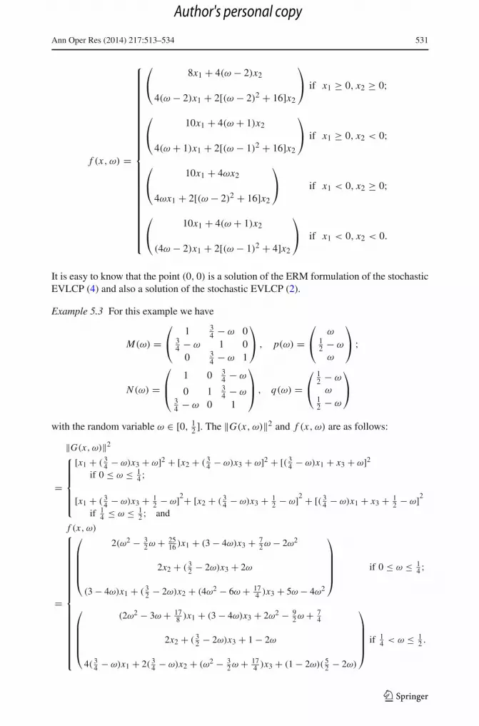
f (x, ω) =

⎧⎪⎪⎪⎪⎪⎪⎪⎪⎪⎪⎪⎪⎪⎪⎪⎪⎪⎪⎪⎪⎪⎪⎪⎪⎨⎪⎪⎪⎪⎪⎪⎪⎪⎪⎪⎪⎪⎪⎪⎪⎪⎪⎪⎪⎪⎪⎪⎪⎪⎩

⎛⎝ 8x1 + 4(ω − 2)x2

4(ω − 2)x1 + 2[(ω − 2)2 + 16]x2

⎞⎠ if x1 ≥ 0, x2 ≥ 0;

⎛⎝ 10x1 + 4(ω + 1)x2

4(ω + 1)x1 + 2[(ω − 1)2 + 16]x2

⎞⎠ if x1 ≥ 0, x2 < 0;

⎛⎝ 10x1 + 4ωx2

4ωx1 + 2[(ω − 2)2 + 16]x2

⎞⎠ if x1 < 0, x2 ≥ 0;

⎛⎝ 10x1 + 4(ω + 1)x2

(4ω − 2)x1 + 2[(ω − 1)2 + 4]x2

⎞⎠ if x1 < 0, x2 < 0.

It is easy to know that the point (0, 0) is a solution of the ERM formulation of the stochasticEVLCP (4) and also a solution of the stochastic EVLCP (2).

Example 5.3 For this example we have

M(ω) =⎛⎝ 1 3

4 − ω 034 − ω 1 0

0 34 − ω 1

⎞⎠ , p(ω) =

⎛⎝ ω

12 − ω

ω

⎞⎠ ;

N (ω) =⎛⎜⎝

1 0 34 − ω

0 1 34 − ω

34 − ω 0 1

⎞⎟⎠ , q(ω) =

⎛⎝

12 − ω

ω12 − ω

⎞⎠

with the random variable ω ∈ [0, 12 ]. The ‖G(x, ω)‖2 and f (x, ω) are as follows:

‖G(x, ω)‖2

=

⎧⎪⎪⎪⎪⎨⎪⎪⎪⎪⎩

[x1 + ( 34 − ω)x3 + ω]2 + [x2 + ( 3

4 − ω)x3 + ω]2 + [( 34 − ω)x1 + x3 + ω]2

if 0 ≤ ω ≤ 14 ;

[x1 + ( 34 − ω)x3 + 1

2 − ω]2+ [x2 + ( 34 − ω)x3 + 1

2 − ω]2 + [( 34 − ω)x1 + x3 + 1

2 − ω]2

if 14 ≤ ω ≤ 1

2 ; and

f (x, ω)

=

⎧⎪⎪⎪⎪⎪⎪⎪⎪⎪⎪⎪⎪⎪⎪⎪⎪⎪⎨⎪⎪⎪⎪⎪⎪⎪⎪⎪⎪⎪⎪⎪⎪⎪⎪⎪⎩

⎛⎜⎜⎜⎜⎝

2(ω2 − 32 ω + 25

16 )x1 + (3 − 4ω)x3 + 72 ω − 2ω2

2x2 + ( 32 − 2ω)x3 + 2ω

(3 − 4ω)x1 + ( 32 − 2ω)x2 + (4ω2 − 6ω + 17

4 )x3 + 5ω − 4ω2

⎞⎟⎟⎟⎟⎠ if 0 ≤ ω ≤ 1

4 ;

⎛⎜⎜⎜⎜⎝

(2ω2 − 3ω + 178 )x1 + (3 − 4ω)x3 + 2ω2 − 9

2 ω + 74

2x2 + ( 32 − 2ω)x3 + 1 − 2ω

4( 34 − ω)x1 + 2( 3

4 − ω)x2 + (ω2 − 32 ω + 17

4 )x3 + (1 − 2ω)( 52 − 2ω)

⎞⎟⎟⎟⎟⎠ if 1

4 < ω ≤ 12 .

123


532 Ann Oper Res (2014) 217:513–534

Example 5.4 This problem consists of

M(ω) =⎛⎝ 1 3

4 − ω ω34 − ω 1 ω

ω 34 − ω 1

⎞⎠ , p(ω) =

⎛⎝ ω

12 − ω

ω

⎞⎠ ;

N (ω) =⎛⎜⎝

1 ω 34 − ω

ω 1 34 − ω

34 − ω ω 1

⎞⎟⎠ , q(ω) =

⎛⎝

12 − ω

ω12 − ω

⎞⎠

with the random variable ω ∈ [0, 12 ]. Both ‖G(x, ω)‖2 and f (x, ω)( f1, f2, f3) for this

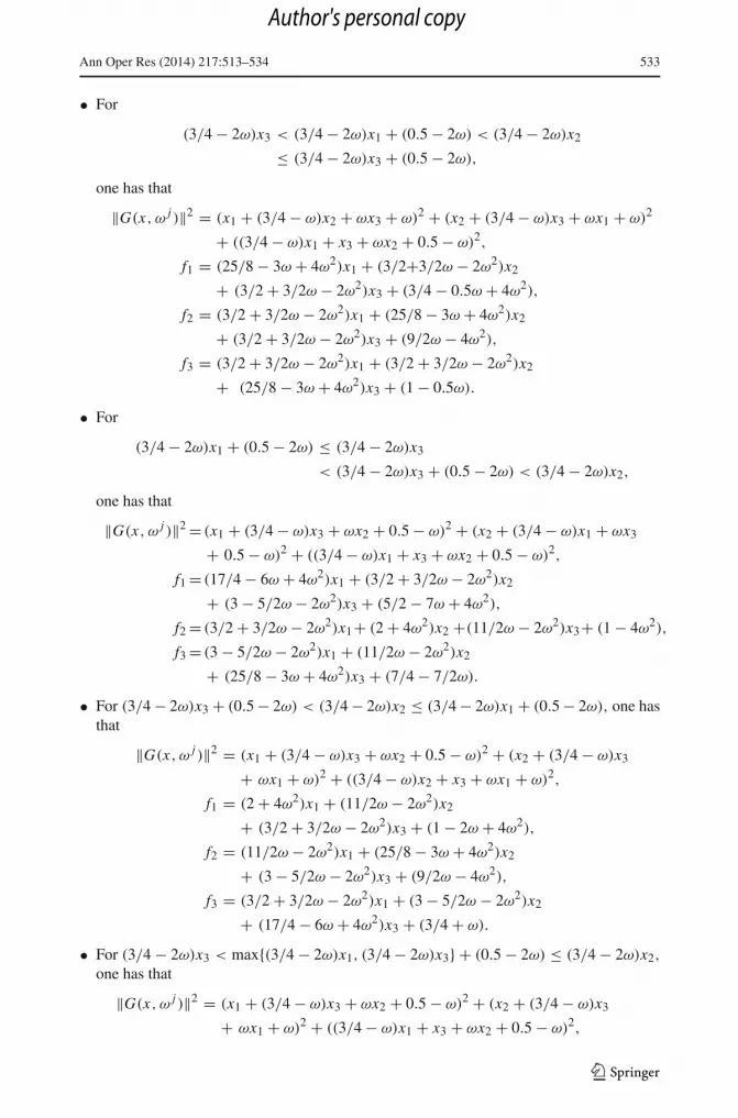
problem consist of lengthy expressions and there are seven different cases. These are asfollows.

• For (3/4 − 2ω)x2 ≤ (3/4 − 2ω)x1 + 0.5 − 2ω ≤ (3/4 − 2ω)x3, one has that

‖G(x, ω j )‖2 = (x1 + (3/4 − ω)x2 + ωx3 + ω)2 + (x2 + (3/4 − ω)x1

+ ωx3 + 0.5 − ω)2 + ((3/4 − ω)x2 + x3 + ωx1 + ω)2,

f1 = (4ω2 − 3ω + 25/8)x1 + (3 − 5/2ω − 2ω2)x2 + (11/2ω − 2ω2)x3,

f2 = (3/2 − 2ω)(ω + 2)x1 + (4ω2 − 6ω + 17/4)x2

+ (3/2 + 3/2, ω − 2ω2)x3 + 1 + ω − 4ω2,

f3 = (11/2ω − 2ω2)x1 + (3/2 + 3/2ω − 2ω2)x2 + (4ω2 + 2)x3 + 3.

• For (3/4 − 2ω)x1 + 0.5 − 2ω < (3/4 − 2ω)x2 ≤ (3/4 − 2ω)x3 or

(3/4 − 2ω)x1+0.5 − 2ω ≤ (3/4 − 2ω)x3 ≤ (3/4 − 2ω)x2 ≤ (3/4 − 2ω)x3 + 0.5 − 2ω,

one has that

‖G(x, ω j )‖2 = (x1 + (3/4 − ω)x2 + ωx3 + ω)2 + (x2 + (3/4 − ω)x1 + ωx3

+ 0.5 − ω)2 + ((3/4 − ω)x1 + x3 + ωx2 + 0.5 − ω)2,

f1 = (17/4 − 6ω + 4ω2)x1 + (3 − 5/2ω − 2ω2)x2 + (3/2+3/2ω − 2ω2)x3

+ (1 + 0.5ω − 4ω2),

f2 = (3/2 − 2ω)(ω + 2)x1 + (25/8 − 3ω + 4ω2)x2 + (11/2ω − 2ω2)x3

+ (1 + 0.5ω − 4ω2),

f3 = (11/2ω − 2ω2)x2 + (3/2 + 3/2ω − 2ω2)x1 + (4ω2 + 2)x3 + (1 − ω).

• For (3/4 − 2ω)x3 ≤ (3/4 − 2ω)x2 ≤ min{(3/4 − 2ω)x1, (3/4 − 2ω)x3} + (0.5 − 2ω),

one has that

‖G(x, ω j )‖2 = (x1 + (3/4 − ω)x2 + ωx3 + ω)2 + (x2 + (3/4 − ω)x3 + ωx1 + ω)2

+ ((3/4 − ω)x2 + x3 + ωx1 + ω)2,

f1 = (2 + 4ω2)x1+ (3/2+3/2ω − 2ω2)x2+(11/2ω − 2ω2)x3 + 2ω + 4ω2,

f2 = (3/2 + 3/2ω − 2ω2)x1 + (17/4 − 6ω + 4ω2)x2 + (3 − 5/2ω − 2ω2)x3

+ (5ω − 4ω2),

f3 = (11/2ω − 2ω2)x1 + (3 − 5/2ω − 2ω2)x2 + (25/8 − 3ω + 4ω2)x3

+ 7/2ω.

123


Ann Oper Res (2014) 217:513–534 533

• For

(3/4 − 2ω)x3 < (3/4 − 2ω)x1 + (0.5 − 2ω) < (3/4 − 2ω)x2

≤ (3/4 − 2ω)x3 + (0.5 − 2ω),

one has that

‖G(x, ω j )‖2 = (x1 + (3/4 − ω)x2 + ωx3 + ω)2 + (x2 + (3/4 − ω)x3 + ωx1 + ω)2

+ ((3/4 − ω)x1 + x3 + ωx2 + 0.5 − ω)2,

f1 = (25/8 − 3ω + 4ω2)x1 + (3/2+3/2ω − 2ω2)x2

+ (3/2 + 3/2ω − 2ω2)x3 + (3/4 − 0.5ω + 4ω2),

f2 = (3/2 + 3/2ω − 2ω2)x1 + (25/8 − 3ω + 4ω2)x2

+ (3/2 + 3/2ω − 2ω2)x3 + (9/2ω − 4ω2),

f3 = (3/2 + 3/2ω − 2ω2)x1 + (3/2 + 3/2ω − 2ω2)x2

+ (25/8 − 3ω + 4ω2)x3 + (1 − 0.5ω).

• For

(3/4 − 2ω)x1 + (0.5 − 2ω) ≤ (3/4 − 2ω)x3

< (3/4 − 2ω)x3 + (0.5 − 2ω) < (3/4 − 2ω)x2,

one has that

‖G(x, ω j )‖2 = (x1 + (3/4 − ω)x3 + ωx2 + 0.5 − ω)2 + (x2 + (3/4 − ω)x1 + ωx3

+ 0.5 − ω)2 + ((3/4 − ω)x1 + x3 + ωx2 + 0.5 − ω)2,

f1 = (17/4 − 6ω + 4ω2)x1 + (3/2 + 3/2ω − 2ω2)x2

+ (3 − 5/2ω − 2ω2)x3 + (5/2 − 7ω + 4ω2),

f2 = (3/2 + 3/2ω − 2ω2)x1+ (2 + 4ω2)x2 +(11/2ω − 2ω2)x3+ (1 − 4ω2),

f3 = (3 − 5/2ω − 2ω2)x1 + (11/2ω − 2ω2)x2

+ (25/8 − 3ω + 4ω2)x3 + (7/4 − 7/2ω).

• For (3/4 − 2ω)x3 + (0.5 − 2ω) < (3/4 − 2ω)x2 ≤ (3/4 − 2ω)x1 + (0.5 − 2ω), one hasthat

‖G(x, ω j )‖2 = (x1 + (3/4 − ω)x3 + ωx2 + 0.5 − ω)2 + (x2 + (3/4 − ω)x3

+ ωx1 + ω)2 + ((3/4 − ω)x2 + x3 + ωx1 + ω)2,

f1 = (2 + 4ω2)x1 + (11/2ω − 2ω2)x2

+ (3/2 + 3/2ω − 2ω2)x3 + (1 − 2ω + 4ω2),

f2 = (11/2ω − 2ω2)x1 + (25/8 − 3ω + 4ω2)x2

+ (3 − 5/2ω − 2ω2)x3 + (9/2ω − 4ω2),

f3 = (3/2 + 3/2ω − 2ω2)x1 + (3 − 5/2ω − 2ω2)x2

+ (17/4 − 6ω + 4ω2)x3 + (3/4 + ω).

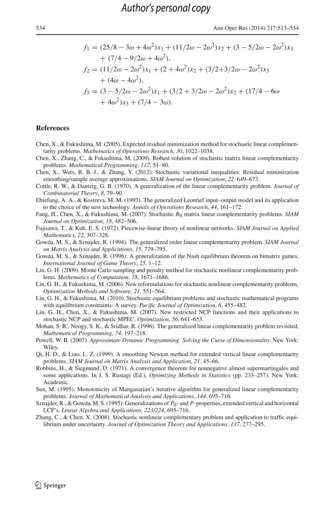
• For (3/4 − 2ω)x3 < max{(3/4 − 2ω)x1, (3/4 − 2ω)x3} + (0.5 − 2ω) ≤ (3/4 − 2ω)x2,

one has that

‖G(x, ω j )‖2 = (x1 + (3/4 − ω)x3 + ωx2 + 0.5 − ω)2 + (x2 + (3/4 − ω)x3

+ ωx1 + ω)2 + ((3/4 − ω)x1 + x3 + ωx2 + 0.5 − ω)2,

123


534 Ann Oper Res (2014) 217:513–534

f1 = (25/8 − 3ω + 4ω2)x1 + (11/2ω − 2ω2)x2 + (3 − 5/2ω − 2ω2)x3

+ (7/4 − 9/2ω + 4ω2),

f2 = (11/2ω − 2ω2)x1 + (2 + 4ω2)x2 + (3/2+3/2ω − 2ω2)x3

+ (4ω − 4ω2),

f3 = (3 − 5/2ω − 2ω2)x1 + (3/2 + 3/2ω − 2ω2)x2 + (17/4 − 6ω

+ 4ω2)x3 + (7/4 − 3ω).

References

Chen, X., & Fukushima, M. (2005). Expected residual minimization method for stochastic linear complemen-tarity problems. Mathematics of Operations Research, 30, 1022–1038.

Chen, X., Zhang, C., & Fukushima, M. (2009). Robust solution of stochastic matrix linear complementarityproblems. Mathematical Programming, 117, 51–80.

Chen, X., Wets, R. B.-J., & Zhang, Y. (2012). Stochastic variational inequalities: Residual minimizationsmoothing/sample average approximations. SIAM Journal on Optimization, 22, 649–673.

Cottle, R. W., & Dantzig, G. B. (1970). A generalization of the linear complementarity problem. Journal ofCombinatorial Theory, 8, 79–90.

Ebiefung, A. A., & Kostreva, M. M. (1993). The generalized Leontief input–output model and its applicationto the choice of the new technology. Annals of Operations Research, 44, 161–172.

Fang, H., Chen, X., & Fukushima, M. (2007). Stochastic R0 matrix linear complementarity problems. SIAMJournal on Optimization, 18, 482–506.

Fujisawa, T., & Kuh, E. S. (1972). Piecewise-linear theory of nonlinear networks. SIAM Journal on AppliedMathematics, 22, 307–328.

Gowda, M. S., & Sznajder, R. (1994). The generalized order linear complementarity problem. SIAM Journalon Matrix Analysis and Applications, 15, 779–795.

Gowda, M. S., & Sznajder, R. (1996). A generalization of the Nash equilibrium theorem on bimatrix games.International Journal of Game Theory, 25, 1–12.

Lin, G. H. (2009). Monte Carlo sampling and penalty method for stochastic nonlinear complementarity prob-lems. Mathematics of Computation, 78, 1671–1686.

Lin, G. H., & Fukushima, M. (2006). New reformulations for stochastic nonlinear complementarity problems.Optimization Methods and Software, 21, 551–564.

Lin, G. H., & Fukushima, M. (2010). Stochastic equilibrium problems and stochastic mathematical programswith equilibrium constraints: A survey. Pacific Journal of Optimization, 6, 455–482.

Lin, G. H., Chen, X., & Fukushima, M. (2007). New restricted NCP functions and their applications tostochastic NCP and stochastic MPEC. Optimization, 56, 641–653.

Mohan, S. R., Neogy, S. K., & Sridhar, R. (1996). The generalized linear complementarity problem revisited.Mathematical Programming, 74, 197–218.

Powell, W. B. (2007). Approximate Dynamic Programming: Solving the Curse of Dimensionality. New York:Wiley.

Qi, H. D., & Liao, L. Z. (1999). A smoothing Newton method for extended vertical linear complementarityproblems. SIAM Journal on Matrix Analysis and Application, 21, 45–66.

Robbins, H., & Siegmund, D. (1971). A convergence theorem for nonnegative almost supermartingales andsome applications. In J. S. Rustagi (Ed.), Optimizing Methods in Statistics (pp. 233–257). New York:Academic.

Sun, M. (1995). Monotonicity of Mangasarian’s iterative algorithm for generalized linear complementarityproblems. Journal of Mathematical Analysis and Applications, 144, 695–716.

Sznajder, R., & Gowda, M. S. (1995). Generalizations of P0- and P-properties, extended vertical and horizontalLCP’s. Linear Algebra and Applications, 223/224, 695–716.

Zhang, C., & Chen, X. (2008). Stochastic nonlinear complementary problem and application to traffic equi-librium under uncertainty. Journal of Optimization Theory and Applications, 137, 277–295.

123


on the erm formulation and a stochastic approximation algorithm of the stochastic- $$r_0$$ r 0 evlcp

Documents