sar-based wind resource statistics in the baltic sea

Remote Sens. 2011, 3, 117-144; doi:10.3390/rs3010117

Remote Sensing ISSN 2072-4292

www.mdpi.com/journal/remotesensing Article

SAR-Based Wind Resource Statistics in the Baltic Sea

Charlotte B. Hasager *, Merete Badger, Alfredo Peña, Xiaoli G. Larsén and Ferhat Bingöl

Wind Energy Division, Risø DTU, Frederiksborgvej 399, 4000 Roskilde, Denmark;

E-Mails: [email protected] (M.B.); [email protected] (A.P.); [email protected] (X.L.);

[email protected] (F.B.)

* Author to whom correspondence should be addressed; E-Mail: [email protected];

Tel.: +45-4677-5014; Fax: +45-4677-5970.

Received: 16 November 2010; in revised form: 22 December 2010 / Accepted: 31 December 2010 /

Published: 11 January 2011

Abstract: Ocean winds in the Baltic Sea are expected to power many wind farms in the

coming years. This study examines satellite Synthetic Aperture Radar (SAR) images from

Envisat ASAR for mapping wind resources with high spatial resolution. Around 900

collocated pairs of wind speed from SAR wind maps and from 10 meteorological masts,

established specifically for wind energy in the study area, are compared. The statistical

results comparing in situ wind speed and SAR-based wind speed show a root mean square

error of 1.17 m s−1, bias of −0.25 m s−1, standard deviation of 1.88 m s−1 and correlation

coefficient of R2 0.783. Wind directions from a global atmospheric model, interpolated in

time and space, are used as input to the geophysical model function CMOD-5 for SAR

wind retrieval. Wind directions compared to mast observations show a root mean square

error of 6.29° with a bias of 7.75°, standard deviation of 20.11° and R2 of 0.950. The scale

and shape parameters, A and k, respectively, from the Weibull probability density function

are compared at only one available mast and the results deviate ~2% for A but ~16% for k.

Maps of A and k, and wind power density based on more than 1000 satellite images show

wind power density values to range from 300 to 800 W m−2 for the 14 existing and

42 planned wind farms.

Keywords: offshore wind; satellite SAR; wind energy; wind resource

OPEN ACCESS

Remote Sens. 2011, 3

118

1. Introduction

Satellite Synthetic Aperture Radar (SAR) can be used for ocean wind mapping at high spatial

resolution. The study aims to verify the applicability of the SAR-based method for wind resource

mapping in part of the Baltic Sea. Firstly, SAR-based wind maps are compared to observations from

10 meteorological in situ masts using around 900 collocations. Thereafter, an offshore wind resource

map is calculated using SAR-based wind maps. Finally, wind resource statistics observed at one site

are compared to the SAR-based results, and the wind resource results from existing and planned

offshore wind farms are examined.

Several studies demonstrate that C-band SAR (~5.3 GHz) can be used to extract wind speed and

wind direction over the ocean at high spatial resolution ~1 km × 1 km [1-6]. In the present study, data

from the Advanced SAR (ASAR), on-board the Envisat satellite launched in 2002 by the European

Space Agency (ESA), are investigated. The ASAR provide several modes, one of them the wide swath

mode (WSM) with 400 km swath. The specific advantage of the Envisat ASAR WSM is the excellent

coverage in the study area, the southwestern part of the Baltic Sea including parts of the Danish,

Swedish, German and Polish waters covering the area from 10° to 19°E longitude and 54° to 58°N

latitude. Kattegat Strait is included. See Figure 1.

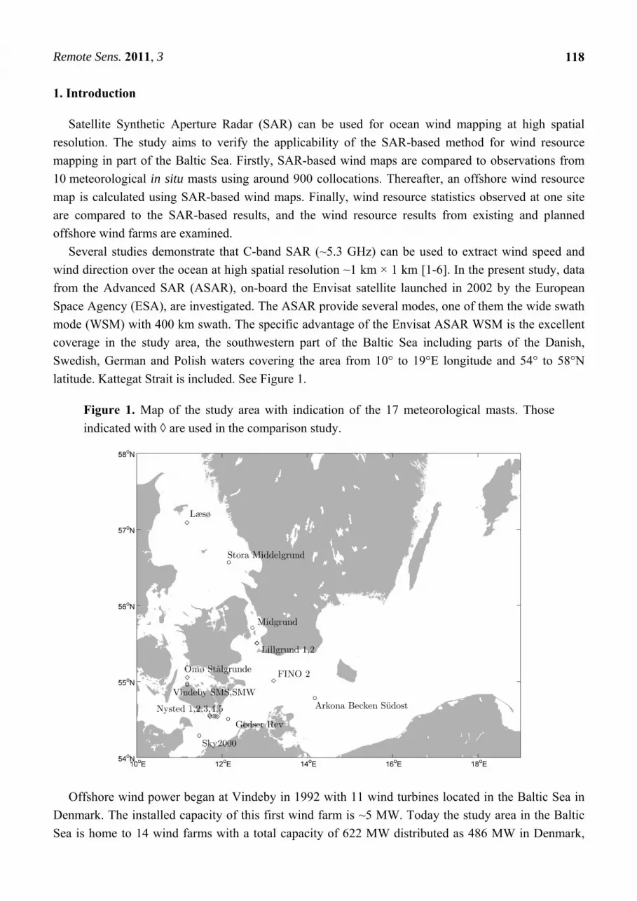
Figure 1. Map of the study area with indication of the 17 meteorological masts. Those

indicated with ◊ are used in the comparison study.

Offshore wind power began at Vindeby in 1992 with 11 wind turbines located in the Baltic Sea in

Denmark. The installed capacity of this first wind farm is ~5 MW. Today the study area in the Baltic

Sea is home to 14 wind farms with a total capacity of 622 MW distributed as 486 MW in Denmark,


119

133 MW in Sweden and 3 MW in Germany. There are plans to increase to a total of 12 GW offshore

wind farm capacity in the Baltic Sea within the study area. The plans include new capacities in

Denmark 1,854 MW, Sweden 5,218 MW, Germany 3,540 MW and Poland 900 MW, see Appendix A

for details. In the Baltic Sea outside the study area there are offshore wind farm plans in Estonia,

Latvia, Lithuania, Russia (Kaliningrad), Finland and Sweden. Thus there is interest in offshore wind

statistics in the Baltic Sea. Predictions on wind resources for the new wind farm sites are interesting.

Satellite SAR used in wind resource estimation has a brief history having started at the turn of the

Millennium [7]. Satellite SAR wind maps from the North Sea have been compared to meteorological

mast data [8-10]. Satellite-based SAR wind mapping in the Baltic Sea encompasses the wind farm

wake study near the Nysted wind farm [11], case studies comparing satellite SAR and mesoscale

model results [1,12-14], and the production of preliminary mean wind speed maps without comparison

to in situ data or model results [15,16].

Observing offshore winds with meteorological masts is costly, but at least 17 masts have been

installed within the study area of the southern Baltic Sea, and the Skagerrak and Kattegat Straits. The

novelty of the present study is the inclusion of ten different meteorological masts—all installed for the

specific purpose of wind resource assessment—enabling a comprehensive comparison within the study

area. It is anticipated that the quality of the meteorological observations will be of higher precision and

accuracy than buoy wind data. The comparison is done case by case, on wind speed using a footprint

averaging technique in the SAR-based wind maps and a time-average from the mast data.

The article describes satellite SAR wind mapping, the meteorological data from the masts, and the

comparison results on wind speed, wind direction and wind resource statistics. Furthermore, the wind

resource map based on more than 1,000 wind maps and wind resource statistics for present and future

offshore wind farms in the study area of the Baltic Sea are presented and the results are discussed.

2. Satellite SAR Wind Mapping

In the Wind Energy Division at Risø DTU satellite, SAR wind mapping is performed using the

Johns Hopkins University, Applied Physics Laboratory (JHU/APL) software APL/NOAA SAR Wind

Retrieval System (ANSWRS). The Envisat ASAR WSM images are downloaded in near-real-time

from ESA and the following automated procedure is applied: The pixels are calibrated to obtain the

Normalized Radar Cross-Section (NRCS) value, then pixels are averaged to around 500 m, and finally

the geophysical model function CMOD-5 [17] is used to retrieve wind speed using the wind direction

a priori from the US Navy Operational Global Atmospheric Prediction System (NOGAPS). The

spatial averaging of SAR pixels suppresses noise effects from longer ocean waves and from speckle,

an inherent property of imaging radars. The 6-hourly model wind vectors are available at a 1 degree

latitude and longitude grid and the wind vectors from the lowest model level around 10 m above the

surface are used. To match the satellite data, the wind vectors are interpolated in time and

space [18,19].

The wind maps resolve details on atmospheric mesoscale wind phenomena. Figure 2 shows the

wind speed map from 1 January 2010 observed at 20.48 UTC. All time stamps in the article are in

UTC. In Skagerrak Strait strong winds are channeled between Norway and Denmark from the

northeast. Wind streaks are present and wind speeds are between 15 and 20 m s−1. In the South Baltic


120

Sea the winds are weaker, around 7 to 12 m s−1 with lee effects southwest of the Danish islands and

along the Swedish coast.

Figure 2. Wind speed map of the South Baltic Sea and interior Danish Seas observed from

Envisat ASAR wide swath mode on 1 January 2010 at 20.48 UTC with the NOGAPS wind

direction vectors shown in white. Risø DTU/JHU APL.

.

The microwave radiation backscattered from the ocean surface is non-linearly proportional to the

size and orientation of capillary and short-gravity waves produced near-instantaneously by the local

surface winds. Thus using information on the radar incidence, azimuth angle, and relative wind


121

direction, the wind speed is retrieved for a neutrally stratified marine atmosphere at 10 m a.s.l. from

the empirical CMOD functions. A more detailed description of SAR-based wind retrieval is given

in [15]. In near-coastal regions non-neutral static stratification often prevails, and a correction to the

neutral wind profile would be ideal. However, for this task accurate sea and air temperatures are

necessary, and this information is generally not available.

Physical obstacles located in the ocean such as ships, oil rigs, and wind turbines act as reflectors

and the backscattered microwave radiation is significantly increased. The CMOD function will, in such

cases, provide a positively biased wind speed observation. In contrast, oil spill and thick algae blooms

at the ocean surface can reduce the backscattered signal as the generation of capillary waves is

hindered. The result is a negatively biased wind speed. Convective rain cells also influence SAR data.

Often a pattern is seen with increased winds around the rain cell, and with reduced wind inside the rain

cell, possibly due to the rain drop’s interference (splashing effect) with the capillary waves and/or

lower winds. Sea bottom structures, ocean and tidal currents [20], and long internal ocean waves can

also influence SAR and override the basic wind speed signal. For the study area one or more of the

above situations may occur. However, despite all these possible shortcomings, ocean winds are

generally mapped reasonably well from C-band SAR [6]. Sea ice was present in parts of the study area

from late January to late February 2010 as it was an unusually cold winter. Information from the

Swedish Meteorological and Hydrological Institute (SMHI) Ice Service and visual inspection of the

wind maps were used to discard some scenes.

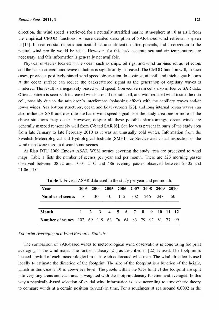
At Risø DTU 1009 Envisat ASAR WSM scenes covering the study area are processed to wind

maps. Table 1 lists the number of scenes per year and per month. There are 523 morning passes

observed between 08.52 and 10.01 UTC and 486 evening passes observed between 20.05 and

21.06 UTC.

Table 1. Envisat ASAR data used in the study per year and per month.

Year 2003 2004 2005 2006 2007 2008 2009 2010

Number of scenes 8 30 10 115 302 246 248 50

Month 1 2 3 4 5 6 7 8 9 10 11 12

Number of scenes 102 69 119 63 76 64 83 79 97 81 77 99

Footprint Averaging and Wind Resource Statistics

The comparison of SAR-based winds to meteorological wind observations is done using footprint

averaging in the wind maps. The footprint theory [21] as described in [22] is used. The footprint is

located upwind of each meteorological mast in each collocated wind map. The wind direction is used

locally to estimate the direction of the footprint. The size of the footprint is a function of the height,

which in this case is 10 m above sea level. The pixels within the 95% limit of the footprint are split

into very tiny areas and each area is weighted with the footprint density function and averaged. In this

way a physically-based selection of spatial wind information is used according to atmospheric theory

to compare winds at a certain position (x,y,z,t) in time. For a roughness at sea around 0.0002 m the


122

footprint stretches around 860 m upwind with the maximum influence at half this distance. The

statistical analysis of SAR wind maps is performed with the Satellite-Wind Atlas Analysis and

Application Program (S-WAsP) tool developed by Risø DTU [23].

The Weibull probability distribution function is commonly used to describe wind speed data as in

the European Wind Atlas [24]. The available wind power density, E, (that is proportional to the wind

speed cubed), may be calculated from the two Weibull parameters, the scale parameter A and the shape

parameter k, using the gamma function Γ, and the air density ρ (~1.245 g/m3 at 10 °C) as

E12

Γ 13. (1)

Studies from the North Sea have shown SAR wind maps to be a possible source of information for

the estimation of A and k [8,10]. Recent results from the North Sea show deviations between

SAR-based wind resource statistics compared to the meteorological data below 5% for the mean wind

speed and A and below 7% for E and k, when a sufficient number of samples are available [10]. If only

100 to 200 samples can be purchased the new wind class method is recommended. It is necessary to

have many more available images in the data archive in order to populate the wind classes. The wind

class method is based on a selection of SAR wind maps for the analysis combined with weighting of

the SAR-based results using long-term mesoscale model statistics as input to quantify the weighting

coefficients. The wind class method is primarily relevant when few samples are available whereas if

more than 400 samples are available the random sampling method appears to be the best option. The

random sampling method is based on equal weight to all available samples. This is used here. Weibull

fitting of the SAR-based wind maps is done with the maximum likelihood estimator suitable for sparse

data sets [25].

3. Meteorological Data

The locations of the 17 meteorological masts are indicated in Figure 1. Table 2 lists the

geographical coordinates of the met-masts and the data owners. The data periods with the first and last

observation from each of the ten masts used in the comparison study and the observational heights are

listed. Data from the other seven masts are not available or do not overlap in time with the satellite

images, however, basic information on these masts is also included in Table 2.

Brief descriptions of the meteorological data and data analysis for each of the ten meteorological

masts are given in Sections 3.1 to 3.5. It is the wind speed at 10 m above sea level that is extracted

from satellite SAR, thus it has been chosen to extrapolate the met-mast wind speed to this height—if

not directly observed at 10 m. In order for the statistics from the masts to match well with the footprint

averaging technique, an hourly average centered at the satellite recording time is used. At shorter

averaging time scales, e.g., 10 minutes, greater scatter is found, probably because the finer scales are

not resolved in SAR. All masts have data stored every 10 minutes and several masts have two-sided

measurements (to avoid mast shadow effects).


123

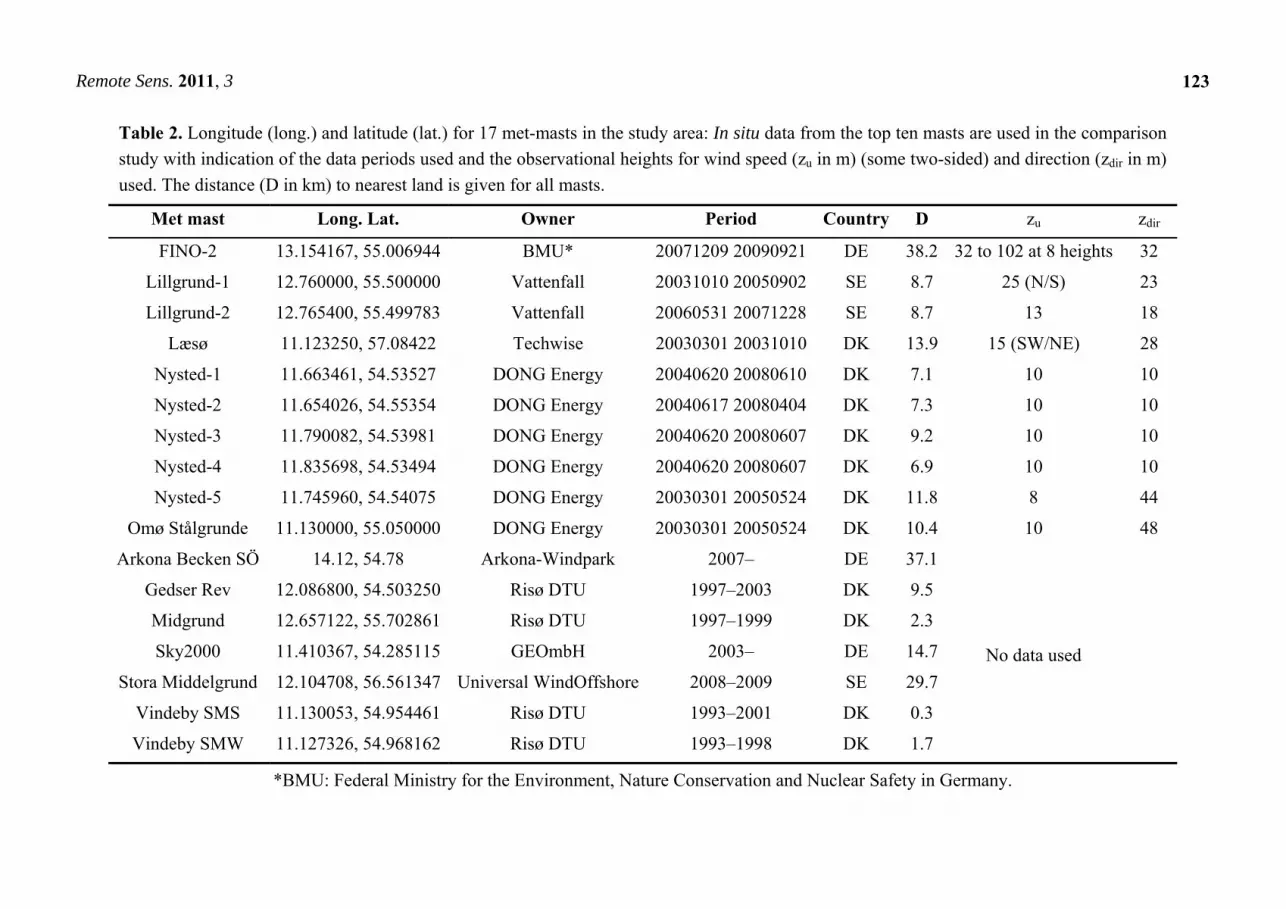
Table 2. Longitude (long.) and latitude (lat.) for 17 met-masts in the study area: In situ data from the top ten masts are used in the comparison

study with indication of the data periods used and the observational heights for wind speed (zu in m) (some two-sided) and direction (zdir in m)

used. The distance (D in km) to nearest land is given for all masts.

Met mast Long. Lat. Owner Period Country D zu zdir

FINO-2 13.154167, 55.006944 BMU* 20071209 20090921 DE 38.2 32 to 102 at 8 heights 32

Lillgrund-1 12.760000, 55.500000 Vattenfall 20031010 20050902 SE 8.7 25 (N/S) 23

Lillgrund-2 12.765400, 55.499783 Vattenfall 20060531 20071228 SE 8.7 13 18

Læsø 11.123250, 57.08422 Techwise 20030301 20031010 DK 13.9 15 (SW/NE) 28

Nysted-1 11.663461, 54.53527 DONG Energy 20040620 20080610 DK 7.1 10 10





Omø Stålgrunde 11.130000, 55.050000 DONG Energy 20030301 20050524 DK 10.4 10 48

Arkona Becken SÖ 14.12, 54.78 Arkona-Windpark 2007– DE 37.1

No data used

Gedser Rev 12.086800, 54.503250 Risø DTU 1997–2003 DK 9.5

Midgrund 12.657122, 55.702861 Risø DTU 1997–1999 DK 2.3

Sky2000 11.410367, 54.285115 GEOmbH 2003– DE 14.7

Stora Middelgrund 12.104708, 56.561347 Universal WindOffshore 2008–2009 SE 29.7

Vindeby SMS 11.130053, 54.954461 Risø DTU 1993–2001 DK 0.3

Vindeby SMW 11.127326, 54.968162 Risø DTU 1993–1998 DK 1.7

*BMU: Federal Ministry for the Environment, Nature Conservation and Nuclear Safety in Germany.


124

Six of the meteorological masts are located near offshore wind farms and observe wind farm wake

effects for certain wind directions, i.e., reduced wind speeds. In the context of comparing

wake-influenced meteorological data and wake-influenced satellite SAR, it is expected that the satellite

wind maps record similarly reduced wind speeds. Only when satellite backscatter is enhanced, due to

returns from the turbine towers and blades, an apparent too high wind speed is expected. The footprint

has a length of around 860 m. Wind speed data are omitted from the verification study (but presented

in a separate table) when wind turbines are positioned closer to the mast than this distance.

3.1. FINO-2 Data

The FINO-2 meteorological mast is the second of the three German ‘Forschungs-plattformen in

Nord- und Ostsee’ (research platforms in the North and Baltic Seas). It is located midway between

Germany and Sweden, around 38.2 km and 38.6 km, respectively. Information is available at

http://212.201.38.20/fino2/. The wind speed at 32, 42, 52, 62, 72, 82, 92, 102 m is extrapolated to 10 m

using the logarithmic wind profile and the Charnock roughness model with the constant set at 0.0144

following [26] and assuming neutral stability. There is no wind farm nearby.

3.2. Lillgrund-1/-2 Data

The Lillgrund-1 data were collected prior to construction of the Lillgrund wind farm that consists of

48 turbines of 2.3 MW. Wind speed observations at 25 m height at two booms in directions north and

south are used. The highest wind speed from the two booms is selected to avoid mast shadow effects.

The wind speed is extrapolated to 10 m as for FINO-2.

The Lillgrund-2 mast is in fact the Lillgrund-1 mast moved to a nearby location and

re-instrumented. The Lillgrund wind farm is constructed less than 500 m east of the Lillgrund-2

meteorological mast. This results in a wind farm wake sector from 300° to 360° and 0° to 120°, and a

free stream wind sector from 120° to 300°. Only the free stream sector is useful for wind speed

verification analysis. The wind speed is observed at 13 m and extrapolated to 10 m as for FINO-2.

3.3. Læsø Data

The Læsø data were recorded in the early years of the Envisat mission. Only a few SAR

observations are collocated with mast data in our dataset. The wind speed is observed at 15 m at two

booms pointing southwest and northeast. The highest wind speed is selected to avoid mast shadow

effects, and the data are extrapolated to 10 m as for FINO-2. There is no wind farm nearby.

3.4. Nysted-1/-2/-3/-4/-5 Data

The five meteorological masts at Nysted are located near the Nysted offshore wind farm. For the

layout of the wind farm and masts see [27] and http://www.dongenergy.com/Nysted. Only

meteorological observations after construction of the wind farm are used in the study. The Nysted

wind farm started to operate on the 1 December 2003. Two of the masts, Nysted-1/-2, are located west

of the wind farm both at distances of less than 500 m from the nearest row of wind turbines. The two

other masts, Nysted-3/-4, are located east of the wind farm at distances of around 1 km and 4 km,


125

respectively, from the nearest row of wind turbines. The fifth mast, Nysted-5, is located within the

wind farm itself. The position of the masts and the wind turbines, results in the following wake and

free stream sectors: Nysted-1/-2 both have wake sectors from 0° to 180° and free stream sectors from

180° to 360°. Nysted-3 and -4 are located far enough from the wind farm to have free stream sector for

all 360°. This only implies that the upwind footprint of the satellite SAR is shorter than the distance to

the nearest wind turbines and the turbines do not contribute high backscatter. Nysted-5 is located

inside the wind farm and has a 360° wake influenced sector.

At Nysted-1/-2/-3/-4, wind speeds are measured with cup anemometers at heights above mean sea

level of 10 m and up to 69 m and wind directions are measured at 10 m and 65 m. At Nysted-5, wind

speeds are measured at 8 m and 44 m and direction at 44 m; here the wind speed at 10 m is

extrapolated from that at 8 m, by using the Charnock formulation for the surface roughness length.

Due to the short distance—here 2 m—the stability effect is neglected.

The study of [13] shows that over the water area where the Nysted wind farm is, the stability

parameter, the Richardson number Ri, is larger than zero for about 61% of the time and about 26% of

the time it is strongly stable with Ri > 0.25, suggesting mainly stable conditions. These features are in

agreement with the studies of [28] and [29], where it was also shown that throughout most of the year,

the atmosphere over the Baltic Sea is stable. This stable condition indicates a source of uncertainty in

the SAR wind retrievals where neutral stability is assumed.

3.5. Omø Stålgrunde Data

The Omå Stålgrunde mast observes wind speeds at 10 m. There is no wind farm nearby.

3.6. Wind Direction from All Masts

Wind directions in the wind maps are from the NOGAPS model. The wind direction is reported

both for free stream and wake influence sectors. Wind direction is poorly defined for very low wind

speeds. Wind direction comparison results are reported only for cases of wind speed larger than 3 m s−1

observed in the SAR wind maps. Wind direction in NOGAPS is from the lowest model layer, around

10 m above surface. For the masts the wind directions are observed at the following heights: FINO-2 at

32 m, Lillgrund-1 at 23 m, Lillgrund-2 at 18 m, Læsø at 28 m, Nysted-1/-2/-3/-4 at 10 m, Nysted-5 at

44 m, and Omø Stålgrunde at 48 m. The wind directions from the mast data have not been adjusted to

10 m as veering is expected to be small.

3.7. Wind Energy Resource Statistics

Wind resource results from the commercial masts cannot be published. Thus only FINO-2 data are

available for wind resource comparison in the Baltic Sea study area. Wind speeds are observed at 32,

42, 52, 62, 72, 82, 92, and 102 m. The Wind Atlas Analysis and Application Program (WAsP) [30] has

been used to fit the Weibull A and k parameters. To what extent the wind resource at 10 m was

estimated similarly from data at all heights was investigated and the result showed variations

indicating flow distortion, in particular, at the lower heights. The final result for comparing SAR-based

and in situ wind resource statistics was estimated from meteorological data at 102 m.


126

4. Results

4.1. Wind Direction

The comparison results on wind direction are presented first, because these are used to initiate the

local wind speed retrieval. The wind directions in the wind maps are the NOGAPS wind directions

interpolated in time and space to match locally in each satellite image. Figure 3 shows wind direction

from all masts versus NOGAPS. In Figure 3 a few observations near 0° and 360° are removed (e.g., in

case met-data shows 355° and NOGAPS shows 10°). The data are removed to provide a suitable basis

for linear regression within 0–360°. Linear regression results, for each mast for its free stream sector

and wake-influenced sector, are listed in Table 3. The statistical results from the free stream sectors

and wake-influenced sectors are similar. Therefore the overall result includes all observations, and the

overall statistics are given in the last column of Table 3. Figure 4 shows the residual plot.

Figure 3. Wind directions from meteorological stations versus NOGAPS, N = 927.


127

Figure 4. Residual plot for the linear regression on wind direction from masts versus NOGAPS.

Table 3. Linear regression results for wind direction between masts versus NOGAPS in

free stream sectors and wake-influenced sectors; and ALL includes both free stream and

wake-influenced sectors; N is number of samples (−); R2 is the correlation coefficient(−);

SD is standard error (°); RMS is root mean square error (°); bias is the offset of the linear

regression (°) and the slope (−).

FINO2 Lill.1 Lill.2 Nys.1 Nys.2 Nys.3 Nys.4 Nys.5 Omø ALL

Free Free Free Wake Free Wake Free Wake Free Free Wake Free ALL

N 165 23 77 42 87 47 63 46 155 56 35 35 927

R2 0.952 0.965 0.881 0.971 0.859 0.764 0.805 0.881 0.970 0.970 0.972 0.971 0.950

SD 18.95 16.64 16.63 22.67 15.94 19.65 17.51 13.85 15.73 15.70 15.07 16.16 20.11

RMS 5.79 4.37 7.86 5.44 8.16 12.68 10.38 6.56 3.85 3.84 3.56 3.88 6.29

Bias −8.44 −11.59 47.16 20.08 48.54 22.71 32.46 12.89 6.83 17.97 5.24 3.02 7.75

Slope 1.01 1.05 0.87 1.01 0.86 0.83 0.90 0.93 1.01 1.00 0.97 0.98 0.99

4.2. Wind Speed

The comparison results on wind speed are calculated for each meteorological mast taking into

account free stream and wind farm wake sectors. The wind directions are taken from NOGAPS to

discriminate which directional sector any given pair of wind speeds from a meteorological mast and a

SAR wind speed map belongs to. There are more data pairs included in the wind speed analysis than in

the wind direction analysis above. Comparison of wind speeds are done also for wind speeds less than

3 m s−1 (in contrast to the wind directional comparison analysis) but for winds less than 2 m s−1, the

software excludes the SAR-wind data. SAR wind maps contain observations below 2 m s−1, yet the

quality of wind speed at this low end is questionable. The linear regression statistics for wind speeds

are shown in Table 4(a,b), for free stream sectors and wake sectors, respectively.


128

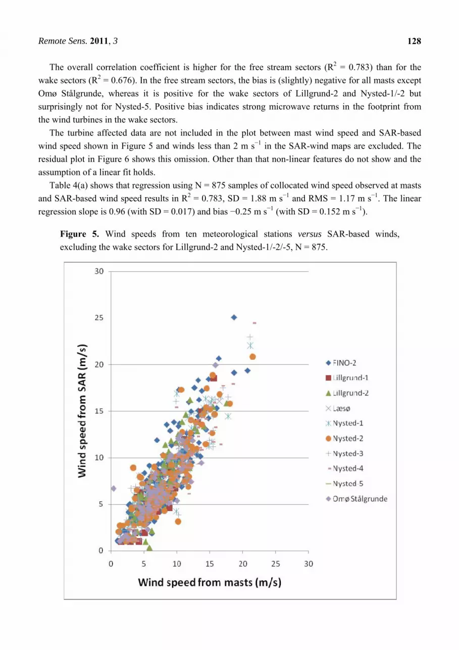
The overall correlation coefficient is higher for the free stream sectors (R2 = 0.783) than for the

wake sectors (R2 = 0.676). In the free stream sectors, the bias is (slightly) negative for all masts except

Omø Stålgrunde, whereas it is positive for the wake sectors of Lillgrund-2 and Nysted-1/-2 but

surprisingly not for Nysted-5. Positive bias indicates strong microwave returns in the footprint from

the wind turbines in the wake sectors.

The turbine affected data are not included in the plot between mast wind speed and SAR-based

wind speed shown in Figure 5 and winds less than 2 m s−1 in the SAR-wind maps are excluded. The

residual plot in Figure 6 shows this omission. Other than that non-linear features do not show and the

assumption of a linear fit holds.

Table 4(a) shows that regression using N = 875 samples of collocated wind speed observed at masts

and SAR-based wind speed results in R2 = 0.783, SD = 1.88 m s−1 and RMS = 1.17 m s−1. The linear

regression slope is 0.96 (with SD = 0.017) and bias −0.25 m s−1 (with SD = 0.152 m s−1).

Figure 5. Wind speeds from ten meteorological stations versus SAR-based winds,

excluding the wake sectors for Lillgrund-2 and Nysted-1/-2/-5, N = 875.


129

Figure 6. Residual plot for the linear regression on wind speed from masts versus SAR wind maps.

Table 4. (a) Linear regression results for wind speed between mast data versus SAR-wind

maps in free stream sectors; (b) wake sectors. N is number of samples (−); R2 is the

correlation coefficient (−); SD is standard error (m s−1); RMS is root mean square error

(m s−1); bias is the offset of the linear regression (m s−1) and the slope (−).

(a) FINO-2 Lill.1 Lill.2 Læsø Nys.1 Nys.2 Nys.3 Nys.4 Omø ALL

N 180 32 86 5 105 110 178 137 42 875

R2 0.765 0.796 0.789 0.973 0.801 0.754 0.804 0.838 0.686 0.783

SD 2.04 1.90 1.71 1.00 1.88 2.09 1.66 1.62 2.12 1.88

RMS 1.31 1.15 1.05 0.23 1.13 1.37 0.99 0.89 1.55 1.17

Bias −0.21 −1.34 −0.61 −2.32 −0.06 −0.10 −0.22 −0.45 0.22 −0.25

Slope 1.03 1.08 1.06 1.16 0.93 0.92 0.92 0.95 0.92 0.96

(b) Lill.2 Nys.1 Nys.2 Nys.4 ALL

N 51 65 57 41 214

R2 0.719 0.669 0.686 0.740 0.676

SD 1.89 1.59 1.58 2.04 1.85

RMS 1.31 1.19 1.15 1.37 1.36

Bias 0.52 0.94 0.98 -0.78 0.57

Slope 1.06 0.80 0.82 1.03 0.91

4.3. Wind Resource Statistics

The wind energy resource statistics in the Baltic Sea study area are calculated based on

1009 Envisat ASAR wind maps using the method in [8] with equal weights to all. The data represent

seasons and twice-daily conditions (cf. Table 1).

The resulting SAR-based maps at 1 km by 1 km resolution are presented in Figure 7(a–d). The first

panel in Figure 7 shows the number of samples and the following three panels show SAR-based results

on Weibull A and k, and wind power density, E. The map of overlapping samples shows the


130

characteristic pattern of satellite passes inclined from ascending and descending tracks. There are more

samples in the northwest part of the study area and less in the southern region. The maximum number

of samples is 538 and the minimum number around 350. Weibull A ranges from 6 m s−1 along the

eastern Swedish coast to 9.5 m s−1 in the Skagerrak Strait, and Weibull k ranges from 1.4 near

coastlines up to 2.1 in the southwestern part of the study area. In Figure 7(b,c) too high values are

found at the Nysted (Rødsand 1) wind farm due to backscatter from the 72 turbines. Wind power

density values range from 249 W m−2 to 934 W m−2. The highest wind power density value is found in

the Skagerrak Strait, not in the Baltic Sea.

Figure 7. Wind resource statistics based on 1009 Envisat ASAR wide swath mode satellite

wind maps covering part of the Baltic Sea and interior Danish Seas. Panels top: (a) number

of samples (−); (b) Weibull A (m s−1); (c) Weibull k (−); and (d) wind power density

(W m−2) including indication of wind farms. The wind farm numbers refer to Appendix 1.

(a)

(b)


131

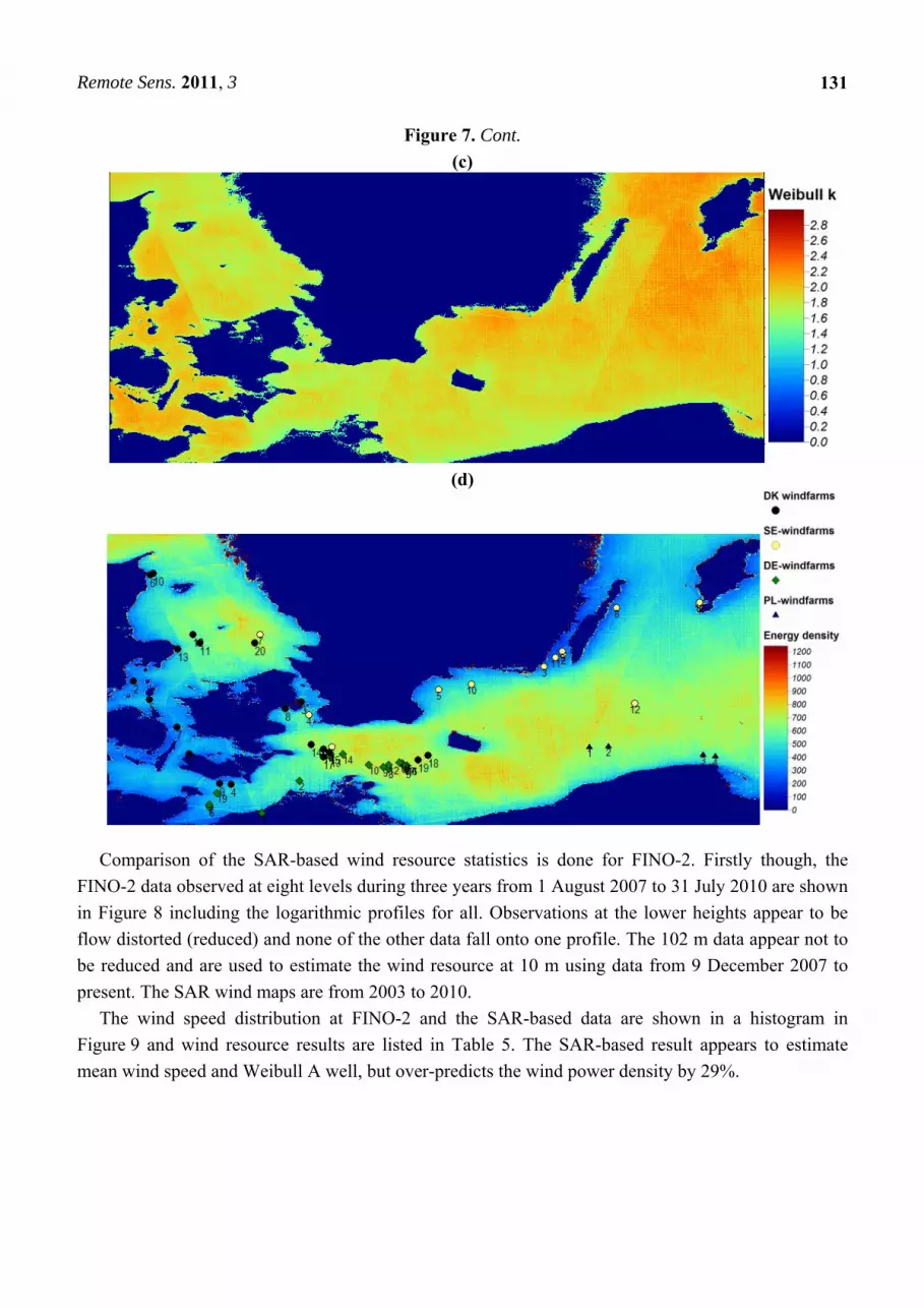
Figure 7. Cont.

(c)

(d)

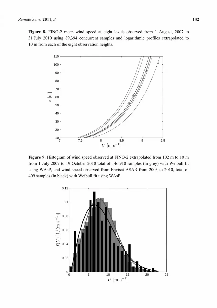
Comparison of the SAR-based wind resource statistics is done for FINO-2. Firstly though, the

FINO-2 data observed at eight levels during three years from 1 August 2007 to 31 July 2010 are shown

in Figure 8 including the logarithmic profiles for all. Observations at the lower heights appear to be

flow distorted (reduced) and none of the other data fall onto one profile. The 102 m data appear not to

be reduced and are used to estimate the wind resource at 10 m using data from 9 December 2007 to

present. The SAR wind maps are from 2003 to 2010.

The wind speed distribution at FINO-2 and the SAR-based data are shown in a histogram in

Figure 9 and wind resource results are listed in Table 5. The SAR-based result appears to estimate

mean wind speed and Weibull A well, but over-predicts the wind power density by 29%.


132

Figure 8. FINO-2 mean wind speed at eight levels observed from 1 August, 2007 to

31 July 2010 using 89,394 concurrent samples and logarithmic profiles extrapolated to

10 m from each of the eight observation heights.

Figure 9. Histogram of wind speed observed at FINO-2 extrapolated from 102 m to 10 m

from 1 July 2007 to 19 October 2010 total of 146,910 samples (in grey) with Weibull fit

using WAsP, and wind speed observed from Envisat ASAR from 2003 to 2010, total of

409 samples (in black) with Weibull fit using WAsP.

7 7.5 8 8.5 9 9.510

20

30

40

50

60

70

80

90

100

110

z[m

]

U [m s−1]

0 5 10 15 20 250

0.02

0.04

0.06

0.08

0.1

0.12

f(U

)[1

/(m

s−1)]

U [m s−1]


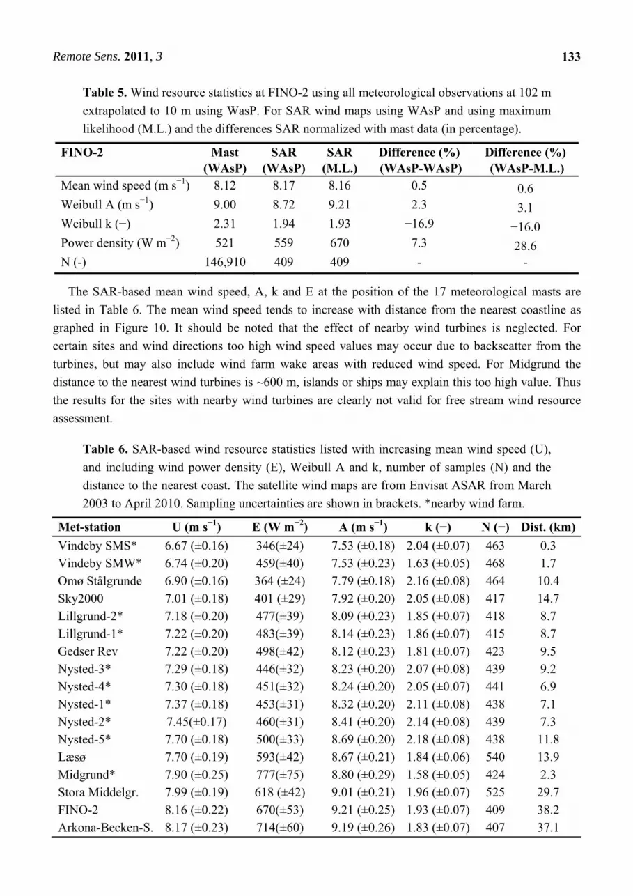
133

Table 5. Wind resource statistics at FINO-2 using all meteorological observations at 102 m

extrapolated to 10 m using WasP. For SAR wind maps using WAsP and using maximum

likelihood (M.L.) and the differences SAR normalized with mast data (in percentage).

FINO-2 Mast (WAsP)

SAR (WAsP)

SAR (M.L.)

Difference (%) (WAsP-WAsP)

Difference (%) (WAsP-M.L.)

Mean wind speed (m s−1) 8.12 8.17 8.16 0.5 0.6 Weibull A (m s−1) 9.00 8.72 9.21 2.3 3.1 Weibull k (−) 2.31 1.94 1.93 −16.9 −16.0 Power density (W m−2) 521 559 670 7.3 28.6 N (-) 146,910 409 409 - -

The SAR-based mean wind speed, A, k and E at the position of the 17 meteorological masts are

listed in Table 6. The mean wind speed tends to increase with distance from the nearest coastline as

graphed in Figure 10. It should be noted that the effect of nearby wind turbines is neglected. For

certain sites and wind directions too high wind speed values may occur due to backscatter from the

turbines, but may also include wind farm wake areas with reduced wind speed. For Midgrund the

distance to the nearest wind turbines is ~600 m, islands or ships may explain this too high value. Thus

the results for the sites with nearby wind turbines are clearly not valid for free stream wind resource

assessment.

Table 6. SAR-based wind resource statistics listed with increasing mean wind speed (U),

and including wind power density (E), Weibull A and k, number of samples (N) and the

distance to the nearest coast. The satellite wind maps are from Envisat ASAR from March

2003 to April 2010. Sampling uncertainties are shown in brackets. *nearby wind farm.

Met-station U (m s−1) E (W m−2) A (m s−1) k (−) N (−) Dist. (km)

Vindeby SMS* 6.67 (±0.16) 346(±24) 7.53 (±0.18) 2.04 (±0.07) 463 0.3 Vindeby SMW* 6.74 (±0.20) 459(±40) 7.53 (±0.23) 1.63 (±0.05) 468 1.7 Omø Stålgrunde 6.90 (±0.16) 364 (±24) 7.79 (±0.18) 2.16 (±0.08) 464 10.4 Sky2000 7.01 (±0.18) 401 (±29) 7.92 (±0.20) 2.05 (±0.08) 417 14.7 Lillgrund-2* 7.18 (±0.20) 477(±39) 8.09 (±0.23) 1.85 (±0.07) 418 8.7 Lillgrund-1* 7.22 (±0.20) 483(±39) 8.14 (±0.23) 1.86 (±0.07) 415 8.7 Gedser Rev 7.22 (±0.20) 498(±42) 8.12 (±0.23) 1.81 (±0.07) 423 9.5 Nysted-3* 7.29 (±0.18) 446(±32) 8.23 (±0.20) 2.07 (±0.08) 439 9.2 Nysted-4* 7.30 (±0.18) 451(±32) 8.24 (±0.20) 2.05 (±0.07) 441 6.9 Nysted-1* 7.37 (±0.18) 453(±31) 8.32 (±0.20) 2.11 (±0.08) 438 7.1 Nysted-2* 7.45(±0.17) 460(±31) 8.41 (±0.20) 2.14 (±0.08) 439 7.3 Nysted-5* 7.70 (±0.18) 500(±33) 8.69 (±0.20) 2.18 (±0.08) 438 11.8 Læsø 7.70 (±0.19) 593(±42) 8.67 (±0.21) 1.84 (±0.06) 540 13.9 Midgrund* 7.90 (±0.25) 777(±75) 8.80 (±0.29) 1.58 (±0.05) 424 2.3 Stora Middelgr. 7.99 (±0.19) 618 (±42) 9.01 (±0.21) 1.96 (±0.07) 525 29.7 FINO-2 8.16 (±0.22) 670(±53) 9.21 (±0.25) 1.93 (±0.07) 409 38.2 Arkona-Becken-S. 8.17 (±0.23) 714(±60) 9.19 (±0.26) 1.83 (±0.07) 407 37.1


134

Figure 10. SAR-based mean wind speed (top) and wind power density (bottom) at the

location of 17 meteorological masts, near or far from wind farms.

Finally, the wind resource statistics based on satellite SAR wind maps are calculated for existing

and planned offshore wind farms in the study area. The existing wind farms include nine in Denmark,

four in Sweden and one in Germany. The three largest are Rødsand 2 with 90 turbines and a total of

207 MW installed capacity since August 2010; Rødsand 1 with 72 turbines and a total of 166 MW

installed capacity since 2003; and Lillgrund with 48 turbines and a total of 110 MW installed capacity

since 2007.

There are plans of adding 42 new wind farms in the study area in coming years. A list of existing

and planned wind farms is provided in Appendix A. The information on the wind farms is taken

mainly from http://www.4coffshore.com/windfarms. The wind resource statistics for existing and

planned wind farms are calculated based on SAR wind maps. The results include mean wind speed,

Weibull A and k, wind power density and the number of wind maps used at each wind farm. Figure 11

shows mean wind speed per country, and Figure 12 shows Weibull A and k, and wind power density

as a function of distance to the nearest coastline.


135

Figure 11. Mean wind speed from Envisat ASAR observations at existing and planned

wind farm sites per country in the Baltic Sea study area (cf. Table A1).

Figure 12. Weibull A and k (top) and wind power density (bottom) calculated from

Envisat ASAR observations at existing and planned wind farms in the study area.


136

5. Discussion

5.1. Wind Direction Comparison

The comparison results between NOGAPS wind direction and meteorological observations are

highly correlated with R2 of 0.950 and RMS at 6.29°. The linear regression slope is 0.99 and the bias

7.75° (i.e., ~2%). Around 900 independent samples are used. The clockwise veering is partly explained

by the Ekman spiral that veers clockwise in the northern hemisphere. The overall wind direction

statistics show good accuracy.

The reproducibility, i.e., the variation arising using the same method among different met-stations,

is very good. Very few extreme outliers in the NOGAPS wind directions are found. Systematic

problems do not appear at the investigated locations. Studies have shown that wind direction may be

obtained from the SAR image itself by identification of the wind streaks aligned approximately with

the dominant wind direction, e.g., [31]. The optimal situation is to use directions from streaks, yet

problems associated with automatic streak detection limits this option. Further, it has been shown that

using wind direction from a local mast to initiate the local wind retrieval also provides very good

results locally [8]. Only very few meteorological masts are available and, for near-real-time SAR wind

mapping, this is not a viable option. However, it can be done offline as post-processing for a specific

local site in order to increase the accuracy nearby. It has to be kept in mind though that wind directions

are neither constant in time nor in space. It is clear that mesoscale atmospheric phenomena occur in

this enclosed sea with many islands, see Figure 2. But despite this fact, the NOGAPS global model

appears to provide good wind directions. This is important as the wind speed retrieval is initiated with

the NOGAPS wind directions.

5.2. Wind Speed Comparison

The overall statistics from the wind speed regression analysis are also of good quality, though with

lower R2 than for wind directions. It is the first time that a comprehensive data set of high-quality

meteorological masts—all designed for wind resource assessment—has been used for comparison to

SAR-based winds. For five masts more than 100 collocated pairs are available. The wind speed

statistics based on nearly 900 collocated pairs of meteorological observations from a total of ten masts

and SAR-based winds in free stream (not including noise from wind turbine backscatter) show

R2 0.783, SD 1.88 m s−1 and RMS 1.17 m s−1. There is a small negative bias −0.25 m s−1 (with SD

0.152 m s−1) and the linear regression slope is 0.960 (with SD 0.017). The statistics are comparable to

results from Horns Rev in the North Sea [8,22] and clearly better than the nominal accuracy of the

geophysical model function with ±2 m s−1 accuracy [17,32]. The water depth at FINO-2 is 25 m

whereas it ranges from 4 to 10 m at Lillgrund and from 6 to 10 m at Læsø, Nysted and Omå

Stålgrunde. Tidal currents are insignificant, thus effects of SAR signatures originating from currents

are expected to be small. Averaging to 1 km by 1 km grid suppresses small-scale effects.


137

5.3. Wind Resource Comparison

In the Baltic Sea study area only wind resource statistics from FINO-2 are available for comparison

with results from SAR. The results show near zero difference between mean wind speed from mast

data and SAR using an extrapolation of wind speed data from 102 m to 10 m. Further the result

deviates ~2% on Weibull A but ~16 % on Weibull k. It is statistically more difficult to estimate the

Weibull k parameter than the Weibull A parameter. More data are needed to achieve similar accuracy.

According to [25] it is necessary with ~70 samples to estimate Weibull A, ~175 samples to estimate

Weibull k, and ~2,000 samples to estimate power density within ±10% accuracy at the 90% confidence

interval. At FINO-2 the difference in power density values is ~29% using 409 samples comparing

results from mast data observed at 102 m using maximum likelihood for Weibull fitting. Using WAsP

Weibull fitting to the SAR data (shown in Figure 9 and listed in Table 5) the difference in power

density is ~7% between mast data and SAR.

The uncertainty on maximum likelihood fitting is listed in Table 6 and typically is within 50 W m−2.

The choice of Weibull fitting influence results as seen in Table 5. Unfortunately only one location is

available for comparison of wind energy density results. The FINO-2 meteorological data shown in

Figure 8 shows a tendency to have (much) higher winds high in the atmosphere than the logarithmic

profile. This may be caused either by: (1) Flow distortion at lower observational heights; (2) stable

stratification; or (3) coastal winds that are not fully adjusted [33]; or a combination of the all three.

The vertical extrapolation adds uncertainty. The wind speed data appear to be influenced by the

relatively heavy mast construction that is likely to add flow distortion to the wind measurements. It

was found that the collocated wind speeds at FINO-2 are less well correlated than for most other

masts, see Table 4. No further assessment has been made. Recent results from the North Sea [10]

comparing mean wind speed, Weibull A and k, and power density between three masts (Horns Rev,

Høvsøre and FINO-1) and SAR-based results have shown deviations less than 5% for mean wind

speed and Weibull A and deviations less than 7% for Weibull k and power density, using

approximately the same number of SAR samples. Reasons for the better agreement in the North Sea

compared to the Baltic Sea could be differences in atmospheric stability. The more enclosed Baltic

Sea, where the coastal flow may not be fully adjusted, could be another reason [33].

Weibull statistics are published from three masts in the study area based on meteorological data

observed ~50 m above sea level in the 1990’ties, i.e., prior to Envisat. The published results are

Weibull A and k of 9.1 m s−1 and 2.3 at 48 m height observed from 1993 to 1997 at Vindeby [34],

Weibull A and k of 8.3 m s−1 and 2.3 at 50 m observed from October 1997 to July 1998 at

Midgrund [35], and Weibull A and k of 8.6 m s−1 and 2.65 observed at 50 m from March to November

1999 at Omø Stålgrunde [36]. For two masts the data cover less than one year. At Midgrund and

Vindeby wind turbines influence the atmospheric flow and the SAR-based results do not reflect free

flow conditions. Comparisons are not attempted due to these conditions.


138

5.4. Examination of Wind Resource Statistics

Examination of the SAR-based maps of Weibull A, k and wind power density (Figure 7) shows as

expected higher wind power density value in relatively open seas. The lee effect of islands in the

Kattegat Strait and Baltic Sea are notable with lower wind power density value near the islands. The

offshore wind climate in the Danish interior seas has lower wind power density than Kattegat,

Skagerrak and most of the Baltic Sea. It is noted that Weibull k appears to be higher in the

southwestern part of the study area than elsewhere. High k indicates relatively steady winds.

The wind resource statistics presented for the 17 meteorological masts (Table 6, Figure 7) show a

trend of higher mean wind speed further offshore. The mean wind speed ranges from 6.7 m s−1 to

8.2 m s−1 with an uncertainty of ±0.2 m s−1. The masts are located from the coast to ~40 km offshore.

Midgrund is seen as an outlier with much higher mean wind speed, Weibull A and wind power density

than other masts at similar distance to the coast. The high values at Midgrund are most likely due to

two wind turbines located less than 600 m from the mast position, nearby islands and ships giving very

high backscatter and therefore unrealistically high winds.

Reflection from turbines alters backscatter values. It is seen at the Nysted-1 wind farm (Figure 7(b–d).

This wind farm has existed since 2003. Also the Lillgrund can be seen. Lillgrund has operated since

2007 whereas Rødsand-2 (from 2010) cannot be clearly seen in the maps.

The SAR-based mean wind speed, Weibull A and wind power density at the Vindeby, Lillgrund

and Nysted masts appear not to be notably affected by wind turbine reflections in contrast to the

Midgrund mast. This is concluded as the wind statistics at Vindeby, Lillgrund and Nysted increase

gradually with distance from the coast and also compare well with similar statistics from masts not

affected by wind turbines (Figure 8).

The Nysted-3/-4 masts are not affected by turbine backscatter but both are affected by wake for

westerly winds, thus the results are expected to be (slightly) negatively biased compared to the

condition prior to the wind farm. Wind farm wake deficit, i.e., reduced wind downwind of a wind

farm, typically is of the order ~10% but may vary dependent upon turbine operations, wind speed and

atmospheric static stability. For more detail on SAR-based wake mapping see [11,37].

It is remarkable how low winds are observed by SAR for Omø Stålgrunde and Sky2000. Both have

mean wind speed of ~7.0 m s−1 whereas Læsø also located ~12 km offshore shows a mean wind speed

of ~7.7 m s−1 (see Table 6). Near Læsø, Omø Stålgrunde and Sky2000 there are no wind farms or other

obstacles and the major difference between these three masts is the more open sea at Læsø (Figures 1

and 7). In Figure 7(d), the energy density map shows high values in the Great Belt between Zealand

and Fyn along the Great Belt Bridge. More interestingly, an S-shape curve east of the Sprogø

windfarm identical to the major ship route for large vessels shows clearly. This is probably due to

reflection from ships.

The mean wind speed at existing and planned wind farm locations in the four countries (Table A1,

Figure 11) shows a gradual increase as a function of further distances to the nearest coast. There is a

significant variation (±0.7 m s−1) in the coastal zone from 0 to 20 km offshore with a mean wind speed

~7.0 m s−1. Beyond 20 km offshore the mean wind speed is ~8.1 m s−1 and varies only ±0.2 m s−1 in all

four countries, Denmark, Germany, Poland and Sweden. Increases in coastal winds previously has

been studied with similar results [33].


139

Further details on the SAR-based wind resource statistics are shown in Figure 10 with the Weibull

A and k and wind power density results with marking of existing and planned wind farms. It is noticed

that all existing wind farms are located less than 11 km offshore whereas only a few new wind farms

are planned this close to land. Many wind farms are planned in the 15 to 20 km zone and wind power

density is seen to vary from 400 to 700 W m−2. The two extremes are Beta Baltic and Arcadis Ost1, see

Table A1. In the coastal zone from 20 km and further offshore, out to 80 km with the Swedish Södra

Midsjöbanken as frontier very far offshore, the wind power density tends to range between 600 and

720 W m−2 with two outliers above, namely Rønne Banke X and V with 800 W m−2.

The statistical uncertainty on mean wind speed is ~2 to 3% when based on roughly 400 samples and

similar for Weibull A. The uncertainty on wind power density is much higher ~7 to 9% and similar for

Weibull k for a data set of this size. According to [25], Weibull A and k may be estimated with ±10%

accuracy and 90% confidence using ~75 and ~175 samples, respectively (assuming perfect data).

The present data set represents all seasons and morning and evening conditions. The SAR coverage

is not homogeneous (Figure 7(a)) and it reflects in results of Weibull k and energy density in Denmark

(a northwest–southeast line) and in the Baltic Sea (a northeast–southwest line). The reason could be

few particular images giving strong impact.

For Breitling only 161 valid samples are found which is due to the location. Breitling is located in

an enclosed harbor area in Rostock, not truly offshore, and therefore the footprint often includes land

and the values are discarded from the series. Furthermore, ocean wind mapping is not adequate in

enclosed water but the wind statistics, surprisingly enough, falls nicely within the other results.

The number of samples is important as well as how well the samples represent the general wind

climate as described in [10]. The variation in wind speed during the day is not resolved by SAR-based

wind maps as these are observed either in the morning or evening passes according to the orbital

parameters. Thus diurnal variation in wind speed may add uncertainty. Seasonal wind variations may

add uncertainty in case the wind maps do not cover the full year as would be the case, for example, in

cold climate regions with sea ice during winter.

SAR-based results are valid at 10 m. A challenging issue is the vertical extrapolation of the

SAR-based wind results up to hub-height. The wind data from FINO-2 indicate the problem. Present

and future wind turbines may operate at 100 m to 300 m above sea level. In the EU-Norsewind project

the vertical extrapolation is being investigated using data from an array of wind profiling lidars observing

at 70 to 200 m above sea level installed in the Northern European Seas. Lidar-based results show that the

wind profile deviates from the surface-layer wind profile high in the boundary layer [38-41]. Mesoscale

modeling of the offshore wind resource is on-going and comparison of results is in progress, yet

beyond the scope of the present paper.

The present analysis is based on Envisat ASAR images. More Envisat ASAR images could be

extracted from the archive as well as imagery from ERS-1/-2, Radarsat-1/-2 and ALOS PALSAR. The

study, however, is the most comprehensive of its kind on wind resource mapping of the Baltic Sea area.

6. Conclusions

The study presents SAR-based ocean winds compared to wind observations from 10 meteorological

masts erected specifically for wind energy mapping in part of the Baltic Sea. Around 900 collocated


140

pairs of Envisat ASAR wide swath mode images and in situ data, show the wind speed to be mapped

with root mean square error 1.17 m s−1, bias −0.25 m s−1, standard deviation 1.88 m s−1, and correlation

coefficient R2 of 0.783. Ocean wind is mapped from CMOD-5, using wind direction input from a

global atmospheric model, and comparison results on wind direction between the model and in situ

data are root mean square error 6.29°, bias 7.75°, standard deviation 20.11°, and R2 of 0.950. Using

more than 1000 Envisat ASAR wind maps, SAR-based wind resource statistics are examined for the

12 existing and 42 planned wind farms in the study area. It is found that the variation in mean wind is

highly variable in the near coastal zone from 0 to 20 km. All existing wind farms are located less than

11 km from the nearest coast but most of the planned wind farms will be located further offshore. Here

the SAR-based results indicate high mean wind speed and high wind power density. It is noted that the

wind power density ranges from 300 to 800 W m−2 for the planned wind farms. Wind resource

statistics are compared only at one meteorological mast, FINO-2, showing Weibull A to deviate ~2%

between in situ and SAR-based results, but Weibull k to deviate ~16%. The power density is found to

deviate ~29% which is considerably higher than found in a recent study in the North Sea using in situ

data from three masts. In the North Sea, the deviations between masts data and SAR-based results

were within 7% on Weibull k and power density using approximately a similar number of samples and

similar wind retrieval. Further investigation on vertical extrapolation is needed.

Acknowledgements

The work was supported by the EU-Norsewind project (TREN-FP7EN-21908) and the EU-South

Baltic OFF.E.R (EU European Development Fund and the South Baltic Program). Satellite data are

provided by the European Space Agency (Cat. 1 project 3644 and ESA-CSA SOAR project 6773).

Meteorological data from DONG Energy from Nysted, Omø Stålgrunde and Læsø masts as well as

meteorological data from Vattenfall from the Lillgrund masts are greatly acknowledged. Also FINO-2

meteorological data from the Forschungsplattformen in Nord- und Ostsee from Bundesamt für

Seeschifffahrt und Hydrographie (BSH) are greatly acknowledged. The Johns Hopkins University,

Applied Physics Laboratory, USA is thanked for providing and supporting the APL/NOAA SAR Wind

Retrieval System (ANSWRS).

References

1. Horstmann, J.; Koch, W.; Lehner, S. Ocean wind fields retrieved from the advanced synthetic

aperture radar aboard ENVISAT. Ocean Dyn. 2004, 54, 570-576.

2. Monaldo, F.M.; Thompson, D.R.; Winstead, N.S.; Pichel, W.G.; Clemente-Colón, P.;

Christiansen, M.B. Ocean wind field mapping from synthetic aperture radar and its application to

research and applied problems. Johns Hopkins Apl. Tech. Dig. 2005, 26, 102-113.

3. Kerbaol, V. Near-Real Time Generation of ENVISAT ASAR Level-2 Wind and Waves Products:

Presentation of the System and Preliminary Achievements. In Proceedings of SEASAR 2008—2nd

International Workshop on Advances on SAR Oceanography from ENVISAT and ERS Missions,

Rome, Italy, January 21–25, 2008; ESA: Paris, France, 2008.


141

4. Kerbaol, V. Improved Bayesian Wind Vector Retrieval Scheme Using ENVISAT ASAR Data:

Principles and Validation Results. In Proceedings of ENVISAT Symposium 2007, Montreux,

Switzerland, April 23–27, 2007; ESA-SP-636; European Space Agency: Paris, France, 2007.

5. Monaldo, F.; Kerbaol, V.; Clemente-Colón, P.; Furevik, B.; Horstmann, J.; Johannessen, J.;

Li, X.; Pichel, W.; Sikora, T.D.; Thomson, D.J.; Wackerman, C. The SAR Measurement of Ocean

surface Winds: An Overview. In Proceedings of the Second Workshop Coastal and Marine

Applications of SAR, Svalbard, Norway, September 2–12, 2003, ESA: Paris, France, 2003;

pp. 15-32.

6. Beal, R.C.; Young, G.S.; Monaldo, F.; Thompson, D.R.; Winstead, N.S.; Schott, C.A. High

Resolution Wind Monitoring with Wide Swath SAR: A User’s Guide; U.S. Department of

Commerce: Washington, DC, USA, 2005; pp. 1-155.

7. Johannessen, O.M.; Bjorgo, E. Wind energy mapping of coastal zones by synthetic aperture radar

(SAR) for siting potential windmill locations. Int. J. Remote Sens. 2000, 21, 1781-1786.

8. Christiansen, M.B.; Koch, W.; Horstmann, J.; Hasager, C.B. Wind resource assessment from

C-band SAR. Remote Sens. Environ. 2006, 105, 68-81.

9. Hasager, C.B.; Barthelmie, R.J.; Christiansen, M.B.; Nielsen, M.; Pryor, S.C. Quantifying

offshore wind resources from satellite wind maps: Study area the North Sea. Wind Energy 2006,

9, 63-74.

10. Badger, M.; Badger, J.; Nielsen, M.; Hasager, C.B.; Peña, A. Wind class sampling of satellite

SAR imagery for offshore wind resource mapping. J. Appl. Meteorol. Climatol. 2010, (in press).

11. Christiansen, M.B.; Hasager, C.B. Wake effects of large offshore wind farms identified from

satellite SAR. Remote Sens. Environ. 2005, 98, 251-268.

12. Larsén, X.G.; Mann, J.; Berg, J.; Göttel, H.; Daniela, J. Wind climate from the regional climate

model REMO. Wind Energy 2010, 13, 279-298.

13. Larsén, X.G.; LARSEN, S.E.; Badger, M. A case study of mesoscale spectra of wind and

temperature, observed and simulated. Q.J.R.Meteorol. Soc. 137, DOI: 10.1002/qj.739, 2010.

14. Horstmann, J.; Koch, W. Evaluation of an Operational SAR Wind Field Retrieval Algorithm for

ENVISAT ASAR. In Proceedings of 2004 IEEE International Geoscience and Remote Sensing

Symposium, Anchorage, AK, USA, September 20–24, 2004.

15. Christiansen, M.B.; Hasager, C.B.; Thompson, D.R.; Monaldo, F. Ocean winds from synthetic

aperture radar. In Ocean Remote Sensing: Recent Techniques and Applications; Niclos, R.,

Caselles, V., Eds.; Research Singpost: Kerala, India, 2008; pp. 31-54.

16. Hasager, C.B.; Peña, A.; Christiansen, M.B.; Astrup, P.; Nielsen, M.; Monaldo, F.M.; Thompson,

D.R.; Nielsen, P. Remote sensing observation used in offshore wind energy. IEEE J. Sel. Topics

Appl. Earth Obs. Remote Sens. 2008, 1, 67-79.

17. Hersbach, H.; Stoffelen, A.; de Haan, S. An improved C-band scatterometer ocean geophysical

model function: CMOD5. J. Geophys. Res. 2007, 112, C03006.

18. Monaldo, F.M.; Thompson, D.R.; Beal, R.C.; Pichel, W.G.; Clemente-Colón, P. Comparison of

SAR-derived wind speed with model predictions and ocean buoy measurements. IEEE Trans.

Geosci. Remote Sens. 2001, 39, 2587-2600.


142

19. Monaldo, F.; Thompson, D.R.; Pichel, W.; Clemente-Colón, P. A systematic comparison of

QuickSCAT and SAR ocean surface wind speeds. IEEE Trans. Geosci. Remote Sens. 2004, 42,

283-291.

20. Capps, S.B.; Zender, C.S. Estimated global ocean wind power potential from QuikSCAT

observations, accounting for turbine characteristics and siting. J. Geophys. Res. 2010, 115,

DO09101.

21. Gash, J.H.C. A note on estimating the effect of a limited fetch on micrometeorological

evaporation measurements. Bound.-Layer Meteorol. 1986, 35, 409-413.

22. Hasager, C.B.; Dellwik, E.; Nielsen, M.; Furevik, B. Validation of ERS-2 SAR offshore

wind-speed maps in the North Sea. Int. J. Remote Sens. 2004, 25, 3817-3841.

23. Nielsen, M.; Astrup, P.; Hasager, C.B.; Barthelmie, R.J.; Pryor, S.C. Satellite Information for

Wind Energy Applications; Risø-R-1479(EN); Risø National Laboratory: Roskilde, Denmark,

2004.

24. Troen, I.; Petersen, E.L. European Wind Atlas; Risø National Laboratory: Roskilde, Denmark,

1989.

25. Pryor, S.C.; Nielsen, M.; Barthelmie, R.J.; Mann, J. Can satellite sampling of offshore wind

speeds realistically represent wind speed distributions? Part II Quantifying uncertainties

associated with sampling strategy and distribution fitting methods. J. Appl. Meteorol. 2004, 43,

739-750.

26. Garratt, J.R. Review of drag coefficients over oceans and continents. Month. Weather Rev. 1977,

105, 915-929.

27. Antoniou, I.; Jørgensen, H.E.; Mikkelsen, T.; Frandsen, S.; Barthelmie, R.; Perstrup, C.;

Hurtig, M. Offshore wind profile measurements from remote sensing instruments. In European

Wind Energy Conference and Exhibition 2006, Athens, Greece, February 27–March 2, 2006;

European Wind Energy Association: Brussels, Belgium, 2007; pp. 1-10.

28. Lange, B.; LARSEN, S.E.; Højstrup, J.; Barthelmie, R. Importance of thermal effects and sea

surface roughness for offshore wind resource assessment. J. Wind Eng. Ind. Aerodyn. 2004, 92,

959-988.

29. Smedman, A.; Högström, U.; Bergstrom, H. The turbulence regime of a very stable marine

airflow with quasi-frictional decoupling. J. Geophys. Res. 1997, 102, 21049-21059.

30. Mortensen, N.; Heathfield, D.N.; Landberg, L.; Rathmann, O.; TROEN, I.; Petersen, E.L. Wind

Atlas Analysis and Wind Atlas Analysis and Application Program: WAsP 7.0 Help Facility; Risø

National Laboratory: Roskilde, Denmark, 2000.

31. Koch, W. Directional analysis of SAR images aiming at wind direction. IEEE Trans. Geosci.

Remote Sens. 2004, 42, 702-710.

32. Stoffelen, A.; Anderson, D.L.T. Scatterometer data interpretation: Estimation and validation of

the transfer fuction CMOD4. J. Geophys. Res. 1997, 102, 5767-5780.

33. Barthelmie, R.; Badger, J.; Pryor, S.; Hasager, C.B.; Christiansen, M.B.; Jørgensen, B.H. Offshore

coastal wind speed gradients: Issues for the design and development of large offshore windfarms.

Wind Eng. 2007, 31, 369-382.

34. Barthelmie, R.; Pryor, S. Challenges in predicting power output from offshore wind. J. Energy

Eng. 2006, 132, 91-103.


143

35. Barthelmie, R.; Courtney, M.; Nielsen, M. The Wind Resource at Middelgrunden; Risø National

Laboratoy: Roskilde, Denmark, 1998.

36. Pryor, S.; Barthelmie, R. Statistical analysis of flow characteristics in the coastal zone. J. Wind

Eng. Ind. Aerodyn. 2002, 90, 201-221.

37. Christiansen, M.B.; Hasager, C.B. Using airborne and satellite SAR for wake mapping offshore.

Wind Energy 2006, 9, 437-455.

38. Sathe, A.; Gryning, S.-E.; Peña, A. Comparison of the Atmospheric Stability and Wind Profile

Climatology at two Wind Farm Sites over a long marine fetch in the North Sea. Wind Energy

2010, (in review).

39. Peña, A.; Hasager, C.B.; Gryning, S.E.; Courtney, M.; Antoniou, I.; Mikkelsen, T. Offshore wind

profiling using light detection and ranging measurements. Wind Energy 2009, 12, 105-124.

40. Peña, A.; Gryning, S.E. Charnock’s roughness length model and non-dimensional wind profiles

over the sea. Bound.-Layer Meteorol. 2008, 128, 191-203.

41. Peña, A.; Gryning, S. E.; Hasager, C. B. Measurements and modelling of the wind speed profile in

the marine atmospheric boundary layer. Bound.-Layer Meteorol. 2008, 129, 479-495.

Appendix 1

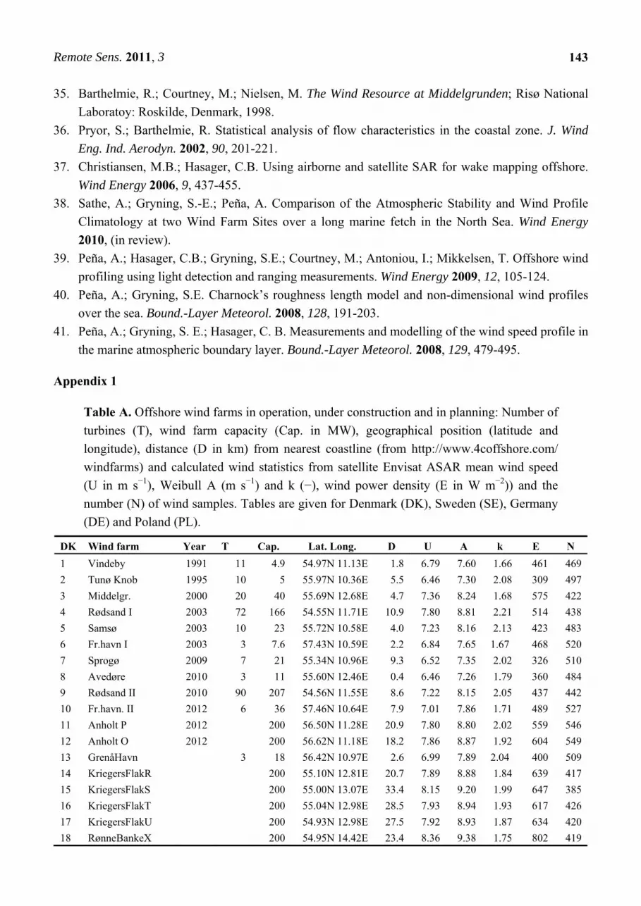
Table A. Offshore wind farms in operation, under construction and in planning: Number of

turbines (T), wind farm capacity (Cap. in MW), geographical position (latitude and

longitude), distance (D in km) from nearest coastline (from http://www.4coffshore.com/

windfarms) and calculated wind statistics from satellite Envisat ASAR mean wind speed

(U in m s−1), Weibull A (m s−1) and k (−), wind power density (E in W m−2)) and the

number (N) of wind samples. Tables are given for Denmark (DK), Sweden (SE), Germany

(DE) and Poland (PL).

DK Wind farm Year T Cap. Lat. Long. D U A k E N

1 Vindeby 1991 11 4.9 54.97N 11.13E 1.8 6.79 7.60 1.66 461 469

2 Tunø Knob 1995 10 5 55.97N 10.36E 5.5 6.46 7.30 2.08 309 497

3 Middelgr. 2000 20 40 55.69N 12.68E 4.7 7.36 8.24 1.68 575 422

4 Rødsand I 2003 72 166 54.55N 11.71E 10.9 7.80 8.81 2.21 514 438

5 Samsø 2003 10 23 55.72N 10.58E 4.0 7.23 8.16 2.13 423 483

6 Fr.havn I 2003 3 7.6 57.43N 10.59E 2.2 6.84 7.65 1.67 468 520

7 Sprogø 2009 7 21 55.34N 10.96E 9.3 6.52 7.35 2.02 326 510

8 Avedøre 2010 3 11 55.60N 12.46E 0.4 6.46 7.26 1.79 360 484

9 Rødsand II 2010 90 207 54.56N 11.55E 8.6 7.22 8.15 2.05 437 442

10 Fr.havn. II 2012 6 36 57.46N 10.64E 7.9 7.01 7.86 1.71 489 527

11 Anholt P 2012 200 56.50N 11.28E 20.9 7.80 8.80 2.02 559 546

12 Anholt O 2012 200 56.62N 11.18E 18.2 7.86 8.87 1.92 604 549

13 GrenåHavn 3 18 56.42N 10.97E 2.6 6.99 7.89 2.04 400 509

14 KriegersFlakR 200 55.10N 12.81E 20.7 7.89 8.88 1.84 639 417

15 KriegersFlakS 200 55.00N 13.07E 33.4 8.15 9.20 1.99 647 385

16 KriegersFlakT 200 55.04N 12.98E 28.5 7.93 8.94 1.93 617 426

17 KriegersFlakU 200 54.93N 12.98E 27.5 7.92 8.93 1.87 634 420

18 RønneBankeX 200 54.95N 14.42E 23.4 8.36 9.38 1.75 802 419


144

Table A. Cont.

19 RønneBankeV 200 54.89N 14.29E 34 8.37 9.39 1.75 809 420

20 Stora Midlgr.Q 200 56.50N 12.04E 44 8.00 9.02 1.95 624 524

SE Wind farm Year T Cap. Lat. Long. D U A k E N

1 Bockstigen 1998 5 3 57.04N 18.15E 5.8 7.08 7.97 1.86 456 442

2 Utgrunden I 2000 7 10 56.34N 16.28E 7.3 6.52 7.35 1.89 349 485

3 Ytre Stengr. 2001 5 10 56.17N 16.02E 3.7 6.62 7.45 1.89 364 459

4 Lillgrund 2007 48 110 55.51N 12.78E 9.3 7.73 8.70 1.86 592 419

5 Taggen 2012 83 300 55.86N 14.57E 16.3 7.09 7.99 1.88 453 436

6 KriegersFlakII 2015 128 640 55.07N 13.10E 32.4 7.95 8.95 1.83 657 407

7 StoraMiddelgr. 2016 108 540 56.61N 12.11E 34.3 7.96 8.98 1.97 610 525

8 Kårehamn 2016 50 56.98N 17.02E 7.0 6.59 7.43 1.93 354 482

9 Utgrunden II 2016 24 90 56.38N 16.27E 8.0 6.34 7.14 1.84 331 482

10 Blekinge 2019 500 2500 55.93N 15.02E 19.5 7.49 8.45 2.02 494 444

11 Trollboda 30 150 56.30N 16.18E 7.7 6.24 7.03 1.91 303 481

12 Södra Midsjö. 900 55.67N 17.27E 78.9 8.33 9.40 1.96 702 461

13 Klasarden 16 48 57.06N 18.16E 1.6 6.93 7.81 1.88 422 442

DE

1 Breitling 2008 1 2.5 54.16N 12.13E 0.3 7.33 8.24 1.81 523 161

2 EnBW Baltic1 2010 21 48 54.61N 12.65E 17.1 7.44 8.38 1.84 537 435

4 VentotecOst2 2014 80 400 54.83N 14.07E 40.0 8.30 9.34 1.86 733 406

5 ArkonaBeck Süd. 80 400 54.78N 14.12E 37.6 8.17 9.19 1.83 679 407

6 GEOFReE 5 25 54.25N 11.40E 18.6 6.91 7.80 1.97 714 419

7 Beta Baltic 50 115 54.28N 11.40E 15.8 6.99 7.89 2.02 585 418

8 ArkoniaSee Sud 80 80 54.78N 13.87E 26.4 8.19 9.24 1.93 403 385

9 ArkoniaSee West 80 80 54.80N 13.80E 25.8 8.17 9.21 1.88 679 387

10 ArcadisOstI 70 350 54.83N 13.60E 20.0 8.15 9.18 1.83 690 409

11 ArcadisOst2 25 75 54.82N 14.13E 40.9 8.16 9.18 1.84 707 398

12 Baltic Eagle 80 480 54.83N 13.87E 30.8 8.25 9.31 1.96 707 386

13 BalticPower West 80 400 54.93N 13.08E 31.8 8.09 9.13 1.98 682 386

14 Baltic Power East 80 400 54.97N 13.24E 33.4 8.23 9.27 1.87 637 411

15 AldergrundNord. 31 155 54.85N 14.06E 40.2 8.25 9.29 1.87 718 405

16 Aldergrund GAP 31 186 54.82N 14.13E 40.9 8.16 9.18 1.84 707 398

17 Aldergrund 500 20 72 54.82N 14.1E 39.0 8.26 9.29 1.84 729 408

18 Arkona SeeOst 150 54.86N 14.02E 39.8 8.25 9.28 1.84 726 405

19 Beltsee 25 125 54.44N 11.51E 13.2 7.14 8.06 2.03 427 434

PL

1 Poland P1 225 55.07N 16.64E 54.1 7.84 8.78 1.70 689 417

2 Poland P2 225 55.08N 16.9E 46.7 8.15 9.18 1.89 683 451

3 Poland P3 225 54.96N 18.21E 14.6 7.79 8.74 1.72 668 411

4 Poland P4 225 54.94N 18.37E 11.8 7.84 8.78 1.70 689 417

© 2011 by the authors; licensee MDPI, Basel, Switzerland. This article is an open access article

distributed under the terms and conditions of the Creative Commons Attribution license

(http://creativecommons.org/licenses/by/3.0/).

sar-based wind resource statistics in the baltic sea

Documents