1st Baltic Earth Conference

Multiple drivers for Earth system changes in the Baltic Sea regionNida, Curonian Spit, Lithuania13 - 17 June 2016

Conference Proceedings

International Baltic Earth Secretariat Publication No. 9, June 2016

Edited by Marcus Reckermann and Silke Köppen

Impressum

International Baltic Earth Secretariat Publications ISSN 2198-4247

International Baltic Earth Secretariat Helmholtz-Zentrum Geesthacht GmbH Max-Planck-Str. 1 D-21502 Geesthacht, Germany

www.baltic-earth.eu balticearth@hzg.de

Front page photo: The Great Dune near Nida on the Curonian Spit, Neringa, Lithuania (Martin Stendel)

Organizers and Sponsors Klaipėda University, Lithuania Helmholtz-Zentrum Geesthacht Centre for Materials and Coastal Research, Germany Swedish Meteorological and Hydrological Institute Norrköping, Sweden Uppsala University, Sweden Leibniz Institute for Baltic Sea Research Warnemünde, Germany

Conference Committee Juris Aigars, Latvia Franz Berger, Germany Inga Dailidienė, Lithuania Jari Haapala, Finland Sirje Keevallik, Estonia Karol Kulinski, Poland Andreas Lehmann, Germany H. E. Markus Meier, Germany and Sweden (Chair) Kai Myrberg, Finland Carin Nilsson, Sweden Anders Omstedt, Sweden Irina Partasenok, Belarus Piia Post, Estonia Marcus Reckermann, Germany Gregor Rehder, Germany Anna Rutgersson, Sweden (Vice-Chair) Corinna Schrum, Germany Benjamin Smith, Sweden Martin Stendel, Denmark Hans von Storch, Germany Ralf Weisse, Germany Sergey Zhuravlev, Russia Organisation Committee Inga Dailidienė, Lithuania Hans-Jörg-Isemer, Germany Silke Köppen, Germany H. E. Markus Meier, Germany and Sweden Marcus Reckermann, Germany Anna Rutgersson, Sweden Acknowledgments This conference is jointly organized by the University of Klaipeda, Lithuania, and the International Baltic Earth Secretariat at Helmholtz Zentrum Geesthacht, Germany. We would like to thank the sponsors for generously supporting the conference. Furthermore, we would like to thank the local organization committee, in particular Inga Dailidienė and Eglė Baltranaitė, and the numerous student helpers. Sabine Billerbeck, Sabine Hartmann and Hans-Jörg Isemer are acknowledged for their invaluable support before and during the conference. Very special thanks go to Silke Köppen of the International Baltic Earth Secretariat for brilliantly organizing the preparation of the conference and associated publications.

Preface Three years ago, Baltic Earth was launched at the final BALTEX Conference in June 2013 on Öland, Sweden. Since then, a lot has happened: An Interim (and later permanent) Science Steering Group was installed with some new faces, but keeping also some experienced BALTEX warriors to warrant continuity. Two summer schools were organized under the Baltic Earth flag, and it was very satisfying to see many students of those summer schools also participating at this conference, presenting their scientific work and actively contributing to the scientific discussion. Baltic Earth, together with different institutions has organized eight workshops, seminars or conference sessions, and two major topical conferences. Then, the second BACC book was published in April 2015 which was a major effort of the BALTEX-Baltic Earth community. Last but not least, a Baltic Earth Science Plan was drafted and will be presented to the Baltic Earth community at this conference. The science plan is intended to reach a large spectrum of scientists and stakeholders in order to attract a wide range of players in the region to Baltic Earth.

The topic of this 1st dedicated Baltic Earth Conference was suggested and discussed at the 2nd Meeting of the Baltic Earth Interim Science Steering Group in Sopot, Poland in November 2013. It arose from the understanding that the regional Earth System changes we perceive are really a mixture of different factors interwoven in complicated ways, and of which climate change is one driver. This was one of the lessons from the BACC II book.

Still, the sessions of this conference reflect the Baltic Earth Grand Challenges plus the conference topic as a brand new Grand Challenge (as of 2016):

• Salinity dynamics • Land-Sea-Atmosphere biogeochemical feedbacks • Natural hazards and high impact events • Sea level dynamics, coastal morphology and erosion • Regional variability of water and energy exchanges • Regional climate system modeling • Multiple and interrelated drivers of environmental changes

The conference is also intended to be a discussion forum about the perspective and future prospects of Baltic Earth, and the new challenges at the horizon. This will be discussed during the two dedicated plenary discussion slots.

For this first Baltic Earth conference, we have received 134 abstracts from 13 countries, among them also countries outside the Baltic Sea region. As for the previous BALTEX conference proceedings, no discrimination is made in this volume regarding poster or oral presentation; they are all sorted alphabetically within topics. We see the large number of abstracts as an indication that Baltic Earth is attractive to a wide range of scientists around the Baltic Sea, and we hope that this interest may still increase in the future.

Markus Meier, Anna Rutgersson and Marcus Reckermann For the Conference Committee

Contents

Contributions are sorted within topics alphabetically.

Keynotes and special talks Rehabilitating the Chesapeake Bay (USA) ecosystem under changing climate Donald F. Boesch, Z. Johnson, M. Li ............................................................................................. 1 Interrelation of geosphere, climate processes and anthroposphere in the Baltic Sea basin during the Holocene Jan Harff, H. Jöns, A. Rosentau ...................................................................................................... 3 Agriculture in the Baltic Sea region, major driver and challenges Christoph Humborg ...................................................................................................................... 4 PannEx: Towards a Regional Hydroclimate Project in the Pannonian Basin Mónika Lakatos, I. Güttler, J. Cuxart Rodamilans ........................................................................ 5 Connecting Analytical Thinking and Intuition: Challenges for leadership and education in Earth System Sciences Anders Omstedt ............................................................................................................................ 7 Two centuries of extreme events over the Baltic Sea and North Sea regions Martin Stendel, E. van den Besselaar, A. Hannachi, J. Jaagus, E. Kent, E. Lefebve, G. Rosenhagen, A. Rutgersson, F. Schenk, G. van der Schrier, T. Woollings ................................... 9

Topic A: Salinity dynamics

Benthic foraminifera record environmental and climate changes in the Bornholm Basin (Baltic Sea) over the last 6 millennia Anna Binczewska, P. Astemann, M. Moros, J. Sławińska ........................................................... 11 Marine saline water intrusions and variation in the Curonian Lagoon Inga Dailidiene, L. Davuliene, V. Genyte .................................................................................... 12 Tracer studies of water exchange in Gulf of Riga, winter 2015-2016 Vilnis Frishfelds, U. Bethers, J. Sennikovs .................................................................................. 13 Investigation of properties of inertial waves on the base of long-term ADCP data at moored stations in the Slupsk Furrow and Gdansk Deep Maria Golenko, K. Sabinin, D. Rak .............................................................................................. 15

On the role of the haline conditions in the Belt Sea in the formation of highly saline barotropic inflows to the Baltic Sea. Katharina Höflich, A. Lehmann, K. Myrberg ............................................................................... 16 Pathways of deep cyclones associated with large volume changes (LVCs) and Major Baltic Inflows (MBIs) Andreas Lehmann, K. Höflich, P. Post, K. Myrberg .................................................................... 18 High-resolution view on the subsurface salinity maxima in the Gulf of Riga Taavi Liblik, M. Skudra, U. Lips ................................................................................................... 20 Statistics of deep estuarine circulation vs reverse estuarine circulation in the Gulf of Finland Madis-Jaak Lilover, J. Elken, T. Liblik .......................................................................................... 21 Salinity oscillations in the range of seasonal variability Ekaterina Litina, E. Zakharchuk .................................................................................................. 23 The impact of the recent series of barotropic inflows on deep water conditions in the Eastern Gotland Basin – time series observations. Volker Mohrholz, T. Heene, S. Beier, G. Nausch, M. Naumann ................................................. 25 A succession of four Major Baltic Inflows in the period 2014-2016 – an overview of propagation and environmental change Michael Naumann, G. Nausch, V. Mohrholz .............................................................................. 27 Assessment of long time series of atmospheric circulation patterns forcing large volume changes and major inflows to the Baltic Sea Piia Post, A. Lehmann ................................................................................................................. 28 A high resolution NEMO-Nordic setup for the Gulf of Bothnia Semjon Schimanke, R. Hordoir, K. Eilola .................................................................................... 30 The dynamic of thermohaline regime of the Baltic Sea after “Major Baltic Inflow” 2014 Sergey Shchuka, D. Rak, V. Solovyev, A. Staskiewicz ................................................................. 31 Using shallow-water Argo floats to monitor the Major Baltic Inflows in the Gotland Deep Simo Siiriä, L. Tuomi, P. Roiha, T. Purokoski, P. Alenius ............................................................. 33 Sedimentology and geochemistry of marine deposits from Bornholm and Gdansk Basins - stratigraphical records Joanna Sławińska, R. Borowka, M. Moros, A. Binczewska, M. Bak ........................................... 34

Topic B: Land-sea-atmosphere biogeochemical feedbacks

Model based inventory of nutrient retention efficiency and coastal filter function along the entire Swedish coast Moa Edman, E. Almroth-Rosell, K. Eilola, J. Sahlberg, H. E. M Meier ....................................... 35 The role of the cyanobacteria life cycle on biogeochemistry of the Baltic Sea - a 3D high resolution coupled physical biogeochemical model study Kari Eilola, E. Almroth-Rosell, M. Gröger, J. Hieronymus, B. Karlson, Y. Liu, S. Saraiva, I. Wahlström, I. Hense, H. E. M. Meier .......................................................................................... 37 Large interspecific differences in dissolved organic carbon decomposition from boreal litter sources Geert Hensgens, C. Arellano, B. Smith, A. Poska, M. Berggren ................................................. 39 Magnetic susceptibility of the surface layer of bottom sediments of the South Baltic, as a quality parameter in the assessment of selected metals pollution of the marine environment Żaneta Kłostowska, L. Łęczyński, G. Kusza, A. Kubowicz-Grajewska, T. Ossowski, D. Zarzeczańska, P. Hulisz, E. Bublijewska ..................................................................................... 41 Peculiarities of the Baltic Sea acid-base system Karol Kuliński, B. Schneider, B. Szymczycha, K. Hammer, A. Winogradow, M. Stokowski, K. Koziorowska ............................................................................................................................... 42 High-resolution modelling of 3D-hydrodynamics in the Finnish Archipelago Sea Elina Miettunen, L. Tuomi, J. Ropponen, R. Lignell .................................................................... 44 Long-term alkalinity trends in the Baltic Sea and their implications for CO2-induced acidification Jens Müller, B. Schneider, G. Rehder ......................................................................................... 46 Modelling pelagic carbon and nutrient turnover without bacteria? Bärbel Müller-Karulis, J. Sundh, C. Karlsson, C. Humborg, Å. Hagström ................................... 48 Modelling the contributions to marine acidification from deposited SOx, NOx, and NHx in the Baltic Sea: Past, present and possible future situations Anders Omstedt, D. Turner, M. Edman, J. Gallego-Urrea, B. Claremar, I-M. Hassellöv, A. Rutgersson .................................................................................................................................. 50 Riverine carbon export and its impacts on Finnish coastal water quality Antti Räike, V. Fleming-Lehtinen, P. Kortelainen, T. Mattsson, P. Kauppila, D. Thomas .......... 52 Abrupt changes in distribution patterns and dynamics of methane and nitrous oxide in the Central Baltic Sea as a consequence of the 2014-2015 Major Baltic Inflow Gregor Rehder, J. Werner, G. Jakobs, L. Umlauf, S. Otto, O. Schmale ....................................... 53

Air-Sea CO2 exchange in the Baltic Sea Anna Rutgersson, E. Sahlée, G. Parard ....................................................................................... 55 Large scale, high resolution land-use based hydrological model for the territory of Lithuania Juris Sennikovs, U. Bethers, S. Plunge, P. Bethers ..................................................................... 57 Robustness and uncertainty in future nutrient loads from land ecosystems across the Baltic Sea catchment area Ben Smith, M. Lindeskog, K. Engström, S. Olin, A. Poska ........................................................... 59 Eutrophication assessments using ecosystem model data Adolf Stips, D. Macia, E. Garcia-Gorriz, S. Miladinova, T. Neumann .......................................... 60 Groundwater discharge to the southern Baltic Sea Beata Szymczycha, J. Pempkowiak ............................................................................................. 62 Carbon-based nutrient cycling modeling of the Baltic Sea: Analysis of twelve basins using three-dimensional flow dynamics for period 2001-2009 Guillaume Vigouroux, V. Cvetkovic, A. Jönsson ........................................................................ 64 Changes of sedimentary organic matter en route from source to sink areas in the Southern Baltic Aleksandra Winogradow, J. Pempkowiak .................................................................................. 66 High nitrite concentration inhibits nitrite-adapted granular anammox biomass less compared to biofilm Ivar Zekker, M. Raudkivi, E. Rikmann, P. Vabamäe, K. Kroon, T. Tenno ................................... 67

Topic C: Natural hazards and high impact events

Relationships of cloud-to-ground lightning with circulation weather types over Estonia 2005–2014 Regina Alber, P. Post, M. Sepp ................................................................................................... 69 HOAPS water vapour characteristic during storms and heavy precipitation events over SE Baltic Sea region Agne Djačenko, G. Stankūnavičius ............................................................................................ 71 Will there be extreme sea ice winters in future? Jari Haapala, P. Uotila, B. An ...................................................................................................... 73 netBaltic – a heterogeneous wireless communications system over the Baltic Sea Michal Hoeft, K. Gierlowski, J. Wozniak, A. Przyborska, M. Białoskórski, B. Pliszka, M. Wichorowski, M. Zwierz, J. Jakacki ............................................................................................ 74

Numerical modelling of convective snow bands in the Baltic Sea area using atmosphere-ocean-wave coupled model systems Julia Jeworrek, L. Wu, A. Rutgersson.......................................................................................... 76 Return period of Estonian precipitation extremes Jüri Kamenik ............................................................................................................................... 78 Changes in the wave climate and severity of storms in the Baltic Sea in 1991 – 2015 from satellite altimetry Nadia Kudryavtseva, T. Soomere ............................................................................................... 80 Summertime thunderstorms prediction in Belarus Palina Lapo, Y. Sokolovskaya, A. Krasouski, A. Svetashev, L. Turishev, S. Barodka ................... 82 Drought monitoring in Lithuania using NDVI Viktorija Mačiulytė, E. Rimkus .................................................................................................... 84 The special features of the wind waves in the Baltic Sea following the results of numerical modelling Alisa Medvedeva, V. Arkhipkin, S. Myslenkov ........................................................................... 86 Heat waves in Belarus Viktar Melnik, Y. Sokolovskaya .................................................................................................. 88 Main trends of climate changes and severe weather activity for last decades across the territory of the Republic of Belarus Viktar Melnik, E. Komarovskaya ................................................................................................ 90 The new established Expertennetzwerk: The focus-region “Südwestliches Schleswig-Holstein” and a case study to long-term changes in the intensity of extreme water levels Jens Möller, H. Heinrich ............................................................................................................. 92 Possible consequences of the construction of the NPP "Hanhikivi-1" for the marine environment of the Gulf of Bothnia: model estimates Vladimir Ryabchenko, A. Dvornikov, T. Eremina, A. Isaev, S. Martyanov .................................. 94 Projected lengthening of spring cereals growing season in Estonia and accompanying high impact events of elevated temperatures Triin Saue, L. Jauhiainen, J. Kadaja, P. Peltonen-Sainio ............................................................. 96 Analysis of severe weather using WRF model Virmantas Šmatas, G. Stankūnavičius ....................................................................................... 98 Extreme weather condition of the northern-eastern part of Poland and their relationship with atmospheric oscillation Zbigniew Szwejkowski, E. Dragańska, I. Cymes, S. Suchecki ................................................... 100

Meteorological observations of signal stations - a data source for the analysis of extreme weather events? Birger Tinz, D. Röhrbein, H. von Storch .................................................................................... 101 Change of extreme floods parameters in the Nemunas River lower reaches and delta Gintaras Valiuškevičius, G. Stankūnavičius, E. Stonevičius, J. Brastovickytė .......................... 102 Assessment of spatial variation of extreme wind speeds Ari Venäläinen, P. Pirinen, M. Horttanainen, M. Laapa, R. Hyvönen, I. Lehtonen, P. Junila, H. Peltola ....................................................................................................................................... 104 Thunderstorm hail and lightning prediction parameters based on dual polarization Doppler weather radar data Tanel Voormansik, P. Post, T. Tanilsoo, D. Moisseev, P. Rossi ................................................. 105 Drivers of precipitation extremes in different spatial and temporal scales Joanna Wibig, P. Piotrowski ..................................................................................................... 107 Detection of trends in the magnitude of spring floods for the eastern parts of the Gulf of Finland basin Sergei Zhuravlev, L. Kurochkina, T. Shalashina ........................................................................ 108

Topic D: Sea level dynamics, coastal morphology and erosion

Investigating sediment resuspension using combined optical and acoustic methods Fred Buschmann, A. Erm, J. Rebane, M. Listak ........................................................................ 111 Intensity of Eolian processes on Lithuanian part of Curonian Spit Algimantas Česnulevičius, A. Bautrėnas, L. Bevainis, R. Morkūnaitė, D. Ovodas .................... 112 A model for simulating extreme sea levels in the Baltic Sea Christian Dieterich, M. Gröger, H. Andersson, S. Nerheim, A. Jönsson .................................. 114 Impacts of regional climate change on the potential longshore sediment transport at the German Baltic Sea coast Norman Dreier, P. Fröhle ......................................................................................................... 115 Interrelated drivers of coastline change in the Baltic Sea Jan Harff, J. Deng, J. Dudzinska-Nowak, A. Groh, B. Hünicke, W. Zhang ................................. 117 Rapid changes in sea level Jürgen Holfort, I. Perlet, I. Stanislawczyk ................................................................................ 119 Acceleration of mean sea-level rise in the Baltic Sea since 1900 Birgit Hünicke, E. Zorita ............................................................................................................ 120

Attribution of storm surge events in the southern Baltic Sea to anthropogenic influences Katharina Klehmet, B. Rockel ................................................................................................... 122 Extreme statistics of storm surges in the Baltic Sea Evgueni Kulikov, I. Medvedev .................................................................................................. 123 The sea level variability at the southeastern coast of the Baltic Sea: from hours to centuries Igor Medvedev, E. Kulikov, A. Rabinovich ................................................................................ 124 Spatial variation of statistical properties of extreme water levels along the eastern Baltic Sea coast Katri Pindsoo, M. Eelsalu, T. Soomere ..................................................................................... 126 Assessment of long-term dynamics of the Curonian Spit foredune in response to hydrometeorological regime change Donatas Pupienis, I. Buynevich, N. Dobrotin, D. Jarmalavičius, G. Žilinskas, L. Jukna, A. Cichon-Pupienis ........................................................................................................................ 128 Determining the combined probability of occurrence of storm surge hydrographs and extreme sea state conditions Dörte Salecker, A. Gruhn, P. Fröhle .......................................................................................... 130 Simulating sea level variations in the Baltic Sea using regional climate scenarios Jani Särkkä, K. Kahma, M. Kämäräinen, M. Johansson ........................................................... 131 Water level extremes signal changes in the wind direction in the north-eastern Baltic Sea Tarmo Soomere, M. Eelsalu, K. Pindsoo .................................................................................. 132

Topic E: Regional variability of water and energy exchanges

Changes in UV radiation in Estonia based on measurements and model calculations of UVA and UVB doses since 1955 at Tõravere Margit Aun, K. Eerme, M. Aun, I. Ansko ................................................................................... 135 Numerical simulation of hydrodynamic process at Oskarshamn harbor—coupling model with Baltic Sea Yuanying Chen, V. Cvetkovic .................................................................................................... 137 Multi-annual eddy-covariance measurements of surface energy balance components for urban, agricultural and natural wetland sites in Poland Krzysztof Fortuniak, W. Pawlak, M. Siedlecki........................................................................... 139 Does soil frost-induced soil moisture precipitation feedback play a role over the Baltic Sea catchment? Stefan Hagemann, T. Blome ..................................................................................................... 141

Regime shift in winter climatic conditions and river runoff in Estonia since the winter 1988/89 Jaak Jaagus, M. Sepp ................................................................................................................ 143 COST Action ES1206: Advanced GNSS tropospheric products for monitoring severe weather events and climate (GNSS4SWEC) Jonathan Jones, G. Guerova, J. Dousa, G. Dick, S. de Haan, E. Pottiaux, O. Bock, R. Pacione . 145 Detection of cold and warm anomalies: The example of Estonia Sirje Keevallik ............................................................................................................................ 146 Luninsky swampland water-level regime Alena Kvach, L. Zhuravovich ..................................................................................................... 148 Sea-lagoon interaction during upwelling processes in the SE Baltic Sea Toma Mingelaite, I. Dailidiene, I. Kozlov ................................................................................. 150 The ice seasons severity by the ice extents sum on the Baltic Sea during 1982-2015 Ove Pärn, J. Rjazin, R. Uiboupin ............................................................................................... 151 Projection of climate changes in Belarus according to ensemble models Irina Partasenok, B. Geyer ........................................................................................................ 153 The spatio-temporal changes of ice regim in the Baltic Sea basin rivers in the Republic of Belarus in a period of global warming Ala Pauros ................................................................................................................................. 155 Precipitation in coastal area of Poland Piotr Piotrowski, J. Jędruszkiewicz, M. Zieliński ...................................................................... 156 The BALTEX Box revisited: The energy budget of the Baltic Sea in the coupled regional climate model REMO-BSIOM Thomas Raub, K. Getzlaff, D. Jacob, A. Lehmann ..................................................................... 158 Relationship between air temperature and sea water temperature in the different depths of SE Baltic Sea Viktorija Rukšėnienė, I. Dailidiene, L. Kelpšaitė-Rimkienė ...................................................... 160 Changes in the life cycle characteristics of cyclones entering the Baltic Sea region Mait Sepp, P. Post, K. Mändla, R. Aunap .................................................................................. 162 Water level changes of the Emajõgi and the Neman rivers in the vegetation period Mait Sepp, A. Järvet ................................................................................................................. 164

Topic F: Regional climate system modeling

The temporal and spatial distribution of the cool episode about 8.2 ka ago in the Baltic Sea basin and surrounding areas Irena Borzenkova, O. Borisova, T. Sapelko ............................................................................... 165 Validity of pattern scaling investigated with a multi-model RCM ensemble over Europe Ole B. Christensen, S. Yang, F. Boberg, C. Fox Maule, P. Thejll, M. Olesen, M. Drews, J. Sørup, J.-H. Christensen ....................................................................................................................... 167 On the relevance of higher trophic levels for modelling ecosystem dynamics in the Baltic Sea Ute Daewel, C. Schrum ............................................................................................................. 168 NEMO-Nordic-SCOBI: A new biogeochemistry model for the North Sea and Baltic Sea Matthias Gröger, E. Almroth-Rosell, H. Anderson, K. Eilola, S. Falahat, F. Frasner, R. Hordoir, A. Höglund, J. Hieronymus, I. Kuznetzov, H. E. M. Meier, S. Saraiva ....................................... 169 A potential remote impact of air-sea coupling over the North and Baltic Sea on precipitation simulated over Central Europe Ha T. M. Ho-Hagemann, M. Gröger, B. Rockel, M. Zahn, B. Geyer, H. E. M. Meier ................ 171 Arctic region climate teleconnections with Baltic Sea region by NCEP-CFSR reanalysis Erko Jakobson, L. Jakobson, P. Post, J. Jaagus .......................................................................... 173 Hydrothermal conditions in Poland until year 2060 and selected climate change scenarios Leszek Kuchar, S. Iwański, E. Gasiorek, E. Diakowska .............................................................. 175 Evaluation of the coupled COSMO-CLM+NEMO-Nordic model with focus on North and Baltic seas Jennifer Lenhardt, J. Brauch, B. Früh, T. von Pham ................................................................. 177 Estimating uncertainties in projections for the Baltic Sea region based upon an ensemble of regional climate system models Markus Meier, M. Edman and members of the Baltic Earth working group on scenario simulations for the Baltic Sea 1960-2100 ................................................................................ 179 The North Sea Region Climate Change Assessment (NOSCCA): What happens in the south west of BACC? Markus Quante, F. Colijn, I. Nöhren ........................................................................................ 180 Comparison of Observed and Modelled Radiative Energy Flows Ehrhard Raschke, S. Kinne ........................................................................................................ 182

An extended North- and Baltic Sea climatology (NBSC) of atmospheric and hydrographic in-situ data Nils H. Schade, R. Sadikni, A. Jahnke-Bornemann, I. Hinrichs .................................................. 183 The future climate regions in Estonia Mait Sepp, T. Tamm, V. Sagris .................................................................................................. 185 Daily temperature and precipitation extremes in the Baltic Sea region derived from the BaltAn65+ reanalysis and EOBS database Velle Toll, P. Post ...................................................................................................................... 186 Climatic wave modeling in Baltic Proper and Gulf of Riga using SWAN Aigars Valainis, U. Bethers, J. Sennikovs .................................................................................. 188

Topic G: Multiple and interrelated drivers of environmental changes

The impact of the urban surface runoff on the receiving river: the case study of Brest, Belarus Ina Bulskaya, A. Kolbas, D. Dyliuk, A. Kuuzmitsky ................................................................... 189 Curonian Lagoon bathing water quality assessment trough microbial pollution modelling Natalja Čerkasova, M. Kataržytė, G. Umgiesser, E. Baltranaitė ............................................... 190 Coastal resources understanding and local governance development: Socio-ecological system and indicators prerequisite Raimonds Ernsteins, E. Lagzdina, J. Lapinkis, A. Lontone, J. Kaulins, I. Kudrenickis ................ 191 The impact of wrecks on the geochemical properties of the surface layer of marine bottom sediments in wrecks deposition areas: The example of ORP Wicher Tomasz Figiel, P. Wysocki, Z. Kłostowska, L. Łęczyński, T. Ossowski, D. Zarzeczańska, M. Figurski ..................................................................................................................................... 193 Using integrated modeling to derive the historical water quality in the south-western Baltic Sea René Friedland, T. Neumann, G. Schernewski ......................................................................... 194 Changes of the baltic sea coastal urban region (with exemple of Klaipeda settlement) Jelena Galiniene, D. Verkuleviciute, S. Gadal .......................................................................... 195 Deposition of sulfur, nitrogen and particles originating from shipping activities in the Baltic and North Seas Karin Haglund, B. Claremar, A. Rutgersson .............................................................................. 197 Analysis of the spread of chemical munitions dumped in the Baltic Sea Jaromir Jakacki, A. Przyborska, M. Białoskórski, B. Pliszka ...................................................... 199

On some hydrometeorological monitoring results in the south-eastern part of the Baltic sea during the last decade Mariya Kapustina, T. Bukanova, Z. Stont ................................................................................. 201 Which factors affect metal and radionuclide pollution in the Baltic Sea? Martin Lodenius ....................................................................................................................... 203 Dialogue- and communication forms as parallel infrastructure of climate- and coastal research at the Southern Baltic Sea coast Insa Meinke .............................................................................................................................. 205 SHEBA – Sustainable shipping and environment of the Baltic Sea Jana Moldanova, M. Quante .................................................................................................... 206 6000 years of human-land-sea interactions: Estimating the impact of land-use and climate changes on DOC production in the Baltic Sea catchment Anneli Poska, B. Pirzamanbin, A. Nielsen, H. Filipsson, M. Lindeskog, B. Smith, D. Conley .... 208 Future projections of pine growth dynamics at peat and mineral soils in Lithuania Egedijus Rimkus, J. Kažys, J. Edvardsson, R. Pukiene, C. Corona, R. Linkevičienė, M. Stoffel .. 209 Myths of the Baltic Sea eutrophication Oleg P. Savchuk ........................................................................................................................ 211 Cluster analysis of contemporary and future climate of Latvia Juris Sennikovs, I. Klints, U. Bethers ......................................................................................... 213 Restoration of the Baltic Proper by decadal oxygenation of the deepwater Anders Stigebrandt ................................................................................................................... 215 Climate change effect on snow climate in Neman basin Edvinas Stonevicius, E. Rimkus, A. Staras, G. Vasiuskevicius ................................................... 216 Psychophysical aesthetic ranking of coastal landscapes: A case study of the Curonian Spit (Lithuania) Arvydas Urbis, R. Povilanskas ................................................................................................... 218 Conceptual challenges of climate servicing Hans von Storch........................................................................................................................ 219 Management of reclaimed coastal areas: case of the new Bronka port in the Neva Bay Vladimir Zhigulski, M. Shilin, A. Ershova .................................................................................. 221

Author Index Alber, R. ....................................... 69 Alenius, P. ..................................... 33 Almroth-Rosell. E. ........... 35, 37, 169 An, BW. ......................................... 73 Andersson, H. ..................... 114, 169 Ansko, I ....................................... 135 Arellano, C. .................................. 39 Arkhipkin, V. ................................ 86 Asteman, P. ................................... 11 Aun, Margit. ................................ 135 Aun, Martin ................................. 135 Aunap, R. .................................... 162 Bak, M. .......................................... 34 Baltranaitė, E. ............................. 190 Barodka, S. .................................... 82 Bautrėnas, A. ............................. 112 Beier, S. ......................................... 25 Berggren, M. ................................ 39 Bethers, P...................................... 57 Bethers, U. ............. 13, 57, 188, 213 Bevainis, L. ................................. 112 Białoskórski, M. .................... 74, 199 Binczewska, A. ........................ 11, 34 Blome, T. .................................... 141 Boberg, F. .................................... 167 Bock, O. ....................................... 145 Boesch, D. ....................................... 1 Borisova, O. ................................ 165 Borowka, R. ................................... 34 Borzenkova, I. ............................ 165 Brastovickytė, J. .......................... 102 Brauch, J. .................................... 177 Bublijewska, E. .............................. 41 Bukanova, T. ............................... 201 Bulskaya, I. .................................. 189 Buschmann, F. ........................... 111 Buynevich, I. ............................... 128 Čerkasova, N. .............................. 190 Česnulevičius, A. ........................ 112 Chen, Y. ...................................... 137 Christensen, J-H. ......................... 167 Christensen, OB. ......................... 167 Cichon-Pupienis, A. ..................... 128 Claremar, B. .......................... 50, 197 Colijn, F. ...................................... 180 Conley, D. .................................... 208 Corona, C. ................................... 209 Cuxart Rodamilans, J....................... 5 Cvetkovic, V. ......................... 64, 137 Cymes, I. ..................................... 100

Daewel, U. ................................. 168 Dailidiene, I. .................. 12, 150, 160 Davuliene, L. ................................. 12 de Haan, S. ................................. 145 Deng, J. ....................................... 117 Diakowska, E. ............................. 175 Dick, G. ....................................... 145 Dieterich, C. ................................ 114 Djačenko, A. ................................. 71 Dobrotin, N. ............................... 128 Dousa, J. ..................................... 145 Dragańska, E. .............................. 100 Dreier, N. ................................... 115 Drews, M. ................................... 167 Dudzinska-Nowak, J ................... 117 Dvornikov, A. ................................ 94 Dyliuk, D. .................................... 189 Edman, M. ....................... 35, 50, 179 Edvardsson, J. ............................. 209 Eelsalu, M. ......................... 126, 132 Eerme, K. .................................... 135 Eilola, K. ..................... 30, 35, 37, 169 Elken, J. ........................................ 21 Engström, K. ................................. 59 Eremina, T. ................................... 94 Erm, A. ....................................... 111 Ernsteins, R. ............................... 191 Ershova, A. ................................. 221 Falahat, S. ................................... 169 Figiel, T. ..................................... 193 Figurski, M. ................................ 193 Filipsson, H. ................................ 208 Fleming-Lehtinen, V. .................... 52 Fortuniak, K. ............................... 139 Fox Maule, C............................... 167 Frasner, F.................................... 169 Friedland, R. ............................... 194 Frishfelds, V. ................................. 13 Fröhle, P. ........................... 114, 130 Früh, B. ....................................... 177 Gadal, S. ..................................... 195 Galiniene, J. ............................... 195 Gallego-Urrea, J. ........................... 50 Garcia-Gorriz E ............................. 60 Gasiorek, E. ................................ 175 Genyte, V. ..................................... 12 Getzlaff, K. .................................. 158 Geyer, B. ............................. 153, 171 Gierlowski, K. ............................... 74 Golenko, M. .................................. 15

Gröger, M. ............ 37, 114, 169, 171 Groh, A. ....................................... 117 Gruhn, A. .................................... 130 Guerova. G. ................................. 145 Güttler, I.......................................... 5 Haapala, J. ..................................... 73 Hagemann, H. ............................. 171 Hagemann, S. ............................. 141 Haglund, K. .................................. 197 Hagström, A. ................................. 48 Hammer, K. .................................. 42 Hannachi, A. .................................... 9 Harff, J. .................................... 3, 117 Hassellöv, I-M. .............................. 50 Heene, T. ...................................... 25 Heinrich, H. ................................... 92 Hense, I. ........................................ 37 Hensgens, G. ................................ 39 Hieronymus, J. ...................... 37, 169 Hinrichs, I. ................................... 183 Hoeft, M. ....................................... 74 Höflich, K. ................................ 16, 18 Höglund, A. ................................. 169 Holfort, J. .................................... 119 Hordoir, R. ............................ 30, 169 Horttanainen, M. ........................ 104 Hulisz, P. ....................................... 41 Humborg, C. .............................. 4, 48 Hünicke, B. .......................... 117, 120 Hyvönen, R. ................................. 104 Isaev, A. ......................................... 94 Iwański, S. ................................... 175 Jaagus, J. ......................... 9, 143, 173 Jacob, D. ...................................... 158 Jahnke-Bornemann, A. ............... 183 Jakacki, J................................ 74, 199 Jakobs, G. ..................................... 53 Jakobson, E. ................................ 173 Jakobson, L. ................................ 173 Jarmalavičius, D. ......................... 128 Järvet, A. .................................... 164 Jauhiainen, L. ................................ 96 Jędruszkiewicz, J. ........................ 156 Jeworrek, J. ................................... 76 Johansson, M. ............................. 131 Johnson, Z. ...................................... 1 Jöns, H. ............................................ 3 Jönsson, A. ............................ 64, 114 Jones, J. ....................................... 145 Jukna, L. ...................................... 128 Junila, P. ...................................... 104 Kadaja, J. ....................................... 96 Kahma, K. .................................... 131

Kämäräinen, M. .......................... 131 Kamenik, J. ................................... 78 Kapustina, M. ............................. 201 Karlson, B. .................................... 37 Karlsson, C. ................................... 48 Kataržytė, M. .............................. 190 Kaulins, J. .................................... 191 Kauppila, P. .................................. 52 Kažys, J. ...................................... 209 Keevallik, S. ................................ 146 Kelpšaitė-Rimkienė, L. ................ 160 Kent, E. ........................................... 9 Kinne, S....................................... 182 Klehmet, K. ................................. 122 Klints, I. ....................................... 213 Kłostowska, Ż. ......................41, 193 Kolbas, A. .................................... 189 Komarovskaya, E. ......................... 90 Kortelainen, P. .............................. 52 Koziorowska, K. ........................... 42 Kozlov, I ...................................... 150 Krasouski, A .................................. 82 Kroon, K. ....................................... 67 Kubowicz-Grajewska, A. ............... 41 Kuchar, L. .................................... 175 Kudrenickis, I. ............................. 191 Kudryavtseva, N. ......................... 80 Kulikov, E. ........................... 123, 124 Kuliński, K. ................................... 42 Kurochkina, L. ............................. 108 Kusza, G. ....................................... 41 Kuzmitsky, A. .............................. 189 Kuznetzov, I ................................ 169 Kvach, A. ..................................... 148 Laapas, M. .................................. 104 Lagzdina, E.................................. 191 Lakatos, M. ..................................... 5 Lapinkis, J. .................................. 191 Lapo, P. ......................................... 82 Łęczyński, L. ...........................41, 193 Lefebve, E. ...................................... 9 Lehmann, A. .............. 16, 18, 28, 158 Lehtonen, I. ................................ 104 Lenhardt, J. ................................. 177 Li, M................................................ 1 Liblik, T. ................................... 20, 21 Lignell, R. ...................................... 44 Lilover, M-J. .................................. 21 Lindeskog, M. ........................59, 208 Linkevičienė, R. .......................... 209 Lips, U. .......................................... 20 Listak, M. ................................... 111 Litina, E. ........................................ 23

Liu, Y. ............................................ 37 Lodenius, M. .............................. 203 Lontone, A. ................................. 191 Macias, D. ..................................... 60 Mačiulytė, V. ................................. 84 Mändla, K. .................................. 162 Martyanov, S................................. 94 Mattsson, T. .................................. 52 Medvedev, I. ....................... 123, 124 Medvedeva, A. .............................. 86 Meier, H.E.M. ... 35, 37, 169, 171,179 Meinke, I. .................................... 205 Melnik, V. ................................ 88, 90 Miettunen, E. ................................ 44 Miladinova S ................................. 60 Mingelaite, T. .............................. 150 Möller, J. ....................................... 92 Mohrholz, V. ........................... 25, 27 Moisseev, D. .............................. 105 Moldanová, J. ............................. 206 Morkūnaitė, R. ............................ 112 Moros, M. ............................... 11, 34 Müller, J. ....................................... 46 Müller-Karulis, B. .......................... 48 Myrberg, K. ............................. 16, 18 Myslenkov, S. ................................ 86 Naumann, M. .......................... 25, 27 Nausch, G. ............................... 25, 27 Nerheim, S. ................................. 114 Neumann, T. ......................... 60, 194 Nielsen, A. ................................... 208 Nöhren, I. .................................... 180 Olesen, M.................................... 167 Olin, S. ........................................... 59 Omstedt, A. ............................... 7, 50 Ossowski, T. .......................... 41, 193 Otto, S. ......................................... 53 Ovodas, D. ................................... 112 Pacione, R. .................................. 145 Parard, G. ...................................... 55 Pärn, O. ....................................... 151 Partasenok, I. .............................. 153 Pauros, A. .................................... 155 Pawlak, W. .................................. 139 Peltola, H. ................................... 104 Peltonen-Sainio, P. ....................... 96 Pempkowiak, J. ....................... 62, 66 Perlet, I. ...................................... 119 Pindsoo, K. ......................... 126, 132 Piotrowski, P. ...................... 107, 156 Pirinen, P. .................................... 104 Pirzamanbin, B. ........................... 208 Pliszka, B. .............................. 74, 199

Plunge, S. ...................................... 57 Poska, A. .......................... 39, 59, 208 Post, P. . 18, 28, 69, 105, 162, 73,186 Pottiaux, E. ................................. 145 Povilanskas, R. ............................ 218 Przyborska, A.........................74, 199 Pukiene, R. ................................. 209 Pupienis, D. ................................ 128 Purokoski, T. ................................. 33 Quante, M. ......................... 180, 206 Rabinovich, A. ............................ 124 Räike, A. ....................................... 52 Rak, D. ..................................... 15, 31 Raschke, E. ................................. 182 Raub, T. ...................................... 158 Raudviki, M. ................................. 67 Rebane, J. .................................. 111 Rehder, G. ............................... 46, 53 Rikmann, E. .................................. 67 Rimkus, E. ...................... 84, 209, 216 Rjazin, J. ...................................... 151 Rockel, B. ............................ 122, 171 Röhrbein, D. .............................. 101 Roiha, P. ....................................... 33 Ropponen, J.................................. 44 Rosenhagen, G. .............................. 9 Rosentau, A. ................................... 3 Rossi, P. ..................................... 105 Rukšėnienė, V. ............................ 160 Rutgersson, A. ....... 9, 50, 55, 76, 197 Ryabchenko, V.............................. 94 Sabinin, K. ..................................... 15 Sadikni, R. ................................... 183 Sagris, V. .................................... 185 Sahlberg, J. ................................... 35 Sahlée, E. ...................................... 55 Salecker, D. ................................ 130 Sapelko, T. ................................. 165 Saraiva, S. ..............................37, 169 Särkkä, J. ..................................... 131 Saue, T. ......................................... 96 Savchuk, O. ................................. 211 Schade, N. .................................. 183 Schenk, F. ....................................... 9 Schernewski, G. .......................... 194 Schimanke, S. ............................... 30 Schmale, O. .................................. 53 Schneider, B. ........................... 42, 46 Schrum, C. ................................. 168 Sennikovs, J. ............ 13, 57, 188, 213 Sepp, M. ....... 69, 143, 162, 164, 185 Shalashina, T. ............................. 108 Shchuka, S. ................................... 31

Shilin, M. ..................................... 221 Siedlecki, M. ................................ 139 Siiriä, S. ......................................... 33 Skudra, M. ..................................... 20 Sławińska, J. ............................ 11, 34 Šmatas, V. ..................................... 98 Smith, B. .......................... 39, 59, 208 Sokolovskaya, Y. ..................... 82, 88 Solovyev, V. .................................. 31 Soomere, T. .................. 80, 126, 132 Sørup, JD. .................................... 167 Stanisławczyk, I. .......................... 119 Stankūnavičius, G. ........... 71, 98, 102 Staras, A. ..................................... 216 Staśkiewicz, A. .............................. 31 Stendel, M. ..................................... 9 Stigebrandt, A. ............................ 215 Stips, A. ......................................... 60 Stoffel, M. ................................... 209 Stokowski, M. .............................. 42 Stonevičius, E. ..................... 102, 216 Stont, Z. ....................................... 201 Suchecki, S. ................................. 100 Suhhova, I. .................................... 21 Sundh, J. ........................................ 48 Svetashev, A. ................................ 82 Szwejkowski, Z. ........................... 100 Szymczycha, B. ........................ 42, 62 Tamm, T. .................................... 185 Tanilsoo, T. ................................. 105 Tenno, T. ....................................... 67 Thejll, P. ...................................... 166 Thomas, D. .................................... 52 Tinz, B. ....................................... 101 Toll, V. ......................................... 186 Tuomi, L. ....................................... 33 Turishev, L. .................................... 82 Turner, D. ...................................... 50 Uiboupin, R. ................................ 151 Umgiesser, G. .............................. 190 Umlauf, L. ..................................... 53 Uotila, P. ....................................... 73 Urbis, A. ...................................... 218 Vabamäe, P ................................... 67 Valainis, A. .................................. 188 Valiuškevičius, G. ................ 102, 216 van den Besselaar, E. ...................... 9 van der Schrier, G. .......................... 9 Venäläinen, A. ............................. 104 Verkuleviciute, D. ....................... 195 Vigouroux, G. ................................ 64 van Pham, T. ............................... 177 von Storch, H. ..................... 101, 219

Voormansik, T. .......................... 105 Wahlström, I ................................ 37 Werner, J. .................................... 53 Wibig, J. ...................................... 107 Wichorowski, M. .......................... 74 Winogradow, A. ...................... 42, 66 Woollings, T. ................................... 9 Wozniak, J. ................................... 74 Wu, L. ........................................... 76 Wysocki, P. ................................ 193 Yang, S. ....................................... 167 Zahn, M. ..................................... 171 Zakharchuk, E. .............................. 23 Zarzeczańska, D. ...................41, 193 Zekker, I. ....................................... 67 Zhang, W. ................................... 117 Zhuravlev, S. ............................... 108 Zhuravovich, L. ........................... 148 Zieliński, M. ................................ 156 Zhigulski, V. ................................ 221 Žilinskas, G. ................................ 128 Zorita, E. ..................................... 120 Zwierz, M...................................... 74

Keynotes

and Special Presentations

Rehabilitating the Chesapeake Bay (USA) ecosystem under changing climate

Donald F. Boesch1, Zoë P. Johnson2 and Ming Li1 1 University of Maryland Center for Environmental Science, Cambridge, Maryland-United States (boesch@umces.edu) 2 Chesapeake Bay Office, National Oceanic and Atmospheric Administration, Annapolis, Maryland-United States

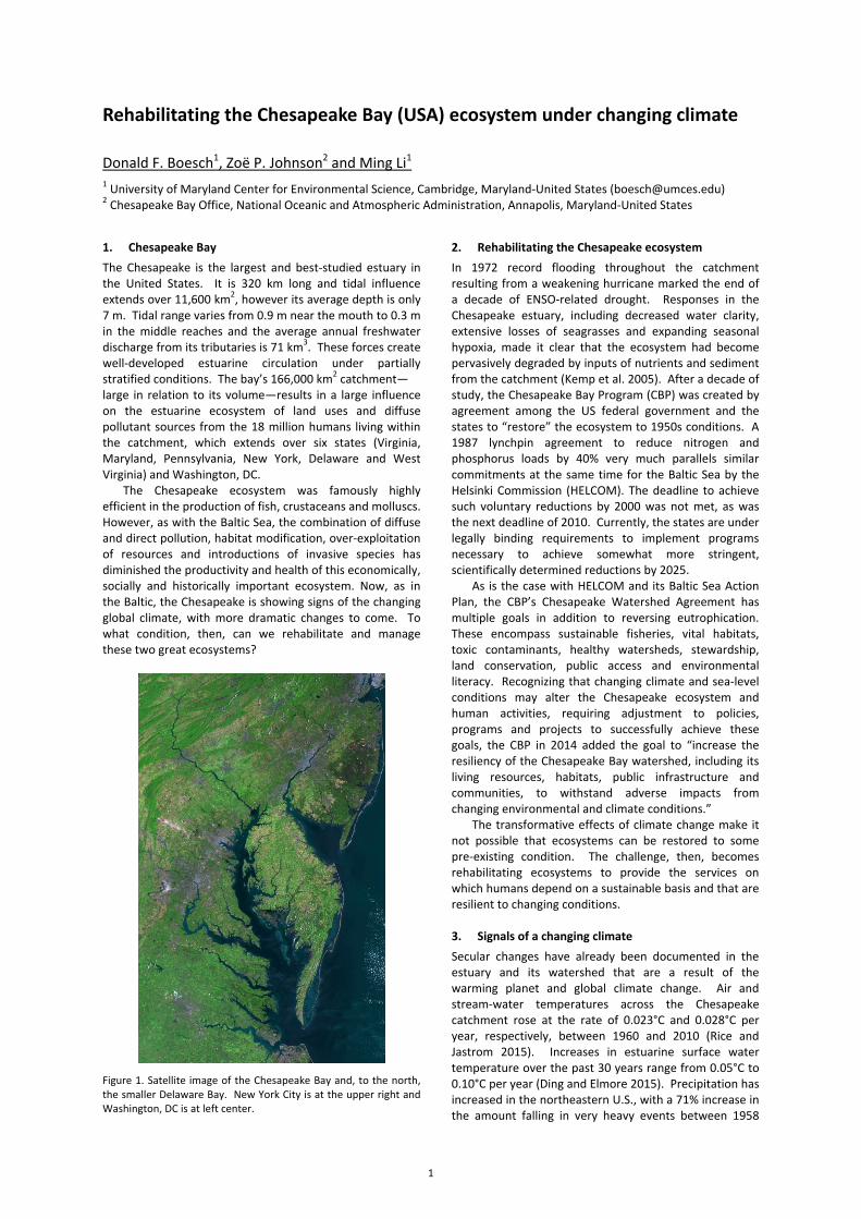
1. Chesapeake Bay The Chesapeake is the largest and best-studied estuary in the United States. It is 320 km long and tidal influence extends over 11,600 km2, however its average depth is only 7 m. Tidal range varies from 0.9 m near the mouth to 0.3 m in the middle reaches and the average annual freshwater discharge from its tributaries is 71 km3. These forces create well-developed estuarine circulation under partially stratified conditions. The bay’s 166,000 km2 catchment— large in relation to its volume—results in a large influence on the estuarine ecosystem of land uses and diffuse pollutant sources from the 18 million humans living within the catchment, which extends over six states (Virginia, Maryland, Pennsylvania, New York, Delaware and West Virginia) and Washington, DC.

The Chesapeake ecosystem was famously highly efficient in the production of fish, crustaceans and molluscs. However, as with the Baltic Sea, the combination of diffuse and direct pollution, habitat modification, over-exploitation of resources and introductions of invasive species has diminished the productivity and health of this economically, socially and historically important ecosystem. Now, as in the Baltic, the Chesapeake is showing signs of the changing global climate, with more dramatic changes to come. To what condition, then, can we rehabilitate and manage these two great ecosystems?

Figure 1. Satellite image of the Chesapeake Bay and, to the north, the smaller Delaware Bay. New York City is at the upper right and Washington, DC is at left center.

2. Rehabilitating the Chesapeake ecosystem In 1972 record flooding throughout the catchment resulting from a weakening hurricane marked the end of a decade of ENSO-related drought. Responses in the Chesapeake estuary, including decreased water clarity, extensive losses of seagrasses and expanding seasonal hypoxia, made it clear that the ecosystem had become pervasively degraded by inputs of nutrients and sediment from the catchment (Kemp et al. 2005). After a decade of study, the Chesapeake Bay Program (CBP) was created by agreement among the US federal government and the states to “restore” the ecosystem to 1950s conditions. A 1987 lynchpin agreement to reduce nitrogen and phosphorus loads by 40% very much parallels similar commitments at the same time for the Baltic Sea by the Helsinki Commission (HELCOM). The deadline to achieve such voluntary reductions by 2000 was not met, as was the next deadline of 2010. Currently, the states are under legally binding requirements to implement programs necessary to achieve somewhat more stringent, scientifically determined reductions by 2025.

As is the case with HELCOM and its Baltic Sea Action Plan, the CBP’s Chesapeake Watershed Agreement has multiple goals in addition to reversing eutrophication. These encompass sustainable fisheries, vital habitats, toxic contaminants, healthy watersheds, stewardship, land conservation, public access and environmental literacy. Recognizing that changing climate and sea-level conditions may alter the Chesapeake ecosystem and human activities, requiring adjustment to policies, programs and projects to successfully achieve these goals, the CBP in 2014 added the goal to “increase the resiliency of the Chesapeake Bay watershed, including its living resources, habitats, public infrastructure and communities, to withstand adverse impacts from changing environmental and climate conditions.”

The transformative effects of climate change make it not possible that ecosystems can be restored to some pre-existing condition. The challenge, then, becomes rehabilitating ecosystems to provide the services on which humans depend on a sustainable basis and that are resilient to changing conditions. 3. Signals of a changing climate Secular changes have already been documented in the estuary and its watershed that are a result of the warming planet and global climate change. Air and stream-water temperatures across the Chesapeake catchment rose at the rate of 0.023°C and 0.028°C per year, respectively, between 1960 and 2010 (Rice and Jastrom 2015). Increases in estuarine surface water temperature over the past 30 years range from 0.05°C to 0.10°C per year (Ding and Elmore 2015). Precipitation has increased in the northeastern U.S., with a 71% increase in the amount falling in very heavy events between 1958

1

and 2012 (Walsh et al. 2014). Sea level has been rising in the Chesapeake Bay relative to land elevations for many hundreds of years as a result of regional subsidence due to glacial isostatic adjustment. Increasing ocean volume associated with global warming added to this relative sea-level rise during the 20th century. Sea-level rise has accelerated along the Mid-Atlantic coast of the U.S. in recent decades. Ezer et al. (2013) found that tide gauge records from Chesapeake Bay and elsewhere along this coast were strongly influenced by variations in the elevation gradient of the Gulf Stream. Thus, the greater recent sea-level rise may be due to the slowdown of the Atlantic Meridional Overturning Circulation. Rising sea levels appear also to be linked to increasing salinity in the Chesapeake Bay as it increases in volume (Hilton et al. 2008). 4. Consequences of projected climate change There are substantial consequences for the Chesapeake Bay ecosystem that will result from climate change projected over the remainder of the 21st century (Najjar et al. 2010): • Temperatures of estuarine waters are very likely to

increase similar to air temperatures (about 1°C by mid-century and between 2 and 4.5°C by the end of the century, depending on the greenhouse gas emissions pathway). Northern species will be lost and southern and distant-water invasive species will establish populations. Oxygen solubility and metabolic rates will be affected.

• Relative sea level is projected in increase by 0.4 to 0.7 m by 2050 and between 0.7 and 1.7 by 2100 (Boesch et al. 2013). This will result in the erosion, deterioration or transgression of important tidal wetlands and expansion of shallow water habitats. The volume of the estuary will increase (by 14% with a 1 m rise), enhancing the influence of the ocean, changing circulation and mixing and, if not counteracted by increased freshwater discharges, increasing salinity. These changes have significant consequences to the distribution of organisms along the salinity gradient, their recruitment and biogeochemical dynamics.

• Freshwater discharges from the multiple rivers discharging to the Chesapeake Bay are projected to increase, but models disagree on the degree. Inflows are likely to increase during winter, but decline in summer, due to stable or reduced precipitation and increased evapotranspiration. Extreme precipitation events are projected to continue to be more prominent. These changes could increase the delivery of nutrients to the estuary and increase density stratification and thus exacerbate eutrophication and seasonal hypoxia.

5. Adaptation strategies for resilient rehabilitation To reduce vulnerability to the consequences of climate change the scientific and engineering community should focus on adaptation strategies that ensure the rehabilitation of the ecosystem and improve its resilience. Among those strategies should be: • Minimizing the vulnerability of humans and

infrastructure to hazards associated with sea-level rise and storm surge. Active efforts are underway in both Maryland and Virginia toward this end.

• Allowing tidal wetlands to transgress across low-lying landscapes and using sediments dredged for channel maintenance to subsidize wetland soil aggradation.

• Utilizing both built and natural infrastructure to reduce flooding, soil loss and stream bank erosion during extreme precipitation events.

• Limiting land development not only to minimize greenhouse gas emissions from transportation but also to restrict delivery of diffuse sources of sediments and nutrient nutrients to the estuary.

• Managing living resources in a way that anticipates future changes in temperature, sea level and salinity.

• Determining achievable states of the ecosystem under the changing climate to better define rehabilitation goals.

• Staying the course to achieve the 2025 nutrient reduction goals while conducting research and modeling to determine future reductions and practices required to achieve climate-resilient rehabilitation goals.

References

Boesch, D.F., Atkinson, L.P., Boicourt, W.C., Boon, J.D., Cahoon, D.R., Dalrymple, R.A., Ezer, T., Jorton, B.P., Johnson, Z. P., Kopp, R.E., Li, M., Moss, R.H., Parris, A. and Sommerfield, C.K. (2013) Updating Maryland’s Sea -level Rise Projections. University of Maryland Center for Environmental Science, Cambridge, Maryland USA

Ding, H. and A. Elmore (2015) Spatio-temporal patterns in water surface temperature from Lansat time series data in the Chesapeake Bay, U.S.A., Remote Sensing of the Environment, 168, pp. 335-348.

Ezer, T., Atkinson L.P., Corlett, W.B. and Blanco, J.L. (2013) Gulf Stream’s induced sea level rise and variability along the U.S. mid-Atlantic coast, Journal of Geophysical Research: Oceans, 118 pp. 1-13.

Kemp, W.M, Boynton, WR, Adolf, J.E., Boesch, D.F., Brush, G., Cornwell, J.C., Fisher, R.R., Glibert, P.M., Hagy, J.D., Harding, L.W., Houde, E.D., Kimmel, D.G., Miller, W.D., Newell, R.E.E., Roman, M.R., Smith, E.M and Stevenson, J.C. (2005) Eutrophication of Chesapeake Bay: historical trends and ecological interactions, Marine Ecology Progress Series, 303, pp. 1-29.

Najjar, R.G, Pyke, C.R., Adams, Brietburg, D,, Hershner, C., Kemp, M., Howarth, R., Mulholland, M.R., Paolisso, M., Secor, D., Sellner, K., Wardrop, D. and Wood, R. (2010). Potential climate-change impacts on the Chesapeake Bay. Estuarine, Coastal and Shelf Science, 86, pp. 1-20.

Rice, K.C. and Jastram, J.D. (2015) Rising air and stream-water temperatures in Chesapeake Bay region, USA, Climatic Change, 128, pp. 127-138.

Hilton, T. W., Najjar, R. G., Zhong L. and Li. M. (2008) Is there a signal of sea-level rise in Chesapeake Bay salinity? Journal of Geophysical Research, 113: C09002, doi:10.1029/ 2007JC004247.

Walsh, J., Wuebbles, D., Hayhoe, K., Kossin, J., Kunkel, K., Stephens, G., Thorne, P., Vose, R., Wehner, M., Willis, J., Anderson, D., Doney, S., Feely, R., Hennon, P., Kharin, V., Knutson, T., Landerer, F., Lenton, T., Kennedy, J. and Somerville, R. (2014) Ch. 2: Our Changing Climate. Climate Change Impacts in the United States: The Third National Climate Assessment, J. M. Melillo, T.C. Richmond and G. W. Yohe, eds., U.S. Global Change Research Program, 19-67. doi:10.7930/J0KW5CXT.

2

Interrelation of geosphere, climate processes and anthroposphere in the Baltic Sea basin during the Holocene Jan Harff1, Hauke Jöns2, Alar Rosentau3

1 Institute of Marine and Coastal Sciences, University of Szczecin, Poland (jan.harff@univ.szczecin.pl) 2 Lower Saxony Institute for Historical Coastal Research, Wilhelmshaven, Germany 3 Department of Geology, University of Tartu, Estonia

The Baltic Sea basin and its coasts allow in an exceptional manner to study the interrelation between changing climate, coastal processes and differences in the societal response from prehistoric to modern communities (Harff and Lüth 2011). Glacio-isostatic uplift is compensating the climatically controlled postglacial sea-level rise at the Fennoscandian Shield, so that advancing coastlines determine the development of (uplifting) paleo-landscapes in Central and Northern Scandinavia. Along the subsiding belt surrounding the Fennoscandian Shield, the eustatic sea-level rise is even enhanced and leads to retreating coastlines so that landscapes along the southern coasts of the Baltic Sea suffer from continuous inundation. Along with permanent flooding, wind-driven waves lead here to coastal erosion and west-to-east directed sediment transport forming the typical sandy spits which separate lagoons from the open sea. In the transition zone between the uplifting North and the subsiding South the influence of crustal uplift is replaced during the Holocene by eustatic sea-level rise leading to special sea-level curves and coastal landforms which can be studied exemplarily at the Estonian coast of the Baltic Sea and the Gulf of Finland (Rosentau et al. 2011, Harff et al. 2016). Since the final retreat of the Fennoscandian ice shield during Early Holocene, hunter gatherer communities were living along the respective Baltic Sea shores where they deployed access to marine resources and to the transportation and communication routes (Harff and Lüth 2011). Adjusted to the type of coasts these communities developed different strategies in the response to the changes in the coastal environment determined by climatically controlled eustasy, atmospheric circulation, and glacio-isostatic adjustment. These strategies were determined during the Holocene mainly by migration following the coastline shifts: down-slope in the North, up-slope in the South, and shifting directions in the transition zones. An active protection of the coast against flooding and erosion is recorded in the Baltic area for the last century only. Especially in areas with high rates of shore displacement, data and numerical models can be used to reconstruct environmental conditions, but in many cases also to date prehistoric coastal sites. Conversely, well-excavated and dated archaeological sites that were originally located on the shore can provide detailed information about the sea level at the time of their occupation and serve as sea-level key sites (Jöns and Harff 2014).

References Harff, J., Deng, J., Dudzinska-Nowak, J., Groh, A., Hünicke, B.,

Zhang, W. (2016) Interrelated drivers of coastline change in the Baltic Sea, 1st Baltic Earth Conference “Multiple drivers for Earth system changes in the Baltic Sea region”, Nida, Lithuania, 13 to 17 June 2016, this abstract volume.

Harff, J., Lüth, F. (eds.) (2011) Sinking Coasts – Geosphere Ecosphere and Anthroposphere of the Holocene Southern Baltic Sea II, Ber. Röm.-Germ. Komm.: 92, 1 – 380.

Jöns, H., Harff, J. (2014) Geoarchaeological Research Strategies in the Baltic Sea Area: Environmental Changes, Shoreline-Displacement and Settlement Strategies, In: Evans, A. M., Flatman, J. C., Flemming, N. C. (eds.), 2014: Prehistoric Archaeology on the Continental Shelf. Springer: N. Y., Heidelberg, Dordrecht, London, p. 173-192.

Rosentau, A., Veski, S., Kriiska, A., Aunap, R., Vassiljev, J., Saarse, L., Hang, T., Heinsalu, A., Oja, T. (2011) Palaeogeographic Model for the SW Estonian Coastal Zone of the Baltic Sea.- in: Harff, J., Björck, S., Hoth, P. (eds.) (2011): The Baltic Sea Basin.- Springer: Heidelberg, N.Y., 165 - 188.

3

Agriculture in the Baltic Sea region, major driver and challenges

Christoph Humborg

Stockholm University, Department of Applied Environmental Science (christoph.humborg@gmail.com)

Globally, agriculture is a major driver for earth system change, i.e. it covers an area as large as Africa and South-America together, stands for some 30% of global GHG emissions, 70% of global water withdrawal and doubled global N and P fluxes by applying inorganic fertilizers (Foley et al. 2011). Nutrient use efficiency (NUE) is a way to estimate the share of applied N and P fertilizers converted into crops, a NUE of 50% means that 50% is harvested as crop biomass, the residual 50% ends up in soils, groundwater, atmosphere or in coastal water bodies as the Baltic Sea. Only 47% of the reactive nitrogen added globally onto cropland is converted into harvested products, compared to 68% in the early 1960s, while synthetic N fertilizer input increased by a factor of 9 over the same period (Lasaletta et al. 2014). The global challenge ahead is to feed some 11 billion people with the same area of agricultural land. This is only possible if we avoid wasting massive amounts of N and P by producing animal protein, the future diet must be based on a larger amount of vegetable protein. Further, we have to use N and P more effectively in cereal production reducing the leakage of N and P to secure aquatic environment and biodiversity.

The situation in the Baltic Sea catchment is not far different. Though nutrient loads to the Baltic have decreased in the major rivers as the Odra, Vistula, Nemunas and Daugava and from coastal point sources mainly due to improved sewage treatment, trends in agricultural activities are contrasting for the various riparian countries. Nutrient accounting covering the period 1990-2010 reveals that countries as Denmark decreased net anthropogenic nitrogen and phosphorus inputs from 12 000 kg km-2 yr-1 to 7 500 kg km-2 yr-1 and 800 kg km-2 yr-1 to 400 kg km-2 yr-1, respectively. This lowered riverine inputs to the Danish Straits significantly. On the other hand, countries as Poland increased their net anthropogenic nitrogen and phosphorus inputs during the last 20 years from 3 800 kg km-2 yr-1 to 5 000 km-2 yr-1 and 300 kg km-2 yr-1to 600 km-2 yr-1, respectively. This means that fertilizer inputs are nowadays much more similar between countries, whereas some 20 years ago eastern countries applied much less fertilizers. Nutrient use efficiency has increased in Denmark and Germany from 50 to 80% whereas in Poland it has decreased from 55% to 50% (Lassaletta et al 2014).

Highest nutrient imbalances are often connected to high live stock densities and a first estimate reveals that livestock produces 1.5 million tons N and 0.3 million tons P in the Baltic Sea catchment, which is at least 3 times more that human sewage. Manure storage and improved techniques on how and when to apply it on the field was a successful management strategy to lower inorganic fertilizer applications in Denmark. In theory, if we would replace one third of chemical fertilizers by manure, we could reduce riverine N loads by roughly 15% and P loads by 10%, which could be a significant contribution to reach the maximum allowable nutrient inputs agreed upon within the BSAP.

Agriculture as a major driver has led to huge accumulations of N and P in agricultural soils, but also in the Baltic Sea water column and sediments over the last 100 years or so. Some of the accumulated pool of P in marine sediments is still mobile and is annually transformed between a solid and dissolved phase and annual fluxes between these pools should not be confused with a net source of P or an “internal load”, which is a misleading concept. Overall, we still accumulate P on land whereas in the Baltic Sea recent trends point towards a more balanced situation, i.e. inputs via rivers and outputs via the Danish straits or by permanent burial are rather comparable after the drastic decrease in P loads from land. However, the P pool on land is at least one order of magnitude larger than in the Baltic Sea and efforts should focus on reducing the leakiness of this pool.

Efforts on land addressing the causes of eutrophication are promising; techniques and management strategies developed in DK, Sweden or Germany can be applied elsewhere, especially in areas where NUE are low. In other words, there is still a lot to do to improve NUE and the agricultural sector can still contribute to lower nutrients loads to the Baltic Sea significantly. There are huge costs connected to this, however, a change in agricultural practices also fulfills climate goals and strategies and techniques developed in the Baltic catchment can be used on a global market. Overall, accumulation of N and P on land has a less steep pace but it still going on, the Baltic Sea still transforms nutrient loads that originate from the 80s when loads from rivers and coastal point sources peaked. Time scales of response in both systems, on land and in the Sea are long and it is fully conceivable that recent increase in N and fertilizers in some countries will counteract the positive trends of decreasing nutrient loads. Changes in the agricultural sector are rapid and drastic in the southern and eastern part of the Baltic Sea catchment towards a more modern and productive agriculture. However, it is vital now to apply best available techniques to reduce the leakage of N and P to the environment and our large-scale analyses reveals that this is not at all the case.

References

Foley et al. 2011 Nature; doi:10.1038/nature10452 Lassaletta et al. 2014. Environ. Res. Lett. 9 (2014) 105011;

doi:10.1088/1748-9326/9/10/105011

4

PannEx: Towards a Regional Hydroclimate Project in the Pannonian Basin

Mónika Lakatos1, Ivan Güttler2, Joan Cuxart Rodamilans3

1 Hungarian Meteorological Service, Budapest, Hungary (lakatos.m@met.hu)

2 Meteorological and Hydrological Service of Croatia, Zagreb, Croatia

3 University of the Balearic Islands, Palma, Spain

1. Initiation of a new Regional Hydroclimate Project in the Pannonian Basin

PannEx is a prospective Regional Hydroclimate Project (RHP) of the World Climate Research Programme (WCRP) Global Energy and Water Exchanges Project (GEWEX). The almost closed structure of the Pannonian basin makes it a unique natural laboratory for the study of the water and energy cycles, focusing on the physical processes of relevance.

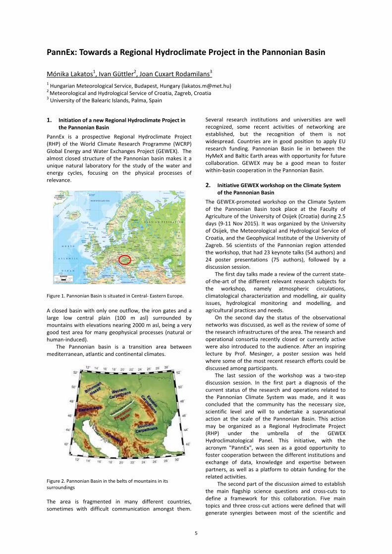
Figure 1. Pannonian Basin is situated in Central- Eastern Europe.

A closed basin with only one outflow, the iron gates and a large low central plain (100 m asl) surrounded by mountains with elevations nearing 2000 m asl, being a very good test area for many geophysical processes (natural or human-induced).

The Pannonian basin is a transition area between mediterranean, atlantic and continental climates.

Figure 2. Pannonian Basin in the belts of mountains in its surroundings The area is fragmented in many different countries, sometimes with difficult communication amongst them.

Several research institutions and universities are well recognized, some recent activities of networking are established, but the recognition of them is not widespread. Countries are in good position to apply EU research funding. Pannonian Basin lie in between the HyMeX and Baltic Earth areas with opportunity for future collaboration. GEWEX may be a good mean to foster within-basin cooperation in the Pannonian Basin. 2. Initiative GEWEX workshop on the Climate System

of the Pannonian Basin The GEWEX-promoted workshop on the Climate System of the Pannonian Basin took place at the Faculty of Agriculture of the University of Osijek (Croatia) during 2.5 days (9-11 Nov 2015). It was organized by the University of Osijek, the Meteorological and Hydrological Service of Croatia, and the Geophysical Institute of the University of Zagreb. 56 scientists of the Pannonian region attended the workshop, that had 23 keynote talks (54 authors) and 24 poster presentations (75 authors), followed by a discussion session.

The first day talks made a review of the current state-of-the-art of the different relevant research subjects for the workshop, namely atmospheric circulations, climatological characterization and modelling, air quality issues, hydrological monitoring and modelling, and agricultural practices and needs.

On the second day the status of the observational networks was discussed, as well as the review of some of the research infrastructures of the area. The research and operational consortia recently closed or currently active were also introduced to the audience. After an inspiring lecture by Prof. Mesinger, a poster session was held where some of the most recent research efforts could be discussed among participants.

The last session of the workshop was a two-step discussion session. In the first part a diagnosis of the current status of the research and operations related to the Pannonian Climate System was made, and it was concluded that the community has the necessary size, scientific level and will to undertake a supranational action at the scale of the Pannonian Basin. This action may be organized as a Regional Hydroclimate Project (RHP) under the umbrella of the GEWEX Hydroclimatological Panel. This initiative, with the acronym "PannEx", was seen as a good opportunity to foster cooperation between the different institutions and exchange of data, knowledge and expertise between partners, as well as a platform to obtain funding for the related activities.

The second part of the discussion aimed to establish the main flagship science questions and cross-cuts to define a framework for this collaboration. Five main topics and three cross-cut actions were defined that will generate synergies between most of the scientific and

5

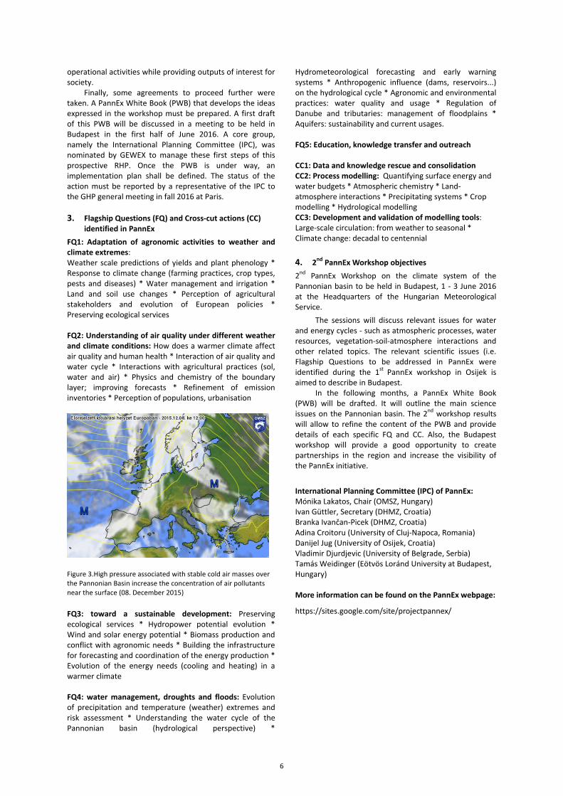
operational activities while providing outputs of interest for society.

Finally, some agreements to proceed further were taken. A PannEx White Book (PWB) that develops the ideas expressed in the workshop must be prepared. A first draft of this PWB will be discussed in a meeting to be held in Budapest in the first half of June 2016. A core group, namely the International Planning Committee (IPC), was nominated by GEWEX to manage these first steps of this prospective RHP. Once the PWB is under way, an implementation plan shall be defined. The status of the action must be reported by a representative of the IPC to the GHP general meeting in fall 2016 at Paris. 3. Flagship Questions (FQ) and Cross-cut actions (CC)

identified in PannEx FQ1: Adaptation of agronomic activities to weather and climate extremes: Weather scale predictions of yields and plant phenology * Response to climate change (farming practices, crop types, pests and diseases) * Water management and irrigation * Land and soil use changes * Perception of agricultural stakeholders and evolution of European policies * Preserving ecological services FQ2: Understanding of air quality under different weather and climate conditions: How does a warmer climate affect air quality and human health * Interaction of air quality and water cycle * Interactions with agricultural practices (sol, water and air) * Physics and chemistry of the boundary layer; improving forecasts * Refinement of emission inventories * Perception of populations, urbanisation

Figure 3.High pressure associated with stable cold air masses over the Pannonian Basin increase the concentration of air pollutants near the surface (08. December 2015)

FQ3: toward a sustainable development: Preserving ecological services * Hydropower potential evolution * Wind and solar energy potential * Biomass production and conflict with agronomic needs * Building the infrastructure for forecasting and coordination of the energy production * Evolution of the energy needs (cooling and heating) in a warmer climate FQ4: water management, droughts and floods: Evolution of precipitation and temperature (weather) extremes and risk assessment * Understanding the water cycle of the Pannonian basin (hydrological perspective) *

Hydrometeorological forecasting and early warning systems * Anthropogenic influence (dams, reservoirs...) on the hydrological cycle * Agronomic and environmental practices: water quality and usage * Regulation of Danube and tributaries: management of floodplains * Aquifers: sustainability and current usages. FQ5: Education, knowledge transfer and outreach CC1: Data and knowledge rescue and consolidation CC2: Process modelling: Quantifying surface energy and water budgets * Atmospheric chemistry * Land-atmosphere interactions * Precipitating systems * Crop modelling * Hydrological modelling CC3: Development and validation of modelling tools: Large-scale circulation: from weather to seasonal * Climate change: decadal to centennial 4. 2nd PannEx Workshop objectives 2nd PannEx Workshop on the climate system of the Pannonian basin to be held in Budapest, 1 - 3 June 2016 at the Headquarters of the Hungarian Meteorological Service.

The sessions will discuss relevant issues for water and energy cycles - such as atmospheric processes, water resources, vegetation-soil-atmosphere interactions and other related topics. The relevant scientific issues (i.e. Flagship Questions to be addressed in PannEx were identified during the 1st PannEx workshop in Osijek is aimed to describe in Budapest.

In the following months, a PannEx White Book (PWB) will be drafted. It will outline the main science issues on the Pannonian basin. The 2nd workshop results will allow to refine the content of the PWB and provide details of each specific FQ and CC. Also, the Budapest workshop will provide a good opportunity to create partnerships in the region and increase the visibility of the PannEx initiative.

International Planning Committee (IPC) of PannEx: Mónika Lakatos, Chair (OMSZ, Hungary) Ivan Güttler, Secretary (DHMZ, Croatia) Branka Ivančan-Picek (DHMZ, Croatia) Adina Croitoru (University of Cluj-Napoca, Romania) Danijel Jug (University of Osijek, Croatia) Vladimir Djurdjevic (University of Belgrade, Serbia) Tamás Weidinger (Eötvös Loránd University at Budapest, Hungary) More information can be found on the PannEx webpage:

https://sites.google.com/site/projectpannex/

6

Connecting Analytical Thinking and Intuition: Challenge’s for leadership and education in Earth System Sciences

Omstedt, A

Department of Marine Sciences, University of Gothenburg, Göteborg, Sweden (anders.omstedt@marine.gu.se)

1. Introduction We are living in a world of increasing complexity in which accurately perceiving reality is important and difficult. Society’s need to address “global grand challenges” (Fig 1.) requires that the scientific community initiate inter-disciplinary research often very unlike current education programmes, which are usually based on intra-disciplinary science. Improving our understanding of complex problems and communicating this understanding to a large group of people of differing backgrounds and educational levels, such as students and scientists from various disciplines, politicians, experts, and laypeople, represents a great challenge.

Figure 1. The Grand Challenges includes energy, climate, food, and health. In this figure from Nature 525, 305, September 2016 the new role of scientist is to join and save the World a questionable task for a scientist?

2. Analytical thinking and intuition Analytical thinking is a powerful way of solving problems and has been used both to develop and destroy society and nature. However, we are only partly aware of the sum of our knowledge (Fig. 2), and we are not restricted to analytical thinking. Art and our dreams are full of feelings and inspirations that can open up new dimensions in our lives. The great need for perceptual accuracy relies on our ability to connect analytical thinking with the intuition often manifested in dreams, literature, and art. This ability to interconnect these human capabilities, however, is not yet recognized in most educational programmes.

In recent decades, the marine environment has experienced serious damage and the scientific community has tried to act as a whistle-blower, though with few noticeable results. Society is entering a new era of conflict marked by increasing pressure on our natural resources and needs for new technology. It is imperative that we change our mentality, to become more environmentally aware, friendly, and caring. The existing trend towards ever greater knowledge fragmentation and increased competition requires that we step back and investigate our behaviour and driving forces in a more mindful way. At universities, the freedom to generate new knowledge needs stronger support, as does the understanding that the teacher’s main missions are to generate new knowledge, educate and to support the joy of learning. Missions not far from science networks such as Baltic Earth

This presentation illustrates how analytical thinking and intuition can be trained, and I propose a method for connecting both aspects in a systematic way (Omstedt, 2016). The dream group process developed by Montague Ullman, which includes training in analytical, empathetic, and self-reflection skills, is an excellent tool that should be included in university curricula, particularly for science students. In science, we learn to observe nature in an objective way, organizing measurement platforms and building mathematical models. Now is the time to employ methods that help us exploring our driving forces, to improve our communication skills and better understand how humans are influencing society and nature.

Figure 2. A view of the Baltic Sea from Bornholm (Photo: Anders Omstedt). Intuition plays an important part in our thinking.

3. Some aspects of connecting Analytical, critical thinking involves analysing, evaluation, problem solving, articulate, apply logical thinking, key skills emphasized in university training. It is slow and limited. Intuition is an insight to know something without any proof or evidence based on our own experience. This is a capacity that everyone has and can be trained. It is fast and theory free. Connecting involves listening, evaluation, summarizing and appreciation our efforts. The method on connecting analytical thinking and intuition which I have been working with is inspired by the dream group method developed by Montague Ullman (Ullman, 1996, Siivola, 2011), in which a group of six to eight people systematically and carefully helps the dreamer or the student to appreciate his or her dreams or projects. Some aspects of this learning group process are: • Catch the dream or idea • Finding words for feelings • Meaning of symbols • Triggers • To be touched • Exploring the unconscious and the unknown • Inspiration • Searching the emotional context • Playback and meaning

7

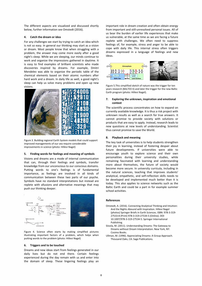
The different aspects are visualized and discussed shortly below, further information see Omstedt (2016). 4. Catch the dream or idea For any challenges we start by trying to catch an idea which is not so easy. In general our thinking may start as a vision or dream. Most people know that when struggling with a problem, the answer may come more easily after a good night’s sleep. While we are sleeping, our minds continue to work and organize the impressions gathered in daytime. It is easy to find examples of brilliant scientists who made discoveries inspired by dreams. For example, Dmitri Mendelev was able to organize the periodic table of the chemical elements based on their atomic numbers after hard work and a dream. In daily life as well, a good night’s sleep can help us solve many problems and open up new visions.

Figure 3. Building regional Earth System models that could support improved managements of our sea require considerable improvements in science (photo: Hillevi Nagel) 5. Finding words for feelings and meaning of symbols Visions and dreams are a mode of internal communication that can, through their feelings and symbols, transfer knowledge from our unconscious to our conscious domains. Putting words to one’s feelings is of fundamental importance, as feelings are involved in all kinds of communication between these two parts of our psyche. Symbols have no standard interpretations but instead are replete with allusions and alternative meanings that may push our thinking deeper.

Figure 4. Science often starts by making simplified pictures illustrating important factors of a problem, which helps when putting words to the problem (photo: Hillevi Nagel) 6. Triggers and to be touched Dreams and new ideas start from feelings generated in our daily lives but do not end there. Certain feelings experienced during the day remain with us and enter into the domain of sleep. These lingering feelings play an

important role in dream creation and often obtain energy from important and still-unresolved personal issues. All of us bear the burden of earlier life experiences that make us vulnerable, at the same time as we are facing a future replete with challenges. We often need to suppress feelings of, for example, stress and anger to be able to cope with daily life. This internal stress often triggers dreams expressed in a language of feelings and new ideas.

Figure 5.This simplified sketch of nature was the trigger for ten years research (BALTEX II) and later the trigger for the new Baltic Earth program (photo: Hillevi Nagel). 7. Exploring the unknown, inspiration and emotional

context The scientific process concentrates on how to expand on currently available knowledge. It is thus a risk project with unknown results as well as a search for true answers. It cannot promise to provide society with solutions or products that are easy to apply. Instead, research leads to new questions at new levels of understanding. Scientist thus cannot promise to save the World. 8. Playback and meaning The key task of universities is to help students strengthen their joy in learning, instead of fostering despair about future developments. If universities were able to encourage youth to explore science and their own personalities during their university studies, while remaining fascinated with learning and understanding more about themselves, the future of society would become more secure. In university curricula, including in the natural sciences, teaching that improves students’ analytical, empathetic, and self-reflection skills needs to be developed and implemented much better than it is today. This also applies to science networks such as the Baltic Earth and could be a part in for example summer school activities.

References

Omstedt, A. (2016). Connecting Analytical Thinking and Intuition: And the Nights Abound with Inspiration. Hillevi Nagel (photos) Springer Briefs in Earth Sciences. ISBN: 978-3-319-27533-8 (Print) 978-3-319-27534-5 (Online). DOI 10.1007/978-3-319-27534-5. Springer International Publishing.

Siivola, M. (2011). Understanding Dreams: The Gateway to Dreams without Dream Interpretation. New York, NY: Cosimo Books.

Ullman, M. (1996). Appreciating Dreams: A Group Approach. Thousand Oaks, CA: Sage Publications.

8

Two centuries of extreme events over the Baltic Sea and North Sea regions

Martin Stendel 1, Else van den Besselaar 2, Abdel Hannachi 3, Jaak Jaagus 4, Elizabeth Kent 5, Christiana Lefebvre 6, Gudrun Rosenhagen 6, Anna Rutgersson 7, Frederik Schenk 3, Gerard van der Schrier 2 and Tim Woollings 8 1 Danish Meteorological Institute, Copenhagen, Denmark (mas@dmi.dk) 2 Royal Netherlands Meteorological Institute, De Bilt, The Netherlands 3 Stockholm University, Sweden 4 University of Tartu, Estonia 5 National Oceanographic Centre, Southampton, United Kingdom 6 German Weather Service, Hamburg, Germany 7 Uppsala University, Sweden 8 University of Oxford, United Kingdom

1. Introduction In the framework of the BACC 2 (for the Baltic Sea) and NOSCCA projects (for the North Sea region), studies of past and present variability and changes in atmospheric variables within the North Sea region over the instrumental period (roughly the past 200 years) have been investigated. We here present selected findings from these two assessments.

There is an overall trend in temperature and precipitation, which goes along with a north-eastward shift of storm tracks and is in agreement with projections from climate model under enhanced greenhouse gas concentrations. 2. Data homogeneity issues This is true even for data-rich regions like the Baltic and North Sea regions. In addition, unlike most other regions in the world, there is a wealth of old observations available for the Baltic and North Sea regions which needs to be carefully digitised and homogenized. For this, a thorough quality control must be applied; otherwise the digitised datasets may be useless or even counterproductive. We present evidence that this step cannot be conducted without human interference and thus cannot be fully automated. Furthermore, inhomogeneities due to e.g. instrumentation and station relocations need to be addressed.

We also consider reanalyses, which can help detect such inhomogeneities in observed time series, but at the same time are prone to biases and/or spurious trends themselves e.g. introduced by changes in the availability and quality of the underlying assimilated data. It therefore in general remains unclear in how far reanalyses prior to the 1970s, that means based entirely on surface observations, are homogeneous.

3. Extreme events Often extreme events and changes in extreme situations are more important and of greater (societal) significance than changes in mean climate. However, changes in extreme weather events are difficult to assess not only because they are, per definition, rare events, but also due to the homogeneity issues outlined above. Taking these into account, we present evidence for changes in extreme events in the Baltic and North Sea regions.

There are indications of an increase in the number of deep cyclones (but not in their total number), while storminess since the late 19th century shows no robust trends. The persistence of circulation types appears to have increased over the last century by 2-4 days, and consequently, there is an indication for 'more extreme' extreme events. While there is no clear evidence for changes in the number of winter storms over the North Sea region, an increase has been reported further east, over the Baltic Sea region.

Concerning temperature, there is a decrease of cold extremes (for example the number of ice days, Tmax<0°C) and an increase of warm extremes (for example the number of tropical nights, Tmin≥20°C). This becomes increasingly obvious when extreme percentiles are considered. As a consequence, the duration of mild periods in winter and the number of heat waves in summer have increased. 4. Further research needed For variables other than temperature and precipitation, long-term trends are difficult to deduce, and it is therefore not obvious which part of the observed changes may be due to anthropogenic activities and which is internally forced. It remains also unclear to what extent atmospheric circulation over the Baltic and North Sea regions is controlled influenced by distant factors, in particular Arctic sea-ice decline in recent decades.

9

10

Topic A

Salinity dynamics in the Baltic Sea

Benthic foraminifera record environmental and climate changes in the Bornholm Basin (Baltic Sea) over the last 6 millennia

A. Binczewska1, I. Polovodova Asteman2, M. Moros3, J. Sławińska4 1Paleoceanography Unit, Faculty of Geosciences, University of Szczecin, Szczecin, Poland (anna.binczewska@gmail.com) 2Uni Research Climate, Bjerknes Centre for Climate Research, Allégaten 55, 5007 Bergen, Norway 3Leibniz Institute for Baltic Sea Research, Warnemünde, Germany 4 Department of Geology and Paleogeography, Faculty of Geosciences, University of Szczecin, Szczecin, Poland We use foraminiferal assemblages and sediment geochemistry (TOC, LOI, TIC, CNS) as a proxy to study past ecosystem changes, which took place during the mid- and late Holocene in the Baltic Sea. The investigated area is a semi-enclosed water body with a limited connection to the North Sea and adjacent Atlantic Ocean. The brackish conditions together with strong meteorological and anthropogenic influences, changes in bottom water mass composition depend on inflows from the North Sea and create a challenging environment for survival of marine organisms. This work provides a high-resolution analysis from well-dated ca. 8 meter long gravity core and 42 cm long multi core taken in the Bornholm Basin in 2013. Age-model is based on 32 AMS 14C dates using mollusc shells of mostly Macoma balthica and 2 AMS 14C dates obtained from benthic foraminiferal shells. For foraminiferal analysis the assemblage was sieved over >63 μm and counted wet to obtain a detailed information about assemblages and different preservation state of foraminiferal shells. The first appearance of foraminiferal shells in investigated record is dated to 6913 cal. yr BP, which can be attributable to the transitional stage between the Ancylus Lake and the Littorina Sea known from the Baltic Sea evolution. This transition was from a fresh water

environment to the brackish-marine conditions. This is also reflected by high abundance of Cladocera (here associated with fresh water conditions) found during ~ 6920 – 7015 cal. yr BP and disappearing in the record following an increase of foraminiferal and ostracods shells at ~ 6905 cal. yr BP.

The foraminiferal diversity in the studied record is low and dominated by Criboelphidium species. This genus is adapted to long-term environmental stress, including prevailing hypoxia to anoxia, brackish conditions and organic-rich sediments, all characteristic for the investigated study area. Additionally, our results indicate an increase of foraminiferal inner organic linings (which remain after a complete dissolution of carbonate shells) concurrent with peaks of total organic carbon (TOC) in the record. Also, our study demonstrates an increase of absolute abundance of benthic foraminifera (ind./g wet sedim.) in relation to the high-salinity bottom water inflows from the North Sea and Atlantic Ocean to the Baltic Sea. From our data, the inflows appear to be more frequent during the Medieval Warm Period (~ 660 – 1110 cal. yr BP) and the Dark Ages (1200-1600 cal. yr BP), as well as between 3800 and 5600 cal. yr BP in contrast to the late 20th century characterized by rare Major Baltic Inflows.

11

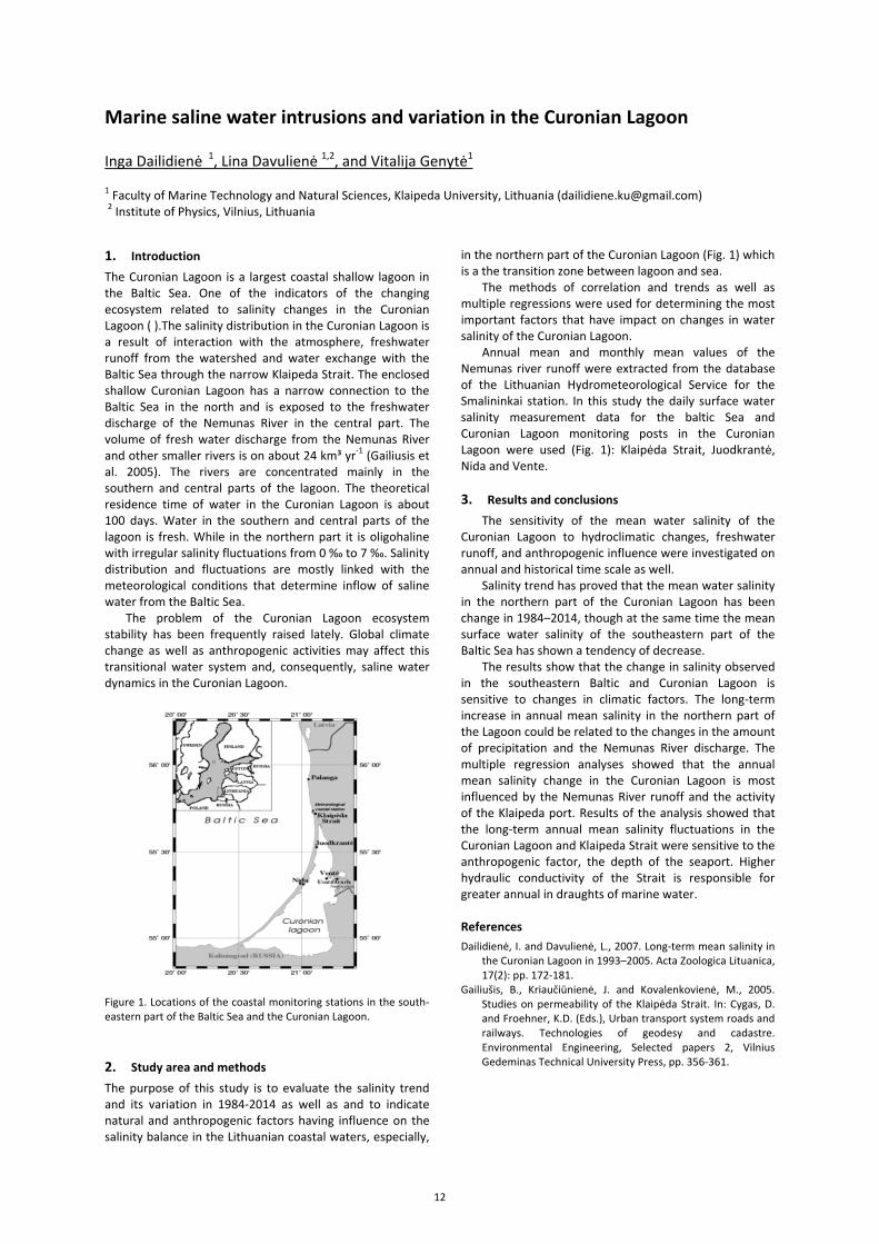
Marine saline water intrusions and variation in the Curonian Lagoon Inga Dailidienė 1, Lina Davulienė 1,2, and Vitalija Genytė1

1 Faculty of Marine Technology and Natural Sciences, Klaipeda University, Lithuania (dailidiene.ku@gmail.com) 2 Institute of Physics, Vilnius, Lithuania

1. Introduction The Curonian Lagoon is a largest coastal shallow lagoon in the Baltic Sea. One of the indicators of the changing ecosystem related to salinity changes in the Curonian Lagoon ( ).The salinity distribution in the Curonian Lagoon is a result of interaction with the atmosphere, freshwater runoff from the watershed and water exchange with the Baltic Sea through the narrow Klaipeda Strait. The enclosed shallow Curonian Lagoon has a narrow connection to the Baltic Sea in the north and is exposed to the freshwater discharge of the Nemunas River in the central part. The volume of fresh water discharge from the Nemunas River and other smaller rivers is on about 24 km³ yr-1 (Gailiusis et al. 2005). The rivers are concentrated mainly in the southern and central parts of the lagoon. The theoretical residence time of water in the Curonian Lagoon is about 100 days. Water in the southern and central parts of the lagoon is fresh. While in the northern part it is oligohaline with irregular salinity fluctuations from 0 ‰ to 7 ‰. Salinity distribution and fluctuations are mostly linked with the meteorological conditions that determine inflow of saline water from the Baltic Sea.

The problem of the Curonian Lagoon ecosystem stability has been frequently raised lately. Global climate change as well as anthropogenic activities may affect this transitional water system and, consequently, saline water dynamics in the Curonian Lagoon.

Figure 1. Locations of the coastal monitoring stations in the south-eastern part of the Baltic Sea and the Curonian Lagoon.

2. Study area and methods The purpose of this study is to evaluate the salinity trend and its variation in 1984-2014 as well as and to indicate natural and anthropogenic factors having influence on the salinity balance in the Lithuanian coastal waters, especially,

in the northern part of the Curonian Lagoon (Fig. 1) which is a the transition zone between lagoon and sea.

The methods of correlation and trends as well as multiple regressions were used for determining the most important factors that have impact on changes in water salinity of the Curonian Lagoon.

Annual mean and monthly mean values of the Nemunas river runoff were extracted from the database of the Lithuanian Hydrometeorological Service for the Smalininkai station. In this study the daily surface water salinity measurement data for the baltic Sea and Curonian Lagoon monitoring posts in the Curonian Lagoon were used (Fig. 1): Klaipėda Strait, Juodkrantė, Nida and Vente.

3. Results and conclusions

The sensitivity of the mean water salinity of the Curonian Lagoon to hydroclimatic changes, freshwater runoff, and anthropogenic influence were investigated on annual and historical time scale as well.

Salinity trend has proved that the mean water salinity in the northern part of the Curonian Lagoon has been change in 1984–2014, though at the same time the mean surface water salinity of the southeastern part of the Baltic Sea has shown a tendency of decrease.

The results show that the change in salinity observed in the southeastern Baltic and Curonian Lagoon is sensitive to changes in climatic factors. The long-term increase in annual mean salinity in the northern part of the Lagoon could be related to the changes in the amount of precipitation and the Nemunas River discharge. The multiple regression analyses showed that the annual mean salinity change in the Curonian Lagoon is most influenced by the Nemunas River runoff and the activity of the Klaipeda port. Results of the analysis showed that the long-term annual mean salinity fluctuations in the Curonian Lagoon and Klaipeda Strait were sensitive to the anthropogenic factor, the depth of the seaport. Higher hydraulic conductivity of the Strait is responsible for greater annual in draughts of marine water.

References Dailidienė, I. and Davulienė, L., 2007. Long-term mean salinity in

the Curonian Lagoon in 1993–2005. Acta Zoologica Lituanica, 17(2): pp. 172-181.

Gailiušis, B., Kriaučiūnienė, J. and Kovalenkovienė, M., 2005. Studies on permeability of the Klaipėda Strait. In: Cygas, D. and Froehner, K.D. (Eds.), Urban transport system roads and railways. Technologies of geodesy and cadastre. Environmental Engineering, Selected papers 2, Vilnius Gedeminas Technical University Press, pp. 356-361.

12

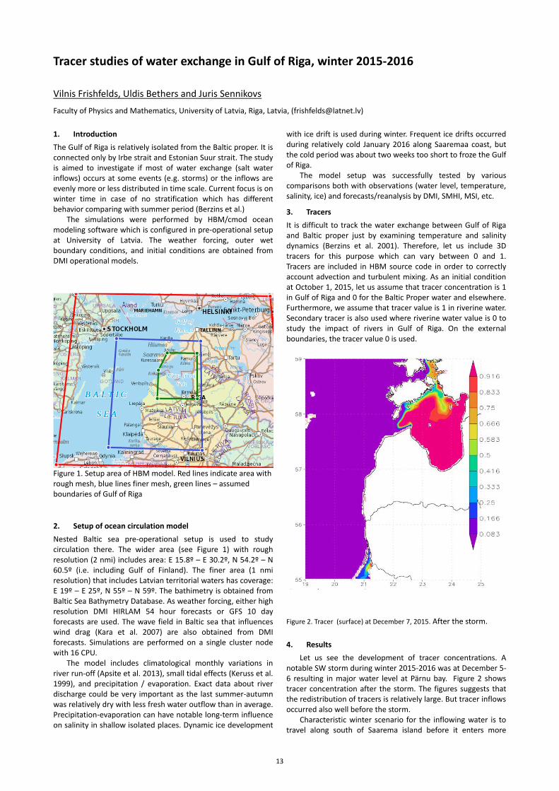
Tracer studies of water exchange in Gulf of Riga, winter 2015-2016

Vilnis Frishfelds, Uldis Bethers and Juris Sennikovs

Faculty of Physics and Mathematics, University of Latvia, Riga, Latvia, (frishfelds@latnet.lv) 1. Introduction The Gulf of Riga is relatively isolated from the Baltic proper. It is connected only by Irbe strait and Estonian Suur strait. The study is aimed to investigate if most of water exchange (salt water inflows) occurs at some events (e.g. storms) or the inflows are evenly more or less distributed in time scale. Current focus is on winter time in case of no stratification which has different behavior comparing with summer period (Berzins et al.)

The simulations were performed by HBM/cmod ocean modeling software which is configured in pre-operational setup at University of Latvia. The weather forcing, outer wet boundary conditions, and initial conditions are obtained from DMI operational models.

Figure 1. Setup area of HBM model. Red lines indicate area with rough mesh, blue lines finer mesh, green lines – assumed boundaries of Gulf of Riga

2. Setup of ocean circulation model Nested Baltic sea pre-operational setup is used to study circulation there. The wider area (see Figure 1) with rough resolution (2 nmi) includes area: E 15.8º – E 30.2º, N 54.2º – N 60.5º (i.e. including Gulf of Finland). The finer area (1 nmi resolution) that includes Latvian territorial waters has coverage: E 19º – E 25º, N 55º – N 59º. The bathimetry is obtained from Baltic Sea Bathymetry Database. As weather forcing, either high resolution DMI HIRLAM 54 hour forecasts or GFS 10 day forecasts are used. The wave field in Baltic sea that influences wind drag (Kara et al. 2007) are also obtained from DMI forecasts. Simulations are performed on a single cluster node with 16 CPU.

The model includes climatological monthly variations in river run-off (Apsite et al. 2013), small tidal effects (Keruss et al. 1999), and precipitation / evaporation. Exact data about river discharge could be very important as the last summer-autumn was relatively dry with less fresh water outflow than in average. Precipitation-evaporation can have notable long-term influence on salinity in shallow isolated places. Dynamic ice development

with ice drift is used during winter. Frequent ice drifts occurred during relatively cold January 2016 along Saaremaa coast, but the cold period was about two weeks too short to froze the Gulf of Riga.

The model setup was successfully tested by various comparisons both with observations (water level, temperature, salinity, ice) and forecasts/reanalysis by DMI, SMHI, MSI, etc. 3. Tracers It is difficult to track the water exchange between Gulf of Riga and Baltic proper just by examining temperature and salinity dynamics (Berzins et al. 2001). Therefore, let us include 3D tracers for this purpose which can vary between 0 and 1. Tracers are included in HBM source code in order to correctly account advection and turbulent mixing. As an initial condition at October 1, 2015, let us assume that tracer concentration is 1 in Gulf of Riga and 0 for the Baltic Proper water and elsewhere. Furthermore, we assume that tracer value is 1 in riverine water. Secondary tracer is also used where riverine water value is 0 to study the impact of rivers in Gulf of Riga. On the external boundaries, the tracer value 0 is used.

Figure 2. Tracer (surface) at December 7, 2015. After the storm. 4. Results

Let us see the development of tracer concentrations. A notable SW storm during winter 2015-2016 was at December 5-6 resulting in major water level at Pärnu bay. Figure 2 shows tracer concentration after the storm. The figures suggests that the redistribution of tracers is relatively large. But tracer inflows occurred also well before the storm.

Characteristic winter scenario for the inflowing water is to travel along south of Saarema island before it enters more

13

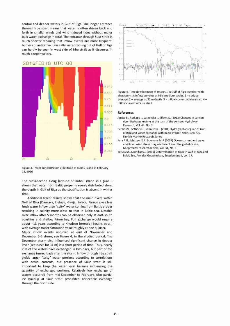
central and deeper waters in Gulf of Riga. The longer entrance through Irbe strait means that water is often driven back and forth in smaller winds and wind induced tides without major bulk water exchange in total. The entrance through Suur strait is much shorter meaning that inflow events are more frequent, but less quantitative. Less salty water coming out of Gulf of Riga can hardly be seen in west side of Irbe strait as it disperses in much deeper waters.

Figure 3. Tracer concentration at latitude of Ruhnu island at February 18, 2016 The cross-section along latitude of Ruhnu island in Figure 3 shows that water from Baltic proper is evenly distributed along the depth in Gulf of Riga as the stratification is absent in winter time.

Additional tracer results shows that the main rivers within Gulf of Riga (Daugava, Lielupe, Gauja, Salaca, Pärnu) gives less fresh water inflow than “salty” water coming from Baltic proper resulting in salinity more close to that in Baltic sea. Notable river inflow after 5 months can be observed only at east-south coastline and shallow Pärnu bay. Full exchange would require about ~13 years according to Knudsen formula (Berzins et al.) with average tracer saturation value roughly at one quarter. Major inflow events occurred at end of November and December 5-6 storm, see Figure 4, in the studied period. The December storm also influenced significant change in deeper layer (see curve for 31 m) in a short period of time. Thus, nearly 2 % of the waters have exchanged in two days, but part of the exchange turned back after the storm. Inflow through Irbe strait yields larger “salty” water portions according to correlations with actual currents, but presence of Suur strait is still important to keep the water level balance influencing the quantity of exchanged portions. Relatively low exchange of waters occurred from mid-December to February. Also partial ice buildup at Suur strait prohibited noticeable exchange through the north side.

Figure 4. Time development of tracers 1 in Gulf of Riga together with characteristic inflow currents at Irbe and Suur straits. 1 – surface average, 2 – average at 31 m depth, 3 - inflow current at Irbe strait, 4 – inflow current at Suur strait. References Apsite E., Rudlapa I., Latkovska I., Elferts D. (2013) Changes in Latvian

river discharge regime at the turn of the century. Hydrology Research, Vol. 44. No. 3

Berzins V., Bethers U., Sennikovs J, (2001) Hydrographic regime of Gulf of Riga and water exchange with Baltic Proper: Years 1991/95. Finnish Marine Research Series

Kara A.B., Metzger E.J., Bourassa M.A (2007) Ocean current and wave effects on wind stress drag coefficient over the global ocean. Geophysical research letters, Vol. 34, No. 1

Keruss M., Sennikovs J. (1999) Determination of tides in Gulf of Riga and Baltic Sea, Annales Geophysicae, Supplement II, Vol. 17.

14

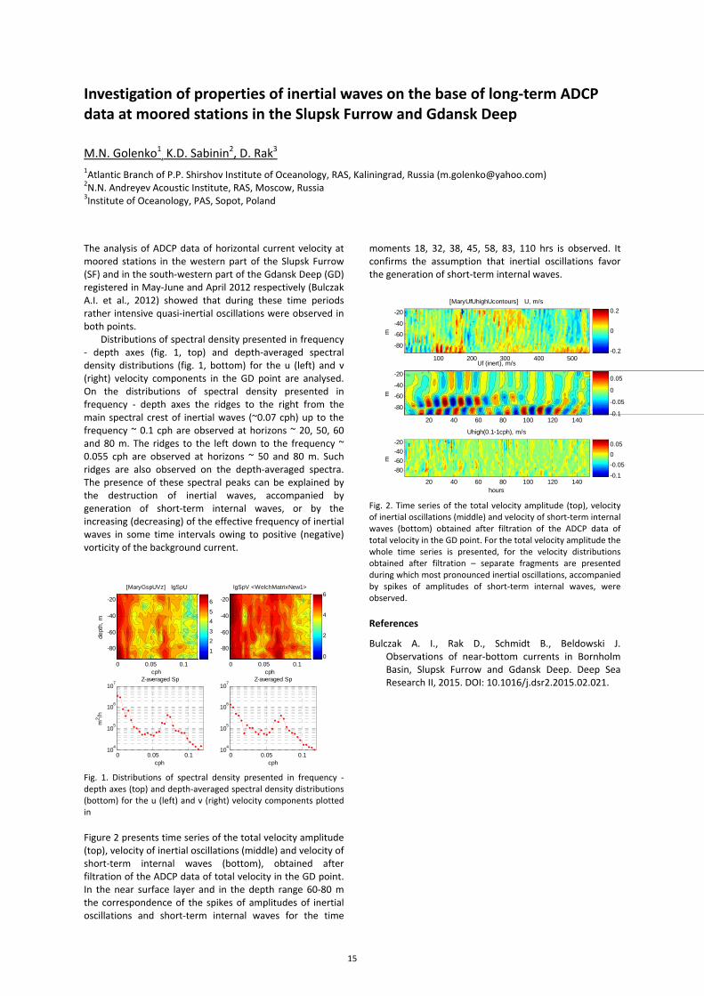
Investigation of properties of inertial waves on the base of long-term ADCP data at moored stations in the Slupsk Furrow and Gdansk Deep

M.N. Golenko1, K.D. Sabinin2, D. Rak3

1Atlantic Branch of P.P. Shirshov Institute of Oceanology, RAS, Kaliningrad, Russia (m.golenko@yahoo.com) 2N.N. Andreyev Acoustic Institute, RAS, Moscow, Russia 3Institute of Oceanology, PAS, Sopot, Poland

The analysis of ADCP data of horizontal current velocity at moored stations in the western part of the Slupsk Furrow (SF) and in the south-western part of the Gdansk Deep (GD) registered in May-June and April 2012 respectively (Bulczak A.I. et al., 2012) showed that during these time periods rather intensive quasi-inertial oscillations were observed in both points.

Distributions of spectral density presented in frequency - depth axes (fig. 1, top) and depth-averaged spectral density distributions (fig. 1, bottom) for the u (left) and v (right) velocity components in the GD point are analysed. On the distributions of spectral density presented in frequency - depth axes the ridges to the right from the main spectral crest of inertial waves (~0.07 cph) up to the frequency ~ 0.1 cph are observed at horizons ~ 20, 50, 60 and 80 m. The ridges to the left down to the frequency ~ 0.055 cph are observed at horizons ~ 50 and 80 m. Such ridges are also observed on the depth-averaged spectra. The presence of these spectral peaks can be explained by the destruction of inertial waves, accompanied by generation of short-term internal waves, or by the increasing (decreasing) of the effective frequency of inertial waves in some time intervals owing to positive (negative) vorticity of the background current.

Fig. 1. Distributions of spectral density presented in frequency - depth axes (top) and depth-averaged spectral density distributions (bottom) for the u (left) and v (right) velocity components plotted in Figure 2 presents time series of the total velocity amplitude (top), velocity of inertial oscillations (middle) and velocity of short-term internal waves (bottom), obtained after filtration of the ADCP data of total velocity in the GD point. In the near surface layer and in the depth range 60-80 m the correspondence of the spikes of amplitudes of inertial oscillations and short-term internal waves for the time

moments 18, 32, 38, 45, 58, 83, 110 hrs is observed. It confirms the assumption that inertial oscillations favor the generation of short-term internal waves.

Fig. 2. Time series of the total velocity amplitude (top), velocity of inertial oscillations (middle) and velocity of short-term internal waves (bottom) obtained after filtration of the ADCP data of total velocity in the GD point. For the total velocity amplitude the whole time series is presented, for the velocity distributions obtained after filtration – separate fragments are presented during which most pronounced inertial oscillations, accompanied by spikes of amplitudes of short-term internal waves, were observed. References

Bulczak A. I., Rak D., Schmidt B., Beldowski J. Observations of near-bottom currents in Bornholm Basin, Slupsk Furrow and Gdansk Deep. Deep Sea Research II, 2015. DOI: 10.1016/j.dsr2.2015.02.021.

cph

lgSpV <WelchMatrixNew1>

0 0.05 0.1

-80

-60

-40

-20

0

2

4

6

0 0.05 0.1104

105

106

107

cph

Z-averaged Spcph

dept

h, m

[MaryGspUVz] lgSpU

0 0.05 0.1

-80

-60

-40

-20

1

23

45

6

0 0.05 0.1104

105

106

107

cph

m2 /h

Z-averaged Sp

m

[MaryUfUhighUcontours] U, m/s

100 200 300 400 500

-80

-60

-40

-20

m

Uf (inert), m/s

20 40 60 80 100 120 140

-80

-60

-40

-20

hours

m

Uhigh(0.1-1cph), m/s

20 40 60 80 100 120 140

-80-60-40-20

-0.2

0

0.2

-0.1

-0.05

0

0.05

-0.1

-0.0500.05

15

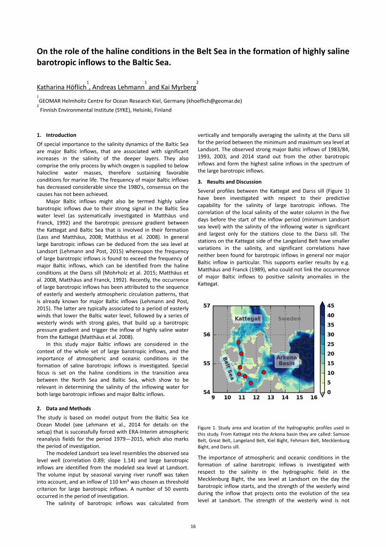
On the role of the haline conditions in the Belt Sea in the formation of highly saline barotropic inflows to the Baltic Sea.

Katharina Höflich1, Andreas Lehmann

1 and Kai Myrberg

2

1GEOMAR Helmholtz Centre for Ocean Research Kiel, Germany (khoeflich@geomar.de)

2 Finnish Environmental Institute (SYKE), Helsinki, Finland

1. Introduction Of special importance to the salinity dynamics of the Baltic Sea are major Baltic inflows, that are associated with significant increases in the salinity of the deeper layers. They also comprise the only process by which oxygen is supplied to below halocline water masses, therefore sustaining favorable conditions for marine life. The frequency of major Baltic inflows has decreased considerable since the 1980's, consensus on the causes has not been achieved.

Major Baltic inflows might also be termed highly saline barotropic inflows due to their strong signal in the Baltic Sea water level (as systematically investigated in Matthäus und Franck, 1992) and the barotropic pressure gradient between the Kattegat and Baltic Sea that is involved in their formation (Lass and Matthäus, 2008; Matthäus et al. 2008). In general large barotropic inflows can be deduced from the sea level at Landsort (Lehmann and Post, 2015) whereupon the frequency of large barotropic inflows is found to exceed the frequency of major Baltic inflows, which can be identified from the haline conditions at the Darss sill (Mohrholz et al. 2015; Matthäus et al. 2008, Matthäus and Franck, 1992). Recently, the occurrence of large barotropic inflows has been attributed to the sequence of easterly and westerly atmospheric circulation patterns, that is already known for major Baltic inflows (Lehmann and Post, 2015). The latter are typically associated to a period of easterly winds that lower the Baltic water level, followed by a series of westerly winds with strong gales, that build up a barotropic pressure gradient and trigger the inflow of highly saline water from the Kattegat (Matthäus et al. 2008).

In this study major Baltic inflows are considered in the context of the whole set of large barotropic inflows, and the importance of atmospheric and oceanic conditions in the formation of saline barotropic inflows is investigated. Special focus is set on the haline conditions in the transition area between the North Sea and Baltic Sea, which show to be relevant in determining the salinity of the inflowing water for both large barotropic inflows and major Baltic inflows.

2. Data and Methods The study is based on model output from the Baltic Sea Ice Ocean Model (see Lehmann et al., 2014 for details on the setup) that is successfully forced with ERA-Interim atmospheric reanalysis fields for the period 1979—2015, which also marks the period of investigation.

The modeled Landsort sea level resembles the observed sea level well (correlation 0.89; slope 1.14) and large barotropic inflows are identified from the modeled sea level at Landsort. The volume input by seasonal varying river runoff was taken into account, and an inflow of 110 km³ was chosen as threshold criterion for large barotropic inflows. A number of 50 events occurred in the period of investigation.

The salinity of barotropic inflows was calculated from

vertically and temporally averaging the salinity at the Darss sill for the period between the minimum and maximum sea level at Landsort. The observed strong major Baltic inflows of 1983/84, 1993, 2003, and 2014 stand out from the other barotropic inflows and form the highest saline inflows in the spectrum of the large barotropic inflows.

3. Results and Discussion Several profiles between the Kattegat and Darss sill (Figure 1) have been investigated with respect to their predictive capability for the salinity of large barotropic inflows. The correlation of the local salinity of the water column in the five days before the start of the inflow period (minimum Landsort sea level) with the salinity of the inflowing water is significant and largest only for the stations close to the Darss sill. The stations on the Kattegat side of the Langeland Belt have smaller variations in the salinity, and significant correlations have neither been found for barotropic inflows in general nor major Baltic inflow in particular. This supports earlier results by e.g. Matthäus and Franck (1989), who could not link the occurrence of major Baltic inflows to positive salinity anomalies in the Kattegat.

Figure 1. Study area and location of the hydrographic profiles used in this study. From Kattegat into the Arkona basin they are called: Samsoe Belt, Great Belt, Langeland Belt, Kiel Bight, Fehmarn Belt, Mecklenburg Bight, and Darss sill. The importance of atmospheric and oceanic conditions in the formation of saline barotropic inflows is investigated with respect to the salinity in the hydrographic field in the Mecklenburg Bight, the sea level at Landsort on the day the barotropic inflow starts, and the strength of the westerly wind during the inflow that projects onto the evolution of the sea level at Landsort. The strength of the westerly wind is not

16

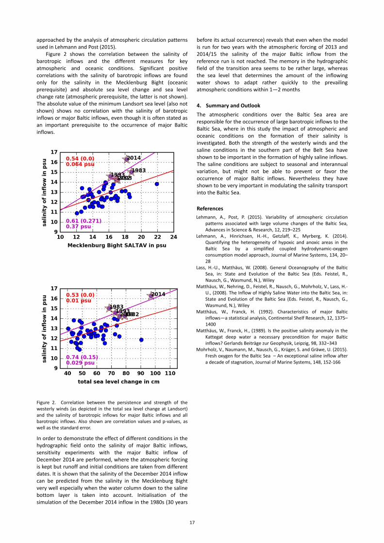
approached by the analysis of atmospheric circulation patterns used in Lehmann and Post (2015).

Figure 2 shows the correlation between the salinity of barotropic inflows and the different measures for key atmospheric and oceanic conditions. Significant positive correlations with the salinity of barotropic inflows are found only for the salinity in the Mecklenburg Bight (oceanic prerequisite) and absolute sea level change and sea level change rate (atmospheric prerequisite, the latter is not shown). The absolute value of the minimum Landsort sea level (also not shown) shows no correlation with the salinity of barotropic inflows or major Baltic inflows, even though it is often stated as an important prerequisite to the occurrence of major Baltic inflows.

Figure 2. Correlation between the persistence and strength of the westerly winds (as depicted in the total sea level change at Landsort) and the salinity of barotropic inflows for major Baltic inflows and all barotropic inflows. Also shown are correlation values and p-values, as well as the standard error. In order to demonstrate the effect of different conditions in the hydrographic field onto the salinity of major Baltic inflows, sensitivity experiments with the major Baltic inflow of December 2014 are performed, where the atmospheric forcing is kept but runoff and initial conditions are taken from different dates. It is shown that the salinity of the December 2014 inflow can be predicted from the salinity in the Mecklenburg Bight very well especially when the water column down to the saline bottom layer is taken into account. Initialisation of the simulation of the December 2014 inflow in the 1980s (30 years

before its actual occurrence) reveals that even when the model is run for two years with the atmospheric forcing of 2013 and 2014/15 the salinity of the major Baltic inflow from the reference run is not reached. The memory in the hydrographic field of the transition area seems to be rather large, whereas the sea level that determines the amount of the inflowing water shows to adapt rather quickly to the prevailing atmospheric conditions within 1—2 months 4. Summary and Outlook The atmospheric conditions over the Baltic Sea area are responsible for the occurrence of large barotropic inflows to the Baltic Sea, where in this study the impact of atmospheric and oceanic conditions on the formation of their salinity is investigated. Both the strength of the westerly winds and the saline conditions in the southern part of the Belt Sea have shown to be important in the formation of highly saline inflows. The saline conditions are subject to seasonal and interannual variation, but might not be able to prevent or favor the occurrence of major Baltic inflows. Nevertheless they have shown to be very important in modulating the salinity transport into the Baltic Sea. References Lehmann, A., Post, P. (2015). Variability of atmospheric circulation

patterns associated with large volume changes of the Baltic Sea, Advances in Science & Research, 12, 219–225

Lehmann, A., Hinrichsen, H.-H., Getzlaff, K., Myrberg, K. (2014). Quantifying the heterogeneity of hypoxic and anoxic areas in the Baltic Sea by a simplified coupled hydrodynamic-oxygen consumption model approach, Journal of Marine Systems, 134, 20–28

Lass, H.-U., Matthäus, W. (2008). General Oceanography of the Baltic Sea, in: State and Evolution of the Baltic Sea (Eds. Feistel, R., Nausch, G., Wasmund, N.), Wiley

Matthäus, W., Nehring, D., Feistel, R., Nausch, G., Mohrholz, V., Lass, H.-U., (2008). The Inflow of Highly Saline Water into the Baltic Sea, in: State and Evolution of the Baltic Sea (Eds. Feistel, R., Nausch, G., Wasmund, N.), Wiley

Matthäus, W., Franck, H. (1992). Characteristics of major Baltic inflows—a statistical analysis, Continental Shelf Research, 12, 1375–1400

Matthäus, W., Franck, H., (1989). Is the positive salinity anomaly in the Kattegat deep water a necessary precondition for major Baltic inflows? Gerlands Beiträge zur Geophysik, Leipzig, 98, 332–343

Mohrholz, V., Naumann, M., Nausch, G., Krüger, S. and Gräwe, U. (2015). Fresh oxygen for the Baltic Sea – An exceptional saline inflow after a decade of stagnation, Journal of Marine Systems, 148, 152-166

17

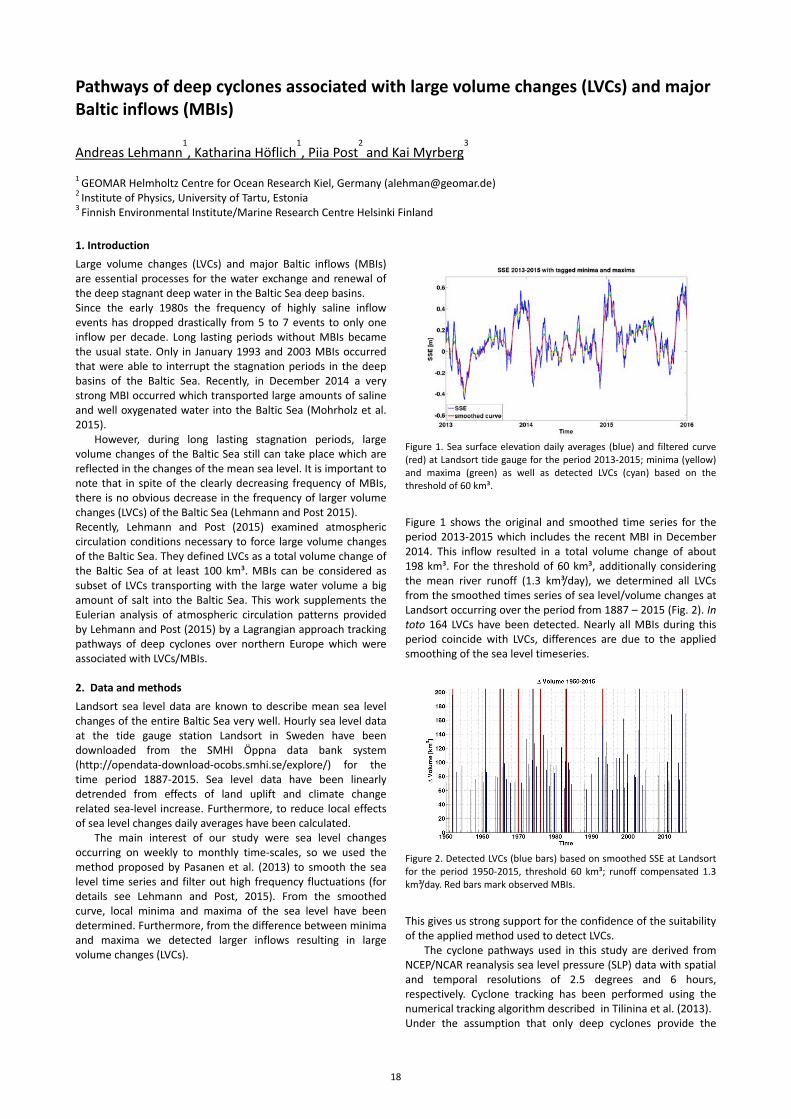
Pathways of deep cyclones associated with large volume changes (LVCs) and major Baltic inflows (MBIs) Andreas Lehmann

1, Katharina Höflich

1, Piia Post

2 and Kai Myrberg

3

1 GEOMAR Helmholtz Centre for Ocean Research Kiel, Germany (alehman@geomar.de) 2 Institute of Physics, University of Tartu, Estonia 3 Finnish Environmental Institute/Marine Research Centre Helsinki Finland 1. Introduction Large volume changes (LVCs) and major Baltic inflows (MBIs) are essential processes for the water exchange and renewal of the deep stagnant deep water in the Baltic Sea deep basins. Since the early 1980s the frequency of highly saline inflow events has dropped drastically from 5 to 7 events to only one inflow per decade. Long lasting periods without MBIs became the usual state. Only in January 1993 and 2003 MBIs occurred that were able to interrupt the stagnation periods in the deep basins of the Baltic Sea. Recently, in December 2014 a very strong MBI occurred which transported large amounts of saline and well oxygenated water into the Baltic Sea (Mohrholz et al. 2015).

However, during long lasting stagnation periods, large volume changes of the Baltic Sea still can take place which are reflected in the changes of the mean sea level. It is important to note that in spite of the clearly decreasing frequency of MBIs, there is no obvious decrease in the frequency of larger volume changes (LVCs) of the Baltic Sea (Lehmann and Post 2015). Recently, Lehmann and Post (2015) examined atmospheric circulation conditions necessary to force large volume changes of the Baltic Sea. They defined LVCs as a total volume change of the Baltic Sea of at least 100 km³. MBIs can be considered as subset of LVCs transporting with the large water volume a big amount of salt into the Baltic Sea. This work supplements the Eulerian analysis of atmospheric circulation patterns provided by Lehmann and Post (2015) by a Lagrangian approach tracking pathways of deep cyclones over northern Europe which were associated with LVCs/MBIs. 2. Data and methods Landsort sea level data are known to describe mean sea level changes of the entire Baltic Sea very well. Hourly sea level data at the tide gauge station Landsort in Sweden have been downloaded from the SMHI Öppna data bank system (http://opendata-download-ocobs.smhi.se/explore/) for the time period 1887-2015. Sea level data have been linearly detrended from effects of land uplift and climate change related sea-level increase. Furthermore, to reduce local effects of sea level changes daily averages have been calculated.

The main interest of our study were sea level changes occurring on weekly to monthly time-scales, so we used the method proposed by Pasanen et al. (2013) to smooth the sea level time series and filter out high frequency fluctuations (for details see Lehmann and Post, 2015). From the smoothed curve, local minima and maxima of the sea level have been determined. Furthermore, from the difference between minima and maxima we detected larger inflows resulting in large volume changes (LVCs).

Figure 1. Sea surface elevation daily averages (blue) and filtered curve (red) at Landsort tide gauge for the period 2013-2015; minima (yellow) and maxima (green) as well as detected LVCs (cyan) based on the threshold of 60 km³.

Figure 1 shows the original and smoothed time series for the period 2013-2015 which includes the recent MBI in December 2014. This inflow resulted in a total volume change of about 198 km³. For the threshold of 60 km³, additionally considering the mean river runoff (1.3 km³/day), we determined all LVCs from the smoothed times series of sea level/volume changes at Landsort occurring over the period from 1887 – 2015 (Fig. 2). In toto 164 LVCs have been detected. Nearly all MBIs during this period coincide with LVCs, differences are due to the applied smoothing of the sea level timeseries.

Figure 2. Detected LVCs (blue bars) based on smoothed SSE at Landsort for the period 1950-2015, threshold 60 km³; runoff compensated 1.3 km³/day. Red bars mark observed MBIs.

This gives us strong support for the confidence of the suitability of the applied method used to detect LVCs.

The cyclone pathways used in this study are derived from NCEP/NCAR reanalysis sea level pressure (SLP) data with spatial and temporal resolutions of 2.5 degrees and 6 hours, respectively. Cyclone tracking has been performed using the numerical tracking algorithm described in Tilinina et al. (2013). Under the assumption that only deep cyclones provide the

18

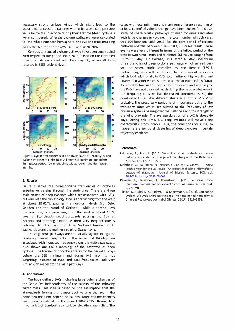
necessary strong surface winds which might lead to the occurrence of LVCs, the cyclones with at least one core pressure value below 980 hPa once during their lifetime (deep cyclones) were considered. Whereas cyclone pathways were calculated for the whole northern hemisphere, the cyclone track mapping was restricted to the area 4°W-32°E and 49°N-70°N.

Composite maps of cyclone pathway have been constructed with respect to the period 1949–2013, based on the identified time intervals associated with LVCs (Fig. 3), where 81 LVCs resulted in 3133 cyclone days.

Figure 3. Cyclone frequency based on NCEP-NCAR SLP reanalysis. and cyclone tracking: top left: 40 days before SSE minimum, top right:: during LVCs period, lower left: climatology, lower right: during MBI months.

3. Results Figure 3 shows the corresponding frequencies of cyclones entering or passing through the study area. There are three main routes of deep cyclones which are associated with LVCs, but also with the climatology. One is approaching from the west at about 58-62°N, passing the northern North Sea, Oslo, Sweden and the Island of Gotland , while a second, less frequent one, is approaching from the west at about 65°N, crossing Scandinavia south-eastwards passing the Sea of Bothnia and entering Finland. A third very frequent one is entering the study area north of Scotland turning north-eastwards along the northern coast of Scandinavia.

These general pathways are statistically significant against randomly chosen days/tracks in the sense that LVC-days are associated with increased frequency along the visible pathways. Also shown are the climatology of the pathways of deep cyclones, the frequency of cyclone tracks for the period 40 days before the SSE minimum and during MBI months. Not surprising, pictures of LVCs and MBI frequencies look very similar with respect to the main pathways. 4. Conclusions

We have defined LVCs indicating large volume changes of the Baltic Sea independently of the salinity of the inflowing water mass. This idea is based on the assumption that the atmospheric forcing that causes such volume changes in the Baltic Sea does not depend on salinity. Large volume changes have been calculated for the period 1887-2015 filtering daily time series of Landsort sea surface elevation anomalies. The

cases with local minimum and maximum difference resulting of at least 60 km³ of volume change have been chosen for a closer study of characteristic pathways of deep cyclones associated with large changes in volume. The total number of such cases was 164 between 1887–2015. For the core period of cyclone pathway analysis between 1948–2013, 81 cases result. These events were very different in terms of the inflow period or the time between maximum and minimum SSE values, ranging from 31 to 116 days. On average, LVCs lasted 40 days. We found three branches of deep cyclone pathways which agreed very well to storm tracks compiled by van Bebber (1891). Forthcoming work will be devoted to the chain of processes which lead additionally to LVCs to an influx of highly saline and oxygenated water which is termed as major Baltic Inflow (MBI). As stated before in this paper, the frequency and intensity of the LVCs have not changed much during the last decades even if the frequency of MBIs has decreased considerable. So, the question will rise: what differentiates a MBI from a LVC? Most probably, the precursory period is of importance but also the transports rates which are related to the frequency of low pressure systems passing over the Baltic Sea and the strength of the wind play role. The average duration of a LVC is about 40 days. During this time, 5-6 deep cyclones will move along characteristic storm tracks. Thus, the conditions for a LVC to happen are a temporal clustering of deep cyclones in certain trajectory corridors. References Lehmann, A., Post, P. (2015) Variability of atmospheric circulation

patterns associated with large volume changes of the Baltic Sea. Adv. Sci. Res. 12, 219 – 225.

Mohrholz, V., Naumann, N., Nausch, G., Krüger, S, Gräwe. U. (2015) Fresh oxygen for the Baltic Sea – An exceptional saline inflow after a decade of stagnation, Journal of Marine Systems, DOI: doi: 10.1016/j.jmarsys.2015.03.005.

Pasanen, L., Launonen, I., Holmström, L.(2013) A scale space multiresolution method for extraction of time series features. Stat, 2, 273-291.

Tilinina, N., Gulev, S. K., Rudeva, I., & Koltermann, P. (2013). Comparing Cyclone Life Cycle Characteristics and Their Interannual Variability in Different Reanalyses. Journal of Climate, 26(17), 6419–6438.

19

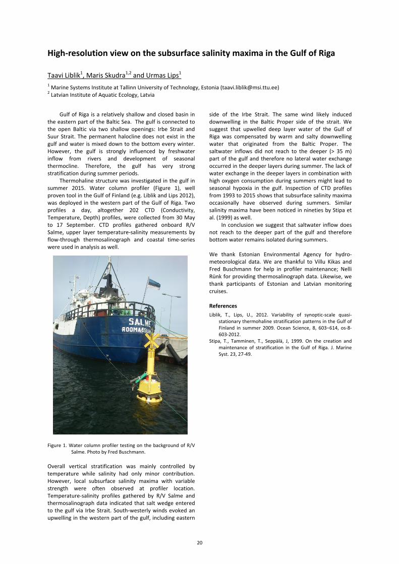
High-resolution view on the subsurface salinity maxima in the Gulf of Riga

Taavi Liblik1, Maris Skudra1,2 and Urmas Lips1 1 Marine Systems Institute at Tallinn University of Technology, Estonia (taavi.liblik@msi.ttu.ee) 2 Latvian Institute of Aquatic Ecology, Latvia

Gulf of Riga is a relatively shallow and closed basin in the eastern part of the Baltic Sea. The gulf is connected to the open Baltic via two shallow openings: Irbe Strait and Suur Strait. The permanent halocline does not exist in the gulf and water is mixed down to the bottom every winter. However, the gulf is strongly influenced by freshwater inflow from rivers and development of seasonal thermocline. Therefore, the gulf has very strong stratification during summer periods.

Thermohaline structure was investigated in the gulf in summer 2015. Water column profiler (Figure 1), well proven tool in the Gulf of Finland (e.g. Liblik and Lips 2012), was deployed in the western part of the Gulf of Riga. Two profiles a day, altogether 202 CTD (Conductivity, Temperature, Depth) profiles, were collected from 30 May to 17 September. CTD profiles gathered onboard R/V Salme, upper layer temperature-salinity measurements by flow-through thermosalinograph and coastal time-series were used in analysis as well.

Figure 1. Water column profiler testing on the background of R/V

Salme. Photo by Fred Buschmann.

Overall vertical stratification was mainly controlled by temperature while salinity had only minor contribution. However, local subsurface salinity maxima with variable strength were often observed at profiler location. Temperature-salinity profiles gathered by R/V Salme and thermosalinograph data indicated that salt wedge entered to the gulf via Irbe Strait. South-westerly winds evoked an upwelling in the western part of the gulf, including eastern

side of the Irbe Strait. The same wind likely induced downwelling in the Baltic Proper side of the strait. We suggest that upwelled deep layer water of the Gulf of Riga was compensated by warm and salty downwelling water that originated from the Baltic Proper. The saltwater inflows did not reach to the deeper (> 35 m) part of the gulf and therefore no lateral water exchange occurred in the deeper layers during summer. The lack of water exchange in the deeper layers in combination with high oxygen consumption during summers might lead to seasonal hypoxia in the gulf. Inspection of CTD profiles from 1993 to 2015 shows that subsurface salinity maxima occasionally have observed during summers. Similar salinity maxima have been noticed in nineties by Stipa et al. (1999) as well.

In conclusion we suggest that saltwater inflow does not reach to the deeper part of the gulf and therefore bottom water remains isolated during summers. We thank Estonian Environmental Agency for hydro-meteorological data. We are thankful to Villu Kikas and Fred Buschmann for help in profiler maintenance; Nelli Rünk for providing thermosalinograph data. Likewise, we thank participants of Estonian and Latvian monitoring cruises. References Liblik, T., Lips, U., 2012. Variability of synoptic-scale quasi-

stationary thermohaline stratification patterns in the Gulf of Finland in summer 2009. Ocean Science, 8, 603−614, os-8-603-2012.

Stipa, T., Tamminen, T., Seppӓlä, J, 1999. On the creation and maintenance of stratification in the Gulf of Riga. J. Marine Syst. 23, 27-49.

20

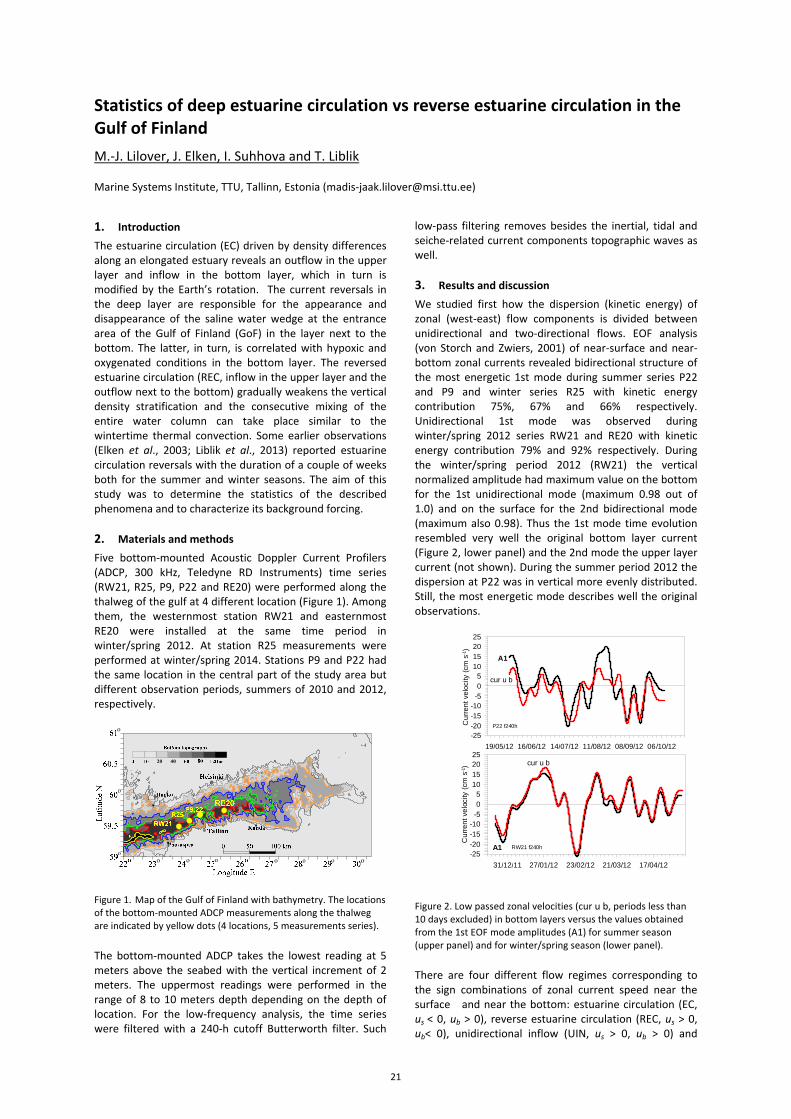
Statistics of deep estuarine circulation vs reverse estuarine circulation in the Gulf of Finland M.-J. Lilover, J. Elken, I. Suhhova and T. Liblik Marine Systems Institute, TTU, Tallinn, Estonia (madis-jaak.lilover@msi.ttu.ee)

1. Introduction The estuarine circulation (EC) driven by density differences along an elongated estuary reveals an outflow in the upper layer and inflow in the bottom layer, which in turn is modified by the Earth’s rotation. The current reversals in the deep layer are responsible for the appearance and disappearance of the saline water wedge at the entrance area of the Gulf of Finland (GoF) in the layer next to the bottom. The latter, in turn, is correlated with hypoxic and oxygenated conditions in the bottom layer. The reversed estuarine circulation (REC, inflow in the upper layer and the outflow next to the bottom) gradually weakens the vertical density stratification and the consecutive mixing of the entire water column can take place similar to the wintertime thermal convection. Some earlier observations (Elken et al., 2003; Liblik et al., 2013) reported estuarine circulation reversals with the duration of a couple of weeks both for the summer and winter seasons. The aim of this study was to determine the statistics of the described phenomena and to characterize its background forcing. 2. Materials and methods Five bottom-mounted Acoustic Doppler Current Profilers (ADCP, 300 kHz, Teledyne RD Instruments) time series (RW21, R25, P9, P22 and RE20) were performed along the thalweg of the gulf at 4 different location (Figure 1). Among them, the westernmost station RW21 and easternmost RE20 were installed at the same time period in winter/spring 2012. At station R25 measurements were performed at winter/spring 2014. Stations P9 and P22 had the same location in the central part of the study area but different observation periods, summers of 2010 and 2012, respectively.

Figure 1. Map of the Gulf of Finland with bathymetry. The locations of the bottom-mounted ADCP measurements along the thalweg are indicated by yellow dots (4 locations, 5 measurements series).

The bottom-mounted ADCP takes the lowest reading at 5 meters above the seabed with the vertical increment of 2 meters. The uppermost readings were performed in the range of 8 to 10 meters depth depending on the depth of location. For the low-frequency analysis, the time series were filtered with a 240-h cutoff Butterworth filter. Such

low-pass filtering removes besides the inertial, tidal and seiche-related current components topographic waves as well. 3. Results and discussion We studied first how the dispersion (kinetic energy) of zonal (west-east) flow components is divided between unidirectional and two-directional flows. EOF analysis (von Storch and Zwiers, 2001) of near-surface and near-bottom zonal currents revealed bidirectional structure of the most energetic 1st mode during summer series P22 and P9 and winter series R25 with kinetic energy contribution 75%, 67% and 66% respectively. Unidirectional 1st mode was observed during winter/spring 2012 series RW21 and RE20 with kinetic energy contribution 79% and 92% respectively. During the winter/spring period 2012 (RW21) the vertical normalized amplitude had maximum value on the bottom for the 1st unidirectional mode (maximum 0.98 out of 1.0) and on the surface for the 2nd bidirectional mode (maximum also 0.98). Thus the 1st mode time evolution resembled very well the original bottom layer current (Figure 2, lower panel) and the 2nd mode the upper layer current (not shown). During the summer period 2012 the dispersion at P22 was in vertical more evenly distributed. Still, the most energetic mode describes well the original observations.

19/05/12 16/06/12 14/07/12 11/08/12 08/09/12 06/10/12-25-20-15-10

-505

10152025

Cur

rent

velo

city

(cm

s-1)

P22 f240h

cur u b

A1

31/12/11 27/01/12 23/02/12 21/03/12 17/04/12-25-20-15-10

-505

10152025

Cur

rent

velo

city

(cm

s-1)

RW21 f240h

cur u b

A1

Figure 2. Low passed zonal velocities (cur u b, periods less than 10 days excluded) in bottom layers versus the values obtained from the 1st EOF mode amplitudes (A1) for summer season (upper panel) and for winter/spring season (lower panel).

There are four different flow regimes corresponding to the sign combinations of zonal current speed near the surface and near the bottom: estuarine circulation (EC, us < 0, ub > 0), reverse estuarine circulation (REC, us > 0, ub< 0), unidirectional inflow (UIN, us > 0, ub > 0) and

21

unidirectional outflow (UOUT, us < 0, ub < 0). Results of analysis presented in Table 1 show that during the summer observation period in 2012 when the mean zonal wind stress was 0.028 N m-2, the prevailing flow type at P22 was bidirectional flow (71% of time) where EC took place in 27% and REC in 44% of time, UIN and UOUT took place in 14% and 15% of time respectively. During another summer of 2010 when mean zonal wind stress was lower (0.011 N m-2), observations at P9 revealed also dominating bidirectional flows, but EC prevailed over REC (43% vs 17%). For winter/spring periods the unidirectional and two-directional flows were roughly in balance. EC took place in about 20% and REC in about 30% of time.

Table 1: Frequency (%) of vertical structures of flow: bidirectional estuarine (EC) and reversed estuarine (REC) flow, unidirectional inflow (UIN) and outflow (UOUT).

Station EC (%) REC (%) UIN (%) UOUT (%) Winter (RW21) 18 28 41 13 Winter (R25) 21 32 24 23 Summer (P22) 27 44 14 15 Summer (P9) 43 17 15 25 Mean 27 30 24 19

Within the theories of wind-forced motions of elongated basins (e.g. Winant, 2004), downwind flows develop on the coastal shoals and on the thin surface Ekman layer of the basin interior, but compensating upwind flows take place in the deeper parts of the basins because the sea level is piled up in the downwind end of the basin. Such mechanisms have been confirmed by the analysis of the results from numerical models (Krauss and Brügge, 1991; Elken et al., 2003), but good observational evidence has been missing due to the lack of sufficient amount of observations. We have found observational evidence that deep along-basin current velocities depend on the wind velocity with correlations above 0.7: maximum deep inflows occur in winter during north-easterly winds and in summer during easterly winds, and outflows during the winds from reverse direction. This relation is in agreement with the results of calculations (not shown) of longitudinal (along the channel axis) wind forced flows, using the analytical model by Winant (2004). For the estuarine flow reversal in real conditions, W or SW wind speed must be stronger from some critical value that depends on the stratification, including the density difference between the Northern Baltic Proper and the Gulf of Finland. Rough guidance to the critical value of wind speed may obtained by analysis of Wedderburn number. Acknowledgements The study was partly supported by institutional research funding IUT 19-6 of the Estonian Ministry of Education and Research, and partly by the Estonian Science Foundation grants 9278 and 9382. ADCP stations were installed within the projects: base funding of Marine Systems Institute (RE20, RW21, P22), IUT 19-6 (R25), Estonian Science Foundation grant 6955 (P9). We are grateful to the crew and the scientific team of R/V Salme for assistance in the deployment of the ADCP, to Jaan Laanemets and Urmas Lips for providing ADCP current measurements data.

References

Elken, J., Raudsepp, U. and Lips, U., 2003. On the estuarine transport reversal in deep layers of the Gulf of Finland. Journal of Sea Research, 49(4), pp.267-274.

Krauss, W. and Brügge, B., 1991. Wind-produced water exchange between the deep basins of the Baltic Sea. Journal of Physical Oceanography, 21(3), pp.373-384.

Liblik, T., Laanemets, J., Raudsepp, U., Elken, J. and Suhhova, I., 2013. Estuarine circulation reversals and related rapid changes in winter near-bottom oxygen conditions in the Gulf of Finland, Baltic Sea. Ocean Science, 9(5), pp.917-930.

Von Storch, H. and Zwiers, F.W., 2001. Statistical analysis in climate research. Cambridge university press.

Winant, C.D., 2004. Three-dimensional wind-driven flow in an elongated, rotating basin. Journal of Physical Oceanography, 34(2), pp.462-476.

22

Salinity oscillations in the range of seasonal variability Ekaterina N.Litina,2, Evgenyi A. Zakharchuk 1,2 1 State Oceanographic Institute, Saint-Petersburg Branch, Saint-Petersburg, Russia (spbsoi@rambler.ru, warzuga@yandex.ru) 2 Saint Petersburg State University, Saint-Petersburg, Russia

1. Introduction During the last decades there are significant changes in the hydrogeological conditions in the Baltic Sea: warming causing temperature rise in the surface and bottom layers [4], a sharp reduction in the number of major Baltic inflows [2, 6], which led to a decrease in salinity, increase the duration anaerobic conditions in the deep depressions [4], increase in the number of dangerous level rise. [3]. It is known that the seasonal component contributes to changes in thermohaline characteristics of the Baltic sea [2], its characteristics change from year to year. Following the work of Monin [5], under the seasonal fluctuations of characteristics we understand the changes occurring with a period of 1 year or year multiple harmonics (overtones). In this work we investigate the interannual variability of seasonal variations in salinity during the significant changes of the hydrological regime on the basis of Fourier analysis carried out taking into account the non-stationary process. 2. Data and methods In the work were used the data of ship measurements of salinity in the open part of the Baltic sea in the 2nd half of the twentieth and early twenty-first centuries at stations for international monitoring (database DAS (http://nest.su.se/das/)). The analysis was carried out for 6 stations located in different parts of the sea: BY2, BY5, BY1, BY20– BY31 LL12. Sampling implemented within a radius of 2 miles from the point of accepted geographical coordinates of international monitoring stations. For each station investigated the near-surface (0 to 5 meters) and the bottom layer, the depth of the latter varied from station to station depending on the bathymetric features of the area and the availability of adequate amount of data for the analysis of specific horizons. Mean monthly values were calculated based on the original series of data. Data gaps in the ranks of the monthly mean values were replaced with the calculated values of these characteristics, evaluated by means of Fourier analysis, the implementation using the method of least squares, taking into account the nonstationarity of the process. For the resulting rows the amplitudes and phases of annual, semiannual, third year, a quarter of annual harmonics using Fourier analysis were calculated, ranks in the stationary and non-stationary approximation were prediction, the trend was removed, the residual number was identified and the variance of these series was assessed. Reliability evaluation was performed for the obtained values of the amplitudes and phases. The confidence interval for the amplitude values calculated by the formula:

√ ,

where σ - standard deviation of the test series, t_ (a) - Student criterion, defined for given values of confidence level α (adopted in this study for 0.95) and the number of members of a number n [1]. The confidence interval for the

phase value is determined by the values of the amplitudes and calculated by the formula:

ф ,

Invalid values were excluded from the assessment.

3. Results The stationary component has a significant role in the seasonal variability of salinity in the surface layer. The ranks are calculated based on the nonstationarity of the process on the background of pre-calculated rows in the stationary approximation is shown in figure 1. It is seen that in some years, there were abnormally high and abnormally low amplitude fluctuations of salinity.

Figure 1. Pre-calculated a series of changes in salinity in the stationary approximation (green line) and taking into account the non-stationarity of the process (black line) for surface (a) and bottom (b) layer with a remote trend to station BY15.

Peaks to mark the appearance of large flows in 1993 and 2003 are observed in the bottom layer.

Figure 2 shows the amplitude of the four waves. It can be seen that the annual wave contributes significantly to the change in salinity in the surface layer, the impact of other waves are less pronounced (fig. 2 - a). The maximum amplitude of the annual wave was observed in 1988 and in 2006. The interannual variability of seasonal variation is less pronounced in the bottom layer (fig. 2 -b), the determining factor here is the large Baltic inflows.

23

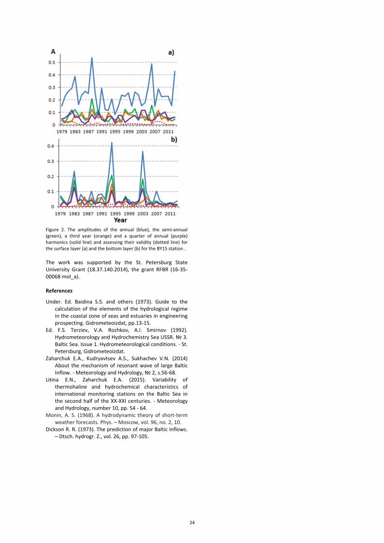
Figure 2. The amplitudes of the annual (blue), the semi-annual (green), a third year (orange) and a quarter of annual (purple) harmonics (solid line) and assessing their validity (dotted line) for the surface layer (a) and the bottom layer (b) for the BY15 station . The work was supported by the St. Petersburg State University Grant (18.37.140.2014), the grant RFBR (16-35-00068 mol_a). References

Under. Ed. Baidina S.S. and others (1973). Guide to the calculation of the elements of the hydrological regime in the coastal zone of seas and estuaries in engineering prospecting. Gidrometeoizdat, pp.13-15.

Ed. F.S. Terziev, V.A. Rozhkov, A.I. Smirnov (1992). Hydrometeorology and Hydrochemistry Sea USSR. № 3. Baltic Sea. Issue 1. Hydrometeorological conditions. - St. Petersburg, Gidrometeoizdat.

Zaharchuk E.A., Kudryavtsev A.S., Sukhachev V.N. (2014) About the mechanism of resonant wave of large Baltic Inflow. - Meteorology and Hydrology, № 2, s.56-68.

Litina E.N., Zaharchuk E.A. (2015). Variability of thermohaline and hydrochemical characteristics of international monitoring stations on the Baltic Sea in the second half of the XX-XXI centuries. - Meteorology and Hydrology, number 10, pp. 54 - 64.

Monin, A. S. (1968). A hydrodynamic theory of short-term weather forecasts. Phys. – Moscow, vol. 96, no. 2, 10.

Dickson R. R. (1973). The prediction of major Baltic inflows. – Dtsch. hydrogr. Z., vol. 26, pp. 97-105.

24

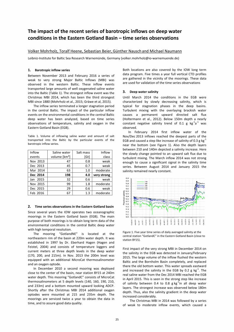
The impact of the recent series of barotropic inflows on deep water conditions in the Eastern Gotland Basin – time series observations

Volker Mohrholz, Toralf Heene, Sebastian Beier, Günther Nausch and Michael Naumann

Leibniz-Institute for Baltic Sea Research Warnemünde, Germany (volker.mohrholz@io-warnemuende.de)

1. Barotropic inflow series Between November 2013 and February 2016 a series of weak to very strong Major Baltic Inflows (MBI) was observed in the western Baltic. These inflow events transported large amounts of well oxygenated saline water into the Baltic (Table 1). The strongest inflow event was the Christmas MBI 2014, which has been the third strongest MBI since 1880 (Mohrholz et al., 2015; Gräwe et al, 2015).

The inflow series terminated a longer stagnation period in the central Baltic. The impact of the particular inflow events on the environmental conditions in the central Baltic deep water has been analyzed, based on time series observations of temperature, salinity and oxygen in the Eastern Gotland Basin (EGB).

Table 1. Volume of inflowing saline water and amount of salt transported into the Baltic by the particular events of the barotropic inflow series.

Inflow events

Saline water volume [km³]

Salt mass [Gt]

Inflow class

Nov 2013 47 0.8 weak Dec 2013 45 0.7 weak Mar 2014 63 1.0 moderate Dec 2014 198 4.0 very strong Jan 2015 32 0.6 weak Nov 2015 99 1.8 moderate Dec 2015 29 0.6 weak Feb 2016 67 1.3 moderate

2. Time series observations in the Eastern Gotland basin Since several years the IOW operates two oceanographic moorings in the Eastern Gotland basin (EGB). The main purpose of both moorings is to obtain long term data of the environmental conditions in the central Baltic deep water with high temporal resolution.

The mooring “GotlandNE” is located at the northeastern rim of the basin at 220m water depth. It was established in 1997 by Dr. Eberhard Hagen (Hagen and Feistel, 2004) and consists of temperature loggers and current meters at three depth levels in the deep water (170, 200, and 215m). In Nov. 2013 the 200m level was equipped with an additional MicroCat thermosalinometer and an oxygen optode.

In December 2010 a second mooring was deployed close to the center of the basin, near station BY15 at 240m water depth. This mooring “GotlandC” consists of MicroCat thermosalinometers at 5 depth levels (140, 160, 190, 210, and 233m) and a bottom mounted upward looking ADCP. Shortly after the Christmas MBI 2014 additional oxygen optodes were mounted at 215 and 235m depth. The moorings are serviced twice a year to obtain the data in time, and to assure good data quality.

Both locations are also covered by the IOW long term data program. Five times a year full vertical CTD profiles are gathered in the vicinity of the moorings. These data are used for validation of the time series observations

3. Deep water salinity Until March 2014 the conditions in the EGB were characterized by slowly decreasing salinity, which is typical for stagnation phases in the deep basins. Turbulent mixing with the overlaying brackish water causes a permanent upward directed salt flux (Holtermann et al., 2012). Below 150m depth a nearly constant negative salinity trend of 0.1 g kg-1a-1 was observed.

In February 2014 first inflow water of the Nov/Dec 2013 inflows reached the deepest parts of the EGB and caused a step like increase of salinity of 0.3 g kg-1 near the bottom (see Figure 1). Also the depth layers between 210 and 140m depicted a salinity increase. Here the slowly change pointed to an upward salt flux due to turbulent mixing. The March inflow 2014 was not strong enough to cause a significant signal in the salinity time series. Between August 2014 and January 2015 the salinity remained nearly constant.

Figure 1. Five year time series of daily averaged salinity at the central station “GotlandC” in the Eastern Gotland Basin (close to station BY15).

First impact of the very strong MBI in December 2014 on the salinity in the EGB was detected in January/February 2015. The large volume of the inflow flushed the western Baltic and the Bornholm Basin completely, and replaced there the old bottom water. This water spreads eastward and increased the salinity in the EGB by 0.2 g kg-1. The real saline water from the Dec 2014 MBI reached the EGB in April 2015. This is seen in the strong step like increase of salinity between 0.4 to 0.8 g kg-1in all deep water layers. The strongest increase was observed below 180m depth. Thus, also the salinity gradient in the deep water increased considerably.

The Christmas MBI in 2014 was followed by a series of weak to moderate inflow events, which caused a

25

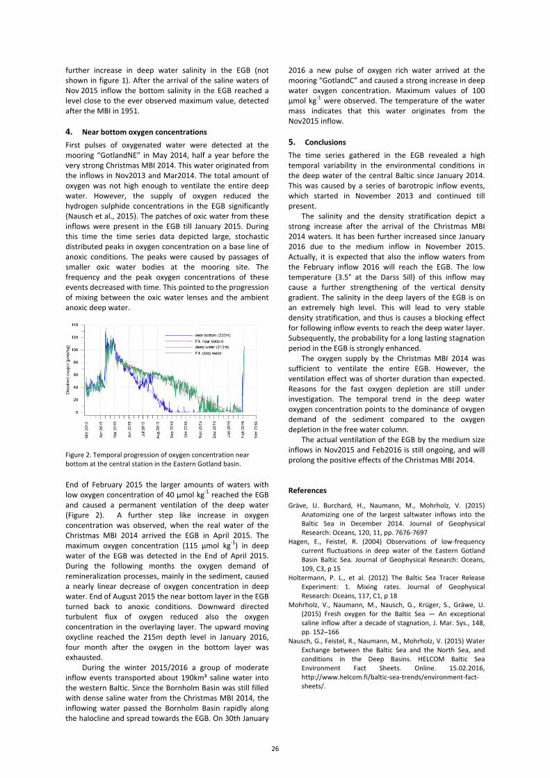
further increase in deep water salinity in the EGB (not shown in figure 1). After the arrival of the saline waters of Nov 2015 inflow the bottom salinity in the EGB reached a level close to the ever observed maximum value, detected after the MBI in 1951. 4. Near bottom oxygen concentrations First pulses of oxygenated water were detected at the mooring “GotlandNE” in May 2014, half a year before the very strong Christmas MBI 2014. This water originated from the inflows in Nov2013 and Mar2014. The total amount of oxygen was not high enough to ventilate the entire deep water. However, the supply of oxygen reduced the hydrogen sulphide concentrations in the EGB significantly (Nausch et al., 2015). The patches of oxic water from these inflows were present in the EGB till January 2015. During this time the time series data depicted large, stochastic distributed peaks in oxygen concentration on a base line of anoxic conditions. The peaks were caused by passages of smaller oxic water bodies at the mooring site. The frequency and the peak oxygen concentrations of these events decreased with time. This pointed to the progression of mixing between the oxic water lenses and the ambient anoxic deep water.

Figure 2. Temporal progression of oxygen concentration near bottom at the central station in the Eastern Gotland basin.

End of February 2015 the larger amounts of waters with low oxygen concentration of 40 µmol kg-1 reached the EGB and caused a permanent ventilation of the deep water (Figure 2). A further step like increase in oxygen concentration was observed, when the real water of the Christmas MBI 2014 arrived the EGB in April 2015. The maximum oxygen concentration (115 µmol kg-1) in deep water of the EGB was detected in the End of April 2015. During the following months the oxygen demand of remineralization processes, mainly in the sediment, caused a nearly linear decrease of oxygen concentration in deep water. End of August 2015 the near bottom layer in the EGB turned back to anoxic conditions. Downward directed turbulent flux of oxygen reduced also the oxygen concentration in the overlaying layer. The upward moving oxycline reached the 215m depth level in January 2016, four month after the oxygen in the bottom layer was exhausted.

During the winter 2015/2016 a group of moderate inflow events transported about 190km³ saline water into the western Baltic. Since the Bornholm Basin was still filled with dense saline water from the Christmas MBI 2014, the inflowing water passed the Bornholm Basin rapidly along the halocline and spread towards the EGB. On 30th January

2016 a new pulse of oxygen rich water arrived at the mooring “GotlandC” and caused a strong increase in deep water oxygen concentration. Maximum values of 100 µmol kg-1 were observed. The temperature of the water mass indicates that this water originates from the Nov2015 inflow. 5. Conclusions The time series gathered in the EGB revealed a high temporal variability in the environmental conditions in the deep water of the central Baltic since January 2014. This was caused by a series of barotropic inflow events, which started in November 2013 and continued till present.

The salinity and the density stratification depict a strong increase after the arrival of the Christmas MBI 2014 waters. It has been further increased since January 2016 due to the medium inflow in November 2015. Actually, it is expected that also the inflow waters from the February inflow 2016 will reach the EGB. The low temperature (3.5° at the Darss Sill) of this inflow may cause a further strengthening of the vertical density gradient. The salinity in the deep layers of the EGB is on an extremely high level. This will lead to very stable density stratification, and thus is causes a blocking effect for following inflow events to reach the deep water layer. Subsequently, the probability for a long lasting stagnation period in the EGB is strongly enhanced.

The oxygen supply by the Christmas MBI 2014 was sufficient to ventilate the entire EGB. However, the ventilation effect was of shorter duration than expected. Reasons for the fast oxygen depletion are still under investigation. The temporal trend in the deep water oxygen concentration points to the dominance of oxygen demand of the sediment compared to the oxygen depletion in the free water column.

The actual ventilation of the EGB by the medium size inflows in Nov2015 and Feb2016 is still ongoing, and will prolong the positive effects of the Christmas MBI 2014. References

Gräve, U. Burchard, H., Naumann, M., Mohrholz, V. (2015) Anatomizing one of the largest saltwater inflows into the Baltic Sea in December 2014. Journal of Geophysical Research: Oceans, 120, 11, pp. 7676-7697

Hagen, E., Feistel, R. (2004) Observations of low-frequency current fluctuations in deep water of the Eastern Gotland Basin Baltic Sea. Journal of Geophysical Research: Oceans, 109, C3, p 15

Holtermann, P. L., et al. (2012) The Baltic Sea Tracer Release Experiment: 1. Mixing rates. Journal of Geophysical Research: Oceans, 117, C1, p 18

Mohrholz, V., Naumann, M., Nausch, G., Krüger, S., Gräwe, U. (2015) Fresh oxygen for the Baltic Sea — An exceptional saline inflow after a decade of stagnation, J. Mar. Sys., 148, pp. 152–166

Nausch, G., Feistel, R., Naumann, M., Mohrholz, V. (2015) Water Exchange between the Baltic Sea and the North Sea, and conditions in the Deep Basins. HELCOM Baltic Sea Environment Fact Sheets. Online. 15.02.2016, http://www.helcom.fi/baltic-sea-trends/environment-fact-sheets/.

26

A succession of four Major Baltic Inflows in the period 2014-2016 – an overview of propagation and environmental change

Michael Naumann1, Günther Nausch2 and Volker Mohrholz1 1 Physical Oceanography and Instrumentation, Leibniz Institute for Baltic Sea Research Warnmünde, Seestraße 15, D-18119 Rostock, Germany (michael.naumann@io-warnemuende.de) 2 Marine Chemistry, Leibniz Institute for Baltic Sea Research Warnmünde, Seestraße 15, D-18119 Rostock, Germany After ten years of stagnation and oxygen depletion in the deep-water of the Baltic Sea, in 2014 a succession of inflows of highly saline water from the North Sea started again and ventilated repeatedly deep-water areas up to the central part of the eastern Gotland Basin. Sporadic events of this kind are called Major Baltic Inflows (MBI) and permit deep-water renewal in the central Baltic, where hypoxic to anoxic conditions are dominating since about 1980. The observed MBI’s were caused by long lasting westerly wind periods during the wintertime 2013/14 (Naumann & Nausch 2015), December 2014 (Mohrholz et al. 2015, Naumann et al. in review), November 2015 and finally in January-February 2016. The process reconstruction of the propagation, their interplay and environmental changes presented in this talk is based on 26 cruises, continuous data records of the Darss Sill measuring mast, the Arkona Basin buoy, both at the shallow Baltic entrance, and tide gauge data. The succession started with a triple of smaller inflows from December 2013 to March 2014, which interacted positively and ventilated in May 2014 the eastern Gotland Basin for the first time since 2003. In December 2014 followed a Major Baltic Inflow of historic size, with a volume of 198 km³ highly saline water and 4 Gt salt import. The propagation and impact of this event was intensively observed by cruises in a rhythm of 3-4 weeks. Since mid-October 2015 the inflow activity started again with a succession of two smaller pulses in October and December as well as two MBI’s of moderate intensity in November 2015 and January-February 2016.The headline style is 9pt Calibri, boldface fond. The body text should be typed in Calibri, 9pt, single spaced, two column text, adjusted, as in this example. Please write your extended abstract into it. References Mohrholz, V.; Naumann, M.; Nausch, G.; Krüger, S.; Gräwe, U.

(2015) Fresh oxygen for the Baltic Sea – An exceptional saline inflow after a decade of stagnation, Journal of Marine Systems, Vol. 148, pp. 152-166

Naumann, M.; Nausch, G. (2015) Salzwassereinstrom 2014 – Die Ostsee atmet auf (english title: The Baltic Sea is breathing on – Salt Water Inlet 2014), Chemie in unserer Zeit, Vol. 49, No. 1, pp. 76-80

Naumann, M.; Nausch, G.; Schulz-Vogt, H.; Donath, J.; Feistel, S.; Gogina, M.; Mohrholz, V.; Prien, R.; Schmidt, M.; Umlauf, L.; Waniek, J.J.; Wasmund, N.; Schulz-Bull, D. (in review) A major oxygenation event in the Baltic Sea, Scientific Reports

27

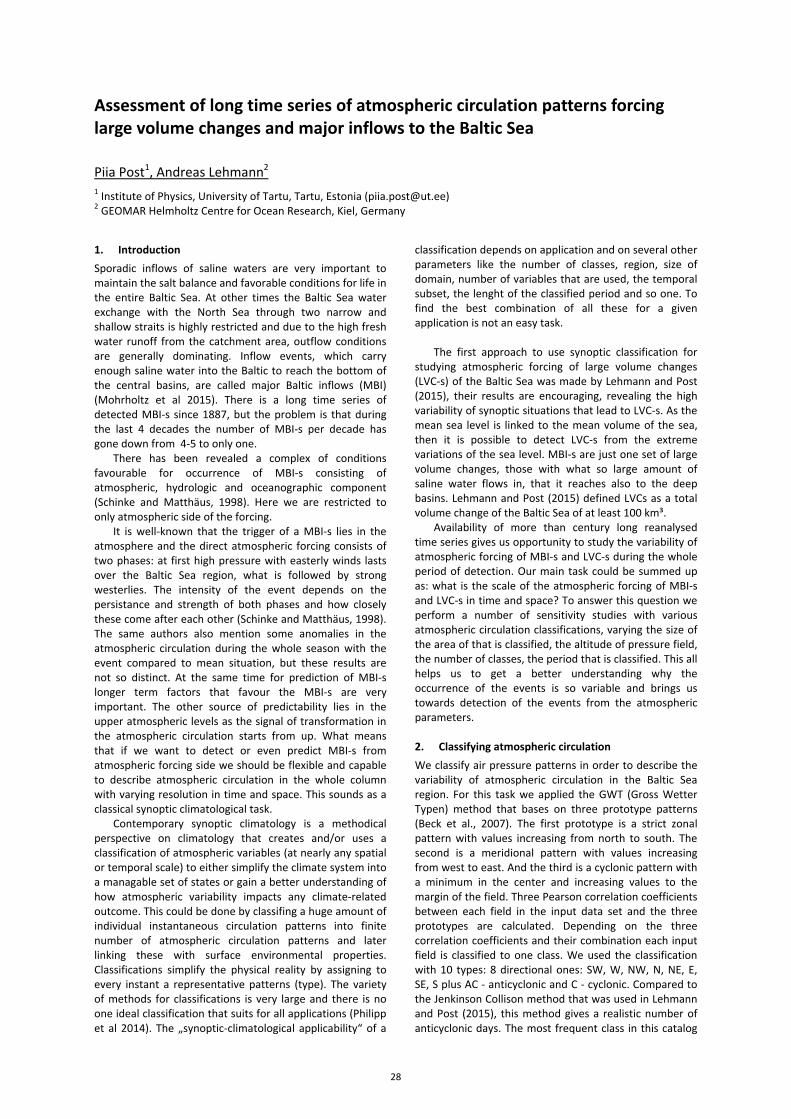
Assessment of long time series of atmospheric circulation patterns forcing large volume changes and major inflows to the Baltic Sea

Piia Post1, Andreas Lehmann2 1 Institute of Physics, University of Tartu, Tartu, Estonia (piia.post@ut.ee) 2 GEOMAR Helmholtz Centre for Ocean Research, Kiel, Germany

1. Introduction Sporadic inflows of saline waters are very important to maintain the salt balance and favorable conditions for life in the entire Baltic Sea. At other times the Baltic Sea water exchange with the North Sea through two narrow and shallow straits is highly restricted and due to the high fresh water runoff from the catchment area, outflow conditions are generally dominating. Inflow events, which carry enough saline water into the Baltic to reach the bottom of the central basins, are called major Baltic inflows (MBI) (Mohrholtz et al 2015). There is a long time series of detected MBI-s since 1887, but the problem is that during the last 4 decades the number of MBI-s per decade has gone down from 4-5 to only one.

There has been revealed a complex of conditions favourable for occurrence of MBI-s consisting of atmospheric, hydrologic and oceanographic component (Schinke and Matthäus, 1998). Here we are restricted to only atmospheric side of the forcing.

It is well-known that the trigger of a MBI-s lies in the atmosphere and the direct atmospheric forcing consists of two phases: at first high pressure with easterly winds lasts over the Baltic Sea region, what is followed by strong westerlies. The intensity of the event depends on the persistance and strength of both phases and how closely these come after each other (Schinke and Matthäus, 1998). The same authors also mention some anomalies in the atmospheric circulation during the whole season with the event compared to mean situation, but these results are not so distinct. At the same time for prediction of MBI-s longer term factors that favour the MBI-s are very important. The other source of predictability lies in the upper atmospheric levels as the signal of transformation in the atmospheric circulation starts from up. What means that if we want to detect or even predict MBI-s from atmospheric forcing side we should be flexible and capable to describe atmospheric circulation in the whole column with varying resolution in time and space. This sounds as a classical synoptic climatological task.

Contemporary synoptic climatology is a methodical perspective on climatology that creates and/or uses a classification of atmospheric variables (at nearly any spatial or temporal scale) to either simplify the climate system into a managable set of states or gain a better understanding of how atmospheric variability impacts any climate-related outcome. This could be done by classifing a huge amount of individual instantaneous circulation patterns into finite number of atmospheric circulation patterns and later linking these with surface environmental properties. Classifications simplify the physical reality by assigning to every instant a representative patterns (type). The variety of methods for classifications is very large and there is no one ideal classification that suits for all applications (Philipp et al 2014). The „synoptic-climatological applicability“ of a

classification depends on application and on several other parameters like the number of classes, region, size of domain, number of variables that are used, the temporal subset, the lenght of the classified period and so one. To find the best combination of all these for a given application is not an easy task.

The first approach to use synoptic classification for studying atmospheric forcing of large volume changes (LVC-s) of the Baltic Sea was made by Lehmann and Post (2015), their results are encouraging, revealing the high variability of synoptic situations that lead to LVC-s. As the mean sea level is linked to the mean volume of the sea, then it is possible to detect LVC-s from the extreme variations of the sea level. MBI-s are just one set of large volume changes, those with what so large amount of saline water flows in, that it reaches also to the deep basins. Lehmann and Post (2015) defined LVCs as a total volume change of the Baltic Sea of at least 100 km³.

Availability of more than century long reanalysed time series gives us opportunity to study the variability of atmospheric forcing of MBI-s and LVC-s during the whole period of detection. Our main task could be summed up as: what is the scale of the atmospheric forcing of MBI-s and LVC-s in time and space? To answer this question we perform a number of sensitivity studies with various atmospheric circulation classifications, varying the size of the area of that is classified, the altitude of pressure field, the number of classes, the period that is classified. This all helps us to get a better understanding why the occurrence of the events is so variable and brings us towards detection of the events from the atmospheric parameters. 2. Classifying atmospheric circulation We classify air pressure patterns in order to describe the variability of atmospheric circulation in the Baltic Sea region. For this task we applied the GWT (Gross Wetter Typen) method that bases on three prototype patterns (Beck et al., 2007). The first prototype is a strict zonal pattern with values increasing from north to south. The second is a meridional pattern with values increasing from west to east. And the third is a cyclonic pattern with a minimum in the center and increasing values to the margin of the field. Three Pearson correlation coefficients between each field in the input data set and the three prototypes are calculated. Depending on the three correlation coefficients and their combination each input field is classified to one class. We used the classification with 10 types: 8 directional ones: SW, W, NW, N, NE, E, SE, S plus AC - anticyclonic and C - cyclonic. Compared to the Jenkinson Collison method that was used in Lehmann and Post (2015), this method gives a realistic number of anticyclonic days. The most frequent class in this catalog

28

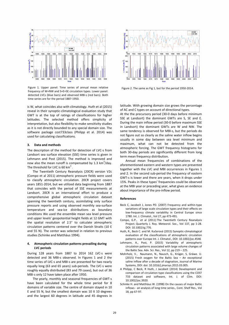
is W, what coincides also with climatology. Huth et al (2015) reveal in their synoptic-climatological evaluation study that GWT is at the top of ratings of classifications for higher latitudes. The selected method offers simplicity of interpretation, but also flexibility to make sensitivity studies as it is not directly bounded to any special domain size. The software package cost733class (Philipp et al. 2014) was used for calculating classifications. 3. Data and methods The description of the method for detection of LVC-s from Landsort sea surface elevation (SSE) time series is given in Lehmann and Post (2015). The method is improved and now also the mean runoff is compensated by 1.3 km3/day. The threshold for LVC is 60 km3 .

The Twentieth Century Reanalysis (20CR) version V2c (Compo et al 2011) atmospheric pressure fields were used to classify atmospheric circulation. 20CR project covers years 1851-2014, but we utilized data beginning from 1887 that coincides with the period of SSE measurements at Landsort. 20CR is an international effort to produce a comprehensive global atmospheric circulation dataset spanning the twentieth century, assimilating only surface pressure reports and using observed monthly sea-surface temperature and sea-ice distributions as boundary conditions We used the ensemble mean sea level pressure and upper levels’ geopotential height fields at 12 GMT with the spatial resolution of 2.5° to calculate atmospheric circulation patterns centered over the Danish Straits (10 E and 55 N). The center was selected in relation to previous studies (Schinke and Matthäus 1994). 4. Atmospheric circulation patterns prevailing during

LVC periods During 128 years from 1887 to 2014 162 LVC-s were detected and 36 MBI-s observed. In Figures 1 and 2 the time series of LVC-s and MBI-s are presented for two nearly equally long (63 and 65 years) sub-periods. The LVC-s were roughly equally distributed (83 and 79 cases), but out of 36 MBI-s only 12 have taken place after 1950.

The yearly, monthly and seasonal frequencies of GWT-s have been calculated for the whole time period for 8 domains of variable size. The centre of domain stayed in 10 E and 55 N, but the smallest domain was 10 X 10 degrees and the largest 60 degrees in latitude and 45 degrees in

latitude. With growing domain size grows the percentage of AC and C types on account of directional types. At the the precursory period (30-0 days before minimum SSE at Landsort) the dominant GWTs are S, SE and E. During the main inflow period (30-0 before maximum SSE in Landsort) the dominant GWTs are W and NW. The same tendency is observed for MBI-s, but the periods do not figure out so clearly as the saline water inflow begins usually in some day between sea level minimum and maximum, what can not be detected from the atmospheric forcing. The GWT frequency histograms for both 30-day periods are significantly different from long term mean frequency distribution.

Annual mean frequencies of combinations of the aforementioned eastern and western types are presented together with the LVC and MBI occurrences in Figures 1 and 2. In the second sub-period the frequency of eastern GWT-s is lower and there are years, when it drops under 15%. Peaks in these types’ frequencies could be observed at the MBI year or preceding year, what gives an evidence about importance of the pre-inflow period. References

Beck C, Jacobeit J, Jones PD. (2007) Frequency and within-type variations of large scale circulation types and their effects on low-frequency climate variability in Central Europe since 1780. Int. J. Climatol., Vol 27, pp 473-491.

Compo, G.P., et al (2011) The Twentieth Century Reanalysis Project. Quarterly J. Roy. Meteorol. Soc., Vol 137, pp 1-28. DOI: 10.1002/qj.776.

Huth, R., Beck C. and M. Kučerová (2015) Synoptic-climatological evaluation of the classifications of atmospheric circulation patterns over Europe Int. J. Climatol., DOI: 10.1002/joc.4546

Lehmann, A., Post, P. (2015) Variability of atmospheric circulation patterns associated with large volume changes of the Baltic Sea. Adv. Sci. Res., Vol 12, pp 219 – 225.

Mohrholz, V., Naumann, N., Nausch, G., Krüger, S, Gräwe. U. (2015) Fresh oxygen for the Baltic Sea – An exceptional saline inflow after a decade of stagnation, Journal of Marine Systems, DOI: doi: 10.1016/j.jmarsys.2015.03.005.

A Philipp, C Beck, R Huth, J Jacobeit (2014) Development and comparison of circulation type classifications using the COST 733 dataset and software, Int. J. of Clim. DOI: 10.1002/joc.3920.

Schinke H. and Matthäus W. (1998) On the causes of major Baltic inflows - an analysis of long time series., Cont. Shelf Res., Vol 18, pp 67-97.

Figure 1. Upper panel: Time series of annual mean relativefrequency of W+NW and S+E+SE circulation types. Lower panel:detected LVCs (blue bars) and observed MBI-s (red bars). Bothtime series are for the period 1887-1950.

Figure 2. The same as Fig 1, but for the period 1950-2014.

29

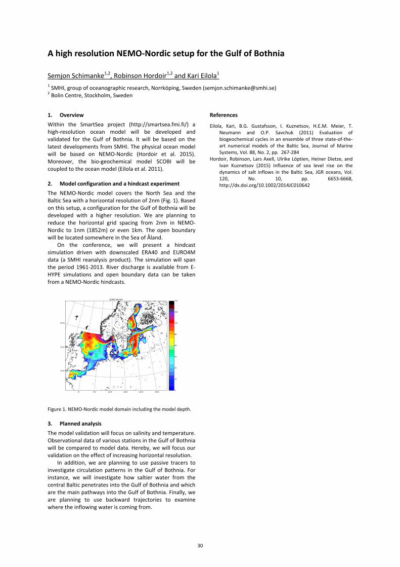
A high resolution NEMO-Nordic setup for the Gulf of Bothnia

Semjon Schimanke1,2, Robinson Hordoir1,2 and Kari Eilola1 1 SMHI, group of oceanographic research, Norrköping, Sweden (semjon.schimanke@smhi.se) 2 Bolin Centre, Stockholm, Sweden

1. Overview Within the SmartSea project (http://smartsea.fmi.fi/) a high-resolution ocean model will be developed and validated for the Gulf of Bothnia. It will be based on the latest developments from SMHI. The physical ocean model will be based on NEMO-Nordic (Hordoir et al. 2015). Moreover, the bio-geochemical model SCOBI will be coupled to the ocean model (Eilola et al. 2011). 2. Model configuration and a hindcast experiment The NEMO-Nordic model covers the North Sea and the Baltic Sea with a horizontal resolution of 2nm (Fig. 1). Based on this setup, a configuration for the Gulf of Bothnia will be developed with a higher resolution. We are planning to reduce the horizontal grid spacing from 2nm in NEMO-Nordic to 1nm (1852m) or even 1km. The open boundary will be located somewhere in the Sea of Åland.

On the conference, we will present a hindcast simulation driven with downscaled ERA40 and EURO4M data (a SMHI reanalysis product). The simulation will span the period 1961-2013. River discharge is available from E-HYPE simulations and open boundary data can be taken from a NEMO-Nordic hindcasts.

Figure 1. NEMO-Nordic model domain including the model depth. 3. Planned analysis The model validation will focus on salinity and temperature. Observational data of various stations in the Gulf of Bothnia will be compared to model data. Hereby, we will focus our validation on the effect of increasing horizontal resolution.

In addition, we are planning to use passive tracers to investigate circulation patterns in the Gulf of Bothnia. For instance, we will investigate how saltier water from the central Baltic penetrates into the Gulf of Bothnia and which are the main pathways into the Gulf of Bothnia. Finally, we are planning to use backward trajectories to examine where the inflowing water is coming from.

References

Eilola, Kari, B.G. Gustafsson, I. Kuznetsov, H.E.M. Meier, T. Neumann and O.P. Savchuk (2011) Evaluation of biogeochemical cycles in an ensemble of three state-of-the-art numerical models of the Baltic Sea, Journal of Marine Systems, Vol. 88, No. 2, pp. 267-284

Hordoir, Robinson, Lars Axell, Ulrike Löptien, Heiner Dietze, and Ivan Kuznetsov (2015) Influence of sea level rise on the dynamics of salt inflows in the Baltic Sea, JGR oceans, Vol. 120, No. 10, pp. 6653-6668, http://dx.doi.org/10.1002/2014JC010642

30

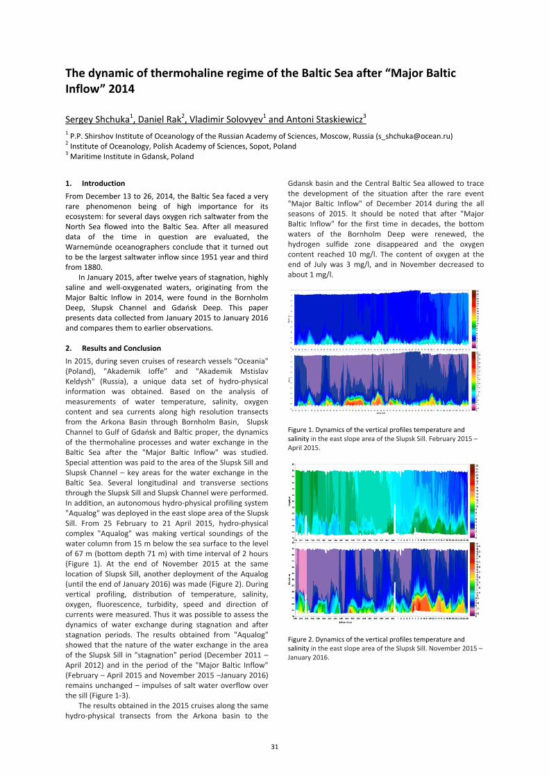
The dynamic of thermohaline regime of the Baltic Sea after “Major Baltic Inflow” 2014

Sergey Shchuka1, Daniel Rak2, Vladimir Solovyev1 and Antoni Staskiewicz3 1 P.P. Shirshov Institute of Oceanology of the Russian Academy of Sciences, Moscow, Russia (s_shchuka@ocean.ru) 2 Institute of Oceanology, Polish Academy of Sciences, Sopot, Poland 3 Maritime Institute in Gdansk, Poland

1. Introduction From December 13 to 26, 2014, the Baltic Sea faced a very rare phenomenon being of high importance for its ecosystem: for several days oxygen rich saltwater from the North Sea flowed into the Baltic Sea. After all measured data of the time in question are evaluated, the Warnemünde oceanographers conclude that it turned out to be the largest saltwater inflow since 1951 year and third from 1880.

In January 2015, after twelve years of stagnation, highly saline and well-oxygenated waters, originating from the Major Baltic Inflow in 2014, were found in the Bornholm Deep, Słupsk Channel and Gdańsk Deep. This paper presents data collected from January 2015 to January 2016 and compares them to earlier observations. 2. Results and Conclusion In 2015, during seven cruises of research vessels "Oceania" (Poland), "Akademik Ioffe" and "Akademik Mstislav Keldysh" (Russia), a unique data set of hydro-physical information was obtained. Based on the analysis of measurements of water temperature, salinity, oxygen content and sea currents along high resolution transects from the Arkona Basin through Bornholm Basin, Slupsk Channel to Gulf of Gdańsk and Baltic proper, the dynamics of the thermohaline processes and water exchange in the Baltic Sea after the "Major Baltic Inflow" was studied. Special attention was paid to the area of the Slupsk Sill and Slupsk Channel – key areas for the water exchange in the Baltic Sea. Several longitudinal and transverse sections through the Slupsk Sill and Slupsk Channel were performed. In addition, an autonomous hydro-physical profiling system "Aqualog" was deployed in the east slope area of the Slupsk Sill. From 25 February to 21 April 2015, hydro-physical complex "Aqualog" was making vertical soundings of the water column from 15 m below the sea surface to the level of 67 m (bottom depth 71 m) with time interval of 2 hours (Figure 1). At the end of November 2015 at the same location of Slupsk Sill, another deployment of the Aqualog (until the end of January 2016) was made (Figure 2). During vertical profiling, distribution of temperature, salinity, oxygen, fluorescence, turbidity, speed and direction of currents were measured. Thus it was possible to assess the dynamics of water exchange during stagnation and after stagnation periods. The results obtained from "Aqualog" showed that the nature of the water exchange in the area of the Slupsk Sill in "stagnation" period (December 2011 – April 2012) and in the period of the "Major Baltic Inflow" (February – April 2015 and November 2015 –January 2016) remains unchanged – impulses of salt water overflow over the sill (Figure 1-3).

The results obtained in the 2015 cruises along the same hydro-physical transects from the Arkona basin to the

Gdansk basin and the Central Baltic Sea allowed to trace the development of the situation after the rare event "Major Baltic Inflow" of December 2014 during the all seasons of 2015. It should be noted that after "Major Baltic Inflow" for the first time in decades, the bottom waters of the Bornholm Deep were renewed, the hydrogen sulfide zone disappeared and the oxygen content reached 10 mg/l. The content of oxygen at the end of July was 3 mg/l, and in November decreased to about 1 mg/l.

Figure 1. Dynamics of the vertical profiles temperature and salinity in the east slope area of the Slupsk Sill. February 2015 – April 2015.

Figure 2. Dynamics of the vertical profiles temperature and salinity in the east slope area of the Slupsk Sill. November 2015 – January 2016.

31

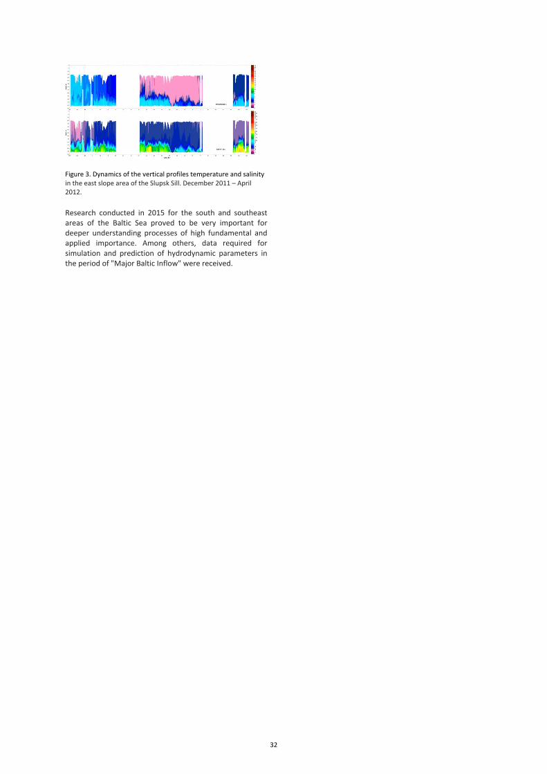
Figure 3. Dynamics of the vertical profiles temperature and salinity in the east slope area of the Slupsk Sill. December 2011 – April 2012.

Research conducted in 2015 for the south and southeast areas of the Baltic Sea proved to be very important for deeper understanding processes of high fundamental and applied importance. Among others, data required for simulation and prediction of hydrodynamic parameters in the period of "Major Baltic Inflow" were received.

32

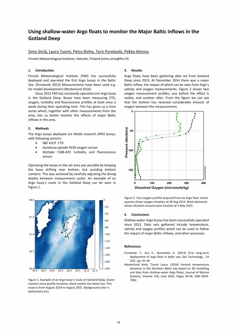
Using shallow-water Argo floats to monitor the Major Baltic inflows in the Gotland Deep

Simo Siiriä, Laura Tuomi, Petra Roiha, Tero Purokoski, Pekka Alenius

Finnish Meteorological Institute, Helsinki, Finland (simo.siiria@fmi.fi)

1. Introduction Finnish Meteorological Institute (FMI) has successfully deployed and operated the first Argo buoys in the Baltic Sea. (Purokoski 2013) Measurements have been used e.g. for model development (Westerlund 2016).

Since 2013 FMI has constantly operated one Argo buoy in the Gotland Deep. Buoys have been measuring CTD, oxygen, turbidity and fluorescence profiles at least once a week during their operating time. This has given us a time series which, together with other measurements from the area, lets us better monitor the effects of major Baltic inflows in the area. 2. Methods The Argo buoys deployed are Webb research APEX buoys, with following sensors:

• SBE 41CP CTD • Aanderaa optode 4330 oxygen sensor • Wetlabs FLBB-AP2 turbidity and fluorescence

sensor

Operating the buoys in the set area was possible by keeping the buoy drifting near bottom, but avoiding bottom contacts. This was achieved by carefully adjusting the diving depths between measurement cycles. An example of an Argo buoy’s route in the Gotland Deep can be seen in Figure 1.

Figure 1. Example of an Argo buoy’s route on Gotland Deep. Green markers show profile locations, black marker the latest one. This route is from August 2014 to August 2015. Background color is bathymetry (m).

3. Results Argo floats have been gathering data set from Gotland Deep since 2013. At December 2014 there was a major Baltic inflow, the impact of which can be seen from Argo’s salinity and oxygen measurements. Figure 2 shows two oxygen measurement profiles, one before the effect is visible, and another after. From the figure we can see that the bottom has received considerable amount of oxygen between the measurements.

Figure 2. Two oxygen profiles acquired from an Argo float. Green squares shows oxygen situation at 28 Aug 2014. Black diamonds shows situation around same location at 5 May 2015.

4. Conclusions Shallow-water Argo buoys has been successfully operated since 2013. Data sets gathered include temperature, salinity and oxygen profiles which can be used to follow the impact of major Baltic inflows, and other processes. References

Purokoski T., Aro E., Nummelin A. (2013) First long-term deployment of argo float in baltic sea, Sea Technology, 54 (10) , pp. 41-44.

Westerlund Antti, Tuomi Laura. (2016) Vertical temperature dynamics in the Northern Baltic Sea based on 3D modelling and data from shallow-water Argo floats, Journal of Marine Systems, Volume 158, June 2016, Pages 34-44, ISSN 0924-7963

33

Sedimentology and geochemistry of marine deposits from Bornholm and Gdansk Basins - stratigraphical records.

J. Slawinska 1, R. Borowka1, M. Moros2, A. Binczewska3, and M. Bak3 1 Department of Geology and Paleogeography, Faculty of Geosciences, University of Szczecin, Szczecin, Poland (joanna.slawinska@univ.szczecin.pl) 2 Leibniz Institute for Baltic Sea Research, Warnemünde, Germany 3 Paleoceanography Unit, Faculty of Geosciences, University of Szczecin, Szczecin, Poland

1. The aim of work

The presentation shows the reconstruction of changes in sedimentation processes and conditions for the accumulation of marine sediments from the bottom of the Bornholm Basin (-gravity core M86-1/24, φ 55°22.648, λ 15°21.802, 98 m depth) and Gdansk Basin (gravity core P475/12, φ 54°49.39, λ 19°11.14, 105 m depth). 2. Methods To calculate the age model for selected sites, for all dates received from the laboratory at Poznan, calibrated age AMS14C was completed and high resolution AMS14C based age models were created. All radiocarbon ages were calibrated using OxCal 4.2 software and the Marine13 calibration curve was applied. Results were given in cal. BP years. No reservoir correction has been used. The results of radiocarbon age designations Makoma sp. shell, in both cores show that drilled sediments ranged in age from the present day to more than 7,500 years cal. BP. Core samples were analyzed to determine the changes in the particle size of sediments and their chemical composition.

Analyses of sediment grain size (-103 samples from gravity core M86-1/24 and 185 samples from gravity core P475/12) were analyzed using a laser granulometer by Mastersizer Micro ver. 2.19 Malvern Instruments Ltd. while the content of selected elements (Na, K, Ca, Mg, Fe, Mn, Cu, Zn, Pb, Ni, Cr and Co) was determined by atomic absorption spectrometry using a 969 Unicam Solaar manual apparatus. 3. Results Stratigraphic analysis of the particle size variability of the Bornholm Basin deposits (gravity core M86-1/24) shows a marked enrichment in fractions of medium and fine sand in the bottom of the profile in sediments older than 6800 years cal. BP, and in the sediment deposited during the periods 3300-3800 and 1200- 3000 years cal. BP. The profile (gravity core P475/12) of the Gdansk Basin, the highest fraction of sand, both medium- and fine-grained, occur in youngest sediments, representing the last 600-700 years, and dated to approx. 1000 and 1700 to 2200 years cal. BP. A high proportion of these fractions fall as the years approx. 3700, 4800 and 6000-6100 years cal. BP. A high proportion of these fractions accrue also for the years approx. 3700, 4800 and 6000-6100 years cal. BP.

Some of the signals of enrichment analyzed in the sandy fractions, especially in the Gdansk Basin, can be closely linked to agricultural activity of man in the catchment area of the Vistula and extreme floods registered in the valley of the river. Starkel L. (1995).

Conversely, a high fraction of sandy sediments in the Bornholm Basin is currently difficult to interpret. There is a possibility that these sediments indicate increased storm activity in this part of the Baltic Sea, combined with erosion of the Gulf of Hanö shores.

Analysis of changes in the chemical composition of deposits in a stratigraphic sequence allowed us to identify periods of increased supply, more saline, and better oxygenated water from the North Sea. References Starkel L. (1995) Evolution of the Vistula river valley during the

last 15 000 years, V, Geogr. Stud., Spec. Issue 8. 720-730. Bronk Ramsey, C. (2008). Deposition models for chronological

records. Quaternary Science Reviews, 27(1-2), 42-60.

34

Topic B

Land-sea-atmosphere biogeochemical feedbacks

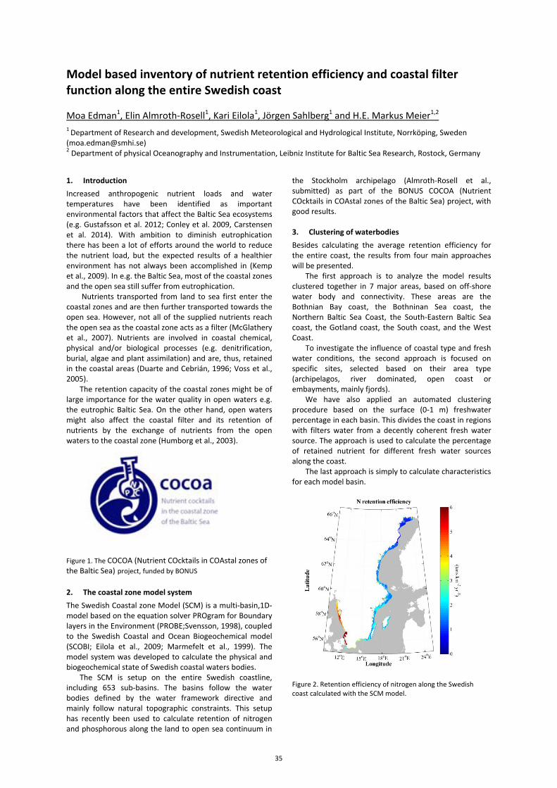
Model based inventory of nutrient retention efficiency and coastal filter function along the entire Swedish coast

Moa Edman1, Elin Almroth-Rosell1, Kari Eilola1, Jörgen Sahlberg1 and H.E. Markus Meier1,2 1 Department of Research and development, Swedish Meteorological and Hydrological Institute, Norrköping, Sweden (moa.edman@smhi.se) 2 Department of physical Oceanography and Instrumentation, Leibniz Institute for Baltic Sea Research, Rostock, Germany

1. Introduction Increased anthropogenic nutrient loads and water temperatures have been identified as important environmental factors that affect the Baltic Sea ecosystems (e.g. Gustafsson et al. 2012; Conley et al. 2009, Carstensen et al. 2014). With ambition to diminish eutrophication there has been a lot of efforts around the world to reduce the nutrient load, but the expected results of a healthier environment has not always been accomplished in (Kemp et al., 2009). In e.g. the Baltic Sea, most of the coastal zones and the open sea still suffer from eutrophication.

Nutrients transported from land to sea first enter the coastal zones and are then further transported towards the open sea. However, not all of the supplied nutrients reach the open sea as the coastal zone acts as a filter (McGlathery et al., 2007). Nutrients are involved in coastal chemical, physical and/or biological processes (e.g. denitrification, burial, algae and plant assimilation) and are, thus, retained in the coastal areas (Duarte and Cebrián, 1996; Voss et al., 2005).

The retention capacity of the coastal zones might be of large importance for the water quality in open waters e.g. the eutrophic Baltic Sea. On the other hand, open waters might also affect the coastal filter and its retention of nutrients by the exchange of nutrients from the open waters to the coastal zone (Humborg et al., 2003).

Figure 1. The COCOA (Nutrient COcktails in COAstal zones of the Baltic Sea) project, funded by BONUS

2. The coastal zone model system The Swedish Coastal zone Model (SCM) is a multi-basin,1D-model based on the equation solver PROgram for Boundary layers in the Environment (PROBE;Svensson, 1998), coupled to the Swedish Coastal and Ocean Biogeochemical model (SCOBI; Eilola et al., 2009; Marmefelt et al., 1999). The model system was developed to calculate the physical and biogeochemical state of Swedish coastal waters bodies.

The SCM is setup on the entire Swedish coastline, including 653 sub-basins. The basins follow the water bodies defined by the water framework directive and mainly follow natural topographic constraints. This setup has recently been used to calculate retention of nitrogen and phosphorous along the land to open sea continuum in

the Stockholm archipelago (Almroth-Rosell et al., submitted) as part of the BONUS COCOA (Nutrient COcktails in COAstal zones of the Baltic Sea) project, with good results. 3. Clustering of waterbodies Besides calculating the average retention efficiency for the entire coast, the results from four main approaches will be presented.

The first approach is to analyze the model results clustered together in 7 major areas, based on off-shore water body and connectivity. These areas are the Bothnian Bay coast, the Bothninan Sea coast, the Northern Baltic Sea Coast, the South-Eastern Baltic Sea coast, the Gotland coast, the South coast, and the West Coast.

To investigate the influence of coastal type and fresh water conditions, the second approach is focused on specific sites, selected based on their area type (archipelagos, river dominated, open coast or embayments, mainly fjords).

We have also applied an automated clustering procedure based on the surface (0-1 m) freshwater percentage in each basin. This divides the coast in regions with filters water from a decently coherent fresh water source. The approach is used to calculate the percentage of retained nutrient for different fresh water sources along the coast.

The last approach is simply to calculate characteristics for each model basin.

Figure 2. Retention efficiency of nitrogen along the Swedish coast calculated with the SCM model.

35

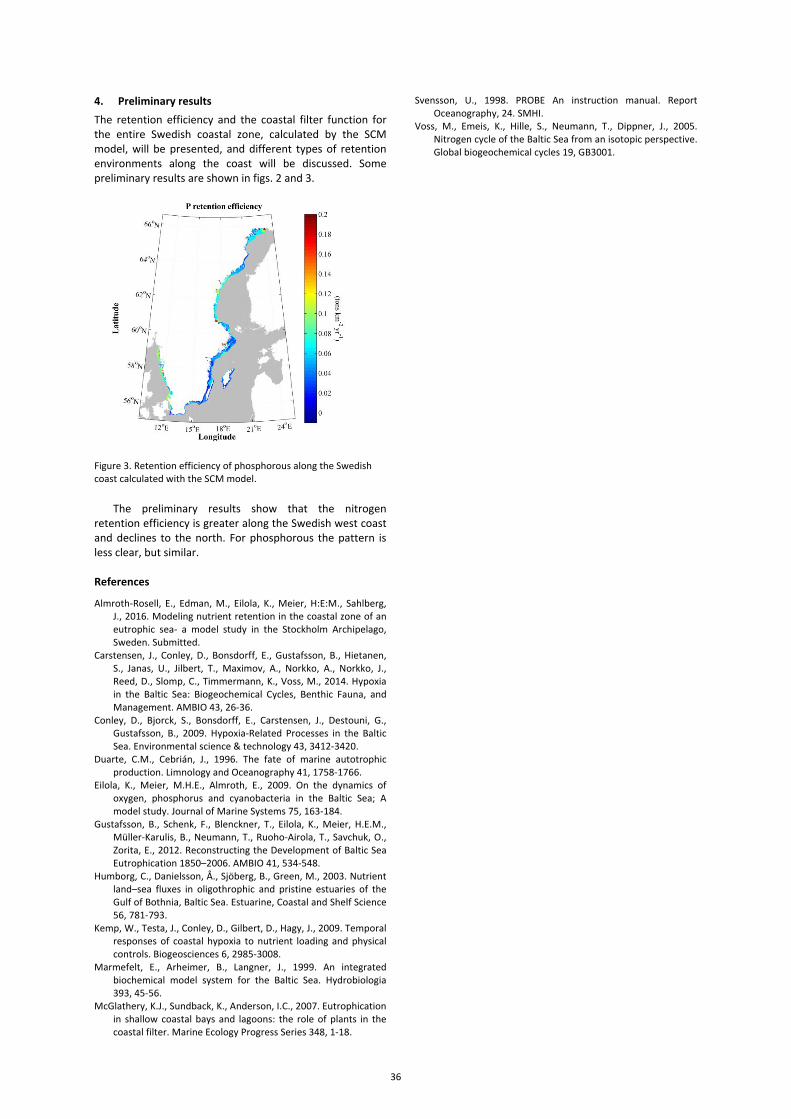
4. Preliminary results The retention efficiency and the coastal filter function for the entire Swedish coastal zone, calculated by the SCM model, will be presented, and different types of retention environments along the coast will be discussed. Some preliminary results are shown in figs. 2 and 3.

Figure 3. Retention efficiency of phosphorous along the Swedish coast calculated with the SCM model.

The preliminary results show that the nitrogen retention efficiency is greater along the Swedish west coast and declines to the north. For phosphorous the pattern is less clear, but similar. References

Almroth-Rosell, E., Edman, M., Eilola, K., Meier, H:E:M., Sahlberg, J., 2016. Modeling nutrient retention in the coastal zone of an eutrophic sea- a model study in the Stockholm Archipelago, Sweden. Submitted.

Carstensen, J., Conley, D., Bonsdorff, E., Gustafsson, B., Hietanen, S., Janas, U., Jilbert, T., Maximov, A., Norkko, A., Norkko, J., Reed, D., Slomp, C., Timmermann, K., Voss, M., 2014. Hypoxia in the Baltic Sea: Biogeochemical Cycles, Benthic Fauna, and Management. AMBIO 43, 26-36.

Conley, D., Bjorck, S., Bonsdorff, E., Carstensen, J., Destouni, G., Gustafsson, B., 2009. Hypoxia-Related Processes in the Baltic Sea. Environmental science & technology 43, 3412-3420.

Duarte, C.M., Cebrián, J., 1996. The fate of marine autotrophic production. Limnology and Oceanography 41, 1758-1766.

Eilola, K., Meier, M.H.E., Almroth, E., 2009. On the dynamics of oxygen, phosphorus and cyanobacteria in the Baltic Sea; A model study. Journal of Marine Systems 75, 163-184.

Gustafsson, B., Schenk, F., Blenckner, T., Eilola, K., Meier, H.E.M., Müller-Karulis, B., Neumann, T., Ruoho-Airola, T., Savchuk, O., Zorita, E., 2012. Reconstructing the Development of Baltic Sea Eutrophication 1850–2006. AMBIO 41, 534-548.

Humborg, C., Danielsson, Å., Sjöberg, B., Green, M., 2003. Nutrient land–sea fluxes in oligothrophic and pristine estuaries of the Gulf of Bothnia, Baltic Sea. Estuarine, Coastal and Shelf Science 56, 781-793.

Kemp, W., Testa, J., Conley, D., Gilbert, D., Hagy, J., 2009. Temporal responses of coastal hypoxia to nutrient loading and physical controls. Biogeosciences 6, 2985-3008.

Marmefelt, E., Arheimer, B., Langner, J., 1999. An integrated biochemical model system for the Baltic Sea. Hydrobiologia 393, 45-56.

McGlathery, K.J., Sundback, K., Anderson, I.C., 2007. Eutrophication in shallow coastal bays and lagoons: the role of plants in the coastal filter. Marine Ecology Progress Series 348, 1-18.

Svensson, U., 1998. PROBE An instruction manual. Report Oceanography, 24. SMHI.

Voss, M., Emeis, K., Hille, S., Neumann, T., Dippner, J., 2005. Nitrogen cycle of the Baltic Sea from an isotopic perspective. Global biogeochemical cycles 19, GB3001.

36

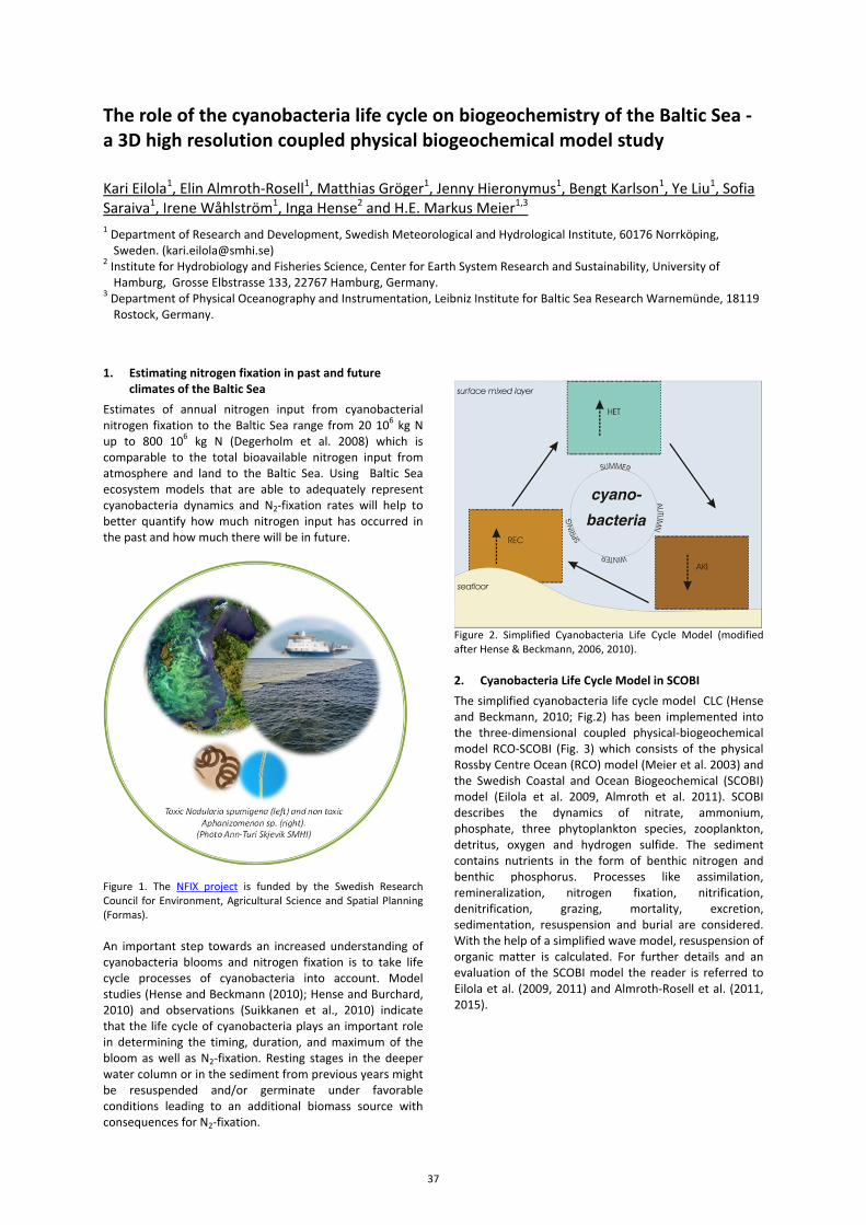
The role of the cyanobacteria life cycle on biogeochemistry of the Baltic Sea - a 3D high resolution coupled physical biogeochemical model study

Kari Eilola1, Elin Almroth-Rosell1, Matthias Gröger1, Jenny Hieronymus1, Bengt Karlson1, Ye Liu1, Sofia Saraiva1, Irene Wåhlström1, Inga Hense2 and H.E. Markus Meier1,3 1 Department of Research and Development, Swedish Meteorological and Hydrological Institute, 60176 Norrköping,

Sweden. (kari.eilola@smhi.se) 2 Institute for Hydrobiology and Fisheries Science, Center for Earth System Research and Sustainability, University of

Hamburg, Grosse Elbstrasse 133, 22767 Hamburg, Germany. 3 Department of Physical Oceanography and Instrumentation, Leibniz Institute for Baltic Sea Research Warnemünde, 18119

Rostock, Germany.

1. Estimating nitrogen fixation in past and future climates of the Baltic Sea

Estimates of annual nitrogen input from cyanobacterial nitrogen fixation to the Baltic Sea range from 20 106 kg N up to 800 106 kg N (Degerholm et al. 2008) which is comparable to the total bioavailable nitrogen input from atmosphere and land to the Baltic Sea. Using Baltic Sea ecosystem models that are able to adequately represent cyanobacteria dynamics and N2-fixation rates will help to better quantify how much nitrogen input has occurred in the past and how much there will be in future.

Figure 1. The NFIX project is funded by the Swedish Research Council for Environment, Agricultural Science and Spatial Planning (Formas). An important step towards an increased understanding of cyanobacteria blooms and nitrogen fixation is to take life cycle processes of cyanobacteria into account. Model studies (Hense and Beckmann (2010); Hense and Burchard, 2010) and observations (Suikkanen et al., 2010) indicate that the life cycle of cyanobacteria plays an important role in determining the timing, duration, and maximum of the bloom as well as N2-fixation. Resting stages in the deeper water column or in the sediment from previous years might be resuspended and/or germinate under favorable conditions leading to an additional biomass source with consequences for N2-fixation.

Figure 2. Simplified Cyanobacteria Life Cycle Model (modified after Hense & Beckmann, 2006, 2010). 2. Cyanobacteria Life Cycle Model in SCOBI The simplified cyanobacteria life cycle model CLC (Hense and Beckmann, 2010; Fig.2) has been implemented into the three-dimensional coupled physical-biogeochemical model RCO-SCOBI (Fig. 3) which consists of the physical Rossby Centre Ocean (RCO) model (Meier et al. 2003) and the Swedish Coastal and Ocean Biogeochemical (SCOBI) model (Eilola et al. 2009, Almroth et al. 2011). SCOBI describes the dynamics of nitrate, ammonium, phosphate, three phytoplankton species, zooplankton, detritus, oxygen and hydrogen sulfide. The sediment contains nutrients in the form of benthic nitrogen and benthic phosphorus. Processes like assimilation, remineralization, nitrogen fixation, nitrification, denitrification, grazing, mortality, excretion, sedimentation, resuspension and burial are considered. With the help of a simplified wave model, resuspension of organic matter is calculated. For further details and an evaluation of the SCOBI model the reader is referred to Eilola et al. (2009, 2011) and Almroth-Rosell et al. (2011, 2015).

37

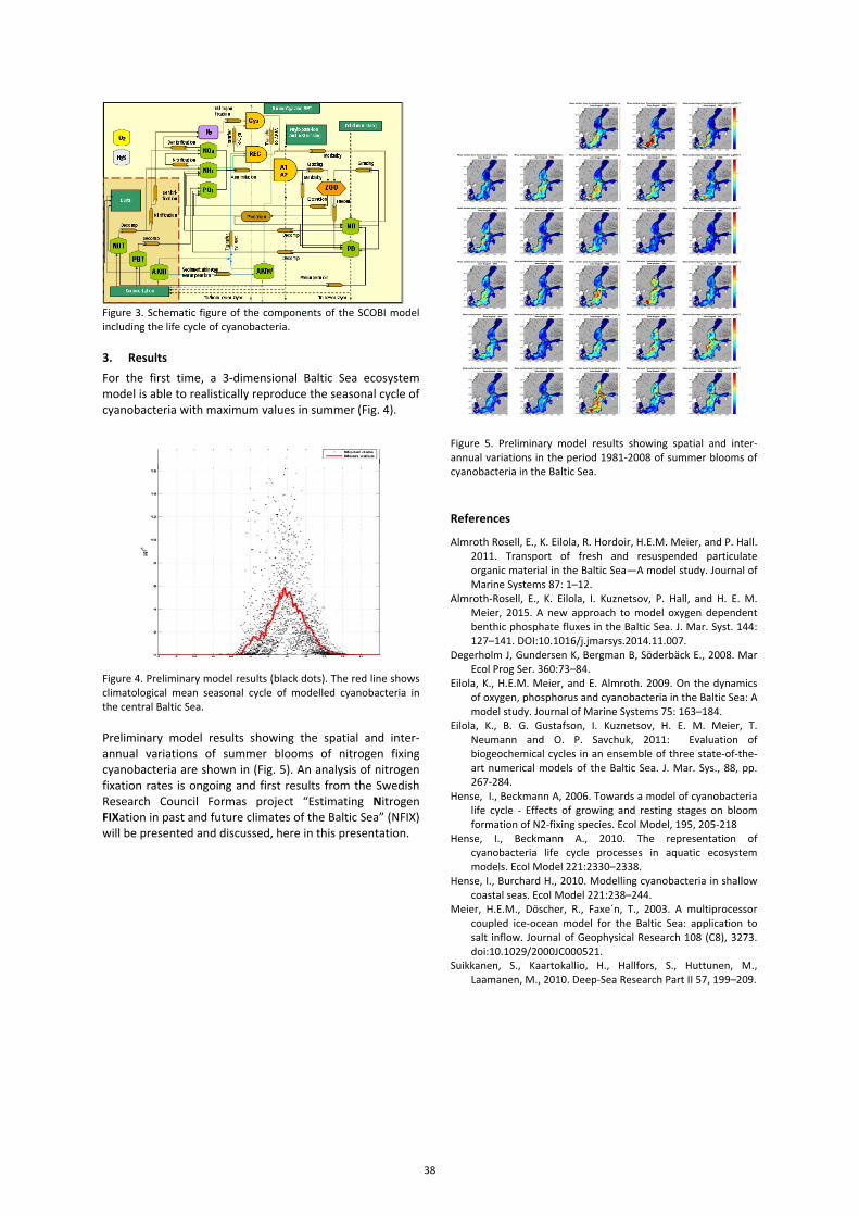
Figure 3. Schematic figure of the components of the SCOBI model including the life cycle of cyanobacteria. 3. Results For the first time, a 3-dimensional Baltic Sea ecosystem model is able to realistically reproduce the seasonal cycle of cyanobacteria with maximum values in summer (Fig. 4).

Figure 4. Preliminary model results (black dots). The red line shows climatological mean seasonal cycle of modelled cyanobacteria in the central Baltic Sea. Preliminary model results showing the spatial and inter-annual variations of summer blooms of nitrogen fixing cyanobacteria are shown in (Fig. 5). An analysis of nitrogen fixation rates is ongoing and first results from the Swedish Research Council Formas project “Estimating Nitrogen FIXation in past and future climates of the Baltic Sea” (NFIX) will be presented and discussed, here in this presentation.

Figure 5. Preliminary model results showing spatial and inter-annual variations in the period 1981-2008 of summer blooms of cyanobacteria in the Baltic Sea.

References

Almroth Rosell, E., K. Eilola, R. Hordoir, H.E.M. Meier, and P. Hall. 2011. Transport of fresh and resuspended particulate organic material in the Baltic Sea—A model study. Journal of Marine Systems 87: 1–12.

Almroth-Rosell, E., K. Eilola, I. Kuznetsov, P. Hall, and H. E. M. Meier, 2015. A new approach to model oxygen dependent benthic phosphate fluxes in the Baltic Sea. J. Mar. Syst. 144: 127–141. DOI:10.1016/j.jmarsys.2014.11.007.

Degerholm J, Gundersen K, Bergman B, Söderbäck E., 2008. Mar Ecol Prog Ser. 360:73–84.

Eilola, K., H.E.M. Meier, and E. Almroth. 2009. On the dynamics of oxygen, phosphorus and cyanobacteria in the Baltic Sea: A model study. Journal of Marine Systems 75: 163–184.

Eilola, K., B. G. Gustafson, I. Kuznetsov, H. E. M. Meier, T. Neumann and O. P. Savchuk, 2011: Evaluation of biogeochemical cycles in an ensemble of three state-of-the-art numerical models of the Baltic Sea. J. Mar. Sys., 88, pp. 267-284.

Hense, I., Beckmann A, 2006. Towards a model of cyanobacteria life cycle - Effects of growing and resting stages on bloom formation of N2-fixing species. Ecol Model, 195, 205-218

Hense, I., Beckmann A., 2010. The representation of cyanobacteria life cycle processes in aquatic ecosystem models. Ecol Model 221:2330–2338.

Hense, I., Burchard H., 2010. Modelling cyanobacteria in shallow coastal seas. Ecol Model 221:238–244.

Meier, H.E.M., Döscher, R., Faxe´n, T., 2003. A multiprocessor coupled ice-ocean model for the Baltic Sea: application to salt inflow. Journal of Geophysical Research 108 (C8), 3273. doi:10.1029/2000JC000521.

Suikkanen, S., Kaartokallio, H., Hallfors, S., Huttunen, M., Laamanen, M., 2010. Deep-Sea Research Part II 57, 199–209.

38

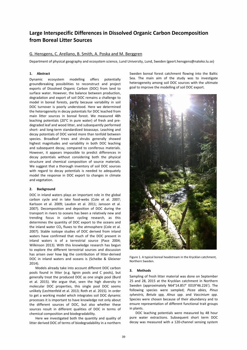
Large Interspecific Differences in Dissolved Organic Carbon Decomposition from Boreal Litter Sources

G. Hensgens, C. Arellano, B. Smith, A. Poska and M. Berggren

Department of physical geography and ecosystem science, Lund University, Lund, Sweden (geert.hensgens@nateko.lu.se)

1. Abstract Dynamic ecosystem modelling offers potentially groundbreaking possibilities to reconstruct and project exports of Dissolved Organic Carbon (DOC) from land to surface water. However, the balance between production, degradation and export of soil DOC remains a challenge to model in boreal forests, partly because variability in soil DOC turnover is poorly understood. Here we determined the heterogeneity in decay potentials for DOC leached from main litter sources in boreal forest. We measured 48h leaching potentials (20°C in pure water) of fresh and pre-degraded leaf and wood litter, and subsequently performed short- and long-term standardized bioassays. Leaching and decay potentials of DOC varied more than tenfold between species. Broadleaf trees and shrubs generally showed highest magnitudes and variability in both DOC leaching and subsequent decay, compared to coniferous materials. However, it appears impossible to predict differences in decay potentials without considering both the physical structure and chemical composition of source materials. We suggest that a thorough inventory of soil DOC sources with regard to decay potentials is needed to adequately model the response in DOC export to changes in climate and vegetation. 2. Background DOC in inland waters plays an important role in the global carbon cycle and in lake food-webs (Cole et al. 2007; Karlsson et al. 2009; Laudon et al. 2011; Jansson et al. 2007). Decomposition and deposition of DOC during the transport in rivers to oceans has been a relatively new and trending focus in carbon cycling research, as this determines the quantity of DOC export to the oceans and the inland water CO2 fluxes to the atmosphere (Cole et al. 2007). Stable isotope studies of DOC derived from inland waters have confirmed that much of the DOC present in inland waters is of a terrestrial source (Pace 2004; Wilkinson 2013). With this knowledge research has begun to explore the different terrestrial sources and discussion has arisen over how big the contribution of litter-derived DOC in inland waters and oceans is (Scheibe & Gleixner 2014).

Models already take into account different DOC carbon pools found in litter (e.g. lignin pools and C pools), but generally treat the produced DOC as one single pool (Burd et al. 2015). We argue that, seen the high diversity in molecular DOC properties, this single pool DOC seems unlikely (Lechtenfeld et al. 2013; Roth et al. 2015). In order to get a working model which integrates soil DOC dynamic processes it is important to have knowledge not only about the different sources of DOC, but also whether these sources result in different qualities of DOC in terms of chemical composition and biodegradability.

Here we investigated both the quantity and quality of litter derived DOC of terms of biodegradability in a northern

Sweden boreal forest catchment flowing into the Baltic Sea. The main aim of the study was to investigate heterogeneity among soil DOC sources with the ultimate goal to improve the modelling of soil DOC export.

Figure 1. A typical boreal headstream in the Krycklan catchment, Northern Sweden.

3. Methods Sampling of fresh litter material was done on September 25 and 28, 2015 at the Krycklan catchment in Northern Sweden (approximately N64°14.857’ E019°46.226’). The following species were sampled; Picea abies, Pinus sylvestris, Betula spp, Alnus spp. and Vaccinium spp. Species were chosen because of their abundancy and to ensure representation of different functional trait groups in plants.

DOC leaching potentials were measured by 48 hour pure water extractions. Subsequent short term DOC decay was measured with a 120-channel sensing system

39

(PreSens, Germany) for up to 7 days. Long term decay was measured by measuring DOC decline at different time-points for up to a year. 4. Findings We found a large heterogeneity in leaching and decay potentials of DOC between different species. In general broadleaf trees and shrubs show higher DOC leaching than coniferous vegetation. We propose that a thorough inventory of soil DOC sources is needed in order to adequately model DOC export across the terrestrial-aquatic interface. References

Burd, A.B. et al., 2015. Terrestrial and marine perspectives on modeling organic matter degradation pathways. Global Change Biology, 22, pp.121–136. Available at: http://dx.doi.org/10.1111/gcb.12987.

Cole, J.J. et al., 2007. Plumbing the global carbon cycle: Integrating inland waters into the terrestrial carbon budget. Ecosystems, 10(1), pp.171–184.

Jansson, M. et al., 2007. Terrestrial carbon and intraspecific size-variation shape lake ecosystems. Trends in Ecology and Evolution, 22(6), pp.316–322.

Karlsson, J. et al., 2009. Light limitation of nutrient-poor lake ecosystems. Nature, 460(7254), pp.506–509.

Laudon, H. et al., 2011. Consequences of more intensive forestry for the sustainable management of forest soils and waters. Forests, 2(1), pp.243–260.

Lechtenfeld, O.J. et al., 2013. The influence of salinity on the molecular and optical properties of surface microlayers in a karstic estuary. Marine Chemistry, 150, pp.25–38.

Pace, M.L., 2004. Whole lake carbon-13 additions reveal terrestrial support of aquatic food webs. Nature, 427(January), pp.240–243.

Roth, V.-N. et al., 2015. The Molecular Composition of Dissolved Organic Matter in Forest Soils as a Function of pH and Temperature. Plos One, 10(3), p.e0119188. Available at: http://dx.plos.org/10.1371/journal.pone.0119188.

Scheibe, A. & Gleixner, G., 2014. Influence of Litter Diversity on Dissolved Organic Matter Release and Soil Carbon Formation in a Mixed Beech Forest. PLoS ONE, 9(12), p.e114040. Available at: http://dx.plos.org/10.1371/journal.pone.0114040.

Wilkinson G.M., Pace M.L. & Cole J.J. (2013). Terrestrial dominance of organic matter in north temperate lakes. Global Biogeochemical Cycles, 27, 43-51.

40

Magnetic susceptibility of the surface layer of bottom sediments of the South Baltic, as a quality parameter in the assessment of selected metals pollution of the marine environment Żaneta Kłostowska1, Leszek Łęczyński1, Grzegorz Kusza2, Agnieszka Kubowicz-Grajewska1, Tadeusz Ossowski3, Dorota Zarzeczańska3, Piotr Hulisz4, Emilia Bublijewska1 1 Institute of Oceanography, University of Gdańsk, Laboratory of Applied Geology, Gdynia, Poland (zaneta.kloostowska@phdstud.ug.edu.pl) 2 Department of Land Protection, University of Opole, Opole, Poland 3 Department of Analytical Chemistry, University of Gdańsk, Gdańsk, Poland 4 Faculty of Earth Sciences, Department of Soil Science and Landscape Management, Nicolaus Copernicus University in Toruń, Toruń, Poland

In recent years, studies of magnetic susceptibility in different environmental matrices, are beginning to be the output parameter for further, complex physical and chemical analysis, requiring a specialized equipment and high-toxic reagents . Screening tests, including surface sediments, are an important source of information of the state of environmental pollution. Magnetic susceptibility determines the size of magnetization as a function of magnetic field strength. Due to the magnetic properties distinguished 3 groups, which split criterion is the behavior of the external magnetic field: ferromagnetic (χ >> 0) paramagnetic (χ> 0), diamagnetic (χ <0). Anomalous values of magnetic susceptibility are a signal characterizing contamination.

The main objective of studies was to determine the relationship between the typed contaminants existing in the surface layer of sediments, and the value of magnetic susceptibility.

Area of study included 5 designated transects from the mouth of the Vistula River to the central part of the Gulf of Gdansk (24 measuring points). Typed profiles included the area of mixing freshwater with saltwater and also characterized by hydrodynamic volatility. Samples of sediments were collected by Van Veen grab, in 2014, from unit k/h Oceanograf-2. The collected sedimentary material was conserved until the analysis. Sediments were analyzed by grain size, measured content of organic matter (LOI550 and LOI950) and the concentrations of selected metals (Pb, Fe, Zn, Cr, Cu, Cd, Ni) by ICP-MS after prior mineralization (9HNO3:1HF). All tests were conducted in accordance with US EPA standards for marine sediments. The magnetic susceptibility was measured by using the MS2B Bartington bridge in the frequency range of 2 χlf = 470 [Hz] and χhf = 4700 [Hz].

The result is a significant correlations of the magnetic susceptibility with metal content and the share of the fine fraction and organic matter. The observed increased susceptibility with increasing share of fine fraction, is conditional by the increased surface area of the sorption, including the selected metal. There was a growing tendency on the measured values of the magnetic susceptibility in each of the selected profile in the direction of the central part of the Gulf of Gdansk. It is associated with hydrodynamic conditions of the basin, which in turn affects the movement of fine sedimentary material including impurities in further areas of the Gulf. Based on the study it

can be concluded that the rate, which is the magnetic susceptibility and the anomalous values, allows for a quick determination of the quality of bottom sediments, relative to metal contamination.

41

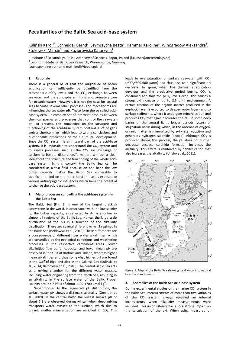
Peculiarities of the Baltic Sea acid-base system

Kuliński Karol1*, Schneider Bernd2, Szymczycha Beata1, Hammer Karoline2, Winogradow Aleksandra1, Stokowski Marcin1 and Koziorowska Katarzyna1 1 Institute of Oceanology, Polish Academy of Sciences, Sopot, Poland (f.author@meteorology.se) 2 Leibniz Institute for Baltic Sea Research, Warnemünde, Germany *corresponding author, e-mail: kroll@iopan.gda.pl

1. Rationale There is a general belief that the magnitude of ocean acidification can sufficiently be quantified from the atmospheric pCO2 levels and the CO2 exchange between seawater and the atmosphere. This is approximately true for oceanic waters. However, it is not the case for coastal seas because several other processes and mechanisms are influencing the seawater pH. These form the so called acid-base system – a complex net of interrelationships between chemical species and processes that control the seawater pH. At present, the knowledge on the structure and functioning of the acid-base system contains a lot of gaps and/or shortcomings, which lead to wrong conclusions and questionable predictions of the future pH development. Since the CO2 system is an integral part of the acid-base system, it is impossible to understand the CO2 system and to assess processes such as the CO2 gas exchange or calcium carbonate dissolution/formation, without a clear idea about the structure and functioning of the whole acid-base system. In this context the Baltic Sea can be considered as a test field because on one hand the low buffer capacity makes the Baltic Sea vulnerable to acidification, and on the other hand the sea is exposed to various anthropogenic influences which have the potential to change the acid-base system. 2. Major processes controlling the acid-base system in

the Baltic Sea The Baltic Sea (Fig. 1) is one of the largest brackish ecosystems in the world. In accordance with the low salinity (S) the buffer capacity, as reflected by AT, is also low in almost all regions of the Baltic Sea. Hence, the large scale distribution of the pH is a function of the alkalinity distribution. There are several different AT vs. S regimes in the Baltic Sea (Beldowski et al., 2010). These differences are a consequence of different river water alkalinities, which are controlled by the geological conditions and weathering processes in the respective catchment areas. Lower alkalinities (low buffer capacity) and lower mean pH are observed in the Gulf of Bothnia and Finland, whereas higher mean alkalinities and thus somewhat higher pH are found in the Gulf of Riga and also in the Gdansk Bay (Kuliński et al., 2014; Beldowski et al., 2010). The central Baltic Sea acts as a mixing chamber for the different water masses, including water originating from the North Sea, resulting in an alkalinity in the surface water of the Baltic Proper (salinity around 7 PSU) of about 1600-1700 µmol kg-1.

Superimposed to the large-scale pH distribution, the surface water pH shows a distinct seasonality (Omstedt et al., 2009). In the central Baltic the lowest surface pH of about 7.8 are observed during winter when deep mixing transports water masses to the surface, which due to organic matter mineralization are enriched in CO2. This

leads to oversaturation of surface seawater with CO2 (pCO2=500-600 µatm) and thus also to a significant pH decrease. In spring when the thermal stratification develops and the productive period begins, CO2 is consumed and thus the pCO2 levels drop. This causes a strong pH increase of up to 8.5 until mid-summer. A certain fraction of the organic matter produced in the euphotic layer is exported to deeper water layers and to surface sediments, where it undergoes mineralization and produces CO2 that again decreases the pH. In some deep basins of the central Baltic longer periods (years) of stagnation occur during which, in the absence of oxygen, organic matter is mineralized by sulphate reduction and generates hydrogen sulphide (anoxia). Although CO2 is produced during this process, the pH does not further decrease because sulphide formation increases the alkalinity. This effect is reinforced by denitrification that also increases the alkalinity (Ulfsbo et al., 2011).

Figure 1. Map of the Baltic Sea showing its division into natural basins and sub-basins 3. Anomalies of the Baltic Sea acid-base system During experimental studies of the marine CO2 system in the Baltic Sea, measurements of more than two variables of the CO2 system always revealed an internal inconsistency when alkalinity measurements were included. This inconsistency has also a strong impact on the calculation of the pH. When using measured or

42

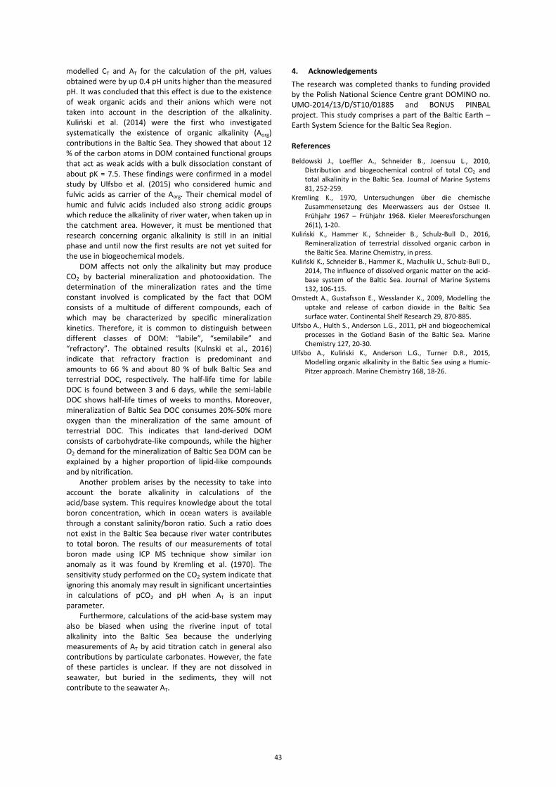
modelled CT and AT for the calculation of the pH, values obtained were by up 0.4 pH units higher than the measured pH. It was concluded that this effect is due to the existence of weak organic acids and their anions which were not taken into account in the description of the alkalinity. Kuliński et al. (2014) were the first who investigated systematically the existence of organic alkalinity (Aorg) contributions in the Baltic Sea. They showed that about 12 % of the carbon atoms in DOM contained functional groups that act as weak acids with a bulk dissociation constant of about pK = 7.5. These findings were confirmed in a model study by Ulfsbo et al. (2015) who considered humic and fulvic acids as carrier of the Aorg. Their chemical model of humic and fulvic acids included also strong acidic groups which reduce the alkalinity of river water, when taken up in the catchment area. However, it must be mentioned that research concerning organic alkalinity is still in an initial phase and until now the first results are not yet suited for the use in biogeochemical models.

DOM affects not only the alkalinity but may produce CO2 by bacterial mineralization and photooxidation. The determination of the mineralization rates and the time constant involved is complicated by the fact that DOM consists of a multitude of different compounds, each of which may be characterized by specific mineralization kinetics. Therefore, it is common to distinguish between different classes of DOM: “labile”, “semilabile” and “refractory”. The obtained results (Kulnski et al., 2016) indicate that refractory fraction is predominant and amounts to 66 % and about 80 % of bulk Baltic Sea and terrestrial DOC, respectively. The half-life time for labile DOC is found between 3 and 6 days, while the semi-labile DOC shows half-life times of weeks to months. Moreover, mineralization of Baltic Sea DOC consumes 20%-50% more oxygen than the mineralization of the same amount of terrestrial DOC. This indicates that land-derived DOM consists of carbohydrate-like compounds, while the higher O2 demand for the mineralization of Baltic Sea DOM can be explained by a higher proportion of lipid-like compounds and by nitrification.

Another problem arises by the necessity to take into account the borate alkalinity in calculations of the acid/base system. This requires knowledge about the total boron concentration, which in ocean waters is available through a constant salinity/boron ratio. Such a ratio does not exist in the Baltic Sea because river water contributes to total boron. The results of our measurements of total boron made using ICP MS technique show similar ion anomaly as it was found by Kremling et al. (1970). The sensitivity study performed on the CO2 system indicate that ignoring this anomaly may result in significant uncertainties in calculations of pCO2 and pH when AT is an input parameter.

Furthermore, calculations of the acid-base system may also be biased when using the riverine input of total alkalinity into the Baltic Sea because the underlying measurements of AT by acid titration catch in general also contributions by particulate carbonates. However, the fate of these particles is unclear. If they are not dissolved in seawater, but buried in the sediments, they will not contribute to the seawater AT.

4. Acknowledgements The research was completed thanks to funding provided by the Polish National Science Centre grant DOMINO no. UMO-2014/13/D/ST10/01885 and BONUS PINBAL project. This study comprises a part of the Baltic Earth – Earth System Science for the Baltic Sea Region. References

Beldowski J., Loeffler A., Schneider B., Joensuu L., 2010, Distribution and biogeochemical control of total CO2 and total alkalinity in the Baltic Sea. Journal of Marine Systems 81, 252-259.

Kremling K., 1970, Untersuchungen über die chemische Zusammensetzung des Meerwassers aus der Ostsee II. Frühjahr 1967 – Frühjahr 1968. Kieler Meeresforschungen 26(1), 1-20.

Kuliński K., Hammer K., Schneider B., Schulz-Bull D., 2016, Remineralization of terrestrial dissolved organic carbon in the Baltic Sea. Marine Chemistry, in press.

Kuliński K., Schneider B., Hammer K., Machulik U., Schulz-Bull D., 2014, The influence of dissolved organic matter on the acid-base system of the Baltic Sea. Journal of Marine Systems 132, 106-115.

Omstedt A., Gustafsson E., Wesslander K., 2009, Modelling the uptake and release of carbon dioxide in the Baltic Sea surface water. Continental Shelf Research 29, 870-885.

Ulfsbo A., Hulth S., Anderson L.G., 2011, pH and biogeochemical processes in the Gotland Basin of the Baltic Sea. Marine Chemistry 127, 20-30.

Ulfsbo A., Kuliński K., Anderson L.G., Turner D.R., 2015, Modelling organic alkalinity in the Baltic Sea using a Humic-Pitzer approach. Marine Chemistry 168, 18-26.

43

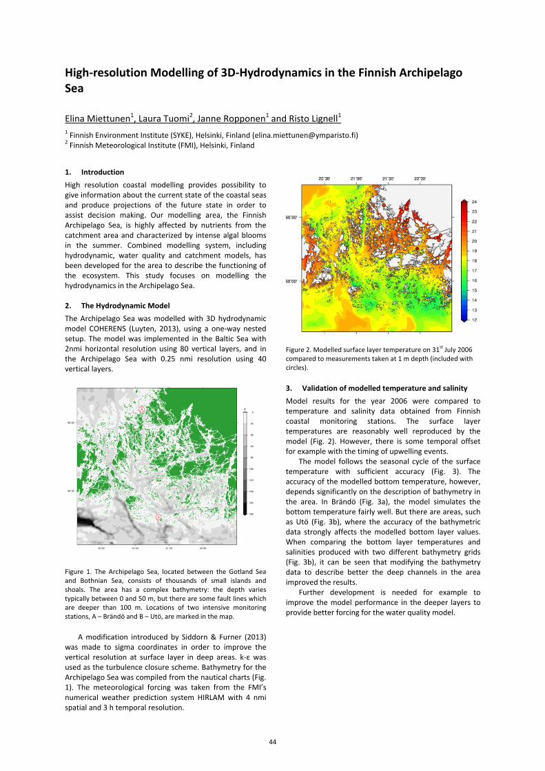
High-resolution Modelling of 3D-Hydrodynamics in the Finnish Archipelago Sea

Elina Miettunen1, Laura Tuomi2, Janne Ropponen1 and Risto Lignell1 1 Finnish Environment Institute (SYKE), Helsinki, Finland (elina.miettunen@ymparisto.fi) 2 Finnish Meteorological Institute (FMI), Helsinki, Finland

1. Introduction High resolution coastal modelling provides possibility to give information about the current state of the coastal seas and produce projections of the future state in order to assist decision making. Our modelling area, the Finnish Archipelago Sea, is highly affected by nutrients from the catchment area and characterized by intense algal blooms in the summer. Combined modelling system, including hydrodynamic, water quality and catchment models, has been developed for the area to describe the functioning of the ecosystem. This study focuses on modelling the hydrodynamics in the Archipelago Sea. 2. The Hydrodynamic Model The Archipelago Sea was modelled with 3D hydrodynamic model COHERENS (Luyten, 2013), using a one-way nested setup. The model was implemented in the Baltic Sea with 2nmi horizontal resolution using 80 vertical layers, and in the Archipelago Sea with 0.25 nmi resolution using 40 vertical layers.

Figure 1. The Archipelago Sea, located between the Gotland Sea and Bothnian Sea, consists of thousands of small islands and shoals. The area has a complex bathymetry: the depth varies typically between 0 and 50 m, but there are some fault lines which are deeper than 100 m. Locations of two intensive monitoring stations, A – Brändö and B – Utö, are marked in the map.

A modification introduced by Siddorn & Furner (2013) was made to sigma coordinates in order to improve the vertical resolution at surface layer in deep areas. k-ε was used as the turbulence closure scheme. Bathymetry for the Archipelago Sea was compiled from the nautical charts (Fig. 1). The meteorological forcing was taken from the FMI’s numerical weather prediction system HIRLAM with 4 nmi spatial and 3 h temporal resolution.

Figure 2. Modelled surface layer temperature on 31st July 2006 compared to measurements taken at 1 m depth (included with circles).

3. Validation of modelled temperature and salinity Model results for the year 2006 were compared to temperature and salinity data obtained from Finnish coastal monitoring stations. The surface layer temperatures are reasonably well reproduced by the model (Fig. 2). However, there is some temporal offset for example with the timing of upwelling events. The model follows the seasonal cycle of the surface temperature with sufficient accuracy (Fig. 3). The accuracy of the modelled bottom temperature, however, depends significantly on the description of bathymetry in the area. In Brändö (Fig. 3a), the model simulates the bottom temperature fairly well. But there are areas, such as Utö (Fig. 3b), where the accuracy of the bathymetric data strongly affects the modelled bottom layer values. When comparing the bottom layer temperatures and salinities produced with two different bathymetry grids (Fig. 3b), it can be seen that modifying the bathymetry data to describe better the deep channels in the area improved the results. Further development is needed for example to improve the model performance in the deeper layers to provide better forcing for the water quality model.

44

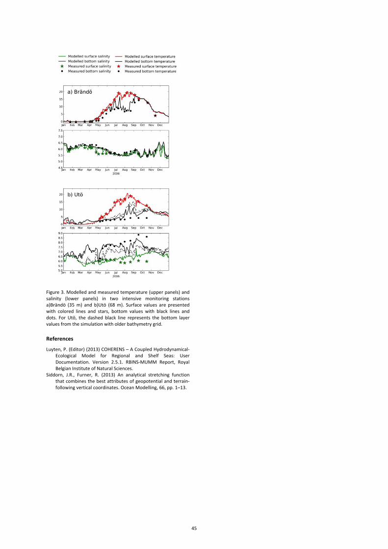
Figure 3. Modelled and measured temperature (upper panels) and salinity (lower panels) in two intensive monitoring stations a)Brändö (35 m) and b)Utö (68 m). Surface values are presented with colored lines and stars, bottom values with black lines and dots. For Utö, the dashed black line represents the bottom layer values from the simulation with older bathymetry grid.

References

Luyten, P. (Editor) (2013) COHERENS – A Coupled Hydrodynamical-Ecological Model for Regional and Shelf Seas: User Documentation. Version 2.5.1. RBINS-MUMM Report, Royal Belgian Institute of Natural Sciences.

Siddorn, J.R., Furner, R. (2013) An analytical stretching function that combines the best attributes of geopotential and terrain-following vertical coordinates. Ocean Modelling, 66, pp. 1–13.

45

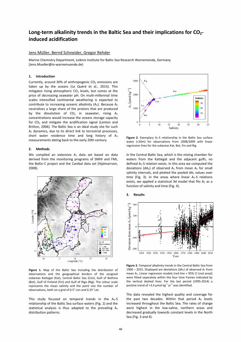
Long-term alkalinity trends in the Baltic Sea and their implications for CO2-induced acidification

Jens Müller, Bernd Schneider, Gregor Rehder

Marine Chemistry Department, Leibniz Institute for Baltic Sea Research Warnemünde, Germany (Jens.Mueller@io-warnemuende.de)

1. Introduction Currently, around 30% of anthropogenic CO2 emissions are taken up by the oceans (Le Quéré et al., 2015). This mitigates rising atmospheric CO2 levels, but comes at the price of decreasing seawater pH. On multi-millennial time scales intensified continental weathering is expected to contribute to increasing oceanic alkalinity (AT). Because AT neutralizes a large share of the protons that are produced by the dissolution of CO2 in seawater, rising AT concentrations would increase the oceans storage capacity for CO2 and mitigate the acidification signal (Lenton and Britton, 2006). The Baltic Sea is an ideal study site for such AT dynamics, due to its direct link to terrestrial processes, short water residence time and long history of AT measurements dating back to the early 20th century. 2. Methods We compiled an extensive AT data set based on data derived from the monitoring programs of SMHI and FMI, the Baltic-C project and the Canibal data set (Hjalmarrson, 2008).

Figure 1. Map of the Baltic Sea including the distribution of observations and the geographical borders of the assigned subareas Kattegat (Kat), Central Baltic Sea (Cen), Gulf of Bothnia (Bot), Gulf of Finland (Fin) and Gulf of Riga (Rig). The colour scale represents the mean salinity and the point size the number of observations, both on a grid of 0.5° Lon and 0.25° Lat.

This study focused on temporal trends in the AT-S relationship of the Baltic Sea surface waters (Fig. 2) and the statistical analysis is thus adapted to the prevailing AT distribution patterns.

Figure 2. Exemplary AT-S relationship in the Baltic Sea surface water (<20m) for observations from 2008/2009 with linear regression lines for the subareas Kat, Bot, Fin and Rig.

In the Central Baltic Sea, which is the mixing chamber for waters from the Kattegat and the adjacent gulfs, no defined AT-S relation exists. In this area we computed the deviations (dAT) of observed AT from mean AT for small salinity intervals, and plotted the pooled dAT values over time (Fig. 3). In the areas where linear AT-S relations exists, we applied a statistical 3d model that fits AT as a function of salinity and time (Fig. 4). 3. Results

Figure 3. Temporal alkalinity trends in the Central Baltic Sea from 1900 – 2015. Displayed are deviations (dAT) of observed AT from mean AT. Linear regression models (red line + 95% CI (red area)) were fitted separately within the four time frames indicated by the vertical dashed lines. For the last period (1995-2014) a positive trend of +3.4 µmol kg-1 yr-1 was identified.

The data revealed the highest quality and coverage for the past two decades. Within that period AT levels increased throughout the Baltic Sea. The rates of change were highest in the low-saline, northern areas and decreased gradually towards constant levels in the North Sea (Fig. 3 and 4).

46

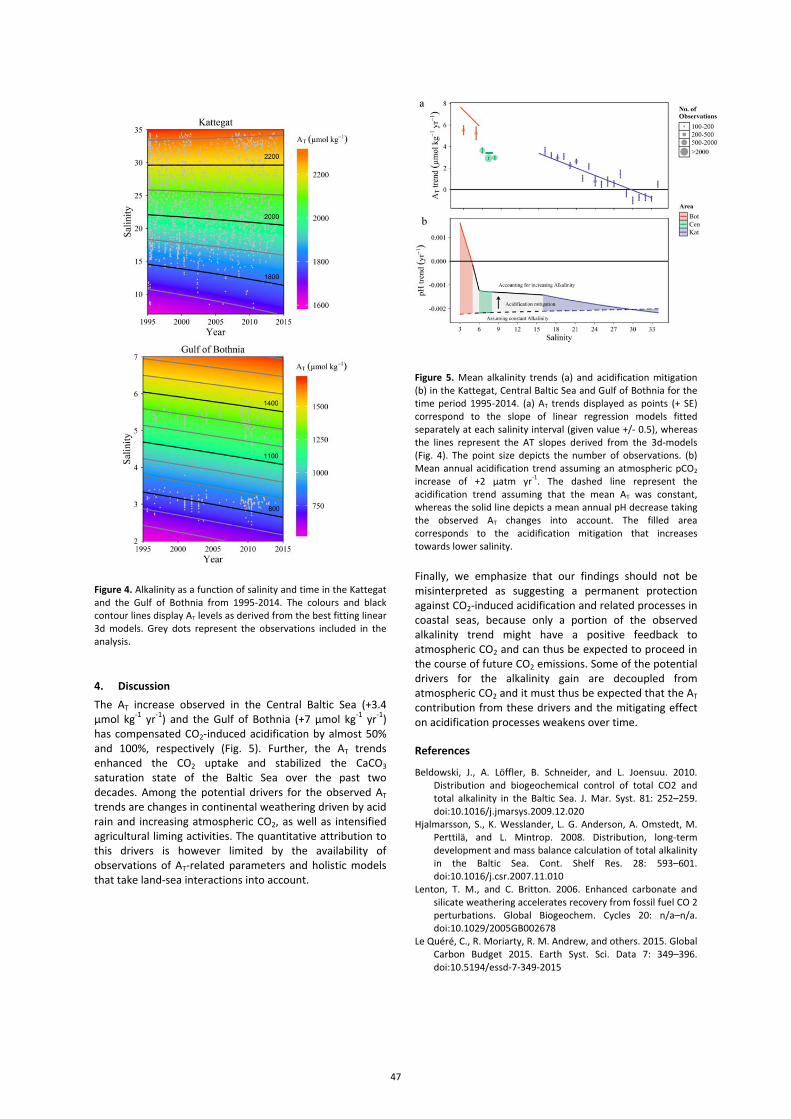
Figure 4. Alkalinity as a function of salinity and time in the Kattegat and the Gulf of Bothnia from 1995-2014. The colours and black contour lines display AT levels as derived from the best fitting linear 3d models. Grey dots represent the observations included in the analysis.

4. Discussion The AT increase observed in the Central Baltic Sea (+3.4 µmol kg-1 yr-1) and the Gulf of Bothnia (+7 µmol kg-1 yr-1) has compensated CO2-induced acidification by almost 50% and 100%, respectively (Fig. 5). Further, the AT trends enhanced the CO2 uptake and stabilized the CaCO3 saturation state of the Baltic Sea over the past two decades. Among the potential drivers for the observed AT trends are changes in continental weathering driven by acid rain and increasing atmospheric CO2, as well as intensified agricultural liming activities. The quantitative attribution to this drivers is however limited by the availability of observations of AT-related parameters and holistic models that take land-sea interactions into account.

Figure 5. Mean alkalinity trends (a) and acidification mitigation (b) in the Kattegat, Central Baltic Sea and Gulf of Bothnia for the time period 1995-2014. (a) AT trends displayed as points (+ SE) correspond to the slope of linear regression models fitted separately at each salinity interval (given value +/- 0.5), whereas the lines represent the AT slopes derived from the 3d-models (Fig. 4). The point size depicts the number of observations. (b) Mean annual acidification trend assuming an atmospheric pCO2 increase of +2 µatm yr-1. The dashed line represent the acidification trend assuming that the mean AT was constant, whereas the solid line depicts a mean annual pH decrease taking the observed AT changes into account. The filled area corresponds to the acidification mitigation that increases towards lower salinity.

Finally, we emphasize that our findings should not be misinterpreted as suggesting a permanent protection against CO2-induced acidification and related processes in coastal seas, because only a portion of the observed alkalinity trend might have a positive feedback to atmospheric CO2 and can thus be expected to proceed in the course of future CO2 emissions. Some of the potential drivers for the alkalinity gain are decoupled from atmospheric CO2 and it must thus be expected that the AT contribution from these drivers and the mitigating effect on acidification processes weakens over time. References

Beldowski, J., A. Löffler, B. Schneider, and L. Joensuu. 2010. Distribution and biogeochemical control of total CO2 and total alkalinity in the Baltic Sea. J. Mar. Syst. 81: 252–259. doi:10.1016/j.jmarsys.2009.12.020

Hjalmarsson, S., K. Wesslander, L. G. Anderson, A. Omstedt, M. Perttilä, and L. Mintrop. 2008. Distribution, long-term development and mass balance calculation of total alkalinity in the Baltic Sea. Cont. Shelf Res. 28: 593–601. doi:10.1016/j.csr.2007.11.010

Lenton, T. M., and C. Britton. 2006. Enhanced carbonate and silicate weathering accelerates recovery from fossil fuel CO 2 perturbations. Global Biogeochem. Cycles 20: n/a–n/a. doi:10.1029/2005GB002678

Le Quéré, C., R. Moriarty, R. M. Andrew, and others. 2015. Global Carbon Budget 2015. Earth Syst. Sci. Data 7: 349–396. doi:10.5194/essd-7-349-2015

47

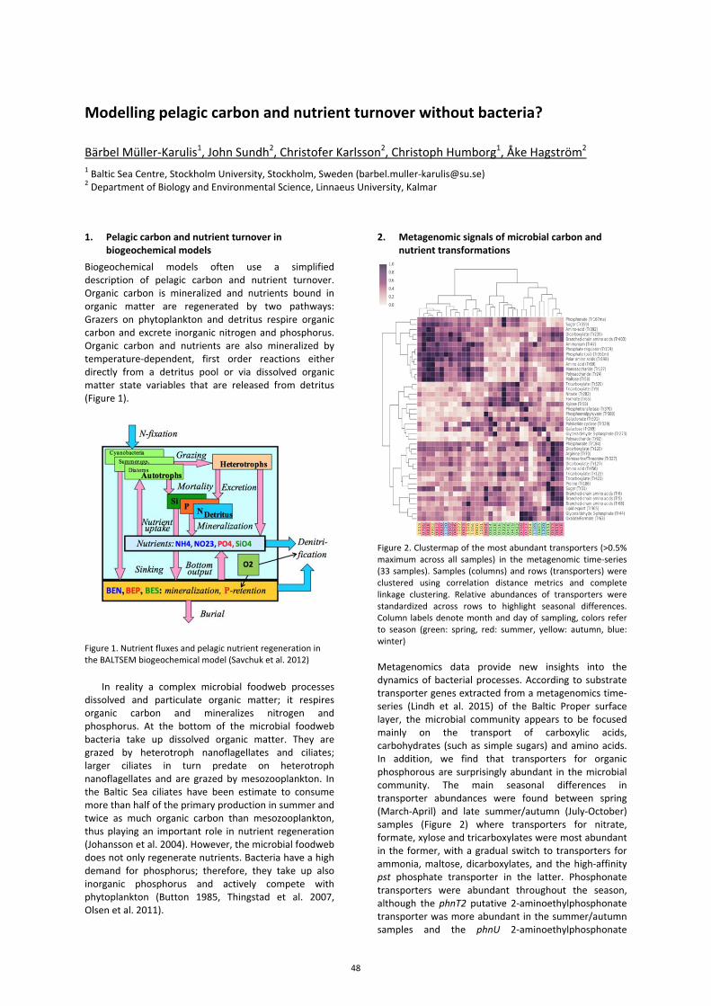
Modelling pelagic carbon and nutrient turnover without bacteria?

Bärbel Müller-Karulis1, John Sundh2, Christofer Karlsson2, Christoph Humborg1, Åke Hagström2 1 Baltic Sea Centre, Stockholm University, Stockholm, Sweden (barbel.muller-karulis@su.se) 2 Department of Biology and Environmental Science, Linnaeus University, Kalmar 1. Pelagic carbon and nutrient turnover in

biogeochemical models Biogeochemical models often use a simplified description of pelagic carbon and nutrient turnover. Organic carbon is mineralized and nutrients bound in organic matter are regenerated by two pathways: Grazers on phytoplankton and detritus respire organic carbon and excrete inorganic nitrogen and phosphorus. Organic carbon and nutrients are also mineralized by temperature-dependent, first order reactions either directly from a detritus pool or via dissolved organic matter state variables that are released from detritus (Figure 1).

Figure 1. Nutrient fluxes and pelagic nutrient regeneration in the BALTSEM biogeochemical model (Savchuk et al. 2012)

In reality a complex microbial foodweb processes dissolved and particulate organic matter; it respires organic carbon and mineralizes nitrogen and phosphorus. At the bottom of the microbial foodweb bacteria take up dissolved organic matter. They are grazed by heterotroph nanoflagellates and ciliates; larger ciliates in turn predate on heterotroph nanoflagellates and are grazed by mesozooplankton. In the Baltic Sea ciliates have been estimate to consume more than half of the primary production in summer and twice as much organic carbon than mesozooplankton, thus playing an important role in nutrient regeneration (Johansson et al. 2004). However, the microbial foodweb does not only regenerate nutrients. Bacteria have a high demand for phosphorus; therefore, they take up also inorganic phosphorus and actively compete with phytoplankton (Button 1985, Thingstad et al. 2007, Olsen et al. 2011).

2. Metagenomic signals of microbial carbon and nutrient transformations

Figure 2. Clustermap of the most abundant transporters (>0.5% maximum across all samples) in the metagenomic time-series (33 samples). Samples (columns) and rows (transporters) were clustered using correlation distance metrics and complete linkage clustering. Relative abundances of transporters were standardized across rows to highlight seasonal differences. Column labels denote month and day of sampling, colors refer to season (green: spring, red: summer, yellow: autumn, blue: winter) Metagenomics data provide new insights into the dynamics of bacterial processes. According to substrate transporter genes extracted from a metagenomics time-series (Lindh et al. 2015) of the Baltic Proper surface layer, the microbial community appears to be focused mainly on the transport of carboxylic acids, carbohydrates (such as simple sugars) and amino acids. In addition, we find that transporters for organic phosphorous are surprisingly abundant in the microbial community. The main seasonal differences in transporter abundances were found between spring (March-April) and late summer/autumn (July-October) samples (Figure 2) where transporters for nitrate, formate, xylose and tricarboxylates were most abundant in the former, with a gradual switch to transporters for ammonia, maltose, dicarboxylates, and the high-affinity pst phosphate transporter in the latter. Phosphonate transporters were abundant throughout the season, although the phnT2 putative 2-aminoethylphosphonate transporter was more abundant in the summer/autumn samples and the phnU 2-aminoethylphosphonate

48

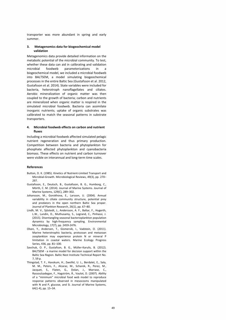
transporter was more abundant in spring and early summer. 3. Metagenomics data for biogeochemical model

validation Metagenomics data provide detailed information on the metabolic potential of the microbial community. To test, whether these data can aid in calibrating and validation microbial foodweb parameterizations in a biogeochemical model, we included a microbial foodweb into BALTSEM, a model simulating biogeochemical processes in the entire Baltic Sea (Gustafsson et al. 2012, Gustafsson et al. 2014). State variables were included for bacteria, heterotroph nanoflagellates and ciliates. Aerobic mineralization of organic matter was then coupled to the growth of bacteria; carbon and nutrients are mineralized when organic matter is respired in the simulated microbial foodweb. Bacteria can assimilate inorganic nutrients; uptake of organic substrates was calibrated to match the seasonal patterns in substrate transporters. 4. Microbial foodweb effects on carbon and nutrient

fluxes Including a microbial foodweb affected simulated pelagic nutrient regeneration and thus primary production. Competition between bacteria and phytoplankton for phosphate affected phytoplankton and cyanobacteria biomass. These effects on nutrient and carbon turnover were visible on interannual and long-term time scales. References Button, D. K. (1985). Kinetics of Nutrient-Limited Transport and

Microbial-Growth. Microbiological Reviews, 49(3), pp. 270–297.

Gustafsson, E., Deutsch, B., Gustafsson, B. G., Humborg, C., Mörth, C. M. (2014). Journal of Marine Systems. Journal of Marine Systems, 129(C), 289–302.

Johansson, M., Gorokhova, E., Larsson, U. (2004). Annual variability in ciliate community structure, potential prey and predators in the open northern Baltic Sea proper. Journal of Plankton Research, 26(1), pp. 67–80.

Lindh, M. V., Sjöstedt, J., Andersson, A. F., Baltar, F., Hugerth, L.W., Lundin, D., Muthusamy, S., Legrand, C., Pinhassi, J. (2015). Disentangling seasonal bacterioplankton population dynamics by high-frequency sampling. Environmental Microbiology, 17(7), pp. 2459-2476.

Olsen, Y., Andersen, T., Gismervik, I., Vadstein, O. (2011). Marine heterotrophic bacteria, protozoan and metazoan zooplankton may experience protein N or mineral P limitation in coastal waters. Marine Ecology Progress Series, 436, pp. 81–100.

Savchuk, O. P., Gustafson, B. G., Müller-Karulis, B. (2012). BALTSEM - a marine model for decision support within the Baltic Sea Region. Baltic Nest Institute Technical Report No. 7, 59 p.

Thingstad, T. F., Havskum, H., Zweifel, U. L., Berdalet, E., Sala, M. M., Peters, F., Alcaraz, M., Scharek, R., Perez, M., Jacquet, S., Flaten, G., Dolan, J., Marrase, C., Rassoulzadegan, F., Hagström, Å., Vaulot, D. (2007). Ability of a “minimum” microbial food web model to reproduce response patterns observed in mesocosms manipulated with N and P, glucose, and Si. Journal of Marine Systems, 64(1-4), pp. 15–34.

49

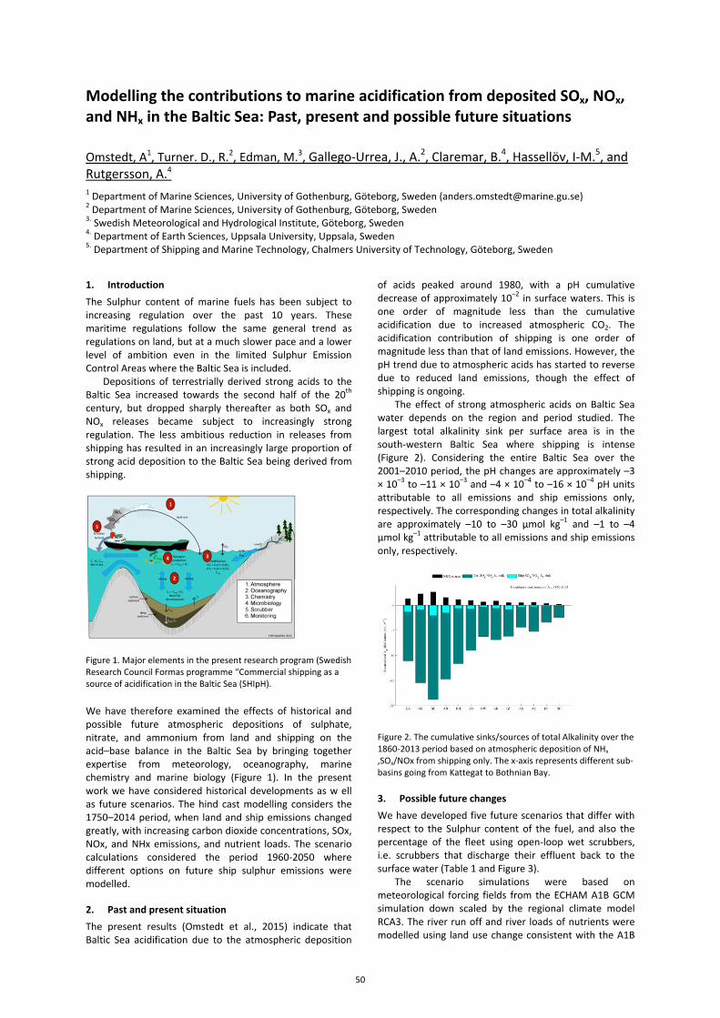
Modelling the contributions to marine acidification from deposited SOx, NOx, and NHx in the Baltic Sea: Past, present and possible future situations

Omstedt, A1, Turner. D., R.2, Edman, M.3, Gallego-Urrea, J., A.2, Claremar, B.4, Hassellöv, I-M.5, and Rutgersson, A.4 1 Department of Marine Sciences, University of Gothenburg, Göteborg, Sweden (anders.omstedt@marine.gu.se) 2 Department of Marine Sciences, University of Gothenburg, Göteborg, Sweden 3. Swedish Meteorological and Hydrological Institute, Göteborg, Sweden 4. Department of Earth Sciences, Uppsala University, Uppsala, Sweden 5. Department of Shipping and Marine Technology, Chalmers University of Technology, Göteborg, Sweden

1. Introduction The Sulphur content of marine fuels has been subject to increasing regulation over the past 10 years. These maritime regulations follow the same general trend as regulations on land, but at a much slower pace and a lower level of ambition even in the limited Sulphur Emission Control Areas where the Baltic Sea is included.

Depositions of terrestrially derived strong acids to the Baltic Sea increased towards the second half of the 20th century, but dropped sharply thereafter as both SOx and NOx releases became subject to increasingly strong regulation. The less ambitious reduction in releases from shipping has resulted in an increasingly large proportion of strong acid deposition to the Baltic Sea being derived from shipping.

Figure 1. Major elements in the present research program (Swedish Research Council Formas programme “Commercial shipping as a source of acidification in the Baltic Sea (SHIpH).

We have therefore examined the effects of historical and possible future atmospheric depositions of sulphate, nitrate, and ammonium from land and shipping on the acid–base balance in the Baltic Sea by bringing together expertise from meteorology, oceanography, marine chemistry and marine biology (Figure 1). In the present work we have considered historical developments as w ell as future scenarios. The hind cast modelling considers the 1750–2014 period, when land and ship emissions changed greatly, with increasing carbon dioxide concentrations, SOx, NOx, and NHx emissions, and nutrient loads. The scenario calculations considered the period 1960-2050 where different options on future ship sulphur emissions were modelled. 2. Past and present situation The present results (Omstedt et al., 2015) indicate that Baltic Sea acidification due to the atmospheric deposition

of acids peaked around 1980, with a pH cumulative decrease of approximately 10–2 in surface waters. This is one order of magnitude less than the cumulative acidification due to increased atmospheric CO2. The acidification contribution of shipping is one order of magnitude less than that of land emissions. However, the pH trend due to atmospheric acids has started to reverse due to reduced land emissions, though the effect of shipping is ongoing.

The effect of strong atmospheric acids on Baltic Sea water depends on the region and period studied. The largest total alkalinity sink per surface area is in the south-western Baltic Sea where shipping is intense (Figure 2). Considering the entire Baltic Sea over the 2001–2010 period, the pH changes are approximately –3 × 10–3 to –11 × 10–3 and –4 × 10–4 to –16 × 10–4 pH units attributable to all emissions and ship emissions only, respectively. The corresponding changes in total alkalinity are approximately –10 to –30 µmol kg–1 and –1 to –4 µmol kg–1 attributable to all emissions and ship emissions only, respectively.

Figure 2. The cumulative sinks/sources of total Alkalinity over the 1860-2013 period based on atmospheric deposition of NHx ,SOx/NOx from shipping only. The x-axis represents different sub-basins going from Kattegat to Bothnian Bay. 3. Possible future changes We have developed five future scenarios that differ with respect to the Sulphur content of the fuel, and also the percentage of the fleet using open-loop wet scrubbers, i.e. scrubbers that discharge their effluent back to the surface water (Table 1 and Figure 3).

The scenario simulations were based on meteorological forcing fields from the ECHAM A1B GCM simulation down scaled by the regional climate model RCA3. The river run off and river loads of nutrients were modelled using land use change consistent with the A1B

50

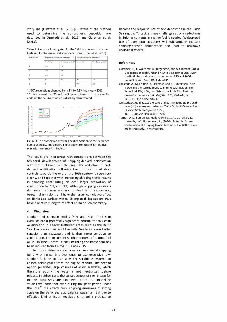
story line (Omstedt et al. [2012]). Details of the method used to determine the atmospheric deposition are described in Omstedt et al. [2015] and Claremar et al. [2013]. Table 1. Scenarios investigated for the Sulphur content of marine fuels and for the use of wet scrubbers (from Turner et al., 2016).

* SECA regulations changed from 1% to 0.1% in January 2015 ** It is assumed that 96% of the Sulphur is taken up in the scrubber and that the scrubber water is discharged untreated

Figure 3. The proportion of strong acid deposition to the Baltic Sea due to shipping. The coloured lines show projections for the five scenarios presented in Table 1. The results are in progress with comparisons between the temporal development of shipping-derived acidification with the total (land plus shipping). The reduction in land-derived acidification following the introduction of strict controls towards the end of the 20th century is seen very clearly, and together with increasing shipping traffic results in shipping contributing an ever larger proportion of acidification by SOx and NOx. Although shipping emissions dominate the strong acid input under this future scenario, terrestrial emissions still have the larger cumulative effect on Baltic Sea surface water. Strong acid depositions thus have a relatively long term effect on Baltic Sea chemistry. 4. Discussion Sulphur and nitrogen oxides (SOx and NOx) from ship exhausts are a potentially significant contributor to Ocean Acidification in heavily trafficked areas such as the Baltic Sea. The brackish water of the Baltic Sea has a lower buffer capacity than seawater, and is thus more sensitive to acidification. The maximum Sulphur content of marine fuel oil in Emission Control Areas (including the Baltic Sea) has been reduced from 1% to 0.1% since 2015.

Two possibilities are available for commercial shipping for environmental improvements: to use expensive low-Sulphur fuel, or to use seawater scrubbing systems to absorb acidic gases from the engine exhaust. The second option generates large volumes of acidic seawater, which therefore acidify the water if not neutralized before release. In either case, the consequences of the release for marine organisms are unknown. From our modelling studies we learn that even during the peak period under the 1980th the effects from shipping emissions of strong acids on the Baltic Sea acid-balance was small. But due to effective land emission regulations, shipping predicts to

become the major source of acid deposition in the Baltic Sea region. To tackle these challenges strong reductions in Sulphur contents in marine fuel is needed. Widespread use of open-loop scrubbers will substantially increase shipping-derived acidification and lead to unknown ecological effects. References

Claremar, B., T. Wallstedt, A. Rutgersson, and A. Omstedt (2013), Deposition of acidifying and neutralising compounds over the Baltic Sea drainage basin between 1960 and 2006, Boreal Environ. Res., 18(6), 425-445.

Omstedt, A., M. Edman, B. Claremar, and A. Rutgersson (2015), Modelling the contributions to marine acidification from deposited SOx, NOx, and NHx in the Baltic Sea: Past and present situations, Cont. Shelf Res. 111, 234-249, doi: 10.1016/j.csr.2015.08.024.

Omstedt, A., et al. (2012), Future changes in the Baltic Sea acid-base (pH) and oxygen balances, Tellus Series B-Chemical and Physical Meteorology, 64, 1958, doi:10.3402/tellusb.v64i0.19586.

Turner, D.,R., Edman, M., Gallero-Urrea, J., A., Claremar, B., Hasselöv, I-M., Rutgersson, A., (2016). Potential future contribution of shipping to acidification of the Baltic Sea: a modelling study. In manuscript.

51

Riverine carbon export and its impacts on Finnish coastal water quality

Antti Räike1, Vivi Fleming-Lehtinen, Pirkko Kortelainen1 Tuija Mattsson1 Pirkko Kauppila1 and David N. Thomas1,2 1 Finnish Environment Institute, Helsinki, Finland (antti.raike@ymparisto.fi) 2 School of Ocean Sciences, Bangor University, Menai Bridge, Anglesey, UK

1. Abstract Annually Finnish rivers export on average 1.5 M t

carbon to the Baltic Sea, with the total organic carbon (TOC) component contributing the major share (nearly 80 %) of this export. The highest organic carbon export originates from peat-dominated catchments in the northern parts of Finland. In contrast rivers draining agricultural catchments have the highest area-specific inorganic carbon fluxes. Over the last two decades dissolved organic carbon (DOC) concentrations have been frequently measured as increasing in freshwaters of the northern hemisphere, but the strong upward trends in TOC concentrations were not reflected as clearly in TOC export trends of Finnish rivers. This was because changes in water flow had a dominant influence on TOC export to the sea and any changes in concentrations were masked behind the variation in flow. Coastal and adjacent riverine TOC concentrations correlated positively demonstrating the effect of terrestrial input. TOC correlated negatively with salinity, and salinity based mixing analysis indicates there is effective carbon removal at low salinities. TOC was not shown to be a major contributor to water clarity, but instead Secchi depth was observed to correlate frequently to Fe and chlorophyll a.

Acknowledgments We thank the Academy of Finland (projects: ‘‘Biogeochemistry of the Baltic Sea in a Changing Climate: From Catchment to Open Sea (FiDiPro)’’ and ‘‘Fluxes of Terminal Electron Acceptors: Linking Human Disturbance to the Health of Aquatic Systems (TEAQUILA)’’ (decision no. 263476)) and NordForsk funded Domqua (Drinking water treatment adaptation to increasing levels of DOM and changing DOM quality under climate change) project for supporting this work. References Fleming-Lehtinen V, Räike A, Kortelainen P, Kauppila P,

Thomas D (2015) Organic carbon concentration in the northern coastal Baltic Sea between 1975 and 2011. Estuaries Coasts 38:466–481.

Räike A, Kortelainen P, Mattsson T, Thomas DN (2012) 36 year trends in dissolved organic carbon export from Finnish rivers to the Baltic Sea. Sci Total Environ 435–436:188–201.

Räike A, Kortelainen P, Mattsson T, Thomas DN (2015) Long-term trends (1975–2014) in the concentrations and export of carbon from Finnish rivers to the Baltic Sea: organic and inorganic components. Aquatic Sciences DOI 10.1007/s00027-015-0451-2.

52

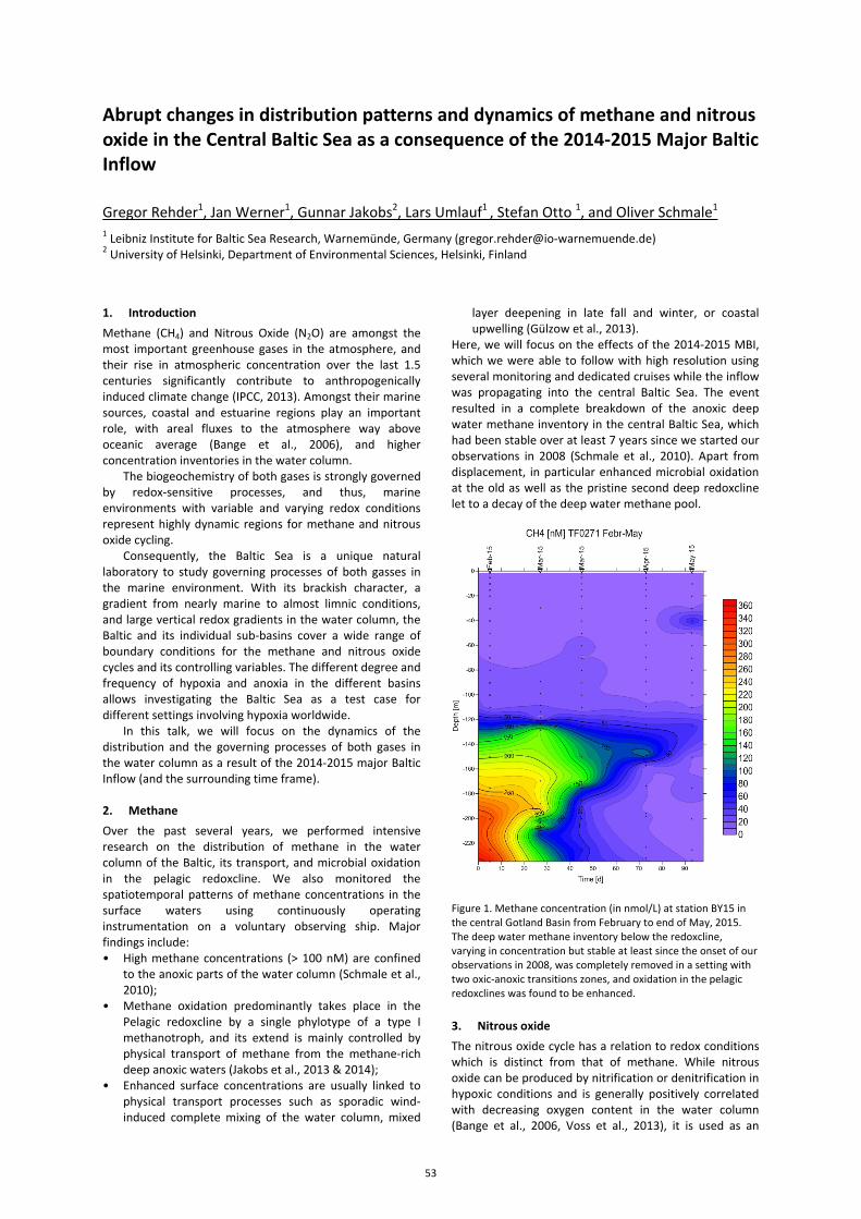
Abrupt changes in distribution patterns and dynamics of methane and nitrous oxide in the Central Baltic Sea as a consequence of the 2014-2015 Major Baltic Inflow

Gregor Rehder1, Jan Werner1, Gunnar Jakobs2, Lars Umlauf1 , Stefan Otto 1, and Oliver Schmale1 1 Leibniz Institute for Baltic Sea Research, Warnemünde, Germany (gregor.rehder@io-warnemuende.de) 2 University of Helsinki, Department of Environmental Sciences, Helsinki, Finland

1. Introduction Methane (CH4) and Nitrous Oxide (N2O) are amongst the most important greenhouse gases in the atmosphere, and their rise in atmospheric concentration over the last 1.5 centuries significantly contribute to anthropogenically induced climate change (IPCC, 2013). Amongst their marine sources, coastal and estuarine regions play an important role, with areal fluxes to the atmosphere way above oceanic average (Bange et al., 2006), and higher concentration inventories in the water column.

The biogeochemistry of both gases is strongly governed by redox-sensitive processes, and thus, marine environments with variable and varying redox conditions represent highly dynamic regions for methane and nitrous oxide cycling.

Consequently, the Baltic Sea is a unique natural laboratory to study governing processes of both gasses in the marine environment. With its brackish character, a gradient from nearly marine to almost limnic conditions, and large vertical redox gradients in the water column, the Baltic and its individual sub-basins cover a wide range of boundary conditions for the methane and nitrous oxide cycles and its controlling variables. The different degree and frequency of hypoxia and anoxia in the different basins allows investigating the Baltic Sea as a test case for different settings involving hypoxia worldwide.

In this talk, we will focus on the dynamics of the distribution and the governing processes of both gases in the water column as a result of the 2014-2015 major Baltic Inflow (and the surrounding time frame). 2. Methane Over the past several years, we performed intensive research on the distribution of methane in the water column of the Baltic, its transport, and microbial oxidation in the pelagic redoxcline. We also monitored the spatiotemporal patterns of methane concentrations in the surface waters using continuously operating instrumentation on a voluntary observing ship. Major findings include: • High methane concentrations (> 100 nM) are confined

to the anoxic parts of the water column (Schmale et al., 2010);

• Methane oxidation predominantly takes place in the Pelagic redoxcline by a single phylotype of a type I methanotroph, and its extend is mainly controlled by physical transport of methane from the methane-rich deep anoxic waters (Jakobs et al., 2013 & 2014);

• Enhanced surface concentrations are usually linked to physical transport processes such as sporadic wind-induced complete mixing of the water column, mixed

layer deepening in late fall and winter, or coastal upwelling (Gülzow et al., 2013).

Here, we will focus on the effects of the 2014-2015 MBI, which we were able to follow with high resolution using several monitoring and dedicated cruises while the inflow was propagating into the central Baltic Sea. The event resulted in a complete breakdown of the anoxic deep water methane inventory in the central Baltic Sea, which had been stable over at least 7 years since we started our observations in 2008 (Schmale et al., 2010). Apart from displacement, in particular enhanced microbial oxidation at the old as well as the pristine second deep redoxcline let to a decay of the deep water methane pool.

Figure 1. Methane concentration (in nmol/L) at station BY15 in the central Gotland Basin from February to end of May, 2015. The deep water methane inventory below the redoxcline, varying in concentration but stable at least since the onset of our observations in 2008, was completely removed in a setting with two oxic-anoxic transitions zones, and oxidation in the pelagic redoxclines was found to be enhanced.

3. Nitrous oxide The nitrous oxide cycle has a relation to redox conditions which is distinct from that of methane. While nitrous oxide can be produced by nitrification or denitrification in hypoxic conditions and is generally positively correlated with decreasing oxygen content in the water column (Bange et al., 2006, Voss et al., 2013), it is used as an

53

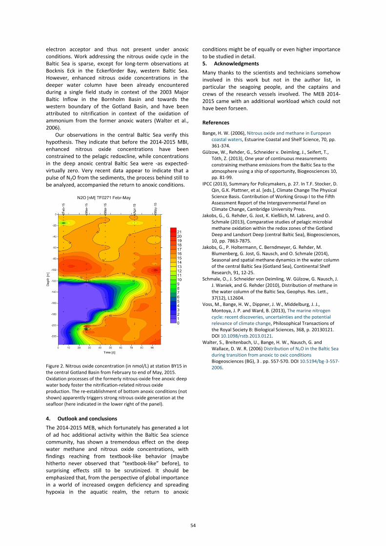
electron acceptor and thus not present under anoxic conditions. Work addressing the nitrous oxide cycle in the Baltic Sea is sparse, except for long-term observations at Bocknis Eck in the Eckerförder Bay, western Baltic Sea. However, enhanced nitrous oxide concentrations in the deeper water column have been already encountered during a single field study in context of the 2003 Major Baltic Inflow in the Bornholm Basin and towards the western boundary of the Gotland Basin, and have been attributed to nitrification in context of the oxidation of ammonium from the former anoxic waters (Walter et al., 2006).

Our observations in the central Baltic Sea verify this hypothesis. They indicate that before the 2014-2015 MBI, enhanced nitrous oxide concentrations have been constrained to the pelagic redoxcline, while concentrations in the deep anoxic central Baltic Sea were -as expected- virtually zero. Very recent data appear to indicate that a pulse of N2O from the sediments, the process behind still to be analyzed, accompanied the return to anoxic conditions.

Figure 2. Nitrous oxide concentration (in nmol/L) at station BY15 in the central Gotland Basin from February to end of May, 2015. Oxidation processes of the formerly nitrous-oxide free anoxic deep water body foster the nitrification-related nitrous oxide production. The re-establishment of bottom anoxic conditions (not shown) apparently triggers strong nitrous oxide generation at the seafloor (here indicated in the lower right of the panel).

4. Outlook and conclusions The 2014-2015 MEB, which fortunately has generated a lot of ad hoc additional activity within the Baltic Sea science community, has shown a tremendous effect on the deep water methane and nitrous oxide concentrations, with findings reaching from textbook-like behavior (maybe hitherto never observed that “textbook-like” before), to surprising effects still to be scrutinized. It should be emphasized that, from the perspective of global importance in a world of increased oxygen deficiency and spreading hypoxia in the aquatic realm, the return to anoxic

conditions might be of equally or even higher importance to be studied in detail. 5. Acknowledgments Many thanks to the scientists and technicians somehow involved in this work but not in the author list, in particular the seagoing people, and the captains and crews of the research vessels involved. The MEB 2014-2015 came with an additional workload which could not have been forseen. References

Bange, H. W. (2006), Nitrous oxide and methane in European coastal waters, Estuarine Coastal and Shelf Science, 70, pp. 361-374.

Gülzow, W., Rehder, G., Schneider v. Deimling, J., Seifert, T., Tóth, Z. (2013), One year of continuous measurements constraining methane emissions from the Baltic Sea to the atmosphere using a ship of opportunity, Biogeosciences 10, pp. 81-99.

IPCC (2013), Summary for Policymakers, p. 27. In T.F. Stocker, D. Qin, G.K. Plattner, et al. [eds.], Climate Change The Physical Science Basis. Contribution of Working Group I to the Fifth Assessment Report of the Intergovernmental Panel on Climate Change, Cambridge University Press.

Jakobs, G., G. Rehder, G. Jost, K. Kießlich, M. Labrenz, and O. Schmale (2013), Comparative studies of pelagic microbial methane oxidation within the redox zones of the Gotland Deep and Landsort Deep (central Baltic Sea), Biogeosciences, 10, pp. 7863-7875.

Jakobs, G., P. Holtermann, C. Berndmeyer, G. Rehder, M. Blumenberg, G. Jost, G. Nausch, and O. Schmale (2014), Seasonal and spatial methane dynamics in the water column of the central Baltic Sea (Gotland Sea), Continental Shelf Research, 91, 12-25.

Schmale, O., J. Schneider von Deimling, W. Gülzow, G. Nausch, J. J. Waniek, and G. Rehder (2010), Distribution of methane in the water column of the Baltic Sea, Geophys. Res. Lett., 37(12), L12604.

Voss, M., Bange, H. W., Dippner, J. W., Middelburg, J. J., Montoya, J. P. and Ward, B. (2013), The marine nitrogen cycle: recent discoveries, uncertainties and the potential relevance of climate change, Philosophical Transactions of the Royal Society B: Biological Sciences, 368, p. 20130121. DOI 10.1098/rstb.2013.0121.

Walter, S., Breitenbach, U., Bange, H. W., Nausch, G. and Wallace, D. W. R. (2006) Distribution of N2O in the Baltic Sea during transition from anoxic to oxic conditions Biogeosciences (BG), 3 . pp. 557-570. DOI 10.5194/bg-3-557-2006.

54

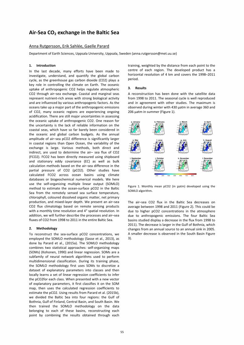
Air-Sea CO2 exchange in the Baltic Sea

Anna Rutgersson, Erik Sahlée, Gaelle Parard Department of Earth Sciences, Uppsala University, Uppsala, Sweden (anna.rutgersson@met.uu.se)

1. Introduction In the last decade, many efforts have been made to investigate, understand, and quantify the global carbon cycle, as the greenhouse gas carbon dioxide (CO2) plays a key role in controlling the climate on Earth. The oceanic uptake of anthropogenic CO2 helps regulate atmospheric CO2 through air–sea exchange. Coastal and marginal seas represent nutrient-rich areas with strong biological activity and are influenced by various anthropogenic factors. As the oceans take up a major part of the anthropogenic emissions of CO2, many oceanic regions are experiencing ongoing acidification. There are still major uncertainties in assessing the oceanic uptake of anthropogenic CO2. One reason for the uncertainty is the lack of reliable information on the coastal seas, which have so far barely been considered in the oceanic and global carbon budgets. As the annual amplitude of air–sea pCO2 difference is significantly larger in coastal regions than Open Ocean, the variability of the exchange is large. Various methods, both direct and indirect, are used to determine the air– sea flux of CO2 (FCO2). FCO2 has been directly measured using shipboard and stationary eddy covariance (EC) as well as bulk calculation methods based on the air–sea difference in the partial pressure of CO2 (pCO2). Other studies have calculated FCO2 across ocean basins using climate databases or biogeochemical numerical models. We here use the self-organizing multiple linear output (SOMLO) method to estimate the ocean-surface pCO2 in the Baltic Sea from the remotely sensed sea surface temperature, chlorophyll, coloured dissolved organic matter, net primary production, and mixed-layer depth. We present an air–sea CO2 flux climatology based on remote sensing products with a monthly time resolution and 4" spatial resolution. In addition, we will further describe the processes and air–sea fluxes of CO2 from 1998 to 2011 in the entire Baltic Sea. 2. Methodology To reconstruct the sea-surface pCO2 concentrations, we employed the SOMLO methodology (Sasse et al., 2013), as done by Parard et al., (2015a). The SOMLO methodology combines two statistical approaches: self-organizing maps (SOMs) (Kohonen, 1990) and linear regression. SOMs are a subfamily of neural network algorithms used to perform multidimensional classification. During its training phase, the SOMLO methodology first uses SOMs to discretize a dataset of explanatory parameters into classes and then locally learns a set of linear regression coefficients to infer the pCO2for each class. When presented with a new vector of explanatory parameters, it first classifies it on the SOM map, then uses the calculated regression coefficients to estimate the pCO2. Using results from Parard et al. (2015b), we divided the Baltic Sea into four regions: the Gulf of Bothnia, Gulf of Finland, Central Basin, and South Basin. We then trained the SOMLO methodology on the data belonging to each of these basins, reconstructing each point by combining the results obtained through each

training, weighted by the distance from each point to the centre of each region. The developed product has a horizontal resolution of 4 km and covers the 1998–2011 period.

3. Results A reconstruction has been done with the satellite data from 1998 to 2011. The seasonal cycle is well reproduced and in agreement with other studies. The maximum is observed during winter with 430 μatm in average 360 and 206 μatm in summer (Figure 1).

Figure 1. Monthly mean pCO2 (in μatm) developed using the SOMLO algorithm. The air–sea CO2 flux in the Baltic Sea decreases on average between 1998 and 2011 (Figure 2). This could be due to higher pCO2 concentrations in the atmosphere due to anthropogenic emissions. The four Baltic Sea basins studied display a decrease in the flux from 1998 to 2011). The decrease is larger in the Gulf of Bothnia, which changes from an annual source to an annual sink in 2005. A smaller decrease is observed in the South Basin Figure 3).

55

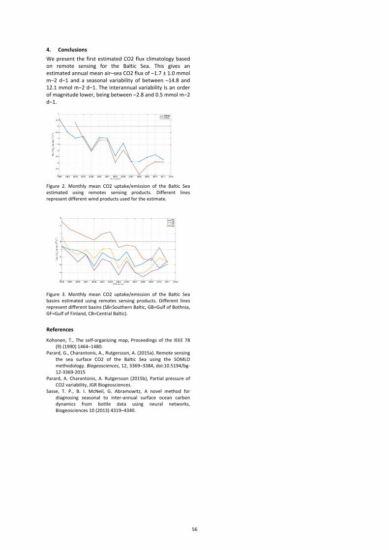
4. Conclusions We present the first estimated CO2 flux climatology based on remote sensing for the Baltic Sea. This gives an estimated annual mean air–sea CO2 flux of –1.7 ± 1.0 mmol m−2 d−1 and a seasonal variability of between –14.8 and 12.1 mmol m−2 d−1. The interannual variability is an order of magnitude lower, being between –2.8 and 0.5 mmol m−2 d−1.

Figure 2. Monthly mean CO2 uptake/emission of the Baltic Sea estimated using remotes sensing products. Different lines represent different wind products used for the estimate.

Figure 3. Monthly mean CO2 uptake/emission of the Baltic Sea basins estimated using remotes sensing products. Different lines represent different basins (SB=Southern Baltic, GB=Gulf of Bothnia, GF=Gulf of Finland, CB=Central Baltic).

References

Kohonen, T., The self-organizing map, Proceedings of the IEEE 78 (9) (1990) 1464–1480.

Parard, G., Charantonis, A., Rutgersson, A. (2015a). Remote sensing the sea surface CO2 of the Baltic Sea using the SOMLO methodology. Biogeosciences, 12, 3369–3384, doi:10.5194/bg-12-3369-2015

Parard, A. Charantonis, A. Rutgersson (2015b), Partial pressure of CO2 variability, JGR Biogeosciences.

Sasse, T. P., B. I. McNeil, G. Abramowitz, A novel method for diagnosing seasonal to inter-annual surface ocean carbon dynamics from bottle data using neural networks, Biogeosciences 10 (2013) 4319–4340.

56

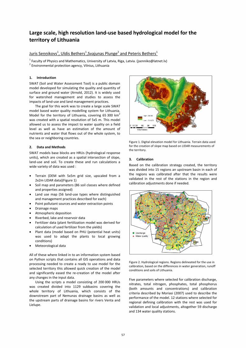
Large scale, high resolution land-use based hydrological model for the territory of Lithuania

Juris Seņņikovs1, Uldis Bethers1,Svajunas Plunge2 and Peteris Bethers1 1 Faculty of Physics and Mathematics, University of Latvia, Riga, Latvia. (jsenniko@latnet.lv) 2 Environmental protection agency, Vilnius, Lithuania

1. Introduction SWAT (Soil and Water Assessment Tool) is a public domain model developed for simulating the quality and quantity of surface and ground water (Arnold, 2012). It is widely used for watershed management and studies to assess the impacts of land-use and land management practices.

The goal for this work was to create a large scale SWAT model based water quality modelling system for Lithuania. Model for the territory of Lithuania, covering 65 300 km2 was created with a spatial resolution of 5x5 m. This model allowed us to assess the impact to water quality on a field level as well as have an estimation of the amount of nutrients and water that flows out of the whole system, to the sea or neighboring countries. 2. Data and Methods SWAT models base blocks are HRUs (hydrological response units), which are created as a spatial intersection of slope, land-use and soil. To create these and run calculations a wide variety of data was used : • Terrain (DEM with 5x5m grid size, upscaled from a

2x2m LIDAR data)(Figure 1) • Soil map and parameters (86 soil classes where defined

and properties assigned) • Land use map (56 land-use types where distinguished

and management practices described for each) • Point pollutant sources and water extraction points • Drainage maps • Atmospheric deposition • Riverbed, lake and reservoir data • Fertilizer data (plant fertilization model was derived for

calculation of used fertilizer from the yields) • Plant data (model based on PHU (potential heat units)

was used to adapt the plants to local growing conditions)

• Meteorological data

All of these where linked in to an information system based on Python scripts that contains all GIS operations and data processing needed to create a ready to use model for the selected territory this allowed quick creation of the model and significantly eased the re-creation of the model after any changes in the input data.

Using the scripts a model consisting of 200 000 HRUs was created divided into 1129 subbasins covering the whole territory of Lithuania, which consists of the downstream part of Nemunas drainage basins as well as the upstream parts of drainage basins for rivers Venta and Lielupe.

Figure 1. Digital elevation model for Lithuania. Terrain data used for the creation of slope map based on LIDAR measurements of the territory.

3. Calibration Based on the calibration strategy created, the territory was divided into 15 regions an upstream basin in each of the regions was calibrated after that the results were validated in the rest of the stations in the region and calibration adjustments done if needed.

Figure 2. Hydrological regions. Regions delineated for the use in calibration, based on the differences in water generation, runoff conditions and soils of Lithuania.

Five parameters where selected for calibration discharge, nitrates, total nitrogen, phosphates, total phosphorus (both amounts and concentrations) and calibration criteria described by Moriasi (2007) used to describe the performance of the model. 12 stations where selected for regional defining calibration with the rest was used for validation and local adjustments, altogether 59 discharge and 134 water quality stations.

57

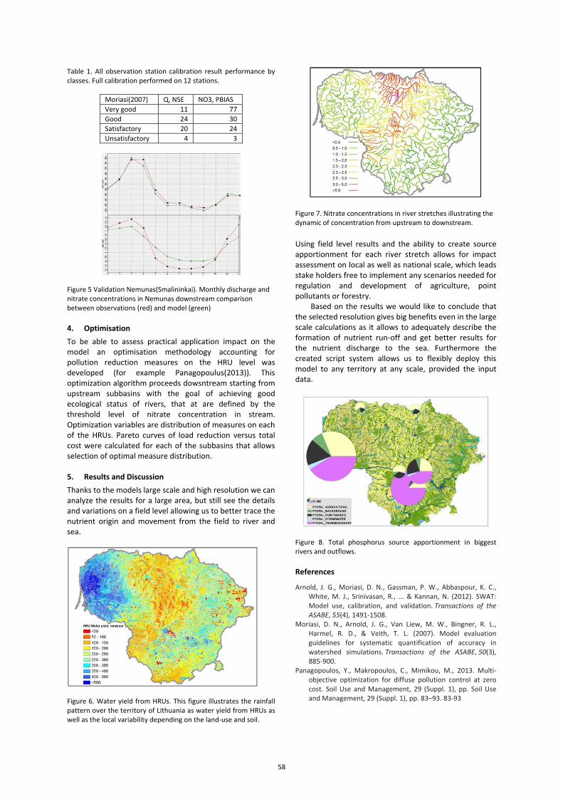
Table 1. All observation station calibration result performance by classes. Full calibration performed on 12 stations.

Moriasi(2007) Q, NSE NO3, PBIASVery good 11 77Good 24 30Satisfactory 20 24Unsatisfactory 4 3

Figure 5 Validation Nemunas(Smalininkai). Monthly discharge and nitrate concentrations in Nemunas downstream comparison between observations (red) and model (green)

4. Optimisation To be able to assess practical application impact on the model an optimisation methodology accounting for pollution reduction measures on the HRU level was developed (for example Panagopoulus(2013)). This optimization algorithm proceeds dowsntream starting from upstream subbasins with the goal of achieving good ecological status of rivers, that at are defined by the threshold level of nitrate concentration in stream. Optimization variables are distribution of measures on each of the HRUs. Pareto curves of load reduction versus total cost were calculated for each of the subbasins that allows selection of optimal measure distribution. 5. Results and Discussion Thanks to the models large scale and high resolution we can analyze the results for a large area, but still see the details and variations on a field level allowing us to better trace the nutrient origin and movement from the field to river and sea.

Figure 6. Water yield from HRUs. This figure illustrates the rainfall pattern over the territory of Lithuania as water yield from HRUs as well as the local variability depending on the land-use and soil.

Figure 7. Nitrate concentrations in river stretches illustrating the dynamic of concentration from upstream to downstream.

Using field level results and the ability to create source apportionment for each river stretch allows for impact assessment on local as well as national scale, which leads stake holders free to implement any scenarios needed for regulation and development of agriculture, point pollutants or forestry.

Based on the results we would like to conclude that the selected resolution gives big benefits even in the large scale calculations as it allows to adequately describe the formation of nutrient run-off and get better results for the nutrient discharge to the sea. Furthermore the created script system allows us to flexibly deploy this model to any territory at any scale, provided the input data.

Figure 8. Total phosphorus source apportionment in biggest rivers and outflows. References

Arnold, J. G., Moriasi, D. N., Gassman, P. W., Abbaspour, K. C., White, M. J., Srinivasan, R., ... & Kannan, N. (2012). SWAT: Model use, calibration, and validation. Transactions of the ASABE, 55(4), 1491-1508.

Moriasi, D. N., Arnold, J. G., Van Liew, M. W., Bingner, R. L., Harmel, R. D., & Veith, T. L. (2007). Model evaluation guidelines for systematic quantification of accuracy in watershed simulations. Transactions of the ASABE, 50(3), 885-900.

Panagopoulos, Y., Makropoulos, C., Mimikou, M., 2013. Multi-objective optimization for diffuse pollution control at zero cost. Soil Use and Management, 29 (Suppl. 1), pp. Soil Use and Management, 29 (Suppl. 1), pp. 83–93. 83-93

58

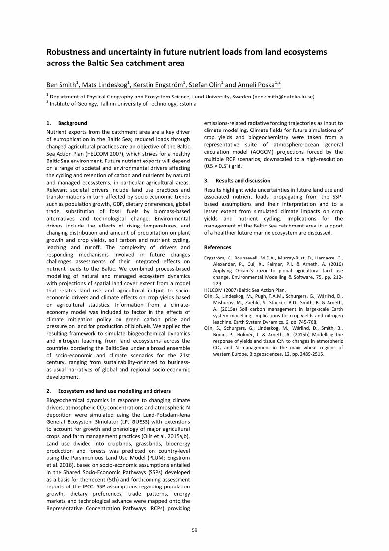
Robustness and uncertainty in future nutrient loads from land ecosystems across the Baltic Sea catchment area

Ben Smith1, Mats Lindeskog1, Kerstin Engström1, Stefan Olin1 and Anneli Poska1,2 1 Department of Physical Geography and Ecosystem Science, Lund University, Sweden (ben.smith@nateko.lu.se) 2 Institute of Geology, Tallinn University of Technology, Estonia

1. Background Nutrient exports from the catchment area are a key driver of eutrophication in the Baltic Sea; reduced loads through changed agricultural practices are an objective of the Baltic Sea Action Plan (HELCOM 2007), which strives for a healthy Baltic Sea environment. Future nutrient exports will depend on a range of societal and environmental drivers affecting the cycling and retention of carbon and nutrients by natural and managed ecosystems, in particular agricultural areas. Relevant societal drivers include land use practices and transformations in turn affected by socio-economic trends such as population growth, GDP, dietary preferences, global trade, substitution of fossil fuels by biomass-based alternatives and technological change. Environmental drivers include the effects of rising temperatures, and changing distribution and amount of precipitation on plant growth and crop yields, soil carbon and nutrient cycling, leaching and runoff. The complexity of drivers and responding mechanisms involved in future changes challenges assessments of their integrated effects on nutrient loads to the Baltic. We combined process-based modelling of natural and managed ecosystem dynamics with projections of spatial land cover extent from a model that relates land use and agricultural output to socio-economic drivers and climate effects on crop yields based on agricultural statistics. Information from a climate-economy model was included to factor in the effects of climate mitigation policy on green carbon price and pressure on land for production of biofuels. We applied the resulting framework to simulate biogeochemical dynamics and nitrogen leaching from land ecosystems across the countries bordering the Baltic Sea under a broad ensemble of socio-economic and climate scenarios for the 21st century, ranging from sustainability-oriented to business-as-usual narratives of global and regional socio-economic development. 2. Ecosystem and land use modelling and drivers Biogeochemical dynamics in response to changing climate drivers, atmospheric CO2 concentrations and atmospheric N deposition were simulated using the Lund-Potsdam-Jena General Ecosystem Simulator (LPJ-GUESS) with extensions to account for growth and phenology of major agricultural crops, and farm management practices (Olin et al. 2015a,b). Land use divided into croplands, grasslands, bioenergy production and forests was predicted on country-level using the Parsimonious Land-Use Model (PLUM; Engström et al. 2016), based on socio-economic assumptions entailed in the Shared Socio-Economic Pathways (SSPs) developed as a basis for the recent (5th) and forthcoming assessment reports of the IPCC. SSP assumptions regarding population growth, dietary preferences, trade patterns, energy markets and technological advance were mapped onto the Representative Concentration Pathways (RCPs) providing

emissions-related radiative forcing trajectories as input to climate modelling. Climate fields for future simulations of crop yields and biogeochemistry were taken from a representative suite of atmosphere-ocean general circulation model (AOGCM) projections forced by the multiple RCP scenarios, downscaled to a high-resolution (0.5 × 0.5°) grid. 3. Results and discussion Results highlight wide uncertainties in future land use and associated nutrient loads, propagating from the SSP-based assumptions and their interpretation and to a lesser extent from simulated climate impacts on crop yields and nutrient cycling. Implications for the management of the Baltic Sea catchment area in support of a healthier future marine ecosystem are discussed. References

Engström, K., Rounsevell, M.D.A., Murray-Rust, D., Hardacre, C., Alexander, P., Cui, X., Palmer, P.I. & Arneth, A. (2016) Applying Occam’s razor to global agricultural land use change. Environmental Modelling & Software, 75, pp. 212-229.

HELCOM (2007) Baltic Sea Action Plan. Olin, S., Lindeskog, M., Pugh, T.A.M., Schurgers, G., Wårlind, D.,

Mishurov, M., Zaehle, S., Stocker, B.D., Smith, B. & Arneth, A. (2015a) Soil carbon management in large-scale Earth system modelling: implications for crop yields and nitrogen leaching, Earth System Dynamics, 6, pp. 745-768.

Olin, S., Schurgers, G., Lindeskog, M., Wårlind, D., Smith, B., Bodin, P., Holmér, J. & Arneth, A. (2015b) Modelling the response of yields and tissue C:N to changes in atmospheric CO2 and N management in the main wheat regions of western Europe, Biogeosciences, 12, pp. 2489-2515.

59

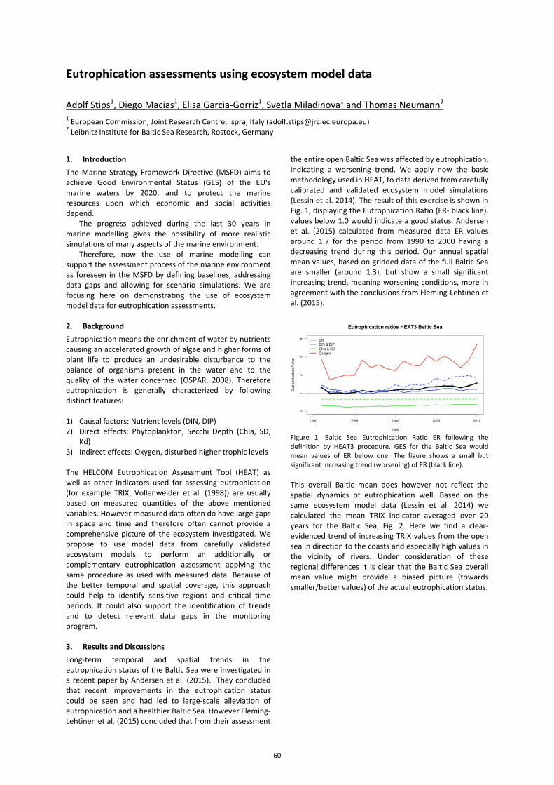
Eutrophication assessments using ecosystem model data

Adolf Stips1, Diego Macias1, Elisa Garcia-Gorriz1, Svetla Miladinova1 and Thomas Neumann2 1 European Commission, Joint Research Centre, Ispra, Italy (adolf.stips@jrc.ec.europa.eu) 2 Leibnitz Institute for Baltic Sea Research, Rostock, Germany

1. Introduction The Marine Strategy Framework Directive (MSFD) aims to achieve Good Environmental Status (GES) of the EU's marine waters by 2020, and to protect the marine resources upon which economic and social activities depend.

The progress achieved during the last 30 years in marine modelling gives the possibility of more realistic simulations of many aspects of the marine environment.

Therefore, now the use of marine modelling can support the assessment process of the marine environment as foreseen in the MSFD by defining baselines, addressing data gaps and allowing for scenario simulations. We are focusing here on demonstrating the use of ecosystem model data for eutrophication assessments. 2. Background Eutrophication means the enrichment of water by nutrients causing an accelerated growth of algae and higher forms of plant life to produce an undesirable disturbance to the balance of organisms present in the water and to the quality of the water concerned (OSPAR, 2008). Therefore eutrophication is generally characterized by following distinct features: 1) Causal factors: Nutrient levels (DIN, DIP) 2) Direct effects: Phytoplankton, Secchi Depth (Chla, SD,

Kd) 3) Indirect effects: Oxygen, disturbed higher trophic levels The HELCOM Eutrophication Assessment Tool (HEAT) as well as other indicators used for assessing eutrophication (for example TRIX, Vollenweider et al. (1998)) are usually based on measured quantities of the above mentioned variables. However measured data often do have large gaps in space and time and therefore often cannot provide a comprehensive picture of the ecosystem investigated. We propose to use model data from carefully validated ecosystem models to perform an additionally or complementary eutrophication assessment applying the same procedure as used with measured data. Because of the better temporal and spatial coverage, this approach could help to identify sensitive regions and critical time periods. It could also support the identification of trends and to detect relevant data gaps in the monitoring program. 3. Results and Discussions Long-term temporal and spatial trends in the eutrophication status of the Baltic Sea were investigated in a recent paper by Andersen et al. (2015). They concluded that recent improvements in the eutrophication status could be seen and had led to large-scale alleviation of eutrophication and a healthier Baltic Sea. However Fleming-Lehtinen et al. (2015) concluded that from their assessment

the entire open Baltic Sea was affected by eutrophication, indicating a worsening trend. We apply now the basic methodology used in HEAT, to data derived from carefully calibrated and validated ecosystem model simulations (Lessin et al. 2014). The result of this exercise is shown in Fig. 1, displaying the Eutrophication Ratio (ER- black line), values below 1.0 would indicate a good status. Andersen et al. (2015) calculated from measured data ER values around 1.7 for the period from 1990 to 2000 having a decreasing trend during this period. Our annual spatial mean values, based on gridded data of the full Baltic Sea are smaller (around 1.3), but show a small significant increasing trend, meaning worsening conditions, more in agreement with the conclusions from Fleming-Lehtinen et al. (2015).

Figure 1. Baltic Sea Eutrophication Ratio ER following the definition by HEAT3 procedure. GES for the Baltic Sea would mean values of ER below one. The figure shows a small but significant increasing trend (worsening) of ER (black line). This overall Baltic mean does however not reflect the spatial dynamics of eutrophication well. Based on the same ecosystem model data (Lessin et al. 2014) we calculated the mean TRIX indicator averaged over 20 years for the Baltic Sea, Fig. 2. Here we find a clear-evidenced trend of increasing TRIX values from the open sea in direction to the coasts and especially high values in the vicinity of rivers. Under consideration of these regional differences it is clear that the Baltic Sea overall mean value might provide a biased picture (towards smaller/better values) of the actual eutrophication status.

60

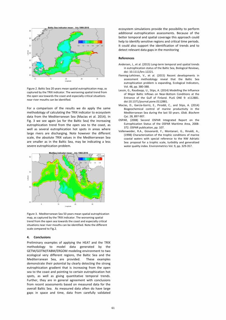
Figure 2. Baltic Sea 20 years mean spatial eutrophication map, as captured by the TRIX indicator. The worsening spatial trend from the open sea towards the coast and especially critical situations near river mouths can be identified.

For a comparison of the results we do apply the same methodology of calculating the TRIX indicator to ecosystem data from the Mediterranean Sea (Macias et al. 2014). In Fig. 3 we see again (as for the Baltic Sea) the increasing eutrophication trend from the open sea to the coast, as well as several eutrophication hot spots in areas where large rivers are discharging. Note however the different scale, the absolute TRIX values in the Mediterranean Sea are smaller as in the Baltic Sea, may be indicating a less severe eutrophication problem.

Figure 3. Mediterranean Sea 50 years mean spatial eutrophication map, as captured by the TRIX indicator. The worsening spatial trend from the open sea towards the coast and especially critical situations near river mouths can be identified. Note the different scale compared to Fig.2.

4. Conclusions Preliminary examples of applying the HEAT and the TRIX methodology to model data generated by the GETM/GOTM/FABM/ERGOM modeling environment to two ecological very different regions, the Baltic Sea and the Mediterranean Sea, are provided. These examples demonstrate their potential by clearly detecting the strong eutrophication gradient that is increasing from the open sea to the coast and pointing to certain eutrophication hot spots, as well as giving quantitative temporal trends. Further, they are in general agreement with conclusions from recent assessments based on measured data for the overall Baltic Sea. As measured data often do have large gaps in space and time, data from carefully validated

ecosystem simulations provide the possibility to perform additional eutrophication assessments. Because of the better temporal and spatial coverage this approach could help to identify sensitive regions and critical time periods. It could also support the identification of trends and to detect relevant data gaps in the monitoring References

Andersen, J., et al. (2015) Long-term temporal and spatial trends in eutrophication status of the Baltic Sea, Biological Reviews, doi: 10.1111/brv.12221.

Fleming-Lehtinen, V., et al. (2015) Recent developments in assessment methodology reveal that the Baltic Sea eutrophication problem is expanding, Ecological Indicators, Vol. 48, pp. 380-388.

Lessin, G., Raudsepp, U., Stips, A. (2014) Modelling the Influence of Major Baltic Inflows on Near-Bottom Conditions at the Entrance of the Gulf of Finland. PLoS ONE 9: e112881. doi:10.1371/journal.pone.0112881.

Macías, D., García-Gorríz, E., Piroddi, C., and Stips, A. (2014) Biogeochemical control of marine productivity in the Mediterranean Sea during the last 50 years. Glob. Biochem Cyc. 28, 897-907.

OSPAR, (2008) Second OSPAR Integrated Report on the Eutrophication Status of the OSPAR Maritime Area, 2008-372. OSPAR publication, pp. 107.

Vollenweider, R.A., Giovanardi, F., Montanari, G., Rinaldi, A., (1998) Characterization of the trophic conditions of marine coastal waters with special reference to the NW Adriatic Sea: proposal for a trophic scale, turbidity and generalized water quality index. Environmetrics Vol. 9, pp. 329-357.

61

Groundwater discharge to the southern Baltic Sea

Beata Szymczycha and Janusz Pempkowiak

Institute of Oceanology Polish Academy of Sciences, Sopot, Poland, beat.sz.@iopan.gda.pl

1. Introduction Groundwater discharge has been recognized as an important exchange pathway between hydrologic reservoirs due to substantial fluxes and its impact on ecology and biogeochemical cycles of the coastal oceans (Burnett et al.,2006). In the Baltic Sea the groundwater fluxes were estimated (Peltonen, 2002), however little is known regarding the concentrations and fluxes of chemical substances via groundwater discharged to the Baltic Sea. There are no studies concerning the importance of geochemical transformations in determining submarine groundwater discharge (SGD)-derived metals, nutrients, dissolved organic carbon and dissolved inorganic carbon fluxes to the Baltic Sea. Therefore in this study we examine the groundwater flow to the Bay of Puck, southern Baltic Sea and the accompanying fluxes of nutrients (NO3

-,NO2-,

NH4+, PO4

3-), dissolved carbon (DIC,DOC) and metals (Cd, Co, Cr, Cu, Hg, Mn, Ni and Zn). Finally we upscale obtained results for the entire Baltic Sea.

2. Materials and Methods Sampling sites were situated along the coast of the southern Baltic Sea: in the Bay of Puck and off the Polish coast at Miedzyzdroje, Kolobrzeg, Wladyslawowo and Leba. Samples of seawater, pore water, groundwater and rivers entering the Bay of Puck (Reda, Zagorska Struga, Plutnica and Gizdepka) were collected in the following periods summer and fall 2009; winter and spring 2010 in the Bay of Puck; summer 2013 and 2014 in all study sites. Bottom sediments of the study sites were diverse: sands of various particle size, silts and organic matter with visible dark chimneys at groundwater discharge zones. Pore water samples were collected by means of groundwater lances. Samples with salinity higher than 0.5 were called seepage water samples, while samples with salinity lower or equal 0.5 were called groundwater samples. Seepage fluxes were measured using seepage meters. The groundwater fraction in the collected seepage water samples was calculated using the end-member method and finally groundwater flux was calculated as a ratio of collected groundwater fraction and the surface area divided by time (Szymczycha et al., 2012). 3. Results and Discussion The differences in seepage water fluxes between different sites during each sampling campaign were significant. The relative standard deviation (RSD) of the obtained average groundwater flux reached up to 70% of the average. Thus, the measured fluxes of seepage water differ both by sampling location and season. One reason for this is the varying contribution of recirculated seawater to the seepage water. Seawater contributions to seepage fluxes ranged between 4 L d -1 m-2 in February 2010 to 44 L d -1 m-2 in November 2010. Consequently, groundwater discharge contributed less than recirculated seawater to seepage water fluxes. The average groundwater discharge turned

out to be well correlated with the average monthly precipitation characteristic of the area. Thus, it can be assumed that groundwater discharge rate in the study area depend strongly on precipitation.

The groundwater discharge phosphate loads to the Bay of Puck were significant relative to loads entering the bay from the atmosphere and rivers, whereas DIN load was less significant relative to these sources. Nutrient loads were projected to the entire Baltic Sea in order to establish overall SGD nutrient contributions within an order of magnitude. The projections indicated significant groundwater discharge contribution to overall phosphate input to the Baltic Sea (Szymczycha et al., 2012).

The projected estimates of dissolved organic carbon and dissolved inorganic carbon fluxes via groundwater discharge were included in the Baltic Sea mass balance of carbon (Szymczycha et al., 2014). The projections demonstrate that SGD sites may transport substantial loads of carbon to the coastal areas. Thus, the Baltic Sea’s status as a source of CO2 to the atmosphere was confirmed. One immediate consequence of this is a change in the biodiversity in seepage-affected areas.

The fluxes of metals via groundwater discharge were significantly higher than these delivered with the rivers runoff. The calculated metals fluxes via groundwater discharge to the entire Baltic Sea equals to 0.3% for Pb, 5% Cd and less than 1‰ for Cu of the total metals load (SGD, rivers, municipalities and industrial plants). Metals fluxes via groundwater discharge to the southern Baltic are a significant source of metals only locally e.g. in the Bay of Puck. Some metals such as dissolved Pb, Zn, Co and Cd present complicate distribution relative to salinity. Dissolved Cr, Cu, Mn, Hg and Ni concentrations differ substantially from those expected in the course of conservative mixing and show non-conservative behavior upon the end-members mixing.

4. Conclusions The obtained results indicate that groundwater discharge can be a significant source of chemical compounds to the Bay of Puck, southern Baltic Sea. Studies on groundwater discharge to other coastal areas of the Baltic Sea should be continued in order to establish more accurate chemical budgets for the Baltic Sea.

62

References Burnett, W.C., Aggarwal, P.K., Aureli, et al., 2006. Quantifying

submarine groundwater discharge in the coastal zone via multiple methods. Science of the Total Environment 367, 498-543.

Peltonen, K., 2002. Direct Groundwater Flow to the Baltic Sea, Nordic Council of Ministers, Temanord, Copenhagen, 78pp.

Szymczycha, B., Vogler, S., Pempkowiak, J., 2012. Nutrients fluxes via Submarine Groundwater Discharge to the Bay of Puck, Southern Baltic. Science of the Total Environment, 438: 86–93.

Szymczycha, B., Maciejewska, A., Winogradow, A., Pempkowiak, J., 2014. Could submarine groundwater discharge be a significant carbon source to the southern Baltic Sea? Oceanologia, 56 (2), 327–347.

63

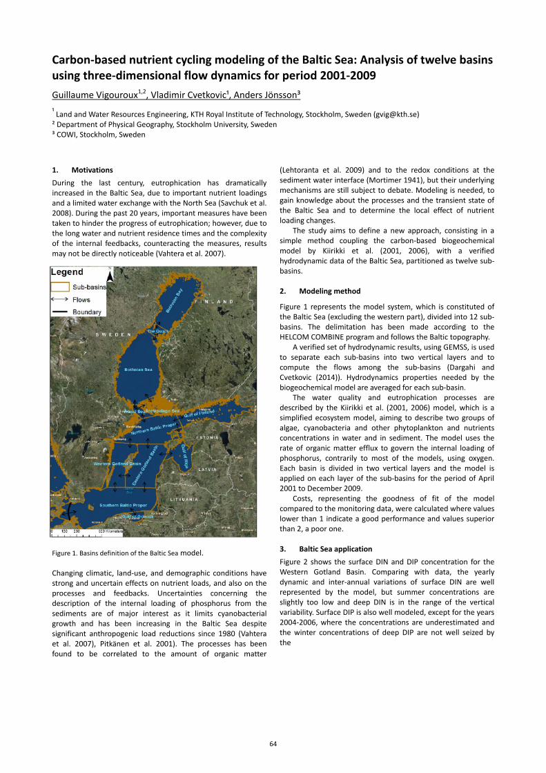
Carbon-based nutrient cycling modeling of the Baltic Sea: Analysis of twelve basins using three-dimensional flow dynamics for period 2001-2009

Guillaume Vigouroux1,2, Vladimir Cvetkovic¹, Anders Jönsson³

¹ Land and Water Resources Engineering, KTH Royal Institute of Technology, Stockholm, Sweden (gvig@kth.se) ² Department of Physical Geography, Stockholm University, Sweden ³ COWI, Stockholm, Sweden 1. Motivations During the last century, eutrophication has dramatically increased in the Baltic Sea, due to important nutrient loadings and a limited water exchange with the North Sea (Savchuk et al. 2008). During the past 20 years, important measures have been taken to hinder the progress of eutrophication; however, due to the long water and nutrient residence times and the complexity of the internal feedbacks, counteracting the measures, results may not be directly noticeable (Vahtera et al. 2007).

Figure 1. Basins definition of the Baltic Sea model.

Changing climatic, land-use, and demographic conditions have strong and uncertain effects on nutrient loads, and also on the processes and feedbacks. Uncertainties concerning the description of the internal loading of phosphorus from the sediments are of major interest as it limits cyanobacterial growth and has been increasing in the Baltic Sea despite significant anthropogenic load reductions since 1980 (Vahtera et al. 2007), Pitkänen et al. 2001). The processes has been found to be correlated to the amount of organic matter

(Lehtoranta et al. 2009) and to the redox conditions at the sediment water interface (Mortimer 1941), but their underlying mechanisms are still subject to debate. Modeling is needed, to gain knowledge about the processes and the transient state of the Baltic Sea and to determine the local effect of nutrient loading changes.

The study aims to define a new approach, consisting in a simple method coupling the carbon-based biogeochemical model by Kiirikki et al. (2001, 2006), with a verified hydrodynamic data of the Baltic Sea, partitioned as twelve sub-basins. 2. Modeling method

Figure 1 represents the model system, which is constituted of the Baltic Sea (excluding the western part), divided into 12 sub-basins. The delimitation has been made according to the HELCOM COMBINE program and follows the Baltic topography.

A verified set of hydrodynamic results, using GEMSS, is used to separate each sub-basins into two vertical layers and to compute the flows among the sub-basins (Dargahi and Cvetkovic (2014)). Hydrodynamics properties needed by the biogeochemical model are averaged for each sub-basin.

The water quality and eutrophication processes are described by the Kiirikki et al. (2001, 2006) model, which is a simplified ecosystem model, aiming to describe two groups of algae, cyanobacteria and other phytoplankton and nutrients concentrations in water and in sediment. The model uses the rate of organic matter efflux to govern the internal loading of phosphorus, contrarily to most of the models, using oxygen. Each basin is divided in two vertical layers and the model is applied on each layer of the sub-basins for the period of April 2001 to December 2009.

Costs, representing the goodness of fit of the model compared to the monitoring data, were calculated where values lower than 1 indicate a good performance and values superior than 2, a poor one. 3. Baltic Sea application Figure 2 shows the surface DIN and DIP concentration for the Western Gotland Basin. Comparing with data, the yearly dynamic and inter-annual variations of surface DIN are well represented by the model, but summer concentrations are slightly too low and deep DIN is in the range of the vertical variability. Surface DIP is also well modeled, except for the years 2004-2006, where the concentrations are underestimated and the winter concentrations of deep DIP are not well seized by the

64

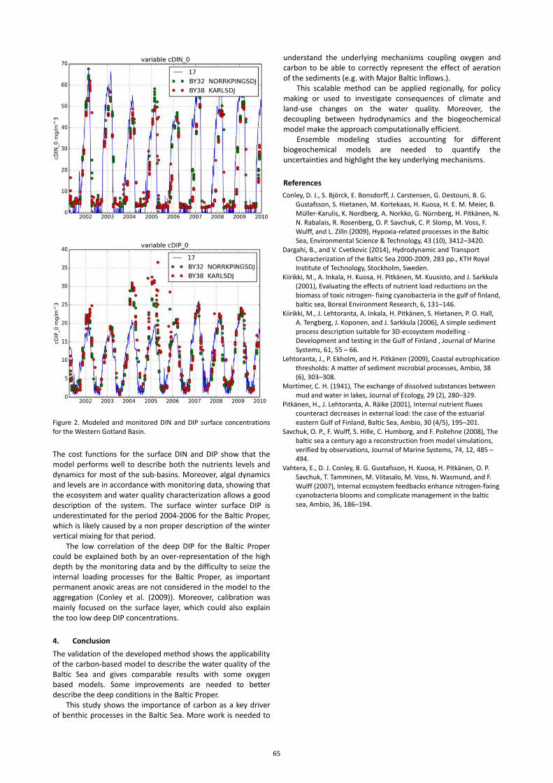
Figure 2. Modeled and monitored DIN and DIP surface concentrations for the Western Gotland Basin. The cost functions for the surface DIN and DIP show that the model performs well to describe both the nutrients levels and dynamics for most of the sub-basins. Moreover, algal dynamics and levels are in accordance with monitoring data, showing that the ecosystem and water quality characterization allows a good description of the system. The surface winter surface DIP is underestimated for the period 2004-2006 for the Baltic Proper, which is likely caused by a non proper description of the winter vertical mixing for that period.

The low correlation of the deep DIP for the Baltic Proper could be explained both by an over-representation of the high depth by the monitoring data and by the difficulty to seize the internal loading processes for the Baltic Proper, as important permanent anoxic areas are not considered in the model to the aggregation (Conley et al. (2009)). Moreover, calibration was mainly focused on the surface layer, which could also explain the too low deep DIP concentrations. 4. Conclusion The validation of the developed method shows the applicability of the carbon-based model to describe the water quality of the Baltic Sea and gives comparable results with some oxygen based models. Some improvements are needed to better describe the deep conditions in the Baltic Proper.

This study shows the importance of carbon as a key driver of benthic processes in the Baltic Sea. More work is needed to

understand the underlying mechanisms coupling oxygen and carbon to be able to correctly represent the effect of aeration of the sediments (e.g. with Major Baltic Inflows.).

This scalable method can be applied regionally, for policy making or used to investigate consequences of climate and land-use changes on the water quality. Moreover, the decoupling between hydrodynamics and the biogeochemical model make the approach computationally efficient.

Ensemble modeling studies accounting for different biogeochemical models are needed to quantify the uncertainties and highlight the key underlying mechanisms. References Conley, D. J., S. Björck, E. Bonsdorff, J. Carstensen, G. Destouni, B. G.

Gustafsson, S. Hietanen, M. Kortekaas, H. Kuosa, H. E. M. Meier, B. Müller-Karulis, K. Nordberg, A. Norkko, G. Nürnberg, H. Pitkänen, N. N. Rabalais, R. Rosenberg, O. P. Savchuk, C. P. Slomp, M. Voss, F. Wulff, and L. Zilln (2009), Hypoxia-related processes in the Baltic Sea, Environmental Science & Technology, 43 (10), 3412–3420.

Dargahi, B., and V. Cvetkovic (2014), Hydrodynamic and Transport Characterization of the Baltic Sea 2000-2009, 283 pp., KTH Royal Institute of Technology, Stockholm, Sweden.

Kiirikki, M., A. Inkala, H. Kuosa, H. Pitkänen, M. Kuusisto, and J. Sarkkula (2001), Evaluating the effects of nutrient load reductions on the biomass of toxic nitrogen- fixing cyanobacteria in the gulf of finland, baltic sea, Boreal Environment Research, 6, 131–146.

Kiirikki, M., J. Lehtoranta, A. Inkala, H. Pitkänen, S. Hietanen, P. O. Hall, A. Tengberg, J. Koponen, and J. Sarkkula (2006), A simple sediment process description suitable for 3D-ecosystem modelling - Development and testing in the Gulf of Finland , Journal of Marine Systems, 61, 55 – 66.

Lehtoranta, J., P. Ekholm, and H. Pitkänen (2009), Coastal eutrophication thresholds: A matter of sediment microbial processes, Ambio, 38 (6), 303–308.

Mortimer, C. H. (1941), The exchange of dissolved substances between mud and water in lakes, Journal of Ecology, 29 (2), 280–329.

Pitkänen, H., J. Lehtoranta, A. Räike (2001), Internal nutrient fluxes counteract decreases in external load: the case of the estuarial eastern Gulf of Finland, Baltic Sea, Ambio, 30 (4/5), 195–201.

Savchuk, O. P., F. Wulff, S. Hille, C. Humborg, and F. Pollehne (2008), The baltic sea a century ago a reconstruction from model simulations, verified by observations, Journal of Marine Systems, 74, 12, 485 – 494.

Vahtera, E., D. J. Conley, B. G. Gustafsson, H. Kuosa, H. Pitkänen, O. P. Savchuk, T. Tamminen, M. Viitasalo, M. Voss, N. Wasmund, and F. Wulff (2007), Internal ecosystem feedbacks enhance nitrogen-fixing cyanobacteria blooms and complicate management in the baltic sea, Ambio, 36, 186–194.

65

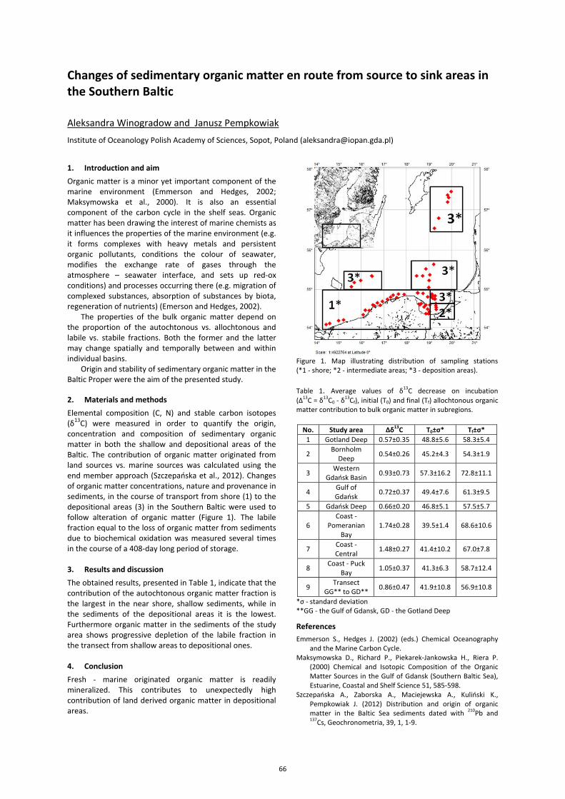
Changes of sedimentary organic matter en route from source to sink areas in the Southern Baltic

Aleksandra Winogradow and Janusz Pempkowiak

Institute of Oceanology Polish Academy of Sciences, Sopot, Poland (aleksandra@iopan.gda.pl)

1. Introduction and aim Organic matter is a minor yet important component of the marine environment (Emmerson and Hedges, 2002; Maksymowska et al., 2000). It is also an essential component of the carbon cycle in the shelf seas. Organic matter has been drawing the interest of marine chemists as it influences the properties of the marine environment (e.g. it forms complexes with heavy metals and persistent organic pollutants, conditions the colour of seawater, modifies the exchange rate of gases through the atmosphere – seawater interface, and sets up red-ox conditions) and processes occurring there (e.g. migration of complexed substances, absorption of substances by biota, regeneration of nutrients) (Emerson and Hedges, 2002).

The properties of the bulk organic matter depend on the proportion of the autochtonous vs. allochtonous and labile vs. stabile fractions. Both the former and the latter may change spatially and temporally between and within individual basins.

Origin and stability of sedimentary organic matter in the Baltic Proper were the aim of the presented study. 2. Materials and methods Elemental composition (C, N) and stable carbon isotopes (δ13C) were measured in order to quantify the origin, concentration and composition of sedimentary organic matter in both the shallow and depositional areas of the Baltic. The contribution of organic matter originated from land sources vs. marine sources was calculated using the end member approach (Szczepańska et al., 2012). Changes of organic matter concentrations, nature and provenance in sediments, in the course of transport from shore (1) to the depositional areas (3) in the Southern Baltic were used to follow alteration of organic matter (Figure 1). The labile fraction equal to the loss of organic matter from sediments due to biochemical oxidation was measured several times in the course of a 408-day long period of storage. 3. Results and discussion The obtained results, presented in Table 1, indicate that the contribution of the autochtonous organic matter fraction is the largest in the near shore, shallow sediments, while in the sediments of the depositional areas it is the lowest. Furthermore organic matter in the sediments of the study area shows progressive depletion of the labile fraction in the transect from shallow areas to depositional ones. 4. Conclusion Fresh - marine originated organic matter is readily mineralized. This contributes to unexpectedly high contribution of land derived organic matter in depositional areas.

Figure 1. Map illustrating distribution of sampling stations (*1 - shore; *2 - intermediate areas; *3 - deposition areas). Table 1. Average values of δ13C decrease on incubation (Δ13C = δ13C0 - δ13Cf), initial (T0) and final (Tf) allochtonous organic matter contribution to bulk organic matter in subregions.

No. Study area Δδ13C T0±σ* Tf±σ*1 Gotland Deep 0.57±0.35 48.8±5.6 58.3±5.4

2 BornholmDeep 0.54±0.26 45.2±4.3 54.3±1.9

3 Western Gdańsk Basin 0.93±0.73 57.3±16.2 72.8±11.1

4 Gulf of Gdańsk 0.72±0.37 49.4±7.6 61.3±9.5

5 Gdańsk Deep 0.66±0.20 46.8±5.1 57.5±5.7

6 Coast -

Pomeranian Bay

1.74±0.28 39.5±1.4 68.6±10.6

7 Coast -Central 1.48±0.27 41.4±10.2 67.0±7.8

8 Coast - Puck Bay 1.05±0.37 41.3±6.3 58.7±12.4

9 Transect GG** to GD** 0.86±0.47 41.9±10.8 56.9±10.8

*σ - standard deviation **GG - the Gulf of Gdansk, GD - the Gotland Deep

References Emmerson S., Hedges J. (2002) (eds.) Chemical Oceanography

and the Marine Carbon Cycle. Maksymowska D., Richard P., Piekarek-Jankowska H., Riera P.

(2000) Chemical and Isotopic Composition of the Organic Matter Sources in the Gulf of Gdansk (Southern Baltic Sea), Estuarine, Coastal and Shelf Science 51, 585-598.

Szczepańska A., Zaborska A., Maciejewska A., Kuliński K., Pempkowiak J. (2012) Distribution and origin of organic matter in the Baltic Sea sediments dated with 210Pb and 137Cs, Geochronometria, 39, 1, 1-9.

66

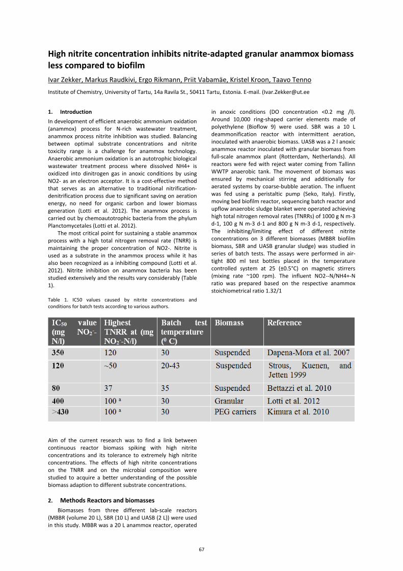
High nitrite concentration inhibits nitrite-adapted granular anammox biomass less compared to biofilm Ivar Zekker, Markus Raudkivi, Ergo Rikmann, Priit Vabamäe, Kristel Kroon, Taavo Tenno

Institute of Chemistry, University of Tartu, 14a Ravila St., 50411 Tartu, Estonia. E-mail. (Ivar.Zekker@ut.ee

1. Introduction In development of efficient anaerobic ammonium oxidation (anammox) process for N-rich wastewater treatment, anammox process nitrite inhibition was studied. Balancing between optimal substrate concentrations and nitrite toxicity range is a challenge for anammox technology. Anaerobic ammonium oxidation is an autotrophic biological wastewater treatment process where dissolved NH4+ is oxidized into dinitrogen gas in anoxic conditions by using NO2- as an electron acceptor. It is a cost-effective method that serves as an alternative to traditional nitrification-denitrification process due to significant saving on aeration energy, no need for organic carbon and lower biomass generation (Lotti et al. 2012). The anammox process is carried out by chemoautotrophic bacteria from the phylum Planctomycetales (Lotti et al. 2012).

The most critical point for sustaining a stable anammox process with a high total nitrogen removal rate (TNRR) is maintaining the proper concentration of NO2-. Nitrite is used as a substrate in the anammox process while it has also been recognized as a inhibiting compound (Lotti et al. 2012). Nitrite inhibition on anammox bacteria has been studied extensively and the results vary considerably (Table 1). Table 1. IC50 values caused by nitrite concentrations and conditions for batch tests according to various authors.

Aim of the current research was to find a link between continuous reactor biomass spiking with high nitrite concentrations and its tolerance to extremely high nitrite concentrations. The effects of high nitrite concentrations on the TNRR and on the microbial composition were studied to acquire a better understanding of the possible biomass adaption to different substrate concentrations. 2. Methods Reactors and biomasses

Biomasses from three different lab-scale reactors (MBBR (volume 20 L), SBR (10 L) and UASB (2 L)) were used in this study. MBBR was a 20 L anammox reactor, operated

in anoxic conditions (DO concentration <0.2 mg /l). Around 10,000 ring-shaped carrier elements made of polyethylene (Bioflow 9) were used. SBR was a 10 L deammonification reactor with intermittent aeration, inoculated with anaerobic biomass. UASB was a 2 l anoxic anammox reactor inoculated with granular biomass from full-scale anammox plant (Rotterdam, Netherlands). All reactors were fed with reject water coming from Tallinn WWTP anaerobic tank. The movement of biomass was ensured by mechanical stirring and additionally for aerated systems by coarse-bubble aeration. The influent was fed using a peristaltic pump (Seko, Italy). Firstly, moving bed biofilm reactor, sequencing batch reactor and upflow anaerobic sludge blanket were operated achieving high total nitrogen removal rates (TNRRs) of 1000 g N m-3 d-1, 100 g N m-3 d-1 and 800 g N m-3 d-1, respectively. The inhibiting/limiting effect of different nitrite concentrations on 3 different biomasses (MBBR biofilm biomass, SBR and UASB granular sludge) was studied in series of batch tests. The assays were performed in air-tight 800 ml test bottles placed in the temperature controlled system at 25 (±0.5°C) on magnetic stirrers (mixing rate ~100 rpm). The influent NO2--N/NH4+-N ratio was prepared based on the respective anammox stoichiometrical ratio 1.32/1

67

3. Results Inhibiting nitrite concentrations causing 50% of biomass

activity decrease were determined at >80, >100 and >225 mg NO2--N L-1 in batch tests performed with moving bed biofilm reactor, sequencing batch reactor and upflow anaerobic sludge blanket reactors biomass, respectively. The highest nitrite concentration used in the batch tests with MBBR biomass was 73 mg NO2--N/l, while the IC50 was calculated to be at 85 mg NO2--N/l (p-value <0.05). The biomass from MBBR achieved the highest TNRR (5 mg N * g-1 TSS * h-1) compared to other systems and the highest TNRR was measured at 40 mg NO2--N/l. Comparing with the other batch tests, the biomass from MBBR achieved the highest TNRR at the lowest nitrite concentration while the IC50 values of MBBR and SBR are comparable (85 and 98 mg NO2--N/l respectively), though the reactor TNRRs differ completely. The highest TNRR was achieved at 83 mg NO2--N/l (p-value <0.05), which was comparable to the respective concentration of the biomass from SBR. The IC50 value for the UASB biomass was calculated to be 240 NO2--N/l (p-value <0.05), which was the highest among three different biomasses used.

In terms of nitrogen converting organisms composition, Planctomycetales clone P4 strains, which were the closest (98 and 99% similarity, respectively) relative to a Candidatus Brocadia fulgida sequences quantities up to 2.5×105 anammox gene copies g-1 TSS were determined by qPCR.

References

Lotti, T., W. R. L. van der Star, R. Kleerebezem, C. Lubello, and M. C. M. van Loosdrecht. 2012. “The Effect of Nitrite Inhibition on the Anammox Process.” Water research 46(8):2559–69. Retrieved April 29, 2014.

Dapena-Mora, A. et al. 2007. “Evaluation of Activity and Inhibition Effects on Anammox Process by Batch Tests Based on the Nitrogen Gas Production.” Enzyme and Microbial Technology 40(4):859–65.

Bettazzi, Elena, Simone Caffaz, Claudia Vannini, and Claudio Lubello. 2010. “Nitrite Inhibition and Intermediates Effects on Anammox Bacteria: A Batch-Scale Experimental Study.” Process Biochemistry 45(4):573–80.

Kimura, Yuya, Kazuichi Isaka, Futaba Kazama, and Tatsuo Sumino. 2010. “Effects of Nitrite Inhibition on Anaerobic Ammonium Oxidation.” Applied Microbiology and Biotechnology 86(1):359–65.

Strous, M., J. G. Kuenen, and M. S. M. Jetten. 1999. “Key Physiology of Anaerobic Ammonium Oxidation.” Applied and Environmental Microbiology 65(7):3248–50.

68

Topic C

Natural hazards

and high impact events

Relationships of cloud-to-ground lightning with circulation weather types over Estonia 2005–2014

Regina Alber1, Piia Post2, Mait Sepp1 1 Institute of Ecology and Earth Sciences, University of Tartu, Tartu, Estonia (regina.alber@ut.ee) 2 Institute of Physics, University of Tartu, Estonia

1. Introduction Thunderstorms are one of the most hazardous natural phenomena in Estonia. They can have economic and health impacts on human. Lightning flashes are one of the detecting ways of the occurrence of thunderstorms. At the same time, they can be very dangerous hitting the ground, objects and living organisms. Thus it is important to study lightning occurrence and its causes. As lightning is associated with atmospheric circulation, moreover, different circulation conditions can conduce them, then this study is looking for answers, which circulation types are more responsive for causing lightning over Estonia. In southern Europe some studies have used for such kind of analyses Lamb´s circulation classification types, for example in Portugal Ramos et al. (2011) or over Iberian Peninsula Tomás et al. (2004). Jenkinson and Collison´s classification (JCT) of circulation weather types, which is used here, is an automatic version of Lamb’s classification. Huth et al. (2015) found that for Baltic Sea region Grosswettertypen (GWT) circulation classification method showed quite good results associated with precipitation and temperature dependence on circulation types. Although, Enno et al. (2014) used JCT for finding relationships between thunderstorms and circulation types.

The aim of the study is to find, which circulation types occur more with lightning and to find possible explanations. To achieve that JCT and GWT circulation methods are used. 2. Data and methods Circulation data analysis of the years 2005-2014 was calculated by cost733 class with data of NCEP/NCAR reanalysis. The middle point of classifications locates in Estonia at 57.5°N and 25°E.

Two domains were used. The smaller locates 10-40 E, 47.5-67.5 N, the bigger one at 0-50 E, 37.5-77.5 N. Two circulation classifications were used for analysis: Jenkinson-Collison´s (JCT) and Grosswettertypen classification (GWT). Both were analysed by 10 and 26 types.

10 weather types were symbolised followingly:

N – northern type NE – northeastern type E – eastern type SE – southeastern type S – southern type SW – southwestern type W – western type NW northwestern type C – cyclonic type AC – anticyclonic type

For describing 26 types the same symbols were used as

marking straight types, but C or A in front of N, NE, E etc. symbolysed cyclonic or anticyclonic type of N, NE, E etc.

Cloud-to-ground lightning data about 2005-2014 was derived from NORDLIS detection network. Lightning data was summed after every 6 hours.

Both cloud-to-ground lightning data from 2005-2014 and circulation data were derived four time per day. Circulation data were about 0, 6, 12 and 18 UTC. Thunderstorm data was summed so that circulation data times were in the middle of six-hour period.

The proportion of cloud-to-ground lightning strokes with 10 and 26 types of JCT and with larger and smaller area of GWT methods was found seasonally and monthly. Additionally was found, which circulation types had more intensive lightning with over 1000 strokes per 6 hour period. 3. Results The most common circulation types in Estonia are W, SW and AC. From May to August type C was also frequent. The most lightning in Estonia occurred from May to October (99.7%), whereas from May to August 94.5%.

Seasonally, some differences of the occurrence of circulation types that influenced Estonia during lightning were found. Firstly, 10 types of JCT and small and large GWT circulation classification methods are analysed.

In spring, the most lightning-prone types were C (10-22%), W (10-17%), SW (13-15%), SE (12-17%). E was common with GWTs, but not with JCT. The least lightning occurred with N but also few with AC.

In summer, lightning is the most common with types W (16-24%) and C (12-17%). Type NW was quite common according to GWT methods. Lightning was rarer with type N but also NE according to JCT and smaller GWT or S according to GWTs.

In autumn, the most lightning-prone circulation types were W (21-37%) and SW (24-30%). According to both GWTs NW was also common, but C with JCT and larger GWT method. The least lightning was with N, NE, E, SE and AC, but with GWTs also S. In winter, lightning was rare and occurred mostly with types SW and W.

Secondly, 26 types of JCT and small and large GWT circulation classification methods are analysed. In summer, the most common type having lightning was C (12-25%), other common types were AC with large GWT and JCT , SW with JCT, CW with small GWT. In spring, lightning was the most common with C (10-22%), but also CSE, and CE with GWTs. In autumn more lightning-prone types were W (10-13%), C (8-17%), SW, CSW, but AW and CW with GWTs. In winter lightning occurred more with types SW and CSW.

Monthly analysis of small and large GWT and JCT circulation methods with 10 types showed that in December and January lightning occurred more with types W and SW; in February with SW, SE, S and AC; in March with NW, but also with C SW or W; in April W, E

69

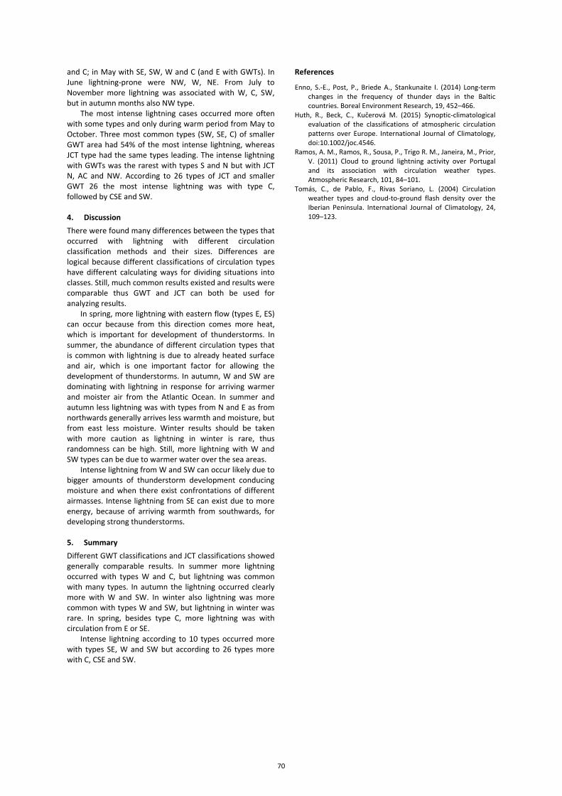
and C; in May with SE, SW, W and C (and E with GWTs). In June lightning-prone were NW, W, NE. From July to November more lightning was associated with W, C, SW, but in autumn months also NW type.

The most intense lightning cases occurred more often with some types and only during warm period from May to October. Three most common types (SW, SE, C) of smaller GWT area had 54% of the most intense lightning, whereas JCT type had the same types leading. The intense lightning with GWTs was the rarest with types S and N but with JCT N, AC and NW. According to 26 types of JCT and smaller GWT 26 the most intense lightning was with type C, followed by CSE and SW.

4. Discussion There were found many differences between the types that occurred with lightning with different circulation classification methods and their sizes. Differences are logical because different classifications of circulation types have different calculating ways for dividing situations into classes. Still, much common results existed and results were comparable thus GWT and JCT can both be used for analyzing results.

In spring, more lightning with eastern flow (types E, ES) can occur because from this direction comes more heat, which is important for development of thunderstorms. In summer, the abundance of different circulation types that is common with lightning is due to already heated surface and air, which is one important factor for allowing the development of thunderstorms. In autumn, W and SW are dominating with lightning in response for arriving warmer and moister air from the Atlantic Ocean. In summer and autumn less lightning was with types from N and E as from northwards generally arrives less warmth and moisture, but from east less moisture. Winter results should be taken with more caution as lightning in winter is rare, thus randomness can be high. Still, more lightning with W and SW types can be due to warmer water over the sea areas.

Intense lightning from W and SW can occur likely due to bigger amounts of thunderstorm development conducing moisture and when there exist confrontations of different airmasses. Intense lightning from SE can exist due to more energy, because of arriving warmth from southwards, for developing strong thunderstorms. 5. Summary Different GWT classifications and JCT classifications showed generally comparable results. In summer more lightning occurred with types W and C, but lightning was common with many types. In autumn the lightning occurred clearly more with W and SW. In winter also lightning was more common with types W and SW, but lightning in winter was rare. In spring, besides type C, more lightning was with circulation from E or SE.

Intense lightning according to 10 types occurred more with types SE, W and SW but according to 26 types more with C, CSE and SW.

References

Enno, S.-E., Post, P., Briede A., Stankunaite I. (2014) Long-term changes in the frequency of thunder days in the Baltic countries. Boreal Environment Research, 19, 452–466.

Huth, R., Beck, C., Kučerová M. (2015) Synoptic-climatological evaluation of the classifications of atmospheric circulation patterns over Europe. International Journal of Climatology, doi:10.1002/joc.4546.

Ramos, A. M., Ramos, R., Sousa, P., Trigo R. M., Janeira, M., Prior, V. (2011) Cloud to ground lightning activity over Portugal and its association with circulation weather types. Atmospheric Research, 101, 84–101.

Tomás, C., de Pablo, F., Rivas Soriano, L. (2004) Circulation weather types and cloud-to-ground flash density over the Iberian Peninsula. International Journal of Climatology, 24, 109–123.

70

HOAPS water vapour characteristic during storms and heavy precipitation events over SE Baltic Sea region

Agnė Djačenko1,2, Gintautas Stankūnavičius1 1 Department of Hydrology and climatology, Vilnius University, Vilnius, Lithuania (agne.djacenko@gf.vu.lt) 2 Lithuanian Hydrometeorological Service under the Ministry of Environment of the Republic of Lithuania

1. Introduction An intensive westerly flow over Southern Scandinavia and the Baltic Sea favors for the heavy gale winds and storm surges in the Lithuanian coastal areas. Storms usually follow behind the low pressure centers passing the Baltic Sea. Strong westerly gales and storm surges are main factors impacting intensive coastal erosion because of national coastal line is almost perpendicular to the predominant westerly wind direction during winter storms. Erosion is affected either by sea level rise during surges or surface waves action on beaches and foredunes or by both processes simultaneously. Huge amount of sand is washed out from the beaches and dunes during every heavy storm. The studies of the developing strong wind speed fields are very important for effective coastal management, rescue services, environmental protection agencies and insurance companies. Intensive precipitation events as well as the storm winds are the counterparts of severe weather in the coastal area of Lithuania. Heavy rains and snowfalls here could be associated either with active atmospheric fronts and developing lows or with mesoscale convective complexes.

The main scope of the study is an assessment of HOAPS data for analysis of strong winds and heavy precipitation patterns over the southern and southeastern Baltic Sea. 2. Data and methods For this analysis HOAPS (Hamburg Ocean Atmosphere Parameters and Fluxes from Satellite Data) database was used. It was formed in 2012. HOAPS data with the dataset range of 1987- 2008 period as daily and sub-daily means (6-hourly mean) of surface wind speed (SWS), vertically integrated water vapour (HTW) were used for comparison with the ground based meteorological data taken from Klaipėda, Nida, Šilutė and Palanga weather stations of Lithuanian Hydrometeorological Service. Anomalies as severe weather parameters were detected for surface wind speed (≥17.2 m/s) and heavy precipitation (≥50 mm/12h rain and ≥20 mm/12 h snow. Climate Data Operators (CDO) were used for extraction and manipulating of HOAPS data. The operators contain simple statistical and arithmetic functions, data selection and filtering tools as well as spatial interpolation. HOAPS data covers only Open Ocean/ sea areas, therefore only three available regions are used within the Baltic Sea (Fig. 1). The coordinates of the three regions are: a) first region: 61.25°—61.75°N 18.75°—19.75°E; b) second region: 58.75°—59.25°N, 20.25°—21.25°E; c) and the third region: 55.75°—56.75°N, 17.25°—19.75°E.

Figure 1. Available HOAPS data areas for the Baltic Sea region. CDO was used to calculate maximum wind speed on every coordination point. A sliding correlation was calculated (every ten days) between the southern Baltic region using HOAPS and Klaipėda weather station data.

Recorded maximum wind speed during the analyzed timespan was categorized using the Beaufort scale into gales (17.2-20.7 m/s), strong gales (20.8-24.4 m/s) and storms (24.5-28.4 m/s). Then the direction of the maximal wind speed was derived from zonal and meridional wind components of the lowest level (1000 hPa level).

Whereas the water vapour content depends on the type of air masses and has directly impact the formation of precipitation it was decided to use this parameter for further analysis. Vertically integrated water vapour (HTW) data from HOAPS dataset were used to identify the HTW anomalies during severe weather events derived from its climatology.

3. Wind characteristics An analysis of correlation (sliding correlations for 40 time points) between daily averages of Klaipėda weather station and HOAPS data showed dominant statistically significant correlations. The correlation coefficients are mostly positive and on average equal 0.6 for the whole timeframe.

Strong wind episodes were derived (Fig. 2) using wind speed threshold of 17.2 m/s as 6-hourly wind speed average. This wind speed threshold was defined by assessing the wind impact on storm surge height and coastal erosion. Most strong winds were recorded from the west and southwestern. Using HOAPS maximum wind speed data monthly mean frequency of storms was estimated.

71

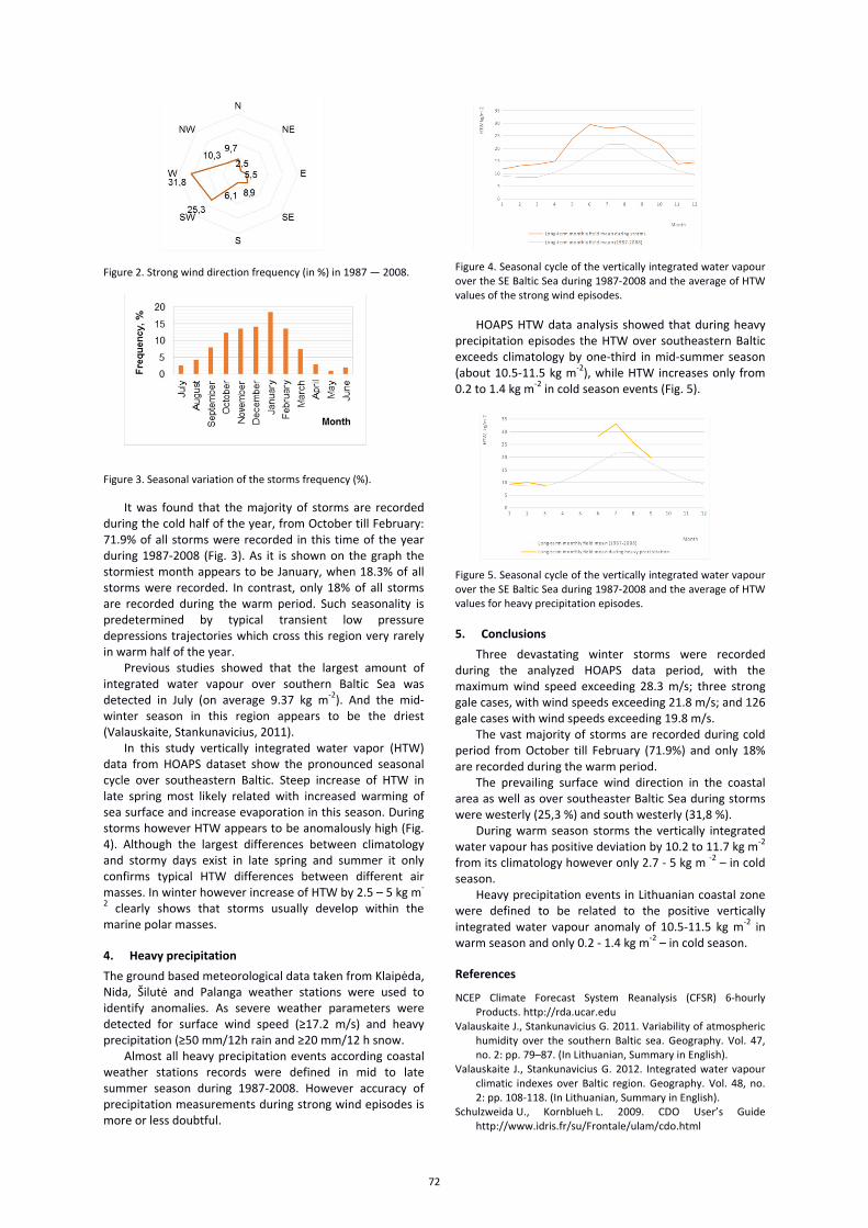
Figure 2. Strong wind direction frequency (in %) in 1987 — 2008.

Figure 3. Seasonal variation of the storms frequency (%).

It was found that the majority of storms are recorded during the cold half of the year, from October till February: 71.9% of all storms were recorded in this time of the year during 1987-2008 (Fig. 3). As it is shown on the graph the stormiest month appears to be January, when 18.3% of all storms were recorded. In contrast, only 18% of all storms are recorded during the warm period. Such seasonality is predetermined by typical transient low pressure depressions trajectories which cross this region very rarely in warm half of the year.

Previous studies showed that the largest amount of integrated water vapour over southern Baltic Sea was detected in July (on average 9.37 kg m-2). And the mid-winter season in this region appears to be the driest (Valauskaite, Stankunavicius, 2011).

In this study vertically integrated water vapor (HTW) data from HOAPS dataset show the pronounced seasonal cycle over southeastern Baltic. Steep increase of HTW in late spring most likely related with increased warming of sea surface and increase evaporation in this season. During storms however HTW appears to be anomalously high (Fig. 4). Although the largest differences between climatology and stormy days exist in late spring and summer it only confirms typical HTW differences between different air masses. In winter however increase of HTW by 2.5 – 5 kg m-

2 clearly shows that storms usually develop within the marine polar masses. 4. Heavy precipitation The ground based meteorological data taken from Klaipėda, Nida, Šilutė and Palanga weather stations were used to identify anomalies. As severe weather parameters were detected for surface wind speed (≥17.2 m/s) and heavy precipitation (≥50 mm/12h rain and ≥20 mm/12 h snow.

Almost all heavy precipitation events according coastal weather stations records were defined in mid to late summer season during 1987-2008. However accuracy of precipitation measurements during strong wind episodes is more or less doubtful.

Figure 4. Seasonal cycle of the vertically integrated water vapour over the SE Baltic Sea during 1987-2008 and the average of HTW values of the strong wind episodes.

HOAPS HTW data analysis showed that during heavy precipitation episodes the HTW over southeastern Baltic exceeds climatology by one-third in mid-summer season (about 10.5-11.5 kg m-2), while HTW increases only from 0.2 to 1.4 kg m-2 in cold season events (Fig. 5).

Figure 5. Seasonal cycle of the vertically integrated water vapour over the SE Baltic Sea during 1987-2008 and the average of HTW values for heavy precipitation episodes. 5. Conclusions

Three devastating winter storms were recorded during the analyzed HOAPS data period, with the maximum wind speed exceeding 28.3 m/s; three strong gale cases, with wind speeds exceeding 21.8 m/s; and 126 gale cases with wind speeds exceeding 19.8 m/s.

The vast majority of storms are recorded during cold period from October till February (71.9%) and only 18% are recorded during the warm period.

The prevailing surface wind direction in the coastal area as well as over southeaster Baltic Sea during storms were westerly (25,3 %) and south westerly (31,8 %).

During warm season storms the vertically integrated water vapour has positive deviation by 10.2 to 11.7 kg m-2 from its climatology however only 2.7 - 5 kg m -2 – in cold season.

Heavy precipitation events in Lithuanian coastal zone were defined to be related to the positive vertically integrated water vapour anomaly of 10.5-11.5 kg m-2 in warm season and only 0.2 - 1.4 kg m-2 – in cold season. References

NCEP Climate Forecast System Reanalysis (CFSR) 6-hourly Products. http://rda.ucar.edu

Valauskaite J., Stankunavicius G. 2011. Variability of atmospheric humidity over the southern Baltic sea. Geography. Vol. 47, no. 2: pp. 79–87. (In Lithuanian, Summary in English).

Valauskaite J., Stankunavicius G. 2012. Integrated water vapour climatic indexes over Baltic region. Geography. Vol. 48, no. 2: pp. 108-118. (In Lithuanian, Summary in English).

Schulzweida U., Kornblueh L. 2009. CDO User’s Guide http://www.idris.fr/su/Frontale/ulam/cdo.html

72

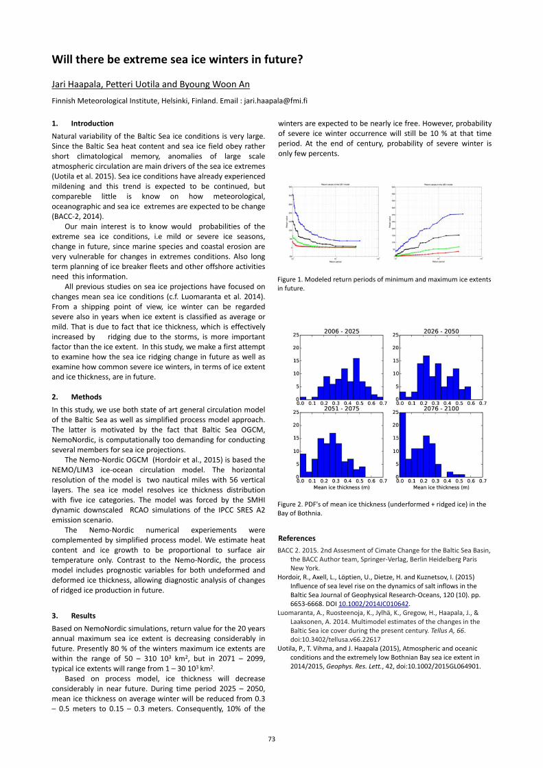
Will there be extreme sea ice winters in future?

Jari Haapala, Petteri Uotila and Byoung Woon An

Finnish Meteorological Institute, Helsinki, Finland. Email : jari.haapala@fmi.fi 1. Introduction Natural variability of the Baltic Sea ice conditions is very large. Since the Baltic Sea heat content and sea ice field obey rather short climatological memory, anomalies of large scale atmospheric circulation are main drivers of the sea ice extremes (Uotila et al. 2015). Sea ice conditions have already experienced mildening and this trend is expected to be continued, but compareble little is know on how meteorological, oceanographic and sea ice extremes are expected to be change (BACC-2, 2014).

Our main interest is to know would probabilities of the extreme sea ice conditions, i.e mild or severe ice seasons, change in future, since marine species and coastal erosion are very vulnerable for changes in extremes conditions. Also long term planning of ice breaker fleets and other offshore activities need this information.

All previous studies on sea ice projections have focused on changes mean sea ice conditions (c.f. Luomaranta et al. 2014). From a shipping point of view, ice winter can be regarded severe also in years when ice extent is classified as average or mild. That is due to fact that ice thickness, which is effectively increased by ridging due to the storms, is more important factor than the ice extent. In this study, we make a first attempt to examine how the sea ice ridging change in future as well as examine how common severe ice winters, in terms of ice extent and ice thickness, are in future. 2. Methods In this study, we use both state of art general circulation model of the Baltic Sea as well as simplified process model approach. The latter is motivated by the fact that Baltic Sea OGCM, NemoNordic, is computationally too demanding for conducting several members for sea ice projections.

The Nemo-Nordic OGCM (Hordoir et al., 2015) is based the NEMO/LIM3 ice-ocean circulation model. The horizontal resolution of the model is two nautical miles with 56 vertical layers. The sea ice model resolves ice thickness distribution with five ice categories. The model was forced by the SMHI dynamic downscaled RCAO simulations of the IPCC SRES A2 emission scenario.

The Nemo-Nordic numerical experiements were complemented by simplified process model. We estimate heat content and ice growth to be proportional to surface air temperature only. Contrast to the Nemo-Nordic, the process model includes prognostic variables for both undeformed and deformed ice thickness, allowing diagnostic analysis of changes of ridged ice production in future.

3. Results Based on NemoNordic simulations, return value for the 20 years annual maximum sea ice extent is decreasing considerably in future. Presently 80 % of the winters maximum ice extents are within the range of 50 – 310 103 km2, but in 2071 – 2099, typical ice extents will range from 1 – 30 103 km2.

Based on process model, ice thickness will decrease considerably in near future. During time period 2025 – 2050, mean ice thickness on average winter will be reduced from 0.3 – 0.5 meters to 0.15 – 0.3 meters. Consequently, 10% of the

winters are expected to be nearly ice free. However, probability of severe ice winter occurrence will still be 10 % at that time period. At the end of century, probability of severe winter is only few percents.

Figure 1. Modeled return periods of minimum and maximum ice extents in future.

Figure 2. PDF's of mean ice thickness (underformed + ridged ice) in the Bay of Bothnia.

References BACC 2. 2015. 2nd Assesment of Cimate Change for the Baltic Sea Basin,

the BACC Author team, Springer-Verlag, Berlin Heidelberg Paris New York.

Hordoir, R., Axell, L., Löptien, U., Dietze, H. and Kuznetsov, I. (2015) Influence of sea level rise on the dynamics of salt inflows in the Baltic Sea Journal of Geophysical Research-Oceans, 120 (10). pp. 6653-6668. DOI 10.1002/2014JC010642.

Luomaranta, A., Ruosteenoja, K., Jylhä, K., Gregow, H., Haapala, J., & Laaksonen, A. 2014. Multimodel estimates of the changes in the Baltic Sea ice cover during the present century. Tellus A, 66. doi:10.3402/tellusa.v66.22617

Uotila, P., T. Vihma, and J. Haapala (2015), Atmospheric and oceanic conditions and the extremely low Bothnian Bay sea ice extent in 2014/2015, Geophys. Res. Lett., 42, doi:10.1002/2015GL064901.

73

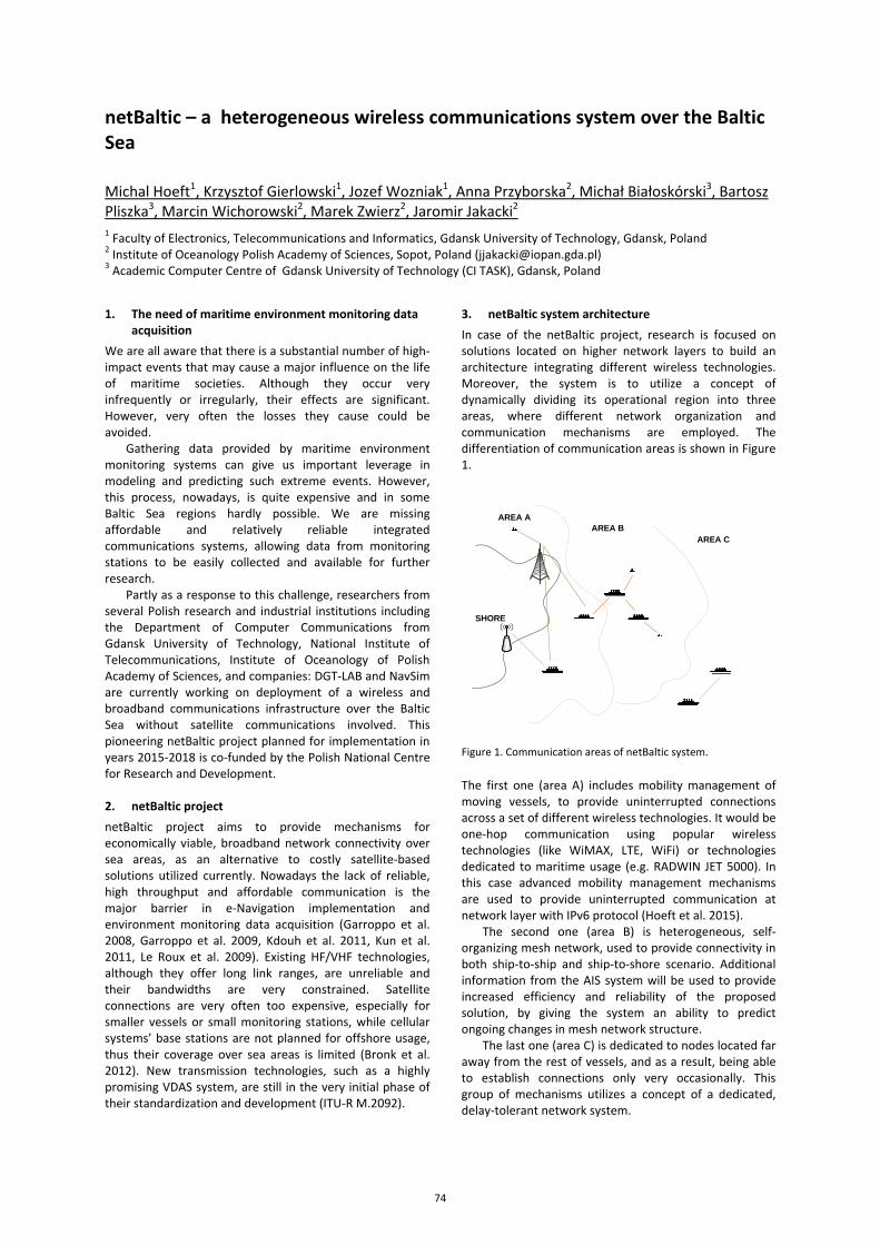
netBaltic – a heterogeneous wireless communications system over the Baltic Sea

Michal Hoeft1, Krzysztof Gierlowski1, Jozef Wozniak1, Anna Przyborska2, Michał Białoskórski3, Bartosz Pliszka3, Marcin Wichorowski2, Marek Zwierz2, Jaromir Jakacki2

1 Faculty of Electronics, Telecommunications and Informatics, Gdansk University of Technology, Gdansk, Poland 2 Institute of Oceanology Polish Academy of Sciences, Sopot, Poland (jjakacki@iopan.gda.pl) 3 Academic Computer Centre of Gdansk University of Technology (CI TASK), Gdansk, Poland

1. The need of maritime environment monitoring data acquisition

We are all aware that there is a substantial number of high-impact events that may cause a major influence on the life of maritime societies. Although they occur very infrequently or irregularly, their effects are significant. However, very often the losses they cause could be avoided.

Gathering data provided by maritime environment monitoring systems can give us important leverage in modeling and predicting such extreme events. However, this process, nowadays, is quite expensive and in some Baltic Sea regions hardly possible. We are missing affordable and relatively reliable integrated communications systems, allowing data from monitoring stations to be easily collected and available for further research.

Partly as a response to this challenge, researchers from several Polish research and industrial institutions including the Department of Computer Communications from Gdansk University of Technology, National Institute of Telecommunications, Institute of Oceanology of Polish Academy of Sciences, and companies: DGT-LAB and NavSim are currently working on deployment of a wireless and broadband communications infrastructure over the Baltic Sea without satellite communications involved. This pioneering netBaltic project planned for implementation in years 2015-2018 is co-funded by the Polish National Centre for Research and Development.

2. netBaltic project netBaltic project aims to provide mechanisms for economically viable, broadband network connectivity over sea areas, as an alternative to costly satellite-based solutions utilized currently. Nowadays the lack of reliable, high throughput and affordable communication is the major barrier in e-Navigation implementation and environment monitoring data acquisition (Garroppo et al. 2008, Garroppo et al. 2009, Kdouh et al. 2011, Kun et al. 2011, Le Roux et al. 2009). Existing HF/VHF technologies, although they offer long link ranges, are unreliable and their bandwidths are very constrained. Satellite connections are very often too expensive, especially for smaller vessels or small monitoring stations, while cellular systems’ base stations are not planned for offshore usage, thus their coverage over sea areas is limited (Bronk et al. 2012). New transmission technologies, such as a highly promising VDAS system, are still in the very initial phase of their standardization and development (ITU-R M.2092).

3. netBaltic system architecture In case of the netBaltic project, research is focused on solutions located on higher network layers to build an architecture integrating different wireless technologies. Moreover, the system is to utilize a concept of dynamically dividing its operational region into three areas, where different network organization and communication mechanisms are employed. The differentiation of communication areas is shown in Figure 1.

SHORE

AREA AAREA B

AREA C

Figure 1. Communication areas of netBaltic system.

The first one (area A) includes mobility management of moving vessels, to provide uninterrupted connections across a set of different wireless technologies. It would be one-hop communication using popular wireless technologies (like WiMAX, LTE, WiFi) or technologies dedicated to maritime usage (e.g. RADWIN JET 5000). In this case advanced mobility management mechanisms are used to provide uninterrupted communication at network layer with IPv6 protocol (Hoeft et al. 2015).

The second one (area B) is heterogeneous, self-organizing mesh network, used to provide connectivity in both ship-to-ship and ship-to-shore scenario. Additional information from the AIS system will be used to provide increased efficiency and reliability of the proposed solution, by giving the system an ability to predict ongoing changes in mesh network structure.

The last one (area C) is dedicated to nodes located far away from the rest of vessels, and as a result, being able to establish connections only very occasionally. This group of mechanisms utilizes a concept of a dedicated, delay-tolerant network system.

74

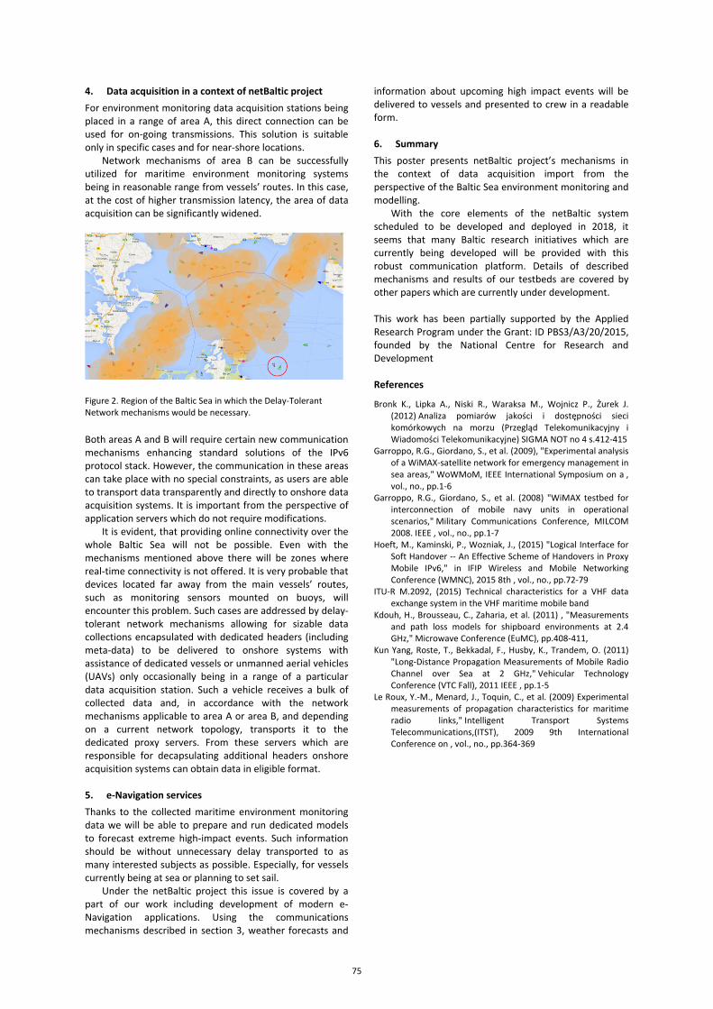
4. Data acquisition in a context of netBaltic project For environment monitoring data acquisition stations being placed in a range of area A, this direct connection can be used for on-going transmissions. This solution is suitable only in specific cases and for near-shore locations.

Network mechanisms of area B can be successfully utilized for maritime environment monitoring systems being in reasonable range from vessels’ routes. In this case, at the cost of higher transmission latency, the area of data acquisition can be significantly widened.

Figure 2. Region of the Baltic Sea in which the Delay-Tolerant Network mechanisms would be necessary.

Both areas A and B will require certain new communication mechanisms enhancing standard solutions of the IPv6 protocol stack. However, the communication in these areas can take place with no special constraints, as users are able to transport data transparently and directly to onshore data acquisition systems. It is important from the perspective of application servers which do not require modifications.

It is evident, that providing online connectivity over the whole Baltic Sea will not be possible. Even with the mechanisms mentioned above there will be zones where real-time connectivity is not offered. It is very probable that devices located far away from the main vessels’ routes, such as monitoring sensors mounted on buoys, will encounter this problem. Such cases are addressed by delay-tolerant network mechanisms allowing for sizable data collections encapsulated with dedicated headers (including meta-data) to be delivered to onshore systems with assistance of dedicated vessels or unmanned aerial vehicles (UAVs) only occasionally being in a range of a particular data acquisition station. Such a vehicle receives a bulk of collected data and, in accordance with the network mechanisms applicable to area A or area B, and depending on a current network topology, transports it to the dedicated proxy servers. From these servers which are responsible for decapsulating additional headers onshore acquisition systems can obtain data in eligible format. 5. e-Navigation services Thanks to the collected maritime environment monitoring data we will be able to prepare and run dedicated models to forecast extreme high-impact events. Such information should be without unnecessary delay transported to as many interested subjects as possible. Especially, for vessels currently being at sea or planning to set sail.

Under the netBaltic project this issue is covered by a part of our work including development of modern e-Navigation applications. Using the communications mechanisms described in section 3, weather forecasts and

information about upcoming high impact events will be delivered to vessels and presented to crew in a readable form. 6. Summary This poster presents netBaltic project’s mechanisms in the context of data acquisition import from the perspective of the Baltic Sea environment monitoring and modelling.

With the core elements of the netBaltic system scheduled to be developed and deployed in 2018, it seems that many Baltic research initiatives which are currently being developed will be provided with this robust communication platform. Details of described mechanisms and results of our testbeds are covered by other papers which are currently under development. This work has been partially supported by the Applied Research Program under the Grant: ID PBS3/A3/20/2015, founded by the National Centre for Research and Development

References

Bronk K., Lipka A., Niski R., Waraksa M., Wojnicz P., Żurek J. (2012) Analiza pomiarów jakości i dostępności sieci komórkowych na morzu (Przegląd Telekomunikacyjny i Wiadomości Telekomunikacyjne) SIGMA NOT no 4 s.412-415

Garroppo, R.G., Giordano, S., et al. (2009), "Experimental analysis of a WiMAX-satellite network for emergency management in sea areas," WoWMoM, IEEE International Symposium on a , vol., no., pp.1-6

Garroppo, R.G., Giordano, S., et al. (2008) "WiMAX testbed for interconnection of mobile navy units in operational scenarios," Military Communications Conference, MILCOM 2008. IEEE , vol., no., pp.1-7

Hoeft, M., Kaminski, P., Wozniak, J., (2015) "Logical Interface for Soft Handover -- An Effective Scheme of Handovers in Proxy Mobile IPv6," in IFIP Wireless and Mobile Networking Conference (WMNC), 2015 8th , vol., no., pp.72-79

ITU-R M.2092, (2015) Technical characteristics for a VHF data exchange system in the VHF maritime mobile band

Kdouh, H., Brousseau, C., Zaharia, et al. (2011) , "Measurements and path loss models for shipboard environments at 2.4 GHz," Microwave Conference (EuMC), pp.408-411,

Kun Yang, Roste, T., Bekkadal, F., Husby, K., Trandem, O. (2011) "Long-Distance Propagation Measurements of Mobile Radio Channel over Sea at 2 GHz," Vehicular Technology Conference (VTC Fall), 2011 IEEE , pp.1-5

Le Roux, Y.-M., Menard, J., Toquin, C., et al. (2009) Experimental measurements of propagation characteristics for maritime radio links," Intelligent Transport Systems Telecommunications,(ITST), 2009 9th International Conference on , vol., no., pp.364-369

75

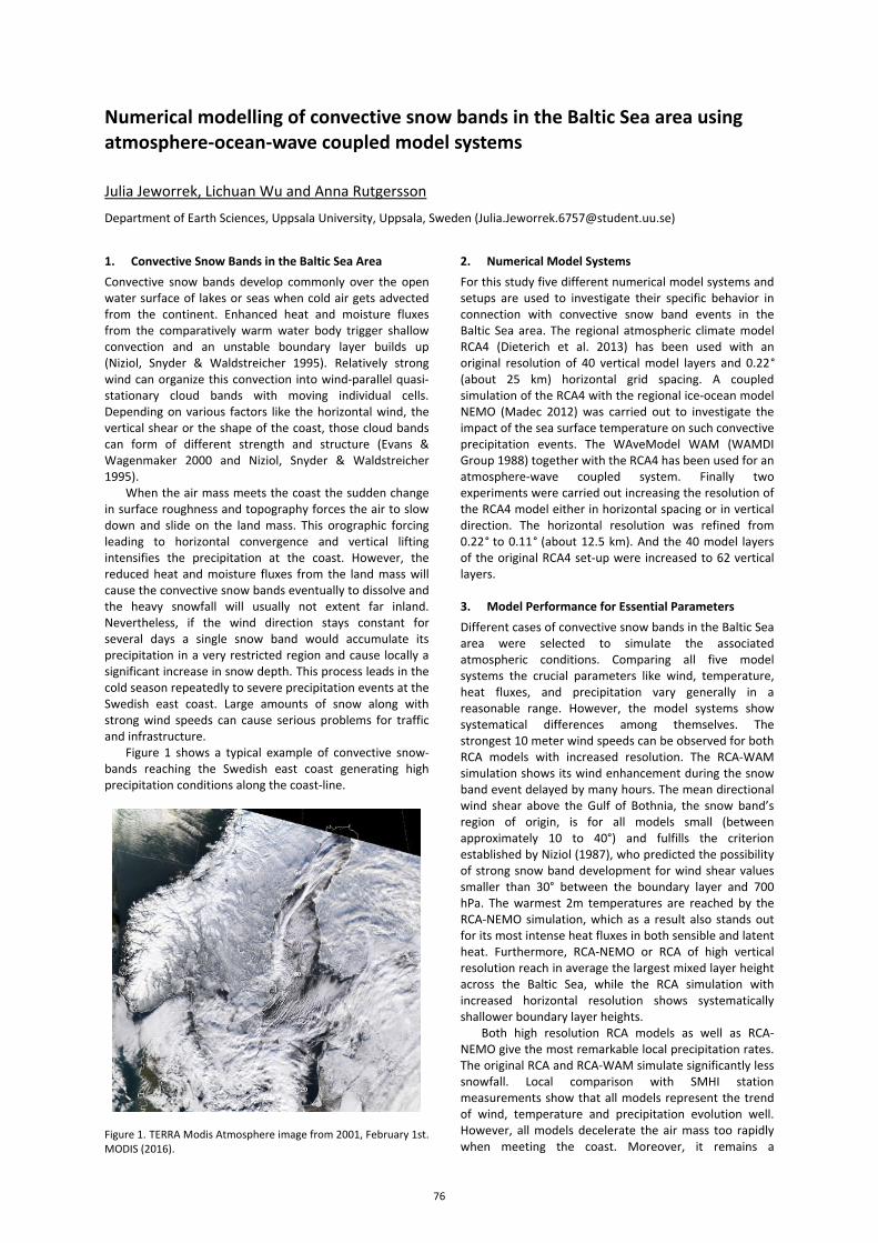
Numerical modelling of convective snow bands in the Baltic Sea area using atmosphere-ocean-wave coupled model systems

Julia Jeworrek, Lichuan Wu and Anna Rutgersson

Department of Earth Sciences, Uppsala University, Uppsala, Sweden (Julia.Jeworrek.6757@student.uu.se)

1. Convective Snow Bands in the Baltic Sea Area Convective snow bands develop commonly over the open water surface of lakes or seas when cold air gets advected from the continent. Enhanced heat and moisture fluxes from the comparatively warm water body trigger shallow convection and an unstable boundary layer builds up (Niziol, Snyder & Waldstreicher 1995). Relatively strong wind can organize this convection into wind-parallel quasi-stationary cloud bands with moving individual cells. Depending on various factors like the horizontal wind, the vertical shear or the shape of the coast, those cloud bands can form of different strength and structure (Evans & Wagenmaker 2000 and Niziol, Snyder & Waldstreicher 1995).

When the air mass meets the coast the sudden change in surface roughness and topography forces the air to slow down and slide on the land mass. This orographic forcing leading to horizontal convergence and vertical lifting intensifies the precipitation at the coast. However, the reduced heat and moisture fluxes from the land mass will cause the convective snow bands eventually to dissolve and the heavy snowfall will usually not extent far inland. Nevertheless, if the wind direction stays constant for several days a single snow band would accumulate its precipitation in a very restricted region and cause locally a significant increase in snow depth. This process leads in the cold season repeatedly to severe precipitation events at the Swedish east coast. Large amounts of snow along with strong wind speeds can cause serious problems for traffic and infrastructure.

Figure 1 shows a typical example of convective snow-bands reaching the Swedish east coast generating high precipitation conditions along the coast-line.

Figure 1. TERRA Modis Atmosphere image from 2001, February 1st. MODIS (2016).

2. Numerical Model Systems For this study five different numerical model systems and setups are used to investigate their specific behavior in connection with convective snow band events in the Baltic Sea area. The regional atmospheric climate model RCA4 (Dieterich et al. 2013) has been used with an original resolution of 40 vertical model layers and 0.22° (about 25 km) horizontal grid spacing. A coupled simulation of the RCA4 with the regional ice-ocean model NEMO (Madec 2012) was carried out to investigate the impact of the sea surface temperature on such convective precipitation events. The WAveModel WAM (WAMDI Group 1988) together with the RCA4 has been used for an atmosphere-wave coupled system. Finally two experiments were carried out increasing the resolution of the RCA4 model either in horizontal spacing or in vertical direction. The horizontal resolution was refined from 0.22° to 0.11° (about 12.5 km). And the 40 model layers of the original RCA4 set-up were increased to 62 vertical layers.

3. Model Performance for Essential Parameters Different cases of convective snow bands in the Baltic Sea area were selected to simulate the associated atmospheric conditions. Comparing all five model systems the crucial parameters like wind, temperature, heat fluxes, and precipitation vary generally in a reasonable range. However, the model systems show systematical differences among themselves. The strongest 10 meter wind speeds can be observed for both RCA models with increased resolution. The RCA-WAM simulation shows its wind enhancement during the snow band event delayed by many hours. The mean directional wind shear above the Gulf of Bothnia, the snow band’s region of origin, is for all models small (between approximately 10 to 40°) and fulfills the criterion established by Niziol (1987), who predicted the possibility of strong snow band development for wind shear values smaller than 30° between the boundary layer and 700 hPa. The warmest 2m temperatures are reached by the RCA-NEMO simulation, which as a result also stands out for its most intense heat fluxes in both sensible and latent heat. Furthermore, RCA-NEMO or RCA of high vertical resolution reach in average the largest mixed layer height across the Baltic Sea, while the RCA simulation with increased horizontal resolution shows systematically shallower boundary layer heights.

Both high resolution RCA models as well as RCA-NEMO give the most remarkable local precipitation rates. The original RCA and RCA-WAM simulate significantly less snowfall. Local comparison with SMHI station measurements show that all models represent the trend of wind, temperature and precipitation evolution well. However, all models decelerate the air mass too rapidly when meeting the coast. Moreover, it remains a

76

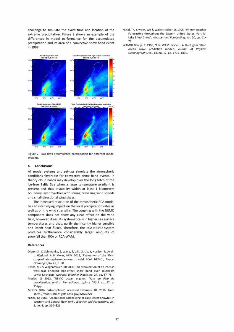
challenge to simulate the exact time and location of the extreme precipitation. Figure 2 shows an example of the differences in model performance for the accumulated precipitation and its area of a convective snow band event in 1998.

Figure 2. Two days accumulated precipitation for different model systems. 4. Conclusions All model systems and set-ups simulate the atmospheric conditions favorable for convective snow band events. In theory cloud bands may develop over the long fetch of the ice-free Baltic Sea when a large temperature gradient is present and thus instability within at least 1 kilometers boundary layer together with strong prevailing wind speeds and small directional wind shear.

The increased resolution of the atmospheric RCA model has an intensifying impact on the local precipitation rates as well as on the wind strengths. The coupling with the NEMO component does not show any clear effect on the wind field, however, it results systematically in higher sea surface temperatures and thus, partly significantly higher sensible and latent heat fluxes. Therefore, the RCA-NEMO system produces furthermore considerably larger amounts of snowfall than RCA or RCA-WAM. References

Dieterich, C, Schimanke, S, Wang, S, Väli, G, Liu, Y, Hordoir, R, Axell, L, Höglund, A & Meier, HEM 2013, ‘Evaluation of the SMHI coupled atmosphere-ice-ocean model RCA4 NEMO’, Report Oceanography 47, p. 80.

Evans, MS & Wagenmaker, RB 2000, ‘An examination of an intense west-east oriented lake-effect snow band over southeast Lower Michigan’, National Weather Digest, no. 24, pp. 67–78.

Madec, G 2012, ‘NEMO ocean engine’, Note du Pôle de modélisation, Institut Pierre-Simon Laplace (IPSL), no. 27, p. 357pp.

MODIS 2016, ’Atmosphere’, accessed February 10, 2016, from <http://modis-atmos.gsfc.nasa.gov/IMAGES/>.

Niziol, TA 1987, ‘Operational Forecasting of Lake Effect Snowfall in Western and Central New York’, Weather and Forecasting, vol. 2, no. 4, pp. 310–321.

Niziol, TA, Snyder, WR & Waldstreicher, JS 1995, ‘Winter weather Forecasting throughout the Eastern United States. Part IV: Lake Effect Snow’, Weather and Forecasting, vol. 10, pp. 61–77.

WAMDI Group, T 1988, ‘The WAM model - A third generation ocean wave prediction model’, Journal of Physical Oceanography, vol. 18, no. 12, pp. 1775–1810.

77

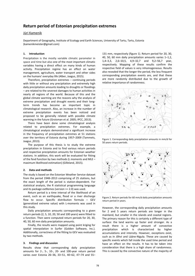
Return period of Estonian precipitation extremes Jüri Kamenik Department of Geography, Institute of Ecology and Earth Sciences, University of Tartu, Tartu, Estonia (kamenikmeister@gmail.com)

1. Introduction Precipitation is the mostly variable climatic parameter in space and time but also one of the most important climatic variables having a direct effect on many kinds of human activity. Precipitation regime has an effect on water management, agriculture, water transport and other sides on the humans' everyday life (Alber, Jaagus, 2015).

Therefore, precipitation extremes – continuing periods with little or without any precipitation and extremely high daily precipitation amounts leading to droughts or floodings – are related to the severest damages to human activities in nearly all regions of the world. Because of this and the global climate warming are the reasons why the analysis of extreme precipitation and drought events and their long-term trends has become an important topic in climatological research. Also, an increase in the number of extreme precipitation events has been noticed and proposed to be generally related with possible climate warming in the future (Groisman et al. 2005; IPCC, 2013).

There have been done some climatological analysis related to precipitation extremes. For example, a climatological analysis demonstrated a significant increase in the frequency of precipitation extremes at 51 stations over the territory of Estonia during 1957–2009 (Tammets, Jaagus ,2013).

The purpose of this thesis is to study the extreme precipitation in Estonia and to find various return periods and respective precipitation amounts for Estonian weather stations. In addition, this work will be evaluated for fitting of the fevd function by two methods (L moments and MLE – maximum likelihood estimation) (Gilleland, 2015). 2. Data and methods The study is based on the Estonian Weather Service dataset from the period 1948–2013 comprising of 25 stations, but the exact length of the period is station-dependent. For statistical analysis, the R statistical programming language and its package extRemes (version >= 2.0) was used.

Return period is a time interval of the likelihood of an event, such as an earthquake, flood or a river discharge flow to occur. Specific distribution formula – GEV (generalized extreme value) with L-moments was used in this study.

Daily precipitation amounts corresponding to a given return periods (2, 5, 10, 20, 50 and 100 years) were fitted to a function. Then were computed return periods for 20, 30, 40, 50, 60 mm daily precipitation amounts.

Finally, the results were mapped using point kriging for spatial interpolation in Surfer (Golden Software, Inc.). Additionally, correctness of the fitting to GEV was evaluated by two methods. 3. Findings and discussion Results show that corresponding daily precipitation amounts for 2-, 5-, 10-, 20- and 100-year return period varies over Estonia 26–36, 33–51, 40–62, 47–74 and 55–

131 mm, respectively (figure 1). Return period for 20, 30, 40, 50, 60 mm daily precipitation amounts varies 1–1,2, 1,4–3,3, 2,6–10,5, 4,9–32,7 and 9,2–56,7 year, respectively. Mapping of these results confirm the respective field of values is very inhomogeneous. Results also revealed that the longer the period, the less frequent corresponding precipitation events are, and that these are more randomly distributed due to the growth of relative importance of randomness.

Figure 1. Corresponding daily precipitation amounts in mm/d for 50 years return periods.

Figure 2. Return periods for 60 mm/d daily precipitation amounts return period in years. However, the corresponding daily precipitation amounts for 2 and 5 years return periods are longer in the mainland, but smaller in the islands and coastal regions. The primary reason for this is certainly a different type of surface: the land warms up faster and stronger. As a result there is a higher amount of convective precipitation which is characterized by higher accumulations and intensity. However, exceptions exist, such as in Jõhvi and Lääne-Nigula. These are caused by specific events which fall inside the used time period and have an effect on the results. It has to be taken into consideration that there is a high share of randomness. This is caused by the convective nature of the majority of

15.1

11.7

18.7

33

22.8

34.6

55.8

14

38.9

23.3

15.1

11.8

16.4

24.5

30.328.8

15.1

37.752.4

17

25.3

9.2

78

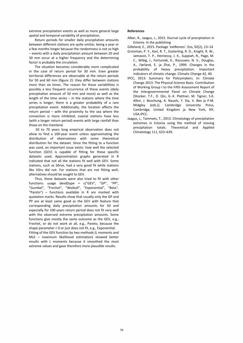
extreme precipitation events as well as more general large spatial and temporal variability of precipitation.

Return periods for smaller daily precipitation amounts between different stations are quite similar, being a year or a few months longer because the randomness is not so high – events with a daily precipitation amount between 20 and 30 mm occur at a higher frequency and the determining factor is probably the circulation.

The situation becomes considerably more complicated in the case of return period for 30 mm. Even greater territorial differences are observable at the return periods for 50 and 60 mm (figure 2): they differ between stations more than six times. The reason for these variabilities is possibly a less frequent occurrence of these events (daily precipitation amount of 50 mm and more) as well as the length of the time series – in the stations where the time series is longer, there is a greater probability of a rare precipitation event. Additionally, the location affects the return period – with the proximity to the sea where the convection is more inhibited, coastal stations have less (with a longer return period) events with large rainfall than those on the mainland.

50 to 70 years long empirical observation does not allow to find a 100-year event unless approximating the distribution of observations with some theoretical distribution for the dataset. Since the fitting to a function was used, an important issue exists: how well the selected function (GEV) is capable of fitting for these specific datasets used. Approximation graphs generated in R indicated that not all the stations fit well with GEV. Some stations, such as Sõrve, had a very good fit while stations like Võru did not. For stations that are not fitting well, alternatives should be sought to GEV.

Thus, these datasets were also tried to fit with other functions: usage devd(type = c("GEV", "GP", "PP", "Gumbel", "Frechet", "Weibull", "Exponential", "Beta", "Pareto") – functions available in R are marked with quotation marks. Results show that usually only the GP and PP are at least same good as the GEV with feature that corresponding daily precipitation amounts for 50 and especially for 100 years return period does not fit very well with the observed extreme precipitation amounts. Some functions give mostly the same outcome as the GEV, e.g., Frechet, or do not work at all, e.g., Pareto, because the shape parameter < 0 or just does not fit, e.g., Exponential. Fitting of the GEV function by two methods (L moments and MLE – maximum likelihood estimation) showed better results with L moments because it smoothed the most extreme values and gave therefore more plausible results.

References

Alber, R., Jaagus, J., 2015. Diurnal cycle of precipitation in Estonia. In the publishing

Gilleland, E., 2015. Package ‘extRemes’. Eos, 92(2), 13–14 Groisman, P. Y., Karl, R. T., Easterling, R. D., Knight, R. W.,

Jamason, F. P., Hennessy, J. K., Suppiah, R., Page, M. C., Wibig, J., Fortuniak, K., Razuvaev, N. V., Douglas, A., Førland, E. ja Zhai, P., 1999. Changes in the probability of heavy precipitation: Important indicators of climatic change. Climatic Change 42, 40.

IPCC, 2013: Summary for Policymakers. In: Climate Change 2013: The Physical Science Basis. Contribution of Working Group I to the Fifth Assessment Report of the Intergovernmental Panel on Climate Change [Stocker, T.F., D. Qin, G.-K. Plattner, M. Tignor, S.K. Allen, J. Boschung, A. Nauels, Y. Xia, V. Bex ja P.M. Midgley (eds.)]. Cambridge University Press, Cambridge, United Kingdom ja New York, NY, USA.IPCC.

Jaagus, J., Tammets, T., 2013. Climatology of precipitation extremes in Estonia using the method of moving precipitation totals. Theoretical and Applied Climatology 111, 623–639.

79

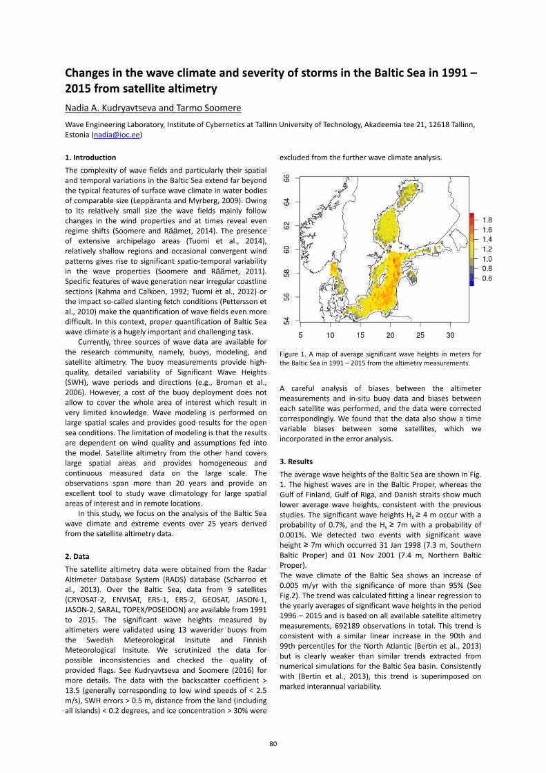
Changes in the wave climate and severity of storms in the Baltic Sea in 1991 – 2015 from satellite altimetry

Nadia A. Kudryavtseva and Tarmo Soomere

Wave Engineering Laboratory, Institute of Cybernetics at Tallinn University of Technology, Akadeemia tee 21, 12618 Tallinn, Estonia (nadia@ioc.ee) 1. Introduction The complexity of wave fields and particularly their spatial and temporal variations in the Baltic Sea extend far beyond the typical features of surface wave climate in water bodies of comparable size (Leppäranta and Myrberg, 2009). Owing to its relatively small size the wave fields mainly follow changes in the wind properties and at times reveal even regime shifts (Soomere and Räämet, 2014). The presence of extensive archipelago areas (Tuomi et al., 2014), relatively shallow regions and occasional convergent wind patterns gives rise to significant spatio-temporal variability in the wave properties (Soomere and Räämet, 2011). Specific features of wave generation near irregular coastline sections (Kahma and Calkoen, 1992; Tuomi et al., 2012) or the impact so-called slanting fetch conditions (Pettersson et al., 2010) make the quantification of wave fields even more difficult. In this context, proper quantification of Baltic Sea wave climate is a hugely important and challenging task.

Currently, three sources of wave data are available for the research community, namely, buoys, modeling, and satellite altimetry. The buoy measurements provide high-quality, detailed variability of Significant Wave Heights (SWH), wave periods and directions (e.g., Broman et al., 2006). However, a cost of the buoy deployment does not allow to cover the whole area of interest which result in very limited knowledge. Wave modeling is performed on large spatial scales and provides good results for the open sea conditions. The limitation of modeling is that the results are dependent on wind quality and assumptions fed into the model. Satellite altimetry from the other hand covers large spatial areas and provides homogeneous and continuous measured data on the large scale. The observations span more than 20 years and provide an excellent tool to study wave climatology for large spatial areas of interest and in remote locations.

In this study, we focus on the analysis of the Baltic Sea wave climate and extreme events over 25 years derived from the satellite altimetry data. 2. Data The satellite altimetry data were obtained from the Radar Altimeter Database System (RADS) database (Scharroo et al., 2013). Over the Baltic Sea, data from 9 satellites (CRYOSAT-2, ENVISAT, ERS-1, ERS-2, GEOSAT, JASON-1, JASON-2, SARAL, TOPEX/POSEIDON) are available from 1991 to 2015. The significant wave heights measured by altimeters were validated using 13 waverider buoys from the Swedish Meteorological Insitute and Finnish Meteorological Insitute. We scrutinized the data for possible inconsistencies and checked the quality of provided flags. See Kudryavtseva and Soomere (2016) for more details. The data with the backscatter coefficient > 13.5 (generally corresponding to low wind speeds of < 2.5 m/s), SWH errors > 0.5 m, distance from the land (including all islands) < 0.2 degrees, and ice concentration > 30% were

excluded from the further wave climate analysis.

Figure 1. A map of average significant wave heights in meters for the Baltic Sea in 1991 – 2015 from the altimetry measurements.

A careful analysis of biases between the altimeter measurements and in-situ buoy data and biases between each satellite was performed, and the data were corrected correspondingly. We found that the data also show a time variable biases between some satellites, which we incorporated in the error analysis. 3. Results The average wave heights of the Baltic Sea are shown in Fig. 1. The highest waves are in the Baltic Proper, whereas the Gulf of Finland, Gulf of Riga, and Danish straits show much lower average wave heights, consistent with the previous studies. The significant wave heights Hs ≥ 4 m occur with a probability of 0.7%, and the Hs ≥ 7m with a probability of 0.001%. We detected two events with significant wave height ≥ 7m which occurred 31 Jan 1998 (7.3 m, Southern Baltic Proper) and 01 Nov 2001 (7.4 m, Northern Baltic Proper). The wave climate of the Baltic Sea shows an increase of 0.005 m/yr with the significance of more than 95% (See Fig.2). The trend was calculated fitting a linear regression to the yearly averages of significant wave heights in the period 1996 – 2015 and is based on all available satellite altimetry measurements, 692189 observations in total. This trend is consistent with a similar linear increase in the 90th and 99th percentiles for the North Atlantic (Bertin et al., 2013) but is clearly weaker than similar trends extracted from numerical simulations for the Baltic Sea basin. Consistently with (Bertin et al., 2013), this trend is superimposed on marked interannual variability.

80

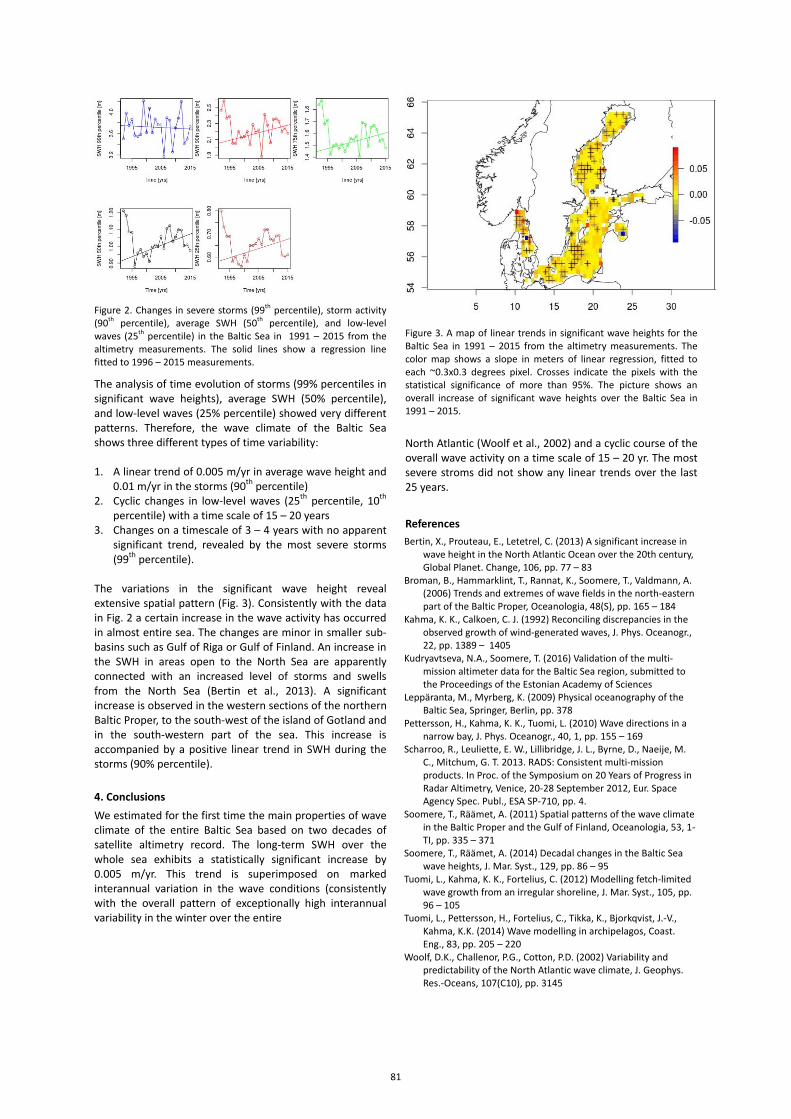
Figure 2. Changes in severe storms (99th percentile), storm activity (90th percentile), average SWH (50th percentile), and low-level waves (25th percentile) in the Baltic Sea in 1991 – 2015 from the altimetry measurements. The solid lines show a regression line fitted to 1996 – 2015 measurements.

The analysis of time evolution of storms (99% percentiles in significant wave heights), average SWH (50% percentile), and low-level waves (25% percentile) showed very different patterns. Therefore, the wave climate of the Baltic Sea shows three different types of time variability:

1. A linear trend of 0.005 m/yr in average wave height and

0.01 m/yr in the storms (90th percentile) 2. Cyclic changes in low-level waves (25th percentile, 10th

percentile) with a time scale of 15 – 20 years 3. Changes on a timescale of 3 – 4 years with no apparent

significant trend, revealed by the most severe storms (99th percentile).

The variations in the significant wave height reveal extensive spatial pattern (Fig. 3). Consistently with the data in Fig. 2 a certain increase in the wave activity has occurred in almost entire sea. The changes are minor in smaller sub-basins such as Gulf of Riga or Gulf of Finland. An increase in the SWH in areas open to the North Sea are apparently connected with an increased level of storms and swells from the North Sea (Bertin et al., 2013). A significant increase is observed in the western sections of the northern Baltic Proper, to the south-west of the island of Gotland and in the south-western part of the sea. This increase is accompanied by a positive linear trend in SWH during the storms (90% percentile). 4. Conclusions We estimated for the first time the main properties of wave climate of the entire Baltic Sea based on two decades of satellite altimetry record. The long-term SWH over the whole sea exhibits a statistically significant increase by 0.005 m/yr. This trend is superimposed on marked interannual variation in the wave conditions (consistently with the overall pattern of exceptionally high interannual variability in the winter over the entire

Figure 3. A map of linear trends in significant wave heights for the Baltic Sea in 1991 – 2015 from the altimetry measurements. The color map shows a slope in meters of linear regression, fitted to each ~0.3x0.3 degrees pixel. Crosses indicate the pixels with the statistical significance of more than 95%. The picture shows an overall increase of significant wave heights over the Baltic Sea in 1991 – 2015. North Atlantic (Woolf et al., 2002) and a cyclic course of the overall wave activity on a time scale of 15 – 20 yr. The most severe stroms did not show any linear trends over the last 25 years.

References Bertin, X., Prouteau, E., Letetrel, C. (2013) A significant increase in

wave height in the North Atlantic Ocean over the 20th century, Global Planet. Change, 106, pp. 77 – 83

Broman, B., Hammarklint, T., Rannat, K., Soomere, T., Valdmann, A. (2006) Trends and extremes of wave fields in the north-eastern part of the Baltic Proper, Oceanologia, 48(S), pp. 165 – 184

Kahma, K. K., Calkoen, C. J. (1992) Reconciling discrepancies in the observed growth of wind-generated waves, J. Phys. Oceanogr., 22, pp. 1389 – 1405

Kudryavtseva, N.A., Soomere, T. (2016) Validation of the multi-mission altimeter data for the Baltic Sea region, submitted to the Proceedings of the Estonian Academy of Sciences

Leppäranta, M., Myrberg, K. (2009) Physical oceanography of the Baltic Sea, Springer, Berlin, pp. 378

Pettersson, H., Kahma, K. K., Tuomi, L. (2010) Wave directions in a narrow bay, J. Phys. Oceanogr., 40, 1, pp. 155 – 169

Scharroo, R., Leuliette, E. W., Lillibridge, J. L., Byrne, D., Naeije, M. C., Mitchum, G. T. 2013. RADS: Consistent multi-mission products. In Proc. of the Symposium on 20 Years of Progress in Radar Altimetry, Venice, 20-28 September 2012, Eur. Space Agency Spec. Publ., ESA SP-710, pp. 4.

Soomere, T., Räämet, A. (2011) Spatial patterns of the wave climate in the Baltic Proper and the Gulf of Finland, Oceanologia, 53, 1-TI, pp. 335 – 371

Soomere, T., Räämet, A. (2014) Decadal changes in the Baltic Sea wave heights, J. Mar. Syst., 129, pp. 86 – 95

Tuomi, L., Kahma, K. K., Fortelius, C. (2012) Modelling fetch-limited wave growth from an irregular shoreline, J. Mar. Syst., 105, pp. 96 – 105

Tuomi, L., Pettersson, H., Fortelius, C., Tikka, K., Bjorkqvist, J.-V., Kahma, K.K. (2014) Wave modelling in archipelagos, Coast. Eng., 83, pp. 205 – 220

Woolf, D.K., Challenor, P.G., Cotton, P.D. (2002) Variability and predictability of the North Atlantic wave climate, J. Geophys. Res.-Oceans, 107(C10), pp. 3145

81

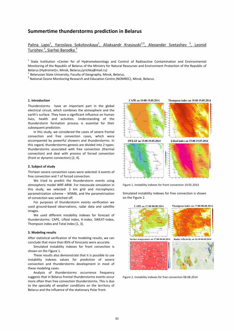
Summertime thunderstorms prediction in Belarus Palina Lapo1, Yaroslava Sokolovskaya1, Aliaksandr Krasouski2,3, Alexander Svetashev 3, Leonid Turishev 3, Siarhei Barodka 3

1 State Institution «Center for of Hydrometeorology and Control of Radioactive Contamination and Environmental Monitoring of the Republic of Belarus of the Ministry for Natural Resourses and Environment Protection of the Republic of Belarus (Hydromet)», Minsk, Belarus,(yrichka@mail.ru) 2 Belarusian State University, Faculty of Geography, Minsk, Belarus, 3 National Ozone Monitoring Research and Education Centre (NOMREC), Minsk, Belarus.

1. Introduction Thunderstorms have an important part in the global electrical circuit, which combines the atmosphere and the earth’s surface. They have a significant influence on human lives, health and activities. Understanding of the thunderstorm formation process is essential for their subsequent prediction.

In this study, we considered the cases of severe frontal convection and free convection cases, which were accompanied by powerful showers and thunderstorms. In this regard, thunderstorms genesis are divided into 2 types: thunderstorms associated with free convection (thermal convection) and deal with process of forced convection (front or dynamic convection) [2, 4].

2. Subject of study Thirteen severe convection cases were selected: 6 events of free convection and 7 of forced convection.

We tried to predict the thunderstorm events using atmospheric model WRF-ARW. For mesoscale simulation in this study, we selected: 3 km grid and microphysics parametrization scheme – WSM6, and the parametrization of convection was switched off.

For purposes of thunderstorm events verification we used ground-based observations, radar data and satellite images.

We used different instability indexes for forecast of thunderstorms: CAPE, Lifted index, K-index, SWEAT-index, Thompson index and Total index [1, 3].

3. Modeling results After statistical verification of the modeling results, we can conclude that more than 85% of forecasts were accurate.

Simulated instability indexes for front convection is shown on the Figure 1.

These results also demonstrate that it is possible to use instability indexes values for prediction of severe convection and thunderstorms development in most of these modeling cases.

Analysis of thunderstorms occurrence frequency suggests that in Belarus frontal thunderstorms events occur more often than free convection thunderstorms. This is due to the specially of weather conditions on the territory of Belarus and the influence of the stationary Polar front.

Figure 1. Instability indexes for front convection 19.05.2014

Simulated instability indexes for free convection is shown on the Figure 2.

Figure 2. Instability indexes for free convection 08.08.2014

82

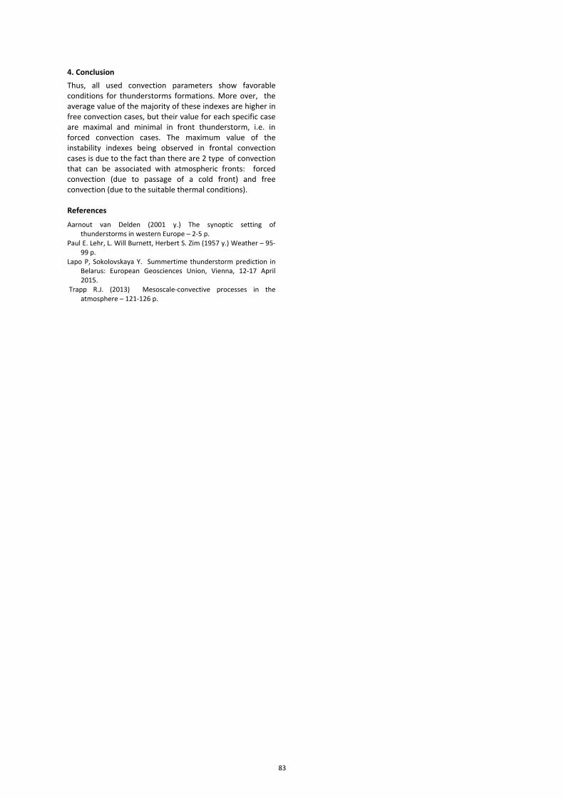
4. Conclusion Thus, all used convection parameters show favorable conditions for thunderstorms formations. More over, the average value of the majority of these indexes are higher in free convection cases, but their value for each specific case are maximal and minimal in front thunderstorm, i.e. in forced convection cases. The maximum value of the instability indexes being observed in frontal convection cases is due to the fact than there are 2 type of convection that can be associated with atmospheric fronts: forced convection (due to passage of a cold front) and free convection (due to the suitable thermal conditions). References

Aarnout van Delden (2001 y.) The synoptic setting of thunderstorms in western Europe – 2-5 p.

Paul E. Lehr, L. Will Burnett, Herbert S. Zim (1957 y.) Weather – 95-99 p.

Lapo P, Sokolovskaya Y. Summertime thunderstorm prediction in Belarus: European Geosciences Union, Vienna, 12-17 April 2015.

Trapp R.J. (2013) Mesoscale-convective processes in the atmosphere – 121-126 p.

83

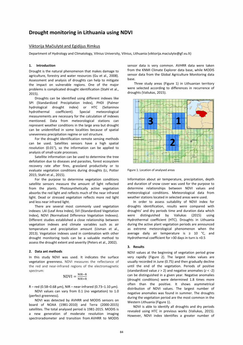
Drought monitoring in Lithuania using NDVI

Viktorija Mačiulytė and Egidijus Rimkus

Department of Hydrology and Climatology, Vilnius University, Vilnius, Lithuania (viktorija.maciulyte@gf.vu.lt)

1. Introduction Drought is the natural phenomenon that makes damage to agriculture, forestry and water resources (Gu et al., 2008). Assessment and analysis of droughts can help to mitigate the impact on vulnerable regions. One of the major problems is complicated drought identification (Stahl et al., 2015).

Droughts can be identified using different indexes like SPI (Standardized Precipitation Index), PHDI (Palmer hydrological drought index) or HTC (Selianinov hydrothermal coefficient). Special meteorological measurements are necessary for the calculation of indexes mentioned. Data from meteorological stations can represent weather conditions in the large area but drought can be unidentified in some localities because of spatial unevenness precipitation regime or soil structure.

For the drought identification remote sensing methods can be used. Satellites sensors have a high spatial resolution (0.01°), so the information can be applied to analysis of small-scale processes.

Satellite information can be used to determine the tree defoliation due to diseases and parasites, forest ecosystem recovery rate after fires, grassland productivity or to evaluate vegetation conditions during droughts (Li, Potter 2015; Stahl et al., 2015).

For the purpose to determine vegetation conditions satellite sensors measure the amount of light reflected from the plants. Photosynthetically active vegetation absorbs the red light and reflects much of the near infrared light. Dead or stressed vegetation reflects more red light and less near infrared light.

There are several most commonly used vegetation indexes: LAI (Leaf Area Index), SVI (Standardized Vegetation Index), NDVI (Normalized Difference Vegetation Indexes). Different studies established a close relationship between vegetation indexes and climate variables such as air temperature and precipitation amount (Usman et al., 2013). Vegetation indexes used in combination with other drought monitoring tools can be a valuable method to assess the drought extent and severity (Peters et al., 2002).

2. Data ant methods In this study NDVI was used. It indicates the surface vegetation greenness. NDVI measures the reflectance of the red and near-infrared regions of the electromagnetic spectrum:

NDVI =

R – red (0.58–0.68 μm), NIR – near-infrared (0.73–1.10 μm). NDVI values can vary from 0.1 (no vegetation) to 1.0

(perfect greenness). NDVI was detected by AVHRR and MODIS sensors on

board of NOAA (1981-2010) and Terra (2000-2015) satellites. The total analysed period is 1981-2015. MODIS is a new generation of moderate resolution imaging spectroradiometer and transition from AVHRR to MODIS

sensor data is very common. AVHRR data were taken from the KNMI Climate Explorer data base, while MODIS sensor data from the Global Agriculture Monitoring data base.

Three study areas (Figure 1) in Lithuanian territory were selected according to differences in recurrence of droughts (Valiukas, 2015).

Figure 1. Location of analysed areas

Information about air temperature, precipitation, depth and duration of snow cover was used for the purpose to determine relationships between NDVI values and meteorological conditions. Meteorological data from weather stations located in selected areas were used.

In order to assess suitability of NDVI index for droughts identification, results were compared with droughts’ and dry periods time and duration data which were distinguished by Valiukas (2015) using Hydrothermal coefficient (HTC). Droughts in Lithuania during the active plant vegetation periods are announced as extreme meteorological phenomenon when the average daily air temperature is ≥ 10 °C, and Hydrothermal coefficient for >30 days in turn is <0.5

3. Results NDVI values at the beginning of vegetation period grow very rapidly (Figure 2). The largest index values are usually recorded in June (0.75) and then gradually decline until the end of the vegetation. Periods of positive (standardized value z > 2) and negative anomalies (z < -2) can be distinguished in a given year. Negative anomalies (drought conditions) were determined 1.8 times more often than the positive. It shows asymmetrical distribution of NDVI values. The largest number of negative anomalies was found in summer. The droughts during the vegetation period are the most common in the Western Lithuania (Figure 1).

NDVI is able to identify all droughts and dry periods revealed using HTC in previous works (Valiukas, 2015). However, NDVI index identifies a greater number of

84

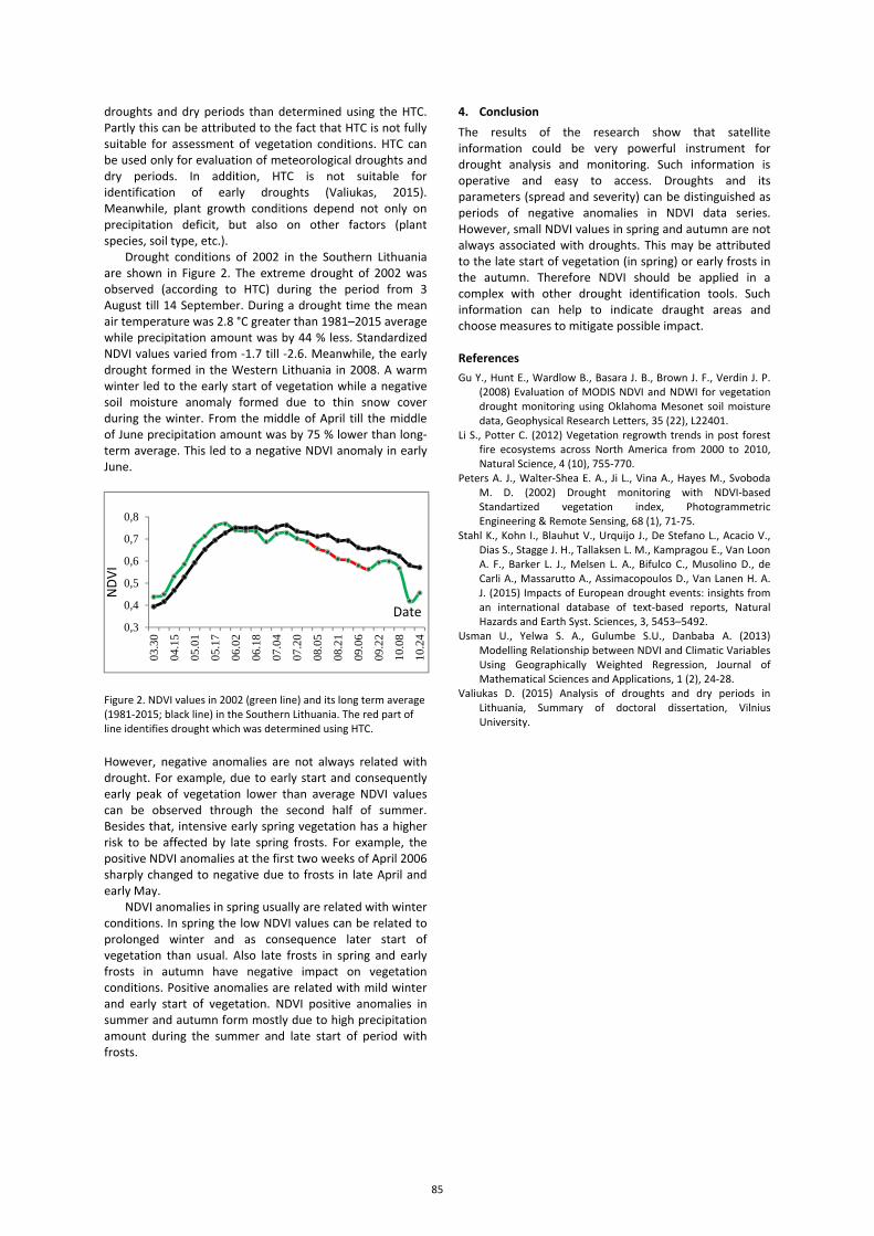
droughts and dry periods than determined using the HTC. Partly this can be attributed to the fact that HTC is not fully suitable for assessment of vegetation conditions. HTC can be used only for evaluation of meteorological droughts and dry periods. In addition, HTC is not suitable for identification of early droughts (Valiukas, 2015). Meanwhile, plant growth conditions depend not only on precipitation deficit, but also on other factors (plant species, soil type, etc.).

Drought conditions of 2002 in the Southern Lithuania are shown in Figure 2. The extreme drought of 2002 was observed (according to HTC) during the period from 3 August till 14 September. During a drought time the mean air temperature was 2.8 °C greater than 1981–2015 average while precipitation amount was by 44 % less. Standardized NDVI values varied from -1.7 till -2.6. Meanwhile, the early drought formed in the Western Lithuania in 2008. A warm winter led to the early start of vegetation while a negative soil moisture anomaly formed due to thin snow cover during the winter. From the middle of April till the middle of June precipitation amount was by 75 % lower than long-term average. This led to a negative NDVI anomaly in early June.

Figure 2. NDVI values in 2002 (green line) and its long term average (1981-2015; black line) in the Southern Lithuania. The red part of line identifies drought which was determined using HTC.

However, negative anomalies are not always related with drought. For example, due to early start and consequently early peak of vegetation lower than average NDVI values can be observed through the second half of summer. Besides that, intensive early spring vegetation has a higher risk to be affected by late spring frosts. For example, the positive NDVI anomalies at the first two weeks of April 2006 sharply changed to negative due to frosts in late April and early May.

NDVI anomalies in spring usually are related with winter conditions. In spring the low NDVI values can be related to prolonged winter and as consequence later start of vegetation than usual. Also late frosts in spring and early frosts in autumn have negative impact on vegetation conditions. Positive anomalies are related with mild winter and early start of vegetation. NDVI positive anomalies in summer and autumn form mostly due to high precipitation amount during the summer and late start of period with frosts.

4. Conclusion The results of the research show that satellite information could be very powerful instrument for drought analysis and monitoring. Such information is operative and easy to access. Droughts and its parameters (spread and severity) can be distinguished as periods of negative anomalies in NDVI data series. However, small NDVI values in spring and autumn are not always associated with droughts. This may be attributed to the late start of vegetation (in spring) or early frosts in the autumn. Therefore NDVI should be applied in a complex with other drought identification tools. Such information can help to indicate draught areas and choose measures to mitigate possible impact.

References Gu Y., Hunt E., Wardlow B., Basara J. B., Brown J. F., Verdin J. P.

(2008) Evaluation of MODIS NDVI and NDWI for vegetation drought monitoring using Oklahoma Mesonet soil moisture data, Geophysical Research Letters, 35 (22), L22401.

Li S., Potter C. (2012) Vegetation regrowth trends in post forest fire ecosystems across North America from 2000 to 2010, Natural Science, 4 (10), 755-770.

Peters A. J., Walter-Shea E. A., Ji L., Vina A., Hayes M., Svoboda M. D. (2002) Drought monitoring with NDVI-based Standartized vegetation index, Photogrammetric Engineering & Remote Sensing, 68 (1), 71-75.

Stahl K., Kohn I., Blauhut V., Urquijo J., De Stefano L., Acacio V., Dias S., Stagge J. H., Tallaksen L. M., Kampragou E., Van Loon A. F., Barker L. J., Melsen L. A., Bifulco C., Musolino D., de Carli A., Massarutto A., Assimacopoulos D., Van Lanen H. A. J. (2015) Impacts of European drought events: insights from an international database of text-based reports, Natural Hazards and Earth Syst. Sciences, 3, 5453–5492.

Usman U., Yelwa S. A., Gulumbe S.U., Danbaba A. (2013) Modelling Relationship between NDVI and Climatic Variables Using Geographically Weighted Regression, Journal of Mathematical Sciences and Applications, 1 (2), 24-28.

Valiukas D. (2015) Analysis of droughts and dry periods in Lithuania, Summary of doctoral dissertation, Vilnius University.

0,3

0,4

0,5

0,6

0,7

0,8

03.

30

04.

15

05.

01

05.

17

06.

02

06.

18

07.

04

07.

20

08.

05

08.

21

09.

06

09.

22

10.

08

10.

24

NDV

I

Date

85

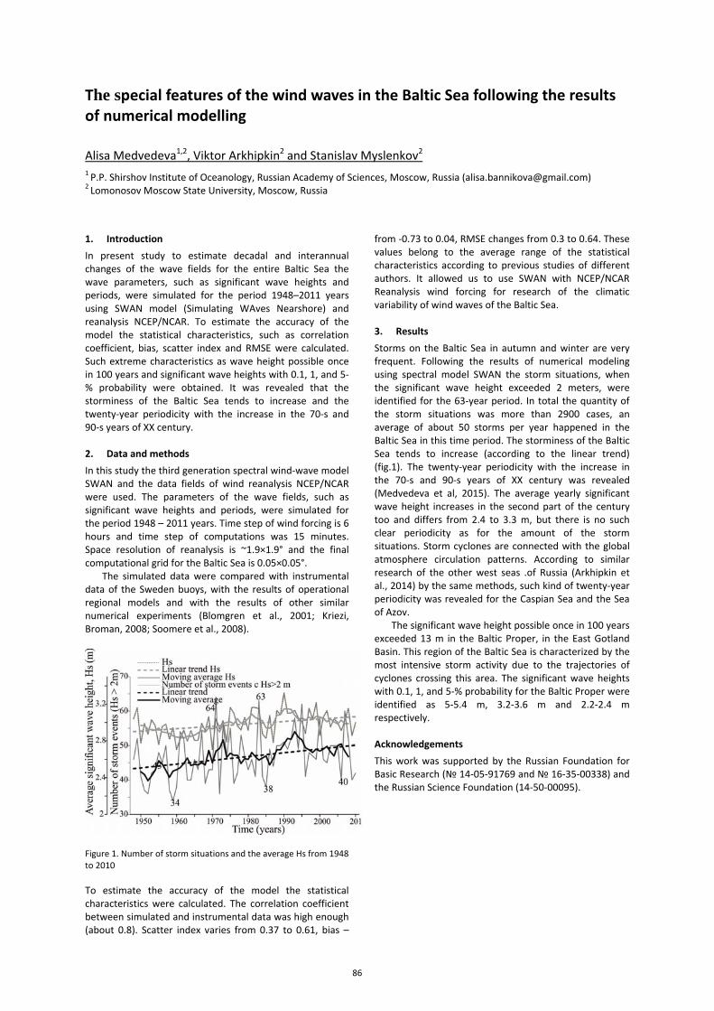
The special features of the wind waves in the Baltic Sea following the results of numerical modelling

Alisa Medvedeva1,2, Viktor Arkhipkin2 and Stanislav Myslenkov2

1 P.P. Shirshov Institute of Oceanology, Russian Academy of Sciences, Moscow, Russia (alisa.bannikova@gmail.com) 2 Lomonosov Moscow State University, Moscow, Russia

1. Introduction In present study to estimate decadal and interannual changes of the wave fields for the entire Baltic Sea the wave parameters, such as significant wave heights and periods, were simulated for the period 1948–2011 years using SWAN model (Simulating WAves Nearshore) and reanalysis NCEP/NCAR. To estimate the accuracy of the model the statistical characteristics, such as correlation coefficient, bias, scatter index and RMSE were calculated. Such extreme characteristics as wave height possible once in 100 years and significant wave heights with 0.1, 1, and 5-% probability were obtained. It was revealed that the storminess of the Baltic Sea tends to increase and the twenty-year periodicity with the increase in the 70-s and 90-s years of XX century. 2. Data and methods In this study the third generation spectral wind-wave model SWAN and the data fields of wind reanalysis NCEP/NCAR were used. The parameters of the wave fields, such as significant wave heights and periods, were simulated for the period 1948 – 2011 years. Time step of wind forcing is 6 hours and time step of computations was 15 minutes. Space resolution of reanalysis is ~1.9×1.9° and the final computational grid for the Baltic Sea is 0.05×0.05°.

The simulated data were compared with instrumental data of the Sweden buoys, with the results of operational regional models and with the results of other similar numerical experiments (Blomgren et al., 2001; Kriezi, Broman, 2008; Soomere et al., 2008).

Figure 1. Number of storm situations and the average Hs from 1948 to 2010

To estimate the accuracy of the model the statistical characteristics were calculated. The correlation coefficient between simulated and instrumental data was high enough (about 0.8). Scatter index varies from 0.37 to 0.61, bias –

from -0.73 to 0.04, RMSE changes from 0.3 to 0.64. These values belong to the average range of the statistical characteristics according to previous studies of different authors. It allowed us to use SWAN with NCEP/NCAR Reanalysis wind forcing for research of the climatic variability of wind waves of the Baltic Sea.

3. Results Storms on the Baltic Sea in autumn and winter are very frequent. Following the results of numerical modeling using spectral model SWAN the storm situations, when the significant wave height exceeded 2 meters, were identified for the 63-year period. In total the quantity of the storm situations was more than 2900 cases, an average of about 50 storms per year happened in the Baltic Sea in this time period. The storminess of the Baltic Sea tends to increase (according to the linear trend) (fig.1). The twenty-year periodicity with the increase in the 70-s and 90-s years of XX century was revealed (Medvedeva et al, 2015). The average yearly significant wave height increases in the second part of the century too and differs from 2.4 to 3.3 m, but there is no such clear periodicity as for the amount of the storm situations. Storm cyclones are connected with the global atmosphere circulation patterns. According to similar research of the other west seas .of Russia (Arkhipkin et al., 2014) by the same methods, such kind of twenty-year periodicity was revealed for the Caspian Sea and the Sea of Azov.

The significant wave height possible once in 100 years exceeded 13 m in the Baltic Proper, in the East Gotland Basin. This region of the Baltic Sea is characterized by the most intensive storm activity due to the trajectories of cyclones crossing this area. The significant wave heights with 0.1, 1, and 5-% probability for the Baltic Proper were identified as 5-5.4 m, 3.2-3.6 m and 2.2-2.4 m respectively. Acknowledgements This work was supported by the Russian Foundation for Basic Research (№ 14-05-91769 and № 16-35-00338) and the Russian Science Foundation (14-50-00095).

86

References Arkhipkin V.S., Gippius F.N., Koltermann K.P. and Surkova G.V.

(2014) Wind waves in the Black Sea: results of a hindcast study. Natural Hazards and Earth System Sciences Discussions, Vol. 14, pp. 2883–2897.

Blomgren S., Larson M., Hanson H. (2001) Numerical Modeling of the Wave Climate in the Southern Baltic Sea. Journal of Coastal Research, Vol. 17, No. 2, pp. 342-352.

Kriezi E.E., Broman B. (2008) Past and future wave climate in the Baltic Sea produced by the SWAN model with forcing from the regional climate model RCA of the Rossby Centre. US/EU-Baltic International Symposium, 2008 IEEE/OES. IEEE (Tallin, Estonia), pp. 1-7.

Medvedeva A.Yu., Arkhipkin V.S., Myslenkov S.A., Zilitinkevich S.S. (2015) Wave climate of the Baltic Sea following the results of the SWAN spectral model application, Vestnik Moskovskogo Unviersiteta, Seriya Geografiya, Vol.5 No1, pp. 12–22.

Soomere T., Behrens A., Tuomi L., Nielsen J. W. (2008) Wave conditions in the Baltic Proper and in the Gulf of Finland during windstorm Gudrun, J. Natural Hazards & Earth System Sciences, Vol. 8, No. 1, pp. 37–46.

87

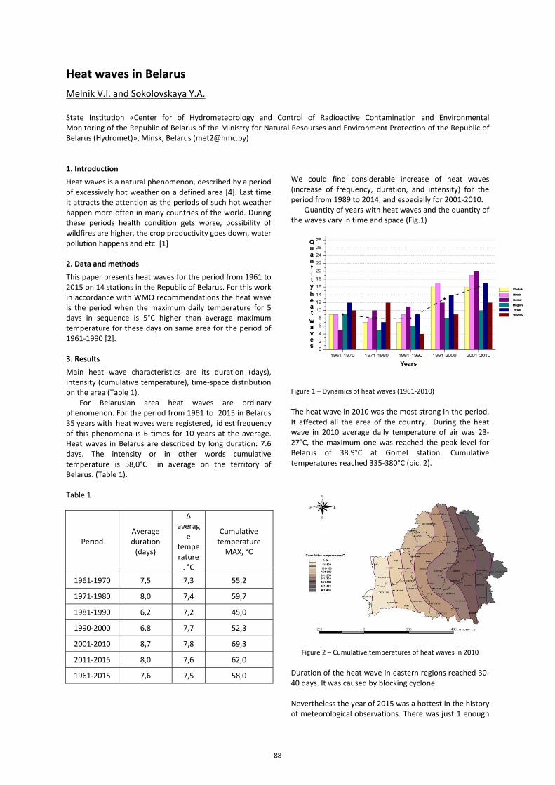
Heat waves in Belarus Melnik V.I. and Sokolovskaya Y.A.

State Institution «Center for of Hydrometeorology and Control of Radioactive Contamination and Environmental Monitoring of the Republic of Belarus of the Ministry for Natural Resourses and Environment Protection of the Republic of Belarus (Hydromet)», Minsk, Belarus (met2@hmc.by)

1. Introduction Heat waves is a natural phenomenon, described by a period of excessively hot weather on a defined area [4]. Last time it attracts the attention as the periods of such hot weather happen more often in many countries of the world. During these periods health condition gets worse, possibility of wildfires are higher, the crop productivity goes down, water pollution happens and etc. [1]

2. Data and methods This paper presents heat waves for the period from 1961 to 2015 on 14 stations in the Republic of Belarus. For this work in accordance with WMO recommendations the heat wave is the period when the maximum daily temperature for 5 days in sequence is 5°С higher than average maximum temperature for these days on same area for the period of 1961-1990 [2].

3. Results Main heat wave characteristics are its duration (days), intensity (cumulative temperature), time-space distribution on the area (Table 1).

For Belarusian area heat waves are ordinary phenomenon. For the period from 1961 to 2015 in Belarus 35 years with heat waves were registered, id est frequency of this phenomena is 6 times for 10 years at the average. Heat waves in Belarus are described by long duration: 7.6 days. The intensity or in other words cumulative temperature is 58,0°С in average on the territory of Belarus. (Table 1).

Table 1

Period Average duration

(days)

∆ averag

e temperature

. °С

Cumulative temperature

МАХ, °С

1961-1970 7,5 7,3 55,2

1971-1980 8,0 7,4 59,7

1981-1990 6,2 7,2 45,0

1990-2000 6,8 7,7 52,3

2001-2010 8,7 7,8 69,3

2011-2015 8,0 7,6 62,0

1961-2015 7,6 7,5 58,0

We could find considerable increase of heat waves (increase of frequency, duration, and intensity) for the period from 1989 to 2014, and especially for 2001-2010.

Quantity of years with heat waves and the quantity of the waves vary in time and space (Fig.1)

Figure 1 – Dynamics of heat waves (1961-2010)

The heat wave in 2010 was the most strong in the period. It affected all the area of the country. During the heat wave in 2010 average daily temperature of air was 23-27°С, the maximum one was reached the peak level for Belarus of 38.9°С at Gomel station. Cumulative temperatures reached 335-380°С (pic. 2).

Figure 2 – Cumulative temperatures of heat waves in 2010

Duration of the heat wave in eastern regions reached 30-40 days. It was caused by blocking cyclone.

Nevertheless the year of 2015 was a hottest in the history of meteorological observations. There was just 1 enough

88

strong heat wave in Belarus with main characteristics (duration, intensity, cumulative temperature) higher then normal and covered all the territory of Belarus. What’s why more deep evaluation of this phenomenon should be carried out for early forecasting. 4. Conclusion The quantity of years with heat waves and quantity of heat waves vary in time and space. We could find out a significant increase of heat waves (increase of frequency, duration and intensity) for the period from 1989 to 2015, especially in 2001-2010. The most strong heat waves were registered in 2010, 2014. The year of 2015 was the hottest for the history of meteorological observations in Belarus and was described by drought, but there were no some significant heat waves. Heat waves trend to further increase of its durations and intensity in time and space, that is an evidence of climate changes (warming).

References

Zverev N.I. About waves in the atmosphere / N.I. Zverev // Works of TsIP. – 1964. - pages 63-91.

Slizkaya K.P. Meteorological conditions of heat waves generation for last decade (2001-2010) /К.P. Slizkaya // Monthly scientific review. – 2014. - No2, part 4. – pages 58-60.

Shevchenko О.G. Heat waves and some methodological problem of its exploring / О.G. Shevchenko, S.I. Snezhko // Ukrainian meteorological review.–2012.-No10–pages 57-63.

Shevchenko О.G. Characteristics of heat waves of summer 2010 on the territory of Ukraine / О.G. Shevchenko // Scientific works UkrNIGMI. – 2010 - pages 51-63.

89

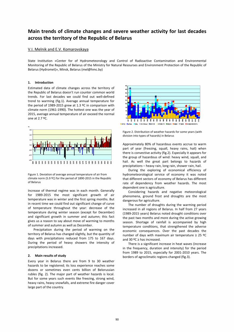
Main trends of climate changes and severe weather activity for last decades across the territory of the Republic of Belarus V.I. Melnik and E.V. Komarovskaya

State Institution «Center for of Hydrometeorology and Control of Radioactive Contamination and Environmental Monitoring of the Republic of Belarus of the Ministry for Natural Resourses and Environment Protection of the Republic of Belarus (Hydromet)», Minsk, Belarus (mel@hmc.by) 1. Introduction Estimated data of climate changes across the territory of the Republic of Belarus doesn’t run counter common world trends. For last decades we could find out well-defined trend to warming (fig.1). Average annual temperature for the period of 1989-2015 grew at 1.3 ºC in comparison with climate norm (1961-1990). The hottest one was the year of 2015, average annual temperature of air exceed the normal one at 2.7 ºC.

Figure 1. Deviation of average annual temperature of air from climate norm (5.9 ºC) for the period of 1890-2015 in the Republic of Belarus Increase of thermal regime was in each month. Generally for 1989-2015 the most significant growth of air temperature was in winter and the first spring months. But in recent time we could find out significant change of curve of temperature throughout the year: decrease of the temperature during winter season (except for December) and significant growth in summer and autumn; this fact gives us a reason to say about move of warming to months of summer and autumn as well as December.

Precipitation during the period of warming on the territory of Belarus has changed slightly, but the quantity of days with precipitations reduced from 175 to 167 days. During the period of heavy showers the intensity of precipitations increased.

2. Main results of study Every year in Belarus there are from 9 to 30 weather hazards to be registered; its loss experience reaches some dozens or sometimes even cents billion of Belorussian rubles (fig. 2). The major part of weather hazards is local. But for some years such events like freezing, strong wind, heavy rains, heavy snowfalls, and extreme fire danger cover large part of the country.

Figure 2. Distribution of weather hazards for some years (with division into types of hazards) in Belarus

Approximately 80% of hazardous events accrue to warm part of year (freezing, squall, heavy rains, hail) when there is convective activity (fig.2). Especially it appears for the group of hazardous of wind: heavy wind, squall, and hail. As well the great part belongs to hazards of precipitations – heavy rain, long rain, shower rain, hail.

During the exploring of economical efficiency of hydrometeorological service of economy it was noted that different sectors of economy of Belarus has different rate of dependency from weather hazards. The most dependent one is agriculture.

Considering hazards and negative meteorological phenomena, ground frost and droughts are the most dangerous for agriculture.

The number of droughts during the warming period increased in all regions of Belarus. In half from 27 years (1989-2015 years) Belarus noted drought conditions over the past two months and more during the active growing season. Shortage of rainfall is accompanied by high temperature conditions, that strengthened the adverse economic consequences. Over the past decades the number of days with maximum air temperature ≥ 25 ºC and 30 ºC ≥ has increased.

There is a significant increase in heat waves (increase in the frequency, duration and intensity) for the period from 1989 to 2015, especially for 2001-2010 years. The borders of agroclimatic regions changed (fig.3).

90

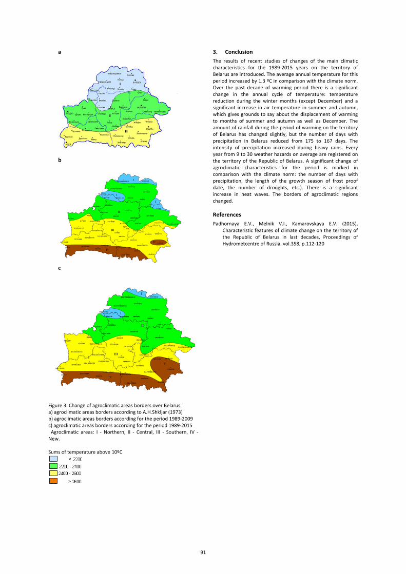
a

b

c

Figure 3. Change of agroclimatic areas borders over Belarus: а) agroclimatic areas borders according to A.H.Shkljar (1973) b) agroclimatic areas borders according for the period 1989-2009 с) agroclimatic areas borders according for the period 1989-2015 Agroclimatic areas: I - Northern, II - Central, III - Southern, IV - New. Sums of temperature above 10ºС

3. Conclusion The results of recent studies of changes of the main climatic characteristics for the 1989-2015 years on the territory of Belarus are introduced. The average annual temperature for this period increased by 1.3 ºC in comparison with the climate norm. Over the past decade of warming period there is a significant change in the annual cycle of temperature: temperature reduction during the winter months (except December) and a significant increase in air temperature in summer and autumn, which gives grounds to say about the displacement of warming to months of summer and autumn as well as December. The amount of rainfall during the period of warming on the territory of Belarus has changed slightly, but the number of days with precipitation in Belarus reduced from 175 to 167 days. The intensity of precipitation increased during heavy rains. Every year from 9 to 30 weather hazards on average are registered on the territory of the Republic of Belarus. A significant change of agroclimatic characteristics for the period is marked in comparison with the climate norm: the number of days with precipitation, the length of the growth season of frost proof date, the number of droughts, etc.). There is a significant increase in heat waves. The borders of agroclimatic regions changed.

References

Padhornaya E.V., Melnik V.I., Kamarovskaya E.V. (2015), Characteristic features of climate change on the territory of the Republic of Belarus in last decades, Proceedings of Hydrometcentre of Russia, vol.358, p.112-120

91

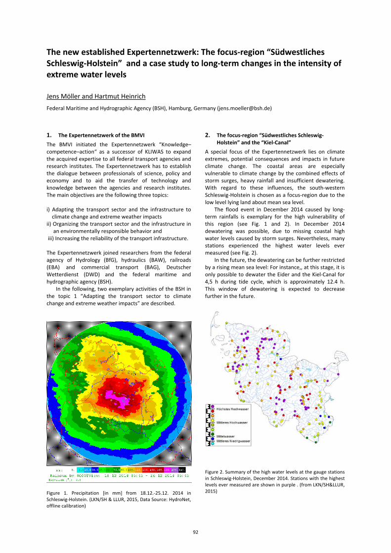
The new established Expertennetzwerk: The focus-region “Südwestliches Schleswig-Holstein” and a case study to long-term changes in the intensity of extreme water levels

Jens Möller and Hartmut Heinrich

Federal Maritime and Hydrographic Agency (BSH), Hamburg, Germany (jens.moeller@bsh.de)

1. The Expertennetzwerk of the BMVI The BMVI initiated the Expertennetzwerk “Knowledge–competence–action“ as a successor of KLIWAS to expand the acquired expertise to all federal transport agencies and research institutes. The Expertennetzwerk has to establish the dialogue between professionals of science, policy and economy and to aid the transfer of technology and knowledge between the agencies and research institutes. The main objectives are the following three topics: i) Adapting the transport sector and the infrastructure to climate change and extreme weather impacts ii) Organizing the transport sector and the infrastructure in an environmentally responsible behavior and iii) Increasing the reliability of the transport infrastructure. The Expertennetzwerk joined researchers from the federal agency of Hydrology (BfG), hydraulics (BAW), railroads (EBA) and commercial transport (BAG), Deutscher Wetterdienst (DWD) and the federal maritime and hydrographic agency (BSH).

In the following, two exemplary activities of the BSH in the topic 1 “Adapting the transport sector to climate change and extreme weather impacts” are described.

Figure 1. Precipitation [in mm] from 18.12.-25.12. 2014 in Schleswig-Holstein. (LKN/SH & LLUR, 2015, Data Source: HydroNet, offline calibration)

2. The focus-region “Südwestliches Schleswig-Holstein” and the “Kiel-Canal”

A special focus of the Expertennetzwerk lies on climate extremes, potential consequences and impacts in future climate change. The coastal areas are especially vulnerable to climate change by the combined effects of storm surges, heavy rainfall and insufficient dewatering. With regard to these influences, the south-western Schleswig-Holstein is chosen as a focus-region due to the low level lying land about mean sea level.

The flood event in December 2014 caused by long-term rainfalls is exemplary for the high vulnerability of this region (see Fig. 1 and 2). In December 2014 dewatering was possible, due to missing coastal high water levels caused by storm surges. Nevertheless, many stations experienced the highest water levels ever measured (see Fig. 2).

In the future, the dewatering can be further restricted by a rising mean sea level: For instance,, at this stage, it is only possible to dewater the Eider and the Kiel-Canal for 4,5 h during tide cycle, which is approximately 12.4 h. This window of dewatering is expected to decrease further in the future.

Figure 2. Summary of the high water levels at the gauge stations in Schleswig-Holstein, December 2014. Stations with the highest levels ever measured are shown in purple . (from LKN/SH&LLUR, 2015)

92

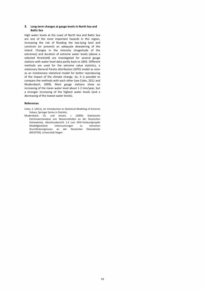
3. Long-term changes at gauge levels in North Sea and Baltic Sea

High water levels at the coast of North Sea and Baltic Sea are one of the most important hazards in this region, increasing the risk of flooding the low-lying land and constrain (or prevent) an adequate dewatering of the inland. Changes in the intensity (magnitude of the extremes) and duration of extreme water levels (above a selected threshold) are investigated for several gauge stations with water level data partly back to 1843. Different methods are used for the extreme value statistics, a stationary General Pareto distribution (GPD) model as soon as an instationary statistical model for better reproducing of the impact of the climate change. So, it is possible to compare the methods with each other (see Coles, 2011 and Mudersbach, 2009). Most gauge stations show an increasing of the mean water level about 1-2 mm/year, but a stronger increasing of the highest water levels (and a decreasing of the lowest water levels). References

Coles, S. (2011), An Introduction to Statistical Modeling of Extreme Values, Springer Series in Statistic.

Mudersbach, Ch. und Jensen, J. (2009): Statistische Extremwertanalyse von Wasserständen an der Deutschen Ostseeküste, Abschlussbericht 1.4 zum KFKI-Verbundprojekt Modellgestützte Untersuchungen zu extremen Sturmflutereignissen an der Deutschen Ostseeküste (MUSTOK), Universität Siegen

93

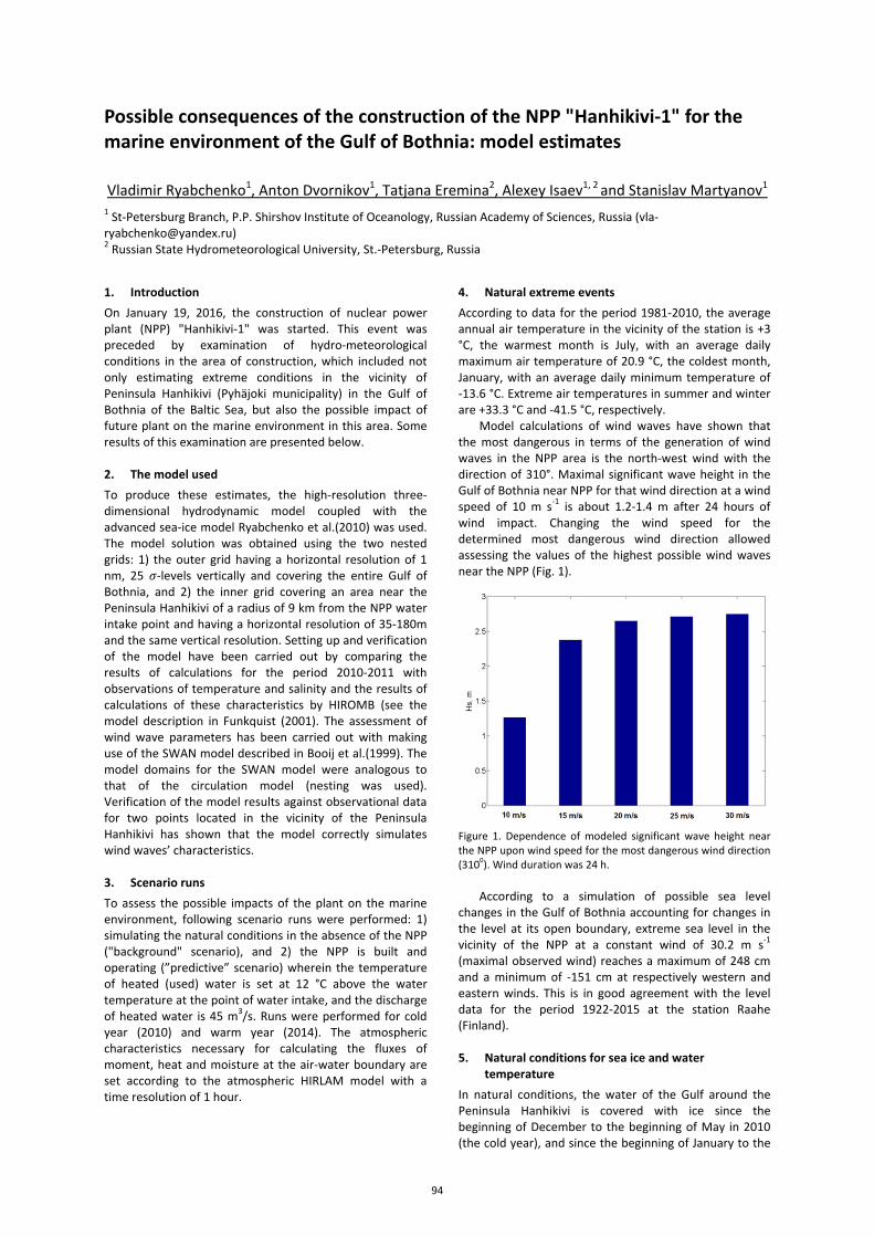
Possible consequences of the construction of the NPP "Hanhikivi-1" for the marine environment of the Gulf of Bothnia: model estimates

Vladimir Ryabchenko1, Anton Dvornikov1, Tatjana Eremina2, Alexey Isaev1, 2 and Stanislav Martyanov1 1 St-Petersburg Branch, P.P. Shirshov Institute of Oceanology, Russian Academy of Sciences, Russia (vla-ryabchenko@yandex.ru) 2 Russian State Hydrometeorological University, St.-Petersburg, Russia

1. Introduction On January 19, 2016, the construction of nuclear power plant (NPP) "Hanhikivi-1" was started. This event was preceded by examination of hydro-meteorological conditions in the area of construction, which included not only estimating extreme conditions in the vicinity of Peninsula Hanhikivi (Pyhäjoki municipality) in the Gulf of Bothnia of the Baltic Sea, but also the possible impact of future plant on the marine environment in this area. Some results of this examination are presented below. 2. The model used To produce these estimates, the high-resolution three-dimensional hydrodynamic model coupled with the advanced sea-ice model Ryabchenko et al.(2010) was used. The model solution was obtained using the two nested grids: 1) the outer grid having a horizontal resolution of 1 nm, 25 -levels vertically and covering the entire Gulf of Bothnia, and 2) the inner grid covering an area near the Peninsula Hanhikivi of a radius of 9 km from the NPP water intake point and having a horizontal resolution of 35-180m and the same vertical resolution. Setting up and verification of the model have been carried out by comparing the results of calculations for the period 2010-2011 with observations of temperature and salinity and the results of calculations of these characteristics by HIROMB (see the model description in Funkquist (2001). The assessment of wind wave parameters has been carried out with making use of the SWAN model described in Booij et al.(1999). The model domains for the SWAN model were analogous to that of the circulation model (nesting was used). Verification of the model results against observational data for two points located in the vicinity of the Peninsula Hanhikivi has shown that the model correctly simulates wind waves’ characteristics. 3. Scenario runs To assess the possible impacts of the plant on the marine environment, following scenario runs were performed: 1) simulating the natural conditions in the absence of the NPP ("background" scenario), and 2) the NPP is built and operating (”predictive” scenario) wherein the temperature of heated (used) water is set at 12 °C above the water temperature at the point of water intake, and the discharge of heated water is 45 m3/s. Runs were performed for cold year (2010) and warm year (2014). The atmospheric characteristics necessary for calculating the fluxes of moment, heat and moisture at the air-water boundary are set according to the atmospheric HIRLAM model with a time resolution of 1 hour.

4. Natural extreme events According to data for the period 1981-2010, the average annual air temperature in the vicinity of the station is +3 °C, the warmest month is July, with an average daily maximum air temperature of 20.9 °C, the coldest month, January, with an average daily minimum temperature of -13.6 °C. Extreme air temperatures in summer and winter are +33.3 °C and -41.5 °C, respectively.

Model calculations of wind waves have shown that the most dangerous in terms of the generation of wind waves in the NPP area is the north-west wind with the direction of 310°. Maximal significant wave height in the Gulf of Bothnia near NPP for that wind direction at a wind speed of 10 m s-1 is about 1.2-1.4 m after 24 hours of wind impact. Changing the wind speed for the determined most dangerous wind direction allowed assessing the values of the highest possible wind waves near the NPP (Fig. 1).

Figure 1. Dependence of modeled significant wave height near the NPP upon wind speed for the most dangerous wind direction (3100). Wind duration was 24 h.

According to a simulation of possible sea level changes in the Gulf of Bothnia accounting for changes in the level at its open boundary, extreme sea level in the vicinity of the NPP at a constant wind of 30.2 m s-1 (maximal observed wind) reaches a maximum of 248 cm and a minimum of -151 cm at respectively western and eastern winds. This is in good agreement with the level data for the period 1922-2015 at the station Raahe (Finland). 5. Natural conditions for sea ice and water

temperature In natural conditions, the water of the Gulf around the Peninsula Hanhikivi is covered with ice since the beginning of December to the beginning of May in 2010 (the cold year), and since the beginning of January to the

94

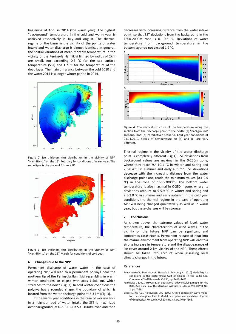
beginning of April in 2014 (the warm year). The highest ”background” temperature in the cold and warm year is achieved respectively in July and August. The thermal regime of the basin in the vicinity of the points of water intake and water discharge is almost identical. In general, the spatial variations of mean monthly temperature in the vicinity of the Peninsula Hanhikivi limited by radius of 2km are small, not exceeding 0.6 °C for the sea surface temperature (SST) and 1.2 °C for the temperature of the deep layer. The main difference between the cold 2010 and the warm 2014 is a longer winter period in 2014.

Figure 2. Ice thickness (m) distribution in the vicinity of NPP "Hanhikivi-1” on the 15th February for conditions of warm year. The red ellipse is the place of future NPP.

Figure 3. Ice thickness (m) distribution in the vicinity of NPP "Hanhikivi-1” on the 15th March for conditions of cold year. 6. Changes due to the NPP Permanent discharge of warm water in the case of operating NPP will lead to a permanent polynya near the northern tip of the Peninsula Hanhikivi resembling in warm winter conditions an ellipse with axes 1.5х6 km, which stretches to the north (Fig. 2). In cold winter conditions the polynya has a rounded shape, the boundary of which is located from the water discharge point at 2-3 km (Fig. 3).

In the warm year conditions in the case of working NPP in a neighborhood of water intake the SST is maximized over background (at 0.7-1.4°C) in 500-1000m zone and then

decreases with increasing distance from the water intake point, so that SST deviations from the background in the 1500-2000m zone is 0.1-0.6 °C. Deviations of water temperature from background temperature in the bottom layer do not exceed 1.2 °C. a

b

Figure 4. The vertical structure of the temperature along the section from the discharge point to the north: (a) “background” scenario, and (b) “predictive” scenario. Cold year conditions of 04.04.2010. Scales of temperature on (a) and (b) are very different.

Thermal regime in the vicinity of the water discharge point is completely different (Fig.4). SST deviations from background values are maximal in the 0-250m zone, where they reach 9.4-10.1 °C in winter and spring and 7.3-8.4 °C in summer and early autumn. SST deviations decrease with the increasing distance from the water discharge point and reach the minimum values (0.1-0.5 °C) in the zone of 1500-2000m. The bottom water temperature is also maximal in 0-250m zone, where its deviations amount to 5-5.9 °C in winter and spring and 2.5-3.0 °C in summer and early autumn. In the cold year conditions the thermal regime in the case of operating APP will being changed qualitatively as well as in warm year, but these changes will be stronger. 7. Conclusions As shown above, the extreme values of level, water temperature, the characteristics of wind waves in the vicinity of the future NPP can be significant and sometimes catastrophic. Permanent release of heat into the marine environment from operating NPP will lead to a strong increase in temperature and the disappearance of ice cover around 2 km vicinity of the NPP. These effects should be taken into account when assessing local climate changes in the future. References

Ryabchenko V., Dvornikov A., Haapala J., Myrberg K. (2010) Modelling ice conditions in the easternmost Gulf of Finland in the Baltic Sea. Continental Shelf Research, Vol.30, pp. 1458–1471

Funkquist L. (2001) HIROMB, an operational eddy-resolving model for the Baltic Sea Bulletin of the Maritime Institute in Gdansk, Vol. XXVIII, No. 2, pp. 7-16.

Booij N., Ris R.C., Holthuijsen L.H. (1999) A third-generation wave model for coastal regions, Part 1. Model description and validation. Journal of Geophysical Research, Vol.104, No.C4, pp.7649-7666.

95

Projected lengthening of spring cereals growing season in Estonia and accompanying high impact events of elevated temperatures around heading

Triin Saue1,2, Lauri Jauhiainen3, Jüri Kadaja1 and Pirjo Peltonen-Sainio3 1 Estonian Crop Research Institute, Saku, Estonia (triin.saue@etki.ee) 2 Marine Systems Institute of Tallinn Technical University, Tallinn, Estonia 3Natural Resources Institute Finland, Jokioinen, Finland

1. Introduction Climate change is already affecting agriculture, with effects unevenly distributed across the world. Future climate warming will likely negatively affect crop production in low latitudes, while in northern latitudes, including the Baltic Sea area, the initial effect is projected to increase crop yields , mostly due to the lengthening of the presently too short growing period. In Estonia there has already been general tendency towards an earlier onset of the climatic seasons in the vernal half of the year (Tarand et al., 2013), which has lead farmers to earlier sowing of several crops.

From the other side, an increase in temperature will speed up crop development, which may have an adverse effect on productivity of cereals. In addition, high temperatures will affect assimilation, which impact depends on the particular crop's demands and phase of development.

In this paper, we examine both aspects: further lengthening of the growing period with accompanying increase in accumulated temperatures, and the probability and impact of high temperatures on grain yields under present and predicted climate conditions.

2. Data and methodology To obtain temperature data for the middle (2040–2070) and end (2070–2100) of the century, monthly mean temperature change for Estonia, derived from EURO-CORDEX multi-model projections (Luhamaa et al., 2014) were applied. Two scenarios – moderate RCP 4.5 and high-warming 8.5 were included. To produce future daily data, projected monthly mean temperature changes were added to de-trended and centered to 1985 series of daily temperatures of 1965-2013 of the 11 Estonian stations. This way, the future set of temperatures is comparable to the reference period of 1971–2000. Such application represents historical temperature variability and structure, possible changes in variability are not included.

These sets of the weather data were employed to derive the information about the changes in thermal growing period – the time of year when the mean daily temperature exceeds permanently 5 ºC. Thus the length of the vegetation period was calculated by the dates of the permanent increase of daily mean temperature above 5 °C in spring and drop below 5 °C in autumn. The part of mean daily temperature above 5 °C is defined by its influence as the effective temperature for crops, expressed as growing degree days (GDD).

To assess the influence of elevated temperatures on spring cereals (barley, wheat, oats) yield, sowing and ripening dates from 5 locations of Estonian Variety Testing Centre (2000–2010) were used, while phenological data (1971–2000) was included from Finnish field experiments to determine long-term mean accumulated temperatures

between different development phases. Univariate regression analysis was performed to test crops responses to elevated temperatures under Estonian current climatic conditions.

Present and future probability of daily mean temperatures ≥21 and 22 °C in the period 1 week before to 2 weeks after heading were calculated for two climatologically different Estonian locations: Jõhvi and Võru. To calculate heading dates, we used fixed effective temperature sums above threshold 5 °C, so it was typical for a cultivar with an average growing time. The duration of vegetative phase in cereals was set to 145 GDD, from there to heading, 314, 358, and 315 GDD was required for barley, oat, and wheat, respectively (Peltonen-Sainio et al. 2015). In these calculations, we used 1. May as a reference sowing day for all crop species. In studying future conditions, the sowing time was also shifted earlier. 3. Results The current length of growing season is 130–250 days in Estonia. Vegetation starts earliest in southern part of the country and latest in western and northern coast, where influence of the Baltic Sea tends to delay the arrival of spring. The end of vegetation period occurs earlier on the mainland and later on islands and coastal area. During the last 50-year period vegetation period has prolonged on average by 3 weeks by trend, mostly due to the earlier spring. Vegetation starts about 20 days earlier in south and 12–13 days earlier in north. Also, a significant increase in growing period accumulated temperatures has taken place.

The projected increase in temperatures suggests that growing season will lengthen forwards together with continuing increase in accumulated temperatures (Table 1). Stronger warming is predicted by RCP 8.5 scenario and for the end of the century. For both scenarios and target periods, the highest warming is projected in spring and winter months, further influencing the start of the vegetation period. The most substantial lengthening is projected to western coast, where we can also expect winters, when temperature does not drop below 5°C. While until now, the lengthening of the vegetation period has mostly occurred in the spring, for the future, the end of thermal vegetation period is also shifting significantly, from middle-October to early or late November, even to early December in western coast and islands. However, the lengthening of the growing season in the autumn is not likely to support growth as effectively as lengthening in the spring, because of insufficient light intensity and short days. Differences between emission scenarios

96

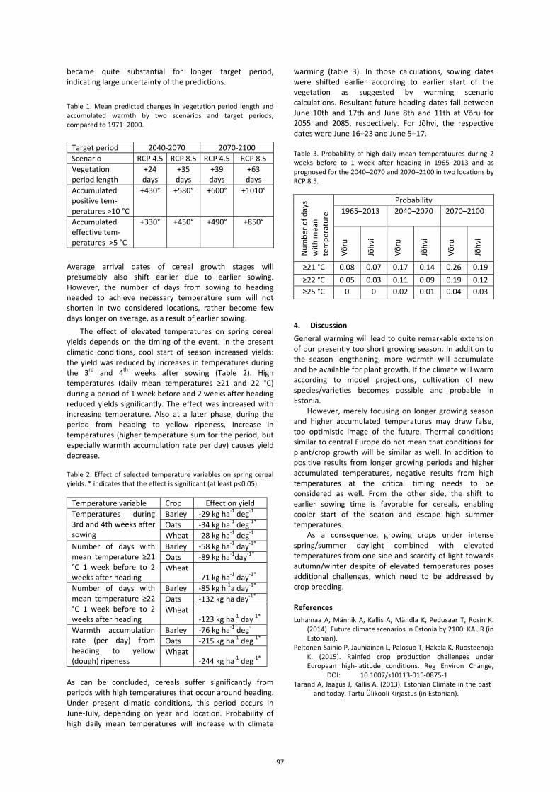
became quite substantial for longer target period, indicating large uncertainty of the predictions.

Table 1. Mean predicted changes in vegetation period length and accumulated warmth by two scenarios and target periods, compared to 1971–2000.

Target period 2040-2070 2070-2100 Scenario RCP 4.5 RCP 8.5 RCP 4.5 RCP 8.5 Vegetation period length

+24 days

+35 days

+39 days

+63 days

Accumulated positive tem-peratures >10 °C

+430° +580° +600° +1010°

Accumulated effective tem-peratures >5 °C

+330° +450° +490° +850°

Average arrival dates of cereal growth stages will presumably also shift earlier due to earlier sowing. However, the number of days from sowing to heading needed to achieve necessary temperature sum will not shorten in two considered locations, rather become few days longer on average, as a result of earlier sowing.

The effect of elevated temperatures on spring cereal yields depends on the timing of the event. In the present climatic conditions, cool start of season increased yields: the yield was reduced by increases in temperatures during the 3rd and 4th weeks after sowing (Table 2). High temperatures (daily mean temperatures ≥21 and 22 °C) during a period of 1 week before and 2 weeks after heading reduced yields significantly. The effect was increased with increasing temperature. Also at a later phase, during the period from heading to yellow ripeness, increase in temperatures (higher temperature sum for the period, but especially warmth accumulation rate per day) causes yield decrease. Table 2. Effect of selected temperature variables on spring cereal yields. * indicates that the effect is significant (at least p<0.05).

Temperature variable Crop Effect on yield Temperatures during 3rd and 4th weeks after sowing

Barley -29 kg ha-1 deg-1 Oats -34 kg ha-1 deg-1* Wheat -28 kg ha-1 deg-1

Number of days with mean temperature ≥21 °C 1 week before to 2 weeks after heading

Barley -58 kg ha-1 day-1* Oats -89 kg ha-1day-1* Wheat

-71 kg ha-1 day-1* Number of days with mean temperature ≥22 °C 1 week before to 2 weeks after heading

Barley -85 kg h-1a day-1* Oats -132 kg ha day-1* Wheat

-123 kg ha-1 day-1* Warmth accumulation rate (per day) from heading to yellow (dough) ripeness

Barley -76 kg ha-1 deg- Oats -215 kg ha-1 deg-1* Wheat

-244 kg ha-1 deg-1* As can be concluded, cereals suffer significantly from periods with high temperatures that occur around heading. Under present climatic conditions, this period occurs in June-July, depending on year and location. Probability of high daily mean temperatures will increase with climate

warming (table 3). In those calculations, sowing dates were shifted earlier according to earlier start of the vegetation as suggested by warming scenario calculations. Resultant future heading dates fall between June 10th and 17th and June 8th and 11th at Võru for 2055 and 2085, respectively. For Jõhvi, the respective dates were June 16–23 and June 5–17. Table 3. Probability of high daily mean temperatuures during 2 weeks before to 1 week after heading in 1965–2013 and as prognosed for the 2040–2070 and 2070–2100 in two locations by RCP 8.5.

Num

ber o

f day

s w

ith m

ean

tem

pera

ture

Probability 1965–2013

2040–2070

2070–2100

Võru

Jõhv

i

Võru

Jõhv

i

Võru

Jõhv

i

≥21 °C 0.08 0.07 0.17 0.14 0.26 0.19 ≥22 °C 0.05 0.03 0.11 0.09 0.19 0.12 ≥25 °C 0 0 0.02 0.01 0.04 0.03

4. Discussion General warming will lead to quite remarkable extension of our presently too short growing season. In addition to the season lengthening, more warmth will accumulate and be available for plant growth. If the climate will warm according to model projections, cultivation of new species/varieties becomes possible and probable in Estonia.

However, merely focusing on longer growing season and higher accumulated temperatures may draw false, too optimistic image of the future. Thermal conditions similar to central Europe do not mean that conditions for plant/crop growth will be similar as well. In addition to positive results from longer growing periods and higher accumulated temperatures, negative results from high temperatures at the critical timing needs to be considered as well. From the other side, the shift to earlier sowing time is favorable for cereals, enabling cooler start of the season and escape high summer temperatures.

As a consequence, growing crops under intense spring/summer daylight combined with elevated temperatures from one side and scarcity of light towards autumn/winter despite of elevated temperatures poses additional challenges, which need to be addressed by crop breeding. References Luhamaa A, Männik A, Kallis A, Mändla K, Pedusaar T, Rosin K.

(2014). Future climate scenarios in Estonia by 2100. KAUR (in Estonian).

Peltonen-Sainio P, Jauhiainen L, Palosuo T, Hakala K, Ruosteenoja K. (2015). Rainfed crop production challenges under European high-latitude conditions. Reg Environ Change, DOI: 10.1007/s10113-015-0875-1

Tarand A, Jaagus J, Kallis A. (2013). Estonian Climate in the past and today. Tartu Ülikooli Kirjastus (in Estonian).

97

Analysis of severe weather using WRF model

Virmantas Šmatas1,2, Gintautas Stankūnavičius1 1 Vilnius University, Vilnius, Lithuania (virmantas.smatas@gf.stud.vu.lt, gintas.stankunavicius@gf.vu.lt) 2 The Nature Research Centre, Vilnius, Lihuania (virmantas.smatas@geo.lt)

1. Introduction Severe weather almost always includes hazardous conditions produced by thunderstorms, including heavy rains, squalls with damaging winds, large hail, sometimes tornadoes, flash flooding etc. Such type of weather very often develops within squall lines. A squall line represents a linear system of convective cells with a continuous, well developed gust front at the leading edge. Squall lines usually develop in unstable very warm air, typically ahead of a cold front, in the extended warm sector in summer season. The weather of squall lines has a very strong daily cycle as well as convective clouds: most hazardous weather is expected in the afternoon hours while decay of intensity – in early morning. Squall lines classified as short living meso-scale meteorological phenomena type and therefore its weather is still hardly predictable.

Nowadays, such phenomena attract attention of atmospheric scientists, meteorologists and decision makers due to its potential threat to human life and property. The main prediction tool for the short time forecasts is numerical weather prediction (NWP) models. As additional techniques there could be applied nowcasting and statistical methods. The main issue of NWP is the fact that its spatio-temporal resolution is too low for this type of phenomena and the large uncertainty of predicted variables such as wind gusts, precipitation rate, instability indices and others.

Number of squalls in Lithuania has significantly increased during the summers of 2010-2014. Two major and most intensive convective storms are analysed in this study. The first storm which possibly was a supercell storm has formed over Lithuania in the night of August8, 2010, and caused considerable losses of property and a widespread damage to the environment. Also, during this storm four people have died. The second convective storm started in 29th of July, 2012. During that event a cluster of convective storms brought damages to the western part of Lithuania. This case also was chosen for analysis due to the rarely observed devastating wind gust speed exceeding 36 m/s in the Nida meteorology station. Both storms were poorly predicted at their appearance time by HIRLAM model at the Lithuanian Hydrometeorological service, that’s why we used the Weather Research and Forecasting (WRF) model for selected events predictability analysis. 2. Synoptic situation Both analysed events are related to the tropical origin air invasion into the Baltic region from the south. Large scale wave pattern: the deep trough over Northwestern and Central Europe and the stationary ridge – over Northeastern Europe (2010 year case) as well as the trough over Northwestern and Western Europe and the ridge over the Eastern Europe (2012 year case) favors such air invasion. The tongue of the warm, moist and unstable air with equivalent potential temperature (θe) exceeding 60 –

64 °C at 850 hPa level was entrained from the eastern Balkans (2010) and from Central Europe (2012). In the first the case the highest θe values were located over the southern and western parts of Lithuania while in the second case – over the westernmost edge of Lithuania. The main difference between those two events was that in the case of 2010 the mesoscale convective low has developed over Lithuania while in case of 2012 the sub-synoptic scale low has developed on the frontal wave over Baltic Sea. Therefore the last event had its strongest intensity in the afternoon while the first – at midnight. Both events were intensified by the development of instability (squall) lines preceding the approaching cold front. Other natural circumstances also favor the development of strong squalls. Cloud tops overshooting the tropopause, precipitable water exceeding 45 mm and the Convective Available Potential Energy (CAPE) being higher than 600 J/kg and Lifted index (LI) being lower than -3 together with the low level jet (strongest wind around 850 hPa level) and the wind shear of 20 m/s were observed during the case of 2010 according to Kaunas sounding data Grusaite (2011). Also, fortunately the sounding station lies within the main path of squalls and the sounding time corresponds to the beginning of widespread squalls. The Kaunas sounding data for the case of 2012 did not match either the severe weather location (more than 200 km eastward) nor its time (sounding was done 12 hours earlier). However according to the parcel trajectory in this case the Kaliningrad sounding data shows CAPE around 1400 J/kg, LI – lower than -4, precipitable water – 41 mm and the mean mixed layer mixing ratio – higher than 15 g/kg. The intensive development of the severe weather on local scale in both cases was rather forced by approaching the local scale positive pressure tendency zone behind the instability line.

3. Methods and model setup All simulations were carried out using the NMM core of Weather Research and Forecasting (WRF) system. The WRF NMM is a fully compressible, limited area, non-hydrostatic mesoscale model with a hydrostatic option to choose. Main model features - model terrain following hybrid sigma-pressure vertical coordinate and it uses staggering Arakawa E-grid Janjic (1984, 2003).

In the present simulation, model was integrated for 24 hours. Domain 1 and domain 2 were used with 12 km and 4 km horizontal resolutions, respectively. Vertical model structure was increased up to 70 sigma-pressure levels. Model initial conditions were taken from CFSR and CFSRR reanalysis with a resolution of 0,5 ° and 38 km grid, respectively. The model has been tested using the Kain-Fritch and modified Tiedtke schemes for cumulus parameterization and WSM 6 class graupel scheme for microphysics. The Kain-Fritch scheme already showed

98

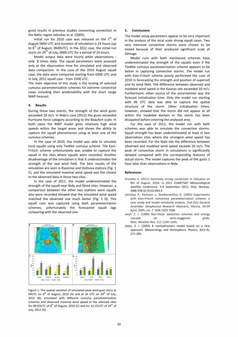
good results in previous studies concerning convection in the Baltic region Jalinskas et al. (2005).

Initial run for 2010 case was released on the 7th of August 0600 UTC and duration of simulation is 24 hours (up to 8th of August, 0600UTC). In the 2012 case, the initial run starts on 29th of July, 0000 UTC for a period of 24 hours.

Model output data were hourly while observations - only 8 times daily. The squall parameters were assessed only at the observation time for simulated and observed data comparison. In the case of the 2010 August squall case, the data were compared starting from 0300 UTC and in July, 2012 squall case - from 1500 UTC. The main objective of this study is the testing of selected cumulus parameterization schemes for extreme convective cases including their predictability with the short range NWP forecast. 4. Results During these two events, the strength of the wind gusts exceeded 20 m/s. In Nida‘s case (2012) the gusts exceeded hurricane force category according to the Beaufort scale. In both cases the NWP model gives relatively high wind speeds within the target areas and shows the ability to capture the squall phenomenon using at least one of the cumulus schemes.

In the case of 2010, the model was able to simulate local squalls using only Tiedtke cumulus scheme. The Kain-Fritsch scheme unfortunately was unable to capture the squall in the sites where squalls were recorded. Another disadvantage of the simulation is that it underestimates the strength of the real wind field. The best results of the simulation are seen in Raseiniai and Dotnuva stations (Fig. 1 C), and the simulated maximal wind speed was the closest to the observed data in those two sites.

In the case of 2012, the model underestimated the strength of the squall near Nida and Šilutė sites. However, a comparison between the other two stations were squalls also were recorded showed that the simulated wind speed matched the observed one much better (Fig. 1 D). This squall case was captured using both parameterization schemes, unfortunately the forecasted squall lags comparing with the observed one.

Figure 1. The spatial variation of simulated peak wind gust (m/s) at 00UTC on 8th of August, 2010 (A) and at 16 UTC on 29th of July, 2012 (B); simulated with different cumulus parameterization schemes and observed maximal wind speed at the selected sites for 00-03UTC of 8th of August, 2010 (C) and for 12-15UTC of 29th of July, 2012 (D).

5. Conclusions The model setup parameters appear to be very important in the analysis of the local scale strong squall cases. Two very intensive convective storms were chosen to be tested because of their produced significant scale of damage.

Model runs with both mentioned schemes have underestimated the strength of the squalls even if the Tiedtke cumulus parameterization scheme appears to be better in capturing convective storms. The model run with Kain-Fritsch scheme poorly performed the case of 2010 in forecasting the strength and position of supercell and its wind field. The difference between observed and modeled wind speed in the Kaunas site exceeded 10 m/s. Furthermore, other source of the uncertainties was the forecast initialization time. Only the model run starting with 06 UTC data was able to capture the spatial structure of the storm. Other initialization times, however, showed that the storm did not appear at all within the modeled domain or the storm has been dissipated before entering the analysed area.

For the case of 2012, the model run with both schemes was able to simulate the convective storms. Squall strength has been underestimated at least in two observation sites where the strongest wind speed has been recorded. For the Nida site the difference between observed and modeled wind speed exceeds 20 m/s. The peak of convective storm in simulations is significantly delayed compared with the corresponding features of actual storm. The model captures the peak of the gusts 1 hour later than observations in Nida References

Grusaite V. (2011) Extremely strong convection in Lithuania on 8th of August, 2010. In 2011 EUMETSAT Meteorological Satellite Conference. 5-9 September 2011, Oslo, Norway. ISBN 978-92-9110-093-4

Jalinskas P., Karlsson J., Stankūnavičius G. (2005) Experiments with Kain-Fritsch convective parameterization scheme: a case study and model sensitivity analysis. 2nd EGU General Assembly: Geophysical Research Abstracts, Vienna, 24-29 April, 2005, vol. 7. ISSN 1029-7006

Janjic Z. I. (1984) Non-linear advection schemes and energy cascade on semi-staggered grids; Mon. Weather Rev. 112 1234–1245.

Janjic, Z. I. (2003) A nonhydrostatic model based on a new approach. Meteorology and Atmospheric Physics, 82(1-4), 271-285.

99

Extreme weather condition of the northern-eastern part of Poland and their relationship with atmospheric oscillation

Zbigniew Szwejkowski1, Ewa Dragańska1, Iwona Cymes1, Stanisław Suchecki2 1 Department of Water, Climate, and Environmental Management, University of Warmia and Mazury in Olsztyn, Poland (szwzbig@uwm.edu.pl), 2 Institute of Meteorology and Water Management. Regional Meteorological Station in Olsztyn, Poland 1. Introduction Studies into global climatic changes are very important and the results are interesting not only to researchers, but also to the general public. However, a need to study climate on a regional and meso-climate scale can be also demonstrated, resulting from the fact that this is where the important climate properties (from the point of view of shaping the environment and human needs) are established. Therefore, for practical reasons, it is important to specify the properties characterizing the climate of the region as well as its possible changes, since only due to such knowledge can key decisions be taken concerning preventive and adjustment activities. Such knowledge, in the context of the needs presented, is more important than information on general indicators of global climate changes Anders et al (2014), Arnell (2004). This work presents extreme weather conditions occurring in recent years in the area, which indicate the influences of the Baltic basin, in conjunction with the global climatic changes and the global circulation and also with the local conditions, typical for the lake districts. 2. Methods and materials The present study analyses data covering years 1981-2010, from six meteorological stations of the Institute of Meteorology and Water Management located within an area determined by coordinates between latitude 53º N and the northern border of Poland and between longitude 19° E to the eastern border of Poland. It is a part of area formed during upper glacial period in Europe, up to 100 km from Baltic sea coast. Measurement sequences of first- and second-order weather stations (synoptic stations), carrying out twenty-four-hour measurements and observations, were used as the basic analytical material.

The obtained data sets were analysed in terms of their homogeneity and representative character, in reflecting the actual state. This analysis ensured correctness of statistical operations performed on the sets [VIZI et al. 2000/2001]. The following aggregated values were taken on the consideration:

• the mean annual and monthly air temperature • the minimum annual and monthy air temperature • the maximum annual and monthly air temperature • daily sum of precipitation

The study contains analysis of extreme thermal conditions, minima and maxima, frost and cold and heat waves, tendencies for their changes, and the impact of global circulation factors in the form of correlation with values of the NAO (North Atlantic Oscillation) Index were determined and were the aim of the project. Also, some human biometeorological factors were determinated.

3. Results The mean annual temperature in the region in the thirty-year period under analysis was 7.2°C. The statistical analysis revealed the existence of a temperature growth trend of almost 0.026°C a year. January was found to be the coldest month of the year (-3.3°C), and July – the warmest (17.5°C). The minimum temperature decreased from the west (4.0°C) to the east of the region (2.5°C) with increasing distance from the shoreline of the Baltic Sea. The maximum temperature changed towards the same direction. The heat waves occurred relatively rarely, but revealed a weak trend increase in the number of days with temperatures exceeding 30 degrees Celsius. The biggest heat waves occurred in 1994. The heat waves were not recorded in areas close to the Baltic Sea. The coldest winter periods occurred in the first and second decade of the period with the temperatures below -30 oC. Frosts were a feature of the climate very dependent on local conditions, a calming effect on the number of listed early spring frosts and late autumn frosts had the presence of lakes.

The highest precipitation sums occurred in the last decade, namely, in 2001-2010. Despite this, the statistical analysis did not demonstrate any significant tendency of precipitation change over thirty years. Annual sums of precipitation in the region were characterized by mean values ranging from 550 mm in the south west to 650 mm in the north west. The area mean for the thirty-year period was 600 mm. The trend of changes of annual extreme precipitation, especially daily sums, although negative, was statistically insignificant.

The basic answer to the question what is the main factor shaping thermal conditions in the region indicate point out the global circulating system in the area mid-latitudes. In our case the link is particularly strong in the winter. The data for this period show very high rates of the R2 describing relation – mean monthly temperature - NAO index - the value calculated and presented by NOAA. The characteristic situation is in the last quarter of the year where in October and December R2 values are clearly high, while in November, absolutely insignificant. In wormer period of the year stronger influence of Baltic Sea is also very clear. References Anders I., Stagl J., Auer I., Pavlik D., 2014, Climate Change in

Central and Eastern Europe. Chapter 2, [in:] Managing Protected Areas in Central and Eastern Europe Under Climate Change..Springer XXV: 17-30

Arnell N. W., 2004, Climate change and global water resources: SRES emissions and socio-economic cenarios. Global Environmental Change (14), Elsevier: 31–52

100

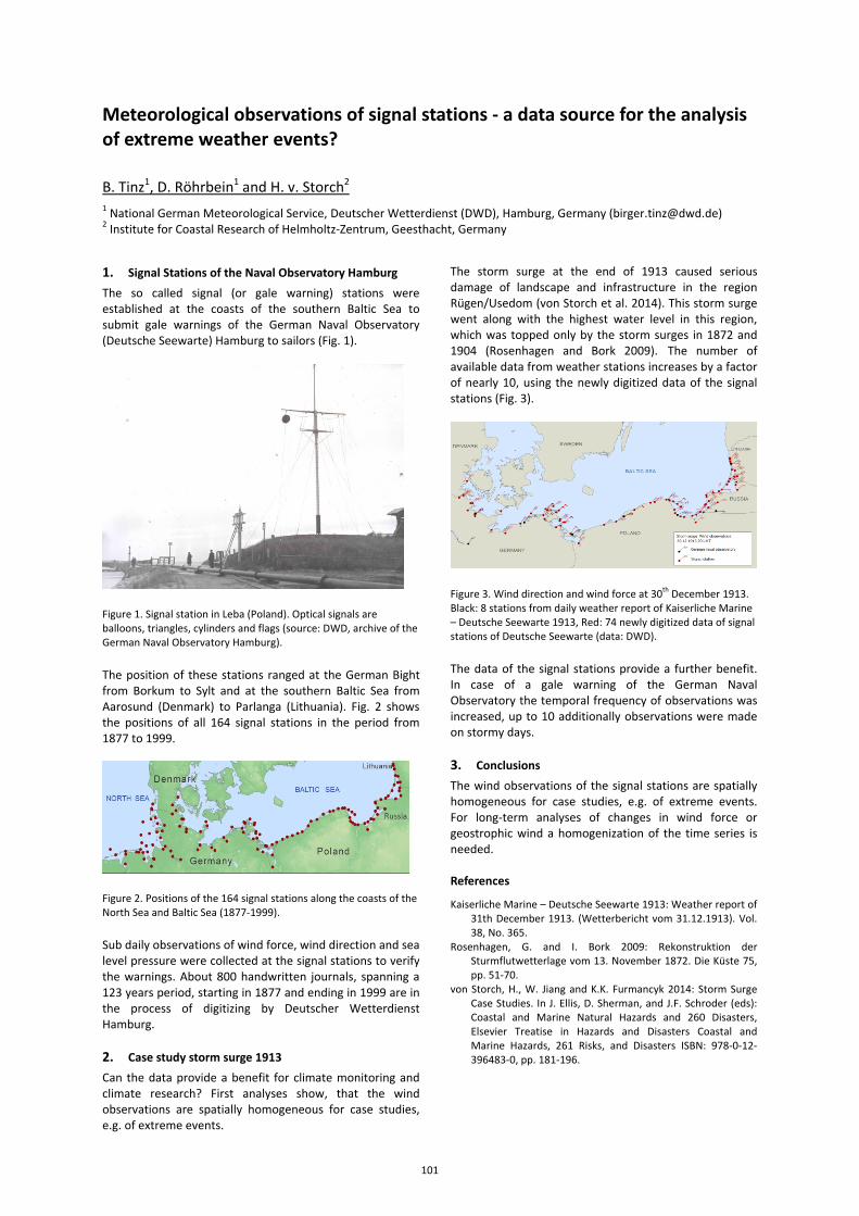
Meteorological observations of signal stations - a data source for the analysis of extreme weather events?

B. Tinz1, D. Röhrbein1 and H. v. Storch2

1 National German Meteorological Service, Deutscher Wetterdienst (DWD), Hamburg, Germany (birger.tinz@dwd.de)

2 Institute for Coastal Research of Helmholtz-Zentrum, Geesthacht, Germany

1. Signal Stations of the Naval Observatory Hamburg The so called signal (or gale warning) stations were established at the coasts of the southern Baltic Sea to submit gale warnings of the German Naval Observatory (Deutsche Seewarte) Hamburg to sailors (Fig. 1).

Figure 1. Signal station in Leba (Poland). Optical signals are balloons, triangles, cylinders and flags (source: DWD, archive of the German Naval Observatory Hamburg).

The position of these stations ranged at the German Bight from Borkum to Sylt and at the southern Baltic Sea from Aarosund (Denmark) to Parlanga (Lithuania). Fig. 2 shows the positions of all 164 signal stations in the period from 1877 to 1999.

Figure 2. Positions of the 164 signal stations along the coasts of the North Sea and Baltic Sea (1877-1999).

Sub daily observations of wind force, wind direction and sea level pressure were collected at the signal stations to verify the warnings. About 800 handwritten journals, spanning a 123 years period, starting in 1877 and ending in 1999 are in the process of digitizing by Deutscher Wetterdienst Hamburg.

2. Case study storm surge 1913 Can the data provide a benefit for climate monitoring and climate research? First analyses show, that the wind observations are spatially homogeneous for case studies, e.g. of extreme events.

The storm surge at the end of 1913 caused serious damage of landscape and infrastructure in the region Rügen/Usedom (von Storch et al. 2014). This storm surge went along with the highest water level in this region, which was topped only by the storm surges in 1872 and 1904 (Rosenhagen and Bork 2009). The number of available data from weather stations increases by a factor of nearly 10, using the newly digitized data of the signal stations (Fig. 3).

Figure 3. Wind direction and wind force at 30th December 1913. Black: 8 stations from daily weather report of Kaiserliche Marine – Deutsche Seewarte 1913, Red: 74 newly digitized data of signal stations of Deutsche Seewarte (data: DWD).

The data of the signal stations provide a further benefit. In case of a gale warning of the German Naval Observatory the temporal frequency of observations was increased, up to 10 additionally observations were made on stormy days. 3. Conclusions The wind observations of the signal stations are spatially homogeneous for case studies, e.g. of extreme events. For long-term analyses of changes in wind force or geostrophic wind a homogenization of the time series is needed.

References

Kaiserliche Marine – Deutsche Seewarte 1913: Weather report of 31th December 1913. (Wetterbericht vom 31.12.1913). Vol. 38, No. 365.

Rosenhagen, G. and I. Bork 2009: Rekonstruktion der Sturmflutwetterlage vom 13. November 1872. Die Küste 75, pp. 51-70.

von Storch, H., W. Jiang and K.K. Furmancyk 2014: Storm Surge Case Studies. In J. Ellis, D. Sherman, and J.F. Schroder (eds): Coastal and Marine Natural Hazards and 260 Disasters, Elsevier Treatise in Hazards and Disasters Coastal and Marine Hazards, 261 Risks, and Disasters ISBN: 978-0-12-396483-0, pp. 181-196.

101

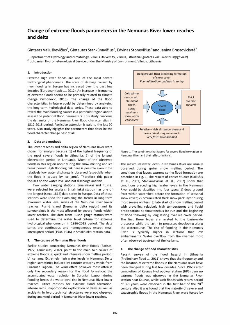
Change of extreme floods parameters in the Nemunas River lower reaches and delta

Gintaras Valiuškevičius1, Gintautas Stankūnavičius1, Edvinas Stonevičius1 and Janina Brastovickytė2 1 Department of Hydrology and climatology, Vilnius University, Vilnius, Lithuania (gintaras.valiuskevicius@gf.vu.lt) 2 Lithuanian Hydrometeorological Service under the Ministry of Environment, Vilnius, Lithuania

1. Introduction Extreme high river floods are one of the most severe hydrological phenomena. The scale of damage caused by river flooding in Europe has increased over the past few decades (European topic ..., 2012). An increase in frequency of extreme floods seems to be primarily related to climate change (Simonovic, 2013). The change of the flood characteristics in future could be determined by analyzing the long-term hydrological data series. These data able to reveal the main flooding causes in a particular region and to assess the potential flood parameters. This study concerns the dynamics of the Nemunas River flood characteristics in 1812-2015 period. Particular attention is paid to the last 90 years. Also study higlights the parameters that describe the flood character change best of all. 2. Data and methods The lower reaches and delta region of Nemunas River were chosen for analysis because: 1) of the highest frequency of the most severe floods in Lithuania; 2) of the longest observation period in Lithuania. Most of the observed floods in this region occur during the snow melting and ice break period. High flooding risk here is possible even if the relatively low water discharge is observed (especially when the flood is caused by ice jams). Therefore this paper focuses on the water level and not discharge analysis.

Two water gauging stations (Smalininkai and Rusnė) were selected for analysis. Smalininkai station has one of the longest (since 1812) data series in Europe. Data of these stations were used for examining the trends in long-term maximum water level series of the Nemunas River lower reaches. Rusnė Island (Nemunas delta region) and its surroundings is the most affected by severe floods within lower reaches. The data from Rusnė gauge station were used to determine the water level criteria for extreme hydrological phenomenon in 1926-2015 period. The data series are continuous and homogeneous except small interrupted period (1944-1946) in Smalininkai station data. 3. The causes of Nemunas River floods Earlier studies concerning Nemunas river floods (Barisas, 1977; Taminskas, 2002), point to the main two causes of extreme floods: a) quick and intensive snow melting period; b) ice jams. Extremely high water levels in Nemunas Delta region sometimes induced by counter-westerly winds from Curonian Lagoon. The wind effect however most often is only the secondary reason for the flood formation: the accumulated water repletion in Curonian Lagoon during flooding forces the water level rise in Nemunas River lower reaches. Other reasons for extreme flood formation: intense rains, inappropriate exploitation of dams as well as accidents in hydrotechnical structures were not observed during analysed period in Nemunas River lower reaches.

Figure 1. The conditions that favors for severe flood formation in Nemunas River and their effect (in italic).

The maximum water levels in Nemunas River are usually observed during spring snow melting period. The conditions that favors extreme spring flood formation are described in Fig. 1. The results of earlier studies (Gailiušis et al., 2001; Stankūnavičius et al., 2007) show that conditions preceding high water levels in the Nemunas River could be classified into four types: 1) deep ground frost within watershed before the formation of seasonal snow cover; 2) accumulated thick snow pack layer during most severe winters; 3) late start of snow melting period with prevailing relatively high temperatures and liquid precipitation; 4) simultaneous ice run and the beginning of flood following by long lasting river ice cover period. The first three types are related to the basin-wide processes while the last - to processes developing along the watercourse. The risk of flooding in the Nemunas River is typically higher in sections that low embankments. Water overflow from the riverbed most often observed upstream of the ice jams.

4. The change of flood characteristics Recent survey of the flood hazard in Lithuania (Preliminary flood ..., 2011) shows that the frequency and the location of extreme floods in the Nemunas River have been changed during last few decades. Since 1960s after completion of Kaunas Hydropower station (HPS) dam no extreme floods was observed in the Nemunas River section near Kaunas, while such floods with return period of 3-8 years were observed in the first half of the 20th century. Also it was found that the majority of severe and catastrophic floods in the Nemunas River were forced by

Deep ground frost preceding formation of snow cover

Poor infiltration condition in spring

Relatively high air temperature and heavy rain during snow melt.

Very fast snowpack melt

Thick river ice. Ice jams

Cold winter season with

abundant snow. Large

maximum snow water equivalent

Severe flood

102

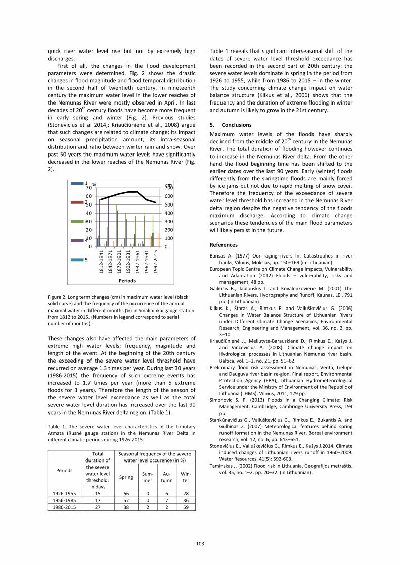
quick river water level rise but not by extremely high discharges.

First of all, the changes in the flood development parameters were determined. Fig. 2 shows the drastic changes in flood magnitude and flood temporal distribution in the second half of twentieth century. In nineteenth century the maximum water level in the lower reaches of the Nemunas River were mostly observed in April. In last decades of 20th century floods have become more frequent in early spring and winter (Fig. 2). Previous studies (Stonevicius et al 2014,; Kriaučiūnienė et al., 2008) argue that such changes are related to climate change: its impact on seasonal precipitation amount, its intra-seasonal distribution and ratio between winter rain and snow. Over past 50 years the maximum water levels have significantly decreased in the lower reaches of the Nemunas River (Fig. 2).

Figure 2. Long term changes (cm) in maximum water level (black solid curve) and the frequency of the occurrence of the annual maximal water in different months (%) in Smalininkai gauge station from 1812 to 2015. (Numbers in legend correspond to serial number of months).

These changes also have affected the main parameters of extreme high water levels: frequency, magnitude and length of the event. At the beginning of the 20th century the exceeding of the severe water level threshold have recurred on average 1.3 times per year. During last 30 years (1986-2015) the frequency of such extreme events has increased to 1.7 times per year (more than 5 extreme floods for 3 years). Therefore the length of the season of the severe water level exceedance as well as the total severe water level duration has increased over the last 90 years in the Nemunas River delta region. (Table 1).

Table 1. The severe water level characteristics in the tributary Atmata (Rusnė gauge station) in the Nemunas River Delta in different climatic periods during 1926-2015.

Periods

Total duration of the severe water level threshold,

in days

Seasonal frequency of the severewater level occurence (in %)

Spring Sum-mer

Au-tumn

Win-ter

1926-1955 15 66 0 6 281956-1985 17 57 0 7 361986-2015 27 38 2 2 59

Table 1 reveals that significant interseasonal shift of the dates of severe water level threshold exceedance has been recorded in the second part of 20th century: the severe water levels dominate in spring in the period from 1926 to 1955, while from 1986 to 2015 – in the winter. The study concerning climate change impact on water balance structure (Kilkus et al., 2006) shows that the frequency and the duration of extreme flooding in winter and autumn is likely to grow in the 21st century. 5. Conclusions Maximum water levels of the floods have sharply declined from the middle of 20th century in the Nemunas River. The total duration of flooding however continues to increase in the Nemunas River delta. From the other hand the flood beginning time has been shifted to the earlier dates over the last 90 years. Early (winter) floods differently from the springtime floods are mainly forced by ice jams but not due to rapid melting of snow cover. Therefore the frequency of the exceedance of severe water level threshold has increased in the Nemunas River delta region despite the negative tendency of the floods maximum discharge. According to climate change scenarios these tendencies of the main flood parameters will likely persist in the future. References

Barisas A. (1977) Our raging rivers In: Catastrophes in river banks, Vilnius, Mokslas, pp. 150–169 (in Lithuanian).

European Topic Centre on Climate Change Impacts, Vulnerability and Adaptation (2012) Floods – vulnerability, risks and management, 48 pp.

Gailiušis B., Jablonskis J. and Kovalenkovienė M. (2001) The Lithuanian Rivers. Hydrography and Runoff, Kaunas, LEI, 791 pp. (in Lithuanian).

Kilkus K., Štaras A., Rimkus E. and Valiuškevičius G. (2006) Changes in Water Balance Structure of Lithuanian Rivers under Different Climate Change Scenarios, Environmental Research, Engineering and Management, vol. 36, no. 2, pp. 3–10.

Kriaučiūnienė J., Meilutytė-Barauskienė D., Rimkus E., Kažys J. and Vincevičius A. (2008). Climate change impact on Hydrological processes in Lithuanian Nemunas river basin. Baltica, vol. 1–2, no. 21, pp. 51–62.

Preliminary flood risk assessment in Nemunas, Venta, Lielupė and Dauguva river basin re-gion. Final report, Environmental Protection Agency (EPA), Lithuanian Hydrometeorological Service under the Ministry of Environment of the Republic of Lithuania (LHMS), Vilnius, 2011, 129 pp.

Simonovic S. P. (2013) Floods in a Changing Climate: Risk Management, Cambridge, Cambridge University Press, 194 pp.

Stankūnavičius G., Valiuškevičius G., Rimkus E., Bukantis A. and Gulbinas Z. (2007) Meteorological features behind spring runoff formation in the Nemunas River, Boreal environment research, vol. 12, no. 6, pp. 643–651.

Stonevičius E., Valiuškevičius G., Rimkus E., Kažys J.2014. Climate induced changes of Lithuanian rivers runoff in 1960–2009. Water Resources, 41(5): 592-603.

Taminskas J. (2002) Flood risk in Lithuania, Geografijos metraštis, vol. 35, no. 1–2, pp. 20–32. (in Lithuanian).

0100200300400500600700

010203040506070

1812

-184

1

1842

-187

1

1872

-190

1

1902

-193

1

1932

-196

1

1962

-199

1

1992

-201

5

cm%

Periods

1

2

3

4

5

103

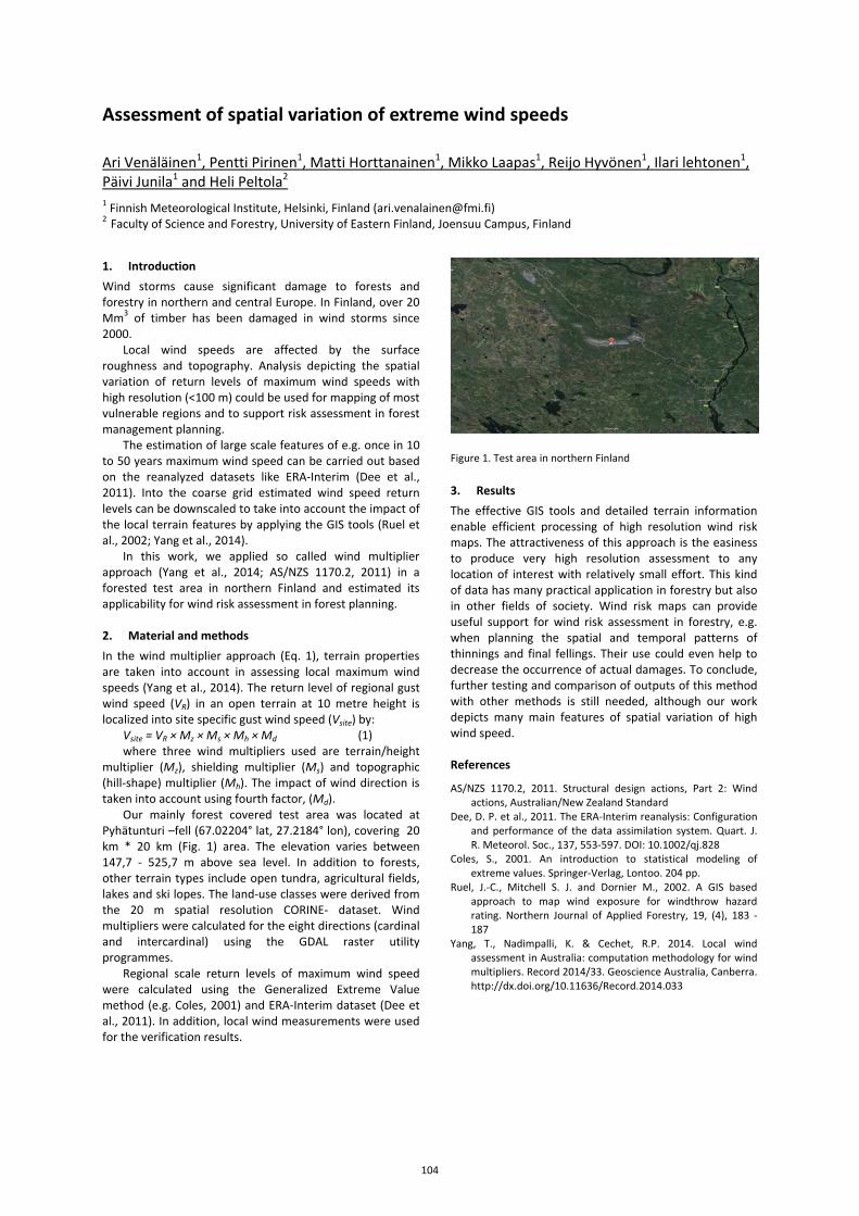
Assessment of spatial variation of extreme wind speeds

Ari Venäläinen1, Pentti Pirinen1, Matti Horttanainen1, Mikko Laapas1, Reijo Hyvönen1, Ilari lehtonen1, Päivi Junila1 and Heli Peltola2 1 Finnish Meteorological Institute, Helsinki, Finland (ari.venalainen@fmi.fi) 2 Faculty of Science and Forestry, University of Eastern Finland, Joensuu Campus, Finland

1. Introduction Wind storms cause significant damage to forests and forestry in northern and central Europe. In Finland, over 20 Mm3 of timber has been damaged in wind storms since 2000.

Local wind speeds are affected by the surface roughness and topography. Analysis depicting the spatial variation of return levels of maximum wind speeds with high resolution (<100 m) could be used for mapping of most vulnerable regions and to support risk assessment in forest management planning.

The estimation of large scale features of e.g. once in 10 to 50 years maximum wind speed can be carried out based on the reanalyzed datasets like ERA-Interim (Dee et al., 2011). Into the coarse grid estimated wind speed return levels can be downscaled to take into account the impact of the local terrain features by applying the GIS tools (Ruel et al., 2002; Yang et al., 2014).

In this work, we applied so called wind multiplier approach (Yang et al., 2014; AS/NZS 1170.2, 2011) in a forested test area in northern Finland and estimated its applicability for wind risk assessment in forest planning. 2. Material and methods In the wind multiplier approach (Eq. 1), terrain properties are taken into account in assessing local maximum wind speeds (Yang et al., 2014). The return level of regional gust wind speed (VR) in an open terrain at 10 metre height is localized into site specific gust wind speed (Vsite) by:

Vsite = VR × Mz × Ms × Mh × Md (1) where three wind multipliers used are terrain/height

multiplier (Mz), shielding multiplier (Ms) and topographic (hill-shape) multiplier (Mh). The impact of wind direction is taken into account using fourth factor, (Md).

Our mainly forest covered test area was located at Pyhätunturi –fell (67.02204° lat, 27.2184° lon), covering 20 km * 20 km (Fig. 1) area. The elevation varies between 147,7 - 525,7 m above sea level. In addition to forests, other terrain types include open tundra, agricultural fields, lakes and ski lopes. The land-use classes were derived from the 20 m spatial resolution CORINE- dataset. Wind multipliers were calculated for the eight directions (cardinal and intercardinal) using the GDAL raster utility programmes.

Regional scale return levels of maximum wind speed were calculated using the Generalized Extreme Value method (e.g. Coles, 2001) and ERA-Interim dataset (Dee et al., 2011). In addition, local wind measurements were used for the verification results.

Figure 1. Test area in northern Finland

3. Results The effective GIS tools and detailed terrain information enable efficient processing of high resolution wind risk maps. The attractiveness of this approach is the easiness to produce very high resolution assessment to any location of interest with relatively small effort. This kind of data has many practical application in forestry but also in other fields of society. Wind risk maps can provide useful support for wind risk assessment in forestry, e.g. when planning the spatial and temporal patterns of thinnings and final fellings. Their use could even help to decrease the occurrence of actual damages. To conclude, further testing and comparison of outputs of this method with other methods is still needed, although our work depicts many main features of spatial variation of high wind speed. References

AS/NZS 1170.2, 2011. Structural design actions, Part 2: Wind actions, Australian/New Zealand Standard

Dee, D. P. et al., 2011. The ERA-Interim reanalysis: Configuration and performance of the data assimilation system. Quart. J. R. Meteorol. Soc., 137, 553-597. DOI: 10.1002/qj.828

Coles, S., 2001. An introduction to statistical modeling of extreme values. Springer-Verlag, Lontoo. 204 pp.

Ruel, J.-C., Mitchell S. J. and Dornier M., 2002. A GIS based approach to map wind exposure for windthrow hazard rating. Northern Journal of Applied Forestry, 19, (4), 183 - 187

Yang, T., Nadimpalli, K. & Cechet, R.P. 2014. Local wind assessment in Australia: computation methodology for wind multipliers. Record 2014/33. Geoscience Australia, Canberra. http://dx.doi.org/10.11636/Record.2014.033

104

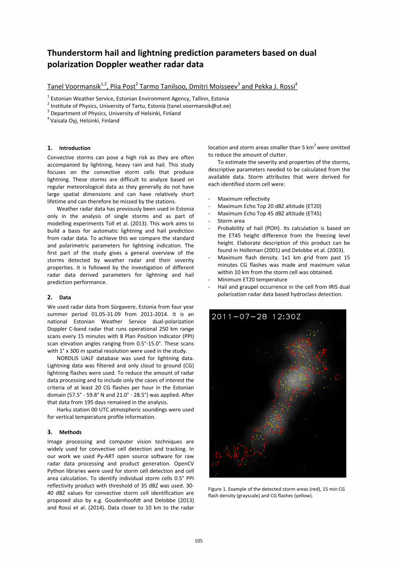
Thunderstorm hail and lightning prediction parameters based on dual polarization Doppler weather radar data

Tanel Voormansik1,2, Piia Post2 Tarmo Tanilsoo, Dmitri Moisseev3 and Pekka J. Rossi4

1 Estonian Weather Service, Estonian Environment Agency, Tallinn, Estonia 2 Institute of Physics, University of Tartu, Estonia (tanel.voormansik@ut.ee) 3 Department of Physics, University of Helsinki, Finland 4 Vaisala Oyj, Helsinki, Finland

1. Introduction Convective storms can pose a high risk as they are often accompanied by lightning, heavy rain and hail. This study focuses on the convective storm cells that produce lightning. These storms are difficult to analyze based on regular meteorological data as they generally do not have large spatial dimensions and can have relatively short lifetime and can therefore be missed by the stations.

Weather radar data has previously been used in Estonia only in the analysis of single storms and as part of modelling experiments Toll et al. (2013). This work aims to build a basis for automatic lightning and hail prediction from radar data. To achieve this we compare the standard and polarimetric parameters for lightning indication. The first part of the study gives a general overview of the storms detected by weather radar and their severity properties. It is followed by the investigation of different radar data derived parameters for lightning and hail prediction performance. 2. Data We used radar data from Sürgavere, Estonia from four year summer period 01.05-31.09 from 2011-2014. It is an national Estonian Weather Service dual-polarization Doppler C-band radar that runs operational 250 km range scans every 15 minutes with 8 Plan Position Indicator (PPI) scan elevation angles ranging from 0.5°-15.0°. These scans with 1° x 300 m spatial resolution were used in the study.

NORDLIS UALF database was used for lightning data. Lightning data was filtered and only cloud to ground (CG) lightning flashes were used. To reduce the amount of radar data processing and to include only the cases of interest the criteria of at least 20 CG flashes per hour in the Estonian domain (57.5° - 59.8° N and 21.0° - 28.5°) was applied. After that data from 195 days remained in the analysis.

Harku station 00 UTC atmospheric soundings were used for vertical temperature profile information. 3. Methods Image processing and computer vision techniques are widely used for convective cell detection and tracking. In our work we used Py-ART open source software for raw radar data processing and product generation. OpenCV Python libraries were used for storm cell detection and cell area calculation. To identify individual storm cells 0.5° PPI reflectivity product with threshold of 35 dBZ was used. 30-40 dBZ values for convective storm cell identification are proposed also by e.g. Goudenhoofdt and Delobbe (2013) and Rossi et al. (2014). Data closer to 10 km to the radar

location and storm areas smaller than 5 km2 were omitted to reduce the amount of clutter.

To estimate the severity and properties of the storms, descriptive parameters needed to be calculated from the available data. Storm attributes that were derived for each identified storm cell were:

- Maximum reflectivity - Maximum Echo Top 20 dBZ altitude (ET20) - Maximum Echo Top 45 dBZ altitude (ET45) - Storm area - Probability of hail (POH). Its calculation is based on

the ET45 height difference from the freezing level height. Elaborate description of this product can be found in Holleman (2001) and Delobbe et al. (2003).

- Maximum flash density. 1x1 km grid from past 15 minutes CG flashes was made and maximum value within 10 km from the storm cell was obtained.

- Minimum ET20 temperature - Hail and graupel occurrence in the cell from IRIS dual

polarization radar data based hydroclass detection.

Figure 1. Example of the detected storm areas (red), 15 min CG flash density (grayscale) and CG flashes (yellow).

105

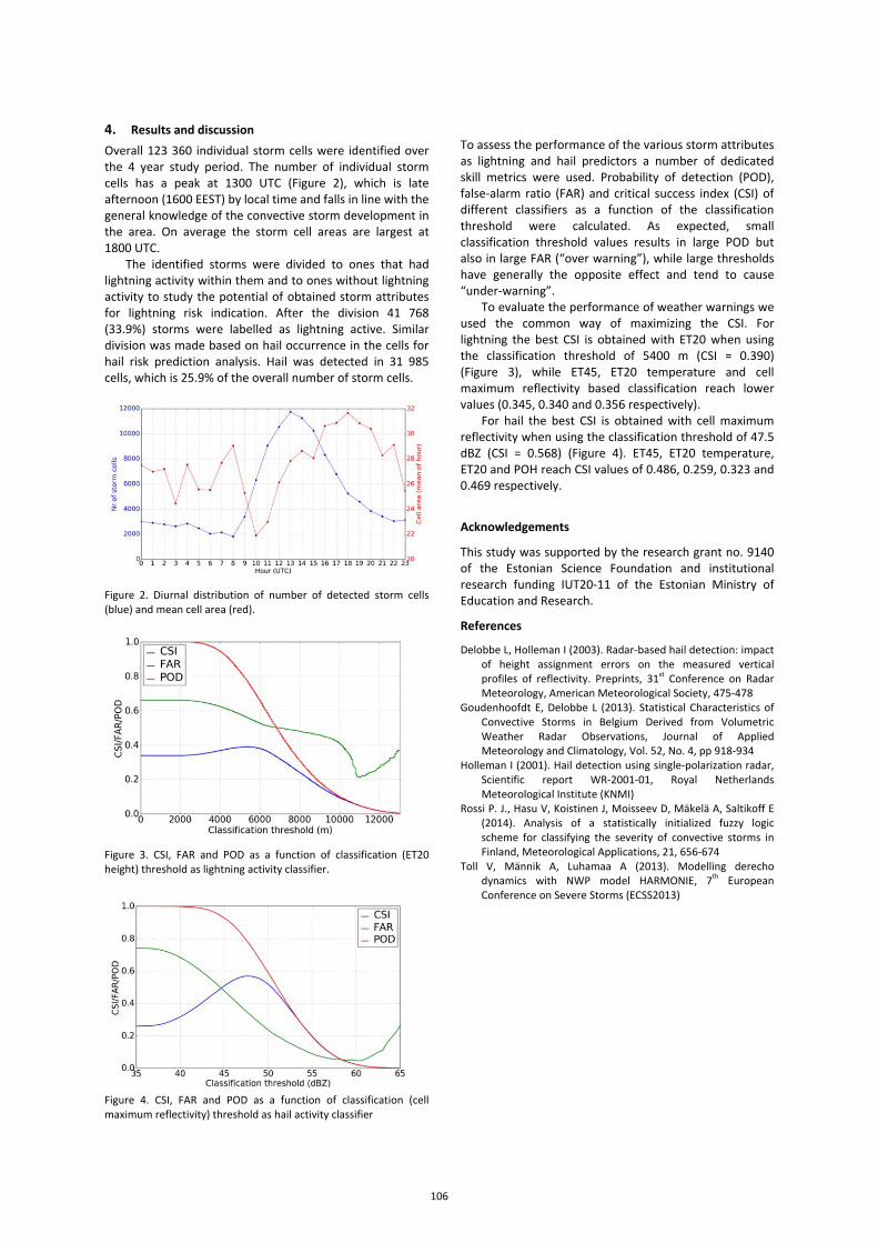
4. Results and discussion Overall 123 360 individual storm cells were identified over the 4 year study period. The number of individual storm cells has a peak at 1300 UTC (Figure 2), which is late afternoon (1600 EEST) by local time and falls in line with the general knowledge of the convective storm development in the area. On average the storm cell areas are largest at 1800 UTC.

The identified storms were divided to ones that had lightning activity within them and to ones without lightning activity to study the potential of obtained storm attributes for lightning risk indication. After the division 41 768 (33.9%) storms were labelled as lightning active. Similar division was made based on hail occurrence in the cells for hail risk prediction analysis. Hail was detected in 31 985 cells, which is 25.9% of the overall number of storm cells.

Figure 2. Diurnal distribution of number of detected storm cells (blue) and mean cell area (red).

Figure 3. CSI, FAR and POD as a function of classification (ET20 height) threshold as lightning activity classifier.

Figure 4. CSI, FAR and POD as a function of classification (cell maximum reflectivity) threshold as hail activity classifier

To assess the performance of the various storm attributes as lightning and hail predictors a number of dedicated skill metrics were used. Probability of detection (POD), false-alarm ratio (FAR) and critical success index (CSI) of different classifiers as a function of the classification threshold were calculated. As expected, small classification threshold values results in large POD but also in large FAR (“over warning”), while large thresholds have generally the opposite effect and tend to cause “under-warning”.

To evaluate the performance of weather warnings we used the common way of maximizing the CSI. For lightning the best CSI is obtained with ET20 when using the classification threshold of 5400 m (CSI = 0.390) (Figure 3), while ET45, ET20 temperature and cell maximum reflectivity based classification reach lower values (0.345, 0.340 and 0.356 respectively).

For hail the best CSI is obtained with cell maximum reflectivity when using the classification threshold of 47.5 dBZ (CSI = 0.568) (Figure 4). ET45, ET20 temperature, ET20 and POH reach CSI values of 0.486, 0.259, 0.323 and 0.469 respectively.

Acknowledgements

This study was supported by the research grant no. 9140 of the Estonian Science Foundation and institutional research funding IUT20-11 of the Estonian Ministry of Education and Research.

References

Delobbe L, Holleman I (2003). Radar-based hail detection: impact of height assignment errors on the measured vertical profiles of reflectivity. Preprints, 31st Conference on Radar Meteorology, American Meteorological Society, 475-478

Goudenhoofdt E, Delobbe L (2013). Statistical Characteristics of Convective Storms in Belgium Derived from Volumetric Weather Radar Observations, Journal of Applied Meteorology and Climatology, Vol. 52, No. 4, pp 918-934

Holleman I (2001). Hail detection using single-polarization radar, Scientific report WR-2001-01, Royal Netherlands Meteorological Institute (KNMI)

Rossi P. J., Hasu V, Koistinen J, Moisseev D, Mäkelä A, Saltikoff E (2014). Analysis of a statistically initialized fuzzy logic scheme for classifying the severity of convective storms in Finland, Meteorological Applications, 21, 656-674

Toll V, Männik A, Luhamaa A (2013). Modelling derecho dynamics with NWP model HARMONIE, 7th European Conference on Severe Storms (ECSS2013)

106

Drivers of precipitation extremes in different spatial and temporal scales

Joanna Wibig and Piotr Piotrowski

Department of Meteorology and Climatology, University of Lodz, Lodz, Poland (zameteo@uni.lodz.pl)

1. Introduction At the moment there is a consensus concerning global warming and the increase of temperature in the Central Europe and Poland (BACC II Author Team, 2015). However much less is known about the hydrological resposne to the warming trend. Changes in precipitation totals, occurrence of prolonged wet and dry spells and precipitation extremes can exert strong impact on humans, ecosystems and economy. The paper will concentrate on precipitation extremes. They can be influenced by warming in numerous ways: • Higher water holding capacity of the air cause that

more water is available for precipitation, so the extreme rain can be more intense (Allan 2012).

• Warmer air and higher water holding capacity can increase the amount of precipitable water in the atmosphere changing precipitation totals and extremes in different temporal scales (hourly, daily, monthly, seasonal) (Lenderink & van Mejigaard 2008).

• Warming is not uniform over the World. It can cause changes in atmospheric circulation modificating the transport of moisture.

• Warmer surface can enhance the instability increasing the percentage of convective precipitation.

• Warming enhances local evaporation changing the amount of water available for ptrecipitation (Held & Soden 2006).

The aim of the paper is to identify potentially important factors driving precipitation extremes in the southern part of Baltic Sea Region. 2. Data and methods To identify extreme precipitation drivers in short temporal scales hourly and daily precipitation totals and temperatures from several stations in Poland and Germany will be used. The methodology proposed by Lenderink & Mejigaard (2010) will be used. The precipitation data will be divided into subseries relative to temperature. Distributions to these binned datas will be fitted and compared, in particular their right tails.

To identify circulation influence on precipitation the water vapour fluxes and their trends will be analysed. The NCEP/NCAR reanalysis dataset will be used: wind components and specific humidity data from three geopotential levels: 850, 700 and 500 hPa from the period 1951-2015. Moisture transport will be assessed using the methodology proposed by Phillips & McGregor (2011) and its trend will be analysed and compared with precipitation totals in temporal scales ranging from days to seasons.

The vapour fluxes in days with extreme precipitation will be compared with the average ones separatelly for all seasons to check the impact of moisture transport on extreme precipitation.

The trial of the separation of precipitation into convective and frontal will be done with the method based on te one proposed by Karagiannidis et al. (2009) for Polish precipitatin stations. Then changes of the percentage one the convective precipitation in different months will be analysed. 3. Acknowledgements The work is supported by grant 2012/05/B/ST10/00945 founded by Polish National Science Centre. References

Allan RP (2012) The role ofwater vapour in earth’s energy flows, Surv. Geophys., DOI: 10.1007/s10712-011-9157-8

BACC II Author Team (2015) Second Assessment of Climate Change for the Baltic Sea Basin, Springer

Held IM, Soden BJ (2006) Robust responses of the hydrologicalcycle to global warming, J. Clim., Vol. 19, 5686-5699

Karagiannidis A, Karacostas T, Maheras P, Makrogiannis T (2009) trends and seasonality of extreme precipitation characteristics related to mid-latitude cyclones in Europe, Adv. in geosci., Vol. 20, 39-43

Lenderink G, van Mejigaard E (2008) Increase in hourly precipitation extreme beyond expectation from temperatutre changes, Nat. Geosci., Vol 1, 511-514

Lenderink G, van Mejigaard E (2010) Linking increases in hourly precipitation extremes to atmospheric temperature and moisture changes, Environ. Res. Lett., Vol. 5, DOI: 10.1088/ 1784-9326/5/2/025208

Phillips ID, McGregor GR (2001) Western European Water Flux – Southwest England Rainfall associations, Jour. of Hedrometeorol., Vol. 2, 505-524

107

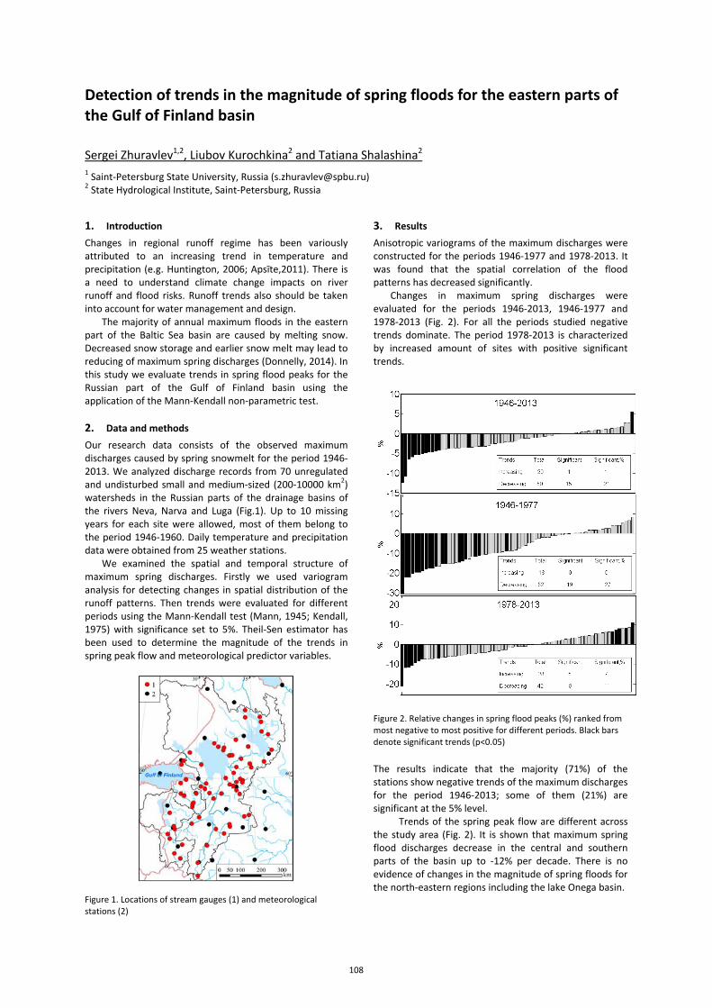
Detection of trends in the magnitude of spring floods for the eastern parts of the Gulf of Finland basin

Sergei Zhuravlev1,2, Liubov Kurochkina2 and Tatiana Shalashina2 1 Saint-Petersburg State University, Russia (s.zhuravlev@spbu.ru) 2 State Hydrological Institute, Saint-Petersburg, Russia

1. Introduction Changes in regional runoff regime has been variously attributed to an increasing trend in temperature and precipitation (e.g. Huntington, 2006; Apsīte,2011). There is a need to understand climate change impacts on river runoff and flood risks. Runoff trends also should be taken into account for water management and design.

The majority of annual maximum floods in the eastern part of the Baltic Sea basin are caused by melting snow. Decreased snow storage and earlier snow melt may lead to reducing of maximum spring discharges (Donnelly, 2014). In this study we evaluate trends in spring flood peaks for the Russian part of the Gulf of Finland basin using the application of the Mann-Kendall non-parametric test. 2. Data and methods Our research data consists of the observed maximum discharges caused by spring snowmelt for the period 1946-2013. We analyzed discharge records from 70 unregulated and undisturbed small and medium-sized (200-10000 km2) watersheds in the Russian parts of the drainage basins of the rivers Neva, Narva and Luga (Fig.1). Up to 10 missing years for each site were allowed, most of them belong to the period 1946-1960. Daily temperature and precipitation data were obtained from 25 weather stations.

We examined the spatial and temporal structure of maximum spring discharges. Firstly we used variogram analysis for detecting changes in spatial distribution of the runoff patterns. Then trends were evaluated for different periods using the Mann-Kendall test (Mann, 1945; Kendall, 1975) with significance set to 5%. Theil-Sen estimator has been used to determine the magnitude of the trends in spring peak flow and meteorological predictor variables.

Figure 1. Locations of stream gauges (1) and meteorological stations (2)

3. Results Anisotropic variograms of the maximum discharges were constructed for the periods 1946-1977 and 1978-2013. It was found that the spatial correlation of the flood patterns has decreased significantly.

Changes in maximum spring discharges were evaluated for the periods 1946-2013, 1946-1977 and 1978-2013 (Fig. 2). For all the periods studied negative trends dominate. The period 1978-2013 is characterized by increased amount of sites with positive significant trends.

Figure 2. Relative changes in spring flood peaks (%) ranked from most negative to most positive for different periods. Black bars denote significant trends (p<0.05)

The results indicate that the majority (71%) of the stations show negative trends of the maximum discharges for the period 1946-2013; some of them (21%) are significant at the 5% level.

Trends of the spring peak flow are different across the study area (Fig. 2). It is shown that maximum spring flood discharges decrease in the central and southern parts of the basin up to -12% per decade. There is no evidence of changes in the magnitude of spring floods for the north-eastern regions including the lake Onega basin.

108

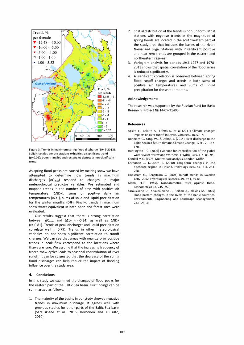
Figure 3. Trends in maximum spring flood discharge (1946-2013). Solid triangles denote stations exhibiting a significant trend (p<0.05); open triangles and rectangles denote a non-significant trend.

As spring flood peaks are caused by melting snow we have attempted to determine how trends in maximum discharges (ΔQmax) respond to changes in major meteorological predictor variables. We estimated and mapped trends in the number of days with positive air temperature (ΔND+), sums of positive daily air temperatures (ΔΣt+), sums of solid and liquid precipitation for the winter months (DJF). Finally, trends in maximum snow water equivalent in both open and forest sites were evaluated.

Our results suggest that there is strong correlation between ΔQmax and ΔΣt+ (r=-0.84) as well as ΔND+ (r=-0.81). Trends of peak discharges and liquid precipitation correlate well (r=0.79). Trends in other meteorological variables do not show significant correlation to runoff changes. We can see that areas with near zero or positive trends in peak flow correspond to the locations where thaws are rare. We assume that the increasing frequency of freeze-thaw cycles leads to seasonal redistribution of river runoff. It can be suggested that the decrease of the spring flood discharges can help reduce the impact of flooding influence over the study area. 4. Conclusions In this study we examined the changes of flood peaks for the eastern part of the Baltic Sea basin. Our findings can be summarized as follows. 1. The majority of the basins in our study showed negative

trends in maximum discharge. It agrees well with previous studies for other parts of the Baltic Sea basin (Sarauskiene et al., 2015; Korhonen and Kuusisto, 2010).

2. Spatial distribution of the trends is non-uniform. Most stations with negative trends in the magnitude of spring floods are located in the southwestern part of the study area that includes the basins of the rivers Narva and Luga. Stations with insignificant positive and near-zero trends are grouped in the eastern and northeastern regions.

3. Variogram analysis for periods 1946-1977 and 1978-2013 shows that spatial correlation of the flood series is reduced significantly.

4. A significant correlation is observed between spring flood runoff changes and trends in both sums of positive air temperatures and sums of liquid precipitation for the winter months.

Acknowledgements

The research was supported by the Russian Fund for Basic Research, Project № 14-05-31403.

References

Apsīte E., Bakute A., Elferts D. et al (2011) Climate changes impacts on river runoff in Latvia. Clim Res., 48, 57–71.

Donnelly, C., Yang, W., & Dahné, J. (2014) River discharge to the Baltic Sea in a future climate. Climatic Change, 122(1-2), 157-170.

Huntington T.G. (2006) Evidence for intensification of the global water cycle: review and synthesis. J Hydrol, 319, 1–4, 83–95.

Kendall M.G. (1975) Multivariate analysis. London: Griffin. Korhonen J., Kuusisto E. (2010) Long-term changes in the

discharge regime in Finland. Hydrology Res., 41, 3-4, 253-268.

Lindström G., Bergström S. (2004) Runoff trends in Sweden 1807–2002. Hydrological Sciences, 49, № 1, 69-83.

Mann, H.B. (1945). Nonparametric tests against trend. Econometrica 13, 245–259.

Sarauskiene D., Kriauciuniene J., Reihan A., Klavins M. (2015) Flood pattern changes in the rivers of the Baltic countries. Environmental Engineering and Landscape Management, 23.1, 28–38.

109

110

Topic D

Sea level dynamics, coastal morphology and erosion

Investigating sediment resuspension using combined optical and acoustic methods

Fred Buschmann1, Ants Erm1, Jaan Rebane2 and Madis Listak1,2 1 Marine Systems Institute, Tallinn University of Technology, Estonia (fred.buschmann@msi.ttu.ee) 2 Centre for Biorobotics, Tallinn University of Technology, Estonia

Tallinn Bay is located on the southern coast of the Gulf of Finland. The coastal zone covers multiple areas: Kakumäe Bay, Kopli Bay, Paljassaare Bay and Tallinn Bay minor. The Bays are shallow but deepen rapidly. The seabed is mostly muddy (aleurite) which changes to sand when moving towards the beach. Heavy anthropogenic pressure (especially high-speed ferry traffic) is putting the area under continuous stress causing sediment resuspension and shoreline erosion.

During period 2009 - 2015 in several places of the Bay two underwater cameras (one equipped with lasers for particle image velocimetry - PIV), acoustic Doppler velocimeter with turbidity sensor and wave pressure buoy were used. The aim of the measurements was to experimentally evaluate sediment resuspension and transport. Measurements involved recording underwater videos (for detecting resuspension and to calculate near-bottom velocity profiles, Figure 1), acoustic measurements gave timeseries of single point velocity (for calibrating the PIV camera). Parallel measurements involved taking sediment and water samples for laboratory analyses (grain size distribution and water sediment concentration). Background data was taken from coastal weather stations (wind) and measured using pressure based wave buoy, which was used to calculate wave parameters.

Figure 1. The start of sediment resuspension captured using PIV camera (near Tallinn harbour, depth 7 m, 01.08.2013 05:19:34 UTC+3). In conclusion the study gave a good overall picture about dominating forces influencing sediments. Critical shear velocity, that causes resuspension, was determined for different types of seabed. Also the dominating sediment transport directions were found. The seabed properties were compared with similar seabed type found by other authors (e.g. Young and Southard 1978, Kuhrts et al. 2004).

This study was made possible by the help and co-operation of Jaan Rebane and Madis Listak from the Centre for Biorobotics at Tallinn University of Technology. The research was funded by Estonian Environmental Investment Centre (project 609) and by grants 7000, 7283 and 9052 from Estonian Science Foundation.

References

Young, R.N., Southard, J.B., 1978. Erosion of fine-grained marine sediments: sea-floor and laboratory experiments. Geological Society of America Bulletin, 89, 663–672.

Kuhrts, C., Fennel, W., Seifert, T., 2004. Model studies of transport of sedimentary material in the western Baltic. Journal of Marine Systems, 52, 167-190.

111

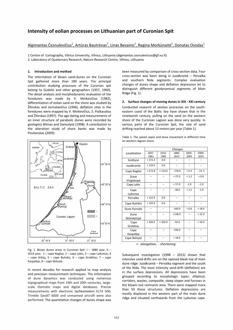
Intensity of eolian processes on Lithuanian part of Curonian Spit

Algimantas Česnulevičius1, Artūras Bautrėnas1, Linas Bevainis1, Regina Morkūnaitė2, Donatas Ovodas1

1 Centre of Cartography, Vilnius University, Vilnius, Lithuania (algimantas.cesnulevicius@gf.vu.lt) 2. Laboratory of Quaternary Research, Nature Research Centre, Vilnius, Lithuania

1. Introduction and method The information of blown sand-dunes on the Curonian Spit gathered more than 180 years. The principal contribution studying processes of the Curonian spit belong to Gudelis and other geographers (1957, 1960). The detail analysis and morphodynamic evaluation of the foredunes was made by V. Minkevičius (1982), differentiation of eolian sand on the shore was studied by Žilinskas and Jarmalavičius (1996), deflation sites in the foredunes were mapped by V. Minkevičius, S. Paškauskas and Žilinskas (1997). The age dating and measurements of an inner structure of parabolic dunes were recorded by geologists Bitinas and Damušytė (1998). A contribution to the alteration study of shore banks was made by Povilanskas (2009).

Fig. 1. Blown dunes areas in Curonian Spit: I – 1880 year, II – 2014 year, 1 – cape Nagliai, 2 – cape Lybis, 3 – cape Lydumas, 4 – cape Arklių, 5 – cape Bulvikis, 6 – cape Grobštas, 7 – cape Kaspalėja, 8 – cape Skilvytė.

In recent decades for research applied to map analysis and precision measurement techniques. The information of dune dynamics was conducted using numerous topographical maps from 19th and 20th centuries, large-scale thematic maps and digital databases. Precise measurements with electronic tacheometers ELTA 500; Trimble GeoXT 6000 and unmanned aircraft were also performed. The quantitative changes of dunes shape was

been measured by comparison of cross-section data. Four cross-section was been doing in Juodkrantė – Pervalka and southern Nida segments. Complex evaluation changes of dunes shape and deflation depression let to distinguish different geodynamical segments of Main Ridge (Fig. 1). 2. Surface changes of moving dunes in XIX - XXI century Conducted research of aeolian processes on the south-eastern coast of the Baltic Sea have shown that in the nineteenth century, pulling on the sand on the western shore of the Curonian Lagoon was done very quickly. In various parts of the Curonian Spit, the rate of sand drifting reached about 13 meters per year (Table 1). Table 1. The speed capes and dune movement in different time on western lagoon shore.

Changes Localization 1837-

1861 1910- 1965

1880- 2015

2003- 2005

2009- 2015

Smiltynė + 272.2 0.0 – – –

Juodkrantė + 129.5 0.0 – – –

Cape Nagliai + 272.8 + 124.0 - 278.0 + 0.3 - 14. 3

Dune Vingiakopė

– – + 27.0 + 1.2 + 9.0

Cape Lybis – – + 57.0 -2.9 - 2.0

Cape Lydumas

– – - 38.0 + 2.2 - 2.0

Pervalka + 122.9 0.0 – – –

Cape Bulvikis + 197.6 0.0 – – –

Dune Parnidis – – -160.0 + 0.6 + 18.0

Dune Sklandytojai

– – +128.0 – + 22.0

Cape Grobštas

+ 320.5 + 102.9 - 42.0 – + 10.4

Cape Kaspalėja

– – -336.0 – –

Cape Skilvytė – – + 18.0 – –

+ alongation, - shortening

Subsequent investigation (1998 – 2015) shown that intensive sand-drifts are on the opened bleak top of main dune ridge: Juodkrantė – Pervalka segment and the south of the Nida. The most intensity sand-drift (deflation) are in the surface depressions. All depressions have been grouped according to morphologic types: elliptical, corridors, wastes, composite, steep slopes and furrows in the blown–out remnants area. There were mapped more than 50 those structures. Deflation depressions are mostly displaced in the western part of the main dune ridge and situated northwards from the Lydumas cape.

112

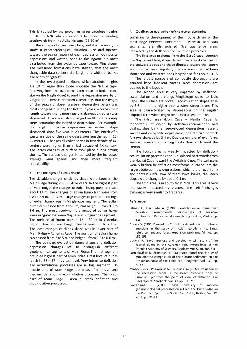
This is caused by the prevailing larger absolute heights (35-40 m NN) when compared to those dominating southwards from the Avikalnis cape (25-30 m).

The surface changes take place, and it is necessary to study a geomorphological situation, size and opened toward the sea or lagoon of each depression. Composite depressions and wastes, open to the lagoon, are most distributed from the Lydumas cape toward Vingiakopė. The measured formations have started, that the most changeable data concern the length and width of banks, and width of “gates".

In the investigated territory, which absolute heights are 10 m larger than those opposite the Nagliai cape, following from the oval depression (near to look-around site on the Naglis dune) toward the depression nearby of Vingiakopė. There is obtained a tendency, that the length of the seaward slope (western depression parts) was most changeable during the last four years, whereas their length toward the lagoon (eastern depression parts) was shortened. There was also changed width of the sandy steps separating the neighbor depressions. For example, the length of some depression an eastern slope shortened since five year in 20 meters. The length of a western slope of the same depression lengthened in 15-25 meters. Changes all eolian forms in first decade of XXI century were higher than in last decade of XX century. The larges changes of surface took place during strong storms. The surface changes influenced by the increased average wind speeds and their more frequent repeatability. 3. The changes of dunes shape The sizeable changes of dunes shape were been in the Main Ridge during 2003 – 2014 years. In the highest part of Main Ridges the changes of eolian hump position reach about 13 m. The changes of eolian hump high were from 0.8 to 2.4 m. The same large changes of position and high of eolian hump was in Vingiakopė segment. The eolian hump cap passed from 4 to 8 m, and height – from 0.8 to 1.6 m. The most geodynamic changes of eolian hump were in “gate” between Nagliai and Vingiakopė segments. The position of hump passed 12 – 30 m in Curonian Lagoon direction and height change from 0.6 to 2.1 m. The least changes of dunes shape was in lower part of Main Ridge – Avikalnis Cape. The position of eolian hump cap passed from 3 to 5 m and height – from 0.3 to 0.6 m.

The complex evaluation dunes shape and deflation depression changes let to distinguish different geodynamical segments of Main Ridge. The first segment occupied highest part of Main Ridge. Crest level of dunes reach to 53 – 57 m by sea level. Very intensive deflation and accumulation processes are in this segment. In middle part of Main Ridge are areas of intensive and medium deflation – accumulation processes. The north part of Main Ridge – area of weak deflation and accumulation processes.

4. Qualitative evaluation of the dunes dynamics Summarising development of the mobile dunes of the main ridge between Juodkrantė – Pervalka and Nida segments, are distinguished five qualitative areas impacted by the deflation-accumulation processes.

The first area prolongs from the Garbė cape, through the Nagliai and Vingiakopė dunes. The largest changes of the seaward slopes and those directed toward the lagoon are obtained here. Regularly, the eastern slope had been shortened and western ones lengthened for about 10-15 m. The largest numbers of composite depressions are situated here, frequent wastes, most depressions are opened to the lagoon.

The second area is very impacted by deflation-accumulation and prolongs Vingiakopė dune to Libis Cape. The surface are broken, accumulation slopes arise by 3-6 m and are higher than western steep slopes. This area is characterized by depressions of the regular elliptical form which might be named as windmulde.

The third area (Libis Cape – Nagliai Cape) is moderately influenced by deflation-accumulation and distinguishes by the steep-sloped depressions, absent wastes and composite depressions, and the size of stack furrows changed by 3-4 m. Depressions are of oval form, seaward opened, containing banks directed toward the lagoon.

The fourth area is weakly impacted by deflation-accumulation processes and is displaced northwards from the Nagliai Cape toward the Avikalnis Cape. The surface is weakly broken by deflation mesoforms, distances are the largest between few depressions, which are of oval form and contain cliffs. Two of them have banks, the steep slopes were changed by about 0.5 m.

The fifth area is in south from Nida. This area is very intensively impacted by visitors. The relief changes dynamic is very similar to first area. References

Bitinas A., Damušytė A. (1998) Parabolic eolian dune near Pervalka, Environmental perspectives of sensitive southeastern Baltic coastal areas through a time, Vilnius, pp. 4-6.

Gudelis V. (1957) Dune of the Curonian spit and several methodic questions in the study of modern eolodynamics, Sands reinforcement and forest expansion problems. Vilnius. pp. 185-198.

Gudelis V. (1960) Geology and developmental history of the coastal dunes in the Curonian spit, Proceedings of the Estonian Academy of Sciences, Geology, Vol. 5, pp. 305-316

Jarmalavičius D, Žilinskas G. (1996) Distributional peculiarities of grnulometric composition of the surface sediments on the Lithuanian coast of the Baltic Sea, Geografija, Vol. 32, pp. 77-82

Minkevičius V., Paskauskas S., Zilinskas G. (1997) Evaluation of the recreation zones in the beach foredune ridge of Curonian Spit from the point of view of deflation. The Geographical Yearbook, Vol. 30, pp. 199-211.

Povilanskas R. (2009) Spatial diversity of modern geomorphological processes on a Holocene Dune Ridge on the Curonian Spit in the South–East Baltic, Baltica, Vol. 22, No. 2, pp. 77-88.

113

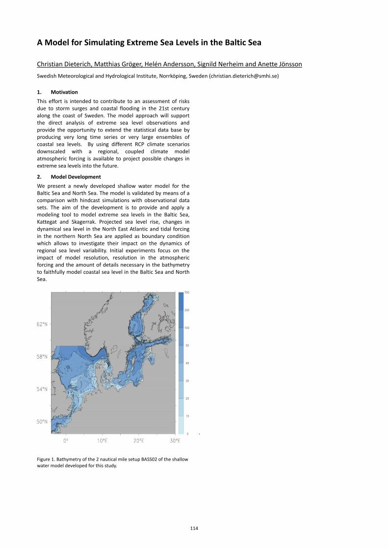
A Model for Simulating Extreme Sea Levels in the Baltic Sea

Christian Dieterich, Matthias Gröger, Helén Andersson, Signild Nerheim and Anette Jönsson

Swedish Meteorological and Hydrological Institute, Norrköping, Sweden (christian.dieterich@smhi.se) 1. Motivation This effort is intended to contribute to an assessment of risks due to storm surges and coastal flooding in the 21st century along the coast of Sweden. The model approach will support the direct analysis of extreme sea level observations and provide the opportunity to extend the statistical data base by producing very long time series or very large ensembles of coastal sea levels. By using different RCP climate scenarios downscaled with a regional, coupled climate model atmospheric forcing is available to project possible changes in extreme sea levels into the future.

2. Model Development We present a newly developed shallow water model for the Baltic Sea and North Sea. The model is validated by means of a comparison with hindcast simulations with observational data sets. The aim of the development is to provide and apply a modeling tool to model extreme sea levels in the Baltic Sea, Kattegat and Skagerrak. Projected sea level rise, changes in dynamical sea level in the North East Atlantic and tidal forcing in the northern North Sea are applied as boundary condition which allows to investigate their impact on the dynamics of regional sea level variability. Initial experiments focus on the impact of model resolution, resolution in the atmospheric forcing and the amount of details necessary in the bathymetry to faithfully model coastal sea level in the Baltic Sea and North Sea.

Figure 1. Bathymetry of the 2 nautical mile setup BASS02 of the shallow water model developed for this study.

.

114

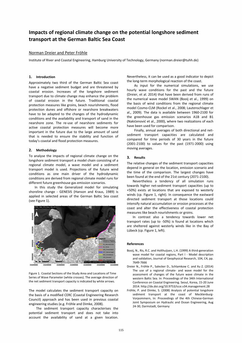
Impacts of regional climate change on the potential longshore sediment transport at the German Baltic Sea Coast

Norman Dreier and Peter Fröhle

Institute of River and Coastal Engineering, Hamburg University of Technology, Germany (norman.dreier@tuhh.de)

1. Introduction Approximately two third of the German Baltic Sea coast have a negative sediment budget and are threatened by coastal erosion. Increases of the longshore sediment transport due to climate change may enhance the problem of coastal erosion in the future. Traditional coastal protection measures like groins, beach nourishments, flood protection dunes and offshore or nearshore breakwaters have to be adapted to the changes of the hydrodynamic conditions and the availability and transport of sand in the nearshore zone. The re-use of nearshore sediments for active coastal protection measures will become more important in the future due to the large amount of sand that is needed to ensure the stability and function of today’s coastal and flood protection measures. 2. Methodology To analyse the impacts of regional climate change on the longshore sediment transport a model chain consisting of a regional climate model, a wave model and a sediment transport model is used. Projections of the future wind conditions as one main driver of the hydrodynamic conditions are derived from regional climate model runs for different future greenhouse gas emission scenarios.

In this study the Generalized model for simulating shoreline change - GENESIS (Hanson and Kraus, 1989) is applied in selected areas of the German Baltic Sea coast (see Figure 1).

Figure 1. Coastal Sections of the Study Area and Locations of Time Series of Wave Parameter (white crosses). The average direction of the net sediment transport capacity is indicated by white arrows.

The model calculates the sediment transport capacity on the basis of a modified CERC (Coastal Engineering Research Council) approach and has been used in previous coastal engineering studies (e.g. Fröhle and Dimke, 2008).

The sediment transport capacity characterises the potential sediment transport and does not take into account the availability of sand at a given location.

Nevertheless, it can be used as a good indicator to depict the long-term morphological reaction of the coast.

As input for the numerical simulations, we use hourly wave conditions for the past and the future (Dreier, et al. 2014) that have been derived from runs of the numerical wave model SWAN (Booij et al., 1999) on the basis of wind conditions from the regional climate model Cosmo-CLM (Rockel et al., 2008; Lautenschlager et al., 2009). The data is available between 1960-2100 for the greenhouse gas emission scenarios A1B and B1 (Nakićenović et al., 2000), where two realizations of each have been used for comparison.

Finally, annual averages of both directional and net-sediment transport capacities are calculated and compared for time periods of 30 years in the future (2001-2100) to values for the past (1971-2000) using moving averages. 3. Results The relative changes of the sediment transport capacities depend in general on the location, emission scenario and the time of the comparison. The largest changes have been found at the end of the 21st century (2071-2100).

Nevertheless a tendency of all simulation runs towards higher net-sediment transport capacities (up to +50%) exists at locations that are exposed to westerly winds (cp. Figure 1, right). In consequence the eastward directed sediment transport at those locations could intensify natural accumulation or erosion processes at the coast and alter the effectiveness of coastal protection measures like beach nourishments or groins.

In contrast also a tendency towards lower net transport rates (up to -50%) is found at locations which are sheltered against westerly winds like in the Bay of Lübeck (cp. Figure 1, left). References

Booij, N., Ris, R.C. and Holthuijsen, L.H. (1999) A third-generation wave model for coastal regions, Part I - Model description and validation, Journal of Geophysical Research, 104, C4, pp. 7649-7666

Dreier N., Fröhle P., Salecker D., Schlamkow C. and Xu Z. (2014) The use of a regional climate- and wave model for the assessment of changes of the future wave climate in the western Baltic Sea. In: Proceedings of the 34th International Conference on Coastal Engineering. Seoul, Korea, 15-20 June 2014. http://dx.doi.org/10.9753/icce.v34.management.28

Fröhle, P. and Dimke, S. (2008) Analysis of potential longshore sediment transport at the coast of Mecklenburg-Vorpommern, In: Proceedings of the 4th Chinese-German Joint Symposium on Hydraulic and Ocean Engineering, Aug 24-30, Darmstadt, Germany

115

Hanson, H. and Kraus, N. C. (1989) GENESIS: Generalized model for simulating shoreline change, Report 1: Technical reference, Tech. Rep. CERC-89-19, U.S. Army Engineer Waterways Experiment Station, Vicksburg, MS.

Lautenschlager, M., Keuler, K., Wunram, C., Keup-Thiel, E., Schubert, M., Will, A., Rockel, B. and Boehm, U. (2009) Climate Simulation with COSMO-CLM, Climate of the 20th Century run no.1-3, Scenario A1B run no.1-2, Scenario B1 run no.1-2 , Data Stream 3: European region MPI-M/MaD. World Data Centre for Climate

Nakićenović, N., Alcamo, J., Davis, G., de Vries, B., Fenhann, J., Gaffin, S., Gregory, K., Grübler, A., Jung, T.Y., Kram, T., La Rovere, E.L., Michaelis, L., Mori, S., Morita, T., Pepper, W., Pitcher, H., Price, L., Raihi, K., Roehrl, A., Rogner, H.-H., Sankovski, A., Schlesinger, M., Shukla, P., Smith, S., Swart, R., van Rooijen, S., Victor, N. and Dadi, Z. (2000) Emissions Scenarios, A Special Report of Working Group III of the Intergovernmental Panel on Climate Change, Cambridge University Press, Cambridge and New York, 599pp.

Rockel, B., Will, A. and Hense, A. (eds.) (2008) Special Issue: Regional circulation modelling with COSMO-CLM (CCLM), Meteorologische Zeitschrift, Vol. 17

116

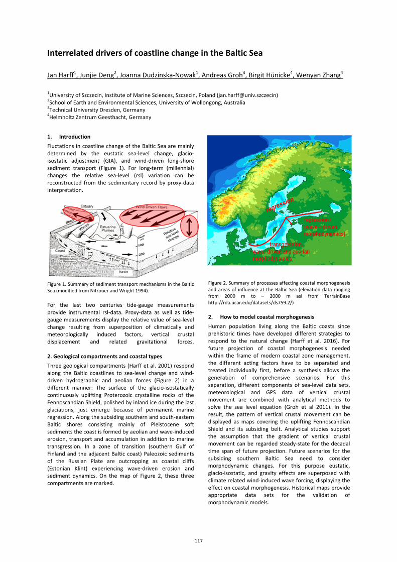
Interrelated drivers of coastline change in the Baltic Sea

Jan Harff1, Junjie Deng2, Joanna Dudzinska-Nowak1, Andreas Groh3, Birgit Hünicke4, Wenyan Zhang4

1University of Szczecin, Institute of Marine Sciences, Szczecin, Poland (jan.harff@univ.szczecin) 2School of Earth and Environmental Sciences, University of Wollongong, Australia 3Technical University Dresden, Germany 4Helmholtz Zentrum Geesthacht, Germany

1. Introduction Fluctations in coastline change of the Baltic Sea are mainly determined by the eustatic sea-level change, glacio-isostatic adjustment (GIA), and wind-driven long-shore sediment transport (Figure 1). For long-term (millennial) changes the relative sea-level (rsl) variation can be reconstructed from the sedimentary record by proxy-data interpretation.

Figure 1. Summary of sediment transport mechanisms in the Baltic Sea (modified from Nitrouer and Wright 1994). For the last two centuries tide-gauge measurements provide instrumental rsl-data. Proxy-data as well as tide-gauge measurements display the relative value of sea-level change resulting from superposition of climatically and meteorologically induced factors, vertical crustal displacement and related gravitational forces. 2. Geological compartments and coastal types Three geological compartments (Harff et al. 2001) respond along the Baltic coastlines to sea-level change and wind-driven hydrographic and aeolian forces (Figure 2) in a different manner: The surface of the glacio-isostatically continuously uplifting Proterozoic crystalline rocks of the Fennoscandian Shield, polished by inland ice during the last glaciations, just emerge because of permanent marine regression. Along the subsiding southern and south-eastern Baltic shores consisting mainly of Pleistocene soft sediments the coast is formed by aeolian and wave-induced erosion, transport and accumulation in addition to marine transgression. In a zone of transition (southern Gulf of Finland and the adjacent Baltic coast) Paleozoic sediments of the Russian Plate are outcropping as coastal cliffs (Estonian Klint) experiencing wave-driven erosion and sediment dynamics. On the map of Figure 2, these three compartments are marked.

Figure 2. Summary of processes affecting coastal morphogenesis and areas of influence at the Baltic Sea (elevation data ranging from 2000 m to – 2000 m asl from TerrainBase http://rda.ucar.edu/datasets/ds759.2/) 2. How to model coastal morphogenesis Human population living along the Baltic coasts since prehistoric times have developed different strategies to respond to the natural change (Harff et al. 2016). For future projection of coastal morphogenesis needed within the frame of modern coastal zone management, the different acting factors have to be separated and treated individually first, before a synthesis allows the generation of comprehensive scenarios. For this separation, different components of sea-level data sets, meteorological and GPS data of vertical crustal movement are combined with analytical methods to solve the sea level equation (Groh et al 2011). In the result, the pattern of vertical crustal movement can be displayed as maps covering the uplifting Fennoscandian Shield and its subsiding belt. Analytical studies support the assumption that the gradient of vertical crustal movement can be regarded steady-state for the decadal time span of future projection. Future scenarios for the subsiding southern Baltic Sea need to consider morphodynamic changes. For this purpose eustatic, glacio-isostatic, and gravity effects are superposed with climate related wind-induced wave forcing, displaying the effect on coastal morphogenesis. Historical maps provide appropriate data sets for the validation of morphodynamic models.

117

Once the models are validated, climate scenarios can be used as input data to generate future coastal projections. Along German and Polish coasts several key areas are selected for case studies (Deng et al. 2014, Zhang et al. 2014). References

Deng, J., Zhang, W., Harff, J., Schneider, R., Dudzinska-Nowak, J., Terefenko, P., Giza, A.; Furmanczyk, K., 2014: A numerical approach to approximate historical morphology of wave-dominated coasts - a case study of the Pomeranian Bight, southern Baltic Sea. – Geomorphology, vol. 204, 425-443.

Groh, A., Dietrich, R., Richter, A. (2011): Geodetic evidence and modelling of sea-level changes and load-induced crustal deformations in the southern Baltic Sea. Ber. Römisch-Germanische Kommission: 92, 17-40.

Harff, J., Jöns, H., Rosentau, A. (2016) Interrelation of geosphere, climate processes and anthroposphere in the Baltic Sea basin during the Holocene, 1st Baltic Earth Conference “Multiple drivers for Earth system changes in the Baltic Sea region”, Nida, Lithuania, 13 to 17 June 2016, this abstract volume.

Harff, J., Frischbutter, A., Lampe, R., Meyer, M. (2001) Sea Level Change in the Baltic Sea - Interrelation of Climatic and Geological Processes.- in: L. C. Gerhard, W. E. Harrison, and B. M. Hanson (eds.): Geological perspectives of global climate change.- AAPG-Studies in Geology, no. 47, p. 231-250.

Nitrouer, C. A., Wrigth, L. D. (1994) Transport of particles across continental shelves, Review of Geophysics: 32, 85-113.

Zhang, W., Harff, J., Schneider, R., Meyer, M., Zorita, E., Hünicke, B., 2014. Holocene morphogenesis at the southern Baltic Sea: simulation of multiscale processes and their interactions for the Darss-Zingst peninsula. Journal of Marine Systems, 129, 4-18.

118

Rapid changes in sea level

Jürgen Holfort1, Ines Perlet1 and Ida Stanisławczyk2 1 Bundesamt für Seeschifffahrt und Hydrographie, Rostock, Germany (juergen.holfort@bsh.de) 2 Instytut Meteorologii i Gospodarki Wodnej, Gdynia, Poland

1. Introduction Not only extreme sea levels itself, but also rapid changes in sea levels can be a hazard. Such rapid changes can be associated with storm surges but can also occur in the form of Seebären (how meteotsunamis are called at the German coast). We are looking through water gauge measurements along the German and Polish coast for such rapid changes, trying to come up with a statistical description and, looking at the atmospheric conditions in special cases, the causes of such events. The goal is to be able to incorporate information of probable rapid changes in sea level in the routine sea level prognosis. In Nida we will present some first, preliminary findings. 2. Sea level data We are using sea level data from several water gauges along the German and Polish Baltic coast. While newer digital data is available with a temporal resolution between 1 and 10 minutes, older digital data (e.G. from the 1960ies) is only available in 1 hour increments at the German coast and with a 3hours resolution at the polish coast. A first search for rapid changes in the hourly data revealed some errors in the data and some few real events. Where possible the rapid changes were also verified using the analog gauge sheets. The better resolved, modern data are better suited for the search of meteotsunami events, but even in more than 10years of minute data only a handful of events were found, which could be named Seebär (or more correctly Seebärchen, which is a small Seebär). 3. Meteorological Information As overarching meteorological information we are using Polish synoptic charts, which are augmented by German and Polish station measurements. In the first analyzed summer event this information could be used to associate the passing of a frontal zone to the local, rapid increase of sea level.

119

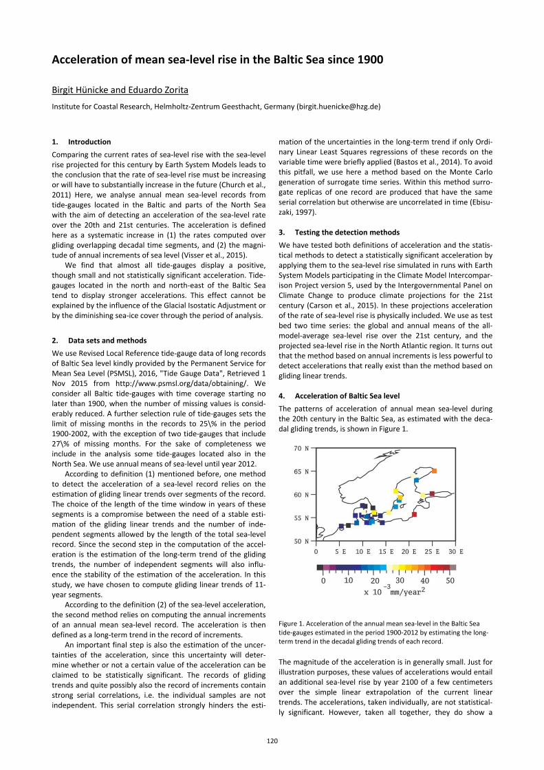
Acceleration of mean sea-level rise in the Baltic Sea since 1900

Birgit Hünicke and Eduardo Zorita Institute for Coastal Research, Helmholtz-Zentrum Geesthacht, Germany (birgit.huenicke@hzg.de) 1. Introduction Comparing the current rates of sea-level rise with the sea-level rise projected for this century by Earth System Models leads to the conclusion that the rate of sea-level rise must be increasing or will have to substantially increase in the future (Church et al., 2011) Here, we analyse annual mean sea-level records from tide-gauges located in the Baltic and parts of the North Sea with the aim of detecting an acceleration of the sea-level rate over the 20th and 21st centuries. The acceleration is defined here as a systematic increase in (1) the rates computed over gliding overlapping decadal time segments, and (2) the magni-tude of annual increments of sea level (Visser et al., 2015).

We find that almost all tide-gauges display a positive, though small and not statistically significant acceleration. Tide-gauges located in the north and north-east of the Baltic Sea tend to display stronger accelerations. This effect cannot be explained by the influence of the Glacial Isostatic Adjustment or by the diminishing sea-ice cover through the period of analysis.

2. Data sets and methods We use Revised Local Reference tide-gauge data of long records of Baltic Sea level kindly provided by the Permanent Service for Mean Sea Level (PSMSL), 2016, "Tide Gauge Data", Retrieved 1 Nov 2015 from http://www.psmsl.org/data/obtaining/. We consider all Baltic tide-gauges with time coverage starting no later than 1900, when the number of missing values is consid-erably reduced. A further selection rule of tide-gauges sets the limit of missing months in the records to 25\% in the period 1900-2002, with the exception of two tide-gauges that include 27\% of missing months. For the sake of completeness we include in the analysis some tide-gauges located also in the North Sea. We use annual means of sea-level until year 2012.

According to definition (1) mentioned before, one method to detect the acceleration of a sea-level record relies on the estimation of gliding linear trends over segments of the record. The choice of the length of the time window in years of these segments is a compromise between the need of a stable esti-mation of the gliding linear trends and the number of inde-pendent segments allowed by the length of the total sea-level record. Since the second step in the computation of the accel-eration is the estimation of the long-term trend of the gliding trends, the number of independent segments will also influ-ence the stability of the estimation of the acceleration. In this study, we have chosen to compute gliding linear trends of 11-year segments.

According to the definition (2) of the sea-level acceleration, the second method relies on computing the annual increments of an annual mean sea-level record. The acceleration is then defined as a long-term trend in the record of increments.

An important final step is also the estimation of the uncer-tainties of the acceleration, since this uncertainty will deter-mine whether or not a certain value of the acceleration can be claimed to be statistically significant. The records of gliding trends and quite possibly also the record of increments contain strong serial correlations, i.e. the individual samples are not independent. This serial correlation strongly hinders the esti-

mation of the uncertainties in the long-term trend if only Ordi-nary Linear Least Squares regressions of these records on the variable time were briefly applied (Bastos et al., 2014). To avoid this pitfall, we use here a method based on the Monte Carlo generation of surrogate time series. Within this method surro-gate replicas of one record are produced that have the same serial correlation but otherwise are uncorrelated in time (Ebisu-zaki, 1997). 3. Testing the detection methods We have tested both definitions of acceleration and the statis-tical methods to detect a statistically significant acceleration by applying them to the sea-level rise simulated in runs with Earth System Models participating in the Climate Model Intercompar-ison Project version 5, used by the Intergovernmental Panel on Climate Change to produce climate projections for the 21st century (Carson et al., 2015). In these projections acceleration of the rate of sea-level rise is physically included. We use as test bed two time series: the global and annual means of the all-model-average sea-level rise over the 21st century, and the projected sea-level rise in the North Atlantic region. It turns out that the method based on annual increments is less powerful to detect accelerations that really exist than the method based on gliding linear trends. 4. Acceleration of Baltic Sea level The patterns of acceleration of annual mean sea-level during the 20th century in the Baltic Sea, as estimated with the deca-dal gliding trends, is shown in Figure 1.

Figure 1. Acceleration of the annual mean sea-level in the Baltic Sea tide-gauges estimated in the period 1900-2012 by estimating the long-term trend in the decadal gliding trends of each record.

The magnitude of the acceleration is in generally small. Just for illustration purposes, these values of accelerations would entail an additional sea-level rise by year 2100 of a few centimeters over the simple linear extrapolation of the current linear trends. The accelerations, taken individually, are not statistical-ly significant. However, taken all together, they do show a

120

coherent pattern of generally positive accelerations, with larger magnitudes at the tide-gauges located in the north and the north-east. 5. Discussion The spatial pattern of accelerations of sea-level rise in the Baltic Sea could be in part determined by the Glacial Isostatic Adjust-ment. The build-up of the Fennoscandian Ice Sheet during the last ice age caused a depression of the Earth Crust of several hundred meters (Wieczerkowski et al., 1999). After the melting of these ice-sheets, the crust tends to recover its original with a lag of several millennia. Since this process relaxes asymptotical-ly, the relative sea-level (difference between the absolute sea-surface height and the crust level) will apparently accelerate, and do it more strongly in the locations where the crust defor-mation was also stronger - in the Northern Baltic. However, estimations of the order of magnitude of this affect indicate that it is too small to explain the estimated pattern of sea-level acceleration at the tide-gauges.

Another possible factor is the melting of sea-ice through the 20th century. Since sea-ice may also affect coastal sea-level, it is slowly but continuous demise during winter time could cause an apparent acceleration of sea-level rise. However, a similar calculation conducted for the summer season, when no sea-ice is present, shows a similar spatial pattern of accelera-tions. Therefore, we conclude that these mechanisms cannot explain this spatial pattern either. References

Carson, M., Köhl, A., Stammer, D., Slangen, A. B. A., Katsman, C. A., van de Wal, R. S. W., Church, J. , White, N. (2016). Coastal sea level changes, observed and projected during the 20th and 21st century. Climatic Change, 134(1-2), 269-281.

Church, J. A., Gregory, J. M., White, N. J., Platten, S. M., Mitrovica, J. X. (2011). Understanding and projecting sea level change. Oceanog-raphy, 24(2), 130-143.

Ebisuzaki, W. (1997). A method to estimate the statistical significance of a correlation when the data are serially correlated. Journal of Climate, 10(9), 2147-2153.

Visser, H., Dangendorf, S., Petersen, A. C. (2015). A review of trend models applied to sea level data with reference to the “accelera-tion-deceleration debate”. Journal of Geophysical Research: Oceans, 120(6), 3873-3895.

Wieczerkowski, K., Mitrovica, J. X., Wolf, D. (1999). A revised relaxation-time spectrum for Fennoscandia. Geophysical Journal Internation-al, 139(1), 69-86.

121

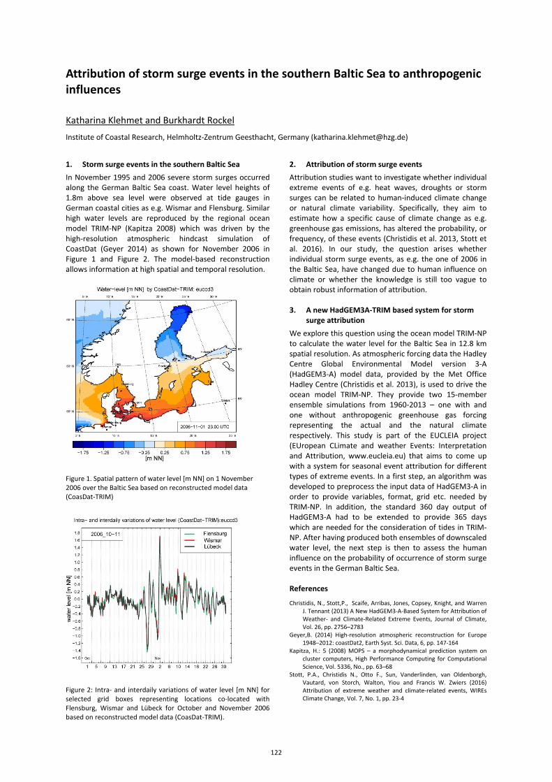
Attribution of storm surge events in the southern Baltic Sea to anthropogenic influences

Katharina Klehmet and Burkhardt Rockel

Institute of Coastal Research, Helmholtz-Zentrum Geesthacht, Germany (katharina.klehmet@hzg.de)

1. Storm surge events in the southern Baltic Sea In November 1995 and 2006 severe storm surges occurred along the German Baltic Sea coast. Water level heights of 1.8m above sea level were observed at tide gauges in German coastal cities as e.g. Wismar and Flensburg. Similar high water levels are reproduced by the regional ocean model TRIM-NP (Kapitza 2008) which was driven by the high-resolution atmospheric hindcast simulation of CoastDat (Geyer 2014) as shown for November 2006 in Figure 1 and Figure 2. The model-based reconstruction allows information at high spatial and temporal resolution.

Figure 1. Spatial pattern of water level [m NN] on 1 November 2006 over the Baltic Sea based on reconstructed model data (CoasDat-TRIM)

Figure 2: Intra- and interdaily variations of water level [m NN] for selected grid boxes representing locations co-located with Flensburg, Wismar and Lübeck for October and November 2006 based on reconstructed model data (CoasDat-TRIM).

2. Attribution of storm surge events Attribution studies want to investigate whether individual extreme events of e.g. heat waves, droughts or storm surges can be related to human-induced climate change or natural climate variability. Specifically, they aim to estimate how a specific cause of climate change as e.g. greenhouse gas emissions, has altered the probability, or frequency, of these events (Christidis et al. 2013, Stott et al. 2016). In our study, the question arises whether individual storm surge events, as e.g. the one of 2006 in the Baltic Sea, have changed due to human influence on climate or whether the knowledge is still too vague to obtain robust information of attribution. 3. A new HadGEM3A-TRIM based system for storm

surge attribution We explore this question using the ocean model TRIM-NP to calculate the water level for the Baltic Sea in 12.8 km spatial resolution. As atmospheric forcing data the Hadley Centre Global Environmental Model version 3-A (HadGEM3-A) model data, provided by the Met Office Hadley Centre (Christidis et al. 2013), is used to drive the ocean model TRIM-NP. They provide two 15-member ensemble simulations from 1960-2013 – one with and one without anthropogenic greenhouse gas forcing representing the actual and the natural climate respectively. This study is part of the EUCLEIA project (EUropean CLimate and weather Events: Interpretation and Attribution, www.eucleia.eu) that aims to come up with a system for seasonal event attribution for different types of extreme events. In a first step, an algorithm was developed to preprocess the input data of HadGEM3-A in order to provide variables, format, grid etc. needed by TRIM-NP. In addition, the standard 360 day output of HadGEM3-A had to be extended to provide 365 days which are needed for the consideration of tides in TRIM-NP. After having produced both ensembles of downscaled water level, the next step is then to assess the human influence on the probability of occurrence of storm surge events in the German Baltic Sea. References

Christidis, N., Stott,P., Scaife, Arribas, Jones, Copsey, Knight, and Warren J. Tennant (2013) A New HadGEM3-A-Based System for Attribution of Weather- and Climate-Related Extreme Events, Journal of Climate, Vol. 26, pp. 2756–2783

Geyer,B. (2014) High-resolution atmospheric reconstruction for Europe 1948–2012: coastDat2, Earth Syst. Sci. Data, 6, pp. 147-164

Kapitza, H.: 5 (2008) MOPS – a morphodynamical prediction system on cluster computers, High Performance Computing for Computational Science, Vol. 5336, No., pp. 63–68

Stott, P.A., Christidis N., Otto F., Sun, Vanderlinden, van Oldenborgh, Vautard, von Storch, Walton, Yiou and Francis W. Zwiers (2016) Attribution of extreme weather and climate-related events, WIREs Climate Change, Vol. 7, No. 1, pp. 23-4

122

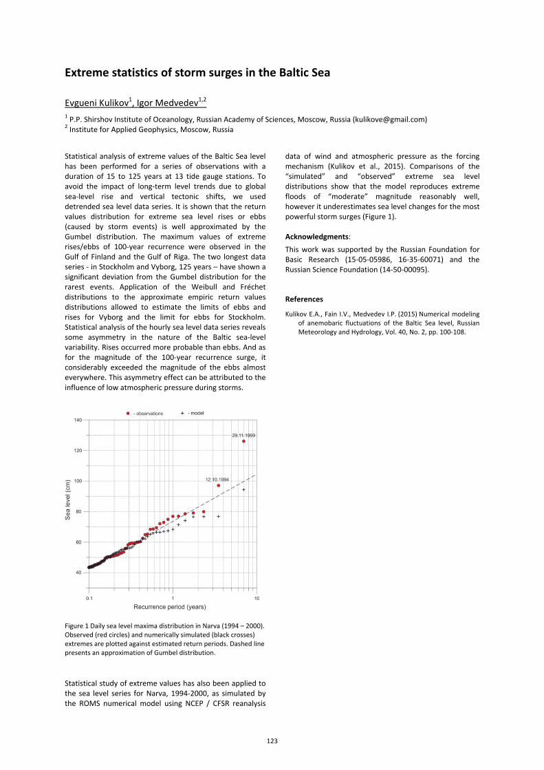
Extreme statistics of storm surges in the Baltic Sea

Evgueni Kulikov1, Igor Medvedev1,2 1 P.P. Shirshov Institute of Oceanology, Russian Academy of Sciences, Moscow, Russia (kulikove@gmail.com) 2 Institute for Applied Geophysics, Moscow, Russia

Statistical analysis of extreme values of the Baltic Sea level has been performed for a series of observations with a duration of 15 to 125 years at 13 tide gauge stations. To avoid the impact of long-term level trends due to global sea-level rise and vertical tectonic shifts, we used detrended sea level data series. It is shown that the return values distribution for extreme sea level rises or ebbs (caused by storm events) is well approximated by the Gumbel distribution. The maximum values of extreme rises/ebbs of 100-year recurrence were observed in the Gulf of Finland and the Gulf of Riga. The two longest data series - in Stockholm and Vyborg, 125 years – have shown a significant deviation from the Gumbel distribution for the rarest events. Application of the Weibull and Fréchet distributions to the approximate empiric return values distributions allowed to estimate the limits of ebbs and rises for Vyborg and the limit for ebbs for Stockholm. Statistical analysis of the hourly sea level data series reveals some asymmetry in the nature of the Baltic sea-level variability. Rises occurred more probable than ebbs. And as for the magnitude of the 100-year recurrence surge, it considerably exceeded the magnitude of the ebbs almost everywhere. This asymmetry effect can be attributed to the influence of low atmospheric pressure during storms.

Figure 1 Daily sea level maxima distribution in Narva (1994 – 2000). Observed (red circles) and numerically simulated (black crosses) extremes are plotted against estimated return periods. Dashed line presents an approximation of Gumbel distribution.

Statistical study of extreme values has also been applied to the sea level series for Narva, 1994-2000, as simulated by the ROMS numerical model using NCEP / CFSR reanalysis

data of wind and atmospheric pressure as the forcing mechanism (Kulikov et al., 2015). Comparisons of the “simulated” and “observed” extreme sea level distributions show that the model reproduces extreme floods of “moderate” magnitude reasonably well, however it underestimates sea level changes for the most powerful storm surges (Figure 1). Acknowledgments: This work was supported by the Russian Foundation for Basic Research (15-05-05986, 16-35-60071) and the Russian Science Foundation (14-50-00095). References

Kulikov E.A., Fain I.V., Medvedev I.P. (2015) Numerical modeling of anemobaric fluctuations of the Baltic Sea level, Russian Meteorology and Hydrology, Vol. 40, No. 2, pp. 100-108.

123

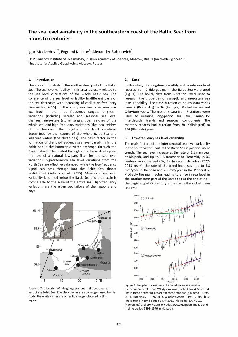
The sea level variability in the southeastern coast of the Baltic Sea: from hours to centuries

Igor Medvedev1,2, Evgueni Kulikov1, Alexander Rabinovich1

1 P.P. Shirshov Institute of Oceanology, Russian Academy of Sciences, Moscow, Russia (medvedev@ocean.ru) 2 Institute for Applied Geophysics, Moscow, Russia

1. Introduction The area of this study is the southeastern part of the Baltic Sea. The sea level variability in this area is closely related to the sea level oscillations of the whole Baltic sea. The coherence of the sea level variability in different parts of the sea decreases with increasing of oscillation frequency [Medvedev, 2015]. In this study sea level spectrum was examined in the three frequency ranges: long-term variations (including secular and seasonal sea level changes), mesoscale (storm surges, tides, seiches of the whole sea) and high-frequency variations (the local seiches of the lagoons). The long-term sea level variations determined by the feature of the whole Baltic Sea and adjacent waters (the North Sea). The basic factor in the formation of the low-frequency sea level variability in the Baltic Sea is the barotropic water exchange through the Danish straits. The limited throughput of these straits plays the role of a natural low-pass filter for the sea level variations: high-frequency sea level variations from the North Sea are effectively damped, while the low-frequency signal can pass through into the Baltic Sea almost undisturbed (Kulikov et al., 2015). Mesoscale sea level variability is formed inside the Baltic Sea and their scale is comparable to the scale of the entire sea. High-frequency variations are the eigen oscillations of the lagoons and bays.

Figure 1. The location of tide gauge stations in the southeastern part of the Baltic Sea. The black circles are tide gauges, used in this study; the white circles are other tide gauges, located in this region.

2. Data In this study the long-term monthly and hourly sea level records from 7 tide gauges in the Baltic Sea were used (Fig. 1). The hourly data from 5 stations were used to research the properties of synoptic and mesoscale sea level variability. The time duration of hourly data varies from 7 (Pionerskiy) to 16 (Baltiysk, Wladyslawowo and Otkrytoe) years. The monthly data from 7 stations were used to examine long-period sea level variability: interdecadal trends and seasonal components. The monthly records had duration from 30 (Kaliningrad) to 114 (Klaipeda) years. 3. Low-frequency sea level variability The main feature of the inter-decadal sea level variability in the southeastern part of the Baltic Sea is positive linear trends. The sea level increase at the rate of 1.5 mm/year at Klaipeda and up to 1.8 mm/year at Pionerskiy in XX century was observed (Fig. 2). In recent decades (1977-2013 years), the rate of the trend increases - up to 3.8 mm/year in Klaipeda and 2.2 mm/year in the Pionerskiy. Probably the main factor leading to a rise in sea level in the southeastern part of the Baltic Sea at the end of XX – the beginning of XXI century is the rise in the global mean sea level.

Figure 2. Long-term variations of annual mean sea level in Klaipeda, Pionerskiy and Władysławowo (dashed lines). Solid red line is trend of the full record for these stations (Klaipeda – 1898-2011, Pionerskiy – 1926-2013, Władysławowo – 1951-2008), blue line is trend in time period 1977-2011 (Klaipeda),1977-2013 (Pionerskiy) and 1977-2008 (Władysławowo), green line is trend in time period 1898-1976 in Klaipeda.

124

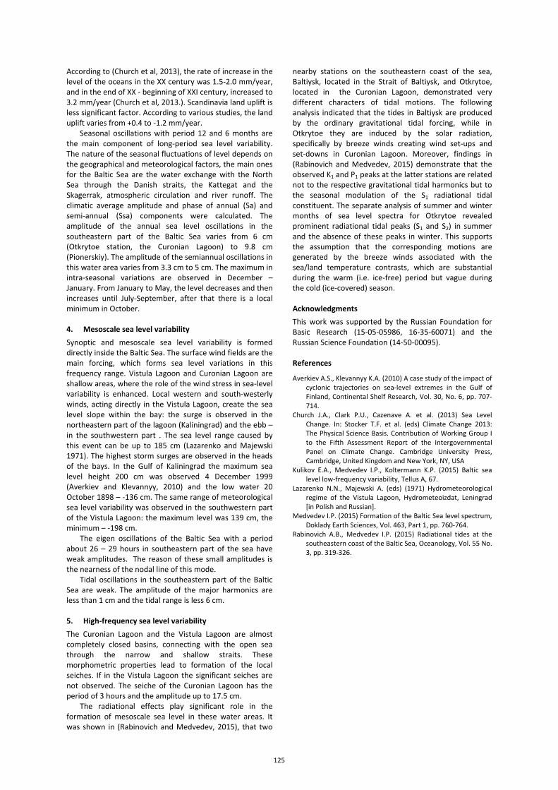
According to (Church et al, 2013), the rate of increase in the level of the oceans in the XX century was 1.5-2.0 mm/year, and in the end of XX - beginning of XXI century, increased to 3.2 mm/year (Church et al, 2013.). Scandinavia land uplift is less significant factor. According to various studies, the land uplift varies from +0.4 to -1.2 mm/year.

Seasonal oscillations with period 12 and 6 months are the main component of long-period sea level variability. The nature of the seasonal fluctuations of level depends on the geographical and meteorological factors, the main ones for the Baltic Sea are the water exchange with the North Sea through the Danish straits, the Kattegat and the Skagerrak, atmospheric circulation and river runoff. The climatic average amplitude and phase of annual (Sa) and semi-annual (Ssa) components were calculated. The amplitude of the annual sea level oscillations in the southeastern part of the Baltic Sea varies from 6 cm (Otkrytoe station, the Curonian Lagoon) to 9.8 cm (Pionerskiy). The amplitude of the semiannual oscillations in this water area varies from 3.3 cm to 5 cm. The maximum in intra-seasonal variations are observed in December – January. From January to May, the level decreases and then increases until July-September, after that there is a local minimum in October. 4. Mesoscale sea level variability Synoptic and mesoscale sea level variability is formed directly inside the Baltic Sea. The surface wind fields are the main forcing, which forms sea level variations in this frequency range. Vistula Lagoon and Curonian Lagoon are shallow areas, where the role of the wind stress in sea-level variability is enhanced. Local western and south-westerly winds, acting directly in the Vistula Lagoon, create the sea level slope within the bay: the surge is observed in the northeastern part of the lagoon (Kaliningrad) and the ebb – in the southwestern part . The sea level range caused by this event can be up to 185 cm (Lazarenko and Majewski 1971). The highest storm surges are observed in the heads of the bays. In the Gulf of Kaliningrad the maximum sea level height 200 cm was observed 4 December 1999 (Averkiev and Klevannyy, 2010) and the low water 20 October 1898 – -136 cm. The same range of meteorological sea level variability was observed in the southwestern part of the Vistula Lagoon: the maximum level was 139 cm, the minimum – -198 cm.

The eigen oscillations of the Baltic Sea with a period about 26 – 29 hours in southeastern part of the sea have weak amplitudes. The reason of these small amplitudes is the nearness of the nodal line of this mode.

Tidal oscillations in the southeastern part of the Baltic Sea are weak. The amplitude of the major harmonics are less than 1 cm and the tidal range is less 6 cm.

5. High-frequency sea level variability The Curonian Lagoon and the Vistula Lagoon are almost completely closed basins, connecting with the open sea through the narrow and shallow straits. These morphometric properties lead to formation of the local seiches. If in the Vistula Lagoon the significant seiches are not observed. The seiche of the Curonian Lagoon has the period of 3 hours and the amplitude up to 17.5 cm.

The radiational effects play significant role in the formation of mesoscale sea level in these water areas. It was shown in (Rabinovich and Medvedev, 2015), that two

nearby stations on the southeastern coast of the sea, Baltiysk, located in the Strait of Baltiysk, and Otkrytoe, located in the Сuronian Lagoon, demonstrated very different characters of tidal motions. The following analysis indicated that the tides in Baltiysk are produced by the ordinary gravitational tidal forcing, while in Otkrytoe they are induced by the solar radiation, specifically by breeze winds creating wind set-ups and set-downs in Curonian Lagoon. Moreover, findings in (Rabinovich and Medvedev, 2015) demonstrate that the observed K1 and P1 peaks at the latter stations are related not to the respective gravitational tidal harmonics but to the seasonal modulation of the S1 radiational tidal constituent. The separate analysis of summer and winter months of sea level spectra for Otkrytoe revealed prominent radiational tidal peaks (S1 and S2) in summer and the absence of these peaks in winter. This supports the assumption that the corresponding motions are generated by the breeze winds associated with the sea/land temperature contrasts, which are substantial during the warm (i.e. ice-free) period but vague during the cold (ice-covered) season. Acknowledgments This work was supported by the Russian Foundation for Basic Research (15-05-05986, 16-35-60071) and the Russian Science Foundation (14-50-00095). References

Averkiev A.S., Klevannyy K.A. (2010) A case study of the impact of cyclonic trajectories on sea-level extremes in the Gulf of Finland, Continental Shelf Research, Vol. 30, No. 6, pp. 707-714.

Church J.A., Clark P.U., Cazenave A. et al. (2013) Sea Level Change. In: Stocker T.F. et al. (eds) Climate Change 2013: The Physical Science Basis. Contribution of Working Group I to the Fifth Assessment Report of the Intergovernmental Panel on Climate Change. Cambridge University Press, Cambridge, United Kingdom and New York, NY, USA

Kulikov E.A., Medvedev I.P., Koltermann K.P. (2015) Baltic sea level low-frequency variability, Tellus A, 67.

Lazarenko N.N., Majewski A. (eds) (1971) Hydrometeorological regime of the Vistula Lagoon, Hydrometeoizdat, Leningrad [in Polish and Russian].

Medvedev I.P. (2015) Formation of the Baltic Sea level spectrum, Doklady Earth Sciences, Vol. 463, Part 1, pp. 760-764.

Rabinovich A.B., Medvedev I.P. (2015) Radiational tides at the southeastern coast of the Baltic Sea, Oceanology, Vol. 55 No. 3, pp. 319-326.

125

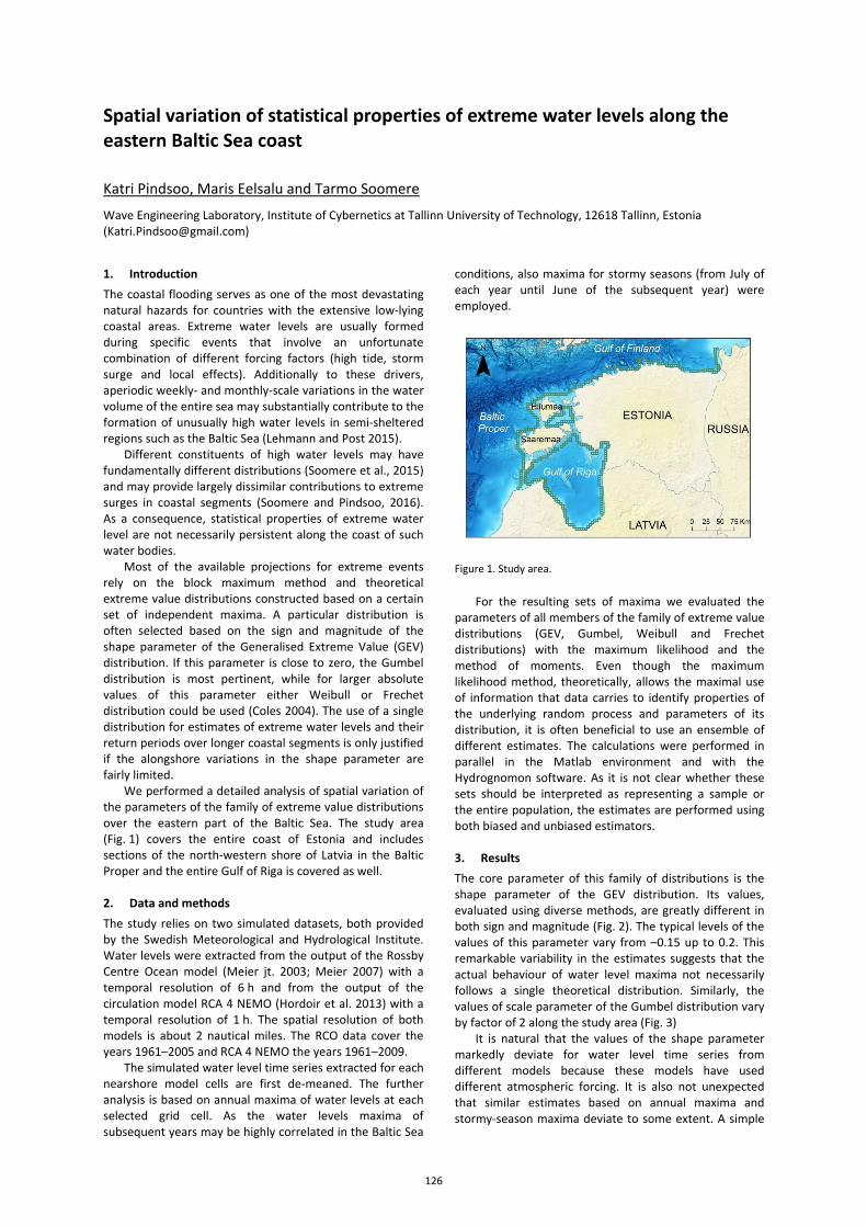
Spatial variation of statistical properties of extreme water levels along the eastern Baltic Sea coast

Katri Pindsoo, Maris Eelsalu and Tarmo Soomere

Wave Engineering Laboratory, Institute of Cybernetics at Tallinn University of Technology, 12618 Tallinn, Estonia (Katri.Pindsoo@gmail.com)

1. Introduction The coastal flooding serves as one of the most devastating natural hazards for countries with the extensive low-lying coastal areas. Extreme water levels are usually formed during specific events that involve an unfortunate combination of different forcing factors (high tide, storm surge and local effects). Additionally to these drivers, aperiodic weekly- and monthly-scale variations in the water volume of the entire sea may substantially contribute to the formation of unusually high water levels in semi-sheltered regions such as the Baltic Sea (Lehmann and Post 2015).

Different constituents of high water levels may have fundamentally different distributions (Soomere et al., 2015) and may provide largely dissimilar contributions to extreme surges in coastal segments (Soomere and Pindsoo, 2016). As a consequence, statistical properties of extreme water level are not necessarily persistent along the coast of such water bodies.

Most of the available projections for extreme events rely on the block maximum method and theoretical extreme value distributions constructed based on a certain set of independent maxima. A particular distribution is often selected based on the sign and magnitude of the shape parameter of the Generalised Extreme Value (GEV) distribution. If this parameter is close to zero, the Gumbel distribution is most pertinent, while for larger absolute values of this parameter either Weibull or Frechet distribution could be used (Coles 2004). The use of a single distribution for estimates of extreme water levels and their return periods over longer coastal segments is only justified if the alongshore variations in the shape parameter are fairly limited.

We performed a detailed analysis of spatial variation of the parameters of the family of extreme value distributions over the eastern part of the Baltic Sea. The study area (Fig. 1) covers the entire coast of Estonia and includes sections of the north-western shore of Latvia in the Baltic Proper and the entire Gulf of Riga is covered as well.

2. Data and methods The study relies on two simulated datasets, both provided by the Swedish Meteorological and Hydrological Institute. Water levels were extracted from the output of the Rossby Centre Ocean model (Meier jt. 2003; Meier 2007) with a temporal resolution of 6 h and from the output of the circulation model RCA 4 NEMO (Hordoir et al. 2013) with a temporal resolution of 1 h. The spatial resolution of both models is about 2 nautical miles. The RCO data cover the years 1961–2005 and RCA 4 NEMO the years 1961–2009.

The simulated water level time series extracted for each nearshore model cells are first de-meaned. The further analysis is based on annual maxima of water levels at each selected grid cell. As the water levels maxima of subsequent years may be highly correlated in the Baltic Sea

conditions, also maxima for stormy seasons (from July of each year until June of the subsequent year) were employed.

Figure 1. Study area.

For the resulting sets of maxima we evaluated the parameters of all members of the family of extreme value distributions (GEV, Gumbel, Weibull and Frechet distributions) with the maximum likelihood and the method of moments. Even though the maximum likelihood method, theoretically, allows the maximal use of information that data carries to identify properties of the underlying random process and parameters of its distribution, it is often beneficial to use an ensemble of different estimates. The calculations were performed in parallel in the Matlab environment and with the Hydrognomon software. As it is not clear whether these sets should be interpreted as representing a sample or the entire population, the estimates are performed using both biased and unbiased estimators.

3. Results The core parameter of this family of distributions is the shape parameter of the GEV distribution. Its values, evaluated using diverse methods, are greatly different in both sign and magnitude (Fig. 2). The typical levels of the values of this parameter vary from –0.15 up to 0.2. This remarkable variability in the estimates suggests that the actual behaviour of water level maxima not necessarily follows a single theoretical distribution. Similarly, the values of scale parameter of the Gumbel distribution vary by factor of 2 along the study area (Fig. 3)

It is natural that the values of the shape parameter markedly deviate for water level time series from different models because these models have used different atmospheric forcing. It is also not unexpected that similar estimates based on annual maxima and stormy-season maxima deviate to some extent. A simple

126

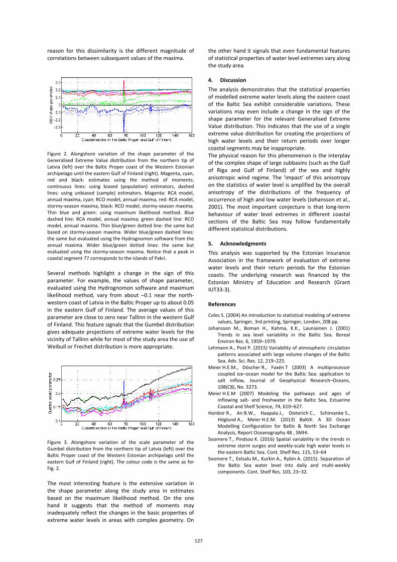
reason for this dissimilarity is the different magnitude of correlations between subsequent values of the maxima.

Figure 2. Alongshore variation of the shape parameter of the Generalised Extreme Value distribution from the northern tip of Latvia (left) over the Baltic Proper coast of the Western Estonian archipelago until the eastern Gulf of Finland (right). Magenta, cyan, red and black: estimates using the method of moments; continuous lines: using biased (population) estimators, dashed lines: using unbiased (sample) estimators. Magenta: RCA model, annual maxima, cyan: RCO model, annual maxima, red: RCA model, stormy-season maxima, black: RCO model, stormy-season maxima. Thin blue and green: using maximum likelihood method. Blue dashed line: RCA model, annual maxima; green dashed line: RCO model, annual maxima. Thin blue/green dotted line: the same but based on stormy-season maxima. Wider blue/green dashed lines: the same but evaluated using the Hydrognomon software from the annual maxima. Wider blue/green dotted lines: the same but evaluated using the stormy-season maxima. Notice that a peak in coastal segment 77 corresponds to the islands of Pakri.

Several methods highlight a change in the sign of this parameter. For example, the values of shape parameter, evaluated using the Hydrognomon software and maximum likelihood method, vary from about –0.1 near the north-western coast of Latvia in the Baltic Proper up to about 0.05 in the eastern Gulf of Finland. The average values of this parameter are close to zero near Tallinn in the western Gulf of Finland. This feature signals that the Gumbel distribution gives adequate projections of extreme water levels for the vicinity of Tallinn while for most of the study area the use of Weibull or Frechet distribution is more appropriate.

Figure 3. Alongshore variation of the scale parameter of the Gumbel distribution from the northern tip of Latvia (left) over the Baltic Proper coast of the Western Estonian archipelago until the eastern Gulf of Finland (right). The colour code is the same as for Fig. 2.

The most interesting feature is the extensive variation in the shape parameter along the study area in estimates based on the maximum likelihood method. On the one hand it suggests that the method of moments may inadequately reflect the changes in the basic properties of extreme water levels in areas with complex geometry. On

the other hand it signals that even fundamental features of statistical properties of water level extremes vary along the study area. 4. Discussion The analysis demonstrates that the statistical properties of modelled extreme water levels along the eastern coast of the Baltic Sea exhibit considerable variations. These variations may even include a change in the sign of the shape parameter for the relevant Generalised Extreme Value distribution. This indicates that the use of a single extreme value distribution for creating the projections of high water levels and their return periods over longer coastal segments may be inappropriate. The physical reason for this phenomenon is the interplay of the complex shape of large subbasins (such as the Gulf of Riga and Gulf of Finland) of the sea and highly anisotropic wind regime. The ‘impact’ of this anisotropy on the statistics of water level is amplified by the overall anisotropy of the distributions of the frequency of occurrence of high and low water levels (Johansson et al., 2001). The most important conjecture is that long-term behaviour of water level extremes in different coastal sections of the Baltic Sea may follow fundamentally different statistical distributions. 5. Acknowledgments This analysis was supported by the Estonian Insurance Association in the framework of evaluation of extreme water levels and their return periods for the Estonian coasts. The underlying research was financed by the Estonian Ministry of Education and Research (Grant IUT33-3). References

Coles S. (2004) An introduction to statistical modeling of extreme values, Springer, 3rd printing, Springer, London, 208 pp.

Johansson M., Boman H., Kahma, K.K., Launiainen J. (2001) Trends in sea level variability in the Baltic Sea. Boreal Environ Res. 6, 1959–1979.

Lehmann A., Post P. (2015) Variability of atmospheric circulation patterns associated with large volume changes of the Baltic Sea. Adv. Sci. Res. 12, 219–225.

Meier H.E.M., Döscher R., Faxén T (2003) A multiprocessor coupled ice–ocean model for the Baltic Sea: application to salt inflow, Journal of Geophysical Research–Oceans, 108(C8), No. 3273.

Meier H.E.M (2007) Modeling the pathways and ages of inflowing salt- and freshwater in the Baltic Sea, Estuarine Coastal and Shelf Science, 74, 610–627.

Hordoir R., An B.W., Haapala J., Dieterich C., Schimanke S., Höglund A., Meier H.E.M. (2013) BaltiX: A 3D Ocean Modelling Configuration for Baltic & North Sea Exchange Analysis, Report Oceanography 48 , SMHI.

Soomere T., Pindsoo K. (2016) Spatial variability in the trends in extreme storm surges and weekly-scale high water levels in the eastern Baltic Sea. Cont. Shelf Res. 115, 53–64

Soomere T., Eelsalu M., Kurkin A., Rybin A. (2015). Separation of the Baltic Sea water level into daily and multi-weekly components. Cont. Shelf Res. 103, 23–32.

127

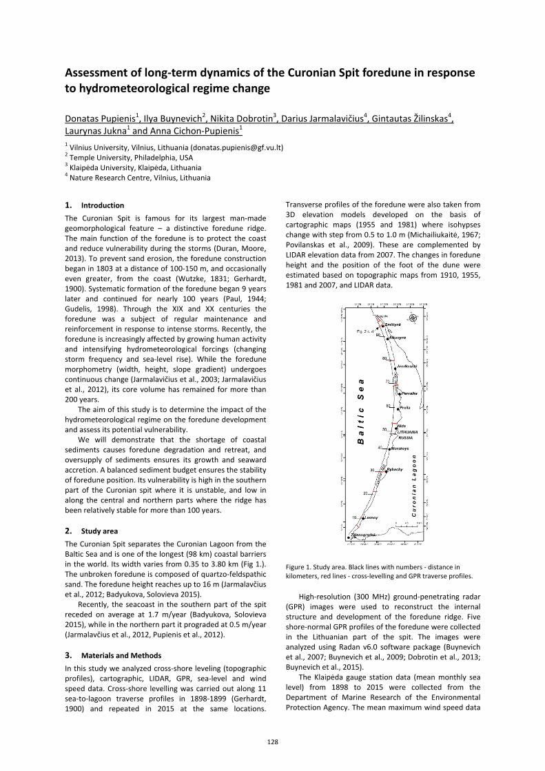
Assessment of long-term dynamics of the Curonian Spit foredune in response to hydrometeorological regime change

Donatas Pupienis1, Ilya Buynevich2, Nikita Dobrotin3, Darius Jarmalavičius4, Gintautas Žilinskas4, Laurynas Jukna1 and Anna Cichon-Pupienis1 1 Vilnius University, Vilnius, Lithuania (donatas.pupienis@gf.vu.lt) 2 Temple University, Philadelphia, USA 3 Klaipėda University, Klaipėda, Lithuania 4 Nature Research Centre, Vilnius, Lithuania

1. Introduction The Curonian Spit is famous for its largest man-made geomorphological feature – a distinctive foredune ridge. The main function of the foredune is to protect the coast and reduce vulnerability during the storms (Duran, Moore, 2013). To prevent sand erosion, the foredune construction began in 1803 at a distance of 100-150 m, and occasionally even greater, from the coast (Wutzke, 1831; Gerhardt, 1900). Systematic formation of the foredune began 9 years later and continued for nearly 100 years (Paul, 1944; Gudelis, 1998). Through the XIX and XX centuries the foredune was a subject of regular maintenance and reinforcement in response to intense storms. Recently, the foredune is increasingly affected by growing human activity and intensifying hydrometeorological forcings (changing storm frequency and sea-level rise). While the foredune morphometry (width, height, slope gradient) undergoes continuous change (Jarmalavičius et al., 2003; Jarmalavičius et al., 2012), its core volume has remained for more than 200 years.

The aim of this study is to determine the impact of the hydrometeorological regime on the foredune development and assess its potential vulnerability.

We will demonstrate that the shortage of coastal sediments causes foredune degradation and retreat, and oversupply of sediments ensures its growth and seaward accretion. A balanced sediment budget ensures the stability of foredune position. Its vulnerability is high in the southern part of the Curonian spit where it is unstable, and low in along the central and northern parts where the ridge has been relatively stable for more than 100 years. 2. Study area The Curonian Spit separates the Curonian Lagoon from the Baltic Sea and is one of the longest (98 km) coastal barriers in the world. Its width varies from 0.35 to 3.80 km (Fig 1.). The unbroken foredune is composed of quartzo-feldspathic sand. The foredune height reaches up to 16 m (Jarmalavčius et al., 2012; Badyukova, Solovieva 2015).

Recently, the seacoast in the southern part of the spit receded on average at 1.7 m/year (Badyukova, Solovieva 2015), while in the northern part it prograded at 0.5 m/year (Jarmalavčius et al., 2012, Pupienis et al., 2012). 3. Materials and Methods In this study we analyzed cross-shore leveling (topographic profiles), cartographic, LIDAR, GPR, sea-level and wind speed data. Cross-shore levelling was carried out along 11 sea-to-lagoon traverse profiles in 1898-1899 (Gerhardt, 1900) and repeated in 2015 at the same locations.

Transverse profiles of the foredune were also taken from 3D elevation models developed on the basis of cartographic maps (1955 and 1981) where isohypses change with step from 0.5 to 1.0 m (Michailiukaitė, 1967; Povilanskas et al., 2009). These are complemented by LIDAR elevation data from 2007. The changes in foredune height and the position of the foot of the dune were estimated based on topographic maps from 1910, 1955, 1981 and 2007, and LIDAR data.

Figure 1. Study area. Black lines with numbers - distance in kilometers, red lines - cross-levelling and GPR traverse profiles.

High-resolution (300 MHz) ground-penetrating radar (GPR) images were used to reconstruct the internal structure and development of the foredune ridge. Five shore-normal GPR profiles of the foredune were collected in the Lithuanian part of the spit. The images were analyzed using Radan v6.0 software package (Buynevich et al., 2007; Buynevich et al., 2009; Dobrotin et al., 2013; Buynevich et al., 2015).

The Klaipėda gauge station data (mean monthly sea level) from 1898 to 2015 were collected from the Department of Marine Research of the Environmental Protection Agency. The mean maximum wind speed data

128

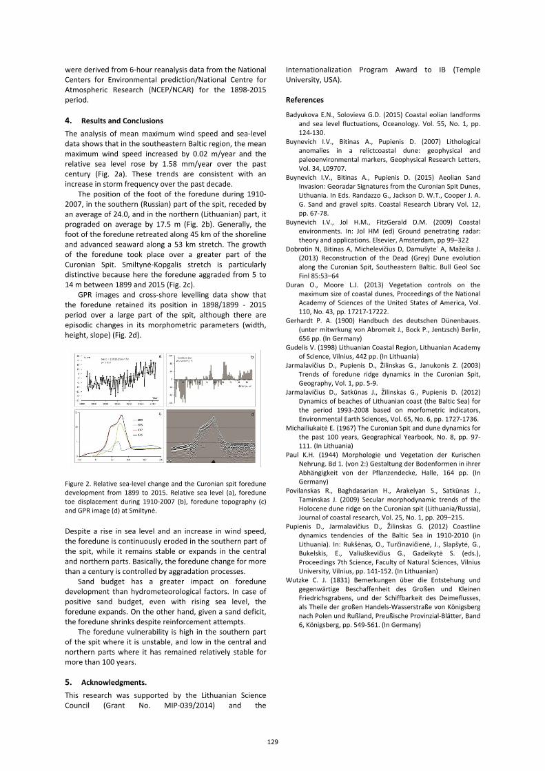
were derived from 6-hour reanalysis data from the National Centers for Environmental prediction/National Centre for Atmospheric Research (NCEP/NCAR) for the 1898-2015 period.

4. Results and Conclusions The analysis of mean maximum wind speed and sea-level data shows that in the southeastern Baltic region, the mean maximum wind speed increased by 0.02 m/year and the relative sea level rose by 1.58 mm/year over the past century (Fig. 2a). These trends are consistent with an increase in storm frequency over the past decade.

The position of the foot of the foredune during 1910-2007, in the southern (Russian) part of the spit, receded by an average of 24.0, and in the northern (Lithuanian) part, it prograded on average by 17.5 m (Fig. 2b). Generally, the foot of the foredune retreated along 45 km of the shoreline and advanced seaward along a 53 km stretch. The growth of the foredune took place over a greater part of the Curonian Spit. Smiltynė-Kopgalis stretch is particularly distinctive because here the foredune aggraded from 5 to 14 m between 1899 and 2015 (Fig. 2c).

GPR images and cross-shore levelling data show that the foredune retained its position in 1898/1899 - 2015 period over a large part of the spit, although there are episodic changes in its morphometric parameters (width, height, slope) (Fig. 2d).

Figure 2. Relative sea-level change and the Curonian spit foredune development from 1899 to 2015. Relative sea level (a), foredune toe displacement during 1910-2007 (b), foredune topography (c) and GPR image (d) at Smiltynė.

Despite a rise in sea level and an increase in wind speed, the foredune is continuously eroded in the southern part of the spit, while it remains stable or expands in the central and northern parts. Basically, the foredune change for more than a century is controlled by aggradation processes.

Sand budget has a greater impact on foredune development than hydrometeorological factors. In case of positive sand budget, even with rising sea level, the foredune expands. On the other hand, given a sand deficit, the foredune shrinks despite reinforcement attempts.

The foredune vulnerability is high in the southern part of the spit where it is unstable, and low in the central and northern parts where it has remained relatively stable for more than 100 years. 5. Acknowledgments. This research was supported by the Lithuanian Science Council (Grant No. MIP-039/2014) and the

Internationalization Program Award to IB (Temple University, USA). References

Badyukova E.N., Solovieva G.D. (2015) Coastal eolian landforms and sea level fluctuations, Oceanology. Vol. 55, No. 1, pp. 124-130.

Buynevich I.V., Bitinas A., Pupienis D. (2007) Lithological anomalies in a relictcoastal dune: geophysical and paleoenvironmental markers, Geophysical Research Letters, Vol. 34, L09707.

Buynevich I.V., Bitinas A., Pupienis D. (2015) Aeolian Sand Invasion: Georadar Signatures from the Curonian Spit Dunes, Lithuania. In Eds. Randazzo G., Jackson D. W.T., Cooper J. A. G. Sand and gravel spits. Coastal Research Library Vol. 12, pp. 67-78.

Buynevich I.V., Jol H.M., FitzGerald D.M. (2009) Coastal environments. In: Jol HM (ed) Ground penetrating radar: theory and applications. Elsevier, Amsterdam, pp 99–322

Dobrotin N, Bitinas A, Michelevičius D, Damušyte˙ A, Mažeika J. (2013) Reconstruction of the Dead (Grey) Dune evolution along the Curonian Spit, Southeastern Baltic. Bull Geol Soc Finl 85:53–64

Duran O., Moore L.J. (2013) Vegetation controls on the maximum size of coastal dunes, Proceedings of the National Academy of Sciences of the United States of America, Vol. 110, No. 43, pp. 17217-17222.

Gerhardt P. A. (1900) Handbuch des deutschen Dünenbaues. (unter mitwrkung von Abromeit J., Bock P., Jentzsch) Berlin, 656 pp. (In Germany)

Gudelis V. (1998) Lithuanian Coastal Region, Lithuanian Academy of Science, Vilnius, 442 pp. (In Lithuania)

Jarmalavičius D., Pupienis D., Žilinskas G., Janukonis Z. (2003) Trends of foredune ridge dynamics in the Curonian Spit, Geography, Vol. 1, pp. 5-9.

Jarmalavičius D., Satkūnas J., Žilinskas G., Pupienis D. (2012) Dynamics of beaches of Lithuanian coast (the Baltic Sea) for the period 1993-2008 based on morfometric indicators, Environmental Earth Sciences, Vol. 65, No. 6, pp. 1727-1736.

Michailiukaitė E. (1967) The Curonian Spit and dune dynamics for the past 100 years, Geographical Yearbook, No. 8, pp. 97-111. (In Lithuania)

Paul K.H. (1944) Morphologie und Vegetation der Kurischen Nehrung. Bd 1. (von 2:) Gestaltung der Bodenformen in ihrer Abhängigkeit von der Pflanzendecke, Halle, 164 pp. (In Germany)

Povilanskas R., Baghdasarian H., Arakelyan S., Satkūnas J., Taminskas J. (2009) Secular morphodynamic trends of the Holocene dune ridge on the Curonian spit (Lithuania/Russia), Journal of coastal research, Vol. 25, No. 1, pp. 209–215.

Pupienis D., Jarmalavičius D., Žilinskas G. (2012) Coastline dynamics tendencies of the Baltic Sea in 1910-2010 (in Lithuania). In: Rukšėnas, O., Turčinavičienė, J., Slapšytė, G., Bukelskis, E., Valiuškevičius G., Gadeikytė S. (eds.), Proceedings 7th Science, Faculty of Natural Sciences, Vilnius University, Vilnius, pp. 141-152. (In Lithuanian)

Wutzke C. J. (1831) Bemerkungen über die Entstehung und gegenwärtige Beschaffenheit des Großen und Kleinen Friedrichsgrabens, und der Schiffbarkeit des Deimeflusses, als Theile der großen Handels-Wasserstraße von Königsberg nach Polen und Rußland, Preußische Provinzial-Blätter, Band 6, Königsberg, pp. 549-561. (In Germany)

129

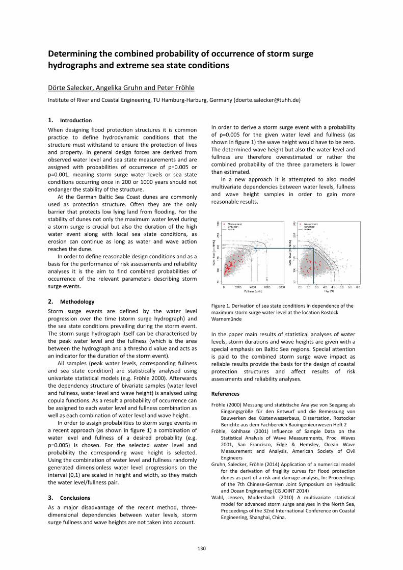
Determining the combined probability of occurrence of storm surge hydrographs and extreme sea state conditions

Dörte Salecker, Angelika Gruhn and Peter Fröhle

Institute of River and Coastal Engineering, TU Hamburg-Harburg, Germany (doerte.salecker@tuhh.de)

1. Introduction When designing flood protection structures it is common practice to define hydrodynamic conditions that the structure must withstand to ensure the protection of lives and property. In general design forces are derived from observed water level and sea state measurements and are assigned with probabilities of occurrence of p=0.005 or p=0.001, meaning storm surge water levels or sea state conditions occurring once in 200 or 1000 years should not endanger the stability of the structure.

At the German Baltic Sea Coast dunes are commonly used as protection structure. Often they are the only barrier that protects low lying land from flooding. For the stability of dunes not only the maximum water level during a storm surge is crucial but also the duration of the high water event along with local sea state conditions, as erosion can continue as long as water and wave action reaches the dune.

In order to define reasonable design conditions and as a basis for the performance of risk assessments and reliability analyses it is the aim to find combined probabilities of occurrence of the relevant parameters describing storm surge events. 2. Methodology Storm surge events are defined by the water level progression over the time (storm surge hydrograph) and the sea state conditions prevailing during the storm event. The storm surge hydrograph itself can be characterised by the peak water level and the fullness (which is the area between the hydrograph and a threshold value and acts as an indicator for the duration of the storm event).

All samples (peak water levels, corresponding fullness and sea state condition) are statistically analysed using univariate statistical models (e.g. Fröhle 2000). Afterwards the dependency structure of bivariate samples (water level and fullness, water level and wave height) is analysed using copula functions. As a result a probability of occurrence can be assigned to each water level and fullness combination as well as each combination of water level and wave height.

In order to assign probabilities to storm surge events in a recent approach (as shown in figure 1) a combination of water level and fullness of a desired probability (e.g. p=0.005) is chosen. For the selected water level and probability the corresponding wave height is selected. Using the combination of water level and fullness randomly generated dimensionless water level progressions on the interval (0,1) are scaled in height and width, so they match the water level/fullness pair. 3. Conclusions As a major disadvantage of the recent method, three-dimensional dependencies between water levels, storm surge fullness and wave heights are not taken into account.

In order to derive a storm surge event with a probability of p=0.005 for the given water level and fullness (as shown in figure 1) the wave height would have to be zero. The determined wave height but also the water level and fullness are therefore overestimated or rather the combined probability of the three parameters is lower than estimated.

In a new approach it is attempted to also model multivariate dependencies between water levels, fullness and wave height samples in order to gain more reasonable results.

Figure 1. Derivation of sea state conditions in dependence of the maximum storm surge water level at the location Rostock Warnemünde

In the paper main results of statistical analyses of water levels, storm durations and wave heights are given with a special emphasis on Baltic Sea regions. Special attention is paid to the combined storm surge wave impact as reliable results provide the basis for the design of coastal protection structures and affect results of risk assessments and reliability analyses. References

Fröhle (2000) Messung und statistische Analyse von Seegang als Eingangsgröße für den Entwurf und die Bemessung von Bauwerken des Küstenwasserbaus, Dissertation, Rostocker Berichte aus dem Fachbereich Bauingenieurwesen Heft 2

Fröhle, Kohlhase (2001) Influence of Sample Data on the Statistical Analysis of Wave Measurements, Proc. Waves 2001, San Francisco, Edge & Hemsley, Ocean Wave Measurement and Analysis, American Society of Civil Engineers

Gruhn, Salecker, Fröhle (2014) Application of a numerical model for the derivation of fragility curves for flood protection dunes as part of a risk and damage analysis, In: Proceedings of the 7th Chinese-German Joint Symposium on Hydraulic and Ocean Engineering (CG JOINT 2014)

Wahl, Jensen, Mudersbach (2010) A multivariate statistical model for advanced storm surge analyses in the North Sea, Proceedings of the 32nd International Conference on Coastal Engineering, Shanghai, China.

130

Simulating sea level variations in the Baltic Sea using regional climate scenarios

Jani Särkkä, Kimmo K. Kahma, Matti Kämäräinen and Milla M. Johansson Finnish Meteorological Institute, Helsinki, Finland (Jani.Sarkka@fmi.fi) 1. Introduction The need to assess the regional effects of the long-term changes in the global climate has initiated many European regional climate simulations. By using a sea level model with regional climate simulations as an atmospheric input, the effects of the climate change on the sea levels can be analyzed. We have made a fast sea level model for the Baltic Sea that can be used to simulate thousand years of sea levels in a reasonable time.

2. Methods Our sea level model is based on five components that separately model different physical processes contributing to the sea level. The intra-basin fluctuations of the Baltic Sea are calculated by a one-layer model introduced by Hansen (1956) and developed by Häkkinen (1980). The Baltic Sea is treated as a closed basin. The grid resolution is 0.25 X 0.5 degrees.

The changes in the water balance of the Baltic Sea are approximated with a linear regression model, based on the dependence between geostrophic zonal winds at 55 N, 15 E (on Bornholm) and sea levels at the Finnish coast. This dependence is discussed by Johansson et al. (2014, 2016). The water balance term depends on the zonal components of the daily geostrophic winds at 55 N, 15 E of the previous 65 days, weighted by an exponentially decaying coefficient.

The two location-dependent sea level components in the model are tide and postglacial land uplift. The fifth component is the mean sea level rise due to the global warming that is general for the entire Baltic Sea. The so-called fingerprint effect could be a sixth component, but it was left out in these simulations.

The performance of the sea level model was tested using ERA-40 and ERA-Interim reanalyzes as atmospheric forcing. The correlation of the simulated sea levels with the tide gauge observations on the Finnish coast is between 0.92 and 0.94. Variations of the long-term mean of the water balance are well reproduced by the model, differing only by few centimetres from the observed mean sea levels. The accuracy of the sea level model is comparable to a three-dimensional ocean circulation model used previously in Baltic Sea level simulations by Meier et al. (2004). Our model allows the calculation of a thousand-year sea level time series within hours.

3. Results Various climate scenario simulations from different European meteorological research institutes were used as an input for the sea level model. After assessing the reliability of the sea level simulation results, six different scenario simulations between 1951 and 2100 were selected. The total number of years simulated was 850, which allows us to estimate the exceedance frequency of 1/850 events per year without extrapolating simulation data.

The long-term means of the sea level given by the different climate scenarios vary between 5 and 20 cm, but the increase in the mean sea level due to the increasing wind speeds by the end of the present century is only between 0 and 10 cm. The scenarios also give differing exceedance frequencies for the high sea levels on the Finnish coast. Therefore it is important to

assess how well the climate scenarios produce realistic air pressure distributions. If there are biases towards deep small-scale low pressures, high sea levels appear too often in the simulations.

The 850-year sea level simulation results for different coastal locations can be used to assess return probabilities of sea floods, providing an alternative to the extreme value analyzes of the tide gauge data. By studying the behaviour of the sea level components in extreme sea level events, the mechanisms behind these events can be better understood. References Hansen W. (1956) Theorie zur Errechnung des Wasserstandes und der

Strömungen in Randmeeren nebst Anwendungen, Tellus, Vol. 8, No. 3, pp. 287-300.

Häkkinen S. (1980) Computation of sea level variations during December 1975 and 1 to 17 September 1977 using numerical models of the Baltic Sea, Dt. Hydr. Z., Vol. 33, No. 4 pp. 158-175

Johansson M.M., Pellikka H., Kahma K. K., Ruosteenoja K. (2014) Global sea level rise scenarios adapted to the Finnish coast, J. Mar. Systems, Vol. 129, pp. 35-46

Johansson M.M., Kahma K. K. (2016) On the statistical relationship between the geostrophic wind and sea level variations in the Baltic Sea, Bor. Env. Res., Vol. 21, in press

Meier H.E.M., Broman B., Kjellström E. (2004) Simulated sea levels in past and future climates of the Baltic Sea, Clim. Res., Vol. 27, No. 1, pp. 59-75

131

Water level extremes signal changes in the wind direction in the north-eastern Baltic Sea

Tarmo Soomere, Maris Eelsalu and Katri Pindsoo

Institute of Cybernetics at Tallinn University of Technology, Tallinn, Estonia (soomere@cs.ioc.ee)

1. Introduction An increase in the magnitude of extreme storm surges is one of the largest concerns of countries with extensive low-lying nearshore areas. The situation is particularly complicated in semi-enclosed water bodies such as the Baltic Sea. The sea-level change in such basins may be faster than in the adjacent regions, the course of water level may depend on specific factors such as local salinity and changes in the entire volume of the sea may markedly add to the high water levels.

The increase in the water level maxima varies greatly in the eastern Baltic Sea and has a spatially variable rate of 5–10 cm/decade (Suursaar and Sooäär, 2007). It is relatively rapid in the interiors of bays deeply cut into the mainland and slower on the coasts of the open sea.

It is often unclear which mechanism is responsible for an increase in the extreme water levels and particularly for the spatial variations of this increase. Classic approaches address this question by means of a separation of the water level course into various types of components (periodic and random components, or constituents driven by fundamentally different mechanisms or having substantially different temporal scales). We demonstrate that a natural and rich in content separation of the processes into short-term and weekly-scale constituents can be produced for the eastern Baltic Sea by means of simple averaging. 2. Data and methods We employ time series of sea levels extracted from the output of the RCO (Rossby Center, Swedish Meteorological and Hydrological Institute) ocean circulation model (Meier et al., 2003). The data were kindly provided in the framework of BONUS BalticWay cooperation. The horizontal and vertical resolutions of the model are 2 × 2 nautical miles (about 3.7 km) and 3–12 m, respectively. The model run for May 1961–May 2005 includes information about sea ice and is driven by atmospheric information a horizontal resolution of 22 km produced from the ERA-40 re-analysis.

The modelled data set is sampled once in 6 h. The model output is complemented with observed water level time series at four coastal locations in the eastern Baltic Sea: Tallinn (only until 1995), Narva-Jõesuu, Ristna and Pärnu.

The water level time series is split into slowly and rapidly changing components by means of using a running average. The averaging length is varied from one day up to a few months. The slowly changing component mimics the water volume of the entire Baltic Sea. Its distribution has, as expected, an almost Gaussian shape. The residual (total water level minus the average) characterises the heights of storm surges. It contains all outliers of the water level time series for averaging intervals longer than about 3 days. The distribution of this component almost exactly matches an exponential distribution for the 8-day average (Soomere et

al., 2015). Therefore, for this averaging length the total water level is split into a component that reflects a Gaussian process and another component driven by a Poisson process. 3. Contributions into extreme water levels The introduced separation makes it possible to evaluate the contribution of processes with different spatio-temporal scales and to highlight the role of different physical drivers in this increase.

The increase rate of the weekly-scale average extreme water levels is almost constant (about 4 cm/decade) along the entire eastern coast of the Baltic Sea. This component reflects the cumulative impact of long sequences of storms (Lehmann and Post, 2015). Its gradual increase therefore means that either the wind speed in such storms has increased or, alternatively, the storm sequences have become longer.

Almost all spatial variability in the trends of the total water level maxima is contained in the residual of the above process, that is, in the component that reflects the impact of single storms. This part of variations in the extreme water levels exhibits almost no changes at the western coast of the Western Estonian archipelago. Even though these locations are open to the predominant directions of strong storms, the changes in the maxima of the total water level in such locations are almost exclusively governed by the water volume of the entire Baltic Sea. This feature signals that a significant increase in the wind speed in strong storms is unlikely and, more probably, the length of sequences of storms that push water into the Baltic Sea has increased.

The maxima of the residual exhibit almost no changes along the eastern coast of the Baltic Proper but a substantial increase in bayheads of large subbasins such as the eastern Gulf of Riga and the eastern Gulf of Finland (Soomere and Pindsoo, 2016). As this component mirrors the features of local storm surges, most of the increase in the contribution of this component to local water level extremes is driven by changes in properties of single storms. In the light of the above, this remarkable spatial variation suggests that, most likely, wind directions in strong storms may have rotated since the 1960s. This conjecture is partially supported by changes in wind directions (Jaagus and Kull, 2011) and air-flow (Keevallik and Soomere, 2014) in some domains of the north-eastern Baltic Sea. 4. Concluding remarks The introduced separation and a careful choice of the time scale for this procedure makes it possible to separate the local water level time series of the Baltic Sea (and possibly other semi-enclosed water bodies) into two components with clear physical relevance. Importantly, these constituents have fundamentally different

132

probability distribution functions. The presence of a Poisson process in this system is not surprising as the formation of storm cyclones can be described by a Poisson process.

The implications of the analysis of the contribution of these components are deeply nontrivial. A straightforward conjecture is that an increase in wind speed in strong storms is unlikely in this area but the duration of storm sequences may have increased and wind direction may have rotated. This pattern of changes may lead to by an order of magnitude greater changes, e.g., in the wave heights than a similar increase in wind speed (Anderson et al., 2016).

A more subtle conjecture of the presence of two processes with fundamentally different distributions is that standard methods for estimates of extreme water levels and their return periods may fail in the eastern Baltic Sea conditions. A feasible way forward is the use of ensemble-based approach for the construction of such projections that are able inter alia to identify the magnitude of local effects in the formation of high water levels (Eelsalu et al., 2014). References

Anderson J.D., Wu C.H., Schwab D.J. (2015) Wave climatology in the Apostle Islands, Lake Superior. J. Geophys. Res.-Oceans, Vol. 120, No. C7, pp. 4869–4890.

Eelsalu M., Soomere T., Pindsoo K., Lagemaa P. (2014) Ensemble approach for projections of return periods of extreme water levels in Estonian waters. Cont. Shelf. Res., Vol. 91, pp. 201–210.

Jaagus J., Kull A. (2011) Changes in surface wind directions in Estonia during 1966-2008 and their relationships with large-scale atmospheric circulation. Estonian J. Earth Sci., Vol. 60, pp. 220–231.

Keevallik S., Soomere T. (2014) Regime shifts in the surface-level average air flow over the Gulf of Finland during 1981–2010. Proc. Estonian Acad. Sci., Vol. 63, No. 4, pp. 428–437.

Lehmann A., Post P. (2015) Variability of atmospheric circulation patterns associated with large volume changes of the Baltic Sea. Adv. Sci. Res., Vol. 12, pp. 219–225.

Meier H.E.M., Döscher, R., Faxén, T. (2003). A multiprocessor coupled ice-ocean model for the Baltic Sea: application to salt inflow. J. Geophys. Res.–Oceans, Vol. 108, No. C8, pp. 32–73.

Soomere T., Eelsalu M., Kurkin A., Rybin A. (2015) Separation of the Baltic Sea water level into daily and multi-weekly components. Cont. Shelf Res., Vol. 103, pp. 23–32.

Soomere T., Pindsoo K. (2016) Spatial variability in the trends in extreme storm surges and weekly-scale high water levels in the eastern Baltic Sea. Cont. Shelf Res., Vol. 115, pp. 53–64.

Suursaar Ü., Sooäär J. (2007) Decadal variations in mean and extreme sea level values along the Estonian coast of the Baltic Sea. Tellus A, Vol. 59, pp. 249–260.

133

134

Topic E

Regional variability of water and energy exchanges

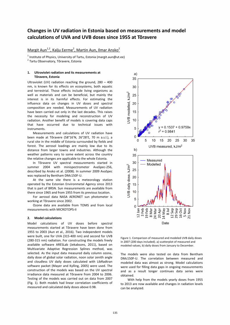
Changes in UV radiation in Estonia based on measurements and model calculations of UVA and UVB doses since 1955 at Tõravere

Margit Aun1,2, Kalju Eerme2, Martin Aun, Ilmar Ansko2 1 Institute of Physics, University of Tartu, Estonia (margit.aun@ut.ee) 2 Tartu Observatory, Tõravere, Estonia

1. Ultraviolet radiation and its measurements at Tõravere, Estonia

Ultraviolet (UV) radiation reaching the ground, 280 – 400 nm, is known for its effects on ecosystems, both aquatic and terrestrial. Those effects include living organisms as well as materials and can be beneficial, but mainly the interest is in its harmful effects. For estimating the influence data on changes in UV doses and spectral composition are needed. Measurements of UV radiation have been carried out only in the last decades. This raises the necessity for modeling and reconstruction of UV radiation. Another benefit of models is covering data caps that have occurred due to technical issues with instruments.

Measurements and calculations of UV radiation have been made at Tõravere (58°16’N, 26°28’E, 70 m a.s.l.), a rural site in the middle of Estonia surrounded by fields and forest. The aerosol loadings are mainly low due to its distance from larger towns and industries. Although the weather patterns vary to some extent across the country the relative changes are applicable to the whole Estonia.

In Tõravere UV spectral measurements started in summer 2004 with minispectrometer AvaSpec-256, described by Ansko et al. (2008). In summer 2009 AvaSpec was replaced by Bentham DMc150F-U.

At the same site there is a meteorology station operated by the Estonian Environmetal Agency since 2013 that is part of BRSN. Sun measurements are available from there since 1965 and from 1955 from its previous location.

For aerosol data NASA AERONET sun photometer is working at Tõravere since 2002.

Ozone data are available from TOMS and from local measurements with MICROTOPS-II 2. Model calculations Model calculations of UV doses before spectral measurements started at Tõravere have been done from 1955 to 2003 (Aun et al., 2016). Two independent models were built, one for UVA (315-400 nm) and second for UVB (280-315 nm) radiation. For constructing the models freely available software ARESLab (Jekabsons, 2011), based on Multivariate Adaptive Regression Splines method, was selected. As the input data measured daily column ozone, daily dose of global solar radiation, noon solar zenith angle and cloudless UV daily doses calculated with LibRadtran software packet (Mayer and Kylling, 2005) were used. The construction of the models was based on the UV spectral irradiance data measured at Tõravere from 2004 to 2006. Testing of the models was carried out on data from 2007 (Fig. 1). Both models had linear correlation coefficients of measured and calculated daily doses above 0.98.

Figure 1. Comparison of measured and modeled UVB daily doses in 2007 (200 days included). a) scatterplot of measured and modeled values, b) daily doses from January to December.

The models were also tested on data from Bentham DMc150F-U. The correlation between measured and modeled data was almost as strong. Model calculations were used for filling data gaps in ongoing measurements and as a result longer continues data series were obtained.

With help from the models yearly doses from 1955 to 2013 are now available and changes in radiation levels can be analyzed.

135

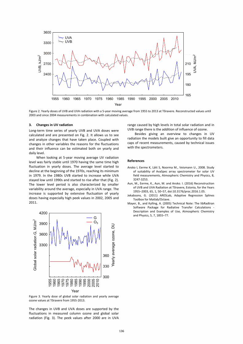
Figure 2. Yearly doses of UVB and UVA radiation with a 5-year moving average from 1955 to 2013 at Tõravere. Reconstructed values until 2003 and since 2004 measurements in combination with calculated values.

3. Changes in UV radiation Long-term time series of yearly UVB and UVA doses were calculated and are presented on Fig. 2. It allows us to see and analyze changes that have taken place. Coupled with changes in other variables the reasons for the fluctuations and their influence can be estimated both on yearly and daily level.

When looking at 5-year moving average UV radiation level was fairly stable until 1970 having the same time high fluctuation in yearly doses. The average level started to decline at the beginning of the 1970s, reaching its minimum in 1979. In the 1980s UVB started to increase while UVA stayed low until 1990s and started to rise after that (Fig. 2). The lower level period is also characterized by smaller variability around the average, especially in UVA range. The increase is supported by extensive fluctuation of yearly doses having especially high peek values in 2002, 2005 and 2011.

Figure 3. Yearly dose of global solar radiation and yearly average ozone values at Tõravere from 1955-2013. The changes in UVB and UVA doses are supported by the fluctuations in measured column ozone and global solar radiation (Fig. 3). The peek values after 2000 are in UVA

range caused by high levels in total solar radiation and in UVB range there is the addition of influence of ozone.

Besides giving an overview to changes in UV radiation the models built give an opportunity to fill data caps of recent measurements, caused by technical issues with the spectrometers. References

Ansko I, Eerme K, Lätt S, Noorma M., Veismann U., 2008. Study of suitability of AvaSpec array spectrometer for solar UV field measurements, Atmospheric Chemistry and Physics, 8, 3247-3253.

Aun, M., Eerme, K., Aun, M. and Ansko. I. (2016) Reconstruction of UVB and UVA Radiation at Tõravere, Estonia, for the Years 1955–2003, 65, 1, 50–57, doi:10.3176/proc.2016.1.05.

Jekabsons, G. (2011) ARESLab, Adaptive Regression Splines Toolbox for Matlab/Octave.

Mayer, B., and Kylling, A. (2005) Technical Note: The libRadtran Software Package for Radiative Transfer Calculations - Description and Examples of Use, Atmospheric Chemistry and Physics, 5, 7, 1855–77.

136

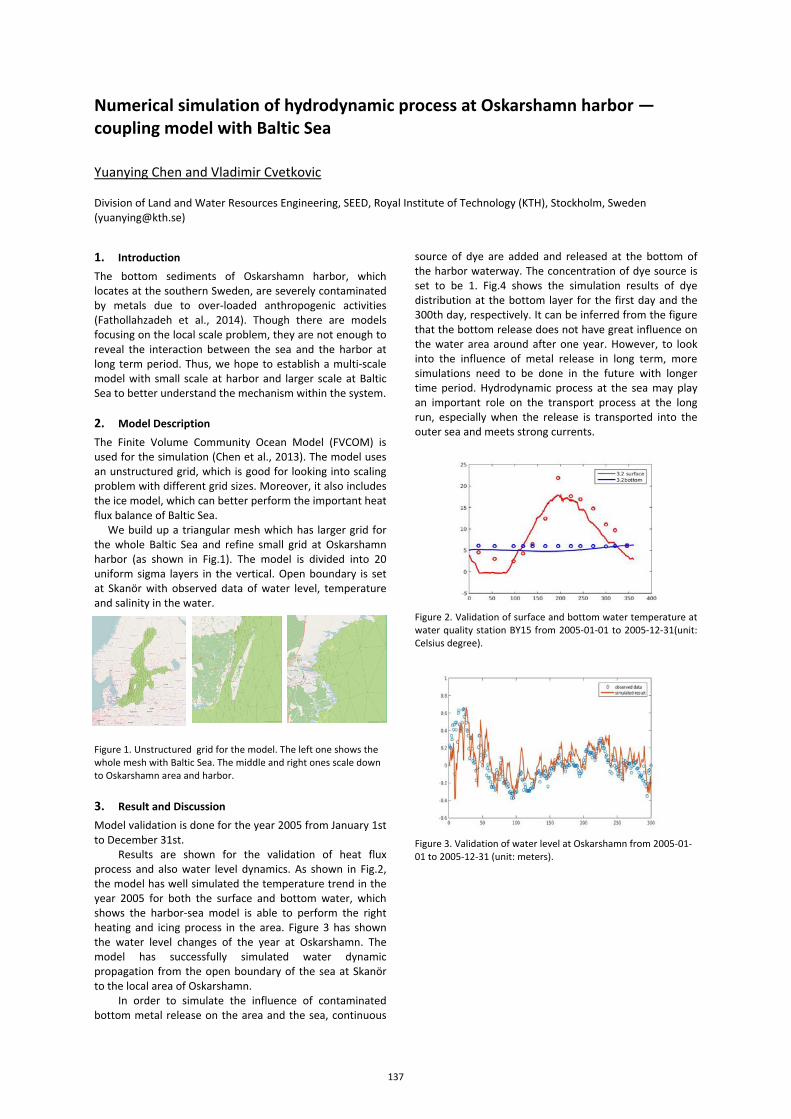
Numerical simulation of hydrodynamic process at Oskarshamn harbor —coupling model with Baltic Sea

Yuanying Chen and Vladimir Cvetkovic

Division of Land and Water Resources Engineering, SEED, Royal Institute of Technology (KTH), Stockholm, Sweden (yuanying@kth.se)

1. Introduction The bottom sediments of Oskarshamn harbor, which locates at the southern Sweden, are severely contaminated by metals due to over-loaded anthropogenic activities (Fathollahzadeh et al., 2014). Though there are models focusing on the local scale problem, they are not enough to reveal the interaction between the sea and the harbor at long term period. Thus, we hope to establish a multi-scale model with small scale at harbor and larger scale at Baltic Sea to better understand the mechanism within the system. 2. Model Description The Finite Volume Community Ocean Model (FVCOM) is used for the simulation (Chen et al., 2013). The model uses an unstructured grid, which is good for looking into scaling problem with different grid sizes. Moreover, it also includes the ice model, which can better perform the important heat flux balance of Baltic Sea. We build up a triangular mesh which has larger grid for the whole Baltic Sea and refine small grid at Oskarshamn harbor (as shown in Fig.1). The model is divided into 20 uniform sigma layers in the vertical. Open boundary is set at Skanör with observed data of water level, temperature and salinity in the water.

Figure 1. Unstructured grid for the model. The left one shows the whole mesh with Baltic Sea. The middle and right ones scale down to Oskarshamn area and harbor.

3. Result and Discussion Model validation is done for the year 2005 from January 1st to December 31st.

Results are shown for the validation of heat flux process and also water level dynamics. As shown in Fig.2, the model has well simulated the temperature trend in the year 2005 for both the surface and bottom water, which shows the harbor-sea model is able to perform the right heating and icing process in the area. Figure 3 has shown the water level changes of the year at Oskarshamn. The model has successfully simulated water dynamic propagation from the open boundary of the sea at Skanör to the local area of Oskarshamn.

In order to simulate the influence of contaminated bottom metal release on the area and the sea, continuous

source of dye are added and released at the bottom of the harbor waterway. The concentration of dye source is set to be 1. Fig.4 shows the simulation results of dye distribution at the bottom layer for the first day and the 300th day, respectively. It can be inferred from the figure that the bottom release does not have great influence on the water area around after one year. However, to look into the influence of metal release in long term, more simulations need to be done in the future with longer time period. Hydrodynamic process at the sea may play an important role on the transport process at the long run, especially when the release is transported into the outer sea and meets strong currents.

Figure 2. Validation of surface and bottom water temperature at water quality station BY15 from 2005-01-01 to 2005-12-31(unit: Celsius degree).

Figure 3. Validation of water level at Oskarshamn from 2005-01-01 to 2005-12-31 (unit: meters).

137

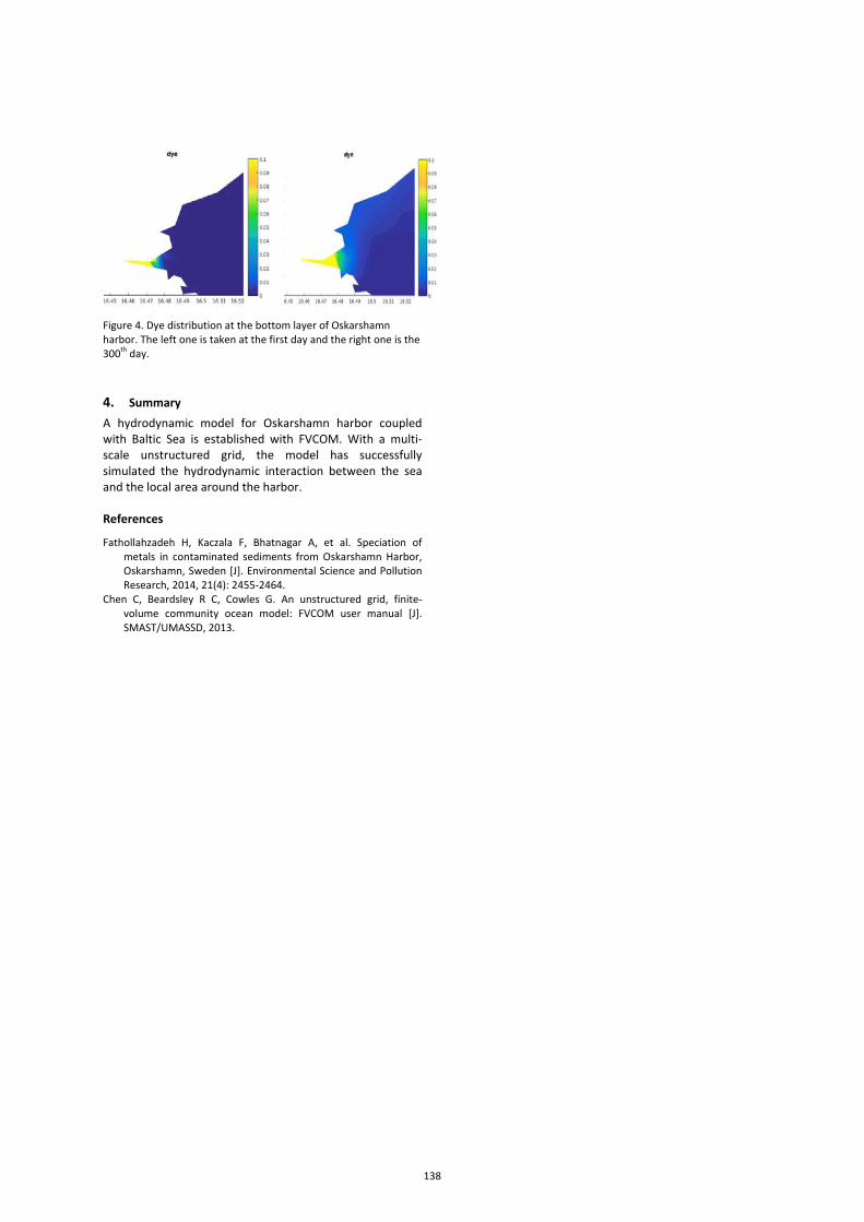
Figure 4. Dye distribution at the bottom layer of Oskarshamn harbor. The left one is taken at the first day and the right one is the 300th day.

4. Summary A hydrodynamic model for Oskarshamn harbor coupled with Baltic Sea is established with FVCOM. With a multi-scale unstructured grid, the model has successfully simulated the hydrodynamic interaction between the sea and the local area around the harbor. References

Fathollahzadeh H, Kaczala F, Bhatnagar A, et al. Speciation of metals in contaminated sediments from Oskarshamn Harbor, Oskarshamn, Sweden [J]. Environmental Science and Pollution Research, 2014, 21(4): 2455-2464.

Chen C, Beardsley R C, Cowles G. An unstructured grid, finite-volume community ocean model: FVCOM user manual [J]. SMAST/UMASSD, 2013.

138

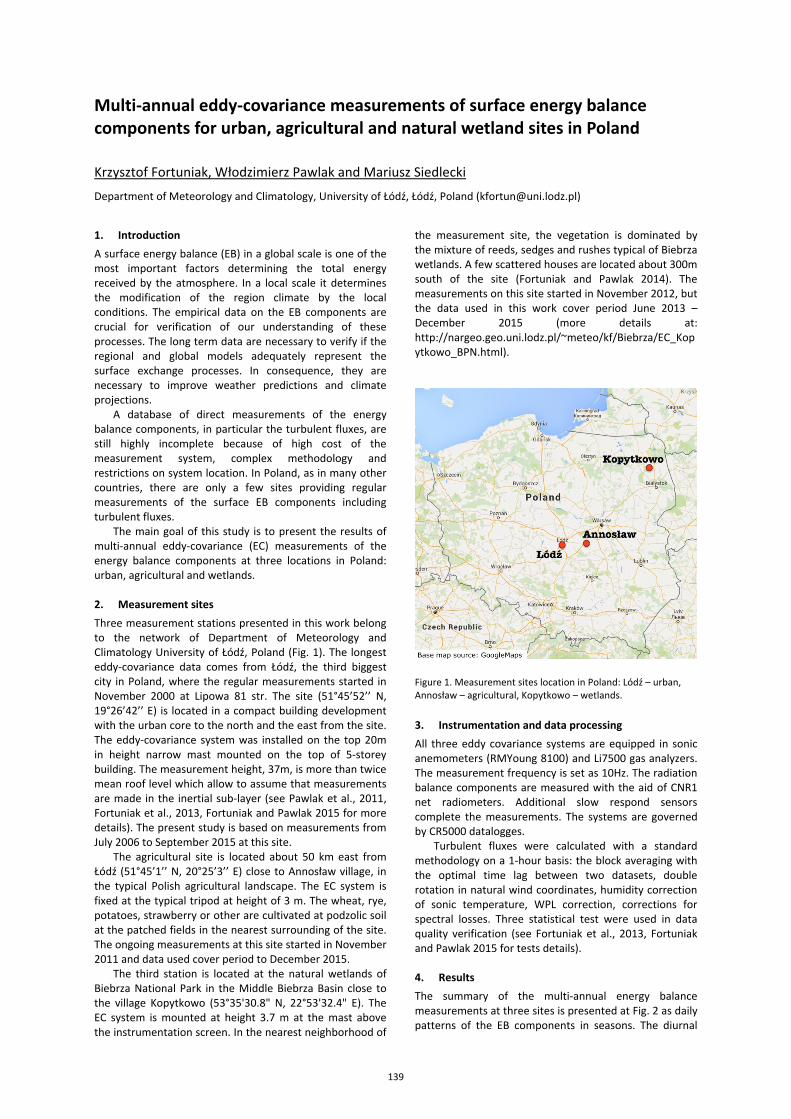
Multi-annual eddy-covariance measurements of surface energy balance components for urban, agricultural and natural wetland sites in Poland

Krzysztof Fortuniak, Włodzimierz Pawlak and Mariusz Siedlecki

Department of Meteorology and Climatology, University of Łódź, Łódź, Poland (kfortun@uni.lodz.pl)

1. Introduction A surface energy balance (EB) in a global scale is one of the most important factors determining the total energy received by the atmosphere. In a local scale it determines the modification of the region climate by the local conditions. The empirical data on the EB components are crucial for verification of our understanding of these processes. The long term data are necessary to verify if the regional and global models adequately represent the surface exchange processes. In consequence, they are necessary to improve weather predictions and climate projections.

A database of direct measurements of the energy balance components, in particular the turbulent fluxes, are still highly incomplete because of high cost of the measurement system, complex methodology and restrictions on system location. In Poland, as in many other countries, there are only a few sites providing regular measurements of the surface EB components including turbulent fluxes.

The main goal of this study is to present the results of multi-annual eddy-covariance (EC) measurements of the energy balance components at three locations in Poland: urban, agricultural and wetlands. 2. Measurement sites Three measurement stations presented in this work belong to the network of Department of Meteorology and Climatology University of Łódź, Poland (Fig. 1). The longest eddy-covariance data comes from Łódź, the third biggest city in Poland, where the regular measurements started in November 2000 at Lipowa 81 str. The site (51°45’52’’ N, 19°26’42’’ E) is located in a compact building development with the urban core to the north and the east from the site. The eddy-covariance system was installed on the top 20m in height narrow mast mounted on the top of 5-storey building. The measurement height, 37m, is more than twice mean roof level which allow to assume that measurements are made in the inertial sub-layer (see Pawlak et al., 2011, Fortuniak et al., 2013, Fortuniak and Pawlak 2015 for more details). The present study is based on measurements from July 2006 to September 2015 at this site.

The agricultural site is located about 50 km east from Łódź (51°45’1’’ N, 20°25’3’’ E) close to Annosław village, in the typical Polish agricultural landscape. The EC system is fixed at the typical tripod at height of 3 m. The wheat, rye, potatoes, strawberry or other are cultivated at podzolic soil at the patched fields in the nearest surrounding of the site. The ongoing measurements at this site started in November 2011 and data used cover period to December 2015.

The third station is located at the natural wetlands of Biebrza National Park in the Middle Biebrza Basin close to the village Kopytkowo (53°35'30.8" N, 22°53'32.4" E). The EC system is mounted at height 3.7 m at the mast above the instrumentation screen. In the nearest neighborhood of

the measurement site, the vegetation is dominated by the mixture of reeds, sedges and rushes typical of Biebrza wetlands. A few scattered houses are located about 300m south of the site (Fortuniak and Pawlak 2014). The measurements on this site started in November 2012, but the data used in this work cover period June 2013 – December 2015 (more details at: http://nargeo.geo.uni.lodz.pl/~meteo/kf/Biebrza/EC_Kopytkowo_BPN.html).

Figure 1. Measurement sites location in Poland: Lódź – urban, Annosław – agricultural, Kopytkowo – wetlands.

3. Instrumentation and data processing All three eddy covariance systems are equipped in sonic anemometers (RMYoung 8100) and Li7500 gas analyzers. The measurement frequency is set as 10Hz. The radiation balance components are measured with the aid of CNR1 net radiometers. Additional slow respond sensors complete the measurements. The systems are governed by CR5000 datalogges.

Turbulent fluxes were calculated with a standard methodology on a 1-hour basis: the block averaging with the optimal time lag between two datasets, double rotation in natural wind coordinates, humidity correction of sonic temperature, WPL correction, corrections for spectral losses. Three statistical test were used in data quality verification (see Fortuniak et al., 2013, Fortuniak and Pawlak 2015 for tests details). 4. Results The summary of the multi-annual energy balance measurements at three sites is presented at Fig. 2 as daily patterns of the EB components in seasons. The diurnal

139

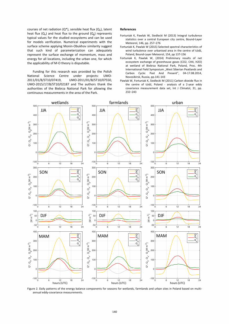
courses of net radiation (Q*), sensible heat flux (Qh), latent heat flux (Qe) and heat flux to the ground (Qg) represents typical values for the studied ecosystems and can be used for models verification. Numerical experiments with the surface scheme applying Monin-Obukhov similarity suggest that such kind of parameterization can adequately represent the surface exchange of momentum, mass and energy for all locations, including the urban one, for which the applicability of M-O theory is disputable.

Funding for this research was provided by the Polish

National Science Centre under projects: UMO-2011/01/B/ST10/07419, UMO-2011/01/B/ST10/07550, UMO-2015/17/B/ST10/02187 and The authors thank the authorities of the Biebrza National Park for allowing the continuous measurements in the area of the Park.

References

Fortuniak K, Pawlak W, Siedlecki M (2013) Integral turbulence statistics over a central European city centre, Bound-Layer Meteorol, 146, pp. 257–276

Fortuniak K, Pawlak W (2015) Selected spectral characteristics of wind turbulence over urbanised area in the centre of Łódź, Poland, Bound-Layer Meteorol, 154, pp 137-156

Fortuniak K, Pawlak W, (2014) Preliminary results of net ecosystem exchange of greenhouse gases (CO2, CH4, H2O) at wetland of Biebrza National Park, Poland, Proc. 4th International Field Symposium „West Siberian Peatlands and Carbon Cycle: Past And Present”, 04-17.08.2014, Novosibirsk, Russia, pp.141-143

Pawlak W, Fortuniak K, Siedlecki M (2011) Carbon dioxide flux in the centre of Łódź, Poland - analysis of a 2-year eddy covariance measurement data set, Int J Climatol, 31, pp. 232–243

Figure 2. Daily patterns of the energy balance components for seasons for wetlands, farmlands and urban sites in Poland based on multi-

annual eddy-covariance measurements.

140

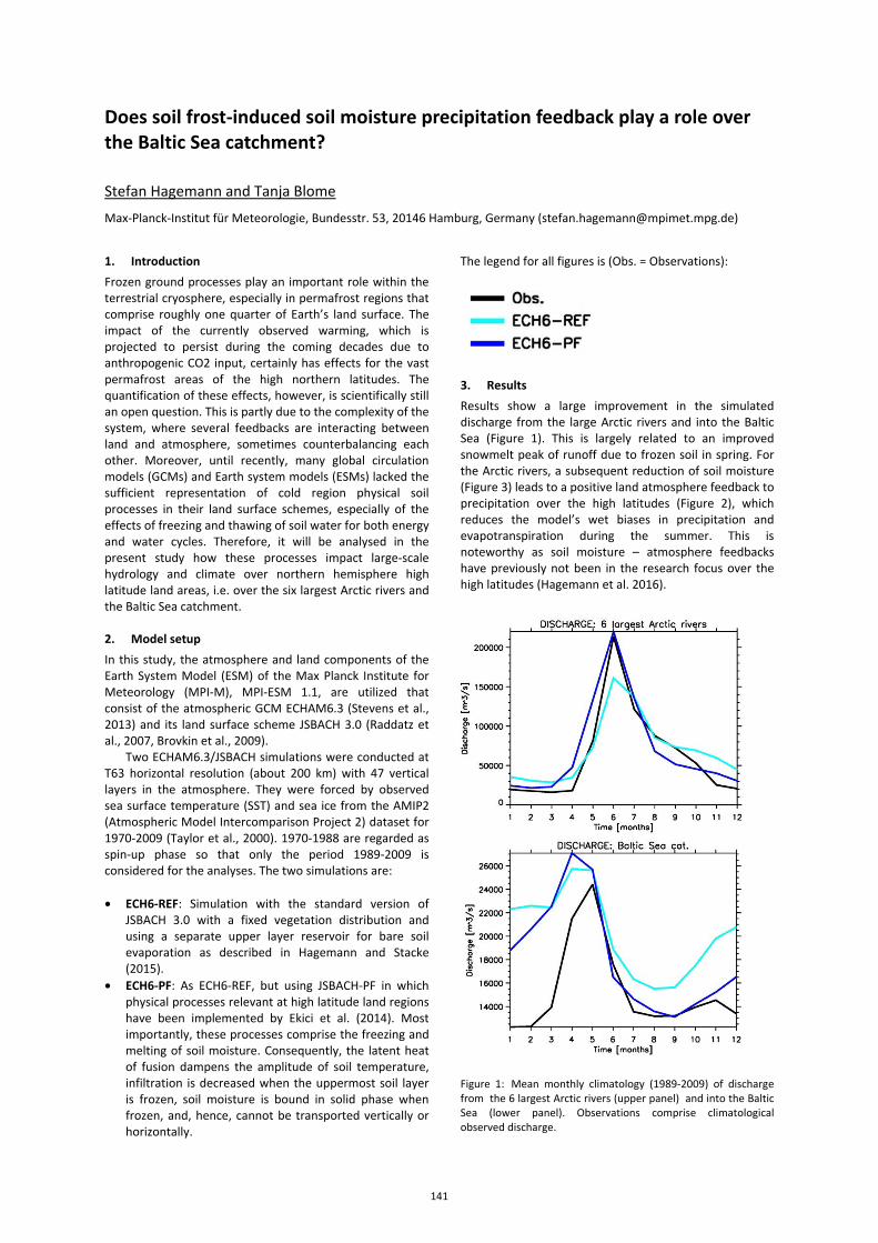
Does soil frost-induced soil moisture precipitation feedback play a role over the Baltic Sea catchment?

Stefan Hagemann and Tanja Blome

Max-Planck-Institut für Meteorologie, Bundesstr. 53, 20146 Hamburg, Germany (stefan.hagemann@mpimet.mpg.de)

1. Introduction Frozen ground processes play an important role within the terrestrial cryosphere, especially in permafrost regions that comprise roughly one quarter of Earth’s land surface. The impact of the currently observed warming, which is projected to persist during the coming decades due to anthropogenic CO2 input, certainly has effects for the vast permafrost areas of the high northern latitudes. The quantification of these effects, however, is scientifically still an open question. This is partly due to the complexity of the system, where several feedbacks are interacting between land and atmosphere, sometimes counterbalancing each other. Moreover, until recently, many global circulation models (GCMs) and Earth system models (ESMs) lacked the sufficient representation of cold region physical soil processes in their land surface schemes, especially of the effects of freezing and thawing of soil water for both energy and water cycles. Therefore, it will be analysed in the present study how these processes impact large-scale hydrology and climate over northern hemisphere high latitude land areas, i.e. over the six largest Arctic rivers and the Baltic Sea catchment. 2. Model setup In this study, the atmosphere and land components of the Earth System Model (ESM) of the Max Planck Institute for Meteorology (MPI-M), MPI-ESM 1.1, are utilized that consist of the atmospheric GCM ECHAM6.3 (Stevens et al., 2013) and its land surface scheme JSBACH 3.0 (Raddatz et al., 2007, Brovkin et al., 2009).

Two ECHAM6.3/JSBACH simulations were conducted at T63 horizontal resolution (about 200 km) with 47 vertical layers in the atmosphere. They were forced by observed sea surface temperature (SST) and sea ice from the AMIP2 (Atmospheric Model Intercomparison Project 2) dataset for 1970-2009 (Taylor et al., 2000). 1970-1988 are regarded as spin-up phase so that only the period 1989-2009 is considered for the analyses. The two simulations are: • ECH6-REF: Simulation with the standard version of

JSBACH 3.0 with a fixed vegetation distribution and using a separate upper layer reservoir for bare soil evaporation as described in Hagemann and Stacke (2015).

• ECH6-PF: As ECH6-REF, but using JSBACH-PF in which physical processes relevant at high latitude land regions have been implemented by Ekici et al. (2014). Most importantly, these processes comprise the freezing and melting of soil moisture. Consequently, the latent heat of fusion dampens the amplitude of soil temperature, infiltration is decreased when the uppermost soil layer is frozen, soil moisture is bound in solid phase when frozen, and, hence, cannot be transported vertically or horizontally.

The legend for all figures is (Obs. = Observations):

3. Results Results show a large improvement in the simulated discharge from the large Arctic rivers and into the Baltic Sea (Figure 1). This is largely related to an improved snowmelt peak of runoff due to frozen soil in spring. For the Arctic rivers, a subsequent reduction of soil moisture (Figure 3) leads to a positive land atmosphere feedback to precipitation over the high latitudes (Figure 2), which reduces the model’s wet biases in precipitation and evapotranspiration during the summer. This is noteworthy as soil moisture – atmosphere feedbacks have previously not been in the research focus over the high latitudes (Hagemann et al. 2016).

Figure 1: Mean monthly climatology (1989-2009) of discharge from the 6 largest Arctic rivers (upper panel) and into the Baltic Sea (lower panel). Observations comprise climatological observed discharge.

141

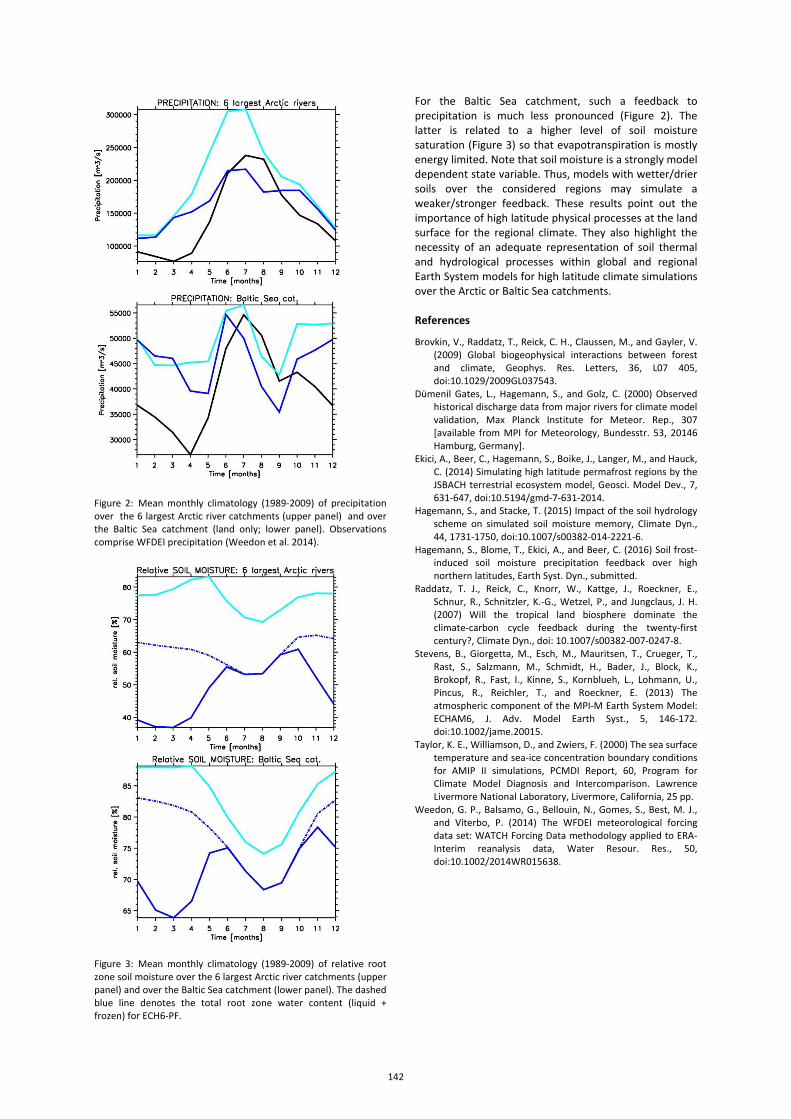
Figure 2: Mean monthly climatology (1989-2009) of precipitation over the 6 largest Arctic river catchments (upper panel) and over the Baltic Sea catchment (land only; lower panel). Observations comprise WFDEI precipitation (Weedon et al. 2014).

Figure 3: Mean monthly climatology (1989-2009) of relative root zone soil moisture over the 6 largest Arctic river catchments (upper panel) and over the Baltic Sea catchment (lower panel). The dashed blue line denotes the total root zone water content (liquid + frozen) for ECH6-PF.

For the Baltic Sea catchment, such a feedback to precipitation is much less pronounced (Figure 2). The latter is related to a higher level of soil moisture saturation (Figure 3) so that evapotranspiration is mostly energy limited. Note that soil moisture is a strongly model dependent state variable. Thus, models with wetter/drier soils over the considered regions may simulate a weaker/stronger feedback. These results point out the importance of high latitude physical processes at the land surface for the regional climate. They also highlight the necessity of an adequate representation of soil thermal and hydrological processes within global and regional Earth System models for high latitude climate simulations over the Arctic or Baltic Sea catchments. References

Brovkin, V., Raddatz, T., Reick, C. H., Claussen, M., and Gayler, V. (2009) Global biogeophysical interactions between forest and climate, Geophys. Res. Letters, 36, L07 405, doi:10.1029/2009GL037543.

Dümenil Gates, L., Hagemann, S., and Golz, C. (2000) Observed historical discharge data from major rivers for climate model validation, Max Planck Institute for Meteor. Rep., 307 [available from MPI for Meteorology, Bundesstr. 53, 20146 Hamburg, Germany].

Ekici, A., Beer, C., Hagemann, S., Boike, J., Langer, M., and Hauck, C. (2014) Simulating high latitude permafrost regions by the JSBACH terrestrial ecosystem model, Geosci. Model Dev., 7, 631-647, doi:10.5194/gmd-7-631-2014.

Hagemann, S., and Stacke, T. (2015) Impact of the soil hydrology scheme on simulated soil moisture memory, Climate Dyn., 44, 1731-1750, doi:10.1007/s00382-014-2221-6.

Hagemann, S., Blome, T., Ekici, A., and Beer, C. (2016) Soil frost-induced soil moisture precipitation feedback over high northern latitudes, Earth Syst. Dyn., submitted.

Raddatz, T. J., Reick, C., Knorr, W., Kattge, J., Roeckner, E., Schnur, R., Schnitzler, K.-G., Wetzel, P., and Jungclaus, J. H. (2007) Will the tropical land biosphere dominate the climate-carbon cycle feedback during the twenty-first century?, Climate Dyn., doi: 10.1007/s00382-007-0247-8.

Stevens, B., Giorgetta, M., Esch, M., Mauritsen, T., Crueger, T., Rast, S., Salzmann, M., Schmidt, H., Bader, J., Block, K., Brokopf, R., Fast, I., Kinne, S., Kornblueh, L., Lohmann, U., Pincus, R., Reichler, T., and Roeckner, E. (2013) The atmospheric component of the MPI-M Earth System Model: ECHAM6, J. Adv. Model Earth Syst., 5, 146-172. doi:10.1002/jame.20015.

Taylor, K. E., Williamson, D., and Zwiers, F. (2000) The sea surface temperature and sea-ice concentration boundary conditions for AMIP II simulations, PCMDI Report, 60, Program for Climate Model Diagnosis and Intercomparison. Lawrence Livermore National Laboratory, Livermore, California, 25 pp.

Weedon, G. P., Balsamo, G., Bellouin, N., Gomes, S., Best, M. J., and Viterbo, P. (2014) The WFDEI meteorological forcing data set: WATCH Forcing Data methodology applied to ERA-Interim reanalysis data, Water Resour. Res., 50, doi:10.1002/2014WR015638.

142

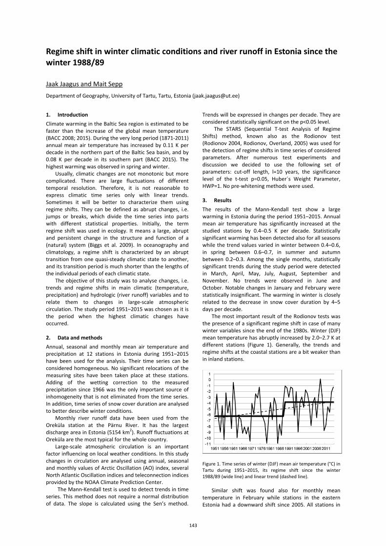
Regime shift in winter climatic conditions and river runoff in Estonia since the winter 1988/89

Jaak Jaagus and Mait Sepp

Department of Geography, University of Tartu, Tartu, Estonia (jaak.jaagus@ut.ee)

1. Introduction Climate warming in the Baltic Sea region is estimated to be faster than the increase of the global mean temperature (BACC 2008; 2015). During the very long period (1871-2011) annual mean air temperature has increased by 0.11 K per decade in the northern part of the Baltic Sea basin, and by 0.08 K per decade in its southern part (BACC 2015). The highest warming was observed in spring and winter.

Usually, climatic changes are not monotonic but more complicated. There are large fluctuations of different temporal resolution. Therefore, it is not reasonable to express climatic time series only with linear trends. Sometimes it will be better to characterize them using regime shifts. They can be defined as abrupt changes, i.e. jumps or breaks, which divide the time series into parts with different statistical properties. Initially, the term regime shift was used in ecology. It means a large, abrupt and persistent change in the structure and function of a (natural) system (Biggs et al. 2009). In oceanography and climatology, a regime shift is characterized by an abrupt transition from one quasi-steady climatic state to another, and its transition period is much shorter than the lengths of the individual periods of each climatic state.

The objective of this study was to analyse changes, i.e. trends and regime shifts in main climatic (temperature, precipitation) and hydrologic (river runoff) variables and to relate them to changes in large-scale atmospheric circulation. The study period 1951–2015 was chosen as it is the period when the highest climatic changes have occurred. 2. Data and methods Annual, seasonal and monthly mean air temperature and precipitation at 12 stations in Estonia during 1951–2015 have been used for the analysis. Their time series can be considered homogeneous. No significant relocations of the measuring sites have been taken place at these stations. Adding of the wetting correction to the measured precipitation since 1966 was the only important source of inhomogeneity that is not eliminated from the time series. In addition, time series of snow cover duration are analysed to better describe winter conditions.

Monthly river runoff data have been used from the Oreküla station at the Pärnu River. It has the largest discharge area in Estonia (5154 km2). Runoff fluctuations at Oreküla are the most typical for the whole country.

Large-scale atmospheric circulation is an important factor influencing on local weather conditions. In this study changes in circulation are analysed using annual, seasonal and monthly values of Arctic Oscillation (AO) index, several North Atlantic Oscillation indices and teleconnection indices provided by the NOAA Climate Prediction Center.

The Mann-Kendall test is used to detect trends in time series. This method does not require a normal distribution of data. The slope is calculated using the Sen’s method.

Trends will be expressed in changes per decade. They are considered statistically significant on the p<0.05 level.

The STARS (Sequential T-test Analysis of Regime Shifts) method, known also as the Rodionov test (Rodionov 2004, Rodionov, Overland, 2005) was used for the detection of regime shifts in time series of considered parameters. After numerous test experiments and discussion we decided to use the following set of parameters: cut-off length, l=10 years, the significance level of the t-test p=0.05, Huber´s Weight Parameter, HWP=1. No pre-whitening methods were used. 3. Results The results of the Mann-Kendall test show a large warming in Estonia during the period 1951–2015. Annual mean air temperature has significantly increased at the studied stations by 0.4–0.5 K per decade. Statistically significant warming has been detected also for all seasons while the trend values varied in winter between 0.4–0.6, in spring between 0.6–0.7, in summer and autumn between 0.2–0.3. Among the single months, statistically significant trends during the study period were detected in March, April, May, July, August, September and November. No trends were observed in June and October. Notable changes in January and February were statistically insignificant. The warming in winter is closely related to the decrease in snow cover duration by 4–5 days per decade.

The most important result of the Rodionov tests was the presence of a significant regime shift in case of many winter variables since the end of the 1980s. Winter (DJF) mean temperature has abruptly increased by 2.0–2.7 K at different stations (Figure 1). Generally, the trends and regime shifts at the coastal stations are a bit weaker than in inland stations.

Figure 1. Time series of winter (DJF) mean air temperature (°C) in Tartu during 1951–2015, its regime shift since the winter 1988/89 (wide line) and linear trend (dashed line).

Similar shift was found also for monthly mean temperature in February while stations in the eastern Estonia had a downward shift since 2005. All stations in

143

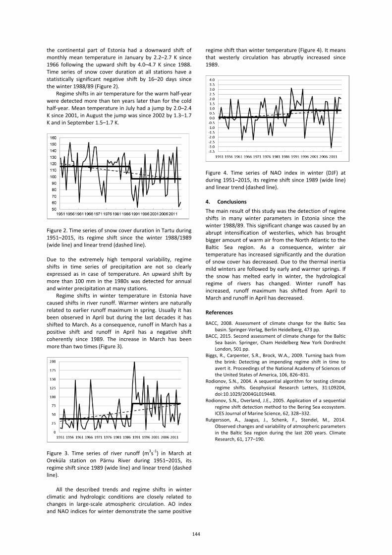
the continental part of Estonia had a downward shift of monthly mean temperature in January by 2.2–2.7 K since 1966 following the upward shift by 4.0–4.7 K since 1988. Time series of snow cover duration at all stations have a statistically significant negative shift by 16–20 days since the winter 1988/89 (Figure 2).

Regime shifts in air temperature for the warm half-year were detected more than ten years later than for the cold half-year. Mean temperature in July had a jump by 2.0–2.4 K since 2001, in August the jump was since 2002 by 1.3–1.7 K and in September 1.5–1.7 K.

Figure 2. Time series of snow cover duration in Tartu during 1951–2015, its regime shift since the winter 1988/1989 (wide line) and linear trend (dashed line). Due to the extremely high temporal variability, regime shifts in time series of precipitation are not so clearly expressed as in case of temperature. An upward shift by more than 100 mm in the 1980s was detected for annual and winter precipitation at many stations.

Regime shifts in winter temperature in Estonia have caused shifts in river runoff. Warmer winters are naturally related to earlier runoff maximum in spring. Usually it has been observed in April but during the last decades it has shifted to March. As a consequence, runoff in March has a positive shift and runoff in April has a negative shift coherently since 1989. The increase in March has been more than two times (Figure 3).

Figure 3. Time series of river runoff (m3s-1) in March at Oreküla station on Pärnu River during 1951–2015, its regime shift since 1989 (wide line) and linear trend (dashed line).

All the described trends and regime shifts in winter climatic and hydrologic conditions are closely related to changes in large-scale atmospheric circulation. AO index and NAO indices for winter demonstrate the same positive

regime shift than winter temperature (Figure 4). It means that westerly circulation has abruptly increased since 1989.

Figure 4. Time series of NAO index in winter (DJF) at during 1951–2015, its regime shift since 1989 (wide line) and linear trend (dashed line). 4. Conclusions The main result of this study was the detection of regime shifts in many winter parameters in Estonia since the winter 1988/89. This significant change was caused by an abrupt intensification of westerlies, which has brought bigger amount of warm air from the North Atlantic to the Baltic Sea region. As a consequence, winter air temperature has increased significantly and the duration of snow cover has decreased. Due to the thermal inertia mild winters are followed by early and warmer springs. If the snow has melted early in winter, the hydrological regime of rivers has changed. Winter runoff has increased, runoff maximum has shifted from April to March and runoff in April has decreased. References

BACC, 2008. Assessment of climate change for the Baltic Sea basin. Springer-Verlag, Berlin Heidelberg, 473 pp.

BACC, 2015. Second assessment of climate change for the Baltic Sea basin. Springer, Cham Heidelberg New York Dordrecht London, 501 pp.

Biggs, R., Carpenter, S.R., Brock, W.A., 2009. Turning back from the brink: Detecting an impending regime shift in time to avert it. Proceedings of the National Academy of Sciences of the United States of America, 106, 826–831.

Rodionov, S.N., 2004. A sequential algorithm for testing climate regime shifts. Geophysical Research Letters, 31:L09204, doi:10.1029/2004GL019448.

Rodionov, S.N., Overland, J.E., 2005. Application of a sequential regime shift detection method to the Bering Sea ecosystem. ICES Journal of Marine Science, 62, 328–332.

Rutgersson, A., Jaagus, J., Schenk, F., Stendel, M., 2014. Observed changes and variability of atmospheric parameters in the Baltic Sea region during the last 200 years. Climate Research, 61, 177–190.

144

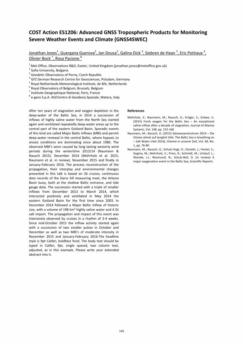
COST Action ES1206: Advanced GNSS Tropospheric Products for Monitoring Severe Weather Events and Climate (GNSS4SWEC)

Jonathan Jones1, Guergana Guerova2, Jan Dousa3, Galina Dick 4, Siebren de Haan 5, Eric Pottiaux 6, Olivier Bock 7, Rosa Pacione 8 1 Met Office, Observations R&D, Exeter, United Kingdom (jonathan.jones@metoffice.gov.uk) 2 Sofia University, Bulgaria 3 Geodetic Observatory of Pecny, Czech Republic 4 GFZ German Research Centre for Geosciences, Potsdam, Germany 5 Royal Netherlands Meteorological Institute, de Bilt, Netherlands 6 Royal Observatory of Belgium, Brussels, Belgium 7 Institute Geographique National, Paris, France 8 e-geos S.p.A. ASI/Centro di Geodesia Spaziale, Matera, Italy After ten years of stagnation and oxygen depletion in the deep-water of the Baltic Sea, in 2014 a succession of inflows of highly saline water from the North Sea started again and ventilated repeatedly deep-water areas up to the central part of the eastern Gotland Basin. Sporadic events of this kind are called Major Baltic Inflows (MBI) and permit deep-water renewal in the central Baltic, where hypoxic to anoxic conditions are dominating since about 1980. The observed MBI’s were caused by long lasting westerly wind periods during the wintertime 2013/14 (Naumann & Nausch 2015), December 2014 (Mohrholz et al. 2015, Naumann et al. in review), November 2015 and finally in January-February 2016. The process reconstruction of the propagation, their interplay and environmental changes presented in this talk is based on 26 cruises, continuous data records of the Darss Sill measuring mast, the Arkona Basin buoy, both at the shallow Baltic entrance, and tide gauge data. The succession started with a triple of smaller inflows from December 2013 to March 2014, which interacted positively and ventilated in May 2014 the eastern Gotland Basin for the first time since 2003. In December 2014 followed a Major Baltic Inflow of historic size, with a volume of 198 km³ highly saline water and 4 Gt salt import. The propagation and impact of this event was intensively observed by cruises in a rhythm of 3-4 weeks. Since mid-October 2015 the inflow activity started again with a succession of two smaller pulses in October and December as well as two MBI’s of moderate intensity in November 2015 and January-February 2016.The headline style is 9pt Calibri, boldface fond. The body text should be typed in Calibri, 9pt, single spaced, two column text, adjusted, as in this example. Please write your extended abstract into it.

References

Mohrholz, V.; Naumann, M.; Nausch, G.; Krüger, S.; Gräwe, U. (2015) Fresh oxygen for the Baltic Sea – An exceptional saline inflow after a decade of stagnation, Journal of Marine Systems, Vol. 148, pp. 152-166

Naumann, M.; Nausch, G. (2015) Salzwassereinstrom 2014 – Die Ostsee atmet auf (english title: The Baltic Sea is breathing on – Salt Water Inlet 2014), Chemie in unserer Zeit, Vol. 49, No. 1, pp. 76-80

Naumann, M.; Nausch, G.; Schulz-Vogt, H.; Donath, J.; Feistel, S.; Gogina, M.; Mohrholz, V.; Prien, R.; Schmidt, M.; Umlauf, L.; Waniek, J.J.; Wasmund, N.; Schulz-Bull, D. (in review) A major oxygenation event in the Baltic Sea, Scientific Reports

145

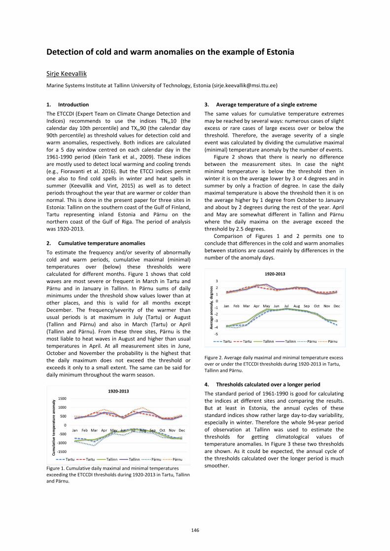
Detection of cold and warm anomalies on the example of Estonia

Sirje Keevallik

Marine Systems Institute at Tallinn University of Technology, Estonia (sirje.keevallik@msi.ttu.ee)

1. Introduction The ETCCDI (Expert Team on Climate Change Detection and Indices) recommends to use the indices TNin10 (the calendar day 10th percentile) and TXin90 (the calendar day 90th percentile) as threshold values for detection cold and warm anomalies, respectively. Both indices are calculated for a 5 day window centred on each calendar day in the 1961-1990 period (Klein Tank et al., 2009). These indices are mostly used to detect local warming and cooling trends (e.g., Fioravanti et al. 2016). But the ETCCI indices permit one also to find cold spells in winter and heat spells in summer (Keevallik and Vint, 2015) as well as to detect periods throughout the year that are warmer or colder than normal. This is done in the present paper for three sites in Estonia: Tallinn on the southern coast of the Gulf of Finland, Tartu representing inland Estonia and Pärnu on the northern coast of the Gulf of Riga. The period of analysis was 1920-2013. 2. Cumulative temperature anomalies To estimate the frequency and/or severity of abnormally cold and warm periods, cumulative maximal (minimal) temperatures over (below) these thresholds were calculated for different months. Figure 1 shows that cold waves are most severe or frequent in March in Tartu and Pärnu and in January in Tallinn. In Pärnu sums of daily minimums under the threshold show values lower than at other places, and this is valid for all months except December. The frequency/severity of the warmer than usual periods is at maximum in July (Tartu) or August (Tallinn and Pärnu) and also in March (Tartu) or April (Tallinn and Pärnu). From these three sites, Pärnu is the most liable to heat waves in August and higher than usual temperatures in April. At all measurement sites in June, October and November the probability is the highest that the daily maximum does not exceed the threshold or exceeds it only to a small extent. The same can be said for daily minimum throughout the warm season.

Figure 1. Cumulative daily maximal and minimal temperatures exceeding the ETCCDI thresholds during 1920-2013 in Tartu, Tallinn and Pärnu.

3. Average temperature of a single extreme The same values for cumulative temperature extremes may be reached by several ways: numerous cases of slight excess or rare cases of large excess over or below the threshold. Therefore, the average severity of a single event was calculated by dividing the cumulative maximal (minimal) temperature anomaly by the number of events.

Figure 2 shows that there is nearly no difference between the measurement sites. In case the night minimal temperature is below the threshold then in winter it is on the average lower by 3 or 4 degrees and in summer by only a fraction of degree. In case the daily maximal temperature is above the threshold then it is on the average higher by 1 degree from October to January and about by 2 degrees during the rest of the year. April and May are somewhat different in Tallinn and Pärnu where the daily maxima on the average exceed the threshold by 2.5 degrees.

Comparison of Figures 1 and 2 permits one to conclude that differences in the cold and warm anomalies between stations are caused mainly by differences in the number of the anomaly days.

Figure 2. Average daily maximal and minimal temperature excess over or under the ETCCDI thresholds during 1920-2013 in Tartu, Tallinn and Pärnu. 4. Thresholds calculated over a longer period The standard period of 1961-1990 is good for calculating the indices at different sites and comparing the results. But at least in Estonia, the annual cycles of these standard indices show rather large day-to-day variability, especially in winter. Therefore the whole 94-year period of observation at Tallinn was used to estimate the thresholds for getting climatological values of temperature anomalies. In Figure 3 these two thresholds are shown. As it could be expected, the annual cycle of the thresholds calculated over the longer period is much smoother.

146

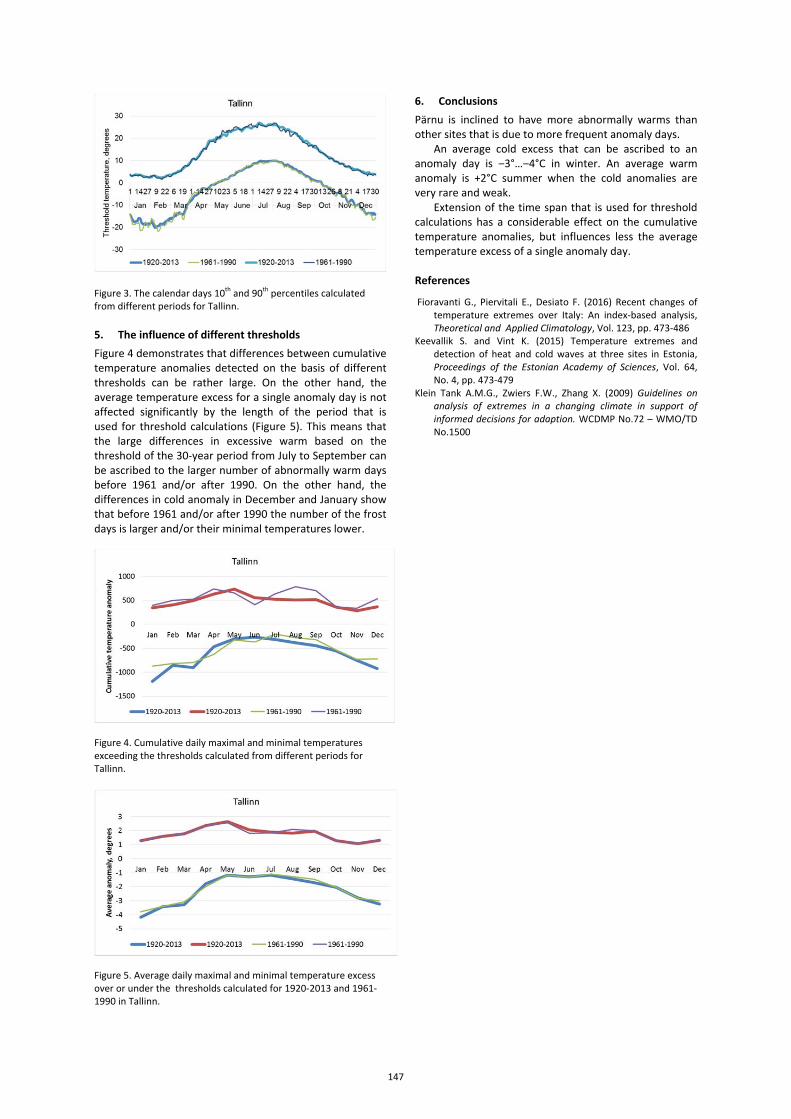
Figure 3. The calendar days 10th and 90th percentiles calculated from different periods for Tallinn. 5. The influence of different thresholds Figure 4 demonstrates that differences between cumulative temperature anomalies detected on the basis of different thresholds can be rather large. On the other hand, the average temperature excess for a single anomaly day is not affected significantly by the length of the period that is used for threshold calculations (Figure 5). This means that the large differences in excessive warm based on the threshold of the 30-year period from July to September can be ascribed to the larger number of abnormally warm days before 1961 and/or after 1990. On the other hand, the differences in cold anomaly in December and January show that before 1961 and/or after 1990 the number of the frost days is larger and/or their minimal temperatures lower.

Figure 4. Cumulative daily maximal and minimal temperatures exceeding the thresholds calculated from different periods for Tallinn.

Figure 5. Average daily maximal and minimal temperature excess over or under the thresholds calculated for 1920-2013 and 1961-1990 in Tallinn.

6. Conclusions Pärnu is inclined to have more abnormally warms than other sites that is due to more frequent anomaly days.

An average cold excess that can be ascribed to an anomaly day is ‒3°…‒4°C in winter. An average warm anomaly is +2°C summer when the cold anomalies are very rare and weak.

Extension of the time span that is used for threshold calculations has a considerable effect on the cumulative temperature anomalies, but influences less the average temperature excess of a single anomaly day.

References

Fioravanti G., Piervitali E., Desiato F. (2016) Recent changes of temperature extremes over Italy: An index-based analysis, Theoretical and Applied Climatology, Vol. 123, pp. 473-486

Keevallik S. and Vint K. (2015) Temperature extremes and detection of heat and cold waves at three sites in Estonia, Proceedings of the Estonian Academy of Sciences, Vol. 64, No. 4, pp. 473-479

Klein Tank A.M.G., Zwiers F.W., Zhang X. (2009) Guidelines on analysis of extremes in a changing climate in support of informed decisions for adaption. WCDMP No.72 – WMO/TD No.1500

147

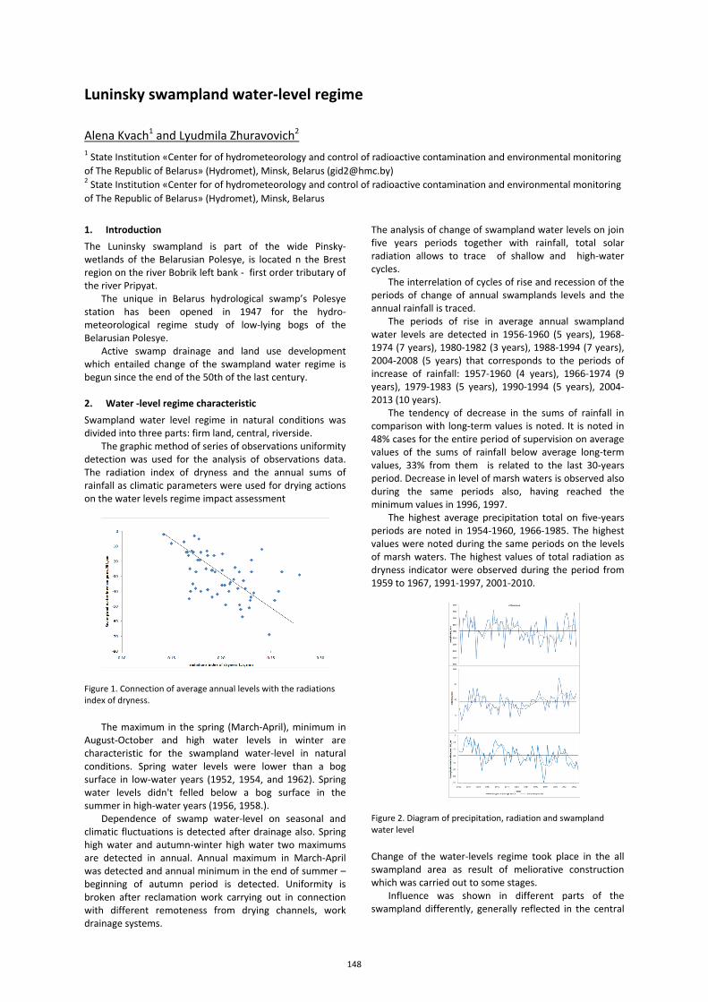
Luninsky swampland water-level regime

Alena Kvach1 and Lyudmila Zhuravovich2 1 State Institution «Center for of hydrometeorology and control of radioactive contamination and environmental monitoring of The Republic of Belarus» (Hydromet), Minsk, Belarus (gid2@hmc.by) 2 State Institution «Center for of hydrometeorology and control of radioactive contamination and environmental monitoring of The Republic of Belarus» (Hydromet), Minsk, Belarus

1. Introduction The Luninsky swampland is part of the wide Pinsky-wetlands of the Belarusian Polesye, is located n the Brest region on the river Bobrik left bank - first order tributary of the river Pripyat.

The unique in Belarus hydrological swamp’s Polesye station has been opened in 1947 for the hydro-meteorological regime study of low-lying bogs of the Belarusian Polesye.

Active swamp drainage and land use development which entailed change of the swampland water regime is begun since the end of the 50th of the last century. 2. Water -level regime characteristic Swampland water level regime in natural conditions was divided into three parts: firm land, central, riverside.

The graphic method of series of observations uniformity detection was used for the analysis of observations data. The radiation index of dryness and the annual sums of rainfall as climatic parameters were used for drying actions on the water levels regime impact assessment

Figure 1. Connection of average annual levels with the radiations index of dryness.

The maximum in the spring (March-April), minimum in August-October and high water levels in winter are characteristic for the swampland water-level in natural conditions. Spring water levels were lower than a bog surface in low-water years (1952, 1954, and 1962). Spring water levels didn't felled below a bog surface in the summer in high-water years (1956, 1958.).

Dependence of swamp water-level on seasonal and climatic fluctuations is detected after drainage also. Spring high water and autumn-winter high water two maximums are detected in annual. Annual maximum in March-April was detected and annual minimum in the end of summer –beginning of autumn period is detected. Uniformity is broken after reclamation work carrying out in connection with different remoteness from drying channels, work drainage systems.

The analysis of change of swampland water levels on join five years periods together with rainfall, total solar radiation allows to trace of shallow and high-water cycles.

The interrelation of cycles of rise and recession of the periods of change of annual swamplands levels and the annual rainfall is traced.

The periods of rise in average annual swampland water levels are detected in 1956-1960 (5 years), 1968-1974 (7 years), 1980-1982 (3 years), 1988-1994 (7 years), 2004-2008 (5 years) that corresponds to the periods of increase of rainfall: 1957-1960 (4 years), 1966-1974 (9 years), 1979-1983 (5 years), 1990-1994 (5 years), 2004-2013 (10 years).

The tendency of decrease in the sums of rainfall in comparison with long-term values is noted. It is noted in 48% cases for the entire period of supervision on average values of the sums of rainfall below average long-term values, 33% from them is related to the last 30-years period. Decrease in level of marsh waters is observed also during the same periods also, having reached the minimum values in 1996, 1997.

The highest average precipitation total on five-years periods are noted in 1954-1960, 1966-1985. The highest values were noted during the same periods on the levels of marsh waters. The highest values of total radiation as dryness indicator were observed during the period from 1959 to 1967, 1991-1997, 2001-2010.

Figure 2. Diagram of precipitation, radiation and swampland water level

Change of the water-levels regime took place in the all swampland area as result of meliorative construction which was carried out to some stages.

Influence was shown in different parts of the swampland differently, generally reflected in the central

148

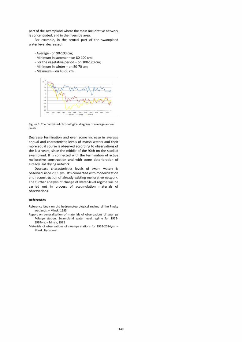
part of the swampland where the main meliorative network is concentrated, and in the riverside area.

For example, in the central part of the swampland water level decreased:

- Average - on 90-100 cm; - Minimum in summer – on 80-100 cm; - For the vegetative period – on 100-120 cm; - Minimum in winter – on 50-70 cm; - Maximum – on 40-60 cm.

Figure 3. The combined chronological diagram of average annual levels.

Decrease termination and even some increase in average annual and characteristic levels of marsh waters and their more equal course is observed according to observations of the last years, since the middle of the 90th on the studied swampland. It is connected with the termination of active meliorative construction and with some deterioration of already laid drying network.

Decrease characteristics levels of swam waters is observed since 2005 yrs. It’s connected with modernization and reconstruction of already existing meliorative network. The further analysis of change of water-level regime will be carried out in process of accumulation materials of observations. References

Reference book on the hydrometeorological regime of the Pinsky wetlands. – Minsk, 1993

Report on generalization of materials of observations of swamps Polesye station. Swampland water level regime for 1952-1984yrs. – Minsk, 1985

Materials of observations of swamps stations for 1952-2014yrs. – Minsk. Hydromet.

149

Sea-lagoon interaction during upwelling processes in the SE Baltic Sea

Toma Mingelaite1, Inga Dailidienė1 and Igor Kozlov1,2 1 Klaipėda University, LT-92291, Lithuania, Klaipėda, Herkaus Manto g. 84 (toma.mingelaite@gmail.com) 2 Russian State Hydrometeorological University, 195196, Russia, Saint-Petersburg, Malookhtinsky pr., 98

1. Introduction Curonian Lagoon is the biggest (total area 1,584 km²) shallow lagoon in the Baltic Sea and all European seas. It is located in the SE Baltic and is separated from the open sea by the relatively narrow sandy Curonian Spit with a connection with the sea through the Klaipėda Strait at the northern end of the lagoon. The most significant factors affecting the water temperature regime of the lagoon are incoming solar radiation, freshwater and marine water inflows. In this study we analyse sea-lagoon interaction during upwelling processes in the SE Baltic Sea. 2. Data, Methods & Results Analysis of available Terra/Aqua MODIS Infrared SST maps (obtained from the NASA OceanColor website (http://oceancolor.gsfc.nasa.gov/)) and in situ data revealed that intensive coastal upwelling events strongly influence not only the SE Baltic coastal zone, but also impacts the hydrological regime of the northern part of the Curonian Lagoon.

MODIS Terra/Aqua infrared SST maps taken between April–September in 2000-2014 show very clear signatures of the intrusion of marine waters to the Curonian Lagoon during 16 coastal upwelling events, resulting in the formation of hydrodynamic fronts with pronounced property gradients there. Such frontal features may strongly influence lagoon ecosystems via changing its main hydrological and hydrochemical properties.

The typical recorded upwelling water propagation distance from the Klaipėda Strait down into the lagoon is about 10-25 km with total affected area being about 40-100 km2, but there have been cases when the inflow was up to 40 km covering about 200 km2 of the lagoon waters. However, such a strong influence of upwelling waters to the northern part of the lagoon is related only to major upwelling events in the SE Baltic and is rather rare. Availability of satellite data helps to understand the hydro-dynamical processes taking place during the intrusion of marine waters to the Curonian Lagoon.

150

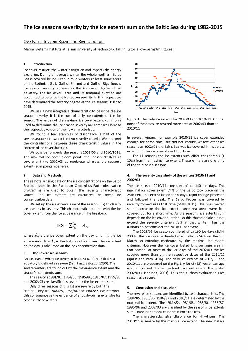
The ice seasons severity by the ice extents sum on the Baltic Sea during 1982-2015

Ove Pärn, Jevgeni Rjazin and Rivo Uiboupin Marine Systems Institute at Tallinn University of Technology, Tallinn, Estonia (ove.parn@msi.ttu.ee) 1. Introduction Ice cover restricts the winter navigation and impacts the energy exchange. During an average winter the whole northern Baltic Sea is covered by ice. Even in mild winters at least some areas of the Bothnian Gulf, Gulf of Finland and Gulf of Riga freeze. Ice season severity appears as the ice cover degree of an aquatory. The ice cover area and its temporal duration are accounted to describe the ice season severity. In this respect we have determined the severity degree of the ice seasons 1982 to 2015.

We use a new integrative characteristic to describe the ice season severity. It is the sum of daily ice extents of the ice season. The values of the maximal ice cover extent commonly used to determine the ice season severity are compared here to the respective values of the new characteristic.

We found a few examples of dissonance (a half of the severe seasons) between the two severity criteria. We interpret the contradictions between these characteristic values in the context of ice cover duration.

We consider properly the seasons 2002/03 and 2010/2011. The maximal ice cover extent points the season 2010/11 as severe and the 2002/03 as moderate whereas the season's extents sum points vice versa.

2. Data and Methods The remote sensing data on the ice concentrations on the Baltic Sea published in the European Copernicus Earth observation programme are used to obtain the severity characteristic values. The ice extents are calculated on these ice concentration data.

We set up the ice extents sum of the season (IES) to classify ice seasons by severity. This characteristic accounts with the ice cover extent from the ice appearance till the break-up.

IES =∑ ,

where is the ice cover extent on the day t, t� is the ice appearance date, is the last day of ice cover. The ice extent on the day is calculated on the ice concentration data. 3. The severe ice seasons An ice season when ice covers at least 73 % of the Baltic Sea aquatory is defined as severe (Seinä and Palosuo, 1996). The severe winters are found out by the maximal ice extent and the season's ice extents sum.

The seasons 1981/82, 1984/85, 1985/86, 1986/87, 1995/96 and 2002/03 are classified as severe by the ice extents sum.

Only three seasons of this list are severe by both the criteria. They are 1984/85, 1985/86 and 1986/87. We interpret this consonance as the evidence of enough-during extensive ice cover in these winters.

Figure 1. The daily ice extents for 2002/03 and 2010/11. On the most of the dates ice covered more area at 2002/03 than at 2010/11 In several winters, for example 2010/11 ice cover extended enough for some time, but did not endure. At few other ice seasons as 2002/03 the Baltic Sea was ice-covered in moderate extent, but the ice cover stayed long time.

For 11 seasons the ice extents sum differ considerably (> 10%) from the maximal ice extent. These winters are one third of the studied ice seasons. 4. The severity case study of the winters 2010/11 and 2002/03 The ice season 2010/11 consisted of ca 140 ice days. The maximal ice cover extent 74% of the Baltic took place on the 25th Feb. This extent lasted for 4 days, rapid change preceded and followed the peak. The Baltic Proper was covered by recently formed nilas that time (SMHI 2011). This nilas melted soon decreasing the ice extent. Large sea areas were ice-covered but for a short time. As the season's ice extents sum depends on the ice cover duration, so this characteristic did not exceed the severity criterion 73% at that winter. Thus the authors do not consider the 2010/11 as severe.

The 2002/03 ice season consisted of ca 190 ice days (SMHI 2003). The ice cover extended maximally to 56% on the 5th March so counting moderate by the maximal ice extent criterion. However the ice cover lasted long on large area in that season. At most of the ice days of the 2002/03 the ice covered more than on the respective dates of the 2010/11 (Rjazin and Pärn 2016). The daily ice extents of 2002/03 and 2010/11 are presented on the Fig.1. A lot of (98) vessel damage events occurred due to the hard ice conditions at the winter 2002/03 (Hänninen, 2003). Thus the authors evaluate this ice season as a severe. 5. Conclusion and discussion The severe ice seasons are identified by two characteristic. The 1984/85, 1985/86, 1986/87 and 2010/11 are determined by the maximal ice extent. The 1981/82, 1984/85, 1985/86, 1986/87, 1995/96 and 2002/03 are classified by the season's ice extents sum. Three ice seasons coincide in both the lists.

The characteristics give dissonance for 4 winters. The 2010/11 is severe by the maximal ice extent. The maximal ice

151

extent lasted only for 4 days and dropped 15% in this time. Using the ice extents sum in the severity study enables to describe the ice cover behaviour more adequately due to accounting with its duration. References

Rjazin J., Pärn O. (2016) Determining the ice seasons severity during 1982-2015 using the ice extents sum as a new characteristic, EGU General Assembly 2016

Rjazin J., Pärn O. (2016) Ice season severity determining methods, MetObs150 (manuscript)

Seinä A., Palosuo, E. (1996) The classification of the maximum annual extent of ice cover in the Baltic Sea 1720–1995, Meri, 27, Report Series of the Finnish Institute of Marine Research, pp. 79–91

SMHI Ice service, Ice chart, 2003 ja 2011. http://www.smhi.se/oceanografi/iceservice/is_prod_en.php (20.12.2015).

152

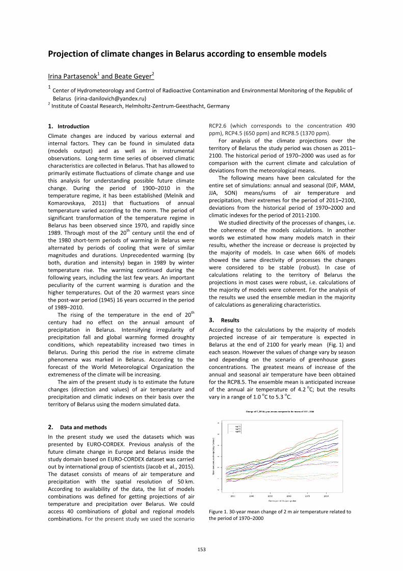
Projection of climate changes in Belarus according to ensemble models

Irina Partasenok1 and Beate Geyer2 1 Center of Hydrometeorology and Control of Radioactive Contamination and Environmental Monitoring of the Republic of

Belarus (irina-danilovich@yandex.ru) 2 Institute of Coastal Research, Helmholtz-Zentrum-Geesthacht, Germany

1. Introduction Climate changes are induced by various external and internal factors. They can be found in simulated data (models output) and as well as in instrumental observations. Long-term time series of observed climatic characteristics are collected in Belarus. That has allowed to primarily estimate fluctuations of climate change and use this analysis for understanding possible future climate change. During the period of 1900–2010 in the temperature regime, it has been established (Melnik and Komarovskaya, 2011) that fluctuations of annual temperature varied according to the norm. The period of significant transformation of the temperature regime in Belarus has been observed since 1970, and rapidly since 1989. Through most of the 20th century until the end of the 1980 short-term periods of warming in Belarus were alternated by periods of cooling that were of similar magnitudes and durations. Unprecedented warming (by both, duration and intensity) began in 1989 by winter temperature rise. The warming continued during the following years, including the last few years. An important peculiarity of the current warming is duration and the higher temperatures. Out of the 20 warmest years since the post-war period (1945) 16 years occurred in the period of 1989–2010.

The rising of the temperature in the end of 20th century had no effect on the annual amount of precipitation in Belarus. Intensifying irregularity of precipitation fall and global warming formed droughty conditions, which repeatability increased two times in Belarus. During this period the rise in extreme climate phenomena was marked in Belarus. According to the forecast of the World Meteorological Organization the extremeness of the climate will be increasing.

The aim of the present study is to estimate the future changes (direction and values) of air temperature and precipitation and climatic indexes on their basis over the territory of Belarus using the modern simulated data.

2. Data and methods In the present study we used the datasets which was presented by EURO-CORDEX. Previous analysis of the future climate change in Europe and Belarus inside the study domain based on EURO-CORDEX dataset was carried out by international group of scientists (Jacob et al., 2015). The dataset consists of means of air temperature and precipitation with the spatial resolution of 50 km. According to availability of the data, the list of models combinations was defined for getting projections of air temperature and precipitation over Belarus. We could access 40 combinations of global and regional models combinations. For the present study we used the scenario

RCP2.6 (which corresponds to the concentration 490 ppm), RCP4.5 (650 ppm) and RCP8.5 (1370 ppm).

For analysis of the climate projections over the territory of Belarus the study period was chosen as 2011–2100. The historical period of 1970–2000 was used as for comparison with the current climate and calculation of deviations from the meteorological means.

The following means have been calculated for the entire set of simulations: annual and seasonal (DJF, MAM, JJA, SON) means/sums of air temperature and precipitation, their extremes for the period of 2011–2100, deviations from the historical period of 1970–2000 and climatic indexes for the period of 2011-2100.

We studied directivity of the processes of changes, i.e. the coherence of the models calculations. In another words we estimated how many models match in their results, whether the increase or decrease is projected by the majority of models. In case when 66% of models showed the same directivity of processes the changes were considered to be stable (robust). In case of calculations relating to the territory of Belarus the projections in most cases were robust, i.e. calculations of the majority of models were coherent. For the analysis of the results we used the ensemble median in the majority of calculations as generalizing characteristics. 3. Results According to the calculations by the majority of models projected increase of air temperature is expected in Belarus at the end of 2100 for yearly mean (Fig. 1) and each season. However the values of change vary by season and depending on the scenario of greenhouse gases concentrations. The greatest means of increase of the annual and seasonal air temperature have been obtained for the RCP8.5. The ensemble mean is anticipated increase of the annual air temperature of 4.2 oC; but the results vary in a range of 1.0 oC to 5.3 oC.

Figure 1. 30-year mean change of 2 m air temperature related to the period of 1970–2000

153

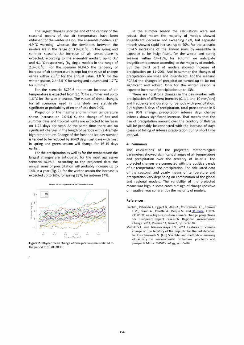
The largest changes until the end of the century of the seasonal means of the air temperature have been obtained for the winter season. The ensemble median is at 4.9 oC warming, whereas the deviations between the models are in the range of 3.9–8.0 oC. In the spring and summer seasons the increase of air temperature is expected, according to the ensemble median, up to 3.7 and 4.1 oC respectively (by single models in the range of 2.3–5.0 oC). For the scenario RCP4.5 the tendency of increase of air temperature is kept but the value of change varies within 2.5 oC for the annual value, 3.0 oC for the winter season, 2.4–2.5 oC for spring and autumn and 1.7 oC for summer.

For the scenario RCP2.6 the mean increase of air temperature is expected from 1.1 oC for summer and up to 1.6 oC for the winter season. The values of these changes for all scenarios used in this study are statistically significant at probability of error of less than 0.05.

Projection of the maxima and minimum temperature shows increase on 2.0-5.0 oC, the change of hot and summer days and tropical nights are expected to increase on 1-24 days per year. At the same time there are no significant changes in the length of periods with extremely high temperature. Change of the frost and ice day number is tended to be reduced by 26-69 days. Last days with frost in spring and green season will change for 16-45 days earlier.

For the precipitation as well as for the temperature the largest changes are anticipated for the most aggressive scenario RCP8.5. According to the projected data the annual sums of precipitation will probably increase up to 14% in a year (Fig. 2), for the winter season the increase is expected up to 26%, for spring 23%, for autumn 14%.

Figure 2: 30-year mean change of precipitation (mm) related to the period of 1970–2000.

In the summer season the calculations were not robust, that meant the majority of models showed insignificant decrease not exceeding 12%, but separate models showed rapid increase up to 40%. For the scenario RCP4.5 increasing of the annual sums by ensemble is expected to be insignificant, for the winter and spring seasons within 14–15%, for autumn we anticipate insignificant decrease according to the majority of models. But the third part of models showed increase of precipitation on 11–20%. And in summer the changes of precipitation are small and insignificant. For the scenario RCP2.6 the changes of precipitation turned up to be not significant and robust. Only for the winter season is expected increase of precipitation up to 13%.

There are no strong changes in the day number with precipitation of different intensity (0.1, 1 and 10 mm/day) and frequency and duration of periods with precipitation. But highest 5 days of precipitation, total precipitation in 5 days 95% change, precipitation intense days change indexes shows significant increase. That means that the rise of precipitation amount over the territory of Belarus will be probably be connected with the increase of days (cases) of falling of intense precipitation during short time interval.

4. Summary The calculations of the projected meteorological parameters showed significant changes of air temperature and precipitation over the territory of Belarus. The projected changes are connected with the positive trends of air temperature and precipitation. The calculated data of the seasonal and yearly means of temperature and precipitation vary depending on combination of the global and regional models. The variability of the projected means was high in some cases but sign of change (positive or negative) was coherent by the majority of models. References

Jacob D., Petersen J., Eggert B., Alias A., Christensen O.B., Bouwer L.M., Braun A., Colette A., Déqué M. and 30 more. EURO-CORDEX: new high-resolution climate change projections for European impact research. Regional Environmental Change. 2014, Volume 14, Issue 2, pp. 563-578.

Melnik V.I. and Komarovskaya E.V. 2011 Features of climate change on the territory of the Republic for the last decades. In: Klyuchenovich V. (Ed.) Scientific and methodical ensuring of activity on environmental protection: problems and prospects Minsk: BelNIC Ecology, pp. 77-84.

.

154

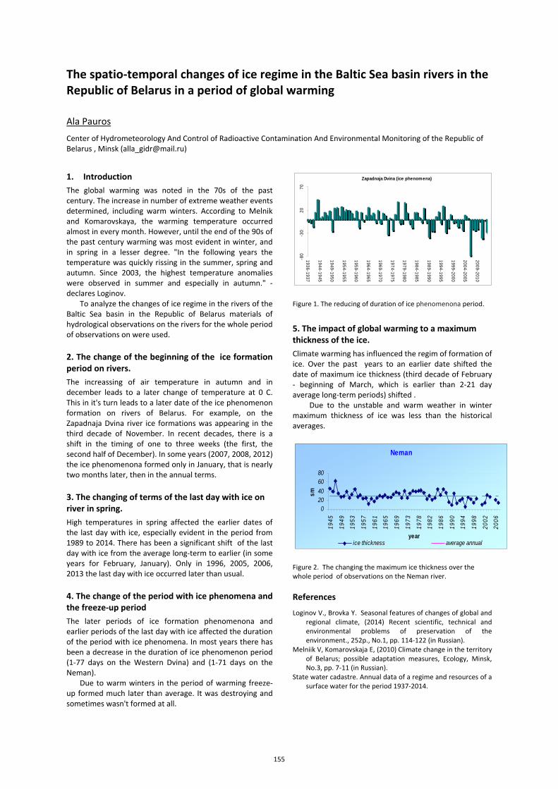
The spatio-temporal changes of ice regime in the Baltic Sea basin rivers in the Republic of Belarus in a period of global warming

Ala Pauros

Center of Hydrometeorology And Control of Radioactive Contamination And Environmental Monitoring of the Republic of Belarus , Minsk (alla_gidr@mail.ru)

1. Introduction The global warming was noted in the 70s of the past century. The increase in number of extreme weather events determined, including warm winters. According to Melnik and Komarovskaya, the warming temperature occurred almost in every month. However, until the end of the 90s of the past century warming was most evident in winter, and in spring in a lesser degree. "In the following years the temperature was quickly rissing in the summer, spring and autumn. Since 2003, the highest temperature anomalies were observed in summer and especially in autumn." - declares Loginov.

To analyze the changes of ice regime in the rivers of the Baltic Sea basin in the Republic of Belarus materials of hydrological observations on the rivers for the whole period of observations on were used. 2. The change of the beginning of the ice formation period on rivers. The increassing of air temperature in autumn and in december leads to a later change of temperature at 0 C. This in it's turn leads to a later date of the ice phenomenon formation on rivers of Belarus. For example, on the Zapadnaja Dvina river ice formations was appearing in the third decade of November. In recent decades, there is a shift in the timing of one to three weeks (the first, the second half of December). In some years (2007, 2008, 2012) the ice phenomenona formed only in January, that is nearly two months later, then in the annual terms. 3. The changing of terms of the last day with ice on river in spring. High temperatures in spring affected the earlier dates of the last day with ice, especially evident in the period from 1989 to 2014. There has been a significant shift of the last day with ice from the average long-term to earlier (in some years for February, January). Only in 1996, 2005, 2006, 2013 the last day with ice occurred later than usual. 4. The change of the period with ice phenomena and the freeze-up period The later periods of ice formation phenomenona and earlier periods of the last day with ice affected the duration of the period with ice phenomena. In most years there has been a decrease in the duration of ice phenomenon period (1-77 days on the Western Dvina) and (1-71 days on the Neman).

Due to warm winters in the period of warming freeze-up formed much later than average. It was destroying and sometimes wasn't formed at all.

Figure 1. The reducing of duration of ice phenomenona period. 5. The impact of global warming to a maximum thickness of the ice. Climate warming has influenced the regim of formation of ice. Over the past years to an earlier date shifted the date of maximum ice thickness (third decade of February - beginning of March, which is earlier than 2-21 day average long-term periods) shifted .

Due to the unstable and warm weather in winter maximum thickness of ice was less than the historical averages.

Figure 2. The changing the maximum ice thickness over the whole period of observations on the Neman river. References

Loginov V., Brovka Y. Seasonal features of changes of global and regional climate, (2014) Recent scientific, technical and environmental problems of preservation of the environment., 252p., No.1, pp. 114-122 (in Russian).

Melniik V, Komarovskaja E, (2010) Climate change in the territory of Belarus; possible adaptation measures, Ecology, Minsk, No.3, pp. 7-11 (in Russian).

State water cadastre. Annual data of a regime and resources of a surface water for the period 1937-2014.

Zapadnaja Dvina (ice phenomena)

-80

-30

2070

1936-1937

1944-1945

1949-1950

1954-1955

1959-1960

1964-1965

1969-1970

1974-1975

1979-1980

1984-1985

1989-1990

1994-1995

1999-2000

2004-2005

2009-2010

Neman

020406080

1945

1949

1953

1957

1961

1965

1969

1973

1978

1982

1986

1990

1994

1998

2002

2006

year

sm

ice thickness average annual

155

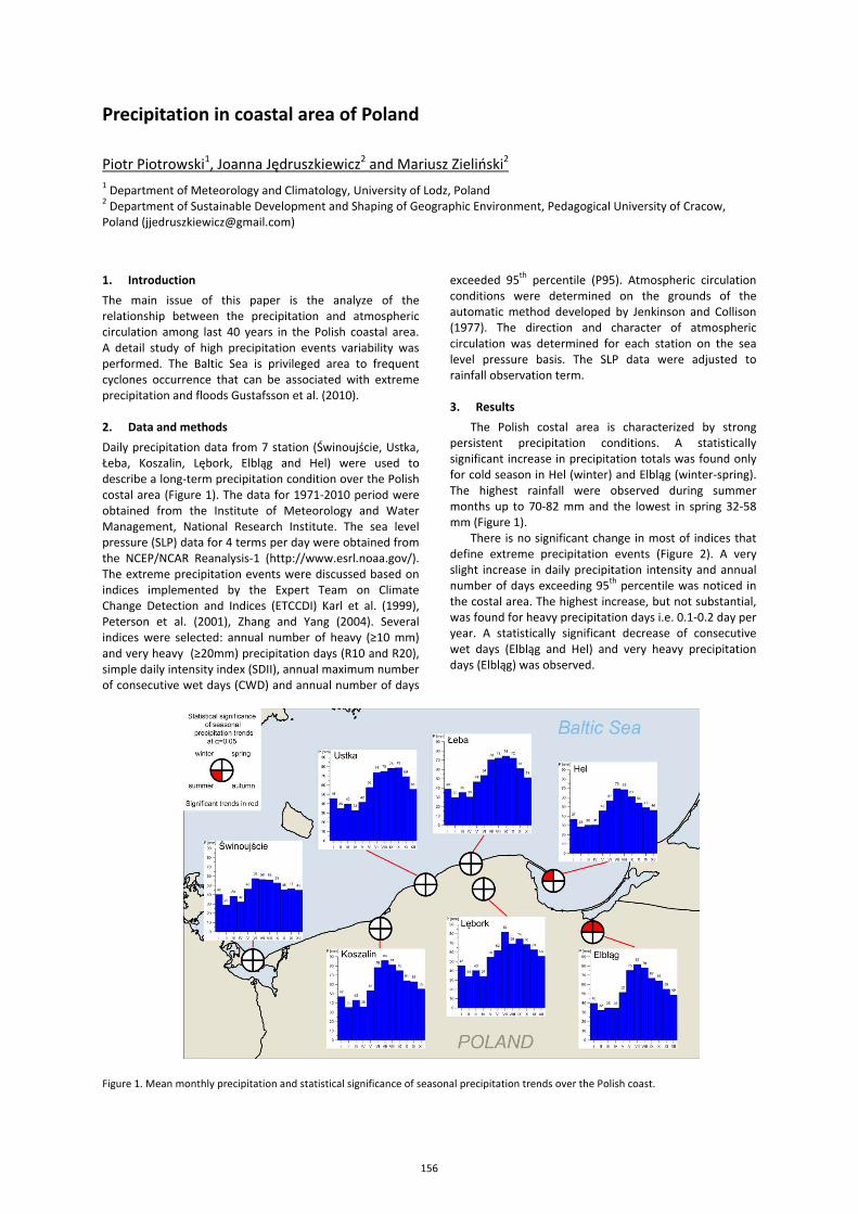
Precipitation in coastal area of Poland

Piotr Piotrowski1, Joanna Jędruszkiewicz2 and Mariusz Zieliński2 1 Department of Meteorology and Climatology, University of Lodz, Poland 2 Department of Sustainable Development and Shaping of Geographic Environment, Pedagogical University of Cracow, Poland (jjedruszkiewicz@gmail.com)

1. Introduction The main issue of this paper is the analyze of the relationship between the precipitation and atmospheric circulation among last 40 years in the Polish coastal area. A detail study of high precipitation events variability was performed. The Baltic Sea is privileged area to frequent cyclones occurrence that can be associated with extreme precipitation and floods Gustafsson et al. (2010). 2. Data and methods Daily precipitation data from 7 station (Świnoujście, Ustka, Łeba, Koszalin, Lębork, Elbląg and Hel) were used to describe a long-term precipitation condition over the Polish costal area (Figure 1). The data for 1971-2010 period were obtained from the Institute of Meteorology and Water Management, National Research Institute. The sea level pressure (SLP) data for 4 terms per day were obtained from the NCEP/NCAR Reanalysis-1 (http://www.esrl.noaa.gov/). The extreme precipitation events were discussed based on indices implemented by the Expert Team on Climate Change Detection and Indices (ETCCDI) Karl et al. (1999), Peterson et al. (2001), Zhang and Yang (2004). Several indices were selected: annual number of heavy (≥10 mm) and very heavy (≥20mm) precipitation days (R10 and R20), simple daily intensity index (SDII), annual maximum number of consecutive wet days (CWD) and annual number of days

exceeded 95th percentile (P95). Atmospheric circulation conditions were determined on the grounds of the automatic method developed by Jenkinson and Collison (1977). The direction and character of atmospheric circulation was determined for each station on the sea level pressure basis. The SLP data were adjusted to rainfall observation term. 3. Results

The Polish costal area is characterized by strong persistent precipitation conditions. A statistically significant increase in precipitation totals was found only for cold season in Hel (winter) and Elbląg (winter-spring). The highest rainfall were observed during summer months up to 70-82 mm and the lowest in spring 32-58 mm (Figure 1).

There is no significant change in most of indices that define extreme precipitation events (Figure 2). A very slight increase in daily precipitation intensity and annual number of days exceeding 95th percentile was noticed in the costal area. The highest increase, but not substantial, was found for heavy precipitation days i.e. 0.1-0.2 day per year. A statistically significant decrease of consecutive wet days (Elbląg and Hel) and very heavy precipitation days (Elbląg) was observed.

Figure 1. Mean monthly precipitation and statistical significance of seasonal precipitation trends over the Polish coast.

156

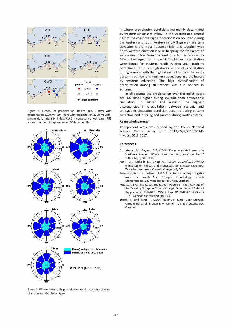
Figure 2. Trends for precipitation indices: R10 - days with precipitation ≥10mm; R20 - days with precipitation ≥20mm; SDII - simple daily intensity index; CWD - consecutive wet days; P95 annual number of days exceeded 95th percentile.

Figure 3. Winter mean daily precipitation totals according to wind direction and circulation type.

In winter precipitation conditions are mainly determined by western air masses inflow. In the western and central part of the coast the highest precipitation occurred during the western and south western inflow (Figure 3). Western advection is the most frequent (45%) and together with north western direction is 61%. In spring the frequency of air masses inflow from the west direction is reduced to 16% and enlarged from the east. The highest precipitation were found for eastern, south eastern and southern advections. There is a high diversification of precipitation during summer with the highest rainfall followed by south eastern, southern and northern advections and the lowest by western advection. The high diversification of precipitation among all stations was also noticed in autumn.

In all seasons the precipitation over the polish coast are 1.6 times higher during cyclonic than anticyclonic circulation. In winter and autumn the highest discrepancies in precipitation between cyclonic and anticyclonic circulation condition occurred during eastern advection and in spring and summer during north eastern.

Acknowledgements The present work was funded by the Polish National Science Centre under grant 2012/05/B/ST10/00945 in years 2013-2017. References

Gustafsson, M., Rayner, D.P. (2010) Extreme rainfall events in Southern Sweden: Where does the moisture come from? Tellus, 62, 5, 605 - 616.

Karl, T.R., Nicholls N., Ghazi A., (1999) CLIVAR/GCOS/WMO workshop on indices and indica-tors for climate extremes: Workshop summary, Climatic Change, 42, 3-7.

Jenkinson, A. F., P., Collison (1977) An initial climatology of gales over the North Sea, Synoptic Climatology Branch Memorandum, 62, Meteorological Office, Brackenll

Peterson, T.C., and Coauthors (2001): Report on the Activities of the Working Group on Climate Change Detection and Related Rapporteurs 1998-2001. WMO, Rep. WCDMP-47, WMO-TD 1071, Geneve, Switzerland, pp. 143.

Zhang, X. and Yang, F. (2004) RClimDex (1.0)—User Manual. Climate Research Branch Envi-ronment Canada Downsview, Ontario.

157

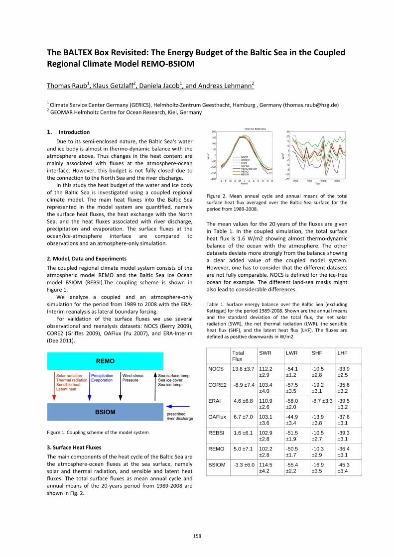
The BALTEX Box Revisited: The Energy Budget of the Baltic Sea in the Coupled Regional Climate Model REMO-BSIOM

Thomas Raub1, Klaus Getzlaff2, Daniela Jacob1, and Andreas Lehmann2

1 Climate Service Center Germany (GERICS), Helmholtz-Zentrum Geesthacht, Hamburg , Germany (thomas.raub@hzg.de) 2 GEOMAR Helmholtz Centre for Ocean Research, Kiel, Germany

1. Introduction Due to its semi-enclosed nature, the Baltic Sea's water

and ice body is almost in thermo-dynamic balance with the atmosphere above. Thus changes in the heat content are mainly associated with fluxes at the atmosphere-ocean interface. However, this budget is not fully closed due to the connection to the North Sea and the river discharge.

In this study the heat budget of the water and ice body of the Baltic Sea is investigated using a coupled regional climate model. The main heat fluxes into the Baltic Sea represented in the model system are quantified, namely the surface heat fluxes, the heat exchange with the North Sea, and the heat fluxes associated with river discharge, precipitation and evaporation. The surface fluxes at the ocean/ice-atmosphere interface are compared to observations and an atmosphere-only simulation. 2. Model, Data and Experiments The coupled regional climate model system consists of the atmospheric model REMO and the Baltic Sea Ice Ocean model BSIOM (REBSI).The coupling scheme is shown in Figure 1.

We analyze a coupled and an atmosphere-only simulation for the period from 1989 to 2008 with the ERA-Interim reanalysis as lateral boundary forcing.

For validation of the surface fluxes we use several observational and reanalysis datasets: NOCS (Berry 2009), CORE2 (Griffes 2009), OAFlux (Yu 2007), and ERA-Interim (Dee 2011).

Figure 1. Coupling scheme of the model system 3. Surface Heat Fluxes The main components of the heat cycle of the Baltic Sea are the atmosphere-ocean fluxes at the sea surface, namely solar and thermal radiation, and sensible and latent heat fluxes. The total surface fluxes as mean annual cycle and annual means of the 20-years period from 1989-2008 are shown in Fig. 2.

Figure 2. Mean annual cycle and annual means of the total surface heat flux averaged over the Baltic Sea surface for the period from 1989-2008. The mean values for the 20 years of the fluxes are given in Table 1. In the coupled simulation, the total surface heat flux is 1.6 W/m2 showing almost thermo-dynamic balance of the ocean with the atmosphere. The other datasets deviate more strongly from the balance showing a clear added value of the coupled model system. However, one has to consider that the different datasets are not fully comparable. NOCS is defined for the ice-free ocean for example. The different land-sea masks might also lead to considerable differences. Table 1. Surface energy balance over the Baltic Sea (excluding Kattegat) for the period 1989-2008. Shown are the annual means and the standard deviation of the total flux, the net solar radiation (SWR), the net thermal radiation (LWR), the sensible heat flux (SHF), and the latent heat flux (LHF). The fluxes are defined as positive downwards in W/m2. Total

Flux SWR LWR SHF LHF

NOCS 13.8 ±3.7 112.2 ±2.9

-54.1 ±1.2

-10.5 ±2.8

-33.9 ±2.5

CORE2 -8.9 ±7.4 103.4 ±4.0

-57.5 ±3.5

-19.2 ±3.1

-35.6 ±3.2

ERAI 4.6 ±6.8 110.9 ±2.6

-58.0 ±2.0

-8.7 ±3.3 -39.5 ±3.2

OAFlux 6.7 ±7.0 103.1 ±3.6

-44.9 ±3.4

-13.9 ±3.8

-37.6 ±3.1

REBSI 1.6 ±6.1 102.9 ±2.8

-51.5 ±1.9

-10.5 ±2.7

-39.3 ±3.1

REMO 5.0 ±7.1 102.2 ±2.8

-50.5 ±1.7

-10.3 ±2.9

-36.4 ±3.1

BSIOM -3.3 ±6.0 114.5 ±4.2

-55.4 ±2.2

-16.9 ±3.5

-45.3 ±3.4

158

4. Heat budget Figure 3 shows a schematic the physical earth system of the Baltic Sea region and the interaction among them, the BALTEX box.

The change in heat content H of the water and ice body of the Baltic Sea can be described as: = + − + + − +

where F is the net surface heat flux from the atmosphere to the open water, I and O are the heat fluxes associated with in- and outflows through the Danish straits, R the heat content of the river discharge, P and E the sensible heat fluxes associated with precipitation and evaporation, and S the latent heat due to snow fall. The fluxes related to ice flow through the Danish Straits and the heat exchange at the bottom are neglected.

The mean values of the heat fluxes averaged over the Baltic Sea (excluding Kattegat) normalized by the surface area in the coupled simulation are given in Table 2. Table 2. Mean heat change and heat fluxes and the inter-annual variability to the Baltic Sea water and ice body for the period from 1989-2008 normalized by the surface area in W/m2. dH/dt F I-O I O R P E S

0.9 ±6.1

1.6 ±6.1

-1.2 ±0.5

3.4 ±0.3

-4.7 ±0.6

1.2 ±0.2

0.8 ±0.1

0.7 ±0.1

-0.3 ±0.1

The heat content changes by 0.9 W/m2 over the simulation period with an inter-annual variability of 6.1 W/m2. The latter is mainly caused by the surface fluxes. However, they do not fully close the heat budget. Even with taking the remaining fluxes into account, we cannot close it, leaving a remainder of about +0.5 W/m2. A potential cause for this imbalance could be that the sensible heat of the sea ice is not treated conservatively or the neglect of the fluxes associated with sea ice flow through the Danish straits. 5. Summary and conclusions In our coupled experiment the Baltic Sea is in close thermo-dynamic balance with the atmosphere above on decadal time scales, due to its semi-enclosed nature, in agreement with other studies. It is usually argued that the small remainder in the heat budget in the order of 1 W/m2 results from the heat exchange between the North Sea and that the other fluxes are negligible. However, according to our analysis the heat fluxes due to river discharge, precipitation and evaporation have the same order of magnitude and should be included into the budget.

References Berry, D. I. and E. C. Kent (2009) A New Air-Sea Interaction

Gridded Dataset from ICOADS With Uncertainty Estimates. Bulletin of the American Meteorological Society, 90 (5), pp. 645-656.

Dee, D. P., et al. (2011) The ERA-Interim reanalysis: confguration and performance of the data assimilation system. Quarterly Journal of the Royal Meteorological Society, 137 (656), pp. 553-597.

Griffes, S. M., et al. (2009) Coordinated Ocean-ice Reference Experiments (COREs). Ocean Modelling, 26 (1-2), pp. 1-46.

Omstedt, A. and C. Nohr (2004) Calculating the water and heat balances of the Baltic Sea using ocean modelling and available meteorological, hydrological and ocean data. Tellus A, 56, pp. 400-414.

Yu, L. and R. Weller (2007) Objectively Analyzed Air-Sea Heat Fluxes for the Global Ice-Free Oceans (1981-2005). Bulletin of the American Meteorological Society, 88 (4), pp. 527-539.

159

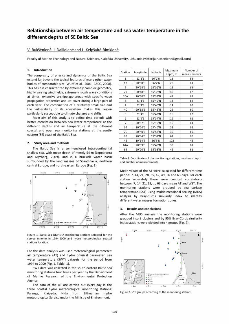
Relationship between air temperature and sea water temperature in the different depths of SE Baltic Sea

V. Rukšėnienė, I. Dailidienė and L. Kelpšaitė-Rimkienė

Faculty of Marine Technology and Natural Sciences, Klaipėda University, Lithuania (viktorija.rukseniene@gmail.com)

1. Introduction The complexity of physics and dynamics of the Baltic Sea extend far beyond the typical features of many other water bodies of comparable size (Wulff et al., 2001; BACC, 2008). This basin is characterized by extremely complex geometry, highly varying wind fields, extremely rough wave conditions at times, extensive archipelago areas with specific wave propagation properties and ice cover during a large part of each year. The combination of a relatively small size and the vulnerability of its ecosystem makes this region particularly susceptible to climate changes and shifts.

Main aim of this study is to define time periods with better correlation between sea water temperature at the different depths and air temperature at the different coastal and open sea monitoring stations at the south-eastern (SE) coast of the Baltic Sea. 2. Study area and methods

The Baltic Sea is a semi-enclosed intra-continental shallow sea, with mean depth of merely 54 m (Leppäranta and Myrberg, 2009), and is a brackish water basin surrounded by the land masses of Scandinavia, northern central Europe, and north-eastern Europe (Fig. 1).

Figure 1. Baltic Sea DMREPA monitoring stations selected for the survey scheme in 1994-2009 and hydro meteorological coastal stations location.

For the data analysis was used meteorological parameter: air temperature (AT) and hydro physical parameter: sea water temperature (SWT) datasets for the period from 1994 to 2009 (Fig. 1, Table. 1).

SWT data was collected in the south-eastern Baltic Sea monitoring stations four times per year by the Department of Marine Research of the Environmental Protection Agency.

The data of the AT are carried out every day in the three coastal hydro meteorological monitoring stations: Palanga, Klaipeda, Nida from Lithuanian Hydro meteorological Service under the Ministry of Environment.

Station Longitude Latitude Maximum depth, m

Number of measurements

1 21°1'E 56°2’N 18 631B 20°50'E 56°2’N 28 612 20°58'E 55°56’N 13 63

20 20°48'E 55°38’N 45 6220A 20°50'E 55°39’N 41 62

3 21°1'E 55°49’N 13 624 21°1'E 55°46’N 14 62

4C 20°58'E 55°45’N 26 605 21°4'E 55°43’N 16 626 21°5'E 55°34’N 16 617 20°57'E 55°19’N 15 61

64 20°54'E 55°46’N 32 622C 20°40'E 55°56’N 30 606B 20°34'E 55°31’N 61 6046 19°14'E 56°5’N 122 43

64A 20°39'E 55°49’N 39 6165 20°20'E 55°53’N 46 61

Table 1. Coordinates of the monitoring stations, maximum depth and number of measurements.

Mean values of the AT were calculated for different time period: 7, 14, 21, 28, 35, 42, 49, 56 and 63 days. For each station separately there were counted correlations between 7, 14, 21, 28, …, 63 days mean AT and WST. The monitoring stations were grouped by sea surface temperature (SST) using multidimensional scaling (MDS) analysis by Bray-Curtis similarity index to identify different water masses formation zones. 3. Results and conclusions After the MDS analysis the monitoring stations were grouped into 9 clusters and by 95% Bray-Curtis similarity index stations were divided into 4 groups (Fig. 2):

Figure 2. SST groups according to the monitoring stations.

160

Curonian lagoon water influence zone (station No.4), coastal stations (green circles), offshore stations (blue circles) and station No. 46.

A significant (p<0,01) strong positive correlation is observed between SST and AT for different time period. Strongest correlation was observed for 35 days AT time period before SST measurement, and it starts decrease after 42 days. Some different tendencies were observed in stations No. 4 (influenced by the water from Curonian Lagoon) and No. 46 (farthest monitoring station and belongs to the open BS Proper).

Figure 3. Correlation between mean AT and mean SST for different time periods (7, 14, 21, 28, …, 63 days).

Correlation between AT and SWT at different depth were calculated. Here we present typical coastal and offshore areas represented stations and correlations at the stations No. 46 and No. 2.

Figure 4. Correlation between mean AT and SWT at different depths for different time periods (7, 14, 21, 28, …, 63 days) at the station No. 46.

At the station No. 46 (Fig. 4) strong positive correlation between AT and SWT for the different time periods is observed until 20 m depth. Deeper up to 70 m correlation significantly decreases and it is equal to zero from 70 m to 75 m depth. Noticeable that deeper than 75 m negative correlation between AT and SWT appear. The same tendencies are for all time periods.

Figure 5. Correlation between mean AT and SWT at different depths for different time periods (7, 14, 21, 28, …, 63 days) at the station No. 4.

At the station No.4 we can see different tendency in the correlation between AT and SWT at different depths. At the SST correlation with the AT is strongest for the 14 days.

Water temperature at the 5 m depth better represents AT of 42 days, 10m and 20 m – 56 days (Fig. 5). Similar situation were observed at the coastal area monitoring stations, for example at the station No. 2 (Fig. 6). At the sea surface water temperature changes is influenced of AT by shorter time than deeper layers (correlation between AT and SST strongest after 35 days and correlation between AT and SWT at 20m depth strongest after 49 days).

Figure 6. Correlation between mean AT and SWT at different depths for different time periods (7, 14, 21, 28, …, 63 days) at the station No. 2.

At the offshore stations we see (Fig. 7) strong positive correlation between AT and SWT for the different time periods is observed until 10 m depth, deeper to 40 m correlation significantly decrease. Correlation coefficient values vary from moderate (7 days) till very strong (63 days). This phenomenon is similar but not as strong as it was observed at the station No. 46.

Figure 7. Correlation between mean AT and SWT at different depths for different time periods (7, 14, 21, 28, …, 63 days) at the station No. 64.

Results of this work would help to assess not the calendar seasons but real natural seasons for oceanographers, ecologists and environmentalists and to improve mathematical models, using only representative marine monitoring stations data. References

Wulf F. V., Rahm L. A., Larsson P. (2001) A systems analysis of the Baltic Sea. Ecological Studies 148, Berlin: Springer, pp. 430

The BACC author team (2008) Assessment of climate change for the Baltic Sea basin, Springer, Berlin, Heidelberg, pp. 473

Leppäranta, M. and Myrberg, K. (2009) Physical Oceanography of the Baltic Sea. SpringerVerlag, Berlin, Heidelberg, New York, pp. 422

161

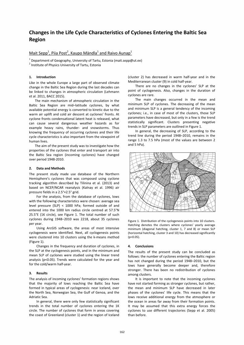
Changes in the Life Cycle Characteristics of Cyclones Entering the Baltic Sea Region

Mait Sepp1, Piia Post2, Kaupo Mändla1 and Raivo Aunap1 1 Department of Geography, University of Tartu, Estonia (mait.sepp@ut.ee) 2 Institute of Physics University of Tartu, Estonia

1. Introduction Like in the whole Europe a large part of observed climate change in the Baltic Sea Region during the last decades can be linked to changes in atmospheric circulation (Lehmann et al. 2011, BACC 2015).

The main mechanism of atmospheric circulation in the Baltic Sea Region are mid–latitude cyclones, by what available potential energy is converted to kinetic due to the warm air uplift and cold air descent at cyclones’ fronts. At cyclone fronts condensational latent heat is released, what can cause several dangerous weather hazards as for example heavy rains, thunder- and snowstorms. Thus knowing the frequency of occurring cyclones and their life cycle characteristics is also important from the viewpoint of human lives.

The aim of the present study was to investigate how the properties of the cyclones that enter and transport air into the Baltic Sea region (incoming cyclones) have changed over period 1948-2010.

2. Data and Methods The present study made use database of the Northern Hemisphere’s cyclones that was composed using cyclone tracking algorithm described by Tilinina et al. (2013) and based on NCEP/NCAR reanalysis (Kalnay et al. 1996) air pressure fields in a 2.5°×2.5° grid.

For the analysis, from the database of cyclones, lows with the following characteristics were chosen: average sea level pressure (SLP) < 1000 hPa; formed outside of and entered into the 1000 km radius circle centred at 57.5°N 25.5°E (1K circle), see Figure 1. The total number of such cyclones during 1948−2010 was 2218, about 35 cyclones per year.

Using ArcGIS software, the areas of most intensive cyclogenesis were identified. Next, all cyclogenesis points were clustered into 10 clusters using the k-means method (Figure 1).

Changes in the frequency and duration of cyclones, in the SLP at the cyclogenesis points, and in the minimum and mean SLP of cyclones were studied using the linear trend analysis (p<0.05). Trends were calculated for the year and for the cold/warm half-year.

3. Results The analysis of incoming cyclones’ formation regions shows that the majority of lows reaching the Baltic Sea have formed in typical areas of cyclogenesis: near Iceland, over the North Sea, Norwegian Sea, the Gulf of Genoa, and the Adriatic Sea.

In general, there were only few statistically significant trends in the total number of cyclones entering the 1K circle. The number of cyclones that form in areas covering the coast of Greenland (cluster 1) and the region of Iceland

(cluster 2) has decreased in warm half-year and in the Mediterranean cluster (9) in cold half-year.

There are no changes in the cyclones’ SLP at the point of cyclogenesis. Also, changes in the duration of cyclones are rare.

The main changes occurred in the mean and minimum SLP of cyclones. The decreasing of the mean and minimum SLP is a general tendency of the incoming cyclones; i.e., in case of most of the clusters, those SLP parameters have decreased, but only in a few is the trend statistically significant. Clusters presenting negative trends in SLP parameters are outlined in Figure 1.

In general, the decreasing of SLP, according to the trend line during the period 1948–2010, remains in the range 1.3 to 7.5 hPa (most of the values are between 2 and 5 hPa).

Figure 1. Distribution of the cyclogenesis points into 10 clusters. Hatching denotes the clusters where cyclones’ yearly average minimum (diagonal hatching, cluster 1, 7 and 8) or mean SLP (horizontal hatching, cluster 3 and 10) has decreased significantly (p<0.05).

4. Conclusions The results of the present study can be concluded as follows: the number of cyclones entering the Baltic region has not changed during the period 1948–2010, but the lows have generally become deeper and, therefore stronger. There has been no redistribution of cyclones among clusters.

It is important to note that the incoming cyclones have not started forming as stronger cyclones, but rather, the mean and minimum SLP have decreased in later phases of the cyclones’ life cycle. This means that the lows receive additional energy from the atmosphere or the ocean in areas far away from their formation points. It may be assumed that this extra energy forces the cyclones to use different trajectories (Sepp et al. 2005) than before.

162

References

BACC (II Author Team) 2015. Second Assessment of Climate Change for the Baltic Sea Basin. Regional Climate Studies. Springer International Publishing.

Kalnay E., Kanamitsu M., Kistler R., Collins W., Deaven D., Gandin L., Iredell M., Saha S., White G., Woollen J., Zhu Y., Leetmaa A., Reynolds R., Chelliah M., Ebisuzaki W., Higgins W., Janowiak J., Mo K.C., Ropelewski C., Wang J., Jenne R. & Joseph D. (1996) The NCEP/NCAR 40–year reanalysis project. Bull. Amer. Meteor. Soc., Vol 77, pp 437–472.

Lehmann A., Getzlaff K. & Harlaß J. (2011) Detailed assessment of climate variability of the Baltic Sea area for the period 1958–2009. Climate Research, Vol 46, pp. 185–196

Sepp M., Post P. & Jaagus J. (2005) Long–term changes in the frequency of cyclones and their trajectories in Central and Northern Europe. Nordic Hydrology, Vol 36, pp. 297–309

Tilinina N., Gulev S.K., Rudeva I. & Koltermann P. 2013. Comparing Cyclone Life Cycle Characteristics and Their Interannual Variability in Different Reanalyses, J. Climate, Vol 26, pp. 6419–6438.

163

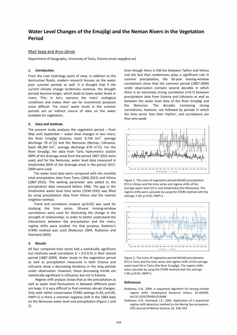
Water Level Changes of the Emajõgi and the Neman Rivers in the Vegetation Period

Mait Sepp and Arvo Järvet

Department of Geography, University of Tartu, Estonia (mait.sepp@ut.ee)

1. Introduction From the river hydrology point of view, in addition to the destructive floods, modern research focuses on the water poor summer periods as well. It is thought that if the current climate change tendencies continue, the drought periods become longer, which leads to lower water levels in rivers. This, in turn, worsens the rivers’ ecological conditions and makes their use for economical purposes more difficult. The rivers’ water levels in the summer periods are an indirect source of data on the water available for vegetation. 2. Data and methods The present study analyses the vegetation period – from May until September – water level changes in two rivers: the River Emajõgi (Estonia, basin 9,740 km2, average discharge 70 m3/s) and the Nemunas (Neman, Lithuania, basin 98,200 km2, average discharge 678 m3/s). For the River Emajõgi, the data from Tartu hydrometric station (80% of the drainage area) from the period 1867-2015 were used, and for the Nemunas, water level data measured in Smalininkai (85% of the drainage area) in the period 1812-2009 were used.

The water level data were compared with the monthly total precipitation data from Tartu (1866-2015) and Vilnius (1887-2015). The wetting parameter was added to the precipitation data measured before 1966. The gap in the Smalininkai water level time series (1930-1932) was filled by using precipitation data from Vilnius and the nearest neighbor method.

Trend and correlation analysis (p<0.05) was used for studying the time series. 30-year moving-window correlations were used for illustrating the change in the strength of relationships. In order to better understand the interactions between the precipitation and the rivers, regime shifts were studied. For that purpose, Rodinov’s STARS method was used (Rodionov 2004, Rodionov and Overland 2005). 3. Results All four compared time series had a statistically significant but relatively weak correlation (r ≈ 0.3-0.5) in their shared period (1887-2009). Water levels in the vegetation period as well as precipitation measured in both Estonia and Lithuania show a decreasing tendency in the long periods under observation. However, these decreasing trends are statistically significant in Lithuania, but not in Estonia.

Regime shift analysis shows that as the precipitation as well as water level fluctuations in between different years are large, it is very difficult to find common abrupt changes. Only with rather conservative STARS settings (l=20, p=0.05, HWP=1) is there a common negative shift in the 1964 data on the Nemunas water level and precipitation (Figure 1 and 2).

Even though there is 430 km between Tallinn and Vilnius and the fact that randomness plays a significant role in summer precipitation, the 30-year moving-window correlations show that the common period (1887-2009) under observation contains several decades in which there is an extremely strong correlation (r>0.7) between precipitation data from Estonia and Lithuania as well as between the water level data of the River Emajõgi and the Nemunas. The decades containing strong correlations, however, are followed by periods in which the time series ‘lose their rhythm’, and correlations are thus very weak.

Figure 1. The sums of vegetation period (MJJAS) precipitation (Pr) in Vilnius and the time series and regime shifts of the average water level (H) in and Smalininkai (the Nemunas). The regime shifts were calculate by using the STARS method with the settings: l=20, p=0.05, HWP=1.

Figure 2. The sums of vegetation period (MJJAS) precipitation (Pr) in Tartu and the time series and regime shifts of the average water level (H) in Tartu (the River Emajõgi). The regime shifts were calculate by using the STARS method with the settings: l=20, p=0.05, HWP=1.

References

Rodionov, S.N., 2004. A sequential algorithm for testing climate regime shifts. Geophysical Research Letters, 31:L09204, doi:10.1029/2004GL019448.

Rodionov, S.N., Overland, J.E., 2005. Application of a sequential regime shift detection method to the Bering Sea ecosystem. ICES Journal of Marine Science, 62, 328–332.

164

Topic F

Regional climate system modeling

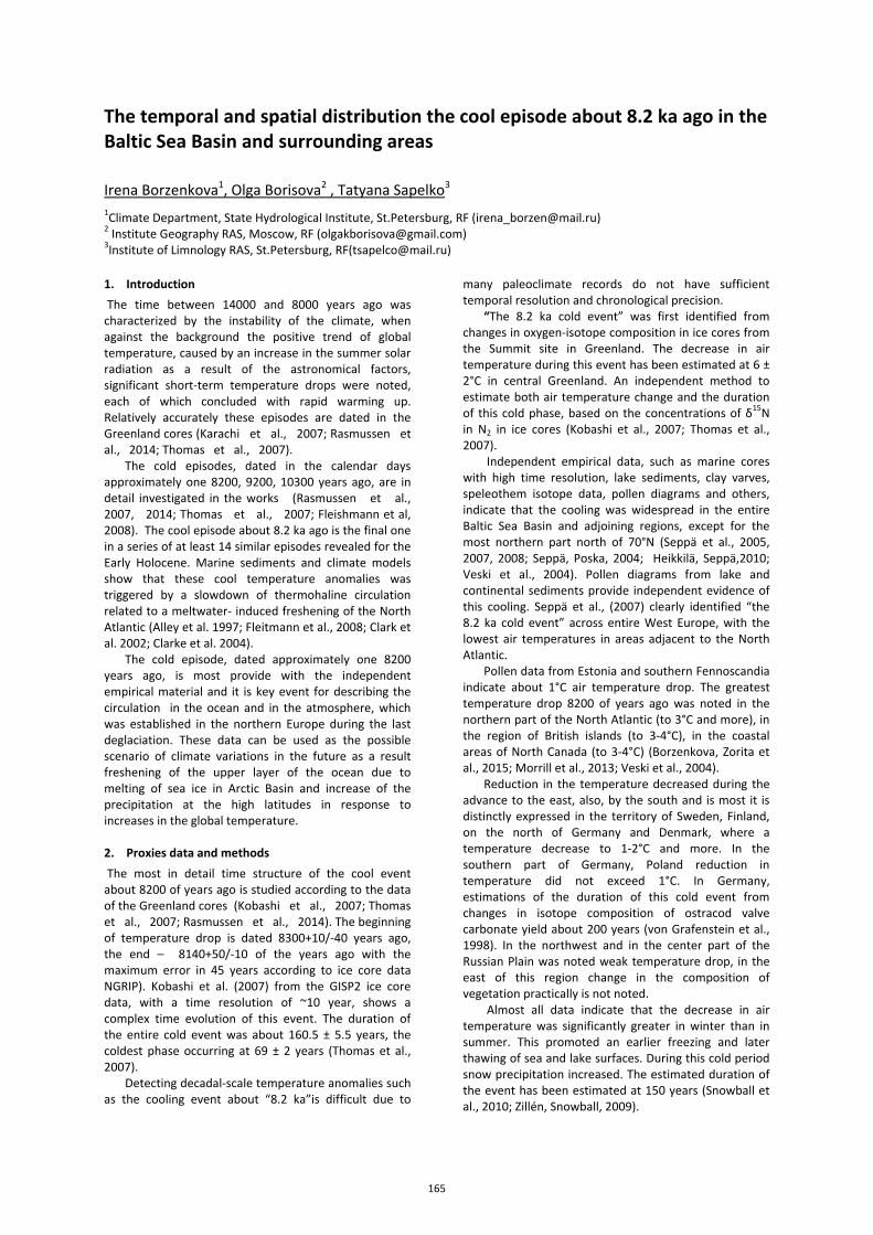
The temporal and spatial distribution the cool episode about 8.2 ka ago in the Baltic Sea Basin and surrounding areas

Irena Borzenkova1, Olga Borisova2 , Tatyana Sapelko3 1Climate Department, State Hydrological Institute, St.Petersburg, RF (irena_borzen@mail.ru) 2 Institute Geography RAS, Moscow, RF (olgakborisova@gmail.com) 3Institute of Limnology RAS, St.Petersburg, RF(tsapelco@mail.ru) 1. Introduction The time between 14000 and 8000 years ago was characterized by the instability of the climate, when against the background the positive trend of global temperature, caused by an increase in the summer solar radiation as a result of the astronomical factors, significant short-term temperature drops were noted, each of which concluded with rapid warming up. Relatively accurately these episodes are dated in the Greenland cores (Karachi et al., 2007; Rasmussen et al., 2014; Thomas et al., 2007).

The cold episodes, dated in the calendar days approximately one 8200, 9200, 10300 years ago, are in detail investigated in the works (Rasmussen et al., 2007, 2014; Thomas et al., 2007; Fleishmann et al, 2008). The cool episode about 8.2 ka ago is the final one in a series of at least 14 similar episodes revealed for the Early Holocene. Marine sediments and climate models show that these cool temperature anomalies was triggered by a slowdown of thermohaline circulation related to a meltwater- induced freshening of the North Atlantic (Alley et al. 1997; Fleitmann et al., 2008; Clark et al. 2002; Clarke et al. 2004).

The cold episode, dated approximately one 8200 years ago, is most provide with the independent empirical material and it is key event for describing the circulation in the ocean and in the atmosphere, which was established in the northern Europe during the last deglaciation. These data can be used as the possible scenario of climate variations in the future as a result freshening of the upper layer of the ocean due to melting of sea ice in Arctic Basin and increase of the precipitation at the high latitudes in response to increases in the global temperature. 2. Proxies data and methods The most in detail time structure of the cool event about 8200 of years ago is studied according to the data of the Greenland cores (Kobashi et al., 2007; Thomas et al., 2007; Rasmussen et al., 2014). The beginning of temperature drop is dated 8300+10/-40 years ago, the end – 8140+50/-10 of the years ago with the maximum error in 45 years according to ice core data NGRIP). Kobashi et al. (2007) from the GISP2 ice core data, with a time resolution of ~10 year, shows a complex time evolution of this event. The duration of the entire cold event was about 160.5 ± 5.5 years, the coldest phase occurring at 69 ± 2 years (Thomas et al., 2007).

Detecting decadal-scale temperature anomalies such as the cooling event about “8.2 ka”is difficult due to

many paleoclimate records do not have sufficient temporal resolution and chronological precision.

“The 8.2 ka cold event” was first identified from changes in oxygen-isotope composition in ice cores from the Summit site in Greenland. The decrease in air temperature during this event has been estimated at 6 ± 2°С in central Greenland. An independent method to estimate both air temperature change and the duration of this cold phase, based on the concentrations of δ15N in N2 in ice cores (Kobashi et al., 2007; Thomas et al., 2007).

Independent empirical data, such as marine cores with high time resolution, lake sediments, clay varves, speleothem isotope data, pollen diagrams and others, indicate that the cooling was widespread in the entire Baltic Sea Basin and adjoining regions, except for the most northern part north of 70°N (Seppä et al., 2005, 2007, 2008; Seppä, Poska, 2004; Heikkilä, Seppä,2010; Veski et al., 2004). Pollen diagrams from lake and continental sediments provide independent evidence of this cooling. Seppä et al., (2007) clearly identified “the 8.2 ka cold event” across entire West Europe, with the lowest air temperatures in areas adjacent to the North Atlantic.

Pollen data from Estonia and southern Fennoscandia indicate about 1°С air temperature drop. The greatest temperature drop 8200 of years ago was noted in the northern part of the North Atlantic (to 3°С and more), in the region of British islands (to 3-4°С), in the coastal areas of North Canada (to 3-4°С) (Borzenkova, Zorita et al., 2015; Morrill et al., 2013; Veski et al., 2004).

Reduction in the temperature decreased during the advance to the east, also, by the south and is most it is distinctly expressed in the territory of Sweden, Finland, on the north of Germany and Denmark, where a temperature decrease to 1-2°С and more. In the southern part of Germany, Poland reduction in temperature did not exceed 1°С. In Germany, estimations of the duration of this cold event from changes in isotope composition of ostracod valve carbonate yield about 200 years (von Grafenstein et al., 1998). In the northwest and in the center part of the Russian Plain was noted weak temperature drop, in the east of this region change in the composition of vegetation practically is not noted.

Almost all data indicate that the decrease in air temperature was significantly greater in winter than in summer. This promoted an earlier freezing and later thawing of sea and lake surfaces. During this cold period snow precipitation increased. The estimated duration of the event has been estimated at 150 years (Snowball et al., 2010; Zillén, Snowball, 2009).

165

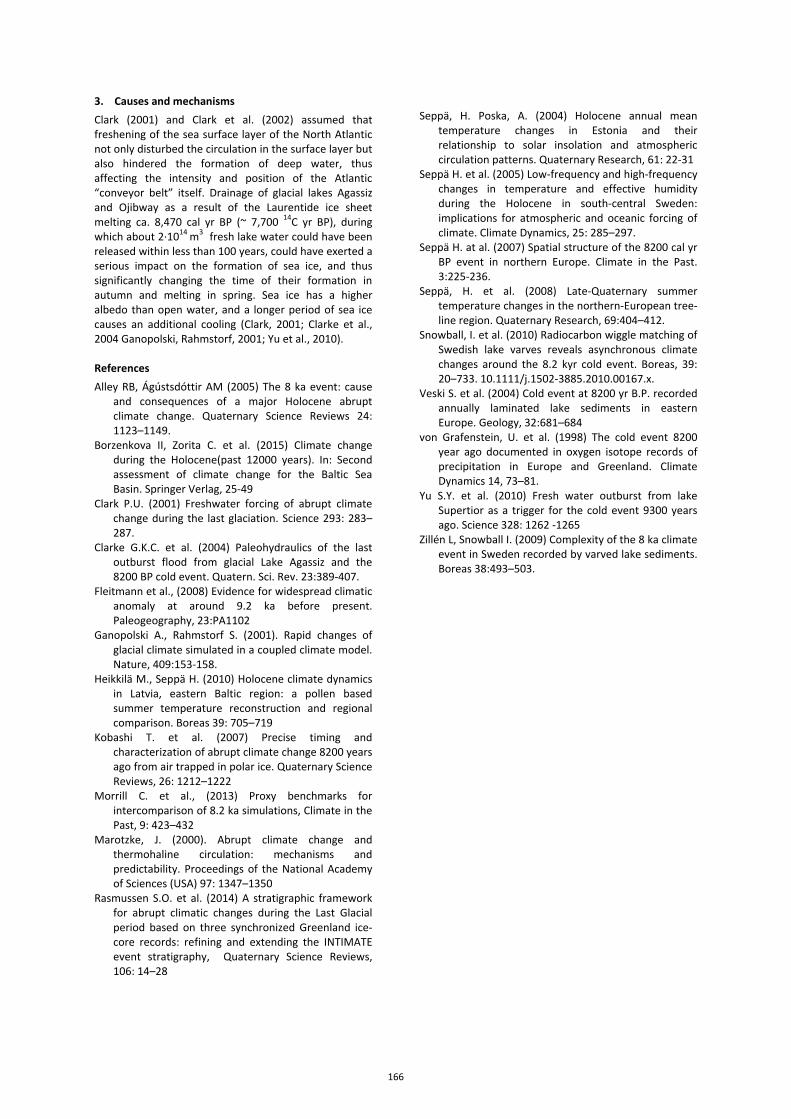
3. Causes and mechanisms Clark (2001) and Clark et al. (2002) assumed that freshening of the sea surface layer of the North Atlantic not only disturbed the circulation in the surface layer but also hindered the formation of deep water, thus affecting the intensity and position of the Atlantic “conveyor belt” itself. Drainage of glacial lakes Agassiz and Ojibway as a result of the Laurentide ice sheet melting ca. 8,470 cal yr ВР (~ 7,700 14С yr BP), during which about 2·1014 m3 fresh lake water could have been released within less than 100 years, could have exerted a serious impact on the formation of sea ice, and thus significantly changing the time of their formation in autumn and melting in spring. Sea ice has a higher albedo than open water, and a longer period of sea ice causes an additional cooling (Clark, 2001; Clarke et al., 2004 Ganopolski, Rahmstorf, 2001; Yu et al., 2010). References Alley RB, Ágústsdóttir AM (2005) The 8 ka event: cause

and consequences of a major Holocene abrupt climate change. Quaternary Science Reviews 24: 1123–1149.

Borzenkova II, Zorita C. et al. (2015) Climate change during the Holocene(past 12000 years). In: Second assessment of climate change for the Baltic Sea Basin. Springer Verlag, 25-49

Clark P.U. (2001) Freshwater forcing of abrupt climate change during the last glaciation. Science 293: 283–287.

Clarke G.K.C. et al. (2004) Paleohydraulics of the last outburst flood from glacial Lake Agassiz and the 8200 BP cold event. Quatern. Sci. Rev. 23:389-407.

Fleitmann et al., (2008) Evidence for widespread climatic anomaly at around 9.2 ka before present. Paleogeography, 23:PA1102

Ganopolski A., Rahmstorf S. (2001). Rapid changes of glacial climate simulated in a coupled climate model. Nature, 409:153-158.

Heikkilä M., Seppä H. (2010) Holocene climate dynamics in Latvia, eastern Baltic region: a pollen based summer temperature reconstruction and regional comparison. Boreas 39: 705–719

Kobashi T. et al. (2007) Precise timing and characterization of abrupt climate change 8200 years ago from air trapped in polar ice. Quaternary Science Reviews, 26: 1212–1222

Morrill C. et al., (2013) Proxy benchmarks for intercomparison of 8.2 ka simulations, Climate in the Past, 9: 423–432

Marotzke, J. (2000). Abrupt climate change and thermohaline circulation: mechanisms and predictability. Proceedings of the National Academy of Sciences (USA) 97: 1347–1350

Rasmussen S.O. et al. (2014) A stratigraphic framework for abrupt climatic changes during the Last Glacial period based on three synchronized Greenland ice-core records: refining and extending the INTIMATE event stratigraphy, Quaternary Science Reviews, 106: 14–28

Seppä, H. Poska, A. (2004) Holocene annual mean

temperature changes in Estonia and their relationship to solar insolation and atmospheric circulation patterns. Quaternary Research, 61: 22-31

Seppä H. et al. (2005) Low-frequency and high-frequency changes in temperature and effective humidity during the Holocene in south-central Sweden: implications for atmospheric and oceanic forcing of climate. Climate Dynamics, 25: 285–297.

Seppä H. at al. (2007) Spatial structure of the 8200 cal yr BP event in northern Europe. Climate in the Past. 3:225-236.

Seppä, H. et al. (2008) Late-Quaternary summer temperature changes in the northern-European tree-line region. Quaternary Research, 69:404–412.

Snowball, I. et al. (2010) Radiocarbon wiggle matching of Swedish lake varves reveals asynchronous climate changes around the 8.2 kyr cold event. Boreas, 39: 20–733. 10.1111/j.1502-3885.2010.00167.x.

Veski S. et al. (2004) Cold event at 8200 yr B.P. recorded annually laminated lake sediments in eastern Europe. Geology, 32:681–684

von Grafenstein, U. et al. (1998) The cold event 8200 year ago documented in oxygen isotope records of precipitation in Europe and Greenland. Climate Dynamics 14, 73–81.

Yu S.Y. et al. (2010) Fresh water outburst from lake Supertior as a trigger for the cold event 9300 years ago. Science 328: 1262 -1265

Zillén L, Snowball I. (2009) Complexity of the 8 ka climate event in Sweden recorded by varved lake sediments. Boreas 38:493–503.

166

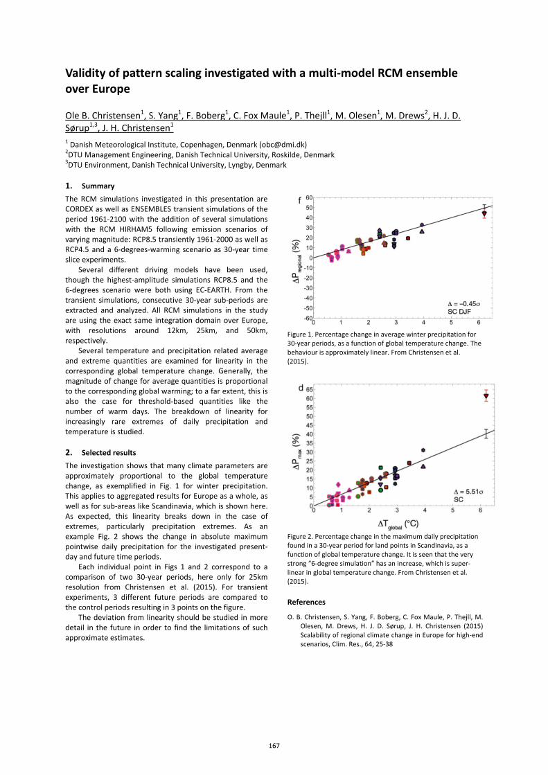
Validity of pattern scaling investigated with a multi-model RCM ensemble over Europe

Ole B. Christensen1, S. Yang1, F. Boberg1, C. Fox Maule1, P. Thejll1, M. Olesen1, M. Drews2, H. J. D. Sørup1,3, J. H. Christensen1 1 Danish Meteorological Institute, Copenhagen, Denmark (obc@dmi.dk) 2DTU Management Engineering, Danish Technical University, Roskilde, Denmark 3DTU Environment, Danish Technical University, Lyngby, Denmark 1. Summary The RCM simulations investigated in this presentation are CORDEX as well as ENSEMBLES transient simulations of the period 1961-2100 with the addition of several simulations with the RCM HIRHAM5 following emission scenarios of varying magnitude: RCP8.5 transiently 1961-2000 as well as RCP4.5 and a 6-degrees-warming scenario as 30-year time slice experiments.

Several different driving models have been used, though the highest-amplitude simulations RCP8.5 and the 6-degrees scenario were both using EC-EARTH. From the transient simulations, consecutive 30-year sub-periods are extracted and analyzed. All RCM simulations in the study are using the exact same integration domain over Europe, with resolutions around 12km, 25km, and 50km, respectively.

Several temperature and precipitation related average and extreme quantities are examined for linearity in the corresponding global temperature change. Generally, the magnitude of change for average quantities is proportional to the corresponding global warming; to a far extent, this is also the case for threshold-based quantities like the number of warm days. The breakdown of linearity for increasingly rare extremes of daily precipitation and temperature is studied. 2. Selected results The investigation shows that many climate parameters are approximately proportional to the global temperature change, as exemplified in Fig. 1 for winter precipitation. This applies to aggregated results for Europe as a whole, as well as for sub-areas like Scandinavia, which is shown here. As expected, this linearity breaks down in the case of extremes, particularly precipitation extremes. As an example Fig. 2 shows the change in absolute maximum pointwise daily precipitation for the investigated present-day and future time periods.

Each individual point in Figs 1 and 2 correspond to a comparison of two 30-year periods, here only for 25km resolution from Christensen et al. (2015). For transient experiments, 3 different future periods are compared to the control periods resulting in 3 points on the figure.

The deviation from linearity should be studied in more detail in the future in order to find the limitations of such approximate estimates.

Figure 1. Percentage change in average winter precipitation for 30-year periods, as a function of global temperature change. The behaviour is approximately linear. From Christensen et al. (2015).

Figure 2. Percentage change in the maximum daily precipitation found in a 30-year period for land points in Scandinavia, as a function of global temperature change. It is seen that the very strong “6-degree simulation” has an increase, which is super-linear in global temperature change. From Christensen et al. (2015).

References

O. B. Christensen, S. Yang, F. Boberg, C. Fox Maule, P. Thejll, M. Olesen, M. Drews, H. J. D. Sørup, J. H. Christensen (2015) Scalability of regional climate change in Europe for high-end scenarios, Clim. Res., 64, 25-38

167

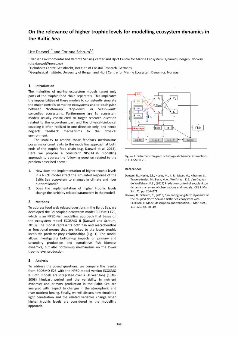
On the relevance of higher trophic levels for modelling ecosystem dynamics in the Baltic Sea

Ute Daewel1,2 and Corinna Schrum2,3 1 Nansen Environmental and Remote Sensing center and Hjort Centre for Marine Ecosystem Dynamics, Bergen, Norway (ute.daewel@nersc.no) 2 Helmholtz Centre Geesthacht, Institute of Coastal Research, Germany 3 Geophysical Institute, University of Bergen and Hjort Centre for Marine Ecosystem Dynamics, Norway 1. Introduction The majorities of marine ecosystem models target only parts of the trophic food chain separately. This implicates the impossibilities of these models to consistently simulate the major controls to marine ecosystems and to distinguish between ‘bottom-up’, ‘top-down’ or ‘wasp-waist’ controlled ecosystems. Furthermore are 3d ecosystem models usually constructed to target research question related to the ecosystem part and the physical-biological coupling is often realized in one direction only, and hence neglects feedback mechanisms to the physical environment.

The inability to resolve those feedback mechanisms poses major constraints to the modelling approach at both ends of the trophic food chain (e.g. Daewel et al. 2013). Here we propose a consistent NPZD-Fish modelling approach to address the following question related to the problem described above: 1. How does the implementation of higher trophic levels

in a NPZD model affect the simulated response of the Baltic Sea ecosystem to changes in climate and river nutrient loads?

2. Does the implementation of higher trophic levels change the turbidity related parameters in the model?

2. Methods To address food web related questions in the Baltic Sea, we developed the 3d coupled ecosystem model ECOSMO E2E, which is an NPZD-Fish modelling approach that bases on the ecosystem model ECOSMO II (Daewel and Schrum, 2013). The model represents both fish and macrobenthos as functional groups that are linked to the lower trophic levels via predator-prey relationships (Fig. 1). The model allows investigating bottom-up impacts on primary and secondary production and cumulative fish biomass dynamics, but also bottom-up mechanisms on the lower trophic level production. 3. Analysis To address the posed questions, we compare the results from ECOSMO E2E with the NPZD model version ECOSMO II. Both models are integrated over a 60 year long (1948-2008) hindcast period and the variability in nutrient dynamics and primary production in the Baltic Sea are analysed with respect to changes in the atmospheric and river nutrient forcing. Finally, we will discuss how simulated light penetration and the related variables change when higher trophic levels are considered in the modelling approach.

Figure 1. Schematic diagram of biological-chemical interactions in ECOSMO E2E.

References

Daewel, U., Hjøllo, S.S., Huret, M., Ji, R., Maar, M., Niiranen, S., Travers-trolet, M., Peck, M.A., Wolfshaar, K.E. Van De, van de Wolfshaar, K.E., (2014) Predation control of zooplankton dynamics: a review of observations and models. ICES J. Mar. Sci., 71, pp. 254–271.

Daewel, U., Schrum, C., (2013) Simulating long-term dynamics of the coupled North Sea and Baltic Sea ecosystem with ECOSMO II: Model description and validation. J. Mar. Syst., 119-120, pp. 30–49.

Nitr

ifica

tion

O2

SIO2

SiO 2 •2H 2 O

N2 NH4

PO4

NO3

P f Z s

Z l P d

D

Pcyan

DOM

Den

itrifi

catio

n

Sed. 3 Si Sed. 1 N Sed. 2 P Benthos

Fish

168

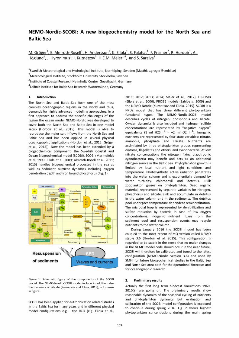
NEMO-Nordic-SCOBI: A new biogeochemistry model for the North Sea and Baltic Sea

M. Gröger1, E. Almroth-Rosell1, H. Andersson1, K. Eilola1, S. Falahat1, F. Frasner2, R. Hordoir1, A. Höglund1, J. Hyronimus1, I. Kuznetzov3, H.E.M. Meier1,4, and S. Saraiva1

1Swedish Meteorological and Hydrological Institute, Norrköping, Sweden (Matthias.groger@smhi.se) 2Meteorological Institute, Stockholm University, Stockholm, Sweden 3Institute of Coastal Research Helmholtz Center Geesthacht, Germany 4Leibniz Institute for Baltic Sea Research Warnemünde, Germany

1. Introduction The North Sea and Baltic Sea form one of the most complex oceanographic regions in the world and thus, demands for highly advanced modelling approaches. In a first approach to address the specific challenges of the region the ocean model NEMO-Nordic was developed to cover both the North Sea and Baltic Sea in one model setup (Hordoir et al., 2015). This model is able to reproduce the major salt inflows from the North Sea and Baltic Sea and has been applied in several physical oceanographic applications (Hordoir et al., 2015, Gröger et al., 2015)). Now the model has been extended by a biogeochemical component, the Swedish Coastal and Ocean Biogeochemical model (SCOBI). SCOBI (Marmefeldt et al. 1999; Eilola et al. 2009; Almroth-Rosell et al. 2011; 2015) handles biogeochemical processes in the sea as well as sediment nutrient dynamics including oxygen penetration depth and iron bound phosphorus (Fig. 1).

Figure 1. Schematic figure of the components of the SCOBI model. The NEMO-Nordic-SCOBI model include in addition also the dynamics of Silicate (Kuznetsov and Eilola, 2015), not shown in figure..

SCOBI has been applied for eutrophication related studies in the Baltic Sea for many years and in different physical model configurations e.g., the RCO (e.g. Eilola et al.,

2011; 2012; 2013; 2014; Meier et al., 2012), HIROMB (Eilola et al., 2006), PROBE models (Sahlberg, 2009) and the NEMO-Nordic (Kuznetsov and Eilola, 2015). SCOBI is a NPDZ model that has three different phytoplankton functional types. The NEMO-Nordic-SCOBI model describes cycles of nitrogen, phosphorus and silicate. Oxygen dynamics is also included and hydrogen sulfide concentrations are represented by ‘‘negative oxygen’’ equivalents (1 ml H2S l-1 = –2 ml O2 l- 1). Inorganic nutrients are represented by four state variables: nitrate, ammonia, phosphate and silicate. Nutrients are assimilated by three phytoplankton groups representing diatoms, flagellates and others, and cyanobacteria. At low nitrate concentrations the nitrogen fixing diazotrophic cyanobacteria may benefit and acts as an additional nitrogen source in the Baltic Sea. Phytoplankton growth is limited by local nutrient and light conditions and temperature. Photosynthetic active radiation penetrates into the water column and is exponentially damped by water turbidity, chlorophyll and detritus. Bulk zooplankton grazes on phytoplankton. Dead organic material, represented by separate variables for nitrogen, phosphorus and silicate, sink and accumulate in detritus in the water column and in the sediments. The detritus pool undergoes temperature dependent remineralization. The microbial loop is represented by denitrification and sulfate reduction by bacteria in case of low oxygen concentrations. Inorganic nutrient fluxes from the sediment pool and resuspension events may recycle nutrients to the water column.

During January 2016 the SCOBI model has been coupled to the most recent NEMO version called NEMO stable 3.6 (Hordoir et al. 2015). This configuration is regarded to be stable in the sense that no major changes in the NEMO model code should occur in the near future. SCOBI will therefore be calibrated and tuned to the latest configuration (NEMO-Nordic version 3.6) and used by SMHI for future biogeochemical studies in the Baltic Sea and North Sea area both for the operational forecasts and for oceanographic research.

2. Preliminary results Actually the first long term hindcast simulations 1960-2010(?) are going on. The preliminary results show reasonable dynamics of the seasonal cycling of nutrients and phytoplankton dynamics but evaluation and calibration of the SCOBI model configuration is expected to continue during spring 2016. Fig. 2 shows highest phytoplankton concentrations during the main spring

169

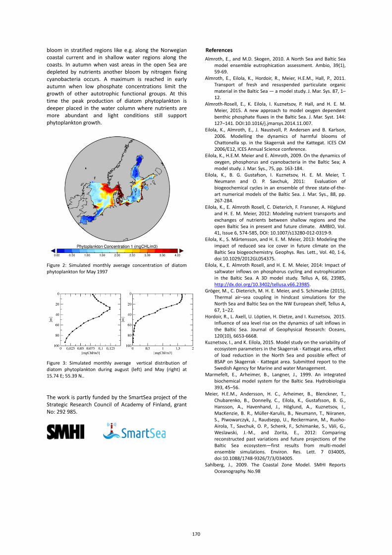
bloom in stratified regions like e.g. along the Norwegian coastal current and in shallow water regions along the coasts. In autumn when vast areas in the open Sea are depleted by nutrients another bloom by nitrogen fixing cyanobacteria occurs. A maximum is reached in early autumn when low phosphate concentrations limit the growth of other autotrophic functional groups. At this time the peak production of diatom phytoplankton is deeper placed in the water column where nutrients are more abundant and light conditions still support phytoplankton growth.

Figure 2: Simulated monthly average concentration of diatom phytoplankton for May 1997

Figure 3: Simulated monthly average vertical distribution of diatom phytoplankton during august (left) and May (right) at 15.74 E; 55.39 N.. The work is partly funded by the SmartSea project of the Strategic Research Council of Academy of Finland, grant No: 292 985.

References Almroth, E., and M.D. Skogen, 2010. A North Sea and Baltic Sea

model ensemble eutrophication assessment. Ambio, 39(1), 59-69.

Almroth, E., Eilola, K., Hordoir, R., Meier, H.E.M., Hall, P., 2011. Transport of fresh and resuspended particulate organic material in the Baltic Sea — a model study. J. Mar. Sys. 87, 1–12.

Almroth-Rosell, E., K. Eilola, I. Kuznetsov, P. Hall, and H. E. M. Meier, 2015. A new approach to model oxygen dependent benthic phosphate fluxes in the Baltic Sea. J. Mar. Syst. 144: 127–141. DOI:10.1016/j.jmarsys.2014.11.007.

Eilola, K., Almroth, E., J. Naustvoll, P. Andersen and B. Karlson, 2006. Modelling the dynamics of harmful blooms of Chattonella sp. in the Skagerrak and the Kattegat. ICES CM 2006/E12, ICES Annual Science conference.

Eilola, K., H.E.M. Meier and E. Almroth, 2009. On the dynamics of oxygen, phosphorus and cyanobacteria in the Baltic Sea; A model study. J. Mar. Sys., 75, pp. 163-184.

Eilola, K., B. G. Gustafson, I. Kuznetsov, H. E. M. Meier, T. Neumann and O. P. Savchuk, 2011: Evaluation of biogeochemical cycles in an ensemble of three state-of-the-art numerical models of the Baltic Sea. J. Mar. Sys., 88, pp. 267-284.

Eilola, K., E. Almroth Rosell, C. Dieterich, F. Fransner, A. Höglund and H. E. M. Meier, 2012: Modeling nutrient transports and exchanges of nutrients between shallow regions and the open Baltic Sea in present and future climate. AMBIO, Vol. 41, Issue 6, 574-585, DOI: 10.1007/s13280-012-0319-9.

Eilola, K., S. Mårtensson, and H. E. M. Meier, 2013: Modeling the impact of reduced sea ice cover in future climate on the Baltic Sea biogeochemistry. Geophys. Res. Lett., Vol. 40, 1-6, doi:10.1029/2012GL054375.

Eilola, K., E. Almroth Rosell, and H. E. M. Meier, 2014: Impact of saltwater inflows on phosphorus cycling and eutrophication in the Baltic Sea. A 3D model study. Tellus A, 66, 23985, http://dx.doi.org/10.3402/tellusa.v66.23985.

Gröger, M., C. Dieterich, M. H. E. Meier, and S. Schimanke (2015), Thermal air–sea coupling in hindcast simulations for the North Sea and Baltic Sea on the NW European shelf, Tellus A, 67, 1–22.

Hordoir, R., L. Axell, U. Löptien, H. Dietze, and I. Kuznetsov, 2015. Influence of sea level rise on the dynamics of salt inflows in the Baltic Sea. Journal of Geophysical Research: Oceans, 120(10), 6653-6668.

Kuznetsov, I., and K. Eilola, 2015. Model study on the variability of ecosystem parameters in the Skagerrak - Kattegat area, effect of load reduction in the North Sea and possible effect of BSAP on Skagerrak - Kattegat area. Submitted report to the Swedish Agency for Marine and water Management.

Marmefelt, E., Arheimer, B., Langner, J., 1999. An integrated biochemical model system for the Baltic Sea. Hydrobiologia 393, 45–56.

Meier, H.E.M., Andersson, H. C., Arheimer, B., Blenckner, T., Chubarenko, B., Donnelly, C., Eilola, K., Gustafsson, B. G., Hansson, A., Havenhand, J., Höglund, A., Kuznetsov, I., MacKenzie, B. R., Müller-Karulis, B., Neumann, T., Niiranen, S., Piwowarczyk, J., Raudsepp, U., Reckermann, M., Ruoho-Airola, T., Savchuk, O. P., Schenk, F., Schimanke, S., Väli, G., Weslawski, J.-M., and Zorita, E., 2012: Comparing reconstructed past variations and future projections of the Baltic Sea ecosystem—first results from multi-model ensemble simulations. Environ. Res. Lett. 7 034005, doi:10.1088/1748-9326/7/3/034005.

Sahlberg, J., 2009. The Coastal Zone Model. SMHI Reports Oceanography. No.98

170

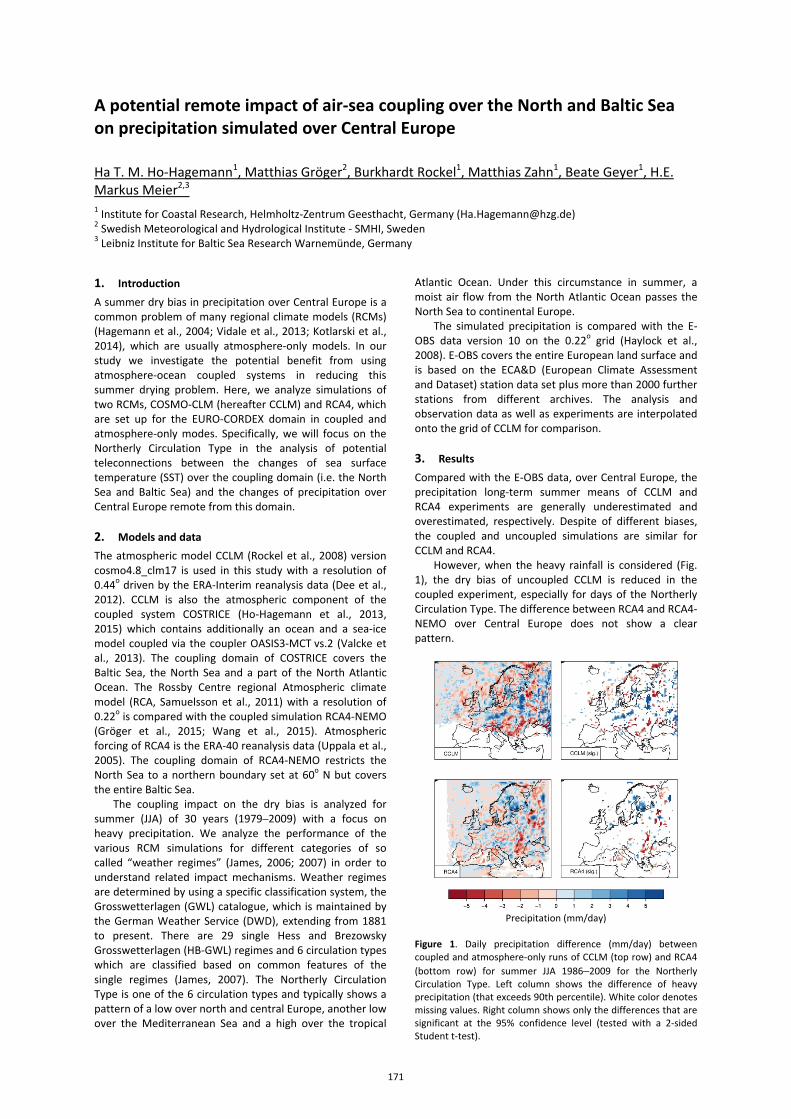
A potential remote impact of air-sea coupling over the North and Baltic Sea on precipitation simulated over Central Europe

Ha T. M. Ho-Hagemann1, Matthias Gröger2, Burkhardt Rockel1, Matthias Zahn1, Beate Geyer1, H.E. Markus Meier2,3

1 Institute for Coastal Research, Helmholtz-Zentrum Geesthacht, Germany (Ha.Hagemann@hzg.de)

2 Swedish Meteorological and Hydrological Institute - SMHI, Sweden

3 Leibniz Institute for Baltic Sea Research Warnemünde, Germany

1. Introduction A summer dry bias in precipitation over Central Europe is a common problem of many regional climate models (RCMs) (Hagemann et al., 2004; Vidale et al., 2013; Kotlarski et al., 2014), which are usually atmosphere-only models. In our study we investigate the potential benefit from using atmosphere-ocean coupled systems in reducing this summer drying problem. Here, we analyze simulations of two RCMs, COSMO-CLM (hereafter CCLM) and RCA4, which are set up for the EURO-CORDEX domain in coupled and atmosphere-only modes. Specifically, we will focus on the Northerly Circulation Type in the analysis of potential teleconnections between the changes of sea surface temperature (SST) over the coupling domain (i.e. the North Sea and Baltic Sea) and the changes of precipitation over Central Europe remote from this domain. 2. Models and data The atmospheric model CCLM (Rockel et al., 2008) version cosmo4.8_clm17 is used in this study with a resolution of 0.44o driven by the ERA-Interim reanalysis data (Dee et al., 2012). CCLM is also the atmospheric component of the coupled system COSTRICE (Ho-Hagemann et al., 2013, 2015) which contains additionally an ocean and a sea-ice model coupled via the coupler OASIS3-MCT vs.2 (Valcke et al., 2013). The coupling domain of COSTRICE covers the Baltic Sea, the North Sea and a part of the North Atlantic Ocean. The Rossby Centre regional Atmospheric climate model (RCA, Samuelsson et al., 2011) with a resolution of 0.22o is compared with the coupled simulation RCA4-NEMO (Gröger et al., 2015; Wang et al., 2015). Atmospheric forcing of RCA4 is the ERA-40 reanalysis data (Uppala et al., 2005). The coupling domain of RCA4-NEMO restricts the North Sea to a northern boundary set at 60o N but covers the entire Baltic Sea.

The coupling impact on the dry bias is analyzed for summer (JJA) of 30 years (1979–2009) with a focus on heavy precipitation. We analyze the performance of the various RCM simulations for different categories of so called “weather regimes” (James, 2006; 2007) in order to understand related impact mechanisms. Weather regimes are determined by using a specific classification system, the Grosswetterlagen (GWL) catalogue, which is maintained by the German Weather Service (DWD), extending from 1881 to present. There are 29 single Hess and Brezowsky Grosswetterlagen (HB-GWL) regimes and 6 circulation types which are classified based on common features of the single regimes (James, 2007). The Northerly Circulation Type is one of the 6 circulation types and typically shows a pattern of a low over north and central Europe, another low over the Mediterranean Sea and a high over the tropical

Atlantic Ocean. Under this circumstance in summer, a moist air flow from the North Atlantic Ocean passes the North Sea to continental Europe.

The simulated precipitation is compared with the E-OBS data version 10 on the 0.22o grid (Haylock et al., 2008). E-OBS covers the entire European land surface and is based on the ECA&D (European Climate Assessment and Dataset) station data set plus more than 2000 further stations from different archives. The analysis and observation data as well as experiments are interpolated onto the grid of CCLM for comparison.

3. Results Compared with the E-OBS data, over Central Europe, the precipitation long-term summer means of CCLM and RCA4 experiments are generally underestimated and overestimated, respectively. Despite of different biases, the coupled and uncoupled simulations are similar for CCLM and RCA4.

However, when the heavy rainfall is considered (Fig. 1), the dry bias of uncoupled CCLM is reduced in the coupled experiment, especially for days of the Northerly Circulation Type. The difference between RCA4 and RCA4-NEMO over Central Europe does not show a clear pattern.

Precipitation (mm/day)

Figure 1. Daily precipitation difference (mm/day) between coupled and atmosphere-only runs of CCLM (top row) and RCA4 (bottom row) for summer JJA 1986–2009 for the Northerly Circulation Type. Left column shows the difference of heavy precipitation (that exceeds 90th percentile). White color denotes missing values. Right column shows only the differences that are significant at the 95% confidence level (tested with a 2-sided Student t-test).

171

Fig. 1 shows significant differences for grid points where the number of rainfall days is larger than 10 % of the total days of the whole time series of the Northerly Circulation Type (i.e. 553 days). Fig. 1 indicates that interactive coupling leads to wetter condition over Central Europe as well as over the North Sea and Baltic Sea, thus diminishing the model’s dry bias significantly in this area for CCLM. Here, COSTRICE provides an averaged reduction of the dry bias in heavy precipitation (exceeding the 90th percentile) by approx. 10 % over Central Europe compared to CCLM only. The dry bias reduction can be up to 38 % over Poland and 30 % over Germany. For RCA4, there is a rather small change in the south of the North Sea and in the Baltic catchment but almost no significant change far remote from the coupling area. The effect is very small in Central Europe but rather pronounced over Finland. 4. Discussion and conclusions The comparisons of the coupled systems against the atmospheric only models show that the benefit of the coupling is different for the considered time-scales. The coupled and uncoupled long-term summer means are mostly identical in both simulations for CCLM and RCA4. However, if extreme precipitation is considered, especially for the Northerly Circulation Type, when the air flow from the North Atlantic Ocean passes the coupling domain over the North Sea, the simulations of the COSTRICE coupled system are generally improved compared to the CCLM atmosphere only run. The benefit of coupling in COSTRICE is that the air-sea (e.g., wind-evaporation-sea surface temperature) feedback and land-sea interactions are better reproduced that consequently lead to an improvement of the large-scale moisture convergence from the seas to land. Basically, increased wind speed over the sea generates increased evaporation rates and increasing latent heat energy, which in turn leads to further increase in wind speeds; however, intensified turbulent mixing at the sea surface due to increased wind speed generates mixed layer deepening and surface cooling (Bender et al., 1993). This sea surface cooling increases the land-sea temperature contrast, which together with the increasing wind speed over the sea, intensifies the large-scale moisture convergence from the North Atlantic Ocean to Central Europe in COSTRICE, especially under conditions of the Northerly Circulation Type in summer.

However, for RCA4, the benefit of coupling is unclear. For heavy precipitation the difference between RCA4 and RCA4-NEMO over Central Europe is not statistically significant, which is consistent to results of Gröger et al. (2015). This different behaviour in the two RCMs may have two main reasons. On the one hand, it may be related to different sensitivities of the atmospheric model components to the change of SST over the coupling domain. On the other hand, the size and exact location of the coupling domain may be an important issue which needs to be further investigated in the future.

Our study has shown that the benefit of coupling strongly depends on the considered time scales, the coupled system and its setup. The CCLM simulations indicate that the coupling over the North Sea and the Baltic Sea can lead to an improved simulation of heavy precipitation over Central Europe. In order to obtain more robust conclusions, the analysis should be conducted for several RCMs, such as CCLM and RCA4, with the same

resolution, coupling domain, SST forcing, and lateral boundary conditions. Then, for example, the coupling area may be varied to find an optimal domain for climate simulations over Europe.

References

Bender, M.A. et al. (1993) Numerical simulations of hurricane-ocean interaction with a high resolution coupled model. J. Geophys. Res., 98: 23245- 23263.

Dee, D.P. et al. (2011) The ERA-Interim reanalysis: Configuration and performance of the data assimilation system. Q. J. R. Meteor. Soc. 137: 553-597, doi: 10.1002/qj.828, 2011.

Gröger, M., Dieterich, C., Meier, H.E.M., and Schimanke, S. (2015) Thermal air-sea coupling in hindcast simulations for the North Sea and Baltic Sea on the NW European shelf. Tellus A, 67, 26911.

Haylock, M.R. et al. (2008) A European daily high-resolution gridded data set of surface temperature and precipitation for 1950-2006. J. Geophys. Res., 113, D20119, doi:10.1029/2008JD010201.

Hagemann, S. et al. (2004) Evaluation of water and energy budgets in regional climate models applied over Europe. Clim. Dyn., 23, 547-567, DOI: 10.1007/s00382-004-0444-7

Ho-Hagemann, H.T.M. et al. (2013) COSTRICE – an atmosphere – ocean – sea ice model coupled system using OASIS3. HZG Report 2013-5, 26pp.

Ho-Hagemann, H.T.M., Hagemann, S., and Rockel, B. (2015) On the role of soil moisture in the generation of heavy rainfall during the Oder flood event in July 1997, Tellus A, 67, 1–17, doi:10.3402/tellusa.v67.28661.

James, P.M. (2006) An assessment of European synoptic variability in Hadley Centre Global Environmental models based on an objective classification of weather regimes, Clim. Dyn., 27, 215–231, doi:10.1007/s00382-006-0133-9.

James, P.M. (2007) An objective classification method for Hess and Brezowsky Grosswetterlagen over Europe. Theor. and App. Clim. 88:17-42.

Kotlarski, S. et al. (2014) Regional climate modelling on European scales: A joint standard evaluation of the EURO-CORDEX RCM ensemble. Geoscientific Model Development, 7, 1297-1333.

Rockel, B., Will, A., Hense, A. (Editorial) (2008) Special issue Regional climate modelling with COSMO-CLM (CCLM), MeteorologischeZeitschrift, Vol. 17, No. 4, pp. 347-348.

Samuelsson, P. et al. (2011) The Rossby Centre Regional Climate model RCA3: model description and performance, Tellus, 63A, 423, 2011.

Valcke, S, Craig, T., Coquart, L. (2013) OASIS3-MCT User Guide, OASIS3-MCT 2.0, Technical Report, TR/CMGC/13/17, CERFACS/CNRS SUC URA No 1875, Toulouse, France.

Vidale, P.L. et al. (2003) Predictability and uncertainty in a regional climate model, J. Geophys. Res. 108 (D18), 4586, doi:10.1029/2002JD002810.

Uppala, S.M. et al. (2005) The ERA-40 re-analysis. Quart. J. R. Meteor. Soc., 131, 2961–3012, doi:10.1256/qJ04.176.

Wang, S. et al. (2015) Development and evaluation of a new regional coupled atmosphere-ocean model RCA4-NEMO and application for future scenario experiments, Tellus A (67), Nr. 24284.

172

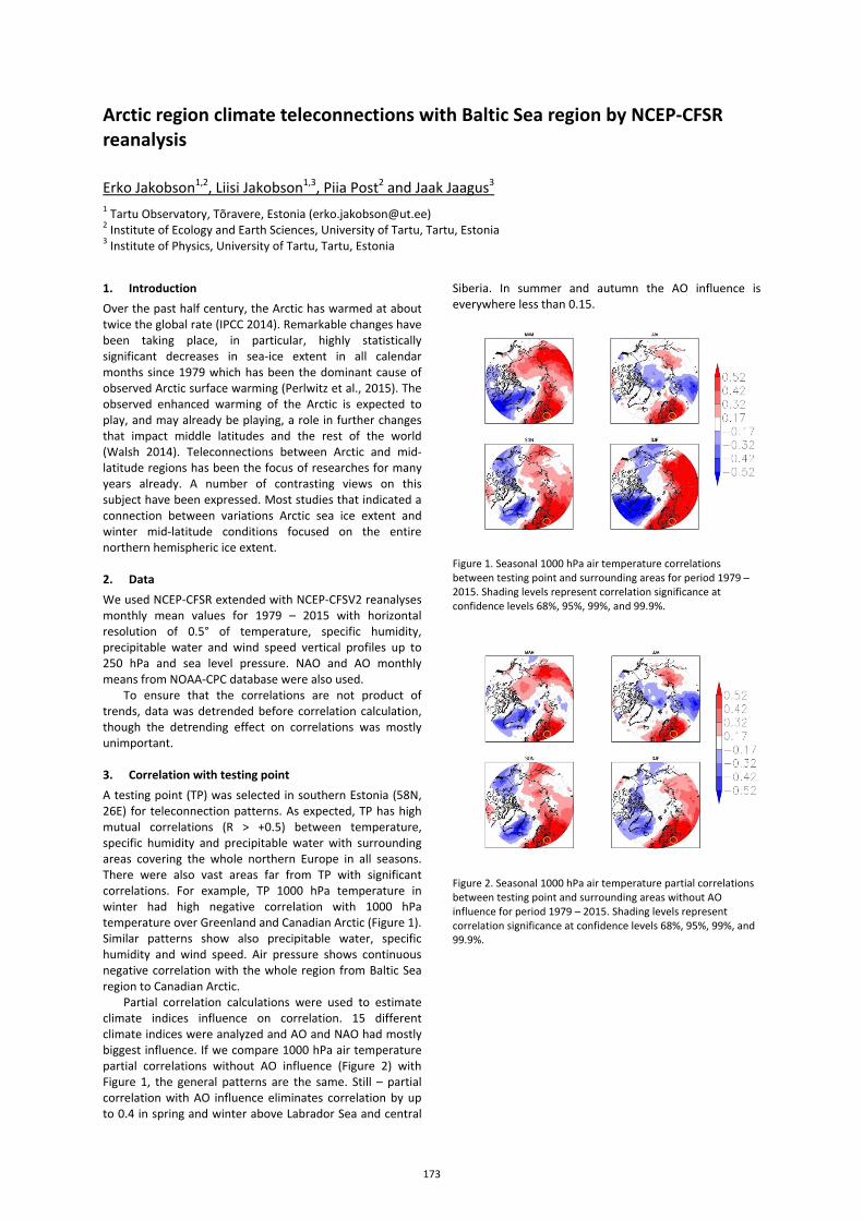
Arctic region climate teleconnections with Baltic Sea region by NCEP-CFSR reanalysis

Erko Jakobson1,2, Liisi Jakobson1,3, Piia Post2 and Jaak Jaagus3 1 Tartu Observatory, Tõravere, Estonia (erko.jakobson@ut.ee) 2 Institute of Ecology and Earth Sciences, University of Tartu, Tartu, Estonia 3 Institute of Physics, University of Tartu, Tartu, Estonia

1. Introduction Over the past half century, the Arctic has warmed at about twice the global rate (IPCC 2014). Remarkable changes have been taking place, in particular, highly statistically significant decreases in sea-ice extent in all calendar months since 1979 which has been the dominant cause of observed Arctic surface warming (Perlwitz et al., 2015). The observed enhanced warming of the Arctic is expected to play, and may already be playing, a role in further changes that impact middle latitudes and the rest of the world (Walsh 2014). Teleconnections between Arctic and mid-latitude regions has been the focus of researches for many years already. A number of contrasting views on this subject have been expressed. Most studies that indicated a connection between variations Arctic sea ice extent and winter mid-latitude conditions focused on the entire northern hemispheric ice extent. 2. Data We used NCEP-CFSR extended with NCEP-CFSV2 reanalyses monthly mean values for 1979 – 2015 with horizontal resolution of 0.5° of temperature, specific humidity, precipitable water and wind speed vertical profiles up to 250 hPa and sea level pressure. NAO and AO monthly means from NOAA-CPC database were also used.

To ensure that the correlations are not product of trends, data was detrended before correlation calculation, though the detrending effect on correlations was mostly unimportant. 3. Correlation with testing point A testing point (TP) was selected in southern Estonia (58N, 26E) for teleconnection patterns. As expected, TP has high mutual correlations (R > +0.5) between temperature, specific humidity and precipitable water with surrounding areas covering the whole northern Europe in all seasons. There were also vast areas far from TP with significant correlations. For example, TP 1000 hPa temperature in winter had high negative correlation with 1000 hPa temperature over Greenland and Canadian Arctic (Figure 1). Similar patterns show also precipitable water, specific humidity and wind speed. Air pressure shows continuous negative correlation with the whole region from Baltic Sea region to Canadian Arctic.

Partial correlation calculations were used to estimate climate indices influence on correlation. 15 different climate indices were analyzed and AO and NAO had mostly biggest influence. If we compare 1000 hPa air temperature partial correlations without AO influence (Figure 2) with Figure 1, the general patterns are the same. Still – partial correlation with AO influence eliminates correlation by up to 0.4 in spring and winter above Labrador Sea and central

Siberia. In summer and autumn the AO influence is everywhere less than 0.15.

Figure 1. Seasonal 1000 hPa air temperature correlations between testing point and surrounding areas for period 1979 – 2015. Shading levels represent correlation significance at confidence levels 68%, 95%, 99%, and 99.9%.

Figure 2. Seasonal 1000 hPa air temperature partial correlations between testing point and surrounding areas without AO influence for period 1979 – 2015. Shading levels represent correlation significance at confidence levels 68%, 95%, 99%, and 99.9%.

173

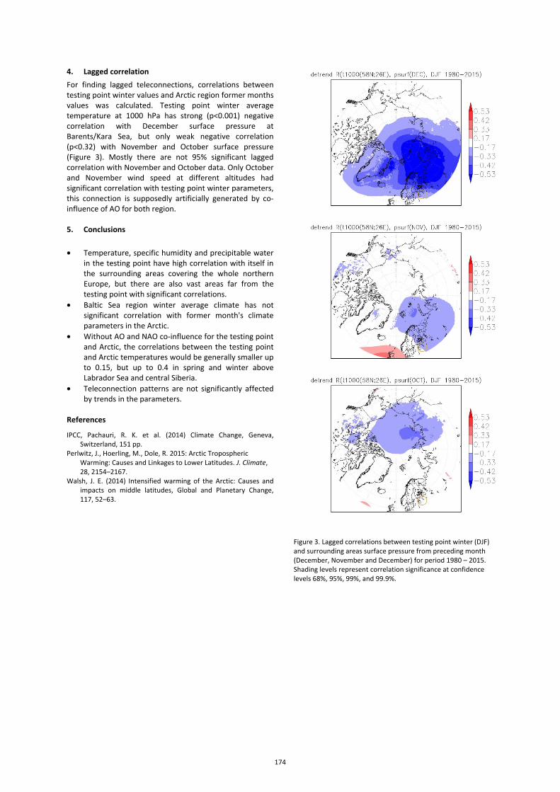
4. Lagged correlation For finding lagged teleconnections, correlations between testing point winter values and Arctic region former months values was calculated. Testing point winter average temperature at 1000 hPa has strong (p<0.001) negative correlation with December surface pressure at Barents/Kara Sea, but only weak negative correlation (p<0.32) with November and October surface pressure (Figure 3). Mostly there are not 95% significant lagged correlation with November and October data. Only October and November wind speed at different altitudes had significant correlation with testing point winter parameters, this connection is supposedly artificially generated by co-influence of AO for both region. 5. Conclusions • Temperature, specific humidity and precipitable water

in the testing point have high correlation with itself in the surrounding areas covering the whole northern Europe, but there are also vast areas far from the testing point with significant correlations.

• Baltic Sea region winter average climate has not significant correlation with former month's climate parameters in the Arctic.

• Without AO and NAO co-influence for the testing point and Arctic, the correlations between the testing point and Arctic temperatures would be generally smaller up to 0.15, but up to 0.4 in spring and winter above Labrador Sea and central Siberia.

• Teleconnection patterns are not significantly affected by trends in the parameters.

References

IPCC, Pachauri, R. K. et al. (2014) Climate Change, Geneva, Switzerland, 151 pp.

Perlwitz, J., Hoerling, M., Dole, R. 2015: Arctic Tropospheric Warming: Causes and Linkages to Lower Latitudes. J. Climate, 28, 2154–2167.

Walsh, J. E. (2014) Intensified warming of the Arctic: Causes and impacts on middle latitudes, Global and Planetary Change, 117, 52–63.

Figure 3. Lagged correlations between testing point winter (DJF) and surrounding areas surface pressure from preceding month (December, November and December) for period 1980 – 2015. Shading levels represent correlation significance at confidence levels 68%, 95%, 99%, and 99.9%.

174

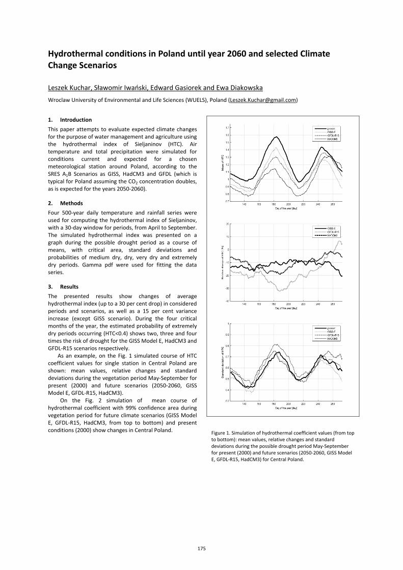
Hydrothermal conditions in Poland until year 2060 and selected Climate Change Scenarios

Leszek Kuchar, Sławomir Iwański, Edward Gasiorek and Ewa Diakowska

Wroclaw University of Environmental and Life Sciences (WUELS), Poland (Leszek.Kuchar@gmail.com)

1. Introduction This paper attempts to evaluate expected climate changes for the purpose of water management and agriculture using the hydrothermal index of Sieljaninov (HTC). Air temperature and total precipitation were simulated for conditions current and expected for a chosen meteorological station around Poland, according to the SRES A1B Scenarios as GISS, HadCM3 and GFDL (which is typical for Poland assuming the CO2 concentration doubles, as is expected for the years 2050-2060). 2. Methods Four 500-year daily temperature and rainfall series were used for computing the hydrothermal index of Sieljaninov, with a 30-day window for periods, from April to September. The simulated hydrothermal index was presented on a graph during the possible drought period as a course of means, with critical area, standard deviations and probabilities of medium dry, dry, very dry and extremely dry periods. Gamma pdf were used for fitting the data series. 3. Results The presented results show changes of average hydrothermal index (up to a 30 per cent drop) in considered periods and scenarios, as well as a 15 per cent variance increase (except GISS scenario). During the four critical months of the year, the estimated probability of extremely dry periods occurring (HTC<0.4) shows two, three and four times the risk of drought for the GISS Model E, HadCM3 and GFDL-R15 scenarios respectively.

As an example, on the Fig. 1 simulated course of HTC coefficient values for single station in Central Poland are shown: mean values, relative changes and standard deviations during the vegetation period May-September for present (2000) and future scenarios (2050-2060, GISS Model E, GFDL-R15, HadCM3).

On the Fig. 2 simulation of mean course of hydrothermal coefficient with 99% confidence area during vegetation period for future climate scenarios (GISS Model E, GFDL-R15, HadCM3, from top to bottom) and present conditions (2000) show changes in Central Poland.

Figure 1. Simulation of hydrothermal coefficient values (from top to bottom): mean values, relative changes and standard deviations during the possible drought period May-September for present (2000) and future scenarios (2050-2060, GISS Model E, GFDL-R15, HadCM3) for Central Poland.

175

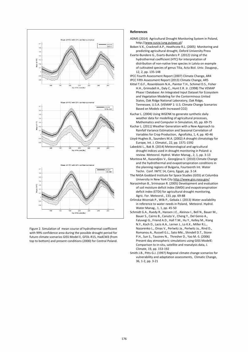
Figure 2. Simulation of mean course of hydrothermal coefficient with 99% confidence area during the possible drought period for future climate scenarios GISS Model E, GFDL-R15, HadCM3 (from top to bottom) and present conditions (2000) for Central Poland.

References

ADMS (2014) Agricultural Drought Monitoring System in Poland, http://www.susza.iung.pulawy.pl/

Boken V.K., Cracknell A.P., Heathcote R.L. (2005) Monitoring and predicting agricultural drought, Oxford University Press

Evarte-Bundere G., Evarts-Bunders P. (2012) Using of the hydrothermal coefficient (HTC) for interpretation of distribution of non-native tree species in Latvia on example of cultivated species of genus Tilia, Acta Biol. Univ. Daugavp., 12, 2, pp. 135-148

IPCC Fourth Assessment Report (2007) Climate Change, AR4 IPCC Fifth Assessment Report (2013) Climate Change, AR5 Kittel T.G.F., Rosenbloom N.A., Painter T.H., Schimel D.S., Fisher

H.H., Grimsdell A., Daly C., Hunt E.R. Jr. (1998) The VEMAP Phase I Database: An Integrated Input Dataset for Ecosystem and Vegetation Modeling for the Conterminous United States, Oak Ridge National Laboratory, Oak Ridge, Tennessee, U.S.A. (VEMAP 1: U.S. Climate Change Scenarios Based on Models with Increased CO2)

Kuchar L. (2004) Using WGENK to generate synthetic daily weather data for modelling of agricultural processes, Mathematics and Computer in Simulation, 65, pp. 69-75

Kuchar L. (2011) Weather Generation with a New Approach to Rainfall Variance Estimation and Seasonal Correlation of Variables for Crop Production, Agrofizika, 1, 4, pp. 40-46

Lloyd-Hughes B., Saunders M.A. (2002) A drought climatology for Europe, Int. J. Climatol., 22, pp. 1571-1592

Labedzki L., Bak B. (2014) Meteorological and agricultural drought indices used in drought monitoring in Poland: a review. Meteorol. Hydrol. Water Manag., 2, 1, pp. 3-13

Monteva M., Kazandjiev V., Georgijeva V. (2010) Climate Change and the hydrothermal and evapotranspiration conditions in the planning regions of Bulgaria, Fourteenth Int. Water Techn. Conf. IWTC 14, Cairo, Egypt, pp. 3-14

The NASA Goddard Institute for Space Studies (GISS) at Columbia University in New York City http://www.giss.nasa.gov/

Narasimhan B., Srinivasan R. (2005) Development and evaluation of soil moisture deficit index (SMDI) and evapotranspiration deficit index (ETDI) for agricultural drought monitoring, Agric. For. Meteorol., 133, pp. 69-88

Orlinska-Wozniak P., Wilk P., Gebala J. (2013) Water availability in reference to water needs in Poland, Meteorol. Hydrol. Water Manag., 1, 1, pp. 45-50

Schmidt G.A., Ruedy R., Hansen J.E., Aleinov I., Bell N., Bauer M., Bauer S., Cairns B., Canuto V., Cheng Y., Del Genio A., Faluvegi G., Friend A.D., Hall T.M., Hu Y., Kelley M., Kiang N.Y., Koch D., Lacis A.A., Lerner J., Lo K.K., Miller R.L., Nazarenko L., Oinas V., Perlwitz Ja., Perlwitz Ju., Rind D., Romanou A., Russell G.L., Sato Mki., Shindell D.T., Stone P.H., Sun S., Tausnev N., Thresher D., Yao M.-S. (2006) Present day atmospheric simulations using GISS ModelE: Comparison to in-situ, satellite and reanalysis data, J. Climate, 19, pp. 153-192

Smith J.B., Pitts G.J. (1997) Regional climate change scenarios for vulnerability and adaptation assessments, Climatic Change, 36, 1-2, pp. 3-21

176

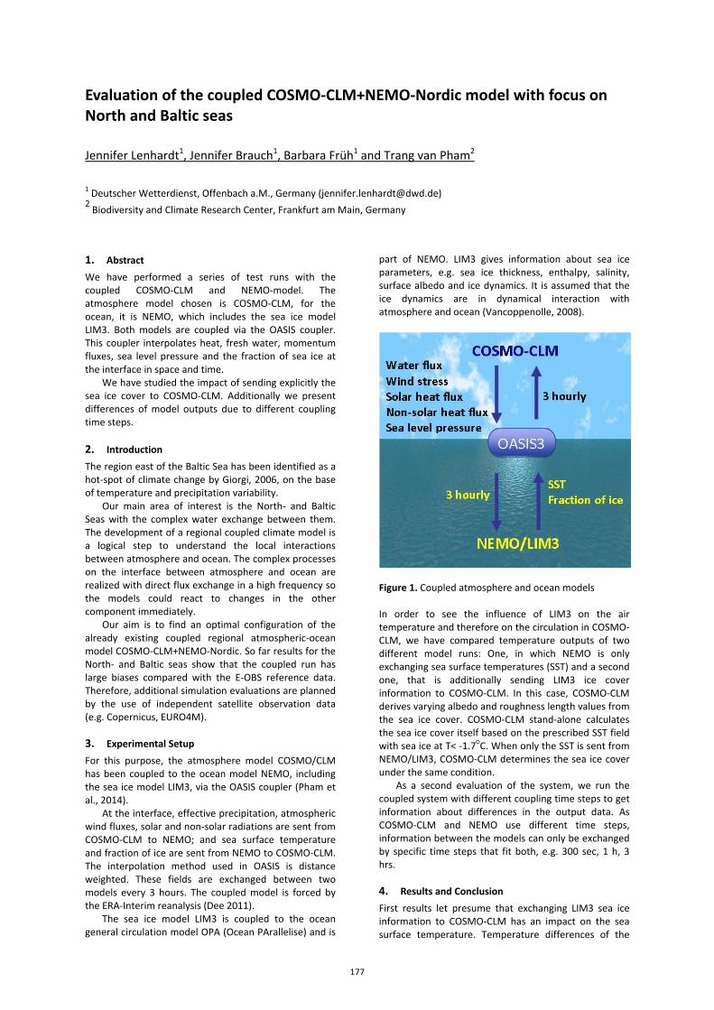
Evaluation of the coupled COSMO-CLM+NEMO-Nordic model with focus on North and Baltic seas

Jennifer Lenhardt1, Jennifer Brauch1, Barbara Früh1 and Trang van Pham2

1 Deutscher Wetterdienst, Offenbach a.M., Germany (jennifer.lenhardt@dwd.de) 2 Biodiversity and Climate Research Center, Frankfurt am Main, Germany

1. Abstract We have performed a series of test runs with the coupled COSMO-CLM and NEMO-model. The atmosphere model chosen is COSMO-CLM, for the ocean, it is NEMO, which includes the sea ice model LIM3. Both models are coupled via the OASIS coupler. This coupler interpolates heat, fresh water, momentum fluxes, sea level pressure and the fraction of sea ice at the interface in space and time.

We have studied the impact of sending explicitly the sea ice cover to COSMO-CLM. Additionally we present differences of model outputs due to different coupling time steps. 2. Introduction The region east of the Baltic Sea has been identified as a hot-spot of climate change by Giorgi, 2006, on the base of temperature and precipitation variability.

Our main area of interest is the North- and Baltic Seas with the complex water exchange between them. The development of a regional coupled climate model is a logical step to understand the local interactions between atmosphere and ocean. The complex processes on the interface between atmosphere and ocean are realized with direct flux exchange in a high frequency so the models could react to changes in the other component immediately.

Our aim is to find an optimal configuration of the already existing coupled regional atmospheric-ocean model COSMO-CLM+NEMO-Nordic. So far results for the North- and Baltic seas show that the coupled run has large biases compared with the E-OBS reference data. Therefore, additional simulation evaluations are planned by the use of independent satellite observation data (e.g. Copernicus, EURO4M). 3. Experimental Setup For this purpose, the atmosphere model COSMO/CLM has been coupled to the ocean model NEMO, including the sea ice model LIM3, via the OASIS coupler (Pham et al., 2014).

At the interface, effective precipitation, atmospheric wind fluxes, solar and non-solar radiations are sent from COSMO-CLM to NEMO; and sea surface temperature and fraction of ice are sent from NEMO to COSMO-CLM. The interpolation method used in OASIS is distance weighted. These fields are exchanged between two models every 3 hours. The coupled model is forced by the ERA-Interim reanalysis (Dee 2011).

The sea ice model LIM3 is coupled to the ocean general circulation model OPA (Ocean PArallelise) and is

part of NEMO. LIM3 gives information about sea ice parameters, e.g. sea ice thickness, enthalpy, salinity, surface albedo and ice dynamics. It is assumed that the ice dynamics are in dynamical interaction with atmosphere and ocean (Vancoppenolle, 2008).

Figure 1. Coupled atmosphere and ocean models In order to see the influence of LIM3 on the air temperature and therefore on the circulation in COSMO-CLM, we have compared temperature outputs of two different model runs: One, in which NEMO is only exchanging sea surface temperatures (SST) and a second one, that is additionally sending LIM3 ice cover information to COSMO-CLM. In this case, COSMO-CLM derives varying albedo and roughness length values from the sea ice cover. COSMO-CLM stand-alone calculates the sea ice cover itself based on the prescribed SST field with sea ice at T< -1.7○C. When only the SST is sent from NEMO/LIM3, COSMO-CLM determines the sea ice cover under the same condition.

As a second evaluation of the system, we run the coupled system with different coupling time steps to get information about differences in the output data. As COSMO-CLM and NEMO use different time steps, information between the models can only be exchanged by specific time steps that fit both, e.g. 300 sec, 1 h, 3 hrs. 4. Results and Conclusion First results let presume that exchanging LIM3 sea ice information to COSMO-CLM has an impact on the sea surface temperature. Temperature differences of the

177

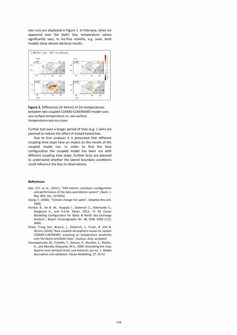
two runs are displayed in Figure 1. In February, when ice appeared over the Baltic Sea, temperature values significantly vary. In ice-free months, e.g. June, both models show almost identical results.

Figure 2. Differences [in Kelvin] of 2m-temperatures between two coupled COSMO-CLM/NEMO model runs: sea-surface-temperature vs. sea-surface temperature+sea ice-cover. Further test over a longer period of time (e.g. 1 Jahr) are planned to reduce the effect of noised based bias.

Due to first analyses it is presumed that different coupling time steps have an impact on the results of the coupled model run. In order to find the best configuration the coupled model has been run with different coupling time steps. Further tests are planned to understand whether the lateral boundary conditions could influence the bias to observations. References

Dee, D.P. et al., (2011), ”ERA-Interim reanalysis configuration and performance of the data assimilation system”, Quart. J. Roy. Met. Soc. 137(656).

Giorgi, F. (2006), “Climate change hot-spots”, Geophys.Res.Lett. 33(8).

Hordoir R., An B. W., Haapala J., Dieterich C., Schimanke S., Hoeglund A., and H.E.M. Meier, 2013, “A 3D Ocean Modelling Configuration for Baltic & North Sea Exchange Analysis”, Report Oceanography No. 48, ISSN: 0283-1112, SMHI.

Pham, Trang Van, Brauch, J., Dieterich, C, Frueh, B. and B. Ahrens (2014),”New coupled atmosphere-ocean-ice system COSMO-CLM/NEMO: assessing air temperature sensitivity over the North and Baltic Seas”, Oceano. Acta, accepted.

Vancoppenolle, M., Fichefet, T., Goosse, H., Bouillon, S., Madec, G., and Morales Maqueda, M.A., 2009: Simulating the mass balance and salinityof Arctic and Antarctic sea ice. 1. Model description and validation. Ocean Modelling, 27, 33-53

178

Estimating uncertainties in projections for the Baltic Sea region based upon an ensemble of regional climate system models

H.E. Markus Meier1,2, M. Edman2 and members of the Baltic Earth working group on scenario simulations for the Baltic Sea 1960-2100 1 Department of Physical Oceanography and Instrumentation, Leibniz Institute for Baltic Sea Research Warnemünde, 18119 Rostock, Germany. (markus.meier@io-warnemuende.de) 2.Department of Research and Development, Swedish Meteorological and Hydrological Institute, 60176 Norrköping, Sweden.

Multi-model ensemble simulations for the Baltic Sea region are presented for the period 1850–2098. For the past period 1850–2006, atmospheric, hydrological and nutrient forcings were reconstructed, based on historical measurements. For the future period 1961-2098, scenario simulations were driven by regionalized global general circulation model (GCM) data using several regional climate system models (RCSMs) and forced by various future greenhouse gas emission and air- and riverborne nutrient load scenarios (ranging from a pessimistic ‘business-as-usual’ to the most optimistic case). To estimate uncertainties caused by biases of RCSMs and GCMs, natural variability and unknown forcing scenarios, different models for the various parts of the Earth system were applied. These simulations constitute the largest ever analyzed multi-model ensemble for the Baltic Sea allowing, inter alia, the statistical evaluation of the ensemble spread. Assuming the IPCC greenhouse gas emission scenarios A1B or A2, we found that water temperatures at the end of this century may be higher and salinities and oxygen concentrations may be lower than ever measured since 1850. There is also a tendency of increased hypoxia and eutrophication in the future, depending on the nutrient load scenario. Despite considerable shortcomings of state-of-the-art models, this study suggests that the future Baltic Sea ecosystem may unprecedentedly change compared to the past 150 yr. As stakeholders today pay only little attention to adaptation and mitigation strategies, more information is needed to raise public awareness of the possible impacts of climate change on marine ecosystems.

179

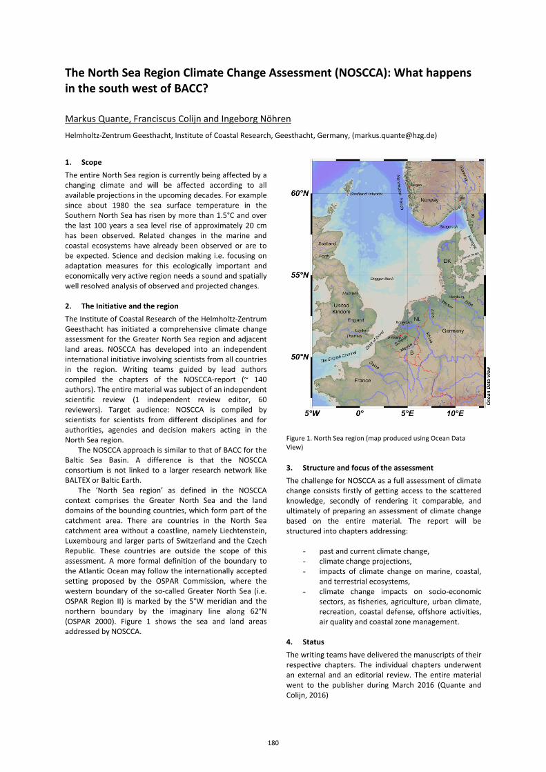
The North Sea Region Climate Change Assessment (NOSCCA): What happens in the south west of BACC?

Markus Quante, Franciscus Colijn and Ingeborg Nöhren

Helmholtz-Zentrum Geesthacht, Institute of Coastal Research, Geesthacht, Germany, (markus.quante@hzg.de)

1. Scope The entire North Sea region is currently being affected by a changing climate and will be affected according to all available projections in the upcoming decades. For example since about 1980 the sea surface temperature in the Southern North Sea has risen by more than 1.5°C and over the last 100 years a sea level rise of approximately 20 cm has been observed. Related changes in the marine and coastal ecosystems have already been observed or are to be expected. Science and decision making i.e. focusing on adaptation measures for this ecologically important and economically very active region needs a sound and spatially well resolved analysis of observed and projected changes. 2. The Initiative and the region The Institute of Coastal Research of the Helmholtz-Zentrum Geesthacht has initiated a comprehensive climate change assessment for the Greater North Sea region and adjacent land areas. NOSCCA has developed into an independent international initiative involving scientists from all countries in the region. Writing teams guided by lead authors compiled the chapters of the NOSCCA-report (~ 140 authors). The entire material was subject of an independent scientific review (1 independent review editor, 60 reviewers). Target audience: NOSCCA is compiled by scientists for scientists from different disciplines and for authorities, agencies and decision makers acting in the North Sea region.

The NOSCCA approach is similar to that of BACC for the Baltic Sea Basin. A difference is that the NOSCCA consortium is not linked to a larger research network like BALTEX or Baltic Earth.

The ‘North Sea region’ as defined in the NOSCCA context comprises the Greater North Sea and the land domains of the bounding countries, which form part of the catchment area. There are countries in the North Sea catchment area without a coastline, namely Liechtenstein, Luxembourg and larger parts of Switzerland and the Czech Republic. These countries are outside the scope of this assessment. A more formal definition of the boundary to the Atlantic Ocean may follow the internationally accepted setting proposed by the OSPAR Commission, where the western boundary of the so-called Greater North Sea (i.e. OSPAR Region II) is marked by the 5°W meridian and the northern boundary by the imaginary line along 62°N (OSPAR 2000). Figure 1 shows the sea and land areas addressed by NOSCCA.

Figure 1. North Sea region (map produced using Ocean Data View)

3. Structure and focus of the assessment The challenge for NOSCCA as a full assessment of climate change consists firstly of getting access to the scattered knowledge, secondly of rendering it comparable, and ultimately of preparing an assessment of climate change based on the entire material. The report will be structured into chapters addressing:

- past and current climate change, - climate change projections, - impacts of climate change on marine, coastal,

and terrestrial ecosystems, - climate change impacts on socio-economic

sectors, as fisheries, agriculture, urban climate, recreation, coastal defense, offshore activities, air quality and coastal zone management.

4. Status The writing teams have delivered the manuscripts of their respective chapters. The individual chapters underwent an external and an editorial review. The entire material went to the publisher during March 2016 (Quante and Colijn, 2016)

180

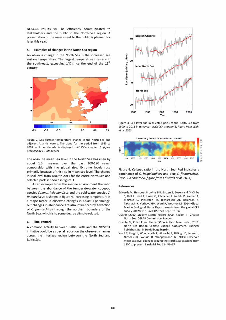
NOSCCA results will be efficiently communicated to stakeholders and the public in the North Sea region. A presentation of the assessment to the public is planned for later this year. 5. Examples of changes in the North Sea region An obvious change in the North Sea is the increased sea surface temperature. The largest temperature rises are in the south-east, exceeding 1°C since the end of the 19th century.

Figure 2. Sea surface temperature change in the North Sea and adjacent Atlantic waters. The trend for the period from 1983 to 2007 in K per decade is displayed. (NOSCCA chapter 2, figure provided by J. Huthnance) The absolute mean sea level in the North Sea has risen by about 1.6 mm/year over the past 100-120 years, comparable with the global rise. Extreme levels rose primarily because of this rise in mean sea level. The change in seal level from 1800 to 2011 for the entire North Sea and selected parts is shown in figure 3.

As an example from the marine environment the ratio between the abundance of the temperate-water copepod species Calanus helgolandicus and the cold-water species C. finmarchicus is shown in figure 4. Increasing temperature is a major factor in observed changes in Calanus phenology, but changes in abundance are also influenced by advection of C. finmarchicus through the northern boundary of the North Sea, which is to some degree climate-related. 6. Final remark A common activity between Baltic Earth and the NOSCCA initiative could be a special report on the observed changes across the interface region between the North Sea and Baltic Sea.

Figure 3. Sea level rise in selected parts of the North Sea from 1900 to 2011 in mm/year. (NOSCCA chapter 3, figure from Wahl et al. 2013)

Figure 4. Calanus ratio in the North Sea. Red indicates a dominance of C. helgolandicus and blue C. finmarchicus. (NOSCCA chapter 8, figure from Edwards et al. 2014) References

Edwards M, Helaouet P, Johns DG, Batten S, Beaugrand G, Chiba S, Hall J, Head E, Hosie G, Kitchener J, Koubbi P, Kreiner A, Melrose C, Pinkerton M, Richardson AJ, Robinson K, Takahashi K, Verheye HM, Ward P, Wootton M (2014) Global Marine Ecological Status Report: results from the global CPR survey 2012/2013. SAHFOS Tech Rep 10:1–37

OSPAR (2000) Quality Status Report 2000, Region II: Greater North Sea. OSPAR Commission, London

Quante M, Colijn F and the NOSCCA Author Team (eds.), 2016: North Sea Region Climate Change Assessment. Springer Publishers Berlin Heidelberg; in print

Wahl T, Haigh I, Woodworth P, Albrecht F, Dillingh D, Jensen J, Nicholls RJ, Weisse R, Wöppelmann G (2013) Observed mean sea level changes around the North Sea coastline from 1800 to present. Earth-Sci Rev 124:51–67

181

Comparison of Observed and Modelled Radiative Energy Flows

Ehrhard Raschke and Stefan Kinne 1 University of Hamburg, Germany, drraschke@aol.com 2 Max-Planck-Institute for Meteorology, Hamburg, Germany

1. Introduction Flows of radiative energy within the climate system are a major component of the overall energy transfer. Therefore enormous efforts are made to derive information on all components of the radiative energy transfer from direct measurements with satellites at the top of the atmosphere and with ground-based radiometers, and to compute it also from other direct and indirect observations of relevant state parameters of the atmosphere and ground. Three such data sets were available for inspection of their mutual agreement in space (100 x 100 km+2) and time. Furthermore similar data sets were available from the climate modelling project CMIP3.

The comparison amongst the three observational data sets showed systematic high uncertainties over areas with dominantly broken cloud fields and high orographic structure of continents. Further uncertainties, which can reach more than 20% of mean values, can be explained by uncertainties of ancillary information on atmospheric aerosols and on surface albedo and emission. Furthermore we found quite high disagreement of directly measured downward SW and LW fluxes and those of our datasets. Differences between model results and the “observation” are of similar magnitude and origin with a preference of surface properties. Models tend generally to underestimate the downward longwave radiation fluxes, globally and annually averaged, by about 10 Wm-2: Specific results are shown in special projections of the BALTEX area. These studies were part of our contribution to the GEWEX datasets assessment. References

Raschke E. et al., 2016: Comparison of radiative energy flow in observational datasets and in climate modelling. J. Appl. Meteor. and Clim., 55, 93-117.

182

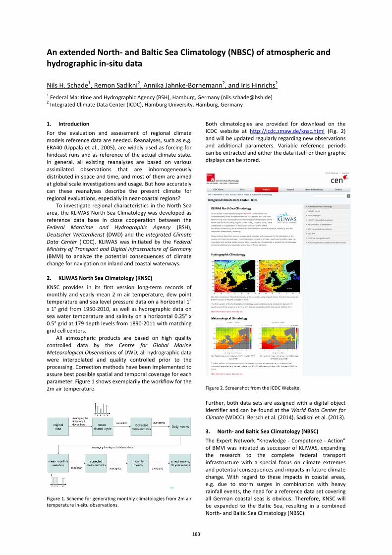
An extended North- and Baltic Sea Climatology (NBSC) of atmospheric and hydrographic in-situ data

Nils H. Schade1, Remon Sadikni2, Annika Jahnke-Bornemann2, and Iris Hinrichs2 1 Federal Maritime and Hydrographic Agency (BSH), Hamburg, Germany (nils.schade@bsh.de) 2 Integrated Climate Data Center (ICDC), Hamburg University, Hamburg, Germany

1. Introduction For the evaluation and assessment of regional climate models reference data are needed. Reanalyses, such as e.g. ERA40 (Uppala et al., 2005), are widely used as forcing for hindcast runs and as reference of the actual climate state. In general, all existing reanalyses are based on various assimilated observations that are inhomogeneously distributed in space and time, and most of them are aimed at global scale investigations and usage. But how accurately can these reanalyses describe the present climate for regional evaluations, especially in near-coastal regions?

To investigate regional characteristics in the North Sea area, the KLIWAS North Sea Climatology was developed as reference data base in close cooperation between the Federal Maritime and Hydrographic Agency (BSH), Deutscher Wetterdienst (DWD) and the Integrated Climate Data Center (ICDC). KLIWAS was initiated by the Federal Ministry of Transport and Digital Infrastructure of Germany (BMVI) to analyze the potential consequences of climate change for navigation on inland and coastal waterways. 2. KLIWAS North Sea Climatology (KNSC) KNSC provides in its first version long-term records of monthly and yearly mean 2 m air temperature, dew point temperature and sea level pressure data on a horizontal 1° x 1° grid from 1950-2010, as well as hydrographic data on sea water temperature and salinity on a horizontal 0.25° x 0.5° grid at 179 depth levels from 1890-2011 with matching grid cell centers.

All atmospheric products are based on high quality controlled data by the Centre for Global Marine Meteorological Observations of DWD, all hydrographic data were interpolated and quality controlled prior to the processing. Correction methods have been implemented to assure best possible spatial and temporal coverage for each parameter. Figure 1 shows exemplarily the workflow for the 2m air temperature.

Figure 1. Scheme for generating monthly climatologies from 2m air temperature in-situ observations.

Both climatologies are provided for download on the ICDC website at http://icdc.zmaw.de/knsc.html (Fig. 2) and will be updated regularly regarding new observations and additional parameters. Variable reference periods can be extracted and either the data itself or their graphic displays can be stored.

Figure 2. Screenshot from the ICDC Website.

Further, both data sets are assigned with a digital object identifier and can be found at the World Data Center for Climate (WDCC): Bersch et al. (2014), Sadikni et al. (2013). 3. North- and Baltic Sea Climatology (NBSC) The Expert Network “Knowledge - Competence - Action” of BMVI was initiated as successor of KLIWAS, expanding the research to the complete federal transport infrastructure with a special focus on climate extremes and potential consequences and impacts in future climate change. With regard to these impacts in coastal areas, e.g. due to storm surges in combination with heavy rainfall events, the need for a reference data set covering all German coastal seas is obvious. Therefore, KNSC will be expanded to the Baltic Sea, resulting in a combined North- and Baltic Sea Climatology (NBSC).

183

In essence, the same procedures and quality controlled data will be used for the atmospheric product. The hydrographic product will be improved by a new quality control procedure complying with the IQUOD standard (http://www.iquod.org). The final product including both the atmospheric and the hydrographic part will be available by the end of 2017.

Standard climatologies will include mean values and standard deviations (per month, year, and decade(s)), extreme values, coverage of observational data with respect to the grid cells, and information about quality and homogeneity up to the preliminary end of the climate period, December 2015. 4. Outlook The final NBSC product will improve the reference data base over sea. It will further be compared to reanalyses products to highlight current shortcomings of global reanalyses in coastal areas, mainly due to coarse horizontal resolution. The new COSMO-REA6 reanalysis (Bollmeyer et al., 2015) is expected to show better accordance, especially in coastal areas, due to the increased horizontal resolution (6 km) alone. Finally, possible additions to the climatology product are discussed, one of which are BSH sea ice data. References

Bersch, M., Gouretski, V., Sadikni, R., and I. Hinrichs (2014): KLIWAS North Sea Climatology of Hydrographic Data (Version 1.1), World Data Center for Climate (WDCC), CERA-DB “KNSC_hyd_v1.1”. http://cera-www.dkrz.de(WDCC/ui/Compact.jsp?acronym=KNSC_hyd_v1.1

Bollmeyer, C., Keller, J.D., Ohlwein, C., Wahl, S., Crewell, S., Friederichs, P., Hense, A., Keune, J., Kneifel, S., Pscheidt, I., Redl, S., and S. Steinke (2015): Towards a high-resolution regional reanalysis for the European CORDEX domain, Quarterly Journal of the Royal Meteorological Society, 141, 1-15. http://dx.doi.org/10.1002/qj.2486

Sadikni, R., Bersch, M., Jahnke-Bornemann, A., and I. Hinrichs (2013): KLIWAS North Sea Climatology of Meteorological Data (Version 1.0), World Data Center for Climate (WDCC). http://dx.doi.org/10.1594/WDCC/KNSC_met_v1.0

Uppala, S.M., Kallberg, P.W., Simmons, A.J., Andrae, U., Da Costa Bechtold, V., Fiorino, M., Gibson, J.K., Haseler, J., Hernandez, A., Kelly, G.A., Li, X., Onogi, K., Saarinen, S., Allan, R.P., Andersson, E., Arpe, K., Balmaseda, M.A., Beljaars, A.C.M., Van De Berg, L., Bidlot, J., Bormann, N., Caires, S., CHevallier, F., Dethof, A., Dragosavac, M., Fisher, M., Fuentes, M., Hagemann, S., Holm, E., Hoskins, B.J., Isaksen, L., Janssen, P.A.E.M., Jenne, R., McNally, A.P., Mahfouf, J.F., Morcrette, J.J., Rayner, N.A., Saunders, R.W., Simon, P., Sterl, A., Trenberth, K.E., Untch, A., Vasiljevic, D., Viterbo, P., and J. Woollen (2005): The ERA-40 re-analysis. Quarterly Journal of the Royal Meteorological Society, 131, 2961-3012. http://dx.doi.org/10.1256/qj.04.176

184

The Future Climate Regions in Estonia

Mait Sepp, Tanel Tamm and Valentina Sagris

Department of Geography, University of Tartu, Estonia (mait.sepp@ut.ee)

1. Introduction Estonia’s long coastline and its location on the border of maritime and continental climates cause rather significant intra-Estonian climatic variations. At times, climate differences in various regions are quite notable. For example, spring arrives about two weeks earlier on southern and south-western Estonia than in northern and north-eastern Estonia.

The climate regionalizing topic has been thoroughly studied in Estonia. For historical reasons, the majority of climatological regionalization here has been based on agricultural interests. The present analysis makes use of Estonian climate regions presented by J. Jaagus and J. Truu (2004). Using cluster analysis and principal component analysis and data from 22 Estonian weather stations (the period of 1966–2000), three main macro-climatic regions were found in the aforementioned study: the Island Estonia, the Mainland Estonia, and the coastal sub-region.

From the climate change point of view, in addition to observing general changes in air temperature and precipitation, it is important to understand how these changes reflect in various climate regions. The key question is whether the climate changes predicted for the 21st century will take place within the present regions or will there also be fundamental changes in the region borders as well? 2. Data and Methods In the present study, changes in air temperature and precipitation predicted for the 21st century are analysed on the basis of the three aforementioned regions. The analysis is based on the outputs from the climate modelling project undertaken by the Estonian Environment Agency for the purpose of finding climate indicators for the periods of 2041–2070 and 2071–2100. In this project, the climate model ensemble of the EURO-CORDEX project was used. The modelling was based on two IPCC climate scenarios: RCP4.5 and RCP8.5. The period of the standard climate is 1971–2000. The output of the project was the change in various meteorological values in comparison to the standard climate.

In order to get the absolute values of air temperature and precipitation in the future climate, the standard climate values and the model’s output were summed using GIS methods. For that, the data from the 24 weather stations was interpolated into a 10x10 km grid covering the whole Estonia by using ArcGIS 10.2 software. The weather station data was obtained from the Estonian Environment Agency. The aforementioned modelling data were added to this standard climate grid data. The absolute values of the future climate precipitation and air temperature were calculated into seasonal (MAM, JJA, SON, DJF) averages. For distinguishing between the three regions and their borders, the tool called ‘Iso Cluster Unsupervised Classification’ of the software ArcGIS 10.2 was used.

Figure 1. The average winter air temperature in the three Estonian climate regions in case of modest warming (RCP4.5) in the period of 2041–2070.

3. Results The analysis results showed that the maritime-coastal-mainland contrasts will remain in the future, i.e. the region pattern presented by Jaagus and Truu (2004) will remain mostly intact. However, the warmest/most precipitation rich region will grow gradually, mostly on the expense of the coastal region.

In terms of air temperature changes, the most important are the ones in winter, for as the warming results in greater contrasts between the mainland and island regions. Even in case of modest warming, the average air temperature in the island region reach permanent above-zero level in the near decades (Figure 1).

In terms of precipitation, the contrast between the islands and the mainland will increase as well. This contrast, however, manifests on scale: in comparison to standard climate, there is more precipitation on the islands and much more precipitation on Estonian mainland. I.e. the amount of precipitation increases more rapidly on Estonian mainland. References

Jaagus, J.; Truu, J. (2004). Climatic regionalisation of Estonia based on multivariate exploratory techniques. In: Tiia Kaare; Jaan-Mati Punning (Ed.). Estonia. Geographical Studies pp. 41−55

185

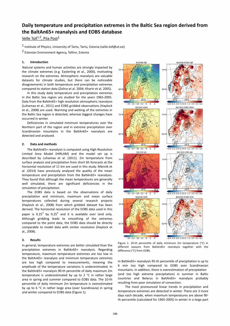
Daily temperature and precipitation extremes in the Baltic Sea region derived fromthe BaltAn65+ reanalysis and EOBS databaseVelle Toll 1,2 , Piia Post 1

1 Institute of Physics, University of Tartu, Tartu, Estonia (velle.toll@ut.ee)2 Estonian Environment Agency, Tallinn, Estonia

1. IntroductionNatural systems and human activities are strongly impacted bythe climate extremes (e.g. Easterling et al., 2000), motivatingresearch on the extremes. Atmospheric reanalysis are valuabledatasets for climate studies, but there can be noticeabledisagreements in both temperature and precipitation extremescompared to station data (Zolina et al. 2004; Kharin et al. 2005).

In this study daily temperature and precipitation extremesin the Baltic Sea region are studied for the years 1965-2005.Data from the BaltAn65+ high resolution atmospheric reanalysis(Luhamaa et al., 2011) and EOBS gridded observations (Haylocket al., 2008) are used. Warming and wetting of the extremes inthe Baltic Sea region is detected, whereas biggest changes haveoccurred in winter.

Deficiencies in simulated minimum temperatures over theNorthern part of the region and in extreme precipitation overScandinavian mountains in the BaltAn65+ reanalysis aredetected and analysed.

2. Data and methodsThe BaltAn65+ reanalysis is computed using High Resolution

Limited Area Model (HIRLAM) and the model set up isdescribed by Luhamaa et al. (2011). 2m temperature fromsurface analysis and precipitation from short 6h forecasts at thehorizontal resolution of 11 km are used in this study. Männik etal. (2014) have previously analysed the quality of the meantemperature and precipitation from the BaltAn65+ reanalysis.They found that although the mean temperatures are generallywell simulated, there are significant deficiencies in thesimulation of precipitation.

The EOBS data is based on the observations of dailyprecipitation and minimum, maximum and mean surfacetemperatures collected during several research projects(Haylock et al., 2008) from which gridded dataset has beenderived. The horizontal resolution of the EOBS data used in thispaper is 0.25° by 0.25° and it is available over land only.Although gridding leads to smoothing of the extremescompared to the point data, the EOBS data should be directlycomparable to model data with similar resolution (Haylock etal., 2008).

3. ResultsIn general, temperature extremes are better simulated than theprecipitation extremes in BaltAn65+ reanalysis. Regardingtemperature, maximum temperature extremes are too low inthe BaltAn65+ reanalysis and minimum temperature extremesare too high compared to measurements, meaning theamplitude of the temperature variations is underestimated. Inthe BaltAn65+ reanalysis 90-th percentile of daily maximum 2mtemperature is underestimated by up to 2 °C in rather largearea in spring and summer compared to EOBS data. The 10-thpercentile of daily minimum 2m temperature is overestimatedby up to 6 °C in rather large area (over Scandinavia) in springand winter compared to EOBS data (Figure 1).

Figure 1. 10-th percentile of daily minimum 2m temperature (°C) indifferent seasons from BaltAn65+ reanalysis together with thedifference (°C) from EOBS.

In BaltAn65+ reanalysis 95-th percentile of precipitation is up to6 mm too high compared to EOBS over Scandinavianmountains. In addition, there is overestimation of precipitation (and too high extreme precipitation) in summer in Balticcountries and Belarus in BaltAn65+ reanalysis probablyresulting from poor simulation of convection.

The most pronounced linear trends in precipitation andtemperature extremes are detected in winter. There are 3 moredays each decade, when maximum temperatures are above 90-th percentile (calculated for 1965-2005) in winter in a large part

186

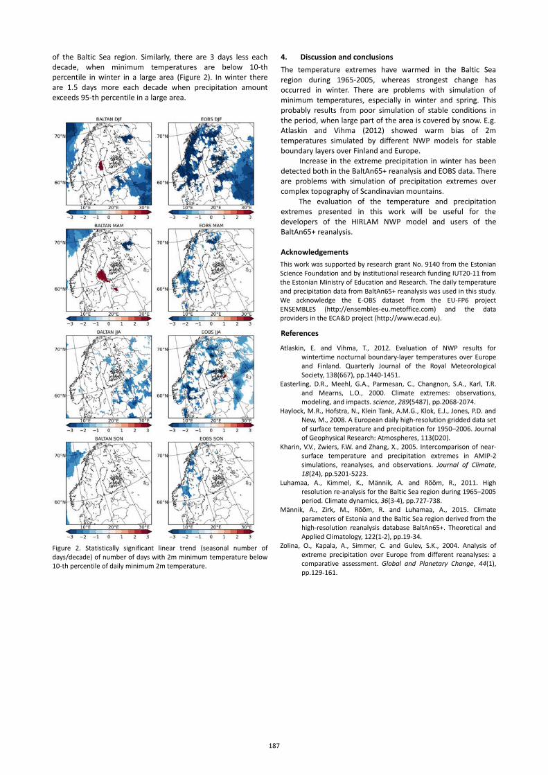
of the Baltic Sea region. Similarly, there are 3 days less eachdecade, when minimum temperatures are below 10-thpercentile in winter in a large area (Figure 2). In winter thereare 1.5 days more each decade when precipitation amountexceeds 95-th percentile in a large area.

Figure 2. Statistically significant linear trend (seasonal number ofdays/decade) of number of days with 2m minimum temperature below10-th percentile of daily minimum 2m temperature.

4. Discussion and conclusionsThe temperature extremes have warmed in the Baltic Searegion during 1965-2005, whereas strongest change hasoccurred in winter. There are problems with simulation ofminimum temperatures, especially in winter and spring. Thisprobably results from poor simulation of stable conditions inthe period, when large part of the area is covered by snow. E.g.Atlaskin and Vihma (2012) showed warm bias of 2mtemperatures simulated by different NWP models for stableboundary layers over Finland and Europe.

Increase in the extreme precipitation in winter has beendetected both in the BaltAn65+ reanalysis and EOBS data. Thereare problems with simulation of precipitation extremes overcomplex topography of Scandinavian mountains.

The evaluation of the temperature and precipitationextremes presented in this work will be useful for thedevelopers of the HIRLAM NWP model and users of theBaltAn65+ reanalysis.

Acknowledgements This work was supported by research grant No. 9140 from the EstonianScience Foundation and by institutional research funding IUT20-11 fromthe Estonian Ministry of Education and Research. The daily temperatureand precipitation data from BaltAn65+ reanalysis was used in this study.We acknowledge the E-OBS dataset from the EU-FP6 projectENSEMBLES (http://ensembles-eu.metoffice.com) and the dataproviders in the ECA&D project (http://www.ecad.eu).

References

Atlaskin, E. and Vihma, T., 2012. Evaluation of NWP results forwintertime nocturnal boundary-layer temperatures over Europeand Finland. Quarterly Journal of the Royal MeteorologicalSociety, 138(667), pp.1440-1451.

Easterling, D.R., Meehl, G.A., Parmesan, C., Changnon, S.A., Karl, T.R.and Mearns, L.O., 2000. Climate extremes: observations,modeling, and impacts. science, 289(5487), pp.2068-2074.

Haylock, M.R., Hofstra, N., Klein Tank, A.M.G., Klok, E.J., Jones, P.D. andNew, M., 2008. A European daily high-resolution gridded data setof surface temperature and precipitation for 1950–2006. Journalof Geophysical Research: Atmospheres, 113(D20).

Kharin, V.V., Zwiers, F.W. and Zhang, X., 2005. Intercomparison of near-surface temperature and precipitation extremes in AMIP-2simulations, reanalyses, and observations. Journal of Climate,18(24), pp.5201-5223.

Luhamaa, A., Kimmel, K., Männik, A. and Rõõm, R., 2011. Highresolution re-analysis for the Baltic Sea region during 1965–2005period. Climate dynamics, 36(3-4), pp.727-738.

Männik, A., Zirk, M., Rõõm, R. and Luhamaa, A., 2015. Climateparameters of Estonia and the Baltic Sea region derived from thehigh-resolution reanalysis database BaltAn65+. Theoretical andApplied Climatology, 122(1-2), pp.19-34.

Zolina, O., Kapala, A., Simmer, C. and Gulev, S.K., 2004. Analysis ofextreme precipitation over Europe from different reanalyses: acomparative assessment. Global and Planetary Change, 44(1),pp.129-161.

187

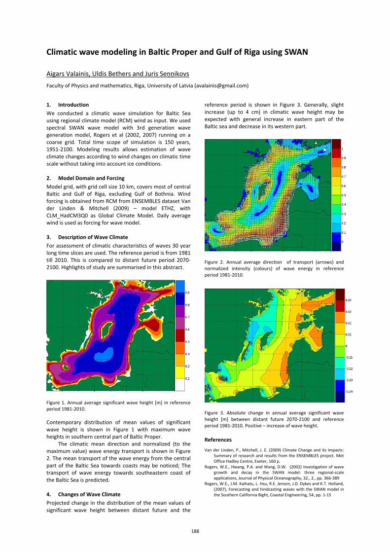
Climatic wave modeling in Baltic Proper and Gulf of Riga using SWAN

Aigars Valainis, Uldis Bethers and Juris Seņņikovs

Faculty of Physics and mathematics, Riga, University of Latvia (avalainis@gmail.com)

1. Introduction We conducted a climatic wave simulation for Baltic Sea using regional climate model (RCM) wind as input. We used spectral SWAN wave model with 3rd generation wave generation model, Rogers et al (2002, 2007) running on a coarse grid. Total time scope of simulation is 150 years, 1951-2100. Modeling results allows estimation of wave climate changes according to wind changes on climatic time scale without taking into account ice conditions. 2. Model Domain and Forcing Model grid, with grid cell size 10 km, covers most of central Baltic and Gulf of Riga, excluding Gulf of Bothnia. Wind forcing is obtained from RCM from ENSEMBLES dataset Van der Linden & Mitchell (2009) – model ETHZ, with CLM_HadCM3Q0 as Global Climate Model. Daily average wind is used as forcing for wave model. 3. Description of Wave Climate For assessment of climatic characteristics of waves 30 year long time slices are used. The reference period is from 1981 till 2010. This is compared to distant future period 2070-2100. Highlights of study are summarised in this abstract.

Figure 1. Annual average significant wave height [m] in reference period 1981-2010.

Contemporary distribution of mean values of significant wave height is shown in Figure 1 with maximum wave heights in southern central part of Baltic Proper.

The climatic mean direction and normalized (to the maximum value) wave energy transport is shown in Figure 2. The mean transport of the wave energy from the central part of the Baltic Sea towards coasts may be noticed; The transport of wave energy towards southeastern coast of the Baltic Sea is predicted. 4. Changes of Wave Climate Projected change in the distribution of the mean values of significant wave height between distant future and the

reference period is shown in Figure 3. Generally, slight increase (up to 4 cm) in climatic wave height may be expected with general increase in eastern part of the Baltic sea and decrease in its western part.

Figure 2. Annual average direction of transport (arrows) and normalized intensity (colours) of wave energy in reference period 1981-2010.

Figure 3. Absolute change in annual average significant wave height [m] between distant future 2070-2100 and reference period 1981-2010. Positive – increase of wave height. References

Van der Linden, P., Mitchell, J. E. (2009) Climate Change and its Impacts: Summary of research and results from the ENSEMBLES project. Met Office Hadley Centre, Exeter, 160 p.

Rogers, W.E., Hwang, P.A. and Wang, D.W. (2002) Investigation of wave growth and decay in the SWAN model: three regional-scale applications, Journal of Physical Oceanography, 32., 2., pp. 366-389

Rogers, W.E., J.M. Kaihatu, L. Hsu, R.E. Jensen, J.D. Dykes and K.T. Holland, (2007), Forecasting and hindcasting waves with the SWAN model in the Southern California Bight, Coastal Engineering, 54, pp. 1-15

188

Topic G

Multiple and interrelated drivers of environmental changes

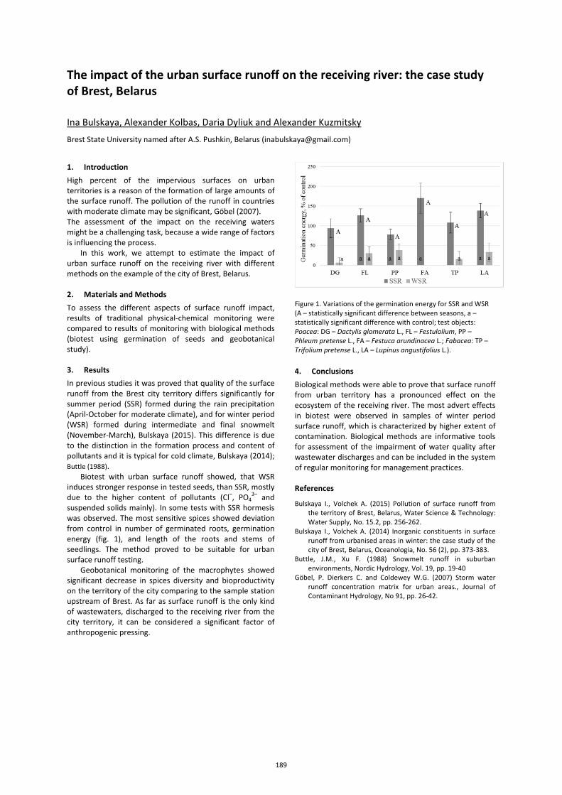
The impact of the urban surface runoff on the receiving river: the case study of Brest, Belarus

Ina Bulskaya, Alexander Kolbas, Daria Dyliuk and Alexander Kuzmitsky

Brest State University named after A.S. Pushkin, Belarus (inabulskaya@gmail.com)

1. Introduction High percent of the impervious surfaces on urban territories is a reason of the formation of large amounts of the surface runoff. The pollution of the runoff in countries with moderate climate may be significant, Göbel (2007). The assessment of the impact on the receiving waters might be a challenging task, because a wide range of factors is influencing the process.

In this work, we attempt to estimate the impact of urban surface runoff on the receiving river with different methods on the example of the city of Brest, Belarus. 2. Materials and Methods To assess the different aspects of surface runoff impact, results of traditional physical-chemical monitoring were compared to results of monitoring with biological methods (biotest using germination of seeds and geobotanical study). 3. Results In previous studies it was proved that quality of the surface runoff from the Brest city territory differs significantly for summer period (SSR) formed during the rain precipitation (April-October for moderate climate), and for winter period (WSR) formed during intermediate and final snowmelt (November-March), Bulskaya (2015). This difference is due to the distinction in the formation process and content of pollutants and it is typical for cold climate, Bulskaya (2014); Buttle (1988).

Biotest with urban surface runoff showed, that WSR induces stronger response in tested seeds, than SSR, mostly due to the higher content of pollutants (Cl–, PO4

3– and suspended solids mainly). In some tests with SSR hormesis was observed. The most sensitive spices showed deviation from control in number of germinated roots, germination energy (fig. 1), and length of the roots and stems of seedlings. The method proved to be suitable for urban surface runoff testing.

Geobotanical monitoring of the macrophytes showed significant decrease in spices diversity and bioproductivity on the territory of the city comparing to the sample station upstream of Brest. As far as surface runoff is the only kind of wastewaters, discharged to the receiving river from the city territory, it can be considered a significant factor of anthropogenic pressing.

Figure 1. Variations of the germination energy for SSR and WSR (A – statistically significant difference between seasons, a – statistically significant difference with control; test objects: Poacea: DG – Dactylis glomerata L., FL – Festulolium, PP – Phleum pretense L., FA – Festuca arundinacea L.; Fabacea: TP – Trifolium pretense L., LA – Lupinus angustifolius L.).

4. Conclusions Biological methods were able to prove that surface runoff from urban territory has a pronounced effect on the ecosystem of the receiving river. The most advert effects in biotest were observed in samples of winter period surface runoff, which is characterized by higher extent of contamination. Biological methods are informative tools for assessment of the impairment of water quality after wastewater discharges and can be included in the system of regular monitoring for management practices. References

Bulskaya I., Volchek A. (2015) Pollution of surface runoff from the territory of Brest, Belarus, Water Science & Technology: Water Supply, No. 15.2, pp. 256-262.

Bulskaya I., Volchek A. (2014) Inorganic constituents in surface runoff from urbanised areas in winter: the case study of the city of Brest, Belarus, Oceanologia, No. 56 (2), pp. 373-383.

Buttle, J.M., Xu F. (1988) Snowmelt runoff in suburban environments, Nordic Hydrology, Vol. 19, pp. 19-40

Göbel, P. Dierkers C. and Coldewey W.G. (2007) Storm water runoff concentration matrix for urban areas., Journal of Contaminant Hydrology, No 91, pp. 26-42.

189

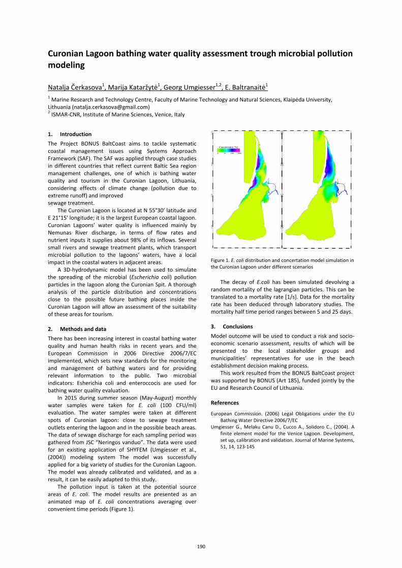
Curonian Lagoon bathing water quality assessment trough microbial pollution modeling

Natalja Čerkasova1, Marija Kataržytė1, Georg Umgiesser1,2, E. Baltranaitė1 1 Marine Research and Technology Centre, Faculty of Marine Technology and Natural Sciences, Klaipėda University, Lithuania (natalja.cerkasova@gmail.com) 2 ISMAR-CNR, Institute of Marine Sciences, Venice, Italy

1. Introduction The Project BONUS BaltCoast aims to tackle systematic coastal management issues using Systems Approach Framework (SAF). The SAF was applied through case studies in different countries that reflect current Baltic Sea region management challenges, one of which is bathing water quality and tourism in the Curonian Lagoon, Lithuania, considering effects of climate change (pollution due to extreme runoff) and improved sewage treatment.

The Curonian Lagoon is located at N 55°30′ latitude and E 21°15′ longitude; it is the largest European coastal lagoon. Curonian Lagoons’ water quality is influenced mainly by Nemunas River discharge, in terms of flow rates and nutrient inputs it supplies about 98% of its inflows. Several small rivers and sewage treatment plants, which transport microbial pollution to the lagoons’ waters, have a local impact in the coastal waters in adjacent areas.

A 3D-hydrodynamic model has been used to simulate the spreading of the microbial (Escherichia coli) pollution particles in the lagoon along the Curonian Spit. A thorough analysis of the particle distribution and concentrations close to the possible future bathing places inside the Curonian Lagoon will allow an assessment of the suitability of these areas for tourism. 2. Methods and data There has been increasing interest in coastal bathing water quality and human health risks in recent years and the European Commission in 2006 Directive 2006/7/EC implemented, which sets new standards for the monitoring and management of bathing waters and for providing relevant information to the public. Two microbial indicators: Esherichia coli and enteroccocis are used for bathing water quality evaluation.

In 2015 during summer season (May-August) monthly water samples were taken for E. coli (100 CFU/ml) evaluation. The water samples were taken at different spots of Curonian lagoon: close to sewage treatment outlets entering the lagoon and in the possible beach areas. The data of sewage discharge for each sampling period was gathered from JSC “Neringos vanduo”. The data were used for an existing application of SHYFEM (Umgiesser et al., (2004)) modeling system The model was successfully applied for a big variety of studies for the Curonian Lagoon. The model was already calibrated and validated, and as a result, it can be easily adapted to this study.

The pollution input is taken at the potential source areas of E. coli. The model results are presented as an animated map of E. coli concentrations averaging over convenient time periods (Figure 1).

Figure 1. E. coli distribution and concertation model simulation in the Curonian Lagoon under different scenarios

The decay of E.coli has been simulated devolving a random mortality of the lagrangian particles. This can be translated to a mortality rate [1/s]. Data for the mortality rate has been deduced through laboratory studies. The mortality half time period ranges between 5 and 25 days. 3. Conclusions Model outcome will be used to conduct a risk and socio-economic scenario assessment, results of which will be presented to the local stakeholder groups and municipalities’ representatives for use in the beach establishment decision making process.

This work resulted from the BONUS BaltCoast project was supported by BONUS (Art 185), funded jointly by the EU and Research Council of Lithuania. References

European Commission. (2006) Legal Obligations under the EU Bathing Water Directive 2006/7/EC

Umgiesser G., Melaku Canu D., Cucco A., Solidoro C., (2004). A finite element model for the Venice Lagoon. Development, set up, calibration and validation. Journal of Marine Systems, 51, 14, 123-145

190

Coastal resources understanding and local governance development: socio-ecological system and indicators prerequisite

Raimonds Ernsteins, Erika Lagzdina, Janis Lapinkis, Anita Lontone, Janis Kaulins, Ivars Kudrenickis

University of Latvia (raimonds. ernsteins@lu.lv)

1. Coastal socio-ecological system: factors integration Integrated coastal zone management (ICZM) is one of the most important issues looking for sustainable development of the Baltic Sea region. A number of research papers identify that decision-makers and politicians at all governance levels have insufficient science-based information and understanding to cope with the ICZM in practice, e.g. to integrate the coastal issues into spatial development planning process. As a result the vulnerabilities to the existing impacts and those caused by the global changes (climate change) is increasing and particularly are to be tackled at the local level, what, unfortunately, traditionally is not done.

The vulnerability of the complex coastal socio-ecological system cannot be maintained in a sustainable way unless the major stake-holders and the local communities are aware of the current situation. Without relevant information, it is hard to assess policy options and take informed decisions. The opportunities to improve the ICZM is to develop science-policy interface – to transfer coastal science knowledge into decision making. This could be done by – science data incorpotation into designed/approved coastal municipal monitoring system and the use of developed related nature-social science factors and their interaction based coastal indicator system.

The University of Latvia in the framework of EU BONUS ICZM program has been implementing several coastal research-and-development projects. Initial studies cover: issues of coastal erosion and flood risk management, development of indicators system, complexity of the coastal socio-economic and governance issues. The case study site - the Salacgriva municipality – is one of 17 Latvian coastal municipalities (638 km2, 9000 population) stretching along coastline in total for 55 km. 2. Governance factors: coastal problems aggregation A method for identification and analysis of the coastal problems was based on system analysis and the iterative, multi-step approach. Extensive planning documentation and data studies allowed to identify a number of coastal problems and draw relationship models. Further discussions organized with the local stake-holders allowed to build a priority list of problems: (i) the state of environment problems (coastal erosion, marine litter, biotopes degradation, forest damage, sea water quality, and algae blooming), and (ii) socio-economic problems or pressures (tourism impacts, restricted access to the sea due to the construction and private fences, lack of sufficient coastal infrastructure, inadequate safety, rescue services, household caused pollution, eventual flooding.

Two essential conclusions were drawn. Firstly, there are few coastal territories in the municipality where resources are over exploited or used in interests of limited stake-holder group or even individuals, this creates additional

stress on resources, as well as environmental pollution and distrust among other stake-holders. At the same time, there are other territories where resources are under managed that causing risks for the further degradation of the coastal resources.

The main causes for this situation are: insufficient understanding of the current situation and potential of the coastal resources for local development; insufficient municipal efforts and capacity to ensure efficient coastal management, limited coastal involvement of many existing self-organizing forms of the local citizens; disperse, very low density of the population on the coast. 3. Physical factors: coastal erosion and retreat

Compared to the other coastal sections of Latvia, research of modern coastal processes (including coastal slope evolution, dune formation and erosion intensity) in the North East part of the Gulf of Riga is quite limited. Partially this is determined by the peculiarities of the geological structure and occurrence of the coastal landforms inherited from the Littorina Sea, due to whom transformation of the coast occurs relatively slowly.

Using historical data from 2005 and data collected during the field work in the Salacgriva municipality in 2015, several coastal sections can be distinguished where long-term coastal retreat or temporary (compensated) erosion during extreme storms can be considered as a significant issue for coastal management - approximately 25% of the municipal coastline, where over the course of last 11 years the average retreat rate in these coastal sections was between 0.3 and 0.6 m/year.

Generally, the Salacgriva municipality coast has been characterized by a significant prevalence of coastal sections, in which coastal evolution is very slow – there is no clear predominance of the erosion or accumulation. Data suggest that, in these – previously dynamically neutral coastal sections, after catastrophic erosion caused by the hurricane Gudrun in 2005, slope regeneration towards pre-storm parameters is very slow that should be considered as a significant issue for the ICZM. Despite increased coastal erosion spread and intensity during the recent decades, coastal sections where coastal slope stability remains high are still widespread in the municipality (29.5 km).

Changes in conditions determining the evolution of the coastal slope is believed to be the main cause of growth in coastal erosion rate and spread in Latvia and in the Salacgriva municipality in particular. Among other, such a conclusion is based on the observations and coastal change measurements carried out in close proximity to the anthropogenic objects affecting the stability of the coast (coastal protection structures and harbours). Long-term negative impact from the coastal protection structures – accelerated erosion of adjacent unprotected coastal segments and impossibility of natural

191

sediment cross-shore exchange, is identified. Impact of the Salacgriva and Kuivizi harbours are manifested as increase both in erosion and accumulation. Salacgriva harbour external hydro-technical structures and fairway maintenance, which is associated with depositing of the excavated material offshore (removing it from coastal system), has led to significant coastal stability disruption to the north of the harbour, however, taking into account, that the area is characterized by a poorly pronounced long-shore sediment exchange and benefits from favorable geological structure, the negative impact is by far less than interference caused by the other harbors in Latvia. 4. Socio-economic factors: inhabitants and flood risk Flood risk management (FRM) is another complementary part of the ICZM that has to be integrated in the local development process by complementary application of the whole set of governance instruments – political/legal, institutional/administrative, planning, economic/financial, infrastructure and particularly FLR communication, incl. information, education, participation and risk orientated behaviour - ensuring municipal preparedness for the FLR. A targeted sociological survey was done (during EU Interreg project Foodweb) to assess the situation and perceptions of the local people about flood risks in the Salacgriva municipality. Study site were chosen based on the flood risk probability detected in the planning maps produced by the BaltCICA project. The survey was built on the collaboration communication approach – identifying risk information, education, participation and risk orientated behavior

The results cover answers received from 130 households. Most of the interviewed think that there are not serious climate change impacts at the local level, however they mention spring floods, heavy rain falls, storm surge, and sea level rise. The latter two have been considered as the main risks to their households. 50 % of the interviewed could not recognize any information on flood risks; one third have heard something in the national media, and only one fifth have recognized the local media, the local civil protection or other planning documents as a source of flood risk related information. 81% of interviewed agreed that flood risk preparedness at the municipal level is essential for climate adaptation. 5. Factors integration: municipal level indicators system The scientific information available to the municipal level manager about the physical state of the coast is often missing or unsatisfactory and too complex, and difficult to use. The introduction of municipal monitoring, initially based on science information, and development of coastal indicator system suitable for unambiguously interpretation of coastal state and conditions is instrument that could be applied by the coastal municipalities and used in practice for the coastal policy development and its implementation. The problem lies in facts that particular socio-ecological system oriented indicator systems have been designed and applied mainly at a large scale – most typically for the international/national level, what do not embed the local communities, where real coastal processes and related decision making do take place. As most of the existing indicator systems are non-relevant to the municipal management scale, and are orientated to the monitoring of activities instead of focusing on the coast, such an indicator system should be developed which is efficient at the local

scale, applicable to monitor coastal situation and implemented activities. This indicator system would allow to predict further coastal development and thus support the coastal governance and decision-making process.

For organization of the municipallevel physical, socio-economic and governance parameters, for their integration and use for qualitative and quantitative characterization of the subject into a coherent multilevel approach, the indicators are principal component at all stages of the governance cycle. Indicators are a tool for organizing information and setting priorities for data gathering. The selected set of indicators is a part of the data flow that can be used for qualitative decisions and well-planned activities.

The importance and suitability of indicators approach for science and policy integration is determined by interface of principal factors: (i) definition and quantification of each indicator shall be strictly methodology (science) based; (ii) a selection of a set of indicators to be used for decision- making shall be based on values acknowledged by the local stake-holders, and those values shall be reflected in realistic activities determined by the local policies. Coastal awareness rising, growing collaboration of municipal stakeholder groups, understanding of common societal and territorial development challenges and opportunities, and their implications towards collaborative decision making, are basic cornerstones for sustainable coastal development which certainly will be reflected in the choice of the indicator system. 6. Conclusions The coastal socio-ecological systems are based on interconnected elements of natural, cultural, socio-economic and governance resources – all related factors need to be integrated, horizontally-vertically and with all main stakeholders interests, for succesful coastal governance starting with municipal level, and using complementary research, monitoring and assessment, and decision making on the coastal resources and their sustainable use potencial/directions for the nature/culture protection and benefit of the local communities. This requires all necessary science-policy integration measures and means – coastal science and monitoring, management instruments, incl. indicator systems (also public based) and collaborative governance, all to be brought into municipal practice to improve coastal processes understanding and management.

Most of studies were done and abstract prepared with financial support of EU BONUS program project Baltcoast.

References Eberhards, G., Lapinskis, J. (2008) The coastal processes of the Batic Sea Latvian

coast// Baltijas jūras Latvijas krasta procesi. University of Latvia, Riga, pp 64.

Ernšteins R., at al, (2012) Climate change adaptation integration into Coastal Municipal Development: governance environment and communication preconditions. In: SGEM, Proceedings, Bulgaria, p. 1077-1084.

Gilbert C. (ed.) (2008) State of the Coast of the South East Baltic: indicators-based approach to evaluating sustainable development in the coastal zone. Gdansk, 158p.

Hopkins T., Bailly D, (2011) A systems approach framework for coastal zones. Ecology and Society 16(4): 25.

Lagzdiņa E., Kudreņickis I.,Kauliņš J, Ernšteins R. (2016) Coastal integrated governance development: system analysis framework application, 74th research conference, Abstract proceedings, University of Latvia, Riga, Latvia, pp. 406-413.

192

The impact of wrecks on the geochemical properties of the surface layer of marine bottom sediments in wrecks deposition areas on the example of ORP Wicher Tomasz Figiel1, Paweł Wysocki1 , Żaneta Kłostowska1, Leszek Łęczyński1, Tadeusz Ossowski2, Dorota Zarzeczańska2, Mateusz Figurski 2 1 Institute of Oceanography, University of Gdańsk, Gdynia, Poland (s213339@stud.ug.edu.pl) 2 Department of Analytical Chemistry, University of Gdańsk, Gdańsk, Poland

In the last few decades on the bottom of the Baltic Sea discovered the remains of World War II for example shipwrecks, chemical warfare or ammunition. These discoveries have not only a historical or tourist value, but are also habitats for marine flora and fauna. With the current knowledge, it is proved that the wrecks are a real threat to the sea environment. Mainly due to the chemicals used for impregnation of structural elements, as well as loading, fuel and weapons (including chemical warfare). In the case of metal wrecks, an important parameter is the degree of corrosion, which is subject to specific elements, whereby contamination gradually and systematically penetrate into the sea environment, where they are incorporated into other elements of the trophic chain. ORP Wicher is located in the area of intense currents for a depth of 5-17 m, which determines the transport of pollutants in further areas of the bay. In the collaboration with Marine Measurements unit of Maritime Office in Gdynia obtained bathymetric data of wreck position.

In 2016, while cruises from unit k / h Oceanograf-2 Institute of Oceanography collected a series of samples of bottom sediments of the ORP Wicher wreck. The surface layer of sediments was subjected to geochemical analysis, measured the content of petroleum substances, organic and inorganic matter and basic physical parameters of sediments. Compared to the reference materials can be concluded that the residual wreck is important point source of pollution in the studied area. Further research and monitoring wrecks areas, allows for the observation of trends in the spread of harmful substances. This is particularly important in the case of petroleum substances which are a real threat for marine environment in long-term aspect and indirectly also for human health and life. Due to their numerous placement at the bottom of the southern Baltic Sea are important sources of input of pollutants into the sea environment.

193

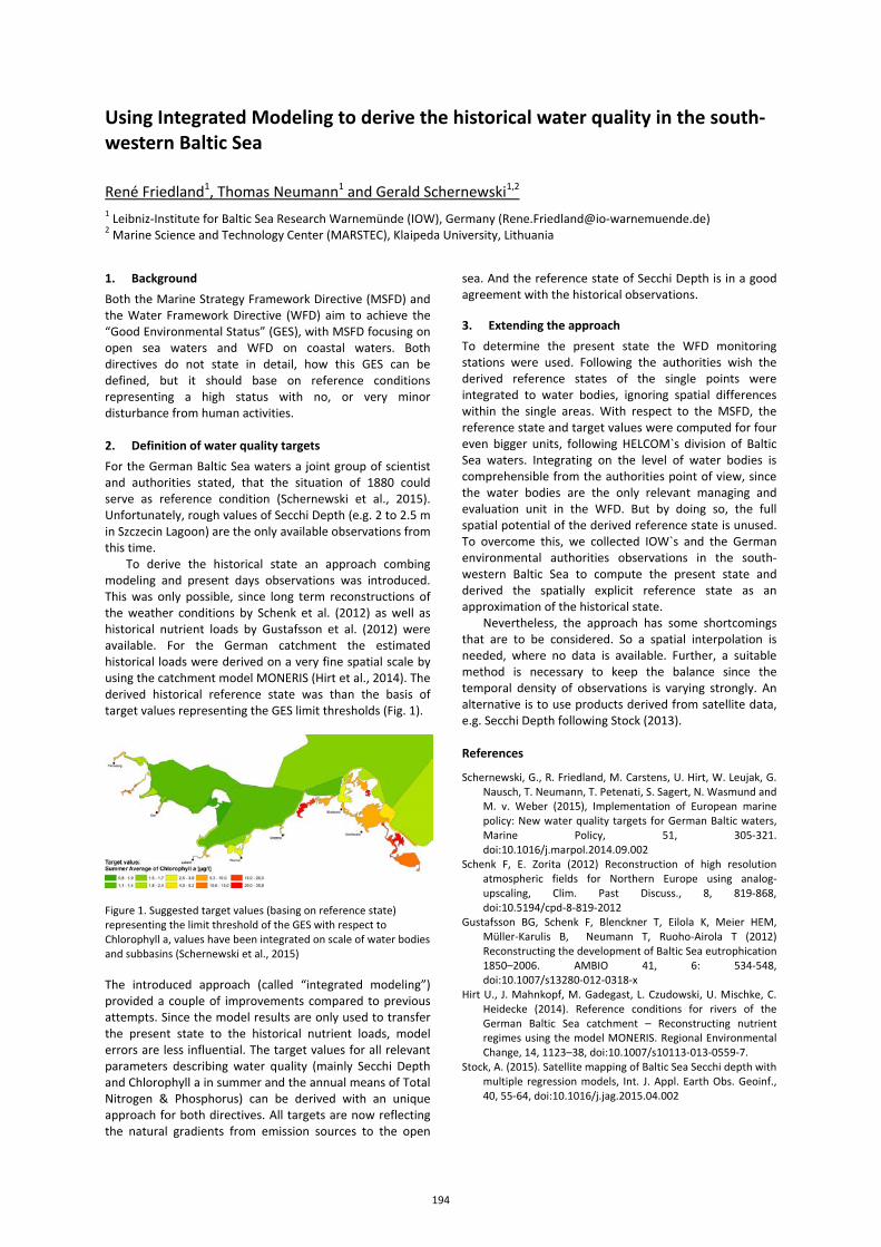
Using Integrated Modeling to derive the historical water quality in the south-western Baltic Sea

René Friedland1, Thomas Neumann1 and Gerald Schernewski1,2 1 Leibniz-Institute for Baltic Sea Research Warnemünde (IOW), Germany (Rene.Friedland@io-warnemuende.de) 2 Marine Science and Technology Center (MARSTEC), Klaipeda University, Lithuania

1. Background Both the Marine Strategy Framework Directive (MSFD) and the Water Framework Directive (WFD) aim to achieve the “Good Environmental Status” (GES), with MSFD focusing on open sea waters and WFD on coastal waters. Both directives do not state in detail, how this GES can be defined, but it should base on reference conditions representing a high status with no, or very minor disturbance from human activities. 2. Definition of water quality targets For the German Baltic Sea waters a joint group of scientist and authorities stated, that the situation of 1880 could serve as reference condition (Schernewski et al., 2015). Unfortunately, rough values of Secchi Depth (e.g. 2 to 2.5 m in Szczecin Lagoon) are the only available observations from this time.

To derive the historical state an approach combing modeling and present days observations was introduced. This was only possible, since long term reconstructions of the weather conditions by Schenk et al. (2012) as well as historical nutrient loads by Gustafsson et al. (2012) were available. For the German catchment the estimated historical loads were derived on a very fine spatial scale by using the catchment model MONERIS (Hirt et al., 2014). The derived historical reference state was than the basis of target values representing the GES limit thresholds (Fig. 1).

Figure 1. Suggested target values (basing on reference state) representing the limit threshold of the GES with respect to Chlorophyll a, values have been integrated on scale of water bodies and subbasins (Schernewski et al., 2015) The introduced approach (called “integrated modeling”) provided a couple of improvements compared to previous attempts. Since the model results are only used to transfer the present state to the historical nutrient loads, model errors are less influential. The target values for all relevant parameters describing water quality (mainly Secchi Depth and Chlorophyll a in summer and the annual means of Total Nitrogen & Phosphorus) can be derived with an unique approach for both directives. All targets are now reflecting the natural gradients from emission sources to the open

sea. And the reference state of Secchi Depth is in a good agreement with the historical observations. 3. Extending the approach To determine the present state the WFD monitoring stations were used. Following the authorities wish the derived reference states of the single points were integrated to water bodies, ignoring spatial differences within the single areas. With respect to the MSFD, the reference state and target values were computed for four even bigger units, following HELCOM`s division of Baltic Sea waters. Integrating on the level of water bodies is comprehensible from the authorities point of view, since the water bodies are the only relevant managing and evaluation unit in the WFD. But by doing so, the full spatial potential of the derived reference state is unused. To overcome this, we collected IOW`s and the German environmental authorities observations in the south-western Baltic Sea to compute the present state and derived the spatially explicit reference state as an approximation of the historical state.

Nevertheless, the approach has some shortcomings that are to be considered. So a spatial interpolation is needed, where no data is available. Further, a suitable method is necessary to keep the balance since the temporal density of observations is varying strongly. An alternative is to use products derived from satellite data, e.g. Secchi Depth following Stock (2013). References

Schernewski, G., R. Friedland, M. Carstens, U. Hirt, W. Leujak, G. Nausch, T. Neumann, T. Petenati, S. Sagert, N. Wasmund and M. v. Weber (2015), Implementation of European marine policy: New water quality targets for German Baltic waters, Marine Policy, 51, 305-321. doi:10.1016/j.marpol.2014.09.002

Schenk F, E. Zorita (2012) Reconstruction of high resolution atmospheric fields for Northern Europe using analog-upscaling, Clim. Past Discuss., 8, 819-868, doi:10.5194/cpd-8-819-2012

Gustafsson BG, Schenk F, Blenckner T, Eilola K, Meier HEM, Müller-Karulis B, Neumann T, Ruoho-Airola T (2012) Reconstructing the development of Baltic Sea eutrophication 1850–2006. AMBIO 41, 6: 534-548, doi:10.1007/s13280-012-0318-x

Hirt U., J. Mahnkopf, M. Gadegast, L. Czudowski, U. Mischke, C. Heidecke (2014). Reference conditions for rivers of the German Baltic Sea catchment – Reconstructing nutrient regimes using the model MONERIS. Regional Environmental Change, 14, 1123–38, doi:10.1007/s10113-013-0559-7.

Stock, A. (2015). Satellite mapping of Baltic Sea Secchi depth with multiple regression models, Int. J. Appl. Earth Obs. Geoinf., 40, 55-64, doi:10.1016/j.jag.2015.04.002

194

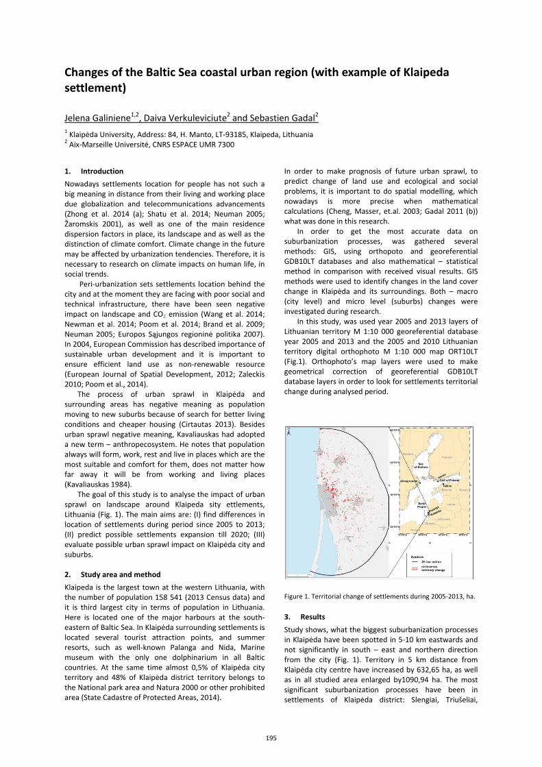
Changes of the Baltic Sea coastal urban region (with example of Klaipeda settlement)

Jelena Galiniene1,2, Daiva Verkuleviciute2 and Sebastien Gadal2 1 Klaipėda University, Address: 84, H. Manto, LT-93185, Klaipeda, Lithuania 2 Aix-Marseille Université, CNRS ESPACE UMR 7300

1. Introduction Nowadays settlements location for people has not such a big meaning in distance from their living and working place due globalization and telecommunications advancements (Zhong et al. 2014 (a); Shatu et al. 2014; Neuman 2005; Žaromskis 2001), as well as one of the main residence dispersion factors in place, its landscape and as well as the distinction of climate comfort. Climate change in the future may be affected by urbanization tendencies. Therefore, it is necessary to research on climate impacts on human life, in social trends.

Peri-urbanization sets settlements location behind the city and at the moment they are facing with poor social and technical infrastructure, there have been seen negative impact on landscape and CO2 emission (Wang et al. 2014; Newman et al. 2014; Poom et al. 2014; Brand et al. 2009; Neuman 2005; Europos Sąjungos regioninė politika 2007). In 2004, European Commission has described importance of sustainable urban development and it is important to ensure efficient land use as non-renewable resource (European Journal of Spatial Development, 2012; Zaleckis 2010; Poom et al., 2014).

The process of urban sprawl in Klaipėda and surrounding areas has negative meaning as population moving to new suburbs because of search for better living conditions and cheaper housing (Cirtautas 2013). Besides urban sprawl negative meaning, Kavaliauskas had adopted a new term – anthropecosystem. He notes that population always will form, work, rest and live in places which are the most suitable and comfort for them, does not matter how far away it will be from working and living places (Kavaliauskas 1984).

The goal of this study is to analyse the impact of urban sprawl on landscape around Klaipeda sity ettlements, Lithuania (Fig. 1). The main aims are: (I) find differences in location of settlements during period since 2005 to 2013; (II) predict possible settlements expansion till 2020; (III) evaluate possible urban sprawl impact on Klaipėda city and suburbs.

2. Study area and method Klaipeda is the largest town at the western Lithuania, with the number of population 158 541 (2013 Census data) and it is third largest city in terms of population in Lithuania. Here is located one of the major harbours at the south-eastern of Baltic Sea. In Klaipėda surrounding settlements is located several tourist attraction points, and summer resorts, such as well-known Palanga and Nida, Marine museum with the only one dolphinarium in all Baltic countries. At the same time almost 0,5% of Klaipėda city territory and 48% of Klaipėda district territory belongs to the National park area and Natura 2000 or other prohibited area (State Cadastre of Protected Areas, 2014).

In order to make prognosis of future urban sprawl, to predict change of land use and ecological and social problems, it is important to do spatial modelling, which nowadays is more precise when mathematical calculations (Cheng, Masser, et.al. 2003; Gadal 2011 (b)) what was done in this research.

In order to get the most accurate data on suburbanization processes, was gathered several methods: GIS, using orthopoto and georeferential GDB10LT databases and also mathematical – statistical method in comparison with received visual results. GIS methods were used to identify changes in the land cover change in Klaipėda and its surroundings. Both – macro (city level) and micro level (suburbs) changes were investigated during research.

In this study, was used year 2005 and 2013 layers of Lithuanian territory M 1:10 000 georeferential database year 2005 and 2013 and the 2005 and 2010 Lithuanian territory digital orthophoto M 1:10 000 map ORT10LT (Fig.1). Orthophoto’s map layers were used to make geometrical correction of georeferential GDB10LT database layers in order to look for settlements territorial change during analysed period.

Figure 1. Territorial change of settlements during 2005-2013, ha.

3. Results Study shows, what the biggest suburbanization processes in Klaipėda have been spotted in 5-10 km eastwards and not significantly in south – east and northern direction from the city (Fig. 1). Territory in 5 km distance from Klaipėda city centre have increased by 632,65 ha, as well as in all studied area enlarged by1090,94 ha. The most significant suburbanization processes have been in settlements of Klaipėda district: Slengiai, Triušeliai,

195

Budrikai, Mazuriškiai. Here was recorded by 56,63% of all changes in Klaipėda district.

One of the best indicator, showing urban sprawl and change of physical landscape is the change of number of population in city and suburban areas (Cirtautas 2015, Newman et al. 2014; Europos Sąjungos regioninė politika 2007). Correlation shows, what population number in Klaipėda city is decreasing but in Klaipėda district increases exponentially (r=-0.92806).

According georeferential data analysis, settlements territory of Klaipėda city suburbs expanded by 1090.94 ha during by 2005-2013. Mostly, suburbs have expanded eastwards and northern in 5 km distance from Klaipėda city (632.65 ha) that is directions parallel to the highway Klaipėda-Vilnius, and on the way to Palanga resort.

If territorial growth of settlements around Klaipėda city will be the same as during 2005-2013 period, settlements around Klaipėda city in 5 km radius, would expand up to 1245,77 ha till year 2020. Future urban sprawl direction should remain the same – eastwards and northern from Klaipėda city.

4. Discussion and conclusions Graphical and statistical analysis of study area showed strong evidence of urban sprawl in Klaipėda suburban areas, especially in 25 km distance. As found Bouwman et al. (2005) in their study, urbanization has a clear effect on human mobility. In this case it changes everything, as Klaipėda city and its suburban municipality governments should rethink transportation system and infrastructure in order to make urban-rural continuum, which describes Bouwman, greener, more suitable for living and more ecological, as the right city design can enhance the use of car alternatives (Zhong et al. 2014 (b), Poom et al. 2014; Jansen et al. 2011). It is very important to think about car alternatives while communication between Klaipėda city and suburbs at the moment is quite weak. Wang et al. (2014) has empirically proven that sub-urbanization have a significant impact on commuting CO2 emission increase.

Study results shows, that Klaipėda region is not exception in the Europe. We are facing fast urban sprawl which has negative impact on regions’ landscape and ergonomics’, social, economic and psychological human being in newly inhabited territories (Kavaliauskas 1984; Europos Sąjungos regioninė politika 2007). Instead of green and recreation zones concentration in suburban areas (Jansen et al. 2011), population moving to live there, leaving cities emptier.

Knowing urban sprawl directions will let us predict future scenarios of land use and will help for urban planners to meet populations’ daily needs in order to avoid mistakes which were made some centuries ago (Zhong et al. 2014 (a); Kavaliauskas 1984; Žaromskis 2001). Canada already taking action in drawing borders, there urban sprawl is not possible, in order to protect the land from residential use and let spread farming.

The analysis of this research showed what no proper action has been taken in order to avoid urban sprawl and Klaipėda’s city emptiness. Also climate change projections and adaptations should play important role in future planning documents of Klaipėda city and its district settlements.

References

Brand, C., Preston, J.M., 2009. ‘60-20 emission’—The unequal distribution of greenhouse gas emissions from personal, non-business travel in the UK. Transport policy, 17:9-19.

Bouwman, M.E., Voogd, H., 2005. Mobility and the Urban-Rural Continuum. GBER, vol. 4(3):60-69.

Cirtautas, M. 2014. Suburban areas centrally collected data use in residential areas development studies. Kvalifikacinio mokslo darbo Nr. 367 ataskaita, Urbanistinės analizės mokslo laboratorija, VGTU, Vilnius.

Cirtautas, M. 2013. Urban Sprawl of Major Cities in the Baltic States. Architecture and Urban Planning. Vilnius Gediminas Technical University, 7:72-79.

Cheng, J., Masser, I., Ottens, H. 2003. Understanding urban growth system: theories and methods. Department of Urban and Regional Planning and Geo-Information Managment, International Institute for Geo-Information Science and Earth Observation (ITC). The Netherlands.

Europos Sąjungos regioninė politika, 2007. Augantys regionai, auganti Europa/Growing regions - growing Europe. Ketvirtoji ekonominės ir socialinės sanglaudos ataskaita. 15-16.

European Journal of Spatial Development 2012. Published by Nordregio, Nordic Centre for Spatial Development and OTB Research Institute, Delft University of Technology.

Gadal, S., 2011 (a). The socio-ecological challenge of the metropolised territories: key-notes. University of Versaille Sanit-Quentin-en-Yvelines.

Gadal, S., 2011 (b). Urban multilevel geographical information satellite generation. University of Versaille Sanit-Quentin-en-Yvelines.

Jansen, J.O., Christensen, H.T., Gram-Hanssen, K., 2011. Sustainable urban development – compact cities or consumer practices? Danish Journal of Geoinformatics and Land Management, Vol. 46(1):50-64.

Neuman, M., 2005. The compact city Fallacy. Journal of Planning Education and Research 25:11-26

Newman, L., Nixon, D., 2014. Farming in an Agriburban Ecovillage Development: An Approach to Limiting Agricultural/Residential Conflict. Sage Open, October-December 2014: 1–10

Poom, A., Ahas, R., Orru, K. 2014. The impact of residential location and settlement hierarchy on ecological footprint. Environment and Planning A, volume 46, pp. 2369-2384.

Shatu, F.M., Kamruzzaman, Md., Deilami, K. 2014. Did Brisbane grow smartly? Drivers of city growth 1991-2001 and lessons for current policies. Sage Open, pp 1-19.

Sudhira, H.S., Ramachandra, T.V., Jagadish, K.S., 2004. Urban sprawl: metrics, dynamics and modelling using GIS. International Journal of Applied Earth Observation and Geoinformation, 5 (1), 29-39.

Wang, Y., Hayashi, Y., Chen, J., Li, Q., 2014. Changing urban form and transport CO2 emissions: an empirical analysis of Beijing, China. Sustainability 6:4558-4579

Zaleckis, K., Kamičaitytė-Virbašienė, J., 2010. Darnus urbanistinių struktūrų vystymasis: Kauno miesto atvejis/Sustainable urban structure development: Kaunas city example. Kauno technologijos universitetas.

Zhong, C., Huang, X., Arisona, S.M., Schmitt, G., Batty, M. 2014 (a). Inferring building functions from probabilistic model using public transportation data. Computers, Environment and Urban Systems 48:124-137.

Zhong, C., Huang, X., Arisona, S.M., Schmitt, G., Batty, M. 2014 (b). Detecting the dynamics of urban structure through spatial network analysis. International Journal of Geographical Information Science, Taylor & Francis.

Žaromskis, R., 2001. Skirtingos žmonių veiklos poveikis pietryčių Baltijos krantų raidai/Different human activities impact on South-Eastern Baltic coastal zone. Geografijos metraštis, Vilnius. 34(1):59-72.

Каваляускас, П., 1984. Проблема комплексной оценки антропологического потенцциала территории. Geographia Lituanica, Vilnius. XXI, 180-190.

196

Deposition of sulfur, nitrogen and particles originating from shipping activities in the Baltic and North Seas

Karin Haglund, Björn Claremar, Anna Rutgersson

Department of Earth Sciences, Uppsala University, Uppsala, Sweden (karin_tuve@hotmail.com)

1. Introduction Increasing emissions of air pollutions is an ongoing global problem. Air pollutions have harmful effects on human health, the environment and buildings. It also has an impact on climate. There has been a significant decrease in land based emissions in Europe ever since the risks associated with high levels of air pollutions were brought into light, two decades ago. During the same time, however, emissions from shipping in the Baltic Sea and the North Sea have increased, with the exception of a recent decrease in sulfur emissions. Shipping is the most cost-effective option for global transport of goods, and over 90% of the world trade is carried by sea. The Baltic Sea area is one of the busiest shipping areas in the world and it is of great importance for the development and economy of the surrounding countries. In order to achieve sustainable shipping, primarily through new regulations and techniques, greater knowledge of dispersion and deposition of air pollutions is required. 2. Method Regional calculations with the model from the European Monitoring and Evaluation Programme (EMEP) of the dispersion of SOx and NOx from the maritime sector in the Baltic Sea and North Sea for 2011 - 2013 have been made. Calculation with the EMEP model has also been made for fine and coarse particles. Today there are gaps in knowledge of the dispersion of particles from shipping. Validation of the model is here made for 2013 with measured data from Vavihill in the South of Sweden and from Utö, a Finnish island in the Archipelago Sea. The shipping contributions to deposition, in the investigated period, are also compared to constructed data in earlier studies. These comprise the past period (1750–2010), as well as a scenario period (2010-2050) where different options on future ship sulphur emissions were modelled. We also discuss the consequence of using on-board sulfur cleaning systems (scrubbers), where high- concentration sulfur fuels can be used but the sulfur goes directly into the sea water. Details of the method used to determine the past atmospheric deposition are described in Omstedt et al. [2012; 2015] and Claremar et al. [2013] and the scenarios in Turner et al., [2016]. 3. Results The calculations with the EMEP model show that the cumulative wet deposition in 2013 from shipping in the Baltic Sea and the North Sea reached over 60 mgS/m2 (mean in Europe: 1.19 mgS/m2) and 80 mgN/m2 (mean in Europe: 3.67 mgN/m2) in some of the areas in Europe. The cumulative dry deposition from shipping in the Baltic Sea and the North Sea for the same year and area reached over 200 mgS/m2 (mean in Europe: 1.13 mgS/m2) and 65 mgN/m2 (mean in Europe: 1.42 mgN/m2). The highest cumulative wet and dry deposition was found in areas close

to some of the shorelines in Europe and near big ports and shipping lanes. Wet deposition of oxidized sulfur and nitrogen was dispersed over a larger area than the dry deposition of the same pollutants. The percentage contribution from shipping emissions to the total cumulative wet deposition of sulphur from all emissions sources reached 30% (mean in Europe: 0.95%) in some areas of Europe and the contributions of dry deposition of sulphur was calculated to a maximum of 84% (mean in Europe: 1.56%). The percentage contribution of wet deposition of nitrogen from shipping varied between 0 and 28% (mean in Europe: 3.77%) in Europe and the contributions of dry deposition of nitrogen reached a maximum of 45% (mean in Europe: 3.56%).

Annual mean concentration of NO2 near the surface from ship emissions in the Baltic Sea and the North Sea in 2013 was calculated to a maximum of 10.25 µg/m3 (mean in Europe: 0.075 µg/m3). In some areas in Europe the contribution of NO2 from shipping in the Baltic Sea and the North Sea represented up to 83% (mean in Europe: 3.45%) of total concentration of NO2. For NO the annual mean concentration from ship emissions was calculated to 2.02 µg/m3 (mean in Europe: 0.006 µg/m3) which in some parts in Europe represented up to 89% (mean in Europe: 3.19%) of total concentration of NO. Annual mean concentrations of SO2, near the surface, reached over 2.14 µg/m3 (mean in Europe: 0.0092 µg/m3) at some places in Europe in 2013. In some areas in Europe the contribution of SO2 from shipping in the Baltic Sea and the North Sea represented up to 88% (mean in Europe: 1.7%) of total concentration of SO2. Contributions of shipping emissions of PM2,5 and PM10 to total concentrations near the surface was calculated to a maximum of 1.61 µg/m3 (mean in Europe: 0.009 µg/m3) and 2.30 µg/m3 (mean in Europe: 0.027 µg/m3). This represented up to 21% (mean in Europe: 0.61%) and 13% (mean in Europe: 0.51%) of the total concentration of the pollutants near the surface, in some parts of the studied area (Figure 1).

The validation of data shows that the EMEP model underestimated the concentrations near the surface of NO2, SO2 and PM2,5 at Utö and also SO2 and PM10 at Vavihill in 2013. The model overestimated the concentrations near the surface of NO2 and PM2,5 at Vavihill. The model calculated the maximum values quite poorly, however, overall the model was consistent with the measured values from Utö and Vavihill in 2013. The main effect of using scrubbers in ships is that the acidification is concentrated along the ship tracks. When emitted into the atmosphere, the deposition is spread out, not only over large sea surfaces, but also over land. Therefore the biological effect in the sea water may be large locally.

197

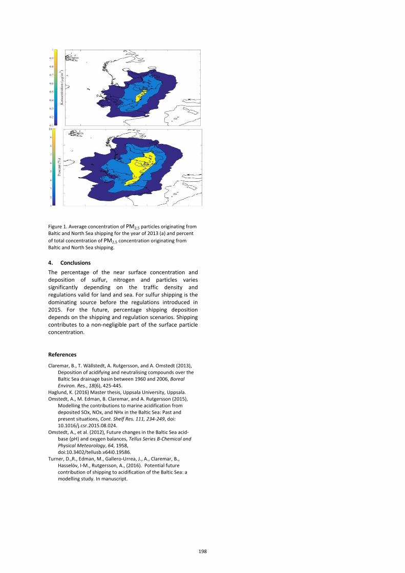
Figure 1. Average concentration of PM2,5 particles originating from Baltic and North Sea shipping for the year of 2013 (a) and percent of total concentration of PM2,5 concentration originating from Baltic and North Sea shipping.

4. Conclusions The percentage of the near surface concentration and deposition of sulfur, nitrogen and particles varies significantly depending on the traffic density and regulations valid for land and sea. For sulfur shipping is the dominating source before the regulations introduced in 2015. For the future, percentage shipping deposition depends on the shipping and regulation scenarios. Shipping contributes to a non-negligible part of the surface particle concentration. References

Claremar, B., T. Wällstedt, A. Rutgersson, and A. Omstedt (2013), Deposition of acidifying and neutralising compounds over the Baltic Sea drainage basin between 1960 and 2006, Boreal Environ. Res., 18(6), 425-445.

Haglund, K. (2016) Master thesis, Uppsala University, Uppsala. Omstedt, A., M. Edman, B. Claremar, and A. Rutgersson (2015),

Modelling the contributions to marine acidification from deposited SOx, NOx, and NHx in the Baltic Sea: Past and present situations, Cont. Shelf Res. 111, 234-249, doi: 10.1016/j.csr.2015.08.024.

Omstedt, A., et al. (2012), Future changes in the Baltic Sea acid-base (pH) and oxygen balances, Tellus Series B-Chemical and Physical Meteorology, 64, 1958, doi:10.3402/tellusb.v64i0.19586.

Turner, D.,R., Edman, M., Gallero-Urrea, J., A., Claremar, B., Hasselöv, I-M., Rutgersson, A., (2016). Potential future contribution of shipping to acidification of the Baltic Sea: a modelling study. In manuscript.

198

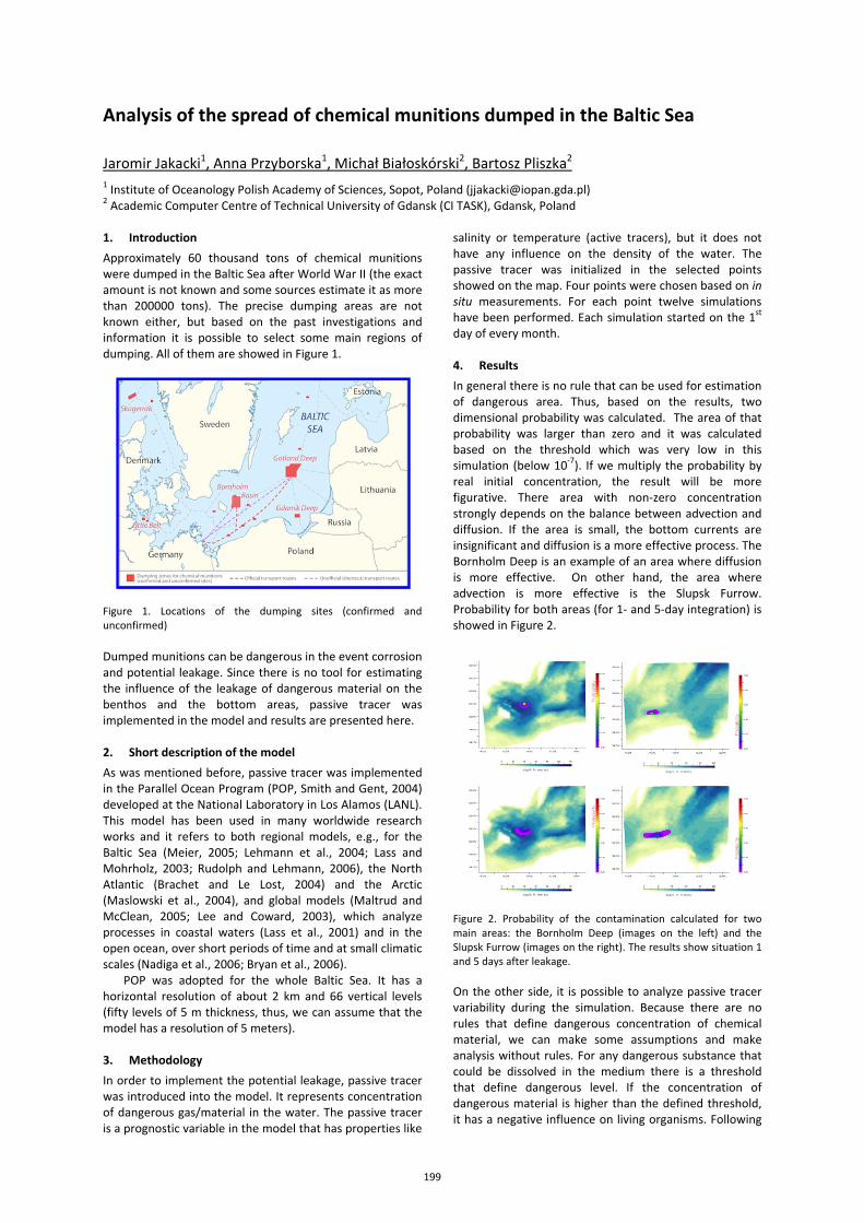
Analysis of the spread of chemical munitions dumped in the Baltic Sea

Jaromir Jakacki1, Anna Przyborska1, Michał Białoskórski2, Bartosz Pliszka2

1 Institute of Oceanology Polish Academy of Sciences, Sopot, Poland (jjakacki@iopan.gda.pl) 2 Academic Computer Centre of Technical University of Gdansk (CI TASK), Gdansk, Poland 1. Introduction Approximately 60 thousand tons of chemical munitions were dumped in the Baltic Sea after World War II (the exact amount is not known and some sources estimate it as more than 200000 tons). The precise dumping areas are not known either, but based on the past investigations and information it is possible to select some main regions of dumping. All of them are showed in Figure 1.

Figure 1. Locations of the dumping sites (confirmed and unconfirmed) Dumped munitions can be dangerous in the event corrosion and potential leakage. Since there is no tool for estimating the influence of the leakage of dangerous material on the benthos and the bottom areas, passive tracer was implemented in the model and results are presented here. 2. Short description of the model As was mentioned before, passive tracer was implemented in the Parallel Ocean Program (POP, Smith and Gent, 2004) developed at the National Laboratory in Los Alamos (LANL). This model has been used in many worldwide research works and it refers to both regional models, e.g., for the Baltic Sea (Meier, 2005; Lehmann et al., 2004; Lass and Mohrholz, 2003; Rudolph and Lehmann, 2006), the North Atlantic (Brachet and Le Lost, 2004) and the Arctic (Maslowski et al., 2004), and global models (Maltrud and McClean, 2005; Lee and Coward, 2003), which analyze processes in coastal waters (Lass et al., 2001) and in the open ocean, over short periods of time and at small climatic scales (Nadiga et al., 2006; Bryan et al., 2006).

POP was adopted for the whole Baltic Sea. It has a horizontal resolution of about 2 km and 66 vertical levels (fifty levels of 5 m thickness, thus, we can assume that the model has a resolution of 5 meters). 3. Methodology In order to implement the potential leakage, passive tracer was introduced into the model. It represents concentration of dangerous gas/material in the water. The passive tracer is a prognostic variable in the model that has properties like

salinity or temperature (active tracers), but it does not have any influence on the density of the water. The passive tracer was initialized in the selected points showed on the map. Four points were chosen based on in situ measurements. For each point twelve simulations have been performed. Each simulation started on the 1st day of every month. 4. Results In general there is no rule that can be used for estimation of dangerous area. Thus, based on the results, two dimensional probability was calculated. The area of that probability was larger than zero and it was calculated based on the threshold which was very low in this simulation (below 10-7). If we multiply the probability by real initial concentration, the result will be more figurative. There area with non-zero concentration strongly depends on the balance between advection and diffusion. If the area is small, the bottom currents are insignificant and diffusion is a more effective process. The Bornholm Deep is an example of an area where diffusion is more effective. On other hand, the area where advection is more effective is the Slupsk Furrow. Probability for both areas (for 1- and 5-day integration) is showed in Figure 2.

Figure 2. Probability of the contamination calculated for two main areas: the Bornholm Deep (images on the left) and the Slupsk Furrow (images on the right). The results show situation 1 and 5 days after leakage. On the other side, it is possible to analyze passive tracer variability during the simulation. Because there are no rules that define dangerous concentration of chemical material, we can make some assumptions and make analysis without rules. For any dangerous substance that could be dissolved in the medium there is a threshold that define dangerous level. If the concentration of dangerous material is higher than the defined threshold, it has a negative influence on living organisms. Following

199

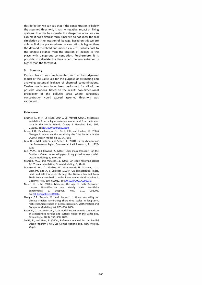
this definition we can say that if the concentration is below the assumed threshold, it has no negative impact on living systems. In order to estimate the dangerous area, we can assume it has a circular form, since we do not know the real circulation at the location of leakage. Based on this we are able to find the places where concentration is higher than the defined threshold and mark a circle of radius equal to the longest distance from the location of leakage to the place with dangerous concentration. Furthermore, it is possible to calculate the time when the concentration is higher than the threshold. 5. Summary Passive tracer was implemented in the hydrodynamic model of the Baltic Sea for the purpose of estimating and analyzing potential leakage of chemical contaminations. Twelve simulations have been performed for all of the possible locations. Based on the results two-dimensional probability of the polluted area where dangerous concentration could exceed assumed threshold was estimated. References

Brachet, S., P. Y. Le Traon, and C. Le Provost (2004), Mesoscale variability from a high-resolution model and from altimeter data in the North Atlantic Ocean, J. Geophys. Res., 109, C12025, doi:10.1029/2004JC002360.

Bryan, F.O., Danabasoglu, G., Gent, P.R., and Lindsay, K. (2006) Changes in ocean ventilation during the 21st Century in the CCSM3, Ocean Modelling 15, 141–156

Lass, H.U., Mohrholz, V., and Seifert, T. (2001) On the dynamics of the Pomeranian Bight, Continental Shelf Research, 21, 1237-1261

Lee, M.M., and Coward, A. (2003) Eddy mass transport for the Southern Ocean in an eddy-permitting global ocean model, Ocean Modelling, 5, 249–266

Maltrud, M.E., and McClean J.L. (2005) An eddy resolving global 1/10° ocean simulation, Ocean Modelling, 8, 31–54

Maslowski, W., D. Marble, W. Walczowski, U. Schauer, J. L. Clement, and A. J. Semtner (2004), On climatological mass, heat, and salt transports through the Barents Sea and Fram Strait from a pan-Arctic coupled ice-ocean model simulation, J. Geophys. Res., 109, C03032, doi:10.1029/2001JC001039.

Meier, H. E. M. (2005), Modeling the age of Baltic Seawater masses: Quantification and steady state sensitivity experiments, J. Geophys. Res., 110, C02006, doi:10.1029/2004JC002607.

Nadiga, B.T., Taylorb, M., and Lorenzc, J.: Ocean modelling for climate studies: Eliminating short time scales in long-term, high-resolution studies of ocean circulation, Mathematical and Computer Modelling, 44, 870–886, 2006.

Rudolph, C., and Lehmann, A.: A model-measurements comparison of atmospheric forcing and surface fluxes of the Baltic Sea, Oceanologia, 48(3), 333–360, 2006.

Smith, R., and Gent, P. (2004), Reference manual for the Parallel Ocean Program (POP), Los Alamos National Lab., New Mexico, 75 pp.

200

On some hydrometeorological monitoring results in the south-eastern part of the Baltic Sea during the last decade

M. Kapustina1, T. Bukanova1, Zh. Stont2

1 P.P. Shirshov Institute of Oceanology, Atlantic Branch 2 Immanuel Kant Baltic Federal University

1. Introduction It is well known, that due to stable stratification and halocline presence the Baltic Sea is especially sensitive to climate change (Backhaus, 1996; Hordoir, Meier, 2011; Omstedt, Nyberg, 1996; Störmer, 2011). The South-Eastern part of the Baltic sea is a particularly vulnerable water zone, which includes inland, separated from the sea by sandy spits, shallow Curonian and Vistula lagoons, being a discharge zone of Vistula river, Kaliningrad and Klaipeda channel.

Air temperature is a key factor in alteration of sea surface temperature (Cayan, 1992), which influences on the vast majority of processes, taking place in plankton societies. Sea surface temperature ascending during winter and spring prevents from convection forming and consequently from nutrient chemicals redistribution, influences on primary production and marine cenosises structure of different trophic levels (Wasmund et al., 1998). Strong summer water warm-up in the Baltic sea is able to stimulate potentially toxic cyanobacteria bloom (Aleksandrov, 2010; Janssen et al., 2004; Wasmund, Uhlig, 2003; Wiktor, Plinski, 1992).

Short-term sea-level fluctuations are also caused by meteorological influence (Ekman, 2009; Kowalewski, Kowalewska-Kalkowska, 2011; Stramska et al., 2013; Theuerkauf et al., 2014). According to the observed trends in wind velocity and direction changes, storms frequency is increasing, the escalation in repetitions in severe storms sourced from the north can be predicted.

The aim of following research is the analysis of interannual and seasonal variability of meteorological parameters in the South-Eastern Baltic during the 2006-2015, revealing their influence on sea surface temperature (SST) and sea level anomalies (SLA).

2. Data and Methods The research was made on the basis of a 10-year data array, collected in the open sea, excluding dry land distortions. There were the lack of hydrometeorological observations for the South-Eastern Baltic for the last several years. The area of interest is not an active navigable water, therefore there is no passing monitoring.

The data, obtained during the ecological monitoring of Kravtsovskoe reservoir (D-6), made by OOO “Lukoil-KMN” from 2004 till now, was used to analyze the variability of air temperature. The offshore ice-resistant fixed platform (D-6) is situated almost 20 km from coast. This platform carries automatic hydrometeorological station “Minicrams-4” at the 27 m high, maintaining continuous measurements.

The analysis of hourly observations of air temperature, wind velocity and direction was made; these observations involve a continuous 12-years data array. Temperature reduction to standard 2 m level was not made due to the fact that it is compliant.

The wind speed was reduced to the 10 m level. The SST and chlorophyll “a” variability was estimated using of the data arrays, derived from ocean color scanner MODIS, installed on NASA satellites Aqua and Terra. Sea level anomalies were measured with a use of satellite altimetry, derived from Radar Altimeter Database System (RADS).

Interannual variability of hydrometeorological parameters was analyzed by dispersive, harmonic and spectral analysis (Bruks, Karuzers, 1963; Rozhkov, 2008). The linear approximation (least square method) of time series was used for estimation of long-term trends, while the Student t-test (Fisher, Yates, 1975) was used for measuring statistical significance of obtained results. Seasonal statistics and mean trend are non-additive.

3. Resume The conducted research of spatial and temporal variability of hydrometeorological parameters over a period of 2006-2015 in the south-eastern part of the Baltic sea revealed: - average annual air temperature has risen; - the year minimum of air temperature moved to

February due to cycling terms variation, indicating the fact that climate of the South-Eastern Baltic became more marine;

- the main role in interannual variability of air temperature plays fluctuations of values during winter;

- one of the reasons for air temperature to vary is circulating conditions: namely direct noticeable relation (r = 0.63 with Р = 95%) for western circulation (W) and inverse noticeable relation (r = –0.62 with Р = 95%) for eastern one;

- the positive SST trend was shown; - there is some spatial inhomogeneity for observed

warming, for instance, coastal zone can be characterized by higher rates of SST rising in comparison with open-sea;

- a strong correlation of SST and air temperature was observed;

- over the period SST was characterized by more intense rise than air temperature. There are two reasons for that: firstly, the main role in interannual variability of temperature plays winter values; secondly, water temperature is defined not only by air, but also water circulation;

- the high correlation rate (R2 = 0.8) between chlorophyll “a” concentration and SST measurement was revealed, confirming a strong connection between these parameters;

- the increase of SST contributes to the growth of chlorophyll “a” concentration.

201

- the positive linear trend of average annual wind speed (0.02 m⋅s–1/year, increment ∼0.2 m⋅s–1/period) and negligible negative trend of wing speed above 20 m/s–1 (0.01 m⋅s–1/year, increment –0.1 m⋅s–1/period) were observed from year 2006 to year 2015;

- the role of south-western winds reduced (-4.1%), along with north-eastern and eastern ones, which are rarely stormy. At the same time the proportion of north-western and south-eastern winds enlarged: +2.1 % and +4.5 % respectively;

- the maximum positive sea level anomalies in the open part of the South-Eastern Baltic were 0.4 m, measured while western winds were presented. Maximum negative sea level anomalies (-0.3 m) were observed simultaneously with eastern winds at southern circumferences of anticyclones;

- the linear trend for sea level anomalies is negative (-0.02 m per year). Emphasizing of eastern component resulted in reducing of mean level deviation.

References

Backhaus J.O. (1996) Climate–sensitivity of European marginal seas, derived from the interpretation of modelling studies, Journal of Marine Systems, No 7, pp. 361–382

Cayan D. R. (1992) Latent and sensible heat flux anomalies over the northern oceans: driving the sea surface temperature, J. Phys. Oceanography, No. 22, pp. 859–881

Ekman M. (2009) The Changing Level of the Baltic Sea during 300 Years: A Clue to Understanding the Earth. A°land Islands Summer Institute for Historical Geophysics

Fisher R.A., Yates F. (1975) Statistical Tables for Biological, Agricultural and Medical Research. Edinburg: Oliver and Boyd

Hordoir R., Meier H.E.M. (2011) Effect of climate change on the thermal stratif cation, Climate Dynamics, No. 38 (9–10), pp. 1–11

Janssen F., Neumann T., Schmidt M. (2004) Interannual variability of cyanobacterial blooms in the Baltic Sea controlled by wintertime hydrographic conditions, Mar. Ecol. Prog. Ser., No. 275, pp. 59–68

Kowalewski M., Kowalewska-Kalkowska H. (2011) Performance of operationally calculated hydrodynamic forecasts during storm surges in the Pomeranian Bay and Szczecin Lagoon, Boreal Environment Research, Res. 16 (suppl. A), pp. 27–41

Omstedt A., Nyberg L. (1996) Response of Baltic Sea ice to seasonal, interannual forcing and Climate change, Tellus, No. 48A (5), pp. 644–662

Störmer O. (2011) Climate Change Impacts on Coastal Waters of the Baltic Sea, Global Change and Baltic Coastal Zones, Dordrecht: Springer, Vol. 1. pp. 51–69

Stramska M., H. Kowalewska-Kalkowska, M. Swirgon (2013) Seasonal variability of the Baltic Sea level, Oceanologia, 55 (4), pp. 1-21

Theuerkauf, E. J., Rodriguez, A. B., Fegley, S. R., & Luettich, R. A. (2014) Sea level anomalies exacerbate beach erosion, Geophysical Research Letters, 41(14), pp. 5139-5147

Wasmund N., Nauch G., Matthäus W. (1998) Phytoplankton spring blooms in the southern Baltic Sea–spatio–temporal development and long–term trends, Journal of Plankton Research, No. 20, pp. 1099–1117

Wasmund N., Uhlig S. (2003) Phytoplankton trends in the Baltic Sea, ICES Journal of Marine Science, No. 60, pp. 177–186

Wiktor K., Plinski M. (1992) Long–term changes in the biocoenosis of the Gulf of Gdansk, Oceanologia, No. 32, pp. 69–79

Aleksandrov S.V. (2010) Vliyanie klimaticheskih izmeneniy na uroven evtrofirovaniya Kurshskogo zaliva, Vestnik Rossiyskogo gosudarstvennogo universiteta im. I. Kanta, No. 1, pp. 49–57

Bruks K., Karuzers N. (1963) Primenenie statisticheskih metodov v meteorologii, Gidrometeoizdat, 416 p

Rozhkov V.A. (2008) Metodyi statisticheskoy gidrometeorologii, Geograficheskie i geoekologicheskie aspektyi razvitiya prirodyi i obschestva, pp. 121-132

202

Which factors affect metal and radionuclide pollution in the Baltic Sea?

Martin Lodenius

Department of Environmental Sciences, University of Helsinki, Finland (martin.lodenius@helsinki.fi)

1. Pollution of the Baltic sea The Baltic Sea is one of the most polluted sea areas in

the world and the ecological status is affected by a relatively shallow depth, a slow water renewal and a salinity gradient increasing from zero to 2.5 %. Salinity and temperature stratification limit water exchange and oxygen depletion is common in bottoms of deep water. The biodiversity is limited due to these special conditions. The status of pollutants in the Baltic Sea has been monitored intensively by HELCOM and its member states which gives us a good knowledge of distribution, trends and ecological importance of pollutants. Emissions of heavy metals and other persistent pollutants have decreased substantially in the catchment area during the last decades. 2. Loads and trends External pollution load comes via rivers, the North Sea and the atmosphere. Emissions originate from urban, agricultural and industrial sources. Internal load come from sediments where e.g. heavy metals may be strongly but not totally irreversibly bound to sulphides. Metals are removed from the water phase by sedimentation and fishing. Organic pollutants like dioxins and PCB are slowly degrading, degradation rates being affected by temperature, oxygen level and biological activity (Gusev 2009, Knuuttila 2009, Hazardous substances in the Baltic Sea 2010, EMEP 2013).

Concentrations and trends of heavy metals in fish, mussels and sediments have been reported for some decades. Often there is an increase during 1980's and 1990's and a decrease after that. The temporal trends are not always significant and they are different for different samples, different areas and different pollutants (Hazardous substances 2010).

Heavy metals and radionuclides are partly sedimentated, partly taken up in biota including fish. The concentrations vary widely but in most cases the trend is decreasing (Polak-Juszczak 2009, 2013, Voigt 1999, 2007). In aquatic environment metals and radionuclides are to a great extent bound to inorganic or organic particles and sedimentated. The concentrations in sediment cores indicate decreasing loads (Leivuori 2000, Vallius & Leivuori 1999, Vallius 2014).

The most significant source of anthropogenic radioactivity in the Baltic Sea is fallout from the Chernobyl accident in 1986 and 137Cs is the main component of manmade radioactivity in seawater. For radionuclides the general trend is steadily decreasing (HELCOM 2009). 3. Interrelated trends for future development Despite decreasing emissions concentrations in water, sediments and biota are still too high in many sea areas. This is true e.g. for cadmium and mercury in sediments (Vallius 2014).

Many factors affect the future development of concentrations including:

• anthropogenic emissions which are related to technological and economic development,

• political decisions and legislation in countries around the Baltic sea,

• climate change and changes in salinity, temperature and water currents,

• changes in eutrophication and oxygen status and related changes in biota,

• changes in fishery, • changes in atmospheric deposition of pollutants. These factors are interrelated and partly difficult to predict. Measures aiming to enhance the ecological status of the Baltic Sea will certainly give positive results but this will take at least several decades (Noyes et al. 2009, Hazardous substances in the Baltic Sea 2010, Sobek et al. 2015).

Large scale changes like eutrophication and climate change affect ecosystems in many ways, directly and indirectly, causing biological and abiotic effects. The time scale is very short in geological sense but long in a political context. References

EMEP (2013) Atmospheric Supply of Nitrogen, Lead, Cadmium, Mercury and Dioxins/Furans to the Baltic Sea in 2013 (J. Bartnicki, A. Gusev, W. Aas, S. Valiyaveetil, Á. Nyíri). EMEP/MSC-W TECHNICAL REPORT 2/2013. 177 p.

Hazardous substances in the Baltic Sea (2010) An integrated thematic assessment of hazardous substances in the Baltic Sea. Baltic Sea Environment Proceedings. Baltic Marine Environment Protection Commission No. 120B. 106 p. + annexes.

HELCOM (2009). Baltic Sea Environment Proceedings No. 117. Radioactivity in the Baltic Sea, 1999-2006. HELCOM thematic assessment.

Gusev A. (2009): Atmospheric deposition of heavy metals to the Baltic Sea. HELCOM Indicator Fact Sheets 2009. Available at http://www.helcom.fi/environment2/ifs/ifs2009/en_GB/hmdeposition/.

Knuuttila S. (Ed.) (2009): Waterborne inputs of heavy metals to the Baltic Sea. HELCOM Indicator Fact Sheet 2009. Available at: http://helcom.fi/baltic-sea-trends/environment-fact-sheets/hazardous-substances/contaminants-in-herring

Leivuori M., (2000) Distribution and Accumulation of Metals in Sediments of the Northern Baltic Sea. Finnish Institute of Marine Research – Contributions 2. 159p.

Leivuori M., Niemistö L. (1993) Trace metals in the sediments of the Gulf of Bothnia. Aqua Fennica 23, pp. 89–100.

Noyes P., M. McElwee, H. Miller, B. Clark, L. Van Tiem L., K. Walcott, K. Erwin, E. Levin (2009) The toxicology of climate change: Environmental contaminants in a warming world. Environ. Internat. 35, pp. 971–986.

Polak-Juszczak L. (2009) Temporal trends in the bioaccumulation of trace metals in herring, sprat, and cod from the southern Baltic Sea in the 1994–2003 period. Chemosphere 76, pp. 1334–1339.

Polak-Juszczak L. (2013) Trace elements in the livers of cod (Gadus morhua L.) from the Baltic Sea: levels and temporal trends. Environ Monit Assess 185, pp. 687–694.

203

Sobek A, K. Sundqvist, A. Assefa, K. Wiberg (2015) Baltic Sea sediment records: Unlikely near-future declines in PCBs and HCB. Sci. Total Environ. 518–519, pp. 8–15.

Vallius, H., Leivuori, M. (1999) The distribution of heavy metals and arsenic in recent sediments of the Gulf of Finland. Boreal Environ. Res. 4, pp. 19–29.

Vallius, H. (2014) Heavy metal concentrations in sediment cores from the northern Baltic Sea: declines over the last two decades. Mar. Pollut. Bull. 79, pp. 359–364.

Verta M., S. Salo, M. Korhonen, T. Assmuth, H. Kiviranta, J. Koistinen, P. Ruokojärvi, P. Isosaari, P.-A. Bergqvist, M. Tysklind, I. Cato, J. Vikelsøe, M. Larsen (2007) Dioxin concentrations in sediments of the Baltic Sea – A survey of existing data. Chemosphere 67, pp. 1762–1775.

Voigt, H-R. (1999) Concentrations of heavy metals in fish from coastal waters around the Baltic Sea. ICES J. Mar. Sci. 56 (Suppl.), pp. 140–141.

Voigt H.-R. (2007) Heavy Metal (Hg, Cd, Zn) Concentrations and Condition of Eelpout (Zoarces viviparus L.), around Baltic Sea. Polish J. Environ. Stud. 16, 6, pp. 909-917.

204

Dialogue- and communication forms as parallel infrastructure of climate- and coastal research at the Southern Baltic Sea coast

Insa Meinke

Institute of Coastal Research, Helmholtz-Zentrum Geesthacht, Germany (insa.meinke@hzg.de)

1. Parallel infrastructure needed While natural science is analyzing the sensitivity of complex systems to natural and human influences an additional infrastructure is needed to enable knowledge as basis for decision making processes at the Southern Baltic Sea.

Agriculture, tourism, energy supply and coastal defense are only some examples for weather sensitive sectors at the southern Baltic Sea coast. In these sectors climate and coastal research can serve as basis for decision processes.

However, scientific knowledge cannot be directly translated into necessary action. Peer reviewed articles with regional focus are widely scattered and scientific agreement is often not documented on regional scales. Also, the format of regional research results is often not decision relevant and public interpretation of research findings does not correspond to scientific knowledge. 2. The Northern German Climate Office Since ten years the Northern Climate Office maintains an intensive stakeholder dialogue to generate decision relevant information based on regional assessments and coastal or climate data available for the Southern Baltic Sea coast and Northern Germany. About once a week a dialogue event takes place, many individual requests are answered and interviews are given to the media. Also, several stakeholder workshops and expert interviews have been conducted. From these dialogue activities information demands of different stakeholder groups have been localized to develop decision relevant information products which may serve a broader group with similar information needs. 3. Stakeholder perspectives More than 1500 stakeholders from different user groups have registered for this service, so far. Each user group seems to prefer particular dialogue and communication forms. Since regional politicians are one of the smallest user groups a survey among mayors in the Southern Baltic Sea region have been conducted. The response shows that in many regions at the Southern Baltic Sea coast climate changes has only little priority. Also, the requested information of the mayors regarding climate change is often not part of the research agenda.

205

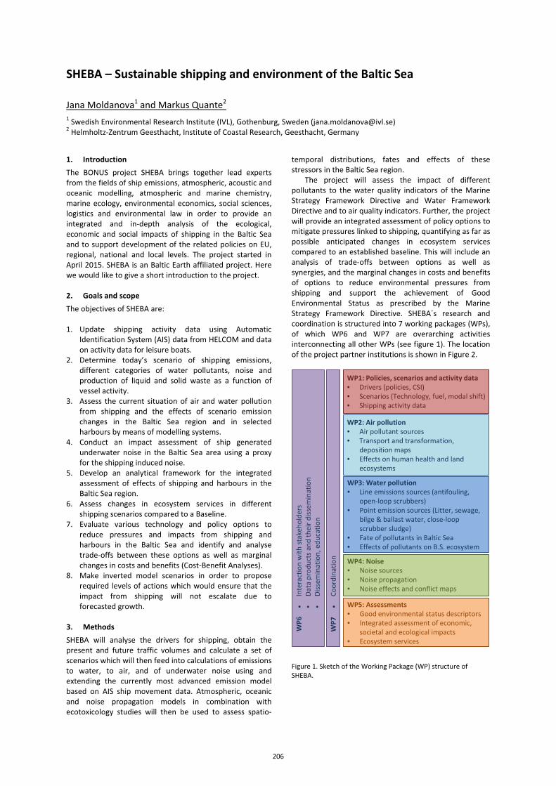
SHEBA – Sustainable shipping and environment of the Baltic Sea

Jana Moldanova1 and Markus Quante2 1 Swedish Environmental Research Institute (IVL), Gothenburg, Sweden (jana.moldanova@ivl.se) 2 Helmholtz-Zentrum Geesthacht, Institute of Coastal Research, Geesthacht, Germany

1. Introduction The BONUS project SHEBA brings together lead experts from the fields of ship emissions, atmospheric, acoustic and oceanic modelling, atmospheric and marine chemistry, marine ecology, environmental economics, social sciences, logistics and environmental law in order to provide an integrated and in-depth analysis of the ecological, economic and social impacts of shipping in the Baltic Sea and to support development of the related policies on EU, regional, national and local levels. The project started in April 2015. SHEBA is an Baltic Earth affiliated project. Here we would like to give a short introduction to the project. 2. Goals and scope The objectives of SHEBA are: 1. Update shipping activity data using Automatic

Identification System (AIS) data from HELCOM and data on activity data for leisure boats.

2. Determine today’s scenario of shipping emissions, different categories of water pollutants, noise and production of liquid and solid waste as a function of vessel activity.

3. Assess the current situation of air and water pollution from shipping and the effects of scenario emission changes in the Baltic Sea region and in selected harbours by means of modelling systems.

4. Conduct an impact assessment of ship generated underwater noise in the Baltic Sea area using a proxy for the shipping induced noise.

5. Develop an analytical framework for the integrated assessment of effects of shipping and harbours in the Baltic Sea region.

6. Assess changes in ecosystem services in different shipping scenarios compared to a Baseline.

7. Evaluate various technology and policy options to reduce pressures and impacts from shipping and harbours in the Baltic Sea and identify and analyse trade-offs between these options as well as marginal changes in costs and benefits (Cost-Benefit Analyses).

8. Make inverted model scenarios in order to propose required levels of actions which would ensure that the impact from shipping will not escalate due to forecasted growth.

3. Methods SHEBA will analyse the drivers for shipping, obtain the present and future traffic volumes and calculate a set of scenarios which will then feed into calculations of emissions to water, to air, and of underwater noise using and extending the currently most advanced emission model based on AIS ship movement data. Atmospheric, oceanic and noise propagation models in combination with ecotoxicology studies will then be used to assess spatio-

temporal distributions, fates and effects of these stressors in the Baltic Sea region.

The project will assess the impact of different pollutants to the water quality indicators of the Marine Strategy Framework Directive and Water Framework Directive and to air quality indicators. Further, the project will provide an integrated assessment of policy options to mitigate pressures linked to shipping, quantifying as far as possible anticipated changes in ecosystem services compared to an established baseline. This will include an analysis of trade-offs between options as well as synergies, and the marginal changes in costs and benefits of options to reduce environmental pressures from shipping and support the achievement of Good Environmental Status as prescribed by the Marine Strategy Framework Directive. SHEBA´s research and coordination is structured into 7 working packages (WPs), of which WP6 and WP7 are overarching activities interconnecting all other WPs (see figure 1). The location of the project partner institutions is shown in Figure 2.

Figure 1. Sketch of the Working Package (WP) structure of SHEBA.

WP4: Noise• Noise sources• Noise propagation• Noise effects and conflict maps

WP2: Air pollution• Air pollutant sources• Transport and transformation,

deposition maps• Effects on human health and land

ecosystems

WP5: Assessments• Good environmental status descriptors• Integrated assessment of economic,

societal and ecological impacts• Ecosystem services

WP1: Policies, scenarios and activity data• Drivers (policies, CSI)• Scenarios (Technology, fuel, modal shift)• Shipping activity data

WP6

•In

tera

ctio

n w

ith st

akeh

olde

rs•

Data

pro

duct

s and

thei

r diss

emin

atio

n•

Diss

emin

atio

n, e

duca

tion

WP7

•Co

ordi

natio

n

WP3: Water pollution• Line emissions sources (antifouling,

open-loop scrubbers)• Point emission sources (Litter, sewage,

bilge & ballast water, close-loop scrubber sludge)

• Fate of pollutants in Baltic Sea• Effects of pollutants on B.S. ecosystem

206

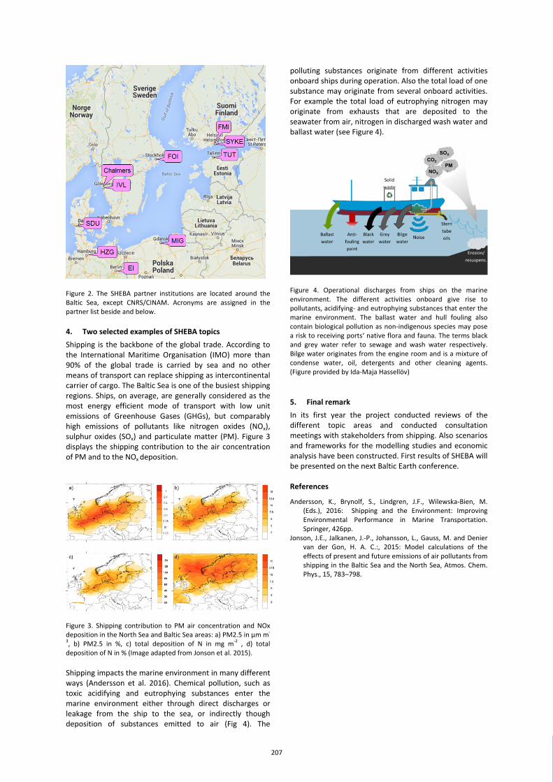
Figure 2. The SHEBA partner institutions are located around the Baltic Sea, except CNRS/CINAM. Acronyms are assigned in the partner list beside and below. 4. Two selected examples of SHEBA topics Shipping is the backbone of the global trade. According to the International Maritime Organisation (IMO) more than 90% of the global trade is carried by sea and no other means of transport can replace shipping as intercontinental carrier of cargo. The Baltic Sea is one of the busiest shipping regions. Ships, on average, are generally considered as the most energy efficient mode of transport with low unit emissions of Greenhouse Gases (GHGs), but comparably high emissions of pollutants like nitrogen oxides (NOx), sulphur oxides (SOx) and particulate matter (PM). Figure 3 displays the shipping contribution to the air concentration of PM and to the NOx deposition.

Figure 3. Shipping contribution to PM air concentration and NOx deposition in the North Sea and Baltic Sea areas: a) PM2.5 in µm m-

3, b) PM2.5 in %, c) total deposition of N in mg m-2 , d) total deposition of N in % (Image adapted from Jonson et al. 2015). Shipping impacts the marine environment in many different ways (Andersson et al. 2016). Chemical pollution, such as toxic acidifying and eutrophying substances enter the marine environment either through direct discharges or leakage from the ship to the sea, or indirectly though deposition of substances emitted to air (Fig 4). The

polluting substances originate from different activities onboard ships during operation. Also the total load of one substance may originate from several onboard activities. For example the total load of eutrophying nitrogen may originate from exhausts that are deposited to the seawater from air, nitrogen in discharged wash water and ballast water (see Figure 4).

Figure 4. Operational discharges from ships on the marine environment. The different activities onboard give rise to pollutants, acidifying- and eutrophying substances that enter the marine environment. The ballast water and hull fouling also contain biological pollution as non-indigenous species may pose a risk to receiving ports‘ native flora and fauna. The terms black and grey water refer to sewage and wash water respectively. Bilge water originates from the engine room and is a mixture of condense water, oil, detergents and other cleaning agents. (Figure provided by Ida-Maja Hassellöv) 5. Final remark In its first year the project conducted reviews of the different topic areas and conducted consultation meetings with stakeholders from shipping. Also scenarios and frameworks for the modelling studies and economic analysis have been constructed. First results of SHEBA will be presented on the next Baltic Earth conference. References

Andersson, K., Brynolf, S., Lindgren, J.F., Wilewska-Bien, M. (Eds.), 2016: Shipping and the Environment: Improving Environmental Performance in Marine Transportation. Springer, 426pp.

Jonson, J.E., Jalkanen, J.-P., Johansson, L., Gauss, M. and Denier van der Gon, H. A. C.:, 2015: Model calculations of the effects of present and future emissions of air pollutants from shipping in the Baltic Sea and the North Sea, Atmos. Chem. Phys., 15, 783–798.

207

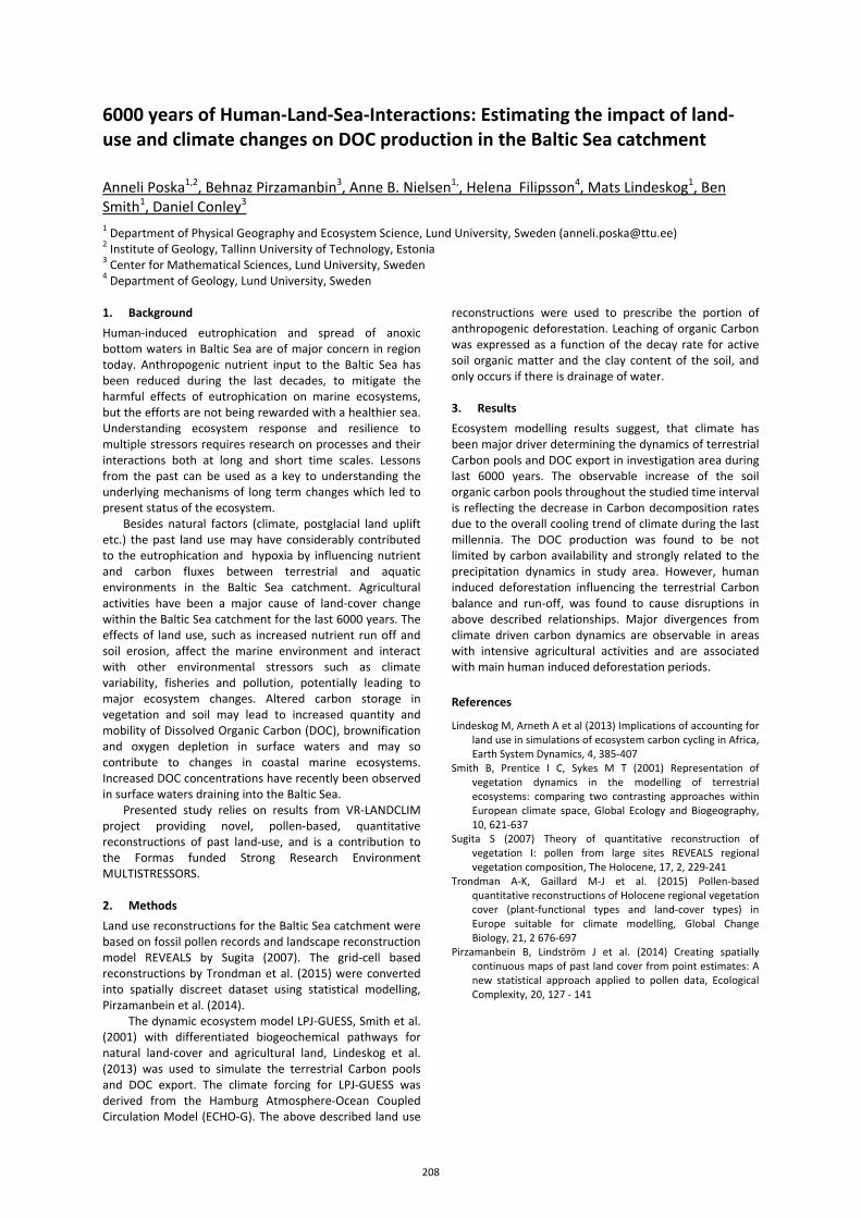
6000 years of Human-Land-Sea-Interactions: Estimating the impact of land-use and climate changes on DOC production in the Baltic Sea catchment

Anneli Poska1,2, Behnaz Pirzamanbin3, Anne B. Nielsen1,, Helena Filipsson4, Mats Lindeskog1, Ben Smith1, Daniel Conley3 1 Department of Physical Geography and Ecosystem Science, Lund University, Sweden (anneli.poska@ttu.ee) 2 Institute of Geology, Tallinn University of Technology, Estonia 3 Center for Mathematical Sciences, Lund University, Sweden 4 Department of Geology, Lund University, Sweden 1. Background Human-induced eutrophication and spread of anoxic bottom waters in Baltic Sea are of major concern in region today. Anthropogenic nutrient input to the Baltic Sea has been reduced during the last decades, to mitigate the harmful effects of eutrophication on marine ecosystems, but the efforts are not being rewarded with a healthier sea. Understanding ecosystem response and resilience to multiple stressors requires research on processes and their interactions both at long and short time scales. Lessons from the past can be used as a key to understanding the underlying mechanisms of long term changes which led to present status of the ecosystem.

Besides natural factors (climate, postglacial land uplift etc.) the past land use may have considerably contributed to the eutrophication and hypoxia by influencing nutrient and carbon fluxes between terrestrial and aquatic environments in the Baltic Sea catchment. Agricultural activities have been a major cause of land-cover change within the Baltic Sea catchment for the last 6000 years. The effects of land use, such as increased nutrient run off and soil erosion, affect the marine environment and interact with other environmental stressors such as climate variability, fisheries and pollution, potentially leading to major ecosystem changes. Altered carbon storage in vegetation and soil may lead to increased quantity and mobility of Dissolved Organic Carbon (DOC), brownification and oxygen depletion in surface waters and may so contribute to changes in coastal marine ecosystems. Increased DOC concentrations have recently been observed in surface waters draining into the Baltic Sea.

Presented study relies on results from VR-LANDCLIM project providing novel, pollen-based, quantitative reconstructions of past land-use, and is a contribution to the Formas funded Strong Research Environment MULTISTRESSORS. 2. Methods Land use reconstructions for the Baltic Sea catchment were based on fossil pollen records and landscape reconstruction model REVEALS by Sugita (2007). The grid-cell based reconstructions by Trondman et al. (2015) were converted into spatially discreet dataset using statistical modelling, Pirzamanbein et al. (2014).

The dynamic ecosystem model LPJ-GUESS, Smith et al. (2001) with differentiated biogeochemical pathways for natural land-cover and agricultural land, Lindeskog et al. (2013) was used to simulate the terrestrial Carbon pools and DOC export. The climate forcing for LPJ-GUESS was derived from the Hamburg Atmosphere-Ocean Coupled Circulation Model (ECHO-G). The above described land use

reconstructions were used to prescribe the portion of anthropogenic deforestation. Leaching of organic Carbon was expressed as a function of the decay rate for active soil organic matter and the clay content of the soil, and only occurs if there is drainage of water. 3. Results Ecosystem modelling results suggest, that climate has been major driver determining the dynamics of terrestrial Carbon pools and DOC export in investigation area during last 6000 years. The observable increase of the soil organic carbon pools throughout the studied time interval is reflecting the decrease in Carbon decomposition rates due to the overall cooling trend of climate during the last millennia. The DOC production was found to be not limited by carbon availability and strongly related to the precipitation dynamics in study area. However, human induced deforestation influencing the terrestrial Carbon balance and run-off, was found to cause disruptions in above described relationships. Major divergences from climate driven carbon dynamics are observable in areas with intensive agricultural activities and are associated with main human induced deforestation periods.

References

Lindeskog M, Arneth A et al (2013) Implications of accounting for land use in simulations of ecosystem carbon cycling in Africa, Earth System Dynamics, 4, 385-407

Smith B, Prentice I C, Sykes M T (2001) Representation of vegetation dynamics in the modelling of terrestrial ecosystems: comparing two contrasting approaches within European climate space, Global Ecology and Biogeography, 10, 621-637

Sugita S (2007) Theory of quantitative reconstruction of vegetation I: pollen from large sites REVEALS regional vegetation composition, The Holocene, 17, 2, 229-241

Trondman A-K, Gaillard M-J et al. (2015) Pollen-based quantitative reconstructions of Holocene regional vegetation cover (plant-functional types and land-cover types) in Europe suitable for climate modelling, Global Change Biology, 21, 2 676-697

Pirzamanbein B, Lindström J et al. (2014) Creating spatially continuous maps of past land cover from point estimates: A new statistical approach applied to pollen data, Ecological Complexity, 20, 127 - 141

208

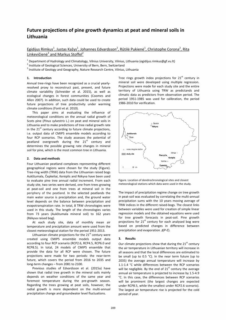
Future projections of pine growth dynamics at peat and mineral soils in Lithuania

Egidijus Rimkus1, Justas Kažys1, Johannes Edvardsson2, Rūtilė Pukienė1, Christophe Corona2, Rita Linkevičienė3 and Markus Stoffel2 1 Department of Hydrology and Climatology, Vilnius University, Vilnius, Lithuania (egidijus.rimkus@gf.vu.lt) 2 Institute of Geological Sciences, University of Bern, Bern, Switzerland 3 Institute of Geology and Geography, Nature Research Centre, Vilnius, Lithuania 1. Introduction Annual tree-rings have been recognized as a crucial yearly-resolved proxy to reconstruct past, present, and future climate variability (Schneider et al. 2015), as well as ecological changes in forest communities (Coomes and Allen 2007). In addition, such data could be used to create future projections of tree productivity under warming climate conditions (Fonti et al. 2010).

This paper aims at evaluating the influence of meteorological conditions on the annual radial growth of Scots pine (Pinus sylvestris L.) on peat and mineral soils in Lithuania and to make predictions of tree radial growth rate in the 21st century according to future climate projections, i.e. output data of CMIP5 ensemble models according to four RCP scenarios. The study assesses the potential of peatland overgrowth during the 21st century and determines the possible growing rate changes in mineral soil for pine, which is the most common tree in Lithuania. 2. Data and methods Four Lithuanian peatland complexes representing different geographical regions were chosen for the study (Figure). Tree-ring width (TRW) data from the Lithuanian raised bogs Aukštumala, Čepkeliai, Kerėplis and Rėkyva have been used to evaluate pine tree annual radial increment. From each study site, two series were derived, one from trees growing at peat-soil and one from trees at mineral soil in the periphery of the peatland. In the selected peatlands the main water source is precipitation and, the ground water level depends on the balance between precipitation and evapotranspiration rate. In total, 8 TRW chronologies were used in this study. The length of the chronologies varies from 73 years (Aukštumala mineral soil) to 162 years (Rėkyva raised bog).

At each study site, data of monthly mean air temperature and precipitation amount were used from the closest meteorological station for the period 1951-2013.

Lithuanian climate projections for the 21st century were created using CMIP5 ensemble models output data according to four RCP scenario (RCP2.6, RCP4.5, RCP6.0 and RCP8.5). In total, 24 models of CMIP5 ensemble that provide the data for all RCP were chosen. The future projections were made for two periods: the near-term future, which covers the period from 2016 to 2035 and long-term changes – from 2081 to 2100.

Previous studies of Edvardsson et al. (2015a) have shown that radial tree growth in the mineral soils mainly depends on weather conditions of the same year and foremost temperature during the pre-growth season. Regarding the trees growing at peat soils, however, the radial growth is more dependent on the multi-annual precipitation change and groundwater level fluctuations.

Tree rings growth index projections for 21st century in mineral soil were developed using multiple regression. Projections were made for each study site and the entire territory of Lithuania using TRW as predictands and climatic data as predictors from observation period. The period 1951-1985 was used for calibration, the period 1986-2010 for verification.

Figure. Location of dendrochronological sites and closest meteorological stations which data were used in the study.

The impact of precipitation regime change on tree growth in peat-soil was evaluated by correlating the multi-annual precipitation sums with the 10 years moving average of TRW indices in the different raised-bogs. The closest links between variables were used for creation of simple linear regression models and the obtained equations were used for tree growth forecasts in peat-soil. Pine growth projections for 21st century for each analysed bog were based on predicted changes in difference between precipitation and evaporation Δ(P-E).

3. Results Our climate projections show that during the 21st century the air temperature in Lithuanian territory will increase in all seasons and that the local differences are estimated to be small (up to 0.5 °C). In the near term future (up to 2035) the average annual temperature will increase by 1.1-1.4 °C while differences between the RCP scenarios will be negligible. By the end of 21st century the average annual air temperature is projected to increase by 1.5-4.9 °C. In this case, the differences between RCP scenarios will be prominent (the largest changes are expected under RCP8.5, while the smallest under RCP2.6 scenario). The largest air temperature rise is projected for the cold period of year.

209

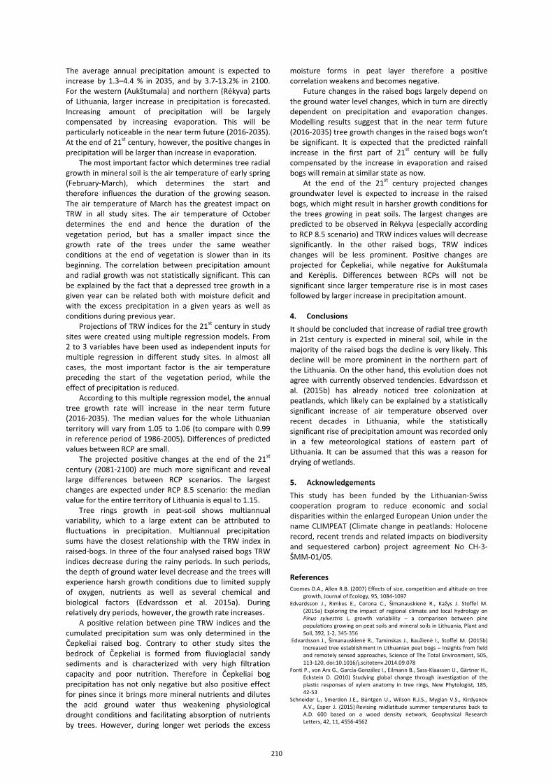
The average annual precipitation amount is expected to increase by 1.3–4.4 % in 2035, and by 3.7-13.2% in 2100. For the western (Aukštumala) and northern (Rėkyva) parts of Lithuania, larger increase in precipitation is forecasted. Increasing amount of precipitation will be largely compensated by increasing evaporation. This will be particularly noticeable in the near term future (2016-2035). At the end of 21st century, however, the positive changes in precipitation will be larger than increase in evaporation.

The most important factor which determines tree radial growth in mineral soil is the air temperature of early spring (February-March), which determines the start and therefore influences the duration of the growing season. The air temperature of March has the greatest impact on TRW in all study sites. The air temperature of October determines the end and hence the duration of the vegetation period, but has a smaller impact since the growth rate of the trees under the same weather conditions at the end of vegetation is slower than in its beginning. The correlation between precipitation amount and radial growth was not statistically significant. This can be explained by the fact that a depressed tree growth in a given year can be related both with moisture deficit and with the excess precipitation in a given years as well as conditions during previous year.

Projections of TRW indices for the 21st century in study sites were created using multiple regression models. From 2 to 3 variables have been used as independent inputs for multiple regression in different study sites. In almost all cases, the most important factor is the air temperature preceding the start of the vegetation period, while the effect of precipitation is reduced.

According to this multiple regression model, the annual tree growth rate will increase in the near term future (2016-2035). The median values for the whole Lithuanian territory will vary from 1.05 to 1.06 (to compare with 0.99 in reference period of 1986-2005). Differences of predicted values between RCP are small.

The projected positive changes at the end of the 21st century (2081-2100) are much more significant and reveal large differences between RCP scenarios. The largest changes are expected under RCP 8.5 scenario: the median value for the entire territory of Lithuania is equal to 1.15.

Tree rings growth in peat-soil shows multiannual variability, which to a large extent can be attributed to fluctuations in precipitation. Multiannual precipitation sums have the closest relationship with the TRW index in raised-bogs. In three of the four analysed raised bogs TRW indices decrease during the rainy periods. In such periods, the depth of ground water level decrease and the trees will experience harsh growth conditions due to limited supply of oxygen, nutrients as well as several chemical and biological factors (Edvardsson et al. 2015a). During relatively dry periods, however, the growth rate increases.

A positive relation between pine TRW indices and the cumulated precipitation sum was only determined in the Čepkeliai raised bog. Contrary to other study sites the bedrock of Čepkeliai is formed from fluvioglacial sandy sediments and is characterized with very high filtration capacity and poor nutrition. Therefore in Čepkeliai bog precipitation has not only negative but also positive effect for pines since it brings more mineral nutrients and dilutes the acid ground water thus weakening physiological drought conditions and facilitating absorption of nutrients by trees. However, during longer wet periods the excess

moisture forms in peat layer therefore a positive correlation weakens and becomes negative.

Future changes in the raised bogs largely depend on the ground water level changes, which in turn are directly dependent on precipitation and evaporation changes. Modelling results suggest that in the near term future (2016-2035) tree growth changes in the raised bogs won’t be significant. It is expected that the predicted rainfall increase in the first part of 21st century will be fully compensated by the increase in evaporation and raised bogs will remain at similar state as now.

At the end of the 21st century projected changes groundwater level is expected to increase in the raised bogs, which might result in harsher growth conditions for the trees growing in peat soils. The largest changes are predicted to be observed in Rėkyva (especially according to RCP 8.5 scenario) and TRW indices values will decrease significantly. In the other raised bogs, TRW indices changes will be less prominent. Positive changes are projected for Čepkeliai, while negative for Aukštumala and Kerėplis. Differences between RCPs will not be significant since larger temperature rise is in most cases followed by larger increase in precipitation amount.

4. Conclusions It should be concluded that increase of radial tree growth in 21st century is expected in mineral soil, while in the majority of the raised bogs the decline is very likely. This decline will be more prominent in the northern part of the Lithuania. On the other hand, this evolution does not agree with currently observed tendencies. Edvardsson et al. (2015b) has already noticed tree colonization at peatlands, which likely can be explained by a statistically significant increase of air temperature observed over recent decades in Lithuania, while the statistically significant rise of precipitation amount was recorded only in a few meteorological stations of eastern part of Lithuania. It can be assumed that this was a reason for drying of wetlands. 5. Acknowledgements This study has been funded by the Lithuanian-Swiss cooperation program to reduce economic and social disparities within the enlarged European Union under the name CLIMPEAT (Climate change in peatlands: Holocene record, recent trends and related impacts on biodiversity and sequestered carbon) project agreement No CH-3-ŠMM-01/05. References Coomes D.A., Allen R.B. (2007) Effects of size, competition and altitude on tree

growth, Journal of Ecology, 95, 1084-1097 Edvardsson J., Rimkus E., Corona C., Šimanauskienė R., Kažys J. Stoffel M.

(2015a) Exploring the impact of regional climate and local hydrology on Pinus sylvestris L. growth variability – a comparison between pine populations growing on peat soils and mineral soils in Lithuania, Plant and Soil, 392, 1-2, 345-356

Edvardsson J., Šimanauskienė R., Taminskas J., Baužienė I., Stoffel M. (2015b) Increased tree establishment in Lithuanian peat bogs – Insights from field and remotely sensed approaches, Science of The Total Environment, 505, 113-120, doi:10.1016/j.scitotenv.2014.09.078

Fonti P., von Arx G., García-González I., Eilmann B., Sass-Klaassen U., Gärtner H., Eckstein D. (2010) Studying global change through investigation of the plastic responses of xylem anatomy in tree rings, New Phytologist, 185, 42-53

Schneider L., Smerdon J.E., Büntgen U., Wilson R.J.S., Myglan V.S., Kirdyanov A.V., Esper J. (2015) Revising midlatitude summer temperatures back to A.D. 600 based on a wood density network, Geophysical Research Letters, 42, 11, 4556-4562

210

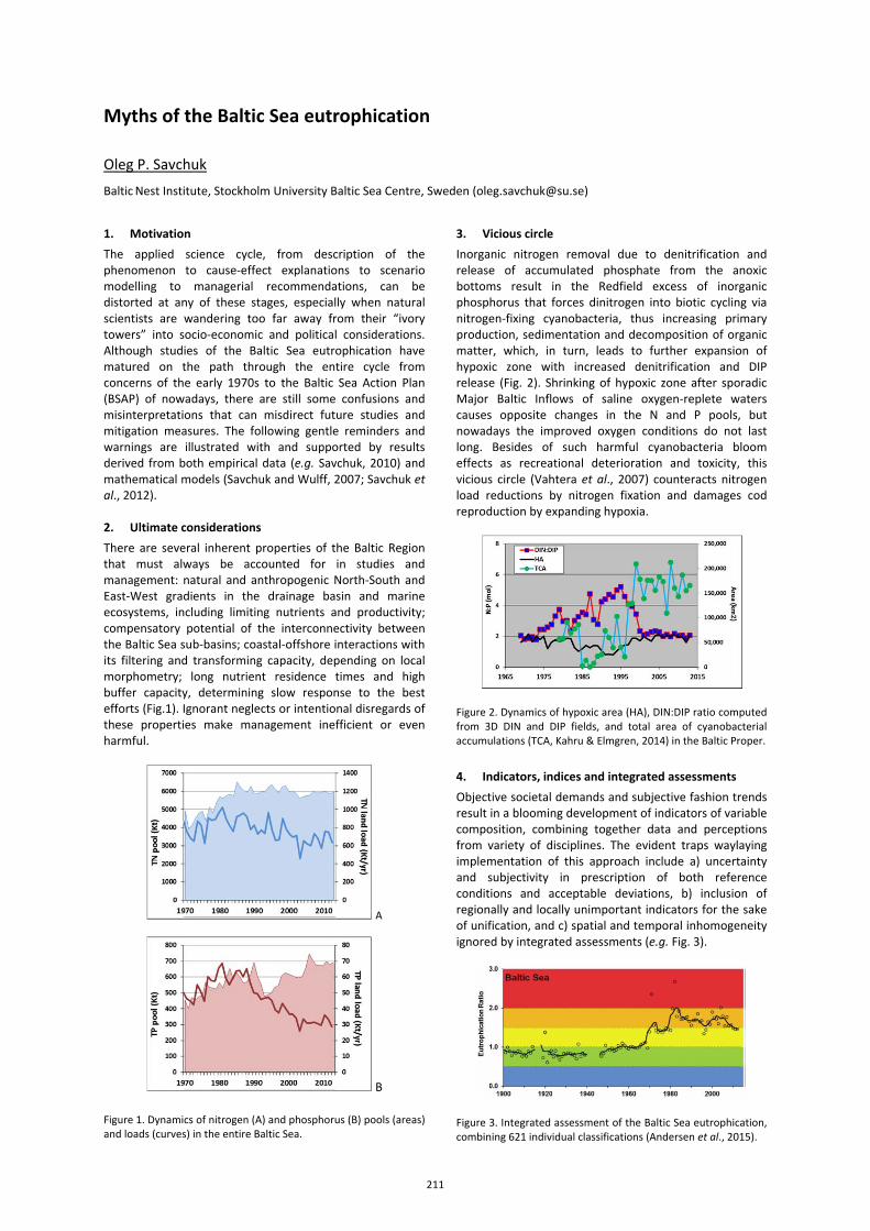
Myths of the Baltic Sea eutrophication

Oleg P. Savchuk

Baltic Nest Institute, Stockholm University Baltic Sea Centre, Sweden (oleg.savchuk@su.se)

1. Motivation The applied science cycle, from description of the phenomenon to cause-effect explanations to scenario modelling to managerial recommendations, can be distorted at any of these stages, especially when natural scientists are wandering too far away from their “ivory towers” into socio-economic and political considerations. Although studies of the Baltic Sea eutrophication have matured on the path through the entire cycle from concerns of the early 1970s to the Baltic Sea Action Plan (BSAP) of nowadays, there are still some confusions and misinterpretations that can misdirect future studies and mitigation measures. The following gentle reminders and warnings are illustrated with and supported by results derived from both empirical data (e.g. Savchuk, 2010) and mathematical models (Savchuk and Wulff, 2007; Savchuk et al., 2012). 2. Ultimate considerations There are several inherent properties of the Baltic Region that must always be accounted for in studies and management: natural and anthropogenic North-South and East-West gradients in the drainage basin and marine ecosystems, including limiting nutrients and productivity; compensatory potential of the interconnectivity between the Baltic Sea sub-basins; coastal-offshore interactions with its filtering and transforming capacity, depending on local morphometry; long nutrient residence times and high buffer capacity, determining slow response to the best efforts (Fig.1). Ignorant neglects or intentional disregards of these properties make management inefficient or even harmful.

A

B

Figure 1. Dynamics of nitrogen (A) and phosphorus (B) pools (areas) and loads (curves) in the entire Baltic Sea.

3. Vicious circle Inorganic nitrogen removal due to denitrification and release of accumulated phosphate from the anoxic bottoms result in the Redfield excess of inorganic phosphorus that forces dinitrogen into biotic cycling via nitrogen-fixing cyanobacteria, thus increasing primary production, sedimentation and decomposition of organic matter, which, in turn, leads to further expansion of hypoxic zone with increased denitrification and DIP release (Fig. 2). Shrinking of hypoxic zone after sporadic Major Baltic Inflows of saline oxygen-replete waters causes opposite changes in the N and P pools, but nowadays the improved oxygen conditions do not last long. Besides of such harmful cyanobacteria bloom effects as recreational deterioration and toxicity, this vicious circle (Vahtera et al., 2007) counteracts nitrogen load reductions by nitrogen fixation and damages cod reproduction by expanding hypoxia.

Figure 2. Dynamics of hypoxic area (HA), DIN:DIP ratio computed from 3D DIN and DIP fields, and total area of cyanobacterial accumulations (TCA, Kahru & Elmgren, 2014) in the Baltic Proper.

4. Indicators, indices and integrated assessments Objective societal demands and subjective fashion trends result in a blooming development of indicators of variable composition, combining together data and perceptions from variety of disciplines. The evident traps waylaying implementation of this approach include a) uncertainty and subjectivity in prescription of both reference conditions and acceptable deviations, b) inclusion of regionally and locally unimportant indicators for the sake of unification, and c) spatial and temporal inhomogeneity ignored by integrated assessments (e.g. Fig. 3).

Figure 3. Integrated assessment of the Baltic Sea eutrophication, combining 621 individual classifications (Andersen et al., 2015).

211

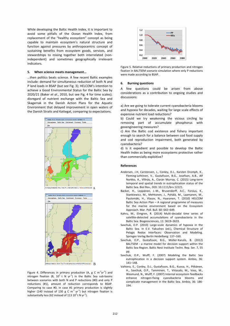
While developing the Baltic Health Index, it is important to avoid some pitfalls of the Ocean Health Index, from replacement of the “healthy ecosystem” concept as being capable to maintain ecosystem’s natural structure and function against pressures by anthropocentric concept of sustaining benefits from ecosystem goods, services, and stewardships to mixing together both interrelated (non-independent) and sometimes geographically irrelevant indicators. 5. When science meets management… …then politics beats science. A few recent Baltic examples include: demand for simultaneous reduction of both N and P land loads in BSAP (but see Fig. 3); HELCOM’s intention to achieve a Good Environmental Status for the Baltic Sea by 2020/21 (Baker et al., 2010, but see Fig. 4 for time scales); disregard of nutrient exchange with the Baltic Sea and Skagerrak in the Danish Action Plans for the Aquatic Environment that delayed improvement in open waters of the Danish Straits and Kattegat, comparing to expectations.

A

B

Figure 4. Differences in primary production (A, g C m-2yr-1) and nitrogen fixation (B, 103 t N yr-1) in the Baltic Sea sub-basins between scenarios with both N and P reductions (#0) and only P reductions (#1), amount of reduction corresponds to BSAP. Comparing to case #0, in case #1 primary production is slightly higher (140 instead of 130 g C m-2 yr-1) but nitrogen fixation is substantially less (62 instead of 113 103 t N yr-1).

Figure 5. Relative reductions of primary production and nitrogen fixation in BALTSEM scenario simulation where only P reductions were made according to BSAP.

6. Burning questions A few questions could be arisen from above considerations as a contribution to ongoing studies and discussions: a) Are we going to tolerate current cyanobacteria blooms and hypoxia for decades, waiting for large scale effects of expensive nutrient load reductions? b) Could we try weakening the vicious circling by removing part of accumulate phosphorus with geoengineering measures? c) Are the Baltic cod existence and fishery important enough to search for a balance between cod food supply and cod reproduction impairment, both generated by cyanobacteria? d) Is it expedient and possible to develop the Baltic Health Index as being more ecosystems protective rather than commercially exploitive?

References

Andersen, J.H, Carstensen, J., Conley, D.J., Karsten Dromph, K., Fleming-Lehtinen, V., Gustafsson, B.G., Josefson, A.B., Alf Norkko, A., Villnäs, A., Ciarán Murray, C. (2015) Long-term temporal and spatial trends in eutrophication status of the Baltic Sea. Biol Rev., DOI: 10.1111/brv.12221.

Backer, H., Leppänen, J.-M., Brusendorff, A.C., Forsius, K., Stankiewicz, M., Mehtonen, J., Pyhälä, M., Laamanen, M., Paulomäki, H., Vlasov, N., Haaranen, T. (2010) HELCOM Baltic Sea Action Plan – A regional programme of measures for the marine environment based on the Ecosystem Approach. Mar. Poll. Bull. 60: 642–649.

Kahru, M., Elmgren, R. (2014) Multi-decadal time series of satellite-detected accumulations of cyanobacteria in the Baltic Sea. Biogeosciences, 11: 3619–3633.

Savchuk, O.P. (2010) Large-scale dynamics of hypoxia in the Baltic Sea. In E.V. Yakushev (ed.), Chemical Structure of Pelagic Redox Interfaces: Observation and Modeling. Springer-Verlag Berlin Heidelberg: 137–160.

Savchuk, O.P., Gustafsson, B.G., Müller-Karulis, B. (2012) BALTSEM - a marine model for decision support within the Baltic Sea Region. Baltic Nest Institute Techn. Rep. Ser. 7, 55 pp.

Savchuk, O.P., Wulff, F. (2007) Modeling the Baltic Sea eutrophication in a decision support system. Ambio, 36: 141–148.

Vahtera, E., Conley, D.J., Gustafsson, B.G., Kuosa, H., Pitkänen, H., Savchuk, O.P., Tamminen, T., Viitasalo, M., Voss, M., Wasmund, N., Wulff, F. (2007) Internal ecosystem feedbacks enhance nitrogen-fixing cyanobacteria blooms and complicate management in the Baltic Sea. Ambio, 36: 186-194.

212

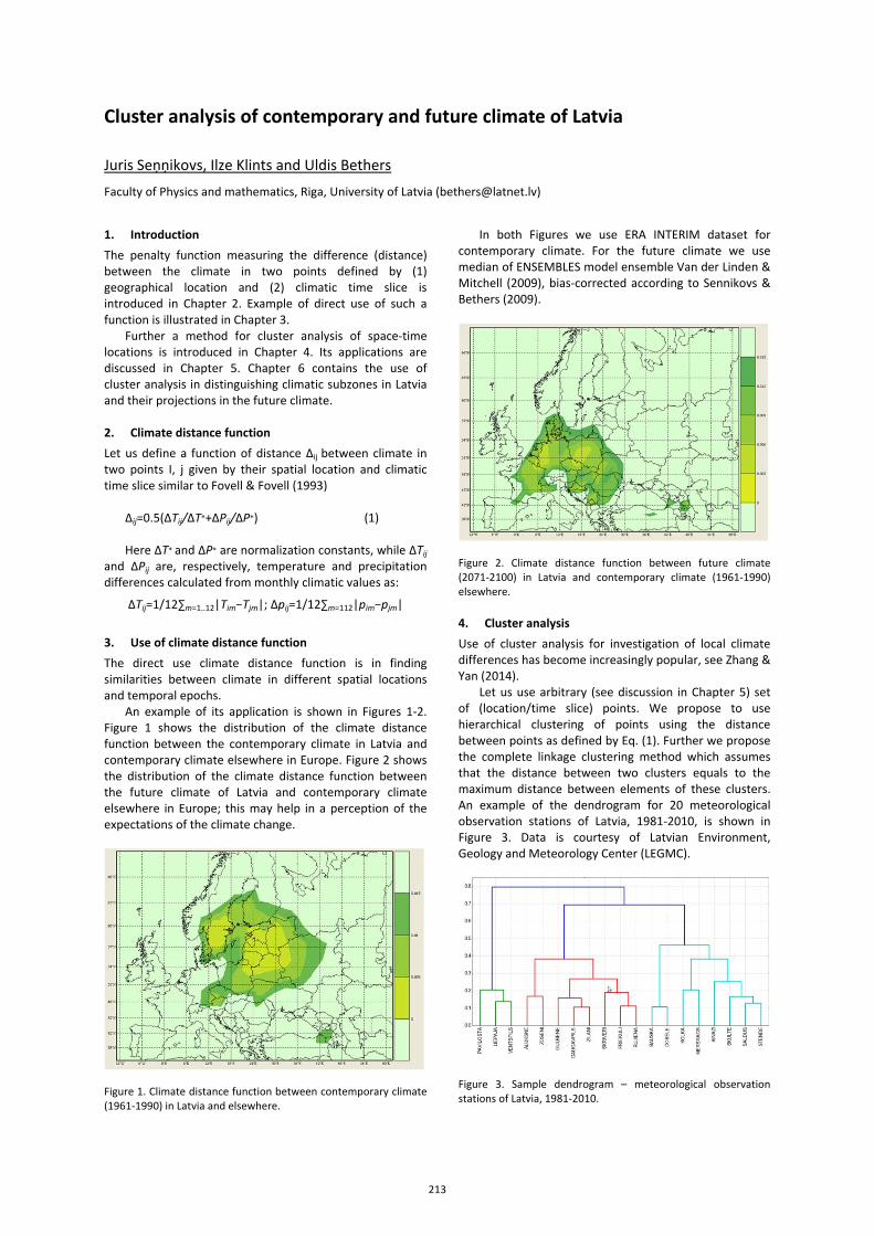
Cluster analysis of contemporary and future climate of Latvia

Juris Seņņikovs, Ilze Klints and Uldis Bethers

Faculty of Physics and mathematics, Riga, University of Latvia (bethers@latnet.lv)

1. Introduction The penalty function measuring the difference (distance) between the climate in two points defined by (1) geographical location and (2) climatic time slice is introduced in Chapter 2. Example of direct use of such a function is illustrated in Chapter 3.

Further a method for cluster analysis of space-time locations is introduced in Chapter 4. Its applications are discussed in Chapter 5. Chapter 6 contains the use of cluster analysis in distinguishing climatic subzones in Latvia and their projections in the future climate. 2. Climate distance function Let us define a function of distance Δij between climate in two points I, j given by their spatial location and climatic time slice similar to Fovell & Fovell (1993)

Δij=0.5(ΔTij/ΔT∗+ΔPij/ΔP∗) (1) Here ΔT∗ and ΔP∗ are normalization constants, while ΔTij

and ΔPij are, respectively, temperature and precipitation differences calculated from monthly climatic values as:

ΔTij=1/12∑m=1..12|Tim−Tjm|; Δpij=1/12∑m=112|pim−pjm|

3. Use of climate distance function The direct use climate distance function is in finding similarities between climate in different spatial locations and temporal epochs.

An example of its application is shown in Figures 1-2. Figure 1 shows the distribution of the climate distance function between the contemporary climate in Latvia and contemporary climate elsewhere in Europe. Figure 2 shows the distribution of the climate distance function between the future climate of Latvia and contemporary climate elsewhere in Europe; this may help in a perception of the expectations of the climate change.

Figure 1. Climate distance function between contemporary climate (1961-1990) in Latvia and elsewhere.

In both Figures we use ERA INTERIM dataset for contemporary climate. For the future climate we use median of ENSEMBLES model ensemble Van der Linden & Mitchell (2009), bias-corrected according to Sennikovs & Bethers (2009).

Figure 2. Climate distance function between future climate (2071-2100) in Latvia and contemporary climate (1961-1990) elsewhere. 4. Cluster analysis Use of cluster analysis for investigation of local climate differences has become increasingly popular, see Zhang & Yan (2014).

Let us use arbitrary (see discussion in Chapter 5) set of (location/time slice) points. We propose to use hierarchical clustering of points using the distance between points as defined by Eq. (1). Further we propose the complete linkage clustering method which assumes that the distance between two clusters equals to the maximum distance between elements of these clusters. An example of the dendrogram for 20 meteorological observation stations of Latvia, 1981-2010, is shown in Figure 3. Data is courtesy of Latvian Environment, Geology and Meteorology Center (LEGMC).

Figure 3. Sample dendrogram – meteorological observation stations of Latvia, 1981-2010.

213

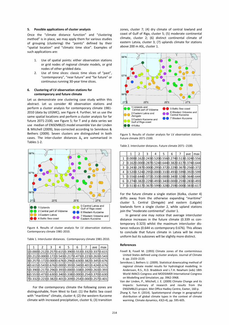
5. Possible applications of cluster analysis Once the “climate distance function” and “clustering method” is in place, we may apply them for various studies of grouping (clustering) the “points” defined by their “spatial location” and “climatic time slice”. Examples of such applications are:

1. Use of spatial points: either observation stations or grid nodes of regional climate models, or grid nodes of other gridded data.

2. Use of time slices: classic time slices of “past”, “contemporary”, “near future” and “far future” or continuous running 30-year time slices.

6. Clustering of LV observation stations for

contemporary and future climate Let us demonstrate one clustering case study within this abstract. Let us consider 40 observation stations and perform a cluster analysis for contemporary climate 1981-2010 (data by LEGMC), see Figure 4. Further, let us use the same spatial locations and perform a cluster analysis for far future 2071-2100, see Figure 5; for T and p data series we use median of ENSEMBLES model ensemble Van der Linden & Mitchell (2009), bias-corrected according to Sennikovs & Bethers (2009). Seven clusters are distinguished in both cases. The inter-cluster distances Δij are summarised in Tables 1-2.

Figure 4. Results of cluster analysis for LV observation stations. Contemporary climate 1981-2010. Table 1. Intercluster distances. Contemporary climate 1981-2010.

1 2 3 4 5 6 7 ave max1 0.000 0.212 0.257 0.615 0.390 0.553 0.332 0.337 0.6152 0.212 0.000 0.172 0.543 0.217 0.473 0.223 0.263 0.5433 0.257 0.172 0.000 0.676 0.296 0.630 0.382 0.345 0.6764 0.615 0.543 0.676 0.000 0.393 0.340 0.401 0.424 0.6765 0.390 0.217 0.296 0.393 0.000 0.338 0.209 0.263 0.3936 0.553 0.473 0.630 0.340 0.338 0.000 0.254 0.370 0.6307 0.332 0.223 0.382 0.401 0.209 0.254 0.000 0.257 0.401

For the contemporary climate the following zones are distinguishable, from West to East: (1) the Baltic Sea coast with “maritime” climate, cluster 4; (2) the western Kurzeme climate with increased precipitation, cluster 6; (3) transition

zones, cluster 7; (4) dry climate of central lowland and coast of Gulf of Riga, cluster 5; (5) moderate continental climate, cluster 2; (6) distinct continental climate of eastern Latvia, cluster 3; (7) uplands climate for stations above 200 m ASL, cluster 1.

Figure 5. Results of cluster analysis for LV observation stations. Future climate 2071-2100. Table 2. Intercluster distances. Future climate 2071--2100.

1 2 3 4 5 6 7 ave max1 0.0000.1620.2430.5200.556 0.274 0.513 0.3240.5562 0.1620.0000.2870.5240.644 0.382 0.617 0.3740.6443 0.2430.2870.0000.2950.372 0.229 0.367 0.2560.3724 0.5200.5240.2950.0000.310 0.493 0.599 0.3920.5995 0.5560.6440.3720.3100.000 0.340 0.328 0.3640.6446 0.2740.3820.2290.4930.340 0.000 0.259 0.2830.4937 0.5130.6170.3670.5990.328 0.259 0.000 0.3830.617

For the future climate a single station (Kolka, cluster 4) drifts away from the otherwise expanding “maritime” cluster 5. Central (Zemgale) and eastern (Latgale) lowlands form a single cluster 2, while upland stations join the “moderate continental” cluster 1.

In general one may notice that average intercluster distance increases in the future climate (0.339 vs con-temporary 0.323) whilst the maximum intercluster dis-tance reduces (0.644 vs contemporary 0.676). This allows to conclude that future climate in Latvia will be more uniform but its subzones will be slightly more distinct. References

Fovell B, Fovell M. (1993) Climate zones of the conterminous United States defined using cluster analysis. Journal of Climate 6: pp. 2103–2135

Sennikovs J, Bethers U. (2009). Statistical downscaling method of regional climate model results for hydrological modelling. In Anderssen, R.S., R.D. Braddock and L.T.H. Newham (eds) 18th World IMACS Congress and MODSIM09 International Congress on Modelling and Simulation, pp. 3962-3968.

Van der Linden, P., Mitchell, J. E. (2009) Climate Change and its Impacts: Summary of research and results from the ENSEMBLES project. Met Office Hadley Centre, Exeter, 160 p.

Zhang X, Yan X. (2014). Spatiotemporal change in geographical distribution of global climate types in the context of climate warming. Climate dynamics, 43(3-4), pp. 595-605.

214

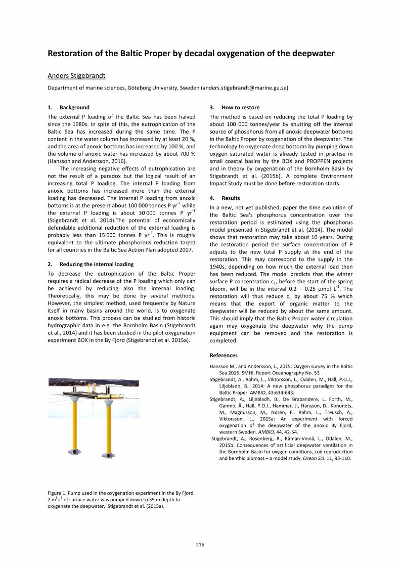
Restoration of the Baltic Proper by decadal oxygenation of the deepwater

Anders Stigebrandt

Department of marine sciences, Göteborg University, Sweden (anders.stigebrandt@marine.gu.se)

1. Background The external P loading of the Baltic Sea has been halved since the 1980s. In spite of this, the eutrophication of the Baltic Sea has increased during the same time. The P content in the water column has increased by at least 20 %, and the area of anoxic bottoms has increased by 100 %, and the volume of anoxic water has increased by about 700 % (Hansson and Andersson, 2016).

The increasing negative effects of eutrophication are not the result of a paradox but the logical result of an increasing total P loading. The internal P loading from anoxic bottoms has increased more than the external loading has decreased. The internal P loading from anoxic bottoms is at the present about 100 000 tonnes P yr-1 while the external P loading is about 30 000 tonnes P yr-1 (Stigebrandt et al. 2014).The potential of economically defendable additional reduction of the external loading is probably less than 15 000 tonnes P yr-1. This is roughly equivalent to the ultimate phosphorous reduction target for all countries in the Baltic Sea Action Plan adopted 2007. 2. Reducing the internal loading To decrease the eutrophication of the Baltic Proper requires a radical decrease of the P loading which only can be achieved by reducing also the internal loading. Theoretically, this may be done by several methods. However, the simplest method, used frequently by Nature itself in many basins around the world, is to oxygenate anoxic bottoms. This process can be studied from historic hydrographic data in e.g. the Bornholm Basin (Stigebrandt et al., 2014) and it has been studied in the pilot oxygenation experiment BOX in the By Fjord (Stigebrandt et al. 2015a).

Figure 1. Pump used in the oxygenation experiment in the By Fjord. 2 m3s-1 of surface water was pumped down to 35 m depth to oxygenate the deepwater, Stigebrandt et al. (2015a).

3. How to restore The method is based on reducing the total P loading by about 100 000 tonnes/year by shutting off the internal source of phosphorus from all anoxic deepwater bottoms in the Baltic Proper by oxygenation of the deepwater. The technology to oxygenate deep bottoms by pumping down oxygen saturated water is already tested in practise in small coastal basins by the BOX and PROPPEN projects and in theory by oxygenation of the Bornholm Basin by Stigebrandt et al. (2015b). A complete Environment Impact Study must be done before restoration starts. 4. Results In a new, not yet published, paper the time evolution of the Baltic Sea's phosphorus concentration over the restoration period is estimated using the phosphorus model presented in Stigebrandt et al. (2014). The model shows that restoration may take about 10 years. During the restoration period the surface concentration of P adjusts to the new total P supply at the end of the restoration. This may correspond to the supply in the 1940s, depending on how much the external load then has been reduced. The model predicts that the winter surface P concentration c1, before the start of the spring bloom, will be in the interval 0.2 – 0.25 µmol L-1. The restoration will thus reduce c1 by about 75 % which means that the export of organic matter to the deepwater will be reduced by about the same amount. This should imply that the Baltic Proper water circulation again may oxygenate the deepwater why the pump equipment can be removed and the restoration is completed. References

Hansson M., and Andersson, L., 2015: Oxygen survey in the Baltic Sea 2015. SMHI, Report Oceanography No. 53

Stigebrandt, A., Rahm, L., Viktorsson, L., Ödalen, M., Hall, P.O.J., Liljebladh, B., 2014: A new phosphorus paradigm for the Baltic Proper. AMBIO, 43:634-643.

Stigebrandt, A., Liljebladh, B., De Brabandere, L. Forth, M., Ganmo, Å., Hall, P.O.J., Hammar, J., Hansson, D., Kononets, M., Magnusson, M., Norén, F., Rahm, L., Treusch, A., Viktorsson, L., 2015a: An experiment with forced oxygenation of the deepwater of the anoxic By Fjord, western Sweden. AMBIO, 44, 42-54.

Stigebrandt, A., Rosenberg, R., Råman-Vinnå, L., Ödalen, M., 2015b: Consequences of artificial deepwater ventilation in the Bornholm Basin for oxygen conditions, cod reproduction and benthic biomass – a model study. Ocean Sci. 11, 93-110.

215

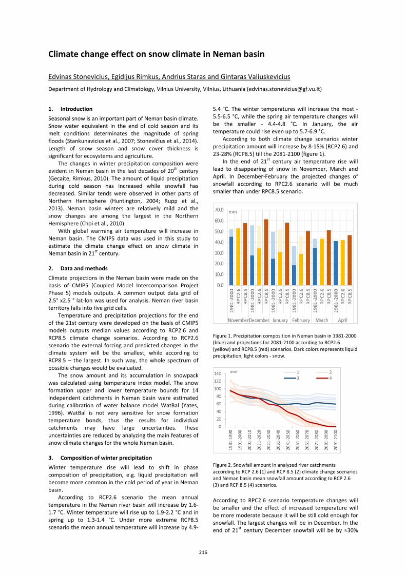
Climate change effect on snow climate in Neman basin

Edvinas Stonevicius, Egidijus Rimkus, Andrius Staras and Gintaras Valiuskevicius

Department of Hydrology and Climatology, Vilnius University, Vilnius, Lithuania (edvinas.stonevicius@gf.vu.lt)

1. Introduction Seasonal snow is an important part of Neman basin climate. Snow water equivalent in the end of cold season and its melt conditions determinates the magnitude of spring floods (Stankunavicius et al., 2007; Stonevičius et al., 2014). Length of snow season and snow cover thickness is significant for ecosystems and agriculture.

The changes in winter precipitation composition were evident in Neman basin in the last decades of 20th century (Gecaite, Rimkus, 2010). The amount of liquid precipitation during cold season has increased while snowfall has decreased. Similar tends were observed in other parts of Northern Hemisphere (Huntington, 2004; Rupp et al., 2013). Neman basin winters are relatively mild and the snow changes are among the largest in the Northern Hemisphere (Choi et al., 2010)

With global warming air temperature will increase in Neman basin. The CMIP5 data was used in this study to estimate the climate change effect on snow climate in Neman basin in 21st century. 2. Data and methods Climate projections in the Neman basin were made on the basis of CMIP5 (Coupled Model Intercomparison Project Phase 5) models outputs. A common output data grid of 2.5° x2.5 ° lat-lon was used for analysis. Neman river basin territory falls into five grid cells.

Temperature and precipitation projections for the end of the 21st century were developed on the basis of CMIP5 models outputs median values according to RCP2.6 and RCP8.5 climate change scenarios. According to RCP2.6 scenario the external forcing and predicted changes in the climate system will be the smallest, while according to RCP8.5 – the largest. In such way, the whole spectrum of possible changes would be evaluated.

The snow amount and its accumulation in snowpack was calculated using temperature index model. The snow formation upper and lower temperature bounds for 14 independent catchments in Neman basin were estimated during calibration of water balance model WatBal (Yates, 1996). WatBal is not very sensitive for snow formation temperature bonds, thus the results for individual catchments may have large uncertainties. These uncertainties are reduced by analyzing the main features of snow climate changes for the whole Neman basin. 3. Composition of winter precipitation Winter temperature rise will lead to shift in phase composition of precipitation, e.g. liquid precipitation will become more common in the cold period of year in Neman basin.

According to RCP2.6 scenario the mean annual temperature in the Neman river basin will increase by 1.6-1.7 °C. Winter temperature will rise up to 1.9-2.2 °C and in spring up to 1.3-1.4 °C. Under more extreme RCP8.5 scenario the mean annual temperature will increase by 4.9-

5.4 °C. The winter temperatures will increase the most - 5.5-6.5 °C, while the spring air temperature changes will be the smaller - 4.4-4.8 °C. In January, the air temperature could rise even up to 5.7-6.9 °C.

According to both climate change scenarios winter precipitation amount will increase by 8-15% (RCP2.6) and 23-28% (RCP8.5) till the 2081-2100 (figure 1).

In the end of 21st century air temperature rise will lead to disappearing of snow in November, March and April. In December-February the projected changes of snowfall according to RPC2.6 scenario will be much smaller than under RPC8.5 scenario.

Figure 1. Precipitation composition in Neman basin in 1981-2000 (blue) and projections for 2081-2100 according to RCP2.6 (yellow) and RCP8.5 (red) scenarios. Dark colors represents liquid precipitation, light colors - snow.

Figure 2. Snowfall amount in analyzed river catchments according to RCP 2.6 (1) and RCP 8.5 (2) climate change scenarios and Neman basin mean snowfall amount according to RCP 2.6 (3) and RCP 8.5 (4) scenarios.

According to RPC2.6 scenario temperature changes will be smaller and the effect of increased temperature will be more moderate because it will be still cold enough for snowfall. The largest changes will be in December. In the end of 21st century December snowfall will be by ≈30%

216

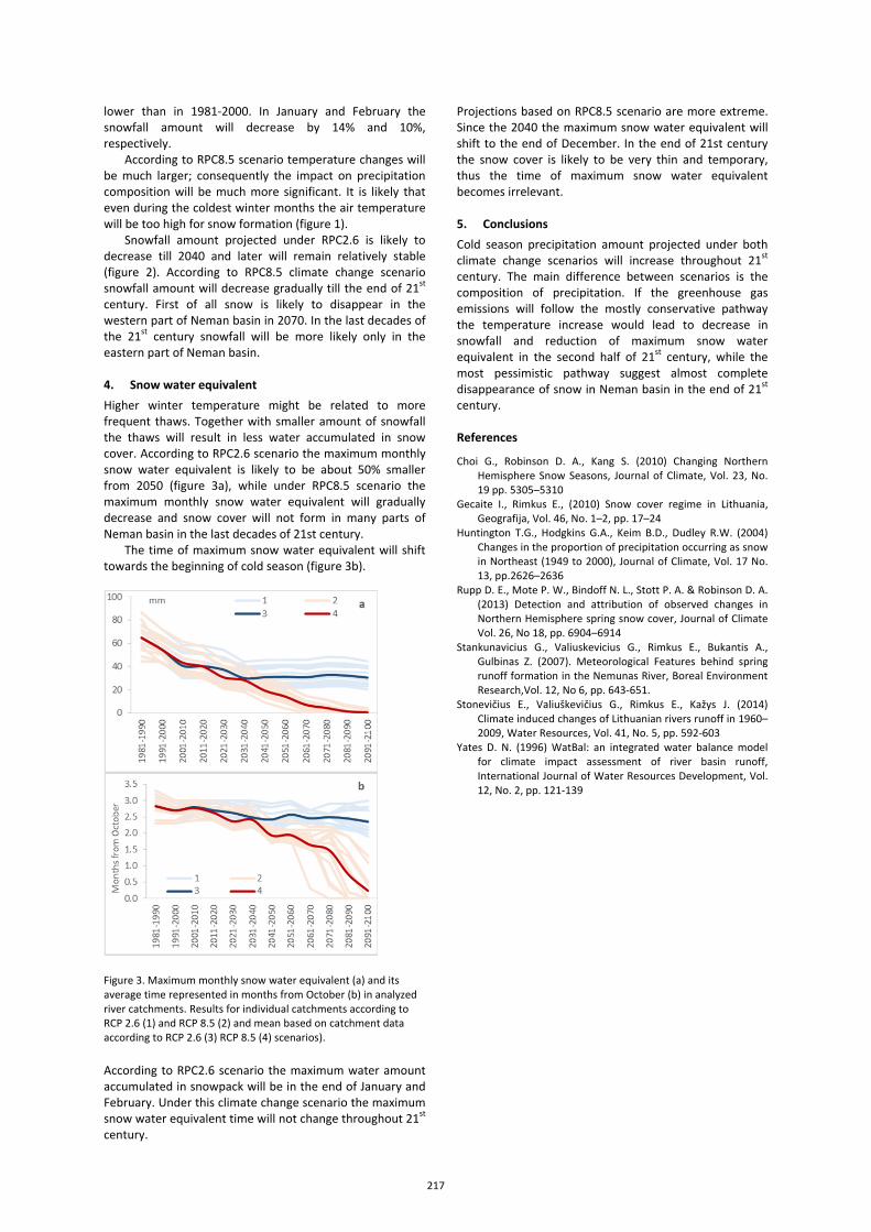
lower than in 1981-2000. In January and February the snowfall amount will decrease by 14% and 10%, respectively.

According to RPC8.5 scenario temperature changes will be much larger; consequently the impact on precipitation composition will be much more significant. It is likely that even during the coldest winter months the air temperature will be too high for snow formation (figure 1).

Snowfall amount projected under RPC2.6 is likely to decrease till 2040 and later will remain relatively stable (figure 2). According to RPC8.5 climate change scenario snowfall amount will decrease gradually till the end of 21st century. First of all snow is likely to disappear in the western part of Neman basin in 2070. In the last decades of the 21st century snowfall will be more likely only in the eastern part of Neman basin. 4. Snow water equivalent Higher winter temperature might be related to more frequent thaws. Together with smaller amount of snowfall the thaws will result in less water accumulated in snow cover. According to RPC2.6 scenario the maximum monthly snow water equivalent is likely to be about 50% smaller from 2050 (figure 3a), while under RPC8.5 scenario the maximum monthly snow water equivalent will gradually decrease and snow cover will not form in many parts of Neman basin in the last decades of 21st century.

The time of maximum snow water equivalent will shift towards the beginning of cold season (figure 3b).

Figure 3. Maximum monthly snow water equivalent (a) and its average time represented in months from October (b) in analyzed river catchments. Results for individual catchments according to RCP 2.6 (1) and RCP 8.5 (2) and mean based on catchment data according to RCP 2.6 (3) RCP 8.5 (4) scenarios).

According to RPC2.6 scenario the maximum water amount accumulated in snowpack will be in the end of January and February. Under this climate change scenario the maximum snow water equivalent time will not change throughout 21st century.

Projections based on RPC8.5 scenario are more extreme. Since the 2040 the maximum snow water equivalent will shift to the end of December. In the end of 21st century the snow cover is likely to be very thin and temporary, thus the time of maximum snow water equivalent becomes irrelevant. 5. Conclusions Cold season precipitation amount projected under both climate change scenarios will increase throughout 21st century. The main difference between scenarios is the composition of precipitation. If the greenhouse gas emissions will follow the mostly conservative pathway the temperature increase would lead to decrease in snowfall and reduction of maximum snow water equivalent in the second half of 21st century, while the most pessimistic pathway suggest almost complete disappearance of snow in Neman basin in the end of 21st century. References

Choi G., Robinson D. A., Kang S. (2010) Changing Northern Hemisphere Snow Seasons, Journal of Climate, Vol. 23, No. 19 pp. 5305–5310

Gecaite I., Rimkus E., (2010) Snow cover regime in Lithuania, Geografija, Vol. 46, No. 1–2, pp. 17–24

Huntington T.G., Hodgkins G.A., Keim B.D., Dudley R.W. (2004) Changes in the proportion of precipitation occurring as snow in Northeast (1949 to 2000), Journal of Climate, Vol. 17 No. 13, pp.2626–2636

Rupp D. E., Mote P. W., Bindoff N. L., Stott P. A. & Robinson D. A. (2013) Detection and attribution of observed changes in Northern Hemisphere spring snow cover, Journal of Climate Vol. 26, No 18, pp. 6904–6914

Stankunavicius G., Valiuskevicius G., Rimkus E., Bukantis A., Gulbinas Z. (2007). Meteorological Features behind spring runoff formation in the Nemunas River, Boreal Environment Research,Vol. 12, No 6, pp. 643-651.

Stonevičius E., Valiuškevičius G., Rimkus E., Kažys J. (2014) Climate induced changes of Lithuanian rivers runoff in 1960–2009, Water Resources, Vol. 41, No. 5, pp. 592-603

Yates D. N. (1996) WatBal: an integrated water balance model for climate impact assessment of river basin runoff, International Journal of Water Resources Development, Vol. 12, No. 2, pp. 121-139

217

Psychophysical aesthetic ranking of coastal landscapes: A case study of the Curonian Spit (Lithuania)

Arvydas Urbis and Ramūnas Povilanskas

Klaipėda University, Lithuania (arvydasurbisku@gmail.com)

Two contrasting research lines – ‘objectivist’ and ‘subjectivist’ – have dominated landscape aesthetics for the last half-century. Hence two different methodological approaches in scenic quality appraisal of various coastal landscapes: an expert-based one vs. a visitor-based one. A psychophysical approach combines these both perspectives into an integrated scenic quality appraisal methodology. In our presentation we also address a long-lasting debate in landscape aesthetics focusing on a fundamental issue of what makes certain types of scenery more beautiful than other ones from the psychophysical point of view. This debate is illustrated practically by assessing a comparative aesthetic appeal of the main dune habitats and landscapes on the Curonian Spit which is a UNESCO-listed World Heritage landscape. For this aim a paired comparison method was applied. The results of our study show that the most attractive dune landscapes of the Curonian Spit are: 1) White shifting dunes; 2) Grey dunes in the foreground with White dunes in the background White dunes in the foreground with, and 3) Grey (grassland) dunes in the background. These results deny the key tenets of both the social and the ecological approach in landscape aesthetics opening new perspectives for a psychophysical interpretation of scenic beauty.

218

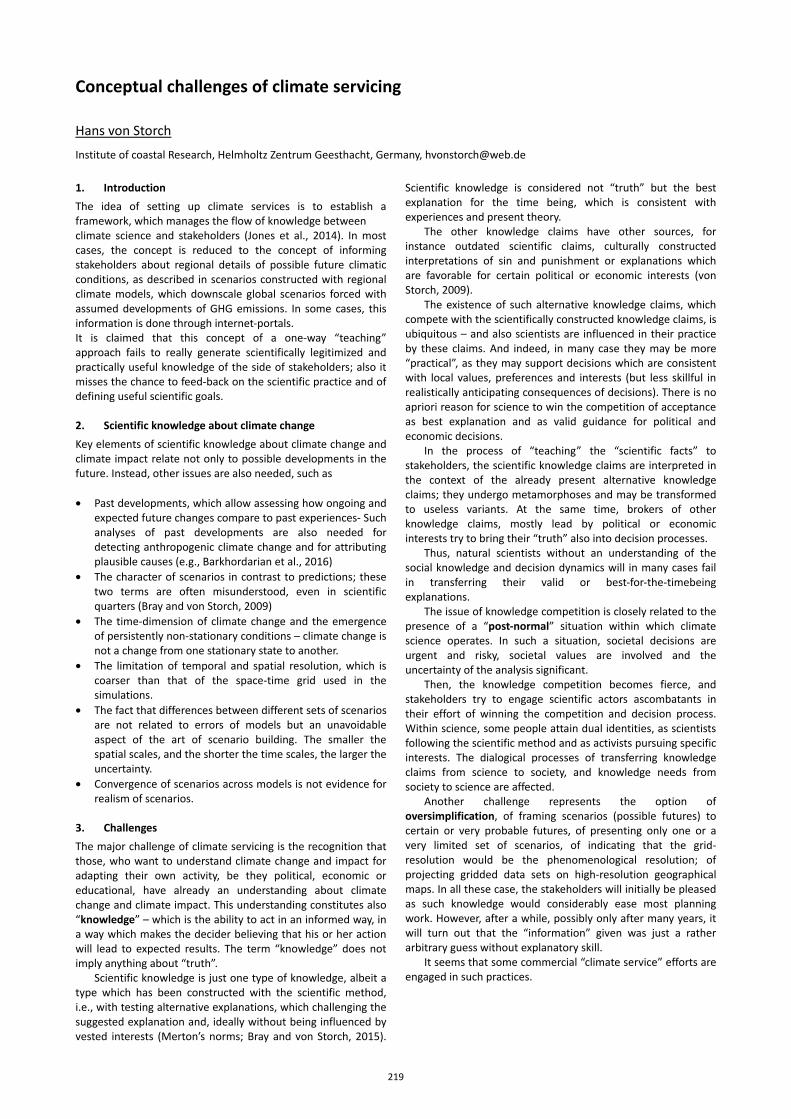
Conceptual challenges of climate servicing

Hans von Storch

Institute of coastal Research, Helmholtz Zentrum Geesthacht, Germany, hvonstorch@web.de

1. Introduction The idea of setting up climate services is to establish a framework, which manages the flow of knowledge between climate science and stakeholders (Jones et al., 2014). In most cases, the concept is reduced to the concept of informing stakeholders about regional details of possible future climatic conditions, as described in scenarios constructed with regional climate models, which downscale global scenarios forced with assumed developments of GHG emissions. In some cases, this information is done through internet‐portals. It is claimed that this concept of a one‐way “teaching” approach fails to really generate scientifically legitimized and practically useful knowledge of the side of stakeholders; also it misses the chance to feed‐back on the scientific practice and of defining useful scientific goals. 2. Scientific knowledge about climate change Key elements of scientific knowledge about climate change and climate impact relate not only to possible developments in the future. Instead, other issues are also needed, such as • Past developments, which allow assessing how ongoing and

expected future changes compare to past experiences‐ Such analyses of past developments are also needed for detecting anthropogenic climate change and for attributing plausible causes (e.g., Barkhordarian et al., 2016)

• The character of scenarios in contrast to predictions; these two terms are often misunderstood, even in scientific quarters (Bray and von Storch, 2009)

• The time‐dimension of climate change and the emergence of persistently non‐stationary conditions – climate change is not a change from one stationary state to another.

• The limitation of temporal and spatial resolution, which is coarser than that of the space‐time grid used in the simulations.

• The fact that differences between different sets of scenarios are not related to errors of models but an unavoidable aspect of the art of scenario building. The smaller the spatial scales, and the shorter the time scales, the larger the uncertainty.

• Convergence of scenarios across models is not evidence for realism of scenarios.

3. Challenges The major challenge of climate servicing is the recognition that those, who want to understand climate change and impact for adapting their own activity, be they political, economic or educational, have already an understanding about climate change and climate impact. This understanding constitutes also “knowledge” – which is the ability to act in an informed way, in a way which makes the decider believing that his or her action will lead to expected results. The term “knowledge” does not imply anything about “truth”.

Scientific knowledge is just one type of knowledge, albeit a type which has been constructed with the scientific method, i.e., with testing alternative explanations, which challenging the suggested explanation and, ideally without being influenced by vested interests (Merton’s norms; Bray and von Storch, 2015).

Scientific knowledge is considered not “truth” but the best explanation for the time being, which is consistent with experiences and present theory.

The other knowledge claims have other sources, for instance outdated scientific claims, culturally constructed interpretations of sin and punishment or explanations which are favorable for certain political or economic interests (von Storch, 2009).

The existence of such alternative knowledge claims, which compete with the scientifically constructed knowledge claims, is ubiquitous – and also scientists are influenced in their practice by these claims. And indeed, in many case they may be more “practical”, as they may support decisions which are consistent with local values, preferences and interests (but less skillful in realistically anticipating consequences of decisions). There is no apriori reason for science to win the competition of acceptance as best explanation and as valid guidance for political and economic decisions.

In the process of “teaching” the “scientific facts” to stakeholders, the scientific knowledge claims are interpreted in the context of the already present alternative knowledge claims; they undergo metamorphoses and may be transformed to useless variants. At the same time, brokers of other knowledge claims, mostly lead by political or economic interests try to bring their “truth” also into decision processes.

Thus, natural scientists without an understanding of the social knowledge and decision dynamics will in many cases fail in transferring their valid or best‐for‐the‐timebeing explanations.

The issue of knowledge competition is closely related to the presence of a “post‐normal” situation within which climate science operates. In such a situation, societal decisions are urgent and risky, societal values are involved and the uncertainty of the analysis significant.

Then, the knowledge competition becomes fierce, and stakeholders try to engage scientific actors ascombatants in their effort of winning the competition and decision process. Within science, some people attain dual identities, as scientists following the scientific method and as activists pursuing specific interests. The dialogical processes of transferring knowledge claims from science to society, and knowledge needs from society to science are affected.

Another challenge represents the option of oversimplification, of framing scenarios (possible futures) to certain or very probable futures, of presenting only one or a very limited set of scenarios, of indicating that the grid‐resolution would be the phenomenological resolution; of projecting gridded data sets on high‐resolution geographical maps. In all these case, the stakeholders will initially be pleased as such knowledge would considerably ease most planning work. However, after a while, possibly only after many years, it will turn out that the “information” given was just a rather arbitrary guess without explanatory skill.

It seems that some commercial “climate service” efforts are engaged in such practices.

219

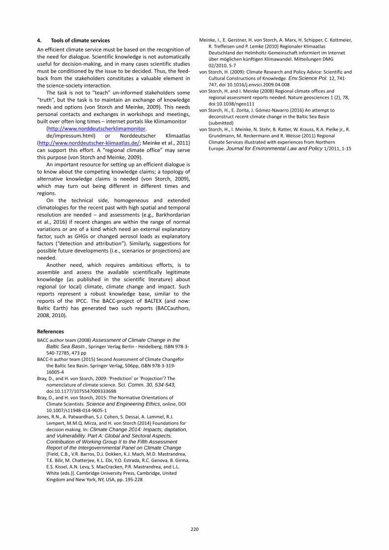
4. Tools of climate services An efficient climate service must be based on the recognition of the need for dialogue. Scientific knowledge is not automatically useful for decision‐making, and in many cases scientific studies must be conditioned by the issue to be decided. Thus, the feed‐back from the stakeholders constitutes a valuable element in the science‐society interaction.

The task is not to “teach” un‐informed stakeholders some “truth”, but the task is to maintain an exchange of knowledge needs and options (von Storch and Meinke, 2009). This needs personal contacts and exchanges in workshops and meetings, built over often long times – internet portals like Klimamonitor

(http://www.norddeutscherklimamonitor. de/impressum.html) or Norddeutscher Klimaatlas

(http://www.norddeutscher‐klimaatlas.de/; Meinke et al., 2011) can support this effort. A “regional climate office” may serve this purpose (von Storch and Meinke, 2009).

An important resource for setting up an efficient dialogue is to know about the competing knowledge claims; a topology of alternative knowledge claims is needed (von Storch, 2009), which may turn out being different in different times and regions.

On the technical side, homogeneous and extended climatologies for the recent past with high spatial and temporal resolution are needed – and assessments (e.g., Barkhordarian et al., 2016) if recent changes are within the range of normal variations or are of a kind which need an external explanatory factor, such as GHGs or changed aerosol loads as explanatory factors (“detection and attribution”). Similarly, suggestions for possible future developments (i.e., scenarios or projections) are needed.

Another need, which requires ambitious efforts, is to assemble and assess the available scientifically legitimate knowledge (as published in the scientific literature) about regional (or local) climate, climate change and impact. Such reports represent a robust knowledge base, similar to the reports of the IPCC. The BACC‐project of BALTEX (and now: Baltic Earth) has generated two such reports (BACCauthors, 2008, 2010). References BACC author team (2008) Assessment of Climate Change in the

Baltic Sea Basin., Springer Verlag Berlin ‐ Heidelberg; ISBN 978‐3‐540‐72785, 473 pp

BACC‐II author team (2015) Second Assessment of Climate Changefor the Baltic Sea Basin. Springer Verlag, 506pp, ISBN 978‐3‐319‐16005‐4

Bray, D., and H. von Storch, 2009: 'Prediction' or 'Projection'? The nomenclature of climate science. Sci. Comm. 30, 534‐543, doi:10.1177/1075547009333698

Bray, D., and H. von Storch, 2015: The Normative Orientations of Climate Scientists. Science and Engineering Ethics, online, DOI 10.1007/s11948‐014‐9605‐1

Jones, R.N., A. Patwardhan, S.J. Cohen, S. Dessai, A. Lammel, R.J. Lempert, M.M.Q. Mirza, and H. von Storch (2014) Foundations for decision making. In: Climate Change 2014: Impacts, daptation, and Vulnerability. Part A: Global and Sectoral Aspects. Contribution of Working Group II to the Fifth Assessment Report of the Intergovernmental Panel on Climate Change [Field, C.B., V.R. Barros, D.J. Dokken, K.J. Mach, M.D. Mastrandrea, T.E. Bilir, M. Chatterjee, K.L. Ebi, Y.O. Estrada, R.C. Genova, B. Girma, E.S. Kissel, A.N. Levy, S. MacCracken, P.R. Mastrandrea, and L.L. White (eds.)]. Cambridge University Press, Cambridge, United Kingdom and New York, NY, USA, pp. 195‐228

Meinke, I., E. Gerstner, H. von Storch, A. Marx, H. Schipper, C. Kottmeier, R. Treffeisen und P. Lemke (2010) Regionaler Klimaatlas Deutschland der Helmholtz‐Gemeinschaft informiert im Internet über möglichen künftigen Klimawandel. Mitteilungen DMG 02/2010, 5‐7

von Storch, H. (2009): Climate Research and Policy Advice: Scientific and Cultural Constructions of Knowledge. Env.Science Pol. 12, 741‐747, doi 10.1016/j.envsci.2009.04.008

von Storch, H. and I. Meinke (2008) Regional climate offices and regional assessment reports needed. Nature geosciences 1 (2), 78, doi:10.1038/ngeo111

von Storch, H., E. Zorita, J. Gómez‐Navarro (2016) An attempt to deconstruct recent climate change in the Baltic Sea Basin (submitted)

von Storch, H., I. Meinke, N. Stehr, B. Ratter, W. Krauss, R.A. Pielke jr., R. Grundmann, M. Reckermann and R. Weisse (2011) Regional Climate Services illustrated with experiences from Northern Europe. Journal for Environmental Law and Policy 1/2011, 1‐15

220

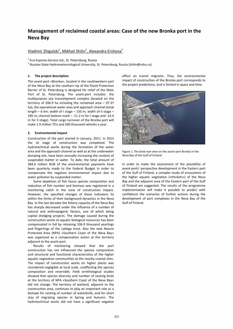
Management of reclaimed coastal areas: Case of the new Bronka port in the Neva Bay

Vladimir Zhigulski1, Mikhail Shilin2, Alexandra Ershova2

1 Eco-Express-Service Ltd., St. Petersburg, Russia 2 Russian State Hydrometeorological University, St. Petersburg, Russia (shilin@rshu.ru)

1. The project description The avant-port «Bronka», located in the southwestern part of the Neva Bay at the southern tip of the Flood Protection Barrier of St. Petersburg is designed for relief of the Main Port of St. Petersburg. The avant-port includes: the multipurpose sea transshipment complex (located on the territory of 206.9 ha including the reclaimed area – 97.37 ha), the operational water area and approach channel (total length – 6 km; width of I stage – 150 m, width of II stage – 185 m; channel bottom mark – -11.2 m for I stage and -14.4 m for II stage). Total cargo turnover of the Bronka port will make 1.9 million TEU and 260 thousand vehicles a year.

2. Environmental impact Construction of the port started in January, 2011. In 2015 the Ist stage of construction was completed. The hydrotechnical works during the formation of the water area and the approach channel as well as at the underwater dumping site, have been annually increasing the content of suspended matter in water. To date, the total amount of 384.6 million RUB of the environmental payments have been quarterly made to the Federal Budget in order to compensate the negative environmental impact due to water pollution by suspended matter.

Some depletion of fish fauna species composition and reduction of fish number and biomass was registered in a monitoring catch in the zone of construction impact. However, the specified changes of these indicators lie within the limits of their background dynamics in the Neva Bay. In the last decades the fishery capacity of the Neva Bay has sharply decreased under the influence of a number of natural and anthropogenic factors, one of which being capital dredging projects. The damage caused during the construction works to aquatic biological resources has been compensated in full by releasing 336.9 thousand yearlings and fingerlings of the Ladoga trout. Also the new Nature Protected Area (NPA) «Southern Coast of the Neva Bay» was organized as a compensation action at the territory adjacent to the avant-port.

Results of monitoring showed that the port construction has not influenced the species composition and structural and functional characteristics of the higher aquatic vegetation communities at the nearby coastal sites. The impact of construction works on higher plants was considered negligible at local scale, unaffecting the species composition and reversible. Field ornithological studies showed that species diversity and number of nesting birds at the territory of NPA «Southern Coast of the Neva Bay» did not change. The territory of wetland, adjacent to the construction area, continues to play an important role as a biotope for nesting of number of waterbirds, and for short stay of migrating species in Spring and Autumn. The hydrotechnical works did not have a significant negative

effect on transit migrants. Thus, the environmental impact of construction of the Bronka port corresponds to the project predictions, and is limited in space and time.

Figure 1. The birds-eye view on the avant-port Bronka in the Neva Bay of the Gulf of Finland

In order to make the assessment of the possibility of avant-ports’ perspective development in the Eastern part of the Gulf of Finland, a complex study of ecosystems of the higher aquatic vegetation («thickets») of the Neva Bay and the adjacent area of the Eastern part of the Gulf of Finland are suggested. The results of the programme implementation will make it possible to predict with confidence the scenarios of further actions during the development of port complexes in the Neva Bay of the Gulf of Finland.

221

222

International Baltic Earth Secretariat Publications ISSN 2198-4247

No. 1 Programme, Abstracts, Participants. Baltic Earth Workshop on ”Natural hazards and extreme events in the Baltic Sea region”. Finnish Meteorological Institute, Dynamicum, Helsinki, 30-31 January 2014. International Baltic Earth Secretariat Publication No. 1, 33 pp, January 2014.

No. 2 Conference Proceedings of the 2nd International Conference on Climate Change - The

environmental and socio-economic response in the Southern Baltic region. Szczecin, Poland, 12-15 May 2014. International Baltic Earth Secretariat Publication No. 2, 110 pp, May 2014.

No. 3 Workshop Proceedings of the 3rd International Lund Regional-Scale Climate Modelling

Workshop ”21st Century Challenges in Regional Climate Modelling”. Lund, Sweden, 16-19 June 2014. International Baltic Earth Secretariat Publication No. 3, 391 pp, June 2014.

No. 4 Programme, Abstracts, Participants. Baltic Earth - Gulf of Finland Year 2014 Modelling

Workshop ”Modelling as a tool to ensure sustainable development of the Gulf of Finland-Baltic Sea ecosystem”. Finnish Environment Institute SYKE, Helsinki, 24-25 November 2014. International Baltic Earth Secretariat Publication No. 4, 27 pp, November 2014.

No. 5 Programme, Abstracts, Participants. A Doctoral Students Conference Challenges for Earth

system science in the Baltic Sea region: From measurements to models. University of Tartu and Vilsandi Island, Estonia, 10 - 14 August 2015. International Baltic Earth Secretariat Publication No. 5, 66 pp, August 2015.

No. 6 Programme, Abstracts, Participants. International advanced PhD course on Impact of

climate change on the marine environment with special focus on the role of changing extremes. Askö Laboratory, Trosa, Sweden, 24 - 30 August 2015 International Baltic Earth Secretariat Publication No. 6, 61 pp, August 2015.

No. 7 Programme, Abstracts, Participants. HyMex-Baltic Earth Workshop: "Joint regional climate

system modelling for the European sea regions". ENEA, Rome, Italy, 5-6 November 2015. International Baltic Earth Secretariat Publication No. 7, 103 pp, October 2015

No. 8 Programme, Abstracts, Participants. A PhD seminar in connection with the Gulf of Finland

Scientific Forum: "Exchange process between the Gulf of Finland and other Baltic Sea basins". Tallinn, Estonia, 19 November 2015. International Baltic Earth Secretariat Publication No. 8, 27 pp, November 2015

No. 9 Conference Proceedings. 1st Baltic Earth Conference. Multiple drivers for Earth system

changes in the Baltic Sea region. Nida, Curonian Spit, Lithuania, 13 - 17 June 2016. International Baltic Earth Secretariat Publication No. 9, 222 pp, June 2016.

For a list of International BALTEX Secretariat Publications (ISSN 1681-6471), see www.baltex-research.eu/publications

International Baltic Earth Secretariat PublicationsISSN 2198-4247