ronen-j-1981-phd-thesis.pdf - spiral@imperial college
TRANSCRIPT

TECHNIQUES FOR MONITORING THE PERFORMANCE
OF PHASED-ARRAY ANTENNAS
by
JACOB RONEN
A Thesis submitted for the Degree of Doctor
of Philosophy in the Faculty of Engineering,
University of London and the Diploma of
Membership of the Imperial College (DIC)
Department of Electrical Engineering
Imperial College of Science and Technology
Exhibition Road, London, S.W.7
January, 1981

- ii -
ABSTRACT
This thesis is concerned with the problem
of monitoring phased-array antennas in general and
Microwave Landing System (MLS) phased arrays in
particular.
Various novel methods of monitoring
phased-array antennas are suggested. One is based on
changes in the far-field radiation pattern arising
from defects in the array. Another method uses the
near-field to far-field transformation, based on the
concept of the plane-wave spectrum, for the detection
of defects in the antenna. A third method is based
on near-field measurements and uses the properties of
the Fresnel integral.
The methods were simulated on the computer
and, where possible, were tested by experiment. A
comparative assessment of the methods is given, and
an operational monitoring system is suggested for the
Microwave Landing System phased array.

- iii -
ACKNOWLEDGEMENTS
The author would like to thank a number of people who aided him throughout this project and in the preparation of the resulting thesis.
Formost he would like to acknowledge his gratitude to his supervisor Dr. R.H. Clarke who guided his efforts and shared his enthusiasm, assistance and valuable suggestions in this project, and for constant encouragement and kindly criticism.
The author is deeply indebted to the discussions held in the first phases of the work with Prof. J. Brown for crystallizing the subject.
He much appreciates the enlightening discussions held with his colleagues in the Microwave Laboratory. To Mr. P.J. Taylor who helped in the initiation of the subject and for his preparedness in constant supplying of any data required. And to his former colleague Dr. I.A. Mashhour.
Also he would like to thank Dr. M . Enein of the Plessey Company for constructively criticizing the interim conclusions of the work. He is very grateful to the College Computer Center for using the Draft-Format typing, to Mrs. T. Shahak and Mr. R . Puddy for the drawings, to M r s . .R. Zilbrass and Mr. N . Hazan for some of the computer runs and to Mr. N.J. Miles for the Photograghs.
The work described in this thesis was carried out while the author was supported by RAFAEL - Israel Ministry of Defence. This is also gratefully acknowledged.

- IV -
To my dear wife Ruth

- 1 -
TABLE OF CONTENTS
Page
ABSTRACT ii
ACKNOWLEDGMENTS iii
TABLE OF CONTENTS 1
CHAPTER 1 INTRODUCTION 9
1.1 A short review of methods for
monitoring the performance of phased
array antennas 10
1.2 Description of the MLS 12
1.3 Expected types of defects in phased
array antennas 14
1.4 Tecniques dealt with in this study 16
CHAPTER 2 THE SUBSTITUTE ELEMENT TECHNIQUE 19
2.1 Patterns of uniformly illuminated ideal
arrays 19
2.2 The concept of an equivalent substitute
array 21
2.3 Sensitivity of antenna patterns to
defective elements in the array 22
2.4 Static and dynamic patterns and defects
in phased array antennas 22
2.5 The equivalent substitute field of a
defective element in an N-element array 24
2.6 Examples of defective elements in
an N-element array 25
2.7 Demonstration of defective array patterns
in the far side-lobe region 27
- 2 -
Page
2.8 A method to extract the location
of a defective element 31
2.9 Identification of the defect 33
2.10 Some computer simulations 33
2.11 Non necessity of measuring in
far field 37
2.12 Applicability of the subtraction
method 37
2.13 Conclusions 38
CHAPTER 3 APPLICATION OF THE SUBSTITUTE
ELEMENT TECHNIQUE 39
3.1 Performance of an array of isotropic
elements with random phase error 39
3.1.1 The mean far-field radiation 40
3.1.2 The variance of the
far-field radiation 41
3.1.3 The incoherent to coherent
far-field power ratio 42
3.2 Use of the proposed subtraction
method in the presence of random phase-
shift errors 44
3.2.1 The static case 44
3.2.2 The dynamic case 45
3.3 Array center reference phase for
defective and non-defective arrays 46
3.4 Computer simulation of defects in
presence of random phase excitation 47

3.6
3.7
3.8
3.9
CHAPTER 4
4.1
4.2
4.3
4.4 4.5
4.6
- 3 -
Page
Inadvertently latched (stuck) phase-
shifter feeding a single element 50
3.5.1 The equivalent substitute element
representation of a stuck phase-
shifter feeding a single element 51
3.5.2 A modification in the subtraction
method for a stuck phase-shifter 54
The equivalent-substitute array
of a stuck phase-shifter feeding
a single subarray 55
A stuck phase-shifter feeding an
M-element subarray with a switched
beam-forming network (B.F.N.) 57
Simulation of stuck phase-shifters
in ideal arrays 58
Discussion 61
MUTUAL COUPLING EFFECTS 62
Mutual coupling effects between
array elements 63
Mutual coupling effects in a two
element array 64
The equivalent substitute array in
a two element array 67
Defects in an infinitely long array 71
Effects of reflected power due
to a defect in array elements 75
Simulation of defective elements
in actual arrays 78

CHAPTER 5
5.1
5.2
5.3
5.4
CHAPTER 6
4 -
Page
4.6.1 Simulation parameters 78
4.6.2 Assessment of the results 81
Discussion (expected usefulness of
the subtraction method in actual
arrays - deterministic case) 81
APPLICATION OF THE ANGULAR
SPECTRUM CONCEPT 84
Summary of the angular spectrum concept 84
5.1.1 The angular spectrum of two
dimensional fields 89
5.1.2 Determination of far-field from
near field measurements 91
Use of the angular spectrum method
to locate defects in antenna arrays 93
5.2.1 Demonstration of the angular
spectrum method 95
Use of the angular autocorrelation (a.c.f.)
of the angular spectrum to locate defects
in the presence of random errors 101
5.3.1 The a.c.f. and the aperture
illumination 101
5.3.2 Demonstration of the a.c.f. method 102
Discussion 107
MONITORING IN THE NEAR FIELD 109
6.1 A focused near-field monitoring
antenna 109
6.3
6.4
CHAPTER 7
7.1
- 5 -
Page
6.1.1 Fresnel diffraction in
the near field 110
6.1.2 Several properties of the Fresnel
integral and the recommended
monitoring technique 112
6.1.3 The near-field monitoring
technique 117
Simulation experiments with a
near-field monitoring antenna 117
6.2.1 Uniform transmitting
antenna aperture field 119
6.2.2 Half-cosine aperture field 124
6.2.3 Sine aperture field 129
6.2.4 Raised cosine (cosine square over
pedestal) aperture field 132
6.2.5 Summary of the near-field
simulation experiment 138
Internal/integral monitoring of
Phased array antennas 140
6.3.1 Sampling the aperture
field of the array 140
6.3.2 Internal sampling of the
radiating elements 142
Discussion 145
EXPERIMENTAL INVESTIGATION
The experimental set-up
7.1.1 The Geometry
7.1.2 antenna array and probes
148
148
148
149
- 6 -
Page
7.1.3 The near-field set-up 153
7.2 Data collection and processing 156
7.2.1 Recording and preprocessing 156
7.2.2 Near field processing 157
7.2.3 Simulation of near-field
measurements 157
7.3 The near-field experimental results 158
7.3.1 open waveguide patterns 158
7.3.2 The subtraction method 165
7.3.3 The angular spectrum method 169
7.3.4 The autocorrelation (a.c.f.)
method 170
7.3.5 Sensitivity to instability
(and thresholds) 174
7.4 Details of some supporting tests 180
7.4.1 Static and dynamic errors 180
7.4.2 Antenna tests (and stray
radiation) 182
7.4.3 Comparison of far field measurements 185
7.4.4 Discussion of the results of
the preliminary tests 187
7.5 Summary and discussion 188
CHAPTER 8 COMPARISON OF THE METHODS 190
8.1 Analysis tools used 190
8.1.1 The equivalent substitute element
technique 190
8.1.2 The approximation to the
Fresnel integral 191
- 7 -
Page
8.1.3 Simulation models used 191
8.2 A summary and comparison of the monitoring
methods suggested 194
8.3 A summary of the experimental investigation 198
8.4 Comparison of the required processing 200
8.4.1 Preprocessing and signal measurements 200
8.4.2 Processing 203
8.5 A tentative proposal for a practical
monitoring system (MLS phased-array) 206
8.5.1 Definition of the monitoring
system 208
8.5.2 A simplified block diagram 210
CHAPTER 9 CONCLUSIONS 217
APPENDIX A Reproduced selected sections from
ICAO (SARPS) report [ 6] 225
APPENDIX B Expected error in estimating phase
reference (the random case) 239
APPENDIX C Angular a.c.f. of the angular-spectrum 242

- 8 -
Page
APPENDIX D Approximations to the near-field
of a half-cosine aperture fields 244
APPENDIX E Listing of computer programs 249
APPENDIX F Commercially advertized electronic products 297
REFERENCES 323

CHAPTER 1
INTRODUCTION
Phased array antennas represent one of the most important
types of modern antenna. They play a major role in the
introduction of novel and sophisticated systems, where performance
of agile beam scanning and/or multi-object detection and tracking
are called upon.
An inherent feature of these antennas is their "graceful"
degradation in performance as elements fail. If a small
percentage of array elements fail the directivity is practically
unchanged and the effective radiated power (ERP) changes only by a
few percent. The advantage of graceful degradation is also a
source of difficulty in monitoring element failure in such arrays.
Phased array antennas are mostly used in two-way
(transmit/receive) systems, for example, in modern Radar systems.
However, they are also used in important one-way systems as in the
proposed Microwave Landing System (MLS), transmit only,
phased-array antennas. There, monitoring is of major importance
as there is no other means available to indicate that the array is
performing normally, such as a Radar display or a
communication-system output.
Monitoring of every single element of the array, although
sometimes used, can be undesirable in a multi-element array where
the reliability of monitoring these multiconnections leads to new
uncertainties.
- 10 -
The purpose of the present work is to look for monitoring
methods based on a composite signal, rather than on the
accumulation of a multitude of individual signals. Specifically,
the MLS phased array parameters will be used whenever possible in
the application of the suggested monitoring methods.
Not much published work has been found that deals with
this kind of monitoring. A short review of known phased-array
monitoring methods is presented in section 1.1. A description of
the MLS will be summarized in 1.2. Expected types of defects in
phased-array antennas will be discussed in section 1.3.
Monitoring techniques presented in the present work will be
summarized in 1.4.
1.1 A short review of methods for monitoring
the performance of phased array antennas.
Blake, Schwartzman and Esposito [ 1] described two
techniques for monitoring large phased array antennas, used in the
" Hard Point Demonstration Array Radar " (HAPDAR).
The first technique makes use of testing the fault
signals resulting in response to the applied control current
feeding the diode phase shifters of the array. Each pulse
repetion period a different phase shifter is sampled. The
# information deduced on diode malfunctioning is recorded as a short
or open circuit condition.
The second technique is a "maintenance system check".
This is a low level (receive only) R.F. check based on a special
phase coding (say between 0 and 45 degrees ) of each specific
phase shifter in turn, while the antenna beam is kept in a fixed
- 11 -
direction. A transmitter on a test tower directs a C.W. signal
towards the array and the resulting received beam phase and
amplitude modulation are analyzed in the computer to calculate the
phase shifts of the tested element. The necessary time stated for
performing the tests over a 2165-element array is 16 minutes.
Neither of these techniques is satisfactory. The first
is an indirect check that does not measure the R.F. performance
of the elements. The second method, besides being too lengthy,
interrupts the normal operation of the system by the requirement
to point the array beam in a fixed direction, and moreover the
phase shifters are not examined with the full transmitted R.F.
power.
Ransom and Mittra [ 2] suggested a method of locating
defective elements in large arrays based on near field (Fresnel
region) recording of phase and amplitude over a plane parallel to,
and of the same size as, the aperture. The solution is based on
the reconstruction of the aperture field by inversion of the
recorded field, using the diffraction formula. Subtracting the
expected correct field from the reconstructed field, gives the
error field whose maxima indicate the presence of defective
elements.
This method which can be used in a near field antenna
measurement is impractical in field-operated systems, such as MLS,
where such obstructions are not permitted.
Another method for pattern measurements of phased-array
antennas is suggested by Scharfman and August [ 3], by focusing
the transmitting antenna into the near zone. As in the previous

- 12 -
case this is not desirable as it changes the original patterns and
it also interrupts the normal operation of the system.
An experimental investigation by a team from the Bendix
Company [ 4] checked the degradation in the performance of MLS
antenna patterns due to array elements failure, using two methods.
The first as in [ 3], focusing the transmitting antenna array (a
60 aperture ), into the near field (to a distance twice the
array aperture ) • The second method used a waveguide line
integral monitor. Both test results showed good agreement with
patterns measured previously on an antenna test range. It was
found that 10% of array components can fail before the side-lobe
increases to 17 db and the beam pointing error exceeds .02
degrees. However as in the previous paper, no specific proposal
has been made for the inverse problem of identifying defective
elements based on monitoring.
No other methods for the monitoring and detection of
defects in operational phased-array antennas are known to the
author. Therefore alternative methods, or modification of present
methods will be sought in the present study.
1.2 Description of the MLS
The Microwave Landing System (MLS) is proposed to replace
the global standard of the present Instrument Landing System (ILS)
in 1985 ; although both systems will coexist for another decade.
The expected improvements of the MLS over the ILS are [ 5 ] :
- A larger coverage area, up to +60 degrees in azimuth and up to
30 degrees in elevation, enabling proportional guidance; compared
to only one straight approach path in the ILS.

- 13 -
- Two hundred frequency channels allocated in the C-band (5.031 to
5.090 GHz) compared to the 40 channels in the VHF and UHF
presently allocated to the ILS.
- The time multiplex signal format will enable angle and data
functions (Azimuth, elevation plus optional capabilities like
flare elevation plus missed approach guidance ) to be
communicated.
Out of several contending proposals, the time-referenced
Scanning Beam (TRBS) system was finally endorsed by the
International Civil Aviation•Organization (ICAO) as the standard
for MLS on April 1978. The operation of the system is as follows.
The coverage area of the ( TRBS) MLS is continuously and
linearly swept by two fan beams - one in azimuth and the other in
elevation. In each scan, two pulses (main beams) are received by
the aircraft, the "to" and the "fro" scans. The on-board
receiver, derives the azimuth and elevation from the time
difference between the scans. The final specifications of the MLS
are not yet available. However, Standards And Recommended
Practices (SARPS), are given in the ICAO SARPS report [ 6], parts
of which are reproduced in Appendix A.

The main recommended approximate specifications are as follows
-Linear angle scan rate (Azimuth and Elevation) 20000 deg/sec
-Antenna beam-widths(in the plane of angle scan) 1 deg.
(Resulting antenna aperture 60 A )
-Data rates Azimuth 13,5 Hz
Elevation 40.5 Hz
-Accuracy 0.01 deg.
-Linearly allowable error degradation to 20
nautical miles along centerline 0.2 deg.
Each functional element of the MLS (e.g, Azimuth,
Elevation etc.) is to be associated with monitor and control
equipment [ 6]. Monitors shall assure the appropriate guidance
qualities. When malfunctions occur, the monitors shall initiate
action to restore normal operations, downgrade performance
categories, or remove the element from service, as appropriate to
the situation.
The requirement is to cause the radiation to cease if
malfunction persists for more than one second (details in
reference [ 6] or Appendix A ). This leads to a requirement on
the monitoring measurements including the processing response
time.
1.3 Expected types of defects in phased array antennas
Phased-arrays can be represented [ 7] as being composed
of the following sections :

- 15 -
- Feed network ; power distribution (in transmit) or combining (In
receive) network.
- Phase control and beam switching network.
- Radiating elements (and sub-arrays).
Defects could be in amplitude, phase or a combination of the two.
Classified according to their origin, defects can be
thought of as either "static" or "dynamic". Defects in the feed
network and the radiating elements are in general of a static
nature. While those in the electronically controlled elements
like phase-shifters and beam switches are generally time
dependent, and hence dynamic.
It is possible to control phased array antennas, with
only phase-shifters feeding each element of the array. However,
it can be shown that more economical systems can be derived based
on "thinned" phase-shifters, where each is feeding a sub-array of
the antenna. If larger angle coverage than that provided by the
sub-array is required, then these subarrays could be fed by
beam-switching networks (e.g., Rotman lenses in one proposal [ 8]
for the MLS phased-array).
Dynamic defects in digital phase shifters are caused when
one or more of the digital phase bits are not responsive to the
digital command ("stuck" phase ). This may be accompanied by one
or more non-responsive beam switches. In systems like the MLS,
where solid-state components of very high reliability are used, it
is very unlikely that a defect will be initiated in more than one
component of the array at one time. On the other hand, the

- 16 -
graceful degradation in the array performance due to defcts in a
small number of the array components, presents, as already
explained, a problem of identifying these defects.
The methods developed in this work to monitor different
kinds of defects, are summarized in the next section.
1.4 Techniques dealt with in this study
The basic idea in the analysis of the effects of array
component failure, on the performance of an array, is to find a
technique to represent defective elements in a convenient way.
The technique of the "equivalent substitute element" to represent
defective elements in an array, is put forward in chapter 2.
Based on the equivalent substitute technique the "subtraction
method" is suggested which enables the inverse process, i.e.,
given the far-field patterns, a defect in a single element of
otherwise ideal arrays, can be traced. Application of the
substitute element technique and the subtraction method in actual
arrays is first demonstrated by the introduction of defects in the
presence of random phase excitation errors in chapter 3. The
random phase excitation is, in part, representing the quantum
behaviour of digital phase shifters ; rather than the ideal
analogue ones. Defects of a dynamic nature ; the stuck phase
shifter feeding a single element or a subarray, are also
represented in the same chapter.
A more realistic representation of defects in actual
arrays is described in chapter 4 . There, defects in the presence
of mutual coupling are discussed. The mutual coupling effects are
demonstrated using Carter Ns equations [ 9,10,11].
- 17 -
Another method of monitoring defects in antenna arrays is
given in chapter 5. There, the application of the angular
spectrum concept [ 12,13] is used to represent the aperture field
of the array as a transform of the far field. The angular
spectrum direct method, is given first. Another method, based on
the Wiener-Khinchin or Van Cittert - Zernike principle [ 14,18],
makes use of the autocorrelation function (a.c.f.) of the angular
spectrum to derive the aperture power distribution across the
array. The a.c.f. method is presented and demonstrated. The
determination of far-field patterns from near-field measurements,
based on the angular spectrum concept, which is widely used
[ 13,14,15,17], is also summarized in this chapter. Use is made
of this technique in the experiments described in chapter 7 .
Near-field analysis based on the Huygens-Fresnel diffraction
formula [ 13,18] is given in chapter 6. Use is made of an
approximation to the Fresnel integral to derive another type of
near-field (Fresnel region) monitoring technique. This technique
enables real time monitoring of the main beam scan of the array,
without the need to focus the transmitting antenna (as has been
done, for example, in [ 3,4] ). The integral/internal monitoring
technique, as a form of very close-in field monitoring, is
described, also based on the Huygens-Fresnel diffraction formula.
The normalized far-field patterns derived from integral/internal
monitoring suggested the application of the far field monitoring
techniques of chapters 2, 3, 4 and 5 to this method of monitoring
also. Simulation on the computer of defects in arrays and the
application of the far-field and near-field techniques, has
accompanied the analysis throughout. However, it was thought to
be vital to obtain experimental verification where possible. The

- 18 -
experimental investigation is described in chapter 7. A
laboratory test set-up has been used, employing waveguide slot
arrays available in the Departmet Microwave laboratory. Defects
were introduced into the arrays and, using the near-field to
far-field transformation, the various monitoring methods were
examined. A detailed comparison of the methods suggested is given
in chapter 8. The conclusions in chapter 9 also contain
recommendations for future work.

- 19 -
CHAPTER 2
THE SUBSTITUTE ELEMENT TECHNIQUE
A method for the detection of defective elements in
antenna arrays, based on a simple idea which uses familiar array
theory[10,20] » is described in this chapter. The method emphasizes
the engineering significance of using rather simple formulas for
accurately determining the location and type of defective elements
in the array, based on changes in the far-field pattern. The idea
of an "equivalent substitute element" is proposed in order to
represent defective elements in an array. Defects of both
"static" and "dynamic"(i.e. with the beam being swung) nature are
discussed and defects of a static nature in ideal arrays are
considered in detail.Other types of defect of a dynamic and static
nature will be discussed in chapters 3 and 4. The "subtraction
method", based on the equivalent substitute element technique, is
presented and the applicability of the method is discussed.
For simplicity two-dimensional situations will be used
throughout most of the work, as it is easier to appreciate the
underlying concepts and methods. In addition most results can be
used almost directly for MLS phased arrays which are characterized
by their two dimensional beam scanning (see section 1.2).
2.1 Patterns of uniformly illuminated ideal arrays.
In this section a summary of known formulas will be
given.
The normalized far-field E^ of an N element, isotropic,
equally spaced and uniformly illuminated linear array is given by
[ 10,20]

- 20 -
< 4 i c i - t ^ t f E
y
p](N -1)0.
f
Z 1 1
®xeftation element"
(2.1)
Fig. 2.1 Array geometry.
where <j> is the total phase-difference as viewed from the
far-field, between successive elements of the array, and consists
of the internal phase-shift introduced between the elements
and the additional spatial phase-shift due to differential
free-space propagation delay between succesive elements. Thus
j) = kd sin0-f OC (2.2)
where d is the spacing between elements and 9 is the angle of
observation, measured to the broadside direction. The propagation
constant is k=2 TT/^ , where is the wavelength of the
radiation. As a variable of the geometry s=sin 9 rather than 0
will be used, thus simplifying the analysis. For a broadside
array 0^=0 and the peak lobe amplitude decays approximately
hyperbolically with s except for the main-beam region, where the
maximum normalized amplitude is limited to unity, and the far
side-lobe levels are tending to the value 1/N . The phase pattern
will be an oscillatory square-wave symmetrical to the broadside
direction (s=0). It is the changes in the far-field patterns in
- 21 -
the side-lobe region that leads to the detection of defective
elements as described in the following section.
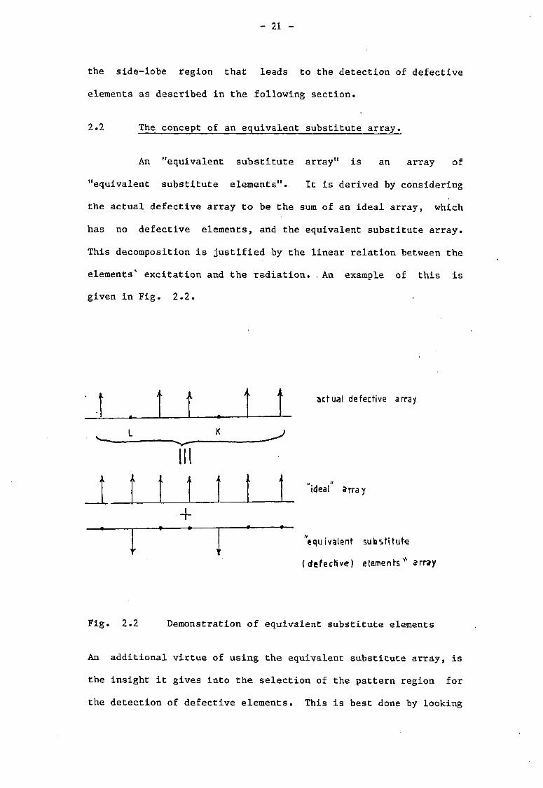
2.2 The concept of an equivalent substitute array.
An "equivalent substitute array" is an array of
"equivalent substitute elements". It is derived by considering
the actual defective array to be the sum of an ideal array, which
has no defective elements, and the equivalent substitute array.
This decomposition is justified by the linear relation between the
elements > excitation and the radiation. . An example of this is
given in Fig. 2.2.
A actual defective array
i I 1 + ideal array
"equivalent substitute
(defective) elements'" array
Fig. 2.2 Demonstration of equivalent substitute elements
An additional virtue of using the equivalent substitute array, is
the insight it gives into the selection of the pattern region for
the detection of defective elements. This is best done by looking
- 22 -
for the sensitivity of antenna patterns to defects in the array,
which follows.
2.3 Sensitivity of antenna patterns to a defective
element in the array.
The field pattern envelope of a unity amplitude
excitation N element array is comparable to a single element
antenna in the far side-lobe region and will be N times higher in
the main-beam region. The substitute array of a missing
(defective) element in the array will be equal to a single element
antenna. Therefore, the effect of a defective element in the
array will be N times larger in the far side-lobe region than in
the main-beam region. It is therefore recommended that use be
made of the far side-lobe region to monitor defects in the antenna
array.
2.4 Static and dynamic patterns and defects in
phased array antennas.
Phased array antenna patterns can be divided into two
main categories : static patterns and dynamic patterns. The
difference is essentially one of method of measurement. The
static pattern of an array could be measured by the conventional
antenna range instrumentation where the antenna phase control and
beam switching networks are fixed throughout the measurement. The
antenna is then rotated relative to the measuring probe and the
pattern recorded. The dynamic pattern, in contrast, will be
recorded when the antenna and the measuring probe are fixed and
the array beam is scanning by dynamically controlling its phase
and beam switching network. If ideal arrays of identical elements

- 23 -
are considered then the main difference between the static and the
dynamic patterns of the array will be due to the element gain
factor and the changing projected aperture area. Differences
between a static pattern and a dynamic pattern measured with the
probe in the broadside direction of the array, are due only to the
element gain factor.
Defects in antenna arrays can similiarly be categorized
into the two main classes of static and dynamic, depending on
whether they affect the static or the dynamic pattern. A static
defect in an array element can be described by a fixed change in
magnitude and phase with respect to the ideal element excitation.
The result is normally a constant error in the pattern beam
pointing, the beam-width and increased side-lobe level. While a
dynamic defect will exhibit a time-dependent shift of the
excitation magnitude and phase. Hence, dynamic errors in the
pattern beam pointing, the beam-width and dynamic changes in the
side-lobe level will be noticed. In realistic phased arrays the
dynamic control of the phase and beam switching networks is often
performed in discrete (quantized) steps rather than continuously,
hence introducing dynamic quantization of the beam scan and the
resulting pattern. Over and above these built-in phase excitation
errors due to quantization, a defect like an unintentionally stuck
phase shifter can occur causing dynamic changes in the array beam
pointing, the beam-width and the side-lobe level.
In the present chapter simple defects of a static nature
will be analyzed, based on the substitute element representation.
Defects of a dynamic nature will be described in chapter 3. While
more complex defects of a static nature (mutual coupling effects)

- 24 -
will be described in chapter 4.
2.5 The equivalent substitute field of a defective
element in an N-element array
Expressions will now be developed for the equivalent
substitute excitation and the resulting far-field radiation for
defects of a static nature in a simple, though important, case.
Combined amplitude and phase defects in a single element of the
array (element K) are assumed. The effect is conveniently
demonstrated by the phasor representation, of Fig. 2.3. (The
analysis for a single defective element also applies to the case
of many elements through the principle of superposition.)
Fig. 2.3 Phasor representation of phase and amplitude
defect, the equivalent substitute element.
Fig. 2.3 shows the ideal element of unit amplitude and phase (j^
referred to the array centre reference phase, where, from equation
(2.1),
- 25 -
[ K - (2.3) A/-M
i ^ ~ v o
and K is the element number concerned. The defective Kth element
has an amplitude ratio of a:l to the ideal, and is shifted
radians in phase. The following expressions are derived for the
normalized magnitude b and the phase shift ^ of the substitute
element,
t « a N 2,a cjcs A ^ ) 1 *
and I (2.4)
% = 7T- arc.5jn
and the radiated normalised far-field E of the defective array-
will, therefore, be a superposition of the good array and the
substitute element far fields, giving
Sit
it can be seen immediately that information on the defective
element location (K) and the nature of the defect (b/ is
contained in equation (2.5). Use will be made of this information
in suggesting the subtraction method of monitoring, and in the
simulation on the computer of defective array patterns. It also
demonstrates the higher sensitivity of the far field pattern to
defects in the far side-lobe region, as explained in section 2.3.
2.6 Examples of defective elements in an
N - element array.
Expressions will now be given for the following examples;
a) The Kth element missing.
Here, ^ = and b=l, therefore the normalized far-field
of the array will be given by
- 26 -
" H 1 s i v i - % -
b) The Kth element with a phase defect only.
Here b=2 sin ( A j ^ ) and fl(T+A<f>) therefore
l ^ S + 2 s i n e x p { j i ( , r } e x p { j 1 }
c) Two missing elements, K and L .
(2.6)
(2.7)
This can be represented by a two-element substitute
subarray. The array far field will be given by
E = [ 4 ^ - 2 c o s 2 ± e x p U a + f - ^ ) ) ^ } ] (2.8)
where D=(L-K) is the difference in element numbers between the
missing elements, and 2 cos
is the interference pattern of
two elements seperated D elements apart. It is clear that the
cosine term will not introduce additional phase jumps of 77"
radian as long as
< ? Z Z (2.9)
N t
array elements number
2 " 1 X
T M ' (
r - 3
0
• 1
C mi ssing J elements ( array
Fig. 2.4 M missing elements equidistantly seperated.

- 27 -
d) M missing elements equidistantly spaced.
Fig. 2.4 shows an N-element array where M of its
elements are missing. The Kth is the first missing element, and
each subsequent Dth element is also missing. The far-field of the
defective array will be,
e S ^ w e x p t k k + * > ( 2 - i o >
This expression will be compared to that used in the case of a
defective subarray described in chapter 3, when defective
subarrays will be dealt with in more detail. A pictorial
representation of some of these effects will now be given.
2.7 Demonstration of defective array patterns in the
far side-lobe region.
In order to emphasize the sensitivity of the far-sidelobe
region to the presence of defective elements, the following three
cases will be considered using equation (2.5) as a basis.
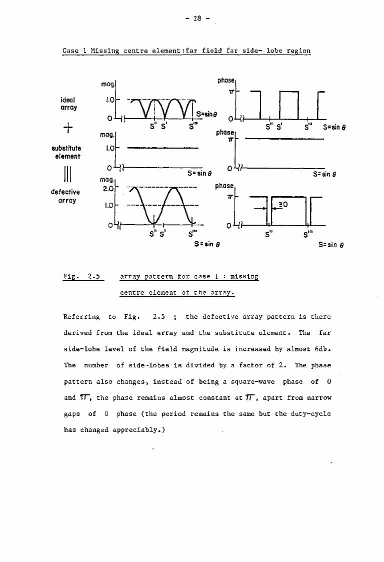
Case 1 Missing center element of the array (Fig. 2.5)
Case 2 Defect of phase shift error and +3db amplitude error in
the center element ( Fig. 2.6).
Case 3 Off-centre defect, described over the entire angular region
(side-lobe and main-lobe). (Fig. 2.7)
- 28 -
Case 1 Missing centre element:far field far side- lobe region
ideal array +
substitute element
defective array
mag.
1.0
phase 7T
•it S=8in0
s" s' s"' •ih
mag.
1.0
phase 7r
S=sin0
S = sin B
s" s' .III _ . _ S S=m Q
S=sin Q
S=sin Q
Fig. 2.5 array pattern for case 1 : missing
centre element of the array.
Referring to Fig. 2.5 ; the defective array pattern is there
derived from the ideal array and the substitute element. The far
side-lobe level of the field magnitude is increased by almost 6db.
The number of side-lobes is divided by a factor of 2. The phase
pattern also changes, instead of being a square-wave phase of 0
and TT, the phase remains almost constant at T T , apart from narrow
gaps of 0 phase (the period remains the same but the duty-cycle
has changed appreciably.)
- 29 -
Case 2 Phase and amplitude defects in centre element ; far-field
far side-lobe region.
idea) array
+
substitute element
defective array
mag. 1.0
mag. 1.0
0 Hh
mag. 1.4
1.0
s" S 1 S=sin 9
S=sin0
oHt S-sin Q
phase IT
O - M F
phase
7T/4
0-H b
phase 3tm ir/Z
7T/4
s" S* S=sin Q
S=sin Q
0-4 h i -i S S S=sin Q
Fig, 2.6 Array pattern for case 2 ; phase and amplitude
defects in center element of the array.
Referring to Fig. 2.6 a defect consisting of a 7T/4 phase shift
and +3db change in amplitude, causes the following changes in
amplitude and phase referred to the pattern of the ideal array.
The nulls of the ideal array side-lobes are filled in and smoothed
with a maximum of 3db between crest and trough. Side-lobe
amplitude periodicity does not change. The phase behaviour also
changes, from a square wave between Jf and 0 into a sine wave
with the same periodicity but ranging between TT/4 and 3TT/4.
From cases 1 and 2, as well as other cases not presented, it
appears that the far side-lobe region contains sufficient
information for identifying defects, at least in the center
element of the array.
- 30 -
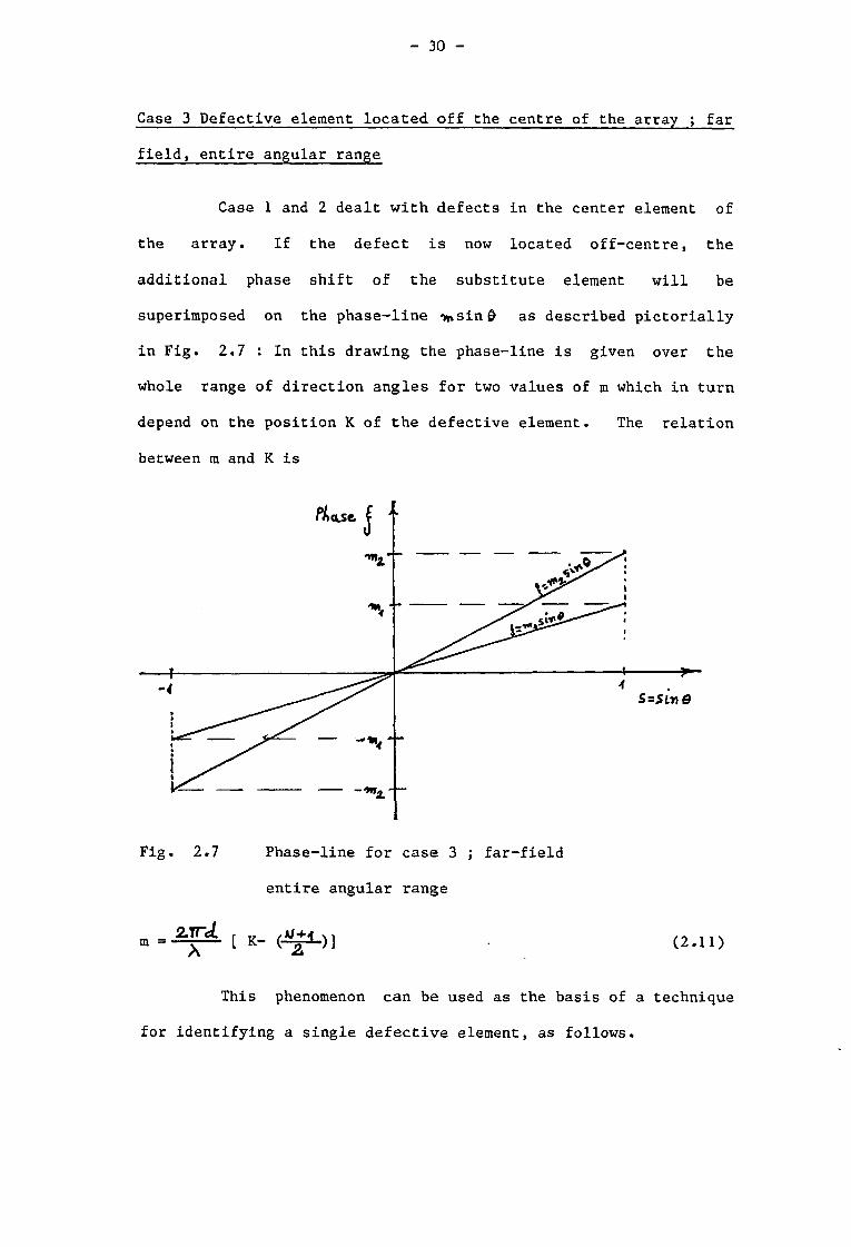
Case 3 Defective element located off the centre of the array ; far
field, entire angular range
Case 1 and 2 dealt with defects in the center element of
the array. If the defect is now located off-centre, the
additional phase shift of the substitute element will be
superimposed on the phase-line >»sin0 as described pictorially
in Fig. 2.7 : In this drawing the phase-line is given over the
whole range of direction angles for two values of m which in turn
depend on the position K of the defective element. The relation
between m and K is
Fig. 2.7 Phase-line for case 3 ; far-field
entire angular range
m = a p L [ K - (J£i.)] (2.ii)
This phenomenon can be used as the basis of a technique
for identifying a single defective element, as follows.

- 31 -
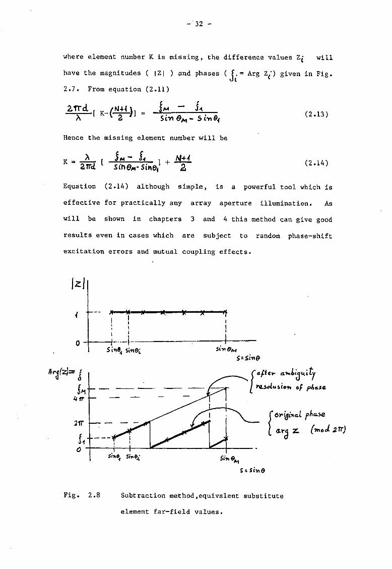
2.8 A method to extract the location of a defective element.
From equation (2.11) it is clear that subtraction of the
ideal array field from the defective array field yields the field
of the equivalent substitute element in the array. A method to
extract a defective element location in an array can be performed
by the "subtraction method" using the following procedure :
- Measure the amplitude and phase in the far field of the
defective array pattern in discrete steps of sin Q«; :
\ = Y(sinet-) , i=l, 2, M ,
where M is the number of samples and Y is complex.
- The corresponding values for the ideal array would be :
X{= X ( s i n ^ ) , i=l,2,....M.
- Subtract, giving :
Z I ~ ^ i " xi> i=l,2,....M. (2.12)
These values will include the required information of the
equivalent-substitute (defective) elements in the array and their
location. This data will then contain the radiation field pattern
of the substitute elements, sampled at M points in the angular
range from & to . If a single element is missing in the array " n
and the resulting phase ambiguity is resolved, two values Z^ and
Z M are sufficient to give full identification of the defective
element. For more than one missing element additional work will
be required. The following example shows how the method is
applied.
Example Given an N-element isotropic homogeneous linear array
- 3 2 -
where element number K is missing, the difference values Zj will
have the magnitudes ( |Z| ) and phases ( J . = Arg Z p given in Fig.
2.7. From equation (2.11)
(2.13)
(2.14)
2TrdL . /N±L\i "" i*
X 1 2 , J 3 $ i y y e M -
Hence the missing element number will be
K = -2L- r & i + M i a n d 1 sine*-sine, 2
Equation (2.14) although simple, is a powerful tool which is
effective for practically any array aperture illumination. As
will be shown in chapters 3 and 4 this method can give good
results even in cases which are subject to random phase-shift
excitation errors and mutual coupling effects.
* * X
S in^ sinei
re.*>otu*>'to-* of pAa.se.
C)ri(jc*a.L phase
dVq 7L (ynoel 2TT) r3
Fig. 2.8 Subtraction method,equivalent substitute
element far-field values.

- 33 -
2.9 Identification of type of defect
The type of defect is identified from the values of the
phase shift error A ^ and the magnitude ratio a (see Fig.
2.3),which can be derived as follows.
After finding the position of the defective element K ,
using equation (2.14), the same equation can be modified to find
the phase shift ^ between the ideal element and the substitute
element. It can be seen from equation (2.5) that S-' is given
by,
^ - fa - [ K - ] Sin e^ (2.15)
where j: , is the phase of Z £ in the direction #
For example if J = £ then sin = sin 0^. The value b is given
by |Z|. Inverting equations (2.4), the relative amplitude and
phase of the defect are
a = ( 1 + b 2 , + 2b cos F ft 7
A ^ = TT - arcsin (•^•sinj' ) (2.16)
Hence a full description of the defective element, namely
its location and type, are given by equations (2.14) and (2.16).
2.10 Some computer simulations •
Simulation on the computer of two types of defective
elements will now be given.
a) A missing element.
An N=99 element linear uniform isotropic array is assumed
with d=.61 /t interelement spacing, where element K = 47 ( -3d

- 34 -
distant from array centre) is missing. The far-field far
side-lobe patterns (in db) of the ideal, the defective and the
substitute array are plotted in Fig. 2.9. The phase-line of the
substitute element is shown in fig. 2.10.
b) A phase defect
Element K = 56 ( +6d from the array center) is then
simulated to have a pure phase defect of A ^ - T T / 4 . The results
are plotted in Figures 2.11 and 2.12, and are similiar to 2.9 and
2.10.
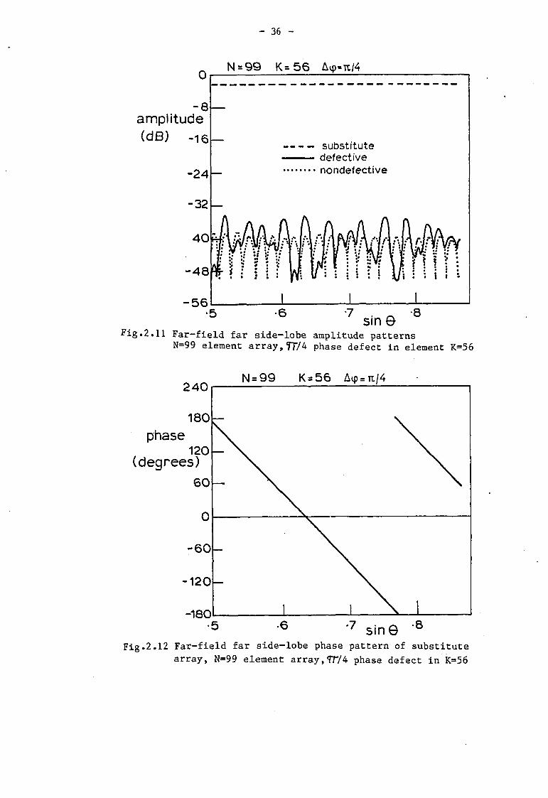
Figures 2.10 and 2.12 give the substitute element phase
lines ( Arg Z ). It can be seen that the linear phase lines are
of opposite signs, for defects located respectively to the left
and to the right of the array phase center. Also the slope is
doubled for doubling the spacing between the defective element and
the array centre. Any region can be used, however the far
side-lobe region enables the subtraction of magnitudes in the
order of 1/N of the main-lobe region (see section 2.3 ). Hence
the expected accuracy in the far side-lobe region will be greatly
enhanced, in cases when measurement noise is present, by a factor
of about N .
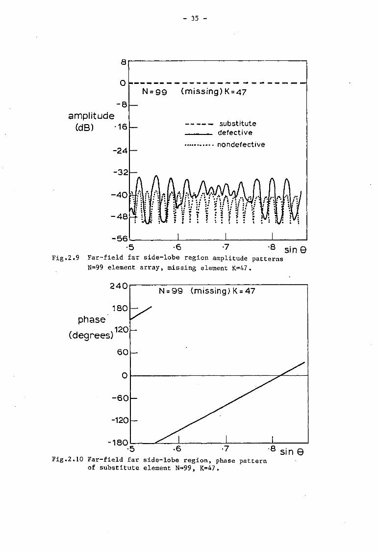
- 35 -
Fig.2.9 Far-field far side-lobe region amplitude patterns
N=99 element array, missing element K=47.
of substitute element N=99, K=47.
- 36 -
Fig.2.11 Far-field far side-lobe amplitude patterns N=99 element array, T f M phase defect in element K=56
Fig.2.12 Far-field far side-lobe phase pattern of substitute
array, N=99 element array, TTV 4 phase defect in K=56

- 37 -
2.11 Non necessity of measuring in the far field
In the case of a single defective element, or of a single
defective sub-array, the subtraction method does not require the
measurement to be performed in the far-field of the complete
array. It is merely necessary to be in the far-field of the
element or the sub-array (whichever is being sought), since the
field due to the complete array is subtracted out.
2.12 Applicability of the subtraction method
The subtraction method gives simple results in cases when
a single element of the array is defective.
Due to the expected high reliability of present and
future solid state phased-arrays, it is very unlikely that more
than one element will fail at any one time. Hence, if the
reference pattern is updated, and previously found failures are
memorized, this modified subtraction method can be used
sequentially for the identification of a sequence of defective
elements in the array.
In comparison to the near-field method suggested by
Ransom and Mittra [ 2], based on inverse diffraction, the
subtraction method uses simple equations and does not require
Fourier transformations. Also, in the subtraction method it is
preferable to use the far side-lobe region, hence avoiding
obstruction of the array radiation, which is required using Ransom
and Mittra xs method. The subtraction method, in addition, enables
the identification of the type of defect. No such claim is made
by Ransom and Mittra.

- 38 -
2.13 Conclusions
The presentation so far has shown that the subtraction
method is a simple but efficient tool for the detection of
defective elements in antenna arrays. As the far side-lobe region
gives the highest sensitivity to the presence of defective
elements, it is recommended that this region be used for
monitoring. Its importance lies in the additional fact that the
monitoring technique does not obstruct the radiation.
The technique is not limited to the far-field region of
the array ; only to the far field of the (equivalent) substitute
element or substitute array.
The technique is so simple that in the case of defects in
ideal arrays, two non-ambiguous measurements are sufficient to
identify a single defective element.
However the high reliability of present and future phased
array antennas enables one to use the modified subtraction method
( explained earlier in section 2.12 ) in cases where there are
many defective elements in the array. The assumption has to be
made that no more than one element fails at a time.
The applicability of the method to more realistic arrays,
including measurements in the presence of random phase excitation
errors and mutual coupling effects, is considered in chapters 3
and 4.

- 39 -
CHAPTER 3
APPLICATION OF THE SUBSTITUTE ELEMENT TECHNIQUE
The analysis has so far dealt with static defects in
ideal arrays. It is the purpose of this chapter to analyze more
realistic models of arrays by the introduction of random phase
excitation errors. The subtraction method will then be examined
in the presence of these random excitation errors.
In the second part of this chapter defects of a dynamic
nature will be analyzed where an unintetional stuck phase-shifter
is introduced into the array. Two cases will be examined. The
first is a stuck phase-shifter in a fully filled array, where each
phase-shifter drives a single element of the antenna. The second
case will be that of a thinned array where each phase-shifter
drives a subarray of the array. The subarray beam is then further
controlled by a beam switching network if a wider angle coverage
than the subarray beam-width is required. The last case should be
applicable to the Plessey MLS phased-array, where present design
proposes to use switchable input ports to a Rotman lens.
3.1 Performance of an array of isotropic
elements with random phase errors.
The far field pattern E(s) of a unity amplitude
illuminated isotropic linear N-element phased-array antenna can be
written in the form ( see equation (2.1) )
H
E(s)= exp{ j k x*s } exp{ j p. } • (3.1) C-i c
Where x =id, the displacement of the ith element from the array
centre and s=sin 9. The random phase excitation errors <3 •

- 40 -
attributed to the ith element, are assumed to be statistically
independent and uniformly distributed over the range ^ = + b , as
shown in Fig. 3.1.
Fig. 3.1
2-b
o + b
Random phase of the ith element
uniformly distributed.
The random phase will reduce the mean, or "coherent",
far-field radiation pattern at the same time introducing a
variance representing the fluctuating, or the "incoherent",
radiated power [ 21]. The far-field pattern can therefore be
regarded as composed of the sum of its coherent and incoherent
components. These will now be described.
3.1.1 The mean far-field radiation
The mean far field will be given by the expectation of
the ensemble of realizations as follows
N <E(s)>=<exp{j ft }> 2[exp{jkx«s} (3.2)
where < > designates the expectation. For a uniformly
distributed phase <exp{j is given by
<exp{j <^}>= J p ^ . C y ) e x p { j y } d y
U
-P = sine b
= / A e x P { j y } d y o
(3.3)
where sine b = sin b /b.

- 41 -
A/
The term exp{jkxis} in equation (3.2) equals the N element <±4
array factor A ^ ( s ) . Hence,
A n ( s ) = exp{jkxi,s} (3.4)
A/yJ(s) equals N for the direction of the main=lobe maximum, and
approximates 1 in the far side lobe region. Hence the coherent
far-field pattern is given by
<E(s)> = A^(s) sine b (3.5)
3.1.2 The variance of the far-field radiation
The variance of the incoherent radiated power, is
Var[ E(s) ] = <|E(s) \ z>- | <E(s)>I 2 , (3.6)
where
<|E(s)| a> = <E(s) E*(s)>
= <exp{j($.-<ri)>exp{jks(x £-x^) (3.7) I i C
The complex conjugate of E(s) is designated by E (s). The term
exp{ j(9&. - ^ )} can be divided into two parts : the first N terms for
which i=l, and the remaining (N^-Nj^or Which 'if 1, Giving,
Af M. <|E (s ) |*> = N+<exp{j (£-dk)> 2 Z exp{jks(x.-x /)} (3.8)
c r & UA < where <exp{j(^.-^)> is given by
<exp{j(^.-^)}> = ( ^ - / e x p { j y } d y )(-^-/exp{-jf)}dy)
= sinc^ b (3'9)
Since and (j) are assumed to be independent. Rearranging
equation (3.8) will give (see also [ 213 ) ;
hi KJ <|E(s)| 2 , > = N(l-sinc 2 b)+sinc ib £ exp{ j k s ( x r x * )} (3 . 1 0 )
f*4

- 42 -
where the double summation, equals the array factor squared,
namely,
H hi * A/ 2 . Z e x p { j k s ( x l - x - ) = 2L exp{ jksx*} 2 exp{-jksx/}
= IA (s) I2, (3.11)
Therefore
Var[E(s)]=fJ(l-sinc2 b) (3.12)
where Var[E(s)] is radiated isotropically (for an isotropic
array ).
3.1.3 The incoherent to coherent far field
radiation power ratio
Two regions will be considered : the main-lobe and the
far side-lobe regions. In the main lobe maximum (s=0 for
broadside array )
lA^ CO) I2- = ri2, (3.13)
In the far side lobe (s~l for broadside array)
M < ) r = * ( 3 a 4 )
Hence the main-lobe incoherent to coherent ratio will be given by
V<lv*[E(S)] _ j U -SI<ncH)
l<£(0)> H Siyic*b
The far side-lobe incoherent power ratio will be given by
Vd-r-[£<&)] _ H U-simcH) ,,
The results of equations (3.15) and (3.16) for several values of b
are given in Table 3.1 and described pictorially in Fig 3.2.
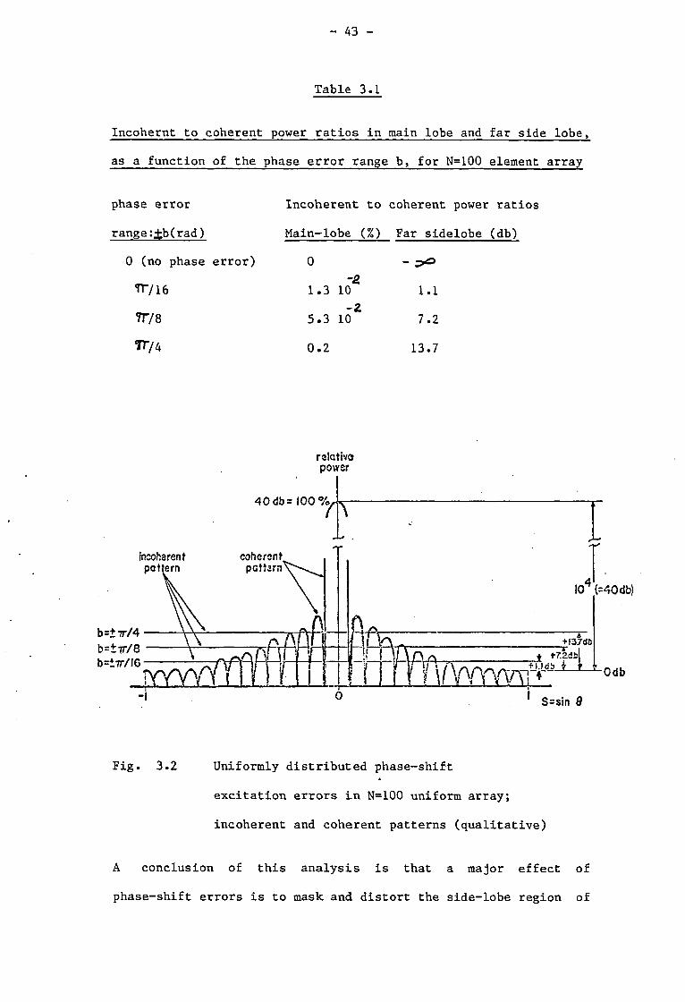
- 43 -
Table 3.1
Incohernt to coherent power ratios in main lobe and far side lobe,
as a function of the phase error range b, for N=100 element array
phase error
range :^b(rad)
0 (no phase error)
TT/16
Try 8 Try 4
Incoherent to coherent power ratios
Main-lobe (%) Far sidelobe (db) - ^
1.1 7.2
0.2 13.7
0
-2. 1.3 10
- 2 5.3 10
relative power
Fig. 3.2 Uniformly distributed phase-shift
excitation errors in N=100 uniform array;
incoherent and coherent patterns (qualitative)
A conclusion of this analysis is that a major effect of
phase-shift errors is to mask and distort the side-lobe region of
- 44 -
the array pattern, threrby complicating the monitoring method
considered previously.
3.2 Use of the proposed subtraction method
in the presence of random phase-shift errors
In spite of the deterioration of the side lobes of the
array in the presence of random phase excitation errors, the
proposed subtraction method seems to be efficient for identifying
a defective element in the array. Two cases will be discussed as
representatives of the types of random-phase excitation: the
"static" and the "dynamic" case (see also section 2.4).
3.2.1 The static case
Here the set of random phase fluctuations is fixed over
the array elements and independent of the pointing angle of the
array beam. This could be the case of a non-scanning linear
array, or it could be a case where ideal phase shifters are used
with non ideal radiation elements. The resulting ZI values will
now contain the information on the location of the defective
element, derived from the phase slope-line according to equation
(2.14). The phase slope would be a non-fluctuating line but will
include an additional constant phase equivalent to the phase
excitation error attributed to the defective element. The type of
defect will not be known (unless the excitation error of the
defective element is known ) but the location of the defect can be
identified with no error (see for example Fig. 3.3), since the
slope is unchanged .
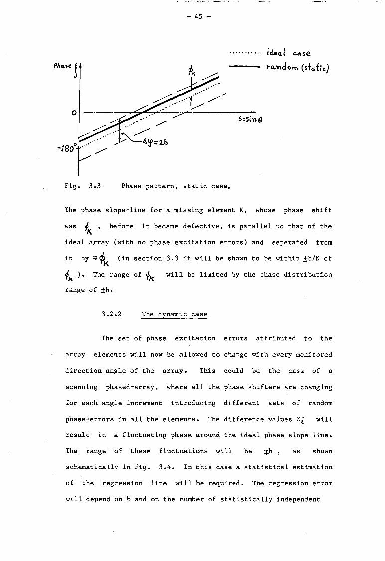
- 45 -
tdeaf case
The phase slope-line for a missing element K, whose phase shift
was ^ , before it became defective, is parallel to that of the K
ideal array (with no phase excitation errors) and seperated from
it by (in section 3.3 it will be shown to be within +b/N of K
<& ). The range of will be limited by the phase distribution ' K 'A
range of ±b.
3.2.2 The dynamic case
The set of phase excitation errors attributed to the
array elements will now be allowed to change with every monitored
direction angle of the array. This could be the case of a
scanning phased-array, where all the phase shifters are changing
for each angle increment introducing different sets of random
phase-errors in all the elements- The difference values will
result in a fluctuating phase around the ideal phase slope line.
The range of these fluctuations will be +b , as shown
schematically in Fig. 3.4. In this case a statistical estimation
of the regression line will be required. The regression error
will depend on b and on the number of statistically independent
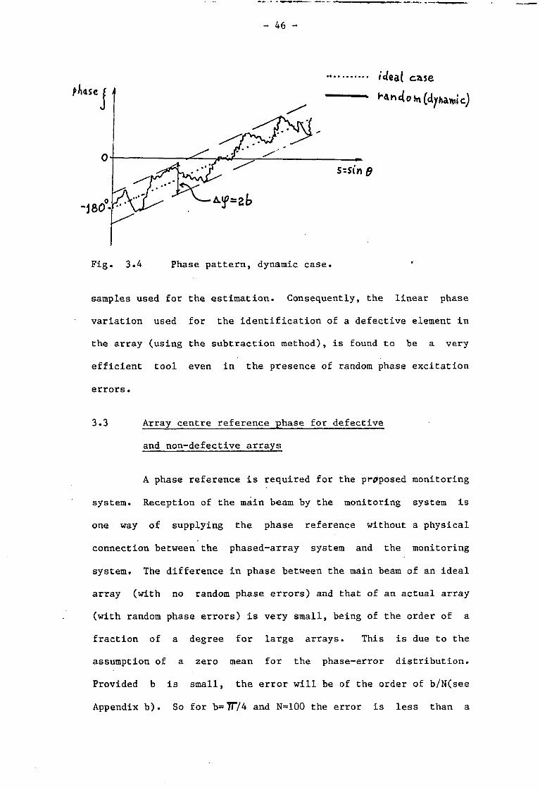
- 46 -
"teat case
samples used for the estimation. Consequently, the linear phase
variation used for the identification of a defective element in
the array (using the subtraction method), is found to be a very
efficient tool even in the presence of random phase excitation
errors.
3.3 Array centre reference phase for defective
and non-defective arrays
A phase reference is required for the proposed monitoring
system. Reception of the main beam by the monitoring system is
one way of supplying the phase reference without a physical
connection between the phased-array system and the monitoring
system. The difference in phase between the main beam of an ideal
array (with no random phase errors) and that of an actual array
(with random phase errors) is very small, being of the order of a
fraction of a degree for large arrays. This is due to the
assumption of a zero mean for the phase-error distribution.
Provided b is small, the error will be of the order of b/N(see
Appendix b). So for b= 7T/4 and N=100 the error is less than a

- 47 -
degree. The same applies to the phase difference between the
actual array before and after a defect in a single element has
happened. It also applies to the extent of the shift in
phase-slope fluctuations in the "dynamic" and "static" cases
already discussed in 3.2.
Consequently, the main beam received by the monitoring
antenna could supply the reference phase, provided a suitable
technique for memorizing this phase is available.
3.4 Computer simulation of defects in presence
of random phase excitation error.
Simulation on the computer of arrays with the two types
of excitation errors will now be given.
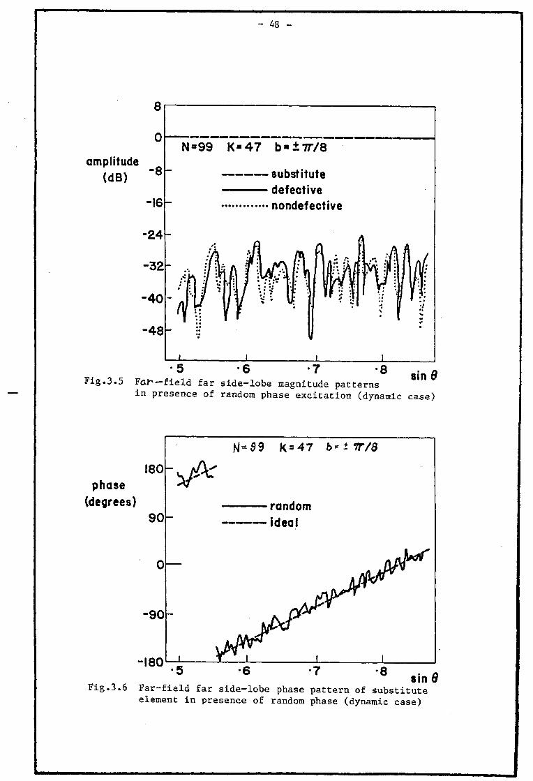
a) A missing element in the presence of
dynamic phase excitation errors.
The same parameters as in 2.10 example a will be used.
In addition a non-reset pseudo-random number generator will
produce dynamic phase errors in the range b=+1T/8 •
The far field patterns (in db) of the non-defective, the
defective and the substitute array are shown in Fig. 3.5. The
phase line is given in Fig 3.6.
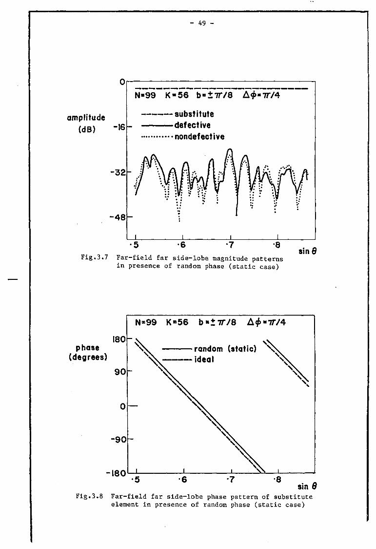
b) A missing element in the presence of static phase errors.
The same parameters as above will be chosen but here a
reset random number generator will produce static phase errors in
the range b=+TT/8. The results are shown in Figures 3.7 and 3.8,
which are similiar to Figures 3.5 and 3.6.
- 48 -
amplitude (dB )
8
0
- 8
-16
N « 9 9 j<«47 b«±77V8
substitute
defective nondefective
_L
sin 8 •5 -6 -7 -8 Fig.3.5 Fa)~—field far side-lobe magnitude patterns
in presence of random phase excitation (dynamic case)
phase (degrees)
180
90
H^S 9 K = 4 7 6- - 7T/8
random ideal
- 9 0
-180 • .c .7 .a sin Q
Fig.3.6 Far-field far side-lobe phase pattern of substitute element in presence of random phase (dynamic case)
- 49 -
amplitude (dB) -16
- 3 2
N«99 K - 5 6 b«±7T/8 A<£«7T/4
substitute defective nondefective
- 4 8
•5 -6 1 -8 Fig.3.7 Far-field far side-lobe magnitude patterns
in presence of random phase (static case)
sin 0
phase (degrees)
180
90
- 9 0
-180
N*99 K«56 b 7T/8 A<£«7774
random (static) x
•8 sin 0
Fig.3.8 Far-field far side-lobe phase pattern of substitute element in presence of random phase (static case)
- 50 -
Figures 3.6 and 3.8 give the substitute-element phase lines. It
can be seen that, as expected from section(3.2.2) the phase line
in Fig. 3.6 fluctuates around the correct mean slope line (dashed
line) which is reproduced from Fig. 2.10. Using equation (2.14)
the "missing" element location can be deduced very precisely (to
be within ~ 10% of the element spacing). In Fig. 3.8, however,
the phase line gives no variation around the mean slope-line but a
parallel line to it as described in section (3.2.1).
These promissing, and quite stable, results have been
examined in circumstances where the good and defective arrays both
exhibit apparently indistinguishable erratic behaviour in their
far fields (see Figs. 3.5 and 3.7; also compare with Fig. 2.9).
The results demonstrate that the method can be used with phased
arrays in the presence of the quantized phase-shift errors.
This concludes the first part of the chapter dealing with
application of the subtraction method in presence of random phase
excitation errors.
Next a dynamic defect of a stuck phase shifter will be
discussed.
3.5 Inadvertently latched (stuck) phase-shifter
feeding a single element.
Having analyzed defects of a static nature in the
presence of static and dynamic phase-excitation errors, it is now
intended to deal with the important practical case of a stuck
phase shifter. As explained previously this type of defect is of
a dynamic nature since the relative phase shift between the
required and the available excitation phasor changes dynamically

- 51 -
with the beam scanning. In the present section the effect of a
stuck phase shifter feeding a single element of the array will be
discussed. This is followed in section 3.6 by an investigation of
a stuck phase-shifter feeding a sub-array of the antenna.
3.5.1 The equivalent substitute element of a stuck
phase-shifter feeding a single element.
It has been shown (section 2.5) that the equivalent
substitute element of a defect with constant amplitude and phase
in a single element is given by
b e x p t j J ' M a exp{ j A ^ } - 1 ]exp{j ^ } (3.17)
Designating ^-fi* and where
<4=£P"dsin© (3.17a) 'O A
we could write the following
b exp{j (j) }=a exp{j (f) } - l-exp{j (3.18)
Now, <£) is constant for a stuck phase shifter while ^ changes as a function of the scan angle 9 (equation 3.18 above).
Therefore b and (p will also change with the scan angle. The rZ
previous case of a missing element could be represented as a
special case of a stuck phase-shifter feeding a missing element,
where a=0 , resulting in b=-l and = , as before. For a^O and
a stuck phase-shifter three cases will be discussed corresponding
to the different value of a; namely, a=l, a<l and a>l. The phasor
representation for all three cases is given in Fig. 3.9.
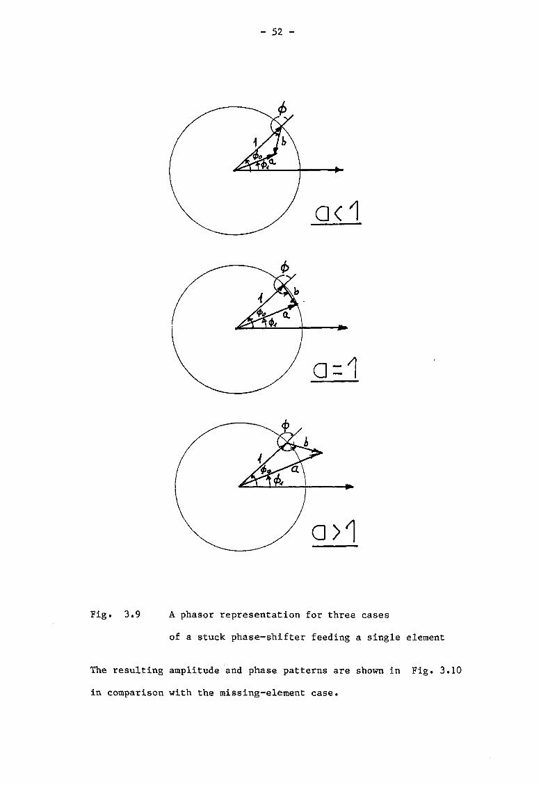
- 52 -
Fig. 3.9 A phasor representation for three cases
of a stuck phase-shifter feeding a single element
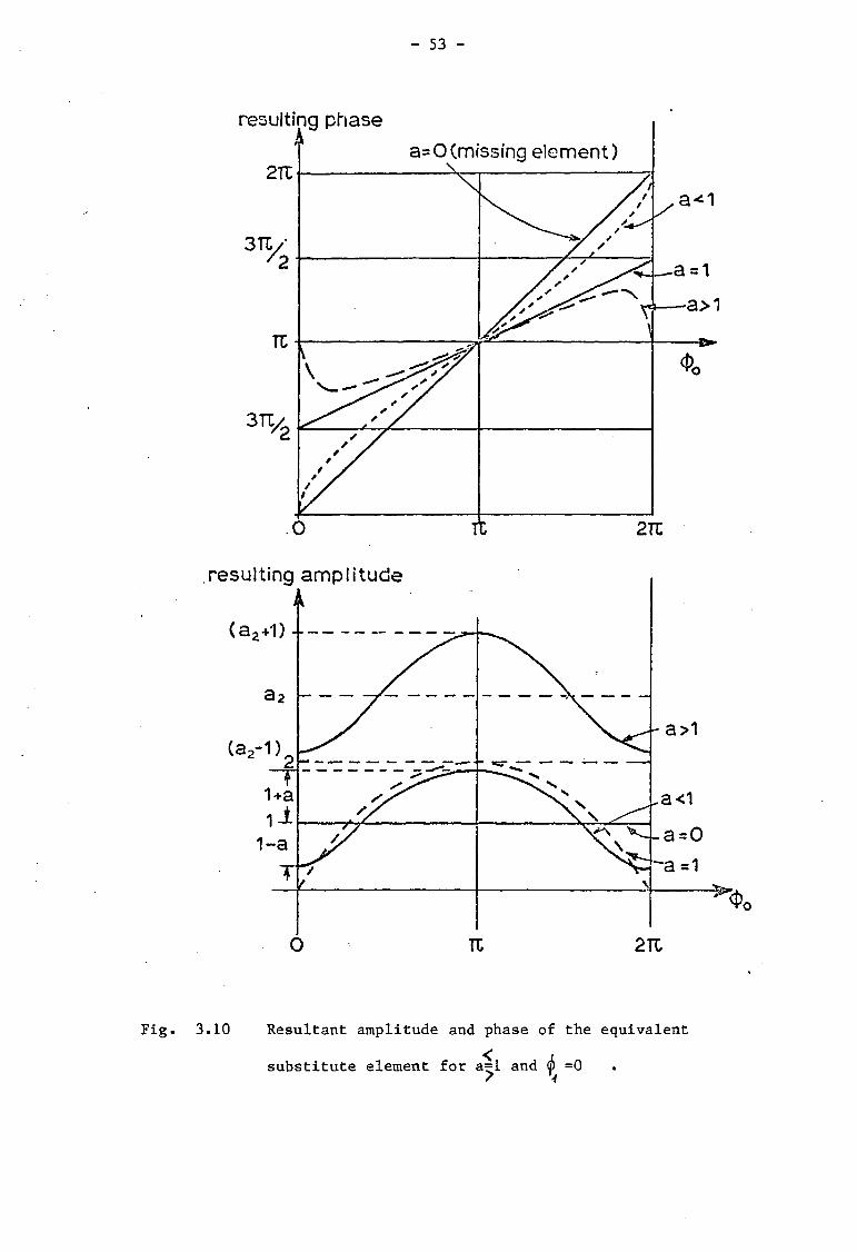
The resulting amplitude and phase patterns are shown in Fig. 3.10
in comparison with the missing-element case.
- 53 -
3.10 Resultant amplitude and phase of the equivalent
substitute element for a=l and (j) =0

- 54 -
It is to be noticed that if then the only additional effect
will be a shift in the location of the zero crossing of the phase
and in the accompanying amplitude maxima and minima.
3.5.2 A modification in the subtraction method for
a stuck phase-shifter.
From Fig. 3.10 it is still possible, although with
somewhat greater difficulty, to decide on the type of defect and
its location, using a modification of the subtraction method
formula (equation 2.14). One possibility is to measure the
periodicity of the phase curve, thus a modified formula like the
following one can be used.
k - + x . 2 T T _ H+4 . . K - T t o T A.S 2 ( 3 , 1 9 )
The sign is that of the phase slope, A s is the direction-cosine
difference for one period (cycle) of the phase variation.
However, when a=l a linear phase variation results, but with half
the slope. Hence, use could be made of equation (2.14), but
doubling the values of the calculated phase difference between the
two samples measured at sin & and sin . The modified • Al equation will then be in the form of
K ]+ (3.19a) 7r<i fcmeM-swe,, 2
Therefore equation (3.19) or (3.19a) can be used to derive the
location of the (defective) stuck phase shifter.

- 55 -
3.6 The equivalent substitute array of a stuck phase-
shifter feeding a single subarray
The main difference between the resulting equivalent
substitute element and the equivalent substitute subarray for a
stuck phase shifter, is in the amplitude and phase dependence of
the subarray factor to that of a single element. A modification
of equation (3.18) will be used as follows
b exp{j^> = a e x p { - A exp{j{>0} (3.18a)
with the following different meaning of the factors a and b. The
factor a is the normalized defective subarray factor, and b is the
resulting normalized equivalent substitute (sub) array factor.
The ideal M element subarray factor A is given by,
A = (3.20)
where s D=sin & o , is the direction cosine of the monitoring
antenna to the array broadside direction. The normalized
defective subarray factor a in the case of a stuck phase-shifter,
is given by
1 _ St*. O l t M c l s e , ,
Si C 3 , 2 1 )
where ^ , as before, is the phase of the stuck phase-shifter.
While A changes with the scan angle, the factor b is fixed for a
given value of ^ and of the direction-cosine s c (if no beam
switching is used).
Example A stuck phase shifter feeding an M element subarray, the
case of s 0 =0, <^=0
The factor a behaves differently in the main-lobe region and in
- 56 -
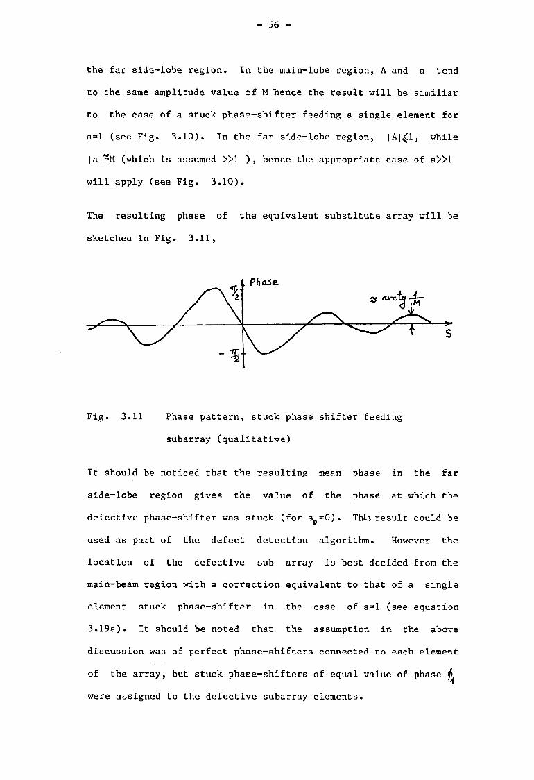
the far side-lobe region. In the main-lobe region, A and a tend
to the same amplitude value of M hence the result will be similiar
to the case of a stuck phase-shifter feeding a single element for
a=l (see Fig. 3.10). In the far side-lobe region, |A|^1, while
la|=M (which is assumed » 1 ), hence the appropriate case of a » l
will apply (see Fig. 3.10).
The resulting phase of the equivalent substitute array will be
sketched in Fig. 3.11,
Fig. 3.11 Phase pattern, stuck phase shifter feeding
subarray (qualitative)
It should be noticed that the resulting mean phase in the far
side-lobe region gives the value of the phase at which the
defective phase-shifter was stuck (for s o = 0 ) . This result could be
used as part of the defect detection algorithm. However the
location of the defective sub array is best decided from the
main-beam region with a correction equivalent to that of a single
element stuck phase-shifter in the case of a=l (see equation
3.19a). It should be noted that the assumption in the above
discussion was of perfect phase-shifters connected to each element
of the array, but stuck phase-shifters of equal value of phase <f>
were assigned to the defective subarray elements.
- 57 -
An additional more complex case where a stuck phase
shifter is feeding a beam switched sub-array will be investigated
next.
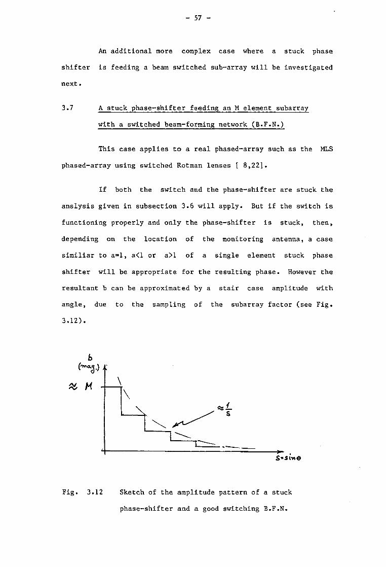
3.7 A stuck phase-shifter feeding an M element subarray
with a switched beam-forming network (B.F.N.)
This case applies to a real phased-array such as the MLS
phased-array using switched Rotman lenses [ 8,22].
If both the switch and the phase-shifter are stuck the
anslysis given in subsection 3.6 will apply. But if the switch is
functioning properly and only the phase-shifter is stuck, then,
depending on the location of the monitoring antenna, a case
similiar to a=l, a<l or a>l of a single element stuck phase
shifter will be appropriate for the resulting phase. However the
resultant b can be approximated by a stair case amplitude with
angle, due to the sampling of the subarray factor (see Fig.
3.12).
SsSi-ne
Fig. 3.12 Sketch of the amplitude pattern of a stuck
phase-shifter and a good switching B.F.N.

- 58 -
Simulation on the computer for several cases of stuck,
phase-shifters will be given next.
3.8 Simulation of stuck phase shifters in ideal arrays
Several examples of defects will be simulated.
An N=100 element array is assumed in the following five
examples.
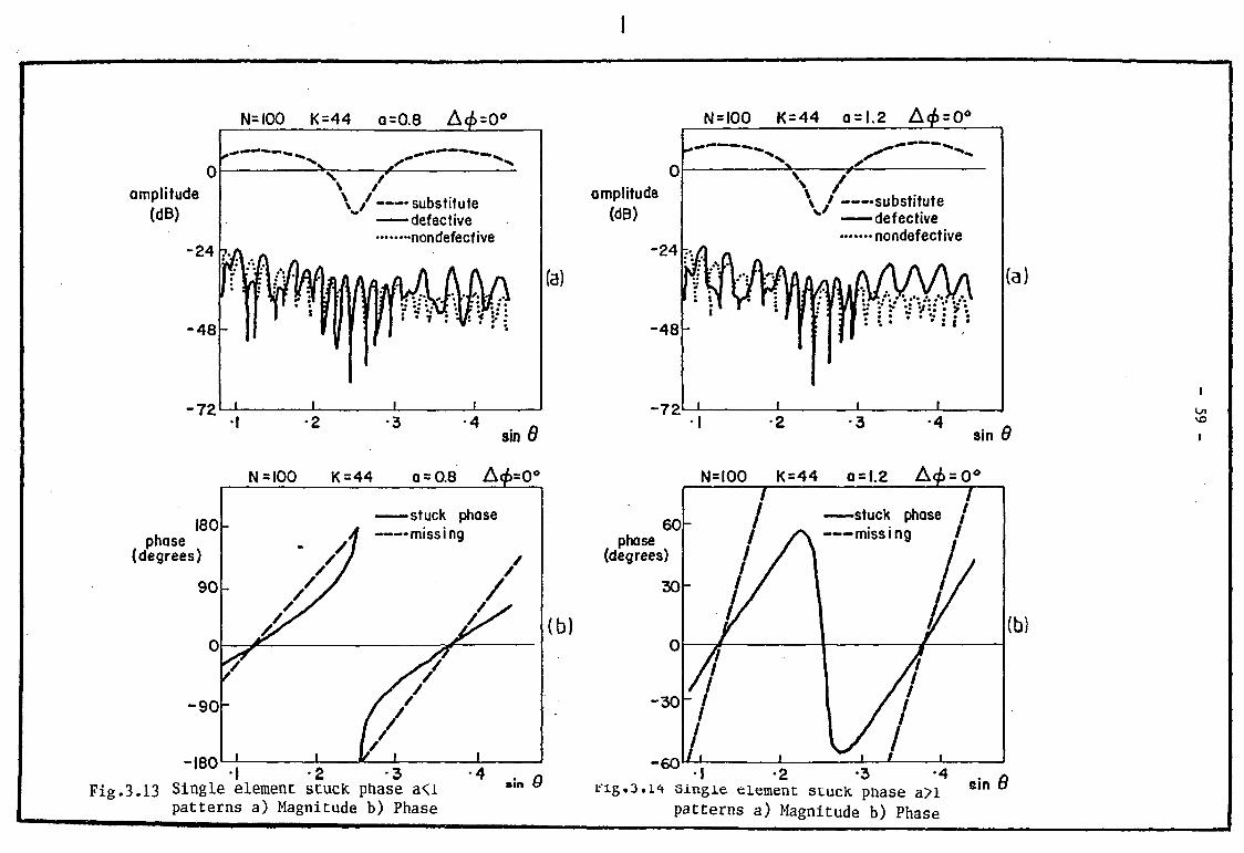
a) A single element defective in amplitude, stuck phase-shifter
with the following parameters.
K=44 (i.e., defective element number 44).
a=0.8 (i.e., a<l amplitude defect).
pl=0 (i.e., phase shifter stuck to 0 phase value).
the far field patterns are shown in Fig. 3.13a and the resulting
phase line in Fig. 3.13b. The same notation as in previous
simulations is used for the patterns and their phase variations.
b) Single element with a larger amplitude defect with stuck
phase-shifter.
K=44 , a=l.2 (i.e. a>l) and pl=0.
The far field patterns are shown in the side lobe region
in Fig. 3.14a. The resulting phase-line is shown in Fig.3.14b.
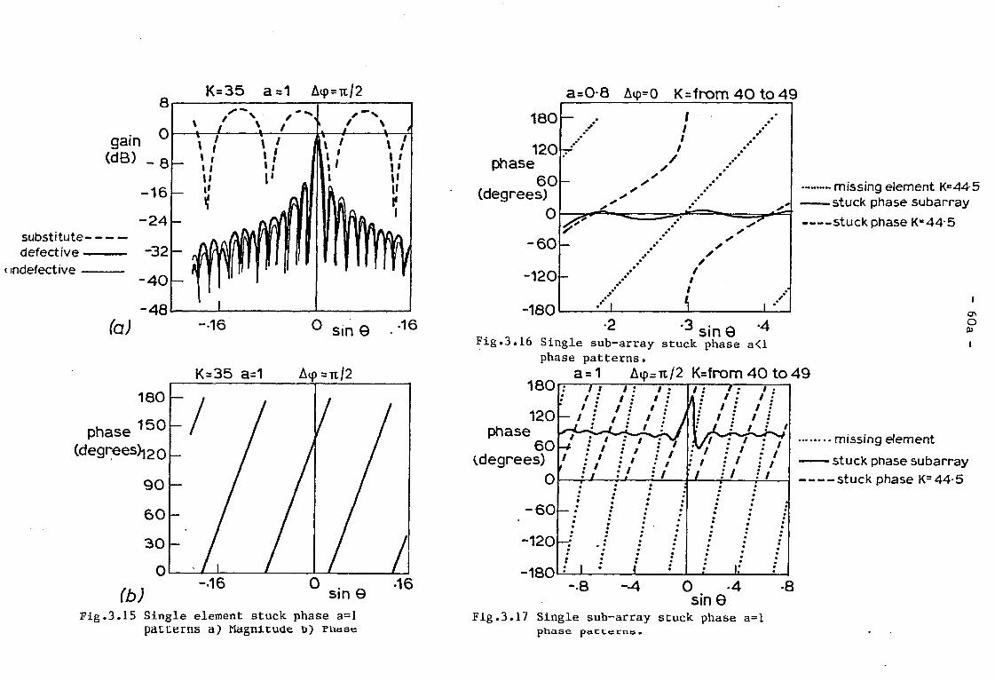
c) Single element defective in phase, stuck phase-shifter with
the following parametrs.
K=35 , a=l (i.e., no amplitude defect ) and pl=0.
The far-field patterns are given in Fig. 3.15a. The
resulting phase-line is given in Fig. 3.15b.
N= 100 K=44 a =0.8 A</>=0°
amplitude (dB)
-24
-48
-72'—1
\ 7 —— substitute
defective -nondefective
(a)
_L
I
180 phase
(degrees)
sin 8 N = 100 K =44 o = 0.8 A< )=0<
>stuck phase -missing
-90"
-180 •2 -3 -4 .
Fig.3.13 Single element stuck phase a<;i s , n
patterns a) Magnitude b) Phase
N = I00 K=44 o = L2 A<ft = 0°
amplitude (dB)
-24
-48
-72
/ \ J substitute v defective
nondefective
f : V: : • : • • • :i s
(a)
sin 0 Ln VO
60 phase
(degrees)
-30
- 6 0
N=I00 K=44 7
0 = 1.2
3IUUI\ pilUSC /
—— missina /
I -2 3 -4 Fig.3.14 Single element stucK phase a>l
patterns a) Magnitude b) Phase
(b)
sin 6
- 60 -
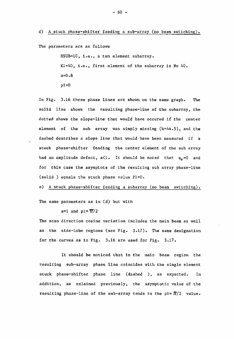
d) A stuck phase-shifter feeding a sub-array (no beam switching).
The parameters are as follows
NSUB=10, i.e., a ten element subarray.
Kl=40, i.e., first element of the subarray is No 40.
a=0.8
pl=0
In Fig. 3.16 three phase lines are shown on the same graph. The
solid line shows the resulting phase-line of the subarray, the
dotted shows the slope-line that would have occured if the center
element of the sub array was simply missing (k=44.5), and the
dashed describes a slope line that would have been measured if a
stuck phase-shifter feeding the center element of the sub array
had an amplitude defect, a<l. It should be noted that so=0 and
for this case the asymptote of the resulting sub array phase-line
(solid ) equals the stuck phase value P1=0.
e) A stuck phase-shifter feeding a subarray (no beam switching).
The same parameters as in (d) but with
a=l and pl= 7T/2
The scan direction cosine variation includes the main beam as well
as the side-lobe regions (see Fig. 3.17). The same designation
for the curves as in Fig. 3.16 are used for Fig. 3.17.
It should be noticed that in the main beam region the
resulting sub-array phase line coincides with the single element
stuck phase-shifter phase line (dashed ), as expected. In
addition, as exlained previously, the asymptotic value of the
resulting phase-line of the sub-array tends to the pl= 77/2 value.
gain MB) _ q
substitute-defective —
<. mdefective —
(a)
K = 3 5 a =1 Aip=rc/2
sin ©
K = 3 5 a=1 Acp = tl/2
phase (degrees)-^
to; sin 9 Fig.3.15 Single element stuck phase a=l
patterns a) Magnitude b) ruase
a=0-8 Avp=0 K=from 40 to 49
120 phase
60 (degrees) • missing element K =44-5
stuck phase subarray
•stuck phase K-44 5
2 sin 9 4
Fig.3.16 Single sub-array stuck phase a<l phase patterns.
a = 1 Aip-n/2 K=from 40 to 49 1801
cn O OJ
120 phase
6 0 (degrees)
0
- 6 0
- 120
-180
t t / ; t ; • ' : / : ' : / : / ; / : , — / : / : / • J
/ / / ' / / / / : ' • » • » • / • / • . ? /
/ : / ; J :
: 1 : 1 : ; / " 1 if : / : / / / : / : /
• • • « : * ;
_ ; / ; • : • * . • • • • m • • • • . . • • _ • • • • » • • • . • • ; : 1 • \
• • • • , • • ! • . •
•* • . • • » •
• • r ; , • . ; 1*
• • missing element
- stuck phase subarray -stuck phase K=44-5
-•8 --4 0 -4 sin 9
Fig.3.17 Single sub-array stuck phase a=l phase patterns•
8
- 61 -
Summarizing these simulation results, it can be said that the
modified formula for the subtraction method can be used in the
main-lobe region (equations 3.19 and 3.19a) for a stuck phase
shifter feeding a single element or a single subarray. Also the
value of the stuck phase-shifter can be found in the case of an
unswitchable beam forming sub—array. The phase line asymptote in
the far side-lobe region points out the value of the stuck phase
if only the monitoring antenna is placed in direction cosine
s o=0(the broadside direction) •
3.9 Discussion
The substitute element technique has been shown to be a
very useful tool for analyzing defects of a dynamic nature as well
as defects of static nature.
The subtraction method has been found to be an efficient
monitoring method for realistic models of antennas in the presence
of random-phase excitation errors.
A modification to the subtraction method has been
suggested for several cases, of stuck phase-shifters, using
analysis and simulation on the computer.
A further important aspect of realistic modelling of
phased-array antennas will be investigated in chapter 4, where
mutual coupling effects will be considered.
- 62 -
CHAPTER 4
MUTUAL COUPLING EFFECTS
In the previous chapter a more realistic model of antenna
arrays has been sought, by the introduction of defects in the
presence of random excitation errors. The present chapter will
lead to a further more realistic antenna model by the inclusion of
coupling effects (in an actual array), and will examine their
influence on the performance of the monitoring method suggested.
Coupling effects could, broadly, be divided into two categories,
the first which is dependent on the separation between elements
and the second which is independent of the separation. The mutual
coupling effect is due to the proximity of the elements and,
hence, is dependent on the separation. Power reflected from an
element affecting other elements of the antenna, through the
antenna feed network, is independent of the distance. The last
statement is made assuming a lossless feed network (this
independence ignores periodic changes of coupling along the feed
network). As the ultimate interest is to judge the major effects
of coupling, with a minimum disturbance of unimportant details,
simplified cases will be demonstrated based on known formulas
[ 9,10,11]. A simplified model of an "actual" array available in
the laboratory [ 23] will be simulated on the computer • In a
later part of this thesis (chapter 7), results of the present
chapter will be compared to those of the experimental
investigation.
The next section will deal with the effect of mutual
coupling.
- 63 -
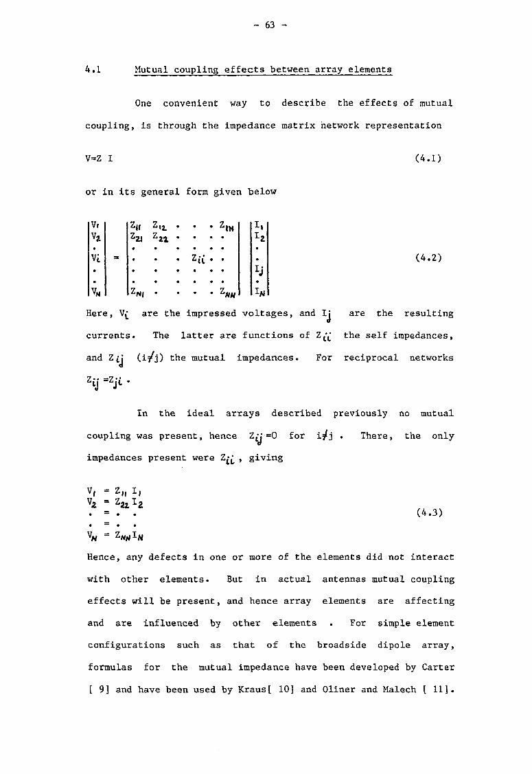
4.1 Mutual coupling effects between array elements
One convenient way to describe the effects of mutual
coupling, is through the impedance matrix network representation
V=Z I (4.1)
or in its general form given below
Vi . ZIH II V 2
Z21 z 2 l . . . vi = . . . Zii . • . . . . . . V„ ZN| . . . ZNH
(4.2)
Here, V£ are the impressed voltages, and Ij are the resulting
currents. The latter are functions of the self impedances,
and Z(J (i/j) the mutual impedances. For reciprocal networks
Z£j -Zjt •
In the ideal arrays described previously no mutual
coupling was present, hence Zg* =0 for i^j . There, the only
impedances present were Z ^ , giving
V, - Zl( I, v2 = Z ^ z
. = . . (4.3) . = . . VN = ZNH 1*
Hence, any defects in one or more of the elements did not interact
with other elements. But in actual antennas mutual coupling
effects will be present, and hence array elements are affecting
and are influenced by other elements . For simple element
configurations such as that of the broadside dipole array,
formulas for the mutual impedance have been developed by Carter
[ 9] and have been used by Kraus[ 10] and Oliner and Malech [ 11].
- 64 -
In the following section a simple case of mutual coupling will be
described for a two element h/2 broadside array, using these
coupling formulas.
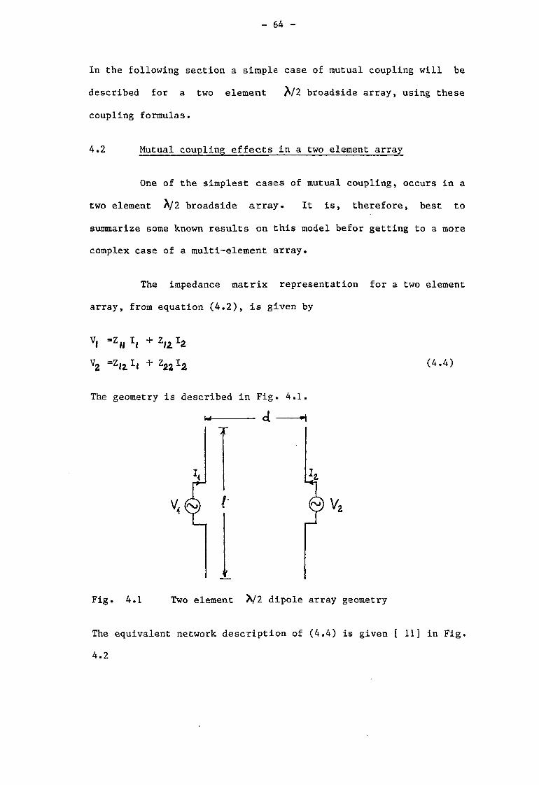
4.2 Mutual coupling effects in a two element array
One of the simplest cases of mutual coupling, occurs in a
two element A/2 broadside array. It is, therefore, best to
summarize some known results on this model befor getting to a more
complex case of a multi-element array.
The impedance matrix representation for a two element
array, from equation (4.2), is given by
Vl " z«| xf + z t Z T i
v2 = z l l l i + H z 1 !
The geometry is described in Fig. 4.1
V,
(4.4)
Fig. 4.1 Two element V 2 dipole array geometry
The equivalent network description of (4.4) is given [ 11] in Fig.
4.2
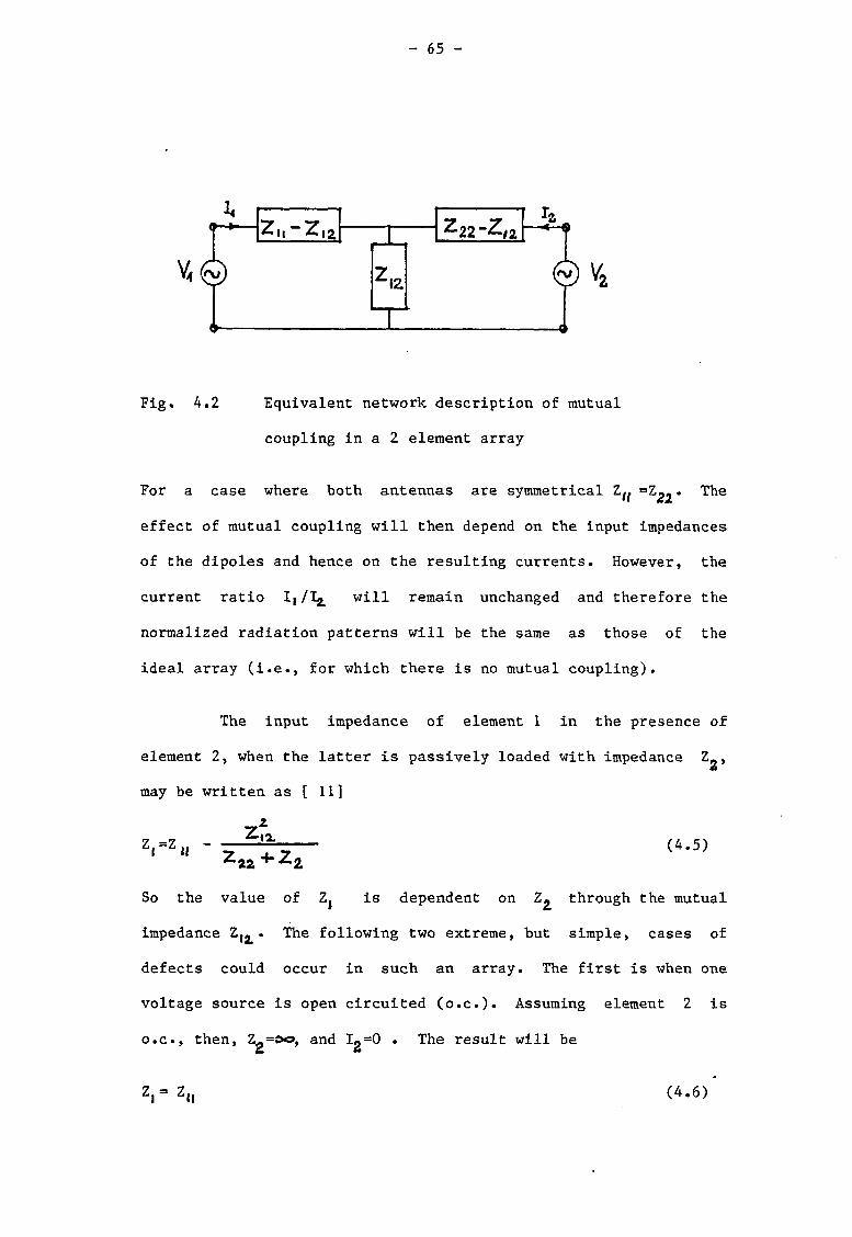
- 65 -
Fig. 4.2 Equivalent network description of mutual
coupling in a 2 element array
For a case where both antennas are symmetrical Z^ *
effect of mutual coupling will then depend on the input impedances
of the dipoles and hence on the resulting currents. However, the
current ratio Ij/I^ will remain unchanged and therefore the
normalized radiation patterns will be the same as those of the
ideal array (i.e., for which there is no mutual coupling).
The input impedance of element 1 in the presence of
element 2, when the latter is passively loaded with impedance Zg,
may be written as [ 11]
z r z ii Z|0L
z 2 2 + z< (4.5)
So the value of Zj is dependent on Z^ through the mutual
impedance Z,^. The following two extreme, but simple, cases of
defects could occur in such an array. The first is when one
voltage source is open circuited (o.c.). Assuming element 2 is
o.c., then, Z-=£o, and I o=0 . The result will be
Z,= Z„ (4.6)
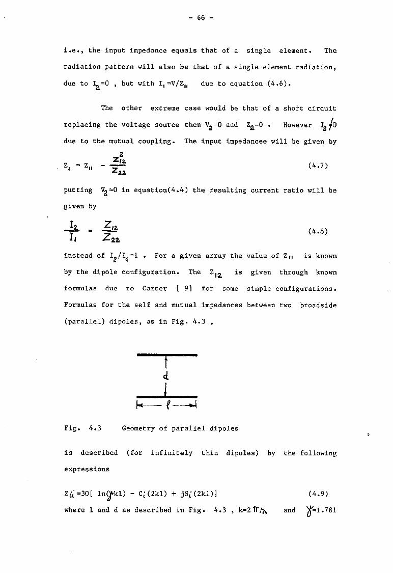
- 66 -
i.e., the input impedance equals that of a single element. The
radiation pattern will also be that of a single element radiation,
due to » but with I, =V/Z U due to equation (4.6).
The other extreme case would be that of a short circuit
replacing the voltage source then and Z ^ O . However ^ / o
due to the mutual coupling. The input impedancee will be given by
Z/2. Z, - Z„ - (4.7)
putting Vg=0 in equation(4.4) the resulting current ratio will be
given by
- k = ( 4 . 8 )
1| ^ 2 2 ,
instead of I^/I^l . For a given array the value of Z|t is known
by the dipole configuration. The is given through known
formulas due to Carter [ 9] for some simple configurations.
Formulas for the self and mutual impedances between two broadside
(parallel) dipoles, as in Fig. 4.3 ,
f I
k — t —
Fig. 4.3 Geometry of parallel dipoles
3
is described (for infinitely thin dipoles) by the following
expressions
Za =30[ ln(Jfkl) - C'(2kl) 4- jSt' (2kl) j
where 1 and d as described in Fig. 4.3 , k=2 TT/^
(4.9)
and ^=1.781
- 67 -
) and ) are the cosine and sine integral defined by
<:,<«> - {Wdx f* .
S£(u) = J ^ p ^ d x (4.10)
These functions are tabulated in various places [ 25,26]. The
mutual impedance is given by
30[2Ct.(kd)-C£(g+kl) - Cc(g-kl)]
-j30§S,;(kd)-S;(g+kl) - Si(g-kl)] (4.11)
where, g= J * (d^ +1^* . Expressions for other simple
configurations, such as collinear dipoles, and parallel dipoles in
echelon, are also given in the literature [ 11]. Expressions for
the mutual coupling of finite size ratios of element shape is also
given in the open literature [ 19].
The above formulas for mutual coupling will now be used
to find the equivalent substitute array in the case of mutual
coupling in a two element array.
4.3 The equivalent substitute array in a two element array
The expressions given in the previous section will now be
used to describe the equivalent substitute array, for those
defects.
The non-defective array is given (for voltage source
generator), by
I, = V/Z, (4.12)
and due to symmetrical elements
- 68 -
I 2 » V/Z 2 = V/Z, (4.13)
Hence the current ratio for the non-defective array equals
i 2 /i, = i
In the case of a defect, this ratio changes to
I 2 / I , = a e x p { j ^ } (4.14)
For the case of v ^ short circuited, the input impedance to
element 1 will remain unchanged (following the assumption of
voltage source generators), and
I 2 / I , =Z | 2 /Z 2 2 =Z I 2 /Z h - | Z , a / Z „ |exp{j(# / 2 -<fu ) } (4 .15)
where ^ =arg(Z„) and ^ = a r g ( Z / 2 ) .
Therefore the non-defective array current excitation and the
defective array current excitation could be described pictorially
as in Fig. 4.4 . The subtraction of these will result in the
equivalent substitute array current excitation, described in the
same figure.
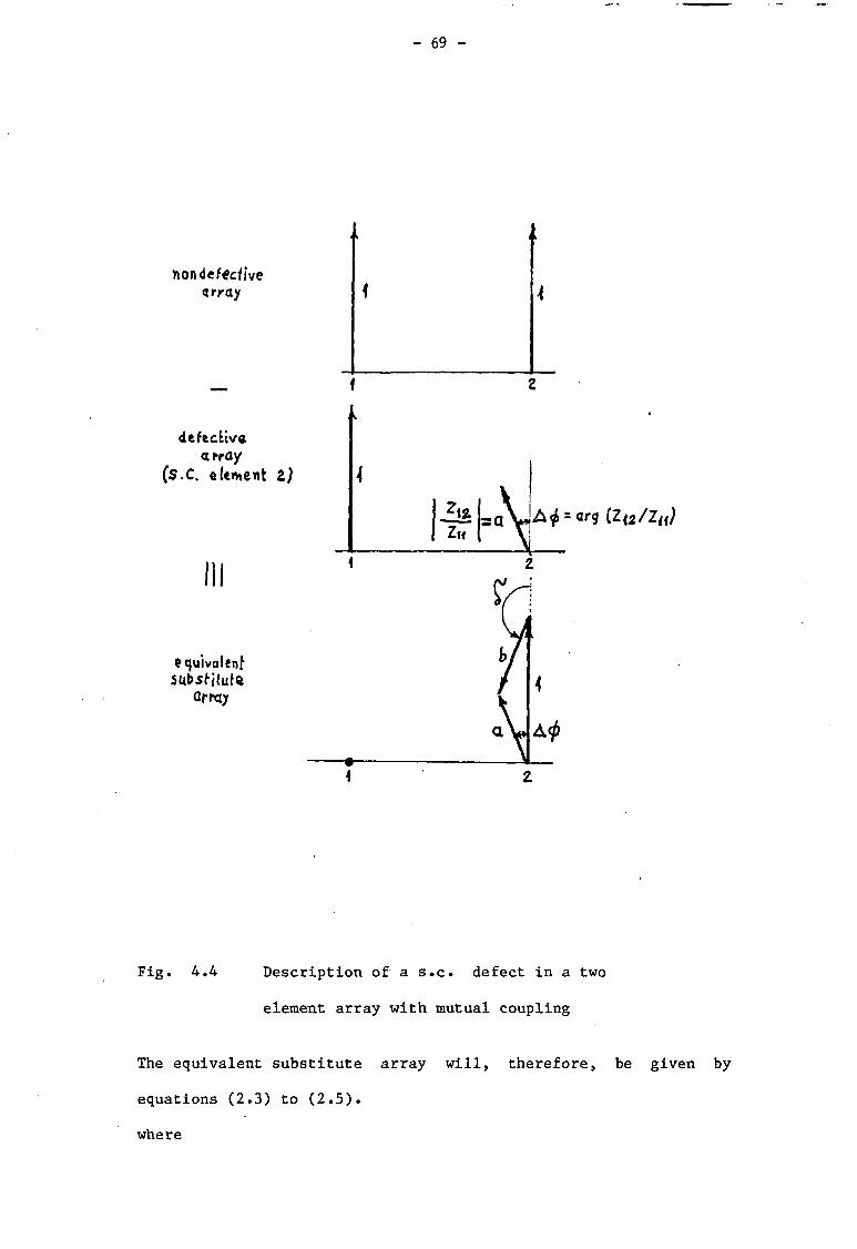
- 69 -
nondefccfive array
defective a fray
(S.C. element Z)
equivalent subsMute
armj
Zu A^i = ar9 (Za/In)
Fig. 4.4 Description of a s.c. defect in a two
element array with mutual coupling
The equivalent substitute array will, therefore, be given by
equations (2.3) to (2.5).
where
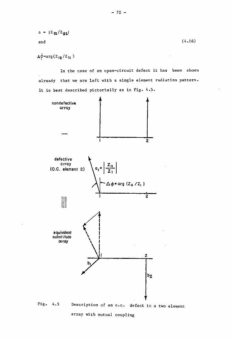
- 70 -
a = |Z ( 2/Z 2 2|
and (4.16)
A<i=,arg(Zl2/Z„ )
In the case of an open-circuit defect it has been shown
already that we are left with a single element radiation pattern.
It is best described pictorially as in Fig. 4.5.
4 i k nondefective
array
defective array
(O.C. element 2)
equivalent substitute
array
Zi
A<£«arg (Z„ /Z, )
b 2
Fig. 4.5 Description of an o.c. defect in a two element
array with mutual coupling
- 71 -
The equivalent substitute array for an o.c. defect in
element 2 (for voltage source generators) will, therefore, be
given by the superposition of two elements, where the equivalent
substitute for element 2 equals -1, and the equivalent substitute
for element 1 is given by equations(2.3) and (2.4). Here,
a = IZn/Z, |
and (4.17)
arg(Z „/Z, )
It is to be noticed that although the excitation and defect
demonstrated has been chosen to give a simple description, other
types of excitation generators and defects can be analyzed
similarly. The example of mutual coupling between broadside
(parallel) elements, is important because mutual coupling for this
configuration is strongest, and hence will produce the largest
effects.
So far, mutual coupling effects between two elements have
been discussed. For large arrays, like the MLS array, the present
analysis has to be extended, which will be done next. The idea of
infinite arrays, as presented by Oliner and Malech [ 27], will be
used.
4.4 Defects in an infinitely long uniform arrays
Large arrays are thought of as consisting of two parts
[27] : a "central part" which constitutes the bulk of a large
array and the regions near the "edges". Each element in the
central portion feels the same environment. Hence the treatment
of mutual coupling effects in infinite arrays is suitable for
large arrays, if edge effects are ignored. It will be assumed for
- 72 -
simplicity, that only first order effects are important. Hence
the effect of changing parameters of a single element (e.g. due
to a defect) will be "felt" by the neighbouring elements and will
modify their parameters without the chain reaction (second order
effects) of each one of the neighbouring elements affecting the
others as well. Ignoring these second order effects simplifies
the analysis by avoiding the need to solve a large number of
simultaneous equations or looking for an infinite series
representation.
Following these assumptions, mutual coupling effects due
to a defect can be calculated seperately for each element in a
manner similiar to the treatment used previously for two elements
(equations 4.16 and 4.17).
For example, assume element i is missing. Then the
magnitudes aj of the substitute elements will be given by the
following expressions
aj -
l zy
/ zj j
1
and the phase A.(j>. by: (4.18)
l=|arg(Z(;i/Zjj )[ J
A defect in one element of the array will cause symmetrical
effects in elements located on both sides of the defective
element, i.e.,
= a M >
' (4.19)

- 73 -
Because of the decrease of mutual coupling, inversely with
distance according to equation (4.11), the modification of the
mutually coupled elements due to the defect will decrease in the
same proportion. The effect is therefore that of a substitute
array with an amplitude taper, decreasing sharply and
symmetrically with the distance, from the location of the defect.
The phase of the coupled element will change in accordance with
the argument ratio of the impedance to the original input
impedance. Fig. 4.6 demonstrates the case of a missing element
in an infinitely long homogeneous array.
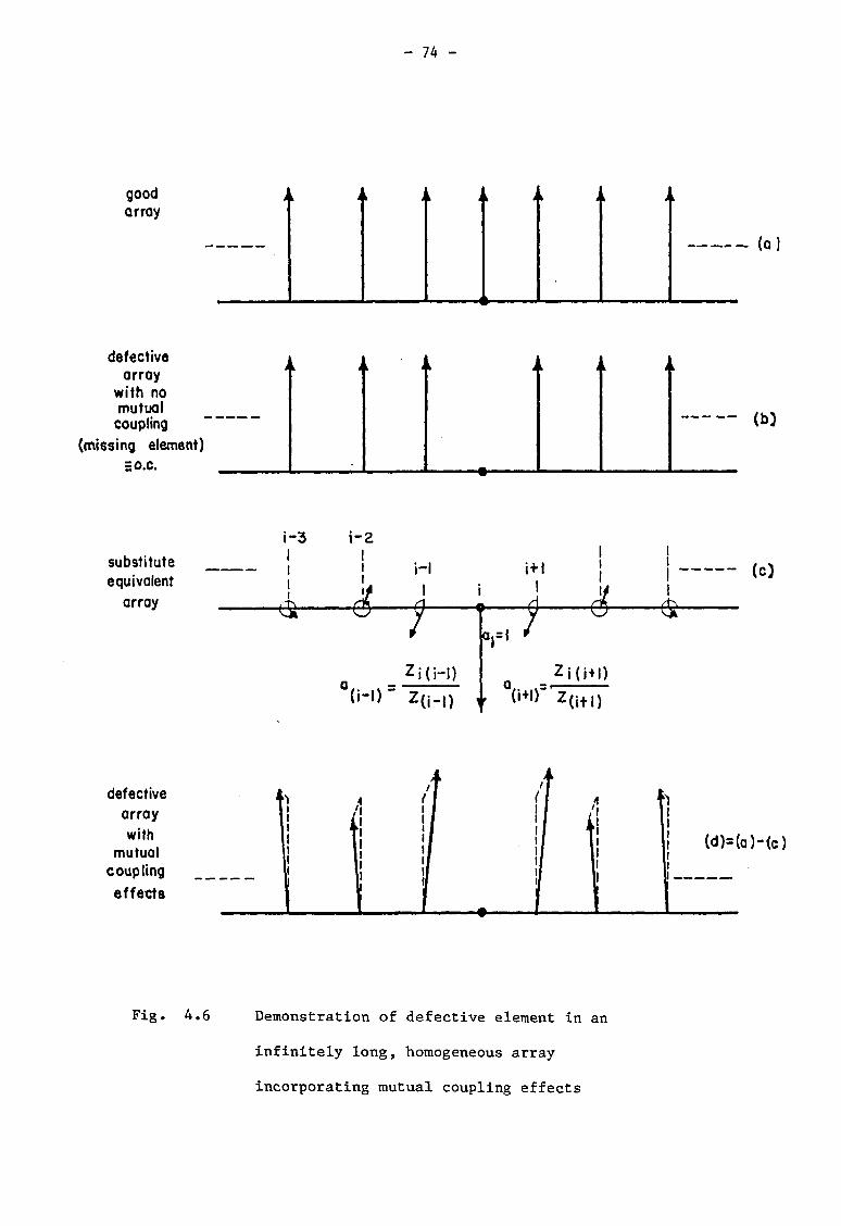
- 74 -
good array
(a)
defective array
with no mutual coupling
(missing element) =o.c.
(tO
substitute equivalent
array
i-3 i-2 1 1
— j ! H
! 1/ 1 i
1
• v j
i (\ rn
i i i - ~ i
•Ofc o y 1
Zi(i-I) °(H)- Z ( M , ,
1 y
a,=l /
a Z i ( i + , )
' V i r z ( l + I )
(c)
defective array with
mutual coupling effects
(d)=(a )-(c)
Fig. 4.6 Demonstration of defective element in an
infinitely long, homogeneous array
incorporating mutual coupling effects

- 75 -
Fig. 4.6 demonstrates qualitatively the substitute subarray of a
missing element i due to mutual coupling effects. It is clear
that the resultant substitute subarray far-field phase-pattern
will now deviate periodically from the ideal phase-line (i.e. if
no mutual coupling is included). Also the far-field magnitude
pattern will be amplitude modulated. It will be found convenient
to use a practical numerical example, which will be presented
next.
Example: A missing element i in an infinite X/2 parallel dipole
array.
The interelement spacing is 0.68 \ (the parameters were chosen to
fit a similiar experimental linear array investigated in chapter
7). Using equations (4.9) to (4.14) and (4.16), (4.17) the
following values are calculated, see table 4.1
Table 4.1
Mutual coupling substitute subarray value for missing elemnt i,
infinite A/2 parallel array 0.68^ interelement spacing.
1 ... -3 -2 -1 0 +1 +2 +3 ... a mag ... .11 .16 .3 1 .3 .16 .11 ... phase ... 112 -10 -126 0 -126 -10 112 • . •
It can be concluded that the expected R.M.S. phase variation is
about 30 degrees. These (periodic) phase variations can be
smoothed using a statistical regression line, as in the case of
random excitation described in section 3.2.2, although less
efficiently due to their non-random nature. The values calculated
in table 4.1 will be used in a computer simulation in a later
section, where the resulting phase (and magnitude) variation will

- 76 -
be given. In order to complete the discussion on interelement
coupling effects, the other type of coupling i.e. the reflected
power due to a defect in an element array, have also to be
included, as follows.
4.5 Effects of reflected power due to a defect
in array element*
As explained in the begining of this chapter, reflected
power in the feed network, comprises another mechanism of
coupling. It was also explained that this effect is not
attenuated with distance, if a lossless feed network is assumed.
The effect of reflected power is dependent on the configuration of
the feed network (e.g., series coupled elements in a waveguide
antenna), and whether the feed network is reciprocal (e.g.,
nonreciprocity could be due to the presence of ferrite isolators).
It is assumed that a travelling wave series-fed antenna array will
mostly be affected by a forward reflected power from an
open-circuited defective element. If all the other elements are
matched to the (characteristic) impedance of the feed line
network, then open circuiting an element only means a longer
transmission line (assumed to be lossless) between the element
preceding the defect, and that following it. The original
excitation signal experiences the same delay to subsequent
elements, as the forward reflected power due to the defect. This
is because both signals travel the same path length in the feed
network. The main effect will, therefore, be in modifying the
excitation of subsequent elements from the defective element.
This will introduce asymmetry (a jump) in the excitation of all
the elements from the defect onward. The amount of this jump in
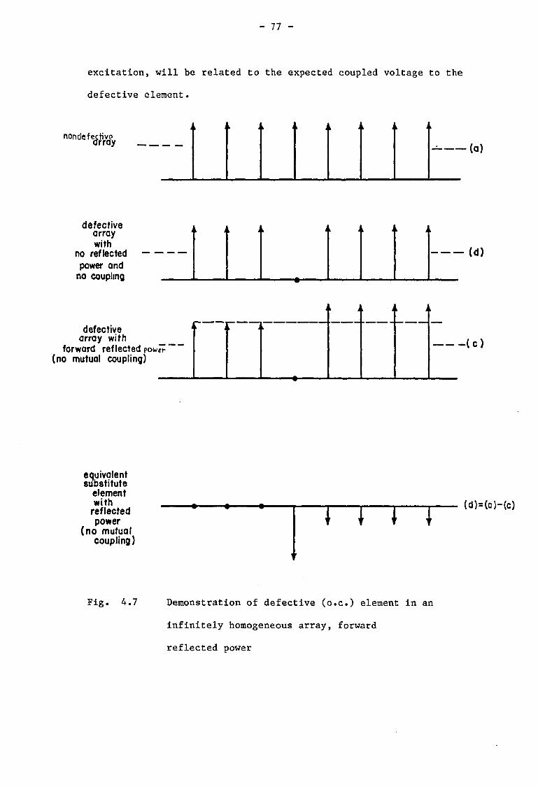
- 77 -
excitation, will be related to the expected coupled voltage to the
defective element.
nondefej^
(a)
defective array with
no reflected power and
no coupling
defective array with
forward reflected power (no mutual coupling)
(d)
( c )
equivalent substitute
element with reflected power
(no mutual coupling)
rrn (d)=(a)-(c)
Fig. 4.7 Demonstration of defective (o.c.) element in an
infinitely homogeneous array, forward
reflected power

- 78 -
Due to asymmetry it is expected that this type of effect, is more
severe in its effect when the subtraction method is applied than
the mutual coupling effect if a short array is considered. A
computer simulation of this type of effect will be demonstrated in
the following section.
4.6 Simulation of defective elements in actual arrays
(deterministic case).
A simulation of the effect of mutual coupling and forward
reflected power due to an open circuited element in an array is
demonstrated in Figs. 4.8 to 4.11. The spacing and element
dimensions are chosen to apply to the array investigated
experimentaly as described in chapter 7. It is seen that the
effect of forward reflected power is more severe than that of
mutual coupling. The mutual coupling values are taken from table
4.1. The reflected power ratio is taken from the design
parameters of a waveguide slot array [ 23]. These results are
compared to those of the experimental investigation in chapter 7.
4.6.1 Simulation parameters
An 8-element A/2 slot array with a cosine square over
pedestal aperture illumination with 0.68^ interelement spacing
is assumed. The mutual coupling effects are given in table 4.1.
The forward reflected power is given in table 4.2, obtained from
the slot-coupled power calculated from the array design parameters
[ 23].
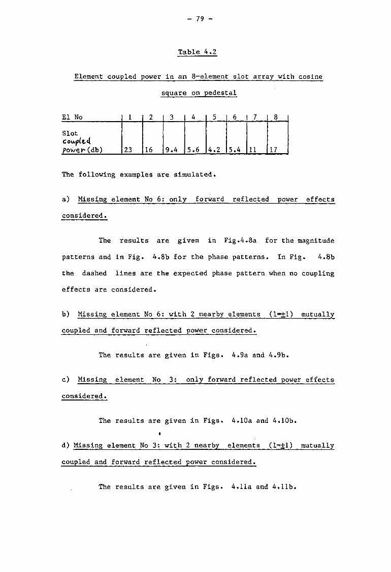
- 79 -
Table 4.2
Element coupled power in an 8-element slot array with cosine
square on pedestal
El No 1 2 3 4 5 6 7 8
Slot couple.4 pov/el^ (db) 23 16 9.4 5.6 4.2 5.4 11 17
The following examples are simulated.
a) Missing element No 6: only forward reflected power effects
considered.
The results are given in Fig.4.8a for the magnitude
patterns and in Fig. 4.8b for the phase patterns. In Fig. 4.8b
the dashed lines are the expected phase pattern when no coupling
effects are considered.
b) Missing element No 6: with 2 nearby elements (1=±1) mutually
coupled and forward reflected power considered.
The results are given in Figs. 4.9a and 4.9b.
c) Missing element No 3: only forward reflected power effects
considered.
The results are given in Figs. 4.10a and 4.10b.
t
d) Missing element No 3: with 2 nearby elements (1=±1) mutually
coupled and forward reflected power considered.
The results are given in Figs. 4.11a and 4.11b.
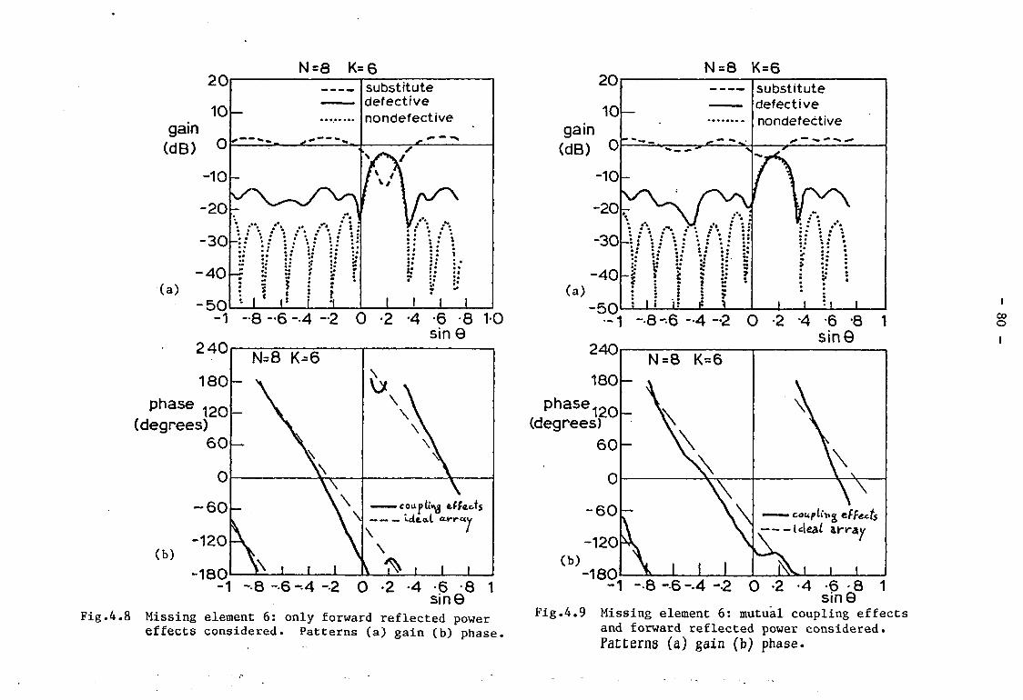
2 0
10
gain (dB) 0
- 1 0
- 2 0
- 3 0
N =8 K= 6
(a)
- 5 0
substitute defective nondefective —
substitute defective nondefective
substitute defective nondefective
<
\ A
J : I: ; r # 5 M 5 M f I' I
A s
f \ A
1a % J: \ • • ;
:: :: \ •• jj i • . . . • • • * • • • • • H ' • Ia
1 I ' l l -1 - 8 - 6 --4 - 2 0 -2 *4 -6 -8 1 0
sin 9 2 4 0
1 8 0
phase 1 2 Q
(degrees) 6 0
0
- 6 0
- 1 2 0 (b)
- 1 8 0
N=8 K-6
~ \ \\
\ \ \
\\ \\ \ \ V i i i
i • •coapU'v i effects _ Ideal a.trre*y
\ 1
\ ft I I I -1 - 8 --6 - 4 - 2 0 -2 -4 -6 -8 1
sin© Fig.4.8 Missing element 6: only forward reflected power
effects considered. Patterns (a) gain (b) phase.
20 10
gain (dB) 0
- 1 0
- 2 0
- 3 0
- 4 0 (a)
- 5 0
2 4 0
1 8 0
phase12Q
(degrees) 60
0
- 6 0
- 1 2 0 (b)
- 1 8 0
N = 8 K = 6
— ~ — — substitute defective
nondefective
~ •» "s
substitute defective
nondefective
~ •» "s » » — . ^ >
J J
s£ :• •• L* •< «• «.
- i ? M m i i r : 1 i i: f *
• • • • •
j ; : f • j ' I
i I ^ I i
-•8--6 - 4 - 2 0 -2 -4 -6 '8 1
sinG N = 8 K = 6
~ V - V
N N \
\ \ \ ^ \ I I I
—— coupiittg effects - l4eaL array
i V l 1 1 -•8 --6 --4 -.2 0 -2 -4 -6 -8 1
sin9 Fig.4.9 Missing element 6: mutual coupling effects
and forward reflected power considered. Patterns (a) gain (b) phase.
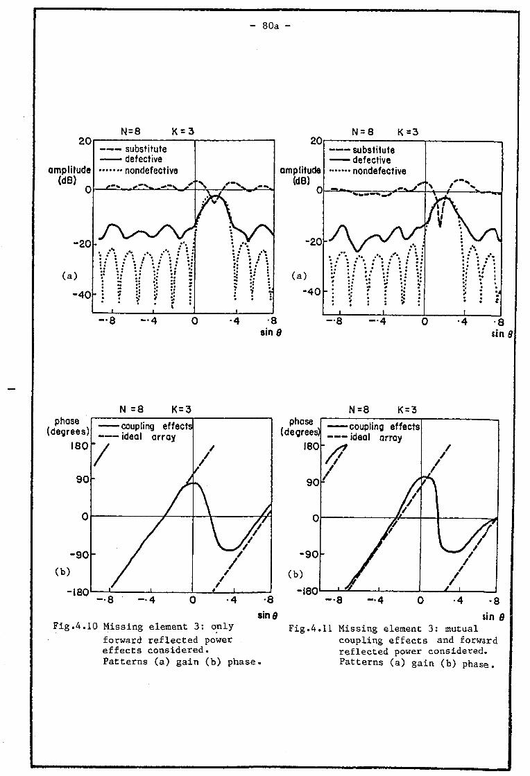
- 80a -
N = 8 K = 3
amplitude (dB)
0
20
amplitude (dB)
0
-20
(a)
-40
N = 8 K =3
substitute — defective
\ / " X • # V A"
• • * » . • • I » • », 1 • . » • » • • * . • • •
• \ M \ \
* / • • • I • • • • . • « • •t #« t :: : • •; :; . ;
I; : •• •• s
fi • t *# • •
* : j; : > • V > : : i : • i
• i t
—8 —4 •8 sin 91
N =8 K= 3 N =8 K = 3 phase
(degrees) 180
90
-90
(b)
-180
— coupling effects — ideal array
/ / /
\ A
i i
\ /* \ // \ /*
/ / / / / / i
- 8 — 4
phase
8 sin ^
Fig.4.10 Missing element 3: only
forward reflected power effects considered. Patterns (a) gain (b) phase.
90
-90
(b)
-180
——coupling effects ideal array
• / / // / / / /
/ / / / A
A ft
i w i
L/ v y / / / / / L-JL _ —8 - 4 0 -4 -8
sin 9 Fig.4.11 Missing element 3: mutual
coupling effects and forward reflected power considered. Patterns (a) gain (b) phase.
- 81 -
4.6.2 Assessment of the results
The examples have been chosen such that the missing
element will be examined to the left and to the right of the array
center, thus introducing different substitute subarrays due to
forward reflected power asymmetry. As expected, the forward
reflected power with the above parameters causes the maximum phase
deviation around the ideal phase-line (dashed), this is in
comparison with the small effect of the mutual coupling model.
The substitute array when element 3 is defective introduces a
larger effect due to the fact that the resulting substitute array
(due to forward reflected power) is larger (5 elements) than that
modeled when element 6 is defective (2 elements). The resulting
phase deviation is about +20 degrees (peak) for missing element 6
and about +60 degrees (peak) for missing element 3.
These results are to be compared to those of the
experimental investigation in chapter 7.
In addition to the phase deviation of the substitute
subarray pattern there are magnitude deviations from the expected
constant line if no coupling effects are considered.
4.7 Discussion (expected usefulness of the subtraction method
in actual arrays - deterministic case)
The analysis in this chapter, combined with simulation on
the computer has shown that coupling effects of the two types,
namely: the mutual coupling and feed network coupling (forward
reflected power) can cause deviations of the resulting phase
around the expected phase-line. It is instructive to deduce the
phase deviation by examining the amplitude variations of the

- 82 -
substitute array pattern (the upper curve in Figs. 4.8a to
4.11a). There the amplitude pattern shows periodic variations
around the "correct" ( constant) value of the substitute element
pattern when no mutual coupling effects are present. If a
statistical regression line is constructed then the ideal array
substitute element amplitude pattern can be derived (i.e. when no
mutual coupling effects are present). Similarly for the phase
variation pattern which accompanies the amplitude pattern. It is
therefore believed that a statistical regression line, constructed
from the phase data points, is able to resolve a defective element
in actual arrays in the presence of coupling effects. (It should
be noticed that the smoothing in this case is expected to be less
effective than in the case of random phase examined in section
3.2.2, due to its non random nature.) In a seperate chapter
(chapter 7) experimental investigation of actual arrays with
similar parameters will be demonstrated, in order to test the
present analysis and simulations.
The present chapter concludes the first part of this work
which investigated the concept of the equivalent substitute
element and the proposed subtraction method, based on this idea.
The subtraction method, first analyzed with defects in ideal
arrays, was then examined in the presence of random phase
excitation errors in chapter 3 and in the presence of mutual
coupling effects in the present chapter. Simulations on the
computer have shown that the subtraction method is a powerful tool
for use in monitoring defects in actual arrays.
It has also been found that the substitute element
technique is a convenient tool to describe defects of both static

- 83 -
and dynamic nature, and has provided insight into the effects of
mutual coupling.
The second part of the work will investigate further
monitoring methods based on the angular plane-wave spectrum
concept.

- 84 -
CHAPTER 5
APPLICATION OF THE ANGULAR SPECTRUM CONCEPT
In the first part of the work a simple method of
monitoring was suggested, called the subtraction method, based on
the equivalent substitute element technique. The method was found
efficient for the detection of defects in a single element or in a
single subarray of the antenna. This technique has also been
found to be applicable for the detection of defects in many
elements if elements fail one at a time. The present chapter
deals with other methods which are more adequate for the detection
of many elements failing at one time, although at the price of
more complex processing. These methods, based on the concept of
the angular plane-wave spectrum, will be referred to as "the
angular spectrum direct method" and the "autocorrelation function
(a.c.f.) method". The basic angular spectrum concept will first
be summarized.
5.1 Summary of the angular spectrum concept
It has long been known that Huygens' principle, which
states that each point on a propagating wavefront can be
considered as a secondary source radiating a spherical wave, is
only one way of describing fields diffracted from apertures, using
Fresnel's formulation based on the principle of superposition. An
alternative way is to represent fields by the superposition of a
discrete set or a continuum of plane waves travelling in different
directions. This is what is meant here by the concept of the
"angular spectrum of plane waves" or, in its abreviated form, "the
angular spectrum" concept. The theory of this approach has been
- 85 -
covered by several authors, see for example, Booker and Clemmow
[ 12], Ratcliffe [ 14] and Clarke and Brown [ 13]. The basic idea
is that the radiation from an aperture can be considered as a
superposition of an infinite number of plane waves propagating in
different directions into the half space in the direction of
propagation. The amplitude and phase of each plane wave depends
on the aperture field distribution. A demonstration of this
representation is given in Fig. 5.1.
Fig. 5.1 A representative plane wave in the field
radiated by an aperture
The field radiated from the aperture can be considered as a
superposition of an infinite number of plane waves radiating into
the half space z>0 . A representative incremental plane wave
propagating in the u direction is shown to have an electric field

- 86 -
e (a phasor vector) that is constant throughout all space and for fV
all time ( For a purely sinusoidal field the time dependence of
exp{jiflrt} will be suppressed). Since the field of plane waves are
wholly transverse, we have
e.u=0 • (M
For a set of plane waves travelling in different directions, their
individual phasor-vector amplitudes can be written as e(u). The /v oJ
vector function of direction ^(u) is related to the angular
spectrum function F(u) by e(u)=F(u) du. Hence F(u) du is the N Al V V fst A/ V fst >\t fj
amplitude of the elemental plane wave. (Note that F(u), being a aJ
function of direction has two independent variables, such as
(9,^), so that du would in that case be d9d^.) The phase of this
elemental plane wave at some point P(r) at vector distance r from rJ n
the origin 0, will be retarded by an amount corresponding to a
distance u.r, which is the projection of r on the direction u as
shown in Fig. 5.1. Hence the electric field at the point pOj)
will be given by
E(r) = | F(u) exp{-jku.r)}du (5.1)
and the corresponding magnetic field H(r) will be given by A/ <V
H(r) = ± I uxF(u) exp{-jku.r} du (5.2) M v 2 J v At
where Z the characteristic impedance of the medium. «
The tangential component ^ c S ^ ) of the aperture field is
given by putting r= P in equation (5.1), as n/ VJa/
E a ( P ) = | ^(u) exp{-jku. P ) du (5.3) Jf4 J A / w Jfs/ *J
where ^ is confined to the aperture plane and defined by two

- 87 -
independent variables. Hence equation (5.3) can define a Fourier
transform from the direction domain u into the position domain P •
The inverse transform yields the angular spectrum
Therefore the angular spectrum can be found from the aperture
field using equation (5.4), and the field anywhere to the right of
the aperture can be deduced using equation (5.1). In general the
solution of equation (5.1) is not simple. However a simple result
is achieved for the far field using the method of stationary
phase.
The far field of an antenna can be resolved by an
approximation to equation (5.1) for k r » l . The phase term in the
integrand of equation (5.1) can be written as
ku.r a kr cos^r (5.5) rst <v
where cos>/r= u.r /r . I M
Since in the far field kr is very large, the phase term will
undergo large variations (through many multiples of 27T ) for
only small changes in the direction u relative to the direction
Uy, (which now coincides with r ), except when c o s i s
stationary. This "stationary-phase" condition occurs when cos^=0
and.u=uw» . Then it can be said that the contributions from the
integrand will tend to cancel one another except in the region
u=uy, • Hence the result will be that /V ( V '
E ( r ) ^ F ( u w ) . (5.6) A/ r j ^
Therefore the far field amplitude depends directly on the angular
- 88 -
spectrum function,
To be specific, an x-polarized component of the radiated
electric field in Cartesian coordinates is
:x,y,z)= J J F x exp{-jk(<^x+^y+^z)}do<'d^ (5.7)
Where E^ the x component of the field at P( x,y,z), see Fig
5.2.
radiat apehture
- X ^ v + V U w + Z u. rsf
$iy\6 cos (j>
Sirsin f
c o s &
Fig. 5.2 Aperture radiation geometry
The angular spectrum of the x component of the aperture field is
where tf and^" are the direction cosines to the
2. Z Z
x,y and z axes (where oi + =1). Similiar expressions can be
given for other components (see Clarke and Brown [ 13] ).
In many cases, like the MLS array, physical fields can be
- 89 -
described based on the simpler two dimensional representation
provided the radiating aperture is separable (i.e. if the
aperture field E ^ X j y ) can be expressed as a product of two
functions say Ea(x,y)=ff (x) f 2(y) )• Then the angular spectrum is
also separable. Then each function can be treated separately
assuming the other is unchanged. Use will be made of the two
dimensional representation in discussing the monitoring methods
based on the angular spectrum, and so the angular spectrum
representation of two dimensional fields will be described next.
5.1.1 The angular spectrum of two dimensional fields
Consider an x-polarized aperture field E a x(x) radiated
into the half-space z>0 in the two-dimensional geometry of Fig.
5.3 .
The field components corresponding to equation (5.1) are then (see
Clarke and Brown [ 13] ),
- 90 -
E^(x,z)' r ' 1
E z(x,z) a F(s) -s/c
,Hy(x,z) i
,1/zc. ,Hy(x,z) r>o ,1/zc.
exp{-jk(sx+cz)}ds (5.8)
where s=sin9 and c=cos8=(l-s i) . The extended integration limits
for 1s|>1 correspond to evanescent waves which although not
propagating are included for completeness of the presentation.
The tangential aperture field is
E a X(x)= E x(x,0)
yo h F(s) exp(-jksx) ds (5.9)
Which is the Fourier transform of the angular spectrum function
F(s). The inverse transform then holds, giving
\ F ( s ) =
t (5.10) EflL)C(x) exp{+jksx} dx
As an example the x component of equation (5.8) is given
approximately by (putting c - l - i s ^ ),
Ej(x,z)=exp{-jkz} I F(s) exp{jl/2 kzs 2 , }exp{-jkxs}ds (5.8a)
This is a Fourier transform of the product of two functions of s
having the following Fourier transforms (pairs)
F(s) E a x ( x )
and
exp{j —-kzs2) (j*/z)k exp{-jV2 kx 2/z)
where the notation ^ ^ designates the Fourier transform relation.
It follows from the convolution theorem of Fourier transforms that
A E^(x,z)=(j/^\z) exp(-jkz) J e xP^"J k (x-xO* , , ^ r } d x (5.8b)
- 91 -
'E^r ,6)' 'cos© •
E*(r,0) =3 -sin6
which is Fresnel's diffraction formula [ 13]. Use of this result
will be made in chapter 6.
The far field is approximated as explained earlier, by
the method of stationary phase to give the following
jT f(sin9) exp{-jkr} (5.11)
- *
or in polar form
E 0(r,e) = ZHy(r,e)= ^ R s i n 9 ) exp{-j(kr-TT/4) } (5.12)
A similar set of equations hold for a y-polarized one-dimensional
aperture fieLtL*
The inverse process, i.e the determination of the aperture field
from the far field measurement will be used as a basis for the
monitoring methods suggested later in this chapter.
The determination of far-field from near field
measurements will be described next.
5.1.2 Determination of far-field from near-
field measurements
The planar near field measurement technique now in
extensive use is only a straight-forward use of the angular
spectrum concept. Consider the system in Fig. 5.4
- 92 -
X '
f,X-poUrtittL IP* "measuring X - p o U r i z t d
Fig. 5.4 Geometry of near field measurement
The far field of an x-polarized aperture is to be determined from
near field measurements. An x-polarized isotropic antenna (in
practice possibly a low gain open waveguide) is traversed over the
plane z=z 0 . From equation (5.8) it follows that:
E x(x,z 0)= I F(s) exp{-jk(sx+cz0)}ds (5.13) J-yo
and since z 0=constant, r E*(x,z0)= exp(-jkczd) I F(s) exp(-jksx) ds (5.14)
Inverting, gives F(s) = e x p ^ k c z j e x p ( j k s x ) d x . (5.15)
This means simply that measuring the field over z0=constant, then
taking its Fourier transform yields the angular spectrum function
of the transmitting antenna (multiplied by exp{-jkcz0} ).
According to the far-field theorem mentioned previously, the far
field is also determined using equation (5.12). In practice
however the measurement range is finite, and hence also are the
integration limits in equation (5.15). This means a truncated
UO
- 93 -
near-field measurement which, again, modifies the results.
According to the convolution principle only a smoothed finite
range of the angular spectrum and hence the far field is, thereby,
determined. A further practice is to apply the discrete Fourier
transform (DFT), using available computer subroutines. The
sampling then needed is done in equal Ax samples, which must
comply with the spatial Nyquist criterion, given by
x ^ A/(2| S / I n < t xl) (5.16)
where | s ^ ^ | = | sin | . In practice however about 1/3 is
used. The above technique was extensively used in the
experimental investigation described in chapter 7.
Having summarized the angular spectrum concept and some
of its applications it is now possible to present the monitoring
method, based on that principle. This will be done in the next
section.
5.2 Use of the angular spectrum method to
locate defects in antenna arrays
The angular spectrum concept enables one to resolve the
aperture illumination of an antenna, if its angular spectrum is
known. The far-field of an antenna is asymptotically equal to its
angular spectrum, and the angular spectrum is the Fourier
transform of the aperture field. Hence the measurement of the
far-field of an antenna can, in principle, yield the aperture
field illumination. It is therefore suggested that the angular
spectrum concept be used as an alternative method for the
detection of defects in antenna arrays.
- 94 -
The monitoring method is based on a procedure for the
detection of defective elements through their effect on the
aperture illumination field, as follows:
- Measure the far field over the range -TT/ 2<&< TT/2.
- Using equation (5.12) solve the angular spectrum function F(s).
- Perform a Fourier transform of the angular spectrum functions
equation (5.9) to yield the aperture field distribution.
Any anomaly in the aperture distribution is due to defects in the
antenna elements excitation.
In practice, however, this procedure is not fully
applicable, due to the finite measurement range of the far-field.
Hence, a modification is needed.
- Measure the far field, with the same polarization of the
transmitted signal, in the direction cosines s( <s<s z . This will
approximate the angular spectrum function of the radiating
aperture.
- Perform a Fourier transform of the truncated angular spectrum
function. This yields the smoothed aperture distribution.
- Identify defects by checking for anomalies in the calculated
aperture field distribution.
It should be noted that the modified calculated aperture
distribution could have a different shape than the unmodified one.
It depends strongly on the range of the direction cosines chosen
for measurement. Broadly, this could be chosen in the two extreme
cases: The far side-lobe region and the main-lobe region. Both
- 95 -
ranges give information on defects in the antenna aperture
distribution. It will be demonstrated with the aid of simplified
examples that, as with the subtraction method, the angular
spectrum method also gives superior information in the far
side-lobe region for monitoring purposes.
5.2.1 Demonstration of the angular spectrum method
An ideal linear uniform broadside array of ty2 spaced
isotropic N elements is assumed, with missing elements in the
antenna. The far side-lobe region of an ideal array pattern can
be approximated by sin(7TNds/>v ), (see equation 2.1). This is
equivalent to the interference pattern of the two edge elements of
the array, with a distance (measured in wavelengths) of Nd/^ in
between, where all other elements have zero illumination.
The Fourier transform of this angular spectrum is given
by two delta functions located at +(Nd/X )/2 (i.e.
E a(x)=E d[ i(x-a/2) + ^(x+a/2)] , thereby representing the edges
of the aperture. Missing elements in the array will be
represented according to equation (2.5) and Fig. 2.9 by
additional delta functions in accordance with their relative
location in the array aperture. The magnitude ratios of the
spectral components of the angular spectrum is given by their
normalized amplitude ratio. Therefore the magnitude ratio is
given by
E^/Efc =2 sin(TTdsa/A ) (5.17)
where E ^ / E ^ the missing to edge-element illumination amplitude
ratio, s a is the mean direction-cosine and sin(TTds a ) is the
reciprocal of the mean side-lobe level magnitude (e.g. in the far
- 96 -
side lobe region 2 ).
If measurements are performed in a region symmetrical
about the main lobe then the Fourier transform of the angular
spectrum will give approximately constant illumination over the
aperture range. Missing elements will be identified by holes in
the calculated illumination. Due to the finite direction-cosine
range used the resulting illumination will spread outside the
theoretical aperture range and the theoretical delta functions
will be replaced by sin[ k(x-x^) L]/k(x-xt") functions, where
2L=direction range, and x i the location of the peaks in the
aperture plane. Qualitative results, when use is made of this
technique, are presented in Fig. 5.5 for two cases: a_ the far
side-lobe region (Fig.5.5a) and b the main lobe region (Fig.
5.5b).
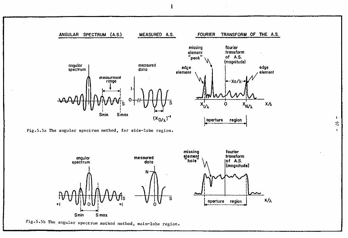
I
ANGULAR SPECTRUM (A.S.) MEASURED A.S. FOURIER TRANSFORM OF THE A.S.
angular spectrum
measurment range
i - U
missing elernem ii , u peak
measured data edge
element
I-
i Smin Smax -I
fourier transform of A.S. (magnitude)
Fig.5.5a The angular spectrum method, far side-lobe region.
aperture region
edge element
vO
angular spectrum
measured data
missing i^emenf
hole
Smin S max Fig.5.5b The angular spectrum method method, main-lobe region.
fourier transform of A.S. (magnitude)
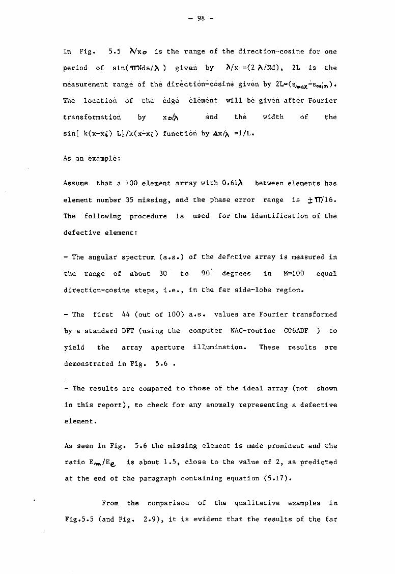
- 98 -
In Fig. 5.5 tyx© is the range of the direction-cosine for one
period of sin( TTTJds/* ) given by */x = (2 */Nd), 2L is the
measurement range of the direction-cosine given by 2L=(s/>f,oX-s(W;y,).
The location of the edge element will be given after Fourier
transformation by xo/* and the width of the
sin( k(x-xi) L]/k(x-xc) function by Ax/^ =1/L.
As an example:
Assume that a 100 element array with 0.61A between elements has
element number 35 missing, and the phase error range is ± IT/16.
The following procedure is used for the identification of the
defective element:
- The angular spectrum (a.s.) of the defctive array is measured in
the range of about 30 to 90 degrees in M=100 equal
direction-cosine steps, i.e., in the far side-lobe region.
- The first 44 (out of 100) a.s. values are Fourier transformed
by a standard DFT (using the computer NAG-routine C06ADF ) to
yield the array aperture illumination. These results are
demonstrated in Fig. 5.6 .
- The results are compared to those of the ideal array (not shown
in this report), to check for any anomaly representing a defective
element.
As seen in Fig. 5.6 the missing element is made prominent and the
ratio E ^ / E ^ is about 1.5, close to the value of 2, as predicted
at the end of the paragraph containing equation (5.17).
From the comparison of the qualitative examples in
Fig.5.5 (and Fig. 2.9), it is evident that the results of the far

- 99 -
side-lobe region are superior to those obtained in the main-lobe
region. This is because the higher peaks of the F.T. of the a.s.
magnitude are all relevant as they point out the antenna edge
elements and the corresponding missing elements. In addition the
peaks of the missing element is pointed out more clearly and with
a larger magnitude ratio to the edge element illumination than in
the main-lobe region.
«
N= 100 K=35
relative magnitude
O.F.T. of A.S.
6.0
4.0
2.0
missing element Nfi 3 5 \ i
edge elements
NS. l \ edge •element
y n s 100
array aperture
o o
[X/\] x [22/120]
aperture coordinate
Fig.5.6 Simulation of detection of a missing element by the angular spectrum method.

- 101 -
5.3 Use of the angular autocorrelation function of
the angular spectrum to locate defects in the
presence of random errors
The autocorrelation function (a.c.f.) is a very useful
function for treating random data. It has the properties of
smoothing the data and extracting sinusoidal components buried in
the fluctuating data points.
It has already been shown that the effect of a defective
element Is broadly to introduce oscillations in the pattern. The
essence of the autocorrelation technique is to extract these
oscillations and hence identify the position of the defect.
Utilization is made of Ratcliffe's work [ 14], based on the Van
Cittert - Zernike theorem [ 18], on the dual Fourier transform
pair: the a.c.f. of the angular spectrum and the aperture power
illumination, a description of which is also given in Appendix C
and is summarized here.
5.3.1 The a.c.f. and the aperture illumination.
It can be shown that the Fourier transform of the a.c.f.
of the angular spectrum yields the aperture power illumination
function (see Appendix C). Designating the a.c.f. for the
direction-cosine displacement & , then
iv l-f(x) f*(x) (5.18)
Where + [ ] the Fourier transform and f(x x) is the
aperture power illumination over the aperture axis x. The a.c.f.
is given by
J >(8')= I F( F(s) F*(s+$) ds (5.19)
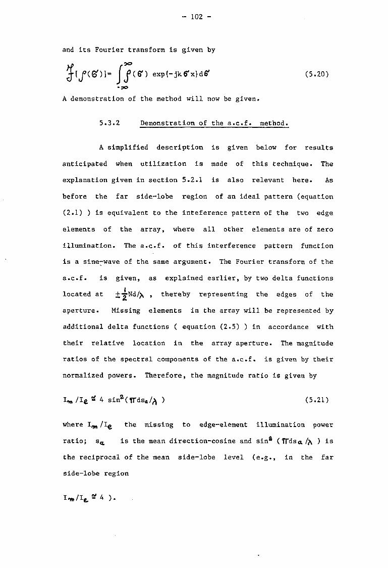
- 102 -
and its Fourier transform is given by
Jj^Ce') exp{-jk^x}d& (5.20)
-30
A demonstration of the method will now be given.
5.3.2 Demonstration of the a.c.f. method.
A simplified description is given below for results
anticipated when utilization is made of this technique. The
explanation given in section 5.2.1 is also relevant here. As
before the far side-lobe region of an ideal pattern (equation
(2.1) ) is equivalent to the inteference pattern of the two edge
elements of the array, where all other elements are of zero
illumination. The a.c.f. of this interference pattern function
is a sine^wave of the same argument. The Fourier transform of the
a.c.f. is given, as explained earlier, by two delta functions
located at i ^ N d , thereby representing the edges of the
aperture. Missing elements in the array will be represented by
additional delta functions ( equation (2.5) ) in accordance with
their relative location in the array aperture. The magnitude
ratios of the spectral components of the a.c.f. is given by their
normalized powers. Therefore, the magnitude ratio is given by
/I e = 4 sina(TTds a/^ ) (5.21)
where /I^ the missing to edge-element illumination power
ratio; s a is the mean direction-cosine and sin a (TTdsa/X ) is
the reciprocal of the mean side-lobe level (e.g., in the far
side-lobe region
I'm/It. = « )•
J[j><er>i

- 103 -
If measurements are performed in a region symmetrical
about the main-lobe, rather than in the side-lobe region, then the
Fourier transform of the a.c.f. will give approximately constant
power illumination over the aperture range. Missing elements will
then be identified by holes in the calculated power illumination.
Due to the finite direction-cosine range utilized the resulting
power illumination will spread outside the theoretical aperture
range and the theoretical delta functions will be replaced by
sin[ k(x-x{) L]/k(x-x£) functions. Qualitative results when use
is made of this technique are presented in Fig. 5.7 for two
cases: £ the far side-lobe region (Fig. 5.7a), and _b the
main-lobe region (Fig. 5.7 b).
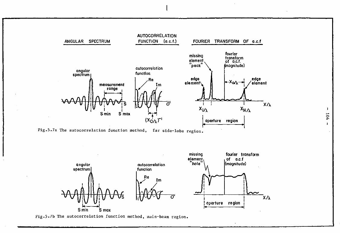
ANGULAR SPECTRUM AUTOCORRELATION FUNCTION (o.c.f.) FOURIER TRANSFORM OF a.c.f
angular spectrum
wvVV
measurement range
h 1
autocorrelation function
Re Im
I S min S max
(Xo/x>"
missing element, ii i peak
edge element^
fourier transform of a.c.f. (magnitude)
i edge /element
Xl/X XN/x
aperture region
Fig.5.7a The autocorrelation function method, far side-lobe region.
angular spectrum
autocorrelation function
missing element
I I , , N hole
fourier transform of a.c.f
(magnitude)
S min S max Fig.5.7b The autocorrelation function method, main-beam region.
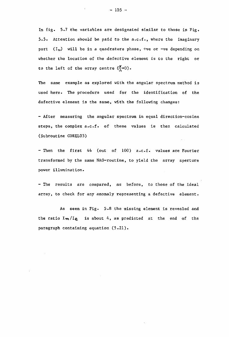
- 105 -
In fig. 5.7 the variables are designated similar to those in Fig.
5.5. Attention should be paid to the a.c.f., where the imaginary
part (Im) will be in a quadrature phase, +ve or -ve depending on
whether the location of the defective element is to the right or
to the left of the array centre (-^=0).
The same example as explored with the angular spectrum method is
used here. The procedure used for the identification of the
defective element is the same, with the following changes:
- After measuring the angular spectrum in equal direction-cosine
steps, the complex a.c.f. of these values is then calculated
(Subroutine COREL03)
- Then the first 44 (out of 100) a.c.f. values are Fourier
transformed by the same NAG-routine, to yield the array aperture
power illumination.
- The results are compared, as before, to those of the ideal
array, to check for any anomaly representing a defective element.
As seen in Fig. 5.8 the missing element is revealed and
the ratio I^/Ig, is about 4, as predicted at the end of the
paragraph containing equation (5.21).
I
relative magnitude
D.F.T. of
o.c.f.
2.1 -
1.4-
0.7 -
N= 100
missing element' No 35
K=35
element edge /element NO 100
arroy aperture
o cr>
[X/xjx[22/l20]
aperture coordinate
Fig.5.8 Simulation of detection of a missing element by the autocorrelation function method.

- 107 -
5.4 Discussion
The three methods suggested so far, the subtraction
method, the angular spectrum method and the autocorrelation
function method (a.c.f.), have all been shown to be capable of
detecting defective elements in antenna arrays. The preferred
region of monitoring has been demonstrated to be in the side-lobe
region for all three methods.
In comparing the methods, the subtraction method uses the
phase variation of the far-field substitute element to determine a
defective element, employing a simple linear equation. The
angular spectrum method, however, uses the relation between the
far field, the angular spectrum function and the aperture field to
yield the aperture illumination modified by the presence of
defects in the array. However, the method requires the
computation of a Fourier transform of the angular spectrum, which
complicates the processing in comparison with the subtraction
method. The a.c.f. of the angular spectrum makes further use of
the angular spectrum concept. Using the a.c.f. method the
aperture power illumination is determined, which when modified by
the presence of defective elements can be used to resolve defects
in the array. The a.c.f. method is expected to give superior
results compared to the angular spectrum method, due to its
properties of smoothing the data, as already explained. However,
this advantage is at the cost 4additional computation of the
a.c.f., which makes this method more demanding from the processing
aspect.
The subtraction method is particularly appropriate for
the detection of a single defective element in the array. As

- 108 -
explained, it can also be used in the case of many defective
elements provided defects do not occur in more than one element at
a time. This assumption is justified by the expected high
reliability of present and future solid-state phased-array
antennas. The other two methods can be used for a single as well
as for many simultaneous defects, but at the cost of more
computational complexity than the subtraction method.
For systems like the MLS where real time processing is
needed it seems that the subtraction method is the only one that
is adequate. However, for maintenance purposes or where longer
delays can be tolerated, a combination of two or even of all three
methods is recommended.
This chapter concludes the analysis of far-field
monitoring methods. Near-field methods will be discussed next.
- 109 -
CHAPTER 6
MONITORING IN THE NEAR FIELD
In the previous chapters far-field analysis was used in
the main for the derivation of the recommended methods of
monitoring, as normally the antenna array is to perform in the
far-field. However, to minimize uncontrolled multipath effects
between the transmitter and the monitor antenna, a near-by
positioning of the monitor antenna is most favorable, provided
measurements can be processed to overcome the inevitable
defocusing effects. The present chapter is therefore concerned
with near-field analysis for the derivation of further monitoring
applications•
This chapter deals with the two aspects of near field
monitoring. The first is concerned mainly with monitoring of the
array main beam pointing, and the second with the application of
the monitoring techniques described earlier to very near field
monitoring. The first part of this chapter is dealing with
monitor antenna focusing for the monitoring of main beam pointing,
based on the properties of Fresnel integrals [ 25]. These are
followed by simulation experiments with a near field monitoring
antenna. The last part of this chapter will describe an
internal/integral monitoring technique based on a beam forming
network of the Blass [ 29] type.
6.1 A focused near field monitoring antenna
The technique of focusing a transmitter antenna into the
near zone, to determine its far field pattern, is widely used
[ 3]. However this technique requires modification of the
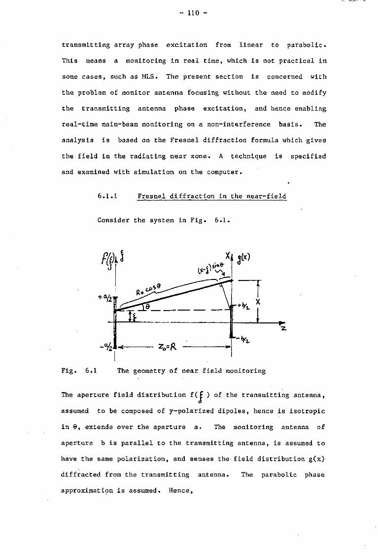
- 110 -
transmitting array phase excitation from linear to parabolic.
This means a monitoring in real time, which is not practical in
some cases, such as MLS. The present section is concerned with
the problem of monitor antenna focusing without the need to modify
the transmitting antenna phase excitation, and hence enabling
real-time main-beam monitoring on a non-interference basis. The
analysis is based on the Fresnel diffraction formula which gives
the field in the radiating near zone. A technique is specified
and examined with simulation on the computer.
6.1.1 Fresnel diffraction in the near-field
Consider the system in Fig. 6.1.
The aperture field distribution f(J ) of the transmitting antenna,
assumed to be composed of y-polarized dipoles, hence is isotropic
in 0, extends over the aperture a. The monitoring antenna of
aperture b is parallel to the transmitting antenna, is assumed to
have the same polarization, and senses the field distribution g(x)
diffracted from the transmitting antenna. The parabolic phase
approximation is assumed. Hence,

- Ill -
s=sin&, c^cose^Cl-sin2- 9 ) ^ = 1 - ^ (6.1)
The signal V received by the monitor antenna is given by
M V = J g(x) dx (6.2)
' b/z
where the received field distribution g(x) is
g(x)=Ey (x,R)
=exp{-jkR}exp{-jkx a/2R }( j/N R)^J f (f ) exp{ jk(^-| - X )}dj
(6.3)
as described in section 5.1.
Assume now that the transmitting antenna is of uniform
illumination f(0), and has a linear phase scan corresponding to
propagation in the direction s. Hence
f(j)=f(0) exp{-jksJ ) (6.4) .
Designating the integral of equation (6.3)
«'<*>-J f(|) exp{jk(^| - 2 * ) } d j
/ 2 > f y: f 2
=f(0) y exp{ jk[ - s)j- (6.5)
This integral can be evaluated in terms of Fresnel
integrals [ 25], after completing squares. Hence
where ^ [ ] is the Fresnel integral. The implication of this
formula will now be examined.
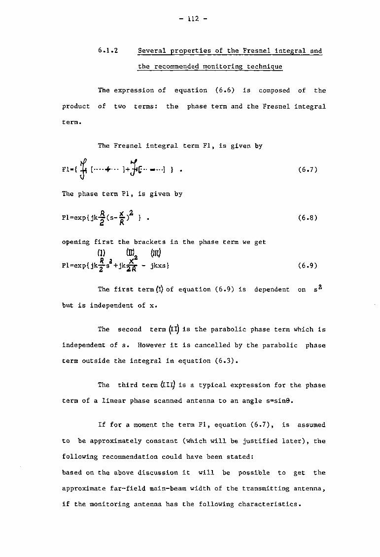
- 112 -
6.1,2 Several properties of the Fresnel integral and
the recommended monitoring technique
The expression of equation (6.6) is composed of the
product of two terms: the phase term and the Fresnel integral
term.
The Fresnel integral term F1, is given by
Fl: } . (6.7)
The phase term PI, is given by
Pl=exp{jk-|(s-^) a } . (6.8)
opening first the brackets in the phase term we get
(i) (ffl2 (in)
Pl=exp{jkjs 3+jk2^ - jkxs} (6.9)
The first term (l) of equation (6.9) is dependent on s^
but is independent of x.
The second term Ll) is the parabolic phase term which is
independent of s. However it is cancelled by the parabolic phase
term outside the integral in equation (6.3).
The third term is a typical expression for the phase
term of a linear phase scanned antenna to an angle s=sin9'.
If for a moment the term F1, equation (6.7), is assumed
to be approximately constant (which will be justified later), the
following recommendation could have been stated:
based on the above discussion it will be possible to get the
approximate far-field main-beam width of the transmitting antenna,
if the monitoring antenna has the following characteristics.

- 113 -
1) The length of the monitoring antenna is equal to the
transmitting antenna,
2) A linear response to the field g(x) is assumed.
With the above assumptions the received signal V which
will be the integral, equation (6.2), of this modified phase term
performed over |x|^b/2 will result in >/2
I V=C | exp{-jkxs}dx
where C is a constant, hence
Sivvdkfes) V=Cb f ^ (6.10)
i k b S
Putting b=a according to our assumption gives,
V=Ca-~—pf ' (6.10a) a k c L S
It should be emphasized that s in these expressions is the
pointing direction cosine, Sp say, of the main antenna. The
pointing Sp can thus be determined, since \ and b are known.
It now remains to discuss our first assumption that has
not been justified yet, of supposing that F1 of equation (6.7) is
approximately a constant.
The asymptotic value of the Fresnel integral > a s
is [ 13,24]
$ ( v ) - (1-j)- ^ e X p { - j ^ } (6.11)
The behaviour of the Fresnel integral for a large positive
argument is therefore of small oscillations which are inversly

- 114 -
proportional to the (TTv), where v is the argument. The period of
the oscillations is v ^ / 4 . The phase has a similiar behaviour: it
3 ( F T
oscillates around the asymptotic value of - T with decreasing
phase proportional to (TTv^ /2). For values of v larger than o.5
the amplitude oscillations are less than about 2.5 db. The phase
magnitude oscillation is about 15 degrees or less, for arguments
^1. For a value of v^0.5 this phase magnitude could reach about
40 degrees. The numerical values are given in Fig. 6.2.
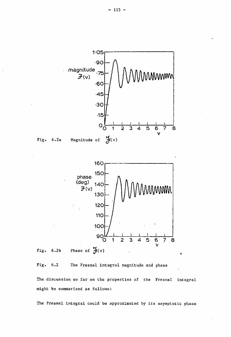
- 115 -
magnitude £<v)
Fig. 6.2a Magnitude of
phase (deg) 1 4 Q
130
Fig. 6.2b
Fig. 6.2 The Fresnel integral magnitude and phase
The discussion so far on the properties of the Fresnel integral
might be summarized as follows:
The Fresnel integral could be approximated by its asymptotic phase
- 116 -
and magnitude values, with errors of
~2db and ~15 degrees
(or 40deg if arguments^).5 are sought).
The term F1 of equation (6.7) which is a difference of two Fresnel
integrals shifted by the argument value of
could similiarly be approximated by a step function of magnitude
and phase extended parallel and over the approximate edges of the
radiating aperture. This approximation to the term F1 holds for
cases of R ^ or where R is a small multiple (or subdivision) of
the aperture a, and where a/^ » 1 which is adequate for the MLS
phased arrays.
recommended for monitoring the main-beam of uniformly illuminated
scanning arrays. One possible implementation of the monitoring
system is sketched in Fig. 6.3.
(6.12)
This concludes the discussion on the technique
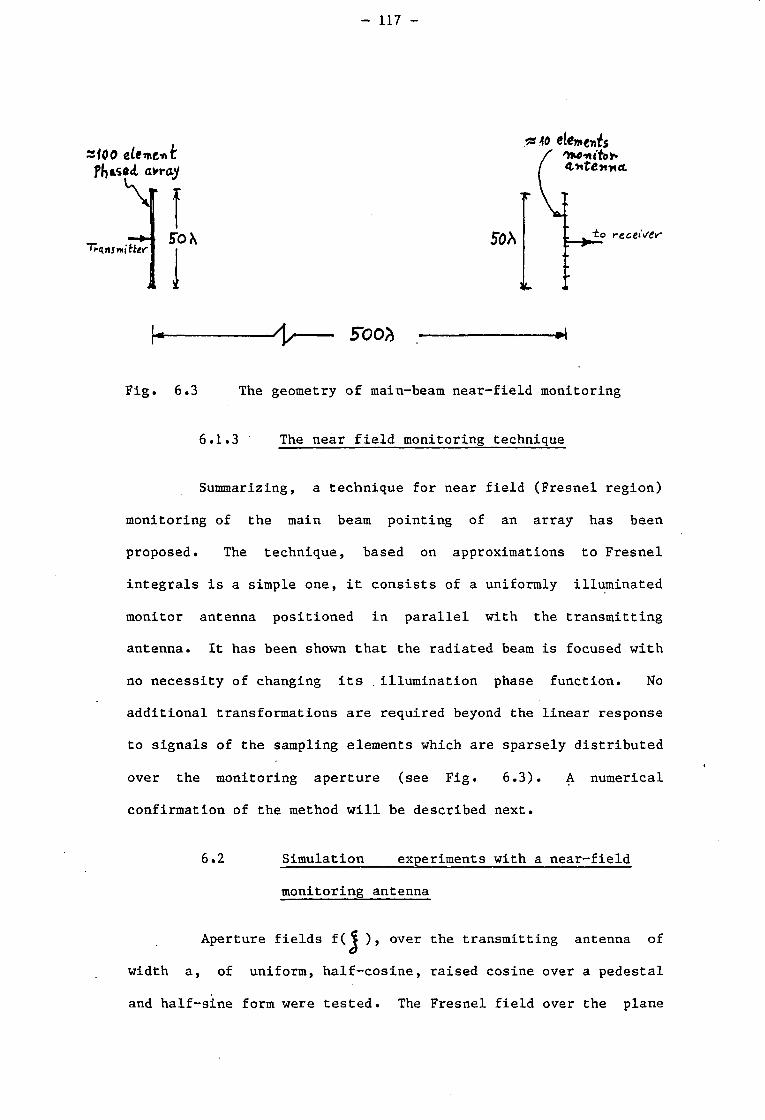
- 117 -
SfOO ekme-rtt PhasaA dvray
elements f OMmieh / <ly*tCny%cL
Transmitter 50*
V j "to receiver"
Fooh
Fig. 6.3 The geometry of main-beam near-field monitoring
6.1.3 The near field monitoring technique
Summarizing, a technique for near field (Fresnel region)
monitoring of the main beam pointing of an array has been
proposed. The technique, based on approximations to Fresnel
integrals is a simple one, it consists of a uniformly illuminated
monitor antenna positioned in parallel with the transmitting
antenna. It has been shown that the radiated beam is focused with
no necessity of changing its . illumination phase function. No
additional transformations are required beyond the linear response
to signals of the sampling elements which are sparsely distributed
over the monitoring aperture (see Fig. 6.3). A numerical
confirmation of the method will be described next.
6.2 Simulation experiments with a near-field
monitoring antenna
Aperture fields f ( J ), over the transmitting antenna of
width a, of uniform, half-cosine, raised cosine over a pedestal
and half-sine form were tested. The Fresnel field over the plane
- 118 -
of observation (see Fig. 6.3), a distance R from the transmitting
antenna, was simulated for aperture fields
f(j ) exp{-jks pJ }
Which is the basic aperture field f(J ) with a linear phase
superimposed in order that it will radiate in the direction making
an angle sin' sp to the transmitting aperture.
The Fresnel field is then sampled at points seperated by
along a line of length b, parallel to the aperture plane. A
rough idea of the required sample spacing can be obtained from
equation (JT*46) with s 5 / a , say, which gives M a / a/10. In
the following simulations the spacing was varied between a/6 and
a/99 (i.e., between 7 and 100 sampling elements).
The width of the linear transmitting phased-array antenna
was kept constant at a=50^ . * The width b of the monitoring
antenna and its distance R were varied.
A comparison of equations (6.8) and (6.9) shows that a
replica of the transmitted far-field beam shape is reproduced in
the monitor antenna when choosing its aperture b=a. However due
to the nature of Fresnel diffraction a sharp (exponential)
decrease is expected for fields in |x|>a/2. Hence choosing b>a is
expected to measure main-beam shape and first side-lobes with
reasonable precision. The wider the monitor antenna aperture the
larger amount of the field radiated into wider direction cosine is
intercepted. Hence a better reconstruction of the focused beam
for farther side-lobes is expected. This last assumption is also
left to be confirmed by the simulation experiments.
- 119 -
The numerical simulation uses the cosine and sine
integrals available as computer NAG library functions S20ADF and
S20ACF. These are used in the precise evaluation of the Fresnel
integrals in their complex form
$Uv}=C(v)-jS(v)
where {v} is the Fresnel integral, and C(v) and S(v) are the
F/t cosine and sineVintegrals which are widely tabulated [ 25].
6.2.1 Uniform transmitting antenna aperture field
In the simulation the focused near-field and the
far-field normalized patterns of a 50 A transmitting aperture are
calculated. To aid comparison a lOdb constant magnitude-ratio is
added to the near field pattern in the figures. The far-field
pattern is generated from the expected sine function. The near
field (focused) pattern is dependent on R/a the distance to
aperture ratio, and N the number of isotropic sampling elements
equispaced over a planar monitoring aperture. The superposition
of these N signals results in the near field reconstruction of the
far-field main-beam pattern. Samples of the simulation results
are given in Figs 6.4 to 6.9, the near-field patterns are shown as
the upper pattern in each simulation, with the lOdb added
artificially.
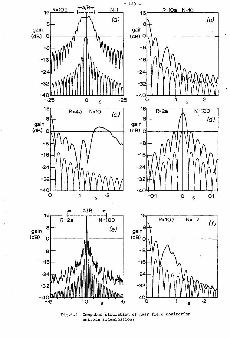
R=10a - 120 -
R=10a N=10
8 gain
(dB) 0
gain (dB) 0
gain (dB) o
gain (dB) o
gain (dB) o
Fig.6.4 Computer simulation of near field monitoring uniform illumination.

121 -
In Fig. 6.4a R/a=10 which is one tenth of the Rayleigh distance
(R ~2a?*/\ ), and N=1, i.e., the signal received is given by the
normalized magnitude of the Fresnel integral with no corrections.
Two areas are noticed in the near-field; the on-axis region where
most of the radiated energy is concentrated giving an almost
constant magnitude over 3 to 4 beam-widths in the region parallel
to the radiating aperture designated by | 1 on the graph.
The other region is in the side-lobe region which becomes
pronounced and more like the far-field side-lobe region, as the
scan angle increases.
In Fig. 6.4b with the same R/a=10 as before, the near
field is sampled over ten isotropic elements, (N=10), equispaced
about 5.5?v apart, over a parallel planar aperture. It is
noticed that the reconstructed main-beam now resembles the far
field main-beam up to about the 10 db point. A better than 0.5 db
difference is achieved up to the 3 db points, and up to 2 db
difference is achieved up to the 10 db points.
In Fig. 6.4c with R/a=4 keeping the same number of
sampling elements the main beam is still reconstructed properly,
but a grating lobe starts to be pronounced (at s£.175) as
anticipated. This is due to the fact that x was arbitrarily
chosen to be about 5A , therefore s^no* is limited roughly to
si¥ncjjO 1/10 (for a=50A )• Hence (ambiguous) reconstruction of
grating lobes can be produced for s>smax. The maximum value for
these grating lobes depends on the side lobe level (peaks) and the
number of sampling elements used. For example, for 10 sampling
elements the grating lobe is expected to be about 20 db higher
than the side lobe level monitored by a single sampling element
- 122 -
(see Fig. 6.4a), which is very close to the value noticed on the
graph.
In Fig. 6.4d and 6.4e a further decrease is used in the
distance of the monitor antenna, now at R/a=2. But, a N=100
elements is used for sampling, hence the grating lobe in Fig.
6.4c, now disappeared. The wide scanning angle is shown in Fig.
6.4e while the main-beam region is shown in Fig. 6.4d.
In Fig. 6.4f The R/a=10 value as in Fig. 6.4b are used
but now with a reduced number of sampling elements N-7. The
result seems to be quite practical as the grating lobe (in s~0.07)
is only 2—3 db above the side-lobe level. However, the main beam
is reproduced quite well. The small number of sampling elements
used in the last example show the potential feasibility of a
practical monitoring antenna.
As explained earlier, it is expected (arguing
heuristically) that the wider the receiving aperture the better
the reproduction of the focused main-beam and first side-lobes. A
demonstration of the "performance" of the monitor antenna for
various b/a aperture ratios, from 0.8 to 3, is given in Figs.
6.5a to f.
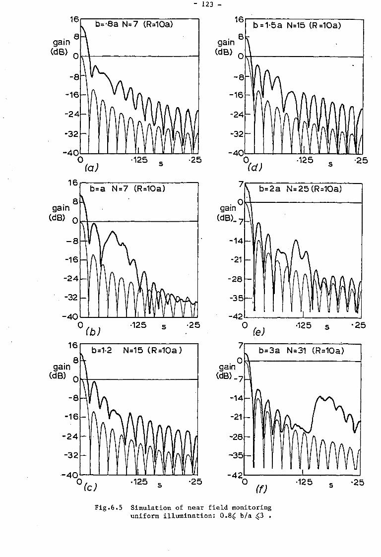
- 123 -
gain (dB)
gain (dB)
Fig.6.5 Simulation of near field monitoring uniform illumination: 0.8^ b/a ^3 .
- 124 -
Figs. 6.5a to f show the results for the focused beam and the
first side-lobes, for various values of b/a. It is seen that for
b^a (fig. 6.5b to f) the focused main beam is reasonably similar
in shape to the far-field beam. However for b=0.8a in Fig. 6.5a
the main beam slope is reproduced less faithfully than in the
previous cases (b^a). Checking the focused first side lobes it is
clearly seen that the wider the monitor antenna aperture the
better the reconstruction of additional side-lobes. This means
that the resolution between main lobe and first side-lobes is
improved for wider apertures, which was to be expected
intuitively.
The simulation of near field focusing of uniformly
illuminated apertures has shown some promising results. The
focused main-beam shape has been reproduced quite faithfully for
monitor apertures equal to or larger than the radiating antenna
aperture. This, while only a few sampling elements have been used
for monitoring. it now remains to show that the uniform
illumination function is not a singular case where this method can
be applied. Hence, other practical illumination functions will be
examined in a similar way. These will be the half cosine and the
sine (i.e., monopulse). As explained earlier almost any wanted
illumination can be decomposed into a series of uniform, cosine
and sine illumination functions. A demonstration of a useful
illumination function, the cosine square over a pedestal [ 23]
will be given later based on such a decomposition. First the half
cosine will be examined next.
6.2.2 Half-cosine aperture field
Following similar stages to those used in deriving
- 125 -
equations (6.2) to (6.5), the diffraction field of a cosine
aperture illuminated scanning antenna can be shown to be equal to;
g(x)=exp{-jkR}exp{-j-||^}I(s) (6.13)
The term I(s) is given by
/ V 2 # TT k f 1
I ( s ) « J ^ p { + j ^ | } + e x p { - j ^ } ] e x p { - j ^ } e x p { j k s j }dj . (6.14)
Where I(s) the normalized near field over the z axis. The
far-field will be derived after ignoring the parabolic phase term
in (6.14). Hence,
I(s)= J(Bxp{+j~| }+exp{-j-£| }]exp{jksJ ) df (6.15)
where the far-field normalized field pattern. It can be
shown that the far field is given by
I(s) o C 9 (6.16)
This expression will now be used for comparison with the
reproduced far -field pattern, described below. Approximations to
equation 6.15 have been derived in a similar way to those derived
previously for uniform illumination. This analysis is represented
in appendix D. The results may be summarized as follows:
c
The cosine illumination leads to the prodution of two
functions which can be approximated to yield the normalized field
over the monitoring aperture as :
exp{j?T(- 3H)} Cos[rr(- & + £ ) ] (6.17)
This should be integrated over -b/2<x<b/2 to yield the monitoring
signal. This is to be compared with the integrand of the far
- 126 -
field expression which is of the form
exp{jTT(-2-^)}cos(£*). (6.18)
The terra fTsR/a (in equation (6.17)) is therefore causing the
difference between the expression for the "correct" far field and
that approximated using the focusing technique. This additional
term can be ignored for s-*K) (i.e., the main beam direction)
provided R/a is not large (i.e. R/a^l). With this additional
restriction the monitoring system described earlier for the
uniform illumination (Fig. 6.3) will also be adequate for the
half-cosine illumination.
Simulation results are given in Fig. 6.6.
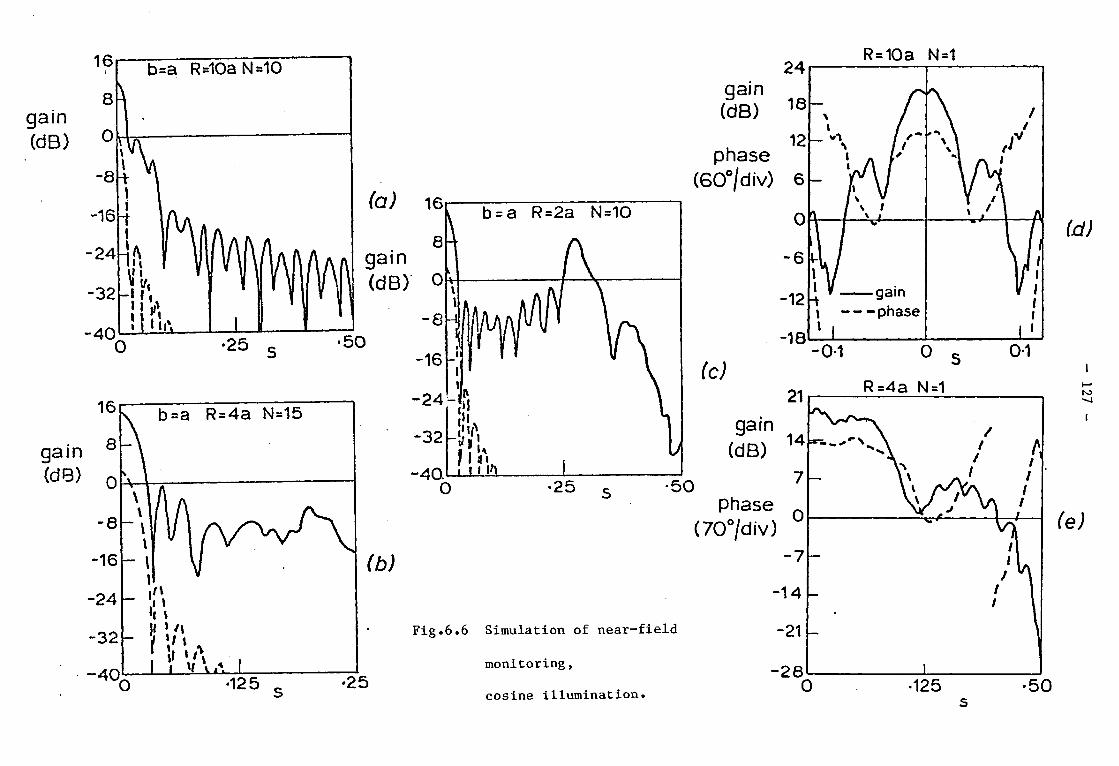
gain (dB)
gain (dB)
2 4
gain (dB) 1 8
12 phase
(60°/div) 6 0
- 6
- 12
- 1 8
R = 10a N=1
\ / 1 /
_ vn / ^ t » A I' i /l [ A \/ I \ v / * '
'V / x i
\ / \ / \ /v A A '
Y f \ % ' i i I w
d / I V 1 V gain
u I phase I I
\ / 1
\J i / 1
V / I 1
1' - 0 - 1 0
R =4 a N=1
0-1
gain
(70°/div)
- 4 0
Fig.6.6 Simulation of near-field
monitoring,
cosine illumination.

- 128 -
Fig. 6.6 a,b,c describe the following simulation results: i
a=50A transmitting antenna. R/a distance ratios of 10, 4, 2.
Reception with 10-Usampling elements equispaced over the monitor
antenna aperture. The following points should be noted:
1) The accuracy of reproducing the main-beam is improved the
closer the monitor and receiving antennas are located.
Example, the -2 db points are within 0.17 db at all 3 distances.
However the -9.5 db points are within 0.7 db for R/a=2, within
1.8 db for R/a=4, and within 4.5 db for R/a=10.
2) However, due to the finite number of samples, interelement
spacing (of almost 3.5A ) grating lobes start to appear at the
closer seperations. Hence the side-lobes are improved with
increasing R/a, as expected.
From points (1) and (2), optimal value could be achieved
for the monitoring system, if adequate weights are given to the
above parameters. The phase and magnitude expected to be received
in a single element monitor antenna, are given in Figs. 6.6d and
6.6e. This justifies the previous assumption, that the changes in
amplitude and phase due to the four Fresnel integral terms are
comparatively small.
^In all the simulations of Fig. 6.6 use has been made of
available computer NAG-Routines for the evaluation of all four
Fresnel integrals arising from equation (6.14) (see Appendix D).
The results so far show that both aperture illuminations
investigated, namely, the uniform and the cosine, enable near
field reconstruction of the far-field main-beam scanning patterns.
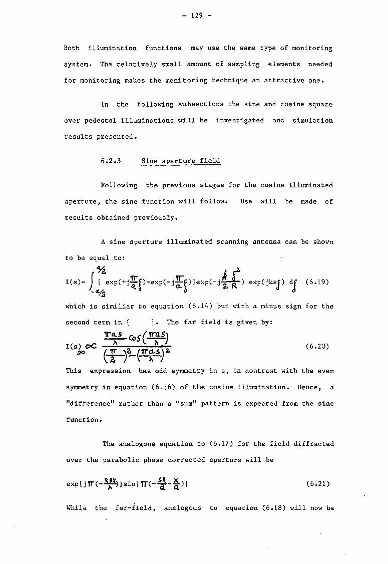
- 129 -
Both illumination functions may use the same type of monitoring
system. The relatively small amount of sampling elements needed
for monitoring makes the monitoring technique an attractive one.
In the following subsections the sine and cosine square
over pedestal illuminations will be investigated and simulation
results presented.
6.2.3 Sine aperture field
Following the previous stages for the cosine illuminated
aperture, the sine function will follow. Use will be made of
results obtained previously.
A sine aperture illuminated scanning antenna can be shown
to be equal to:
[ V t i f I(s)= J [ e x p ( + j ^ p - e x p ( - j ^ ) ] e x p ( - j S - g r ) exp(jksj) dj (6.19)
which is similiar to equation (6.14) but with a minus sign for the
second term in [ ]. The far field is given by:
I(s) O C ^—r * n " # ' (6.20)
This expression has odd symmetry in s, in contrast with the even
symmetry in equation (6.16) of the cosine illumination. Hence, a
"difference" rather than a "sum" pattern is expected from the sine
function.
The analogous equation to (6.17) for the field diffracted
over the parabolic phase corrected aperture will be
e x p { j T T ( - ^ ) } s i n [ T r ( - ^ + ) ] (6.21)
While the far-field, analogous to equation (6.18) will now be
- 130 -
given by
e x p { j T r ( - ^ ) } s i n ( £ * ) (6.22)
opening the brackets of the sine function in equation (6.21)
^ r*r/ SR .i * m 4 1TSft TTX , TTSR . fTX sin{TT(- — 4 — )}=-sin cos —-+cos-j^-sin— (6.23)
As before for small scanning angles s « l hence the first r.h.s.
term can be ignored and cos(' . Hence we remain with the
approximated near field of the form
e x p { j T T ( - s i n 2 2 (6.24)
which is the required form as in equation (6.22). Therefore the
same recommendation given for
monitoring the cosine illuminated
aperture apply also to the sine illuminated aperture. Simulation results are given in Fig. 6.7a,b,c,d.
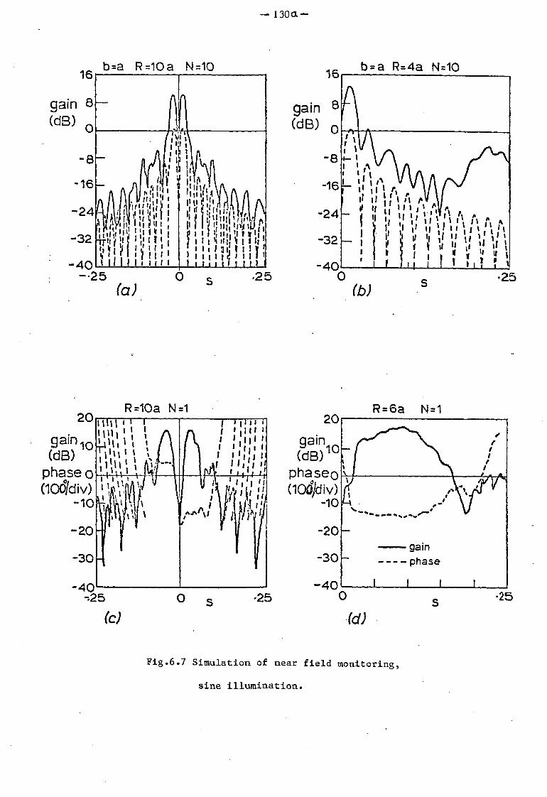
— 13 0 a ~
b=a R =10 a N =10 b = a R=4a N=10
gain 8 (dB)
•25
R=10a N=1
gain1Q (dB)
phase o (10o/div)
- 1 0
- 2 0
-30
-.25
20 R = 6a N=1
gain 10 (dB) phaseo (10$div)
- 1 0
- 2 0
-30
-40
1 j t 1 \ 1
\ / \ / \ / \ / V / > / \ / A *
\J V '9/1/ li v
t \ I \ /
gain
I
phase
! 1 I
•25
(d)
Fig.6.7 Simulation of near field monitoring,
sine illumination.
- 131 -
Fig. 6.7a,b give the following simulation results :
a=5C^ transmitting aperture.
R/a distance ratios 10 and 4, respectively.
Reception with 15 sampling elements equispaced over the monitoring
antenna aperture.
The following results are noted:
1) The reproduced main-beam pointing is more precise with closer
receive and transmit antennas. When farther apart the beam tends
to squint towards the center (the z axis).
2) The accuracy of the reproduced level is within 0.25 db for the
range of -5.1 db (through the peak at 0.0 db) to the -2.0 db
point, for R/a=4. While for R/a=10 the accuracy in the same range
is reduced to about 1.0 db.
3) Due to the finite number of sampling elements for R/a=4 the
grating lobe is about 1 to 2 db higher than for R/a=10, as
expected.

- 132 -
The phase and magnitude expected to be received in a
single element monitoring antenna are given in Fig. 6.7c and d
for R/a=10 and 4, respectively.
The magnitude shows the expected null in the direction
s=0 due to the phase inversion. Besides this region the magnitude
and phase behave quite smoothly over the region parallel to the
transmitting aperture. This justifies the approximations made in
the analysis.
Having analayzed the uniform, cosine and sine
illumination functions, the practical example of cosine square
over pedestal illumination will now be analyzed in the following
subsection.
6.2.4 Raised cosine (cosine square over pedestal)
aperture illumination
It was proposed by Chignell [ 23] that a cosine square
over pedestal illumination is optimal where the function is given
by
l/7+6/7cos2 ( p (6.25)
where the argument TTx/a. The geometrical identity is used
cos2'(£)=l/2(l+cos2f) (6.26)
Therefore the illumination of equation (6.25) could be described
by the following expression
l/7+6/7jl/2( cos
=0.5714+0.4286cos(2^) (6.27)
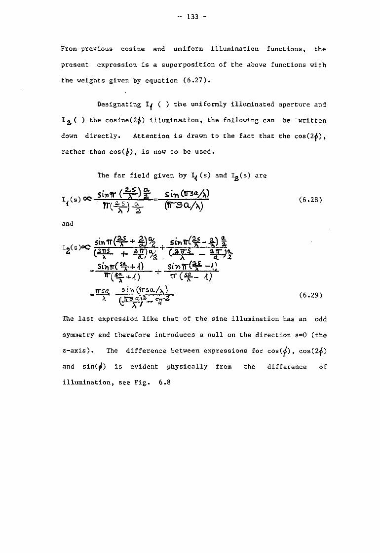
- 133 -
From previous cosine and uniform illumination functions, the
present expression is a superposition of the above functions with
the weights given by equation (6.27).
Designating ( ) the uniformly illuminated aperture and
Ig(( ) the cosine(2<j>) illumination, the following can be written
down directly. Attention is drawn to the fact that the cos(2£),
rather than cos(f), is now to be used.
The far field given by (s) and Ig(s) are
i.(s)QO finCrsaA) ( f - s a A )
and
Tsa. sir\(vs,<L/\) A (JTS CLj* _ cjj-Z
(6.29)
A
The last expression like that of the sine illumination has an odd
symmetry and therefore introduces a null on the direction s=0 (the
z-axis). The difference between expressions for cos(^f) , cos(20
and sin(jO is evident physically from the difference of
illumination, see Fig. 6.8
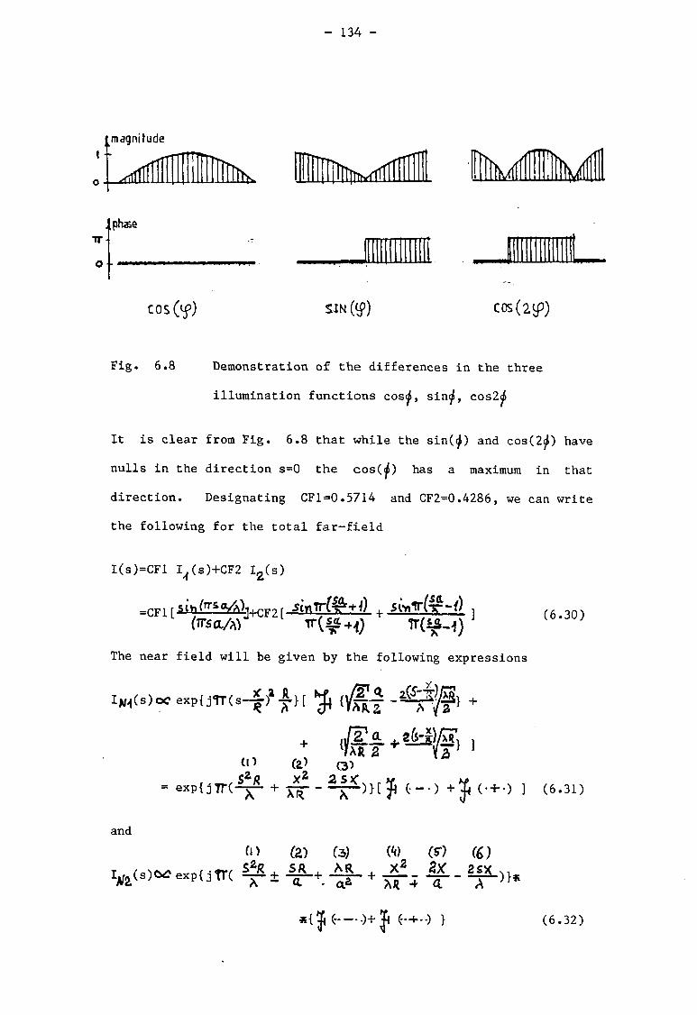
- 134 -
magnitude t -
I f f l l t T T T ^ l u f k i
TT •
o •
phase
cos Of) sin (g>) cos(2 5P)
Fig. 6.8 Demonstration of the differences in the three
illumination functions cos^, sin^, cos2^
It is clear from Fig. 6.8 that while the sin(^) and cos(2^) have
nulls in the direction s=0 the cos(^) has a maximum in that
direction. Designating CF1=0.5714 and CF2=0.4286, we can write
the following for the total far-field
I(s)=CFl I{(s)+CF2 I 2(s)
- C F 1 [ s i n ^s q ^ ) i l c r 2 r sinrrtQ+l) si^l^-i) 1
(irsaA)
The near field will be given by the following expressions
x N 1 ( s ) o c e x p { j T r ( s - | )J | } [ % { y f | - j S
(6.30)
{ A y a
Ya C a2 C 3 )
= exp{j7T(^f- + jfi (•-•) + $ (• + •) ] (6.31)
(O
s2/?
and
<»> (z) (a) W (s-)
ar a
(6.32)
- 135 -
where due to the uniform and I ^ ^ 8 ) due t o cos(2^).
As before, analysis of the effects of the phase terms in
the two equations (6.31) and (6.32) will follow
Term (1) in exp and exp,. are equal.
Term (2) of exp. and term (4) of exp,. are the parabolic m hiz
phase terms which are cancelled out as before.
Term (3) of exp and term (6) of exp are the linear
phase scanned array term.
Terms (2) and (5) of exp_ comprise the cos,TT*(sR/a-2x/a) ?N2
result of the cosine illuminated aperture, but this time the
(+2x/a) rather than the (+x/a) is used.
Term (3) of exp is to be included this time due to the tya
fact that it does not appear in exp.
Discussion on the effect of term (3):
Term (3) is introducing additional phase-shift between the linear
and the cos(2^) illuminated aperture. It is assumed that its
effect is negligible in the near field where
XR/a2 « 1 , given a » A and R/aZl , (6.33)
Example \ a=50A , R=a=50A and X =4 giving >R/a^ =1/50 hence « A</= 7T/50-3.5 deg.
Example 2 what is R where this term introduces a 7T radian phase
shift.
Giving R=100a=5000^ .
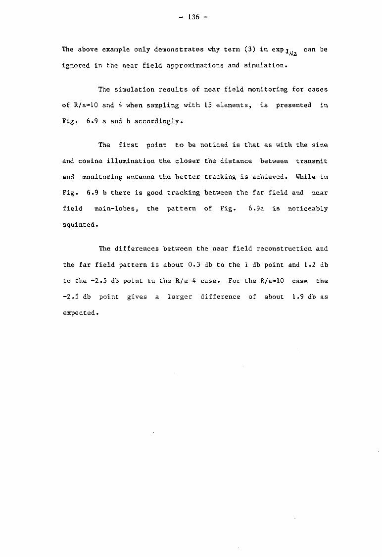
- 136 -
The above example only demonstrates why term (3) in exp j can be
ignored in the near field approximations and simulation.
The simulation results of near field monitoring for cases
of R/a=10 and A when sampling with 15 elements, is presented in
Fig. 6.9 a and b accordingly.
The first point to be noticed is that as with the sine
and cosine illumination the closer the distance between transmit
and monitoring antenna the better tracking is achieved. While in
Fig. 6.9 b there is good tracking between the far field and near
field main-lobes, the pattern of Fig. 6.9a is noticeably
squinted.
The differences between the near field reconstruction and
the far field pattern is about 0.3 db to the 1 db point and 1.2 db
to the -2.5 db point in the R/a=4 case. For the R/a=10 case the
-2.5 db point gives a larger difference of about 1.9 db as
expected.
b=a R=10a N=15
- 4 Q k ' V ' M i l
-1 -.05 0
R=10a N=1
l u m
.05 s .1
20 gain (db) 10
phase
o 0
dWftJiv)
-10
Fig.6.9 Simulation of near field monitoring,
cosine square on pedestal.
u>
- 138 -
In Figs. 6.9 c, d and e the magnitude and phase received at the
point x=0 of the monitoring aperture is simulated by sampling with
a single element on the z-axis. This gives an additional
justification for the assumption of almost constant amplitude and
phase in the region parallel to the radiating aperture.
6.2.5 Summary of the near-field simulation
experiments
Approximations based on the properties of Fresnel
integrals led to a proposal of a novel technique for monitoring in
the near-field (Fresnel region) of the field radiated from the
antenna aperture to yield its far-field pointing and beam shape.
The technique is quite simple, it consists of a monitor antenna of
the same size, or larger than, the radiating antenna, with only a
few sampling elements whose signals are linearly combined, to
produce the output signal. This output signal is a reproduction
of the far-field main-beam shape.
The first step taken in order to get some confirmation of
the idea based on the above approximations was a computer
simulation. The technique, based on these approximations could be
"tested" against precise representation for the Fresnel integral
expressions, using very accurate Computer NAG-Library Functions.
In the simulation various aperture fields were examined,
namely, the constant (uniform), 1/2 sine, 1/2 cosine, and cosine,
which are the first few basis functions of a complete Fourier
analysis of the aperture field.
The output of the simulation was in the form of computer
(line printer) graphics which replace (at least in its early

- 139 -
stages) a more precise but difficult analysis or actual
experiment. This output was used to asses the technique and to
vary the parameters of such a monitoring system, and gives a
useful assessment of some of the capabilities and limitations of
the proposed technique.
Initial conclusions are:
For a 50X radiating antenna aperture, the monitor
antenna can be placed anywhere from a fraction of an aperture to
about 10 apertures. The accuracy of the reproduced beam shape is
improved the closer the monitor antenna. However this requires a
larger number of sampling elements to avoid excessive grating
lobes from being generated in the monitor antenna. No
optimization has been made and only "good" engineering sense has
used for selecting the number of sampling elements. The effect of
increasing the size of the monitoring aperture improves the
reproduction of the first side-lobes. However, the unavoidable
increase in the number of sampling elements occurs. The following
points are to be stressed.
The first is that the technique proposed so far should be
regarded as the first steps in putting forward the basic idea.
Secondly, that a fuller and more general analysis should
eventually be carried out. And thirdly that this type of
simulation forms a very valuable substitute (at least in the early
stages) for what could be quite a difficult analysis in
conventional terms.
Having analyzed the near-field monitoring, the following
section deals with a closer distance monitoring technique of

- 140 -
internal/integral monitoring, based in part on the results
obtained in the earlier part of this chapter.
6.3 Internal/integral monitoring of phased array antennas
Having dealt with monitoring in the far-field (the
Fraunhofer region) and in the near-field (the Fresnel region), the
present topic of internal monitoring, can be regarded as
monitoring in the very near-field of the antenna.
Internal monitoring may be classified broadly into two
main types. One type which involves radiation, although to very
short distances, and the other that does not involve radiation.
The ultimate concern of internal monitoring as presented in this
study is to extend the techniques analyzed so far to apply them to
this type of monitoring. Therefore, the direct performance
measurements of the individual components of the array, like
radiators, phase-shifters, beam switches, etc., are not dealt with
here.
The two types of sampling, one external and the other
internal to the radiating aperture, will be described in the
following subsections.
6.3.1 Sampling the aperture field of the array
From the presentation of the Huygens-Fresnel diffraction
analysis, in the previous section, it is clear that sampling the
field at a very short distance from the aperture, R/a«l this
field is only negligibly different from the aperture field. Hence
the far-field pattern can be obtained, using the angular spectrum
concept, as the inverse Fourier transform of this aperture field.
- 141 -
For practical implementation, it is only necessary to
sample the aperture field with the number of samples that comply
with Nyquist's spatial criterion. As before this number depends
on the maximum direction-cosine for which the reconstructed
far-field pattern is to be monitored, giving, for a linear
antenna, the value of
N > 2a/* (6.34)
where N is the number of equispaced sampling points required, and
a/">v is the aperture width measured in wavelengths (for the one
dimensional spectrum).
In practice it is necessary to avoid obstruction of the
aperture field. Therefore, the idea of mutual-coupling can be
used to give the very near-field, using appropriate geometry. The
superposition of the above samples will then produce a signal
that, if normalized, will represent the far field pattern of the
scanning array. In a practical system, the superposition and
sampling, could be done with the aid of an equally long and
adequately polarized linear array, located parallel and inclined
to the aperture of the antenna, thereby eliminating obstruction.
As an example, a slot waveguide array mutually coupled to the
antenna aperture and mounted, as explained above, could be used,
and is shown in Fig. 6.10.
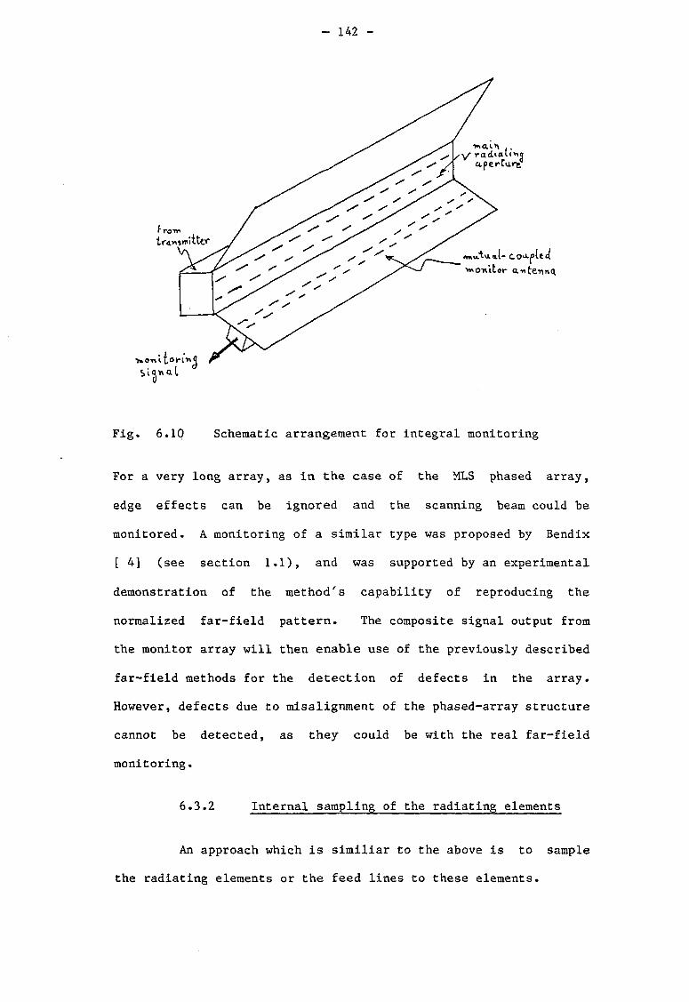
- 142 -
Fig. 6.10 Schematic arrangement for integral monitoring
For a very long array, as in the case of the MLS phased array,
edge effects can be ignored and the scanning beam could be
monitored. A monitoring of a similar type was proposed by Bendix
[ 4] (see section 1.1), and was supported by an experimental
demonstration of the method's capability of reproducing the
normalized far-field pattern. The composite signal output from
the monitor array will then enable use of the previously described
far-field methods for the detection of defects in the array.
However, defects due to misalignment of the phased-array structure
cannot be detected, as they could be with the real far-field
monitoring.
6.3.2 Internal sampling of the radiating elements
An approach which is similiar to the above is to sample
the radiating elements or the feed lines to these elements.
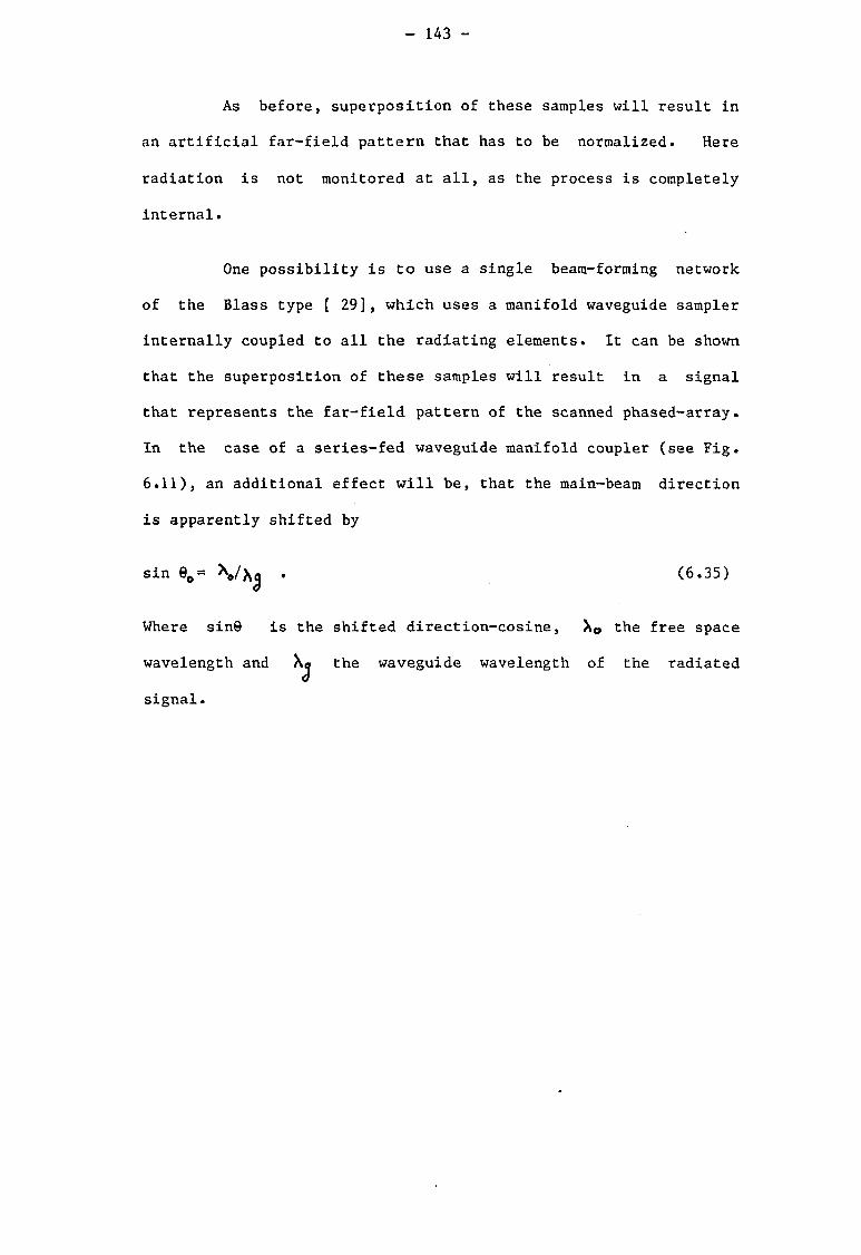
- 143 -
As before, superposition of these samples will result in
an artificial far-field pattern that has to be normalized. Here
radiation is not monitored at all, as the process is completely
internal•
One possibility is to use a single beam-forming network
of the Blass type [ 29], which uses a manifold waveguide sampler
internally coupled to all the radiating elements. It can be shown
that the superposition of these samples will result in a signal
that represents the far-field pattern of the scanned phased-array.
In the case of a series-fed waveguide manifold coupler (see Fig.
6.11), an additional effect will be, that the main-beam direction
is apparently shifted by
sin e o« V ^ • (6.35)
Where sinB is the shifted direction-cosine, the free space
wavelength and Xj the waveguide wavelength of the radiated
signal.
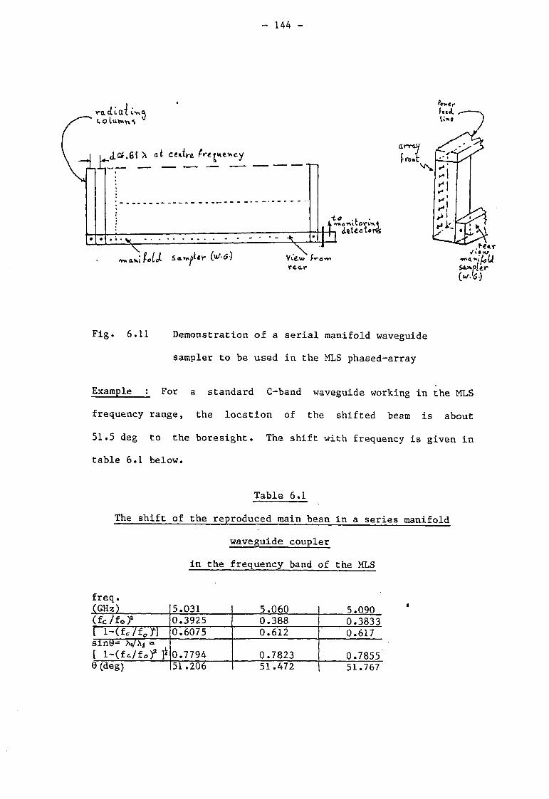
- 144 -
Fig. 6.11 Demonstration of a serial manifold waveguide
sampler to be used in the MLS phased-array
Example : For a standard C-band waveguide working in the MLS
frequency range, the location of the shifted beam is about
51.5 deg to the boresight • The shift with frequency is given in
table 6.1 below.
Table 6.1
The shift of the reproduced main bean in a series manifold
waveguide coupler
in the frequency band of the MLS
freq. (GHz) 5.031 5.060 5.090 (fc/fo)* 0.3925 0.388 0.3833 [ l-(fc/f0f] 0.6075 0.612 0.617 siny= *<>/hj = [ l-(fc/f0)
2 ]* 0.7794 0.7823 0.7855
e (deg) 51.206 51.472 51.767

- 145 -
In monitoring of main beam pointing other values of shift
angle may be required. As an example, if a special size waveguide
(I.D.: 1.27 nx0.59", see section 7.1.2) is being used it can be
shown that 21.75 rather than the above 51.5 deg will be obtained.
Similarly if a XN-band waveguide (a Narda company designation,
I.D.: 1.372"x0.622"), is used, then a shift of 33.3 deg is
obtained. Also, if sampling slots of "opposite hand" rather than
of the "same hand" ( which was assumed before) are used, then,
very small shifts can be obtained. As an example, if the above
special size waveguide with opposite hand slots is used, then, a
shift of about 2.9 deg can be obtained. These results will be
used in proposing a monitoring system for the MLS, in section 8.5.
According to the above description, either type of
internal monitoring scheme could be used in practical
applications.
6.4 Discussion
The analysis has so far dealt with monitoring techniques
in the near-field and in the very near-field regions of the
transmitting antenna aperture.
Near field monitoring
The investigation of near-field monitoring was mainly
concerned with the far-field main-beam reconstruction of a
scanning array. A technique based on focusing the receiving
antenna is suggested as an approximation to the expected far-field
scanned main-beam.
Using an approximation to the Fresnel integral and the
- 146 -
spatial sampling Nyquist citerion, a relatively small number of
sampling elements on a planar aperture give the required
recommendation. It was found that for monitoring a uniformly
illuminated aperture size 50 A : ten sampling elements on an
aperture seperateda 10 apertures distance from the radiating
antenna reproduce the main-beam shape with an accuracy of about
0.5 db to the 3 db points and better than 2 db to the lOdb points.
If, however, the far-field far side-lobe pattern is
required, an even simpler solution could be used. A single
sampling element located at large R/a (distance to aperture ratio)
can give a satisfactory answer, at least in the case of a
uniformly illuminated aperture (this must be left to be
investigated further by a future more precise analysis). It is
clear that this method does not need any additional transformation
or processing besides the linear combination of the signals sensed
by the sampling elements.
Very near-field monitoring (internal monitoring)
The analysis of internal-integral monitoring, although
more limited with regard to actual radiation, can give an even
better approximation than that of the near-field technique. Here,
a good approximation to the far-field main-beam and side-lobe
pattern is reconstructed. This is because only a negligible part
of the aperture field (edge effects) is ignored. Hence, the
recommended technique of sampling the aperture field internally or
through the aid of mutual coupling is the answer. This probing
could be done using a linear array of sampling elements located in
parallel and edequately polarized, of the same length aperture,
assuming, of course, that the internally monitored field is
- 147 -
eventually radiated.
Therefore, the far-field techniques analyzed and
recommended in the first part of the thesis could successfully be
utilized for internal-integral monitoring. The simulation results
for a single sampling element in the near field (Fresnel region)
show its potential capability to reproduce quite nicely the
normalized far-field side-lobe pattern of the radiating antenna
(see Fig. 6.4a), hence, if this will be proved to be the case, it
could also be used for application of the far-field monitoring
techniques in the near-field (Fresnel region) of the antenna.
Incidentally, the simulation on the computer to derive
the expected response from a focusing monitor antenna in the
near-field (Fresnel region) of the radiating antenna has proved
itself to be a useful and cheap replacement for a detailed
analyzis (at least in its earlier stages), enabling the user to
gain familiarity with, and apreciation of, the advantages and
limitations of this monitoring method.
The next chapter is devoted to the experimental
investigation to support, where possible, the recommendations and
techniques so far suggested. As the investigation was conducted
indoors, near-field methods have mainly been used.
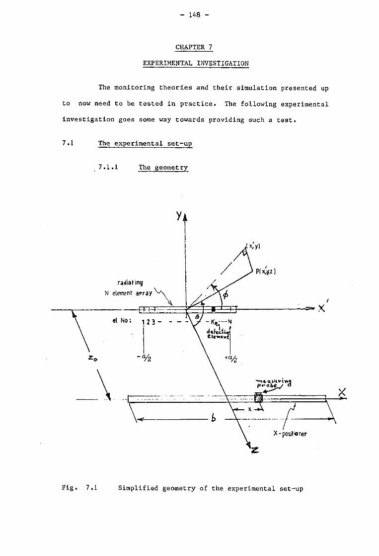
- 148 -
CHAPTER 7
EXPERIMENTAL INVESTIGATION
The monitoring theories and their simulation presented up
to now need to be tested in practice. The following experimental
investigation goes some way towards providing such a test.
7.1 The experimental set-up
7.1.1 The geometry
radiating N element a r r a y
el No; i
Fig. 7.1 Simplified geometry of the experimental set-up

- 149 -
As shown in Fig.7.1 the linear N-element radiating test
array is located along the x'-axis with its aperture, width a,
symmetrical about the y-axis. The input to the array is fed from
the direction of element number 1 and a matched load terminates
the array beyond element N. Element K is the defective element
(usually by blocking with a piece of metal tape). The near-field
measuring probe is at a distance z 0 from the array and is moved
in parallel to it, over a linear aperture of width b along the
x-axis. For linear arrays the two dimensional case (see section
5.1) holds, hence, the x-z plane (y=0) solely is used for the
experiments. When the main beam region is to be probed the
measurement aperture is positioned symmetrically about the z-axis.
When the side-lobe region is to be investigated, the measuring
aperture center is moved to the left (x<0) or to the right, an
adequate distance. The polarization of the test array is mainly
horizontal (x-polarized). The probe polarization is therefore
(ko^ifco-ntaO
normally x^polarized unless cross polarization effects are sought,
or when the ^=777 2, rather than the ^=0 plane characteristics are
investigated.
7.1.2 Antenna arrays and probes
The antenna arrays
The test antennas are samples of linear waveguide slot
arrays investigated earlier by Chignell [ 23] in the department's
microwave laboratory. The antennas are an open ended waveguide
and 8, 16 and 30 slot arrays (see plate 7.1).
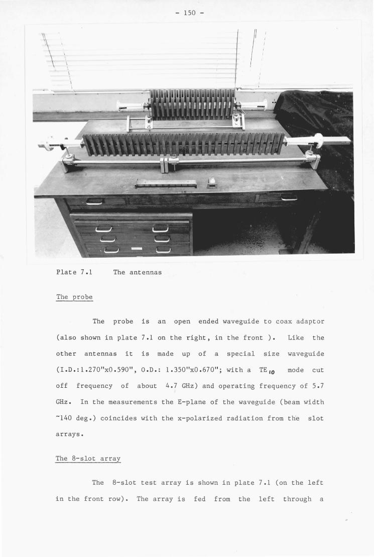
- 150 -
Plate 7.1 The antennas
The probe
The probe is an open ended waveguide to coax adaptor
(also shown in plate 7.1 on the right, in the front ). Like the
other antennas it is made up of a special size waveguide
(I.D.:1.270"x0.590", O.D.: 1.350"x0.670"; with a TE 10 mode cut
off frequency of about 4.7 GHz) and operating frequency of 5.7
GHz. In the measurements the E-plane of the waveguide (beam width
-140 deg.) coincides with the x-polarized radiation from the slot
arrays.
The 8-slot array
The 8-slot test array is shown in plate 7.1 (on the left
in the front row). The array is fed from the left through a
- 151 -
tapered section and is terminated from the right through a similar
taper (the tapers to the standard C-band waveguide and termination
are shown connected to the 30-slot array in the middle row). The
array length (from element 1 to 8) is 25.3 cm with interelement
spacing of about 3.6 cm (0.69?i). Different I-shaped slots cut in
the narrow wall of the waveguide were designed by Chignell [ 23]
to approximate an aperture field illumination of the form
l/7+6/7cos^ giving a 3db beamwidth of about 10 degrees. The
above interelement spacing which was optimized for matching also
causes the beam to squint from the broadside direction by about
8.5 degrees towards the load. Similiar illumination and beam
squint was noticed in all the test arrays.
The 16-slot array
The 16-slot test array (in the rear row of plate 7.1) is'
shown with the matching tapers to the standard C-band waveguide
(WR-187). This array incorporates a grid of crosspolarization
suppression baffles. The array length is 58cm with interelement
spacing of .73^ . The 3db beam width is about 6 degrees.
The 30-slot array
The 30-slot test array (in the middle row of plate 7.1)
is shown with the waveguide tapers and the matched load
termination (right) and the input waveguide to coax adaptor
(left). As with the 16-slot array the crosspolarization
suppression baffles are incorporated. The array length is 110 cm
with interelement spacing of .72?\ . The 3db beam width is about 4
degrees.
Additional details on the slot arrays can be found in

- 152 -
Chignell's work [ 23].
7.1.3 The near field set-up
An experimental set-up was used for near-field
measurements of antenna characteristics before and after the
antenna has been subjected to defects.
It was decided to experiment with available C-band linear
arrays described earlier operating at the center frequency of 5.7
GHz. These were the probe and 8, 16, and 30-element slot
waveguide arrays with about 0.7.X interelement spacing.
The required linear motion of a probe to measure the
near-field radiated from the antenna under test, was carried out
with an x-positioner available in the microwave laboratory.
The schematic diagram is given in Fig. 7.2.
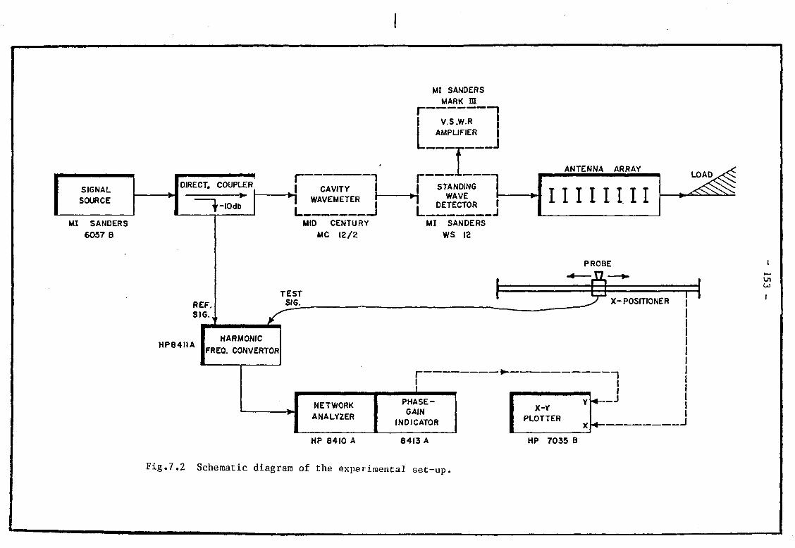
MI SANDERS
MARK m
Fig.7.2 Schematic diagram of the experimental set-up.

- 154 -
In Fig. 7.2 a Gunn oscillator signal source is used to feed the
antenna under test, which is terminated in a matched load. The
field transmitted from the antenna array is sensed by a receiving
probe, normally an open waveguide, which is moved transversally on
the x-positioner placed in parallel with the array. The received
signal gain (db) and phase is measured by a network analyzer,
whose output is connected to the Y input of an X-Y plotter. The
reference for the network analyzer is taken from a directional
coupler placed between the signal source and the transmitting
array. A voltage proportional to the transversal motion of the
probe, is taken from an helical potentiometer linked to the chain
drive mechanism of the x-positioner. When conducting V.S.W.R.
tests of the antenna or when the signal source frequency is to be
checked, a cavity wavemeter is connected through a slot waveguide
standing wave detector (shown dashed in Fig. 7.1), to the array
input.
The actual set-up is shown in plates 7.2 and 7.3 for two
different sets of measurements. In plate 7.2 the set-up is
prepared for near field measurements in the (x<0) side-lobe region
of the 30-slot array. The absorbing material is purposely removed
to give a clear view of the signal source and the directional
coupler power splitter. These are normally covered by the
absorsing material in order to minimize their stray radiation.
In plate 7.3 the system is shown ready for V.S.W.R. and
frequency tests.
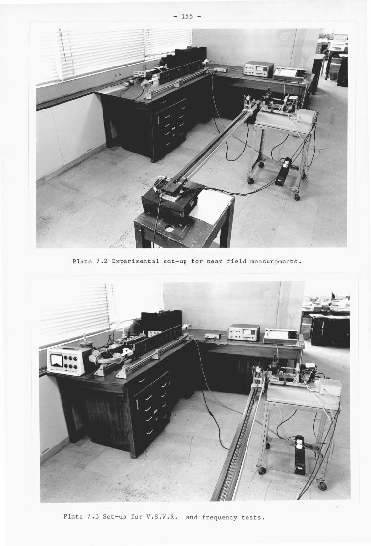
- 155 -
Plate 7.2 Experimental set-up for near field measurements.
Plate 7.3 Set-up for V.S.W.R. and frequency tests.
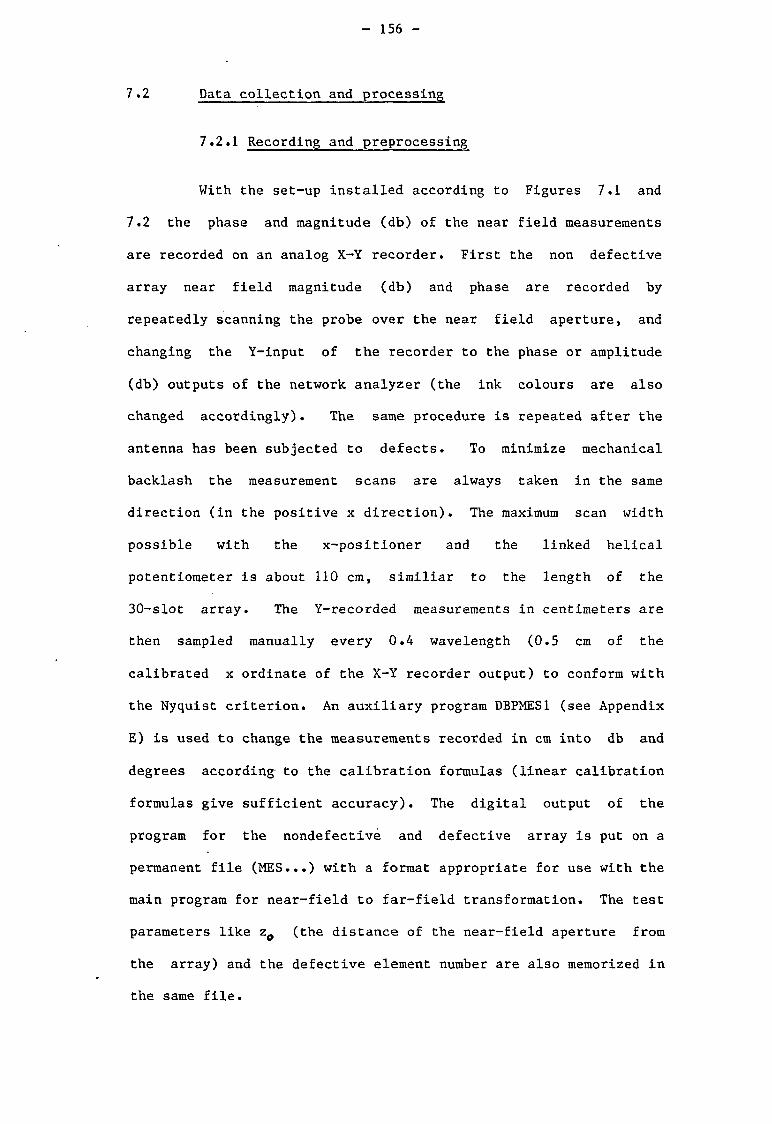
- 156 -
7 .2 Data collection and processing
7.2.1 Recording and preprocessing
With the set-up installed according to Figures 7.1 and
7.2 the phase and magnitude (db) of the near field measurements
are recorded on an analog X-Y recorder. First the non defective
array near field magnitude (db) and phase are recorded by
repeatedly scanning the probe over the near field aperture, and
changing the Y-input of the recorder to the phase or amplitude
(db) outputs of the network analyzer (the ink colours are also
changed accordingly). The same procedure is repeated after the
antenna has been subjected to defects. To minimize mechanical
backlash the measurement scans are always taken in the same
direction (in the positive x direction). The maximum scan width
possible with the x-positioner and the linked helical
potentiometer is about 110 cm, similiar to the length of the
30-slot array. The Y-recorded measurements in centimeters are
then sampled manually every 0.4 wavelength (0.5 cm of the
calibrated x ordinate of the X-Y recorder output) to conform with
the Nyquist criterion. An auxiliary program DBPMES1 (see Appendix
E) is used to change the measurements recorded in cm into db and
degrees according to the calibration formulas (linear calibration
formulas give sufficient accuracy). The digital output of the
program for the nondefective and defective array is put on a
permanent file (MES...) with a format appropriate for use with the
main program for near-field to far-field transformation. The test
parameters like z 0 (the distance of the near-field aperture from
the array) and the defective element number are also memorized in
the same file.
- 157 -
7.2.2 Near field processing
The near field program JACK30 (see appendix E) calls data
from a permanent file (MES...), to a local file (FINX-TAPE7). The
near field to far field transformations, according to equations
(5.15) and (5.12), are then carried out using a discrete Fourier
transform algorithm for the "reference" and "defective" arrays.
The "subtraction method" equations (2.12) to (2.14) are then
applied to resolve equivalent substitute element array far field
pattern over the appropriate angular region, according to the
measurement geometry. The results are then displayed against
s=sin$, numerically and graphically. In addition the "angular
spectrum method" is applied using a computer NAG routine (C06ADF)
for F.F.T. of the normalized angular spectrum (which is
asymptotically proportional to the far field pattern) to derive
the aperture field illumination function via equation (5.9). If
the "a.c.f. method" is implemented then subroutine COREL03 (see
Appendix E) is used to find the autocorrelation function of the
angular spectrum before application of the F.F.T., as explained
earlier (see section 5.3). The aperture power illumination rather
than the aperture magnitude illumination, is then derived and
displayed.
7.2.3 Simulation of near field measurements
' Subroutine EJIX (see Appendix E) could be used with
program JACK30 before the actual measurements have taken place.
The subroutine simulates the near field measurements of a cos^ +
pedestal or a uniformly illuminated ideal N-element array with or
without defects. It can also be used as a comparative check on
the experimental results.

- 158 -
7.3 The near-field experimental results
7.3.1 Open waveguide patterns
The single element near field phase pattern is given by
the hyperbolic parametric equation
R* -x* = zi ( 7 . 1 )
<f - - R 2 T T / * (7.2)
where R, x and z 0 as given in Fig. 7.3
X
Fig. 7.3 Simplified geometry of near field measurement
The amplitude A (assuming isotropic radiators) is inversly
proportional to R. Hence
A o c l / R = l/(x 2 +z| fi = cos6/z 0 (7.3)
These functions are described in Fig. 7.4 and 7.5
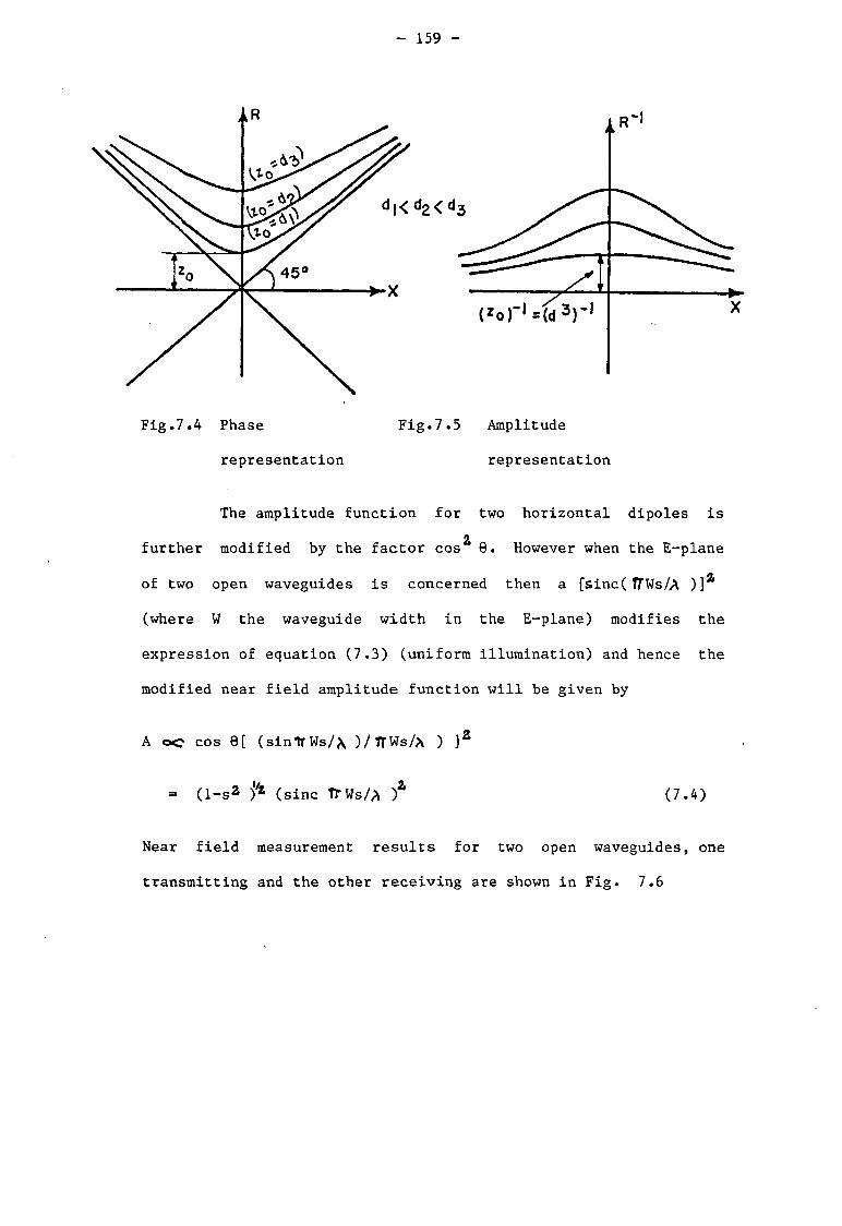
- 159 -
d 2<d
cor'std3)-' X
Fig ,7.4 Phase
representation
Fig.7.5 Amplitude
representation
The amplitude function for two horizontal dipoles is
a
further modified by the factor cos 9. However when the E-plane
of two open waveguides is concerned then a [sinc( TTWS/A
(where W the waveguide width in the E-plane) modifies the
expression of equation (7.3) (uniform illumination) and hence the
modified near field amplitude function will be given by
A o c cos 6[ (sintrWs/X )/7TWS/a ) ]Z
= (1-s* j 4 (sine TTWs/A ) Z (7.4)
Near field measurement results for two open waveguides, one
transmitting and the other receiving are shown in Fig. 7.6
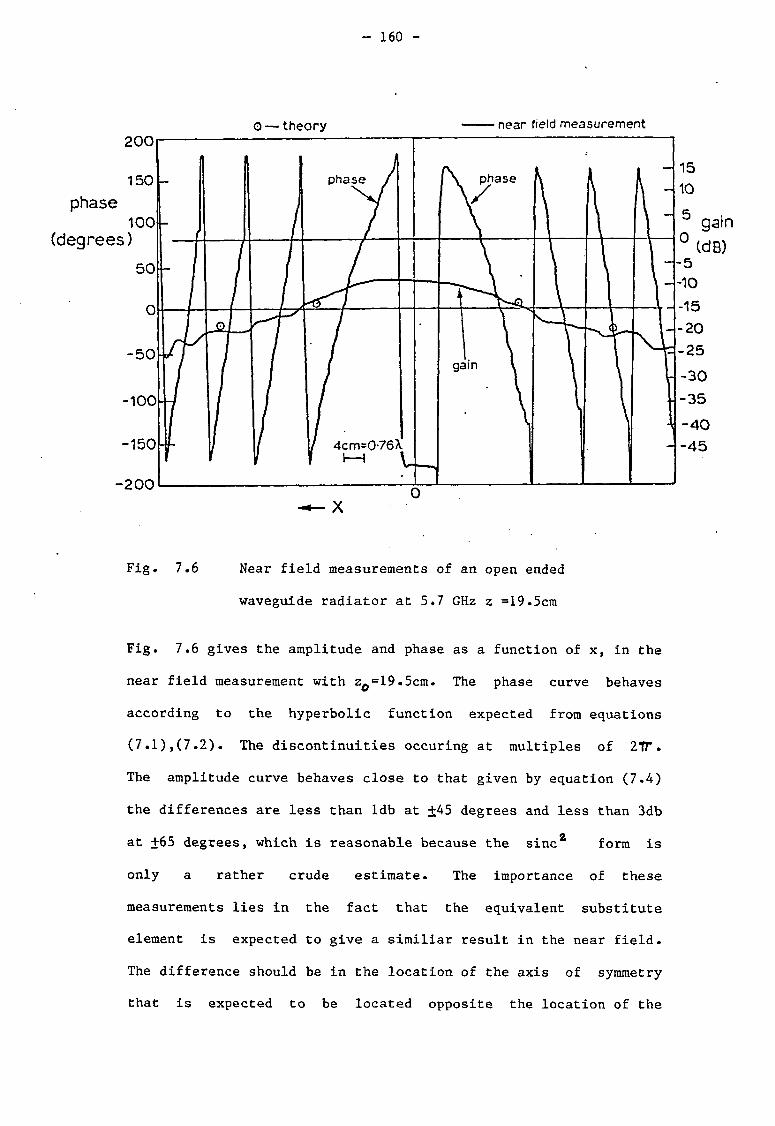
- 160 -
O — theory near field measurement
phase
(degrees)
-200
gain
Fig. 7.6 Near field measurements of an open ended
waveguide radiator at 5.7 GHz z =19.5cm
Fig. 7.6 gives the amplitude and phase as a function of x, in the
near field measurement with z 0=19«5cm. The phase curve behaves
according to the hyperbolic function expected from equations
(7.1),(7.2). The discontinuities occuring at multiples of 21T.
The amplitude curve behaves close to that given by equation (7.4)
the differences are less than ldb at ±45 degrees and less than 3db
at +65 degrees, which is reasonable because the sine 2 form is
only a rather crude estimate. The importance of these
measurements lies in the fact that the equivalent substitute
element is expected to give a similiar result in the near field.
The difference should be in the location of the axis of symmetry
that is expected to be located opposite the location of the

- 161 -
defective element.
The direct measurements of single elements radiating from
an 8-slot array (where all the other elements are covered by metal
tapes) are demonstrated in Figures 7.7 and 7.8.
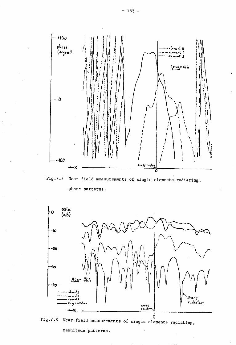
- 162 -
—+<80
phase
— 0
I 460
tUtntid 6 eUwoit k tU-^tnt 2
4 cm = 0. ftb
IS
ill
i \ h M: \M
Fig.7.7 Near field measurements of single elements radiating,
phase patterns.
magnitude patterns.
- 163 -
Fig. 7.7 shows the phase curves of elements 2, 4 and 6 radiating.
The curves show an hyperbolic variation similiar to those
described by Chignell [ 23] for a dipole affected by the baffle
wall, although no such walls are present.
The amplitude curves are described in Fig. 7.8. Element
2 amplitude is lower than element 4 or 6 as expected, due to the
cos + pedestal illumination. The tendency of the mean
amplitude curve is similiar to that of Fig. 7.6 (open ended
waveguide). However it has a higher ripple, which is caused by
interference with stray radiation. The amount of stray radiation
present in these measurements can be judged from the near field
measurements where all elements are covered (the lower curve of
Fig. 7.8). The stray radiation is superimposed and therefore
affects the radiation from element 2 more than 4 or 6, due to the
lower illumination of 2 compared to 4 or 6.
The far-field transformation of the radiation from
element 6 is shown in Figs. 7.9 and 7.10.
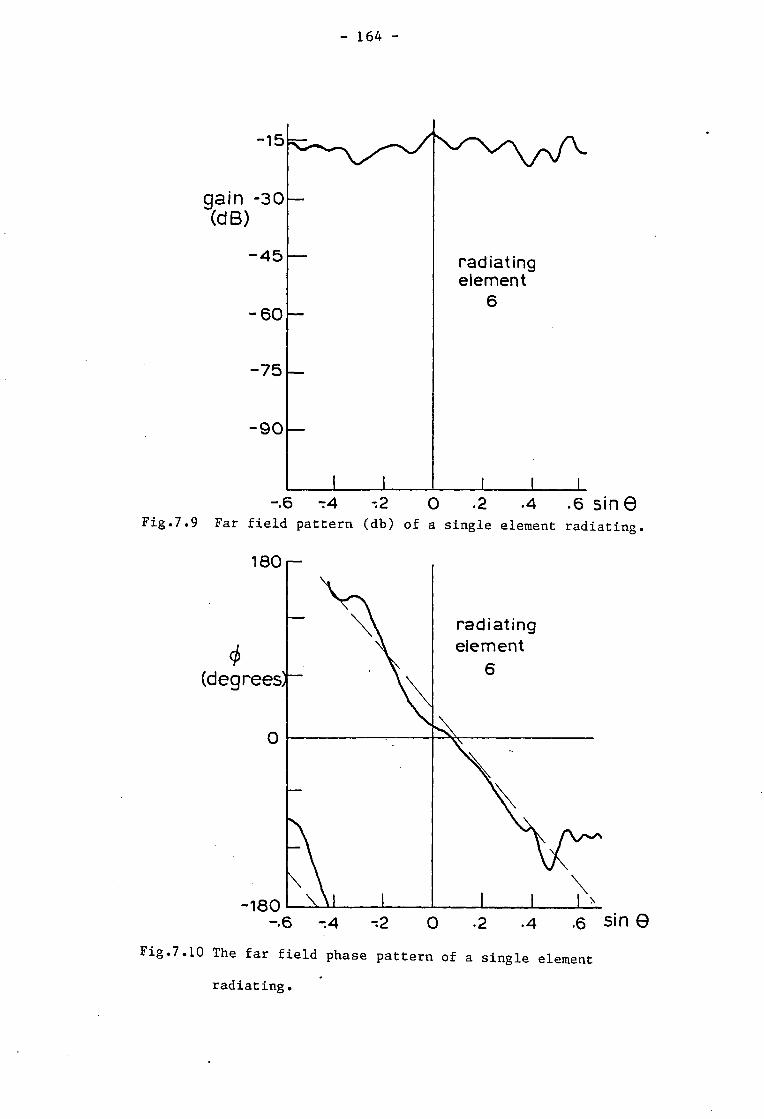
- 164 -
-15 /
g a i n -30 ( d B )
- 4 5 — radiating element
- 6 0 — 6
-75 —
- 9 0
I I I I I -.6 - 4 -.2 0 .2 .4 .6 Sin 6
Fig.7.9 Far field pattern (db) of a single element radiating.
Fig.7.10 The far field phase pattern of a single element
radiating.
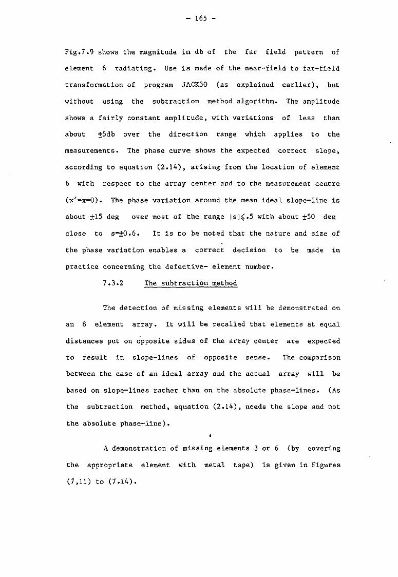
- 165 -
Fig.7.9 shows the magnitude in db of the far field pattern of
element 6 radiating. Use is made of the near-field to far-field
transformation of program JACK30 (as explained earlier), but
without using the subtraction method algorithm. The amplitude
shows a fairly constant amplitude, with variations of less than
about +5db over the direction range which applies to the
measurements. The phase curve shows the expected correct slope,
according to equation (2.14), arising from the location of element
6 with respect to the array center and to the measurement centre
(x'=x=0). The phase variation around the mean ideal slope-line is
about +15 deg over most of the range |s|^.5 with about +50 deg
close to s=±0.6. It is to be noted that the nature and size of
the phase variation enables a correct decision to be made in
practice concerning the defective- element number.
7.3.2 The subtraction method
The detection of missing elements will be demonstrated on
an 8 element array. It will be recalled that elements at equal
distances put on opposite sides of the array center are expected
to result in slope-lines of opposite sense. The comparison
between the case of an ideal array and the actual array will be
based on slope-lines rather than on the absolute phase-lines. (As
the subtraction method, equation (2.14), needs the slope and not
the absolute phase-line).
« A demonstration of missing elements 3 or 6 (by covering
the appropriate element with metal tape) is given in Figures
(7,11) to (7.14).
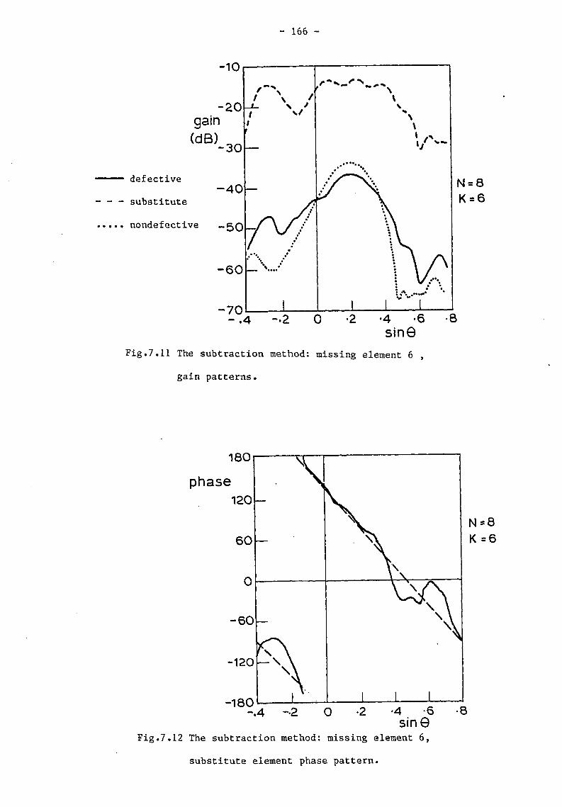
- 166 -
Fig.7.11 The subtraction method: missing element 6 ,
gain patterns.
Fig.7.12 The subtraction method: missing element 6,
substitute element phase pattern.
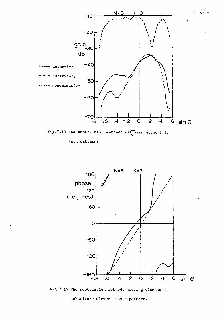
N = 8 K =
g a i n
defective
substitute
nondefective
- 167 -
- 7 0 -.8 -.6 - 4 --2 O 2 -4 .6 sin 9
Fig.7.13 The subtraction method: misusing element 3,
gain patterns.
1 8 0
p h a s e
120 (degrees)
N = 8 K = 3
- 1 8 0 -.8 - 6 -.4 - 2 0 -2 -4 .6 s i n ©
Fig.7.14 The subtraction method: missing element 3,
substitute element phase pattern.
- 168 -
Figs. 7.11 and 7.13 show the amplitude (in db) of the non
defective 8-element array, the defective array, and the equivalent
substitute element pattern magnitude where element 6 (Fig.7.11) or
element 3 (Fig. 7.13) are covered by pieces of metal tape. In
Fig. 7.12 and 7.14 the phase patterns are shown of the equivalent
substitute element of the defective element 6 (Fig. 7.12) and
element 3 (Fig. 7.14). The ideal slope lines, give the phase
variation of the computed values using the subtraction method.
Both measured patterns show the correct mean slope value.
The phase variations when element 6 is missing are +15deg at most
(apart from +30deg at the edges). The phase variations for
element 3 missing are much larger and reach about 120deg close to
the edges. However it should be noted that the agreement between
the theoretical and experimental slopes for the phase variation is
excellent when the amplitude of the equivalent substitute element
is roughly constant. The amplitude curves, Fig.(7.11) and(7.13),
also show lower ripple for the equivalent substitute magnitude
pattern of missing element 6 compared to that when element 3 is
missing .
These results are in accord with the mutual coupling
effect model outlined in chapter 4, Figs. (4.8) to (4.11). There
the main reason for excessive variation is related to the
asymmetry caused by forward reflected power due to the metal tape
cover of the radiating element. Hence element 3 causes higher
asymmetry than element 6.
It can therefore be concluded that the subtraction method
of monitoring can be applied to actual arrays, based on the
promising results of this test. Other aspects, such as the set-up
- 169 -
instability and thresholds proposed for the subtraction method
will be given in section 7.3.5.
7.3.3 The angular spectrum method
The 30-slot array was subjected to defects in either
element 13 or element 18. The detection of these will now be
examined with the angular spectrum method algorithm. The
technique is described in subsection 7.2.2; the results are given
in Figures 7.15 and 7.16, which show aperture illumination deduced
from the angular spectrum in the main beam region. A smooth curve
similiar to the cos^1 + pedestal illumination can be imagined for
the non-defective array. The aperture illumination of the
defective array has an anomaly (a "hole") in the vicinity of the
missing element 13 or 18 respectively.
In these same figures the derived aperture field for the
equivalent substitute element is given. It can be seen that in
both cases a clear indication of the location of the missing
element is given. It can therefore be concluded that the angular
spectrum method is also a practical monitoring method that can
usefully be applied to actual arrays.
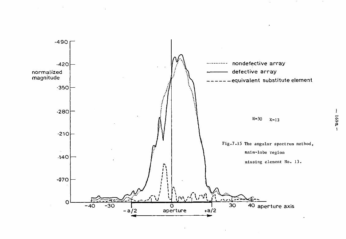
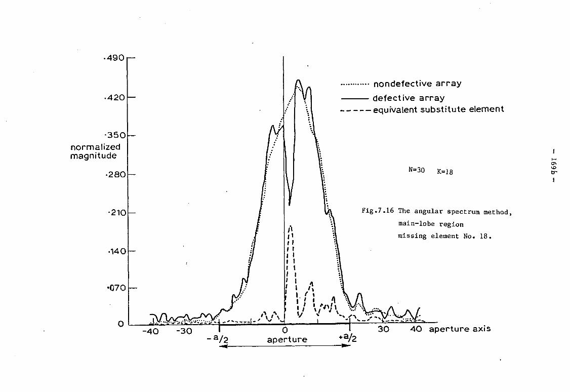
• 490 r—
•420
•350 normalized magnitude
•280
210
•140
•Q70
A V ^ ^ t ^ ^ i - 1 - ^ n I -40 •30
- a / 2
fl /» 11 i i i i i i i l I i ' f
nondefective a r r a y defect ive a r r ay equivalent substitute element
Fig.7.16 The angular spectrum method,
A. o
aperture
K=18
main-lobe region
missing element No. 18.
I ' 1 *j\ f\ !J v ' V
30 40 aperture axis

- 170 -
7.3.4 The autocorrelation (a.c.f.) method
The autocorrelation function method will be demonstrated
in the side lobe region of the 30-slot array. The array will be
subjected to the same defects as before. The measurements are now
taken from x ^ - ^ - ^ S c m to x,^ x=-55cm ( x ^ ^ is opposite element
number 1). The measurement aperture is placed at z o=110cm, hence
the direction cosines S-.45 to 0.8 are covered.
Attention should be paid to the fact that the
1/7+6/7 cos2 rather than the uniform illumination (which was
demonstrated in subsection 5.2.2 is now present. Therefore the
power peaks of the edge elements are now expected to be fainter by
about (1/6) if a center element of the array is missing. The
results are demonstrated in Figs. 7.17 to 7.20.
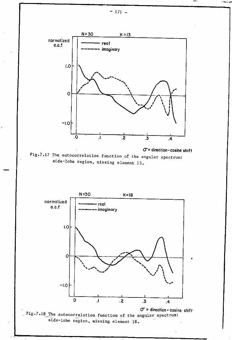
- 171 -
CT= direction-cosine shift Fig.7.17 The autocorrelation function of the angular spectrum:
side-lobe region, missing element 13.
N =30 K= 18
normalized a.c.f
CT = direction-cosine shift Fig.7.18jThe autocorrelation function of the angular spectrum:
side-lobe region, missing element 18.

- 172 -
Figs. 7.17 and 7.18 show the real and imaginary components of the
autocorrelation function for missing elements to the left and to
the right of the array centre. Attention should be paid to the
imaginary component of the a.c.f. which is of opposite polarity
for defects to the right and to the left of the array center.
The Fourier transform of the a.c.f. of the angular
spectrum, in the side-lobe region is approximating the modified
aperture power illumination as explained in subsection 5.2.2 (but
with a fainter edge-element response, as explained earlier, due to
the cos21 +ped illumination). The modified aperture power
illumination derived from side-lobe region measurements is given
in Figs 7.19 and 7.20.
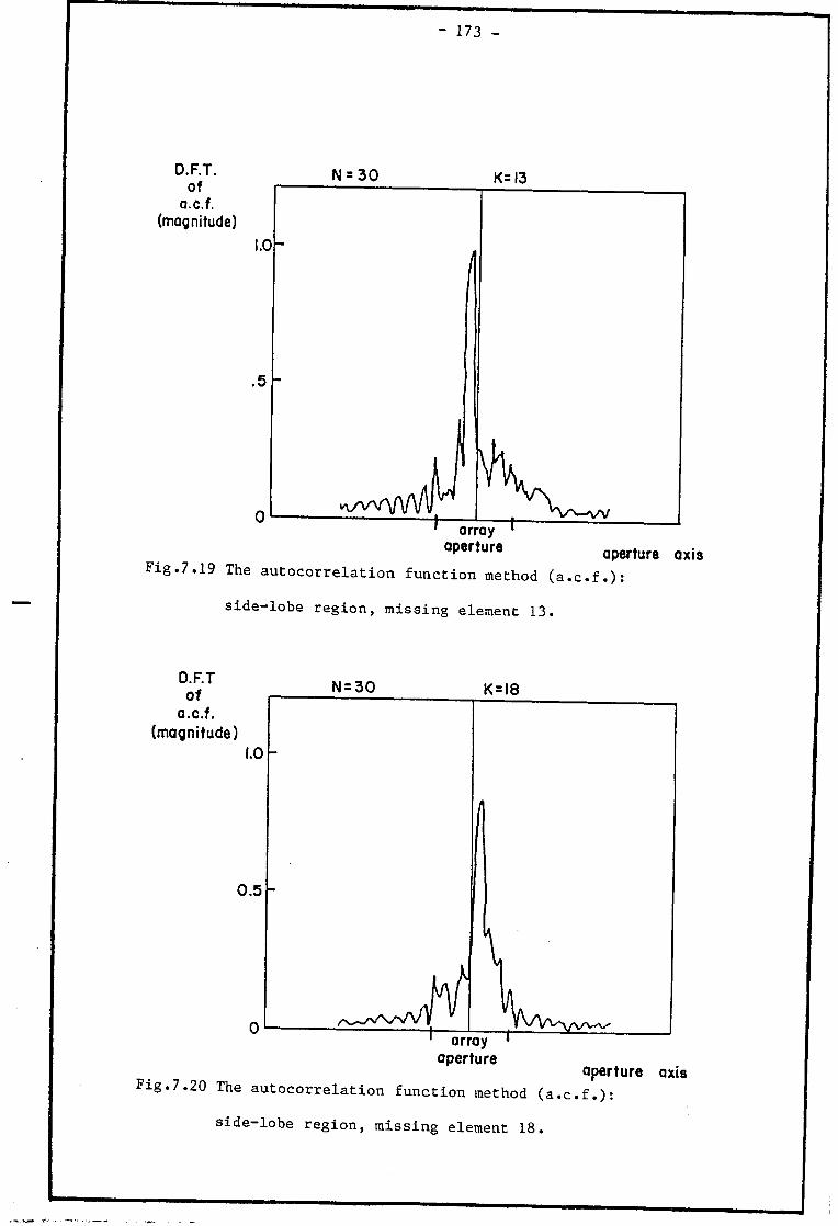
- 173 -
D.F.T. of
a.c.f. (magnitude)
N = 30 K= 13
° P e r t u r e aperture axis Fig.7.19 The autocorrelation function method (a.c.f.):
side-lobe region, missing element 13.
D.F.T of
a.c.f. (magnitude)
N = 30
0.5 h
K=I8
array aperture
aperture axis Fig.7.20 The autocorrelation function method (a.c.f.):
side-lobe region, missing element 18.

- 174 -
Figs. 7.19 and 7.20 show the modified aperture power illumination
calculated from measurements in the side-lobe region. The
illumination due to the equivalent substitute element 13 or 18
missing are pointed out in the relevant figure. Hence it can be
concluded that, as with the other two methods, the a.c.f. method
can be used with actual arrays.
This concludes the demonstration of the three methods
applied to actual arrays. The sensitivity to instability and the
problem of thresholds will be discussed next.
7.3.5 Sensitivity to instability ( and thresholds)
An experiment has been carried out to examine the effect
of instability in the measurements on the performance of the
subtraction method.
The angular spectrum method and the a.c.f. method both
use absolute magnitudes for comparison in order to identify
defective elements by anomalies in the aperture illumination. The
subtraction method, however, uses a comparison between complex
numbers. Hence it is more important to check the effects of these
instabilities with the subtraction method in particular.
It should be noted however that in the case of the
angular spectrum and the a.c.f. methods a constant phase drift
will have practically no effect on the resulting magnitudes.
However a drift in the measured magnitude will result in a
proportional change in the aperture illumination function.
The effect on the subtraction method of any drift could
introduce an apparent defect. The resulting error pattern is the

- 175 -
phasor subtraction of the two reference patterns measured before
and after a drift has been introduced into the measuring
instrumentation (i.e. in amplitude and phase). It is expected
that the effect will be noticed more severely in the main beam
region where the subtraction of two large complex numbers might
result in a large error due to a small amplitude or phase error.
In the side-lobe region the effect is fainter according to the
ratio of the main beam to side lobe levels. There the effect of
amplitude or phase drift will be minimal and will, in practice,
not affect the phase slope (although the absolute phase can be
affected). Therefore the subtraction method is expected to be
affected in a similar manner to the other two methods in the side
lobe region.
A demonstration of using the near field reference pattern
to resolve defects after 5 days with drifts of about 1 to 2 db in
magnitude and 40 deg. in phase is given in Figs. 7.21 to 7.25.
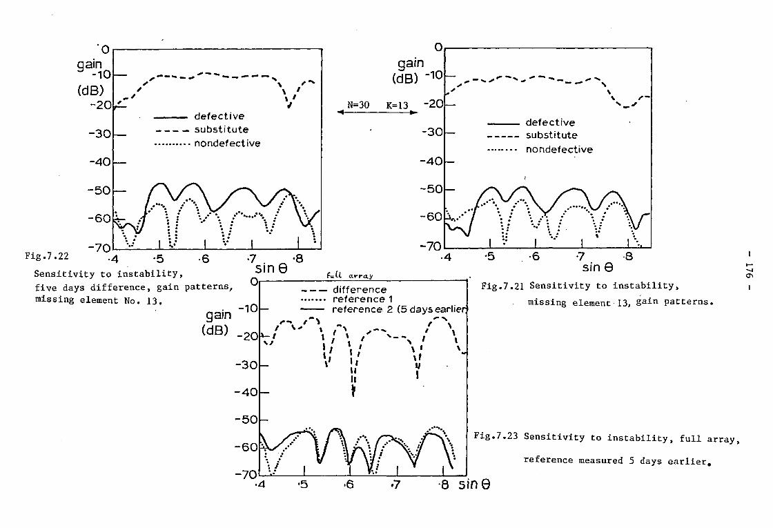
0
qain 3 - 1 0 (dB)
- 2 0
-30
-40
_ / v • defective
— substitute nondefective
Fig.7.22 .4 .5 . 6
Sensitivity to instability,
five days difference, gain patterns, ^
missing element No. 13. - 1 0
gain (dB) "10
N=30 K=13 - 2 0
-30
-40
-50
- 6 0
-70
CM array
gain (dB) - 2 0
-30
-40
W
difference reference 1 reference 2 (5 days earlier
V
/ 1 ^ N
• \! II II \
N ' \ • \l 1/ I
\
defective substitute nondefective
Fig.7.21 Sensitivity to instability,
missing element 13, §a i n
patterns.
Fig.7.23 Sensitivity to instability, full array,
reference measured 5 days earlier.
8 sine
- 177 -
Figs. 7.21 to 7.23 give the far field patterns derived from
near-field measurements. Figs. 7.21 and 7.22 show the far field
magnitude patterns of missing element 13. In Fig. 7.21 the
reference used is measured shortly before the introduction of the
defect, while in Fig. 7.22 a reference measured 5 days earlier is
used. Fig. 7.23 shows the far field pattern of the two reference
measurements taken 5 days apart, when no defect is present.
Comparing the substitute element pattern of a defective array with
this non-defective array shows a difference of about 10 db (the
pattern of the substitute missing element is 10 db stronger than
the non-defective condition). The phase patterns are given in
Figs. 7.24 and 7.25.
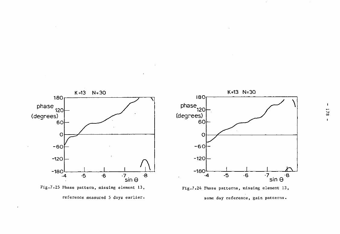
K =13 N = 30
Fig.7.25 Phase pattern, missing element 13,
reference measured 5 days earlier.
K=13 N = 3 0
Fig.7.24 Phase patterns, missing element 13,
same day reference, gain patterns.

- 179 -
Fig. 7.24 shows the phase patterns of element 13 missing where
only a short time has elapsed between the measurements of the
reference and the defective array. In Fig. 7.25 the same
defective array measurements are compared to a reference measured
5 days earlier. As can be judged from the graphs, the delay has
no appreciable affect on the resulting phase slope line.
Another important result is derived by checking the
previously mentioned 10 db difference between an apparent defect
(due to drift between two reference patterns) and an actual
defect. A recommendation is therefore made to use a -6db level
threshold to differentiate between an actual defect and an
apparent one.
Summarizing the results of sensitivity to instability:
The preferred region for all three methods is in the side
lobe region. The subtraction method is expected to be the most
vulnerable of the three methods if it is used in the main lobe
region in the presence of unstable measurements.
A threshold level of about 6 db can be used in the
side-lobe region to distinguish between an apparent defect and an
actual one, and ignoring the phase line deviations in the
direction cosine regions , below that threshold. For higher
instabilities or for a greater delay in taking the reference
patten measurements other values for the threshold could be found
adequate. Hence using the monitoring methods in the side- lobe
region enables the use of measurement systems which have inferior
qualities. This is another example of the advantage of using the
side-lobe region for measurement.

- 180 -
The experimental investigation was preceded by a series
of supporting tests. These are described next.
7.4 Details of some supporting tests
Inspection of the equations used in the near-field to
far-field transformation, the following variables are to be
considered: wavelength, phase, amplitude and geometry. Therefore
the first part of the experimental investigation was dedicated to
assessing the systematic and dynamic errors in the measurement of
these variables.
7.4.1 Static and dynamic errors
The following tests have been conducted:
Long term stability measurements
- Frequency stability of the microwave power source. (Fig 7.26)
- Phase and amplitude stability of the set-up. (Fig. 7.27)
- Stability of x-coordinate reading.
The dynamic tests included
- Phase and amplitude jitter due to bending of the coaxial cable.
- backlash of the drive mechanism related to the helical
potentiometer output signal.
- Repeatability of the drive mechanism when motion in the same
direction is examined.
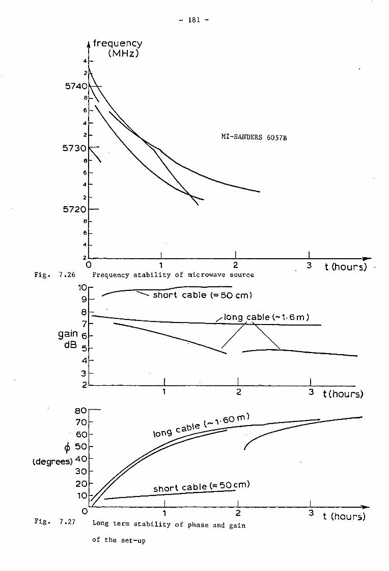
- 181 -
4 frequency (MHz)
4
2
5740 8
6
4
2
5730 8
6
4
2
5720
4
2
MI-SANDERS 6057B
0 1 2 Fig. 7.26 Frequency stability of microwave source
10. . 3 t (hours)
9 8 7
gain 6 dB 5
4 3 2
short cab le (=50 cm)
/ l o n g c a b l e ( ~ l - 6 m )
3 t(hours)
1 2
Fig. 7.27 Long term stability of phase and gain
of the set-up
3 t (hours)

- 182 -
Fig. 7.26 shows the frequency of the Gunn source measured over
sequences of several hours. The result is about -12MHz/hour
frequency drift. In Fig. 7.27 the total phase shift is given as
a function of time. Two groups are noticed: small changes of
about +4deg/hour and large ones of about +35deg/hour. The reason
for these differences was identified with the cable length used
between "test" and "reference" channels of the Network Analyzer.
Hence the effect is mainly due to the frequency instability of the
source (according to Fig. 7.26).
The results of these and of the additional stability
tests are summarized in table 7.1.
Table 7.1
Set-up instability errors
Mesured quantities Error
Bias errors
Frequency stability <-12MHz/hour Gain stability <+.5 to-2.0 db/hour Phase stability (3m cable) <+35deg/hour Phase stability (1.3m cable) <+4deg/hour Stability of x-positioner <+0.5cm/hour Parallelism
<±0.5cm (estimate) Translation orthogonality < +2deg (estimate)
Dynamic errors Phase jitter due to bending (radius>10cm)
< +10deg Backlash of x-positioner < +0.5cm Repeatability of x-positioner (same direction)
<± 0.2cm
Note Set-up tests at 5.7GHz measured after 15 minutes warm up time.
7.4.2 Antenna tests (and stray radiation)
The following tests have been made in addition to those
previously described, to find out the effect of blocking a
radiating slot with metal tape (used to introduce artificial
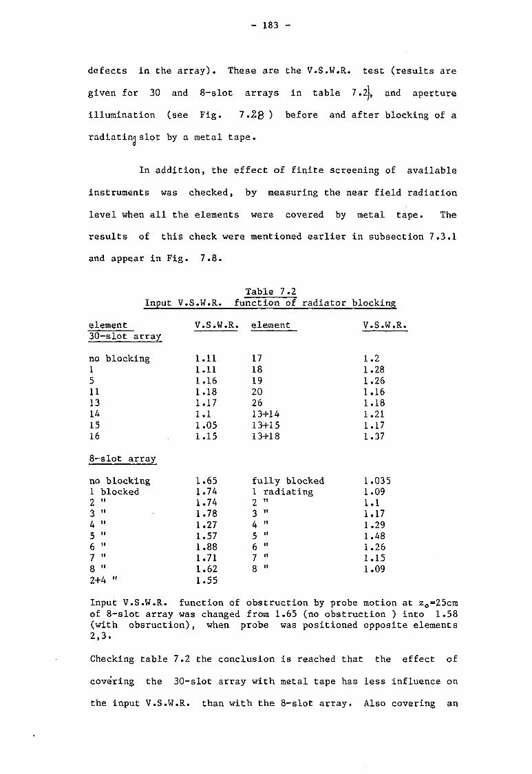
- 183 -
defects in the array). These are the V.S.W.R. test (results are
given for 30 and 8-slot arrays in table 7.2), and aperture
illumination (see Fig. 7.28 ) before and after blocking of a
radiating slot by a metal tape.
In addition, the effect of finite screening of available
instruments was checked, by measuring the near field radiation
level when all the elements were covered by metal tape. The
results of this check were mentioned earlier in subsection 7.3.1
and appear in Fig. 7.8.
Table 7.2 Input V.S.W.R. function of radiator blocking
element 30-slot array
no blocking 1 5 11 13 14 15 16
8-slot array
no blocking 1 blocked 2 3 4 5 6 7 8 2+4
V.S.W.R. element
1.11 1.11 1.16 1.18 1.17 1.1 1.05 1.15
1.65 1.74 1.74 1.78 1.27 1.57 1.88 1.71 1.62 1.55
17 18 19 20 26 13+14 13+15 13+18
fully blocked 1 radiating 2 3 4 5 6 7 8
V.S.W.R.
1.2 1.28 1.26 1.16 1.18 1.21 1.17 1.37
1.035 1.09 1.1 1.17 1.29 1.48 1.26 1.15 1.09
Input V.S.W.R. function of obstruction by probe motion at z 0=25cm of 8-slot array was changed from 1.65 (no obstruction ) into 1.58 (with obsruction), when probe was positioned opposite elements 2,3.
Checking table 7.2 the conclusion is reached that the effect of
covering the 30-slot array with metal tape has less influence on
the input V.S.W.R. than with the 8-slot array. Also covering an

- 184 -
element which has a higher illumination has a larger effect on the
input V.S.W.R.
The effect of covering a radiating slot with a metal tape will be
given next, (see Fig 7*28)
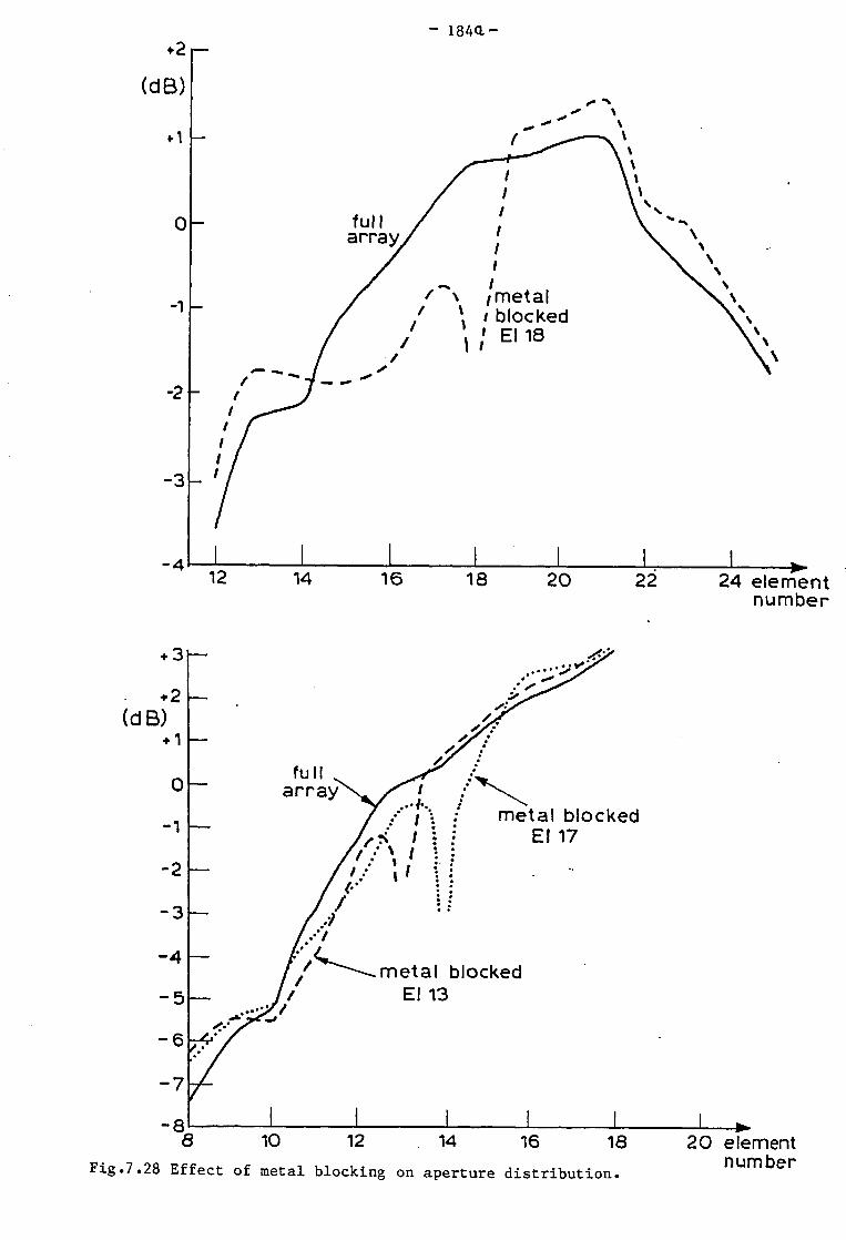
- 184 -
- 185 -
The changes in the aperture distribution shown in Fig. 7.28 are
as follows.
In the forward direction (towards the load) the amplitude is
raised by about 0.2 to 0.5 db . In the backward direction
(reflection towards the generator) a decrease by about -ldb is
noticed (in the 3-4 neighbouring elements). This confirms in part
the model used when mutual coupling effects were discussed in
chapter 4 (the forward reflected power model).
7.4.3 Comparison of far field measurements
In order to check the applicability of the set up and of
the processing (program JACK30), an experiment has been performed
to compare the near field measurements transformed to the far
field with actual far field measurements. The only antenna that
could be checked inside the Microwave laboratory was the 8-slot
array, which allows a practical indoors Rayleigh distance
(R=2a a ) of about 2.8 meter.
The 8-slot array near field measurements of subsection
7.3.2 have been compared to the pattern measured at 3.0 meter
assumed to be the far field. The "far-field" set-up is shown in
plate 7.4. The far-field measurement results are shown in Fig.
7.29.
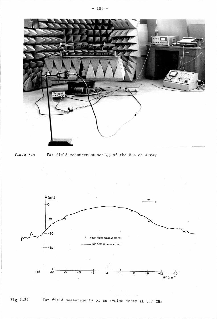
- 1 8 6 -
Plate 7.4 Far field measurement set-up of the 8-slot array
-I I 1 1 ! | I I I , * 7 e O o i Is Tg -12 =15"
angle
Fig 7.29 Far field measurements of an 8-slot array at 5.7 GHz
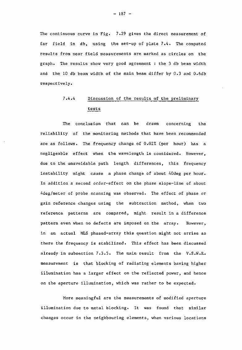
- 187 -
The continuous curve in Fig. 7.29 gives the direct measurement of
far field in db, using the set-up of plate 7.4. The computed
results from near field measurements are marked as circles on the
graph. The results show very good agreement : the 3 db beam width
and the 10 db beam width of the main beam differ by 0.3 and 0.6db
respectively.
7.4.4 Discussion of the results of the preliminary
tests
The conclusion that can be drawn concerning the
reliability of the monitoring methods that have been recommended
are as follows. The frequency change of 0.02% (per hour) has a
negligeable effect when the wavelength is considered. However,
due to the unavoidable path length differences, this frequency
instability might cause a phase change of about 40deg per hour.
In addition a second order-effect on the phase slope-line of about
4deg/meter of probe scanning was observed. The effect of phase or
gain reference changes using the subtraction method, when two
reference patterns are compared, might result in a difference
pattern even when no defects are imposed on the array. However,
in an actual MLS phased-array this question might not arrise as
there the frequency is stabilized. This effect has been discussed
already in subsection 7.3.5. The main result from the V.S.W.R.
measurement is that blocking of radiating elements having higher
illumination has a larger effect on the reflected power, and hence
on the aperture illumination, which was rather to be expected.
More meaningful are the measurements of modified aperture
illumination due to metal blocking. It was found that similar
changes occur in the neighbouring elements, when various locations

- 188 -
were chosen for the imposed defects. The main effect (see
Fig.7.28) is the increase in the forward power, apart from the
"hole" due to the blocked element. This is similar to the model
used in chapter 4 for the internal coupling effects (forward
reflected power). This effect is expected to be of second order
in actual systems which are not fed in series. The results of the
far field measurements comparison to the near field measurements
show that the system including the program are of good quality in
spite of the errors discussed in the present section.
7 .5 Summary and discussion
The monitoring methods recommended in this work have been
found to give the expected results, for artificial, defects of
single missing elements in the array.
Hence a partial verification of the theoretical methods
proposed has been achieved. A full verification of the method
proposed will be possible only if one-to-one models of actual
phased-arrays, with frequency stabilized source, could be checked
using the same methods, in particular in the far field. Some
conclusions can also be drawn concerning the use of practical
measurement system (with phase and amplitude instabilities). In
such cases, a threshold should be applied below which results are
to be ignored and only results complying with the threshold are to
be considered for the methods. This means that the long term
instabilities can be tolerated in practice.
The side-lobe region have been found to be preferable for
measurement, as being least sensitive to parameter instabilities.
The shape of the phase deviation for differnt locations
- 189 -
of the artificial defect (to the right or to the left of the array-
centre), justify in part the model of internal coupling
(asymmetrical reflections due to a defect, as explained in chapter
4). The shape of the phase deviations also mean that mutual
coupling (external) has only a second order effect compared to the
internal coupling and hence is not of prime interest in arrays
with interelement spacings of about 0.7/\, as used in the
experiments. It is believed that MLS arrays (although with .61^
interelement spacings) are expected to have lower internal
coupling effects due to the power distribution network structure.
The near field to far field comparison shows encouraging
results with the laboratory set-up used for these experiments and
can be regarded as an overall check on the quality of the
experimental system.
«

- 190 -
CHAPTER 8
COMPARISON OF THE METHODS
In previous chapters several monitoring techniques have
been analyzed, and also tested by computer simulation and in part
by experiments. A comparison will now be made between the
different methods proposed and their applicability demonstrated in
a specific example in the form of a proposed monitoring system for
the MLS phased-array.
8.1 Analysis tools used
Effectively two analysis tools have been suggested and
used in this work. These are the equivalent substitute element
technique and the approximations to the Fresnel integral.
8.1.1 The equivalent substitute element technique
This technique proposed the representation of defective
elements by their equivalent substitute array (equation 2.4).
This representation gives simplified results if a single element
is defective in the array, and where defects are of a static
nature like a constant amplitude and/or phase defects. In the
dynamic case of a stuck phase-shifter, a modified result is
expected (see equations 3.19 and 3.19a). This is further
modified if a thinned phase-shift network is used, i.e., where
single phase-shifters are used to control the phase of a group of
elements (a sub-array). An important feature of the equivalent
substitute element technique is its inherent normalized phase-line
resulting when a single element is defective in the array. This
means that the resulting phase-line is independent of the
illumination function of array elements. (Hence it is very

- 191 -
attractive for use in practical arrays).
8.1.2 The approximation to the Fresnel integral
Another important tool that has been investigated is an
approximation to the Fresnel integral. This representation is
specifically helpful in describing the near field (Fresnel region)
of a scanning-beam aperture antenna in terms of the antenna
aperture illumination and the angle scanning function. The use of
this presentation has been described in chapter 6 and will be
summarized in a later section dealing with the near-field
monitoring technique.
8.1.3 Simulation models used
Simulation on the computer has been found to be a most
useful tool as an aid to analysis. Two main tasks have been
performed by the simulation. The first was to produce a
verification of the analysis, modelling antennas and defective
elements in the presence of a variaty of excitation errors, so as
to represent actual array performance. The simulation was also
used as a kind of "scratch pad" to check and produce ideas leading
to new methods. As it is very easy to come to erroneous
conclusions, care was taken to check the quality of the simulation
and in particular whether any errors were present in the computer
programs developed, or in the equations and parameters used in the
models. As an example the quality of the random number generator
called as a computer function (RANGET), was checked with a
subroutine COREL03 (see Appendix E) developed to calculate the
autocorrelation function. The computer results have been compared
to the expected statistical equations. This comparison then led
- 192 -
to two conclusions. First, that the random number generator is of
a good quality of statistically independent numbers, for the sizes
used. It also had an accompanying important conclusion that the
autocorrelation function subroutine used was correct. Line
printer graphics (computer library GRAFIC and GRAFIT), although of
insufficient resolution, have been widely used to produce fast and
inexpensive displays of selected numerical results, so that spot
checks could be used to trace any anomalies in the programs and,
also, to enable an immediate assessment of the results. The
simulation included programs of the far-field and the near field
patterns of N element array of various illumination functions,
subjected to defects in single or multiple elements or subarrays,
in the presence of random phase excitation errors. The models
assumed perfect tracking analogue phase-shifters. Defects of a
dynamic nature were examined when, for example, a single
phase-shifter was held fixed while the others changed in the
prescribed manner. Dynamic phase-shift errors, due to digital
quantization of the phase, have been combined in a statistical
rather than a deterministic way, which facilitates their
modelling. It is also ecconomical, and gives the results neatly
in the form of an envelope. A preassigned range of uniformly
distributed random phase-shifts are added to the correct
calculated values of phase-shift. This range could represent the
inaccuracy due to the value of the least significant bit in an
m-bit phase shifter. Then, two types of random excitation errors
have accordingly been used - static or dynamic, depending on
whether the random number generator was reset or not after each
sequence of phase settings. Static errors can represent actual
phase errors due to production inaccuracies of array elements;
- 193 -
dynamic errors represent, as explained earlier, the built in phase
quantization.
Mutual coupling effects were incorporated in the
simulation using normalized values of mutual impedances according
to Carter's [ 9] equations, for the external coupling. While
internal coupling was represented by a simplified model of forward
and/or backward reflected power, due to the supposed defect.
These effects were incorporated as an equivalent substitute array,
the illumination of which is a function of the values derived from
the calculated mutual coupling effects.
Near fields of antenna apertures have been simulated
using the Fresnel-Huygens diffraction formula. NAG Routine
functions, (S20ADF and S20ACF) given by a series approximation due
to Abramowitz and Stegun [ 25] have been used for the evaluation
of the cosine and sine integrals. Near-field to far-field
transformation used the discrete Fourier transformation (D.F.T.),
using NAG Subroutines (C06ADF). However, D.F.T. programs had to
be developed (by the author) in cases when the required number of
transformed values was larger than the number of input samples
available (the standard procedure which is available as a NAG
Routine has equal input and output samples). For example the
transformation of near-field to far-field patterns used this
technique to achieve small direction increments.
Near-field measurements simulation was helped by an
auxiliary Subroutine EJIX (see Appendix E). This subroutine
calculated the near-field received over a linear measurement
region from an N-element transmitting array. And was used, for
example, to find out how critical the near-field sampling

- 194 -
increments were in terms of the resulting far-field pattern.
Additional programs are given in Appendix E are DBPMES used for
preprocessing to translate data from the X-Y recorder plot into
phase and amplitude in the required format for program JACK30.
Program JACK20 for mutual coupling between parallel dipoles.
Program JACK42 near field focusing of near fields diffracted from
a uniformly illuminated aperture. Program JACK37 as before but
for half cosine aperture field. Program JACK38 as before but
for cosine over pedestal illumination . Program JACK45 for far
field radiation from a pyramidal horn antenna with a predetermined
phase error.
8.2 A summary and comparison of the monitoring methods
Far-field and near—field monitoring methods have been
suggested. The far field methods included:
- The subtraction method.
- the angular spectrum(direct) method, and
- The autocorrelation function (a.c.f.) method.
These three physically distinct methods also correspond
to three quite distinct levels of processing, in that they demand
an increasing amount of processing time for their implementation.
The near field methods included:
- The near-field monitoring technique.
- The integral and
- Internal monitoring.

- 195 -
These methods will also be compared. Special attention
will now be paid to their applicability to monitoring the MLS
phased-array antennas.
The subtraction method, based on the representation of
defective elements by their equivalent substitute array, has been
found to be a most efficient method. Specifically where a single
element has become defective in the array. Then in the case of
defects in ideal arrays only a few measurement samples are needed
to resolve the phase ambiguity and give the equivalent substitute
element phase-line, thereby enabling the identification of the
location of the defective element and the type of defect. As
explained in chapter 3 this method could be used for practically
any type of illumination function, including thinned arrays.
This capability, of identifying the type of defect, is
not available in the other two methods used, namely, the angular
spectrum (direct) method and the a.c.f. method. It is also not
available, as explained in the introduction (chapter 1 ), in the
method suggested by Ransom and Mittra [ 2]. Although those other
methods enable the identification of one or of several defective
elements occuring at one time in the array. However, with the
expected reliability of operational phased-arrays like the MLS,
this type of defect occurrence is highly improbable. Hence
sequentially memorizing the occurrence of defects in the array
could be used instead as an aid to maintenance. A simple
criterion can be used for the monitoring and control thresholds.
For example, the maximum percentage of defective elements, say
10%, of the array, can be tolerated (see Bendix corporation
experimental investigation [ 4 ] ) before a shut down procedure
- 196 -
(see ICAO [ 6]) and alarm are to be initiated. Hence, the
subtraction method can be used to monitor a multitude of defects
in practical antenna arrays. An additional important advantage of
the subtraction method arises from the fact that the expected
processing time needed is very short, enabling real-time decisions
to be made. Incidentally, the time required is far below the 1
second reaction time required by ICAO Standards And Recommended
Practices (SARPS) [ 6 ] .
Alternatively, or in parallel, it is possible to use the
other methods to verify the findings of the subtraction method or,
if real-time processing is possible, to use them altogether in
order to make a decision.
The two other methods, the angular spectrum and the
a.c.f. methods, use the aperture illumination magnitude and
power, accordingly, for a decision on the presence of defective
elements due to anomalies in the aperture distribution. The
angular spectrum method requires a longer processing time than the
subtraction method, due to the far-field to aperture axis
transformation needed. As is evident, this method required many
data samples to be Fourier transformed to achieve the normalized
aperture illumination function. The resulting illumination
function magnitude, is to be compared with a reference aperture
illumination pattern of the array, before it became defective.
Then, using proper thresholds to minimize false alarms, a decision
can be taken on the location of defective elements over the array
aperture. As will be shown, in section 8.4, the angular spectrum
(direct) method still enables real-time processing, especially^ if
F.F.T. processing is available on the systenTs already installed
- 197 -
microcomputer.
The autocorrelation method is expected to give results of
higher quality (fewer false alarms in a given measurement "noise"
background), due to its inherent smoothing capability. This
smoothing is a result of correlating many data samples which are
used to extract the periodic oscillations, due to elements failure
(see section 5.3), before transforming into the aperture plane.
This means a longer processing time than that required by the
angular spectrum (direct) method.
The near field monitoring methods give the following
results. The near field monitoring technique (section 6.2) is
expected to give a reconstructed main-beam scanning by near-field
(Fresnel region) measurements. The main importance of the
near-field monitoring technique, which is based on approximations
to the Fresnel integral (chapter 6 ), is in the non necessity for
corrections to be made in the transmitting array and in its
real-time (main-beam pointing) monitoring capability. This is due
to the fact that no further near-field to far-field (Fourier)
transformation are needed. In addition it requires only a few
(say 10) sampling elements over the near field monitoring antenna
aperture. However, the requirement that this aperture should be
extended to the length of the transmitting antenna is a
disadvantage. It must be pointed out that the subtraction method
could be used in the array near-field if a single element (or a
single subarray) is concerned. It is then only necessary for the
measurements to be performed in the far-field of the single
elenlent (or sub-array), as explained in section 2.7.
In addition it can be speculated, based on the simulation

- 198 -
of the near-field received by a single monitor element (section
6.2.1 and figure 6.4a), that the near field far side-lobe pattern
behaves in a manner very similar to that of the far-field. Hence,
if this is really the case, the near-field far side-lobe region
can be used for the detection of a multitude of defective elements
using the far field monitoring techniques, with no need for
additional preceding near-field to far-field transformations.
However, a modification may be needed to take account of the
residual parallax effects.
The other near-field techniques, namely the
integral/internal monitoring, are techniques already used for
getting the far-field pattern from very near-field monitoring (see
Bendix [ 4 ] ) as explained in section 6.3. The suggestion which
was presented, using the serial waveguide sampler, has shown that
main-beams scanned to about 51deg, 33deg or 22deg using standard
waveguides are detected. Therefore the two main beam locations at
+51, +33 or +22 degrees, of the MLS angular coverage (+60deg.),
can be detected if use is made of the two opposite ends of the
serial waveguide samplers. This may be found advantageous for
simplifying the monitoring of the main beam scan coverage.
Having compared the different methods from an analytical
point of view, backed up by simulation, it is instructive to
recall the experience using actual arrays.
8.3 A summary of the experimental investigation
The experimental investigation was aimed at getting
additional verification, where possible, of the methods suggested,
and of their simulation on a computer. The measurements have been
- 199 -
limited to the near-field radiated from linear slot waveguide
antennas, operating at a frequency close to that used by the MLS.
The array elements were subjected to artificial defects.
Far-field monitoring methods have been used for the detection of
defective elements in the array, after transforming the
measurements to the far-field, using computer programs. The
outcome was that these computed patterns have been shown to be
similar to those predicted by simulation where mutual coupling
effects have been included. Hence, some verification of the
far-field monitoring methods has been achieved. Also far field
pattern measurements have been made and results very close to
those of the near-field measurement after being transformed to the
far field have been obtained in the main beam region (see section
7.4.3). Hence a further confirmation of the programs used from
near field to the far-field has been reached.
In addition, it has been demonstrated that the far
side-lobe region is a preferred region, compared to the main-lobe
region, as explained in section 2.3.
An important result was the outcome of the long term
stability experiments of section 7.3.5. It was shown that
practical measurement systems are sufficiently stable. A shift of
about 40 degrees in phase and of about 2 db in magnitude between
two such measurements, cuased no significant change in the
resulting phase-line of a defective element, using the subtraction
method. The two reference patterns in this instance were measured
5 days apart. Also in the calculation of aperture illumination
using the angular spectrum methods, no significant difference has
been noticed. These stability measurements have shown that a

- 200 -
threshold is important, to distinguish between the case of
defective elements and that of an unstable reference. A
difference of about 10 db has been observed between the case of a
missing element and that due to the subtraction of two unstable
reference patterns. Hence a 6db level, below the magnitude
expected from a missing element, can be used as a practical
threshold.
8.4 Comparison of the required processing
The complexity of processing is dependent on the
monitoring method to be used. Hence, there are three main levels
of processing, (see section 8.2). The processing is composed of
two parts: the preprocessing and the main processing.
Preprocessing is necessary to normalize the measured quantities,
before the monitoring algorithms can be examined in the main
processing. The amount of preprocessing needed is therefore
dependent on such factors as the dynamic range and accuracy of
measured signal variables. These, in turn, affect the design of
the measurement system. Preprocessing and processing will be
discussed in the following two sections.
8.4.1 Preprocessing and signal measurements
Magnitude and phase are the variables to be measured.
However the quantities used in all the monitoring methods are in
effect the real and imaginary parts of the complex signal. Hence,
measurement of real and imaginary parts of the complex signal are
preferable than the measurement of the signal magnitude and phase.
The necessary dynamic range is dependent on the
measurement region. If main-beam and side-lobe regions are to be

- 201 -
included, then about 50db dynamic range is required. However, if
only the far side-lobe region is of interest, then a 20 to 30 db
dynamic range can be sufficient, enabling linear circuits to be
used. This is to be preferred as the circuitry is simplified and
becomes cheaper. If a 50db dynamic range is required, then
non-linear circuitry, such as logarithmic amplifiers, might be
necessary. Due to the non-linear measurements additional
preprocessing in order to achieve linearization has to be used,
before the monitoring algorithms can be examined. This is in
addition to the more complex and expensive circuitry required,
like instanteneous logarithmic amplifiers and phase matched
limiters.
A block diagram of the above circuits will now be
described.
The quadriphase-demodulator widely used in monopulse
Radar and data communication, enables one to obtain unambiguous
measurements of the phase difference <j> between two input signals,
resolved into two quadrature output bipolar video channels I and
Q . A block diagram is describd in Fig. 8.1.
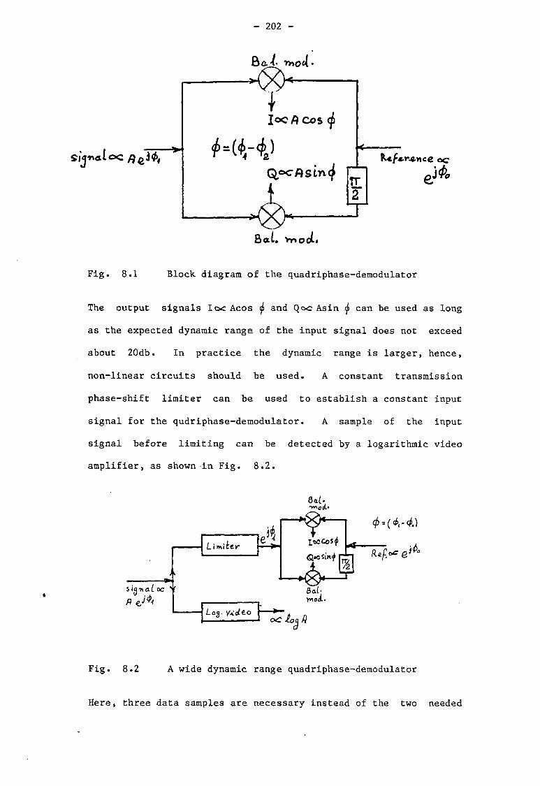
- 202 -
Bal. VnooL
Fig. 8.1 Block diagram of the quadriphase-demodulator
The output signals lex Acos <j> and Qo<c Asin <f> can be used as long
as the expected dynamic range of the input signal does not exceed
about 20db. In practice the dynamic range is larger, hence,
non-linear circuits should be used. A constant transmission
phase-shift limiter can be used to establish a constant input
signal for the qudriphase-demodulator. A sample of the input
signal before limiting can be detected by a logarithmic video
amplifier, as shown in Fig. 8.2.
sicj-naLoc V R
Limitev
L03. vxdto
6a ^061*
r - ^ H
Qociinf r
8a£' Ynoii>
ocL^f)
Fig. 8.2 A wide dynamic range quadriphase-demodulator
Here, three data samples are necessary instead of the two needed

- 203 -
in the linear case (Fig. 8.1). As explained earlier in this
section an additional translation of log A into A will be needed
in the preprocessing. This value will then be multiplied by the I
and Q values of the amplitude limited signal, in order to resolve
the two orthogonal samples needed for processing.
Quadrature-demodulators, limiters and logarithmic amplifiers are
available commercially with sufficient accuracies in the I.F.
frequencies (see Appendix F) . It will, therefore, be recommended
that phase and amplitude detection be performed at I.F.
8.4.2 Processing
The approximate number of operations necessary for the
processing of the different monitoring methods, will now be
discussed. Following section 8.4.1 it will be assumed that
normalized real (designated I, i.e., Inphase) and imaginary
(designated Q, i.e., Quadrature) signals are to be processed,
according to the appropriate algorithms, as follows.
The subtraction method
For ideal antennas, only two complex samples are required
in two direction-cosines of the array, for the detecton of
defects, using this method. The defect in a single element can be
located using the linear equation (see equation 2.14 ).
K = A ( ^ )+B l^K^N . (8.1)
Where, two arctangent functions of the resulting equivalent
substitute element ratio Q/I, give the two phase-line points (ft
and (It , in the two directions 0, and 8- . f 2 1 2
A= >>/2frd [ sin 0-sin 9] , where d is the interelement spacing.

- 204 -
Fixing and ^ , in advance, makes A a constant which could be
calculated and placed in memory beforehand. In order to calculate
the total phase it is necessary to resolve the phase ambiguity.
This can be done by adding one to two more samples, with direction
cosines sufficiently closely spaced. From equation (8.1), it is
clear that the steepest phase slope-line will occur when an edge
element of the array is defective. Then
Isin -sin 0 2 | = A /Tr a Ify-<j> I (8.2)
As an example : for an aperture a=50A , and required
-jji TT/2, then 4 ) should be 1/4 deg , near the
broadside direction. For actual antennas and measurements this
small number of samples might not be sufficient. A statistical
estimation of a phase regression-line will then be needed, using
tens of data samples.
Summarizing, the number of operations required, each
time, using the subtraction method according to equation (8.1)
will be
1 addition
2 subtractions
1 multiplication
1 division
1 inverse trigonometrical function
This is assuming an inphase and phase-quadrature (I-Q)
representaion of the complex signals. It is self evident that the
number of operations required in an actual monitoring system, play
an important role in determinating the type of microcomputer to be
used for real time monitoring and production of alarms.
- 205 -
The higher levels of processing will now be summarized.
It will be assumed, as before, that quadrature channels are used
to represent the complex signals.
According to the Nyquist criterion, the number of samples
required, using the angular spectrum method, is dependent on the
array dimension (a/^\ ) and the maximum measured scan angle. For
example, for a/fc =50 and |sin 1, a minimum of 100 samples are
required. The resulting resolution in the aperture-axis is
dependent on the maximum scan angle (see section 5.1). In order
to assess the complexity of processing quantitatively, 128 samples
are assumed to be Fourier transformed (D.F.T.), giving the
aperture distribution. Using the F.F.T. algorithm it can be
shown that about 1800 additions and 1800 multiplications are
needed. If F.F.T. processing is not available, than the D.F.T.
might require about 18 times more additions and multiplications.
Using the autocorrelation method and assuming M=64
shifted samples and F.F.T. calculated over 128 points, it can be
shown that about 75 000 additions and 40 000 multiplications are
needed. As before, if F.F.T. processing is not available, then
the D.F.T. might require about 105 000 additions and about 70 000
multiplications.
In addition, it should be mentioned that for actual
antenna arrays additional criteria, such as thresholds, are to be
used which add to the number of operations required.
Summarizing, the first level of processing, the
subtraction method, is adequate for real-time processing in actual
monitoring systems using microcomputer processing. The second
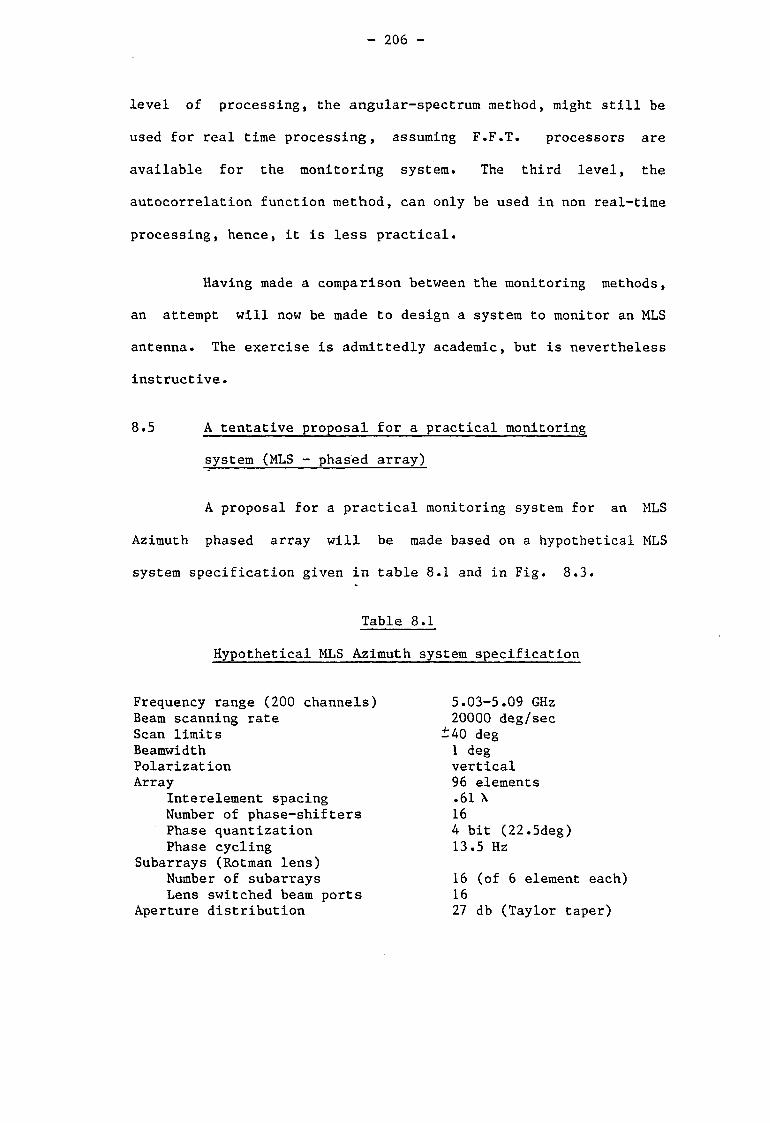
- 206 -
level of processing, the angular-spectrum method, might still be
used for real time processing, assuming F.F.T. processors are
available for the monitoring system. The third level, the
autocorrelation function method, can only be used in non real-time
processing, hence, it is less practical.
Having made a comparison between the monitoring methods,
an attempt will now be made to design a system to monitor an MLS
antenna. The exercise is admittedly academic, but is nevertheless
instructive.
8.5 A tentative proposal for a practical monitoring
system (MLS - phased array)
A proposal for a practical monitoring system for an MLS
Azimuth phased array will be made based on a hypothetical MLS
system specification given in table 8.1 and in Fig. 8.3.
Table 8.1
Hypothetical MLS Azimuth system specification
Frequency range (200 channels) Beam scanning rate Scan limits Beamwidth Polarization Array
Interelement spacing Number of phase-shifters Phase quantization Phase cycling
Subarrays (Rotman lens) Number of subarrays Lens switched beam ports
Aperture distribution
5.03-5.09 GHz 20000 deg/sec
±40 deg 1 deg vertical 96 elements .61 X 16 4 bit (22.5deg) 13.5 Hz
16 (of 6 element each) 16 27 db (Taylor taper)
- 207 -
Fig. 8.3 Block diagram of MLS phased array
The monitoring system for the MLS phased-array specified
in Table 8.1 and Fig. 8.3 is outlined in Table 8.2. The
monitoring is composed of two main tasks. The direct measurements
giving the beam pointing error. The indirect measurements giving
maintenance alarms in the presence of failed elements in the
array. Using a preassigned number, for multielement failure, a
downgrade or shut down alarm can be produced (see ICAO [ 6] or
Appendix A)

- 208 -
Table 8.2
Tentative monitoring system specification
Frequency range 4.95-5.2 GHz Instantaneous frequency band width 5 MHz Dynamic range 50 db Accuracy of magnitude measurements 0.5 db Accuracy of phase measurements 10 deg Repeatability of phase measurements 5 deg Proportional angle signals error (direct measurement)
Beam pointing accuracy 0.01 deg Side-lobe level and ERP 0.5 db
Number of selected directons in the angle coverage region internal/integral monitoring 3 Field monitoring (near field or far field)
1 Indirect measurement of proportional angle signal errors
Number of preassigned multielement failure 12
Levels of alarms 2 Maintenance alarm 1 Down grade/shut down alarm 1
Reaction time proportional angle monitoring 0.5 sec Element failure processing 0.5 sec
8.5.1 Definition of the monitoring system
A near-field monitoring system is assumed for the
detection of defects. This enables minimization of interference
and multipath effects.
The monitoring system will be composed of a single
monitor antenna, preferably a pyramidal horn, located in the
Fresnel region, about 1/10 the Rayleigh distance from the
transmitting antenna. ( If a near-field real time beam pointing
monitoring scheme is required, then a planar monitor antenna
should be used (see section 6.1). This or alternatively far-field
monitoring might be required as the internal/integral monitoring
does not give information on pointing errors due to mechanical or
geometrical changes. ) Internal or integral monitoring, is to be
used for the detection of defects in parallel with the near field
- 209 -
antenna. The near field antenna will enable the determination of
any geometrical shift of the array, and will also be used in the
subtraction method for the detection of single defective elements
in the array. The angular spectrum method (and the a.c.f.
method) should only be used with internal/integral monitoring to
avoid the additional processing required of near-field to
far-field transformations.
The phase detecting system should be composed of two
quadrature (I-Q) channels to minimize processing operations (see
Fig. 8.1).
The phase reference to the monitoring system will be
taken from a single side band (S.S.B.) shifted frequency. The
difference between the transmitted frequency and the S.S.B. will
be used for the I.F. frequecy of the monitor receiver. The
availability of commercial circuits (see Appendx F), leads to the
recommendation of using an I.F. centre frequency in the range 30
to 160 MHz. As the required dynamic range is 50 db an
instanteneous logarithmic I.F. amplifier should be used for the
detecton of amplitude. The phase is to be determined by a
quadratic demodulator where its input signal is normalized by a
limiter (with a constant transmission phase-shift), as explained
in section 8.4.1 and Fig.8.2. This arrangement can achieve the
required amplitude and phase accuracies over the dynamic range of
the input signal. The I.F. width is given by the expected phase
jumps of the scanning array. The MLS specification is an angular
scanning rate of 20000 deg/sec, over a range of +40 deg in
azimuth. Using a 4-bit phase-shifter, this leads to an average 4
microsecond period for one phase bit, resulting in a minimum width

- 210 -
of about 2AO KHz. Hence I.F. circuitry with a 5 to 10 MHz
band-width, which is normally available (see Appendix F), will be
adequate.
The Instanteneous main-beam pointing angle will be
determined from a synchronous timing signal fed from the MLS.
The processing system should include an update memory to
record sequentially the presence of all defective elements, using
the subtraction method. Periodically, the angular spectrum method
will be used for comparison, with the memorized updated defects.
An alarm will be given if more than a preassigned number of
elements are found to be defective.
8.5.2 A simplified block diagram
Following the system's definition and the explanations in
8.5.1, it is now possible to describe a practical monitoring
scheme. The system might be arranged as shown in Fig. 8.4
«
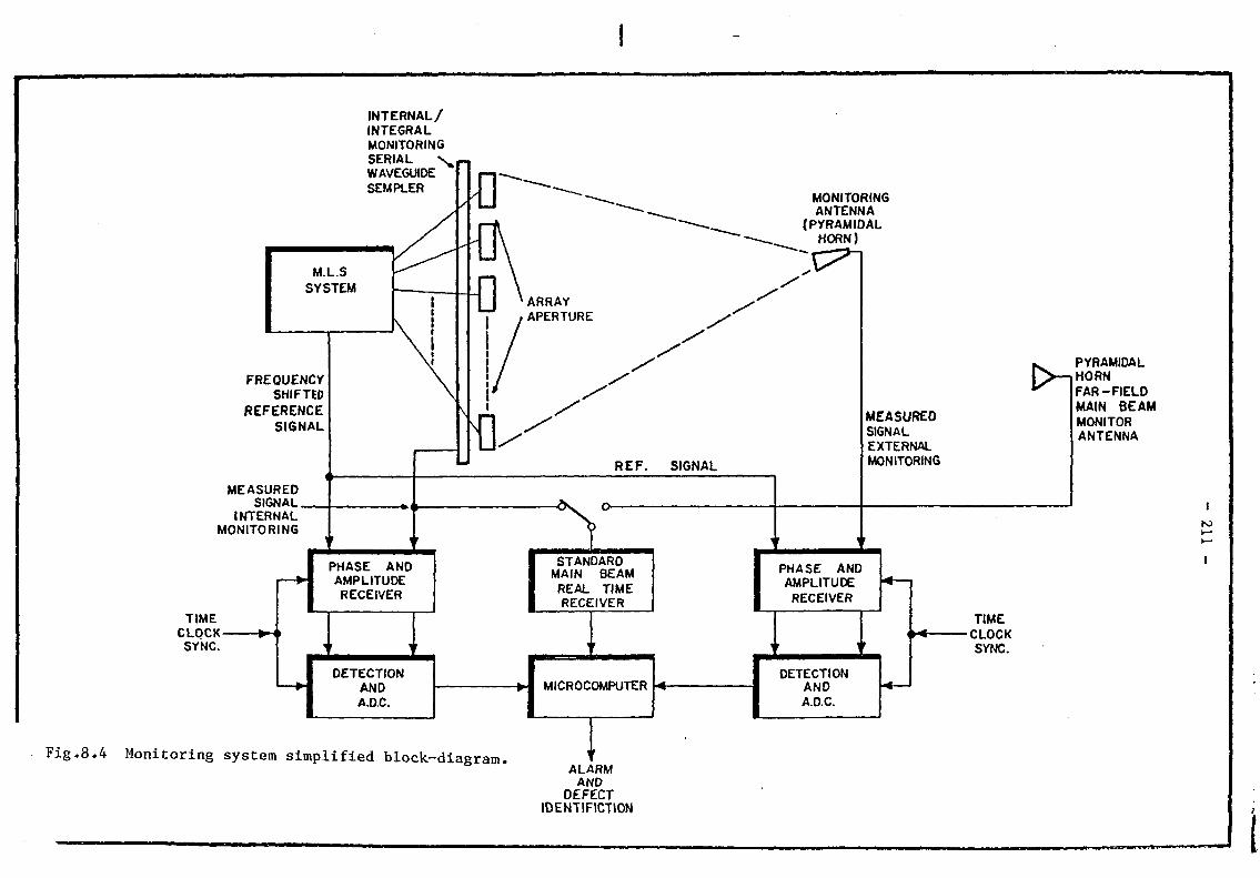
INTERNAL/ INTEGRAL MONITORING SERIAL v WAVEGUIDE SEMPLER MONITORING
ANTENNA (PYRAMIDAL
HORN)
FREQUENCY SHIFTED
REFERENCE SIGNAL
MEASURED SIGNAL
INTERNAL MONITORING
> 1
MEASURED SIGNAL EXTERNAL MONITORING
PYRAMIDAL HORN FAR-FIELD MAIN BEAM MONITOR ANTENNA
I fo
TIME CLOCK-SYNC.
PHASE AND AMPLITUDE RECEIVER
STANDARD MAIN BEAM REAL TIME RECEIVER
PHASE AND AMPLITUDE RECEIVER
DETECTION AND A.D.C.
Fig.8.4 Monitoring system simplified block-diagram.
DETECTION AND A.D.C.
TIME CLOCK SYNC.
t ALARM
AND DEFECT
1DENT1FICTION
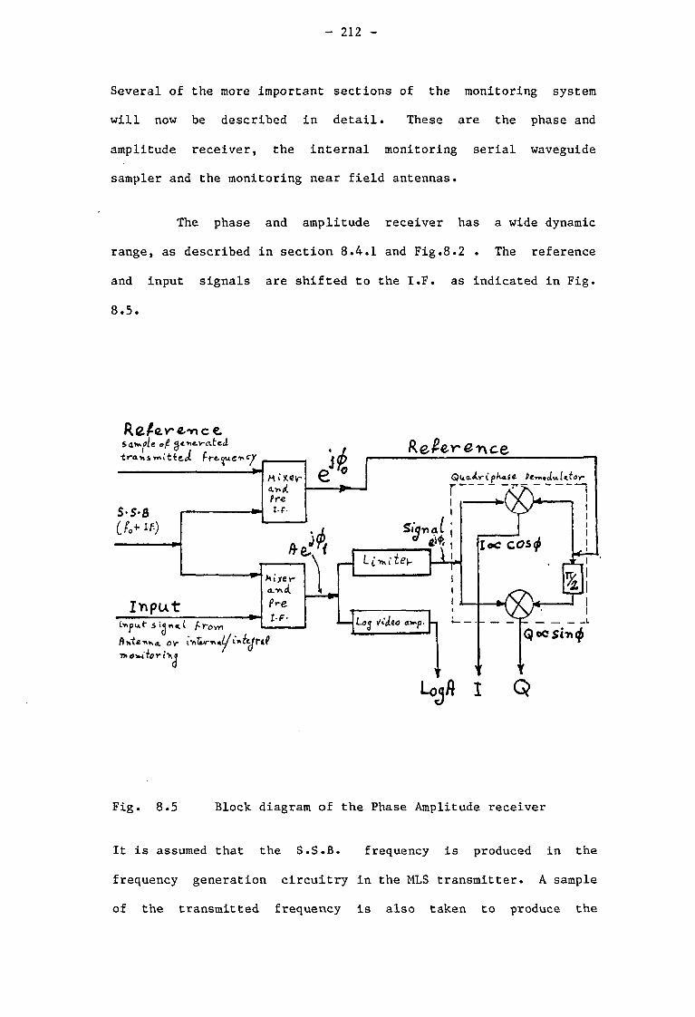
- 212 -
Several of the more important sections of the monitoring system
will now be described in detail. These are the phase and
amplitude receiver, the internal monitoring serial waveguide
sampler and the monitoring near field antennas.
The phase and amplitude receiver has a wide dynamic
range, as described in section 8.4.1 and Fig.8.2 . The reference
and input signals are shifted to the I.F. as indicated in Fig.
8.5.
R c / e v - e - o c €.
traniwi tie-Ji
S-S-B C t.+ I f )
M i xey-
t-F-
it e 0
R e ^ e r ^ n c e
Qua<(ri f>k*SA ii UUy r — t a 1
k£ T<
IttpUt
pufsi<jn«i( f-)royr\
Ant£-**a. Dv- iv*tvifv
Mixev-k m
Pre IF-IF-
iin^itey
Siqmal * M
1 £oC C O S $
Qoosit»<£
Lojfl I Q
Fig. 8.5 Block diagram of the Phase Amplitude receiver
It is assumed that the S.S.B. frequency is produced in the
frequency generation circuitry in the MLS transmitter. A sample
of the transmitted frequency is also taken to produce the
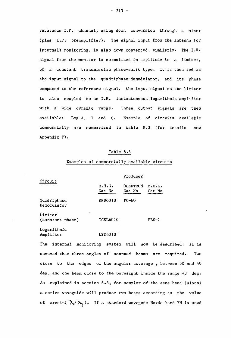
- 213 -
reference I.F. channel, using down conversion through a mixer
(plus I.F. preamplifier). The signal input from the antenna (or
internal) monitoring, is also down converted, similarly. The I.F.
signal from the monitor is normalized in amplitude in a limiter,
of a constant transmission phase-shift type. It is then fed as
the input signal to the quadriphase-demodulator, and its phase
compared to the reference signal, the input signal to the limiter
is also coupled to an I.F. instanteneous logarithmic amplifier
with a wide dynamic range. Three output signals are then
available: Log A, I and Q. Example of circuits available
commercially are summarized in table 8.3 (for details see
Appendix F).
Table 8.3
Examples of commercially available circuits
Producer Circuit
R.H.G. OLEKTRON M.C.L. Cat No Cat No Cat No
Quadriphase DPD6010 PC-60 Demodulator
Limiter
(constant phase) ICSL6010 PLS-1
Logarithmic
Amplifier LST6010
The internal monitoring system will now be described. It is
assumed that three angles of scanned beams are required. Two
close to the edges of the angular coverage , between 30 and 40
deg, and one beam close to the boresight inside the range ±3 deg.
As explained in section 6.3, for sampler of the same hand (slots)
a series waveguide will produce two beams according to the value
of arcsin( ^a ). If a standard wavegude Narda band XN is used
- 214 -
(a=l.372",b=0.622"), then the angles of the reproduced main beam
will be at approximately +33 deg, if the two edges of the
waveguide sampler are used. The beam close to the boresight can
be reproduced using the standard C-band waveguide (a=1.872",
b=0.872" ) and opposite hand slots are to be used. It can be
shown that a beam at an angle of about 2.9 deg, will then be
produced. As before the +2.9 or the -2.9 deg can be chosen,
according to the waveguide sampler edge used, see Fig. 8.6,
H a co
Opposite
A
I
K / \ / \ s \ / / / / ¥
\
+33 Sa- e ha.-nc(
Y*f>r<xLuctioy\
/ - / \ V
-t / t / \
A . -33°
^production
Fig. 8.6 Description of internal monitor waveguide samplers.
Two side by side waveguide samplers of different waveguide cross
section are used for internal monitoring.
For the near-field monitor antenna a medium-gain or even
a low-gain antenna, can be used. However, in order to minimize
the effects of multipath, a medium gain pyramidal horn is
recommended; the requirement being that its beamwidth will be
sufficient to cover the antenna aperture. A 16 to 20 db gain
symmetrical (pyramidal) horn can be used, giving a distance of a
few (say 4 to 6) aperture widths from the array; then it will fully

- 215 -
cover the array aperture. The near field horn can be used mainly
for the detection of defects in the array elements, in parallel
with the internal monitoring, using the subtraction method as
explained in sections 2.7 and 8.2. It can also be used, after
transformation of near-field to far-field, with the angular
spectrum and a.c.f. methods. But as this requires much more
processing only non-real-time analysis can be assumed in that
case.
The main beam-pointing error is to be detected using a
far-field monitor (at the Rayleigh distance). A similar horn can
be used. A real-time receiver similar to the airborne one is to
be fed to the microprocessor, as a monitor input. As explained,
due to expected excessive multipath affects, it is not recommended
that the far-field monitoring be used for the identification of
defects in the array elements.
The far-field monitoring of main beam pointing errors, is
the simplest one. However, as explained in chapter 6, a near
field focused monitor antenna can be used instead. This is not
justified economically, unless a decision to use a real-time
near-field (Fresnel region) monitor antenna is made. Such an
antenna can have the followng shape, according to section 6.1 and
as described in Fig. 8.7

- 216 -
MLS pJ»a*ecf a v r a y #
1
a
1=1 i i -£=4-6 a-
W f-uU
to
**-eceiVev
Fig. 8.7 Near field focused monitor antenna
According to sections 6.1 and 6.2 , about 10 to 15 sampling
elements are sufficient to comply with the Nyquist criterion, in a
distance of 4 to 6 aperture widths. These elements are to be
equally distributed over the planar aperture.

- 217 -
CHAPTER 9
CONCLUSIONS
The motivation for the present work arose from the
author's discovery of gaps in the solutions which are available to
monitor the performance of phased-array antennas. In particular,
methods of dealing with the identification of defects in the
elements of the array were lacking.
First a method of simplifying the representation of
defective elements in antenna arrays was sought. The equivalent
substitute element technique, suggested in chapter 2, turns out to
be a very efficient tool for this purpose. In this technique the
defective array is represented as a superposition of two arrays -
the ideal array and the equivalent substitute array. The
far-field pattern of the defective array is then given by the
superposition of the pattern of the ideal array and that of the
equivalent substitute array.
The inverse problem, the detection of defective elements
in the array due to anomalies in its far-field pattern, has been
solved in several different ways. These are the subtraction
method, the angular spectrum (direct) method and the
autocorrelation method. In the near field the near-field
monitoring technique and internal/integral monitoring have been
examined.
The first method, the subtraction method, involves the
subtraction of the far-field pattern of the ideal array from that
of the defective array. The result is, therefore, the equivalent
substitute array far-field pattern. It has been shown that for

- 218 -
the case of a single defective element in the array its
identification is straightforward. The location of the defective
element is a linear function of the phase of the substitute array
pattern. Therefore the process suggested for the identification
of a single defective element in the array is quite simple, at
least where defects in ideal arrays are concerned.
More realistic array models have been incorporated into
the analysis by the inclusion of effects of random phase
excitation and mutual coupling into the antenna model. It has
been shown that using simple statistical estimation (a linear
regression line) of the phase-line a correct identification of a
single defective element can be achieved.
It was further suggested that use be made of the far
side-lobe region for monitoring. There, the variations due to the
presence of defective elements is more pronounced than in the
main-beam region. Hence, a higher sensitivity to the presence of
defects and a greater immunity to the effect of measurement-noise
is achieved. For the same reason the danger of large errors
generated by the subtraction of two large numbers, reproducing the
substitute element pattern, is minimized in that region. In
addition, the analysis and the experimental investigation have
shown that thresholds, to minimize false alarms, are easier to
implement in the side-lobe region. This is important in cases
where long-term instabilities are expected in the measurement
system.
A question still remains: could this simple method be
used as a general method in the presence of many defective
elements in the array ? The answer given to that is in the

- 219 -
affirmative, but with the following assumption, which seems
justified, that failures do not occur in more than a single
element of the array at any one time. Then, the subtraction
method can be implemented sequentially with one modification; an
updated reference pattern is to be used rather then the original
reference. The process will then be one of memorizing the
previously detected elements and applying the modified subtration
method sequentially. Taking into account the high reliability of
present and future solid-state phased-array antennas, the failure
of more than a single element at one time is very unlikely. This
assumption is recommended for further investigation.
An additional important feature of the subtraction method
is its possible application in near-field monitoring. It has been
explained in section 2.7 that in the case of a defective single
element or single subarray the subtraction method does not require
the measurements to be performed in the far-field of the complete
array. It is merely necessary to be in the far-field of the
element or the subarray (whichever is being sought), since the
field due to the complete array is subtracted out.
Before continuing with the other proposed monitoring
methods, the findings on mutual coupling effects on the monitoring
will first be summarized. Mutual coupling can be thought of as
consisting of two components, one external and the other internal
(see chapter 4). The external component can be represented by an
equivalent substitute subarray symmetrical, in large arrays, about
the location of the defective radiating element. The internal
component can in many cases be represented by an odd-symmetrical
equivalent substitute subarray (e.g., in a serial waveguide slot

- 220 -
antenna). This odd symmetry causes relatively larger errors in
the fault detection process than the symmetrical equivalent
substitute array. However, in practical arrays, many of which are
using directional feed distribution networks and non-reciprocal
phase-shifters, the internal component is expected to have only a
second-order effect on the monitoring. The external component is
dependent on the interelement separation. For separations greater
than 0.5)* , this component is about one order of magnitude less
than that of the equivalent substitute element. Hence a ripple is
introduced on the resulting phase-line of the substitute element.
This can be smoothed using a statistical regression line, as
explained previously.
The other far-field monitoring methods, the angular
spectrum method and the autocorrelation function (a.c.f.) method
are based on the Fourier transform relation between the far-field
pattern of the array and the aperture illumination. In comparison
to Ransom and Mittra's [ 2] method the angular spectrum method
gives a simpler solution, as only the Fourier transform of the
far-field pattern is needed to derive the aperture illumination.
In contrast, the method suggested by Ransom and Mittra requires
the Fourier transform of two functions. The a.c.f. technique is
a method to derive the aperture power illumination, rather than
the magnitude illumination which is derived using the angular
spectrum method or Ransom and Mittra's method. It is based on the
known Wiener-Kinchine [ 14] transform relation between the
autocorrelation and the power spectrum. This method requires the
process of deriving the autocorrelation function of the far-field
pattern before Fourier transforming onto the aperture axis. This
process of autocorrelation has the adventage of smoothing the data
- 221 -
before caking the Fourier transform, where the angular spectrum
method does not. However, the disadvantage is that it is a
time-consuming process; so that where real-time processing is
concerned the angular spectrum method is the preferred one. The
application of the angular spectrum method and the a.c.f. method
in the far side-lobe region has been shown to give results which
are directly applicable to the monitoring of defects. The
resulting aperture pattern emphasizes the edge elements and the
defective elements of the array. Hence, as in the subtraction
method, the far side-lobe region gives results which are directly
related to the requirements of the monitoring system in most
cases. However, it has been shown that for cases like stuck
phase-shifters (chapter 3) measurements which cover the main lobe
as well as the side-lobe regions are more useful.
A summary of the far-field monitoring methods will now be
given. The simplest method, out of the three investigated, is the
subtraction method which requires the minimum number of processing
operations out of the three. The method can be used sequentially
for the detection of multiple defects, as long as they occur one
at a time. It can also be used in real-time monitoring.
The angular spectrum method requires more processing than
the subtraction method. However, it can still be used with modern
processors in real time monitoring. A dedicated F.F.T. processor
would reduce the required processing by an order of magnitude. It
therefore seems worthwhile to investigate whether such processing
devices can be implemented economically.

- 222 -
The a.c.f. method requires an even larger amount of
processing, hence it is recommended only for non real-time
processing•
The two methods, the angular spectrum and the a.c.f., can
be used periodically to check the detection of defective elements
by the subtraction method.
Turning now to the near-field methods, they can be
divided into two groups. One group deals with very close-in field
monitoring of the array, and the second uses the Fresnel region of
the radiation from the array for monitoring.
The two methods of internal or integral monitoring use
the very close-in field of the array. The composite field,
measured by the internal/integral monitoring system, gives the
far-field patterns of the array. Hence the far field methods can
be used with the internal/integral monitoring system. However,
these methods do not give information on beam pointing errors due
to, say, an external mechanical shift of the full array system.
Hence, a far-field or a near field (Fresnel region) main-beam
pointing error detection is necessary in addition. The far-field
main-beam pointing uses a simple antenna. However, uncontrolled
multipath errors can be introduced, thus causing uncertainty in
the decisions. In order to overcome possible multipath errors,
methods for Fresnel-region monitoring can be used. Focusing of
the transmitting array is one possibility, as explained in section
1.1. This method is not always acceptable in practice, as it
changes the original aperture phase distribution. Hence, the
monitor is not measuring the real transmitted wavefront signal.

- 223 -
A near field monitoring technique has therefore been
proposed (in chapter 6) to overcome the above problem. It
suggests a monitor antenna to be focused onto the transmitting
array antenna, with no changes in the transmitting array signal.
The idea was developed using the properties of the Fresnel
integral to describe the aperture diffraction according to the
Huygens-Fresnel formula. Analysis and computer simulation has
shown that the main-beam and the near side lobes of a scanning
phased-array antenna can be reproduced, with a good quality, in
the focused monitor antenna. This requires the monitor antenna to
be laid out in parallel to the geometrical aperture of the
transmitting array. In this scheme the number of sampling
elements required over the monitoring aperture, has been
demonstrated by computer simulation to be quite modest. For
distances of a few apertures between the transmitting and
monitoring arrays the simulations have shown that only few
sampling elements (about ten) may be necessary. This proposal
makes available an additional technique for near field monitoring,
if required.
As explained in chapter 7 the analysis and computer
simulation have been accompanied in part by experimental
investigation. A near-field measurement set-up has been used with
waveguide slot linear arrays. The arrays have been subjected to
synthetic defects and the monitoring methods have, in part, been
demonstrated and verified. The near-field monitoring technique
has not been investigated experimentally and is, therefore,
recommended for further experimental investigation.

- 224 -
A final point will be made concerning the experience
gained using computer simulations. It was found that computer
simulations accompanied by the line printer graphical output are a
very important tool for fast but rough analysis with immediate
feed back. This can be vital in the early stages of an analysis
in gaining familiarity with the subject and leading to new ideas.
It can also be used as a replacement for a more precise and
difficult analysis (which can follow later), as with the case of
the near field monitoring technique (chapter 6). There, the
technique proposed, based on an approximation to the Fresnel
integral, was later checked against a precise "experiment", using
NAG-Functions to represent the Fresnel integral.

- 225 -
APPENDIX A
Reproduced selected sections from ICAO
Standards And Recommended Practices (SARPS)
for the MLS [ 6]

1.0 - Definitions
Airborne Subsystem. MLS airborne equlfneit necessary to obtain, process, and output guidance information.
Auxiliary Data. A feature of the signal format that:
(a) provides data to refine airborne positions calculations; (b) provides meteorological information; (c) provides runway status and supplementary infonnatioi 'or display 1n
the cockpit.
Basic Data. The required data associated directly with the operation of the landimj guidance system and ai'/i ory data on the status of the MLS facil it ies.
Clearance Guidance Sector. The designated volume of airspace which ;„pple-monts the proportional guidance sector where the proportional guidance sector is less than the coverage sector ,-r/ided by a function. In this sector, the angular guidance service pro/ided is constant throughout, and not proportionally related to angular displacement of the receiver antenna with respect to (reference).
Control Noise. That portion oi *.sie guidance signal error which could affect aircraft attitude and causes control surface, wheel and column motions during couj'i.'J flight. Control Noise contains thoM« frequency components of the guidance signal produced by an airborne receiver with an ou, di ; Li le constant of 0.1 second which lie above 0.3 radian/second for azimuth data or above 0.5 raJions/second for elevation data.
Course Line. Tlit ljcus of points in the horizontal plane which have the selected azimuth angle.
Coverage Ixtrtr.ics. The boundary of guidance service specified at the maximum range for 3 particular angular posiMcn.
Coverage Sector. A volune of airspace of defined dimensions wltMi viiilt.li service is provided by a particular function in which the signal power density is o<;ual to or <jivater then the specified minimum.
1
Datum point. The origin of the approach and n.lssed approach sector ccv.-rages Is defined.as a point on the runway ccnterlir.e defined by the intersection of the runway center1, ine with a vertical plane parpcndicul&r to the ccnterl-.rs o.-J containing the phase ccntcr of the elevatio.i antenna.
OME/M. The precision range element associated with the standard XLS. An L-Band Distance Measuring Equipment (DME) is used that is compatible with existing equipment while providing improved accuracy and channel izatlci. • . capabiliities.
Facil ity. The MLS ground equipment necessary to transmit a gi-cn function.
Flare Coverage Zone. A zone that extends horizontally between the r-»n. ay • edges and longitudinally from 90 meters (300 feet) - to 7£0 nvters (2SC0 feet)
after runway threshold and vertically from near the runway surface to a height in the order of 45 meters (150 feet).
Function. A particular guidance service (e.g., approach azimuth) providoJ ly the MLS.
to to
Functional Element. The ground and airborne components necessary to achieve the transmission and reception of a given MLS function, e.g., approach cz:r-..jtn. '
Glide Path. The locus of points in the vertical plane which have the selected ('•evation angle.
Ground Subsystem. MLS ground equipment necessary to provide guidance Information at a particular runway.
Missed Approach Reference Oatum. The origin of th? accuracy requirer-tnl 'or the missed approach azimuth functional element 1s de:mod as a coint li rciers (50 feet) ebove the horizontal plane of the dat-r. point and located J-.c/e thi runway centerl ine at the rum/ay midpoint.
Out of Coverage Indication (0CI). A signal radiated by certain facil ities into LJ-.i,regions which ara not withir tiguidance coverage ot the •*ccil:t;/.
Path following Error. Tric-i portion of the ouicJoncc signcl error ».iiic.n cn<Si&
I
i
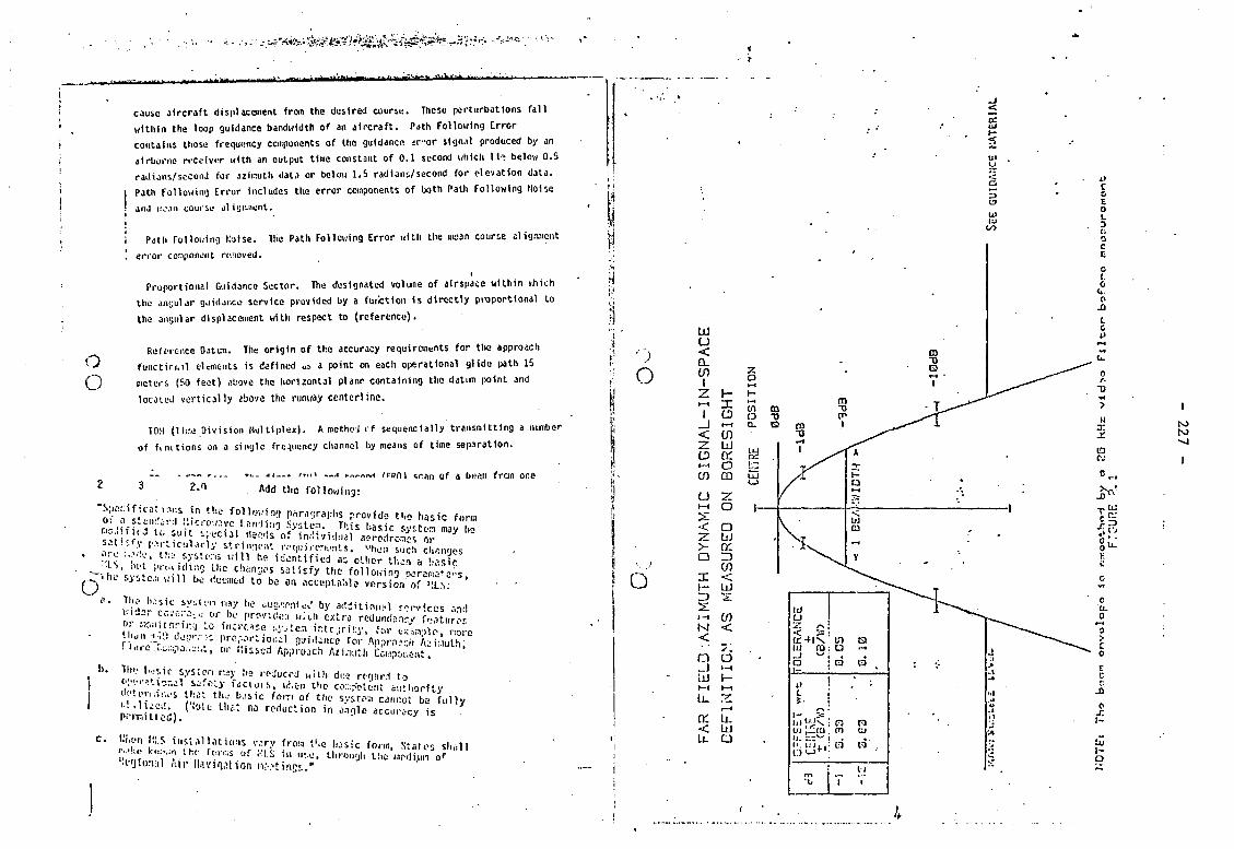
•v. •• 4-,., V ••
IT.,. ^ •• « Mill- itrfnr • - 1 . nWrmri iViitW.rr, . W . i. . .
cause aircraft displacement from the desired course. These perturbations fall within the loop guidance bandwidth of an aircraft. Path Following Error contains those frequency components of the guidance ir-or signal produced by an airborne receiver with an output time constant of 0.1 second which 11* below 0.5 radians/second for azinuth data or below 1.5 radian-.;/second for elevation data.
| Path Following Error includes the error components of both Path Following Noise : anJ iiujii course alignment, i i ! Path Following Koise. The Path Following Error with the mean course alignment . error component removed.
*
Proportional Guidance Sector. The designated volume of airspace within v.hich the aivjular guidance service provided by a function 1s directly proportional to the angular displacement with respect to (reference).
Reference Datun. The origin of the accuracy requirements for the approach 0
functiri.il elements is defined ua a point on each operational glide path 15 ( 3 meters (SO feet) above the horizontal plane containing the datim point and
located vertically above the runway centerlino. TDM (line Division Multiplex). A methoi rf sequencially transmitting a number
of fmctions on a single frequency channel by means of time separation.
-1- . n . « . . . /..«> /roni scan of a beam fran one 2 3 2.n Add the following:
S "rj"®™* Ii*er»£»j»ts. Vhon surt 3,anges . a.« , the systons will be identified an other then a '-sir
n 1 ; ' 5 ? e c h a n 3 " " t i s f y the following Mranatc^s f . y h c .'Ostc., wi l l bo deemed to be a n acceptable version of MLs; • •
^ 1,0 * u f c n t « ' b y ^ ^ l o n - l services one! n - f'ro-Mti : : i extra redundant future* o n:,„ orirn to incrr-ce :.y;tca into ;rit:y. for ro-e hua decMv.s pro,ortio,;fi| guHlsnw f o r Aopro h A ^utS
or Hissed Approach Azimuth fcittponontt t »>. 11,.. t-jsic systen nay !>- reducrd with due rrciarf to | o^rtu^] s foiy factor s, wr.en the content authority 1 !f; " r 1 o ™ 0 f t h c s>"st™ ba fully
p-'-m t i ) ( n ° r o d u c t i o n i n accuracy is
c. Ui-n lus.al .nuns vary from t'.e basic fonn, States shall vti T l J't-S in use. throng the .awliun o<" •>tfjiori.il Aip iMvination nv ' t i rms "
? - ?
cr. h. < UJ U. Q
NJ tO
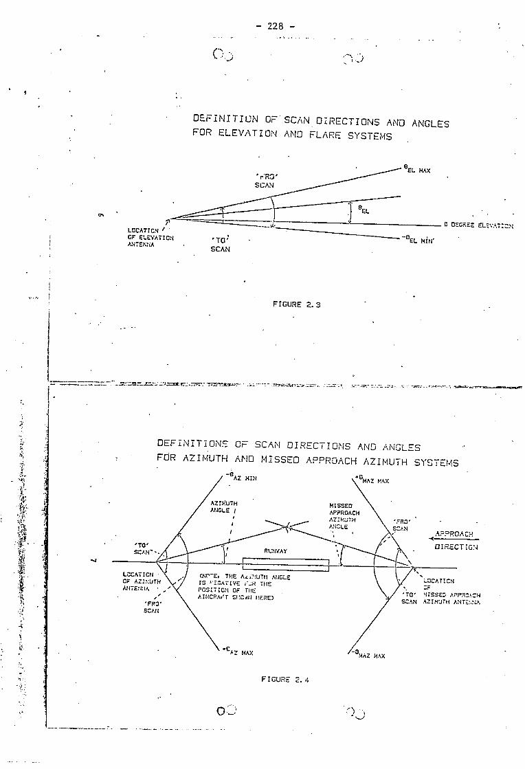
- 228 -
D E F I N I T I O N Or S C A N D I R E C T I O N S A N D A N G L E S
F O R E L E V A T I O N A M D F L A R E S Y S T E M S
FIGURE 2.3
D E F I N I T I O N S C F S C A N D I R E C T I O N S A N D A N G L E S
F O R A Z I M U T H A N D M I S S E D A P P R O A C H A Z I M U T H S Y S T E M S
FIGURE 2. 4

2.5.2 The DME/M transponder antenna shall be 1 »c. ted as close as possible to the approach azimuth element.
2.5.3 The transponder delay shall be adjusted to produce zero, range Indication at the transponder antenna site.
2.5.4 Distance information shall be provided throughout anycovcragc volttne in.which azimuth guidance is available. «v-z. ••
2.6 - Coordinate System
The MLS azimuth angle Information shall be radiated in conical or planar coordinates. The coordinate system in use shall be indicated by the auxiliary data transmissions, fhe MLS elevation and flare information shall be radiated in conical co-ordinates.
2.7 • Monitor and Control
Monitor and control equipment shall bo associated with each functional element.
2.7.1 Monitors shall assure guidance qualities appropriate to the performance category of operations. When malfunctions occur, the monitors shall initiate action to restore normal operations, downgrade performance categories, or remove the element fron service, as appropriate to the rituation.
2.7.2 Local and remote controls shall be provided to facilitate muintcnai.ce actions and to allow switch over with redundant equipment, downgrad-ing of performance categories, or removal of facilities from service.
3.0 - Signal Format (Angle and Data Functions)
3.1 - General
3.1.1 Both angle and data infoimation shall he transmitted by time division cxltiplexing (T0.-1) on a single frequency cnannel. A Preamble shall identify thc- particular type of information being transmitted so that each function trti'.r.iit'.ed is an independent entity, and proper decoding of a function docs not depend ?n Us position in the sequence. Data and Preamble shall be modulated using the fiii'ferintial Phase Shift Keying (flPSK) technique. •
10
3.2 - CHANNELIZATION
3.2.1 The functional elements shall be capable of operating on any cr.e of 200 channels spaced 300 kHz".'part with center frequencies between 5021.0 ::i<z cnd 5090.7 MHz and numbered 500 to 699 as per Table 3.1.
J.Vt^The pairing of the MLS channel and the channel of the associated ranging equipment shall be taken in accordance with the provisions in Chafer 3.5, 7aj>i« A (DME Channeling and Pairing).
Initial Implementation of MLS shall be In accordance with the s.agc-s ir/M cited 1n 4X, Annex 10, Part I I .
X 3 . M Frequency Tolerance. The operating radio frequency of •; faciliti.-r. shall not vary nore than plus or minus 10 I'.'.z fran the assigned frequency. The frequency stabi l i ty sh;ll Le such th*» there is no more than a plus or minus SO !ii deviation fror. the nominal
'! frequency during &'.vj o:ie-second interval.
i 3.5?-b lilt.'rferencff. The transmitted signal shell hs such that, M during the transmission tinie, tha mean power density above a heifj^t o f
j ; 600 meters (2,009 feci) shall not exceed -100.& Cw/n? for an'jlc" j J fjui dance and !S diiw/n^ for data, ;ir. measured in a 150 i;uz ' bandwidth centered at a frequency cf 2>t0 kHz or r-ere fro-. the nt-ninal ! frequency.
than one-quarter of the allowable path following error appl1c2b1e at that location.
to to v£>
S O 3.3.3 All system accuracy limits are to be met with the receiving ertenna up to twenty degrees fran the vertically polarized .loJtlon.
3.4 - Function Sequence
Each function transmission shall be en independent entity which cm occur In any position in the Tp:< sequent. Tli° tice interval bef./v.-n rerv.Uive transmissions of any one function shal. Le varied in a mai.r.er which provides protection Iron synchronous interference.
Note.-A transmission sequence that satisfied the requiro-ients of 3..', Is described In Appendix X.
11
I
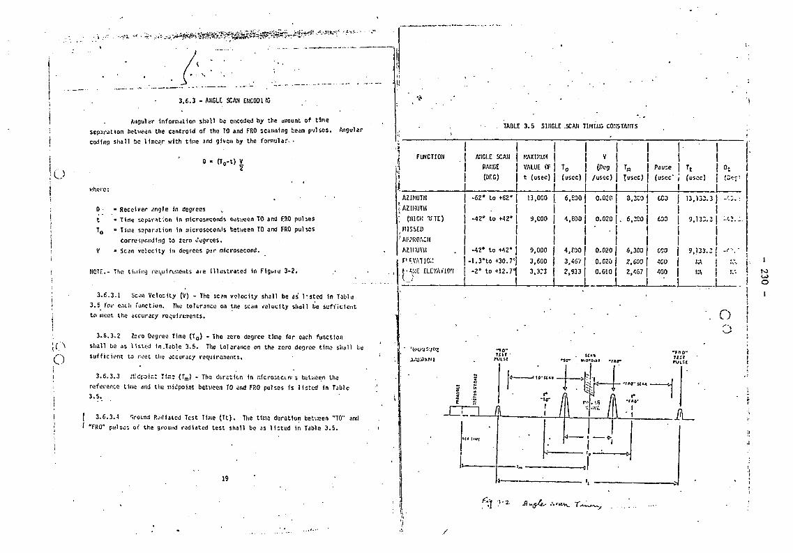
3.6.3 - ANGLE SCAN EtiCODI 'G
Angular Information shall be encoded by the amount of time separation between the cantroid of the TO and FRO scanning beam pulses. Angula coding shall be linear with time and given by the formulae .
0 - CT0-t) V 2
where:
0 » Receiver v>ngle in degrees t = Tine separation in microseconds betv/cen TO and FRO pulses T0 • Tine separation in microseconds between TO and FRO pulses
corresponding to zero degrees. V • Scan velocity in degrees par microsecond.
NCTF.- The timing roquirtr.ients are illustrated in Figuie 3-2.
3.6.3.1 Scan Velocity (V) - The scan velocity shall be as l.sted in Table 3.5 for each function. The tolerance on the scan velocity shall be sufficient to meet the accuracy requirements.
3.6.3.2 Zero Degree Time (T0) - The zero degree tine for each function shall be as listed in.Table 3.6. The tolerance on the zero degree time shall b sufficient to meet the accuracy requirements.
3.6.3.3 Midpai.-;: Ti~c (Tra) - The duration in nrfcroscciw s between the reference tine and the midpoint between TO and FRO pulses is listed in Tabic 3.5.
( 3.6.3.4 Ground Radiated Test Time (Tt). The tine duration between "TO" and ' "FRO" pulsos of the ground radiated test shall be as listed in Table 3.5.
19
TABLE 3.5 SINGLE .SCAN TIMING CO! STANTS
FUNCTION 1 I j ANGLE SCAN { MAX!hum j 1 V j
1 1
J RAISE j VALUE CF | To | (Deg j Tn 1 Pause h 1 0: 1 (DEG) j I |
t (usee) j (usee) J | /usee) | I usee) | (usee* (usee) 1
1 (Osc '
AZIMUTH | -62* to +62° | 13,OGO J 6,£30 | 0.020 | 3,200 | CCD 13,133 3 j AZIWJTK 1 1
(111GK UTE) j -42° to +42" j 9,000 j 4,MO | 0.020 j . 6.2C0 j 600 9,133. 3 j MISSED 1 1 I | I APPROACH 1 1 1 j AZIMUTH | -42" to +42° J 9,000 J 4,£00 | 0.020 j 6,300 j CCO 9,133. •» l F> t VAT I Oi l J -1.3°to +30.7 3,600 j 3,467 j 0.G20 | 2,600 j 400 /a i l-'AKE ELEVAi'10'l U
[ -2° to +12.7°J
J L 3,3:3 j 2,933 |
1 0.G10 | 2,467 j 400 I i -L.
O

•rtftj'.'.y'iyiiiTi'r j' y - i. ••-, -r J.-- rum;-? ' Viwifri't lfafiafrl ^ ^ tt " v •; -• for alphanumeric cturacter data. llu» content and timing of the Auxili.'r.1' Odta words arc described in Appendix X.
—5ig*al"homatHRaiigC'ftfnction)'3,
Note.-The MLS DME has several.technical issued which must be resolved before appropriate draft SARPS can be provided. Proposed draft SAHPS for DUE should be av,ri-V!il)TeJdte 1979 or,early, 1980.^ -
5.0 - Ground Subsystem Characteristics
Introduction
twJ,'-'.--«o|ip|
- i i
it ¥^ h
O, < ,
The ground subsystem technical and operational characteristics are defined and specified in this ch.intcr. This includes standards on the coverages, power densities, accuracies, monitoring and control and siting requirements for the various fac i l i t i es .
5.1 - Azimuth o 5.1.1 - COVERAGE
5.1.1.1 The approach azimuth^shal1 provide guidance in at least the following volur.e of space:
5.1.1.1.1 Approach Region
(a) Laterally and longitudinally within a sector +40° about the runway centarline originating at the datum point and extending in the direction of the approach to 20 nm from the runway threshold.
(b) Vertically between
(1) a conical surfacc originating 8 feet above the runway threshold inclined at .9" above the horizontal, and
( i i ) a conical surface originating at the azimuth fac i l i ty Inclined at 15° above the horizontal to a height o." fc)00 meters (20,000 feet).
U
Note.-Where intervening obstacles penetrate the .9° surface, guidance need not be provided at lqss than line of sight heights.
6.1.1.1.2 Kur.wc.y teg ion
(a) Laterally ar.d longitudinally within a sector 160 feet each side of the runway ccnterl ir.e beginning at the stop end and extending parallel with
21
the runway centerlinc In the direction of the approach to ?oin the approach region.
(b) Vertically bet\/een (1> 8 feet above the runway surface (1i) a conical surface originating at the azicuth fac i l i t y ir.cHnz-d
20° above the horizontal up to a height of 600 meters (20C0 feet) .
RECOMiENOATION.-The azimuth fac i l i t y should provide ve r t i ca l covcrc,-e up to above the horizontal.
5.1.1.1.3 The minimum proportional guidance sector shall be +10* obo'-t the runv/ay centerline. Where the proportional guidance ' c t o r provided is less ih the minimum lateral coverage specified in Paragraphs b. 1.1.1.1 and 5 . l . 1 .2 . c l signals shall be provided to supplement the promotional scctcr.
5.1.1.2 The missed approach azimuth fac i l i ty shall provide propc.-iicn:l guidance in at least the following volume of spece:
• (a) l i t t * a l l y and. longitudinally within a sector+20° about the runway centerline originating at the missed approach azimuth fac i l i t y and extcr i i ra in the direction of the missed approach at least to 5 r.n from the runway stop end.
(b) Vertically ( i ) Runway region
Between 8 feet above the runway surface and a ccnical s<:rfice originate t . t the missed approach azimuth fac i l i ty ii'-'.r.cd ».t 20° above the horizontal up to a height cf 6C0 meters (2CC3 feet).
RECGMMEHDATlOfl: The missed approach azimutn fac i l i t y should provide guidance to 30° above the horizontal.
Mote.-Whoreobstacles penetrate the lower covr.age limits, guidance nesd rot be provided at less than line of sight heights.
( i i ) Missed Approach Region Between a conical surface originating 8 feet *bove the runway stop end, Inclined i t 0.9® above the horizontal. ar.d a ccnicj l surface originating at the missed approach ar!r:ath facility. Inclined at 15° above the horizontal up to a height c r
. • meters (5000 feet).
k2
any other signal in the appropriate clearance sector.
5.1.1.4 Cut of Coverage Indicat.oi. (OCI) - OCI signals, where used, shall be at least 3 dB greater than any other signal In the appropriate OCI sector ( left , right, and rear).
5.1.1.4.1 RECGMHEf.'DATION.-OCI signals should be provided in all lateral
23 Add now para flew para to read as follows: 5.1.1.5 • "5.1.1.5 «",rourtd Sniiatcd Tost
(GI»T) - fiRT signals slial1 ho provide.! t .rcu-j'Hiut the covor.vios in'licated in paragraphs 5.1.1.1 an1 5.1.1.2."
ANTENNA BEAMW1DTH (3 dB)
FUNCTION/I'ARMETER DPSK 1° 2° 3°
POl.TI! CENS1TY (dBw/mz) . -89.5 -88(1) -85. 51" 1) -82 (1) (2)
POl.'ES DENSITY (dRw/m2) Mir -.i) ;.r?nc.c:i asikoth
-81 -79.5 -77 -73.5
(1) At the reference datum, the power density shall be greatei than 'hat Indi-cated in the Table by at least 15 dB. At 8 feet above the run-v/uy surface, the power density shall be greater than that indicated" in the Table by at least 5 dB.
(2) For AZ (High Rate* Mie power density can be reduced as deocribed in the Guidance notorial.
5.1.3 - ACCURACY
5.1.3.1 At the appropriate reference datum the AZ functional element shall provide performance in accordance with the error components listed in Table 5-1.
j Note.-Tl-e overall accuracy limits l.i Table 5-1-1 include, errors from all causes j such as airborne instrumentation, mean course alignment, and multipath pro pea a-j lion effecti. DoUilltJ occurocy Uuiiycis ore I-k.1u.UtU In tiiu cjuidjntc ujici Ij).
23
TABLE 5-1 - AZIMUTH .V.CUH/.CY
TABLE 5-1-1 - SYSTEM ACCURACY ERROR COMPONENT | : APPROACH AZII?JTH j MISSCO WfWM f-2!:~ 'TH PATH F.'l .OWING ERROR |
1 +6 METER . ^20 FT)
• \ ) | +5 l!£T£(:S FT; | " *
TABLE 5-1-2 - SIGNAL-IN-SPACE NOISE LIMITS ERRCR Cn:-?0:!EIIT 1 approach azi;:jtii I M'.ssiD rr:\ r-v.r; PATH FOLLOWING NOISE | |
(95% PliCSASlLITY) | +3.5 I'.CTEKS (Ml . 5 FT) j O. i i I'LTEEG FT) I I
CONTROL MOTION NOISE |
. (95% PROSAUIL1TY) j +3 METERS (+10 FT) | +3 METERS (*1'j FT)
Note.-Control Motion Noise Includes both the ground and propagation error components. - .
I -Note.-It is Intended that the error limits are to be applied ever c r.i.isuron-^t. interval that includes the reference dattzi. Tl.e interpretation of neiscre-ment interval appropriate for flight inspection Is discussed in thi ij-jjdar.ee material.
5.1.3.2 For the approach azimuth facility the equivalent airul,:r Path Following Noise accuracy shall be maintained along the ccnterline out to a rcnge of 3500 feet from the reference datum point.
5.1.3.3 RECOIMENDATION.-The approach azinulh functional elcner.t sliould provide a path following error not greater than plus or rnlnu". 4 rttcr^ (12.S feet).
5.1.3.4 Degradation Allowance
5.1.3.4.1 The/linear accuracy specified at the reference datum shall be maintained throughout the runway coverage region defined in Paragrsi>. 5.1.1.4.
Note.-To det'ermine the allowable errors 1n other region?, tha r.ccr/x /. is-.cinti t .- .- .CJ .V1 ih
at the reference datim should .first be converts frcm itsfe^uivalcit c.-.jUl.ir value with an origin at the antenna.
5.1.3.4.2 The allowable angular path following error calculatcd i-.r the reference datus shall be allowed to increase linearly to the coveran- v.'nr.*s as Indicated in Table 5-X-l.
24
• 5.1.3.4.3 At the reference datum, In no case shall the control lotion noise exceed 0.1 degree. Furthermore, It shall not exceed O.i degree out to a range of 10 mi.
5.1.3.4.4 For the approach azimuth fac i l i ty , along the centerline from a range of 3500 feet out to a range of 7000 feet from the reference datun point the equivalent path following noise error is permitted to in^r j iaseJ inear ly^^ Beyond this point the combined course alignment error and patiyshdll 'be within the overall path following error.
Table 5-X-l, ALLOWABLE AZIMUTH ERROR DEGRADATION
MNFARIY Al.l Ol.'ARLE ERROR DEGRADATION
ERR0:'. C0!?0::E'IT WITH
DISTANCE Willi AZ1MU1II
ANGLF. WITH
ELEVATION ANGLE
PA1II FOLLOWING ERROR TO 0.2 DEGREE AT THE ^f!.IT OF COVERAGE ALONG THE CLHTERLINE
1.5:1 2:1 FROM 0 DEGREES TO 15 DEGREES
CONTROL MOTION NOISE TO 0.20 DECREE AT THE LiMIT OF COVERAGE ALONG THE CENTER!. INE
1.3:1 OUT TO 40°
NONE
5.1.4 - MONITOR AMD C0NTR0I
5.1.4.1 The nvn.tor system shall cause the radiation to cease If any of the following conditions persist for longer than the periods specified:
(a) 1 hurts is a shift in the one-second average of the estimates of the zero degree coursc line of mora '.n 4.3 meters (15.7 feet) at the reference datirn.
(b) Thare is a changs in the ground equipment performance which would cause tlu* error, i f measured along any radial, to cxcecd the limits s p e c i f i e d in Paragraph 5.1.3.3 for a period of more than one second.
(c) There is :i reduction in the radiated power to less than that nr-ccsssry to produce tha requirements of Paragraph 5.1.2 for a period of more than one second.
Ma
(d) There Is an error in the preamble DPS* transmissions which occurs more than once in any one second.
(e) The timing tolerances specified in X.2 arc exceeded for a period of more thin one second.
• ( f ) The temporal CMN generated by the ground subsystem, *hen ix-a:urrf ov *r any 10 seconds, exceeds 0.03 degrees.
i:
5.1.4.1.1 Design and operation of the monitor systr.n shall he i or.si stent with the requirement that radiation shall cease and a warning shall be provided at the designated control points in the event of failure of the ror.itor systt-s i tse l f .
TABLE 5-2. AZIMUTH MONITOR WARNING LIMITS
I MEAN CC!;hse LI.VE i : : : : r I AT THE fcEFEPEKCE f.\7\;i
APPROACH AZIMUTH 1 | PLUS
•I Cft MINUS 4. ,8 METERS (15.7 FEET)
MISSED.APPROACH AZIMUTH 1 | PLUS 1 1
at MINUS 4. .0 METERS (i0.7 FEET)
5.1.4.2 RECOMMENDATION.-When a path following error of plus or c.inus 4 meters (13.5 feet) is being maintained par 5.1.3.2, the mean course limits of Table 5-2 should be reduced to plus or minus 3.2 meters (10.5 feet) t k the reference datum.
5.1.4.3 The mean course alignment of the *.*imuth faci l i ty shall adjusted and maintained to one half the limits snown in Table 5-2.
Note.-It is intended that faci l i t ies be adjusted and maintained so tha-. th; limits specified in Paragraph 5.1.4.3 are reached on very rare occask.i'..
5.1.4.4 The period during which erroneous guidance information is shall be as short as practicable and shall r,ct exceed cne second. At t^pts to Clear the fault by resetting the primary equipment or by switching to :rzr.tT.-j cquijinent shall be completed within th> 1 second period. If •(:': fiuIt is :A

o O
O o
/.•• > n'.. • -^^T/V*hf?
v:v •-- •
cleared within the time allowed, the facility shall be shutdown. After shutdown, no attempts shall be «»ade to restore service until a period of 20 seconds has elapsed.
Note.-Detailed monitoring configurations and information on facility down-grading and shutdown arc provided in the guidance material.
5.1.5 -SITING
5.1.5.1 The approach azimuth facility antenna systen slia'.l .lormally be located on the extension of the centerline of the runway beyond the stop end, and the antenna shall be adjusted so that the zero degree course line will be at the reference datum.
5.1.5.2 The missed approach azimuth facility antenna system shall normally be located on the extension of the centerline of the runway at the threshold end, and the antenna shall be adjusted so that the zero degree course line will be at the missed approach azimuth inference datum.
Note.-When siting the approach azimuth or missed approach azimuth antenna along the extended runway centerline is not practical, alternative siting configura-tions are provided for in the guidance material.
5.2 - Elevation
5.2.1 - COVERAGE
5.2.1.1 The approach elevation facility shall provide proportional guidance In at least the following volume of space.
(a) Laterally within a sector originating at the d<>tun point which Is at least cqu.il to . the proportional guidance sector provided by the
| approach azimuth facil ity, i I ! (b) Longitudinally, frc:n 250 feet from the dati a ->o1nt to 20 .m from : threshold.
(c) Vertically within the sector bounded by:
( i ) a surface 8 feet above the runway (1i) a conical surface originating at the datum point Inclined at .9"
above the horizontal, anj „
26
(111) a conical surface originating at the datun point Incline! at 7.5 above the horizontal up to heights of 6CCO meters (20,CCD feet).
5.2.1.1.1 RECOMMENDATION.-The elevation facility should provide s-ido.-.cs greater than 7.5° above the holzontal where necessary to meet operating requirements.
Note.-Where intervening obstacles penetrate'the 0.9° surface, guidance- r<eei not be provided at less than line of sight heights-
5.2.1.2 Flare Elevation - The Flare Elev-t.cn facility shall provide proportional guidance Information 1n at least the following voli*=e of sp;c.:
(a) Laterally and longitudinally over the runway surface and within a sector j lO® about the runway cntorline originating at a point on the ruway 2500 feet from threshold and extending to 5 ren from threshold ii the direction of the approach.
(b) Vertically within the sector bounded by:
( i ) surfaces 3 feet and 150 feet above the runway ( i i ) a conical surface originating 8 feet above the runway surface at
the thrcsluld Inclined at .9° above the horizontal (110 a conical surface originating 0n thr* rur.t;ay 2,yX) fc-.-t frcr;
.the threshold inclined at 7.5 dccrcea above the horizontal up to 5000 feet.
5.2.1.3 Elevation Antenna Lateral Radiation Pattern:.
5.2.1.3.1^ RECOMMENDATION - The horizontal pattern of the Approach Ele/rtion and Flare Elevation antennas should gradually de-enphaslse the signal tv.jy frcn
27
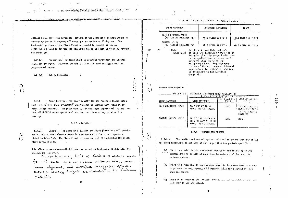
O
antenna boresight. The horizontal pattern of the Approach Elevation should be reduced by 3dl5 at 20 degrees off boresight and by Gdll at 10 degrees. The horizontal pattern of the Flare Elevation should be reduced as low as practicable bt-yond 10 degrees off boresight and by at least 12 dB at 40 degrees off boresigiit.
5.2.1.4 Proportional guidance shall be provided throughout the vertical elevation coverage. Clearance signals shall-not be used to supplement the proportional sector.
5.2.1.5 O.C.I. Elevation. t v . « . I
5.2.2 Power Density - The power density for the Preamble transmission J shall not be less than -89.5dBW/\!? under operation weather conditions at any
point within coverage. The power density for the angle signal shall he not less than -So.Odull/i:;2 under operational weather conditions at any point within coverage.
5.2.3 - ACCURACY
5.2.3.1 General - The Approach Elevation and Flare Elevation shall provide O performance at the reference datum in accordance with the r.r"or components
listed in Table 5-3. The Flare Elevation accuracy applies throughout the entire flare coverage zone. «
No to. -"H**-* Hi-ti'iwn ww'—pa i e—M—dvseu j ssrd—in t h a - i j u i d d b .
*rtvt rv.CwJUfci ^ TcU-U. £ -2 ^ <U. erv
v vs tdt </a (ftrAAo. ) yvvto-v
Couwt oJ-c^ivuJ evwV r^'pj, fWprg—f^ .
M. Ui-. J^.
ir.uu s-j. utvrtirju accuracy /.' .(Li l;:l::cc sail*;!
ERROR COMPONENT APPROACH ELEVATION FLARE
PATH FOL'.OWING ERROR (95 rHiiCLHT PROBABILITY) +0.6 M'.TER (2 FFET) +0.6 METER (2 r£ET)
CONTROL hOiSE (95 PERCENT PROBABILITY) +0.3 METFR n FfinU •n. HfTfP /I rrs.is
29 Note Delate existing Note anl r.c'i-(Tc-blc 0-3) st i tutc the follo-./ir^ 'In'.?: " I t is
inLfii:!iil that t^e error li:;i!.«; arr to bo s;>;»l ir.-.J over a noastu•'.viyit interval that inc'ii'.'-is t'ltr reference di!?<jr.. Tt*e in'.crjrc-1.1 on nf th.> r-'Msinv-'.'."'. i "tc rv.il i»iipro;>ri«ii.e for fli«y».t w-.nf.oct ion is discussed in the flui'Iar.cc Material."
cav.«;cu o.uo ae^rees.
TABLE 5-X-2 - ALLOWABLE ELEVATION FRR0R DEGRADATION LliiLAhLY ALLU'.-.Aui.K p j j t t&SX^t iy i
ERROR COMPONENT WITH DISTANCE wiTini~uJiir
A.'.'CLE PATH FOLLOWING ERROR
CONTROL MOTION NOISE
TO 0.20" AT 20 NM ALONG THE CENTERLINE
to o.ie at io i;m and THEN TO 0.2° AT 20 NM ALONG THE CEN7EP.LI.NE
NONE
NONE
TTfr-jJ: .rXic — Wll
TO NIT :-;>: : 0.4 ir.c-.:E w:Tr;-IN THE •.•R7!::;.l CGVEfc/.C:
5.2.4 - MONITOR AND CONTROL-
! 5.2.4.1 The monitor and control system shall act to ensure that a.-.y of •:•.«? j following conditions do not persist for longer than the periods specificJ: i ! (a) There is a shift in the one-second average of the c-stinatss cf cny | ' ' conmissioned glide path of more than 0.4 meters (1.3 feet) a-. J * | reference ditun.
(b) There is a reduction in the radiated power to less than that rt-cssiry to produce the requirements of Paragraph 5A.2 for a period of < 'jr.« than one second.
(c) There is an rrror in the »i>r.i'. irai.'.»i:-.ior.: ^i-t, Ui.m once in jny one second.
29
(d) The timing tolcratKus specified in X.2 an? exceeded for a period of more than one second.
(e) The temporal CMN generated by the ground •>> system, when measured over any 10 seconds, exceeds 0.03 degrees.
5.2.4.1.1 Design and operation of the monitor system shall be consistent with the requirement that radiation shall cease and a warning shall be provided at the designated control points in the event of failure of the monitor system itself.
TABLE 5-4. ELEVATION MONITOR WARNING Llt'TS
FACILITY MEAN GLIDE PATH LIMIT AT THE REFERENCE DATUM
o I 1 1
. v..'
APPROACH ELEVATION j PLUS CR MINUS 0.4 METERS (1.3 FEET) I
FLAKE ELEVATION I PLUS CR MINUS 0.4 METERS (1.3 FEET) I O
5.2.4.2 The elevation facilities shall be adjusted and maintained to tolerances oqual to one half those shown in Table 5-4.. . Kjc'wS. ; fil.- <.:» i "*t
.--a 5.2.5 - SITING rv-tri'.z-A^it.i
o
O
The Approach Elevation and Flare Elevation s'ia'l bo located beyond the threshold of the runway being served and offset frcm the runway centcrl ins. The distance offset from runway centerline shall he consistent with obstruction clearance practices given in ICAO Annex 14. The antenna shall have the minimum height necessary ' j satisfy the ground clearance requirements necessary ic suit local oporctii.g conditions. .
o 5.2.5.1 Tlie Approach Elevation shall be sited so that the
operationally preferred glide p.ilh crosses the threshold at a height of 50 feet above the runway 'urface. When collocated with an 1LS glfdo jvth , the same 11.S and MI S gl ide paths i-.'iould be coincident above the runway threshold.
5.2.5.2 RECOMMENDATION.-The Flare Elevation antenna should be located about 1070 motors (3500 feet) along the runway frc;n threshold.
5.2.5.3 Ine siting Coordinates of the Approach Elevation and Flare Llcvjiton .u-.u-nn.is S h a l l be transmitted en the Data Channel as defimd Ifi l.S.G.
5.3 - Oata
5.3.1 - COVERAGE
5.3.1.1 The Basic and Auxiliary Data shall be radiated througLout ar.y coverage volune In which Azimuth guidance is available. a. <-.*€
5.3.1.2 The power density for the DPSK signals shall not he less than U.i levels indicated in Table 5-X, under operational weather conditions, at any point within coverage.
5.3.2 - ACCURACY
5.3.2.1 The phase imbalance in the DPSK modulation 1n the 0 dc-iree ar.d 120 degree phase states shall be less than plus or minus 10 degrees.
' ^ . w i . i i . . , ... i.->_ . . 5.3.3 - SITIuG
5.3.3.1 Data shall be transmitted frcm the Approach Azimuth facil ity v£e«-e practicable.
5.3.4 - MONITOR AND CONTROL
5.3.4.1 Monitor System - The Monitor system shall provide a war-.irg to the designated control points if the radiated power is less than that nc-r."cs3ry to provide the requirement of 5.1.2 or 1f an error 1n a data word trans." issior. is detected.
5.3.4.2 Control Actions - I f any error repeated cn two cons;quti/e updates in an Individual data field, the radiation of this field shell c~a<e within one second.
5.3.5 - BASIC OATA
5.3.5. Basic data shall be transmitted by all ground subsystem. Provis-ion shall be made for the transmission of six Basic Data V.'ords, each with e
19
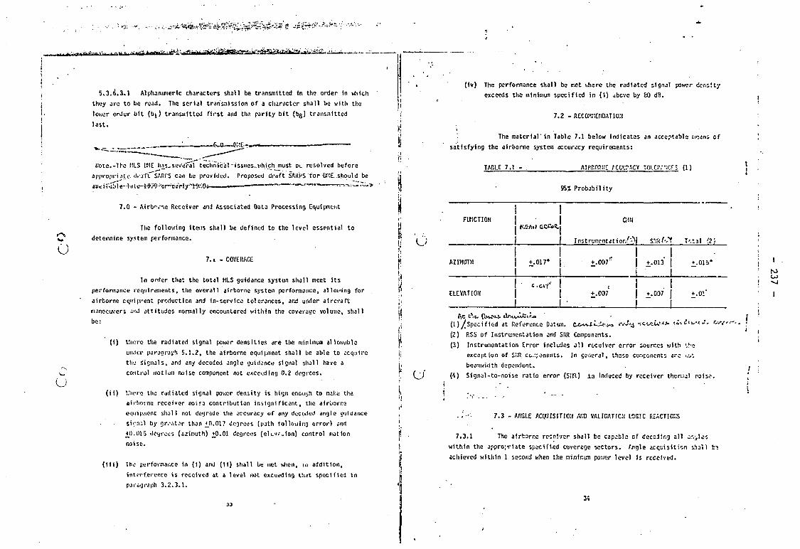
5.3.6.3.1 Alphanimerlc characters shall be transmitted in the order in which they are to be read. The serial transmission of a character shall be with the lower order bit (bj ) transmitted f irst and the parity bit (bg) transmitted last .
Note.-The MLS DME ha_ $ - s e v e r"al technical "issiies..which must o«. resolved before appropriate, ilrait SARI'S can be provided. Proposed draft SARPS for DMt.should be jf-c i<-j L» 1 c- Id t a-i-fti^)-cr-ca'rl —
7.0 - Airborne Receiver and Associated Data Processing Equipment
The following i t ess shall be defined to the level essential to determine system performance.
7.i - COVERAGE
In order that the total MLS guidance system shall meet I ts performance requirements, the overall airborne system performance, allowing for airborne equipment production and in-service tolerances, and under aircraft manoouvers and attitudes normally encountered within the coverage volume, shall be:
(1) Unere the radiated signal power densities are the minimum allowable under paragraph 5.1.2, the airborne equipment shall be able to acquire the Signals, and any decoded angle guidance signal shall have a control motion noise component not exceodlng 0.2 degrees.
( i i ) l.'liere the radiated signal power density is high enough to make the airborne receiver noif2 contribution insignificant, the airborne equi|s.ncnt shall not degrade the accuracy of any decoded angle guidance si<j:ul by gr.-ator than jO.Ol? degrees (path following error) and JI0.015 degrees (azimuth) _+0.01 degrees (el v ? »1on) control motion noise.
The performance in ( i ) and (11) shall be met when, iii addition, inti-rf.crer.ee is received at a level not exceeding that specified in pjragraph 3.2.3.1.
(1v) The performance shall be met where the radiated signal power density exceeds the inlnlmun specified in (1) ubeve by £0 dB.
7.2 - RECOMMENDATION
The material ' In Table 7.1 below indicates an acceptable tiianj cf satisfying the airborne system accuracy requirements:
TABLE 7.1 - . AIRBORNE ACCL'PACV TOI.EP.'r.Xf.; (1)
95% Probability
FUNCTION 1 1
j ttCAd CCCe j C1N
1 f Instrumentation^ s-Ai-y. T'.tal (2)
AZIMUTH 1 1 | +.017° | | |
, 1 +.0071 |
i
. 1 +.013 |
1 +.015°
ELEVATION 1 C-cif 1
1 1 1 1
1 +.007 j
1
. I +.007 j
1
+ .01'
Ac (bvMJ. dTAv»Vfc«.f.® (1)^/Specified at Reference Datum, Cowt i^.- .^ -i-t'-c.u.'ti- r.s (r (2) P.SS of Instruner.tation and SNR Components. (3) Instrumentation Error includes a l l receiver error sources with tf-e
exception of SNR cu:*onents. In general, these components are I.-J*.
beamwidth dependent. (4) Signal-to-noise ratio error (SIR) i 3 induced by receiver then.:al noise.
7.3 - Af.-GLE ACQUISITION AM) VALIDATION LOGIC REACTIONS
7.3.1 The airborne receiver shall be capabls of decoding al l av-jles within the appropriate specified coverage sectors, Angle acquisition shall t"! achieved within 1 second when the ninir.izn power level is received.
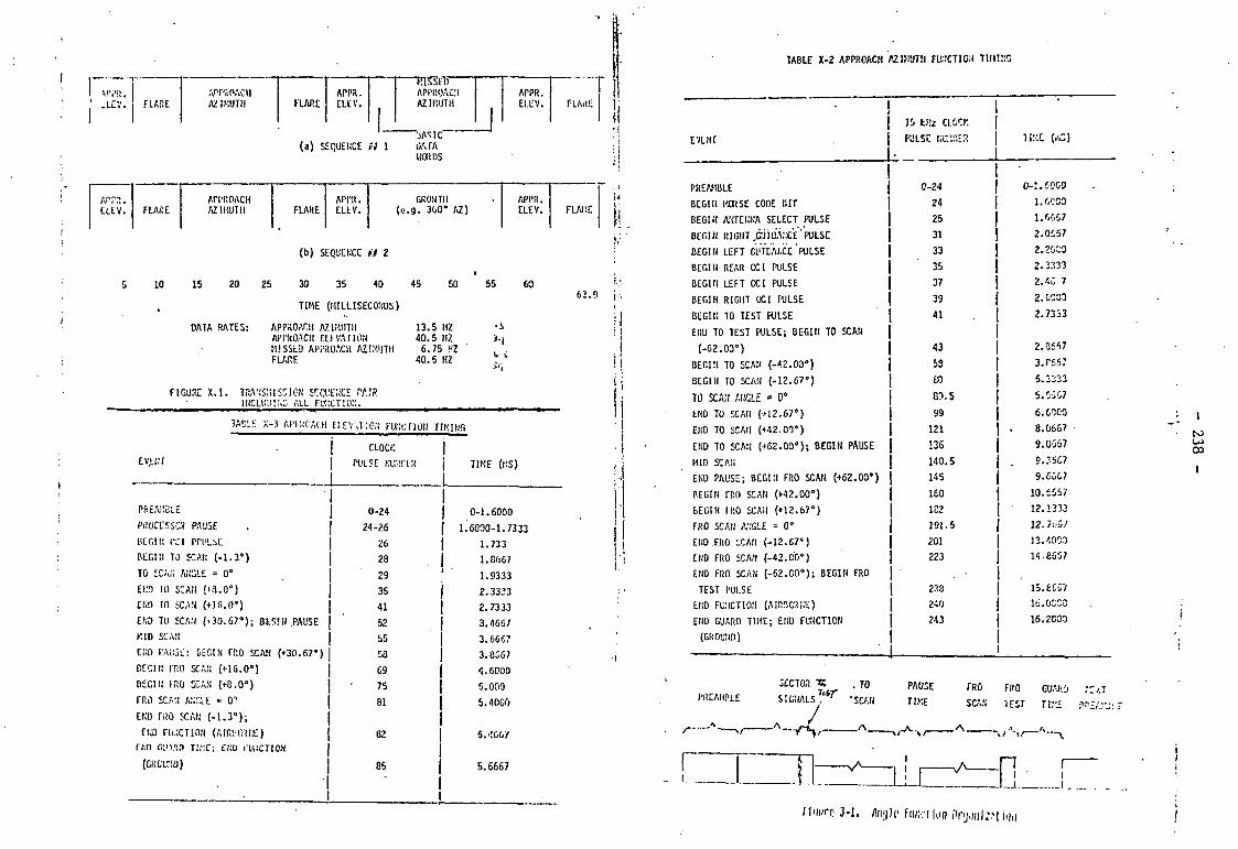
I -LEV.
MISSED APPROACH APPR. APPROACH APPR.
FLARE AZIMUTH FLARE ELEV. 1
AZIMUTH 1
ELEV. FLAitE
(a) SEQUENCE f# 1 "'ASIC DATA WORDS
APfR. APPROACH APPR. GROWTH APPR. CUV. FLARE AZIMUTH FLARE ELLV. (e.g. 360° AZ) ELEV. FLARE
10
(b) SEQUENCE »9 2 i
15 20 25 30 35 40 45 50 55 60
TIME (MILLISECONDS)
DATA RATES: APPROAm A7.1MUTII 13.5 HZ APPROACH ELEVATION 40.5 HZ MISSED APPROACH AZIMUTH 6.75 HZ FLARE 40.5 HZ
• i
L i
62.9
FIGURE X.l. TRANSMISSION SEQUENCE PAIR INCLUDING ALL FUNCTION.
TABLE X-3 APMcCACH i:lev,t:o?; function TIMING CLOCK 1 EVfl.T PULSE NUMBER j TIME (MS)
1
PREAMBLE 0-24 1 | 0-1.6000
PROCCSSCR PAUSE 24-26 j 1.6000-1.73 33 BEGIN OCt PPl'LM! 26 j 1.733 BEGIN TO SCAN (-1.3°) 28 j 1.B667 TO SCAN ANGLE = 0° 29 ' ' 1.9333 END TO SCAN {(3.0°) 35 j 2.3333 ENO TO SCAN (+16.0®) 41 j 2. 7333 END TO SCAN (*30.67o); Bf;!N .PAUSE 52 | 3.466/ KID SCAN 55 | 3.6667 ENO PAUSE: &EGIN TRO SCAN (+30.67°) 58 J 3.8S67 BEGIN FRO SCAN (+16.0®) 69 j 4.6000 BEGIN IP.O SCAN (+8.0") 75 j 5.000 TRO SCAN AT.GLE » 0' 81 j 5.4000 END FRO SCAN (-1.3°); | ENO n..;CTlON (AIRi'O.UIE) 02 { 5. -160/ rt:n cinnn ti;;l"; e;;o rujcnoN | (CRCU:;d) 85 j 5.6667
1
TABLE X-2 APPROACH AZIMUTH FUNCTION TIMING
EVLMT 15 kHz CLOCK PULSE NC:'.:'.!?. Tll'.E faZ)
PREAMBLE 0-24 0 -2.COCO BEGIN MOUSE CODE BIT 24 l.CCCO BEGIN ANTENNA SELECT PULSE 25 1.6607 BEGIN RIGHT,GUIDANCE PULSE 31 2.0057 BEGIN LEFT CL'VDAI.CE PULSE 33 2.20C0 BEGIN REAR OCI PULSE 35 2.2333 BEGIN LEFT OCI PULSE 37 2.4C 7 BEGIN RIGHT OCI PULSE 39 2.6C00 BEGIN TO TEST PULSE 41 2.7333 END TO TEST PULSE; BEGIN TO SCAN (-62.00°) 43 2.3667
BEGIN TO SCAN (-42.00") 53 3.P557 BEGIN TO SCAN (-12.67°) CO 5.3223 TO SCAN ANGLE » 0® B?.S 5.0507 END TO SCAN (+12.67°) 99 6.60CQ END TO SCAN (+42.00°) 121 8.0667 END TO SCAN (+62.00°); BEGIN PAUSE 136 9.0G67 MID SCAN 140.5 9.:-5G7 END PAUSE; BEGIN FRO SCAN (+62.00°) 145 9.C6C7 BEGIN FRO SCAN (+42.00°) 160 10.6667 BEGIN ll'.O SCAN (+12.67°) 182 12.1333 FRO SCAN A/.'GLE = 0° 191,5 12.tvul END FRO ICMl (-12.67") 201 J3.4OC0 END FRO SCAN (-42.00°) 223 14-8607 END FRO SCAN (-62.G00); BEGIN FRO TEST PULSE 233 15.£657
END FUNCTION (AIRBORNE) 240 l'J.O^CO END GUARD TIME; END FUNCTION 243 16.2CG0 (GROUND)
_J 1
PREAMBLE 3£C TOR TZ. . JO
Ttsr ' ' 'SCAN SIGNALS
• U
PAUSE TIME
FRO FHO GUAI-.j ; C / . T SCAN 1 EST II.",£ pni;.:-
T n r I I
I.
rfiicrc 3-1, /t,];|j(> f,„;r, j(lfJ firy()„(:»j j„()

- 239 -
APPENDIX B
Expected error in estimating the far-field
phase reference (the random case)
The resultant field E w of an N element array excited
with constant amplitude E 0 and random statistically independent
phase fluctuation in the range :
A The estimated mean field E^ equals
A w
- E^Zexpij^P; } a-4
in direction of maximum beam (s=0, for broadside array) whose
expectation (mean) has been shown to be :
Jexp{jf = E osincb (B.l)
-b
in the direction of maximum radiation (s=0)#
Estimated resultant phase of the full array (on beam)
£
T / I 2 & ) r V N 1 ,
= arctan [ :—j , ] R e , C fc £
b i cc^f
Expectation of would be (for a full array)
m £> l - U ^ t y o < W > - * = — : = 0 (B.3)
= arctan V} t p .— (B.2)
fe n , SiWJ> n [ ^ f c
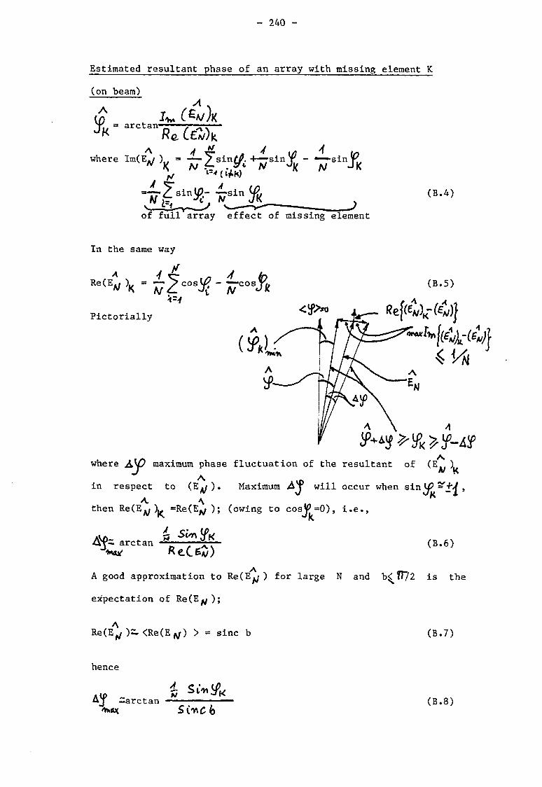
- 240 -
Estimated resultant phase of an array with missing element K
(on beam)
A arctan
where
Re, Ce«X i-acv) - - 77"slnJPK
of full array effect of missing element
(B.4)
In the same way
/
( B . 5 )
Pictorially <!f>o Re{«C,)K-(4)j
where maximum phase fluctuation of the resultant of (E^
in respect to ( E ^ ). Maximum will occur when sin
a. ^ K
then R e ( E ^ =Re(E^ ); (owing to cosjp=0), i.e., k & arctan ^ , . v
RcCzZ) (B.6)
A good approximation to R e ( E ^ ) for large N and b^fF?2 is the
expectation of R e ( E ^ ) ;
Re(E^y <Re(E > = sine b
hence
. it A j —arctan ——————
cuc Si^cb
(B.7)
(B.8)
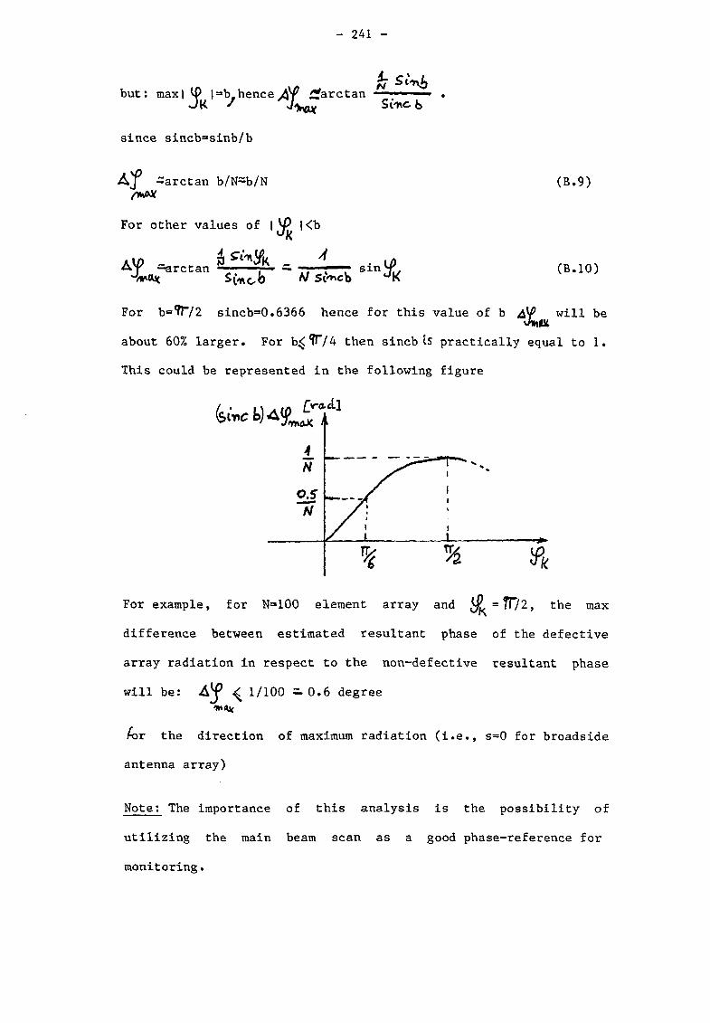
- 241 -
N but: max | VP ) =b_ hence /^f £farctan •
J K / Si'nc b
since sincb^sinb/b
A ^ f -arctan b/N^b/N
For other values of | ^ |<b
(B.9)
A^P Cretan . (B.10) V Si'ncb
For b=7T72 sincb=0.6366 hence for this value of b will be v/*lUt
about 60% larger. For b^^T/4 then sincb ts practically equal to 1.
This could be represented in the following figure
For example, for N=100 element array and ijj ~ 2, the max
difference between estimated resultant phase of the defective
array radiation in respect to the non-defective resultant phase
will be: A ^ ^ 1/100 - 0 . 6 degree
/or the direction of maximum radiation (i.e., s=0 for broadside
antenna array)
Note: The importance of this analysis is the possibility of
utilizing the main beam scan as a good phase-reference for
monitoring.

- 242 -
APPENDIX C
Angular a.c.f. of the angular spectrum and the
aperture illumination
Following Ratcliffe [ 14] , utilization has been made of
the dual transform pair of the angular autocorrelation function
(a.c.f.) of the angular spectrum and the array aperture power
illumination (see section 5.3). Using the relations of the
transform pair of angular spectrum and the aperture illumination,
expressions for the dual transform pair of angular a.c.f. of the
angular spectrum and the aperture power illumination, will be
derived.
CI Angular spectrum and aperture illumination
where f(x) is the aperture illumination, and F(s) is the angular
spectrum, with s=sin $
C2 A.c.f. of the angular spectrum and aperture power
illumination
The autocorrelation function (a.c.f.) of the angular
spectrum can be defined as
The dual Fourier transform relation :
(C.l)
f(x)
(C.3)
The Fourier transform of is
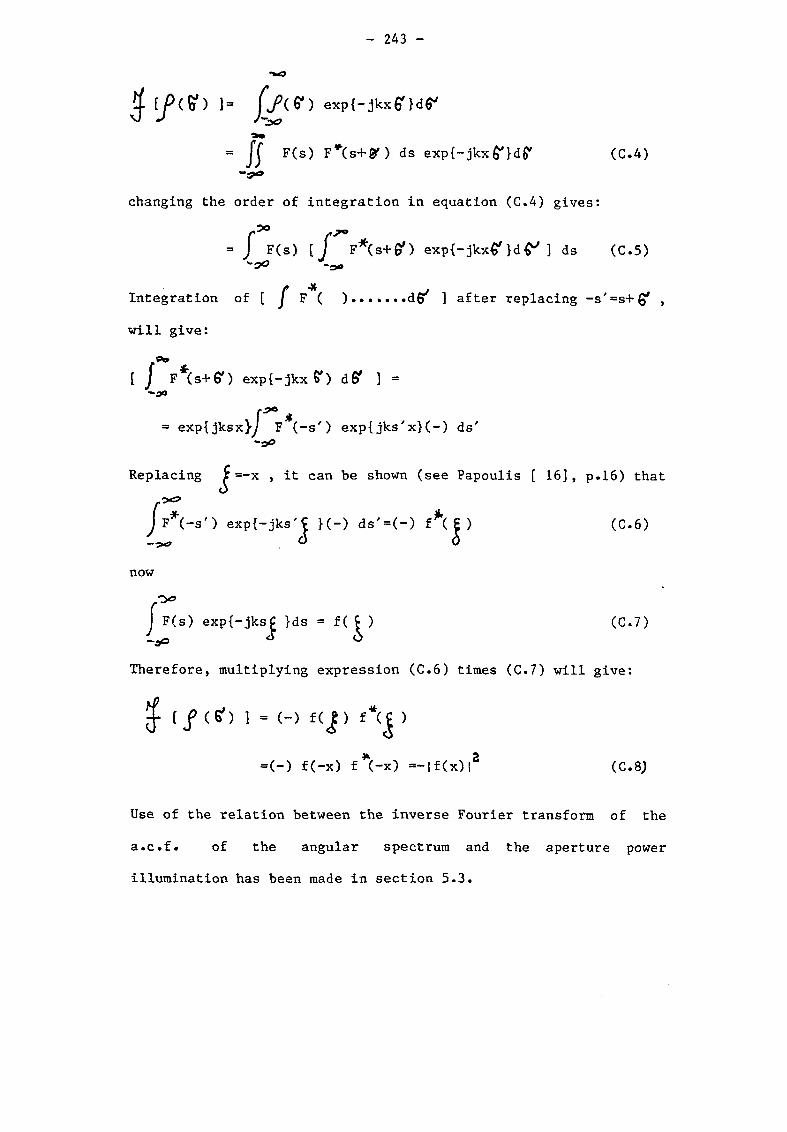
- 243 -
•W3
^ [J>{$) ]= j f i V ) exp{-jkx6'}d^
= j j F(s) F * ( s + y ) ds exp{-jkx£'}d£r (C.4)
changing the order of integration in equation (C.4) gives:
= J F(s) [ J F ^ s + a ' ) e x p i - j k x ^ l d ^ ] ds (C.5)
Integration of [ f F*( ) d ^ ] after replacing -s /=s+6' ,
will give:
r 9* [ J F*(s+6 /) expt-jkxfr) d & ] =
-yo
= exp{jksx}/ F*(~s') exp{jks'x}(-) ds'
Replacing £ =-x , it can be shown (see Papoulis [ 16], p.16) that
J f * ( - s ' ) exp{-jks'j }(-) ds'=(-) f * ( | ) (C.6)
now
j F(s) exp{-jksj }ds = f ( £ ) (G.7)
Therefore, multiplying expression (C.6) times (C.7) will give:
Jf (tf) 1 = (-) f ( j ) f*(J )
=(-) f(-x) f*(-x) =-|f(x)| 2 (C.8)
Use of the relation between the inverse Fourier transform of the
a.c.f. of the angular spectrum and the aperture power
illumination has been made in section 5.3.
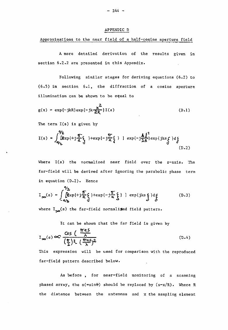
- 244 -
APPENDIC D
Approximations to the near field of a half-cosine aperture field
A more detailed derivation of the results given in
section 6.2.2 are presented in this Appendix.
Following similar stages for deriving equations (6.2) to
(6.5) in section 6.1, the diffraction of a cosine aperture
illumination can be shown to be equal to
g(x) = exp{-jkR}exp{-jk-~-}I(s) (D.l)
The term I(s) is given by
I(s) p l + j - f ^ ) + e x p { - j ~ J } ] exp{-j£|-}exp{jks£
^ (D.2)
Where I(s) the normalized near field over the z-axis. The
far-field will be derived after ignoring the parabolic phase term
in equation (D.2). Hence
= J 1 e x p { j k s j } d j (D.3)
where I__(s) the far-field normalised field pattern.
It can be shown that the far field is given by
^ / fraS ^ cps (
U s ) o C * (D.4)
This expression will be used for comparison with the reproduced
far-field pattern described below.
As before , for near-field monitoring of a scanning
phased array, the s(=sin&) should be replaced by (s-x/R). Where R
the distance between the antennas and x the sampling element

- 245 -
location in the x-axis (monitoring aperture). The following is
the result
X(s-x/R)oO exp{ j f o i U 1
1 ^ > *
+ ^ ] +
for which, as before, the following assumptions will be made:
The aperture a and the distance R are much greater than
the wavelength ( a , R » X ) , and that R=n-a where n varies
from 1 to 10 (D.6)
. / m V 4 Hence, the term ± y-r- — in the [ ] , could be ignored in
rr a relation to i/-=r— . As has been shown, the Fresnel integral is
' 2*
insensitive to small changes of arguments larger than 1 . Hence
the following approximation is achieved (Attention is drawn to the
fact that the 1/a term is not ignored in the exponential phase
terms):
I(s-x/R)— t e x p { j ^ R ( + i +
- - r * - - Us-V/t +exp(3-j7 W £ } 1*

- 246 -
Opening the brackets in the exp^ and exp^ terms, where exp^
exp the first and second exponential accordingly, we get : «v
(1) (2) (3) (4) (5) (6)
, . ^ s * / ? ,5ft , M , yj X asx exp, + e x P ^ - e*p{3ir< A ' T " ~ ) } +
^ 5R , >sR , X*. X ^ ^ • e x p i j T r c i r V 1 a.*)*'xr 1 a " " ( D ' 8 )
It is instructive to analyze the six terms of exp^ and e x P ^ > i n
equation (D.8)
- Term(l) Is independent of x and affects all elements of the
receiving aperture (the monitor antenna).
- Term (2) is dependent on s but has opposite signs in exp and i
exp^ •
- Term (3) is a constant.
- Term (4) is the parabolic phase term which is cancelled, as with
the uniform illumination (shown erlier in section 6.1.1), by the
parabolic phase term outside the integral of equation (6.1.3).
- Term (5) is a linear phase term function of the position only,
but has opposite signs in exp. and exp . A Zf
- Term (6) is the known linear phase scanned array term.
The other terms in equation (D.7), given by the Fresnel integrals
are, again, assumed to be approximated by a constant amplitude and
phase over the receiving antenna aperture.
A comparison will be made between the terms given by the
expected far-field of a cosine illuminated aperture, and those
terms which cause differences between the expected and the
reproduced patterns will be discussed. This will lead to the
definition of the near field monitoring antenna.*
- 247 -
From equations (D.3) and (D.4) the far-field is given by
an integral of the form
« n H f r r - _ , , i ii» a* \ r J a \
v 6 c* v ncv [ exp{jrr(- rr } + e x P { j r ( + r - r 1 (D.9)
-7-"b
Ignoring terms (1) and (3) in equation (D.8), we are left with the
following expression.
Sfl x* fLSX ex P{j?T(+ ~ - •J-)}exp{j7T(- -=JJ-) }+
+exp{jTT(- ^ + j-)}exp{jT(- > (D.10)
This will be used as the field diffracted over the monitoring
aperture (the x-axis) from the transmitter, proportional to the
expression,
exp{j?T(- ^f~)}cos[ TT (- ~ + £ - ) ] • (D.ll)
This expression is to be integrated over -b/2<x<+b/2 for getting
the monitoring signal, now the far-field, equation (0 .9), is
given by the integral over - a / 2 < ^ <+a/2 of the expression
exp{jT(- }cos(tTx/a) (D.12)
Hence we have to correct for the term TTsR/a in equation (D.ll).
By trigonometry,
cos[ TT(sR/a-x/a)]=cos TTsR/a cos TTx/a - sin TTsR/a sin fTx/a
03.13)
Now, examining the r.h.s. terms in equation (D.13) then for s « l ,
which is true for the main-beam region and if R/a^l, then
sin( fTsR/a) — ^ 0 .
Therefore,
- 248 -
cos[Tf(sR/a - x/a)]^cosJTx/a , (D.14)
s « l
i.e., the required expression, equal to that needed in equation
(D.12), has been achieved.
Hence, summarizing, it can be stated that the far-field
main-beam is approximated from near-field measurements by the
following procedure:
- (1) The signal should be integrated over the receiving aperture
placed in parallel to the transmitting array and having the same
aperture length.
- (2) The seperation between the receiving and transmitting
apertures should be small, of the order of R/a^l .
Thus the system described in Fig. 6.3 will also be
adequate for monitoring a cosine illuminated aperture
scanning-beam, if only the seperation between receiving and
transmitting antenna is decreased according to (2) above.

- 249 -
APPENDIX E
Computer programs listing
The following computer programs will be listed.
JACK18 Far field of N element array with
random phase error
JACK19 Far field of N=8 element array, with
mutual coupling (uses values computed in
JACK20 ), and with random phase error.
C0REL03 Subroutine to compute the correlation
function of the angular spectrum for JACK18
(or JACK19)
JACK20 Mutual coupling between broadside
parallel dipoles.
JACK30 Near field measurements, far field NN
element array.
Page
251
258
265
268
271
EJIX Subroutine to be used with JACK30.
Simulation of near field measurements 279
SHIFT01 Subroutine to be used with JACK30 to
introduce controlled shift of measured data. 280
DBMES1 A program to change measured values
from x-y plot in centimeters into db and
phase angle, using linear calibration. 281

- 250 -
Page
SHIFT1 A Subroutine to be used with DBMES1
for shifting data. 283
JACK37 Monitoring in the near field with a
focused antenna, cosine illumination. 284
JACK38 Monitoring in the near field with a
focused antenna, cosine square over pedestal. 287
JACK39 Monitoring in the near field with a focused
antenna, sine illumination. 290
JACK42 Near field of an aperture antenna
with uniform illumination. 293
JACK45 Angular spectrum of a Pyramidal horn
with TT/2 phase error, Fresnel integral. 295
- 251 -
FAR FIELD OF N ELEMENT ARRAY UNIFORM DISTRIBUTION , RANDOM PHASE ERROR THIS PROGRAM IS LINEAR WITH SIN(ANGLE)
PROGRAM JACK18 (INPUT=500B, OUTPUT,TAPE5=INPUT,TAPE6=OUTPUT ) COMMON X(4,400),Y(4,400),Z(4,400),AX(500),BY(500),CY(500),
1 BZ(500),CZ(500),DZ(500),YC(500),XC(500) , 2 ARXY(500),AIXY(500),VAS(50) , 3 AXY(350),SXY(350),V(350) ,SVS(350),SVA(350) DIMENSION Wl(250), W2(20),AR(250) ,BJ(250), IW(250) , AFT(350) DIMENSION MS(350) DIMENSION XDB(IOO) ,XPH(100) ,XAM(100) ,YDB(100) ,YPH(100) ,YAM(100) DIMENSION AATZ(IOO),AAZ(100) ,AXZ(100) ,XYZ(350),ZC(100) DIMENSION Y1(350) COMPLEX AMPT ,AMPT1, AMPTZ ,AMPY COMPLEX AMPTX,AMPTY,AMPZ COMPLEX AMPTO NOLIST
CHOOSE INVERSE(INVFT=1) OR FORWARD(INVFT=0) FOR F.F.T. INVFT=0
INITIALIZE 100 SIZE ARRAYS DIMENSION IXNIL=0 DO 51 NIL=1,100 IXNIL=IXNIL+1 XDB(NIL)=0.0 XPH(NIL)=0.0 XAM(NIL)=0.0 YDB(NIL)=0.0 YPH(NIL)=0.0 YAM(NIL)=0.0 AATZ(NIL)=0.0 AAZ(NIL)=0.0 AXZ(IXNIL)= FLOAT(IXNIL) MS (NIL)=0 ZC(NIL)=0.0 AR(NIL)=0.0 BJ(NIL)=0.0
51 CONTINUE WRITE(6,19)
19 FORMAT(IX//3X," LMIN LMAX MMIN MMAX KX 10 II", * " RP PRO11//) READ(5,13) LMIN READ( 5,13)LMAX READ(5,13) MMIN READ(5,13)MMAX READ(5,13) KX READ(5,13) 10 READ(5,13) II READ(5,13) INEAR READ(5,13) IAMPL READ(5,13) NN
13 FORMAT(14) READ(5,15)RP READ(5,15) PRO
15 FORMAT(F10.2) PI=4.*ATAN(1.)
- 252 -
P=180./PI READ(5, 791) Al READ(5,793) IAM, IPH
791 FORMAT( F10.3 ) 793 FORMAT(2(I4))
LX=0 AMX=0.0 IXSTOP=l IYSTOP=l
6666 CONTINUE WRITE ( 6,17 ) LMIN, LMAX, MMIN, MMAX, KX, 10,11, RP, PRO, INEAR, IAMPL, NN
17 FORMAT(3X, 7(1X,14),2(F10.2) ,7H INEAR®,II,7H IAMPL=,I1,4H NN=,I3) WRITE(6,90)
C RANDOM NOISE GENERATOR IS RESET WHEN RP .LT.-.l , OTHERWISE NONRESET IRESET=0 I F ( R P . L T 1 ) IRESET=1 RPP=ABS(RP) AL=2.*PI/RPP
S=0.61 C INITIALIZE 350 SIZE ARRAYS DIMENSION
DO 65 INIL=1,350 X( 1,INIL)=0.0 X(2,INIL)=0.0 X(3,INIL)=0.0 X(4, INIL)=0.0 Y(1,INIL)=0.0 Y(2,INIL)=0.0 Y(3,INIL)=0.0 Y(4,INIL)=0.0 Yl(INIL)= 0.0 AX(INIL)=0.0 ARXY(INIL)=0.0 AIXY(INIL)=0.0 SVA(INIL)=0.0 SVS(INIL)=0.0 SXY(INIL)=0.0 AXY(INIL)=0.0 XC(INIL)=0.0 YC(INIL)=0.0 AFT(INIL)=0.0
65 CONTINUE N=KX NV=KX KS=KX NIW=250 NW1=250 NW2=20 IFAIL=0 DEL=0.00001 THO=0.0 K=0
KC=240 THQ=0.0
- 253 -
EN=0.0 EN1=0.0 CN=NN
C NN IS THE NUMBER OF ELEMENTS IN THE ARRAY RL=FLOAT(I0)/CN RU=FLOAT(I1)/CN CALL RANSET(PI)
WRITE(6,90) WRITE(6,90) WRITE(6,31)
31 F0RMAT(3X,"J ANG PHE AME QE RE PHI 1AM1 QE1 RE1 PHO AMO QO RO"//) DO 9 J= LMIN,LMAX
C CHANGE INITIAL VALUE OF RANSET FOR DIFF. EXPERIMENTS IF(IRESET.EQ.1) CALL RANSET(PI) C=J CC=C
C THE FOLLOWING 4 STATEMENTS ARE INTENDED TO CHANGE X SCALE TO SIN MOD=J/KC IF(ABS(C).GT.FLOAT(KC)) CC=2.*FLOAT(MOD)*KC - C IF(ABS(FLOAT(MOD)).GT.l.)CC=0.0 SIC=CC/FLOAT(KC) THP=ASIN(SIC) AMPT=0.0 AMPTZ=0.0 AMPT1=0.0 AMPY=0.0
11223 CONTINUE 113=0
C CHOOSE NUMBER OF ELEMENTS IN SUBARRAY NSUB= NSUB=6 IF(Il.EQ.O) NSUB=1 IF((I1+NSUB-1).GT.NN) NSUB=NN-I1+1 G=FLOAT(11)+FLOAT(NSUB-1)*0.5
C CHOOSE DEFECTIVE ELEMENT AMPLITUDE RATIO Al= AND PHASE Pl= Al=l • P1=0.0
APY=1.0 14=0 AMPT0=0.0 AMPT1=0.0 AMPY=0•0 AMPZ=0.0 AMPTZ=0.0
C CALCULATE NORMALIZED FAR-FIELD OF THE NN ELEMENT ARRAY DO 10 1=1,NN 13=0 RIJ=0.0 RA=RANF(0.0) PR=(RA-0.5)*AL*PRO D=I F=2.*PI*S*(D-(CN+1.)*.5)*SIN(THO) APS=-(2.*PI*S*(D-(CN+1.)*.5)*SIN(THP))+ PR FT=F+APS A=1.
- 254 -
C- CHANGES FOR NEAR FIELD MONITORING XI1 = S*(D-(CN+1.)*.5) IF(INEAR.EQ.1) RIJ=-2.*PI*SQRT((XI1-XJ2)**2.+PD**2.) FT=F+APS+RIJ
C- FOR CS SQUARE OVER A PEDESTAL , CHANGE A AS FOLLOWES IF(IAMPL.EQ.l) AIl=l./7.+6./7.*(COS(XIl/((CN+l.)*.5)*PI*.5))**2. IF(IAMPL.EQ.l) A=AI1 A2=A IF( I.EQ.IFIX(G+.5)) A2=A AMPT=A*CEXP(CMPLX(0.,FT))+AMPT IF(I.GE.II.AND.I.LE.(Il+NSUB-1)) 13=1
IF(I3.EQ.l) FF=F+P1+RIJ IF( I3.EQ.1) AMPT0=A*CEXP(CMPLX(0.,FT))+AMPTO IF(13.EQ.1) AMPY=A1*A*CEXP(CMPLX(0.,FF))+AMPY IF(13.EQ.1) MS(I)=I
10 CONTINUE K=K+1 RIJ=0.0 F=2.*PI*S*(G-(CN+1.)*.5)*SIN(THO) APS=-(2.*PI*S*(G-(CN+1.)*.5)*SIN(THP)) FT1=F+APS FT2=F+P1
C- TO CHANGE REF. MIS/STUCK FROM FAR FIELD INTO NEAR FIELD XI1=S*(G-(CN+1.)*.5) IF(INEAR.EQ.1) RIJ=-2.*PI*SQRT((XI1-XJ2)**2.+PD**2.) FT1=F+APS+RIJ FT2=F+P1+RIJ AMPZ=A2*CEXP(CMPLX(0.,FT1)) AMPTZ=A1 *CEXP (CMPLX(0., FT2 ) )-AMPZ AMPT1=AMPT-AMPTO+AMPY AMPT1=APY *AMPT1 X(1,K)=(CABS(AMPT)/CN) X(3,K)=AIMAG(AMPT)+1.E-10 X(4,K)=REAL(AMPT) X(2,K)=ATAN2(X(3,K),X(4,K)) *180./PI Y(3,K)=AIMAG(AMPT1)+l.E-10 Y(4,K)=REAL (AMPT1) Y(2,K)=ATAN2(Y(3,K),Y(4,K))*180./PI Y(1,K)=(CABS(AMPT1)/CN) Z(3,K)=Y(3,K)-X(3,K)+1.E-10 Z(4,K)=Y(4,K)-X(4,K)+1.E-10 Z(2,K)=ATAN2(Z(3,K),Z(4,K))*180./PI Z(1,K)=SQRT(Z(4,K)*Z(4,K)+Z(3,K)*Z(3,K)) ARXY(K)=X(4,K) AIXY(K)=X(3,K) IF(INVFT.EQ.l) AIXY(K)=-AIXY(K) SVA(K)=Y(3,K) SVS(K)=Y(4,K) IF(INVFT. EQ.l) SVA(K)=-SVA(K) AR(K)=Z(4,K) BJ(K)=Z(3,K) IF(INVFT.EQ.l) BJ(K)=-BJ(K) AIM1=AIMAG(AMPZ)+l.E-10 REL1=REAL(AMPZ) Yl ( K )=AT AN 2 ( AIM1 ,REL1 )*180 ./PI
- 255 -
AIM2=3AIMAG(AMPTZ )+l .E-10 REL2=REAL(AMPTZ) DZ(K)=ATAN2(AIM2,REL2)*180•/ PI AX(K)=SIC XC(K)=20.*ALOG10(X(1,K)) IF(IXl.GT.l) Y(1,K)= .00001 YC(K)=20.*(ALOG10(Y(1,K))) ZC(K)=20.*(ALOG10(Z(1,K)))
C REARRANGE CORRECT ORDER OF F.F.T. COMPONENTS V(K)=FLOAT(K-l) KKX=KX/2 +1 IF(K.GT.KKX) V(K)=FLOAT(K-l) - FLOAT(KX) WRITE(6,33)J,THP*P , Z(2,K) ,Z(1,K) ,Z(3,K),Z(4,K),Y(2,K), 1Y(1,K),Y(3,K),Y(4,K),X(2,K) ,X(1,K),X(3,K),X(4,K)
33 F0RMAT(1X,I4, F6.1,3(2X,F6.1,1X,F8.4,1X,F9.4,1X,F9.4)) BY(K)= X(1,K) CY(K)= Y(1,K) BZ(K)= Z(1,K) CZ(K)= Z(2,K) IF(BY(K).GT.0.3) BY(K)=0.3 IF(CY(K).GT.0.3) CY(K)=0.3 EN1=(Y(1,K)+EN1) EN=(Y(1,K)*Y(1,K)+EN)
9 CONTINUE WRITE(6,90) WRITE(6,90) CLL=FLOAT(LMAX-LMIN) IF(CLL.LE.1.0)CLL=1. EN1=EN1/CLL EN=EN/CLL WRITE (6,1230) 113
C DESCRIBE ARRAY OF ELEMENTS WHERE "0"= NO DEFECT , "(.NE.O)"=DEFECT 1230 FORMAT(3X,"MISSING ELEMENTS=",I3," MISS. ELEMENTS NUMBERS ARE"//)
WRITE(6,1240) (MS(K),K=1,40) WRITE(6,1240)(MS(K),K=41,80) WRITE(6,1240)(MS(K),K=81,100)
1240 FORMAT(3X,40I3//) WRITE(6,1200)
1200 FORMAT(1H///3X," 10 II MIS.ELS ABS ENERGY"///) WRITE(6,1220) 10,11, 113 ,EN1,EN
1220 FORMAT(2X,3(I3,3X),2(F10.5,2X)) G0T013131 CALL COREL03 (LMIN ,LMAX ,MMIN ,MMAX,KP )
13131 CONTINUE SQN=NV SQN=SQRT(SQN) CALL C06ADF( ARXY,AIXY,N,NV,KS,IW,NIW,W1 ,NW1 ,W2,NW2,IFAIL ) IF(IFAIL.NE.0)GOTO 210
DO 3100 L=1,N AXY(L)=SQRT(ARXY(L)*ARXY(L)+AIXY(L)*AIXY( L))/SQN IF(ABS(ARXY(L)) «LE.DEL)ARXY(L)=DEL IF(INVFT.EQ.l) AIXY(L)=~AIXY(L) SXY(L)= ATAN2(AIXY(L) , ARXY(L))*180./PI
3100 CONTINUE CALL C06ADF(SVS,SVA, N,NV,KS, IW,NIW,W1,NW1,W2,NW2,IFAIL ) DO 3120 L=1,N
- 256 -
SVS(L)=SVS(L)/SQN IF( ABS(SVS(L)).LE.DEL) SVS(L)=DEL SVA(L)=SVA(L)/SQN IF(INVFT.EQ. 1) SVA(L)=-SVA(L) AFT(L)=SQRT(SVS(L)*SVS(L)+SVA(L)*SVA(L))
3120 CONTINUE CALL C06ADF(AR, BJ , N, NV,KS, IW, NIW,W1 ,NW1 ,W2,NW2,IFAIL ) DO 3110 L=1,N IF(ABS(AR(L)).LE.DEL) AR(L)=DEL ARL=AR(L)/SQN BJL=BJ(L)/SQN AR(L)=SQRT(ARL*ARL+BJL*BJL) IF(INVFT.EQ.l) BJL=-BJL BJ(L)=ATAN2(BJL,ARL)*180./PI
3110 CONTINUE WRITE(6,992) (IW(I),1=1,5)
992 FORMAT(1H///3X, 18HOPTIMUM VALUES ARE/2X,3HKF=, 17/2X, *5HKMAX=,I5/2X,4HNIW=, I6/2X, 4HNW1=, I6/2X, 4HNW2=, 16///) GOTO 800
210 WRITE(6,991) IFAIL 991 FORMAT (1H ,24HFAILURE IN C06ADF,IFAIL=, 14)
WRITE(6,992) (IW(I),1=1,5) 800 CONTINUE
WRITE(6,90) WRITE(6,90)
90 F0RMAT(1X//) WRITE(6,880)
880 FORMAT(9X,MSIN REL FX IMG FX ABS FX PHASE FX" * FTRY FTJY AFTY AFXZ PH.Z"//) DO 21 MM=1,KX LD=MM MN=MM-1 WRITE (6,850) MN, AX(LD) , ARXY(MM) ,AIXY(MM) , AXY(MM) ,SXY(MM)
* , SVS(MM),SVA(MM), AFT(MM) , AR(MM), BJ(MM) 850 F0RMAT(1X,I4,1X, F6.3 , 3(3X,F8.4),5X,F6.1, 4(3X,F8.4),5X,F6.1 ) 21 CONTINUE
C LINE PRINTER GRAPHICS OUTPUT KK=KX K=KX KKZ=2*KK KKK=3*KK KZ=0 AFT(1)=0.0 AR(1)=0.0 DO 777 LXY=1,KKK KZ=KZ+1 K2Z=KZ IF(KZ.GT.KK)K2 Z=KZ-KK IF(KZ.GT.2*KK)K2Z=KZ-2*KK AX(KZ)=AX(K2Z) V(KZ)=V(K2Z) IF(KZ.LE.KK)XYZ(KZ)=XC(K2Z) IF(KZ.LE.2*KK.AND.KZ.GT.KK)XYZ(KZ)=YC(K2Z) IF (KZ.LE. 3*KK. AND .KZ. GT. 2*KK)XYZ (KZ )=ZC (K2Z ) IF(KZ.LE.2*KK.AND.KZ.GT.KK) CZ(KZ)=Y1(K2Z) IF(KZ.LE.3*KK.AND.KZ.GT.2*KK) CZ(KZ)=DZ(K2Z)
- 257 -
IF(KZ.LE.2*KK.AND.KZ.GT.KK) AXY(KZ)= AFT(K2Z) IF ( KZ. LE. 3*KK. AND. KZ. GT. 2*KK) AXY ( KZ )=AR( K2 Z ) IF(KZ.LE.2*KK.AND.KZ.GT.KK) SXY(KZ)=ATAN2( SVA(K2Z),SVS(K2Z))*P IF(KZ.LE.3*KK.AND.KZ.GT.2*KK)SXY(KZ)=BJ(K2Z) IF(XYZ(KZ).LE.-50.) XYZ(KZ)=-50.
777 CONTINUE LKK=LX*2 MZ=0
CALL GRAFIT(AX, XYZ, KKK, KK, KK, -70) C- X=SINE ANG. If*"-DB FULL ARRAY,,"X"-DB DEFECT. ARRAY, !,0U-DB MISS. EL.
WRITE(6,173) 173 FORMAT(2X,"X=SIN ANG. Y=FAR FLD. DB , *- FULL ARRAY, X-DEF. 0-MS")
CALL GRAFIC(AX,CZ,KK) WRITE(6,45)
45 FORMAT(2X,"X=SIN ANG.Y=*-PHASE SB.A.,X-PH. MS EL(CTR) ,0-PH.ST.C") WRITE(6,3000) LMIN,LMAX,MMIN,MMAX, KX,I0,I1 ,IRESET,PRO,RPP CALL GRAF IT ( V, AXY,KKK,KK,KK,-70) WRITE(6,4120)
4120 FORMAT( 10X,"X=APERTUR,Y=*-MAG FFT X,X-FFT Y , 0-FFT Z ") WRITE(6,3003) LMIN,LMAX,MMIN,MMAX, KX,I0,I1 ,IRESET,PRO,RPP, * INEARjIAMPL CALL GRAF IT ( V, SXY ,KKK,KK,KK,-70) WRITE(6,450)
450 FORMAT(1 OX,"X=APERTURE,Y=*-FFT X PHASE, X- FFT PHASE Y, 0-FT P Z") 3000 FORMAT(3X,6H LMIN=,I4,6H LMAX=,I4,6H MMIN=,I4,6H MMAX=,I4,
1 12H NO SAMPLES3,14,11H MISS ELEM= ,13,IX,13,8H IRESET= ,11 , 27H PHASE=,F2.0 ,4H*PI/,F5.1 )
3003 FORMAT(3X,6H LMIN=,I4,6H LMAX=,I4,6H MMIN=,I4,6H MMAX=,I4, 1 12H NO SAMPLES=,14,11H MISS ELEM= ,13,IX,13,8H IRESET= ,11 , 27H PHASE=,F2.0 ,4H*PI/,F5.1, 7H INEAR=,I1,7H IAMPL=,I1 )
1000 STOP END
END OF FILE
- 258 -
C- FAR FIELD OF N ELEMENT ARRAY C INCLUDING MUTUAL COUPLING EFFECTS C DATA OF MUTUAL COUPLING FOR 8-ELEMENT ARRAY IS GIVEN IN C NORMALIZED AMPLITUDE=AZA12( ) AND PHASE=APH12( ) C UNIFORM DISTRIBUTION , RANDOM PHASE ERROR C THIS PROGRAM IS LINEAR WITH SIN(ANGLE)
PROGRAM JACK19 (INPUT=131B, OUTPUT= 131B, TAPE5=INPUT,TAPE6=OUTPUT) COMMON X(4,350) ,Y(4,350) ,Z(4,350) ,AX(500) ,BY(500) ,CY(500),
1 BZ(500),CZ(500),DZ(500),YC(500),XC(500) , 2 ARXY(450),AIXY(450),VAS(50) , 3 AXY(350) ,SXY(350) ,V(350) ,SVS(350) ,SVA(350) DIMENSION Wl(250), W2(20),AR(250) ,BJ(250), IW(250) , AFT(350) DIMENSION MS(350) DIMENSION XDB(IOO) ,XPH(100) ,XAM(100),YDB(100) ,YPH(100) ,YAM(100) DIMENSION AATZ(IOO),AAZ(100) ,AXZ(100) ,XYZ(350),ZC(100) DIMENSION YI(350),AZA12(10),APH12(I0) COMPLEX AMPT ,AMPT1, AMPTZ ,AMPY COMPLEX AMPTX,AMPTY,AMPZ COMPLEX AMPTO DATA(AZA12(M),M=1,8)/.0,.0547 , .08081488,1.01488,.0808,.0547/ DATA(APH12(L),L=1,8)/0.0,112. ,-10 .,-126.,0.0,-126.,-10.,112./
C CHOOSE INVERSE(INVFT=1) OR FORWARD(INVFT=0) FOR F.F.T. INVFT=0
C INITIALIZE 100 SIZE ARRAYS DIMENSION IXNIL=0 DO 51 NIL=1,100 IXNIL=IXNIL+1 XDB(NIL)=0.0 XPH(NIL)=0.0 XAM(NIL)=0.0 YDB(NIL)=0.0 YPH(NIL)=0.0 YAM(NIL)=0.0 AATZ(NIL)=0.0 AAZ(NIL)=0.0 AXZ(IXNIL)= FLOAT(IXNIL) MS(NIL)=0 ZC(NIL)=0.0 AR(NIL)=0.0 BJ(NIL)=0.0
51 CONTINUE WRITE(6,16)
16 FORMAT(5X,"VALUES LMIN,LMAX,MMIN,MMAX,KX, 10,11,INEAR, IAMPL,NN") READ ( 5 , ) LMIN, LMAX, MMIN, MMAX, KX, 10,11, INEAR, I AMPL, NN WRITE(6,18)
18 FORMAT(5X,"VALUES A1,RP,PR0 , IAM,IPH, NSUB , KC ") READ(5, )A1,RP,PRO,IAM,IPH,NSUB,KC WRITE(6,19)NSUB
19 FORMAT(1X//3X," LMIN LMAX MMIN MMAX KX 10 II", * " RP PRO NSUB=",14//) PI=4.*ATAN(1.) P=180./PI 1X1=0 LX=0 AMX=0.0 IXSTOP=l IYSTOP=l
6666 CONTINUE
- 259 -
WRITE ( 6,17 ) LMIN, LMAX, MMIN ,MMAX,KX,10,I1,RP, PRO, INEAR, IAMPL, NN 17 FORMAT(3X, 7(1X,I4),2(F10.2) ,7H INEAR=,I1,7H IAMPL=,I1,4H NN=,I3)
WRITE(6,90)
RANDOM NOISE GENERATOR IS RESET WHEN RP .LT.-.l , OTHERWISE NONRESET IRESET=0 IF(RP.LT.-.l) IRESET=1 RPP=ABS(RP) AL=2.*PI/RPP
C CHOOSE S=.61 FOR MLS (100 ELEMENT ) S=.687 FOR 8 ELEMENTS ARRAY S=0.687
C INITIALIZE 350 SIZE ARRAYS DIMENSION DO 65 INIL=1,350 X(1,INIL)=0.0 X(2,INIL)=0.0 X(3,INIL)=0.0 ' X(4,INIL)=0.0 Y(1,INIL)-0.0 Y(2,INIL)=0.0 Y(3,INIL)=0.0 Y(4,INIL)=0.0 Yl(INIL)= 0.0 AX(INIL)=0.0 ARXY(INIL)=0.0 AIXY(INIL)=0.0 SVA(INIL)=0.0 SVS(INIL)=0.0 SXY(INIL)=0.0 AXY(INIL)=0.0 XC(INIL)=0.0 YC(INIL)=0.0 AFT(INIL)=0.0
65 CONTINUE N=KX NV=KX KS=KX NIW=250 NW1=250 NW2=20 IFAIL=0 DEL=0.00001 THO=0.0 K=0
THO=ASIN(0.18) EN=0.0 EN1=0.0 CN=NN
C NN IS THE NUMBER OF ELEMENTS IN THE ARRAY RL=FLOAT(10)/CN RU=FLOAT(I1)/CN CALL RANSET(PI)
WRITE(6,90) WRITE(6,90) WRITE(6,31)
- 260 -
31 FORMAT(3X,"J ANG PHE AME QE RE PHI 1AM1 QE1 RE1 PHO AMO QO RO"//) DO 9 J= LMIN,LMAX
C CHANGE INITIAL VALUE OF RANSET FOR DIFF. EXPERIMENTS IF(IRESET.EQ. 1) CALL RANSET(PI) C=J CC=C
C THE FOLLOWING 4 STATEMENTS ARE INTENDED TO CHANGE X SCALE TO SIN MOD=J/KC IF(ABS(C).GT.FLOAT(KC)) CC=2.*FLOAT(MOD)*KC - C IF(ABS(FLOAT(MOD)).GT.l.)CC=0.0 SIC=CC/FLOAT(KC) THP=ASIN(SIC) AMPT=0.0 AMPTZ=0.0 AMPT1=0.0 AMPY=0•0
11223 CONTINUE 113=0 IF(Il.EQ.O) NSUB=1 NSBB=(NSUB-l)/2 NSB=4-NSBB A2=l • KM=1 G=FL0AT(I1) A1=0 •
APY=1.0 P1=0.0 14=0 AMPT0=0.0 AMPT1=0.0 AMPY=0.0 AMPZ=0.0 AMPTZ=0.0 DO 10 1=1,NN 13=0 RIJ=0.0 RA=RANF(0.0) PR=(RA-0.5)*AL*PRO D=I F=2.*PI*S*(D-(CN+1.)* .5)*SIN(TH0) APS=-(2.*PI*S*(D-(CN+1.)*.5)*SIN(THP))+ PR FT=F+APS A=1 •
C- CHANGES FOR NEAR FIELD MONITORING XI1= S*(D-(CN+1.)*.5) IF(INEAR.EQ.l) RIJ=-2 .*PI*SQRT( (XI1-XJ2 )**2 .+PD**2.) FT=F+APS+RIJ
C- FOR CS SQUARF OVER A PEDESTAL , CHANGE A AS FOLLOWES IF(IAMPL.EQ.l) AIl=l./7.+6./7.*(COS(XIl/((CN+l.)*.5)*PI*.5))**2. IF(IAMPL.EQ.l) A=AI1 IF( I.EQ.IFIX(G+.5)) A2=A AMPT=A*CEXP ( CMPLX( 0., FT ) )+AMPT IF(I.GE.(Il-NSBB).AND.I.LE.(Il+NSBB))13=1 IF(13.EQ.1)KM=I-Il+5 IF(I.GT.(I1+NSBB))KM=1
- 261 -
PH12=APH12(KM)/P AM12=AZA12(KM)
IF(I3.EQ.l) FF=FT+PH12 IF( 13.EQ.l) AMPT0=A*CEXP(CMPLX(0.,FT))+AMPT0 IF( 13.EQ.l ) AMPY=AM12*CEXP(CMPLX(0.,FF))+AMPY IF(I3.EQ.l) MS(I)=I
10 CONTINUE K=K+1 RIJ=0.0 F=2.*PI*S*(G-(CN+1.)*.5)*SIN(TH0) APS=-(2.*PI*S*(G-(CN+1.)*.5)*SIN(THP)) FT1=F+APS FT2=F+P1
C- TO CHANGE REF. MIS/STUCK FROM FAR FIELD INTO NEAR FIELD XI1=S*(G-(CN+1.)*.5) IF(INEAR.EQ.l) RIJ=-2.*PI*SQRT((XI1-XJ2)**2.+PD**2.) FT1=F+AP S+RIJ FT2=F+P1+RIJ AMPZ=A2*CEXP(CMPLX(0.,FT1)) AMPTZ=A1*CEXP(CMPLX(0.,FT2))-AMPZ AMPT1=AMPT-AMPT0+AMPY AMPT1=APY*AMPT1 AMPT1=AMPT-A2*AMPY X(1,K)=(CABS(AMPT)/CN) X(3,K)=AIMAG(AMPT)+1.E-10 X(4,K)=REAL(AMPT) X(2,K)=ATAN2(X(3,K),X(4,K)) *180./PI Y(3 ,K)=AIMAG(AMPT1 )+l .E—10 Y(4,K)=REAL (AMPT1) Y(2,K)=ATAN2(Y(3,K),Y(4 ,K) )*180 ./PI Y(1,K) = (CABS( AMPT1)/CN) Z(3,K)=Y(3,K)-X(3,K)+1.E-10 Z(4,K)=Y(4,K)-X(4,K)+1.E-10 Z(2,K)=ATAN2(Z(3,K),Z(4,K))*180./PI Z(1,K)=SQRT(Z(4,K)*Z(4,K)+Z(3,K)*Z(3,K)) ARXY(K)=X(4,K) AIXY(K)=X(3,K) IF(INVFT.EQ.l) AIXY(K)=—AIXY(K) SVA(K)=Y(3,K) SVS(K)=Y(4,K) IF(INVFT. EQ.l) SVA(K)=-SVA(K) AR(K)=Z(4,K) BJ(K)=Z(3,K) IF(INVFT.EQ.l) BJ(K)=-BJ(K) AIM1=AIMAG(AMPZ)+1 .E-10 REL1=REAL(AMPZ) Yl(K)=ATAN2(AIM1,REL1)*180./PI AIM2=AIMAG( AMPTZ)+l.E-10 REL2=REAL(AMPTZ) DZ(K)=ATAN2(AIM2,REL2)*180./ PI AX(K)=SIC XC(K)=20.*ALOG10(X(1,K)) IF(IXl.GT.l) Y(1,K)= .00001 YC(K)=20.*(ALOG10(Y(1,K))) ZC(K)=20.*(AL0G10(Z(1,K)))
- 262 -
C REARRANGE CORRECT ORDER OF F.F.T. COMPONENTS V(K)-FLOAT(K-l) KKX-KX/2 +1 IF(K.GT.KKX) V(K)=FLOAT(K-1) - FLOAT(KX) WRITE(6,33)J,THP*P , Z(2,K) ,Z(1,K),Z(3,K),Z(4,K),Y(2,K), 1Y(1,K),Y(3,K),Y(4,K),X(2,K) ,X(1,K),X(3,K),X(4,K)
33 F0RMAT(1X,I4, F6.1,3(2X,F6.1, 1X,F8.4,1X,F9.4,1X,F9.4)) BY(K)= X(1,K) CY(K)= Y(1,K) BZ(K)= Z(1,K) CZ(K)= Z(2,K) IF(BY(K).GT.0.3) BY(K)=0.3 IF(CY(K).GT.0.3) CY(K)=0.3 EN1=(Y(1,K)+EN1) EN=(Y(1,K)*Y(1,K)+EN)
9 CONTINUE WRITE(6,90) WRITE(6,90) CLL=*FLO AT(LMAX-LMIN) IF(CLL.LE.1.0)CLL=1. EN1=EN1/CLL EN=EN/CLL
C DESCRIBE ARRAY OF ELEMENTS WHERE nO"=NO DEFECT , "(.NE.0)"=DEFECT C
WRITE (6,1230) 113 1230 FORMAT(3X,"MISSING ELEMENTS=" ,13," MISS. ELEMENTS NUMBERS ARE"//)
WRITE(6,1240) (MS(K),K=1,40) WRITE(6,1240)(MS(K),K=41,80) WRITE(6,1240)(MS(K),K=81,100)
1240 FORMAT(3X,40I3//) WRITE(6,1200)
1200 FORMAT(1H///3X,"I0 II MIS.ELS ABS ENERGY"///) WRITE(6,1220) 10,11, 113 ,EN1,EN
1220 FORMAT(2X,3(I3,3X),2(F10.5,2X)) C CANCEL NEXT LINE (GOTO ....) IF USE OF COREL IS REQUIRED
G0T013131 CALL COREL03(LMIN,LMAX,MMIN,MMAX,KP)
13131 CONTINUE SQN=NV SQN=SQRT(SQN) CALL C06ADF( ARXY ,AIXY,N,NV ,KS ,IW,NIW,W1 ,NW1 ,W2 ,NW2,IFAIL ) IF(IFAIL.NE.0)GOTO 210
DO 3100 L=1,N AXY(L)=SQRT(ARXY(L)*ARXY(L)+AIXY(L)*AIXY( L))/SQN IF ( ABS ( ARXY (L)). LE. DEL ) ARXY (L )=DEL IF(INVFT.EQ.l) AIXY(L)=-AIXY(L) SXY(L)= ATAN2(AIXY(L) , ARXY(L))*180./PI ,
3100 CONTINUE CALL C06ADF(SVS,SVA, N,NV,KS, IW,NIW,W1 ,NW1 ,W2,NW2,IFAIL ) DO 3120 L=1,N SVS(L)=SVS(L)/SQN IF( ABS(SVS(L)).LE.DEL) SVS(L)=DEL SVA(L)=SVA(L)/SQN IF(INVFT.EQ. 1) SVA(L)=-SVA(L) AFT(L)=SQRT(SVS(L)*SVS(L)+SVA(L)*SVA(L))
3120 CONTINUE
- 263 -
CALL C06ADF(AR, BJ , N, NV,KS, IW, NIW,W1 ,NW1 ,W2 ,NW2, IFAIL ) DO 3110 L=1,N IF(ABS(AR(L)).LE.DEL) AR(L)=DEL ARL=AR(L)/SQN BJL=BJ(L)/SQN AR(L)=SQRT(ARL*ARL+BJL*BJL) IF(INVFT.EQ.l) BJL=-BJL BJ(L)=ATAN2(BJL,ARL)*180 ./PI
3110 CONTINUE WRITE(6,992) (IW(I),1=1,5)
992 FORMAT(1H///3X, 18HOPTIMUM VALUES ARE/2X,3HKF=, I7/2X, *5HKMAX=,15/2X,4HNIW=, I6/2X, 4HNW1=, I6/2X, 4HNW2=, 16///) GOTO 800
210 WRITE(6,991) IFAIL 991 FORMAT (1H ,24HFAILURE IN C06ADF,IFAIL=, 14)
WRITE(6,992) (IW(I),1=1,5) 800 CONTINUE
WRITE(6,90) WRITE(6,90)
90 F0RMAT(1X//) WRITE(6,880)
880 FORMAT(9X,"SIN REL FX IMG FX ABS FX PHASE FX" ," * FTRY FTJY AFTY AFXZ PH.Z"//) DO 21 MM=1,KX LD=MM MN=MM-1 WRITE (6,850) MN, AX(LD), ARXY(MM),AIXY(MM), AXY(MM),SXY(MM)
* , SVS(MM),SVA(MM), AFT(MM), AR(MM), BJ(MM) 850 FORMAT(IX,14,IX, F6.3 , 3(3X,F8.4),5X,F6.1, 4(3X,F8.4),5X,F6.1 ) 21 CONTINUE
C C LINE PRINTER GRAF OUTPUT SECTION C
KK=KX K=KX KKZ=2*KK KKK=3*KK KZ=0 DO 777 LXY=1,KKK KZ=KZ+1 K2Z=KZ IF ( KZ. GT. KK ) K2 Z=KZ-KK IF(KZ.GT.2*KK)K2Z=KZ-2*KK AX(KZ)=AX(K2Z) V(KZ)=V(K2Z) IF(KZ.LE.KK)XYZ(KZ)=XC(K2Z) IF(KZ.LE.2*KK.AND.KZ.GT.KK)XYZ(KZ)=YC(K2Z) IF(KZ.LE.3*KK.AND.KZ.GT.2*KK)XYZ(KZ)=ZC(K2Z) IF(KZ.LE.2*KK.AND.KZ.GT.KK) CZ(KZ)=Y1(K2Z) IF(KZ.LE.3*KK.AND.KZ.GT.2*KK) CZ(KZ)=DZ(K2Z) IF(KZ.LE.2*KK.AND.KZ.GT.KK) AXY(KZ)= AFT(K2Z) IF ( KZ. LE. 3 *KK. AND. KZ. GT. 2 *KK ) AXY (KZ ) = AR ( K2 Z ) IF(KZ.LE.2*KK.AND.KZ.GT.KK) SXY(KZ)=ATAN2( SVA(K2Z) ,SVS(K2Z))*P IF(KZ.LE.3*KK.AND.KZ.GT.2*KK)SXY(KZ)=BJ(K2Z) IF(XYZ(KZ).LE.-50.) XYZ(KZ)=-50.
777 CONTINUE LKK=LX*2
- 264 -
MZ=0
50 FORMAT(1HI) CALL GRAFIT(AX, XYZ, KKK, KK, KK, -70)
C- X=SINE ANG. "*"-DB FULL ARRAY, ,"X"-DB DEFECT. ARRAY, "Olf-DB MISS. EL. WRITE(6,173)
173 FORMAT(2X,"X=*SIN ANG. Y=FAR FLD. DB , - FULL ARRAY, X-DEF. 0-MS") CALL GRAFIC(AX,CZ,KK) WRITE(6,45)
45 FORMAT(2X,"X=SIN ANG.Y= -PHASE SB.A. ,X-PH. MS EL(CTR),0-PH.ST.C") WRITE(6,3000) LMIN,LMAX,MMIN,MMAX, KX, 10,II,IRESET,PRO ,RPP CALL GRAF IT ( V, AXY,KKK,KK,KK,-70) WRITE(6,4120)
4120 FORMAT( 10X,!IX=APERTUR,Y= -MAG FFT X,X-FFT Y , 0-FFT Z ") WRITE(6,3003) LMIN,LMAX,MMIN,MMAX, KX,I0,I1 ,IRESET,PRO,RPP,
* INEAR,IAMPL CALL GRAF IT ( V, SXY,KKK,KK,KK,-70) WRITE(6,450)
450 FORMAT(1 OX,"X=APERTURE,Y= -FFT X PHASE, X- FFT PHASE Y, O-FT P Z") 3000 FORMAT(3X,6H LMIN=,I4,6H LMAX=,I4,6H MMIN=,I4,6H MMAX=,I4,
1 12H NO SAMPLES=,14,11H MISS ELEM= ,13,IX,13,8H IRESET= ,11 , 27H PHASE=,F2.0 ,4H*PI/,F5.1 )
3003 FORMAT(3X,6H LMIN=,I4,6H LMAX=,I4,6H MMIN=,I4,6H MMAX=,I4, 1 12H NO SAMPLES=,14,11H MISS ELEM= ,13,IX,13,8H IRESET= ,11 , 27H PHASE35,F2.0 ,4H*PI/,F5 .1, 7H INEAR=,I1,7H IAMPL=,I1 )
1000 STOP END
END OF FILE

- 265 -
SUBROUTINE C0REL03(LMIN,LMAX,MMIN,MMAX,KP ) COMMON Y(4,400),X(4,400),Z(4 ,400) ,AX(500) ,BY(500),CY(500), 1 BZ(500),CZ(500),DZ(500),YC(500),XC(500), 2 ARXY (500) ,AIXY(500) ,VAS(50) , 3 AXY(350) ,SXY(350) ,V(350) ,SVS(350) ,SVA(350)
C KP - NUMBER OF TERM IN THE OUTPUT ARRAY OF COREL C M IS THE DIFFERENCE INDEX OF THE CORELATION COEFICIENT - C(M) C
KP=0 C
DO 6 M=MMIN,MMAX KL-0 S44=0.0 S33=0.0 S43=0.0 S34=0.0 S11=0.0 S11S=0.0 S4A=0.0 S3A=0.0 S1A=0.0 S11A=0.0 S4B=0.0 S3B=0.0 S1B=0.0 S11B=0.0 V4A=0.0 V3A=0.0 V1A=0.0 V11A=0.0 V4B=0.0 V3B=0.0 V1B=0.0 V11B=0.0 LL=0 KP=KP+1 L=M+1 NM=LMAX-LMIN-M
C C LL IS THE INDEX OF DISCRETE ANG . SPECT. IN THE (LMIN+LL) DIRECTION C OR LL IS THE INDEX OF THE SUMATION XI C LM IS THE INDEX OF THE SUMATION X2 - LM=LL+M C THE SUMATION IS PERFORMED ONLY OVER (N-M) TERMS C N IS THE NUMBER OF TERMS - N=LMAX-LMIN+1 . HENCE C THE IF STATMENT TERMINATES THE DO 5 AFTER INDEX (LMAX-M) C X(l, )=ABS X(3, ) = IMAGINARY X(4, ) = REAL C
DO 5 K=LMIN,LMAX LL=LL+1 KL=KL+1 LM=LL+M IF(LL.GT.NM) GOTO 3
C A SUMATION OVER XI INDEX LL S4A=X(4,LL)+S4A S3A=X(3,LL)+S3A S1A=X(I,LL)+S1A S11A=X(1,LL)**2.+S11A
C B SUMATION OVER X2 INDEX LM=LL+M S4B=X(4,LM)+S4B S3B=X(3,LM)+S3B
- 266 -
S1B=X(1,LM)+S1B S11B=«X(1,LM)**2.+S11B
C SUMATION OVER CROSS MULTIPLICATIONS S44=X(4,LL)*X(4,LM)+S44 S33=X(3,LL)*X(3,LM)+S33 S43=X(4,LL)*X(3,LM)+S43 S34=X(3,LL)*X(4,LM)+S34 S11=X(1,LL)*X(1,LM)+S11 S11S=X(1,LL)**2.*X(1,LM)**2. +S11S
C SUMATION OF SQUARE TERMS FOR THE VARIANCE CALCULATION C A SUMATION OVER THE XI TERMS
V4A=X(4,LL)*X(4,LL)+V4A V3A=X(3,LL)*X(3,LL)+V3A V1A=»X(1 ,LL)*X(1 ,LL)+V1A VI1A=X(1,LL)**4. +V11A
C B SUMATION OVER THE X2 TERMS V4B=X(4,LM)*X(4,LM)+V4B V3B=X(3,LM)*X(3,LM)+V3B V1B=X(1,LM)*X(1,LM)+V1B VI1B=X(1,LM)**4• +V11B
5 CONTINUE KS=KL
3 IF(LL.GT.NM) KS=KL-1 IF(KL.LE.l) KS=1 CL=FLOAT(KS) IF(KS.LT.l)GOTO 4 VRZA=V4A-S4A*S4A/CL VIZA=V3A-S3A*S3A/CL VRZB=V4B-S4B*S4B/CL VIZB=V3B-S3B*S3B/CL VZA=VRZA+VIZA VZB=VRZB+VIZB SAZ=SQRT(VZA) SBZ=SQRT(VZB) VAB=SAZ*SBZ VSA=V1A-S1A*S1A/CL VSB=V1B-S1B*S1B/CL IF(VSA.LT.O.O)VSA=ABS(VSA) IF(VSB.LT.O.O) VSB=ABS(VSB) VA=SQRT(VSA*VSB) VSSA=V11A-S11A*S11A/CL VSSB=V11B-S11B*S11B/CL IF(VSSA.LT.O.O) VSSA=ABS(VSSA) IF(VSSB.LT.O.O) VSSB=ABS(VSSB) VSS=SQRT(VSSA*VSSB) ARXY(L)=((S44+S33)-(S4A*S4B+S3A*S3B)/CL)/VAB AIXY(L)=((S43-S34)-(S4A*S3B-S3A*S4B)/CL)/VAB AXY(L)=(S11-S1A*S1B/CL)/VA SXY(L)=(S11S-S11A*S11B/CL)/VSS SVS(L)=ARXY(L) SVA(L)=AIXY(L)
4 CONTINUE IF(KP.GT.l)GOTO 8 VAS(1)=CL VAS(2)=S44 VAS(3)=S33 VAS(4)=S43 VAS(5)=S34 VAS(6)=S4A VAS(7)=S3A

VAS(8)=S4B VAS(9)=S3B VAS(10)=VRZA VAS(11)=VIZA VAS(12)=VRZB VAS(13)=VIZB VAS(14 )=»VZA VAS(15)=VZB VAS(16)=VAB VAS(17)=VSA VAS(18)=VSB VAS(19)=VA VAS(20)=VSSA VAS(21)=VSSB VAS(22)=VSS VAS(23)=FLOAT(L)
8 CONTINUE 6 CONTINUE
RETURN END
END OF FILE
- 268 -
C- - MUTUAL COUPLING BETWEEN BROADSIDE PARALLEL DIPOLES PROGRAM JACK20(INPUT,OUTPUT,TAPE5=INPUT,TAPE6=OUTPUT) DIMENSION X(500),Y(500),X1(150) ,X2(150) ,X3(150),X4(150)
*,X5(150),X6(150),X7(150),X8(150) ,X9(150),X10(150),XI1(150),XX(120) COMPLEX Z,Z1,Z11,Z21,XPS1 PI=4.*ATAN(1.) DEL=0.0000001 GAMA=0.57721566490153 EXGAMA=1.78107241799019 P=180./PI Dl=0.5 C=30. GHZ=5.0 WRITE(6,70)
70 FORMAT(5X,"VALUES EL.LENGTH=D1,GHZ,LMIN,LMAX,KC ") READ(5,*)D1,GHZ,LMIN,LMAX,KC LAMBDA=C/GHZ AK=2.*PI/LAMBDA D=2.*PI*D1 CI= S13ACF(2.*D,1) SI=S13ADF(2.*D,1) REL1=GAMA+ALOG(2.*D)-CI AIM1=SI- PI/2. REL1=30.*REL1 IF(ABS(REL1).LE.DEL) REL1=DEL AIM1=30.*AIM1 Zll= CMPLX(REL1,AIM1) AT=ATAN 2(REL1,AIM1)*180./PI WRITE(6,52)
52 FORMAT(3X//// ) WRITE(6,90) REL1,AIM1,AT
90 FORMAT(3X,"RLZ=",F10.5,5X,"IM.Z=",F10.5, 5X,"PH.Z=",F6.1 ) WRITE(6,52) WRITE(6,80)
80 FORMAT(2X," K S DB.C PH.12 IM12" *," RE 12 IM Z1 RE.Z1 PH(Zl-Zll) Z120 PH.120 C1DB" 2 ," V(Z1)/V(Z11)") WRITE(6,50)
50 F0RMAT(1X//) K=0 DO10 I=LMIN,LMAX K=K+1 S=FLOAT( I)/FLOAT(KC) A=2.*PI*S G=SQRT( A*A+D*D) D1=A D2=G+D D3=G-D SI1=S13ADF(D1,1)-PI/2. SI2=S13ADF(D2,1)-PI/2. SI3=S13ADF(D3,1)-PI/2. CI1=S13ACF(D1,1) CI2=S13ACF(D2,1) CI3=S13ACF(D3,1) REL=2.*CI1-CI2-CI3 IF(ABS(REL).LE.DEL*.01) REL=DEL*.01 AIM=-(2.*SI1-SI2-SI3) IF(ABS(REL).LE.DEL*.01) REL=DEL*.01
- 269 -
AIM=-(2.*SI1-SI2-SI3) Z21=30.*CMPLX(REL,AIM) CP= GABS(Z21) / (2.*REL1) PHZ=ATAN2(REAL(Z21),AIMAG(Z21))*180./PI Z1=Z11+Z21 XI(K)=S
X2(K)=20.*ALOG10(CP) PSl=(A-PI/2.) XPS1=CEXP(CMPLX(0.,PS1)) REXPS1=REAL(XPS1) IF(ABS(REXPS1).LE.DEL)REXPS1=DEL AIMXPS1=AIMAG(XPS1) PSM=ATAN2(REXPS1,-AIMXPSl) X10(K)=PSM*P X3(K)= PHZ- X10(K) AX3=X3(K) IF(AX3.GE.180.)X3(K)=AX3-180. IF(AX3.GE.270.)X3(K)=360.-AX3 IF(AX3.LE.-180.)X3(K)=AX3+180 • IF(AX3.LE.-270.)X3(K)=AX3+360 . X3(K)=-X3(K) X4(K)=AIMAG(Z21) X5(K)= REAL(Z21) X6(K)=AIMAG(Z1) X7(K)= REAL(Zl) APH= ( ATAN2 (REAL ( Z1) ,AIMAG( Z1) ) -ATAN2 ( REAL ( Z11) ,AIMAG ( Z11) ) ) *P X8(K)=APH REL2=X7(K) CP1= CABS(Z21)/(2.*REL2) XI1(K)= 20.^ALOGIO(CP1)
C Z120=120./A*CEXP(0.0,-(A-PI/2.)) X9(K)= 120./A XX(K)= CABS(Z1)/CABS(Zll) WRITE(6,100) K,X1(K),X2(K),X3(K) ,X4(K),X5(K),X6(K),X7(K) *, X8(K),X9(K),X10(K) ,X11(K) ,XX(K)
10 CONTINUE 100 FORMAT(3X,14,2X,F8.4,2X,F6.2,2X,F6.1,2X,4(F8.4,2X),F6.1
*,2X,F8.4,2X,F6.1,2X,F8.2,2X,F8.4 ) CALL GRAFIC(X1,X2,K) WRITE(6,110)
110 FORMAT(1OX,IfX=SPACING S/LAMBDA, Y= MUTUAL COUPLING DB. " ) CALL GRAFIC(X1,X3,K) WRITE(6,120)
120 FORMAT(10X,"X=SPACING S/LAMBDA, Y= PH.Z21 - PH. Z120 ") CALL GRAFIC(X1,X4,K) WRITE(6,130)
130 FORMAT(10X,"X=SPACING S/LAMBDA, Y= IMAG Z21") CALL GRAFIC(X1,X5,K) WRITE(6,140)
140 FORMAT( 10X," X=SPACING S/LAMBDA, Y=REAL Z21" ) CALL GRAFIC(X1,X8,K) WRITE(6,150)
150 FORMAT(10X,"X=SPACING S/LAMBDA, Y= PH.Z1-PH.Z11") CALL GRAFIC(X1, X11,K) WRITE(6,160)
160 FORMAT(10X,"X=SPACING, Y=CORRECTED COUPLING DB.(REAL(Z1)) ") CALL GRAFIC(X1,XX,K)

- 270 -
WRITE(6,170) 170 FORMAT( 10X,"X=SPACING, Y=V0LTAGE RATIO COUPLED/UNCOUPLED EL. ")
STOP END
END OF FILE
- 271 -
C- NEAR FIELD MEASURMENTS , FAR FIELD NN ELEMENT ARRAY C XDB() ,YDB() MEASURED FIELD IN DB. XPH YPH MEASURED PHASE IN DEG C THIS PROGRAM IS LINEAR WITH SIN(ANGLE)
PROGRAM JACK30(INPUT=131B,OUTPUT=131B,FINX,TAPE5=INPUT, * TAPE6=OUTPUT,TAPE7=FINX) COMMON X(4,400),Y(4,400),Z(4,400),AX(500),BY(500), 1 BZ(500),CZ(500),DZ(500) ,YC(500),XC(500), 2 ARXY(500),AIXY(500),VAS(100) , 3 AXY(350),SXY(350),V(350) ,SVS(350),SVA(350) DIMENSION Wl(250), W2(20) ,AR(250) ,BJ(250), IW(250) , AFT(350) DIMENSION MS(350) DIMENSION XDB(IOO) ,XPH(100) ,XAM(100) ,YDB(100) ,YPH(100) ,YAM(100) DIMENSION AATZ(IOO),AAZ(100) ,AXZ(100) ,XYZ(350),ZC(100) DIMENSION Yl(350) COMPLEX AMPT ,AMPT1, AMPTZ ,AMPY COMPLEX AMPTX, AMPTY, AMPZ COMPLEX AMPTO NOLIST INVFT=0
C INITIALIZE 100 SIZE ARRAYS DIMENSION IXNIL=0 DO 51 NIL=1,100 IXNIL=IXNIL+1 XDB(NIL)=0.0 XPH(NIL)=0.0 XAM(NIL)=0.0 YDB(NIL)=0.0 YPH(NIL)=0.0 YAM(NIL)=0.0 AATZ(NIL)=0.0 AAZ(NIL)=0.0 AXZ(IXNIL)= FLOAT(IXNIL) MS(NIL)=0 ZC(NIL)=0.0 AR(NIL)=0.0 BJ(NIL)=0.0 VAS(NIL)=0.0
51 CONTINUE WRITE(6,19)
19 F0RMAT(1X//3X," LMIN LMAX MMIN MMAX KX IO II", * " RP PRO11//) READ(5,13) LMIN READ( 5,13)LMAX READ(5,13) MMIN READ(5,13)MMAX READ(5,13) KX READ(5,13) 10 READ(5,13) II READ(5,13) INEAR READ (5,13) IAMPL READ (5,13) NN
13 FORMAT(14) READ(5,15)RP READ(5,15) PRO
15 FORMAT(F10.2) PI=4.*ATAN(1.) P=180./PI DEL=0.00001
- 272 -
READ(5, 791) Al READ(5,793) IAM, IPH
791 FORMAT( F10.3 ) 793 F0RMAT(2(I4))
LX=0 AMX=0.0 IXSTOP=l IYSTOP=l IZ0K=0 IEJIX=0 IF(IAM.GE.10.AND.IPH.GE.10 )IEJIX=1 IF(IEJIX.EQ.l) LX=4l IF(IEJIX.EQ.1) GOTO 666 DO 53 LLX=1,100 LX=LX+1
C READ NEAR FIELD MEASUREMENTS DATA FROM TAPE7 READ(7,55) XDB(LX),XPH(LX),IXSTOP ,IZOK IF(IXSTOP.LT.0)GOTO 121 DBX=XDB(LX)/20.0 XAM(LX)=FL0AT(NN)*10.0**DBX XPH(LX)=XPH(LX)/P AMX=AMX+XAM ( LX )
53 CONTINUE 121 CONTINUE
LX=LX-1 55 F0RMAT(F10.2,F10.2,I4,I6 )
111=0 IF(II.EQ.0.AND.I0.EQ.0)I11=1 IF( (-IXSTOP).GT.l) GOTO 666 LY=0 DO 57 LLY=1,100 LY=LY+1 READ(7,55) YDB(LY),YPH(LY),IYSTOP IF((-IYSTOP).GT.1)I1=(-IYST0P) IF(I11.EQ.1)11=0 IF(LY.EQ.Il) MS(LY)=LY IF(IYSTOP.LT.O) GOTO 23 DBY=YDB(LY)/20.0 YPH(LY)=YPH(LY)/P YAM(LY)= FLOAT(NN)*10.0**DBY
57 CONTINUE 23 CONTINUE
LY=LY-1 666 CONTINUE
1X1=0 IF( (-IXSTOP).GT.l) Il=(—IXSTOP) IF( (-IXSTOP).GT.1)1X1= (-IXSTOP) NN2=NN NN=LX WRITE (6,17 )LMIN ,LMAX ,MMIN ,MMAX, KX, 10,11, RP, PRO, INEAR, I AMPL, NN
17 FORMAT(3X, 7(1X,I4),2(F10.2),7H INEAR=,I1,7H IAMPL=,I1,4H NN=,I3) WRITE(6,90) ST8=.18 ST16=.08 S2= .404 N8=8 S=0.404
- 273 -
Nl = N8 N2=LX STH0=ST8 S8=.687 S1=S8 Z0K=20. IF(IZOK.LT.0)ZOK=ABS(FLOAT(IZOK))*0.1 WRITE(6, 178)
178 FORMAT( 3X," N1 N2 SI S2 ZOK STHO "//) WRITE(6,176) N1,N2, Sl,S2,ZOK, STHO
176 FORMAT( 3X,2(I4), 4(2X, F8.4) //) WRITE(6,129)
129 FORMAT (3X,11 II X DB XAMP XPHASE Y DB Y AMP *" Y PHASE REAL Z IMAG Z AMP Z PHASE Z" ,11X,"VAS PH.Z"//) AMPTX=0. AMPTY=0. AMPZ=0. IL=0 PD=ZOK/5.26 CN=LX LI=0 IF(IEJIX.EQ.O) GOTO 6161
CALL EJIX(XAM,XPH,N1,N2,S1,S2,PD ,STHO, 0, 0 , AMX,1,10 )
CALL EJIX(YAM,YPH,N1,N2,S1,S2,PD ,STHO, 0, II , AMX,1,10 ) 6161 CONTINUE
H=1. IF(IEJIX.EQ.l) H=-l. DO 125 11=1,LX IL=IL+1 PX=XPH(IL) AMPTX=XAM(IL)*CEXP(CMPLX(0.,PX)) PY=YPH(IL) AMPTY=YAM(IL)*CEXP(CMPLX(0.,PY)) AMPZ= AMPTY - AMPTX RIZ=REAL(AMPZ) AlZ=AIMAG(AMPZ) IF(ABS(RIZ).LE.DEL) RIZ=DEL ATZ= ATAN2(AIZ,RIZ)*P AZ=CABS(AMPZ) AATZ( I.L)= ATZ AAZ(IL)=AZ
D=FLOAT(IL) TANTO=S*(D-(CN+1.)*.5)/PD THP=ATAN(TANTO) F=H*2.*PI*PD*COS(THP) SUBT=0. IMT=1 IF(IL.GT.1)SUBT=AATZ(IL-1)-AATZ(IL) IF(SUBT.GT.0.)IMT=-1 IF(ABS(SUBT).GT.180•) LI=LI+IMT FT= F+ATZ/P VASI= FT -FLOAT(LI)*2.*PI IF(IL.EQ.l)VASO=VASI V AS (IL )=V AS I - V AS 0 WRITE(6,127) IL,XDB(IL),XAM(IL) ,XPH(IL)*P, YDB(IL),YAM(IL),
- 274 -
1 YPH(IL)*P,RIZ,AIZ,AZ,ATZ ,VAS(IL)/(2.*PI) 127 FORMAT( 3X, 14, 11(2X,F8.3)) 125 CONTINUE
12521 CONTINUE C START NEAR FIELD TO FAR FIELD TRANSFORMATION C INITIALIZE 350 SIZE ARRAYS DIMENSION
DO 65 INIL=1,350 X(1,INIL)=0.0 X(2,INIL)=0.0 X(3,INIL)=0.0 X(4,INIL)=0.0 Y(1,INIL)=0.0 Y(2,INIL)=0.0 Y(3,INIL)=0.0 Y(4,INIL)=0.0 Yl(INIL)= 0.0 AX(INIL)=0.0 ARXY(INIL)=0.0 AIXY(INIL)=0.0 SVA(INIL)=0.0 SVS(INIL)=0.0 SXY(INIL)=0.0 AXY(INIL)=0.0 XC(INIL)=0.0 YC(INIL)=0.0 AFT(INIL)=0.0
65 CONTINUE N=KX NV=KX KS=KX NIW=250 NW1=250 NW2=20 IFAIL=0 THO=0•0 K=0 KC=50
PD=ZOK/5.26 TH0=0.0 EN=0.0 EN1=0.0 CN=NN
C NN IS THE NUMBER OF RL=FLOAT(10)/ CN RU=FLOAT(I1)/CN WRITE(6,90) WRITE(6,31)
31 FORMAT (3X,"J ANG 1AM1 QE1
DO 9 J= LMIN,LMAX. C=J CC=C
C THE FOLLOWING 4 STATEMENTS ARE INTENDED TO CHANGE X SCALE TO SIN MOD=J/KC IF(ABS(C).GT.FLOAT(KC)) CC=2 .*FLOAT(MOD)*KC - C
ELEMENTS IN THE ARRAY
PHE AME QE RE PHI RE1 PHO AMO 00 RO"//)
- 275 -
IF (ABS (FLOAT (MOD ) ) .GT.l . )CC=0.0 SIC=CC/FLOAT(KC) THP=ASIN(SIC) AMPT=0.0 AMPTZ=0.0 AMPT1=0.0 AMPY=0.0
11223 CONTINUE 113=0 P1=0.0 14=0 AMPT0=0.0 AMPT1=0.0 AMPYO.O AMPZ=0.0 AMPTZ=0.0
C START D.F.T. LOOP DO 11 1=1,LX D=FL0AT(I) F=H*2.*PI*PD*COS(THP) APS=-(2.*PI*S*(D-(CN+1.)*.5)*SIN(THP))- XPH(I) APY=-(2.*PI*S*(D-(CN+1.)*.5)*SIN(THP))- YPH(I) FT=F+APS TF=F+APY A=XAM(I)/AMX B=YAM(I)/AMX AMPT=A*CEXP(CMPLX(0.,FT))+AMPT AMPY=B*CEXP(CMPLX(0.,TF))+AMPY IF(111.EQ.l)AMPY=AMPT
11 CONTINUE AMPT1=AMPY K=K+1 X(1,K)=(CABS(AMPT)/CN) X(3,K)=AIMAG(AMPT)+1.E-10 X(4,K)=REAL(AMPT) X(2,K)=ATAN2(X(3,K),X(4,K)) *180./PI Y(3 ,K)=AIMAG(AMPT1 )+l .E-10 Y(4,K)=REAL (AMPT1) Y(2,K)=ATAN2(Y(3,K),Y(4,K))*180./PI Y(1,K)=(CABS(AMPT1)/CN) Z(3,K)=Y(3,K)-X(3,K)+1.E-10 Z(4,K)=Y(4,K)-X(4,K)+1.E-10 Z(2,K)=ATAN2(Z(3,K),Z(4,K))*180./PI Z(1,K)=SQRT(Z(4,K)*Z(4,K)+Z(3,K)*Z(3,K)) ARXY(K)=X(4,K) AIXY(K)=X(3,K) IF(INVFT.EQ.I) AIXY(K)=-AIXY(K) SVA(K)=Y(3,K) SVS(K)=Y(4,K) IF(INVFT. EQ.l) SVA(K)=-SVA(K) AR(K)=Z(4,K) BJ(K)=Z(3,K) IF(INVFT.EQ.l) BJ(K)=-BJ(K) AIM1=AIMAG(AMP Z)+1.E-10 REL1=REAL(AMPZ) Y1(K)=ATAN2(AIM1,REL1)*180./PI
- 276 -
AIM2 =AIMAG(AMPTZ)+1.E-10 REL2=,REAL( AMPTZ) DZ(K)=ATAN2(AIM2,REL2)*180./ PI AX(K)=SIC XC(K)=20.*AL0G10(X(1 ,K) ) IF(IXl.GT.l) Y(1,K)= .00001 YC(K)=20.*(ALOG10(Y(1,K))) ZC(K)=20.*(ALOG10(Z(1,K))) V(K)=FLOAT(K-l) KKX=KX/2 +1 IF(K.GT.KKX) V(K)=FL0AT(K-1) - FLOAT(KX) WRITE(6,33)J,THP*P , Z(2 ,K) ,Z(1,K),Z(3,K),Z(4,K),Y(2,K), 1Y(1,K),Y(3,K),Y(4,K),X(2,K) ,X(1,K),X(3,K),X(4,K)
33 FORMAT(IX,14, F6.1,3(2X,F6.1, 1X,F8.4,1X,F9.4,1X,F9.4)) BY(K)= X(1,K) BZ(K)= Z(1,K) CZ(K)= Z(2,K) IF(BY(K).GT.0.3) BY(K)=0.3 EN1=(Y(1,K)+EN1) EN=(Y(1,K)*Y(1,K)+EN)
9 CONTINUE WRITE(6,90) WRITE(6,90) CLL=FLOAT(LMAX-LMIN) IF ( CLL .LE. 1.0 ) CLL= 1. EN1=EN1/CLL EN=EN/CLL WRITE (6,1230) 113
1230 F0RMAT(3X,"MISSING ELEMENTS 3" ,13," MISS. ELEMENTS NUMBERS ARE"//) WRITE(6,1240) (MS(K),K=1,40) WRITE(6,1240)(MS(K),K=41,80) WRITE(6,1240)(MS(K),K=81,100)
1240 FORMAT(3X,40I3//) WRITE(6,1200)
1200 FORMAT(1H///3X,"IO II MIS.ELS ABS ENERGY"///) WRITE(6,1220) 10,11, 113 ,EN1,EN
1220 F0RMAT(2X,3(I3,3X),2(F10.5,2X)) SQN=NV SQN=SQRT(SQN) CALL C06ADF( ARXY,AIXY,N,NV,KS,IW,NIW,W1 ,NW1 ,W2,NW2,IFAIL ) IF(IFAIL.NE.O)GOTO 210 DO 3100 L=1,N AXY(L)=SQRT(ARXY(L)*ARXY(L)+AIXY(L)*AIXY( L))/SQN IF(ABS(ARXY(L)) .LE .DEL)ARXY(L)=DEL IF(INVFT.EQ.l) AIXY(L)=-AIXY(L) SXY(L)= ATAN2(AIXY(L) , ARXY(L))*180./PI
3100 CONTINUE CALL C06ADF(SVS,SVA, N,NV,KS, IW,NIW,W1,NW1,W2,NW2,IFAIL ) DO 3120 L=1,N SVS(L)=SVS(L)/SQN IF( ABS(SVS(L)).LE.DEL) SVS(L)=DEL SVA(L)=SVA(L)/SQN IF(INVFT.EQ. 1) SVA(L)=-SVA(L) AFT(L)=SQRT(SVS(L)*SVS(L)+SVA(L)*SVA(L))
3120 CONTINUE CALL C06ADF(AR, BJ , N, NV,KS, IW, NIW,W1 ,NW1 ,W2,NW2,IFAIL ) DO 3110 L=1,N
- 277 -
IF(ABS(AR(L)).LE.DEL) AR(L)=DEL ARL=AR(L)/SQN BJL=BJ(L)/SQN AR(L)=S QRT(ARL *ARL+BJL *BJL ) IF(INVFT.EQ.1) BJL=-BJL BJ(L)=ATAN2(BJL,ARL)*180./PI
3110 CONTINUE WRITE(6,992) (IW(I),1=1,5)
992 F0RMAT(1H///3X, 18HOPTIMUM VALUES ARE/2X,3HKF=, I7/2X, *5HKMAX=,15/2X,4HNIW=, I6/2X, 4HNW1=, I6/2X, 4HNW2=, 16///) GOTO 800
210 WRITE(6,991) IFAIL 991 FORMAT (1H ,24HFAILURE IN C06ADF,IFAIL=, 14)
WRITE(6,992) (IW(I),1=1,5) 800 CONTINUE
WRITE(6,90) WRITE(6,90) WRITE(6,880)
880 FORMAT(9X,"SIN REL FX IMG FX ABS FX PHASE FX" ," * FTRY FTJY AFTY AFXZ PH.Z"//) DO 21 MM=1,KX LD=MM MN=MM-1 WRITE (6,850) MN, AX(LD), ARXY(MM),AIXY(MM), AXY(MM),SXY(MM)
* , SVS(MM),SVA(MM), AFT(MM), AR(MM), BJ(MM) 850 FORMAT(IX,14,IX, F6.3 , 3(3X,F8.4),5X,F6.1, 4(3X,F8.4),5X,F6.1 ) 21 CONTINUE
90 F0RMAT(1X//)
C LINE PRINTER GRAPHICS OUTPUT KK=KX K=KX KKZ=2*KK KKK=3*KK KZ=0 DO 777 LXY=1,KKK KZ=KZ+1 K2Z=KZ IF(KZ.GT.KK)K2Z=KZ-KK IF(KZ.GT.2*KK)K2Z=KZ-2*KK AX(KZ)=AX(K2Z) V(KZ)=V(K2Z) IF(KZ.LE.KK)XYZ(KZ)=XC(K2Z) IF(KZ.LE.2*KK.AND.KZ.GT.KK)XYZ(KZ)=YC(K2Z) IF (KZ. LE. 3*KK.AND.KZ. GT. 2*KK)XYZ (KZ )=ZC (K2Z ) IF(KZ.LE.2*KK.AND.KZ.GT.KK) CZ(KZ)=Y1(K2Z) IF(KZ.LE.3*KK.AND.KZ.GT.2*KK) CZ(KZ)=DZ(K2Z) IF(KZ.LE.2*KK.AND.KZ.GT.KK) AXY(KZ)= AFT(K2Z) IF(KZ.LE.3*KK.AND.KZ.GT.2*KK)AXY (KZ)=AR(K2Z) IF(KZ.LE.3*KK.AND.KZ.GT.2*KK)AXY(KZ)=ABS(AR(K2Z)-AR(N/2) ) IF(KZ.LE.2*KK.AND.KZ.GT.KK) SXY(KZ)=ATAN2( SVA(K2Z),SVS(K2Z))*P IF(KZ.LE.3*KK.AND.KZ.GT.2*KK)SXY(KZ)=BJ(K2Z) IF(XYZ(KZ).LE.-70.) XYZ(KZ)=-70.
777 CONTINUE LKK=LX*2 MZ=0
- 278 -
DO 779 LZZ=1,LKK MZ=MZ+1 M2Z=MZ IF(MZ.GT.LX)M2Z=MZ-LX IF(MZ.GT.2*LX)M2Z=MZ-2*LX AXZ(MZ)=AXZ(M2Z) IF(MZ.LE.LX)AATZ(MZ)=AATZ(M2Z) IF (MZ.LE . 2*LX. AND .MZ.GT.LX) AATZ(HZ ) =AAZ(M2Z)* 15 .
-779 CONTINUE 50 FORMAT(lHl)
CALL GRAFIT(AXZ,AATZ,LKK,LX,LX,-70) C - X=APERTURE LINEAR SCALE. "*"- PHASE(Z) ,"Xlf- =15.*AMP(Z),NEAR FIELD.
WRITE(6,171) 171 FORMAT(10X,"X53APERTURE AXIS. Y= *- PHASE Z , X- 15.*AMP(Z) ,NR.FL")
CALL GRAF IT (AX, XYZ, KKK, KK, KK, -70) C- X=SINE ANG. "*"-DB FULL ARRAY,, MX"-DB DEFECT. ARRAY, "0"-DB MISS. EL.
WRITE(6,173) 173 FORMAT(2X,"X=SIN ANG. Y=FAR FLD. DB , *- FULL ARRAY, X-DEF. O-MS")
CALL GRAFIC(AX,CZ,KK) WRITE(6,45)
45 FORMAT(2X,"X=SIN ANG.Y=*-PHASE SB.A.,X-PH. MS EL(CTR) ,0-PH.ST .C") WRITE(6,3000) LMIN,LMAX,MMIN,MMAX, KX, 10,11 ,IRESET,PRO,RPP CALL GRAF IT ( V, AXY,KKK,KK,KK,-70) WRITE(6,4120)
4120 FORMAT( 10X,"X=APERTUR,Y=*-MAG FFT X,X-FFT Y , 0-FFT Z ") WRITE(6,3003) LMIN,LMAX,MMIN,MMAX, KX,I0,I1 ,IRESET,PRO,RPP,
* INEAR,IAMPL CALL GRAF IT ( V, SXY,KKK,KK,KK,-70) WRITE(6,450)
450 FORMAT(1 OX,"X=APERTURE,Y=*-FFT X PHASE, X- FFT PHASE Y, 0-FT P Z") 3000 FORMAT(3X,6H LMIN=,I4,6H LMAX=,I4,6H MMIN=,I4,6H MMAX=,I4,
1 12H NO SAMPLES3,14,11H MISS ELEM= ,13,IX,13,8H IRESET= ,11 , 27H PHASE3,F2.0 ,4H*PI/,F5.1 )
3003 FORMAT(3X,6H LMIN=,I4,6H LMAX 3,14,6H MMIN3,14,6H MMAX 3,14, 1 12H NO SAMPLES3,14,11H MISS ELEM 3 ,13,IX,13,8H IRESET3 ,11 , 27H PHASE=,F2.0 ,4H*PI/,F5.1, 7H INEAR3,II,7H IAMPL3,II )
1000 STOP END
- 279 -
SUBROUTINE EJIX(XAM,XPH,N1 ,N2 ,S1 ,S2 ,PD ,STHO,10,II ,AMX ,IT,M ) C C SIMULATION OF NEAR FIELD C C M=0 FOR SYMETRICAL COUPLING C M=1 FOR ASYMETRICAL COUPLING C M=10 FOR NO INTERNAL COUPLING
DIMENSION XAM(IOO), XPH(IOO) COMPLEX EJI , EJ , EJ1 PI=4.*ATAN(1.) P=180./PI DEL=.0000001 AMX=0.0
C THE FOLLOWING 4 STATEMENTS ARE INTENDED INTERNAL COUPLING IN W/G GL=5.26/9.233 G1=FL0AT(II) XX1=(G1-FL0AT(N1+1)*.5)*S1 AA1=1 ,/6 .+6 ./7 .*(C0S(XX1 /(FLOAT(Nl+1 )* .5)*PI* .5) )**2 . XX2=-2.*PI*XX1 *STHO DO 3 J=1 ,N2 EJ=0.0 JE=J XJ2= (FLOAT(JE) - FL0AT(N2+1)*.5 )*S2 DO 5 1=1,N1 XI1=(FL0AT(I)-FL0AT(N1+1)*.5)*S1 AI1= 1./7. + 6./7.*(COS(XIl/(FLOAT(Nl+l)*.5)*PI*.5))**2. RIJ=SQRT((XI1-XJ2)**2.+PD **2.) IF(I.EQ.IO.OR.I.EQ.Il) AI1=0.0 AIJ= -2.*PI*( XI1*STH0 +RIJ)
C THE FOLLOWING 7 STATEMENTS ARE INTENDED INTERNAL COUPLING IN W/G B=SQRT(2.)/2. IF(M.EQ.1.AND.1.LT.II)B=-SQRT(2.)/2. IF(M.EQ.2)B=0. IF(M.EQ.2.AND.I.GT.I1)B=1. XI3=(G1-FL0AT(I))*S1*2.*PI*GL XI2=-ABS(XI3) +XX2 EJI=B*AA1*CEXP(CMPLX(0.,XI2)) IF(M.EQ.10)EJ1=0.0 EJI=AI1*(1.+EJ1)/RIJ*CEXP(CMPLX(0.,AlJ)) TETA=ATAN2((XJ2-XI1),PD) IF(IT.EQ.l) EJI=EJI*COS(TETA) IF(IT.EQ.2) EJI=EJI*(COS(TETA))**2. EJ=EJI+EJ
5 CONTINUE XAM(J)= CABS(EJ) *10. XRM= REAL(EJ) XIM= AIMAG (EJ) IF( ABS(XRM).LE.DEL) XRM=DEL XPH(J)= ATAN2(XIM,XRM) AMX=AMX+XAM( J)
3 CONTINUE RETURN END
END OF FILE
- 280 -
SUBROUTINE SHIFT01( XDB, XAM,XPH,YDB,YAM,YPH , Al, IAM,IPH,NN,NN2) DIMENSION XDB(IOO) ,XAM(100) ,XPH(100) ,YDB(100) ,YAM( 100) ,YPH( 100) ,
*DB(100),PH(100) IF (IAM.EQ.0. AND. IPH. EQ. 0 ) GOTO 10 PI=4.*ATAN(1•) DEL= .01 IX=0 IF(A1.LE.-DEL)IX=-1 DO 2 K=1,NN DB(K)=YDB(K) IF(IX.EQ.-1)DB(K)=XDB(K) PH(K)=YPH(K) IF(IX.EQ.-1)PH(K)= XPH(K)
2 CONTINUE H1=ABS(A1) IH1=INT(H1) H1=H1 - ABS(FLOAT(IH1)) Gl= 1.0 -HI JX=INT(ABS(A1)) L=0 DO 3 1=1,NN L=L+1 IF(I .GT.(NN-JX-1)) GOTO 9 IF(IAM.EQ.O) GOTO 11 YD=G1*DB(I+JX) +H1 *DB (I+JX+1)
11 IF(IPH.EQ.O) GOTO 13 YPP=PH(I+JX+1) - PH(I+JX) IPM=0 IF(ABS(YPP).GT.PI)IPM=1 B=1. IF(YPP.LT.O.O) B=-l. PM=PH(I+JX)+B*2.* PI YP=G1*PH(I+JX)+H1*PH(I+JX+1) IF(IPM.EQ.l) YP=G1*PM +H1*PH(I+JX+1) IF(ABS(YP).GT.PI.AND.YP.GT.0.0) YP=YP-2.*PI IF ( ABS (YP ) . GT.PI .AND.YP .LT. 0.0 ) YP=2. *PI+YP
13 CONTINUE IF(IAM.EQ.O) YD=DB(I) IF(IPH.EQ.O) YP=PH(I) DBY= YD/20. AMY=FLOAT(NN2)* 10.0**DBY IF(IX.EQ.O) YDB(I) =YD IF(IX.EQ.O) YAM(I)=AMY IF(IX.EQ.O) YPH(I)=YP IF(IX.EQ.-1)XDB(I)=YD IF(IX.EQ. -1) XAM(I)=AMY IF(IX.EQ.-1)XPH(I)= YP
3 CONTINUE 9 CONTINUE
NN2=L-1 10 CONTINUE
RETURN END
END OF FILE
- 281 -
C- THIS PROGRAM C H A N G E S M E A S U R E D VALUES IN CM OF X-Y PLOT TO C DB AND P H A S E ( D E G ) A C C O R D I N G TO CALIBRATION CHART ASSUMED C TO BE L I N E A R IN DB A N D PHASE
PROGRAM D B P M E S 1 ( I N P U T = 131B , O U T P U T = l 3 1 B , F I G X , F I G Y , * TAPE 5 = I N P U T , T A P E 6 = O U T P U T , TAPE7 = F I G X , T A P E 8 = F I G Y ) DIMENSION X D C M ( I O O ) ,XPCM(100 ) ,YDCM(100),YPCM(100) DIMENSION X D B ( I O O ) , X P H ( 1 0 0 ) ,YDB(100),YPH(100) INORDER=1 R E A D ( 5 , ) D E L X , D E L Y D B , D E L Y P H
C DELX IS THE A B S I S A S H I F T OF THE GRAPH IN CM TO THE R E F . C DELYDB IS THE O R D I N A T E SHIFT OF DB IN CM TO THE R E F . C DELYPH IS THE O R D I N A T E SHIFT OF PH IN CM TO THE R E F .
D E L = 0 . 0 0 0 0 0 1
PI=ATAN(1 . ) *4 • DB0=10 .25 PH0=8.15 CONSTDB=-10 .25*40 ./9 .3 CONSTPH=8 .15*360 ./15 .7 APH=-3 60 ./15 .7 A D B = 4 0 . / 9 . 3 1 = 0 DO 10 M=1,100 R E A D ( 7 , ) X D C M ( M ) , X P C M ( M ) 1 = 1 + 1 I F ( X P C M ( M ) . G T . 0 . 0 ) G O T O 120 R E A D ( 7 , ) I X S T O P , I Z O K GOTO 122
120 CONTINUE 10 CONTINUE
122 CONTINUE IL=I-1 LX= I CALL S H I F T 1 ( X D C M , X P C M , 0 . 0 , 0 . 0 , 0 . 0 , LX ) DO 1000 1=1,IL X D B ( I ) = X D C M ( I ) * A D B + C O N S T D B X P H ( I ) = X P C M ( I ) * A P H + C O N S T P H GOTO 15 W R I T E ( 6 , 1 2 ) X D B ( I ) ,XPH(I) ,ZOK,I
12 F O R M A T ( 5 X , "XDB = ",F7.2 , " XPH = ",F7.2," ZOK=",F7 . 2 , 4X,14) 15 CONTINUE
1000 CONTINUE X D B ( I L + 1 ) = X P H ( I L + 1 ) = D E L Z O K = F L O A T ( I A B S ( I Z O K ) ) K=0 DO 20 M=1 ,100 R E A D ( 8 , ) Y D C M ( M ) , Y P C M ( M ) K=K+1 I F ( Y P C M ( M ) . G T . 0 . 0 ) G O T O 130 R E A D ( 8 , )IYSTOP GOTO 133
130 CONTINUE 20 CONTINUE
133 CONTINUE CALL S H I F T 1 ( Y D C M , Y P C M , D E L X , D E L Y D B , D E L Y P H , L X ) DO 2000 K=1,IL Y D B ( K ) = Y D C M ( K ) * A D B + C O N S T D B YPH(K)=YP CM(K)*APH + C O N S T P H
- 282 -
2000 CONTINUE Y D B ( I L + 1 ) = Y P H ( I L + 1 ) = D E L IIXSTOP=0 IIZOK=0 IIYSTOP=0 I F ( I N O R D E R . E Q . 1 ) G O T O 45 DO 22 1=1,IL K = I L + 1 - I X D C M ( K ) = X D B ( I ) X P C M ( K ) = X P H ( I ) Y D C M ( K ) = Y D B ( I ) Y P C M ( K ) = Y P H ( I )
22 CONTINUE DO 55 1=1,IL+1 IF(I . E Q . I L + 1 ) I I X S T O P = IXSTOP IF(I . E Q . I L + 1 ) I I Z O K = I Z O K X D C M ( I L + 1 ) = X P C M ( I L + 1 ) = Y D C M ( I L + 1 ) = Y P C M ( I L + 1 ) = D E L W R I T E ( 6 , 8 0 ) X D C M ( I ) , X P C M ( I ) , I I X S T O P , I I Z O K
55 CONTINUE DO 65 1=1,IL+1 IF(I.EQ.IL+1 ) I I Y S T O P = IYSTOP W R I T E ( 6 , 8 0 ) Y D C M ( I ) , Y P C M ( I ) , I I Y S T O P
65 CONTINUE GOTO 75
45 CONTINUE DO 40 1=1,IL+1 I F ( I . E Q . I L + 1 ) I I X S T O P = I X S T O P I F ( I . E Q . I L + 1 ) I I Z O K = IZOK W R I T E ( 6 , 8 0 ) X D B ( I ) , X P H ( I ) , I I X S T O P , I I Z O K
40 CONTINUE 80 F O R M A T ( 1 X , F 9 . 2 , F 1 0 . 2 , I 4 , I 6 )
DO 60 1=1,IL+1 I F ( I . E Q . I L + 1 ) I I Y S T O P = I Y S T O P W R I T E ( 6 , 8 0 ) Y D B ( I ) , Y P H ( I ) ,IIYSTOP
60 CONTINUE 75 CONTINUE
STOP END
- 283 -
SUBROUTINE SHIFT 1 ( X D C M , X P C M , D E L X , D E L Y D B , D E L Y P H , L X ) DIMENSION X D C M ( I O O ) , X P C M ( 1 0 0 ) DEL = 0 .000001 PI = 4 . * A T A N ( 1 . ) I F ( A B S ( D E L X ) . L E . D E L ) G O TO 100 K=0 DO 10 1=1,LX-1 K=K+1 D C M = X D C M ( I ) D D C M = X D C M ( 1 + 1) A = D D C M - D C M P C M = X P C M ( I ) D P C M = X P C M ( 1 + 1 ) P=DP CM-PCM I F ( A B S ( P ) . G E . 7 . ) P = 0 .0 X D C M ( I ) = D C M + A * D E L X X P C M ( I ) = P C M + P * D E L X
10 CONTINUE 100 CONTINUE
I F ( A B S ( D E L Y D B ) . L E . D E L ) G O T O 200 DO 20 1=1,LX D C M = X D C M ( I ) X D C M ( I ) = D C M + D E L Y D B
20 CONTINUE 200 CONTINUE
I F ( A B S ( D E L Y P H ) . L E . D E L ) G O T O 300 DO 30 1=1,LX P C M = X P C M ( I ) X P C M ( I ) = P C M + D E L Y P H
30 CONTINUE 300 CONTINUE
RETURN END
END OF FILE
- 284 -
C- MONITORING IN THE NEAR FIELD WITH A FOCUSED ANTENNA, COS ILLUMIN PROGRAM JACK37(INPUT®131B, OUTPUT®131B,TAPE5=INPUT
*,TAPE61,TAPE66,TAPE6=OUTPUT) COMMON X(500),Y(500),Z1(500) ,Z2(500) ,Z3(500),Z4(500),Z5(500) DIMENSION IBCD(3),NUM(4) ,XN(10) COMPLEX F00,AJ,V1,VV,V20,VA,VP,VM DATA(IBCD(M) ,M=1,3) / 10H A B R W,10H LMIN LMAX,10H KC NG DX/ PI=4.*ATAN(1.) DEL=0.0001 AJ=0.5*CMPLX(1•, 1.) WRITE(6,50) IIS=IPH=0
50 FORMAT(1OX,"VALUES,A,B,R,W,LMIN,LMAX,KC, IMAX") READ (5,*)A,B,R,W,LMIN, LMAX, KC, IMAX WRITE(6,70)IIS,IPH
70 FORMAT(5X," IIS(CORRECTION)=",12," IPH=",I2) READ(5,*)IIS,IPH WRITE(6,60)A,B,R,W,LMIN,LMAX,KC,IMAX WRITE(6,70)IIS,IPH
60 FORMAT(5X,4(F10.5,2X),4(I5,2X)) IF((LMAX-LMIN) .GT.150)LMAX=LMIN+150 KK=LMAX-LMIN+1 R=R*A A=A*W B=B*A R=R*W P=SQRT(2./(R*W)) K=0 ,BK=FLOAT( IMAX-1) IF(ABS(BK).LE.DEL)BK=1. DX=B/BK CC=1./(FLOAT(IMAX)) WRITE(6, 1 5 0 )
150 FORMAT (1 OX, "K S V2 DF V6 V7 AT "//) DO 5 L=LMIN,LMAX K=K+1 S=FLOAT(L)/FLOAT(KC) V1=0.0 VA=0.0 DO 7 1=1,IMAX XX= (FLOAT(I)-FLOAT(IMAX+1)*0.5)*DX Ul=(+(S*R-XX)+A/2.)*P U2=(-(S*R-XX)+A/2.)*P U3=P*A/2.-1./P*(2.*(S-XX/R)/W+l./A) U4=P*A/2.+1./P*(2.*(S-XX/R)/W+l./A) U5=P*A/2.-l./P*(2.*(S-XX/R)/W-l./A) U6=P*A/2.+1./P*(2.*(S-XX/R)/W-l./A) FM=PI*( R*S/A-XX/A-2.*S*XX/W) FP=PI*(-R*S/A+XX/A-2.*S*XX/W) X1=S20ADF(U1,1) Y1=S20ACF(U1,1) X2=S20ADF(U2,1) Y2=S20ACF(U2,1) X3=S20ADF(U3,1) Y3=S20ACF(U3,1) X4=S20ADF(U4,1) Y4=S20ACF(U4,1) X5=S20ADF(U5,1) Y5=S20ACF(U5,1) X6=S20ADF(U6,1)
- 285 -
Y6=»S20ACF(U6,1) W=CMPLX(X1 ,-Yl)+CMPLX(X2,-Y2) VP=(CHPLX(X3,-Y3)+CMPLX(X4 , -Y4 ))* CEXP(CMPLX(0.,FP)) VM= ( CMPLX( X5 , -Y 5 ) +CMPLX ( X6 , - Y 6 ) ) * CE XP ( CMPLX (0.,FM ) ) F=-2.*PI/W*XX*S FF=PI*XX/A CSNR=COS(FF) SSNR=»SIN(FF) XDR=-PI*XX*XX/(W*R) SRA=PI*S*R/A CSSR=COS(SRA) IF(ABS(CSSR)•LE•DEL)CS SR=DEL SSSR=SIN(SRA) CISR=1./CSSR TGSR=*SSSR*CISR SIGN=1.0 IF(IIS.LT.0)SIGN=-1.0 CF=1.0 IF(IABS(IIS).EQ.l)CF=CISR
IF(IABS(IIS).EQ.2)CF=CISR*(1.0+SIGN*TGSR*SSNR) IF(IABS(IIS).EQ.3)CF=CISR*(SIGN*TGSR*SSNR) VA=VA+(VP+VM)*CF VI=V1+CSNR* VV* CEXP(CMPLX(0.,F))
7 CONTINUE V1=VA V8=CABS(VA) V2=CABS(V1)*CC REL1=REAL(V1) AIM1=AIMAG(V1) IF(ABS(REL1).LE.DEL)REL1=DEL AT=ATAN2(REL1,AIM1)*180./PI V3=AT VF1=V2 IF(VF1.LE.DEL)VF1=DEL DF=20.*ALOG10(VF1) TETA=PI*A*S/W TETl=TETA+PI/2. TET2=TETA-PI/2. IF(ABS(TET1).LE.DEL)TET1=DEL IF(ABS(TET2).LE.DEL)TET2=DEL ASN1=SIN(TET1) ASN2=SIN(TET2) ACSN=ASN1/TET1+ASN2/TET2 ASN=SIN(TETA) IF(ABS(TETA).LE.DEL)TETA=DEL IF(ABS(TETA).LE.DEL)ASN=DEL ASNX=AS N/TETA V6=ABS(ASNX) V6=ABS(ACSN) V66=V6 IF(V66.LE.DEL)V66=DEL V7=20.*ALOG10(V66) WRITE(6,200)K,S,V2,DF,V6,V7,AT
200 FORMAT(1X,I4,6(F10.5)) FD1=DF+10. DF=FD1 IF(DF.LE.-4 0.)DF=-40. IF(DF.GE.30.)DF=30. IF(V7.LE.-40.)V7=-40.
- 286 -
X(K)=S X(K+KK)=S Z2(K)=V2 Z3(K)=V3 Z5(K)=DF Y(K)=V6 Z1(K)=V7 IF(IPH.EQ.l)Z1(K)=AT/10• Z5(K+KK)=Z1(K) NUM(1)=NUM(2)=NUM(3)=KK
5 CONTINUE KK=LMAX-LMIN+1 XN(1)=A XN(2)=0.0 XN(3)=R XN(4)=W XN(5)=FLOAT(LMIN) XN(6)=FL0AT(LMAX) XN(7)=FLOAT(KC) XN(8)=0.0 XN(9)=DX NDEC=0 CC=0.75 YY=2.0 DO 3 1=1,9 XX1=CC*FL0AT(I)
3 CONTINUE CALL GRAFIT(X,Z5,2*KK,KK,KK,-70) WRITE(6,100)
100 FORMAT(1OX,"X=SIN ANGL, Y=DB•*NR FLD+10.DB,X=FAR FLD") WRITE(6,50) WRITE(6,60)A,B,R,W, LMIN, LMAX, KC, IMAX WRITE(6,70)IIS,IPH STOP END
END OF FILE
- 287 -
C- MONITORING IN THE NEAR FIELD WITH A FOCUSED ANTENNA, COS.SQ.+PED PROGRAM JACK3JK INPUT=131B, OUTPUT=l31B, TAPE5=INPUT
*,TAPE61,TAPE66,TAPE6=OUTPUT) COMMON X(500),Y(500),Z1(500) ,Z2(500) ,Z3(500),Z4(500),Z5(500) DIMENSION IBCD(3),NUM(4),XN(10) COMPLEX F00,AJ,V1,VV,V20,VA,VP,VM DATA(IBCD(M) ,M=1,3)/10H A B R W,10H LMIN LMAX,10H KC NG DX/ PI=4.*ATAN(1.) DEL=0.0001 AJ=0.5*CMPLX(1•, 1.) WRITE(6,50) IIS=IPH=0 CF1=0.5714 CF2=0.4285
50 FORMATdOX,"VALUES,A,B,R,W,LMIN,LMAX,KC,IMAX!I) READ(5,*)A,B,R,W,LMIN,LMAX,KC, IMAX WRITE(6,70)CF1,CF2,IPH
70 FORMAT(5X," CF1(0.5714)=",F6.3," CF2(0.4285)=M,F6.3," IPH=",I2) READ(5,*)CF1,CF2,IPH WRITE( 6,60 ) A,B ,R ,W ,LMIN ,LMAX,KC, IMAX WRITE(6,70)CF1,CF2,IPH
60 F0RMAT(5X,4(F10.5,2X),4(I5,2X)) IF ( ( LMAX-LMIN ) . GT. 15 0 ) LMAX=LMIN+15 0 KK=LMAX-LMIN+1 R=R*A A=A*W B=B*A R=R*W P=SQRT(2./(R*W)) K=0 BK=FLOAT(IMAX-1) IF(ABS(BK).LE.DEL)BK=1. DX=B/BK CC=l./(FLOAT(IMAX)) WRITE(6,150)
150 FORMATdOX,"K S V2 DF V6 V7 AT "//) DO 5 L=LMIN,LMAX K=K+1 S=FLOAT(L)/FLOAT(KC) V1=0.0 VA=0.0 DO 7 1=1,IMAX XX=(FLOAT(I)-FLOAT(IMAX+1)*0.5)*DX Ul=(+(S*R-XX)+A/2.)*P U2=(-(S*R-XX)+A/2.)*P U3=P*A/2.-l./P*(2.*(S-XX/R)/W+2./A) U4=P*A/2.+1./P*(2.*(S-XX/R)/W+2./A) U5=P*A/2.-1./P*(2.*(S-XX/R)/W-2./A) U6=P*A/2.+l./P*(2.*(S-XX/R)/W-2./A) AA=1../(A*A) FM=PI*( 2 .*R*S/A-2 .*XX/A-2 .*S*XX/W+W*R*AA) FP=PI*(-2.*R*S/A+2.*XX/A-2.*S*XX/W+W*R*AA) X1=S20ADF(U1,1) Y1=S20ACF(U1,1) X2=S20ADF(U2,1) Y2=S20ACF(U2,1) X3=S20ADF(U3,1) Y3=S20ACF(U3,1) X4=S20ADF(U4,1) Y4=S20ACF(U4,1)
- 288 -
X5=S20ADF(U5,1) Y5=S20ACF(U5,1) X6=S20ADF(U6,1) Y6=S20ACF(U6,1) W=CMPLX(X1 ,-Yl )+CMPLX(X2 ,-Y2 ) VP=(CMPLX(X3 ,-Y3)+CMPLX(X4 ,-Y4) )*CEXP(CMPLX(0. ,FP) ) VM= ( CMPLX ( X5 , -Y5 ) +CMPLX ( X6 , -Y6 ) ) *CEXP ( CMPLX ( 0., FM ) ) F=-2.*PI/W*XX*S FF=PI*XX/A CSNR=COS(FF) SSNR=SIN(FF) XDR=-PI*XX*XX/ (W*R) SRA-PI*S*R/A CSSR=COS(SRA) IF(ABS(CSSR).LE.DEL)CSSR=DEL SSSR=SIN(SRA) CISR=1./CSSR TGSR=SSSR*CISR SIGN=1.0 IF(IIS.LT.0)SIGN=-1.0 CF=1.0 IF(IABS(IIS).EQ.1)CF=CISR
IF(IABS(IIS).EQ.2)CF=CISR*( 1.0+SIGN*TGSR*SSNR) IF(IABS(IIS).EQ.3)CF=CISR*(SIGN*TGSR*SSNR) VA=VA+CF2*(VP+VM) +CF1 *VV*CEXP(CMPLX(0.,F)) VI =V1+CSNR*VV*CEXP( CMPLX(0., F ) )
7 CONTINUE V1=VA V8=CABS(VA) V2=CABS(V1)*CC REL1=REAL(V1) AIM1=AIMAG(V1) IF(ABS(REL1).LE.DEL)REL1 =DEL AT=ATAN2(REL1,AIM1)*180./PI V3=AT VF1=V2 IF(VF1.LE.DEL)VF1=DEL DF=20.*ALOG10(VF1) TETA=PI*A*S/W TET1=TETA+PI TET2=TETA-PI IF(ABS(TET1).LE.DEL)TET1=DEL IF(ABS(TET2)•LE.DEL)TET2 =DEL ASN1=SIN(TET1) ASN2=SIN(TET2) ACSN=ASN1/TET1+ASN2/TET2 ACSN=CF2*ACSN ASN=SIN(TETA) IF(ABS(TETA).LE.DEL)TETA=DEL IF(ABS(TETA).LE.DEL)ASN=DEL ASNX=ASN/TETA ASNX=CF1*ASNX V6=ABS(ASNX) V6 =AB S(AC SN+ASNX) V66=V6 IF(V6 6.LE.DEL)V6 6=DEL V7=20.*ALOG10(V66) WRITE(6,200)K,S,V2,DF,V6,V7,AT
200 FORMAT(IX,14,6(F10.5))
- 289 -
FD1=DF+10. DF=FD1 IF(DF.LE.-40.)DF=-40. IF(DF.GE.30•)DF=30• IF(V7.LE.-40•)V7=-40. X(K)=S X(K+KK)=S Z2(K)=V2 Z3(K)=V3 Z5(K)=DF Y(K)=V6 Z1(K)=V7 IF(IPH.EQ.1)Z1(K)=AT/10. Z5(K+KK)=Z1(K) NUM(1)=NUM(2)=NUM(3)=KK
5 CONTINUE KK=LMAX-LMIN+1 XN(1)=A XN(2)=0.0 XN(3)=R XN(4)=W XN (5)=FLOAT(LMIN) XN(6)=FL0AT(LMAX) XN(7)=FLOAT(KC) XN(8)=0.0 XN(9)=DX NDEC=0 CC=0.75 YY=2.0 DO 3 1=1,9 XX1=CC*FL0AT(I)
3 CONTINUE CALL GRAFIT(X,Z5,2*KK,KK,KK.,-70) WRITE(6,100)
100 FORMAT(1OX,"X=SIN ANGL, Y=DB•*NR FLD+10.DB,X=FAR FLD") WRITE(6,50) WRITE(6,60 )A,B,R,W ,LMIN,LMAX,KC, IMAX WRITE(6,70)CF1,CF2,IPH STOP END
END OF FILE
- 290 -
C MONITORING IN THE NEAR FIELD WITH A FOCUSED ANTENNA, SIN ILLUMIN PROGRAM JACK3$(INPUT=131B,OUTPUT=131B,TAPE5=INPUT
*,TAPE61, TAPE66, TAPE6=0UTPUT) COMMON X(500),Y(500),Z1(500) ,Z2(500) ,Z3(500),Z4(500),Z5(500) DIMENSION IBCD(3),NUM(4) ,XN( 10) COMPLEX FOO,AJ,V1,VV,V20,VA,VP,VM DATA(IBCD(M) ,M=1,3)/10H A B R W,10H LMIN LMAX,10H KC NG DX/ PI=4.*ATAN(1•) DEL=0.0001 AJ=0.5*CMPLX(1•, 1.) WRITE(6,50) IIS=IPH=0
50 FORMAT(1 OX,"VALUES,A,B,R,W,LMIN,LMAX,KC,IMAX") READ(5,*) A, B,R,W,LMIN,LMAX,KC, IMAX WRITE(6,70)IIS,IPH
70 FORMAT(5X," IIS (CORRECTION) 3", 12," IPH=If,I2) READ(5,*)IIS,IPH WRITE ( 6,60 ) A, B, R,W, LMIN , LMAX ,KC, IMAX WRITE(6,70)IIS,IPH
60 FORMAT(5X,4(F10.5,2X),4(15,2X)) IF ( ( LMAX-LMIN ) . GT . 150 ) LMAX=LMIN+150 KK=LMAX-LMIN+1 R=R*A A=A*W B=B*A R=R*W P=SQRT(2./(R*W)) K=0 BK=FLOAT(IMAX-l) IF(ABS(BK).LE.DEL)BK=1. DX=B/BK CC=1./(FLOAT(IMAX)) WRITE(6,150)
150 F0RMAT(10X,"K S V2 DF V6 V7 AT "//) DO 5 L=LMIN,LMAX K=K+1 S=FLOAT(L)/FLOAT(KC) V1=0.0 VA=0.0 DO 7 1=1,IMAX XX= (FLOAT(I)-FLOAT(IMAX+1)*0.5)*DX Ul=(+(S*R-XX)+A/2.)*P U2=(-(S*R-XX)+A/2•)*P U3=P*A/2.-l./P*(2.*(S-XX/R)/W+l./A) U4=P*A/2,+1./P*(2.*(S-XX/R)/W+1./A) U5=P*A/2.-l./P*(2.*(S-XX/R)/W-l./A) U6=P*A/2,+l./P*(2.*(S-XX/R)/W-l./A) FM=PI*( R*S/A-XX/A-2.*S*XX/W) FP=PI*(-R*S/A+XX/A-2.*S*XX/W) X1=S20ADF(U1,1) Y1=S20ACF(U1,1) X2=S20ADF(U2,1) Y2=S20ACF(U2,1) X3=S20ADF(U3,1) Y3=S20ACF(U3,1) X4=S20ADF(U4,1) Y4=S20ACF(U4,1) X5=S20ADF(U5,1)
- 291 -
Y5=S20ACF(U5,1) X6=S20ADF(U6,1) Y6=S20ACF(U6,1) W=CMPLX(X1 ,-Yl )+CMPLX(X2 ,-Y2 ) VP= (CMPLX(X3 ,-Y3 )+CMPLX(X4,-Y4))*CEXP(CMPLX(0., FP) ) VM= ( CMPLX(X5 , -Y5 )+CMPLX( X6 , -Y 6 ) )*CEXP ( CMPLX( 0., FM) ) F=-2•*PI/W*XX*S FF=PI*XX/A CSNR=COS(FF) SSNR=SIN(FF) XDR=-PI*XX*XX/(W*R) SRA=PI*S*R/A CSSR=COS(SRA) IF(ABS(CSSR).LE.DEL)CSSR=DEL SSSR=SIN(SRA) CISR=1./CSSR TGSR=SSSR*CISR SIGN=1.0 IF(IIS.LT.0)SIGN=-1.0 CF=1.0 IF(IABS(IIS).EQ.1)CF=CISR
IF(IABS(IIS).EQ.2)CF=CISR*(1.0+SIGN*TGSR*SSNR) IF(IABS(IIS).EQ.3)CF=CISR*(SIGN*TGSR*SSNR) VA=VA+(VP-VM)*CF V1=V1+CSNR*VV*CEXP(CMPLX(0. ,F))
7 CONTINUE V1=VA V8=CABS(VA) V2=CABS(V1)*CC REL1=REAL(V1) AIM1=AIMAG(V1) IF ( AB S ( REL1) . LE. DEL ) REL1 =DEL AT=ATAN2(REL1,AIM1)*180 . /PI V3=AT VF1=V2 IF(VF1.LE.DEL)VF1=DEL DF=20.*ALOG10(VF1) TETA=PI*A*S/W TETl=TETA+PI/2. TET2=TETA-PI/2. IF(ABS(TET1).LE.DEL)TET1=DEL IF(ABS(TET2).LE.DEL)TET2=DEL ASN1=SIN(TET1) ASN2=SIN(TET2) ACSN=ASN1/TET1-ASN2/TET2 ASN=SIN(TETA) IF(ABS(TETA)•LE•DEL)TETA=DEL IF(ABS(TETA).LE.DEL)ASN=DEL ASNX=ASN/TETA V6=ABS(ASNX) V6=ABS(ACSN) V66=V6 IF(V66.LE.DEL)V66=DEL V7=20.*AL0G10(V66) WRITE(6,200)K,S,V2,DF,V6,V7,AT
200 FORMAT(1X,I4,6(F10.5)) FD1=DF+10•
- 292 -
DF=FD1 IF(DF.LE.-40.)DF=-40. IF(DF.GE.30.)DF=30. IF(V7.LE.-40.)V7=-40. X(K)=S X(K+KK)=S Z2(K)=V2 Z3(K)=V3 Z5(K)=aDF Y(K)=V6 Z1(K)=V7 IF(IPH.EQ.l)Z1(K)=AT/10. Z5(K+KK)=Z1(K) NUM(1)=NUM(2)=NUM(3)=KK
5 CONTINUE KK=LMAX-LMIN+1 XN(1)=A XN(2)=0.0 XN(3)-R XN(4)=W XN ( 5)=FLOAT(LMIN) XN(6)=FL0AT(LMAX) XN(7)-FLOAT(KC) XN(8)-0.0 XN(9)=DX NDEC=0 CC=0.75 YY=2.0 DO 3 1=1,9 XXI=CC*FLOAT(I)
3 CONTINUE CALL GRAFIT(X,Z5,2*KK,KK,KK,-70) WRITE(6,100)
100 FORMAT(1OX,"X=SIN ANGL, Y=DB.*NR FLD+10.DB,X=FAR FLD") WRITE(6,50) WRITE( 6,60 )A, B,R,W,LMIN,LMAX,KC, IMAX WRITE(6,70)IIS,IPH STOP END
END OF FILE
- 293 -
NEAR FIELD OF APERTURE ANTENNA UNIFORM ILLUMINATION PROGRAM JACK42(INPUT=13IB,OUTPUT, TAPE5=INPUT,TAPE6=OUTPUT) DIMENSION X(500),Y(500),Z1(500) ,Z2(500),Z3(500),Z4(500) COMPLEX FOO,AJ,V1,VV ,V20 PI=4.*ATAN(1.) DEL=0.0000001 AJ=0.5*CMPLX(1., 1.) KC=20 KC=40 KC=10 KC=100 ALZ=1. W=1. A=10.*W A=*50.*W ALZ=A*A ALZ=A*A/30• ALZ=A*A/3. ALZ=A*A*10. ALZ=A*W ALZ=2•*A*W ALZ=A*A/2. ALZ=A*A*2. P=SQRT(2./ALZ) K=0 WRITE(6,3)
3 FORMAT(2X," NO X UI U2 C(U1) " *" S(U1) C(U2) S(U2) ABS( W(U)) 20LOG(W) DO 5 L^O,100 K=K+1 S=FLOAT(L)/FLOAT(KC)*A Ul=(-S+A/2•)*P U1=S U2=(-S-A/2.)*P X1=S20ADF(U1,1) Y1=S20ACF(U1,1) V1=CMPLX(X1,-Yl) X2=S20ADF(U2,1) Y2=S20ACF(U2,1) V20=CMPLX(X2,-Y2) VV=AJ*(V1-V20) V2=CABS(VV) V2=CABS(V1) V22=V2 IF(V22.LE.DEL)V22=DEL V3=20.^ALOGIO(V22) REL=X1 IF(ABS(REL).LE.DEL)REL=DEL V3=sATAN2(REL,-Yl )*180 ./PI X(K)=S Y(K)=V2 Z1(K)=V3 WRITE(6,8) K,S ,U1 ,U2 ,X1 ,-Yl ,X2 ,-Y2 ,V2 ,V3
8 FORMAT(2X,I4,9(2X,F10.5)) IF(V3.LE.-80.) V3=-80.
5 CONTINUE WRITE(6,30)
30 FORMAT( 2X///)

- 294 -
CALL GRAFIC(X,Y,100) WRITE(6,10)
10 FORMAT(10X,"X=X , Y=AMPLITUDE W(U) . N.B. U=X*SQRT(2./ALZ) ") CALL GRAFIC(X,Z1,100) WRITE(6,12)
12 FORMAT(10X,"X=X , Y=AMPLITUDE W(U)IN DB. N.B. U=X*SQRT(2./ALZ)") STOP END
END OF FILE
- 295 -
ANGULAR SPECTRUM OF PYRAMIDAL HORN WITH PI/2 PHASE ERROR .FRESNEL INT PROGRAM JACK45(INPUT=131B,OUTPUT, TAPE5=INPUT,TAPE6=OUTPUT) DIMENSION X(500),Y(500),Z1(500),Z2(500),Z3(500),Z4(500) ,Z5(500) COMPLEX FOO,AJ,V1,VV ,V20 ,VO,V9,VU,VD PI-4.*ATAN(1•) DEL=0.0000001 AJ-O•5 *CMPLX(1., 1.) KC=50 W=*l. A=10.*W B=A EL=0.5*A*A/W HL=EL ALZ=EL*W ZLA=EL/W P-SQRT(2./ALZ) Pl=P*A/2. Q=SQRT(2.*ZLA) R=1./SQRT(2.*ALZ) T=SQRT(ALZ/2.) WRITE(6,3)
3 FORMAT (2X," NO SIN ANG ABS (INT 1) AMP UNT 1 DB * " ABS(INT 2) ABS(INT 2) DB ABS(SINC) SINC DB" //) K=0 DO 5 L=0,100 K=K+1 S=FLOAT(L)/FLOAT(KC) U1=(P1-Q*S) U2=(P1+Q*S) U3=B*R+(2.*S/W-1./B)*T U4=B*R-(2.*S/W-1./B)*T U5=B*R+(2.*S/W+1./B)*T U6=B*R-(2.*S/W+1./B)*T FM=PI/4.*ALZ*(2.*S/W-1./B)**2 FP=PI/4.*ALZ*(2.*S/W+1./B)**2 X1=S20ADF(U1,1 Y1=S20ACF(U1,1 X2=S20ADF(U2,1 Y2=S20ACF(U2,1 X3=S20ADF(U3,1 Y3=S20ACF(U3,1 X4=S20ADF(U4,1 Y4=S20ACF(U4,1 X5=S20ADF(U5,1 Y5=S20ACF(U5,1 X6=S20ADF(U6,1 Y6=S20ACF(U6,1 V1=CMPLX(X1,-Yl)+CMPLX(X2,-Y2) W=(CMPLX(X3 ,-Y3 )+CMPLX(X4 ,-Y4))*CEXP(CMPLX(0. ,FM) )+
*( CMPLX(X5, -Y5)+CMPLX(X6, -Y6 ) )*CEXP(CMPLX(0.,FP) ) V2=CABS(V1) V22=V2 IF(V22.LE,DEL)V22=DEL V3=20.*ALOG10(V22) V4=CABS(VV) V44=V4 IF(V44.LE.DEL)V44=DEL V5=20.*ALOG1Q(V44)
- 296 -
TETA=PI*A*S/W ASN=SIN(TETA) IF(ABS(TETA).LE.DEL)TETA-DEL IF(ABS(TETA) .LE. DEL) ASN=DEL ASNX=»ASN/TETA V6=ABS(ASNX) V66=V6 IF(V66.LE.DEL)V66=DEL V7=20.*ALOG10( V66) WRITE(6,8) K,S,V2,V3,V4,V5 ,V6,V7
8 FORMAT(2X,I4,7(2X,F10.5)) IF(V3.LE.-60.) V3=-60. IF(V5.LE.-60.) V5=-60. IF(V7.LE.-60.) V7=-60. X(K)=S Z2(K)=V2 Z3(K)=V3 Z4(K)=V4 Z5(K)=V5 Y(K)=V6 Z1(K)=V7
5 CONTINUE WRITE(6,30)
30 FORMAT( 2X///) CALL GRAFIC(X,Z2,100) WRITE(6,10)
10 FORMAT(1OX," X=SIN ANGLE, Y=AMP UNIFORM+PI/2 ") CALL GRAFIC(X,Z3,100) WRITE(6,12)
12 FORMAT(1OX," X=SIN ANGLE, Y=AMP DB UNIFORM+PI/2 ") CALL GRAFIC(X,Z4,100) WRITE(6,14)
14 FORMAT(10X," X=SIN ANGLE, Y=AMP COSINE+PI/2 ") CALL GRAFIC(X,Z5,100) WRITE(6,16)
16 FORMAT(1OX," X=SIN ANGLE, Y=AMP DB COSINE+PI/2 ") CALL GRAFIC(X,Y ,100) WRITE(6,18)
18 FORMAT(10X," X=SIN ANGLE, Y=AMP SIN(X)/X") CALL GRAFIC(X,Z1,100) WRITE(6,20)
20 FORMAT(1OX," X=SIN ANGLE, Y=AMP DB SIN(X)/X") STOP END
END OF FILE

- 297 -
APPENDIX F
Commercially advertized electronic products
Company Page
Olektron 298
R.H.G. 302
M.C.L. 314
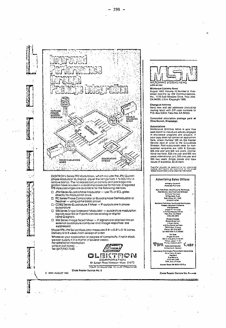
- 298 -
OLEKTRON's Series FP8 Modulators, which include the JPM Quadri-phase Modulator illustrated, cover the range from 1 to 500 MH2 in octave bands. The increased circuit density and package inte-gration have resulted in overall improved performance. Integrated FP8 style packages are available for the following devices. • JPM Series Quadriphcse Modulator — use TTl or ECL gates
directly for modulation drive. • PC Series Phase Comparator or Quadriphcse Demodulator or
Resolver — using same basic circuit. • • CDBQ Series Quadrature IF Mixer — IF outputs are in phase
quadrature. • SS8 Series Single Sideband Modulator — quadrature modulation
signals applied at IF ports can be analog or digital I and Q signals.
• IRM Series Image Reject Mixer — IF signals are applied into an external auadrature combiner and image responses are suppressed.
Model FP8-JPM Series Modulator measures 0.81 x 0.81 x 0.14 inches. Delivery 6 to 8 weeks from receipt of order. Whatever your application or degree of complexity, if not in stock, we can supply it in a matter of several weeks. For additional information write or call today... Tel: (617) 943-7440
O L n K T ^ o r y C O R P O R A T I O N
61 Sutton Road/Webster. Mass 01570 Y Q U O C H A L L E N G E S CXJH P O O G F ^ S S
Circle Reader Service No. S 2 MSN: AUGUST 1980
(USPS 401-030) Microwave Systems News August 1980, Volume 10 Number 8. Pub-lished monthly by EW Communications, Inc., 1170 East Meadow Drive. Palo Alto. CA 94303, U.S.A. Copyright 1980.
Change ol Address Send new and old addresses (including mailing label) with ZIP code numbers to P.O. Box 50249, Palo Alto. CA 94303.
Controlled circulation postage paid a t Olive Branch, Mississippi.
Subscriptions MICROWAVE SYSTEMS NEWS is sent free each month to individuals actively engaged in microwave programs and projects. If your copy does not contain an application form, check Number 300 on the Reader Service card or write to the Circulation Director. Paid subscription rates tor non-qualified recipients are: USA & Canada. $25 one year and S45 two years: interna-tional (surface). S35 one year and S65 two years; international (air), $45 one year and S85 two years. Single copies and back issues (if available), S5.00 each.
Publish*/ assumes no rtsponiiStltly for unsoircttitf •T.3t9rt£t. Csr:.':3u!C-'t f9SF0~!>?!4 <C r*49*s0 ot praonittry ind/or cl*ssit>*a intormshon
Advertising Sales Offices Anthony Yacone'.ll Associate PuSi'sner
New York Stat*. Ntw England. Northeast, Mid-Atlantic, Southeast and Midwest
Anthony Yaeonettl * 13 Reynolds Road
Glen Cove. NY 11542 (Si 6) 671-8758
Northern California. Southwest Washington, Oregon. Southern California
and Colorado Joseph n Hmoiosa
1I70 fas I Meadow Ornn Palo Alto. CA 94303
(415) 494-2800 Western Europe Rofce/1 8roe«mai>
L'Avant-Seine 4-8 Rue Robert an Flora
750)5 Pirn. Franco Phone 331-579-0627
331-609-9595 TLX 270560 Far Cast
Shigeo Ka/ama 8-2-3. Hirayama. Hmo-shi
Tokyo. Japan. T 191
WQQfl ^. AOD V D r n Sale*Administrator » > . A D r
Kimbertey S Hanson Advertising Coordlnalor'ftecruitnient Advertising
Anne Mane St John Assistant
Sue Murphy (415)494-2500
TWX 910-379-6584 Answer Back: EW MSN HQ PLA
Circle Reader Service No. 6
- 299 -
Phase Comparators SERIES PC
Ttie PC Series of phase compara-tors provide two dc outputs proportional to the sine and cosine of the phase difference between n reference and an Input RF signal. Standard units are available in Fiatpack /prefix FPS) or Pin Header (prefix P) or in connector ver-sion (pre.'ix with connector type).
MODEL Mo!'" r~ CONNECTOR "" PREFIX TYPE O- SMA (3MM) B- BNC T- TNC S- SEALECTRO
NOTE: The two F, signals must bo P'occrly terminated m order to realize the M capacity at the device. Oiektron manufactures mini-aturo diptexers lor this soecal purpose.
FUNCTIONAL SCHEMATIC, PHASE COMPARATOR
SERIES PC PHASE COMPARATORS
MODEL NO. FREQUENCY
RANGE (MHz)
REF LEVEL
(-KiCnv) INPUT LEVEL (dBmt
OUTPUT mV P-P
(nominal) PHASE RANGE
——i—>— PHASE ERROR
(max) PC-15 10-20 r io • 0 300 0-360° 5° PC-30 20-40 10 0 300 0-36C 5° PC-60 40-80 10 "0 300 0-360° 5" PC-120 80-160 10 0 300 0-360° 5° PC-150 100-200 10 0 300 0-360° 5° PC-240 160-320 10 0 300 0-360* 5° PC-300 225-400 10 0 300 0-360° 5° PC-400 300-500 10 0 300 0-360° 5° __PC-500 _ 400-600 10 0 300 0-360° 5° PC-800 700-900 10 0 300 0-360° 5° PC-1000 j 800-1200 10 0 300 0-360° 5°
TYPE FP8
SMA, SEALECTRO
Z£7 OLEKTRON
Attenuators and Phase Shifters
-..300 -
OLEKTRON's line of impedance matched attenuators and phase shifters are designed tor radar and signal processing applicaiions. Units include both analog and digital control types. Attenuators utilize PIN diodes a s the control element and analog phase shifters utilize varactor diodes. For applications where RF impedance match is not required at high attenua-tion levels the Balanced PIN Diode modulators described on cage 10 may be used as current control attenuators.
These economical units cover band-widths in excess of a decade.
• The Series ATT-100 impedance matched PIN diode attenuators utilize quadrature matching networks and PIN diooe with long minority carrier life-times. This series is designed for IF system applications where small size is required. Standard packages include the illustrated P1 Header and Relay Header. Pairs with matched phase and amplitude characteristics can be sup-plied on request.
TYPER
SERIES ATT-100 MATCHED PIN DIODE ATTENUATORS
MOOEL NO.
FREOUENCY RAMGE (MHz)
- - • • • • • " " " *rW>* INSERTION
LOSS ATTENUATION IMPEDANCE (Tin) RANGE 2o VSWR (dB) (dB) (ohms) (mat)
P1-ATT-100-60 JPIjATT^lOeO P1-ATT-1QQ-30 P1-ATT-110-30 PI-ATT-100-120
60*6 1.5 32 50 1.5 1 P1-ATT-100-60 JPIjATT^lOeO P1-ATT-1QQ-30 P1-ATT-110-30 PI-ATT-100-120
60*6 1.5 32 75 1.5 1 P1-ATT-100-60
JPIjATT^lOeO P1-ATT-1QQ-30 P1-ATT-110-30 PI-ATT-100-120
30*3 1.5 32 50 1.5 1
P1-ATT-100-60 JPIjATT^lOeO P1-ATT-1QQ-30 P1-ATT-110-30 PI-ATT-100-120
30± 3 1.5 32 75 1.5 1
P1-ATT-100-60 JPIjATT^lOeO P1-ATT-1QQ-30 P1-ATT-110-30 PI-ATT-100-120 120* 10 1.5 32 50 1.5 1 P1-ATT-100-200 ! 200 ±20 1.5 30 50 1.5.1 TYPE PI
£T £ 5 § oc uj E a 3 £ a O <z o SJ 9E z
CHARACTERISTIC CURVES OF MATCHED PIN OIODE ATTENUATORS
v —ATT-100-30 [ i , ,m | \
s * * * * ATT-100-60
| 10 15
CONTROL CURRENT <mA) 20
\ ..LOWCURRE NONPHASt NT REGION inverting
T V r x HlrtHCIIRBFMT QPr.lON m PHASE INVES ting
LM
TYPICAL TRANSMISSION PHASE SHIFT
'. 1
ro :-o ao ATTENUATION SETTING ,'lB)
„.J . . . J id7 OLEK^nON 33
- 30 L -
PIN Diode Bridge Digital Attenuators Attenuators
OLEKTRON's PIN diode bridge attenuators are designed for signal amplitude control applications where extreme flatness of attenuation' versus frequency, and low inherent phase shift versus control setting are required. The PIN diode bridge attenuators require a symmetrical source of bias such as standard ± 5 volts used in systems with high performance and control voltage source. Bridges are inherently biphasal and a reversal of control voltage polarity results in a reversal of transmitted RF or IF signals.
The ATTB Series of at tenuators tabulated on page 35 are illustrations of standard units available in s tandard relay leader, R package, or our FP8 flatpack. We can supply custom units tailored to your requirements includ-ing special control and bias voltage and dynamic range requirements.
OLEKTRON's digital attenuators are designed primarily for RF/IF signal pro-cessing applications requiring rapid discrete level changing under TTL control. Units feature TTL compatible control and balanced PIN diode switches to switch attenuator sections. The leakage of control transients into the attenuator RF output or input is kept below 50 MV peak by the balanced circuits.
The basic DATT Series is offered in the illustrated pin package. Several attenuator steps can be cascaded to form multiple step attenuators. Only a single 5-volt supply is required.
OLEKTRON can supply on request other package configurations with multiple step binary or decimal coded attenuators for your special applications.
INSULATED PIN 0 03 DIA
T
f TYPE P PACKAGE FO.R DIGITAL ATTENUATOR
TYPICAL TRANSMISSION CHARACTERISTIC FOR R:ATT B-70
3 4 / C 7 O L E K T R O N
IC LOG AMPS TO 1 GHz
J For high resolution systems: <10 nanosecond rise times, j For frequency agile systems: Identical log curves over wide frequency swaths.
The combination of microwave transistors and IC cchnology results in an extension of frequency up
;o I Gigahertz where the performance shown in fig-ire A was achieved. In the UHF band, frequency Avaths of 200-300 MHz are covered in a single
amplifier. This results in extremely fast rise times for very wide-band signals and, in addition, a shift-ing center frequency wili produce virtually identical log curves anywhere in the band'(see figure B).
Center Operating Dynamic Linearity' Model Freq. (MHz) BW(MHz) Range (dB)1 (dB) Price 1
ICLT150 150 100-200 70 i 1 S 975 ICLT300 300 200-400 60 ± 1 1100 ICLT375 375 250-500 60 i 1.5 1150 ICLT450 450 300-600 60 i 1.5 1250 ICLT475 475 400-550 60 ±1.5 1100 ICLT625 625 550-700 60 ±1.5 1200 ICLT775 775 700-850 60 ± 2 1300 ICLT925 925 850-1000 60 ± 2 1400 ICLT1000 1000 950-1050 60 ± 2 1400
STANDARD SPECIFICATIONS: a) DC Coupled video. b) Output voltage: 1.25 Volts into 93Q o) Input impedance: 50Q .1) Power: ± 1 2 V O C a t 8 0 m a t y p . ( ± 15 VDC. add Suffix
"C", no charge). e) Size: 3-25/32" x 1-1/2 'x 15/32" f) Weight: <4 oz. NOTES: 1. Input range is from - 65 to - 5 dBm. (0 to - 70 dBm
on 70 dB range units). 2. Nominal at center frequency for standard units.
Add ± 1 dB for - 30 *C to + 71 *C.
3. Standard Units: Prices shown are for standard units optimized for operation at center frequency with pulse rise times of < 10 nanoseconds.
4. Frequency Agile Units: S250 additional. Add Suffix "A". These units are optimized tor use over entire operating band with CW or pulsed signals—see reverse side for additional specifications. 5. Limited IF output: S75 additional, add Suffix "B".
OPTIONS (Contact Factory) 1. Up to 80 dB dynamic range units available. 2. Units with hermetically sealed transistors available. 3. Special configurations. 4. Special center frequency/bandwidth combinations.
- 303 -
SUOBB
LOGARITHMIC IF AMPLIFIERS B True Log Compression B Dynamic Ranges to 80 dB
IST SERIES Center Band- Rise Input Freq. width time Range
Model (MHi) (MHi) 0<jec) (dB) Price LST1003 10 3 030 80 $700 LST2005 20 5 020 80 700 LST3002 30 2 0.50 80 620 LST3010 30 10 0.10 80 620 LST6010 60 10 0.10 80 620 LST6020 60 20 005 80 650 LST7010 70 10 0.10 80 65 0
LST7030 70 30 0 04 80 700 LST12040 120 40 0 03 80 825 LST16C20 160 20 005 80 825 LST16040 160 40 003 80 825
NOTCS: 1. Input dynamic range referenced to 0 dBm high end (nominal). 2. Video output 0.25 to 2.5V (typ) into 93Q. Units direct coupled. 3. Linearity 11 dQ over incut range 4. Limited IF output: OdBm 5. Power • 12V it 70 ma (± 15V. add Suffix "C". N/C) OPTIONS: 1. RFI protection—includes power line filtering and RFt gasketed covers.
Add suffix "RFI" $40 additional. 2. SMA connectors: add sutfix "SMA" additional cost $25. 3. 90 dB dynamic ranges, contact factory.
MODEL LST3010
STANDARD MODELS • 93 ohm Video Load Capability • DC Coupled Video This series offers the user high (idelity " logging" of wide dynamic signal ranges thru the use of succes-sive detection and video summing.
LLT SERIES Center Band- Rise Input Freq. width time Range
Modei (MHz) (MHi) ( .sec) (dB) Price ! LLT1003 10 3 030 80 $795 LLT2005 20 5 0 20 80 795 LLT3002 30 2 0 50 80 680 LLT3010 30 10 0.10 80 680 LLT6010 60 10 0.10 80 680 LLT6020 60 20 0.05 80 750 LLT7Q1Q 70 10 0.10 80 750
.v-'-v-vjij
*RHG
MODEL LLT3002
NOTES: 1. Input dynamic range referenced to 0 dBm high end (nominal). 2. Video output: 0.25 to 2.5V (typ) into 93'J direct coupled. 3. Linearity: ± 1 dB over 80 dB. 4. Limited IF output:OdBm 5. Power; ±12V« 70 ma ( * 15V. add suffix "C". N/C)
. MINIATURE MODELS • Reduced Volume • RFI Protected
The " L L T " series duplicates the " L S T " performance In 1 / 2 the package volume.
2.5V
MODEL L ST30 0 t
l 1 1 1
50w\ i i
50w\
— 80 d3 R ange i 1c S A C :urac VI — 1
-80 - 70 - 60 - 50 - 40 -30 -20 -10 0 + IF INPUT (dBm)
INPUT-OUTPUT CHARACTERISTIC
This chart shows a lypical transfer curve of a log ampli-fier. Note that input signals from - 80 to 0 d B m may be accommodated and will provide an output which is com-pressed so that it varies from 0.25 to 2.5 or 20 dB. Note also that i 1 d B accuracy is obtained over an 80 dB por-tion of that range and that the average slope of the transfer characteristic is equal to 28 m» per dB.
L .tits are available with wider dynamic ranges and/or better linearity. For details, contact factory.
- 304 -
soccoRsexaBi
HYBRID IC IF LIMITERS B Constant Transmission Phase Shift a Wide Dynamic Range • Models to 400 MHz
B Matched Sets Available a Pulse and CW Operation B Small Size
M O D E L ICSL3010
STANDARD MODELS The ICSL limiters offer outstanding performance over a wide dynamic range. The use of input filters, multiple limiting stages and a buffered output help to rcduce internally generated phase error as well as load change variations. The amplifiers utilize se-lected components and are stabilized from - 40° to + 70 °C.
MINIATURE MODELS The ICUL series of constant phase IF limiters feature higher operating frequencies and smaller size and weight than have been previously available. The aluminum housed units measure only 2-1/2" x 1-1/2" x 15/32"and weigh only two ounces.
SPECIFICATIONS: 1 . Input dynamic range: - 70 to - 5 d B m 2. Phase shift over input range: <5* ( < 10* for 160, 200 and
400 MHz models) 3. Output level variation over Input range: < 0.5 dB 4 . Noise figure: <10 dB 5. Input Z: 50 chmsj lVSWR 1.5:1 max 6. Output Z: 50 ohms, V S W R 1.5:1 max
MODEL ICUL400
STANDARD MODELS ICSL S E R I E S
Center Ffeq. (MHi)
Min. Bandwidth'
(MHi)
Nominal Output (dBm)
ICSL3010 30 10 + 10 $675 ICSL6010 60 10 + 10 675 ICSL6020 60 20 + 10 675 ICSL7010 70 10 + 10 675 ICSL16020 160 20 + 10 750
M IN IATURE M O D E L S ICUL S E R I E S
Center Mln. Nominal Freq. Bandwidth Output
Model (MHi) (MHz) (dBm) Price ICUL3010 30 10 + 10 $750 ICUL6010 60 10 + 10 750 ICUL7010 70 10 + 10 750 ICUL16020 160 20 + 10 825 ICUL200 200 50 + 10 895 ICUL400 400 100 + 10 995
7 . Operating Temperature Range: - 4 0 * C t o + 70*C. 8. P o w e r : - 1 2 VDC at 150 ma (typ)
( - 1 5 VDC, add Suffix " C " , N/C)
NOTE: Units designed to work with pulsed or C W signals. Typically 100 nanosecond pulses for 10 MHz bandwiaths and 50 nanosecond pulses for 20 MHz bandwidths.
a
All RHG limiting amplifiers and subsystems are dynam-ically aligned and tested utilizing the amplitude sweep-ing RHG Log Test Set (TSL series). This technique pre-sents an instantaneous dynamic display of phase vs. input amplitude on a standard oscilloscope. The overall affects of adjusting any part of the device or subsystem are Immediately seen. It is particularly advantageous when matching multiple channels.
This technique is made possible by the wide range amplitude sweeping characteristics of the RHG TSL test set. The linear sweep range of 80 dB allows straight-forward scope calibration for the horizontal (in dB/cm). The use of a conventional output phase detector pro-vides a direct readout of phase shift in degrees on the vertical axis.
31
t - 305 -
y g i K i c ^
IC LIMITER5-MATCHED SETS B 2 and 3 Channels b Frequencies to 400 MHz a Matching to ± 2.5°
Matchcd sets of limiters are available for mono-pulse and other applications requiring constant phase transmission characteristics and accurate matching over input dynamic range and tempera-
I C S L M S E R I E S Center Min. Freq. Bandwidth Price for Price tor
Model (MHz) (MHz) 2 channels 3 channels ICSLM3010 30 10 $1550 S2325 ICSLM6010 60 10 1550 2325 (CSLM6020 60 20 1550 2325 ICSLM7010 70 10 1550 2325 ICSLM 16020 160 20 2000 3000
B a s i c S p e c i f i c a t i o n s : The basic specifications are the same a s those of the standard ICSirseries.
A D D I T I O N A L S P E C I F I C A T I O N S
2 Channels—phase matched over - 7 0 to - 5 d B m input range: ±2.5* at room temperature (30 thru 160 MHz) * 5.0'from -tO'Cio + 7 0 ' C ± 5.0* at room temperature (200 thru 400 MHz) * 10* from - 40*C to + 7 0 ' C
To Order: 2 channel set. add su f f ix—"2C"
ture. Offered in 2 or 3 channcf sets, they utilize the Super ICSL and ICUL limiters (see reverse side) and meet all of the specifications of that series.
ICULM S E R I E S Center • Min. ICULM S E R I E S Freq. Bandwidth Price for Price lor Model (MHz) (MHz) 2 channels 3 channels ICULM3010 30 10 S1700 $2550 ICULM6010 60 10 1700 2550 ICULM7010 70 10 1700 2550 ICULM 16020 160 20 1850 2775 ICULM200 200 50 1930 2985 ICULM400 400 100 2190 3235
B a s i c S p e c i f i c a t i o n s : The basic specifications are the same as those of the standard ICUL series.
3 Channels—phase matched over - 7 0 to - 5 d B m input range: ±3.0* at room temperature ±6.0 ' f rom - 4 0 ' C t o +70 'C {30 thru 160 MHz) * 6.0' at room temperature ±12* from - 4 0 * C t o + 70*C(200 thru 400 MHz)
To Order: 3 channel set, add suf f ix—"3C"
f— ! I ^ C r ^ f c g R M G E L 5 C T R Q M 1 C S L A B O R A T D R Y - l i X I C
HHTr.VVltV.i3f iflffr? 1 a 161 East Industry Court n Deer Park, New York 11729 n (516)242-1100 3 TWX 510-227-6033 3 2 For Reliability, Innovation, and Service
306 -
IF PHASE DETECTOR SUBSYSTEMS • Self-contained a Small size a IC construction b MIL grade
Tracking radars H Interferometers n Direction Finders a Test Equipment
RHG now offers a line of complete IF phase detec-tor subsystems. These phase dctectors produce direct-coupled video output(s) that are functions of the instantaneous phase diffcrcnce between the IF in-puts, over a wide rr.nec of input levels. The phase dctectors are optimized for pulsed signals, but are equally useable for CW or analog inputs.
The phase detector subsystems are intended for use in monopulsc and interferometer receivers as well as for use in instrumentation. They arc complete subsystems, incorporating all necessary limiters, IF
components, and video amplifiers, requiring only IF input and video output connections and DC power for operation. Each subsystem is fully cali-brated and characterized. This eliminates the usual interfacing and alignment difficulties encountered when assembling a system from individual com-ponents.
This data sheet describes three of the most com-mon types of phase dctectors. Other configurations are available on special order.
RHG is pleased to provide this section to assist professional engineering personnel with some of the new "language" being used in the field.
Angular Accuracy Angular accuracy is defined as the difference, in degrees, be-tween the actual input phase difference and the phase differ-ence determined Irom the oulput voltage using the nominal phase detector transfer function. In these phase detectors, ac-curacy is guaranteed for phase angles within * 45 * of crossover.
For example: For cosine output:
-135* < 4 < -45 ' ,45* < i < 135* For sine output:
-180* < i < -135 ' ; -45* < i < 45*. 135* < i < 180*
Ratio Accuracy On a return to boresight system, the levels and phase polarity of the A (difference) inputs relative to the I (sum) input, are measured. The accuracy is defined as how closely the system can detect crossover, i.e.. zero A level. This accuracy is stated as the highest ratio of tlx that will produce a zero output voltage.
Settling Time Settling time is the time required for the phase detector output to stabilize within rated accuracy limits, for a pulsed IF input.
Dynamic Range The phase detector is guaranteed to be within rated-accuracy as long as both input levels are within the specified dynamic range, and as long as the difference in input levels is no greater than 30 dB.
Information Bandwidth The information bandwidth is the subsystem 3 dB IF bandwidth (referred to the input). The video bandwidth is amply wide to be transparent to the information bandwidth.
Accuracy Bandwidth The accuracy bandwidth is the range of center frequencies c\er which rated accuracy is maintained. This is of necessity ICJS than the information bandwidth.
- 307 -
TWO CHANNEL, SINGLE OUTPUT PHASE DETECTOR SUBSYSTEM!
PD&QPD SERIES
I * 0 * for PD Model E1 = 2.5 cos ®(PD Model) j ... ' 90MorQP0Model E2 = 2.5sin 0(QPDModel)
The two channel, single output phase detector sub-systems are intended for use in phase demodulator systems where the cxpcctcd input phase difference is less than ±90°. Both in-phase (cos 0 output)and
quadrature (sin 0 output) models are available. Separate limiters and IF processing modules are
mounted to a common base plate with all power connections made to a single barrier strip.
Center Information Accuracy Settling Angular Freq. Bandwidth Bandwidth Time Accuracy Model (MHz) (MHz) (MHz) (fjsec) (degrees) Price in-Phar.o PD3010 30 10 2 0.1 ± 5 $2,250 P06010 60 10 2 0.1 ±5 2,250 PD6020 60 20 4 0.03 ± 5 2,350 PD7020 70 20 4 0.08 ± 5 2,350 PD16020 160 . 20 4 0.08 ± 7 2,650 Quadrature QPD3010 30 10 2 0.1 ' ± 5 2,275 QPD6010 60 10 2 0.1 ± 5 2,275 QPD6020 60 20 4 0.08 ± 5 2,375 QPD7020 70 20 4 0.08 ± 5 2,375 QPD16020 160 20 4 0.08 ±7 2,675
ADDITIONAL SPECIFICATIONS 1. Input Impedance: 50 Q (VSWR 1.5:1 nom) 2. Input Dynamic Range: 0 t o - 6 0 dBm ( - 5 t o - 6 0 dBm for 160 MHz units) 3. Input Level Difference: 0 to 30 dB 4. Output Impedance: 75Q 5. Connectors: . SMA 6. Power ± 12V (± 15V available N/C, add Suffix "C") NOTES 1. See Glossary (page 33) for detailed definitions of terms. 2. Special parameters, other frequencies, etc. are available—Contact factory. 3. PD and QPD models are available for use with one limiter channel and an external reference—Contact factory.
g O E K l C ^ R X 3 L / U S Q r a A T C S Y - l f t S C tefcVir, -J.T--J 161 East Industry C o u r t s Deer Park, New York 11729 ^ (516)242-1100 s TV/X 510-227-6083 For Reliability, Innovation, and Service
- 308 -
TWO CHANNEL, DUAL OUTPUT PHASE DETECTOR SUBSYSTEMS
DPD SERIES
0 - I B - Z A E1 = 2.5COS® E2= 2.5 sin 0
The two channel, dual output phase detector sub-system offers, by means of the two quadrature out-puts, an unambiguous measurement of the input phase difference. This technique is used in angular measuring devices such as interferometers, direction
finders and instrumentation. The two limiters and the IF processor are
mounted to an aluminum base plate with all power connections brought out to a single barrier strip.
Settling Angular
(P sec) (degrees) Price 0.1 ±5* $2,500 0.1 2,500 0.08 x5* 2,600 0.08 ±5* 2,600 0.08 ±7* 2,950
Center information Accuracy Freq. Bandwidth Bandwidth
Model (MHz) (MHz) (MHz) DPD3010 30 10 2 DP06010 60 10 2 DPD6020 60 20 4 DPD7020 70 20 4 DPD16020 160 20 4
ADDITIONAL SPECIFICATIONS 1. Input Dynamic Range: 2. Input Level Difference: 3. Irlput Impcdance: 4. Output Impedance: 5. Connectors: 6. Power:
Oto -60dBm(-5 to -60 dBm for 160 MHz) 0 to 30 dB 50 S2 (VSWR 1.5:1 nom) 75 Q SMA ± 12V (± 15V available N/C, add Suffix "C".)
NOTES 1. See Glossary (page 33) for detailed definitions of terms. 2. Special parameters, other frequencies, etc. are available—Contact factory.
E Z T ^ ^ Z S ^ L Z ^ J a 131 East Industry Court n Deer Park, New York 11729 3 (516)242-1100 v: TWX 510-227-6063
For Reliability, Innovation, and Service
- 309 -
. -tttir^ , y
TECHNICAL DATA
i i
DOUBLE BALANCED MIC MIXERS N AND MIXER PREAMPS
To fill the growing need for multioctave devices in surveillance, ECM, and other specialized receiver applications, RHG has developed a complete line of double balanced mixers, and double balanced imageless mixers—obtainable with or without built in IF preamplifiers.
These MIC (Microwave Integrated Circuitry) mixers provide coverage of up to 1 to 26 GHz in a single assembly. This performance has been achieved through the use of a unique microwave configura-tion. Excellent performance is maintained over five octaves with extremely low intermodulation distor-tion and high isolation.
Available since late 1969 the " D M " series of double balanced mixers, in standard octave or multioctave versions, has gained wide acceptance in both prototype and production applications.
Recent developments at RHG have produced a I to 26 GHz unit, and the industry's smallest 1 to !8 GHz mixer (1/2" x 1/2" x 1/2"). RHG's leadership in the mixer field is evidenced by the growing num-ber of imitators. However, only at RHG can the customer receive the latest technology coupled with custom designs and ongoing service.
In addition, all RHG mixers can be provided with a fully integrated IF preamp, with IF coverage spanning 1 MHz to 4 GHz.
NOISE FIGURE & ISOLATION
- 310 -
DM SERIES TECHNICAL DATA
IF RESPONSE OF DM. OMX, & DMH SER IES
3 -S
0 100 MO 300 400 500 600 3000 5000 7000 9000 IF FREQ (MHi)
PHASE DETECTOR PERFORMANCE
30 60 90 120 150 PHASE DIFFERENCE (DECREES)
INTERMOOULATION PERFORMANCE (Standard LO Level)
MODEL DM).18
^ I v.. ,
10 « • 10<J8m t
-5 -10 - IS -20 -25 RF INPUT POWER (dBm)
RF PHASE AND AMPLITUDE TRACKING-TWO 0 M M 8 MIXERS
> *10
: 5) + 5 SJ : oc o
JO c — : - 1 0
> \ +1.0 j c + 05 j ® 0 1 — » -OS
- 1 . 0
/ , / N /
ill
E TYP) TRAC il
l
E TYP)
A At N./ \ \ / J / \ > vJ
1 OF AMPLIT UOE rSAC/<ISGiTYP|
6 8 10 12 14 IS 13 20 FREQUENCY (GHz)
INTERMODULATION PERFORMANCE (H.qh LO Level)
-60
-70
5 -80
MODEL D M M 8
L O a + 16dBm |
•5 -10 -15 -20 -25
RF INPUT POWER (dBm)
HARMONIC MIXING
MC DEL OMI- 8 (MlO 8A >40)
— ; - — T TT7T
TV PRO
\ •
PICAL SUCTION .
LO = 1 • lOdBm
VARIATION J J
0 - s -to -15 ' -20 -25 RF INPUT POWER (flBmi
' " I M G ; S L E C T R O M I C S ? , A E ? - a n A T a R Y - i P s J c
Ltygffi.T/'S'i'.TTTTim 161 East Industry Court r Deer Park, New York 11729 n (516) 242-1100 n TWX 510-227-6083
42 For Reliability, Innovation, and Service
— -31-1
c :
DOUBLE BALANCED MIC MIXERS B 1.0 to 18 GHz in one mixer a Low IM
OCTAVE M O D E L S
Freq. Model No. (GHz|
NV.H) (dB)
Mix N.F.(1) (dB) Price
DM1-2 OM2-4
l.Oto 20 2 0 to 4 0
65 7.0
75 s o ;
$250 250
DM48 DM8-12 OM12-18
4 0 to 8 0 8 0 to 12.0
I2.0to 18 0
70 8.0 90
8.0 90
100
280 . 315 395
MULT IOCTAVE M O D E L S DM1-4 DM1-8 D M M 2
l.Oto 4.0 l.Oto 80 t.O to 12.0
7.0 70 80
80 8.0 90
280 295 350
OM118 DMS1-2S
10 to 180 1.0 to 26 0
9.0 80
10.0 95
450 695
Th« OMS1-26 is tuily described on an individual DMS1-26 data sheet. NOTES: 1. Based on V5dB IF noise figure. 2. R F&LO VSWR: 2 5:1 ctypV 3. 10 injection: +5 to • 10 dBm (typ). 4 . Connectors: SMA all oorts (lor leed thru terminal at IF output—add
Sullix "PT"—no chargel 5. LOtoRF ISO: >20d0. STANDARD OPTIONS 1. IF response to 500 MHz: add sutilx "A", $10 additional. 2. low corner noise dioaes: reduce 1/1 noise in "zero IF " applications.
Add sullix "8". 350 adcitionat.
STANDARD MODELS • DC to 300 MHz IF • 1 to 26 GHz RF/LO
The " D M " series utilizes a rugged cast housing and special SMA connectors to provide reliable performance.
OCTAVE M O D E L S Typ. Typ.
N.F.(dB)<1) N.F .MBim Model No Freq.tGHz) 0 dBm LO -10 dBm LO Price
DMB 12 1 to 2 80 . 12.0 S335 DMB 2-4 2to4 8.5 12.0 335 DM6 48 4 to 8 9.5 13.0 380 OMB 8-12 8 to 12 100 140 440 DMB 12-18 12 to 18 11.5 155 525
MULT IOCTAVE M O O E L S OMB 1-12 1 to 12 9.0 13.0 495
• DMB 2-18 2 to 18 11.0 150 625 The OMB 2-18 is tuiiy described on an individual OMB 2-18 data sheet. NOTES: 1. NF Includes: 1.5dB IF contribution. 2. IF coverage: 10 to300 MHz. 3. LO/RFisolation: 18dBtyp. 4 . RF/LO VSWR: 2.0:1 typ.
5. Bias: + 12V at 2 ma typ. 6. For IF lo 500 MHz: add
suffix "A", $50 additional (not available on 0MB1-2 or 0MB1-12.
STARVED LO MODELS • Operation at -10 dBm LO a l t o 18 GHz
For application where LO power is minimal, the "DMB" series provides all the benefits of doubly balanced mixers.
OC to 2 GHz I F M O D E L S
Modal No. Freq. (GHz) (dB)
Max. N.F.(I)
(dB)
NOTES: 1. N.F. includes 1.5 d8 IF contribution. 2. LO injection: • 10 d8m. 3. LO to RF ISO: > 20 dB ( > 16 dB on DtoH).
DMX 2-4 2 to 4 8.0 90 $395 DMX 4-8 4(03 8.0 90 425 DMX 8-12 8 to 12 9.0 100 450 OMX 12-18 210 18 10 0 11 0 475
1 to 8 GHz IF MOOEL DMH2-18C 2.0 to 18 0 90 110 $560 The OMH2-18C is fully described on an individual OMH2-18C data sheet.
MICROWAVE IF MODELS • I F Coverage to 8 GHz . • RF/LO to 18 GHz
I F s to 8 GHZ for up or down conversion. The " D M X " " O M H " series provide state-of-the-art performance.
and
- 312 -
DOUBLE BALANCED MIC MIXER PREAMPS • 1 to 26 GHz B IC Preamps • Small Size
- • j/t ; V'.\ V \ •' . Wj! ' <Nfs {r<. - * >•>; • ••• V ;
r
i
STANDARD & SPECIAL PREAMP MODELS
Every RHG mixer can be supplied with a wide range of IF preamplifiers. These IC preamps are mechan-ically and electrically integrated with the mixer to provide optimum noise figure. The use of a mixer/ preamp assures this optimum noise performance, sincc the mixcr/prcamp interface is a key factor
and is often improperly established when separate mixers and preamps are used.
The models listed on the following pages reflect many of the most requested combinations. If your needs are not met by a standard, we will be happy to provide a special unit on request.
OCTAVP MODELS MULTIOCTAVE MODELS IF TYP MAX IF
Model Freq/BW N.F. N.F. Model Freq/BW N.F. RFBand Number MHz (dB) (dB) Price RF Band Number MHz (d8) Price L-Band DM1-2/10A 60/10 7.0 3.0 $575 0.1 to 1.0 GHz 0M0.1-1/10A 60/10 See S 675 1.0-2.0 GHz OM1-2/10B 60/20 7.0 8.0 575 DM0.1-1/10B G0/20 note 1 675
DM1-2/10C 30/10 7.0 8.0 575 DM0.1-1/10C 30/10 below 675 S-Band OM2-4/10A 60/10 7.5 8.5 575 1.0 to 8.0 GHz DM1-8/10A 60/10 See 625 2.0-4.0 GHz DM2-4/10B 60/20 7.5 8.5 575 DM1-8/10B 60/20 N o t e l 625
DM2-4/10C 30/10 7.5 8.5 575 DM1-8/10C 30/10 below 625 C-Band DM4-8M0A 6C/10 7.5 8 5 575 1.0 to 12.0GHZ DM1-12/10A 60/10 See 695 4.0-8.0 GHz DM4-8/10B 60/20 7.5 8.5 575 DMM2/10B 60/20 Note 1 695
DM4-8/10C 30/10 7.5 8.5 575 DM1-12/10C 3ono below 695 X-Band DM8-12/10A 60/10 8.5 9.5 625 1.0 to 18.0 GHz DMM8/10A 60/10 See 870 8.0-12.0 GHz DM8-12/10B 60/20 8.5 9.5 625 DM1-18/108 60/20 N o t e l 870
DM8-12/1CC 30/10 8.5 9 5 625 DM1-18/10C 30/10 below 870 Ku-Band OM12-18/1CA 60/10 9 5 10.5 745 1.0 to 26.0 GHz DM 1-26/1 OA 60/10 See 1050 12.0-18.0 GHz DM12-18/10B 60/20 9.5 105 745 DM1-26/10B e 0/20 Note 1 1050
DM12-18/10C 30/10 9.5 10.5 745 DM1-26/10C 30/10 below 1050 K-Band 18.0-26.0 GHz
DM18-26/10A DM18-26/10B DM18-26/10C
60/10 60/20 30/10
8.5 8.5 8.5
10.0 10.0 10.0
995 995 995
- SPECIAL P R E A M P S * T o , e o ' a c e s u f t i * w i t n ' preamp type desired
Preamp Cent. Band- RF-IF Freq. width Gain 'Addit. 'Addit. (MHz) (MHi mini IdB mini N.F. Cost
10KK 10 2 25 0.5 $40 10LL 20 6 25 0.0 40 100 70 10 25 0.0 25 1 0 J J 70 30 25 0.0 25 10BB 120 20 25 1.0 40 10DD 130 50 25 1.0 50 10HH 10 to 200 20 10 50 • Added to mixer preamp mm 10A preamp type
For 160 MHz models, see " EF " series on reverse side
NOTES: 1. Noise figure of multioctave models is typically
<10 dB 0.1 to 1.0GHz < 8 d B 1 .0to8GHz <10 dB 8.0 to 26 GHz
2. V S W R : Typically 2.5:1 3. LOinjfection: +7 to +10 dBm 4. IF output capability: > 0 d B m (all models) 5. LO-RF isolation: 20 d8 6. Impedance level: 50Q. all ports 7. Connectors: SMA 8. Gain (RF-IF): 25 dB (min) unless noted otherwise 9. Weight: Approx. 3 oz.
10. Power: +12 VDC at 20 ma (typ) For +15 V C C add sultix " C " (no charge).
11. Most units available with biasable mixers for low LO power. Contact factory for details.
- 313 -
I
M C M 3 C B
DOUBLE BALANCED MIC MIXER PREAMPS B Special Purpose Mixer Preamps n MIC/IC Construction
GAIN AND PHASE MATCHED MODELS WITH ELECTRONIC GAIN CONTROL
OCTAVE M O D E L S
1 Si
& ii
1 i."
fl £
r1 »
I -
56
IF N.F. Price Per RF Band Model Number Fr«q/8W (dB) Channel (1)
L-Band MOM1-2/12A 60/10 7.7 $ 675 l .Oto 2.0 GHz M0M1-2/12B 60/20 7.7 675
MOM1-2/12C 30/10 7.7 675
S-Band MDM2-4/12A 60/10 8.2 675 2.0 to 4.0 GHz MDM2-4/12B 60/20 8.2 675
MOM2-4/12C 30/t0 8.2 675
C-Band MOM4-8/12A 60/10 8.2 675 4.0 to 8.0 GHz MOM4-8/12B 60/20 8.2 675
MDM4-8/12C 30/10 8.2 675
X-Band MDM8-12/12A 60/10 9.2 725 8 to 12 GHz MDM8-12/12B 60/20 9.2 725
MOM8-12/12C 30/10 9.2 725 Ku-Band MOM12-18/12A 60/10 9.7 845 12 to 18 GHz MDM12-18/12B 60/20 9.7 845
MDM12-18/12C 30/10 9.7 845 K-Band MOM 18-26/1 OA 60/10 10.5 1095 18 to 26 GHz MDM18-26/10B 60/20 10.5 1095
MDM18-26/10C 30/10 10.5 1095
MULT IOCTAVE M O D E L S
RF Band Model Number IF
FreqiBW N.F. Price Per (dB) Channel (1)
l .Oto 12.0GHz MDM1-12/12A 60/10 See 795 M0M1-12/12B 60/20 Note 2 795 MDM1-12/12C 30/10 795
1.0to 18.0GHz MOM1-16/12A 60/10 See 970 MDM1-18/12B 60/20 Note 2 970
• MDM1-18/12C 30/!0 070 1.0 to 26 GHz MDM1-26/12A
MDM1-26/12B MOM1-26M2C
60(10 60/20 30/10
See Note 2
1220 1220 1220
NOTES: 1. For single channel with gain control. $50. less per unit. 2. NF : < 9 d B t o 0 G H z : < l 0 d 8 to 12 GHz ;< 11 dB to 26 G H ; 3. Overall RF-IF Gain: 20 dB min. 4. RF-LO Isolation: 20 dB min. 5. Power: + 12 VOC at 90 ma (typ).
+ 15 VOC available N/C. add suffix " C " 6. Matching: + 5 * and ± 1 dB over specified ga in control
and temperature ranges. 7. Ga in Control Range: 20 dB tor 0 to - 3V (nom.) 8. Meets MIL-E 5400, Class II requirements ( - 30* to +71 'C|
ECM AND SURVEILLANCE MODELS WITH 160 MHz IF AND HIGH OUTPUT CAPABILITY
OCTAVE M O D E L S MULT IOCTAVE M O D E L S RF Band Model Number
TYP MAX N.F.(dB) N.F.(dB) Price RF Band Model Number
TYP MAX N.F.(dB) N.F.(dB) Price
L-Band 1.0 to 2.0 GHz
DM1-2mEF 7.0 8.0 $ 725 0.25 to 1 GHz DM0.25-1/14EF 10.0 11.0 S 825 L-Band 1.0 to 2.0 GHz 1.0to 12 GHz DM1-12/14EF 9.5 10.5 eso S-Band 2.0 to 4.0 GHz
DM2-4/14EF 7.5 8.5 725 1.0 to 18GHz 0Ml-ia/14EF 10.5 11.5 1025 S-Band 2.0 to 4.0 GHz 1.0 to 26 GHz DM1-26/14EF '11.0 12.0 1275 C-Band 4.0 to 8.0 GHz
0M4-8/14EF 7.5 8.5 725
X-Band 8.0 to 12.0 GHz
DM8-12/14EF 8.5 9.5 800 Ku-Band 12.0 to 18.0 GHz
0M12-18/14EF 9.5 10.5 925
K-Band 18 to 26 GHz
OM18-26/14EF 10.0 11.0 117'
ADDITIONAL SPECIFICATIONS: 1. LO Power: + 10 dBm 2. LO-RF Isolation 20 dB 3. RF-IF Gain: 25 dB (min) 4. Output Power: + i 3 d B m a t 1 dB compression. 5. IF Freq/Bandwidth: 160/50 MHz. 6. Units tested to: Temperature: - 5 4 # C t o + 7 l * C
Vibration: Curve 1A of MIL-E-5400L ( 2 10g's to 2000 Hz)
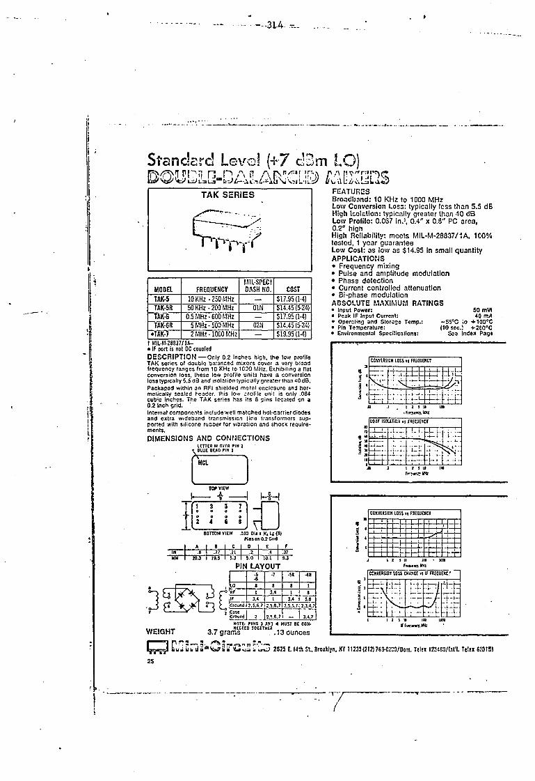
— --314. '
f;
S t a n d a r d L e v e l ( + 7 d 3 m L O ) r?n n , . H u a n s l ® m n m
TAK S E R I E S
MODEL FREQUENCY MIL-SPECt DASH NO. COST
TAK-5 10 KHz - 2 5 0 MHz — $17.95(1-4) TAK-5R 50 KHz - 2 0 0 MHz 01N $14.45(5-24) TAK-6 0 .5 M H z - 6 0 0 MHz — $17.95(1-4) TAK-6R 5 M H z - 5 0 0 MHz 02N $14.45(5-24)
•TAK-7 2 MHz- 1000 MHz — $ 1 9 . 9 5 ( 1 4 ) t MIL-M-28837/1A-• IF port is not OC couoled D E S C R I P T I O N — O n l y 0.2 inches high, the low profile TAK series of double balanced mixers cover a very broad frequency ranges from 10 KHz to 1COO MHz. Exhibiting a flat conversion loss, these low profile units have a conversion loss typically 5.5 dB and isolation typically greater than 40 dB. Packaged within an RFI shielded metal enclosure and her-metically sealed header, this low profile unit is only .064 cubic inches. The TAK series has its 8 pins located on a 0.2 inch grid. Internal components include well matched hot-carrier diodes and extra wideband transmission line transformers sup-ported with silicone rubber for vibration and shock require-ments. DIMENSIONS AND CONNECTIONS
5.3 I 5.0 1 10.1 19.3
PIN LAYOUT -5 -6
-7 •5R -6R
LO 8 8 3 1 piRF 1 3,4 1 8
f jcround 3.4 1 3.4 5.6
f jcround 2.5.6.7 2.5,6.7 2.5.5,7 2.3,4.7
(Ground 2 2,5.6.7 3,4,7
WEIGHT £
N0TC: PINS 1 AfO 4 MUST B£ CON-_ _ NECTED TOGETHER 3 . 7 g r a m s . 1 3 o u n c e s
FEATURES Broadband: 10 KHz to 1000 MHz Low Conversion Loss: typically less than 5.5 dB High Isolation: typically greater than 40 dB Low Profile: 0.C67 in.3, 0.4" x 0.8" PC area, 0.2" high High Reliability: meets MIL-M-28837/1A, 100% tested, 1 year guarantee Low Cost: as low as $14.95 in small quantity APPLICATIONS • Frequency mixing • Pulse and amplitude modulation • Phase detection • Current controlled attenuation • Bi-phase modulation ABSOLUTE MAXIMUM RATINGS • Input Power: • Peak IF Input Current: • Operating and Storage Temp.: -55°C io +100°C • Pin Temperature: (10 sec.i +260°C • Environmental Specifications: See Index Pag<
50 mW 40 mA
IO IF ISOUTIQ:) »$ FUFLATMCR i i r L i . I. ;. L i .
R. I UIL'I.
- j — . I t" _.—i. 1 - : R-F-
C0MVERSJ0H LOSS i s FREOUEHCT
1 t 1 | I 1 I i 1 | ! ! 1 1 i 1 ; | 1
1 J 1 1
1 1 i 1 ' i ! 1 ! ! 1 ! J
1 ! 1 ' 1 ! 1 1 S 1) ICC FrtguencT, "to
CONVERSION10SS CHANGE t l If FREQUENCE
l i i
t 7 L h t i
- i — « _ .
- t - l -5 It 100 f finwncr. "Hz
j Cw liu"wdi,' C ^ H i J-3 2825 E. 14th St., Brooklyn, NY 11235(212)76S-C2CO/Oom. Telex 122460/lnfl. Telex 623155
25
/
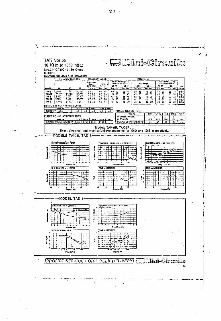
- 315 -
T A K S e r i e s 1 0 K H z to 10C0 M H z SPECIF ICATIONS: 50 Ohms MIXING CONVERSION LOGS AND ISOLATION
.Svi)
Model NO.
Frequency Range. MHi
10 RF IF
Conversion loss. dB Ont Octavo
From Total D»nd(0(1 Rinse T»o.*Ml«. To. Mat.
Lower Bind (die to One Decide Higner
t o Wf 10IF~ TvS. Min" Tyii. Min.
Isolation, u3
Mid Rjnfe 10-RF 10-IF
Tvo. Min. Trs. Min.
Uoper Bind (dee To One Octive lower
~ _tO-RF" t0-1F _ tro. Min. Tro. Min.
rm layout
TAK-5 TAK-5R TAK-6 TAK6R TAK-7
.01-250 .01-250 0C-250
.05-200 .05-200 DC-200
.5500 .5-600 DC-6C0 5-500 5-500 DC-500 2-1000 2-1000 .5 500
5 5 7.0 6.5 8.5 5.5 6.5 6.5 8.0 5.5 7.5 6.5 8.5 6.0 7.0 6.5 8.0 5.5 7.5 6.5 8.5
60 50 55 45 55 50 50 45 60 50 55 45 55 50 49 40 45 30 45 30
50 35 45 30 45 35 40 30 50 30 45 30 45 30 40 25 35 20 35 20
40 30 35 25 45' 35 40 30 40 25 30 20 35 30 30 25 30 20 30 20
Fig. 1 Fig. 3 Fig. 1 Fig. 4 Fig. 2
SIGNAL 1 dB C O M P R E S S I O N LEVEL Medtl rsr. J I1«-3X nm TIX-CR TAK-7
SIGNAL UYU.IdBx.) + 1 + 1 + 1 + 1 + 1 PHASE DETECTION Model Nl. T»K1 IMS* TAX-6 TiM* TM-7
ELECTRONIC ATTENUATION OCOffSET.ImV) TYP. 1 1 1 1 — M0<|| HI. urn nr. in TIK CD T»X-7 DC POLARITY NEC NEG NEG NEG —
MINIMUM ArUNUAflON. 120 mA) 1.5 <33 1.7 £3 3.5 dH 3.5 dB | — MAXIMUM OUTPUT, (VOLTS) TYP. .25 25 .25 .25 —
Models TAK-5R, TAK-6R . . . Exact electrical and mechanical replacements (or M6D and M6E respectively.
MODELS TAK-5, TAK-6 • CONVERSION 10SS n 10 POWER
- H - K - H — H —
!—i—j—1—!— H -
—
{CONVERSION 10SS CHANCE n i> FREQUENCY
m i t
-
f i T T " H " M rf
t r-T T^
-r -r i M
• . i i -. i
CONVERSION LOSS n RF INPUT L E Y E l
• 1 I I I t I I I I It II u 10 fw. Aim
10 RF ISOLATION n FRf'lUENCT
x n p p p i r
YSWR n FREQUENCY
i-4-
• <
FEE -13
W -
F I B S ±t
Fr«mm),IMt fnqumT.MKr
MODEL TAK-7-
II, 5 II 100 frtqwnqr. l!Hj
I <
F K h - T - i i - M - , -rr-f-l-f-T-r-F-
-3 -2 -1 0 I 2 Rf Input Intl. dsn
N a M loo rmumj.KHi
IPRG;.IPT SERVICE / WEEK DELIVERY/ rJ3au3i-G5rciiaG"!i3 26
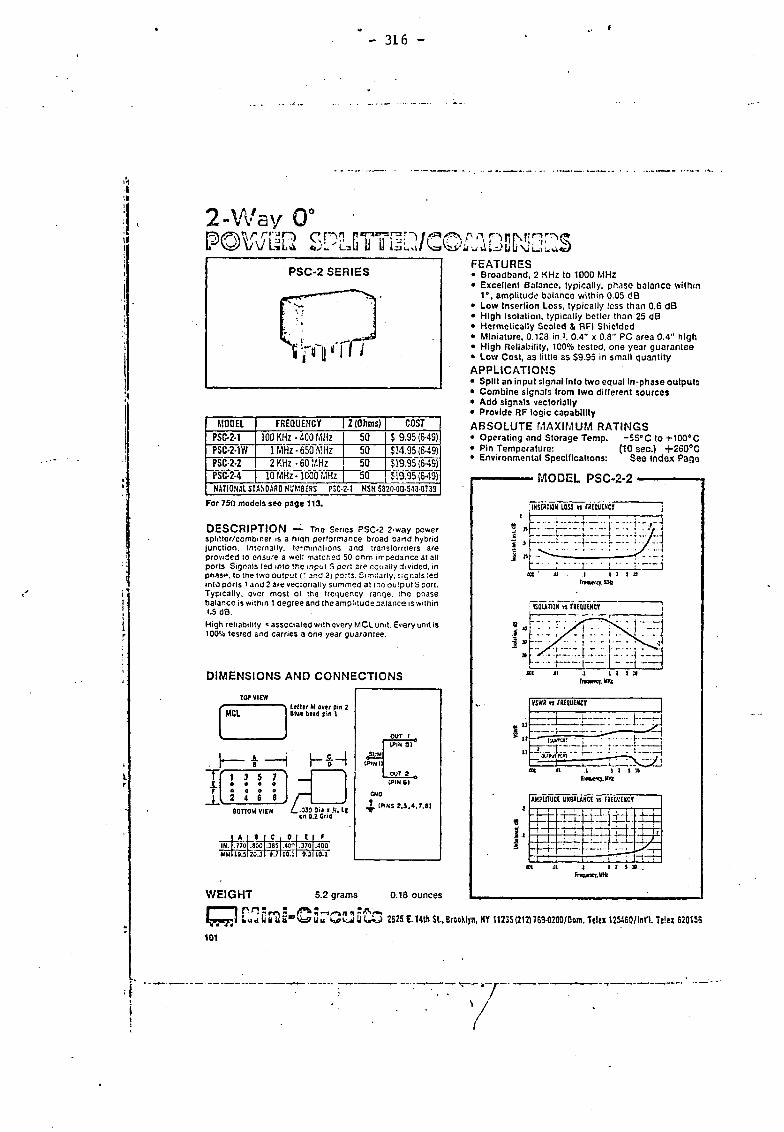
- 316 -
2 - W a y 0 °
S P i L G Y T i l Q / C O ^ B E I ^ S
MOOEL FREQUENCY Z (Ohms) COST PSC-2-1 100 KHz - 4 0 0 MHz 5 0 $ 9 . 9 5 (6-49) PSC-2-1W 1 M H z - 6 5 0 MHZ 5 0 $14 .95(6-49) PSC-2-2 PSC"2"4
2 KHz - 6 0 MHz 10 MHz- 1000 MHz
5 0 5 0
$19 .95(6-49) $19 .95(6-49)
NATIONAL STANDARD NUMBERS PSC-2-1 NSN 5320-00-543-0739
For 750 models seo page 113.
DESCRIPTION — The Series PSC-2 2-way power splitter/combiner is a niqh performance broad band hybrid junction. Internally. terminations and transformers are provided to ensure a well matched 50 ohm impedance at all ports Signals fed into the input S port are equally divided, in phas<\ to the two output (1 and 2) ports. Similarly, signals fed into ports i and 2 are vectorially summed at tne output S port. Typically, over most of the frequency range, the phase balance is within 1 degree and the amplitude balance is within (-5 dB. High reliability « associated with every M C L unit. Every unit is 100% tested and carries a one year guarantee.
DIMENSIONS AND CONNECTIONS
MCI letter M aver pin 2 Blue bead pin 1
L - A J o I
13 5 7
2 4 6 8 h L. -03c .030 Oil I K» l(
an 0.2 Grid
I A I B I C . 0 I O7>70tT8G0t385j .lO T IMI 19.5126.31 9.71 T0.IL
OUT 1 U»IN S)
0SUM (PIN II
OUT 2 0 (PIN 6)
GNO J,. (PINS 2,3.4,7,81
WEIGHT 5.2 grams 0.18 ounces
FEATURES • Broadband, 2 KHz to 1000 MHz • Excellent Balance, typically, phase balance within
1°, amplitude balance within 0.05 dB • Low Insertion Loss, typically less than 0.6 dB • High Isolation, typically better than 25 dB • Hermetically Sealed & RFI Shielded • Miniature, 0.128 in.3. 0.4" x 0.8" PC area 0.4" high • High Reliability, 100% tested, one year guarantee • Low Cost, as little as $9.95 in small quantity APPLICATIONS • Split an input signal into two equal In-phase outputs • Combine signals from two different sources • Add signals vectorially • Provide RF logic capability ABSOLUTE MAXIMUM RATINGS • Operating and Storage Temp. -55°C to+100°C • Pin Temperature: (10 sec.) +260°C • Environmental Specifications: See Index Pago
MODEL PSC-2-2
•INSERTION LOSS n FREQUENCY
S
1 *
E j E E t H - i
j i i i u Fmunxy. KHl
1 I 2 i U Fnqumj. Mtt
vsw» r» rmuincr
... r. t . . iJZq AtTB.ii trtr 1 ' . ' . 1
.1 1 1 5 U Frtqwfcy.UMi
3
1 j
Mtfinuoc UNBALANCE N FRCQC'CNCT & W 4 ± ± r f -
>
1 I
H - H . r r „ >
»l J 1 2 I 10 . frecutiict.UHi
UdUaiJ-a n **** n 99 m ***
U U b U O 2825 E. 14th SL. BrooWyn, HY 11235 (212) 769-Q200/0om. Telex 1254S0/lnt'l. Telex 620158
101
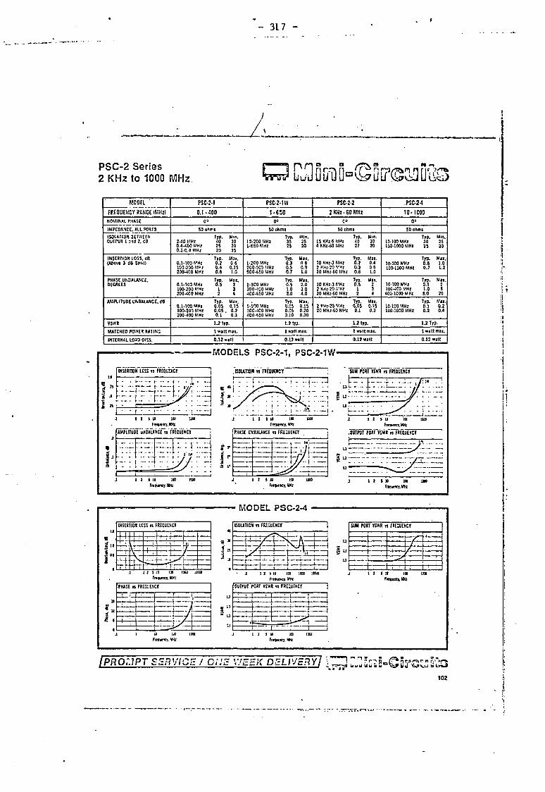
3 L 7 - '
P S C - 2 S e r i e s 2 K H z to 1000 M H z .
M00EI ' PSC-2-1 P S C M W PSC-2-2 . PSC-2 4
FREQUENCY RANGE (MHi) 0.1-400 1-650 2 KHz-60 MHz 10-1000 NOMINAL PHASE 03 OO 0 °
00
IMPCDANCE. A l l PORTS 50 ohms 50 ohms 50 ohms 50 ohms ISOLATION 3ETWECN OUTPUT 1 ;nd 2, eo
Typ. Min. 2-40 MHz 40 30 0.4-400 MHz 25 20 0.1-0.4 MHz 20 15
Typ. Min. 10-200 MHz 35 25 1-650 MHz 25 20
Typ. Min. 15 KHz-6 MHz 40 30 4 KHt-60 MHz 27 20
Typ. Min. 10-100 MHz 30 25 100-1000 MHz 25 20
INSERTION LOSS. 08 (Atovo 3 08 Split)
Typ. Mai. 0.1*100 MHz 0.2 0.6 103-200 MHZ 0.4 0.75 200-400 MHZ 0.6 1.0
Typ. Mat. 1-2C0 MHz 0.3 0.6 200-500 MHZ 0.5 0.9 500-650 MHZ 0.7 1.0
Typ. Mai. 10 KHz-3 MHz 0.2 0.4 2 KHz-20 MHz 0.3 0.6 20 MHz-60 MHz 0.6 1.0
Typ. Mai. 10-100 MHz 0.6 1.0 100-1000 MHI 0.7 1.2
PHASE UNOALANCE, DECREES
Typ. Mn. 0.1-100 MHz 0.5 2 100-200 MHZ 1 1 200-400 MHZ 2 4
Typ. Max. 1-100 MHz 0.5 2.0 100-400 MHZ 1.0 3.0 400-850 MHZ 2.0 4.0
Typ. Mai. 10 KHz-3 MHz 0.5 2 2 KHz-20 MHz 1 3 20 MHZ-60 MHZ 2 4
Typ. Max. lO-tCO MHz 0.5 2 100-400 MHZ 1.0 S 400-1000 MHZ 8.0 20
AMPLITUDE UNBALANCE, dB Typ. Ma«. 0.1-100 MHz 0.05 0.15 100-200 MHZ 0.05 . 0.2 200-400 MHZ 0.1 0.3
Typ. Mai. MOO MHZ 0.05 0.15 100-400 MHZ 0.05 0.20 400-650 MHZ 0.10 0.30
Typ. Mai. 2 KHz-20 MHz 0.05 0.15 20 MHZ-60 MHz 0.1 0.3
Typ. Mn. 10-100 MHZ 0.1 0.2 100-1000 MHz 0.2 0.4
VSWR 1.2 typ. 1.2 typ- 1.2 typ. 1.2 Typ. MATCHED POWER RATING 1 wattmai. 1 watt max. 1 watt mai. 1 watt max.
INTERNAL LOAD OISS. 0.12 wait 0.12 watt 0.12 watt 0.12 watt
•MODELS PSC-2-1, PSC-2-1W-INSERTION LOSS n FREQ'jENCT ISOLATION n FREQUENCY
• • L" - I — • • • ,L •
12 I II 109 Fre^iWI. MXZ
MINUBT'UNBAIANCRII' FREQUENCY'
SUM PORT VSWR n FREQUENCY
u : r : : v . j : — >FF~.
12 S 10 100 Fi««»nct. MW
I 2 J 10 100 Fmunwr.MH/
•vl^q:-r: tr
a =5 r
.OUTPUT PORT VSWR n FREQUENCY
i 2 s to too Fnowney. VHj
I 2 5 10 100 Frtqwncy. MW
I 2 I 10 100 Fnguffiy, MHz
MODEL PSC-2-4 ISOLATION n FREQUENCY j
yr-r - X A —
yr-r
( — : i • t f t - M
I 2 S 10 100 1000 10000 frequency. WHi
1 ill 100 Frequency. Mm
12 9 10 100 Fn9KSi.MHt
I PROMPT SERVICE / CUE WEEK DELIVERY / f^H IJ] 52 a B-eS5T©L3 523
102
- 318 - *
2 - W a y 9 0 '
P O W B 2 S P L l T ¥ G D / C © n B S r C u Q S
MODEL FREQUENCY Z (Ohms) COST PSCQ-2-13 12 M H z - 1 4 MHz 50 $ 1 2 . 9 5 (5-49) PSCQ-2-14 12 M H z - 1 6 MHz 50 512 .95 (5 -49) PSCQ-2-40 2 3 M H z - 4 0 M H r 50 S 16.95 (5-49) PSCQ-2-50 2 5 M H z - 5 0 MHz 5 0 [""$"19.95 (5-49) PSCQ-2-S0 5 5 M H z - 9 0 MHz 50 r $ 1 9 . 9 5 (5-49) PSCQ-2-1GQ 120 M H z - 1 8 0 MHz 50 $ 1 9 . 9 5 ( 5 4 9 1
DESCRIPTION — The Series PSCO-2 2-vvay power splitter/combiner is a high performance broad band hybrid junction. Signals fed into the input S port are equally divided, 90* out of phase to the two output ports. Similarly, signals fed into ports 1 and 2 are vectorially summed at the output Sport. Typically, over most of the frequency range, the phase balance is within 1 degree and the amplitude balance is within 0.6 dB. The PSCQ-2 is ruggedly constructed to provide reliable service under severe environmental conditions. This hermetically sealed unit performs wel l under high relative humidity condiVons and over temperature extremes from -55* C to +100°C. High reliability is associated with every M C L unit. Every unit is 100% tested and carries a one year guarantee.
DIMENSIONS AND CONNECTIONS
MCL letter M aver pin 2 Blue beid pin 1
L - J L J o 1
f i.
' 1 0
3 e
5 e
7 ' 0
I » 2 4 6 8
^"olo Dia i H«
IN. 1.7701.8001.3851.4001.3701.400 MMil9.5T20.3T 9.7110.11 9.3110.1
SUM (PIN I)
-—-I TERMINATE WITH < 50 A (PIN M
XGNO (PINS 3.«,7,8)
WEIGHT 5.2 grams 0.18 ounces
FEATURES • Broadband, 12 MHz to 180 MHz • Excellent Balance, typically, phase deviation from
quadrature It-ss than 1°, amplitude unbalance 0.6 dB • Low Insertion Loss, typically average loss is less
than 0.3 dB • High Isolation, typically better than 25 dB • Hermetically Sealed & RFI Shielded • Miniature, 0.123 in.3, 0.4" x 0.8" PC area 0.4" high • High Reliability, 100% tested, one year guarantee • Low Cost, as little as S12.95 in smal>' Quantity APPLICATIONS • Split an input signal into two equal phase quad-
rature outputs • Add signals vcctorially • SSB modulators • Image reject mixers ABSOLUTE MAXIMUM RATINGS • Operating and Storage Temp. -55°C to+100°C • Pin Temperature: (10 sec.) + 260°C • Environmental Specifications: See index Pago
T W O - T O N E
I N T E R M O D U L A T I O N M E A S U R E M E N T
RF INPUT C O N D I T I O N S
TONE I - 50 MHz at »7dB.-n INPUT -TONE 2 -51MHz at *7dBm INPUT S P E C T R U M DISPLAY
RESOLUTION - 500kHz PER DIVISION VERTICAL - 10 dB PER DIVISION
ii- :s f
. r 1 - V •.
>-,» ••• J j J :
IH'i . n ».: H •. • ' ? . ' ' • • - * • . . . .
[Y] ^ £ 3 S " © 0u 'OZJl 2525 L 14th SL, Brooklyn, H1 11235(212)763-0200/Dom. TelM 125450/lntl. Telex 5201 SS
117
T 7 ~ '
/
- 319 - *
2 - W a y 9 0 °
p a w u a s P L e ¥ ¥ H [ Q / c o m B e ^ G K S MOOEL PSCCI-2-4Q PSCQ-2-50 PSCQ-2-20 PSCQ-2-1S0
FREGUENCYPANGElMHri 23- •JO 25- 50 55- 90 120 180 NOMINAL PHASE 00» 90-> 10J 90® . IMPEOANCE. ALL P JR IS 50 ofmi 50 ohms SO onms 50 ohms ISOLATION BETWEEN OUTPUT 1 mo 2. 60 Typ.
21 Min.
IS Tyo. 30
Mm. 20
Tyo. 30
Mm. 20
Typ. 23
Mm. 15
INSERTION LOSS. dB (Averatt cf Coupled Outputs Leu 3 dOI
T»P. 0.3
Mat. 0.7
Typ. 0.3
Mil. 0.7
Typ. 0.3
Max. 0.7
Typ. 0.3
Max. 0.7
PHASE DEVIATION FROM QUADRATURE. DECREES
Typ. 1
Max. 4
Typ. 1
Max. 3
Typ. 1
Max. 3
Typ. 2
Mat. 4
AMPLITUDE UNBALANCE, dO Typ. l.o •
Mat. 1.5
Typ. 0.4
Max. 1.5
Typ. ^ 0.4
Max. 1.2
Typ. 0.4
Max. 1.2
VSWR 1.2 typ. 1.2 typ. 1.2 typ. 1.35 typ. INPUT POWER RATING 2 witts max. 2 watts mat. 2 watts max. 2 watts max.
MODEL PSCQ-2-40
Frequency. tOtt Frequency . K H j f r e q u e n c y , U H j
MODEL PSCQ-2-50 INSERTION LOSS is FREQUENCY u:tt > •• W5»nic»i lets
I I ' M 1 1 ! 1 ! i 1 1
I : 1 — ^ • Kt! i ! i • ^ ^ • • > ; ! i
i ~ ... i>.»ti ; (
—so-4 - — — — — — — 1 —
lo a
f
o 40 so id
equenry, MHJ
f r t g u e n c y , K H z
2825 E. 14th S t , Brooklyn, NT 11235{212)769-0200/0oni. Telex 125460/lnfL Telex 820158
117
- 320 -
MODEL PSCQ-2-90
JVPIITUOE UNMUHCE h flitQ'jcNCT : i
M — —
/ — —
\ / \ / \ / \ /
Frtqwnqr. MHf
I PROMPT SERVICE / ONE WEEK DELIVERY/ ^ • s^Gfce^Co
120
*- 321 -
Broadband U M T E E 2 S
P L S S E R I E S
MOOEL FREQUENCY Z(Ohms) COST PLS-1 100 KHz-150 MHz 50 $18.95(549) PLS-2 100 MHz-900 MHz 50 $18.95 (549) PLS-6 3 KHz • 1 MHz 50 $29.95(549)
D E S C R I P T I O N — H a v i n g a volume of only .128 cu. Inches, the H t s series covers a very broad frequency range from 3 KHz to 900 MHz. They have a dynamic range from +3 to +20 dBm and provide exceptionally hard limiting of a .05 dB output change per dB input change. The PLS series has been designed to provide very small phase variations as the inpu' 'evel Is changed. A bias current of about 3 mA from a 50 0 source is required to excite the P L S limiter. When the P L S series limiter is used with Mini-Circuits ZHL series amplifiers, a constant +15 dBm output can be ob-tained from .4 to 900 MHz. Packaged within an R F I shielded metal enclosure and hermetically sea'ed header, thase high performance units have their pins orim:ed on a 0.2 inch grid. Only well matched hot-carrier diodes and ruggedly con-structed transmission line transformers are used. Internally, every component is bonded to the header and case with silicone rubber to provide super reliable protection against shock, vibration and acceleration.
DIMENSIONS AND CONNECTIONS TOP VIEW
- L i J - L i - e i o | e j > I. . 7 7 0 j . 3 0 0 | . 3 3 5 . 4 0 0 . 3 7 0 1 . 4 0 0 _ Ml 1 9 . 5 1 2 0 . 3 1 9 . 7 1 1 0 11 9 . 3 1 1 0 . 1
PINS ro* CUE CROUHO Model No. Pint
•1 2 •2 2.5,6,7 •6 —
NOTE-. PINS 3 AND 4 MUST BE CONNECTED TOGETHER EXTERNALLY.
FEATURES • Broadband: 3 KHz to 900 MHz • Largo Dynamic Range: +3 dBm to +20 dBm • Excellent Phase Characteristics • Miniature: 0.128 in3, 0.4" x 0.8" PC area,
0.4" high • H gh Reliability: 100% tested • Low Cost: as low as $18.95 (5-49) APPLICATIONS • Stabilizing generator outputs • Providing constant amplitude signals in phase
sensitive systems • Reducing amplitude variations in FM detection
systems ABSOLUTE MAXIMUM RATINGS • Input Power: • Peak IF Input Current: • Operating and Storage Temp.: • Pin Temperature: • Environmental Specifications:
100 fflW AO mA
— 55°C to +100°C (10 sec.) +260°C
See Index Page •MODEL PLS-6*
OUTPUT LEVEL n FREQUENCY i i 1 1 1 ! 1 i i
• i , l i | I j 1 | ' i I • ' 1 : 1
1 1 ' !" t i l l ' i ; j : : , I i u !
• } > — ' ' ! • * 1 ! . 1 ' j i i |i i i . i i : i | i i
.1 I J » IO M F«$tsnc». MHl
5.2 grams n i
.18 ounces
PHASE DEVIATION t l IXfUT
I *i tt i i +i *U +I« -HI *u .;«*a IrguliHl tSa
WEIGHT
I j T ^ l u u J i i a a ® ^ b i W i i i - J 2625 E. 14th SL, Brooklyn, NT 11235 (212) 763-02C0/0cm. Telex 125453/lnU Telex 620158
203
- 322 - *
P L S Series
3 K H z to SCO M H z SPECIFICATIONS: 50 Ohms
n n D ®
i w t a o n r
Model Mo.
frrqutncy MM/
lr jut Fl-fl oiim
CutejfLevel (C o.iT.-ol Current 3 mil
Central C.rrtnl Srurce
RF Input level, dBm RF Input Level. tJBm T»P-Control Current
mA aty. Price Model Mo.
frrqutncy MM/
lr jut Fl-fl oiim
CutejfLevel (C o.iT.-ol Current 3 mil
Central C.rrtnl Srurce limiting
(A Out/All ca/d3> Relative Ptiato Variation
T»P-Control Current
mA aty. Price PLS-1 0.1-150 1-6-+20 • -l . ' idbm
Typ. 50 ohms 4-6--H0 + 10--16 + 16-^20 + 6-+101+10-+16 +16--+- 20 3 5-49 $18.95 PLS-1 0.1-150 1-6-+20 • -l . ' idbm
Typ. 50 ohms
O.l 0.1 0.2 0.5 1 0.5 1.0 3 5-49 $18.95
PLS-2 100-900 +3-+15 - 5 d3m Typ.
50 ohms +3-+3 Typ. Max. 0.1 0.2
+ 8-+12 Typ. Max. 0.1 0.2
+ 12-+15 Typ. Max. 0.2 0.4
Entire Ran;e 10 5-49 $18.95
PLS-2 100-900 +3-+15 - 5 d3m Typ.
50 ohms +3-+3 Typ. Max. 0.1 0.2
+ 8-+12 Typ. Max. 0.1 0.2
+ 12-+15 Typ. Max. 0.2 0.4
I 3 Typ. 2 J Max. 10 5-49 $18.95
PLS-6 0.003-1 +6-4-20 —3 dBm Typ.
50 ohms + 6-+10 Typ. Max. .10 1
+ 10-+16 Typ. Max. .05 .1
+• 15-+20 Typ. Max. .05 .15
Full Rantre 5 5-49 $29.95
PLS-6 0.003-1 +6-4-20 —3 dBm Typ.
50 ohms + 6-+10 Typ. Max. .10 1
+ 10-+16 Typ. Max. .05 .1
+• 15-+20 Typ. Max. .05 .15
.2nyp. 1.0J Max. 5 5-49 $29.95
• M O D E L PLS-1-
OUTPUT LEVEL » FSEJUEKCT 1 i 1 1 I ' > i ' : | ( 1 | 1 1 swtu . i . . i m > ! ! -i- ": ! 1 i ' 1 • :
' -T-J ' ! ' i i i ; , ]v i i 1
1 1 i l l , 1 i •
I-.
i -
OUTPUT LEVEL ts INPUT
• - : i :
—;—f—:—i— ":;iTioi c'j«t>t j'.n-
I fx* '.X M'• —; —J— C'.«iir
1 I 5 M !Cd Fmuew. MHI
kiput Im*.
MODEL PLS-2'
ttsiMuovouigiun Frrrjtnci Wtt OUTPUT LEVEL K INPUT
O.II'Cl CJ«t"»I imi ~ -1 1 .
OUTPUT LEVEL n INPUT
I + U + iS » l l +11 hcul Lewi «8m
I +12 rli .11 Input l««i. «3m
(PHASE VARIATION is INPUT LEVEL
1 < " x . - - : i i :: -i-r •
r ^ —r~T;— 1 . y. -J-*/ i | • ; ; i i , I |roif»:i c ' w i . ! » » • I I • ;
I +12 -US +11 +21 twt Lewi. 08i»
frequency. MHa
(PROMPT SERVICE / ONE WEEK DELIVERY/ "Js^fl-GarCUaSS 117

- 323 -
REFERENCES
Blake, C.S., Schwartzman, L . and Esposito, F.J. (1972):
"Evaluation of large phased-array antennas". Phased
array antennas (Editors: Oliner A . A . and Knittel,
G.H.) Aertech house.
Ransom, P.L. and Mittra, R . (1972):
"A method of locating defective elements in large
phased arrays". Phased array antennas (Editors:
Oliner, A.A. and Knittel, G.H. ) Aertech house.
Scharfman, W.E and August, G . "(1972):
"Pattern measurements of phased-arrayed antennas by
focusing into the near zone". Phased array antennas
(Editors: Oliner, A.A. and Knittel, G.) Aertech
house.
Bendix Company (1973):
" MLS EL-1 antenna pattern monitor". Bendix company
technical note MLS-BCD-TN082.
Bearsed, S.V. and Herbaugh, R.E. (1973):
"Scanning beam landing system - endorsed as a global
standard". Microwaves no 5, p.12.
International Committee for Aviation Organisation (ICAO)
(1979):
"Microwave Landing System (angle guidance documents)"
AWOP,WGM/2 report Appendix A revised 10 October 1979.
Kummer, W . H . (1966): "Feeding and phase
scanning" in "Microwave scanning antennas" (Ed.
Hansen, R.C.) vol.3 Academic Press.
Taylor, P.J. (1979):
"MLS beam forming" Plessey internal report.

- 324 -
9. Carter, P.S. (1932):
"Circuit relations in radiating systems and
applications to antenna problems". Proc. IRE, Vol.
20 pp.1004-1041.
10. Kraus, J.D. (1950) :
"Antennas" McGraw-Hill.
11. Oliner, A.A. and Malech R.G.(1966):
"Radiating elements and mutual coupling" in
"Microwave scanning antennas", Vol.2 (Ed. Hansen,
R.C.) Academic Press.
12. Booker, H . G . and Clemmow, P . C . (1950):
"The concept of an angular spectrum of plane waves,
and its relation to that of polar diagram and
aperture distribution". Proc. IEE Vol. 97, Pt.III,
pp.11-17.
13. Clarke, R.H. and Brown, J . (1980):
"Diffraction Theory and antennas" Ellis Horwood
(Wiley).
14. Ratcliffe, J.A. (1956): "Some aspects of
diffraction theory and their application to the
ionosphere". Reports on progress in physics, Vol.
19, pp. 188-267.
15. Paris, D.T. Leach, W . M . and Joy, E.B. (1978):
"Basic theory of probe-compensated near-field
measurements". Trans, IEEE, Vol.AP-26(3) pp.373-379.
16. Papoulis, A . (1962):
"The Fourier integral and its applications " ,
McGraw-Hill.

- 325 -
17. Kerns, D . M . (1970):
"Corrections of near-field measurements made with an
arbitrary but known measuring antenna". Electronic
Letters Vol. 6 No.11 p p . 346-347.
18. Born, M . and Wolf, E . (1975):
"Principles of optics" fifth edition,Pergamon.
19. Schelkunoff, S.A. (1952) :
"Advanced antenna theory". Wiley.
20. Jordan, E . C . and Balmain, K . G . (1960) :
" Electro-magnetic waves and radiating systems"
Prentice-Hall.
21. Beckman, P . and Spizzichino, A . (1963) :
"The scattering of electro' magnetic waves from rough
surfaces". Macmillan.
22. Rotman, W . and Turner, R . F . (1963) :
"Wide-angle microwave lens for line source
application". IEEE Trans. on Antenna and
Propagation V o l . AP-11 (Nov), pp. 623-632.
23. Chignell, R.J.(1975):
"Slot loss coupling studies in stacked linear array
application". Ph.D. Thesis, University of London.
24. Schelkunoff, S.A. (1948):
"Applied mathematics for engineers and scientists"
Van Nostrand.
25. Abramowitz, M . and Stegun, I.A. (1964):
" Handbook of mathematical functions, graphs, and
mathematical tables" National Bureau of Standards
U.S. Government Printing Office.

- 326 -
26. Jahnke, E . and Emde, F . (1945) :
" Tables of functions with formulae and curves"
Fourth edition, D o v e r .
27. Oliner, A.A. and Malech, R . G . (1966):
" Mutual coupling in infinite scanning arrays" in
"Microwave scanning antennas" (Ed. Hansen, R.C.)
Vol.2 , Academic Press.
28. Clemmow, P.C. (1966) : (*)
"The plane wave spectrum representation of elctro
magnetic fields". Pergamon Press.
29. Blass, J . (1960):
" Multidirectional antenna a new approach to stacked
beams" IRE National Convention Record. U.S.A.
30. Clarke, R.H. (1979) : (*)
"Random propagating fields". Post Graduate Course
Notes, Imperial College, London.
31. Gradsteyn, I.S. and Ryzhik, I.M. (1965): (*)
" Tables of integrals, series, and products" Fourth
Edition, Academic Press.
32. Champney, D.C. (1973): (*)
"Fourier transforms and their physical applications"
Academic Press.
33. Schelkunoff, S.A. and Friis, A.T. (1952): (*)
"Antennas theory and practice", Wiley.
34. Lange F.H. (1967): (*)
"Correlation techniques" (English edition), Iliffe.
35. Williams, N . (1975): (*)
"Mutual coupling in waveguide slot arrays". Ph.D.
Thesis, University of London.

- 327 -
(*) NOTE:
References marked with an asterisk (*) are not
mentioned in the text but have been found to be very
important for the study.