mcmahon-thesis.pdf - stanford university
TRANSCRIPT
RESEARCH SYNTHESIS FOR MULTIWAY TABLES OF
VARYING SHAPES AND SIZE
A DISSERTATION
SUBMITTED TO THE DEPARTMENT OF STATISTICS
AND THE COMMITTEE ON GRADUATE STUDIES
OF STANFORD UNIVERSITY
IN PARTIAL FULFILLMENT OF THE REQUIREMENTS
FOR THE DEGREE OF
DOCTOR OF PHILOSOPHY
Donal McMahon
November 2009

c© Copyright by Donal McMahon 2010
All Rights Reserved
ii

I certify that I have read this dissertation and that, in my opinion, it
is fully adequate in scope and quality as a dissertation for the degree
of Doctor of Philosophy.
(Trevor Hastie) Principal Adviser
I certify that I have read this dissertation and that, in my opinion, it
is fully adequate in scope and quality as a dissertation for the degree
of Doctor of Philosophy.
(Robert Tibshirani)
I certify that I have read this dissertation and that, in my opinion, it
is fully adequate in scope and quality as a dissertation for the degree
of Doctor of Philosophy.
(Wing Wong)
Approved for the University Committee on Graduate Studies.
iii

iv

Abstract
This thesis will present techniques for synthesizing partially classified contingency
tables with complex missing data patterns. Data of this form is prevalent in modern
genetics, with disparate research groups performing independent association studies.
We will propose models for combining the results of such studies in a single meta-
analysis.
Two main algorithms are developed in this dissertation. The first is a likelihood-
based approach, using the EM algorithm and loglinear models. Secondly, we will
propose a Bayesian alternative, utilizing the data augmentation algorithm and con-
strained Dirichlet-Multinomial distributions. These general models will then be ex-
tended to deal with data-specific problems; such as retrospective sampling, condi-
tional slices and multiple perspective linked tables. Variance estimation techniques,
model-selection criteria and tests for homogeneity are also derived.
Mendelian diseases are deterministic in nature, with direct genetic inheritance
paths established between parent and offspring. However, the vast majority of in-
herited diseases are in fact non-Mendelian, such as early-onset Alzheimer’s, psoriasis,
breast cancer and cystic fibrosis. Here both genetic and non-genetic factors affect
inheritance patterns, with multiple genes and environmental factors interacting in a
complex fashion. We shall propose methods for the amalgamation of existing clinical
research for such diseases. Each study incrementally measures a particular factor or
group of factors, but is missing data on the combination of all potentially relevant
variables, thereby producing underdetermined results. By integrating these studies
into a single meta-analysis, disease prediction can be carried out across the full set of
risk factors.
v

Acknowledgments
I would like to thank Professor Hastie for his unending support and patience through-
out my PhD. It has been an immensely enjoyable experience to complete this work
under his guidance, especially the early morning surf sessions and statistical chats be-
tween sets. Gene Security Network posed the initial problem and kindly supplied the
datasets in this thesis. Professor Olkin provided much sage advice on meta-analysis
methods and my thesis committee of Professors Tibshirani, Owen, Wong and Lavori
supplied many helpful ideas for the extension of this research. My classmates and the
members of the Hastie-Tibshirani research group also contributed valuable feedback
throughout my time at Stanford.
In addition, I thank the trustees of the Ric Weiland Stanford Graduate Fellowship,
National University of Ireland Travelling Studentship and Fulbright Award for their
generous support of this work.
I have been extremely fortunate to have received guidance and positive direction
from many great teachers and professors, especially in my mathematical training.
I certainly would not have come this far without the support of great educators
such as Donie Houlihan and Prof Philip Boland, and I hope to one day continue
their tradition in moulding future generations of Irish statisticians. Finally and most
importantly, I would like to thank my parents, family and friends who have provided
great encouragement throughout my education, little did they know it would take so
long! Mar a deir an seanfhocal, “ Tig maith mor as moill bheag”.
vi

Contents
Abstract v
Acknowledgments vi
1 Introduction 1
1.1 Outline of the problem . . . . . . . . . . . . . . . . . . . . . . . . . . 1
1.2 In vitro fertilization . . . . . . . . . . . . . . . . . . . . . . . . . . . . 3
1.3 Gene Security Network (GSN) . . . . . . . . . . . . . . . . . . . . . . 5
1.4 An introduction to the data . . . . . . . . . . . . . . . . . . . . . . . 6
1.5 Previous research . . . . . . . . . . . . . . . . . . . . . . . . . . . . . 8
1.6 Outline of the dissertation . . . . . . . . . . . . . . . . . . . . . . . . 9
2 Likelihood-based Methods 11
2.1 Notation . . . . . . . . . . . . . . . . . . . . . . . . . . . . . . . . . . 11
2.2 Loglinear models . . . . . . . . . . . . . . . . . . . . . . . . . . . . . 12
2.3 Fitting loglinear models . . . . . . . . . . . . . . . . . . . . . . . . . 15
2.4 Meta loglinear models . . . . . . . . . . . . . . . . . . . . . . . . . . 16
2.5 Modifications to deal with complex data structures . . . . . . . . . . 18
2.6 The ECM Algorithm . . . . . . . . . . . . . . . . . . . . . . . . . . . 20
2.7 Investigating the IPF algorithm . . . . . . . . . . . . . . . . . . . . . 21
2.7.1 Case 1: Full information . . . . . . . . . . . . . . . . . . . . . 21
2.7.2 Case 2: Two margins . . . . . . . . . . . . . . . . . . . . . . . 22
2.7.3 Case 3: Multiple margins and higher dimensional tables . . . . 24
2.8 Testing homogeneity and detecting aberrant studies . . . . . . . . . . 25
vii
2.9 Modifications for retrospective studies . . . . . . . . . . . . . . . . . . 26
2.10 Model selection and testing goodness-of-fit . . . . . . . . . . . . . . . 26
3 Data Augmentation 29
3.1 The Data Augmentation algorithm . . . . . . . . . . . . . . . . . . . 29
3.2 Dirichlet-Multinomial conjugate pair . . . . . . . . . . . . . . . . . . 31
3.2.1 The Multinomial distribution . . . . . . . . . . . . . . . . . . 31
3.2.2 The Dirichlet distribution . . . . . . . . . . . . . . . . . . . . 31
3.2.3 The conjugate pair . . . . . . . . . . . . . . . . . . . . . . . . 32
3.3 Existing models . . . . . . . . . . . . . . . . . . . . . . . . . . . . . . 32
3.3.1 Multinomial saturated model . . . . . . . . . . . . . . . . . . 33
3.3.2 Bayesian constrained model . . . . . . . . . . . . . . . . . . . 34
3.4 Extensions to the DA algorithm . . . . . . . . . . . . . . . . . . . . . 35
3.5 Simulation studies . . . . . . . . . . . . . . . . . . . . . . . . . . . . 37
4 Variance Estimation 39
4.1 The sandwich estimate . . . . . . . . . . . . . . . . . . . . . . . . . . 39
4.2 Extending the sandwich estimate to missing data . . . . . . . . . . . 43
4.3 Supplemented EM . . . . . . . . . . . . . . . . . . . . . . . . . . . . 44
4.4 The jackknife . . . . . . . . . . . . . . . . . . . . . . . . . . . . . . . 46
4.5 The bootstrap . . . . . . . . . . . . . . . . . . . . . . . . . . . . . . . 47
4.6 Bayesian posterior . . . . . . . . . . . . . . . . . . . . . . . . . . . . 48
4.7 Simulation studies . . . . . . . . . . . . . . . . . . . . . . . . . . . . 50
5 Retrospective Adjustment 54
5.1 Description of the problem . . . . . . . . . . . . . . . . . . . . . . . . 54
5.2 Maximum likelihood method . . . . . . . . . . . . . . . . . . . . . . . 55
5.3 Mantel-Haenszel method . . . . . . . . . . . . . . . . . . . . . . . . . 55
5.4 Pooling log-odds ratios . . . . . . . . . . . . . . . . . . . . . . . . . . 56
5.5 Modification for retrospective sampling . . . . . . . . . . . . . . . . . 57
5.6 Extension of the modification for retrospective studies . . . . . . . . . 58
5.7 Loglinear-logit model connection . . . . . . . . . . . . . . . . . . . . . 60
viii

5.8 Modification in the loglinear setting . . . . . . . . . . . . . . . . . . . 61
5.9 Simulation studies . . . . . . . . . . . . . . . . . . . . . . . . . . . . 62
6 Psoriasis Meta-Analysis 67
6.1 Psoriasis . . . . . . . . . . . . . . . . . . . . . . . . . . . . . . . . . . 67
6.2 The data . . . . . . . . . . . . . . . . . . . . . . . . . . . . . . . . . . 70
6.3 Methods . . . . . . . . . . . . . . . . . . . . . . . . . . . . . . . . . . 72
6.4 Results . . . . . . . . . . . . . . . . . . . . . . . . . . . . . . . . . . . 75
6.4.1 Model fitting . . . . . . . . . . . . . . . . . . . . . . . . . . . 75
6.4.2 Testing homogeneity and finding influential studies . . . . . . 76
6.4.3 Comparison against standard meta-analysis . . . . . . . . . . 78
6.4.4 Disease prediction . . . . . . . . . . . . . . . . . . . . . . . . . 80
7 Alzheimer’s Disease Meta-Analysis 82
7.1 Alzheimer’s disease . . . . . . . . . . . . . . . . . . . . . . . . . . . . 82
7.2 The data . . . . . . . . . . . . . . . . . . . . . . . . . . . . . . . . . . 84
7.3 Results . . . . . . . . . . . . . . . . . . . . . . . . . . . . . . . . . . . 87
8 Conclusions 91
A Studies in the psoriasis data base 93
B Interactions present in psoriasis studies 94
C Studies in the Alzheimer’s data base 95
D Interactions present in Alzheimer’s studies 97
ix

List of Tables
1.1 Tsuang et al. [2005] . . . . . . . . . . . . . . . . . . . . . . . . . . . . 7
2.1 Poisson Param’s(µ) . . . . . . . . . . . . . . . . . . . . . . . . . . . . 21
2.2 Observed Data (D) . . . . . . . . . . . . . . . . . . . . . . . . . . . . 21
2.3 Poisson Param’s(µ) . . . . . . . . . . . . . . . . . . . . . . . . . . . . 22
2.4 Observed Data (D) . . . . . . . . . . . . . . . . . . . . . . . . . . . . 22
5.1 Combining S fully observed two-way tables . . . . . . . . . . . . . . . 54
5.2 Equivalent loglinear and logistic models for a three-way contingency
table with a binary response variable Y . . . . . . . . . . . . . . . . . 61
6.1 Raw Data: Alenius et al. (2002) . . . . . . . . . . . . . . . . . . . . . 71
6.2 Processed Data: Alenius et al. (2002) . . . . . . . . . . . . . . . . . . 72
6.3 G2 and residual deviances for 12 candidate loglinear models . . . . . 75
6.4 Estimated marginal disease probabilities and odds-ratios . . . . . . . 80
7.1 Raw Data: Lehtovirta et al. (1996) . . . . . . . . . . . . . . . . . . . 85
7.2 Processed Data: Lehtovirta et al. (1996) . . . . . . . . . . . . . . . . 86
x

List of Figures
1.1 Four stages in embryonic development, from a single cell to embryo
transfer. . . . . . . . . . . . . . . . . . . . . . . . . . . . . . . . . . . 4
1.2 GSN Logo . . . . . . . . . . . . . . . . . . . . . . . . . . . . . . . . . 5
1.3 GSN Process Overview, . . . . . . . . . . . . . . . . . . . . . . . . . 6
2.1 Examples of three-way contingency tables . . . . . . . . . . . . . . . 12
2.2 Further examples of three-way contingency tables, here with slices of
information . . . . . . . . . . . . . . . . . . . . . . . . . . . . . . . . 13
3.1 Simulation results comparing the marginal parameter estimates under
the likelihood-based approach and the Bayesian methods . . . . . . . 38
4.1 Variance estimation: simulation results for cells 1 to 4 . . . . . . . . . 50
4.2 Variance estimation: simulation results for cells 5 to 8 . . . . . . . . . 52
4.3 Investigating alternatives, one sample . . . . . . . . . . . . . . . . . . 53
5.1 Confirming the retrospective adjustment for loglinear models with vary-
ing sample size, as sample size increases both the retrospective and
prospective models provide similarly better estimates . . . . . . . . . 64
5.2 Confirming the retrospective adjustment for loglinear models with vary-
ing the number of studies. . . . . . . . . . . . . . . . . . . . . . . . . 65
5.3 Misspecification of the population disease rate . . . . . . . . . . . . . 66
6.1 Multiple tables from a single study . . . . . . . . . . . . . . . . . . . 73
6.2 Multiple studies to produce the full table . . . . . . . . . . . . . . . . 74
xi

6.3 Convergence for 20 elements of the Psoriasis estimated table . . . . . 77
6.4 Finding studies of high influence using the jackknife influence . . . . . 78
6.5 Combining 5 studies using fixed and random effect models . . . . . . 79
6.6 Prediction intervals for four patients with different risk characteristics 81
7.1 ApoE and NOS3 structures . . . . . . . . . . . . . . . . . . . . . . . 85
7.2 Finding aberrant studies in the Alzheimer’s disease data set . . . . . 87
7.3 Estimated marginal distributions gender and the three genetic risk factors 89
7.4 Prediction intervals for two patients with specific risk characteristic loci 90
xii

Chapter 1
Introduction
1.1 Outline of the problem
At present there is a lack of suitable statistical models that successfully characterize
the effects of genetic and non-genetic variability on non-Mendelian disease risk. For
most of these diseases, there exists no single clinical study which considers all of
the relevant risk factors. Generally there are hundreds of published studies that
investigate a single gene and its association to a particular disease phenotype. Each
study measures a specific factor or a group of factors, but these are merely a subset
of all possibly relevant factors. All is not lost however, as each of these studies
does contain useful information on its respective factors. In this dissertation we will
research new methods to combine multiple clinical studies in a statistically coherent
fashion. This class of problem is known as a meta-analysis, with techniques for
amalgamating, summarizing, and reviewing previous quantitative research in order
to increase statistical power. Care must be taken to adjust for potential publication
bias and to ensure that only homogeneous studies are included in the analysis.
In this research we develop and implement new meta-analysis techniques for deal-
ing with multiway tables arising from multiple studies. The underdetermined data
problem is not novel in statistical research, nor even within meta-analysis. Histori-
cally, techniques such as data imputation, Buck’s method and complete case analysis
have been employed [Cooper and Hedges, 1994]. These standard methods have severe
1
2 CHAPTER 1. INTRODUCTION
limitations, especially in cases where the data is sparse. More advanced model-based
techniques, such as data augmentation and likelihood factorization, require that at
least some complete samples are observed [Fuchs, 1982]. There are many other issues
specific to this type of data set, such as retrospective sampling and multiple slices of
information from a single study, which require novel solutions also. Therefore existing
modeling techniques are not sufficient to solve this problem.
We have developed two distinct approaches to this class of problems. The first of
these is a likelihood-based approach based primarily on the expectation maximization
(EM) algorithm [Dempster et al., 1977] and loglinear models. The EM algorithm
enables maximum likelihood estimation of parameters in probabilistic models, where
the model depends on unobserved latent variables. This allows for model fitting,
even in cases of missing data such as ours. The second method is a Bayesian alterna-
tive, extending data augmentation techniques introduced in Tanner and Wong [1987].
These Bayesian methods allow us to consider the full joint probability distribution.
Using the predictive models developed directly in this research, genetic screening
can be carried out to assess disease probability. Potential applications include the
identification of high-risk patients for preventative care and as a non-intrusive prenatal
testing alternative to amniocentesis. Future clinical research may also be directed by
the evidence garnered from the results of our meta-analysis, further enhancing the
understanding of the disease mechanism. This data may in turn be incorporated in
an advanced second-generation meta-analysis model.
This research grew from a collaboration with a local start-up company. The
company, Gene Security Network (GSN), required the analysis of complex datasets
in order to produce predictive models for a variety of genetic diseases (39 diseases
in total). These models are to be used to enable clinicians and parents make more
informed decisions during the process of in vitro fertilization (IVF). More information
on IVF and preimplantation genetic diagnosis (PGD) is provided in Section 1.2, while
further details on the role of GSN is available in Section 1.3.
1.2. IN VITRO FERTILIZATION 3
1.2 In vitro fertilization
IVF is a fertility treatment in which the female eggs are fertilized outside the woman’s
womb. Following ovarian stimulation, eggs (ova) are removed from the patient’s
ovaries and sperm is added to them in a fluid medium, in vitro. The “best” fertil-
ized egg/eggs (zygotes) are then transferred to the female’s uterus via a thin plastic
catheter, hopefully leading to a completed and safe pregnancy.
While the first successful IVF treatment was achieved in 1978, it is in recent years
that it has exploded in popularity. Today over 1% of births in the United States are
conceived in-vitro, while in Europe rates can be as high as 4% in some countries such
Denmark. It is estimated that infertility affects approximately 6.1 million people in
the USA, with 10% of women of reproductive age having an infertility-related medical
appointment in the past. IVF is the most popular and successful form of assisted re-
productive technology (ART), accounting for 99% of successful births. Births through
IVF have been shown to have over twice the rate of genetic disease and a higher risk
of certain birth defects [Reefhuis et al., 2009]. This high profile study has been highly
cited by those on both sides of the ethical debate regarding genetic screening and
IVF.
Preimplantation genetic diagnosis (PGD) refers to procedures performed on em-
bryos prior to implantation, screening for particular genetic diseases. It currently
offers prospective parents with a family history of a Mendelian genetic disorder, such
as Tay Sachs or Fanconi’s Anemia, the opportunity to avoid passing the disease on to
their children through embryo selection. Utilizing polymerase chain reaction (PCR)
technology, the first screening took place in 1990. It is used in conjunction with IVF
treatment and as an alternative to more invasive prenatal testing techniques such as
amniocentesis. 4-6% of all IVF cycles in the U.S. include PGD, and this number is
growing at 33% per year. In 2005, clinicians performed roughly 134,000 cycles of IVF
in the United States and 653,000 cycles abroad, corresponding to 8,040 and 39,180
cycles of PGD respectively.
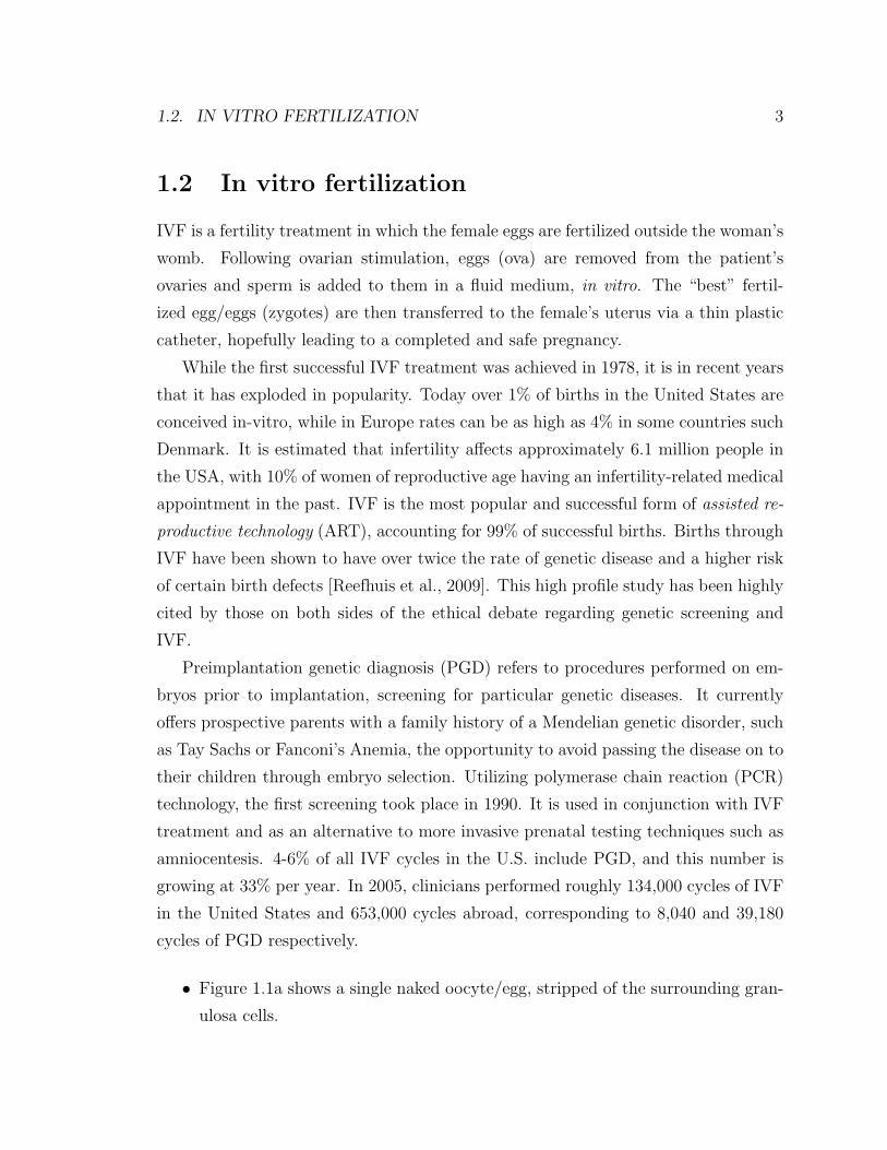
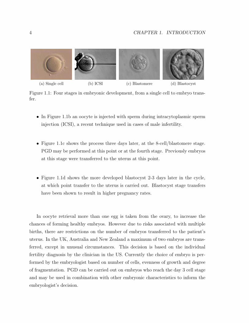
• Figure 1.1a shows a single naked oocyte/egg, stripped of the surrounding gran-
ulosa cells.
4 CHAPTER 1. INTRODUCTION
(a) Single cell (b) ICSI (c) Blastomere (d) Blastocyst
Figure 1.1: Four stages in embryonic development, from a single cell to embryo trans-fer.
• In Figure 1.1b an oocyte is injected with sperm during intracytoplasmic sperm
injection (ICSI), a recent technique used in cases of male infertility.
• Figure 1.1c shows the process three days later, at the 8-cell/blastomere stage.
PGD may be performed at this point or at the fourth stage. Previously embryos
at this stage were transferred to the uterus at this point.
• Figure 1.1d shows the more developed blastocyst 2-3 days later in the cycle,
at which point transfer to the uterus is carried out. Blastocyst stage transfers
have been shown to result in higher pregnancy rates.
In oocyte retrieval more than one egg is taken from the ovary, to increase the
chances of forming healthy embryos. However due to risks associated with multiple
births, there are restrictions on the number of embryos transferred to the patient’s
uterus. In the UK, Australia and New Zealand a maximum of two embryos are trans-
ferred, except in unusual circumstances. This decision is based on the individual
fertility diagnosis by the clinician in the US. Currently the choice of embryo is per-
formed by the embryologist based on number of cells, evenness of growth and degree
of fragmentation. PGD can be carried out on embryos who reach the day 3 cell stage
and may be used in combination with other embryonic characteristics to inform the
embryologist’s decision.
1.3. GENE SECURITY NETWORK (GSN) 5
1.3 Gene Security Network (GSN)
GSN Mission: Enable clinicians to use complex genetic and phenotypic information
to make effective medical interventions.
Figure 1.2: GSN Logo
Gene Security Network is a molecular diagnostics company that has developed
proprietary bioinformatics technologies for complex testing of small quantities of ge-
netic material. GSN operates a laboratory for preimplantation genetic diagnosis to
guide doctors in screening embryos for disease susceptibility during in-vitro fertiliza-
tion. The company is based out of Redwood City, California.
Current PGD technology cannot provide parents information on the vast major-
ity of inherited diseases, which have the non-Mendelian inheritance patterns outlined
previously. GSN’s major advancement thus far is in their proprietary technology,
Parental Support, which uses noisy genetic measurements on the blastomeres in com-
bination with:
• Parents’ diploid blood samples
• Father’s haploid sperm sample
• Data from dbSNP
• Data from Hapmap project
Hence they can reconstruct the embryonic DNA at high confidence level; with
sensitivity and specificity above 99.9%. The cost for GSN’s method is $250 versus
the current cost of $5000-$7000 for existing PCR-based techniques. An overview of
the full role played by GSN in a typical IVF treatment is found in Figure 1.3.
If the prospective parents request PGD, blood and sperm samples are taken firstly.
This allows GSN to predict the risk of each genetic disease, utilizing the methods
6 CHAPTER 1. INTRODUCTION
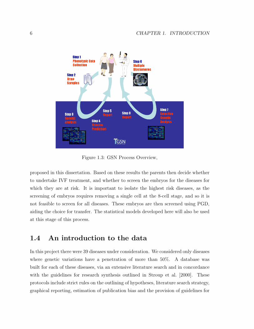
Figure 1.3: GSN Process Overview,
proposed in this dissertation. Based on these results the parents then decide whether
to undertake IVF treatment, and whether to screen the embryos for the diseases for
which they are at risk. It is important to isolate the highest risk diseases, as the
screening of embryos requires removing a single cell at the 8-cell stage, and so it is
not feasible to screen for all diseases. These embryos are then screened using PGD,
aiding the choice for transfer. The statistical models developed here will also be used
at this stage of this process.
1.4 An introduction to the data
In this project there were 39 diseases under consideration. We considered only diseases
where genetic variations have a penetration of more than 50%. A database was
built for each of these diseases, via an extensive literature search and in concordance
with the guidelines for research synthesis outlined in Stroup et al. [2000]. These
protocols include strict rules on the outlining of hypotheses, literature search strategy,
graphical reporting, estimation of publication bias and the provision of guidelines for

1.4. AN INTRODUCTION TO THE DATA 7
future research. Alzheimer’s, cystic fibrosis, breast cancer, myocardial infarction and
psoriasis are some of the candidate diseases under research. In this dissertation we will
concentrate on the analysis of two particular datasets, those relating to Alzheimer’s
disease and psoriasis.
As a general introduction to the data structure however, each database consists
of approximately 100 published papers. Patient recods are aggregated by key demo-
graphic, clinical and genotypic variables. For example in the Alzheimer’s database,
one such paper is Tsuang et al. [2005] (Table 1.1). A summary of the subjects involved
in this study is provided below:
• Gene = ApoE
• Ethnicity = Caucasian
• Familial History = NA
• Onset = NA
• Mean(Age) = 67.70
• SD(Age) = 10.7
There are some variables present (case-control and gender/ApoE), missing (familial
history, onset and ApoE/gender) and conditional (ethnicity) in each of the respective
observed tables.
Case ControlMale 19 93
Female 38 104
Case Controlε2 ε2 0 0ε2 ε3 3 32ε2 ε4 1 3ε3 ε3 21 118ε3 ε4 29 47ε4 ε4 5 3
Table 1.1: Tsuang et al. [2005]
8 CHAPTER 1. INTRODUCTION
1.5 Previous research
Historically, techniques such as (i) the analysis of complete cases only, (ii) single value
imputation and (iii) Buck’s method have been utilized for the meta-analysis of data
with missing values. Under the analysis of only complete cases, it is assumed that
the complete cases are representative of the original sampling. This is not always
reasonable, especially in cases where there is informative censoring/missingness. Sin-
gle value imputation fills in with the mean value of the variable calculated from the
cases that observed the variable. It does however, assume a high degree of homo-
geneity and thus underestimates the variance. Adjustments are possible, but tests
for homogeneity of effect sizes are not. Buck’s method replaces missing values with
the conditional mean. For every pattern of missing data, complete cases are used
to calculate regression equations predicting a value for each missing variable using
the set of completely observed variables. This assumes that the missing variables are
linearly related to other variables in the data.
More advanced model-based techniques have been developed, which may be amended
to deal with categorical data structures for research synthesis. Maximum likelihood
approaches are outlined in Little and Rubin [2002] and analogous Bayesian methods
are provided in Schafer [1997]. Unfortunately, neither of these methods is sufficient
for the needs of the datasets explored in this analysis.
It has been established that there are three different types of missing data in
research synthesis; missing studies in the sample (publication bias), missing effect
sizes from particular studies and missing information on study characteristics. It is
the second of these which is most prevalent in our research. The technical reasons for
missing data in studies are threefold also.
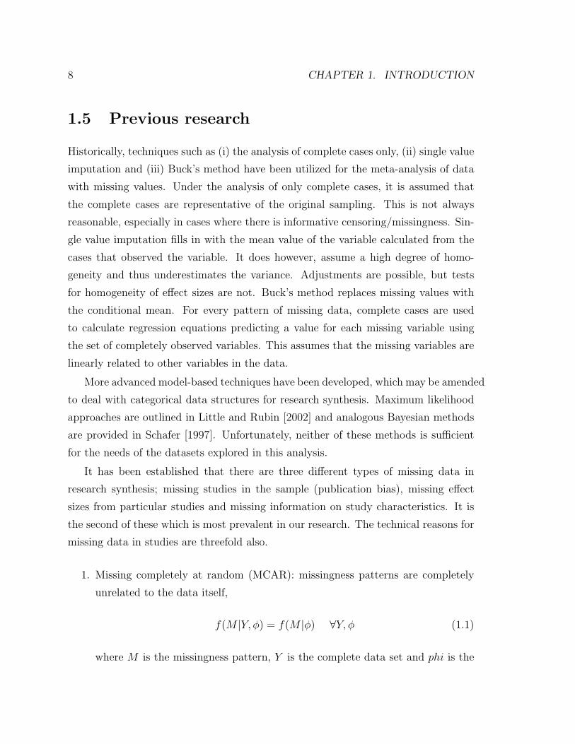
1. Missing completely at random (MCAR): missingness patterns are completely
unrelated to the data itself,
f(M |Y, φ) = f(M |φ) ∀Y, φ (1.1)
where M is the missingness pattern, Y is the complete data set and phi is the

1.6. OUTLINE OF THE DISSERTATION 9
unknown parameter under investigation. If the reasons for the missing values
are not related to any information in the data set itself, then complete cases
may be considered a random sample of the original set of studies.
2. Missing at random (MAR): missingness patterns are related to the completely
observed components,
f(M |Y, φ) = f(M |Yobs, φ) ∀Ymiss, φ (1.2)
where Y = Ymiss ∪ Yobs, with Ymiss and Yobs the missing and observed data
respectively. This assumption is less strict than MCAR and is the most common
made in developing new methods for handling missing data.
3. Not missing at random (NMAR): missingness patterns are related to the missing
values themselves,
f(M |Y, φ) = f(M |Yobs, Ymiss, φ) ∀φ. (1.3)
NMAR would occur if study results or effect sizes were not reported when
not significant. Censoring in survival analysis is another common example of
not missing at random, as patients may leave the study for reasons directly
attributable to the treatment effect.
1.6 Outline of the dissertation
Chapter 2 will consider likelihood-based approaches to this class of problems. We
will introduce the notation used throughout this thesis and derive a generalized EM
algorithm based on meta loglinear models. Extensions and modifications to this
algorithm are also introduced, to deal with issues specific to the data structures.
Tests for homogeneity and finding influential studies are explained, and existing tests
for model adequacy are to accommodate this new class of model.
In Chapter 3, we will introduce a Bayesian alternative based on data augmentation
techniques. In addition to providing a natural method for variance estimation, the

10 CHAPTER 1. INTRODUCTION
derived algorithm will allow for the analysis of the full posterior distribution.
Chapter 4 concentrates on the various options available for variance estimation
under the models proposed in earlier chapters. We will consider such methods as
the sandwich estimator, the jackknife, bootstrapping, posterior standard error and
multiple imputation. Simulation studies are carried out to establish the adequacy of
each of these methods.
In Chapter 5, we will develop methods to adjust for retrospective sampling in mul-
tiway tables. Logistic and loglinear models are compared, with instances of equiva-
lency and difference investigated. Simulations studies confirm the validity of the new
retrospective adjustments.
Chapter 6 and Chapter 7 will contain the results of the analysis of the Alzheimer’s
and psoriasis data sets. We will fit both the likelihood-based and Bayesian models
and investigate the model adequacy, comparing against the limited existing methods.
Discussion and conclusions shall be provided in Chapter 8.
Chapter 2
Likelihood-based Methods
2.1 Notation
So if we consider a multivariate distribution π obtained by the crossing of a collection
of K categorical factors F = F1, . . . FK, the kth of which has Lk levels. π is a
multiway table of probabilities with each element ∈ [0, 1] and the sum of all the
elements is 1. The dimension of π is L1 × L2 × . . . × LK . We will use the notation∑F πF = 1. If we partition the variables in F into two mutually exclusive subsets
O and M, with O ∪M = F , then πO =∑M πF =
∑M πO,M denotes the marginal
table indexed by variables in O obtained by summing the entries of π over all levels
of the variables inM. O shall be referred to as observed variables andM as missing
or marginal variables.
We have data from S different studies, and the ith such study gives us an observed
table NOi, i.e it is a complete table on a subset Oi of the variables in F . The Oi of
different studies will typically involve different variables, and also different numbers
of variables. Also, typically none of the studies will have Oi = F , although this is not
excluded. The goal of this meta-analysis is to combine all these studies to produce a
coherent estimate πF of πF .
We shall also generalize this model to deal with other kinds of partial information:
(i) Rather than a marginal table we sometimes see a section or slice; we see a
complete table in Oi, but rather than marginalized wrt toMi, it is conditioned
11

12 CHAPTER 2. LIKELIHOOD-BASED METHODS
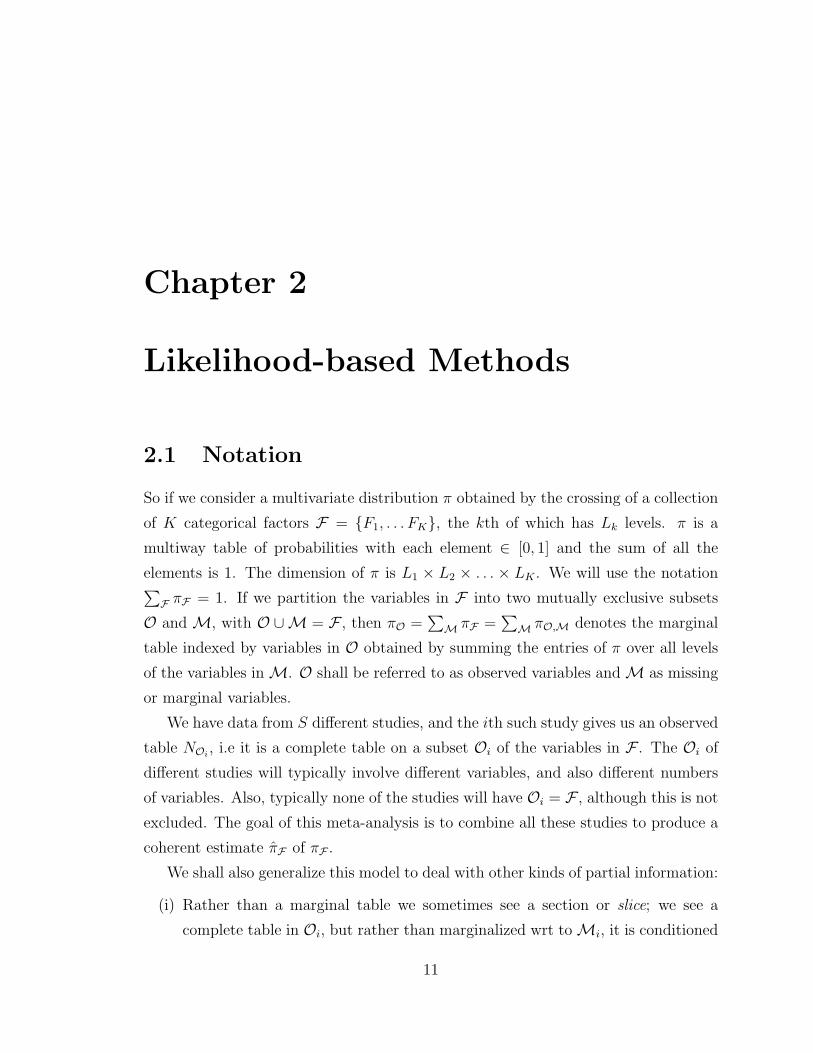
(a) Basic three factor contingency table (b) Two factors observed, one marginal/missing
Figure 2.1: Examples of three-way contingency tables
on particular values for each of the variables in Ci, with Oi ∪ Ci = F .
(ii) We can see both marginals and slices. We see a complete table inOi, conditioned
on particular values of variables in Ci, and all marginalized wrt to Mi, with
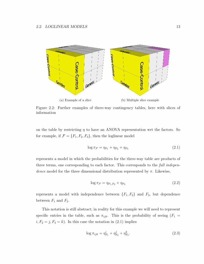
Oi ∪ Ci ∪Mi = F . A figurative example of this is shown in Figure 2.2a.
(iii) It is possible for a single study to comprise of multiple tables, each with their
own set of observed, missing and conditional variables. Study i may contain of
numerous tables, the jth of which has the following variable set (Oji ,Mji , C
ji ),
with Oji ∪Mji ∪C
ji = F for each j. Multiple colored slices may be seen in Figure
2.2b.
Initially we deal only with the simple marginal case, but later we discuss these other
three cases also.
2.2 Loglinear models
A traditional approach to modeling a multiway table is to represent the probabilities
by a loglinear model log π = η, where we implicitly assume that the entries in π are
strictly ∈ (0, 1). Usually we have only a single observed table N , and impose structure
2.2. LOGLINEAR MODELS 13
(a) Example of a slice (b) Multiple slice example
Figure 2.2: Further examples of three-way contingency tables, here with slices ofinformation
on the table by restricting η to have an ANOVA representation wrt the factors. So
for example, if F = F1, F2, F3, then the loglinear model
log πF = ηF1 + ηF2 + ηF3 (2.1)
represents a model in which the probabilities for the three-way table are products of
three terms, one corresponding to each factor. This corresponds to the full indepen-
dence model for the three dimensional distribution represented by π. Likewise,
log πF = ηF1,F2 + ηF3 (2.2)
represents a model with independence between F1, F2 and F3, but dependence
between F1 and F2.
This notation is still abstract; in reality for this example we will need to represent
specific entries in the table, such as πijk. This is the probability of seeing (F1 =
i, F2 = j, F3 = k). In this case the notation in (2.1) implies
log πijk = ηiF1+ ηjF2
+ ηkF3. (2.3)

14 CHAPTER 2. LIKELIHOOD-BASED METHODS
Thus the number of different constants of the form η`F represented by a generic term
like ηF is the number of levels of F . Likewise, the number of constants for a generic
term ηF1,F2 is L1 × L2.
Just as in multiway ANOVA, this would lead to a redundant coding, and certain
parameters would be aliased with each other and hence not be identifiable. Two
general approaches to combat this are
1. Set every instance of ηLj
Fj= 0 — i.e. any constant involving any of the factors
at the highest level to zero.
2. Include a quadratic regularization term on all the constants when fitting the
model.
For this application we prefer 1.
One can enumerate the entire set of models of this form for any given high-
dimensional table. Typically we chose one that has simple structure, but represents
the observed data well.
As an aside, many of the models correspond to some type of independence or con-
ditional independence, and hence can be represented by a graphical model (directed
acyclic graph). There are some, such as
log πF = ηF1,F2 + ηF2,F3 + ηF1,F3 (2.4)
(no third-order interaction model) which does not represent any form of conditional
independence, and cannot be uniquely represented by a graphical model.
Usually we represent model such as (2.1),(2.2) & (2.4) in terms of a model matrix
X and a parameter vector θ:
log π = η(θ) = Xθ (2.5)
Here π is a vector of probabilities of length∏K
k=1 Lk, filled in lexicographical ordering
(indices varying most rapidly from right to left). The parameter vector θ consists of
all the identifiable parameters in the model, excluding the ones that are zero, and
2.3. FITTING LOGLINEAR MODELS 15
the rows of X are filled with zeros and ones to indicate the presence or absence of a
particular parameter for that element of log π.
Loglinear models are well described in a number of books, such as McCullagh and
Nelder [1983].
2.3 Fitting loglinear models
Typically loglinear models are fit using Poisson maximum-likelihood. Often a multi-
nomial is more appropriate, since the original sample was conditional on certain
marginals. It turns out that as long as there are terms in the loglinear model corre-
sponding to these fixed counts, Poisson ML is equivalent to multinomial ML.
The log-likelihood of an observed table, given a model structure is
`(θ) = n∑F
(rFηF(θ)− eηF (θ)), (2.6)
where rF = NF/n are the observed proportions, and n =∑F NF is the total count in
the table. This log-likelihood is convex in θ (if X is full column rank). Differentiating
wrt θ, and using (2.5), we get (in matrix notation)
d`(θ)
dθ= nXT (r− π) = 0 (2.7)
These equations are quite intuitive, since X is binary. It says that certain marginals
of the fitted table π should match the corresponding data marginals. In fact, the
marginals that have to match correspond exactly to the presence of terms indexed
by factors in (2.1),(2.2) & (2.4). The iterative proportional fitting algorithm (IPF)
exploits this fact, and starting with a constant table, cycles around correcting the
table so that it matches each marginal as required in turn.
Alternatively we can compute the Hessian matrix
d2`(θ)
dθdθT= −nXTDπX, (2.8)

16 CHAPTER 2. LIKELIHOOD-BASED METHODS
and use the Newton algorithm to solve for θ. Here Dπ = diag(π).
Conveniently, the Newton algorithm can be represented as an iteratively reweighted
least squares (IRLS) algorithm:
1. Compute the working response z = η + D−1π (r− π).
2. Fit a weighted linear regression of z on X with weights Dπ to update the
coefficients θ.
2.4 Meta loglinear models
We now propose a method to generalize the loglinear model for the multiple study
scenario outlined in Section 2.1. Each of the observed tables N iOi
is indexed by a
subset Oi ⊆ F of the full collection of factors. We consider the following model for
π:
log πF =S∑i=1
ηOi. (2.9)
This model has loglinear terms to cover each of the observed tables, likely with many
redundancies. These redundancies can easily be removed when the model is repre-
sented in the form (2.5), simply by removing duplicate columns in X. We will write
this model as
log πF = xTFθ (2.10)
We propose to fit the model by maximizing the likelihood of the observed tables
N iOi
. Oi represents the factors in F observed for study i, and its complementMi are
those factors in F not observed. The probabilities under the model of the observed
factors are
πOi=
∑Mi
πF (2.11)
=∑Mi
exTFθ (2.12)
2.4. META LOGLINEAR MODELS 17
Hence the sum of the Poisson log-likelihoods of the observed tables is
`(θ) =S∑i=1
ni∑Oi
[riOilog πOi
(θ)− πOi(θ)] (2.13)
Again riOiare the observed proportions corresponding to N i
Oi, and ni =
∑OiN iOi
is
the total count for study i. As such ni is the weight assigned to study i, and we may
consider other weights if there is too much imbalance.
Although in principle we could go through the motions to maximize (2.13), we
no longer get a simple expression for the gradient. This is because each of the terms
log πOi(θ) is a log of a sum of exponential terms, and does not simplify. This is
a classical case for the EM algorithm [Dempster et al., 1977], which is an iterative
algorithm for simplifying such situations.
Next we present the EM algorithm for this meta analysis. It consists of alternating
the following two steps till convergence.
E Step: For each observed table riOi, fill it out to become a full table riF by expanding
the missing dimensions using the current estimate πF :
riF = riOiπMi|Oi
(2.14)
= rOi
πFπOi
(2.15)
M Step: Fit the model using the filled out tables by maximizing the full log-likelihood
`full(θ) =M∑i=1
ni∑F
[riF log πF(θ)− πF(θ)]. (2.16)
Note that, because of (2.10), the first term in the sum simplifies. It is easy to see
that the gradient is given by
d`full(θ)
dθ=
M∑i=1
niXT (riF − πF). (2.17)

18 CHAPTER 2. LIKELIHOOD-BASED METHODS
Letting
rF =
∑Si=1 nir
iF∑S
i=1 ni, (2.18)
we see that the likelihood equation simplifies to
XT (rF − πF) = 0. (2.19)
We are back in the situation of Section 2.3, and this equation can easily be solved by
either the Newton method or IPF.
There may be occasion to fit a saturated multinomial model rather than the meta-
loglinear model outlined in the algorithm above. This may be achieved quite easily
with an EM algorithm similar to that outlined above. The E-step in fact remains
completely unchanged, with the M-step becoming merely a weighted mean of the
expanded tables.
2.5 Modifications to deal with complex data struc-
tures
In the introduction to this chapter we described three types of data structure not
addressed in the basic EM algorithm outlined in Section 2.1. In this section we
propose some amendments to the algorithm to incorporate such data.
(i) We may observe all the variables in Oi, but at fixed levels of each of the variables
in Ci. In this case, we need to modify our model and the E-step of the EM
algorithm. For the model, we should include a term corresponding to Oi ∪Ci =
F ; in other words the complete model. For the E-step, let ci be the actual
levels of the variables in Ci that are observed; hence our observed partial table
can be written ni · riOi|Ci=ci . Let the current estimated conditional table be
πOi|Ci . Let πiOi|Ci be the modification of πOi|Ci obtained by replacing πOi|Ci=ci
with riOi|Ci=ci .Then
riF = πiOi|Ci πCi . (2.20)

2.5. MODIFICATIONS TO DEAL WITH COMPLEX DATA STRUCTURES 19
(ii) If we observe a slice in some variables, and some are missing (marginal), then
our strategy is similar. The model term corresponds to Oi ∪Ci. For the E-step,
we need to first marginalize πF with respect toMi to compute πOi∪Ci and hence
πOi|Ci . Then we proceed as above, obtaining
riOi∪Ci = πiOi|Ci πCi , (2.21)
and finally
riF = riOi∪Ci πMi|(Oi∪Ci) (2.22)
= πiOi|Ci πCi πMi|(Oi∪Ci).
(iii) We may observe multiple slices, each with an associated set of missing variables.
Again, adjustments are required to the E-step and the model term. Firstly we
need to marginalize with respect to the appropriate missing dimensions Mji
for all j = 1, . . . , J , to compute πOji∪C
ji
and hence πOji |C
ji. Proceeding with the
modification steps already outlined above, we can calculate the estimated full
table for the jth table in study i
rij
F = πij
Oji |C
ji
πCjiπMj
i |(Oji∪C
ji ). (2.23)
Hence we can find the estimated full table for study i as the weighted mean of
these tables
riF =J∑j=i
njiniri
j
F . (2.24)
Although not obvious at first, this is in fact equivalent to providing a relative
weighting on the observed partial tables and then carrying out the expansion
in a more step-by-step process. This is explained in Section 6.3. Both methods
produce the ML solution for the full set of expanded tables, as each observed
table contains an independent set of observations. This elegant solution is only
possible since we assumed disjoint perspectives only, which is true in our dataset,

20 CHAPTER 2. LIKELIHOOD-BASED METHODS
but perhaps not more widely. Therefore we mutually satisfy each observed
margin, without introducing any further model complexity. Similarly the P-Step
in the Bayesian method outlined in Sections 3.3.1 and 3.4 provides an equivalent
solution involving the summation of the cell counts rather than weighting the
cell probabilities.
In more complicated situations where we do not have disjoint slices, it is neces-
sary to use the IPF algorithm in solving for the ML estimate of the full table.
This would allow us to mutually satisfy the marginal densities, even if they
contain some intersection. The Bayesian solution would follow a similar line,
with constrained sampling from product multinomial distributions.
There are in fact multiple model terms relating to this study;O1i ∪ C1
i , . . . ,OJi ∪ CJi
.
In each of the three cases above, the weight ni is the total number of observations
observed in the study.
2.6 The ECM Algorithm
In many cases, and especially with large data sets, the EM algorithm may be unduly
cumbersome. Even with the huge advances in computing speed convergence times
may be debilitating, and therefore speed-ups to the algorithm are attractive. It has
been shown [Meng and Rubin, 1993] that it may not be necessary to iterate until full
convergence at each M-step, with a single cycle of the model-fitting process sufficient.
In the context of the algorithm we have proposed in this chapter, this would equate
to a single cycle of the IPF algorithm. This modification has become known as
the expectation-conditional maximization (ECM) algorithm. ECM retains the same
reliable convergence properties as EM, increasing the observed-data log-likelihood at
each step. The M-step is replaced by the quicker CM-step, which still asymptotically
converges to a maximum over the full parameter space ΘM . As in IPF, the starting
values for θ should lie in the interior of the parameter space, with structural zeros
being assigned a zero/null value and uniform values elsewhere as advised in Agresti
[2002].

2.7. INVESTIGATING THE IPF ALGORITHM 21
µ11 µ12 . . . µ1J
µ21 µ22 . . . µ2J
......
. . ....
µI1 µI2 . . . µIJ
Table 2.1: Poisson Param’s(µ)
n11 n12 . . . n1J
n21 n22 . . . n2J
......
. . ....
nI1 nI2 . . . nIJ
Table 2.2: Observed Data (D)
2.7 Investigating the IPF algorithm
Throughout this dissertation we speak about methods to combine different sources
of marginal and conditional information, in fact this is the central thesis of our work.
In particular we have discussed the use of the iterative proportional fitting algorithm
(IPF) as a method to find the ML estimates when we have multiple perspectives on
the same data. This method is well-established in cases where a full table is known
and a constrained model is required [Agresti, 2002]. However, the literature does not
explicitly consider data where multiple independent margins or slices are produced
from a single study, i.e. where no full table is observed. In this section we will
introduce some of the different forms of marginal information that may arise from
Poisson generated contingency tables, where data arrives only in a partially classified
form. We will show that the estimates produced by the IPF algorithm are in fact the
ML estimates of the unknown parameters (cell probabilities).
2.7.1 Case 1: Full information
Firstly and most trivially, we will consider the simplest case whereby we have full
information on the table of interest, in order to familiarize ourselves with the notation
that will be used hereafter. In the two-way example we are given an IxJ table of
Poisson parameters (µ) and an IxJ set of observed counts (D).
Pµ(D) =I∏i=1
J∏j=1
e−µijµnij
ij
nij!(2.25)
= eµ..
I,J∏i,j=1
µnij
ij
nij!(2.26)

22 CHAPTER 2. LIKELIHOOD-BASED METHODS
Therefore the log-likelihood is,
⇒ `D(µ) = −µ.. +
I,J∑i,j=1
nijlogµij +
I,J∑i,j=1
log(nij!) (2.27)
and unsurprisingly the MLE’s are,
µij = nij (2.28)
2.7.2 Case 2: Two margins
In this second case we shall consider situations where we are provided with two
margins of information for a two-way table. We are not privy however to any full
information, i.e. a fully categorized two-way table. We observe the two margins
D = D1 ∩D2, shown in Table 2.4.
µ11 µ12 . . . µ1J µ1.
µ21 µ22 . . . µ2J µ2.
......
. . ....
...µI1 µI2 . . . µIJ µI.
µ.1 µ.2 . . . µ.J µ..
Table 2.3: Poisson Param’s(µ)
n1.
n2.
...nI.
n.1 n.2 . . . n.J
Table 2.4: Observed Data (D)
Pµ(D) = P (D1 ∩D2) = P (D1 ∩D2|n..)P (n..) (2.29)
= P (D1|n..)P (D2|n..)P (n..) (2.30)

2.7. INVESTIGATING THE IPF ALGORITHM 23
P (D1|n..) = P (X1. = n1., . . . , XI. = nI.|x.. = n..) (2.31)
=
∏Ii=1
e−µi.µni.i.
ni.!e−µ..µn..
..
n..!
(2.32)
=n..!∏Ii=1 ni.!
I∏i=1
µni.i.
µn....
(2.33)
=n..!∏Ii=1 ni.!
I∏i=1
πni.i. (2.34)
⇒ Pµ(D) =
(n..!∏Ii=1 ni.!
I∏i=1
πni.i.
)(n..!∏Jj=1 n.j!
J∏j=1
πn.j
.j
)(e−µ..
µn....
n..!
)(2.35)
`D(π, µ..) =I∑i=1
ni.logπi. +J∑j=1
n.jlogπ.j − µ.. + n..logµ.. + . . . (2.36)
∂lD(π, µ..)
∂µ..= −1 +
n..µ..
(2.37)
⇒ µ.. = n.. (2.38)
and the profile likelihood is,
`D(π) =I∑i=1
ni.logπi. +J∑j=1
n.jlogπ.j + . . . (2.39)
This has no direct solution, but if the two contraints,∑I
i=1 πi. = 1 and∑J
j=1 π.j = 1,
are added via Lagrangian multipliers we get a modified profile likelihood,
`D(π, λ1, λ2) =I∑i=1
ni.logπi. +J∑j=1
n.jlogπ.j − λ1
(I∑i=1
πi. − 1
)− λ2
(J∑j=1
π.j − 1
)(2.40)

24 CHAPTER 2. LIKELIHOOD-BASED METHODS
∂`D(π, λ1, λ2)
∂λ1
=I∑i=1
πi. − 1 Constraint 1 (2.41)
∂`D(π, λ1, λ2)
∂λ2
=J∑j=1
π.j − 1 Constraint 2 (2.42)
∂`D(π, λ1, λ2)
∂πi.=
ni.πi.− λ1 (2.43)
⇒ πi. = λ1ni. =ni.n..
(2.44)
with the last equality holding since,
I∑i=1
πi. =I∑i=1
λ1ni. = 1 (2.45)
⇒ λ1 =1∑Ii=1 ni.
=1
n..(2.46)
Since πi. =µi.µ..
it is found that µi. = ni. for all i = 1, . . . , I and similarly µ.j = n.j
for all j = 1, . . . , J . Therefore, given two margins of information, the likelihood only
provides information regarding the marginal sums. The estimates are consistent with
those produced under IPF.
2.7.3 Case 3: Multiple margins and higher dimensional ta-
bles
Generalizing the previous case, we can easily extend the proof to multidimensional
tables (IxJxKx. . .). For example in the IxJxK case we find that the maximum
likelihood approach leads to µi.. = ni.. for all i = 1, . . . , I, µ.j. = n.j. for all j = 1, . . . , J
and µ..k = n..k for all k = 1, . . . , J . Again it is relatively straightforward, using the
methods from Case 2 above, to show equivalency between the estimates provided by
the IPF algorithm and the true ML estimates.

2.8. TESTING HOMOGENEITY AND DETECTING ABERRANT STUDIES 25
2.8 Testing homogeneity and detecting aberrant
studies
Before pooling the estimates of an effect size from a series of studies, it is important
to determine whether the studies can be described as sharing a common effect size.
The Q-statistic [Hedges and Olkin, 1985] has been developed as a statistical test for
the homogeneity of the effect size. Formally it is a test of the hypothesis
Ho : θ(1) = θ(2) = . . . = θ(S) (2.47)
versus the alternative that at least one differs. θ(i) is a length p vector of effect sizes for
study i, with θ(i) the associated estimate. Define the column vector θ∗ of dimension
Sp by
θ∗ = (θ(1), . . . , θ(S))′. (2.48)
Similarly define the associated estimated covariance matrix Σ∗ by
Σ∗ = Diag(Σ(1), . . . , Σ(S)). (2.49)
where Σ(1), . . . , Σ(S) are the large sample estimates of the covariance matrices of the
θ(1), . . . , θ(S). We can now calculate the Q-statistic
Q∗ = θ′∗Cθ∗, (2.50)
where
C = Λ∗ − Λ∗ee′Λ∗/e
′Λ∗e, (2.51)
Λ∗ is the inverse of Σ∗ and e is column vector of Sp ones.
The formal test is based in the fact that if θ(1) = . . . = θ(S) and the sample size
in all studies is reasonably large, then Q∗ has a chi-square distribution with (S − 1)p
degrees of freedom.
Another method to detect aberrant studies utilizes the jackknife samples found
in the variance estimation (Section 4.4). Faulty or suspicious data can be identified

26 CHAPTER 2. LIKELIHOOD-BASED METHODS
using the jackknife influence statistic, which measures the distance (d) between the
leave-one-out estimate and the left-out observations
d(θ(i), θ(.)
). (2.52)
It is necessary to select an appropriate distance measure for multivariate analysis, and
we have chosen to use the established Kullback-Leibler divergence (relative entropy)
[Kullback and Leibler, 1951],
d(θ(i), θ(.)
)=∑
θ(i)logθ(i)
θ(.)
. (2.53)
2.9 Modifications for retrospective studies
The methods proposed thus far in this dissertation have dealt exclusively with data
collected from prospective research studies. However, in retrospective or observational
sampling designs, such as case-control biomedical studies, an adjustment is required
in order to correctly estimate the effect sizes. This topic will be explored detail in
Chapter 5.
2.10 Model selection and testing goodness-of-fit
It is customary to measure the quality of a model and test it against alternatives, to
ensure both model optimization and parsimony. The goodness-of-fit of a statistical
model describes how well it fits a set of observations. For loglinear models we use the
deviance likelihood ratio test (G2) or Pearson chi-squared statistic (X2)
G2 = 2∑j
njlog
(njµj
)X2 =
∑j
(nj − µj)2
µj(2.54)
2.10. MODEL SELECTION AND TESTING GOODNESS-OF-FIT 27
with nj denoting the observed data and µj the expected counts under the proposed
model.
These tests may be extended to cases with partially classified tables. In these
circumstances, we sum over the incomplete tables, but unlike the complete-data cases
we obtain nonzero values for the test statistics under the saturated model. In fact
the values for G2 and X2 for the saturated model provide tests for whether the data
are missing completely at random (MCAR) or missing at random (MAR). Chi-square
statistics for restricted models may be obtained by calculating G2 (or X2) for both
the restricted model and the saturated model, and subtracting these two quantities
[Fuchs, 1982].
G2 = 2S∑i=1
∑Oi
niriOilog
(riOi
rOi
)−G2
0
X2 =S∑i=1
∑Oi
ni(riOi− rOi
)2
rOi
−X20 (2.55)
where G20 and X2
0 denote the value of the statistic evaluated at the MLE for the
saturated model. Also both G2 and X2 are χ2 distributed with df = q− p− 1, where
q is the total number of cells in the contingency table and p is the number of terms
in the fitted loglinear model. It should be noted that these two test statistics have
the same number of degrees of freedom as the chi-square test for the restricted model
with complete data. Using these tests we may compare competing models and test
hypotheses such as the inclusion and exclusion of parameters.
An alternative method for choosing the most appropriate model is cross-validation.
Cross-validation has been proposed in model-selection for many other situation such
as those outlined in Hastie et al. [2001]. We naturally have a leave-one-out sample
via the jackknife method (Section 4.4). For each sample, we fit models of different
sizes to each of the training set, with α denoting the tuning parameter of model size,

28 CHAPTER 2. LIKELIHOOD-BASED METHODS
and then test each model on the left out sample.
CV (α) =1
N
N∑i=1
L(yi, f
−κ(i)(xi, α))
(2.56)
Here CV (α) is an unbiased estimate of the test error curve, under some chosen loss
function L. yi are the observed responses, and f−κ(i)(xi, α) is the estimated fit on the
test set, based on the model found on the training set. Hence we find the model size
α which minimizes this test error. The best model (f(x, α)) of this size is then fitted
to the full data set. It should be noted that the fitted model of size α may or not be
equivalent to any of the best models in the leave-one-out samples.

Chapter 3
Data Augmentation
3.1 The Data Augmentation algorithm
To date we have exclusively considered and developed likelihood-based approaches
to this class of problems. However, various Bayesian methods have been created as
an alternative to the EM framework, most notably data augmentation [Tanner and
Wong, 1987]. Throughout this chapter I will assume that the reader a rudimentary
knowledge of modern statistical methods, and so will not delve into great depth on
the basics of distribution theory nor Bayesian methods.
The data augmentation (DA) algorithm is analogous to the EM algorithm, in
that is exploits the simplicity of the likelihood function (posterior distribution) of
the unknown parameter given the augmented data. Interestingly the steps of the
algorithm also follow the same logic as the EM and this is seen below. In contrast to
the EM algorithm where just the maximum and curvature are found, in DA the entire
posterior distribution is obtained. This is especially useful in improving inference in
small sample cases, where assumptions about the regularity of the likelihood may be
questionable.
The DA algorithm augments the observed data Y with some latent data Z. The
overall aim of this algorithm is the calculation of the posterior distribution p(θ|Y ), but
unfortunately this is intractable due to the presence of the latent data. Given both
Y and Z, it is assumed that one can calculate or at least sample from p(θ|Y, Z), the
29
30 CHAPTER 3. DATA AUGMENTATION
augmented posterior distribution. So in order to procure the posterior distribution,
multiple imputations of Z from the predictive distribution p(Z|Y ) are found and then
we compute the average of p(θ|Y, Z) over these imputations. However since p(Z|Y )
depends on p(θ|Y ), an iterative algorithm is necessary for the calculation of p(θ|Y ).
There are two identities which provide the foundation for the DA algorithm:
1. The posterior identity:
p(θ|Y ) =
∫Z
p(θ|Y, Z)p(Z|Y )dZ. (3.1)
2. The predictive identity:
p(Z|Y ) =
∫Θ
p(Z|φ, Y )p(φ|Y ), (3.2)
where p(Z|φ, Y ) is the conditional predictive distribution. Monte Carlo methods
are used to perform the integration in the posterior identity. Given a value θ(t) of θ
drawn at iteration t the DA algorithm iterates between the following two steps:
Imputation (I) Step: Generate a sample z1, z2, . . . , zm (Z(t+1)) from the current
approximation to the predictive distribution p(Z|Y, θ(t)).
Posterior (P) Step: Update the current approximation of p(θ|Y ) as the mixture of
the augmented posteriors of θ, i.e. draw θ(t+1) with density p(θ|Y, Z(t+1)).
This iterative procedure can be shown to eventually converge to a draw from the
joint distribution of Z, θ|Y as t tends to infinity. The value of m need not be very
large, in fact with m = 1 the DA algorithm reduces to a special case of the Gibbs
sampler where the random vector is just partitioned into two sub-vectors [German
and German, 1984].

3.2. DIRICHLET-MULTINOMIAL CONJUGATE PAIR 31
3.2 Dirichlet-Multinomial conjugate pair
3.2.1 The Multinomial distribution
Suppose that Y = (y1, y2, . . . , yn)T , with yi a categorical variable taking one of C
possible values c = 1, 2, . . . , C. If we set nc to be the number of observations for
which yi = c, then∑C
c=1 nc = n. Conditional on the total sample size n, the counts
in each category (n1, n2, . . . , nC) have a multinomial distribution with probabilities
π = (π1π2, . . . , πC) and index n. It should be noted that∑C
c=1 πc = 1 and therefore
the sampling distribution is:
p(Y |π) =
(n!
n1!n2! . . . nC !
)( C∏c=1
πncc
)(3.3)
Hence we find the likelihood of θ to be:
`(π|Y ) =C∑c=1
nclogπc, (3.4)
and the MLE is found to be πc = nc/n, the sample proportion. The binomial is a
special case of the multinomial distribution, where C = 2.
3.2.2 The Dirichlet distribution
Suppose that π = (π1, π2, . . . , πC) is a vector of random variables with the property
that πc ≥ 0 for all c = 1, 2, . . . , C and∑C
c=1 πc = 1. Then π is said to have a Dirichlet
distribution with parameter α = (α1, α2, . . . , αC) with density:
p(π|α) =Γ(∑C
c=1 αc)
Γ(α1)Γ(α2) . . . ,Γ(αC)πα1−1
1 πα2−12 . . . παC−1
C (3.5)
over the simplex Π, where Γ denotes the gamma function. This is a valid proba-
bility density if πc > 0 for all c = 1, 2, . . . , C.
The Dirichlet distribution is a multivariate generalization of the Beta distribution.

32 CHAPTER 3. DATA AUGMENTATION
3.2.3 The conjugate pair
In fact the Dirichlet density 3.4 is of the same functional form as equation 3.3 and
so they form a conjugate pair. So if we assume that the prior density for the π
parameters in equation 3.3 have a Dirichlet distribution, D(α), then the posterior
distribution is found to be:
p(π1, π2, . . . , πC |Y ) ∝C∏c=1
πnc+αc−1C , (3.6)
again with πc > 0 for all c = 1, 2, . . . , C and∑C
c=1 πc = 1. In other words, it is
Dirichlet(nc + αc). Therefore, the posterior mean of πc is (nc + αc)/(n. + α.), where
n. =∑C
c=1 nc and α. =∑C
c=1 αc. There are some common choices for αc:
1. αc = 0 for all c = 1, 2, . . . , C, here the posterior mean coincides with the ML
estimate for complete-data cases for parameters which are linear functions of the
estimated terms π1, π2, . . . , πC . This choice is not suitable if there are empty
cells in the contingency table. This is an improper prior; the existence of a
proper posterior under this prior is not guaranteed.
2. αc = 1/2 for all c = 1, 2, . . . , C, this yields Jeffreys prior, an improper prior here
but a reasonable compromise between the choices of αc = 0 or αc = 1.
3. αc = 1 for all c = 1, 2, . . . , C, this is a diffuse prior and yields the uniform
distribution.
4. αc > 1 for all c = 1, 2, . . . , C, can be used as a flattening prior for sparse tables.
3.3 Existing models
Data augmentation methods have been developed to deal with structures similar to
those in our datasets. In fact in the original paper Tanner and Wong [1987] there
is some work on latent class analysis which utilizes the Dirichlet-Binomial conjugate
pair. Schafer [1997] elaborates on this area further, introducing two models for data

3.3. EXISTING MODELS 33
similar 1 to ours, the multinomial saturated model 3.3.1 and the constrained Bayesian
model 3.3.2. While the models proposed by Schafer deal with similar but more basic
data structures to those seen in our datasets, much work was required to develop new
methods to deal with such issues as:
• Each study provides information on just a subset of the risk factors. Schafer’s
methods deal with fully classified tables with additional partially classified ta-
bles.
• Dealing with conditional slices, where data is observed at conditional values of
some of the risk factors.
• Combining multiple sources of information from within a single study.
• Adjusting for retrospective sampling in each study.
3.3.1 Multinomial saturated model
Throughout this and Section 3.3.2, it is assumed that the ith observed study table,
riOi, contains information on a subset Oi of the K categorical factors. The remaining
factors, Mi, are missing for that study. In the EM algorithm in Chapter 2, the E
step consisted of filling out each riOiover the missing variables using the appropriate
conditional table, πMi|Oi, from the current estimate of the full table. Analogously in
the DA algorithm we simulate the sampling distribution to produce an appropriate
estimate of the full table for each study, riF . Under the assumption of a Dirichlet
prior θ ∼ D(α), the P step is then just a random simulation of θ from the augmented
posterior D(α + r). The algorithm iterates between the following two steps:
I Step: Draw each riF from its respective product multinomial distribution
M(niriOi, πMi|Oi
). (3.7)
1All data augmentation methods in this thesis were in fact developed independently of Schafer’swork, but the author does wish to acknowledge similarities in the basic methods.
34 CHAPTER 3. DATA AUGMENTATION
where πMi|Oi= πF
πOi. The summation of these complete-data tables r =
∑Si=1 nir
iF
is found for use in the P step below, as each of these simulated tables is viewed
as an independent draw from the true multinomial distribution. Hence, under the
Dirichlet-multinomial conjugacy in Section 3.2.3, the multinomial parameter for each
cell is the sum of the respective cells from the constituent tables.
P Step: Draw πF with from the augmented posterior density
D(r + α) (3.8)
3.3.2 Bayesian constrained model
The Bayesian iterative proportional fitting (IPF) DA algorithm follows much the
same form as that of the saturated multinomial model. In fact the I-steps in both
are exactly equivalent, with the changes coming in the posterior (P) step. Instead
of fitting a saturated multinomial model at the P step, constraints are put on the
Dirichlet posterior, mimicking those of the loglinear models in Section 2.4. The
iterative method of generating random draws from a constrained Dirichlet posterior
was first presented in Gelman et al. [1995]. There are obvious similarities between
this method and iterative proportional fitting; hence it was termed Bayesian IPF.
An example of the algorithm in operation is provided below for a three-way con-
tingency table, fitted with only two-way interactions (the model of homogeneous as-
sociation). The previous P step is replaced by three conditional posterior (CP) steps.
In the algorithm below, each of the r terms is a proportion in the observed tables,
and gijk are the simulated proportions in accordance with the model restrictions as
outlined for example in Equation 3.12.
I Step: Draw each riF from its respective product multinomial distribution
M(niriOi, πMi|Oi
). (3.9)
3.4. EXTENSIONS TO THE DA ALGORITHM 35
CP1 Step:
π(t+1/3)jkl = π
(t+0/3)jkl
(gjk+/g+++
π(t+0/3)jk+
)∀j, k, l. (3.10)
CP2 Step:
π(t+2/3)jkl = π
(t+1/3)jkl
(gj+l/g+++
π(t+1/3)j+l
)∀j, k, l. (3.11)
CP3 Step:
π(t+3/3)jkl = π
(t+2/3)jkl
(g+kl/g+++
π(t+2/3)+kl
)∀j, k, l. (3.12)
Here g(t+1/3)jk+ are draws from the Dirichlet distribution, with
p(πjk+|π(t)j+l, π
(t)+kl, Y
(t)) ∝J∏j=1
K∏k=1
παjk++µ(t)jk+−1, (3.13)
and g+++ =∑
JK gjk+. gj+L and g+kl are drawn subsequently with their correspond-
ing restrictions. Similarly to the ECM algorithm (Section 2.6) a single run through
the CP steps each iteration is sufficient. This helps to speed up convergence.
More details on both of these algorithms and practical advice on implementation
is available in chapter 4 of Schafer [1997].
3.4 Extensions to the DA algorithm
As outlined in Section 2.1, there are many novel issues found in the meta-analysis
datasets we have analyzed. While data augmentation methods have been researched
for the general case of multiple partially classified tables, extensions are required
in order to deal with these extra complications. Here we shall outline each of the
problems and the solution we have developed.
(i) We may observe all the variables in Oi, but at fixed levels of each of the variables
in Ci (a slice). Here Oi ∪ Ci = F is the model term contributed by the study to
the Bayesian IPF step and a modification to the I-step of the DA algorithm is

36 CHAPTER 3. DATA AUGMENTATION
necessary. If ci are the actual levels of the variables in Ci that are observed, our
observed partial table can be written niriOi|Ci=ci . It should be noted that this
section of the contingency table is in fact fully classified, with the remainder
of the table missing, i.e. Ci 6= ci or C ′i . Therefore we need only generate
multinomial samples in the section Oi|C′i with the distribution:
M
(ni
∑πOi|C
′i∑
πOi|Ci, πOi|C
′i
), (3.14)
where πOi|C′i
=∑C′iπF . This generated table collated with nir
iOi|Ci=ci will con-
stitute the output from the imputation step.
(ii) If we observe a slice in some variables, while some factors are also missing
(marginal), then our strategy is somewhat similar. The model term corresponds
to Oi ∪ Ci as these are the only terms observed in the study. The two sections
of the table, the slice and the non-slice, may be generated separately as they
contain variable sets which are disjoint. For the slice section (Oi ∪Ci ∪Mi), we
generate from the product multinomial distribution
M(niri(Oi∪Ci), πMi|(Oi∪Ci)). (3.15)
There is a two step process for the non-slice section (Oi ∪ C′i ∪Mi). Firstly we
deal with sample across the non-observed conditional levels to find A,
A ∼M
(ni
∑π(Oi∪Mi)|C
′i∑
π(Oi∪Mi)|Ci, πOi|(Mi∪C
′i)
)(3.16)
We then expand this multiway table over the missing margin, via a product
multinomial distribution once more,
M(A, πMi|(Oi∪C′i)). (3.17)
The distributions resulting from the steps in equations 3.15 and 3.17 are then
collated to provide the output of the I-step.
3.5. SIMULATION STUDIES 37
(iii) We may observe multiple (J) slices in a single study, each with its associated
set of missing variables. Again, adjustments are required to both the I-step
and the model term. There are in fact a collection of model terms relating to
this study,O1i ∪ C1
i , . . . ,OJi ∪ CJi
. For each of these slices we carry out the
algorithm as it is outlined in (ii) above, generating a separate full model for
each. The sum of these J fully classified tables provides the input from study
i for the P-step of the algorithm. The methods outlined here assume that the
slices are in fact disjoint. If they are not, the I-step may become a complex task
involving factored posterior generation. We did not encounter such difficulties
in the data sets in this dissertation.
(iv) The retrospective sampling adjustment is relatively straightforward to imple-
ment in the data augmentation framework when using Bayesian IPF. We put a
final constraint on the IPF to ensure that the case-control totals are equivalent
to the those of the population for each of the constituent studies. This results
in an extra CP step for each observed study and is similar in nature to the pro-
posed likelihood-based approach. There are more details on the use of Bayesian
models for retrospective sampling schemes available in Seaman and Richardson
[2001], however the multiple study version has not been previously dealt with
elsewhere.
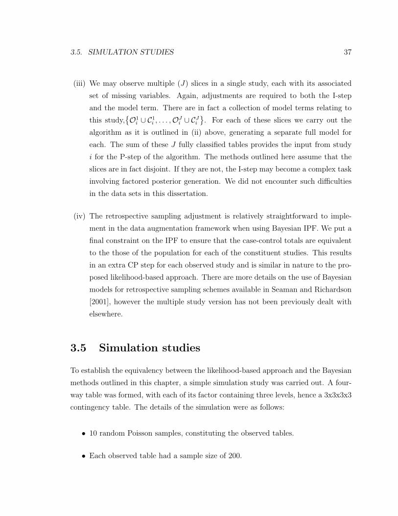
3.5 Simulation studies
To establish the equivalency between the likelihood-based approach and the Bayesian
methods outlined in this chapter, a simple simulation study was carried out. A four-
way table was formed, with each of its factor containing three levels, hence a 3x3x3x3
contingency table. The details of the simulation were as follows:
• 10 random Poisson samples, constituting the observed tables.
• Each observed table had a sample size of 200.
38 CHAPTER 3. DATA AUGMENTATION
• Each table had a random missingness patterns constructed so as to mimic those
outlined in Chapter 2, i.e. each observed table/sample contained missing and
conditional variables, with no single complete table observed.
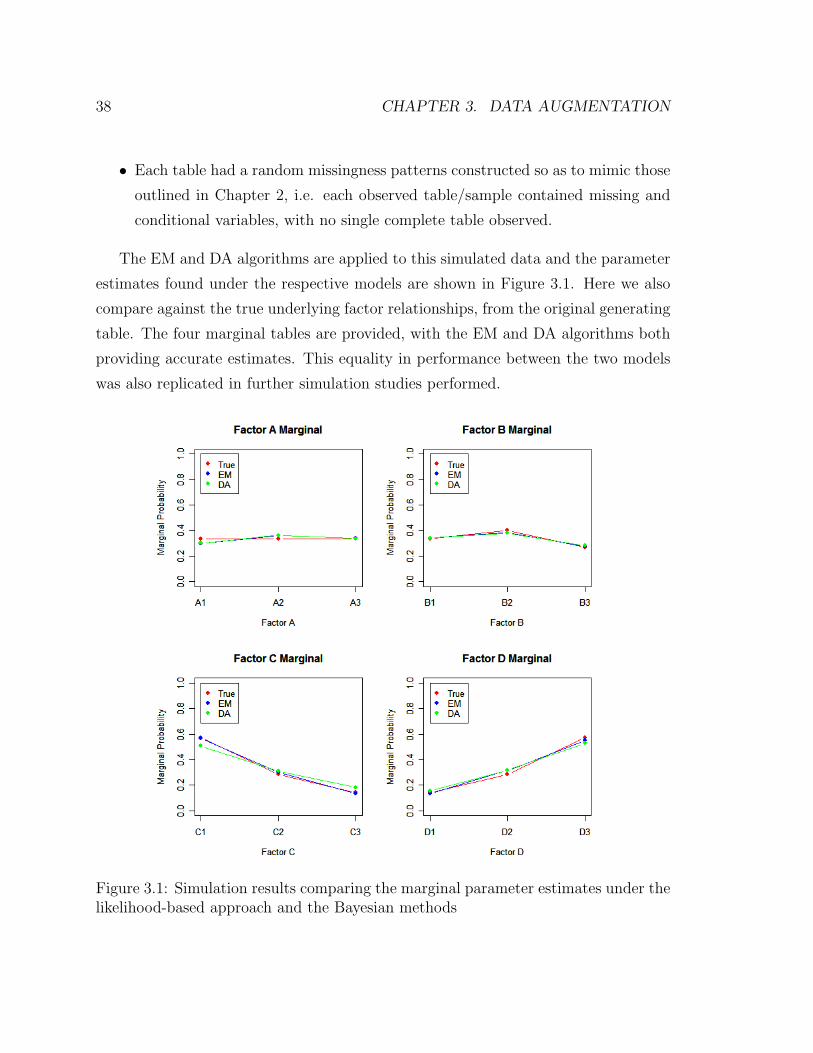
The EM and DA algorithms are applied to this simulated data and the parameter
estimates found under the respective models are shown in Figure 3.1. Here we also
compare against the true underlying factor relationships, from the original generating
table. The four marginal tables are provided, with the EM and DA algorithms both
providing accurate estimates. This equality in performance between the two models
was also replicated in further simulation studies performed.
Figure 3.1: Simulation results comparing the marginal parameter estimates under thelikelihood-based approach and the Bayesian methods
Chapter 4
Variance Estimation
4.1 The sandwich estimate
In this section we will consider robust parameter estimation. It is reasonable to
say that the model we choose to fit is often not the true underlying probability
structure which generated the data. While this seems at first glance to be detrimental,
here we will outline methods developed which correct for this model misspecification.
Some features of the distribution can still be consistently estimated and it is possible
to produce unbiased variance estimates. In particular we will concentrate on how
maximum likelihood estimation performs under such conditions.
Suppose x1, x2, . . . , xn are an iid sample from an unknown distribution g(x) and
our model is fθ(x). Maximizing the likelihood is equivalent to
maximizing1
n
∑i
log fθ(xi), (4.1)
which in large samples is equivalent to,
minimizing − Eg log fθ(x) = −∫g(x) log fθ(x)dx. (4.2)
Since Eg log g(x) is an unknown constant wrt θ it is also equivalent to minimizing the
39

40 CHAPTER 4. VARIANCE ESTIMATION
Kullback-Leibler distance,
minimizing D(f, g) = Eg log g(x)− Eg log fθ(x) (4.3)
Hence maximizing the likelihood is equivalent to finding the distribution closest to
the truth under the Kullback-Leibler distance measure.
In truth x1, x2, . . . , xn are an iid sample from an unknown distribution g(x), while
we assume a model fθ(x). θ is the maximum likelihood estimate based on this assumed
model. θ0 is the parameter being estimated by the ML procedure and is the maximum
of λ(θ) ≡ Ex log fθ(x). We expect that θp→ θ0 (Pawitan [2001] Theorem 13.1).
Let θ be a consistent estimate of θ0, assuming the model fθ(x) . Allow θ to be a
vector and define
J = E
(∂fθ(x)
∂θ
)(∂fθ(x)
∂θ′
)|θ=θ0 (4.4)
I = −E(∂2fθ(x)
∂θ∂θ′
)|θ=θ0 (4.5)
J and I are identical if fθ0(x) is the true model, and hence in this case the estimated
variance is the “naive” inverse Fisher information.
Theorem A. Assuming the standard regularity conditions 1√n(θ−θ0)
d→ N(0, I−1J I−1)
Proof: The log-likelihood of θ is
logL(θ) =∑i
log fθ(xi) (4.6)
Using a Taylor series approximation, we expand the score function around θ,
logL(θ0)
∂θ=
∂ logL(θ0)
∂θ|θ=θ +
∂2 logL(θ∗)
∂θ∂θ′(θ − θ) (4.7)
=∂2 logL(θ∗)
∂θ∂θ′(θ − θ) (4.8)

4.1. THE SANDWICH ESTIMATE 41
where |θ∗ − θ| ≤ |θ − θ| and let
yi ≡∂ log fθ(xi)
∂θ. (4.9)
Therefore,∂ logL(θ)
∂θ=∂∑
i log fθ(xi)
∂θ=∑i
∂ log fθ(xi)
∂θ=∑i
yi (4.10)
and so∂ logL(θ)
∂θis the sum of iid yi, with mean
E(Yi) = E∂ log fθ(xi)
∂θ(4.11)
=∂E log fθ(xi)
∂θ= λ
′(θ) (4.12)
At θ = θ0, EYi = 0 and variance
var(Yi) = J = E
(∂fθ(x)
∂θ
)(∂fθ(x)
∂θ′
)|θ=θ0 (4.13)
By the central limit theorem at θ = θ0
1Regularity conditions [Lehmann and Casella, 1998]:
(a) The parameter space Ω is an open interval (not necessarily finite).
(b) The distribution Pθ of the Xi have common support, so that the set A = x : fθ(x) > 0 isindependent of θ.
(c) For every x ∈ A, the density fθ(x) is twice differentiable under w.r.t. θ, and the secondderivative is continuous in θ.
(d) The integral∫fθ(x)dµ(x) can be twice diffentiated under the integral sign.
(e) The Fisher information I(θ) satistfies 0 < I(θ) <∞.
(f) For any given θ0 ∈ Ω, there exists a positive number c and a function M(x) (both of which
may depend on θ0) such that∣∣∣∣∂2 log fθ(x)
∂θ2
∣∣∣∣ ≤ M(x), ∀x ∈ A, θ0 − c < θ < θ0 + c and
Eθ0 [M(x)] <∞.
(g) E
[∂ log fθ(x)
∂θ
]= 0.
(h) E
[−∂
2 log fθ(x)∂θ2
]= E
[∂ log fθ(x)
∂θ
]2= I(θ).
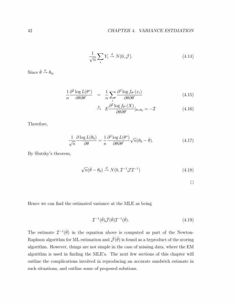
42 CHAPTER 4. VARIANCE ESTIMATION
1√n
∑i
Yid→ N(0,J ). (4.14)
Since θp→ θ0,
1
n
∂2 logL(θ∗)
∂θ∂θ′=
1
n
∑i
∂2 log fθ∗(xi)
∂θ∂θ′(4.15)
p→ E∂2 log fθ∗(X)
∂θ∂θ′|θ=θ0 = −I (4.16)
Therefore,
1√n
∂ logL(θ0)
∂θ=
1
n
∂2 logL(θ∗)
∂θ∂θ′√n(θ0 − θ). (4.17)
By Slutsky’s theorem,
√n(θ − θ0)
d→ N(0, I−1J I−1) (4.18)
Hence we can find the estimated variance at the MLE as being
I−1(θ)J (θ)I−1(θ). (4.19)
The estimate I−1(θ) in the equation above is computed as part of the Newton-
Raphson algorithm for ML estimation and J (θ) is found as a byproduct of the scoring
algorithm. However, things are not simple in the case of missing data, where the EM
algorithm is used in finding the MLE’s. The next few sections of this chapter will
outline the complications involved in reproducing an accurate sandwich estimate in
such situations, and outline some of proposed solutions.
4.2. EXTENDING THE SANDWICH ESTIMATE TO MISSING DATA 43
4.2 Extending the sandwich estimate to missing
data
As outlined in the previous section, the constituent parts of the large-sample covari-
ance matrix 4.19 are not produced as direct by-products of the EM algorithm and
hence must be produced independently of this process. The observed information
matrix I−1(θ) is in fact stated more correctly as I−1( ˆθ|Yobs) in this setting, as we
have both observed and unobserved data. This can be found directly as the second
derivative of the log-likelihood, calculated at θ = θ. Unfortunately this work may be
restricted by computational restrictions, especially in the inversion of the information
matrix.
Alternatively, one may calculate the information matrix as the difference of the
complete data information and the missing information [Meng and Rubin, 1991]:
I(θ|Yobs) = −∂2Q(θ|θ)∂θ∂θ′
+∂2H(θ|θ)∂θ∂θ′
(4.20)
where,
Q(θ|θ(t)) =
∫[`(θ|Yobs, Ymis)] f(Ymis|Yobs, θ(t))dYmis (4.21)
H(θ|θ(t)) =
∫[log f(Ymis|Yobs, θ)] f(Ymis|Yobs, θ(t))dYmis (4.22)
Due to the missingness in the data, numerical approximations are applied only in
calculating the missing information (matrix), the term involving H(θ|θ). Hence, this
can be lead to unstable estimates of the covariance matrix.
There are a collection of large-sample methods developed from the sandwich esti-
mator. Foremost amongst them is the SEM algorithm, outlined in the next section.
Other noteworthy alternatives include those developed by Louis [1982], which requires
the calculation of the conditional expectation of the squared complete-data score func-
tion, and Little and Rubin [2002] involving a two part quadratic approximation to
the likelihood.

44 CHAPTER 4. VARIANCE ESTIMATION
4.3 Supplemented EM
Supplemented EM [Meng and Rubin, 1991] was introduced as an alternative method
to estimate the variance-covariance matrix, specifically when the EM algorithm is
used to find parameter estimates. Advantages for this method include:
1 Uses only code from the E and M steps
2 Does not require the missing information explicitly, uses only the large-sample
complete data variance-covariance matrix (Vc)
3 Only standard matrix operations required
4 More stable than numerically differentiating l(θ|Yobs)
Using the notation in Meng and Rubin [1991], we define
icom =∂2Q(θ|θ)∂θ∂θ′
|θ=θ∗
imis =∂2H(θ|θ)∂θ∂θ′
|θ=θ∗
iobs = I(θ|Yobs)|θ=θ∗ (4.23)
DM is the derivative of the EM mapping (M). Even though M does not have an
explicit mathematical form, its derivative DM can be estimated from the output
of forced EM steps, whereby we effectively numerically differentiate M . This is the
central concept of the SEM algorithm. So in effect DM represents the fraction of
missing information in the gradient of the EM mapping, and hence controls the speed
of convergence with,
DM = imisi−1com = I − iobsi−1
com (4.24)
We denote the converged value of θ to be θ∗. Therefore,

4.3. SUPPLEMENTED EM 45
Vobs = i−1obs
= Vcom(I −DM)−1
= Vcom(I −DM +DM)(I −DM)−1
= Vcom + VcomDM(I −DM)−1
= Vcom + ∆V (4.25)
Firstly we obtain the MLE θ and then a sequence of SEM iterations are run,
iteration (t+ 1) taking the following form:
Input: θ and θ(t).
Step 1: Run the usual E and M steps to obtain θ(t+1).
Step 2: Fix i = 1 and calculate
θ(t)(i) = (θ1, . . . , θi−1, θ(t)i , θi+1, . . . , θd) (4.26)
which is θ, with the ith component replaced by θ(t)i .
Step 3: Treating θ(t)(i) as the current estimate of θ , run one iteration of EM
to obtain θ(t+1)(i).
Step 4: Find the ratio,
r(t)ij =
θ(t+1)(i)− θjθ
(t)i − θi
, for j = 1, . . . , d (4.27)
Output: θ(t+1) andr
(t)ij : i, j = 1, . . . , d
.
Hence we can find DM as limt→∞ rij, with the element rij found once the sequence
r(t∗)ij , r
(t∗+1)ij , . . . is stable for some t∗. It is likely that different values of t∗ will be used
for different elements rij. When all elements in the ith row of DM have been obtained,
steps 2-4 are no longer required for that value of i in subsequent iterations.

46 CHAPTER 4. VARIANCE ESTIMATION
Once we have found the converged DM, it is easy to reconstruct the observed
variance Vobs, using Equation 4.25. This method is designed so as to estimate the
variance of the unknown parameters θ, but the variances of other quantities of interest
(e.g. cell probabilities) may be reconstructed once the full covariance function for θ
has been established.
In practice we did find some limitations in the SEM algorithm:
• Despite the claims in the paper, this method does not necessarily produce a sym-
metric covariance matrix, with large discrepancies noted in large dimensional
cases.
• DM is often not positive semi-definite, small adjustments to the eigenvalues are
required to correct for this.
• Each parameter converges at a different rate, so it requires quite a bit of hand-
tuning in order to confirm convergence across all parameters.
• Tends to overestimate the variance slightly, a drawback outlined in the original
paper also.
4.4 The jackknife
The jackknife method is employed in order to estimate the standard error of the
prediction from the fitted model. A version of cross-validation, the jackknife uses
the leave-one-out method to estimate the bias and the standard error of an estimate.
Given the full data, x = (x1, ..., xn), the jackknife methods creates n sub-samples,
leaving one sample out each time: x(i) = (x1, ..., xi−1, xi+1, ..., xn) for i = 1, . . . , n.
Therefore the parameter of interest θ is estimated in each sub-sample by θ(i) = f(x(i)),
with θ(i) the jackknife replication of θ. The jackknife estimate of bias is defined as
biasjack = (n− 1)(θ(.) − θ) (4.28)
4.5. THE BOOTSTRAP 47
where
θ(.) =1
n
n∑i=1
θ(i). (4.29)
The jackknife estimate of the standard error is defined as
sejack =
[n− 1
n
n∑i=1
(θ(i) − θ(.)
)2] 1
2
. (4.30)
This method can be adapted to deal with data such as those we have encountered
in this dissertation. Rather than excluding a single sample, we omit one full study
at a time, producing a set of S parameter estimates θ(1), . . . , θ(S). There are also
some beneficial side-effects in using the jackknife variance method. The jackknife
samples may be used to cross-validate for model-selection (Section 2.10). As explained
in Section 2.8 faulty data or aberrant studies can be identified using the jackknife
influence.
4.5 The bootstrap
The jackknife may be regarded as a special case of the bootstrap [Efron and Tibshi-
rani, 1993], in the general family of resampling techniques. The general bootstrap
method provides a computer-based nonparametric estimate of the standard error, but
with similar asymptotic properties to the sandwich estimator. Each bootstrap sam-
ple is a sample with replacement of size n from the observations, and B independent
samples such as this are found, x∗1, . . . ,x∗B. θ∗(b) is the ML estimate of θ based on
the bth bootstrap sample x∗b. Therefore the overall bootstrap estimate of θ is
θboot =1
B
B∑b=1
θ(b), (4.31)
and the bootstrap estimate of the standard error of θ or θboot is
seboot =
[1
B − 1
B∑b=1
(θ(b) − θboot)2
]1/2
(4.32)
48 CHAPTER 4. VARIANCE ESTIMATION
As in the jackknife, samples are formed here on a study-to-study basis in the meta-
analysis setting; choosing n studies (from the total of S studies) for each bootstrap
sample.
The bootstrap yields valid large-sample standard errors regardless of the validity of
the assumptions of the underlying model. It is however limited in cases with moderate
data sets or extensive missing data, as many of the bootstrap samples will exclude
the data required for vital parameter estimates. Therefore the jackknife method is
more appropriate for fitting the sparsely classified multiway tables observed in this
thesis, as the resampling excludes a smaller proportion of the pivotal data.
4.6 Bayesian posterior
The data augmentation algorithm outlined in Chapter 3 produces an accurate esti-
mate of variance when a uniform prior is used. Under this prior the posterior mode is
the ML estimate and the posterior variance is a consistent estimate of the large-sample
variance of the ML estimate. It is an attractive approach due to this asymptotic prop-
erty, in addition to its superior performance in small sample cases. Here it provides
inference based directly on the posterior distribution without invoking large-sample
normal approximations.
We denote θ(1), . . . , θ(M) as the resulting estimates from a single simulation run of
the data augmentation algorithm of length M . We shall discard the output during
the initial burn-in period. For any scalar function φ, we define φ(t) = φ(θ(t)) and its
sample average as
φ =1
M
M∑t=1
φ(t). (4.33)
The sample variance of φ overestimates the true variance V (φ), because the elements
in the sequence φ(1), . . . , φ(M) are correlated. This is because the input for each
iteration of the data augmentation algorithm is the output from the last. The single
run sample variance does at least provide a crude lower bound for the variance.
Therefore, it is essential to adjust for this autocorrelation. This may be achieved

4.6. BAYESIAN POSTERIOR 49
via subsampling; averaging over every bth iterate instead:
φ(b) =1
m
m∑t=1
φ(tb), (4.34)
where m = M/b. If the choice of b is made carefully (and checked by inspection of
the sample ACF), then we may estimate V (φ) by:
V (φ(b)) =1
m
m∑t=1
(φ(tb) − φ(b))1/2. (4.35)
Unfortunately this method tends to overestimate the true variance V (φ) [Schafer,
1997].
A more stable and reliable method for posterior variance estimation is found using
multiple chain simulation of the algorithm. We shall perform R replicate runs from
a common starting distribution, again discarding data from the burn-in period. A
sample of size M is then found from each run, with the tth estimate of θ from the rth
run denoted θ(r:t). The within-run sample average is
φ(r) =1
M
M∑t=1
φ(r:t), (4.36)
and the pooled sample average is found as
φ =1
RM
r=1∑R
M∑t=1
φ(r:t). (4.37)
Hence we may find an unbiased estimate of the variance of a single φ(r) using the
between-run variance
B =1
R− 1
r=1∑R
(φ(r)−)1/2 − φ, (4.38)
withB
Ra reasonable approximation to the variance of the pooled estimate, V (φ).
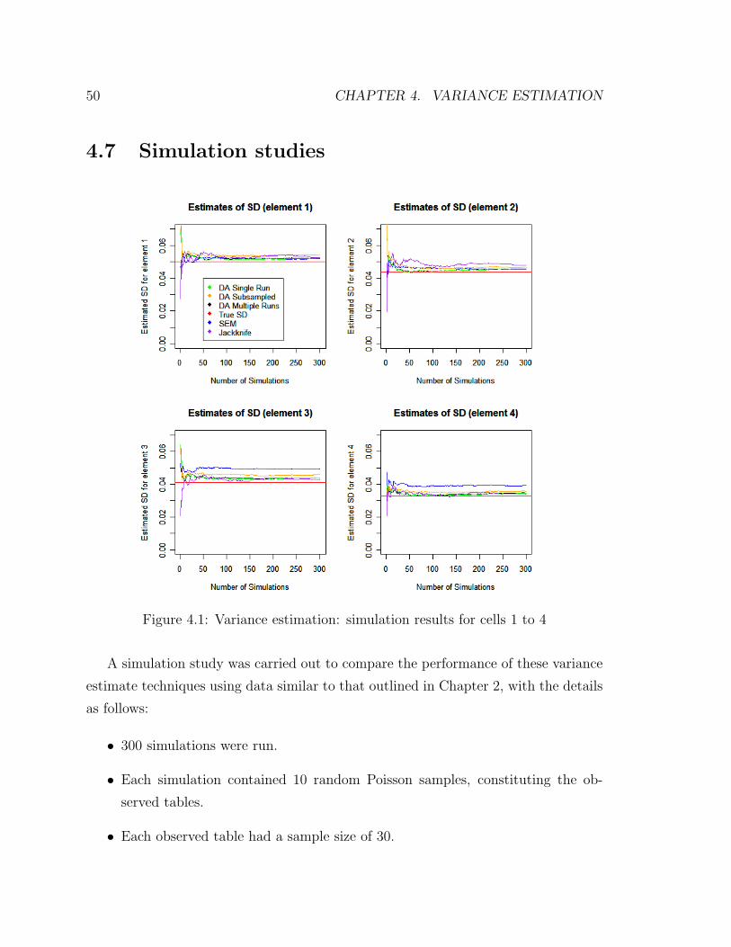
50 CHAPTER 4. VARIANCE ESTIMATION
4.7 Simulation studies
Figure 4.1: Variance estimation: simulation results for cells 1 to 4
A simulation study was carried out to compare the performance of these variance
estimate techniques using data similar to that outlined in Chapter 2, with the details
as follows:
• 300 simulations were run.
• Each simulation contained 10 random Poisson samples, constituting the ob-
served tables.
• Each observed table had a sample size of 30.

4.7. SIMULATION STUDIES 51
• The true underlying ”full” contingency table had three factors, each with two
levels (2x2x2 table). A table of this low-order in magnitude was necessary so
as to allow for feasible computation. Since there are eight cells in total, this is
what is observed in the associated plots.
• Each table had a random missingness patterns constructed so as to mimic those
outlined in Chapter 2, i.e. each observed table/sample contained missing and
conditional variables, with no single complete table observed.
We generated random Poisson counts from the true underlying distribution, and
compared the estimates produced by the candidate methods against the true standard
deviation, shown in red in each of the plots (calculated using the multinomial variance
formula). Each of the other five lines shows the cumulative estimate of the standard
deviation for its respective method, after that number of simulation. Therefore a
suitable method should converge to the truth as the number of simulations increases.
Figures 4.1 and 4.2 show the results of this analysis for each of the eight cells in the
table. We have also reproduced the results from a single cell in Figure 4.3 in order to
provide a clearer view of the plot details for at least one element.
It is clear from this simulation and others we also completed, that the SEM is not a
viable method for this analysis. It overestimates the variance considerably in many of
these plots and required quite a high level of parameter-tuning by the user to achieve
results even this accurate. The data augmentation methods were quite accurate and
tended to follow-one another closely. This is perhaps due in part to a common starting
distribution and random seed. The bootstrap results were not shown in these plots, as
they were quite similar to those of the jackknife. The jackknife method was perhaps
the most accurate of all the methods here, and this was replicated in other simulation
studies also. Combined with the additional side-benefits as outlined above in Section
4.4, the authors conclude that this is the most suitable variance estimation method
for the likelihood-based models.
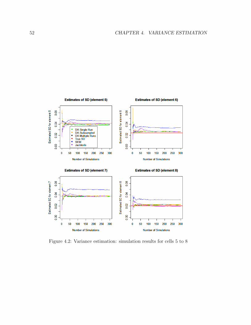
52 CHAPTER 4. VARIANCE ESTIMATION
Figure 4.2: Variance estimation: simulation results for cells 5 to 8
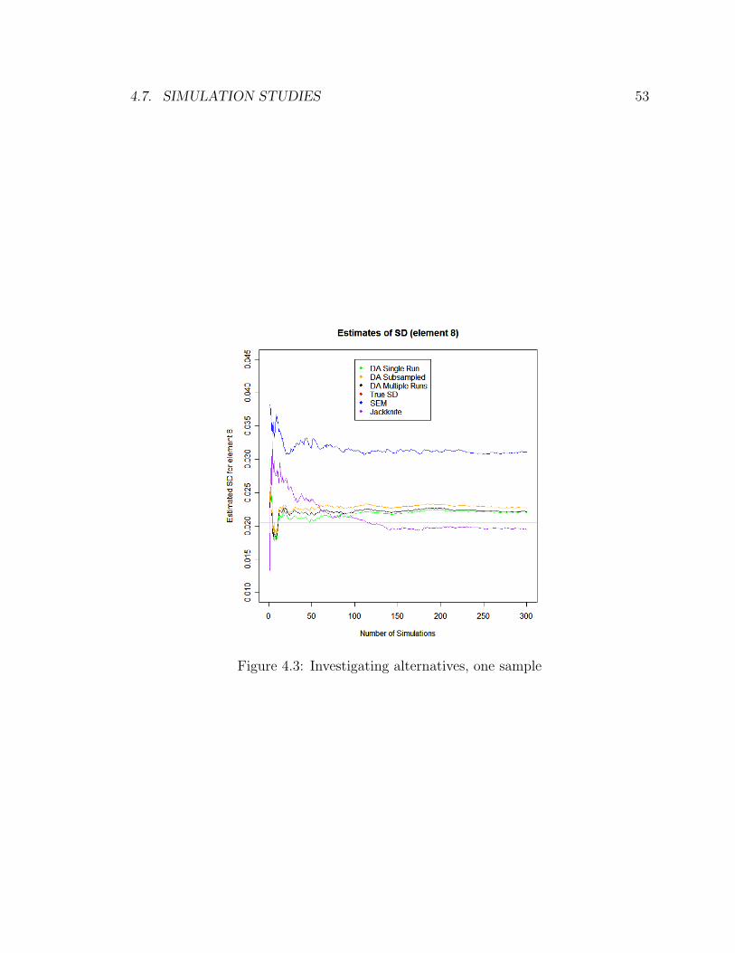
4.7. SIMULATION STUDIES 53
Figure 4.3: Investigating alternatives, one sample

Chapter 5
Retrospective Adjustment
5.1 Description of the problem
Meta-analysis attempts to aggregate the results of many studies in order to leverage
their combined power. It is therefore often necessary to combine effect size estimates
from numerous constituent studies. In this chapter we will address the issues in-
volved in combining fixed effect or random effect estimates for categorical data, and
in particular we will discuss the issues involved in adjusting for retrospective sampling.
For example and without loss of generalization we shall look at S studies, each
providing a 2x2 table for a set of factors A and B. The number of subjects in study s
who observed the i, j combination of factors A and B is denoted n(s)ij . A fully observed
set of tables may be denoted:
B1 B2
A1 n(1)11 n
(1)12
A2 n(1)21 n
(1)22
B1 B2
A1 n(2)11 n
(2)12
A2 n(2)21 n
(2)22
. . . . . .
B1 B2
A1 n(S)11 n
(S)12
A2 n(S)21 n
(S)22
Table 5.1: Combining S fully observed two-way tables
In sections 5.2, 5.3 and 5.4 we will introduce contemporary methods for combin-
ing such tables for prospective studies. While in sections 5.5, 5.6, 5.7 and 5.8 we
will develop new techniques for adjusting these methods to account for retrospective
sampling schemes.
54

5.2. MAXIMUM LIKELIHOOD METHOD 55
5.2 Maximum likelihood method
The maximum likelihood method is most easily implemented via logistic regression.
We treat the studies as a third variable C and we now use the notation πjs =n
(s)1j
n(s)1.
=
P (A = 1|B = j, C = s). Using the model
logit(πjs) = α + βxj, j = 1, 2. (5.1)
where x1 = 1, x2 = 0. This model assumes that the AB conditional odds ratio is
the same at each category of C, namely exp(β). The maximum likelihood estimate
of the common odds ratio is exp(β)
The ML estimate β of the log odds ratio tends to be too large in absolute value
when S is large and the data are sparse. For example in the sparse-data case, with
only a single matched pair in each study, βp→ 2β as n→∞.
5.3 Mantel-Haenszel method
Mantel and Haenszel [1959] proposed a non model-based approach to this problem.
Here the joint odds ratio estimate oMH is
oMH =
∑Ss=1 n
(s)11 n
(s)22 /n
(s)..∑S
s=1 n(s)12 n
(s)21 /n
(s)..
. (5.2)
Robins et al. [1986] derived an associated non-null standard error estimate for
log(oMH):
SE =1∑A(s)√
2
(∑A(s)B(s) + oMH
∑(B(s)C(s) + A(s)D(s)
)+ o2
MH
∑C(s)D(s)
) 12
(5.3)
where,

56 CHAPTER 5. RETROSPECTIVE ADJUSTMENT
A(s) =n
(s)11 n
(s)22
n(s)..
(5.4)
B(s) =n
(s)11 + n
(s)22
n(s)..
(5.5)
C(s) =n
(s)12 n
(s)21
n(s)..
(5.6)
D(s) =n
(s)12 + n
(s)21
n(s)..
(5.7)
5.4 Pooling log-odds ratios
A widely used alternative to the Mantel-Haenszel techniques is the pooling of the log
odds ratios across the S studies. An adjustment factor of 0.5 is made to each cell
count to avoid a divide by zero error. Define:
Ls = ln(n
(s)11 + 0.5)(n
(s)22 + 0.5)
(n(s)12 + 0.5)(n
(s)21 + 0.5)
, (5.8)
and
Ws =
(∑i
∑j
1
n(s)ij + 0.5
)−1
. (5.9)
The pooled log odds ratio is
L* =
∑WsLs
(∑Ws)1/2
, (5.10)
with a standard error of
SE =1
(∑Ws)1/2
. (5.11)
When the cell frequencies within all of the S studies are large, the Mantel-Haenszel
estimate will be close in value to the estimate obtained by pooling the log odds ratio.
There is disagreement however in cases where the cell frequencies are small. In such
circumstances the Mantel-Haenszel estimator is superior to the log odds ratio [Hauck,
5.5. MODIFICATION FOR RETROSPECTIVE SAMPLING 57
1979]. There have been other alternatives proposed, but these competitors have been
shown to be inferior in the case of stratified studies [Agresti, 2002].
5.5 Modification for retrospective sampling
The methods proposed thus far have dealt with data collected from prospective re-
search. However, in retrospective sampling designs, such as case-control biomedical
studies, an adjustment is required in order to correctly estimate the effects. This is
because in case-control studies the explanatory variable X is random, rather than the
response variable Y. Anderson and Richardson [1979] proposed a solution to this prob-
lem for the single study case, using Bayes theorem and the logit link function. Let Z
indicate whether each subject is sampled (1=yes, 0=no), with ρ0 = P (Z = 1|Y = 1)
denoting the probability of sampling a case and ρ1 = P (Z = 1|Y = 0) denoting the
probability of sampling a control.
P (Y = 1|Z = 1, X = x) =P (Z = 1|Y = 1, X = x)P (Y = 1|X = x)∑1j=0 P (Z = 1|Y = j,X = x)P (Y = j|X = x)
=P (Z = 1|Y = 1)P (Y = 1|X = x)∑1j=0 P (Z = 1|Y = j)P (Y = j|X = x)
=ρ1exp(α + βx)
ρ0 + ρ1exp(α + βx)
=exp(α + log(ρ1/ρ0) + βx)
1 + exp(α + log(ρ1/ρ0) + βx)(5.12)
So by fitting a logistic model, the estimated effect parameter β is equivalent to that
produced by a prospective study. There is an intercept parameter change however
with
α∗ = α + log(ρ1
ρ0
) (5.13)
Hence, when attempting prediction in a case-control study it is necessary to adjust
only the intercept parameter for the fitted logistic model. This can be done by
adjusting the estimates on the logit scale, using external information about the actual
disease prevalence in the entire population.

58 CHAPTER 5. RETROSPECTIVE ADJUSTMENT
Since,
ρ1 = P (Z = 1|Y = 1) =P (Y = 1|Z = 1)P (Z = 1)
P (Y = 1)
ρ0 = P (Z = 1|Y = 0) =P (Y = 0|Z = 1)P (Z = 1)
P (Y = 0). (5.14)
Therefore,
log
(ρ1
ρ0
)= log
(P (Y = 1|Z = 1)
P (Y = 0|Z = 1)
)− log
(P (Y = 1)
P (Y = 0)
), (5.15)
with P (Y = 1|Z = 1) = P (Case|Sampled) and P (Y = 1) = P (Case) in entire
population.
5.6 Extension of the modification for retrospective
studies
However, in the case of multiple studies investigating the effect size of the same factor
it is necessary to extend the model outlined above. This is because the case-control
mix in each of the constituent studies will be different. Here
ρ(s)1 = P (Z = 1|Y = 1, S = s) (5.16)
denotes the probability of sampling a case in the sth study, with
ρ(s)0 = P (Z = 1|Y = 0, S = s) (5.17)

5.6. EXTENSION OF THE MODIFICATION FOR RETROSPECTIVE STUDIES59
the corresponding probability of sampling a control.
P (Y = 1|Z = 1, X = x, S = s) =P (Z = 1|Y = 1, X = x, S = s)P (Y = 1|X = x, S = s)∑1j=0 P (Z = 1|Y = j,X = x, S = s)P (Y = j|X = x, S = s)
=P (Z = 1|Y = 1, S = s)P (Y = 1|X = x, S = s)∑1j=0 P (Z = 1|Y = j, S = s)P (Y = j|X = x, S = s)
=ρ
(s)1 exp(αs + βx)
ρ(s)0 + ρ
(s)1 exp(αs + βx)
=exp(αs + log(ρ
(s)1 /ρ
(s)0 ) + βx)
1 + exp(αs + log(ρ(s)1 /ρ
(s)0 ) + βx)
(5.18)
The only assumption made in this section is that
P (Z = 1|Y = 1, X = x, S = s) = P (Z = 1|Y = 1, S = s) (5.19)
i.e. the sampling probabilities do not depend on the covariate of interest. Again we
have
ρ(s)1 = P (Z = 1|Y = 1, S = s) =
P (Y = 1|Z = 1, S = s)P (Z = 1)
P (Y = 1)
ρ(s)0 = P (Z = 1|Y = 0, S = s) =
P (Y = 0|Z = 1, S = s)P (Z = 1)
P (Y = 0)(5.20)
and the adjustment has the same form,
α∗s = αs + log
(ρ
(s)1
ρ(s)0
), (5.21)
with,
log
(ρ
(s)1
ρ(s)0
)= log
(P (Y = 1|Z = 1, S = s)
P (Y = 0|Z = 1, S = s)
)− log
(P (Y = 1)
P (Y = 0)
)(5.22)
The full logistic model is
logit(πjs) = αs + βxj, j = 1, 2. (5.23)
60 CHAPTER 5. RETROSPECTIVE ADJUSTMENT
So this adjustment must be made separately for the adjusted cell predictions from
each of the S studies. The exp(β) is the maximum likelihood estimate of the odds
ratio exp(β). This method can be extended easily to case where X has more than
two levels or is a continuous variable, and even to cases with multiple parameter
estimation.
5.7 Loglinear-logit model connection
Logit models consider a single categorical response variable and it’s relationship with
a group of explanatory variables. Loglinear models, by contrast, treat all categori-
cal equivalently, focusing on associations and interactions in their joint distribution.
There is however, a well-established equivalency between loglinear and logistic mod-
els when the categorical (response for logit) variable, Y, is binary. For example if we
consider a three-way table and the fitted loglinear model (XY,XZ,YZ), the logit of Y
is:
logP (Y = 1|X = i, Z = k))
P (Y = 1|X = i, Z = k))= log
µi1kµi0k
= log (µi1k)− log (µi0k)
=(λ+ λXi + λY1 + λZk + λXYi1 + λXZik + λY Z1k
)−(λ+ λXi + λY0 + λZk + λXYi0 + λXZik + λY Z0k
)=
(λY1 − λY0
)+(λXYi1 − λXYi0
)+(λY Z1k − λY Z0k
)(5.24)
Therefore, the logit has the additive form:
logit [P (Y = 1|X = i, Z = k] = α + βXi + βZk (5.25)
whereby the first parameter is a constant, the second parenthetical term depends
only on the category i of X and the third parameter depends solely on category k of
Z. This may be denoted an (X + Z) logistic model. Table 5.2 outlines some more
equivalent models in the three-way example.
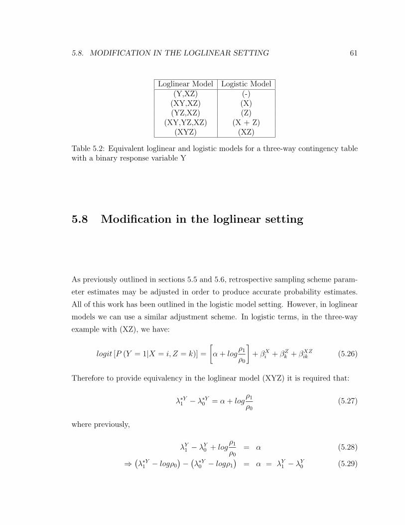
5.8. MODIFICATION IN THE LOGLINEAR SETTING 61
Loglinear Model Logistic Model(Y,XZ) (-)
(XY,XZ) (X)(YZ,XZ) (Z)
(XY,YZ,XZ) (X + Z)(XYZ) (XZ)
Table 5.2: Equivalent loglinear and logistic models for a three-way contingency tablewith a binary response variable Y
5.8 Modification in the loglinear setting
As previously outlined in sections 5.5 and 5.6, retrospective sampling scheme param-
eter estimates may be adjusted in order to produce accurate probability estimates.
All of this work has been outlined in the logistic model setting. However, in loglinear
models we can use a similar adjustment scheme. In logistic terms, in the three-way
example with (XZ), we have:
logit [P (Y = 1|X = i, Z = k)] =
[α + log
ρ1
ρ0
]+ βXi + βZk + βXZik (5.26)
Therefore to provide equivalency in the loglinear model (XYZ) it is required that:
λ∗Y1 − λ∗Y0 = α + logρ1
ρ0
(5.27)
where previously,
λY1 − λY0 + logρ1
ρ0
= α (5.28)
⇒(λ∗Y1 − logρ0
)−(λ∗Y0 − logρ1
)= α = λY1 − λY0 (5.29)

62 CHAPTER 5. RETROSPECTIVE ADJUSTMENT
Thus the intercepts for cases (Y = 1) and the controls (Y = 0) are adjusted separately
using,
ρ1 =P (Y = 1|Z = 1)
P (Y = 1)(5.30)
ρ0 =P (Y = 0|Z = 1)
P (Y = 0)(5.31)
with Z = 1 for sampled observations. This method is extended as we did in section
5.6 to deal with multiple studies, with each study having it own set of intercept
adjustment factors. In terms of practical model fitting, this is implemented as an
offset term.
In this chapter thus far we have not mentioned how to deal with retrospective
sampling in cases where there are slices of information from some studies. The general
procedure mentioned in the Section 2.5 referred to an E-step in such cases where the
estimated table is modified to include such slices. In these cases only the full expanded
table riF must be adjusted as above.
5.9 Simulation studies
In order to confirm the findings in this chapter, we carried out simulation studies with
both retrospective and prospective sampling schemes. The details of these sampling
schemes were as follows:
• Random multinomial draws were made from a five-way contingency table, with
the five factors having two, two, two, three and four levels respectively (2x2x2x3x4
table).
• Each table had a random missingness patterns constructed so as to mimic those
outlined in Chapter 2, i.e. each observed table/sample contained missing and
conditional variables, with no single complete table observed.
• Two sets of data were produced in each simulation run:

5.9. SIMULATION STUDIES 63
1. The first of these had a preassigned (random) reweighting factor, which is
consistent with retrospective studies.
2. The second did not have this reweighting factor and hence simulated the
more straightforward prospective studies.
• Two loglinear models were fit, with the offsets for the case-control data.
• We then analyzed the performance of the case-control adjustment developed in
this chapter.
In the first set of plots, Figure 5.1, 10 random studies were generated for each data
point. We looked over a range of sample sizes per study to see if this affected the
accuracy of the fitted models. Unsurprisingly, large sample sizes resulted in a better
fit. A similar relationship between model fit and the number of studies would be
expected and this is witnessed in Figure 5.2 (with sample size fixed at 40 per study). In
both figures, the top two plots consider the overall fit via Kullback-Leibler divergence
and Euclidean distance, while the other two plots investigate prediction error for
two particular cells in the contingency table. It is apparent that the adjustment for
retrospective sampling has succeeded, as the performances of the retrospective and
prospective models are shown to be similar in this analysis.
An issue not discussed thus far is the estimate of the population disease incidence
rate for the , and in particular the effect of a misspecified rate. Of course this is a
difficult thing to estimate for some diseases, but small errors in this estimation can
lead to large errors in the model predictions as seen in Figure 5.3. In this simulation
study the true population disease rate (P (Y = 1) = P (Case)) is 0.2 and we have
generated random multinomial samples at this rate. The assumed rate used in the
retrospective adjustment was varied in the range from 0 to 1, and we can see that
a small misspecification in this rate can lead to a large divergence in the resulting
model from the true underlying distribution.
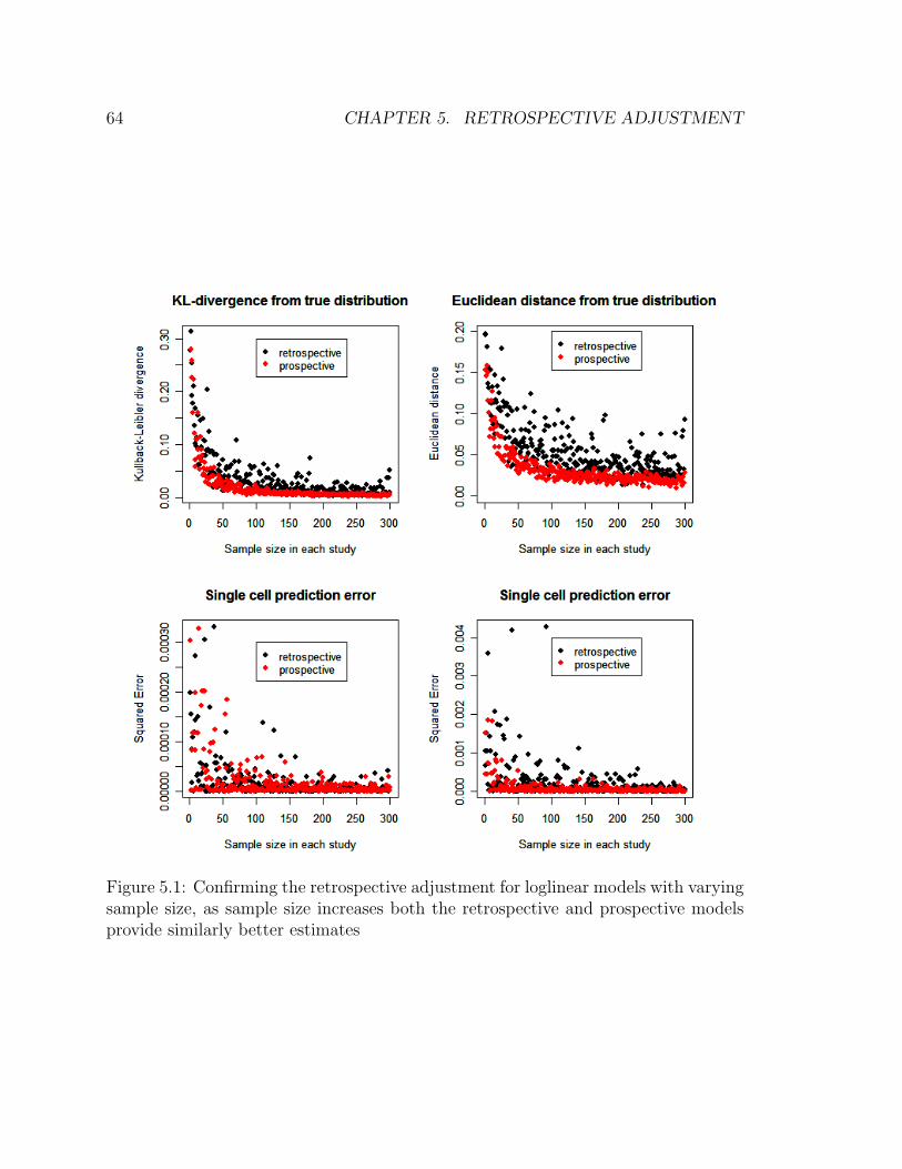
64 CHAPTER 5. RETROSPECTIVE ADJUSTMENT
Figure 5.1: Confirming the retrospective adjustment for loglinear models with varyingsample size, as sample size increases both the retrospective and prospective modelsprovide similarly better estimates
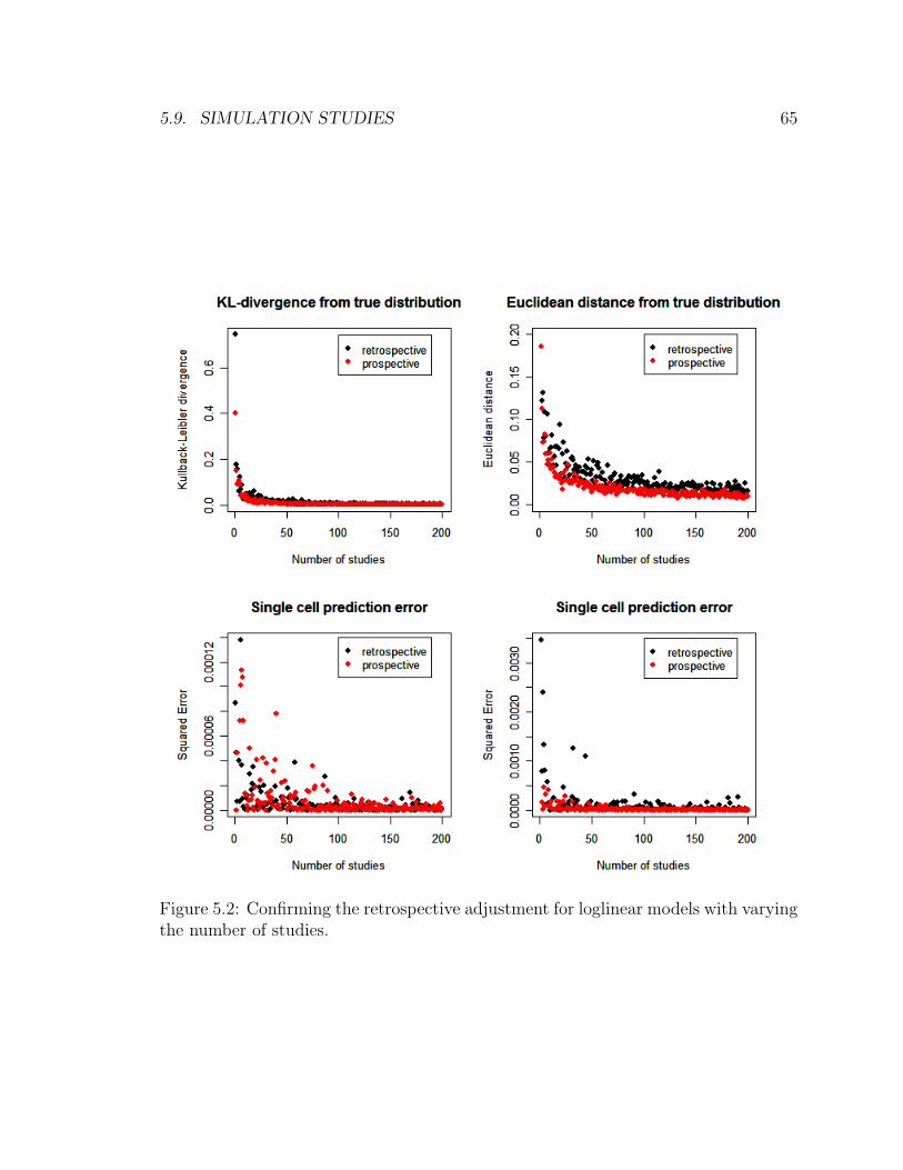
5.9. SIMULATION STUDIES 65
Figure 5.2: Confirming the retrospective adjustment for loglinear models with varyingthe number of studies.
66 CHAPTER 5. RETROSPECTIVE ADJUSTMENT
Figure 5.3: Misspecification of the population disease rate
Chapter 6
Psoriasis Meta-Analysis
6.1 Psoriasis
Psoriasis is a chronic non-contagious autoimmune disease affecting the skins and
joints of patients. Often the symptoms include thick red scaly patches on the skin or
fingernails, the severity of which can range from small localized patches to full body
coverage. It has been acknowledged in medical literature as early as ancient Greece,
where psora was used to describe an itchy skin condition, and as tzaraat in the Bible.
However, the condition name psoriasis was not termed until 1841 by Ferdinand von
Hebra, a Vienese dermatologist [Meenan, 1955]. It is estimated that approximately
2% of the population worldwide are affected by psoriasis [Griffiths and Barker, 2007],
with 35% of patients classified as having moderate to severe symptoms (> 3% of body
surface). Both males and females suffer from this disease and it may occur at any age,
although the majority of cases are initially diagnosed between the ages of 15 and 25
years. Diagnosis of the disease is made based on the appearance of the the skin alone,
to date no special blood tests or diagnostic procedures have been developed. There
are many treatments available, but because of its chronic recurrent nature psoriasis
is a challenge to treat.
There are in fact two main types of psoriasis which we will deal with it in this
analysis:
1. Type I: Also known as early onset psoriasis, these are cases where chronic plaque
67

68 CHAPTER 6. PSORIASIS META-ANALYSIS
first appears before 40 years. Approximately 75% of patients suffer from this
type of psoriasis.
2. Type II: For late onset psoriasis, symptoms present after 40 years. Although
this is the rarer form of the disease, it is the potentially fatal variant.
While much investigation into the cause of psoriasis has been carried out, the
mechanism is still not fully understood. There are two main hypotheses about the
process leading to the development of the disease. The first such theory states that
the disease can be simply traced to faults in the epidermis and its keratinocytes. The
second hypothesis views the disorder as being an immune-mediated disease, where
the skin inflammations are secondary to factors produced by the immune system. It
states that the excessive production of skin cells is in fact initiated by the activation
of T cells and their migration to the dermis. Unfortunately, we do not yet understand
why the T cells become activated, as their natural function is to help protect the body
against infection.
Psoriasis remains an idiosyncratic disease; patients report that the condition often
improves and worsens for no apparent reason. Although the exact cause of psoriasis
has not been established, many triggers associated with the onset and worsening of
the symptoms have been discovered in recent research. Established triggers include:
• stress
• skin injury (Koebner phenomenon)
• excessive alcohol consumption
• smoking
• changes of season or climate
• obesity
• streptococcal infection
• medications including Lithium, Antimalarials, Inderal, Quinidine and Indomethacin
6.1. PSORIASIS 69
A combination of genetic and environmental factors have been shown to be associ-
ated with the onset of psoriasis [Griffiths and Barker, 2007]. Almost 35% of psoriasis
patients report a family history of the disease, while monozygotic twins have been
shown to have a much higher concordance rate than dizygotic twins (65-73% versus
15-30%). Psoriasis has been found to be a typical complex disease in which both
genetic and environmental factors affect susceptability in family-based linkage and
epidemiological studies. The heritability of psoriasis, a measure of the proportion of
variability of the disease due to genetic factors, is estimated as 60-90% in Caucasians
[Elder et al., 1994]. Remarkably, this rate has been shown to be as high as 90-100%
in Danish twins[Brandrup and Green, 1981].
Traditional approaches to the identification of genetic risk factors, such as population-
based candidate gene association studies, have had moderate success. Associations
with markers in the major histocompatibility complex (MHC) region on chromosome
6 more were discovered over 35 years ago [Russell et al., 1972]. To date this locus
remains the major susceptibility locus for psoriasis, attributable directly to 35-50%
of Causasian genetic susceptibility for early-onset psoriasis. Strong associations have
been found between familial psoriasis and human leukocyte antigen (HLA) class I
genes, particularly HLA-Cw6. This has been shown to have a prevalence of up to
85% in early-onset patients compared with 15% in late-onset psoriasis and approxi-
mately 10% in the general population [Henseler and Christophers, 1985].
It is still unclear how these genes work together, with the main value of genetic
studies lying in the identification of molecular mechanisms and pathways for further
study. The majority of epidemiological research published to date has been concerned
with HLA-Cw6 exclusively as a genetic factor (with a multitude of environmental
factors), and the meta-analysis carried out in this thesis has concentrated exclusively
on this research. As further research is carried out into alternative candidate genes,
the methods developed here can incorporate these in the analysis with little extra
effort.
Contemporary genetic psoriasis research has already shown potential, with nine
locations(loci) of interest being found in single nucleotide polymorphism (SNP)-based
70 CHAPTER 6. PSORIASIS META-ANALYSIS
genome-wide association studies (GWASs). These are termed psoriasis susceptibil-
ity 1 through 9 (PSORS1 through PSORS9) [Nestle et al., 2009]. Within those loci
are genes, with HLA-Cw6 lying in the PSORS1 region. Many other of those genes
are on pathways that lead to inflammation. Technological advances leading to high-
throughput, accurate and simultaneous genotyping of hundreds of thousands of SNPs
has bought a new era of genetic studies in which the whole genome can be systemati-
cally screened in a hypothesis-free manner. This has the potential to uncover further
novel susceptibility markers in GWAS’s for psoriasis.
6.2 The data
The data set used in this analysis was gathered from 65 association studies in the
time period 1980 to 2008. Appendix A contains the references for the chosen papers.
Studies were included and excluded from this dataset in line with standard meta-
analysis procedures as outlined in [Stroup et al., 2000]. Linkage and family studies
were not considered at this stage of the analysis. We chose to include only studies
containing carrier frequencies, and replicated studies on same cohorts were excluded.
Each study was retrospective, and looked specifically at genotype information (HLA-
Cw6) plus a collection of other known risk factors, both demographic and clinical. In
addition to the case-control variable, the factors chosen for inclusion in this analysis
were the following:
• Gender (male or female)
• HLA-Cw6 (positive or negative)
• Ethnicity (Asian or Caucasian)
• Onset (early or late)
• Familial history (yes or no)
• Arthritis (yes or no)
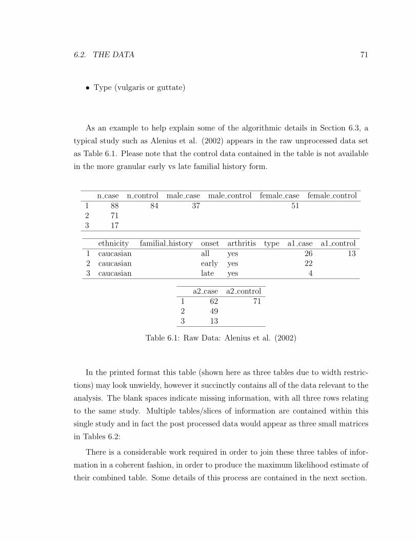
6.2. THE DATA 71
• Type (vulgaris or guttate)
As an example to help explain some of the algorithmic details in Section 6.3, a
typical study such as Alenius et al. (2002) appears in the raw unprocessed data set
as Table 6.1. Please note that the control data contained in the table is not available
in the more granular early vs late familial history form.
n case n control male case male control female case female control1 88 84 37 512 713 17
ethnicity familial history onset arthritis type a1 case a1 control1 caucasian all yes 26 132 caucasian early yes 223 caucasian late yes 4
a2 case a2 control1 62 712 493 13
Table 6.1: Raw Data: Alenius et al. (2002)
In the printed format this table (shown here as three tables due to width restric-
tions) may look unwieldy, however it succinctly contains all of the data relevant to the
analysis. The blank spaces indicate missing information, with all three rows relating
to the same study. Multiple tables/slices of information are contained within this
single study and in fact the post processed data would appear as three small matrices
in Tables 6.2:
There is a considerable work required in order to join these three tables of infor-
mation in a coherent fashion, in order to produce the maximum likelihood estimate of
their combined table. Some details of this process are contained in the next section.

72 CHAPTER 6. PSORIASIS META-ANALYSIS
male femalecase 37 51
(a) Table 1
a1 a2control 13 71
(b) Table 2
onset a1 a2early 22 49late 4 13
(c) Table 3
Table 6.2: Processed Data: Alenius et al. (2002)
6.3 Methods
While the general methods involved in the EM algorithm have been previously ex-
plained (Chapter 2), some of the details of the data-specific problems have been
overlooked to date. In this section we will extrapolate upon the specific practical
mechanics involved in the E and first part of the M step of the overall algorithm. In
particular we shall concentrate on the five steps of how we go from tables such as
6.2 above for each study (with restricted subsets of the risk factors of interest) to an
overall estimate for the full-factor table. We have attempted to explain the concepts
herein without resorting to the use of mathematical notation, so as to appeal to a
larger audience. A more rigorous mathematical development is available in Chapter
2.
Level 1: This is the starting level of the analysis, often with multiple tables for each
study of differing sizes and shapes. Level 1 to Level 3 is the process by which the
within-study tables are combined and this is shown in a simplified picture in 6.1 To
achieve this we first found the smallest common table (SCT) for each study. This is
the minimum sized multidimensional array that contains all of the observed tables
from a particular study. Obviously each studies may have a different SCT.
Level 2: Each table has variables which are present, missing and conditional, when
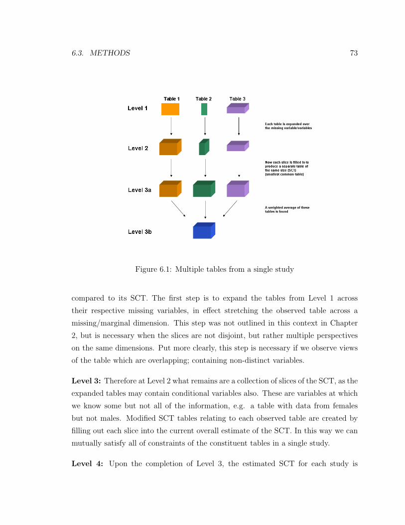
6.3. METHODS 73
Figure 6.1: Multiple tables from a single study
compared to its SCT. The first step is to expand the tables from Level 1 across
their respective missing variables, in effect stretching the observed table across a
missing/marginal dimension. This step was not outlined in this context in Chapter
2, but is necessary when the slices are not disjoint, but rather multiple perspectives
on the same dimensions. Put more clearly, this step is necessary if we observe views
of the table which are overlapping; containing non-distinct variables.
Level 3: Therefore at Level 2 what remains are a collection of slices of the SCT, as the
expanded tables may contain conditional variables also. These are variables at which
we know some but not all of the information, e.g. a table with data from females
but not males. Modified SCT tables relating to each observed table are created by
filling out each slice into the current overall estimate of the SCT. In this way we can
mutually satisfy all of constraints of the constituent tables in a single study.
Level 4: Upon the completion of Level 3, the estimated SCT for each study is
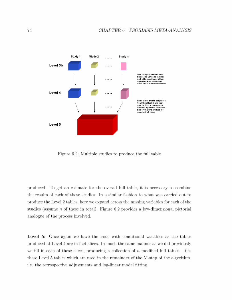
74 CHAPTER 6. PSORIASIS META-ANALYSIS
Figure 6.2: Multiple studies to produce the full table
produced. To get an estimate for the overall full table, it is necessary to combine
the results of each of these studies. In a similar fashion to what was carried out to
produce the Level 2 tables, here we expand across the missing variables for each of the
studies (assume n of these in total). Figure 6.2 provides a low-dimensional pictorial
analogue of the process involved.
Level 5: Once again we have the issue with conditional variables as the tables
produced at Level 4 are in fact slices. In much the same manner as we did previously
we fill in each of these slices, producing a collection of n modified full tables. It is
these Level 5 tables which are used in the remainder of the M-step of the algorithm,
i.e. the retrospective adjustments and log-linear model fitting.

6.4. RESULTS 75
6.4 Results
6.4.1 Model fitting
The model-fitting process for these data sets must be approached with care. We have
already outlined that only interactions present in at least one constituent study may
appear in the overall M-step model, but we discovered many redundant model terms
even under these restrictions. For a full list of all potential terms, please see Appendix
B. This model had a G2 value of 10.19, with df = 96. The model-selection process
outlined in Section 2.10 allowed us to prune the final model appreciably, using the
G2 value and by testing the residual deviance.
Fitted Models G2 Residual Deviance df1 Saturated model 10.19 0 12 All linear terms 15.51 1253 2473 Case-control 25.88 14159 2544 Gender 52.37 44925 2545 Genetic 41.83 38573 2546 Ethnicity 41.83 38573 2547 Onset 52.39 38648 2548 Familial history 52.45 44923 2549 Arthritis 52.39 44926 254
10 Type 52.49 44886 25411 Intercept-only 52.44 44693 25512 Chosen Model 10.52 14 232
Table 6.3: G2 and residual deviances for 12 candidate loglinear models
Table 6.3 shows a set of 12 models, from the fully saturated model to the intercept-
only model, with a collection of models involving only single linear terms in between.
Contained within this table is also the associated G2, residual deviance and degrees
of freedom (df) for each of the model fits. As stated previously, an appropriate model
would have a low G2 and also low residual deviance, but with few fitted parameters
(a high df). What is immediately apparent is that the case-control variable is pivotal,
as it provides a large proportion of the reduction in the G2 value, when we compare
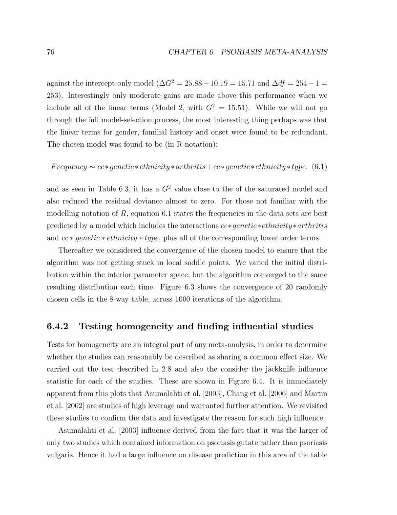
76 CHAPTER 6. PSORIASIS META-ANALYSIS
against the intercept-only model (∆G2 = 25.88−10.19 = 15.71 and ∆df = 254−1 =
253). Interestingly only moderate gains are made above this performance when we
include all of the linear terms (Model 2, with G2 = 15.51). While we will not go
through the full model-selection process, the most interesting thing perhaps was that
the linear terms for gender, familial history and onset were found to be redundant.
The chosen model was found to be (in R notation):
Frequency ∼ cc∗genetic∗ethnicity ∗arthritis+cc∗genetic∗ethnicity ∗ type. (6.1)
and as seen in Table 6.3, it has a G2 value close to the of the saturated model and
also reduced the residual deviance almost to zero. For those not familiar with the
modelling notation of R, equation 6.1 states the frequencies in the data sets are best
predicted by a model which includes the interactions cc∗genetic∗ethnicity∗arthritisand cc ∗ genetic ∗ ethnicity ∗ type, plus all of the corresponding lower order terms.
Thereafter we considered the convergence of the chosen model to ensure that the
algorithm was not getting stuck in local saddle points. We varied the initial distri-
bution within the interior parameter space, but the algorithm converged to the same
resulting distribution each time. Figure 6.3 shows the convergence of 20 randomly
chosen cells in the 8-way table, across 1000 iterations of the algorithm.
6.4.2 Testing homogeneity and finding influential studies
Tests for homogeneity are an integral part of any meta-analysis, in order to determine
whether the studies can reasonably be described as sharing a common effect size. We
carried out the test described in 2.8 and also the consider the jackknife influence
statistic for each of the studies. These are shown in Figure 6.4. It is immediately
apparent from this plots that Asumalahti et al. [2003], Chang et al. [2006] and Martin
et al. [2002] are studies of high leverage and warranted further attention. We revisited
these studies to confirm the data and investigate the reason for such high influence.
Asumalahti et al. [2003] influence derived from the fact that it was the larger of
only two studies which contained information on psoriasis gutate rather than psoriasis
vulgaris. Hence it had a large influence on disease prediction in this area of the table
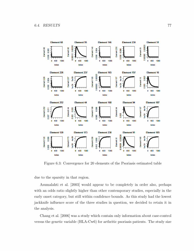
6.4. RESULTS 77
Figure 6.3: Convergence for 20 elements of the Psoriasis estimated table
due to the sparsity in that region.
Asumalahti et al. [2003] would appear to be completely in order also, perhaps
with an odds ratio slightly higher than other contemporary studies, especially in the
early onset category, but still within confidence bounds. As this study had the lowest
jackknife influence score of the three studies in question, we decided to retain it in
the analysis.
Chang et al. [2006] was a study which contain only information about case-control
versus the genetic variable (HLA-Cw6) for arthritic psoriasis patients. The study size
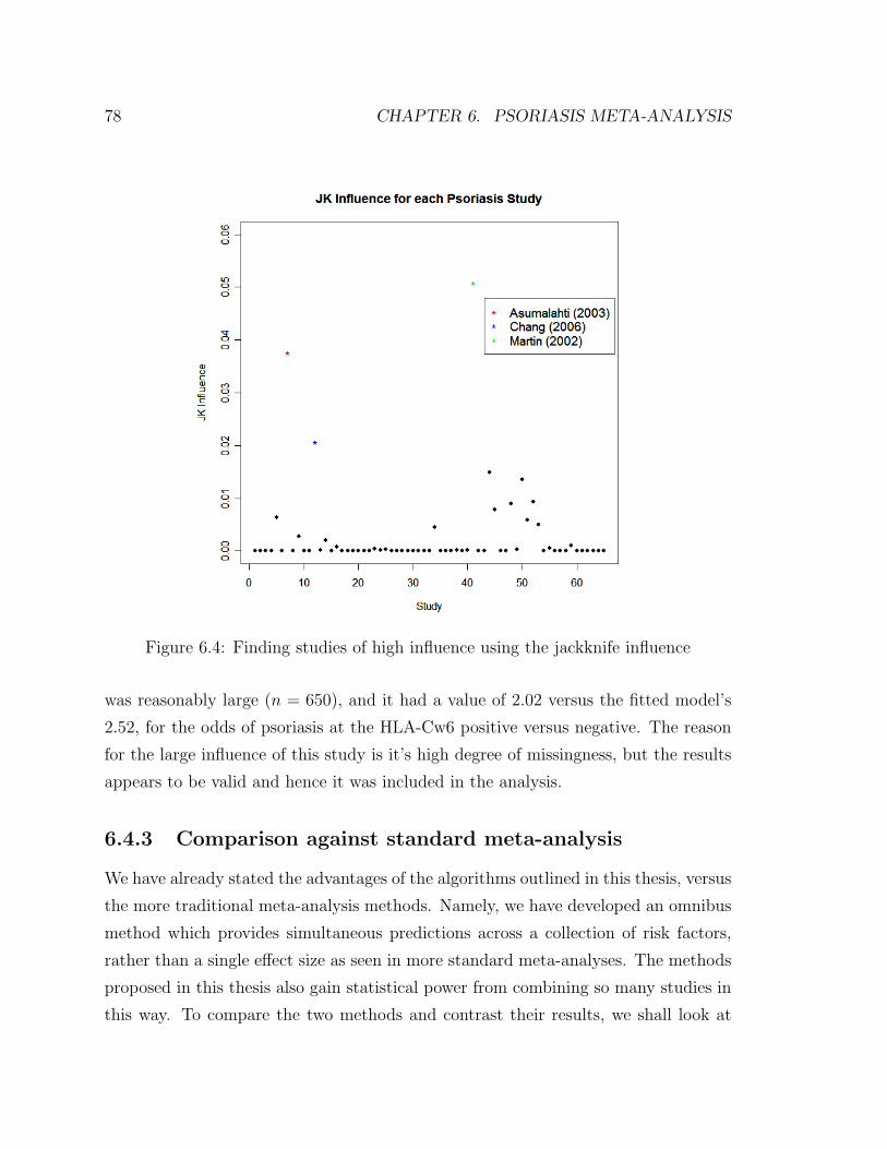
78 CHAPTER 6. PSORIASIS META-ANALYSIS
Figure 6.4: Finding studies of high influence using the jackknife influence
was reasonably large (n = 650), and it had a value of 2.02 versus the fitted model’s
2.52, for the odds of psoriasis at the HLA-Cw6 positive versus negative. The reason
for the large influence of this study is it’s high degree of missingness, but the results
appears to be valid and hence it was included in the analysis.
6.4.3 Comparison against standard meta-analysis
We have already stated the advantages of the algorithms outlined in this thesis, versus
the more traditional meta-analysis methods. Namely, we have developed an omnibus
method which provides simultaneous predictions across a collection of risk factors,
rather than a single effect size as seen in more standard meta-analyses. The methods
proposed in this thesis also gain statistical power from combining so many studies in
this way. To compare the two methods and contrast their results, we shall look at
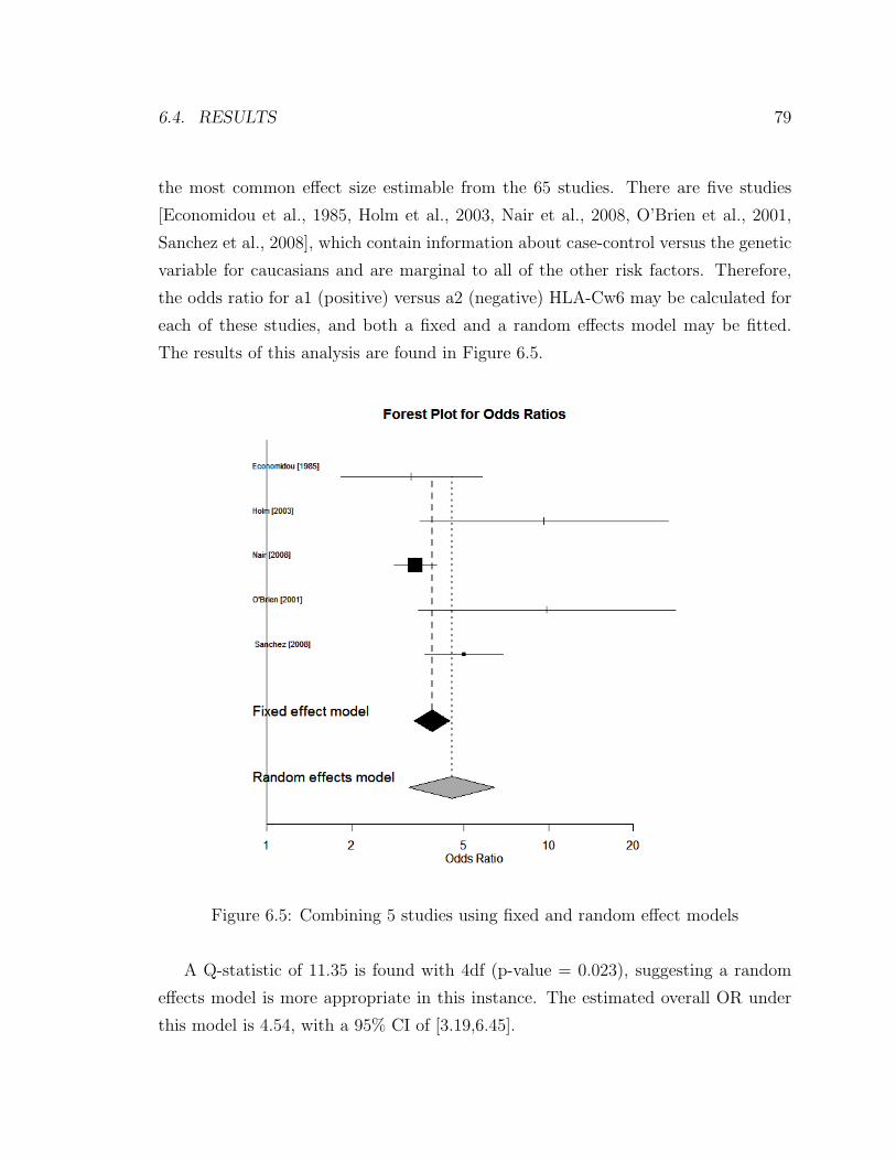
6.4. RESULTS 79
the most common effect size estimable from the 65 studies. There are five studies
[Economidou et al., 1985, Holm et al., 2003, Nair et al., 2008, O’Brien et al., 2001,
Sanchez et al., 2008], which contain information about case-control versus the genetic
variable for caucasians and are marginal to all of the other risk factors. Therefore,
the odds ratio for a1 (positive) versus a2 (negative) HLA-Cw6 may be calculated for
each of these studies, and both a fixed and a random effects model may be fitted.
The results of this analysis are found in Figure 6.5.
Figure 6.5: Combining 5 studies using fixed and random effect models
A Q-statistic of 11.35 is found with 4df (p-value = 0.023), suggesting a random
effects model is more appropriate in this instance. The estimated overall OR under
this model is 4.54, with a 95% CI of [3.19,6.45].

80 CHAPTER 6. PSORIASIS META-ANALYSIS
These results do not concur completely with those produced using our methods.
Using the likelihood-based approach, the estimated odds-ratio was 2.82, with a 95%
CI of [2.27,3.50]. Most obviously, this estimate is much lower than that produced by
the conventional meta-analysis. This may be accounted for by the fact that these
five studies were not the only contributary studies in finding the estimate under
our model, as many other studies contained information about this slice of the full
table. Upon further inspection, we found that many of the other studies contributed
lower OR estimates for this variable combination, with a mean OR of 1.65. Hence
the results found under our model were perhaps more reasonable, as the traditional
meta-analysis methods were not able to leverage these overlapping studies.
6.4.4 Disease prediction
The stated aim in building these models was to provide a method to estimate disease
probability for patients based on their individual risk characteristics. The major
advantage of the models we have fit, lies in the fact that they predict across the full
range of risk factors. In the psoriasis data set, we found four significant risk factors:
gene HLA-Cw6, ethnicity, arthritis and type. While the model itself includes many
higher order terms, to provide an overall picture for the relationship between each
of these risk factors and the disease probability, the marginal disease probabilities
for these variables are provided in Tables 6.4. The estimated odds ratios are also
included.
Factor Level1 Level2 OR1 Genetic (a1 vs a2) 0.033 0.015 2.212 Ethnicity (caucasian vs asian) 0.055 0.008 7.273 Arthritis (no vs yes) 0.018 0.022 0.824 Type (vulgaris vs gutate) 0.026 0.015 1.68
Table 6.4: Estimated marginal disease probabilities and odds-ratios
Please note that while there is a very high OR estimate for ethnicity, the CI is
also quite wide [1.25,8.62]. This is because only one moderately sized study contained
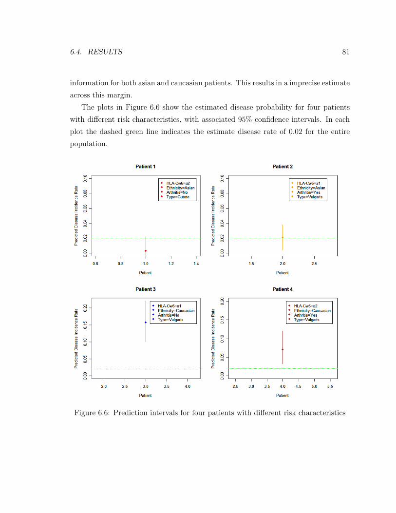
6.4. RESULTS 81
information for both asian and caucasian patients. This results in a imprecise estimate
across this margin.
The plots in Figure 6.6 show the estimated disease probability for four patients
with different risk characteristics, with associated 95% confidence intervals. In each
plot the dashed green line indicates the estimate disease rate of 0.02 for the entire
population.
Figure 6.6: Prediction intervals for four patients with different risk characteristics

Chapter 7
Alzheimer’s Disease Meta-Analysis
7.1 Alzheimer’s disease
Alzheimer’s disease (AD) is a progressive and fatal brain disorder first diagnosed by
a German physician named Alois Alzheimer in 1906. A degenerative and incurable
condition, it is the most common form of dementia, accounting for up to 70% of
cases. AD destroys brain cells, leading to memory and intellectual problems, severely
inhibiting the quality of life of those affected. For the majority of sufferers it is a late
onset disease (over 65 years), but an early onset version does also exist. It is estimated
that 26.6 million patients worldwide suffer from the disease, and this figure is expected
to quadruple before 2050. There is an accelerating worldwide effort under way to find
better ways to treat the disease, delay its onset, or prevent it from developing. No
succesful treatments have been found to delay onset or reduce disease risk, but it
remains an active research area for large pharmaceutical companies. For example,
in 2008 there were over 500 clinical studies investigating AD treatments. Although
the gestation period before diagnosis differs across patients, the mean life expectancy
is seven years. In fact fewer than 3% of sufferers survive more than fourteen years
following diagnosis.
While the cause and development of Alzheimer’s disease are not fully understood,
modern experts have linked the disease with plaques and tangles in the brain. This
link has been garnered predominantly based on autopsy evidence, and it is believed
82

7.1. ALZHEIMER’S DISEASE 83
that abnormally high growths of these structures disrupt, damage and kill nerve cells.
Some established and proposed risk factors for Alzheimer’s include:
• Age: the greatest known risk factor, with the likelihood of developing the disease
doubling every five years for those over 65.
• Family history: it has been found the risk of the disease doubles if a sibling has
previously suffered from the disease. Approximately 7% of disease incidence is
due to direct inheritance patterns associated with rare genes and regarded med-
ically as familial, i.e. passed on to 50% of the affected individual’s progeny. The
vast majority of these are attributable to mutations in one of three genes, amy-
loid precursor protein (APP) and presenilins 1 and 2 [Waring and Rosenberg,
2008].
• Aluminum: during the 1960s and 1970s it was suspected that regular exposure
to aluminum in household items such as pots, pans, beverage containers and
antiperspirants was linked to the onset of Alzheimer’s. Recent research has
failed to confirm this hypothesis, with few scientists still supporting this link.
• Head injury: serious cranial trauma has been shown to be linked directly with
the disease.
• General health: physically active and mentally stimulated individuals with a
healthy diet have been found to have both a lower rate of the disease and also
a later mean onset age for those who are diagnosed.
• Heart problems: the risk of developing the disease is increased by conditions
that damage the heart and blood vessels, such as diabetes, stroke, heart disease
and high cholesterol. Plaque and tangle growth has been shown to be greater
in AD sufferers who have heart issues.
• Genetic factors: the vast majority of cases of Alzheimer’s disease are sporadic
rather than familial, with genetic differences deigned only to be risk factors
here. The most established genetic link is the ε4 allele of the apolipoprotein

84 CHAPTER 7. ALZHEIMER’S DISEASE META-ANALYSIS
E (ApoE). This gene has been implicated in up to 50% of late onset sporadic
AD. Recent research has also linked angiotensin-converting enzyme (ACE) and
nitric oxide synthase (NOS3) to disease development, although this relationshop
has not yet been confirmed as conclusive. As noted for psoriasis genome-wide
association studies (GWASs) is unveiling avenues of discovery.
7.2 The data
The data set used in this analysis was gathered from 95 association studies in the
time period 1994 to 2006. Appendix B contains the references for the chosen papers.
Studies were included and excluded from this dataset in line with standard meta-
analysis procedures as outlined in [Stroup et al., 2000]. Linkage and family studies
were not considered at this stage of the analysis. We chose to include only studies
containing carrier frequencies, and replicated studies on same cohorts were excluded.
Each study was retrospective, and looked specifically at genotype information (ApoE,
ACE and NOS3) plus a collection of other known risk factors, both demographic and
clinical. In addition to the case-control variable, the factors chosen for inclusion in
this analysis were the following:
1. Gender: 2 levels (male and female)
2. ApoE: 6 levels, for each possible allele pair combination (ε2 ε2, ε2 ε3, ε2 ε4, ε3 ε3,
ε3 ε4 and ε4 ε4)
3. ACE: 3 levels, for each possible allele pair combination (ins ins, ins del and
del del)
4. NOS3: 3 levels, for each possible allele pair combination (glu glu, glu asp and
asp asp)
5. Ethnicity: 4 levels (caucasian, hispanic, asian and african)
6. Onset: 2 levels (early and late)
7. Familial history: 2 levels (familial or sporadic)
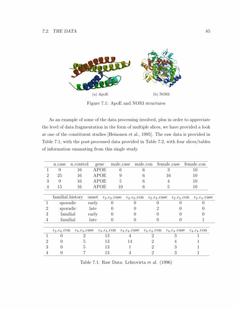
7.2. THE DATA 85
(a) ApoE (b) NOS3
Figure 7.1: ApoE and NOS3 structures
As an example of some of the data processing involved, plus in order to appreciate
the level of data fragmentation in the form of multiple slices, we have provided a look
at one of the constituent studies [Heinonen et al., 1995]. The raw data is provided in
Table 7.1, with the post-processed data provided in Table 7.2, with four slices/tables
of information emanating from this single study.
n case n control gene male case male con female case female con1 9 16 APOE 6 6 3 102 25 16 APOE 9 6 16 103 9 16 APOE 5 6 4 104 15 16 APOE 10 6 5 10
familial history onset ε2 ε2 case ε2 ε2 con ε2 ε3 case ε2 ε3 con ε2 ε4 case1 sporadic early 0 0 0 0 02 sporadic late 0 0 2 0 03 familial early 0 0 0 0 04 familial late 0 0 0 0 1
ε2 ε4 con ε3 ε3 case ε3 ε3 con ε3 ε4 case ε3 ε4 con ε4 ε4 case ε4 ε4 con1 0 2 13 4 2 3 12 0 5 13 14 2 4 13 0 5 13 1 2 3 14 0 7 13 4 2 3 1
Table 7.1: Raw Data: Lehtovirta et al. (1996)
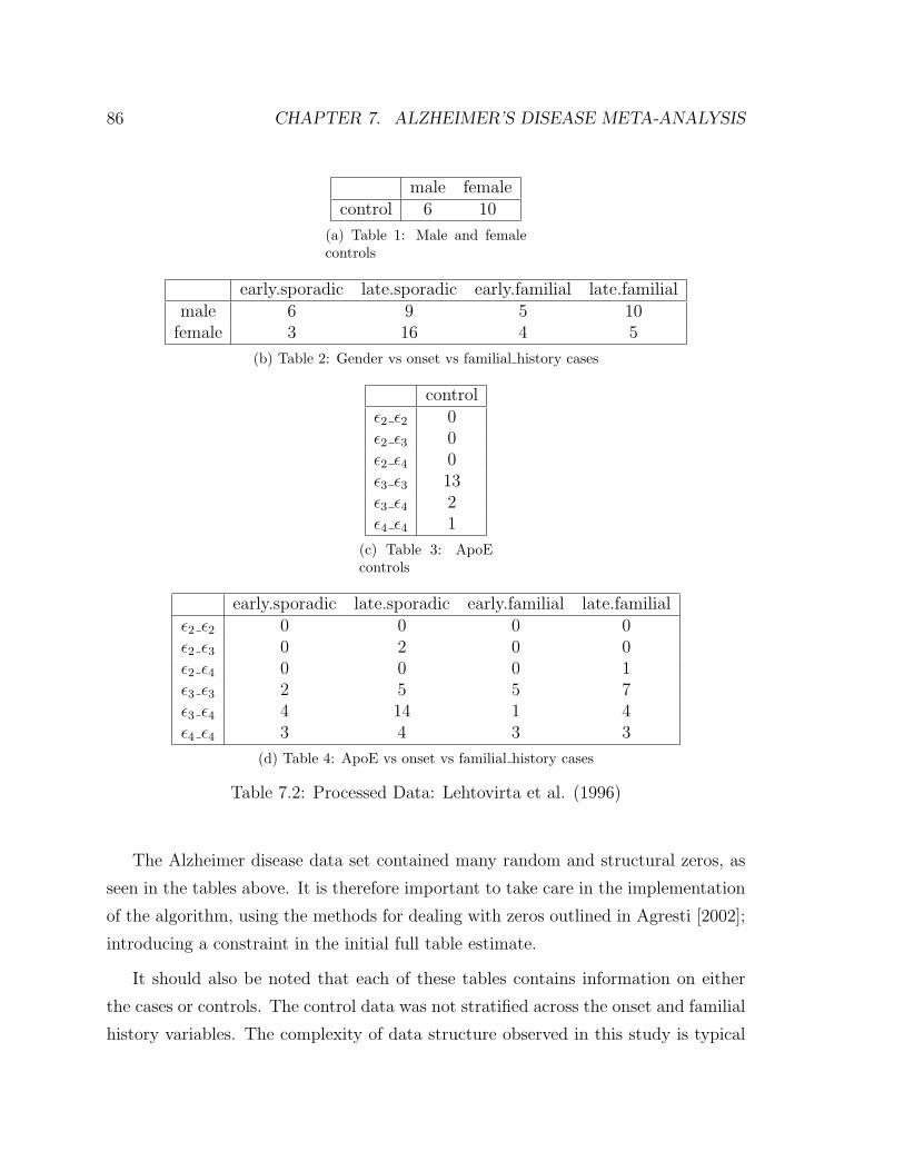
86 CHAPTER 7. ALZHEIMER’S DISEASE META-ANALYSIS
male femalecontrol 6 10
(a) Table 1: Male and femalecontrols
early.sporadic late.sporadic early.familial late.familialmale 6 9 5 10
female 3 16 4 5
(b) Table 2: Gender vs onset vs familial history cases
controlε2 ε2 0ε2 ε3 0ε2 ε4 0ε3 ε3 13ε3 ε4 2ε4 ε4 1
(c) Table 3: ApoEcontrols
early.sporadic late.sporadic early.familial late.familialε2 ε2 0 0 0 0ε2 ε3 0 2 0 0ε2 ε4 0 0 0 1ε3 ε3 2 5 5 7ε3 ε4 4 14 1 4ε4 ε4 3 4 3 3
(d) Table 4: ApoE vs onset vs familial history cases
Table 7.2: Processed Data: Lehtovirta et al. (1996)
The Alzheimer disease data set contained many random and structural zeros, as
seen in the tables above. It is therefore important to take care in the implementation
of the algorithm, using the methods for dealing with zeros outlined in Agresti [2002];
introducing a constraint in the initial full table estimate.
It should also be noted that each of these tables contains information on either
the cases or controls. The control data was not stratified across the onset and familial
history variables. The complexity of data structure observed in this study is typical
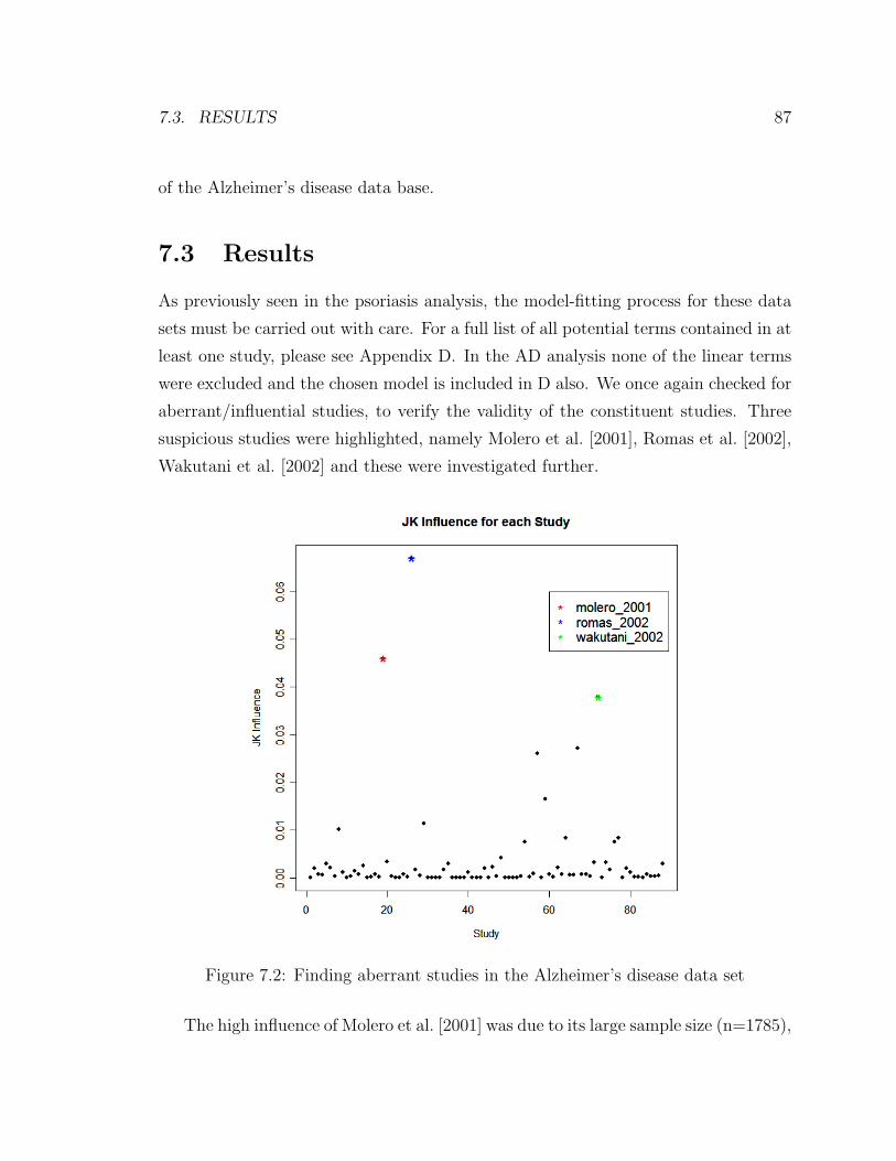
7.3. RESULTS 87
of the Alzheimer’s disease data base.
7.3 Results
As previously seen in the psoriasis analysis, the model-fitting process for these data
sets must be carried out with care. For a full list of all potential terms contained in at
least one study, please see Appendix D. In the AD analysis none of the linear terms
were excluded and the chosen model is included in D also. We once again checked for
aberrant/influential studies, to verify the validity of the constituent studies. Three
suspicious studies were highlighted, namely Molero et al. [2001], Romas et al. [2002],
Wakutani et al. [2002] and these were investigated further.
Figure 7.2: Finding aberrant studies in the Alzheimer’s disease data set
The high influence of Molero et al. [2001] was due to its large sample size (n=1785),

88 CHAPTER 7. ALZHEIMER’S DISEASE META-ANALYSIS
and hence we have chosen to retain this study in the analysis.
Romas et al. [2002] was yet another study of a Latin population, but with a
particularly large odds ratio for the ε3 ε3 versus ε2 ε2 of 2.97. There does not seem
to anything peculiar in the research itself, but this effect size is outside the range of
the estimate upon its exclusion. Therefore this study has been excluded from the
remainder of the analysis.
As the sole japanese study in this analysis, Wakutani et al. [2002] differs in its
observed rates than those of the other Asian studies it is pooled with, which otherwise
concentrate on predominantly Chinese populations. Again this does not appear to
be an homogeneous study and is excluded until such time as other Japanese studies
are included in the data base.
It is difficult to provide plots which give an appreciable perspective of such a high
dimensional model. In Figure 7.3 we show odds ratios relating to the four margins of
the fitted model, for gender and the three genetic variables. Of course it is important
to note that each of these plots looks at the variable effect summed across the other
variables levels, while in reality the model contains many interactions hidden from
these figures. However, even after considering this fact, the results shown in these
plots are exceptionally interesting. Each plot contained the OR estimate against the
chosen baseline, with a 95% confidence interval provided.
Firstly, the higher risk of AD is confirmed for females, and the well established
ε4 (a3) risk in ApoE was immediately obvious in second plot also. Perhaps the most
interesting conclusions are highlighted in the remaining two plots. Here we see that
ACE and NOS3 both have significant odds-ratio, indicating that they do indeed have
a link with the onset of Alzheimer’s disease. This relationship was suspected but not
confirmed in previous literature.
Two prediction plots, with their associated confidence intervals, are provided in
Figure 7.4 for patients with differing risk characteristics. Plots such as this will inform
patients and doctors in IVF clinics, and guide decisions on further genetic screening.
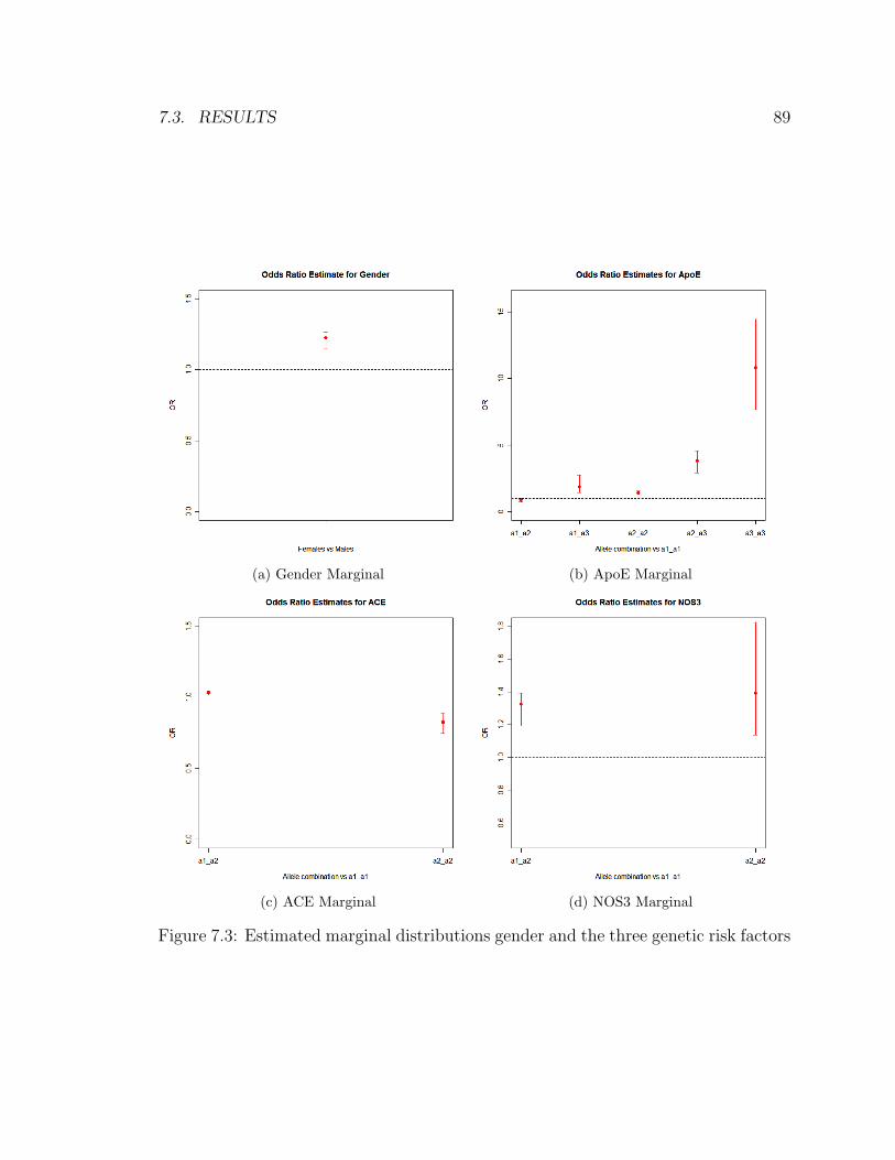
7.3. RESULTS 89
(a) Gender Marginal (b) ApoE Marginal
(c) ACE Marginal (d) NOS3 Marginal
Figure 7.3: Estimated marginal distributions gender and the three genetic risk factors
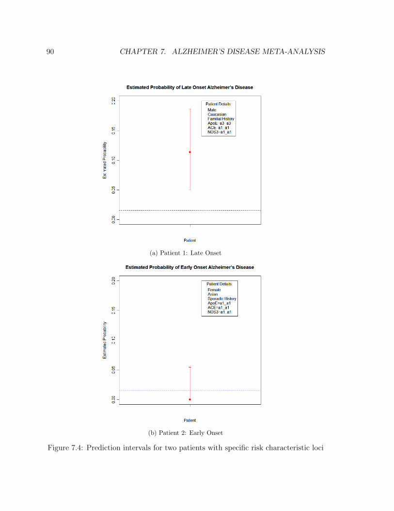
90 CHAPTER 7. ALZHEIMER’S DISEASE META-ANALYSIS
(a) Patient 1: Late Onset
(b) Patient 2: Early Onset
Figure 7.4: Prediction intervals for two patients with specific risk characteristic loci

Chapter 8
Conclusions
The main contributions of this thesis are as follows:
• A likelihood-based model was developed for the synthesis of many partially
classified contingency tables, using the EM algorithm and loglinear models.
This algorithm searches each constituent table and includes only interactions
observed in at least one table in the overall model. We have shown this method
to be consistent and accurate.
• We have also proposed a second, Bayesian model. This algorithm uses the anal-
ogous Data Augmentation algorithm in conjunction with Bayesian IPF, and
produces estimates close to those of the likelihood-based model. It does how-
ever have the beneficial property of providing an estimate for the full posterior
distribution, rather than just a point estimate for the mean as we saw in the
earlier model.
• The missing data patterns in this thesis were complex and varied. We provided
solutions for dealing with missingness due to marginal and conditional variables,
and combinations thereof, for both the likelihood-based setting and the Bayesian
model.
• Each study in the meta-analysis was case-control. We extended the previous
work on adjustments for retrospective sampling, finding the suitable correction
91
92 CHAPTER 8. CONCLUSIONS
under the logistic model for multiple studies. The loglinear case was not ex-
plored in previous research, but here we provided the adjustments necessary for
the single and multiple study scenario under this model.
• A multitude of variance estimates were investigated, including parametric meth-
ods based on the sandwich estimate, the bootstrap, the jackknife, SEM and the
posterior variance. The jackknife was found to out-perform the parametric
methods, while also providing supplementary benefits including natural cross-
validation samples for model-selection and in finding influential studies.
• Two meta-analysis were presented in this dissertation, using data sets collected
for psoriasis and Alzheimer’s disease. Predictive models were found using the
techniques developed in this thesis on a wide range of risk factors. These are
the largest and most accurate predictive models found to date for these high
profile diseases, confirming some hitherto unproven hypotheses regarding risk
factors using the increased power of the aggregated samples.
Appendix A
Studies in the psoriasis data base
The following studies were contained in the psoriasis data base: Al-Heresh et al.
[2002], Alenius et al. [2002], Allen et al. [2005], Armstrong et al. [1983], Asahina
et al. [1991], Asumalahti et al. [2000, 2003], Atasoy et al. [2006], Brenner et al. [1978],
Chang et al. [2003a,b, 2006], Choi et al. [2000], Dobosz et al. [2005], Duffin and
Krueger [2009], Economidou et al. [1985], Fan et al. [2007], Fojtikova et al. [2009],
Fry et al. [2006], Gladman et al. [1999], Gonzalez et al. [2001, 2000, 1999], Gudjonsson
et al. [2003], Helms et al. [2005], Ho et al. [2008], Hohler et al. [1996], Holm et al.
[2003, 2005a,b], Ikaheimo et al. [1996], Jobim et al. [2008], Kastelan et al. [2000], Kim
et al. [2000b], Kundakci et al. [2002], Liao et al. [2008], Lopez-Larrea et al. [1990],
Luszczek et al. [2003], Mallon et al. [2000, 1997, 1998], Martin et al. [2002], Martinez-
Borra et al. [2003], Murray et al. [1980], Nair et al. [2008], Nakagawa et al. [1991],
O’Brien et al. [2001], Orru et al. [2002], Ozawa et al. [1988], Pyo et al. [2003], Queiro
et al. [2008, 2006, 2003], Queiro-Silva et al. [2004], Rahman et al. [2003], Rani et al.
[1998], Roitberg-Tambur et al. [1994], Romphruk et al. [2003], Sanchez et al. [2004,
2008], Schmitt-Egenolf et al. [1996], Szczerkowska-Dobosz et al. [2004], Vejbaesya
et al. [1998], Williams et al. [2005], Wisniewski et al. [2003]
93
Appendix B
Interactions present in psoriasis
studies
A full list of the interactions present in at least one psoriasis model is given by the
following:
cc+ gender+ genetic+ ethnicity+ onset+ familialhistory+ arthritis+ type+
gender ∗ cc ∗ ethnicity ∗ arthritis+ cc ∗ genetic ∗ ethnicity ∗ arthritis+ genetic ∗ cc ∗ethnicity∗arthritis+onset∗genetic∗cc∗ethnicity∗arthritis+gender∗cc∗ethnicity∗onset∗type+cc∗genetic∗ethnicity∗onset∗type+genetic∗cc∗ethnicity+arthritis∗genetic∗ cc∗ethnicity+gender ∗ cc∗ethnicity ∗ type+ cc∗genetic∗ethnicity ∗ type+
onset∗genetic∗cc∗ethnicity+cc∗genetic∗type+cc∗gender∗ethnicity∗type+genetic∗cc∗ethnicity ∗ type+onset∗genetic∗cc∗ethnicity ∗ type+cc∗genetic∗onset∗ type+
gender ∗ cc ∗ ethnicity+ cc ∗ genetic ∗ ethnicity+ cc ∗ genetic+ gender ∗ genetic ∗ cc ∗ethnicity+cc∗genetic∗ethnicity∗onset∗arthritis+type∗gender∗cc∗ethnicity+type∗genetic∗cc∗ethnicity+gender ∗cc∗ethnicity ∗onset∗arthritis∗ type+cc∗genetic∗ethnicity ∗ onset ∗ arthritis ∗ type+ arthritis ∗ gender ∗ cc ∗ ethnicity+ cc ∗ gender ∗ethnicity∗onset∗type+genetic∗cc∗ethnicity∗onset+gender∗genetic∗cc∗ethnicity∗onset+ cc ∗ gender ∗ type+ genetic ∗ cc ∗ type+ onset ∗ genetic ∗ cc ∗ type+ genetic ∗familialhistory∗onset∗cc∗ethnicity∗type+genetic∗onset∗gender∗cc∗ethnicity∗type+ cc ∗ genetic ∗ arthritis+ genetic ∗ cc ∗ onset+ arthritis ∗ genetic ∗ cc ∗ onset
94
Appendix C
Studies in the Alzheimer’s data
base
The following studies were contained in the Alzheimer’s disease data base:
Adroer et al. [1995],Alvarez et al. [1999],Alvarez-Alvarez et al. [2003],Arboleda
et al. [2001],Bang et al. [2003],Buss et al. [2002],Cacabelos et al. [2003],Camelo et al.
[2004],Carrieri et al. [2001],Chen et al. [1999a],Chen et al. [1999b],Cheng et al. [2002],Corder
et al. [1994],Crawford et al. [2000],Cui et al. [2000],Farrer et al. [2000],Graff-Radford
et al. [2002],Guidi et al. [2005],Heinonen et al. [1995],Higuchi et al. [2000],Hong et al.
[1996],Hu et al. [1999],Huang et al. [2002],Isbir et al. [2000],Juhasz et al. [2005],Kim
et al. [2000a],Kim et al. [2001],Kolsch et al. [2005],Kukull et al. [1996],Kunugi et al.
[2000],Lambert et al. [1998],Lannfelt et al. [1994],Lehtovirta et al. [1996],Lendon et al.
[2002],Liu et al. [1999],Lopez et al. [1998],Ma et al. [2005],Maestre et al. [1995],Molero
et al. [2001],Monastero et al. [2002],Monastero et al. [2003],Mui et al. [1996],Myl-
lykangas et al. [2000],Nakayama and Kuzuhara [1999],Nalbantoglu et al. [1994],Narain
et al. [2000],Nunomura et al. [1996],Osuntokun et al. [1995],Panza et al. [2000],Panza
et al. [2003],Perry et al. [2001],Poirier et al. [1993],Prince et al. [2001],Quiroga et al.
[1999],Raygani et al. [2005],Richard et al. [2001],Romas et al. [2002],Roses [1997],Sa-
hota et al. [1997],Sanchez-Guerra et al. [2001],Scacchi et al. [1995],Scott et al. [1997],Seripa
et al. [2003],Seripa et al. [2004],Singleton et al. [2001],Sleegers et al. [2005],Slooter
et al. [1998],Sorbi et al. [1994],Souza et al. [2003],Styczynska et al. [2003],Sulkava
95
96 APPENDIX C. STUDIES IN THE ALZHEIMER’S DATA BASE
et al. [1996],Sunderland et al. [2004],Talbot et al. [1994],Tang et al. [1998],Tapi-
ola et al. [1998],Tedde et al. [2002],Tilley et al. [1999],Town et al. [1998],Tsuang
et al. [2005],van Duijn et al. [1995],Vuletic et al. [2005],Wakutani et al. [2002],Wang
et al. [2000],Wang et al. [2006],Wiebusch et al. [1999],Yang et al. [2000],Yang et al.
[2003],Zambenedetti et al. [2003],Zhang et al. [2003] and Zuliani et al. [2001]
Appendix D
Interactions present in Alzheimer’s
studies
A full list of the interactions present in at least one Alzheimer’s disease study is given
by the following:
cc + gender + APOE + ACE + NOS3 + ethnicity + onset + familialhistory +
cc ∗ gender ∗ ethnicity+ cc ∗APOE ∗ ethnicity+ gender ∗ cc ∗ ethnicity ∗ onset+ cc ∗ACE ∗ethnicity∗onset+cc∗gender∗ethnicity+cc∗APOE ∗ethnicity+cc∗gender∗ethnicity ∗onset+cc∗ACE ∗ethnicity ∗onset+cc∗APOE+cc∗APOE ∗ethnicity ∗familialhistory+gender∗cc∗onset+cc∗ACE∗onset+cc∗ACE∗onset+cc∗APOE∗ethnicity ∗onset+cc∗gender∗ethnicity ∗onset+cc∗APOE ∗ethnicity ∗onset+cc∗gender ∗ ethnicity+ cc∗ACE ∗ ethnicity+ cc∗APOE ∗ ethnicity ∗familialhistory ∗onset+ cc∗ACE ∗ethnicity ∗familialhistory+ cc∗APOE ∗ethnicity+ cc∗gender ∗ethnicity+cc∗ACE∗ethnicity+cc∗gender∗ethnicity∗onset+cc∗ACE∗ethnicity∗onset+cc∗gender∗ethnicity∗onset+cc∗ACE∗ethnicity∗familialhistory∗onset+cc∗APOE∗ethnicity+gender∗cc∗ethnicity∗familialhistory+cc∗ACE∗ethnicity∗familialhistory+ cc ∗ gender ∗ ethnicity ∗ familialhistory+ cc ∗NOS3 ∗ ethnicity ∗familialhistory+ cc∗ACE ∗ ethnicity+ cc∗NOS3∗ ethnicity ∗onset+ cc∗gender ∗ethnicity ∗ familialhistory ∗ onset+ cc ∗APOE ∗ ethnicity ∗ familialhistory ∗ onset
97

Bibliography
R Adroer, P Santacruz, R Blesa, S Lopez-Pousa, C Ascaso, and R Oliva. Apolipopro-
tein E4 allele frequency in Spanish Alzheimer and control cases. Neurosci Lett, 189
(3):182–6, 1995.
A. Agresti. Categorical Data Analysis. Wiley, New York, 2nd edition, 2002.
A M Al-Heresh, J Proctor, S M Jones, J Dixey, B Cox, K Welsh, and N McHugh. Tu-
mour necrosis factor-alpha polymorphism and the HLA-Cw*0602 allele in psoriatic
arthritis. Rheumatology (Oxford), 41(5):525–30, 2002.
G-M Alenius, E Jidell, L Nordmark, and S Rantapaa Dahlqvist. Disease manifesta-
tions and HLA antigens in psoriatic arthritis in northern Sweden. Clin Rheumatol,
21(5):357–62, 2002.
Michael Hugh Allen, Hahreen Ameen, Colin Veal, Julie Evans, V S Ramrakha-Jones,
A M Marsland, A David Burden, C E M Griffiths, Richard C Trembath, and
Jonathan N W N Barker. The major psoriasis susceptibility locus PSORS1 is not
a risk factor for late-onset psoriasis. J Invest Dermatol, 124(1):103–6, 2005.
R Alvarez, V Alvarez, C H Lahoz, C Martinez, J Pena, J M Sanchez, L M Guisasola,
J Salas-Puig, G Moris, J A Vidal, R Ribacoba, B B Menes, D Uria, and E Coto.
Angiotensin converting enzyme and endothelial nitric oxide synthase DNA poly-
morphisms and late onset Alzheimer’s disease. J Neurol Neurosurg Psychiatry, 67
(6):733–6, 1999.
Maite Alvarez-Alvarez, Luis Galdos, Manuel Fernandez-Martinez, Fernando Gomez-
Busto, Victoria Garcia-Centeno, Caridad Arias-Arias, Carmen Sanchez-Salazar,
98

BIBLIOGRAPHY 99
Ana Belen Rodriguez-Martinez, Juan Jose Zarranz, and Marian M de Pancorbo.
5-Hydroxytryptamine 6 receptor (5-HT(6)) receptor and apolipoprotein E (ApoE)
polymorphisms in patients with Alzheimer’s disease in the Basque Country. Neu-
rosci Lett, 339(1):85–7, 2003.
J. A. Anderson and S. C. Richardson. Logistic discrimination and bias correction in
maximum likelihood estimation. Technometrics, 21(1):71–78, 1979. ISSN 00401706.
URL http://www.jstor.org/stable/1268582.
G H Arboleda, J J Yunis, R Pardo, C M Gomez, D Hedmont, G Arango, and H Ar-
boleda. Apolipoprotein E genotyping in a sample of Colombian patients with
Alzheimer’s disease. Neurosci Lett, 305(2):135–8, 2001.
R D Armstrong, G S Panayi, and K I Welsh. Histocompatibility antigens in psoriasis,
psoriatic arthropathy, and ankylosing spondylitis. Ann Rheum Dis, 42(2):142–6,
1983.
A Asahina, S Akazaki, H Nakagawa, S Kuwata, K Tokunaga, Y Ishibashi, and T Juji.
Specific nucleotide sequence of HLA-C is strongly associated with psoriasis vulgaris.
J Invest Dermatol, 97(2):254–8, 1991.
K Asumalahti, T Laitinen, R Itkonen-Vatjus, M L Lokki, S Suomela, E Snellman,
U Saarialho-Kere, and J Kere. A candidate gene for psoriasis near HLA-C, HCR
(Pg8), is highly polymorphic with a disease-associated susceptibility allele. Hum
Mol Genet, 9(10):1533–42, 2000.
Kati Asumalahti, Mahreen Ameen, Sari Suomela, Eva Hagforsen, Gerd Michaelsson,
Julie Evans, Margo Munro, Colin Veal, Michael Allen, Joyce Leman, A David
Burden, Brian Kirby, Maureen Connolly, Christopher E M Griffiths, Richard C
Trembath, Juha Kere, Ulpu Saarialho-Kere, and Jonathan N W N Barker. Genetic
analysis of PSORS1 distinguishes guttate psoriasis and palmoplantar pustulosis. J
Invest Dermatol, 120(4):627–32, 2003.
Mustafa Atasoy, Ibrahim Pirim, Omer F Bayrak, Sevki Ozdemir, Mevlit Ikbal, Teo-
man Erdem, and Akin Aktas. Association of HLA class I and class II alleles with
100 BIBLIOGRAPHY
psoriasis vulgaris in Turkish population. Influence of type I and II psoriasis. Saudi
Med J, 27(3):373–6, 2006.
Oh Young Bang, Yong Tae Kwak, In Soo Joo, and Kyoon Huh. Important link
between dementia subtype and apolipoprotein E: a meta-analysis. Yonsei Med J,
44(3):401–13, 2003.
F Brandrup and A Green. The prevalence of psoriasis in Denmark. Acta Derm
Venereol, 61(4):344–6, 1981.
W Brenner, F Gschnait, and W R Mayr. HLA B13, B17, B37 and Cw6 in psoriasis
vulgaris: association with the age of onset. Arch Dermatol Res, 262(3):337–9, 1978.
Svenja Buss, Tomas Muller-Thomsen, Cristoph Hock, Antonella Alberici, Giuliano
Binetti, Roger M Nitsch, Andreas Gal, and Ulrich Finckh. No association between
DCP1 genotype and late-onset Alzheimer disease. Am J Med Genet, 114(4):440–5,
2002.
Ramon Cacabelos, Lucia Fernandez-Novoa, Valter Lombardi, Lola Corzo, Victor
Pichel, and Yasuhiko Kubota. Cerebrovascular risk factors in Alzheimer’s dis-
ease: brain hemodynamics and pharmacogenomic implications. Neurol Res, 25(6):
567–80, 2003.
Dalila Camelo, Gonzalo Arboleda, Juan J Yunis, Rodrigo Pardo, Gabriel Arango, Eu-
genia Solano, Luis Lopez, Daniel Hedmont, and Humberto Arboleda. Angiotensin-
converting enzyme and alpha-2-macroglobulin gene polymorphisms are not associ-
ated with Alzheimer’s disease in Colombian patients. J Neurol Sci, 218(1-2):47–51,
2004.
G Carrieri, M Bonafe, M De Luca, G Rose, O Varcasia, A Bruni, R Maletta,
B Nacmias, S Sorbi, F Corsonello, E Feraco, K F Andreev, A I Yashin, C Franceschi,
and G De Benedictis. Mitochondrial DNA haplogroups and APOE4 allele are non-
independent variables in sporadic Alzheimer’s disease. Hum Genet, 108(3):194–8,
2001.
BIBLIOGRAPHY 101
Y T Chang, S F Tsai, D D Lee, Y M Shiao, C Y Huang, H N Liu, W J Wang,
and C K Wong. A study of candidate genes for psoriasis near HLA-C in Chinese
patients with psoriasis. Br J Dermatol, 148(3):418–23, 2003a.
Y T Chang, S F Tsai, M W Lin, H N Liu, D D Lee, Y M Shiao, P J Chin, and W J
Wang. SPR1 gene near HLA-C is unlikely to be a psoriasis susceptibility gene. Exp
Dermatol, 12(3):307–14, 2003b.
Yun-Ting Chang, Chan-Te Chou, Yu-Ming Shiao, Ming-Wei Lin, Chia-Wen Yu, Chih-
Chiang Chen, Cheng-Hung Huang, Ding-Dar Lee, Han-Nan Liu, Wen-Jen Wang,
and Shih-Feng Tsai. The killer cell immunoglobulin-like receptor genes do not confer
susceptibility to psoriasis vulgaris independently in Chinese. J Invest Dermatol, 126
(10):2335–8, 2006.
L Chen, L Baum, H K Ng, L Y Chan, and C P Pang. Apolipoprotein E genotype and
its pathological correlation in Chinese Alzheimer’s disease with late onset. Hum
Pathol, 30(10):1172–7, 1999a.
L Chen, L Baum, H K Ng, L Y Chan, and C P Pang. Apolipoprotein E genotype and
its pathological correlation in Chinese Alzheimer’s disease with late onset. Hum
Pathol, 30(10):1172–7, 1999b.
Chih-Ya Cheng, Chen-Jee Hong, Hsiu-Chih Liu, Tsung-Yun Liu, and Shih-Jen Tsai.
Study of the association between Alzheimer’s disease and angiotensin-converting
enzyme gene polymorphism using DNA from lymphocytes. Eur Neurol, 47(1):26–9,
2002.
H B Choi, H Han, J I Youn, T Y Kim, and T G Kim. MICA 5.1 allele is a susceptibility
marker for psoriasis in the Korean population. Tissue Antigens, 56(6):548–50, 2000.
H. Cooper and L.V. Hedges. The Handbook of Research Synthesis. Russell Sage
Foundation, New York, 1994.
E H Corder, A M Saunders, N J Risch, W J Strittmatter, D E Schmechel, P C Jr
Gaskell, J B Rimmler, P A Locke, P M Conneally, and K E Schmader. Protective
102 BIBLIOGRAPHY
effect of apolipoprotein E type 2 allele for late onset Alzheimer disease. Nat Genet,
7(2):180–4, 1994.
F Crawford, L Abdullah, J Schinka, Z Suo, M Gold, R Duara, and M Mullan. Gender-
specific association of the angiotensin converting enzyme gene with Alzheimer’s
disease. Neurosci Lett, 280(3):215–9, 2000.
T Cui, X Zhou, W Jin, F Zheng, and X Cao. Gene polymorphism in apolipoprotein
E and presenilin-1 in patients with late-onset Alzheimer’s disease. Chin Med J
(Engl), 113(4):340–4, 2000.
A.P. Dempster, N.M. Laird, and D.B. Rubin. Maximum likelihood from incomplete
data via the em algorithm. Journal of the Royal Statistical Society Series B, B(39):
1–38, 1977.
A Szczerkowska Dobosz, K Rebala, Z Szczerkowska, and B Nedoszytko. HLA-C
locus alleles distribution in patients from northern Poland with psoriatic arthritis–
preliminary report. Int J Immunogenet, 32(6):389–91, 2005.
Kristina Callis Duffin and Gerald G Krueger. Genetic variations in cytokines and
cytokine receptors associated with psoriasis found by genome-wide association. J
Invest Dermatol, 129(4):827–33, 2009.
J Economidou, C Papasteriades, M Varla-Leftherioti, A Vareltzidis, and J Stratigos.
Human lymphocyte antigens A, B, and C in Greek patients with psoriasis: relation
to age and clinical expression of the disease. J Am Acad Dermatol, 13(4):578–82,
1985.
Bradley Efron and Robert J. Tibshirani. An Introduction to the Bootstrap. Chapman
and Hall, London, 1993.
J T Elder, R P Nair, S W Guo, T Henseler, E Christophers, and J J Voorhees. The
genetics of psoriasis. Arch Dermatol, 130(2):216–24, 1994.
BIBLIOGRAPHY 103
Xing Fan, Sen Yang, Liang Dan Sun, Yan Hua Liang, Min Gao, Kai Yue Zhang,
Wei Huang, and XueJun Zhang. Comparison of clinical features of HLA-Cw*0602-
positive and -negative psoriasis patients in a Han Chinese population. Acta Derm
Venereol, 87(4):335–40, 2007.
L A Farrer, T Sherbatich, S A Keryanov, G I Korovaitseva, E A Rogaeva, S Petruk,
S Premkumar, Y Moliaka, Y Q Song, Y Pei, C Sato, N D Selezneva, S Voskre-
senskaya, V Golimbet, S Sorbi, R Duara, S Gavrilova, P H St George-Hyslop, and
E I Rogaev. Association between angiotensin-converting enzyme and Alzheimer
disease. Arch Neurol, 57(2):210–4, 2000.
Marketa Fojtikova, Jiri Stolfa, Peter Novota, Pavlina Cejkova, Ctibor Dostal, and
Marie Cerna. HLA-Cw*06 class I region rather than MICA is associated with
psoriatic arthritis in Czech population. Rheumatol Int, 29(11):1293–9, 2009.
L Fry, A V Powles, S Corcoran, S Rogers, J Ward, and D J Unsworth. HLA Cw*06
is not essential for streptococcal-induced psoriasis. Br J Dermatol, 154(5):850–3,
2006.
Camil Fuchs. Maximum likelihood estimation and model selection in contingency
tables with missing data. Journal of the American Statistical Association, 77(378):
270–278, 1982. ISSN 01621459. URL http://www.jstor.org/stable/2287230.
A. Gelman, D.B Rubin, J. Carlin, and H. Stern. Bayesian Data Analysis. Chapman
and Hall, London, 1995.
Stuart German and Donald German. Stochastic relaxation, gibbs distributions, and
the bayesian restoration of images. IEEE Transactions on Pattern Analysis and
Machine Intelligence, PAMI-6(6):721–741, Nov. 1984.
D D Gladman, C Cheung, C M Ng, and J A Wade. HLA-C locus alleles in patients
with psoriatic arthritis (PsA). Hum Immunol, 60(3):259–61, 1999.
S Gonzalez, J Martinez-Borra, J C Torre-Alonso, S Gonzalez-Roces, J Sanchez del
Rio, A Rodriguez Perez, C Brautbar, and C Lopez-Larrea. The MICA-A9 triplet
104 BIBLIOGRAPHY
repeat polymorphism in the transmembrane region confers additional susceptibility
to the development of psoriatic arthritis and is independent of the association of
Cw*0602 in psoriasis. Arthritis Rheum, 42(5):1010–6, 1999.
S Gonzalez, J Martinez-Borra, J S Del Rio, J Santos-Juanes, A Lopez-Vazquez,
M Blanco-Gelaz, and C Lopez-Larrea. The OTF3 gene polymorphism confers sus-
ceptibility to psoriasis independent of the association of HLA-Cw*0602. J Invest
Dermatol, 115(5):824–8, 2000.
S Gonzalez, C Brautbar, J Martinez-Borra, A Lopez-Vazquez, R Segal, M A Blanco-
Gelaz, C D Enk, C Safriman, and C Lopez-Larrea. Polymorphism in MICA rather
than HLA-B/C genes is associated with psoriatic arthritis in the Jewish population.
Hum Immunol, 62(6):632–8, 2001.
Neill R Graff-Radford, Robert C Green, Rodney C P Go, Michael L Hutton, Timi
Edeki, David Bachman, Jennifer L Adamson, Patrick Griffith, Floyd B Willis, Mary
Williams, Yvonne Hipps, Jonathan L Haines, L Adrienne Cupples, and Lindsay A
Farrer. Association between apolipoprotein E genotype and Alzheimer disease in
African American subjects. Arch Neurol, 59(4):594–600, 2002.
Christopher E M Griffiths and Jonathan N W N Barker. Pathogenesis and clinical
features of psoriasis. Lancet, 370(9583):263–71, 2007.
J E Gudjonsson, A Karason, A Antonsdottir, E H Runarsdottir, V B Hauksson,
R Upmanyu, J Gulcher, K Stefansson, and H Valdimarsson. Psoriasis patients
who are homozygous for the HLA-Cw*0602 allele have a 2.5-fold increased risk of
developing psoriasis compared with Cw6 heterozygotes. Br J Dermatol, 148(2):
233–5, 2003.
Ilaria Guidi, Daniela Galimberti, Eliana Venturelli, Carlo Lovati, Roberto Del Bo,
Chiara Fenoglio, Alberto Gatti, Roberto Dominici, Sara Galbiati, Roberta Vir-
gilio, Simone Pomati, Giacomo P Comi, Claudio Mariani, Gianluigi Forloni, Nereo
Bresolin, and Elio Scarpini. Influence of the Glu298Asp polymorphism of NOS3
BIBLIOGRAPHY 105
on age at onset and homocysteine levels in AD patients. Neurobiol Aging, 26(6):
789–94, 2005.
T.J. Hastie, R.J. Tibshirani, and J.H. Friedman. The Elements of Statistical Learning.
Springer, New York, 2001.
Walter W. Hauck. The large sample variance of the mantel-haenszel estimator of
a common odds ratio. Biometrics, 35(4):817–819, 1979. ISSN 0006341X. URL
http://www.jstor.org/stable/2530114.
Larry V. Hedges and Ingram Olkin. Statistical Methods for Meta-Analysis. Academic
Press,San Diego, 1985.
O Heinonen, M Lehtovirta, H Soininen, S Helisalmi, A Mannermaa, H Sorvari, O Ko-
sunen, L Paljarvi, M Ryynanen, and P J Sr Riekkinen. Alzheimer pathology of
patients carrying apolipoprotein E epsilon 4 allele. Neurobiol Aging, 16(4):505–13,
1995.
Cynthia Helms, Nancy L Saccone, Li Cao, Jil A Wright Daw, Kai Cao, Tony M Hsu,
Patricia Taillon-Miller, Shenghui Duan, Derek Gordon, Brandon Pierce, Jurg Ott,
John Rice, Marcelo A Fernandez-Vina, Pui-Yan Kwok, Alan Menter, and Anne M
Bowcock. Localization of PSORS1 to a haplotype block harboring HLA-C and
distinct from corneodesmosin and HCR. Hum Genet, 118(3-4):466–76, 2005.
T Henseler and E Christophers. Psoriasis of early and late onset: characterization of
two types of psoriasis vulgaris. J Am Acad Dermatol, 13(3):450–6, 1985.
S Higuchi, S Ohta, S Matsushita, T Matsui, T Yuzuriha, K Urakami, and H Arai.
NOS3 polymorphism not associated with Alzheimer’s disease in Japanese. Ann
Neurol, 48(4):685, 2000.
P Y P C Ho, A Barton, J Worthington, D Plant, C E M Griffiths, H S Young,
P Bradburn, W Thomson, A J Silman, and I N Bruce. Investigating the role
of the HLA-Cw*06 and HLA-DRB1 genes in susceptibility to psoriatic arthritis:
106 BIBLIOGRAPHY
comparison with psoriasis and undifferentiated inflammatory arthritis. Ann Rheum
Dis, 67(5):677–82, 2008.
T Hohler, A Weinmann, P M Schneider, C Rittner, R E Schopf, J Knop,
P Hasenclever, K H Meyer zum Buschenfelde, and E Marker-Hermann. TAP-
polymorphisms in juvenile onset psoriasis and psoriatic arthritis. Hum Immunol,
51(1):49–54, 1996.
Sofia J Holm, Lina M Carlen, Lotus Mallbris, Mona Stahle-Backdahl, and Kevin P
O’Brien. Polymorphisms in the SEEK1 and SPR1 genes on 6p21.3 associate with
psoriasis in the Swedish population. Exp Dermatol, 12(4):435–44, 2003.
Sofia J Holm, Kazuko Sakuraba, Lotus Mallbris, Katarina Wolk, Mona Stahle, and
Fabio O Sanchez. Distinct HLA-C/KIR genotype profile associates with guttate
psoriasis. J Invest Dermatol, 125(4):721–30, 2005a.
Sofia J Holm, Fabio Sanchez, Lina M Carlen, Lotus Mallbris, Mona Stahle, and
Kevin P O’Brien. HLA-Cw*0602 associates more strongly to psoriasis in the
Swedish population than variants of the novel 6p21.3 gene PSORS1C3. Acta Derm
Venereol, 85(1):2–8, 2005b.
C J Hong, T Y Liu, H C Liu, S J Wang, J L Fuh, C W Chi, K Y Lee, and C B
Sim. Epsilon 4 allele of apolipoprotein E increases risk of Alzheimer’s disease in a
Chinese population. Neurology, 46(6):1749–51, 1996.
J Hu, F Miyatake, Y Aizu, H Nakagawa, S Nakamura, A Tamaoka, R Takahash,
K Urakami, and M Shoji. Angiotensin-converting enzyme genotype is associated
with Alzheimer disease in the Japanese population. Neurosci Lett, 277(1):65–7,
1999.
H-M Huang, Y-M Kuo, H-C Ou, C-C Lin, and L-J Chuo. Apolipoprotein E polymor-
phism in various dementias in Taiwan Chinese population. J Neural Transm, 109
(11):1415–21, 2002.
BIBLIOGRAPHY 107
I Ikaheimo, S Silvennoinen-Kassinen, J Karvonen, T Jarvinen, and A Ti-
ilikainen. Immunogenetic profile of psoriasis vulgaris: association with haplotypes
A2,B13,Cw6,DR7,DQA1*0201 and A1,B17,Cw6,DR7,DQA1*0201. Arch Dermatol
Res, 288(2):63–7, 1996.
T Isbir, B Agachan, H Yilmaz, and M Aydin. Angiotensin converting enzyme gene
polymorphism in Alzheimer’s disease. Cell Biochem Funct, 18(2):141–2, 2000.
M Jobim, L F J Jobim, P H Salim, T F Cestari, R Toresan, B C Gil, M R Jobim, T J
Wilson, M Kruger, J Schlottfeldt, and G Schwartsmann. A study of the killer cell
immunoglobulin-like receptor gene KIR2DS1 in a Caucasoid Brazilian population
with psoriasis vulgaris. Tissue Antigens, 72(4):392–6, 2008.
Anna Juhasz, Agnes Rimanoczy, Krisztina Boda, Gabor Vincze, Gyozo Szlavik, Mari-
anna Zana, Annamaria Bjelik, Magdolna Pakaski, Nikoletta Bodi, Andras Palotas,
Zoltan Janka, and Janos Kalman. CYP46 T/C polymorphism is not associated
with Alzheimer’s dementia in a population from Hungary. Neurochem Res, 30(8):
943–8, 2005.
M Kastelan, F Gruber, E Cecuk, V Kerhin-Brkljacic, L Brkljacic-Surkalovic, and
A Kastelan. Analysis of HLA antigens in Croatian patients with psoriasis. Acta
Derm Venereol Suppl (Stockh), NIL(211):12–3, 2000.
H C Kim, D K Kim, I J Choi, K H Kang, S D Yi, J Park, and Y N Park. Relation of
apolipoprotein E polymorphism to clinically diagnosed Alzheimer’s disease in the
Korean population. Psychiatry Clin Neurosci, 55(2):115–20, 2001.
K W Kim, J H Jhoo, K U Lee, D Y Lee, J H Lee, J Y Youn, B J Lee, S H Han,
and J I Woo. No association between alpha-1-antichymotrypsin polymorphism and
Alzheimer’s disease in Koreans. Am J Med Genet, 91(5):355–8, 2000a.
T G Kim, H J Lee, J I Youn, T Y Kim, and H Han. The association of psoriasis with
human leukocyte antigens in Korean population and the influence of age of onset
and sex. J Invest Dermatol, 114(2):309–13, 2000b.
108 BIBLIOGRAPHY
H Kolsch, F Jessen, N Freymann, M Kreis, F Hentschel, W Maier, and R Heun.
ACE I/D polymorphism is a risk factor of Alzheimer’s disease but not of vascular
dementia. Neurosci Lett, 377(1):37–9, 2005.
W A Kukull, G D Schellenberg, J D Bowen, W C McCormick, C E Yu, L Teri,
J D Thompson, E S O’Meara, and E B Larson. Apolipoprotein E in Alzheimer’s
disease risk and case detection: a case-control study. J Clin Epidemiol, 49(10):
1143–8, 1996.
S. Kullback and R. A. Leibler. On information and sufficiency. The An-
nals of Mathematical Statistics, 22(1):79–86, 1951. ISSN 00034851. URL
http://www.jstor.org/stable/2236703.
N Kundakci, T Oskay, U Olmez, H Tutkak, and E Gurgey. Association of psoriasis
vulgaris with HLA class I and class II antigens in the Turkish population, according
to the age at onset. Int J Dermatol, 41(6):345–8, 2002.
H Kunugi, A Akahane, A Ueki, M Otsuka, K Isse, H Hirasawa, N Kato, T Nabika,
S Kobayashi, and S Nanko. No evidence for an association between the Glu298Asp
polymorphism of the NOS3 gene and Alzheimer’s disease. J Neural Transm, 107
(8-9):1081–4, 2000.
J C Lambert, C Berr, F Pasquier, A Delacourte, B Frigard, D Cottel, J Perez-Tur,
V Mouroux, M Mohr, D Cecyre, D Galasko, C Lendon, J Poirier, J Hardy, D Mann,
P Amouyel, and M C Chartier-Harlin. Pronounced impact of Th1/E47cs mutation
compared with -491 AT mutation on neural APOE gene expression and risk of
developing Alzheimer’s disease. Hum Mol Genet, 7(9):1511–6, 1998.
L Lannfelt, L Lilius, M Nastase, M Viitanen, L Fratiglioni, G Eggertsen, L Berglund,
B Angelin, J Linder, and B Winblad. Lack of association between apolipoprotein
E allele epsilon 4 and sporadic Alzheimer’s disease. Neurosci Lett, 169(1-2):175–8,
1994.
E.L. Lehmann and G. Casella. Theory of Point Estimation. Springer Verlag, New
York, 2nd edition, 1998.
BIBLIOGRAPHY 109
M Lehtovirta, H Soininen, S Helisalmi, A Mannermaa, E L Helkala, P Hartikainen,
T Hanninen, M Ryynanen, and P J Riekkinen. Clinical and neuropsychological
characteristics in familial and sporadic Alzheimer’s disease: relation to apolipopro-
tein E polymorphism. Neurology, 46(2):413–9, 1996.
C L Lendon, U Thaker, J M Harris, A M McDonagh, J-C Lambert, M-C Chartier-
Harlin, T Iwatsubo, S M Pickering-Brown, and D M A Mann. The angiotensin 1-
converting enzyme insertion (I)/deletion (D) polymorphism does not influence the
extent of amyloid or tau pathology in patients with sporadic Alzheimer’s disease.
Neurosci Lett, 328(3):314–8, 2002.
Hsien-Tzung Liao, Kuan-Chia Lin, Yun-Ting Chang, Chun-Hsiung Chen, Toong-Hua
Liang, Wei-Sheng Chen, Kuei-Ying Su, Chang-Youh Tsai, and Chung-Tei Chou.
Human leukocyte antigen and clinical and demographic characteristics in psoriatic
arthritis and psoriasis in Chinese patients. J Rheumatol, 35(5):891–5, 2008.
Roderick J.A. Little and Donald B. Rubin. Statistical Analysis with Missing Data.
Wiley and Sons, New York, 2nd edition, 2002.
H C Liu, C J Hong, S J Wang, J L Fuh, P N Wang, H Y Shyu, and E L Teng.
ApoE genotype in relation to AD and cholesterol: a study of 2,326 Chinese adults.
Neurology, 53(5):962–6, 1999.
O L Lopez, S Lopez-Pousa, M I Kamboh, R Adroer, R Oliva, M Lozano-Gallego, J T
Becker, and S T DeKosky. Apolipoprotein E polymorphism in Alzheimer’s disease:
a comparative study of two research populations from Spain and the United States.
Eur Neurol, 39(4):229–33, 1998.
C Lopez-Larrea, J C Torre Alonso, A Rodriguez Perez, and E Coto. HLA antigens in
psoriatic arthritis subtypes of a Spanish population. Ann Rheum Dis, 49(5):318–9,
1990.
Thomas A. Louis. Finding the observed information matrix when using the em al-
gorithm. Journal of the Royal Statistical Society. Series B (Methodological), 44(2):
226–233, 1982. ISSN 00359246. URL http://www.jstor.org/stable/2345828.
110 BIBLIOGRAPHY
Wioleta Luszczek, Wioletta Kubicka, Maria Cislo, Piotr Nockowski, Maria Manczak,
Grzegorz Woszczek, Eugeniusz Baran, and Piotr Kusnierczyk. Strong association
of HLA-Cw6 allele with juvenile psoriasis in Polish patients. Immunol Lett, 85(1):
59–64, 2003.
Suk Ling Ma, Nelson Leung Sang Tang, Linda Chiu Wa Lam, and Helen Fung Kum
Chiu. The association between promoter polymorphism of the interleukin-10 gene
and Alzheimer’s disease. Neurobiol Aging, 26(7):1005–10, 2005.
G Maestre, R Ottman, Y Stern, B Gurland, M Chun, M X Tang, M Shelanski, B Ty-
cko, and R Mayeux. Apolipoprotein E and Alzheimer’s disease: ethnic variation in
genotypic risks. Ann Neurol, 37(2):254–9, 1995.
E Mallon, M Bunce, F Wojnarowska, and K Welsh. HLA-CW*0602 is a susceptibility
factor in type I psoriasis, and evidence Ala-73 is increased in male type I psoriatics.
J Invest Dermatol, 109(2):183–6, 1997.
E Mallon, D Young, M Bunce, F M Gotch, P J Easterbrook, R Newson, and C B
Bunker. HLA-Cw*0602 and HIV-associated psoriasis. Br J Dermatol, 139(3):527–
33, 1998.
E Mallon, M Bunce, H Savoie, A Rowe, R Newson, F Gotch, and C B Bunker. HLA-C
and guttate psoriasis. Br J Dermatol, 143(6):1177–82, 2000.
N. Mantel and W. Haenszel. Statistical aspects of the analysis of data from retro-
spective studies of disease. J. Natl. Cancer Inst., 22:719–748, 1959.
Maureen P Martin, George Nelson, Jeong-Hee Lee, Fawnda Pellett, Xiaojiang Gao,
Judith Wade, Michael J Wilson, John Trowsdale, Dafna Gladman, and Mary Car-
rington. Cutting edge: susceptibility to psoriatic arthritis: influence of activating
killer Ig-like receptor genes in the absence of specific HLA-C alleles. J Immunol,
169(6):2818–22, 2002.
J Martinez-Borra, S Gonzalez, J Santos-Juanes, J Sanchez del Rio, J C Torre-Alonso,
A Lopez-Vazquez, M A Blanco-Gelaz, and C Lopez-Larrea. Psoriasis vulgaris and
BIBLIOGRAPHY 111
psoriatic arthritis share a 100 kb susceptibility region telomeric to HLA-C. Rheuma-
tology (Oxford), 42(9):1089–92, 2003.
P. McCullagh and J.A. Nelder. Generalized Linear Models. Chapman and Hall,
London, 2nd edition, 1983.
F O Meenan. A note on the history of psoriasis. Ir J Med Sci, 6(351):141–2, 1955.
Xiao-Li Meng and Donald B. Rubin. Using em to obtain asymptotic
variance-covariance matrices: The sem algorithm. Journal of the Ameri-
can Statistical Association, 86(416):899–909, 1991. ISSN 01621459. URL
http://www.jstor.org/stable/2290503.
X.L. Meng and D.B. Rubin. Maximum likelihood estimation via the ecm algorithm:
A general framework. Biometrika, 80:267–278, 1993.
A E Molero, G Pino-Ramirez, and G E Maestre. Modulation by age and gender of risk
for Alzheimer’s disease and vascular dementia associated with the apolipoprotein
E-epsilon4 allele in Latin Americans: findings from the Maracaibo Aging Study.
Neurosci Lett, 307(1):5–8, 2001.
Roberto Monastero, Rosalia Caldarella, Marina Mannino, Angelo B Cefalu, Gianluca
Lopez, Davide Noto, Cecilia Camarda, Lawrence K C Camarda, Alberto Notar-
bartolo, Maurizio R Averna, and Rosolino Camarda. Lack of association between
angiotensin converting enzyme polymorphism and sporadic Alzheimer’s disease.
Neurosci Lett, 335(2):147–9, 2002.
Roberto Monastero, Angelo B Cefalu, Cecilia Camarda, Carmela M Buglino, Marina
Mannino, Carlo M Barbagallo, Gianluca Lopez, Lawrence K C Camarda, Salva-
tore Travali, Rosolino Camarda, and Maurizio R Averna. No association between
Glu298Asp endothelial nitric oxide synthase polymorphism and Italian sporadic
Alzheimer’s disease. Neurosci Lett, 341(3):229–32, 2003.
S Mui, M Briggs, H Chung, R B Wallace, T Gomez-Isla, G W Rebeck, and B T
Hyman. A newly identified polymorphism in the apolipoprotein E enhancer gene

112 BIBLIOGRAPHY
region is associated with Alzheimer’s disease and strongly with the epsilon 4 allele.
Neurology, 47(1):196–201, 1996.
C Murray, D L Mann, L N Gerber, W Barth, S Perlmann, J L Decker, and T P
Nigra. Histocompatibility alloantigens in psoriasis and psoriatic arthritis. Evidence
for the influence of multiple genes in the major histocompatibility complex. J Clin
Invest, 66(4):670–5, 1980.
L Myllykangas, T Polvikoski, R Sulkava, A Verkkoniemi, P Tienari, L Niinisto,
K Kontula, J Hardy, M Haltia, and J Perez-Tur. Cardiovascular risk factors and
Alzheimer’s disease: a genetic association study in a population aged 85 or over.
Neurosci Lett, 292(3):195–8, 2000.
Rajan P Nair, Andreas Ruether, Philip E Stuart, Stefan Jenisch, Trilokraj Tejasvi,
Ravi Hiremagalore, Stefan Schreiber, Dieter Kabelitz, Henry W Lim, John J
Voorhees, Enno Christophers, James T Elder, and Michael Weichenthal. Poly-
morphisms of the IL12B and IL23R genes are associated with psoriasis. J Invest
Dermatol, 128(7):1653–61, 2008.
H Nakagawa, S Akazaki, A Asahina, K Tokunaga, K Matsuki, S Kuwata, Y Ishibashi,
and T Juji. Study of HLA class I, class II and complement genes (C2, C4A, C4B
and BF) in Japanese psoriatics and analysis of a newly-found high-risk haplotype
by pulsed field gel electrophoresis. Arch Dermatol Res, 283(5):281–4, 1991.
S Nakayama and S Kuzuhara. Apolipoprotein E phenotypes in healthy normal con-
trols and demented subjects with Alzheimer’s disease and vascular dementia in Mie
Prefecture of Japan. Psychiatry Clin Neurosci, 53(6):643–8, 1999.
J Nalbantoglu, B M Gilfix, P Bertrand, Y Robitaille, S Gauthier, D S Rosenblatt, and
J Poirier. Predictive value of apolipoprotein E genotyping in Alzheimer’s disease:
results of an autopsy series and an analysis of several combined studies. Ann Neurol,
36(6):889–95, 1994.
Y Narain, A Yip, T Murphy, C Brayne, D Easton, J G Evans, J Xuereb, N Cairns,
BIBLIOGRAPHY 113
M M Esiri, R A Furlong, and D C Rubinsztein. The ACE gene and Alzheimer’s
disease susceptibility. J Med Genet, 37(9):695–7, 2000.
Frank O Nestle, Daniel H Kaplan, and Jonathan Barker. Psoriasis. N Engl J Med,
361(5):496–509, 2009.
A Nunomura, S Chiba, M Eto, M Saito, I Makino, and T Miyagishi. Apolipoprotein
E polymorphism and susceptibility to early- and late-onset sporadic Alzheimer’s
disease in Hokkaido, the northern part of Japan. Neurosci Lett, 206(1):17–20, 1996.
K P O’Brien, S J Holm, S Nilsson, L Carlen, T Rosenmuller, C Enerback, A Inerot,
and M Stahle-Backdahl. The HCR gene on 6p21 is unlikely to be a psoriasis
susceptibility gene. J Invest Dermatol, 116(5):750–4, 2001.
S Orru, E Giuressi, M Casula, A Loizedda, R Murru, M Mulargia, M V Masala,
D Cerimele, M Zucca, N Aste, P Biggio, C Carcassi, and L Contu. Psoriasis is
associated with a SNP haplotype of the corneodesmosin gene (CDSN). Tissue
Antigens, 60(4):292–8, 2002.
B O Osuntokun, A Sahota, A O Ogunniyi, O Gureje, O Baiyewu, A Adeyinka, S O
Oluwole, O Komolafe, K S Hall, and F W Unverzagt. Lack of an association
between apolipoprotein E epsilon 4 and Alzheimer’s disease in elderly Nigerians.
Ann Neurol, 38(3):463–5, 1995.
A Ozawa, M Ohkido, H Inoko, A Ando, and K Tsuji. Specific restriction fragment
length polymorphism on the HLA-C region and susceptibility to psoriasis vulgaris.
J Invest Dermatol, 90(3):402–5, 1988.
F Panza, V Solfrizzi, F Torres, F Mastroianni, A M Colacicco, A M Basile, C Capurso,
A D’Introno, A Del Parigi, and A Capurso. Apolipoprotein E in Southern Italy:
protective effect of epsilon 2 allele in early- and late-onset sporadic Alzheimer’s
disease. Neurosci Lett, 292(2):79–82, 2000.
Francesco Panza, Vincenzo Solfrizzi, Anna M Colacicco, Anna M Basile, Alessia
114 BIBLIOGRAPHY
D’Introno, Cristiano Capurso, Maria Sabba, Sabrina Capurso, and Antonio Ca-
purso. Apolipoprotein E (APOE) polymorphism influences serum APOE levels in
Alzheimer’s disease patients and centenarians. Neuroreport, 14(4):605–8, 2003.
Yudi Pawitan. In All Likelihood. Oxford University Press, Oxford, 2001.
R T Perry, J S Collins, L E Harrell, R T Acton, and R C Go. Investigation of
association of 13 polymorphisms in eight genes in southeastern African American
Alzheimer disease patients as compared to age-matched controls. Am J Med Genet,
105(4):332–42, 2001.
J Poirier, J Davignon, D Bouthillier, S Kogan, P Bertrand, and S Gauthier.
Apolipoprotein E polymorphism and Alzheimer’s disease. Lancet, 342(8873):697–9,
1993.
J A Prince, L Feuk, S L Sawyer, J Gottfries, A Ricksten, K Nagga, N Bogdanovic,
K Blennow, and A J Brookes. Lack of replication of association findings in complex
disease: an analysis of 15 polymorphisms in prior candidate genes for sporadic
Alzheimer’s disease. Eur J Hum Genet, 9(6):437–44, 2001.
Chul-Woo Pyo, Seong-Suk Hur, Yang-Kyum Kim, Tae-Yoon Kim, and Tai-Gyu Kim.
Association of TAP and HLA-DM genes with psoriasis in Koreans. J Invest Der-
matol, 120(4):616–22, 2003.
R Queiro, P Moreno, C Sarasqueta, M Alperi, J L Riestra, and J Ballina. Synovitis-
acne-pustulosis-hyperostosis-osteitis syndrome and psoriatic arthritis exhibit a dif-
ferent immunogenetic profile. Clin Exp Rheumatol, 26(1):125–8, 2008.
Ruben Queiro, Juan Carlos Torre, Segundo Gonzalez, Carlos Lopez-Larrea, Tomas
Tinture, and Isaac Lopez-Lagunas. HLA antigens may influence the age of onset
of psoriasis and psoriatic arthritis. J Rheumatol, 30(3):505–7, 2003.
Ruben Queiro, Segundo Gonzalez, Carlos Lopez-Larrea, Mercedes Alperi, Cristina
Sarasqueta, Jose Luis Riestra, and Javier Ballina. HLA-C locus alleles may mod-
ulate the clinical expression of psoriatic arthritis. Arthritis Res Ther, 8(6):R185,
2006.
BIBLIOGRAPHY 115
R Queiro-Silva, J C Torre-Alonso, T Tinture-Eguren, and I Lopez-Lagunas. The effect
of HLA-DR antigens on the susceptibility to, and clinical expression of psoriatic
arthritis. Scand J Rheumatol, 33(5):318–22, 2004.
P Quiroga, C Calvo, C Albala, J Urquidi, J L Santos, H Perez, and G Klaassen.
Apolipoprotein E polymorphism in elderly Chilean people with Alzheimer’s disease.
Neuroepidemiology, 18(1):48–52, 1999.
P Rahman, S Bartlett, F Siannis, F J Pellett, V T Farewell, L Peddle, C T Schentag,
C A Alderdice, S Hamilton, M Khraishi, Y Tobin, D Hefferton, and D D Gladman.
CARD15: a pleiotropic autoimmune gene that confers susceptibility to psoriatic
arthritis. Am J Hum Genet, 73(3):677–81, 2003.
R Rani, R Narayan, M A Fernandez-Vina, and P Stastny. Role of HLA-B and C
alleles in development of psoriasis in patients from North India. Tissue Antigens,
51(6):618–22, 1998.
Asad Vaisi Raygani, Mahine Zahrai, Akbar Vaisi Raygani, Mahmood Doosti, Ebrahim
Javadi, Mansour Rezaei, and Tayebeh Pourmotabbed. Association between
apolipoprotein E polymorphism and Alzheimer disease in Tehran, Iran. Neurosci
Lett, 375(1):1–6, 2005.
J Reefhuis, M A Honein, L A Schieve, A Correa, C A Hobbs, and S A Rasmussen.
Assisted reproductive technology and major structural birth defects in the United
States. Hum Reprod, 24(2):360–6, 2009.
F Richard, I Fromentin-David, F Ricolfi, P Ducimetiere, C Di Menza, P Amouyel,
and N Helbecque. The angiotensin I converting enzyme gene as a susceptibility
factor for dementia. Neurology, 56(11):1593–5, 2001.
James Robins, Norman Breslow, and Sander Greenland. Estimators of the
mantel-haenszel variance consistent in both sparse data and large-strata lim-
iting models. Biometrics, 42(2):311–323, 1986. ISSN 0006341X. URL
http://www.jstor.org/stable/2531052.
116 BIBLIOGRAPHY
A Roitberg-Tambur, A Friedmann, E E Tzfoni, S Battat, R Ben Hammo, C Safirman,
K Tokunaga, A Asahina, and C Brautbar. Do specific pockets of HLA-C molecules
predispose Jewish patients to psoriasis vulgaris? J Am Acad Dermatol, 31(6):
964–8, 1994.
Stavra N Romas, Vincent Santana, Jennifer Williamson, Alejandra Ciappa, Joseph H
Lee, Haydee Z Rondon, Pedro Estevez, Rafael Lantigua, Martin Medrano, May-
obanex Torres, Yaakov Stern, Benjamin Tycko, and Richard Mayeux. Familial
Alzheimer disease among Caribbean Hispanics: a reexamination of its association
with APOE. Arch Neurol, 59(1):87–91, 2002.
A V Romphruk, A Oka, A Romphruk, M Tomizawa, C Choonhakarn, T K Naruse,
C Puapairoj, G Tamiya, C Leelayuwat, and H Inoko. Corneodesmosin gene: no ev-
idence for PSORS 1 gene in North-eastern Thai psoriasis patients. Tissue Antigens,
62(3):217–24, 2003.
A D Roses. A model for susceptibility polymorphisms for complex diseases:
apolipoprotein E and Alzheimer disease. Neurogenetics, 1(1):3–11, 1997.
T J Russell, L M Schultes, and D J Kuban. Histocompatibility (HL-A) antigens
associated with psoriasis. N Engl J Med, 287(15):738–40, 1972.
A Sahota, M Yang, S Gao, S L Hui, O Baiyewu, O Gureje, S Oluwole, A Ogunniyi,
K S Hall, and H C Hendrie. Apolipoprotein E-associated risk for Alzheimer’s
disease in the African-American population is genotype dependent. Ann Neurol,
42(4):659–61, 1997.
Fabio Sanchez, Sofia J Holm, Lotus Mallbris, Kevin P O’Brien, and Mona Stahle.
STG does not associate with psoriasis in the Swedish population. Exp Dermatol,
13(7):413–8, 2004.
Fabio O Sanchez, M V Prasad Linga Reddy, Lotus Mallbris, Kazuko Sakuraba, Mona
Stahle, and Marta E Alarcon-Riquelme. IFN-regulatory factor 5 gene variants
interact with the class I MHC locus in the Swedish psoriasis population. J Invest
Dermatol, 128(7):1704–9, 2008.
BIBLIOGRAPHY 117
M Sanchez-Guerra, O Combarros, A Alvarez-Arcaya, I Mateo, J Berciano,
J Gonzalez-Garcia, and J Llorca. The Glu298Asp polymorphism in the NOS3 gene
is not associated with sporadic Alzheimer’s disease. J Neurol Neurosurg Psychiatry,
70(4):566–7, 2001.
R Scacchi, L De Bernardini, E Mantuano, L M Donini, T Vilardo, and R M Corbo.
Apolipoprotein E (APOE) allele frequencies in late-onset sporadic Alzheimer’s dis-
ease (AD), mixed dementia and vascular dementia: lack of association of epsilon 4
allele with AD in Italian octogenarian patients. Neurosci Lett, 201(3):231–4, 1995.
Joeseph L. Schafer. Analysis of Incomplete Multivariate Data. Chapman and Hall,
New York, 1997.
M Schmitt-Egenolf, T H Eiermann, W H Boehncke, M Stander, and W Sterry.
Familial juvenile onset psoriasis is associated with the human leukocyte antigen
(HLA) class I side of the extended haplotype Cw6-B57-DRB1*0701-DQA1*0201-
DQB1*0303: a population- and family-based study. J Invest Dermatol, 106(4):
711–4, 1996.
W K Scott, A M Saunders, P C Gaskell, P A Locke, J H Growdon, L A Farrer,
S A Auerbach, A D Roses, J L Haines, and M A Pericak-Vance. Apolipoprotein
E epsilon2 does not increase risk of early-onset sporadic Alzheimer’s disease. Ann
Neurol, 42(3):376–8, 1997.
Shaun R. Seaman and Sylvia Richardson. Bayesian analysis of case-control studies
with categorical covariates. Biometrika, 88(4):1073–1088, 2001. ISSN 00063444.
URL http://www.jstor.org/stable/2673702.
D Seripa, M G Matera, R P D’Andrea, C Gravina, C Masullo, A Daniele, A Bizzarro,
M Rinaldi, P Antuono, D R Wekstein, G Dal Forno, and V M Fazio. Alzheimer
disease risk associated with APOE4 is modified by STH gene polymorphism. Neu-
rology, 62(9):1631–3, 2004.
Davide Seripa, Gloria Dal Forno, Maria G Matera, Carolina Gravina, Maurizio Mar-
gaglione, Mark T Palermo, David R Wekstein, Piero Antuono, Daron G Davis,

118 BIBLIOGRAPHY
Antonio Daniele, Carlo Masullo, Alessandra Bizzarro, Massimo Gennarelli, and
Vito M Fazio. Methylenetetrahydrofolate reductase and angiotensin converting en-
zyme gene polymorphisms in two genetically and diagnostically distinct cohort of
Alzheimer patients. Neurobiol Aging, 24(7):933–9, 2003.
A B Singleton, A M Gibson, I G McKeith, C G Ballard, J A Edwardson, and C M
Morris. Nitric oxide synthase gene polymorphisms in Alzheimer’s disease and de-
mentia with Lewy bodies. Neurosci Lett, 303(1):33–6, 2001.
Kristel Sleegers, Tom den Heijer, Ewoud J van Dijk, Albert Hofman, Aida M Bertoli-
Avella, Peter J Koudstaal, Monique M B Breteler, and Cornelia M van Duijn.
ACE gene is associated with Alzheimer’s disease and atrophy of hippocampus and
amygdala. Neurobiol Aging, 26(8):1153–9, 2005.
A J Slooter, M Cruts, S Kalmijn, A Hofman, M M Breteler, C Van Broeckhoven,
and C M van Duijn. Risk estimates of dementia by apolipoprotein E genotypes
from a population-based incidence study: the Rotterdam Study. Arch Neurol, 55
(7):964–8, 1998.
S Sorbi, B Nacmias, P Forleo, S Latorraca, I Gobbini, L Bracco, S Piacentini, and
L Amaducci. ApoE allele frequencies in Italian sporadic and familial Alzheimer’s
disease. Neurosci Lett, 177(1-2):100–2, 1994.
D R S Souza, M R de Godoy, J Hotta, E H Tajara, A C Brandao, S Pinheiro Junior,
W A Tognola, and J E dos Santos. Association of apolipoprotein E polymorphism
in late-onset Alzheimer’s disease and vascular dementia in Brazilians. Braz J Med
Biol Res, 36(7):919–23, 2003.
D F Stroup, J A Berlin, S C Morton, I Olkin, G D Williamson, D Rennie, D Moher,
B J Becker, T A Sipe, and S B Thacker. Meta-analysis of observational studies in
epidemiology: a proposal for reporting. Meta-analysis Of Observational Studies in
Epidemiology (MOOSE) group. JAMA, 283(15):2008–12, 2000.
Maria Styczynska, Dorota Religa, Anna Pfeffer, Elzbieta Luczywek, Boguslaw
Wasiak, Grzegorz Styczynski, Beata Peplonska, Tomasz Gabryelewicz, Marek
BIBLIOGRAPHY 119
Golebiowski, Malgorzata Kobrys, and Maria Barcikowska. Simultaneous analy-
sis of five genetic risk factors in Polish patients with Alzheimer’s disease. Neurosci
Lett, 344(2):99–102, 2003.
R Sulkava, K Kainulainen, A Verkkoniemi, L Niinisto, E Sobel, Z Davanipour,
T Polvikoski, M Haltia, and K Kontula. APOE alleles in Alzheimer’s disease and
vascular dementia in a population aged 85+. Neurobiol Aging, 17(3):373–6, 1996.
Trey Sunderland, Nadeem Mirza, Karen T Putnam, Gary Linker, Deepa Bhupali,
Rob Durham, Holly Soares, Lida Kimmel, David Friedman, Judy Bergeson, Gyorgy
Csako, James A Levy, John J Bartko, and Robert M Cohen. Cerebrospinal fluid
beta-amyloid1-42 and tau in control subjects at risk for Alzheimer’s disease: the
effect of APOE epsilon4 allele. Biol Psychiatry, 56(9):670–6, 2004.
Aneta Szczerkowska-Dobosz, Krzysztof Rebala, Zofia Szczerkowska, and Anna
Witkowska-Tobola. Correlation of HLA-Cw*06 allele frequency with some clin-
ical features of psoriasis vulgaris in the population of northern Poland. J Appl
Genet, 45(4):473–6, 2004.
C Talbot, C Lendon, N Craddock, S Shears, J C Morris, and A Goate. Protection
against Alzheimer’s disease with apoE epsilon 2. Lancet, 343(8910):1432–3, 1994.
M X Tang, Y Stern, K Marder, K Bell, B Gurland, R Lantigua, H Andrews, L Feng,
B Tycko, and R Mayeux. The APOE-epsilon4 allele and the risk of Alzheimer
disease among African Americans, whites, and Hispanics. JAMA, 279(10):751–5,
1998.
Martin A. Tanner and Wing Hung Wong. The calculation of posterior distributions
by data augmentation. Journal of the American Statistical Association, 82(398):
528–540, 1987. ISSN 01621459. URL http://www.jstor.org/stable/2289457.
T Tapiola, M Lehtovirta, J Ramberg, S Helisalmi, K Linnaranta, P Sr Riekkinen, and
H Soininen. CSF tau is related to apolipoprotein E genotype in early Alzheimer’s
disease. Neurology, 50(1):169–74, 1998.
120 BIBLIOGRAPHY
Andrea Tedde, Benedetta Nacmias, Elena Cellini, Silvia Bagnoli, and Sandro Sorbi.
Lack of association between NOS3 poly morphism and Italian sporadic and familial
Alzheimer’s disease. J Neurol, 249(1):110–1, 2002.
L Tilley, K Morgan, J Grainger, P Marsters, L Morgan, J Lowe, J Xuereb, C Wischik,
C Harrington, and N Kalsheker. Evaluation of polymorphisms in the presenilin-
1 gene and the butyrylcholinesterase gene as risk factors in sporadic Alzheimer’s
disease. Eur J Hum Genet, 7(6):659–63, 1999.
T Town, D Paris, D Fallin, R Duara, W Barker, M Gold, F Crawford, and M Mul-
lan. The -491A/T apolipoprotein E promoter polymorphism association with
Alzheimer’s disease: independent risk and linkage disequilibrium with the known
APOE polymorphism. Neurosci Lett, 252(2):95–8, 1998.
D W Tsuang, R K Wilson, O L Lopez, E K Luedecking-Zimmer, J B Leverenz,
S T DeKosky, M I Kamboh, and R L Hamilton. Genetic association between the
APOE*4 allele and Lewy bodies in Alzheimer disease. Neurology, 64(3):509–13,
2005.
C M van Duijn, P de Knijff, A Wehnert, J De Voecht, J B Bronzova, L M Havekes,
A Hofman, and C Van Broeckhoven. The apolipoprotein E epsilon 2 allele is
associated with an increased risk of early-onset Alzheimer’s disease and a reduced
survival. Ann Neurol, 37(5):605–10, 1995.
S Vejbaesya, T H Eiermann, P Suthipinititharm, C Bancha, H A Stephens, K Lu-
angtrakool, and D Chandanayingyong. Serological and molecular analysis of HLA
class I and II alleles in Thai patients with psoriasis vulgaris. Tissue Antigens, 52
(4):389–92, 1998.
Simona Vuletic, Elaine R Peskind, Santica M Marcovina, Joseph F Quinn, Marian C
Cheung, Hal Kennedy, Jeffrey A Kaye, Lee-Way Jin, and John J Albers. Reduced
CSF PLTP activity in Alzheimer’s disease and other neurologic diseases; PLTP
induces ApoE secretion in primary human astrocytes in vitro. J Neurosci Res, 80
(3):406–13, 2005.
BIBLIOGRAPHY 121
Yosuke Wakutani, Hisanori Kowa, Masayoshi Kusumi, Kaoru Yamagata, Kenji Wada-
Isoe, Yoshiki Adachi, Takao Takeshima, Katsuya Urakami, and Kenji Nakashima.
Genetic analysis of vascular factors in Alzheimer’s disease. Ann N Y Acad Sci, 977
(NIL):232–8, 2002.
H K Wang, H C Fung, W C Hsu, Y R Wu, J C Lin, L S Ro, K H Chang, F J Hwu,
Y Hsu, S Y Huang, G J Lee-Chen, and C M Chen. Apolipoprotein E, angiotensin-
converting enzyme and kallikrein gene polymorphisms and the risk of Alzheimer’s
disease and vascular dementia. J Neural Transm, 113(10):1499–509, 2006.
J C Wang, J M Kwon, P Shah, J C Morris, and A Goate. Effect of APOE genotype
and promoter polymorphism on risk of Alzheimer’s disease. Neurology, 55(11):
1644–9, 2000.
Stephen C Waring and Roger N Rosenberg. Genome-wide association studies in
Alzheimer disease. Arch Neurol, 65(3):329–34, 2008.
H Wiebusch, J Poirier, P Sevigny, and K Schappert. Further evidence for a synergistic
association between APOE epsilon4 and BCHE-K in confirmed Alzheimer’s disease.
Hum Genet, 104(2):158–63, 1999.
Fionnuala Williams, Ashley Meenagh, Carole Sleator, Daniel Cook, Marcelo
Fernandez-Vina, Anne M Bowcock, and Derek Middleton. Activating killer cell
immunoglobulin-like receptor gene KIR2DS1 is associated with psoriatic arthritis.
Hum Immunol, 66(7):836–41, 2005.
Andrzej Wisniewski, Wioleta Luszczek, Maria Manczak, Monika Jasek, Wioletta Ku-
bicka, Maria Cislo, and Piotr Kusnierczyk. Distribution of LILRA3 (ILT6/LIR4)
deletion in psoriatic patients and healthy controls. Hum Immunol, 64(4):458–61,
2003.
J D Yang, G Feng, J Zhang, Z X Lin, T Shen, G Breen, D St Clair, and L He. As-
sociation between angiotensin-converting enzyme gene and late onset Alzheimer’s
disease in Han chinese. Neurosci Lett, 295(1-2):41–4, 2000.

122 BIBLIOGRAPHY
J D Yang, G Y Feng, J Zhang, J Cheung, D St Clair, L He, and Keiichi Ichimura.
Apolipoprotein E -491 promoter polymorphism is an independent risk factor for
Alzheimer’s disease in the Chinese population. Neurosci Lett, 350(1):25–8, 2003.
Pamela Zambenedetti, GianLuca De Bellis, Ida Biunno, Massimo Musicco, and Paolo
Zatta. Transferrin C2 variant does confer a risk for Alzheimer’s disease in cau-
casians. J Alzheimers Dis, 5(6):423–7, 2003.
Peng Zhang, Ze Yang, Chuanfang Zhang, Zeping Lu, Xiaohong Shi, Weidong Zheng,
Chunling Wan, Duanyang Zhang, Chenguang Zheng, Shu Li, Feng Jin, and
Li Wang. Association study between late-onset Alzheimer’s disease and the trans-
ferrin gene polymorphisms in Chinese. Neurosci Lett, 349(3):209–11, 2003.
G Zuliani, A Ble’, R Zanca, M R Munari, A Zurlo, C Vavalle, A R Atti, and R Fellin.
Genetic polymorphisms in older subjects with vascular or Alzheimer’s dementia.
Acta Neurol Scand, 103(5):304–8, 2001.