book.pdf - stanford exploration project
TRANSCRIPT
STANFORD EXPLORATION PROJECT
Abdullah Al Theyab, Gboyega Ayeni, Biondo Biondi, Jon Claerbout, Robert Clapp,Claudio Guerra, Seth Haines, Adam Halpert, Ching-Bih Liaw, Mohammad Maysami,
Francis Muir, Nelson Nagales, Sjoerd de Ridder, Xukai Shen, Jeff Shragge, andYaxun Tang
Report Number 136, October 2008

Copyright c© 2008
by the Board of Trustees of the Leland Stanford Junior University
Copying permited for all internal purposes of the Sponsors of Stanford Exploration Project
Preface
The electronic version of this report1 makes the included programs and applications availableto the reader. The markings [ER], [CR], and [NR] are promises by the author about thereproducibility of each figure result. Reproducibility is a way of organizing computationalresearch that allows both the author and the reader of a publication to verify the reportedresults. Reproducibility facilitates the transfer of knowledge within SEP and between SEPand its sponsors.
ER denotes Easily Reproducible and are the results of processing described in the pa-per. The author claims that you can reproduce such a figure from the programs,parameters, and makefiles included in the electronic document. The data must eitherbe included in the electronic distribution, be easily available to all researchers (e.g.,SEG-EAGE data sets), or be available in the SEP data library2. We assume you havea UNIX workstation with Fortran, Fortran90, C, X-Windows system and the softwaredownloadable from our website (SEP makerules, SEPlib, and the SEP latex package),or other free software such as SU. Before the publication of the electronic document,someone other than the author tests the author’s claim by destroying and rebuildingall ER figures. Some ER figures may not be reproducible by outsiders because theydepend on data sets that are too large to distribute, or data that we do not havepermission to redistribute but are in the SEP data library.
CR denotes Conditional Reproducibility. The author certifies that the commands are inplace to reproduce the figure if certain resources are available. The primary reasons forthe CR designation is that the processing requires 20 minutes or more, or commercialpackages such as Matlab or Mathematica.
NR denotes Non-Reproducible figures. SEP discourages authors from flagging their fig-ures as NR except for figures that are used solely for motivation, comparison, orillustration of the theory, such as: artist drawings, scannings, or figures taken fromSEP reports not by the authors or from non-SEP publications.
Our testing is currently limited to LINUX 2.6 (using the Intel Fortran90 compiler), but thecode should be portable to other architectures. Reader’s suggestions are welcome. Moreinformation on reproducing SEP’s electronic documents is available online3.
1http://sepwww.stanford.edu/private/docs/sep1362http://sepwww.stanford.edu/public/docs/sepdatalib/toc html3http://sepwww.stanford.edu/research/redoc/

i
SEP136 — TABLE OF CONTENTS
Velocity Analysis
Yaxun Tang and Claudio Guerra and Biondo Biondi, Image-space wave-equation tomography in the generalized source domain . . . . . . 1
Claudio Guerra and Biondo Biondi, Phase encoding with Gold codes forwave-equation migration . . . . . . . . . . . . . . . . . . . . . . . . . . . . . . . . . . . 23
Biondo Biondi, An image-focusing semblance functional for velocity anal-ysis . . . . . . . . . . . . . . . . . . . . . . . . . . . . . . . . . . . . . . . . . . . . . . . . . . . . . . . . . 43
Mohammad Maysami, Migration velocity analysis with cross-gradient con-straint . . . . . . . . . . . . . . . . . . . . . . . . . . . . . . . . . . . . . . . . . . . . . . . . . . . . . . 55
Abdullah Al Theyab and Biondo Biondi, Transmission effects of localizedvariations of Earth’s visco-acoustic parameters . . . . . . . . . . . . . . 61
Imaging Hessian
Gboyega Ayeni and Biondo Biondi, Joint wave-equation inversion of time-lapse seismic data . . . . . . . . . . . . . . . . . . . . . . . . . . . . . . . . . . . . . . . . . . . 71
Yaxun Tang, Modeling, migration, and inversion in the generalized sourceand receiver domain . . . . . . . . . . . . . . . . . . . . . . . . . . . . . . . . . . . . . . . . 97
Computation and Interpretation
Adam Halpert and Robert G. Clapp, Salt body segmentation with dip andfrequency attributes. . . . . . . . . . . . . . . . . . . . . . . . . . . . . . . . . . . . . . . . . 113
Robert G. Clapp and Nelson Nagales, Hyercube viewer: New displays andnew data-types . . . . . . . . . . . . . . . . . . . . . . . . . . . . . . . . . . . . . . . . . . . . . 125
Ching-Bih Liaw and Robert G. Clapp, Many-core and PSPI: Mixing fine-grain and coarse-grain parallelism . . . . . . . . . . . . . . . . . . . . . . . . . . . 131
Robert G. Clapp, Reverse time migration: Saving the boundaries. . . . . . . . 137
Imaging with non-standard coordinates and sources
Jeff Shragge, Angle-domain common-image gathers in generalized coordi-nates . . . . . . . . . . . . . . . . . . . . . . . . . . . . . . . . . . . . . . . . . . . . . . . . . . . . . . . 145
Sjoerd de Ridder, Seismic interferometry versus spatial auto-correlationmethod on the regional coda of the NPE . . . . . . . . . . . . . . . . . . . . 165
Interpolation and Inversion
Xukai Shen, 3D pyramid interpolation . . . . . . . . . . . . . . . . . . . . . . . . . . . . . . . . . . 179
ii
Jon Claerbout, Anti-crosstalk . . . . . . . . . . . . . . . . . . . . . . . . . . . . . . . . . . . . . . . . . . . 189
Miscellaneous
Sjoerd de Ridder and Seth S. Haines, Seismic investigation of natural coalfires: A pre-fieldwork synthetic feasibility study. . . . . . . . . . . . . . 195
Jon Claerbout and Francis Muir, Hubbert math . . . . . . . . . . . . . . . . . . . . . . . . 203
Jon Claerbout, Tar sands: Reprieve or apocalypse? . . . . . . . . . . . . . . . . . . . . . 207
SEP phone directory . . . . . . . . . . . . . . . . . . . . . . . . . . . . . . . . . . . . . . . . . . . . . . . . . . . 213
(’SEP article published or in press, 2008’,) . . . . . . . . . . . . . . . . . . . . . . . . . . . . . . 219
Stanford Exploration Project, Report SEP136, April 14, 2009
Image-space wave-equation tomography in the generalizedsource domain
Yaxun Tang, Claudio Guerra, and Biondo Biondi
ABSTRACT
We extend the theory of image-space wave-equation tomography to the generalizedsource domain, where a smaller number of synthesized shot gathers are generated ei-ther by data-space phase encoding or image-space phase encoding. We demonstratehow to evaluate the wave-equation forward tomographic operator and its adjoint inthis new domain. We compare the gradients of the tomography objective functionalobtained using both data-space and image-space encoded gathers with that obtainedusing the original shot gathers. We show that with those encoded shot gathers we canobtain a gradient similar to that computed in the original shot-profile domain, but atlower computational cost. The saving in cost is important for putting this theory intopractical applications. We illustrate our examples on a simple model with Gaussiananomalies in the subsurface.
INTRODUCTION
Wave-equation tomography has the potential to accurately estimate the velocity model incomplex geological scenarios where ray-based traveltime tomography is prone to fail. Wave-equation-based tomography uses band-limited wavefields instead of infinite-frequency raysas carriers of information, thus it is robust even in the presence of strong velocity contrastsand immune from multi-pathing issues. Generally speaking, wave-equation tomography canbe classified into two different categories based on the domain where it minimizes the resid-ual. The domain can be either the data space or the image space. The data-space approachdirectly compares the modeled waveform with the recorded waveform, and is widely knownas waveform inversion, or data-space wave-equation tomography (Tarantola, 1987; Mora,1989; Woodward, 1992; Pratt, 1999). The main disadvantage of the data-space approach isthat in complex areas, the recorded waveforms can be very complicated and are usually oflow signal-to-noise ratio (S/N), so matching the full waveform might be extremely difficult.On the other hand, the image-space approach, also known as image-space wave-equationtomography, minimizes the residual in the image domain obtained after migration. Themigrated image is often much simpler than the original data, because even with a relativelyinaccurate velocity, migration is able to (partially) collapse diffractions and enhance theS/N; thus the image-space wave-equation tomography has the potential to mitigate someof the difficulties that we encounter in the data-space approach. Another advantage of theimage-space approach is that the more efficient one-way wave-equation extrapolator can beused. In waveform inversion, however, the one-way propagator is difficult (if not impossi-ble) to use because of its inability to model the multiple arrivals, although some tweaks canbe employed so that the one-way propagator can be applied to turning-wave tomography(Shragge, 2007).
1
2 Tang et al. SEP-136
However, despite its theoretical advantages, image-space wave-equation tomography isstill computationally challenging. Each iteration of tomographic velocity updating is com-putationally expensive and often converges slowly. Practical applications are still rare andsmall in scale (Biondi and Sava, 1999; Shen et al., 2005; Albertin et al., 2006). The goalof this paper is to extend the theory of image-space wave-equation tomography from theconventional shot-profile domain (Shen, 2004; Shen et al., 2005) to the generalized sourcedomain, where a smaller number of synthesized shot gathers make the tomographic velocityupdate substantially faster.
The generalized source domain can be obtained either by data-space phase encodingor image-space phase encoding. For the data-space phase encoding, the synthesized shotgathers are obtained by linear combination of the original shot gathers after some kind ofphase encoding; in particular, here we mainly consider plane-wave phase encoding (Whit-more, 1995; Zhang et al., 2005; Duquet and Lailly, 2006; Liu et al., 2006) and randomphase encoding (Romero et al., 2000). As the encoding process is done in the data space,we call it data-space phase encoding. For the image-space phase encoding, the synthesizedgathers are obtained by prestack exploding-reflector modeling (Biondi, 2006, 2007; Guerraand Biondi, 2008b), where several subsurface-offset-domain common-image gathers (SOD-CIGs) and several reflectors are simultaneously demigrated to generate areal source andareal receiver gathers. To attenuate the cross-talk, the SODCIGs and the reflectors haveto be encoded, e.g., by random phase encoding. Because the encoding process is done inthe image space, we call it image-space phase encoding. We show that in these generalizedsource domains, we can obtain gradients, which are used for updating the velocity model,similar to that obtained in the original shot-profile domain, but with less computationalcost.
This paper is organized as follows: We first briefly review the theory of image-spacewave-equation tomography. Then we discuss how to evaluate the forward tomographicoperator and its adjoint in the original shot-profile domain. The latter is an importantcomponent in computing the gradient of the tomography objective functional. We thenextend the theory to the generalized source domain. Finally, we show examples on a simplesynthetic model.
IMAGE-SPACE WAVE-EQUATION TOMOGRAPHY
Image-space wave-equation tomography is a non-linear inverse problem that tries to findan optimal background slowness that minimizes the residual field, ∆I, defined in the imagespace. The residual field is derived from the background image, I, which is computed with abackground slowness (or the current estimate of the slowness). The residual field measuresthe correctness of the background slowness; its minimum (under some norm, e.g. `2) isachieved when a correct background slowness has been used for migration. There are manychoices of the residual field, such as residual moveout in the Angle-Domain Common-ImageGathers (ADCIGs), differential semblance in the ADCIGs, reflection-angle stacking power(in which case we have to maximize the residual field, or minimize the negative stackingpower), etc.. Here we follow a definition similar to that in Biondi (2008), and define ageneral form of the residual field as follows:
∆I = I− F(I), (1)
SEP-136 Image-space wave-equation tomography 3
where F is a focusing operator, which measures the focusing of the migrated image. For ex-ample, in the Differential Semblance Optimization (DSO) method (Shen, 2004), the focusingoperator takes the following form:
F(I) = (1−O) I, (2)
where 1 is the identity operator and O is the DSO operator either in the subsurface offsetdomain or in the angle domain (Shen, 2004). The subsurface-offset-domain DSO focusesthe energy at zero offset, whereas the angle-domain DSO flattens the ADCIGs.
In the wave-equation migration velocity analysis (WEMVA) method (Sava, 2004), thefocusing operator is the linearized residual migration operator defined as follows:
F(I) = R[ρ]I ≈ I + K[∆ρ]I, (3)
where ρ is the ratio between the background slowness s and the true slowness s, and∆ρ = 1 − ρ = 1 − bs
s ; R[ρ] is the residual migration operator (Sava, 2003), and K[∆ρ]is the differential residual migration operator defined as follows (Sava and Biondi, 2004a,b):
K[∆ρ] = ∆ρ∂R[ρ]
∂ρ
∣∣∣∣ρ=1
. (4)
The linear operator K[∆ρ] applies different phase rotations to the image for different re-flection angles and geological dips (Biondi, 2008).
In general, if we choose `2 norm, the tomography objective function to minimize can bewritten as follows:
J =12||∆I||2 =
12||I− F(I)||2, (5)
where || · ||2 stands for the `2 norm. Gradient-based optimization techniques such as thequasi-Newton method and the conjugate gradient method can be used to minimize theobjective function J . The gradient of J with respect to the slowness s reads as follows:
∇J = <((
∂I∂s− ∂F(I)
∂s
)′(I− F(I))
), (6)
where < denotes taking the real part of a complex value and ′ denotes the adjoint. For theDSO method, the linear operator O is independent of the slowness, so we have
∂F(I)∂s
= (1−O)∂I∂s
. (7)
Substituting Equations 2 and 7 into Equation 6 and evaluating the gradient at a backgroundslowness yields
∇JDSO = <((
∂I∂s
∣∣∣∣s=bs)′
O′OI)
, (8)
where I is the background image computed using the background slowness s.
For the WEMVA method, the gradient is slightly more complicated, because in thiscase, the focusing operator is also dependent on the slowness s. However, one can simplify
4 Tang et al. SEP-136
it by assuming that the focusing operator is applied on the background image I instead ofI, and ∆ρ is also picked from the background image I, that is
F(I) = I + K[∆ρ]I. (9)
With these assumptions, we get the ”classic” WEMVA gradient as follows:
∇JWEMVA = <(−(
∂I∂s
∣∣∣∣s=bs)′
K[∆ρ]I)
. (10)
The complete WEMVA gradient without the above assumptions can also be derived follow-ing the method described by Biondi (2008).
No matter which gradient we choose to back-project the slowness perturbation, we haveto evaluate the adjoint of the linear operator ∂I
∂s
∣∣s=bs, which defines a linear mapping from the
slowness perturbation ∆s to the image perturbation ∆I. This is easy to see by expandingthe image I around the background slowness s as follows:
I = I +∂I∂s
∣∣∣∣s=bs (s− s) + · · · . (11)
Keeping only the zero and first order terms, we get the linear operator ∂I∂s
∣∣s=bs as follows:
∆I =∂I∂s
∣∣∣∣s=bs ∆s = T∆s, (12)
where ∆I = I− I and ∆s = s− s. T = ∂I∂s
∣∣s=bs is the wave-equation tomographic operator.
The tomographic operator can be evaluated either in the source and receiver domain (Sava,2004) or in the shot-profile domain (Shen, 2004). In next section we follow an approachsimilar to that discussed by Shen (2004) and review the forward and adjoint tomographicoperator in the shot-profile domain. In the subsequent sections, we generalize the expressionof the tomographic operator to the generalized source domain.
THE TOMOGRAPHIC OPERATOR IN THE SHOT-PROFILEDOMAIN
For the conventional shot-profile migration, both source and receiver wavefields are down-ward continued with the following one-way wave equations (Claerbout, 1971):{ (
∂∂z + i
√ω2s2(x)− |k|2
)D(x,xs, ω) = 0
D(x, y, z = 0,xs, ω) = fs(ω)δ(x− xs), (13)
and { (∂∂z + i
√ω2s2(x)− |k|2
)U(x,xs, ω) = 0
U(x, y, z = 0,xs, ω) = Q(x, y, z = 0,xs, ω), (14)
where the overline stands for complex conjugate; D(x,xs, ω) is the source wavefield for asingle frequency ω at image point x = (x, y, z) with the source located at xs = (xs, ys, 0);U(x,xs, ω) is the receiver wavefield for a single frequency ω at image point x for the source
SEP-136 Image-space wave-equation tomography 5
located at xs; s(x) is the slowness at x; k = (kx, ky) is the spatial wavenumber vector; fs(ω)is the frequency dependent source signature, and fs(ω)δ(x− xs) defines the point sourcefunction at xs, which serves as the boundary condition of Equation 13. Q(x, y, z = 0,xs, ω)is the recorded shot gather for the shot located at xs, which serves as the boundary conditionof Equation 14. To produce the image, the following cross-correlation imaging condition isused:
I(x,h) =∑xs
∑ω
D(x− h,xs, ω)U(x + h,xs, ω), (15)
where h = (hx, hy, hz) is the subsurface half offset.
The perturbed image can be derived by a simple application of the chain rule to Equation15:
∆I(x,h) =∑xs
∑ω
(∆D(x− h,xs, ω)U(x + h,xs, ω)+
D(x− h,xs, ω)∆U(x + h,xs, ω))
, (16)
where D(x−h,xs, ω) and U(x+h,xs, ω) are the background source and receiver wavefieldscomputed with the background slowness s(x); ∆D(x − h,xs, ω) and ∆U(x + h,xs, ω) arethe perturbed source wavefield and perturbed receiver wavefield, which are the results ofthe slowness perturbation ∆s(x). The perturbed source and receiver wavefields satisfythe following one-way wave equations, which are linearized with respect to slowness (seeAppendix A for derivations):
(∂∂z + i
√ω2s2(x)− |k|2
)∆D(x,xs, ω) = −iω∆s(x)r
1− |k|2ω2bs2(x)
D(x,xs, ω)
∆D(x, y, z = 0,xs, ω) = 0, (17)
and (
∂∂z + i
√ω2s2(x)− |k|2
)∆U(x,xs, ω) = −iω∆s(x)r
1− |k|2ω2bs2(x)
U(x,xs, ω)
∆U(x, y, z = 0,xs, ω) = 0. (18)
Recursively solving Equations 17 and 18 gives us the perturbed source and receiver wave-fields. The perturbed source and receiver wavefields are then used in Equation 16 to gener-ate the perturbed image ∆I(x,h), where the background source and receiver wavefields areprecomputed by recursively solving Equations 13 and 14 with a background slowness s(x).Appendix B gives a more detailed matrix representation of how to evaluate the forwardtomographic operator T.
To evaluate the adjoint tomographic operator T′, we first apply the adjoint of theimaging condition in Equation 16 to get the perturbed source and receiver wavefields∆D(x,xs, ω) and ∆U(x,xs, ω) as follows:
∆D(x,xs, ω) =∑h
∆I(x,h)U(x + h,xs, ω), (19)
∆U(x,xs, ω) =∑h
∆I(x,h)D(x− h,xs, ω). (20)
6 Tang et al. SEP-136
Then we solve the adjoint equations of Equations 17 and 18 to get the slowness pertur-bation ∆s(x). Again, in order to solve the adjoint equations of Equations 17 and 18, thebackground source wavefield D(x,xs, ω) and the background receiver wavefield U(x,xs, ω)have to be computed in advance. Appendix C gives a more detailed matrix representationof how to evaluate the adjoint tomographic operator T
′.
TOMOGRAPHY WITH THE ENCODED WAVEFIELDS
It is clear from previous sections that the cost for computing the gradient of the objectivefunction J in the original shot-profile domain is at least twice the cost of a shot-profilemigration, because to compute the perturbed wavefields, the background wavefields arerequired. Because minimizing the objective function J requires a considerable number ofgradient and function evaluations, image-space wave-equation tomography in the conven-tional shot-profile domain seems to be infeasible for large-scale 3-D applications, even withmodern computer resources. To reduce the cost and make this powerful method more prac-tical, we extend the theory of image-space wave-equation tomography to the generalizedsource domain, where a smaller number of synthesized shot gathers are used for computingthe gradient. We discuss two different strategies to generate the generalized shot gathers,i.e., the data-space phase-encoding method and the image-space phase-encoding method,both of which can achieve considerable data reduction while still keeping the necessarykinematic information for velocity analysis.
Data-space encoded wavefields
The data-space encoded shot gathers are obtained by linear combination of the originalshot gathers after phase encoding. For simplicity, we mainly consider plane-wave phase-encoding (Whitmore, 1995; Zhang et al., 2005; Duquet and Lailly, 2006; Liu et al., 2006)and random phase-encoding (Romero et al., 2000). Because of the linearity of the one-waywave equation with respect to the wavefield, the encoded source and receiver wavefields alsosatisfy the same one-way wave equations defined by Equations 13 and 14, but with differentboundary conditions:{ (
∂∂z + i
√ω2s2(x)− |k|2
)D(x,ps, ω) = 0
D(x, y, z = 0,ps, ω) =∑
xsfs(ω)δ(x− xs)α(xs,ps, ω)
, (21)
and { (∂∂z + i
√ω2s2(x)− |k|2
)U(x,ps, ω) = 0
U(x, y, z = 0,xs, ω) =∑
xsQ(x, y, z = 0,xs, ω)α(xs,ps, ω)
, (22)
where D(x,ps, ω) and U(x,ps, ω) are the encoded source and receiver wavefields respec-tively, and α(xs,ps, ω) is the phase-encoding function. In the case of plane-wave phaseencoding, α(xs,ps, ω) is defined as
α(xs,ps, ω) = eiωpsxs , (23)
SEP-136 Image-space wave-equation tomography 7
where ps is the ray parameter for the source plane waves on the surface. In the case ofrandom phase encoding, the phase function is
α(xs,ps, ω) = eiγ(xs,ps,ω), (24)
where γ(xs,ps, ω) is a random sequence in xs and ω. The parameter ps defines the indexof different realizations of the random sequence (Tang, 2008). The final image is obtainedby applying the cross-correlation imaging condition and summing the images for all ps’s:
Ide(x,h) =∑ps
∑ω
|c|2D(x− h,ps, ω)U(x + h,ps, ω), (25)
where c = ω for plane-wave phase encoding and c = 1 for random phase encoding (Tang,2008). It has been shown by Etgen (2005) and Liu et al. (2006) that plane-wave phase-encoding migration, by stacking a considerable number of ps, produces a migrated imagealmost identical to the shot-profile migrated image. If the original shots are well sampled,the number of plane waves required for migration is generally much smaller than the numberof the original shot gathers (Etgen, 2005). Therefore plane-wave source migration is widelyused in practice. Random-phase encoding migration is also an efficient tool, but the randomphase function is not very effective in attenuating the crosstalk, especially when manysources are simultaneously encoded (Romero et al., 2000; Tang, 2008). Nevertheless, ifmany realizations of the random sequences are used, the final stacked image would alsobe approximately the same as the shot-profile migrated image. Therefore, the followingrelation approximately holds:
I(x,h) ≈ Ide(x,h). (26)
That is, with the data-space encoded gathers, we obtain an image similar to that computedby the more expensive shot-profile migration. From Equation 25, the perturbed image canbe easily obtained as follows:
∆Ide(x,h) =∑ps
∑ω
|c|2(
∆D(x− h,ps, ω) U(x + h,ps, ω)+
D(x− h,ps, ω)∆U(x + h,ps, ω)
), (27)
where D(x,ps, ω) and U(x,ps, ω) are the data-space encoded background source and re-ceiver wavefields; ∆D(x,ps, ω) and ∆U(x,ps, ω) are the perturbed source and receiverwavefields in the data-space phase-encoding domain, which satisfy the perturbed one-waywave equations defined by Equations 17 and 18. The tomographic operator T and its ad-joint T′ can be implemented in a manner similar to that discussed in Appendices B and Cby replacing the original wavefields with the data-space phase encoded wavefields.
Image-space encoded wavefields
The image-space encoded gathers are obtained using the prestack exploding-reflector mod-eling method introduced by Biondi (2006) and Biondi (2007). The general idea of thismethod is to model the data and the corresponding source function that are related to only
8 Tang et al. SEP-136
one event in the subsurface, where a single unfocused SODCIG (obtained with an inaccuratevelocity model) is used as the initial condition for the recursive upward continuation withthe following one-way wave equations:{ (
∂∂z − i
√ω2s2(x)− |k|2
)QD(x, ω;xm, ym) = ID(x,h;xm, ym)
QD(x, y, z = zmax, ω;xm, ym) = 0, (28)
and { (∂∂z − i
√ω2s2(x)− |k|2
)QU (x, ω;xm, ym) = IU (x,h;xm, ym)
QU (x, y, z = zmax, ω;xm, ym) = 0, (29)
where ID(x,h;xm, ym) and IU (x,h;xm, ym) are the isolated SODCIGs at the horizontallocation (xm, ym) for a single reflector, and are suitable for the initial conditions for thesource and receiver wavefields, respectively. They are obtained by rotating the originalunfocused SODCIGs according to the apparent geological dip of the reflector. This rotationmaintains the velocity information needed for migration velocity analysis, especially fordipping reflectors (Biondi, 2007). By collecting the wavefields at the surface, we obtainthe areal source data QD(x, y, z = 0, ω;xm, ym) and the areal receiver data QU (x, y, z =0, ω;xm, ym) for a single reflector and a single SODCIG located at (xm, ym).
Since the size of the migrated image volume can be very big in practice and there areusually many reflectors in the subsurface, modeling each reflector and each SODCIG one byone may generate a data set even bigger than the original data set. One strategy to reducethe cost is to model several reflectors and several SODCIGs simultaneously (Biondi, 2006);however, this process generates unwanted crosstalk. As discussed by Guerra and Biondi(2008b,a), random phase encoding could be used to attenuate the crosstalk. The randomlyencoded areal source and areal receiver wavefields can be computed as follows:{ (
∂∂z − i
√ω2s2(x)− |k|2
)QD(x,pm, ω) = ID(x,h,pm, ω)
QD(x, y, z = zmax,pm, ω) = 0, (30)
and { (∂∂z − i
√ω2s2(x)− |k|2
)QU (x,pm, ω) = IU (x,h,pm, ω)
QU (x, y, z = zmax,pm, ω) = 0, (31)
where ID(x,h,pm, ω) and IU (x,h,pm, ω) are the encoded SODCIGs after rotations. Theyare defined as follows:
ID(x,h,pm, ω) =∑xm
∑ym
ID(x,h, xm, ym)β(x, xm, ym,pm, ω), (32)
IU (x,h,pm, ω) =∑xm
∑ym
IU (x,h, xm, ym)β(x, xm, ym,pm, ω), (33)
where β(x, xm, ym,pm, ω) = eiγ(x,xm,ym,pm,ω) is chosen to be the random phase-encodingfunction, with γ(x, xm, ym,pm, ω) being a uniformly distributed random sequence in x, xm,ym and ω; the variable pm is the index of different realizations of the random sequence.Recursively solving Equations 30 and 31 gives us the encoded areal source data QD(x, y, z =
SEP-136 Image-space wave-equation tomography 9
0,pm, ω) and areal receiver data QU (x, y, z = 0,pm, ω), which can be collected on thesurface.
The synthesized new data sets are downward continued using the same one-way waveequation defined by Equations 13 and 14 (with different boundary conditions) as follows:{ (
∂∂z + i
√ω2s2(x)− |k|2
)D(x,pm, ω) = 0
D(x, y, z = 0,pm, ω) = QD(x, y, z = 0,pm, ω), (34)
and { (∂∂z + i
√ω2s2(x)− |k|2
)U(x,pm, ω) = 0
U(x, y, z = 0,xs, ω) = QU (x, y, z = 0,pm, ω), (35)
where D(x,pm, ω) and U(x,pm, ω) are the downward continued areal source and arealreceiver wavefields for realization pm. The image is produced by cross-correlating the twowavefields and summing images for all realization pm as follows:
Ime(x,h) =∑pm
∑ω
D(x,pm, ω)U(x,pm, ω). (36)
The crosstalk artifacts can be further attenuated if the number of pm is large; therefore,approximately, the image obtained by migrating the image-space encoded gathers is kine-matically equivalent to the image obtained in the shot-profile domain.
From Equation 36, the perturbed image is easily obtained as follows:
∆Ime(x,h) =∑pm
∑ω
(∆D(x− h,pm, ω) U(x + h,pm, ω)+
D(x− h,pm, ω)∆U(x + h,pm, ω)
), (37)
where D(x,pm, ω) and U(x,pm, ω) are the image-space encoded background source and
receiver wavefields; ∆D(x,pm, ω) and ∆U(x,pm, ω) are the perturbed source and receiverwavefields in the image-space phase-encoding domain, which satisfy the perturbed one-waywave equations defined by Equations 17 and 18. The tomographic operator T and itsadjoint T′ can be implemented in a manner similar to that discussed in Appendices B andC, by replacing the original wavefields with the image-space phase-encoded wavefields.
NUMERICAL EXAMPLES
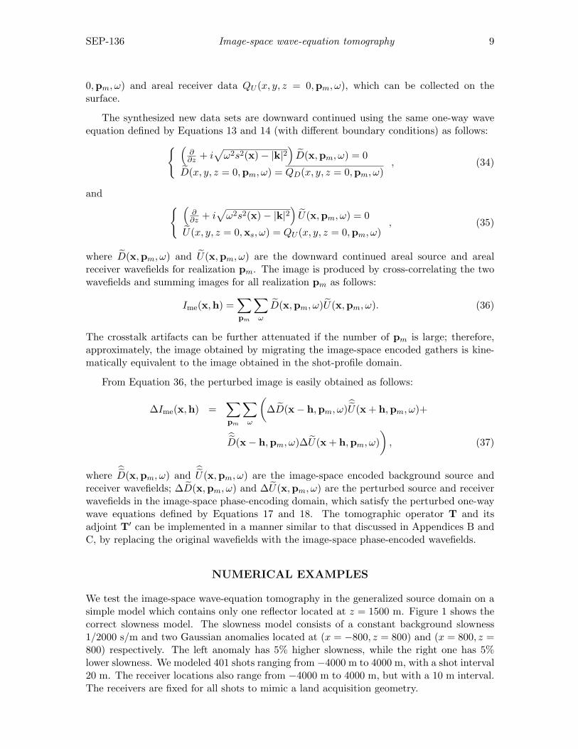
We test the image-space wave-equation tomography in the generalized source domain on asimple model which contains only one reflector located at z = 1500 m. Figure 1 shows thecorrect slowness model. The slowness model consists of a constant background slowness1/2000 s/m and two Gaussian anomalies located at (x = −800, z = 800) and (x = 800, z =800) respectively. The left anomaly has 5% higher slowness, while the right one has 5%lower slowness. We modeled 401 shots ranging from −4000 m to 4000 m, with a shot interval20 m. The receiver locations also range from −4000 m to 4000 m, but with a 10 m interval.The receivers are fixed for all shots to mimic a land acquisition geometry.
10 Tang et al. SEP-136
Figure 1: The correct slowness model. The slowness model consists of a constant backgroundslowness (1/2000 s/m) and two 5% Gaussian anomalies. [ER] yaxun1/. twin-slow
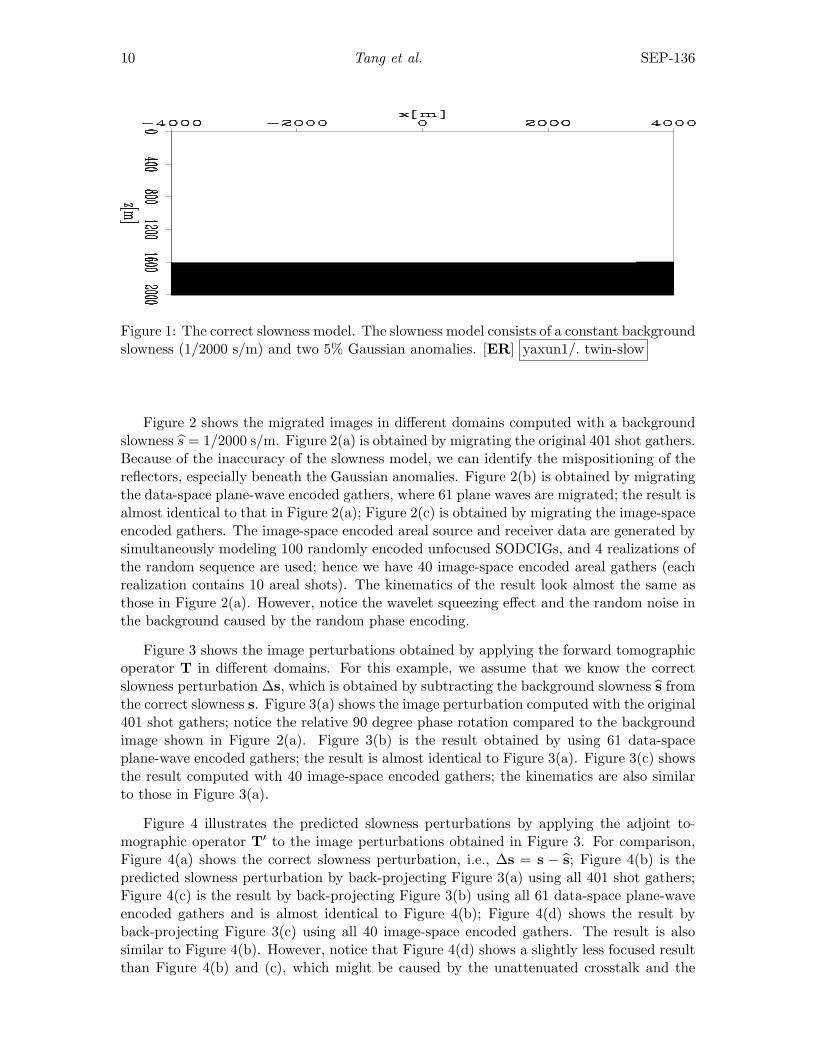
Figure 2 shows the migrated images in different domains computed with a backgroundslowness s = 1/2000 s/m. Figure 2(a) is obtained by migrating the original 401 shot gathers.Because of the inaccuracy of the slowness model, we can identify the mispositioning of thereflectors, especially beneath the Gaussian anomalies. Figure 2(b) is obtained by migratingthe data-space plane-wave encoded gathers, where 61 plane waves are migrated; the result isalmost identical to that in Figure 2(a); Figure 2(c) is obtained by migrating the image-spaceencoded gathers. The image-space encoded areal source and receiver data are generated bysimultaneously modeling 100 randomly encoded unfocused SODCIGs, and 4 realizations ofthe random sequence are used; hence we have 40 image-space encoded areal gathers (eachrealization contains 10 areal shots). The kinematics of the result look almost the same asthose in Figure 2(a). However, notice the wavelet squeezing effect and the random noise inthe background caused by the random phase encoding.
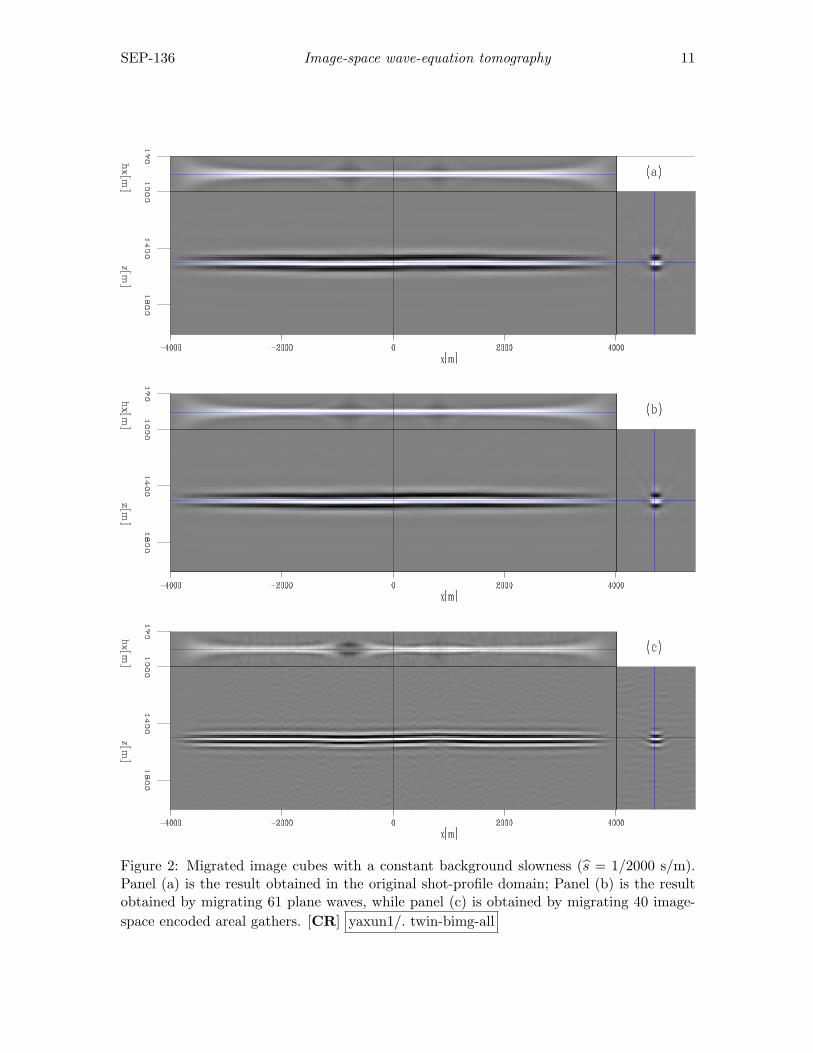
Figure 3 shows the image perturbations obtained by applying the forward tomographicoperator T in different domains. For this example, we assume that we know the correctslowness perturbation ∆s, which is obtained by subtracting the background slowness s fromthe correct slowness s. Figure 3(a) shows the image perturbation computed with the original401 shot gathers; notice the relative 90 degree phase rotation compared to the backgroundimage shown in Figure 2(a). Figure 3(b) is the result obtained by using 61 data-spaceplane-wave encoded gathers; the result is almost identical to Figure 3(a). Figure 3(c) showsthe result computed with 40 image-space encoded gathers; the kinematics are also similarto those in Figure 3(a).
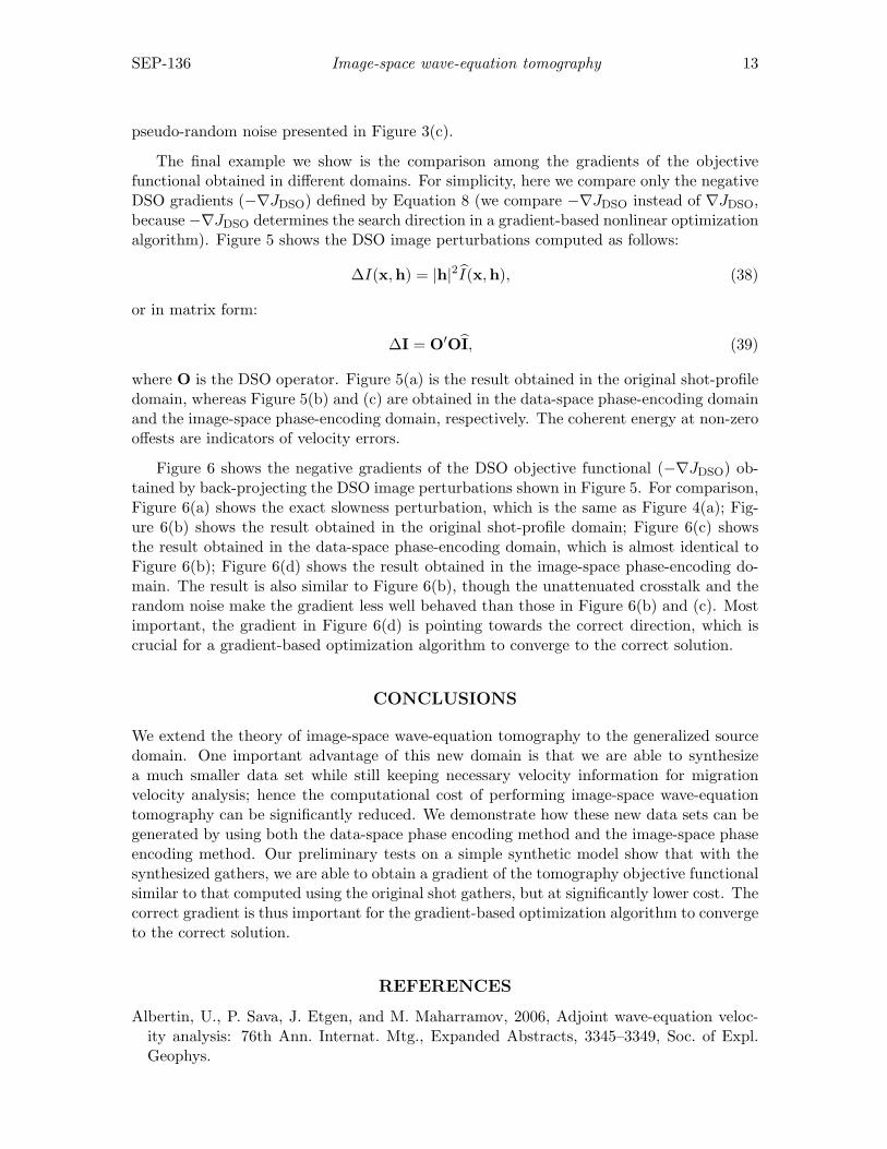
Figure 4 illustrates the predicted slowness perturbations by applying the adjoint to-mographic operator T′ to the image perturbations obtained in Figure 3. For comparison,Figure 4(a) shows the correct slowness perturbation, i.e., ∆s = s − s; Figure 4(b) is thepredicted slowness perturbation by back-projecting Figure 3(a) using all 401 shot gathers;Figure 4(c) is the result by back-projecting Figure 3(b) using all 61 data-space plane-waveencoded gathers and is almost identical to Figure 4(b); Figure 4(d) shows the result byback-projecting Figure 3(c) using all 40 image-space encoded gathers. The result is alsosimilar to Figure 4(b). However, notice that Figure 4(d) shows a slightly less focused resultthan Figure 4(b) and (c), which might be caused by the unattenuated crosstalk and the
SEP-136 Image-space wave-equation tomography 11
Figure 2: Migrated image cubes with a constant background slowness (s = 1/2000 s/m).Panel (a) is the result obtained in the original shot-profile domain; Panel (b) is the resultobtained by migrating 61 plane waves, while panel (c) is obtained by migrating 40 image-space encoded areal gathers. [CR] yaxun1/. twin-bimg-all
12 Tang et al. SEP-136
Figure 3: The image perturbations obtained by applying the forward tomographic operatorT to the correct slowness perturbations in different domains. Panel (a) shows the imageperturbation obtained using the original shot gathers, while panels (b) and (c) are obtainedusing the data-space encoded gathers and image-space encoded gathers, respectively. [CR]yaxun1/. twin-dimg-all
SEP-136 Image-space wave-equation tomography 13
pseudo-random noise presented in Figure 3(c).
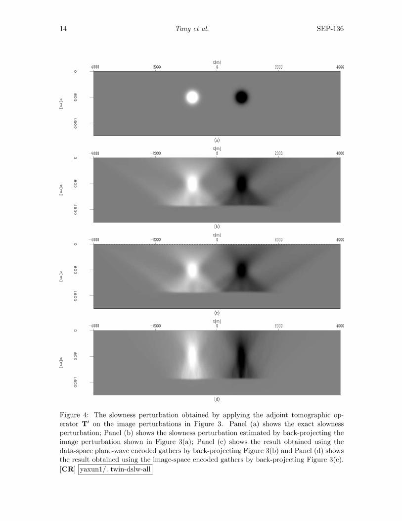
The final example we show is the comparison among the gradients of the objectivefunctional obtained in different domains. For simplicity, here we compare only the negativeDSO gradients (−∇JDSO) defined by Equation 8 (we compare −∇JDSO instead of ∇JDSO,because −∇JDSO determines the search direction in a gradient-based nonlinear optimizationalgorithm). Figure 5 shows the DSO image perturbations computed as follows:
∆I(x,h) = |h|2I(x,h), (38)
or in matrix form:
∆I = O′OI, (39)
where O is the DSO operator. Figure 5(a) is the result obtained in the original shot-profiledomain, whereas Figure 5(b) and (c) are obtained in the data-space phase-encoding domainand the image-space phase-encoding domain, respectively. The coherent energy at non-zerooffests are indicators of velocity errors.
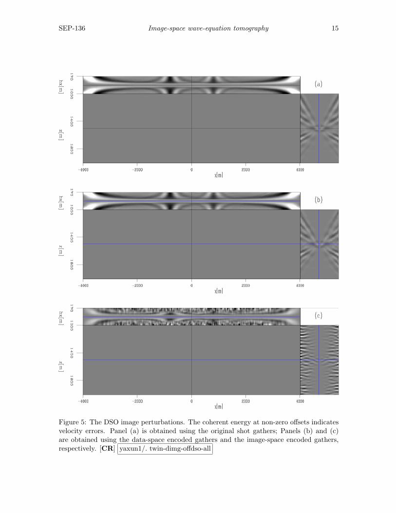
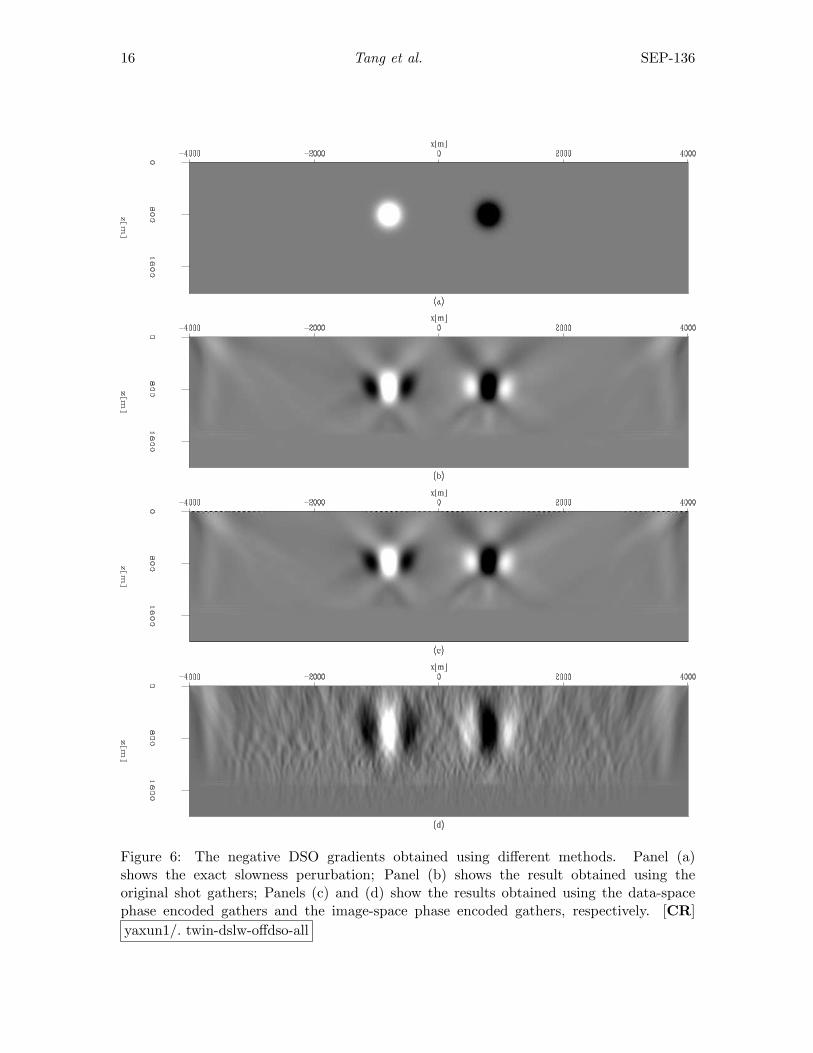
Figure 6 shows the negative gradients of the DSO objective functional (−∇JDSO) ob-tained by back-projecting the DSO image perturbations shown in Figure 5. For comparison,Figure 6(a) shows the exact slowness perturbation, which is the same as Figure 4(a); Fig-ure 6(b) shows the result obtained in the original shot-profile domain; Figure 6(c) showsthe result obtained in the data-space phase-encoding domain, which is almost identical toFigure 6(b); Figure 6(d) shows the result obtained in the image-space phase-encoding do-main. The result is also similar to Figure 6(b), though the unattenuated crosstalk and therandom noise make the gradient less well behaved than those in Figure 6(b) and (c). Mostimportant, the gradient in Figure 6(d) is pointing towards the correct direction, which iscrucial for a gradient-based optimization algorithm to converge to the correct solution.
CONCLUSIONS
We extend the theory of image-space wave-equation tomography to the generalized sourcedomain. One important advantage of this new domain is that we are able to synthesizea much smaller data set while still keeping necessary velocity information for migrationvelocity analysis; hence the computational cost of performing image-space wave-equationtomography can be significantly reduced. We demonstrate how these new data sets can begenerated by using both the data-space phase encoding method and the image-space phaseencoding method. Our preliminary tests on a simple synthetic model show that with thesynthesized gathers, we are able to obtain a gradient of the tomography objective functionalsimilar to that computed using the original shot gathers, but at significantly lower cost. Thecorrect gradient is thus important for the gradient-based optimization algorithm to convergeto the correct solution.
REFERENCES
Albertin, U., P. Sava, J. Etgen, and M. Maharramov, 2006, Adjoint wave-equation veloc-ity analysis: 76th Ann. Internat. Mtg., Expanded Abstracts, 3345–3349, Soc. of Expl.Geophys.
14 Tang et al. SEP-136
Figure 4: The slowness perturbation obtained by applying the adjoint tomographic op-erator T′ on the image perturbations in Figure 3. Panel (a) shows the exact slownessperturbation; Panel (b) shows the slowness perturbation estimated by back-projecting theimage perturbation shown in Figure 3(a); Panel (c) shows the result obtained using thedata-space plane-wave encoded gathers by back-projecting Figure 3(b) and Panel (d) showsthe result obtained using the image-space encoded gathers by back-projecting Figure 3(c).[CR] yaxun1/. twin-dslw-all
SEP-136 Image-space wave-equation tomography 15
Figure 5: The DSO image perturbations. The coherent energy at non-zero offsets indicatesvelocity errors. Panel (a) is obtained using the original shot gathers; Panels (b) and (c)are obtained using the data-space encoded gathers and the image-space encoded gathers,respectively. [CR] yaxun1/. twin-dimg-offdso-all
16 Tang et al. SEP-136
Figure 6: The negative DSO gradients obtained using different methods. Panel (a)shows the exact slowness perurbation; Panel (b) shows the result obtained using theoriginal shot gathers; Panels (c) and (d) show the results obtained using the data-spacephase encoded gathers and the image-space phase encoded gathers, respectively. [CR]yaxun1/. twin-dslw-offdso-all
SEP-136 Image-space wave-equation tomography 17
Biondi, B., 2006, Prestack exploding-reflectors modeling for migration velocity analysis:76th Ann. Internat. Mtg., Expanded Abstracts, 3056–3060, Soc. of Expl. Geophys.
——–, 2007, Prestack modeling of image events for migration velocity analysis: SEP-131,101–118.
——–, 2008, Automatic wave-equation migration velocity analysis: SEP-134, 65–78.Biondi, B. and P. Sava, 1999, Wave-equation migration velocity analysis: 69th Ann. Inter-
nat. Mtg., Expanded Abstracts, 1723–1726, Soc. of Expl. Geophys.Claerbout, J. F., 1971, Towards a unified theory of reflector mapping: Geophysics, 36,
467–481.Duquet, B. and P. Lailly, 2006, Efficient 3D wave-equation migration using virtual planar
sources: Geophysics, 71, S185–S197.Etgen, J. T., 2005, How many angles do we really need for delayed-shot migration: 75th
Ann. Internat. Mtg., Expanded Abstracts, 1985–1988, Soc. of Expl. Geophys.Guerra, C. and B. Biondi, 2008a, Phase-encoding with Gold codes for wave-equation mi-
gration: SEP-136.——–, 2008b, Prestack exploding reflector modeling: The crosstalk problem: SEP-134,
79–92.Liu, F., D. W. Hanson, N. D. Whitmore, R. S. Day, and R. H. Stolt, 2006, Toward a unified
analysis for source plane-wave migration: Geophysics, 71, S129–S139.Mora, P., 1989, Inversion = migration + tomography: Geophysics, 54, 1575–1586.Pratt, R. G., 1999, Seismic waveform inversion in the frequency domain, Part 1: Theory
and verification in a physical scale model: Geophysics, 64, 888–901.Romero, L. A., D. C. Ghiglia, C. C. Ober, and S. A. Morton, 2000, Phase encoding of shot
records in prestack migration: Geophysics, 65, 426–436.Sava, P., 2003, Prestack residual migration in frequency domain: Geophysics, 68, 634–640.——–, 2004, Migration and Velocity Analysis by Wavefield Extrapolation: PhD thesis,
Stanford University.Sava, P. and B. Biondi, 2004a, Wave-equation migration velocity analysis-I: Theory: Geo-
physical Prospecting, 52, 593–606.——–, 2004b, Wave-equation migration velocity analysis-II: Examples: Geophysical
Prospecting, 52, 607–623.Shen, P., 2004, Wave-equation Migration Velocity Analysis by Differential Semblance Op-
timization: PhD thesis, Rice University.Shen, P., W. Symes, S. Morton, and H. Calandra, 2005, Differential semblance velocity
analysis via shot-profile migration: 75th Ann. Internat. Mtg., Expanded Abstracts, 2249–2252, Soc. of Expl. Geophys.
Shragge, J., 2007, Waveform inversion by one-way wavefield extrapolation: Geophysics, 72,A47–A50.
Tang, Y., 2008, Modeling, migration and inversion in the generalized source and receiverdomain: SEP-136.
Tarantola, A., 1987, Inverse problem theory: Methods for data fitting and model parameterestimation: Elsevier.
Whitmore, N. D., 1995, An Imaging Hierarchy for Common Angle Plane Wave Seismogram:PhD thesis, University of Tulsa.
Woodward, M. J., 1992, Wave-equation tomography: Geophysics, 57, 15–26.Zhang, Y., J. Sun, C. Notfors, S. Grey, L. Chemis, and J. Young, 2005, Delayed-shot 3D
depth migration: Geophysics, 70, E21–E28.
18 Tang et al. SEP-136
APPENDIX A
This appendix derives the perturbed one-way wave equation with respect to the slownessperturbation. Let us start with the one-way wave equation for the source wavefield asfollows: { (
∂∂z + i
√ω2s2(x)− |k|2
)D(x,xs, ω) = 0
D(x, y, z = 0,xs, ω) = fs(ω)δ(x− xs), (A-1)
We can rewrite the slowness and the source wavefield as follows:
s(x) = s(x) + ∆s(x) (A-2)D(x,xs, ω) = D(x,xs, ω) + ∆D(x,xs, ω), (A-3)
where s(x) and D(x,xs, ω) are the background slowness and background wavefield, and∆s(x) and ∆D(x,xs, ω) are small perturbations in slowness and source wavefield, respec-tively. If ∆s(x) is small, then the square root in the first equation of A-1 can be approxi-mated using Taylor expansion as follows:
√ω2s2(x)− |k|2 ≈
√ω2s2(x)− |k|2 +
ω∆s(x)√1− |k|2
ω2bs2(x)
. (A-4)
Substituting Equations A-2, A-3 and A-4 into Equation A-1 and ignoring the second-orderterms yield the following linearized one-way wave equation for the perturbed source wave-field:
(∂∂z + i
√ω2s2(x)− |k|2
)∆D(x,xs, ω) = −iω∆s(x)r
1− |k|2ω2bs2(x)
D(x,xs, ω)
∆D(x, y, z = 0,xs, ω) = 0. (A-5)
Similarly, we can also obtain the linearized one-way wave equation for the perturbed receiverwavefield as follows:
(∂∂z + i
√ω2s2(x)− |k|2
)∆U(x,xs, ω) = −iω∆s(x)r
1− |k|2ω2bs2(x)
U(x,xs, ω)
∆U(x, y, z = 0,xs, ω) = 0. (A-6)
APPENDIX B
This appendix demonstrates a matrix representation of the forward tomographic operatorT. Let us start with the source wavefield, where the source wavefield Dz at depth z isdownward continued to depth z + ∆z by the one-way extrapolator Ez(sz) as follows:
Dz+∆z = Ez(sz)Dz, (B-1)
where the one-way extrapolator is defined as follows:
Ez(sz) = e−ikz(sz)∆z = e−i√
ω2s2z−|k|2 (B-2)
SEP-136 Image-space wave-equation tomography 19
The perturbed source wavefield at some depth level can be derived from the backgroundwavefield by a simple application of the chain rule to equation B-1:
∆Dz+∆z = Ez(sz)∆Dz + ∆Ez(sz)Dz, (B-3)
where Dz is the background source wavefield and ∆Ez represents the perturbed extrap-olator, which can be obtained by a formal linearization with respect to slowness of theextrapolator defined in Equation B-2:
Ez(sz) = e−ikz(sz)∆z ≈ e−i∆zbkz + e−i∆zbkz
(−i∆z
dkz
dsz
∣∣∣∣sz=bsz
)∆sz
= Ez(sz) + Ez(sz)
(−i∆z
dkz
dsz
∣∣∣∣sz=bsz
)∆sz, (B-4)
where kz = kz(sz) and sz is the background slowness at depth z. From Equation B-4, theperturbed extrapolator reads as follows:
∆Ez(sz) = Ez(sz)
(−i∆z
dkz
dsz
∣∣∣∣sz=bsz
)∆sz. (B-5)
Substituting Equation B-5 into B-3 yields
∆Dz+∆z = Ez(sz)∆Dz + Ez(sz)
(−i∆z
dkz
dsz
∣∣∣∣sz=bsz
)Dz∆sz. (B-6)
Let us define a scattering operator Gz that interacts with the background wavefield asfollows:
Gz(Dz, sz) =
(−i∆z
dkz
dsz
∣∣∣∣sz=bsz
)Dz =
−iω∆z√1− |k|2
ω2bs2zDz. (B-7)
Then the perturbed source wavefield for depth z + ∆z can be rewritten as follows:
∆Dz+∆z = Ez(sz)∆Dz + Ez(sz)Gz(Dz, sz)∆sz. (B-8)
We can further write out the recursive Equation B-8 for all depths in the following matrixform:
0BBBBBB@
∆D0∆D1∆D2
.
.
.∆Dn
1CCCCCCA =
0BBBBBB@
0 0 0 · · · 0 0E0 0 0 · · · 0 00 E1 0 · · · 0 0
.
.
.
.
.
.
.
.
.
.
.
.
.
.
.
.
.
.0 0 0 · · · En−1 0
1CCCCCCA
0BBBBBB@
∆D0∆D1∆D2
.
.
.∆Dn
1CCCCCCA +
0BBBBBB@
0 0 0 · · · 0 0E0 0 0 · · · 0 00 E1 0 · · · 0 0
.
.
.
.
.
.
.
.
.
.
.
.
.
.
. 00 0 0 · · · En−1 0
1CCCCCCA
0BBBBBB@
G0 0 0 · · · 00 G1 0 · · · 00 0 G2 · · · 0
.
.
.
.
.
.
.
.
.
.
.
.
.
.
.0 0 0 · · · Gn
1CCCCCCA
0BBBBBB@
∆s0∆s1∆s2
.
.
.∆sn
1CCCCCCA ,
or in a more compact notation,
∆D = E(s)∆D + E(s)G(D, s)∆s. (B-9)
20 Tang et al. SEP-136
The solution of Equation B-9 can be formally written as follows:
∆D = (1−E(s))−1 E(s)G(D, s)∆s. (B-10)
Similarly, the perturbed receiver wavefield satisfies the following recursive relation:
∆Uz+∆z = Ez(sz)∆Uz + Ez(sz)Gz(Uz, sz)∆sz, (B-11)
where Gz(Uz, sz) is the scattering operator, which interacts with the background receiverwavefield as follows:
Gz(Uz, sz) =
(−i∆z
dkz
dsz
∣∣∣∣sz=bsz
)Uz =
−iω∆z√1− |k|2
ω2bs2zUz. (B-12)
We can also write out the recursive Equation B-12 for all depth levels in the following matrixform: 0BBBBBB@
∆U0∆U1∆U2
.
.
.∆Un
1CCCCCCA =
0BBBBBB@
0 0 0 · · · 0 0E0 0 0 · · · 0 00 E1 0 · · · 0 0
.
.
.
.
.
.
.
.
.
.
.
.
.
.
.
.
.
.0 0 0 · · · En−1 0
1CCCCCCA
0BBBBBB@
∆U0∆U1∆U2
.
.
.∆Un
1CCCCCCA +
0BBBBBB@
0 0 0 · · · 0 0E0 0 0 · · · 0 00 E1 0 · · · 0 0
.
.
.
.
.
.
.
.
.
.
.
.
.
.
. 00 0 0 · · · En−1 0
1CCCCCCA
0BBBBBB@
G0 0 0 · · · 00 G1 0 · · · 00 0 G2 · · · 0
.
.
.
.
.
.
.
.
.
.
.
.
.
.
.0 0 0 · · · Gn
1CCCCCCA
0BBBBBB@
∆s0∆s1∆s2
.
.
.∆sn
1CCCCCCA ,
or in a more compact notation,
∆U = E(s)∆U + E(s)G(U, s)∆s. (B-13)
The solution of Equation B-13 can be formally written as follows:
∆U = (1−E(s))−1 E(s)G(U, s)∆s. (B-14)
With the background wavefields and the perturbed wavefields, the perturbed image canbe obtained as follows:
0BBBBBB@
∆I0∆I1∆I2
.
.
.∆In
1CCCCCCA =
0BBBBBBB@
bU0 0 0 · · · 0
0 bU1 0 · · · 0
0 0 bU2 · · · 0
.
.
.
.
.
.
.
.
.
.
.
.
.
.
.
0 0 0 · · · bUn
1CCCCCCCA
0BBBBBB@
∆D0∆D1∆D2
.
.
.∆Dn
1CCCCCCA +
0BBBBBBB@
bD0 0 0 · · · 0
0 bD1 0 · · · 0
0 0 bD2 · · · 0
.
.
.
.
.
.
.
.
.
.
.
.
.
.
.
0 0 0 · · · bDn
1CCCCCCCA
0BBBBBB@
∆U0∆U1∆U2
.
.
.∆Un
1CCCCCCA ,
or in a more compact notation,
∆I = diag(U)∆D + diag
(D)∆U. (B-15)
Substituting Equations B-10 and B-14 into Equation B-15 yields
∆I =(diag
(U)
(1−E(s))−1 E(s)G(D, s) +
diag(D)
(1−E(s))−1 E(s)G(U, s))∆s, (B-16)
from which we can read the forward tomographic operator T as follows:
T = diag(U)
(1−E(s))−1 E(s)G(D, s) +
diag(D)
(1−E(s))−1 E(s)G(U, s). (B-17)
SEP-136 Image-space wave-equation tomography 21
APPENDIX C
This appendix demonstrates a matrix representation of the adjoint tomographic operatorT
′. Since the slowness perturbation ∆s is linearly related to the perturbed wavefields,
∆D and ∆U, to obtain the back-projected slowness perturbation, we first must get theback-projected perturbed wavefields from the perturbed image ∆I. From Equation B-15,the back-projected perturbed source and receiver wavefields are obtained as follows:
∆D = diag(U)∆I (C-1)
and
∆U = diag(D)∆I. (C-2)
Then the adjoint equations of Equations B-10 and B-14 are used to get the back-projectedslowness perturbation ∆s. Let us first look at the adjoint equation of Equation B-10, whichcan be written as follows:
∆sD = G′(D, s)E′(s)(1−E′(s)
)−1 ∆D. (C-3)
We can define a temporary wavefield ∆PD that satisfies the following equation:
∆PD = E′(s)(1−E′(s)
)−1 ∆D. (C-4)
After some simple algebra, the above equation can be rewritten as follows:
∆PD = E′(s)∆PD + E′(s)∆D. (C-5)
Substituting Equation C-1 into equation C-5 yields
∆PD = E′(s)∆PD + E′(s)diag(U)∆I. (C-6)
Therefore, ∆PD can be obtained by recursive upward continuation, where ∆D = diag(U)∆I
serves as the initial condition. The back-projected slowness perturbation from the perturbedsource wavefield is then obtained by applying the adjoint of the scattering operator G(D, s)to the wavefield ∆PD as follows:
∆sD = G′(D, s)∆PD. (C-7)
Similarly, the adjoint equation of Equation B-14 reads as follows:
∆sU = G′(U, s)E(s)′(1−E(s)′
)−1 ∆U. (C-8)
We can also define a temporary wavefield ∆PU that satisfies the following equation:
∆PU = E(s)′(1−E(s)′
)−1 ∆U. (C-9)
After rewriting it, we get the following recursive form:
∆PU = E(s)′∆PU + E(s)′∆U
= E(s)′∆PU + E(s)′diag(D)∆I. (C-10)

22 Tang et al. SEP-136
The back-projected slowness perturbation from the perturbed receiver wavefield is thenobtained by applying the adjoint of the scattering operator G(U, s) to the wavefield ∆PU
as follows:
∆sU = G′(U, s)∆PU . (C-11)
The total back-projected slowness perturbation is obtained by adding ∆sD and ∆sU to-gether:
∆s = ∆sD + ∆sU . (C-12)
Stanford Exploration Project, Report SEP136, April 14, 2009
Phase encoding with Gold codes for wave-equation migration
Claudio Guerra and Biondo Biondi
ABSTRACT
Prestack exploding-reflector modeling aims to synthesize a small dataset comprised ofareal shots, while preserving the correct kinematics to be used in iterations of migrationvelocity analysis. To achieve this goal, the amount of data is reduced by combiningthe modeled areal data into sets, we call super-areal data. However, crosstalk arisesduring migration due to the correlation of wavefields resulting from different modelingexperiments. Phase encoding the modeling experiments can attenuate crosstalk duringmigration. In the geophysical community, the most used phase-encoding schemes areplane-wave-phase encoding and random-phase encoding. Here, we exploit the appli-cation of Gold codes commonly used in wireless communication, radar and medicalimaging communities to phase encode data. We show that adequately selecting theGold codes can potentially shift the crosstalk out of the migration domain, or the re-gion of interest if a target-oriented approach is used, yielding an image free of crosstalk.
INTRODUCTION
Biondi (2006, 2007) introduced the concept of the prestack exploding-reflector modeling.This method synthesizes source and receiver wavefields along the entire survey at the surface,in the form of areal data, starting from a prestack migrated image cube computed with wave-equation migration. For migration velocity analysis, the aim is to generate a considerablysmaller dataset than the one used in the initial migration, while maintaining the necessarykinematic information to update the velocity.
Conceptually, the synthesized areal data are computed by upward propagating sourceand receiver wavefields using subsurface-offset-domain common-image gathers (SODCIGs)as initial conditions. To decrease the number of experiments to migrate, we take advan-tage of the linearity of the wave propagation to combine several experiments into a set ofcomposite records. Combining several experiments gives rise to crosstalk during imaging(Biondi, 2006; Guerra and Biondi, 2008). Guerra and Biondi (2008) use pseudo-random-phase encoding (Romero et al., 2000) during the modeling step to attenuate crosstalk.
It is common, in the exploration geophysics community, to employ pseudo-random codesusing intrinsic functions specific to the programing language. These pseudo-random codespresent, generally, a uniform distribution. Their autocorrelation and cross-correlation func-tions have no special properties. The autocorrelation function presents nearly periodic sidelobes with additive low-amplitude random variations. The peak-to-side lobe ratio is around30. The cross-correlation function is pseudo-random, and its amplitudes are of the sameorder of magnitude as those of the non-zero lags of the autocorrelation function. Herein,theses codes are called conventional random codes.
23
24 Guerra and Biondi SEP–136
In wireless communication, especially for systems using Code Division Multiple Ac-cess (CDMA), a class of different pseudo-random codes have been widely used (Shi andSchelgel, 2003). These codes are binary sequences and have unique autocorrelation andcross-correlations properties which make them more suited to achieve the above-mentionedobjectives with minimal crosstalk. The autocorrelation function is represented by a largepeak, whose amplitude equals the number of samples in the code, and the cross-correlationpeaks, at non-zero lags, with the same amplitudes as that of the autocorrelation. Examplesof binary pseudo-random codes used by these communities are Golay (Golay, 1961; Tseng,1972), Kasami (Kasami, 1966) and Gold codes (Gold, 1967). Medical imaging (Gran, 2005)and radar communities (Levanon and Mozeson, 2004) also exploit the statistical proper-ties of these pseudo-random codes to increase bandwidth, signal-to-noise ratio and pulsecompression.
Quan and Harris (1991) analyze orthogonal codes to encode simultaneous source sig-natures for cross-well surveys, and conclude that m-sequences and Gold codes provide thebest results on the separation of the seismograms. Here, we exploit the properties of theGold codes to encode the prestack exploding reflector modeling experiments.
In the next section we give a brief description of the prestack exploding-reflector mod-eling. Then we discuss how to compute the Gold codes. To illustrate the effectiveness ofphase encoding with Gold codes, we compare the migration of prestack-exploding-reflectormodeled data encoded with conventional random codes and Gold codes.
PRESTACK EXPLODING-REFLECTOR MODELING
Starting from a prestack image obtained by wave-equation migration represented by a singleSODCIG, areal source and receiver wavefields are modeled at the surface by
S(x, y, z = 0, ω;xm) = G(xm − h;x, y, z = 0, ω) ∗ Is(x,h;xm),R(x, y, z = 0, ω;xm) = G(xm + h;x, y, z = 0, ω) ∗ Ir(x,h;xm),
(1)
where S(x, y, z = 0, ω;xm) is the source wavefield and R(x, y, z = 0, ω;xm) is the receiverwavefield. Is(x,h;xm) and Ir(x,h;xm) are the prestack images used as initial conditionsfor the source and receiver wavefield extrapolation, respectively, at a selected position,xm. These prestack images should be dip-independent gathers. They are computed by re-mapping the dip along the offset direction according to the apparent geological dip (Biondi,2007). G(xm±h;x, z = 0, ω) represents the operator that extrapolates the wavefields fromthe subsurface to the surface; h is the subsurface offset; ω is the temporal frequency; andx is the vector of spatial coordinates.
In the case of using an one-way extrapolator, the source and receiver wavefields areupward continued according to the one-way wave equations{ (
∂∂z + i
√ω2s2(x)− |k|2
)S(x, ω;xm) = Is(x,h;xm)
S(x, y, z = zmax, ω;xm) = 0, (2)
and { (∂∂z − i
√ω2s2(x)− |k|2
)R(x, ω;xm) = Ir(x,h;xm)
R(x, y, z = zmax, ω;xm) = 0, (3)
SEP–136 Phase encoding with Gold codes 25
where s(x) is the slowness at x; k = (kx, ky) is the spatial wavenumber vector.
Using the linearity of the wave propagation, sets of individual modeling experiments canbe combined into the same areal data, such that the amount of data input into migration canbe significantly decreased, reducing its cost. However, this procedure generates crosstalkwhen applying the imaging condition during migration.
Guerra and Biondi (2008) introduce strategies to attenuate the crosstalk. Migration of(x, ω)-random-phase encoded data disperses the crosstalk energy throughout the image asa pseudo-random background noise. By adding more realizations of random-phase encodedareal data, the speckled noise can be further attenuated. The encoded source wavefield,S(x,pm, ω), and the encoded receiver wavefield, R(x,pm, ω), are synthesized according to{ (
∂∂z + i
√ω2s2(x)− |k|2
)S(x,pm, ω) = Is(x,h,pm, ω)
S(x, y, z = zmax,pm, ω) = 0, (4)
and { (∂∂z − i
√ω2s2(x)− |k|2
)R(x,pm, ω) = Ir(x,h,pm, ω)
R(x, y, z = zmax,pm, ω) = 0, (5)
where Is(x,h,pm, ω) and Ir(x,h,pm, ω) are the encoded SODCIGs after rotations. Theyare defined as follows:
Is(x,h,pm, ω) =∑xm
Is(x,h,xm)β(x,xm,pm, ω), (6)
Ir(x,h,pm, ω) =∑xm
Ir(x,h,xm)β(x,xm,pm, ω), (7)
where β(x,xm,pm, ω) = eiγ(x,xm,pm,ω) is the phase-encoding function; the variable pm isthe index of different realizations of phase encoding.
The areal shot migration is performed by downward continuation of the areal sourceand receiver wavefields according to the following one-way wave equations{ (
∂∂z − i
√ω2s2(x)− |k|2
)S(x,pm, ω) = 0
S(x, y, z = 0,pm, ω) = S(x, y, z = 0,pm, ω), (8)
and { (∂∂z + i
√ω2s2(x)− |k|2
)R(x,pm, ω) = 0
R(x, y, z = 0,pm, ω) = R(x, y, z = 0,pm, ω), (9)
where the encoded source wavefield, S(x,pm, ω), and the encoded receiver wavefield, R(x,pm, ω),are used as boundary conditions.
The image, I(x,h), is obtained by cross-correlation of the source wavefield, S(x,pm, ω),with the receiver wavefield, R(x,pm, ω)
I(x,h) =∑ω
∑pm
S?(x− h,pm, ω)R(x + h,pm, ω), (10)
where ? represents complex conjugation.

26 Guerra and Biondi SEP–136
GOLD CODES
Before describing Gold codes it is useful to define maximum length sequences.
Linear feedback shift registers (LFSR) (Moon and Stirling, 2000) are called state ma-chines, whose components and functions are:
• the shift register – shifts the bit pattern and registers the output bit; and
• the feedback function – computes the input bit according to the tap sequence andinserts the computed bit into the input bit position.
The output sequence of bits form pseudo-random binary sequences, which are completelycontrolled by the tap sequence. A tap sequence defines which bits in the current state willbe combined to determine the input bit for the next state. The combination is generallyperformed using module-2 addition (exclusive or – XOR). This means that adding theselected bit values defined by the tap sequence, if the sum is odd the output of the functionis one; otherwise the output is zero. Table 1 shows the internal states and the outputsequence of a 4-bit LFSR with tap sequence [4, 1]. For the current state, the input bit (bit1) is computed by the sum module–2 of the bits defined by the tap sequence(bits 1 and 4).The rest of the bits in the register (bits 2, 3 and 4) are obtained by shifting the bit valuesin the previous state to the right. For example, bit 2 of the current state is bit 1 of theprevious state. The output bit of the current state is the last bit (bit 4) in the register fromthe previous state.
Register Statesbit1 bit2 bit3 bit4 Output
(Tap) (Tap) Sequence1 1 0 10 1 1 0 10 0 1 1 01 0 0 1 10 1 0 0 10 0 1 0 00 0 0 1 01 0 0 0 11 1 0 0 01 1 1 0 01 1 1 1 00 1 1 1 11 0 1 1 10 1 0 1 11 0 1 0 11 1 0 1 0
Table 1: Internal states and the output sequence of a 4-bit LFSR with tap sequence [4,1].
In number theory, Galois fields (GF) are finite fields in which all operations result in anelement of the field (Lidl and Niederreiter, 1994). Addition, subtraction and multiplication

SEP–136 Phase encoding with Gold codes 27
of polynomials are defined in a finite field. Module 2 arithmetic forms the basis of GF(2)(Galois field of order 2). Addition and multiplication operations in GF(2) can be representedby bitwise operators XOR and AND, respectively. Table 2 synthesizes the possible outputvalues of addition and multiplication over GF(2).
+ 0 1 × 0 10 0 1 0 0 01 1 0 1 0 1
Table 2: GF(2) addition and multiplication possible outcomes.
If a polynomial can not be represented as the product of two or more polynomials, it iscalled an irreducible polynomial. For instance, x2 +x+1 is irreducible over GF(2) becauseit can not be factored. However, x2 +1 is not irreducible over GF(2) because, using normalalgebra, (x + 1)(x + 1) = x2 + 2x + 1, and after reduction module–2, is x2 + 1 (the term 2xis dropped). So, in GF(2), x2 + 1 ≡ x2 + 2x + 1.
The importance of studying irreducible polynomials GF(2) is that they are used torepresent tap sequences. Considering an irreducible polynomial, the corresponding tapsequence is given by the exponents of the terms with coefficients of 1 (Dinan and Jabbari,1998). Special tap sequences can be used to generate particular pseudo-random binarysequences. They are called maximum length sequences (m-sequences) and, by definition,are the largest codes that can be generated by a LFSR for a given tap sequence. Theirlength is (bn− 1), where n is the number of elements of the tap sequence, and b = 2, 3 or 5.
The autocorrelation function of an m-sequence, Φmls(k), is given by
Φmls(k) ={
bn − 1 for k = 0,−1 for k 6= 0,
(11)
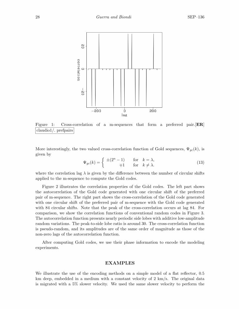
where k is the lag of correlation. In spite of the good autocorrelation properties, m-sequences, in general, are not immune to cross-correlation problems, and they may havelarge and unpredictable cross-correlation values. However, the so-called preferred pairsof m-sequences have cross-correlation functions which might assume the predicted values,−1, − 1 + p, and −1− p, where p = 2(n+1)/2 for n odd or p = 2(n+2)/2 for n even. Given a(2n− 1)–length m-sequence, a(k), and gcd{n, 4} = 1 (greatest common divisor of n and 4),its preferred pair is the result of decimation computed by applying on a(k) a circular shiftof q samples, where q = 2m + 1 and gcd{m,n} = 1. Figure 1 shows the cross-correlation ofm-sequences that form a preferred pair computed with m = 5.
The number of possible preferred pairs of m-sequences is limited, when compared tothe requirements of practical applications of wireless communication. Preferred pairs ofm-sequences, however, are used to generate Gold codes (Dinan and Jabbari, 1998).
In CDMA, Gold codes are used as chipping sequences that allow several callers to usethe same frequency, resulting in less interference and better utilization of the availablebandwidth. Originally proposed by Gold (1967), Gold codes can be computed by module-2addition (exclusive or) of circularly shifted preferred pairs of m-sequences of length 2n− 1.The autocorrelation function of a Gold code, Φgc(k), is given by
Φgc(k) ={±2n − 1 for k = 0,
±1 for k 6= 0.(12)
28 Guerra and Biondi SEP–136
Figure 1: Cross-correlation of a m-sequences that form a preferred pair.[ER]claudio1/. prefpairs
More interestingly, the two valued cross-correlation function of Gold sequences, Ψgc(k), isgiven by
Ψgc(k) ={±(2n − 1) for k = λ,
∓1 for k 6= λ.(13)
where the correlation lag λ is given by the difference between the number of circular shiftsapplied to the m-sequence to compute the Gold codes.
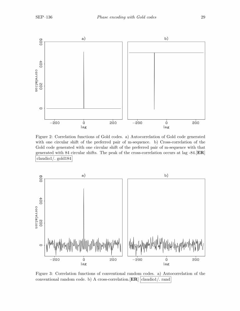
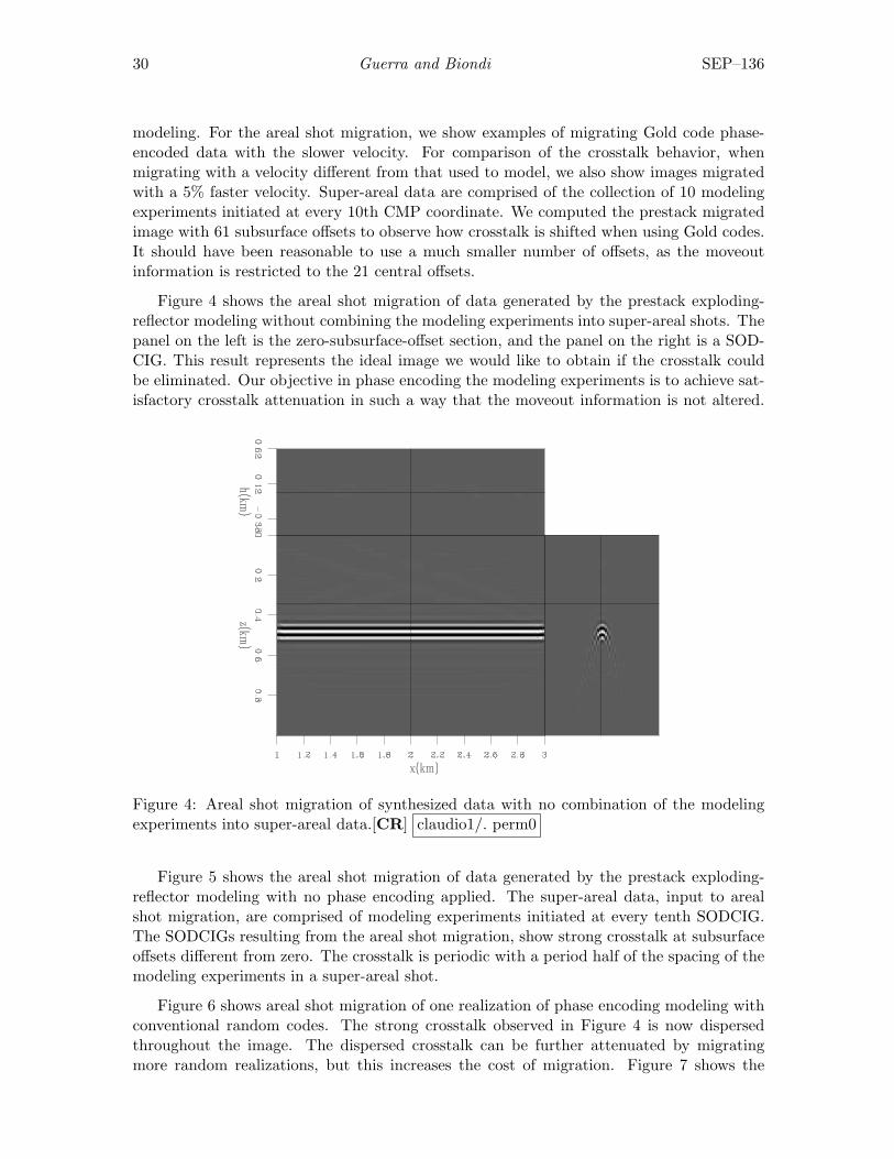
Figure 2 illustrates the correlation properties of the Gold codes. The left part showsthe autocorrelation of the Gold code generated with one circular shift of the preferredpair of m-sequence. The right part shows the cross-correlation of the Gold code generatedwith one circular shift of the preferred pair of m-sequence with the Gold code generatedwith 84 circular shifts. Note that the peak of the cross-correlation occurs at lag 84. Forcomparison, we show the correlation functions of conventional random codes in Figure 3.The autocorrelation function presents nearly periodic side lobes with additive low-amplituderandom variations. The peak-to-side lobe ratio is around 30. The cross-correlation functionis pseudo-random, and its amplitudes are of the same order of magnitude as those of thenon-zero lags of the autocorrelation function.
After computing Gold codes, we use their phase information to encode the modelingexperiments.
EXAMPLES
We illustrate the use of the encoding methods on a simple model of a flat reflector, 0.5km deep, embedded in a medium with a constant velocity of 2 km/s. The original datais migrated with a 5% slower velocity. We used the same slower velocity to perform the
SEP–136 Phase encoding with Gold codes 29
Figure 2: Correlation functions of Gold codes. a) Autocorrelation of Gold code generatedwith one circular shift of the preferred pair of m-sequence. b) Cross-correlation of theGold code generated with one circular shift of the preferred pair of m-sequence with thatgenerated with 84 circular shifts. The peak of the cross-correlation occurs at lag -84.[ER]claudio1/. gold184
Figure 3: Correlation functions of conventional random codes. a) Autocorrelation of theconventional random code. b) A cross-correlation.[ER] claudio1/. rand
30 Guerra and Biondi SEP–136
modeling. For the areal shot migration, we show examples of migrating Gold code phase-encoded data with the slower velocity. For comparison of the crosstalk behavior, whenmigrating with a velocity different from that used to model, we also show images migratedwith a 5% faster velocity. Super-areal data are comprised of the collection of 10 modelingexperiments initiated at every 10th CMP coordinate. We computed the prestack migratedimage with 61 subsurface offsets to observe how crosstalk is shifted when using Gold codes.It should have been reasonable to use a much smaller number of offsets, as the moveoutinformation is restricted to the 21 central offsets.
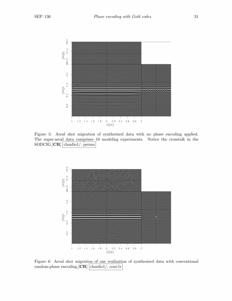
Figure 4 shows the areal shot migration of data generated by the prestack exploding-reflector modeling without combining the modeling experiments into super-areal shots. Thepanel on the left is the zero-subsurface-offset section, and the panel on the right is a SOD-CIG. This result represents the ideal image we would like to obtain if the crosstalk couldbe eliminated. Our objective in phase encoding the modeling experiments is to achieve sat-isfactory crosstalk attenuation in such a way that the moveout information is not altered.
Figure 4: Areal shot migration of synthesized data with no combination of the modelingexperiments into super-areal data.[CR] claudio1/. perm0
Figure 5 shows the areal shot migration of data generated by the prestack exploding-reflector modeling with no phase encoding applied. The super-areal data, input to arealshot migration, are comprised of modeling experiments initiated at every tenth SODCIG.The SODCIGs resulting from the areal shot migration, show strong crosstalk at subsurfaceoffsets different from zero. The crosstalk is periodic with a period half of the spacing of themodeling experiments in a super-areal shot.
Figure 6 shows areal shot migration of one realization of phase encoding modeling withconventional random codes. The strong crosstalk observed in Figure 4 is now dispersedthroughout the image. The dispersed crosstalk can be further attenuated by migratingmore random realizations, but this increases the cost of migration. Figure 7 shows the
SEP–136 Phase encoding with Gold codes 31
Figure 5: Areal shot migration of synthesized data with no phase encoding applied.The super-areal data comprises 10 modeling experiments. Notice the crosstalk in theSODCIG.[CR] claudio1/. perma
Figure 6: Areal shot migration of one realization of synthesized data with conventionalrandom-phase encoding.[CR] claudio1/. conv1r
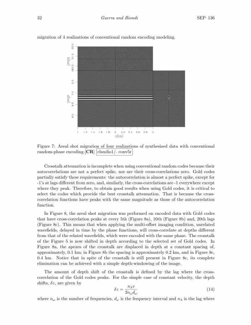
32 Guerra and Biondi SEP–136
migration of 4 realizations of conventional random encoding modeling.
Figure 7: Areal shot migration of four realizations of synthesized data with conventionalrandom-phase encoding.[CR] claudio1/. conv5r
Crosstalk attenuation is incomplete when using conventional random codes because theirautocorrelations are not a perfect spike, nor are their cross-correlations zero. Gold codespartially satisfy these requirements: the autocorrelation is almost a perfect spike, except for-1’s at lags different from zero, and, similarly, the cross-correlations are -1 everywhere exceptwhere they peak. Therefore, to obtain good results when using Gold codes, it is critical toselect the codes which provide the best crosstalk attenuation. That is because the cross-correlation functions have peaks with the same magnitude as those of the autocorrelationfunction.
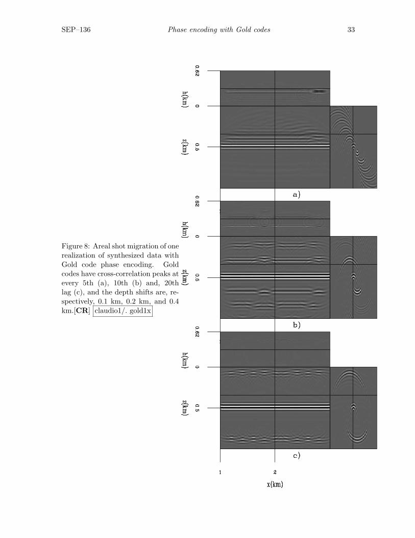
In Figure 8, the areal shot migration was performed on encoded data with Gold codesthat have cross-correlation peaks at every 5th (Figure 8a), 10th (Figure 8b) and, 20th lags(Figure 8c). This means that when applying the multi-offset imaging condition, unrelatedwavefields, delayed in time by the phase functions, will cross-correlate at depths differentfrom that of the related wavefields, which were encoded with the same phase. The crosstalkof the Figure 5 is now shifted in depth according to the selected set of Gold codes. InFigure 8a, the apexes of the crosstalk are displaced in depth at a constant spacing of,approximately, 0.1 km; in Figure 8b the spacing is approximately 0.2 km, and in Figure 8c,0.4 km. Notice that in spite of the crosstalk is still present in Figure 8c, its completeelimination can be achieved with a simple depth-windowing of the image.
The amount of depth shift of the crosstalk is defined by the lag where the cross-correlation of the Gold codes peaks. For the simple case of constant velocity, the depthshifts, δz, are given by
δz =nλv
2nωdω(14)
where nω is the number of frequencies, dω is the frequency interval and nλ is the lag where
SEP–136 Phase encoding with Gold codes 33
Figure 8: Areal shot migration of onerealization of synthesized data withGold code phase encoding. Goldcodes have cross-correlation peaks atevery 5th (a), 10th (b) and, 20thlag (c), and the depth shifts are, re-spectively, 0.1 km, 0.2 km, and 0.4km.[CR] claudio1/. gold1x
34 Guerra and Biondi SEP–136
the cross-correlation of the Gold codes peaks. For the present example, this amounts toδz = 0.021 ∗ nλ km.
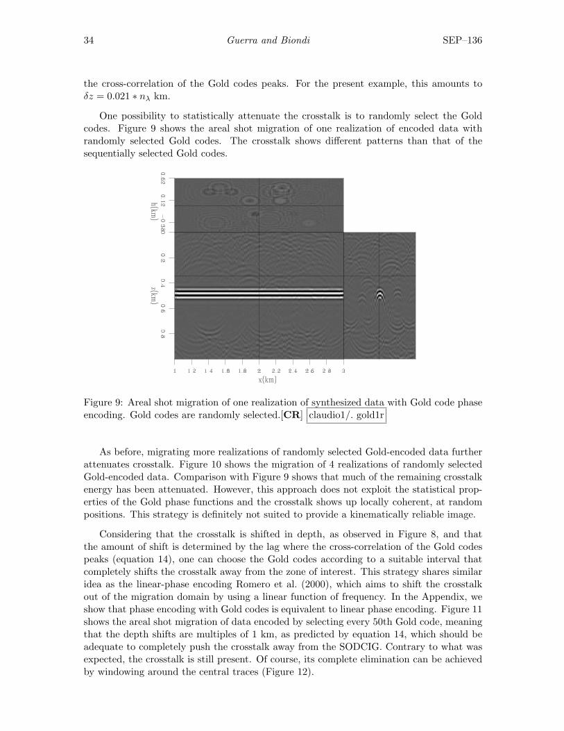
One possibility to statistically attenuate the crosstalk is to randomly select the Goldcodes. Figure 9 shows the areal shot migration of one realization of encoded data withrandomly selected Gold codes. The crosstalk shows different patterns than that of thesequentially selected Gold codes.
Figure 9: Areal shot migration of one realization of synthesized data with Gold code phaseencoding. Gold codes are randomly selected.[CR] claudio1/. gold1r
As before, migrating more realizations of randomly selected Gold-encoded data furtherattenuates crosstalk. Figure 10 shows the migration of 4 realizations of randomly selectedGold-encoded data. Comparison with Figure 9 shows that much of the remaining crosstalkenergy has been attenuated. However, this approach does not exploit the statistical prop-erties of the Gold phase functions and the crosstalk shows up locally coherent, at randompositions. This strategy is definitely not suited to provide a kinematically reliable image.
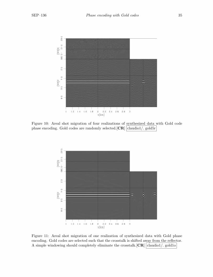
Considering that the crosstalk is shifted in depth, as observed in Figure 8, and thatthe amount of shift is determined by the lag where the cross-correlation of the Gold codespeaks (equation 14), one can choose the Gold codes according to a suitable interval thatcompletely shifts the crosstalk away from the zone of interest. This strategy shares similaridea as the linear-phase encoding Romero et al. (2000), which aims to shift the crosstalkout of the migration domain by using a linear function of frequency. In the Appendix, weshow that phase encoding with Gold codes is equivalent to linear phase encoding. Figure 11shows the areal shot migration of data encoded by selecting every 50th Gold code, meaningthat the depth shifts are multiples of 1 km, as predicted by equation 14, which should beadequate to completely push the crosstalk away from the SODCIG. Contrary to what wasexpected, the crosstalk is still present. Of course, its complete elimination can be achievedby windowing around the central traces (Figure 12).
SEP–136 Phase encoding with Gold codes 35
Figure 10: Areal shot migration of four realizations of synthesized data with Gold codephase encoding. Gold codes are randomly selected.[CR] claudio1/. gold5r
Figure 11: Areal shot migration of one realization of synthesized data with Gold phaseencoding. Gold codes are selected such that the crosstalk is shifted away from the reflector.A simple windowing should completely eliminate the crosstalk.[CR] claudio1/. gold1o
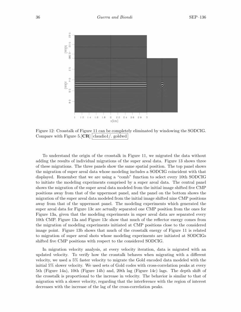
36 Guerra and Biondi SEP–136
Figure 12: Crosstalk of Figure 11 can be completely eliminated by windowing the SODCIG.Compare with Figure 5.[CR] claudio1/. goldwd
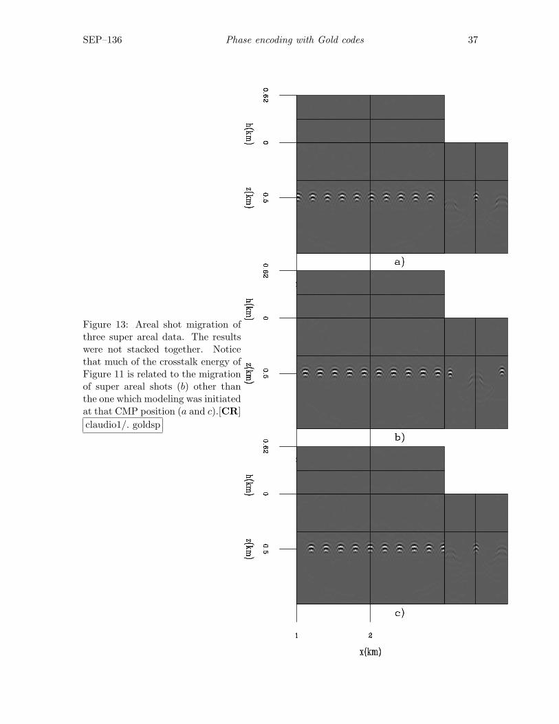
To understand the origin of the crosstalk in Figure 11, we migrated the data withoutadding the results of individual migrations of the super areal data. Figure 13 shows threeof these migrations. The three panels show the same spatial position. The top panel showsthe migration of super areal data whose modeling includes a SODCIG coincident with thatdisplayed. Remember that we are using a “comb” function to select every 10th SODCIGto initiate the modeling experiments comprised by a super areal data. The central panelshows the migration of the super areal data modeled from the initial image shifted five CMPpositions away from that of the uppermost panel, and the panel on the bottom shows themigration of the super areal data modeled from the initial image shifted nine CMP positionsaway from that of the uppermost panel. The modeling experiments which generated thesuper areal data for Figure 13c are actually separated one CMP position from the ones forFigure 13a, given that the modeling experiments in super areal data are separated every10th CMP. Figure 13a and Figure 13c show that much of the reflector energy comes fromthe migration of modeling experiments initiated at CMP positions close to the consideredimage point. Figure 13b shows that much of the crosstalk energy of Figure 11 is relatedto migration of super areal shots whose modeling experiments are initiated at SODCIGsshifted five CMP positions with respect to the considered SODCIG.
In migration velocity analysis, at every velocity iteration, data is migrated with anupdated velocity. To verify how the crosstalk behaves when migrating with a differentvelocity, we used a 5% faster velocity to migrate the Gold encoded data modeled with theinitial 5% slower velocity. We used sets of Gold codes with cross-correlation peaks at every5th (Figure 14a), 10th (Figure 14b) and, 20th lag (Figure 14c) lags. The depth shift ofthe crosstalk is proportional to the increase in velocity. The behavior is similar to that ofmigration with a slower velocity, regarding that the interference with the region of interestdecreases with the increase of the lag of the cross-correlation peaks.
SEP–136 Phase encoding with Gold codes 37
Figure 13: Areal shot migration ofthree super areal data. The resultswere not stacked together. Noticethat much of the crosstalk energy ofFigure 11 is related to the migrationof super areal shots (b) other thanthe one which modeling was initiatedat that CMP position (a and c).[CR]claudio1/. goldsp

38 Guerra and Biondi SEP–136
Figure 14: Areal shot migration ofone realization of synthesized datawith Gold phase encoding. Goldcodes have cross-correlation peaks atevery 5th (a), 10th (b) and, 20th lag(c).[CR] claudio1/. gold2x
SEP–136 Phase encoding with Gold codes 39
The use of Gold codes can be less costly than conventional random codes, given thatjust one realization is necessary to achieve an almost perfect result, while even using morerealizations of conventional random encoding does not produce an image with similar qual-ity. In addition, it is suited to be used in a horizon based strategy to migration velocityanalysis, where a few important reflectors are chosen to do velocity update.
However, an inadequate choice of the Gold codes is potentially more dangerous thanusing conventional random codes. Because the crosstalk may not be shifted out of theregion of interest, coherent artifacts can coincide with reflectors and obliterate the moveoutinformation. Conventional random codes, in turn, randomizes the crosstalk. This canlead to a noisy residual moveout scan or a noisy gradient. In a companion paper Tanget al. (2008) show that the prestack exploding-reflector modeled data, phase encoded withconventional random codes, is able to provide a reasonable direction for velocity update.
CONCLUSION
We showed that the use of Gold codes in phase encoding can virtually eliminate crosstalkif the codes are satisfactorily selected. Its advantage over conventional random codes is notonly in the image quality but also cost. The elimination of the crosstalk can be achieved withonly one realization of Gold codes, while for conventional random codes more realizationsare needed to obtain reasonable images, but still of lower quality when compared to theones obtained by using Gold codes. The need for more realizations increases the cost ofmodeling and migration.
We also showed that the phase of the cross-correlation of Gold codes is given by the lagin time where the cross-correlation peaks multiplied by frequency. This amounts to applylinear phase encoding to the encoded wavefields.
We used a simple example with just one reflector to illustrate the encoding techniques.The performance of the Gold codes in the presence of more than one reflector needs tobe tested. However, as just one realization is sufficient to drastically reduce the crosstalk,they can be affordable to use in a horizon-based approach to the modeling in which eachreflector is modeled separately. Additional research is needed to analyze the performanceof Gold codes in more complex situations, where the depth shift of the crosstalk may notbe a simple function of velocity.
ACKNOWLEDGEMENTS
We thank Jerry Harris and Youli Quan for the suggestion of using codes applied in wirelesscommunications.
REFERENCES
Biondi, B., 2006, Prestack exploding-reflectors modeling for migration velocity analyis:SEP-Report, 124, 45–60.
——–, 2007, Prestack modeling of image events for migration velocity analysis: SEP-131,101–118.
40 Guerra and Biondi SEP–136
Dinan, E. and B. Jabbari, 1998, Spreading codes for direct sequence CDMA and widebandCDMA cellular networks: IEEE Communications Magazine, 36, 48–54.
Golay, M., 1961, Complementary sequences: IRE Trans. on Info.Theory, IT-7, 82–87.Gold, R., 1967, Optimal binary sequences for spread spectrum multiplexing: IEEE Trans-
actions on Information Theory, 14, 619–621.Gran, F., 2005, Spatio-temporal encoding in medical ultrasound imaging: PhD thesis, Tech-
nical University of Denmark.Guerra, C. and B. Biondi, 2008, Prestack exploding reflector modeling: The crosstalk
problem: SEP-134, 79–91.Kasami, T., 1966, Weight distribution formula for some class of cyclic codes.Levanon, N. and E. Mozeson, 2004, Radar Signals: John Wiley & Sons.Lidl, R. and H. Niederreiter, 1994, Introduction to Finite Fields and their Applications:
Cambridge Univeristy.Moon, T. K. and W. C. Stirling, 2000, Mathematical Methods and Algorithms for Signal
Processing: Prentice Hall.Quan, Y. and J. M. Harris, 1991, Orthogonal coded signals as simultaneous source signa-
tures: Report of Seismic Tomography Project at Stanford University, 2, H1–H14.Romero, L., D. Ghiglia, C. Ober, and S. Morton, 2000, Phase encoding of shot records in
prestack migration: Geophysics, 65, 426–436.Shi, Z. and C. Schelgel, 2003, Spreading code construction for CDMA: IEEE Communica-
tions letters, 1, 4–6.Tang, Y., C. Guerra, and B. Biondi, 2008, Image-space wave-equation tomography in the
generalized source domain: SEP-136.Tseng, C., 1972, Complementary sets of sequences: IEEE Trans. on Info.Theory, IT-18,
644–652.

SEP–136 Phase encoding with Gold codes 41
APPENDIX
We show that phase encoding using Gold codes is equivalent to the linear phase encodingintroduced by (Romero et al., 2000). The cross-correlation function of Gold codes is givenby equation 13. It corresponds to a spike of amplitude ±2n at lag λ, which depends on thedifference between the number of circular shifts applied to the m-sequences to compute theGold codes, plus a DC term, ∓1. The phase of the cross-correlation function is given bythe phase of the spike, tλω, and is equal to the phase difference of the input signals. If Goldcodes have phases γ1(ω) and γ2(ω), the phase of their cross-correlation is
γ1(ω)− γ2(ω) = tλω. (A-1)
According to equation A-1, the phase of the cross-correlation of Gold codes is a linearfunction of the frequency. Equation A-1 is equal to equation 26 of Romero’s paper.

42 Guerra and Biondi SEP–136
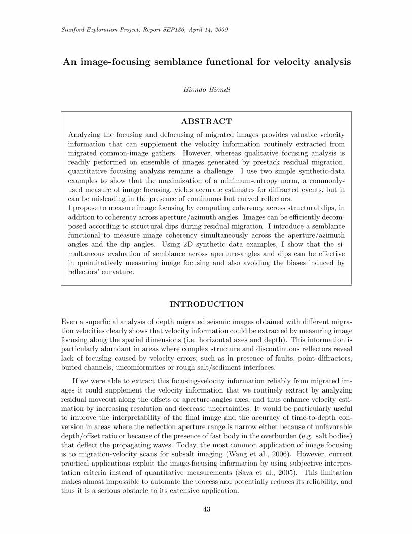
Stanford Exploration Project, Report SEP136, April 14, 2009
An image-focusing semblance functional for velocity analysis
Biondo Biondi
ABSTRACT
Analyzing the focusing and defocusing of migrated images provides valuable velocityinformation that can supplement the velocity information routinely extracted frommigrated common-image gathers. However, whereas qualitative focusing analysis isreadily performed on ensemble of images generated by prestack residual migration,quantitative focusing analysis remains a challenge. I use two simple synthetic-dataexamples to show that the maximization of a minimum-entropy norm, a commonly-used measure of image focusing, yields accurate estimates for diffracted events, but itcan be misleading in the presence of continuous but curved reflectors.I propose to measure image focusing by computing coherency across structural dips, inaddition to coherency across aperture/azimuth angles. Images can be efficiently decom-posed according to structural dips during residual migration. I introduce a semblancefunctional to measure image coherency simultaneously across the aperture/azimuthangles and the dip angles. Using 2D synthetic data examples, I show that the si-multaneous evaluation of semblance across aperture-angles and dips can be effectivein quantitatively measuring image focusing and also avoiding the biases induced byreflectors’ curvature.
INTRODUCTION
Even a superficial analysis of depth migrated seismic images obtained with different migra-tion velocities clearly shows that velocity information could be extracted by measuring imagefocusing along the spatial dimensions (i.e. horizontal axes and depth). This information isparticularly abundant in areas where complex structure and discontinuous reflectors reveallack of focusing caused by velocity errors; such as in presence of faults, point diffractors,buried channels, uncomformities or rough salt/sediment interfaces.
If we were able to extract this focusing-velocity information reliably from migrated im-ages it could supplement the velocity information that we routinely extract by analyzingresidual moveout along the offsets or aperture-angles axes, and thus enhance velocity esti-mation by increasing resolution and decrease uncertainties. It would be particularly usefulto improve the interpretability of the final image and the accuracy of time-to-depth con-version in areas where the reflection aperture range is narrow either because of unfavorabledepth/offset ratio or because of the presence of fast body in the overburden (e.g. salt bodies)that deflect the propagating waves. Today, the most common application of image focusingis to migration-velocity scans for subsalt imaging (Wang et al., 2006). However, currentpractical applications exploit the image-focusing information by using subjective interpre-tation criteria instead of quantitative measurements (Sava et al., 2005). This limitationmakes almost impossible to automate the process and potentially reduces its reliability, andthus it is a serious obstacle to its extensive application.
43

44 Biondi SEP-136
Minimum entropy has been often proposed as a quantitative measure of image focusing,starting with Harlan et al. (1984), De Vries and Berkhout (1984), and more recently byStinson et al. (2005) and Fomel et al. (2007). Minimizing the “spatial entropy” measured onimage windows privileges images that consist of isolated spikes. If the reflectivity functionconsists of isolated diffractors, minimum entropy is a good indicator of image focusing.However, field data are usually a combination of diffracted events, specular reflections fromplanar reflectors, and reflections for high-curvature reflectors. In these cases minimumentropy may yield bias estimates unless the diffractions are successfully separated from theother events before performing the analysis (Fomel et al., 2007). In complex geology, thisseparation can be unreliable when performed in the data space, and even more challengingwhen performed in the image space because it is biased by the initial migration velocity. Inthe following section I show that in presence of reflector curvature (e.g. a sinusoidal reflector)measuring focusing by minimum entropy leads to under-migrated images of convex reflectors(e.g. an anticline,) and over-migrated images of concave reflectors (e.g. a syncline.)
I aim to overcome these shortcomings by generalizing the conventional concept of sem-blance commonly used in velocity analysis. In addition to measuring semblance along thereflection-aperture angle (or offset for Kirchhoff migration,) as is routinely done, I proposeto measure semblance along the structural-dip axes. In this paper I work with 2D data,and thus I compute semblance on 2D patches (structural dip and aperture angle.) With 3Dfull-azimuth data, semblance would be computed on 4D patches (indexed by two structuraldips, reflection aperture and reflection azimuth.)
The proposed method can be applied to locally select the best-focused image amongan ensemble of images obtained with different migration velocities. I use residual prestackdepth migration in the angle domain (Biondi, 2008) to generate this ensemble of imagesstarting from prestack depth-migrated image in the angle domain. Stolt prestack depthmigration could be used as well to perform residual prestack migration (Sava, 2003). Witheither choice of residual migration, the image decomposition according to structural dipis easily performed within the residual prestack migration process, since both migrationsrequire the image to be transformed into the spatial Fourier domain. The final goal, notaddressed by this paper, is to use the image focusing information to enhance interval-velocityestimation for depth migration. In particular, I plan to update the interval-velocity modelby using the wave-equation migration velocity analysis method starting from a spatially-varying field of optimal-focusing parameters (Biondi and Sava, 1999; Sava and Biondi,2004a,b; Sava, 2004).
THE CHALLENGE OF QUANTIFYING IMAGE FOCUSING
In this section, I introduce two simple synthetic data sets that illustrate the opportunitiesand challenges of measuring image focusing for velocity analysis. I start by showing how theapplication of a minimum entropy functional can help to determine the correct migrationvelocity, but also it can mislead the estimation.
Figure 1a and Figure 2a show the reflectivity functions assumed to generate the two datasets. The first one contains a strong diffractor and two dipping planar reflectors broken bya fault. Focusing analysis of the diffractor and the reflectors’ truncations provides velocityinformation additional to the one available by conventional analysis of the reflections fromthe planar interfaces. The second model consists of a continuous sinusoidal reflector. It
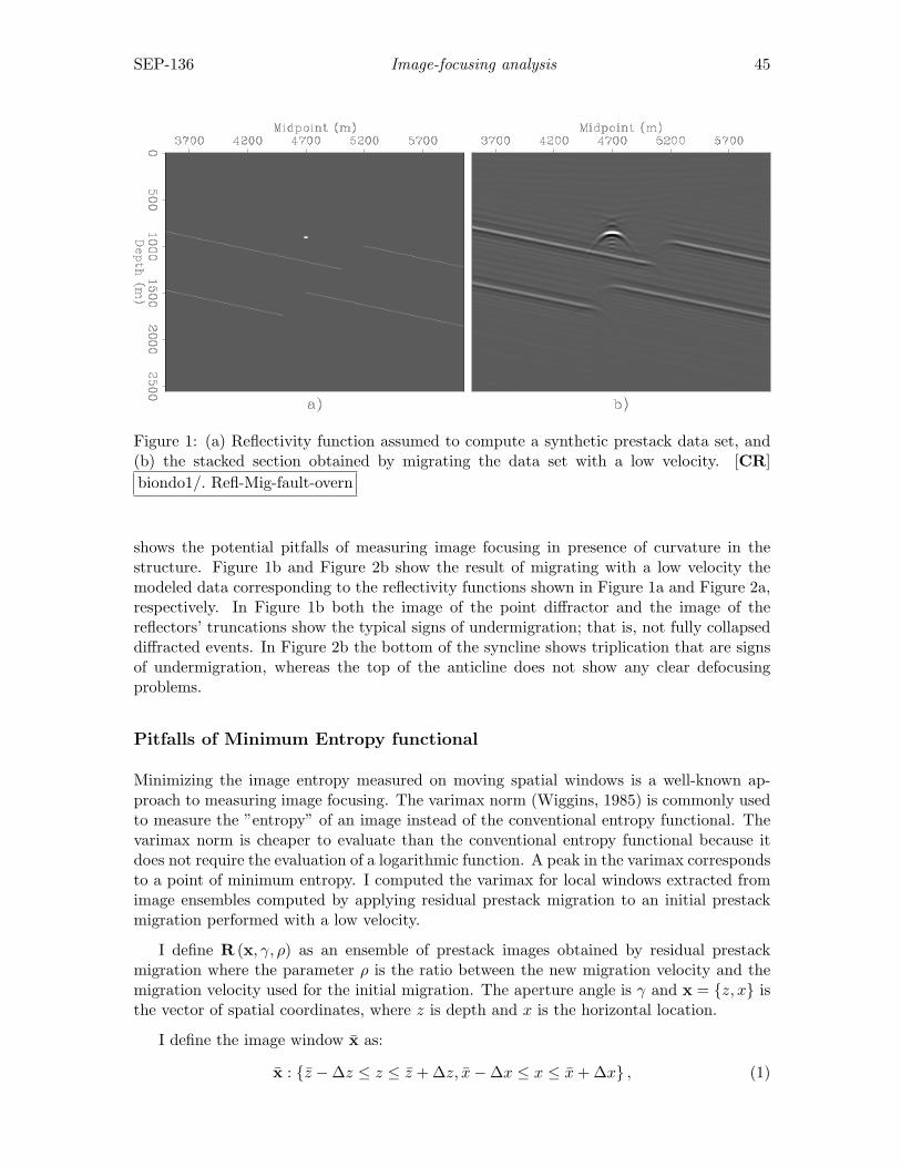
SEP-136 Image-focusing analysis 45
Figure 1: (a) Reflectivity function assumed to compute a synthetic prestack data set, and(b) the stacked section obtained by migrating the data set with a low velocity. [CR]biondo1/. Refl-Mig-fault-overn
shows the potential pitfalls of measuring image focusing in presence of curvature in thestructure. Figure 1b and Figure 2b show the result of migrating with a low velocity themodeled data corresponding to the reflectivity functions shown in Figure 1a and Figure 2a,respectively. In Figure 1b both the image of the point diffractor and the image of thereflectors’ truncations show the typical signs of undermigration; that is, not fully collapseddiffracted events. In Figure 2b the bottom of the syncline shows triplication that are signsof undermigration, whereas the top of the anticline does not show any clear defocusingproblems.
Pitfalls of Minimum Entropy functional
Minimizing the image entropy measured on moving spatial windows is a well-known ap-proach to measuring image focusing. The varimax norm (Wiggins, 1985) is commonly usedto measure the ”entropy” of an image instead of the conventional entropy functional. Thevarimax norm is cheaper to evaluate than the conventional entropy functional because itdoes not require the evaluation of a logarithmic function. A peak in the varimax correspondsto a point of minimum entropy. I computed the varimax for local windows extracted fromimage ensembles computed by applying residual prestack migration to an initial prestackmigration performed with a low velocity.
I define R (x, γ, ρ) as an ensemble of prestack images obtained by residual prestackmigration where the parameter ρ is the ratio between the new migration velocity and themigration velocity used for the initial migration. The aperture angle is γ and x = {z, x} isthe vector of spatial coordinates, where z is depth and x is the horizontal location.
I define the image window x as:
x : {z −∆z ≤ z ≤ z + ∆z, x−∆x ≤ x ≤ x + ∆x} , (1)
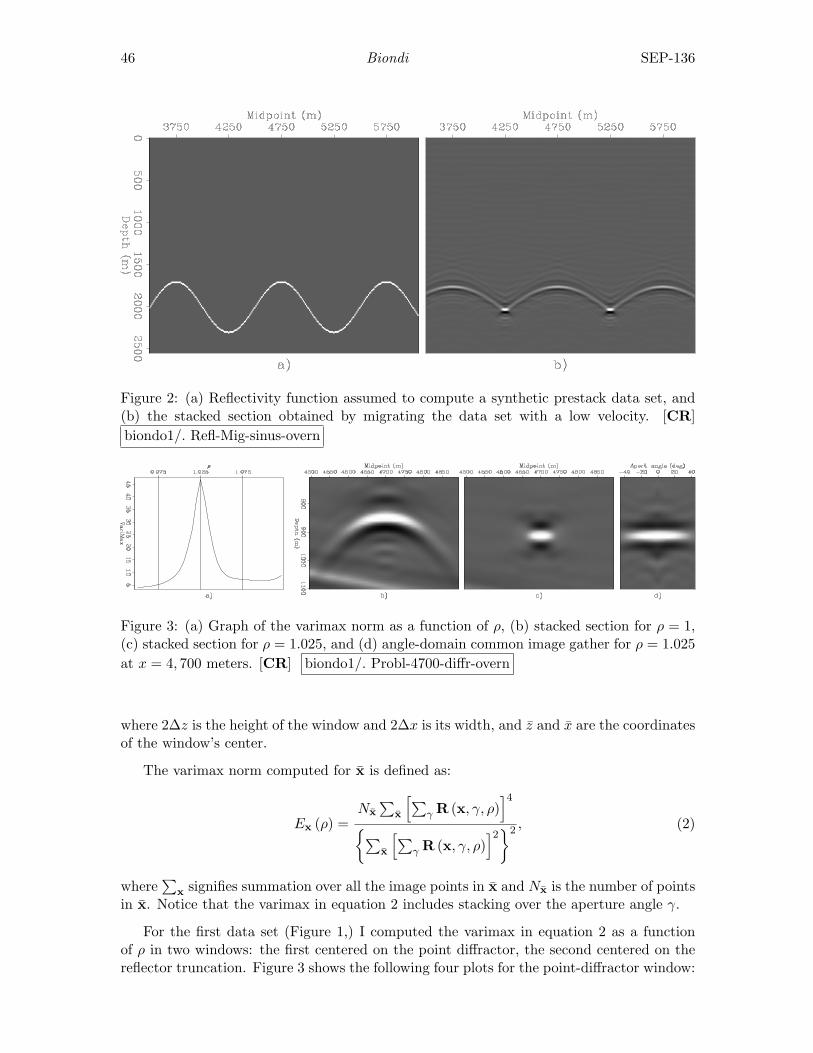
46 Biondi SEP-136
Figure 2: (a) Reflectivity function assumed to compute a synthetic prestack data set, and(b) the stacked section obtained by migrating the data set with a low velocity. [CR]biondo1/. Refl-Mig-sinus-overn
Figure 3: (a) Graph of the varimax norm as a function of ρ, (b) stacked section for ρ = 1,(c) stacked section for ρ = 1.025, and (d) angle-domain common image gather for ρ = 1.025at x = 4, 700 meters. [CR] biondo1/. Probl-4700-diffr-overn
where 2∆z is the height of the window and 2∆x is its width, and z and x are the coordinatesof the window’s center.
The varimax norm computed for x is defined as:
Ex (ρ) =Nx∑
x
[∑γ R (x, γ, ρ)
]4{∑
x
[∑γ R (x, γ, ρ)
]2}2 , (2)
where∑
x signifies summation over all the image points in x and Nx is the number of pointsin x. Notice that the varimax in equation 2 includes stacking over the aperture angle γ.
For the first data set (Figure 1,) I computed the varimax in equation 2 as a functionof ρ in two windows: the first centered on the point diffractor, the second centered on thereflector truncation. Figure 3 shows the following four plots for the point-diffractor window:
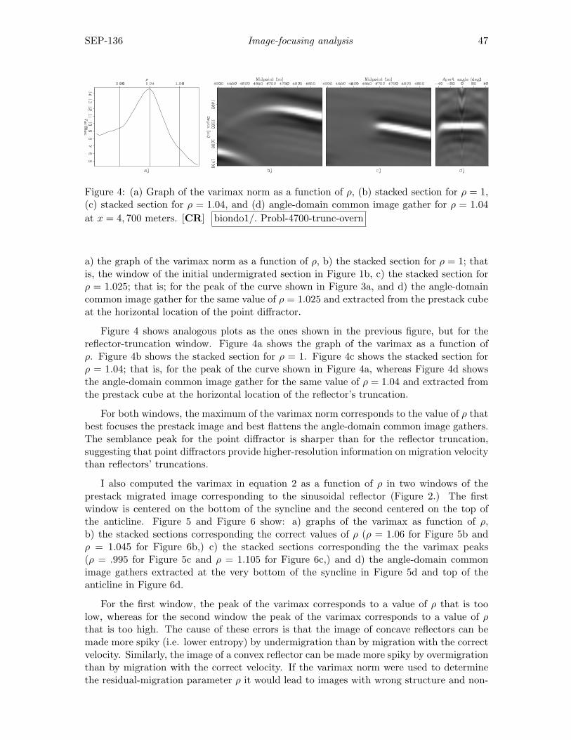
SEP-136 Image-focusing analysis 47
Figure 4: (a) Graph of the varimax norm as a function of ρ, (b) stacked section for ρ = 1,(c) stacked section for ρ = 1.04, and (d) angle-domain common image gather for ρ = 1.04at x = 4, 700 meters. [CR] biondo1/. Probl-4700-trunc-overn
a) the graph of the varimax norm as a function of ρ, b) the stacked section for ρ = 1; thatis, the window of the initial undermigrated section in Figure 1b, c) the stacked section forρ = 1.025; that is; for the peak of the curve shown in Figure 3a, and d) the angle-domaincommon image gather for the same value of ρ = 1.025 and extracted from the prestack cubeat the horizontal location of the point diffractor.
Figure 4 shows analogous plots as the ones shown in the previous figure, but for thereflector-truncation window. Figure 4a shows the graph of the varimax as a function ofρ. Figure 4b shows the stacked section for ρ = 1. Figure 4c shows the stacked section forρ = 1.04; that is, for the peak of the curve shown in Figure 4a, whereas Figure 4d showsthe angle-domain common image gather for the same value of ρ = 1.04 and extracted fromthe prestack cube at the horizontal location of the reflector’s truncation.
For both windows, the maximum of the varimax norm corresponds to the value of ρ thatbest focuses the prestack image and best flattens the angle-domain common image gathers.The semblance peak for the point diffractor is sharper than for the reflector truncation,suggesting that point diffractors provide higher-resolution information on migration velocitythan reflectors’ truncations.
I also computed the varimax in equation 2 as a function of ρ in two windows of theprestack migrated image corresponding to the sinusoidal reflector (Figure 2.) The firstwindow is centered on the bottom of the syncline and the second centered on the top ofthe anticline. Figure 5 and Figure 6 show: a) graphs of the varimax as function of ρ,b) the stacked sections corresponding the correct values of ρ (ρ = 1.06 for Figure 5b andρ = 1.045 for Figure 6b,) c) the stacked sections corresponding the the varimax peaks(ρ = .995 for Figure 5c and ρ = 1.105 for Figure 6c,) and d) the angle-domain commonimage gathers extracted at the very bottom of the syncline in Figure 5d and top of theanticline in Figure 6d.
For the first window, the peak of the varimax corresponds to a value of ρ that is toolow, whereas for the second window the peak of the varimax corresponds to a value of ρthat is too high. The cause of these errors is that the image of concave reflectors can bemade more spiky (i.e. lower entropy) by undermigration than by migration with the correctvelocity. Similarly, the image of a convex reflector can be made more spiky by overmigrationthan by migration with the correct velocity. If the varimax norm were used to determinethe residual-migration parameter ρ it would lead to images with wrong structure and non-
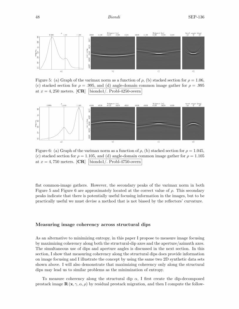
48 Biondi SEP-136
Figure 5: (a) Graph of the varimax norm as a function of ρ, (b) stacked section for ρ = 1.06,(c) stacked section for ρ = .995, and (d) angle-domain common image gather for ρ = .995at x = 4, 250 meters. [CR] biondo1/. Probl-4250-overn
Figure 6: (a) Graph of the varimax norm as a function of ρ, (b) stacked section for ρ = 1.045,(c) stacked section for ρ = 1.105, and (d) angle-domain common image gather for ρ = 1.105at x = 4, 750 meters. [CR] biondo1/. Probl-4750-overn
flat common-image gathers. However, the secondary peaks of the varimax norm in bothFigure 5 and Figure 6 are approximately located at the correct value of ρ. This secondarypeaks indicate that there is potentially useful focusing information in the images, but to bepractically useful we must devise a method that is not biased by the reflectors’ curvature.
Measuring image coherency across structural dips
As an alternative to minimizing entropy, in this paper I propose to measure image focusingby maximizing coherency along both the structural-dip axes and the aperture/azimuth axes.The simultaneous use of dips and aperture angles is discussed in the next section. In thissection, I show that measuring coherency along the structural dips does provide informationon image focusing and I illustrate the concept by using the same two 2D synthetic data setsshown above. I will also demonstrate that maximizing coherency only along the structuraldips may lead us to similar problems as the minimization of entropy.
To measure coherency along the structural dip α, I first create the dip-decomposedprestack image R (x, γ, α, ρ) by residual prestack migration, and then I compute the follow-
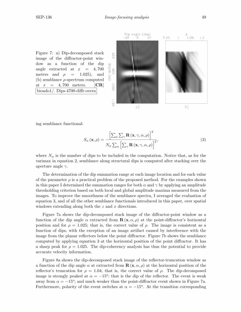
SEP-136 Image-focusing analysis 49
Figure 7: a) Dip-decomposed stackimage of the diffractor-point win-dow as a function of the dipangle extracted at x = 4, 700meters and ρ = 1.025), and(b) semblance ρ-spectrum computedat x = 4, 700 meters. [CR]biondo1/. Dips-4700-diffr-overn
ing semblance functional:
Sα (x, ρ) =
[∑α
∑γ R (x, γ, α, ρ)
]2Nα∑
α
[∑γ R (x, γ, α, ρ)
]2 , (3)
where Nα is the number of dips to be included in the computation. Notice that, as for thevarimax in equation 2, semblance along structural dips is computed after stacking over theaperture angle γ.
The determination of the dip summation range at each image location and for each valueof the parameter ρ is a practical problem of the proposed method. For the examples shownin this paper I determined the summation ranges for both α and γ by applying an amplitudethresholding criterion based on both local and global amplitude maxima measured from theimages. To improve the smoothness of the semblance spectra, I averaged the evaluation ofequation 3, and of all the other semblance functionals introduced in this paper, over spatialwindows extending along both the z and x directions.
Figure 7a shows the dip-decomposed stack image of the diffractor-point window as afunction of the dip angle α extracted from R (x, α, ρ) at the point-diffractor’s horizontalposition and for ρ = 1.025; that is, the correct value of ρ. The image is consistent as afunction of dips, with the exception of an image artifact caused by interference with theimage from the planar reflectors below the point diffractor. Figure 7b shows the semblancecomputed by applying equation 3 at the horizontal position of the point diffractor. It hasa sharp peak for ρ = 1.025. The dip-coherency analysis has thus the potential to provideaccurate velocity information.
Figure 8a shows the dip-decomposed stack image of the reflector-truncation window asa function of the dip angle α at extracted from R (x, α, ρ) at the horizontal position of thereflector’s truncation for ρ = 1.04; that is, the correct value of ρ. The dip-decomposedimage is strongly peaked at α = −15o; that is the dip of the reflector. The event is weakaway from α = −15o; and much weaker than the point-diffractor event shown in Figure 7a.Furthermore, polarity of the event switches at α = −15o. At the transition corresponding
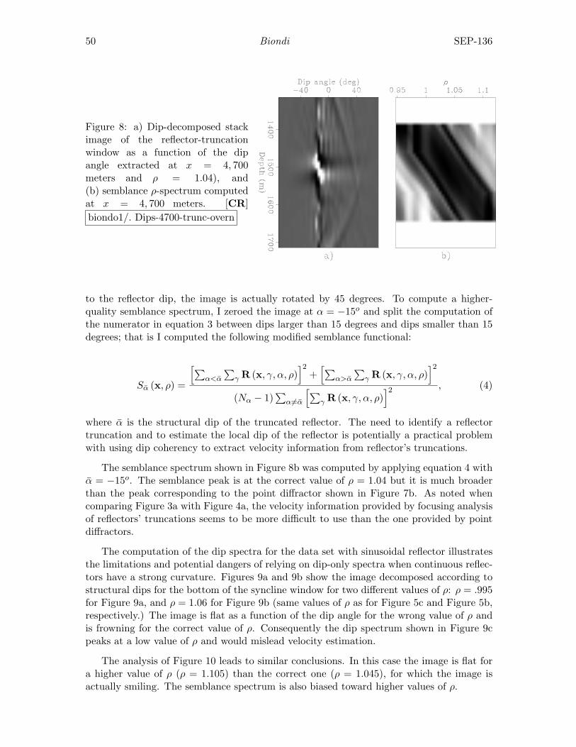
50 Biondi SEP-136
Figure 8: a) Dip-decomposed stackimage of the reflector-truncationwindow as a function of the dipangle extracted at x = 4, 700meters and ρ = 1.04), and(b) semblance ρ-spectrum computedat x = 4, 700 meters. [CR]biondo1/. Dips-4700-trunc-overn
to the reflector dip, the image is actually rotated by 45 degrees. To compute a higher-quality semblance spectrum, I zeroed the image at α = −15o and split the computation ofthe numerator in equation 3 between dips larger than 15 degrees and dips smaller than 15degrees; that is I computed the following modified semblance functional:
Sα (x, ρ) =
[∑α<α
∑γ R (x, γ, α, ρ)
]2+[∑
α>α
∑γ R (x, γ, α, ρ)
]2(Nα − 1)
∑α 6=α
[∑γ R (x, γ, α, ρ)
]2 , (4)
where α is the structural dip of the truncated reflector. The need to identify a reflectortruncation and to estimate the local dip of the reflector is potentially a practical problemwith using dip coherency to extract velocity information from reflector’s truncations.
The semblance spectrum shown in Figure 8b was computed by applying equation 4 withα = −15o. The semblance peak is at the correct value of ρ = 1.04 but it is much broaderthan the peak corresponding to the point diffractor shown in Figure 7b. As noted whencomparing Figure 3a with Figure 4a, the velocity information provided by focusing analysisof reflectors’ truncations seems to be more difficult to use than the one provided by pointdiffractors.
The computation of the dip spectra for the data set with sinusoidal reflector illustratesthe limitations and potential dangers of relying on dip-only spectra when continuous reflec-tors have a strong curvature. Figures 9a and 9b show the image decomposed according tostructural dips for the bottom of the syncline window for two different values of ρ: ρ = .995for Figure 9a, and ρ = 1.06 for Figure 9b (same values of ρ as for Figure 5c and Figure 5b,respectively.) The image is flat as a function of the dip angle for the wrong value of ρ andis frowning for the correct value of ρ. Consequently the dip spectrum shown in Figure 9cpeaks at a low value of ρ and would mislead velocity estimation.
The analysis of Figure 10 leads to similar conclusions. In this case the image is flat fora higher value of ρ (ρ = 1.105) than the correct one (ρ = 1.045), for which the image isactually smiling. The semblance spectrum is also biased toward higher values of ρ.
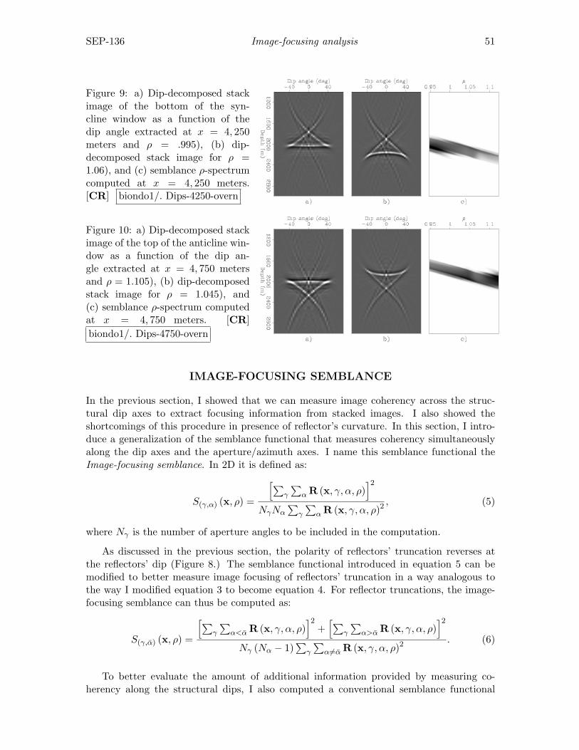
SEP-136 Image-focusing analysis 51
Figure 9: a) Dip-decomposed stackimage of the bottom of the syn-cline window as a function of thedip angle extracted at x = 4, 250meters and ρ = .995), (b) dip-decomposed stack image for ρ =1.06), and (c) semblance ρ-spectrumcomputed at x = 4, 250 meters.[CR] biondo1/. Dips-4250-overn
Figure 10: a) Dip-decomposed stackimage of the top of the anticline win-dow as a function of the dip an-gle extracted at x = 4, 750 metersand ρ = 1.105), (b) dip-decomposedstack image for ρ = 1.045), and(c) semblance ρ-spectrum computedat x = 4, 750 meters. [CR]biondo1/. Dips-4750-overn
IMAGE-FOCUSING SEMBLANCE
In the previous section, I showed that we can measure image coherency across the struc-tural dip axes to extract focusing information from stacked images. I also showed theshortcomings of this procedure in presence of reflector’s curvature. In this section, I intro-duce a generalization of the semblance functional that measures coherency simultaneouslyalong the dip axes and the aperture/azimuth axes. I name this semblance functional theImage-focusing semblance. In 2D it is defined as:
S(γ,α) (x, ρ) =
[∑γ
∑α R (x, γ, α, ρ)
]2NγNα
∑γ
∑α R (x, γ, α, ρ)2
, (5)
where Nγ is the number of aperture angles to be included in the computation.
As discussed in the previous section, the polarity of reflectors’ truncation reverses atthe reflectors’ dip (Figure 8.) The semblance functional introduced in equation 5 can bemodified to better measure image focusing of reflectors’ truncation in a way analogous tothe way I modified equation 3 to become equation 4. For reflector truncations, the image-focusing semblance can thus be computed as:
S(γ,α) (x, ρ) =
[∑γ
∑α<α R (x, γ, α, ρ)
]2+[∑
γ
∑α>α R (x, γ, α, ρ)
]2Nγ (Nα − 1)
∑γ
∑α 6=α R (x, γ, α, ρ)2
. (6)
To better evaluate the amount of additional information provided by measuring co-herency along the structural dips, I also computed a conventional semblance functional
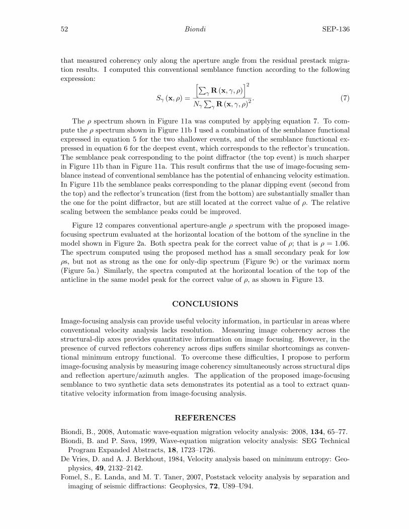
52 Biondi SEP-136
that measured coherency only along the aperture angle from the residual prestack migra-tion results. I computed this conventional semblance function according to the followingexpression:
Sγ (x, ρ) =
[∑γ R (x, γ, ρ)
]2Nγ∑
γ R (x, γ, ρ)2. (7)
The ρ spectrum shown in Figure 11a was computed by applying equation 7. To com-pute the ρ spectrum shown in Figure 11b I used a combination of the semblance functionalexpressed in equation 5 for the two shallower events, and of the semblance functional ex-pressed in equation 6 for the deepest event, which corresponds to the reflector’s truncation.The semblance peak corresponding to the point diffractor (the top event) is much sharperin Figure 11b than in Figure 11a. This result confirms that the use of image-focusing sem-blance instead of conventional semblance has the potential of enhancing velocity estimation.In Figure 11b the semblance peaks corresponding to the planar dipping event (second fromthe top) and the reflector’s truncation (first from the bottom) are substantially smaller thanthe one for the point diffractor, but are still located at the correct value of ρ. The relativescaling between the semblance peaks could be improved.
Figure 12 compares conventional aperture-angle ρ spectrum with the proposed image-focusing spectrum evaluated at the horizontal location of the bottom of the syncline in themodel shown in Figure 2a. Both spectra peak for the correct value of ρ; that is ρ = 1.06.The spectrum computed using the proposed method has a small secondary peak for lowρs, but not as strong as the one for only-dip spectrum (Figure 9c) or the varimax norm(Figure 5a.) Similarly, the spectra computed at the horizontal location of the top of theanticline in the same model peak for the correct value of ρ, as shown in Figure 13.
CONCLUSIONS
Image-focusing analysis can provide useful velocity information, in particular in areas whereconventional velocity analysis lacks resolution. Measuring image coherency across thestructural-dip axes provides quantitative information on image focusing. However, in thepresence of curved reflectors coherency across dips suffers similar shortcomings as conven-tional minimum entropy functional. To overcome these difficulties, I propose to performimage-focusing analysis by measuring image coherency simultaneously across structural dipsand reflection aperture/azimuth angles. The application of the proposed image-focusingsemblance to two synthetic data sets demonstrates its potential as a tool to extract quan-titative velocity information from image-focusing analysis.
REFERENCES
Biondi, B., 2008, Automatic wave-equation migration velocity analysis: 2008, 134, 65–77.Biondi, B. and P. Sava, 1999, Wave-equation migration velocity analysis: SEG Technical
Program Expanded Abstracts, 18, 1723–1726.De Vries, D. and A. J. Berkhout, 1984, Velocity analysis based on minimum entropy: Geo-
physics, 49, 2132–2142.Fomel, S., E. Landa, and M. T. Taner, 2007, Poststack velocity analysis by separation and
imaging of seismic diffractions: Geophysics, 72, U89–U94.
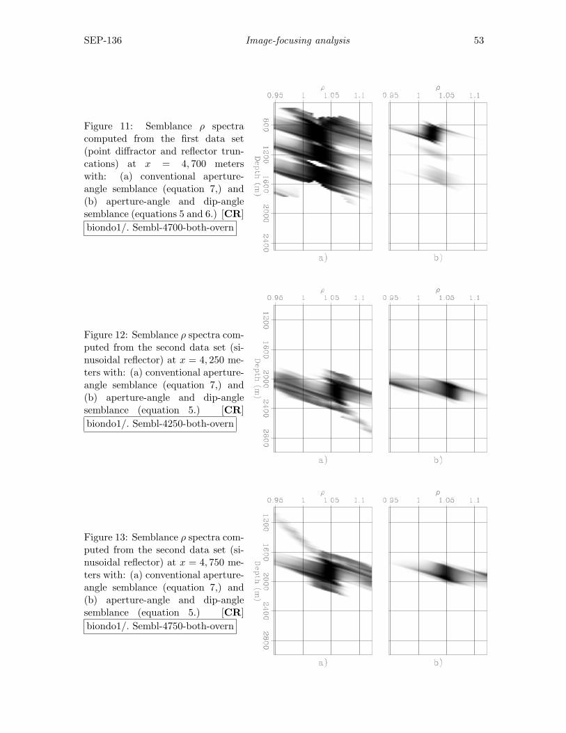
SEP-136 Image-focusing analysis 53
Figure 11: Semblance ρ spectracomputed from the first data set(point diffractor and reflector trun-cations) at x = 4, 700 meterswith: (a) conventional aperture-angle semblance (equation 7,) and(b) aperture-angle and dip-anglesemblance (equations 5 and 6.) [CR]biondo1/. Sembl-4700-both-overn
Figure 12: Semblance ρ spectra com-puted from the second data set (si-nusoidal reflector) at x = 4, 250 me-ters with: (a) conventional aperture-angle semblance (equation 7,) and(b) aperture-angle and dip-anglesemblance (equation 5.) [CR]biondo1/. Sembl-4250-both-overn
Figure 13: Semblance ρ spectra com-puted from the second data set (si-nusoidal reflector) at x = 4, 750 me-ters with: (a) conventional aperture-angle semblance (equation 7,) and(b) aperture-angle and dip-anglesemblance (equation 5.) [CR]biondo1/. Sembl-4750-both-overn
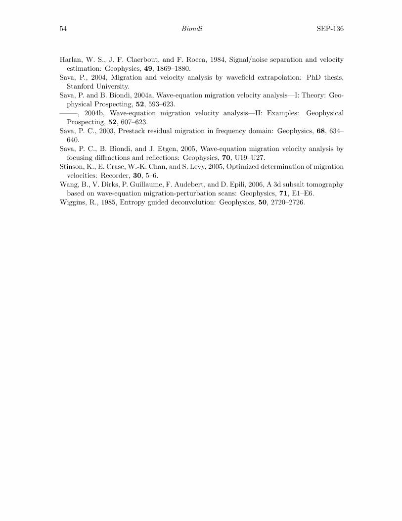
54 Biondi SEP-136
Harlan, W. S., J. F. Claerbout, and F. Rocca, 1984, Signal/noise separation and velocityestimation: Geophysics, 49, 1869–1880.
Sava, P., 2004, Migration and velocity analysis by wavefield extrapolation: PhD thesis,Stanford University.
Sava, P. and B. Biondi, 2004a, Wave-equation migration velocity analysis—I: Theory: Geo-physical Prospecting, 52, 593–623.
——–, 2004b, Wave-equation migration velocity analysis—II: Examples: GeophysicalProspecting, 52, 607–623.
Sava, P. C., 2003, Prestack residual migration in frequency domain: Geophysics, 68, 634–640.
Sava, P. C., B. Biondi, and J. Etgen, 2005, Wave-equation migration velocity analysis byfocusing diffractions and reflections: Geophysics, 70, U19–U27.
Stinson, K., E. Crase, W.-K. Chan, and S. Levy, 2005, Optimized determination of migrationvelocities: Recorder, 30, 5–6.
Wang, B., V. Dirks, P. Guillaume, F. Audebert, and D. Epili, 2006, A 3d subsalt tomographybased on wave-equation migration-perturbation scans: Geophysics, 71, E1–E6.
Wiggins, R., 1985, Entropy guided deconvolution: Geophysics, 50, 2720–2726.
Stanford Exploration Project, Report SEP136, April 14, 2009
Migration velocity analysis with cross-gradient constraint
Mohammad Maysami
ABSTRACT
Velocity analysis plays a fundamental to seismic imaging. A variety of techniquesusing pre-stack seismic data exist for migration-velocity analysis, including reflectiontomographic inversion methods. However, when the wavefield propagation is complex,reflection tomography may fail to converge to a geologically reasonable velocity esti-mation. Non-seismic geological properties can be integrated in the reflection-seismictomography problem to achieve better velocity estimation. Here, I propose to usecross-gradients function as a similarity measure to constrain the tomography problemand enforce a general geometrical structure for the seismic velocity estimates.
INTRODUCTION
Precise estimation of subsurface velocities is a requirement for high quality seismic imaging.Without an accurate velocity, seismic reflectors are misplaced, the image is unfocused, andseismic images can easily mislead earth scientists (Claerbout, 1999; Clapp, 2001). Defininga reliable velocity model for seismic imaging is a difficult task, especially when sharp lateraland vertical velocity variations are present. Velocity estimation becomes even more chal-lenging when seismic data are noisy. Therefore it is harder to extract velocity information(Clapp, 2001).
In areas with complex structures, and significant lateral velocity variations, velocityanalysis is a challenging task. In these areas, reflection-tomography methods are oftenmore effective than conventional velocity-estimation methods based on measurements ofstacking velocities (Biondi, 1990; Clapp, 2001). Unfortunately, the reflection-tomographyproblem is ill-posed and under-determined. Furthermore, it may not converge to a realisticvelocity model without a priori information, e.g., regularization constraints and other typesof geophysical properties in addition to seismic data (Clapp, 2001).
The main challenge in integrating different geophysical data sets is the absence of ananalytical relationship between properties exploited by different geophysical surveys. Mostoften, probabilistic relations among these geophysical properties are used to address thisshortcoming. A different approach would be to use gradients field as an objective measureof geometrical similarity. This is true since the variations of geophysical properties can bedescribed by a magnitude and a direction (Gallardo and Meju, 2004, 2007).
Here, I use the cross-gradients function introduced by Gallardo and Meju (2004, 2007)to integrate the resistivity field measured by electromagnetic surveys into the reflection-seismic tomography problem. The integration of this additional piece of information maylead to velocity estimates that are geologically reasonable.
My paper is organized as follows. First, I present a short overview of reflection tomog-raphy, followed by introducing the cross-gradients function as a structural similarity mea-
55
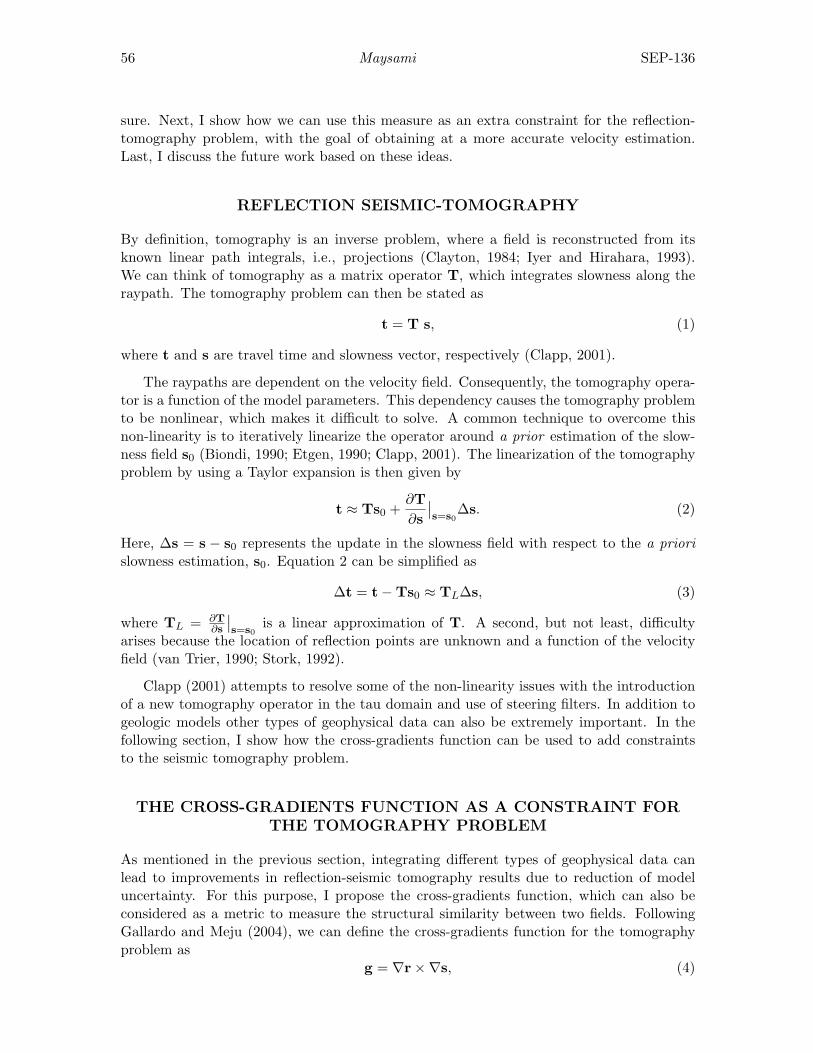
56 Maysami SEP-136
sure. Next, I show how we can use this measure as an extra constraint for the reflection-tomography problem, with the goal of obtaining at a more accurate velocity estimation.Last, I discuss the future work based on these ideas.
REFLECTION SEISMIC-TOMOGRAPHY
By definition, tomography is an inverse problem, where a field is reconstructed from itsknown linear path integrals, i.e., projections (Clayton, 1984; Iyer and Hirahara, 1993).We can think of tomography as a matrix operator T, which integrates slowness along theraypath. The tomography problem can then be stated as
t = T s, (1)
where t and s are travel time and slowness vector, respectively (Clapp, 2001).
The raypaths are dependent on the velocity field. Consequently, the tomography opera-tor is a function of the model parameters. This dependency causes the tomography problemto be nonlinear, which makes it difficult to solve. A common technique to overcome thisnon-linearity is to iteratively linearize the operator around a prior estimation of the slow-ness field s0 (Biondi, 1990; Etgen, 1990; Clapp, 2001). The linearization of the tomographyproblem by using a Taylor expansion is then given by
t ≈ Ts0 +∂T∂s
∣∣s=s0
∆s. (2)
Here, ∆s = s − s0 represents the update in the slowness field with respect to the a priorislowness estimation, s0. Equation 2 can be simplified as
∆t = t−Ts0 ≈ TL∆s, (3)
where TL = ∂T∂s
∣∣s=s0
is a linear approximation of T. A second, but not least, difficultyarises because the location of reflection points are unknown and a function of the velocityfield (van Trier, 1990; Stork, 1992).
Clapp (2001) attempts to resolve some of the non-linearity issues with the introductionof a new tomography operator in the tau domain and use of steering filters. In addition togeologic models other types of geophysical data can also be extremely important. In thefollowing section, I show how the cross-gradients function can be used to add constraintsto the seismic tomography problem.
THE CROSS-GRADIENTS FUNCTION AS A CONSTRAINT FORTHE TOMOGRAPHY PROBLEM
As mentioned in the previous section, integrating different types of geophysical data canlead to improvements in reflection-seismic tomography results due to reduction of modeluncertainty. For this purpose, I propose the cross-gradients function, which can also beconsidered as a metric to measure the structural similarity between two fields. FollowingGallardo and Meju (2004), we can define the cross-gradients function for the tomographyproblem as
g = ∇r×∇s, (4)
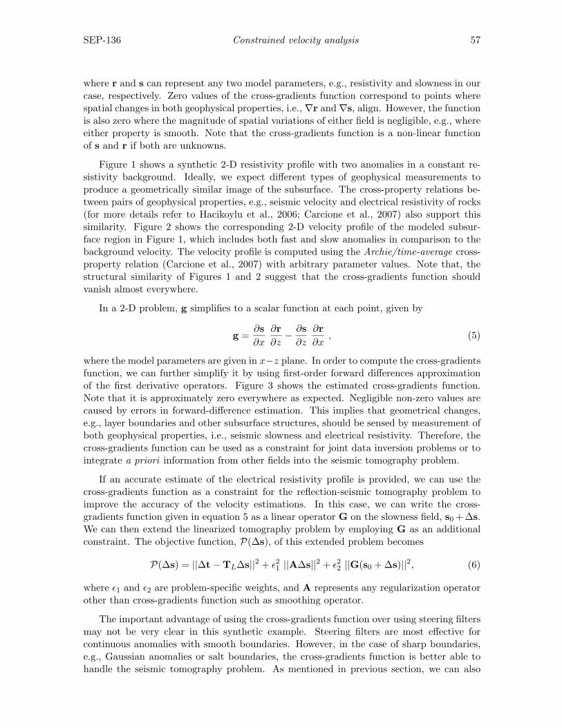
SEP-136 Constrained velocity analysis 57
where r and s can represent any two model parameters, e.g., resistivity and slowness in ourcase, respectively. Zero values of the cross-gradients function correspond to points wherespatial changes in both geophysical properties, i.e., ∇r and ∇s, align. However, the functionis also zero where the magnitude of spatial variations of either field is negligible, e.g., whereeither property is smooth. Note that the cross-gradients function is a non-linear functionof s and r if both are unknowns.
Figure 1 shows a synthetic 2-D resistivity profile with two anomalies in a constant re-sistivity background. Ideally, we expect different types of geophysical measurements toproduce a geometrically similar image of the subsurface. The cross-property relations be-tween pairs of geophysical properties, e.g., seismic velocity and electrical resistivity of rocks(for more details refer to Hacikoylu et al., 2006; Carcione et al., 2007) also support thissimilarity. Figure 2 shows the corresponding 2-D velocity profile of the modeled subsur-face region in Figure 1, which includes both fast and slow anomalies in comparison to thebackground velocity. The velocity profile is computed using the Archie/time-average cross-property relation (Carcione et al., 2007) with arbitrary parameter values. Note that, thestructural similarity of Figures 1 and 2 suggest that the cross-gradients function shouldvanish almost everywhere.
In a 2-D problem, g simplifies to a scalar function at each point, given by
g =∂s∂x
∂r∂z− ∂s
∂z
∂r∂x
, (5)
where the model parameters are given in x−z plane. In order to compute the cross-gradientsfunction, we can further simplify it by using first-order forward differences approximationof the first derivative operators. Figure 3 shows the estimated cross-gradients function.Note that it is approximately zero everywhere as expected. Negligible non-zero values arecaused by errors in forward-difference estimation. This implies that geometrical changes,e.g., layer boundaries and other subsurface structures, should be sensed by measurement ofboth geophysical properties, i.e., seismic slowness and electrical resistivity. Therefore, thecross-gradients function can be used as a constraint for joint data inversion problems or tointegrate a priori information from other fields into the seismic tomography problem.
If an accurate estimate of the electrical resistivity profile is provided, we can use thecross-gradients function as a constraint for the reflection-seismic tomography problem toimprove the accuracy of the velocity estimations. In this case, we can write the cross-gradients function given in equation 5 as a linear operator G on the slowness field, s0 +∆s.We can then extend the linearized tomography problem by employing G as an additionalconstraint. The objective function, P(∆s), of this extended problem becomes
P(∆s) = ||∆t−TL∆s||2 + ε21 ||A∆s||2 + ε22 ||G(s0 + ∆s)||2, (6)
where ε1 and ε2 are problem-specific weights, and A represents any regularization operatorother than cross-gradients function such as smoothing operator.
The important advantage of using the cross-gradients function over using steering filtersmay not be very clear in this synthetic example. Steering filters are most effective forcontinuous anomalies with smooth boundaries. However, in the case of sharp boundaries,e.g., Gaussian anomalies or salt boundaries, the cross-gradients function is better able tohandle the seismic tomography problem. As mentioned in previous section, we can also
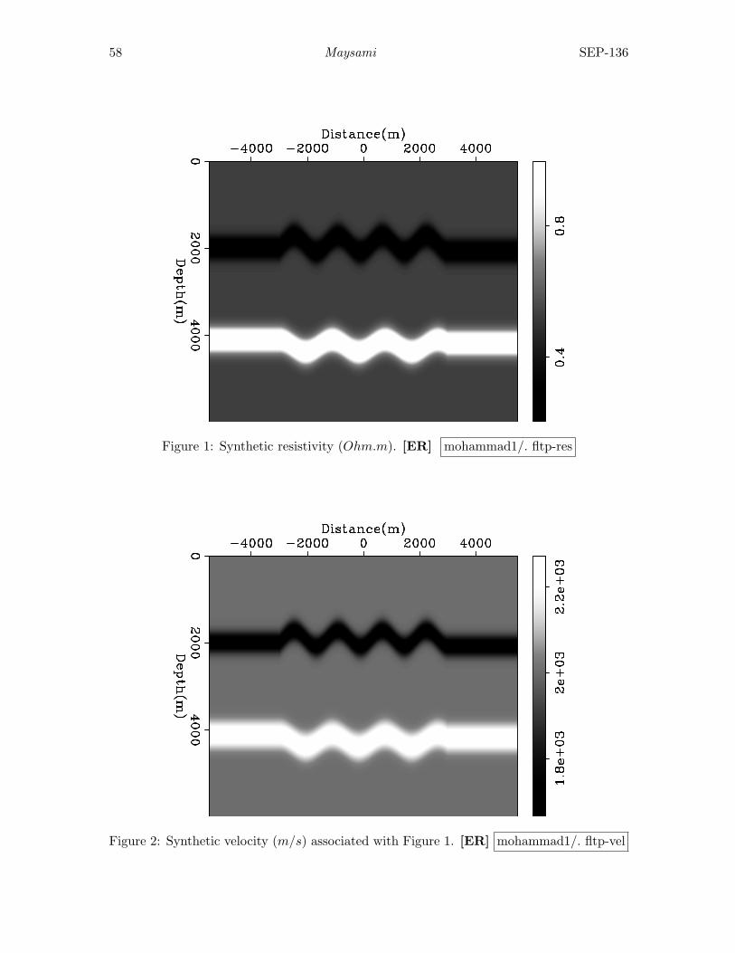
58 Maysami SEP-136
Figure 1: Synthetic resistivity (Ohm.m). [ER] mohammad1/. fltp-res
Figure 2: Synthetic velocity (m/s) associated with Figure 1. [ER] mohammad1/. fltp-vel
SEP-136 Constrained velocity analysis 59
Figure 3: Cross-gradients function of the velocity and resistivity shown in Figures 1 and 2.[ER] mohammad1/. fltp-xgrad
use the cross-gradients function as a constraint for joint inversion, where steering filters arenot effective. This is true because steering filters assume a priori knowledge of the modelparameters while the cross-gradients function use the collocated data field to build thisinformation.
FUTURE WORK
The tomography problem stated in Equation 6 is based on the assumption that we havea reasonably accurate estimate of the collocated resistivity field. Given this assumption, Iexpect the similarity constraint to improve the estimation of slowness profile. I will firstincorporate the similarity constraint into the reflection-seismic tomography problem forthe synthetic model shown above. Then, I will extend the application of the idea to thetomography problem for 2-D sections of a field data set.
REFERENCES
Biondi, B., 1990, Velocity analysis using beam stacks: PhD thesis, Stanford University.Carcione, J. M., B. Ursin, and J. I. Nordskag, 2007, Cross-property relations between
electrical conductivity and the seismic velocity of rocks: Geophysics, 72, E193–E204.Claerbout, J., 1999, Everything depends on v(x,y,z): SEP-Report, 100, 1–10.Clapp, R. G., 2001, Geologically constrained migration velocity analysis: PhD thesis, Stan-
ford University.Clayton, R. W., 1984, Seismic tomography: Eos, Trans., Am. Geophys Union., 65.
60 Maysami SEP-136
Etgen, J., 1990, Residual prestack migration and interval velocity estimation: PhD thesis,Stanford University.
Gallardo, L. A. and M. A. Meju, 2004, Joint two-dimensional dc resistivity and seismictravel time inversion with cross-gradients constraints: J. Geophys. Res., 109.
——–, 2007, Joint two-dimensional cross-gradient imaging of magnetotelluric and seismictraveltime data for structural and lithological classication: Geoph. J. Int., 169, 1261–1272.
Hacikoylu, P., J. Dvorkin, and G. Mavko, 2006, Resistivity-velocity transforms revisited:The Leading Edge, 25, 1006 – 1009.
Iyer, H. and K. Hirahara, eds., 1993, Seismic tomography: Theory and practice, 1st. ed.:Chapman & Hall.
Stork, C., 1992, Reflection tomography in the postmigrated domain: Geophysics, 57, 680–692.
van Trier, J., 1990, Tomographic determination of structural velocities from depth migratedseismic data: PhD thesis, Stanford University.

Stanford Exploration Project, Report SEP136, April 14, 2009
Transmission effects of localized variations of Earth’svisco-acoustic parameters
Abdullah Al Theyab and Biondo Biondi
ABSTRACT
In an effort to understand the transmission effects of localized heterogenities in thesubsurface, we present the travel-time and amplitude distortions caused by localizedvariations in velocity and absorption. To examine the relative impact of velocity andabsorption heterogeneities on seismic events, we conducted numerical experiments usingvisco-acoustic finite-difference modeling of the linearized wave-equation for Newtonianfluids. We analyzed the distortions in the midpoint-offset domain. We find that thedistortion caused by an anomaly that is both slow and absorptive is different from thatan anomaly that is either slow or absorptive, but not both. Our results also indicatethat amplitude distortion of highly absorptive anomalies (Q < 50) can be comparableto that of small velocity variation (less than 4%), and therefore absorption must beconsidered in seismic amplitude inversion and AVO analysis.
INTRODUCTION
Localized heterogeneities in the subsurface cause amplitude and travel-time distortions ofseismic reflections from underlying reflectors. These distortions are problematic to imagingand AVO analysis. The distortions come in almost regular patterns and usually are recog-nizable by V-shaped trajectories in the midpoint-offset domain (X-shapes for split-spreadacquisition geometry). These distortions can be used to find the locations of the anoma-lies, which can reveal valuable information for interpreters such as fault locations (Hatchell,2000). Moreover, they can be used to invert for velocity and absorption anomalies. Theanalyses of several authors Vlad (2005), Hatchell (2000) and Harlan (1994) have consideredmostly velocity anomalies, which cause focusing and defocusing effects.
In this report, we stress that absorption must be considered in the analysis of thesedistortions. A seismic amplitude inversion that disregards absorption is likly to be biased,especially if velocity perturbations of interest are less than 4%. We examine the relativeimpact of localized velocity anomalies versus absorption anomalies on seismic amplitude.
BACKGROUND
For a constant background velocity with non-dipping reflector, the distortion trajectory (i.e.the location in prestack data space) caused by a single anomaly can be described by
h =t
t− ta| m−ma | , (1)
61
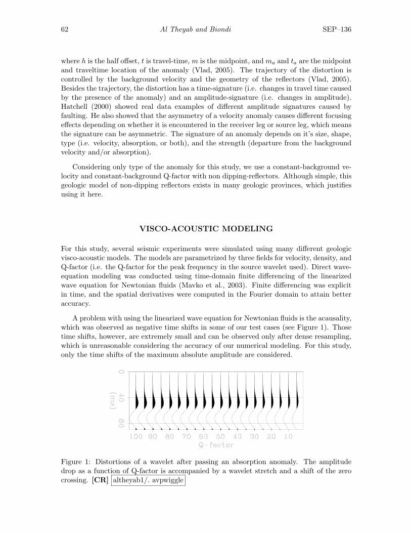
62 Al Theyab and Biondi SEP–136
where h is the half offset, t is travel-time, m is the midpoint, and ma and ta are the midpointand traveltime location of the anomaly (Vlad, 2005). The trajectory of the distortion iscontrolled by the background velocity and the geometry of the reflectors (Vlad, 2005).Besides the trajectory, the distortion has a time-signature (i.e. changes in travel time causedby the presence of the anomaly) and an amplitude-signature (i.e. changes in amplitude).Hatchell (2000) showed real data examples of different amplitude signatures caused byfaulting. He also showed that the asymmetry of a velocity anomaly causes different focusingeffects depending on whether it is encountered in the receiver leg or source leg, which meansthe signature can be asymmetric. The signature of an anomaly depends on it’s size, shape,type (i.e. velocity, absorption, or both), and the strength (departure from the backgroundvelocity and/or absorption).
Considering only type of the anomaly for this study, we use a constant-background ve-locity and constant-background Q-factor with non dipping-reflectors. Although simple, thisgeologic model of non-dipping reflectors exists in many geologic provinces, which justifiesusing it here.
VISCO-ACOUSTIC MODELING
For this study, several seismic experiments were simulated using many different geologicvisco-acoustic models. The models are parametrized by three fields for velocity, density, andQ-factor (i.e. the Q-factor for the peak frequency in the source wavelet used). Direct wave-equation modeling was conducted using time-domain finite differencing of the linearizedwave equation for Newtonian fluids (Mavko et al., 2003). Finite differencing was explicitin time, and the spatial derivatives were computed in the Fourier domain to attain betteraccuracy.
A problem with using the linearized wave equation for Newtonian fluids is the acausality,which was observed as negative time shifts in some of our test cases (see Figure 1). Thosetime shifts, however, are extremely small and can be observed only after dense resampling,which is unreasonable considering the accuracy of our numerical modeling. For this study,only the time shifts of the maximum absolute amplitude are considered.
Figure 1: Distortions of a wavelet after passing an absorption anomaly. The amplitudedrop as a function of Q-factor is accompanied by a wavelet stretch and a shift of the zerocrossing. [CR] altheyab1/. avpwiggle
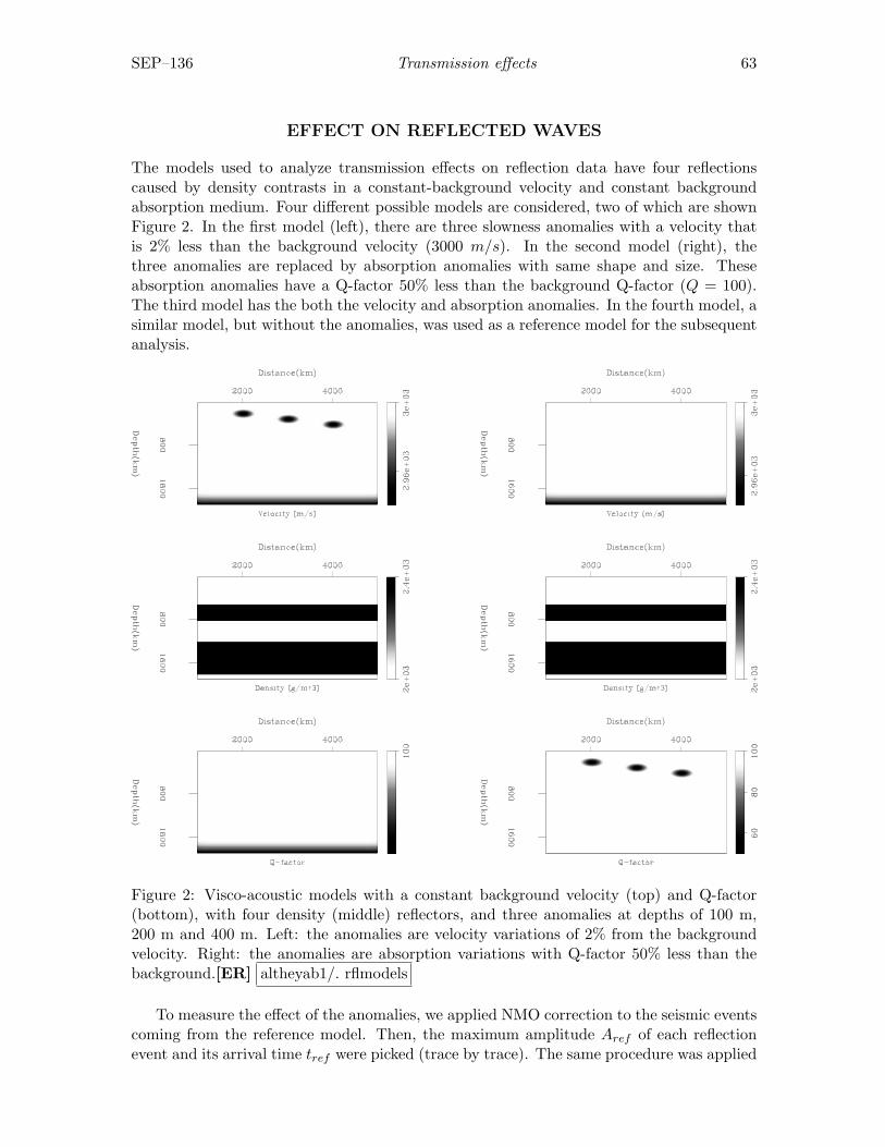
SEP–136 Transmission effects 63
EFFECT ON REFLECTED WAVES
The models used to analyze transmission effects on reflection data have four reflectionscaused by density contrasts in a constant-background velocity and constant backgroundabsorption medium. Four different possible models are considered, two of which are shownFigure 2. In the first model (left), there are three slowness anomalies with a velocity thatis 2% less than the background velocity (3000 m/s). In the second model (right), thethree anomalies are replaced by absorption anomalies with same shape and size. Theseabsorption anomalies have a Q-factor 50% less than the background Q-factor (Q = 100).The third model has the both the velocity and absorption anomalies. In the fourth model, asimilar model, but without the anomalies, was used as a reference model for the subsequentanalysis.
Figure 2: Visco-acoustic models with a constant background velocity (top) and Q-factor(bottom), with four density (middle) reflectors, and three anomalies at depths of 100 m,200 m and 400 m. Left: the anomalies are velocity variations of 2% from the backgroundvelocity. Right: the anomalies are absorption variations with Q-factor 50% less than thebackground.[ER] altheyab1/. rflmodels
To measure the effect of the anomalies, we applied NMO correction to the seismic eventscoming from the reference model. Then, the maximum amplitude Aref of each reflectionevent and its arrival time tref were picked (trace by trace). The same procedure was applied
64 Al Theyab and Biondi SEP–136
to the resulting data from the models with anomalies to obtain Amax and tmax. Time delaysare then computed by taking the difference of the arrival times,
δt = tmax − tref . (2)
Figure 3 shows the travel-time delays δt of the maximum amplitude (caused by the presenceof the anomalies) sorted into the midpoint-offset domain. The maximum amplitude differ-ences normalized with the amplitude of reference reflections (i.e. reflections if the modelhad no anomalies) were computed using
δA =Amax −Aref
Aref, (3)
and are shown in Figure 4.
Each row of the Figures 3 and 4 corresponds to one of the four reflectors; the top rowsare for the shallowest reflector and the bottom ones are for the deepest. The left columnsof the two figures are for the data resulting from the left model in Figure 2, and the rightcolumns are for the right model in Figure 2.
Each anomaly in the model causes an X-shaped signature centered at the midpointlocation of the anomaly. The arms of the shape generally spread further apart and eachbecomes broader with increasing offsets. The trajectory angle (i.e. the angle between thearms of the X-shape) is generally narrower for the deepest anomaly, especially for the firstreflector, with which the anomaly coincides. This distinction, however, is gradually lostwith increasing depth of reflectors, as shown in the fourth reflector, where the trajectoryangles are almost the same for all three anomalies.
As expected, the slow anomalies cause time delays (positive shifts) as shown in the leftside of Figure 3. The magnitudes of the time shifts are smaller for deeper reflectors, andspan a larger range of offsets, which results in fatter patterns. Absorption anomalies causealmost no time shifts. The width of the signature is less dependent on increasing offset.Instead, it depends on the depth of the anomaly.
Amplitude distortions in Figure 4 show trajectories similar to time shifts in the midpoint-offset domain. The magnitude of the distortion generally decreases with depth, and becomesless focused with increasing offsets. The arms of signatures narrow with depth. Because oftilting of the upcoming waves, the energy is confined closer to the source and stretches withincreasing offset. This causes the asymmetry of the signatures about the axes of the arms.Velocity anomalies cause focusing. Therefore, we have higher amplitudes paired with twoshadow zones (drops in amplitude), as shown in the left side of Figure 4. The absorptionsignature, on the other hand, shows only a drop in amplitude. The width of the absorptionsignature is generally smaller than that of velocity because of the absence of focusing.
From Figures 3 and 4, we can observe that the time delay of the velocity signature isstrictly positive, and the amplitude signature has a doublet of positive and negative ampli-tude changes. The absorption amplitude signature is strictly negative, with no time shifts.It should be noticed, however, that that the magnitude of the absorption amplitude distor-tions matches those of the velocity distortions. This is shown in the two cases presented.Figure 6 shows amplitude changes to the zero-offset reflection that passes twice throughan anomaly (left). The changes in amplitude are shown as functions of percentile changeof velocity (middle) relative to the background velocity (v = 3000 m/s), and Q-factor
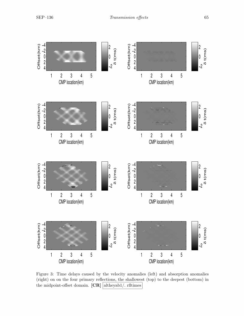
SEP–136 Transmission effects 65
CMP location(km)
Offset(
km
)
1 2 3 4 5
−4−2
024
δ t(m
s)
−202
CMP location(km)
Offset(
km
)
1 2 3 4 5
−4−2
024
δ t(m
s)
−202
CMP location(km)
Offset(
km
)
1 2 3 4 5
−4−2
024
δ t(m
s)
−202
CMP location(km)
Offset(
km
)
1 2 3 4 5
−4−2
024
δ t(m
s)
−202
CMP location(km)
Offset(
km
)
1 2 3 4 5
−4−2
024
δ t(m
s)
−202
CMP location(km)
Offset(
km
)
1 2 3 4 5
−4−2
024
δ t(m
s)
−202
CMP location(km)
Offset(
km
)
1 2 3 4 5
−4−2
024
δ t(m
s)
−202
CMP location(km)
Offset(
km
)
1 2 3 4 5
−4−2
024
δ t(m
s)
−202
Figure 3: Time delays caused by the velocity anomalies (left) and absorption anomalies(right) on on the four primary reflections, the shallowest (top) to the deepest (bottom) inthe midpoint-offset domain. [CR] altheyab1/. rfltimes
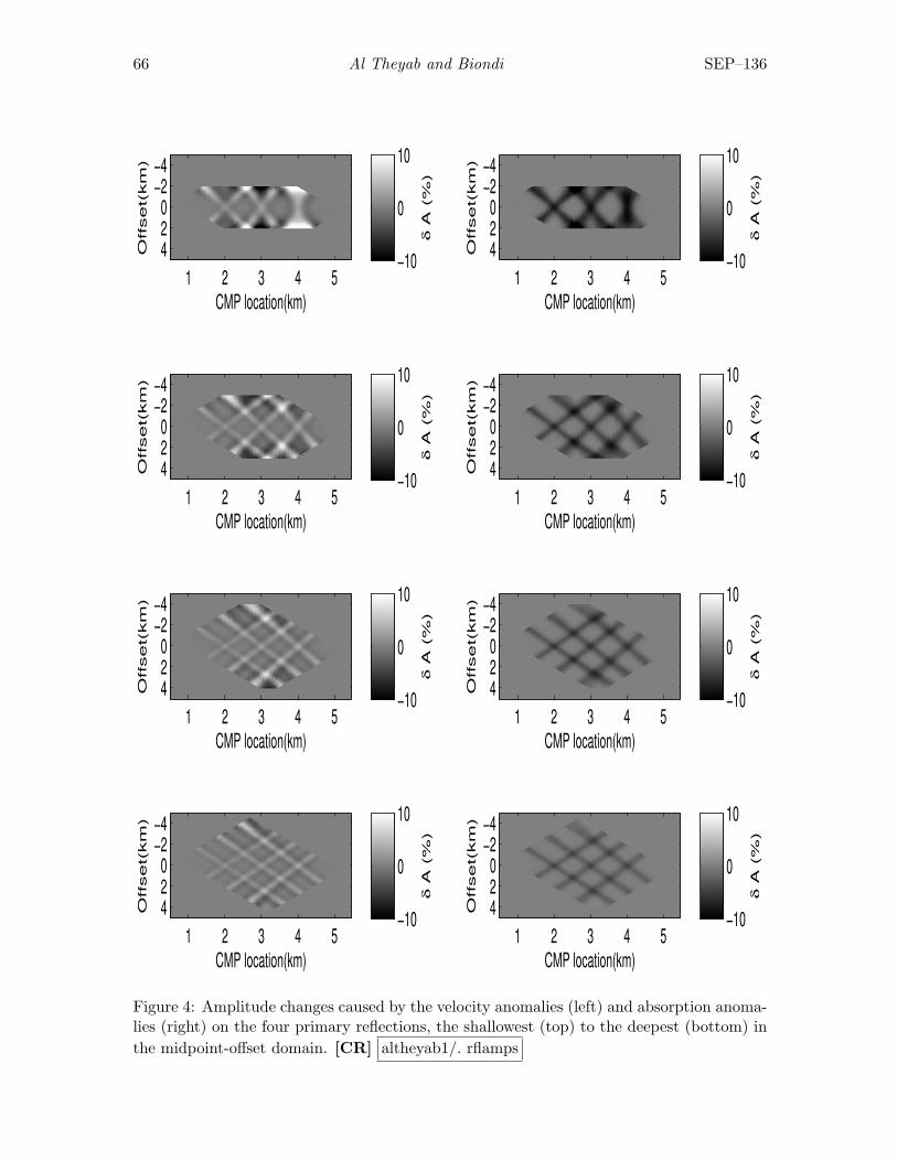
66 Al Theyab and Biondi SEP–136
CMP location(km)
Offset(
km
)
1 2 3 4 5
−4−2
024
δ A
(%
)
−10
0
10
CMP location(km)
Offset(
km
)
1 2 3 4 5
−4−2
024
δ A
(%
)
−10
0
10
CMP location(km)
Offset(
km
)
1 2 3 4 5
−4−2
024
δ A
(%
)
−10
0
10
CMP location(km)
Offset(
km
)
1 2 3 4 5
−4−2
024
δ A
(%
)
−10
0
10
CMP location(km)
Offset(
km
)
1 2 3 4 5
−4−2
024
δ A
(%
)
−10
0
10
CMP location(km)
Offset(
km
)
1 2 3 4 5
−4−2
024
δ A
(%
)
−10
0
10
CMP location(km)
Offset(
km
)
1 2 3 4 5
−4−2
024
δ A
(%
)
−10
0
10
CMP location(km)
Offset(
km
)
1 2 3 4 5
−4−2
024
δ A
(%
)
−10
0
10
Figure 4: Amplitude changes caused by the velocity anomalies (left) and absorption anoma-lies (right) on the four primary reflections, the shallowest (top) to the deepest (bottom) inthe midpoint-offset domain. [CR] altheyab1/. rflamps
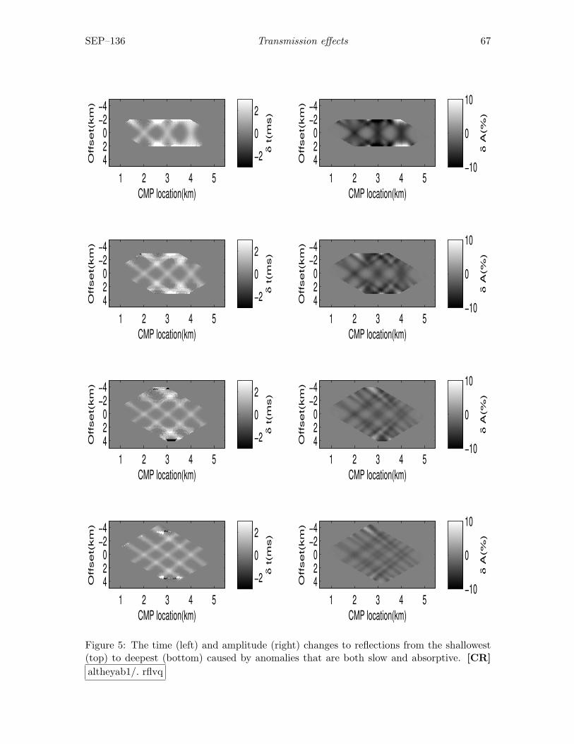
SEP–136 Transmission effects 67
CMP location(km)
Offset(
km
)
1 2 3 4 5
−4−2
024
δ t(m
s)
−202
CMP location(km)
Offset(
km
)
1 2 3 4 5
−4−2
024
δ t(m
s)
−202
CMP location(km)
Offset(
km
)
1 2 3 4 5
−4−2
024
δ t(m
s)
−202
CMP location(km)
Offset(
km
)
1 2 3 4 5
−4−2
024
δ t(m
s)
−202
CMP location(km)
Offset(
km
)
1 2 3 4 5
−4−2
024
δ A
(%)
−10
0
10
CMP location(km)
Offset(
km
)
1 2 3 4 5
−4−2
024
δ A
(%)
−10
0
10
CMP location(km)
Offset(
km
)
1 2 3 4 5
−4−2
024
δ A
(%)
−10
0
10
CMP location(km)
Offset(
km
)
1 2 3 4 5
−4−2
024
δ A
(%)
−10
0
10
Figure 5: The time (left) and amplitude (right) changes to reflections from the shallowest(top) to deepest (bottom) caused by anomalies that are both slow and absorptive. [CR]altheyab1/. rflvq
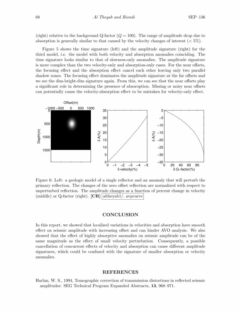
68 Al Theyab and Biondi SEP–136
(right) relative to the background Q-factor (Q = 100). The range of amplitude drop due toabsorption is generally similar to that caused by the velocity changes of interest (< 5%).
Figure 5 shows the time signature (left) and the amplitude signature (right) for thethird model, i.e. the model with both velocity and absorption anomalies coinciding. Thetime signature looks similar to that of slowness-only anomalies. The amplitude signatureis more complex than the two velocity-only and absorption-only cases. For the near offsets,the focusing effect and the absorption effect cancel each other leaving only two parallelshadow zones. The focusing effect dominates the amplitude signature at the far offsets andwe see the dim-bright-dim signature again. From this, we can see that the near offsets playa significant role in determining the presence of absoroption. Missing or noisy near offsetscan potentially cause the velocity-absorption effect to be mistaken for velocity-only effect.
Offset(m)
Dept
h(m
)
−1000 −500 0 500 10000
500
1000
1500
0 −1 −2 −3 −4 −50
5
10
15
20
25
30
35
δ velocity(%)
δ A(
%)
0 20 40 60 80−35
−30
−25
−20
−15
−10
−5
0
δ Q−factor(%)
δ A(
%)
Figure 6: Left: a geologic model of a single reflector and an anomaly that will perturb theprimary reflection. The changes of the zero offset reflection are normalized with respect tounperturbed reflection. The amplitude changes as a function of percent change in velocity(middle) or Q-factor (right). [CR] altheyab1/. avpcurve
CONCLUSION
In this report, we showed that localized variations in velocities and absorption have smootheffect on seismic amplitude with increasing offset and can hinder AVO analysis. We alsoshowed that the effect of highly absorptive anomalies on seismic amplitude can be of thesame magnitude as the effect of small velocity perturbation. Consequently, a possiblecancellation of concurrent effects of velocity and absorption can cause different amplitudesignatures, which could be confused with the signature of smaller absorption or velocityanomalies.
REFERENCES
Harlan, W. S., 1994, Tomographic correction of transmission distortions in reflected seismicamplitudes: SEG Technical Program Expanded Abstracts, 13, 968–971.

SEP–136 Transmission effects 69
Hatchell, P. J., 2000, Fault whispers: Transmission distortions on prestack seismic reflectiondata: Geophysics, 65, 377–389.
Mavko, G., T. Mukerji, and J. Dvorkin, 2003, The rock physics handbook: CambridgeUniversity Press.
Vlad, I., 2005, Focusing-effect AVO/AVA: overview of results and assessment of problems:Technical report, SEP-120.

70 Al Theyab and Biondi SEP–136
Stanford Exploration Project, Report SEP136, April 14, 2009
Joint wave-equation inversion of time-lapse seismic data
Gboyega Ayeni and Biondo Biondi
ABSTRACT
We discuss two regularized least-squares inversion formulations for time-lapse seismicimaging. Differences in acquisition geometries of baseline and monitor datasets or thepresence of a complex overburden can degrade the quality of the time-lapse seismicsignature. In such a scenario, the time-lapse amplitude information are poor indicatorsof the true reservoir property changes. Although the migration operator accuratelyimages the seismic data, it does not remove these amplitude distortions. We posetime-lapse imaging as joint linear inverse problems that utilize concatenations of atarget-oriented approximation to the least squares imaging Hessian. In one of the twoformulations considered, outputs are inverted time-lapse images, while in the other,outputs are evolving images of the study area. Using a 2D-synthetic sub-salt model,we demonstrate that either joint-inversion formulation can attenuate overburden andgeometry artifacts in time-lapse images and that joint wave-equation inversion yieldsmore accurate results than migration or separate inversion.
INTRODUCTION
Hydrocarbon exploration and production has gradually shifted from simple to complex geo-logical environments. Relatively simple imaging and monitoring objectives (e.g. anticlinal-type traps) have been replaced by more complex ones (e.g., sub-salt reservoirs and strati-graphic traps). Since most of the current time-lapse seismic imaging technologies are inad-equate in many emerging frontiers, new imaging and monitoring methods are required. Inaddition, differences almost always exist between acquisition geometries of different seismicdatasets. Such geometry differences may be due to new (or more efficient) acquisition sys-tems and design, production facilities (absent at the time of the baseline survey) or nature(e.g., ocean currents).
Our goal is to attenuate artifacts from two major sources:
1. poor and uneven sub-surface illumination in reservoirs under complex overburden,and
2. disparities in acquisition geometries of the baseline and monitor surveys.
We achieve these objectives by simultaneously inverting migrated images from differentvintages with a target-oriented approximation (Valenciano, 2008) to the linear least-squareswave-equation Hessian. The Hessian operator in this problem can be regarded as a set ofnon-stationary deconvolution filters in a single survey, or a concatenation of sub-matricesbuilt from such filters in multiple surveys. We discuss two joint-inversion formulations ofthe seismic monitoring problem:
71
72 Ayeni and Biondi SEP-136
1. regularized joint-inversion for image differences (RJID):
• input: staggered sums of migrated images, and
• output: inverted baseline image and image differences between successive sur-veys;
2. regularized joint-inversion of multiple images (RJMI)
• input: migrated images for all surveys,
• output: inverted images for all input surveys.
Solving a single joint-inversion problem enables the incorporation of prior knowledge of thereservoir location, extent and geometry, temporal constraints or information from othersources (e.g., production history-matching).
As previously noted, inputs into the RJID formulation are staggered sums of migratedimages from multiple surveys and the outputs are inverted baseline and time-lapse imagesbetween successive surveys. Since the imaging and monitoring objectives are decoupled, dif-ferent regularization schemes can be defined for the baseline and time-lapse images. Inputsand outputs to RJMI are migrated images and corresponding inverted images respectively.RJMI differs from separate inversion, because a coupling operator introduces desirable tem-poral constraints during inversion.
In order to arrive at both formulations, we have assumed that the background baselinevelocity model is known and that it changes slowly between surveys. We also assume thatsuch small velocity changes have negligible impact on wave propagation through the earth,at least to the top of the reservoir. Where there are noticeable displacements betweenimages — as a result of significant velocity changes or geomechanical effects around thereservoir — an event alignment step (Hale, 2007) can be applied prior to inversion.
In this paper, we briefly summarize the seismic monitoring problem, and then we discussthe basic theory of linear least-squares inversion and its extension to the RJID and RJMIformulations for an arbitarary number of surveys. Finally, using six datasets from a 2D-synthetic sub-salt model, we show that both joint-inversion formulations yield noticeablyimproved results over migration or separate inversion.
BACKGROUND
There is a wide range of published work on the most important considerations for time-lapseseismic monitoring. For example, Batzle and Wang (1992) outline important rock and fluidrelationships; Lumley (1995), Rickett and Lumley (2001), Calvert (2005), and Johnston(2005) discuss important processing and practical applications; and Lefeuvre et al. (2003),Whitcombe et al. (2004), and Zou et al. (2006) showed successful case studies. Ayeniand Biondi (2008) discuss additional considerations and previous work related to seismicmonitoring of hydrocarbon reservoirs.
Nemeth et al. (1999), Kuhl and Sacchi (2001), Clapp (2005), and Valenciano (2008) haveshown that linear least-squares wave-equation migration of seismic data improves structuraland amplitude information. We demonstrate that an extension of least-squares migration to
SEP-136 Joint time-lapse inversion 73
the time-lapse imaging can improve time-lapse amplitude information, especially if all avail-able data are jointly inverted. Previous authors have discussed joint-inversion applications,including impedance inversion (Sarkar et al., 2003), ray-tomography (Ajo-Franklin et al.,2005) and wave-equation velocity analysis (Albertin et al., 2006). Lumley et al. (2003) showthat improvements can be made to time-lapse processing through simultaneous processing.Dynamic imaging strategies that utilize aspects of spatio-temporal regularization have alsobeen discussed in other scientific disciplines (Schmitt and Louis, 2002; Schmitt et al., 2002;Zhang et al., 2005; Kindermann and Leitao, 2007).
A joint wave-equation inversion formulation of the time-lapse imaging problem has theadvantage that the attenuation of image differences is based on the physics of wave propa-gation, making it less susceptible to removal of true time-lapse changes than conventionalmethods. The method proposed by Ajo-Franklin et al. (2005) for tomographic inversioncan be directly extended to wave-equation inversion, and it actually forms a first step inthe RJMI formulation. Such direct extension to wave-equation migration is too expensive,requiring at least one set of migration and modeling per survey per iteration. In mostpractical inversion problems, parameter selection requires that the inversion procedure becarried out more than once. By pre-computing the Hessian operators, we are able to testdifferent regularization schemes and parameters for the inversion at several orders of mag-nitude cheaper than directly solving the least-squares migration problem. In addition, weavoid the use of matching filters which can have unpredictable effects on time-lapse changeswithin the reservoir (Lumley et al., 2003).
THEORY
Linear inversion
Given a linear modeling operator L, the seismic data d can be computed as
Lm = d, (1)
where m is the reflectivity model. The modeling operator, L, in this study, representsthe seismic acquisition process. Two different surveys — say a baseline and monitor —acquired at different times (t = 0 and t = 1 respectively) over the same earth model canbe represented as follows:
L0m0 = d0,L1m1 = d1,
(2)
where m0 and m1 are respectively the reflectivity models at the times when the datasets d0
and d1 were acquired, and L0 and L1 are the modeling operators defining the acquisitionprocess for the two surveys (baseline and monitor).
The quadratic cost functions for equation 2 are given by
S(m0) = ‖L0m0 − d0‖2,S(m1) = ‖L1m1 − d1‖2,
(3)
and the least-squares solutions are
m0 = (L′0L0)−1L′0d0 = (L′0L0)−1m0 = H−10 m0,
m1 = (L′1L1)−1L′1d1 = (L′1L1)−1m1 = H−11 m1,
(4)
74 Ayeni and Biondi SEP-136
where m0 and m1 are the migrated baseline and monitor images, m0 and m1 are theinverted images, L′0 and L′1 are the migration operators (adjoints to the modeling operatorsL0 and L1 respectively), and H0 ≡ L′0L0 and H1 ≡ L′1L1, are the Hessian matrices.Here, and in other parts of this paper, the symbol ′ denotes transposed complex conjugate.These formulations are based on (but not limited to) one-way wave-equation extrapolationmethods.
The Hessian matrices are the second derivatives of the cost functions (equation 3) withrespect to all model points in the image. Because the Hessian matrices are generally notinvertible for almost any practical scenario, equation 4 is solved iteratively as follows:
H0m0 = m0,H1m1 = m1.
(5)
An inverted time-lapse image, ∆m, can be obtained as the difference between the twoimages, m1 and m0, obtained from equation 5:
∆m = m1 − m0. (6)
We will refer to the method of computing the time-lapse image using equation 6 as separateinversion throughout the rest of this paper.
Joint-inversion
Two joint-inversion formulations are discussed in the following sections.
Joint-inversion for image differences (JID)
First, we re-formulate the data modeling operations for the two surveys in equation 2 asfollows:
L0m0 = d0,L1(m0 + ∆m) = d1,
(7)
where m0 + ∆m = m1. In matrix form, these expressions can be combined to give[L0 0L1 L1
] [m0
∆m
]=[
d0
d1
]. (8)
In principle, using an iterative solver, a least-squares solution to equation 8 can beobtained by minimizing the cost function
S(m0,∆m) =∣∣∣∣∣∣∣∣[ L0 0
L1 L1
] [m0
∆m
]−[
d0
d1
]∣∣∣∣∣∣∣∣2 . (9)
The computational cost of this approach is proportional to the number of iterations timesat least twice the cost of one set of migrations — since each iteration requires at least onemodeling and one migration for the baseline and monitor datasets. Since several iterationswould typically be required to reach convergence, and the inversion process would usuallybe repeated several times to fine-tune inversion parameters, the overall cost of this scheme
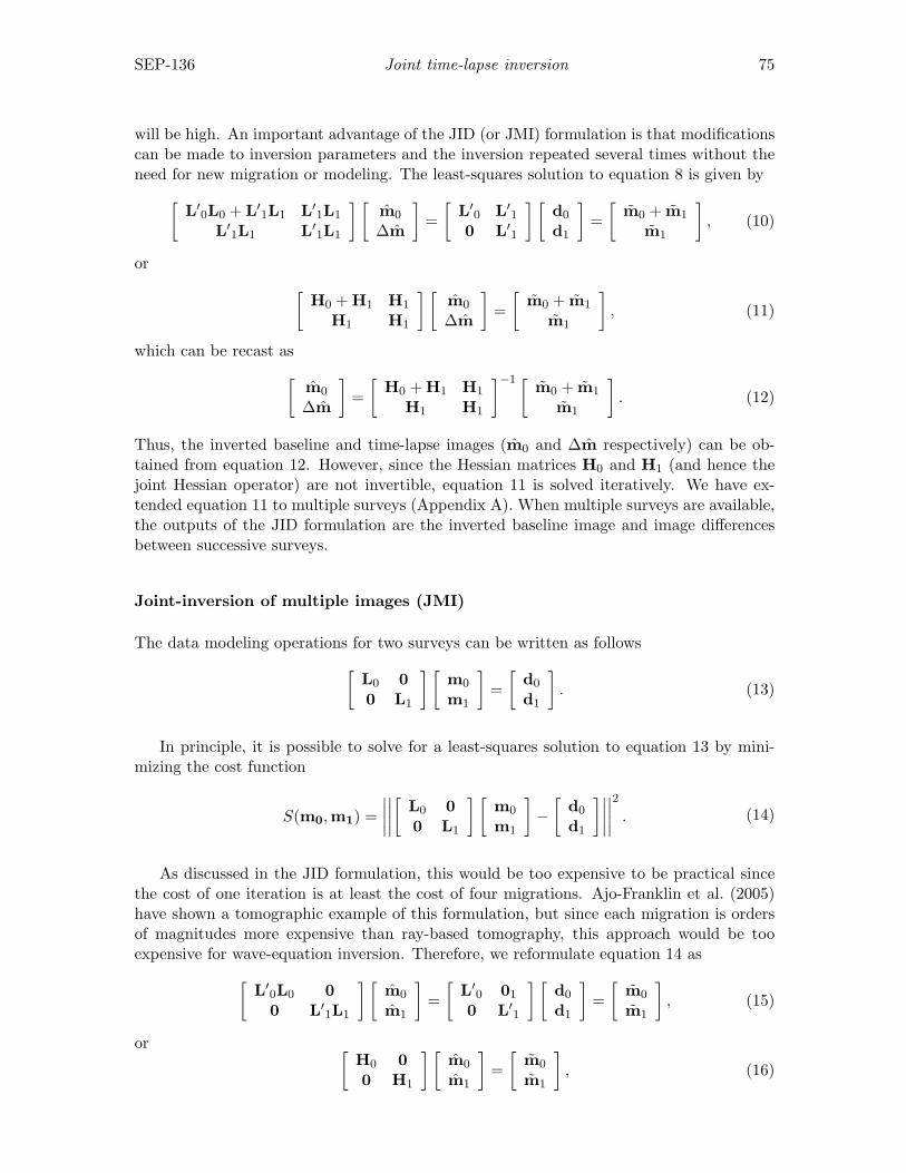
SEP-136 Joint time-lapse inversion 75
will be high. An important advantage of the JID (or JMI) formulation is that modificationscan be made to inversion parameters and the inversion repeated several times without theneed for new migration or modeling. The least-squares solution to equation 8 is given by[
L′0L0 + L′1L1 L′1L1
L′1L1 L′1L1
] [m0
∆m
]=[
L′0 L′10 L′1
] [d0
d1
]=[
m0 + m1
m1
], (10)
or [H0 + H1 H1
H1 H1
] [m0
∆m
]=[
m0 + m1
m1
], (11)
which can be recast as[m0
∆m
]=[
H0 + H1 H1
H1 H1
]−1 [ m0 + m1
m1
]. (12)
Thus, the inverted baseline and time-lapse images (m0 and ∆m respectively) can be ob-tained from equation 12. However, since the Hessian matrices H0 and H1 (and hence thejoint Hessian operator) are not invertible, equation 11 is solved iteratively. We have ex-tended equation 11 to multiple surveys (Appendix A). When multiple surveys are available,the outputs of the JID formulation are the inverted baseline image and image differencesbetween successive surveys.
Joint-inversion of multiple images (JMI)
The data modeling operations for two surveys can be written as follows[L0 00 L1
] [m0
m1
]=[
d0
d1
]. (13)
In principle, it is possible to solve for a least-squares solution to equation 13 by mini-mizing the cost function
S(m0,m1) =∣∣∣∣∣∣∣∣[ L0 0
0 L1
] [m0
m1
]−[
d0
d1
]∣∣∣∣∣∣∣∣2 . (14)
As discussed in the JID formulation, this would be too expensive to be practical sincethe cost of one iteration is at least the cost of four migrations. Ajo-Franklin et al. (2005)have shown a tomographic example of this formulation, but since each migration is ordersof magnitudes more expensive than ray-based tomography, this approach would be tooexpensive for wave-equation inversion. Therefore, we reformulate equation 14 as[
L′0L0 00 L′1L1
] [m0
m1
]=[
L′0 01
0 L′1
] [d0
d1
]=[
m0
m1
], (15)
or [H0 00 H1
] [m0
m1
]=[
m0
m1
], (16)
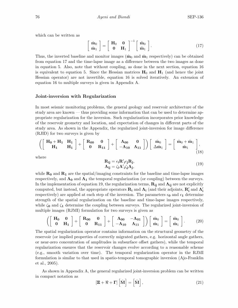
76 Ayeni and Biondi SEP-136
which can be written as [m0
m1
]=[
H0 00 H1
]−1 [ m0
m1
]. (17)
Thus, the inverted baseline and monitor images (m0 and m1 respectively) can be obtainedfrom equation 17 and the time-lapse image as a difference between the two images as donein equation 5. Also, note that without coupling, as done in the next section, equation 16is equivalent to equation 5. Since the Hessian matrices H0 and H1 (and hence the jointHessian operator) are not invertible, equation 16 is solved iteratively. An extension ofequation 16 to multiple surveys is given in Appendix A.
Joint-inversion with Regularization
In most seismic monitoring problems, the general geology and reservoir architecture of thestudy area are known — thus providing some information that can be used to determine ap-propriate regularization for the inversion. Such regularization incorporates prior knowledgeof the reservoir geometry and location, and expectation of changes in different parts of thestudy area. As shown in the Appendix, the regularized joint-inversion for image difference(RJID) for two surveys is given by([
H0 + H1 H1
H1 H1
]+[
R00 00 R11
]+[
Λ00 0−Λ10 Λ11
])[m0
∆m1
]=[
m0 + m1
m1
],
(18)where
Rij = εiR′iεjRj,
Λij = ζiΛ′iζjΛj,
(19)
while R0 and R1 are the spatial/imaging constraints for the baseline and time-lapse imagesrespectively, and Λ0 and Λ1 the temporal regularization (or coupling) between the surveys.In the implementation of equation 19, the regularization terms, Rij and Λij are not explicitlycomputed, but instead, the appropriate operators Ri and Λi (and their adjoints, R′
i and Λ′i
respectively) are applied at each step of the inversion. The parameters ε0 and ε1 determinestrength of the spatial regularization on the baseline and time-lapse images respectively,while ζ0 and ζ1 determine the coupling between surveys. The regularized joint-inversion ofmultiple images (RJMI) formulation for two surveys is given as([
H0 00 H1
]+[
R00 00 R11
]+[
Λ00 −Λ01
−Λ10 Λ11
])[m0
m1
]=[
m0
m1
]. (20)
The spatial regularization operator contains information on the structural geometry of thereservoir (or implied properties of correctly migrated gathers, e.g. horizontal angle gathers,or near-zero concentration of amplitudes in subsurface offset gathers), while the temporalregularization ensures that the reservoir changes evolve according to a reasonable scheme(e.g., smooth variation over time). The temporal regularization operator in the RJMIformulation is similar to that used in spatio-temporal tomographic inversion (Ajo-Franklinet al., 2005).
As shown in Appendix A, the general regularized joint-inversion problem can be writtenin compact notation as
[Ξ + <+ Γ][M]
=[M], (21)
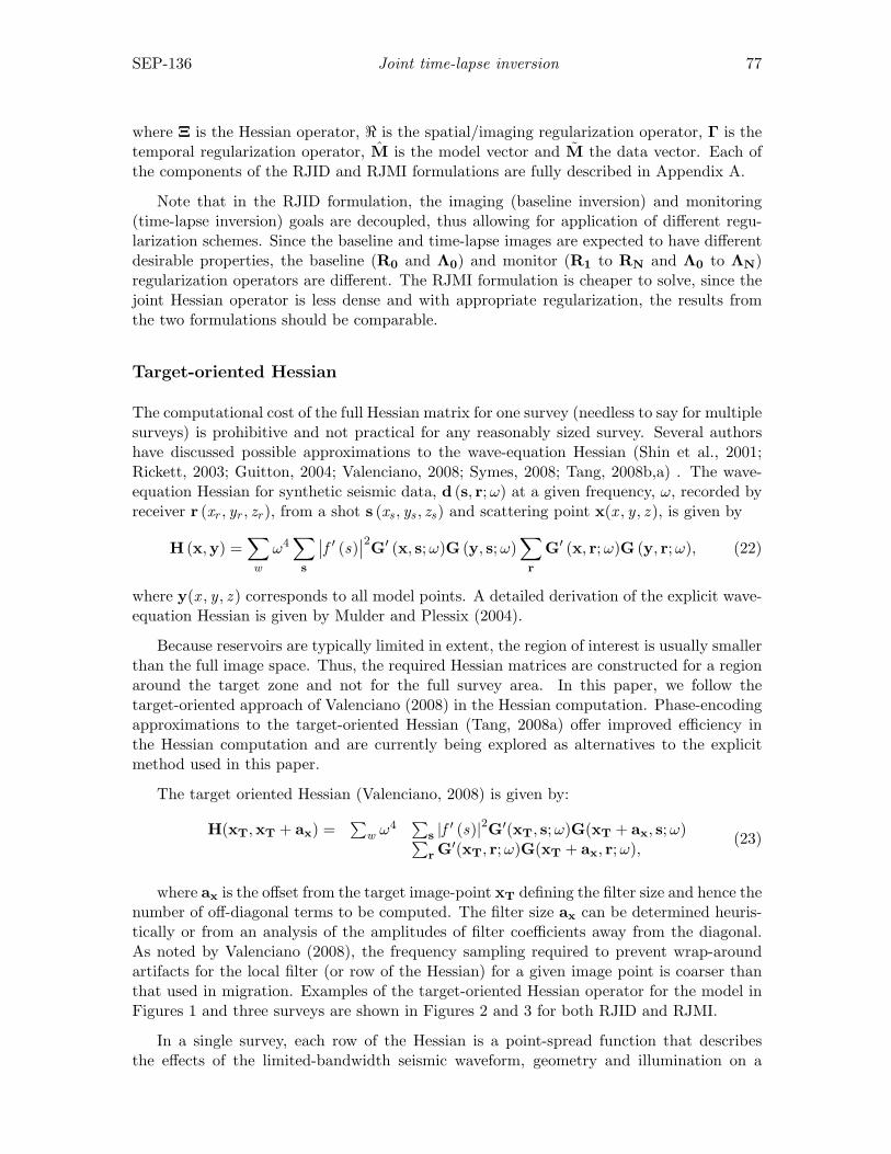
SEP-136 Joint time-lapse inversion 77
where Ξ is the Hessian operator, < is the spatial/imaging regularization operator, Γ is thetemporal regularization operator, M is the model vector and M the data vector. Each ofthe components of the RJID and RJMI formulations are fully described in Appendix A.
Note that in the RJID formulation, the imaging (baseline inversion) and monitoring(time-lapse inversion) goals are decoupled, thus allowing for application of different regu-larization schemes. Since the baseline and time-lapse images are expected to have differentdesirable properties, the baseline (R0 and Λ0) and monitor (R1 to RN and Λ0 to ΛN)regularization operators are different. The RJMI formulation is cheaper to solve, since thejoint Hessian operator is less dense and with appropriate regularization, the results fromthe two formulations should be comparable.
Target-oriented Hessian
The computational cost of the full Hessian matrix for one survey (needless to say for multiplesurveys) is prohibitive and not practical for any reasonably sized survey. Several authorshave discussed possible approximations to the wave-equation Hessian (Shin et al., 2001;Rickett, 2003; Guitton, 2004; Valenciano, 2008; Symes, 2008; Tang, 2008b,a) . The wave-equation Hessian for synthetic seismic data, d (s, r;ω) at a given frequency, ω, recorded byreceiver r (xr , yr , zr ), from a shot s (xs , ys , zs) and scattering point x(x , y , z ), is given by
H (x,y) =∑w
ω4∑s
∣∣f ′ (s)∣∣2G′ (x, s;ω)G (y, s;ω)∑r
G′ (x, r;ω)G (y, r;ω), (22)
where y(x , y , z ) corresponds to all model points. A detailed derivation of the explicit wave-equation Hessian is given by Mulder and Plessix (2004).
Because reservoirs are typically limited in extent, the region of interest is usually smallerthan the full image space. Thus, the required Hessian matrices are constructed for a regionaround the target zone and not for the full survey area. In this paper, we follow thetarget-oriented approach of Valenciano (2008) in the Hessian computation. Phase-encodingapproximations to the target-oriented Hessian (Tang, 2008a) offer improved efficiency inthe Hessian computation and are currently being explored as alternatives to the explicitmethod used in this paper.
The target oriented Hessian (Valenciano, 2008) is given by:
H(xT,xT + ax) =∑
w ω4∑
s |f ′ (s)|2G′(xT, s;ω)G(xT + ax, s;ω)∑
r G′(xT, r;ω)G(xT + ax, r;ω),(23)
where ax is the offset from the target image-point xT defining the filter size and hence thenumber of off-diagonal terms to be computed. The filter size ax can be determined heuris-tically or from an analysis of the amplitudes of filter coefficients away from the diagonal.As noted by Valenciano (2008), the frequency sampling required to prevent wrap-aroundartifacts for the local filter (or row of the Hessian) for a given image point is coarser thanthat used in migration. Examples of the target-oriented Hessian operator for the model inFigures 1 and three surveys are shown in Figures 2 and 3 for both RJID and RJMI.
In a single survey, each row of the Hessian is a point-spread function that describesthe effects of the limited-bandwidth seismic waveform, geometry and illumination on a
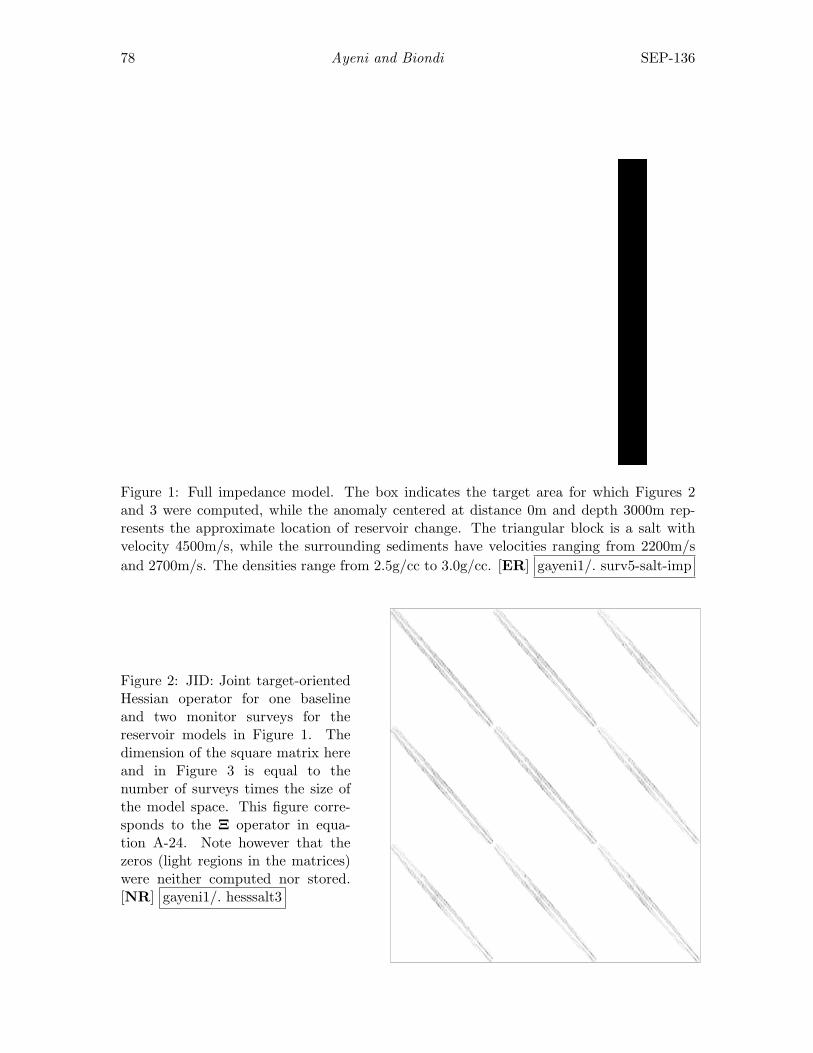
78 Ayeni and Biondi SEP-136
Figure 1: Full impedance model. The box indicates the target area for which Figures 2and 3 were computed, while the anomaly centered at distance 0m and depth 3000m rep-resents the approximate location of reservoir change. The triangular block is a salt withvelocity 4500m/s, while the surrounding sediments have velocities ranging from 2200m/sand 2700m/s. The densities range from 2.5g/cc to 3.0g/cc. [ER] gayeni1/. surv5-salt-imp
Figure 2: JID: Joint target-orientedHessian operator for one baselineand two monitor surveys for thereservoir models in Figure 1. Thedimension of the square matrix hereand in Figure 3 is equal to thenumber of surveys times the size ofthe model space. This figure corre-sponds to the Ξ operator in equa-tion A-24. Note however that thezeros (light regions in the matrices)were neither computed nor stored.[NR] gayeni1/. hesssalt3
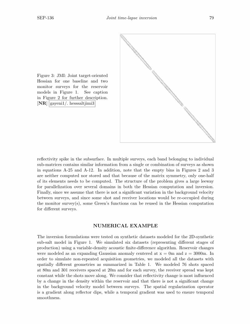
SEP-136 Joint time-lapse inversion 79
Figure 3: JMI: Joint target-orientedHessian for one baseline and twomonitor surveys for the reservoirmodels in Figure 1. See captionin Figure 2 for further description.[NR] gayeni1/. hesssaltjimi3
reflectivity spike in the subsurface. In multiple surveys, each band belonging to individualsub-matrices contains similar information from a single or combination of surveys as shownin equations A-25 and A-12. In addition, note that the empty bins in Figures 2 and 3are neither computed nor stored and that because of the matrix symmetry, only one-halfof its elements needs to be computed. The structure of the problem gives a large leewayfor parallelization over several domains in both the Hessian computation and inversion.Finally, since we assume that there is not a significant variation in the background velocitybetween surveys, and since some shot and receiver locations would be re-occupied duringthe monitor survey(s), some Green’s functions can be reused in the Hessian computationfor different surveys.
NUMERICAL EXAMPLE
The inversion formulations were tested on synthetic datasets modeled for the 2D-syntheticsub-salt model in Figure 1. We simulated six datasets (representing different stages ofproduction) using a variable-density acoustic finite-difference algorithm. Reservoir changeswere modeled as an expanding Gaussian anomaly centered at x = 0m and z = 3000m. Inorder to simulate non-repeated acquisition geometries, we modeled all the datasets withspatially different geometries as summarized in Table 1. We modeled 76 shots spacedat 80m and 301 receivers spaced at 20m and for each survey, the receiver spread was keptconstant while the shots move along. We consider that reflectivity change is most influencedby a change in the density within the reservoir and that there is not a significant changein the background velocity model between surveys. The spatial regularization operatoris a gradient along reflector dips, while a temporal gradient was used to ensure temporalsmoothness.
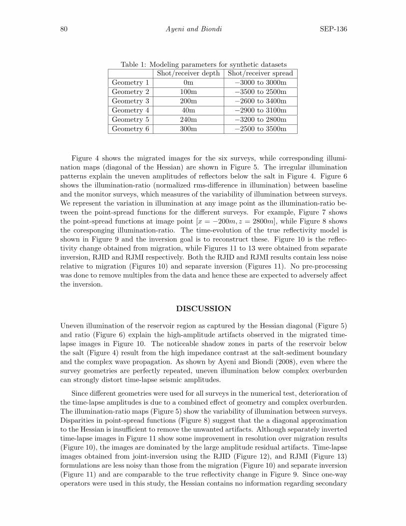
80 Ayeni and Biondi SEP-136
Table 1: Modeling parameters for synthetic datasetsShot/receiver depth Shot/receiver spread
Geometry 1 0m −3000 to 3000mGeometry 2 100m −3500 to 2500mGeometry 3 200m −2600 to 3400mGeometry 4 40m −2900 to 3100mGeometry 5 240m −3200 to 2800mGeometry 6 300m −2500 to 3500m
Figure 4 shows the migrated images for the six surveys, while corresponding illumi-nation maps (diagonal of the Hessian) are shown in Figure 5. The irregular illuminationpatterns explain the uneven amplitudes of reflectors below the salt in Figure 4. Figure 6shows the illumination-ratio (normalized rms-difference in illumination) between baselineand the monitor surveys, which measures of the variability of illumination between surveys.We represent the variation in illumination at any image point as the illumination-ratio be-tween the point-spread functions for the different surveys. For example, Figure 7 showsthe point-spread functions at image point [x = −200m, z = 2800m], while Figure 8 showsthe coresponging illumination-ratio. The time-evolution of the true reflectivity model isshown in Figure 9 and the inversion goal is to reconstruct these. Figure 10 is the reflec-tivity change obtained from migration, while Figures 11 to 13 were obtained from separateinversion, RJID and RJMI respectively. Both the RJID and RJMI results contain less noiserelative to migration (Figures 10) and separate inversion (Figures 11). No pre-processingwas done to remove multiples from the data and hence these are expected to adversely affectthe inversion.
DISCUSSION
Uneven illumination of the reservoir region as captured by the Hessian diagonal (Figure 5)and ratio (Figure 6) explain the high-amplitude artifacts observed in the migrated time-lapse images in Figure 10. The noticeable shadow zones in parts of the reservoir belowthe salt (Figure 4) result from the high impedance contrast at the salt-sediment boundaryand the complex wave propagation. As shown by Ayeni and Biondi (2008), even where thesurvey geometries are perfectly repeated, uneven illumination below complex overburdencan strongly distort time-lapse seismic amplitudes.
Since different geometries were used for all surveys in the numerical test, deterioration ofthe time-lapse amplitudes is due to a combined effect of geometry and complex overburden.The illumination-ratio maps (Figure 5) show the variability of illumination between surveys.Disparities in point-spread functions (Figure 8) suggest that the a diagonal approximationto the Hessian is insufficient to remove the unwanted artifacts. Although separately invertedtime-lapse images in Figure 11 show some improvement in resolution over migration results(Figure 10), the images are dominated by the large amplitude residual artifacts. Time-lapseimages obtained from joint-inversion using the RJID (Figure 12), and RJMI (Figure 13)formulations are less noisy than those from the migration (Figure 10) and separate inversion(Figure 11) and are comparable to the true reflectivity change in Figure 9. Since one-wayoperators were used in this study, the Hessian contains no information regarding secondary

SEP-136 Joint time-lapse inversion 81
Figure 4: Migrated images obtained for six surveys (see modeling parameters in Table 1) forthe target area in shown Figure 1. Figure (a) is the baseline image, while Figures (b)-(f) areimages of the monitor images. Note the irregular amplitude patterns cause by the presenceof the overlying salt structure.[CR] gayeni1/. migs
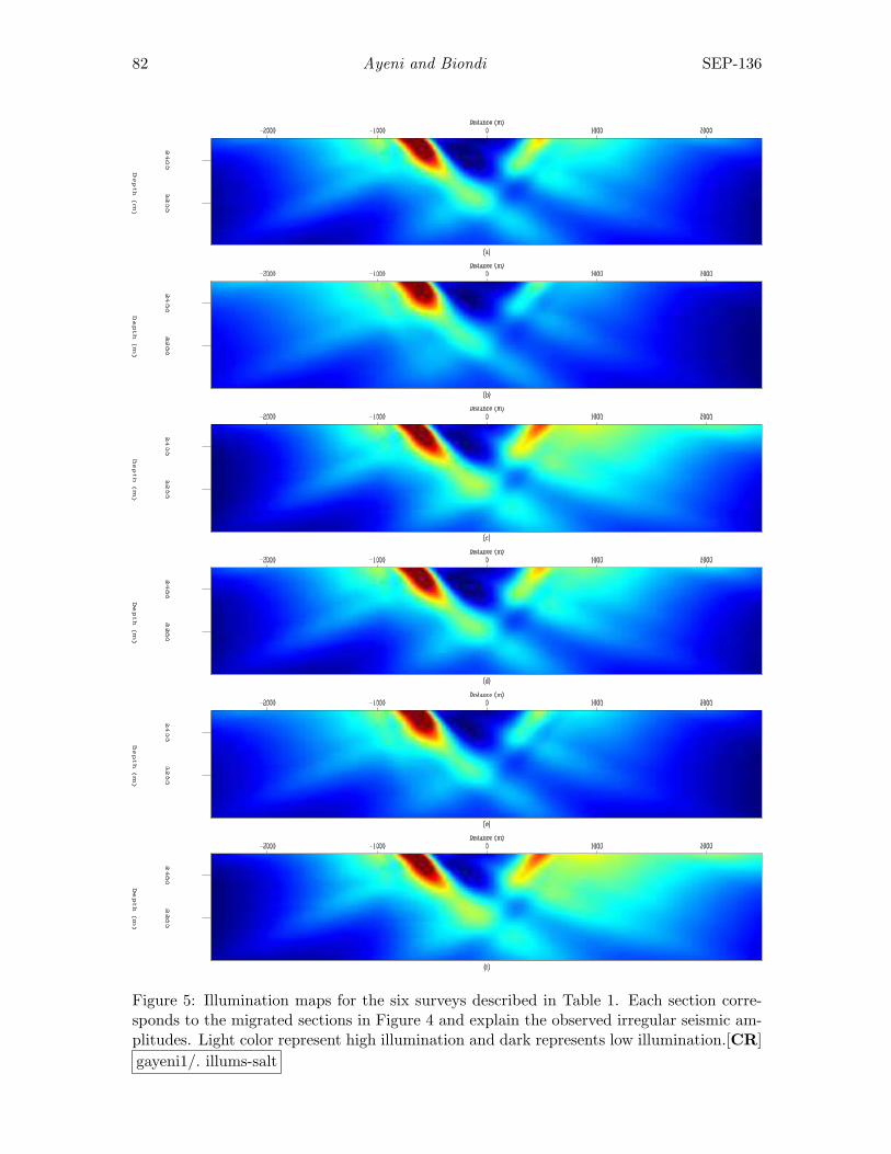
82 Ayeni and Biondi SEP-136
Figure 5: Illumination maps for the six surveys described in Table 1. Each section corre-sponds to the migrated sections in Figure 4 and explain the observed irregular seismic am-plitudes. Light color represent high illumination and dark represents low illumination.[CR]gayeni1/. illums-salt
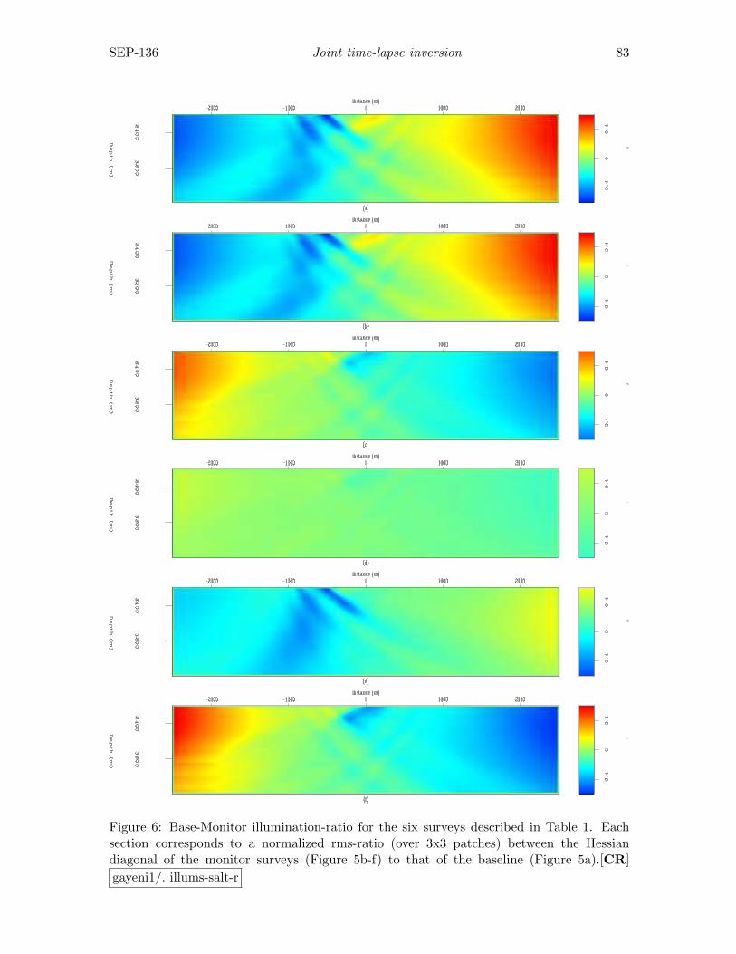
SEP-136 Joint time-lapse inversion 83
Figure 6: Base-Monitor illumination-ratio for the six surveys described in Table 1. Eachsection corresponds to a normalized rms-ratio (over 3x3 patches) between the Hessiandiagonal of the monitor surveys (Figure 5b-f) to that of the baseline (Figure 5a).[CR]gayeni1/. illums-salt-r
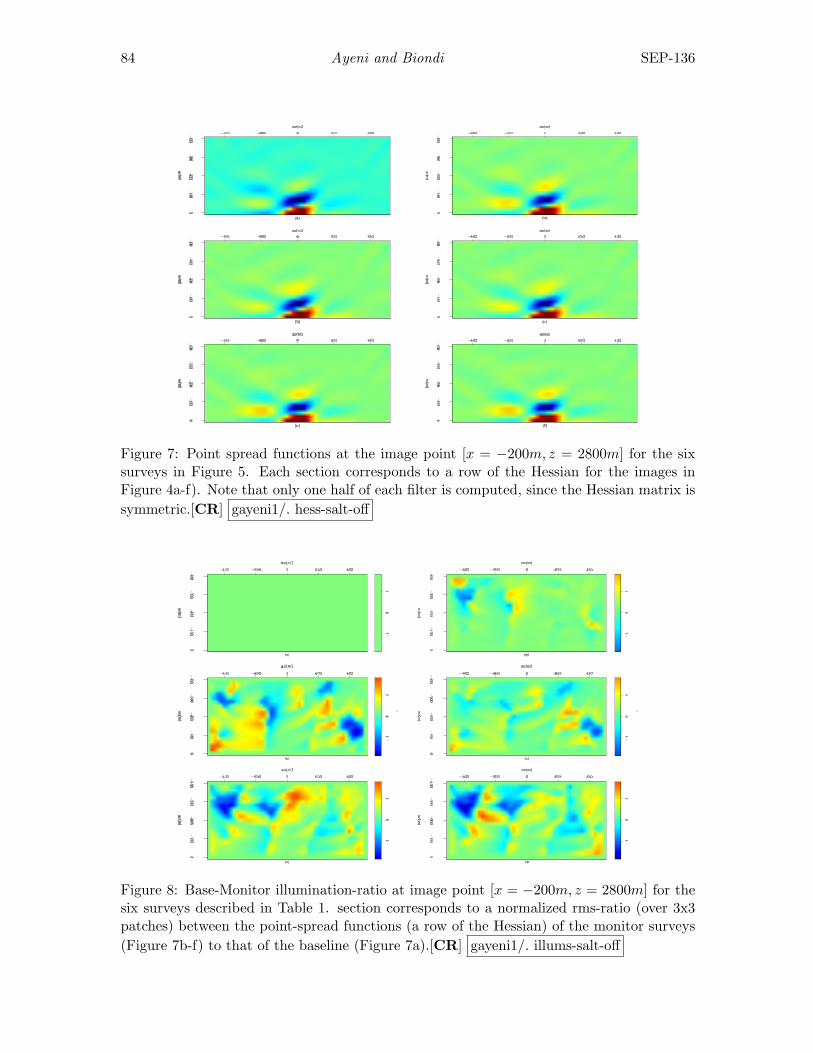
84 Ayeni and Biondi SEP-136
Figure 7: Point spread functions at the image point [x = −200m, z = 2800m] for the sixsurveys in Figure 5. Each section corresponds to a row of the Hessian for the images inFigure 4a-f). Note that only one half of each filter is computed, since the Hessian matrix issymmetric.[CR] gayeni1/. hess-salt-off
Figure 8: Base-Monitor illumination-ratio at image point [x = −200m, z = 2800m] for thesix surveys described in Table 1. section corresponds to a normalized rms-ratio (over 3x3patches) between the point-spread functions (a row of the Hessian) of the monitor surveys(Figure 7b-f) to that of the baseline (Figure 7a).[CR] gayeni1/. illums-salt-off
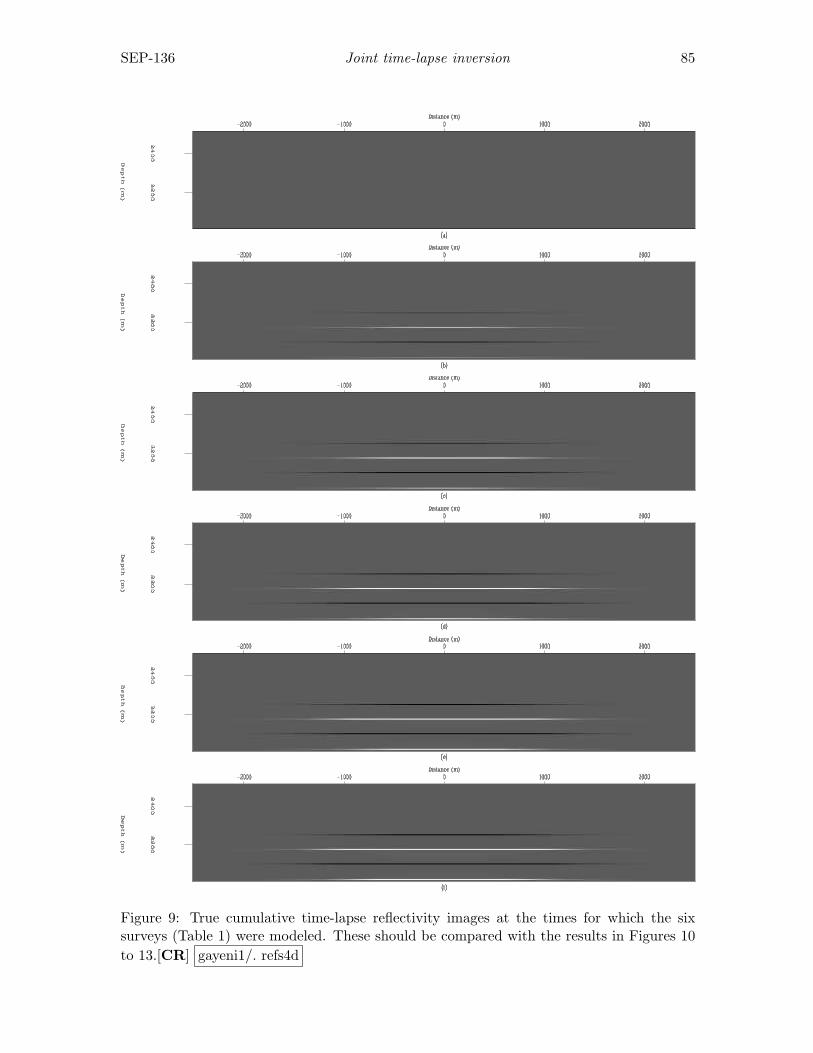
SEP-136 Joint time-lapse inversion 85
Figure 9: True cumulative time-lapse reflectivity images at the times for which the sixsurveys (Table 1) were modeled. These should be compared with the results in Figures 10to 13.[CR] gayeni1/. refs4d
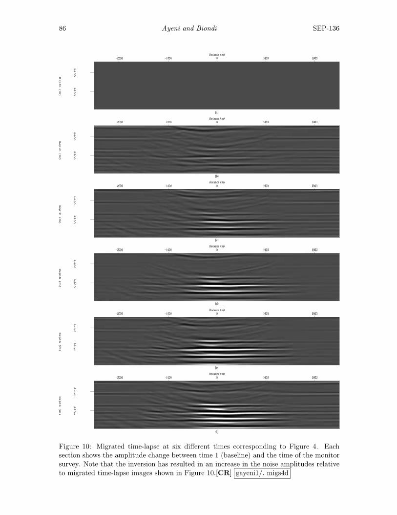
86 Ayeni and Biondi SEP-136
Figure 10: Migrated time-lapse at six different times corresponding to Figure 4. Eachsection shows the amplitude change between time 1 (baseline) and the time of the monitorsurvey. Note that the inversion has resulted in an increase in the noise amplitudes relativeto migrated time-lapse images shown in Figure 10.[CR] gayeni1/. migs4d
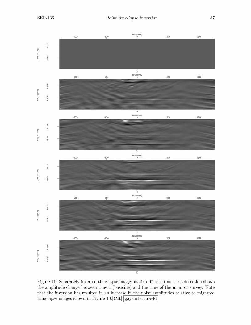
SEP-136 Joint time-lapse inversion 87
Figure 11: Separately inverted time-lapse images at six different times. Each section showsthe amplitude change between time 1 (baseline) and the time of the monitor survey. Notethat the inversion has resulted in an increase in the noise amplitudes relative to migratedtime-lapse images shown in Figure 10.[CR] gayeni1/. invs4d

88 Ayeni and Biondi SEP-136
Figure 12: RJID: Jointly inverted time-lapse images at six different times. Each sectionshows the amplitude change between time 1 (baseline) and the time of the monitor survey.Compare these results to Figures 9, 10, 11 and 13.[CR] gayeni1/. inv14d
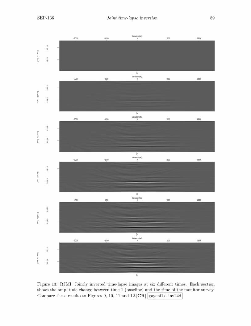
SEP-136 Joint time-lapse inversion 89
Figure 13: RJMI: Jointly inverted time-lapse images at six different times. Each sectionshows the amplitude change between time 1 (baseline) and the time of the monitor survey.Compare these results to Figures 9, 10, 11 and 12.[CR] gayeni1/. inv24d
90 Ayeni and Biondi SEP-136
events such as multiples. Residual effects of internal multiples due to the salt persist in theinversion results but are significantly suppressed in the jointly inverted images. In manycases of interest, multiple energy will be sufficiently attenuated or may not fall within thetarget region, and thus have little impact on the inversion.
CONCLUSIONS
We have proposed two regularized least-squares inversion formulations for time-lapse seismicimaging. -hese formulations arise from the linearized least-square wave-equation inversion.By using a target-oriented approximation to the least-squares Hessian with appropriatespatial and temporal regularization, we have shown that image difference due to geometrydissimilarity and complex overburden can be attenuated. We show that we can directlyinvert for image differences (RJID) or multiple images (RJMI) using a concatenation oftarget-oriented Hessian operators and combinations of migrated images. From numeri-cal tests using a synthetic 2D-subsalt model, we conclude that both the RJID and RJMIjoint-inversion formulations give more accurate time-lapse images than either migration orseparate inversion.
REFERENCES
Ajo-Franklin, J. B., J. Urban, and J. M. Harris, 2005, Temporal integration of seismictraveltime tomography: SEG Technical Program Expanded Abstracts, 24, 2468–2471.
Albertin, U., P. Sava, J. Etgen, and M. Maharramov, 2006, Adjoint wave-equation velocityanalysis: SEG Technical Program Expanded Abstracts, 25, 3345–3349.
Ayeni, G. and B. Biondi, 2008, Time-lapse inversion: SEP 134.Batzle, M. and Z. Wang, 1992, Seismic properties of pore fluids: Geophysics, 57, 1396–1408.Calvert, R., 2005, Insights and methods for 4D reservoir monitoring and characterization:
SEG/EAGE DISC (Distinguished Instructor Lecture Course).Clapp, M. L., 2005, Imaging under salt: illumination compensation by regularized inversion:
PhD thesis, Stanford University.Guitton, A., 2004, Amplitude and kinematic corrections of migrated images for nonunitary
imaging operators: Geophysics, 69, 1017–1024.Hale, D., 2007, A method for estimating apparent displacement vectors from time-lapse
seismic images: CWP Report-566.Johnston, D., 2005, Time-lapse 4D technology: Reservoir surveillance: AAPG Search and
Discovery.Kindermann, S. and A. Leitao, 2007, Regularization by dynamic programming: Journal of
Inverse and Ill-posed Problems, 15, 295–310.Kuhl, H. and M. Sacchi, 2001, Generalized least-squares dsr migration using a common angle
imaging condtion: 71st Annual International Meeting, Expanded Abstracts, 1025–1028,SEG.
Lefeuvre, F., Y. Kerdraon, J. Peliganga, S. Medina, P. Charrier, R. L’Houtellier, and D.Dubucq, 2003, Improved reservoir understanding through rapid and effective 4D: Girassolfield, Angola, West Africa: SEG Technical Program Expanded Abstracts, 22, 1334–1337.
Lumley, D., D. C. Adams, M. Meadows, S. Cole, and R. Wright, 2003, 4d seismic dataprocessing issues and examples: SEG Technical Program Expanded Abstracts, 22, 1394–1397.
SEP-136 Joint time-lapse inversion 91
Lumley, D. E., 1995, Seismic time-lapse monitoring of subsurface fluid flow: PhD thesis,Stanford University, http://sepwww.stanford.edu/public/docs/sep91/.
Mulder, W. and R.-E. Plessix, 2004, Frequency-domain finite-frequency amplitude-preserving migration: Geophysical Journal International, 157, 975–985.
Nemeth, T., C. Wu, and G. T. Schuster, 1999, Least-squares migration of incomplete re-flection data: Geophysics, 64, 208–221.
Rickett, J., 2003, Illumination-based normalization for wave-equation depth migration:Geophysics, 68, 1371–1379.
Rickett, J. and D. E. Lumley, 2001, Cross-equalization data processing for time-lapse seismicreservoir monitoring: A case study from the Gulf of Mexico: Geophysics, 66, 1015–1025.
Sarkar, S., W. P. Gouveia, and D. H. Johnston, 2003, On the inversion of time-lapse seismicdata: SEG Technical Program Expanded Abstracts, 22, 1489–1492.
Schmitt, U. and A. K. Louis, 2002, Efficient algorithms for the regularization of dynamicinverse problems: I. theory: Inverse Problems, 18, 645–658.
Schmitt, U., A. K. Louis, C. Wolters, and M. Vauhkonen, 2002, Efficient algorithms forthe regularization of dynamic inverse problems: Ii. applications: Inverse Problems, 18,659–676.
Shin, C., S. Jang, and D.-J. Min, 2001, Improved amplitude preservation for prestack depthmigration by inverse scattering theory: Geophysical Prospecting, 49, 592–606.
Symes, W. W., 2008, Approximate linearized inversion by optimal scaling of prestack depthmigration: Geophysics, 73, R23–R35.
Tang, Y., 2008a, Modeling, migration and inversion in the generalized source and receiverdomain: SEP 136.
——–, 2008b, Wave-equation hessian by phase encoding: SEP 134.Valenciano, A., 2008, Imaging by Wave-Equation Inversion: PhD thesis, Stanford Univer-
sity.Whitcombe, D. N., J. M. Marsh, P. J. Clifford, M. Dyce, C. J. S. McKenzie, S. Campbell,
A. J. Hill, R. S. Parr, C. Pearse, T. A. Ricketts, C. P. Slater, and O. L. Barkved, 2004,The systematic application of 4D in BP’s North-West Europe operations — 5 years on:SEG Technical Program Expanded Abstracts, 23, 2251–2254.
Zhang, Y., A. Ghodrati, and D. H. Brooks, 2005, An analytical comparison of three spatio-temporal regularization methods for dynamic linear inverse problems in a common sta-tistical framework: Inverse Problems, 21, 357–382.
Zou, Y., L. R. Bentley, L. R. Lines, and D. Coombe, 2006, Integration of seismic methodswith reservoir simulation, Pikes Peak heavy-oil field, Saskatchewan: The Leading Edge,25, 764–781.
APPENDIX A
JOINT-INVERSION FORMULATIONS FOR MULTIPLE SURVEYS
Here, we show a brief derivation of the joint-inversion formulation for two surveys and itsgeneralization to multiple surveys.
92 Ayeni and Biondi SEP-136
Regularized joint-inversion
The process of acquiring two seismic datasets over an evolving earth model can be repre-sented as [
L0 00 L1
] [m0
m1
]=[
d0
d1
], (A-1)
where d0 and d1 are the baseline and monitor datasets, and m0 and m1 are the baselineand monitor reflectivity models respectively. The linear operators (L0 and L1) define themodeling/acquisition experiments for datasets d0 and d1 respectively. We rewrite equa-tion A-1 to include spatial and regularization operators (R0 and Λ0 respectively), and weseek to minimize the objective function
S(m0,m1) =
∣∣∣∣∣∣∣∣∣∣
∣∣∣∣∣∣∣∣∣∣
L0 00 L1
R0 00 R1
−Λ0 Λ1
[
m0
m1
]−
d0
d1
000
∣∣∣∣∣∣∣∣∣∣
∣∣∣∣∣∣∣∣∣∣
2
. (A-2)
This cost function can be expanded as follows:([L′0L0 0
0 L′1L1
]+[
R′0R0 00 R′
1R1
]+[
Λ′0Λ0 −Λ′
0Λ1
−Λ′1Λ0 Λ′
1Λ1
])[m0
m1
]=[
m0
m1
],
(A-3)which can be written as([
H0 00 H1
]+[
R00 00 R11
]+[
Λ00 −Λ01
−Λ10 Λ11
])[m0
m1
]=[
m0
m1
], (A-4)
whereRij = εiR′
iεjRj,Λij = ζiΛ′
iζjΛj,(A-5)
while R0 and R1 are the spatial/imaging constraints for the baseline and monitor imagesrespectively, and Λ0 and Λ1 the temporal constraints between the surveys. The parametersε0 and ε1 determine the strength of the spatial regularization on the baseline and monitorimages respectively, while ζ0 and ζ1 determine the coupling between surveys. Equation A-4is the RJMI formulation. Using a similar procedure, the RJID formulation for two seismicdatasets can be shown to be([
H0 + H1 H1
H1 H1
]+[
R00 00 R11
]+[
Λ00 0−Λ10 Λ11
])[m0
∆m1
]=[
m0 + m1
m1
].
(A-6)In the next sections, we derive the RJID and RJMI formulations for multiple surveys.
Regularized joint-inversion of multiple images: RJMI
The data modeling process for three seismic datasets (a baseline and two monitors) over anevolving earth model can be written as L0 0 0
0 L1 00 0 L2
m0
m1
m2
=
d0
d1
d2
, (A-7)
SEP-136 Joint time-lapse inversion 93
where d0, d1 and d2 are respectively datasets for the baseline, first and second monitor,m0, m1, and m2 are the baseline and monitor reflectivity models. The linear operators(L0, L1 and L2) define the modeling/acquisition experiments for datasets d0, d1 and d2
respectively. The least-squares solution to equation A-7 is given as L′0L0 0 00 L′1L1 00 0 L′2L2
m0
m1
m2
=
L′0 0 00 L′1 00 0 L′2
d0
d1
d2
, (A-8)
where the symbol ′ denotes transposed complex conjugate.
We rewrite equation A-8 as H0 0 00 H1 00 0 H2
m0
m1
m2
=
m0
m1
m2
, (A-9)
where mi is the migrated image from the ith survey, and Hi is the corresponding Hessianmatrix. Introducing spatial and temporal constraints into equation A-9 we obtain H0 0 0
0 H1 00 0 H2
+
R00 0 00 R11 00 0 R22
+
Λ00 −Λ01 0−Λ10 2Λ11 −Λ12
0 −Λ21 Λ22
m0
m1
m2
=
m0
m1
m2
.
(A-10)Equation A-10 can be generalized to an arbitrary number of surveys as follows
[Ξ + <+ Γ][M]
=[M], (A-11)
where, Ξ is the Hessian operator, defined as
Ξ =
H0 0 0 ... 0 00 H1 0 ... 0 00 0 H2 ... ... 0: : : : : :: : : : HN−1 00 0 0 ... 0 HN
. (A-12)
The spatial and temporal regularization operators, < and Γ are defined as
< = R′R,Γ = Λ′Λ,
(A-13)
where,
R =
R0 0 0 ... 0 00 R1 0 ... 0 00 0 R2 ... 0 0: : : : : :: : : 0 RN−1 00 0 0 0 0 RN
, (A-14)
94 Ayeni and Biondi SEP-136
and,
Λ =
Λ0 Λ1 0 0 ... 00 −Λ1 Λ2 0 ... 00 0 −Λ2 −Λ3 ... 0: : : : : :0 0 ... 0 −ΛN−1 ΛN
0 0 ... 0 0 ΛN
. (A-15)
The input vector into the RJMI formulation, M is given as
M =
m0
m1
m2
:mN−1
mN
, (A-16)
while the inversion targets are in the vector:
M =
m0
m1
m2
:mN−1
mN
. (A-17)
Regularized joint-inversion for image differences: RJID
The data modeling process for three seismic datasets over an evolving earth model can bewritten as L0 0 0
L1 L1 0L2 L2 L2
m0
∆m1
∆m2
=
d0
d1
d2
, (A-18)
where d0, d1 and d2 are respectively datasets for the baseline, first and second monitor,m0 is the baseline reflectivity and the time-lapse reflectivities ∆m1 and ∆m2 are definedas
∆m1 = m1 −m0,∆m2 = m2 −m1,
(A-19)
where m1 and m2 are respectively the monitor reflectivities at the times data d1 and d2
were acquired (with survey geometries defined by the linear L1 and L2).
The least-squares solution to equation A-18 is given as L′0L0 + L′1L1 + L′2L2 L′1L1 + L′2L2 L′2L2
L′1L1 + L′2L2 L′1L1 + L′2L2 L′2L2
L′2L2 L′2L2 L′2L2
m0
∆m1
∆m2
=
L′0 L′1 L′2L′1 L′2
L′2
d0
d1
d2
,
(A-20)
SEP-136 Joint time-lapse inversion 95
where the symbol ′ denotes transpose complex conjugate. We rewrite equation A-20 as H0 + H1 + H2 H1 + H2 H2
H1 + H2 H1 + H2 H2
H2 H2 H2
m0
∆m1
∆m2
=
m0 + m1 + m2
m1 + m2
m2
, (A-21)
where mi is the migrated image from the ith survey, and Hi is the corresponding Hes-sian matrix. Introducing spatial and temporal regularization goals that incorporates priorknowledge of the reservoir geometry and location as well as constraints on the invertedtime-lapse images into equation A-21 we obtain H0 + H1 + H2 H1 + H2 H2
H1 + H2 H1 + H2 H2
H2 H2 H2
+
R00 0 00 R11 00 0 R22
+
Λ00 0 00 2Λ11 −Λ12
0 −Λ21 Λ22
m0
∆m1
∆m2
=
m0 + m1 + m2
m1 + m2
m2
,
(A-22)
where,Rij = εiR′
iεjRj
Λij = ζiΛ′iζjΛj
, (A-23)
with Ri being the spatial regularization terms for the baseline and time-lapse images re-spectively while Λi is the temporal regularization between the surveys. Note that Rij andΛij are not explicitly computed, but instead, the regularization operators Ri and Λi (andtheir adjoints) are applied at each step of the inversion. Parameters εi and ζi determine therelative strengths of the spatial and temporal regularization respectively. Equation A-22can be generalized to an arbitrary number of surveys as follows
[Ξ + <+ Γ][M]
=[M], (A-24)
where, Ξ is the Hessian operator, defined as
Ξ =
H0 + .. + HN H1 + .. + HN H2 + .. + HN ... HN−1 + HN HN
H1 + .. + HN H1 + .. + HN H2 + .. + HN ... HN−1 + HN HN
H2 + .. + HN H2 + .. + HN H2 + .. + HN ... ... HN
: : : : : :: : : : HN−1 + HN HN
HN HN HN ... NN HN
. (A-25)
The regularization operators < and Γ are defined as
< = R′R,Γ = Λ′Λ,
(A-26)
where,
R =
R0 0 0 ... 0 00 R1 0 ... 0 00 0 R2 ... 0 0: : : : : :: : : 0 RN−1 00 0 0 0 0 RN
, (A-27)
96 Ayeni and Biondi SEP-136
and,
Λ =
Λ0 0 0 0 ... 00 −Λ1 Λ2 0 ... 00 0 −Λ2 −Λ3 ... 0: : : : : :0 0 ... 0 −ΛN−1 ΛN
0 0 ... 0 0 ΛN
. (A-28)
The input vector into the RJID formulation, M is given as
M =
m0 + ... + mN
m1 + ... + mN
m2 + ... + mN
:mN−1 + mN
mN
, (A-29)
while the inversion targets are
M =
m0
∆m1
∆m2
::
∆mN
. (A-30)
The temporal constraint on the baseline image, Λ0 may be set to zero, since it is assumedthat the original geological structure is unchanged over time or that geomechanical changesare accounted for before/during inversion.
Stanford Exploration Project, Report SEP136, April 14, 2009
Modeling, migration, and inversion in the generalized sourceand receiver domain
Yaxun Tang
ABSTRACT
I extend the theory of Born modeling, migration and inversion to the generalized sourceand receiver domain, a transformed domain that is obtained by linear combination ofthe encoded sources and receivers. I show how to construct the target-oriented imagingHessian with encoded sources, with encoded receivers and with simultaneously encodedsources and receivers. I also demonstrate the connection of the imaging Hessian in thegeneralized source and receiver domain to the phase-encoded Hessian that I developedin SEP-134. As an application of the theory, I introduce a mixed phase-encodingscheme to compute the Hessian operator. The new scheme combines the advantages ofboth random phase encoding and plane-wave phase encoding. My preliminary tests ofthis new method on a simple model show promising results.
INTRODUCTION
Shot-profile migration is an accurate imaging technique. The computation is performed ineach shot gather; thus it closely mimics the actual physical experiment. However, migratingshot by shot is expensive, since the number of shot gathers is usually very big for a typicalseismic survey. To reduce the cost, Whitmore (1995), Zhang et al. (2005) and Duquet andLailly (2006) develop plane-wave source or delayed-shot migration, which migrates a smallnumber of synthesized shots made by linear combination of the original shot gathers afterlinear time delays. In fact, plane-wave source or delayed-shot migration is only a specialcase of a more general class of migration technique, phase-encoding migration (Romeroet al., 2000; Liu et al., 2006), where the source encoding functions can be any type ofphase functions, such as linear phase functions, random phase functions, etc.. Though themethods mentioned above involve encoding only the original sources, there is no reason thatthe receivers could not be encoded. For example, besides assuming tilted line sources (plane-wave source or delayed-shot migration), we can also assume the data are recorded by tiltedline receivers, or assume both line sources and line receivers at the same time. Such ideashave been explored by Stoffa et al. (2006), who develop the ray-based asymptotic theoryfor plane-wave source migration, plane-wave receiver migration and plane-wave source andreceiver migration. In this paper, I extend those ideas from the plane-wave domain to moregeneral cases and unify them under the generalized source and receiver domain.
Another important aspect of imaging is how to preserve the amplitude information of thereflectors. It is widely known that because of the non-unitary nature of the Born forwardmodeling operator, its adjoint, the migration operator, can only preserve the kinematicinformation of the reflectors (Lailly, 1983). To better preserve the amplitude, the inversionshould be used. Bleistein (2007) derives closed-form asymptotic inversion formulas based
97
98 Tang SEP-136
on the synthesized shot gathers (e.g. plane-wave sources) under the assumption that theacquisition geometry is infinite. However, we never have infinite acquisition geometry inpractice. In fact, the limited acquisition geometry is an important factor distorting theamplitude of the reflectors, especially in complex geologies; hence it should not be neglected.
In this paper, I also extend the target-oriented inversion theory (Valenciano, 2008) tothe generalized source and receiver domain for limited acquisition geometry. The effectof limited acquisition geometry is then taken into account in the least-squares sense andcorrected by the pseudo-inverse of the target-oriented Hessian, the second derivative of theleast-squares misfit functional with respect to the model parameters (Plessix and Mulder,2004; Valenciano, 2008; Tang, 2008). I demonstrate that in the generalized source andreceiver domain, the target-oriented Hessian can be more efficiently computed withoutstoring the Green’s functions, which is a major obstacle for the Hessian computation in theoriginal shot-profile domain. I also show that the Hessian obtained in the generalized sourceand receiver domain is essentially the same as the phase-encoded Hessian (Tang, 2008), thephysics of which, however, was not carefully discussed in Tang (2008). Therefore, fromthis perspective, this paper completes the discussion of the phase-encoded Hessian from thephysical point of view. The modeling, migration and target-oriented Hessian formulas areall derived in terms of Green’s functions, so that any type of Green’s functions can be usedunder this framework, such as ray-based asymptotic Green’s functions, Green’s functionsobtained by solving one-way wave equations, and Green’s functions obtained by solvingtwo-way wave equations. Anisotropy can also be taken into account, provided that theGreen’s functions are properly modeled.
This paper is organized as follows: I first briefly review the theory of Born modeling,migration and the target-oriented Hessian in the original shot-profile domain. Then I extendthe theory to the encoded source domain, the encoded receiver domain, and the encodedsource and receiver domain. Finally, I introduce a new phase-encoding scheme, whichmixes both random and plane-wave phase encoding, to compute the Hessian operator. Thenew scheme combines advantages of both random phase encoding and plane-wave phaseencoding. Finally, I apply the mixed phase-encoding scheme to a simple synthetic model.
BORN MODELING AND INVERSION IN THE SHOT-PROFILEDOMAIN
By using the Born approximation to the two-way wave equation, the primaries can bemodeled by a linear operator as follows:
d(xr,xs, ω) =∑x
G(x,xs, ω)G(x,xr, ω)m(x), (1)
where d(xr,xs, ω) is the modeled data for a single frequency ω with source and receiverlocated at xs = (xs, ys, 0) and xr = (xr, yr, 0) on the surface; G(x,xs, ω) and G(x,xr, ω)are the Green’s functions connecting the source and receiver, respectively, to the imagepoint x = (x, y, z) in the subsurface; and m(x) denotes the reflectivity at image point x. InEquation 1, we assume xs and xr are infinite in extent and independent of each other. For aparticular survey, however, we do not have infinitely long cable and infinitely many sources;thus we have to introduce an acquisition mask matrix to limit the size of the modeling. We
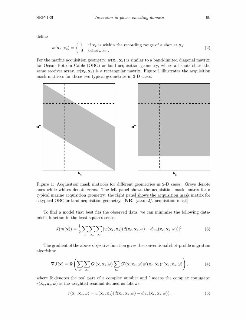
SEP-136 Inversion in phase-encoding domain 99
define
w(xr,xs) ={
1 if xr is within the recording range of a shot at xs;0 otherwise .
(2)
For the marine acquisition geometry, w(xr,xs) is similar to a band-limited diagonal matrix;for Ocean Bottom Cable (OBC) or land acquisition geometry, where all shots share thesame receiver array, w(xr,xs) is a rectangular matrix. Figure 1 illustrates the acquisitionmask matrices for these two typical geometries in 2-D cases.
Figure 1: Acquisition mask matrices for different geometries in 2-D cases. Greys denoteones while whites denote zeros. The left panel shows the acquisition mask matrix for atypical marine acquisition geometry; the right panel shows the acquisition mask matrix fora typical OBC or land acquisition geometry. [NR] yaxun2/. acquisition-mask
To find a model that best fits the observed data, we can minimize the following data-misfit function in the least-squares sense:
J(m(x)) =12
∑ω
∑xs
∑xr
|w(xr,xs)(d(xr,xs, ω)− dobs(xr,xs, ω))|2. (3)
The gradient of the above objective function gives the conventional shot-profile migrationalgorithm:
∇J(x) = <
(∑ω
∑xs
G′(x,xs, ω)∑xr
G′(x,xr, ω)w′(xr,xs)r(xr,xs, ω)
), (4)
where < denotes the real part of a complex number and ′ means the complex conjugate;r(xr,xs, ω) is the weighted residual defined as follows:
r(xr,xs, ω) = w(xr,xs)(d(xr,xs, ω)− dobs(xr,xs, ω)). (5)
100 Tang SEP-136
The gradient or migration is only a rough estimate of the model m(x); to get a bet-ter recovery of the model space, the inverse of the Hessian, the second derivatives of theobjective function, should be applied to the gradient:
m ≈ H−1∇J. (6)
The Hessian can be explicitly constructed by taking the second-order derivatives of theobjective function with respect to the model parameters as follows (Plessix and Mulder,2004; Valenciano, 2008; Tang, 2008):
H(x,y) = <
(∑ω
∑xs
G(x,xs, ω)G′(y,xs, ω) ×
∑xr
w2(xr,xs)G(x,xr, ω)G′(y,xr, ω)
), (7)
where y is a neighbor point around the image point x in the subsurface.
Valenciano (2008) demonstrates that the Hessian can be directly computed using theabove formula; however it requires storing a large number of Green’s functions, which isinconvenient for dealing with large 3-D data set. Tang (2008) shows that with some minoralteration of Equation 7, an approximate Hessian can be efficiently computed using thephase-encoding method. However, Tang (2008) focuses more on the algorithm development,and the physics behind the Hessian by phase-encoding has not been carefully discussed. Inthis companion paper, I complete the discussion of the actual physics behind using phase-encoding methods, such as plane-wave phase encoding and random phase encoding, toobtain the Hessian. In the subsequent sections, I start with the modeling equation in theencoded source, encoded receiver and simultaneously encoded source and receiver domains.I show that the corresponding imaging Hessian in the generalized source and receiver domainis the same as those phase-encoded Hessians discussed in Tang (2008).
ENCODED SOURCES
Let us define the encoding transform along the xs coordinate of the surface data as follows:
d(xr,ps, ω) =∑xs
w(xr,xs)d(xr,xs, ω)α(xs,ps, ω), (8)
where α(xs,ps, ω) is the source phase-encoding function. Equation 8 integrates along thehorizontal dashed lines shown in Figure 1 for each receiver location xr and transformsthe surface data from (xs,xr) domain into the (ps,xr) domain. For the plane-wave phaseencoding, the encoding function is:
α(xs,ps, ω) = eiωpsxs , (9)
where ps is defined to be the ray parameter of the source plane waves. For random phaseencoding, the encoding function is
α(xs,ps, ω) = eiγ(xs,ps,ω), (10)
SEP-136 Inversion in phase-encoding domain 101
where γ(xs,ps, ω) is a random sequence in xs and ω, and ps defines the index of differentrealizations of the random sequence.
Substituting Equation 1 into 8, rearranging the order of summation, we get the forwardmodeling equation in the encoded source domain:
d(xr,ps, ω) =∑x
G(x,xr, ω)G(x,ps, ω;xr)m(x), (11)
where the encoded source Green’s function G(x,ps, ω;xr) is defined as follows:
G(x,ps, ω;xr) =∑xs
w(xr,xs)G(x,xs, ω)α(xs,ps, ω). (12)
Note that G(x,ps, ω;xr) depends on xr because of the acquisition mask w(xr,xs) insidethe summation. It should only integrate the grey segment for each horizontal dashed lineshown in Figure 1.
As derived in Appendix A, the objective function in the encoded source domain can bewritten as follows:
J(m(x)) =12
∑ω
|c|2∑xr
∑ps
|d(xr,ps, ω)− dobs(xr,ps, ω)|2, (13)
where c = ω for plane-wave phase encoding, and c = 1 for random phase encoding.
The gradient of the objective function in Equation 13 gives the following migrationformula in the encoded source domain:
∇J(x) = <
(∑ω
|c|2∑ps
G′(x,ps, ω;xr)∑xr
G′(x,xr, ω)r(xr,ps, ω)
), (14)
where the residual r(xr,ps, ω) is defined as follows:
r(xr,ps, ω) = d(xr,ps, ω)− dobs(xr,ps, ω). (15)
It is easy to see that Equation 14 defines the phase-encoding migration (Liu et al., 2006;Romero et al., 2000). By taking the second-order derivatives of the objective functiondefined in Equation 13 with respect to the model paramters, we obtain the Hessian in theencoded source domain:
H(x,y) = <
(∑ω
|c|2∑xr
G(x,xr, ω)G′(y,xr, ω) ×
∑ps
G(x,ps, ω;xr)G′(y,ps, ω;xr)
). (16)
ENCODED RECEIVERS
Let us define the encoding transform along the xr coordinate of the surface data as follows:
d(pr,xs, ω) =∑xr
w(xr,xs)d(xr,xs, ω)β(xr,pr, ω), (17)
102 Tang SEP-136
where β(xr,pr, ω) is the receiver phase-encoding function. Equation 17 integrates alongthe vertical dashed lines shown in Figure 1 for each source location xs and transforms thesurface data from (xs,xr) domain into the (xs,pr) domain. The receiver phase-encodingfunction is defined similar to the source phase-encoding function discussed in the previoussection. For receiver plane-wave phase encoding,
β(xr,pr, ω) = eiωprxr , (18)
where pr is the ray parameter for the receiver plane-waves. For receiver random phaseencoding,
β(xr,pr, ω) = eiγ(xr,pr,ω), (19)
where γ(xr,pr, ω) is the prth random realization. Substituting Equation 1 into 17, we getthe forward modeling equation in the receiver plane-wave domain:
d(pr,xs, ω) =∑x
G(x,xs, ω)G(x,pr, ω;xs)m(x), (20)
where G(x,pr, ω;xs) is the encoded receiver Green’s function defined as follows:
G(x,pr, ω;xs) =∑xr
w(xr,xs)G(x,xr, ω)β(xr,pr, ω). (21)
Also note that G(x,pr, ω;xs) depends on xs because of the acquisition mask matrix insidethe summation. It should only integrate the grey segment for each vertical dashed lineshown in Figure 1.
We minimize the following objective function in the encoded receiver domain (see Ap-pendix B for derivation):
J(m(x)) =∑ω
|c|2∑pr
∑xs
|d(pr,xs, ω)− dobs(pr,xs, ω)|2, (22)
The gradient of the objective function in Equation 22 gives the following migration formulain the encoded receiver domain:
∇J(x) = <
(∑ω
|c|2∑xs
G′(x,xs, ω)∑pr
G′(x,pr, ω;xs)r(pr,xs, ω)
), (23)
where the residual r(pr,xs, ω) is defined as follows:
r(pr,xs, ω) = d(pr,xs, ω)− dobs(pr,xs, ω). (24)
The Hessian in the encoded receiver domain is then obtained by taking the second derivativeof the objective function:
H(x,y) = <
(∑ω
|c|2∑xs
G(x,xs, ω)G′(y,xs, ω) ×
∑pr
G(x,pr, ω;xs)G′(y,pr, ω;xs)
). (25)
SEP-136 Inversion in phase-encoding domain 103
We can rewrite Equation 25 as follows
H(x,y) =∑pr
H(x,y,pr), (26)
where
H(x,y,pr) = <
(∑ω
|c|2∑xs
G(x,xs, ω)G′(y,xs, ω) ×
G(x,pr, ω;xs)G′(y,pr, ω;xs))
= <
(∑ω
|c|2∑xs
G(x,xs, ω)G′(y,xs, ω) ×(∑xr
w(xr,xs)G(x,xr, ω)β(xr,pr, ω)
)×∑
x′r
w(xr,xs)G(y,x′r, ω)β(x′r,pr, ω)
′ . (27)
Equation 27 is equivalent to Equations 9 and B-1 in Tang (2008), which are called thereceiver-side encoded Hessian. As I show here, the receiver-side encoded Hessian is thesame as the Hessian in the encoded receiver domain; both of them are derived from thesame forward modeling equation defined in Equation 20.
ENCODED SOURCES AND RECEIVERS
We can simultaneously encode the sources and the receivers as follows:
d(pr,ps, ω) =∑xr
∑xs
w(xr,xs)d(xr,xs, ω)α(xs,ps, ω)β(xr,pr, ω), (28)
where α(xs,ps, ω) and β(xr,pr, ω) are defined by Equations 9 and 18, respectively, forplane-wave phase encoding, and by Equations 10 and 19, respectively, for random phaseencoding.
Substituting Equations 1 into 28, notice that w2(xr,xs) = w(xr,xs). With the defini-tion of G(x,ps, ω;xr) and G(x,pr, ω;xs) by Equations 12 and 21, we obtain the forwardmodeling equation in the encoded source and receiver domain:
d(pr,ps, ω) =∑x
G(x,pr, ω;xs)G(x,ps, ω;xr)m(x). (29)
Now we minimize the following objective function in the encoded source and receiverdomain (see Appendix C for derivation):
J(m(x)) =∑ω
|c|4∑pr
∑ps
|d(pr,ps, ω)− dobs(pr,ps, ω)|2. (30)

104 Tang SEP-136
The gradient of the objective function in Equation 30 gives the following migration formulain the encoded source and receiver domain:
∇J(x) = <
(∑ω
|c|4∑pr
G′(x,pr, ω;xs)∑ps
G′(x,ps, ω;xr)r(pr,ps, ω)
), (31)
where r(pr,ps, ω) is the residual in the encoded source and receiver domain:
r(pr,ps, ω) = d(pr,ps, ω)− dobs(pr,ps, ω). (32)
The Hessian is obtained as follows:
H(x,y) = <
(∑ω
|c|4∑pr
G(x,pr, ω;xs)G′(y,pr, ω;xs) ×
∑ps
G(x,ps, ω;xr)G′(y,ps, ω;xr)
). (33)
We can also rewrite Equation 33 as follows:
H(x,y) =∑ps
∑pr
H(x,y,ps,pr), (34)
where
H(x,y,ps,pr)
= <
(∑ω
|c|4G(x,ps, ω;xr)G′(y,ps, ω;xr)G(x,pr, ω;xs)G′(y,pr, ω;xs)
)
= <
(∑ω
|c|4 ×
(∑xs
w(xr,xs)G(x,xs, ω)α(xs,ps, ω)
)∑x′
s
w(xr,x′s)G(y,x′s, ω)α(x′s,ps, ω)
′
×
(∑xr
w(xr,xs)G(x,xr, ω)β(xr,pr, ω)
)∑x′
r
w(x′r,xs)G(y,x′r, ω)β(x′r,pr, ω)
′ .
(35)
Equation 35 is equivalent to Equations 17 and C-1 in Tang (2008), which are called thesimultaneously encoded Hessian. However, Equation 35 is more general, because it is notlimited to OBC or land acquisition geometry. Up to this point, we have proved that boththe simultaneously encoded Hessian and the Hessian in the encoded source and receiverdomain are derived from the same forward modeling equation defined in 29.
A MIXED PHASE-ENCODING SCHEME
Tang (2008) compares the computational cost for the Hessian obtained using different phase-encoding and shows that the most efficient way to compute the Hessian is to use simultane-ous random phase encoding. The cost is just two downward continuations (using one-way
SEP-136 Inversion in phase-encoding domain 105
wave equation to model the Green’s functions) of the encoded wavefields plus the cross-correlation (for a single realization of the random phases). However, the random phaseencoding may not be very effective in attenuating the cross-talk when many Green’s func-tions are simultaneously encoded (Romero et al., 2000; Tang, 2008); a lot of random noisemay appear in the final result. In fact, for the simultaneous phase encoding or the Hes-sian in the encoded source and receiver domain defined by Equation 33, the phase-encodingfunctions for sources (α(xs,ps, ω))and receivers (β(xr,pr, ω)) need not be the same. For ex-ample, we can use plane-wave phase encoding function to encode the sources but use randomphase-encoding function to encode the receivers, or vice visa. Because plane-wave phaseencoding functions are very effective in attenuating the cross-talk (Liu et al., 2006; Tang,2008), while random phase encoding is efficient, by combining those two phase-encodingfunctions, we are able to balance cost and accuracy.
I apply this idea to a simple constant-velocity model. The acquisition geometry isassumed to be OBC geometry, where all shots share the same receiver array. There are 201shots from −2000 m to 2000 m with a 10 m sampling; for each shot, there are 201 receiversspanning from −2000 m to 2000 m. Figure 2 shows the diagonal of the Hessian obtainedusing different methods. Figure 2(a) shows the exact diagonal of the Hessian computedin the original shot-profile domain with Equation 7, which requires pre-computing andsaving the Green’s functions and is efficient for practical applications. However, since thereis no cross-talk in the original shot-profile domain, I use the result as a benchmark tocompare the accuracy of other methods. Figure 2(b) is obtained using the most efficientsimultaneous random phase-encoding method (only one realization of the random-phasefunctions has been used), by using Equation 33, with both α(xs,ps, ω) and β(xr,pr, ω)being random phase functions. As expected, the result is full of random noise, usefulillumination information is greatly distorted, and the result is very far from the exactHessian. Figure 2(c) shows the result obtained using the mixed phase-encoding scheme,i.e., by using Equation 33, with the weighting function α(xs,ps, ω) being the plane-wavephase-encoding function and β(xr,pr, ω) being the random phase-encoding function. Atotal of 61 plane-wave-encoded source-side Green’s functions have been used to generatethe result. The cost is the same as a plane-wave source migration with 61 source planewaves. The result looks very similar to the exact Hessian, and the random noise shownin Figure 2(b) has been greatly reduced. For comparison, Figure 2(d) shows the Hessiancomputed in the encoded receiver domain, i.e., by using Equation 25, where the weightingfunction β(xr,pr, ω) is chosen to be a random phase function. The result is also veryaccurate. However, its cost is the same as a shot-profile migration with 201 shot gathers(Tang, 2008).
Figure 3 and 4 show the Hessian with off-diagonals (with size 21 × 21) obtained usingdifferent methods. Figure 3 illustrates the result at image point (x = 0, z = 800), whileFigure 4 illustrates the result at image point (x = 420, z = 800). These results also demon-strate that although simultaneous random phase encoding is efficient, the Hessian operatorobtained by this method (Figure 3(b) and Figure 4(b)) suffers a lot from unwanted crosstalk.Encoding only the receiver-side Green’s function with random phase functions gives accu-rate results (Figure 3(d) and Figure 4(d)); however, the cost is similar to a shot-profilemigration. In situations where the number of shot gathers is big, this encoding scheme maynot be a good choice. In contrast, the mixed phase-encoding scheme gives us very accu-rate results (Figure 3(c) and Figure 4(c)) but with less cost than the receiver-side encodedHessian.
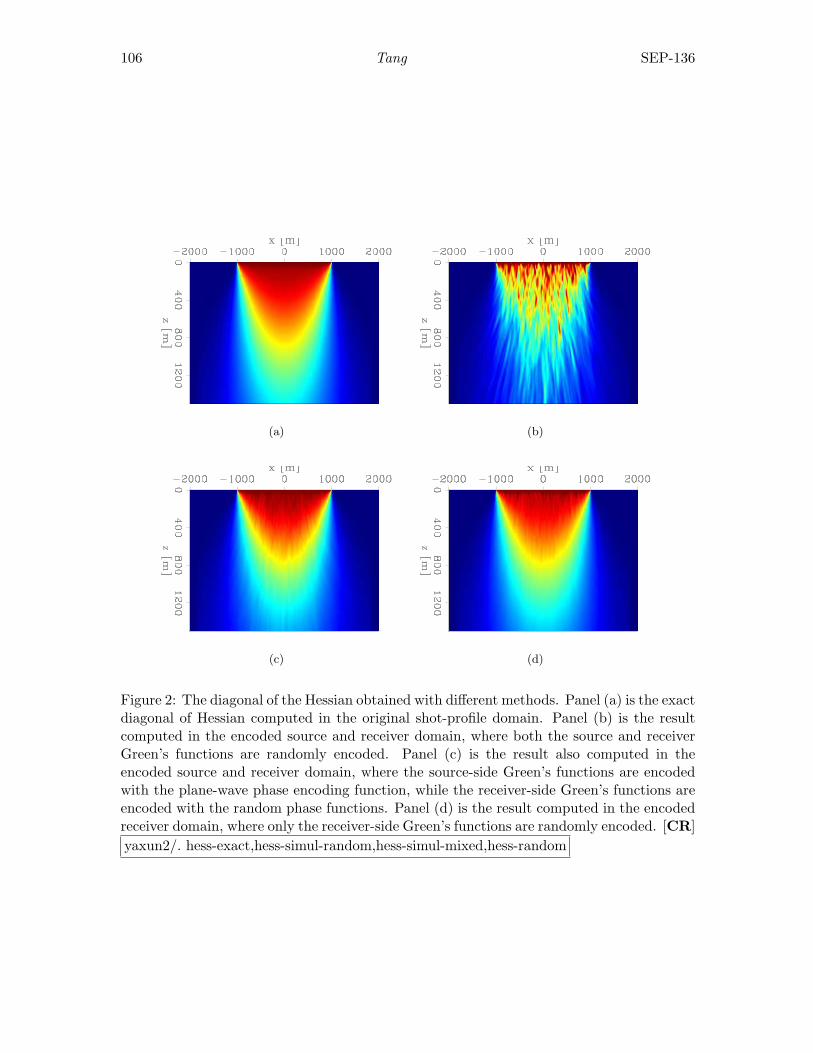
106 Tang SEP-136
(a) (b)
(c) (d)
Figure 2: The diagonal of the Hessian obtained with different methods. Panel (a) is the exactdiagonal of Hessian computed in the original shot-profile domain. Panel (b) is the resultcomputed in the encoded source and receiver domain, where both the source and receiverGreen’s functions are randomly encoded. Panel (c) is the result also computed in theencoded source and receiver domain, where the source-side Green’s functions are encodedwith the plane-wave phase encoding function, while the receiver-side Green’s functions areencoded with the random phase functions. Panel (d) is the result computed in the encodedreceiver domain, where only the receiver-side Green’s functions are randomly encoded. [CR]yaxun2/. hess-exact,hess-simul-random,hess-simul-mixed,hess-random
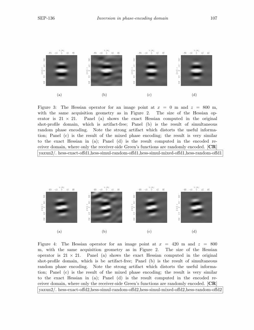
SEP-136 Inversion in phase-encoding domain 107
(a) (b) (c) (d)
Figure 3: The Hessian operator for an image point at x = 0 m and z = 800 m,with the same acquisition geometry as in Figure 2. The size of the Hessian op-erator is 21 × 21. Panel (a) shows the exact Hessian computed in the originalshot-profile domain, which is artifact-free; Panel (b) is the result of simultaneousrandom phase encoding. Note the strong artifact which distorts the useful informa-tion; Panel (c) is the result of the mixed phase encoding; the result is very similarto the exact Hessian in (a); Panel (d) is the result computed in the encoded re-ceiver domain, where only the receiver-side Green’s functions are randomly encoded. [CR]yaxun2/. hess-exact-offd1,hess-simul-random-offd1,hess-simul-mixed-offd1,hess-random-offd1
(a) (b) (c) (d)
Figure 4: The Hessian operator for an image point at x = 420 m and z = 800m, with the same acquisition geometry as in Figure 2. The size of the Hessianoperator is 21 × 21. Panel (a) shows the exact Hessian computed in the originalshot-profile domain, which is be artifact-free; Panel (b) is the result of simultaneousrandom phase encoding. Note the strong artifact which distorts the useful informa-tion; Panel (c) is the result of the mixed phase encoding; the result is very similarto the exact Hessian in (a); Panel (d) is the result computed in the encoded re-ceiver domain, where only the receiver-side Green’s functions are randomly encoded. [CR]yaxun2/. hess-exact-offd2,hess-simul-random-offd2,hess-simul-mixed-offd2,hess-random-offd2
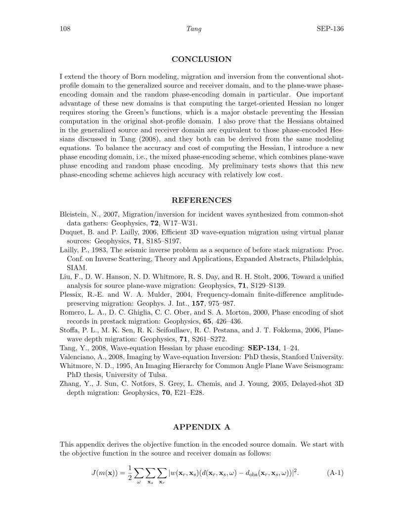
108 Tang SEP-136
CONCLUSION
I extend the theory of Born modeling, migration and inversion from the conventional shot-profile domain to the generalized source and receiver domain, and to the plane-wave phase-encoding domain and the random phase-encoding domain in particular. One importantadvantage of these new domains is that computing the target-oriented Hessian no longerrequires storing the Green’s functions, which is a major obstacle preventing the Hessiancomputation in the original shot-profile domain. I also prove that the Hessians obtainedin the generalized source and receiver domain are equivalent to those phase-encoded Hes-sians discussed in Tang (2008), and they both can be derived from the same modelingequations. To balance the accuracy and cost of computing the Hessian, I introduce a newphase encoding domain, i.e., the mixed phase-encoding scheme, which combines plane-wavephase encoding and random phase encoding. My preliminary tests shows that this newphase-encoding scheme achieves high accuracy with relatively low cost.
REFERENCES
Bleistein, N., 2007, Migration/inversion for incident waves synthesized from common-shotdata gathers: Geophysics, 72, W17–W31.
Duquet, B. and P. Lailly, 2006, Efficient 3D wave-equation migration using virtual planarsources: Geophysics, 71, S185–S197.
Lailly, P., 1983, The seismic inverse problem as a sequence of before stack migration: Proc.Conf. on Inverse Scattering, Theory and Applications, Expanded Abstracts, Philadelphia,SIAM.
Liu, F., D. W. Hanson, N. D. Whitmore, R. S. Day, and R. H. Stolt, 2006, Toward a unifiedanalysis for source plane-wave migration: Geophysics, 71, S129–S139.
Plessix, R.-E. and W. A. Mulder, 2004, Frequency-domain finite-difference amplitude-preserving migration: Geophys. J. Int., 157, 975–987.
Romero, L. A., D. C. Ghiglia, C. C. Ober, and S. A. Morton, 2000, Phase encoding of shotrecords in prestack migration: Geophysics, 65, 426–436.
Stoffa, P. L., M. K. Sen, R. K. Seifoullaev, R. C. Pestana, and J. T. Fokkema, 2006, Plane-wave depth migration: Geophysics, 71, S261–S272.
Tang, Y., 2008, Wave-equation Hessian by phase encoding: SEP-134, 1–24.Valenciano, A., 2008, Imaging by Wave-equation Inversion: PhD thesis, Stanford University.Whitmore, N. D., 1995, An Imaging Hierarchy for Common Angle Plane Wave Seismogram:
PhD thesis, University of Tulsa.Zhang, Y., J. Sun, C. Notfors, S. Grey, L. Chemis, and J. Young, 2005, Delayed-shot 3D
depth migration: Geophysics, 70, E21–E28.
APPENDIX A
This appendix derives the objective function in the encoded source domain. We start withthe objective function in the source and receiver domain as follows:
J(m(x)) =12
∑ω
∑xs
∑xr
|w(xr,xs)(d(xr,xs, ω)− dobs(xr,xs, ω))|2. (A-1)
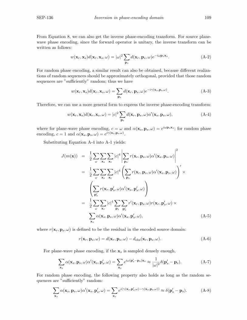
SEP-136 Inversion in phase-encoding domain 109
From Equation 8, we can also get the inverse phase-encoding transform. For source plane-wave phase encoding, since the forward operator is unitary, the inverse transform can bewritten as follows:
w(xr,xs)d(xr,xs, ω) = |ω|2∑ps
d(xr,ps, ω)e−iωpsxs . (A-2)
For random phase encoding, a similar result can also be obtained, because different realiza-tions of random sequences should be approximately orthogonal, provided that those randomsequences are ”sufficiently” random; thus we have
w(xr,xs)d(xr,xs, ω) =∑ps
d(xr,ps, ω)e−iγ(xs,ps,ω). (A-3)
Therefore, we can use a more general form to express the inverse phase-encoding transform:
w(xr,xs)d(xr,xs, ω) = |c|2∑ps
d(xr,ps, ω)α′(xs,ps, ω), (A-4)
where for plane-wave phase encoding, c = ω and α(xs,ps, ω) = eiωpsxs ; for random phaseencoding, c = 1 and α(xs,ps, ω) = eiγ(xs,ps,ω).
Substituting Equation A-4 into A-1 yields:
J(m(x)) =12
∑ω
∑xs
∑xr
|c|4∣∣∣∣∣∑
ps
r(xr,ps, ω)α′(xs,ps, ω)
∣∣∣∣∣2
=12
∑ω
∑xs
∑xr
|c|4(∑
ps
r(xr,ps, ω)α′(xs,ps, ω)
)′×∑
p′s
r(xr,p′s, ω)α′(xs,p′s, ω)
=
12
∑ω
∑xr
|c|4∑ps
∑p′
s
r′(xr,ps, ω)r(xr,p′s, ω)×
∑xs
α(xs,ps, ω)α′(xs,p′s, ω), (A-5)
where r(xr,ps, ω) is defined to be the residual in the encoded source domain:
r(xr,ps, ω) = d(xr,ps, ω)− dobs(xr,ps, ω). (A-6)
For plane-wave phase encoding, if the xs is sampled densely enough,∑xs
α(xs,ps, ω)α′(xs,p′s, ω) =∑xs
eiω(p′s−ps)xs ≈ 1
|ω|2δ(p′s − ps). (A-7)
For random phase encoding, the following property also holds as long as the random se-quences are ”sufficiently” random:∑
xs
α(xs,ps, ω)α′(xs,p′s, ω) =∑xs
ei(γ(xs,p′s,ω)−γ(xs,ps,ω)) ≈ δ(p′s − ps). (A-8)
110 Tang SEP-136
Substituting Equation A-7 or A-8 into A-5, we get the data-misfit function in the encodedsource domain:
J(m(x)) ≈ 12
∑ω
|c|2∑xr
∑ps
|d(xr,ps, ω)− dobs(xr,ps, ω)|2. (A-9)
APPENDIX B
This appendix derives the objective function in the encoded receiver domain. We start withthe objective function in the source and receiver domain as follows:
J(m(x)) =12
∑ω
∑xs
∑xr
|w(xr,xs)(d(xr,xs, ω)− dobs(xr,xs, ω))|2. (B-1)
Similar to the discussion in Appendix A, the general form of the inverse transform of receiverphase encoding can be written as follows:
w(xr,xs)d(xr,xs, ω) = |c|2∑pr
d(pr,xs, ω)β′(xr,pr, ω), (B-2)
where for plane-wave phase encoding, c = ω and β(xr,pr, ω) = eiωprxr ; for random phaseencoding, c = 1 and β(xr,pr, ω) = eiγ(xr,pr,ω). Substituting Equation B-2 into B-1 yields:
J(m(x)) =12
∑ω
∑xs
∑xr
|c|4∣∣∣∣∣∑
pr
r(pr,xs, ω)β′(xr,pr, ω)
∣∣∣∣∣2
=12
∑ω
∑xs
∑xr
|c|4(∑
pr
r(pr,xs, ω)β′(xr,pr, ω)
)′×∑
p′r
r(p′r,xs, ω)β′(xr,p′r, ω)
=
12
∑ω
∑xs
|c|4∑pr
∑p′
r
r′(pr,xs, ω)r(p′r,xs, ω)×
∑xr
β(xr,pr, ω)β′(xr,p′r, ω), (B-3)
where r(pr,xs, ω) is defined to be the residual in the encoded receiver domain:
r(pr,xs, ω) = d(pr,xs, ω)− dobs(pr,xs, ω). (B-4)
Similar to the discussion in Appendix A, the inner-most summation in Equation B-3 isapproximately a Dirac delta function under certain conditions. Therefore, the data-misfitfunction in the encoded receiver domain reads as follows:
J(m(x)) ≈ 12
∑ω
|c|2∑pr
∑xs
|d(pr,xs, ω)− dobs(pr,xs, ω)|2. (B-5)
SEP-136 Inversion in phase-encoding domain 111
APPENDIX C
This appendix derives the objective function in the simultaneously encoded source andreceiver domain. We start with the objective function in the source and receiver domain asfollows:
J(m(x)) =12
∑ω
∑xs
∑xr
|w(xr,xs)(d(xr,xs, ω)− dobs(xr,xs, ω))|2. (C-1)
If we follow a discussion similar to those in Appendices A and B, we obtain the generalexpression of the inverse transform of the simultaneous encoding:
w(xr,xs, ω)d(xr,xs, ω) = |c|4∑ps
∑pr
d(pr,ps, ω)α′(xs,ps, ω)β′(xr,pr, ω). (C-2)
Substituting Equation C-2 into C-1 yields:
J(m(x)) =12
∑ω
∑xs
∑xr
|c|8∣∣∣∣∣∑
ps
∑pr
r(pr,ps, ω)α′(xs,ps, ω)β′(xr,pr, ω)
∣∣∣∣∣2
=12
∑ω
∑xs
∑xr
|c|8(∑
ps
∑pr
r(pr,ps, ω)α′(xs,ps, ω)β′(xr,pr, ω)
)′×∑
p′s
∑p′
r
r(p′r,p′s, ω)α′(xs,p′s, ω)β′(xr,p′r, ω)
=
12
∑ω
|c|8∑ps
∑p′
s
∑pr
∑p′
r
r′(pr,ps, ω)r(p′r,p′s, ω)×
∑xs
∑xr
α(xs,ps, ω)β(xr,pr, ω)α′(xs,p′s, ω)β′(xr,p′r, ω), (C-3)
where r(pr,ps, ω) is defined to be the residual in the encoded source and receiver domain:
r(pr,ps, ω) = d(pr,ps, ω)− dobs(pr,ps, ω). (C-4)
For plane-wave phase encoding, with sampling dense enough in xs and xr, the inner-mostsummations become Dirac delta functions:∑
xs
∑xr
α(xs,ps, ω)β(xr,pr, ω)α′(xs,p′s, ω)β′(xr,p′r, ω)
≈ 1|ω|4
δ(p′r − pr)δ(p′s − ps). (C-5)
For random phase encoding, we can also approximately have∑xs
∑xr
α(xs,ps, ω)β(xr,pr, ω)α′(xs,p′s, ω)β′(xr,p′r, ω)
≈ δ(p′r − pr)δ(p′s − ps). (C-6)
Therefore the data-misfit function in the encoded source and receiver domain is
J(m(x)) ≈ 12
∑ω
|c|4∑ps
∑pr
|d(pr,ps, ω)− dobs(pr,ps, ω)|2. (C-7)

112 Tang SEP-136
Stanford Exploration Project, Report SEP136, April 14, 2009
Salt body segmentation with dip and frequency attributes
Adam Halpert and Robert G. Clapp
ABSTRACT
Image segmentation can automatically locate salt boundaries on seismic sections, anoften time-consuming and tedious task when undertaken manually. However, using asingle seismic attribute (usually amplitude) is sometimes insufficient to achieve an ac-curate segmentation. Since any quantifiable measure may be employed as an attributefor segmentation, exploring other possible attributes is an important step in developinga more robust segmentation algorithm. Dip variability within a seismic section is oneattribute with many advantages for segmentation, and experimenting with differentmethods for calculating dips can yield improved results. Determining the frequencycontent of a seismic image offers other opportunities for improvement. Specifically,instantaneous frequency shows promise as another attribute for segmentation, whileemploying a continuous wavelet transform to study envelope amplitude at differentfrequencies can improve the performance of the amplitude attribute.
INTRODUCTION
Automated image segmentation offers a means of quickly and efficiently delineating saltbodies on seismic images. When adapted for seismic purposes (Lomask, 2007; Lomasket al., 2007), the Normalized Cuts Image Segmentation (NCIS) algorithm (Shi and Malik,2000) provides a global solution to the salt boundary calculation. This helps overcome someof the weaknesses of other methods, such as local horizon trackers, that can fail when theboundary fades or becomes discontinuous. A global determination of salt boundaries canbe especially important for building velocity models in complex areas; in such cases, imagesegmentation may be employed to automatically build or update velocity models, helpingto alleviate a major bottleneck for iterative imaging projects (Halpert and Clapp, 2008).
The NCIS algorithm relies on one or more seismic attributes to segment an image; themost straightforward of these attributes is envelope of the amplitude. Often, this singleattribute provides an accurate calculation of the salt boundary. Unfortunately, in someinstances a single attribute is insufficient, and the algorithm cannot produce a reasonableresult. Here, we demonstrate situations in which a single-attribute segmentation fails. Wethen explore possibilities for useful attributes other than amplitude, most notably dip andinstantaneous frequency. Finally, we discuss an ultimate goal of designing an interpreter-guided multi-attribute segmentation scheme.
ATTRIBUTE-BASED SEGMENTATION
The NCIS algorithm (Shi and Malik, 2000) functions by calculating relationships betweenindividual pixel pairs in an image. For seismic image segmentation, each pixel is compared
113
114 Halpert and Clapp SEP-136
to a random selection of neighboring pixels (Lomask, 2007), and each pair is assigned aweight value inversely proportional to the likelihood of a salt boundary existing betweenthem. If these weights are placed in a matrix W, a salt boundary path may be calculatedvia the eigensystem
(D−W)y = λDy , (1)
where D is a diagonal matrix whose elements are the sum of each column of W, and λand y are an eigenvalue and eigenvector of the system, respectively. Because the smallesteigenvalue will yield only a constant eigenvector, the eigenvector correseponding to thesecond smallest eigenvalue of the system is used to segment the image. The eigenvector inquestion ranges in value from -1 to +1 across the estimated boundary path. The image issegmented either by following a constant eigenvector value across the image - usually thezero-value contour; see Lomask (2007) - or by using outside information to follow differenteigenvector values across the image (Halpert and Clapp, 2008).
In the examples cited above, the most common measure or attribute used to determinethe likely presence of a salt boundary is amplitude of the envelope. For instance, a largeamplitude between two pixels suggests a salt boundary is likely, and will result in a relativelysmall weight assigned to that pixel pair. Amplitude, however, is not the only attribute thatcan be used for this purpose. In fact, any quantifiable measure that relates to the presenceof a salt boundary may be used as an attribute for segmentation.
Limitations of a single attribute
The sources cited above contain several examples of accurate salt boundary picking usingonly amplitude to segment the image. In some instances, however, such an approach canlead to inaccurate results. Figure 1 shows one such instance. Since the algorithm attemptsto find a minimized path across the image, it often tends toward a straight line in areasof uncertainty. In this case, the algorithm incorrectly cuts across a very steep salt canyonin the Sigsbee synthetic model. Even though the outline of the salt top is faintly visible,amplitude information alone is not enough to correctly guide the segmentation process inthis instance. This suggests that further information, in the form of attributes other thanamplitude, may be an important part of a more robust segmentation algorithm.
DIP AS AN ATTRIBUTE
Estimating dip in seismic images has long been recognized as a useful interpretation tech-nique, especially for 3D volumes (Bednar, 1997). Dip can be a particularly useful attributewhen the goal is delineation of salt bodies. Lomask (2007) notes that salt boundaries andnearby sediments will often display different dips; furthermore, the seemingly random dipsthat often characterize the interior of salt bodies on field seismic data should contrast con-siderably with more ordered dipping layers outside the salt. Therefore, an attribute thathighlights variability in dip throughout a seismic image may be helpful for locating saltboundaries.
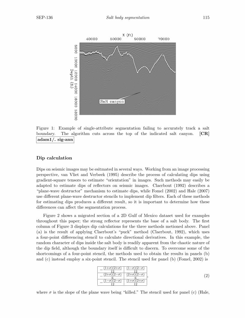
SEP-136 Salt body segmentation 115
Figure 1: Example of single-attribute segmentation failing to accurately track a saltboundary. The algorithm cuts across the top of the indicated salt canyon. [CR]adam1/. sig-ann
Dip calculation
Dips on seismic images may be esitmated in several ways. Working from an image processingperspective, van Vliet and Verbeek (1995) describe the process of calculating dips usinggradient-square tensors to estimate “orientation” in images. Such methods may easily beadapted to estimate dips of reflectors on seismic images. Claerbout (1992) describes a“plane-wave destructor” mechanism to estimate dips, while Fomel (2002) and Hale (2007)use different plane-wave destructor stencils to implement dip filters. Each of these methodsfor estimating dips produces a different result, so it is important to determine how thesedifferences can affect the segmentation process.
Figure 2 shows a migrated section of a 2D Gulf of Mexico dataset used for examplesthroughout this paper; the strong reflector represents the base of a salt body. The firstcolumn of Figure 3 displays dip calculations for the three methods metioned above. Panel(a) is the result of applying Claerbout’s “puck” method (Claerbout, 1992), which usesa four-point differencing stencil to calculate directional derivatives. In this example, therandom character of dips inside the salt body is readily apparent from the chaotic nature ofthe dip field, although the boundary itself is difficult to discern. To overcome some of theshortcomings of a four-point stencil, the methods used to obtain the results in panels (b)and (c) instead employ a six-point stencil. The stencil used for panel (b) (Fomel, 2002) is
− (1+σ)(2+σ)12
(1−σ)(2−σ)12
− (2+σ)(2−σ)6
(2+σ)(2−σ)6
− (1−σ)(2−σ)12
(1+σ)(2+σ)12
, (2)
where σ is the slope of the plane wave being “killed.” The stencil used for panel (c) (Hale,
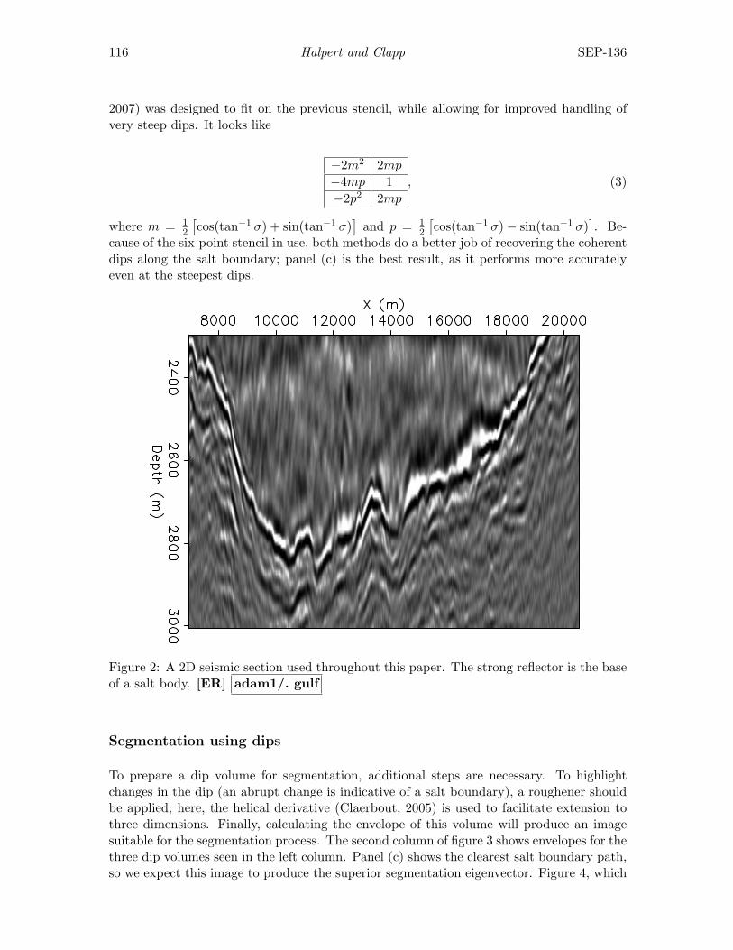
116 Halpert and Clapp SEP-136
2007) was designed to fit on the previous stencil, while allowing for improved handling ofvery steep dips. It looks like
−2m2 2mp
−4mp 1−2p2 2mp
, (3)
where m = 12
[cos(tan−1 σ) + sin(tan−1 σ)
]and p = 1
2
[cos(tan−1 σ)− sin(tan−1 σ)
]. Be-
cause of the six-point stencil in use, both methods do a better job of recovering the coherentdips along the salt boundary; panel (c) is the best result, as it performs more accuratelyeven at the steepest dips.
Figure 2: A 2D seismic section used throughout this paper. The strong reflector is the baseof a salt body. [ER] adam1/. gulf
Segmentation using dips
To prepare a dip volume for segmentation, additional steps are necessary. To highlightchanges in the dip (an abrupt change is indicative of a salt boundary), a roughener shouldbe applied; here, the helical derivative (Claerbout, 2005) is used to facilitate extension tothree dimensions. Finally, calculating the envelope of this volume will produce an imagesuitable for the segmentation process. The second column of figure 3 shows envelopes for thethree dip volumes seen in the left column. Panel (c) shows the clearest salt boundary path,so we expect this image to produce the superior segmentation eigenvector. Figure 4, which
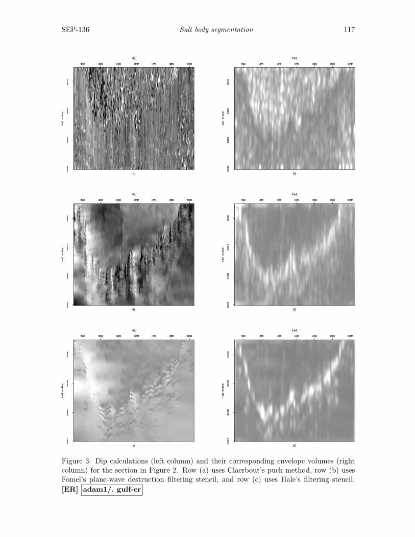
SEP-136 Salt body segmentation 117
Figure 3: Dip calculations (left column) and their corresponding envelope volumes (rightcolumn) for the section in Figure 2. Row (a) uses Claerbout’s puck method, row (b) usesFomel’s plane-wave destruction filtering stencil, and row (c) uses Hale’s filtering stencil.[ER] adam1/. gulf-er
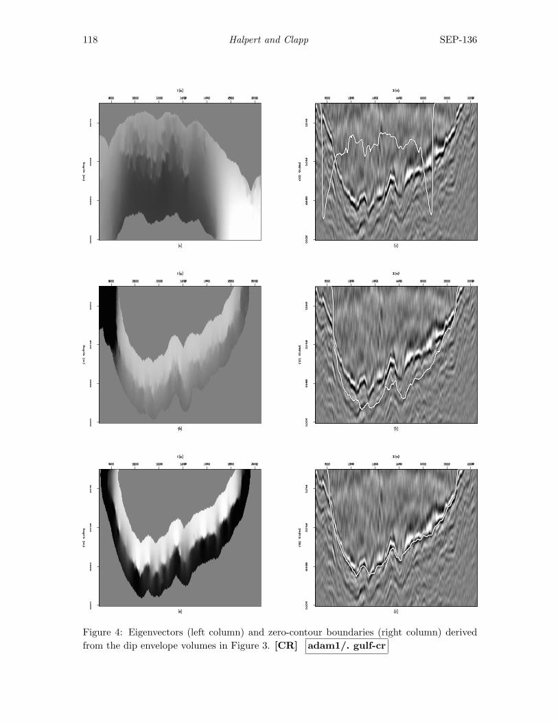
118 Halpert and Clapp SEP-136
Figure 4: Eigenvectors (left column) and zero-contour boundaries (right column) derivedfrom the dip envelope volumes in Figure 3. [CR] adam1/. gulf-cr
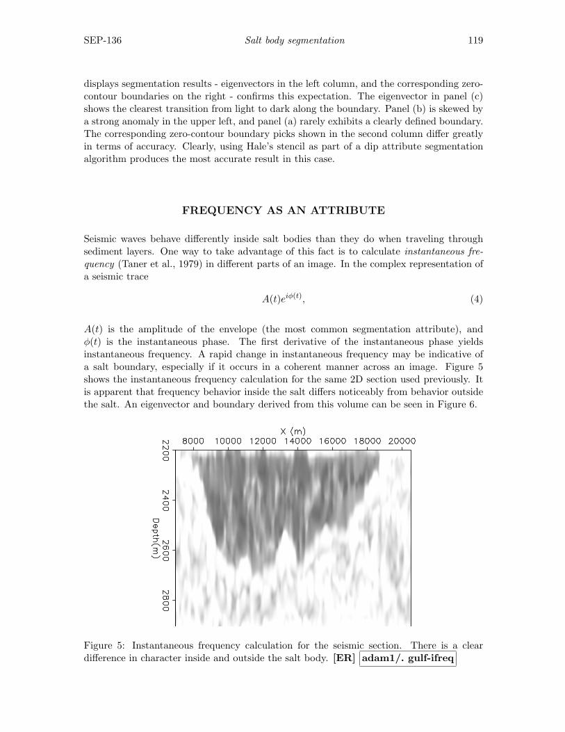
SEP-136 Salt body segmentation 119
displays segmentation results - eigenvectors in the left column, and the corresponding zero-contour boundaries on the right - confirms this expectation. The eigenvector in panel (c)shows the clearest transition from light to dark along the boundary. Panel (b) is skewed bya strong anomaly in the upper left, and panel (a) rarely exhibits a clearly defined boundary.The corresponding zero-contour boundary picks shown in the second column differ greatlyin terms of accuracy. Clearly, using Hale’s stencil as part of a dip attribute segmentationalgorithm produces the most accurate result in this case.
FREQUENCY AS AN ATTRIBUTE
Seismic waves behave differently inside salt bodies than they do when traveling throughsediment layers. One way to take advantage of this fact is to calculate instantaneous fre-quency (Taner et al., 1979) in different parts of an image. In the complex representation ofa seismic trace
A(t)eiφ(t), (4)
A(t) is the amplitude of the envelope (the most common segmentation attribute), andφ(t) is the instantaneous phase. The first derivative of the instantaneous phase yieldsinstantaneous frequency. A rapid change in instantaneous frequency may be indicative ofa salt boundary, especially if it occurs in a coherent manner across an image. Figure 5shows the instantaneous frequency calculation for the same 2D section used previously. Itis apparent that frequency behavior inside the salt differs noticeably from behavior outsidethe salt. An eigenvector and boundary derived from this volume can be seen in Figure 6.
Figure 5: Instantaneous frequency calculation for the seismic section. There is a cleardifference in character inside and outside the salt body. [ER] adam1/. gulf-ifreq
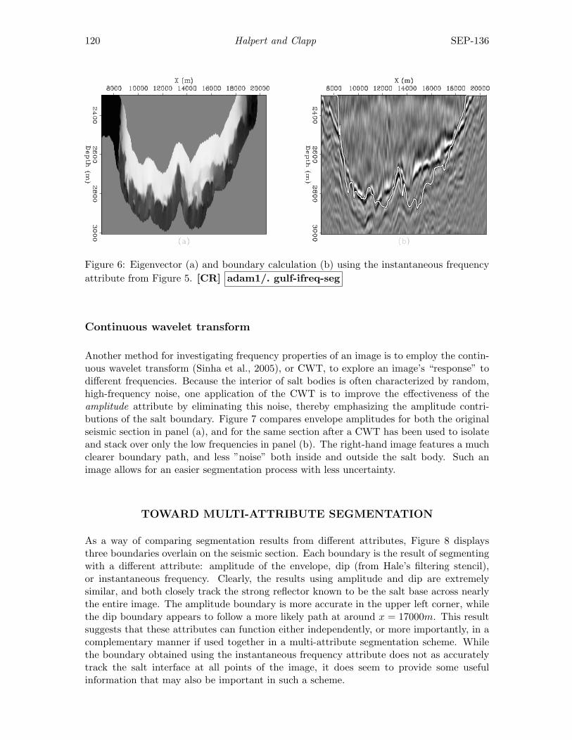
120 Halpert and Clapp SEP-136
Figure 6: Eigenvector (a) and boundary calculation (b) using the instantaneous frequencyattribute from Figure 5. [CR] adam1/. gulf-ifreq-seg
Continuous wavelet transform
Another method for investigating frequency properties of an image is to employ the contin-uous wavelet transform (Sinha et al., 2005), or CWT, to explore an image’s “response” todifferent frequencies. Because the interior of salt bodies is often characterized by random,high-frequency noise, one application of the CWT is to improve the effectiveness of theamplitude attribute by eliminating this noise, thereby emphasizing the amplitude contri-butions of the salt boundary. Figure 7 compares envelope amplitudes for both the originalseismic section in panel (a), and for the same section after a CWT has been used to isolateand stack over only the low frequencies in panel (b). The right-hand image features a muchclearer boundary path, and less ”noise” both inside and outside the salt body. Such animage allows for an easier segmentation process with less uncertainty.
TOWARD MULTI-ATTRIBUTE SEGMENTATION
As a way of comparing segmentation results from different attributes, Figure 8 displaysthree boundaries overlain on the seismic section. Each boundary is the result of segmentingwith a different attribute: amplitude of the envelope, dip (from Hale’s filtering stencil),or instantaneous frequency. Clearly, the results using amplitude and dip are extremelysimilar, and both closely track the strong reflector known to be the salt base across nearlythe entire image. The amplitude boundary is more accurate in the upper left corner, whilethe dip boundary appears to follow a more likely path at around x = 17000m. This resultsuggests that these attributes can function either independently, or more importantly, in acomplementary manner if used together in a multi-attribute segmentation scheme. Whilethe boundary obtained using the instantaneous frequency attribute does not as accuratelytrack the salt interface at all points of the image, it does seem to provide some usefulinformation that may also be important in such a scheme.
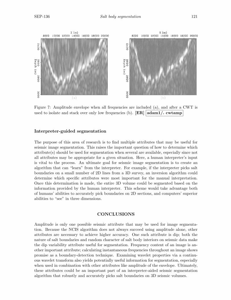
SEP-136 Salt body segmentation 121
Figure 7: Amplitude envelope when all frequencies are included (a), and after a CWT isused to isolate and stack over only low frequencies (b). [ER] adam1/. cwtamp
Interpreter-guided segmentation
The purpose of this area of research is to find multiple attributes that may be useful forseismic image segmentation. This raises the important question of how to determine whichattribute(s) should be used for segmentation when several are available, especially since notall attributes may be appropriate for a given situation. Here, a human interpreter’s inputis vital to the process. An ultimate goal for seismic image segmentation is to create analgorithm that can “learn” from the interpreter. For example, if the interpreter picks saltboundaries on a small number of 2D lines from a 3D survey, an inversion algorithm coulddetermine which specific attributes were most important for the manual interpretation.Once this determination is made, the entire 3D volume could be segmented based on theinformation provided by the human interpreter. This scheme would take advantage bothof humans’ abilities to accurately pick boundaries on 2D sections, and computers’ superiorabilities to “see” in three dimensions.
CONCLUSIONS
Amplitude is only one possible seismic attribute that may be used for image segmenta-tion. Because the NCIS algorithm does not always succeed using amplitude alone, otherattributes are necessary to achieve higher accuracy. One such attribute is dip; both thenature of salt boundaries and random character of salt body interiors on seismic data makethe dip variability attribute useful for segmentation. Frequency content of an image is an-other important attribute; calculating instantaneous frequencies throughout an image showspromise as a boundary-detection technique. Examining wavelet properties via a continu-ous wavelet transform also yields potentially useful information for segmentation, especiallywhen used in combination with other attributes like amplitude of the envelope. Ultimately,these attributes could be an important part of an interpreter-aided seismic segmentationalgorithm that robustly and accurately picks salt boundaries on 3D seismic volumes.
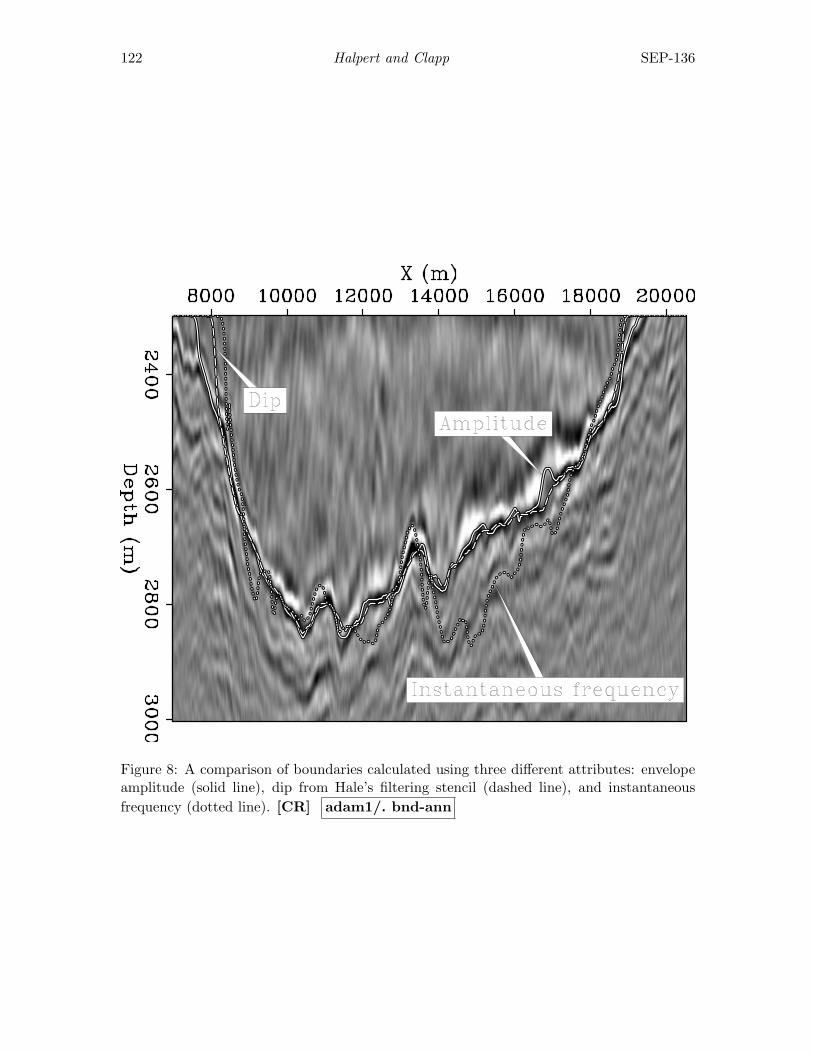
122 Halpert and Clapp SEP-136
Figure 8: A comparison of boundaries calculated using three different attributes: envelopeamplitude (solid line), dip from Hale’s filtering stencil (dashed line), and instantaneousfrequency (dotted line). [CR] adam1/. bnd-ann
SEP-136 Salt body segmentation 123
ACKNOWLEDGMENTS
We would like to thank SMAART JV for the Sigsbee synthetic dataset, and WesternGecofor providing the real data example in this paper.
REFERENCES
Bednar, J. B., 1997, Least squares dip and coherency attributes: SEP-Report, 95, 219–225.Claerbout, J., 1992, Earth soundings analysis: Processing versus inversion: Blackwell Sci-
entific Publications.——–, 2005, Image estimation by example: Stanford University.Fomel, S., 2002, Applications of plane-wave destruction filters: Geophysics, 67, 1946–1960.Hale, D., 2007, Local dip filtering with directional laplacians: CWP-Report, 567.Halpert, A. and R. G. Clapp, 2008, Image segmentation for velocity model construction
and updating: 2008, 134, 159–170.Lomask, J., 2007, Seismic volumetric flattening and segmentation: PhD thesis, Stanford
University.Lomask, J., R. G. Clapp, and B. Biondi, 2007, Application of image segmentation to tracking
3d salt boundaries: Geophysics, 72, P47–P56.Shi, J. and J. Malik, 2000, Normalized cuts and image segmentation: Institute of Electrical
and Electronics Engineers Transactions on Pattern Analysis and Machine Intelligence,22, 838–905.
Sinha, S., P. S. Routh, P. D. Anno, and J. P. Castagna, 2005, Spectral decomposition ofseismic data with continuous-wavelet transform: Geophysics, 70, P19–P25.
Taner, M. T., F. Koehler, and R. E. Sheriff, 1979, Complex seismic trace analysis: Geo-physics, 44, 1041–1063.
van Vliet, L. J. and P. W. Verbeek, 1995, Estimators for orientation and anisotropy indigitized images, in Proceedings, Conference of the Advanced School for Computing andImaging, 442–450.

124 Halpert and Clapp SEP-136
Stanford Exploration Project, Report SEP136, April 14, 2009
Hyercube viewer: New displays and new data-types
Robert G. Clapp and Nelson Nagales
ABSTRACT
No single way to view seismic data is effective in all cases. Rather than buildingseparate tools for each viewing approach, we added functionality to SEP’s existinghypercube viewing tool. In addition to other functionality improvements, we addedthe capability to view wiggle traces, contours, out-of-core datasets, and datasets withdifferent number of dimensions and size.
INTRODUCTION
Seismic viewing tools can be broken into two categories: batch viewing programs and inter-active viewers. SEP has a long history of both program types. Static viewing programs canproduce line graphs, wiggle traces, hidden line plots, contours, and raster images. Theseprograms, in combination with utility programs that allow windowing and transposing ofarrays offer the ability to create effective static graphics. For viewing and understandingmulti-dimensional volumes, these tools are not as useful.
A series of SEP’s interactive viewers (Ottolini, 1982, 1983, 1988, 1990; Clapp, 2001;Chen and Clapp, 2006) have also been developed at SEP. These viewers are more effectivein viewing multi-dimensional volumes but have been limited in three key ways. The firstshortcoming is their inability to produce high quality graphics and reproduce a given viewof a dataset. Second, they were restricted to viewing a single (later a few) datasets thathad to be identical in size and fit in memory. Finally, they only display data in rasterformat. Clapp et al. (2008) made an initial attempt in addressing the first shortcoming byrecording, and allowing, replaying of mouse and keyboard actions.
In this paper we attempt to address the viewer’s dataset and display limitations. Wedescribe changes to the way the program interacts with datasets. These changes allow theviewer to handle datasets with different sampling and different number of dimensions, andeven operate in an out-of-core mode. We show the new display options that allow the userto view the data as contour and wiggle plots. Finally we describe additional changes in theUI to the viewer and briefly discuss what might be added in the future.
DISPLAY OPTIONS
There are several possible ways to plot regular fields. SEP has generally used raster plots todisplay data. These plots have the advantage of being able to display relatively dense datawithin wide spatial frequency range. In some cases raster is not the ideal plotting option.
When examining waveforms it is often useful to display traces in a wiggle format. Wiggleformat allows you to see more clearly the actual waveform recorded by the sensor. Figure 1
125
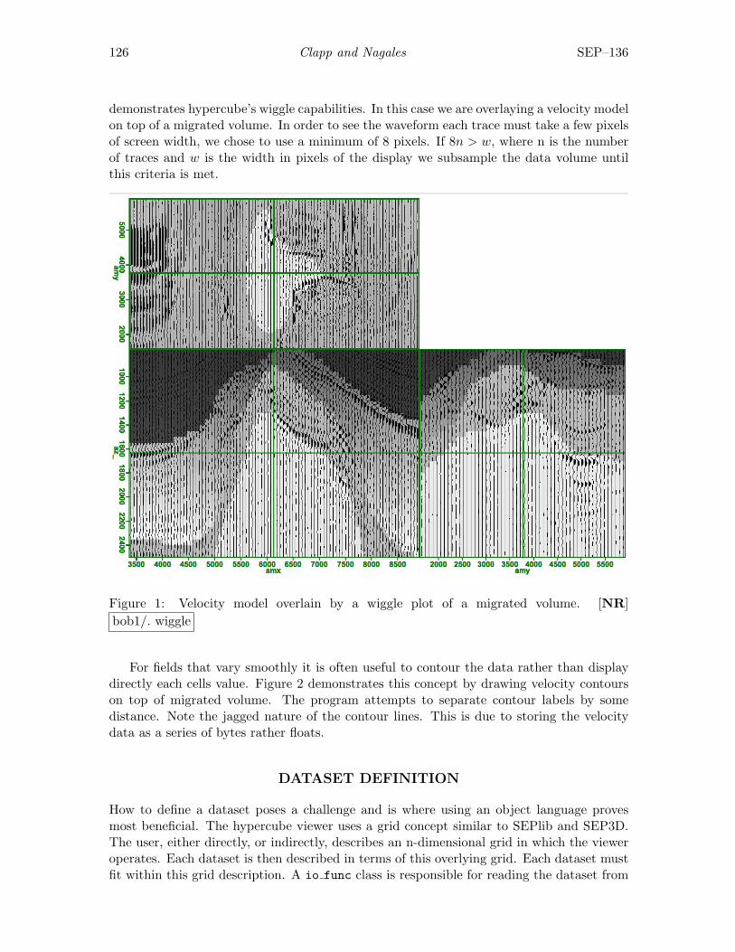
126 Clapp and Nagales SEP–136
demonstrates hypercube’s wiggle capabilities. In this case we are overlaying a velocity modelon top of a migrated volume. In order to see the waveform each trace must take a few pixelsof screen width, we chose to use a minimum of 8 pixels. If 8n > w, where n is the numberof traces and w is the width in pixels of the display we subsample the data volume untilthis criteria is met.
Figure 1: Velocity model overlain by a wiggle plot of a migrated volume. [NR]bob1/. wiggle
For fields that vary smoothly it is often useful to contour the data rather than displaydirectly each cells value. Figure 2 demonstrates this concept by drawing velocity contourson top of migrated volume. The program attempts to separate contour labels by somedistance. Note the jagged nature of the contour lines. This is due to storing the velocitydata as a series of bytes rather floats.
DATASET DEFINITION
How to define a dataset poses a challenge and is where using an object language provesmost beneficial. The hypercube viewer uses a grid concept similar to SEPlib and SEP3D.The user, either directly, or indirectly, describes an n-dimensional grid in which the vieweroperates. Each dataset is then described in terms of this overlying grid. Each dataset mustfit within this grid description. A io func class is responsible for reading the dataset from
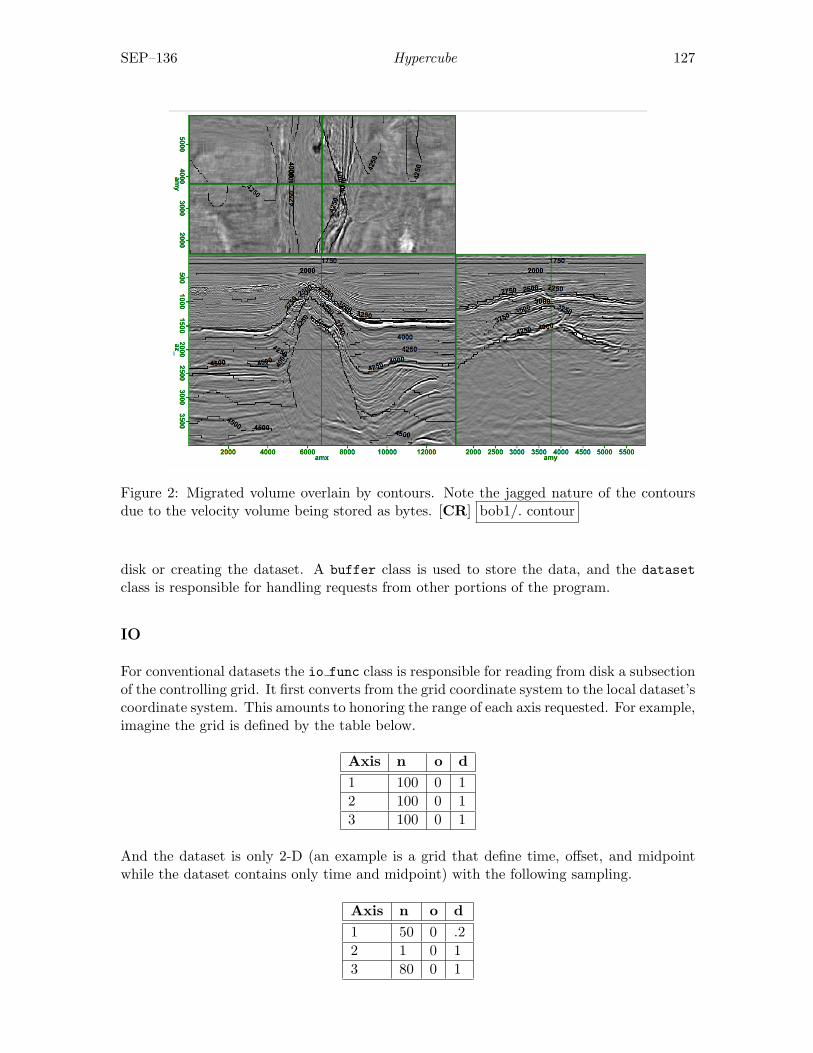
SEP–136 Hypercube 127
Figure 2: Migrated volume overlain by contours. Note the jagged nature of the contoursdue to the velocity volume being stored as bytes. [CR] bob1/. contour
disk or creating the dataset. A buffer class is used to store the data, and the datasetclass is responsible for handling requests from other portions of the program.
IO
For conventional datasets the io func class is responsible for reading from disk a subsectionof the controlling grid. It first converts from the grid coordinate system to the local dataset’scoordinate system. This amounts to honoring the range of each axis requested. For example,imagine the grid is defined by the table below.
Axis n o d1 100 0 12 100 0 13 100 0 1
And the dataset is only 2-D (an example is a grid that define time, offset, and midpointwhile the dataset contains only time and midpoint) with the following sampling.
Axis n o d1 50 0 .22 1 0 13 80 0 1
128 Clapp and Nagales SEP–136
If there is a read request for the entire volume it will be converted into a read request forthe 2-D subsection of the grid in which the dataset exists. Currently the io func modulecan read SEPlib, RSF, SU, SEG-Y, and SeisPak formats from disk in this manner.
The io func does not necessarily have to read from disk, and the data isn’t necessarilystatic. For example imagine doing interactive NMO on 2-D dataset. Three datasets canexist: the original CMP, a semblance panel, and NMO corrected gather. In this case the gridcontains 4 axes: time, offset, midpoint, and velocity. None of the three datasets contain allfour axes. The latter two change depending user interaction. When the midpoint locationchanges semblance is recomputed. When a new velocity is selected on the semblance panelthe NMOed data changes. To support this type of functionality the io func has a changedboolean.
Buffer
The buffer class has two main responsibilities. It holds a subsection of the data and canreturn a 2-D slice of the subsection it holds in memory. Currently buffer class stores dataas either a series of bytes of floats in a regular mesh, but it is not limited to this storagemechanism. The data could be stored in number of compressed formats. A dataset can becomposed of several different buffers.
Dataset
A dataset is initialized by an io func and creates buffers as it needs them. Currently thereare four basic buffer types. The simplest is inherited from incore data. As the nameimplies this data type is stored completely in memory and has the same number of axesas the controlling grid. The created data class is for data that changes depending onthe user’s interaction with the program. An example of this is the semblance and NMOcorrected datasets in the velocity analysis example. If a dataset does not contain all of theaxes of the grid, it should be stored using the partial data class.
The outcore data class, as the name implies, is for datasets that are not stored com-pletely in memory. This class reads in a 3-D subset of the domain based on the order theaxes are being displayed in a given view. For example, given a 4-D volume and a view thatis displaying the first, third, and fourth axis, a 3-D subset of the data will be read centeredat the current position along the second axis. As long as the position is only being changedin these three dimension no further read requests are necessary. Several of these out-of-corebuffers are created for each dataset allowing multiple views display multiple subsets andallowing switching back and forth between positions without having constant data readdelays.
USER INTERFACE CHANGES
Several changes where made to the user interface beyond the plotting options discussedabove. In this section we will highlight the most significant changes.
SEP–136 Hypercube 129
Mouse/status
As discussed in Clapp et al. (2008) how the hypercube viewer interacts with the mouse canbe altered. The main tab, submenu info the mouse controls can be modified. Currentlythere are three options: zoom, navigate, and pick. The options refer to the action of theleft mouse button. The effect of the middle and right button can be displayed in the statusbar.
Status bar
The status bar is located at the bottom portion of the view window. It starts off displayingthe current mouse controls. The main tab, submenu info changes the status bar to displayeither the current position, in grid coordinates, or the actual sample value that has beenselected.
Overlay/display options
The view tab, submenu data has been modified so that both the primary displayed dataand the data (if any) you wish to overlay can be changed easily.
How you wish to display the primary and overlaid data can be modified in the Displaytab, general submenu. For each dataset you can choose to display using various color maps,in wiggle format, or with contours. The Display tab contains two additional submenus,Wiggle and Contour. The Wiggle submenu allows you to change the line color and whether,and what color, to fill positive and negative portion of the wiggle trace. The Contoursubmenu allows you to set the number of contours, the initial contour value, and the contourinterval.
FUTURE DIRECTIONS
There are three active areas of development for the viewer. The first is the ability topartition space in N-D. This ability will enable the second area, interactive processing. Manyprocesses need human guidance but that guidance often is more complex then modifying asingle 1-D line. The final area is the ability to store additional data types. The ability tostore data in a compressed form, such as curvelets, would enable very large volumes to bemanipulated effectively.
CONCLUSION
We expanded SEP’s hypercube viewer by addressing two of its weaknesses. First we addthe ability to view contour and wiggle plots. Second we added the ability to view multipledatasets which exist in the same space but might not have the sampling, the same numberof dimensions, or even be possible to completely hold in memory.
130 Clapp and Nagales SEP–136
REFERENCES
Chen, D. M. and R. G. Clapp, 2006, Data-fusion of volumes, visualization of paths, andrevision of viewing sequences in ricksep: SEP-Report, 125.
Clapp, R., 2001, Ricksep: Interactive display of multi-dimensional data: SEP-Report, 110,163–172.
Clapp, R. G., D. M. Chen, and S. Luo, 2008, Hypercube viewer: 2008, 134, 179–192.Ottolini, R., 1982, Interactive movie machine user’s documentation: SEP-Report, 32, 183–
196.——–, 1983, Movie cubes: SEP-Report, 35, 235–240.——–, 1988, Movies on the Macintosh II: SEP-Report, 59, 255–268.——–, 1990, Seismic movies on the XView graphics system: SEP-Report, 65, 315.
Stanford Exploration Project, Report SEP136, April 14, 2009
Many-core and PSPI: Mixing fine-grain and coarse-grainparallelism
Ching-Bih Liaw and Robert G. Clapp
ABSTRACT
Many of today’s computer architectures are supported for fine-grain, rather than coarse-grain, parallelism. Conversely, many seismic imaging algorithms have been imple-mented using coarse-grain parallelization techniques. Sun’s Niagara2 uses several pro-cessing threads per computational core, therefore the amount of memory per threadmakes a strict coarse-grain approach to problems impractical. A strictly fine-grain par-allelism approach can be problematic in algorithms that require frequent synchroniza-tion. We use a combination of fine-gain and coarse-grain parallelism in implementing adownward continuation based migration algorithm on the Niagara2. We show the bestperformance can be achieved by mixing these two programing styles.
INTRODUCTION
Seismic imaging problems lend themselves well to coarse-grain parallelism. Kirchoff migra-tion can be parallelized by splitting the image space (and/or data space) over many pro-cessing units. Downward continuation based migration can be parallelized over frequency.Flavors of downward continuation and reverse time migration can be further parallelizedover shot or plane wave. All of these parallelism methods can be described as ‘coarse-gained’.Coarse-grained parallelism fits well the cluster computing of the last decade. Several excit-ing new architectures including Nvidia’s Grahic’s Precision Unit (GPU), IBM’s cell, FieldProgramable Gate Arrays (FPGA), and Sun’s Niagara platform are more aimed at a fine-grained parallelism model. These platforms can have threads in the 10s-100s often makingcoarse-grain parallelism impractical because of memory constraints. Early results (Pellet al., 2008) on these architecture’s are promising but implementation can be challenging.
Downward-continuation based migration (Claerbout, 1995) is a more challenging imag-ing algorithm to implement on a fine-grained parallel machine. The challenge in the imple-mentation comes from the 2-D (shot-profile, plane-wave) 3-D (common-azimuth), or 4-D(narrow-azimuth, full-azimuth) FFT. The implicit-transpose and the non-uniform data ac-cess pattern does not easily port to FPGA and GPU solutions. The multi-thread per coreapproach of the Sun Niagara2 offers an easier parallelism route.
In this paper we demonstrate that the optimal solution for PSPI migration on theNiagara2 is by mixing the coarse-grained and fine-grained parallelism models. We beginby presenting an overview of the Niagara2 architecture and the PSPI algorithm. We showhow some portions of the PSPI algorithm benefit from Niagara’s multiple threads per corewhile others show only minimal improvement. We conclude by discussing the bottlenecksto further efficiency improvements.
131
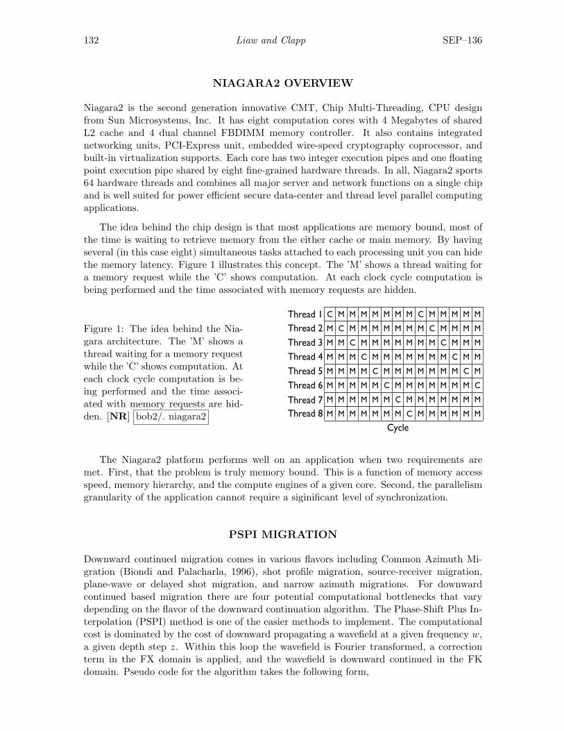
132 Liaw and Clapp SEP–136
NIAGARA2 OVERVIEW
Niagara2 is the second generation innovative CMT, Chip Multi-Threading, CPU designfrom Sun Microsystems, Inc. It has eight computation cores with 4 Megabytes of sharedL2 cache and 4 dual channel FBDIMM memory controller. It also contains integratednetworking units, PCI-Express unit, embedded wire-speed cryptography coprocessor, andbuilt-in virtualization supports. Each core has two integer execution pipes and one floatingpoint execution pipe shared by eight fine-grained hardware threads. In all, Niagara2 sports64 hardware threads and combines all major server and network functions on a single chipand is well suited for power efficient secure data-center and thread level parallel computingapplications.
The idea behind the chip design is that most applications are memory bound, most ofthe time is waiting to retrieve memory from the either cache or main memory. By havingseveral (in this case eight) simultaneous tasks attached to each processing unit you can hidethe memory latency. Figure 1 illustrates this concept. The ’M’ shows a thread waiting fora memory request while the ’C’ shows computation. At each clock cycle computation isbeing performed and the time associated with memory requests are hidden.
Figure 1: The idea behind the Nia-gara architecture. The ’M’ shows athread waiting for a memory requestwhile the ’C’ shows computation. Ateach clock cycle computation is be-ing performed and the time associ-ated with memory requests are hid-den. [NR] bob2/. niagara2
C M M M M M M M C M M M M M
M C M M M M M M M C M M M M
M M C M M M M M M M C M M M
M M M C M M M M M M M C M M
M M M M C M M M M M M M C M
M M M M M C M M M M M M M C
M M M M M M C M M M M M M M
M M M M M M M C M M M M M M
Thread 1
Thread 2
Thread 3
Thread 4
Thread 5
Thread 6
Thread 7
Thread 8
Cycle
The Niagara2 platform performs well on an application when two requirements aremet. First, that the problem is truly memory bound. This is a function of memory accessspeed, memory hierarchy, and the compute engines of a given core. Second, the parallelismgranularity of the application cannot require a siginificant level of synchronization.
PSPI MIGRATION
Downward continued migration comes in various flavors including Common Azimuth Mi-gration (Biondi and Palacharla, 1996), shot profile migration, source-receiver migration,plane-wave or delayed shot migration, and narrow azimuth migrations. For downwardcontinued based migration there are four potential computational bottlenecks that varydepending on the flavor of the downward continuation algorithm. The Phase-Shift Plus In-terpolation (PSPI) method is one of the easier methods to implement. The computationalcost is dominated by the cost of downward propagating a wavefield at a given frequency w,a given depth step z. Within this loop the wavefield is Fourier transformed, a correctionterm in the FX domain is applied, and the wavefield is downward continued in the FKdomain. Pseudo code for the algorithm takes the following form,
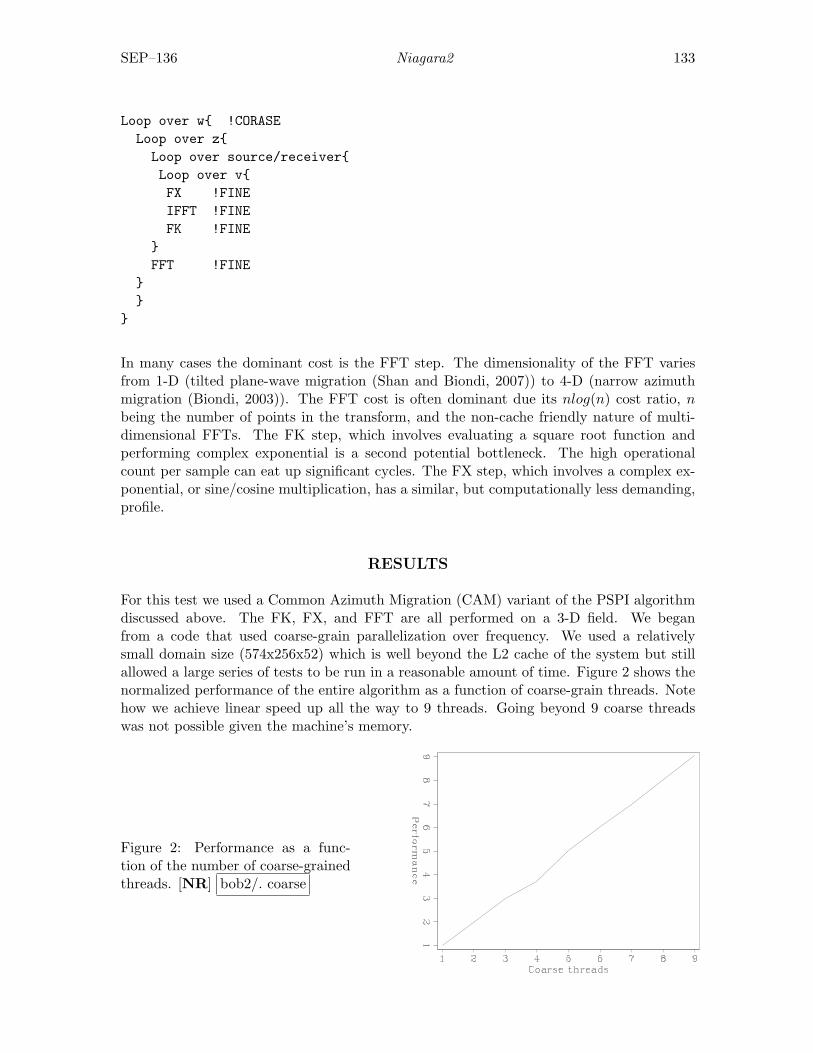
SEP–136 Niagara2 133
Loop over w{ !CORASELoop over z{
Loop over source/receiver{Loop over v{FX !FINEIFFT !FINEFK !FINE
}FFT !FINE
}}
}
In many cases the dominant cost is the FFT step. The dimensionality of the FFT variesfrom 1-D (tilted plane-wave migration (Shan and Biondi, 2007)) to 4-D (narrow azimuthmigration (Biondi, 2003)). The FFT cost is often dominant due its nlog(n) cost ratio, nbeing the number of points in the transform, and the non-cache friendly nature of multi-dimensional FFTs. The FK step, which involves evaluating a square root function andperforming complex exponential is a second potential bottleneck. The high operationalcount per sample can eat up significant cycles. The FX step, which involves a complex ex-ponential, or sine/cosine multiplication, has a similar, but computationally less demanding,profile.
RESULTS
For this test we used a Common Azimuth Migration (CAM) variant of the PSPI algorithmdiscussed above. The FK, FX, and FFT are all performed on a 3-D field. We beganfrom a code that used coarse-grain parallelization over frequency. We used a relativelysmall domain size (574x256x52) which is well beyond the L2 cache of the system but stillallowed a large series of tests to be run in a reasonable amount of time. Figure 2 shows thenormalized performance of the entire algorithm as a function of coarse-grain threads. Notehow we achieve linear speed up all the way to 9 threads. Going beyond 9 coarse threadswas not possible given the machine’s memory.
Figure 2: Performance as a func-tion of the number of coarse-grainedthreads. [NR] bob2/. coarse
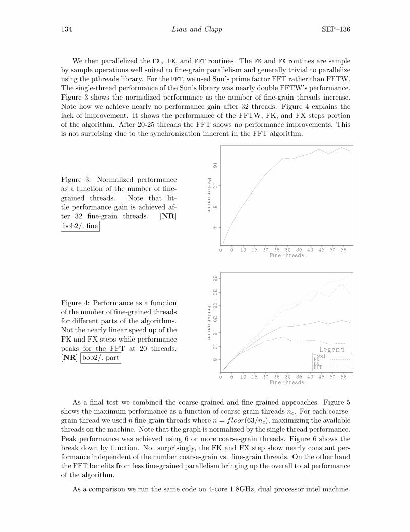
134 Liaw and Clapp SEP–136
We then parallelized the FX, FK, and FFT routines. The FK and FX routines are sampleby sample operations well suited to fine-grain parallelism and generally trivial to parallelizeusing the pthreads library. For the FFT, we used Sun’s prime factor FFT rather than FFTW.The single-thread performance of the Sun’s library was nearly double FFTW’s performance.Figure 3 shows the normalized performance as the number of fine-grain threads increase.Note how we achieve nearly no performance gain after 32 threads. Figure 4 explains thelack of improvement. It shows the performance of the FFTW, FK, and FX steps portionof the algorithm. After 20-25 threads the FFT shows no performance improvements. Thisis not surprising due to the synchronization inherent in the FFT algorithm.
Figure 3: Normalized performanceas a function of the number of fine-grained threads. Note that lit-tle performance gain is achieved af-ter 32 fine-grain threads. [NR]bob2/. fine
Figure 4: Performance as a functionof the number of fine-grained threadsfor different parts of the algorithms.Not the nearly linear speed up of theFK and FX steps while performancepeaks for the FFT at 20 threads.[NR] bob2/. part
As a final test we combined the coarse-grained and fine-grained approaches. Figure 5shows the maximum performance as a function of coarse-grain threads nc. For each coarse-grain thread we used n fine-grain threads where n = floor(63/nc), maximizing the availablethreads on the machine. Note that the graph is normalized by the single thread performance.Peak performance was achieved using 6 or more coarse-grain threads. Figure 6 shows thebreak down by function. Not surprisingly, the FK and FX step show nearly constant per-formance independent of the number coarse-grain vs. fine-grain threads. On the other handthe FFT benefits from less fine-grained parallelism bringing up the overall total performanceof the algorithm.
As a comparison we run the same code on 4-core 1.8GHz, dual processor intel machine.
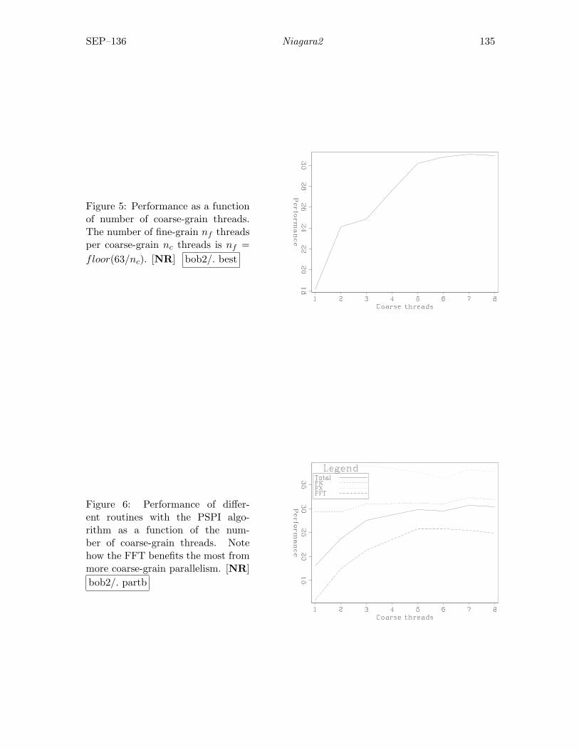
SEP–136 Niagara2 135
Figure 5: Performance as a functionof number of coarse-grain threads.The number of fine-grain nf threadsper coarse-grain nc threads is nf =floor(63/nc). [NR] bob2/. best
Figure 6: Performance of differ-ent routines with the PSPI algo-rithm as a function of the num-ber of coarse-grain threads. Notehow the FFT benefits the most frommore coarse-grain parallelism. [NR]bob2/. partb

136 Liaw and Clapp SEP–136
Running 8 coarse-grain threads and normalizing in terms of the the Niagara2 single threadresults we found:
Segment Relative speedFFT 23.9FX 10.9FK 61.8Total 23.9
In general the code scaled linearly with number of processors.The FX ratio was low comparedto the Niagara because of the significant memory requests (due to the velocity correction),something that the Niagara2 archetecture is well designed for. The FK number was largedue to the vector nature of the computation and its high floating point operation count.
Improving the floating point and vector potential of the Niagara architecture could havea large impact on these results. Both the FFT and the FK steps involve significant floatingpoint computations. The synchronization requirements of the FFT algorithm limits effectivescaling to approximately 16 threads even for large volumes.
CONCLUSIONS
We implemented PSPI migration on the Sun Niagara2 by combining coarse-grained and fine-grained prallelism. We showed that the multi-thread per core model leads to significantuplift in performance over a single thread approach. Compared to a strictly fine grainparallelism we achieved a 60% uplift. Compared to a coarse grain approach the improvementwas 5X. Improved floating point/vector performance could lead to signficant uplift for thisaglorithm.
REFERENCES
Biondi, B., 2003, Narrow azimuth migration of marine streamer data: SEG, ExpandedAbstracts, 22, 897–900.
Biondi, B. and G. Palacharla, 1996, 3-d prestack migration of common-azimuth data: Geo-physics, 1822–1832, Soc. of Expl. Geophys.
Claerbout, J. F., 1995, Basic Earth Imaging: Stanford Exploration Project.Pell, O., T. Nemeth, J. Stefani, and R. Ergas, 2008, Design space analysis for the acoustic
wave equation implementation on fpga circuits: European Association of Geoscientistsand Engineers, Expanded Abstracts, 1406–1409.
Shan, G. and B. Biondi, 2007, Angle domain common image gathers for steep reflectors:2007, 131, 33–46.
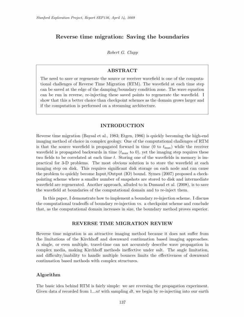
Stanford Exploration Project, Report SEP136, April 14, 2009
Reverse time migration: Saving the boundaries
Robert G. Clapp
ABSTRACT
The need to save or regenerate the source or receiver wavefield is one of the computa-tional challenges of Reverse Time Migration (RTM). The wavefield at each time stepcan be saved at the edge of the damping/boundary condition zone. The wave equationcan be run in reverse, re-injecting these saved points to regenerate the wavefield. Ishow that this a better choice than checkpoint schemes as the domain grows larger andif the computation is performed on a streaming architecture.
INTRODUCTION
Reverse time migration (Baysal et al., 1983; Etgen, 1986) is quickly becoming the high-endimaging method of choice in complex geology. One of the computational challenges of RTMis that the source wavefield is propagated forward in time (0 to tmax) while the receiverwavefield is propagated backwards in time (tmax to 0), yet the imaging step requires thesetwo fields to be correlated at each time t. Storing one of the wavefields in memory is im-practical for 3-D problems. The most obvious solution is to store the wavefield at eachimaging step on disk. This requires significant disk storage on each node and can causethe problem to quickly become Input/Output (IO) bound. Symes (2007) proposed a check-pointing scheme where a smaller number of snapshots are stored to disk and intermediatewavefield are regenerated. Another approach, alluded to in Dussaud et al. (2008), is to savethe wavefield at boundaries of the computational domain and to re-inject them.
In this paper, I demonstrate how to implement a boundary re-injection scheme. I discussthe computational tradeoffs of boundary re-injection vs. a checkpoint scheme and concludethat, as the computational domain increases in size, the boundary method proves superior.
REVERSE TIME MIGRATION REVIEW
Reverse time migration is an attractive imaging method because it does not suffer fromthe limitations of the Kirchhoff and downward continuation based imaging approaches.A single, or even multiple, travel-time can not accurately describe wave propagation incomplex media, making Kirchhoff methods ineffective under salt. The angle limitation,and difficulty/inability to handle multiple bounces limits the effectiveness of downwardcontinuation based methods with complex structures.
Algorithm
The basic idea behind RTM is fairly simple: we are reversing the propagation experiment.Given data d recorded from 1...nt with sampling dt, we begin by re-injecting into our earth
137
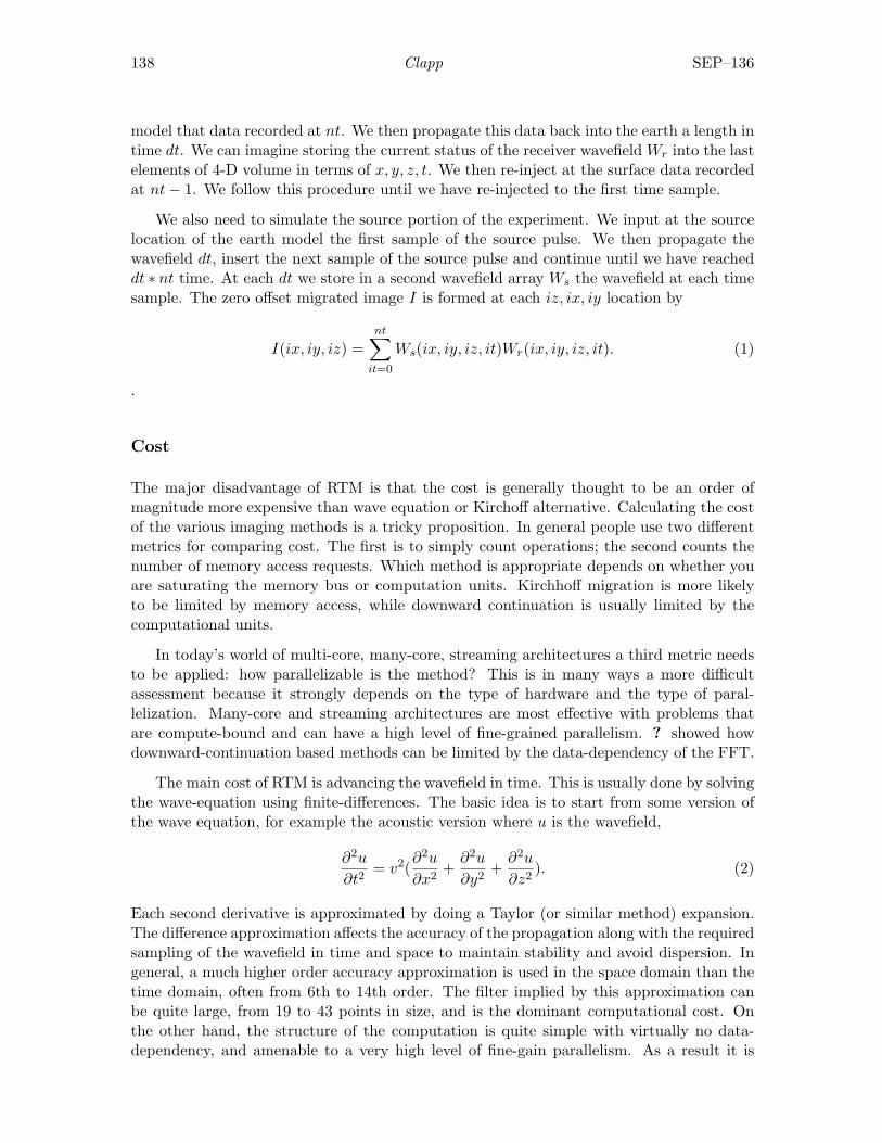
138 Clapp SEP–136
model that data recorded at nt. We then propagate this data back into the earth a length intime dt. We can imagine storing the current status of the receiver wavefield Wr into the lastelements of 4-D volume in terms of x, y, z, t. We then re-inject at the surface data recordedat nt− 1. We follow this procedure until we have re-injected to the first time sample.
We also need to simulate the source portion of the experiment. We input at the sourcelocation of the earth model the first sample of the source pulse. We then propagate thewavefield dt, insert the next sample of the source pulse and continue until we have reacheddt ∗ nt time. At each dt we store in a second wavefield array Ws the wavefield at each timesample. The zero offset migrated image I is formed at each iz, ix, iy location by
I(ix, iy, iz) =nt∑
it=0
Ws(ix, iy, iz, it)Wr(ix, iy, iz, it). (1)
.
Cost
The major disadvantage of RTM is that the cost is generally thought to be an order ofmagnitude more expensive than wave equation or Kirchoff alternative. Calculating the costof the various imaging methods is a tricky proposition. In general people use two differentmetrics for comparing cost. The first is to simply count operations; the second counts thenumber of memory access requests. Which method is appropriate depends on whether youare saturating the memory bus or computation units. Kirchhoff migration is more likelyto be limited by memory access, while downward continuation is usually limited by thecomputational units.
In today’s world of multi-core, many-core, streaming architectures a third metric needsto be applied: how parallelizable is the method? This is in many ways a more difficultassessment because it strongly depends on the type of hardware and the type of paral-lelization. Many-core and streaming architectures are most effective with problems thatare compute-bound and can have a high level of fine-grained parallelism. ? showed howdownward-continuation based methods can be limited by the data-dependency of the FFT.
The main cost of RTM is advancing the wavefield in time. This is usually done by solvingthe wave-equation using finite-differences. The basic idea is to start from some version ofthe wave equation, for example the acoustic version where u is the wavefield,
∂2u
∂t2= v2(
∂2u
∂x2+
∂2u
∂y2+
∂2u
∂z2). (2)
Each second derivative is approximated by doing a Taylor (or similar method) expansion.The difference approximation affects the accuracy of the propagation along with the requiredsampling of the wavefield in time and space to maintain stability and avoid dispersion. Ingeneral, a much higher order accuracy approximation is used in the space domain than thetime domain, often from 6th to 14th order. The filter implied by this approximation canbe quite large, from 19 to 43 points in size, and is the dominant computational cost. Onthe other hand, the structure of the computation is quite simple with virtually no data-dependency, and amenable to a very high level of fine-gain parallelism. As a result it is
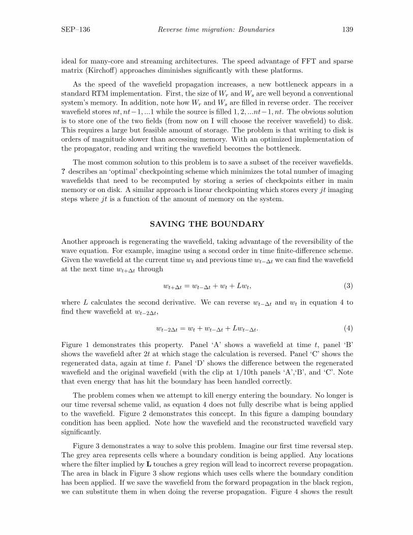
SEP–136 Reverse time migration: Boundaries 139
ideal for many-core and streaming architectures. The speed advantage of FFT and sparsematrix (Kirchoff) approaches diminishes significantly with these platforms.
As the speed of the wavefield propagation increases, a new bottleneck appears in astandard RTM implementation. First, the size of Wr and Ws are well beyond a conventionalsystem’s memory. In addition, note how Wr and Ws are filled in reverse order. The receiverwavefield stores nt, nt−1, ...1 while the source is filled 1, 2, ...nt−1, nt. The obvious solutionis to store one of the two fields (from now on I will choose the receiver wavefield) to disk.This requires a large but feasible amount of storage. The problem is that writing to disk isorders of magnitude slower than accessing memory. With an optimized implementation ofthe propagator, reading and writing the wavefield becomes the bottleneck.
The most common solution to this problem is to save a subset of the receiver wavefields.? describes an ‘optimal’ checkpointing scheme which minimizes the total number of imagingwavefields that need to be recomputed by storing a series of checkpoints either in mainmemory or on disk. A similar approach is linear checkpointing which stores every jt imagingsteps where jt is a function of the amount of memory on the system.
SAVING THE BOUNDARY
Another approach is regenerating the wavefield, taking advantage of the reversibility of thewave equation. For example, imagine using a second order in time finite-difference scheme.Given the wavefield at the current time wt and previous time wt−∆t we can find the wavefieldat the next time wt+∆t through
wt+∆t = wt−∆t + wt + Lwt, (3)
where L calculates the second derivative. We can reverse wt−∆t and wt in equation 4 tofind thew wavefield at wt−2∆t,
wt−2∆t = wt + wt−∆t + Lwt−∆t. (4)
Figure 1 demonstrates this property. Panel ‘A’ shows a wavefield at time t, panel ‘B’shows the wavefield after 2t at which stage the calculation is reversed. Panel ‘C’ shows theregenerated data, again at time t. Panel ‘D’ shows the difference between the regeneratedwavefield and the original wavefield (with the clip at 1/10th panels ‘A’,‘B’, and ‘C’. Notethat even energy that has hit the boundary has been handled correctly.
The problem comes when we attempt to kill energy entering the boundary. No longer isour time reversal scheme valid, as equation 4 does not fully describe what is being appliedto the wavefield. Figure 2 demonstrates this concept. In this figure a damping boundarycondition has been applied. Note how the wavefield and the reconstructed wavefield varysignificantly.
Figure 3 demonstrates a way to solve this problem. Imagine our first time reversal step.The grey area represents cells where a boundary condition is being applied. Any locationswhere the filter implied by L touches a grey region will lead to incorrect reverse propagation.The area in black in Figure 3 show regions which uses cells where the boundary conditionhas been applied. If we save the wavefield from the forward propagation in the black region,we can substitute them in when doing the reverse propagation. Figure 4 shows the result
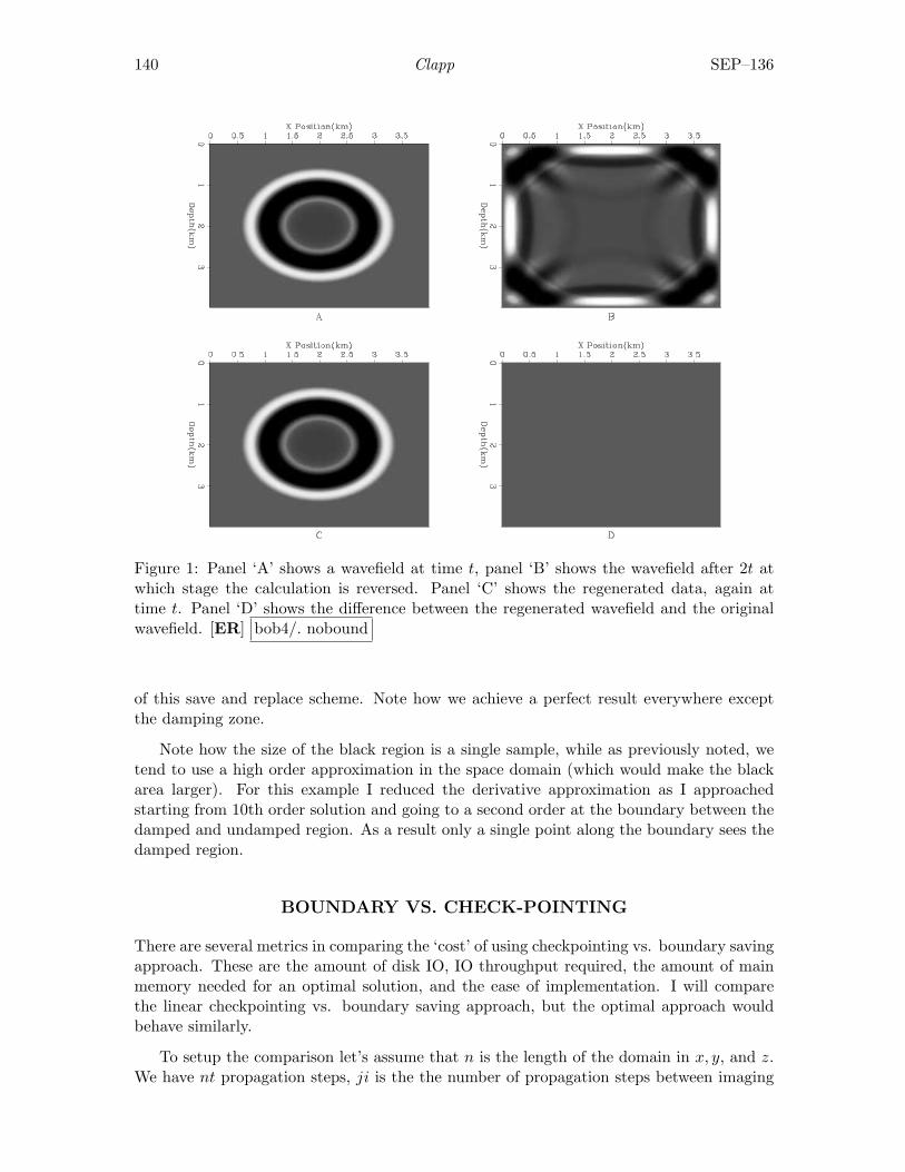
140 Clapp SEP–136
Figure 1: Panel ‘A’ shows a wavefield at time t, panel ‘B’ shows the wavefield after 2t atwhich stage the calculation is reversed. Panel ‘C’ shows the regenerated data, again attime t. Panel ‘D’ shows the difference between the regenerated wavefield and the originalwavefield. [ER] bob4/. nobound
of this save and replace scheme. Note how we achieve a perfect result everywhere exceptthe damping zone.
Note how the size of the black region is a single sample, while as previously noted, wetend to use a high order approximation in the space domain (which would make the blackarea larger). For this example I reduced the derivative approximation as I approachedstarting from 10th order solution and going to a second order at the boundary between thedamped and undamped region. As a result only a single point along the boundary sees thedamped region.
BOUNDARY VS. CHECK-POINTING
There are several metrics in comparing the ‘cost’ of using checkpointing vs. boundary savingapproach. These are the amount of disk IO, IO throughput required, the amount of mainmemory needed for an optimal solution, and the ease of implementation. I will comparethe linear checkpointing vs. boundary saving approach, but the optimal approach wouldbehave similarly.
To setup the comparison let’s assume that n is the length of the domain in x, y, and z.We have nt propagation steps, ji is the the number of propagation steps between imaging
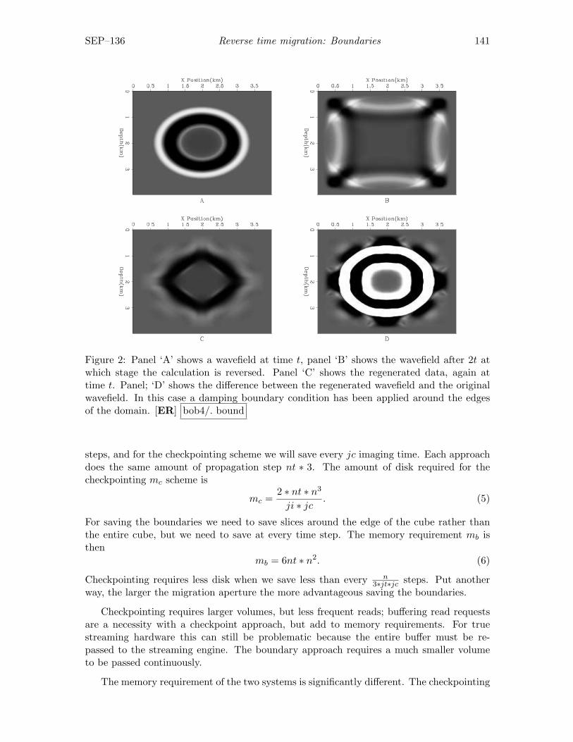
SEP–136 Reverse time migration: Boundaries 141
Figure 2: Panel ‘A’ shows a wavefield at time t, panel ‘B’ shows the wavefield after 2t atwhich stage the calculation is reversed. Panel ‘C’ shows the regenerated data, again attime t. Panel; ‘D’ shows the difference between the regenerated wavefield and the originalwavefield. In this case a damping boundary condition has been applied around the edgesof the domain. [ER] bob4/. bound
steps, and for the checkpointing scheme we will save every jc imaging time. Each approachdoes the same amount of propagation step nt ∗ 3. The amount of disk required for thecheckpointing mc scheme is
mc =2 ∗ nt ∗ n3
ji ∗ jc. (5)
For saving the boundaries we need to save slices around the edge of the cube rather thanthe entire cube, but we need to save at every time step. The memory requirement mb isthen
mb = 6nt ∗ n2. (6)
Checkpointing requires less disk when we save less than every n3∗jt∗jc steps. Put another
way, the larger the migration aperture the more advantageous saving the boundaries.
Checkpointing requires larger volumes, but less frequent reads; buffering read requestsare a necessity with a checkpoint approach, but add to memory requirements. For truestreaming hardware this can still be problematic because the entire buffer must be re-passed to the streaming engine. The boundary approach requires a much smaller volumeto be passed continuously.
The memory requirement of the two systems is significantly different. The checkpointing
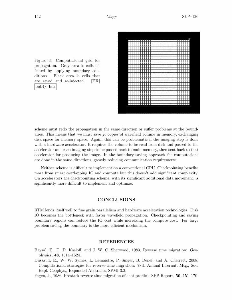
142 Clapp SEP–136
Figure 3: Computational grid forpropagation. Grey area is cells ef-fected by applying boundary con-ditions. Black area is cells thatare saved and re-injected. [ER]bob4/. box
scheme must redo the propagation in the same direction or suffer problems at the bound-aries. This means that we must save jc copies of wavefield volume in memory, exchangingdisk space for memory space. Again, this can be problematic if the imaging step is donewith a hardware accelerator. It requires the volume to be read from disk and passed to theaccelerator and each imaging step to be passed back to main memory, then sent back to thataccelerator for producing the image. In the boundary saving approach the computationsare done in the same directions, greatly reducing communication requirements.
Neither scheme is difficult to implement on a conventional CPU. Checkpointing benefitsmore from smart overlapping IO and compute but this doesn’t add significant complexity.On accelerators the checkpointing scheme, with its significant additional data movement, issignificantly more difficult to implement and optimize.
CONCLUSIONS
RTM lends itself well to fine grain parallelism and hardware acceleration technologies. DiskIO becomes the bottleneck with faster wavefield propagation. Checkpointing and savingboundary regions can reduce the IO cost while increasing the compute cost. For largeproblem saving the boundary is the more efficient mechanism.
REFERENCES
Baysal, E., D. D. Kosloff, and J. W. C. Sherwood, 1983, Reverse time migration: Geo-physics, 48, 1514–1524.
Dussaud, E., W. W. Symes, L. Lemaistre, P. Singer, B. Denel, and A. Cherrett, 2008,Computational strategies for reverse-time migration: 78th Annual Internat. Mtg., Soc.Expl. Geophys., Expanded Abstracts, SPMI 3.3.
Etgen, J., 1986, Prestack reverse time migration of shot profiles: SEP-Report, 50, 151–170.
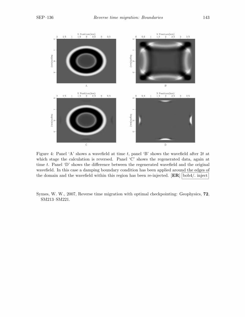
SEP–136 Reverse time migration: Boundaries 143
Figure 4: Panel ‘A’ shows a wavefield at time t, panel ‘B’ shows the wavefield after 2t atwhich stage the calculation is reversed. Panel ‘C’ shows the regenerated data, again attime t. Panel ‘D’ shows the difference between the regenerated wavefield and the originalwavefield. In this case a damping boundary condition has been applied around the edges ofthe domain and the wavefield within this region has been re-injected. [ER] bob4/. inject
Symes, W. W., 2007, Reverse time migration with optimal checkpointing: Geophysics, 72,SM213–SM221.

144 Clapp SEP–136
Stanford Exploration Project, Report SEP136, April 14, 2009
Angle-domain common-image gathers in generalizedcoordinates
Jeff Shragge
ABSTRACT
The theory of angle-domain common-image gathers (ADCIGs) is extended to migra-tions performed in generalized 2D coordinate systems. I develop an expression link-ing the definition of reflection opening angle to various generalized geometric factors.I demonstrate that generalized coordinate ADCIGs can be calculated directly usingFourier-based offset-to-angle approaches for coordinate systems satisfying the Cauchy-Riemann differentiability criteria. The canonical examples of tilted Cartesian, polar,and elliptic coordinates are used to illustrate the ADCIG theory. I compare analyti-cally and numerically generated image volumes for a set of elliptically shaped reflec-tors. Experiments with a synthetic data set illustrate that elliptic-coordinate ADCIGsbetter-resolve the reflection opening angles of steeply dipping structure, relative toconventional Cartesian image volumes, due to improved large-angle propagation andenhanced sensitivity to steep structural dips afforded by coordinate system transfor-mations.
INTRODUCTION
Angle-domain common-image gathers (ADCIGs) are used increasingly in seismic imagingto examine migration velocity model accuracy (?). The key idea is that migrating with thecorrect velocity model leads to flat angle gathers that shift neither vertically nor horizontallyas a function of reflection opening angle. Migrating with an incorrect velocity, though, leadsto inconsistent angle-domain reflectivity and generates residual curvature in the ADCIGvolume. ADCIGs are thus an effective velocity analysis tool and have been incorporated inwave-equation-based inversion schemes to update velocity profiles (??).
Wave-equation imaging techniques generate ADCIGs in straightforward manners forboth shot-profile (???) and shot-geophone (??) migration approaches. In shot-profilemigration, one first generates a subsurface-offset axis at each depth step by correlatingthe source and receiver wavefields at a number of subsurface shifts. The second step in-volves computing an offset-to-angle domain transformation using, for example, post-imagingFourier-based operators (?).
Conventional ADCIG theory usually assumes horizontal wavefield shifts, largely be-cause wavefield extrapolation and imaging are most commonly performed in Cartesian co-ordinates. However, a number of studies have noted that these ADCIG results degradefor steeply dipping structures, such as salt flanks (??). Although this is partially due toproblems associated with inaccurate large-angle extrapolation, ADCIGs calculated usinghorizontal wavefield shifts become decreasingly sensitive for increasingly steep structuraldips. ? demonstrate that this problem can be addressed by generating ADCIGs with ver-tical subsurface-offset-domain common-image gathers (VODCIGs); however, this approach
145
146 Shragge SEP–136
is less desirable computationally because it requires storing the larger wavefield volumesrequired to calculate the VODCIGs in memory.
The introduction of shot-profile migration in more general coordinate systems [e.g. tiltedCartesian (?) and elliptic meshes (?)] presents an opportunity to circumvent problems as-sociated with generating ADCIGs for steeply dipping structure. In particular, migrationdomains can be oriented such that geologic structures with steep dips in Cartesian mesheshave relatively gentle dip in generalized coordinate systems, thus improving the robustnessof the ADCIG calculation. Developing an ADCIG theory capable of handling more arbi-trary coordinate meshes, though, requires proper treatment of the effects of non-Cartesiangeometries. For example, wavefield extrapolation in non-Cartesian coordinate systems in-duces local wavenumber stretches, rotations and/or shearing (?). Similarly, non-uniformwavefield sampling can lead to anisotropic angle-domain stretching. These effects can becorrected using Jacobian change-of-variable transformations.
The goal of this paper is to extend ADCIG theory to non-Cartesian geometries. Idemonstrate that ADCIG theory, as developed in a differential sense (?), remains validfor arbitrary geometries provided that the corresponding derivative operators are properlyspecified. Non-Cartesian coordinates do, however, introduce space-domain geometric fac-tors that can render Fourier-based offset-to-angle methods unsuitable. However, I showthat ADCIGs can be calculated directly in the Fourier domain for all coordinate systemssatisfying the Cauchy-Riemann differentiability criteria (?). Moreover, ADCIGs can becalculated in all situations using the slant-stack approaches discussed in ?.
I begin by discussing how to generate subsurface offsets and ADCIGs in Cartesian coor-dinates. I then provide an extension to generalized coordinate systems based on Jacobianchange-of-variable arguments. I examine two canonical coordinate systems, tilted Cartesianand elliptic meshes, where the reflection angle can be explicitly calculated using Fourier-based methods, and a third, polar coordinates, where it cannot. I test the generalizedADCIG theory analytically and numerically using a set of elliptic reflectors, and demon-strate how computing angle gathers in elliptic coordinates can lead to improvements relativeto Cartesian coordinates, especially for steeply dipping structure.
ADCIG THEORY
The ADCIG theory presented in this section draws from that presented in ?. In the ensuingdevelopment, x = [x1, x3] denotes the Cartesian variables and ξ = [ξ1, ξ3] represents ageneralized Riemannian coordinate system. I also use a convention where the extrapolationaxis is oriented in the x3 (ξ3) direction for Cartesian (Riemannian) coordinates. Coordinatesx2 = ξ2 = 0 are assumed throughout.
Generating subsurface offsets axes
Shot-profile migration in Cartesian coordinates consists of completing a recursive two-stepprocedure. The first step involves propagating the source and receiver wavefields, S and R,
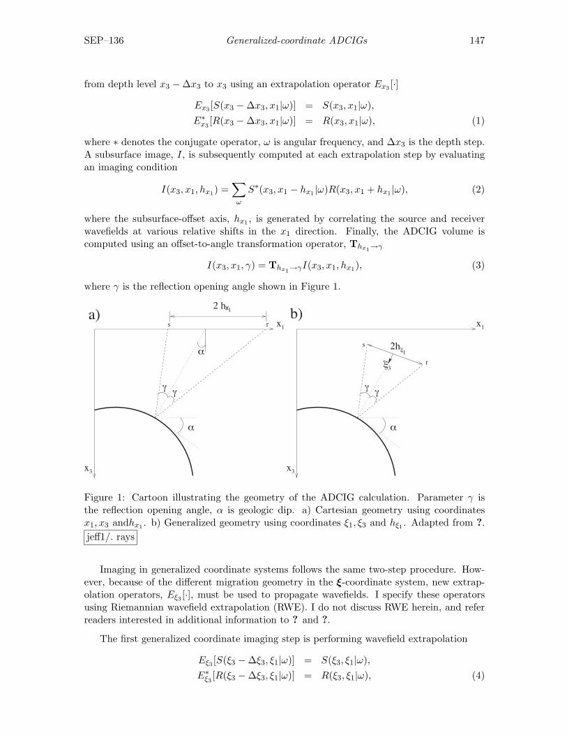
SEP–136 Generalized-coordinate ADCIGs 147
from depth level x3 −∆x3 to x3 using an extrapolation operator Ex3 [·]
Ex3 [S(x3 −∆x3, x1|ω)] = S(x3, x1|ω),E∗
x3[R(x3 −∆x3, x1|ω)] = R(x3, x1|ω), (1)
where ∗ denotes the conjugate operator, ω is angular frequency, and ∆x3 is the depth step.A subsurface image, I, is subsequently computed at each extrapolation step by evaluatingan imaging condition
I(x3, x1, hx1) =∑ω
S∗(x3, x1 − hx1 |ω)R(x3, x1 + hx1 |ω), (2)
where the subsurface-offset axis, hx1 , is generated by correlating the source and receiverwavefields at various relative shifts in the x1 direction. Finally, the ADCIG volume iscomputed using an offset-to-angle transformation operator, Thx1→γ
I(x3, x1, γ) = Thx1→γI(x3, x1, hx1), (3)
where γ is the reflection opening angle shown in Figure 1.
x
α
γγ
3
x1
s
r
2hξ1
2 h
x
α
α
γγ
3
1
rs x1
ξ3
b)a) x
Figure 1: Cartoon illustrating the geometry of the ADCIG calculation. Parameter γ isthe reflection opening angle, α is geologic dip. a) Cartesian geometry using coordinatesx1, x3 andhx1 . b) Generalized geometry using coordinates ξ1, ξ3 and hξ1 . Adapted from ?.jeff1/. rays
Imaging in generalized coordinate systems follows the same two-step procedure. How-ever, because of the different migration geometry in the ξ-coordinate system, new extrap-olation operators, Eξ3 [·], must be used to propagate wavefields. I specify these operatorsusing Riemannian wavefield extrapolation (RWE). I do not discuss RWE herein, and referreaders interested in additional information to ? and ?.
The first generalized coordinate imaging step is performing wavefield extrapolation
Eξ3 [S(ξ3 −∆ξ3, ξ1|ω)] = S(ξ3, ξ1|ω),E∗
ξ3 [R(ξ3 −∆ξ3, ξ1|ω)] = R(ξ3, ξ1|ω), (4)
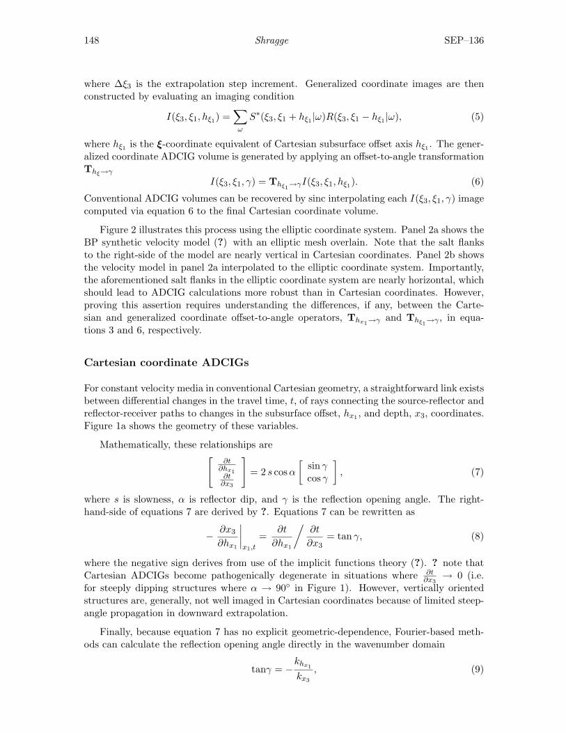
148 Shragge SEP–136
where ∆ξ3 is the extrapolation step increment. Generalized coordinate images are thenconstructed by evaluating an imaging condition
I(ξ3, ξ1, hξ1) =∑ω
S∗(ξ3, ξ1 + hξ1 |ω)R(ξ3, ξ1 − hξ1 |ω), (5)
where hξ1 is the ξ-coordinate equivalent of Cartesian subsurface offset axis hξ1 . The gener-alized coordinate ADCIG volume is generated by applying an offset-to-angle transformationThξ→γ
I(ξ3, ξ1, γ) = Thξ1→γI(ξ3, ξ1, hξ1). (6)
Conventional ADCIG volumes can be recovered by sinc interpolating each I(ξ3, ξ1, γ) imagecomputed via equation 6 to the final Cartesian coordinate volume.
Figure 2 illustrates this process using the elliptic coordinate system. Panel 2a shows theBP synthetic velocity model (?) with an elliptic mesh overlain. Note that the salt flanksto the right-side of the model are nearly vertical in Cartesian coordinates. Panel 2b showsthe velocity model in panel 2a interpolated to the elliptic coordinate system. Importantly,the aforementioned salt flanks in the elliptic coordinate system are nearly horizontal, whichshould lead to ADCIG calculations more robust than in Cartesian coordinates. However,proving this assertion requires understanding the differences, if any, between the Carte-sian and generalized coordinate offset-to-angle operators, Thx1→γ and Thξ1
→γ , in equa-tions 3 and 6, respectively.
Cartesian coordinate ADCIGs
For constant velocity media in conventional Cartesian geometry, a straightforward link existsbetween differential changes in the travel time, t, of rays connecting the source-reflector andreflector-receiver paths to changes in the subsurface offset, hx1 , and depth, x3, coordinates.Figure 1a shows the geometry of these variables.
Mathematically, these relationships are[∂t
∂hx1∂t
∂x3
]= 2 s cos α
[sin γcos γ
], (7)
where s is slowness, α is reflector dip, and γ is the reflection opening angle. The right-hand-side of equations 7 are derived by ?. Equations 7 can be rewritten as
− ∂x3
∂hx1
∣∣∣∣x1,t
=∂t
∂hx1
/∂t
∂x3= tan γ, (8)
where the negative sign derives from use of the implicit functions theory (?). ? note thatCartesian ADCIGs become pathogenically degenerate in situations where ∂t
∂x3→ 0 (i.e.
for steeply dipping structures where α → 90◦ in Figure 1). However, vertically orientedstructures are, generally, not well imaged in Cartesian coordinates because of limited steep-angle propagation in downward extrapolation.
Finally, because equation 7 has no explicit geometric-dependence, Fourier-based meth-ods can calculate the reflection opening angle directly in the wavenumber domain
tanγ = −khx1
kx3
, (9)
SEP–136 Generalized-coordinate ADCIGs 149
Figure 2: Prestack migration test in elliptic coordinates. a) Benchmark synthetic velocitymodel with an overlying elliptic coordinate system. b) Effective slowness model in thetransformed elliptic coordinate system in a). c) Benchmark synthetic velocity model witha different overlying elliptic coordinate system. d) Effective elliptic coordinate slownessmodel for the coordinate system in c). jeff1/. RC2
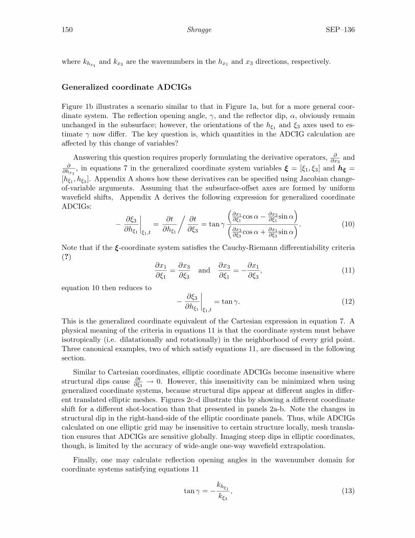
150 Shragge SEP–136
where khx1and kx3 are the wavenumbers in the hx1 and x3 directions, respectively.
Generalized coordinate ADCIGs
Figure 1b illustrates a scenario similar to that in Figure 1a, but for a more general coor-dinate system. The reflection opening angle, γ, and the reflector dip, α, obviously remainunchanged in the subsurface; however, the orientations of the hξ1 and ξ3 axes used to es-timate γ now differ. The key question is, which quantities in the ADCIG calculation areaffected by this change of variables?
Answering this question requires properly formulating the derivative operators, ∂∂x3
and∂
∂hx1, in equations 7 in the generalized coordinate system variables ξ = [ξ1, ξ3] and hξ =
[hξ1 , hξ3 ]. Appendix A shows how these derivatives can be specified using Jacobian change-of-variable arguments. Assuming that the subsurface-offset axes are formed by uniformwavefield shifts, Appendix A derives the following expression for generalized coordinateADCIGs:
− ∂ξ3
∂hξ1
∣∣∣∣ξ1,t
=∂t
∂hξ1
/∂t
∂ξ3= tan γ
(∂x1∂ξ1
cos α− ∂x3∂ξ1
sinα)
(∂x3∂ξ3
cos α + ∂x1∂ξ3
sinα) . (10)
Note that if the ξ-coordinate system satisfies the Cauchy-Riemann differentiability criteria(?)
∂x1
∂ξ1=
∂x3
∂ξ3and
∂x3
∂ξ1= −∂x1
∂ξ3, (11)
equation 10 then reduces to
− ∂ξ3
∂hξ1
∣∣∣∣ξ1,t
= tan γ. (12)
This is the generalized coordinate equivalent of the Cartesian expression in equation 7. Aphysical meaning of the criteria in equations 11 is that the coordinate system must behaveisotropically (i.e. dilatationally and rotationally) in the neighborhood of every grid point.Three canonical examples, two of which satisfy equations 11, are discussed in the followingsection.
Similar to Cartesian coordinates, elliptic coordinate ADCIGs become insensitive wherestructural dips cause ∂t
∂ξ3→ 0. However, this insensitivity can be minimized when using
generalized coordinate systems, because structural dips appear at different angles in differ-ent translated elliptic meshes. Figures 2c-d illustrate this by showing a different coordinateshift for a different shot-location than that presented in panels 2a-b. Note the changes instructural dip in the right-hand-side of the elliptic coordinate panels. Thus, while ADCIGscalculated on one elliptic grid may be insensitive to certain structure locally, mesh transla-tion ensures that ADCIGs are sensitive globally. Imaging steep dips in elliptic coordinates,though, is limited by the accuracy of wide-angle one-way wavefield extrapolation.
Finally, one may calculate reflection opening angles in the wavenumber domain forcoordinate systems satisfying equations 11
tan γ = −khξ1
kξ3
, (13)
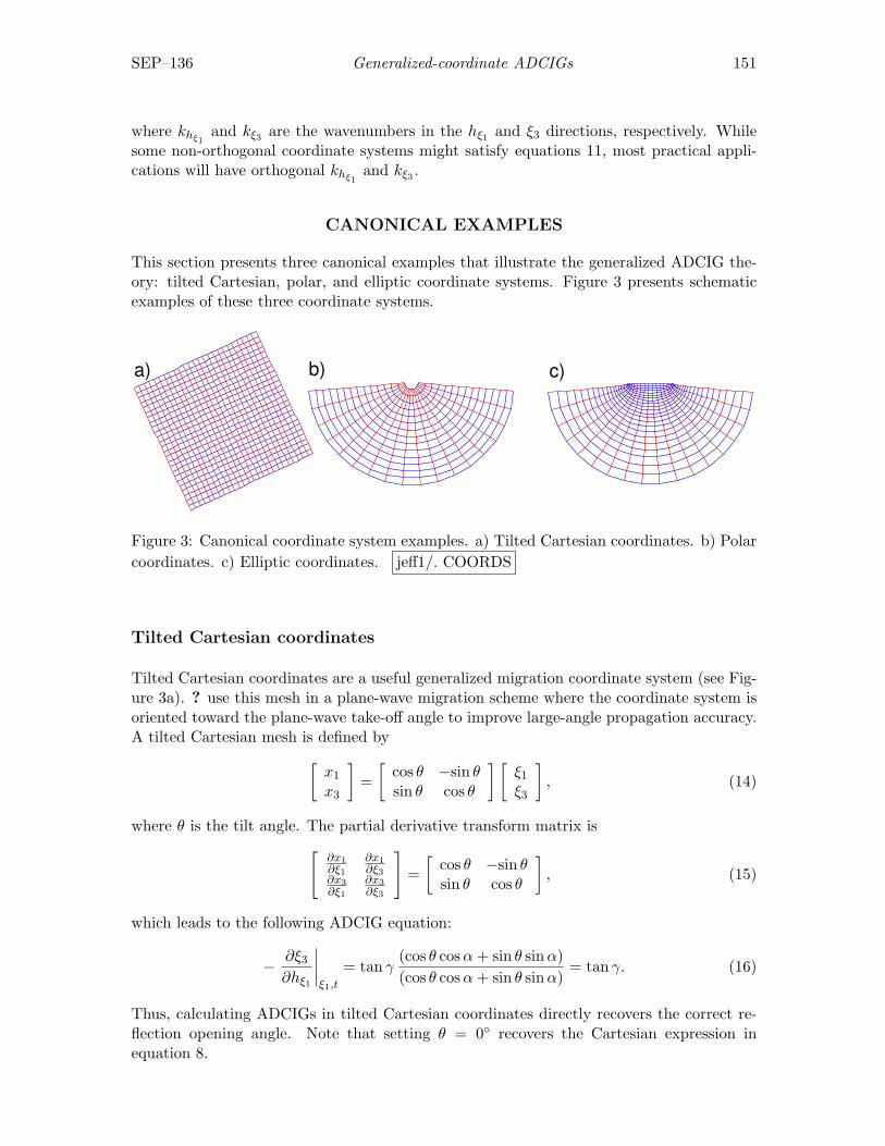
SEP–136 Generalized-coordinate ADCIGs 151
where khξ1and kξ3 are the wavenumbers in the hξ1 and ξ3 directions, respectively. While
some non-orthogonal coordinate systems might satisfy equations 11, most practical appli-cations will have orthogonal khξ1
and kξ3 .
CANONICAL EXAMPLES
This section presents three canonical examples that illustrate the generalized ADCIG the-ory: tilted Cartesian, polar, and elliptic coordinate systems. Figure 3 presents schematicexamples of these three coordinate systems.
a) b) c)
Figure 3: Canonical coordinate system examples. a) Tilted Cartesian coordinates. b) Polarcoordinates. c) Elliptic coordinates. jeff1/. COORDS
Tilted Cartesian coordinates
Tilted Cartesian coordinates are a useful generalized migration coordinate system (see Fig-ure 3a). ? use this mesh in a plane-wave migration scheme where the coordinate system isoriented toward the plane-wave take-off angle to improve large-angle propagation accuracy.A tilted Cartesian mesh is defined by[
x1
x3
]=[
cos θ −sin θsin θ cos θ
] [ξ1
ξ3
], (14)
where θ is the tilt angle. The partial derivative transform matrix is[∂x1∂ξ1
∂x1∂ξ3
∂x3∂ξ1
∂x3∂ξ3
]=[
cos θ −sin θsin θ cos θ
], (15)
which leads to the following ADCIG equation:
− ∂ξ3
∂hξ1
∣∣∣∣ξ1,t
= tan γ(cos θ cos α + sin θ sinα)(cos θ cos α + sin θ sinα)
= tan γ. (16)
Thus, calculating ADCIGs in tilted Cartesian coordinates directly recovers the correct re-flection opening angle. Note that setting θ = 0◦ recovers the Cartesian expression inequation 8.

152 Shragge SEP–136
Polar coordinates
The polar coordinate system (see Figure 3b), where the extrapolation direction is orientedalong the radial direction, is appropriate for generating 2D Green’s function estimates. Thepolar coordinate system is defined by[
x1
x3
]=[
a ξ3 cos ξ1
a ξ3 sin ξ1
]. (17)
The partial derivative transformation matrix is[∂x1∂ξ1
∂x1∂ξ3
∂x3∂ξ1
∂x3∂ξ3
]=[−a ξ3 sin ξ1 a cos ξ1
a ξ3 cos ξ1 a sin ξ1
], (18)
which leads to the following ADCIG equation:
− ∂ξ3
∂hξ1
∣∣∣∣ξ1,t
= ξ3 tan γ(−sin ξ1 cos α− cos ξ1 sinα)(sin ξ1cos α + cos ξ1 sin, α)
= −ξ3 tan γ. (19)
Thus, one cannot calculate ADCIGs directly with Fourier-based methods in polar coor-dinates because of the spatial geometric dependence on ξ3. However, polar-coordinateADCIGs can be calculated using slant-stack operators (?), because the geometric factor ξ3
is no more than a local weight applied to the velocity model used to calculate the anglegathers.
Elliptic coordinates
Elliptic coordinates (see Figure 3c) are a useful coordinate system for performing 2D shot-profile migration (?). An elliptic mesh is defined by[
x1
x3
]=[
a cosh ξ3 cos ξ1
a sinh ξ3 sin ξ1
]. (20)
The partial derivative transformation matrix is[∂x1∂ξ1
∂x1∂ξ3
∂x3∂ξ1
∂x3∂ξ3
]= a
[cosh ξ3 sin ξ1 sinh ξ3 cos ξ1
−sinh ξ3 cos ξ1 cosh ξ3 sin ξ1
], (21)
which leads to the following ADCIG equation:
− ∂ξ3
∂hξ1
∣∣∣∣ξ1,t
= tan γ(cosh ξ3 sin ξ1 cos α− sinh ξ3 cos ξ1 sinα)(cosh ξ3 sin ξ1 cos α− sinh ξ3 cos ξ1 sinα)
= tan γ. (22)
Thus, calculating ADCIGs in elliptic coordinates with Fourier-based methods will di-rectly recover the true reflection opening angle.
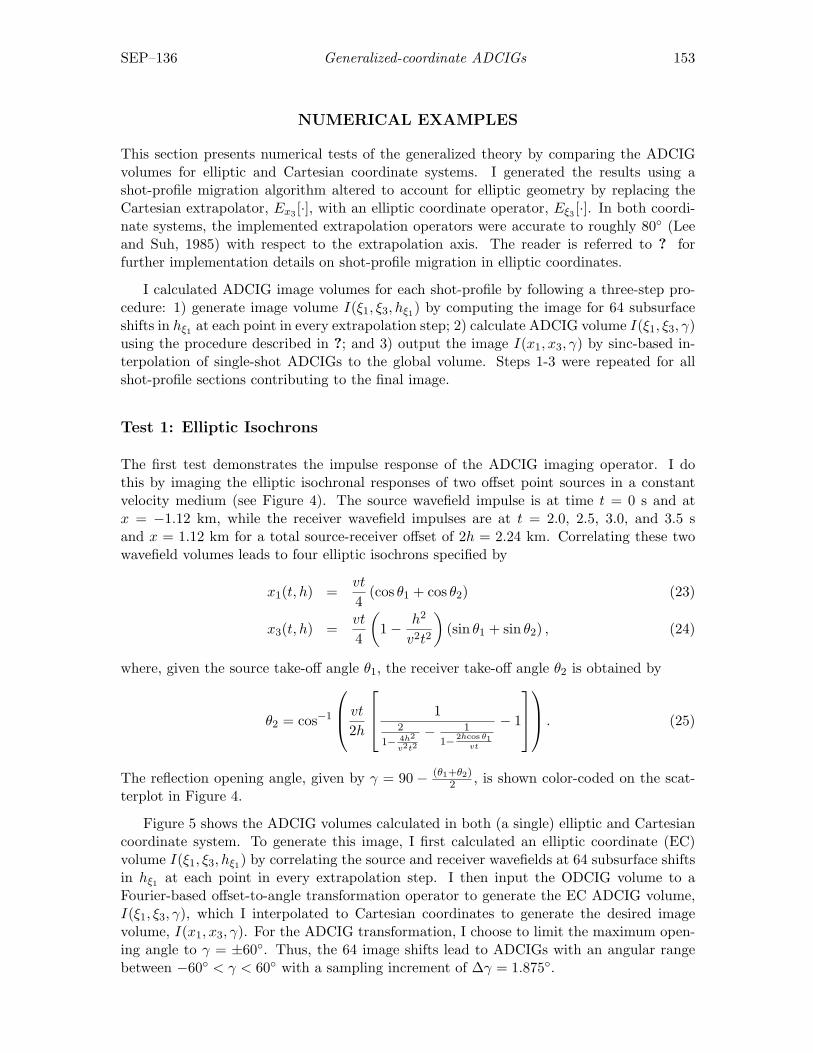
SEP–136 Generalized-coordinate ADCIGs 153
NUMERICAL EXAMPLES
This section presents numerical tests of the generalized theory by comparing the ADCIGvolumes for elliptic and Cartesian coordinate systems. I generated the results using ashot-profile migration algorithm altered to account for elliptic geometry by replacing theCartesian extrapolator, Ex3 [·], with an elliptic coordinate operator, Eξ3 [·]. In both coordi-nate systems, the implemented extrapolation operators were accurate to roughly 80◦ (Leeand Suh, 1985) with respect to the extrapolation axis. The reader is referred to ? forfurther implementation details on shot-profile migration in elliptic coordinates.
I calculated ADCIG image volumes for each shot-profile by following a three-step pro-cedure: 1) generate image volume I(ξ1, ξ3, hξ1) by computing the image for 64 subsurfaceshifts in hξ1 at each point in every extrapolation step; 2) calculate ADCIG volume I(ξ1, ξ3, γ)using the procedure described in ?; and 3) output the image I(x1, x3, γ) by sinc-based in-terpolation of single-shot ADCIGs to the global volume. Steps 1-3 were repeated for allshot-profile sections contributing to the final image.
Test 1: Elliptic Isochrons
The first test demonstrates the impulse response of the ADCIG imaging operator. I dothis by imaging the elliptic isochronal responses of two offset point sources in a constantvelocity medium (see Figure 4). The source wavefield impulse is at time t = 0 s and atx = −1.12 km, while the receiver wavefield impulses are at t = 2.0, 2.5, 3.0, and 3.5 sand x = 1.12 km for a total source-receiver offset of 2h = 2.24 km. Correlating these twowavefield volumes leads to four elliptic isochrons specified by
x1(t, h) =vt
4(cos θ1 + cos θ2) (23)
x3(t, h) =vt
4
(1− h2
v2t2
)(sin θ1 + sin θ2) , (24)
where, given the source take-off angle θ1, the receiver take-off angle θ2 is obtained by
θ2 = cos−1
vt
2h
12
1− 4h2
v2t2
− 1
1− 2hcos θ1vt
− 1
. (25)
The reflection opening angle, given by γ = 90 − (θ1+θ2)2 , is shown color-coded on the scat-
terplot in Figure 4.
Figure 5 shows the ADCIG volumes calculated in both (a single) elliptic and Cartesiancoordinate system. To generate this image, I first calculated an elliptic coordinate (EC)volume I(ξ1, ξ3, hξ1) by correlating the source and receiver wavefields at 64 subsurface shiftsin hξ1 at each point in every extrapolation step. I then input the ODCIG volume to aFourier-based offset-to-angle transformation operator to generate the EC ADCIG volume,I(ξ1, ξ3, γ), which I interpolated to Cartesian coordinates to generate the desired imagevolume, I(x1, x3, γ). For the ADCIG transformation, I choose to limit the maximum open-ing angle to γ = ±60◦. Thus, the 64 image shifts lead to ADCIGs with an angular rangebetween −60◦ < γ < 60◦ with a sampling increment of ∆γ = 1.875◦.
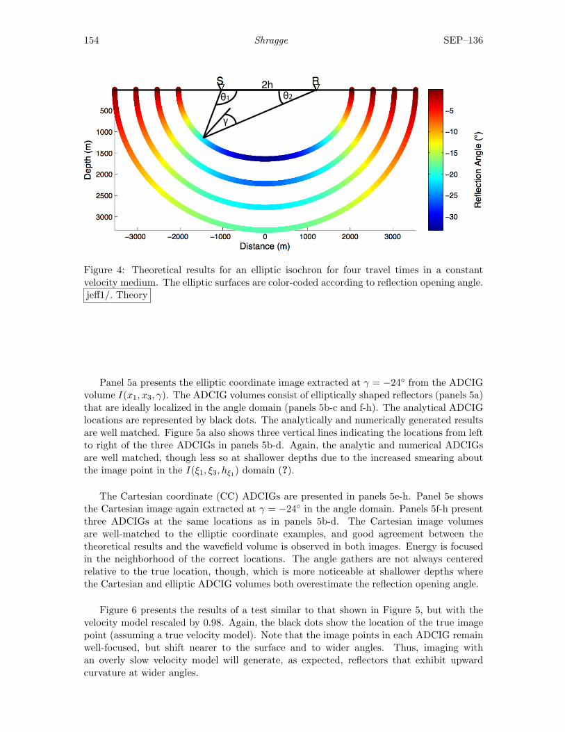
154 Shragge SEP–136
θ1 θ2
γ
2h
Figure 4: Theoretical results for an elliptic isochron for four travel times in a constantvelocity medium. The elliptic surfaces are color-coded according to reflection opening angle.jeff1/. Theory
Panel 5a presents the elliptic coordinate image extracted at γ = −24◦ from the ADCIGvolume I(x1, x3, γ). The ADCIG volumes consist of elliptically shaped reflectors (panels 5a)that are ideally localized in the angle domain (panels 5b-c and f-h). The analytical ADCIGlocations are represented by black dots. The analytically and numerically generated resultsare well matched. Figure 5a also shows three vertical lines indicating the locations from leftto right of the three ADCIGs in panels 5b-d. Again, the analytic and numerical ADCIGsare well matched, though less so at shallower depths due to the increased smearing aboutthe image point in the I(ξ1, ξ3, hξ1) domain (?).
The Cartesian coordinate (CC) ADCIGs are presented in panels 5e-h. Panel 5e showsthe Cartesian image again extracted at γ = −24◦ in the angle domain. Panels 5f-h presentthree ADCIGs at the same locations as in panels 5b-d. The Cartesian image volumesare well-matched to the elliptic coordinate examples, and good agreement between thetheoretical results and the wavefield volume is observed in both images. Energy is focusedin the neighborhood of the correct locations. The angle gathers are not always centeredrelative to the true location, though, which is more noticeable at shallower depths wherethe Cartesian and elliptic ADCIG volumes both overestimate the reflection opening angle.
Figure 6 presents the results of a test similar to that shown in Figure 5, but with thevelocity model rescaled by 0.98. Again, the black dots show the location of the true imagepoint (assuming a true velocity model). Note that the image points in each ADCIG remainwell-focused, but shift nearer to the surface and to wider angles. Thus, imaging withan overly slow velocity model will generate, as expected, reflectors that exhibit upwardcurvature at wider angles.
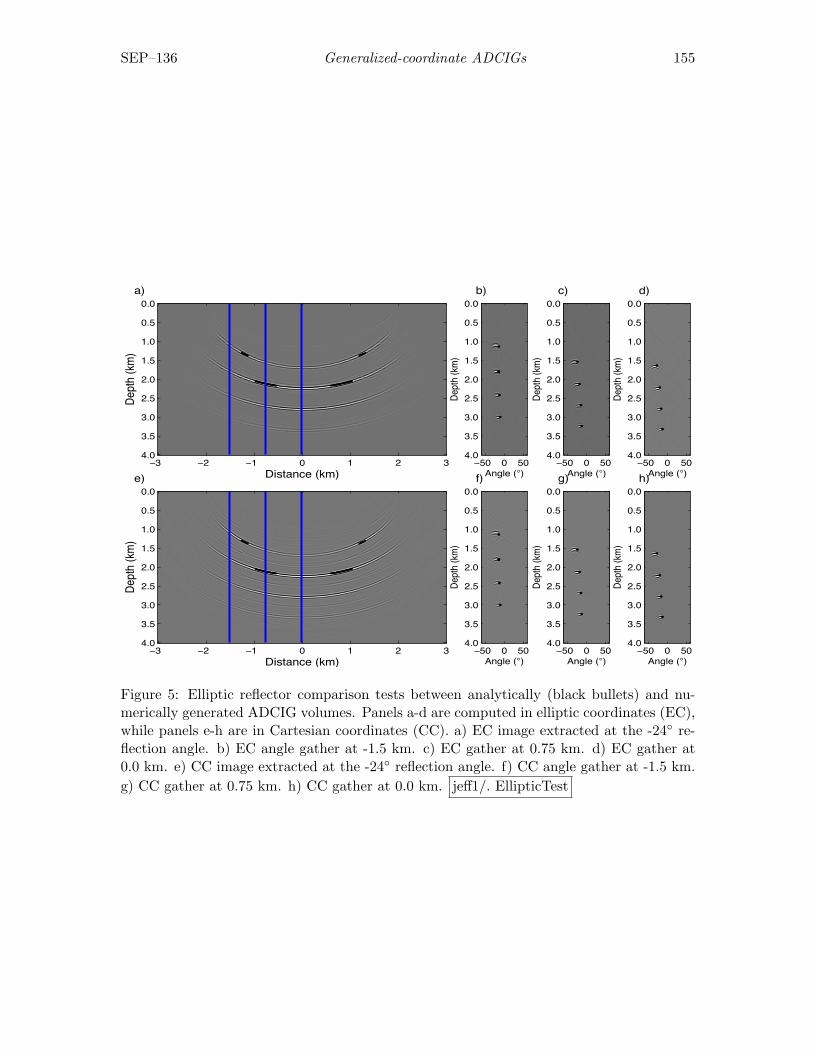
SEP–136 Generalized-coordinate ADCIGs 155
e)
••••••••••••••••••••
••••••••••••••••••••••••••••••••••••••••••••••••••• •••••••••••••••••••••••••••••••••••••••••••••••••••
••••••••••••••••••
Dept
h (k
m)
Distance (km)−3 −2 −1 0 1 2 3
0.0
0.5
1.0
1.5
2.0
2.5
3.0
3.5
4.0
Dept
h (k
m)
Angle (°)
f)
•
••
•
•
−50 0 50
0.0
0.5
1.0
1.5
2.0
2.5
3.0
3.5
4.0
Dept
h (k
m)
Angle (°)
g)
•
•
•
•
−50 0 50
0.0
0.5
1.0
1.5
2.0
2.5
3.0
3.5
4.0
Dept
h (k
m)
Angle (°)
h)
•
•
•
•
−50 0 50
0.0
0.5
1.0
1.5
2.0
2.5
3.0
3.5
4.0
a)
••••••••••••••••••••
••••••••••••••••••••••••••••••••••••••••••••••••••• •••••••••••••••••••••••••••••••••••••••••••••••••••
••••••••••••••••••
Dept
h (k
m)
Distance (km)−3 −2 −1 0 1 2 3
0.0
0.5
1.0
1.5
2.0
2.5
3.0
3.5
4.0De
pth
(km
)
Angle (°)
b)
•
••
•
•
−50 0 50
0.0
0.5
1.0
1.5
2.0
2.5
3.0
3.5
4.0
Dept
h (k
m)
Angle (°)
c)
•
•
•
•
−50 0 50
0.0
0.5
1.0
1.5
2.0
2.5
3.0
3.5
4.0
Dept
h (k
m)
Angle (°)
d)
•
•
•
•
−50 0 50
0.0
0.5
1.0
1.5
2.0
2.5
3.0
3.5
4.0
Figure 5: Elliptic reflector comparison tests between analytically (black bullets) and nu-merically generated ADCIG volumes. Panels a-d are computed in elliptic coordinates (EC),while panels e-h are in Cartesian coordinates (CC). a) EC image extracted at the -24◦ re-flection angle. b) EC angle gather at -1.5 km. c) EC gather at 0.75 km. d) EC gather at0.0 km. e) CC image extracted at the -24◦ reflection angle. f) CC angle gather at -1.5 km.g) CC gather at 0.75 km. h) CC gather at 0.0 km. jeff1/. EllipticTest
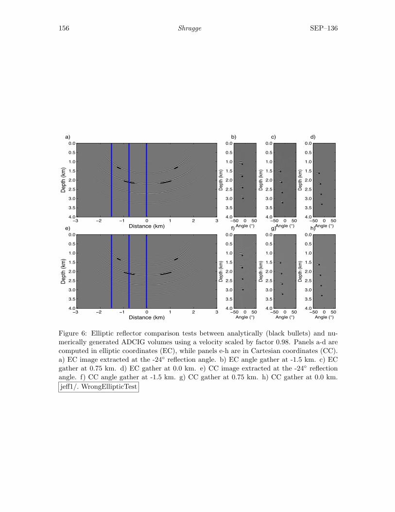
156 Shragge SEP–136
e)
••••••••••••••••••••
••••••••••••••••••••••••••••••••••••••••••••••••••• •••••••••••••••••••••••••••••••••••••••••••••••••••
••••••••••••••••••
Dept
h (k
m)
Distance (km)−3 −2 −1 0 1 2 3
0.0
0.5
1.0
1.5
2.0
2.5
3.0
3.5
4.0
Dept
h (k
m)
Angle (°)
f)
•
••
•
•
−50 0 50
0.0
0.5
1.0
1.5
2.0
2.5
3.0
3.5
4.0
Dept
h (k
m)
Angle (°)
g)
•
•
•
•
−50 0 50
0.0
0.5
1.0
1.5
2.0
2.5
3.0
3.5
4.0
Dept
h (k
m)
Angle (°)
h)
•
•
•
•
−50 0 50
0.0
0.5
1.0
1.5
2.0
2.5
3.0
3.5
4.0
a)
••••••••••••••••••••
••••••••••••••••••••••••••••••••••••••••••••••••••• •••••••••••••••••••••••••••••••••••••••••••••••••••
••••••••••••••••••
Dept
h (k
m)
Distance (km)−3 −2 −1 0 1 2 3
0.0
0.5
1.0
1.5
2.0
2.5
3.0
3.5
4.0De
pth
(km
)Angle (°)
b)
•
••
•
•
−50 0 50
0.0
0.5
1.0
1.5
2.0
2.5
3.0
3.5
4.0
Dept
h (k
m)
Angle (°)
c)
•
•
•
•
−50 0 50
0.0
0.5
1.0
1.5
2.0
2.5
3.0
3.5
4.0
Dept
h (k
m)
Angle (°)
d)
•
•
•
•
−50 0 50
0.0
0.5
1.0
1.5
2.0
2.5
3.0
3.5
4.0
Figure 6: Elliptic reflector comparison tests between analytically (black bullets) and nu-merically generated ADCIG volumes using a velocity scaled by factor 0.98. Panels a-d arecomputed in elliptic coordinates (EC), while panels e-h are in Cartesian coordinates (CC).a) EC image extracted at the -24◦ reflection angle. b) EC angle gather at -1.5 km. c) ECgather at 0.75 km. d) EC gather at 0.0 km. e) CC image extracted at the -24◦ reflectionangle. f) CC angle gather at -1.5 km. g) CC gather at 0.75 km. h) CC gather at 0.0 km.jeff1/. WrongEllipticTest
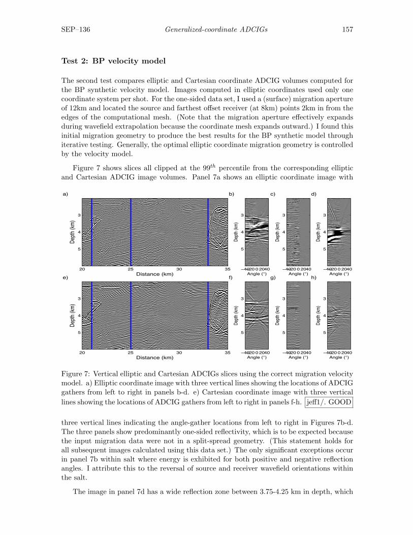
SEP–136 Generalized-coordinate ADCIGs 157
Test 2: BP velocity model
The second test compares elliptic and Cartesian coordinate ADCIG volumes computed forthe BP synthetic velocity model. Images computed in elliptic coordinates used only onecoordinate system per shot. For the one-sided data set, I used a (surface) migration apertureof 12km and located the source and farthest offset receiver (at 8km) points 2km in from theedges of the computational mesh. (Note that the migration aperture effectively expandsduring wavefield extrapolation because the coordinate mesh expands outward.) I found thisinitial migration geometry to produce the best results for the BP synthetic model throughiterative testing. Generally, the optimal elliptic coordinate migration geometry is controlledby the velocity model.
Figure 7 shows slices all clipped at the 99th percentile from the corresponding ellipticand Cartesian ADCIG image volumes. Panel 7a shows an elliptic coordinate image with
e)
Depth
(km)
Distance (km)20 25 30 35
3
4
5
Depth
(km)
Angle (°)
f)
−40−20 0 2040
3
4
5
Depth
(km)
Angle (°)
g)
−40−20 0 2040
3
4
5
Depth
(km)
Angle (°)
h)
−40−20 0 2040
3
4
5
a)
Depth
(km)
Distance (km)20 25 30 35
3
4
5
Depth
(km)
Angle (°)
b)
−40−20 0 2040
3
4
5
Depth
(km)
Angle (°)
c)
−40−20 0 2040
3
4
5
Depth
(km)
Angle (°)
d)
−40−20 0 2040
3
4
5
Figure 7: Vertical elliptic and Cartesian ADCIGs slices using the correct migration velocitymodel. a) Elliptic coordinate image with three vertical lines showing the locations of ADCIGgathers from left to right in panels b-d. e) Cartesian coordinate image with three verticallines showing the locations of ADCIG gathers from left to right in panels f-h. jeff1/. GOOD
three vertical lines indicating the angle-gather locations from left to right in Figures 7b-d.The three panels show predominantly one-sided reflectivity, which is to be expected becausethe input migration data were not in a split-spread geometry. (This statement holds forall subsequent images calculated using this data set.) The only significant exceptions occurin panel 7b within salt where energy is exhibited for both positive and negative reflectionangles. I attribute this to the reversal of source and receiver wavefield orientations withinthe salt.
The image in panel 7d has a wide reflection zone between 3.75-4.25 km in depth, which
158 Shragge SEP–136
occurs because the shown angle gather is a vertical slice through the nearly vertical saltflank. This creates the appears of low-frequency noise, which is the appropriate responsefor a near-vertical reflector. Panel 7e shows the Cartesian image for the same locationas panel 7a, while panels 7f-h are extracted from the same locations as panels 7b-d. TheCartesian angle gathers look similar to those in elliptic coordinates, except for the salt flanksto the right-hand-side of panel 7h.
A final observation from Figure 7 is that ADCIGs calculated via subsurface correlationswill generate artifacts at locations near salt-sediment interfaces - whether in an elliptic ora Cartesian coordinate system. This geologic setting leads to situations where a wavefieldsample inside a salt body is correlated with another sample located in the sediment with asignificantly different velocity. This velocity difference violates one of the theoretical ADCIGassumptions, namely that the velocity remains constant across the correlation window.Hence, one must be careful not to interpret ADCIG artifacts as signal useful for migrationvelocity analysis.
Figure 8 shows horizontal slices that better resolve the vertical salt flank. Panel 8apresents the elliptic coordinate image, with three horizontal lines showing the ADCIG slicelocations from top to bottom. The right-hand sides of panels 8b-d display the well-focusedvertical salt-flank reflector. This demonstrates the robustness of the ADCIG calculationin elliptic coordinates. Panel 8e shows the Cartesian coordinate image with three hori-zontal lines showing the locations of the ADCIG slices. The right-hand salt-flank reflectorin panel 8f is similarly well-resolved, largely because the structural dip is relatively low.However, the salt-flank images in panels 8g-h are somewhat blurred out. I attribute this tothe combined effects of inaccurate large-angle extrapolation and insensitivity of the ADCIGcalculation to steep structural dip.
An additional test examines how the ADCIG volumes change when introducing an in-correct migration velocity profile. Figure 9 presents ADCIG volumes similar to those shownin Figure 7 after using a migration velocity profile rescaled by 98%. Both images are poorlyfocused and have residual curvature indicating an incorrect migration velocity. Because thereflectors are near vertical, though, the sensitivity of horizontal gathers is weak. This lowsensitivity is greatly improved when examining the horizontal slices in Figure 10 taken atthe same locations as in Figure 8. The elliptic angle gathers in panels 10b-d, and especiallyto the right-hand side in panel 10d, show much greater residual curvature. This indicatesthat the elliptic coordinate horizontal ADCIGs have greater sensitivity to velocity errorfor near-vertical structures than Cartesian coordinate horizontal ADCIGs. The imagingenhancements afforded by elliptic coordinates should improve any migration velocity anal-ysis approach that uses residual curvature in steeply dipping reflectors to compute velocitymodel updates.
Discussion
Extending the above theory of generalized coordinate ADCIGs to 3D coordinate systems isfairly straightforward, though more difficult to implement numerically. ? presents a theoryfor 3D Cartesian coordinates that specifies the differential travel-time expressions requiredto express the reflection opening angle, γ, in 3D Cartesian ADCIGs [see equation 16 in ?].Applying Jacobian change-of-variable transformations to these equations should yield a 3D
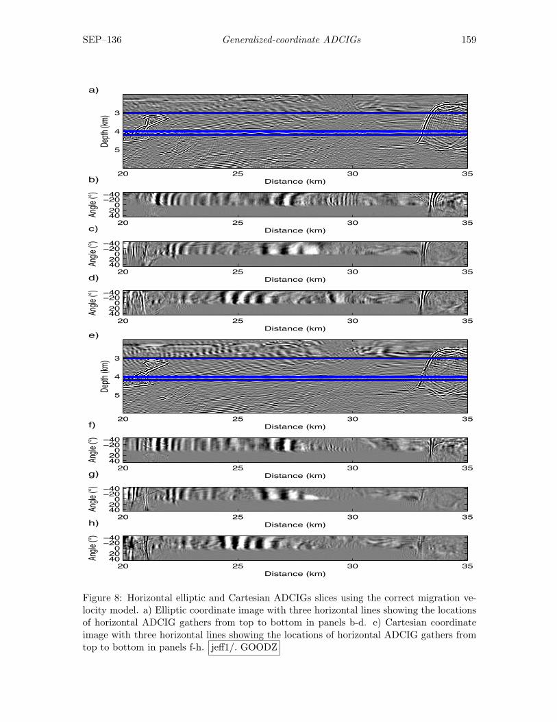
SEP–136 Generalized-coordinate ADCIGs 159
e)
Depth
(km)
Distance (km)20 25 30 35
3
4
5
Distance (km)
Angle
(°)
f)
20 25 30 35
−40−20
02040
Distance (km)
Angle
(°)
g)
20 25 30 35
−40−20
02040
Distance (km)
Angle
(°)
h)
20 25 30 35
−40−20
02040
a)
Depth
(km)
Distance (km)20 25 30 35
3
4
5
Distance (km)
Angle
(°)
b)
20 25 30 35
−40−20
02040
Distance (km)
Angle
(°)
c)
20 25 30 35
−40−20
02040
Distance (km)
Angle
(°)
d)
20 25 30 35
−40−20
02040
Figure 8: Horizontal elliptic and Cartesian ADCIGs slices using the correct migration ve-locity model. a) Elliptic coordinate image with three horizontal lines showing the locationsof horizontal ADCIG gathers from top to bottom in panels b-d. e) Cartesian coordinateimage with three horizontal lines showing the locations of horizontal ADCIG gathers fromtop to bottom in panels f-h. jeff1/. GOODZ
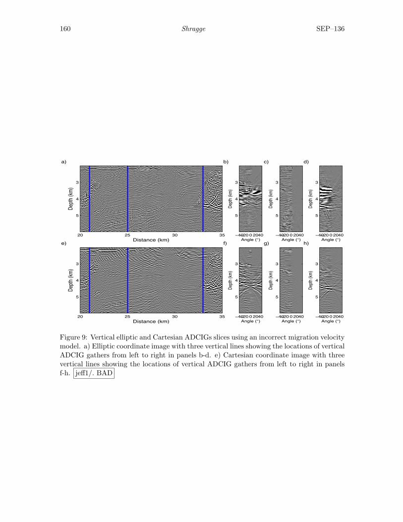
160 Shragge SEP–136
e)
Depth
(km)
Distance (km)20 25 30 35
3
4
5
Depth
(km)
Angle (°)
f)
−40−20 0 2040
3
4
5
Depth
(km)
Angle (°)
g)
−40−20 0 2040
3
4
5
Depth
(km)
Angle (°)
h)
−40−20 0 2040
3
4
5
a)
Depth
(km)
Distance (km)20 25 30 35
3
4
5
Depth
(km)
Angle (°)
b)
−40−20 0 2040
3
4
5
Depth
(km)
Angle (°)
c)
−40−20 0 2040
3
4
5
Depth
(km)
Angle (°)
d)
−40−20 0 2040
3
4
5
Figure 9: Vertical elliptic and Cartesian ADCIGs slices using an incorrect migration velocitymodel. a) Elliptic coordinate image with three vertical lines showing the locations of verticalADCIG gathers from left to right in panels b-d. e) Cartesian coordinate image with threevertical lines showing the locations of vertical ADCIG gathers from left to right in panelsf-h. jeff1/. BAD
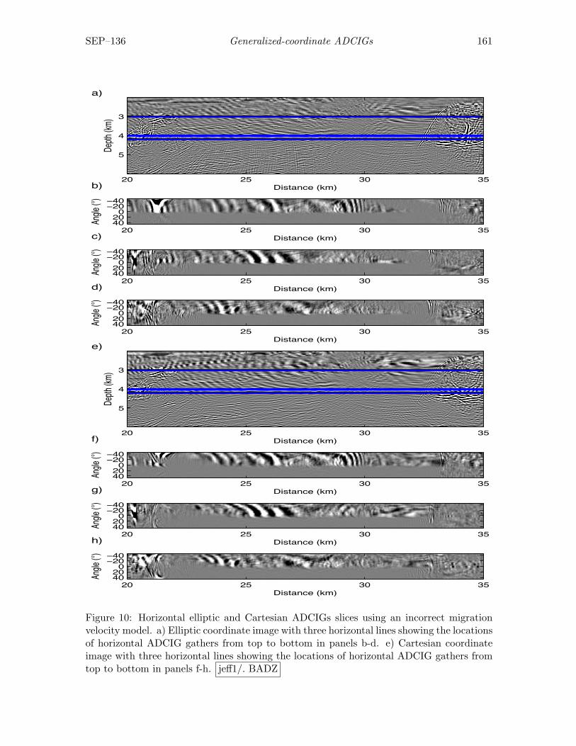
SEP–136 Generalized-coordinate ADCIGs 161
e)
Depth
(km)
Distance (km)20 25 30 35
3
4
5
Distance (km)
Angle
(°)
f)
20 25 30 35
−40−20
02040
Distance (km)
Angle
(°)
g)
20 25 30 35
−40−20
02040
Distance (km)
Angle
(°)
h)
20 25 30 35
−40−20
02040
a)
Depth
(km)
Distance (km)20 25 30 35
3
4
5
Distance (km)
Angle
(°)
b)
20 25 30 35
−40−20
02040
Distance (km)
Angle
(°)
c)
20 25 30 35
−40−20
02040
Distance (km)
Angle
(°)
d)
20 25 30 35
−40−20
02040
Figure 10: Horizontal elliptic and Cartesian ADCIGs slices using an incorrect migrationvelocity model. a) Elliptic coordinate image with three horizontal lines showing the locationsof horizontal ADCIG gathers from top to bottom in panels b-d. e) Cartesian coordinateimage with three horizontal lines showing the locations of horizontal ADCIG gathers fromtop to bottom in panels f-h. jeff1/. BADZ
162 Shragge SEP–136
expression for reflection angle. Similar to 3D Cartesian coordinates, though, this quantitywill depend on geologic dips and need to be computed by one of the two algorithms suggestedby ?.
Given that a 3D expression can be formulated, there are a number of coordinate systemswell-suited to imaging steep geologic dips where 3D ADCIG volumes could be a gooddiagnostic tool for velocity analysis. ? discusses how a judicious choice of 3D coordinatesystem depends greatly on the acquisition geometry and the desired migration geometry. Forexample, the migration geometries employed in shot-profile migration of wide-azimuth datasets are well-matched with 3D ellipsoidal meshes that enable high-angle and turning-wavepropagation in all directions. Evaluating ADCIG image focussing in such a 3D coordinategeometry would then provide information on velocity model accuracy for steeply dippingreflectors - such as salt flanks. These somewhat speculative extensions, though, are beyondthe scope of this paper and remain an active area of research.
CONCLUSIONS
I extend the Cartesian ADCIG theory to 2D generalized coordinate systems. The gen-eralized ADCIG expressions related the reflection opening angle to differential traveltimeoperators and spatially varying weights derived from the non-Cartesian geometry. I showthat these geometric expressions cancel out for coordinate systems satisfying the Cauchy-Riemann differentiability criteria, which include tilted Cartesian and elliptic meshes. Theprocedure for calculating ADCIGs in elliptic coordinates is very similar to that in Cartesiancoordinates. I validate the approach by comparing analytically and numerically generatedADCIG volumes, and with tests on the BP synthetic data set. ADCIGs calculations aremore robust where computed in elliptic coordinates than in Cartesian coordinate. I as-sert that this result is due to improved large-angle propagation and enhanced sensitivity tosteep structural dips afforded by the coordinate transforms. Finally, the imaging advantagesafforded by elliptic coordinates should improve the procedure of any migration velocity anal-ysis approach that uses residual ADCIG curvature on steeply dipping reflectors to computevelocity model updates.
ACKNOWLEDGMENTS
I would like to thank Biondo Biondi, Alejandro Valenciano, Antoine Guitton and BradArtman for helpful discussions, and BP for releasing the synthetic data used in the examples.I thank Tamas Nemeth, Samuel Gray, and an anonymous reviewer for helpful comments onthe early stages of this manuscript. I acknowledge the sponsors of the SEP consortium fortheir continuing support.
REFERENCES
Lee, M. W. and S. Y. Suh, 1985, Optimization of one-way wave-equations (short note):Geophysics, 50, 1634–1637.
SEP–136 Generalized-coordinate ADCIGs 163
APPENDIX A
ADCIG COORDINATE TRANSFORM
This appendix addresses how to express operators ∂∂x3
and ∂∂hx1
in generalized coordinatesystems to derive equation 10. I first assume that generalized coordinate systems are relatedto the Cartesian variables through a bijection (i.e., one-to-one mapping)
x1 = f(ξ1, ξ3) and x3 = g(ξ1, ξ3) (A-1)
with a non-vanishing Jacobian of coordinate transformation, Jξ. The bijection betweena generalized and Cartesian coordinate system allows us to rewrite the left-hand-sides ofequations 7 as (?)
∂t
∂x1=
1Jξ
∂(t, x3)∂(ξ1, ξ3)
and∂t
∂x3=
1Jξ
∂(x1, t)∂(ξ1, ξ3)
. (A-2)
Expanding the Jacobian notation leads to[∂t∂ξ1
∂x3∂ξ3− ∂t
∂ξ3∂x3∂ξ1
∂t∂ξ3
∂x1∂ξ1− ∂t
∂ξ1∂x1∂ξ3
]= 2Jξ s cos γ
[sinαcos α
]. (A-3)
The right-hand-sides of equations A-3 are analogous to those derived by ?. Cross-multiplyingthe expressions by factors ∂x1
∂ξ3and ∂x3
∂ξ3 ∂x1∂ξ3
(∂t∂ξ1
∂x3∂ξ3− ∂t
∂ξ3∂x3∂ξ1
)∂x3∂ξ3
(∂t∂ξ3
∂x1∂ξ1− ∂t
∂ξ1∂x1∂ξ3
) = 2Jξ s cos γ
[∂x1∂ξ3
sinα∂x3∂ξ3
cos α
](A-4)
and adding the two expressions results in
∂t
∂ξ3
(∂x3
∂ξ3
∂x1
∂ξ1− ∂x1
∂ξ3
∂x3
∂ξ1
)= 2Jξ s cos γ
(∂x1
∂ξ3sinα +
∂x3
∂ξ3cos α
). (A-5)
A similar argument can be used to construct the equations for the subsurface-offsetaxis. The bijection between the generalized coordinate and Cartesian subsurface-offset axesallows for the left-hand-side of equations 7 to be rewritten as
∂t
∂hx1
=1Jh
∂(t, hx3)∂(hξ1 , hξ3)
and∂t
∂hx3
=1Jh
∂(hx1 , t)∂(hξ1 , hξ3)
, (A-6)
where Jh is the subsurface-offset Jacobian of transformation. Expanding the Jacobiannotation leads to ∂t
∂hξ1
∂hx3∂hξ3
− ∂t∂hξ3
∂hx3∂hξ1
∂t∂hξ3
∂hx1∂hξ1
− ∂t∂hξ1
∂hx1∂hξ3
= 2Jh s sin γ
[cos αsinα
]. (A-7)
The right-hand-side of equations A-7 are again analogous to those given by ?. Cross-multiplying the expressions by factors ∂hx1
∂hξ1and ∂hx3
∂hξ1 ∂hx1∂hξ1
(∂t
∂hξ1
∂hx3∂hξ3
− ∂t∂hξ3
∂hx3∂hξ1
)∂hx3∂hξ1
(∂t
∂hξ3
∂hx1∂hξ1
− ∂t∂hξ1
∂hx1∂hξ3
) = 2Jh s sin γ
∂hx1∂hξ1
cos α∂hx3∂hξ1
sinα
, (A-8)
164 Shragge SEP–136
and subtracting the two expressions above yields
∂t
∂hξ1
(∂hx1
∂hξ1
∂hx3
∂hξ3
− ∂hx1
∂hξ3
∂hx3
∂hξ1
)= 2Jh s sin γ
(∂hx1
∂hξ1
cosα− ∂hx3
∂hξ1
sinα
). (A-9)
An expression for ADCIGs can be obtained by dividing equation A-9 by equation A-5
∂t∂hξ1
∂t∂ξ3
(∂hx1∂hξ1
∂hx3∂hξ3
− ∂hx1∂hξ3
∂hx3∂hξ1
)(
∂x3∂ξ3
∂x1∂ξ1− ∂x1
∂ξ3∂x3∂ξ1
) = tan γJh
Jξ
(∂hx1∂hξ1
cos α− ∂hx3∂hξ1
sinα)
(∂x3∂ξ3
cos α + ∂x1∂ξ3
sinα) . (A-10)
One question arising from the geometric factors in equation A-10 is what do the terms∂hx1∂hξ1
, ∂hx3∂hξ1
, ∂hx1∂hξ3
and ∂hx3∂hξ3
represent? I assume that the subsurface offset axes are generatedby uniform wavefield shifting such that the following equations are valid:
hx1
hx3
hξ1
hξ1
=
x1
x3
ξ1
ξ3
such that
∂hx1∂hξ1∂hx3∂hξ1∂hx1∂hξ3∂hx3∂hξ3
=
∂x1∂ξ1∂x3∂ξ1∂x1∂ξ3∂x3∂ξ3
. (A-11)
If the subsurface offset axes were generated by anything other than uniform shifting (e.g.hx1 = x2
1), then the assumptions behind equations A-11 would not be honored.
Using these identities in equation A-5 reduces equation A-10 to
− ∂ξ3
∂hξ1
∣∣∣∣ξ1,t
=∂t
∂hξ1
/∂t
∂ξ3= tan γ
(∂x1∂ξ1
cos α− ∂x3∂ξ1
sinα)
(∂x3∂ξ3
cos α + ∂x1∂ξ3
sinα) , (A-12)
where the two Jacobian transformations are equivalent (i.e. Jξ = Jh). This completes thederivation of equation 10.
Stanford Exploration Project, Report SEP136, April 14, 2009
Seismic interferometry versus spatial auto-correlationmethod on the regional coda of the NPE
Sjoerd de Ridder
ABSTRACT
A seismic recording of the non-proliferation experiment (NPE) contains the first breakof the regional P phases followed by a three minute long coda. The frequency-domainresult of seismic interferometry is studied. This procedure is analogous to the spatialauto-correlation (SPAC) method, devised for studying microtremors by Aki (1957).Cross-correlating two receiver stations retrieves, under favorable circumstances, an ap-proximation of the Green’s function between these two stations. To first order, thisGreen’s function consists of a direct event traveling between the receivers. In thefrequency-domain, the lowest mode in the Green’s function is a weighted and scaledzero-order Bessel function of the first kind, J0. The cross-spectrum from the coda ofthe NPE is estimated using multitaper spectral analysis. The retrieved Green’s func-tions are fitted to damped J0 functions to recover phase velocity and estimates of theattenuation coefficients. Only energy between 1-4 Hz can be fitted unambiguously withJ0 functions, because higher frequencies contain too much spurious energy. This resultshows the equivalence of the SPAC method and seismic interferometry for the lowestmode in the Green’s function. This study also demonstrates that the coda of a re-gional event, seemingly unfavorably positioned, can contain energy useful for seismicinterferometry.
INTRODUCTION
In an efort to ban all nuclear tests, a large majority at the United Nations General Assemblyin New York passed the comprehensive test ban treaty (CTBT) in September, 1996. Al-though 180 states signed the treaty, only 145 ratified it, prohibiting the treaty from enteringinto force (CTBTO, 2008). The US Department of Energy detonated a 1.5 kiloton chemicalexplosive charge at the Nevada test site on September 22nd, 1993. The experiment, namedthe non-proliferation experiment (NPE), was conducted in anticipation of the CTBT. Theexplosion was recorded by over 50 broadband seismic stations in the western United States(Tinker and Wallace, 1997). Scientists used these recordings and other measurements tolearn to distinguish between nuclear and chemical explosions (Carr, 1994).
A less well known recording was made by the Subsurface Exploration Company ofPasadena, CA, which operated a 610-channel petroleum-exploration seismic array approxi-mately 200 km distant. The array was oriented east-west in Railroad Valley, Nevada, whichis located north of the Nevada Test Site, see Figure 1. This sign-bit equipment was ac-tivated at midnight and recorded an extraordinary coda over 5 minutes in length. Theincoming waves are spatially coherent at early times, when all energy comes in as a singleplane wave (see Figure 2a). Very rapidly after the first break, the wavefield becomes more
165
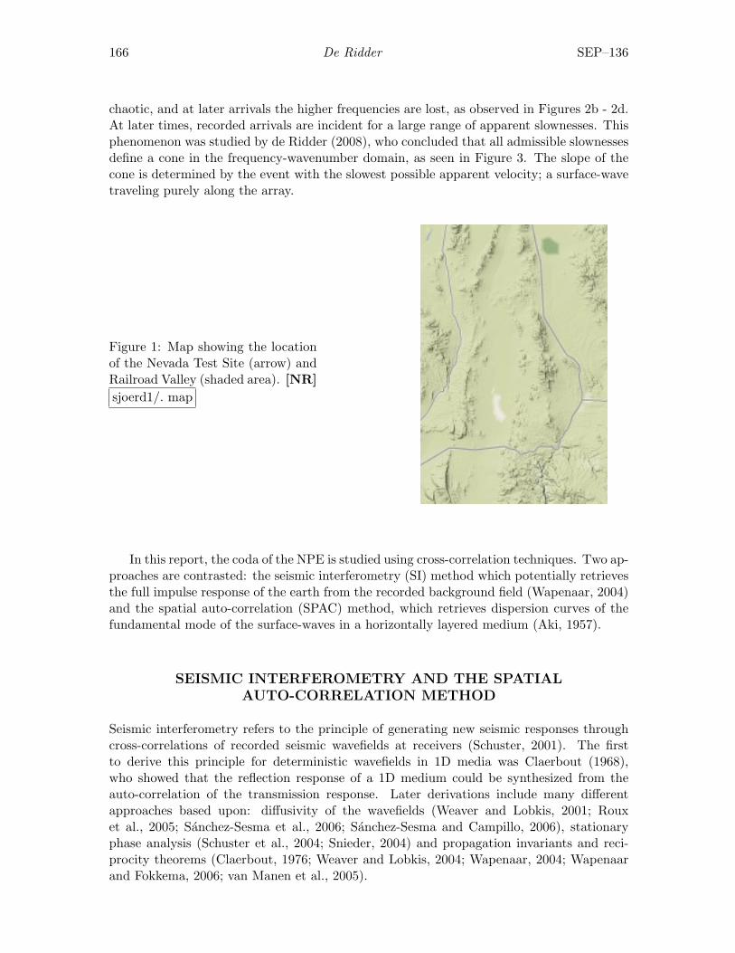
166 De Ridder SEP–136
chaotic, and at later arrivals the higher frequencies are lost, as observed in Figures 2b - 2d.At later times, recorded arrivals are incident for a large range of apparent slownesses. Thisphenomenon was studied by de Ridder (2008), who concluded that all admissible slownessesdefine a cone in the frequency-wavenumber domain, as seen in Figure 3. The slope of thecone is determined by the event with the slowest possible apparent velocity; a surface-wavetraveling purely along the array.
Figure 1: Map showing the locationof the Nevada Test Site (arrow) andRailroad Valley (shaded area). [NR]sjoerd1/. map
In this report, the coda of the NPE is studied using cross-correlation techniques. Two ap-proaches are contrasted: the seismic interferometry (SI) method which potentially retrievesthe full impulse response of the earth from the recorded background field (Wapenaar, 2004)and the spatial auto-correlation (SPAC) method, which retrieves dispersion curves of thefundamental mode of the surface-waves in a horizontally layered medium (Aki, 1957).
SEISMIC INTERFEROMETRY AND THE SPATIALAUTO-CORRELATION METHOD
Seismic interferometry refers to the principle of generating new seismic responses throughcross-correlations of recorded seismic wavefields at receivers (Schuster, 2001). The firstto derive this principle for deterministic wavefields in 1D media was Claerbout (1968),who showed that the reflection response of a 1D medium could be synthesized from theauto-correlation of the transmission response. Later derivations include many differentapproaches based upon: diffusivity of the wavefields (Weaver and Lobkis, 2001; Rouxet al., 2005; Sanchez-Sesma et al., 2006; Sanchez-Sesma and Campillo, 2006), stationaryphase analysis (Schuster et al., 2004; Snieder, 2004) and propagation invariants and reci-procity theorems (Claerbout, 1976; Weaver and Lobkis, 2004; Wapenaar, 2004; Wapenaarand Fokkema, 2006; van Manen et al., 2005).
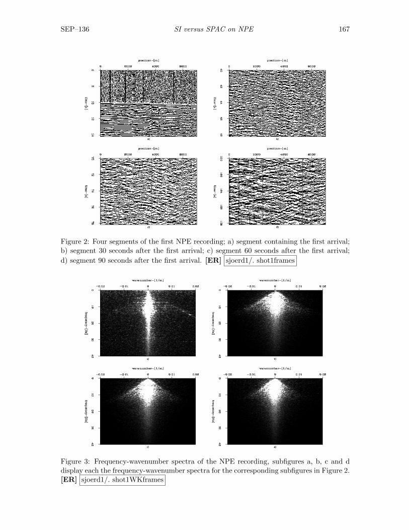
SEP–136 SI versus SPAC on NPE 167
Figure 2: Four segments of the first NPE recording; a) segment containing the first arrival;b) segment 30 seconds after the first arrival; c) segment 60 seconds after the first arrival;d) segment 90 seconds after the first arrival. [ER] sjoerd1/. shot1frames
Figure 3: Frequency-wavenumber spectra of the NPE recording, subfigures a, b, c and ddisplay each the frequency-wavenumber spectra for the corresponding subfigures in Figure 2.[ER] sjoerd1/. shot1WKframes
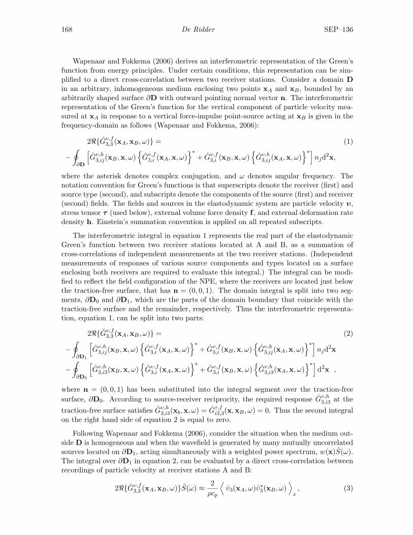
168 De Ridder SEP–136
Wapenaar and Fokkema (2006) derives an interferometric representation of the Green’sfunction from energy principles. Under certain conditions, this representation can be sim-plified to a direct cross-correlation between two receiver stations. Consider a domain Din an arbitrary, inhomogeneous medium enclosing two points xA and xB, bounded by anarbitrarily shaped surface ∂D with outward pointing normal vector n. The interferometricrepresentation of the Green’s function for the vertical component of particle velocity mea-sured at xA in response to a vertical force-impulse point-source acting at xB is given in thefrequency-domain as follows (Wapenaar and Fokkema, 2006):
2<{Gυ,f3,3 (xA,xB, ω)} = (1)
−∮
∂D
[Gυ,h
3,ij(xB,x, ω){
Gυ,f3,i (xA,x, ω)
}∗+ Gυ,f
3,i (xB,x, ω){
Gυ,h3,ij(xA,x, ω)
}∗]njd2x,
where the asterisk denotes complex conjugation, and ω denotes angular frequency. Thenotation convention for Green’s functions is that superscripts denote the receiver (first) andsource type (second), and subscripts denote the components of the source (first) and receiver(second) fields. The fields and sources in the elastodynamic system are particle velocity υ,stress tensor τ (used below), external volume force density f , and external deformation ratedensity h. Einstein’s summation convention is applied on all repeated subscripts.
The interferometric integral in equation 1 represents the real part of the elastodynamicGreen’s function between two receiver stations located at A and B, as a summation ofcross-correlations of independent measurements at the two receiver stations. (Independentmeasurements of responses of various source components and types located on a surfaceenclosing both receivers are required to evaluate this integral.) The integral can be modi-fied to reflect the field configuration of the NPE, where the receivers are located just belowthe traction-free surface, that has n = (0, 0, 1). The domain integral is split into two seg-ments, ∂D0 and ∂D1, which are the parts of the domain boundary that coincide with thetraction-free surface and the remainder, respectively. Thus the interferometric representa-tion, equation 1, can be split into two parts:
2<{Gυ,f3,3 (xA,xB, ω)} = (2)
−∮
∂D1
[Gυ,h
3,ij(xB,x, ω){
Gυ,f3,i (xA,x, ω)
}∗+ Gυ,f
3,i (xB,x, ω){
Gυ,h3,ij(xA,x, ω)
}∗]njd2x
−∮
∂D0
[Gυ,h
3,i3(xB,x, ω){
Gυ,f3,i (xA,x, ω)
}∗+ Gυ,f
3,i (xB,x, ω){
Gυ,h3,i3(xA,x, ω)
}∗]d2x ,
where n = (0, 0, 1) has been substituted into the integral segment over the traction-freesurface, ∂D0. According to source-receiver reciprocity, the required response Gυ,h
3,i3 at the
traction-free surface satisfies Gυ,h3,i3(xb,x, ω) = Gτ,f
i3,3(x,xB, ω) = 0. Thus the second integralon the right hand side of equation 2 is equal to zero.
Following Wapenaar and Fokkema (2006), consider the situation when the medium out-side D is homogeneous and when the wavefield is generated by many mutually uncorrelatedsources located on ∂D1, acting simultaneously with a weighted power spectrum, w(x)S(ω).The integral over ∂D1 in equation 2, can be evaluated by a direct cross-correlation betweenrecordings of particle velocity at receiver stations A and B:
2<{Gυ,f3,3 (xA,xB, ω)}S(ω) ≈ 2
ρcp
⟨υ3(xA, ω)υ∗3(xB, ω)
⟩x, (3)
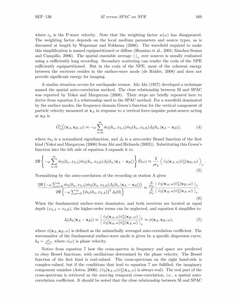
SEP–136 SI versus SPAC on NPE 169
where cp is the P-wave velocity. Note that the weighting factor w(ω) has disappeared.The weighting factor depends on the local medium parameters and source types, as isdiscussed at length by Wapenaar and Fokkema (2006). The wavefield required to makethis simplification is named equipartitioned or diffuse (Hennino et al., 2001; Sanchez-Sesmaand Campillo, 2006). The spatial ensemble average 〈·〉x over sources is usually evaluatedusing a sufficiently long recording. Secondary scattering can render the coda of the NPEsufficiently equipartitioned. But in the coda of the NPE, most of the coherent energybetween the receivers resides in the surface-wave mode (de Ridder, 2008) and does notprovide significant energy for imaging.
A similar situation occurs for earthquake tremor. Aki Aki (1957) developed a techniquenamed the spatial auto-correlation method. The close relationship between SI and SPACwas reported by Yokoi and Margaryan (2008). Their steps are briefly repeated here toderive from equation 3 a relationship used in the SPAC method. For a wavefield dominatedby the surface modes, the frequency-domain Green’s function for the vertical component ofparticle velocity measured at xA in response to a vertical force-impulse point-source actingat xB is
Gυ,f3,3 (xA,xB, ω) ≈ −ω
∞∑n=0
m2(kn, x3,A)m2(kn, x3,B)J0(kn |xA − xB|), (4)
where m2 is a normalized eigenfunction, and J0 is a zero-order Bessel function of the firstkind (Yokoi and Margaryan (2008) from Aki and Richards (2002)). Substituting this Green’sfunction into the left side of equation 3 expands it to
2<
{−ω
∞∑n=0
m2(kn, x3,A)m2(kn, x3,B)J0(kn |xA − xB|)
}S(ω) ≈ 2
ρcp
⟨υ3(xA, ω)υ∗3(xB, ω)
⟩x.
(5)Normalizing by the auto-correlation of the recording at station A gives
2<{−ω∑∞
n=0 m2(kn, x3,A)m2(kn, x3,B)J0(kn |xA − xB|)}
2<{−ω
∑∞n=0 {m2(kn, x3,A)}2 J0(0)
} ≈2
ρcp〈 υ3(xA, ω)υ∗3(xB, ω) 〉x
2ρcp〈 υ3(xA, ω)υ∗3(xA, ω) 〉x
.
(6)When the fundamental surface-wave dominates, and both receivers are located at equaldepth (x3,A = x3,B), the higher-order terms can be neglected, and equation 6 simplifies to
J0(k0 |xA − xB|) ≈〈 υ3(xA, ω)υ∗3(xB, ω) 〉x〈 υ3(xA, ω)υ∗3(xA, ω) 〉x
≈ φ(xA,xB, ω), (7)
where φ(xA,xB, ω) is defined as the azimuthally averaged auto-correlation coefficient. Thewavenumber of the fundamental surface-wave mode is given by a specific dispersion curve,k0 = ω
c(ω) , where c(ω) is phase velocity.
Notice from equation 7 how the cross-spectra in frequency and space are predictedto obey Bessel functions, with oscillations determined by the phase velocity. The Besselfunction of the first kind is real-valued. The cross-spectrum on the right hand-side iscomplex-valued, but if the conditions that lead to equation 7 are fulfilled, the imaginarycomponent vanishes (Asten, 2006), (υ3(xA, ω)υ∗3(xA, ω) is always real). The real part of thecross-spectrum is retrieved as the zero-lag temporal cross-correlation, i.e., a spatial auto-correlation coefficient. It should be noted that the close relationship between SI and SPAC
170 De Ridder SEP–136
seems to hold only for surface-waves in horizontally stratified media. The SPAC method ascommonly applied involves fitting Bessel functions to the computed auto-correlation coef-ficient with frequency, with explicit directional averaging of the wavefield in all directions.In the case of isotropic wavefields, this averaging is unnecessary (Aki, 1957; Okada, 2003).The coda of the NPE quickly becomes isotropic after the first break, thus this relationshipseems suitable for the cross-spectra calculated from NPE data. To introduce an estimationof attenuation, the Green’s function, equation 4, is supplemented with an exponential at-tenuation factor Q(ω), (Aki and Richards, 2002). The final model for the frequency-domainspatial auto-correlation coefficient φ(xA,xB, ω) becomes
φ(xA,xB, ω) = J0
(ω
c(ω)|xA − xB|
)exp
{− ω
c(ω)1
2Q(ω)|xA − xB|
}. (8)
DATA ANALYSIS
The two records analyzed are of approximately 131 seconds duration (214 samples at a 125Hz sampling frequency) at 610 stations with a 45-foot spacing. The second recording startsa few seconds after the first recording ends. Although the exact location of the NPE arrayis unknown, the data shows that the first 66 stations were located at an angle with respectto the other stations. Starting from station 67 located at 0 m in Figure 2, 512 stations areanalyzed. The first arrivals were muted from the first record. All records were filtered inthe frequency-wavenumber domain with a high-cut cosine filter centered around an anglecorresponding to a velocity of 770 m/s, determined from Figure 3. This removes noise fromthe coda and interpolates the missing traces. For velocities smaller and equal to 770 m/sthis did not affect the estimation of the surface wave velocity as described below.
The spectrum at each station was estimated using a multitaper spectral-estimationtechnique. This provides several statistically independent estimates of the spectrum anddecreases spectral leakage (Prieto et al., 2007, 2008b). In this procedure, a time record withN samples is first multiplied with a set of K orthogonal Slepian tapers (Thomson, 1982).Second, the discrete Fourier transformation is computed for each tapered trace as follows:
xk(ω) =N−1∑t=0
x(t)νk(t)exp {−iωt} , (9)
where the kth Slepian taper is denoted by νk(t). The cross-spectrum ρ(ω) between twotraces x and y is calculated from the spectral estimations xk(ω) and yk(ω) according to
ρ(ω) =K∑
k=1
xk(ω){
yk(ω)}∗
. (10)
Interferometric gathers in the frequency-domain are computed by consecutively selectingeach station in the array as a master station and computing the cross-spectra between allother stations and this master station. The collection of interferometric gathers is furtheranalyzed in the midpoint-offset domain (m,h). To enhance the signal-to-noise ratio, theretrieved gathers are smoothed over 50 midpoints, corresponding to a length of 680 m.
We first study the result from processing the records in the time domain, as is commonin seismic interferometry practices. A common-midpoint section at m = 5144 m is given in
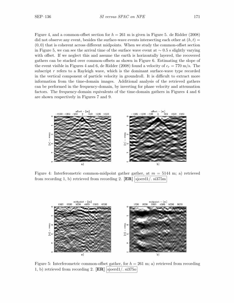
SEP–136 SI versus SPAC on NPE 171
Figure 4, and a common-offset section for h = 261 m is given in Figure 5. de Ridder (2008)did not observe any event, besides the surface-wave events intersecting each other at (h, t) =(0, 0) that is coherent across different midpoints. When we study the common-offset sectionin Figure 5, we can see the arrival time of the surface wave event at ∼ 0.5 s slightly varyingwith offset. If we neglect this and assume the earth is horizontally layered, the recoveredgathers can be stacked over common-offsets as shown in Figure 6. Estimating the slope ofthe event visible in Figures 4 and 6, de Ridder (2008) found a velocity of cr = 770 m/s. Thesubscript r refers to a Rayleigh wave, which is the dominant surface-wave type recordedin the vertical component of particle velocity in groundroll. It is difficult to extract moreinformation from the time-domain images. Additional analysis of the retrieved gatherscan be performed in the frequency-domain, by inverting for phase velocity and attenuationfactors. The frequency-domain equivalents of the time-domain gathers in Figures 4 and 6are shown respectively in Figures 7 and 9.
Figure 4: Interferometric common-midpoint gather gather, at m = 5144 m; a) retrievedfrom recording 1, b) retrieved from recording 2. [ER] sjoerd1/. si375m
Figure 5: Interferometric common-offset gather, for h = 261 m; a) retrieved from recording1, b) retrieved from recording 2. [ER] sjoerd1/. si375o
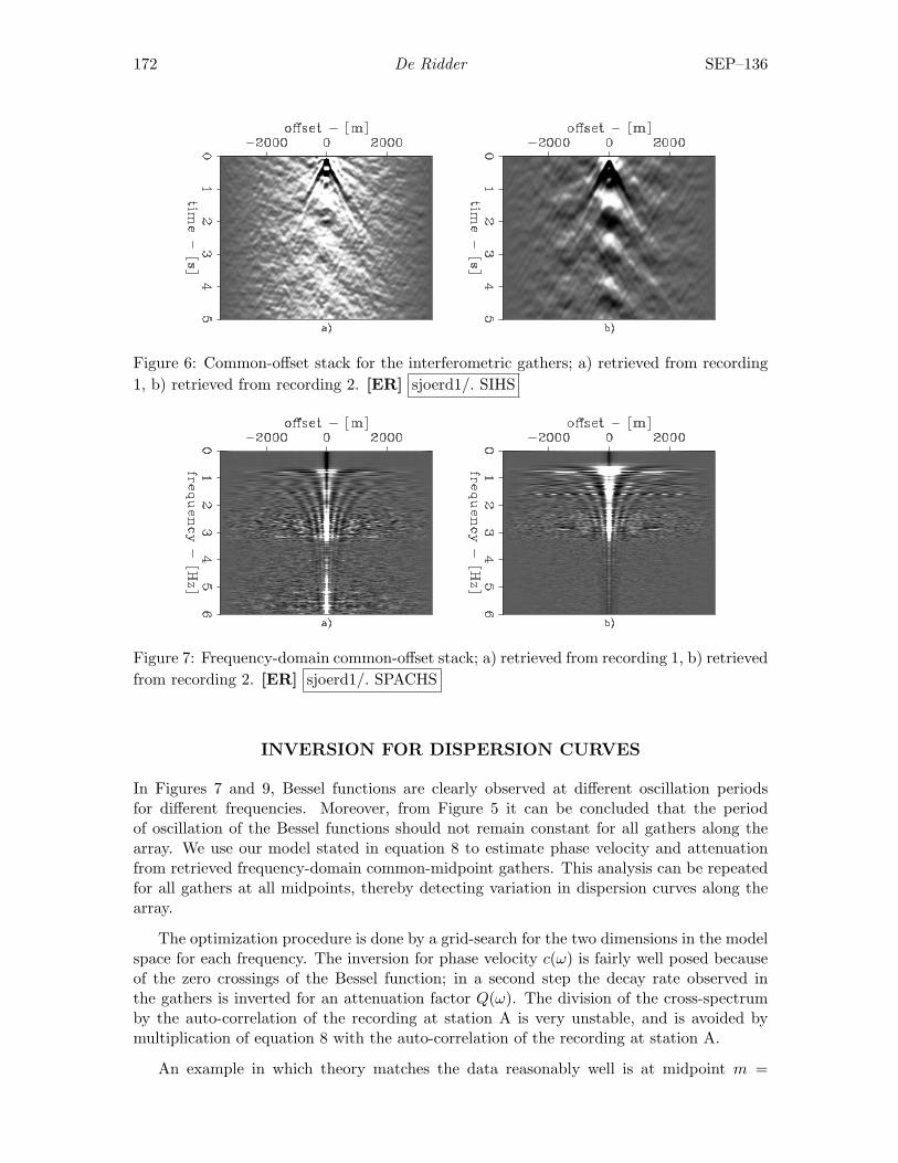
172 De Ridder SEP–136
Figure 6: Common-offset stack for the interferometric gathers; a) retrieved from recording1, b) retrieved from recording 2. [ER] sjoerd1/. SIHS
Figure 7: Frequency-domain common-offset stack; a) retrieved from recording 1, b) retrievedfrom recording 2. [ER] sjoerd1/. SPACHS
INVERSION FOR DISPERSION CURVES
In Figures 7 and 9, Bessel functions are clearly observed at different oscillation periodsfor different frequencies. Moreover, from Figure 5 it can be concluded that the periodof oscillation of the Bessel functions should not remain constant for all gathers along thearray. We use our model stated in equation 8 to estimate phase velocity and attenuationfrom retrieved frequency-domain common-midpoint gathers. This analysis can be repeatedfor all gathers at all midpoints, thereby detecting variation in dispersion curves along thearray.
The optimization procedure is done by a grid-search for the two dimensions in the modelspace for each frequency. The inversion for phase velocity c(ω) is fairly well posed becauseof the zero crossings of the Bessel function; in a second step the decay rate observed inthe gathers is inverted for an attenuation factor Q(ω). The division of the cross-spectrumby the auto-correlation of the recording at station A is very unstable, and is avoided bymultiplication of equation 8 with the auto-correlation of the recording at station A.
An example in which theory matches the data reasonably well is at midpoint m =
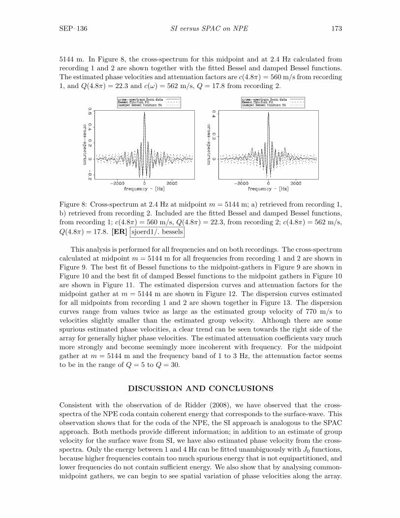
SEP–136 SI versus SPAC on NPE 173
5144 m. In Figure 8, the cross-spectrum for this midpoint and at 2.4 Hz calculated fromrecording 1 and 2 are shown together with the fitted Bessel and damped Bessel functions.The estimated phase velocities and attenuation factors are c(4.8π) = 560 m/s from recording1, and Q(4.8π) = 22.3 and c(ω) = 562 m/s, Q = 17.8 from recording 2.
Figure 8: Cross-spectrum at 2.4 Hz at midpoint m = 5144 m; a) retrieved from recording 1,b) retrieved from recording 2. Included are the fitted Bessel and damped Bessel functions,from recording 1; c(4.8π) = 560 m/s, Q(4.8π) = 22.3, from recording 2; c(4.8π) = 562 m/s,Q(4.8π) = 17.8. [ER] sjoerd1/. bessels
This analysis is performed for all frequencies and on both recordings. The cross-spectrumcalculated at midpoint m = 5144 m for all frequencies from recording 1 and 2 are shown inFigure 9. The best fit of Bessel functions to the midpoint-gathers in Figure 9 are shown inFigure 10 and the best fit of damped Bessel functions to the midpoint gathers in Figure 10are shown in Figure 11. The estimated dispersion curves and attenuation factors for themidpoint gather at m = 5144 m are shown in Figure 12. The dispersion curves estimatedfor all midpoints from recording 1 and 2 are shown together in Figure 13. The dispersioncurves range from values twice as large as the estimated group velocity of 770 m/s tovelocities slightly smaller than the estimated group velocity. Although there are somespurious estimated phase velocities, a clear trend can be seen towards the right side of thearray for generally higher phase velocities. The estimated attenuation coefficients vary muchmore strongly and become seemingly more incoherent with frequency. For the midpointgather at m = 5144 m and the frequency band of 1 to 3 Hz, the attenuation factor seemsto be in the range of Q = 5 to Q = 30.
DISCUSSION AND CONCLUSIONS
Consistent with the observation of de Ridder (2008), we have observed that the cross-spectra of the NPE coda contain coherent energy that corresponds to the surface-wave. Thisobservation shows that for the coda of the NPE, the SI approach is analogous to the SPACapproach. Both methods provide different information; in addition to an estimate of groupvelocity for the surface wave from SI, we have also estimated phase velocity from the cross-spectra. Only the energy between 1 and 4 Hz can be fitted unambiguously with J0 functions,because higher frequencies contain too much spurious energy that is not equipartitioned, andlower frequencies do not contain sufficient energy. We also show that by analysing common-midpoint gathers, we can begin to see spatial variation of phase velocities along the array.
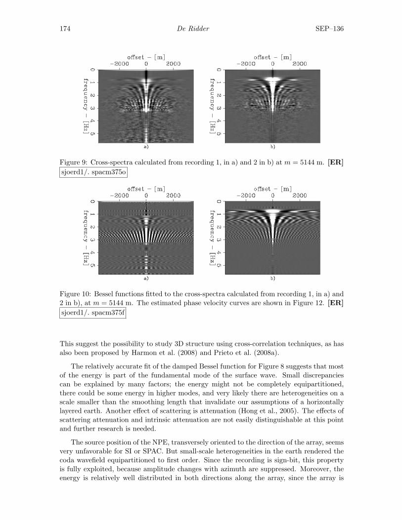
174 De Ridder SEP–136
Figure 9: Cross-spectra calculated from recording 1, in a) and 2 in b) at m = 5144 m. [ER]sjoerd1/. spacm375o
Figure 10: Bessel functions fitted to the cross-spectra calculated from recording 1, in a) and2 in b), at m = 5144 m. The estimated phase velocity curves are shown in Figure 12. [ER]sjoerd1/. spacm375f
This suggest the possibility to study 3D structure using cross-correlation techniques, as hasalso been proposed by Harmon et al. (2008) and Prieto et al. (2008a).
The relatively accurate fit of the damped Bessel function for Figure 8 suggests that mostof the energy is part of the fundamental mode of the surface wave. Small discrepanciescan be explained by many factors; the energy might not be completely equipartitioned,there could be some energy in higher modes, and very likely there are heterogeneities on ascale smaller than the smoothing length that invalidate our assumptions of a horizontallylayered earth. Another effect of scattering is attenuation (Hong et al., 2005). The effects ofscattering attenuation and intrinsic attenuation are not easily distinguishable at this pointand further research is needed.
The source position of the NPE, transversely oriented to the direction of the array, seemsvery unfavorable for SI or SPAC. But small-scale heterogeneities in the earth rendered thecoda wavefield equipartitioned to first order. Since the recording is sign-bit, this propertyis fully exploited, because amplitude changes with azimuth are suppressed. Moreover, theenergy is relatively well distributed in both directions along the array, since the array is
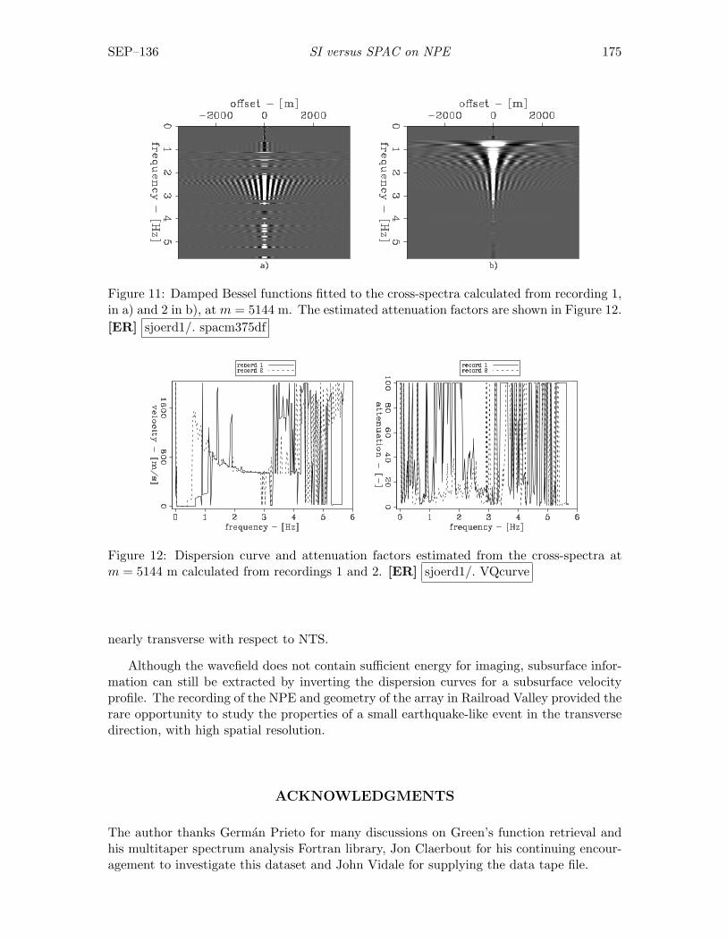
SEP–136 SI versus SPAC on NPE 175
Figure 11: Damped Bessel functions fitted to the cross-spectra calculated from recording 1,in a) and 2 in b), at m = 5144 m. The estimated attenuation factors are shown in Figure 12.[ER] sjoerd1/. spacm375df
Figure 12: Dispersion curve and attenuation factors estimated from the cross-spectra atm = 5144 m calculated from recordings 1 and 2. [ER] sjoerd1/. VQcurve
nearly transverse with respect to NTS.
Although the wavefield does not contain sufficient energy for imaging, subsurface infor-mation can still be extracted by inverting the dispersion curves for a subsurface velocityprofile. The recording of the NPE and geometry of the array in Railroad Valley provided therare opportunity to study the properties of a small earthquake-like event in the transversedirection, with high spatial resolution.
ACKNOWLEDGMENTS
The author thanks German Prieto for many discussions on Green’s function retrieval andhis multitaper spectrum analysis Fortran library, Jon Claerbout for his continuing encour-agement to investigate this dataset and John Vidale for supplying the data tape file.
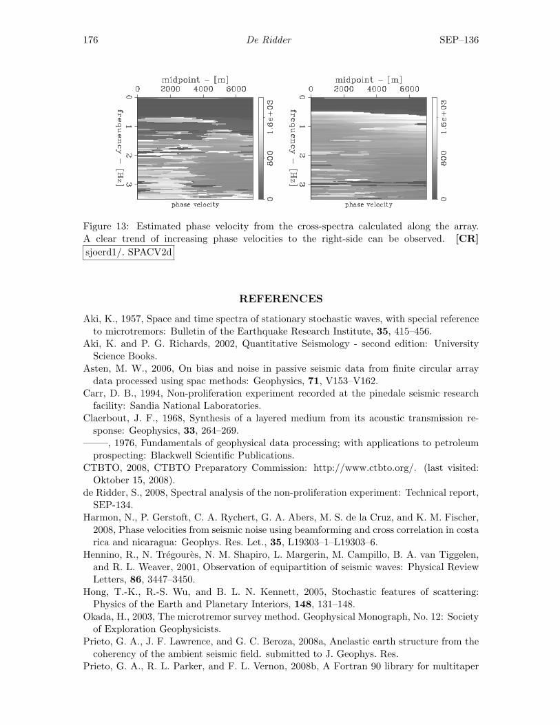
176 De Ridder SEP–136
Figure 13: Estimated phase velocity from the cross-spectra calculated along the array.A clear trend of increasing phase velocities to the right-side can be observed. [CR]sjoerd1/. SPACV2d
REFERENCES
Aki, K., 1957, Space and time spectra of stationary stochastic waves, with special referenceto microtremors: Bulletin of the Earthquake Research Institute, 35, 415–456.
Aki, K. and P. G. Richards, 2002, Quantitative Seismology - second edition: UniversityScience Books.
Asten, M. W., 2006, On bias and noise in passive seismic data from finite circular arraydata processed using spac methods: Geophysics, 71, V153–V162.
Carr, D. B., 1994, Non-proliferation experiment recorded at the pinedale seismic researchfacility: Sandia National Laboratories.
Claerbout, J. F., 1968, Synthesis of a layered medium from its acoustic transmission re-sponse: Geophysics, 33, 264–269.
——–, 1976, Fundamentals of geophysical data processing; with applications to petroleumprospecting: Blackwell Scientific Publications.
CTBTO, 2008, CTBTO Preparatory Commission: http://www.ctbto.org/. (last visited:Oktober 15, 2008).
de Ridder, S., 2008, Spectral analysis of the non-proliferation experiment: Technical report,SEP-134.
Harmon, N., P. Gerstoft, C. A. Rychert, G. A. Abers, M. S. de la Cruz, and K. M. Fischer,2008, Phase velocities from seismic noise using beamforming and cross correlation in costarica and nicaragua: Geophys. Res. Let., 35, L19303–1–L19303–6.
Hennino, R., N. Tregoures, N. M. Shapiro, L. Margerin, M. Campillo, B. A. van Tiggelen,and R. L. Weaver, 2001, Observation of equipartition of seismic waves: Physical ReviewLetters, 86, 3447–3450.
Hong, T.-K., R.-S. Wu, and B. L. N. Kennett, 2005, Stochastic features of scattering:Physics of the Earth and Planetary Interiors, 148, 131–148.
Okada, H., 2003, The microtremor survey method. Geophysical Monograph, No. 12: Societyof Exploration Geophysicists.
Prieto, G. A., J. F. Lawrence, and G. C. Beroza, 2008a, Anelastic earth structure from thecoherency of the ambient seismic field. submitted to J. Geophys. Res.
Prieto, G. A., R. L. Parker, and F. L. Vernon, 2008b, A Fortran 90 library for multitaper
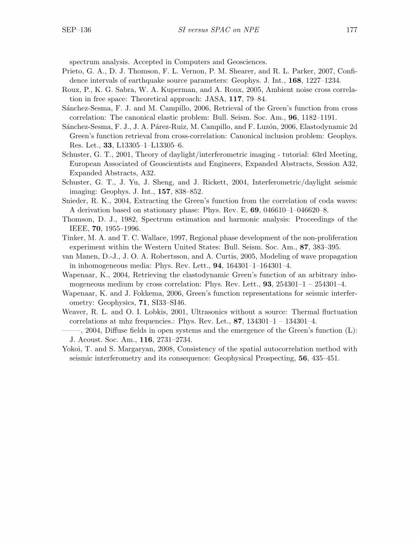
SEP–136 SI versus SPAC on NPE 177
spectrum analysis. Accepted in Computers and Geosciences.Prieto, G. A., D. J. Thomson, F. L. Vernon, P. M. Shearer, and R. L. Parker, 2007, Confi-
dence intervals of earthquake source parameters: Geophys. J. Int., 168, 1227–1234.Roux, P., K. G. Sabra, W. A. Kuperman, and A. Roux, 2005, Ambient noise cross correla-
tion in free space: Theoretical approach: JASA, 117, 79–84.Sanchez-Sesma, F. J. and M. Campillo, 2006, Retrieval of the Green’s function from cross
correlation: The canonical elastic problem: Bull. Seism. Soc. Am., 96, 1182–1191.Sanchez-Sesma, F. J., J. A. Parez-Ruiz, M. Campillo, and F. Luzon, 2006, Elastodynamic 2d
Green’s function retrieval from cross-correlation: Canonical inclusion problem: Geophys.Res. Let., 33, L13305–1–L13305–6.
Schuster, G. T., 2001, Theory of daylight/interferometric imaging - tutorial: 63rd Meeting,European Associated of Geoscientists and Engineers, Expanded Abstracts, Session A32,Expanded Abstracts, A32.
Schuster, G. T., J. Yu, J. Sheng, and J. Rickett, 2004, Interferometric/daylight seismicimaging: Geophys. J. Int., 157, 838–852.
Snieder, R. K., 2004, Extracting the Green’s function from the correlation of coda waves:A derivation based on stationary phase: Phys. Rev. E, 69, 046610–1–046620–8.
Thomson, D. J., 1982, Spectrum estimation and harmonic analysis: Proceedings of theIEEE, 70, 1955–1996.
Tinker, M. A. and T. C. Wallace, 1997, Regional phase development of the non-proliferationexperiment within the Western United States: Bull. Seism. Soc. Am., 87, 383–395.
van Manen, D.-J., J. O. A. Robertsson, and A. Curtis, 2005, Modeling of wave propagationin inhomogeneous media: Phys. Rev. Lett., 94, 164301–1–164301–4.
Wapenaar, K., 2004, Retrieving the elastodynamic Green’s function of an arbitrary inho-mogeneous medium by cross correlation: Phys. Rev. Lett., 93, 254301–1 – 254301–4.
Wapenaar, K. and J. Fokkema, 2006, Green’s function representations for seismic interfer-ometry: Geophysics, 71, SI33–SI46.
Weaver, R. L. and O. I. Lobkis, 2001, Ultrasonics without a source: Thermal fluctuationcorrelations at mhz frequencies.: Phys. Rev. Let., 87, 134301–1 – 134301–4.
——–, 2004, Diffuse fields in open systems and the emergence of the Green’s function (L):J. Acoust. Soc. Am., 116, 2731–2734.
Yokoi, T. and S. Margaryan, 2008, Consistency of the spatial autocorrelation method withseismic interferometry and its consequence: Geophysical Prospecting, 56, 435–451.

178 De Ridder SEP–136
Stanford Exploration Project, Report SEP136, April 14, 2009
3D pyramid interpolation
Xukai Shen
ABSTRACT
Seismic data geometries are not always as nice and regular as we want due to variousacquisition constraints. In such cases, data interpolation becomes necessary. Usuallyhigh-frequency data are aliased, while low-frequency data are not, so information inlow frequencies can help us interpolate aliased high-frequency data. In this paper, Ipresent a 3D data interpolation scheme in pyramid domain, in which I use informationin low-frequency data to interpolate aliased high-frequency data. This is possible sincein pyramid domain, only one prediction error filter (PEF) is needed to represent anystationary event (plane-wave) across all offsets and frequencies. However, if we needto estimate both the missing data and PEF, the problem becomes nonlinear. Byalternately estimating the missing data and PEF, we can linearize the problem andsolve it using a conventional least-squares solver.
INTRODUCTION
Data interpolation is an important step in seismic data processing that can greatly affectthe results of later processing steps, such as multiple removal, migration and inversion.There are many ways to interpolate data, including Fourier-transform-based approaches(e.g., Xu et al., 2005) and PEF-based approaches (e.g., Spitz, 1991; Crawley, 2000). A PEFis a filter that predicts one data sample from n previous samples, where n is the lengthof the PEF. One important feature of a PEF is that it has the inverse spectrum of theknown data, so when it is convolved with known data, it minimizes the convolution resultin the least-square sense. PEF estimation can be done in either time-space (t-x) domain orfrequency-space (f -x) domain (e.g. Claerbout, 1999; Crawley, 2000; Curry, 2007), however,if PEF estimation is done in the f -x domain, every frequency needs one distinct PEF.
The pyramid domain was introduced by Ronen (Hung et al., 2005), and is a resampledrepresentation of an ordinary f -x domain. Although it has frequency and space axes, thespatial sampling is different for different frequencies. This is attractive because we can usesparser sampling to adequately sample the data at lower frequencies, which makes uniformsampling for all frequencies unnecessary. Therefore in the pyramid domain, coarser gridspacing is used for lower frequencies, while finer spacing is used for higher frequencies. Thismakes it possible to capture the character of all frequency components of stationary eventswith only one PEF. So the information in the low frequency data can be better used tointerpolate higher frequency data.
In this paper, I present a 3D version of data interpolation in the pyramid domain basedon PEF estimation, which is based on Shen (2008). The paper is organized as follows: Ifirst show the 3D pyramid transform and corresponding missing-data interpolation and PEFestimation. I then show synthetic data examples. Finally, I conclude with the advantagesand disadvantages of this interpolation method.
179
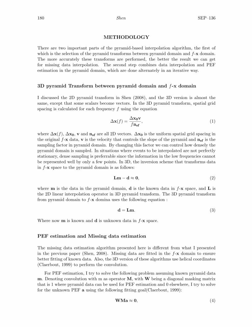
180 Shen SEP–136
METHODOLOGY
There are two important parts of the pyramid-based interpolation algorithm, the first ofwhich is the selection of the pyramid transforms between pyramid domain and f -x domain.The more accurately these transforms are performed, the better the result we can getfor missing data interpolation. The second step combines data interpolation and PEFestimation in the pyramid domain, which are done alternately in an iterative way.
3D pyramid Transform between pyramid domain and f-x domain
I discussed the 2D pyramid transform in Shen (2008), and the 3D version is almost thesame, except that some scalars become vectors. In the 3D pyramid transform, spatial gridspacing is calculated for each frequency f using the equation
∆x(f) =∆x0vfnsf
, (1)
where ∆x(f), ∆x0, v and nsf are all 2D vectors. ∆x0 is the uniform spatial grid spacing inthe original f -x data, v is the velocity that controls the slope of the pyramid and nsf is thesampling factor in pyramid domain. By changing this factor we can control how densely thepyramid domain is sampled. In situations where events to be interpolated are not perfectlystationary, dense sampling is preferrable since the information in the low frequencies cannotbe represented well by only a few points. In 3D, the inversion scheme that transforms datain f -x space to the pyramid domain is as follows:
Lm− d ≈ 0, (2)
where m is the data in the pyramid domain, d is the known data in f -x space, and L isthe 2D linear interpolation operator in 3D pyramid transform. The 3D pyramid transformfrom pyramid domain to f -x domina uses the following equation :
d = Lm. (3)
Where now m is known and d is unknown data in f -x space.
PEF estimation and Missing data estimation
The missing data estimation algorithm presented here is different from what I presentedin the previous paper (Shen, 2008). Missing data are fitted in the f -x domain to ensurebetter fitting of known data. Also, the 3D version of these algorithms use helical coordinates(Claerbout, 1999) to perform the convolution.
For PEF estimation, I try to solve the following problem assuming known pyramid datam. Denoting convolution with m as operator M, with W being a diagonal masking matrixthat is 1 where pyramid data can be used for PEF estimation and 0 elsewhere, I try to solvefor the unknown PEF a using the following fitting goal(Claerbout, 1999):
WMa ≈ 0, (4)
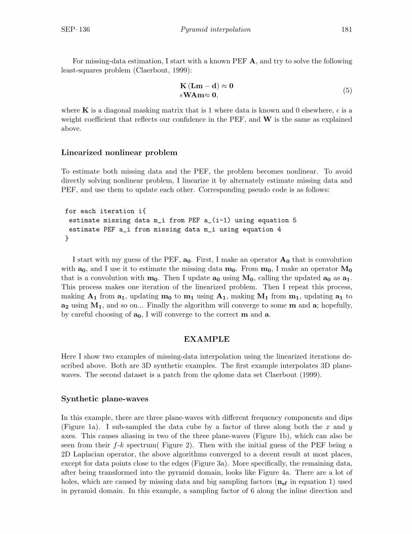
SEP–136 Pyramid interpolation 181
For missing-data estimation, I start with a known PEF A, and try to solve the followingleast-squares problem (Claerbout, 1999):
K (Lm− d) ≈ 0εWAm≈ 0,
(5)
where K is a diagonal masking matrix that is 1 where data is known and 0 elsewhere, ε is aweight coefficient that reflects our confidence in the PEF, and W is the same as explainedabove.
Linearized nonlinear problem
To estimate both missing data and the PEF, the problem becomes nonlinear. To avoiddirectly solving nonlinear problem, I linearize it by alternately estimate missing data andPEF, and use them to update each other. Corresponding pseudo code is as follows:
for each iteration i{estimate missing data m_i from PEF a_(i-1) using equation 5estimate PEF a_i from missing data m_i using equation 4}
I start with my guess of the PEF, a0. First, I make an operator A0 that is convolutionwith a0, and I use it to estimate the missing data m0. From m0, I make an operator M0
that is a convolution with m0. Then I update a0 using M0, calling the updated a0 as a1.This process makes one iteration of the linearized problem. Then I repeat this process,making A1 from a1, updating m0 to m1 using A1, making M1 from m1, updating a1 toa2 using M1, and so on... Finally the algorithm will converge to some m and a; hopefully,by careful choosing of a0, I will converge to the correct m and a.
EXAMPLE
Here I show two examples of missing-data interpolation using the linearized iterations de-scribed above. Both are 3D synthetic examples. The first example interpolates 3D plane-waves. The second dataset is a patch from the qdome data set Claerbout (1999).
Synthetic plane-waves
In this example, there are three plane-waves with different frequency components and dips(Figure 1a). I sub-sampled the data cube by a factor of three along both the x and yaxes. This causes aliasing in two of the three plane-waves (Figure 1b), which can also beseen from their f -k spectrum( Figure 2). Then with the initial guess of the PEF being a2D Laplacian operator, the above algorithms converged to a decent result at most places,except for data points close to the edges (Figure 3a). More specifically, the remaining data,after being transformed into the pyramid domain, looks like Figure 4a. There are a lot ofholes, which are caused by missing data and big sampling factors (nsf in equation 1) usedin pyramid domain. In this example, a sampling factor of 6 along the inline direction and
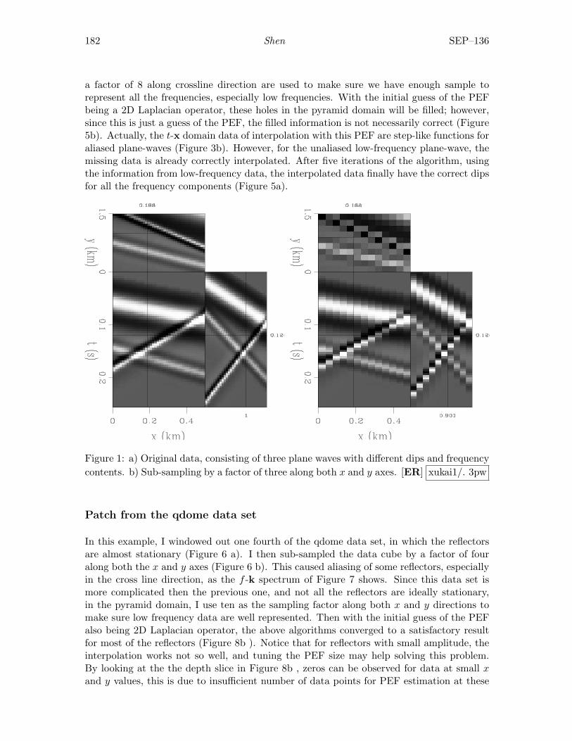
182 Shen SEP–136
a factor of 8 along crossline direction are used to make sure we have enough sample torepresent all the frequencies, especially low frequencies. With the initial guess of the PEFbeing a 2D Laplacian operator, these holes in the pyramid domain will be filled; however,since this is just a guess of the PEF, the filled information is not necessarily correct (Figure5b). Actually, the t-x domain data of interpolation with this PEF are step-like functions foraliased plane-waves (Figure 3b). However, for the unaliased low-frequency plane-wave, themissing data is already correctly interpolated. After five iterations of the algorithm, usingthe information from low-frequency data, the interpolated data finally have the correct dipsfor all the frequency components (Figure 5a).
Figure 1: a) Original data, consisting of three plane waves with different dips and frequencycontents. b) Sub-sampling by a factor of three along both x and y axes. [ER] xukai1/. 3pw
Patch from the qdome data set
In this example, I windowed out one fourth of the qdome data set, in which the reflectorsare almost stationary (Figure 6 a). I then sub-sampled the data cube by a factor of fouralong both the x and y axes (Figure 6 b). This caused aliasing of some reflectors, especiallyin the cross line direction, as the f -k spectrum of Figure 7 shows. Since this data set ismore complicated then the previous one, and not all the reflectors are ideally stationary,in the pyramid domain, I use ten as the sampling factor along both x and y directions tomake sure low frequency data are well represented. Then with the initial guess of the PEFalso being 2D Laplacian operator, the above algorithms converged to a satisfactory resultfor most of the reflectors (Figure 8b ). Notice that for reflectors with small amplitude, theinterpolation works not so well, and tuning the PEF size may help solving this problem.By looking at the the depth slice in Figure 8b , zeros can be observed for data at small xand y values, this is due to insufficient number of data points for PEF estimation at these
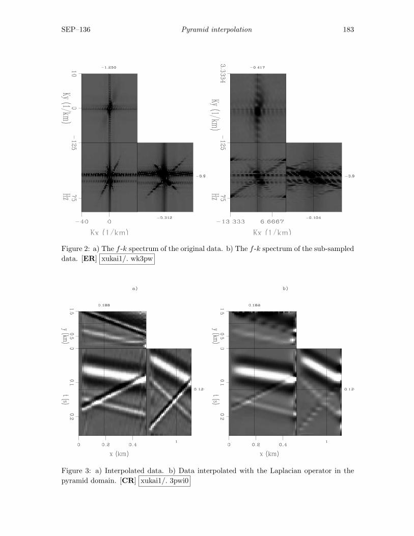
SEP–136 Pyramid interpolation 183
Figure 2: a) The f -k spectrum of the original data. b) The f -k spectrum of the sub-sampleddata. [ER] xukai1/. wk3pw
Figure 3: a) Interpolated data. b) Data interpolated with the Laplacian operator in thepyramid domain. [CR] xukai1/. 3pwi0
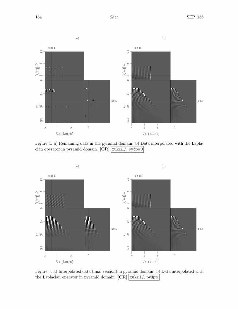
184 Shen SEP–136
Figure 4: a) Remaining data in the pyramid domain. b) Data interpolated with the Lapla-cian operator in pyramid domain. [CR] xukai1/. py3pw0
Figure 5: a) Interpolated data (final version) in pyramid domain. b) Data interpolated withthe Laplacian operator in pyramid domain. [CR] xukai1/. py3pw
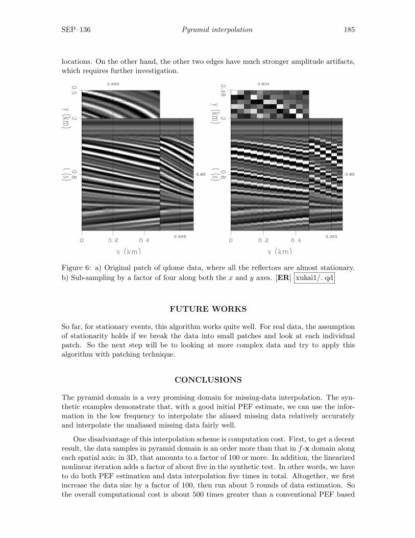
SEP–136 Pyramid interpolation 185
locations. On the other hand, the other two edges have much stronger amplitude artifacts,which requires further investigation.
Figure 6: a) Original patch of qdome data, where all the reflectors are almost stationary.b) Sub-sampling by a factor of four along both the x and y axes. [ER] xukai1/. qd
FUTURE WORKS
So far, for stationary events, this algorithm works quite well. For real data, the assumptionof stationarity holds if we break the data into small patches and look at each individualpatch. So the next step will be to looking at more complex data and try to apply thisalgorithm with patching technique.
CONCLUSIONS
The pyramid domain is a very promising domain for missing-data interpolation. The syn-thetic examples demonstrate that, with a good initial PEF estimate, we can use the infor-mation in the low frequency to interpolate the aliased missing data relatively accuratelyand interpolate the unaliased missing data fairly well.
One disadvantage of this interpolation scheme is computation cost. First, to get a decentresult, the data samples in pyramid domain is an order more than that in f -x domain alongeach spatial axis; in 3D, that amounts to a factor of 100 or more. In addition, the linearizednonlinear iteration adds a factor of about five in the synthetic test. In other words, we haveto do both PEF estimation and data interpolation five times in total. Altogether, we firstincrease the data size by a factor of 100, then run about 5 rounds of data estimation. Sothe overall computational cost is about 500 times greater than a conventional PEF based
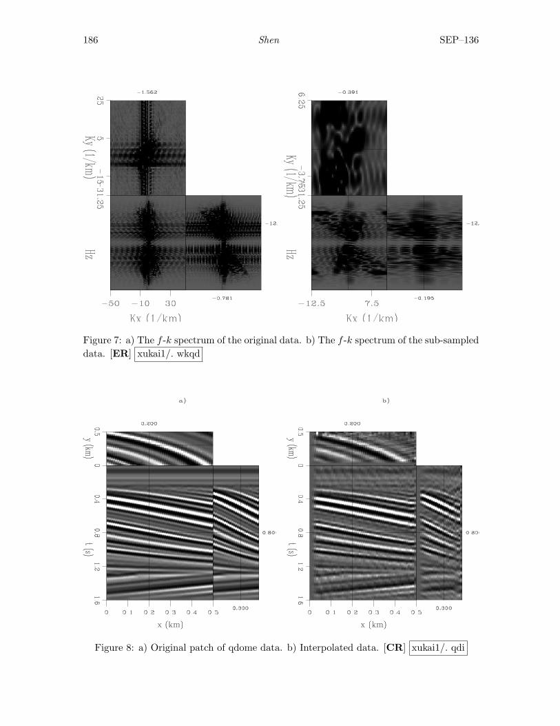
186 Shen SEP–136
Figure 7: a) The f -k spectrum of the original data. b) The f -k spectrum of the sub-sampleddata. [ER] xukai1/. wkqd
Figure 8: a) Original patch of qdome data. b) Interpolated data. [CR] xukai1/. qdi

SEP–136 Pyramid interpolation 187
interpolation scheme (e.g. Spitz, 1991). However, with a patching technique, many patchesof data can be interpolated simutaneously using parallelized version of this algorithm.
ACKNOWLEDGMENTS
I would like to thank Jon Claerbout for ideas about data interpolation in the pyramiddomain, Bob Clapp for synthetic example suggestions, and Antoine Guitton and WilliamCurry for numerous debugging suggestions.
REFERENCES
Claerbout, J., 1999, Geophysical estimation by example: Environmental soundings imageenhancement: Stanford Exploration Project.
Crawley, S., 2000, Seismic trace interpolation with nonstationary prediction-error filters:PhD thesis, Stanford University.
Curry, W., 2007, f-x domain non-stationary interpolation in patches: SEP-Report, 131.Hung, B., C. Notfors, and S. Ronen, 2005, Seismic data reconstruction using the pyramid
transform: 67th Meeting, EAGE, Expanded Abstracts, A039.Shen, X., 2008, Data interpolation in pyramid domain: SEP-134, 225–230.Spitz, S., 1991, Seismic trace interpolation in the F-X domain: Geophysics, 56, 785–794.Xu, S., Y. Zhang, D. Pham, and G. Lambare, 2005, Antileakage Fourier transform for
seismic data regularization: Geophysics, 70, V87–V95.

188 Shen SEP–136
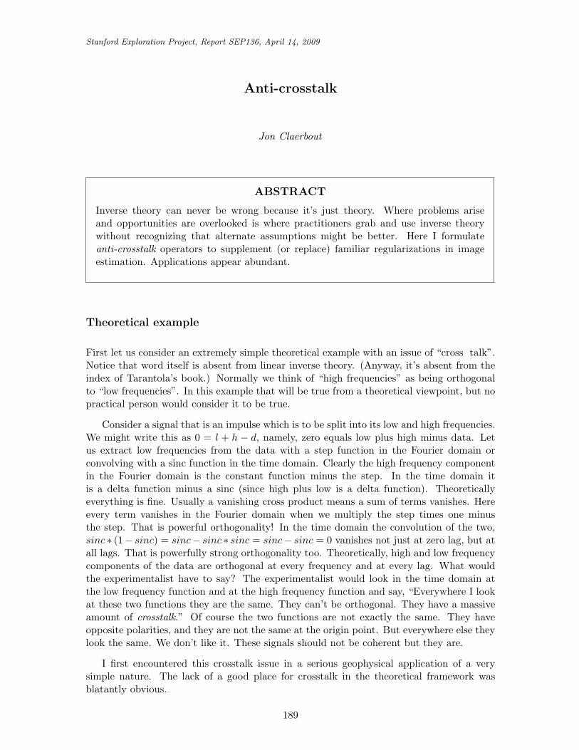
Stanford Exploration Project, Report SEP136, April 14, 2009
Anti-crosstalk
Jon Claerbout
ABSTRACT
Inverse theory can never be wrong because it’s just theory. Where problems ariseand opportunities are overlooked is where practitioners grab and use inverse theorywithout recognizing that alternate assumptions might be better. Here I formulateanti-crosstalk operators to supplement (or replace) familiar regularizations in imageestimation. Applications appear abundant.
Theoretical example
First let us consider an extremely simple theoretical example with an issue of “cross talk”.Notice that word itself is absent from linear inverse theory. (Anyway, it’s absent from theindex of Tarantola’s book.) Normally we think of “high frequencies” as being orthogonalto “low frequencies”. In this example that will be true from a theoretical viewpoint, but nopractical person would consider it to be true.
Consider a signal that is an impulse which is to be split into its low and high frequencies.We might write this as 0 = l + h − d, namely, zero equals low plus high minus data. Letus extract low frequencies from the data with a step function in the Fourier domain orconvolving with a sinc function in the time domain. Clearly the high frequency componentin the Fourier domain is the constant function minus the step. In the time domain itis a delta function minus a sinc (since high plus low is a delta function). Theoreticallyeverything is fine. Usually a vanishing cross product means a sum of terms vanishes. Hereevery term vanishes in the Fourier domain when we multiply the step times one minusthe step. That is powerful orthogonality! In the time domain the convolution of the two,sinc ∗ (1− sinc) = sinc− sinc ∗ sinc = sinc− sinc = 0 vanishes not just at zero lag, but atall lags. That is powerfully strong orthogonality too. Theoretically, high and low frequencycomponents of the data are orthogonal at every frequency and at every lag. What wouldthe experimentalist have to say? The experimentalist would look in the time domain atthe low frequency function and at the high frequency function and say, “Everywhere I lookat these two functions they are the same. They can’t be orthogonal. They have a massiveamount of crosstalk.” Of course the two functions are not exactly the same. They haveopposite polarities, and they are not the same at the origin point. But everywhere else theylook the same. We don’t like it. These signals should not be coherent but they are.
I first encountered this crosstalk issue in a serious geophysical application of a verysimple nature. The lack of a good place for crosstalk in the theoretical framework wasblatantly obvious.
189
190 Claerbout SEP–136
Lake example
A depth sounding survey was made of a lake. A boat with a depth sounder sailed a gridworkof passes on the lake. Upon analysis the final image contained obvious evidence of the surveygrid. Oops! We should always hide our data acquisition footprint. The footprint is not thegeography or geology we wish to show. How did this happen? We guessed the water levelchanged during the survey. Perhaps it rained or perhaps the water was used for agriculture.Perhaps the wind caused the lake to “pendulum” (seiche). Perhaps the operator sat inthe front of the boat, or sometimes its back, or ran it at various speeds giving the depthmeasurement a different bias. Our data measured the difference between the top and thebottom of the lake; yet we had no idea how to model the top. Eventually we modeledthe top as an “arbitrary low frequency function” in data space (a one dimensional functionfollowing the boat). This got rid of the tracks in the model space (map space) but led tomuch embarrassment. It was embarrassing to discover that the geography (as seen in dataspace) was correlated with the lake surface (rain and drain).
Let us express these ideas mathematically: d is the data, depth along the survey coordi-nate d(s). Here s is a parameter like time. It increases steadily whether the boat is sailingnorth-south or east-west or turning inbetween. The model space is the depth h(x, y). Therewill be a regularization on the depth, perhaps 0 ≈ ∇h(x, y).
For the top of the lake with the ship we need some slowly variable function of location s.It’s embarrassing for us to need to specify it because we have no good model for it. So, wespecify a slowly variable function u = u(s) by asking a random noise function n = n(s) torun thru a low frequency filter, say L. We are not comfortable also about needing to chooseL. We call the function u = Ln the rain and drain function. We take the regularizationfor the unknown n to be 0 ≈ n. (Least squares will tend to drive components of n tosimilar values, and under some conditions likewise the spectrum of n will tend to white, sowe expect (and often find) the spectrum of u comes out that of L.)
The operator we do understand very clearly is the geography operator G. Given wewish to make a theoretical data point (water depth), the geography operator G tells uswhere to go on the map to get it. Of course each of the two regularizations 0 ≈ ∇h(x, y)and 0 ≈ n has its own epsilon which is annoying because we need to specify those too.With all these definitions our unknowns are the geography h and the noise n that buildsus a drift function. Our data fitting goal says the data should be the separation of the topand bottom of the lake.
0 ≈ Gh + Ln− d (1)
In my free on-line textbook GEE all this seemed rather conventional and rather fine.Our embarrassment came when we compared the geographically modeled part of the dataGh to the drift (rain and drain) modeled part of the data Ln. They were visibly correlated.This is crazy! The boat being in deep water should not correlate with rain (or drain). Weneeded to add an ingredient to the formulation saying u = Ln should be orthogonal to Gh(which is practically the same as d) in some generalized sense. Let us see how this mightbe done.
SEP–136 Anti-crosstalk 191
A regression to minimize crosstalk
Observing the geographically modeled data Gh correlating with the data drift u = Ln wewish to articulate a regression that says they should not correlate. Since the drift u is asmall correction to the data d, in other words Gh ≈ d, we can simplify the goal by askingthat the dot product of d with u should vanish, vanish not necessarily over the entire dataset; but that it should vanish under many triangular weighed windows.
Let us define D as a diagonal matrix with d on the diagonal. This may be a littleunfamiliar. Often we see positive weighting functions on the diagonal. Here we see data(possibly with both polarities) on the diagonal. Additionally, let us define a matrix T ofconvolution with a triangle. Columns of T contain shifted triangle functions, likewise dorows. Take t′ to be any row of T. Then t′D is a row vector of triangle weighted data. Wewant the regression 0 ≈ t′Du for all shifts of the triangle function. The way to express thisis:
0 ≈ (TD)u (2)0 ≈ (TD)Ln (3)
Hooray! Now we know what coding to do! But first, to better understand the regression(2) imagine instead that T is a square matrix of all ones, say 1. That would be like superwide triangular windows. Then every component of the vector 1Du contains the same dotproduct d · u. Using T instead of 1 gives us those dot products under a triangle weight,each final vector component having a shifted triangle.
What is a good name for TD? It measures the similarity of d and u. It might becalled the “data similarity” operator. What is a good name for its adjoint DT? Assumingwhatever comes out of T is a smooth positive function, then DT is a data gaining operator(its input being a gain function). Do we have any geophysical problems where the unknownis the gain?
Crosstalk in a more general context
We seemed to escape nonlinearity in the lake depth sounding example above, but that wasa lucky accident. Since the data there was mostly explained by geography with a smallperturbation by rain and drain, the crosstalk while fundamentally nonlinear was practicallylinear. More generally anti-crosstalk strategies seem little (if ever!) developed becausethey lead us directly into nonlinear regression. Let us work through the general case, thenonlinear theory.
Consider data d a shot gather or CMP gather. We might choose to model it as reflections(hyperbolas) d1 plus linear events d2 (noises or head waves). We might thus set up theregression
0 ≈ d1 + d2 − d (4)0 ≈ F1m1 + F2m2 − d (5)
Of course we need some damping regularization on m1 and m2 which for simplicity of ex-position I will take to be 0 ≈ m1 and 0 ≈ m2. Is that all there is to this problem? Not
192 Claerbout SEP–136
necessarily. We’ll be annoyed if we discover a lot of cross talk between d1 and d2. Twodifferent physical mechanisms are supposed to have created our data. We’ll be annoyed todiscover they both make the same contribution or that they make opposite contributions.The regularization should reduce (or prevent) the contributions from coming out opposite.If they are opposites, it could represent our lack of analytic skills in formulating the regu-larization, or it could represent our need for the anti-crosstalk methodology being proposedhere.
We’d like that the modeled data parts d1 and d2 do not ”look like” each other. It’snot enough that the dot product d1 · d2 vanish. That dot product should be small underall shifted (say triangular) weighting windows. Since d1 is a linear function of the modelm1 and likewise for d2, the orthogonality we seek involves the product of m1 with m2 soour goals are a non-linear function of our unknowns. Never fear. We have done non-linearproblems before. They don’t turn out badly when we are able to define a good startinglocation (which we do by solving the linearized non-linear problem first).
The full non-linear derivation
For warm up we linearize in the simplest possible way. Suppose we allow only m1 to varykeeping m2 fixed. We put d2 on the diagonal of a matrix, say D2. The regression foranti-crosstalk is now
0 ≈ TD2d1 (6)0 ≈ TD2F1m1 (7)
Define the element-by-element cross product of d2 times d1 to be d1 × d2. Now let uslinearize the full non-linear anti-crosstalk regularization. Let a single element of d1×d2 bedecomposed as a base plus a perturbation d = d+d. A single component of the vector d1×d2
is (d1 + d1)(d2 + d2). Linearizing the product (neglecting the product of the perturbations)gives
d2d1 + d1d2 + d2d1 (8)
This is one component. We seek an expression for all. It will be a vector which is a productof a matrix with a vector. We want no unknowns in matrices; we want them all in vectorsso we will know how to solve for them.
D2d1 + D1d2 + D1d2 (9)
Express the perturbation parts of the vectors as functions of the model space
D2F1m1 + D1F2m2 + D1d2 (10)
This vector should be viewed under many windows (triangle shaped, for example). Undereach window we hope to see the product have a small value. The desired anti-crosstalkregression is to minimize the length of the vector below by variation of the model parametersm1 and m2.
0 ≈ T(D2F1m1 + D1F2m2 + D1d2) (11)
This regression augments our usual regularizations. Perhaps it partially or significantlysupplants them. Unfortunately, it requires yet another epsilon.
Upon finding m1 and m2 we update the base model m← m + m and iterate.
SEP–136 Anti-crosstalk 193
Outlook
Many examples suggest themselves.
1. We might model reflection data as a superposition of primaries and multiples. Wemight model it as a superposition of pressure waves and shear waves.
2. In tomography we might model event flatness as a superposition of shallow and deepslownesses. The shallow and deep slownesses have wholly different causes separatedby millions of years. They should not show crosstalk.
3. The problem of segregating signal and noise offers many examples. We’d like to seesignal containing no evident noise and vice versa.
4. In time-lapse seismology we would like to see the the image change unpolluted bythe original image. Unfortunately, the methodology proposed here does not allow fortime-shifted crosstalk.
Getting started
As the concepts here are quite new to us, the first thing we should do is cook up somesuper simple synthetic examples. With working synthetic codes in hand we should see if wecan go ahead and repair the Galilee survey. Hopefully we’ll recognize we have built somereusable software to facilitate other projects.
Getting started will not be easy. Most commonly we have a simple synthetic exampleunder control and struggle to find an appropriate real data set. Here we have a suitablebeginners’ data set (Galilee) but we need to find a synthetic data set to provide examplesthat give clarity to the whole process. Just one issue is dealing with the relative scalingof the three regularizations. We’d like meaningful examples where only one or two of theregularizations are actually required.
There are many paths to explore with anti-crosstalk technology. Besides the manypotential applications one can hope that the anti-crosstalk regularization eliminates (orreduces) the need for the usual regularizations. That would be nice if true. The need tospecify a suitable regularization is often what makes it difficult to automate data analysisbased on inversion.
I’m worried about the job as I defined it for the first-year SEP students. Given thelinearization I suggested to them, did they know how to measure success?

194 Claerbout SEP–136
Stanford Exploration Project, Report SEP136, April 14, 2009
Seismic investigation of natural coal fires: A pre-fieldworksynthetic feasibility study.
Sjoerd de Ridder and Seth S. Haines
ABSTRACT
Natural underground coal fires are a world-wide concern, emitting carbon dioxide andother pollutant gasses into the atmosphere; one such coal fire is located at Durango,Colorado. We carried out elastic modeling in order to investigate the potential ofapplying P-wave seismic methods to the problem of differentiating between burnedand unburned coal in the upper ∼30 m of the subsurface at the site near Durango.This is a challenging problem for any geophysical method, but preliminary modelingresults show that the problem is tractable under certain circumstances. Our highlysimplified model suggests that imaging the coal layer can potentially be accomplishedwith adequately high frequencies (source center frequency > 125 Hz); imaging theactual burned zone would be more difficult. The model neglects the major near-surfaceheterogeneity known to exist at the site; features such as fissures would surely resultin diffractions and reflections that could obscure much of the desired signal.
INTRODUCTION
Ongoing research at a site outside Durango, Colorado, is focused on characterizing andmodeling a coal bed that has been burning underground for a number of years. The goal isto develop an understanding of how coal fires burn for the purpose of designing optimumsolutions for extinguishing coal fires around the world. The unique aspect of this particularfire is that it is small-scale and easily accessible. We were asked whether seismic methodscould potentially provide useful information at the site, ideally as a way to map the burnedand unburned coal. Any related information would be useful, such as mapping only theunburned coal, and/or locating fissures and other subsidence features that might not reachthe surface.
We conducted elastic modeling to simulate a P-wave seismic survey at the site, to assessthe likelihood of successfully applying seismic methods to this problem, and to determineoptimal parameters for any field data acquisition. The model is highly simplified given thatit neglects the fissures and other overburden heterogeneity. The main target is the partiallyburned coal layer.
The site is roughly 300m by 100m. Researchers of the Global Climate & Energy Projectat Stanford University (GCEP, 2008) have been studying the site using a number of differentapproaches to understand the progression of the fire over time and try to predict its likelyfuture trends. One approach has been the mapping of surface anomalies across the site –mainly fissures resulting from the compaction of the ash as the coal burns. Researchershave also drilled a total of 14 wells across the site, in areas where they know the coal hasburned, where they think the burn front is located, and in unburned areas. A 100 ft core
195
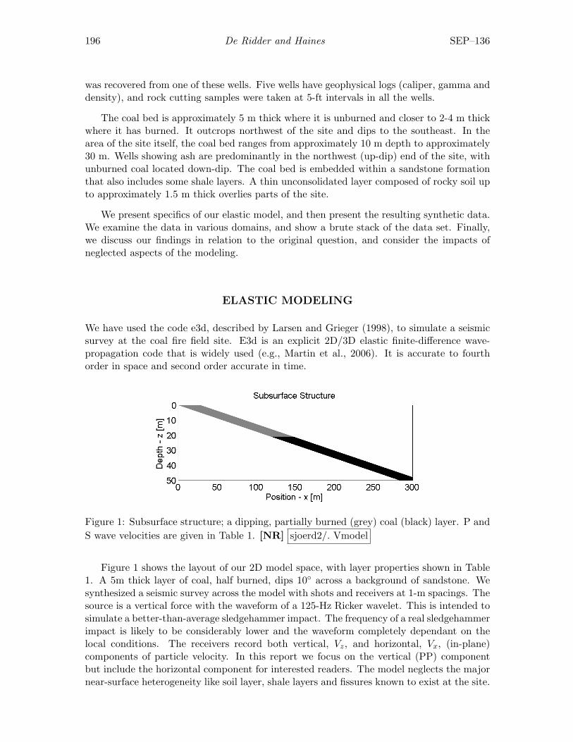
196 De Ridder and Haines SEP–136
was recovered from one of these wells. Five wells have geophysical logs (caliper, gamma anddensity), and rock cutting samples were taken at 5-ft intervals in all the wells.
The coal bed is approximately 5 m thick where it is unburned and closer to 2-4 m thickwhere it has burned. It outcrops northwest of the site and dips to the southeast. In thearea of the site itself, the coal bed ranges from approximately 10 m depth to approximately30 m. Wells showing ash are predominantly in the northwest (up-dip) end of the site, withunburned coal located down-dip. The coal bed is embedded within a sandstone formationthat also includes some shale layers. A thin unconsolidated layer composed of rocky soil upto approximately 1.5 m thick overlies parts of the site.
We present specifics of our elastic model, and then present the resulting synthetic data.We examine the data in various domains, and show a brute stack of the data set. Finally,we discuss our findings in relation to the original question, and consider the impacts ofneglected aspects of the modeling.
ELASTIC MODELING
We have used the code e3d, described by Larsen and Grieger (1998), to simulate a seismicsurvey at the coal fire field site. E3d is an explicit 2D/3D elastic finite-difference wave-propagation code that is widely used (e.g., Martin et al., 2006). It is accurate to fourthorder in space and second order accurate in time.
Figure 1: Subsurface structure; a dipping, partially burned (grey) coal (black) layer. P andS wave velocities are given in Table 1. [NR] sjoerd2/. Vmodel
Figure 1 shows the layout of our 2D model space, with layer properties shown in Table1. A 5m thick layer of coal, half burned, dips 10◦ across a background of sandstone. Wesynthesized a seismic survey across the model with shots and receivers at 1-m spacings. Thesource is a vertical force with the waveform of a 125-Hz Ricker wavelet. This is intended tosimulate a better-than-average sledgehammer impact. The frequency of a real sledgehammerimpact is likely to be considerably lower and the waveform completely dependant on thelocal conditions. The receivers record both vertical, Vz, and horizontal, Vx, (in-plane)components of particle velocity. In this report we focus on the vertical (PP) componentbut include the horizontal component for interested readers. The model neglects the majornear-surface heterogeneity like soil layer, shale layers and fissures known to exist at the site.
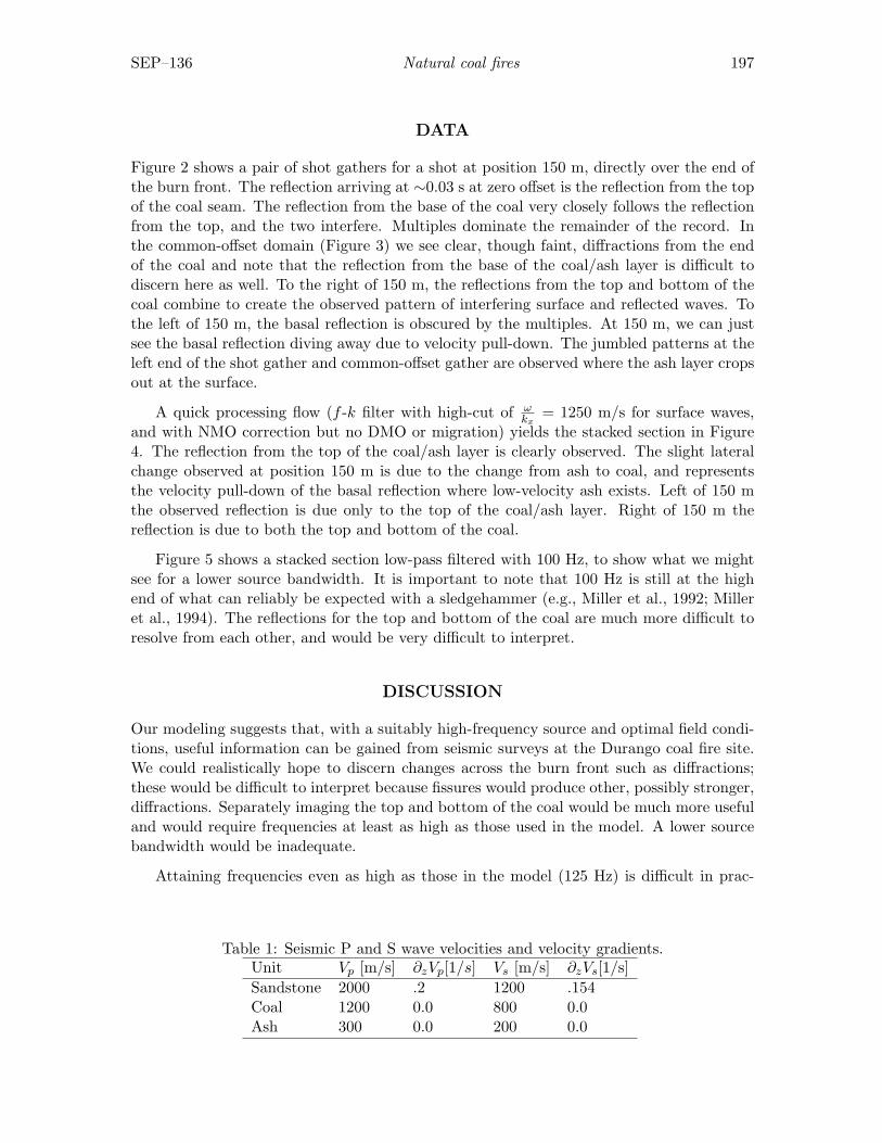
SEP–136 Natural coal fires 197
DATA
Figure 2 shows a pair of shot gathers for a shot at position 150 m, directly over the end ofthe burn front. The reflection arriving at ∼0.03 s at zero offset is the reflection from the topof the coal seam. The reflection from the base of the coal very closely follows the reflectionfrom the top, and the two interfere. Multiples dominate the remainder of the record. Inthe common-offset domain (Figure 3) we see clear, though faint, diffractions from the endof the coal and note that the reflection from the base of the coal/ash layer is difficult todiscern here as well. To the right of 150 m, the reflections from the top and bottom of thecoal combine to create the observed pattern of interfering surface and reflected waves. Tothe left of 150 m, the basal reflection is obscured by the multiples. At 150 m, we can justsee the basal reflection diving away due to velocity pull-down. The jumbled patterns at theleft end of the shot gather and common-offset gather are observed where the ash layer cropsout at the surface.
A quick processing flow (f -k filter with high-cut of ωkx
= 1250 m/s for surface waves,and with NMO correction but no DMO or migration) yields the stacked section in Figure4. The reflection from the top of the coal/ash layer is clearly observed. The slight lateralchange observed at position 150 m is due to the change from ash to coal, and representsthe velocity pull-down of the basal reflection where low-velocity ash exists. Left of 150 mthe observed reflection is due only to the top of the coal/ash layer. Right of 150 m thereflection is due to both the top and bottom of the coal.
Figure 5 shows a stacked section low-pass filtered with 100 Hz, to show what we mightsee for a lower source bandwidth. It is important to note that 100 Hz is still at the highend of what can reliably be expected with a sledgehammer (e.g., Miller et al., 1992; Milleret al., 1994). The reflections for the top and bottom of the coal are much more difficult toresolve from each other, and would be very difficult to interpret.
DISCUSSION
Our modeling suggests that, with a suitably high-frequency source and optimal field condi-tions, useful information can be gained from seismic surveys at the Durango coal fire site.We could realistically hope to discern changes across the burn front such as diffractions;these would be difficult to interpret because fissures would produce other, possibly stronger,diffractions. Separately imaging the top and bottom of the coal would be much more usefuland would require frequencies at least as high as those used in the model. A lower sourcebandwidth would be inadequate.
Attaining frequencies even as high as those in the model (125 Hz) is difficult in prac-
Table 1: Seismic P and S wave velocities and velocity gradients.Unit Vp [m/s] ∂zVp[1/s] Vs [m/s] ∂zVs[1/s]Sandstone 2000 .2 1200 .154Coal 1200 0.0 800 0.0Ash 300 0.0 200 0.0
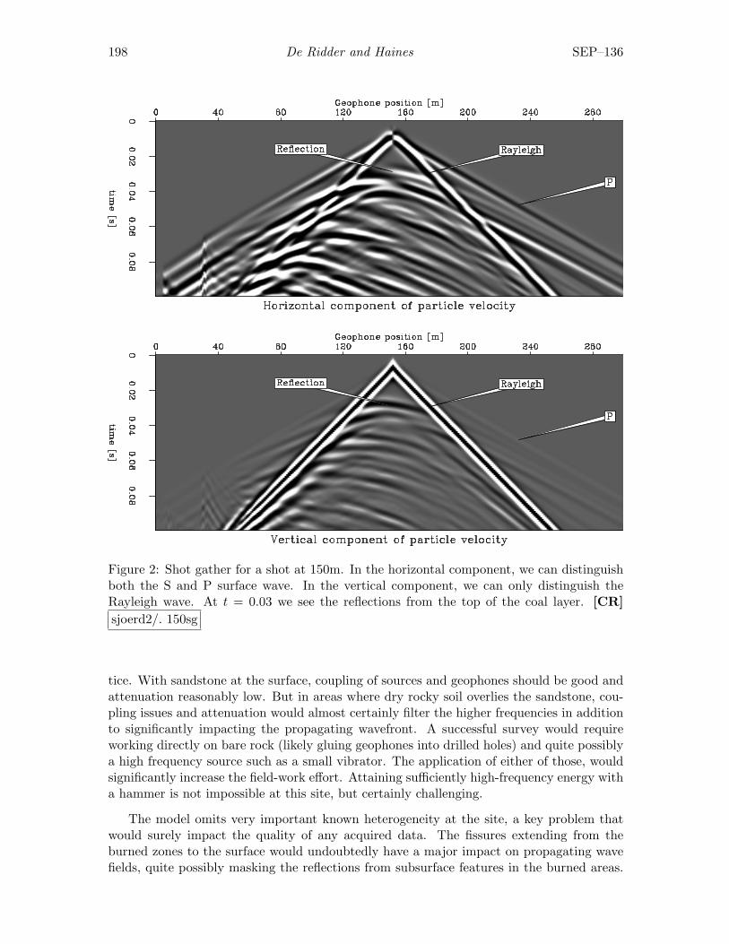
198 De Ridder and Haines SEP–136
Figure 2: Shot gather for a shot at 150m. In the horizontal component, we can distinguishboth the S and P surface wave. In the vertical component, we can only distinguish theRayleigh wave. At t = 0.03 we see the reflections from the top of the coal layer. [CR]sjoerd2/. 150sg
tice. With sandstone at the surface, coupling of sources and geophones should be good andattenuation reasonably low. But in areas where dry rocky soil overlies the sandstone, cou-pling issues and attenuation would almost certainly filter the higher frequencies in additionto significantly impacting the propagating wavefront. A successful survey would requireworking directly on bare rock (likely gluing geophones into drilled holes) and quite possiblya high frequency source such as a small vibrator. The application of either of those, wouldsignificantly increase the field-work effort. Attaining sufficiently high-frequency energy witha hammer is not impossible at this site, but certainly challenging.
The model omits very important known heterogeneity at the site, a key problem thatwould surely impact the quality of any acquired data. The fissures extending from theburned zones to the surface would undoubtedly have a major impact on propagating wavefields, quite possibly masking the reflections from subsurface features in the burned areas.
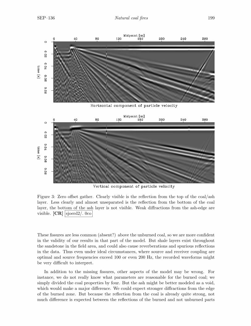
SEP–136 Natural coal fires 199
Figure 3: Zero offset gather. Clearly visible is the reflection from the top of the coal/ashlayer. Less clearly and almost unseparated is the reflection from the bottom of the coallayer, the bottom of the ash layer is not visible. Weak diffractions from the ash-edge arevisible. [CR] sjoerd2/. 0co
These fissures are less common (absent?) above the unburned coal, so we are more confidentin the validity of our results in that part of the model. But shale layers exist throughoutthe sandstone in the field area, and could also cause reverberations and spurious reflectionsin the data. Thus even under ideal circumstances, where source and receiver coupling areoptimal and source frequencies exceed 100 or even 200 Hz, the recorded waveforms mightbe very difficult to interpret.
In addition to the missing fissures, other aspects of the model may be wrong. Forinstance, we do not really know what parameters are reasonable for the burned coal; wesimply divided the coal properties by four. But the ash might be better modeled as a void,which would make a major difference. We could expect stronger diffractions from the edgeof the burned zone. But because the reflection from the coal is already quite strong, notmuch difference is expected between the reflections of the burned and not unburned parts

200 De Ridder and Haines SEP–136
Figure 4: Stacked section, after surface wave removal and NMO correction. The bottomof the coal layer is visible, but clearly overlaps with the reflection from the top of the coallayer. [CR] sjoerd2/. ZOsect
of the coal seam. In any case, the known subsidence and rock changes that exist above theburned zone at this site and observed at other such sites (e.g., Wolf, 2006) would surelyimpact both wave propagation above, and within, the burned zone. The absence of thisheterogeneity in the model is a major simplification of the real case.
We have not simulated an SH-wave survey at the site, an option that should be consid-ered in any near-surface application. Being strongly sensitive to voids, shear waves mightprove useful in this case. Their lower propagation speed would lead to shorter wavelengthand better resolution for a given frequency, but generation of high frequency sources is evenharder for SH-wave sources than it is for P-wave sources. In addition, the jumbled natureof the fissured sandstone would likely lead to many spurious S-P conversions that wouldcomplicate interpretation of the observed wave field. Accurately simulating the complexitiesof an SH-wave survey at the site would be difficult.
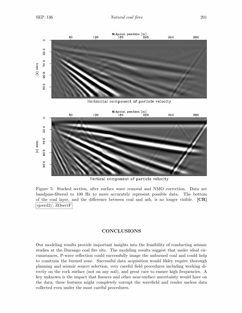
SEP–136 Natural coal fires 201
Figure 5: Stacked section, after surface wave removal and NMO correction. Data arebandpass-filtered to 100 Hz to more accurately represent possible data. The bottomof the coal layer, and the difference between coal and ash, is no longer visible. [CR]sjoerd2/. ZOsectF
CONCLUSIONS
Our modeling results provide important insights into the feasibility of conducting seismicstudies at the Durango coal fire site. The modeling results suggest that under ideal cir-cumstances, P-wave reflection could successfully image the unburned coal and could helpto constrain the burned zone. Successful data acquisition would likley require thoroughplanning and seismic source selection, very careful field procedures including working di-rectly on the rock surface (not on any soil), and great care to ensure high frequencies. Akey unknown is the impact that fissures and other near-surface uncertainty would have onthe data; these features might completely corrupt the wavefield and render useless datacollected even under the most careful procedures.
202 De Ridder and Haines SEP–136
ACKNOWLEDGMENTS
We are grateful to Bob Clapp for helpful discussions on this topic. We are also grateful toLynn Orr, Taku Ide, and Nigel Crook for bringing this project to our attention and helpingus to understand the key aspects of the problem. And finally, we thank Shawn Larsen forhis help with e3d.
REFERENCES
GCEP, 2008, Global energy and climate project, Stanford University:http://www.gcep.org/. (last visited: October 20, 2008).
Larsen, S. C. and J. C. Grieger, 1998, Elastic modeling initiative, Part III: 3-D computa-tional modeling: 68th Ann. Internat. Mtg, 1803–1806, Soc. of Expl. Geophys.
Martin, G. S., 2006, Marmousi2: An upgrade for marmousi: The Leading Edge, 25, 156–166.
Miller, R. D., S. E. Pullan, D. W. Steeples, and J. A. Hunter, 1994, Field comparison ofshallow P-wave seismic sources near Houston, Texas: Geophysics, 59, 1713–1728.
Miller, R. D., S. F. Pullan, D. W. Steeples, and J. A. Hunter, 1992, Field comparison ofshallow seismic sources near Chino, California: Geophysics, 57, 693–709.
Wolf, K. H. A. A., 2006, The interaction between underground coal fires and their roofrocks.: PhD thesis, Delft University of Technology.

Stanford Exploration Project, Report SEP136, April 14, 2009
Hubbert math
Jon Claerbout and Francis Muir
ABSTRACT
Hubbert fits growth and decay of petroleum production to the logistic function. Hub-bert’s relationship is commonly encountered in four different forms. They are all statedhere, then derived from one of them, thus showing they are equivalent.
PREFACE
This article was rejected by Wikipedia. They say an encyclopedia should not contain thederivation of important equations so we prepared this article for that purpose. The many ref-erences to this paper (missing here) are web links which may be found at http://sep.stanford.edu/sep/jon/tarsand/
THE FOUR FORMS OF HUBBERT’S EQUATION
Over the long haul populations grow and decay. To describe the growth and decay ofcivilization’s dependence on nuclear and fossil fuels, M. King Hubbert chose an equationthat describes many natural processes. Introduce bacteria to food and their populationwill grow exponentially until there no longer is food. As we catch all the fish in the lakeour daily catch will be proportional to the number of remaining fish. Hubbert’s equationmodels both exponential growth and decay with a single equation of three parameters tobe chosen from the data. He predicted 52 years ago that worldwide oil production wouldbe peaking about now (2008). It is.
Hubbert’s math has four different forms which we examine before showing they aremathematically equivalent.
Basic definitions
We define:
• t is time in years
• Q(t) is cumulative production in billion barrels at year t.
• Q∞ is the ultimate recoverable resource.
• P (t) = dQ/dt is production in billion barrels/year at year t.
• τ is the year at which production peaks.
203
204 Claerbout and Muir SEP–136
• ω is an inverse decay time (imaginary frequency).
The Hubbert’s equation can be expressed in four forms. First, the differential form
dQ
dt= P = ω Q
(1− Q
Q∞
)(1)
This equation is non-linear in Q but it reduces to familiar linear equations near thebeginning and Q ≈ 0 and near the end at Q ≈ Q∞. As production begins and Q/Q∞ issmall, equation (1) reduces to dQ/dt = ωQ which displays exponential growth at a rate ω.As production ends near Q ≈ Q∞ the non-linear equation reduces to exponential decay. Toprove this fact change variables from Q to q by inserting Q = Q∞ − q. Then evaluate theresult at small q. The form (1) exhibits growth and decay as a dynamic process.
The second form of the Hubbert equation is found by dividing equation (1) by Q. It issometimes called the Hubbert Linearization.
P
Q= ω
(1− Q
Q∞
)(2)
The important thing about this equation is that it is linear in the two variables Q andP/Q. If you have historical measurements of Pi and Qi, you can plot these points in the(Q,P/Q)-plane and hope for them to reasonably fit a straight line. Fitting the best line tothe scattered points we can read the axis intercepts. At Q = 0 with equation (2) we can readoff the value of the growth/decay parameter ω = (P/Q)intercept. For world oil, accordingto Deffeyes (Remember! The references are links on the web version of this paper.) it is5.3 percent/year. At the other intercept, P/Q = 0 we must have Q = Q∞. According toDeffeyes, Q∞ is two trillion barrels.
The third form of Hubbert’s equation is the one best known. It looks like a Gaussian,but it isn’t. (A Gaussian decays much faster.) The current production P = dQ/dt is
P (t) = Q∞ ω1
(e−(ω/2)(τ−t) + e(ω/2)(τ−t))2(3)
This is the equation of a blob, also known as “Hubbert’s pimple”, symmetric about thepoint t = τ . Asymptotically it decreases (or increases) exponentially towards its maximumvalue at the center at t = τ . The function resembles a Gaussian but exponential decay ismuch weaker than Gaussian decay. Exponential growth is common in ecological systemswhich may also decay exponentially as resources are depleted or predator numbers growexponentially.
All that remains is to figure out τ . The Hubbert curve is symmetrical and reachesits maximum when half the oil is gone. That happens when Q = Q∞/2. In the case ofUSA production which has passed its peak we can find the year that Q reached that value(about 1973). There is some debate about what year world production peaks, but generalagreement is that it is about now (2008). Under Hubbert assumptions the decline curveis a mirror of the rise curve. That means we start down gently over the next decade, but
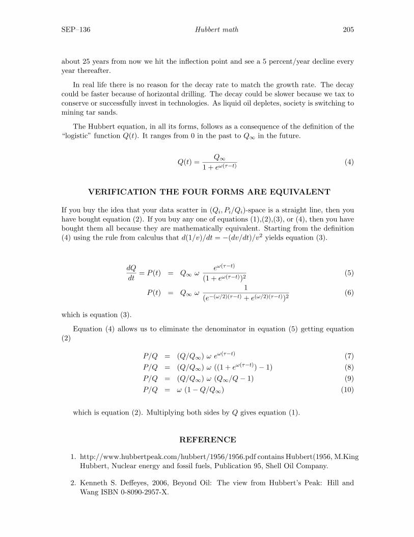
SEP–136 Hubbert math 205
about 25 years from now we hit the inflection point and see a 5 percent/year decline everyyear thereafter.
In real life there is no reason for the decay rate to match the growth rate. The decaycould be faster because of horizontal drilling. The decay could be slower because we tax toconserve or successfully invest in technologies. As liquid oil depletes, society is switching tomining tar sands.
The Hubbert equation, in all its forms, follows as a consequence of the definition of the“logistic” function Q(t). It ranges from 0 in the past to Q∞ in the future.
Q(t) =Q∞
1 + eω(τ−t)(4)
VERIFICATION THE FOUR FORMS ARE EQUIVALENT
If you buy the idea that your data scatter in (Qi, Pi/Qi)-space is a straight line, then youhave bought equation (2). If you buy any one of equations (1),(2),(3), or (4), then you havebought them all because they are mathematically equivalent. Starting from the definition(4) using the rule from calculus that d(1/v)/dt = −(dv/dt)/v2 yields equation (3).
dQ
dt= P (t) = Q∞ ω
eω(τ−t)
(1 + eω(τ−t))2(5)
P (t) = Q∞ ω1
(e−(ω/2)(τ−t) + e(ω/2)(τ−t))2(6)
which is equation (3).
Equation (4) allows us to eliminate the denominator in equation (5) getting equation(2)
P/Q = (Q/Q∞) ω eω(τ−t) (7)P/Q = (Q/Q∞) ω ((1 + eω(τ−t))− 1) (8)P/Q = (Q/Q∞) ω (Q∞/Q− 1) (9)P/Q = ω (1−Q/Q∞) (10)
which is equation (2). Multiplying both sides by Q gives equation (1).
REFERENCE
1. http://www.hubbertpeak.com/hubbert/1956/1956.pdf contains Hubbert(1956, M.KingHubbert, Nuclear energy and fossil fuels, Publication 95, Shell Oil Company.
2. Kenneth S. Deffeyes, 2006, Beyond Oil: The view from Hubbert’s Peak: Hill andWang ISBN 0-8090-2957-X.

206 Claerbout and Muir SEP–136
POSTFACE
One day I learned that Firefox had a much better way of zooming web pages, zoomingthe pictures too. Knowing that equations are pictures I went to Wikipedia, and looked up“Fourier Analysis”. I was delighted. A table of equations looked beautiful and could bezoomed up to a size suitable for public lectures! It was as if html had finally incorporatedmath. In reality the math had been done via LaTeX and inserted as photos. Wanting tohave on-line lectures drawn exactly from my books I learned to contribute to Wikipediaincluding equations.
At the same time I was reading Deffeyes book “Beyond Oil” (a play on the slogan“Beyond Petroleum”). I wanted to play with Hubbert’s curve fitting of worldwide oilproduction. Francis Muir gave me the algebraic tips I needed. I prepared my contributionin my “sandbox” and then moved it to the main encyclopedia. One of their volunteermanagers soon found it and didn’t like it. Rather than quote his opinions, I paraphrasesaying “equation derivations do not belong in an encyclopedia.”
So, I gave up and prepared this PDF file instead. It’s not as seamlessly web viewableas html, but I’m much happier with it – and I am able to include it in this report!
A goal I cannot meet today is to write a single LaTeX file that becomes two things:(1) print media that is attractive, readable, and contains its web references (perhaps infootnotes), and (2) a PDF file with references as web links that work. I would like to seemy books and all SEP report articles in this form. I’m not going to develop this myself.Someone else will do it; and I’ll try to be an early adopter.

Stanford Exploration Project, Report SEP136, April 14, 2009
Tar sands: Reprieve or apocalypse?
Jon Claerbout
ABSTRACT
Based on a Hubbert-type analysis two projections are made of tar sands production.With tar sand production growing at 5%/year total petroleum production declines atan annual rate of 1-2%. With tar sand production growing at 10%/year total petroleumproduction continues rising at almost the historic rate until 2040 followed by a catas-trophic rate of 50%/decade.
PREFACE
This paper with references as embedded web links may be found at http://sep.stanford.edu/sep/jon/tarsand/
TAR SANDS
Tar Sands are an amazing resource, mostly in Canada. Already in 2007, 44% of Canadianpetroleum production came from tar sands. The total Canadian resource (not all prod-ucable) is estimated to be 2.2 trillion barrels. That’s a lot! For comparison producibleworld petroleum liquids are estimated at 2 trillion barrels, half of which have already beenconsumed. Below are two scenarios for future tar-sands production. The plot on the left(labeled Malthusian) shows tar sands growing and decaying at the same 5% annual rate thatliquid petroleum has done. The decay of the sum is not severe, roughly 15% per decade,1-2% per year. The plot on the right (labeled Cornucopian) shows what might happen incase of laissez-faire or perceived grave urgency, a 10% tar-sands growth rate for 30-35 yearsfollowed by precipitous collapse about 50% per decade.
Unfortunately, of the Canadian 2.2 trillion barrels only 20% is estimated to be recover-able by strip mining. Having myself seen that the residual output of a tar sand extractionplant is clean white sand, we may take that resource to be 100% fully recoverable, 440 bil-lion barrels. Hooray! Unfortunately, what is not reachable by strip mining is more difficultto recover. I took this to be 25%, so that 80% adds 420 billion barrels.
You may hear, “Tar sands are profitably produced at $28-$44/barrel”. Yes, and theremay be oil in the Middle East that can be produced at $1-$2/barrel. That oil will be sold forthe “market clearing price”. Even if someone could rapidly produce great volumes from tarsands it would only accelerate the subsequent decline (as the Cornucopian plot shows). Tarsand production requires monsterous industrial machinery. “Obscene profits” are buildingit now.
We neglect here many things. Natural gas is an important resource about the sizeof oil with a peak trailing oil by a few decades. Tar sands will need to replace the
207
208 Claerbout SEP–136
Liquid
Tar sand
SumLiquid
Tar sand
Sum
Figure 1: Two scenarios for tar sands exploitation.[NR] jontarsand/. tarannotated
natural gas too! Venezuela has a reserve of heavy oil possibly comparable to Canada’s.Past nationalization of investments has effectively stopped current investment, but theoil in place has been quoted as 1.3 trillion barrels with a 20% recovery, netting 260 bil-lion barrels – a bump a quarter the size of Canada occuring later in time. Shale oilcan be burned like coal. Unfortunately liquifaction of shale oil and world-wide gas hy-drates are nice to dream about, but there are no functioning demonstration productionfacilities anywhere. Recently USGS forecast 1/10 trillion barrels in the arctic, a pim-ple on the graphs above. Nuclear is not a transportation fuel. Coal (with its own Hub-bert curve) can be converted to the gaseous fuel dimethyl ether (DMD) particularly suit-able as a replacement for diesel fuel. Ironically, nuclear, including the fast breeder reac-tor, including thorium as well as uranium is more fully described by the old-time geolo-gist Hubbert in 1956 than by today’s Cal Tech physicist and vice provost David Good-stein in his 2004 book “Out of gas”. http://www.usgs.gov/newsroom/article.asp?ID=1980http://www.hubbertpeak.com/hubbert/1956/1956.pdf
WILL THIS AFFECT YOU?
You may ask, “What makes you believe these predictions?” The classic paper of M.KingHubbert, written in 1956 predicted a USA liquid oil peak in 1973. It did peak then. That pa-per also predicted a world peak about the year 2000, a bit early, but not much. Most recentpredictions [1] [2] calculate twice as much oil as Hubbert predicted, but the peak has movedonly about a decade later, about now. Why does double the oil move the peak so little?Because so much is depleted in the middle decades. http://www.amazon.com/Beyond-Oil-View-Hubberts-Peak/dp/080902957X/
Didn’t you assume the total oil in place? Not for the liquids. When the productionpeaks, half is gone; the other half is left. There is widespread agreement the productionwill soon or has already peaked. For the tar sands resource size I refer to The PetroleumSociety of Canada. http://www.energy.gov.ab.ca/OilSands/pdfs/RPT Chops app3.pdf
The next question is, “Does it matter to me?” I suggest you print this page. Upon theprinted page draw a horizontal arrow from the day you were born to then plus 84 years.

SEP–136 Tar sands 209
Then draw the arrows for your parents, your children, and grandchildren.
Poor people will be the first to conserve. After that people with long commutes. Afterthat comes you. You have some time prepare yourself before the crowds. Don’t waste it!How much time do we have? If the choice is political between the Malthusian and theCornucopian which choice do you think will be made? I fear the disaster. (Sorry.) Wouldthat the Canadians learned the lesson of the East Texas Oil Field and the Texas RailroadCommission.
CREDITS
Helpful comments were received from Roland Horne, David Lumley, Amos Nur, GeorgeSibbald, and Kevin Wolf.
CONFLICT OF INTEREST STATEMENT
The author is an emeritus (retired) professor specialized in the geophysical prospectingindustry, an industry dependent for customers on the oil industry (but little on its tarsands sector).

210 Claerbout SEP–136
SEP–136 213
SEP PHONE DIRECTORY
Name Phone Login Name
Al Theyab, Abdullah 723-0463 altheyabAyeni, Gboyega 723-6006 gayeniBerryman, James – berrymanBiondi, Biondo 723-1319 biondoCardoso, Claudio 723-1250 claudioClaerbout, Jon 723-3717 jonClapp, Bob 725-1334 bobde Ridder, Sjoerd 723-1250 sjoerdGuitton, Antoine – antoineHalpert, Adam 723-6006 adamLau, Diane 723-1703 dianeLi, Elita 723-9282 myfusanMaysami, Mohammad 723-9282 mohammadShen, Xukai 723-0463 xukaiShragge, Jeff 723-0463 jeffTang, Yaxun 723-1250 tangWong, Mandy 723-9282 mandyman
SEP fax number: (650) 723-0683
Our Internet address is “sep.stanford.edu”; i.e., send Jon electronic mail with the address“[email protected]”.
WORLD-WIDE WEB SERVER INFORMATION
Sponsors who have provided us with their domain names are not prompted for a passwordwhen they access from work. If you are a sponsor, and would like to access our restrictedarea away from work, visit our website and attempt to download the material. You willthen fill out a form, and we will send the username/password to your e-mail address at asponsor company.
214 SEP–136
Research Personnel
Abdullah Al Theyab graduated from the University of Tulsawith a double major in Geosciences and Computer Science. In2005, he joined the Exploration Organization in Saudi Aramcoworking in seismic data processing and interpretation. Currently,he is pursuing a M.S. degree in Stanford Exploration Project.
Gboyega Ayeni received his B.Sc. in Applied Geophysics fromObafemi Awolowo University, Nigeria in 2004. He was a Shellsholar at University of Leeds, where he obtained an M.Sc withDistinction in Exploration Geophysics. Gboyega joined SEP inSeptember 2006 to work towards his Ph.D in Geophysics. He isa member of SEG, EAGE, AGU and AAPG.
Biondo L. Biondi graduated from Politecnico di Milano in1984 and received an M.S. (1988) and a Ph.D. (1990) in geo-physics from Stanford. SEG Outstanding Paper award 1994.During 1987, he worked as a Research Geophysicist for TOTAL,Compagnie Francaise des Petroles in Paris. After his Ph.D. atStanford, Biondo worked for three years with Thinking MachinesCo. on the applications of massively parallel computers to seis-mic processing. After leaving Thinking Machines, Biondo started3DGeo Development, a software and service company devoted tohigh-end seismic imaging. Biondo is now Associate Professor(Research) of Geophysics and leads SEP efforts in 3-D imaging.He is a member of SEG and EAGE.
SEP–136 215
Jon F. Claerbout (M.I.T., B.S. physics, 1960; M.S. 1963;Ph.D. geophysics, 1967), professor at Stanford University, 1967.Best Presentation Award from the Society of Exploration Geo-physicists (SEG) for his paper, Extrapolation of Wave Fields.Honorary member and SEG Fessenden Award “in recognition ofhis outstanding and original pioneering work in seismic wave anal-ysis.” Founded the Stanford Exploration Project (SEP) in 1973.Elected Fellow of the American Geophysical Union. Authoredthree published books and five internet books. Elected to theNational Academy of Engineering. Maurice Ewing Medal, SEG’shighest award. Honorary Member of the European Assn. of Geo-scientists & Engineers (EAGE). EAGE’s highest recognition, theErasmus Award.
Robert Clapp received his B.Sc. (Hons.) in Geophysical En-gineering from Colorado School of Mines in May 1993. He joinedSEP in September 1993, received his Masters in June 1995, andhis Ph.D. in December 2000. He is a member of the SEG andAGU.
Claudio Guerra received his B.Sc. in Geology from FederalUniversity of Rio de Janeiro, Brazil in 1988 and a M.Sc. fromState University of Campinas, Brazil in 1999. Since 1989, he hasbeen working for Petrobras, Brazil. He joined SEP in 2006 and iscurrently pursuing a Ph.D. in geophysics at Stanford University.He is member of SEG and SBGf.
216 SEP–136
Seth Haines received a B.A. in Geology and Physics (doublemajor) from Middlebury College in 1997, and began graduatework in the Stanford Geophysics Department in 1998 studyingthe Tibetan crust with seismic methods. He received his M.Sc.in 2001, and a Ph.D. in 2004 (SEP119) with a thesis titled ”Seis-moelectric imaging of shallow targets”. He is currently a ResearchGeophysicist with the USGS Central Energy Resources Team inDenver, working on near-surface seismic methods for various ap-plications including gas hydrates.
Adam Halpert graduated from Rice University in May 2007with a B.Sc. in Earth Science and a B.A. in Policy Studies.He joined SEP in the summer of 2007, and is currently workingtoward a Ph.D. in Geophysics. He is a student member of theSEG and AGU.
Mohammad Maysami graduated in 2005 with two B.Sc. inElectrical Engineering and Petroleum Engineering from SharifUniversity of Technology, Tehran, Iran. After completing aM.A.Sc. degree in January 2008 in Geophysics at Universityof British Columbia in Vancouver, Canada, he joined SEP. Heis working toward a Ph.D. in Earth, Energy, and EnvironmentalSciences (EEES) which is jointly supervised by SEP and SCRF(Stanford Center for Reservoir Forecasting). He is a studentmember of SEG, AGU, and SPE.
SEP–136 217
Francis Muir has a degree in Mathematics from Balliol College,Oxford. In 1954 he joined Seismograph Service, where he workedin research and on reflection and refraction crews in England,North Africa, West Africa, Papua and Western Australia. Hejoined West Australian Petroleum in 1962, where he supervisedseismic crews around Exmouth Gulf, the Great Sandy Desert andBarrow Island, and in 1967 transferred to Chevron Oil Field Re-search Company. He left Chevron as a Senior Research Associatein 1983. Francis has an appointment as Consulting Professor atStanford, and also consults with industry on various aspects ofexploration. He is a Fellow of the Royal Astronomical Society,and is a member of the SEG Research Committee.
Sjoerd de Ridder received his B.Sc. (Dec. 2004) in Earth Sci-ences at Utrecht University, the Netherlands. He was a graduateexchange student at the Department of Geophysics, ColoradoSchool of Mines, USA, in the fall of 2004 and the spring of 2005.He obtained an M.Sc. (Aug. 2007) at Delft University of Technol-ogy, the Netherlands, for his thesis ’Simulation of interferometricseismoelectric Green’s function recovery’ in Applied Earth Sci-ences with specialisation in applied geophysics. He joined SEPin the fall of 2007 and is currently persuing a Ph.D. in Geophysicsat Stanford University.
Xukai Shen graduated from Tsinghua University in July 2007with a B.E. in Electrical Engineering. He joined SEP in the fallof 2007, and is currently working toward a Ph.D. in Geophysics.He is a student member of the SEG.
Jeff Shragge graduated in 1998 with a BScH in Honours Physicsfrom Queen’s University in Kingston, Canada. After completinga MSc degree in 2001 in teleseismic imaging at the UBC in Van-couver, Canada, he spent 2001 and 2002 working for a smallgeophysical consulting company based out of Woburn, MA. Hejoined SEP in 2002, and is working towards a Ph.D. in Geo-physics. His main research interest is migration and wavefieldinversion. He is a member of SEG and AGU.
218 SEP–136
Yaxun Tang received his B.Sc. (Jul. 2003) and M.Sc. (Aug.2005) in Geophysics from School of Ocean and Earth Science,Tongji University, Shanghai. He joined SEP in 2005 and is cur-rently working towards a Ph.D. in Geophysics at Stanford Uni-versity. He is a member of SEG.
SEP–136 219
SEP ARTICLES PUBLISHED OR IN PRESS
Ayeni, G., A. Huck, and P. de Groot, 2008, Extending reservoir property prediction withpsedo-wells: First Break. 26, 11–15.
Biondi, B., 2007a, Angle-domain common image gathers from anisotropic migration: Geo-physics, 72, S81–S91.
——–, 2007b, Residual moveout in anisotropic angle-domain common-image gathers: Geo-physics, 72, S93–S103.
Biondi, B. L., 2006, 3D Seismic Imaging: Society of Exploration Geophysicists.——–, 2007c, Concepts and Applications in 3D Seismic Imaging: Society of Exploration
Geophysicists, in press.de Ridder, S., Prieto, G.A., 2008, Seismic Interferometry and the Spatial Auto-Correlation
Method on the Regional Coda of the Non-Proliferation Experiment: AGU Fall Meeting,S31A-1885.
Gray, S., D. Trad, B. Biondi, and L. Lines, 2006, Towards wave-equation imaging andvelocity estimation: Recoder, 31, 47–53.
Guitton, A., B. Kaelin, and B. Biondi, 2007, Least-squares attenuation of reverse-time-migration artifacts: Geophysics, 72, G19–G23.
Gunther, R. and M. Reshef, 2007, Dip corrections for velocity analysis in super-gathers: J.Seis. Expl., 16.
Haines, S., A. Guitton, and B. Biondi, 2007a, Seismoelectric data processing for surfacesurveys of shallow targets: Geophysics, 72, G1–G8.
Haines, S., S. Pride, S. Klemperer, and B. Biondi, 2007b, Seismoelectric imaging of shallowtargets: Geophysics, 72, G9–G20.
Halpert, A., Clapp, R.G., Lomask, J. and B. Biondi, 2008, Image segmentation for velocitymodel construction and updating: SEG Technical Program Expanded Abstracts 27, 3088-3092.
Lomask, J., R. G. Clapp, and B. Biondi, 2007, Application of image segmentation to tracking3D salt boundaries: Geophysics, in press.
Maysami, M., and F. J. Herrmann, 2008, Lithology constraints from seismic waveforms:application to opal-A to opal-CT transition: SEG Technical Program Expanded Abstracts27, 2011-2015.
Rosales, D. and B. Biondi, 2006, Converted-wave azimuth moveout: Geophysics, 71, S99–S110.
Rosales, D. A., S. Fomel, and B. Biondi, 2007, Angle-domain common-image gathers forconverted-wave: Geophysics, in press.
Shragge, J., 2007, Waveform inversion by one-way wavefield extrapolation: SEG TechnicalProgram Expanded Abstracts, 26, 2040–2044.
——–, 2008, Riemannian wavefield extrapolation: Nonorthogonal coordinate systems: Geo-physics, 73, T11–T21.
Shragge, J. and G. Shan, 2007, Prestack depth migration in elliptic coordinates: SEGTechnical Program Expanded Abstracts, 26, 2185–2189.
Tang, Y. and R. G. Clapp, 2006, Selection of reference-anisotropy parameters for wavefieldextrapolation by Lloyd’s algorithm: SEG Technical Program Expanded Abstracts 25,189-193.
Tang, Y., 2007, Selective stacking in the reflection-angle and azimuth domain: SEG Tech-nical Program Expanded Abstracts 26, 2320-2324.
——–, 2008, Wave-equation Hessian by phase encoding: SEG Technical Program Expanded

220 SEP–136
Abstracts 27, 2201-2205.Valenciano, A., B. Biondi, and A. Guitton, 2006, Target-oriented wave-equation inversion:
Geophysics, 71, A35.
221