remote sensing

Article

Detection of Magnesite and Associated GangueMinerals Using Hyperspectral Remote Sensing—ALaboratory Approach

Baru Chung 1, Jaehyung Yu 2,* , Lei Wang 3 , Nam Hoon Kim 4 , Bum Han Lee 4,Sangmo Koh 4 and Sangin Lee 5

1 Department of Astronomy, Space Science and Geology, Chungnam National University, Daejeon 34134,Korea; cbaru@o.cnu.ac.kr

2 Department of Geological Sciences, Chungnam National University, Daejeon 31134, Korea3 Department of Geography & Anthropology, Louisiana State University, Baton Rouge, LA 70803, USA;

leiwang@lsu.edu4 Convergence Research Center for Development of Mineral Resources (DMR), Korea Institute of Geoscience

and Mineral Resources, Daejeon 34132, Korea; nhkim@kigam.re.kr (N.H.K.); leebh@kigam.re.kr (B.H.L.);kohsm@kigam.re.kr (S.K.)

5 Department of Information and Statistics, Chungnam National University, Daejeon 31134, Korea;sanginlee44@gmail.com

* Correspondence: jaeyu@cnu.ac.kr; Tel.: +82-42-821-6426

Received: 26 March 2020; Accepted: 20 April 2020; Published: 22 April 2020�����������������

Abstract: This study introduced a detection method for magnesite and associated gangue minerals,including dolomite, calcite, and talc, based on mineralogical, chemical, and hyperspectral analysesusing hand samples from thirteen different source locations and Specim hyperspectral short waveinfrared (SWIR) hyperspectral images. Band ratio methods and logistic regression models weredeveloped based on the spectral bands selected by the random forest algorithm. The mineralogicalanalysis revealed the heterogeneity of mineral composition for naturally occurring samples, showingvarious carbonate and silicate minerals as accessory minerals. The Mg and Ca composition of magnesiteand dolomite varied significantly, inferring the mixture of minerals. The spectral characteristics ofmagnesite and associated gangue minerals showed major absorption features of the target mineralsmixed with the absorption features of accessory carbonate minerals and talc affected by mineralcomposition. The spectral characteristics of magnesite and dolomite showed a systematic shift of theMg-OH absorption features toward a shorter wavelength with an increased Mg content. The spectralbands identified by the random forest algorithm for detecting magnesite and gangue mineralswere mainly associated with spectral features manifested by Mg-OH, CO3, and OH. A two-stepband ratio classification method achieved an overall accuracy of 92% and 55.2%. The classificationmodels developed by logistic regression models showed a significantly higher accuracy of 98~99.9%for training samples and 82–99.8% for validation samples. Because the samples were collectedfrom heterogeneous sites all over the world, we believe that the results and the approach to bandselection and logistic regression developed in this study can be generalized to other case studies ofmagnesite exploration.

Keywords: magnesite; gangue mineral; hyperspectral; random forest; logistic regression; naturaloccurrence; exploration

Remote Sens. 2020, 12, 1325; doi:10.3390/rs12081325 www.mdpi.com/journal/remotesensing

Remote Sens. 2020, 12, 1325 2 of 26

1. Introduction

Magnesite (MgCO3) is one of the major source minerals for Mg ore [1]. It occurs as crystallineor cryptocrystalline forms by serpentine alteration, fissure filling, or metasomatic ore deposits oflimestone or dolostone. The major occurrence is associated with limestone and dolostone, where calcite(CaCO3), dolomite (CaMg(CO3)2), and talc (Mg3Si4O10(OH)2) are commonly found as gangue minerals.Magnesium is a major resource for various industrial uses including alloy materials, refractories,fertilizers, drug medicines, and automobile engines [2,3]. There are more than 60 minerals containingwide ranges of magnesium concentration. Differently from dolomite and magnesite, host rocks such aslimestone and marble accompany Mg as an accessory element, while magnesite has a high Mg/Ca ratioby concentration [4].

Magnesite mineralization is mainly associated with the evaporation of Mg-rich fluid and secondaryrecrystallization during the diagenesis process of carbonate rocks that originated from marine,evaporite, lagoon, and lacustrine environments [5–10]. Moreover, the replacement of carbonate rocksby Mg-rich hydrothermal fluid often produces abundant dolomite and magnesite bodies [8,11–13].Dolomitization can occur at relatively lower temperature in a marine environment and is controlledby variations in the Mg/Ca content in carbonate rocks. Differently from dolomite, magnesitemineralization only occurs at a relatively higher temperature (>60 ◦C) with elevating CO2 pressure.On the other hand, talc mineralization mainly occurs in hydrothermal activities on dolomite andmagnesite [14,15], where the silicate composition originates from the hydrothermal solution and thecarbonate composition originates from dolomite and/or magnesite. Due to the geological characteristics,magnesite mineralization is mainly associated with carbonate rocks with talc as an accessory mineral,and thus, the commonly found gangue minerals are calcite, dolomite, and talc.

Carbonate minerals including calcite, dolomite, and magnesite show similar mineralproperties [16–18], and thus, it is relatively hard to discern these minerals in the field, and such work wasmostly conducted using staining methods (e.g., Alizarine Red) [19,20] or laboratory techniques (e.g., X-raydiffraction) [21]. However, the traditional methods are labor and time intensive, requiring many stepsof analytical procedures including field sampling, sample preparation, and analysis. Compared to thetraditional laboratory tests, high efficiency and non-destructive spectroscopic analysis using hand-heldspectrometers or airborne hyperspectral remote sensing were proposed to expedite the mineralclassification. Specifically, superior to multispectral remote sensing [22–27], hyperspectral images havebeen collected for mineralogy studies from space-borne [28–30], air-borne [31,32], or ground-basedplatforms [33–35]. For example, [30] explored hydrothermal alteration zones for the limestone areabased on EO-1 Hyperion data and defined dolomite and chlorite distributions. [29] distinguishedTrona (Na-carbonate mineral) from evaporites and chert with 84% accuracy using the EO-1 Hyperiondata. [28] tested hyperspectral airborne system (AVIRIS) and a spaceborne system (Hyperion) to detectcalcite, clay minerals, and silicate minerals in Nevada, US. [31] mapped clay minerals, ore minerals, anddolomite with AVIRIS at 50% accuracy due to the similarity of spectral features. [32] classified calcite,pyrite, chalcopyrite, and silicate minerals for hydrothermal alteration studies by employing HyMap.The low accuracy of the mineral mapping from satellites and airborne systems calls for more groundsurveys and spectroscopic analyses to provide additional in situ knowledge of the spectral propertiesof minerals. [34] defined the zonation of limestone and dolostone using a HySpex-320m Specimhyperspectral short wave infrared (SWIR) hyperspectral scanner. [33] detected limestone, dolostone,chert-cemented dolostone, fossiliferous limestone, chert, and carbonate nodules in a sedimentary layerwith 80% accuracy using a SWIR hyperspectral scanner. [35] determined the Ca/Mg content in dolomiteand calcite using a SisuCHEMA hyperspectral scanner.

The spectral characteristics of carbonate minerals such as magnesite, dolomite, and calcite aremainly controlled by the combination of carbonate and cations [36,37]. Those minerals have commonabsorption features manifested by CO3 at 1800 and 2160 nm. The absorption feature at 2300 nm iscontrolled by the proportion between Mg and Ca contents [33]. The absorption feature causes a minorshift in spectral position, which is affected by its Mg and Ca content, where the absorption of magnesite

Remote Sens. 2020, 12, 1325 3 of 26

is at 2300 nm, that of dolomite is at 2320 nm, and that of calcite is at 2340 nm [34]. The mixture ofthose minerals would make complications in the spectral signatures. The spectral characteristics of talchad distinctive absorptions at 1400 nm, caused by hydrolysis components and doublet absorptionsat 2300 nm of the MgOH component [38]. Due to the common absorptions and variations in theabsorption positions of magnesite and gangue minerals, the natural occurrence with the mixture ofthose minerals would increase the complexity of its spectral classification.

Sufficient spectroscopic evidence for magnesite exploration is lacking given that many have puttheir efforts into mapping carbonate minerals with limestone and dolostone, because of not only the highcost in spectroscopic data collection, but also the heterogeneity of the geologic settings of different casestudies. Indeed, geological applications are often site-specific, and thus, mapping techniques at one siteare not applicable to other sites. The objective of this research is to provide a generalizable spectroscopicregression model for mapping magnesite and associated gangue minerals. This has been accomplishedby collecting spectroscopic samples from a variety of sites and conducting a comprehensive analysis ofthe spectral characteristics of the samples with different mineral compositions. We expect that thisstudy may form the basis for airborne or satellite-based approaches.

2. Materials and Methods

2.1. Sample Selection

Magnesite ore mostly occurs in carbonate rocks such as limestone and dolostone, mixed withgangue minerals including dolomite, calcite, and talc. This study used the magnesite samples collectedfrom sites in China, North Korea, and South Korea. In fact, North Korea and China account for 38% ofoverall magnesite reserves all over the world [39]. Notably, China produces 70% of the magnesite.

We collected a total of 113 magnesite and associated mineral hand samples from China, NorthKorea, and South Korea sites, including 28 magnesite samples from 4 different locations, 38 dolomitesamples from 6 different locations, 30 limestone samples from 6 different locations, and 17 talc samplesfrom 3 different locations. The sample sizes ranged from 3 to 23 cm in diameter. In addition, we included12 other types of rock sample to verify if the models in this study worked with other types of rock(Table 1). We used 20 magnesite, 17 dolomite, 21 limestone, 12 talc, and 9 other type samples fortraining the regression models and 8 magnesite, 21 dolomite, 5 talc, 9 calcite, and 3 other type samplesfor validation (Table 1), based on a random selection.

Table 1. The source locations and types of sample used in this study.

ID Location Type ID Location Type ID Location Type

1 Muhak, N.K M(T) 43 Geomdeog, N.K D(T) 85 Sinwol, S.K C(T)2 Daehung, N.K M(T) 44 Geomdeog, N.K D(T) 86 Sinwol, S.K C(T)3 Dashiqiao, C M(T) 45 Dashiqiao, C D(T) 87 Sinwol, S.K C(T)4 Muhak, N.K M(T) 46 Sungshin, S.K D(V) 88 Jecheon, S.K C(V)5 Dashiqiao, C M(T) 47 Sungshin, S.K D(V) 89 Hansol, S.K C(V)6 Ryongyang, N.K M(T) 48 Sungshin, S.K D(V) 90 Hansol, S.K C(V)7 Ryongyang, N.K M(T) 49 Sungshin, S.K D(V) 91 Hansol, S.K C(V)8 Ryongyang, N.K M(T) 50 Mungok, S.K D(V) 92 Sinwol, S.K C(V)9 Ryongyang, N.K M(T) 51 Mungok, S.K D(V) 93 Sinwol, S.K C(V)

10 Ryongyang, N.K M(T) 52 Mungok, S.K D(V) 94 Sinwol, S.K C(V)11 Ryongyang, N.K M(T) 53 Yeongwol, S.K D(V) 95 Jecheon, S.K C(V)12 Ryongyang, N.K M(T) 54 Yeongwol, S.K D(V) 96 Geumsan, S,K C(V)13 Ryongyang, N.K M(T) 55 Yeongwol, S.K D(V) 97 Dashiqiao, C T(T)14 Muhak, N.K M(T) 56 Yeongwol, S.K D(V) 98 Myeongjin, S.K T(T)15 Ryongyang, N.K M(T) 57 Yeongwol, S.K D(V) 99 Myeongjin, S.K T(T)16 Daehung, N.K M(T) 58 Yeongwol, S.K D(V) 100 Myeongjin, S.K T(T)17 Daehung, N.K M(T) 59 Yeongwol, S.K D(V) 101 Myeongjin, S.K T(T)18 Daehung, N.K M(T) 60 Yeongwol, S.K D(V) 102 Myeongjin, S.K T(T)19 Daehung, N.K M(T) 61 Jecheon, S.K D(V) 103 Myeongjin, S.K T(T)20 Daehung, N.K M(T) 62 Jecheon, S.K D(V) 104 Myeongjin, S.K T(T)

Remote Sens. 2020, 12, 1325 4 of 26

Table 1. Cont.

ID Location Type ID Location Type ID Location Type

21 Ryongyang, N.K M(V) 63 Jecheon, S.K D(V) 105 Myeongjin, S.K T(T)22 Ryongyang, N.K M(V) 64 Jecheon, S.K D(V) 106 Myeongjin, S.K T(T)23 Daehung, N.K M(V) 65 Geomdeog, N.K D(V) 107 Myeongjin, S.K T(T)24 Daehung, N.K M(V) 66 Geomdeog, N.K D(V) 108 Myeongjin, S.K T(T)25 Daehung, N.K M(V) 67 Myeongjin, S.K C(T) 109 Myeongjin, S.K T(V)26 Daehung, N.K M(V) 68 Myeongjin, S.K C(T) 110 Myeongjin, S.K T(V)27 Daehung, N.K M(V) 69 Myeongjin, S.K C(T) 111 Myeongjin, S.K T(V)28 Daehung, N.K M(V) 70 Myeongjin, S.K C(T) 112 Myeongjin, S.K T(V)29 Sungshin, S.K D(T) 71 Myeongjin, S.K C(T) 113 Geumsan, S.K T(V)30 Sungshin, S.K D(T) 72 Myeongjin, S.K C(T) 114 Sinwol, S.K O(T), Sandstone31 Dashiqiao, C D(T) 73 Hansol, S.K C(T) 115 Sinwol, S.K O(T), Shale32 Mungok, S.K D(T) 74 Hansol, S.K C(T) 116 Sinwol, S.K O(T), Tuff33 Mungok, S.K D(T) 75 Hansol, S.K C(T) 117 Sinwol, S.K O(T), Igneous rock34 Mungok, S.K D(T) 76 Hansol, S.K C(T) 118 Sinwol, S.K O(T), Sandstone35 Mungok, S.K D(T) 77 Hansol, S.K C(T) 119 Sinwol, S.K O(T), Conglomerate36 Yeongwol, S.K D(T) 78 Myeongjin, S.K C(T) 120 Sinwol, S.K O(T), Mudstone37 Yeongwol, S.K D(T) 79 Myeongjin, S.K C(T) 121 Sinwol, S.K O(T), Shale38 Jecheon, S.K D(T) 80 Myeongjin, S.K C(T) 122 Sinwol, S.K O(T), Conglomerate39 Jecheon, S.K D(T) 81 Myeongjin, S.K C(T) 123 Sinwol, S.K O(V), Sandstone40 Geomdeog, N.K D(T) 82 Sinwol, S.K C(T) 124 Sinwol, S.K O(V), Tuff41 Geomdeog, N.K D(T) 83 Sinwol, S.K C(T) 125 Sinwol, S.K O(V), Shale42 Geomdeog, N.K D(T) 84 Sinwol, S.K C(T)

Location: S.K = South Korea, N.K = North Korea, C = China. Type: M = magnesite ore, D = dolomite, C = calcite,T = talc, O = other type. (T) = training samples, (V) = validation samples.

2.2. Mineral Composition Analysis

In the real world, pure carbonate minerals are rarely found, and any natural sample might includea mixture of different minerals. Therefore, the hard classification of mineral types by referencing to aspectral library is almost impossible for making sense. To measure the mineral composition of thesamples, we carried out X-ray Diffraction (XRD hereafter) analysis using a D8 Advance diffractometer(Bruker-AXS) with a Cu target and LynxEye position sensitive detector. The parameters for diffractionpattern acquisition were a step size of 0.01◦, 2θ range of 5◦–100◦, 1 sec counting time for each step,and 30 rpm in PE bottles. The fundamental parameters were calibrated with standard materials (LaB6,NIST SRM 660b) with the same conditions. The representative portion of the hand samples wereselected based on the visual inspection and cut. The cutting surface of each slab was sanded to removecontamination. The processed samples were air dried for one day to get rid of their moisture andcrushed with rock hammers and jaw crushers. The quadrisect samples were powdered with the agatemortar for the XRD analysis and with a tungsten carbide disc mill for X-ray fluorescence (XRF hereafter)spectrometry analysis.

2.3. Chemical Analysis

As mentioned, both magnesite and dolomite contain MgO and CaO, whereas magnesite hasmore Mg content, and thus, the two minerals often show similar patterns in their spectral signatures.Moreover, the MgO content of one specific mineral varies significantly due to the impurities of naturallyformed minerals. To analyze the spectral characteristics of magnesite and dolomite associated withMgO and CaO content, we analyzed MgO and CaO content based on Lab XRF analysis. Of eachpreprocessed sample, 1 g was mixed with 5.5 g of Li-tetraborate (Li2B4O7) in a platinum crucible.The mixed samples were entirely melted in a gas furnace at 1100 ◦C for 10 minutes. The glass beadswere prepared by quenching the totally molten mixed samples in a polished platinum mold. Theseglass beads were used for the XRF analyses. The analytical errors for MgO and CaO were within 1%.We analyzed the Mg and Ca content of all 28 magnesite samples and 38 dolomite samples using thepowered samples selected in the previous step.

Remote Sens. 2020, 12, 1325 5 of 26

2.4. Hyperspectral Image Acquisition and Preprocessing

The hyperspectral images of the samples were acquired by a Specim hyperspectral short waveinfrared (SWIR) camera (Spectral Imaging Ltd, Finland) in a laboratory conditions. The SWIR imagingspectrometer has a spectral range of 1000–2500 nm, with a 15 nm bandwidth and 5.6 nm spectralsampling, producing hyperspectral images of 288 bands for 384 spatial pixels. For the Lambertianreflectance data acquisition, the samples were leveled to the camera nadir view, with a halogen lampas the light source. The white reference panel (Spectralon material with 99% reflectance) was stationednext to the samples in the field of view for radiometric calibration.

The acquired hyperspectral images were preprocessed following the workflow of [33,40]. Moreover,the image pixels corresponding to the sample images were selected for further processing, excludingthe background pixels. The radiance recorded by the sensor was calibrated with the empirical linemethod, using the reflectance panel, and converted to reflectance spectra [41]. In addition, we appliedthe maximum noise fraction (MNF) transformation to remove random noise in the hyperspectraldata [42]. The noise bands were determined by the eigenvalues less or equal to 2. Previous studies(e.g., [43]) suggested cut-off eigenvalues of 2 for maximum noise removal without disturbance of theoriginal data, where approximately 120 dimensions were retained in this study. The noise bands werethen replaced with zero values and the data were transformed back to the spectral domain by inverseMNF transformation.

The denoised hyperspectral reflectance of the samples was extracted and transformed with a hullquotient correction. The hull quotient correction techniques enhance absorption features in reflectancespectra and are efficient for the detection of the position and depth of the absorption characteristics [44].The hull quotient corrected spectra were used to analyze the spectral characteristics associated withmineral composition for all carbonate minerals, as well as the spectral variations associated with Mgand Ca content for dolomite and magnesite.

3. Classification Model Development

3.1. Band Importance Filtering by Random Forest

This study used band ratio method and logistic regression models to derive simplified openclassification models that are applicable in other cases of magnesite exploration based on laboratoryhyperspectral approaches. To reduce the number of variables for model construction, a randomforest (RF) algorithm was employed to select the best representative bands for magnesite and gangueassociated mineral classification. The RF algorithm is a machine learning and ensemble-basedmodel [45–47]. Although RF models can do classification and regression as well, one of its usefulaspects in addition to the regression function is its ability to rank the variable importance by theGini index [48]. The Gini index is also called the impurity index. It is used by the decision treealgorithm to select the best variable for splitting the samples. The lowest Gini index represents the mostimportant variable in the classification model. The RF is developed based on a bootstrap sample [45].The model grows trees from random sampling on the dataset and the variables. The RF model uses 2/3(known as “in-bag”) samples for the training set, and the remaining 1/3 (known as “out-of-bag”) foraccuracy assessment by cross-validation [45]. The randomly selected subsets of variables are created byuser-defined number of features (known as “Mtry”), and the random forest grows to the user-definednumber of trees (known as “Ntree”). The final classification is decided based on majority votes fromall the trees. Two parameters need to be set in order to produce the forest trees: Ntree and Mtry.In general, the RF classifier can have the maximum number of trees (Ntree) due to its strength of noover-fit. However, we assigned 500 Ntree for this study, as previous studies revealed that the finaldecision is commonly made before Ntree reaches 500 [49]. The Mtry parameter is set to the squareroot of the number of input variables [50]. For band selection, we extracted 1000 pixels from eachsample image containing information for 269 spectral bands and selected 30 bands derived from theRF model as a by-product for the derivation of band ratios and logistic regression models for the

Remote Sens. 2020, 12, 1325 6 of 26

classification of magnesite and associated gangue minerals. We used the SPSS random forest packagefor band selection.

3.2. Band Ratio

The band ratio is a commonly used multiband image processing method to enhance differencesin spectral characteristics and remove environmental biases such as illumination variation andshadows [51–53], which has often been used for hyperspectral data classification [54,55]. For selectingthe best band radio combination from the 30 bands selected by the RF algorithm, we created a simpleband assemblage based on the 30 bands:

Y =∑30

k

XkXn

(n = 1, 2, 3, ... , 30) (1)

Each band ratio for mineral classes was tested by ANOVA tests, and the tested band combinationwas further statistically analyzed by the Tamhane T2 test [56] to compare classification performanceamong the mineral classes. The band combination with the best classification performance was furtheranalyzed to define index ranges, indicating each class by box plots. The band combination classifiedcarbonate minerals and other types including talc and other types of rock.

3.3. Multi-Variate Logistic Regression

While the band ratio method can select two bands at a time, a multi-variate logistic regression modelincludes all candidate bands in one model to detect mineral existence. The logistic regression methodis a statistical method developed for the analysis and classification of categorical variables [57–59].Therefore, the method is an appropriate approach for detection of a specific mineral [60]. The logisticregression assumes that the occurrence of binary response variable (Y) is controlled by variable (X) and,thus, creates two class plots indicating the event (Y = 1) and no event (Y = 0). The logistic functionderives a probability model based on input variables and transforms the probability value to 0 or 1 basedon the cut-off value of 0.5 [58,61]. We derived a logistic regression model for each mineral class basedon the reflectance value of 30 selected bands from the RF model, following Equations (2) and (3) [62].

Logit(P)mineral = ln( P

1− P

)= C + β1X1 + β2X2 + . . .+ βnXn (2)

where Logit(P)mineral indicates the logistic probability of specific mineral occurrence, C is the interceptvalue, β are the contributions of the covariates to the probability of dependent variable occurrence,and X is the reflectance value of the selected band. Then, the probability of the target event iscalculated as

Pmineral =e(C +β1X1+β2X2 ...+βnXn)

1 + e(C +β1X1+β2X2 ...+βnXn)(3)

The final p value of a mineral occurrence is assigned as either 1 or 0 based on the 0.5 cut-off value [63].The logistic regression models developed for each mineral were evaluated by -2 log-likelihood(-2LL)tests and Hosmer and Lemeshow tests. The -2LL evaluates the goodness of fit for the model basedon the maximum likelihood regarding the observation and prediction dataset, where a lower valueindicates a better fit [64]. The Hosmer and Lemeshow tests evaluate a model based on a log-likelihoodratio between the observation and prediction values, where a model with the highest ratio is consideredto have the highest statistical significance [65]. In addition, two coefficients of determination, pseudo-R2

values of “Cox and Snell” and “Nagelkerke”, were used to evaluate the logistic regression models [66,67].The pseudo-R2 values are calculated as

R2 = 1−

L(MC)

L(Mβ

) 2N

, Cox and Snell (4)

Remote Sens. 2020, 12, 1325 7 of 26

R2 =

1−{

L(MC)

L(Mβ)

} 2N

1− L(Mβ

) 2N

, Nagelkerke (5)

where L(MC) is the log-likelihood for a model without explanatory variables, and L(Mβ

)is the

log-likelihood for a model with the explanatory variables. Both pseudo-R2 values range from 0 to1, where values closer to 1 indicate better model effectiveness [68]. Moreover, the Wald statistic((b/standard error)2) was used to evaluate the statistical significance of each explanatory variable [58].

4. Results and Discussion

4.1. Mineral Composition of Mineral Samples Associated with Magnesite

The XRD analysis revealed the mineral composition of the magnesite, dolomite, calcite, and talcsamples in this study (Table 2). The mineral composition of the magnesite samples from four differentorigins showed a various combination of accessory minerals. The results confirmed that the naturaloccurrence of magnesite ore was not pure and was in the form of mineral mixtures. The accessoryminerals include dolomite, calcite, chabazite, clinochlore, quartz, and siderite, where dolomite occurredin all magnesite samples. Differently from magnesite samples, dolomite and calcite samples showedsignificant variations in mineral composition (Table 2), as they are also considered as major rockforming minerals of carbonate rocks. Talc samples contained magnesite, dolomite, and calcite asaccessory minerals (Table 2).

Given the fact that carbonate rocks mainly consist of calcite and dolomite and that magnesitemineralization is mainly associated with carbonate rocks with talc as an accessory mineral, pureminerals with a 100% concentration of a specific mineral are rare in field samples. Dependingon the involvement of hydrothermal activity, evaporation, replacement, and recrystallization,the compositional combination of calcite, dolomite, magnesite, and talc varies significantly. The resultsindicate heterogeneous mineral compositions, even for the same types of sample. Because the mineralcomposition in one type of mineral showed large variations in the mixture of magnesite, dolomite,and calcite, it is highly possible that the spectral information of the spectral library may not be ableto detect natural occurrence. Therefore, hyperspectral approaches for magnesite exploration mustconsider variations in mineral composition for expanded applicability in real-world cases.

Table 2. The mineral compositions of the samples used in this study.

ID Origin Type Major Mineral Accessory Mineral

1 Muhak, N.K Magnesite Magnesite Siderite2 Daehung, N.K Magnesite Magnesite, Dolomite, Chlinochlore Calcite3 Dashiqiao, C Magnesite Magnesite Dolomite, Talc4 Muhak, N.K Magnesite Magnesite Quartz5 Dashiqiao, C Magnesite Magnesite Dolomite6 Ryongyang, N.K Magnesite Magnesite Chabazite, Calcite7 Ryongyang, N.K Magnesite Magnesite Dolomite8 Ryongyang, N.K Magnesite Magnesite Dolomite9 Ryongyang, N.K Magnesite Magnesite Dolomite

10 Ryongyang, N.K Magnesite Magnesite Dolomite11 Ryongyang, N.K Magnesite Magnesite Dolomite12 Ryongyang, N.K Magnesite Magnesite13 Ryongyang, N.K Magnesite Magnesite Dolomite14 Muhak, N.K Magnesite Magnesite Quartz15 Ryongyang, N.K Magnesite Magnesite16 Daehung, N.K Magnesite Magnesite Calcite17 Daehung, N.K Magnesite Magnesite18 Daehung, N.K Magnesite Magnesite19 Daehung, N.K Magnesite Magnesite20 Daehung, N.K Magnesite Magnesite Dolomite21 Ryongyang, N.K Magnesite Magnesite Dolomite

Remote Sens. 2020, 12, 1325 8 of 26

Table 2. Cont.

ID Origin Type Major Mineral Accessory Mineral

22 Ryongyang, N.K Magnesite Magnesite Dolomite23 Daehung, N.K Magnesite Magnesite Dolomite24 Daehung, N.K Magnesite Magnesite Dolomite25 Daehung, N.K Magnesite Magnesite Dolomite26 Daehung, N.K Magnesite Magnesite27 Daehung, N.K Magnesite Magnesite28 Daehung, N.K Magnesite Magnesite Dolomite29 Sungshin, S.K Dolomite Dolomite Calcite, Magnesite, Quartz30 Sungshin, S.K Dolomite Dolomite, Magnesite Calcite, Chlinochlore Quartz31 Dashiqiao, C Dolomite Dolomite Calcite32 Mungok, S.K Dolomite Dolomite Quartz33 Mungok, S.K Dolomite Dolomite Quartz34 Mungok, S.K Dolomite Dolomite Quartz35 Mungok, S.K Dolomite Dolomite36 Yeongwol, S.K Dolomite Dolomite37 Yeongwol, S.K Dolomite Dolomite Magnesite38 Jecheon, S.K Dolomite Dolomite Actinolite, Phlogopite39 Jecheon, S.K Dolomite Dolomite Actinolite, Augite40 Geomdeog, N.K Dolomite Dolomite41 Geomdeog, N.K Dolomite Dolomite42 Geomdeog, N.K Dolomite Dolomite43 Geomdeog, N.K Dolomite Dolomite44 Geomdeog, N.K Dolomite Dolomite45 Dashiqiao, C Dolomite Dolomite Calcite46 Sungshin, S.K Dolomite Dolomite47 Sungshin, S.K Dolomite Dolomite48 Sungshin, S.K Dolomite Dolomite49 Sungshin, S.K Dolomite Dolomite50 Mungok, S.K Dolomite Dolomite Quartz51 Mungok, S.K Dolomite Dolomite, Calcite Quartz52 Mungok, S.K Dolomite Dolomite Quartz53 Yeongwol, S.K Dolomite Dolomite, Quartz54 Yeongwol, S.K Dolomite Dolomite Magnesite55 Yeongwol, S.K Dolomite Dolomite Quartz56 Yeongwol, S.K Dolomite Dolomite57 Yeongwol, S.K Dolomite Dolomite Magnesite58 Yeongwol, S.K Dolomite Dolomite Quartz59 Yeongwol, S.K Dolomite Dolomite Quartz60 Yeongwol, S.K Dolomite Dolomite61 Jecheon, S.K Dolomite Dolomite, Calcite Magnesite62 Jecheon, S.K Dolomite Dolomite63 Jecheon, S.K Dolomite Dolomite, Calcite64 Jecheon, S.K Dolomite Dolomite, Calcite Titanite65 Geomdeog, N.K Dolomite Dolomite Calcite66 Geomdeog, N.K Dolomite Dolomite Calcite67 Myeongjin, S.K Calcite Calcite Magnesite, Dolomite68 Myeongjin, S.K Calcite Calcite, Dolomite69 Myeongjin, S.K Calcite Calcite70 Myeongjin, S.K Calcite Calcite, Graphite71 Myeongjin, S.K Calcite Calcite72 Myeongjin, S.K Calcite Calcite73 Hansol, S.K Calcite Calcite Magnesite74 Hansol, S.K Calcite Calcite75 Hansol, S.K Calcite Calcite Magnesite76 Hansol, S.K Calcite Calcite Magnesite77 Hansol, S.K Calcite Calcite78 Myeongjin, S.K Calcite Calcite79 Myeongjin, S.K Calcite Calcite Magnesite80 Myeongjin, S.K Calcite Calcite, Dolomite81 Myeongjin, S.K Calcite Calcite, Dolomite82 Sinwol, S.K Calcite Calcite, Quartz83 Sinwol, S.K Calcite Calcite Quartz84 Sinwol, S.K Calcite Calcite Quartz85 Sinwol, S.K Calcite Calcite Quartz86 Sinwol, S.K Calcite Calcite, Quartz87 Sinwol, S.K Calcite Calcite88 Jecheon, S.K Calcite Calcite, Magnesite, Dolomite89 Hansol, S.K Calcite Calcite Magnesite90 Hansol, S.K Calcite Calcite, Magnesite91 Hansol, S.K Calcite Calcite Magnesite92 Sinwol, S.K Calcite Calcite93 Sinwol, S.K Calcite Calcite94 Sinwol, S.K Calcite Calcite

Remote Sens. 2020, 12, 1325 9 of 26

Table 2. Cont.

ID Origin Type Major Mineral Accessory Mineral

95 Jecheon, S.K Calcite Calcite96 Geumsan, S,K Calcite Calcite Quartz97 Dashiqiao, C Talc Talc, Calcite Magnesite98 Myeongjin, S.K Talc Talc99 Myeongjin, S.K Talc Talc100 Myeongjin, S.K Talc Talc, Dolomite101 Myeongjin, S.K Talc Talc102 Myeongjin, S.K Talc Talc, Dolomite103 Myeongjin, S.K Talc Talc, Dolomite104 Myeongjin, S.K Talc Talc, Dolomite105 Myeongjin, S.K Talc Talc, Dolomite106 Myeongjin, S.K Talc Talc107 Myeongjin, S.K Talc Talc, Dolomite108 Myeongjin, S.K Talc Talc, Dolomite109 Myeongjin, S.K Talc Talc110 Myeongjin, S.K Talc Talc111 Myeongjin, S.K Talc Talc, Dolomite112 Myeongjin, S.K Talc Talc113 Geumsan, S.K Talc Talc

4.2. MgO and CaO Content of Magnesite and Dolomite

The major compositional difference between magnesite (MgCO3) and dolomite (CaMg(CO3)2)is mainly determined by Mg and Ca contents, where magnesite rarely contains Ca and dolomitecontains low Mg. The chemical composition of magnesite samples from four different locations showedrelatively constant MgO and CaO contents (Table 3). The MgO content of magnesite samples rangedfrom 45.5% to 47.6%, with very low CaO content (<0.79%). Compared to magnesite, dolomite samplesfrom six different locations showed larger compositional variation, showing MgO content rangingfrom 13.7% to 21.7% and CaO content ranging from 21.0% to 30.8% (Table 3). The stoichiometry studieson magnesite revealed that decreases in Ca, Mg, HCO3, and the Ca/Mg ratio in carbonate fluid (calciteand aragonite) caused magnesite and dolomite mineralization. Dolomite mineralization takes the Cafrom the carbonate fluid, resulting in a combination of Mg and Ca contents. Differently from dolomitemineralization, magnesite mineralization occurs at relatively higher temperatures associated withrecrystallization, reducing Ca phase replacement in the mineral structure [69]. This result confirmsthe mineral identification of magnesite and dolomite samples, and variations in Ca compositionbetween the minerals may cause the mineral spectral signature to change. Given the fact that mineralcomposition and chemical composition are heterogeneous and vary by origin, spectral variationassociated with these components accompanies.

Table 3. The average MgO and CaO contents of representative magnesite and dolomite samples basedon X-ray fluorescence (XRF) analysis.

Location Type Number of Samples MgO CaO

Muhak, N.K Magnesite 3 45.5 0.65Dashiqiao, C Magnesite 2 47.5 0.79

Ryongyang, N.K Magnesite 11 47.6 0.73Daehung, N.K Magnesite 12 47.4 0.65Sungshin, S.K Dolomite 6 13.7 21.0Mungok, S.K Dolomite 7 13.8 21.1

Yeongwol, S.K Dolomite 10 20.8 29.5Jecheon, S.K Dolomite 6 20.5 28.8

Geomdeog, N.K Dolomite 7 21.7 30.8Dashiqiao, C Dolomite 2 21.6 30.7

Remote Sens. 2020, 12, 1325 10 of 26

4.3. Spectral Characteristics Associated with Mineral Composition

4.3.1. Spectral Characteristics of Magnesite Samples

Spectral analysis on the hull-quoted reflectance spectra of magnesite samples identified strongabsorption features at 1850, 1930, 2130, 2300, and 2450 nm, and weak absorption features at 1720 and2360 nm (Figure 1). Comparing the spectra of magnesite with the JPL (Jet Propulsion Laboratory)reference spectrum, the overlaps in absorption features could only be found at 1389, 1920, 2300,and 2450 nm. The absorption features of the samples at 1720, 1850, and 2130 nm are manifested bydolomite, and that at 2360 nm is affected by calcite and talc.

Figure 1. The average hull quotient corrected reflectance spectra of magnesite sample pixels comparedwith those from library spectra.

4.3.2. Spectral Characteristics of Dolomite Samples

The spectral characteristics of dolomite can be subdivided to three groups based on mineralcomposition and absorption features (Figure 2). Comparing the absorption features of the three groups,only two absorptions at 2320 nm of Mg-OH and 2460 nm of CaCO3 overlaps for all groups. Group 1includes samples from Sungshin, Geomdeog and Dashiqiao, where calcite accompanies dolomite asa common accessory mineral. The absorption features of group 1 spectra were found at 1860, 2320,and 2460 nm. Group 2 includes samples from Yeongwol and Mungok, where quartz occurs as a commonaccessory mineral. The absorption features of the group were located at 1900 nm, with additionalabsorption at 1440 nm, where calcite occurs as an accessory mineral. Group 3 of samples from Jecheonhas unique spectral characteristics, showing a smaller number of absorption features and weakerabsorptions. The group contains relatively complicated mineral compositions (Table 2). The absorptionfeatures were detected at 1389 and 1920 nm of the magnesite signal; at 1720, 2140, and 2320 nm of thedolomite signal; and at 2470 nm of calcite signal. As the results showed, the spectral characteristics ofdolomite varied by mineral composition. Comparing the spectral characteristics between magnesitesamples and dolomite samples, many absorption features overlap, and the condition is case dependent.It confirms our concern that even when using the hyperspectral images, the magnesite and dolomitesamples are hardly separable by simple classification methods and need comprehensive spectralanalyses and band selection.

Remote Sens. 2020, 12, 1325 11 of 26

Figure 2. The average hull quotient corrected reflectance spectra of 3 groups of dolomite sample pixels(red = group 1; green = group 2; blue = group 3) compared with library reference spectra.

4.3.3. Spectral Characteristics of Calcite Samples

The spectral characteristics of calcite samples can be subdivided to two types. Group 1 includessamples from Myeongjin, Hansol, and Jecheon. The absorption features of group 1 occur at 1394,1440, 1730, 1920, 2294, 2340, 2470, and 2450 nm, where absorptions at 1440, 2340, and 2470 nm areassociated with calcite, and those at 1394, 1920, 2294, and 2450 nm are manifested by magnesite.Additional absorptions of dolomite were found at 1730 nm (Figure 3). These spectral characteristicsindicate that they were affected by accessory minerals (Table 2). On the other hand, the spectral curvesof group 2 from Sinwol and Geumsan have relatively simple analytical features, where accessoryminerals were rarely found. The absorption features of calcite mainly control the spectral characteristics,where absorptions were found at 1411, 1876, 1990, 2160, 2340, and 2470 nm (Figure 3). In the samemanner as the other minerals, the calcite samples show large variations in absorption features causedby heterogeneous mineral composition.

Figure 3. The average hull quotient corrected reflectance spectra of 2 groups of calcite sample pixels(red = group 1; blue = group 2) compared with library reference spectra.

Remote Sens. 2020, 12, 1325 12 of 26

4.3.4. Spectral Characteristics of Talc

Differently from those for other types of mineral, the spectral characteristics of talc samplesshowed dominant common absorption features at 1276, 1300, 1389, 1910, 2010, 2077, 2133, 2172, 2233,2290, 2311, and 2383 nm, which were manifested by talc, while minor variation by mineral compositionwas observed. Group 1 of Myeongjin has talc and dolomite as major minerals, with magnesite as anaccessory mineral, showing additional absorption features at 1500, 1800, and 1900 nm. Group 2 ofGeumsan shows more distinctive talc spectral features at 1300, 1400, and 1530 nm, where talc is theonly major mineral. Group 3 includes samples from Dashiqiao, containing talc and calcite as majorminerals and magnesite as an accessory mineral. This group showed additional absorptions of calciteat 1870 nm. These results also confirmed the heterogeneous mineral compositions of naturally formedsamples and associated complex variations in spectral curves (Figure 4).

Figure 4. The average hull quotient corrected reflectance spectra of 3 groups of Talc sample pixels(red = group 1; green = group 2; blue = group 3) compared with the library reference spectra.

4.3.5. Spectral Characteristics of Magnesite and Dolomite Associated with MgO/CaO Content

To figure out the spectral variations of magnesite and dolomite associated with Mg/Ca content,we analyzed the spectral characteristics of magnesite and dolomite by the MgO/CaO content (Figure 5).It is well known that the absorption feature of Mg-OH around 2300 nm is associated with MgO/CaOcontent [25,70]. The results showed a systematic shift of the Mg-OH absorption toward a shorterwavelength, with an increase in Mg content regardless of source location. For example, the dolomitespectrum with a MgO content of 13.7% (ID 46) has the maximum absorption at 2322 nm, and thatwith a MgO content of 21.9 % (ID 55) has the maximum absorption at 2316 nm, showing 6 nm ofshift. The maximum absorption feature of Mg-OH for magnesite samples was located at 2294 nm.Compared to the dolomite spectrum of ID 46, the shift of Mg-OH absorption is as much as 28 nm.This study found the same phenomenon from the previous studies for the samples from various sourcelocations [25,70]. It indicates that the shift of Mg-OH absorption is a general phenomenon that may beuseful for the detection of Mg content in dolomite and magnesite regardless of source location.

Remote Sens. 2020, 12, 1325 13 of 26

Figure 5. The spectral characteristics of magnesite (red lines) and dolomite samples (blue lines)associated with MgO content.

4.4. Band Selection Based on the Random Forest Model

We put the samples into the classification model of a random forest with Ntree = 500 andMtry = 70. The model returned an overall accuracy of 98.2% (Table 4). The variable importance graphproduced from the random forest algorithm (Figure 6) displayed the importance index of all of theinput bands. [50] verified that the classification accuracy is superior if a sufficiently higher number ofNtree is used for the small number of variables. The smaller number of variables reduced variablecollinearity, and thus could improve a multi-variate regression model. We selected 30 bands for the nextstep of analysis because, based on Figure 7, the out-of-bag (OOB) error was the lowest near 30 bands.The selected bands were mainly associated with Mg-OH (2289–2384 nm), CO3 (2467–2500 nm), and OH(1389–1400 nm) (Figures 1 and 6).

Table 4. A confusion matrix for the random forest model used for band selection.

ClassPredicted Class (Number of Pixels)

Magnesite Dolomite Talc Other Calcite Accuracy (%)

Act

ualC

lass Magnesite 985 1 4 7 3 98.5

Dolomite 3 964 2 10 21 99.6Talc 0 3 996 0 1 99.6

Other 0 11 0 981 8 98.1Calcite 3 8 0 7 982 98.2

Overall Accuracy 98.2

Among the 30 selected bands, the highest peak in Figure 6 is near the absorption feature of2289–2384 nm by Mg-OH. This range has the major absorption features of magnesite, dolomite, calcite,and talc, with a minor shift between the minerals [34,71–73]. The second peak in terms of bandimportance corresponded to carbonate absorptions at 2467–2500nm (magnesite 2450 nm, dolomite/talc2460 nm, and calcite 2470 nm). Notably, the spectral region showed higher importance than the otherabsorption features associated with CO3

2- such as 1750 nm, 1870 nm, 1980 nm, and 2160 nm [36,37,74,75].The minor shifts of absorption features in the bands between the minerals made the spectral region moreeffective for classification. The third largest peak comprises of the bands in the range 1389–1394 nm,which is the absorption caused by OH. The spectral bands correspond with the absorption features ofmagnesite and talc. The selected 30 bands gave an OOB error of less than 1.5% from the RF model(Figure 7). The RF model provides an alternative dimension reduction method for hyperspectraldata processing.

Remote Sens. 2020, 12, 1325 14 of 26

Figure 6. The importance values of spectral bands derived from the random forest (RF) method.

Figure 7. The results for out-of-bag (OOB) errors, using the importance of bands in separating amongthe studied class.

Remote Sens. 2020, 12, 1325 15 of 26

4.5. Classification of Magnesite and Associated Gangue Minerals

4.5.1. Band Ratio

Based on the combination of 30 selected bands, we derived two band ratio equations, followingthe band ratio driving method [22]. The band ratio equations were tested for all combinations of bandmath operations, and the final equations were selected based on Tamhane T2 and ANOVA tests withthe best output results. The first band ratio combination was used to classify carbonate minerals andother types including talc, as Equation (6) below,

Y =B2328 X B2389B2344 X B2483

(6)

where B2328 is the spectral band of 2328 nm, B2344 is the spectral band of 2344 nm, B2389 is thespectral band of 2389 nm, and B2483 is the spectral band of 2483 nm, where the bands of B2328, B2344,and B2483 are related to the absorptions of carbonate minerals and band B2389 corresponds with theabsorption shoulder. Then, the second band combination for the classification of carbonate mineralsincluding magnesite, dolomite, and calcite was developed as in Equation (7)

Y =B2294 X B2355B2333 X B2383

(7)

where B2294 is the spectral band of 2294 nm, B2333 is the spectral band of 2333 nm, B2355 is the spectralband of 2355 nm, and B2383 is the spectral band of 2383 nm. B2294 discerns dolomite with higherreflectance than the reflectance of calcite. B2333, B2355, and B2383 show a high reflectance of magnesiteand low reflectance of calcite, where absorption locations aligned in order of magnesite, dolomite,and calcite. B2294 is the major absorption band of magnesite, showing a higher reflectance of dolomite.

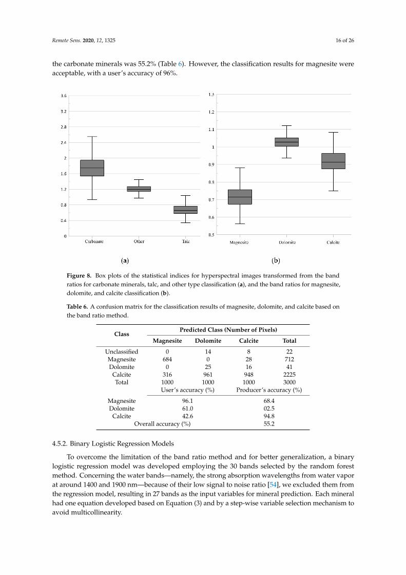
The classification results based on the band ratios derived above are presented in the box plot(Figure 8) [76]. The first band ratio showed median values for carbonate rock of 1.74, for other typesof 1.2, and for talc of 0.65. As shown in Figure 8a, the first band ratio effectively classified carbonateminerals from talc, while the confusion between carbonate minerals and other types was expected.The overall accuracy of the classification was 82% (Table 5), yet the overall accuracy was acceptable,with the producer’s accuracy for carbonate minerals being 63.9%.

Table 5. A confusion matrix for the classification results of carbonate minerals, talc, and other types, bythe band ratio method.

ClassPredicted Class (Number of Pixels)

Talc Other Carbonate Total

Unclassified 3 0 8 11Talc 0 0 638 638

Other 829 6 42 877Carbonate 168 994 312 1474

Total 1000 1000 1000 3000User’s accuracy (%) Producer’s accuracy (%)

Talc 94.5 82.9Other 67.4 99.4

Carbonate 100 63.8Overall accuracy (%) 82.0

The second band ratio for the discrimination for carbonate minerals showed median values formagnesite of 0.71, calcite of 0.91, and dolomite of 1.02. The range of the index is 0.56–0.88 for magnesite,0.75–1.08 for calcite, 0.94–1.12 for dolomite (Figure 8b). The overall accuracy of classification for

Remote Sens. 2020, 12, 1325 16 of 26

the carbonate minerals was 55.2% (Table 6). However, the classification results for magnesite wereacceptable, with a user’s accuracy of 96%.

Figure 8. Box plots of the statistical indices for hyperspectral images transformed from the bandratios for carbonate minerals, talc, and other type classification (a), and the band ratios for magnesite,dolomite, and calcite classification (b).

Table 6. A confusion matrix for the classification results of magnesite, dolomite, and calcite based onthe band ratio method.

ClassPredicted Class (Number of Pixels)

Magnesite Dolomite Calcite Total

Unclassified 0 14 8 22Magnesite 684 0 28 712Dolomite 0 25 16 41

Calcite 316 961 948 2225Total 1000 1000 1000 3000

User’s accuracy (%) Producer’s accuracy (%)

Magnesite 96.1 68.4Dolomite 61.0 02.5

Calcite 42.6 94.8Overall accuracy (%) 55.2

4.5.2. Binary Logistic Regression Models

To overcome the limitation of the band ratio method and for better generalization, a binarylogistic regression model was developed employing the 30 bands selected by the random forestmethod. Concerning the water bands—namely, the strong absorption wavelengths from water vaporat around 1400 and 1900 nm—because of their low signal to noise ratio [54], we excluded them fromthe regression model, resulting in 27 bands as the input variables for mineral prediction. Each mineralhad one equation developed based on Equation (3) and by a step-wise variable selection mechanism toavoid multicollinearity.

Remote Sens. 2020, 12, 1325 17 of 26

The stepwise variable selection for each target mineral is listed in Table 7. The classificationequation for magnesite employed 11 variables, among which eight bands are associated with Mg-OHspectral features, two bands are from Ca features, and one band is at 1237 nm (Table 7). For dolomite,the equation was developed based on nine bands from Mg-OH features, four bands from Ca features,and one band at 1248 nm (Table 7). Differently from magnesite, seven bands were significant, and themost important bands were 2361 and 2489 nm of Mg-OH features. The calcite equation was derivedfrom nine bands from Mg-OH features and four bands from Ca features, along with bands at 1237and 1248 nm. The band at 1248 nm plays an important role in calcite detection. Talc classification wasbased on seven bands of Mg-OH features, four bands of Ca features, and the band at 1237 nm (Table 7),where Mg-OH bands play important roles.

Table 7. The final selected variables in the equation and Wald test results from the logisticregression models.

Variable B1 S.E.2 Wald3 Df4 Sig.5 Exp(B)6

Final selected variables for magnesite classificationB1237 (1237 nm) 44.2 10.237 18.642 1 0 1.57 × 1019

B2294(2294 nm) −1013.851 235.214 18.579 1 0 0B2305 (2305 nm) −1529.829 457.557 11.179 1 0.001 0B2311 (2311 nm) 1710.024 392.844 18.948 1 0 0B2316 (2316 nm) −1645.734 383.517 18.414 1 0 0B2322 (2322 nm) 1931.354 351.626 30.169 1 0 0B2361 (2361 nm) −362.818 88.704 16.73 1 0 0B2389 (2389 nm) 1629.333 339.902 22.978 1 0 0B2394 (2394 nm) −1253.898 306.746 16.71 1 0 0B2467 (2467 nm) 1211.941 268.864 20.319 1 0 0B2478 (2478 nm) −705.467 188.34 14.03 1 0 0

Constant −11.785 2.24 27.674 1 0 0

Final selected variables for dolomite classificationB1248 (1248 nm) −44.668 3.422 170.402 1 0 0B2294 (2294 nm) 289.719 32.46 79.663 1 0 6.66 × 10125

B2316 (2316 nm) −365.45 51.395 50.561 1 0 0B2328 (2328 nm) 238.129 63.567 14.033 1 0 2.62 × 10103

B2339 (2339 nm) −621.411 81.109 58.697 1 0 0B2344 (2344 nm) 132.733 69.632 3.634 1 0.057 4.42 × 1057

B2355 (2355 nm) 186.986 60.982 9.402 1 0.002 1.61 × 1081

B2361 (2361 nm) 615.639 71.841 73.436 1 0 2.34 × 10267

B2383 (2383 nm) −334.633 68.317 23.993 1 0 0B2389 (2389 nm) −182.19 67.463 7.293 1 0.007 0B2467 (2467 nm) 346.041 52.612 43.26 1 0 1.92 × 10150

B2483 (2483 nm) −382.869 79.088 23.436 1 0 0B2489 (2489 nm) 375.279 86.236 18.938 1 0 9.58 × 10162

B2495 (2495 nm) −268.606 63.377 17.962 1 0 0Constant −1.855 0.203 83.133 1 0 0.157

Final selected variables for calcite classificationB1237 (1237 nm) −366.642 122.121 9.014 1 0.003 0.000B1248 (1248 nm) 338.763 121.725 7.745 1 0.005 1.327 × 10147

B2311 (2311 nm) −2798.173 460.679 36.894 1 0.000 0.000B2316 (2316 nm) 3090.930 506.840 37.191 1 0.000 0.000B2339 (2339 nm) 1640.527 312.480 27.563 1 0.000 0.000B2350 (2350 nm) −1925.792 462.775 17.317 1 0.000 0.000B2355 (2355 nm) −2276.548 479.895 22.504 1 0.000 0.000B2361 (2361 nm) 2574.915 592.343 18.896 1 0.000 0.000B2367 (2367 nm) −1173.638 465.077 6.368 1 0.012 0.000B2383 (2383 nm) 3050.209 512.796 35.381 1 0.000 0.000B2394 (2394 nm) −2088.940 482.653 18.732 1 0.000 0.000B2467 (2467 nm) 1188.275 342.139 12.062 1 0.001 0.000B2489 (2489 nm) −3875.854 731.276 28.091 1 0.000 0.000B2495 (2495 nm) 3897.919 799.287 23.783 1 0.000 0.000B2500 (2500 nm) −1745.837 463.723 14.174 1 0.000 0.000

Constant 0.952 0.842 1.278 1 0.258 2.591

Remote Sens. 2020, 12, 1325 18 of 26

Table 7. Cont.

Variable B1 S.E.2 Wald3 Df4 Sig.5 Exp(B)6

Final selected variables for talc classificationB1237 (1237 nm) 63.06 7.802 65.335 1 0 2.44 × 1027

B2294 (2294 nm) 494.21 133.41 13.723 1 0 4.29 × 10214

B2322 (2322 nm) −352.872 183.233 3.709 1 0.054 0B2333 (2333 nm) −440.763 180.68 5.951 1 0.015 0B2344 (2344 nm) 763.836 194.177 15.474 1 0 0B2355 (2355 nm) −669.464 151.933 19.416 1 0 0B2372 (2372 nm) 383.697 226.936 2.859 1 0.091 4.34 × 10189

B2383 (2383 nm) −391.674 143.916 7.407 1 0.006 0B2467 (2467 nm) −311.595 204.861 2.313 1 0.128 0B2478 (2478 nm) 435.462 262.939 2.743 1 0.098 1.32 × 10189

B2495 (2495 nm) 468.646 291.343 2.587 1 0.108 3.39 × 10203

B2500 (2500 nm) −544.645 219.341 6.166 1 0.013 0Constant −6.352 1.213 27.417 1 0 0.002

B1 = logistic coefficient; S.E.2 = standard error of estimate; Wald3 = Wald chi-square values; Df4 = degree of freedom;Sig.5 = P-value; Exp(B)6 = exponentiated coefficient

All logistic regression equations employed the band at 2467 nm, and three models employed thebands at 1237, 2294, 2316, 2355, 2361, and 2495 nm. The absorption features associated with Mg-OH andCa participated in all regression equations, where the absorption depth, peak absorption, and absorptionwidth vary among the target minerals. Exceptionally, the spectral band of 1237 nm participated inthree regression models, even though the band has no absorption feature. The spectral signatures(1200 nm range) of the minerals show consistent low standard errors (Table 7). Indeed, [77] also usedspectral features other than the 2000–2300 nm region for the detection and classification of carbonatitesamong sedimentary carbonates. Moreover, the RF algorithm identified 1200 nm as important spectralbands for the classification of target minerals. The overall accuracy of the classification was 99.9% formagnesite, 98% for dolomite, 99.6% for calcite, and 99.8% for talc (Table 8).

Table 8. An accuracy table for the classification results derived from binary logistic regression models.

Predicted (Number of Pixels) Correct PercentageObserved No Event (0) Event (1)

Magnesite 0 3999 1 1001 5 995 99.5Overall Percentage 99.9

Dolomite 0 3975 25 99.41 77 923 92.3Overall Percentage 98.0

Calcite 0 3991 9 99.81 7 993 99.3Overall Percentage 99.7

Talc 0 3995 5 99.91 5 995 99.5Overall Percentage 99.8

Evaluation of Binary Regression Models

The results of Hosmer and Lemeshow test showed that the p values of the X2 values of the logisticregression models for the target minerals range from 0.472 for dolomite to 0.997 for magnesite andcalcite (Table 9). In general, significance higher than 0.05 is acceptable, and the test showed that allmodels are statistically coherent [64].

Remote Sens. 2020, 12, 1325 19 of 26

Table 9. The statistical parameters of the logistic regression models.

Statistical ParametersHosmer and Lemeshow Test Pseudo-R2

X2 df P Value Cox & Snell R2 Nagelkerke R2

Magnesite 1.180 8 0.997 0.628 0.994Dolomite 7.613 8 0.472 0.580 0.917

Calcite 1.129 8 0.997 0.625 0.988Talc 1.425 8 0.994 0.626 0.989

In addition, the goodness of fit was tested based on pseudo-R2, where pseudo-R2 ranged from0.58 to 0.628 for Cox & Snell R2, and 0.917 to 0.994 for Nagelkerke R2 (Table 9). In general, Cox & Snellpseudo-R2 values larger than 0.2 are considered to indicate good fit [78]. The psuedo-R2 values of themodels validated that all models have a strong goodness of fit.

Validation of Binary Regression Models

The binary regression models for detection of magnesite, dolomite, calcite, and talc developedfrom training samples were applied to 46 validation samples (Figure 9). The accuracy of the magnesitelogistic regression model was 97.6%. All magnesite samples were correctly detected, while some pixelsof magnesite samples were classified as none (Figure 9a and Table 10). The overall accuracy of thedolomite model was 82%, where the model classified 9 out of 21 dolomite samples (Figure 9b andTable 10). The accuracy of dolomite was lower than of the other minerals. The erroneous samplesinclude calcite and/or quartz as major minerals (Table 2). The bias might be caused by the mix ofmajor spectra manifested by both minerals. The calcite model classified 94.6% of calcite pixels correctly(Figure 9c and Table 10). The accuracy of the talc model was very high (99.8%, Figure 9d and Table 10).

Table 10. A confusion matrix for the classification results of the validation set from the binaryregression models.

ClassCorrect Class Non Correct Class Overall

Accuracy (%)Producer’sAccuracy (%)

User’sAccuracy (%)

Producer’sAccuracy (%)

User’sAccuracy (%)

Magnesite 99.7 95.6 95.6 99.7 97.6Dolomite 54.4 99.3 77.3 99.8 82

Calcite 47.6 71.1 95.9 98.4 94.6Talc 99.5 92.31 99.8 99.9 99.8

Remote Sens. 2020, 12, 1325 20 of 26

Figure 9. Classification images of the logistic regression models applied to the validation models of(a) magnesite, (b) dolomite, (c) calcite, and (d) talc; a Specim hyperspectral short wave infrared (SWIR)false color composite image (R:2250 nm; G:2283 nm; B:2433 nm) (e); and a gray scale image of the 2266nm band (f) for the validation samples, where the sample label of M shows the magnesite sample,D the dolomite sample, C calcite, T talc, and O other types.

Remote Sens. 2020, 12, 1325 21 of 26

4.6. Discussions and Limitations of the Present Work

Based on the classification results applied to the validation samples, the logistic regression modelsshowed significantly higher accuracy than the band ratio method. While the band ratio method iseasier to apply, its overall accuracy was about 40% lower than that of the logistic regression models forcarbonate mineral classification. In addition, we compared the effectiveness of the logistic regressionmodels with the RF method. The classification results of the RF method for the validation samplesshowed an accuracy ranging from 92.6% to 99.9%, with an overall accuracy of 96.6% (Table 11).The accuracy of the RF method was similar with the logistic regression models except for the dolomitesamples. The RF method showed better performance on dolomite classification, with 92.6%. Althoughthe RF method shows a slightly better accuracy, the knowledge learned by the RF algorithm is wrappedin its complex data structure as a black box to the researchers. On the contrary, the logistic modelshave simple form and can be easily generalized to other case studies for magnesite exploration.

Given the fact that this study developed the models using naturally occurring samples from variouslocations and that the mineral composition is heterogeneous, the models tested in this study couldbe applicable for real-world cases as prompt analytical methods for sample discrimination. Analystscan select the best model for their case studies. For hyperspectral band surveys, we recommend thelogistic regression model.

Although our study is comprehensive on the band selection, the target minerals only include fourmajor ones. It is not difficult to conclude that if more minerals are considered, the complexity of theprediction model will drastically increase. Furthermore, this study is based on fresh samples withcontrolled dry conditions. The weathering process and wet surface would complicate the spectralsignals associated with hydrolysis and water components [38,79]. Adding controlled moisture andweathered samples would allow us to better understand the uncertainty in mapping magnesite in anatural environment. The band selection and band-ratio equations will be different under differentassumptions of surface moisture and weathering. Our research proved the feasibility of the methodwe developed for fresh dry samples and could serve a role model for these future case studies.

Table 11. A confusion matrix for the classification results of the validation set from the randomforest algorithm.

ClassPredicted Class (Number of Pixels)

Magnesite Dolomite Talc Calcite Accuracy (%)

Actual Class

Magnesite 997 3 0 0 99.7Dolomite 2 926 0 72 92.6

Talc 0 0 999 1 99.9Calcite 0 56 0 944 94.4

Overall Accuracy (%) 96.6

5. Conclusions

This study introduced a detection method for magnesite and associated gangue minerals includingdolomite, calcite, and talc based on mineralogical, chemical, and hyperspectral analyses using SWIRhyperspectral images under laboratory conditions. The samples used for this study originatedfrom thirteen different locations in South Korea, China, and North Korea and were used to developdetection models with wide applicability. The spectral characteristics of sample spectra were analyzedwith consideration of minerals and composition. Using the spectral characteristics derived from thehyperspectral images, the random forest algorithm was used for band selection and dimension reduction.Band ratio and logistic regression models were developed to find the most useful detection methods.

The mineralogical analysis revealed the heterogeneity of mineral composition for naturallyoccurring samples. Magnesite samples contains accessory minerals such as dolomite, calcite, chabazite,clinochlore, quartz, and siderite. Dolomite and calcite samples showed the accessory mineralsactinolite, augite, calcite, graphite, magnesite, phlogopite, quartz, and titanite. Talc samples had

Remote Sens. 2020, 12, 1325 22 of 26

magnesite, dolomite, and calcite as accessory minerals. The results indicate the heterogeneity ofmineral composition, even for the same types of sample. Because the mineral composition in one typeof mineral showed large variations—mainly mixed forms of magnesite, dolomite, and calcite—thehyperspectral approaches for magnesite exploration must consider variations in mineral compositionin other case studies. The Mg and Ca composition of magnesite and dolomite varied significantly,where magnesite had more Mg content and dolomite had more Ca content. These results confirmedthe heterogeneity of minerals in not only the mineral composition but also the chemical composition ofmajor elements.

The spectral characteristics of the magnesite samples were found at the absorption features locatedat 1850, 1930, 2130, 2300, and 2450 nm, with weak absorptions at 1720 and 2360 nm. The spectralcharacteristics represent the heterogeneity of mineral composition, where absorption features ofdolomite, calcite, and talc were found in the spectra of magnesite samples. The same phenomenonwas found for dolomite, calcite, and talc samples, where major absorptions of each mineral weremixed with other minerals’ absorptions from the sample spectra, representing heterogeneous mineralcomposition. The spectral characteristics of magnesite and dolomite showed systematic variationsin Mg-OH absorption features toward a shorter wavelength, with an increase in Mg content. Thisindicates that the shift of Mg-OH absorption may be useful for the detection of Mg content in dolomiteand magnesite.

The random forest algorithm reduced the number of bands by selecting 30 of the most sensitivebands for the classification of magnesite and associated gangue minerals. The selected bands weremainly associated with Mg-OH (2289–2384 nm), CO3 (2467–2500 nm), and OH (1389–1400 nm).Among the selected bands, the bands with the highest importance were found in spectral range ofMg-OH absorptions, followed by the spectral bands around carbonate and hydrolysis absorptions.A two-step band ratio method was derived using the selected bands. The first step classified carbonateminerals from talc and other types of sample with an accuracy of 92%. The second step classifiedmagnesite, dolomite, and calcite with an accuracy of 55.2%, where the classification results were notsatisfactory. The logistic regression models based on the 27 selected bands excluding water bandsachieved accuracies of 98%~99.9% for the training samples and 82–99.8% for the validation samples.

Given the fact that this study found the naturally formed samples from various locations showingheterogeneous mineral composition, the applicability of the models would expand to general use as aprompt analytical method for sample discrimination. It is necessary to include more samples withmore source locations to refine and enhance the model. Furthermore, the method would expand itsapplicability to carbonate rocks and minerals exploration significantly if the method was tested inthe field.

Author Contributions: Conceptualization, J.Y. and B.C.; Methodology, J.Y. and B.C.; Software, B.C.; Validation,J.Y. and L.W.; Formal Analysis, B.C. and S.L.; Investigation, J.Y., B.C., and L.W.; Resources, Y.J., N.H.K., and B.H.L.;Data Curation, B.C. and N.H.K.; Writing-Original Draft Preparation, B.C. and J.Y.; Writing-Review & Editing, J.Y.and L.W.; Visualization, B.C.; Supervision, J.Y.; Project Administration, J.Y., B.H.L., and S.K.; Funding Acquisition,J.Y. and S.K. All authors have read and agreed to the published version of the manuscript.

Funding: This work was supported by the National Research Council of Science & Technology (NST) grant by theKorea Government (MSIT) (No. CRC-15-06-KIGAM) and the National Research Foundation (NRF) of Korea grantby the Korean Government (NRF-2020R1A2C200543911).

Acknowledgments: The authors deeply appreciate anonymous academic editor and reviewers for theirconstructive comments.

Conflicts of Interest: The authors declare no conflict of interest.

References

1. Salazar, K. Mineral Commodity Summaries 2013: US Geological Survey (USGS). US Geol. Surv. 2013.[CrossRef]

2. Park, H.-K.; Park, J.-T.; Lee, H.-I.; Choi, Y.-Y. Characteristics in Calcination of Magnesite Ore in YongyangMines. J. Korean Inst. Resour. Recycl. 2005, 14, 33–38.

Remote Sens. 2020, 12, 1325 23 of 26

3. Sibanda, Z.; Amponsah-Dacosta, F.; Mhlongo, S. Characterization and evaluation of magnesite tailings fortheir potential utilization: A case study of nyala magnesite mine, limpopo province of South Africa. ARPN J.Eng. Appl. Sci. 2013, 8, 606–613.

4. Melezhik, V.A.; Fallick, A.E.; Medvedev, P.V.; Makarikhin, V.V. Palaeoproterozoic magnesite: Lithologicaland isotopic evidence for playa/sabkha environments. Sedimentology 2001, 48, 379–397. [CrossRef]

5. Lippmann, F. Sedimentary Carbonate Minerals; Springer Science & Business Media: Heidelberg, Germany,2012; Volume 6.

6. Machel, H.G. Concepts and models of dolomitization: A critical reappraisal. Geol. Soc. Lond. Spec. Publ.2004, 235, 7–63. [CrossRef]

7. Pohl, W. Comparative geology of magnesite deposits and occurrences. Magnesite Geol. Mineral. Geochem.Form. Mg-Carbonates 1989, 28, 1–13.

8. Pohl, W. Genesis of magnesite deposits—Models and trends. Geol. Rundsch. 1990, 79, 291–299. [CrossRef]9. Warren, J. Dolomite: Occurrence, evolution and economically important associations. Earth Sci. Rev. 2000,

52, 1–81. [CrossRef]10. Baldermann, A.; Deditius, A.P.; Dietzel, M.; Fichtner, V.; Fischer, C.; Hippler, D.; Leis, A.; Baldermann, C.;

Mavromatis, V.; Stickler, C.P. The role of bacterial sulfate reduction during dolomite precipitation: Implicationsfrom Upper Jurassic platform carbonates. Chem. Geol. 2015, 412, 1–14. [CrossRef]

11. Given, R.K.; Wilkinson, B.H. Dolomite abundance and stratigraphic age; constraints on rates and mechanismsof Phanerozoic dolostone formation. J. Sediment. Res. 1987, 57, 1068–1078. [CrossRef]

12. Budd, D. Cenozoic dolomites of carbonate islands: Their attributes and origin. Earth Sci. Rev. 1997, 42, 1–47.[CrossRef]

13. Prochaska, W. Genetic concepts on the formation of the Austrian magnesite and siderite mineralizations inthe Eastern Alps of Austria. Geol. Croat. 2016, 69, 31–38. [CrossRef]

14. Misch, D.; Pluch, H.; Mali, H.; Ebner, F.; Huang, H. Genesis of giant Early Proterozoic magnesite and relatedtalc deposits in the Mafeng area, Liaoning Province, NE China. J. Asian Earth Sci. 2018, 160, 1–12. [CrossRef]

15. Neubauer, F. Structural Control on the Formation of Ttalc Deposits; Balkeema Publ.: Lassing, Austria, 2001.16. Railsback, L.B. Patterns in the compositions, properties, and geochemistry of carbonate minerals. Carbonates

Evaporites 1999, 14, 1. [CrossRef]17. Tangestani, M.H.; Moore, F. Iron oxide and hydroxyl enhancement using the Crosta Method: A case study

from the Zagros Belt, Fars Province, Iran. Int. J. Appl. Earth Obs. Geoinf. 2000, 2, 140–146. [CrossRef]18. Yip, C.K.; Provis, J.L.; Lukey, G.C.; van Deventer, J.S. Carbonate mineral addition to metakaolin-based

geopolymers. Cem. Concr. Compos. 2008, 30, 979–985. [CrossRef]19. Friedman, G.M. Identification of carbonate minerals by staining methods. J. Sediment. Res. 1959, 29, 87–97.

[CrossRef]20. Dickson, J. Carbonate identification and genesis as revealed by staining. J. Sediment. Res. 1966, 36, 491–505.

[CrossRef]21. Laakso, K.; Middleton, M.; Heinig, T.; Bärs, R.; Lintinen, P. Assessing the ability to combine hyperspectral

imaging (HSI) data with Mineral Liberation Analyzer (MLA) data to characterize phosphate rocks. Int. J.Appl. Earth Obs. Geoinf. 2018, 69, 1–12. [CrossRef]

22. Rajendran, S.; Hersi, O.S.; Al-Harthy, A.; Al-Wardi, M.; El-Ghali, M.A.; Al-Abri, A.H. Capability of advancedspaceborne thermal emission and reflection radiometer (ASTER) on discrimination of carbonates andassociated rocks and mineral identification of eastern mountain region (Saih Hatat window) of Sultanate ofOman. Carbonates Evaporites 2011, 26, 351–364. [CrossRef]

23. Rajendran, S.; Nasir, S. ASTER spectral analysis of ultramafic lamprophyres (carbonatites and aillikites)within the Batain Nappe, northeastern margin of Oman: A proposal developed for spectral absorption. Int.J. Remote Sens. 2013, 34, 2763–2795. [CrossRef]

24. Rajendran, S.; Nasir, S.; Kusky, T.M.; Ghulam, A.; Gabr, S.; El-Ghali, M.A. Detection of hydrothermalmineralized zones associated with listwaenites in Central Oman using ASTER data. Ore Geol. Rev. 2013, 53,470–488. [CrossRef]

25. Mars, J.C.; Rowan, L.C. Spectral assessment of new ASTER SWIR surface reflectance data products forspectroscopic mapping of rocks and minerals. Remote Sens. Environ. 2010, 114, 2011–2025. [CrossRef]

26. Amer, R.; Kusky, T.; Ghulam, A. Lithological mapping in the Central Eastern Desert of Egypt using ASTERdata. J. Afr. Earth Sci. 2010, 56, 75–82. [CrossRef]

Remote Sens. 2020, 12, 1325 24 of 26

27. Gabr, S.; Ghulam, A.; Kusky, T. Detecting areas of high-potential gold mineralization using ASTER data. OreGeol. Rev. 2010, 38, 59–69. [CrossRef]

28. Kruse, F.A.; Boardman, J.W.; Huntington, J.F. Comparison of airborne hyperspectral data and EO-1 Hyperionfor mineral mapping. IEEE Trans. Geosci. Remote Sens. 2003, 41, 1388–1400. [CrossRef]

29. Kodikara, G.R.; Woldai, T.; van Ruitenbeek, F.J.; Kuria, Z.; van der Meer, F.; Shepherd, K.D.; Van Hummel, G.Hyperspectral remote sensing of evaporate minerals and associated sediments in Lake Magadi area, Kenya.Int. J. Appl. Earth Obs. Geoinf. 2012, 14, 22–32. [CrossRef]

30. Govil, H.; Gill, N.; Rajendran, S.; Santosh, M.; Kumar, S. Identification of new base metal mineralization inKumaon Himalaya, India, using hyperspectral remote sensing and hydrothermal alteration. ORE Geol. Rev.2018, 92, 271–283. [CrossRef]

31. Jain, R.; Sharma, R.U. Airborne hyperspectral data for mineral mapping in Southeastern Rajasthan, India.Int. J. Appl. Earth Obs. Geoinf. 2019, 81, 137–145. [CrossRef]

32. Carrino, T.A.; Crósta, A.P.; Toledo, C.L.B.; Silva, A.M. Hyperspectral remote sensing applied to mineralexploration in southern Peru: A multiple data integration approach in the Chapi Chiara gold prospect. Int. J.Appl. Earth Obs. Geoinf. 2018, 64, 287–300. [CrossRef]

33. Krupnik, D.; Khan, S.; Okyay, U.; Hartzell, P.; Zhou, H.-W. Study of Upper Albian rudist buildups in theEdwards Formation using ground-based hyperspectral imaging and terrestrial laser scanning. Sediment.Geol. 2016, 345, 154–167. [CrossRef]

34. Baissa, R.; Labbassi, K.; Launeau, P.; Gaudin, A.; Ouajhain, B. Using HySpex SWIR-320m hyperspectral datafor the identification and mapping of minerals in hand specimens of carbonate rocks from the AnklouteFormation (Agadir Basin, Western Morocco). J. Afr. Earth Sci. 2011, 61, 1–9. [CrossRef]

35. Zaini, N.; Van der Meer, F.; Van der Werff, H. Determination of carbonate rock chemistry usinglaboratory-based hyperspectral imagery. Remote Sens. 2014, 6, 4149–4172. [CrossRef]

36. Hunt, G.R.; Salisbury, J.W. Visible and near infrared spectra of minerals and rocks. II. Carbonates. Mod. Geol.1971, 2, 23–30.

37. Gaffey, S.J. Spectral reflectance of carbonate minerals in the visible and near infrared (0.35-2.55 microns);calcite, aragonite, and dolomite. Am. Mineral. 1986, 71, 151–162.

38. Shin, J.H.; Yu, J.; Wang, L.; Kim, J.; Koh, S.-M.; Kim, S.-O. Spectral responses of heavy metal contaminatedsoils in the vicinity of a hydrothermal ore deposit: A case study of Boksu Mine, South Korea. IEEE Trans.Geosci. Remote Sens. 2019, 57, 4092–4106. [CrossRef]

39. Quinn, T. About Magforum. 2017; ISSN 1756-364X.40. Kruse, F.A.; Bedell, R.L.; Taranik, J.V.; Peppin, W.A.; Weatherbee, O.; Calvin, W.M. Mapping alteration

minerals at prospect, outcrop and drill core scales using imaging spectrometry. Int. J. Remote Sens. 2012, 33,1780–1798. [CrossRef]

41. Smith, G.M.; Milton, E.J. The use of the empirical line method to calibrate remotely sensed data to reflectance.Int. J. Remote Sens. 1999, 20, 2653–2662. [CrossRef]

42. Green, A.A.; Berman, M.; Switzer, P.; Craig, M.D. A transformation for ordering multispectral data in termsof image quality with implications for noise removal. IEEE Trans. Geosci. Remote Sens. 1988, 26, 65–74.[CrossRef]

43. Shawky, M.M.; El-Arafy, R.A.; El Zalaky, M.A.; Elarif, T. Validating (MNF) transform to determine the leastinherent dimensionality of ASTER image data of some uranium localities at Central Eastern Desert, Egypt.J. Afr. Earth Sci. 2019, 149, 441–450. [CrossRef]

44. Kokaly, R.F.; Clark, R.N. Spectroscopic determination of leaf biochemistry using band-depth analysis ofabsorption features and stepwise multiple linear regression. Remote Sens. Environ. 1999, 67, 267–287.[CrossRef]

45. Breiman, L. Random forests. Mach. Learn. 2001, 45, 5–32. [CrossRef]46. Guo, L.; Chehata, N.; Mallet, C.; Boukir, S. Relevance of airborne lidar and multispectral image data for urban

scene classification using Random Forests. ISPRS J. Photogramm. Remote Sens. 2011, 66, 56–66. [CrossRef]47. Rodriguez-Galiano, V.F.; Ghimire, B.; Rogan, J.; Chica-Olmo, M.; Rigol-Sanchez, J.P. An assessment of the

effectiveness of a random forest classifier for land-cover classification. ISPRS J. Photogramm. Remote Sens.2012, 67, 93–104. [CrossRef]

Remote Sens. 2020, 12, 1325 25 of 26

48. Abdel-Rahman, E.M.; Mutanga, O.; Adam, E.; Ismail, R. Detecting Sirex noctilio grey-attacked andlightning-struck pine trees using airborne hyperspectral data, random forest and support vector machinesclassifiers. ISPRS J. Photogramm. Remote Sens. 2014, 88, 48–59. [CrossRef]

49. Lawrence, R.L.; Wood, S.D.; Sheley, R.L. Mapping invasive plants using hyperspectral imagery and BreimanCutler classifications (RandomForest). Remote Sens. Environ. 2006, 100, 356–362. [CrossRef]

50. Gislason, P.O.; Benediktsson, J.A.; Sveinsson, J.R. Random forests for land cover classification. PatternRecognit. Lett. 2006, 27, 294–300. [CrossRef]

51. Kim, M.S.; Chen, Y.-R.; Cho, B.-K.; Chao, K.; Yang, C.-C.; Lefcourt, A.M.; Chan, D. Hyperspectral reflectanceand fluorescence line-scan imaging for online defect and fecal contamination inspection of apples. Sens.Instrum. Food Qual. Saf. 2007, 1, 151. [CrossRef]

52. Ninomiya, Y.; Fu, B.; Cudahy, T.J. Detecting lithology with Advanced Spaceborne Thermal Emission andReflection Radiometer (ASTER) multispectral thermal infrared “radiance-at-sensor” data. Remote Sens.Environ. 2005, 99, 127–139. [CrossRef]

53. Rajendran, S.; Al-Khirbash, S.; Pracejus, B.; Nasir, S.; Al-Abri, A.H.; Kusky, T.M.; Ghulam, A. ASTER detectionof chromite bearing mineralized zones in Semail Ophiolite Massifs of the northern Oman Mountains:Exploration strategy. ORE Geol. Rev. 2012, 44, 121–135. [CrossRef]

54. Kurz, T.H.; Dewit, J.; Buckley, S.J.; Thurmond, J.B.; Hunt, D.W.; Swennen, R. Hyperspectral image analysis ofdifferent carbonate lithologies (limestone, karst and hydrothermal dolomites): The Pozalagua Quarry casestudy (Cantabria, North-west Spain). Sedimentology 2012, 59, 623–645. [CrossRef]

55. Gad, S.; Kusky, T. ASTER spectral ratioing for lithological mapping in the Arabian–Nubian shield, theNeoproterozoic Wadi Kid area, Sinai, Egypt. Gondwana Res. 2007, 11, 326–335. [CrossRef]

56. Kay, D.; Crowther, J.; Stapleton, C.M.; Wyer, M.D.; Fewtrell, L.; Edwards, A.; Francis, C.; McDonald, A.T.;Watkins, J.; Wilkinson, J. Faecal indicator organism concentrations in sewage and treated effluents. Water Res.2008, 42, 442–454. [CrossRef] [PubMed]

57. Agresti, A. Categorical Data Analysis. John Wiley & Sons: Hoboken, NJ, USA, 2003; Volume 482.58. Hair, J.F.; Black, W.C.; Babin, B.J.; Anderson, R.E.; Tatham, R.L. Multivariate Data Analysis; Pearson Prentice

Hall: Upper Saddle River, NJ, USA, 2006; Volume 6.59. Pohar, M.; Blas, M.; Turk, S. Comparison of logistic regression and linear discriminant analysis: A simulation

study. Metodoloski Zv. 2004, 1, 143.60. Yousefi, M.; Carranza, E.J.M. Prediction–area (P–A) plot and C–A fractal analysis to classify and evaluate

evidential maps for mineral prospectivity modeling. Comput. Geosci. 2015, 79, 69–81. [CrossRef]61. Bewick, V.; Cheek, L.; Ball, J. Statistics review 14: Logistic regression. Crit. Care 2005, 9, 112. [CrossRef]62. Hosmer Jr, D.W.; Lemeshow, S.; Sturdivant, R.X. Applied Logistic Regression; John Wiley & Sons: New Jersey,

NJ, USA, 2013; Volume 398.63. Sahoo, N.R.; Pandalai, H.S. Integration of Sparse Geologic Information in Gold Targeting Using Logistic

Regression Analysis in the Hutti–Maski Schist Belt, Raichur, Karnataka, India—A Case Study. Nat. Resour.Res. 1999, 8, 233–250. [CrossRef]

64. Mokhtari, A.R. Hydrothermal alteration mapping through multivariate logistic regression analysis oflithogeochemical data. J. Geochem. Explor. 2014, 145, 207–212. [CrossRef]

65. Hosmer, D.W.; Lemeshow, S. Applied Logistic Regression; John Wiley & Sons,: New York, NJ, USA, 1989.66. Menard, S. Coefficients of determination for multiple logistic regression analysis. Am. Stat. 2000, 54, 17–24.67. Nagelkerke, N.J. A note on a general definition of the coefficient of determination. Biometrika 1991, 78,

691–692. [CrossRef]68. Ayalew, L.; Yamagishi, H. The application of GIS-based logistic regression for landslide susceptibility

mapping in the Kakuda-Yahiko Mountains, Central Japan. Geomorphology 2005, 65, 15–31. [CrossRef]69. Kell-Duivestein, I.J.; Baldermann, A.; Mavromatis, V.; Dietzel, M. Controls of temperature, alkalinity and

calcium carbonate reactant on the evolution of dolomite and magnesite stoichiometry and dolomite cationordering degree-An experimental approach. Chem. Geol. 2019, 529, 119292. [CrossRef]

70. Combe, J.P.; Launeau, P.; Pinet, P.; Despan, D.; Harris, E.; Ceuleneer, G.; Sotin, C. Mapping of an ophiolitecomplex by high-resolution visible-infrared spectrometry. Geochem. Geophys. Geosystems 2006, 7. [CrossRef]

71. Hauff, P. An Overview of VIS-NIR-SWIR Field Spectroscopy as Applied to Precious Metals Exploration; SpectralInternational Inc.: Arvada, CO, USA, 2008; Volume 80001, pp. 303–403.

Remote Sens. 2020, 12, 1325 26 of 26

72. Ben-Dor, E. Characterization of soil properties using reflectance spectroscopy. In Hyperspectral Remote Sensingof Vegetation; CRC Press: Boca Raton, FL, USA, 2016; pp. 548–593.

73. Bishop, J.; Lane, M.; Dyar, M.; Brown, A. Reflectance and emission spectroscopy study of four groups ofphyllosilicates: Smectites, kaolinite-serpentines, chlorites and micas. Clay Miner. 2008, 43, 35–54. [CrossRef]

74. Clark, R.N.; King, T.V.; Klejwa, M.; Swayze, G.A.; Vergo, N. High spectral resolution reflectance spectroscopyof minerals. J. Geophys. Res. Solid Earth 1990, 95, 12653–12680. [CrossRef]

75. Crowley, J.K. Visible and near-infrared spectra of carbonate rocks: Reflectance variations related topetrographic texture and impurities. J. Geophys. Res. Solid Earth 1986, 91, 5001–5012. [CrossRef]

76. Hoaglin, D.C.; Mosteller, F.; Tukey, J.W. Understanding Robust and Exploratory Data Analysis; Wiley: New York,NY, USA, 1983; Volume 3.

77. Shavers, E.J.; Ghulam, A.; Encarnacion, J. Surface alteration of a melilitite-clan carbonatite and the potentialfor remote carbonatite detection. ORE Geol. Rev. 2018, 92, 19–28. [CrossRef]

78. Clark, W.; Hoskings, P. Statistical methods for geographers. In Clark Statistical Methods for Geographers; JohnWiley and Sons: New York, NY, USA, 1986.

79. Shin, H.; Yu, J.; Jeong, Y.; Wang, L.; Yang, D. Case-based regression models defining the relationships betweenmoisture content and shortwave infrared reflectance of beach sands. IEEE J. Sel. Top. Appl. Earth Obs. RemoteSens. 2017, 10, 4512–4521. [CrossRef]

© 2020 by the authors. Licensee MDPI, Basel, Switzerland. This article is an open accessarticle distributed under the terms and conditions of the Creative Commons Attribution(CC BY) license (http://creativecommons.org/licenses/by/4.0/).