image processing & remote sensing: analyzing sequences of

HAL Id: tel-00616558https://tel.archives-ouvertes.fr/tel-00616558

Submitted on 23 Aug 2011

HAL is a multi-disciplinary open accessarchive for the deposit and dissemination of sci-entific research documents, whether they are pub-lished or not. The documents may come fromteaching and research institutions in France orabroad, or from public or private research centers.

L’archive ouverte pluridisciplinaire HAL, estdestinée au dépôt et à la diffusion de documentsscientifiques de niveau recherche, publiés ou non,émanant des établissements d’enseignement et derecherche français ou étrangers, des laboratoirespublics ou privés.

Image processing & remote sensing: analyzing sequencesof low and very high spatial resolution

Thomas Corpetti

To cite this version:Thomas Corpetti. Image processing & remote sensing: analyzing sequences of low and very highspatial resolution. Signal and Image processing. Université Rennes 1, 2011. tel-00616558

https://tel.archives-ouvertes.fr/tel-00616558

https://hal.archives-ouvertes.fr

HABILITATION À DIRIGER DES RECHERCHES

présentée devant

l’Université de RENNES 1Mention : Traitement du Signal et

Télécommunications

parThomas Corpetti

Image processing & remote sensing : analyzing sequences of lowand very high spatial resolution

Soutenue le 20 juin 2011 à Telecom Paris Tech

Devant le jury composé de :

Patrick Bouthemy - Dir. de Recherche INRIA, Rennes (France)

Lorenzo Bruzzone - Prof. RS Lab, Trento (Italie) RapporteurJocelyn Chanussot - Prof. GIPSA Lab, Grenoble (France) Président du juryLaurence Hubert-Moy - Prof. COSTEL/OSUR, Rennes (France)

Henri Maitre - Prof., Telecom Paris Tech (France) RapporteurEtienne Mémin - Dir. de Recherche INRIA, Rennes (France)

Olivier Talagrand - Dir. de Recherche CNRS, LMD Paris (France) Rapporteur

Remerciements

Il n’est pas facile d’écrire une page de remerciements tant les personnes rencontrées aucours de ces dix dernières années sont nombreuses et m’ont toutes apporté une aide ou unsoutien précieux. Il est encore plus difficile d’organiser ces remerciements.

D’avance je préviens donc que l’ordre d’apparition n’est pas signe d’importance et jem’excuse pour celles ou ceux que j’aurais oubliés.

Je remercie les membres du jury pour avoir dégagé du temps (et ça n’est pas facile) afinde s’intéresser à mes travaux et pour certains, de les rapporter.

– Merci à Jocelyn Chanussot pour avoir accepté de présider ce jury et pour toutes sesremarques/conseils/commentaires qui m’ont été utiles ;

– Merci à Henri Maître pour avoir rapporté ce travail et pour le grand intérêt qu’il porteà ces recherches depuis de nombreuses années ;

– Merci à Olivier Talagrand pour avoir apporté son regard de physicien et de spécialisted’assimilation de données à ce travail ;

– Un grazie speciale a Lorenzo Bruzzone per avermi rapporto nella redazione di questatesi e per esser venuto da Trento ad onorarmi della sua presenza alla discussione dellatesi ;

– Merci à Patrick Bouthemy pour son rôle dans le jury et plus globalement pour toutesles relations que l’on entretient depuis 10 ans. Merci de m’avoir toujours ouvert laporte et de m’avoir accepté à nouveau dans VISTA puis à l’INRIA entre 2007 et2009. Cela m’a infiniment aidé ;

– Merci à Laurence Hubert-Moy pour les collaborations que nous entretenons depuis2004 et pour ses nombreux encouragements à ne pas baisser les bras lorsque je mesentais un peu trop noyé dans la géographie ;

– Merci enfin à Etienne Mémin avec qui je travaille avec plaisir depuis plus de 10 ans.Travailler avec Etienne c’est s’assurer d’aborder des thèmes passionnants, ambitieuxdans un contexte scientifique de qualité !

Merci aussi à Telecom ParisTech d’avoir accueilli la soutenance.Je remercie plus globalement les personnes rencontrées au Cemagref de Rennes (en

particulier Dominique Heitz, Johan Carlier et Georges Arroyo), à COSTEL (entre autres,merci à Jean-Pierre Marchand, Vincent Dubreuil ainsi que Hervé, Olivier, Samuel, et tous lesautres) et à l’INRIA (Patrick Pérez, Charles Kervrann, Pierre Hellier, Ivan Laptev, Thierry,Sophie, ...) pour tous les bons moments, scientifiques et personnels, passés ensemble.

Un très grand merci aux étudiants que j’ai encadrés et qui ont une participation évidenteaux travaux présentés dans ce document. En particulier, merci à :

– Antoine Lefebvre que j’ai eu le plaisir d’encadrer avec Laurence Hubert-Moy pendantsa thèse (soutenue en avril 2011) sur l’analyse d’images agricoles (deuxième partie dece document) ;

– Pierre Allain, encadré avec Nicolas Courty, sur l’analyse de mouvements de foules.Merci aussi d’avoir fait l’effort de passer quelques mois à Pékin, je sais que c’étaitbeaucoup te demander !

– Claire Thomas qui a travaillé en post-doctorat sur le suivi de cellules convectives ;– Les étudiants de MASTER Gong Xing et Pascal Zille ayant travaillé sur la détectionde changements et la multi-résolution.

Merci également à tous mes collaborateurs, en particulier Nicolas Papadakis, RonanFablet, Sileye Ba, Cyril Cassisa, Bertrand Chapron, Shao Liang, Guixiang Cui, ZhaoshunZhang, Jiang Zhu, ...

Mention spéciale à Nicolas Courty qui, au delà des collaborations que nous avons, estégalement un ami avec qui je travaille avec grand plaisir ! Mention particulière également à

ii

Patrick Héas pour tous les excellents moments passés ensemble, que ce soit dans le bureau,en conférence ou en famille.

Depuis 2009 je suis détaché en Chine au LIAMA et cette expérience est extraordinaire.Je suis très reconnaissant au CNRS de nous donner l’opportunité de réaliser de tels projetset je remercie toutes les personnes ayant joué un rôle dans ce détachement (VéroniquePrinet, Véronique Donzeau-Gouge, Stéphane Grumbach, Philippe Baptiste, Michel Bidoit,Jean-Claude Thivolle, Jean-Pierre Jouannaud, Diane Brami, Laurence Hubert-Moy, MarcRobin, Franck Davoine).

Merci enfin à ma famille, mon épouse Catherine et mes 3 enfants Lucien, Rozenn etAntonina, pour tout ce qu’on vit ensemble depuis toutes ces années et aussi pour avoiraccepté de vivre l’inconnu en s’exilant en Chine. Merci Catherine pour tout. Merci enfinà Paul Sablonnière pour avoir apporté son aide lors de la préparation de la soutenance etd’avoir rempli la salle lors de celle-ci.

Enfin, ci joint une liste, probablement non exhaustive, de toutes celles et tous ceux quej’aimerais remercier.

Many Thanks Merci beaucoupPierre Allain Georges ArroyoSileye Ba Adrien Bartoli

Sophie Blestel Patrick BouthemyCyril Cassisa Bertrand ChapronSamuel Corgne Nicolas CourtyGuixiang Cui Philippe De Reffye

Vincent Dubreuil Nadia DupontPauline Dusseux Ronan Fablet

Stéphane Grumbach Xing GongPatrick Héas Dominique HeitzPierre Hellier Bizhen Hong

Laurence Hubert-Moy Stéphanie Jehan-BessonJean Pierre Jouannaud Meng Zhen Kang

Charles Kervrann Ivan LaptevRémi Lecerf Antoine LefebvreDongmin Ma Jean-Pierre Marchand

Paul Marcombes Etienne MéminGrégoire Mercier Kristel MichelNicolas Papadakis Thierry Pecot

Patrick Pérez Olivier PlanchonVéronique Prinet Hervé QuénolLaurent Sarry Liang Shao

Jean-Claude Thivolle Christophe TilmantClaire Thomas Zhaoshun Zhang

Jiang Zhu Pascal Zille... ...

Table des matières

I First part : Low resolution remote sensing images : flow ana-lysis and tracking 7

1 Motion estimation from a pair of images 111.1 Overview . . . . . . . . . . . . . . . . . . . . . . . . . . . . . . . . . . . . . 111.2 General principles . . . . . . . . . . . . . . . . . . . . . . . . . . . . . . . . 12

1.2.1 Notations . . . . . . . . . . . . . . . . . . . . . . . . . . . . . . . . . 121.2.2 Observation model . . . . . . . . . . . . . . . . . . . . . . . . . . . . 121.2.3 Spatial constraints . . . . . . . . . . . . . . . . . . . . . . . . . . . . 131.2.4 Related works . . . . . . . . . . . . . . . . . . . . . . . . . . . . . . . 14

1.3 Application for fluid dynamics . . . . . . . . . . . . . . . . . . . . . . . . . 151.4 A proposed fluid motion estimator . . . . . . . . . . . . . . . . . . . . . . . 16

1.4.1 Continuity equation based observation model . . . . . . . . . . . . . 171.4.2 Div-Curl smoothing term . . . . . . . . . . . . . . . . . . . . . . . . 181.4.3 Some results . . . . . . . . . . . . . . . . . . . . . . . . . . . . . . . 18

1.5 An alternative observation model based on stochastic uncertainties . . . . . 201.5.1 Stochastic luminance function . . . . . . . . . . . . . . . . . . . . . . 211.5.2 Uncertainty models for luminance conservation . . . . . . . . . . . . 231.5.3 Uncertainty estimation . . . . . . . . . . . . . . . . . . . . . . . . . . 241.5.4 Some results . . . . . . . . . . . . . . . . . . . . . . . . . . . . . . . 25

1.6 Summary . . . . . . . . . . . . . . . . . . . . . . . . . . . . . . . . . . . . . 28

2 Motion estimation from a sequence of images : introduction of dynamicallaws 292.1 Overiew . . . . . . . . . . . . . . . . . . . . . . . . . . . . . . . . . . . . . . 292.2 Data assimilation . . . . . . . . . . . . . . . . . . . . . . . . . . . . . . . . . 302.3 Motion estimation for atmospheric flows . . . . . . . . . . . . . . . . . . . . 32

2.3.1 System state . . . . . . . . . . . . . . . . . . . . . . . . . . . . . . . 322.3.2 Dynamical model . . . . . . . . . . . . . . . . . . . . . . . . . . . . . 322.3.3 Observation operator . . . . . . . . . . . . . . . . . . . . . . . . . . . 342.3.4 Error covariance matrices and initialization issues . . . . . . . . . . . 342.3.5 Some results on meteorological sequences . . . . . . . . . . . . . . . 35

2.4 Pressure image assimilation for various atmospheric layers . . . . . . . . . . 352.4.1 Perfect dynamical model . . . . . . . . . . . . . . . . . . . . . . . . . 382.4.2 Imperfect dynamical model . . . . . . . . . . . . . . . . . . . . . . . 39

2.5 Other application : rigid motion estimation . . . . . . . . . . . . . . . . . . 402.5.1 System state and dynamic model . . . . . . . . . . . . . . . . . . . . 402.5.2 Observation system . . . . . . . . . . . . . . . . . . . . . . . . . . . 402.5.3 Some results . . . . . . . . . . . . . . . . . . . . . . . . . . . . . . . 42

2.6 Summary . . . . . . . . . . . . . . . . . . . . . . . . . . . . . . . . . . . . . 42

3 Others applications of data assimilation 453.1 Overview . . . . . . . . . . . . . . . . . . . . . . . . . . . . . . . . . . . . . 453.2 Convective cell tracking . . . . . . . . . . . . . . . . . . . . . . . . . . . . . 46

3.2.1 System state and dynamical model . . . . . . . . . . . . . . . . . . . 463.2.2 Observation operator . . . . . . . . . . . . . . . . . . . . . . . . . . . 48

iv Table des matières

3.2.3 Some results . . . . . . . . . . . . . . . . . . . . . . . . . . . . . . . 483.3 Sea Surface Temperature reconstruction . . . . . . . . . . . . . . . . . . . . 493.4 Data assimilation for multi-resolution . . . . . . . . . . . . . . . . . . . . . 51

3.4.1 General principle of multi-resolution . . . . . . . . . . . . . . . . . . 513.4.2 Difficulties . . . . . . . . . . . . . . . . . . . . . . . . . . . . . . . . . 523.4.3 Variational assimilation for multi-resolution . . . . . . . . . . . . . . 523.4.4 Some results . . . . . . . . . . . . . . . . . . . . . . . . . . . . . . . 53

3.5 Application to other “flows” : crowd motion analysis . . . . . . . . . . . . . 543.5.1 Dynamic crowd model . . . . . . . . . . . . . . . . . . . . . . . . . . 553.5.2 Crowd analysis using variational assimilation . . . . . . . . . . . . . 553.5.3 Crowd animation using variational assimilation . . . . . . . . . . . . 56

3.6 Summary . . . . . . . . . . . . . . . . . . . . . . . . . . . . . . . . . . . . . 59

II Second part : Very high resolution remote sensing images :pattern analysis and change detection 63

4 Descriptors of agricultural parcels with wavelets and evidence theory 674.1 Overview . . . . . . . . . . . . . . . . . . . . . . . . . . . . . . . . . . . . . 674.2 Generalities about wavelet & assumptions . . . . . . . . . . . . . . . . . . . 68

4.2.1 Wavelet decomposition of signals and images . . . . . . . . . . . . . 684.2.2 Assumption related to wavelet coefficients . . . . . . . . . . . . . . . 68

4.3 Characterization of agricultural parcels . . . . . . . . . . . . . . . . . . . . . 694.4 Comparison of agricultural parcels with data fusion . . . . . . . . . . . . . . 70

4.4.1 Comparison of luminance . . . . . . . . . . . . . . . . . . . . . . . . 704.4.2 Comparison of texture . . . . . . . . . . . . . . . . . . . . . . . . . . 704.4.3 Fusion of similarity criteria . . . . . . . . . . . . . . . . . . . . . . . 71

4.5 Summary . . . . . . . . . . . . . . . . . . . . . . . . . . . . . . . . . . . . . 72

5 Application to various remote sensing problems 755.1 Overview . . . . . . . . . . . . . . . . . . . . . . . . . . . . . . . . . . . . . 755.2 Segmentation of agricultural parcels . . . . . . . . . . . . . . . . . . . . . . 75

5.2.1 Previous step : wavelet watershed segmentation . . . . . . . . . . . . 765.2.2 Merging agricultural parcels . . . . . . . . . . . . . . . . . . . . . . . 76

5.3 Estimation of the orientation of textured patterns . . . . . . . . . . . . . . . 775.3.1 Problematic and related works . . . . . . . . . . . . . . . . . . . . . 775.3.2 Proposed solution . . . . . . . . . . . . . . . . . . . . . . . . . . . . 785.3.3 Some results . . . . . . . . . . . . . . . . . . . . . . . . . . . . . . . 78

5.4 Classification and supervised segmentation of agricultural parcels . . . . . . 805.5 Detection of sea breeze fronts . . . . . . . . . . . . . . . . . . . . . . . . . . 80

5.5.1 Problem of front detection and tracking . . . . . . . . . . . . . . . . 805.5.2 Proposed solution . . . . . . . . . . . . . . . . . . . . . . . . . . . . 815.5.3 Some results . . . . . . . . . . . . . . . . . . . . . . . . . . . . . . . 82

5.6 Summary . . . . . . . . . . . . . . . . . . . . . . . . . . . . . . . . . . . . . 82

6 Change detection 856.1 Overview . . . . . . . . . . . . . . . . . . . . . . . . . . . . . . . . . . . . . 856.2 Change detection using pre-segmented maps . . . . . . . . . . . . . . . . . . 86

6.2.1 Measurements to qualify the changes from segmented objects . . . . 876.2.2 Some results . . . . . . . . . . . . . . . . . . . . . . . . . . . . . . . 88

Table des matières v

6.3 Change detection without pre-segmented maps using patches of various size 896.3.1 Overview . . . . . . . . . . . . . . . . . . . . . . . . . . . . . . . . . 896.3.2 Change maps . . . . . . . . . . . . . . . . . . . . . . . . . . . . . . . 906.3.3 Some results . . . . . . . . . . . . . . . . . . . . . . . . . . . . . . . 92

6.4 Multilabel change detection using model selection . . . . . . . . . . . . . . . 956.4.1 Overview . . . . . . . . . . . . . . . . . . . . . . . . . . . . . . . . . 956.4.2 Model selection . . . . . . . . . . . . . . . . . . . . . . . . . . . . . . 966.4.3 Preliminary results . . . . . . . . . . . . . . . . . . . . . . . . . . . . 97

6.5 Summary . . . . . . . . . . . . . . . . . . . . . . . . . . . . . . . . . . . . . 98

III Conclusion & Perspectives 101

Bibliographie 107

General Introduction

General introduction

This habilitation thesis is devoted to the analysis of time series of remote sensing data.We in particular focus on two kind of imagery :

1. Low Spatial Resolution (LSR) remote sensing images ;

2. Very High Spatial Resolution (VHRS) remote sensing images.

Roughly, the associated spatial resolutions of these data are ∼ 3− 5km for LSR and < 2m

for VHSR. Due to current physical limitations related to the behavior of satellites, the rateof acquisition of such images is inversely proportional to their spatial resolution. Thereforewith LSR images, the cadence is very high (for instance one image every 15min with MSG–Meteosat Second Generation) and enables an analysis of the turbulent atmospheric flowsobserved through the motion of the clouds, the oceanic circulation, ... On the other hand,with VHSR images, the time between two data can be from several weeks to several months.The related studies are rather concerned with the definition of advanced change detectiontechniques to highlight the main structural changes between images. Some illustrations ofsuch data are visible in the top of figure Fig. 1.

Applications are numerous. Many domains related to geosciences exploit remote sensingimages in reason of the huge amount of spatial (and sometimes temporal) data that canconsiderably supplement the local probes. Remote sensing from satellites give invaluableinformation and knowledge on many topics related to environment as for instance :

– dynamics of the atmosphere ;– dynamics of the ocean ;– dynamics of landscapes ;– analysis of soils ;– ...

Informations that have to be extracted are related to the detection and tracking of extremeevents such as storms or cyclones, the monitoring of the evolution of river plumes, thetracking of pollutants, the estimation of motions in ocean or atmosphere, the identificationof changed areas from data acquired several years apart, the identification of agriculturalparcels, of green areas in cities, ... The last decades remote sensing reached the opera-tional level and led to the development of operational services for atmosphere monitoring(storing, managing and distributing multimodal satellite observation data) or agriculturemanagement (identification of wetlands, of bare soils, of carbon, ...).

The potential of information extraction from remote sensing is however widely unex-ploited since the analysis of such data remain a difficult task for several reasons. Let us inparticular note that :

– the complexity of the structures that appear in LSR data (deformable clouds sub-mitted to sudden winds partially described by non linear equations of turbulence)and

– the complexity of the structures involved in VHSR data (high internal variabilityinside an object)

yield their recognition from images very difficult. This study is a contribution in the designof tools for manipulating such data.

Although the information embedded in LSR and VHSR images are related to differenttopics (atmosphere/ocean on the one hand, agriculture or urban monitoring on the otherhand), most of the applications of these researches were connected to the COSTEL group(Climate and Land Cover with Remote Sensing) where the long term objectives concern

4 Table des matières

LSR data VHSR Data

COSTEL: Climate and Land Cover with Remote Sensing

Urban climate

Influence of urbanization, industrial areas

• Coastal climate

Sea breezes fronts

• Fine scale climate

Local (parcel size) climate

• Rainfall studies

Convective cells, monitoringrainfall

• Dynamics of landscapes

Modeling, detection of local and global changes

• Detection of relevant areas

Wetlands bare soils, pioneer frontsin particular

• Land cover monitoring

• Hydrosystems Analysis

• Impact of land cover changes on climate

• Interactions continent-ocean

Remote Sensing

data

Meteorological image analysis

rainfall, cloudy structures

High Resolution Image Analysis

Land Cover, Wetlands, …

Figure 1 – Examples of processed images and organization of the COSTEL group

Table des matières 5

the analysis of relationships between climate and land cover using remote sensing data.Therefore outputs of the methods that are presented in this document provide a contributionin that direction. The organization of the COSTEL group is schematized in the second partof figure Fig. 1.

This document is structured into two parts related to the analysis of LSR and VHSRdata respectively. In the first part, the challenges concern the design of tools for analyzingturbulent motions and structures from images. It is composed of 3 chapters :

– The chapter 1 is concerned with the motion estimation problem from a pairof images. It presents the general context of motion estimation and proposes sometechniques especially designed for fluid flows ;

– The chapter 2 is concerned with the motion estimation problem from a sequenceof images. In that context, the integration and the manipulation of dynamical lawscoming from fluid mechanics is exploited. We have in particular worked on the varia-tional assimilation framework to design efficient tools ;

– The chapter 3 presents other applications of data assimilation for various com-puter vision problems (segmentation, data reconstruction, multi-resolution and alsocrowd analysis).

As for the second part, the topics refer to the analysis of objects observed in VHSR dataand to the change detection problem. It is also composed of 3 chapters :

– The chapter 4 presents a way to deal with the textured objects observed in VHSRdata. We present original descriptors based on a wavelet decomposition and anoriginal technique to compare them based on evidence theory ;

– The chapter 5 uses these descriptors in various remote sensing problem (seg-mentation, classification, estimation of the orientation, front detection) ;

– Finally, the chapter 6 is devoted to the change detection problem. We proposeseveral solutions for binary and multi-label detection that are based on pre-segmentedimages (that can in practice be provided by external sources) or not. In this lattercase we exploit patches of various size and model selection.

It should be pointed out that these works (and in particular the second part) have mainlybeen motivated by the research challenges of the COSTEL group. As a matter of fact notonly the methodology was necessary but it was also required that possibly non-specialistsresearchers (from an image processing and computer science point of view) can easily applythe approaches to massive databases. This point has had an influence on some methodolo-gical choices.

Let us now turn to the first part of this document.

Première partie

Low resolution remote sensingimages : flow analysis and tracking

Introduction

This first part concentrates on the analysis of Low Spatial Resolution (LSR) data.Related applications mainly concern the dynamics of the atmosphere and the ocean sincethe rate of acquisition of such images is high compared to the involved phenomena.

We first have worked on motion estimation techniques for such flows. We have dis-tinguished the situations where only a pair of images (chapter 1) and where a completesequence (chapter 2) is available. The involved methodological tools indeed differ in thesense that one can take benefit of some dynamical laws issued from fluid mechanics when asequence is accessible. Finally, in chapter 3 we present other works using the data assimila-tion methodological framework presented in chapter 2 for various computer vision problems(segmentation, data reconstruction, multi-resolution analysis and crowd analysis).

Chapitre 1

Motion estimation from a pair ofimages

Sommaire1.1 Overview . . . . . . . . . . . . . . . . . . . . . . . . . . . . . . . . . 111.2 General principles . . . . . . . . . . . . . . . . . . . . . . . . . . . . 12

1.2.1 Notations . . . . . . . . . . . . . . . . . . . . . . . . . . . . . . . . . 121.2.2 Observation model . . . . . . . . . . . . . . . . . . . . . . . . . . . . 121.2.3 Spatial constraints . . . . . . . . . . . . . . . . . . . . . . . . . . . . 131.2.4 Related works . . . . . . . . . . . . . . . . . . . . . . . . . . . . . . . 14

1.3 Application for fluid dynamics . . . . . . . . . . . . . . . . . . . . 151.4 A proposed fluid motion estimator . . . . . . . . . . . . . . . . . . 16

1.4.1 Continuity equation based observation model . . . . . . . . . . . . . 171.4.2 Div-Curl smoothing term . . . . . . . . . . . . . . . . . . . . . . . . 181.4.3 Some results . . . . . . . . . . . . . . . . . . . . . . . . . . . . . . . 18

1.5 An alternative observation model based on stochastic uncertainties 201.5.1 Stochastic luminance function . . . . . . . . . . . . . . . . . . . . . . 211.5.2 Uncertainty models for luminance conservation . . . . . . . . . . . . 231.5.3 Uncertainty estimation . . . . . . . . . . . . . . . . . . . . . . . . . . 241.5.4 Some results . . . . . . . . . . . . . . . . . . . . . . . . . . . . . . . 25

1.6 Summary . . . . . . . . . . . . . . . . . . . . . . . . . . . . . . . . . 28

1.1 Overview

The estimation of motion from a pair of images, commonly named “optical flow”, is thetask that consists in extracting the apparent velocity field between two images. This is anopen and intensively studied problem in computer vision since the seminal works of Horn& Schunck [Horn 1981] and Lucas & Kanade [Lucas 1981].

It is obvious that applications of optical-flow are unlimited. As non-exhaustive examples,one can cite works related to scene and action analysis [Yacoob 1996], video coding andcompression [Belfiore 2005], video surveillance [Cohen 1999], segmentation [Mémin 1998],medicine [Cuzol 2007, Mikic 1998] or fluid and geophysical motion analysis [Corpetti 2002,Heitz 2009, Papadakis 2008, Ruhnau 2004, Sakaino 2008]. This last application is stron-gly connected to flows observed in Low Spatial Resolution images (LSR) and proposedtechniques of this document belong to this family of approaches. The reader can refer to[Barron 1994, Galvin 1998, Mitiche 1996] for presentations and overviews of optical flowtechniques and to [Baker 2007] for an introduction to the middleburry web-site 1 which is

1. http://vision.middlebury.edu/flow/data/

http://vision.middlebury.edu/flow/data/

12 Chapitre 1. Motion estimation from a pair of images

devoted to the analysis and comparison of advanced optical flow techniques by providingsequences and comparison tools.

To estimate the optical flow from a pair of images, one should start with a so-calledobservation model that links the image luminance to the velocity to estimate. As we willexplain in the next section, a single observation model leads to ill-posed problems and weneed to add some constraints. These latter are generally issued from a spatial prior on thedistribution of the motion field and are either called smoothing or regularization terms.

The next section presents the general ideas of motion estimation techniques. In section1.3 we discuss about optical flow estimation in physics and especially in applications rela-ted to fluid flows. In sections 1.4 and 1.5 we present some contributions for fluid motionestimation.

1.2 General principles

1.2.1 Notations

In this document, the velocity field is v(x) = (u(x), v(x))T and is defined at a positionx ∈ Ω between two images (generally It−1(x) = I(x, t−1) at time t−1 and It(x) = I(x, t)

at time t). When they are not needed for the comprehension, we omit the spatial or temporalindexes.

1.2.2 Observation model

The most used and simple observation model proposed for optical-flow estimation is thebrightness consistency assumption :

dI

dt=∂I(x, t)

∂t+ v(x, t) · ∇I(x, t) ∼ 0 (1.1)

and assumes that the points x keep their intensity along their displacements, the lumi-nance I being viewed as a continuous function and ∇ = (∂/∂x, ∂/∂y)T being the gradientoperator. Applied to a pair of images this relation reads :

It(x+ ∆tv(x))− It−1(x) = 0⇒ It(x)− It−1(x)

∆t+ v(x) · ∇It(x) = 0 (1.2)

where we have a first order Taylor development of the conservation constraint It(x +

∆tv(x)) − It−1(x) = 0 around ∆tv(x) and ∆t is the time between two images (byconvention we assume ∆t = 1). This creates a link between the displaced frame differenceIt(x) − It−1(x), the spatial gradients of the second image ∇It(x) and the velocity. Theequations in (1.1-1.2) are commonly named the optical-flow constraint equations (ofce)and are the basis of huge amount of studies 2. At this step, it is easy to observe that :

1. in homogeneous areas, all terms vanish and there is an infinity of solutions ;

2. because of the projection v · ∇I, only the normal component to the photometricgradients can be extracted with such a formulation. This problem is known as the“aperture problem”.

Therefore, the relation in (1.1) is in itself not sufficient to extract the velocity field. Weneed to add some constraints on the velocity to estimate.

2. In the rest of the document, when we mention the ofce, we refer to the continuous version (1.1).

1.2. General principles 13

1.2.3 Spatial constraints

All the existing constraints rely on a prior knowledge of the spatial distribution of thevelocity field. Roughly, one can classify the main ones into three families :

1. correlation based techniques : v(x) is locally estimated as the one which maximizes acorrelation criteria between a window centered in x in the first image and a displacedwindow centered in x+ v(x) in the second image. The size of the correlation windowplays as a spatial prior knowledge on the velocity ;

2. Lucas & Kanade based techniques : v(x) is locally estimated by assuming that itsvalue is homogeneous in a neighborhood of x ;

3. Horn & Schunck based techniques : the velocity v is globally estimated on the wholeimage plane Ω by minimizing a cost function composed of an observation and asmoothing term.

Correlation

As mentioned above, the general principle is to find at each point x ∈ Ω the velocitythat maximizes a correlation criteria CW in a local window W(x) centered in x :

v = maxv=−U,...,U×−V,...,V

∑

x∈W(x)

CW (I(x+ v, t), I(x, t− 1)) . (1.3)

The state space of possible solutions for v is discrete. Usually the correlation criterion CWassumes the ofce and is either based on the displaced frame difference (first term of relation(1.2)), the cross-correlation :

CW (I(x+ v, t), I(x, t− 1)) = I(x+ v, t)I(x, t− 1) (1.4)

or the normalized cross-correlation :

CW (I(x+ v, t), I(x, t− 1)) =(I(x+ v, t)− I(x+ v, t))(I(x, t− 1)− I(x, t− 1))

σW,I(x+v,t)σW,I(x,t−1)(1.5)

where I(•) and σW,I(•,t) are the empirical mean and standard deviation of I(•) in a windowW. Note that taking benefit of interesting properties of the Fourier transform, in particularthat a convolution product in the spatial domain becomes a simple product in the Fourierspace, very efficient correlation techniques can be implemented [Foroosh 2002, Jahne 1998].

Lucas & Kanade

In the work of Lucas & Kanade [Lucas 1981], the authors have assumed for each locationx that the velocity is locally constant. It is estimated as :

v = minv=(u,v)T

∫

Ω

gσ ∗(∂I(x, t)

∂t+ v(x, t) · ∇I(x, t)

)2

dx, (1.6)

where gσ is a Gaussian window of standard deviation σ in which the velocity v is assumedto be homogeneous. When we cancel the derivative of the previous relation with respect tov, one gets :

v = −(gσ ∗

[I2x IxIy

IxIy I2y

])−1

gσ ∗[IxItIyIt

], (1.7)

where I• = ∂I/∂•. To guarantee a good conditioning of the previous matrix to invert,the spatial gradients must not vanish. The gaussian smoothing aims in fact at alleviating


homogeneous areas by capturing the spatial information at a scale related to σ. Thereforethe estimated velocity is intrinsically related to this scale σ. Its choice is then crucial : atoo small value is likely to keep constant areas whereas large values will smooth out thefine scale structures. If one is able to fix it, the Lucas & Kanade estimator is very efficientand because of its simplicity, it is still largely used in many vision systems [Baker 2004].

Horn & Schunck

In the work of Horn & Schunck [Horn 1981], the authors have combined the brightnessconsistency term with the minimization of a first-order spatial regularizer that promotessolutions with a global consistency of the motion field. Therefore, the velocity is estimatedby minimizing :

v = minv=(u,v)T

∫

Ω

(∂I(x, t)

∂t+ v(x, t) · ∇I(x, t)

)2

+ α(|∇u(x)|2 + |∇v(x)|2

)dx, (1.8)

where α is a parameter balancing the relative influence of the observation model and thesmoothing term. This regularization aims at generating smooth velocity fields with lowspatial gradients.

1.2.4 Related works

A substantial number of approaches has been proposed for various video applicationsbased on the ofce and some spatial constraints. Correlation techniques are for instance thebasis of almost all video-compression methods [Girod 2005, Wiegand 2003]. As the Lucas& Kanade technique gives in a fast way a valuable motion information, it can efficientlybe used as a dynamic information for a tracking system or for any process requiring aconsistent (but not very precise) motion information. The reader can refer to [Baker 2004]for a presentation of applications related to Lucas & Kanade. The last three decades, hugenumber of methods have been proposed by the computer vision community on the basis ofHorn and Schunck’s seminal work. One of the key issue comes from the fact that the firstorder smoothing term in (1.8) can be viewed as the convergence of an isotropic diffusionwith a constant parameter :

∂u

∂τ= ∆u = div(g∇u)

∂v

∂τ= ∆v = div(g∇v),

(1.9)

where g = 1, τ is an artificial time, ∆ = ∂2/∂x2 + ∂2/∂y2 is the Laplacian ope-rator and divv = ∂u/∂x + ∂v/∂y is the divergence. This is easily demonstratedusing the Euler-Lagrange equations associated to the functional in (1.8). The factthat g = 1 indicates an isotropic diffusion in any directions. Therefore, it removesnoisy distributions but on the drawback, discontinuities are not well extracted. Manyauthors have then designed very efficient techniques for diffusing in a proper wayaround the discontinuities, in particular based on new regularization terms or advan-ced minimization and representation strategies [Black 1992, Brox 2004, Fitzpatrick 1988,Lempitsky 2008, Mémin 1998, Nagel 1990, Nesi 1993, Papenberg 2006, Schunck 1986,Sun 2010a, Sun 2010b, Tetriak 1984, Weber 1995, Wedel 2008, Weickert 2001a, Xu 2008].Comparative performance evaluations of some of these techniques can be found in[Baker 2007, Barron 1994, Galvin 1998] and in the middleburry website.

Apart from the correlation techniques, the Lucas & Kanade and Horn & Schunck arebased on the differential version of the ofce and therefore only hold for small displace-ments. To accurately measure the large displacements likely to occur, many authors have

1.3. Application for fluid dynamics 15

proposed a multi-resolution framework [Bergen 1992]. The general idea consists in succes-sively estimating fine displacements that correspond to a specific range of the motion. Ausual way to do it is to divide J times the size of the lines and rows of image by a factor2 and to perform the estimation from the coarsest to the finest image (more details aboutmulti-resolution are presented in section 3.4 of chapter 3).

Leu us now focus on the motion estimation problem for physical images and in particularfluid flows.

1.3 Application for fluid dynamics

Many domains related to physics exploit image sequences to observe a target event :meteorology, oceanography, biology, fluid mechanics, medicine, ... Depending on the acqui-sition process, the resulting images are often specific and need a dedicated processing toassess the cinematic information.

The correlation techniques are intensively used in meteorology and experimentalfluid mechanics. In meteorology, operational centers estimate winds from the displace-ments of clouds observed on images using correlation-based approaches. Several strategiesfor fast implementations, velocity post-processing or temporal consistency have been pro-posed as for examples methods in [Fujita 1968, Leese 1971, Menzel 2001, Schmetz 1987,Smith 1971, Wu 1995, Wu 1997]. The reader will find in [Menzel 2001] references concer-ning correlation techniques for meteorology. In experimental fluid imagery, it is commonto visualize and analyze flows with particles : the fluid flow is seeded with small par-ticles and enlighten through a laser sheet. These techniques are usually referred as PIV(Particles Image Velocimetry) methods. On such PIV data, the most efficient availabletools rely on advanced correlation techniques, as for instance using adaptive window search[Adrian 1991, Adrian 2005, Becker 2008, Raffel 2007, Tropea 2007]. Even if correlation tech-niques enable to extract only displacement vectors on the image lattice, many extended me-thods have been proposed to achieve “sub pixel” accuracy. All these correlation techniquesshare nevertheless some common limitations which prevent a comfortable use :

1. due to the finite size of the interrogation area (and particle drop out in PIV), a “ lossof pairing” may alter the estimation. In this case, the maximum of correlation doesnot correspond to the actual motion. The definition of the size of the interrogationwindow is indeed very problematic to extract a relevant motion in accordance withthe observed phenomenon ;

2. The existence of velocity and speeding gradient in the interrogation region introducesa bias towards the lower displacements and higher seeded sub-regions as a result ofthe more frequent pairings. For large interrogation windows, this is very problematic.It is nevertheless important to note that this can be (at least partially) overcomeusing variable size windows and deformable grids ;

Roughly, these techniques perform well for large scales but appear too limited for smallerscale structures.

Since one decade, global approaches using the minimization of a cost-function spe-cifically designed to fluid flows have been proposed in order to cope with the difficultiesassociated to correlation. One can cite techniques embedding a more physically-based ob-servation term issued from fluid mechanics laws [Arnaud 2006, Cassisa 2010, Corpetti 2002,Corpetti 2006, Fitzpatrick 1988, Haussecker 2001, Héas 2007, Liu 2008]. Such terms allowfor instance to deal with the influence of small-scale structures or changes of density (andtherefore of luminance if the image is linked to the density) submitted by a fluid along itsdisplacement (dilatations, dissipation, ...). As for the spatial constraints, let us first note


that any velocity field v can be decomposed in an irrotational virr, a solenoidal vsol and aharmonic vhar component yielding the so-called Helmholtz decomposition. The irrotationalterm has no rotation (or curl) whereas the solenoidal part has no divergence. The harmoniccomponent is div-curl free. For a 2D velocity field v = (u, v)T , the divergence and curl aredefined as :

divv = ∇ · v =∂u

∂x+∂v

∂y

curlv = ∇∧ v =∂v

∂x− ∂u

∂y.

(1.10)

The figure Fig. 1.1 illustrates this decomposition.It can be shown that a first order smoothing term as the one in (1.8) tends to promote

velocity fields with low vorticity and divergence (see [Corpetti 2002] for the demonstra-tion). This is problematic since these quantities are often used as reliable descriptors of theflow. Therefore several authors have proposed motion estimation techniques able to recovermore accurately these quantities. Related approaches either use a representation of the ve-locity on some basis dedicated to fluids (like div-curl splines [Suter 1994] or vortex particles[Chorin 1973], see [Amodei 1991, Cuzol 2005, Cuzol 2008, Isambert 2008, Suter 1994] forexamples) or use an advanced smoothing terms based on a physical law or on the preser-vation of the divergence and the vorticity [Corpetti 2002, Corpetti 2006, Ruhnau 2007,Yuan 2007] (the next section presents the specific smoothing term we proposed in[Corpetti 2002]). Note that recently, Héas and coworkers have proposed a smoothing basedon the spectrum of the vorticity [Héas 2009].

−50 0 50 100 150 200 250 300−50

0

50

100

150

200

250

300

−50 0 50 100 150 200 250 300−50

0

50

100

150

200

250

300

−50 0 50 100 150 200 250 300−50

0

50

100

150

200

250

300

−50 0 50 100 150 200 250 300−50

0

50

100

150

200

250

300

(a) (b) (c) (d)

Figure 1.1 – Helmholtz decomposition (a) : a motion field ; (b) its solenoidal part ; (c) itsirrotational part ; (d) its harmonic part

Finally, to take advantage of local approaches that estimate well the large scales andglobal approaches that deal in a proper way with the fineer scale structures, some au-thors have proposed hybrid techniques [Alvarez 2009, Bruhn 2005, Héas 2008, Héas 2007,Heitz 2008, Sugii 2000]. The reader can refer to [Heitz 2009] for a recent and very completeoverview of motion estimation techniques for fluid flows. In the next section we introducebriefly the fluid dedicated estimator we proposed in [Corpetti 2002, Corpetti 2006].

1.4 A proposed fluid motion estimator

In 2002, we have proposed a technique for estimating dense fluid flows. We started fromtwo observations :

1. the observation of compressible fluids or of integrated quantities along the vertical axis(as in meteorology) generate a 2D divergence in the image plane where a variation ofdensity along the displacement is likely to appear. This generates a loss of intensityalong the displacement which is in contradiction with the ofce, as illustrated in figure1.2 ;

1.4. A proposed fluid motion estimator 17

2. it can easily be proved by writing the Euler-Lagrange equations that minimizing afirst order smoothing term is equivalent to minimize the divergence and the vorticityof the flow. This is prejudicial for fluids since these quantities can reach high values.

Figure 1.2 – A convective cell phenomenon. Because of the vertical motions, we have a 2Ddivergence that generates a loss on intensity along the displacement of each points.

To answer to these difficulties, we have proposed dedicated observation and smoothingterms.

1.4.1 Continuity equation based observation model

If the image irradiance is related to the density of a physical quantity (mass in trans-mittance imagery, dye, smoke, particle concentration in particle image velocimetry, heat ininfrared imagery, the reader will find in [Corpetti 2002, Fitzpatrick 1988, Haussecker 2001]an analysis of this link depending on the visualization process) transported by the flowunder a global conservation constraint, this density ρ obeys the continuity equation :

∂ρ

∂t+ div(ρV ) = 0, (1.11)

where V is the three-dimensional velocity field. This equation derives from the global conser-vation assumption by stating that the temporal variation of the quantity under considera-tion within an infinitesimal volume amounts exactly to the flux of this quantity throughthe boundary surface of the volume.

One can then assume by analogy that the two-dimensional image brightness I and theapparent velocity v satisfy :

∂I

∂t+ div(Iv) = 0. (1.12)

For incompressible fluids such as water, the three-dimensional flow is divergence free. Assu-ming the resulting apparent bi-dimensional flow is divergence free as well, the bi-dimensionalcontinuity equation above amounts exactly to the brightness constancy constraint (1.1),since div(Iv) = v · ∇I + Idivv. In other cases, i.e. when flows are compressible such as inmeteorological satellite imagery, the brightness constraint expressed by (1.12) differs fromthe standard one, (1.1), by the additional term Idivv. This terms links the divergence tothe loss of intensity in images.

It is then possible to apply this new observation term as an alternative to the ofce in(1.1). In addition, by analogy to the integrated version of the ofce in (1.2) that holdswhat ever the magnitude of the displacement is, it is possible to design an integratedversion of the relation in (1.12). To this end we first rewrite (1.12) using the identitydiv(Iv) = Idivv +∇I · v and the definition dI

dt = ∂I∂t +∇I · v of the total derivative. We

get :dI

dt+ Idivv = 0. (1.13)

Integrating this ordinary differential equation with initial condition I(x, t− 1) yields :

I(x+ ∆tv(x), t) = I(x, t− 1) exp (−∆tvv(x)) . (1.14)


where ∆tv(x) is the displacement between the images (usually by convention ∆t = 1).According to this constraint, the brightness is scaled by the factor exp

(−div∆tv

). It

decreases (resp. increases) for motions with positive (resp. negative) divergence. When thedivergence is zero, this constraint amounts exactly to the ofce (1.2).

1.4.2 Div-Curl smoothing term

As already mentioned, the key information included in divergence and vorticity will bepartly ignored with a first-order regularization. Furthermore, in the prospect of using anobservation model which makes explicit use of the divergence like the one of the previoussection, an under-estimation of the divergence field would be critical.

Hence, we have proposed to use a second-order regularization. Since the divergence andthe vorticity of the flow are much more physically meaningful than the spatial gradient, thesecond-order div-curl regularizer introduced by Suter [Suter 1994]

minv

∫

Ω

|∇divv|2 + |∇curlv|2 (1.15)

is particularly appealing. We have however modified it by introducing two auxiliary sca-lar fields, ζ and D, which will constitute direct estimates of the divergence and vorticity,respectively. The regularizer is then given by :

minv,D,ζ

∫

Ω

|divv −D|2 + λf2(|∇D|) +

∫

Ω

|curlv − ζ|2 + λf2(|∇ζ|), (1.16)

where f2 is a quadratic or a more sophisticated penalization term that prevents from dis-continuities [Delanay 1998, Geman 1992, Huber 1981]. The first part of each integral en-courages the displacement to comply with the current divergence and vorticity estimatesD and ζ, through a quadratic goodness-of-fit. The second part equips the divergence andthe vorticity estimates with a robust first-order regularization favoring piece-wise smoothconfigurations. The benefit of this smoothing term, compared to the one in (1.15) is two-fold. First, it prevents from dealing with fourth order partial differential equations (PDE)resulting from the associated Euler-Lagrange equations. Second, the two scalar fields D andζ permits to introduce even more sophisticated priors on the divergence and the vorticityof the imaged flow, for instance coming from in situ measurements.

1.4.3 Some results

The figure Fig. 1.3 presents an example of motion estimation on LSR images issuedfrom the water vapor channel of the Meteosat sensor. We used an estimator composedof the two energy terms of the last section, applied on successive pair of images. Thesequence exhibits a rotating structure on the left part and an explosion of convective cells(characterized by strong divergence values) on the right part 3. On Fig. 1.3(a,b) we havesuperimposed to the last image of the sequence the reconstructed trajectories obtainedby integrating the successive instantaneous velocity fields using the proposed approach(Fig. 1.3(a)) and a Horn & Schunck based one (Fig. 1.3(b)). On these images, the luminanceis poorly contrasted and the estimation in Fig. 1.3(b) is mainly influenced by the first-ordersmoothing term, yielding a quite smooth motion field without the rotating and divergingstructures. At the opposite, the trajectories in Fig. 1.3(a) are more in accordance with theobserved phenomenon. These observations are confirmed on the instantaneous velocity field

3. The complete sequence and other results can be seen athttp://www.irisa.fr/vista/Themes/Demos/MouvementFluide/fluide.html

http://www.irisa.fr/vista/Themes/Demos/MouvementFluide/fluide.html

1.4. A proposed fluid motion estimator 19

illustrated in the second line of the figure. The last line presents the maps of divergence andvorticity corresponding to the velocity field in Fig. 1.3(c) where the different structures areclearly highlighted.

Continuity equation + Div-curl Horn& Schunck

!"# $%&'()&*+, +- .(*, /*01'21,)1 (,3 4+'&*)*&56&'7)&7'18

!" #$ %&'$ ($)$&*$+,- .$/*01/$+2 *%$ '1(*030*- &/++0'$(4$/3$ "*(53*5($" &($ 6$- $/*0*0$" 71( +$"3(080/425/+$("*&/+0/42 &/+ )($+03*0/42 0.&4$+ 7,50+ 7,1#"9 :&"$+1/ & +$/"$ +0"),&3$.$/* 70$,+ )($'015",- $"*0.&*$+2 "53%"*(53*5($" 3&/ 8$ 0+$/*070$+ '0& *%$ $;*(&3*01/ &/+ &/&,-"0"

17 *%$ 3(0*03&, )10/*" <09$92 #%$($ *%$ ")$$+ '&/0"%$" ,13&,,-=17 *%$ 7,1# >??@2 >?A@2 >?B@2 >?C@2 >DD@2 >DE@9 F%0" 5"5&,,-($G50($" *%$ 70**0/4 17 )&(&.$*(03 .1*01/ .1+$," &/+ 40'$"&33$"" 1/,- *1 *%$ "*(53*5($ 17 0/*$($"* .1+5,1 *%$ ,&.0/&(<09$92 +0'$(4$/3$ &/+ '1(*030*- 7($$= 31.)1/$/* 17 *%$ 7,1#H I7& '1(*$; 0" *(&/")1(*$+ 8- & 4,18&, ,&.0/&( .1*01/2 "&- &*(&/",&*01/2 0*" 3$/*$(2 8$0/4 /1/"*&*01/&(-2 #0,, /1* 8$ &

!"# $%%% &'()*(+&$,)* ,) -(&&%') ()(./*$* ()0 1(+2$)% $)&%..$3%)+%4 5,.6 784 ),6 !4 1('+2 7997

:;<6 =96 9:1 313*)(&13 ;+31< (8 )+;=('13 &+ &:1 '+>78& 21,1'*) ;+31< +, &:1 ?@ .1&1+8(& 81A71,)1> *?@ABCDEFG G;ADEBHFCFIJ K;FEGAFAJ;CBJFG KLMC JNF O- ;CB<FA ;I :;<6 P ?A;I< Q&MDR JNF GFG;HBJFG HMAJ K?IHJ;MI !"

! ! #!"" BIG QSMJJMCR JNF <FIFL;H HMAJ K?IHJ;MI $"

! ! #$"" 6

:;<6 P6?@ .1&1+8(& *;(218 KM?L HMIAFH?J;TF ;CB<FA KLMC JNF JFAJ AFU?FIHF4 V;JN B EBL<F AD;LBE;I< GFDLFAA;MI ;I JNF EFKJ DBLJ BIG HMITFHJ;TF HFEEAQGBLWR LBD;GEX FYDBIG;I< ;I JNF L;<NJ DBLJ6

:;<6 ==6 /*01'21,)1 (,3 0+'&*)*&5 81A71,)18 B*&: &:1 313*)(&13 (=='+(): BA GFL;TFG KLMC JNF G;ADEBHFCFIJ K;FEGA ;I JNF JMD LMV MK :;<6 =96 Q&MDRG;TFL<FIHF4 QSMJJMCR TMLJ;H;JX6 &NF AJB@EF TMLJ;H;JX AJL?HJ?LF MK JNF GFDLFAA;MI BIG JNF JLBIA;FIJ G;TFL<FIJ AJL?HJ?LFA MK JNF HMITFHJ;TF HFEEA FCFL<FHEFBLEX6

:;<6 =76 9'(C1)&+'*18 '1)+,8&'7)&13 *, &:1 ?@ *;(218 @BAFG MI JNF G;ADEBHFCFIJ K;FEGA FAJ;CBJFG V;JN Q&MDR JNF LM@?AJ GFG;HBJFG HMAJ BIGQSMJJMCR JNF LM@?AJ <FIFL;H HMAJ6 &NF JLBZFHJML;FA BLF A?DFL;CDMAFG MI JNF K;IBE ;CB<F MK JNF AFU?FIHF6

!"# $%&'()&*+, +- .(*, /*01'21,)1 (,3 4+'&*)*&56&'7)&7'18

!" #$ %&'$ ($)$&*$+,- .$/*01/$+2 *%$ '1(*030*- &/++0'$(4$/3$ "*(53*5($" &($ 6$- $/*0*0$" 71( +$"3(080/425/+$("*&/+0/42 &/+ )($+03*0/42 0.&4$+ 7,50+ 7,1#"9 :&"$+1/ & +$/"$ +0"),&3$.$/* 70$,+ )($'015",- $"*0.&*$+2 "53%"*(53*5($" 3&/ 8$ 0+$/*070$+ '0& *%$ $;*(&3*01/ &/+ &/&,-"0"

17 *%$ 3(0*03&, )10/*" <09$92 #%$($ *%$ ")$$+ '&/0"%$" ,13&,,-=17 *%$ 7,1# >??@2 >?A@2 >?B@2 >?C@2 >DD@2 >DE@9 F%0" 5"5&,,-($G50($" *%$ 70**0/4 17 )&(&.$*(03 .1*01/ .1+$," &/+ 40'$"&33$"" 1/,- *1 *%$ "*(53*5($ 17 0/*$($"* .1+5,1 *%$ ,&.0/&(<09$92 +0'$(4$/3$ &/+ '1(*030*- 7($$= 31.)1/$/* 17 *%$ 7,1#H I7& '1(*$; 0" *(&/")1(*$+ 8- & 4,18&, ,&.0/&( .1*01/2 "&- &*(&/",&*01/2 0*" 3$/*$(2 8$0/4 /1/"*&*01/&(-2 #0,, /1* 8$ &

!"# $%%% &'()*(+&$,)* ,) -(&&%') ()(./*$* ()0 1(+2$)% $)&%..$3%)+%4 5,.6 784 ),6 !4 1('+2 7997



! ! #$"" 6




(a) (b)

!"# $%&'()&*+, +- .(*, /*01'21,)1 (,3 4+'&*)*&56&'7)&7'18

!" #$ %&'$ ($)$&*$+,- .$/*01/$+2 *%$ '1(*030*- &/++0'$(4$/3$ "*(53*5($" &($ 6$- $/*0*0$" 71( +$"3(080/425/+$("*&/+0/42 &/+ )($+03*0/42 0.&4$+ 7,50+ 7,1#"9 :&"$+1/ & +$/"$ +0"),&3$.$/* 70$,+ )($'015",- $"*0.&*$+2 "53%"*(53*5($" 3&/ 8$ 0+$/*070$+ '0& *%$ $;*(&3*01/ &/+ &/&,-"0"

17 *%$ 3(0*03&, )10/*" <09$92 #%$($ *%$ ")$$+ '&/0"%$" ,13&,,-=17 *%$ 7,1# >??@2 >?A@2 >?B@2 >?C@2 >DD@2 >DE@9 F%0" 5"5&,,-($G50($" *%$ 70**0/4 17 )&(&.$*(03 .1*01/ .1+$," &/+ 40'$"&33$"" 1/,- *1 *%$ "*(53*5($ 17 0/*$($"* .1+5,1 *%$ ,&.0/&(<09$92 +0'$(4$/3$ &/+ '1(*030*- 7($$= 31.)1/$/* 17 *%$ 7,1#H I7& '1(*$; 0" *(&/")1(*$+ 8- & 4,18&, ,&.0/&( .1*01/2 "&- &*(&/",&*01/2 0*" 3$/*$(2 8$0/4 /1/"*&*01/&(-2 #0,, /1* 8$ &

!"# $%%% &'()*(+&$,)* ,) -(&&%') ()(./*$* ()0 1(+2$)% $)&%..$3%)+%4 5,.6 784 ),6 !4 1('+2 7997



! ! #$"" 6




!"# $%&'()&*+, +- .(*, /*01'21,)1 (,3 4+'&*)*&56&'7)&7'18

!" #$ %&'$ ($)$&*$+,- .$/*01/$+2 *%$ '1(*030*- &/++0'$(4$/3$ "*(53*5($" &($ 6$- $/*0*0$" 71( +$"3(080/425/+$("*&/+0/42 &/+ )($+03*0/42 0.&4$+ 7,50+ 7,1#"9 :&"$+1/ & +$/"$ +0"),&3$.$/* 70$,+ )($'015",- $"*0.&*$+2 "53%"*(53*5($" 3&/ 8$ 0+$/*070$+ '0& *%$ $;*(&3*01/ &/+ &/&,-"0"

17 *%$ 3(0*03&, )10/*" <09$92 #%$($ *%$ ")$$+ '&/0"%$" ,13&,,-=17 *%$ 7,1# >??@2 >?A@2 >?B@2 >?C@2 >DD@2 >DE@9 F%0" 5"5&,,-($G50($" *%$ 70**0/4 17 )&(&.$*(03 .1*01/ .1+$," &/+ 40'$"&33$"" 1/,- *1 *%$ "*(53*5($ 17 0/*$($"* .1+5,1 *%$ ,&.0/&(<09$92 +0'$(4$/3$ &/+ '1(*030*- 7($$= 31.)1/$/* 17 *%$ 7,1#H I7& '1(*$; 0" *(&/")1(*$+ 8- & 4,18&, ,&.0/&( .1*01/2 "&- &*(&/",&*01/2 0*" 3$/*$(2 8$0/4 /1/"*&*01/&(-2 #0,, /1* 8$ &

!"# $%%% &'()*(+&$,)* ,) -(&&%') ()(./*$* ()0 1(+2$)% $)&%..$3%)+%4 5,.6 784 ),6 !4 1('+2 7997



! ! #$"" 6




(c) (d)

(e) (f)

Figure 1.3 – Motion estimation on LSR data issued from Meteosat. (a,b) : reconstructedtrajectories integrated from estimated motion fields and (c,d) an instantaneous velocity field of thesequence obtained with our proposed estimator and a Horn & Schunck [Horn 1981] based one. In(e,f) are presented the maps of estimated vorticity ζ and divergence D for the velocity field in (c)

More complete quantitative and qualitative results are in [Corpetti 2002, Corpetti 2006].In order to assess the quality of the estimator with respect to fluid mechanics properties, wehave analyzed several specific flows observed with PIV techniques with known properties.Here we focus on the study of an area located behind a cylinder submitted to a homogeneousflow, as illustrated in figure Fig. 1.4 (a). We have compared our motion estimation techniqueto the PIV software of La VISION 4 based on correlation. In figure Fig. 1.4(b-c), we presenttwo instantaneous velocity fields on which we can observe that they are in accordance eachothers. However, the one issued from our technique is dense (one vector per pixel) whereasthe one issued from PIV has one vector out of 32 pixels, because of limitations due to thesize of the interrogation window. On figure Fig. 1.4(d-e), we have depicted for a series of3000 experiments the velocity profiles taken vertically just after the cylinder of the meanhorizontal u and vertical v component. As one can observe, they are in accordance but theone we propose has the advantage to provide dense velocity fields.

This estimator performs then efficiently. The introduction of some physical knowledgein the observation and smoothing terms enables to recover more properly the differentstructures of the flow. However, let us note that the physical models are defined in acontinuous formalism whereas the data are available only on some discrete grid points.

4. http://www.lavision.de/

http://www.lavision.de/


Homogeneous flow

Cylinder

Analyzed area

(a)

(b) (c)

Further improvements could be obtained using a robustpenalty function f2 is the second part of the regulariza-tion term of Eq. 15:

aZZ

X

divd! nj j2"kf2# rnk k$

" aZZ

X

curld! fj j2"kf2# rfk k$

Such a penalty term should be able to obtain betterestimates of the motion fields and in particular to extractbetter local extrema of the Reynolds stress. Neverthe-less, this form yields to the definition of an otherthreshold parameter. In order to quantify the e!ect of arobust penalty function, new research studies with ded-icated experiments are currently in progress in our lab-oratories. For x/D=3.6, the di!erences between the twoapproaches were consistent with the distinct estimationof the recirculation region, seen above for the formationlength.

8 Conclusion

In this paper, we have experimentally evaluated a newmethod for estimating instantaneous velocities of fluid

flows from image sequences. This method is an extensionof the standard optical-flow based approaches used incomputer vision where a robust objective function isminimized. The two parts (i.e, the data term and theregularizer) of the novel cost function have been spe-cifically designed to suit image sequences of fluid flows.

The data term is based on a continuity equation, as amore physically-grounded alternative to the usualbrightness constancy assumption. To be compatible withlarge displacements, we chose to use it in an integratedform. Such situations occur when the imaged flow is fast(like in most of the fluid experiments), or when thetemporal sampling rate is low (as with satellite images).

As for the regularization, we state that only a second-order regularizer is able to preserve completely thedivergence and vorticity structures of the flows. Usingthe div–curl formalism, we thus introduced a second-order regularizer which captures the divergence andvorticity of the unknown flow.

The developed approach has been tested on syntheticimages (issued from the VSJ) and on two experimentalflows representing a mixing layer and the near wake of acircular cylinder, respectively. In each case, we com-pared our results with the ones issued from PIV. It canbe pointed out that main parameters values extractedwith both methods had the same order of magnitude.The relevance of the obtained motion fields was then

Fig. 9 Comparison of profiles of mean velocity components U and V at two locations downstream of the cylinder: continuous line, optical-flow measurements; open diamond, PIV measurements

94

Further improvements could be obtained using a robustpenalty function f2 is the second part of the regulariza-tion term of Eq. 15:

aZZ

X

divd! nj j2"kf2# rnk k$

" aZZ

X

curld! fj j2"kf2# rfk k$

Such a penalty term should be able to obtain betterestimates of the motion fields and in particular to extractbetter local extrema of the Reynolds stress. Neverthe-less, this form yields to the definition of an otherthreshold parameter. In order to quantify the e!ect of arobust penalty function, new research studies with ded-icated experiments are currently in progress in our lab-oratories. For x/D=3.6, the di!erences between the twoapproaches were consistent with the distinct estimationof the recirculation region, seen above for the formationlength.

8 Conclusion

In this paper, we have experimentally evaluated a newmethod for estimating instantaneous velocities of fluid

flows from image sequences. This method is an extensionof the standard optical-flow based approaches used incomputer vision where a robust objective function isminimized. The two parts (i.e, the data term and theregularizer) of the novel cost function have been spe-cifically designed to suit image sequences of fluid flows.

The data term is based on a continuity equation, as amore physically-grounded alternative to the usualbrightness constancy assumption. To be compatible withlarge displacements, we chose to use it in an integratedform. Such situations occur when the imaged flow is fast(like in most of the fluid experiments), or when thetemporal sampling rate is low (as with satellite images).

As for the regularization, we state that only a second-order regularizer is able to preserve completely thedivergence and vorticity structures of the flows. Usingthe div–curl formalism, we thus introduced a second-order regularizer which captures the divergence andvorticity of the unknown flow.

The developed approach has been tested on syntheticimages (issued from the VSJ) and on two experimentalflows representing a mixing layer and the near wake of acircular cylinder, respectively. In each case, we com-pared our results with the ones issued from PIV. It canbe pointed out that main parameters values extractedwith both methods had the same order of magnitude.The relevance of the obtained motion fields was then

Fig. 9 Comparison of profiles of mean velocity components U and V at two locations downstream of the cylinder: continuous line, optical-flow measurements; open diamond, PIV measurements

94

(d) (e)

Figure 1.4 – “Cylinder” experiment. (a) : a scheme of the analyzed area ; (b) an instantaneousvelocity field estimated with our technique (1 vector over 128 is depicted) ; (c) : an instantaneousvelocity field estimated with La VISION software (1 vector over 16 is depicted) ; (d-e) : mean ver-tical velocity profiles just after the cylinder of the u and v components (plain lines : our technique,circles : La VISION)

Recently, we have proposed an extension of the formulation of the total derivative dI thattakes into account the uncertainty between grid points (and more generally uncertainty dueto homogeneous areas). This is realized using a stochastic formalism and is presented in thenext section.

1.5 An alternative observation model based on stochas-tic uncertainties

As just mentioned, the conventional optical flow constraint relation (1.1) or alternativeformulations as the one we proposed in (1.13) are defined on the basis of the differentialdI of the luminance function known only on spatial and temporal discrete point positions(related to the image sequence spatio-temporal lattice). This is somewhat a strong constraintsince in practice, the grid points on which is defined the luminance is transported by aflow itself known only up to the same discrete positions. It results from this discretizationprocess an inherent uncertainty on the point locations that can reveal to be of importantmagnitude when are involved strong motions, large inter frames lapse rate or crude spatialdiscretization (associated for instance to large spatial scales measurements). The idea istherefore to encode such a location uncertainty as a random variable and to incorporate the

1.5. An alternative observation model based on stochastic uncertainties 21

(a) : Grid at time t− 1 (b) : Displaced grid at time t

Figure 1.5 – Displacement of the grid of points. The initial grid at time t − 1 in (a) istransported by the velocity field v to reach the configuration at time t represented in (b), up tosome uncertainties (dashed lines).

uncertainty transportation into the various observation terms (in this part we use only theofce to validate the principle). Stochastic calculus provides the differentiation rules neededto formalize such evolution law of uncertainty terms. To this end, we rewrite the evolutionof the image luminance on an image grid where these uncertainties are integrated. This isthe scope of the next section.

1.5.1 Stochastic luminance function

Representing as a vector X = (X1, . . . ,Xm)T a grid of 2D points (Xs ∈ R2), the“pixel” grid Xt−1 of the images is represented by the position of a grid X at the initialtime, set to t − 1 (see figure 1.5 (a)). This grid is driven by a velocity field v(Xt−1, t − 1)

defined on the initial grid Xt−1 to generate the new point positions Xt at time t (see figure1.5 (b)). We then rewrite the image luminance as the function of a stochastic process relatedto the position of image points. As the velocity v to estimate transports the grid fromXt−1

to Xt up to a Brownian motion, we can write :

dXt = v(Xt−1, t− 1)dt+ Σ(t,Xt)dBt, (1.17)

where Bt = (B1t , ...,B

mt )T is a multidimensional standard Brownian motion of R2m, Σ a

(2m×2m) covariance matrix and dXt = Xt−Xt−1 represents the difference between the gridpositions. The luminance function I usually defined on spatial points x = (x, y) (as in theprevious section) at time t is here defined on the grid as a map from R+×R2m into Rm and isassumed to be C1,2(R+,R2m). Its differential is obtained following the differentiation rulesof stochastic calculus (the so called Îto formulae) that gives the expression of the differentialof any continuous function of an Îto diffusion of the form (1.17) (see [Oksendal 1998] for anintroduction to stochastic calculus) :

dI(Xt, t) =∂I

∂tdt+

∑

i=(1,2)

∂I(Xt, t)

∂xidXi

t+

1

2

∑

(i,j)=(1,2)×(1,2)

∂2I(Xt, t)

∂xi∂xjd <Xi

t ,Xjt > .

(1.18)


The term < Xit ,X

jt > denotes the joint quadratic variations of Xi and Xj and can be

computed according to the following rules :

< dBi, dBj >= δijt

< h(t), h(t) >=< h(t), dBi >=< Bj , h(t) >= 0,(1.19)

where δij = 1 if i = j, δij = 0 otherwise and h(t) is a deterministic function. Comparedto classical differential calculus, new terms related to the Brownian random motions havebeen introduced in this stochastic formulation. A possible way to represent the stochasticpart of (1.17) is to use an isotropic uncertainty variance map σ(Xt, t) : R+ × R2m → Rm

Σ(Xt, t)dBt = diag(σ(Xt, t))⊗ I2dBt, (1.20)

where I2 is the (2×2) identity matrix and ⊗ denotes the Kronecker product. Alternatively,one can use anisotropic intensity-based uncertainties along the normal (with a variance ση)and the tangent (with a variance στ ) of the photometric contour following :

Σ(Xt, t)dBt = diag(ση(Xt, t))⊗ ηdBηt + diag(στ (Xt, t))⊗ τdBτt . (1.21)

The vectors

η=1

|∇I|

(IxIy

), τ =

1

|∇I|

(−IyIx

),

represent respectively the normal and tangent of the photometric isolines, Bη and Bτ aretwo scalar independant multidimensional Brownian noises of Rm and I• = ∂I(Xt, t)/∂• for• = (x, y). Let us now express the luminance variations dI(Xt, t) under such isotropic oranisotropic uncertainties.

Isotropic uncertainties

Applying Îto formula (1.18) to the isotropic uncertainty model yields a luminance va-riation defined as :

dI(Xt, t) =

(∂I

∂t+ ∇I · v +

1

2σ2∆I

)dt+ σ∇I · dBt. (1.22)

Anisotropic uncertainties

Considering the anisotropic uncertainty model (1.21), the corresponding quadratic va-riations read :

d<X1t ,X

1t > =

1

|∇I|2 (σ2ηI

2x + σ2

τI2y )dt, (1.23)

d<X2t ,X

2t > =

1

|∇I|2 (σ2ηI

2y + σ2

τI2x)dt, (1.24)

d<X1t ,X

2t > =

1

|∇I|2 (IxIy)(σ2η − σ2

τ )dt, (1.25)

and the variation of luminance, dI, reads now :

dI(Xt, t)=

(∂I

∂t+∇I · v+

∇IT∇2I∇I

2|∇I|2 (σ2η − σ2

τ )

+σ2τ∆I

2

)dt+ ση‖∇f‖dBηt + στ∇IT τdBτt︸︷︷︸

=0

.(1.26)


In this brightness variation model the stochastic term related to the uncertainty along thetangent vanishes (since the projection of the gradient along the level lines is null).

It is straightforward to remark that the standard brightness consistency assumption isobtained from (1.22) or (1.26) using zero uncertainties (σ = ση = στ = 0). The proposedstochastic formulation enables thus to use a softer constraint. From this formulation, letus now derive generic models for the evolution of the image luminance transported by avelocity field with local uncertainties.

1.5.2 Uncertainty models for luminance conservation

Starting from a known grid Xt−1 and its corresponding velocity, the conservationof the image luminance can be quite naturally defined as the conditional expectationE (dI(Xt, t)|Xt−1) between t − 1 and t. To compute this term, we exploit the fact (asshown in [Corpetti 2011]) that the expectation of any function Ψ(Xt, t) of a stochasticprocess dXt (as in (1.17)) knowing the grid Xt−1 reads :

E(Ψ(Xt, t)|Xt−1) = Ψ(Xt−1 + v, t) ∗ N (0,Σ), (1.27)

where N (0,Σ) is a multidimensional centered Gaussian. This latter relation indicates thatthe expectation of a function Ψ(Xt, t) knowing the location Xt−1 under a Brownian uncer-tainty of variance Σ is obtained by a convolution of Ψ(Xt−1+v, t) with a centered Gaussiankernel of variance Σ.

Assuming Σ known, our new conservation model H(I,v) for the luminance evolution ishence defined as :

H(I,v) = gΣ ∗ (dI(Xt−1 + v, t))

= gΣ ∗(∇I · v +

∂I

∂t+ F(I)

),

(1.28)

where the operator F(I) depends on the uncertainty model. For an isotropic diffusion, thislatter relation reads

H(I,v) = gσ ∗

∇I · v +∂I

∂t+

1

2σ2∆I︸︷︷︸F(I)

, (1.29)

whereas for the anisotropic version it is :

H(I,v) = gΣ ∗

∇I ·v+∂I

∂t+

∇IT∇2I∇I

2|∇I|2 (σ2η − σ2

τ ) +σ2τ∆I

2︸︷︷︸F(I)

. (1.30)

Comments

If the brightness conservation constraint strictly holds, one obtains σ = ση = στ = 0 ;the Gaussian kernels turn to Dirac distributions and relations (1.28), (1.29) and (1.30)correspond to the ofce in (1.1). The proposed model provides thus a natural extension ofthe usual brightness consistency data model.

In addition, it is very interesting to observe that the model in (1.29) is closed toturbulence-based models of the form

∂I

∂t+ ∇I · v + τ∆I = 0, (1.31)


where τ is a dissipation coefficient and depends among others on the influence of the finer(unobserved) scales. Its value is the object of numerous studies related to turbulence andLarge Eddy Simulation (LES).

In the next section we propose a way to estimate the uncertainties ση and στ .

1.5.3 Uncertainty estimation

Assuming an observed motion field vobs that transports the luminance is available (wedescribe in [Corpetti 2011] a local technique for this estimation), it is possible to estimatethe uncertainties ση(x, t) and στ (x, t) for each location x at time t.

Estimation of ση

Computing the quadratic variation of the luminance function dI between t − 1 and t

using the properties in (1.19) yields, for the isotropic or anisotropic version :

d〈I(Xt, t), I(Xt, t)〉 = σ2η(Xt, t)‖∇I(Xt, t))‖2, (1.32)

where σ = ση in the isotropic formulation. This quadratic variation can also be approxima-ted from the luminance I by :

d〈I(Xt, t),I(Xt, t)〉 ≈ (I(Xt, t)− I(Xt−1, t− 1))2. (1.33)

Considering now that the conditional expectation of both previous terms should be identical,one can estimate the variance by :

ση(Xt) =

√E (I(Xt, t)− I(Xt−1, t− 1))

2

E (‖∇I(Xt, t))‖2). (1.34)

The expectation in the numerator and denominator are then computed at the displacedpoint Xt−1 + vobs(Xt−1) through the convolution of variance Σ(Xt−1, t − 1). A recursiveestimation process is thus emerging from equation (1.34). In the case of an anisotropic noisemodel the uncertainty along the tangent is also needed.

Estimation of στ

It is not possible to estimate uncertainty along the tangent of the photometric contoursin a similar way since, as shown in (1.26), this quantity does not appear in the noiseassociated to the luminance variation and therefore is not involved in the correspondingquadratic variations. Writing the Îto diffusion associated to the velocity projected alongthe tangent yields

vTobsτ = v(Xt−1, t− 1)T τdt+ στ (t,Xt)dBτt . (1.35)

This scalar product constitutes a scalar Gaussian random field of mean µ = v(Xt−1, t−1)T τ

(assuming v(x, t) is a deterministic function) and covariance (diag(στ )). We assume thatthe scalar product vT τ and the tangent uncertainty στ (t,x) are sufficiently smooth in spaceand can be respectively well approximated by the local empirical mean and variance overa local spatial neighborhood N(x) of point x. Therrfore we estimate στ using :

µ =1

|N(x)|∑

xi∈N(x)

(vobs(xi, t− 1)T τ ), (1.36)

σ2τ =

√√√√ 1

|N(x)| − 1

∑

xi∈N(x)

(vobs(xi, t− 1)T τ − µ)2. (1.37)


Summary

The relations (1.29) and (1.30) provide new models for the variation of the image lu-minance under isotropic or anisotropic uncertainties. In section 1.5.3 we have presented atechnique to estimate such uncertainties from an available velocity field. A complete lo-cal technique based on Lucas & Kanade and these new observation terms is presented in[Corpetti 2011]. In consists in a multi-resolution and incremental framework using theseobservation terms. The multi-resolution is also interpreted as a stochastic process (this isintroduced in section 3.4.1 of chapter 3), yielding a natural framework to deal with largedisplacements. The next section focuses on the application of those extended brightnessconsistency models for motion estimation.

1.5.4 Some results

PIV synthetic data

To validate quantitatively our new observation terms that take into account the discretenature of the images, we have developed an incremental local motion estimation techniquebased on Lucas & Kanade that embeds our proposed observation models and estimatesthe uncertainties (see [Corpetti 2011]). We have used a synthetic pair issued from DirectNumerical Simulation of Navier-Stokes equations representing a 2D turbulent flow to testthe technique. The sequence simulates PIV data and one image is visible in figure Fig. 1.6(a). Numerical values of average angular error (AAE) [Barron 1994] and of the Root MeanSquare Error (RMSE) are used as criteria to compare our estimators (isotropic and ani-sotropic) with some of the state-of-the-art approaches and are depicted in table 1.1. Thetechniques to which the proposed estimators are compared are :

– a Horn & Schunck estimator (HS) [Horn 1981]– a commercial software based on correlation (DaVis 7.2 from La Vision GmbH)– a pyramidal incremental implementation of the Lucas-Kanade estimator – LK –[Lucas 1981]

– a proposed framework completely described in [Corpetti 2011] with the ofce as anobservation model – ofce – (i.e with a zero uncertainty)

– two fluid-dedicated dense motion estimators based on a Div-Curl smoothing withdifferent minimization strategies (DC1–DC2, [Corpetti 2002, Yuan 2007]).

– a fluid-dedicated dense motion estimator based on a turbulence subgrid model in thedata-term (TUR, [Cassisa 2010]).

The pyramidal Lucas and Kanade corresponds to our estimator with zero uncertaintyand a specific scale parameter (see [Corpetti 2011] for details).

In figure Fig. 1.6, we present an image of the sequence, the estimated flow with theproposed method (anisotropic version) and the error flow field. We have also plotted infigure 1.7 the velocity spectra of the different techniques and compared them with theground truth. These spectra are represented in a log-log coordinate (figure Fig. 1.7(a)) anda standard-log coordinate system (figure Fig. 1.7(b)) in order to highlight small and largescales respectively.

On table 1.1, one can immediately observe that compared to the other local approaches,our method provides very good results since the global accuracy is highly superior than theLucas-Kanade (LK) and the commercial software (COM). Compared to dense techniques(HS, TUR, DC1 and DC2), our numerical results are in the same order of magnitude whichis a very relevant point. They are competitive with some dense estimation techniques dedica-ted to fluid flows analysis (TUR–DC1–DC2, [Cassisa 2010, Corpetti 2002, Yuan 2007]). Thecomparison between the results OFCE, ISO and ANI is very interesting since it highlights


LK COM HS DC 1 DC 2 TUR OFCE ISO ANISOAAE 6.07o 4.58o 4.27o 4.35o 3.04o 4.49o 4.53o 3.59o 3.12o

RMSE 0.1699 0.1520 0.1385 0.1340 0.09602 0.1490 0.1243 0.1072 0.0961

Table 1.1 – Quantitative comparisons on the DNS sequence with a Pyramidal Lucas-Kanade (LK, [Lucas 1981]), a commercial technique based on correlation (COM, La Vision sys-tem), Horn & Schunck (HS, [Horn 1981]), two fluid dedicated motion estimators with div-curlsmoothing terms (DC 1 : [Corpetti 2002] ; DC2 : [Yuan 2007]), a fluid dedicated motion estimatorwith turbulence sub-grid models in the data term (TUR, [Cassisa 2010]), our approach using theclassic Optical-Flow Constraint Equation (OFCE), our approach in isotropic (ISO) and anisotropic(ANISO).

the benefit of the stochastic formulation of the image luminance. These three results haveindeed been estimated with the same incremental estimation framework of [Corpetti 2011]but using an observation model respectively based on the usual OFCE, an isotropic un-certainty (equation (1.29), technique ISO) and an anisotropic uncertainty (equation (1.30),technique ANI). From the corresponding quantitative errors it is obvious that the uncer-tainty modeling greatly improves the results, especially in the anisotropic approach.

If now one observes the spectra of the velocity shown in figure Fig. 1.7, we see thatthe small scales (right part of the graph) are much better recovered with the proposedestimators than with the dense ones. The fine scales are generally difficult to estimate andare often smoothed out with the spatial regularizers introduced in the dense techniques.Even if the Lucas-Kanade method seems to exhibit better results on small scales, whenobserving the figure Fig. 1.7(b), it is obvious to note that large scales are badly estimatedwith this approach and this yields a very poor overall accuracy (see table 1.1). As for thelarge scales the results are comparable with the best dense dedicated techniques. We believehence that our estimator constitutes an appealing alternative observation model adaptedto PIV data.

Let us now analyze a result of the anisotropic version on a pair of LSR images issuedfrom radar.

Radar data

We have tested the technique on a pair of radar data given by Meteo France, the frenchinstitute for research and operational meteorology. An image is shown in figure Fig. 1.8(a). As one can observe, the available data do not cover the whole image. Therefore globalmethods are tricky to use on such images since the conservation assumptions are corruptedin many locations (note that it is however possible to use non-quadratic penalizations toremove outliers [Huber 1981, Delanay 1998, Geman 1992]). The velocity field obtained withthe local technique of [Corpetti 2011] using anisotropic uncertainties is shown on Fig. 1.8(b) (one vector out of 20 is shown) and the associated uncertainty on Fig. 1.8 (c). On figureFig. 1.8 (d) we have plotted the results obtained by the operational tool of Meteo Francebased on correlation (all vectors are represented). From these images we observe that bothvelocity fields are similar which indicates that the proposed approach is as consistent asoperational tools. In addition, we provide more data (1 vector per km with our techniquecompared to 1 vector every 32km with correlation-based techniques used in the operationaltool) and our process also extracts the uncertainty map which reveals interesting propertieson Fig. 1.8 (c) (in particular, the estimation is not confident at the border). This experimentproves that the technique performs efficiently on LSR data.


(a) (b) (c) (d)

!50 0 50 100 150 200 250 300!50

0

50

100

150

200

250

300

!50 0 50 100 150 200 250 300!50

0

50

100

150

200

250

300

!50 0 50 100 150 200 250 300!50

0

50

100

150

200

250

300

(e) (f) (g) (h)

Figure 1.6 – Results on the DNS sequence : Top (a) : an image of the sequence ; (b) : theestimated flow ; (c) : the real flow ; (d) : the difference flow represented with the coding color in(i) ; Bottom (e) : the coding color vor vector flow representation ; (f-g-h) vector representation ofthe estimated motion field, the ground truth and the difference field (×25).

1e-08

1e-07

1e-06

1e-05

0.0001

0.001

0.01

0.1

1

10

100

0.001 0.01 0.1 1

Ground truthOur approachLucas Kanade

Horn and SchunckCorpetti et al. (2002)

Yuan et al (2007)

0

10

20

30

40

50

60

0.001 0.01 0.1 1

Ground truthOur approachLucas Kanade

Horn and SchunckCorpetti et al. (2002)

Yuan et al (2007)

(a) (b)

Figure 1.7 – Spectra of the velocity compared with ground truth and several me-thod (a) : log-log representation (highlights small scales on the right part) and (b) : non log-logrepresentation (highlights large scales on the left part). Color are : Red : ground truth ; Green :our approach (anisotropic version) ; Blue : Lucas-Kanade [Lucas 1981] ; Purple : Horn and Schunck[Horn 1981] ; Cyan : Div-Curl smoothing [Corpetti 2002] and Black : Div-Curl in mimetic discre-tization [Yuan 2007].


50 100 150 200 250 300 350 400 450 500

50

100

150

200

250

300

350

400

450

500

0 100 200 300 400 500 6000

100

200

300

400

500

600

50 100 150 200 250 300 350 400 450 500

50

100

150

200

250

300

350

400

450

500

0.5

1

1.5

2

2.5

0 100 200 300 400 500 6000

100

200

300

400

500

600

(a) (b) (c) (d)

Figure 1.8 – Results on a pair of radar images (a) : a radar data (b) : our velocity field(one vector out of 20 is plotted) ; (c) : associated uncertainty and (d) : the velocity issued from themeteo france tool (all vectors are plotted).

As our observation terms hold not only for fluid and turbulence, we have applied it onusual images. The results can be seen in [Corpetti 2011].

1.6 Summary

In this chapter we have been focused on frame-to-frame motion estimation techniques.We have presented the main foundations and some contributions for fluid flows, both onobservation and smoothing terms. Even if fluid based spatial priors are more adapted, theystill rely on assumptions but do not on physical laws. When a sequence is available, it isthen of prime importance to exploit the available dynamical models. This is the scope ofthe next chapter.

Chapitre 2

Motion estimation from asequence of images : introduction

of dynamical laws

Sommaire2.1 Overiew . . . . . . . . . . . . . . . . . . . . . . . . . . . . . . . . . . 292.2 Data assimilation . . . . . . . . . . . . . . . . . . . . . . . . . . . . 302.3 Motion estimation for atmospheric flows . . . . . . . . . . . . . . 32

2.3.1 System state . . . . . . . . . . . . . . . . . . . . . . . . . . . . . . . 322.3.2 Dynamical model . . . . . . . . . . . . . . . . . . . . . . . . . . . . . 322.3.3 Observation operator . . . . . . . . . . . . . . . . . . . . . . . . . . . 342.3.4 Error covariance matrices and initialization issues . . . . . . . . . . . 342.3.5 Some results on meteorological sequences . . . . . . . . . . . . . . . 35

2.4 Pressure image assimilation for various atmospheric layers . . . 352.4.1 Perfect dynamical model . . . . . . . . . . . . . . . . . . . . . . . . . 382.4.2 Imperfect dynamical model . . . . . . . . . . . . . . . . . . . . . . . 39

2.5 Other application : rigid motion estimation . . . . . . . . . . . . . 402.5.1 System state and dynamic model . . . . . . . . . . . . . . . . . . . . 402.5.2 Observation system . . . . . . . . . . . . . . . . . . . . . . . . . . . 402.5.3 Some results . . . . . . . . . . . . . . . . . . . . . . . . . . . . . . . 42

2.6 Summary . . . . . . . . . . . . . . . . . . . . . . . . . . . . . . . . . 42

2.1 Overiew

In the previous chapter we have addressed the problem of motion estimation from apair of images. In this chapter we are interested in image sequences. The computation ofthe optical flow over a complete sequence remains a difficult problem if one wishes expli-citly to maintain a relevant global spatio-temporal coherence. Even if some spatio-temporalestimators have been proposed in previous studies [Black 1991, Brox 2004, Nagel 1990,Weickert 2001b], none of them introduce an explicit dynamic law as a temporal consis-tency, except the two frames Stockes regularization of [Ruhnau 2007]. As a matter of fact,spatio-temporal regularizers as introduced in [Black 1991, Weickert 2001b] only consider acrude stationary local prior. Moreover, strong artifacts are managed with difficulty. Suchapproach can not be used to enforce on the whole sequence a solution minimizing an imagebased discrepancy measure and in the same time that follows a given dynamical model.This kind of tracking process, usually managed using stochastic techniques, is very difficultto design in such application as the variable’s state space is of huge dimension (theoretically

30Chapitre 2. Motion estimation from a sequence of images : introduction of

dynamical laws

infinite) and can not be efficiently handled with usual recursive Bayesian filters such as theparticle filter.

In this chapter, we rely on a variational technique which allows us to estimate a sequenceof dense motion fields guided by a given dynamical law. To that end, we suggest to exploitrecipes related to optimal control theory [Lions 1971, Le Dimet 1986, Talagrand 1997] andvariational data assimilation [Le Dimet 1986, Talagrand 1997]. In the same way as Baye-sian smoothing, such techniques give a mean to estimate on the basis of noisy and possi-bly incomplete observations a feature trajectory (a sequence of dense motion fields in ourapplication) respecting a specified evolution law. The associated minimization process isefficiently expressed considering an adjoint formulation. The adjoint variable introducedenables to compute the gradient of the cost-function from a forward-backward integrationof two coupled evolution models. This efficient procedure authorizes coping with state spaceof very large dimensions.

The next section briefly introduces the variational assimilation whereas sections 2.3,2.4 and 2.5 use this framework for several situations (atmospheric flows, pressure data andgeneral video sequences).

2.2 Data assimilation

In this section we present the main principles of variational data assimilation for an im-perfect dynamic model. We refer the reader to [Bennett 1992, Le Dimet 1986, Lions 1971,Papadakis 2007a, Talagrand 1987, Talagrand 1997, Vidard 2000] for complete methodolo-gical aspects of data assimilation and applications concerning geophysical flows.

Our problem consists in recovering, from an initial condition, a system’s stateX partiallyobserved and driven by approximately known dynamics. This can be formalized as findingX(x, t), for any location x at time t ∈ [t0, tf ], that satisfies the system :

∂X

∂t(x, t) + M(X(x, t)) = νm(x), (2.1)

X(x, t0) = X0(x) + νn(x), (2.2)

Y(x, t) = H(X(x, t)) + νo(x, t), (2.3)

where M is the non-linear operator relative to the dynamics, X0 is the initial vector at timet0 and (νn, νm) are (unknown) additive control variables relative to noise on the dynamicsand the initial condition respectively. In addition, noisy measurements Y of the unknownstate are available through the non-linear operator H up to νo. To estimate the system’sstate, a common methodology relies on the minimization of the cost function J :

J (X) =1

2

∫ tf

t0

‖Y −H(X(νm, νn))‖2R−1dt

+1

2‖X(x, t0)−X0(x)‖2B−1

+1

2

∫ tf

t0

‖∂X∂t

(x, t) + M(X(x, t))‖2Q−1dt,

(2.4)

where we have introduced the information matrices R,B,Q relative to the covariance of theerrors (νm, νn, νo). The Mahalanobis distance that has been used reads, for an informationmatrix A : ‖X‖A−1 = XTA−1X. The evaluation of X can be done by canceling the gradientδJX(θ) = limβ→0

J(X+βθ)−J(X)β of (2.4). Unfortunately, the estimation of such gradient is

in practice unfeasible for a large system’s state since it would be necessary to integratethe dynamical model along all possible perturbations of the components of X. This is

2.2. Data assimilation 31

computationally impossible with actual hardwares when one deals with a complete sequenceof images. One way to cope with this difficulty is to write an adjoint formulation of theproblem. To that end, the adjoint variables λ that express the errors of the dynamic modelare introduced as :

λ = Q−1

(∂X

∂t+ M(X)

). (2.5)

Denoting–(∂M∂X

)and

(∂H∂X

)the linear tangent operators of M and H respectively. The linear

tangent of an operator A is the directional derivative of the operator (the Gâteauxderivative) :

(∂A∂X

)(dX) = lim

β→0

A(X + βdX)− A(X)

β, (2.6)

– (∂XM)∗ and (∂XH)

∗ their adjoint operators. The adjoint A∗ of a linear operator Aon a space D is such as :

∀x1, x2 ∈ D, < Ax1, x2 >=< x1,A∗x2 > . (2.7)

It can be shown that canceling the gradient δJX(θ) with respect to the adjoint variables λleads to a retrograde integration of an adjoint evolution model that takes into account theobservations. Once the adjoint variables λ are estimated, one can recover the system stateX using relation (2.5). Finally, when dealing with non-linear models, recovering X leads tothe following incremental algorithm [Bennett 1992] :

1. Starting from X(x, t0) = X0(x), perform a forward integration : ∂X∂t

+ M(X) = 0

2. X(x, t) being available, compute the adjoint variables λ(x, t) with the backwardequation :

λ(tf ) = 0 ;

− ∂λ

∂t(t) + (∂XM)∗ λ(t) = (∂XH)∗R−1(Y −H(X))(t)

(2.8)

3. Update the initial condition : dX(t0) = Bλ(t0) ;

4. λ being available, compute the state space dX(t) from dX(t0) with the forwardintegration

∂dX

∂t(t) +

(∂M∂X

)dX(t) = Qλ(t) (2.9)

5. Update : X = X + dX

6. Loop to step (2) until convergence

Intuitively, the adjoint variables λ contain information about the discrepancy betweenthe observations and the dynamic model. They are computed from a current solution X withthe backward integration (2.8) that encompasses both the observations and the dynamicoperators. This deviation indicator between the observations and the model is then used torefine the initial condition (step (3)) and to recover the system state through an imperfectdynamic model where errors are Qλ (step (4)). It should be noted that if the dynamic isperfect, the associated error covariance Q is zero and the algorithm only refines the initialcondition. However from an image analysis point of view, a perfect modeling is difficult toobtain since the different models on which we rely are usually inaccurate due, for instance,to 3D-2D projections, varying lighting conditions, completely unknown boundary conditionsat the image boarders, etc.


dynamical laws

This framework is then an appealing solution for large system states, as the ones we havefor the extraction of a complete sequence of dense motion fields. To design an assimilationprocess, we need to define :

1. The system state ;2. The dynamical model (and its adjoint) ;3. The observation operator (and its adjoint) ;4. The error covariance matrices.

Usually, in geosciences applications like meteorology, the quantity of interest is directlyobserved and the dynamical models are perfect. However when one deals with images,because of the reasons mentioned above, adapted operators (observation and dynamic) aswell as error covariance matrices have to be set up. In the next two sections we present twomotion estimators for fluid flows based on the variational assimilation framework.

2.3 Motion estimation for atmospheric flows

2.3.1 System state

Following the Helmholtz decomposition (see figure Fig. 1.1), any motion can be repre-sented with its vorticity ζ, its divergence D and its harmonic component vhar. This lattercomponent is in practice estimated once using a Horn & Schunck estimator with a strongbalance of the smoothing term in order to extract only the div-curl free part of the flow.Therefore only (ζ,D) are needed and the system state is X = [ζ,D]T . The knowledge of Xenables to recover the motion field through Biot-Savart law :

v = ∇⊥G ∗ ζ +∇G ∗D = HG(X), (2.10)

where we have introduced the operator HG : [ζ,D]T → v = [u, v]T such as HG(X) =

∇⊥G∗ζ+∇G∗D, ∇⊥ = (∂/∂y,−∂/∂x)T and G denotes the Green kernel (G = 12π ln(|x|))

associated to the Laplacian operator. This computation can be very efficiently done in theFourier domain [Corpetti 2003].

2.3.2 Dynamical model

Vorticity model

Following a mean incompressibility assumption (divergence is weak and the motion ismainly influenced by horizontal scales), we rely on the vorticity velocity formulation of theNavier-Stokes equation. This model reads :

∂ζ

∂t+ v · ∇ζ − ν∆ζ = 0 (2.11)

where ν is a dissipation coefficient. For vorticity based large eddy simulation formulations,we may either rely on

1. the Smagorinsky model : ν = (Cδx)2√

2(u2x + v2

y + (uy + vx)2) where C is the Sma-gorinsky coefficient (which is usually fixed to 0.17) and δx the grid size ;

2. enstrophy-based sub-grid models [Mansour 1978]. This sub-grid dissipation mo-del is based on Taylor’s vorticity transfer and dissipation by small scales theory[Taylor 1932] and reads ν = (Cδx)2|ζ|.

In practice we use the second formula.

2.3. Motion estimation for atmospheric flows 33

Divergence model

Since at large scales, the divergence can be considered weak almost everywhere, we willrely on an approximate evolution law. We assume that the divergence is advected by theflow and a noise variable that encodes the uncertainty on the model. More precisely weassume that the divergence map is a function of a stochastic process representing a particleposition and is driven by the following stochastic differential equation :

dXt = v(Xt)dt+√

2νdBt. (2.12)

This equation states that the particle position is known only up to an uncertainty thatgrows linearly with time. As in the previous chapter, Bt denotes a standard Brownianmotion of R2. The process Xt starts at point X0. It can be shown through the Îto formulaand Kolmogorov’s forward equation, that the expectation ξ(t,X) = E[divv(Xt)] at time tof such divergence follows an advection diffusion equation [Oksendal 1998] :

ξt + v · ∇ξ + ξdiv(v)− ν∆ξ = 0,

ξ(0,X0) = divv(X0).(2.13)

Assuming that for large scales the divergence of the flow is given by its expectation (D ≈ ξ),one writes the simplified divergence model as :

∂D

∂t+ v · ∇D +D2 = ν∆D (2.14)

In this model we assume that D is weak and is similar to the divergence expectation.Following the relation (2.14), the expectation of the divergence value is advected by theflow and dissipates due to a subgrid isotropic uncertainty. This hypothesis is quite naturalin large scale modeling.

Total model

Following equations (2.11-2.14), the dynamic system reads, with X = [ζ,D]T :

∂

∂t

[ζ

D

]+

[v · ∇ζ − ν∆ζ

v · ∇D +D2 − ν∆D

]

︸︷︷︸M(X)

= νm (2.15)

Tangent-linear, adjoint evolution model & implementation

This model is non-linear and its linear-tangent operator is, with X = X + dX is :

(∂M∂X

)(dX) =

[HG(X) · ∇dζ + HG(dX) · ∇ζ − ν∆dζ

HG(X) · ∇dD + HG(dX) · ∇D + 2DdD − ν∆dD

]

=

[HG(X) · ∇+∇ζ ·HG − ν∆

HG(X) · ∇+∇D ·HG + 2D − ν∆

]dX

(2.16)

The discretization of this model ought to be cautiously done. The advective terms of theform w · ∇dX (where w is a vector) must be in particular treated specifically since theyare likely to introduce many numerical errors. In order to achieve an accurate and stablediscretization of the advection terms one must use conservative numerical schemes. Suchschemes are designed to exactly respect the conservation law within the cell by integratingthe flux value at cell boundaries. Total Variation Diminishing (TVD) schemes (which are


dynamical laws

monotonicity preserving flux) prevent from an increase of oscillations over time and enableto transport shocks. In this work, we used semidiscrete central schemes [Kurganov 2000a,Kurganov 2000b] associated to a second order accurate methods [Levy 1997] based on amin-mod limiter for the vorticity reconstruction. The time integration is realized with athird-order Runge Kutta scheme, which also respect the TVD property [Giles 2000].

The relation (2.8) requires the adjoint operator (∂XM)∗ of the linear tangent

(∂M∂X

)defi-

ned in (2.16). Its expression is not trivial as this operator is expressed through a convolutionproduct. It can be demonstrated in the Fourier space (see [Papadakis 2008] for details) thatthe adjoint of HG is −HG. As for other terms, once the direct operators (advection, diffu-sion) have been discretized, the corresponding adjoint is simply obtained using the transposeof the direct models. More details about the construction of adjoint models can be foundin [Talagrand 1987].

2.3.3 Observation operator

For atmospheric flows we can either start from the ofce (if the divergence is weak) orfrom the mass conservation law :

∂I

∂t+∇I · v + Idivv = 0. (2.17)

The ofce corresponds to the previous relation without the term Idivv. Noting that v =

HG(X) and divv = D , the observation system Y = H(X) is constructed from the availableimages with :

Y =∂I

∂tand H(X) =

(−∇ITHG − [0, I]

)X (2.18)

The adjoint (∂XH)∗ of H is

(∂XH)∗

= HG∇I − [0, I]T (2.19)

It should be noted that this observation operator is submitted to the aperture problem.Difficult situations, in particular in homogeneous areas, are then not exploitable and haveto be addressed in the error covariance matrix R. If such situations are likely to be numerous,it is also possible to assume, like the Lucas & Kanade technique, that the unknown velocityat location x is constant within some local neighborhood and to convolve relations (2.18)and (2.19) with a Gaussian kernel.

2.3.4 Error covariance matrices and initialization issues

Observations

We have proposed two different solutions for the error covariance matrix R related tothe observations. The first one relies on the magnitude of the gradient :

R(x) = Rmin + (Rmax −Rmin) exp−‖∇I(x)‖2σ2obs

(2.20)

where Rmin, Rmin and σobs are fixed and depend on the data. The uncertainty on theobservation operator, related to the value of R(x), is then maximal (resp. minimal) when‖∇I(x)‖ is low (resp. high), which is consistent with observations of the previous chapterstating that the quality of the estimation of the motion is strongly related to the importanceof ‖∇I(x)‖.

2.4. Pressure image assimilation for various atmospheric layers 35

The second solution can be applied if one uses external motion fields or advance motionestimation techniques. In this case the estimation is less related to the magnitude of thegradient and one can define R−1 as :

R−1(x) = Rmax exp− [Y −H(X)]2

σ2obs

(2.21)

As shown in [Corpetti 2009], this penalization amounts to considering a robust norm on thefirst term of the cost-function in (2.4). Such a robust function allows the discarding of pointshaving large “residual” values of the observation error [Y − H(X)] (called outliers in theRobust Statistics literature [Huber 1981, Geman 1992, Delanay 1998]). In our application,it enables to properly deal with corrupted areas that do not fit our data model exactly.

Initial conditions

We have chosen to represent the covariance matrix B of the initial condition as B =

Id− exp−|Y(t0)−Y(X0)|/σ2

B

where σB is a parameter to fix. Here again, it is related

to the adequacy of the current state at time t0 and the initial condition.

Dynamic model

The covariance matrix Q has been fixed to a constant diagonal matrix as we have noprior on the spatio-temporal adequacy of the dynamical model.

2.3.5 Some results on meteorological sequences

We applied this technique on two infra-red meteorological sequences showing severalcyclones. The first sequence (top of figure Fig. 2.1) was acquired on October, 9th 2005 andcorresponds to the “Vince” cyclone. We present the estimated motion fields superimposedto their corresponding image for three frames of the sequence (first line). The second linepresents the corresponding vorticity and the third line the vorticity obtained with thededicated fluid motion estimator we proposed in [Corpetti 2002]. As many location of theimage plane are disturbed by non-valid data, it can be observed that the dedicated estimatorpresents some temporal inconsistencies and discontinuities in terms of vorticity. These noisyvalues are completely removed by the technique presented which provides smooth andcoherent vorticity maps. More consistent evaluations with quantitative experiments canbe found in [Papadakis 2007b]. The second sequence at the bottom of figure Fig. 2.1 wasacquired in 1998 and represents a depression in the south of Europe. We have blurred severalinput data, as shown in Fig. 2.1 (j–m). The images in Fig. 2.1 (n–q) represent the motionsobtained with the presented assimilation technique whereas the last line (Fig. 2.1 (r–u))exhibits the corresponding motion fields without any temporal consistency (estimator in[Corpetti 2002]). One can observe that our technique significantly improves the consistencyof the results. Let us now turn to experiments on pressure image data.

2.4 Pressure image assimilation for various atmosphericlayers

We have addressed the problem of estimating motion fields from pressure data at variousatmospheric depths for a whole image sequence. Such data correspond to pressure differenceshk(x) = pk(x) − pk of a given pressure pk(x) and its mean value pk over a layer k of the


dynamical laws

(a) (b) (c)

50 100 150 200 250 300 350 400 450 500

50

100

150

200

250

50 100 150 200 250 300 350 400 450 500

50

100

150

200

250

50 100 150 200 250 300 350 400 450 500

50

100

150

200

250

(d) (e) (f)

50 100 150 200 250 300 350 400 450 500

50

100

150

200

250

50 100 150 200 250 300 350 400 450 500

50

100

150

200

250

50 100 150 200 250 300 350 400 450 500

50

100

150

200

250

(g) (h) (i)

(j) (k) (l) (m)

(n) (o) (p) (q)

(r) (s) (t) (u)

Figure 2.1 – Experimental results on real Meteosat data TOP : Vince sequence : (a–c) : three images and the corresponding motion field ; (d–f) : the estimated vorticity ; (g–i) :the vorticity obtained with a fluid dedicated estimator without any temporal consistency.BOTTOM : a depression sequence : (j–m) 4 images of the sequence where some of them areblurred ; (n–q) motion fields with the assimilation process ; (r–u) motion fields without anytemporal consistency


(a) (b) (c) (d)

Figure 2.2 – Pressure image observations issued from METEOSAT (Northern AtlanticOcean on June 2004 from 13h30 until 15H45 UTC). (a) : cloud top pressure image ; (b) :pressure difference of the higher layer ; (c) : pressure difference of the intermediate layer ;(d) : pressure difference of the lower layer. Black regions correspond to missing observationsand white lines represent coastal contours, meridians and parallels (every 10o).

atmosphere. They are routinely provided by the EUMETSAT consortium 1 and the figureFig. 2.2 gives an illustration. As one can observe, most layers exhibit important areasof missing data and it is obvious that a frame-to-frame motion estimator would lead toinconsistent values.

Based on a vertical decomposition of the atmosphere, we have proposed two dynamicallyconsistent atmospheric motion estimators relying on slightly different multi-layer dynamicmodels :

1. The first one assimilates the data hk and the velocity vk at large scales under aperfect dynamical model where only hk is observed. Therefore, the velocity is extracteduniquely on the basis of pressure difference observations and no motion estimationequation is needed. As we will see, this technique works efficiently but requires aperfect modeling and extracts only the large scale structures ;

2. The second one relaxes the perfect dynamical model assumption and estimates thevorticity and the divergence of the different flows under a simplified shallow-watervorticity-divergence system.

These estimators are roughly presented in the two next sections and more details can befound in [Corpetti 2008a, Corpetti 2008b, Corpetti 2009]. They are based on the shallow-water approximation (horizontal motion much greater than vertical motion under the as-sumption of incompressibility) [Saint-Venant (De) 1871] where the filtered horizontal mo-mentum equations for atmospheric motion read :

dudt + px

ρ0− vfφ = νT∆u

dvdt +

pyρ0

+ ufφ = νT∆v(2.22)

where– Kδx is a gaussian kernel of standard deviation δx ;– p = Kδx ∗ p is the filtered pressure p at scale δx ;– v = (u, v)T = Kδx ∗ (u, v)T is the filtered velocity field at scale δx

with– ρ0 : local mean density– fφ : Coriolis factor depending on latitude φ– νT : turbulent viscosity produced at sub-grid scales [Frisch 1995]. In practice we usethe same as the previous section.

Let us now describe how we proposed two assimilation systems based on the model in (2.22).

1. http://www.eumetsat.int/, consortium in charge of the management of Meteosat data

http://www.eumetsat.int/


dynamical laws

2.4.1 Perfect dynamical model

The model in (2.22) is valid for the upper range of mesoscale analysis in a layeredatmosphere. Considering horizontal scales of order of 100 km, combined with layer depthsof order of 1 km, makes the shallow-water approximation relevant. Therefore, in order toobtain a valid dynamical model on a pixel grid of resolution δp in kilometers, we can filterthe dynamical equations with a Gaussian kernel function Kδx of standard deviation equalto δx = 100δ−1

p , where δp denote the image pixel resolution in kilometers.After several manipulations that consist in :– expanding total derivatives in isobaric coordinates ;– using the fact that we have incompressible flows ;– performing a vertical integration of the shallow-water equations and using the conti-

nuity equation ;one obtain independent shallow-water equation systems for atmospheric layers k ∈ [1,K]

that read :

∂hk

∂t +div(qk) = 0

∂(qk)∂t +div( 1

hkqk ⊗ qk)+ 1

2ρk∇xy(hk)2+

[0 −1

1 0

]fφqk=νkT∆(qk),

(2.23)

with :· qk = hkvk and

· div( 1hk

qk ⊗ qk) =

[∂(hk(uk)2)

∂x + ∂(hkukvk)∂y

∂(hkukvk)∂x + ∂(hk(vk)2)

∂y

]

The first relation of (2.23) is simply the mass conservation law whereas the second one isan advection-diffusion process where vertical interactions and Coriolis effects are taken intoaccount. The k index expresses a quantity related to the kth layer.

On the basis of this system, we have developed an assimilation process where the systemstate is X = [hk, qk]T and the observation are simply provided by the data of pressuredifferences hkobs :

Y = hkobs = Kδx ∗ hkobsH = [Id, 0]

. (2.24)

As one can see, no motion observation equation is introduced. The overall system (as-sociated linear tangent operator, adjoints, covariances, ...) is described in details in[Corpetti 2008a, Corpetti 2009]. The figure Fig. 2.3 illustrates some results for the lowestlayer of the atmosphere available in our data. As one can observe, results are interestingsince we recovered consistent large scale data related to hkobs. In addition, let us outlinethat the velocity fields have been estimated without any motion observation equation butthey only rely on corrections with respect to the dynamical model. This is, to our opinion,a very relevant way to recover motion fields. Qualitative and quantitative results can befound in [Corpetti 2008a, Corpetti 2009]. Despite a good accuracy, only the large scalesstructures can be extracted since we assumed a perfect dynamical model that only managelarge scales. The overall equations that include fine scales without any simplifications yieldindeed a too complex system with several unknown quantities that can not be used for theassimilation. In order to relax the layering assumption, we describe in the next section theevolution of the filtered state variables using a simplified version of the previously introdu-ced shallow-water equations and perform assimilation using an imperfect modeling scheme.As will be illustrated, this authorizes the extraction of finer structures.


t=0 min t= 1h15min t= 2h30min

Figure 2.3 – Horizontal wind fields and large scales pressure data recovered by assi-milation with a perfect model. First line : input pressure data for the lowest layer available ;second line : recovered large scales pressure and associated wind fields.

2.4.2 Imperfect dynamical model

In order to overcome the limitations mentioned above, we have described the evolutionof the filtered state variables from a simplified version of the previously introduced shallow-water equations and performed assimilation using an imperfect modeling scheme. Afterseveral manipulations that consist in :

– rewriting the system in (2.23) in terms of vorticity ζk (this has the advantage toprovide an independency from pressure) ;

– assuming that the divergence model in (2.14), quite natural for large scale modeling,holds for the divergence Dk at each layer k,

one gets the system :∂ζk

∂t + vk ·∇ζk + (ζk + fφ)Dk − νT∆ζk ≈ 0∂Dk

∂t+vk ·∇Dk + (Dk)2− νT∆Dk

︸︷︷︸dynamic model M(ζk,Dk)

≈ 0 . (2.25)

for any velocity field Xk = [ζk, Dk] at each layer k of the atmosphere. Concerning the vor-ticity equation, this model is an advection-diffusion influenced by the Coriolis force and thevertical motions (term (ζk+fφ)Dk). The observation model used here is the same than theone proposed in (2.18) and is based on the mass conservation law that is valid for pressuredata. The overall system (associated linear tangent operator, adjoints, covariances matricesand implementation issues) is described in details in [Corpetti 2008a, Corpetti 2009]. Thefigure Fig. 2.4 illustrates some results for the images of the first line of figure Fig. 2.3(lowest layer of the atmosphere). The motion fields as well as their associated vorticityand divergence are depicted and compared with the ones extracted by a frame-to-framemotion estimator adapted to layers and described in [Héas 2007]. From these results, itshould de noted that the motion of some small cloud structures have been well characteri-zed by this assimilation scheme. This is due to the fact that the shallow-water assumptionis not assumed to be strictly respected everywhere. Thus, small scale information from the


dynamical laws

image observations may locally generate a motion field which significantly departs fromthe shallow-water solution. This constitutes a benefit of our approach since our preliminaryexperiments of the previous section and described in details in [Corpetti 2008a] have shownthat the motions of small structures can not be extracted from an assimilation scheme com-bining a primitive shallow-water model (2.23) and pressure image measurements. It can beobserved, from a visual comparison between the vorticity-divergence components estimatedby [Héas 2007] and by the proposed assimilation system, that both fields are similar. Time-persistent large structures of the flow are accurately estimated by both methods while noiseand time-inconsistent structures have been removed only with the assimilation approach.

Let us now briefly describe a more generic time consistent estimator for general images.

2.5 Other application : rigid motion estimation

Although the main application concerns the analysis of flows in remote sensing data,such variational assimilation framework can also be applied for generic images. This is thescope of this section where we present a time consistent motion estimation technique forusual video data.

2.5.1 System state and dynamic model

As there is no reason to be based on the divergence and the vorticity for usual videosinvolving rigid objects, the system state reads X = v = [u, v]T . As for the evolution model,no universal physical law can be stated for general videos showing moving objects of differentnature. It is therefore difficult to propose a generic formulation that describes accuratelythe evolution of the velocity. However, one can rationally assume over a short range oftime that the velocity is transported by itself up to a Gaussian discretization error. Usingstochastic rules introduced in the previous chapter, it can be shown that this yields thefollowing dynamical model :

dv

dt=∂v

∂t+ ∇v · v = ν∆v (2.26)

where ν is to be fixed (but could be considered as a model’s parameter to assimilate). Theoperator M is then :

M(X) = X ·∇X − ν∆X. (2.27)

2.5.2 Observation system

As the relation in (2.27) is rather a prior knowledge than a pure dynamic model, weprefer to apply a more suitable observation operator based on the optical flow constraintequation accompanied with a first order robust smoothing. The motion field v to extractmay be formulated as :

v(x, t) ≈ minv(x,t)

∫

Ω

f1

([∇I(x, t) · v(x, t) + It(x, t)]

2)

+ α

∫

Ω

f2(|∇u|2) + f2(|∇v|2),

(2.28)

where Ω is the image plane, α is a smoothing positive parameter and f1 and f2 are tworobust penalty functions such that f(

√y2) is concave. A weighted quadratic formulation

2.5. Other application : rigid motion estimation 41

vk(0min) vk(1h15min) vk(2h30min) vk(2h30)− vk(1h15)

ζk(0min) ζk(1h15min) ζk(2h30min)

Dk(0min) Dk(1h15min) Dk(2h30min)

ζk(0min) ζk(1h15min) ζk(2h30min)

Dk(0min) Dk(1h15min) Dk(2h30min)

Figure 2.4 – Comparison of results from assimilation (top) and a frame-to-frametechnique (bottom) for the lower layer at t = 0min, t = 1h15min and t = 2h30min respectively.First line : three assimilated motion fields and the difference vk(2h30)− vk(1h15) that illustratesthe temporal changes ; second and third lines : corresponding vorticity and divergence ; fourth andfifth lines : corresponding vorticity and divergence estimated with [Héas 2007]. One can concludethat both estimations are in accordance but the one from the assimilation has a better temporalconsistency.


dynamical laws

of these cost functions can then be obtained [Huber 1981, Delanay 1998, Geman 1992] andone gets the following system :

v(x, t) ≈ minv,δo,δu,δv

∫

Ω

δo [∇I(x, t) · v(x, t) + It(x, t)]2

+ φ(δo) + α

∫

Ω

δu(|∇u|)2 + δv(|∇v|)2 + φ(δu) + φ(δv),

(2.29)

where the minimization w.r.t the additional outliers variables (δ•) is given explicitly throughthe derivative of function f : δ•(y) = f

′

•(√y2) (see [Holland 1977] for more details). The

Euler-Lagrange equations of the previous functional may be written as the following systemof coupled equations :

δo∇I(x, t)(∇I(x, t)Tv(x, t) + It(x, t)

)− αδu∆∇u− αδv∆∇v = 0 and

δ•(x) = f ′•(√x2).

(2.30)

The observation system for our tracking problem is thus defined as (with δ•(x) = f ′•(√x2)) :

H(X(t), t) =

[δo∇I(x, t)∇I(x, t)T − α

(δu∆ 0

0 δv∆

)]X(t)

Y = −δo∇I(x, t)It(x, t)

Given the weights values (which are obtained explicitly for a value of the velocity and thecorresponding robust function argument) the operator H is linear w.r.t. the state functionv. All implementation details of this estimator can be found in [Papadakis 2007b].

2.5.3 Some results

To assess the benefit of the temporal model, we have blurred 3 images a sequencerepresenting the motion of a car as depicted in figure Fig. 2.5(b–d). This kind of artifactsmay appear when one wants to restore old videos for instance. The figures in Fig. 2.5(e–h) represent 4 motion fields obtained with our approach whereas figures 2.5 (i–l) showthe corresponding motion fields obtained with a robust motion estimator [Mémin 1998].Thanks to the optimal control process, the motion fields recovered are not affected by thestrong artifacts introduced. This kind of results might be interesting for applications inthe field of video coding and/or restoration. As for the computation time, this processwas two-times faster than the successive estimations of dense motion fields with the sameobservation operator. Such an approach could be used also to estimate motion of temporarilyoccluded objects in video, and as a consequence constitutes an important basic ingredientfor video object removing in video post-processing. To assess quantitatively the benefit ofsuch approach, we have processed the Yosemite sequence with our technique. One imageand three estimated motion fields can be seen in Fig. 2.6. In the table 2.1 we have depictedthe average angular errors obtained with the same observation operator without and witha temporal consistency. From these values it is obvious that the assimilation improves thequality of the results.

2.6 Summary

In this chapter a framework allowing to estimate and track dense motion fields witha temporal consistency has been introduced. The approach is related to optimal controltheory. It authorizes through noisy and incomplete observations to estimate a sequence of

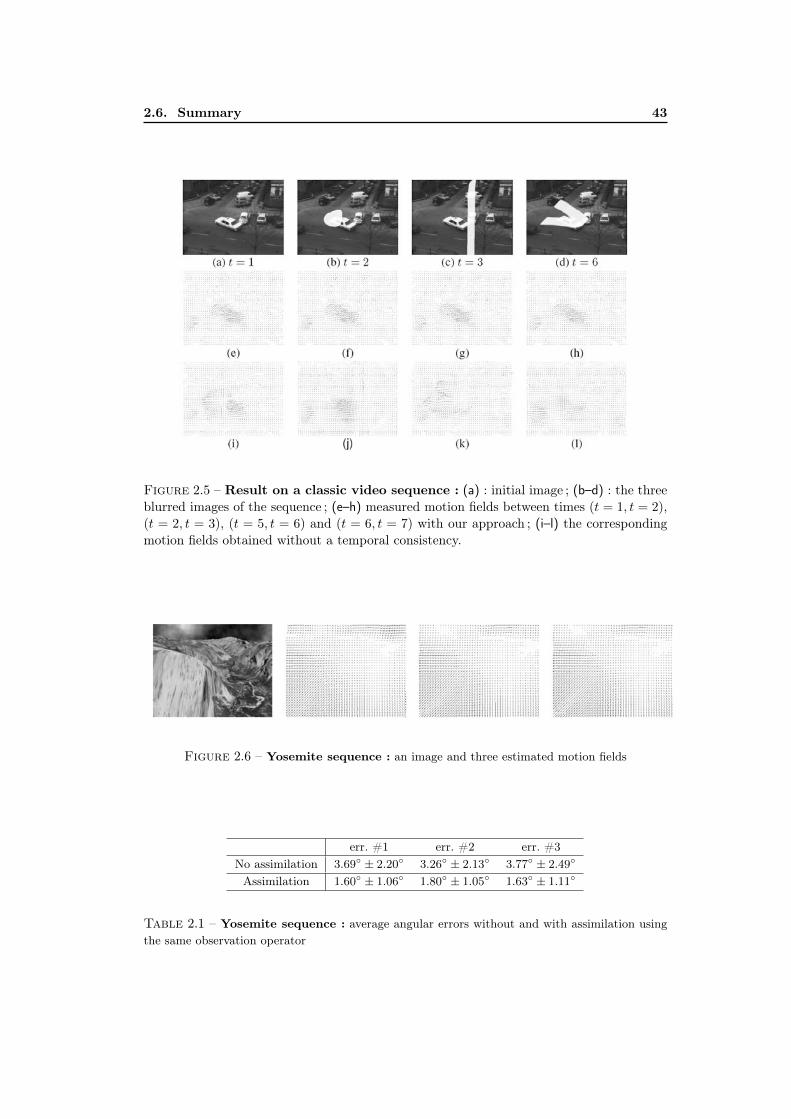
2.6. Summary 43

Figure 2.5 – Result on a classic video sequence : (a) : initial image ; (b–d) : the threeblurred images of the sequence ; (e–h) measured motion fields between times (t = 1, t = 2),(t = 2, t = 3), (t = 5, t = 6) and (t = 6, t = 7) with our approach ; (i–l) the correspondingmotion fields obtained without a temporal consistency.

Figure 2.6 – Yosemite sequence : an image and three estimated motion fields

err. #1 err. #2 err. #3No assimilation 3.69 ± 2.20 3.26 ± 2.13 3.77 ± 2.49

Assimilation 1.60 ± 1.06 1.80 ± 1.05 1.63 ± 1.11

Table 2.1 – Yosemite sequence : average angular errors without and with assimilation usingthe same observation operator


dynamical laws

motion fields guided by a dynamical model . To correctly deal with the huge state space weare facing, the minimization is handled using an adjoint formulation. The resulting processconsists in alternating a forward integration of the state variable and a backward integrationof the introduced adjoint variables.

This technique has been successfully applied in different situations : atmospheric mo-tions, pressure data and classic video sequences involving rigid objects. In the next chapterwe present other applications of the variational assimilation framework not directly relatedto motion estimation in image sequences.

Chapitre 3

Others applications of dataassimilation

Sommaire3.1 Overview . . . . . . . . . . . . . . . . . . . . . . . . . . . . . . . . . 453.2 Convective cell tracking . . . . . . . . . . . . . . . . . . . . . . . . 46

3.2.1 System state and dynamical model . . . . . . . . . . . . . . . . . . . 463.2.2 Observation operator . . . . . . . . . . . . . . . . . . . . . . . . . . . 483.2.3 Some results . . . . . . . . . . . . . . . . . . . . . . . . . . . . . . . 48

3.3 Sea Surface Temperature reconstruction . . . . . . . . . . . . . . 493.4 Data assimilation for multi-resolution . . . . . . . . . . . . . . . . 51

3.4.1 General principle of multi-resolution . . . . . . . . . . . . . . . . . . 513.4.2 Difficulties . . . . . . . . . . . . . . . . . . . . . . . . . . . . . . . . . 523.4.3 Variational assimilation for multi-resolution . . . . . . . . . . . . . . 523.4.4 Some results . . . . . . . . . . . . . . . . . . . . . . . . . . . . . . . 53

3.5 Application to other “flows” : crowd motion analysis . . . . . . . 543.5.1 Dynamic crowd model . . . . . . . . . . . . . . . . . . . . . . . . . . 553.5.2 Crowd analysis using variational assimilation . . . . . . . . . . . . . 553.5.3 Crowd animation using variational assimilation . . . . . . . . . . . . 56

3.6 Summary . . . . . . . . . . . . . . . . . . . . . . . . . . . . . . . . . 59

3.1 Overview

In the previous chapter we have introduced the variational assimilation framework torecover time consistent motion fields from image sequences. This framework has been ableto deal efficiently with the large system states composed by the velocity fields we werefocused on. Of course, the assimilation framework is not only devoted to the estimation ofmotion fields but various parameters can be recovered.

In this chapter we present four other applications related to computer vision. The firstone, in section 3.2, concerns curve tracking where we aim at monitoring two curves cor-responding to the heart and the active areas of some convective systems. The second ap-plication is devoted to Sea Surface Temperature (SST) data reconstruction (section 3.3).The third one in section 3.4 uses the framework of variational data assimilation to performefficient multi-resolution techniques (with applications to optical-flow computation), thetime being related to the different scales of the flow. Lastly, based on some studies thatcreate a link between very dense crowds and fluid flows, we use in section 3.5 techniquesissued from variational data assimilation to manage crowds with videos (estimation of thevelocities and other parameters, animation of crowded scenes).

46 Chapitre 3. Others applications of data assimilation

3.2 Convective cell tracking

Convective cells are atmospheric events that are known to be associated with hazardousconsequences, such as strong wind drafts, lightnings, heavy rainfalls, hails or even torna-does. Over tropical areas such as central Africa, convective cells produce most of the rainduring the monsoon period. They are also indirectly linked to droughts and floods, whichmight afflict this area. Their analysis and forecasting are thus of the utmost interest formeteorologists and forecasters. They can be characterized by two distinct regions : the heart(also named core, center or active part) where the strongest rains appear and the influencearea. An example of a convective cell phenomenon is illustrated in figure Fig. 1.2.

The measurement of the convective cells parameters can be done either by the use ofconventional probes or through satellite data. However, over remote areas (like the Ama-zonian forest for instance), conventional sensors such as radiosonde, rain gauges, radars orlightning detectors have a limited coverage. Satellite information constitutes therefore anappealing alternative for the study of convective atmospheric activity over these particularregions. In practice, such phenomena are analyzed using the temperature computed fromdifferent channels of meteorological data. Our image observations I are then related to thetemperature.

In computer vision, a primal strategy to delineate the contours of complex objectsrelies on the implementation of partial differential equations encoding the evolution ofparametric or non parametric curves toward the minimizers of an energy functional[Caselles 1997, Chan 2001, Kass 1988]. The corresponding functionals include generally adata term representative of a photometric distribution characterizing the object of inter-est and some regularity constraints on the curves. These non linear deterministic mini-mization strategies are in practice very sensitive to the initial curve location and topo-logy. Among the different extensions of those methods, the Eulerian “level-set” approach[Osher 1988, Sethian 1999] has been specifically proposed to alleviate such shortcomings. Inthis framework, the contour’s shape is represented as the zero level-set of an implicit higher-dimensional scalar function. The evolution of this implicit surface describes the contour’sevolution and naturally enables the handling of topology changes. Such techniques havebeen already proposed in a meteorological context [Cohen 1998, Papin 2000, Yahia 1998].However they generally remain on static detection/segmentation approaches applied quasi-independently on the images of the sequence with no temporal consistency guaranty on therecovered shape sequences.

We have proposed to exploit the variational assimilation framework to simultaneouslytrack the two regions of interest of convective cells. This is briefly introduced in the nextsections.

3.2.1 System state and dynamical model

Within level sets, a curve at time t, Ct(p) = C(p, t) : [a, b] × R+ → R2, is implicitlydescribed by the zero level set of a scalar function φ(x, t) : Ω× R+→ R :

Ct(.) = C(., t) = x ∈ Ω | φ(x, t) = 0, (3.1)

where Ω stands for the image spatial domain. The surface is driven by the contours dynamicsand is chosen so as to have for instance positive values inside the curve and negativevalues outside. A common choice for the implicit function is the signed distance but anyother surfaces whose level sets fits the curves of interest is possible. In order to encode thedescription of a convective cloud system encapsulating a set of convective cells, the systemstate X we used is then composed of two implicit surfaces :

3.2. Convective cell tracking 47

– The first one, φe, is devoted to the description of the external delimitations (i.e.influence area) of the convective cells, Ce(t). These curves will be associated to a firstlevel of brightness temperature threshold Te.

– The second one, φc represents the cold core region of each cells, Cc(t). It is related toa colder threshold value Tc of the brightness temperature.

The first level set is defined on the whole image domain Ω : φe(x, t) : Ω × R+ → Rwhereas the second one is defined inside the domain encapsulated by the convective cellscontours, I = x | φe(x, t) > 0 (i.e. the domain delineated by the zero level set of φe) :φc(x, t) : I × R+→ R. Assuming that each curve is :

1. submitted to a motion field along its normal ;2. propagated by this motion field ;3. up to an uncertainty along its normal ;4. up to an uncertainty along its tangent,

we can formalize, for any of the two curves :

dCit = (wi · ni)nidt+ σnnidBn

t + στni⊥dBτ

t . (3.2)

Here nidBn and ni⊥dBτ are two independent Brownian motions directed along and perpen-dicularly to the curves normals and σn, στ are the associated uncertainties. In this model,the curve is transported by a deterministic drift associated to the velocity field (first termof relation (3.2)) that is mitigated with isotropic Gaussian incertitudes –along the normaland tangent– whose covariances grow linearly in time (second and third terms of (3.2)). Asmentioned previously, the curve location is defined from the evolution of an implicit surfaceφi(x, t). Therefore this surface depends on the stochastic process Ct and its differential mustbe defined using stochastic calculus differentiation rules and in particular the so called Îtoformula [Oksendal 1998], already introduced in chapter 1. We get the following stochasticpartial differential equation (in the following, for sake of clarity, we will drop the curve’sindex i = e, c unless explicitly needed) :

∂tφ+ w · ∇φ+

1

2

∑

xi,xj=x,y

∂2φ

∂xi∂xjd〈Cxit , C

xjt 〉

dt+ σn|∇φ|dBn

t = 0, (3.3)

where Cxt and Cyt correspond to the coordinates of the curve-points in the Euclidian plan attime t. As previously, we have introduced velocity drifts w(x) and Brownian motions Bn

t (x)

which are extensions on the whole plane of the curves drift and noise. For the drifts, weconsidered a unique smooth velocity field defined on the whole plane for both curves. Thisvelocity field is in practice obtained by the estimator proposed in section 1.4 of chapter 1.Developing the quadratic variations of the form 〈Cxit , C

xjt 〉 yields :

( ∂φ

∂t+ M(φ)

︸︷︷︸dynamic model

)dt+ σn|∇φ|dB = 0, (3.4)

with

M(φ) = w · ∇φ+σ2τ

2κ|∇φ|+ σ2

n

2|∇φ|2∇φT∇2φ ∇φ, (3.5)

where ∇2φ denotes the Hessian matrix and κ is the mean curvature : κ = curv(φ) =1‖∇φ‖ (∆φ−∇φT∇2φ ∇φ). The temporal expectation of relation (3.4) is its deterministic partand gives our evolution models for curves φi, i = e, c. All details regarding this dynamicalmodel, the way we estimate the uncertainties (σn, στ ), the formulations of adjoints and theimplementations can be found in [Thomas 2009, Thomas 2010].


Figure 3.1 – Convective cell tracking : sequence#1. 4 images of the sequence. Thefirst line corresponds to the contours obtained after the propagation of the initial contourwith the proposed level set’s dynamics ; the second line shows the final results after theassimilation process. Influence area are in blue and active part in red.

3.2.2 Observation operator

It is not possible to construct an observation term that relies on a reference temperaturehistogram since the spatial organization of the temperature inside a convective cell evolvesalong time. Assuming, as it is commonly done in convective cells detection issues, that thecore’s activity (resp. its external area) lies in temperatures under a given threshold Tc (resp.above Te), the function φ, whose zero-level corresponds to the border to extract, should besuch as :

H(I(x)− T•)(1−H(φ•(x))) +H(T• − I(x))H(φ•(x)) = ε, (3.6)

where • = e, c and H is the Heaviside function (H(x) = 0 if x < 0 and H(x) = 1

elsewhere). This relation is zero if I(x) > T• and φ(x) > 0 or if I(x) < T• and φ(x) < 0.This measurement model favors thus the curve interior to be above of a given threshold andthe exterior to be lower of the same threshold. Otherwise this function is always positive.Hence, this relation enables to define the observation system Y = H(φ) as :

Y = 0

H(φ) = H(I(x)− T•)(1−H(φ(x))) +H(T• − I(x))H(φ(x))(3.7)

The operator H is non-linear with respect to φ. Its associated tangent linear operator,adjoint operator, associated error covariance matrices and implementations issues can befound in [Thomas 2009, Thomas 2010].

3.2.3 Some results

We have first tested the method on a sequence of images that exhibits the evolution ofan important convective cell. The assimilation results are shown in figure Fig. 3.1. The firstline represents four images of the sequence where the propagation of the initial contoursthrough the dynamical model are superimposed (the contour in blue represents the celland the one in red is related to the core). The second line exhibits the results after theassimilation. On the first row of this figure, one can observe that the development of thedynamical model provides already a coarse approximation of the final contour location forthe whole convective cell (larger contour). In this particular example, the cell development isprogressive and almost linear. The level set dynamical model has been able to predict quite

3.3. Sea Surface Temperature reconstruction 49

Figure 3.2 – Convective cell tracking : sequence#2 : 4 images of the sequence wherethe influence area of the cell (blue) and its heart (red) obtained after the assimilation processare superimposed.

accurately the successive locations of the cell contours. At the opposite, the cell core is slowlydissipating along the sequence and undergoes a far more chaotic behavior. The benefit of theassimilation process clearly appears on the second line of the figure 3.1 since the estimatedcurves related to the contour and the core of the cell are well in line with the visualizedsequence. The second experiment represents a more complex scene since it contains severalcells at different degrees of evolution. In addition, as no convective phenomena are initiatedin the first image, no curves were used for the initial condition. The very first forecast ofthe initial flat temperature surface corresponding to this initial condition obviously failed inpredicting the first series of contours where new cells develop. Despite this, we can observedon figure Fig. 3.2 that the assimilation process enables to estimate accurately the contoursof the convective cells and their hearts. These two experiments demonstrate the ability ofthe proposed assimilation process to recover reliable curves related to the contour and theheart of the convective cells.

Let us now turn to the reconstruction of sea surface temperature images.

3.3 Sea Surface Temperature reconstruction

Because of the cloud coverage, sea surface temperature (SST) images produced fromsatellite recordings contain missing data, as illustrated in the first line of figure Fig. 3.3.Usually, a preliminary step before any processing on the SST images is the missing datainterpolation. Many algorithms have already been proposed for missing data interpolation.Up to now, most of the existing methods are based on Kalman Filtering or smoothingframeworks [Belyaev 2001]. The main drawback of the Kalman filtering methods is that,because of the large dimensionality of SST images, estimating the covariance matrix ofthe states tends to be computationally expensive, as it requires the inversion of very largematrices. We have proposed a method based on the variational data assimilation frameworkto assimilate missing data in SST images.

To perform the assimilation, the system state X corresponds to the SST (also noted θ)and the observation operator is the identity. Its dynamics follows the heat equation :

∂X

∂t= ν∆X (3.8)

where ν is a diffusion coefficient. Adapting the observation error covariance matrix R (cfrelation (2.4)) to the presence/absence of data allows to recover the SST information ateach location of the ocean, as illustrated in the second line of figure Fig. 3.3. This temporalregularity constraint has enabled to improve the interpolated SST data compared withusual interpolation techniques. To carry on with the quality of the reconstruction, it shouldbe noted that at some locations, chlorophyll observations are available. This scalar quantityevolves following an advection-diffusion process and has fronts at the same location thanSST ones. It is therefore possible to exploit this property by assimilating both SST and


Figure 3.3 – Assimilation of Sea Surface Temperature (SST) images. First line : inputdata corrupted with cloud coverage ; Second line : assimilated SST.

(a) (b) (c) (d)

Figure 3.4 – Joint assimilation of SST and chlorophyll images. (a-b) : input SST andchlorophyll images ; (c-d) : corresponding assimilated results.

chlorophyll. The system state reads then X = [θ, χ]T where χ stands for the chlorophyllconcentration values. Therefore one rewrites the cost function of the variational assimilationframework in (2.4) by adding a penalization term yielding :

J (X) =1

2

∫ tf

t0

‖θobs − θ‖2R−1θ

dt+1

2

∫ tf

t0

‖χobs− χ‖2R−1χdt+

1

2‖X(x, t0)−X0(x)‖2B−1

+1

2

∫ tf

t0

‖∂X∂t

(x, t) + M(X(x, t))‖2Q−1dt− 1

2

∫ tf

t0

gβ(|∇θ|)⟨ ∇θ|∇θ| ,

∇χ⊥|∇χ|

⟩dt,

(3.9)

where the evolution model is composed of the heat equation for θ and advection-diffusionfor χ. It reads :

M(X) =

(−∆ 0

0 v · ∇ − ν∆

)(θ

χ

)(3.10)

where v is an external velocity field (provided by meteorological centers or estimated fromthe data). The additional term of the cost-function (last part of relation (3.9)) aims atimposing SST and chlorophyll fronts at the same locations. It is composed of an edgedetector : gβ(x) = 2/(1+βx)−1 that highlights SST fronts and the scalar product enforcesa same direction of the gradients ∇θ and ∇χ. The figure Fig. 3.4 illustrates some results.It can be observed that fronts appear more clearly for both data and their locations areconsistent.

Despite an overall rating very efficient compared to existing approaches, it neverthelessappeared during the validation step that most of the errors were concentrated on the fine

3.4. Data assimilation for multi-resolution 51

scale structures of the flow. Our current work is then concentrating on the use of moreadapted models for a better recovery of the fine scale structures. In particular we focuson Surface Quasi-Geostrophic equations dynamical models [Lapeyre 2006]. They are basedon an advection-diffusion principle where the diffusion is “softer” than the usual Laplacian.It corresponds to a diffusion of a scalar θ of the type

√∆θ instead of ∆θ. It is proved in

[Lapeyre 2006] that such models are more adapted to the fine scales. To solve mathemati-cally the problem, we are rewriting the assimilation system in a spectral domain in orderto simplify the computational aspects related to this new diffusion.

Let us now introduce the way we used the variational assimilation framework for multi-resolution analysis.

3.4 Data assimilation for multi-resolution

In this section we briefly introduce the principle of the multi-resolution process (nextparagraph), then we highlight some difficulties (in section 3.4.2) and in section 3.4.3, wepropose an original way based on variational assimilation to perform the multi-resolution.This work is under process and preliminary results are exhibited here.

3.4.1 General principle of multi-resolution

Many computer vision techniques (related to motion estimation, segmentation, charac-terization, ...) can be seen as finding a variable X by solving an equation H(X, I,X0) thatdepends on the image luminance I and the pixel grid X0.

Because most of the assumptions used often only hold in a linear case (as the opticalflow constraint equation of relation (1.1) which is valid only for small displacements), it iscommon to embed the resolution of H(X, I,X0) in a so-called “multi-resolution” scheme.The main principle consists in redefining the images on smaller grids XN that correspondto the initial grid X0 divided by a factor N . On such “coarse” images, we assume that deresolution of H(X, I,XN ) can be done under linear constraints and this provide a coarseapproximation XN of the final solution X. In a step forward, this approximation XN isused as an initial condition for a new problem where the goal is to extract a refinementdX (with X = XN + dX) that can be estimated from XN using linear constraints. Suchprocess is commonly repeated for several levels of resolutions yielding a succession of linearproblems.

To get such “coarse” data on which the problem is solved, a usual strategy consists inusing a pyramidal decomposition of the images, for instance with wavelet decompositions orgaussian filtering followed by decimations, as illustrated in Fig. 3.5(a) for a factor N = 2.The estimation is then performed first from the smallest images (under linear constraints)and the solution is reprojected to the following level. Another possibility that we haveproposed in [Corpetti 2011] consists in obtaining X` (related to the solution of a problemH(X, I,X`) at a resolution `) by performing a convolution of H(X, I,X0) by a gaussiankernel of standard deviation `. Indeed, a multi-resolution scheme consists in redefining theproblem on a grid X` which can be viewed as a coarse representation of the initial gridX0 = X with a Brownian isotropic uncertainty of constant variance ` (see the illustrationin figure 3.5(b)) :

X` = X0 + ` I2dB. (3.11)

where B is a standard Brownian motion and I the 2D identity matrix. Any solu-tion X` of a problem H(X, I,X`) defined on a grid X` should satisfy the expectationE(H(X, I,X`)|X0) which is equivalent (see [Corpetti 2011] for the demonstration) to


(a)

grid X0

grid X l

(b)

Figure 3.5 –Different representations of the multiresolution. (a) : a usual pyramidaldecomposition ; (b) a stochastic process where green circles represent the original pixel gridand red circles represented the grid at a given resolution `.

a convolution of H(X, I,X0) with the isotropic gaussian N (O, `). Therefore the multi-resolution can be performed by solving a family of problems g` ∗H(X, I,X0) at the variousresolutions `. A main advantage of such a formulation of the multi-resolution setup is tonaturally get rid of the use of a pyramidal image representation. Instead of dealing withsuccessive decimations of factor 2 of the initial image to fix the different multiresolutionlevels, the evolutions of the levels ` are much flexible here.

3.4.2 Difficulties

Whatever the multi-resolution setup chosen, one of the main difficulty remains on thesuccession of independent problems : at a given resolution `n, the problem consists in findingdX`n using X`n+1 as a coarse approximation : X`n = X`n+1 + dX`n . Once X`n estimated,its value is kept during the rest of the process. This is somewhat prejudicial since it is nowrecognized that small scales (related to finer resolutions) interact with larger scales. Withsuch schemes, at a given resolution `n, the information related to smaller scales ` < `n cannot be taken into account. In addition, any error in the estimation of X`n will also be keptand propagated across the resolutions without any possibilities of correction.

To deal with these difficulties, we propose in the following section a solution based ondata assimilation.

3.4.3 Variational assimilation for multi-resolution

In this section we illustrate the way we exploit the variational assimilation frameworkfor efficient multi-resolution schemes.

The usual temporal variable t is now connected to the different resolutions. We rather

3.4. Data assimilation for multi-resolution 53

prefer to represent its value with the parameter ` : ` = 0 corresponds to the “plain” resolutionat the image grid and we assume that the system state X evolves across the resolutionsfollowing :

∂X

∂`=

1

2∆X. (3.12)

Indeed, it can easily be demonstrated that the solution of the previous relation is

X` = X(`) = g√` ∗X(0), (3.13)

where g√` is a gaussian kernel of standard deviation `. As shown in the previous paragraph,this relation enables to accede to the various scales of X. The model in (3.12) is then aperfect modeling for an exploration of X at different resolution levels.

The multi-resolution estimation procedure consists now to estimate X(0) at the initialartificial time ` = 0 (which corresponds to the image grid) under the perfect model ofrelation (3.12). The initial condition X0 is set to zero and the observation system Y(X0) =

H(X0, X0) defined at the image grid X0 reads for any resolution ` > 0 :

Y(X`) = g√` ∗Y(X0)

H(X`, X`) = g√` ∗H(X0, X0).(3.14)

Following the algorithm described in section 2.2 of chapter 2, as the first integration of thedynamic model in (3.12) with null initial condition gives zeros, the process is expressedas (with B and R the error covariance matrices related to the uncertainty on the initialcondition and the observations) :

1. X(`) = 0 ∀` ∈ [0, `f ] compute the adjoint variables λ(`) with the downscaling equa-tion :

λ(`f ) = 0 ;

− ∂λ

∂`(`)− 1

2∆λ(`) =

(∂XH`

)∗R−1(Y(X`)−H(X`, X`))

(3.15)

2. Update the correction at the image grid : dX(0) = Bλ(0) ;

3. Assess to the correction at all the resolution levels dX(`) from dX(0) with the upscalingequation :

∂dX

∂`=

1

2∆dX (3.16)

4. Update : X = X + dX, ∀` ∈ [0, `f ]

5. Loop to step (1) until convergence

The first step corresponds to the usual downscaling approach : from coarse to fineresolutions, we compute and propagate the errors. This enables to refine the solution atthe image grid (step 2). Unlike the classic multi-resolution, we then re-propagate thiscorrection at the various resolutions (step 3) and the process is repeated until convergence.This framework enables to modify former solutions at given resolution ` = L by takinginto account their influence on smaller scales ` < L. This answers a difficulty mentioned insection 3.4.2 and authorizes a correction of the estimations at the resolution levels.

3.4.4 Some results

We have tested this framework for the motion estimation issue. The system state X =

v = [u, v]T represents the velocity field to estimate between images I(X0, t−1) and I(X0, t).


COM HS DC 1 DC 2 ANISO LK OFCE AMRAAE 4.58o 4.27o 4.35o 3.04o 3.12o 6.07o 4.53o 3.74o

RMSE 0.1520 0.1385 0.1340 0.09602 0.0961 0.1699 0.1243 0.1057

Table 3.1 – Quantitative comparisons on the DNS sequence with a commercial tech-nique based on correlation (COM, La Vision system), Horn & Schunck (HS, [Horn 1981]), twofluid dedicated motion estimators with div-curl smoothing terms (DC 1 : [Corpetti 2002] ; DC2 :[Yuan 2007]), the stochastic approach presented in chapter 1 in anisotropic version (ANISO), aPyramidal Lucas-Kanade (LK, [Lucas 1981]), a Lucas-Kanade term embed in a multi-resolutionscheme with successive convolutions without any assimilation (as presented in section 3.4.1, OFCE)and the proposed multi-resolution using variational assimilation (AMR).

Using a Lucas-Kanade technique (presented in section 1.2.3 of chapter 1) at a resolution `yields an observation system defined as :

Y(X`) = g√` ∗ gσ ∗

(I(X0, t)− I(X0, t− 1)

)

H(X`, X`) = −g√` ∗ gσ ∗∇IT (X0, t)(3.17)

where the adjoint(∂XH(X`, X`)

)∗ reads −g√` ∗ gσ ∗∇I(X0, t) and gσ is a convolutionwith a gaussian of standard deviation σ related to the Lucas & Kanade strategy. It shouldbe outlined that this observation model is implemented for a testing issue but obviously,one of the main advantage of this framework is its possibility to naturally embed in theobservation term some physical models accurately defined at a given resolution ` (sub-gridmodels in particular).

We have tested this technique on the synthetic particle images represented in the figureFig. 1.6 of chapter 1. We also have re-depicted some of the numerical values of table 1.1in table 3.1 where we have compared the proposed strategy with other techniques. It isvery interesting to observe on this sequence that, for the same simple observation termrelated to the ofce but embed in various multi-resolution strategies (LK : pyramidal,OFCE : access to the resolution levels but convolutions, AMR : the proposed technique),the presented one is the most efficient. We also outline from this table that the pyramidaltechnique usually exploited to obtain the various scales is less performing than a series ofconvolutions. Compared to more advanced techniques related to optical-flow or devotedto fluid images, the improvement obtained with this framework yields this technique verycompetitive.

More advanced evaluations are in progress. Let us now turn to the application of theassimilation framework for the analysis of crowds.

3.5 Application to other “flows” : crowd motion analysis

We also have used the variational assimilation framework for the analysis of crowds.Although the application is completely different, we have been based on some works (inparticular [Hughes 2002, Hughes 2003]) that use fluid mechanics properties to model densecrowds. Analyzing crowd footages is of prime interest in a variety of problems : it can helpto i) better understand crowd dynamics or the related behaviors [Helbing 2007], ii) developsurveillance or crowd control systems [Mehran 2009], iii) design and configure public spacesor as well iv) enrich computer animation models used in the context of video games or specialeffects [Courty 2007a, Courty 2007b, Lee 2007]. In the two last decades, two main strategieshave been carried out to represent crowds :

3.5. Application to other “flows” : crowd motion analysis 55

1. representation at the pedestrian level : each individual is an entity/particle driven ina Lagrangian framework. The crowd representation results from the combination ofa large number of entities.

2. the crowd is modeled in a continuous framework related to some scalar/vectorialcharacteristic quantities (density or displacement field for instance). The governingequations are represented in an Eulerian context and the individual notion is vanished.

The assimilation framework is adapted to this last representation. We have worked intothree directions. First, we have proposed a simple crowd evolution model based on conti-nuous laws. Roughly, this model states that the pedestrians aim at reaching their optimaldirection (depending on their goal, position and obstacles) while preventing from denseareas. In a second step, this model has been exploited in a completely continuous way torecover the motion fields and the associated density of pedestrians. Lastly, a mixed conti-nuous/discrete version of the model has been used to animate various crowd scenarios withspecific properties fixed by the user. This is presented in the next sections.

3.5.1 Dynamic crowd model

We start from a scene with obstacles where all humans share the same goal. Reasonablyassuming that each pedestrian aims at minimizing his travel time to his objective, theoptimal direction P at a given location can be derived from the gradient of a potentialfunction φ defined over the whole domain Ω. It can be shown that this potential is thesolution of the classical Eikonal equation which has among others been widely used inthe context of path planing [Kimmel 2001]. For a given scene, we then derive an optimalnormalized direction field P = (U, V )T = ∇φ/‖∇φ‖ of the pedestrians that correspondsto the theoretical normalized direction of a pedestrian without any constraints. If nowthe pedestrians evolve in a crowded environment, we assume that the deviations of theirvelocity from the optimal direction is due to the density that prevents from aiming theoptimal direction. Therefore, we propose the following dynamical model :

v(x, t) = α(ρ)(

P (x, t)︸︷︷︸wished direction

− β(ρ)∇ρ(x, t)︸︷︷︸density repulsion

)(3.18)

where α and β depend on the density ρ and need to be defined. The rule of α is to precisethe global magnitude of the velocity of the pedestrians. As for parameter β, it aims atspecifying the way the density influences the optimal direction. Their exact definition ispresented in [Allain 2009], as well as strategies to avoid pedestrian collision. The output ofthe simulation model in (3.18) can be used as the input of a rendering processes in orderto animate some flows using various conditions (lighting, shooting angle, ...). The figureFig. 3.6 gives an example of some produced scenarios with various obstacles. This modelhas been validated from the point of emergent situations where we have demonstratedthat some known emerging phenomena (depending on density/obstacles) are accuratelyreproduced.

3.5.2 Crowd analysis using variational assimilation

The aim is to extract the velocity and the density of the crowd. The estimation of thedensity is a tricky task in crowd analysis and the assimilation framework gives an appealingsolution. The system’s state X is composed of the two components of the velocity fieldv = (u, v)T and of the density of the crowd ρ (X = (u, v, ρ)T = (v, ρ)T ). The dynamicmodel for the velocity is described in relation (3.18). As for the density we assume that


(a) (b) (c) (d)

Figure 3.6 – Crowd simulation model. (a) : a real crowd picture ; (b–d) : some simulationsprovided by our model

this quantity is transported by the motion field and is diffused along time with a coefficientβ(ρ(x, t)). It then obeys to a classical advection-diffusion relation and the overall dynamicmodel is (the spatio-temporal indexes (x, t) being removed) :

[v∂ρ∂t

]+

0 α(ρ)β(ρ)∇

0 v ·∇− β(ρ)∆

︸︷︷︸M(X)

[v

ρ

]=

[α(ρ)P

0

]+ νm (3.19)

where νm is an uncertainty.The observation system Y = H(X) + νo is defined on the basis of the ofce (relation

(1.1) which is valid for such rigid bodies) for the velocity field and no observations areavailable for the density. Therefore it reads

Y =∂I(x, t)

∂tand H =

[−Ix(x, t), −Iy(x, t), 0

]. (3.20)

This observation operator involves only the motion field. This means that the density cor-rection will be achieved only from deviations of the dynamic model.

An illustration of the assimilation results on a real sequence representing a crowd en-tering a railway station in the city of Monaco is in Fig. 3.7. This example is interestingsince a variety of phenomena are present : a continuous flow at the beginning followed by acompression of some peoples in the left part of the images. In addition, the limit of the dooris a barrier that creates an opposite flux in the crowd flow. In this example, our methodhas detected (cf. images 3.7.(g-h)) two sensible areas where the density is growing larger :the end of the barrier and the wall on the right of the image. This kind of informationassociated to the density is very useful in many topics related to security, design, ... and isdifficult to achieve with usual computer vision techniques. The reader can find more detailsin [Allain 2009].

3.5.3 Crowd animation using variational assimilation

In this section we aim at simulating some crowds with specific properties.Simulating crowd of individuals has drawn a lot of attention over the past decades

for the potential interests of computer graphics but also for safety engineering or roboticsapplications. Controlling a crowd to achieve a given effect is a rather difficult task, mostlybecause the only control parameters are those of the simulation model, which are generallynot designed for it. We have proposed to solve this problem using data assimilation.

3.5. Application to other “flows” : crowd motion analysis 57

(a) (b) (c) (d)

(e) (f) (g) (h)

0 20 40 60 80 100 120 140 160 180!20

0

20

40

60

80

100

120

0 20 40 60 80 100 120 140 160 180!20

0

20

40

60

80

100

120

0 20 40 60 80 100 120 140 160 180!20

0

20

40

60

80

100

120

0 20 40 60 80 100 120 140 160 180!20

0

20

40

60

80

100

120

(i) (j) (k) (l)t = 1s t = 70s t = 140s t = 240s

Figure 3.7 – Results on a real crowd flow representing the entrance of a subway. (a–d) : 4 images of the sequence (t = 1s, 70s, 140s, 240s) where the obstacles are superimposed(in white) ; (e–h) : estimated density and some level-lines ; (i–l) estimated motion fields fort = 1s, 70s, 140s, 240s.


t = 1s t = 5s t = 7s

t = 12s t = 15s t = 17s

Figure 3.8 –Crowd animation : snapshots of a sequence obtained by imposing a constantvorticity of the motion field at time t = 7s in the left part of the image and at time t = 15s

in the right part.

The crowd is composed of a set of N pedestrians and the system’s state is of the formX = [x1,v1, ...,xN ,vN ]T where i = 1, ..., N and components xi (resp. vi) are related totheir positions and velocities. We have adapted the dynamical model in (3.19) to this newrepresentation and we also included some constraints to avoid pedestrian collisions. Theproblem is now : how to find a complete sequence of states X(t) submitted to a dynamicalmodel where at some locations ti we expect some components of the system state (positionor velocity or both) to reach a given configuration fixed by the user. To answer this question,one can use the assimilation framework where the observation model Y(t) = X(t) reads :

Y(t) = [xobs(t),vobs(t)]T (3.21)

where xobs and vobs are the wishes positions and velocities. The associated error covariancematrix R−1(t) is diagonal and of the form :

R−1(t) =

[R−1

x 0

0 R−1v

](3.22)

where 0 is a null diagonal matrix of size N × N . The matrices R−1x and R−1

v are alsodiagonal of size N × N . Their corresponding values are 0 when the user has no specificrequirements and 1 otherwise.

Using the strategy of section 2.2 with these system state and observations models autho-rize the computation of the sequence X(t) that corresponds to the positions and velocitiesof each pedestrians, under the constraints fixed by the user. For instance, in figure 3.8, wehave plotted 8 images of an animated sequence of 20s. Pedestrians aim at going on theright part of the image. We have imposed the vorticity of the global velocity field to reachconstant homogeneous areas at time t = 7s in the left part of the image and t = 15s in theright part. The process has then builded a consistent set of trajectories for all the pedes-trians, as we try to illustrate in figure 3.8. Note that if the observations are issued from realmeasurements (on image sequences) one gets a mean to produce a synthetic animation ofan observed crowd.

3.6. Summary 59

3.6 Summary

In this section we have presented several computer vision tools based on assimilationtechniques. We have in particular proposed approaches able to track curves, reconstructmissing data, perform multi-resolution and analyze crowd behaviors. For all these applica-tions, the assimilation framework is an appealing solution for dealing in an efficient waywith the large system state and the potentially lack of data. In addition, as shown in thecrowd example, this tool is very promising for the estimation of unobserved parameters(like the density for crowds). We then believe that the data assimilation framework is verywell adapted to the analysis of image sequences.

Conclusion of the first part

In this first part, we have been focused on the analysis of Low Spatial Resolution imagesequences. On such data, atmospheric flows and oceanic circulations are visible and wehave been focused on the definition of tools for motion estimation, curve tracking or datareconstruction for such specific motions.

To this end, we have first proposed original techniques for the motion estimation pro-blem from a pair of images. The solutions include new observation terms either based onphysical laws or on a stochastic interpretation of the luminance associated with adaptedsmoothing priors. When a sequence of image is available, we have been based on the va-riational assimilation framework which is an elegant way to efficiently deal with dynamicalconstraints, large system states and noising and/or missing observations. Several motionestimation techniques have been introduced, as well as tools for curve tracking and datareconstruction.

As the processing of such LSR data require some techniques issued from computer vision,we also have proposed more generic tools for time-consistent motion estimation and multi-resolution analysis. In addition, we have presented an original way to manipulate crowds.In this latter situation, more than the application, an original technique to simulate anddeal with discrete objects (pedestrians) submitted to continuous flows has been introduced.

In the second part of this document, we now focus on the analysis of Very High SpatialResolution remote sensing images.

Deuxième partie

Very high resolution remotesensing images : pattern analysis

and change detection

Introduction

As mentioned in the general introduction, the global context and long term objectiveof the researches that are developed concern the analysis of relationships between climateand land cover. Remote Sensing images are a privilege source of observation.

In that context, VHSR (Very High Spatial Resolution) data provide a valuable source ofinformation for the analysis of land cover. However analyzing the patterns of VHSR imagesis more complex than with medium or low resolution data. As a matter of fact, VHSRimages contain many relevant information but they also embed non-informative structuressuch as shadows, cars, animals, ... Many commercial tools exist for the manipulation ofsuch data (such as IDRISI c© 1, ENVI c© 2 or eCognition c© 3) but they appear to be limitedfor advanced studies related to agriculture characterization or change detection. In thispart, we are then focusing on the definition of techniques mainly (but not only) focused onthe manipulation of agricultural data. It should be noted that these works have been donewithin the COSTEL group where not only the methodology was necessary but it was alsorequired that possibly non-specialists researchers (from an image processing and computerscience point of view) can easily apply the approaches to massive databases. This point hashad an influence on some methodological choices.

This second part is structured as follows :– The chapter 4 presents a general framework for the characterization and compa-rison of agricultural parcels and more generally textured patterns ;

– The chapter 5 gives some applications of the previous descriptors for the segmen-tation and the classification of agricultural parcels, the estimation of the orientationand the detection of textured fronts ;

– Finally the chapter 6 is devoted to the change detection problem where we pro-pose several tools that either rely on the works of the previous chapters but we alsointroduce more generic approaches.

1. http://www.clarklabs.org/2. http://www.ittvis.com/ProductServices/ENVI.aspx3. http://www.ecognition.com/

http://www.clarklabs.org/

http://www.ittvis.com/ProductServices/ENVI.aspx

http://www.ecognition.com/

Chapitre 4

Descriptors of agricultural parcelswith wavelets and evidence theory

Sommaire4.1 Overview . . . . . . . . . . . . . . . . . . . . . . . . . . . . . . . . . 67

4.2 Generalities about wavelet & assumptions . . . . . . . . . . . . . 68

4.2.1 Wavelet decomposition of signals and images . . . . . . . . . . . . . 68

4.2.2 Assumption related to wavelet coefficients . . . . . . . . . . . . . . . 68

4.3 Characterization of agricultural parcels . . . . . . . . . . . . . . . 69

4.4 Comparison of agricultural parcels with data fusion . . . . . . . 70

4.4.1 Comparison of luminance . . . . . . . . . . . . . . . . . . . . . . . . 70

4.4.2 Comparison of texture . . . . . . . . . . . . . . . . . . . . . . . . . . 70

4.4.3 Fusion of similarity criteria . . . . . . . . . . . . . . . . . . . . . . . 71

4.5 Summary . . . . . . . . . . . . . . . . . . . . . . . . . . . . . . . . . 72

4.1 Overview

In this chapter we are focused on some specific patterns that appear in several remotesensing data. These patterns can either be related to :

– agricultural parcels : the different kind of cultures in crops, the different ways ofdiggings, ... make some specific textured patterns whose analysis is crucial in order tomonitor the vegetation (see Fig. 4.1(a–c)) ;

– specific organization of clouds : for instance, the clouds generated at the so-called “seabreeze front” are natural markers of the limit of the penetration of the sea breezeinland, as illustrated in figure Fig. 4.1(d).

From these illustrations it is obvious that patterns are well discriminated by their orienta-tion, scale, texture, ... Therefore a multi-scale analysis at different orientations appears tobe a rational choice. In that context, wavelets consists in an appealing solution. In addition,as we will observe in the next chapter, we will have to compare some parcels whose size aredifferent. The descriptors have then to be insensitive to the size of the patterns.

We then suggest to represent the different properties of the textured areas on the basisof the distribution of their wavelet coefficients. A general introduction and the underlyingassumptions on which we rely are addressed in section 4.2. The section 4.3 presents ourdescriptors and section 4.4 introduces the way we compare two regions.

68Chapitre 4. Descriptors of agricultural parcels with wavelets and evidence

theory

(a) (b) (c) (d)

Figure 4.1 – Illustration of textured patterns ;(a–c) : VHSR data representing cereals,sowed meadow and forest ; (d) : LSR data where the white line corresponds to the coast linewhereas the red line corresponds to the sea breeze front, identify by the limit of a texturedarea composed of a line of cumuliform clouds.

4.2 Generalities about wavelet & assumptions

4.2.1 Wavelet decomposition of signals and images

Noting f(x) a real signal (1-dimensional for the sake of clarity), its continuous waveletdecomposition F is :

F(a, b) =

∫ ∞

−∞f(t)

1√aψ

(t− ba

)dt (4.1)

where ψ stands for the analyzing wavelet, ψ being the complex conjugate of ψ and a (resp. b)is a scaling (resp. position) parameter. Any combinations of scaling and position parameterare possible. For digital signals I[n], a discrete transform can be defined as :

I[j, k] =

N/2∑

n=−N/2I[n]2−

j2ψ[2−

j2 (n− k)

](4.2)

for a position k and a scaling factor j. The support of the wavelet ψ is [−N/2, N/2]. Itcan be shown (see [Mallat 1989] for instance) that the family ψj,k = ψ(2−

j2 (n − k)) for

(j, k) ∈ Z2 constitutes an orthonormal basis and any digital signal I can be represented as :

I[n] =∑

k

A[k]φJ,k[n] +−1∑

j=−J

∑

k

I[j, k]ψj,k[n] (4.3)

where φ is the scaling function. The coefficients A[k] correspond to an approximation (alsonamed continuous component) of the initial signal I at resolution J and all I[j, k] are thedetails associated to the scale j. The total numbers coefficients A and I equals the numberof elements of I. For 2D discrete signals like digital images, the extension of the orthonormalbasis gives a wavelet decomposition that highlights an approximation band and three kindsdetails : horizontal, vertical and diagonals, as shown in figure 4.2(a-b).

4.2.2 Assumption related to wavelet coefficients

In a given sub-band of the wavelet decomposition, S.G. Mallat verified that the distri-bution of the wavelet coefficients related to details I[j, k] of any texture pattern follows aGeneralized Gaussian Density (GGD) function [Mallat 1989]. The GGD reads :

p(x;α, β) =β

2αΓ(1/β)e−( |x|α )

β

, (4.4)

4.3. Characterization of agricultural parcels 69

8 1re soumission à Revue Internationale de Géomatique

wJ+1

wJ+1

wJ+1

1

2

3

wJ+2

wJ+2

wJ+2

1

2

3

IJ

h

g

Rangées

Colonnes

Rangées

Colonnes

h

g

h

g

h

g

h

g

h

g

IJ+3

Figure 2. Application successive de filtres miroir en quadrature ; h est une filtre passe-bas et ’g’ est un filtre passe-haut

IJ+3

WJ+21

WJ+2

2WJ+2

3WJ+1

WJ+1

WJ+1

1

2 3

(a) (b) (c)

Figure 3. Décomposition en ondelettes d’une image : a. Image originale, b. compo-santes issues de la transformée, c. notations des composantes

En pratique, ces coefficients sont calculés par l’application successive de filtresmiroir en quadrature (Van de Wouwer et al., 1999) sur les rangées et les colonnes del’image (Figure 2). À chaque étape de filtrage, nous obtenons une série de coefficientspour une résolution donnée : IJ,n correspond à une image basse ré solution et les sérieswj,n comportent 3 images de détails. Comme les images de détails sont obtenues enappliquant horizontalement et verticalement un filtre passe-haut et un filtre passe-bas,elles contiennent les directions verticales, horizontales et diagonales. Enfin, l’imagebasse résolution peut à son tour être décomposée pour obtenir une nouvelle série decoefficients à plus grande échelle. La figure 2.1 donne un exemple de décompositiond’une image ainsi que la représentation de l’organisation des composantes qui en ré-sulte. Si le nombre de niveaux de décomposition est suffisant, alors on peut associerles informations de luminance des objets à la composante d’approximation, tandis queles informations de textures correspondant aux variations locales de la fonction de lu-minance sont captées par les composantes de détails. Dans cet article, l’ensemble descomposantes sont utilisées, ce qui permet de prendre en compte à la fois les propriétésde luminance et de texture des images.

(a) (b) (c)

Figure 4.2 – Example of a wavelet decomposition : (a) : an input image ; (b) itsdecomposition on an orthonormal basis where the approximation band and the horizontal(resp. vertical, diagonal) are shown for 2 levels of decomposition. The vertical orientationof the pattern in (a) clearly appears in the vertical bands and does not affect other ones ;(c) : distribution and corresponding GGD for the vertical coefficients in the first level ofthe decomposition

and is characterized by two cœfficients : the scale parameter α and the shape parameterβ 1. The term Γ(t) =

∫ +∞0

e−zzt−1dz is the mathematical Gamma function. Figure 4.2(c)illustrates the GGD distribution of the coefficients in a sub-band of a wavelet decomposition.

4.3 Characterization of agricultural parcels

Under the representation with GGD, any texture pattern can be characterized by asequence :

T = (αj,Z , βj,Z) (4.5)

where J ≤ j ≤ −1 is the scale analysis and (αj,Z , βj,Z) are coefficients related to GGD inthe Z = H,V,D directions (corresponding to the horizontal, vertical or diagonal band).In practice, the estimation of parameters (αj,Z , βj,Z) from a set of data is performed usinga maximum-likelihood technique, as detailed in [Varanasi 1989]. The representation in (4.5)does not take into account the approximation of the original signal and is therefore onlyrelated to the texture components. In general the distribution of the approximation banddoes not a fit a GGD. If one desires to embed such continuous part in the representation,the descriptor is defined as :

T = (p, αj,Z , βj,Z) (4.6)

where p is a smooth histogram of the empirical distribution of the coefficients A[k]. Weprefer to rely on histograms in order to guarantee an independency with respect to thespatial location of the coefficients. The smoothing prevents from bad interpretations of theempirical distributions that are likely to be locally noisy. The technique used to smoothhistograms is a kernel method [Bowman 1997].

The descriptors in (4.5-4.6) characterize our textured pattern issued from remote sen-sing data. As we use either a parametric representation of the distribution of coefficients(through GGD) or a smoothed histogram, some uncertainties ∆ = (∆p,∆j,Z) are introdu-ced compared to the empirical distributions. They are computed from the root mean square

1. A gaussian distribution corresponds to β = 2


theory

error of the estimation :

∆• =

√1

x2 − x1

∫ x2

x1

(p•(x)− p•(x))2dx (4.7)

where p•(x) (resp. p•) ∈ [x1, x2] is the empirical (resp. smoothed) distribution in the band•. The next section proposes a way to compare two regions Ra and Rb characterized byTa and Tb (relations (4.5) or (4.6)) and their associated uncertainties ∆a and ∆b (relation(4.7)).

4.4 Comparison of agricultural parcels with data fusion

To be more general, we assume that our descriptors include the approximation part(formulation in (4.6)). We aim at comparing two regions Ra and Rd described withTa = (pa, αa,j,Z , βa,j,Z) and Tb = (pb, αb,j,Z , βb,j,Z). We first define one similarity indi-cator L(Ra, Rb) based on the luminance and several similarity indicators Tj,Z(Ra, Rb) (jcorresponding to the scale and Z to the horizontal, vertical or diagonal band of the waveletdecomposition) based on the texture. All the indicators are then fused in a step forward todefine a unique similarity criterion.

4.4.1 Comparison of luminance

The luminance information is embedded in the approximation part. A criterion basedon the Bhattacharyya formula is used :

L(Ra, Rb) =

(1−

∫ √pa(x)pb(x)dx

). (4.8)

This criterion L is null for two identical distributions and grows up to 1 when they differ.The associated incertitude is derived following uncertainty computations stating that anyfunction f(pa,pb) such that pa(x) = pa(x)±∆pa and pb(x) = pb(x)±∆pb is associated toan uncertainty ∆f(pa,pb) that reads :

∆f(pa,pb) =

∣∣∣∣∂f

∂pa(pa,pb)

∣∣∣∣∆pa +

∣∣∣∣∂f

∂pb(pa,pb)

∣∣∣∣∆pb. (4.9)

This latter relation comes from the Taylor’s theorem where all uncertainties have positivecontributions. We then associate an uncertainty ∆L to the criterion (4.8) which is :

∆L(Ra, Rb) =

∫ (∣∣∣∣pb

2√papb

∣∣∣∣∆pa +

∣∣∣∣pa

2√papb

∣∣∣∣∆pb), (4.10)

4.4.2 Comparison of texture

We are based on the Kullback-Leibler criterion. This latter is defined between distribu-tions pa and pb as :

KL(pa,pb) =

∫ +∞

−∞pa(x) log

pa(x)

pb(x)dx (4.11)

This criterion is non-symmetric. Depending on the application, it might be useful to use asymmetric version of the type KLS(pa,pb) = (KL(pa,pb) +KL(pa,pb))/2. For instance,if one wants to compare two regions, a symmetric version is useful. At the opposite, if weexpect to highlight transitions between two parcels, a non-symmetric version is preferred.

4.4. Comparison of agricultural parcels with data fusion 71

For two GGD pa and pb defined with (αa, βa) and (αb, βb), this similarity measurementreads [Do 2002] :

KL(αa, βa, αb, βb) = log

(βaαbΓ(1/βb)

βbαaΓ(1/βa)

)+

(αaαb

)βb Γ((βb + 1)/βa)

Γ(1/βa)− 1

βa. (4.12)

Its value is null for two identical distributions and progressively grows up when the dis-tributions differ. To derive a criterion measurement in [0, 1] from the KL dissimilarity,we hence apply a function g of the type g : [O,+∞[−→ [0, 1[. The function g used isg(x) = x2/(σ2 + x2) and the critera Tj,Z(Ra, Rb) for all pair j, Z are finally defined by :

Tj,Z(Ra, Rb) = g(KL•(pa,pb)) (4.13)

where KL• is either the criterion in (4.11) or its symmetric version. The associated uncer-tainty reads (for KL• = KL) :

∆Tj,Z (Ra, Rb) =2σ2KL(pa,pb)

(σ2 +KL(pa,pb)2)2∆KL(pa,pb) with

∆KL(pa,pb) =

∫ +∞

−∞

∣∣∣∣1−pb(x)

pa(x)+ log

pa(x)

pb(x)

∣∣∣∣∆padx. (4.14)

It is important to outline that one could have use other similarity criteria, like the Bhatta-charyya one, which has the advantage to directly be in the interval [0, 1]. However, in ourexperiments, this latter was less discriminative than Kullback-Leibler [Lefebvre 2009]. Fur-thermore, to the best of our knowledge, the Kullback-Leibler criterion between two GGDis the only one that can be expressed in an analytic way, which simplifies many practicalaspects.

A set of P indicators C = L(Ra, Rb), Tj,Z(Ra, Rb) (J ≤ j ≤ −1, Z = H,V,D)with associated incertitudes ∆C = ∆L(Ra, Rb),∆T (Ra, Rb) is then available to sense thesimilarity between regions Ra and Rb on the basis of their luminance and texture. From Cand ∆C , the next section proposes a way to derive a unique similarity criterion.

4.4.3 Fusion of similarity criteria

For each criterion C(`), ` = 1...P , we define three mass functions mA(C(`)), mB(C(`))and mA∪B(C(`)) related to the belief on three hypotheses :

1. Hypothesis A : regions Ra and Rb are similar following criterion C(`) ;2. Hypothesis B : regions Ra and Rb are not similar following criterion C(`) ;3. Hypothesis A∪B : uncertainty about the similarity of the regions following criterionC(`) ;

where mA(C(`))+mB(C(`))+mA∪B(C(`)) = 1. The way we get m from any criteria in C(`)is only a normalization step :

S = 1 + ∆C(`) and

mA(C(`)) =(

1− C(`))/S

mB(C(`)) = C(`)/SmA∪B(C(`)) = ∆C(`)/S

(4.15)

The values mA(C(`)), mB(C(`)) and mA∪B(C(`)) constitute mass functions commonly usedin evidence theory and can then be fused together. Among the available fusion approaches,we chose the Dempster’s fusion rule issued from the well-known Dempster-Shafer theory


theory

[Shafer 1976] that has proved to be very efficient in such context. This latter reads, for anyhypothesis H 6= ∅ and mass functions m1 and m2 to fuse :

m(H) = [m1 ⊕m2] (H) =

∑H1∩H2=H

m1(H1)m2(H2)

1− ∑H1∩H2=∅

m1(H1)m2(H2)(4.16)

where K =∑

H1∩H2=∅m1(H1)m2(H2) measures the conflict between sources m1 and m2. It

should be noted that this fusion rule holds for independent sources of data. For that reason,we use wavelet packet decomposition since the related coefficients are less correlatedtogether. In the future we will use Dempster-Shafer’s based technique that take intoaccount a dependency between sources of informations [Denoeux 2008]. As the Demps-ter’s fusion rule is associative, one can apply the following algorithm to fuse all our criteria :

%Initialization at ` = 1:PA(Ra, Rb) := mA(C(1))PB(Ra, Rb) := mB(C(1))PA∪B(Ra, Rb) := mA∪B(C(1))%Fusion of all the criteriafor ı = 2 to P

PA(Ra, Rb) =

mA(C(ı))PA(Ra, Rb) + PA(Ra, Rb)mA∪B(C(ı)) +mA(C(ı))PA∪B(Ra, Rb)

1− (PA(Ra, Rb)mB(C(ı)) +mA(C(ı))PB(Ra, Rb))

PB(Ra, Rb) =

mB(C(ı))PB(Ra, Rb) + PB(Ra, Rb)mA∪B(C(ı)) +mB(C(ı))PA∪B(Ra, Rb)


PA∪B(Ra, Rb) =

mA∪B(C(ı))PA∪B(Ra, Rb)


end

Finally, the similarity measurement between regions Ra and Rb retained isκ(Ra, Rb)±∆κ(Ra, Rb) ∈ [0, 1] such as :

κ(Ra, Rb) := PA(Ra, Rb)

∆κ(Ra, Rb) = PA∪B(Ra, Rb). (4.17)

4.5 Summary

In this chapter we have proposed some descriptors for the characterization of texturepatterns. They are based on a representation of the detail coefficients (and eventually onthe approximation component) of a wavelet decomposition. As for the approximation part,it can be useful if one compares patterns in similar conditions (same image for instance)but this component is often not used when we deal with images of different sensors.

We have assumed that the distribution of the coefficients follows a generalized gaussiandensity and this distribution can therefore be characterized only with two parameters relatedto the scale and the shape.This drastically reduces the size of the descriptor. In addition,the associated uncertainties related to the fitting of each GGD are extracted.

4.5. Summary 73

We have introduced a way to compare regions identified by the proposed descriptors.This relies on similarity measurements (Kullback-Leibler) from which we define mass func-tions that are fused together. It results in a unique similarity criterion with an associateduncertainty.

In the next chapter we present applications using such descriptors.

Chapitre 5

Application to various remotesensing problems

Sommaire5.1 Overview . . . . . . . . . . . . . . . . . . . . . . . . . . . . . . . . . 755.2 Segmentation of agricultural parcels . . . . . . . . . . . . . . . . . 75

5.2.1 Previous step : wavelet watershed segmentation . . . . . . . . . . . . 765.2.2 Merging agricultural parcels . . . . . . . . . . . . . . . . . . . . . . . 76

5.3 Estimation of the orientation of textured patterns . . . . . . . . 775.3.1 Problematic and related works . . . . . . . . . . . . . . . . . . . . . 775.3.2 Proposed solution . . . . . . . . . . . . . . . . . . . . . . . . . . . . 785.3.3 Some results . . . . . . . . . . . . . . . . . . . . . . . . . . . . . . . 78

5.4 Classification and supervised segmentation of agricultural parcels 805.5 Detection of sea breeze fronts . . . . . . . . . . . . . . . . . . . . . 80

5.5.1 Problem of front detection and tracking . . . . . . . . . . . . . . . . 805.5.2 Proposed solution . . . . . . . . . . . . . . . . . . . . . . . . . . . . 815.5.3 Some results . . . . . . . . . . . . . . . . . . . . . . . . . . . . . . . 82

5.6 Summary . . . . . . . . . . . . . . . . . . . . . . . . . . . . . . . . . 82

5.1 Overview

In this chapter we apply the descriptors of the previous chapter to several open remotesensing problems : segmentation, classification, detection of fronts and estimation of theorientation of the digging for some agricultural parcels. It should be noted that the presentedtechniques can also be applied in other fields than remote sensing.

5.2 Segmentation of agricultural parcels

A very important panel of methods is available for segmenting an image [Pal 1993]and this task is a crucial step in many computer vision problems. As for the Very HighSpatial Resolution (VHSR) remote sensing images, a large amount of approaches has alreadybeen proposed and the reader can refer to [Carleer 2005, Dey 2010] for an overview. Dueto the complexity and the variety of the input data, each approach is often devoted toa specific kind of imagery. In many practical applications, researchers or engineers usecommercial multi-resolution segmentation softwares to extract regions at different scalesbased on several consistency criteria learned on training samples. Despite the efficiency ofsuch approaches, this requires some features selection and thresholds to tune the classifier

76 Chapitre 5. Application to various remote sensing problems

[Schiewe 2001]. As a consequence an expert knowledge is needed and this makes impossiblethe generalization of such a process for various types of data.

We have proposed an unsupervised segmentation adapted to gray-scale images whichrequires few input parameters and produces regions of different sizes and different shapes.It is devoted to gray-scale images in order to process any kind of optical image and to be astransposable as possible. The idea consists in performing in a first step an over-segmentedmap where the objects are merged in a second step, according to the criterion presented inchapter 4.

The preliminary segmentation step is based on the combination of a wavelet trans-form and a watershed segmentation algorithm. This method has been introduced by[Jung 2007, Kim 2003]. We have been based on such approach since it is simple to im-plement and it detects properly the regions edges. Nevertheless it remains over-segmentedobjects, especially when one is dealing with highly textured pattern, like those included inVHSR remote sensing images. It is then of prime importance in a second step to mergesimilar regions. This is presented in the two next paragraphs.

5.2.1 Previous step : wavelet watershed segmentation

Here we rely on a watershed associated to the detail cœfficients at a given resolutionof the image [Jung 2007, Kim 2003]. The resolution level is chosen by the user. It is inpractice related to the spatial resolution of the input data and corresponds to the limit ofan “entity” that composes an object. For instance in the case of an agricultural parcel, weassume that this latter is composed of several textured patterns (i.e. entities) generated bythe digging and the spatial organization of plants. The choice of the resolution level is suchthat a single pattern will appear as a more or less uniform object at the chosen resolution.As a consequence, the application of a watershed process makes sense.

As will be shown in the experimental part, such a process results in over-segmentedregions that need to be merged. This is the scope of the next section.

5.2.2 Merging agricultural parcels

In order to organize the different regions issued from the watershed step , we use RegionAdjacency Graph (RAG) [Sonka 1993]. This is an non-oriented graph where the nodescorrespond to the regions centroids and the edges represent a common border betweenregions. For each nodes we evaluate the similarity between its connected regions. They arethen fused if a similarity criterion is validated. When no regions can be fused, the processis stopped.

As already mentioned, for VHSR data, the texture is often a reliable descriptor. Howeverfor very small objects, like the ones often extracted with a watershed technique, the notionof texture is ambiguous since the spatial information is too poor. For these kind of patterns,we rather prefer to rely on their gray-level to evaluate their similarity :

d(Ra, Rb) =√

(Ma −Mb)2, (5.1)

whereMa (resp.Mb) is the mean luminance of the region Ra (resp. Rb). The overall processconsists then in performing a watershed segmentation, building a Region Adjacency Graph,merging small similar objets based on the criterion on (5.1) and merging large objects basedon the criterion of the previous chapter. All details can be found in Antoine Lefebvre’s PhD[Lefebvre 2011a]. This is summarized in figure Fig. 5.1. An example on a aerial photographis displayed in figure 5.2. The subfigure (a) shows the output of our watershed segmentation,subfigure (b) corresponds to the merging of small elements whereas subfigure (c) depicts the

5.3. Estimation of the orientation of textured patterns 77

IMAGE 1. Wavelet transform

Approximationcoe!cients

Details coe!cients

2. Watershed segmentation

Over-segmented regions

3. Small region mergingon the basis of the luminance

Over-segmented and

homogeneous regions

4. Large region mergingon the basis of proposed criteria

FINAL MAP

Figure 5.1 – Unsupervised segmentation process that consists in 2 merging step.Ellipses are data, rectangles are operations, arrows are outputs, dotted lines are input.

(a) (b) (c)

Figure 5.2 – Segmentation of an aerial photograph. (a) : results after the watershedsegmentation (step 1) ; (b) : results after the merging of small entities ; (c) : results afterthe merging of similar objects

final segmentation where similar objects have been merged following the presented method.This example highlights its efficiency. We indeed observe that the watershed segmentationdetects accurately the edges of each geographical entities but provides over-segmented ob-jects. In a step forward, small similar objects from a luminance point of view are mergedand the segmentation in (b) is generated. Lastly, the proposed merging step based on thecriterion (4.17) of the previous chapter allows to separate the geographical entities accordingtheir texture and intensities. On this example, the ability to merge highly textured patternsof the different vineyards and roads is demonstrated : some large regions, fitting correctlywith the edges of each vine plots, associated with long and thin regions representing roads,are extracted. More experiments can be seen in [Lefebvre 2010c, Lefebvre 2011a].

5.3 Estimation of the orientation of textured patterns

5.3.1 Problematic and related works

Here we are interested in the estimation of the dominant orientation of textured pat-terns that appear in a number of images. The applications are numerous (remote sensingbut also biology or natural sciences for instance). In remote sensing, the main orienta-tion of agricultural parcels often indicates relevant properties with regards to the topo-logy and the underlying soil. Among the existing approaches related to orientation esti-mation, one can roughly classify them into gradient-based [Freeman 1991, Germain 2003,Le Pouliquen 2005, Michelet 2007] and spectral-based approaches [Jafari-Khouzani 2005,Josso 2005]. Techniques of the first family extract an orientation vector at each location ofthe image, which is not desired in our application since we rather prefer to extract a singlevector representing the orientation of a whole object. Most of methods of the second familyfail when multiple and sometimes non-rectangular objects occur in a single image. As amatter of fact, they are all based on the Fourier transform and the lack of space informa-


tion prevents from the localization of any structured pattern. We then propose to rely onwavelets to solve this problem.

5.3.2 Proposed solution

The strategy is based on the maximization of a criterion that deals with the coefficientsenclosed in the different bands of a wavelet decomposition of the original image. Moreprecisely, we search for the orientation that best concentrates the energy of the coefficientsin a single direction (chosen as vertical here) :

θ = maxθ

(E(D, Iθ)

)=θ|E(D, Iθ) = Emax

, where

E(D, Iθ) =J∑

=0

(D(V θ , Hθ) + D(V θ , D

θ)) .

(5.2)

where Hθ (resp. V θ , D

θ) represents the horizontal (resp. vertical and diagonal) band along

the th level of the wavelet decomposition of an original pattern I rotated by an angleθ. Here, D(•1, •2) is a symmetric similarity measurement between the distribution of thecoefficients in the bands •1 and •2 based on the representation of the previous chapter. Therelation (5.2) reaches its maximum for the angle θ that corresponds to the rotation requiredto align the main orientation of the analyzed pattern to the vertical axis.

The way we optimize the function in (5.2) is detailed in [Lefebvre 2010b, Lefebvre 2011a].It should be noted that the proposed technique is able to evaluate whether a given texture isoriented or not. This is done using the different values reached by E during the optimizationprocess (that are connected to an isotropy degree).

5.3.3 Some results

The articles in [Lefebvre 2010a, Lefebvre 2010b, Lefebvre 2011a] contain complete qua-litative and quantitative evaluations of the technique and comparison with other ones. Herewe present a snapshot of result. We have estimated the orientation angle on a set of 150

pre-segmented patterns extracted on remotely sensed images of 60cm resolution issued fromdifferent sensors : very high spatial resolution data, grey scale aerial photographs and pan-chromatic satellite images. Five classes of land coverage have been distinguished : meadow,bare soil, forest, cereals, and vineyard. Among them, bare soils, meadows and forests areconsidered as “non-oriented” (or isotropic) textures whereas the cereals and vineyards are“oriented” (or anisotropic).

First, the rate of correct classification between oriented and non-oriented textures is96.7% with our approach whereas it is of 82.7% with the approach in [Josso 2005]. Forsome important differences in the estimation of angles, we have plotted in figure 5.3 there-oriented patterns along the vertical axis with both estimated angles. From these figures,it is clear that the accuracy is more important with the proposed technique since our re-oriented patterns fit better with the vertical axis. We also have applied the framework toestimate the orientation at each location of PTV (Patricle Tracking Velocimetry) images.This technique of visualization enables to observe the motion of particles in a fluid flowusing their trace in images, yielding oriented patterns (cf figure Fig. 5.4(a)). The processhas been applied on a patch around each position. On the estimated angles of figure 5.4(b),it is very promising to observe that they are consistent with the flow where the differentareas are accurately extracted (disturbance just after the obstacle and homogeneous flowoutside).

5.3. Estimation of the orientation of textured patterns 79

(a) (b) (c)

Figure 5.3 – Reorientation of the patterns for some agricultural parcels (top and bot-tom). (a) represents the input textures ; (b) rotation of (a) along the vertical axis accordingto the proposed method ; and (c) rotation of (a) according to [Josso 2005]

Figure 5.4 – Estimation of the orientation on PTV (Particle Tracking Velocime-try) images. Left : a PTV image ; right : estimated angles at each location



Bâti

Surfaces avec végétation rase

Surfaces boisées

Sol nu

Eau

Voirie

250 m NBâti


Surfaces boisées

Sol nu

Eau

Voirie

250 m N

0%

10%

20%

30%

40%

50%

60%

70%

80%

90%

100%

1978 2001

Voirie

Eau

Sol nu

Surfaces avec

végéta!on rase

Surfaces

boisées

Zone 1 : Cesson-Sévigné

Surfaces artificialisées en 1978 et 2001

Surfaces non-artificielles en 1978 et 2001

"Désartificialisation" des sols entre 1978 et 2001

Artificialisation des sols entre 1978 et 2001

250 m N

woodlandsBâti


Surfaces boisées

Sol nu

Eau

Voirie

250 m NBâti


Surfaces boisées

Sol nu

Eau

Voirie

250 m N

0%

10%

20%

30%

40%

50%

60%

70%

80%

90%

100%

1978 2001

Voirie

Eau

Sol nu

Surfaces avec

végéta!on rase

Surfaces

boisées






250 m N

bare soil

Bâti


Surfaces boisées

Sol nu

Eau

Voirie

250 m NBâti


Surfaces boisées

Sol nu

Eau

Voirie

250 m N

0%

10%

20%

30%

40%

50%

60%

70%

80%

90%

100%

1978 2001

Voirie

Eau

Sol nu

Surfaces avec

végéta!on rase

Surfaces

boisées






250 m N

vegetationBâti


Surfaces boisées

Sol nu

Eau

Voirie

250 m NBâti


Surfaces boisées

Sol nu

Eau

Voirie

250 m N

0%

10%

20%

30%

40%

50%

60%

70%

80%

90%

100%

1978 2001

Voirie

Eau

Sol nu

Surfaces avec

végéta!on rase

Surfaces

boisées






250 m N

roadsBâti


Surfaces boisées

Sol nu

Eau

Voirie

250 m NBâti


Surfaces boisées

Sol nu

Eau

Voirie

250 m N

0%

10%

20%

30%

40%

50%

60%

70%

80%

90%

100%

1978 2001

Voirie

Eau

Sol nu

Surfaces avec

végéta!on rase

Surfaces

boisées






250 m N

builded areas

Bâti


Surfaces boisées

Sol nu

Eau

Voirie

250 m NBâti


Surfaces boisées

Sol nu

Eau

Voirie

250 m N

0%

10%

20%

30%

40%

50%

60%

70%

80%

90%

100%

1978 2001

Voirie

Eau

Sol nu

Surfaces avec

végéta!on rase

Surfaces

boisées






250 m N

water1978 2001

Figure 6.5 – Supervised segmentation Two VHSR images from 1978 and 2001, theassociated segmentation and the legend.

tation of section 6.1.1. Based on samples, any class can be characterized using the proposeddescriptors of previous chapter and compared together with our proposed criterion. Howeverfor agriculture applications, a recurrent problem when one performs supervised segmenta-tion comes from the digging which in general is different when samples are taken at differentlocations. As a consequence, two agricultural parcels with the same land cover but differentdiggings are likely to be labelled in different classes. We then propose to re-orient all thepre-segmented objects on a common axis using the approach of the previous section.

Some results are depicted in figure 6.5 for 6 classes related to . More examples withdetailed quantitative comparisons are in [?, Lefebvre 2011].

6.4 Detection of sea breeze fronts

6.4.1 Problem of front detection and tracking

6.4.2 Proposed solutions

1978 2001

Figure 5.5 – Supervised segmentation Two VHSR images from 1978 and 2001, theassociated segmentation and the legend.

5.4 Classification and supervised segmentation of agri-cultural parcels

Classification in remote sensing is a key issue and has been widely studied overthe last decades (see for instance [Benediktsson 1990, Bruzzone 2009, Bruzzone 2010,Chanussot 2010, Heermann 1992, Tison 2007] for applications and reviews related to re-mote sensing).

With the framework of section 5.2, it is possible to design in an easy way an objectclassification technique (and therefore a supervised segmentation if one classifies the objectsissued from the watershed segmentation of section 5.2.1). Based on samples, any class canbe characterized using the descriptors of previous chapter (relations (4.5) and (4.6)) andcompared with other objects using the proposed criterion in (4.17) of the previous chapter.However for agriculture applications, a recurrent problem when one performs supervisedsegmentation comes from the digging which in general is different when samples are takenat different locations. As a consequence, two agricultural parcels with the same land coverbut different diggings are likely to be labelled in different classes. We then propose to re-orient all the pre-segmented objects in a common axis using the approach of the previoussection.

Some results are depicted in figure 5.5 for 6 classes related to woodlands, bare soil,vegetation, roads, builded areas and water. The training step was the same for both images.It is interesting to outline that the overall accuracy is good and we observe that suchapproach is able to efficiently segment and classify objects of various shapes (linear or not),textures and at various scales. More examples with detailed quantitative comparisons arein [Lefebvre 2011a, Lefebvre 2011b]. Let us now turn to the identification of texture fronts.

5.5 Detection of sea breeze fronts

5.5.1 Problem of front detection and tracking

This study was motivated by the necessity to automatically detect the sea breeze fronts(see an example in figure Fig. 4.1(d)) that appears as a textured front in the images.Physically, the sea breeze is a wind issued from the contrast between sea and land surfacetemperatures. The onset of the sea breeze causes a sudden squall at the inland boundaryof the sea breeze circulation, which is called the sea breeze front. The rising air near thesea breeze front often condenses and allows the development of clouds. Therefore, the sea

5.5. Detection of sea breeze fronts 81

Brief Article

The Author

January 6, 2011

R!1

R!2

!

1

Figure 5.6 – Regions Rθ1 and Rθ2 depending on the angle θ for each location x.

breeze front can be deduced from the appearance of a line of cumuliform clouds parallelto the coast and pushed inland by the sea breeze circulation. The identification of thesecloud patterns in MSG images can be used to determine how far the sea breeze spreadsinto inland. From a climatic point of view, the sea breeze front moves according to theseasons and its diurnal evolution as well as its consequences on the local climate are notstill completely known.

The difficulty to face here is that the sea breeze front does not appear clearly througha limit in terms of luminance but is rather characterized by the limit of two textured areascomposed on the one side of a cloud-free region and on the other side of a zone with cu-mulus clouds. Therefore usual front extraction/characterization techniques, as for instancecontrast-invariant image representations [Alvarez 1993, Monasse 2000] or approaches basedon Lyapunov coefficients are inefficient here.

5.5.2 Proposed solution

We have proposed to solve this problem of edge detection by the definition of a potentialmap P related to the presence/absence of fronts on which a segmentation technique (activecontour [Kass 1988] in our situation) is applied. At each location x of an image, we havecomputed the potential P such as :

P (x) = maxθ

κ(Rθ1 , Rf )κ(Rθ2 , Rf ) + κ(Rθ1 , Rf )κ(Rθ2 , Rf )

(5.3)

where· θ is an angle ;· Rf is a region, pre-selected once by the user, that is representative of the area ofcumulus that limits the sea breeze penetration ;· Rθ1 and Rθ2 are two adjacent regions around location x delineated with the angle θ(see the illustration in figure 5.6) ;· κ(Rθ` , Rf ), ` = 1, 2 is the similarity criterion between regions Rθ` and Rf definedin (4.17) and· κ(Rθ` , Rf ) = 1− κ(Rθ` , Rf )−∆κ(Rθ` , Rf ) is the belief in the fact that region Rθ` isdifferent than region Rf

This potential extracts the maximum value stating that the region Rθ1 (resp. the regionRθ2) belongs (resp. does not belong) to the region Rf or conversely. It is therefore relatedto the presence/absence of fronts delineated by an area similar to Rf . More details, and inparticular the way one can deal with transparency, can be found in [Corpetti 2010]. Oncethe potential P is estimated, we have embed it in an active contour framework [Kass 1988]


eventually using minimal paths (if the end points are known due to physical limitations)[Cohen 1997] in order to extract the fronts.

5.5.3 Some results

The figure Fig. 5.7 (a) represents an image issued from the visible channel of the Me-teosat Second Generation satellite on the Brazilian coast where we have superimposed theinitial snake (at the coast line). One can observe the sea breeze front on the north of theimage. Figure 5.7 (b) is a detail of fig. 5.7 (a) to accurately observe the texture borderand some clouds which create a phenomenon of transparency. To compare with usual tech-niques, we present in 5.7 (c-d) the final snake obtained with the classic potential termP (x) = λ‖∇I(x)‖ based on the norm of the gradient of the luminance to detect edges. Theassociated potential P is shown in 5.7 (e). The Fig. 5.7 (c) (resp. Fig. 5.7 (d)) is the frontextracted when the first and last points are unknown (resp. known). The correspondingfinal snakes obtained by the proposed method are represented in 5.7(f,g) as well as theassociated potential function in a narrow band around the final snake in 5.7(h). On thisreal example, it appears clearly that our potential map is consistent. As a consequence,the resulting fronts are correctly segregated in both situations (known and unknown limitpoints). The same consequence does not hold with a classic approach (fig 5.7 (c,d)) wherethe final contour is attracted by high-gradient areas and it is obvious that they do notcorrespond to any physical front. This experience shows our method is efficient to identifythe sea breeze fronts in meteosat images. We also have tested the approach for generaltexture data. We aim at detecting the central texture pattern of figure 5.8 (a) which exhi-bits an object on two different backgrounds. This original synthetic image has been blurredby transparency on three areas at the boundaries. This is represented in Fig. 5.8 (d) inwhich the initial contour is superimposed. Figure 5.8 (b) shows the final snake obtainedwith our approach and Fig. 5.8 (e) represents the proposed potential function P computedon the whole image. To compare with usual active contour approaches, we have depictedin figure 5.8 (c) the final snake obtained with a classic potential term based on the normof the gradients, this latter being represented in figure 5.8 (f). It is interesting to observethat the proposed potential clearly highlights the boundaries of the desired structure andconsequently, the final snake has correctly extracted the region of interest. At the opposite,a usual potential term attracted by high gradients fails in identifying the expected border.Quantitative evaluations and other experiments can be found in [Corpetti 2010].

5.6 Summary

In this chapter, we have successfully design techniques based on the descriptors presentedin chapter 4 devoted to various tasks : segmentation, classification, estimation of the orien-tation, front detection. All these experiments prove that such descriptors are sufficientlygeneric to provide reliable solutions for remote sensing data and texture analysis.

5.6. Summary 83

(a) (b)limit points unknown limit points known potential function P

(c) : classic approach (d) : classic approach (e) : classic approach

(f) : proposed solution (g) : proposed solution (h) : proposed solution

Figure 5.7 – Sea breezee front detection : (a) : original satellite image with the initialsnake ; (b) : detail of the area in the square of (a) where one can observe that a clouddisturbs the visualization of the front ; (c,f) : the final contour obtained respectively witha classic approach (based on the norm of the gradients) and our technique when the limitpoints are unknown ; (d,g) : same as (c,f) when the limit points are known ; (e,f) : associatedpotential maps


Our technique Classic potential

(a) : Input data (b) (c)

(d) : Initial snake (e) (f)

Figure 5.8 – Synthetic texture example : (a) : original image ; (d) : the initial snakesuperimposed to the blurred image ; (b) : the final contour obtained with the proposedapproach ; (e) : the associated potential scalar ; (c) : the final contour extracted with ausual potential P (x) = λ‖∇I(x)‖, this latter being in (f).

Chapitre 6

Change detection

Sommaire6.1 Overview . . . . . . . . . . . . . . . . . . . . . . . . . . . . . . . . . 856.2 Change detection using pre-segmented maps . . . . . . . . . . . . 86

6.2.1 Measurements to qualify the changes from segmented objects . . . . 876.2.2 Some results . . . . . . . . . . . . . . . . . . . . . . . . . . . . . . . 88

6.3 Change detection without pre-segmented maps using patches ofvarious size . . . . . . . . . . . . . . . . . . . . . . . . . . . . . . . . 89

6.3.1 Overview . . . . . . . . . . . . . . . . . . . . . . . . . . . . . . . . . 896.3.2 Change maps . . . . . . . . . . . . . . . . . . . . . . . . . . . . . . . 906.3.3 Some results . . . . . . . . . . . . . . . . . . . . . . . . . . . . . . . 92

6.4 Multilabel change detection using model selection . . . . . . . . 956.4.1 Overview . . . . . . . . . . . . . . . . . . . . . . . . . . . . . . . . . 956.4.2 Model selection . . . . . . . . . . . . . . . . . . . . . . . . . . . . . . 966.4.3 Preliminary results . . . . . . . . . . . . . . . . . . . . . . . . . . . . 97

6.5 Summary . . . . . . . . . . . . . . . . . . . . . . . . . . . . . . . . . 98

6.1 Overview

This chapter is concerned with “structural” change detection in pair of images. This isa challenging and open problem in computer vision in general and in remote sensing inparticular since the difficulties stemming from the confusion between real changes (depen-ding on the objects/structures inside the images) and visual changes (observed through thedifference in terms of image luminance) are numerous. Many applications are concernedwith this crucial task including video surveillance, event detection and of course remotesensing [Bosc 2003, Collins 2000, Lu 2004, Radke 2005].

From two images of possibly different nature (different sensors in remote sensing, dif-ferent lighting conditions or viewpoint for instance), the problem consists in identifying theareas where a structural change has appeared. Such changes can be generated with the appa-rition/disparition of objects, cars, man-made structures (roads, bridges, buildings, houses,industries, ...), different exploitation of the agriculture (fusion/merging of fields, change oftype of culture), etc. They are generally caused by changes of rhythms and patterns rangingeither from abrupt (on large areas) to subtle (small regular surfaces like agricultural parcelsor urban sprawl) differences. They obviously differ from the observed alterations in termsof image luminance in the sense that these latter include differences due to various lightingconditions, view angles, shadows, camera or scene noise which do not correspond to thereal semantic changes. Moreover the intrinsic variability inside a specific object introducessome bias that makes the change recognition task extremely difficult.

Applications of change detection techniques are numerous. In video-surveillance, identi-fying new people, cars, objects, ... in a scene is naturally of prime importance. In biology, the

86 Chapitre 6. Change detection

changes endured by proteins help the understanding of some phenomena [Pecot 2009]. Inremote sensing, because of the large time rate between two satellite images, highlighting theurban or agricultural changes from two images acquired several years apart is of prime im-portance for environment monitoring. Several techniques have already been proposed in thatcontext (see in particular [Radke 2005]) for medium and high resolution data (roughly from250m to 1m resolution). However since one decade, the images provided by new VHSR re-mote sensors have generated a valuable source of data and opened a wide domain of researchconcerning their analysis. The very precise nature of the embedded information requires in-deed new developments for recognition, detection, classification, ... and in particular changedetection of sensed objects. At the moment, most of the change detection methods routi-nely used by experts on remote sensing data (such as [Lu 2004, Radke 2005, Ridd 1998]applied in urban and peri-urban areas) have been developed to highlight abrupt changes ofland use from remote sensing images at low or medium resolution using almost exclusivelythe spectral response of the pixels. This performs efficiently when such spectral responseis a reliable descriptor of the different objects. Obviously this is not sufficient with VHSRdata or with any kind of images whose embedded objects exhibit heterogeneous luminancevalues.

Historically the change detection problem was faced using a thresholding on the imageluminance differences. Such natural approach is efficient but is nevertheless strongly relatedto the value of the considered thresholds (see [Otsu 1979, Rosin 2002]) and appears limitedfor textured objects or structures with high internal variability. More advanced methodshave been developed as for example predictive and patch-based models exploiting the spatial(and temporal when more than two images are available) relationships between points[Aach 1993, Kervrann 2009, Pecot 2008], statistical hypothesis tests [Hsu 1984] or texturebased similarity criteria [Lefebvre 2009]. Post classifications techniques on pre-segmentedobjects have also been efficiently designed in [Bruzzone 2002, Deer 2002]. We refer the readerto the very complete reviews of change detection algorithms in [Lu 2004, Radke 2005] formore information.

We have worked on several directions. As we already have proposed, in section 5.4 of theprevious chapter, some tools for the classification of objects, it is then obvious that fromtwo classified images, one can easily qualify the changes. This is illustrated in figure Fig. 6.1from the images of Fig. 5.5 where we have qualify 4 types of changes : no changes (betweenartificial surfaces or not), surfaces that became artificial and delayering of soils. Howeversuch kind of solution is not optimal since errors of the segmentation and the classificationsteps for both images contribute to the uncertainty of the final result. We then suggestin sections 6.3 and 6.4 more advanced techniques that directly deal with images withoutpre-segmentation/classification steps.

Before describing these techniques, the next section proposes a change vector based onthe descriptors of chapter 4 that enable to qualify the nature of the change between two(non classified) objects.

6.2 Change detection using pre-segmented maps

The goal of this section is to provide measurements able to qualify the different typeof changes between two pre-segmented maps. In practice these segmentations can either beprovided by specialists (from expert knowledge on soils for instance) or extracted with animage processing tool (as the one proposed in section 5.2 or using a commercial software).

6.2. Change detection using pre-segmented maps 87


Bâti


Surfaces boisées

Sol nuVoirie

250 m NBâti


Surfaces boisées

Sol nuVoirie

250 m N

0%

10%

20%

30%

40%

50%

60%

70%

80%

90%

100%

Voirie

Sol nu

Surfaces avec

végéta!on rase

Surfaces

boisées

1978 2001

Zone 2 : Saint-Grégoire

1978 2001






250 m Nartificial surfaces in 1978 and 2001

Bâti


Surfaces boisées

Sol nuVoirie

250 m NBâti


Surfaces boisées

Sol nuVoirie

250 m N

0%

10%

20%

30%

40%

50%

60%

70%

80%

90%

100%

Voirie

Sol nu

Surfaces avec

végéta!on rase

Surfaces

boisées

1978 2001


1978 2001






250 m N

surfaces that became artificial between 1978 and 2001

Bâti


Surfaces boisées

Sol nuVoirie

250 m NBâti


Surfaces boisées

Sol nuVoirie

250 m N

0%

10%

20%

30%

40%

50%

60%

70%

80%

90%

100%

Voirie

Sol nu

Surfaces avec

végéta!on rase

Surfaces

boisées

1978 2001


1978 2001






250 m N

non artificial surfaces in 1978 and 2001

Bâti


Surfaces boisées

Sol nuVoirie

250 m NBâti


Surfaces boisées

Sol nuVoirie

250 m N

0%

10%

20%

30%

40%

50%

60%

70%

80%

90%

100%

Voirie

Sol nu

Surfaces avec

végéta!on rase

Surfaces

boisées

1978 2001


1978 2001






250 m N

delayering of soils between 1978 and 2001

Figure 7.1 – Change detection using pre-classified objects on the two images ofFig. 6.5 between 1978 and 2001

the moment, most of the change detection methods routinely used by experts on remotesensing data (such as [?, ?, ?] applied in urban and peri-urban areas) have been developedto highlight abrupt changes of land use from remote sensing images at low or medium reso-lution using almost exclusively the spectral response of the pixels. This performs efficientlywhen such spectral response is a reliable descriptor of the different objects. Obviously thisis not sufficient with VHR data or with any kind of images whose embedded objects exhibitheterogeneous luminance values.

Historically the change detection problem was faced using a thresholding on the imageluminance differences. Such natural approach is efficient but is nevertheless strongly relatedto the value of the considered threshold (see [?, ?, ?]) and appears limited for texturedobjects or structures with high internal variability. More advanced methods have beendeveloped as for example predictive and patch-based models exploiting the spatial (andtemporal when more than two images are available) relationships between points [?, ?, ?],statistical hypothesis tests [?] or texture based similarity criteria [?]. Post classificationstechniques on pre-segmented objects have also been efficiently designed in [?, ?, ?]. Werefer the reader to the very complete reviews of change detection algorithms in [?, ?] formore information.

We have worked on several directions. As we already have proposed, in section ?? ofprevious chapter, some tools for the classification of objects,it is then evident that fromtwo images they can be used and the differences in terms of classification directly enablesto qualify the changes. This is illustrated in figure Fig. 7.1. However such kind of solutionis not optimal since errors of the segmentation and the classification steps for both imagescontribute to the uncertainty of the final result. We then suggest in sections 7.2 and 7.3 moreadvanced techniques that directly deal with images without pre-segmentation/classificationsteps. Before describing these techniques, the next section presents some proposed measure-ments based on the descriptors of chapter 5 that enable to qualify the nature of the changebetween two objects.

Figure 6.1 – Change detection using pre-classified objects on the two images ofFig. 5.5 between 1978 and 2001

6.2.1 Measurements to qualify the changes from segmented objects

Here we consider that the luminance information is irrelevant since the images are issuedfrom sensors with different properties. Only the texture is required for characterizing thechanges. We perform a wavelet decomposition of each image and each pre-segmented objectOa is characterized by a vector Ta = (αa,j,Z , βa,j,Z) where (α•, β•) are scale and shapeparameters related to the GGD (see relation (4.4)) that characterize the distribution of thewavelet coefficients (the reader can refer to section 4.2 of chapter 4 for more details). Fromtwo entities (Oa,Ob), characterized with (Ta, Tb), the goal is then to identify the natureof the change. To that end we rely on the values of the Kullback-Leibler dissimilaritiesbetween each GGD characterized with (αa,j,Z , βa,j,Z) and (αb,j,Z , βb,j,Z) and computedusing relation (4.12).

In the field of change analysis for remote sensing data, it is assumed that a change ischaracterized by its scale (small-scale, large-scale or both), its intensity and can in additionbe subtle or abrupt. To identify the nature of the observed change, we then propose to definea change vector D composed of 5 indicators :

1. the average for the overall KL in all bands of the decomposition : this discriminatesan abrupt change to a subtle one ;

2. the ratio between the dissimilarity of one coefficient and the sum of others : thishighlights the components that best measure the differences between textures ;

3. the standard deviation of the dissimilarities over the different scale levels (j variable)for a same kind of detail (horizontal, vertical or diagonal, i.e. Z is fixed) : this detectschanges occurring only in some scale levels ;

4. the standard deviation of the dissimilarities of a same scale level (j fixed) in the 3types of detail (Z variable) : this detects changes that occur only in a particulardirection ;

5. The degree of isotropy issued from section 5.3 : this discriminates changes from ho-mogeneous to oriented changes.

All the components of D enable to highlight the different changes. For instance, a large-scale change will exhibit dissimilarities in the detail bands that increase when the scaleincreases, as illustrated for diagonal details in figure Fig. 6.2. In this particular example,the 3rd component of D brings out the change.


KL = 0.1226 KL = 0.7545

!50 0 500

5000

Niv.1 - Détails diagonauxKLD = 0.12264

!200 0 2000

2000

4000


!500 0 5000

5000

10000

Niv.3 - Détails diagonaux KLD = 0.75455

!1000 0 10000

5000

10000


20 40 60 80 100120

20

40

60

80

100

12040

60

80

100

120

140

Image 1 : Prairie

20 40 60 80 100 120

20

40

60

80

100

120020406080100120140160180200

Image 2 : Forêt

!50 0 500

5000


!200 0 2000

2000

4000


!500 0 5000

5000

10000


!1000 0 10000

5000

10000


20 40 60 80 100120

20

40

60

80

100

12040

60

80

100

120

140

Image 1 : Prairie

20 40 60 80 100 120

20

40

60

80

100

120020406080100120140160180200

Image 2 : Forêt

(a) : im 1 (c) : dia. band, level 1 (e) : dia. band, level 3

KL = 0.3206 KL = 1.0916

!50 0 500

5000


!200 0 2000

2000

4000


!500 0 5000

5000

10000


!1000 0 10000

5000

10000


20 40 60 80 100120

20

40

60

80

100

12040

60

80

100

120

140

Image 1 : Prairie

20 40 60 80 100 120

20

40

60

80

100

120020406080100120140160180200

Image 2 : Forêt

!50 0 500

5000


!200 0 2000

2000

4000


!500 0 5000

5000

10000


!1000 0 10000

5000

10000


20 40 60 80 100120

20

40

60

80

100

12040

60

80

100

120

140

Image 1 : Prairie

20 40 60 80 100 120

20

40

60

80

100

120020406080100120140160180200

Image 2 : Forêt

(b) : im2 (d) : dia. band, level 2 (f) : dia. band, level 4

Figure 6.2 – Abrupt change between two homogeneous textures. The amplitude of theKL dissimilarity grows with the scale analysis of a given detail band (diagonal here)

6.2.2 Some results

To validate such change vector, we have characterized changes on all pairs of imagesissued from a benchmark of 2400 agricultural parcels extracted on airborne images with aspatial resolution of 50cm. We identified six types of textures that correspond to differentland use and five classes of changes are possible :

1. large-scale, abrupt and oriented-change (example : transition from cereals to a – sowedor not – meadow) ;

2. large-scale, subtle and oriented-change (example : transition from a meadow to sowedmeadow) ;

3. change between two homogeneous textures with the same scale (example : transitionfrom corn to meadow) ;

4. large-scale and small-scale, abrupt and oriented-change (example : transition from asprayed corn to meadow) ;

5. large-scale change between two homogeneous textures (example : transition from ameadow to a forest) ;

The classification of changes is performed using decision trees [Breiman 1984, Friedl 1997].The vector D was used to compare the textures. For each class, a set of 30% of the samplesis chosen for the construction of the tree and 70% is used for the evaluation. The table 6.1exhibits the rate of good detection for each of the 5 types of changes previously mentioned.As one can observe, the rate of good detection is very high. In addition, we have depictedthe most discriminative component of D corresponding to the change. This experience on areal benchmark proves the ability of the proposed change vector to accurately discriminatethe textures and to analyze their changes.

We also have characterized changes on a real situation between the two images of figureFig. 6.3. The first one is a scanned aerial photograph dating from 1970. Its noise is highand its spatial resolution quite low (≈ 1m). The second image is issued from the Quickbirdsatellite and was acquired in 2003 with 61cm resolution. We are interested on three kind ofparticular changes : 1– “subtle agricultural changes” (changes in terms of type of culture) ;

6.3. Change detection without pre-segmented maps using patches of varioussize 89

Type of Change Rate good det. Main comp. of D1 92% 1–52 98% 1–2–4–53 86% 1–54 98% 1–2–55 93% 3

Table 6.1 – Rate of good detections and main component of D exploited for the changeclassification on agricultural benchmarks.

(a) : 1970 (b) : 2003 (c) : change map

Figure 6.3 – Change detection (a–b) : input images ; (c) : the change detection. Yellow : changeof cultures ; Blue : abrupt changes ; Red : new roads.

2– “abrupt changes” (from culture to forest, farms, orchard or inversely) ; 3– new roads. Toidentify these changes, the 3rd and 4th components of D (changes only in some scales andoriented changes) were used to isolate the class 1. Class 2 has been detected with the 2nd

and 3rd components (scale changes associated or not to subtle changes) and class 3 with the2nd and 4th components (scale and oriented changes). Results are shown on figure 6.3(c).One can observe that the different changes have correctly been identified, despite the factthat the input images were very different in terms of quality and resolution.

These experiments demonstrate the ability of our vector D to discriminate the type ofchanges on pre-segmented objects images. The reader can find quantitative evaluations in[Lefebvre 2009, Lefebvre 2011a]. In the next section we focus on a more general situationwhere pre-segmentations are not available.

6.3 Change detection without pre-segmented mapsusing patches of various size

6.3.1 Overview

We have proposed a technique for detecting changes in various kind of imagery. Thisis formalized as the extraction of a binary map `(x) ∈ 0, 1 (also named “change mask”)that classifies the changed (`(x) = 1) and non-changed (`(x) = 0) regions between twoinput images It(x) and It+1(x). This section briefly presents the core of the technique butmore details regarding the specific pre-processing step, the construction of change mapsand minimization issues can be found in [Gong 2010].

The approach relies on a Bayesian formalism : we aim at maximizing the posteriorprobability of a label configuration ` depending on the image data I and some modelsMcreating a link between the data I an the change label ` :

P(`|I,M) =P(I|`,M)P(`|M)

P(I|M)=

likelihood× priorevidence

. (6.1)


In general the model M is fixed whatever the data are and the denominator of the pre-vious relation has no influence. It can then be ignored in the optimization process. UsingGibbs distributions to model the involved probabilities, the previous maximization equalsto minimize a cost function composed of a data term and a prior smoothing.

In this work, the global-cost function embeds several criteria issued from statistics onlocal patches. The optimization is performed using an efficient min-cut/max-flow strategy.The energy to minimize consists in N thresholding of value τi on N change maps Xi,i = 1, ..., N (related to the change measurements between the two images) and a simplesmoothing term :

E(`(x), I(x)) =∑

x∈Xt

N∑

i=1

kαiφ1(Xi(x), τi, `(x)) + kβ∑

(x,y)∈Vφ2(I, `(x), `(y)), (6.2)

where Xt is the image grid, V a neighborhood system, kαi and kβ are coefficients, φ1 is afunction related to the thresholding (i.e. φ1 is minimal if Xi(x) > τi (resp. Xi(x) < τi) and`(x) = 1 (resp. `(x) = 0)) and function φ2 is a compactness prior, eventually equipped witha strategy to alleviate over smoothing effects around edges in the different change maps.The value of the thresholds τi can in practice be automatically fixed for instance usingcross-validation but we observed quite stable results with natural values fixed by hand. Thenext section coarsely introduces the change maps Xi we defined on patches.

6.3.2 Change maps

Before describing the change maps, we indicate a way to represent the images. Thispoint of view enables to define a strategy for the estimation of the size of the patches.

Image representation

As already done, we assume that the grid Xt on which is defined the image It followsa so-called Îto process defined as :

dXt = 0 · dt+ Σ(t,Xt)dBt = Σ(t,Xt)dBt, (6.3)

where dBt is a standard Brownian motion of R2, Σ a 2 × 2 covariance matrix and dXt =

Xt+1−Xt represents the difference between the grid positions at time t and t+1. Roughly,since the deterministic part of relation (6.3) vanishes, we assume that the grid of points Xt

and Xt+1 on which are defined It and It+1 are identical up to the “uncertainty” Σ(t,Xt).High values (resp. small) of this latter parameter are related to large (resp. small) objects.Each point is free to move anywhere inside this uncertainty area corresponding to the object,as illustrated in figure 6.4.

A possible way to represent the stochastic part of (6.3) is to use an isotropic uncertaintyvariance map σ(Xt) :

Σ(Xt, t)dBt = diag(σ(Xt))⊗ I2dBt, (6.4)

where I2 is the (2×2) identity matrix and ⊗ denotes the Kronecker product. The differentialof any continuous function f defined on such a diffusion process has already been introducedin chapter 1 (section 1.5) and is reached with the Îto formula. Applied on the model griddescribed in (6.3) we get :

df(Xt, t) =

(∂f

∂t+

1

2σ2∆f

)dt+ σ∇f · dBt. (6.5)


JOURNAL OF SELECTED TOPIC IN APPLIED EARTH OBSERVATIONS & REMOTE SENSING 4

Points of the grid Xt

A given object

A given point x ! Xt

Ex. of possible displacements in x

Associated uncertainty area of variance !(t, x)

Fig. 1. Displacement of the grid of points. The initial grid at time t ! 1 in (a) is transported by the velocity field to reach the configuration at time trepresented in (b), up to some uncertainties (dashed lines).

of a change or an homogeneous area whereas small values

are connected to small structures or no change locations.

If !(t, Xt) is small whereas its value increase in presenceof a change.

The luminance function f usually defined on spatial pointsx = (x, y) at time t is here defined on the grid as a map fromR+ " R2m into Rm and is assumed to be C1,2(R+, R2m).Its differential is obtained following the differentiation rules

of stochastic calculus (the so called Ito formulae) that gives

the expression of the differential of any continuous function

of an Ito diffusion of the form 13 (see [?] for an introduction

to stochastic calculus):

A patch PIx,q is the vector of (2q +1)" (2q +1) va lues of

image I around a local neighborhood of location x = (x, y) :

PIx,q = [I(x # q, y # q), ..., I(x + q, y + q)]T (14)

we intend to adaptively select the patch size qx according to

the local property around x. the following is our procedure.

1) Initialize qx with a uniform patch size.

2) given patch size qx, compute similarity measurement

Dq,x

3) with the local property Dq,x,update qx =!

Dq,x

!"Dq,x!4) goto step 2, until qx converges.

Size of the patches q. This parameter is Size of thesearching window r of relation (9). In our application,

the images have been coarsely aligned with geographical

coordinate. Therefore, the eventual registration errors are small

and we chose r = 3;

IV. EXPERIMENTAL RESULTS

In this part we aim at validating the proposed change detec-

tion strategy. We have tested our approach on images extracted

from a database composed of panchromatic Quickbird images

with a spatial resolution of 60cm/pixel, acquired in 2002and 2003 in the urban area of Beijing, China. The various

images abound with heterogeneous content of different nature :

diverse structure of man-made building, greenland, water area,

... Examples can be seen in figures 2 to 4. Some pair of images

from this dataset have been manually labeled in 2005 by urban

specialists.

In section IV-B, the overall technique is applied on real data

with ground truth available in order to analyze quantitatively

our methodology and its sensitivity with respect to several

parameters (similarity criteria, smoothing filter ! and pre-

processing). The section IV-C presents some results on other

real data. Before entering into details, we first discuss about

some implementation details.

A. Implementation details

Several parameters are to fix for the algorithm:

• Parameter " of relation (4). In all problems related toMRF and Bayes formulation, this parameter is crucial.

We chose " = 2.5 in order to homogenize the magnitudesof terms V1 and V2;

• Parameters #i of relation (6). To ensure an equal

participation of the subtle and abrupt change criteria, we

chose #1 = #2 = 1/4 and #3 = 1/2;• Thresholds $i of relation (6). The value of these

thresholds is very crucial. Concerning the ones related

to the subtle change similarity criteria !1 and !2, we

have fixed $1 = $2 = 0.65. This choice is based onour experiments and is fixed in all our applications. We

plan to automatically adjust it in the future. Threshold $3

related to the abrupt change criteria is $3 = 1. Usuallywhen one deals with the L2-norm between two quantities

%1 and %2, a reasonable choice for a local threshold

$(x) is $(x) = max(var(%1(x)), var(%2(x))). In ourapplication, as the criteria !3 in (12) directly takes into

account the local variance, the choice $3 = 1 appearsrational.

Let us now analyze quantitatively our approach.

B. Results on real data with ground truth

We have first applied our change detection method on the

pair of images in figure 2 (a-b). On these pair of images,

it is obvious to observe that the global luminance as well

as the remaining shadows arise from different nature. In the

image 2 (b), several large-scale buildings on the left part of

the image and small-scales constructions in the lower right-part

Figure 6.4 – Uncertainty related to the grid points of the images It and It+1. Anypoint x ∈ Xt is free to move in its “uncertainty area” related to its underlying objectwithout modifying the content of any change criteria defined from the images

If one assumes the image luminance I as a continuous function, this latter relation holdsfor f = I and we get

dI(Xt, t) =

(∂I

∂t+

1

2σ2∆I

)dt+ σ∇I · dBt. (6.6)

In this relation, the deterministic part would in practice correspond to the difference ofthe two images (term ∂I/∂t) up to some uncertainties (term (σ2∆I)/2). Its value is smallwhen no changes appear and is large in presence of changes. This is a quite natural criteriaenabling to highlight the changes. However in this work, instead of using criteria only basedon the difference of images, we rather prefer to highlight the change areas using a set of Nstochastic criteria Zi, i = 1, ..., N related to subtle and abrupt changes. Therefore, insteadof using the relation (6.6) based on dI(Xt, t), we rather prefer to start from a relation of thetype Zi(dI(Xt, t)) where Zi are functions allowing to measure the importance of specificchanges from I. Assuming functions Zi are linear (this assumption is discussed later in thedocument and in [Gong 2010]), we then have

Zi(dI(Xt, t)) = Zi(I(Xt, t), σ(Xt))︸︷︷︸Deterministic part

dt+ σ∇Zi(I(Xt, t))︸︷︷︸Stochastic part

·dBt. (6.7)

Finally, the deterministic criteria Xi used in (6.2) to highlight the changes between imagesIt and It+1 are chosen as the expectation of Zi, yielding

Xi = E (Zi(dI(Xt, t))

= Zi(I(Xt, t), σ(Xt)).(6.8)

In practice, for each x ∈Xt, we decide to compute the value of Xi(x) on patches whose sizeis defined according to the uncertainty σ(Xt). Before describing the procedure to estimateσ(Xt), we briefly talk about the change maps.

Change maps

As for the content of the change maps Xi, a large number is possible, depending of thenature of the changes one desires to extract. For instance each Xi can be issued from onecomponent of the change vector D defined in section 6.2. However here in order to evaluatethe principle of the technique, we only used three subtle change criteria (based on the


Kullback-Leibler distances between the detail coefficients in the 3 directions Z = H,V,Dof one level of a wavelet decomposition) and one abrupt change criteria based on a L2-normwith information matrices, as in [Boulanger 2007].

Size of the patches

Statistics on patches are generally known to be reliable descriptors in many image pro-cessing problems. However a sensible point remains on the definition of the size of thepatches which has a dramatic influence on the final result. We have proposed an originalway to fix this key parameter. We assume that a consistent patch of half-size q should berelated to σ(x) in relation (6.7). Computing the quadratic variation of the relation (6.7)between t and t+ 1 and after several manipulations, one can estimate the size of the patchas :

σ(Xt, t) =

√AT b

ATAwith

A =

[|∇X1(Xt))|2, ..., |∇XN (Xt))|2

]T is a N × 1 vector and

b =[X 2

1 (Xt), ...,X 2N (Xt)

]T is a N × 1 vector.(6.9)

Intuitively, such relation makes sense : when the position x is inside a large object,the change maps Xi should be more or less spatially consistent and therefore exhibitsmall gradients, which will enlarge the size of the patch. On the drawback, the gradient‖∇Xi(Xt, t))‖ at a position near a frontier will increase and generate a smaller patch sizewith relation (6.9). In the above relation both the numerator and denominator have to bedefined using maps Xi (that require the values of σ(Xt)). In addition as we have assumedthat functions Zi were linear which is not necessarily verified, we suggest a recursiveprocess to fix σ(Xt) and thus estimate the maps Xi as follows :

Incremental technique for fixing σ(Xt) and Xi(Xt)– Initializations :

– k = 1 ;– Fix an uncertainty σ1

1. Compute all maps X ki for each i, i = 1, ..., N with a patch of size σk

2. Estimate σk+1 using X ki and relation (6.9)

3. k := k + 1

4. Loop to step 1 until convergence (|X k+1i −Xni | < ε) ;

– Final maps Xi = X ki ,∀i = 1, ..., N

Let us now turn to some experiments.

6.3.3 Some results

In [Gong 2010] we have tested and compared our technique with state-of-the art oneson various kind of imagery. Here we first illustrate the benefit of the automatic selectionof the patch size. We have processed a synthetic pair of images artificially created from aVHSR image visualizing the city of Beijing (China) by including small patterns onto realimages. This pair is visible in figure 6.5(a-b) and the ground truth is depicted in 6.5(c,f).A gaussian noise of variance 25 has also been added in order to analyze the stability withrespect to noise. The results of the change detection technique using fixed and adaptivepatch-size are respectively represented in fig. 6.5(d) and 6.5(e). Concerning the fixed size,several possibilities ranging from low (half-size q = 3) to high (q = 15) values have been


(a) : image 1 (b) : image 2 (c) : ground truth in blue

(d) : estimated map with (e) : estimated map with (f) : ground truth in black &fixed patch size adaptive patch size white

Figure 6.5 – Change detection results on synthetic data with adaptive and fixed patchsize.

tested and the best result is depicted in fig. 6.5(d). From these images, one can observethat the change areas are better preserved within the adaptive selection process. Thisobservation is verified on the quantitative measurements of table 6.2. In this latter arerepresented the average values of true/false positive/negative and their global accuracy(ratio TRUE(positive-negative)/FALSE(positive-negative)) for the tested images. Apartfrom the true positive situation (where the fixed size q = 7 performs better), all othercriteria, including the overall accuracy for positive and negative detection, exhibit theirbest results with the adaptive patch size process. We then conclude that the proposedtechnique is efficient and prevents from the delicate task of fixing a patch size.

We also have tested our approach on various pair of images : agricultural data(Fig. 6.6(a,b)), urban data (Fig. 6.6(d,e)) and video data (Fig. 6.6(g,h)). Change detectionresults are respectively in Fig. 6.6(c,f,i).

Concerning agricultural images, these latter are often affluent in anisotropic texturedue to the different type of crops, the digging, ... In addition, because of the lack of meta-information in the first image, it is impossible to ensure a proper registration of the data.On such situations, it is hence very difficult to extract spatially consistent change areaswithout performing a pre-segmentation step. It is firstly promising to observe that theextracted areas are quite compact despite the difficulties mentioned above. In addition, ourapproach exhibits changed regions in accordance with the visual inspection one can performon this scene. For instance on the forest area (right part of the images), three different kindof changes have appeared and correctly been detected :

1. the apparition of a new agricultural parcel (white band in the bottom part) ;2. the change of land cover of the top-left part of the forest ;3. the reforestation in the top right part.

The same conclusions hold when observing other changes. We then conclude that our tech-nique is able to highlight correctly the changes in these difficult situations.

On the urban pair, many changes from different nature have occurred (apparition ofvarious kind of buildings, different land cover for instance). In addition, several effects dueto shadows (more important in the second image) or different shooting angles are likelyto disturb the estimation. One can observe that the estimated masks seem to correctlysegregate the various changes that have appeared. In addition, the strong shadows of the


(a) : image 1 (1970) (b) : image 2 (2003) (c) : changes in blue

(d) : image 1 (2001) (e) : image 2 (2003) (f) : changes in blue

(g) : image 1 (h) : image 2 (i) : changes in blue

Figure 6.6 – Change detection results on various real data corresponding to agriculture,urban and usual video. Left column : image 1 ; Middle column : image 2 ; Right column : estimatedchange areas

6.4. Multilabel change detection using model selection 95

Table 6.2 – Quantitative detection indexes for fixed and variable size of the patches.First column (resp. Fourth column) : True positive (resp. True negative) index ; Second column(resp. Fifth column) : False positive (resp. False negative) index ; Third column (resp. Sixth co-lumn) : Accuracy of positive dection : ratio True positive over False positive (resp. Accuracy ofnegative dection : ratio True negative over False negative)

Patch Size True Pos. False Pos. Acc. Pos. True Neg. False Neg. Acc. Neg.q = 3 92.9% 2.2% 42.0 99.6% 1.1% 90.6q = 5 93.6% 2.5% 37.4 99.6% 1.0% 99.6q = 7 93.6% 2.8% 33.9 99.5% 1.0% 99.5q = 9 93.5% 3.0% 31.2 99.5% 1.0% 99.5q = 11 92.7% 3.0% 30.9 99.5% 1.1% 90.5q = 13 92.3% 3.1% 29.8 99.5% 1.2% 82.9q = 15 91.9% 3.1% 29.4 99.5% 1.3% 76.5adaptive 92.2% 1.9% 48.9 99.7% 0.9% 110.7

2003 image have not influenced the estimation. From these observations one can concludethat the proposed technique performs efficiently on these tricky images.

It is remarkable to outline the reliable accuracy of the experiment in usual videosequences, despite the fact that the couple of images exhibits different lighting conditions(shadows not properly aligned, different global luminance, ...). For instance, let us pointout that the pedestrian has correctly been extracted while its shadows is not assigned to achange area, which is to our opinion a very interesting behavior.

These experiments on various data demonstrate the ability of such approach to correctlyestimate changes in various situations. Others experiments can be seen in our web-page 1.

6.4 Multilabel change detection using model selection

6.4.1 Overview

This work, in progress, extends the methodology of the previous section to perform amulti-label change detection. As :

– the changes come from different sources (change of scale, orientation, land cover, ...)and ;

– several possibilities are available to sense these various changes (in particular usingcriteria of the section 6.2),

the objective is now, for each location x of an image, to select the best change map Xidepending on the data. The possible labels are then `(x) = 0 if no change appear or`(x) = i if a change associated to the map Xi (subtle, abrupt, scale, ...) was involved. Thisproblem of multi-label change detection reduces then to a problem of model selection : howto find the best modelMi (corresponding to a threshold on map Xi) depending on the dataI. As a consequence, it is now impossible to ignore the denominator of relation (6.1) as wedid in the previous section. We then need to rewrite the maximization process.

1. http://liama.ia.ac.cn/tipe/site/demos.html

http://liama.ia.ac.cn/tipe/site/demos.html


6.4.2 Model selection

Each model Mi is related to a particular change and corresponds in practice to athresholding on the change map Xi. The associated probability reads :

P(I|`,Mi) =1

CMi

exp−∑

x

φ1(Xi(x), τi, `(x)) (6.10)

where CMiis a normalization constant. Noting that the prior term P(`|Mi) reads :

P(`|Mi) =1

Cpexp−kβ

∑

(x,y)∈Vφ2(I, `(x), `(y)) (6.11)

where Cp is the associated normalization constant, from relation (6.1) we now need to findi, `∗ such thatMi and `∗ maximize the relation :

maxi,`∗P(I|`,Mi) =

1

CMiCpP(I|,Mi)

exp−(∑

x

φ1(Xi(x), τi, `(x))

+kβ∑

(x,y)∈Vφ2(I, `(x), `(y))

,

(6.12)

In is shown in [MacKay 1992] that solving this 2-level of inference problem yields to :

1. a model fitting step. This is the first level of inference. All labels `i(x) are computedfor all modelsMi independently ;

2. a model comparison step. This is the second level of inference. We wish to infer whichmodel is most plausible given the data. The posterior probability of each model issuch that :

P(Mi|I) ∝ P(I|Mi)P(Mi). (6.13)

Assuming we have no reason to assign strongly differing priors P(Mi) to the alter-native modelsMi, they are ranked by evaluating the evidence P(I|Mi).

The first step has no difficulties and is performed following the technique of the previoussection where the data term reduces to a single model Mi. The second step requires toevaluate the evidence P(I|Mi) which is obtained by marginalization of P(I|Mi) :

P(I|Mi) =

∫P(I|`,Mi)P(`|Mi)d`. (6.14)

Obviously its direct numerical evaluation is impossible since it would require too manycomputations as the set of possible configurations of ` is huge. Moreover, the normalizationconstants involved in relations (6.11-6.12) are unknown. In order to alleviate this problem,let us note that the normalization constant Cp associated to the prior term in (6.11) doesnot depend on the modelMi since it is a simple regularizer. Therefore we have :

P(I|Mi) ∝∫P(I|`,Mi) exp−

kβ

∑

(x,y)∈Vφ2(I, `(x), `(y))

. (6.15)

The evaluation of this term can be performed using the Metropolis-Hasting algorithm[Hastings 1970, Metropolis 1953]. This generates in an efficient way and without the know-ledge of CMi

a set of M samples `ı, ı = 1, ...,M following the distribution P(I|`,Mi).

6.4. Multilabel change detection using model selection 97

From these M samples we get an approximation of the previous relation through :

P(I|Mi) ≈1

M

M∑

ı=1

exp−

kβ

∑

(x,y)∈Vφ2(I, `ı(x), `ı(y))

. (6.16)

The evidence of each model can then be evaluated and we keep the one with the highestvalue. The final technique for multi-label change detection reads then :

Multi-label change detection– N maps Xi, i = 1, ..., N associated to the confidence on the label i are available.– For all locations x ∈Xt do :

– 1st level of inference. For i = 1, ..., N– Computed the value ì(x) on a patch around x by minimizing the cost-function in

(6.2) where only the map Xi is involved.– if ∀i, ì(x) = 0, we have no change and `(x) = 0, else

– 2nd level of inference. For i = 1, ..., N– Creation ofM samples `ı, ı = 1, ...,M of P(I|`,Mi) using a Metropolis algorithm ;– Evaluate the evidence P(I|Mi) using relation (6.16) ;

– Final result :– Select the model i with the highest value of the evidence P(I|Mi) ;– If ì(x) = 0, no change appear and `(x) = 0 otherwise `(x) = i

It should be pointed out that most of the existing techniques for multi-label changedetection use some training samples and machine learning. This requires a fastidious taskof manually label the training set and yield some data-dependant techniques. The proposedapproach does not need any learning step which is to our opinion a key point. The processis at the moment under development and we present preliminary results in the next section.

6.4.3 Preliminary results

We have tested the process on the synthetic pair of images depicted in figuresFig. 6.7(a,b). The image Fig. 6.7(b) has been generated from the image in Fig. 6.7(a)by blurring two parts : the top-left one with an abrupt change (the global luminance ismodified) and the bottom-right one with a subtle change (the global luminance is kept butthe internal texture is modified). The multi-label change detection strategy was used withtwo change maps : an abrupt change one based on the difference in terms of luminanceand a subtle change one based on the Kullback-Leibler difference of the distribution ofthe gradients of the luminance inside a given patch. Multi-label results are shown in figureFig. 6.7(c). It is very encouraging to observe that the two areas have been correctly labeled.This synthetic example is a first validation of the methodology.

Using the same technique on real data requires to use more advanced change maps.Indeed, the simple measurements based on the luminance and the gradients defined tosegregate abrupt and subtle changes are obviously too simple regarding the complexity ofthe real structures encountered in remote sensing data. On such images, it is preferable touse more advanced change maps as the components of the change vector D proposed insection 6.2. This is under development.

Nevertheless to our opinion, the promising results on the synthetic pair of image alreadyvalidates this multi-label strategy which is of great importance since no training samplesare required.

98 Chapitre 6. Change detection8 Gong Xing

(a) (b) (c)

Fig. 1. Comparison of the multi-label change detection results. (a), (b): thetwo input images; (c): results i; The green area stands for abrupt change, the blue areastands for subtle change.

4. Boulanger, J., Kervrann, C., Bouthemy, P.: Space-time adaptation for patch basedimage sequence restoration. IEEE Trans. on Patt. Ana. and Mach. Intel. 29 (2007)1096–1102

5. Besag, J.: Spatial interaction and the statistical analysis of lattice systems. Journalof the Royal Statistical Society. Series B (Methodological) 36 (1974) 192–236

6. Kolmogorov, V., Zabih, R.: Computing visual correspondence with occlusions viagraph cuts. In: In International Conference on Computer Vision. (2001) 508–515

7. MacKay, D.: Bayesian interpolation. Neural computation (1992)

8. Heas, P., Memin, E., Heitz, D., Mininni, P.D.: Bayesian selection of scaling laws formotion modeling in images. In: ICCV. (2009)

6 appendix

6.1 Metropolis Hasting sampling

The Metropolis Hastings algorithm is a Markov chain Monte Carlo method forobtaining a sequence of random samples from a probability distribution for whichdirect sampling is difficult. This sequence can be used to approximate the dis-tribution(i,e.,to generate a histogram), or to compute an integral(such as anexpected value).

The Metropolis hasting algorithm can draw samples from any probability dis-tribution P (), requiring only that a function proportional to the density can becalculated. In Bayesian applications, the normalization factor is often extremelydifficult to compute, so the ability to generate a sample without knowing thisconstant proportionality is a major virtue of the algorithm. The algorithm gener-ates a Markov chain in which each state t+1 depends only on the previous statet. The algorithm uses a proposal density Q(; t),which depends on the currentstate t, to generate a new proposed sample . This proposal is “accepted” as

8 Gong Xing

(a) (b) (c)







6 appendix




8 Gong Xing

(a) (b) (c)







6 appendix




(a) : image 1 (b) : image 2 (c) : subtle changes in blue ;abrupt changes in green

Figure 6.7 – Multi-label change detection results on a synthetic pair of images. (a,b) :two input images with abrupt and subtle changes : (c) estimated labels of change areas

6.5 Summary

In this chapter we have proposed some solutions for the change detection problem. Thisissue is very crucial in computer vision and in particular in remote sensing. Depending onthe input data and in particular on the availability of some pre-segmented maps or not, wehave proposed several tools for sensing the changes.

The first one is rather related to the measurements and aims at qualifying the na-ture of the changes between two objects. It relies on some combinations at differentscales/orientations of similarity criteria between the distributions of coefficients issued froma wavelet decomposition.

The second one does not rely on pre-segmented objects and labels the changes by mi-nimizing a cost function on patches where we have proposed an original way to fix itssize.

These two techniques have been successfully validated on synthetic and real data.We also have proposed the theoretical aspects of a multi-label change detection technique

that formalize the problem through a model selection one. We then need to calculate thechange for each model (related to a label) and then to evaluate the evidence, this latter beingapproximated using Metropolis sampling techniques. This process is under development andpreliminary results on synthetic pair of images are encouraging.

Conclusion of the second part

In this second part, we were focused on the analysis of time series of Very High SpatialResolution (VHSR) remote sensing data.

To that end, we first have worked on the definition of descriptors. VHSR data indeedembed very complex objets for which there is no general tools to describe them. We haveproposed an efficient and simple way to represent the different structures based on the dis-tributions of the coefficients issued from a wavelet decomposition of the images. We in addi-tion have introduced a technique that relies on evidence theory able to compare two entitiescharacterized with such descriptors. They have been successfully used for various remotesensing problems including segmentation, classification, front detection, texture orientationestimation and change detection.

Concerning this last application, we in addition have presented some techniques forbinary and multi label change detection based on patches, stochastic representation of thedata and model selection.

Troisième partie

Conclusion & Perspectives

General Conclusion &Prespectives

Conclusion

In the presented works, we have proposed solutions for dealing with time series of LowSpatial Resolution and Very High Spatial Resolution remote sensing images. The manipu-lation of such data require indeed specific processing since the involved structures (clouds,urban or agricultural parcels, ...) exhibit complex properties in terms of luminance (texture,deformations, transparency, ...) that can hardly be managed using conventional tools.

The challenges related to LSR data that we have faced were concerned with motionestimation, curve tracking and oceanic data reconstruction. We have mainly been based onthe variational data assimilation framework for which we have proposed adapted observationoperators, dynamical models and error covariance matrices that include recipes of imageprocessing.

As for VHSR images, we have proposed some descriptors of the textured entities thatappear (crops, urban, clouds, ...). They rely on wavelet coefficients. From two objects, wehave been based on the evidence theory to derive a unique similarity criterion betweenthem. These descriptors have been used for segmentation, classification and estimationof the orientation of agricultural parcels. In addition, we have addressed the problem ofbinary and multi-label change detection between two images. To that end we have computedstatistics on patches where an original technique for defining their size based on a stochasticrepresentation of the data has been proposed. As regards the multi-label issue, this has beenformalized as a model selection problem.

Although remote sensing was the privilege application, most of our tools have beensuccessfully used in other contexts as for instance usual video sequences (motion estimation,change detection, texture description) or crowd analysis.

Let us now turn to the perspectives for the next years.

Perspectives

As for the future works, one can note that :

1. it has been observed in some applications that the dynamically consistent techniquesproposed for LSR images exhibit errors mainly concentrated at the fine scale struc-tures. These latter are however crucial for the flow analysis. In addition, due to inverse-cascade effects, a poor-estimation of fine scales (unresolved subgrid-scales) disturbsthe accuracy of the estimation on the larger structures of the flow. It is now of primeimportance to directly deal with models on the different scales of the flow ;

2. A very large number of VHSR satellites are launched. For instance, Quickbird, Geoeyeor Ikonos are at the moment available. In addition, very important missions such asthe Venus (CNES 2-ISA 3) and the Sentinel-2 (ESA 4) ones are expected in 2012 and

2. Acronym for : National Center of Spatial Studies3. Acronym for : International Spatial Agency4. Acronym for : European Spatial Agency

104

2013. Therefore, this provides a more or less temporal consistency in VHSR observa-tions of the land use of some relevant sites (intense agricultural areas in particular).The analysis of such time series is of prime importance for all topics related to envi-ronmental applications. However at the moment, no computer vision system is ableto deal with such specific time series, where the observations are issued from differentsensors.

As a consequence my future researches will continue to design some image processing me-thods for time series of LSR and VHSR data in order to overcome the mentioned difficulties.The following two paragraphs propose some directions that will be explored.

LSR data

Concerning the LSR data, we plan now to rely on advanced spatial models for subgrid-scale modeling. The problem of turbulence, in particular the small scale turbulence (i.e.,under pixel), is generally ignored in the flow equation of existing methods. However, in thereality most of the fluid flows are highly turbulent : atmospheric motions, ocean currents,vascular flows, ... The level of turbulence of the flow is controlled by the Reynolds numberRe = UL/ν where U , L are the velocity and length scales of the flow and ν the kineticviscosity of the fluid. For high Re, the flow is turbulent. The ratio between scale of largeeddy and smallest wave length of movement that can appear in the fluid (Kolmogorov scale)is proportional to Re3/4. This implies that to get all scales which appear in the turbulentflow, time and space resolution have to be equivalent to Re3/4 (for example, for atmosphericflows Re ≈ 1010). Generally, time and space image resolution are much sparser than thesmallest scales. Depending on the rate of turbulence, missing information in the imagesequence may not be neglected. The influence of these small scales cannot be computedbut should be modeled. To this end, subgrid modeling developed in Large Eddy Simulationof turbulent flows should be benefit. In particular, since last five years, L. Shao and hiscollaborators develop in a physical and rational way a set of subgrid models, the so-calledReDLES. The main point in this approach is to use statistical 2-point approach such asthe structure function and the multi-scale energy budget which are well adapted for takinginto account the interaction between different turbulent scales. This approach has beenproved to be more suitable for the physical modeling of the influence of the subgrid scale[Cui 2007, Lévêque 2007]. We plan then to explore these kind of models to improve theactual data assimilation techniques.

VHSR data

As for the VHSR images, biophysical variables derived from satellite observations likethe LAI (Leaf Area Index), fCOVER (fraction of vegetation cover) or fAPAR (fractionof Absorbed Photosynthetically Active Radiation) are now widely used to monitor thedynamics in canopy vegetation over large areas at global and regional scales. Biophysicalproducts derived from current coarse and medium sensors allow estimating changes in land-scapes made of large patches. However in fragmented landscapes characterizing intensiveagricultural areas, the medium spatial resolution is not suited to identify changes in vege-tation cover due to mixing effects. Higher spatial resolution is thus required to analyze thevegetation. However, the models that extract bio-physical parameters have been built fordata with lower spatial resolutions. Thus, they have to be adapted, or other models that fitwith high spatial resolution data have to be conceived.

The COSTEL group (presented in the introduction), with the OSUR 5 (Observatory for

5. http://osur.univ-rennes1.fr/

http://osur.univ-rennes1.fr/

105

Universe Sciences at Rennes, France) and their collaborators, are working on the design oforiginal approaches to estimate biophysical variables for VHSR sensors. More precisely, wehave worked together on the estimation of fAPAR, LAI and fCOVER based on a radiativetransfer model (PROSPECT-SAIL) [Lecerf 2005]. This results in time series of biophysicaldata that however suffer from a lack of temporal consistency due to the temporal andcontent heterogeneity of the data used.

Future researches will then consist in retrieving time consistent series of such biophysicalparameters. To that end, we plan to use tracking and filtering techniques in which we willexplore some agricultural models for vegetation evolution. We will first focus on BONSAIand STICS (Simulateur mulTIdisciplinaire pour les Cultures Standard) models, developedby INRA, that simulate the usual bio-physical variables (LAI in particular) and othersrelevant variables like the total biomass [Brisson 2002]. We will also collaborate with theECO-INFO team of LIAMA which is working on the definition of plant growing models[Cournède 2006, Fourcaud 2008]. We already have started to use the GreenLab model forthe assimilation of LAI [Kang 2011].

Context

We have created a new LIAMA team entitled TIPE 6 for “Turbulence, Images, Physicsand Environment”. I am the principal investigator of this group. This is a CNRS & TsinghuaUniversity joined project focused on the analysis of time series of remote sensing data, bothon low and very high spatial resolution images.

Involved CNRS partners are Ecole Centrale Lyon (especially with LMFA : Lab of FluidMechanics & Acoustics 7) and OSUR (especially with COSTEL Lab). As for TsinghuaUniversity, the Turbulence Lab 8 of the Department of Engineering Mechanics is involvedin this team.

I then plan to develop these researches in the context on the TIPE group. An additionalimportant goal is to consolidate collaborations between french and chinese groups on thesetopics.

6. http://liama.ia.ac.cn/tipe/7. http://lmfa.ec-lyon.fr/8. http://me.tsinghua.edu.cn/english/index.php3

http://liama.ia.ac.cn/tipe/

http://lmfa.ec-lyon.fr/

http://me.tsinghua.edu.cn/english/index.php3

Bibliographie

[Aach 1993] T. Aach, A. Kaup et R. Mester. Statistical model-based change detection inmoving video. Signal Processing, vol. 31, no. 2, pages 165–180, Mars 1993. 86

[Adrian 1991] R.J. Adrian. Particle-Imaging Techniques for Experimental Fluid Mechanics.Annual Review of Fluid Mechanics, vol. 23, pages 261–304, 1991. 15

[Adrian 2005] R.J. Adrian. Twenty years of particle image velocimetry. Experiments inFluids, vol. 39, no. 2, pages 159–169, 2005. 15

[Allain 2009] P. Allain, N. Courty et T. Corpetti. Crowd Flow Characterization with Opti-mal Control Theory. In LNCS, editeur, Proc. of 9th Asian Conference on ComputerVision, ACCV’09, pages 279–290, Xi’an, China, 2009. 55, 56

[Alvarez 1993] L. Alvarez, F. Guichard, P.-L. Lions et J.-M. Morel. Axioms and funda-mental equations of image processing. Archive for Rational Mechanics and Analysis,vol. 123, no. 3, pages 199–257, 1993. 81

[Alvarez 2009] L. Alvarez, C.A. Castano, M. GarcÌa, K. Krissian, L. Mazorra, A. Salgado etJ. Sanchez. A new energy-based method for 3D motion estimation of incompressiblePIV flows. Computer Vision and Image Understanding, vol. 113, no. 7, pages 802–810, 2009. 16

[Amodei 1991] L. Amodei et M.N. Benbourhim. A vector spline approximation. J. Approx.Theory, vol. 67, no. 1, pages 51–79, 1991. 16

[Arnaud 2006] E. Arnaud, E. Mémin, R. Sosa et G. Artana. A fluid motion estimator forSchlieren imaging velocymetry. In Proc. European Conf. Comp. Vision (ECCV’06),volume 3951 (LNCS, pages 198–210, Graz, Austria, 2006. 15

[Baker 2004] S. Baker et I. Matthews. Lucas-Kanade 20 Years On : A Unifying Framework.International Journal of Computer Vision, vol. 56, no. 3, pages 221–255, 2004. 14

[Baker 2007] S. Baker, D. Scharstein, J.P. Lewis, S. Roth, M. Black et R. Szeliski. ADatabase and Evaluation Methodology for Optical Flow. In Int. Conf. on Comp.Vis., ICCV 2007, 2007. 11, 14

[Barron 1994] J.L. Barron, D.J. Fleet, S.S. Beauchemin et T.A. Burkitt. Performance OfOptical Flow Techniques. International Journal of Computer Vision, vol. 12, no. 1,pages 43–77, 1994. 11, 14, 25

[Becker 2008] F. Becker, B. Wieneke, J. Yuan et C. Schnoerr. A Variational Approach toAdaptive Correlation for Motion Estimation in Particle Image Velocimetry. PatternRecognition, vol. 5096, pages 335–344, 2008. 15

[Belfiore 2005] S. Belfiore, M. Grangetto, E. Magli et G. Olmo. Concealment of whole-framelosses for wireless low bit-rate video based on multiframe optical flow estimation.IEEE Transactions on Multimedia, vol. 7, no. 2, pages 316–329, Avril 2005. 11

[Belyaev 2001] K.P. Belyaev, C.A.S. Tanajura et J.J. O Brien. A data assimilation methodused with an ocean circulation model and its application to the tropical atlantic.Applied Mathematical Modelling, pages 655–670, 2001. 49

[Benediktsson 1990] J.A. Benediktsson, P.H. Swain et O.K. Ersoy. Neural Network Ap-proaches Versus Statistical Methods In Classification Of Multisource Remote Sen-sing Data. Geoscience and Remote Sensing, IEEE Transactions on, vol. 28, no. 4,pages 540 – 552, Juillet 1990. 80

108 Bibliographie

[Bennett 1992] A.F. Bennett. Inverse Methods in Physical Oceanography. CambridgeUniversity Press, 1992. 30, 31

[Bergen 1992] J.R. Bergen, P. Anandan, K.J. Hanna et R. Hingorani. Hierarchical Model-Based Motion Estimation. In G Sandini, editeur, ECCV, volume 2 of Lecture Notesin Computer Science, pages 237–252. Springer, 1992. 15

[Black 1991] M.J. Black et P. Anandan. Robust dynamic motion estimation over time. InIEEE Conf. on Comp. Vis. and Patt. Rec., pages 292–302, Maui, HI, USA, 1991. 29

[Black 1992] M.J. Black. Robust incremental optical flow. PhD thesis, Yale University,Department of Computer Science, 1992. 14

[Bosc 2003] M. Bosc, F. Heitz, J.-P. Armspach, I. Namer, D. Gounot et L. Rumbach. Auto-matic change detection in multimodal serial MRI : application to multiple sclerosislesion evolution. NeuroImage, vol. 20, no. 2, pages 643–656, Octobre 2003. 85

[Boulanger 2007] J. Boulanger, C. Kervrann et P. Bouthemy. Space-time adaptation forpatch-based image sequence restoration. Pattern Analysis and, vol. 29, no. 6, pages1096–102, Juin 2007. 92

[Bowman 1997] A.W. Bowman et A. Azzalini. Applied Smoothing Techniques for DataAnalysis. Oxford Univ. Press, 1997. 69

[Breiman 1984] L. Breiman, J. Friedman, R. Olshen et C. Stone. Classification and Re-gression Trees. Wadsworth and Brooks, Monterey, CA, 1984. 88

[Brisson 2002] N. Brisson, F. Ruget, P. Gate, J. Lorgeou, B. Nicoullaud, X. Tayot, D. Ple-net, .M-H. Jeuffroy, A. Bouthier, D. Ripoche, B. Mary et E. Justes. STICS : ageneric model for simulating crops and their water and nitrogen balances. II. Modelvalidation for wheat and maize. Agronomie, vol. 22, no. 1, pages 69–92, 2002. 105

[Brox 2004] T. Brox, A. Bruhn, N. Papenberg et J. Weickert. High accuracy optical flowestimation based on a theory for warping. In European Conference on Comput. Vis.(ECCV’04). Springer–Verlag, 2004. 14, 29

[Bruhn 2005] A. Bruhn, J. Weickert et C. Schnörr. Lucas/Kanade Meets Horn/Schunck :Combining Local and Global Optic Flow Methods. Int. J. Comput. Vis., vol. 61,no. 3, pages 211–231, 2005. 16

[Bruzzone 2002] L. Bruzzone et S.B. Serpico. An iterative technique for the detection ofland-cover transitions in multitemporal remote-sensing images. IEEE Transactionson Geosciences and Remote Sensing, vol. 35, no. 4, pages 858–867, Juillet 2002. 86

[Bruzzone 2009] L. Bruzzone et C. Persello. A Novel Approach to the Selection of SpatiallyInvariant Features for the Classification of Hyperspectral Images With ImprovedGeneralization Capability. Geoscience and Remote Sensing, IEEE Transactions on,vol. 47, no. 9, pages 3180 –3191, 2009. 80

[Bruzzone 2010] L. Bruzzone et M. Marconcini. Domain Adaptation Problems : A DASVMClassification Technique and a Circular Validation Strategy. Pattern Analysis andMachine Intelligence, IEEE Transactions on, vol. 32, no. 5, pages 770 –787, Mai2010. 80

[Carleer 2005] A.P. Carleer, O. Debeir et E. Wolff. Assessment of very high spatial re-solution satellite image segmentations. Photogrammetric Engineering and RemoteSensing, vol. 71, pages 1285–1294, 2005. 75

[Caselles 1997] V. Caselles, R. Kimmel et G. Sapiro. Geodesic Active Contours. Int. J.Comput. Vision, vol. 22, no. 1, 1997. 46

Bibliographie 109

[Cassisa 2010] C. Cassisa, S. Simoens, V. Prinet et L. Shao. Sub-grid physical optical flowfor remote sensing of sandstorm. In Proceedings of the International Geoscienceand Remote Sensing Symposium (IGARSS’10), Hawai, US, 2010. 15, 25, 26

[Chan 2001] T. Chan et L. Vese. Active contours whitout edges. IEEE Trans. Image Pro-cessing, vol. 10, no. 2, pages 266–277, 2001. 46

[Chanussot 2010] J. Chanussot, M. M. Crawford et B.-C. Kuo. Foreword to the Special Issueon Hyperspectral Image and Signal Processing. Geoscience and Remote Sensing,IEEE Transactions on, vol. 48, no. 11, pages 3871 –3876, 2010. 80

[Chorin 1973] A.J. Chorin. Numerical Study of Slightly Viscous Flow. Journal of FluidMechanics, vol. 57, no. 4, pages 785–796, 1973. 16

[Cohen 1997] L.D. Cohen et R. Kimmel. Global Minimum for Active Contour Models : AMinimal Path Approach. International Journal of Computer Vision, vol. 24, no. 1,pages 57–78, 1997. 82

[Cohen 1998] I. Cohen et I. Herlin. Tracking meteorological structures through curve(s)matching using geodesic paths. In Proc of 6th IEEE Int. Conf on Computer Vision,pages 396–401, Bombay, 1998. 46

[Cohen 1999] I. Cohen et G. Medioni. Detecting and Tracking Moving Objects in VideoSurveillance. In Proceedings of IEEE Computer Vision and Pattern Recognition,1999. 11

[Collins 2000] R. Collins, A. Lipton et T. Kanade. Introduction to the special section onvideo surveillance. IEEE Trans. on Patt. Anal. and Mach. Intell., vol. 22, no. 8,pages 745–746, 2000. 85

[Corpetti 2002] T. Corpetti, E. Mémin et P. Pérez. Dense Estimation of Fluid Flows.IEEE Transactions on Pattern Analysis and Machine Intelligence, vol. 24, no. 3,pages 365–380, 2002. 11, 15, 16, 17, 19, 25, 26, 27, 35, 54

[Corpetti 2003] T. Corpetti, E. Mémin et P. Pérez. Extraction of Singular Points fromDense Motion Fields : an Analytic Approach. Journal of Mathematical Imaging andVision, vol. 19, no. 3, pages 175–198, 2003. 32

[Corpetti 2006] T. Corpetti, D. Heitz, G. Arroyo, E. Mémin et A. Santa-Cruz. Fluid ex-perimental flow estimation based on an optical-flow scheme. Experiments in fluids,vol. 40, no. 1, pages 80–97, 2006. 15, 16, 19

[Corpetti 2008a] T. Corpetti, P. Héas, E. Mémin et N. Papadakis. Pressure image assimi-lation for atmospheric motion estimation. Research Report 6507, INRIA, 2008. 37,38, 39, 40

[Corpetti 2008b] T. Corpetti, P. Héas, E. Mémin et N. Papadakis. Variational pressureimage assimilation for atmospheric motion estimation. In IEEE Int. Geoscienceand Remote Sensing Symp., IGARSS ’08, volume 2, pages 505–508, Boston, USA,2008. 37

[Corpetti 2009] T. Corpetti, P. Héas, E. Mémin et N. Papadakis. Pressure image assimi-lation for atmospheric motion estimation. Tellus Series A : Dynamic Meteorologyand Oceanography, vol. 61, no. 1, pages 160–178, 2009. 35, 37, 38, 39

[Corpetti 2010] T. Corpetti et O. Planchon. Front detection on satellite images based onwavelet and evidence theory : application to the sea breeze fronts. Remote Sensingof Environment, to appear, 2010. 81, 82

[Corpetti 2011] T. Corpetti et E. Mémin. Stochastic uncertainty models for the luminanceconsistency assumption. IEEE Trans. on Image Processing, 2011. 23, 24, 25, 26, 28,51

110 Bibliographie

[Cournède 2006] P.-H. Cournède, M.-Z. Kang, A. Mathieu, J.-F. Barczi, H.-P. Yan, B.-G.Hu et P. De Reffye. Structural Factorization of Plants to Compute Their Functionaland Architectural Growth. Simulation, vol. 82, no. 7, pages 427–438, 2006. 105

[Courty 2007a] N. Courty et T. Corpetti. Crowd Motion Capture. Journal of Visualizationand Computer Animation, vol. 18, no. 4, pages 361–370, 2007. 54

[Courty 2007b] N. Courty et T. Corpetti. Data-Driven Animation of Crowds. In LNCS,editeur, Proceedings of Mirage 2007 – Computer Vision / Computer Graphics Col-laboration Techniques and Applications, volume 4418, pages 377–388, Paris, France,2007. 54

[Cui 2007] G.X. Cui, C.X. Xu, L. Fang, Z.S. Zhang et L. Shao. A New subgrid eddy-viscosity model for large-eddy simulation of anisotropic turbulence. Journal of FluidMechanics, vol. 582, pages 377–397, 2007. 104

[Cuzol 2005] A. Cuzol et E. Memin. A Stochastic Filter for Fluid Motion Tracking. TenthIEEE International Conference on Computer Vision ICCV05 Volume 1, pages 396–402, 2005. 16

[Cuzol 2007] A. Cuzol, P. Hellier et E. Mémin. A low dimensional fluid motion estimator.International Journal of Computer Vision, vol. 75, no. 3, pages 329–349, 2007. 11

[Cuzol 2008] A. Cuzol et E. Mémin. A stochastic filter technique for fluid flows velocityfields tracking. IEEE Trans. Pattern Anal. Machine Intell., 2008. 16

[Deer 2002] P. Deer et P. Eklund. VALUES FOR THE FUZZY -MEANS CLASSIFIERIN CHANGE DETECTION FOR REMOTE SENSING. In 9th Int. Conf. on Infor-mation Processing and Management of Uncertainty (IPMU 2002), pages 187–194,2002. 86

[Delanay 1998] A. Delanay et Y. Bresler. Globally convergent edge-preserving regularizedreconstruction : an application to limited-angle tomography. IEEE Trans. ImageProcessing, vol. 7, no. 2, pages 204–221, 1998. 18, 26, 35, 42

[Denoeux 2008] T. Denoeux. Conjunctive and disjunctive combination of belief functionsinduced by nondistinct bodies of evidence. Artificial Intelligence, vol. 172, no. 2-3,pages 234–264, 2008. 72

[Dey 2010] V. Dey, Y. Zhang et M. Zhong. A review on image segmentation techniqueswith remote sensing perspectives. In ISPRS TC VII Symposium, volume XXXVIII,pages 31–42, 2010. 75

[Do 2002] M.N Do et M. Vetterli. Wavelet-based texture retrieval using generalized Gaussiandensity and Kullback-Leibler distance. IEEE Transactions on Image Processing,vol. 11, no. 2, pages 146–158, 2002. 71

[Fitzpatrick 1988] J.M. Fitzpatrick. The Existence of Geometrical Density-Image Transfor-mations Corresponding to Object Motion. Comput. Vision, Graphics, Image Proc.,vol. 44, no. 2, pages 155–174, 1988. 14, 15, 17

[Foroosh 2002] H. Foroosh, J. Zerubia et M. Berthod. Extension of phase correlation tosubpixel registration. IEEE Trans. Image Processing, vol. 11, no. 3, pages 188–200,2002. 13

[Fourcaud 2008] T. Fourcaud, X. Zhang, A. Stokes, H. Lambers et C. Korner. Plant GrowthModelling and Applications : The Increasing Importance of Plant Architecture inGrowth Models. Annals of Botany, vol. 101, no. 8, pages 1053–1063, 2008. 105

[Freeman 1991] W.T. Freeman et E.H. Adelson. The design and use of steerable filters.IEEE Trans. on Patt. Anal. and Mach. Intell., vol. 13, no. 9, pages 891–906, 1991.77

Bibliographie 111

[Friedl 1997] M.A. Friedl et C.E. Brodley. Decision tree classification of land cover fromremotely sensed data. Rem. Sens. of Env., vol. 61, pages 399–409, 1997. 88

[Frisch 1995] U. Frisch. Turbulence : the legacy of A.N. Kolmogorov. Cambridge universitypress, 1995. 37

[Fujita 1968] T. Fujita, D.L. Bradbury, Ð¡. Murino et L. Mull. A Study of Mesoscale CloudMotions Computed from ATS-1 and Terrestrial Photographs from Satellite. Meso-meteorological Research Project Research Paper No 71, vol. Dept. of G, page 25,1968. 15

[Galvin 1998] B. Galvin, B. McCane, K. Novins, D. Mason et S. Mills. Recovering motionfields : an analysis of eight optical flow algorithms. In Proc. British Mach. Vis.Conf., Southampton, 1998. 11, 14

[Geman 1992] D. Geman et G. Reynolds. Constrained Restoration and The Recovery OfDiscontinuities. IEEE Trans. Pattern Anal. Machine Intell., vol. 14, no. 3, pages367–383, 1992. 18, 26, 35, 42

[Germain 2003] C. Germain, J.P. Da Costa, O. Lavialle et P. Baylou. Multiscale estimationof vector field anisotropy. Application to texture characterization. Signal Proces-sing, vol. 83, pages 1487–1503, 2003. 77

[Giles 2000] M. Giles. On the use of Runge-Kutta time-marching and multigrid for thesolution of steady adjoint equations. Rapport technique 00/10, Oxford UniversityComputing Laboratory, 2000. 34

[Girod 2005] B. Girod, A.M. Aaron, S. Rane et D. Rebollo-Monedero. Distributed VideoCoding. Proceedings of the IEEE, vol. 93, no. 1, pages 71–83, 2005. 14

[Gong 2010] X. Gong et T. Corpetti. Change detection using patches of various size. IEEETransactions on Image Processing, submitted, 2010. 89, 91, 92

[Hastings 1970] W.K. Hastings. Monte Carlo sampling methods using Markov chains andtheir applications. Biometrika, vol. 57, no. 1, pages 97–109, 1970. 96

[Haussecker 2001] H.W. Haussecker et D.J. Fleet. Computing optical flow with physicalmodels of brightness variation. IEEE Transactions on Pattern Analysis and MachineIntelligence, vol. 23, no. 6, pages 661–673, 2001. 15, 17

[Héas 2007] P. Héas, E. Mémin, N. Papadakis et A. Szantai. Layered estimation of atmos-pheric mesoscale dynamics from satellite imagery. IEEE trans. on Geoscience andRemote sensing, vol. 45, no. 12, pages 4087–4104, 2007. 15, 16, 39, 40, 41

[Héas 2008] P. Héas et E. Mémin. 3D motion estimation of atmospheric layers from imagesequences. IEEE Trans. Geoscience and Remote Sensing, 2008. 16

[Héas 2009] P. Héas, E. Mémin, D. Heitz et P.D. Mininni. Bayesian selection of scalinglaws for motion modeling in images. In International Conference on ComputerVision (ICCV’09), 2009. 16

[Heermann 1992] P.D. Heermann et N. Khazenie. Classification of multispectral remote sen-sing data using a back-propagation neural network. Geoscience and Remote Sensing,IEEE Transactions on, vol. 30, no. 1, pages 81 –88, Janvier 1992. 80

[Heitz 2008] D. Heitz, P. Héas, E. Mémin et J. Carlier. Dynamic consistent correlation-variational approach for robust optical flow estimation. Exp. Fluids, vol. 45, no. 4,pages 595–608, 2008. 16

[Heitz 2009] D. Heitz, E. Mémin et C. Schnoerr. Variational fluid flow measurements fromimage sequences : synopsis and perspectives. Experiments in Fluids, vol. 48, no. 3,pages 369–393, Novembre 2009. 11, 16

112 Bibliographie

[Helbing 2007] D. Helbing, A. Johansson et H. Al-Abideen. Dynamics of crowd disasters :An empirical study. Physical Review E (Statistical, Nonlinear, and Soft MatterPhysics), vol. 75, no. 4, page 46109, 2007. 54

[Holland 1977] P. Holland et R. Welsch. Robust Regression Using Iteratively ReweightedLeast-Squares. Commun. Statis.-Theor. Meth., vol. A6, no. 9, pages 813–827, 1977.42

[Horn 1981] B.K.P. Horn et B.G. Schunck. Determining optical flow. Artificial Intelligence,vol. 17, no. 1-3, pages 185–203, 1981. 11, 14, 19, 25, 26, 27, 54

[Hsu 1984] Y. Z. Hsu, H.-H. Nagel et G. Rekers. New likelihood test methods for changedetection in image sequences. Computer vision, graphics, and image processing,vol. 26, pages 73—-106, 1984. 86

[Huber 1981] P. Huber. Robust Statistics. John Wiley & Sons, 1981. 18, 26, 35, 42

[Hughes 2002] R.L. Hughes. A continuum theory for the flow of pedestrians. TransportationResearch Part B : Methodological, vol. 36, no. 6, pages 507–535, 2002. 54

[Hughes 2003] R.L. Hughes. The Flow of Human Crowds. Annual Review of Fluid Mecha-nics, vol. 35, no. 1, pages 169–182, 2003. 54

[Isambert 2008] T. Isambert, J.-P. Berroir et I. Herlin. A Multi-scale Vector Spline Methodfor Estimating the Fluids Motion on Satellite Images. In David Forsyth, Philip Torret Andrew Zisserman, editeurs, European Conference on Computer Vision, ECCV2008, volume 5305 of Lecture Notes in Computer Science, pages 665–676. SpringerBerlin / Heidelberg, 2008. 16

[Jafari-Khouzani 2005] K. Jafari-Khouzani et H. Soltanian-Zadeh. Radon TransformOrientation Estimation for Rotation Invariant Texture Analysis. IEEE Trans. onPatt. Anal. and Mach. Intell., vol. 27, no. 6, pages 1004–1008, 2005. 77

[Jahne 1998] B. Jahne, H.W. Haussecker, H. Spies, D. Schmundt et U. Schurr. Study ofdynamical processes with tensor-based spatiotemporal image processing techniques.In Proc. Europ. Conf. Comput. Vis., Freiburg, Germany, 1998. 13

[Josso 2005] B. Josso, D.R. Burton et M.K. Lalor. Texture orientation and anisotropycalculation by Fourier transform and Principal Component Analysis. Me-chanical Systems and Signal Processing, vol. 19, pages 1152–1161, 2005. 77, 78,79

[Jung 2007] C.R. Jung. Combining wavelets and watersheds for robust multiscale imagesegmentation. Image and Vision Computing, vol. 25, page 24ï¿1

233, 2007. 76

[Kang 2011] M.-Z. Kang, T. Corpetti et P. De Reffye. Estimating biomass dynamics fromremote sensing through a plant model. In Remote Sensing of Biomass : Principlesand Applications / Book 1, ISBN 978-953-307-177-0., to appear. Intech, 2011. 105

[Kass 1988] M. Kass, A. Witkin et D. Terzopoulos. Snakes : Active Contour Models. Int.J. Comput. Vis., vol. 1, no. 4, pages 321–331, 1988. 46, 81

[Kervrann 2009] C. Kervrann, J. Boulanger et T. Pécot. DISCRIMINANT RAN-DOM FIELD AND PATCH-BASED REDUNDANCY ANALYSIS FOR IMAGECHANGE DETECTION. In Machine Learning for Signal Processing, 2009. MLSP2009. IEEE International Workshop on, numéro 3, pages 1 – 6, 2009. 86

[Kim 2003] J.B. Kim et H.J. Kim. Multiresolution-based watersheds for efficient imagesegmentation. Pattern Recognition Letters, vol. 24, pages 473–488, 2003. 76

[Kimmel 2001] R. Kimmel et J. Sethian. Optimal Algorithm for Shape from Shading andPath Planning. J. of Math. Ima. and Vis., vol. 14, no. 3, pages 237–244, 2001. 55

Bibliographie 113

[Kurganov 2000a] A. Kurganov et D. Levy. A Third-Order Semidiscrete Central Schemefor Conservation Laws and Convection-Diffusion Equations. SIAM J. Sci. Comput.,vol. 22, no. 4, pages 1461–1488, 2000. 34

[Kurganov 2000b] A. Kurganov et E. Tadmor. New high-resolution central schemes fornonlinear conservation laws and convetion-diffusion equations. J. Comput. Phys.,vol. 160, no. 1, pages 241–282, 2000. 34

[Lapeyre 2006] G. Lapeyre et P. Klein. Dynamics of the Upper Oceanic Layers in Terms ofSurface Quasigeostrophy Theory. Journal of Physical Oceanography, vol. 36, no. 2,page 165, 2006. 51

[Le Dimet 1986] F.-X. Le Dimet et O. Talagrand. Variational algorithms for analysis andassimilation of meteorological observations : theoretical aspects. Tellus, pages 97–110,1986. 30

[Le Pouliquen 2005] F. Le Pouliquen, J.-P. Da Costa, C. Germain et P. Baylou. A newadaptive framework for unbiased orientation estimation in textured images. PatternRecognition, vol. 38, no. 11, pages 2032–2046, 2005. 77

[Lecerf 2005] R. Lecerf, T. Corpetti, L. Hubert-Moy et V. Dubreuil. Monitoring land useand land cover changes in oceanic and fragmented landscapes with reconstructedMODIS time series. In Third International Workshop on the Analysis of Multi-temporal Remote Sensing Images, Multitemp, pages 195–199, Biloxi, MississippiUSA, May 2005. 105

[Lee 2007] K. Lee, M. Choi, Q. Hong et J. Lee. Group behavior from video : a data-driven approach to crowd simulation. In ACM SIGGRAPH/Eurographics Symp. onComputer Animation, SCA’07, pages 109–118, San Diego, California, 2007. 54

[Leese 1971] J.A. Leese, C.S. Novak et B.B Clark. An Automated Technique for Obtai-ning Cloud Motion from Geosynchronous Satellite Data Using Cross Correlation.American Meteorological Society, vol. 10, no. 1, pages 118–132, 1971. 15

[Lefebvre 2009] A. Lefebvre, T. Corpetti et L. Hubert-Moy. A measure for change detectionin very high resolution remote sensing images based on texture analysis. In IEEEInternational Conference on Image Processing, ICIP ’09, pages 1697–1700, Cairo,Egypt, 2009. 71, 86, 89

[Lefebvre 2010a] A. Lefebvre, T. Corpetti, V. Bonnardot, H. Quénol et L. Hubert-Moy.Vineyard identification and characterization based on texture analysis in the Hel-derberg basin (South-Africa). In IEEE Int. Geoscience and Remote Sensing Symp.,IGARSS ’10, Honolulu, Hawaii, USA, 2010. 78

[Lefebvre 2010b] A. Lefebvre, T. Corpetti et L. Hubert-Moy. Estimation of the orientationof textured patterns via wavelet analysis. Pattern Recognition Letters, to appear,2010. 78

[Lefebvre 2010c] A. Lefebvre, T. Corpetti et L. Hubert-Moy. Segmentation of very highspatial resolution panchromatic images based on wavelets and evidence theory. InSPIE International Conference on Image and Signal Processing for Remote Sensing,Toulouse, France, 2010. 77

[Lefebvre 2011a] A. Lefebvre. Agriculture et périurbanisation : Détection et suivi de chan-gements d’occupation et d’usage des sols par télédétection. PhD thesis, UniversityRennes 2, 2011. 76, 77, 78, 80, 89

[Lefebvre 2011b] A. Lefebvre, T. Corpetti et L. Hubert-Moy. Application d’une méthodeorientée objet basée sur une transformée en ondelettes et la théorie de Dempster-Shafer pour la caractérisation et le suivi des changements d’occupation des sols.Revue Internationale de Geomatique, soumis, 2011. 80

114 Bibliographie

[Lempitsky 2008] V. Lempitsky, S. Roth et C. Rother. FusionFlow : Discrete-ContinuousOptimization for Optical Flow Estimation. In Proc. IEEE Comp. Vis. Patt. Rec.(CVPR), 2008. 14

[Lévêque 2007] E. Lévêque, F. Toschi, L. Shao et J.P. Bertoglio. Shear-improved Smago-rinsky model for large-eddy simulation of wall-bounded turbulent flows. Journal ofFluid Mechanics, vol. 570, pages 491–502, 2007. 104

[Levy 1997] D. Levy et E. Tadmor. Non-oscillatory Central Schemes for the Incompressible2-D Euler Equations. Math. Res. Let, vol. 4, pages 321–340, 1997. 34

[Lions 1971] J.-L. Lions. Optimal control of systems governed by PDEs. Springer-Verlag,1971. 30

[Liu 2008] T. Liu et L. Shen. Fluid flow and optical flow. Journal of Fluid Mechanics,vol. 614, page 253, 2008. 15

[Lu 2004] D. Lu, P. Mausel, E. Brondízio et E. Moran. Change detection techniques. In-ternational Journal of Remote Sensing, vol. 25, no. 12, pages 2365–2401, 2004. 85,86

[Lucas 1981] B.D. Lucas et T. Kanade. An iterative image registration technique with anapplication to stereo vision. International joint conference on artificial, vol. 130,pages 121–130, 1981. 11, 13, 25, 26, 27, 54

[MacKay 1992] D.J.C. MacKay. Bayesian Interpolation. Neural Computation, vol. 4, no. 3,pages 415–447, 1992. 96

[Mallat 1989] S. Mallat. Multiresolution Approximations and Wavelet Orthonormal Basesof L2(R). Transactions of the American Mathematical Society, vol. 315, no. 1, pages69–87, 1989. 68

[Mansour 1978] N.N. Mansour, J.H. Ferziger et W.C. Reynolds. Large-eddy simulation ofa turbulent mixing layer. Rapport technique, Report TF-11, Thermosciences Div.,Dept. of Mech. Eng., Standford University, 1978. 32

[Mehran 2009] R. Mehran, A. Oyama et M. Shah. Abnormal crowd behavior detectionusing social force model. In IEEE Conference on Computer Vision and PatternRecognition, volume 0, pages 935–942, Los Alamitos, CA, USA, 2009. 54

[Mémin 1998] E. Mémin et P. Pérez. Dense estimation and object-based segmentation ofthe optical flow with robust techniques. IEEE transactions on image processing :a publication of the IEEE Signal Processing Society, vol. 7, no. 5, pages 703–19,Janvier 1998. 11, 14, 42

[Menzel 2001] W.P. Menzel. Cloud Tracking with Satellite Imagery : From the PioneeringWork of Ted Fujita to the Present. Bulletin of the American Meteorological Society,vol. 82, no. 1, pages 33–48, 2001. 15

[Metropolis 1953] N. Metropolis, A.W. Rosenbluth, M.N. Rosenbluth, A.H. Teller et E. Tel-ler. Equation of State Calculations by Fast Computing Machines. The Journal ofChemical Physics, vol. 21, no. 6, pages 1087–1092, 1953. 96

[Michelet 2007] F. Michelet, J.-P. Da Costa, O. Lavialle, Y. Berthoumieu, P. Baylou etC. Germain. Estimating Local Multiple Orientations. Signal Processing, vol. 87,pages 1655–1669, 2007. 77

[Mikic 1998] I. Mikic, S. Krucinski et J.D. Thomas. Segmentation and tracking in echo-cardiographic sequences : active contours guided by optical flow estimates. IEEEtransactions on medical imaging, vol. 17, no. 2, pages 274–84, Avril 1998. 11

Bibliographie 115

[Mitiche 1996] A. Mitiche et P. Bouthemy. Computation of image motion : a synopsis ofcurrent problems and methods. Int. Journ. of Comp. Vis., vol. 19, no. 1, pages 29–55,1996. 11

[Monasse 2000] P. Monasse et F. Guichard. Fast computation of a contrast-invariant imagerepresentation. IEEE Transactions on Image Processing, vol. 9, no. 5, pages 860–872,2000. 81

[Nagel 1990] H.H. Nagel. Extending The Oriented Smoothness Constraint Into The Tem-poral Domain and The Estimation Of Derivatives Of Optical Flow. In Proc. FirstEuropean Conference On Comput. Vis., pages 139–148, Antibes, France, 1990. Sprin-ger. 14, 29

[Nesi 1993] P. Nesi. Variational Approach To Optical Flow Estimation Managing Discon-tinuities. Image and Vision Computing, vol. 11, no. 7, pages 419–439, 1993. 14

[Oksendal 1998] B. Oksendal. Stochastic differential equations. Spinger-Verlag, 1998. 21,33, 47

[Osher 1988] S. Osher et J.A. Sethian. Fronts propagating with curvature-dependent speed :algorithms based on Hamilton–Jacobi formulations. J. Comput. Phys., vol. 79, no. 1,pages 12–49, 1988. 46

[Otsu 1979] N. Otsu. A threshold selection method from gray-level histograms. IEEE Tran-sactions on Systems, Man and Cybernetics, vol. 9, no. 1, pages 62—-66, 1979. 86

[Pal 1993] N.R. Pal et S.K. Pal. A review on image segmentation techniques. PatternRecognition, vol. 26, no. 9, pages 1277–1294, 1993. 75

[Papadakis 2007a] N. Papadakis. Assimilation de données images : application au suivi decourbes et de champs de vecteurs. PhD thesis, University Rennes 1, 2007. 30

[Papadakis 2007b] N. Papadakis, T. Corpetti et E. Mémin. Dynamically consistent opticalflow estimation. In IEEE International Conference on Computer Vision, ICCV’07,pages 1–7. Ieee, Octobre 2007. 35, 42

[Papadakis 2008] N. Papadakis et E. Memin. Variational Assimilation of Fluid Motionfrom Image Sequence. SIAM Journal on Imaging Sciences, vol. 1, no. 4, page 343,2008. 11, 34

[Papenberg 2006] N. Papenberg, A. Bruhn, T. Brox, S. Didas et J. Weickert. Highly Accu-rate Optic Flow Computation with Theoretically Justified Warping. Int. J. Comput.Vision, vol. 67, no. 2, pages 141–158, 2006. 14

[Papin 2000] C. Papin, P. Bouthemy, E. Mémin et G. Rochard. Tracking and Characteri-zation of Highly Deformable Cloud Structures. In D Vernon, editeur, Proc. Europ.Conf. Comput. Vis., volume II, pages 428–442, Dublin, Irland, 2000. Springer notesin computer science 1843. 46

[Pecot 2008] T. Pecot et C. Kervrann. Patch-based markov models for change detection inimage sequence analysis. In Workshop on Local and Non-local Approximation inImage Processing, pages 1–6, Lausanne,Switzerland, 2008. 86

[Pecot 2009] T. Pecot, A. Chessel, S. Bardin, J. Salamero, P. Bouthemy et C. Kervrann.Conditional Random Fields for object and background estimation in fluorescencevideo-microscopy. In Proc. IEEE Int. Symp. on Biomedical Imaging : from nano tomacro (ISBI’09), volume 2, pages 734—-737, 2009. 86

[Radke 2005] R.J. Radke, S. Andra, O. Al-Kofahi et B. Roysam. Image change detectionalgorithms : a systematic survey. Image Processing„ vol. 14, no. 3, pages 294–307,Mars 2005. 85, 86

116 Bibliographie

[Raffel 2007] M. Raffel, C.E. Willert et S. Wereley. Particle image velocimetry : a practicalguide, volume 36. Springer Verlag, 2007. 15

[Ridd 1998] M.K. Ridd et J. Liu. A comparison of four algorithms for change detectionin an urban environment. Remote Sensing of Environment, vol. 63, pages 95–100,1998. 86

[Rosin 2002] P.L. Rosin. Thresholding for Change Detection. Computer Vision and ImageUnderstanding, vol. 86, no. 2, pages 79–95, 2002. 86

[Ruhnau 2004] P. Ruhnau, T. Kohlberger, C. Schnoerr et H. Nobach. Variational opticalflow estimation for particle image velocimetry. Experiments in Fluids, vol. 38, no. 1,pages 21–32, 2004. 11

[Ruhnau 2007] P. Ruhnau et C. Schnoerr. Optical Stokes Flow Estimation : An Imaging-Based Control Approach. Exp.in Fluids, vol. 42, no. 1, pages 61–78, 2007. 16, 29

[Saint-Venant (De) 1871] A.J.C. Saint-Venant (De). Théorie du mouvement non-permanentdes eaux, avec application aux crues des rivières et à l’introduction des marées dansleur lit. C. R. Acad. Sc. Paris, vol. 73, pages 147–154, 1871. 37

[Sakaino 2008] H. Sakaino. Fluid Motion Estimation Method based on Physical Propertiesof Waves. In Proceedings of the 21st IEEE Conference on Computer Vision andPattern Recognition CVPR 08, 2008. 11

[Schiewe 2001] J. Schiewe, L. Tufte et M. Ehlers. Potential and problems of multi-scalesegmentation methods in remote sensing. GeoBIT/GIS, vol. 6, pages 34–39, 2001.76

[Schmetz 1987] J. Schmetz et M. Nuret. Automatic tracking of high-level clouds in MeteosatIR images with a radiance windowing technique. ESA J, vol. 11, pages 275–286, 1987.15

[Schunck 1986] B.G. Schunck. The Image Flow Constraint Equation. Comput. Vision,Graphics, Image Proc., vol. 35, pages 20–46, 1986. 14

[Sethian 1999] J.A. Sethian. Level Set Methods and Fast Marching Methods : EvolvingInterfaces in Computational Geometry, Fluid Mechanics, Computer Vision and Ma-terials Science. Cambridge University Press, 1999. 46

[Shafer 1976] G.A. Shafer. Mathematical Theory of Evidence. Princeton University Press,1976. 72

[Smith 1971] E.A. Smith et D.R. Phillips. Automated cloud tracking using precisely aligneddigital ATS pictures. IEEE Transactions on Computers, vol. C-21, pages 715–729,1971. 15

[Sonka 1993] M. Sonka, V. Hlavac et R. Boyle. Image Processing, Analysis, and MachineVision. CL-Engineering, 1993. 76

[Sugii 2000] Y. Sugii, S. Nishio, T. Okuno et K. Okamoto. A highly accurate iterative PIVtechnique using a gradient method. Measurement Science and Technology, vol. 11,no. 12, page 1666, 2000. 16

[Sun 2010a] D. Sun, S. Roth et M.J. Black. Secrets of optical flow estimation and theirprinciples. In Proc. 2010 IEEE Computer Vision and Pattern Recognition, pages2432 – 2439, 2010. 14

[Sun 2010b] D. Sun, E.B. Sudderth et M.J. Black. Layered Image Motion with ExplicitOcclusions , Temporal Consistency , and Depth Ordering. ReCALL, pages 1–9,2010. 14

Bibliographie 117

[Suter 1994] D. Suter. Motion Estimation and Vector Splines. In Proc. Conf. Comp. VisionPattern Rec., pages 939–942, Seattle, USA, 1994. 16, 18

[Talagrand 1987] O. Talagrand et P. Courtier. Variational assimilation of meteorologicalobservations with the adjoint vorticity equation. I : Theory. J. of Roy. Meteo. soc.,vol. 113, pages 1311–1328, 1987. 30, 34

[Talagrand 1997] O. Talagrand. Assimilation of observations, an introduction. J. Meteor.Soc. Jap., vol. 75, pages 191–209, 1997. 30

[Taylor 1932] G.I. Taylor. The transport of vorticity and heat through fluids in turbulentmotion. In Proc London Math Soc. Ser A, pages 151–421, 1932. 32

[Tetriak 1984] O. Tetriak et L. Pastor. Velocity estimation from image sequences withsecond order differential operators. In Int. Conf. on Pattern Recogition, Montreal,1984. 14

[Thomas 2009] C. Thomas, T. Corpetti et E. Mémin. Data Assimilation for ConvectiveCells Tracking in MSG images. In IEEE Int. Geoscience and Remote SensingSymp., IGARSS ’09, complete references to appear, volume 2, pages 813–816, CapeTown, South Africa, 2009. 47, 48

[Thomas 2010] C. Thomas, T. Corpetti et E. Mémin. Data Assimilation for ConvectiveCells Tracking on Meteorological Image Sequences. IEEE Transactions on Geos-ciences and Remote Sensing, vol. 48, no. 8, pages 3162–3177, 2010. 47, 48

[Tison 2007] C. Tison, F. Tupin et H. Maitre. A Fusion Scheme for Joint Retrieval of UrbanHeight Map and Classification From High-Resolution Interferometric SAR Images.Geoscience and Remote Sensing, IEEE Transactions on, vol. 45, no. 2, pages 496–505, 2007. 80

[Tropea 2007] C. Tropea, A.L. Yarin et J.F. Foss. Springer Handbook of ExperimentalFluid Mechanics, volume 46. Springer Verlag, 2007. 15

[Varanasi 1989] M.K. Varanasi et B. Aazhang. Parametric generalized Gaussian densityestimation. Journal of the Acoustical Society of America, vol. 86, pages 1404–1415,1989. 69

[Vidard 2000] P.A. Vidard, E. Blayo, F.-X. Le Dimet et A. Piacentini. 4D Variational DataAnalysis with Imperfect Model. Flow, Turbulence and Combustion, vol. 65, no. 3-4,pages 489–504, 2000. 30

[Weber 1995] J. Weber et J. Malik. Robust Computation of Optical Flow in a Multi-ScaleDifferential Framework. Int. J. Comput. Vis., vol. 14, no. 1, 1995. 14

[Wedel 2008] A. Wedel, T. Pock, J. Braun, U. Franke et D. Cremers. Duality TV-L1 Flowwith Fundamental Matrix Prior. In Image Vision and Computing, Auckland, NewZealand, 2008. 14

[Weickert 2001a] J. Weickert et C. Schnoerr. A Theoretical Framework for Convex Re-gularizers in PDE-Based Computation of Image Motion. International Journal ofComputer Vision, vol. 45, no. 3, pages 245 – 264, 2001. 14

[Weickert 2001b] J. Weickert et C. Schnörr. Variational optic-flow computation with aspatio-temporal smoothness constraint. J. Math. Imaging and Vision, vol. 14, no. 3,pages 245–255, 2001. 29

[Wiegand 2003] T. Wiegand, G.J. Sullivan, G. Bjontegaard et A. Luthra. Overview of theH.264/AVC video coding standard. IEEE Transactions on Circuits and Systems forVideo Technology, vol. 13, no. 7, pages 560–576, 2003. 14

118 Bibliographie

[Wu 1995] Q.X. Wu. A Correlation-Relaxation-Labeling Framework for Computing OpticalFlow - Template Matching from a New Perspective. IEEE Transactions on PatternAnalysis and Machine Intelligence, vol. 17, no. 8, pages 843–853, 1995. 15

[Wu 1997] Q.X. Wu, S.J. McNeill et D. Pairman. Correlation and relaxation labelling :an experimental investigation on fast algorithms. International Journal of RemoteSensing, vol. 18, no. 3, pages 651–662, 1997. 15

[Xu 2008] L. Xu, J.N. Chen et J.Y. Jia. A Segmentation Based Variational Model forAccurate Optical Flow Estimation. In Eur. Conf. Comp. Vis., pages I : 671–684,2008. 14

[Yacoob 1996] Y. Yacoob et L.S. David. Recognizing human facial expressions from longimage sequences using optical flow. Pattern Analysis and Machine Intelligence, IEEETransactions on, vol. 18, no. 6, pages 636–642, 1996. 11

[Yahia 1998] H. Yahia et J.P. Berroir. Segmentation of deformable templates with level setscharacterized by particle systems. In Proc. Int. Conf. Pattern Recognition, pages1421–1423, Brisbane, 1998. 46

[Yuan 2007] J. Yuan, C. Schnoerr et E. Mémin. Discrete orthogonal decomposition and va-riational fluid flow estimation. Journ. of Mathematical Imaging and Vision, vol. 28,no. 1, pages 67–80, 2007. 16, 25, 26, 27, 54

Abstract

This PhD Habilitation is devoted to the analysis of time series of Low Spatial Resolution(LSR) and Very High Spatial Resolution (VHSR) remote sensing images. Events of interestare related to meteorology and oceanography (for LSR data) and to agriculture and urbanapplications (for VHSR data).

The rate of acquisition of satellite data is inversely proportional to their spatial resolu-tion. Therefore with LSR images, the cadence is very high (for instance one image every15min with MSG –Meteosat Second Generation) and enables an analysis of the turbulentatmospheric flows observed through the motion of the clouds, the oceanic circulation, ...Related computer vision problems concern motion estimation, curve tracking and missingdata interpolation. On the other hand, with VHSR images, the time between two data canbe from several weeks to several months. The related studies are rather concerned with thedefinition of advanced change detection techniques to highlight the main structural changesbetween images.

From a methodological point of view, we are based on the introduction of physicalknowledge in computer vision tools in order to define specific techniques for the analysis ofstructures in LSR data. A large part is devoted to variational assimilation approaches. Asfor VHSR images, we propose original descriptors to characterize the textured areas andapplied them for numerous problems (segmentation, classification, orientation estimation,textured front detection). Finally, a chapter is especially devoted to the change detectionissue where we introduce techniques for binary and multi-label change detection.

ResuméCe document d’habilitation est consacré à l’étude de séries temporelles d’images detélédétection à basse (LSR) et à très haute résolution spatiale (VHSR). Les phénomènesétudiés concernent la météorologie et l’océanographie (données LSR) et l’agriculture et lemilieu urbain (données VHSR).

La fréquence d’acquisition des données satellites est inversement proportionnelle à larésolution spatiale. Ainsi, pour des données LSR, la cadence d’acquisition est élevée (uneimages pour 15min avec le satellite MSG –Météosat Seconde Génération) et cela autorisel’étude des mouvement atmosphériques turbulents observés à travers le mouvement desnuages, la circulation océanique, ... Les problèmes d’analyse d’images associés concernentl’estimation du mouvement, le suivi de courbe ou encore l’interpolation de données man-quantes. En ce qui concerne les données VHSR, la période séparant deux images peut varierde quelques semaines à quelques mois. Les études associées sont alors dédiées à la détectionde changements structurels entre deux images.

Du point de vue méthodologique, l’analyse de données LSR est principalement réali-sée en introduisant des connaissances physiques a priori dans les outils classiques d’ana-lyse d’images. Une part importante est dédiée à l’utilisation de techniques d’assimilationvariationnelle de données. Pour l’analyse de données VHSR, nous proposons des descrip-teurs spécifiques permettant de caractériser les motifs texturés que l’on a à manipuler. Cesdescripteurs sont ensuite utilisés pour résoudre différents problèmes d’analyse de donnéesVHSR tels que la segmentation, la classification, la détection de fronts texturés ou encorel’estimation de l’orientation. Enfin, un chapitre est consacré à la détection de changementsoù nous proposons des techniques pour le détection binaire et multi-labels.

image processing & remote sensing: analyzing sequences of

Documents