remote sensing

Article

Experimental Evidence of Swell Signaturesin Airborne L5/E5a GNSS-Reflectometry

Joan Francesc Munoz-Martin 1,* , Raul Onrubia 1 , Daniel Pascual 1 , Hyuk Park 1 ,Adriano Camps 1 , Christoph Rüdiger 2 , Jeffrey Walker 2 and Alessandra Monerris 3

1 CommSensLab—UPC, Universitat Politècnica de Catalunya—BarcelonaTech, and IEEC/CTE-UPC,08034 Barcelona, Spain; onrubia@tsc.upc.edu (R.O.); daniel.pascual@upc.edu (D.P.);park.hyuk@tsc.upc.edu (H.P.); camps@tsc.upc.edu (A.C.)

2 Department of Civil Engineering, Monash University, Clayton, VIC 3800, Australia;chris.rudiger@monash.edu (C.R.); jeff.walker@monash.edu (J.W.)

3 Department of Infrastructure Engineering, The University of Melbourne, Parkville, VIC 3010, Australia;alessandra.monerris@unimelb.edu.au

* Correspondence: joan.francesc@tsc.upc.edu; Tel.: +34-626-253-955

Received: 22 April 2020; Accepted: 27 May 2020; Published: 29 May 2020�����������������

Abstract: As compared to GPS L1C/A signals, L5/E5a Global Navigation Satellite System-Reflectometry(GNSS-R) improves the spatial resolution due to the narrower auto-correlation function. Furthermore,the larger transmitted power (+3 dB), and correlation gain (+10 dB) allow the reception of weakerreflected signals. If directive antennas are used, very short incoherent integration times are enoughto achieve good signal-to-noise ratios, allowing the reception of multiple specular reflection pointswithout the blurring induced by long incoherent integration times. This study presents for the firsttime experimental evidence of the wind and swell waves signatures in the GNSS-R waveforms, and itperforms a statistical analysis, a time-domain analysis, and a frequency-domain analysis for a uniquedata set of waveforms collected by the UPC MIR instrument during a series of flights over the BassStrait, Australia.

Keywords: GNSS-R; waveform; GPS; Galileo; sea; swell; waves

1. Introduction

The Microwave Interferometric Reflectometer (MIR) is an airborne multi-constellation, dual-beam,and dual-band (L1/E1 and L5/E5a), conventional and interferometric GNSS-R [1] instrument(Figure 1). It has two very directive antenna arrays to pick the direct and reflected GNSS signals [2,3].MIR was conceived for real-time processing, but raw data is also stored at 32.768 MS/s at 1 bit I/Qfor offline processing. One of its maiden flights was over the Bass Strait that separates Australiaand Tasmania. The large antenna directivity (18.1 dB for the down-looking array @ L5/E5a) allowsa clean detection of the reflected signal even with short incoherent integration times (40–300 ms).In these conditions, the peak of the reflected signal is not blurred, and re-tracking is not required.This has allowed that multiple peaks systematically appear in the Delay-Doppler Maps (DDM)and waveforms (WF), provided they occur within the antenna footprint. As it is presented in thisstudy, these multiple peaks are related to sea wave information, produced by multiple reflections onconsecutive waves, producing a forward Bragg scattering in consecutive wave crests.

Wind-driven and swell period or wavelengths have both been measured using other remotesensing techniques such as High Frequency (HF) radar [4], where the HF signal is back Bragg scatteredover multiple swell crests, and the signal retrieved contains a modulation in frequency based onthe scattered signal. Swell retrieval has been also conducted using microwaves signals, as the approach

Remote Sens. 2020, 12, 1759; doi:10.3390/rs12111759 www.mdpi.com/journal/remotesensing

Remote Sens. 2020, 12, 1759 2 of 18

using a Doppler radar at S-Band [5], where both wind sea and swell components can be measuredthrough spectral analysis. Moreover, Synthetic Aperture Radar (SAR) instruments have also retrievedswell parameters from space based on spectral estimation, as in Sentinel-1 [6]. As seen, most of thosemeasurements are based on a back Bragg scattering mechanism in consecutive wave crests (Chapter 10of [7]).

(a) (b)

Figure 1. (a) Microwave Interferometric Reflectometer (MIR) instrument and up-looking array mountedinside the airplane, and (b) down-looking array covered with a radome hanging from the airplane’sfuselage [2].

The same physical principle is presented in this study, but using GNSS-R signals in a forwardscattering configuration. As stated in [8], swell components can only be seen using large bandwidthsignals with narrow auto-correlation functions. Examples are given for resolutions up to 30 m.However, this is not the case for current GNSS-R instruments, which are nearly all designed to workwith GPS L1 C/A signals, with 300 m spatial resolution (width of the auto-correlation function).However, the use of a higher spatial resolution signal, such as the GNSS L5 (with a spatial resolutionof 30 m), opens the possibility to measure the swell spectra, as the spatial resolution provided by thesesignals is comparable to the swell wavelength, as will be covered in the next section.

2. Data set Description and Validation Data

On 6th June 2018 MIR flew over the Bass Strait, Australia, installed on an airplane flying at∼1500 m height, and at speed of 74 m/s. During the post-processing of the waveforms generatedby MIR (as shown in [9]), it has been found that most L5/E5 waveforms have second peak. In orderto illustrate it, two different tracks have been selected, as shown in Figures 2 and 3. Each track hastwo beams directly pointing to a GNSS satellite reflection, as detailed in Table 1, which summarizesthe metadata information of the reflection, including the satellite PRN, constellation, and the reflectionincidence angle to each of the tracks shown in Figure 3. Incidence angle is defined as the anglebetween transmitter-to-specular point ray and the zenith vector perpendicular to the reflection surface,which is assumed flat for the sake of simplicity.

The data acquired by MIR is sampled at 32.768 MS/s, packetized, and time-tagged every 300 ms.In order to ease the data processing scheme, a single 300 ms packet is used for a single waveform,but a much shorter incoherent integration time of 40 ms is used to avoid blurring of the waveform dueto the plane movement. Taking into account the plane speed (74 m/s), and the incoherent integrationtime (40 ms), the blurring corresponds to an integration over ∼3 m. In addition, the generation rateof the waveform (i.e., the final observable) is at 3.33 Hz, or one every 300 ms, hence each waveformis separated ∼22 m.

Remote Sens. 2020, 12, 1759 3 of 18

Table 1. Track, beam, PRN, and mean incidence angle of the measurement.

Track ID Beam ID Constellation and PRN Incidence Angle (o)

1 1 GPS #1 40

1 2 GPS #32 52

2 1 Galileo #3 20

2 2 GPS #3 42

In order to understand the origin of all the secondary peaks observed in the waveforms(see Section 3), the sea state conditions during the flight are studied. As there is a lack of in situbuoy information in the area, the ICON model [10] wind wave period [s], swell wave period (s),and wind speed over the sea [m/s] are shown in Figure 2. The waves shown in Figure 2a havea period of Twind ≈ 5 s, and they are moving with a look angle with respect to the plane trajectoryof ∼50o. The swell waves (Figure 2b) have a period of Tswell ≈ 9 s, and the look angle with respectto the plane trajectory is∼120o. Both wind-driven and swell wave period are related to the wave speed,and therefore to the waves wavelength (Λwaves) [11] (i.e., distance between the crests of the wave)by means of Equation (1).

Cwaves = 1.56 · Twaves,

Λwaves = Cwaves · Twaves,(1)

where Cwaves is the sea wave celerity (or speed (m/s)), and Twaves is either the swell period Tswellor the wind-driven period Twind as defined in the previous section. In deep water conditions,the relationship between them is the above closed formula.

Note that the nomenclature used in this study is Xwaves (X stands for any parameter as C, T, or Λ)for any measurement that is not directly related to either wind-driven or swell waves, and Xwind or Xswellfor any measurement directly related to the wind or the swell respectively, retrieved from the ICON model.

In the case under study, the wavelengths of the wind and swell waves are between 39 m and 126 m.Note that, the aggregation of the different waves may cause a different set of wavelengths or periodsright with a minimum wavelength of 39 m and a maximum wavelength of 126 m. The followingsections show a complete analysis of this second peak and its relations to the sea state conditions.As stated in [12,13], wind-driven and swell waves are combined forming different waves with differentperiods and heights. The wind and swell components (or even multiple swell components) canbe separated by means of spectral analysis [14].

(a) (b) (c)

Figure 2. Position of the plane superposed to (a) wind-driven wave period, (b) swell wave period,and (c) wind speed over sea of the data used for the secondary specular reflection analysis. The planetrajectories framed in white box is zoomed in Figure 3. The wind-driven period, the swell period,and the wind speed are provided below the white box [15]

Remote Sens. 2020, 12, 1759 4 of 18

Figure 3. Top frame—plane position and specular point position of Track 1 (a) and Track 2 (c).Bottom frame—incidence angle to the specular point of Track 1 (b) and Track 2 (d). The plane positionscorrespond to the white frame box in Figure 2. Note that, the plane position and specular point of Beam1 of Track 2 are superposed due to the very low incidence angle (i.e., almost nadir).

3. Sea Wavelength Retrieval from Waveforms

As in most GNSS scenarios, and due to the sea surface roughness, the combination of both swellwaves and wind-driven waves cause multiple reflections, which are then captured by the down-lookingantenna of the GNSS-R instrument. Despite that, and as seen in other works [9,16], the reflection overthe sea surface presents a notable coherent component, which depends on the geometry of the reflectionand the wind speed. Most of the waveforms retrieved in this work present a very high coherentcomponent, the same data set used in [9] is now used to analyze the presence of secondary peaksin the retrieved waveforms, which turns to be linked to two strong reflections over nearby wave crests.

The reflection scenario is illustrated in Figure 4. Note that, the semi-radius of the ellipse formedby the first Fresnel zone [17] (i.e., the area that contains the specular reflection) in the described scenariois limited by the plane altitude as shown in Equation (2).

lFr =

√λRr

cos(θinc), where Rr =

hcos(θinc)

(2)

where λ = 25 cm for L5, h = 1500 m, and θinc is the wave incidence angle. Therefore, at θinc = 45o,lFr 6 45

= 33 m, whereas for an almost-nadir reflection as Beam 1 of Track 2, lFr 6 20= 21 m.

Remote Sens. 2020, 12, 1759 5 of 18

In this case, second and third reflections occurring in consecutive wave crests in the first Fresnelzone produce different signal wave fronts that are added constructively or destructively in the receiverantenna. However, thanks to the large bandwidth, and hence the very narrow auto-correlation [18]function of the L5/E5a GNSS signal (i.e., 30 m in space), reflections from nearby crests with a distancebetween them larger than 30 m can produce second peaks in the retrieved waveform.

(a) (b)

Figure 4. (a) An example of the reflection scenario, where two wavefronts are reflected over twoconsecutive wave crests, where θinc is the incidence angle of the reflected signal. (b) The first 10 Fresnelzones associated to the reflection scenario described in (a), computed at θinc = 45o. Note that eachFresnel zone corresponds to a 180o phase rotation.

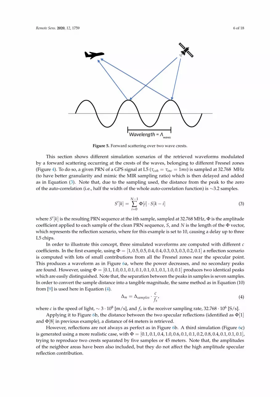
As an example, two wavefronts are reflected over two successive wave crests, and hencetwo different specular points, resulting in the addition of the two signals in the receiver antenna,which is detected as a second peak in the processed waveform, as detailed in Figure 5. Sometimeseven a third peak appears.

Due to the variability and the surface roughness of the ocean, the distance between twocrests varies. In this case, where wind wave and swell wave components are both strong and also withdifferent directions of propagation, the peak-to-peak distance is not preserved from one realizationto the next one.

As explained in [19], wind-driven or swell wave period is not a fixed magnitude, but the averageof the swell waves component period for the swell waves, and the average of the wind-driven periodfor the wind-driven waves. As an example, a swell period of 9–10 s generates a larger span of waves,which have a period between them from 8 s to 11 s. Therefore, a relative large data set analysisis required to correctly retrieve the swell waves period or wind-driven waves period.

Finally, the peak-to-peak distance does not only reproduce the crest-to-crest between twoconsecutive waves, but also a modulation depending on the height between the two waves wherethe reflection has occurred.

3.1. Waveform Simulation

As opposed to reflections in L1 C/A, where the spatial resolution is mostly limited by the chiplength (i.e., 300 m), the new GPS L5 or Galileo E5a signals have 10 times higher spatial resolution, as theauto-correlation function is 10 times narrower (i.e., 30 m in space), allowing de reception of multiplespecular points with a distance larger than 30 m. In this case, any reflection from any point separatedby more than 30 m produces a secondary peak on the retrieved waveform instead of a blurring onthe retrieved wavelength.

Remote Sens. 2020, 12, 1759 6 of 18

Figure 5. Forward scattering over two wave crests.

This section shows different simulation scenarios of the retrieved waveforms modulatedby a forward scattering occurring at the crests of the waves, belonging to different Fresnel zones(Figure 4). To do so, a given PRN of a GPS signal at L5 (τcoh = τinc = 1ms) is sampled at 32.768 MHz(to have better granularity and mimic the MIR sampling ratio) which is then delayed and addedas in Equation (3). Note that, due to the sampling used, the distance from the peak to the zeroof the auto-correlation (i.e., half the width of the whole auto-correlation function) is ∼3.2 samples.

S′[k] =N−1

∑i=0

Φ[i] · S[k− i] (3)

where S′[k] is the resulting PRN sequence at the kth sample, sampled at 32.768 MHz, Φ is the amplitudecoefficient applied to each sample of the clean PRN sequence, S, and N is the length of the Φ vector,which represents the reflection scenario, where for this example is set to 10, causing a delay up to threeL5 chips.

In order to illustrate this concept, three simulated waveforms are computed with different ccoefficients. In the first example, using Φ = [1, 0.5, 0.5, 0.4, 0.4, 0.3, 0.3, 0.3, 0.2, 0.1] a reflection scenariois computed with lots of small contributions from all the Fresnel zones near the specular point.This produces a waveform as in Figure 6a, where the power decreases, and no secondary peaksare found. However, using Φ = [0.1, 1.0, 0.1, 0.1, 0.1, 0.1, 0.1, 0.1, 1.0, 0.1] produces two identical peakswhich are easily distinguished. Note that, the separation between the peaks in samples is seven samples.In order to convert the sample distance into a tangible magnitude, the same method as in Equation (10)from [9] is used here in Equation (4).

∆m = ∆samples ·cfs

, (4)

where c is the speed of light, ∼ 3 · 108 [m/s], and fs is the receiver sampling rate, 32.768 · 106 [S/s].Applying it to Figure 6b, the distance between the two specular reflections (identified as Φ[1]

and Φ[8] in previous example), a distance of 64 meters is retrieved.However, reflections are not always as perfect as in Figure 6b. A third simulation (Figure 6c)

is generated using a more realistic case, with Φ = [0.1, 0.1, 0.4, 1.0, 0.6, 0.1, 0.1, 0.2, 0.8, 0.4, 0.1, 0.1, 0.1],trying to reproduce two crests separated by five samples or 45 meters. Note that, the amplitudesof the neighbor areas have been also included, but they do not affect the high amplitude specularreflection contribution.

Remote Sens. 2020, 12, 1759 7 of 18

(a) (b) (c)

Figure 6. Three simulated waveforms different contributions from nearby Fresnel zones,producing secondary peaks driven by strong specular and coherent reflections over two hypotheticalconsecutive wave crest. (a) Simulated waveform with small contributions from all the nearbyFresnel zones, (b) simulated waveform with two ideal peak reflections separated by seven samples,and (c) simulated waveform with realistic contributions from a secondary strong reflection separatedby five samples.

3.2. Evolution of Complex Waveforms in a Single Beam

The previous section has shown three different simulated waveforms synthetically generatedto illustrate the concept of a second specular reflection in a consecutive wave crest around the secondto sixth Fresnel zones.

In this section, three consecutive measured waveforms (see Figure 7) have been selectedto illustrate these effects. The separation in time between each waveform is 600 ms, and they have beenselected because of their similitude to the ones simulated in the previous section. Note that, the threeselected waveforms are from Track 1 Beam 1, and both amplitude and phase evolution of the waveformare shown.

The first waveform (Figure 7a) shows an example similar to the one in Figure 6a, where verysmall contributions from all nearby Fresnel zones causes a blurring of the tail of the waveform.

The main peak is around sample count 17, with a phase approximately constant around +100o.Furthermore, there is a second small peak (in sample 25) around eight samples (i.e., 73 m in space)after the main one (in sample 17). The distance between the peaks indicates that small reflectionsare coming from the sixth to eighth Fresnel zones.

The second waveform (Figure 7b) shows a example similar to the one in Figure 6b, but withthe reflection occurring in a closer Fresnel zone. In this case, the distance between these two peaks is threesamples or ∼30 m, which corresponds to a reflection in the second Fresnel zone. Compared to the firstwaveform, the reflections occurred within the first Fresnel zone causing a blurring and a wideningof the L5 auto-correlation function are now split in two different peaks.

As seen, the first peak (in sample 17) has a phase of ∼−110o, and the second peak (in sample 20)has a phase of ∼110o (i.e., close to the phase of the peak in Figure 7b), with a relative phase difference∼220o, corresponding to reflection in the second Fresnel zone, as both are separated more than180o. Note that, there is a strong phase jump between the two peaks, indicating that both reflectionsare coherent (i.e., the phase information is preserved in both cases). As in the previous case, this thirdpeak (in sample count 26) has an approximately constant phase around −50o. In addition and similarto the first waveform, a third small peak is also present nine samples (i.e., 82 m in space) awayfrom the very first one. In this case, the reflection is taking place between the eighth and the tenthFresnel zones.

Finally, the third waveform (Figure 7c) shows a similar shape as the simulation in Figure 6c,with a relative high second peak (in sample 22) in the reflected waveform which in this case is fivesamples from the main one (in sample 17). In this last case, the phase evolution is approximatelyconstant in both peaks with a strong jump in the transition between them (i.e., very small incoherent

Remote Sens. 2020, 12, 1759 8 of 18

reflection from other Fresnel zones). Note that in this case the relative phase difference is ∼50o, but asthe delay in time is ∼45 m, the reflection takes place further away than the second Fresnel zone,the phase with respect to the first peak has advanced at least 180o. Therefore, the absolute phase shiftbetween the two peaks is ∼315o.

(a) (b) (c)

Figure 7. Three sample waveforms containing different contributions from different Fresnel zones,producing secondary peaks with different shapes. (a) Retrieved waveform with small contributionsfrom all the nearby Fresnel zones, (b) retrieved waveform with two big peaks of the same amplitudeseparated three samples one from other, and (c) retrieved waveform with two peaks with differentamplitudes and separated by five samples.

3.3. First Waveform Analysis: Determination of the Crest-to-Crest Distance from Peak-to-Peak Distance

The last section showed three examples of three different waveforms retrieved from Track 1Beam 1, where the location of the second peak varies with time. Furthermore, it has been shownthat this second reflection comes from a different Fresnel zone, and in some cases present a coherentcomponent (i.e., a single specular reflection over a wave crest). Figure 8 illustrates the exampleof different consecutive peaks present in the GNSS waveforms originated by the forward scattering ontwo consecutive wave crests, but now in the two beams for the two tracks of the flight.

Note that, the two waveforms for each track (i.e., beams 1 and 2 for Track 1 and beams 1and 2 for Track 2) are taken at the same moment. As seen, the four waveforms present, at least,one second reflection.

Analyzing each of the tracks, Figure 8a,c present a single second reflection at six samples fromthe specular one. For the beam 2 case, Figure 8b presents a very large second reflection at six samplesfrom the specular one. In addition, two small reflections are taking place 10 and 13 samples fromthe specular one. Finally, Figure 8d shows a very low secondary reflection point at nine samples fromthe main peak.

Applying Equation (4) to the waveform shown in Figure 8, the distance between the peaksin meters are: 54.9 m for both Figure 8a,c, 54.9 m for the first peak of Figure 8b, and 91.5 m for the thirdpeak. Finally for Figure 8d, the distance between the peaks is 82.4 m.

Comparing those retrieved waveforms to the simulated waveforms from Figure 6, it is possibleto identify a clear similitude between them, where the second peak (i.e., the one in Figure 8b) remindsthe simulated in Figure 6c, due to a specular reflection over a wave crest.

In order to improve the estimations of the separation between peaks in the waveform,since raw data was acquired satisfying the Nyquist criteria at baseband for L5/E5a signals(i.e., fs > 10 MHz), therefore the signal can be re-sampled without loss of information. Therefore,waveforms are re-sampled using the Fourier interpolation method (i.e., by inverse FFTof the zero-padded FFT of the waveform), and the local maxima of the interpolated waveformis located. The first two maxima of the waveform are the ones used to retrieve the distance between twoconsecutive wave crests. The difference in samples between the two peaks position is then convertedinto meters following the same approach as in previous section, but with a sampling rate fs scaledby the interpolation rate K.

Remote Sens. 2020, 12, 1759 9 of 18

(a) (b)

(c) (d)

Figure 8. Reflected waveform for (a) Track 1, Beam 1; (b) Track 1, Beam 2; (c) Track 2, Beam 1;and (d) Track 2, Beam 2 of GPS L5 and Galileo E5a signals over the sea surface with an incoherentintegration time of 40 ms.

The selection of this parameter is a trade-off between computational requirements and accuracywhen selecting the final position of the multiple peaks. In order to efficiently apply the Fourierinterpolation using the Fast Fourier Transform, the signal shall be a multiple of 2, and hencethe interpolation rate K, shall be a multiple of 2 as well. In addition, the larger the K parameter is,the lower is the error determination of the peak position of the reflected waveform. For this case aninterpolation rate of K = 2 has a peak position uncertainty of 4.5 meters, and a K = 8 has a peakposition uncertainty of ∼1 m.

In this case, an interpolation rate of K = 8 has been selected (i.e., now fs = 256 MHz).Furthermore, Figure 9 shows the re-sampled version of the waveforms in Figure 8 following the Fourierinterpolation method.

The re-sampled versions of the waveforms show a better spatial resolution when estimatingthe peak-to-peak distance. In this case the distance in samples is: 50, 39, 42, and 70 respectively form(a) to (d). Moreover, the third peak of Figure 9b is located at 77 samples from the specular one.

Applying Equation (4) to the above sample distances, the retrieved crest-to-crest distance (Λwaves)in meters is: 57.2, 44.6, 48, and 80.1 m respectively for (a) to (d), and 88.1 m for the third peakof (b). Table 2 compares the values prior to the re-sampling with the re-sampled values. Note that,the estimation of both the first peak position is enhanced thanks to the FFT interpolation. In addition,the estimation of the position of the second peaks is also enhanced. A proper estimation of the positionof both peaks is crucial to better determine the distance between the two reflections (i.e., the twowave crests). Note the difference in Beam 2 of Track 1 and Beam 1 of Track 2, where the first

Remote Sens. 2020, 12, 1759 10 of 18

approach does not show the proper crest-to-crest distance, introducing an error of almost 10 min the measurement.

(a) (b)

(c) (d)

Figure 9. Reflected waveforms for (a) Track 1, Beam 1; (b) Track 1, Beam 2; (c) Track 2, Beam 1;and (d) Track 2, Beam 2 from Figure 8 now sampled at 256 MHz. Note that, thanks to the re-samplingthe determination of the peak position is enhanced.

This section has covered the simulation and its comparison with real data of different scenarioswhere different specular reflections are generating second and even third peaks on the reflected waveform.The study on the phase evolution in this secondary peaks shows that the second reflection is coherent,and hence is coming from a different specular point, as was detailed in Figure 5. Finally, the use of FFTinterpolation enhances the determination of the peak-to-peak distance, showing a better granularitywhen determining this magnitude.

Table 2. Track, beam, crest-to-crest estimated distance using the original waveform, and the crest-to-crestdistance after re-sampling the original waveform using the FFT interpolation.

Track ID Beam ID Original Crest-to-Crest Distance [m] Re-Sampled Crest-to-Crest Distance [m]

1 1 54.5 57.2

1 2 54.5 44.6

2 1 54.5 48.0

2 2 82.4 80.1

4. Sea Wavelength Retrieval Using Large Data Set

The study of a larger data set is required to validate the relationship between sea waveswavelength Λwaves or wave period Twaves to the distance between the peaks in the waveforms.

Remote Sens. 2020, 12, 1759 11 of 18

Tracks identified in Table 1 of Section 2 are composed by 1470 waveforms, and 1994 waveformsrespectively, generated once per 30 ms (i.e., 3.33 Hz), which corresponds to ∼8 min of data for eachof the two beams for the first track, and 11 minutes of data for the second track. In order to analyzethe data set, three different approaches are considered:

• Statistical analysis: statistics of the retrieved crest-to-crest distance and presence or not of third peaks.• Time-series analysis: analysis in the time domain of the retrieved crest-to-crest distance.• Spectral analysis: analysis in the frequency domain of the time-series data.

4.1. Statistical Analysis

Reviewing the histogram of all the 1470 measurements for Track 1 (see Figure 10),most of the results are condensed between 30 m (the wind-driven wavelength from the modelis 39 m) and 80 m (the swell wavelength from the model is 126 m).

Figure 10. Histogram of the peak-to-peak distances for Track 1. Top figure corresponds to Beam 1(GPS L5) and bottom figure to Beam 2 (GPS L5).

In addition, the distance to a third peak (if is exists) is condensed just at the end of the histogram,at the end of the histogram of the distance to the second peak. As seen, the measurements are condensedmostly between 40 and 90 m for both beams.

Both beams are following similar statistics for the second peak distance, with an average valueof 54.3 m for Beam 1, and an average value of 52.6 m for Beam 2. The third peak has an average valueof 74.5 m for Beam 1, and 73.5 m for Beam 2. Note that, the average of the measurements is a mixtureof all possible wave crest distance contributions. Note that, the least wave crest distance is ∼ 30 m,which coincides with the spatial resolution due to the chip bandwidth of the L5/E5a signal, 30 m.

In addition, the same histogram of the second-track is shown in Figure 11. The first beamcorresponds to a Galileo E5a signal, which has an incidence angle of ∼20o. The mean peak-to-peakdistance in this case is 50.8 m. The second beam has an incidence angle of 42o, with an average valueof 53.5 m.

Remote Sens. 2020, 12, 1759 12 of 18

Figure 11. Histogram of the peak-to-peak distances for Track 2. Top figure corresponds to Beam 1(Galileo E5a) and bottom figure to Beam 2 (GPS L5).

In case of this first beam, as the incidence angle is lower, the semi-radius of the first Fresnel zoneis smaller (from 33 m with θinc = 45o to 21 m with θinc = 20o). As the overall sizes of the Fresnelzones are smaller, the area where the possible strong reflection occurs over a wave crest is also smaller,hence some waves with a large distance between them can not be captured.

Note that, in this case, the third peak position for Beam 1 is poorly determined because of the smallincidence angle, and the size of the Fresnel zones for that case. As seen in the histogram, the amountof third peak reflections in Beam 1 with respect to Beam 2 is in the order of 0.25.

As seen in the two tracks, the histogram analysis shows that multiple reflections are presentin most of the waveforms, with an average value ∼50 m for the distance between the first two peaks.From this first analysis, the wind-driven waves wavelength can be estimated (i.e., the model set thisdistance to 40 m), and from it the wind-driven wave period.

4.2. Time-Series Analysis

The statistical analysis through the histogram visualization shows that the crest-to-crest distancesare in the same range than in the ICON model (Section 2), the analysis of the time evolutionof the peak-to-peak distances shows a wavy behavior.

In order to reduce the noise of the measurement, four different averaging windows have beenapplied to the peak-to-peak distance. In this case, the averaging selected is 5, 10, 15, and 30 samples.As seen in Figure 12, this wavy behavior is clearly identified in the measurement, which is present evenwith large averaging windows. As seen with the highest averaging time, the mean of the crest-to-crest

Remote Sens. 2020, 12, 1759 13 of 18

distance is ∼55 m for Beam 1, and ∼52.5 m for Beam 2. As seen in [14,19], the average wave period,or the average wavelength, Λwaves, tends to the combination of all the different wave contributions.

A similar behavior is also found in Track 2, as shown in Figure 13. The Galileo signal (i.e., Beam 1),has a mean value ∼50 m, and Beam 2 a mean value on the order of ∼ 52.5 m, as in Track 1. Note that,a large portion (∼ 40%) of the Beam 1 reflections do not have a secondary peak because of the reflectiongeometry. As the incidence angle is very close to 0o (i.e., very close to nadir), the possible reflectionsare coming from closer wave crests, therefore the receiver is only able to infer consecutive crests whichare closer one to each other.

Figure 12. Time-series evolution of the Track 1 peak-to-peak calibrated distance with different movingaverage windows. Top figure corresponds to Beam 1, and bottom figure to Beam 2.

Figure 13. Time-series evolution of the Track 2 peak-to-peak calibrated distance with different movingaverage windows. Top figure corresponds to Beam 1, and bottom figure to Beam 2.

Remote Sens. 2020, 12, 1759 14 of 18

4.3. Spectral Analysis

The time-series analysis together with the statistical one show that there is a vast range of retrievedsea wave wavelengths Λwaves, with some apparent periodicity. As detailed in [12,14], a spectralanalysis over the magnitude under study helps to separate the different swell or wind-drivenwave contributions.

In order to do that, the power spectral density of the time-series data from previous sectionis computed. Figure 14 shows the power spectral density of the distance to the second peak (or the firstencountered crest in the sea wave surface). In all four figures, there are some common frequencies at∼0.06 Hz, 0.1 Hz, 0.15 Hz, and also a 0.2 Hz component in Beam 1 of both Tracks 1 and 2.

Figure 14. Fourier Transform of the time series evolution of (Figures 12 and 13), for the secondpeak distances.

Converting those frequencies to seconds, the wave periods of each of the wavelengthsare T1 = 16.6 s, T2 = 10 s, and T3 = 6.66 s. Comparing the three periods to the swell and wind-drivenwave periods to the ones of the ICON model in Figure 2, T2 ' Tswell and T3 ' Twind.

Remote Sens. 2020, 12, 1759 15 of 18

In addition, the 0.2 Hz component, corresponding to a period of T4 = 5 s, which is only presentin Beam 1 of both Track 1 and Track 2, exactly matches the wind-driven prediction by the model,where Twind = 5 s.

As already stated, the lower the incidence angle of the beam, the shorter waves can be retrieved(i.e., waves with shorter period), which is mostly the case for Figure 14c, where the incidence angleis closer to 0o (i.e., nadir), and hence wind-wave periods can be retrieved rather than swell-drivenwave periods.

Furthermore, in case of analyzing the power spectral density (Figure 15) for the distanceto the third peak, the fundamental frequencies are below the previous case, with a first fundamentalfrequency consistent in (a), (c), and (d) around ∼0.03 Hz, 33 s of period.

The spectrum shape of this third peak indicates a long period sea wavelength which is notcontemplated in the model. As stated in [19], this high order period is present on swell waves, and alsomodulates the amplitude of the swell waves, it is known as second swell.

Figure 15. Fourier Transform of the time series evolution of (Figures 12 and 13), for the thirdpeak distances.

Remote Sens. 2020, 12, 1759 16 of 18

In this case, the third peak spectrum does not give as much information as the second peak,from where it is possible to infer the wave period for different wave sources, as swell, wind-drivenwind, or secondary swell waves.

5. Discussion

Each analysis provides a different perspective and hence a different parameter of the oceancan be estimated, and they are all summarized and compared to the values predicted by the ICONmodel in Table 3. Note that, the wave periods in the statistical and time-series approaches have beendetermined from the average crest-to-crest distance and assuming Λwaves = 1.56 · T2

waves, as in (1).

Table 3. Estimated wave period from the three different analysis applied and its comparison otthe ICON model prediction.

Measurement Est. Wave Period ICON Model Estimation

Statistical analysis 5.8 sWind-driven = 5 sSwell = 9 s

Time-series analysis 5.6 sWind-driven = 5 sSwell = 9 s

Spectral analysisFour components:5 s, 6.3 s, 10 s, 16.6 s

Wind-driven = 5 sSwell = 9 s

In this case, both the statistical and the time-series analysis are providing a good estimationof the wind-driven wavelength, as the period of the wind-driven waves is smaller, the amountof wave crests per unit of area is larger, and hence the mean value of the waves is biased towardsthe wind-driven waves.

It is also important to remark that the time analysis serves to illustrate the wavy behaviorof the crest-to-crest distance with respect to time. In this case, this analysis shows in a qualitative wayhow crest-to-crest distance is a mixture of different components, as explained in [12,14].

Last but not least, the spectral analysis clearly shows the different periods that can be identifiedin the time analysis. Multiple periods can be identified, among them τswell and τwind are identified asthe main components of the spectrum of the crest-to-crest distance.

Furthermore, the results from the spectral analysis and the statistical analysis confirm that dueto the geometry of the reflection, the lower the incidence angle is, the closer the reflection of the secondcrest occurs.

Finally, the spectral analysis also shows very low frequency components due to secondary swellor high period gravitational waves, which are interesting for other oceanographic studies, but stillneed further investigation.

6. Conclusions

This work has presented the first experimental evidence of wind and swell waves signaturesin L5/E5a GNSS-R waveforms from second and third peaks. An algorithm has been presentedto retrieve the peak-to-peak distance. Evidences for both the first and the second peaks are presented,and a detailed analysis from a large data set N > 1000 waveforms has been presented. The analysisin three domains (statistical, time, and spectrum) shows that additional ocean parameters canbe retrieved from GNSS-R measurements, e.g., wind driven waves period and swell period, which havenot been measured yet using GNSS-R technique.

This application still requires further refinements and a more exhaustive analysis with in-situdata. However, this study shows the promising results for the use of L5/E5a GNSS-R signals to infernew geophysical parameters as the wave period or wavelength of the sea thanks to the sharper shapeof the auto-correlation function.

Remote Sens. 2020, 12, 1759 17 of 18

Author Contributions: Conceptualization, J.F.M.-M., H.P. and A.C.; methodology, J.F.M.-M.; software, J.F.M.-M.;validation, J.F.M-M. and A.C.; formal analysis, J.F.M.-M. and A.C.; investigation, J.F.M.-M.; resources, R.O., D.P.,H.P., A.C., C.R., J.W. and A.M.; data curation J.F.M.-M., R.O., D.P.; visualization J.F.M-M.; supervision, H.P.,A.C.; project administration, A.C.; funding acquisition, A.C.; writing—original draft preparation, J.F.M.-M.;writing—review and editing, J.F.M.-M., H.P., A.C. All authors have read and agreed to the published version ofthe manuscript.

Funding: This work was founded by the Spanish Ministry of Science, Innovation and Universities, “Sensing withPioneering Opportunistic Techniques”, grant RTI2018-099008-B-C21, and the grant for recruitment of early-stageresearch staff FI-DGR 2015 of the AGAUR - Generalitat de Catalunya (FEDER), Spain, and the grant for recruitmentof early-stage research staff FI 2018 of the AGAUR - Generalitat de Catalunya (FEDER), Spain, and Unidad deExcelencia María de Maeztu MDM-2016-060.

Acknowledgments: Thanks to the CommsSensLab administrative and research personnel and to the NanoSatLabmembers for the support, specially to Adrian Pérez to help us mounting the database system that helpedthe authors to better analyze the retrieved data.

Conflicts of Interest: The authors declare no conflict of interest.

References

1. Zavorotny, V.U.; Gleason, S.; Cardellach, E.; Camps, A. Tutorial on Remote Sensing Using GNSS BistaticRadar of Opportunity. IEEE Geosci. Remote. Sens. Mag. 2014, 2, 8–45, doi:10.1109/MGRS.2014.2374220.[CrossRef]

2. Onrubia, R.; Pascual, D.; Park, H.; Camps, A.; Rüdiger, C.; Walker, J.; Monerris, A. Satellite Cross-Talk ImpactAnalysis in Airborne Interferometric Global Navigation Satellite System-Reflectometry with the MicrowaveInterferometric Reflectometer. Remote. Sens. 2019, 11, 1120, doi:10.3390/rs11091120. [CrossRef]

3. Onrubia, R.; Pascual, D.; Park, H.; Camps, A. Preliminary Altimetric and Scatterometric Results with theMicrowave Interferometric Reflectometer (MIR) during Its first Airborne Experiment; ARSI-KEO 2019; ESA:Noordwijk, The Netherlands, 2019.

4. Bathgate, J.S.; Heron, M.L.; Prytz, A. A Method of Swell-Wave Parameter Extraction From HF Ocean SurfaceRadar Spectra. IEEE J. Ocean. Eng. 2006, 31, 812–818.

5. Chen, Z.; Zhang, L.; Zhao, C.; Chen, X. Wind sea and swell meansurements using S-band Doppler radar.In Proceedings of the OCEANS 2016, Shanghai, China, 19–23 September 2016; pp. 1–5.

6. Johnsen, H.; Husson, R.; Vincent, P.; Hajduch, G. Sentinel-1 Ocean Swell Wave Spectra (OSW) AlgorithmDefinition; Northern Research Institute (Norut): Tromso, Norway, 2020.

7. Robinson, I.S. Measuring the Oceans from Space: The Principles and Methods of Satellite Oceanography; Springer:Berlin, Germany, 2004.

8. Ward, K.D.; Tough, R.J.A.; Watts, S. Sea clutter: Scattering, the K distribution and radar performance.Waves Random Complex Media 2007, 17, 233–234, doi:10.1080/17455030601097927. [CrossRef]

9. Munoz-Martin, J.F.; Onrubia, R.; Pascual, D.; Park, H.; Camps, A.; Rüdiger, C.; Walker, J.; Monerris,A. Untangling the Incoherent and Coherent Scattering Components in GNSS-R and Novel Applications.Remote. Sens. 2020, 12, 1208, doi:10.3390/rs12071208. [CrossRef]

10. (DWD), D.W. ICON model description by DWD. Available online: https://www.dwd.de (accessed on7 Januray 2020).

11. US Army Corpsof Engineers. Coastal Engineering Manual Part II: Coastal Hydrodynamics (EM 1110-2-1100);Books Express Publishing: Newbury Berkshire, UK, 2012.

12. Wang, D.W.; Hwang, P.A. An Operational Method for Separating Wind Sea and Swell from Ocean Wave Spectra.J. Atmos. Ocean. Technol. 2001, 18, 2052–2062, doi:10.1175/1520-0426(2001)018<2052:AOMFSW>2.0.CO;2. [CrossRef]

13. Portilla, J.; Ocampo-Torres, F.J.; Monbaliu, J. Spectral Partitioning and Identification of Wind Sea and Swell.J. Atmos. Ocean. Technol. 2009, 26, 107–122, doi:10.1175/2008JTECHO609.1. [CrossRef]

14. Hwang, P.A.; Ocampo-Torres, F.J.; García-Nava, H. Wind Sea and Swell Separation of 1D Wave Spectrum bya Spectrum Integration Method. J. Atmos. Ocean. Technol. 2012, 29, 116–128, doi:10.1175/JTECH-D-11-00075.1.[CrossRef]

15. InMeteo. Ventusky. Available online: https://ventusky.com (accessed on 7 January 2020).16. Voronovich, A.G.; Zavorotny, V.U. The Transition From Weak to Strong Diffuse Radar Bistatic Scattering

From Rough Ocean Surface. IEEE Trans. Antennas Propag. 2017, 65, 6029–6034. [CrossRef]

Remote Sens. 2020, 12, 1759 18 of 18

17. Giacobazzi, J. 50 - Line of sight radio systems. In Telecommunications Engineer’s Reference Book; Mazda, F.,Ed.; Butterworth-Heinemann: Oxford, UK, 1993; pp. 50-1–50-17, doi:10.1016/B978-0-7506-1162-6.50056-3.[CrossRef]

18. Saleem, T.; Usman, M.; Elahi, A.; Gul, N. Simulation and Performance Evaluations of the New GPS L5 andL1 Signals. Wirel. Commun. Mob. Comput. 2017, 2017, 1–4, doi:10.1155/2017/7492703. [CrossRef]

19. Government, A. Waves. Available online: http://www.bom.gov.au/marine/knowledge-centre/reference/waves.shtml (accessed on 14 March 2020).

c© 2020 by the authors. Licensee MDPI, Basel, Switzerland. This article is an open accessarticle distributed under the terms and conditions of the Creative Commons Attribution(CC BY) license (http://creativecommons.org/licenses/by/4.0/).