Remote Sensing Applications to Biodiversity Conservation

Synthesis document

P. Timon McPhearson and Osman C. Wallace

Reproduction of this material is authorized by the recipient institution for non-profit/non-commercial educational use and distribution to students enrolled in course work at the institution. Distribution may be made by photocopying or via the institution’s intranet restricted to enrolled students. Recipient agrees not to make commercial use, such as, without limitation, in publications distributed by a commercial publisher, without the prior express written consent of AMNH. All reproduction or distribution must provide full citation of the original work and provide a copyright notice as follows: “Copyright 2007, by the author of the material and the Center for Biodiversity and Conservation of the American Museum of Natural History. All rights reserved.” This material is based on work supported by the National Science Foundation under the Course, Curriculum and Laboratory Improvement program (NSF 0127506), and the United States Fish and Wildlife Service (Grant Agreement No. 98210-1-G017). Any opinions, findings and conclusions, or recommendations expressed in this material are those of the authors and do not necessarily reflect the views of the American Museum of Natural History, the National Science Foundation, or the United States Fish and Wildlife Service.

2

Remote Sensing Applications to Biodiversity Conservation

I. WHAT IS REMOTE SENSING?...................................................................................4

HIGHLIGHTS OF REMOTE SENSING HISTORY.............................................................5

PASSIVE AND ACTIVE SENSORS ..............................................................................6

INTRODUCTION TO RESOLUTION .............................................................................6

II. TERRESTRIAL APPLICATIONS .................................................................................8

MONITORING FORESTS ..........................................................................................8

FIRE DETECTION AND MONITORING .........................................................................9

PREPAREDNESS..............................................................................................11

DETECTION AND RESPONSE .............................................................................11

POST-FIRE ASSESSMENT .................................................................................12

SMOKE...............................................................................................................12

HABITAT DETERMINATION ....................................................................................13

LANDSCAPE ECOLOGY.........................................................................................15

LANDSCAPE USE AND LAND COVER CHANGE..........................................................16

CHANGE DETECTION ANALYSIS.............................................................................18

AGRICULTURE ....................................................................................................19

MINING ..............................................................................................................21

SOILS ................................................................................................................22

III. AQUATIC APPLICATIONS .....................................................................................22

GENERAL HYDROLOGY ........................................................................................23

RAINFALL........................................................................................................23

WATER RUNOFF/DRAINAGE ..............................................................................23

WATER QUALITY..............................................................................................24

LAKES ............................................................................................................24

WATER TEMPERATURE ....................................................................................24

WATER ELEVATION ..........................................................................................24

WATER DEPTH ................................................................................................25

3

FLOW RATES...................................................................................................25

SNOW ................................................................................................................26

SEA ICE AND SEA SURFACE TEMPERATURE............................................................26

AQUATIC VEGETATION .........................................................................................27

ALGAL BLOOMS...................................................................................................28

CORAL REEFS.....................................................................................................28

BENTHIC HABITAT ...............................................................................................29

OIL SPILLS..........................................................................................................30

IV. ATMOSPHERIC APPLICATIONS.............................................................................33

AIR POLLUTION ...................................................................................................33

WEATHER ..........................................................................................................33

V. ACCURACY ASSESSMENT ....................................................................................34

ACCURACY RESULTS...........................................................................................34

POSITION AND THEMATIC ERROR ..........................................................................35

VI. SUMMARY.........................................................................................................35

VII. ACKNOWLEDGEMENTS......................................................................................36

VIII. LITERATURE CITED ..........................................................................................37

IX. FIGURES AND TABLES..................................................................................... 44X

X. APPENDICES......................................................................................................59

APPENDIX A .......................................................................................................59

4

Remote Sensing Applications to

Biodiversity Conservation

P. Timon McPhearson and Osman C. Wallace

The primary focus of this module will be applications of remote sensing for biodiversity conservation as a subset of earth observation techniques. This will involve linking remote sensing capabilities to practical and strategic environmental and conservation applications. The module will cover biodiversity conservation applications in terrestrial, aquatic, and atmospheric contexts, often illustrated with focused examples that portray land managers seeking new tools and methods to better address the state of their managed natural systems. I. WHAT IS REMOTE SENSING? Remote sensing is the science (and art!) of acquiring information about an object without actually coming into contact with it. This is typically done by sensing and recording reflected or emitted energy and processing and analyzing that information to help understand a feature of interest. The most common example of remote sensing is human sight. Our eyes receive light and analyze it to make sense of the world. A definition more appropriate for our purposes incorporates the conditions that the object is on or near the Earth’s surface, that the views are made from above the object, and that the information is some measurable property of the electromagnetic (EM) spectrum. This narrower definition excludes such techniques as sonar, geomagnetic and seismic sounding, as well as medical imaging, but includes a wide and fairly coherent set of techniques, often known by the alternative name of Earth Observation (EO) (Rees, 1999). EO can be thought of as ‘reading’ information from the Earth’s surface by various sensors, and then analyzing the data to make sense of it. Satellite remote sensing involves the measurement of radiation of different wavelengths reflected or emitted from distant objects or materials. Objects can then be identified and categorized by class/type, substance, and spatial distribution. Appendix A provides a lengthy list of the various satellite sensor characteristics used to observe the Earth. A Geographic Information System (GIS) is distinct from remote sensing. A GIS is a system capable of integrating, storing, editing, analyzing, and displaying or mapping spatially referenced information. Data stored in a GIS are represented in two ways: attribute data describes what the feature is, and spatial data defines where it is using points, lines, polygons, or pixels. These spatial features are stored in a coordinate system (latitude/longitude, state plane, UTM, etc.), which references a particular place on the earth. Spatial data and associated attributes in the same coordinate system can then be layered together for mapping and analysis.

5

HIGHLIGHTS OF REMOTE SENSING HISTORY Remote sensing has seen dramatic growth over the last few decades. In part, this can be attributed to the technical developments outlined below, but remotely sensed data also have some tangible advantages. Probably the most important of these is the fact that data can be gathered from a large area of the Earth’s surface (or a large volume of the atmosphere) in a short space of time, allowing a virtually instantaneous ‘snapshot’ to be obtained. For example, the Landsat Thematic Mapper (TM) sensor can acquire data from an area 185 km x 185 km in about half a minute. When this aspect is combined with the fact that airborne and spaceborne systems can obtain information from locations that would be difficult (slow, expensive, dangerous, and politically awkward) to measure on the ground the potential power of remote sensing becomes apparent. Further advantages derive from the fact that most remote sensing systems now generate calibrated digital data that can be manipulated in a computer. Historic overview of Remote Sensing

Remote sensing began with the invention of the camera. Around 1858, Gaspard Felix Tournachon made the first aerial photograph from a balloon at a height of about 80 meters above the village of Petit Becetre, near Paris. Cameras mounted on everything from balloons, kites, and pigeons, to rockets, were used to remotely sense the earth.

During World War I, cameras mounted on airplanes provided an aerial view of fairly large surface areas, which were mainly used for military reconnaissance. By World War II, the technology had become highly sophisticated, pushing remote sensing technology beyond visible-spectrum photography into infrared detection and radar systems. However, until the 1970s, the photograph remained the single standard tool for depicting the earth’s surface from a vertical or oblique perspective.

Satellite remote sensing began in the early days of the space age (both Russian and American programs). With the emergence of the space program in the 1960s, Earth-orbiting cosmonauts and astronauts were able to take photos out the window of their spacecraft. Eventually, earth orbiting satellites were created to remotely sense the earth. Optical remote sensing moved to outer space only months after the first manned satellite (Sputnik 1, 4 October 1957). The United States’ Explorer 6 transmitted the first space photograph of the Earth in August 1959. The first systematic satellite observation came with the launch of the United States’ TIROS 1 in 1960. This meteorological satellite was designed to track clouds.

6

PASSIVE AND ACTIVE SENSORS Remote sensing instruments can be grouped into two categories—passive and active. Passive instruments, or sensors, detect the sun’s energy that is reflected or emitted from the observed object or scene. Active sensors, however, provide their own energy (electromagnetic radiation) to illuminate an object or scene under observation. They send a pulse of energy from the sensor to the object and then receive the radiation that returns from that object. There are many types of active sensors including Radar, scatterometer, Lidar, and laser altimeter. Radar imaging satellites were developed and began flight during the space age of the late 1950’s to 1960’s. Radar has advantages over other sensors due to the cloud penetrating ability of microwave energy. This “all weather” capability is especially important in tropical regions, which are typically under cloud cover throughout the year. INTRODUCTION TO RESOLUTION Passive sensors typically record infrared and visible electromagnetic (EM) energy in segments called bands. If using a single band, the measured EM energy reflected off of various features on the Earth’s surface (soil, trees, shrubs, grass, rock, water) may not be sufficient to identify the feature. Table 1 lists the surface reflectance of different Earth objects in the visible EM, similar to what a human eye would see. We perceive reflectance as colors in the narrow band of visible light. Remote sensing devices can measure reflected energy of wavelengths far larger and smaller than what we can see. Comparing spectral characteristics of land features using multiple bands provides more information to help us identify different features.

In the mid-1960s the U.S. Department of the Interior conceived the concept of an Earth-monitoring satellite for resource managers and Earth scientists. The National Aeronautics and Space Administration (NASA) joined the initiative, and in the early 1970s NASA and the U.S. Geological Survey entered into a partnership, with NASA operating the Landsat satellites and the U.S. Geological Survey handling the data. The Landsat program is the longest running program of remote sensing from space. This highly successful earth monitoring system has provided scientists and lay people with medium resolution images of the earth’s surface for over 30 years.

Newer satellites are regularly being launched for earth observation. The French launched the SPOT satellite in 1978. In 1988 the Indian Remote Sensing Satellite was launched, and then a whole series of new government and commercial satellites were developed including Radarsat in 1995, and IKONOS, QUICKBIRD and NASA Terra satellites in 1999.

7

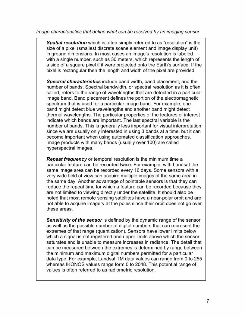
Image characteristics that define what can be resolved by an imaging sensor

Spatial resolution which is often simply referred to as “resolution” is the size of a pixel (smallest discrete scene element and image display unit) in ground dimensions. In most cases an image’s resolution is labeled with a single number, such as 30 meters, which represents the length of a side of a square pixel if it were projected onto the Earth’s surface. If the pixel is rectangular then the length and width of the pixel are provided.

Spectral characteristics include band width, band placement, and the number of bands. Spectral bandwidth, or spectral resolution as it is often called, refers to the range of wavelengths that are detected in a particular image band. Band placement defines the portion of the electromagnetic spectrum that is used for a particular image band. For example, one band might detect blue wavelengths and another band might detect thermal wavelengths. The particular properties of the features of interest indicate which bands are important. The last spectral variable is the number of bands. This is generally less important for visual interpretation since we are usually only interested in using 3 bands at a time, but it can become important when using automated classification approaches. Image products with many bands (usually over 100) are called hyperspectral images.

Repeat frequency or temporal resolution is the minimum time a particular feature can be recorded twice. For example, with Landsat the same image area can be recorded every 16 days. Some sensors with a very wide field of view can acquire multiple images of the same area in the same day. Another advantage of pointable sensors is that they can reduce the repeat time for which a feature can be recorded because they are not limited to viewing directly under the satellite. It should also be noted that most remote sensing satellites have a near-polar orbit and are not able to acquire imagery at the poles since their orbit does not go over these areas.

Sensitivity of the sensor is defined by the dynamic range of the sensor as well as the possible number of digital numbers that can represent the extremes of that range (quantization). Sensors have lower limits below which a signal is not registered and upper limits above which the sensor saturates and is unable to measure increases in radiance. The detail that can be measured between the extremes is determined by range between the minimum and maximum digital numbers permitted for a particular data type. For example, Landsat TM data values can range from 0 to 255 whereas IKONOS values range form 0 to 2048. This potential range of values is often referred to as radiometric resolution.

8

Many remote sensing systems record energy over several separate wavelength ranges. These are referred to as multi-spectral sensors. Advanced multi-spectral sensors called hyperspectral sensors detect hundreds of very narrow spectral bands throughout the visible, near-infrared, and mid-infrared portions of the EM spectrum. Their very high spectral resolution facilitates discrimination between different targets based on their spectral response in each of the narrow bands. Hyperspectral sensors, for example, are used to detect individual vegetation species (Asner and Vitousek 2005) and other groups of identifiable species (species stands, wetlands) as compared to more broad assignments (forests, riparian zones) that are used to categorize data from coarser spectral resolution sensors. Identification of specific targets often requires high spatial resolution in addition to hyperspectral resolution. II. TERRESTRIAL APPLICATIONS Terrestrial applications of remote sensing include, but are not limited to, determining habitat types, fire detection and monitoring, mapping deforestation and reforestation, landscape change detection, and analyzing agriculture and mining areas. Remote sensing applications are demonstrated in several following examples. MONITORING FORESTS Satellite and airborne remote sensing techniques provide many useful products and services for forestry applications including a) initial inventory and assessment of forest resources and their condition; b) updating of existing information; c) forest area and type mapping; d) stand delineation and associated silvicultural parameters (tree height, stand density, timber volume estimation); e) mapping of silvicultural activities (clearcuts, reforestation areas); and f) mapping of forest damage (storm, fire, and insect calamities) (Holmgren and Thuresson, 1998). Traditional field data can be supplemented with high-resolution aerial photography and change detection using satellite image data. A sample of high-resolution imagery can detect moderate changes in land cover and discriminate among detailed categories of forest cover and land use. In contrast, field data measures the slow and subtle changes that occur in forests, which is important for interpreting remotely sensed data. of the effective use of microwave remote sensing for monitoring forest health is based on the assumption that physiological activities of forest stands are influenced by the vitality and health status of the trees (Oren, 1993). Reduced forest tree vitality and reduced canopy biomass are often a consequence of disadvantageous forest stand conditions such as lack of water supply and low nutrient availability in the soil. Pollutants in the air and the soil can also negatively affect the metabolism of the trees and cause visible symptoms of

9

decline. Reduced tree health ultimately leads to a decreasing leaf or needle biomass and thus canopy density. A direct relationship is often assumed between the variation in the water content of tree parts (stems, leaves, trunk) and the canopy density, stand vitality, and forest decline (Zink et al. 1997). Since the dielectric constant of water (this constant determines water’s polarity and ionization) is much higher than that of other tree constituents, microwave signatures contain direct information on the water status of forest canopies pertaining to stand vitality parameters (Zink et al. 1997). Other studies have utilized microwave backscatter to determine above-ground biomass density (i.e. canopy density) and tree density (Beaudoin et al., 1994; Baker et al., 1994; Green, 1998). The accuracy with which biophysical parameters can be retrieved from backscatter measurements of forests depends considerably upon vegetation structure and ground conditions. Microwaves and backscatter explained Lidar can also be used to measure forest structure (Lefsky et al.) Airporne lidar systems are routinely used to get estimates of forest height and from these measurements in tandem with land cover maps other parameters such as biomass and timber volume can be determined by developing equations that predict these qualities based on tree height for individual species. An area of active research is to determine forest structure from lidar data (Lefsky et al.). FIRE DETECTION AND MONITORING By virtue of the frequent, wide area coverage provided by Earth-orbiting platforms, satellite remote sensing can provide detailed information on the location, frequency and spatial distribution of vegetation fires (data that is unavailable using other methods of investigation). Fire activity results in two primary signatures that can be detected via remote sensing, active fire flaming and smoldering. Although the rate of combustion is higher during the flaming phase, more smoke, aerosol particles and greenhouse gases are emitted during the smoldering phase due to the lower combustion efficiency, which has the greatest influence on regional pollution and, potentially, on global climate change. In December 1999 NASA launched the MODIS (or Moderate-resolution Imaging Spectroradiometer) instrument onboard the EOS (Earth Observing System) Terra satellite and gained an improved ability to detect forest fires anywhere on Earth’s surface. MODIS measures the heat emitted by fires and therefore enables detection of active fires, accurately estimates rates of combustion, as well as the amounts of emission products—such as smoke, greenhouse gases, and aerosol

Microwaves are electromagnetic waves with wavelengths longer than those of infrared light, but shorter than radio waves. Backscatter is the reflection of light, radar, radio, or other EM waves directly back to the direction they came from.

10

particles—the fires produce (Kaufman et al, 2001). The MODIS instruments aboard NASA’s Terra and Aqua platforms have the added ability to detect fire activity during both the flaming and smoldering phases. The advanced fire monitoring capability is due to the higher saturation thresholds, compared to other sensors, as well as MODIS’ large number of spectral channels to better characterize the atmosphere and fires. Sensor saturation is analogous to the human eye, which becomes quickly saturated when directly viewing the sun, because the sun is so bright. A higher saturation threshold is important because remote sensors can become saturated when viewing hot, bright fires, rendering it impossible for them to distinguish important characteristics about the fire, such as intensity of combustion. The narrow spectral width of individual bands and a radiometric resolution of 12 bits enable the MODIS sensor to detect bright, hot fires both at night and in the daylight without being oversaturated by the brightness of the fire signature (Herring 1998). Fire monitoring scenario

Consider a semi-arid ecosystem, where a shrub and grass fuel fire is threatening the adjacent upland oak and conifer forests and surrounding human settlements. Because of heavy smoke and clouds, air reconnaissance and traditional firefighting efforts will not be practical. Seeking a reliable tool to monitor and direct the fire, a forest biologist in charge of managing the extensive and fragile upland forest habitats is asked to predict fire spread behavior, manage ground control efforts, monitor smoke dispersion (a critical issue for the health of flora and fauna living in the area), and assess post-fire green-up. The forest biologist must understand that managing wildland fires effectively depends on the quality of the information, the characteristics of the geographic region, and the current and evolving phase of the wildland fire (Ehrlich et al., 1997). Suppression planning and prioritization of areas for surveillance requires assessment of the wildland fire potential (risk and hazard mapping) in the fire-prone areas. During the crisis phase, it is necessary for the forest biologist to know the exact position of the wildland fire (detection), how it is developing and spreading (behavior), how it has progressed over time (monitoring), and how it is likely to develop into the future (behavior prediction). After suppression it may be necessary to examine the type and extent of damage and to plan for recovery actions (assessment, mapping, and rehabilitation). In addition, during wildland fire management and suppression, the forest biologist would need additional data, such as information on human settlements (sometimes referred to as the wildland-urban interface) in the wildland fire area, location of water sources for wildland fire suppression, and road networks for access to the area. This essential information is needed for all phases of managing wildland fire. Examples of frequently used sources of information are orthorectified imagery and topographic maps (Langaas 1992). Fire information, combined with three-dimensional views (composed of high-resolution imagery draped over digital elevation surface models) can be very useful.

11

In the following sub-sections, wildland fire management is divided into three different phases: preparedness, detection and response, and post-fire assessment. The information requirements are typically different in each phase. The most significant differences relate to the temporal and spatial resolution and accuracy of the required information. Preparedness The most important task during the preparedness phase of wildland fire management is to assess the values at risk. Conducting risk assessment studies to identify areas with the greatest potential for protecting human lives, property, and natural resources can help authorities impose greater surveillance and/or restrictions on fire use in these areas (Levine 1996a). Risk assessment considers variables such as land use and land cover, wildland fire history, demography, infrastructure, and urban interface. Remote sensing is used to derive vegetation stress variables, which are subsequently related to wildland fire occurrence. Two common data sources for this information are MODIS and National Oceanographic and Atmospheric Administration (NOAA) Advanced very High Resolution Radiometer (AVHRR) data (Figure 1). Alternative data sources are ATSR-2, the VEGETATION sensor onboard SPOT 4, as well as the GLI (Global Imager), which was launched onboard ADEOS-II. Measurement of vegetation stress is one of the most frequent uses of remote sensing in wildland fire management (Klaver et al., 1997). Vegetation indices are frequently based on the estimation of live and dead vegetation moisture content that are derived from meteorological variables (such as climatological and terrain data) which may be obtained from meteorological satellite data. The information needed for fuels-mapping include fuels, climatological data, terrain data, vegetation type and moisture level (green, senescent, and dead), historic fire regime, and DEMs (Figure 2). Fuel mapping is really a modeling exercise using the inputs listed above. One process to map fuels looks at departures of current vegetation / forest types from potential vegetation types (Klaver et al. 1997). Fire danger assessments must also include human settlement location and lines of communication, information on fire fuel sources, types of ecological boundaries, vegetation stress, and meteorological data (Levine 1996b). Information on high-risk wildland fire areas is pivotal to planning for preparedness and wildland fire prevention. Detection and response Most of the existing satellite sensors with wildland fire detection capabilities are not used to their fullest technical extent (Ahern et al., 2001). This is because most of the sensors currently used were not designed with wildfire detection as an objective. They are instruments with alternative missions that have been creatively used to detect wildfires (with varying degrees of success). They

12

include NOAA-GOES, NOAA-AVHRR, and DMSP-OLS. MODIS is the only instrument that has a working prototype of regional and global fire detection systems and includes, as one of its mission objectives, the detection of wildfires with a working prototype of regional and global fire detection systems. Generating and distributing daily wildland fire products on regional to global scales from the MODIS system is now achievable (Figures 3 and 4) with freely available data for both wildland fire management and prevention. There are also multi-instrument integration algorithms that are currently being developed that could increase the value of any one system (Ahern et al. 2001). Post-fire assessment The most important post-crisis activity in wildland fire management is the assessment of the burned area and protection of watersheds and critical resources (Alexander 1991). Although remote sensing has already proven its usefulness in this activity, very few authorities use spaceborne data operationally for assessment of wildland fire damage. With spaceborne remote sensing, the wildland fire damage or the extent of burned area can be determined by the single-date or multi-temporal analysis of the images. MODIS and ATSR-2 are presently capable of determining area, location, intensity of burn scars from fires, and damage extent to natural and manmade resources. They can also discriminate between the amount of smoke, aerosols, and particulate matter from a fire, and determine the type of flora burned at regional scales. An operational, worldwide system to determine the area burned and the fuel type would provide a better global understanding of the scale and impact of biomass burning. SMOKE Biomass burning combusts Earth’s vegetation (in forests, savannas, grasslands), over huge areas of the Earth’s surface, and results in vast amounts of smoke containing particulates and pollutants in the atmosphere detrimental to the environment and its cohabitants. Globally it is estimated that perhaps 50% of atmospheric nitrogen dioxide and nitric oxide, 12% of ammonium, 10% of methane and up to 40% of carbon dioxide emissions attributed to human activity are a direct result of biomass burning (Levine et al., 1996). Ninety percent of all biomass burning occurs in the tropics, primarily on the African continent, though significant burning also occurs in the boreal region. Some estimates suggest that up to one third of African savannas burn annually, and it is clear that the resultant pyrogenic emissions have a direct and very significant influence on atmospheric chemistry and on the radiative budget of the Earth, potentially leading to significant increases in greenhouse warming (Scholes and Andreae, 2000). For this reason biomass burning emissions inventory is now a major focus in the global change community and improved pyrogenic emissions estimation is a key research goal.

13

Every year, the public media focuses on a number of unusually large fires burning in various parts of the world. In October 1997, smoke from the widespread burning in Indonesia covered a large portion of the Asia-Pacific region and was linked to a high number of environmental and health problems and some deaths in that country. From May through July 1998, more than 1,000 fires burned in southern Mexico and Central America, producing a cloud of smoke so dense and widespread that visibility in parts of southern Texas was reduced to 2 km. Some flights in that region were cancelled due to poor visibility and 53 counties were placed on a health advisory. Largely as a result of these fires, Mexico’s CONABIO (National Commission for Understanding and Utilizing Biodiversity) initiated a national fire protection system for fire detection and monitoring using NOAA-AVHRR images. Near real-time active hotspots are now detected and reported both by coarse-resolution satellite observations (MODIS) and by a dedicated ground volunteer organization comprised of farmers, ranchers, and community organizations. Similar fire management programs have been initiated in Argentina, Bolivia, Brazil, Guatemala, Peru, and a network of fifteen nations in Africa (AfriFireNet). Remote sensing from satellites is now a feasible way of accurately quantifying this large scale but highly variable phenomenon. Further introductory material is available at NASA’s Earth Observatory: http://earthobservatory.nasa.gov/Library/GlobalFire/ http://earthobservatory.nasa.gov/Library/BiomassBurning/ HABITAT DETERMINATION Species (plant or animal) occurrences by habitat can be predicted using mapped biophysical data from remote sensing images and a geographic information system (GIS). Ecological modeling of species distributions (based on known habitat preferences) is used to make recommendations for protection, including establishing land easements, designing parks and preserves, and prioritizing management activities. Habitat models are often built to reveal ‘gaps’ in protection. (Ecological modeling is explained in greater detail in the NCEP module on Application of Remote Sensing to Ecological Modeling .) Gap analysis is an empirical model that determines species habitat using restrictive criteria (i.e. vegetation preference, elevation range, minimum patch size, geologic, soil, and water requirements) derived from land cover maps. Habitat models are also constrained by human-imprinted areas such as towns and cities, transportation routes and utility corridors, quarries, strip mines, gravel pits, pastures, and protected areas. Determining potential suitable habitat is predicted by removing all unsuitable land use and buffering the habitat at a reasonable distance from human threats and disturbance. The resulting high-quality habitat areas can be overlaid on existing protected areas, and the final map displays protected and unprotected potential high-quality habitat. Gap analysis can be used as a tool to help solve conservation problems such as the one below involving desert tortoises. The objective of gap analysis is a) to model species occurrences by habitat using mapped biophysical data and a GIS

14

and, b) to use this information to make recommendations on design of a regional reserve system (see detail example in text box below). Predicting habitat to protect the endangered desert tortoise

A conservation biologist is put in charge of monitoring and managing the habitat of a threatened species. Remote sensing combined with a GIS can provide effective information for addressing the problem. For example, the desert tortoise, Gopherus agassizii, was listed as threatened April 2, 1990 by the US Fish and Wildlife Service. Recent decline in its population in many areas has been due to human activity. Direct human impacts include loss of individuals through poaching, collection for pets, military training activities, and vehicular impact. Indirect impacts are largely through habitat degradation and fragmentation but also include trampling by livestock ,and encroachment into tortoise habitats by ravens due to the presence of garbage dumps. Habitat degradation and fragmentation occur mainly as a result of urban and suburban sprawl and livestock grazing practicesDesert tortoises also face the threat of a deadly upper respiratory disease in the Western Mojave area (Jacobson et al., 1991). The majority of desert tortoise populations in the United States are located in the Mojave and Sonora deserts of California and southwestern Arizona. Large parcels of land are managed by a variety of federal agencies (U.S. Department of Agriculture, Bureau of Land Management, U.S. Forest Service), with few natural resource personnel assigned for monitoring and management. Limited time and resources for agency biologists are common complaints. With a good understanding on where the target species and their habitat occur and which of them are already protected, a conservation biologist can decide where new reserves might be located to fill in the “gaps” in protection. Thus, an empirical model of desert tortoise habitat would be needed for protecting species populations and assisting in planning new projects and prioritizing management objectives. Accordingly, the conservation biologist in charge of monitoring and managing habitat of the desert tortoise could use remotely sensed image products and thematic data as GIS layers to establish a criteria-based empirical model for determining habitat and need for protection.

15

LANDSCAPE ECOLOGY Landscape ecology studies ways in which the mosaic nature of the environment (i.e., landscapes dominated by heterogeneous patches of different land cover) influences the functioning of ecological systems. It is characterized as a group of principles and theories for understanding the structure, functioning, and change of landscapes over time (Wallace et al., 2003). Specifically, it considers: a) the development and dynamics of spatial heterogeneity (variations in land cover pattern;), b) interactions across heterogeneous landscapes, c) the influences of spatial heterogeneity on biotic and abiotic processes, and d) the management of spatial heterogeneity. The consideration of spatial patterns distinguishes landscape ecology from traditional ecological studies, which frequently assume that systems are spatially homogeneous. To that end, satellite images offer another unique facility for observing and documenting landscape structure, function, and change. There is a wide variety of landscape metrics and many software programs to calculate them (O’Neill et al., 1988, Turner and Gardner, 1991). Many of these metrics have been shown to be highly correlated with one another, and, according to factor analysis study, the information contained in 55 different landscape metrics could be narrowed down to 5 core metrics (Riiters et al., 1995). These metrics have also been proposed for implementation as watershed integrity indicators, landscape stability and resilience indicators, and biotic integrity and diversity indicators (U.S. EPA, 1997). The metrics include patch density, edge density, Shannon’s Diversity Index, Interspersion and Juxtaposition Index, and Contagion. These indices can be derived directly from classified satellite images using geospatial software including Arcview with Spatial Analyst and Patch Analyst (ESRI), and non-proprietary FRAGSTATS software (McGarigal and Marks, 1995).

. Data layers for the model would include: • Vegetation maps from satellite image classifications indicating

primary diet, vegetation presence, and range requirements of the desert tortoise. Only vegetation areas common to these requirements would be included in the analysis.

• Similarly, elevation maps derived from a DEM (digital elevation model) will be used to model the distribution of the species to within its known elevation range (i.e. limit dispersal of species to a narrow gradient between, for example, 300 to 1067 meters). This criterion is based on field observations.

• Conducive surfaces and topsoils for burrowing can be identified from remotely sensed soil and geologic maps.

16

LANDSCAPE USE AND LAND COVER CHANGE The science of land use and land cover change (LULCC) uses remote sensing to perform repeated inventories of land use and land cover from space, and to develop the scientific understanding and models necessary to simulate and predict the processes (i.e., land conversion and use) taking place on the ground. Land cover change may be the most significant agent of global change; it has an important influence on hydrology, climate, and global biogeochemical cycles (Skole et al., 1997). Remotely sensed data are inherently suited to provide information on land cover characteristics related to ecological and dynamic aspects of ecosystems at multiple spatial and temporal scales (Ridd, 1995). An increasingly common application of remotely sensed data is for change detection. Generally speaking, change detection is the process of identifying differences in the state of an object or phenomenon by observing it at different times (Singh, 1989). In remote sensing terms, change detection identifies which pixels are significantly ‘different’ between a given satellite image pair of the same surface landscape acquired on two separate dates. Landscape change detection is important for biodiversity conservation because managers can examine changes to habitat over time. Sensors are used to monitor the structural, spatial, and temporal changes of surface composition and conditions over time and space, such as those wrought by development. Applications of change detection include change detection in urban areas, which focuses on land conversion from one use to another (for example, conversion of agricultural fields to urban/suburban developed land). Urban development typically leads to increases in land consumption, forest fragmentation, and creation of impervious surfaces that all have implications for biodiversity conservation as they affect ecosystem dynamics and associated terrestrial, hydrological, and biological processes. Change detection can also be readily applied to studies of deforestation. The basic premise when using remote sensing data for detection of deforestation is that changes in the forest cover will result in changes in radiance values that are separable from changes caused by other factors, such as differences in atmospheric conditions, illumination and viewing angle, and soil moisture. It is sometimes necessary to require that targeted changes (i.e. those of interest) be separable from expected or uninteresting events, such as seasonal, weather, tidal or diurnal effects. Many of the existing deforestation change detection algorithms are documented in Singh (1989).

17

Change detection scenario

Imagine that a scientist working for an environmental protection agency in a primary tropical rainforest ecosystem is assigned to measure the actual clearing of land by loggers, farmers, and cattle ranchers in a remote, protected region. The agency’s responsibilities include assessing regional land cover change (changes in physical structure and pattern of the landscape related to vegetation, habitat, species richness) and enforcing deforestation regulations. Fines and penalties are assessed only if the clearings are 1) human-induced;, and 2) located in primary forest, rather than savanna and fringe areas that have already been cleared. Hence, the primary goal of the scientist is to detect whether or not prior forest conversion to agricultural (pastures and crops) and urban land use has taken place in a protected area. The scientist will need to employ a change detection technique. One way to do this is by utilizing a current Landsat TM image and an older TM image of the same area to detect forest conversion. The selected attributes in the digital image taken at “Time 2” are subtracted from a corresponding image taken at “Time 1”. The results form a “difference image.” However, all sorts of irrelevant phenomena can cause differences between images. If there is a cloud in the Time 2 image and none in the Time 1 scene, it will create a big patch of “difference.” If Time 1 is a spring scene and Time 2 a fall scene, the scientist will detect a lot of seasonal “differences” that don’t mean much in terms of long-term landscape change. If the two images aren’t accurately registered (“matched up”) to each other beforehand, the misregistrations will appear as “changes.” It is therefore necessary to set certain conditions before attempting change detection:

1. Both images must show the same season—preferably summer, when vegetation conditions are relatively stable.

2. The two images must be accurately registered to the ground and to each other.

3. Cloud-affected areas must be removed from analysis. 4. The two images must be “radiometrically calibrated” to minimize

effects of variations in sensing instrument performance and atmospheric haze between the two dates.

When these conditions are met, a difference image can reveal where significant changes have taken place in surface phenomena like vegetation. But that still may not be very informative. Typically, the biggest vegetation changes between successive summers take place on the farm, as crops and cultivation methods rotate from field to field. These bold shifts—which again don’t mean much in terms of landscape ecology—overwhelm the subtler patterns of forest change the scientist is trying to trace. So before image differencing, the scientist must also:

1. Broadly differentiate between forest and nonforest areas in both the Time 1 and Time 2 images.

2. Exclude from consideration all areas shown to be nonforest in both images.

If the scientist carries out these preparatory steps satisfactorily, the pattern of between-date differences can be informative regarding what kind of change is taking place in the forest.

18

CHANGE DETECTION ANALYSIS Figure 5a –displays the results from a change detection analysis showing an area of severe damage. We present the Time 1 image on the left and the Time 2 image on the right, with the difference image between them. A simple legend (Figure 5b) is employed to explain the difference image. It is based on the fact that brightness differences between corresponding pixels in the two images tend to form a bell-shaped distribution about a mean of “no difference.” The values in the central 80 percent of the curve (1.3 standard deviations from the mean, in statistical terms) are considered to represent negligible “background” differences, while the outer portions of the curve represent significant changes. These change thresholds are arbitrary: we could depict virtually the entire forest as “change,” and that would be true—everything in the forest is changing all the time—but our purpose is to show where the large, landscape-affecting alterations are occurring. Values on the left of the distribution (red and orange in the difference image) are changes in the direction of less vegetation: land clearing, forest cutting, and road building. Values on the right (dark and light green in the difference image) are changes in the direction of more vegetation: reforestation and regrowth. These classes are labelled in the legend using the more readable English phrasing shown here, however, it is useful to keep in mind the statistical basis of the classes. This sort of strictly statistical presentation of forest change is both relatively easy to perform and objective in nature, but it has disadvantages as well. For example, it says nothing about the causes of vegetation loss and gain: wind damage, timber harvesting and flooding are lumped together as losses; desirable and undesirable regrowth as gains. Most importantly, as indicated in Figure 5a, the arbitrary statistical thresholds will display roughly the same proportionate acreages of “change” and “no change” no matter what has actually happened in the area analyzed. This means it is not possible, using this method of presenting forest change, to compare analysis units and say which area has shown the most vegetation loss; nor can a user determine whether vegetation gain or loss is more prevalent within an analysis unit, as both will be depicted at approximately the same level. Satellite image analysis can in fact answer these questions, but the answers are more costly to obtain and more difficult to standardize across large regions. However, after visually examining the change from Time 1 to Time 2, the agency scientist can conclude that the loss of forest cover seems to be related to a natural phenomenon (wind damage?) as evidenced by random and irregular pattern of forest loss. Human-related deforestation is usually depicted by systematic and regular pattern of changes in land cover as shown in Figure 6. The images in Figure 6 show the progression of deforestation in a tropical lowland forest. Tree clearing has begun in the 1985 photo, in a typical herringbone pattern fanning out from roads and rivers. By 1992 it is much more

19

advanced and the town in the center of the image has grown. Note that these conclusions can be quickly obtained by visual interpretation. If needed, landscape metrics can be derived from the satellite images for further investigation. The strength of image differencing is that it quickly pinpoints where major forest changes have occurred within the area covered by two images taken at different dates. More advanced models of change detection may allow the user a greater choice of change detection displays, and perhaps even identify causative agents. AGRICULTURE Almost all of the agricultural applications of remote sensing to date have been based on observing crops in distinct areas of the EM spectrum. Agricultural remote sensing is commonly done in the visible, near-infrared, and thermal infrared portions of the EM; however, new applications in the microwave area are also under development. Crop assessments make use of the different characteristics of crop species. Similarly, crop canopy is lower in the red region of the EM spectrum compared to the soil but much higher in the near-infrared. The response of vegetation in the red and near-infrared have been used to form ‘vegetation indices,’ which typically involve a ratio of near-infrared to red reflectance. A common vegetation index is the Normalized Difference Vegetation Index (NDVI), which can be used to quantify the density of growth and characterize the health of plants. To determine the density of crops on a patch of land, remote sensors such as NOAA’s AVHRR detect visible and near-infrared sunlight reflected by the plants. Chlorophyll in plant leaves strongly absorbs visible light for use in photosynthesis. The cell structure of leaves reflects near-infrared light. The calculation of NDVI involves a comparison of the visible and near-infrared light reflected by vegetation calculated simply as near-infrared radiation minus visible radiation divided by near-infrared radiation plus visible radiation (Weier and Herring 2005). In the NDVI image depicted in Figure 7, bands 3 and 4 are compared using the formula, NDVI = (NIR – Red) / (NIR + Red). The thermal portion of the EM spectrum is another area that is useful for assessing crop conditions. Measures of radiance in this area can be used to derive the surface temperature of the crop. Plants take up water from the soil and then release it from their leaves back to the air (i.e., evapotranspiration). As the water transpires from the plant, its leaves are cooled (the same way we are cooled by our perspiration). If a crop cannot get enough water, its surface temperature will increase, so the plant’s surface temperature can tell us something about how healthy it is. Large area evapotranspiration estimation and crop water stress detection are common applications of thermal remote sensing to agriculture. Quantifying water stress (which signals the need for irrigation (Idso, 1982)), and water deficit indices (used during early stages of crop

20

development to monitor soil influence on canopy temperature (Moran et al., 1994)) are model approaches for detection of sub optimal growing conditions. In semiarid ecosystems, comprehensive rangeland information from satellite remote sensing and GIS can assist farmers in managing their rangelands for better forage production. Often, the objective is to develop and produce a suite of rangeland information products to assist ranchers and rangeland managers to efficiently manage their ranges for enhanced forage production (of mainly grass species). Landsat and MODIS images are often used to produce grass cover, height, and total forage maps in grass-dominant rangelands. Forage area, height, and biomass are modelled from vegetation indices, and require ground-truth (reference or field data collected from surface) for calibration (assessment of satellite-derived estimates by comparison to reference field data) (Wallace et al., 2003). Once calibrated, products are tested in similar fashion at other regional semi-arid landscapes (a procedure known as ‘validation’), and calibrated/validated products are finally delivered to ranchers and rangeland managers. This application illustrates a role of satellite technology for sustainable agricultural livestock management and decision support systems (DSS), a predictive management tool based on observations of crop systems. Value-added rangeland products derived from satellite imagery are used in DSS for studying fire suppression policies in naturally burning grasslands and riparian forest galleries as observed by large increases in homogeneous areas of mesquite and shrubs over previous grasslands, and increasing biomass and patch size of invasive species such as Lehman’s lovegrass (Eragrostis Lehmanniana), cheatgrass (Bromus tectorum), saltcedar (Tamarix aphylla), Dalmation toadflax (Linaria dalmatica), leafy spurge (Euphorbia esula), and camelthorn (Alhagi pseudalhagi)). These species are primarily spread by livestock grazing and wind in northern Mexico and southwestern United States (Wallace et al., 2003). Precision agriculture and remote sensing

The prominent role of remote sensing in precision agriculture is notable (Moran et al., 1997). ‘Precision Agriculture’ is the title given to a method of crop management by which areas of land/crop within a field may be managed with different levels of input depending upon the yield potential of the crop in that particular area of land. The benefits of doing so are two-fold: a) the cost of producing the crop in that area can be reduced and, b) the risk of environmental pollution from agrochemicals applied at levels greater than those required by the crop can be reduced (Earl et al., 1996). Precision farming is an integrated agricultural management system incorporating several technologies. The technological tools often include, in addition to remote sensing and GIS, the global positioning systems, yield monitors, and variable rate technology.

21

MINING Potential environmental and physical hazards are great and are associated with closed, abandoned, and operational mines. Planning and management of mining activities using remote sensing can help improve mine closure impact assessments, monitor existing operational mining activities, and assess rehabilitation of surrounding lands. Traditional on-site or aerial methods of monitoring and assessing mine hazards can be costly and inefficient. Mines are often far removed from civilized and populated areas and the logistics of on-site or aerial surveillance can be onerous. In comparison, high-resolution Earth-observation satellite data are cost-effective (e.g. large areas can be monitored remotely avoiding high logistics costs), easily interpreted, and suitable for long-term monitoring. Moreover, mine sites can be monitored on either an ad hoc or a regular basis to meet security and operational needs. And, considering mine rehabilitation is an activity that can last decades, mine operators will be able to use routine satellite monitoring to assure government agencies and the public that the mine rehabilitation programs and plans are being implemented to meet regulatory and environmental mandates. The major hazards that can potentially be monitored by high-resolution satellite data (i.e., QuickBird and Ikonos) and often with moderate resolution data (i.e. MODIS) include:

• Acid mine drainage • Clogged streams and stream lands • Dangerous highwall, impoundment, slides, piles, and embankments • Gob piles and tailings (clay, rocks, and soil waste from mining

activities) • Hazardous equipment or facilities • Surface burning and smoke from underground mine fires • Industrial waste • Mine openings

Remotely sensed data are used to identify and map natural and anthropogenic sources of acid generation in and around mining districts. Downstream and/or downwind transport of minerals associated with acid generation from mine sites and zones of unmined, altered rock can be evidenced. Carbonates and other acid-buffering minerals that neutralize acidic, metal-bearing solutions can also be identified to mitigate their environmental effects. High altitude (i.e., spaceborne) optical and microwave sensors are often used to screen and evaluate watersheds that contain multiple sources of mining-related heavy metal releases where traditional methods of multi-media sampling and analysis would be extensive, costly, and time consuming. Severely impacted and/or mineralized areas identified by satellite data typically require more detailed mapping from low altitude (i.e., airborne) data acquisition.

22

SOILS Sensor capabilities can be used for identification of various soil properties and are applicable to soil mapping. One of the easiest soil characteristics to sense remotely is the moisture content. Sensors measure reflectivity of a surface; hence areas of higher moisture content appear as darker areas, since water (in liquid and vapor form) lowers the reflectance of an object. Water temperature also changes less in response to daily changes than surrounding material. This thermal energy differential can easily be sensed by systems that use the thermal infrared bands. Soil moisture can also be measured by passive radar which measures the longwave energy emitted form the soil or active radar by measuring soil reflectance. Water affects the dielectric constant of soil (soil conductivity of electricity) and this can be measured using active radar instruments. The knowledge of soil moisture content can be very helpful in the understanding of other soil characteristics. Low soil moisture is often a result of well-drained soils, which are influenced by their texture. Similarly, different patterns in soil moisture contents often result from differing drainage patterns that can be indicative of parent material. The sharpness of the soil moisture boundaries is also related to the texture of the soil. Sharp gradations between light and dark areas are generally suggestive of coarse-grained soils, while more gradual boundaries are due to finer-grained material (Lillesand and Kiefer, 1994). Spectral reflectance of an object is the intensity of a specific wavelength of light that is reflected from the surface of the object. Soil reflectance is partially dependent upon chemical composition. The minerals that reflect the most from soils are those which are produced from alteration, for instance, iron oxides and clays (Drury, 1990). The texture, roughness and organic content of the soil also affect the reflectance. When there is no water, coarse soils have a lower reflectance than fine soils. The opposite is true when the water content increases. As stated earlier, water lowers reflectance, so coarser soil that holds less water has a higher reflectance than fine soil that holds more water. Soil roughness and organic matter also both lower the reflectance of a soil (Lillesand and Kiefer, 1994). Another factor in reflectance is the vegetation cover. Since the soil type may affect the types of vegetation it supports, classified land cover maps may in some cases be used to delineate boundaries between soil types. Radar backscatter is also useful for identification of parent material, and can penetrate through vegetation to determine soil moisture content in heavily vegetated areas. By combining sensor data with data about elevation (e.g., slope, aspect), the agreement between soil maps and previously made soil surveys generally improve (Lee et al., 1988), and other parameters such as soil erosion can be calculated. III. AQUATIC APPLICATIONS

23

Remote sensing can be applied to a variety of aquatic issues that conservation biologists regularly encounter. Aquatic applications include, but are not limited to, mapping rainfall, determining watershed geometry, water flow, surface elevation and depth, water temperature, examining water quality, tracking algal blooms, monitoring oil spills, and even assessing benthic habitats. In addition, satellite systems support a variety of investigations relating to the sea. Sensor capabilities in marine applications include ship detection, wind retrieval, coastal mapping, oil spill detection, oceanic phenomena (ocean wave measurement, dune fields), and sea ice (Vachon and Olsen, 2000). In this section aquatic applications are discussed generally and remote sensing solutions are demonstrated for focused examples. Common problems are addressed from a technical perspective with a detailed examination of solutions available through the understanding and application of remote sensing. GENERAL HYDROLOGY Different sensors can provide unique information about properties of the surface or under a few centimeters of soil. For example, measurements of the reflected solar radiation give information on surface water, thermal sensors measure surface temperature, and microwave sensors measure the moisture content of surface soil or snow. The various applications of remote sensing to hydrology measure the different hydrologic variables or processes related to the water and energy cycle; that is precipitation, snow, evaporation, watershed and runoff modeling, and water quality. Rainfall Whereas the visible/infrared techniques provide only indirect estimates of rain, microwave techniques such as Radar are effective for mapping rainfall. Microwave techniques react to rain in two ways: by emission/absorption and by scattering. With the emission/absorption approach, rainfall is observed by the emission of thermal energy by the raindrops (latent heat in water vapor) against a cold, uniform background (e.g., oceans). A number of algorithms have been developed to estimate the precipitation over the ocean and land (Wilheit et al., 1977; Kummerow et al., 1998). With the scattering approach the rain is observed through enhanced scattering primarily caused by frozen water particles and not directly by the rain. Thus rain rates must be established empirically or with cloud models but this method is not restricted to ocean backgrounds and may be the only feasible approach for estimating rain over land with microwave radiometry (Spencer et al., 1988). Water runoff/drainage Topography is a basic dataset needed for any hydrologic analysis. Digital elevation models (DEM) can be produced used remotely sensed methods. These DEMs can be used to calculate slope which is important when calculating runoff, infiltration, erosion and evapotranspiration or modeling other watershed characteristics...

24

Water quality In fact, remote sensing techniques can be used to assess several water quality parameters that are key factors for monitoring the sources and extent of water pollution. One example is the relationship between sensor reflectance and suspended sediments when sediments are monitored over a large range (Ritchie et al., 1976, 1990; Curran and Novo, 1988). This relationship occurs because the amount of reflected radiance tends to increase rapidly as suspended sediment concentrations increase. Landsat TM and ETM+ data have also been widely used for estimating chlorophyll, temperature (Ritchie et al. 1990; Ritchie and Schiebe 2000), and other turbidity indicators, such as Secchi depth and Trophic State Index, for freshwater studies (Bilge et al.). Lakes Lakes and other water bodies depend mainly on their watersheds for nutrients and other substances to sustain biological activities. While these nutrients and substances are required for a healthy aquatic environment, an excess of these inputs leads to nutrient enrichment and eutrophication of the lake. Eutrophication is usually quantified in terms of nutrient status and productivity, often measured by chlorophyll concentration in the algae/plankton. Remote sensing can be used to measure chlorophyll concentrations and patterns in water bodies. As with suspended sediment measurements, remote sensing of chlorophyll in water is based on developing relationships between radiance/reflectance in narrow bands or band ratios and chlorophyll. Water temperature Thermal remote sensing is a useful tool for monitoring freshwater systems to detect such thermal changes that may affect biological productivity. The most common sources of thermal pollution are cooling water releases from electrical power plants. Mapping thermal enrichment in streams, lakes, reservoirs, and coastal waters has been useful in managing thermal releases from electrical power plants and understanding aquatic ecosystems (Gibbons et al., 1989). Water temperature is usually measured using thermal infrared remote sensing data (3 µm to 5 µm and 8 µm to 14 µm). From these wavelengths, only temperature in the top 1 mm of the water surface is measured. For large bodies of water (greater than 10km2) satellite measures are routinely used to measure and monitor water temperature. AHVRR and MODIS are commonly used sensors include (Oesch et al. 2005). For smaller bodies of water such as rivers and streams where finer spatial resolution data are necessary, airborne thermal sensors can be used (Torgersen et al. 2001). Water elevation Water surface elevation is often used as a proxy variable for volume – the higher the water surface the greater the volume. In inaccessible areas this is often the only information available related to water volume.

25

There are two techniques commonly used to measure water surface elevation. Radar altimetry data (Birkett 2000), from satellites such as TOPEX or Envisat, measures surface elevation by timing the radar signal as it travels from the transmitter, bounces off the Earth’s surface and is detected by the receiver. Another option is to use lidar data. As of 2005, ICESat is the only satellite-based lidar system available (Braun 2004). Aerial mounted lidar systems are also frequently used for this purpose (Ritchie 1995). Another technique, radar interferometry, can be used to monitor changes in water surface elevation. Interferometry does not measure elevation itself, it only measures differences in elevation between two times or locations. Interferometry uses radar data that are either acquired over the same area at different times (to determine changes in elevation over time) or from different view angles (to map variation in elevation over the Earth’s surface). Interferometric SIR-C data collected from NASA’s Space Shuttle have been used to detect changes in water surface elevation with a precision of one centimetre (Alsdorf et al. 2000). Water depth Traditionally water depth is measured using sonar technology. Although this method works very well, it is time consuming to produce data for a broad area. Using remote sensing methods, water depths of up to 20m – 30m can be mapped with varying levels of accuracy. Measuring water depth is based on the principal that light is attenuated as it enters water so the deeper the water the more the signal is attenuated. The shorter wavelengths of light such as blue and ultraviolet can penetrate better than the longer wavelengths so these are usually favored for water depth studies. Because of this high attenuation, the intensity of the returned light signal is so low that measuring subtle differences in water depth is difficult if not impossible. Both airborne and satellite platforms with optical sensors have been used to map water depth and, although some results look quite promising (Lee, 1999; Durand 2000), these studies involve a tremendous amount of ground data to develop or train the algorithms used to correlate water depth with radiance measured by a sensor. This is still an area of active research, and at present it is not recommended for systematic local, regional, or global applications. Flow rates Measuring the rate of flow in streams and rivers requires some form of baseline flow data that can be tied to changes in the water surface area that can be detected using remotely sensed data. Sufficient spatial resolution is necessary to monitor changes in water surface area with enough precision to make meaningful flow rate estimates (Smith 1997). Due to the requirement for baseline flow data it is only feasible to monitor river flow rates at local scales. Remotely sensed data can still provide useful ancillary information regarding drainage networks, as well as model inputs such as soil moisture, terrain, land

26

cover, and rainfall that can be used to predict flow rate with an appropriate model. SNOW Snow is a form of precipitation; however, in hydrology it is treated differently from rainfall because of the lag between when it falls and when it produces runoff, groundwater recharge, and its involvement in other hydrologic processes. Remote sensing is a valuable tool for obtaining snow data for predicting snowmelt runoff as well as climate studies (Rango, 1993). Nearly all regions of the EM spectrum provide useful information about the snowpack. Depending on the need, one may like to know the aerial extent of the snow, its water equivalent, or the “condition” or grain size, density and presence of liquid water. Although no single region of the EM spectrum provides all these properties, techniques have been developed to provide these properties with varying degrees of accuracy. Snow can readily be identified and mapped with the visible bands of satellite imagery because of its high reflectance in comparison to non-snow areas (Table 1). However, the contrast between clouds and snow is greater in the near and mid-infrared region and serves as a useful discriminator between clouds and snow (Dozier, 1984). Thermal data are perhaps the least useful of the common remote sensing products for measuring snow and its properties, but they can help identify snow/no-snow boundaries and discriminate between clouds and snow. Among current systems microwave sensors offers the most promise for future applications to snow hydrology. This is because the microwave backscatter data can provide information on the snowpack properties of most interest to hydrologists; i.e., snow cover area, snow water equivalent (or depth), and the presence of liquid water in the snowpack which signals the onset of melt (Kunzi et al., 1982). With the availability of satellite microwave data, algorithms for estimating snow water equivalent for dry snow and depth and global extent of snow cover maps can be developed. Radar remote sensing has the potential to provide important information about the snow pack (Stiles et al., 1981; Rott, 1986). In addition, SAR can discriminate between snow and glaciers from other targets and discriminate between wet and dry snow (Shi and Dozier, 1992; Shi et al., 1994). SEA ICE AND SEA SURFACE TEMPERATURE Because passive microwave sensors (e.g., Special Sensor Microwave/Imager (SSM/I) and Advanced Microwave Scanning Radiometer (AMSR)) are sensitive to variations in the salinity, surface roughness and surface wetness of ice, this type of imagery is very useful to agencies who locate, monitor, and evaluate the movement of sea ice on the sub-polar and polar regions of Earth (Darkin et al.). Determining ice type and monitoring ice motion are important parameters for coastal ship navigation. Based on information from the sensor, navigators can determine the path of least resistance and plan the ships’ routes through the ice. Sea ice remote sensing is also used for modeling mesoscale ocean-atmosphere

27

interaction for global change studies. Specifically, this research realm studies the long-term variability of the polar sea ice cover and its relationship to climate change. Study of air-sea-ice interactions at polar latitudes and the development and validation of sea ice algorithms are other related research areas. Given the large extent of Earth’s oceans and seas and the complexity of oceanic processes, the only feasible means of monitoring changes in surface water properties and currents over such a large area and on a regular basis is by satellite remote sensing. A variety of sensors on satellites can measure the sea surface temperature (SST, which can also show current patterns), ocean color (from which the chlorophyll concentration can be derived, and thus phytoplankton distribution), variations in sea level (from which ocean currents can be estimated) and sea surface roughness (providing surface waves and wind direction information). Global coverage of SST is estimated most widely from infrared (IR) observations collected by the Advanced Very High Resolution Radiometer (AVHRR) sensors flown on Polar Orbiting Environmental Satellite (POES) series. These polar-orbiting satellites revisit the same ground area twice every 24 hours, and have 1.1 km spatial resolution. SST is computed using the multi-channel sea-surface temperature (MCSST) algorithm developed by McClain et al., (1983). The approximate root mean square (rms) error of the AVHRR SST retrievals is of the order of 0.5 degrees Celsius (Brown et al., 1985; Minnett, 1991). The AVHRR senses the thermal infrared radiance from the earth or sea surface in two different wavelengths, enabling the so-called “brightness temperatures” in these two channels to be calculated. Calibrated radiances are converted to temperatures using pre-computed radiance to temperature conversion tables based on the response curves of each of the AVHRR thermal detectors (Brown et al. 1985). Because the atmosphere absorbs some of the radiant energy, these brightness temperatures are generally slightly cooler than the true surface temperature and have to be corrected for the atmospheric effect using this standard SST algorithm. AQUATIC VEGETATION Estuary and wetland programs often use both ETM+ and hyperspectral imagery to improve understanding of wetland habitat linkage and the complex habitat needs of wetland species. Remote sensing can be used in a number of wetland studies by providing input on classification of land cover and inventory, ecological studies, hydrologic studies, and monitoring change. The hydrologic parameters of wetlands change regularly. Therefore, timely, repetitive coverage made possible with EO satellites are an attractive source of monitoring information. Wetland communities are naturally heterogeneous and result in regular vegetation gradients. There are also many spectral classes in uplands that can duplicate those in wetlands, which can cause classification problems when applying remote sensing data. However, a variety of remote-sensing techniques can be used to identify, inventory and monitor wetlands once a decision has been made on the requirements of the classification. The use of GIS to link maps, remote sensing images and other estuary and watershed data allows

28

coastal and wetland managers to collect, organize, understand and use this information. ALGAL BLOOMS Every spring, Earth’s oceans produce extensive ‘blooms’ of algae viewable from space. These surges in phytoplankton, appear as sudden bright blooms in satellite images. Phytoplankton blooms occur in all the Earth’s oceans when nutrient and sunlight conditions are optimal (DAAC, 2004). During photosynthesis, chlorophyll absorbs light, which allows plants to produce carbohydrates from carbon dioxide and water. The amount of organic carbon plants produce is called primary productivity. Ocean remote sensing instruments estimate the amount of light absorbed by phytoplankton chlorophyll and use this information to determine primary productivity. Phytoplankton fluorescence occurs when phytoplankton absorb light then emit light at a longer wavelength. When phytoplankton cells absorb light efficiently for photosynthesis, they have less light energy available for fluorescence. Therefore, researchers can evaluate phytoplankton health by looking at fluorescence levels. Relatively low fluorescence indicates a healthy area and appears darker. Variation in the intensity of light emitted is termed ocean color. Ocean color is determined by the interactions of incident light with substances or particles in water, such as phytoplankton and inorganic particulates. The first remote sensing instrument designed to survey ocean color, the Coastal Zone Color Scanner (CZCS), operated from 1978 to 1986. The Sea-viewing Wide Field of View Sensor (SeaWiFS) was launched in 1997 and is still operational. As the concentration of chlorophyll increases, satellite images show the ocean surface changing from blue to shades of green. Monitoring fluorescence can help scientists describe the physiological state of phytoplankton, determine the cause of population decreases, and make accurate estimates of primary productivity on a global scale. Good examples of global phytoplankton blooms sensed by satellite can be seen at ocean-color.gsfc.nasa.gov. Determining ocean color has proved useful in tracking marine “dead zones” (low oxygen water that allows very little to grow) caused by terrestrial nutrient run-off, such as the seasonal dead zone in the Gulf of Mexico (see example at http://sciencebulletins.amnh.org/bio/s/deadzones.20040903/) CORAL REEFS Knowing the exact location and distribution of coral reefs is essential to their protection and preservation. Coastal managers often use high-resolution imagery to map coral reefs (see examples at http://www.reefbase.org/). This information helps managers a) determine if coral reefs are adequately protected by existing parks or marine protected areas; b) identify coral reefs at risk from harmful or destructive activities; and c) make future comparisons for restoration projects or

29

research studies. To map submerged features, scientists (such as those involved in the Millennium Coral reef study at http://imars.usf.edu/corals/) need imagery that penetrates the water. In addition, they need a high-resolution data set – one that is capable of detecting small features on the seafloor. Coarse and moderate-resolution sensors such as SeaWiFS and Landsat 7 ETM+ are useful for mapping shallow lagoons and water areas, shoreline delineation, and are typically used in conjunction with more detailed data sources. High-resolution sensors such as IKONOS can provide more detailed imagery for coral mapping because in clear water IKONOS can penetrate up to 30 meters, detect features as small as 1 meter, and be collected at various angles to minimize the sun’s reflection and glare off the water. IKONOS data are captured in four spectral bands; red, blue, green, and near-infrared. Because of the multiple bands, researchers can use the imagery for visual interpretation, similar to a traditional aerial photography, or they can run mathematical models (primary productivity, vulnerability to water erosion, reef fish habitat) on the spectral data to extract more detailed information. Local resource managers use these base maps to monitor coral reefs for habitat degradation and to plan restoration projects. Additional uses could include integrating coral maps with pollutant run-off data, information on recreational and commercial fishing, and population growth to help monitor and protect corals. BENTHIC HABITAT Benthic habitats are mapped and studied using a variety of tools and techniques. Some methods are used to characterize relatively large areas. For example, satellite images and aerial photographs can be used to identify different habitats along the shore and in shallow water. The resolution of some satellite images may be too coarse (e.g., several hundred meters) to discriminate different habitats. Airborne sensors gather more detailed information than most satellite sensors and are often used because most satellite sensors are not ideal for benthic habitat mapping. The spatial resolution of these systems can be controlled by altitude. They normally range from about 0.5-20 meters, though this resolution is not unique to airborne platforms. Airborne Hyperspectral Imaging (HSI) is an example of this type of sensor used for benthic habitat mapping in coastal and nearshore areas. The shorter wavelength blue bands available on hyperspectral sensors allow for better water penetration than the blue bands on land-focused sensors making them very popular for benthic mapping. Satellites and aircraft equipped with active sensors (i.e., active microwave systems and LIDAR) can provide information on near-shore benthic and shallow reef habitats. These sensors can provide descriptive information of seafloor features including corals, seagrass, sand, and shellfish beds through the use of processing techniques similar to algae detection discussed above. A variety of optical (i.e., video, still cameras, lasers) and physical (i.e., shipboard acoustic surveys) sampling techniques allow researchers to take a closer, fine-scale look at small sections of the seafloor. These methods generally involve the use of specialized equipment that deploy from ships. They provide an opportunity to gather more detailed information about a particular area of seafloor and to verify or calibrate

30

interpretations of broad-scale data, such as that collected from satellites, aircraft, and acoustic surveys. This more detailed information is important for improving and expanding scientists’ ability to characterize and map benthic habitats. LIDAR is another tool for mapping shallow water benthic environments. This instrument is used to collect topographic data along shorelines. The LIDAR sensor is mounted on an aircraft and emits a narrow, high frequency laser beam downward to the surface. When the laser beam hits the water, part of the energy is reflected off the surface and the rest travels through the water column and reflects off the seafloor. The sensor records the time it takes for the reflected signals from the surface and seafloor to return to the aircraft. The water depth is calculated from the time difference between the returns. LIDAR requires good water clarity and is an option for inshore, high-resolution, bathymetric mapping projects. OIL SPILLS Oil is optically thick, absorbs solar radiation and re-emits a portion of this radiation as thermal energy (Fingas and Brown 2000). Many types of sensors are employed by remote sensing practitioners in the detection and tracking of oil spills. Oil spills, especially in coastal waters, have serious environmental and economic consequences. Response organizations need to be able to detect and monitor spills in an expeditious manner for clean-up, investigation, and assessment of possible statutory dumping violations. The most common forms of oil spill surveillance and mapping are done with simple still or video photography from an aircraft. Most techniques in oil spill remote sensing are restricted to documentation of the spill because there is no mechanism for reliable oil detection. Furthermore, there are many interferences or false alarms where features can be mistaken for oil. Examples include sun glint or wind sheens, bioorganic material such as surface weeds or sunken kelp beds, and shoreline weeds, which also inhibit oil detection. Therefore, the usefulness of the visible spectrum, i.e., photography, for oil detection is limited. It is, however, an economical way to document spills and provide baseline data on shorelines or relative positions.

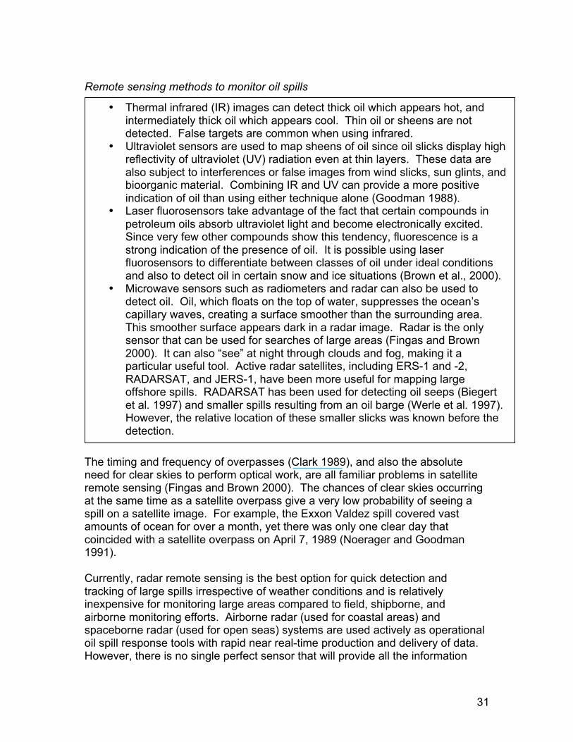
31

Remote sensing methods to monitor oil spills The timing and frequency of overpasses (Clark 1989), and also the absolute need for clear skies to perform optical work, are all familiar problems in satellite remote sensing (Fingas and Brown 2000). The chances of clear skies occurring at the same time as a satellite overpass give a very low probability of seeing a spill on a satellite image. For example, the Exxon Valdez spill covered vast amounts of ocean for over a month, yet there was only one clear day that coincided with a satellite overpass on April 7, 1989 (Noerager and Goodman 1991). Currently, radar remote sensing is the best option for quick detection and tracking of large spills irrespective of weather conditions and is relatively inexpensive for monitoring large areas compared to field, shipborne, and airborne monitoring efforts. Airborne radar (used for coastal areas) and spaceborne radar (used for open seas) systems are used actively as operational oil spill response tools with rapid near real-time production and delivery of data. However, there is no single perfect sensor that will provide all the information

• Thermal infrared (IR) images can detect thick oil which appears hot, and intermediately thick oil which appears cool. Thin oil or sheens are not detected. False targets are common when using infrared.

• Ultraviolet sensors are used to map sheens of oil since oil slicks display high reflectivity of ultraviolet (UV) radiation even at thin layers. These data are also subject to interferences or false images from wind slicks, sun glints, and bioorganic material. Combining IR and UV can provide a more positive indication of oil than using either technique alone (Goodman 1988).

• Laser fluorosensors take advantage of the fact that certain compounds in petroleum oils absorb ultraviolet light and become electronically excited. Since very few other compounds show this tendency, fluorescence is a strong indication of the presence of oil. It is possible using laser fluorosensors to differentiate between classes of oil under ideal conditions and also to detect oil in certain snow and ice situations (Brown et al., 2000).

• Microwave sensors such as radiometers and radar can also be used to detect oil. Oil, which floats on the top of water, suppresses the ocean’s capillary waves, creating a surface smoother than the surrounding area. This smoother surface appears dark in a radar image. Radar is the only sensor that can be used for searches of large areas (Fingas and Brown 2000). It can also “see” at night through clouds and fog, making it a particular useful tool. Active radar satellites, including ERS-1 and -2, RADARSAT, and JERS-1, have been more useful for mapping large offshore spills. RADARSAT has been used for detecting oil seeps (Biegert et al. 1997) and smaller spills resulting from an oil barge (Werle et al. 1997). However, the relative location of these smaller slicks was known before the detection.

32

required to detect, classify, and quantify oil in the marine and coastal environment. Oil spill monitoring scenario

For example, a marine biologist in charge of monitoring oil spills must consider all the above limitations of current technology, and also evaluate cost limitations. If the choice of technology is radar satellites, their utility can be applied for monitoring cause, extent, and direction of ship-borne pollution. Using radar, operational and accidental ship-borne discharges can be detected, in addition to detection of wave and tide patterns that serve as indicators of the direction of spills on the open seas. A marine biologist, for example, may decide to use a SAR instrument onboard the ERS satellite. A good general rule to remember is: the brighter the sea surface the rougher the sea (the higher the wind speed), though oil on the water dampens the rough surface and it becomes smooth again (and dark; Figure 8, 9). When using composite radar imagery a collection of images may be taken on different days over the same surface area. In order to distinguish the information from each of the days, each image is assigned to a different color in Figure 10 (Figure 10; 13 September is shown in red, 19 September is shown in green, and 25 September is shown in blue). In this example, all images were acquired at the same time of the day, at 10:20 GMT. If all the 3 images were identical, we would expect a black-and-white image, because in each point of the image we would find an equal amount of blue, green and red. Any change would be seen as a different color. For example, a) a little less blue with constant green and red would turn the color from grey to yellow; b) a little less green with constant blue and red would turn the color from grey to magenta; and c) a little less red with constant green and blue would turn the color to cyan. Therefore, the colors in the image are linked to changes in radar response or backscatter within this period of time. Although it is a very short period, backscatter on the open seas may change rapidly because of the wind conditions. The magenta on the sea indicates stronger winds on 13 and 25 September. The horizontal blue/magenta line is a wind-front announcing the arrival of a weather change on 25 September. This example would allow a marine biologist to discover an oil slick in the lower right corner of Figure 10. It is of magenta color. On the black-and-white image of the day the individual satellite image was taken this slick appears in black. However, oil slicks drift with the current and little also with the winds. In this example, the drifting is about 320 meters per hour. The current is westwards. Consequently, the oil will reach the coast in relatively short order and coastal remedial operations need to be initiated immediately.

33

IV. ATMOSPHERIC APPLICATIONS Monitoring atmospheric changes using remote sensing has only increased over the last few decades. Monitoring weather is a daily activity around the globe for weather forecasting as well as for prediction and application to ecological management needs. Air quality has become a pressing issue in recent years partly due to the scientific evidence linking fine aerosols with increasing mortality to humans and negative impacts on ecosystems. National standards have been set for the concentration of major pollutants (ozone, carbon monoxide, sulfur dioxide, nitrogen dioxide). Until recently, the study of air pollution relied primarily on ground-based measurements, intermittent field campaigns, and chemical transport models. Increasingly the data required to forecast and assess air quality is growing to larger spatial scales. Over the next decade, the data for air pollution monitoring and control will need to cover large spatial areas in order to accommodate decisions for pollutants across the geopolitical and intercontinental boundaries. The sources and extent of air pollution can be monitored with satellite borne sensors, which will provide needed data needed for recording the growing effects of atmospheric pollutants on biodiversity. AIR POLLUTION With significant advancement emerging in sensor capability in recent years, remote sensing is shown to be an important tool to monitor air pollution for global, regional, and local assessments. For example, the MAPS (Measurement of Air Pollution from Satellite) instrument of NASA measures the distribution of carbon monoxide in the Earth’s lower atmosphere (3 to 10 kilometers above the surface). The instrument provides the near-global database of atmospheric carbon monoxide levels to help scientists better understand how well the atmosphere can cleanse itself of pollutants and how far pollutants are transported from their source areas and the size of the sources. Currently, NASA’s Earth Probe satellite’s TOMS (Total Ozone Mapping Spectrometer) instrument measures aerosols, ozone, UV irradiance, and volcanic (sulfur dioxide) ash emissions. Modern sensors designed for monitoring air pollution can measure the proportion of light blocked by particulate matter for atmospheric modeling of contaminants. ‘Pollution’ or air quality maps of urban centers are developed from modeling and ground measurements to explain how air pollution spreads over a basin, and what the effects are to the human population and the environment (Sifakis et al., 1998). WEATHER On April 1, 1960, the first weather satellite in the United States, "TIROS I", was launched into orbit. Today, weather satellites measure cloud cover, monitor concentrations of ozone, CO2, water vapor, temperature, and more. NOAA (National Ocean and Atmospheric Association) has two groups of satellites designed to monitor weather, the GOES (Geostationary Operational

34

Environmental Satellites) and POES (Polar Orbiting Environmental Satellites) systems. Hurricane monitoring GOES-9, as well as its older counterparts, are critical to the National Weather Service operations. Atmospheric temperature, winds, moisture and cloud cover can be derived from GOES-9 sensor measurements. However, it is difficult to distinguish among low, middle, and high level clouds in a visible satellite image, since they can all have a similar albedo and, for this distinction, infrared satellite images are needed. POES have meteorological and geophysical importance because of their high-resolution global coverage and well calibrated channels. They are designed to stay in a low earth orbit and reach high latitudes. The POES program began in 1960 with the launch of TIROS-1. Following the launch of TIROS-1, the program was improved with the Improved TIROS Operational Satellite (ITOS) program; expanded to capture concurrent multiple-channel data on a daily basis. V. ACCURACY ASSESSMENT When looking at a land cover map it is important to remember that it is not a perfect representation of reality. There are always errors in maps and before evaluating the utility of a particular map a conservation manager will need to have an idea of how accurate it really is and how accurate it should be to sufficiently meet the requirements for the intended application. The only way to reliably check the accuracy of a map is to design and implement an accuracy assessment. Without such an objective measure of the map’s quality a manager might be limited to using qualitative statements from people who have used the map. These comments may provide a rough indication as to the quality of a map but they tend to be very subjective and can often be misleading. ACCURACY RESULTS The result of an accuracy assessment typically provides users with an overall accuracy of the map and the accuracy for each class in the map. For example,

Hurricane Katrina (2005), with winds of 135 miles per hour (217 kilometers per hour) was tracked extensively using satellite remote sensing. This hurricane created a powerful storm surge, and heavy rains, pounding the U.S. Gulf Coast, triggering extensive life-threatening flooding, and resulted in extensive ecological and economic damage to island refuges and coastal reserves. The GOES image in Figure 11 illustrates the type of imagery typically captured. This GOES image shows the storm as it moved over southern Mississippi at 9:02 a.m, August 29, 2005 (Figure 11). The eye of the storm is due east of New Orleans, Louisiana when this image was taken, and then continued to move north into Mississippi.

35

in a land cover map the water class could be very accurate but some of the vegetation classes might be less accurate. This can have a significant effect on the utility of the map and in some cases may indicate that some classes should be merged. For example if two forest types, say deciduous and coniferous are relatively inaccurate it might make sense to combine them into a single forest class with much higher accuracy. Conducting a proper accuracy assessment of a product created using remotely sensed data can be time consuming and costly. This is the primary reason why this important step is often not carried out in a mapping project. It is common for accuracy assessment to be detailed in the project design but unfortunately, it is regularly dropped or greatly modified in the interest of saving time or money. POSITION AND THEMATIC ERROR There are two primary components of error in thematic maps such as land cover maps; position error and thematic error. In a map with poor position error the shape and size of a particular feature, such as a lake, might be correct but the placement on the map is incorrect. Thematic error occurs when a feature is misidentified. For example, if an area labelled shrub on the map were actually grassland then the thematic error of the map would increase. In most cases both of these error components work together. For example, when trying to delineate the boundary between two cover types that gradually change from the one cover type to the other it is difficult to accurately draw that line that divides these two cover types. When a conservation practitioner looks at the accuracy of a land cover map, that practitioner typically does not differentiate between position and thematic errors. The accuracy assessment sampling design usually has a built-in mechanism that allows for reasonable position errors based on the input data being used and on the scale of the final map. In the end, however, the accuracy figures do not indicate if the error is due to a positional error or a thematic error. Additionally, looking at accuracy statistics can be misleading if a practitioner does not understand what they represent. VI. SUMMARY Remote sensing can be successfully used to address a plethora of biodiversity conservation issues and is a valuable tool for scientists, conservation practitioners, land managers, and many others. Aquatic, atmospheric and terrestrial systems are all amenable to study with remote sensing techniques. However, remote sensing is not a panacea for all problems conservation biologists may encounter. There are limitations to the technology. A few of those have been outlined above. This module is primarily designed to introduce the applications of remote sensing to typical problems biodiversity conservation practitioners commonly encounter. Though a brief introduction to remote sensing was written to give a cursory overview of the history of the technology, the

36

module is meant to focus on applications to biodiversity conservation. An attempt has been made to utilize case studies on multiple topics to give a more detailed examination of the protocols, tools, and skills needed to pragmatically address problems. Notable examples include fire detection and monitoring, habitat assessment, landscape change detection, and monitoring oil spills. VII. ACKNOWLEDGEMENTS The following people are gratefully acknowledged for their helpful comments on early drafts of this document: Nora Bynum, James Danoff-Berg, Peter Ersts, Ned Gardiner, Ian Harrison, Ned Horning, Kevin Koy, Melina Laverty, and Eleanor Sterling.

37

VIII. LITERATURE CITED Ahern, F. J.G. Goldammer and C. Justice. 2001. Global and regional vegetation fire monitoring from space: Planning a coordinated international effort. SPB Academic Publishing, The Hague, Netherlands. Alsdorf, D.E., J.M.Melack, T. Dunne, L.A.K. Mertes, L.L. Hess and L.C. Smith 2000. Interferometric radar measurements of water level changes on the Amazon floodplain. Nature 404: 174-177. Alexander, D. 1991. Information technology in real-time for monitoring and managing natural disasters. Progress in Physical Geography 15:238-260. Alfoldi, T.T. and N.A. Prout. 1982. The Use of Satellite Data for Monitoring Oil Spills in Canada, Environment Canada Report EPS 3-EC-82-5, Ottawa, Ontario. Alpers, W. and H. Hühnerfuss. 1987. Radar Signatures of Oil Films Floating on the Sea Surface, in Proceedings of IGARSS ‘87 Symposium, Ann Arbor, Michigan, pp. 741-745. Anderson, G. and C. Yang. 1996. Preliminary field results of mapping grain sorghum management zones using aerial videography. Presented at the 26th symposium on remote sensing of environment, March 25-29, 1996. Vancouver, Canada. Asner, G.P. and P.M. Vitousek. 2005. Remote analysis of biological invasion and biogeochemical change. PNAS 102:4383–4386. Baker J.R., P.L. Mitchell, R.A. Cordey, G.B. Groom, J.J. Settle and M.R. Stileman. 1994. Relationships between physical characteristics and polarimetric radar backscatter for Corsican pine stands in Thetford Forest, UK. International Journal of Remote Sensing 15:2827-2849. Barbosa, P.M., J.M. Gregoire and J.M.C. Pereira. 1999. An algorithm for extracting burned areas from time series of AVHRR GAC data applied at a continental scale. Remote Sensing of Environment 69:253-263. Beaudoin, A., T. L. Toan, S. Goze, E. Nezry, A. Lopes, E. Mougin, C.C. Hsu, H.C. Han, J.A. Kong and R.T. Shin. 1994. Retrieval of forest biomass from SAR data. International Journal of Remote Sensing 15:2777-2796. Biegert, E.K., Baker, R.N., Berry, J.L., Mott, S. and S. Scantland. 1997. A Gulf Offshore Satellite Applications Project Detects Oil Slicks Using Radarsat, in Proceedings of International Symposium: Geomatics in the Era of Radarsat, Ottawa, Canada. Bilge, F., B. Yazici, T. Dogeroglu, and C. Ayday. 2003. Statistical evaluation of remotely sensed data for water quality monitoring. International Journal of Remote Sensing 25(24):5317-5326 Birkett, C.M. 2000. Synergistic remote sensing of Lake Chad: Variability of basin inundation, Remote Sensing of the Environment, 72:218-236. Braun, A., K. Cheng, B. Csatho, C.K. Shum. 2004. ICESat Laser Altimetry in the Great Lakes, ION 60th Annual Meeting CDROM Proceedings, Dayton, Ohio, June 7-9, 2004

38

Brown, O. B., J. W. Brown and R. H. Evans. 1985. Calibration of advanced very high resolution radiometer infrared observations. Journal of Geophysical Research 90:11667-11678. Brown, C.E., M.F. Fingas, R.H. Goodman, J.V. Mullin, M. Choquet and J-P. Monchalin. 2000. Airborne Oil Slick Thickness Measurement, Pages I219-224 in Proceedings of the Fifth International Conference on Remote Sensing for Marine and Coastal Environments, Environmental Research Institute of Michigan, Ann Arbor, Michigan. Burgan, R.E. and M.B. Shasby. 1984. Mapping Broad-Area Fire Potential From Digital Fuel, Terrain, and Weather Data Journal of Forestry 8:228-231. Clark, C.D. 1989. Satellite Remote Sensing for Marine Pollution Investigations. Marine Pollution Bulletin 26(7): 92-96. Curran, P.J. and E.M.M. Novo. 1988. The relationship between suspended sediment concentration and remotely sensed spectral radiance: A review. Journal of Coastal Research 4:351-368. Darkin, D.V., L.M. Mitnik, and V.A. Dubina. 2004. Ice cover of the Okhotsk Sea: a study using ENVISAT ASAR, ERS-2 SAR and AQUA AMSR-E data. In proceedings of the 2004 Envisat & ERS Symposium (ESA SP-572), Salzburg, Austria. Dozier, J. 1984. Snow reflectance from Landsat-4 thematic mapper. IEEE Transactions in Geoscience and Remote Sensing GE-22(3):323-328. Durand, D., J. Bijaoui, and F. Cauneau. 2000. Optical remote sensing of shallow- water environmental parameters: A feasibility study. Remote Sensing of Environment 73:152-161. Drury, S. A. 1990. A Guide to Remote Sensing: Interpreting Images of the Earth. Oxford University Press, New York, USA. Dull, C.W. and B. Lee. 2001. Satellite earth observation information requirements of the wildland fire management community. In F.J. Ahern, J.G. Goldammer, and C.O. Justice, eds., Global and Regional Vegetation Fire Monitoring from Space: Planning a Coordinated International Effort. SPB Academic Publishing, The Hague, Netherlands. Earl R., P.N. Wheeler, B.S. Blackmore, and R.J. Blackmore. 1996. Precision Farming - The Management of Variability. The Journal of the Institution of Agricultural Engineers 4:18-23. Ehrlich D., E.F. Lambin and J. Malingreau. 1997. Biomass Burning and Broad- Scale Land Cover Changes in Western Africa. Remote Sensing of the Environment 61:201-209. Fingas, M.F., C.E. Brown and J.V. Mullin. 1998. The Visibility Limits of Oil on Water and Remote Sensing Thickness Detection Limits, Pages 411-418 in Proceedings of the Fifth Thematic Conference on Remote Sensing for Marine and Coastal Environments, Environmental Research Institute of Michigan, Ann Arbor, Michigan Fingas, M. & Brown, C.E. 2000. Review of Oil Spill Remote Sensing. In Proceedings SPILLCON 2000: 8th International Oil Spill Conference, Darwin, Australia, 15-17 August 2000, 23 pp. (available at http://www.aip.com.au/amosc/spillcon/speakers.htm).

39

Forget, P. and P. Brochu. 1996. Slicks, Waves and Fronts Observed in Sea Coastal Area by an X-band Airborne Synthetic Aperture Radar. Remote Sensing of the Environment 57:1-12. Frysinger, G.S., Asher, W.E., Korenowski, G.M., Barger, W.R., Klusty, M.A., Frew, N.M. and R.K. Nelson. 1992. Study of Ocean Slicks by Nonlinear Laser Processes in Second-Harmonic Generation. Journal of Geophysical Research 97(C4): 5253-5269. Gade, M., Alpers, W., Huehnerfuss, H. and V. Wismann. 1996. Radar Signatures of Different Oceanic Surface Films Measured during the SIR- C-X-SAR Missions, Pages 233-240 in Remote Sensing (96), 16th Symposium of the European Association of Remote Sensing Laboratories (EARsel), Rotterdam. Gibbons, D.E., G.E. Wukelic, J.P. Leighton, and M.J. Doyle. 1989. Application of Landsat Thematic Mapper data for coastal thermal plume analysis at Diablo Canyon. Photogrammetric Engineering and Remote Sensing 55: 903-909. Goodman, R.H. 1988. Simple Remote Sensing System for the Detection of Oil on Water, Environmental Studies Research Fund Report Number 98, Ottawa, Ontario. Green, R.M. 1998. Relationships between polarmetric SAR backscatter and forest canopy and sub-canopy biophysical properties. International Journal of Remote Sensing 19:2395-2412. Greer, J.D. 2000. Crossing the millenium: Integrating spatial technologies and ecological principles for a new age in fire management, in Proceedings of the Joint Fire Science Conference and Workshop at Boise Idaho in June 1999. ASPRS, Bethesda, United States. Herring, D. 1998. NASA Demonstrates New Technology for Monitoring Fires From Space. Available from http://earthobservatory.nasa.gov/Study/Fire/. [Accessed on March 2, 2005] Hielm, J.H. 1989. NIFO Comparative Trials. Pages 67-75 in The Remote Sensing of Oil Slicks, A.E. Lodge, ed., John Wiley and Sons, Chichester, United Kingdom. Holmgren, P., and T. Thuresson. 1998. Satellite remote sensing for forestry planning—a review. Scandinavian Journal of Forest Research 13:90-110. Hühnerfuss, H., Alpers, W., Dannhauer, H., Gade, M., Lange, P.A., Neumann, V. and V. Wismann. 1996. Natural and Man-made Sea Slicks in the North Sea Investigated by a Helicopter-borne 5-frequency Radar Scatterometer. International Journal of Remote Sensing 17(8):1567-1582. Hühnerfuss, H., Alpers, W. and F. Witte. 1989. Layers of Different Thicknesses in Mineral Oil Spills Detected by Grey Level Textures of Real Aperture Radar Images. International Journal of Remote Sensing 10:1093-1099. Idso, S.B. 1982. Non-water-stressed baselines: a key to measuring and interpreting plant water stress. Agricultural Meteorology 27:59-70. Jacobson, E. R., J. M. Gaskin, M. B. Brown, R. K Harris, C. H. Gardiner, J. L. LaPointe, H. P. Adams and C. Reggiardo. 1991. Chronic upper

40

respiratory tract disease of free-ranging desert tortoises (Xerobates agassizii). Journal of Wildlife Diseases 27(2):296-316. Lefsky, M.A., W.B. Cohen, G.G. Parker, and D.J. Harding. 2002. Lidar remote sensing for ecosystem studies. BioScience 52(1):19-30. Kaufman, Y. J., et al., 2001. Absorption of sunlight by dust as inferred from satellite and ground-based remote sensing. Geophysical Resources Letters 28:1479–1483. Klaver, R., G. Fosnight, and A. Singh. 1997. Global forest fire watch: Wildfire potential, detection, monitoring, and assessment. EROS Data Center, Sioux Falls, USA. Kummerow, C., W. Barnes, T. Kozu, J. Shiue and J. Simpson. 1998. The Tropical Rainfall Measuring Mission (TRMM) sensor package. Journal of Atmospheric and Ocean Technology 15:808-816. Kunzi, K.F., S. Patil, and H. Rott. 1982. Snow-covered parameters retrieved from NIMBUS-7 SMMR data. IEEE Transactions in Geoscience and Remote Sensing GE-20:452-467. Langaas, S. 1992. Temporal and spatial distribution of savanna fires in Senegal and Gambia, West Africa. International Journal of Wildland Fire 2(1):21- 36. Lee, K., G. B. Lee and E.J. Tyler. 1988. Determination of Soil Characteristics from Thematic Mapper Data of a Cropped Organic-Inorganic Soil Landscape. Soil Science Society of America Journal 52:1100-1107. Lee, Z.P., K.L. Carder, C.D. Mobley, R.G. Steward, and J.S. Patch. 1999. Hyperspectral remote sensing for shallow waters: 2. Deriving bottom depths and water properties by optimization. Applied Optics 38:3831- 3843. Levine, J.S. 1996a. Biomass burning and global change, volume 1: Biomass burning in Africa. The MIT Press, Inc., Cambridge, USA. Levine, J.S. 1996b. Biomass burning and global change, volume 2: Biomass burning in South America, southeast Asia, temperate and boreal ecosystems, and the oil fires of Kuwait. The MIT Press, Inc., Cambridge, USA. Levine, J.S., E.L. Winstead, D.A.B. Parsons, M.C. Scholes, R.J. Scholes, W.R. Cofer, III, D.R. Cahoon, Jr. and D.I. Sebacher. 1996. Biogenic soil emissions of nitric oxide (NO) and nitrous oxide (N2O) from savannas in South Africa: The impact of wetting and burning. Journal of Geophysical Research 101(23):689-698. Lillesand, T.M., and R.W. Kiefer. 1994. Remote Imaging and Image Interpretation. John Wiley & Son, New York, USA. Marmorino, G.O., Thompson, D.R., Graber, H.C. and C.L. Trump. 1997. Correlation of Oceanographic Signatures Appearing in Synthetic Aperature Radar and Interferometric Synthetic Aperture Radar Imagery with in-situ Measurements. Journal of Geophysical Research 102(C8):18,723-18,736.

41

Mastin, G.A., J.J. Mason, J.D. Bradley, R.M. Axline, and G.L. Hover. 1994. A Comparative Evaluation of SAR and SLAR. in Proceedings of the Second Thematic Conference on Remote Sensing for Marine and Coastal Environments: Needs, Solutions and Applications, ERIM Conferences, Ann Arbor, Michigan. McClain, E. P., W. G. Pichel, C. C. Walton, Z. Ahmad and J. Sutton. 1983. Multi-channel improvements to satellite-derived global sea-surface temperatures. Advanced Space Research 2(6):43-47. McGarigal, K. and B. J. Marks. 1995. Fragstats: Spatial Pattern Analysis Program for Quantifying Landscape Structure. General Technical Report PNW-GTR-351. U.S. Department of Agriculture, Forest Service, Pacific Northwest Research Station, Portland, USA. Minnett, P. J. 1991. Consequences of sea surface temperature variability on the validation and applications of satellite measurements. Journal of Geophysical Research. 96(C10):18475-18489. Moran, S., R. D. Jackson, P. N. Slater and P. M. Teillet. 1992 . Evaluation of simplified procedures for retrieval of land surface reflectance factors from satellite sensor output. Remote Sensing of Environment 41:169–184. Noerager, J.A. and R.H. Goodman. 1991. Oil Tracking, Containment and Recovery During the EXXON VALDEZ Response. Pages 193-203 in Proceedings of the 1991 Oil Spill Conference, American Petroleum Institute, Washington, D.C. Oesch, D., J.-M. Jaquet, A. Hauser and S. Wunderle 2005. Lake surface water temperature retrieval using AVHRR and MODIS data: Validation and feasibility study, Journal of Geophysical Research - Oceans, accepted for publication. Okamoto, K., Kobayashi, T., Masuko, H., Ochiai, S., Horie, H., Kumagai, H., Nakamua, K. and M. Shimada. 1996. Results of Experiments Using Synthetic Aperture Radar Onboard the European Remote Sensing Satellite 1 - 4. Artificial Oil Pollution Detection, Journal of the Communications Research Laboratory 43 (3):327-344. O’Neill, R.V., S.W. Christensen, V.H. Dale, D.L. DeAngelis, R.H. Gardner, R.L. Graham, B. Jackson, J.R. Krummel, B.T. Milne, G. Sugihara, M.G. Turner and B. Zygmunt. 1988. Indices of landscape pattern. Landscape Ecology 1:153-162. Oren R., K. S. Werk, N. Buchmann and R. Zimmermann. 1993. Chlorophyll as an index to nutrient limitation in Picea abies (L.) Karst. stands at different stages of decline. Canadian Journal of Forest Research 23:1187-1195. Poitevin, J. and C. Khaif. 1992. A Numerical Study of the Backscattered Radar Power in Presence of Oil Slicks on the Sea Surface. Pages 171-182 in Proceedings of the First Thematic Conference on Remote Sensing for Marine and Coastal Environments, ERIM Conferences, Ann Arbor, Michigan. Rango, A. 1993. Snow hydrology processes and remote sensing. Hydrological Processes 7:121-138.

42

Rees, G. 1999. The Remote Sensing Data Book. Cambridge University Press, New York, USA. Ridd, M. 1995. Exploring a V-I-S model for urban ecosystem analysis through remote sensing: comparative anatomy of cities. Journal of Remote Sensing 16:2165-2185. Riiters, K.H., R.V. O’Neill, C.T. Hunsaker, J.D. Wickham, D.H. Yankee, S.P. Timmins, K.B. Jones and B.L. Jackson. 1995. A factor analysis of landscape pattern and structure metrics. Landscape Ecology 10:23-39. Ritchie, J.C., F.R. Schiebe, and J.R. McHenry. 1976. Remote sensing of suspended sediment surface water. Photogrammetric Engineering and Remote Sensing 42:1539-1545. Ritchie, J.C., C.M. Cooper, and F.R. Schiebe. 1990. The relationship of MSS and TM digital data with suspended sediments, chlorophyll, and temperature in Moon Lake, Mississippi. Remote Sensing Environment 33:137-148. Ritchie, J.C. and F.R. Schiebe. 2000. Water Quality. In G.A. Schultz and E.T. Engman, eds., Remote Sensing in Hydrology and Water Management. Springer-Verlag, Berlin, Germany. Rott, H. 1986. Prospects of microwave remote sensing for snow hydrology. Hydrologic Applications of Space Technology: Proceedings of the Cocoa Beach Workshop. IAHS Publications 160:215-223. Scholes, M. and M.O. Andreae. 2000. Biogenic and pyrogenic emissions from Africa and their impact on the global atmosphere. Ambio 29: 23-29. Shi, J.C., and J. Dozier. 1992. Radar Response to Snow Wetness. Proceedings from IGARSS 92, IEEE 92 CH3041-1. 927-929. Shi, J.C., J. Dozier and H. Rott. 1994. Snow Mapping in Alpine Regions with Synthetic Aperture Radar, IEEE Transactions on Geoscience and Remote Sensing 32(1). Sifakis, N., N. Soulakellis and D. Paronis. 1998. Quantitative mapping of air pollution density using Earth observations: A new processing method and application on an urban area. International Journal of Remote Sensing 19:3289-3300. Singh, A. 1989. Digital change detection techniques using remotely sensed data. International Journal of Remote Sensing. 10:989-1003. Skole, D.L., C.O. Justice, A.C. Janetos, and J.R.G. Townshend. 1997. A land cover change monitoring program; strategy for an international effort. Mitigation and Adaptation Strategies for Global Change 2:157-175. Smith, L.C. 1997. Satellite remote sensing of river inundation area, stage, and discharge: A review. Hydrological Processes 11:1427-1439. Spencer, R.W., H. M. Goodman and R.E. Wood. 1988. Precipitation retrieval over land and ocean with SSM/I, Part 1: Identification and Characteristics of the Scattering Signal. Journal of Atmospheric and Oceanic Technology 2:254-263. Stiles, W.H., F.T. Ulaby and A. Rango. 1981. Microwave measurements of snowpack properties. Nordic Hydrology 12:143-166.

43

Tennyson, E.J. 1985. Shipborne Radar as an Oil Spill Tracking Tool. Proceedings of the Eleventh Arctic and Marine Oilspill Program Technical Seminar, Environment Canada, Ottawa, Ontario. Torgersen, C.E., R.N. Faux, B.A. McIntosh, N.J. Poage and D.J. Norton. 2001. Airborne thermal remote sensing for water temperature assessment in rivers and Streams. Remote Sensing of Environment 76:386-398. Turner, M.G. and R.H. Gardner. 1991. Quantitative Methods in Landscape Ecology. Springer-Verlag, New York, USA. Vachon, P.W. and R.B. Olsen. 2000. Ship detection with satellite based sensors: a summary of workshop presentations. Backscatter. Fall 2000:23-26. Voloshina, I.P. and O.Y. Sochnev. 1992. Observations of Surface Contamination of the Region of the Kol’shii Gulf from IR Measurements. Soviet Journal of Remote Sensing 9(6):996-1000. Wallace, O.C., J. Qi, P. Heilman and R.C. Marsett. 2003. Remote sensing for cover change assessment in southeast Arizona. Journal of Range Management 56:402-409. Weier, J. and D. herring. 2005. Measuring Vegetation (NDVI and EVI). Available from http://earthobservatory.nasa.gov/Library/MeasuringVegetation/ [Accessed March 16, 2005]. Werle, D., Tittley, B., Theriault, E. and B. Whitehouse. 1997. Using Radarsat-1 SAR Imagery to Monitor the Recovery of the Irving Whale Oil Barge. Proceedings of International Symposium: Geomatics in the Era of Radarsat, Ottawa, Canada. Wilheit, T.T., A.T.C. Chang, M.S.V. Rao, E.B.Rodgers and J.S.Theon. 1977. A satellite technique for quantitatively mapping rainfall rates over oceans. Journal of Applied Meteorology 16:551.

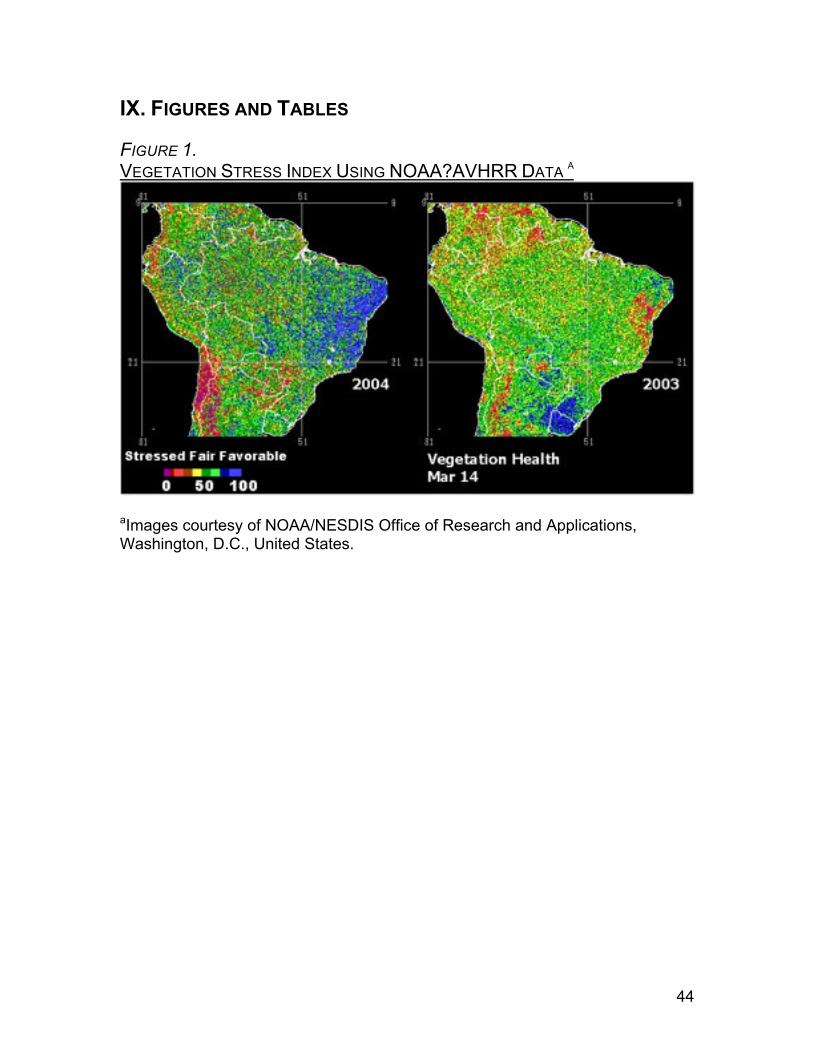
44

IX. FIGURES AND TABLES FIGURE 1. VEGETATION STRESS INDEX USING NOAA?AVHRR DATA A

aImages courtesy of NOAA/NESDIS Office of Research and Applications, Washington, D.C., United States.

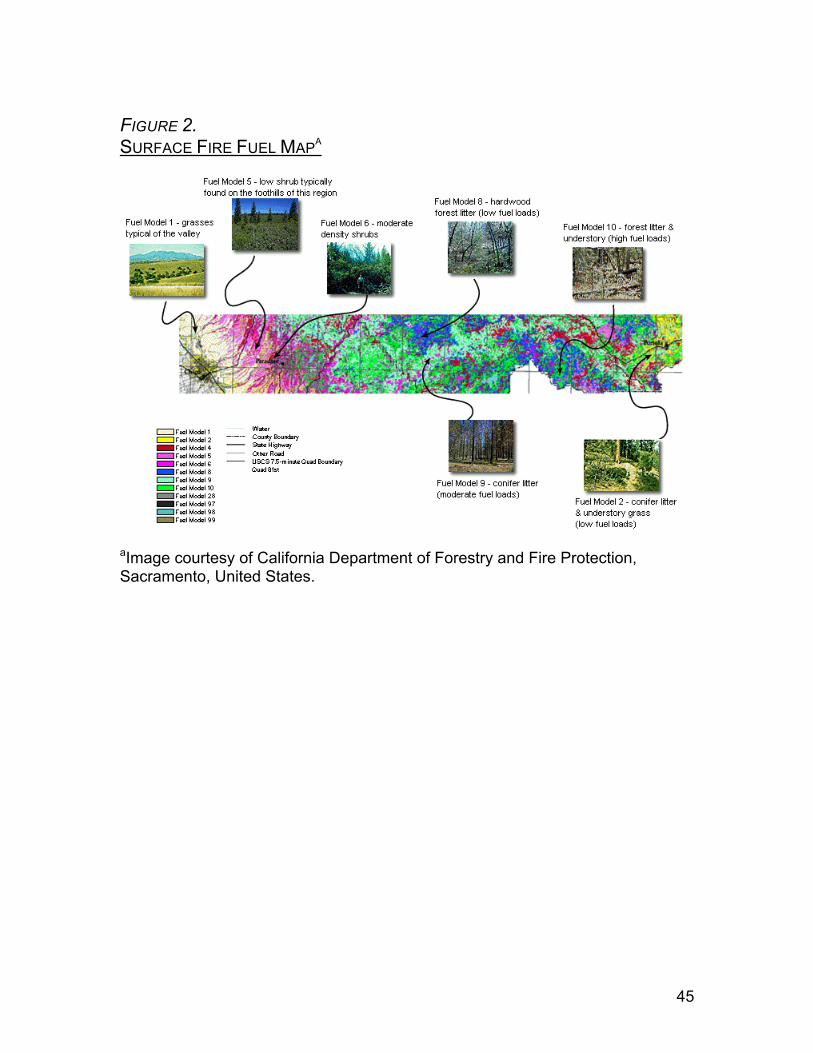
45

FIGURE 2. SURFACE FIRE FUEL MAPA

aImage courtesy of California Department of Forestry and Fire Protection, Sacramento, United States.

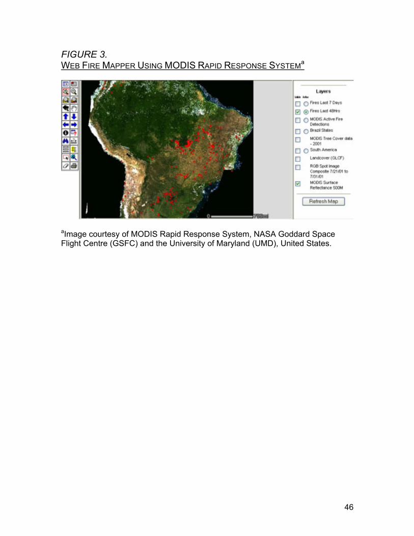
46

FIGURE 3. WEB FIRE MAPPER USING MODIS RAPID RESPONSE SYSTEMa

aImage courtesy of MODIS Rapid Response System, NASA Goddard Space Flight Centre (GSFC) and the University of Maryland (UMD), United States.

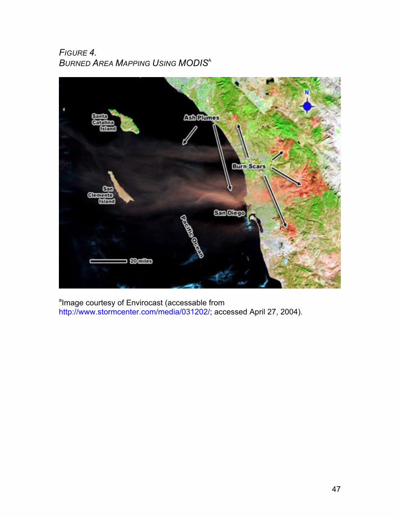
47

FIGURE 4. BURNED AREA MAPPING USING MODISA

aImage courtesy of Envirocast (accessable from http://www.stormcenter.com/media/031202/; accessed April 27, 2004).

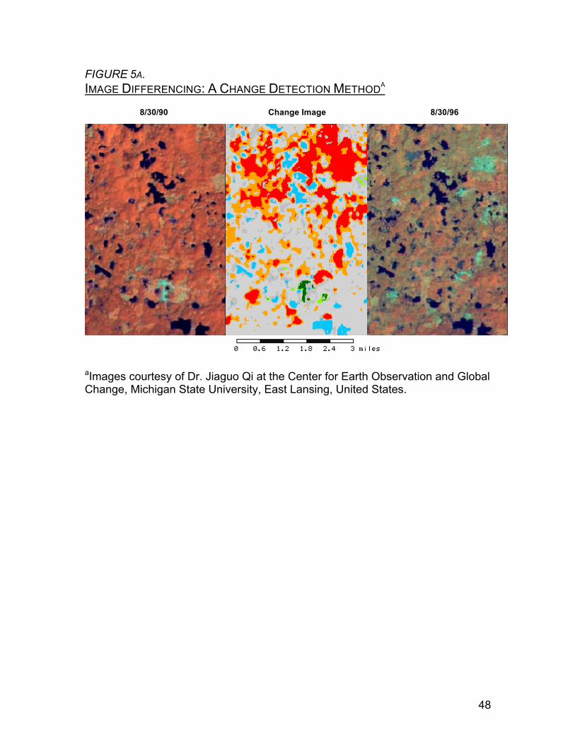
48

FIGURE 5A. IMAGE DIFFERENCING: A CHANGE DETECTION METHODA

8/30/90 Change Image 8/30/96

aImages courtesy of Dr. Jiaguo Qi at the Center for Earth Observation and Global Change, Michigan State University, East Lansing, United States.

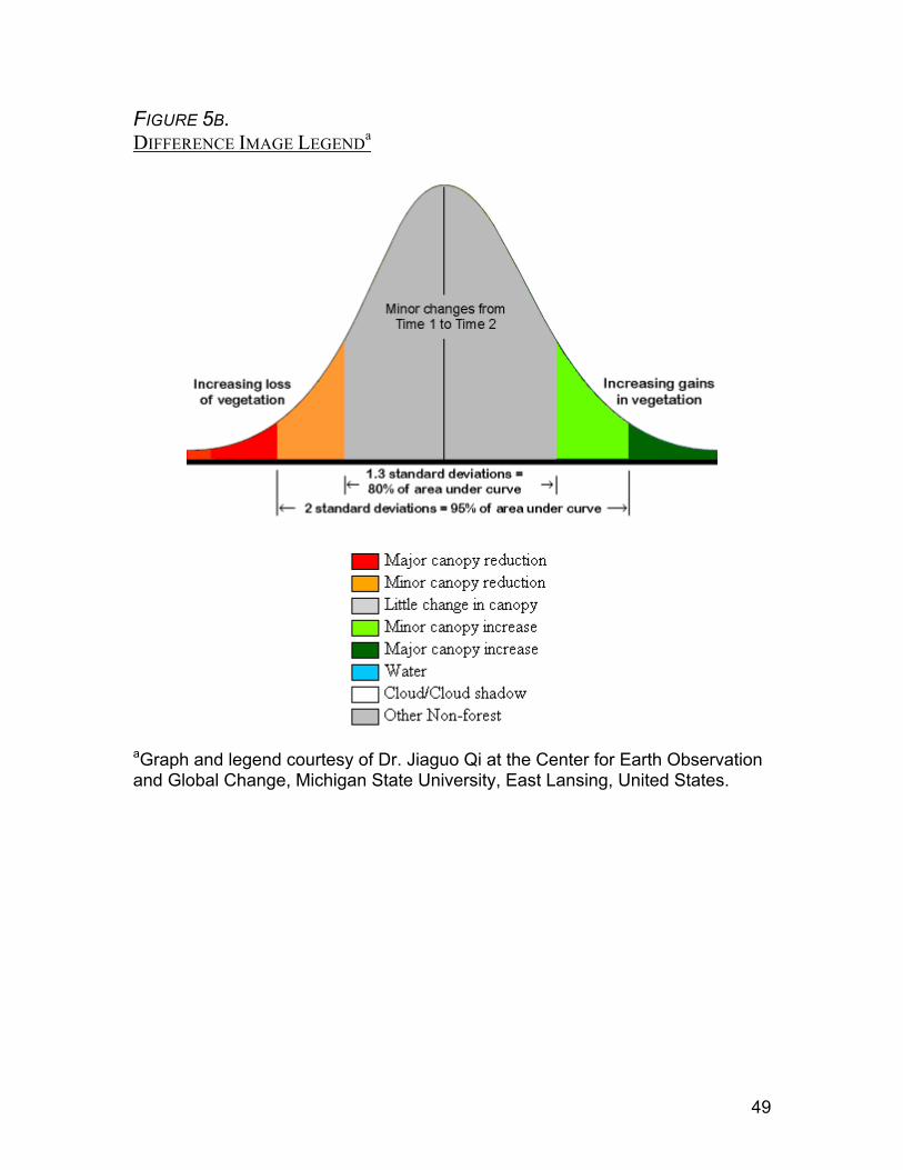
49

FIGURE 5B. DIFFERENCE IMAGE LEGENDa

aGraph and legend courtesy of Dr. Jiaguo Qi at the Center for Earth Observation and Global Change, Michigan State University, East Lansing, United States.

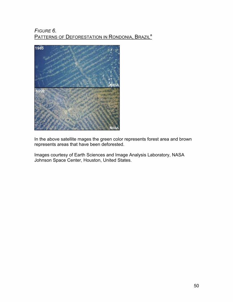
50

FIGURE 6. PATTERNS OF DEFORESTATION IN RONDONIA, BRAZILa

In the above satellite mages the green color represents forest area and brown represents areas that have been deforested. Images courtesy of Earth Sciences and Image Analysis Laboratory, NASA Johnson Space Center, Houston, United States.

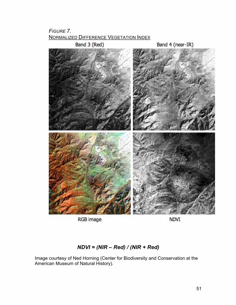
51

FIGURE 7. NORMALIZED DIFFERENCE VEGETATION INDEX

NDVI = (NIR – Red) / (NIR + Red) Image courtesy of Ned Horning (Center for Biodiversity and Conservation at the American Museum of Natural History).

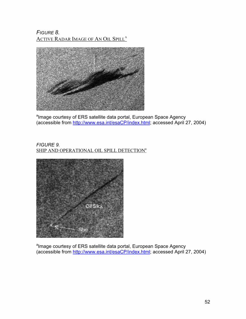
52

FIGURE 8. ACTIVE RADAR IMAGE OF AN OIL SPILLA

aImage courtesy of ERS satellite data portal, European Space Agency (accessible from http://www.esa.int/esaCP/index.html; accessed April 27, 2004) FIGURE 9. SHIP AND OPERATIONAL OIL SPILL DETECTIONa

aImage courtesy of ERS satellite data portal, European Space Agency (accessible from http://www.esa.int/esaCP/index.html; accessed April 27, 2004)

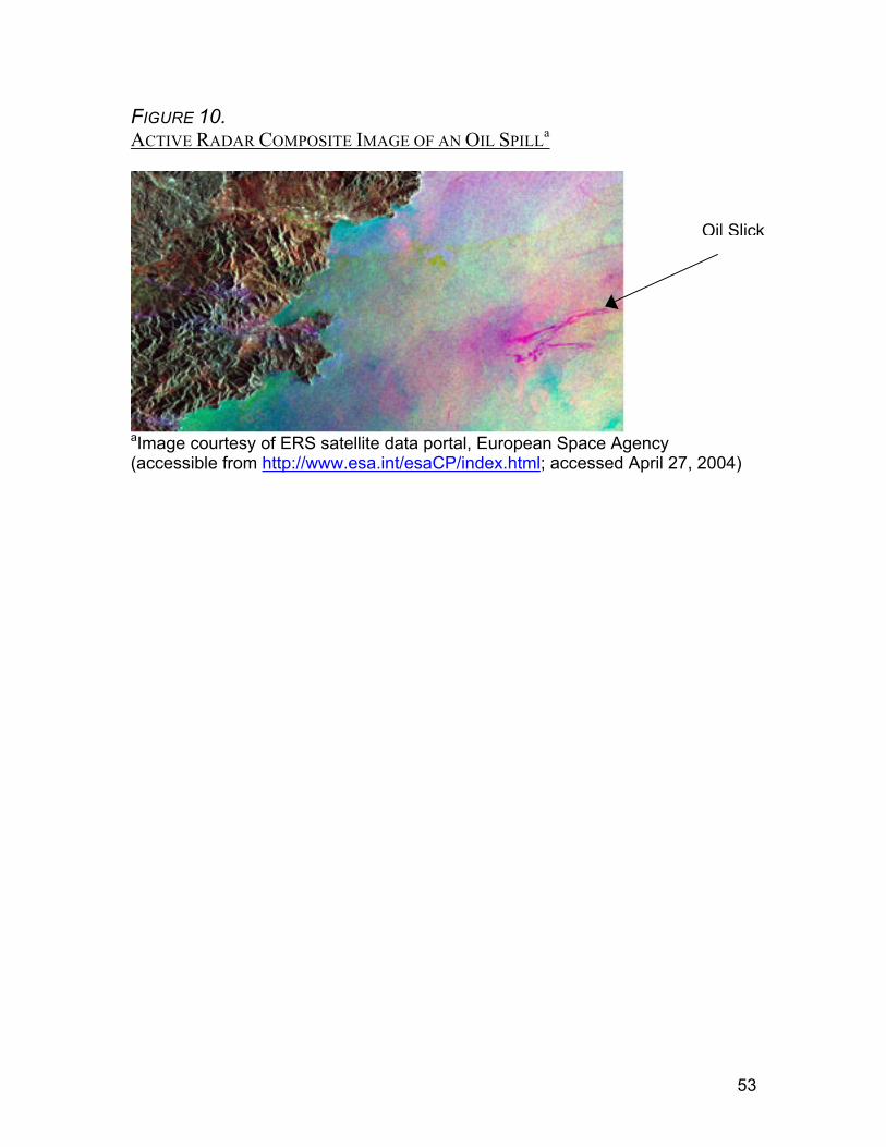
53

FIGURE 10. ACTIVE RADAR COMPOSITE IMAGE OF AN OIL SPILLa

aImage courtesy of ERS satellite data portal, European Space Agency (accessible from http://www.esa.int/esaCP/index.html; accessed April 27, 2004)

Oil Slick

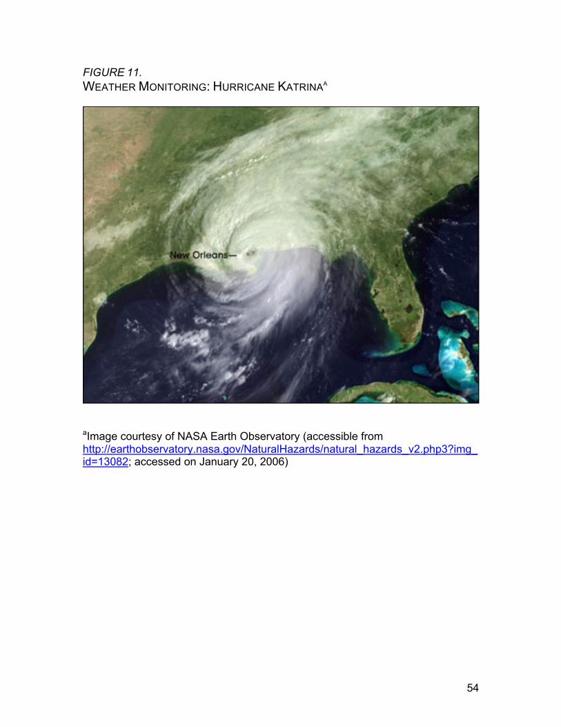
54

FIGURE 11. WEATHER MONITORING: HURRICANE KATRINAA

aImage courtesy of NASA Earth Observatory (accessible from http://earthobservatory.nasa.gov/NaturalHazards/natural_hazards_v2.php3?img_id=13082; accessed on January 20, 2006)

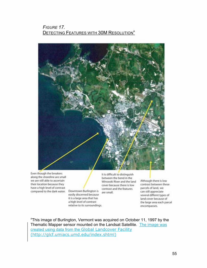
55

FIGURE 17. DETECTING FEATURES WITH 30M RESOLUTIONA

aThis image of Burlington, Vermont was acquired on October 11, 1997 by the Thematic Mapper sensor mounted on the Landsat Satellite. The image was created using data from the Global Landcover Facility (http://glcf.umiacs.umd.edu/index.shtml)

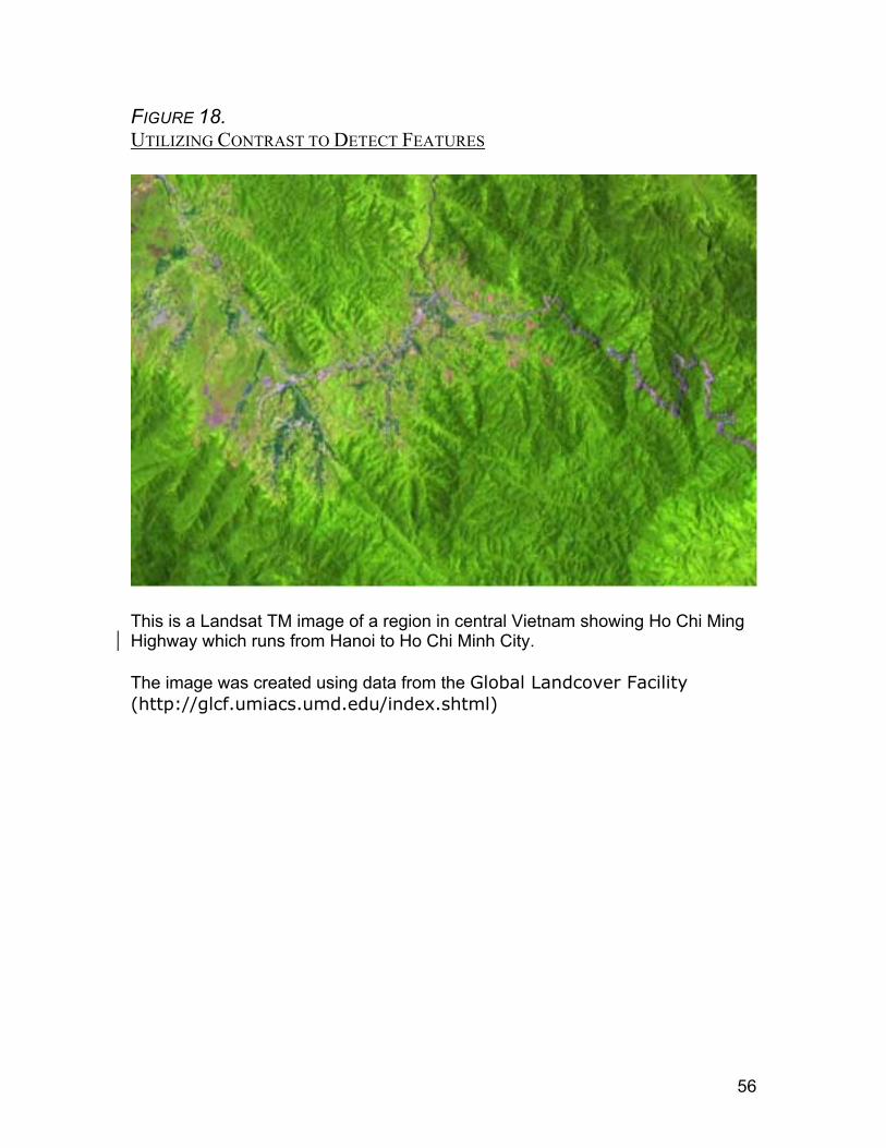
56

FIGURE 18. UTILIZING CONTRAST TO DETECT FEATURES

This is a Landsat TM image of a region in central Vietnam showing Ho Chi Ming Highway which runs from Hanoi to Ho Chi Minh City.

The image was created using data from the Global Landcover Facility (http://glcf.umiacs.umd.edu/index.shtml)

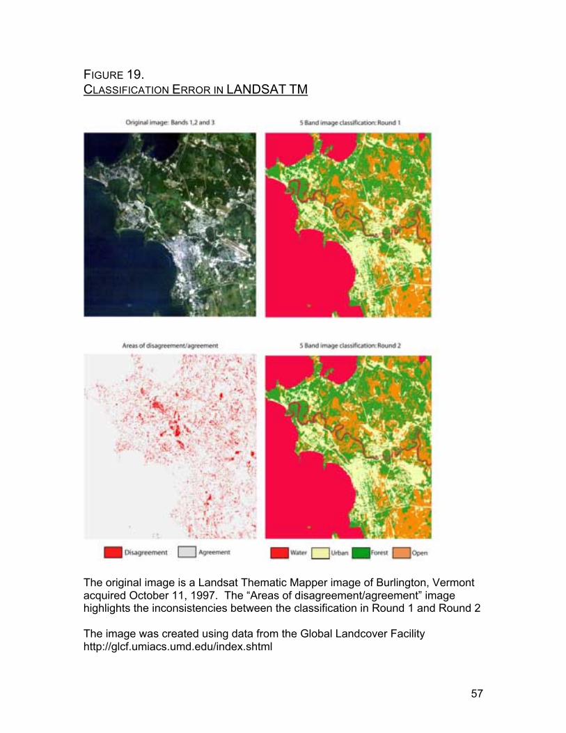
57

FIGURE 19. CLASSIFICATION ERROR IN LANDSAT TM

The original image is a Landsat Thematic Mapper image of Burlington, Vermont acquired October 11, 1997. The “Areas of disagreement/agreement” image highlights the inconsistencies between the classification in Round 1 and Round 2 The image was created using data from the Global Landcover Facility http://glcf.umiacs.umd.edu/index.shtml

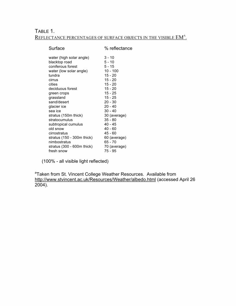
TABLE 1. REFLECTANCE PERCENTAGES OF SURFACE OBJECTS IN THE VISIBLE EMA.

Surface % reflectance

water (high solar angle) 3 - 10 blacktop road 5 - 10 coniferous forest 5 - 15 water (low solar angle) 10 - 100 tundra 15 - 20 cirrus 15 - 20 cities 15 - 20 deciduous forest 15 - 20 green crops 15 - 25 grassland 15 - 25 sand/desert 20 - 30 glacier ice 20 - 40 sea ice 30 - 40 stratus (150m thick) 30 (average) stratocumulus 35 - 80 subtropical cumulus 40 - 45 old snow 40 - 60 cirrostratus 45 - 60 stratus (150 - 300m thick) 60 (average) nimbostratus 65 - 70 stratus (300 - 600m thick) 70 (average) fresh snow 75 - 95

(100% - all visible light reflected) aTaken from St. Vincent College Weather Resources. Available from http://www.stvincent.ac.uk/Resources/Weather/albedo.html (accessed April 26 2004).

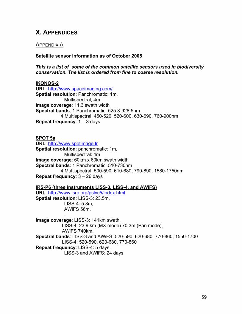
59

X. APPENDICES APPENDIX A Satellite sensor information as of October 2005

This is a list of some of the common satellite sensors used in biodiversity conservation. The list is ordered from fine to coarse resolution. IKONOS-2 URL: http://www.spaceimaging.com/ Spatial resolution: Panchromatic: 1m,

Multispectral; 4m Image coverage: 11.3 swath width Spectral bands: 1 Panchromatic: 525.8-928.5nm

4 Multispectral: 450-520, 520-600, 630-690, 760-900nm Repeat frequency: 1 – 3 days SPOT 5a URL: http://www.spotimage.fr Spatial resolution: panchromatic: 1m,

Multispectral: 4m Image coverage: 60km x 60km swath width Spectral bands: 1 Panchromatic: 510-730nm

4 Multispectral: 500-590, 610-680, 790-890, 1580-1750nm Repeat frequency: 3 – 26 days IRS-P6 (three instruments LISS-3, LISS-4, and AWiFS) URL: http://www.isro.org/pslvc5/index.html Spatial resolution: LISS-3: 23.5m,

LISS-4: 5.8m, AWiFS 56m. .

Image coverage: LISS-3: 141km swath, LISS-4: 23.9 km (MX mode) 70.3m (Pan mode), AWiFS 740km.

Spectral bands: LISS-3 and AWiFS: 520-590, 620-680, 770-860, 1550-1700 LISS-4: 520-590, 620-680, 770-860

Repeat frequency: LISS-4: 5 days, LISS-3 and AWiFS: 24 days

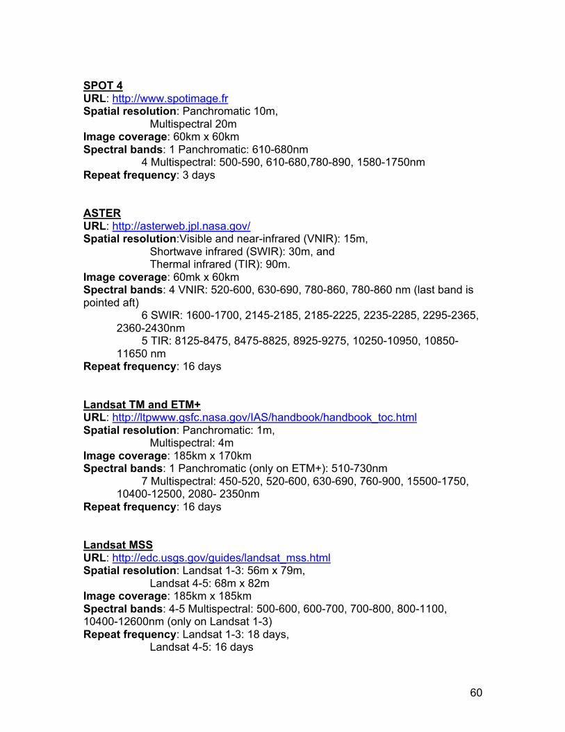
60

SPOT 4 URL: http://www.spotimage.fr Spatial resolution: Panchromatic 10m,

Multispectral 20m Image coverage: 60km x 60km Spectral bands: 1 Panchromatic: 610-680nm

4 Multispectral: 500-590, 610-680,780-890, 1580-1750nm Repeat frequency: 3 days ASTER URL: http://asterweb.jpl.nasa.gov/ Spatial resolution:Visible and near-infrared (VNIR): 15m,

Shortwave infrared (SWIR): 30m, and Thermal infrared (TIR): 90m.

Image coverage: 60mk x 60km Spectral bands: 4 VNIR: 520-600, 630-690, 780-860, 780-860 nm (last band is pointed aft)

6 SWIR: 1600-1700, 2145-2185, 2185-2225, 2235-2285, 2295-2365, 2360-2430nm

5 TIR: 8125-8475, 8475-8825, 8925-9275, 10250-10950, 10850-11650 nm

Repeat frequency: 16 days Landsat TM and ETM+ URL: http://ltpwww.gsfc.nasa.gov/IAS/handbook/handbook_toc.html Spatial resolution: Panchromatic: 1m,

Multispectral: 4m Image coverage: 185km x 170km Spectral bands: 1 Panchromatic (only on ETM+): 510-730nm

7 Multispectral: 450-520, 520-600, 630-690, 760-900, 15500-1750, 10400-12500, 2080- 2350nm

Repeat frequency: 16 days Landsat MSS URL: http://edc.usgs.gov/guides/landsat_mss.html Spatial resolution: Landsat 1-3: 56m x 79m,

Landsat 4-5: 68m x 82m Image coverage: 185km x 185km Spectral bands: 4-5 Multispectral: 500-600, 600-700, 700-800, 800-1100, 10400-12600nm (only on Landsat 1-3) Repeat frequency: Landsat 1-3: 18 days,

Landsat 4-5: 16 days

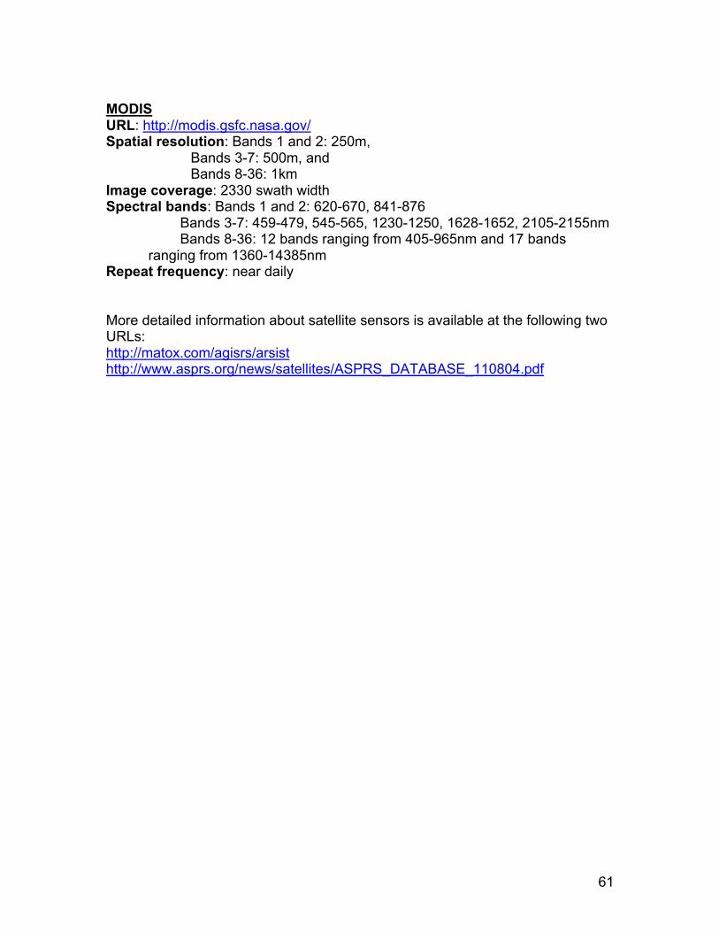
61

MODIS URL: http://modis.gsfc.nasa.gov/ Spatial resolution: Bands 1 and 2: 250m,

Bands 3-7: 500m, and Bands 8-36: 1km

Image coverage: 2330 swath width Spectral bands: Bands 1 and 2: 620-670, 841-876

Bands 3-7: 459-479, 545-565, 1230-1250, 1628-1652, 2105-2155nm Bands 8-36: 12 bands ranging from 405-965nm and 17 bands

ranging from 1360-14385nm Repeat frequency: near daily More detailed information about satellite sensors is available at the following two URLs: http://matox.com/agisrs/arsist http://www.asprs.org/news/satellites/ASPRS_DATABASE_110804.pdf