/II

Graduate Course

DISCIPLINE SPECIFIC CORE COURSE / In Lieu of

MODERN INDIAN LANGUAGE

Principles of Microeconomic I

CONTENTS

Lesson 9 : Production

Lesson 10 : Cost

Lesson 11 : Economics of Scale

Lesson 12 : Perfect Competition

Editor :

Dr. Janmejoy Khuntia

SCHOOL OF OPEN LEARNING University of Delhi

5, Cavalry Lane, Delhi-110007

1

LESSON: 9

PRODUCTION

INTRODUCTION

Traditional economic theory centers around the working of a capitalist economy (which is also

termed as free enterprise or free market economy). As observed earlier too, all the three central

problems (viz. (1) what goods to produce and in what quantities, (2) how to produce them, and (3)

how to distribute the net output amongst the members of society) are solved basically through the

price mechanism in a capitalist economy. Price mechanism is nothing but the sum total of all

prices (both of goods and factors of production) prevailing in the economy and determined jointly

by the forces of demand and supply in the respective markets. You have had an elementary view

of the price mechanism in a previous set, but for a thorough understanding, it is necessary to go

deeper into what lies behind the forces of demand and supply in a capitalist economy. Set 4 gave

you a fair idea of the major factors underlying demand and how changes in them influence the

latter. We now propose to take up supply or production for a detailed analysis. Only after

examining what lies beneath the forces of demand and supply, will you be equipped to analyse

the working of price mechanism in a capitalist economy in all its aspects.

While analyzing the behaviour of a consumer (i.e., the basic decision-taking unit in the theory

of Demand) and determining his equilibrium, it was assumed that the consumer, being a rational

human being, always tries to maximize his utility. In the field of production economics, firms -

the basic decision-taking units - are assumed to have profit maximization as their objective. The

common-sense relationship between rationality and maximization of utility (utility being defined

as the capacity of a good to yield satisfaction) is more obvious and justifiable than the rationality

of the goal of profit maximization in the context of firms. Still, the latter is basic to the traditional

economic analysis of a private enterprise economy. It follows from this basic premise that a firm

will always try to operate at that level of price and output at which the difference between its total

revenue and total cost is the largest. We take up the cost aspect first, postponing the discussion of

revenue conditions of a firm to the next set of lessons. The cost of production of a commodity

depends upon two things: (i) the quantities of various factors of production used and their

physical productivities, and (ii) prices per unit of the factors of production. The former specifies

purely technical relationships while the latter has to be taken into account by the firms when

taking economic decisions. We shall consider the technical relationships first.

After going through this lesson, you will be able to : -

• Define production function.

• Distinguish between short and long run production function.

• Explain the working of the law of variable proportions.

• Explain the law of returns to scale in the long run.

• Define and draw isoquant for two variable inputs.

• Determine the equilibrium of a producer, and the choice of optimum combination of

factors.

• Find out explanation path of the producer.

2

9.1 CONCEPT OF PRODUCTION FUNCTION

You know that various inputs are required to produce a particular product. For example,

land, water, seeds, fertilizers, plough, bullocks etc., are required to produce wheat. Similarly, a

firm planning to produce cloth requires a factory, workers with requisite skills, cotton yam,

machinery, fuel, tools and implements etc. Economists divide inputs into certain broad categories

on the basis of similar economic features and call them ‘factors of production’. The outcome of

the process of production using these factor inputs is called output which may be a final

consumption good (e.g.. bread, cloth), a service (e.g., teaching), an intermediate good (e.g. coal

for a steel furnace or power for a cloth mill) or a durable-use capital good (e.g. factory building,

blast furnace). Now the production function describes the technical relation that may exist at any

time between the quantities of factor inputs and the resulting output, given the prevailing state of

technology. It describes the laws governing transformation of factor inputs into products per unit

of time. In other words the production function represents the technology of a firm or industry or

the economy as a whole. Thus, with technological progress, the production function necessarily

undergoes a change.

Let us note that a production function includes only technically efficient methods of

production, that is, methods which produce maximum possible output for a given quantity of

factor inputs (or, which is the same thing, which use the minimum quantity of inputs for a given

output). Moreover, a production function may describe the alternative combinations of the various

factor inputs (i.e. alternative methods of production) for producing a given output or it may

describe the response of total output either (a) to changes in all factor inputs in the same or

different proportions (a long run possibility) or (b) to changes in the amounts of some variable

factor (or factors) while keeping the amount of other factors constant (a short run possibility).

A production function can be expressed either as a schedule (or a table) or as a graph (or a

curve) or in the form of an algebraic equation (or as a mathematical model). Production function

in one form can be converted in any of the alternative forms. Real life production functions

include a wide range of independent variables (i.e., factor inputs) such as land, labour, raw

materials, fixed capital, entrepreneurial- organizational efficiency, scale factor, etc.

In equation form, we can write production function as follows:

Q = f (L, K, D, E, ϒ, λ)

Where, Q = Output, f = function, L = Labour, K = Capital, D = Land, E = Entrepreneurship, ϒ

is a Greek letter pronounced as upsilon and stands for Efficiency in production, λ is a Greek letter

pronounced as lamda and stands for scale factor in production.

Intext questions:

Q.1. Define Production Function.

Q.2. What are the 4 Factors of production?

9.2 DISTINCTION BETWEEN THE SHORT-RUN AND THE LONG-RUN

PRODUCTION FUNCTIONS

There are three possible ways of increasing the level of output. Output can be increased

either by changing the amounts of all factors by the same proportion or by increasing their

amounts in different proportions or by increasing the amounts of some factor(s) while keeping the

amounts of other factors fixed. While the first two alternatives are available only in the long run,

the third alternative is available in the short run. This brings us to the important question of the

3

distinction between the short run and long run and the analytical significance of this distinction in

the present context.

The Fixed and Variable Inputs

In order to produce any commodity, a producer needs two kinds of factor inputs which can

be described as ‘variable inputs’ and ‘fixed outputs’. The amounts of some factor inputs can be

varied easily in accordance with the requirements of production as and when necessary, while the

amounts of some factors cannot be so adjusted over certain periods. The inputs of the first type

are known as ‘variable inputs’ and the inputs of the other type are known as ‘fixed inputs’. Raw

materials, direct labour, fuel, power, lubricants, ordinary repairs and maintenance, etc,, are

examples of variable inputs. Their amounts can be adjusted according to the level of output

without any difficulty. If production stops, these inputs can be completely dispensed with. On the

other hand, fixed inputs include durable-use capital goods such as machines, building, land, tools

and equipment which, if looked after and maintained, properly, can aid production over long

periods. The use of such equipment does not finish with a single act of production but extends

over several years. In other words, the returns from such durable use capital goods are spread over

the whole of their productive lives. Therefore, while planning to install such equipment, the

producer has necessarily to base his plan on the expected average level of sales over the whole of

its productive life.

The planning of a firm consists in deciding the ‘size’ of the ‘fixed’ factors, which determine

the size of the ‘plant’ because they set limits to its production. (Variable factors such as lab our

and raw materials are assumed not to set limits on ‘size’ because the firm can acquire them easily

form the market without any time lag). A businessman starts his planning with a certain figure for

the average level of output which he expects selling over the relevant period and will choose the

plant size which will enable him to produce that level of output most efficiently over the whole of

its productive life. Before an investment is decided, the producer is in the long-run situation in the

sense that he is free to choose any plant size from among the different available plant sizes. Once,

However, the investment decision is taken and funds are tied up in a given plant, the producer’s

long-run freedom of choice ceases. So long as the productive life of the installed plant lasts he

cannot discard it and choose another plant simply because of the heavy costs involved. During

this period he can meet fluctuations in demand only by working the given plant more or less

intensively (i.e., by applying larger or smaller amounts of other variable inputs with the given

plant), but cannot choose a different plant. Executives, managers, supervisors and other

permanent staff, constituting what is known as the ‘management of the firm’, are also of the

nature of fixed inputs. Their services also cannot be adjusted in accordance with the requirements

of output. The configuration of the durable use capital goods and the management, known as

‘plant’, represents affixed cost for the producer because he cannot escape these costs even if he

stops production completely. That is the reason why the costs of such inputs are called ‘fixed

costs’.

We will discuss this aspect latter in greater detail. At this point it should suffice to say that

in the short run a producer can increase or decrease the level of output only by increasing or

decreasing the application of ‘variable’ inputs with a fixed amount of some other factors (i.e., the

plant). On the other hand, in the long run (when the producer is free from short-run commitments)

all factors are variable and he can vary the level of output by varying the amounts of all factors.

Short run may be defined as the period which is too short to permit firms to adjust amounts of all

factors in accordance with the requirements of production but long enough to permit adjustment

of output by applying larger or smaller amounts of variable factors with the fixed equipment of

the firm. Long run, on the other hand, refers to the time period which is long enough to permit

firms to adjust amounts of all factors to suit long-run requirements. Short and long runs do not

refer to any definite time period . Short and long periods vary from industry to industry. For

4

example, the short run from the standpoint of steel industry may range over five to seven decades,

whereas it may be just a few months for fishermen who do not use much fixed capital except their

fishing nets.

Corresponding to the distinction between short and long runs, we have short-run and long-run

production functions. The short-run production function describes the technical relation between

the quantities of some variable input(s) and the resulting output when amounts of some factors are

fixed. On the other hand, the long run production function describes the technical relation

between quantities of factor inputs and the resulting output when amounts of all factors are

variable in the same proportion or different proportions.

Intext Questions:

Q.1. Fill in the blanks:

• All inputs/Factors of Production become variable in nature in the _______ run.

(Answer: Long Run)

Q.2. True/False:

• 'Plant size' of a firm is a variable input / Factor of Production.

(Answer: False)

• Raw materials, Fuel, power are variable factors of production.

(Answer: True)

• All Factor of Production are fixed (in nature) I the short run

(Answer: False)

9.3 THE SHORT-RUN PRODUCTION FUNCTION

In the preceding section we explained in some detail the basis of the distinction between the

long-run and the short-run. Short-run is a period during which the durable-use capital equipments

(and also the management) of a firm are fixed and changes in output can be brought about only by

applying larger or smaller amounts of the variable factor(s) with the given equipment. When a

firm tries to increase its output in this way, it evidently changes the proportion between the fixed

and the variable factors. Let us assume that fixed factors are represented by capital (K) and

variable factors are represented by labour (L).

We can write the short-run production function as:

Q = f (L) Ќ

This says that output (Q) is a function of or depends on labour (L) given fixed amount of

capital at Ќ.

The production function in this case is described by the Law of Variable Proportions or what

is more popularly known as the ‘Law of Diminishing Returns’.

Assuming that there is only one variable factor (consisting of homogeneous units) and

constant technology, the Law can be stated as follows:

‘Other things remaining constant, when more and more units of a variable factor are used

with a fixed quantity of other factors, eventually the marginal product of the variable factor starts

diminishing’. Marginal product refers to the addition made to total output due to the use of an

additional unit of a variable factor, the amounts of all other factors remaining constant. For

example, if due to the employment of 11 labours instead of 10 the total output increases form 100

5

units to 115 units per day, in that case the marginal product due to the eleventh labourer will be

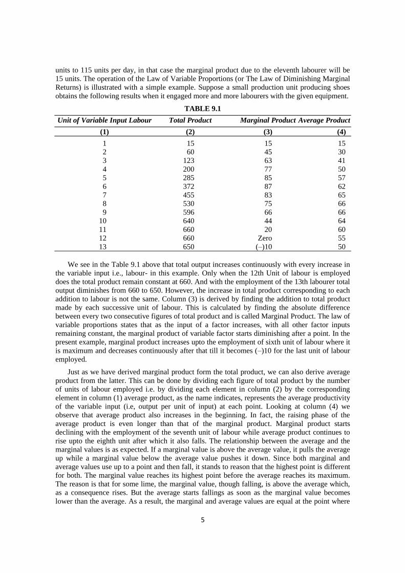
15 units. The operation of the Law of Variable Proportions (or The Law of Diminishing Marginal

Returns) is illustrated with a simple example. Suppose a small production unit producing shoes

obtains the following results when it engaged more and more labourers with the given equipment.

TABLE 9.1

Unit of Variable Input Labour Total Product Marginal Product Average Product

(1) (2) (3) (4)

1 15 15 15

2 60 45 30

3 123 63 41

4 200 77 50

5 285 85 57

6 372 87 62

7 455 83 65

8 530 75 66

9 596 66 66

10 640 44 64

11 660 20 60

12 660 Zero 55

13 650 (–)10 50

We see in the Table 9.1 above that total output increases continuously with every increase in

the variable input i.e., labour- in this example. Only when the 12th Unit of labour is employed

does the total product remain constant at 660. And with the employment of the 13th labourer total

output diminishes from 660 to 650. However, the increase in total product corresponding to each

addition to labour is not the same. Column (3) is derived by finding the addition to total product

made by each successive unit of labour. This is calculated by finding the absolute difference

between every two consecutive figures of total product and is called Marginal Product. The law of

variable proportions states that as the input of a factor increases, with all other factor inputs

remaining constant, the marginal product of variable factor starts diminishing after a point. In the

present example, marginal product increases upto the employment of sixth unit of labour where it

is maximum and decreases continuously after that till it becomes (–)10 for the last unit of labour

employed.

Just as we have derived marginal product form the total product, we can also derive average

product from the latter. This can be done by dividing each figure of total product by the number

of units of labour employed i.e. by dividing each element in column (2) by the corresponding

element in column (1) average product, as the name indicates, represents the average productivity

of the variable input (i.e, output per unit of input) at each point. Looking at column (4) we

observe that average product also increases in the beginning. In fact, the raising phase of the

average product is even longer than that of the marginal product. Marginal product starts

declining with the employment of the seventh unit of labour while average product continues to

rise upto the eighth unit after which it also falls. The relationship between the average and the

marginal values is as expected. If a marginal value is above the average value, it pulls the average

up while a marginal value below the average value pushes it down. Since both marginal and

average values use up to a point and then fall, it stands to reason that the highest point is different

for both. The marginal value reaches its highest point before the average reaches its maximum.

The reason is that for some lime, the marginal value, though falling, is above the average which,

as a consequence rises. But the average starts fallings as soon as the marginal value becomes

lower than the average. As a result, the marginal and average values are equal at the point where

6

the average reaches its highest point, in the example given above, this happens when the ninth

unit of labour is employed. You may also observe that the marginal product falls at a much faster

rate compared to the average product which experience a relatively gradual decline. As for the

reason for first rising and then falling average product we may say that there exists an optimum

proportion in which fixed and variable inputs can be combined. When the variable input is

combined with the fixed factors in this particular proportion, average product attains its highest

value or output per unit of input is the maximum. Before this point, the variable input is spread

too sparsely over the fixed factor inputs and every increase in the variable input leads to a more

than proportionate increase in total product, thus raising the average product. After this point, the

variable input is used too intensively and further increases in this input result in less than

proportionate increase in total product, thus lowering the average product.

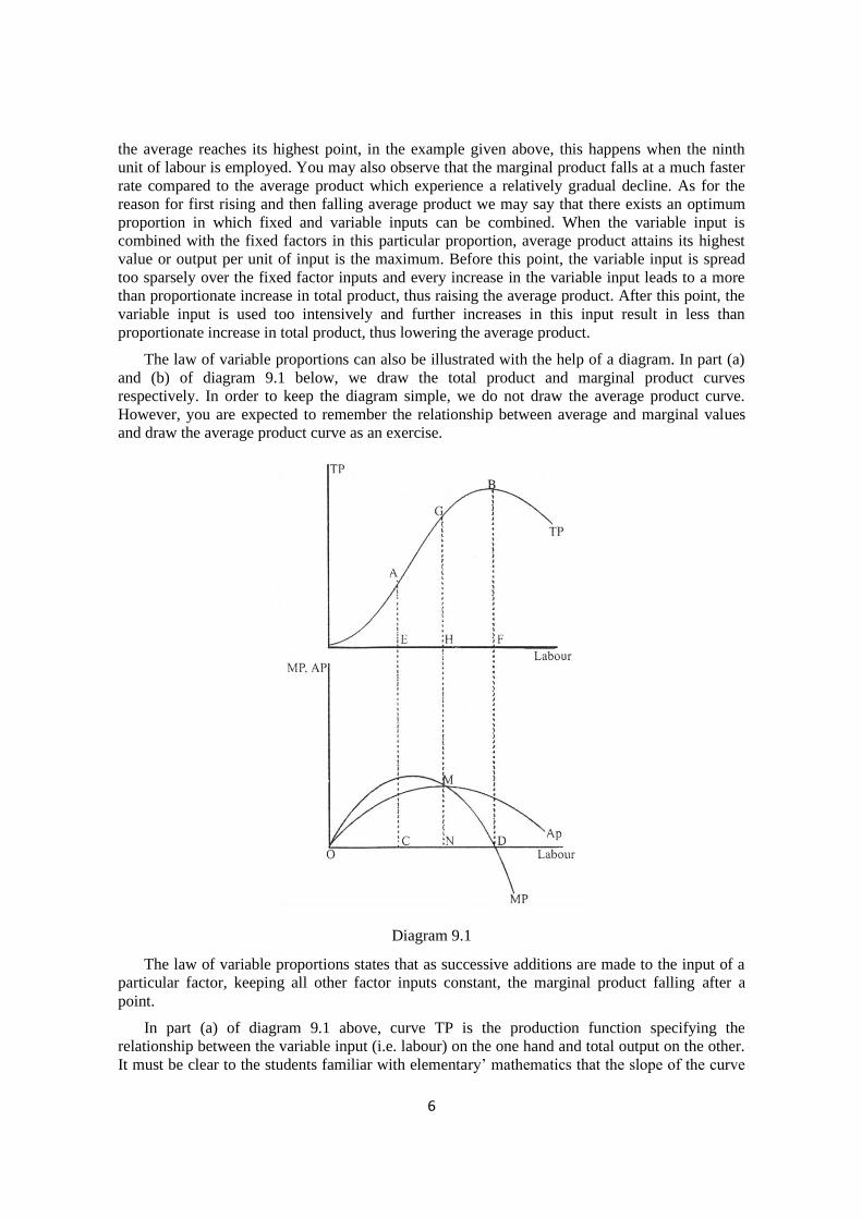
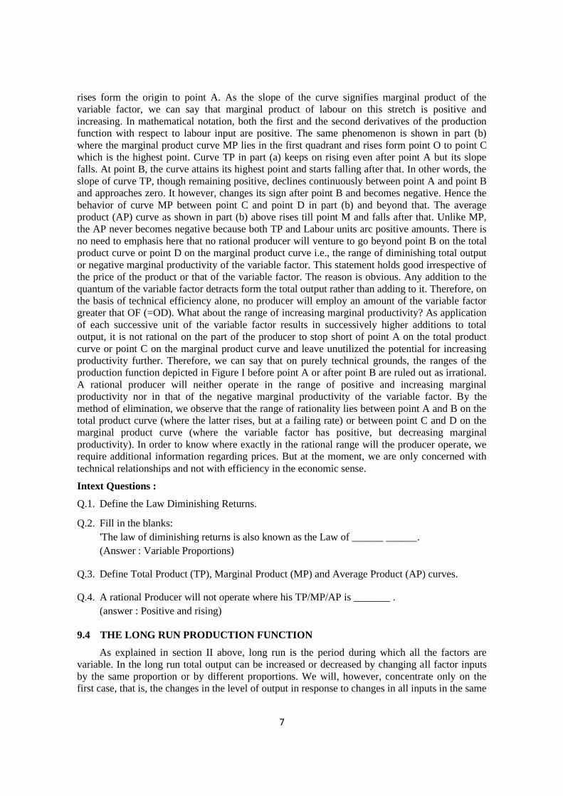
The law of variable proportions can also be illustrated with the help of a diagram. In part (a)

and (b) of diagram 9.1 below, we draw the total product and marginal product curves

respectively. In order to keep the diagram simple, we do not draw the average product curve.

However, you are expected to remember the relationship between average and marginal values

and draw the average product curve as an exercise.

Diagram 9.1

The law of variable proportions states that as successive additions are made to the input of a

particular factor, keeping all other factor inputs constant, the marginal product falling after a

point.

In part (a) of diagram 9.1 above, curve TP is the production function specifying the

relationship between the variable input (i.e. labour) on the one hand and total output on the other.

It must be clear to the students familiar with elementary’ mathematics that the slope of the curve

7

rises form the origin to point A. As the slope of the curve signifies marginal product of the

variable factor, we can say that marginal product of labour on this stretch is positive and

increasing. In mathematical notation, both the first and the second derivatives of the production

function with respect to labour input are positive. The same phenomenon is shown in part (b)

where the marginal product curve MP lies in the first quadrant and rises form point O to point C

which is the highest point. Curve TP in part (a) keeps on rising even after point A but its slope

falls. At point B, the curve attains its highest point and starts falling after that. In other words, the

slope of curve TP, though remaining positive, declines continuously between point A and point B

and approaches zero. It however, changes its sign after point B and becomes negative. Hence the

behavior of curve MP between point C and point D in part (b) and beyond that. The average

product (AP) curve as shown in part (b) above rises till point M and falls after that. Unlike MP,

the AP never becomes negative because both TP and Labour units arc positive amounts. There is

no need to emphasis here that no rational producer will venture to go beyond point B on the total

product curve or point D on the marginal product curve i.e., the range of diminishing total output

or negative marginal productivity of the variable factor. This statement holds good irrespective of

the price of the product or that of the variable factor. The reason is obvious. Any addition to the

quantum of the variable factor detracts form the total output rather than adding to it. Therefore, on

the basis of technical efficiency alone, no producer will employ an amount of the variable factor

greater that OF (=OD). What about the range of increasing marginal productivity? As application

of each successive unit of the variable factor results in successively higher additions to total

output, it is not rational on the part of the producer to stop short of point A on the total product

curve or point C on the marginal product curve and leave unutilized the potential for increasing

productivity further. Therefore, we can say that on purely technical grounds, the ranges of the

production function depicted in Figure I before point A or after point B are ruled out as irrational.

A rational producer will neither operate in the range of positive and increasing marginal

productivity nor in that of the negative marginal productivity of the variable factor. By the

method of elimination, we observe that the range of rationality lies between point A and B on the

total product curve (where the latter rises, but at a failing rate) or between point C and D on the

marginal product curve (where the variable factor has positive, but decreasing marginal

productivity). In order to know where exactly in the rational range will the producer operate, we

require additional information regarding prices. But at the moment, we are only concerned with

technical relationships and not with efficiency in the economic sense.

Intext Questions :

Q.1. Define the Law Diminishing Returns.

Q.2. Fill in the blanks:

'The law of diminishing returns is also known as the Law of ______ ______.

(Answer : Variable Proportions)

Q.3. Define Total Product (TP), Marginal Product (MP) and Average Product (AP) curves.

Q.4. A rational Producer will not operate where his TP/MP/AP is _______ .

(answer : Positive and rising)

9.4 THE LONG RUN PRODUCTION FUNCTION

As explained in section II above, long run is the period during which all the factors are

variable. In the long run total output can be increased or decreased by changing all factor inputs

by the same proportion or by different proportions. We will, however, concentrate only on the

first case, that is, the changes in the level of output in response to changes in all inputs in the same

8

proportion. The term ‘returns to scale’ refers to the response of total output to changes in all

inputs by the same proportion. The laws of "returns to scale’ refer to the effects of scale

relationships. However, before studying the laws of ‘returns to scale’ let us explain and important

tool of analysis- the concept of an ‘isoquant’ (’iso’ meaning equal and ‘quant’ meaning quantity).

An ‘isoquant’ or an ‘iso-product curve’ is a graphical depiction of the alternative combinations of

two factor inputs (i.e. methods of production) to produce a given level of output.

The Concept of Isoquant

Usually, it is possible to produce a commodity using different combinations of factor inputs (or

what is the same thing, methods of production). For example, it may be possible to produce one

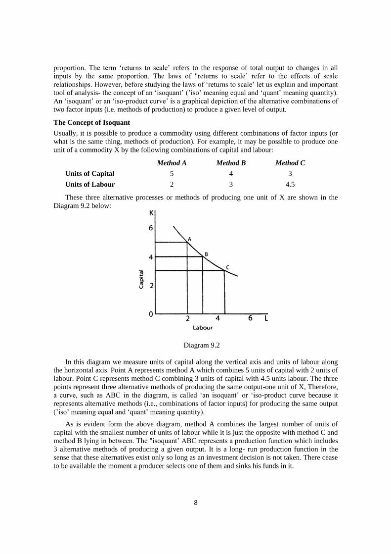
unit of a commodity X by the following combinations of capital and labour:

Method A Method B Method C

Units of Capital 5 4 3

Units of Labour 2 3 4.5

These three alternative processes or methods of producing one unit of X are shown in the

Diagram 9.2 below:

Diagram 9.2

In this diagram we measure units of capital along the vertical axis and units of labour along

the horizontal axis. Point A represents method A which combines 5 units of capital with 2 units of

labour. Point C represents method C combining 3 units of capital with 4.5 units labour. The three

points represent three alternative methods of producing the same output-one unit of X, Therefore,

a curve, such as ABC in the diagram, is called ‘an isoquant’ or ‘iso-product curve because it

represents alternative methods (i.e., combinations of factor inputs) for producing the same output

(’iso’ meaning equal and ‘quant’ meaning quantity).

As is evident form the above diagram, method A combines the largest number of units of

capital with the smallest number of units of labour while it is just the opposite with method C and

method B lying in between. The "isoquant’ ABC represents a production function which includes

3 alternative methods of producing a given output. It is a long- run production function in the

sense that these alternatives exist only so long as an investment decision is not taken. There cease

to be available the moment a producer selects one of them and sinks his funds in it.

9

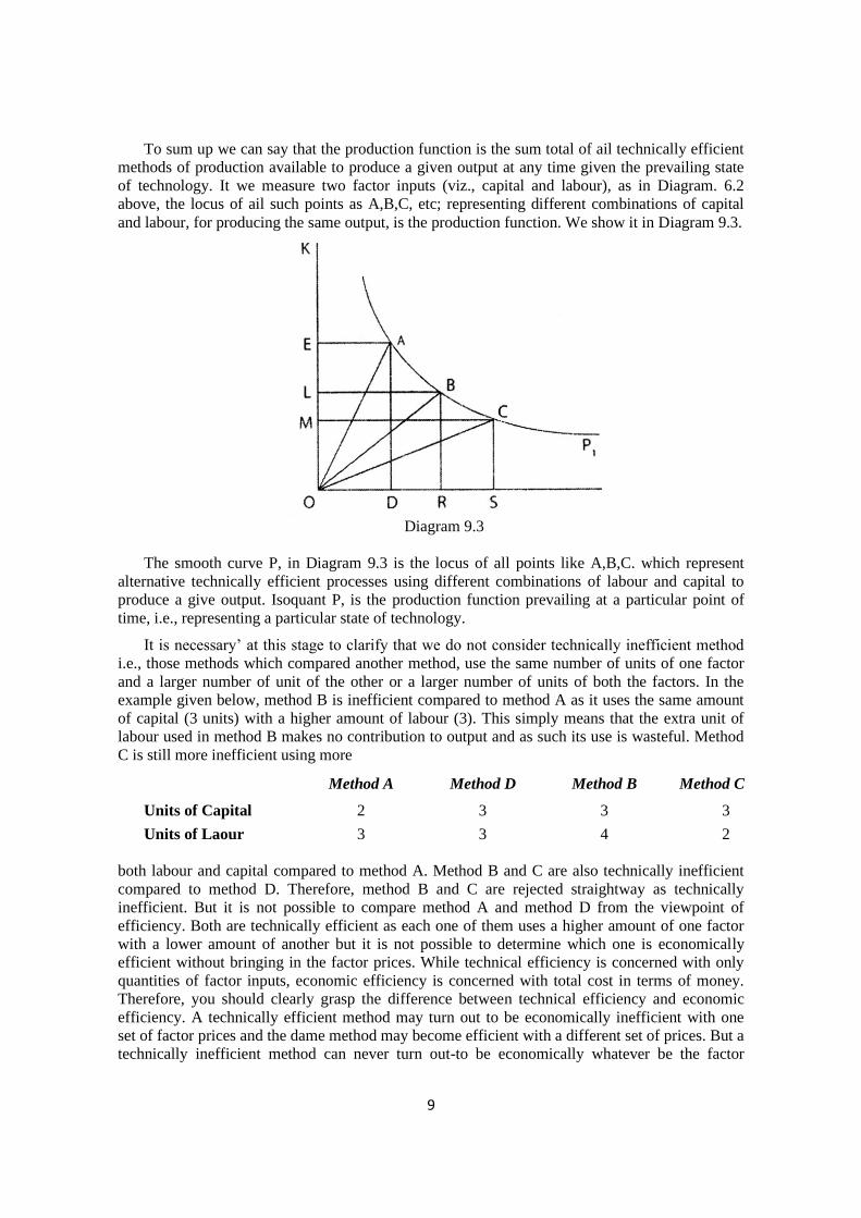
To sum up we can say that the production function is the sum total of ail technically efficient

methods of production available to produce a given output at any time given the prevailing state

of technology. It we measure two factor inputs (viz., capital and labour), as in Diagram. 6.2

above, the locus of ail such points as A,B,C, etc; representing different combinations of capital

and labour, for producing the same output, is the production function. We show it in Diagram 9.3.

Diagram 9.3

The smooth curve P, in Diagram 9.3 is the locus of all points like A,B,C. which represent

alternative technically efficient processes using different combinations of labour and capital to

produce a give output. Isoquant P, is the production function prevailing at a particular point of

time, i.e., representing a particular state of technology.

It is necessary’ at this stage to clarify that we do not consider technically inefficient method

i.e., those methods which compared another method, use the same number of units of one factor

and a larger number of unit of the other or a larger number of units of both the factors. In the

example given below, method B is inefficient compared to method A as it uses the same amount

of capital (3 units) with a higher amount of labour (3). This simply means that the extra unit of

labour used in method B makes no contribution to output and as such its use is wasteful. Method

C is still more inefficient using more

Method A Method D Method B Method C

Units of Capital 2 3 3 3

Units of Laour 3 3 4 2

both labour and capital compared to method A. Method B and C are also technically inefficient

compared to method D. Therefore, method B and C are rejected straightway as technically

inefficient. But it is not possible to compare method A and method D from the viewpoint of

efficiency. Both are technically efficient as each one of them uses a higher amount of one factor

with a lower amount of another but it is not possible to determine which one is economically

efficient without bringing in the factor prices. While technical efficiency is concerned with only

quantities of factor inputs, economic efficiency is concerned with total cost in terms of money.

Therefore, you should clearly grasp the difference between technical efficiency and economic

efficiency. A technically efficient method may turn out to be economically inefficient with one

set of factor prices and the dame method may become efficient with a different set of prices. But a

technically inefficient method can never turn out-to be economically whatever be the factor

10

prices. We illustrate this point with a simple example. Let us suppose that in order to produce a

unit of X the following three methods are available:

Method A Method B Method C

Units of Capital 5 4 3

Units of Labour 3 4 5

It we assume per unit prices of capital and labour to be Rs. 5 and Rs. 3 respectively, then

method C is the most efficient. However, if the per unit prices of capital and labour are Rs. 3 and

Rs. 5 respectively, in that case method A turns out to be the cheapest. Thus, technical efficiency

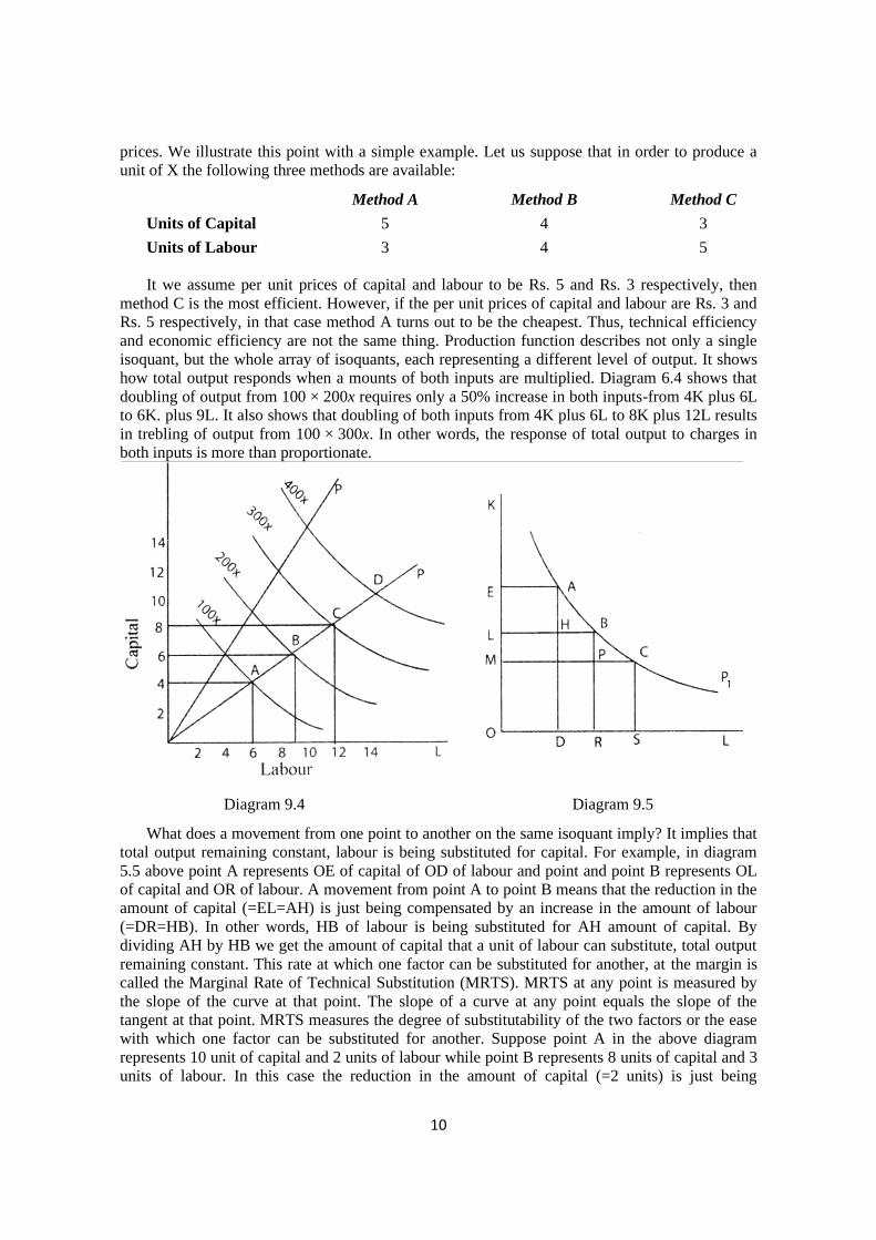
and economic efficiency are not the same thing. Production function describes not only a single

isoquant, but the whole array of isoquants, each representing a different level of output. It shows

how total output responds when a mounts of both inputs are multiplied. Diagram 6.4 shows that

doubling of output from 100 × 200x requires only a 50% increase in both inputs-from 4K plus 6L

to 6K. plus 9L. It also shows that doubling of both inputs from 4K plus 6L to 8K plus 12L results

in trebling of output from 100 × 300x. In other words, the response of total output to charges in

both inputs is more than proportionate.

Diagram 9.4 Diagram 9.5

What does a movement from one point to another on the same isoquant imply? It implies that

total output remaining constant, labour is being substituted for capital. For example, in diagram

5.5 above point A represents OE of capital of OD of labour and point and point B represents OL

of capital and OR of labour. A movement from point A to point B means that the reduction in the

amount of capital (=EL=AH) is just being compensated by an increase in the amount of labour

(=DR=HB). In other words, HB of labour is being substituted for AH amount of capital. By

dividing AH by HB we get the amount of capital that a unit of labour can substitute, total output

remaining constant. This rate at which one factor can be substituted for another, at the margin is

called the Marginal Rate of Technical Substitution (MRTS). MRTS at any point is measured by

the slope of the curve at that point. The slope of a curve at any point equals the slope of the

tangent at that point. MRTS measures the degree of substitutability of the two factors or the ease

with which one factor can be substituted for another. Suppose point A in the above diagram

represents 10 unit of capital and 2 units of labour while point B represents 8 units of capital and 3

units of labour. In this case the reduction in the amount of capital (=2 units) is just being

11

compensated by one unity increase in the amount of labour so that the total output remains the

same. In other words, the MRTS of labour for capital in this case is(–)2/l = (–)2.

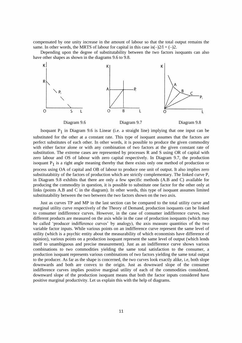
Depending upon the degree of substitutability between the two factors isoquants can also

have other shapes as shown in the diagrams 9.6 to 9.8.

Diagram 9.6 Diagram 9.7 Diagram 9.8

Isoquant P1 in Diagram 9.6 is Linear (i.e. a straight line) implying that one input can be

substituted for the other at a constant rate. This type of isoquant assumes that the factors are

perfect substitutes of each other. In other words, it is possible to produce the given commodity

with either factor alone or with any combination of two factors at the given constant rate of

substitution. The extreme cases are represented by processes R and S using OR of capital with

zero labour and OS of labour with zero capital respectively. In Diagram 9.7, the production

isoquant P1 is a right angle meaning thereby that there exists only one method of production or

process using OA of capital and OB of labour to produce one unit of output. It also implies zero

substitutabitity of the factors of production which are strictly complementary. The linked curve P,

in Diagram 9.8 exhibits that there are only a few specific methods (A.B and C) available for

producing the commodity in question, it is possible to substitute one factor for the other only at

links (points A.B and C in the diagram). In other words, this type of isoquant assumes limited

substitutability between the two between the two factors shown on the two axis.

Just as curves TP and MP in the last section can be compared to the total utility curve and

marginal utility curve respectively of the Theory of Demand, production isoquants can be linked

to consumer indifference curves. However, in the case of consumer indifference curves, two

different products are measured on the axis while in the case of production isoquants (which may

be called ‘producer indifference curves’ by analogy), the axis measure quantities of the two

variable factor inputs. While various points on an indifference curve represent the same level of

utility (which is a psychic entity about the measurability of which economists have difference of

opinion), various points on a production isoquant represent the same level of output (which lends

itself to unambiguous and precise measurement). Just as an indifference curve shows various

combinations to two commodities yielding the same total satisfaction to the consumer, a

production isoquant represents various combinations of two factors yielding the same total output

to the producer. As far as the shape is concerned, the two curves look exactly alike, i.e, both slope

downwards and both are convex to the origin. Just as downward slope of the consumer

indifference curves implies positive marginal utility of each of the commodities considered,

downward slope of the production isoquant means that both the factor inputs considered have

positive marginal productivity. Let us explain this with the help of diagrams.

12

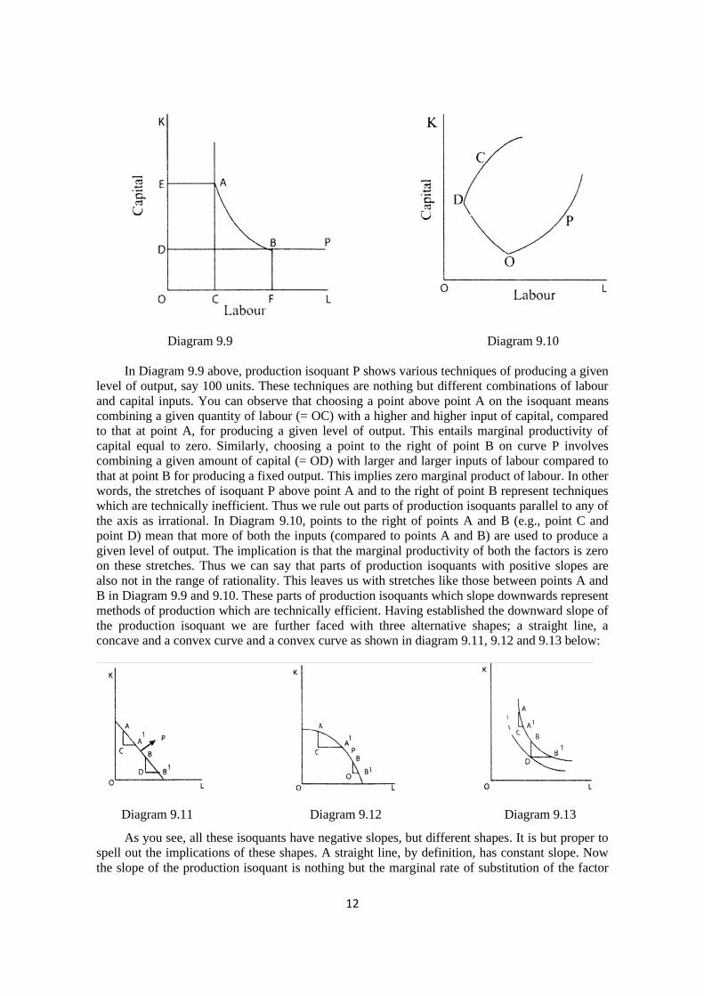
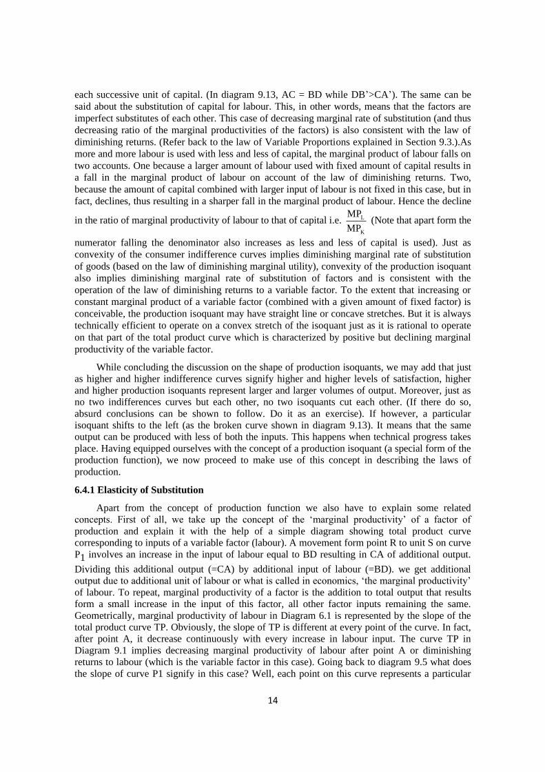
Diagram 9.9 Diagram 9.10

In Diagram 9.9 above, production isoquant P shows various techniques of producing a given

level of output, say 100 units. These techniques are nothing but different combinations of labour

and capital inputs. You can observe that choosing a point above point A on the isoquant means

combining a given quantity of labour (= OC) with a higher and higher input of capital, compared

to that at point A, for producing a given level of output. This entails marginal productivity of

capital equal to zero. Similarly, choosing a point to the right of point B on curve P involves

combining a given amount of capital (= OD) with larger and larger inputs of labour compared to

that at point B for producing a fixed output. This implies zero marginal product of labour. In other

words, the stretches of isoquant P above point A and to the right of point B represent techniques

which are technically inefficient. Thus we rule out parts of production isoquants parallel to any of

the axis as irrational. In Diagram 9.10, points to the right of points A and B (e.g., point C and

point D) mean that more of both the inputs (compared to points A and B) are used to produce a

given level of output. The implication is that the marginal productivity of both the factors is zero

on these stretches. Thus we can say that parts of production isoquants with positive slopes are

also not in the range of rationality. This leaves us with stretches like those between points A and

B in Diagram 9.9 and 9.10. These parts of production isoquants which slope downwards represent

methods of production which are technically efficient. Having established the downward slope of

the production isoquant we are further faced with three alternative shapes; a straight line, a

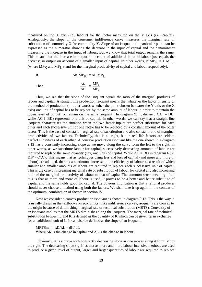
concave and a convex curve and a convex curve as shown in diagram 9.11, 9.12 and 9.13 below:

Diagram 9.11 Diagram 9.12 Diagram 9.13

As you see, all these isoquants have negative slopes, but different shapes. It is but proper to

spell out the implications of these shapes. A straight line, by definition, has constant slope. Now

the slope of the production isoquant is nothing but the marginal rate of substitution of the factor

13

measured on the X axis (i.e., labour) for the factor measured on the Y axis (i.e., capital).

Analogously, the slope of the consumer indifference curve measures the marginal rate of

substitution of commodity X for commodity Y. Slope of an isoquant at a particular point can be

expressed as the numerator showing the decrease in the input of capital and the denominator

measuring the increase in the input of labour. But we know that total output remains the same.

This means that the increase in output on account of additional input of labour just equals the

decrease in output on account of a smaller input of capital. In other words, K.MPK = L.MPL,

(where MPK and MPL stand for the marginal productivity of capital and labour respectively).

If K.MPK = L.MPL

Then K

L

= L

K

MP

MP

Thus, we see that the slope of the isoquant equals the ratio of the marginal products of

labour and capital. A straight line production isoquant means that whatever the factor intensity of

the method of production (in other words whether the point chosen is nearer the Y axis or the X

axis) one unit of capital has to be replace by the same amount of labour in order to maintain the

given level of output (or remain on the same isoquant). In diagram 9.11, distance CA’ = DB’

while AC (=BD) represents one unit of capital. In other words, we can say that a straight line

isoquant characterises the situation when the two factor inputs are perfect substitutes for each

other and each successive unit of one factor has to be replaced by a constant amount of the other

factor. This is the case of constant marginal rate of substitution and also constant ratio of marginal

productivities of two factors. Technically, this is all right, but in real life factors are seldom

perfect substitutes of each other. A concave production isoquant like the one shown in a diagram

9.12 has a constantly increasing slope as we move along the curve form the left to the right. In

other words, as we substitute labour for capital, successively decreasing amounts of labour are

required to replace the same quantity (say, one unit) of capital. While AC = BD in diagram 6.12,

DB’ <C’A>. This means that as techniques using less and less of capital (and more and more of

labour) are adopted, there is a continuous increase in the efficiency of labour as a result of which

smaller and smaller amounts of labour are required to replace each successsive unit of capital.

This is the case of increasing marginal rate of substitution of labour for capital and also increasing

ratio of the marginal productivity of labour to that of capital.The common sense meaning of all

this is that as more and more of labour is used, it proves to be a better and better substitute of

capital and the same holds good for capital. The obvious implication is that a rational producer

should never choose a method using both the factors. We shall take it up again in the context of

the optimum, combination of factors in section IV.

Now we consider a convex production isoquant as shown in diagram 9.13. This is the way it

is usually drawn in the textbooks on economics. Like indifference curves, isoquants are convex to

the origin because of diminishing marginal rate of technical substitution (MRTS). Convexity of

an isoquant implies that the MRTS diminishes along the isoquant. The marginal rate of technical

substitution between L and K is defined as the quantity of K which can be given up in exchange

for an additional unit of L. It can also be defined as the slope of an isoquant.

MRTSLK = –∆K/∆L = dK/ dL

Where ∆K is the change in capital and ∆L is the change in labour.

Obviously, it is a curve with constantly decreasing slope as one moves along it form left to

the right. The decreasing slope signifies that as more and more labour intensive methods are used

to produce a given level of output, larger and larger quantities of labour are required to replace

14

each successive unit of capital. (In diagram 9.13, AC = BD while DB’>CA’). The same can be

said about the substitution of capital for labour. This, in other words, means that the factors are

imperfect substitutes of each other. This case of decreasing marginal rate of substitution (and thus

decreasing ratio of the marginal productivities of the factors) is also consistent with the law of

diminishing returns. (Refer back to the law of Variable Proportions explained in Section 9.3.).As

more and more labour is used with less and less of capital, the marginal product of labour falls on

two accounts. One because a larger amount of labour used with fixed amount of capital results in

a fall in the marginal product of labour on account of the law of diminishing returns. Two,

because the amount of capital combined with larger input of labour is not fixed in this case, but in

fact, declines, thus resulting in a sharper fall in the marginal product of labour. Hence the decline

in the ratio of marginal productivity of labour to that of capital i.e. L

K

MP

MP (Note that apart form the

numerator falling the denominator also increases as less and less of capital is used). Just as

convexity of the consumer indifference curves implies diminishing marginal rate of substitution

of goods (based on the law of diminishing marginal utility), convexity of the production isoquant

also implies diminishing marginal rate of substitution of factors and is consistent with the

operation of the law of diminishing returns to a variable factor. To the extent that increasing or

constant marginal product of a variable factor (combined with a given amount of fixed factor) is

conceivable, the production isoquant may have straight line or concave stretches. But it is always

technically efficient to operate on a convex stretch of the isoquant just as it is rational to operate

on that part of the total product curve which is characterized by positive but declining marginal

productivity of the variable factor.

While concluding the discussion on the shape of production isoquants, we may add that just

as higher and higher indifference curves signify higher and higher levels of satisfaction, higher

and higher production isoquants represent larger and larger volumes of output. Moreover, just as

no two indifferences curves but each other, no two isoquants cut each other. (If there do so,

absurd conclusions can be shown to follow. Do it as an exercise). If however, a particular

isoquant shifts to the left (as the broken curve shown in diagram 9.13). It means that the same

output can be produced with less of both the inputs. This happens when technical progress takes

place. Having equipped ourselves with the concept of a production isoquant (a special form of the

production function), we now proceed to make use of this concept in describing the laws of

production.

6.4.1 Elasticity of Substitution

Apart from the concept of production function we also have to explain some related

concepts. First of all, we take up the concept of the ‘marginal productivity’ of a factor of

production and explain it with the help of a simple diagram showing total product curve

corresponding to inputs of a variable factor (labour). A movement form point R to unit S on curve

P1 involves an increase in the input of labour equal to BD resulting in CA of additional output.

Dividing this additional output (=CA) by additional input of labour (=BD). we get additional

output due to additional unit of labour or what is called in economics, ‘the marginal productivity’

of labour. To repeat, marginal productivity of a factor is the addition to total output that results

form a small increase in the input of this factor, all other factor inputs remaining the same.

Geometrically, marginal productivity of labour in Diagram 6.1 is represented by the slope of the

total product curve TP. Obviously, the slope of TP is different at every point of the curve. In fact,

after point A, it decrease continuously with every increase in labour input. The curve TP in

Diagram 9.1 implies decreasing marginal productivity of labour after point A or diminishing

returns to labour (which is the variable factor in this case). Going back to diagram 9.5 what does

the slope of curve P1 signify in this case? Well, each point on this curve represents a particular

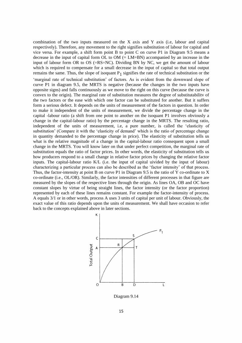
15

combination of the two inputs measured on the X axis and Y axis (i.e, labour and capital

respectively). Therefore, any movement to the right signifies substitution of labour for capital and

vice versa. For example, a shift form point B to point C on curve P1 in Diagram 9.5 means a

decrease in the input of capital form OL to OM (= LM=BN) accompanied by an increase in the

input of labour form OR to OS (=RS=NC). Dividing BN by NC, we get the amount of labour

which is required to compensate for a small decrease in the input of capital so that total output

remains the same. Thus, the slope of isoquant P1 signifies the rate of technical substitution or the

‘marginal rate of technical substitution’ of factors. As is evident from the downward slope of

curve P1 in diagram 9.5, the MRTS is negative (because the changes in the two inputs have

opposite signs) and falls continuously as we move to the right on this curve (because the curve is

convex to the origin). The marginal rate of substitution measures the degree of substitutabilitv of

the two factors or the ease with which one factor can be substituted for another. But it suffers

form a serious defect. It depends on the units of measurement of the factors in question. In order

to make it independent of the units of measurement, we divide the percentage change in the

capital -labour ratio (a shift from one point to another on the isoquant P1 involves obviously a

change in the capital-labour ratio) by the percentage change in the MRTS. The resulting ratio,

independent of the units of measurement, i.e, a pure number, is called the ‘elasticity of

substitution’ (Compare it with the ‘elasticity of demand’ which is the ratio of percentage change

in quantity demanded to the percentage change in price). The elasticity of substitution tells us

what is the relative magnitude of a change in the capital-labour ratio consequent upon a small

change in the MRTS. You will know later on that under perfect competition, the marginal rate of

substitution equals the ratio of factor prices. In other words, the elasticity of substitution tells us

how producers respond to a small change in relative factor prices by changing the relative factor

inputs. The capital-labour ratio K/L (i.e. the input of capital uivided by the input of labour)

characterizing a particular process can also be described as the ‘factor intensity’ of that process.

Thus, the factor-intensity at point B on curve P1 in Diagram 9.5 is the ratio of Y co-ordinate to X

co-ordinate (i.e., OL/OR). Similarly, the factor intensities of different processes in that figure are

measured by the slopes of the respective lines through the origin. As lines OA, OB and OC have

constant slopes by virtue of being straight lines, the factor intensity (or the factor proportion)

represented by each of these lines remains constant. For example the factor-intensity of process.

A equals 3/1 or in other words, process A uses 3 units of capital per unit of labour. Obviously, the

exact value of this ratio depends upon the units of measurement. We shall have occasion to refer

back to the concepts explained above in later sections.

Diagram 9.14

16

Intext questions :

Q.1. Define Returns to Scale (RTS).

Q.2. Define Isoquants.

Q.3. True/False.

(i) There are Returns to scale in the Short Run and Long Run.

(Answer : False)

(ii) Isoproduct curve are same output curve with different input variations.

(Answer : True)

Q.4 Define Marginal Rate of Technical substitution (MRTS).

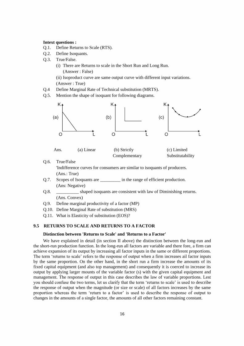
Q.5. Mention the shape of isoquant for following diagrams.

Ans. (a) Linear (b) Strictly (c) Limited

Complementary Substitutability

Q.6. True/False

'Indifference curves for consumers are similar to isoquants of producers.

(Ans.: True)

Q.7. Scopes of Isoquants are _________ in the range of efficient production.

(Ans: Negative)

Q.8. __________ shaped isoquants are consistent with law of Diminishing returns.

(Ans. Convex)

Q.9. Define marginal productivity of a factor (MP)

Q.10. Define Marginal Rate of substitution (MRS)

Q.11. What is Elasticity of substitution (EOS)?

9.5 RETURNS TO SCALE AND RETURNS TO A FACTOR

Distinction between 'Returns to Scale' and 'Returns to a Factor'

We have explained in detail (in section II above) the distinction between the long-run and

the short-run production function. In the long-run all factors are variable and there fore, a firm can

achieve expansion of its output by increasing all factor inputs in the same or different proportions.

The term ‘returns to scale’ refers to the response of output when a firm increases ail factor inputs

by the same proportion. On the other hand, in the short run a firm increase the amounts of its

fixed capital equipment (and also top management) and consequently it is coerced to increase its

output by applying larger mounts of the variable factor (s) with the given capital equipment and

management. The response of output in this case describes the law of variable proportions. Lest

you should confuse the two terms, let us clarify that the term ‘returns to scale’ is used to describe

the response of output when the magnitude (or size or scale) of all factors increases by the same

proportion whereas the term ‘return to a factor’ is used to describe the response of output to

changes in the amounts of a single factor, the amounts of all other factors remaining constant.

17

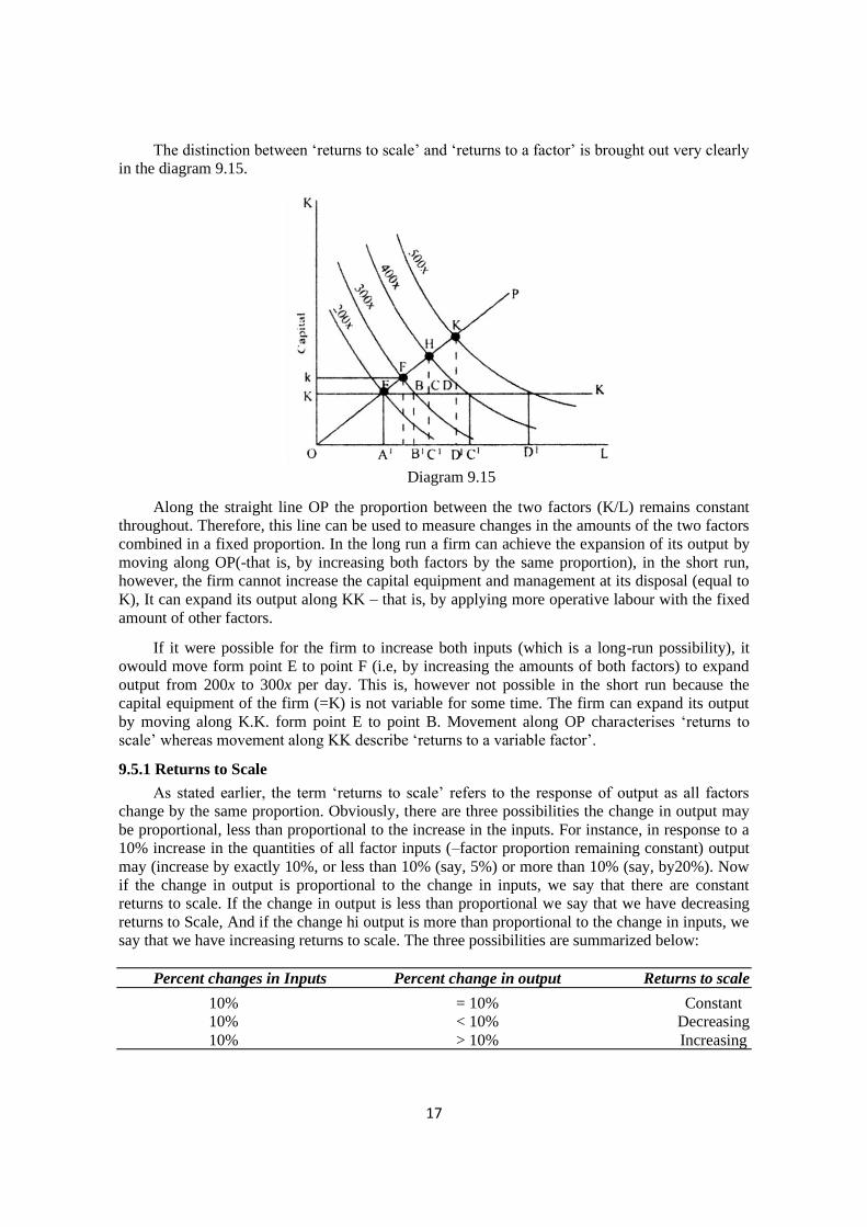
The distinction between ‘returns to scale’ and ‘returns to a factor’ is brought out very clearly

in the diagram 9.15.

Diagram 9.15

Along the straight line OP the proportion between the two factors (K/L) remains constant

throughout. Therefore, this line can be used to measure changes in the amounts of the two factors

combined in a fixed proportion. In the long run a firm can achieve the expansion of its output by

moving along OP(-that is, by increasing both factors by the same proportion), in the short run,

however, the firm cannot increase the capital equipment and management at its disposal (equal to

K), It can expand its output along KK – that is, by applying more operative labour with the fixed

amount of other factors.

If it were possible for the firm to increase both inputs (which is a long-run possibility), it

owould move form point E to point F (i.e, by increasing the amounts of both factors) to expand

output from 200x to 300x per day. This is, however not possible in the short run because the

capital equipment of the firm (=K) is not variable for some time. The firm can expand its output

by moving along K.K. form point E to point B. Movement along OP characterises ‘returns to

scale’ whereas movement along KK describe ‘returns to a variable factor’.

9.5.1 Returns to Scale

As stated earlier, the term ‘returns to scale’ refers to the response of output as all factors

change by the same proportion. Obviously, there are three possibilities the change in output may

be proportional, less than proportional to the increase in the inputs. For instance, in response to a

10% increase in the quantities of all factor inputs (–factor proportion remaining constant) output

may (increase by exactly 10%, or less than 10% (say, 5%) or more than 10% (say, by20%). Now

if the change in output is proportional to the change in inputs, we say that there are constant

returns to scale. If the change in output is less than proportional we say that we have decreasing

returns to Scale, And if the change hi output is more than proportional to the change in inputs, we

say that we have increasing returns to scale. The three possibilities are summarized below:

Percent changes in Inputs Percent change in output Returns to scale

10% = 10% Constant

10% < 10% Decreasing

10% > 10% Increasing

18

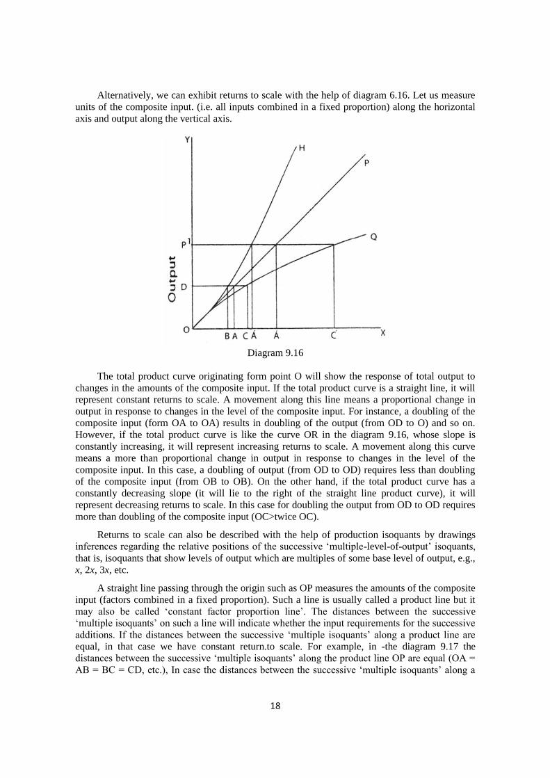
Alternatively, we can exhibit returns to scale with the help of diagram 6.16. Let us measure

units of the composite input. (i.e. all inputs combined in a fixed proportion) along the horizontal

axis and output along the vertical axis.

Diagram 9.16

The total product curve originating form point O will show the response of total output to

changes in the amounts of the composite input. If the total product curve is a straight line, it will

represent constant returns to scale. A movement along this line means a proportional change in

output in response to changes in the level of the composite input. For instance, a doubling of the

composite input (form OA to OA) results in doubling of the output (from OD to O) and so on.

However, if the total product curve is like the curve OR in the diagram 9.16, whose slope is

constantly increasing, it will represent increasing returns to scale. A movement along this curve

means a more than proportional change in output in response to changes in the level of the

composite input. In this case, a doubling of output (from OD to OD) requires less than doubling

of the composite input (from OB to OB). On the other hand, if the total product curve has a

constantly decreasing slope (it will lie to the right of the straight line product curve), it will

represent decreasing returns to scale. In this case for doubling the output from OD to OD requires

more than doubling of the composite input (OC>twice OC).

Returns to scale can also be described with the help of production isoquants by drawings

inferences regarding the relative positions of the successive ‘multiple-level-of-output’ isoquants,

that is, isoquants that show levels of output which are multiples of some base level of output, e.g.,

x, 2x, 3x, etc.

A straight line passing through the origin such as OP measures the amounts of the composite

input (factors combined in a fixed proportion). Such a line is usually called a product line but it

may also be called ‘constant factor proportion line’. The distances between the successive

‘multiple isoquants’ on such a line will indicate whether the input requirements for the successive

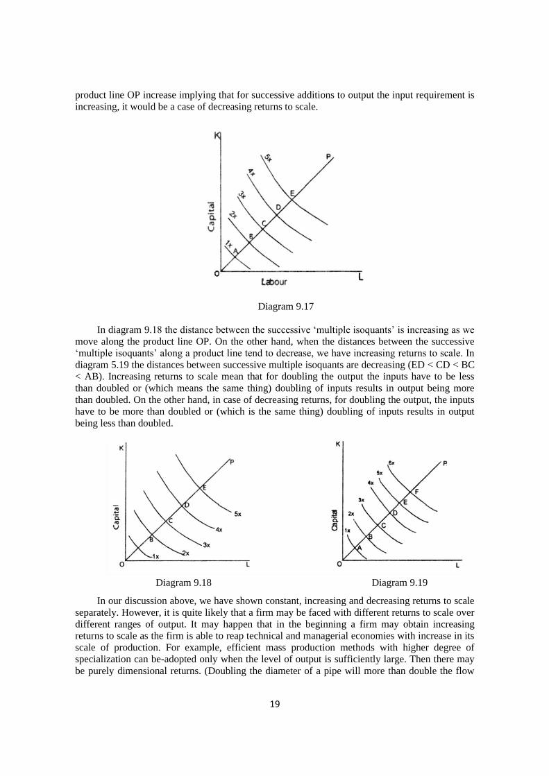
additions. If the distances between the successive ‘multiple isoquants’ along a product line are

equal, in that case we have constant return.to scale. For example, in -the diagram 9.17 the

distances between the successive ‘multiple isoquants’ along the product line OP are equal (OA =

AB = BC = CD, etc.), In case the distances between the successive ‘multiple isoquants’ along a

19

product line OP increase implying that for successive additions to output the input requirement is

increasing, it would be a case of decreasing returns to scale.

Diagram 9.17

In diagram 9.18 the distance between the successive ‘multiple isoquants’ is increasing as we

move along the product line OP. On the other hand, when the distances between the successive

‘multiple isoquants’ along a product line tend to decrease, we have increasing returns to scale. In

diagram 5.19 the distances between successive multiple isoquants are decreasing (ED < CD < BC

< AB). Increasing returns to scale mean that for doubling the output the inputs have to be less

than doubled or (which means the same thing) doubling of inputs results in output being more

than doubled. On the other hand, in case of decreasing returns, for doubling the output, the inputs

have to be more than doubled or (which is the same thing) doubling of inputs results in output

being less than doubled.

Diagram 9.18 Diagram 9.19

In our discussion above, we have shown constant, increasing and decreasing returns to scale

separately. However, it is quite likely that a firm may be faced with different returns to scale over

different ranges of output. It may happen that in the beginning a firm may obtain increasing

returns to scale as the firm is able to reap technical and managerial economies with increase in its

scale of production. For example, efficient mass production methods with higher degree of

specialization can be-adopted only when the level of output is sufficiently large. Then there may

be purely dimensional returns. (Doubling the diameter of a pipe will more than double the flow

20

through it). Indivisibility may also give rise to increasing returns to scale. For example, certain

equipment may be available in minimum size or in definite ranges of sizes. Such equipment may

be used more fully at a higher scale of production. Then, along with an increase in other inputs, a

larger amount of managerial talent may result in more efficient functioning through increased

specialization. This phase may be followed by constant returns to scale when reaching a ‘multiple

isoquant requires replication of the plant accordingly. For example, output may be doubled by

building and operation another plant which is exactly like the previous one. Decreasing returns to

scale are generally explained through indivisibility of the factor of production called

‘entrepreneurship’. It is argued that the entrepreneur and his decision-making are indivisible and

incapable of augmentation. Therefore, as the scale increases, mounting difficulties of coordination

and control lead to decreasing returns. But the use of the term ‘scale’ here is suspect as at least of

the factor inputs has been assumed to be fixed while increase in scale implies a proportional

increase in all the inputs.

9.5.2 Are Increasing or Constant Returns to Scale Consistent with Diminishing Returns to a

Factor?

In section 5 above we have explained the difference between ‘returns to scale’ and ‘returns

to a factor’ and also illustrated this difference with production isoquants. You would recall that

diminishing returns to a factor account for the convexity of the production isoquants. (Refer to the

discussion regarding the shapes of production isoquants). Given the convexity of production

isoquants, it can be shown that constant or diminishing returns to scale cannot prevent

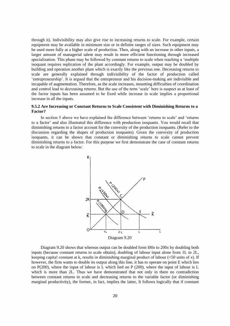
diminishing returns to a factor. For this purpose we first demonstrate the case of constant returns

to scale in the diagram below:

Diagram 9.20

Diagram 9.20 shows that whereas output can be doubled form l00x to 200x by doubling both

inputs (because constant returns to scale obtain), doubling of labour input alone from 1L to 2L,

keeping capita! constant at k, results in diminishing marginal product of labour (=50 units of x). If

however, the firm wants to double its output along this line, it has to operate on point E which lies

on P(200), where the input of labour is L which lied on P (200), where the input of labour is L

which is more than 2L. Thus we have demonstrated that not only in there no contradiction

between constant returns to scale and decreasing returns to the variable factor (or diminishing

marginal productivity), the former, in fact, implies the latter, It follows logically that if constant

21

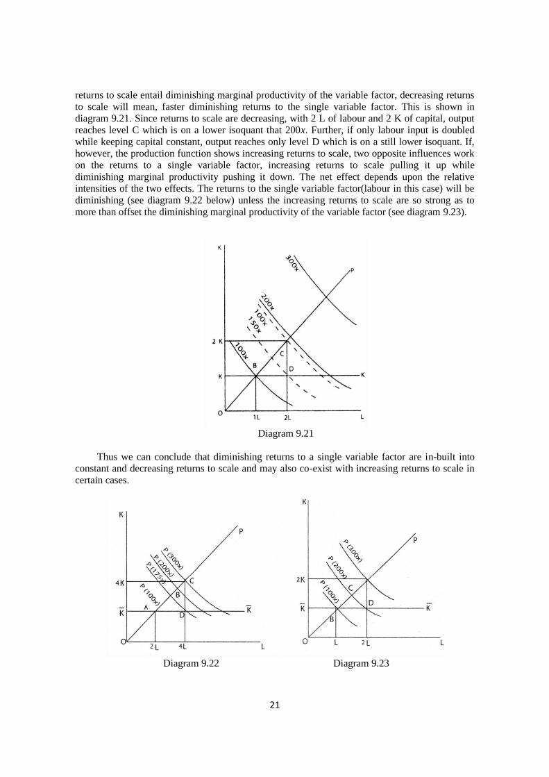
returns to scale entail diminishing marginal productivity of the variable factor, decreasing returns

to scale will mean, faster diminishing returns to the single variable factor. This is shown in

diagram 9.21. Since returns to scale are decreasing, with 2 L of labour and 2 K of capital, output

reaches level C which is on a lower isoquant that 200x. Further, if only labour input is doubled

while keeping capital constant, output reaches only level D which is on a still lower isoquant. If,

however, the production function shows increasing returns to scale, two opposite influences work

on the returns to a single variable factor, increasing returns to scale pulling it up while

diminishing marginal productivity pushing it down. The net effect depends upon the relative

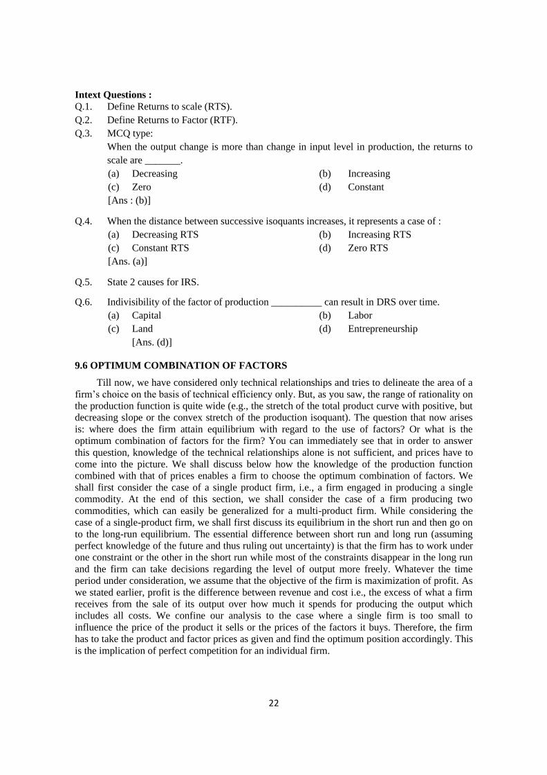
intensities of the two effects. The returns to the single variable factor(labour in this case) will be

diminishing (see diagram 9.22 below) unless the increasing returns to scale are so strong as to

more than offset the diminishing marginal productivity of the variable factor (see diagram 9.23).

Diagram 9.21

Thus we can conclude that diminishing returns to a single variable factor are in-built into

constant and decreasing returns to scale and may also co-exist with increasing returns to scale in

certain cases.

Diagram 9.22 Diagram 9.23

22

Intext Questions :

Q.1. Define Returns to scale (RTS).

Q.2. Define Returns to Factor (RTF).

Q.3. MCQ type:

When the output change is more than change in input level in production, the returns to

scale are _______.

(a) Decreasing (b) Increasing

(c) Zero (d) Constant

[Ans : (b)]

Q.4. When the distance between successive isoquants increases, it represents a case of :

(a) Decreasing RTS (b) Increasing RTS

(c) Constant RTS (d) Zero RTS

[Ans. (a)]

Q.5. State 2 causes for IRS.

Q.6. Indivisibility of the factor of production __________ can result in DRS over time.

(a) Capital (b) Labor

(c) Land (d) Entrepreneurship

[Ans. (d)]

9.6 OPTIMUM COMBINATION OF FACTORS

Till now, we have considered only technical relationships and tries to delineate the area of a

firm’s choice on the basis of technical efficiency only. But, as you saw, the range of rationality on

the production function is quite wide (e.g., the stretch of the total product curve with positive, but

decreasing slope or the convex stretch of the production isoquant). The question that now arises

is: where does the firm attain equilibrium with regard to the use of factors? Or what is the

optimum combination of factors for the firm? You can immediately see that in order to answer

this question, knowledge of the technical relationships alone is not sufficient, and prices have to

come into the picture. We shall discuss below how the knowledge of the production function

combined with that of prices enables a firm to choose the optimum combination of factors. We

shall first consider the case of a single product firm, i.e., a firm engaged in producing a single

commodity. At the end of this section, we shall consider the case of a firm producing two

commodities, which can easily be generalized for a multi-product firm. While considering the

case of a single-product firm, we shall first discuss its equilibrium in the short run and then go on

to the long-run equilibrium. The essential difference between short run and long run (assuming

perfect knowledge of the future and thus ruling out uncertainty) is that the firm has to work under

one constraint or the other in the short run while most of the constraints disappear in the long run

and the firm can take decisions regarding the level of output more freely. Whatever the time

period under consideration, we assume that the objective of the firm is maximization of profit. As

we stated earlier, profit is the difference between revenue and cost i.e., the excess of what a firm

receives from the sale of its output over how much it spends for producing the output which

includes all costs. We confine our analysis to the case where a single firm is too small to

influence the price of the product it sells or the prices of the factors it buys. Therefore, the firm

has to take the product and factor prices as given and find the optimum position accordingly. This

is the implication of perfect competition for an individual firm.

23

One possible situation is that the amount of total resources at the disposal of the firm is

given. In other words, the firm has to operate within the framework of a cost constraint. The goal

of the firm, as stated earlier, is to maximize profit. If we denote profit by Π, revenue by R and

cost by C, we can write the problem as:

maximise Π = R – C

Now the revenue of the firm depends upon the level of its output and the price of the

product. In other words, R = PX. X where X is the output of product X and PX is the price per

unit of X. As both PX and total cost assumed to be constant, the problem boils down to:

maximise Π = PX . X – C

The bar over PX and C signifies that these are constants. Thus, we are left with X as the

only variable on the right-hand side of the above equation. In ordinary language, it means that the

firm has to maximize its output with the given amount of resources at its disposal if it wants to

maximize profit.

Let us see how the firm goes about it. We conduct the analysis with the help of production

isoquants (described in detail in Section 4) and isocost lines. We shall first explain what an

‘isocost line’ means. !n Section 4, we compared an isoquant to a consumer indifference curve. In

the same way, we can compare an isocost line to the price line (or budget line) of the consumer.

Just as consumer’s budget line shows various combinations of two factors which have the same

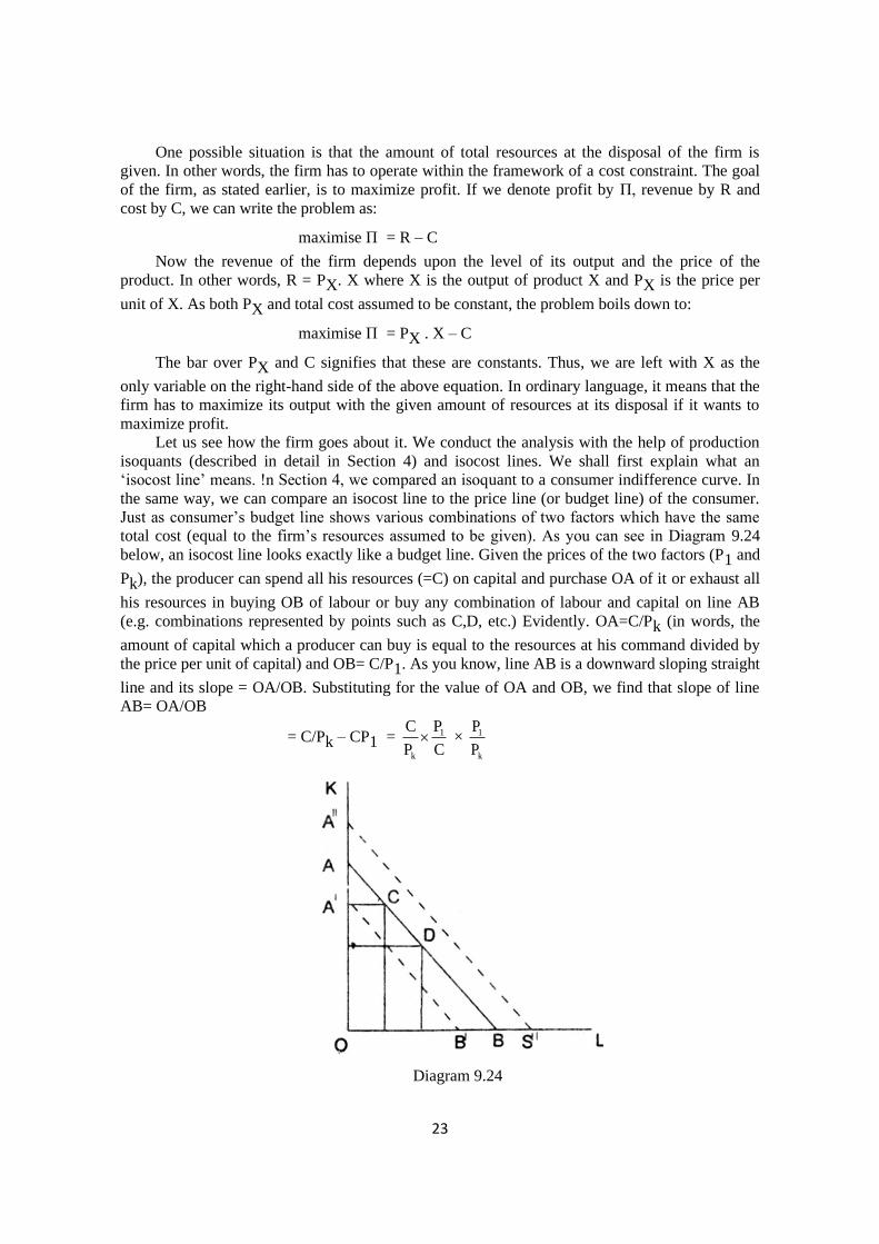
total cost (equal to the firm’s resources assumed to be given). As you can see in Diagram 9.24

below, an isocost line looks exactly like a budget line. Given the prices of the two factors (P1 and

Pk), the producer can spend all his resources (=C) on capital and purchase OA of it or exhaust all

his resources in buying OB of labour or buy any combination of labour and capital on line AB

(e.g. combinations represented by points such as C,D, etc.) Evidently. OA=C/Pk (in words, the

amount of capital which a producer can buy is equal to the resources at his command divided by

the price per unit of capital) and OB= C/P1. As you know, line AB is a downward sloping straight

line and its slope = OA/OB. Substituting for the value of OA and OB, we find that slope of line

AB= OA/OB

= C/Pk – CP1 = 1

k

PC

P C × 1

k

P

P

Diagram 9.24

24

Thus, you see that the slope of the isocost line represents the ratio of factor prices. (You

remember that the slope of consumer’s budget line equals the ratio of commodity prices). To take

the analogy further, the position or location of an isocost line depends upon the firm’s cost or

outlay just as the location of a budget line depends upon the level of consumer’s income. Line A

B in diagram 9.24 represents a lower level of cost or outlay compared to that relating to line AB,

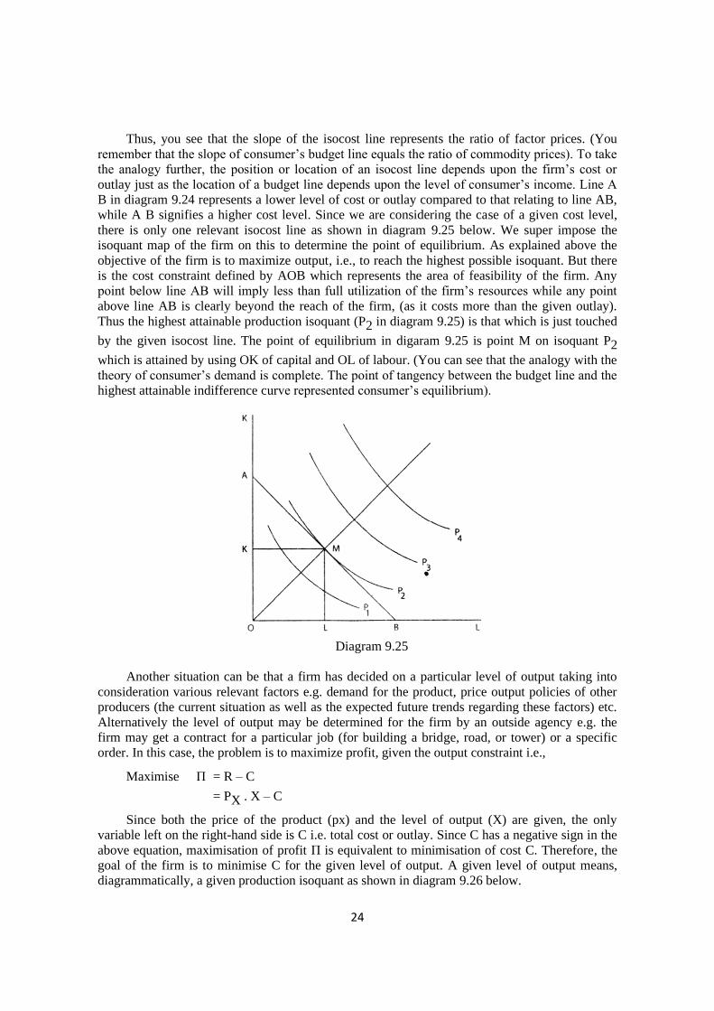
while A B signifies a higher cost level. Since we are considering the case of a given cost level,

there is only one relevant isocost line as shown in diagram 9.25 below. We super impose the

isoquant map of the firm on this to determine the point of equilibrium. As explained above the

objective of the firm is to maximize output, i.e., to reach the highest possible isoquant. But there

is the cost constraint defined by AOB which represents the area of feasibility of the firm. Any

point below line AB will imply less than full utilization of the firm’s resources while any point

above line AB is clearly beyond the reach of the firm, (as it costs more than the given outlay).

Thus the highest attainable production isoquant (P2 in diagram 9.25) is that which is just touched

by the given isocost line. The point of equilibrium in digaram 9.25 is point M on isoquant P2

which is attained by using OK of capital and OL of labour. (You can see that the analogy with the

theory of consumer’s demand is complete. The point of tangency between the budget line and the

highest attainable indifference curve represented consumer’s equilibrium).

Diagram 9.25

Another situation can be that a firm has decided on a particular level of output taking into

consideration various relevant factors e.g. demand for the product, price output policies of other

producers (the current situation as well as the expected future trends regarding these factors) etc.

Alternatively the level of output may be determined for the firm by an outside agency e.g. the

firm may get a contract for a particular job (for building a bridge, road, or tower) or a specific

order. In this case, the problem is to maximize profit, given the output constraint i.e.,

Maximise Π = R – C

= PX . X – C

Since both the price of the product (px) and the level of output (X) are given, the only

variable left on the right-hand side is C i.e. total cost or outlay. Since C has a negative sign in the

above equation, maximisation of profit Π is equivalent to minimisation of cost C. Therefore, the

goal of the firm is to minimise C for the given level of output. A given level of output means,

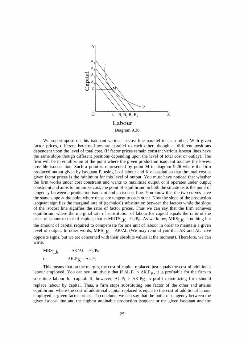
diagrammatically, a given production isoquant as shown in diagram 9.26 below.

25

Diagram 9.26

We superimpose on this isoquant various isocost line parallel to each other. With given

factor prices, different iso-cost lines are parallel to each other, though at different positions

dependent upon the level of total cost. (If factor prices remain constant various isocost lines have

the same slope though different positions depending upon the level of total cost or outlay). The

firm will be in equilibrium at the point where the given production isoquant touches the lowest

possible isocost line. Such a point is represented by point M in diagram 9.26 where the firm

produced output given by isoquant P, using L of labour and K of capital so that the total cost at

given factor prices is the minimum for this level of output. You must have noticed that whether

the firm works under cost constraint and wants to maximize output or it operates under output

constraint and aims to minimize cost, the point of equilibrium in both the situations is the point of

tangency between a production isoquant and an isocost line. You know that the two curves have

the same slope at the point where these are tangent to each other. Now the slope of the production

isoquant signifies the marginal rate of (technical) substitution between the factors while the slope

of the isocost line signifies the ratio of factor prices. Thus we can say that the firm achieves

equilibrium where the marginal rate of substitution of labour for capital equals the ratio of the

price of labour to that of capital, that is MRTSl,K= PL/PK. As we know, MRSl,K is nothing but

the amount of capital required to compensate for one unit of labour in order to maintain a given

level of output. In other words, MRSl,K = ∆K/∆L (We may remind you that ∆K and ∆L have

opposite signs, but we are concerned with their absolute values at the moment). Therefore, we can

wirte,

MRS1,k = ∆K/∆L = PL/PK

or ∆K.PK = ∆L.PL

This means that on the margin, the cost of capital replaced just equals the cost of additional

labour employed. You can see intuitively that if ∆L.PL < ∆K.PK, it is profitable for the firm to

substitute labour for capital. If, however, ∆L.PL > ∆K.PK, a profit maximizing firm should

replace labour by capital. Thus, a firm stops substituting one factor of the other and attains

equilibrium where the cost of additional capital replaced is equal to the cost of additional labour

employed at given factor prices. To conclude, we can say that the point of tangency between the

given isocost line and the highest attainable production isoquant or the given isoquant and the

26

lowest possible isocost line indicates to the firm the optimum proportion in which it would

combine the two factors.

Intext Questions :

Q.1. In perfect competition :

(a) TR=TC (b) TR=TC=0

(c) TR > TC (d) TR < TC

(Where TR=total Revenue , TC= Total cost)

[Ans. (a)]

Q.2. Define Isocost line.

Q.3. Isocost lines are also called ____________ of the consumer.

(Ans. Budget Line / Price Line)

Q.4. Point of equilibrium of the firm is the point of tangency between :

(a) Indifference curve and isocost line

(b) Isocost line and isoquant

(c) Isoquant and indifference curve

(d) Isoquant and x-axis

[Ans. (c)]

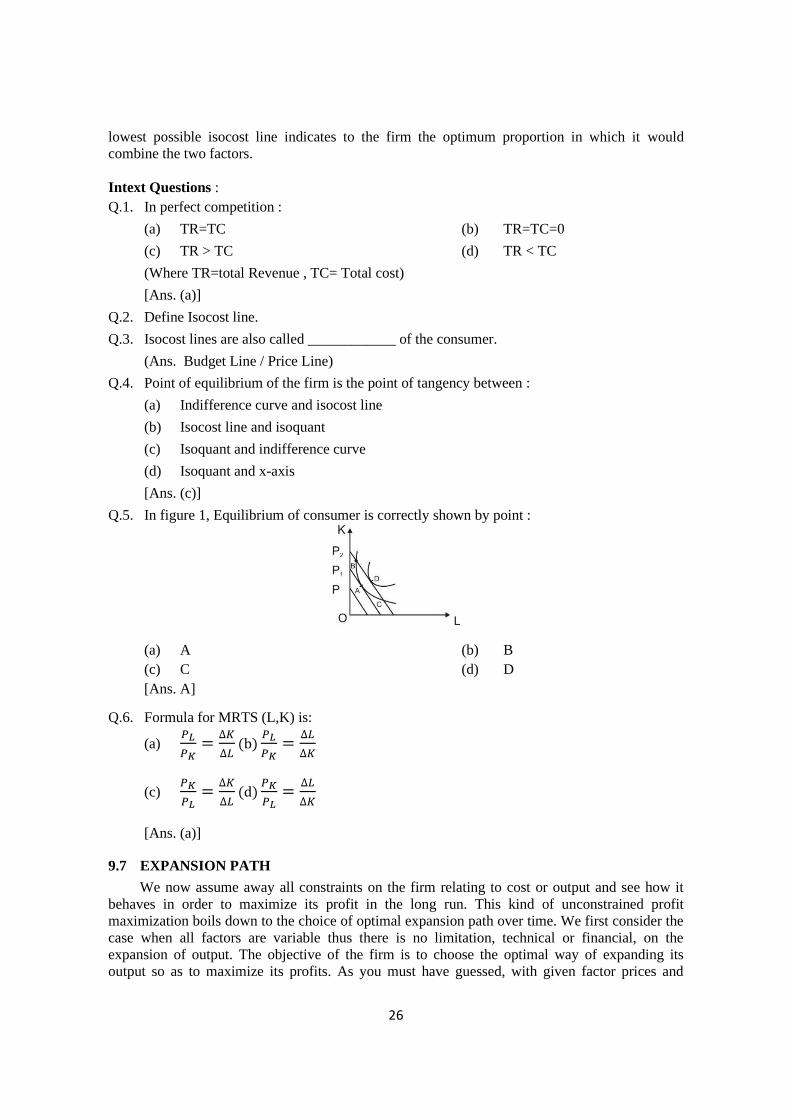
Q.5. In figure 1, Equilibrium of consumer is correctly shown by point :

(a) A (b) B

(c) C (d) D

[Ans. A]

Q.6. Formula for MRTS (L,K) is:

(a) 𝑃𝐿

𝑃𝐾=

∆𝐾

∆𝐿(b)

𝑃𝐿

𝑃𝐾=

∆𝐿

∆𝐾

(c) 𝑃𝐾

𝑃𝐿=

∆𝐾

∆𝐿(d)

𝑃𝐾

𝑃𝐿=

∆𝐿

∆𝐾

[Ans. (a)]

9.7 EXPANSION PATH

We now assume away all constraints on the firm relating to cost or output and see how it

behaves in order to maximize its profit in the long run. This kind of unconstrained profit

maximization boils down to the choice of optimal expansion path over time. We first consider the

case when all factors are variable thus there is no limitation, technical or financial, on the

expansion of output. The objective of the firm is to choose the optimal way of expanding its

output so as to maximize its profits. As you must have guessed, with given factor prices and

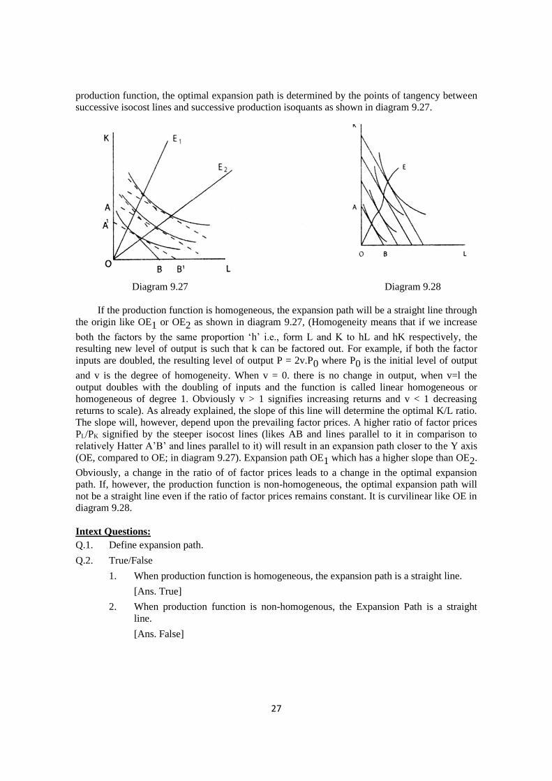
27

production function, the optimal expansion path is determined by the points of tangency between

successive isocost lines and successive production isoquants as shown in diagram 9.27.

Diagram 9.27 Diagram 9.28

If the production function is homogeneous, the expansion path will be a straight line through

the origin like OE1 or OE2 as shown in diagram 9.27, (Homogeneity means that if we increase

both the factors by the same proportion ‘h’ i.e., form L and K to hL and hK respectively, the

resulting new level of output is such that k can be factored out. For example, if both the factor

inputs are doubled, the resulting level of output P = 2v.P0 where P0 is the initial level of output

and v is the degree of homogeneity. When v = 0. there is no change in output, when v=l the

output doubles with the doubling of inputs and the function is called linear homogeneous or

homogeneous of degree 1. Obviously v > 1 signifies increasing returns and v < 1 decreasing

returns to scale). As already explained, the slope of this line will determine the optimal K/L ratio.

The slope will, however, depend upon the prevailing factor prices. A higher ratio of factor prices

PL/PK signified by the steeper isocost lines (likes AB and lines parallel to it in comparison to

relatively Hatter A’B’ and lines parallel to it) will result in an expansion path closer to the Y axis

(OE, compared to OE; in diagram 9.27). Expansion path OE1 which has a higher slope than OE2.

Obviously, a change in the ratio of of factor prices leads to a change in the optimal expansion

path. If, however, the production function is non-homogeneous, the optimal expansion path will

not be a straight line even if the ratio of factor prices remains constant. It is curvilinear like OE in

diagram 9.28.

Intext Questions:

Q.1. Define expansion path.

Q.2. True/False

1. When production function is homogeneous, the expansion path is a straight line.

[Ans. True]

2. When production function is non-homogenous, the Expansion Path is a straight

line.

[Ans. False]

28

Learning Outcomes

In this lesson you have learnt the following:-

• Production function is defined as the technique, combination of various inputs required to

produce a product.

• In the short run there is presence of both fixed and variable factors whereas in the long run

all the factors are variable. The law of variable proportion which operates in the short run

states that when more and more units of a variable factor is used with a fixed factor the

marginal product of the variable factor may increase in the beginning but it will eventually

fall.

• Stages of variable factor known as:-

1. Stage of increasing returns to factor

2. Stage of decreasing returns to factor

3. Stage of negative returns to factors

• In the long run assuming homogenous production function the law of return to scale

operates in three different ways:-

1. Law of constant returns to scale

2. Increasing returns to scale

3. Decreasing returns to scale

• Isoquant is defined as the locus of various combinations of two variable factors giving same

level of output at each combination. If factors are prevented, it substitutes the isoquant

becomes straight line, which is L shaped when factors are complementary to each other. The

slope of the isoquant is called marginal rate of technical substitution.

• The optimum combination of factor which is also the equilibrium of the producer is

achieved at the point where the isocost and isoquant are tangent to each other.

• The locus of the equilibrium points resulting out of changing isocost of the producer is

called expansion path.

TERMINAL QUESTIONS

Q.1. Explain RTS and its 3 types with diagrams.

Q.2. Critically examine the Law of variable proportions in the short and Long run with diagrams.

29

LESSON: 10

COST

INTRODUCTION

It bears repetition to say that we are analyzing the behavior of a rational producer who is

assumed to produce each level of output at the minimum possible cost under the given set of

conditions and to sell the output produced to obtain maximum total revenue. This implies that the

producer has perfect knowledge regarding technical aspects of production (physical input/ output

relationship), factor prices (and hence the optimum factor combinations) and the demand

conditions for this product. This is a purely theoretical construct aimed at simplifying the

analysis. That the producer (or the so called ‘entrepreneur’) has no such knowledge in a capitalist

economy and the consequences arising out of the lack of knowledge are discussed in Set VIII of

this paper. Till then we will continue to assume that the producer has perfect knowledge of the

magnitudes relevant for his decision-making.

After going through this lesson you will learn:-

• Distinguish between fixed and variable cost

• Draw the short run cost curves

• Explain the U-shape of the cost curves

• Derive the long run cost curves

• Determine the relationship between various cost curves, such as average cost and marginal

cost.

• Define total average and marginal revenue

• Determine relationship between average and marginal revenue.

10.1 COMPONENTS OF TOTAL COSTS; FIXED AND VARIABLE COSTS

Whatever costs a firm incurs in order to produce a certain output (including implicit costs)

constitute total costs of that output. However, when we carefully examine the nature of various

inputs used in production, we find that while some inputs can be varied as and when desired,

some others cannot be varied at will over certain period, which restrict the firm’s freedom of

choice of alternative production possibilities over the relevant period.

A. Fixed Costs

Firstly, in order to produce a certain level of output a firm has to equip itself with a certain

amount of durable-use capital goods such as machines, buildings, tools, equipment, etc., which if

property maintained aid production over a long period of time. Their use is not confined to a

single act of production but extends over time into the future. The returns form such capital goods

are spread over the whole of their productive lives. Therefore, while planning to install them a

producer has necessarily to take into consideration the whole stream of returns obtainable form

over the whole of their productive lives. A producer would install such capital goods only if they

are expected to yield a normal return (at least equal to the rate of interest) over the whole of their

productive lives and not merely on the basis of short-run prospect. Also such capital goods

generally take considerable time to build. Because of these constraints the amounts of such

durable use capital goods cannot be varied over short periods. In other words, their amounts are

fixed in the short run. The only alternative available to the firm for meeting short run fluctuations

in demand is to produce a larger or a smaller output by applying more or fewer units of other

factors with the fixed equipment of the firm. Executives, managers, supervisors and other

30

permanent staff, constituting what is called the ‘management of the firm’, are also of the nature of

fixed factors. This configuration of the fixed capital equipment and management is designed to

produce a certain output at the minimum average cost. This, however, does not mean that the

given fixed equipment cannot produce a larger or a smaller than the optimum output. It is possible

to produce a larger or a smaller output by using given equipment more or less intensively (by

applying more or fewer other variable inputs) but in that case average cost would be more than

the optimum level. The costs of factors whose amounts cannot be increased or decreased over

certain periods are called fixed costs.

B. Variable Costs

There are certain other inputs whose amounts can be varied in the short run according to

production requirements. The costs of such inputs are called variable costs. Costs of operative

labour, raw materials, power, fuel, lubricants, transport, etc., are some examples of various costs.

For example, if a spinning mill decides to produce more yarn, it will need more cotton, more

labour, more power, fuel, lubricants, etc. On the other hand, if it decides to produce less it will

need less of such items. And if the mill stops production completely, it will require no amount of

such items and consequently its variable costs will be zero. Thus, we see that (a) variable costs

need to be incurred only when some output is produced and (b) their total varies directly with

variations in the level of output produced.

Intext Questions :

Q.1. Define fixed cost (FC).

Q.2. Define variable cost (VC).

Q.3. Total cost (TC) for a firm is :

(a) TC=FC (b) TC=VC

(c) TC=VC+FC (d) TC=TI (profit)

[Ans. (b)]

10.2 ANALYTICAL SIGNIFICANT OF THE DISTINCTION

What is the analysis significance of the classification of costs into the fixed and variable

components? By definition, fixed costs are independent of the short run changes in the level of

output. In the short run, whether a firm produces a larger or a smaller output, the total of fixed

costs remains unaffected. Having once committed its resources in such factors, the firm has no

alternative but to bear the loss represented by the total fixed costs even if the firm produces no

output at all. On the other hand, a firm needs to incur variable costs only when it undertakes some

production. It will not incur any variable costs at ail when production is suspended. But the

burden of fixed costs will continue even when production is suspended in the short run. It short,

while variable costs are ‘avoidable’ fixed costs are ‘unavoidable’ and have to be borne even if no

output is produced. From this it follows that the costs relevant for short-run production decisions

of a firm are the variable costs and not fixed costs.

If the firm stops production completely, its maximum loss would equal the amount of Total

Fixed Costs (TFC). If it decides to produce some output, it will have to incur some variable costs

as well. If, in the short run, the price of the product does not cover even the variable costs, the

firm will not undertake production because by producing some output under these conditions, it

will incur a loss on variable cost, also (besides the loss represented by the fixed costs) and thus,

will further add to the loss represented by the fixed costs. But the loss on variable costs is

avoidable. Therefore, under such conditions the firm will prefer smaller loss (=TFC) to a greater

loss. On the other hand, if the price of the product covers the variable costs and also leaves a

31

margin which goes to meet at least a part of the fixed costs (though not the w hole of the fixed

costs). It would be rational for the firm to undertake production because by doing so it would be

minimizing the loss which, it has to bear even in case of stoppage of production. From this it

follows that fixed costs have no bearing on the short run production decisions of a firm. Whether

or not a firm will undertake any production in the short run, will depend on whether or not the

price of the production covers the average variable cost. If the price covers the average variable

cost and leaves some margin, the firm will undertake production other wise it will not. It is in this

sense that fixed costs are irrelevant form the stand point of short-run production decisions.

The bearing of variable costs on the short run production decisions of a firm is clearly

brought out with the help of hypothetical figures given in the Table below. We assume that total

of fixed costs (TFC) of the firm is Rs. 10,000 and for producing 1000 units of output it has to

incur Rs. 5,000 as variable costs so that total cost (total of variable and fixed costs) of producing

1,000 units amounts to Rs. 15,000. Four alternative price situations are considered in the Table

10.1 below.

TABLE 10.1

Px AVC TFC TVC TC TR Losses

1 – – 10,000 – 10,000 – 11,000

2 4 5 10,000 5,000 15,000 5,000 10,000

3 5 5 10,000 5,000 15,000 5,000 10000

4 6 5 10,000 5,000 15,000 6,000 9,000

In the table above;

Px stands for the market price of the product.

AVC stands for average variable cost per unit of output.

TFC stands for total fixed costs.

TC stands for total cost whihc equal TFC + TVC.

TR stands for total revenue form the sale of 1,000 units, and Losses equal TC – TR.

In the above table, figures in the first row relate to the situation when the firm undertakes no

production at all in the short run. Total loss of the firm in that case would equal to Rs. 10,000.

Figures in the second row relate to the situation when the market price of the commodity

produced does not cover even the variable costs and consequently the firm’s total loss would

amount to Rs. 11,000 if it produces output in that situation. If this were the cost-price-situation

confronting the firm, it will stop production. (it will prefer a smaller loss of Rs. 10,000 to a

greater loss of Rs. 10,000 to a greater loss of Rs. 11,000). Figures in the third row relate to the

situation where price of the product just covers the variable costs. Firm’s total loss in this case is

the same as it would be when no output is produced (situation I). Therefore the firm would be

indiffernet whether or not to undertake production in this situation. It may or may not undertake

production in this situation. Figures in the fourth row relate to the situation when the price of the

product covers the variable costs and leaves a margin of Rs. 1 per unit of output whihc goes to

meet a part of the total fixed costs, thus reducing the losses of the firm to Rs. 9000. It is, thus,

evident that though even in this situation the firm is producing at a loss but the loss in this case is

smaller than what it would be in the event of stoppage of production.

We thus, reach the following conclusions:

1. Fixed costs have no bearing on the short run production decisions of a firm. Costs relevant

for decision making in the short run are variable costs and not fixed costs.

2. In the short run a firm will not undertake any production if the price of the product does not

cover even the variable costs (price<AVC). Production will be undertaken when price more

32

than covers the variable costs even if it does not cover the full costs (price > AVC but <AC).

It will be indifferent when price just covers the variable cost (price = AVC).

10.2.1 All Costs are Variable in the Long Run

The distinction between the short run and the long run is based on the invariability of certain

factors over certain periods. Short run may be defined as the period which is too short to permit

firms to adjust quantities of all factors in accordance with the requirements of production hut

long enough to permit them to adjust their outputs by applying more or fewer units of other

variable factors with their given fixed factors. Long period, on the other hand, refers to the time

period which is long enough to permit firms to adjust quantities of all factors to suit their

requirements. The distinction between short and long runs does not refer to any definite time

period. Short and long periods vary form industry to industry, For example, the short run form the

stand point of steel industry may range over a few years, where as it may be just a few months for

fishermen who do not use much fixed capital except their fishing nets and boats.

In the long run all costs are variable. It is difficult to think of a factor input whose quantity

cannot be varied, given sufficient time for producing it and for allowing old ones to decay and

thus, go out of use. Thus, in the long run firms can vary the quantities of all factors as desired.

From this it follows that if in an industry a firm is not able to cover its full costs (variable as well

as fixed), in the long run (i.e.as soon as it is free from its short run cost commitments) it will leave

that industry for better prospects elsewhere. In the short-run a firm is compelled to undertake

production even at a loss (i.e., price > AVC but <AC) because of its short run commitments. But

in the long run a firm free form all commitments and can choose to stay in the industry or to leave

it. It follows that in the long run a firm will not stay in an industry where the price of the product

does not cover the average cost including both the fixed and variable components. We may

express the same thing by saying that in the long run a firm will continue prodution only if the

price of the product is at least equal to AC (including both fixed and variable components). As

summary of out discussion of the fixed and variable costs and the corresponding short and long

runs, we may state the following:

1. In the short run a firm will undertake production only if price of the product at least covers

AVC.

2. In the long run a firm will undertake or continue production only if price of the product at

least covers AC(inclusive affixed and variable components).

Intext Questions :

Q.1. In short run, _________ cost remain unaffected.

(Ans. Fixed costs)

Q.2. A firm will not operate in the short run when :

(a) P < AVC (b) P > AVC

(c) P= AVC (d) P =AVC = 0

[Ans. (a)]

10.3 TOTAL, AVERAGE AND MARGINAL COST CONCEPTS

Total Cost (TC): Total Cost of inputs (purchased from other as well as those supplied by

the owners themselves) used for producting a certain output constitute the total cost of that output.

Since there are two components of total costs, the variable costs and the fixed costs, therefore,

total costs equal the sum of total fixed costs and total variable costs.

33

Thus:

TC = TFC + TVC

Average Cost (AC): Total costs incurred for producing a certain output divided by the

number of units produced is the average cost per unit of output. Since total costs equal the sum of

total fixed costs (TFC) and total variable costs (TVC), it follows that average cost will also equal

average fixed cost (AFC) plus average variable cost (AVC). AFC equals TFC divided by the

number to units of output produced and, similarly, AVC equals TVC divided by the number of

units of output produced.

Thus:

TC = TFC + TVC

AFC = TFC / Q where Q = units of output produced

AVC = TVC / Q where Q = units of output produced

Therefore, AC = AFC + AVC.

For example, if for producing 100 units of output a firm incurs Rs.5,000 as variable costs

over and above its total fixed costs amounting to Rs. 10,000, the three average cost concepts

explained above will be as given below.

TFC = Rs.10,000

TVC = Rs.5.000

TC = Rs. 10,000 + Rs. 5,000 = Rs. 15.000

AFC = Rs. 10,000 / 100 = Rs. 100

AVC = Rs 5,000 / 100 = Rs. 50

AC = Rs. 100 + Rs.50 = Rs.l50

Marginal Cost

The addition made to total costs of a firm due to the production of an additional unit of

output (e.g., 101 units instead of 100) is called the marginal cost (MC) of the additional unit. For

example, if the total costs of a firm increased from Rs. 15,000 to Rs. 15,200 when it produced 101

units instead of 100, the MC of the l0l the unit would be Rs. 200. In general we can say that MC

of the nth unit of output equals TC of n units minus TC of (n–1) units.

Thus:

MC = TCn – TCn–1

As explained above, TFC does not change in the short run with variations in the level of

output produced. In other words, the addition to TFC due to the production of additional units

equals zero in the short run. Therefore, MC on account of fixed costs equals zero: MFC = zero.

From this it follows that MC is essentially MVC, i.e., equals the change in total variable costs due

to the production of an additional unit of output.

Thus:

MC = MFC + MVC

MFC = zero

Therefore,

MC = MVC

MCn = TVCn – TVC(n–l)

34

Thus, in calculating MC we can completely ignore fixed costs. MC can be calculated

directly from variable costs. However, the result would be the same whether MC is calculated as a

change in TVC or TC.

10.3.1 Relationship between Average and Marginal Cost

MC is the addition made to TC due to the production of an additional unit of output. AC is

TC divided by the number of units produced. Naturally, MC, which affects TC, will immediately

affect AC as well. For example, if the MC due to the production of an additional unit is greater

than the AC of the other units, it will push up the latter. Suppose, the AC of 100 units is Rs. 150

and the MC to the 101th unit is Rs.251 (i.e. greater than the earlier AC of 100 units), AC of 101

units will equal Rs. 151 (150 × 100 + 251 = 15,251 / 101 = 151). On the other hand, if the MC of

the additional unit is less than the AC of the earlier units, the AC of all the units taken together

would fall. In the example above, if the MC of the 101th unit were only Rs. 49 (instead of Rs.

251), AC of all the 101 units taken together would fall to Rs. 149 (i.e 150 × l00 + 49 = 15, 049 /

101 = 149). And finally, if the MC of the additional unit happens to equal the AC of the other

units, AC of the units taken together would remain unchanged. In the example above, if the MC

of the 101th unit were Rs. 150, the AC of 101 units would have remained constant at Rs. l50 (i.e.,

150 × 100 + 150 = 15150 / 101 = 150).

Table 10.2 below gives some figures of AC, TC and MC which clearly bring out the

relationship between AC and MC.

TABLE 10.2

Units of output (n) AC of (n) TC of (n) MC of (n+l) th unit TC of (n+1) unit AC of

(n+1) unit

1 2 3 45 6

1 10 10 9.0 19 9.5

2 9.5 19 8.0 27 9.0

3 9.0 27 7.0 34 8.5

4 8.5 34 6.0 40 8.0

5 8.0 48 8.0 48 8.0

6 8.0 40 8.0 56 8.0

7 8.0 56 8.0 64 8.0

8 8.0 64 8.0 72 8.0

9 8.0 72 18.0 90 9.0

10 9.0 90 20.0 110 10.0

11 10.0 110 22.0 132 11.0

12 11.0 132 24.0 156 12.0

The first four rows of the above Table show that so long as MC is less than the preceding

AC, the successive AC falls. The next four rows show that so long as MC equals the preceding

AC, the successive AC will remain constant. The last four rows shows that so long as MC is

greater than the preceding AC, successive AC will rise.

Regarding the relationship between Me and AC (and for that matter between any marginal

average value) it should be very carefully understood that what maters is the absolute value of

MC and not its rise or fall or constancy. For example, the necessary condition for the AC to rise

is that the MC should be greater (in absolute terms) than the former, whether MC is rising, falling

or constant is immaterial. Thus whether MC is rising, falling or constant, so long as it is higher

than AC the latter will rise. Similarly, the necessary condition for then AC to fall is that MC

should be less than the former, whether the latter is rising, falling or constant is not material. Thus

in conclusion we may say that rising, falling or constant MC is compatible with a rising AC

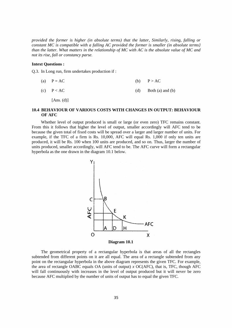
35

provided the former is higher (in absolute terms) that the latter, Similarly, rising, falling or

constant MC is compatible with a falling AC provided the former is smaller (in absolute terms}

than the latter. What matters in the relationship of MC with AC is the absolute value of MC and

not its rise, fall or constancy parse.

Intext Questions :

Q.3. In Long run, firm undertakes production if :

(a) P = AC (b) P > AC

(c) P < AC (d) Both (a) and (b)

[Ans. (d)]

10.4 BEHAVIOUR OF VARIOUS COSTS WITH CHANGES IN OUTPUT: BEHAVIOUR

OF AFC

Whether level of output produced is small or large (or even zero) TFC remains constant.

From this it follows that higher the level of output, smaller accordingly will AFC tend to be

because the given total of fixed costs will be spread over a larger and larger number of units. For

example, if the TFC of a firm is Rs. 10,000, AFC will equal Rs. 1,000 if only ten units are

produced, it will be Rs. 100 when 100 units are produced, and so on. Thus, larger the number of

units produced, smaller accordingly, will AFC tend to be. The AFC curve will form a rectangular

hyperbola as the one drawn in the diagram 10.1 below.

Diagram 10.1

The geometrical property of a rectangular hyperbola is that areas of all the rectangles

subtended from different points on it are all equal. The area of a rectangle subtended from any

point on the rectangular hyperbola in the above diagram represents the given TFC. For example,

the area of rectangle OABC equals OA (units of output) x OC(AFC), that is, TFC, though AFC

will fall continuously with increases in the level of output produced but it will never be zero

because AFC multiplied by the number of units of output has to equal the given TFC.

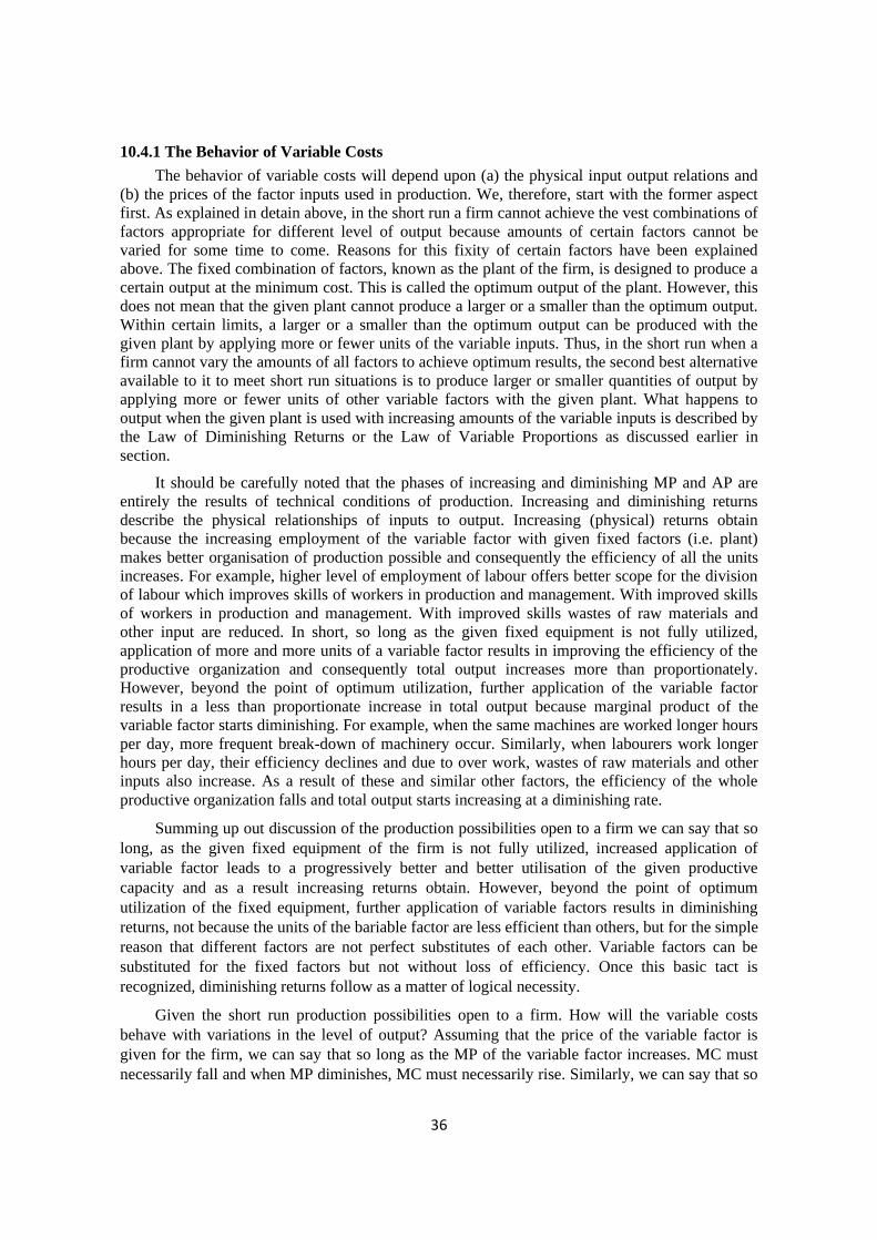
36

10.4.1 The Behavior of Variable Costs

The behavior of variable costs will depend upon (a) the physical input output relations and

(b) the prices of the factor inputs used in production. We, therefore, start with the former aspect

first. As explained in detain above, in the short run a firm cannot achieve the vest combinations of

factors appropriate for different level of output because amounts of certain factors cannot be

varied for some time to come. Reasons for this fixity of certain factors have been explained

above. The fixed combination of factors, known as the plant of the firm, is designed to produce a

certain output at the minimum cost. This is called the optimum output of the plant. However, this

does not mean that the given plant cannot produce a larger or a smaller than the optimum output.

Within certain limits, a larger or a smaller than the optimum output can be produced with the

given plant by applying more or fewer units of the variable inputs. Thus, in the short run when a

firm cannot vary the amounts of all factors to achieve optimum results, the second best alternative

available to it to meet short run situations is to produce larger or smaller quantities of output by

applying more or fewer units of other variable factors with the given plant. What happens to

output when the given plant is used with increasing amounts of the variable inputs is described by

the Law of Diminishing Returns or the Law of Variable Proportions as discussed earlier in

section.

It should be carefully noted that the phases of increasing and diminishing MP and AP are

entirely the results of technical conditions of production. Increasing and diminishing returns

describe the physical relationships of inputs to output. Increasing (physical) returns obtain

because the increasing employment of the variable factor with given fixed factors (i.e. plant)

makes better organisation of production possible and consequently the efficiency of all the units

increases. For example, higher level of employment of labour offers better scope for the division

of labour which improves skills of workers in production and management. With improved skills

of workers in production and management. With improved skills wastes of raw materials and

other input are reduced. In short, so long as the given fixed equipment is not fully utilized,

application of more and more units of a variable factor results in improving the efficiency of the

productive organization and consequently total output increases more than proportionately.

However, beyond the point of optimum utilization, further application of the variable factor

results in a less than proportionate increase in total output because marginal product of the

variable factor starts diminishing. For example, when the same machines are worked longer hours

per day, more frequent break-down of machinery occur. Similarly, when labourers work longer

hours per day, their efficiency declines and due to over work, wastes of raw materials and other

inputs also increase. As a result of these and similar other factors, the efficiency of the whole

productive organization falls and total output starts increasing at a diminishing rate.

Summing up out discussion of the production possibilities open to a firm we can say that so

long, as the given fixed equipment of the firm is not fully utilized, increased application of

variable factor leads to a progressively better and better utilisation of the given productive

capacity and as a result increasing returns obtain. However, beyond the point of optimum

utilization of the fixed equipment, further application of variable factors results in diminishing

returns, not because the units of the bariable factor are less efficient than others, but for the simple

reason that different factors are not perfect substitutes of each other. Variable factors can be

substituted for the fixed factors but not without loss of efficiency. Once this basic tact is

recognized, diminishing returns follow as a matter of logical necessity.

Given the short run production possibilities open to a firm. How will the variable costs

behave with variations in the level of output? Assuming that the price of the variable factor is

given for the firm, we can say that so long as the MP of the variable factor increases. MC must

necessarily fall and when MP diminishes, MC must necessarily rise. Similarly, we can say that so

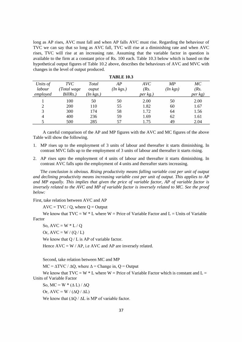
37

long as AP rises, AVC must fall and when AP falls AVC must rise. Regarding the behaviour of

TVC we can say that so long as AVC fall, TVC will rise at a diminishing rate and when AVC

rises, TVC will rise at an increasing rate. Assuming that the variable factor in question is

available to the firm at a constant price of Rs. 100 each. Table 10.3 below which is based on the

hypothetical output figures of Table 10.2 above, describes the behaviours of AVC and MVC with

changes in the level of output produced.

TABLE 10.3

Units of TVC Total AP AVC MP MC

labour (Total wage ouput (In kgs.) (Rs. (In kgs) (Rs.

employed BillRs.) (In kgs.) per kg.) per kg)

1 100 50 50 2.00 50 2.00

2 200 110 55 1.82 60 1.67

3 300 174 58 1.72 64 1.56

4 400 236 59 1.69 62 1.61

5 500 285 57 1.75 49 2.04

A careful comparison of the AP and MP figures with the AVC and MC figures of the above

Table will show the following.

1. MP rises up to the employment of 3 units of labour and thereafter it starts diminishing. In

contrast MVC falls up to the employment of 3 units of labour and thereafter it starts rising.

2. AP rises upto the employment of 4 units of labour and thereafter it starts diminishing. In

contrast AVC falls upto the employment of 4 units and thereafter starts increasing.

The conclusion is obvious. Rising productivity means falling variable cost per unit of output

and declining productivity means increasing variable cost per unit of output. This applies to AP

and MP equally. This implies that given the price of variable factor, AP of variable factor is

inversely related to the AVC and MP of variable factor is inversely related to MC. See the proof

below:

First, take relation between AVC and AP

AVC = TVC / Q, where Q = Output

We know that TVC = W * L where W = Price of Variable Factor and L = Units of Variable

Factor

So, AVC = W * L / Q

Or, AVC = W / (Q / L)

We know that Q / L is AP of variable factor.

Hence AVC = W / AP, i.e AVC and AP are inversely related.

Second, take relation between MC and MP

MC = ∆TVC / ∆Q, where ∆ = Change in, Q = Output

We know that TVC = W * L where W = Price of Variable Factor which is constant and L =

Units of Variable Factor

So, MC = W * (∆ L) / ∆Q

Or, AVC = W / (∆Q / ∆L)

We know that (∆Q / ∆L is MP of variable factor.

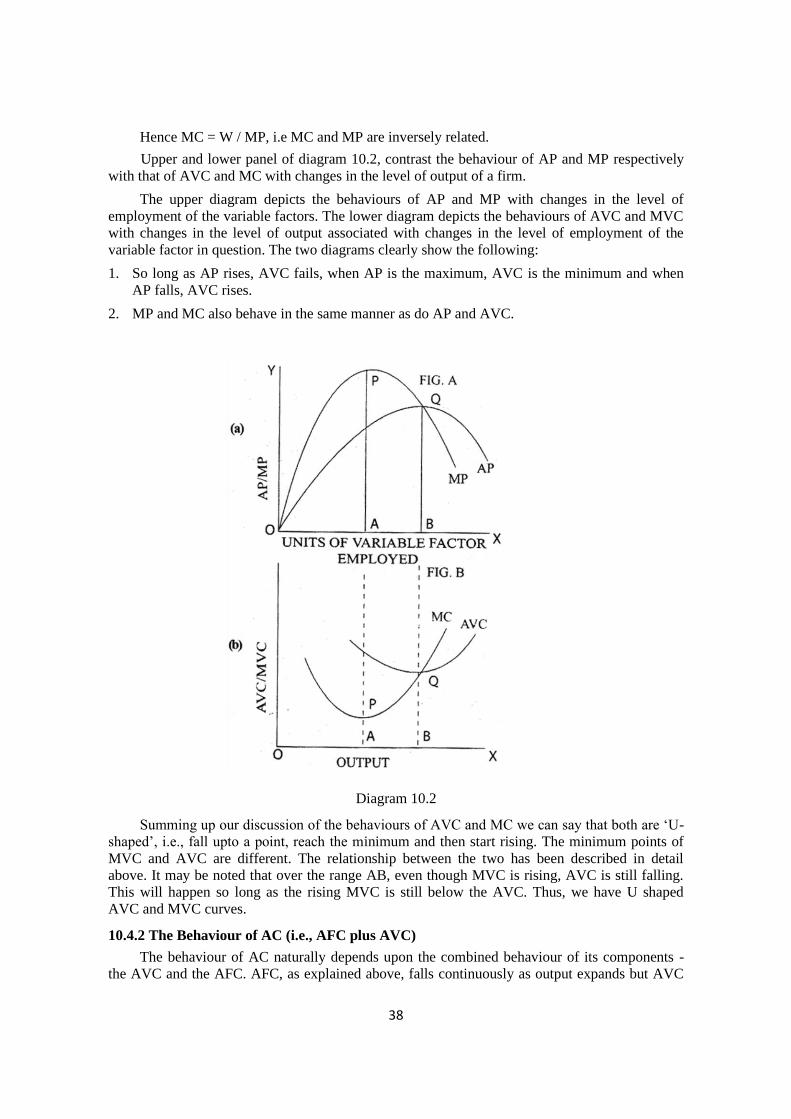
38

Hence MC = W / MP, i.e MC and MP are inversely related.

Upper and lower panel of diagram 10.2, contrast the behaviour of AP and MP respectively

with that of AVC and MC with changes in the level of output of a firm.

The upper diagram depicts the behaviours of AP and MP with changes in the level of

employment of the variable factors. The lower diagram depicts the behaviours of AVC and MVC

with changes in the level of output associated with changes in the level of employment of the

variable factor in question. The two diagrams clearly show the following:

1. So long as AP rises, AVC fails, when AP is the maximum, AVC is the minimum and when

AP falls, AVC rises.

2. MP and MC also behave in the same manner as do AP and AVC.

Diagram 10.2

Summing up our discussion of the behaviours of AVC and MC we can say that both are ‘U-

shaped’, i.e., fall upto a point, reach the minimum and then start rising. The minimum points of

MVC and AVC are different. The relationship between the two has been described in detail

above. It may be noted that over the range AB, even though MVC is rising, AVC is still falling.

This will happen so long as the rising MVC is still below the AVC. Thus, we have U shaped

AVC and MVC curves.

10.4.2 The Behaviour of AC (i.e., AFC plus AVC)

The behaviour of AC naturally depends upon the combined behaviour of its components -

the AVC and the AFC. AFC, as explained above, falls continuously as output expands but AVC

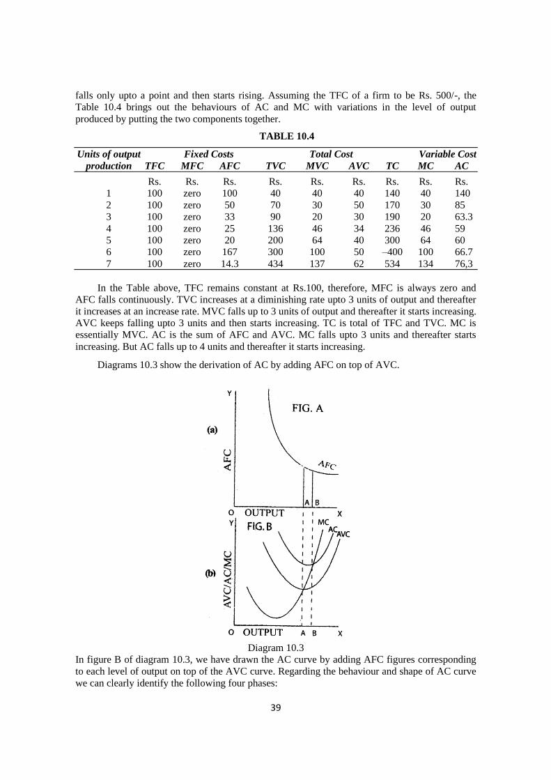
39

falls only upto a point and then starts rising. Assuming the TFC of a firm to be Rs. 500/-, the

Table 10.4 brings out the behaviours of AC and MC with variations in the level of output

produced by putting the two components together.

TABLE 10.4

Units of output Fixed Costs Total Cost Variable Cost

production TFC MFC AFC TVC MVC AVC TC MC AC

Rs. Rs. Rs. Rs. Rs. Rs. Rs. Rs. Rs.

1 100 zero 100 40 40 40 140 40 140

2 100 zero 50 70 30 50 170 30 85

3 100 zero 33 90 20 30 190 20 63.3

4 100 zero 25 136 46 34 236 46 59

5 100 zero 20 200 64 40 300 64 60

6 100 zero 167 300 100 50 –400 100 66.7

7 100 zero 14.3 434 137 62 534 134 76,3

In the Table above, TFC remains constant at Rs.100, therefore, MFC is always zero and

AFC falls continuously. TVC increases at a diminishing rate upto 3 units of output and thereafter

it increases at an increase rate. MVC falls up to 3 units of output and thereafter it starts increasing.

AVC keeps falling upto 3 units and then starts increasing. TC is total of TFC and TVC. MC is

essentially MVC. AC is the sum of AFC and AVC. MC falls upto 3 units and thereafter starts

increasing. But AC falls up to 4 units and thereafter it starts increasing.

Diagrams 10.3 show the derivation of AC by adding AFC on top of AVC.

Diagram 10.3

In figure B of diagram 10.3, we have drawn the AC curve by adding AFC figures corresponding

to each level of output on top of the AVC curve. Regarding the behaviour and shape of AC curve

we can clearly identify the following four phases:

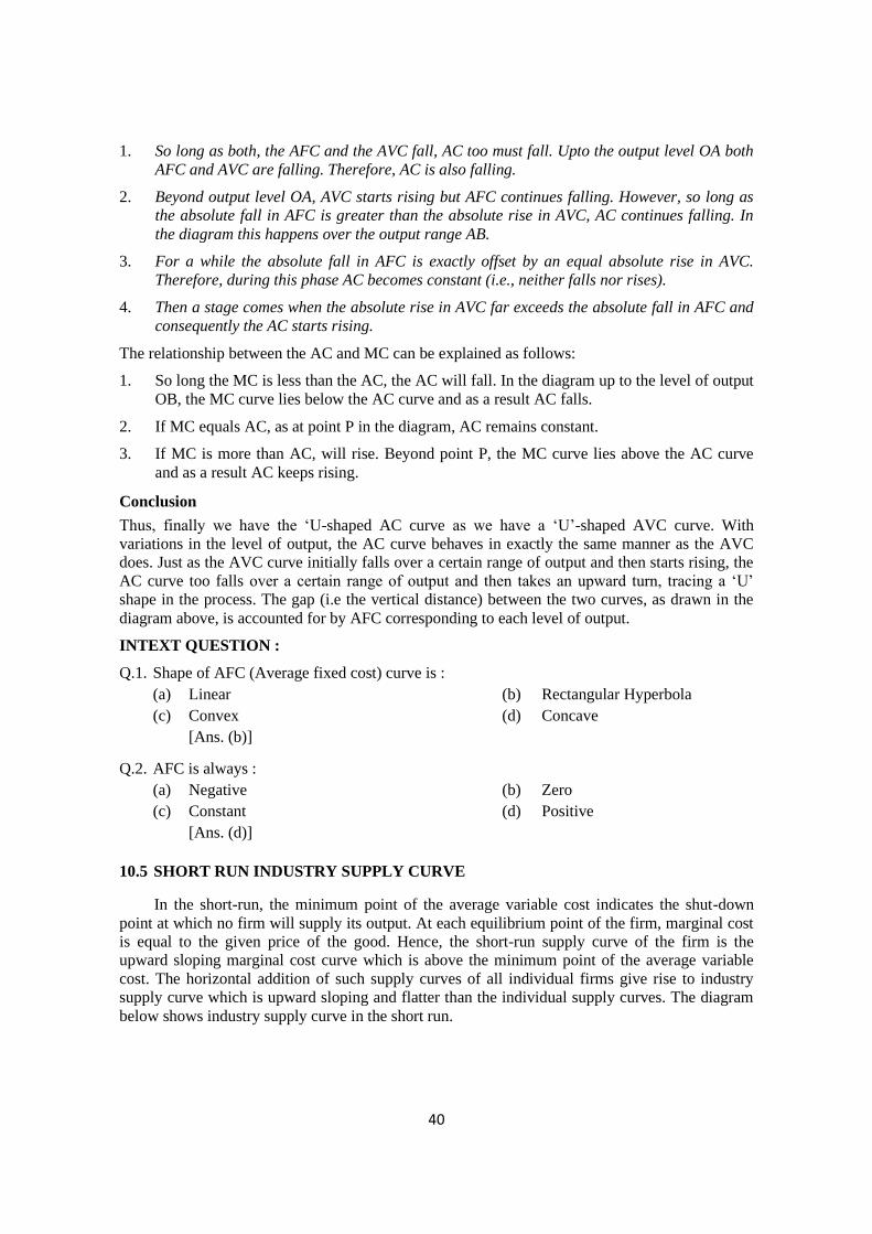
40

1. So long as both, the AFC and the AVC fall, AC too must fall. Upto the output level OA both

AFC and AVC are falling. Therefore, AC is also falling.

2. Beyond output level OA, AVC starts rising but AFC continues falling. However, so long as

the absolute fall in AFC is greater than the absolute rise in AVC, AC continues falling. In

the diagram this happens over the output range AB.

3. For a while the absolute fall in AFC is exactly offset by an equal absolute rise in AVC.

Therefore, during this phase AC becomes constant (i.e., neither falls nor rises).

4. Then a stage comes when the absolute rise in AVC far exceeds the absolute fall in AFC and

consequently the AC starts rising.

The relationship between the AC and MC can be explained as follows:

1. So long the MC is less than the AC, the AC will fall. In the diagram up to the level of output

OB, the MC curve lies below the AC curve and as a result AC falls.

2. If MC equals AC, as at point P in the diagram, AC remains constant.

3. If MC is more than AC, will rise. Beyond point P, the MC curve lies above the AC curve

and as a result AC keeps rising.

Conclusion

Thus, finally we have the ‘U-shaped AC curve as we have a ‘U’-shaped AVC curve. With

variations in the level of output, the AC curve behaves in exactly the same manner as the AVC

does. Just as the AVC curve initially falls over a certain range of output and then starts rising, the

AC curve too falls over a certain range of output and then takes an upward turn, tracing a ‘U’

shape in the process. The gap (i.e the vertical distance) between the two curves, as drawn in the

diagram above, is accounted for by AFC corresponding to each level of output.

INTEXT QUESTION :

Q.1. Shape of AFC (Average fixed cost) curve is :

(a) Linear (b) Rectangular Hyperbola

(c) Convex (d) Concave

[Ans. (b)]

Q.2. AFC is always :

(a) Negative (b) Zero

(c) Constant (d) Positive

[Ans. (d)]

10.5 SHORT RUN INDUSTRY SUPPLY CURVE

In the short-run, the minimum point of the average variable cost indicates the shut-down

point at which no firm will supply its output. At each equilibrium point of the firm, marginal cost

is equal to the given price of the good. Hence, the short-run supply curve of the firm is the

upward sloping marginal cost curve which is above the minimum point of the average variable

cost. The horizontal addition of such supply curves of all individual firms give rise to industry

supply curve which is upward sloping and flatter than the individual supply curves. The diagram

below shows industry supply curve in the short run.

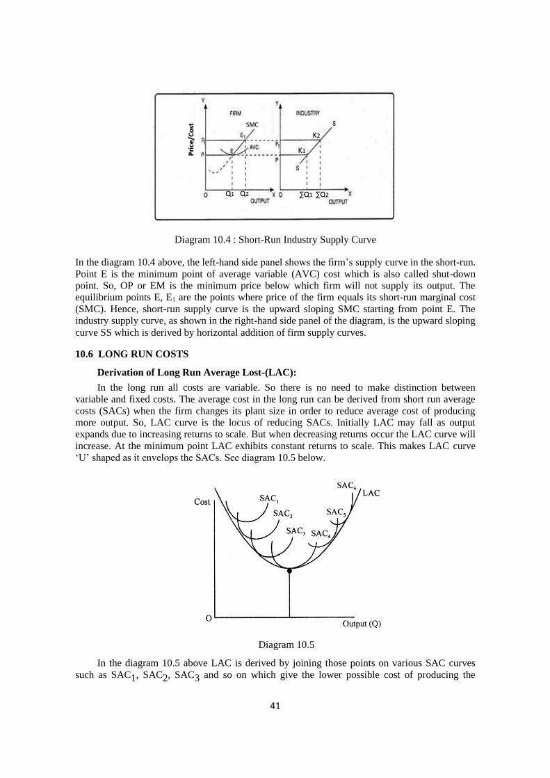
41

Diagram 10.4 : Short-Run Industry Supply Curve

In the diagram 10.4 above, the left-hand side panel shows the firm’s supply curve in the short-run.

Point E is the minimum point of average variable (AVC) cost which is also called shut-down

point. So, OP or EM is the minimum price below which firm will not supply its output. The

equilibrium points E, E1 are the points where price of the firm equals its short-run marginal cost

(SMC). Hence, short-run supply curve is the upward sloping SMC starting from point E. The

industry supply curve, as shown in the right-hand side panel of the diagram, is the upward sloping

curve SS which is derived by horizontal addition of firm supply curves.

10.6 LONG RUN COSTS

Derivation of Long Run Average Lost-(LAC):

In the long run all costs are variable. So there is no need to make distinction between

variable and fixed costs. The average cost in the long run can be derived from short run average

costs (SACs) when the firm changes its plant size in order to reduce average cost of producing

more output. So, LAC curve is the locus of reducing SACs. Initially LAC may fall as output

expands due to increasing returns to scale. But when decreasing returns occur the LAC curve will

increase. At the minimum point LAC exhibits constant returns to scale. This makes LAC curve

‘U’ shaped as it envelops the SACs. See diagram 10.5 below.

Diagram 10.5

In the diagram 10.5 above LAC is derived by joining those points on various SAC curves

such as SAC1, SAC2, SAC3 and so on which give the lower possible cost of producing the

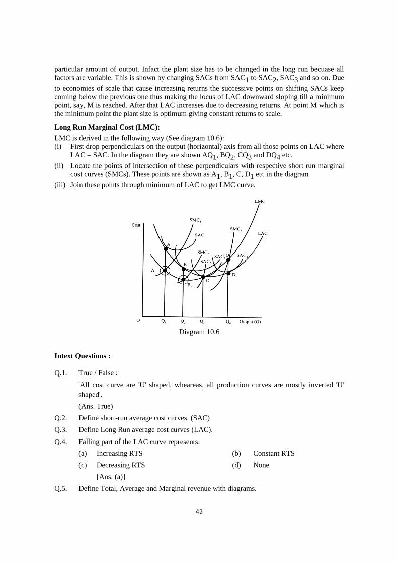
42

particular amount of output. Infact the plant size has to be changed in the long run becuase all

factors are variable. This is shown by changing SACs from SAC1 to SAC2, SAC3 and so on. Due

to economies of scale that cause increasing returns the successive points on shifting SACs keep

coming below the previous one thus making the locus of LAC downward sloping till a minimum

point, say, M is reached. After that LAC increases due to decreasing returns. At point M which is

the minimum point the plant size is optimum giving constant returns to scale.

Long Run Marginal Cost (LMC):

LMC is derived in the following way (See diagram 10.6):

(i) First drop perpendiculars on the output (horizontal) axis from all those points on LAC where

LAC = SAC. In the diagram they are shown AQ1, BQ2, CQ3 and DQ4 etc.

(ii) Locate the points of intersection of these perpendiculars with respective short run marginal

cost curves (SMCs). These points are shown as A1, B1, C, D1 etc in the diagram

(iii) Join these points through minimum of LAC to get LMC curve.

Diagram 10.6

Intext Questions :

Q.1. True / False :

'All cost curve are 'U' shaped, wheareas, all production curves are mostly inverted 'U'

shaped'.

(Ans. True)

Q.2. Define short-run average cost curves. (SAC)

Q.3. Define Long Run average cost curves (LAC).

Q.4. Falling part of the LAC curve represents:

(a) Increasing RTS (b) Constant RTS

(c) Decreasing RTS (d) None

[Ans. (a)]

Q.5. Define Total, Average and Marginal revenue with diagrams.

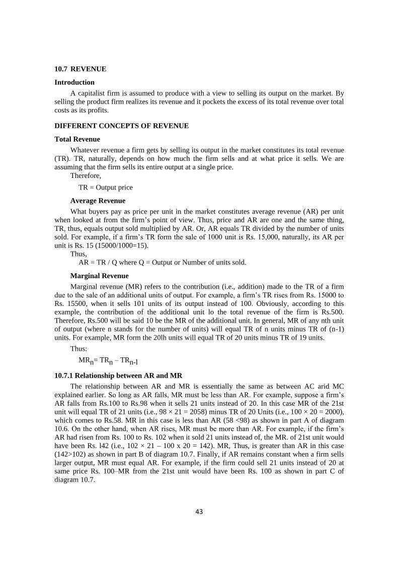
43

10.7 REVENUE

Introduction

A capitalist firm is assumed to produce with a view to selling its output on the market. By

selling the product firm realizes its revenue and it pockets the excess of its total revenue over total

costs as its profits.

DIFFERENT CONCEPTS OF REVENUE

Total Revenue

Whatever revenue a firm gets by selling its output in the market constitutes its total revenue

(TR). TR, naturally, depends on how much the firm sells and at what price it sells. We are

assuming that the firm sells its entire output at a single price.

Therefore,

TR = Output price

Average Revenue

What buyers pay as price per unit in the market constitutes average revenue (AR) per unit

when looked at from the firm’s point of view. Thus, price and AR are one and the same thing,

TR, thus, equals output sold multiplied by AR. Or, AR equals TR divided by the number of units

sold. For example, if a firm’s TR form the sale of 1000 unit is Rs. 15,000, naturally, its AR per

unit is Rs. 15 (15000/1000=15).

Thus,

AR = TR / Q where Q = Output or Number of units sold.

Marginal Revenue

Marginal revenue (MR) refers to the contribution (i.e., addition) made to the TR of a firm

due to the sale of an additional units of output. For example, a firm’s TR rises from Rs. 15000 to

Rs. 15500, when it sells 101 units of its output instead of 100. Obviously, according to this

example, the contribution of the additional unit lo the total revenue of the firm is Rs.500.

Therefore, Rs.500 will be said 10 be the MR of the additional unit. In general, MR of any nth unit

of output (where n stands for the number of units) will equal TR of n units minus TR of (n-1)

units. For example, MR form the 20lh units will equal TR of 20 units minus TR of 19 units.

Thus:

MRn= TRn – TRn-l

10.7.1 Relationship between AR and MR

The relationship between AR and MR is essentially the same as between AC arid MC

explained earlier. So long as AR falls, MR must be less than AR. For example, suppose a firm’s

AR falls from Rs.100 to Rs.98 when it sells 21 units instead of 20. In this case MR of the 21st

unit will equal TR of 21 units (i.e., 98 × 21 = 2058) minus TR of 20 Units (i.e., 100 × 20 = 2000),

which comes to Rs.58. MR in this case is less than AR (58 <98) as shown in part A of diagram

10.6. On the other hand, when AR rises, MR must be more than AR. For example, if the firm’s

AR had risen from Rs. 100 to Rs. 102 when it sold 21 units instead of, the MR. of 21st unit would

have been Rs. l42 (i.e., 102 × 21 – 100 x 20 = 142). MR, Thus, is greater than AR in this case

(142>102) as shown in part B of diagram 10.7. Finally, if AR remains constant when a firm sells

larger output, MR must equal AR. For example, if the firm could sell 21 units instead of 20 at

same price Rs. 100–MR from the 21st unit would have been Rs. 100 as shown in part C of

diagram 10.7.

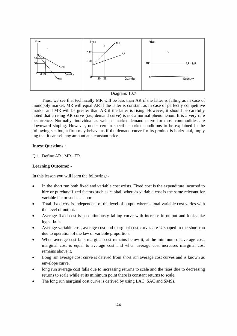
44

Diagram: 10.7

Thus, we see that technically MR will be less than AR if the latter is falling as in case of

monopoly market, MR will equal AR if the latter is constant as in case of perfectly competitive

market and MR will be greater than AR if the latter is rising. However, it should be carefully

noted that a rising AR curve (i.e., demand curve) is not a normal phenomenon. It is a very rare

occurrence. Normally, individual as well as market demand curve for most commodities are

downward sloping. However, under certain specific market conditions to be explained in the

following section, a firm may behave as if the demand curve for its product is horizontal, imply

ing that it can sell any amount at a constant price.

Intext Questions :

Q.1 Define AR , MR , TR.

Learning Outcome: -

In this lesson you will learn the following: -

• In the short run both fixed and variable cost exists. Fixed cost is the expenditure incurred to

hire or purchase fixed factors such as capital, whereas variable cost is the same relevant for

variable factor such as labor.

• Total fixed cost is independent of the level of output whereas total variable cost varies with

the level of output.

• Average fixed cost is a continuously falling curve with increase in output and looks like

hyper bola

• Average variable cost, average cost and marginal cost curves are U-shaped in the short run

due to operation of the law of variable proportion.

• When average cost falls marginal cost remains below it, at the minimum of average cost,

marginal cost is equal to average cost and when average cost increases marginal cost

remains above it.

• Long run average cost curve is derived from short run average cost curves and is known as

envelope curve.

• long run average cost falls due to increasing returns to scale and the rises due to decreasing

returns to scale while at its minimum point there is constant returns to scale.

• The long run marginal cost curve is derived by using LAC, SAC and SMSs.

45

• Total revenue is the total sale receipts of the firm from selling a product while average

revenue is the price of the product. Marginal revenue is defined as the change in total

revenue due to change in the quantity of the product.

• Given price as a constant value AR=MR, if price falls with increase in quantity then MR

remains below AR.

• Under perfect competition the total revenue is straight line through the origin as it appears

on the quantity sold, whereas under monopoly the total revenue increases at a decreasing

rate and finally reaches the maximum and then falls with increase in output.

Long Answer type questions

Q.1. In detail, explain and derive the Long Run Production function Curve.

Q.2. Explain the relationship between TP, AP, MP diagrammatically.

Q.3. Diagrammatically explain the relationship between MC and AC.

46

LESSON: 11

ECONOMICS OF SCALE

INTRODUCTION

Increasing returns to scale are cause economies of scale Economies of scale can be internal

or external. The former arise due to change in the size of the firm and the latter on account of

expansion of the industry, i.e., number of firms. In each case, however, the economies accrue to

the firm (though in the case of external economies, for no action of its own). A firm can increase

its production only by increasing its outlay or expenditure on various factors of production. It can

do this either by keeping the factor proportions constant i.e., by increasing the amount of each

factor used by the same proportion (e.g., doubling or trebling all the inputs) or by increase the

factor quantities, but varying at the same time the proportions in which various factors are used.

When various factor are varied in level, but kept constant in proportion, the relationship between

the change in composite input and that in output is characterized by ‘returns to scale’. If all the

factor inputs are multiplied by a factor λ and the resulting output is µ times the original output,

increasing, constant and decreasing returns to scale can be defined according to whether µ>λ, µ=λ

or µ<λ respectively. If the firm decides to increase the number of plants identical to each other

(e.g., building another plant in order to double the output). It can at least achieve constant returns

to scale. The process is known as ‘replication’. Returns to scale may increase or decrease or

remain constant if, however, the firm increases the size of the plant but keeps the factor

proportions constant. However, the firm may find it more profitable to change the proportion in

which factors are combined, i.e, to change the technique of production to achieve a higher level of

output. The economies which accrue to the firm in some of the above-mentioned cases are ‘real

economies’ as these originate from the technical relationships. In contrast, ‘pecuniary economies’

arise due to lower prices paid by a firm for the factors of production it buys while increasing its

level of output. The former is associated with lower physical quantities of resources required per

unit of output while the latter with lower prices per unit for the factor/factors. We shall first

discuss real economies in some detail.

After going through this lesson you will learn: -

• Understand the concept of economies and diseconomies of scale

• Distinguish between internal and external economies

11.1 CONCEPT OF AND TYPES OF ECONOMIES OF SCALE

Economies of Scale refer to the cost advantages experienced by a firm when it increases its

level of output by increasing its scale of operation. It assumed that scale of operation can be

increased by increasing the factors simultaneously. This results in decreasing per unit cost of

production manifested by a fall in long run average cost curve till it reaches its minimum point.

Economies of scale can be of two types: (i) Internal economies and (ii) External economies.

See the Chart below. Internal economies are further divided into two groups – Real and Pecuniary

economies respectively. Internal economies are the advantages or benefits reaped by the firm due

the factors which are under its control. Real economies consist of a mixture of several functions

noticed at work place such as: efficiency of labour or labour economies, use of better technology

called technical economies, existence of inventories, managerial abilities, marketing and demand

and supply management. Pecuniary economies include immediate monetary gains due to

discounts.

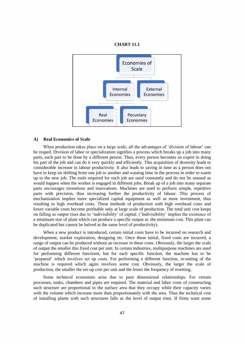
47

CHART 11.1

A) Real Economics of Scale

When production takes place on a large scale, all the advantages of ‘division of labour’ can

be reaped. Division of labor or specialization signifies a process which breaks up a job into many

parts, each part to be done by a different person. Thus, every person becomes an expert in doing

his part of the job and can do it very quickly and efficiently. This acquisition of dexterity leads to

considerable increase in labour productivity. It also leads to saving in time as a person does not

have to keep on shifting from one job to another and wasting time in the process in order to warm

up to the new job. The tools required for each job are used constantly and do not lie unused as

would happen when the worker is engaged in different jobs. Break up of a job into many separate

parts encourages inventions and innovations. Machines are used to perform simple, repetitive

parts with precision, thus increasing further the productivity of labour. This process of

mechanization implies more specialized capital equipment as well as more investment, thus

resulting in high overhead costs. These methods of production with high overhead costs and

lower variable costs become profitable only at large scale of production. The total unit cost keeps

on falling as output rises due to ‘indivisibility’ of capital. (’Indivisibility’ implies the existence of

a minimum size of plant which can produce a specific output at. the minimum cost. This plant can

be duplicated but cannot be halved at the same level of productivity).

When a new product is introduced, certain initial costs have to be incurred on research and

development, market exploration, designing etc. Once these initial, fixed costs are incurred, a

range of output can be produced without an increase in these costs. Obviously, the larger the scale

of output the smaller this fixed cost per unit. In certain industries, multipurpose machines are used

for performing different functions, but for each specific function, the machine has to be

‘prepared’ which involves set up costs. For performing a different function, re-setting of the

machine is required which again involves some cost. Obviously, the larger the scale of

production, the smaller the set-up cost per unit and the lesser the frequency of resetting.

Some technical economies arise due to pure dimensional relationships. For certain

processes, tanks, chambers and pipes are required. The material and labor costs of constructing

such structure are proportional to the surface area that they occupy while their capacity varies

with the volume which increase more than proportionately with the area. Thus the technical cost

of installing plants with such structures falls as the level of output rises. If firms want some

48

reserve capacity to maintain a smooth flow of output in case of breakdown of machinery, again

firms with larger output stand to gain. A small firm has to spend a proportionately larger part of

its investment in fixed capital to maintain some reserve capacity while the cost of reserve capacity

to a big firm is lower. Similarly, in order to meet random changes in the supply of inputs,

especially raw materials, and demand, a firm needs to keep stocks of raw materials and finished

product. But the required size of inventories does not increase proportionately with the size of

output. A bigger firm can maintain its flow of input and output with proportionately smaller

inventories of raw materials and output.

Under monopolistic competition, all firms whether old or new need to advertise their

products. But advertising costs do not increase proportionately with the size of output. The

advertising budget is decided based on availability of funds, profits of the firm, existence of close

substitutes of the product, advertising activities of the competitors etc. Therefore, selling costs per

unit generally fall with increase in output. The expenditure on other types of selling activities (e.g.

number of salesmen, distribution of samples, agreements with distributors etc.) also increases less

than proportionately with the size of output. A change in the model or style of the product

involves considerable expenditure on research and development, new materials and equipment,

sales promotion etc. The spreading of such overheads is lower per unit if the size of output is

large. To sum up, we can say that whatever the social and economic role of advertising, selling

cost per unit of output does fall with scale of output up to a point at least due to existence of

marketing economies.

Large size of a firm makes possible division of managerial tasks relating to production,

sales, finance, personnel etc. This division of labor increases managerial efficiency and reduces

cost per unit of output. But small firms cannot reap the advantages of such specialization.

Moreover, with decentralization of decision making, the efficiency of management increases.

Large firms can also afford to apply highly mechanized and efficient techniques of management,

e.g., telephones, telex machines, closed circuit televisions, computers etc. The use of such aids

increases managerial efficiency and reduces cost per unit of output. However, many economists

think that after a point the management of a large enterprise becomes extremely complex and

difficulties of supervision and coordination give rise to managerial diseconomies, thus leading to

an upward turn in the average cost curve.

There are economies of large scale with respect to storage and transport also. Storage and

transport costs are incurred both on the production side and selling side. As the construction of

store-houses follows the geometrical relationship between area and volume, the cost of storage

per unit falls with size of output. Increasing the number of floors of storehouses will be still more

economical. Similarly, the unit cost of transport will fall up to the point of full capacity of the

firm’s means of transportation. Use of larger vehicles at a larger scale of output would also lead to

a fall in unit cost of transport. However, with public transport, the unit costs will normally

increase with distance unless there are concessional freight rates for bulk transport.

B. Pecuniary Economies of Scale

Firms engaged in large scale operations can generally obtain ‘discounts’ or concessions on

many accounts. They can purchase raw materials at lower prices, get loans at lower rates of

interest (and other favorable terms), advertise their products at concessional rates and transport

their goods at lower rates. All these concessions are given due to the large size of operations. Big

firms can also sometimes hire workers at lower wages due to their monopolistic power. (A

monopsonist is one who controls a major part of the demand for a commodity or a factor of

production). Due to all such pecuniary economies, the average cost falls with size of output. The

economists do not, however, agree on whether there is continuous reduction in unit costs with

increase in output or the average cost curve rises after a certain point due to diseconomies (mainly

49

managerial) of scale. Only a sufficiently large number of empirical studies, conducted

scientifically, can resolve this issue.

Intext Questions :

Q.1. What are the types of EOS.

Q.2. Which of the following is not a part of Real EOS?

(a) Technical (b) Marketing

(c) Labor (d) Cheap raw material

[Ans. (d)]

Q.3. Define Real EOS..

Q.4. Define Pecuniary EOS.

11.2. EXTERNAL ECONOMIES:

External economies refer to all those benefits which accrue to all the firms operating in a

given industry. Generally, these economies accrue due to the expansion of industry and other

facilities expanded by the Government. They are benefits which are shared by several firms or

industries when the scale of production in any industry increases.

Locational advantage of a firm is an example of external economies. Similarly, when the

number of firms in an area increases each firm enjoys some benefits like, transport and

communication, availability of raw materials, research and invention etc. Further, financial

assistance from banks and non-bank institutions easily accrue to individual firms. When many

firms come together to form an industrial cluster or township, they become mutually dependent

on each other. These firms can form their trade association/confederation etc to serve the common

purpose by sharing cost. There will be no need of independent research on individual basis. Many

scientific and trade journals can be published to supply information to all relating to new markets,

sources of raw materials, latest techniques of production etc at a lower cost. These benefits are

called Economies of Information.

As an industry develops, all the firms engaged in it decide to divide and sub-divide the

process of production among themselves. Each firm specializes in its own process. These benefits

are called Economies of Disintegration. It is of two types-horizontal disintegration and vertical

disintegration. In case of horizontal disintegration each firm in the industry tries to specialize in

one item whereas, under vertical disintegration every firm endeavour to specialize in different

types of items. Material of one firm may be available and useable as raw materials in the other

firms. Thus, wastes are converted into by-products. The selling firms reduce their costs of

production and drive the average cost of production down.

The industry can also develop common R&D for benefit of all firms.

11.3 DISECONOMIES OF SCALE

A) Internal diseconomies of scale:

Refer to diseconomies that raise the cost of production of an organization. The main factors

that influence the cost of production of an organization include the lack of decision, supervision,

and technical difficulties.

50

B) External diseconomies of scale:

Refer to diseconomies that limit the expansion of an organization or industry. The factors

that act as restraint to expansion include increased cost of production, scarcity of raw materials,

and low supply of skilled labourer.

C) Decreasing returns to scale are caused by diseconomies of scale which maybe due to the

following factors-

(i) Managerial inefficiency caused by excess burden of work on managers

(ii) Fall in availability of non-renewable resources due to continuous consumption overtime.

Livestock and fisheries do have gestation period during which there may not be an adequate

supply.

(iii) Taxation by government may drive a firm out of business.

INTEXT QUESTIONS :

Q.1. Which of these factors will NOT result is Diseconomies of scale?

(a) Managerial inefficiency

(b) Reduction in Non-Renewable Resources

(c) Small Plant size

(d) Taxation

[Ans. ©]

Q.2. Define Diseconomies of scales.

LEARNING OUTCOMES

In this lesson you have learnt the following: -

• Increasing returns to scale are caused by economies of scale line while decreasing returns

are caused by diseconomies of scale.

• Internal economies arrives due to efficiency of the factors indigenous to the firm. Some of

the internal economies are division of labour, technical economies, inventories, managerial

efficiency, marketing strategy, transport and wage facilities, low cost finance and

discontinuous due to bulk purchase.

• External economies are caused by exogenous factors such as Government subsidy, Tax

rebate, export promotion, good rainfall in agriculture etc.

• Diseconomies of scale are caused due to heavy burden of working load on managers,

unavailability of resources caused by increasing competitions and depletion in natural

resources.

• External diseconomies are caused by exogenous factors such as tax by Government.

TERMINAL QUESTION

Q. Discuss in detail the Economies and Diseconomies of scale.

51

LESSON: 12

PERFECT COMPETITION

INTRODUCTION

Market demand curves for most commodities are downward sloping indicating that larger

quantities of a commodity can be sold in the market only at lower and lower prices. However,

what matters for a profit maximizing firm is not the total market demand for the commodity, but

that part of it which flows to it. If a firm happens to be the only producer of a commodity, then

the market demand for it is the demand for the firm’s product. In such a case the firm will know

that by increasing or decreasing its sales it will affect the price of the product. In contrast to this,

consider a situation in which the market demand for a commodity is met by such a large number

of firms that an individual firm meets a negligibly small fraction of it. In such a case, the firm can

never imagine that it can influence the market price by increasing or decreasing its scale of

operation. Besides the question of number of firms in the market, there are other variables such as

availability of close substitutes, their prices, preferences of buyers, advertisement, and so on;

which have a considerable bearing on the demand for an individual firm’s product. It is beyond

the scope of this paper to consider all market situations and analyze their effects on firm’s

revenue. We will consider only two extreme market situations, viz., perfect competition and

monopoly in addition to imperfect competition.

After going through this lesson, you will be able to learn: -

• Know the features of perfect competition

• Equilibrium of firm and industry under perfect competition in the short run.

• Equilibrium of firm and industry under perfect competition in the long run.

• Derivation of short run supply curve of firm under perfect competition and finally derivation

of long run supply curve of industry.

• Explain allocative efficiency of perfect competition

12.1 MEANING AND FEATURES OF PERFECT COMPETITION

Perfect competition refers to a theoretical market situation in which a single price,

determined by the market forces of supply and demand for a commodity, ruling in the market is a

datum for individual buyers and sellers and when firms in the industry, in the long run, are able to

earn no more than normal profits (i.e., normal earnings of management) which are assumed

included in the firm’s average (total) cost as an element of fixed cost. In other words, perfect

competition prevails when (a) individual buyers and sellers of the commodity are price takers and

not the price-sellers (i.e., are unable to influence the given market price in the slightest degree by

increasing their sales or purchase} and (b) when in the long run TR of a firm equals its TC which

includes normal profits (or alternatively when AR equals AC).

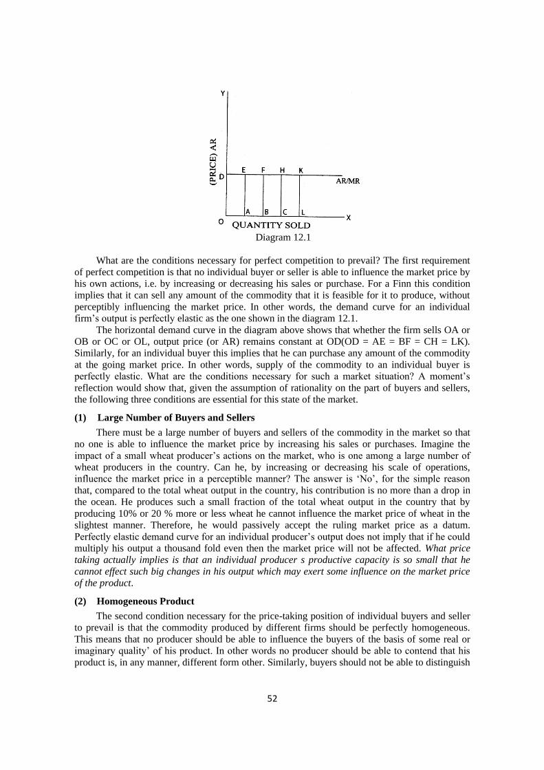
52

Diagram 12.1

What are the conditions necessary for perfect competition to prevail? The first requirement

of perfect competition is that no individual buyer or seller is able to influence the market price by

his own actions, i.e. by increasing or decreasing his sales or purchase. For a Finn this condition

implies that it can sell any amount of the commodity that it is feasible for it to produce, without

perceptibly influencing the market price. In other words, the demand curve for an individual

firm’s output is perfectly elastic as the one shown in the diagram 12.1.

The horizontal demand curve in the diagram above shows that whether the firm sells OA or

OB or OC or OL, output price (or AR) remains constant at OD(OD = AE = BF = CH = LK).

Similarly, for an individual buyer this implies that he can purchase any amount of the commodity

at the going market price. In other words, supply of the commodity to an individual buyer is

perfectly elastic. What are the conditions necessary for such a market situation? A moment’s

reflection would show that, given the assumption of rationality on the part of buyers and sellers,

the following three conditions are essential for this state of the market.

(1) Large Number of Buyers and Sellers

There must be a large number of buyers and sellers of the commodity in the market so that

no one is able to influence the market price by increasing his sales or purchases. Imagine the

impact of a small wheat producer’s actions on the market, who is one among a large number of

wheat producers in the country. Can he, by increasing or decreasing his scale of operations,

influence the market price in a perceptible manner? The answer is ‘No’, for the simple reason

that, compared to the total wheat output in the country, his contribution is no more than a drop in

the ocean. He produces such a small fraction of the total wheat output in the country that by

producing 10% or 20 % more or less wheat he cannot influence the market price of wheat in the

slightest manner. Therefore, he would passively accept the ruling market price as a datum.

Perfectly elastic demand curve for an individual producer’s output does not imply that if he could

multiply his output a thousand fold even then the market price will not be affected. What price

taking actually implies is that an individual producer s productive capacity is so small that he

cannot effect such big changes in his output which may exert some influence on the market price

of the product.

(2) Homogeneous Product

The second condition necessary for the price-taking position of individual buyers and seller

to prevail is that the commodity produced by different firms should be perfectly homogeneous.

This means that no producer should be able to influence the buyers of the basis of some real or

imaginary quality’ of his product. In other words no producer should be able to contend that his

product is, in any manner, different form other. Similarly, buyers should not be able to distinguish

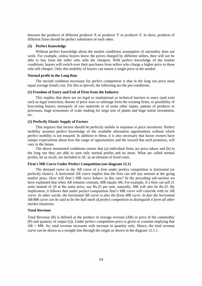
53

between the products of different producer X or producer Y or producer Z. In short, products of

different firms should be perfect substitutes of each other.

(3) Perfect Knowledge

Without perfect knowledge about the market conditions assumption of rationality does not

work. For example, unless buyers know the prices charged by different sellers, they will not be

able to buy form the seller who sells the cheapest. With perfect knowledge of the market

conditions, buyers will switch over their purchases from sellers who charge a higher price to those

who sell cheaper. Only this mobility of buyers can ensure a single price in the market.

Normal profit in the Long Run

The second condition necessary for perfect competition is that in the long run price must

equal average (total) cost. For this to prevail, the following are the pre-conditions.

(1) Freedom of Entry and Exit of Firm from the Industry

This implies that there are no legal or institutional or technical barriers to entry (and exit)

such as legal restriction, threats of price wars or sabotage form the existing firms, or possibility of

boycotting buyers, monopoly of raw materials or of some other inputs, patents of products or

processes, huge economies of scale making for large size of plants and huge initial investment,

etc.

(2) Perfectly Elastic Supply of Factors

This requires that factors should be perfectly mobile in response to price incentives. Perfect

mobility assumes perfect knowledge of the available alternative opportunities without which

perfect mobility is not ensured. In addition to these, it is also necessary that factor owners have

unique expectations about how the range of opportunities and the reward that each promises, will

vary in the future.

The above mentioned conditions ensure that (a) individual firms are price takers and (b) in

the long run they are able to earn only normal profits and no more. What are called normal

profits, let us recall, are included in AC as an element of fixed costs.

Firm's MR Curve Under Perfect Competition (see diagram 12.1)

The demand curve or the AR curve of a firm under perfect competition is horizontal (or

perfectly elastic). A horizontal AR curve implies that the firm can sell any amount at the going

market price. How will firm’s MR curve behave in this case? In the preceding sub-section we

have explained that when AR remains constant, MR equals AR, For example, if a firm can sell 21

units instead of 20 at the same price, say Rs.25 per unit, naturally, MR will also be Rs.25. By

implication, it follows that under perfect competition firm’s MR curve will coincide with its AR

curve. In other words, the horizontal AR curve is also the firms MR curve. In fact the horizontal

AR/MR curve can be said to be the hall mark of perfect competition to distinguish it form all other

market situations.

Total Revenue

Total Revenue (R) is defined as the product of average revenue (AR) or price of the commodity

(P) and quantity of output (Q). Under perfect competition price is given or constant implying that

AR = MR. So, total revenue increases with increase in quantity only. Hence, the total revenue

curve can be drawn as a straight line through the origin as shown in the diagram 12.1.1.

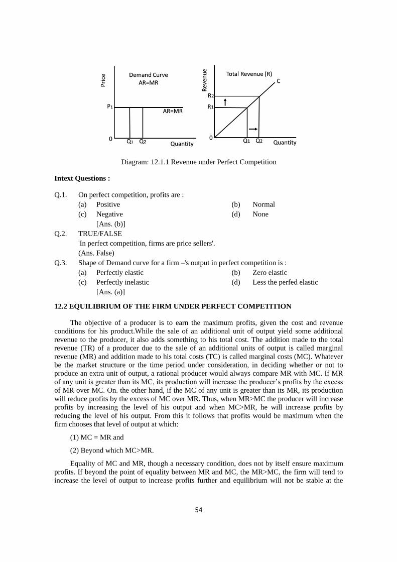
54

Diagram: 12.1.1 Revenue under Perfect Competition

Intext Questions :

Q.1. On perfect competition, profits are :

(a) Positive (b) Normal

(c) Negative (d) None

[Ans. (b)]

Q.2. TRUE/FALSE

'In perfect competition, firms are price sellers'.

(Ans. False)

Q.3. Shape of Demand curve for a firm –'s output in perfect competition is :

(a) Perfectly elastic (b) Zero elastic

(c) Perfectly inelastic (d) Less the perfed elastic

[Ans. (a)]

12.2 EQUILIBRIUM OF THE FIRM UNDER PERFECT COMPETITION

The objective of a producer is to earn the maximum profits, given the cost and revenue

conditions for his product.While the sale of an additional unit of output yield some additional

revenue to the producer, it also adds something to his total cost. The addition made to the total

revenue (TR) of a producer due to the sale of an additional units of output is called marginal

revenue (MR) and addition made to his total costs (TC) is called marginal costs (MC). Whatever

be the market structure or the time period under consideration, in deciding whether or not to

produce an extra unit of output, a rational producer would always compare MR with MC. If MR

of any unit is greater than its MC, its production will increase the producer’s profits by the excess

of MR over MC. On. the other hand, if the MC of any unit is greater than its MR, its production

will reduce profits by the excess of MC over MR. Thus, when MR>MC the producer will increase

profits by increasing the level of his output and when MC>MR, he will increase profits by

reducing the level of his output. From this it follows that profits would be maximum when the

firm chooses that level of output at which:

(1) MC = MR and

(2) Beyond which MC>MR.

Equality of MC and MR, though a necessary condition, does not by itself ensure maximum

profits. If beyond the point of equality between MR and MC, the MR>MC, the firm will tend to

increase the level of output to increase profits further and equilibrium will not be stable at the

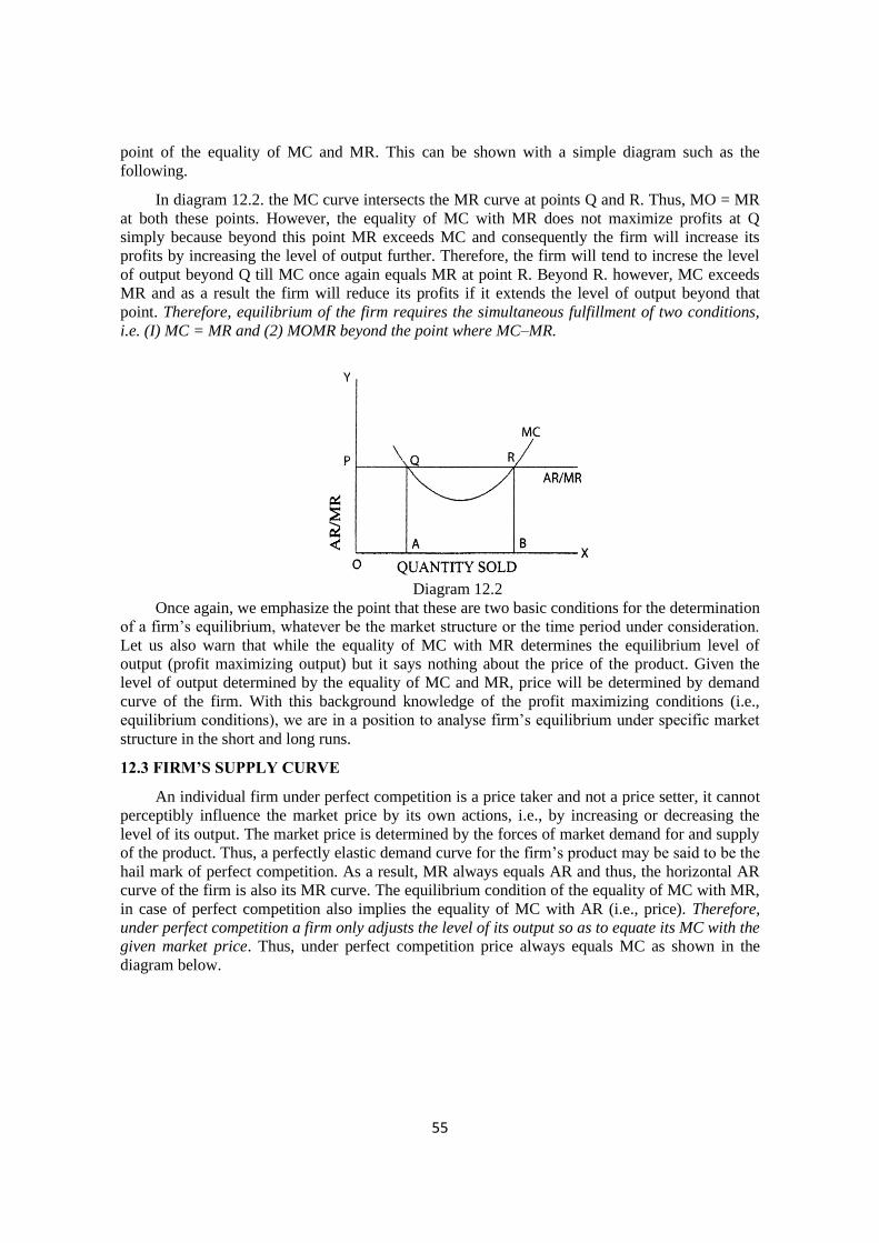
55

point of the equality of MC and MR. This can be shown with a simple diagram such as the

following.

In diagram 12.2. the MC curve intersects the MR curve at points Q and R. Thus, MO = MR

at both these points. However, the equality of MC with MR does not maximize profits at Q

simply because beyond this point MR exceeds MC and consequently the firm will increase its

profits by increasing the level of output further. Therefore, the firm will tend to increse the level

of output beyond Q till MC once again equals MR at point R. Beyond R. however, MC exceeds

MR and as a result the firm will reduce its profits if it extends the level of output beyond that

point. Therefore, equilibrium of the firm requires the simultaneous fulfillment of two conditions,

i.e. (I) MC = MR and (2) MOMR beyond the point where MC–MR.

Diagram 12.2

Once again, we emphasize the point that these are two basic conditions for the determination

of a firm’s equilibrium, whatever be the market structure or the time period under consideration.

Let us also warn that while the equality of MC with MR determines the equilibrium level of

output (profit maximizing output) but it says nothing about the price of the product. Given the

level of output determined by the equality of MC and MR, price will be determined by demand

curve of the firm. With this background knowledge of the profit maximizing conditions (i.e.,

equilibrium conditions), we are in a position to analyse firm’s equilibrium under specific market

structure in the short and long runs.

12.3 FIRM’S SUPPLY CURVE

An individual firm under perfect competition is a price taker and not a price setter, it cannot

perceptibly influence the market price by its own actions, i.e., by increasing or decreasing the

level of its output. The market price is determined by the forces of market demand for and supply

of the product. Thus, a perfectly elastic demand curve for the firm’s product may be said to be the

hail mark of perfect competition. As a result, MR always equals AR and thus, the horizontal AR

curve of the firm is also its MR curve. The equilibrium condition of the equality of MC with MR,

in case of perfect competition also implies the equality of MC with AR (i.e., price). Therefore,

under perfect competition a firm only adjusts the level of its output so as to equate its MC with the

given market price. Thus, under perfect competition price always equals MC as shown in the

diagram below.

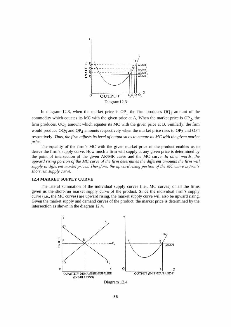
56

Diagram12.3

In diagram 12.3, when the market price is OP1 the firm produces OQ1 amount of the

commodity which equates its MC with the given price at A, When the market price is OP2, the

firm produces. OQ2 amount which equates its MC with the given price at B. Similarly, the firm

would produce OQ3 and OP4 amounts respectively when the market price rises to OP3 and OP4

respectively. Thus, the firm adjusts its level of output so as to equate its MC with the given market

price.

The equality of the firm’s MC with the given market price of the product enables us to

derive the firm’s supply curve. How much a firm will supply at any given price is determined by

the point of intersection of the given AR/MR curve and the MC curve. In other words, the

upward rising portion of the MC curve of the firm determines the different amounts the firm will

supply at different market prices. Therefore, the upward rising portion of the MC curve is firm’s

short run supply curve.

12.4 MARKET SUPPLY CURVE

The lateral summation of the individual supply curves (i.e., MC curves) of all the firms

given us the short-run market supply curve of the product. Since the individual firm’s supply

curve (i.e., the MC curves) are upward rising, the market supply curve will also be upward rising.

Given the market supply and demand curves of the product, the market price is determined by the

intersection as shown in the diagram 12.4.

Diagram 12.4

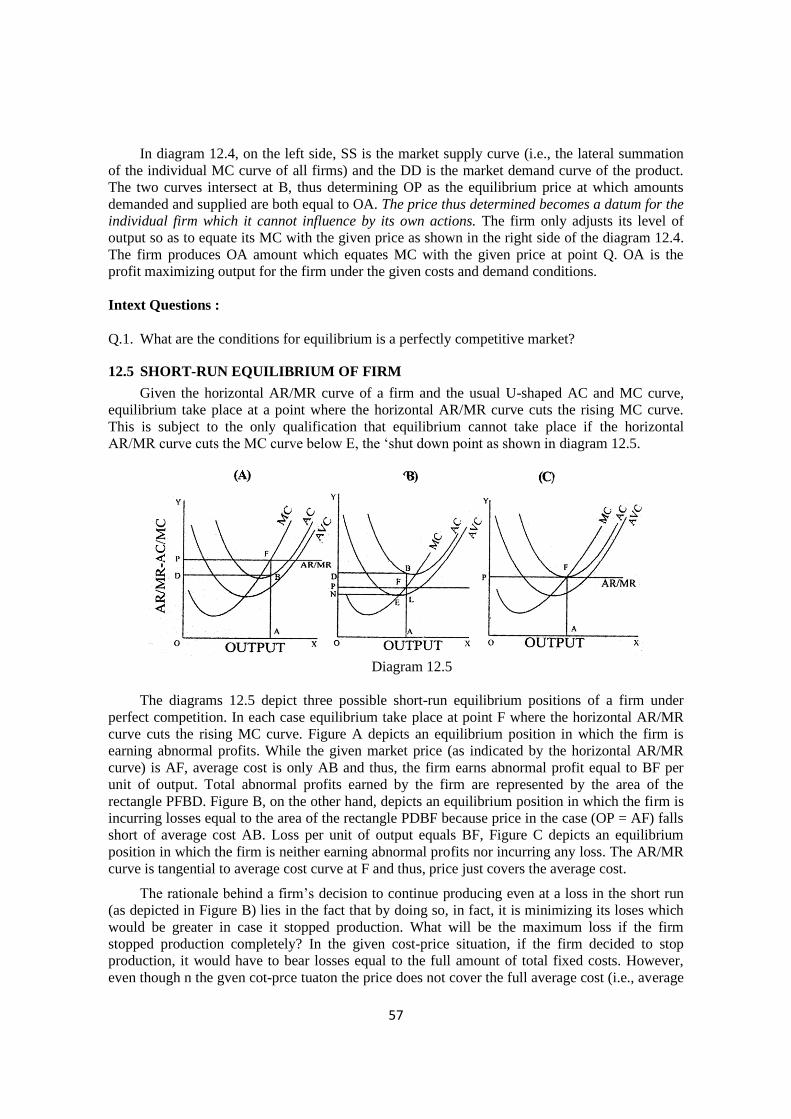
57

In diagram 12.4, on the left side, SS is the market supply curve (i.e., the lateral summation

of the individual MC curve of all firms) and the DD is the market demand curve of the product.

The two curves intersect at B, thus determining OP as the equilibrium price at which amounts

demanded and supplied are both equal to OA. The price thus determined becomes a datum for the

individual firm which it cannot influence by its own actions. The firm only adjusts its level of

output so as to equate its MC with the given price as shown in the right side of the diagram 12.4.

The firm produces OA amount which equates MC with the given price at point Q. OA is the

profit maximizing output for the firm under the given costs and demand conditions.

Intext Questions :

Q.1. What are the conditions for equilibrium is a perfectly competitive market?

12.5 SHORT-RUN EQUILIBRIUM OF FIRM

Given the horizontal AR/MR curve of a firm and the usual U-shaped AC and MC curve,

equilibrium take place at a point where the horizontal AR/MR curve cuts the rising MC curve.

This is subject to the only qualification that equilibrium cannot take place if the horizontal

AR/MR curve cuts the MC curve below E, the ‘shut down point as shown in diagram 12.5.

Diagram 12.5

The diagrams 12.5 depict three possible short-run equilibrium positions of a firm under

perfect competition. In each case equilibrium take place at point F where the horizontal AR/MR

curve cuts the rising MC curve. Figure A depicts an equilibrium position in which the firm is

earning abnormal profits. While the given market price (as indicated by the horizontal AR/MR

curve) is AF, average cost is only AB and thus, the firm earns abnormal profit equal to BF per

unit of output. Total abnormal profits earned by the firm are represented by the area of the

rectangle PFBD. Figure B, on the other hand, depicts an equilibrium position in which the firm is

incurring losses equal to the area of the rectangle PDBF because price in the case (OP = AF) falls

short of average cost AB. Loss per unit of output equals BF, Figure C depicts an equilibrium

position in which the firm is neither earning abnormal profits nor incurring any loss. The AR/MR

curve is tangential to average cost curve at F and thus, price just covers the average cost.

The rationale behind a firm’s decision to continue producing even at a loss in the short run

(as depicted in Figure B) lies in the fact that by doing so, in fact, it is minimizing its loses which

would be greater in case it stopped production. What will be the maximum loss if the firm

stopped production completely? In the given cost-price situation, if the firm decided to stop

production, it would have to bear losses equal to the full amount of total fixed costs. However,

even though n the gven cot-prce tuaton the price does not cover the full average cost (i.e., average

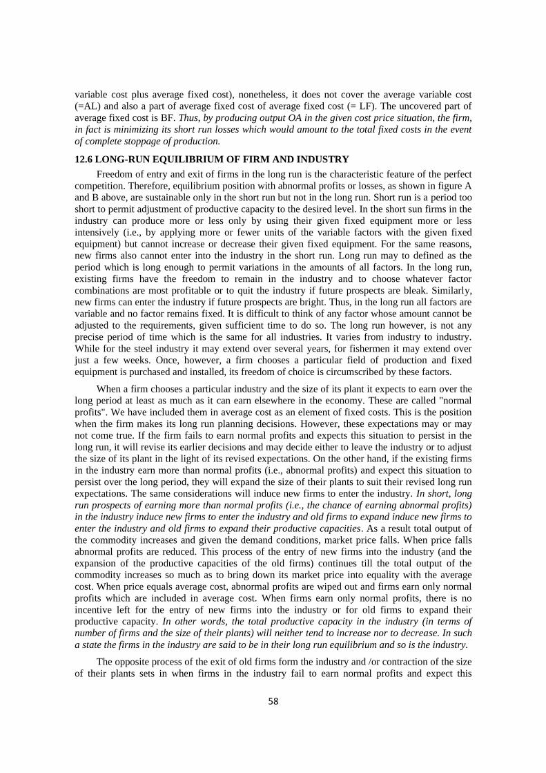
58

variable cost plus average fixed cost), nonetheless, it does not cover the average variable cost

(=AL) and also a part of average fixed cost of average fixed cost (= LF). The uncovered part of

average fixed cost is BF. Thus, by producing output OA in the given cost price situation, the firm,

in fact is minimizing its short run losses which would amount to the total fixed costs in the event

of complete stoppage of production.

12.6 LONG-RUN EQUILIBRIUM OF FIRM AND INDUSTRY

Freedom of entry and exit of firms in the long run is the characteristic feature of the perfect

competition. Therefore, equilibrium position with abnormal profits or losses, as shown in figure A

and B above, are sustainable only in the short run but not in the long run. Short run is a period too

short to permit adjustment of productive capacity to the desired level. In the short sun firms in the

industry can produce more or less only by using their given fixed equipment more or less

intensively (i.e., by applying more or fewer units of the variable factors with the given fixed

equipment) but cannot increase or decrease their given fixed equipment. For the same reasons,

new firms also cannot enter into the industry in the short run. Long run may to defined as the

period which is long enough to permit variations in the amounts of all factors. In the long run,

existing firms have the freedom to remain in the industry and to choose whatever factor

combinations are most profitable or to quit the industry if future prospects are bleak. Similarly,

new firms can enter the industry if future prospects are bright. Thus, in the long run all factors are

variable and no factor remains fixed. It is difficult to think of any factor whose amount cannot be

adjusted to the requirements, given sufficient time to do so. The long run however, is not any

precise period of time which is the same for all industries. It varies from industry to industry.

While for the steel industry it may extend over several years, for fishermen it may extend over

just a few weeks. Once, however, a firm chooses a particular field of production and fixed

equipment is purchased and installed, its freedom of choice is circumscribed by these factors.

When a firm chooses a particular industry and the size of its plant it expects to earn over the

long period at least as much as it can earn elsewhere in the economy. These are called "normal

profits". We have included them in average cost as an element of fixed costs. This is the position

when the firm makes its long run planning decisions. However, these expectations may or may

not come true. If the firm fails to earn normal profits and expects this situation to persist in the

long run, it will revise its earlier decisions and may decide either to leave the industry or to adjust

the size of its plant in the light of its revised expectations. On the other hand, if the existing firms

in the industry earn more than normal profits (i.e., abnormal profits) and expect this situation to

persist over the long period, they will expand the size of their plants to suit their revised long run

expectations. The same considerations will induce new firms to enter the industry. In short, long

run prospects of earning more than normal profits (i.e., the chance of earning abnormal profits)

in the industry induce new firms to enter the industry and old firms to expand induce new firms to

enter the industry and old firms to expand their productive capacities. As a result total output of

the commodity increases and given the demand conditions, market price falls. When price falls

abnormal profits are reduced. This process of the entry of new firms into the industry (and the

expansion of the productive capacities of the old firms) continues till the total output of the

commodity increases so much as to bring down its market price into equality with the average

cost. When price equals average cost, abnormal profits are wiped out and firms earn only normal

profits which are included in average cost. When firms earn only normal profits, there is no

incentive left for the entry of new firms into the industry or for old firms to expand their

productive capacity. In other words, the total productive capacity in the industry (in terms of

number of firms and the size of their plants) will neither tend to increase nor to decrease. In such

a state the firms in the industry are said to be in their long run equilibrium and so is the industry.

The opposite process of the exit of old firms form the industry and /or contraction of the size

of their plants sets in when firms in the industry fail to earn normal profits and expect this

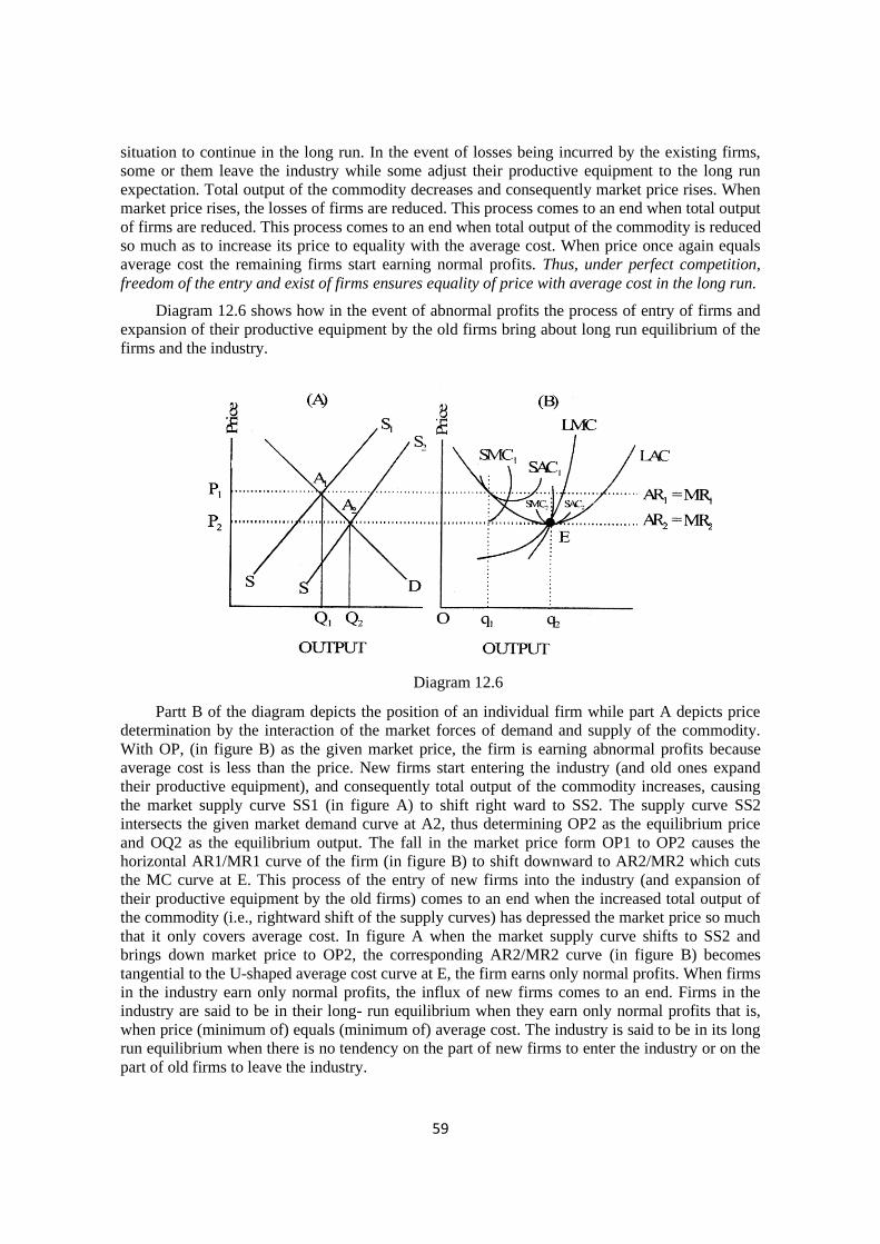
59

situation to continue in the long run. In the event of losses being incurred by the existing firms,

some or them leave the industry while some adjust their productive equipment to the long run

expectation. Total output of the commodity decreases and consequently market price rises. When

market price rises, the losses of firms are reduced. This process comes to an end when total output

of firms are reduced. This process comes to an end when total output of the commodity is reduced

so much as to increase its price to equality with the average cost. When price once again equals

average cost the remaining firms start earning normal profits. Thus, under perfect competition,

freedom of the entry and exist of firms ensures equality of price with average cost in the long run.

Diagram 12.6 shows how in the event of abnormal profits the process of entry of firms and

expansion of their productive equipment by the old firms bring about long run equilibrium of the

firms and the industry.

Diagram 12.6

Partt B of the diagram depicts the position of an individual firm while part A depicts price

determination by the interaction of the market forces of demand and supply of the commodity.

With OP, (in figure B) as the given market price, the firm is earning abnormal profits because

average cost is less than the price. New firms start entering the industry (and old ones expand

their productive equipment), and consequently total output of the commodity increases, causing

the market supply curve SS1 (in figure A) to shift right ward to SS2. The supply curve SS2

intersects the given market demand curve at A2, thus determining OP2 as the equilibrium price

and OQ2 as the equilibrium output. The fall in the market price form OP1 to OP2 causes the

horizontal AR1/MR1 curve of the firm (in figure B) to shift downward to AR2/MR2 which cuts

the MC curve at E. This process of the entry of new firms into the industry (and expansion of

their productive equipment by the old firms) comes to an end when the increased total output of

the commodity (i.e., rightward shift of the supply curves) has depressed the market price so much

that it only covers average cost. In figure A when the market supply curve shifts to SS2 and

brings down market price to OP2, the corresponding AR2/MR2 curve (in figure B) becomes

tangential to the U-shaped average cost curve at E, the firm earns only normal profits. When firms

in the industry earn only normal profits, the influx of new firms comes to an end. Firms in the

industry are said to be in their long- run equilibrium when they earn only normal profits that is,

when price (minimum of) equals (minimum of) average cost. The industry is said to be in its long

run equilibrium when there is no tendency on the part of new firms to enter the industry or on the

part of old firms to leave the industry.

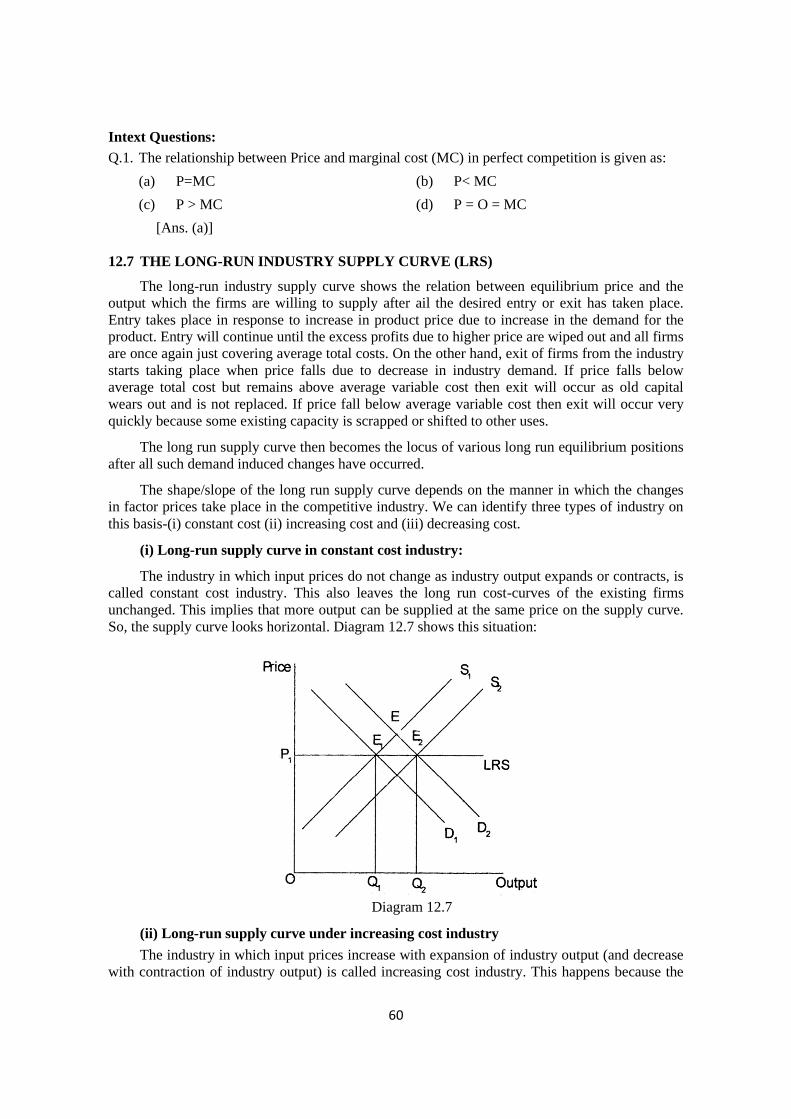
60

Intext Questions:

Q.1. The relationship between Price and marginal cost (MC) in perfect competition is given as:

(a) P=MC (b) P< MC

(c) P > MC (d) P = O = MC

[Ans. (a)]

12.7 THE LONG-RUN INDUSTRY SUPPLY CURVE (LRS)

The long-run industry supply curve shows the relation between equilibrium price and the

output which the firms are willing to supply after ail the desired entry or exit has taken place.

Entry takes place in response to increase in product price due to increase in the demand for the

product. Entry will continue until the excess profits due to higher price are wiped out and all firms

are once again just covering average total costs. On the other hand, exit of firms from the industry

starts taking place when price falls due to decrease in industry demand. If price falls below

average total cost but remains above average variable cost then exit will occur as old capital

wears out and is not replaced. If price fall below average variable cost then exit will occur very

quickly because some existing capacity is scrapped or shifted to other uses.

The long run supply curve then becomes the locus of various long run equilibrium positions

after all such demand induced changes have occurred.

The shape/slope of the long run supply curve depends on the manner in which the changes

in factor prices take place in the competitive industry. We can identify three types of industry on

this basis-(i) constant cost (ii) increasing cost and (iii) decreasing cost.

(i) Long-run supply curve in constant cost industry:

The industry in which input prices do not change as industry output expands or contracts, is

called constant cost industry. This also leaves the long run cost-curves of the existing firms

unchanged. This implies that more output can be supplied at the same price on the supply curve.

So, the supply curve looks horizontal. Diagram 12.7 shows this situation:

Diagram 12.7

(ii) Long-run supply curve under increasing cost industry

The industry in which input prices increase with expansion of industry output (and decrease

with contraction of industry output) is called increasing cost industry. This happens because the

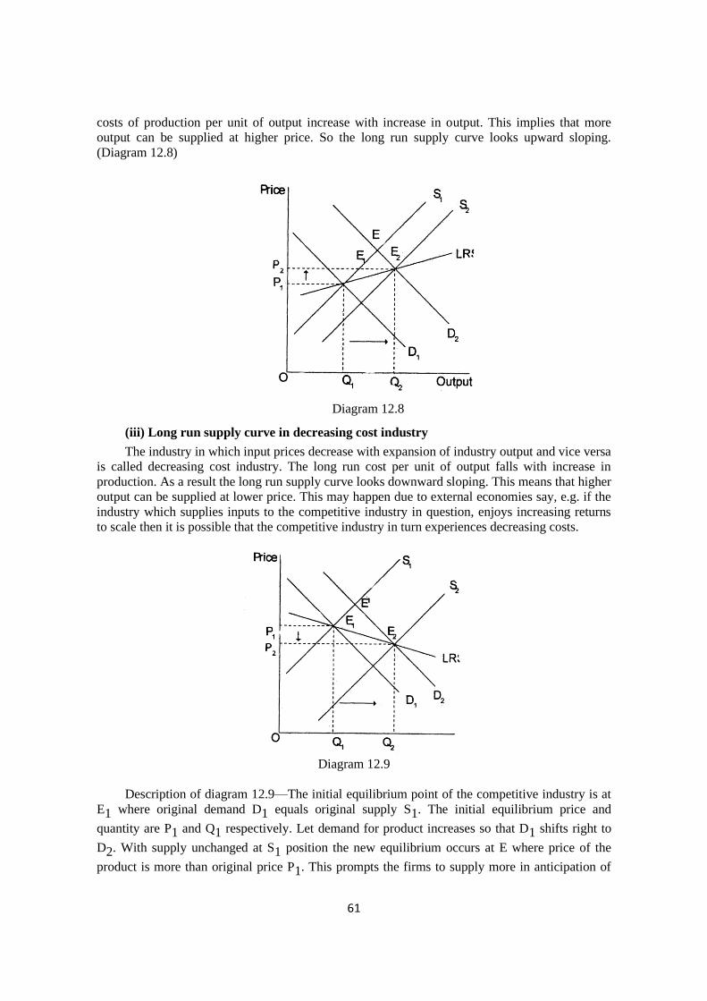
61

costs of production per unit of output increase with increase in output. This implies that more

output can be supplied at higher price. So the long run supply curve looks upward sloping.

(Diagram 12.8)

Diagram 12.8

(iii) Long run supply curve in decreasing cost industry

The industry in which input prices decrease with expansion of industry output and vice versa

is called decreasing cost industry. The long run cost per unit of output falls with increase in

production. As a result the long run supply curve looks downward sloping. This means that higher

output can be supplied at lower price. This may happen due to external economies say, e.g. if the

industry which supplies inputs to the competitive industry in question, enjoys increasing returns

to scale then it is possible that the competitive industry in turn experiences decreasing costs.

Diagram 12.9

Description of diagram 12.9—The initial equilibrium point of the competitive industry is at

E1 where original demand D1 equals original supply S1. The initial equilibrium price and

quantity are P1 and Q1 respectively. Let demand for product increases so that D1 shifts right to

D2. With supply unchanged at S1 position the new equilibrium occurs at E where price of the

product is more than original price P1. This prompts the firms to supply more in anticipation of

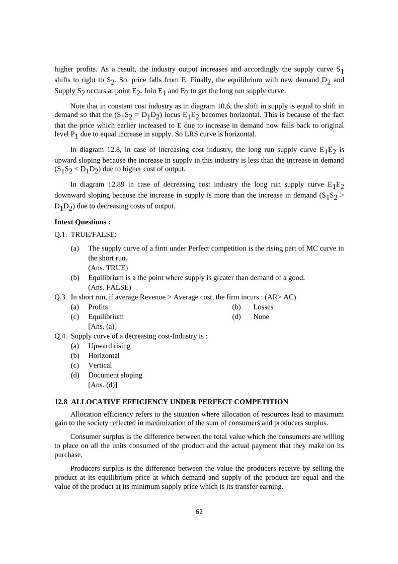
62

higher profits. As a result, the industry output increases and accordingly the supply curve S1

shifts to right to S2. So, price falls from E. Finally, the equilibrium with new demand D2 and

Supply S2 occurs at point E2. Join E1 and E2 to get the long run supply curve.

Note that in constant cost industry as in diagram 10.6, the shift in supply is equal to shift in

demand so that the (S1S2 = D1D2) locus E1E2 becomes horizontal. This is because of the fact

that the price which earlier increased to E due to increase in demand now falls back to original

level P1 due to equal increase in supply. So LRS curve is horizontal.

In diagram 12.8, in case of increasing cost industry, the long run supply curve E1E2 is

upward sloping because the increase in supply in this industry is less than the increase in demand

(S1S2 < D1D2) due to higher cost of output.

In diagram 12.89 in case of decreasing cost industry the long run supply curve E1E2

downward sloping because the increase in supply is more than the increase in demand (S1S2 >

D1D2) due to decreasing costs of output.

Intext Questions :

Q.1. TRUE/FALSE:

(a) The supply curve of a firm under Perfect competition is the rising part of MC curve in

the short run.

(Ans. TRUE)

(b) Equilibrium is a the point where supply is greater than demand of a good.

(Ans. FALSE)

Q.3. In short run, if average Revenue > Average cost, the firm incurs : (AR> AC)

(a) Profits (b) Losses

(c) Equilibrium (d) None

[Ans. (a)]

Q.4. Supply curve of a decreasing cost-Industry is :

(a) Upward rising

(b) Horizontal

(c) Vertical

(d) Document sloping

[Ans. (d)]

12.8 ALLOCATIVE EFFICIENCY UNDER PERFECT COMPETITION

Allocation efficiency refers to the situation where allocation of resources lead to maximum

gain to the society reflected in maximization of the sum of consumers and producers surplus.

Consumer surplus is the difference between the total value which the consumers are willing

to place on all the units consumed of the product and the actual payment that they make on its

purchase.

Producers surplus is the difference between the value the producers receive by selling the

product at its equilibrium price at which demand and supply of the product are equal and the

value of the product at its minimum supply price which is its transfer earning.

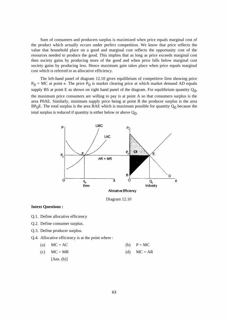
63

Sum of consumers and producers surplus is maximized when price equals marginal cost of

the product which actually occurs under perfect competition. We know that price reflects the

value that household place on a good and marginal cost reflects the opportunity cost of the

resources needed to produce the good. This implies that as long as price exceeds marginal cost

then society gains by producing more of the good and when price falls below marginal cost

society gains by producing less. Hence maximum gain takes place when price equals marginal

cost which is referred to as allocative efficiency.

The left-hand panel of diagram 12.10 gives equilibrium of competitive firm showing price

P0 = MC at point e. The price P0 is market clearing price at which market demand AD equals

supply BS at point E as shown on right hand panel of the diagram. For equilibrium quantity Q0,

the maximum price consumers are willing to pay is at point A so that consumers surplus is the

area P0AE. Similarly, minimum supply price being at point B the producer surplus is the area

BP0E. The total surplus is the area BAE which is maximum possible for quantity Q0 because the

total surplus is reduced if quantity is either below or above Q0.

Diagram 12.10

Intext Questions :

Q.1. Define allocative efficiency

Q.2. Define consumer surplus.

Q.3. Define producer surplus.

Q.4. Allocative efficiency is at the point where :

(a) MC = AC (b) P = MC

(c) MC > MR (d) MC = AR

[Ans. (b)]

64

LEARNING OUTCOME

In this lesson you have learned the following: -

1. There are large number of buyers and sellers, product is homogenous, freedom of entry and

exit, no Government intervention, objective of profit maximization, perfect knowledge and

perfect mobility of factors.

2. In the short the firm may earn abnormal profit or normal profit. There may be losses or even

the firm may shut down.

3. The industry is a price maker as it determines price of the product at the point of intersection

between downward sloping demand curve and upward slopping demand curve of the

product.

4. The supply curve of the curve of the firm is upward portion of the marginal cost curve above

the minimum point of its average variable cost.

5. In the long run the firm earns normal profit because the price is equal to movement of the

long run average variable cost.

6. Allocative efficiency implies maximization of the sum of consumers and producer surplus

which happens under perfect competition. There is also productive efficiency due to the fact

that competitive firm produces at the minimum point of its long run average cost curve.

7. The shape of long run supply curve of all competitive firm depends on the cost conditions in

the industry. In an increasing cost industry long run supply curve is upward sloping whereas

it is downward sloping in the decreasing cost industry and horizontal in a constant curve

industry.

TERMINAL QUESTIONS

Q.1. Diagrammatically explain the concept of consumer surplus, producer surplus and total

surplus.

Q.2. Diagrammatically explain shapes of supply curve in constant, increasing and decreasing cost

industries.

Q.3. Examine Long and Short Run Equilibrium of a firm in a Perfectly competitive Market.

Q.4. List the features of firm of a perfectly competitive market.