Essays in Applied Microeconomics

By

Paul S. Niekamp

Dissertation

Submitted to the Faculty of the

Graduate School of Vanderbilt University

in partial fulfillment of the requirements

for the degree of

DOCTOR OF PHILOSOPHY

in

Economics

August 9, 2019

Nashville, Tennessee

Approved:

Christopher S. Carpenter, Ph.D.

Andrew Goodman-Bacon, Ph.D.

Michelle Marcus, Ph.D.

Carolyn J. Heinrich, Ph.D.

To my parents, who did everything they could to set me up for success

ii

ACKNOWLEDGMENTS

I have many people to thank for the influences they have had on my life. Above all, I thank

my family. My parents, who dedicatedly supplemented grade school, never missed a sports event,

and always challenged me to do better. I am deeply indebted to my wife, Alyssa Niekamp, who

has supported me since undergrad and inspires me to be a better person. She has selflessly spent

significant time helping me digitize data and proofreading my drafts. Her willingness to listen

to and critique my research ideas is tremendously helpful and broadens my perspective. My

brother, who is a work ethic role model and showed me that graduate school was a possibility

and worthwhile investment. My sisters, who have motivated me throughout my education.

Second, I am grateful for the friends I have made at Vanderbilt University, particularly Daniel

Mangrum, Adam Watkins, Nicolas Mäder, Zeeshan Samad, Frank Ciarliero, Caitlan Miller, Tam

Bui, Sebastian Tello-Trillo, James Harrison, Jonah Yuen, Jason Campbell, Katie Yewell, Sam

Eppink, Salama Freed, Melissa Icenhour, and Nina Mangrum, who have provided companionship

and acted as a sounding board for research ideas throughout my graduate education. Additionally,

I am appreciative of my undergraduate professors at the Miami University Farmer School of

Business and especially Bill Even, for advising my Departmental Honors thesis and introducing

me to applied microeconomic methods.

I would like to thank the Department of Economics at Vanderbilt University for a quality

education and five years of financial support. I fully appreciate the research support I have received

from the Council of Economics Graduate Students (CEGS). I especially thank committee members

Andrew Goodman-Bacon, Michelle Marcus, and Carolyn Heinrich as well as Andrew Dustan,

Federico Gutierrez, Bill Collins, Sayeh Nikpay, and Andrea Moro. Each of these individuals has

dedicated time to provide constructive feedback that has improved my research and presentation

style. I thank Senior Lecturer Christina Rennhoff for being a role model teacher that I can only

aspire to be. Lastly, I wholeheartedly thank my adviser and committee chair, Kitt Carpenter, for

dedicating so much of his time toward my professional development. His constructive criticism,

iii

notes on drafts, presentation technique advice, and suggestions have invaluably improved my

research and my ability to convey a message.

iv

TABLE OF CONTENTS

Page

DEDICATION . . . . . . . . . . . . . . . . . . . . . . . . . . . . . . . . . . . . . . . . . ii

ACKNOWLEDGMENTS . . . . . . . . . . . . . . . . . . . . . . . . . . . . . . . . . . . . iii

LIST OF TABLES . . . . . . . . . . . . . . . . . . . . . . . . . . . . . . . . . . . . . . . viii

LIST OF FIGURES . . . . . . . . . . . . . . . . . . . . . . . . . . . . . . . . . . . . . . . ix

INTRODUCTION . . . . . . . . . . . . . . . . . . . . . . . . . . . . . . . . . . . . . . . 1

Chapter . . . . . . . . . . . . . . . . . . . . . . . . . . . . . . . . . . . . . . . . . . . . . 3

1 GOOD BANG FOR THE BUCK: EFFECTS OF RURAL GUN USE ON CRIME . . . . 3

1.1 Introduction . . . . . . . . . . . . . . . . . . . . . . . . . . . . . . . . . . . . . . . 3

1.2 Literature Review . . . . . . . . . . . . . . . . . . . . . . . . . . . . . . . . . . . . 6

1.2.1 The Relationship Between Guns and Crime: a Conceptual Framework . . . . . 6

1.2.2 Studies on The Effects of Aggregate Gun Ownership . . . . . . . . . . . . . . 9

1.2.3 Studies on The Effects of Gun Policy . . . . . . . . . . . . . . . . . . . . . . . 10

1.2.4 Studies on The Effects of Gun Use . . . . . . . . . . . . . . . . . . . . . . . . 11

1.3 Institutional Background . . . . . . . . . . . . . . . . . . . . . . . . . . . . . . . . . 13

1.3.1 Different People, Different Guns, Different Reasons . . . . . . . . . . . . . . . 13

1.3.2 U.S. Hunting Participation . . . . . . . . . . . . . . . . . . . . . . . . . . . . 15

1.3.3 Deer Hunting Seasons . . . . . . . . . . . . . . . . . . . . . . . . . . . . . . . 17

1.3.4 Discontinuous Hunting Activity . . . . . . . . . . . . . . . . . . . . . . . . . 18

1.4 Data . . . . . . . . . . . . . . . . . . . . . . . . . . . . . . . . . . . . . . . . . . . 18

1.4.1 Deer Season Regulation Data . . . . . . . . . . . . . . . . . . . . . . . . . . . 18

1.4.2 Deer Hunting Data . . . . . . . . . . . . . . . . . . . . . . . . . . . . . . . . 19

1.4.3 Granular Employment Data . . . . . . . . . . . . . . . . . . . . . . . . . . . . 20

1.4.4 Crime Data . . . . . . . . . . . . . . . . . . . . . . . . . . . . . . . . . . . . 20

v

1.4.5 Measures of Gun Use and Crime . . . . . . . . . . . . . . . . . . . . . . . . . 21

1.5 Empirical Strategy . . . . . . . . . . . . . . . . . . . . . . . . . . . . . . . . . . . . 23

1.6 Results . . . . . . . . . . . . . . . . . . . . . . . . . . . . . . . . . . . . . . . . . . 24

1.6.1 Effects of Firearm Season on Gun Use and Violent Crime . . . . . . . . . . . . 24

1.6.2 Effects on Weapon Law Violations . . . . . . . . . . . . . . . . . . . . . . . . 28

1.6.3 Effects on Alcohol and Narcotic Crimes . . . . . . . . . . . . . . . . . . . . . 28

1.6.4 Robustness to Law Enforcement Agency Population . . . . . . . . . . . . . . . 30

1.7 Discussion . . . . . . . . . . . . . . . . . . . . . . . . . . . . . . . . . . . . . . . . 31

1.8 Conclusion . . . . . . . . . . . . . . . . . . . . . . . . . . . . . . . . . . . . . . . . 33

1.9 Appendix . . . . . . . . . . . . . . . . . . . . . . . . . . . . . . . . . . . . . . . . . 54

2 BAKKEN OUT OF EDUCATION TO TOIL IN OIL . . . . . . . . . . . . . . . . . . . . 69

2.1 Introduction . . . . . . . . . . . . . . . . . . . . . . . . . . . . . . . . . . . . . . . 69

2.2 Literature Review . . . . . . . . . . . . . . . . . . . . . . . . . . . . . . . . . . . . 73

2.2.1 Economic Conditions and Educational Attainment . . . . . . . . . . . . . . . . 73

2.2.2 Effects of the 21st Century Fracking Boom . . . . . . . . . . . . . . . . . . . 75

2.3 Institutional Background . . . . . . . . . . . . . . . . . . . . . . . . . . . . . . . . . 76

2.4 Data . . . . . . . . . . . . . . . . . . . . . . . . . . . . . . . . . . . . . . . . . . . 77

2.5 Empirical Strategy . . . . . . . . . . . . . . . . . . . . . . . . . . . . . . . . . . . . 79

2.6 Results . . . . . . . . . . . . . . . . . . . . . . . . . . . . . . . . . . . . . . . . . . 81

2.6.1 Effects on High School Graduation Rates . . . . . . . . . . . . . . . . . . . . 81

2.6.2 Effects on NDUS Enrollment Rates . . . . . . . . . . . . . . . . . . . . . . . 82

2.6.3 Effects on NDDPI Post-Graduation Outcomes . . . . . . . . . . . . . . . . . . 84

2.7 Conclusion . . . . . . . . . . . . . . . . . . . . . . . . . . . . . . . . . . . . . . . . 85

2.8 Appendix . . . . . . . . . . . . . . . . . . . . . . . . . . . . . . . . . . . . . . . . . 114

3 ECONOMIC CONDITIONS AND SLEEP . . . . . . . . . . . . . . . . . . . . . . . . . 122

3.1 Introduction . . . . . . . . . . . . . . . . . . . . . . . . . . . . . . . . . . . . . . . 122

3.2 Data and Methodology . . . . . . . . . . . . . . . . . . . . . . . . . . . . . . . . . . 123

vi

3.3 Results . . . . . . . . . . . . . . . . . . . . . . . . . . . . . . . . . . . . . . . . . . 125

3.4 Conclusion . . . . . . . . . . . . . . . . . . . . . . . . . . . . . . . . . . . . . . . . 129

BIBLIOGRAPHY . . . . . . . . . . . . . . . . . . . . . . . . . . . . . . . . . . . . . . . 131

vii

LIST OF TABLES

Table Page

1.1 Hunting Summary Statistics . . . . . . . . . . . . . . . . . . . . . . . . . . . . . 35

1.2 Summary Statistics of Hunting Demographics . . . . . . . . . . . . . . . . . . . . 36

1.3 Firearm Ownership Rates by Demographic . . . . . . . . . . . . . . . . . . . . . 37

1.4 Reasons for Ownership by Firearm Type . . . . . . . . . . . . . . . . . . . . . . . 37

1.5 Estimated Effects of Firearm Season on Male Rural Crime . . . . . . . . . . . . . 38

1.6 Estimated Effects of Firearm Season on Male Rural Crime . . . . . . . . . . . . . 39

1.A1 NIBRS State Coverage . . . . . . . . . . . . . . . . . . . . . . . . . . . . . . . . 61

1.A2 Estimated Effects of Firearm Season on Male Rural Crime . . . . . . . . . . . . . 62

1.A3 Effects on Rural Male 21 & Under Alcohol Arrests by Opening Day . . . . . . . . 63

1.A4 Firearm Season and Male Urban Crime . . . . . . . . . . . . . . . . . . . . . . . 64

1.A5 Linear Probability Model: Male Arrestees Armed with Long Gun . . . . . . . . . 65

1.A6 Linear Probability Model: Male Violent Crime Offenses . . . . . . . . . . . . . . 66

1.A7 Linear Probability Model: Male Alcohol-Related Arrests . . . . . . . . . . . . . . 67

1.A8 Linear Probability Model: Male Narcotic Arrests . . . . . . . . . . . . . . . . . . 68

2.1 NDUS Enrollment Summary Statistics . . . . . . . . . . . . . . . . . . . . . . . . 110

2.2 Estimated Effects on NDUS Student Enrollment Rates . . . . . . . . . . . . . . . 111

2.3 Estimated Effects on NDUS Student Enrollment Numbers . . . . . . . . . . . . . 112

2.4 Post-Graduation Outcomes Summary Statistics . . . . . . . . . . . . . . . . . . . 113

3.1 Average Sleep by Great Recession Severity . . . . . . . . . . . . . . . . . . . . . 123

3.2 Effect of Employment Rate on Sleep . . . . . . . . . . . . . . . . . . . . . . . . . 126

3.3 Employment and Sleep by Marital Status . . . . . . . . . . . . . . . . . . . . . . 127

3.4 Employment Effects by Workweek Structure . . . . . . . . . . . . . . . . . . . . 129

viii

LIST OF FIGURES

Figure Page

1.1 Long Gun Use in Violent Crime Offenses . . . . . . . . . . . . . . . . . . . . . . 40

1.2 2011: Estimated Participation in Main Firearm Season for States Covered by NIBRS 41

1.3 Patterns of Hunting Around Wisconsin Opening Day (2017) . . . . . . . . . . . . 42

1.4 Pennsylvania Employee Male-Female Vacation Hour Differential (2016) . . . . . . 43

1.5 Rural Male Arrests in Zones Opening on Monday . . . . . . . . . . . . . . . . . . 44

1.6 Estimated Effects of Firearm Season on Rural Male Gun Prevalence and Number

of Arrests Using Variation in Season Access . . . . . . . . . . . . . . . . . . . . . 45

1.7 Estimated Effects on Rural Male Armed Arrestees with Handguns versus Long

Guns to Test Attribution . . . . . . . . . . . . . . . . . . . . . . . . . . . . . . . 46

1.8 Estimated Effects of Firearm Season on Rural Male Long Gun Prevalence and

Violent Crime Incidents . . . . . . . . . . . . . . . . . . . . . . . . . . . . . . . 47

1.9 Estimated Effects of Firearm Season on Young (21 & under) Rural Male Long

Gun Prevalence and Violent Crime Incidents . . . . . . . . . . . . . . . . . . . . 48

1.10 Estimated Effects of Firearm Season on Weapon Law Violations by Age . . . . . . 49

1.11 Estimated Effects of Firearm Season on Male Alcohol Arrests by Age . . . . . . . 50

1.12 Estimated Effects of Firearm Season on Narcotic Offenses by Age . . . . . . . . . 51

1.13 Estimated Effects on Violent Crime Incidents on First Two Days of Season by

Population of Law Enforcement Agency . . . . . . . . . . . . . . . . . . . . . . . 52

1.14 Estimated Effects on Alcohol-Related Arrests on First Two Days of Season by

Population of Law Enforcement Agency . . . . . . . . . . . . . . . . . . . . . . . 53

1.A1 Hunting Demographics . . . . . . . . . . . . . . . . . . . . . . . . . . . . . . . . 54

1.A2 Hunting Time Use . . . . . . . . . . . . . . . . . . . . . . . . . . . . . . . . . . 55

1.A3 Example of Firearm Hunting Season Opening Days (2015) . . . . . . . . . . . . . 56

1.A4 Rural Male Arrests in Zones Opening on Saturday . . . . . . . . . . . . . . . . . 57

ix

1.A5 Urban Male Arrests in Zones Opening on Monday . . . . . . . . . . . . . . . . . 58

1.A6 Estimated Effects of Firearm Season on Rural Male Violent Crime . . . . . . . . . 59

1.A7 Male 21 & Under Alcohol-Related Arrests . . . . . . . . . . . . . . . . . . . . . 60

2.1 Percent Change in County Unemployment Rate . . . . . . . . . . . . . . . . . . . 88

2.2 North Dakota Average Weekly Wages . . . . . . . . . . . . . . . . . . . . . . . . 89

2.3 QCEW Employment Level and Establishment Count . . . . . . . . . . . . . . . . 90

2.4 Leisure & Hospitality Employment Level and Wages . . . . . . . . . . . . . . . . 91

2.5 Bakken Formation . . . . . . . . . . . . . . . . . . . . . . . . . . . . . . . . . . 92

2.6 North Dakota Counties . . . . . . . . . . . . . . . . . . . . . . . . . . . . . . . . 93

2.7 Civilian Labor Force by County . . . . . . . . . . . . . . . . . . . . . . . . . . . 94

2.8 ND Oil and Gas Drilling Rigs . . . . . . . . . . . . . . . . . . . . . . . . . . . . 95

2.9 ND Oil Production . . . . . . . . . . . . . . . . . . . . . . . . . . . . . . . . . . 96

2.10 NASA Earth Observatory Night-Lights Imagery . . . . . . . . . . . . . . . . . . . 97

2.11 Graduation Rate Trends . . . . . . . . . . . . . . . . . . . . . . . . . . . . . . . 98

2.12 Graduation Rate Event-Studies . . . . . . . . . . . . . . . . . . . . . . . . . . . . 99

2.13 NDUS College Enrollment Rate Trends . . . . . . . . . . . . . . . . . . . . . . . 100

2.14 NDUS College Enrollment Rate Event-Study . . . . . . . . . . . . . . . . . . . . 101

2.15 Event-Studies of 4 Year versus 2 Year College . . . . . . . . . . . . . . . . . . . . 102

2.16 Event-Studies by Type of 4 Year College . . . . . . . . . . . . . . . . . . . . . . 103

2.17 Event-Studies of Log Number of Students Enrolled . . . . . . . . . . . . . . . . . 104

2.18 Event Study Estimates of Any College Enrollment . . . . . . . . . . . . . . . . . 105

2.19 Event Study Estimates of Employment . . . . . . . . . . . . . . . . . . . . . . . . 106

2.20 Event Study Estimates of 4 Year College . . . . . . . . . . . . . . . . . . . . . . 107

2.21 Event Study Estimates of 2 Year College . . . . . . . . . . . . . . . . . . . . . . 108

2.22 Event Study Estimates of Military Enrollment . . . . . . . . . . . . . . . . . . . . 109

2.A1 Number of High School Graduates . . . . . . . . . . . . . . . . . . . . . . . . . . 114

2.A2 College Enrollment Rate Trends . . . . . . . . . . . . . . . . . . . . . . . . . . . 115

x

2.A3 Employment Rate Trends . . . . . . . . . . . . . . . . . . . . . . . . . . . . . . . 116

2.A4 2 Year College Enrollment Trends . . . . . . . . . . . . . . . . . . . . . . . . . . 117

2.A5 4 Year College Enrollment Trends . . . . . . . . . . . . . . . . . . . . . . . . . . 118

2.A6 Voc-Tech Enrollment Trends . . . . . . . . . . . . . . . . . . . . . . . . . . . . . 119

2.A7 Military Enrollment Trends . . . . . . . . . . . . . . . . . . . . . . . . . . . . . . 120

2.A8 Unknown Decision Trends . . . . . . . . . . . . . . . . . . . . . . . . . . . . . . 121

3.1 Average Minutes Worked per Day . . . . . . . . . . . . . . . . . . . . . . . . . . 124

3.2 Sleep Structure by Employment Status . . . . . . . . . . . . . . . . . . . . . . . . 124

3.3 Workweek Structure by Industry . . . . . . . . . . . . . . . . . . . . . . . . . . . 128

xi

INTRODUCTION

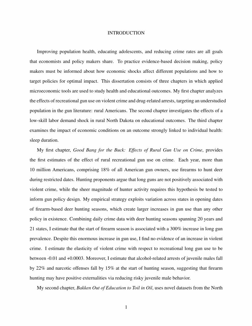
Improving population health, educating adolescents, and reducing crime rates are all goals

that economists and policy makers share. To practice evidence-based decision making, policy

makers must be informed about how economic shocks affect different populations and how to

target policies for optimal impact. This dissertation consists of three chapters in which applied

microeconomic tools are used to study health and educational outcomes. My first chapter analyzes

the effects of recreational gun use on violent crime and drug-related arrests, targeting an understudied

population in the gun literature: rural Americans. The second chapter investigates the effects of a

low-skill labor demand shock in rural North Dakota on educational outcomes. The third chapter

examines the impact of economic conditions on an outcome strongly linked to individual health:

sleep duration.

My first chapter, Good Bang for the Buck: Effects of Rural Gun Use on Crime, provides

the first estimates of the effect of rural recreational gun use on crime. Each year, more than

10 million Americans, comprising 18% of all American gun owners, use firearms to hunt deer

during restricted dates. Hunting proponents argue that long guns are not positively associated with

violent crime, while the sheer magnitude of hunter activity requires this hypothesis be tested to

inform gun policy design. My empirical strategy exploits variation across states in opening dates

of firearm-based deer hunting seasons, which create larger increases in gun use than any other

policy in existence. Combining daily crime data with deer hunting seasons spanning 20 years and

21 states, I estimate that the start of firearm season is associated with a 300% increase in long gun

prevalence. Despite this enormous increase in gun use, I find no evidence of an increase in violent

crime. I estimate the elasticity of violent crime with respect to recreational long gun use to be

between -0.01 and +0.0003. Moreover, I estimate that alcohol-related arrests of juvenile males fall

by 22% and narcotic offenses fall by 15% at the start of hunting season, suggesting that firearm

hunting may have positive externalities via reducing risky juvenile male behavior.

My second chapter, Bakken Out of Education to Toil in Oil, uses novel datasets from the North

1

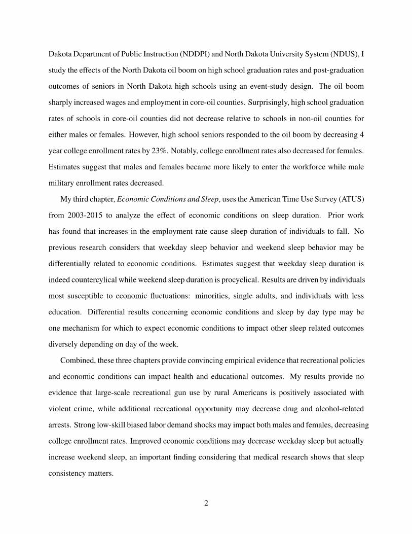
Dakota Department of Public Instruction (NDDPI) and North Dakota University System (NDUS), I

study the effects of the North Dakota oil boom on high school graduation rates and post-graduation

outcomes of seniors in North Dakota high schools using an event-study design. The oil boom

sharply increased wages and employment in core-oil counties. Surprisingly, high school graduation

rates of schools in core-oil counties did not decrease relative to schools in non-oil counties for

either males or females. However, high school seniors responded to the oil boom by decreasing 4

year college enrollment rates by 23%. Notably, college enrollment rates also decreased for females.

Estimates suggest that males and females became more likely to enter the workforce while male

military enrollment rates decreased.

My third chapter, Economic Conditions and Sleep, uses the American Time Use Survey (ATUS)

from 2003-2015 to analyze the effect of economic conditions on sleep duration. Prior work

has found that increases in the employment rate cause sleep duration of individuals to fall. No

previous research considers that weekday sleep behavior and weekend sleep behavior may be

differentially related to economic conditions. Estimates suggest that weekday sleep duration is

indeed countercylical while weekend sleep duration is procyclical. Results are driven by individuals

most susceptible to economic fluctuations: minorities, single adults, and individuals with less

education. Differential results concerning economic conditions and sleep by day type may be

one mechanism for which to expect economic conditions to impact other sleep related outcomes

diversely depending on day of the week.

Combined, these three chapters provide convincing empirical evidence that recreational policies

and economic conditions can impact health and educational outcomes. My results provide no

evidence that large-scale recreational gun use by rural Americans is positively associated with

violent crime, while additional recreational opportunity may decrease drug and alcohol-related

arrests. Strong low-skill biased labor demand shocks may impact both males and females, decreasing

college enrollment rates. Improved economic conditions may decrease weekday sleep but actually

increase weekend sleep, an important finding considering that medical research shows that sleep

consistency matters.

2

CHAPTER 1

GOOD BANG FOR THE BUCK: EFFECTS OF RURAL GUN USE ON CRIME

1.1 Introduction

In 2015, firearms were used in 71.5% of US homicides, 40.8% of robberies, and 24.2% of

aggravated assaults (FBI, 2016). The high rate of firearm use in violent crime has fueled a growing

debate concerning the relationship between gun prevalence and violent crime. If firearms impose

a negative externality (Cook and Ludwig, 2006; Duggan, 2001), then optimal gun policy should

target guns and gun owners that impose the largest social costs. In this spirit, many existing gun

regulations specifically apply to youths, individuals with mental health conditions or criminal

records, or to specific kinds of firearms such as “assault weapons.”1 However, lack of research

exploring the heterogeneity of social costs across gun owners and gun types provides limited

insight for optimally targeting along other dimensions. Much of the economics literature focuses

on handguns, as “they account for 80% of all gun homicides...Hence the social costs of handgun

ownership are much higher than ownership of rifles and shotguns. Unfortunately, it is difficult to

distinguish between the prevalence of long gun ownership and handgun ownership...”(Cook and

Ludwig, 2006).

Remarkably, no studies to date have focused on potentially the largest group of gun users who

claim that their guns do not increase violent crime: rural hunters with shotguns and rifles.2 A

group so powerful that Democratic President Bill Clinton went hunting after signing the Brady

Handgun bill to distance his policies from hunters and so important in Midwestern swing-states

that Democrat John Kerry included an Ohio goose hunt in his 2004 presidential campaign to woo

rural voters.3 This study focuses on males, who, as discussed in Section 1.3.2, comprise 89% of1The term “assault weapon” is hotly debated. Some groups refer to semi-automatic rifles with detachable

magazines as assault weapons, while other groups consider a firearm to be an assault weapon if the firearm hasselective-fire capabilities: the ability to switch between semi-automatic, burst, or automatic firing modes.

2Approximately half of members in the National Rifle Association (NRA), a group that believes guns decreasecrime, are hunters (Parker, 2018).

3As suggested by his Iowa campaign director, John Kerry went pheasant hunting in Iowa to build rapport and

3

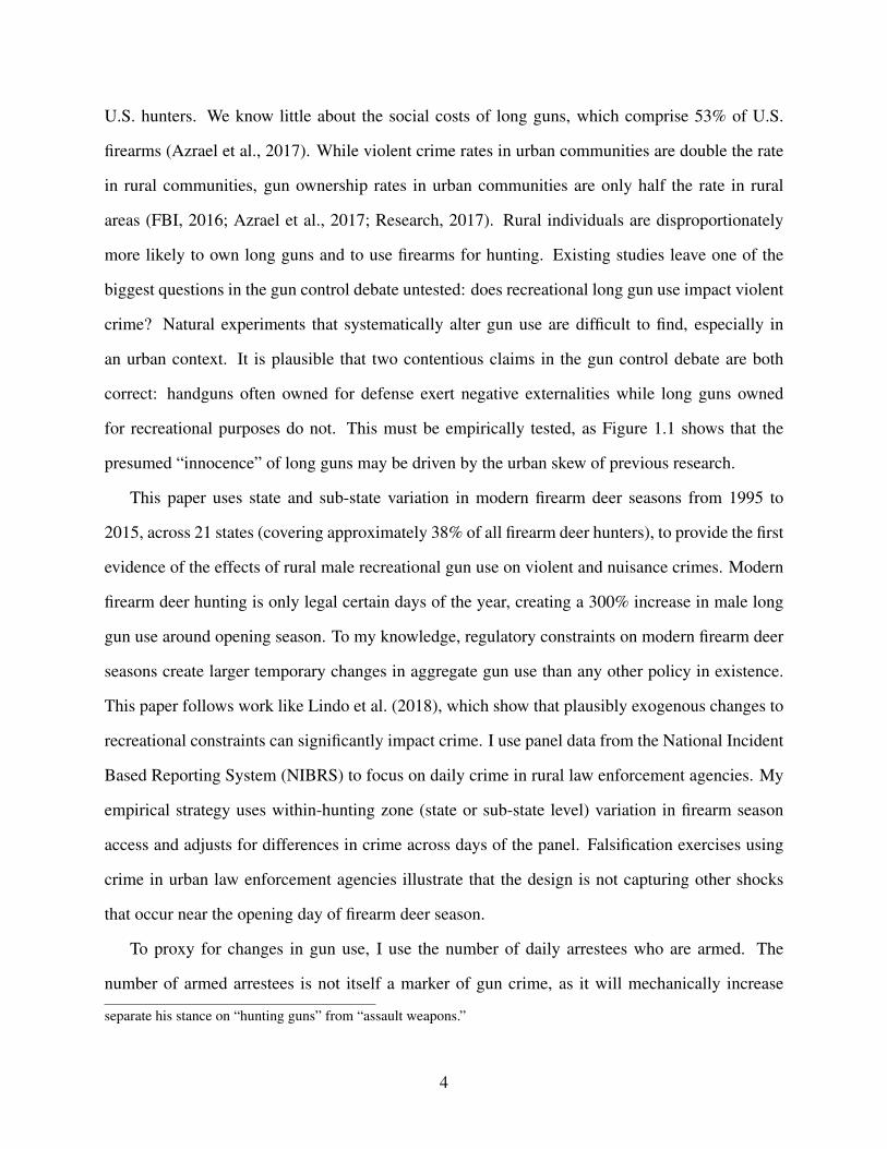
U.S. hunters. We know little about the social costs of long guns, which comprise 53% of U.S.

firearms (Azrael et al., 2017). While violent crime rates in urban communities are double the rate

in rural communities, gun ownership rates in urban communities are only half the rate in rural

areas (FBI, 2016; Azrael et al., 2017; Research, 2017). Rural individuals are disproportionately

more likely to own long guns and to use firearms for hunting. Existing studies leave one of the

biggest questions in the gun control debate untested: does recreational long gun use impact violent

crime? Natural experiments that systematically alter gun use are difficult to find, especially in

an urban context. It is plausible that two contentious claims in the gun control debate are both

correct: handguns often owned for defense exert negative externalities while long guns owned

for recreational purposes do not. This must be empirically tested, as Figure 1.1 shows that the

presumed “innocence” of long guns may be driven by the urban skew of previous research.

This paper uses state and sub-state variation in modern firearm deer seasons from 1995 to

2015, across 21 states (covering approximately 38% of all firearm deer hunters), to provide the first

evidence of the effects of rural male recreational gun use on violent and nuisance crimes. Modern

firearm deer hunting is only legal certain days of the year, creating a 300% increase in male long

gun use around opening season. To my knowledge, regulatory constraints on modern firearm deer

seasons create larger temporary changes in aggregate gun use than any other policy in existence.

This paper follows work like Lindo et al. (2018), which show that plausibly exogenous changes to

recreational constraints can significantly impact crime. I use panel data from the National Incident

Based Reporting System (NIBRS) to focus on daily crime in rural law enforcement agencies. My

empirical strategy uses within-hunting zone (state or sub-state level) variation in firearm season

access and adjusts for differences in crime across days of the panel. Falsification exercises using

crime in urban law enforcement agencies illustrate that the design is not capturing other shocks

that occur near the opening day of firearm deer season.

To proxy for changes in gun use, I use the number of daily arrestees who are armed. The

number of armed arrestees is not itself a marker of gun crime, as it will mechanically increase

separate his stance on “hunting guns” from “assault weapons.”

4

if more of the rural population is armed but arrested for non-violent reasons. I estimate that the

number of male arrestees armed with a long gun in rural jurisdictions increases 300% upon the

opening of firearm deer season. Considering overall rural arrests remain stable, this provides

strong evidence that societal gun use increases. That is, the 4.2 million hunters covered by my

sample who hunt during modern firearm season are interacting with society enough to be arrested

(for any type of crime).

Given the enormous increase in long gun use, it is notable that estimates provide no evidence

that violent crime increases upon opening season. On opening day, when upwards of 30% of rural

males are using long guns, estimates can rule out positive effects on violent crime larger than

6% (point estimate of 0.02). Estimated effects on violent crime for the second and third day of

firearm season are actually negative. Using armed arrestees as a proxy for long gun use implies an

elasticity of violent crime with respect to recreational long gun use between -0.01 and +0.0003.

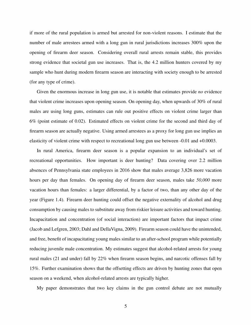
In rural America, firearm deer season is a popular expansion to an individual’s set of

recreational opportunities. How important is deer hunting? Data covering over 2.2 million

absences of Pennsylvania state employees in 2016 show that males average 3,826 more vacation

hours per day than females. On opening day of firearm deer season, males take 50,000 more

vacation hours than females: a larger differential, by a factor of two, than any other day of the

year (Figure 1.4). Firearm deer hunting could offset the negative externality of alcohol and drug

consumption by causing males to substitute away from riskier leisure activities and toward hunting.

Incapacitation and concentration (of social interaction) are important factors that impact crime

(Jacob and Lefgren, 2003; Dahl and DellaVigna, 2009). Firearm season could have the unintended,

and free, benefit of incapacitating young males similar to an after-school program while potentially

reducing juvenile male concentration. My estimates suggest that alcohol-related arrests for young

rural males (21 and under) fall by 22% when firearm season begins, and narcotic offenses fall by

15%. Further examination shows that the offsetting effects are driven by hunting zones that open

season on a weekend, when alcohol-related arrests are typically higher.

My paper demonstrates that two key claims in the gun control debate are not mutually

5

exclusive. It is plausible that handguns used for defensive purposes increase violent crime while

long guns used in rural, recreational environments do not. The social costs of gun use may depend

on the type of gun and reason for ownership. While previous literature sheds light on the effects of

firearm ownership, we know almost nothing about the effects of recreational firearm use. I provide

the first evidence of the crime effects of large increases in rural firearm use due to hunting season

regulations. In doing so, I observe enormous, systematic fluctuations in firearm use that do not

exist in any urban setting. These regulations impact 12.7 million firearm deer hunters each year

and 4.3 million covered by my sample. Second, I examine an understudied sample: rural male

recreational long gun users who actively use firearms. Hunters comprise up to one quarter of total

firearm owners, and over half of all firearms in the United States are long guns (Azrael et al., 2017).

Given that rural individuals own different firearms for different reasons than other firearm owners

commonly studied in the literature, impacts on violent crime may differ.

Aside from the contributions above, this paper is meaningful for policy-makers as it provides

evidence that immense changes in rural recreational long gun use have no economically significant

impacts on violent crime. As this population is a large stakeholder in the gun policy debate,

results suggest that policy makers should target other firearms types and owners that have a tighter

relationship with violent crime. My results imply that policies that aim to restrict recreational

long gun use will have no beneficial impact on crime. Additionally, my results suggest that state

policy-makers could capitalize on the positive externality of firearm season on alcohol and drug

related arrests by moving the opening day of firearm season to days where the counterfactual

leisure activity is most likely to be alcohol-related: the weekend.

1.2 Literature Review

1.2.1 The Relationship Between Guns and Crime: a Conceptual Framework

A 2015 survey by (Azrael et al., 2017) found that 22%, or 55 million Americans, report owning

firearms (with the average owner having 4.8 guns), leading to an estimate of 265 million firearms

6

in the U.S. Given the prevalence of gun ownership and violent crime in the United States, a body

of literature has attempted to estimate the aggregate relationship between guns and violent crime.

I build on the framework in Kovandzic et al. (2013) to summarize key channels by which guns can

impact crime. Aggregate violent crime, VCz, in zone z are modeled as a function of gun prevalence

(gun ownership, gun access, et cetera) gz, so that VCz = VC(gz). Guns may impact crime via the

following channels:

1. Deterrence: ∂VCz∂gz

< 0. Aggregate gun prevalence could deter violent crime if criminals

anticipate that potential victims or helpful bystanders are more likely to be armed. Gun

prevalence could exert a positive externality similar to LoJack (Ayres and Levitt, 1998) if

criminals are unable to determine whether a potential victim is armed.

2. Facilitation of Crime: ∂VCz∂gz

> 0. Guns may decrease the difficulty of incapacitating a victim,

which may increase the expected success rate of an attack and increase crime on the extensive

margin. Gun access may also escalate an argument or simple assault to a more serious

altercation leading to aggravated assault or homicide.

3. Supply of Stealable Guns: ∂VCz∂gz

> 0. Even guns owned by non-criminals may increase

violent crime if criminals access firearms via burglary. Over 1.4 million firearms were stolen

between 2005 and 2010, with handguns being the most common target (Langton, 2012).

It is likely that the relationship between guns and crime is heterogeneous (Cook and Ludwig,

2006). As stated in Cook et al. (2010), “The disparity between the demography of gun sports and

of gun crime is telling: sportsmen are disproportionately older white males from small towns and

rural areas, while the criminal misuse of guns is concentrated among young urban males, especially

minorities.” While hunting permit data from Wisconsin (Figure 1.A1b) show that juveniles also

hunt at high rates, it is likely that the relationship between guns and crime is a function of individual

and gun characteristics.

∂VCz

∂gz=

∂VCz

∂gz(GunTypez,GunUsez,OwnerCharacteristicsz)

7

GunTypez may matter, as criminals may have differing preferences over handguns, long

guns, or semi-automatic weapons. Previous literature focuses on handguns because they are

the primary gun used in violent crime, as criminals prefer high-caliber semiautomatic handguns

that are easily concealable in a waistband (Zawitz, 1995; Cook and Ludwig, 2006). GunUsez,

whether the gun is used for offensive, defense, or recreational purposes, may also matter. Lastly,

owner characteristics, OwnerCharacteristicsz, may impact the relationship with crime. Older and

higher income gun owners may be less associated with violent crime (Cook et al., 2010), while

the same may hold for individuals who legally possess a gun. In a simple case where gz =

gz(handgunz, long gunz), even if ∂VCz∂gz

> 0 it is possible that the aggregate positive relationship is

driven by ∂VCz∂handgunz

> 0 while ∂VCz∂ long gunz

≤ 0. Current studies are hamstrung by lack of high-quality

panel data on gun prevalence, much less gun type. Finding valid proxies for aggregate gun

prevalence is difficult enough (Kovandzic et al., 2013; Kleck, 2004) while gun-specific proxies

are even more challenging to find.

1.2.1.1 Channels Specific to Recreational Gun Use and Crime

Participation in firearm hunting requires that an individual has access to both a firearm and

ammunition. While a hunter personally carries a firearm in woods, there will be an enormous

increase in individuals with firearms in vehicles. One could imagine an individual who leaves his

firearm in his vehicle, drinks at a bar after hunting, and escalates a bar fight (simple assault) to

aggravated assault with a firearm. Moreover, any hunter who returns home and neglects to re-lock

his firearm increases firearm access for all non-hunting family members or friends. From the

channels listed above, firearm season could increase deterrence, enhance the facilitation of crime,

and increase the supply of stealable guns that can be used in crime.

From a psychological perspective, it has been argued that hunting could desensitize individuals

to committing violent acts and is “teaching children to kill” (Shapiro, 2016) similar to violent video

games or movies studied by Dahl and DellaVigna (2009). This argument is a less extreme analogy

to the U.S. military desensitizing servicemen and servicewomen to killing (Robinson, 2005), which

8

may increase proclivity to violence (Rohlfs, 2010; Lindo and Stoecker, 2014). A successful hunter

must consciously aim and pull the trigger to kill an animal, while even ethical kill-shot locations

like the heart or lungs do not result in instant death. Deer typically run after being shot and

thrash on the ground with significant bleeding. For some the guilt never leaves, while for others

it “Becomes all automatic...Find target, bring rifle (or whatever) track, locate in sights...make my

decision “shoot/not shoot”...based on what where, makeable shot percentage...bang...don’t feel it

or even hear it...” (hunter63, 2017). It is possible that desensitization to killing could transcend

deer, reducing the mental costs of committing violent crimes against humans.

1.2.2 Studies on The Effects of Aggregate Gun Ownership

Much of the economics and criminology literature has attempted to estimate the aggregate

sign and magnitude of ∂VCz∂gz

. Causal identification is hindered by potential reverse causality: areas

with increases in violent crime may experience increases in gun prevalence. Additionally, other

factors may influence both gun prevalence and violent crime. Cook and Ludwig (2006) estimate

the social costs of gun ownership using within county variation in estimated gun prevalence. Using

fraction of suicides committed with a firearm as a proxy for gun ownership, the authors estimated

an elasticity of homicide with respect to gun prevalence of +0.1 - +0.3. The authors noted that

the social costs of handguns were almost certainly higher than the social costs of long guns, as

handguns are the most common gun used in violent crimes and suicides. Duggan (2001) estimated

a similar elasticity of +0.2 when using firearm magazine sales as a proxy for gun prevalence.

However, Kovandzic et al. (2013) argue that the preceding studies use proxies that are valid for

cross-sectional gun prevalence but invalid proxies for changes in prevalence over time. Using an

instrumental variables strategy, the authors find that gun prevalence has a negative (deterrent) effect

on crime. Other studies find no evidence of a causal relationship between guns and crime (Moody

and Marvell, 2005; Kleck and Patterson, 1993).

9

1.2.3 Studies on The Effects of Gun Policy

What do we know about the effects of gun policies? In 2018, the RAND Corporation’s

Gun Policy in America initiative published a review of quasi-experimental evidence (from 63

papers meeting inclusion criteria) on 13 classes of gun policy (Morral et al., 2018). The study

summarized that background checks and mental-illness restrictions may reduce violent crime

while stand-your-ground laws and concealed-carry laws may increase violent crime. Child-access

prevention (CAP) laws were found to decrease suicides and firearm-injuries among children.

The authors state, “Notably, research into four of our outcomes was essentially unavailable,

with three of these four outcomes- defensive gun use, hunting and recreation, and the gun

industry-representing issues of particular concern to gun owners or gun industry stakeholders.” My

study aims to fill part of the research void concerning hunting and recreation, not as an outcome,

but as a lever of plausibly exogenous variation in long gun use.

Safe-storage laws have been passed by states to reduce accidental gun deaths, especially

among minors. Lott and Whitley (2001) found that safe-storage laws may increase crime against

noncriminals while having no beneficial impact on accidental gun deaths or suicides while

Cummings et al. (1997) find they decrease accidental firearm deaths among children with no

statistically significant impact on firearm homicide. More recent work has found that CAP laws

decrease nonfatal gun injuries among children (DeSimone et al., 2013) and may decrease juvenile

homicides committed with a gun by 19% (Anderson et al., 2018). On a similar motive to limit

firearm access to high-risk youths, firearm age restrictions have been passed. Though homicide

rates among young males are high, age restrictions on handguns may have no significant impact

on homicide rates (Rosengart et al., 2005).

One channel by which guns could decrease crime is by deterrence. If right-to-carry laws

increase noncriminal carry rates, violent crime could be thwarted. Work by Lott and Mustard

(1997) suggesting that right-to-carry laws reduce violent crime was quickly followed by opposite

or null results (Dezhbakhsh and Rubin, 1998; Duggan, 2001; Black and Nagin, 1998; Ludwig,

1998; Rubin and Dezhbakhsh, 2003; Ayres and Donohue III, 2003; Aneja et al., 2011). Related

10

to handguns and concealed-carry laws, Gius (2015) found that firearm homicides decreased after

the passage of the Brady Handgun Bill. Similar to the rationale of right-to-carry laws, “stand your

ground” laws were passed by states to expand rights to use deadly force within one’s home, which

could theoretically deter crime. Cheng and Hoekstra (2013) found that “stand your ground” laws

have no deterrent effect on burglary or aggravated assault, but lead to an increase in murder.

Policies concerning ease of firearm access have also been studied. Policies that delay the

time between purchasing and receiving a firearm, so called “waiting periods”, have no impact on

homicides but may decrease gun related suicide (Edwards et al., 2018). Knight (2013) found that

guns used in crimes are often sourced from states with weaker gun laws. In this vein, Dube et al.

(2013) find that access to U.S. based assault weapons increased homicides and violent crime in

Mexico. However, no cohesive evidence exists concerning the effects of a assault weapons in the

U.S. (Morral et al., 2018). Others have been concerned that the “gun show loophole” has made

it easier for criminals to access firearms without undergoing background checks. Matthay et al.

(2017) found that gun shows in states with less restrictive gun control laws may cause a short-term

increase in firearm injuries, driven by interpersonal violence. However, Duggan et al. (2011)

studied 3,400 gun shows in California and Texas, finding no evidence of increases in suicides

or homicides. Other studies have examined the impact of permit to purchase laws, which require

an individual to obtain a permit before purchasing a firearm. Webster et al. (2014) found that the

repeal of permit to purchase in Missouri increased the homicide rate. Using a synthetic-control

method, Rudolph et al. (2015) reported that the permit-to-purchase law reduced Connecticut’s

firearm homicide rate by 40%.

1.2.4 Studies on The Effects of Gun Use

While most of the literature focuses on firearm ownership or effects of gun policies, little is

known about the effects of gun use. The reasons for this are practical: systematic data covering

state or county level gun ownership are limited while ownership can be proxied for by using firearm

magazine subscriptions or fraction of suicides by firearm (Duggan, 2001; Cook and Ludwig, 2006).

11

Unfortunately, data is even more sparse concerning gun use and especially temporary fluctuations

in gun use. One way to study the effects of temporary changes in gun use is to find a natural

experiment that plausibly impacts gun use. Jena and Olenski (2018) study NRA conventions,

which may temporarily decrease firearm use if gun-users are attending conventions (and don’t

bring firearms). The authors found that gun-related injuries decrease during NRA convention

dates, suggesting that even experienced gun owners are at risk of gun-related injury.

Evidence of rural male firearm use and violent crime is much more sparse. Conlin et al. (2009)

study deer hunting accidents in Pennsylvania, finding that minimum antler requirements may lead

hunters to take more calculated shots and reduce hunting accidents. These studies provide evidence

on accidental injuries, but leave questions about whether violent crime is impacted. According to

a Pew Research poll, 50% of NRA members hunt (Parker, 2018). Yamane (2017) propose that

recreational use of guns like hunting are a driver of the strong gun culture in America. Glaeser and

Glendon (1998) suggest that gun ownership is highest where police accessibility is the lowest and

for individuals who distrust the government. The strong gun culture of rural America is illustrated

in a 2017 Pew Research poll finding that 58% of rural households own a gun versus 19% of urban

households (Igielnik, 2017). Of these rural gun owners, 47% reported that they obtained their first

gun before the age of 18. Rural gun owners were 23 percentage points more likely to say that the

right to own guns was “essential to their own sense of freedom.” Moreover, Tables 1.3 and 1.4

show that rural gun owners are much more likely to own long guns, which are most commonly

used for hunting, unlike handguns which are most commonly used for self-defense. The strong

gun culture of rural America makes the effects of rural gun use on violent crime an imperative area

to study to further understand the unique perspective that rural Americans hold on gun control.

The net effects of increased gun access on violent crime due to firearm season are ambiguous.

Sharp increases in gun carry rates of prime-age males and youths may increase violent crime or

escalate the intensity of arguments above the counterfactual in which firearms were not present.

Additionally, easier access for non-hunting youths in a hunting household may increase violent

crime. Evidence suggests that child access prevention (CAP) gun control laws reduce gun carrying

12

rates and rates of weapon-related threats or injuries among youths (Anderson and Sabia, in press).

However, hunting is a time consuming activity that may reduce crime via voluntary incapacitation,

similar to violent movies (Dahl and DellaVigna, 2009). Additionally, Jacob and Lefgren (2003)

suggest that activities that incapacitate and deconcentrate juveniles will have the most beneficial

impact on juvenile crime. Males may deconcentrate when deer hunting in the woods, which may

decrease crimes associated with social interaction.

1.3 Institutional Background

1.3.1 Different People, Different Guns, Different Reasons

Firearms are designed for different uses: self-defense, hunting, recreation, etc. Previous

literature heavily focuses on handguns because they are the primary gun used in violent crime,

as criminals prefer high-caliber semiautomatic handguns that are easily concealable in a waistband

(Zawitz, 1995; Cook and Ludwig, 2006). Handgun owners who own no other guns almost

exclusively report self-defense as a reason for ownership (Table 1.4), while Wright and Rossi

(1986) suggests that offensive firearm use is more correlated with defense than recreational

ownership. Recreational long guns are more likely to be legally possessed than handguns, as

handguns are the most common type of stolen gun while semi-automatic handguns are common in

illicit markets (Langton, 2012; Koper, 2014).

Table 1.3 reports firearm ownership by demographic, as estimated by the 2015 National

Firearms Survey (Azrael et al., 2017), showing stark differences in ownership patterns of rural

versus urban individuals. Rural individuals are more than twice as likely as urban individuals to

own a firearm (33% versus 15%). While rural individuals are actually less likely to report owning

only a handgun, they are three times as likely to report owning only a long gun and 2.7 times

more likely to report owning both a handgun and long gun. Gun differences are just as stark when

broken out by race. While black individuals are approximately half as likely to own a gun as

white individuals, they are actually 1.6 times more likely to own only a handgun. While 6% of

13

whites own only a long gun, only 1% of blacks do so. Table 1.3 makes it clear that urban and

black individuals are demonstrably more likely to own handguns, which are primarily used for

protection against humans. The economics and criminology literature has focused on this subset

because urban and black violent crime rates are significantly higher than the population average.

For example, O’Flaherty and Sethi (2010) studied why black Americans are seven times more

likely than white Americans to murder someone. Evans et al. (2018) studied the emergence of

crack cocaine markets in urban areas and the long run impact, via increased gun prevalence, on

young black male murder rates. However, current literature has left long gun toting white and rural

individuals understudied. This group is significantly more likely to use firearms for hunting or

other sporting purposes.

Modern firearms for hunting fit in three primary groups: muzzleloaders, rifles and shotguns.

A muzzleloader is a single-shot rifle or shotgun that is loaded from the muzzle. In most states,

modern shotguns and rifles are more popular due to ease of use. A modern rifle has a rifled

barrel (helical grooves in the bore) to spin the bullet as it exits the firearm, increasing accuracy

for long-range targets. A hunter with a rifle can execute an ethical kill shot on a deer from over

300 yards (three football fields) away. A shotgun typically has a smooth bore barrel, providing a

more limited ethical kill range. Shotgun shells often include numerous pellets that spread around

the target, with the spread increasing with distance. This increased margin-of-error is one reason

why shotguns are often touted as being better for home-defense than a rifle or handgun. Shotgun

deer hunters are typically restricted to using shotgun slugs, large single-bullet projectiles, which

provide an ethical kill-range for a deer around 75 yards.

The iconic hunting gun might be a single-shot bolt action rifle or a single-shot shotgun, which

may mislead one to think that hunting firearms are inherently innocent. But U.S. crime data,

discussed in Section 1.4.4, show that the share of violent gun crimes committed with long guns

increases linearly as the population of the law enforcement jurisdiction decreases (Figure 1.1). It is

clear that long guns are commonly used in crime, just not in urban areas. Furthermore, many rifles

and shotguns used for hunting are semi-automatic, defined as autoloading firearms that fire one

14

time per trigger pull (pump-action shotguns can hold multiple shells but are not semi-automatic

because a hunter must pump between trigger pulls). The public is much more concerned about

these weapons. These guns have been subject to confiscations in other countries such as the 1996

Australian gun buyback program, which confiscated semi-automatic and pump-action shotguns.

This buyback may have reduced suicides and homicides (Leigh and Neill, 2010; Chapman et al.,

2006).

In particular, AR-15s and AR-15 variants have been the most hotly debated firearm of

the last 30 years. Even the name itself is debated, with some calling it an “assault rifle” or

“assault-style rifle” while others and the gun industry call it a modern sporting rifle. AR-15 rifles

and variants have been heavily publicized due to use in tragic mass shootings (Parkland, Florida;

Las Vegas, Nevada; Newtown, Connecticut; etc.).4 The 1994-2004 Federal Assault Weapons

Ban targeted semi-automatic rifles like the AR-15: semi-automatic firearms with a pistol grip,

detachable magazine, et cetera. While objective survey data do not exist, a study by the National

Shooting Sports Foundation reported that 27% of hunters have used a modern sporting rifle (or

“assault-style rifle”) to hunt game. Semi-automatic shotguns are often preferred by hunters who

desire superior recoil-reduction systems (less “kick”), which are especially beneficial for smaller

hunters. Similarly, the accurate AR-15 is lightweight with an adjustable stock and limited recoil

which benefits hunters with smaller frames. The ability to follow a target with a semi-automatic

firearm with limited recoil makes the weapon popular for varmint, coyotes, wild hogs, et cetera.

Semi-automatic rifles and shotguns are common hunting implements, implying that we cannot a

priori characterize hunting firearms as innocent.

1.3.2 U.S. Hunting Participation

Hunting is a popular recreational activity throughout the United States, especially in rural

areas. Data from the US Fish, Hunting, and Wildlife-Associated Recreation (FHWAR) survey

4https://www.nytimes.com/interactive/2018/02/28/us/ar-15-rifle-mass-shootings.html;https://www.usatoday.com/story/news/2017/11/06/ar-15-style-rifles-common-among-mass -shootings/838283001/

15

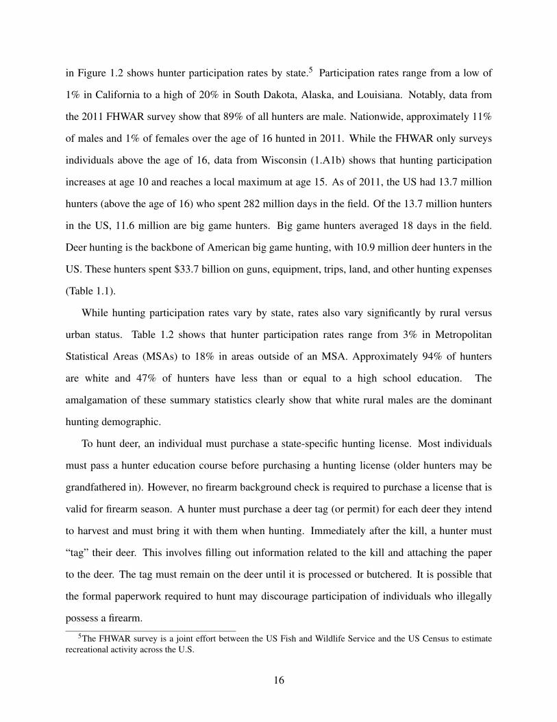
in Figure 1.2 shows hunter participation rates by state.5 Participation rates range from a low of

1% in California to a high of 20% in South Dakota, Alaska, and Louisiana. Notably, data from

the 2011 FHWAR survey show that 89% of all hunters are male. Nationwide, approximately 11%

of males and 1% of females over the age of 16 hunted in 2011. While the FHWAR only surveys

individuals above the age of 16, data from Wisconsin (1.A1b) shows that hunting participation

increases at age 10 and reaches a local maximum at age 15. As of 2011, the US had 13.7 million

hunters (above the age of 16) who spent 282 million days in the field. Of the 13.7 million hunters

in the US, 11.6 million are big game hunters. Big game hunters averaged 18 days in the field.

Deer hunting is the backbone of American big game hunting, with 10.9 million deer hunters in the

US. These hunters spent $33.7 billion on guns, equipment, trips, land, and other hunting expenses

(Table 1.1).

While hunting participation rates vary by state, rates also vary significantly by rural versus

urban status. Table 1.2 shows that hunter participation rates range from 3% in Metropolitan

Statistical Areas (MSAs) to 18% in areas outside of an MSA. Approximately 94% of hunters

are white and 47% of hunters have less than or equal to a high school education. The

amalgamation of these summary statistics clearly show that white rural males are the dominant

hunting demographic.

To hunt deer, an individual must purchase a state-specific hunting license. Most individuals

must pass a hunter education course before purchasing a hunting license (older hunters may be

grandfathered in). However, no firearm background check is required to purchase a license that is

valid for firearm season. A hunter must purchase a deer tag (or permit) for each deer they intend

to harvest and must bring it with them when hunting. Immediately after the kill, a hunter must

“tag” their deer. This involves filling out information related to the kill and attaching the paper

to the deer. The tag must remain on the deer until it is processed or butchered. It is possible that

the formal paperwork required to hunt may discourage participation of individuals who illegally

possess a firearm.

5The FHWAR survey is a joint effort between the US Fish and Wildlife Service and the US Census to estimaterecreational activity across the U.S.

16

1.3.3 Deer Hunting Seasons

A typical state has a multitude of deer hunting seasons each year. Archery season typically

open in early fall and runs to early January of the following year. Seasons with relatively

little participation are often scattered throughout late fall. These include special seasons for

muzzleloaders, flintlocks, or even spear-hunting (in Alabama).6 A youth weekend often precludes

the main firearm season by a week or two and is usually limited to hunters under the age of 15

(supervised by an adult at least 18 or 21 years old, depending on the state). The main firearm

season (often called “main season”, “traditional season”, or “modern firearm”), the season used in

this study, typically starts between October and December (Figure 1.A3 illustrates opening dates

for 2015). Table 1.2 shows that 12.73 million (93%) U.S. hunters use rifles and shotguns, which

are the key implements of “modern firearm” seasons. For example, from 2005-2015, hunters in

Wisconsin harvested 300,000-500,000 deer per year. Approximately 70% of all deer are harvested

in the 9 day firearm season with over 100,000 deer harvested on opening weekend.

Even during deer season, hunting is not allowed all hours of the day. A typical hunting time

table allows a hunter to kill between 30 minutes before sunrise to 30 minutes after sunset. Deer are

a crepuscular animal, meaning that they are most active during dawn and dusk. This incentivizes

hunters to be in the woods before sunrise or late in the evening. Deer harvest data from Ohio show

that the majority of kills in the first 5 days of firearm season are reported in the morning or evening

(Figure 1.A2b). Figure 1.A2a uses data from the American Time Use Survey to show that hunters

average 5-6 hours in the field on days in which they hunt between October and January (main

deer seasons). Similarly, state-level data from Wisconsin hunter surveys show that hunters average

4.12 hours per trip, while this number is certainly higher at the start of firearm season. If a hunter

is successful, he must either transport his kill to a butcher or process the deer himself. Skinning

and processing a deer can take the hunter another 4-5 hours. Combined, these statistics show that

hunting has the potential to crowd out other uses of one’s time.

6A flintlock (introduced in the 17th century) and muzzleloader season often target hunters who appreciate huntingfor its heritage and tradition.

17

1.3.4 Discontinuous Hunting Activity

As seen in Figure 1.3, short season windows coupled with hunter anticipation create large

discontinuities in hunting activity on opening day. Firearm deer seasons induce a discrete jump in

hunter activity on opening day for a variety of reasons.

1. The stock of deer is at its peak because few have been harvested (some deer are harvested

in the aforementioned seasons that preclude the main firearm season). If a hunter wants to

optimize his success rate, he should hunt when the stock of deer is highest.

2. Deer can be “pressured” when hunter activity is high. Widespread increases in human

activity can impact deer behavior. This change in deer behavior can reduce a hunter’s success

rate, incentivizing an individual to hunt while the woods are fresh.

3. Firearm deer hunting is popular and restricted season dates create anticipation. Newspapers

and magazines like Field & Stream or REALTREE often advertise tips for opening day

(Carpenter, 2018).

While deer hunting activity is discrete, hunters certainly prepare weapons and ammunition in

the days before opening season. The constrained nature of firearm seasons provides a large change

to recreational opportunities that may lead hunters to substitute away from other leisure activities

or risky behaviors.

1.4 Data

In order to study how shocks to gun carry rates due to firearm deer season impact violent crime,

I combine high-frequency crime data with finely delineated deer regulations.

1.4.1 Deer Season Regulation Data

I construct a novel dataset of historical modern firearm deer season dates. Hunting season

dates are determined by state agencies. However, states are often divided by wildlife management

18

units (WMUs) that may have different opening season dates. Primary sources of data are historical

state-specific hunting regulation digests and Freedom of Information Act (FOIA) requests form

state game commissions or natural resource departments. Data for some states were obtained via

phone calls with state deer project coordinators. Missing years of data are imputed using reference

dates from the Quality Deer Management Association (QDMA) Whitetail Report (QDMA, 2017).

The majority of states have one primary firearm season. If a state has multiple main firearm

seasons, the first firearm season of the year is used. Treatment is defined by “zone,” the largest

zone within a state that has the same opening firearm season date. For most states the treatment

zone is equivalent to the state, as all WMUs share the same opening date. Other states, like South

Dakota, may be comprised of multiple treatment zones of varying opening dates. As an example,

Figure 1.A3 provides state-level opening firearm deer season dates for 2015. Opening firearm

dates in the sample range from October 24 in Montana to December 5 in Iowa. States open firearm

season on different days of the week: Monday, Friday, Saturday, and Sunday.

1.4.2 Deer Hunting Data

I use the US Fish, Hunting, and Wildlife-Associated Recreation (FHWAR) survey for summary

statistics concerning hunters. The FHWAR survey has been administered every 5 years since 1955.

Survey questions are designed by the US Fish and Wildlife Service while data is collected by the

US Census Bureau. I primarily use the 2011 FHWAR, which provides state-level estimates of

hunting participation rates.7 The survey includes information on recreational time use and includes

demographic traits of hunters like sex, age, race, and income. The survey also splits estimates by

type of game, allowing specifics insights into deer hunting.

I supplement FHWAR data with deer harvest report data from Wisconsin and Ohio. Harvest

report data are constructed from deer tags. Some states require all hunters to fill out deer tags and

report their harvest to state agencies. These harvest datasets include the date of every reported

deer kill (Ohio includes the time-of-kill and age of the hunter). Wisconsin also includes how many

7The FHWAR became more limited in 2016, as the survey was reduced to a nationally representative survey.

19

hours a successful hunter hunted on the day of their kill. Deer harvest report data from Wisconsin

clearly show a first stage discontinuity in hunter activity on the first day of the 2017 firearm season

(Figure 1.3). Prior to firearm season, Wisconsin hunters harvested less than 2,000 deer per day.

Hunter activity abruptly increased on opening weekend of firearm season, when hunters harvested

100,000 deer. Combined with hunter success rates from the Wisconsin DNR, these data can be

used to estimate the scale of hunter activity upon opening season.

1.4.3 Granular Employment Data

Recreational opportunities that are only available certain days of the year may be important

factors for whether employees take vacation leave or sick leave. However, almost all large

scale employee absence data is aggregated, such as at the monthly level. To provide additional

evidence of the important ramifications of deer season regulations, I submitted a FOIA request to

Pennsylvania for microdata of all absences of state employees. The data cover over 2.2 million

records of employee absence in 2016 and includes the date of absence, gender of employee, and

type of absence (annual-vacation leave or sick leave). I collapse observations by day-of-year

and gender, and take the difference between male and female vacation hours. The male-female

differential in vacation hours signals relative absenteeism while netting out factors, like holidays,

that impact both genders. As shown in Figure 1.4, the male-female differential of vacation hours

is significantly more pronounced on the first two days of firearm season than any other days of the

year, providing strong evidence that deer hunting regulations have considerable effects on male

time-use.

1.4.4 Crime Data

The main source of crime and arrest data is from NIBRS (FBI, 2009), which comprises data

collected by US law enforcement agencies and aggregated by the Federal Bureau of Investigation

(FBI). NIBRS has three key benefits for this study. First, the data includes the date, time, and

location of the crime. Second, the data provides a population group underlying the respective law

20

enforcement agency which can be exploited to focus on rural jurisdictions. Third, NIBRS details

whether an offender was armed with a firearm during a crime and distinguishes between rifles,

shotguns, and hand guns. This is relevant because the majority of firearm deer hunters use a rifle

or shotgun. One limitation of NIBRS is that state coverage is incomplete, which limits the sample

for analysis. By 2012, 32 states were certified to submit NIBRS data to the FBI (JRSA, 2018).

This study uses a sample of 22 states that have adequate coverage.

I use NIBRS data from 1995 to 2015, collapsing crime data into zone-date cells. As hunter

participation rates are higher in rural areas than urban, I split the analysis to focus on crime in rural

areas, defined as law enforcement agencies covering less than 25,000 individuals. All jurisdictions

with less than 25,000 individuals are collapsed into a hunting zone-day cell. Results are robust to

other population-based definitions of rural. I also split analysis by sex of the offender or arrestee

because approximately 90% of deer hunters nationwide are male. NIBRS offense files include

data on Group A offenses like violent crime and weapon law violations. Data concerning Group B

offenses like driving under the influence are only available in arrest files. An advantage of arrest

data over offense data is that sex of the arrestee is always given while sex of the offender is often

missing. However, offense data may provide a more complete and contemporaneous picture of

daily crime because not all crimes lead to an arrest. I show that results concerning violent crime

are robust to using either the arrest or offense files.

1.4.5 Measures of Gun Use and Crime

Recreational survey data from the US FHWAR show that over 10 million Americans firearm

deer hunted in 2011, which directly implies that over 10 million Americans carried and used long

guns during firearm deer season. However, no data exists to estimate daily firearm carry or use

rates. Additionally, “societal use” is arguably more important. If 50% of rural males are armed

on opening day versus 10% on a typical day (a 400% increase in firearm use) but these hunters

walk from their farm to their woods and back without interacting with society, then it might be

less surprising to find that recreational firearm use has no impact on violent crime. We would

21

expect firearms to have a larger impact on violent crime if individuals actually interact with society

while armed with a firearm. NIBRS arrest data denote whether an arrestee of any kind is armed,

which does not imply that a gun crime has occurred (an individual may be armed during a DUI

or property crime). To proxy for changes in firearm use, I use the daily number of arrestees who

are armed. While this number will certainly understate the level of armed individuals, percent

changes in the number of armed arrestees provide an estimate of changes in firearm usage rates if

the proportion of armed individuals who are arrested remains the same. I will further break out

results by arrestees armed with a long gun versus those armed with a handgun.

I use two different measures for daily violent crime: incidents and arrests. An advantage of

arrest data is that the gender and age of the arrestee is always denoted and the type of gun used in

the crime will be more accurate than that in the incident file. But not all violent crime incidents

lead to an arrest in general, and especially on the same day that the incident occurred. Additionally,

using incident data should mitigate concerns of potential changes in law enforcement effort due

to deer hunting regulation (as an assault victim may report the incident to the police even if the

offender is not arrested). Given that benefits exists for using both incidents and arrests as outcomes,

I show that results are robust to using either as an outcome.

My main measures of crime are violent crime incidents or arrests. Using definitions of the

Federal Bureau of Investigation (FBI), I define daily violent crime as the sum of all homicide,

aggravated assault, rape, and robbery arrests or incidents. Aside from violent crime, a key outcome

of interest related to firearm use is weapon law violations: illegally carrying a concealed weapon,

unlicensed weapon, unregistered weapon, using suppressors (silencers), et cetera.

As firearm deer season is a popular recreational activity, I focus on crimes that are likely to be

related to risky leisure behavior. First, I aggregate all alcohol-related arrests together (incident data

is not taken for alcohol-related offenses): driving under the influence (DUI), disorderly conduct,

liquor law violations, and drunkenness. Second, I use the number of narcotic arrests or offenses.

These include incidents of consuming, dealing, transporting, or making drugs.

22

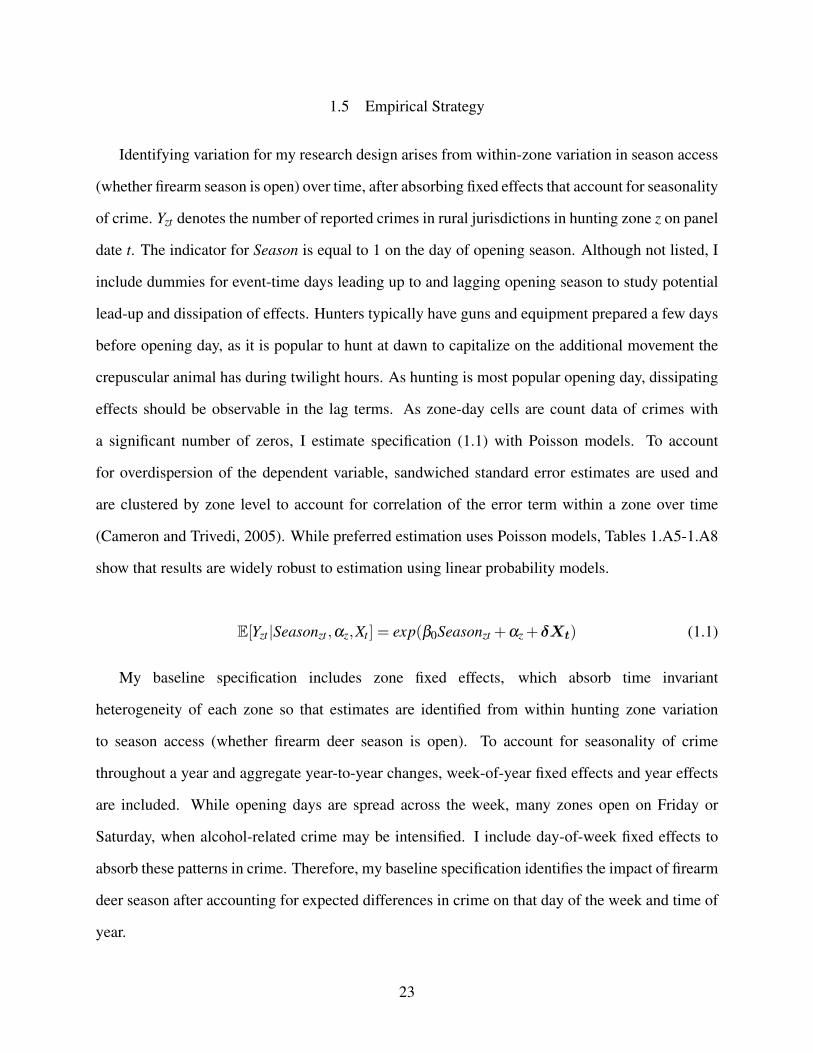
1.5 Empirical Strategy

Identifying variation for my research design arises from within-zone variation in season access

(whether firearm season is open) over time, after absorbing fixed effects that account for seasonality

of crime. Yzt denotes the number of reported crimes in rural jurisdictions in hunting zone z on panel

date t. The indicator for Season is equal to 1 on the day of opening season. Although not listed, I

include dummies for event-time days leading up to and lagging opening season to study potential

lead-up and dissipation of effects. Hunters typically have guns and equipment prepared a few days

before opening day, as it is popular to hunt at dawn to capitalize on the additional movement the

crepuscular animal has during twilight hours. As hunting is most popular opening day, dissipating

effects should be observable in the lag terms. As zone-day cells are count data of crimes with

a significant number of zeros, I estimate specification (1.1) with Poisson models. To account

for overdispersion of the dependent variable, sandwiched standard error estimates are used and

are clustered by zone level to account for correlation of the error term within a zone over time

(Cameron and Trivedi, 2005). While preferred estimation uses Poisson models, Tables 1.A5-1.A8

show that results are widely robust to estimation using linear probability models.

E[Yzt |Seasonzt ,αz,Xt ] = exp(β0Seasonzt +αz +δXt) (1.1)

My baseline specification includes zone fixed effects, which absorb time invariant

heterogeneity of each zone so that estimates are identified from within hunting zone variation

to season access (whether firearm deer season is open). To account for seasonality of crime

throughout a year and aggregate year-to-year changes, week-of-year fixed effects and year effects

are included. While opening days are spread across the week, many zones open on Friday or

Saturday, when alcohol-related crime may be intensified. I include day-of-week fixed effects to

absorb these patterns in crime. Therefore, my baseline specification identifies the impact of firearm

deer season after accounting for expected differences in crime on that day of the week and time of

year.

23

Though unlikely, due to the wide spread of zone-specific opening days throughout the year,

it is possible that the baseline model neglects the effects of holidays or other factors that may be

correlated with zone-specific opening days. To ameliorate this concern, I enrich my specification

to include zone fixed effects and day-of-panel fixed effects. Using within-zone variation, estimates

identify the effects on crime associated with firearm season beyond what would be expected on that

day of the panel (or day-of-year-by-year). One remaining concern is that the unit of analysis is the

zone-day count of crime, which aggregates daily counts of reported crime from all agencies in the

zone. However, agency reporting has generally increased over the time-frame of this panel while

not all agencies report to NIBRS every month. To account for the change in zone composition

that may change month-to-month, I estimate another model that includes day-of-panel fixed effects

and zone-by-month-of-panel fixed effects. In this specification, effects are estimated by comparing

within-zone crime on opening day to crime on other days of the respective month, after accounting

for average changes in crime on that day of the panel. My preferred specification is the richest

specification, which includes day-of-panel fixed effects and zone-by-month-of-panel fixed effects.

While this specification is used for all figures, Tables 1.5-1.6 show that estimates are robust across

all three models.

1.6 Results

1.6.1 Effects of Firearm Season on Gun Use and Violent Crime

It is obvious that the number of rural armed males skyrockets around the opening of firearm

deer season. If 700,000 firearm deer hunters were actively hunting in Wisconsin during a 9-day

season, then 700,000 individuals were armed with a weapon because one cannot firearm hunt

without a firearm. However, an important factor with implications for violent crime is the degree

to which a hunter interacts with society. A hunter who is a farmer and walks to his woods and

returns carries a gun but has no interaction with society. As explained above, the number of armed

arrestees may proxy for societal gun prevalence, as individuals must interact with society enough

24

to be arrested.

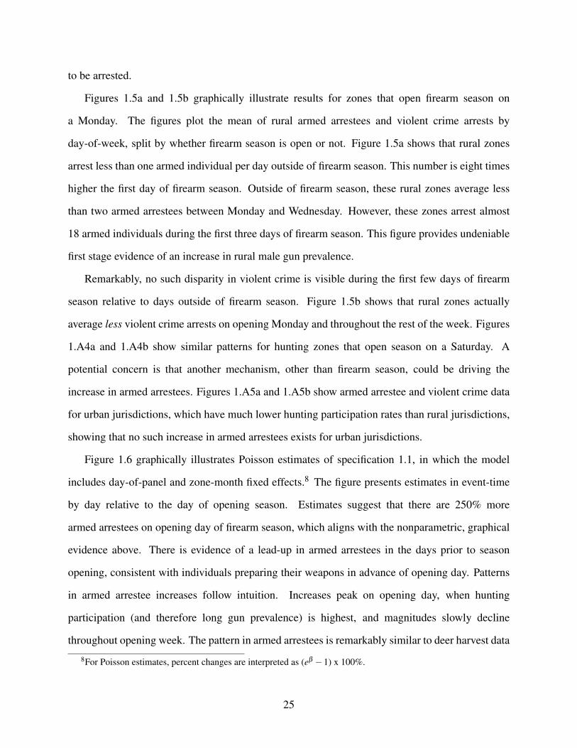
Figures 1.5a and 1.5b graphically illustrate results for zones that open firearm season on

a Monday. The figures plot the mean of rural armed arrestees and violent crime arrests by

day-of-week, split by whether firearm season is open or not. Figure 1.5a shows that rural zones

arrest less than one armed individual per day outside of firearm season. This number is eight times

higher the first day of firearm season. Outside of firearm season, these rural zones average less

than two armed arrestees between Monday and Wednesday. However, these zones arrest almost

18 armed individuals during the first three days of firearm season. This figure provides undeniable

first stage evidence of an increase in rural male gun prevalence.

Remarkably, no such disparity in violent crime is visible during the first few days of firearm

season relative to days outside of firearm season. Figure 1.5b shows that rural zones actually

average less violent crime arrests on opening Monday and throughout the rest of the week. Figures

1.A4a and 1.A4b show similar patterns for hunting zones that open season on a Saturday. A

potential concern is that another mechanism, other than firearm season, could be driving the

increase in armed arrestees. Figures 1.A5a and 1.A5b show armed arrestee and violent crime data

for urban jurisdictions, which have much lower hunting participation rates than rural jurisdictions,

showing that no such increase in armed arrestees exists for urban jurisdictions.

Figure 1.6 graphically illustrates Poisson estimates of specification 1.1, in which the model

includes day-of-panel and zone-month fixed effects.8 The figure presents estimates in event-time

by day relative to the day of opening season. Estimates suggest that there are 250% more

armed arrestees on opening day of firearm season, which aligns with the nonparametric, graphical

evidence above. There is evidence of a lead-up in armed arrestees in the days prior to season

opening, consistent with individuals preparing their weapons in advance of opening day. Patterns

in armed arrestee increases follow intuition. Increases peak on opening day, when hunting

participation (and therefore long gun prevalence) is highest, and magnitudes slowly decline

throughout opening week. The pattern in armed arrestees is remarkably similar to deer harvest data

8For Poisson estimates, percent changes are interpreted as (eβ −1) x 100%.

25

from Wisconsin in Figure 1.3. While the number of armed arrestees increases significantly, Figure

1.6 provides no evidence that overall number of males arrests changes. This is supportive evidence

of internal validity, suggesting that law enforcement efforts are not systematically changing open

opening season. If there is a 250% increase in male armed arrestees but no increase in number

of male arrests, this simply implies that arrested males are more likely to be armed for violent or

non-violent reasons.

One potential threat to the validity of my design would be any other policy or shock that aligns

with the opening day of firearm deer season and impacts crime. Firearm hunters almost exclusively

hunt with shotguns or rifles, which are long guns. Any concerns that my design is picking up

effects from non-hunting policies should be ameliorated by Figure 1.7, which shows that the entire

increase in armed arrestees is driven by long gun prevalence. Estimates suggest that the number

of arrestees armed with a long gun is 300% higher on opening day, with similar lead-up effects

and dissipation effects as found above. Even a week after firearm season opens, the number of

long gun armed arrestees is 50% higher. These patterns provide strong evidence that my design is

isolating the effects of hunting policies.

Given the strong evidence of an immense and persistent increase in recreational long gun

prevalence, it is striking that Figure 1.8 provides no evidence of an increase in rural male violent

crime incidents. On opening day, when long gun prevalence is 300% higher, the estimated effect

on rural male violent crime offenses is economically and statistically insignificant (point estimate

of 0.003). Point estimates for the second and third day of firearm season are actually negative.

Figure 1.8 shows that for all days surrounding the beginning of firearm season, estimated effects

on violent crime consistently hover around zero. Any potential concern of population in-migration

to rural areas during hunting season (as urban or suburban hunters access woods in rural areas)

would place an upward bias on violent crime estimates. As shown in Figure 1.A6a, results are

robust to using violent crime arrests.

Results in Table 1.5 show that estimates on long gun prevalence and violent crime are

remarkably stable across specifications that flexibly alter fixed effects. In each specification,

26

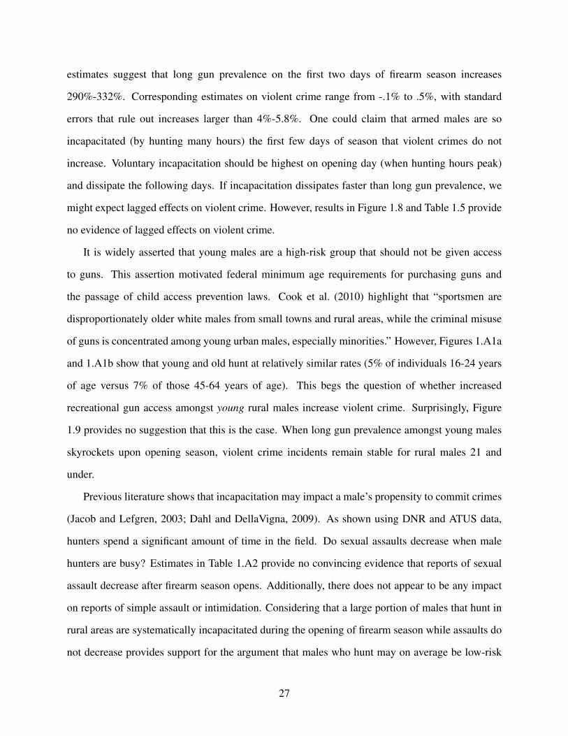
estimates suggest that long gun prevalence on the first two days of firearm season increases

290%-332%. Corresponding estimates on violent crime range from -.1% to .5%, with standard

errors that rule out increases larger than 4%-5.8%. One could claim that armed males are so

incapacitated (by hunting many hours) the first few days of season that violent crimes do not

increase. Voluntary incapacitation should be highest on opening day (when hunting hours peak)

and dissipate the following days. If incapacitation dissipates faster than long gun prevalence, we

might expect lagged effects on violent crime. However, results in Figure 1.8 and Table 1.5 provide

no evidence of lagged effects on violent crime.

It is widely asserted that young males are a high-risk group that should not be given access

to guns. This assertion motivated federal minimum age requirements for purchasing guns and

the passage of child access prevention laws. Cook et al. (2010) highlight that “sportsmen are

disproportionately older white males from small towns and rural areas, while the criminal misuse

of guns is concentrated among young urban males, especially minorities.” However, Figures 1.A1a

and 1.A1b show that young and old hunt at relatively similar rates (5% of individuals 16-24 years

of age versus 7% of those 45-64 years of age). This begs the question of whether increased

recreational gun access amongst young rural males increase violent crime. Surprisingly, Figure

1.9 provides no suggestion that this is the case. When long gun prevalence amongst young males

skyrockets upon opening season, violent crime incidents remain stable for rural males 21 and

under.

Previous literature shows that incapacitation may impact a male’s propensity to commit crimes

(Jacob and Lefgren, 2003; Dahl and DellaVigna, 2009). As shown using DNR and ATUS data,

hunters spend a significant amount of time in the field. Do sexual assaults decrease when male

hunters are busy? Estimates in Table 1.A2 provide no convincing evidence that reports of sexual

assault decrease after firearm season opens. Additionally, there does not appear to be any impact

on reports of simple assault or intimidation. Considering that a large portion of males that hunt in

rural areas are systematically incapacitated during the opening of firearm season while assaults do

not decrease provides support for the argument that males who hunt may on average be low-risk

27

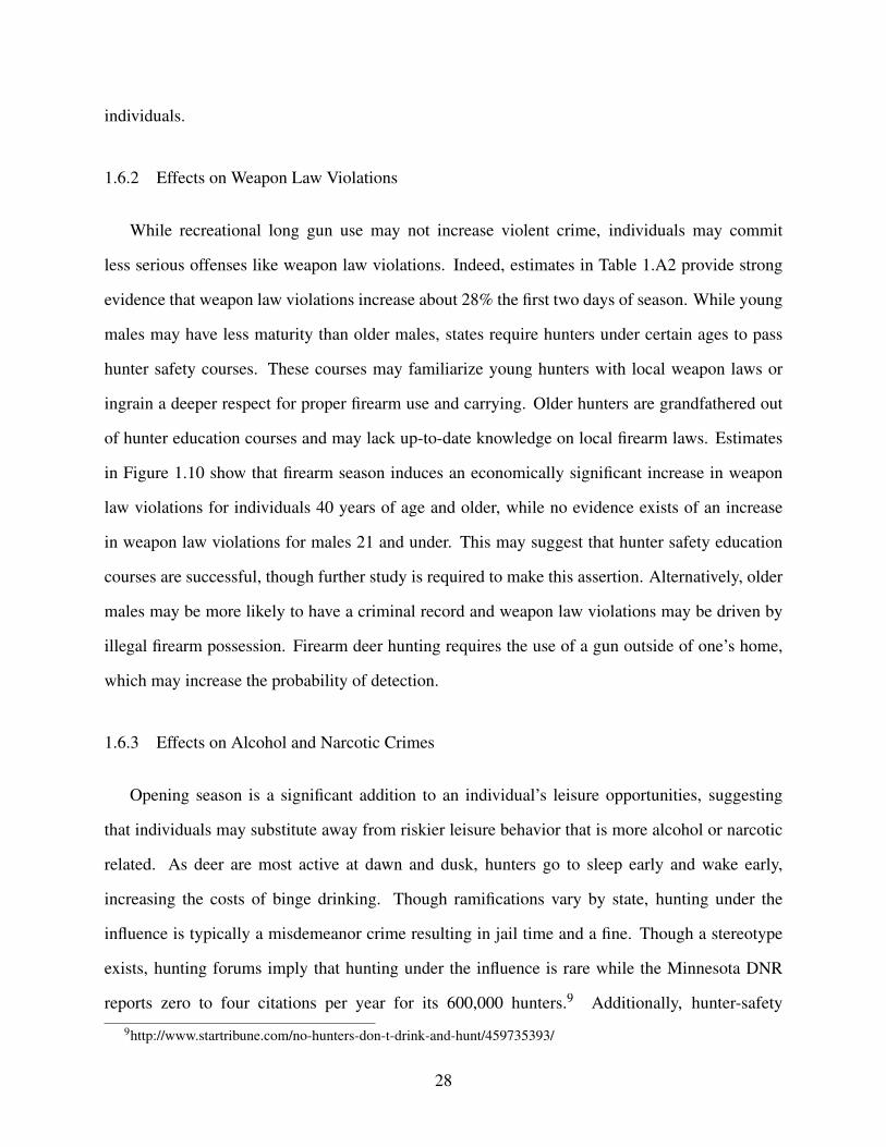
individuals.

1.6.2 Effects on Weapon Law Violations

While recreational long gun use may not increase violent crime, individuals may commit

less serious offenses like weapon law violations. Indeed, estimates in Table 1.A2 provide strong

evidence that weapon law violations increase about 28% the first two days of season. While young

males may have less maturity than older males, states require hunters under certain ages to pass

hunter safety courses. These courses may familiarize young hunters with local weapon laws or

ingrain a deeper respect for proper firearm use and carrying. Older hunters are grandfathered out

of hunter education courses and may lack up-to-date knowledge on local firearm laws. Estimates

in Figure 1.10 show that firearm season induces an economically significant increase in weapon

law violations for individuals 40 years of age and older, while no evidence exists of an increase

in weapon law violations for males 21 and under. This may suggest that hunter safety education

courses are successful, though further study is required to make this assertion. Alternatively, older

males may be more likely to have a criminal record and weapon law violations may be driven by

illegal firearm possession. Firearm deer hunting requires the use of a gun outside of one’s home,

which may increase the probability of detection.

1.6.3 Effects on Alcohol and Narcotic Crimes

Opening season is a significant addition to an individual’s leisure opportunities, suggesting

that individuals may substitute away from riskier leisure behavior that is more alcohol or narcotic

related. As deer are most active at dawn and dusk, hunters go to sleep early and wake early,

increasing the costs of binge drinking. Though ramifications vary by state, hunting under the

influence is typically a misdemeanor crime resulting in jail time and a fine. Though a stereotype

exists, hunting forums imply that hunting under the influence is rare while the Minnesota DNR

reports zero to four citations per year for its 600,000 hunters.9 Additionally, hunter-safety

9http://www.startribune.com/no-hunters-don-t-drink-and-hunt/459735393/

28

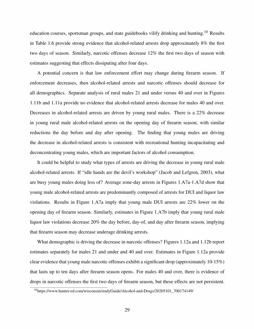
education courses, sportsman groups, and state guidebooks vilify drinking and hunting.10 Results

in Table 1.6 provide strong evidence that alcohol-related arrests drop approximately 8% the first

two days of season. Similarly, narcotic offenses decrease 12% the first two days of season with

estimates suggesting that effects dissipating after four days.

A potential concern is that law enforcement effort may change during firearm season. If

enforcement decreases, then alcohol-related arrests and narcotic offenses should decrease for

all demographics. Separate analysis of rural males 21 and under versus 40 and over in Figures

1.11b and 1.11a provide no evidence that alcohol-related arrests decrease for males 40 and over.

Decreases in alcohol-related arrests are driven by young rural males. There is a 22% decrease

in young rural male alcohol-related arrests on the opening day of firearm season, with similar

reductions the day before and day after opening. The finding that young males are driving

the decrease in alcohol-related arrests is consistent with recreational hunting incapacitating and

deconcentrating young males, which are important factors of alcohol consumption.

It could be helpful to study what types of arrests are driving the decrease in young rural male

alcohol-related arrests. If “idle hands are the devil’s workshop” (Jacob and Lefgren, 2003), what

are busy young males doing less of? Average zone-day arrests in Figures 1.A7a-1.A7d show that

young male alcohol-related arrests are predominantly composed of arrests for DUI and liquor law

violations. Results in Figure 1.A7a imply that young male DUI arrests are 22% lower on the

opening day of firearm season. Similarly, estimates in Figure 1.A7b imply that young rural male

liquor law violations decrease 20% the day before, day-of, and day after firearm season, implying

that firearm season may decrease underage drinking arrests.

What demographic is driving the decrease in narcotic offenses? Figures 1.12a and 1.12b report

estimates separately for males 21 and under and 40 and over. Estimates in Figure 1.12a provide

clear evidence that young male narcotic offenses exhibit a significant drop (approximately 10-15%)

that lasts up to ten days after firearm season opens. For males 40 and over, there is evidence of

drops in narcotic offenses the first two days of firearm season, but these effects are not persistent.

10https://www.hunter-ed.com/wisconsin/studyGuide/Alcohol-and-Drugs/20205101_700174149/

29

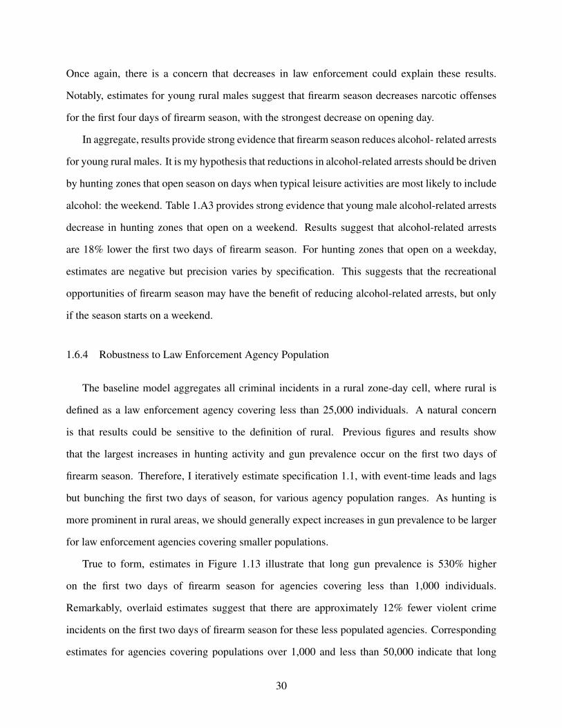
Once again, there is a concern that decreases in law enforcement could explain these results.

Notably, estimates for young rural males suggest that firearm season decreases narcotic offenses

for the first four days of firearm season, with the strongest decrease on opening day.

In aggregate, results provide strong evidence that firearm season reduces alcohol- related arrests

for young rural males. It is my hypothesis that reductions in alcohol-related arrests should be driven

by hunting zones that open season on days when typical leisure activities are most likely to include

alcohol: the weekend. Table 1.A3 provides strong evidence that young male alcohol-related arrests

decrease in hunting zones that open on a weekend. Results suggest that alcohol-related arrests

are 18% lower the first two days of firearm season. For hunting zones that open on a weekday,

estimates are negative but precision varies by specification. This suggests that the recreational

opportunities of firearm season may have the benefit of reducing alcohol-related arrests, but only

if the season starts on a weekend.

1.6.4 Robustness to Law Enforcement Agency Population

The baseline model aggregates all criminal incidents in a rural zone-day cell, where rural is

defined as a law enforcement agency covering less than 25,000 individuals. A natural concern

is that results could be sensitive to the definition of rural. Previous figures and results show

that the largest increases in hunting activity and gun prevalence occur on the first two days of

firearm season. Therefore, I iteratively estimate specification 1.1, with event-time leads and lags

but bunching the first two days of season, for various agency population ranges. As hunting is

more prominent in rural areas, we should generally expect increases in gun prevalence to be larger

for law enforcement agencies covering smaller populations.

True to form, estimates in Figure 1.13 illustrate that long gun prevalence is 530% higher

on the first two days of firearm season for agencies covering less than 1,000 individuals.

Remarkably, overlaid estimates suggest that there are approximately 12% fewer violent crime

incidents on the first two days of firearm season for these less populated agencies. Corresponding

estimates for agencies covering populations over 1,000 and less than 50,000 indicate that long

30

gun prevalence is approximately 50%-125% higher, while all estimated effects on violent crime

incidents consistently hover around zero. Estimated effects on long gun prevalence disappear for

agencies covering more than 50,000 individuals, which aligns with lower hunting participation in

urban areas.

Similarly, Figure 1.14 breaks out estimated effects on alcohol-related arrests by age group of

the offender and population of the law enforcement agency. Estimates suggest that decreases in

alcohol-related arrests are greatest for less populous areas and for younger males. Males under

the age of 18 exhibit 24%-38% decreases in alcohol-related arrests on the first two days of firearm

season for agencies covering less than 15,000 individuals. Meanwhile, males 40 and over only

exhibit decreases in alcohol-related arrests for agencies covering less than 1,000 individuals.

1.7 Discussion

The results of this paper provide strong evidence that enormous increases in recreational long

gun prevalence are not associated with any increase in violent crime. In the least populous areas,

where long gun prevalence increased 530%, estimates suggest that male violent crime actually

decreased. This section discusses three reasons why my results might differ from the aggregate

positive relationship between guns and crime often found in previous studies.

First, hunting is a time-consuming activity that is inherently incapacitating, which may

decrease crime (Jacob and Lefgren, 2003; Dahl and DellaVigna, 2009). Various sources of deer

hunter data suggest that hunters spend upwards of six hours per day in the field, with additional

time spent processing harvested deer. Males may be too preoccupied to use their guns nefarious

purposes. Additionally, hunting may decrease social interaction (due to hunting in the woods)

which may decrease potential violent conflict (Jacob and Lefgren, 2003).

Second, hunters may comprise a low-risk sample. As stated in Cook et al. (2010), hunters are

often older white males in rural areas while violent crime is more rampant among young minority

males in urban areas. However, casting all hunters as old white males ignores the large contingent

of young male hunters (Figures 1.A1a-1.A1b). No demographic has been more vilified concerning

31

gun use and crime than young males. Why isn’t gun use among young rural male hunters associated

with an increase in violent crime?

One potential reason is that the context in which a young rural male acquires a gun differs

from the context of a young urban male, who are often highlighted in the literature. Historically,

hunting has primarily been a tradition passed down from father to son. To the degree that young

hunters adopt behavior similar to low-risk role models like fathers (Case and Katz, 1991) and

hunter education instructors, the peer effects that young hunters pick up regarding guns will differ

from that of youths in urban areas.

Another reason that hunters may be a low-risk sample is because patient individuals may select

into deer hunting. Deer hunting is often characterized as an activity in which an individual sits

in a tree stand for hours on end, waiting for a deer to walk by. It is possible that only patient

individuals are willing to participate in this gun-related recreational activity. Lochner and Moretti

(2004) cite increased patience as a mechanism that decreases propensity to commit crime because

more patient people discount future punishments less.

Third, hunters may face more regulation than other gun owners. These regulations may

improve firearm etiquette and discourage high-risk individuals from hunting. In a 2015 survey,

Rowhani-Rahbar et al. (2018) estimate that only 61% of firearm owners have received firearm

training. To the contrary, all hunters must pass a hunter education course (unless grandfathered

out) that teaches proper firearm use and etiquette. Therefore, all non-grandfathered hunters have

received formal firearm training while many non-hunters haven’t. After passing a hunter education

course, an individual must purchase a hunting license and deer tag for each deer they desire to

harvest. Although no background check is required, formal paperwork and courses that require

placing one’s name in a state database may discourage individuals who illegally possess a firearm

from hunting. This is particularly important as individuals who commit gun crimes often do not

legally possess the firearm (Fabio et al., 2016).

32

1.8 Conclusion

This paper breaks new ground in gun policy research on a culturally iconic sample of gun

owners that has before now gone unexplored: the 18% (≈ 25% at the beginning of my sample) of

American gun owners who use firearms to hunt. Each year, hunters expend approximately 30% of

all shots fired in America. This paper tests the contentious claim of rural long gun owners that their

firearm use does not increase violent crime. I am the first to examine how irregularities in hunting

season regulations, which increase long gun use over 300%, impact violent crime in rural America.

To my knowledge, this is the first quasi-experimental study, with direct estimates of actual firearm

use, that examines the effects of firearm use on violent crime. The enormous changes in firearm

use caused by hunting regulations are unparalleled by any other policy in existence. There are no

other policies that induce 600,000 Wisconsin males or 530,000 Michigan males to systematically

and temporarily carry and use firearms.

Despite the fact that firearm season increases rural long gun use by over 300%, estimates

using within-hunting zone variation provide no evidence that rural violent crime increases. I

estimate the elasticity of violent crime with respect to recreational long gun use to be between

-0.01 and +0.0003. While there is no evidence of an increase in violent crime, results suggest that

male weapon law violations increase substantially. Americans exude dichotomous perspectives

concerning the relationship between gun use and violent crime. Paradoxically, both perspectives

may be correct if the patterns between gun use and violent crime are heterogeneous across gun

users and gun types. My results suggest that previous studies examining the violent crime effects

of aggregate gun ownership or use may muddy the detrimental effects of urban-skewed handguns

with the nonexistent effects of rural-skewed long guns. Stark differences in gun types and reasons

for ownership between urban and rural individuals may be one mechanism by which guns have a

stronger link to violent crime in urban areas.

Firearm deer hunting is a recreational activity that rural males strongly anticipate. Additional

recreation opportunities like firearm hunting could partially offset the negative externality of

alcohol and drug consumption if males substitute away from riskier behavior and toward hunting. I

33

find strong evidence that alcohol-related arrests of juvenile males fall by 22% and narcotic offenses

fall by 15% at the start of hunting season. Aligning with juvenile alcohol consumption patterns, my

results suggest that hunting zones that open season on a weekend may experience larger decreases

in alcohol-related crime.

One limitation of this study is lack of daily injury and mortality data. While the effects of

gun use and violent crime are a hot area of debate, the enormous increase in gun use and access

during firearm deer season could exert social costs not captured by violent crime. Child-access

prevention (CAP) laws have been found to decrease suicides and unintentional injuries or death

(Morral et al., 2018). While handguns are a more common implement for suicide, individuals

may substitute to long guns if relative ease of access changes. As long gun access unequivocally

increases during firearm season, for hunters and non-hunters, future work should examine the link

between increased long gun use and non-crime related costs.

34

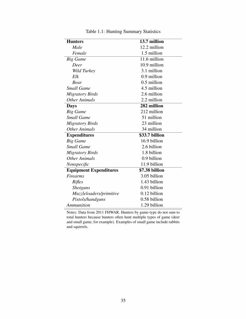
Table 1.1: Hunting Summary Statistics

Hunters 13.7 millionMale 12.2 millionFemale 1.5 million

Big Game 11.6 millionDeer 10.9 millionWild Turkey 3.1 millionElk 0.9 millionBear 0.5 million

Small Game 4.5 millionMigratory Birds 2.6 millionOther Animals 2.2 millionDays 282 millionBig Game 212 millionSmall Game 51 millionMigratory Birds 23 millionOther Animals 34 millionExpenditures $33.7 billionBig Game 16.9 billionSmall Game 2.6 billionMigratory Birds 1.8 billionOther Animals 0.9 billionNonspecific 11.9 billionEquipment Expenditures $7.38 billionFirearms 3.05 billion

Rifles 1.43 billionShotguns 0.91 billionMuzzleloaders/primitive 0.12 billionPistols/handguns 0.58 billion

Ammunition 1.29 billionNotes: Data from 2011 FHWAR. Hunters by game-type do not sum tototal hunters because hunters often hunt multiple types of game (deerand small game, for example). Examples of small game include rabbitsand squirrels.

35

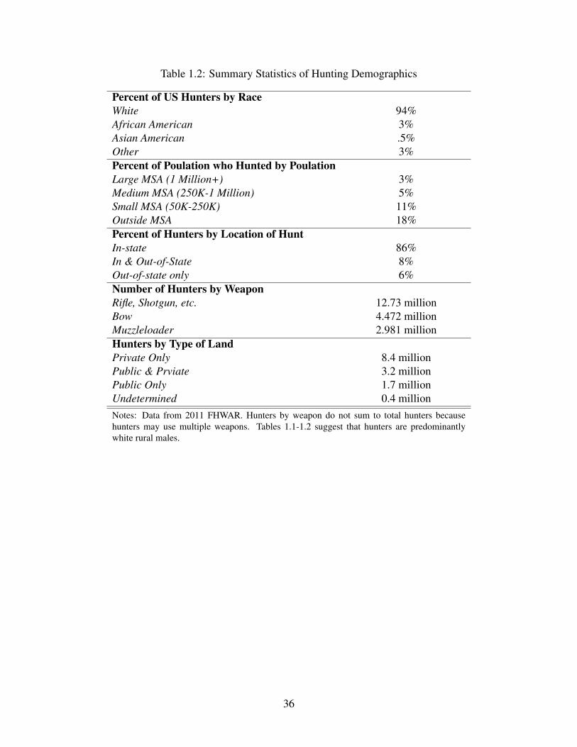
Table 1.2: Summary Statistics of Hunting Demographics

Percent of US Hunters by RaceWhite 94%African American 3%Asian American .5%Other 3%Percent of Poulation who Hunted by PoulationLarge MSA (1 Million+) 3%Medium MSA (250K-1 Million) 5%Small MSA (50K-250K) 11%Outside MSA 18%Percent of Hunters by Location of HuntIn-state 86%In & Out-of-State 8%Out-of-state only 6%Number of Hunters by WeaponRifle, Shotgun, etc. 12.73 millionBow 4.472 millionMuzzleloader 2.981 millionHunters by Type of LandPrivate Only 8.4 millionPublic & Prviate 3.2 millionPublic Only 1.7 millionUndetermined 0.4 millionNotes: Data from 2011 FHWAR. Hunters by weapon do not sum to total hunters becausehunters may use multiple weapons. Tables 1.1-1.2 suggest that hunters are predominantlywhite rural males.

36

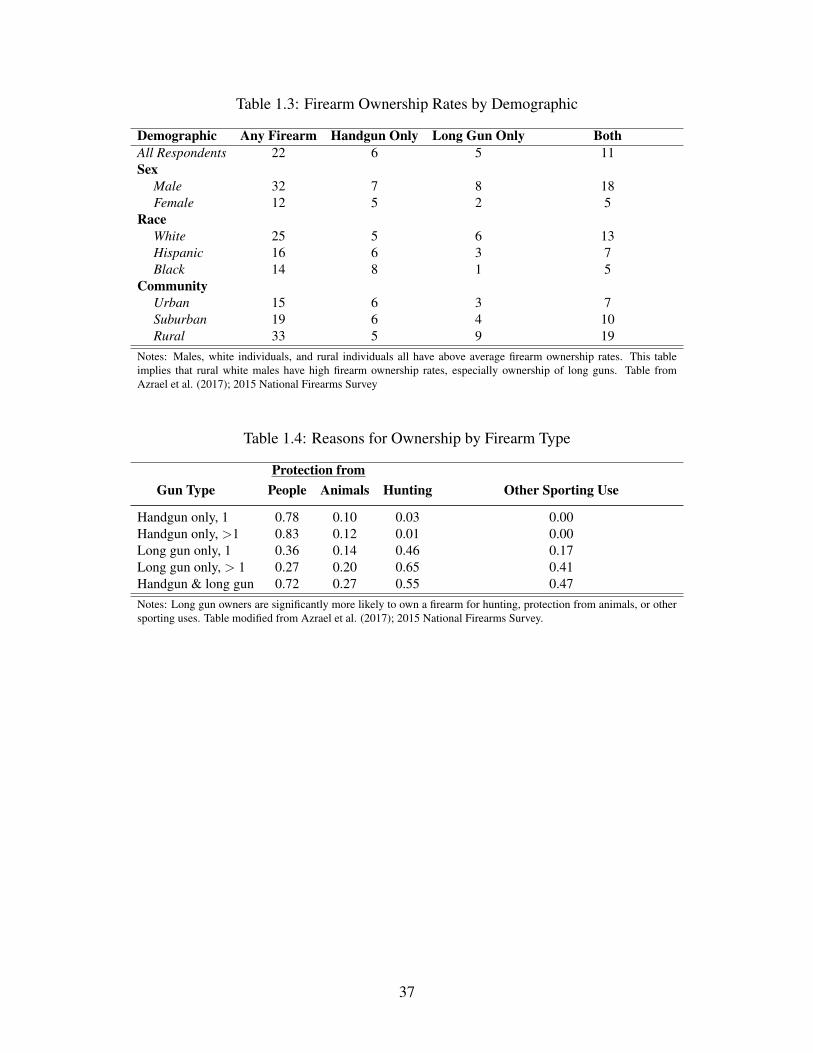
Table 1.3: Firearm Ownership Rates by Demographic

Demographic Any Firearm Handgun Only Long Gun Only BothAll Respondents 22 6 5 11Sex

Male 32 7 8 18Female 12 5 2 5

RaceWhite 25 5 6 13Hispanic 16 6 3 7Black 14 8 1 5

CommunityUrban 15 6 3 7Suburban 19 6 4 10Rural 33 5 9 19

Notes: Males, white individuals, and rural individuals all have above average firearm ownership rates. This tableimplies that rural white males have high firearm ownership rates, especially ownership of long guns. Table fromAzrael et al. (2017); 2015 National Firearms Survey

Table 1.4: Reasons for Ownership by Firearm Type

Protection fromGun Type People Animals Hunting Other Sporting Use

Handgun only, 1 0.78 0.10 0.03 0.00Handgun only, >1 0.83 0.12 0.01 0.00Long gun only, 1 0.36 0.14 0.46 0.17Long gun only, > 1 0.27 0.20 0.65 0.41Handgun & long gun 0.72 0.27 0.55 0.47Notes: Long gun owners are significantly more likely to own a firearm for hunting, protection from animals, or othersporting uses. Table modified from Azrael et al. (2017); 2015 National Firearms Survey.

37

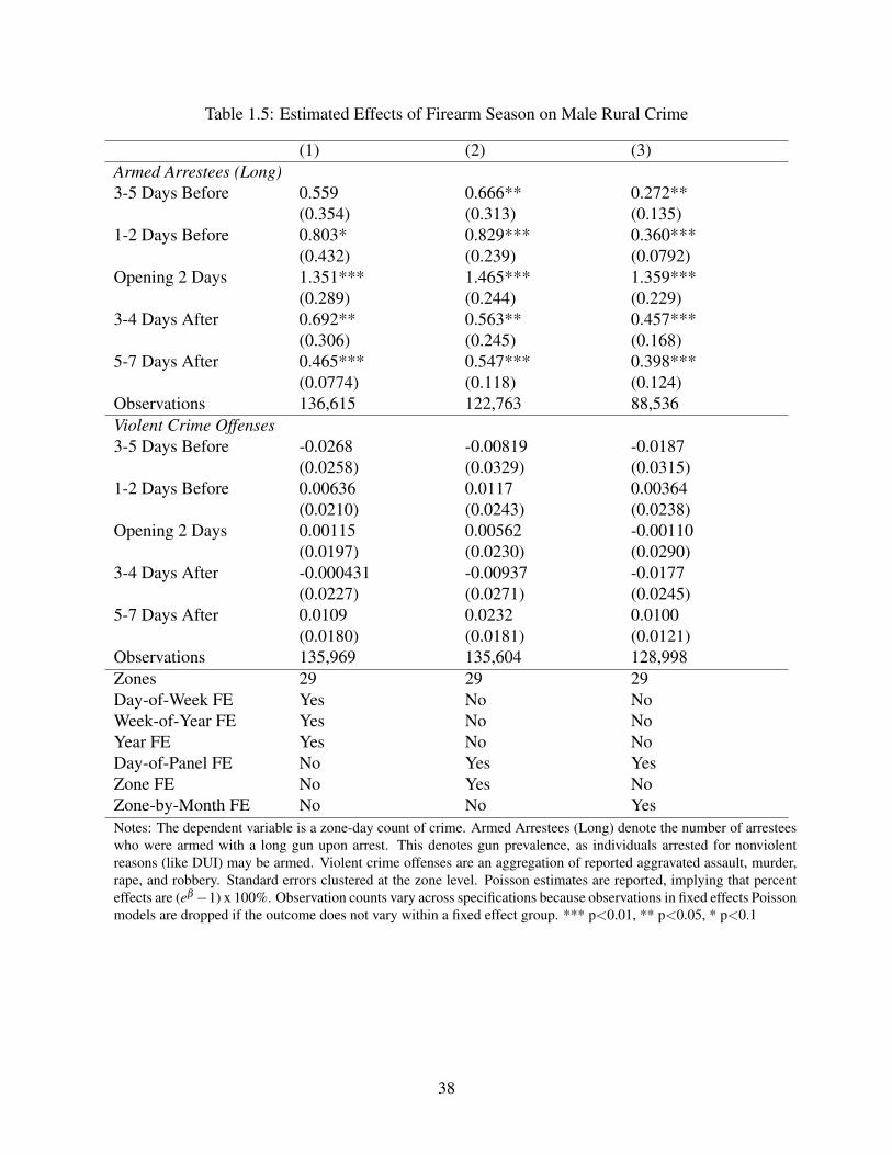
Table 1.5: Estimated Effects of Firearm Season on Male Rural Crime

(1) (2) (3)Armed Arrestees (Long)3-5 Days Before 0.559 0.666** 0.272**

(0.354) (0.313) (0.135)1-2 Days Before 0.803* 0.829*** 0.360***

(0.432) (0.239) (0.0792)Opening 2 Days 1.351*** 1.465*** 1.359***

(0.289) (0.244) (0.229)3-4 Days After 0.692** 0.563** 0.457***

(0.306) (0.245) (0.168)5-7 Days After 0.465*** 0.547*** 0.398***

(0.0774) (0.118) (0.124)Observations 136,615 122,763 88,536Violent Crime Offenses3-5 Days Before -0.0268 -0.00819 -0.0187

(0.0258) (0.0329) (0.0315)1-2 Days Before 0.00636 0.0117 0.00364

(0.0210) (0.0243) (0.0238)Opening 2 Days 0.00115 0.00562 -0.00110

(0.0197) (0.0230) (0.0290)3-4 Days After -0.000431 -0.00937 -0.0177

(0.0227) (0.0271) (0.0245)5-7 Days After 0.0109 0.0232 0.0100

(0.0180) (0.0181) (0.0121)Observations 135,969 135,604 128,998Zones 29 29 29Day-of-Week FE Yes No NoWeek-of-Year FE Yes No NoYear FE Yes No NoDay-of-Panel FE No Yes YesZone FE No Yes NoZone-by-Month FE No No YesNotes: The dependent variable is a zone-day count of crime. Armed Arrestees (Long) denote the number of arresteeswho were armed with a long gun upon arrest. This denotes gun prevalence, as individuals arrested for nonviolentreasons (like DUI) may be armed. Violent crime offenses are an aggregation of reported aggravated assault, murder,rape, and robbery. Standard errors clustered at the zone level. Poisson estimates are reported, implying that percenteffects are (eβ−1) x 100%. Observation counts vary across specifications because observations in fixed effects Poissonmodels are dropped if the outcome does not vary within a fixed effect group. *** p<0.01, ** p<0.05, * p<0.1

38

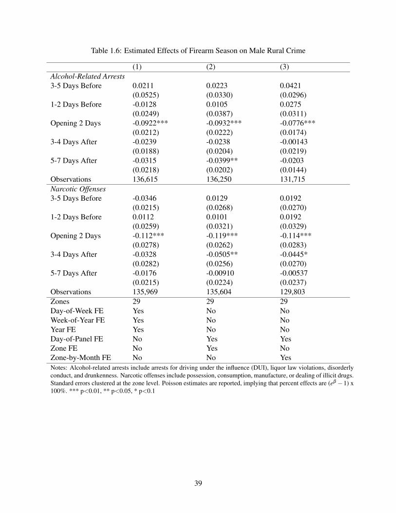
Table 1.6: Estimated Effects of Firearm Season on Male Rural Crime

(1) (2) (3)Alcohol-Related Arrests3-5 Days Before 0.0211 0.0223 0.0421

(0.0525) (0.0330) (0.0296)1-2 Days Before -0.0128 0.0105 0.0275

(0.0249) (0.0387) (0.0311)Opening 2 Days -0.0922*** -0.0932*** -0.0776***

(0.0212) (0.0222) (0.0174)3-4 Days After -0.0239 -0.0238 -0.00143

(0.0188) (0.0204) (0.0219)5-7 Days After -0.0315 -0.0399** -0.0203

(0.0218) (0.0202) (0.0144)Observations 136,615 136,250 131,715Narcotic Offenses3-5 Days Before -0.0346 0.0129 0.0192

(0.0215) (0.0268) (0.0270)1-2 Days Before 0.0112 0.0101 0.0192

(0.0259) (0.0321) (0.0329)Opening 2 Days -0.112*** -0.119*** -0.114***

(0.0278) (0.0262) (0.0283)3-4 Days After -0.0328 -0.0505** -0.0445*

(0.0282) (0.0256) (0.0270)5-7 Days After -0.0176 -0.00910 -0.00537

(0.0215) (0.0224) (0.0237)Observations 135,969 135,604 129,803Zones 29 29 29Day-of-Week FE Yes No NoWeek-of-Year FE Yes No NoYear FE Yes No NoDay-of-Panel FE No Yes YesZone FE No Yes NoZone-by-Month FE No No YesNotes: Alcohol-related arrests include arrests for driving under the influence (DUI), liquor law violations, disorderlyconduct, and drunkenness. Narcotic offenses include possession, consumption, manufacture, or dealing of illicit drugs.Standard errors clustered at the zone level. Poisson estimates are reported, implying that percent effects are (eβ −1) x100%. *** p<0.01, ** p<0.05, * p<0.1

39

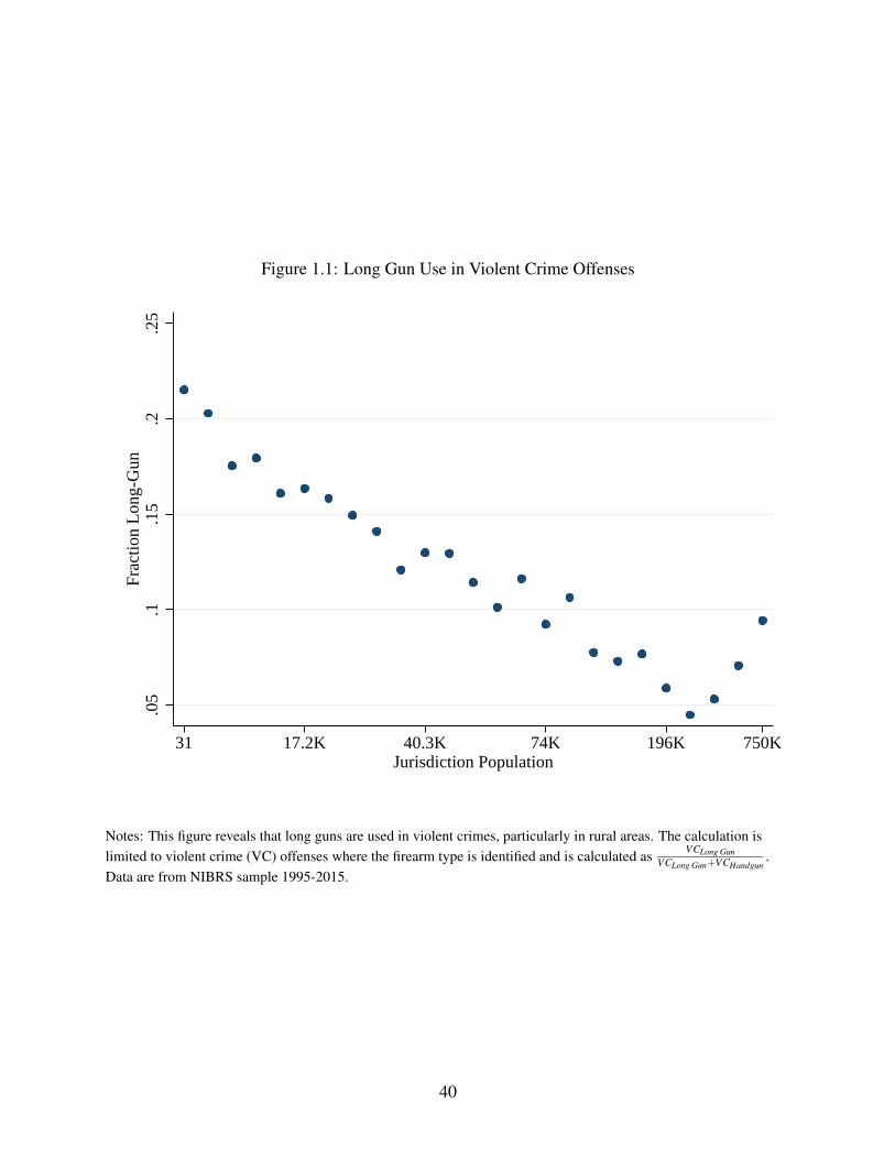
Figure 1.1: Long Gun Use in Violent Crime Offenses

.05

.1.1

5.2

.25

Frac

tion

Lon

g-G

un

31 17.2K 40.3K 74K 196K 750KJurisdiction Population

Notes: This figure reveals that long guns are used in violent crimes, particularly in rural areas. The calculation islimited to violent crime (VC) offenses where the firearm type is identified and is calculated as VCLong Gun

VCLong Gun+VCHandgun.

Data are from NIBRS sample 1995-2015.

40

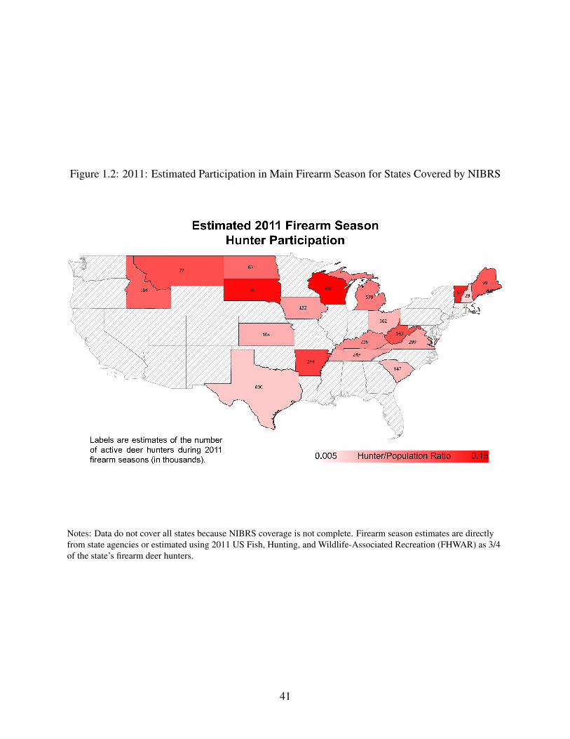
Figure 1.2: 2011: Estimated Participation in Main Firearm Season for States Covered by NIBRS

Notes: Data do not cover all states because NIBRS coverage is not complete. Firearm season estimates are directlyfrom state agencies or estimated using 2011 US Fish, Hunting, and Wildlife-Associated Recreation (FHWAR) as 3/4of the state’s firearm deer hunters.

41

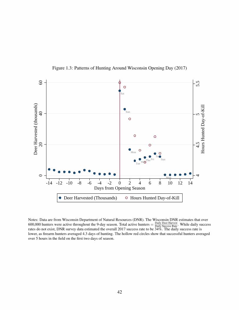
Figure 1.3: Patterns of Hunting Around Wisconsin Opening Day (2017)

Sat

Sun

Mon

TueWed

Thu FriSat

Sun

Mon

44.

55

5.5

Hou

rs H

unte

d D

ay-o

f-K

ill

020

4060

Dee

r H

arve

sted

(th

ousa

nds)

-14 -12 -10 -8 -6 -4 -2 0 2 4 6 8 10 12 14Days from Opening Season

Deer Harvested (Thousands) Hours Hunted Day-of-Kill

Notes: Data are from Wisconsin Department of Natural Resources (DNR). The Wisconsin DNR estimates that over600,000 hunters were active throughout the 9-day season. Total active hunters = Daily Deer Harvest

Daily Success Rate . While daily successrates do not exist, DNR survey data estimated the overall 2017 success rate to be 34%. The daily success rate islower, as firearm hunters averaged 4.3 days of hunting. The hollow red circles show that successful hunters averagedover 5 hours in the field on the first two days of season.

42

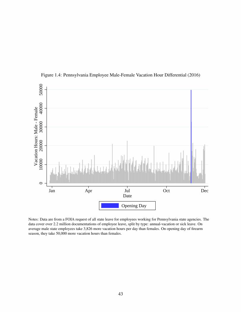
Figure 1.4: Pennsylvania Employee Male-Female Vacation Hour Differential (2016)

010

000

2000

030

000

4000

050

000

Vac

atio

n H

ours

: Mal

e -

Fem

ale

Jan Apr Jul Oct DecDate

Opening Day

Notes: Data are from a FOIA request of all state leave for employees working for Pennsylvania state agencies. Thedata cover over 2.2 million documentations of employee leave, split by type: annual-vacation or sick leave. Onaverage male state employees take 3,826 more vacation hours per day than females. On opening day of firearmseason, they take 50,000 more vacation hours than females.

43

Figure 1.5: Rural Male Arrests in Zones Opening on Monday

(a) Number of Armed Arrestees

(b) Number of Violent Crime Arrests

Notes: This figure displays average daily male armed arrestees and violent crime (aggravated assault, murder, rape,and robbery) arrests for zones that open on Monday. Averages are provided for the opening week of firearm seasonand for other weeks of the year.

44

Figure 1.6: Estimated Effects of Firearm Season on Rural Male Gun Prevalence and Number ofArrests Using Variation in Season Access

-.5

0

.5

1

1.5

2

Coe

ffic

ient

Est

imat

es

-14 -12 -10 -8 -6 -4 -2 0 2 4 6 8 10 12 14Day from Opening Season

Armed ArresteesZone-Day Mean: 0.80

Number of ArrestsZone-Day Mean: 67.61

Notes: Violent crime offenses are an aggregation of reported aggravated assault, murder, rape, and robbery. Themean of the dependent variable is the average count of respective arrests per zone-day. Poisson estimates of leads andlags are reported, implying that percent effects are (eβ −1) x 100%. The model includes day-of-panel andzone-month fixed effects. Standard errors are clustered by zone, with 95% confidence intervals provided.

45

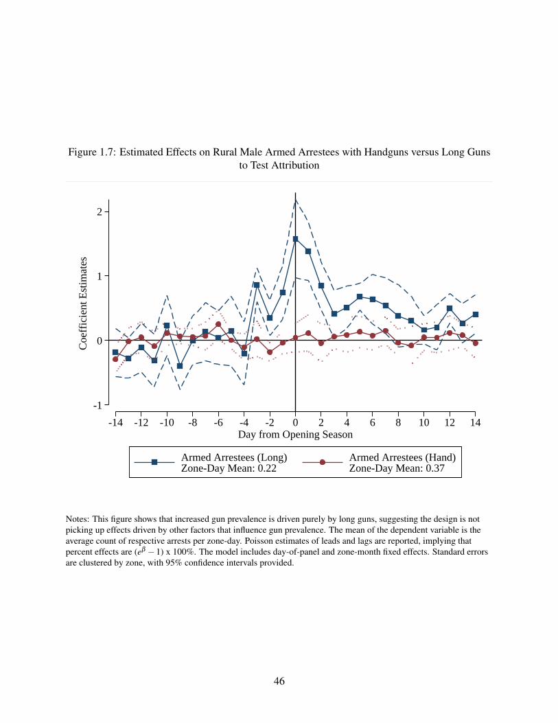
Figure 1.7: Estimated Effects on Rural Male Armed Arrestees with Handguns versus Long Gunsto Test Attribution

-1

0

1

2

Coe

ffic

ient

Est

imat

es

-14 -12 -10 -8 -6 -4 -2 0 2 4 6 8 10 12 14Day from Opening Season

Armed Arrestees (Long)Zone-Day Mean: 0.22

Armed Arrestees (Hand)Zone-Day Mean: 0.37

Notes: This figure shows that increased gun prevalence is driven purely by long guns, suggesting the design is notpicking up effects driven by other factors that influence gun prevalence. The mean of the dependent variable is theaverage count of respective arrests per zone-day. Poisson estimates of leads and lags are reported, implying thatpercent effects are (eβ −1) x 100%. The model includes day-of-panel and zone-month fixed effects. Standard errorsare clustered by zone, with 95% confidence intervals provided.

46

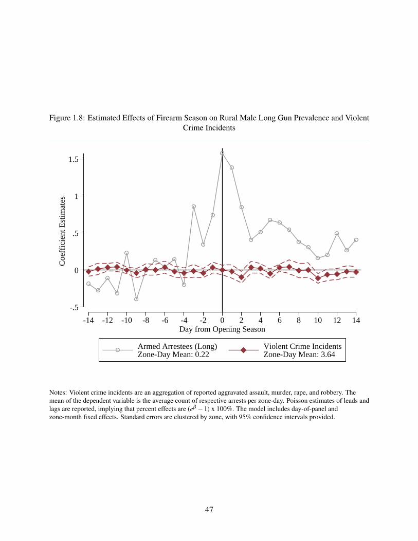
Figure 1.8: Estimated Effects of Firearm Season on Rural Male Long Gun Prevalence and ViolentCrime Incidents

-.5

0

.5

1

1.5

Coe

ffic

ient

Est

imat

es

-14 -12 -10 -8 -6 -4 -2 0 2 4 6 8 10 12 14Day from Opening Season

Armed Arrestees (Long)Zone-Day Mean: 0.22

Violent Crime IncidentsZone-Day Mean: 3.64

Notes: Violent crime incidents are an aggregation of reported aggravated assault, murder, rape, and robbery. Themean of the dependent variable is the average count of respective arrests per zone-day. Poisson estimates of leads andlags are reported, implying that percent effects are (eβ −1) x 100%. The model includes day-of-panel andzone-month fixed effects. Standard errors are clustered by zone, with 95% confidence intervals provided.

47

Figure 1.9: Estimated Effects of Firearm Season on Young (21 & under) Rural Male Long GunPrevalence and Violent Crime Incidents

-2

-1

0

1

2

Coe

ffic

ient

Est

imat

es

-14 -12 -10 -8 -6 -4 -2 0 2 4 6 8 10 12 14Day from Opening Season

Armed Arrestees (Long)Zone-Day Mean: 0.05

Violent Crime IncidentsZone-Day Mean: 1.04

Notes: Violent crime incidents are an aggregation of reported aggravated assault, murder, rape, and robbery. Themean of the dependent variable is the average count of respective arrests per zone-day. Poisson estimates of leads andlags are reported, implying that percent effects are (eβ −1) x 100%. The model includes day-of-panel andzone-month fixed effects. Standard errors are clustered by zone, with 95% confidence intervals provided.

48

Figure 1.10: Estimated Effects of Firearm Season on Weapon Law Violations by Age

-.5

0

.5

1

Coe

ffic

ient

Est

imat

es

-14 -12 -10 -8 -6 -4 -2 0 2 4 6 8 10 12 14Day from Opening Season

40 and OverZone-Day Mean: 0.29

21 and UnderZone-Day Mean: 0.24

Notes: Weapon law violations include arrests for illegally carrying a concealed weapon, unlicensed weaponpossession, unregistered weapon possession, using suppressors (silencers), et cetera. The mean of the dependentvariable is the average count of respective arrests per zone-day. Poisson estimates of leads and lags are reported,implying that percent effects are (eβ −1) x 100%. The model includes day-of-panel and zone-month fixed effects.Standard errors are clustered by zone, with 95% confidence intervals provided.

49

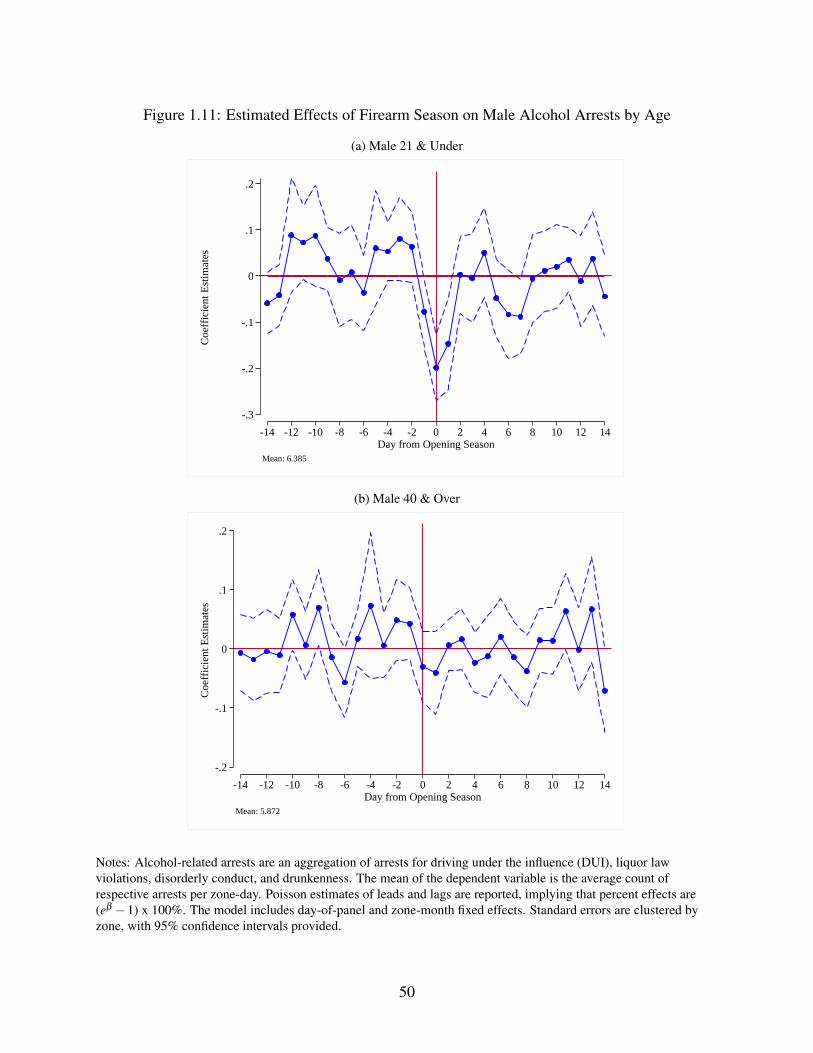
Figure 1.11: Estimated Effects of Firearm Season on Male Alcohol Arrests by Age

(a) Male 21 & Under

-.3

-.2

-.1

0

.1

.2

Coe

ffic

ient

Est

imat

es

-14 -12 -10 -8 -6 -4 -2 0 2 4 6 8 10 12 14Day from Opening Season

Mean: 6.385

(b) Male 40 & Over

-.2

-.1

0

.1

.2

Coe

ffic

ient

Est

imat

es

-14 -12 -10 -8 -6 -4 -2 0 2 4 6 8 10 12 14Day from Opening Season

Mean: 5.872

Notes: Alcohol-related arrests are an aggregation of arrests for driving under the influence (DUI), liquor lawviolations, disorderly conduct, and drunkenness. The mean of the dependent variable is the average count ofrespective arrests per zone-day. Poisson estimates of leads and lags are reported, implying that percent effects are(eβ −1) x 100%. The model includes day-of-panel and zone-month fixed effects. Standard errors are clustered byzone, with 95% confidence intervals provided.

50

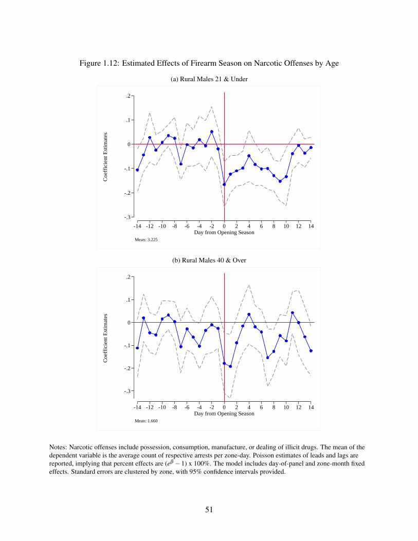
Figure 1.12: Estimated Effects of Firearm Season on Narcotic Offenses by Age

(a) Rural Males 21 & Under

-.3

-.2

-.1

0

.1

.2

Coe

ffic

ient

Est

imat

es

-14 -12 -10 -8 -6 -4 -2 0 2 4 6 8 10 12 14Day from Opening Season

Mean: 3.225

(b) Rural Males 40 & Over

-.3

-.2

-.1

0

.1

.2

Coe

ffic

ient

Est

imat

es

-14 -12 -10 -8 -6 -4 -2 0 2 4 6 8 10 12 14Day from Opening Season

Mean: 1.660

Notes: Narcotic offenses include possession, consumption, manufacture, or dealing of illicit drugs. The mean of thedependent variable is the average count of respective arrests per zone-day. Poisson estimates of leads and lags arereported, implying that percent effects are (eβ −1) x 100%. The model includes day-of-panel and zone-month fixedeffects. Standard errors are clustered by zone, with 95% confidence intervals provided.

51

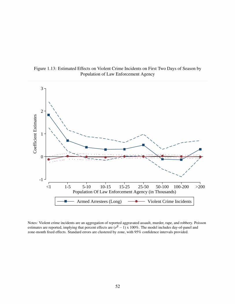
Figure 1.13: Estimated Effects on Violent Crime Incidents on First Two Days of Season byPopulation of Law Enforcement Agency

-1

0

1

2

3

Coe

ffic

ient

Est

imat

es

<1 1-5 5-10 10-15 15-25 25-50 50-100 100-200 >200Population Of Law Enforcement Agency (in Thousands)

Armed Arrestees (Long) Violent Crime Incidents

Notes: Violent crime incidents are an aggregation of reported aggravated assault, murder, rape, and robbery. Poissonestimates are reported, implying that percent effects are (eβ −1) x 100%. The model includes day-of-panel andzone-month fixed effects. Standard errors are clustered by zone, with 95% confidence intervals provided.

52

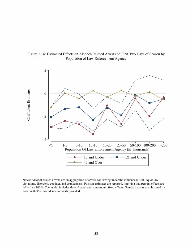
Figure 1.14: Estimated Effects on Alcohol-Related Arrests on First Two Days of Season byPopulation of Law Enforcement Agency

-.4

-.2

0

.2

Coe

ffic

ient

Est

imat

es

<1 1-5 5-10 10-15 15-25 25-50 50-100 100-200 >200Population Of Law Enforcement Agency (in Thousands)

18 and Under 21 and Under

40 and Over

Notes: Alcohol-related arrests are an aggregation of arrests for driving under the influence (DUI), liquor lawviolations, disorderly conduct, and drunkenness. Poisson estimates are reported, implying that percent effects are(eβ −1) x 100%. The model includes day-of-panel and zone-month fixed effects. Standard errors are clustered byzone, with 95% confidence intervals provided.

53

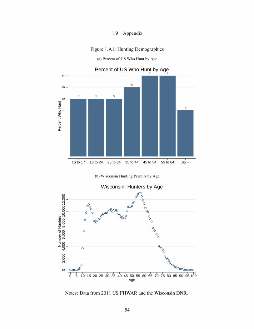
1.9 Appendix

Figure 1.A1: Hunting Demographics

(a) Percent of US Who Hunt by Age

5 5 5

6

7 7

4

45

67

Per

cent

Who

Hun

t

16 to 17 18 to 24 25 to 34 35 to 44 45 to 54 55 to 64 65 +

Percent of US Who Hunt by Age

(b) Wisconsin Hunting Permits by Age

02,

000

4,00

06,

000

8,00

010

,000

12,0

00N

umbe

r of

Hun

ters

0 5 10 15 20 25 30 35 40 45 50 55 60 65 70 75 80 85 90 95 100Age

Wisconsin: Hunters by Age

Notes: Data from 2011 US FHWAR and the Wisconsin DNR.

54

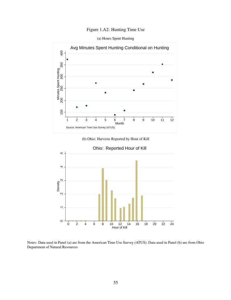
Figure 1.A2: Hunting Time Use

(a) Hours Spent Hunting

150

200

250

300

350

400

Min

utes

Spe

nt H

untin

g

1 2 3 4 5 6 7 8 9 10 11 12Month

Source: American Time Use Survey (ATUS)

Avg Minutes Spent Hunting Conditional on Hunting

(b) Ohio: Harvests Reported by Hour of Kill

0.1

.2.3

.4.5

Den

sity

0 2 4 6 8 10 12 14 16 18 20 22 24Hour of Kill

Ohio: Reported Hour of Kill

Notes: Data used in Panel (a) are from the American Time Use Survey (ATUS). Data used in Panel (b) are from OhioDepartment of Natural Resources

55

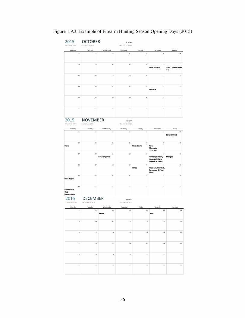
Figure 1.A3: Example of Firearm Hunting Season Opening Days (2015)

2015 MONDAY

CALENDAR YEAR FIRST DAY OF WEEK

Monday Tuesday Wednesday Thursday Friday Saturday Sunday

28 29 30 01 02 03 04

05 06 07 08 09 10 11

Idaho (Zone 2) South Carolina (Zones

1-2)

12 13 14 15 16 17 18

19 20 21 22 23 24 25

Montana

26 27 28 29 30 31 01

02 03 04 05 06 07 08

OCTOBERCALENDAR MONTH

2015 MONDAY

CALENDAR YEAR FIRST DAY OF WEEK

Monday Tuesday Wednesday Thursday Friday Saturday Sunday

26 27 28 29 30 31 01

SD (Black Hills)

02 03 04 05 06 07 08

Maine North Dakota Texas

Minnesota

SD (other)

09 10 11 12 13 14 15

New Hampshire Vermont, Kentucky

Arkansas, Indiana,

Virginia, SD (West)

Michigan

16 17 18 19 20 21 22

Illinois Wisconsin, New York,

Tennessee, SD (East

River)

23 24 25 26 27 28 29

West Virginia

30 01 02 03 04 05 06

Pennsylvania

Ohio

Massachusetts

NOVEMBERCALENDAR MONTH

2015 MONDAY

CALENDAR YEAR FIRST DAY OF WEEK

Monday Tuesday Wednesday Thursday Friday Saturday Sunday

30 01 02 03 04 05 06

Kansas Iowa

07 08 09 10 11 12 13

14 15 16 17 18 19 20

21 22 23 24 25 26 27

28 29 30 31 01 02 03

04 05 06 07 08 09 10

DECEMBERCALENDAR MONTH

56

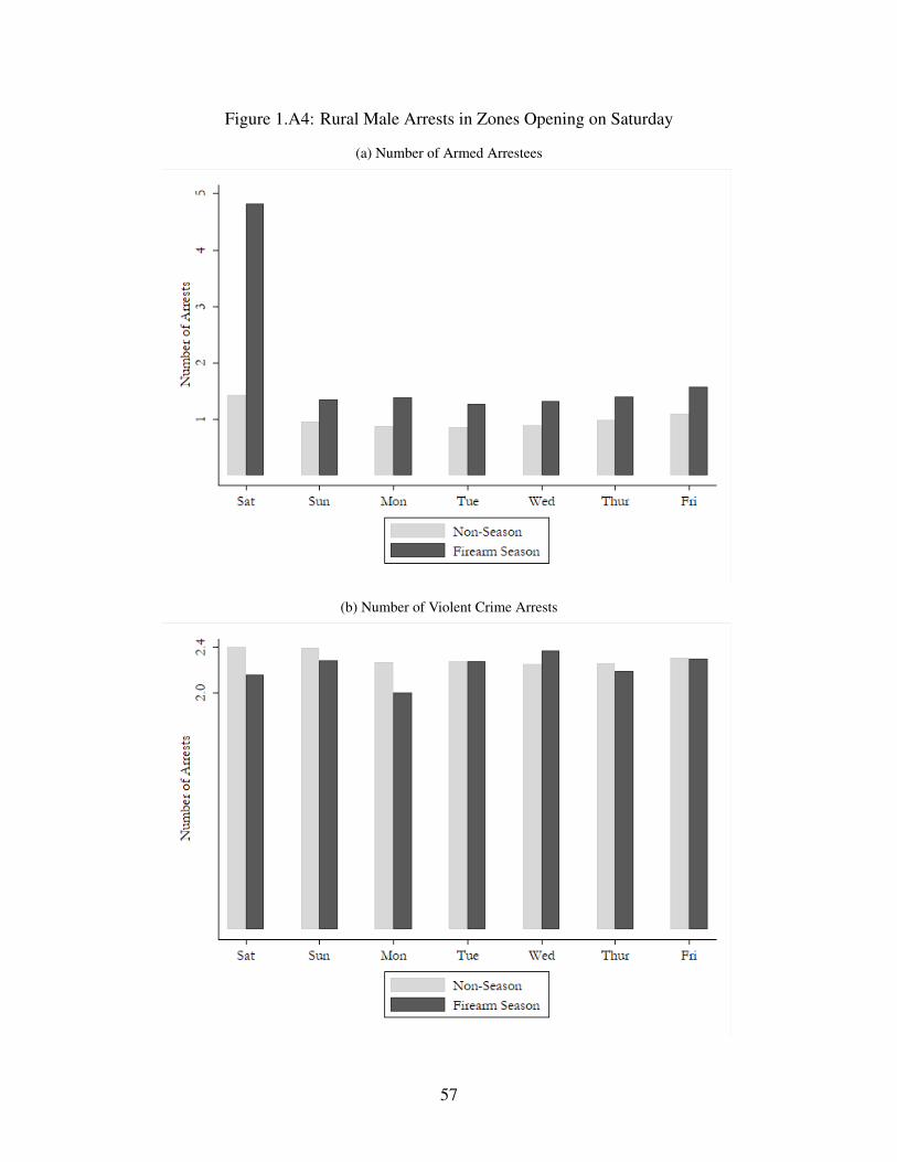
Figure 1.A4: Rural Male Arrests in Zones Opening on Saturday

(a) Number of Armed Arrestees

(b) Number of Violent Crime Arrests

57

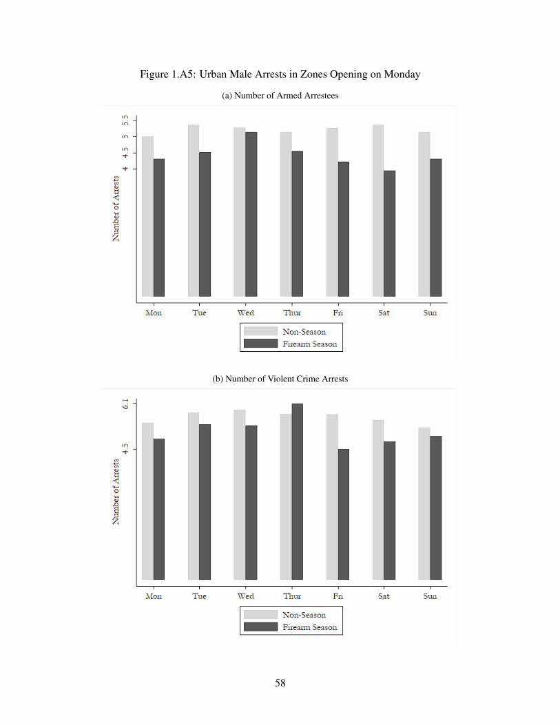
Figure 1.A5: Urban Male Arrests in Zones Opening on Monday

(a) Number of Armed Arrestees

(b) Number of Violent Crime Arrests

58

Figure 1.A6: Estimated Effects of Firearm Season on Rural Male Violent Crime

(a) Violent Crime Arrests

-.2

-.1

0

.1

.2

.3C

oeff

icie

nt E

stim

ates

-14 -12 -10 -8 -6 -4 -2 0 2 4 6 8 10 12 14Day from Opening Season

Mean: 1.886

(b) Violent Crime Offenses

-.2

-.1

0

.1

.2

Coe

ffic

ient

Est

imat

es

-14 -12 -10 -8 -6 -4 -2 0 2 4 6 8 10 12 14Day from Opening Season

Mean: 3.645

59

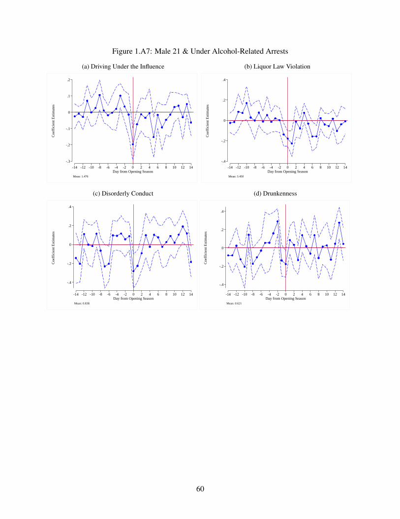
Figure 1.A7: Male 21 & Under Alcohol-Related Arrests

(a) Driving Under the Influence

-.3

-.2

-.1

0

.1

.2

Coe

ffic

ient

Est

imat

es

-14 -12 -10 -8 -6 -4 -2 0 2 4 6 8 10 12 14Day from Opening Season

Mean: 1.476

(b) Liquor Law Violation

-.4

-.2

0

.2

.4

Coe

ffic

ient

Est

imat

es

-14 -12 -10 -8 -6 -4 -2 0 2 4 6 8 10 12 14Day from Opening Season

Mean: 3.450

(c) Disorderly Conduct

-.4

-.2

0

.2

.4

Coe

ffic

ient

Est

imat

es

-14 -12 -10 -8 -6 -4 -2 0 2 4 6 8 10 12 14Day from Opening Season

Mean: 0.838

(d) Drunkenness

-.4

-.2

0

.2

.4

Coe

ffic

ient

Est

imat

es

-14 -12 -10 -8 -6 -4 -2 0 2 4 6 8 10 12 14Day from Opening Season

Mean: 0.621

60

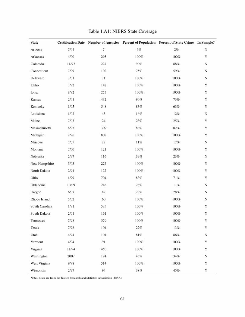
Table 1.A1: NIBRS State Coverage

State Certification Date Number of Agencies Percent of Population Percent of State Crime In Sample?

Arizona 7/04 7 6% 2% N

Arkansas 4/00 295 100% 100% Y

Colorado 11/97 227 90% 88% N

Connecticut 7/99 102 75% 59% N

Delaware 7/01 71 100% 100% N

Idaho 7/92 142 100% 100% Y

Iowa 8/92 253 100% 100% Y

Kansas 2/01 432 90% 73% Y

Kentucky 1/05 548 83% 63% Y

Louisiana 1/02 45 16% 12% N

Maine 7/03 24 23% 25% Y

Massachusetts 8/95 309 86% 82% Y

Michigan 2/96 802 100% 100% Y

Missouri 7/05 22 11% 17% N

Montana 7/00 121 100% 100% Y

Nebraska 2/97 116 39% 23% N

New Hampshire 5/03 227 100% 100% Y

North Dakota 2/91 127 100% 100% Y

Ohio 1/99 704 83% 71% Y

Oklahoma 10/09 248 28% 11% N

Oregon 6/97 87 29% 28% N

Rhode Island 5/02 60 100% 100% N

South Carolina 1/91 535 100% 100% Y

South Dakota 2/01 161 100% 100% Y

Tennessee 7/98 579 100% 100% Y

Texas 7/98 104 22% 13% Y

Utah 4/94 104 81% 86% N

Vermont 4/94 91 100% 100% Y

Virginia 11/94 450 100% 100% Y

Washington 2007 194 45% 34% N

West Virginia 9/98 514 100% 100% Y

Wisconsin 2/97 94 38% 45% Y

Notes: Data are from the Justice Research and Statistics Association (JRSA).

61

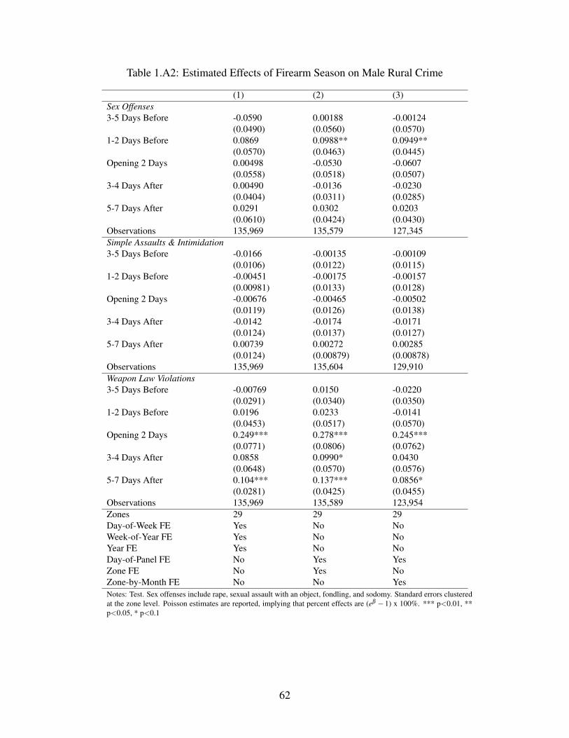
Table 1.A2: Estimated Effects of Firearm Season on Male Rural Crime

(1) (2) (3)Sex Offenses3-5 Days Before -0.0590 0.00188 -0.00124

(0.0490) (0.0560) (0.0570)1-2 Days Before 0.0869 0.0988** 0.0949**

(0.0570) (0.0463) (0.0445)Opening 2 Days 0.00498 -0.0530 -0.0607

(0.0558) (0.0518) (0.0507)3-4 Days After 0.00490 -0.0136 -0.0230

(0.0404) (0.0311) (0.0285)5-7 Days After 0.0291 0.0302 0.0203

(0.0610) (0.0424) (0.0430)Observations 135,969 135,579 127,345Simple Assaults & Intimidation3-5 Days Before -0.0166 -0.00135 -0.00109

(0.0106) (0.0122) (0.0115)1-2 Days Before -0.00451 -0.00175 -0.00157

(0.00981) (0.0133) (0.0128)Opening 2 Days -0.00676 -0.00465 -0.00502

(0.0119) (0.0126) (0.0138)3-4 Days After -0.0142 -0.0174 -0.0171

(0.0124) (0.0137) (0.0127)5-7 Days After 0.00739 0.00272 0.00285

(0.0124) (0.00879) (0.00878)Observations 135,969 135,604 129,910Weapon Law Violations3-5 Days Before -0.00769 0.0150 -0.0220

(0.0291) (0.0340) (0.0350)1-2 Days Before 0.0196 0.0233 -0.0141

(0.0453) (0.0517) (0.0570)Opening 2 Days 0.249*** 0.278*** 0.245***

(0.0771) (0.0806) (0.0762)3-4 Days After 0.0858 0.0990* 0.0430

(0.0648) (0.0570) (0.0576)5-7 Days After 0.104*** 0.137*** 0.0856*

(0.0281) (0.0425) (0.0455)Observations 135,969 135,589 123,954Zones 29 29 29Day-of-Week FE Yes No NoWeek-of-Year FE Yes No NoYear FE Yes No NoDay-of-Panel FE No Yes YesZone FE No Yes NoZone-by-Month FE No No YesNotes: Test. Sex offenses include rape, sexual assault with an object, fondling, and sodomy. Standard errors clusteredat the zone level. Poisson estimates are reported, implying that percent effects are (eβ −1) x 100%. *** p<0.01, **p<0.05, * p<0.1

62

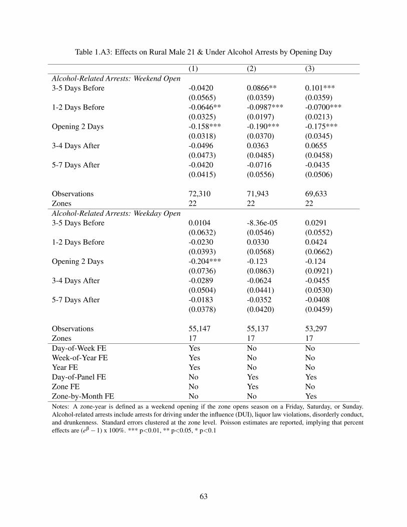
Table 1.A3: Effects on Rural Male 21 & Under Alcohol Arrests by Opening Day

(1) (2) (3)Alcohol-Related Arrests: Weekend Open3-5 Days Before -0.0420 0.0866** 0.101***

(0.0565) (0.0359) (0.0359)1-2 Days Before -0.0646** -0.0987*** -0.0700***

(0.0325) (0.0197) (0.0213)Opening 2 Days -0.158*** -0.190*** -0.175***

(0.0318) (0.0370) (0.0345)3-4 Days After -0.0496 0.0363 0.0655

(0.0473) (0.0485) (0.0458)5-7 Days After -0.0420 -0.0716 -0.0435

(0.0415) (0.0556) (0.0506)

Observations 72,310 71,943 69,633Zones 22 22 22Alcohol-Related Arrests: Weekday Open3-5 Days Before 0.0104 -8.36e-05 0.0291

(0.0632) (0.0546) (0.0552)1-2 Days Before -0.0230 0.0330 0.0424

(0.0393) (0.0568) (0.0662)Opening 2 Days -0.204*** -0.123 -0.124

(0.0736) (0.0863) (0.0921)3-4 Days After -0.0289 -0.0624 -0.0455

(0.0504) (0.0441) (0.0530)5-7 Days After -0.0183 -0.0352 -0.0408

(0.0378) (0.0420) (0.0459)

Observations 55,147 55,137 53,297Zones 17 17 17Day-of-Week FE Yes No NoWeek-of-Year FE Yes No NoYear FE Yes No NoDay-of-Panel FE No Yes YesZone FE No Yes NoZone-by-Month FE No No YesNotes: A zone-year is defined as a weekend opening if the zone opens season on a Friday, Saturday, or Sunday.Alcohol-related arrests include arrests for driving under the influence (DUI), liquor law violations, disorderly conduct,and drunkenness. Standard errors clustered at the zone level. Poisson estimates are reported, implying that percenteffects are (eβ −1) x 100%. *** p<0.01, ** p<0.05, * p<0.1

63

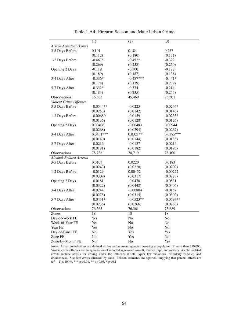
Table 1.A4: Firearm Season and Male Urban Crime

(1) (2) (3)Armed Arrestees (Long)3-5 Days Before 0.101 0.184 0.257

(0.112) (0.180) (0.171)1-2 Days Before -0.467* -0.452* -0.322

(0.269) (0.258) (0.250)Opening 2 Days -0.119 -0.300 -0.128

(0.189) (0.187) (0.138)3-4 Days After -0.336* -0.487*** -0.441*

(0.178) (0.179) (0.239)5-7 Days After -0.332* -0.374 -0.214

(0.183) (0.235) (0.255)Observations 76,365 45,469 23,501Violent Crime Offenses3-5 Days Before -0.0544** -0.0225 -0.0246*

(0.0253) (0.0142) (0.0146)1-2 Days Before -0.00680 -0.0159 -0.0233*

(0.0136) (0.0128) (0.0126)Opening 2 Days 0.00406 -0.00483 0.00944

(0.0268) (0.0294) (0.0267)3-4 Days After 0.0451*** 0.0321** 0.0385***

(0.0140) (0.0144) (0.0133)5-7 Days After -0.0216 -0.0137 -0.0214

(0.0181) (0.0182) (0.0195)Observations 78,736 78,719 78,100Alcohol-Related Arrests3-5 Days Before 0.0103 0.0220 0.0183

(0.0243) (0.0220) (0.0202)1-2 Days Before -0.0129 0.00452 -0.00272

(0.0309) (0.0317) (0.0283)Opening 2 Days -0.0181 -0.0470 -0.0531

(0.0322) (0.0448) (0.0406)3-4 Days After -0.0244 -0.00804 -0.0157

(0.0275) (0.0315) (0.0302)5-7 Days After -0.0431* -0.0523** -0.0593**

(0.0236) (0.0266) (0.0268)Observations 76,365 76,361 75,689Zones 18 18 18Day-of-Week FE Yes No NoWeek-of-Year FE Yes No NoYear FE Yes No NoDay-of-Panel FE No Yes YesZone FE No Yes NoZone-by-Month FE No No YesNotes: Urban jurisdictions are defined as law enforcement agencies covering a population of more than 250,000.Violent crime offenses are an aggregation of reported aggravated assault, murder, rape, and robbery. Alcohol-relatedarrests include arrests for driving under the influence (DUI), liquor law violations, disorderly conduct, anddrunkenness. Standard errors clustered by zone. Poisson estimates are reported, implying that percent effects are(eβ −1) x 100%. *** p<0.01, ** p<0.05, * p<0.1

64

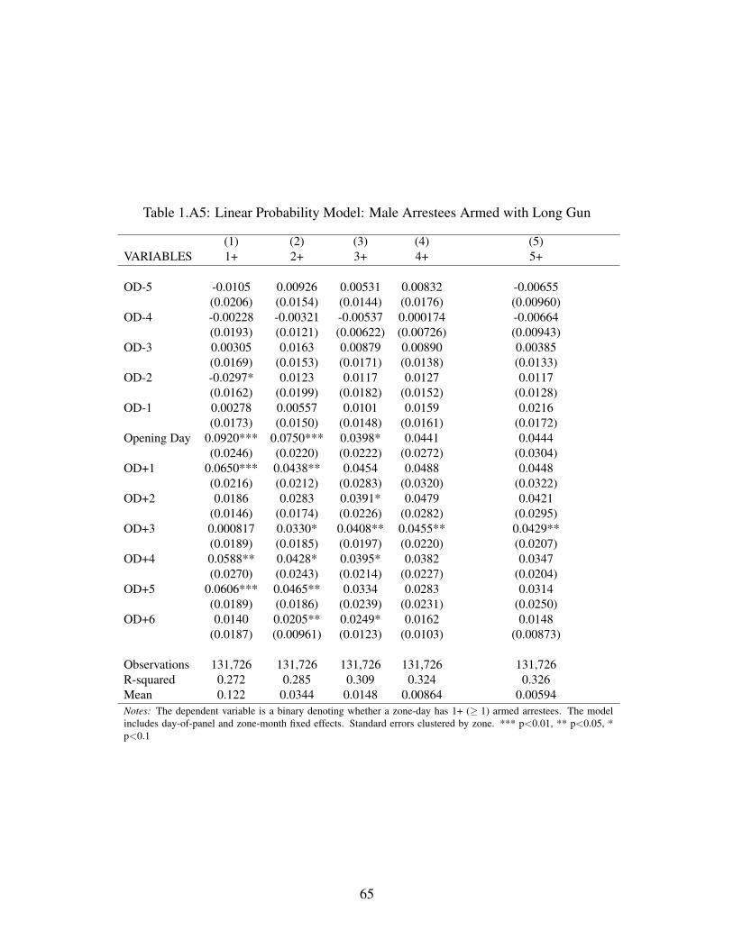
Table 1.A5: Linear Probability Model: Male Arrestees Armed with Long Gun

(1) (2) (3) (4) (5)VARIABLES 1+ 2+ 3+ 4+ 5+

OD-5 -0.0105 0.00926 0.00531 0.00832 -0.00655(0.0206) (0.0154) (0.0144) (0.0176) (0.00960)

OD-4 -0.00228 -0.00321 -0.00537 0.000174 -0.00664(0.0193) (0.0121) (0.00622) (0.00726) (0.00943)

OD-3 0.00305 0.0163 0.00879 0.00890 0.00385(0.0169) (0.0153) (0.0171) (0.0138) (0.0133)

OD-2 -0.0297* 0.0123 0.0117 0.0127 0.0117(0.0162) (0.0199) (0.0182) (0.0152) (0.0128)

OD-1 0.00278 0.00557 0.0101 0.0159 0.0216(0.0173) (0.0150) (0.0148) (0.0161) (0.0172)

Opening Day 0.0920*** 0.0750*** 0.0398* 0.0441 0.0444(0.0246) (0.0220) (0.0222) (0.0272) (0.0304)

OD+1 0.0650*** 0.0438** 0.0454 0.0488 0.0448(0.0216) (0.0212) (0.0283) (0.0320) (0.0322)

OD+2 0.0186 0.0283 0.0391* 0.0479 0.0421(0.0146) (0.0174) (0.0226) (0.0282) (0.0295)

OD+3 0.000817 0.0330* 0.0408** 0.0455** 0.0429**(0.0189) (0.0185) (0.0197) (0.0220) (0.0207)

OD+4 0.0588** 0.0428* 0.0395* 0.0382 0.0347(0.0270) (0.0243) (0.0214) (0.0227) (0.0204)

OD+5 0.0606*** 0.0465** 0.0334 0.0283 0.0314(0.0189) (0.0186) (0.0239) (0.0231) (0.0250)

OD+6 0.0140 0.0205** 0.0249* 0.0162 0.0148(0.0187) (0.00961) (0.0123) (0.0103) (0.00873)

Observations 131,726 131,726 131,726 131,726 131,726R-squared 0.272 0.285 0.309 0.324 0.326Mean 0.122 0.0344 0.0148 0.00864 0.00594Notes: The dependent variable is a binary denoting whether a zone-day has 1+ (≥ 1) armed arrestees. The modelincludes day-of-panel and zone-month fixed effects. Standard errors clustered by zone. *** p<0.01, ** p<0.05, *p<0.1

65

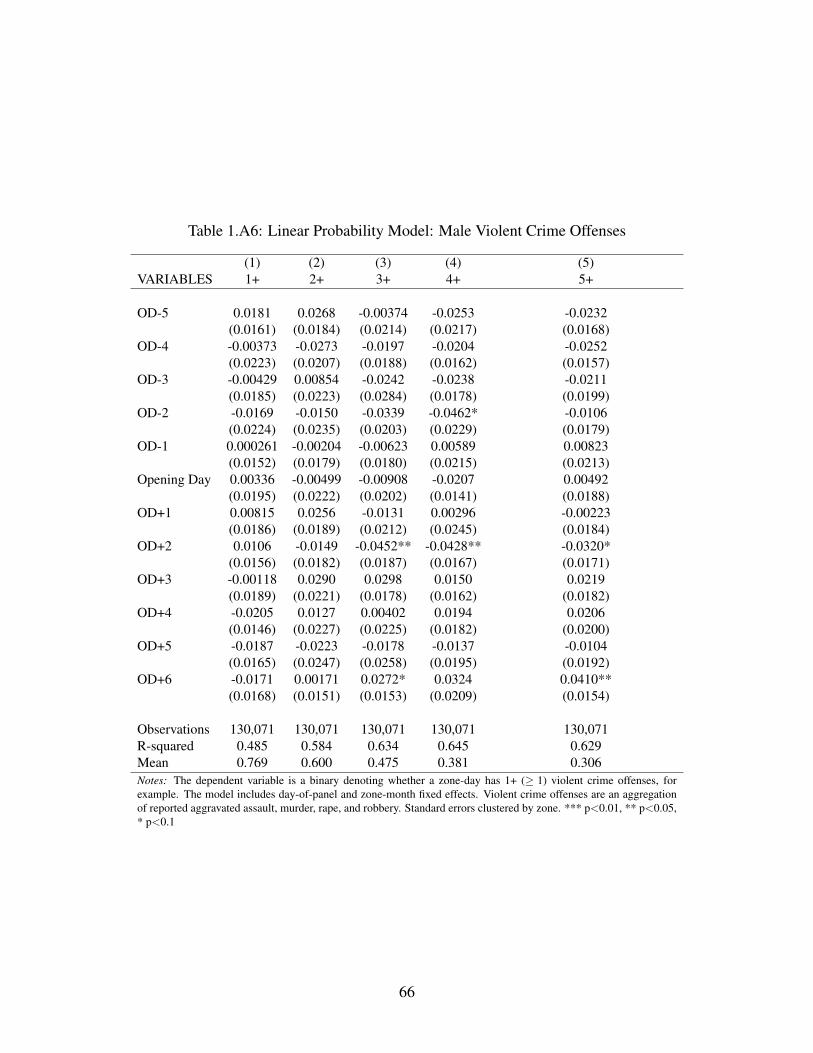
Table 1.A6: Linear Probability Model: Male Violent Crime Offenses

(1) (2) (3) (4) (5)VARIABLES 1+ 2+ 3+ 4+ 5+

OD-5 0.0181 0.0268 -0.00374 -0.0253 -0.0232(0.0161) (0.0184) (0.0214) (0.0217) (0.0168)

OD-4 -0.00373 -0.0273 -0.0197 -0.0204 -0.0252(0.0223) (0.0207) (0.0188) (0.0162) (0.0157)

OD-3 -0.00429 0.00854 -0.0242 -0.0238 -0.0211(0.0185) (0.0223) (0.0284) (0.0178) (0.0199)

OD-2 -0.0169 -0.0150 -0.0339 -0.0462* -0.0106(0.0224) (0.0235) (0.0203) (0.0229) (0.0179)

OD-1 0.000261 -0.00204 -0.00623 0.00589 0.00823(0.0152) (0.0179) (0.0180) (0.0215) (0.0213)

Opening Day 0.00336 -0.00499 -0.00908 -0.0207 0.00492(0.0195) (0.0222) (0.0202) (0.0141) (0.0188)

OD+1 0.00815 0.0256 -0.0131 0.00296 -0.00223(0.0186) (0.0189) (0.0212) (0.0245) (0.0184)

OD+2 0.0106 -0.0149 -0.0452** -0.0428** -0.0320*(0.0156) (0.0182) (0.0187) (0.0167) (0.0171)

OD+3 -0.00118 0.0290 0.0298 0.0150 0.0219(0.0189) (0.0221) (0.0178) (0.0162) (0.0182)

OD+4 -0.0205 0.0127 0.00402 0.0194 0.0206(0.0146) (0.0227) (0.0225) (0.0182) (0.0200)

OD+5 -0.0187 -0.0223 -0.0178 -0.0137 -0.0104(0.0165) (0.0247) (0.0258) (0.0195) (0.0192)

OD+6 -0.0171 0.00171 0.0272* 0.0324 0.0410**(0.0168) (0.0151) (0.0153) (0.0209) (0.0154)

Observations 130,071 130,071 130,071 130,071 130,071R-squared 0.485 0.584 0.634 0.645 0.629Mean 0.769 0.600 0.475 0.381 0.306Notes: The dependent variable is a binary denoting whether a zone-day has 1+ (≥ 1) violent crime offenses, forexample. The model includes day-of-panel and zone-month fixed effects. Violent crime offenses are an aggregationof reported aggravated assault, murder, rape, and robbery. Standard errors clustered by zone. *** p<0.01, ** p<0.05,* p<0.1

66

Table 1.A7: Linear Probability Model: Male Alcohol-Related Arrests

(1) (2) (3) (4) (5) (6)VARIABLES 1+ 5+ 10+ 15+ 20+ 25+

OD-5 -0.0133** 0.00812 0.0547* 0.0785* 0.0505 0.00114(0.00619) (0.0191) (0.0306) (0.0419) (0.0368) (0.0280)

OD-4 0.00900 -0.0256 -0.00638 0.0426 0.0358 0.0409(0.00868) (0.0287) (0.0267) (0.0352) (0.0382) (0.0426)

OD-3 0.00619 -0.0203 0.0267 0.0388 0.0523 0.00339(0.00640) (0.0197) (0.0214) (0.0241) (0.0334) (0.0343)

OD-2 -0.00349 0.00585 -0.0279 -0.00611 0.00442 0.00204(0.00975) (0.0286) (0.0228) (0.0342) (0.0364) (0.0298)

OD-1 -0.00274 -0.000866 -0.0466* -0.0354 -0.0193 -0.0164(0.00588) (0.0175) (0.0248) (0.0327) (0.0343) (0.0273)

Opening Day 0.00616 0.0310 -0.0560* -0.0798** -0.0767** -0.0650**(0.0127) (0.0209) (0.0286) (0.0341) (0.0358) (0.0303)

OD+1 -0.00827 0.0141 -0.00902 -0.0380 -0.0449 -0.0285(0.0115) (0.0171) (0.0168) (0.0280) (0.0291) (0.0316)

OD+2 0.0243* -0.0154 0.0275 0.0347 0.000485 -0.0191(0.0140) (0.0254) (0.0243) (0.0276) (0.0234) (0.0256)

OD+3 0.0112 -0.0154 -0.0151 0.0211 0.0225 0.0117(0.0126) (0.0211) (0.0201) (0.0228) (0.0374) (0.0420)

OD+4 -0.0139 0.00114 -0.00991 0.0191 0.0193 0.0172(0.0156) (0.0199) (0.0209) (0.0334) (0.0387) (0.0397)

OD+5 0.00910 0.0191 -0.0495** -0.0515 -0.00524 0.00934(0.0111) (0.0210) (0.0217) (0.0334) (0.0373) (0.0343)

OD+6 0.00475 0.00199 -0.0607** -0.0418 -0.0146 0.00117(0.00720) (0.0173) (0.0290) (0.0286) (0.0269) (0.0259)

Observations 131,726 131,726 131,726 131,726 131,726 131,726R-squared 0.404 0.603 0.653 0.680 0.687 0.676Mean 0.960 0.793 0.567 0.432 0.341 0.278Notes: The dependent variable is a binary denoting whether a zone-day has 1+ (≥ 1) alcohol-related arrests, forexample. The model includes day-of-panel and zone-month fixed effects. Alcohol-related arrests include arrestsfor driving under the influence (DUI), liquor law violations, disorderly conduct, and drunkenness. Standard errorsclustered by zone. *** p<0.01, ** p<0.05, * p<0.1

67

Table 1.A8: Linear Probability Model: Male Narcotic Arrests

(1) (2) (3) (4) (5)VARIABLES 1+ 2+ 3+ 4+ 5+

OD-5 -0.00853 -0.0160 0.00911 -0.00457 0.0114(0.0125) (0.0194) (0.0139) (0.0148) (0.0169)

OD-4 -0.00983 -0.0134 0.00834 0.00201 0.00345(0.0163) (0.0242) (0.0203) (0.0193) (0.0183)

OD-3 0.0488** 0.00194 0.0150 -0.0122 0.00153(0.0184) (0.0202) (0.0226) (0.0167) (0.0156)

OD-2 0.0130 0.0240 -0.00116 0.00748 0.00807(0.0173) (0.0190) (0.0176) (0.0199) (0.0226)

OD-1 -0.0123 -0.0490** -0.0177 -0.00858 -0.0221(0.0171) (0.0193) (0.0195) (0.0212) (0.0205)

Opening Day 0.00449 -0.0300* -0.0301** -0.0220 -0.0468**(0.0155) (0.0148) (0.0132) (0.0184) (0.0194)

OD+1 0.0316** -0.00624 -0.00827 -0.0260 -0.0468**(0.0139) (0.0253) (0.0249) (0.0211) (0.0225)

OD+2 -0.00296 1.42e-05 -0.0202 -0.00734 -0.00234(0.0148) (0.0203) (0.0173) (0.0154) (0.0177)

OD+3 0.0140 -0.0323 -0.0165 -0.0167 -0.0252(0.0198) (0.0192) (0.0197) (0.0191) (0.0193)

OD+4 0.0452*** 0.0245 -0.00788 -0.00495 -0.00603(0.0158) (0.0204) (0.0194) (0.0243) (0.0269)

OD+5 -0.00359 -0.00154 -0.00844 -0.0185 -0.0205(0.0197) (0.0223) (0.0194) (0.0184) (0.0170)

OD+6 0.0360* 0.0231 -0.00635 -0.0319* -0.0349*(0.0178) (0.0160) (0.0161) (0.0173) (0.0174)

Observations 136,250 136,250 136,250 136,250 136,250R-squared 0.463 0.487 0.522 0.555 0.582Mean 0.829 0.719 0.621 0.539 0.471Notes: The dependent variable is a binary denoting whether a zone-day has 1+ (≥ 1) narcotic arrests, for example.The model includes day-of-panel and zone-month fixed effects. Standard errors clustered by zone. *** p<0.01, **p<0.05, * p<0.1

68

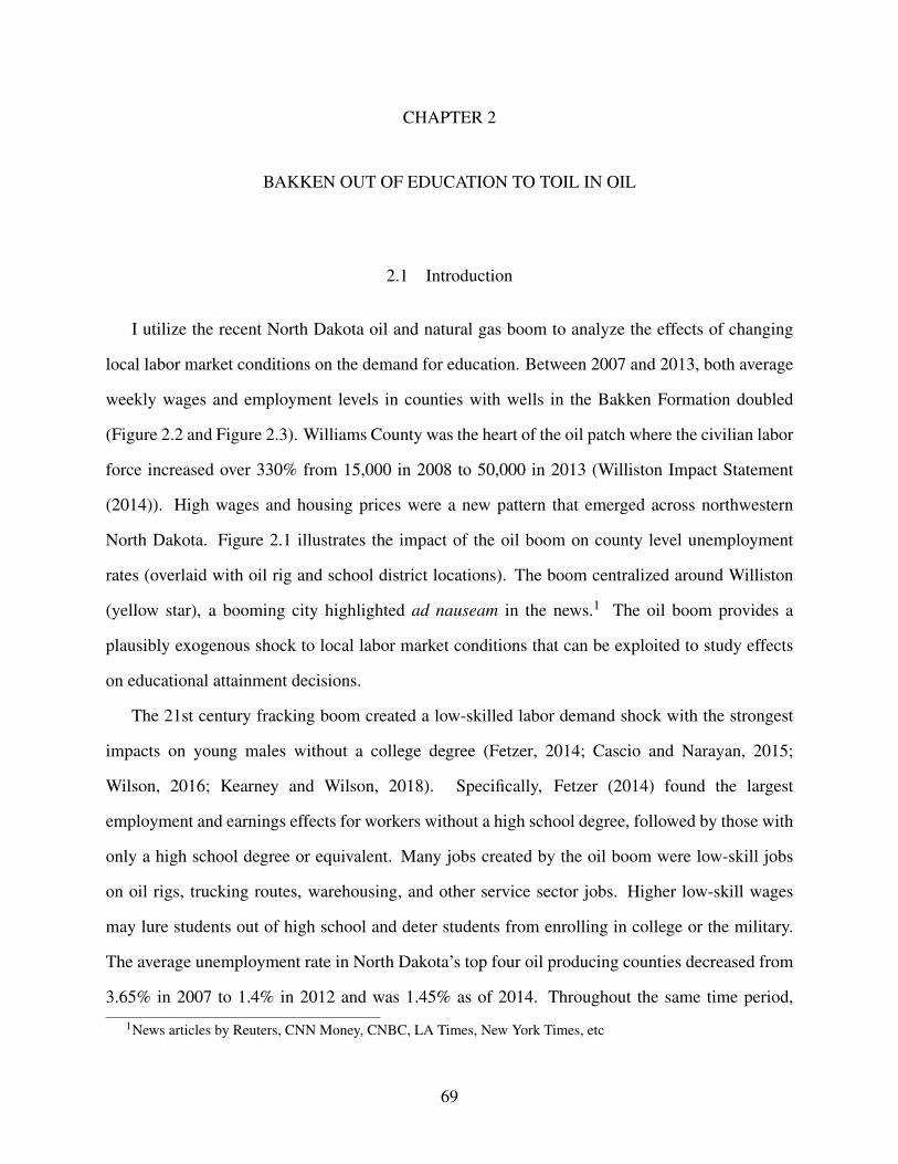
CHAPTER 2

BAKKEN OUT OF EDUCATION TO TOIL IN OIL

2.1 Introduction

I utilize the recent North Dakota oil and natural gas boom to analyze the effects of changing

local labor market conditions on the demand for education. Between 2007 and 2013, both average

weekly wages and employment levels in counties with wells in the Bakken Formation doubled

(Figure 2.2 and Figure 2.3). Williams County was the heart of the oil patch where the civilian labor

force increased over 330% from 15,000 in 2008 to 50,000 in 2013 (Williston Impact Statement

(2014)). High wages and housing prices were a new pattern that emerged across northwestern

North Dakota. Figure 2.1 illustrates the impact of the oil boom on county level unemployment

rates (overlaid with oil rig and school district locations). The boom centralized around Williston

(yellow star), a booming city highlighted ad nauseam in the news.1 The oil boom provides a

plausibly exogenous shock to local labor market conditions that can be exploited to study effects

on educational attainment decisions.

The 21st century fracking boom created a low-skilled labor demand shock with the strongest

impacts on young males without a college degree (Fetzer, 2014; Cascio and Narayan, 2015;

Wilson, 2016; Kearney and Wilson, 2018). Specifically, Fetzer (2014) found the largest

employment and earnings effects for workers without a high school degree, followed by those with

only a high school degree or equivalent. Many jobs created by the oil boom were low-skill jobs

on oil rigs, trucking routes, warehousing, and other service sector jobs. Higher low-skill wages

may lure students out of high school and deter students from enrolling in college or the military.

The average unemployment rate in North Dakota’s top four oil producing counties decreased from

3.65% in 2007 to 1.4% in 2012 and was 1.45% as of 2014. Throughout the same time period,

1News articles by Reuters, CNN Money, CNBC, LA Times, New York Times, etc

69

the average unemployment rate of North Dakota’s remaining 49 counties actually increased from

3.73% to 3.79%.2 The increase in low-skill labor employment and wages creates a substitution

effect that incentivizes high school graduates to forgo college or the military and enter the labor

force instead.

Although the boom created incentives to forgo college, it may also have created conditions

to encourage further education. With higher income, families may place greater value on

college education or are better able to finance it, thereby making a high school graduate more

likely to enroll in college. There is high correlation between family income and educational

attainment, which may counteract the substitution effect of higher wages (Blanden and Gregg

(2004)). Additionally, better financed high schools and scholarship funding may increase

college enrollment. According to ND Office of the Governor, oil tax revenues have created an

unprecedented government budget surplus, allowing the state to appropriate greater funding to

school districts, higher education grants, and need-based scholarships (Dakota, 2013). Increases

in high school funding and higher education grants may make a student more likely to graduate

from high school and more likely to enroll in college. These conflicting effects that may encourage

or discourage an adolescent from continuing their education imply that net impacts can only be

understood through empirical analysis.

The ND oil boom is an ideal natural experiment to analyze the impact of a changing local

economy on educational attainment. Prior to 2014, the oil boom was expected to last at least 20

to 30 years (under the crucial assumption that crude prices remained above $60 per barrel) with

estimates up to 100 years as echoed in the New York Times (Brown, 2013). This unpredicted

economic shock would have a significant long term impact on expected individual lifetime

earnings. However, in 2014 and 2015, market determined crude oil prices drastically dropped

from $100 to under $50 per barrel, reducing ND extraction profit margins and placing many rigs

below break-even prices.

In conjunction with the boom having an abrupt start, the boom was focused in northwestern

2North Dakota’s top four oil producing counties are Dunn, McKenzie, Mountrail, and Williams

70

ND, which traditionally had a population density less than ten people per square mile (fourth lowest

in the U.S.). In 2008, ND had a total population of 641,481 residents, 40 percent of whom lived

in only four cities. In 2014, the US Census Bureau estimate of North Dakota’s population was

739,482, giving the state one of the highest population growth rates in the United States in contrast

to its late twentieth and early twenty-first century population stagnation. Low population density

and a geographically large state help define an affected local labor market (northwestern ND) in

contrast to other less affected areas in eastern ND (with towns up to 450 road-miles away from

Williston).

This paper analyzes the impact of the North Dakota oil boom on two educational attainment

decisions: high school graduation and post-graduation plans. To empirically examine the effect

of the boom on educational choices, I use a difference in difference research design paired with

event-study analyses (Jacobson et al., 1993). I use yearly oil production data to differentiate

between the pre-boom and post-boom period and compare outcomes in core-oil producing counties

relative to low or non-producing counties. Economic theory suggests that schools in the proximity

of the oil boom centroid are those most impacted by the boom. As distance from the oil boom

increases, so do commute times. Individuals further from the boom have longer commutes and

must leave social networks and are less likely to have social connections in the oil drilling area.

Identification hinges on comparing outcomes in schools within core-oil counties versus non-oil

counties before and after the oil boom.

I find that the ND oil boom had no discernible effect on high school graduation rates within

core-oil producing counties. Event-study analyses provide no evidence that the oil boom had any

negative effect on core-oil high school graduation rates or males or females. However, results

suggest that the oil boom had a strong impact on post-graduation educational outcomes of both

genders. Event-study figures clearly show that the oil boom had a large, negative effect on 4

year college enrollment rates. DD estimates imply that 4 year college enrollment rates decreased

12 percentage points (23%) in core-oil counties relative to non-oil counties. Surprisingly, core-oil

county enrollment rates at North Dakota research universities dropped 25%, suggesting even higher

71

skill students can be on the margin between attending 4 year university and taking a job out of high

school. Results using administrative high school data reaffirm that high school seniors decreased

college enrollment rates. Evidence suggests that both males and females in core-oil counties

became more likely to enter the labor force upon graduation while males became less likely to

enroll in the military. The decrease in male military enrollment may be because both military

and fracking related work are largely dominated by young males. My results suggest that there

are many North Dakota students on the margin between post-graduation plans while there are few

students making marginal decisions concerning high school graduation.

This paper provides three key contributions to the existing literature. First, to this author’s

knowledge, this is the first paper to analyze the effect of a natural resource boom on both high

school graduation rates and post-graduation decisions of the same population. Previous research

focuses almost purely on high school graduation rates. The results of this paper suggest that

an economic shock is able to have little effect on high school graduation rates, while strongly

impacting post-graduation plans. Second, this paper studies both male and female outcomes.

Previous work focuses on male outcomes or male-female gaps in education because natural

resource booms are usually male and low-skill biased. However, I provide clear evidence that

the North Dakota oil boom also created strong growth in non-oil sectors with higher female

participation rates, implying that female educational decisions should also be studied. Third, the

paper exploits previously unused data from the North Dakota Department of Public Instruction

(NDDPI) to study a population that can’t be studied via conventional surveys due to low sample

size or privacy restrictions. This paper is of considerable interest due to its policy implications.

Between 2014 and 2015 the ND oil boom frenzy calmed with the decrease in market crude oil

prices. However, if crude oil prices increase above the break-even prices of more rigs, the oil boom

will flare up again and high school students will face similar incentives. Regions that experience

reductions in college enrollment rates in lieu of employment may benefit during the boom, but will

be left with a surplus of low-skill unemployed workers when the boom goes bust.

72

2.2 Literature Review

2.2.1 Economic Conditions and Educational Attainment

Simple human capital models predict that students will attain less education when the rate of

return on education falls. As public high school is free for students, forgone earnings are the

greatest opportunity cost of earning a high school degree. Meanwhile, the opportunity cost of a

college education is the sum of college tuition costs and forgone earnings. All else equal, economic

theory predicts that an increase in the opportunity cost of a college degree will lower the rate of

return on education and drive an individual to attain less education. Therefore, any economic

shock that reduces the ratio of high school graduate to dropout earnings will reduce high school

graduation rates and any shock that reduces the ratio of college graduate to high school graduate

earnings will reduce college enrollment rates. Literature has studied this link by exploiting local

area unemployment rates.

A wealth of research illustrates that there is countercyclical demand for education.

Boffy-Ramirez et al. (2013) find that higher unemployment rates before high school graduation

increase the amount of education a student receives and a student’s probability of graduating

from college for students in the fourth quintile of the Armed Forces Qualifying Test distribution.

However, they do not find that higher unemployment rates affected the likelihood of high school

graduation. Both Manski and Wise (1983) and Card and Lemieux (2001) find only weak evidence

of a relationship between statewide unemployment and educational attainment while other studies

find unemployment rates to have a significant positive effect on schooling (Dellas and Sakellaris

(2003)).

Unemployment changes may have differing effects on demand for education depending on

whether the change in labor demand occurred in high or low-skill jobs. Unemployment reductions

driven by higher skill labor demand will not increase the opportunity cost of college because high

school graduates are excluded from those jobs. High skill labor booms may actually incentivize

individuals to pursue more education in order to obtain higher skill jobs. Natural resource booms

73

like the ND oil boom tend to drive growth in low-skill labor demand, implying that the opportunity

cost of college and military enrollment is impacted. Warner (2012) finds that a decrease in the

civilian unemployment rate reduces high quality military recruits. As unemployment has fallen

with the increase in demand for labor in northwest ND, we may expect military enrollment rates

to decrease in areas affected by the oil boom.

Evans et al. (2006) claim that one commonality among papers that only find weak effects of

local labor markets on educational attainment is that they measure labor markets on a statewide

basis. Adolescents may make educational attainment decisions within their local labor markets,

which may be smaller than the state in which they live. Even within a state, much heterogeneity

of unemployment exists, which is especially true for a low density, large state like ND. Defining

local labor markets at an area more granular than the state level also provides a large source of

exogenous variation in labor market conditions. Therefore, many authors have investigated the

subject using more granular data to define a local labor market. Rivkin (1995) discovered that

higher county unemployment rates increased the likelihood of school enrollment for both high

school and college students. Similarly, I will define treatment at the county level by using county

level oil statuses designated by the state of North Dakota.

Research has also been conducted on local labor market shocks and demand for education.

Evans et al. (2006) examined the impacts of federal legislation in 1988 that led to almost 400

Indian casino openings. Within rural local labor markets, Indian casinos improved employment

and wages of lower skilled jobs. They found that adolescents were more likely to drop out of

high school and less likely to enroll in college. The ND oil boom is similar in that it is focused in

rural areas and increased low-skill employment levels and wages. My research is similar to that of

Black et al. (2005) insofar as I examine the effects of a natural resource mining boom on demand

for labor. They analyzed the impact of the Appalachian coal boom on high school enrollment rates,

finding that increases in lower skilled employment and wages led to lower high school enrollment

rates. My results suggest that the strong impact of the 1970s coal boom on high school graduation

rates cannot be extrapolated to the modern day setting in ND. Most recently, Cascio and Narayan

74

(2015) find that fracking induced labor demand shocks particularly affect males and low-skilled

labor. They find that fracking slowed the closing gap between male and female high school dropout

rates. Additionally, the magnitude of the effect of fracking on dropout rates increases when they

take North Dakota out of their sample. The null effects of fracking on high school dropouts I find

in North Dakota support their results while also suggesting that interesting heterogeneous effects

may exist. I contribute to this literature by using novel datasets that can hone in on rural areas with

more precision than survey-based datasets. I expand analysis to both genders, as females may also

be impacted by non-oil employment opportunities created by oil booms.

2.2.2 Effects of the 21st Century Fracking Boom

Others have used the recent nationwide fracking boom to study key outcomes like employment,

migration, and crime. Feyrer et al. (2017) estimate that a million dollars of new fracking revenue

drives over $250,000 in wage growth and over $280,000 in mineral rights royalty and business

income within 100 miles of the fracking activity. Fetzer (2014) estimates that each additional

fracking-related oil and gas job created another 2.17 non-mining jobs. The author found that the

largest gains in employment and earnings, in both mining and non-mining sectors, were driven by

individuals without a high school degree, followed by individuals with only a high school degree or

GED. The strong low-skill labor demand shock in ND led to large-scale migration into extraction

areas, driven by young single males with below average education (Wilson, 2016).

This in-migration of high-risk individuals like young males, individuals with criminal records,

and increasing numbers of individuals living in group quarters or “man camps” increased local

violent crime and property crime (Andrews and Deza, 2018; James and Smith, 2017). Bartik et

al. (2016) estimate that local households are willing to pay up to -$1,600 per year for increases

in violent crime, noise, and other decreases in amenities associated with fracking. While the

literature shows that fracking booms may increase crime, Street (2018) made creative use of

multiple microdata sources to illustrate that crime amongst local residents (prior to the boom)

of ND actually decreased. This suggests that increases in violent crime and property crime found

75

by Andrews and Deza (2018) and James and Smith (2017) were driven solely by in-migrants.

2.3 Institutional Background

The Bakken Shale formation, a subset of the Three Forks Formation, is an oil and natural gas

rich rock unit spanning northwestern North Dakota, northeastern Montana, and southern Canada

(Figure 2.5). Although discovered in 1953, little oil was extracted from the Bakken Formation

until 2007 due to the application of horizontal drilling and hydraulic fracturing (fracking), which

dramatically increased the percent of original oil in place estimated to be technically recoverable.

In 2008, the U.S. Geological Survey (USGS) estimated there to be between 3 to 4.3 billion barrels

of technically recoverable oil within the Bakken Formation, which was 25 times higher than the

1995 USGS estimate. Changing from single-stage to multi-stage fracking gave companies more

access to reservoir rock, a subsurface rock that contains petroleum. In 2013, the USGS increased

its estimate of recoverable barrels of oil within the Three Forks Formation from 3.65 billion barrels

of oil in 2008 to 7.4 in 2013, making it one of the largest oil discoveries in the history of the United

States.3 Therefore, the majority of all well drilling, a large job creator, occurred in northwestern

ND.

The top oil producing counties in ND are Mountrail, Williams, McKenzie, and Dunn.4 As of

2014, they accounted for about 89 percent of all ND oil production (see Figure 2.6 for map of

ND counties). Adding Burke, Divide, and Stark counties accounts for 95 percent of all ND oil

production. It would be both tempting and misguided to suggest that high county oil production

is directly related to job growth. Although McKenzie and Mountrail are the top oil producing

counties, both had populations less than 7,000 in 2008 and neither experienced the majority of oil

boom job growth. Williston, ND in Williams County has been the heart of the oil patch. Between

2009 and 2013, the civilian labor force in Williams County increased more than threefold from

13,500 to 48,000 (Figure 2.7). Figure 2.8 displays a map of ND oil and gas drilling rig locations

3Source: 2013 USGS Release https://www.doi.gov/news/pressreleases/usgs-releases-new-oil-and-gas-assessment-for-bakken-and-three-forks-formations

4North Dakota Drilling and Production Statistics, Department of Mineral Resources

76

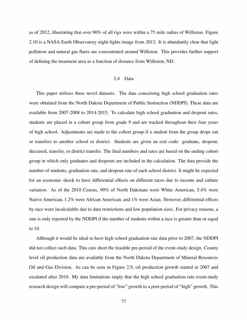
as of 2012, illustrating that over 90% of all rigs were within a 75 mile radius of Williston. Figure

2.10 is a NASA Earth Observatory night-lights image from 2012. It is abundantly clear that light

pollution and natural gas flares are concentrated around Williston. This provides further support

of defining the treatment area as a function of distance from Williston, ND.

2.4 Data

This paper utilizes three novel datasets. The data concerning high school graduation rates

were obtained from the North Dakota Department of Public Instruction (NDDPI). These data are

available from 2007-2008 to 2014-2015. To calculate high school graduation and dropout rates,

students are placed in a cohort group from grade 9 and are tracked throughout their four years

of high school. Adjustments are made to the cohort group if a student from the group drops out

or transfers to another school or district. Students are given an exit code: graduate, dropout,

deceased, transfer, or district transfer. The final numbers and rates are based on the ending cohort

group in which only graduates and dropouts are included in the calculation. The data provide the

number of students, graduation rate, and dropout rate of each school district. It might be expected

for an economic shock to have differential effects on different races due to income and culture

variation. As of the 2010 Census, 90% of North Dakotans were White American, 5.4% were

Native American, 1.2% were African American, and 1% were Asian. However, differential effects

by race were incalculable due to data restrictions and low population sizes. For privacy reasons, a

rate is only reported by the NDDPI if the number of students within a race is greater than or equal

to 10.

Although it would be ideal to have high school graduation rate data prior to 2007, the NDDPI

did not collect such data. This cuts short the feasible pre-period of the event-study design. County

level oil production data are available from the North Dakota Department of Mineral Resources

Oil and Gas Division. As can be seen in Figure 2.9, oil production growth started in 2007 and

escalated after 2010. My data limitations imply that the high school graduation rate event-study

research design will compare a pre-period of “low” growth to a post-period of “high” growth. This

77

suggests that results may understate the true effect of the oil boom on high school graduation rates.

The second source of data I use are Historical North Dakota University System (NDUS) Fall

Enrollment Reports from 1998 to 2014. These administrative reports total the number of students

in the NDUS by county-year-college cell. The NDUS includes 5 community colleges, 4 regional

universities, and 2 research universities. The research institutions, North Dakota State University

and the University of North Dakota, together have a total enrollment of around 29,000 students.

Bismark State College and Minot State University both have total enrollments of around 4,000

students and are the 3rd and 4th largest universities in the State. Therefore, the NDUS largely

represents the college choices of ND high schoolers if they decide to attend college in-state. One

benefit of NDUS enrollment data over NDDPI post-graduation outcome data is that there is no

issue of recall error on the part of school administrators so NDUS enrollment data should be less

noisy.

The third data source I use are post-graduation outcomes obtained from the (NDDPI). Data

is collected from every public and private school in all 53 ND counties. For each school district,

the dataset provides the number of students, split by gender, with the respective post-graduation

outcome. Data collection procedures may vary by school. In some schools, administrators

determine the post-graduation outcomes in the summer after high school graduation. Given that

North Dakota schools are small and social networks are tight, a guidance counselor can recall the

outcome of each high school graduate. These outcomes are then reported to the NDDPI. The six

options are employment, 2 year college, 4 year college, vocational technical school (henceforth,

voc-tech), military, and unknown. The data spans 1998-1999 to 2013-2014. It is possible that

an administrator may recall that a graduate attended college after graduation but may noisily

decipher 2 year college from 4 year college. Therefore, I often aggregate 2 year and 4 year

college enrollment into a total college enrollment rate. NDDPI post-graduation data may be

noisier than NDUS enrollment data, but allow analysis by gender and make it feasible to study

other post-graduation outcomes like employment or military enrollment. The NDDPI have the

additional benefit of studying all students who attend college, not just those who attend school

78

within the NDUS.

I use geolocated data from the ND Department of Mineral Resources Oil and Gas Division.

The data include monthly snapshots of all active oil rigs in ND. Unfortunately, this data is only

digitized back to 2012. Figure 2.1 displays a map of the change in average county unemployment

before and after 2010, overlaid with public school districts and oil rig locations in 2012. The

figure clearly shows that large unemployment reductions occurred in northwestern ND. Main oil

producing counties experienced decreases in unemployment between 30% and 60%, from base

rate unemployment between 2.1% to 4%. Thus, the oil boom improved the economic conditions

of a geographic region that already had tight labor markets.

2.5 Empirical Strategy

To study the effects of the oil boom on high school graduation rates and post-graduation

outcomes, I use an event-study specification paired with difference in difference (DD) estimates.

The design compares outcomes in schools within core-oil counties relative to non-oil counties

before and after the oil boom. Economic theory suggests that schools in the proximity of the oil

boom centroid are those most impacted by the boom. Commute times and psychic costs increase

as distance from the oil boom increases. Individuals further from the boom must leave social

networks and are less likely to have social connections in the oil drilling area. This is particularly

salient in northwest ND as housing became expensive in two ways. One, the oil boom caused

housing prices and rent to skyrocket with some news sources comparing rent to that found in New

York City.5 Second, the cheaper alternatives of living out of a Recreational Vehicle (RV) or in a

“man camp” have non-monetary costs associated with limited amenities and overcrowding.

Core-oil counties are defined by the state of North Dakota (Center, 2017) and are seen in Figure

2.6. Figures 2.2 and 2.3 illustrate the rapid divergence between wages and employment levels in

core-oil verus non-oil producing counties. Figure 2.4 provides clear evidence that employment

and wages also increased in female dominated sectors like leisure and hospitality. For high school

5http://www.nydailynews.com/life-style/real-estate/average-rent-williston-n-tops-costs-nyc-article-1.1617187

79

graduation rates, I define “Post" oil boom as 2011 and later. I determined this using yearly oil

production data and limited leeway due to lack of data before the boom. Between 2007 and

2010, North Dakota oil production increased to 100 million barrels of oil per year. Between

2011 and 2014, oil production jumped to nearly 400 million barrels per year. Using 2011 as

the cutoff provides three years of data before the boom and five years of data after the boom.

Figure 2.3 displays average monthly employment levels for core-oil and non-oil counties. Core

oil and non-oil counties share remarkably similar trends up to 2007, when employment in oil

counties starts to increase. Employment in oil counties increases steadily until 2010, after which

employment in oil counties skyrockets. As stated in the data section, the NDDPI did not collect

high school graduation rate data prior to 2007. Due to this restriction on high school graduation

rate data, the research design will compare educational outcomes in periods of high wage and

employment growth to periods with tamer wage and employment growth. To the extent that high

school graduation rates started to change prior to 2010, the DD estimate will understate the true

extent of the effect of the oil boom on educational outcomes.

NDUS enrollment data and NDDPI post-graduation outcome data are available back to 1998

and the respective oil boom starting year is defined as 2009. I estimate specification (2.1), a linear

fractional response model using an event-study research design. I estimate the model separately

for each of the six post-graduation plan outcomes. Yct is the fraction of students in county c

in year t who report the respective post-graduation outcome. “Core” is a binary variable equal

to one for core-oil counties. λt denotes year fixed effects to account for statewide yearly shocks.

County fixed effects, φc, absorb time invariant unobserved heterogeneity of county specific factors.

I cluster standard errors at a county level to allow correlation of the error term within a county over

time (Bertrand et al., 2004).

Yct = φc +λt +−2

∑y=−11

δyCorec1(t−T ∗ = y)+5

∑y=0

γyCorec1(t−T ∗ = y)+ ect (2.1)

80

2.6 Results

2.6.1 Effects on High School Graduation Rates

The work of Black et al. (2005) and Cascio and Narayan (2015) both suggest that natural

resource booms, which heavily rely on low-skill labor, decrease high school graduation rates.

Therefore, it is surprising that raw trends in Figure 2.11 illustrate no visible decrease in high

school graduation rates for schools within core-oil counties. The figures show that core-oil county

graduation rates follow similar trends to non-oil counties for the years in which core-oil county

wages increase the most relative to non-oil county wages. This holds true for both males and

females. The most notable drop in high school graduation rates occurs with the onset of The

Great Recession in 2009. To formally test whether the oil boom impacted graduation rates, Figure

2.12 presents event-study estimates. Event study estimates provide no evidence that the oil boom

decreased graduation rates in core-oil counties for males or females. These results contrast with

Cascio and Narayan (2015), suggesting that impacts of shale oil booms on high school attainment

decisions are not uniform throughout the United States.

Although the oil boom increased lower skilled employment and wages, many of these jobs,

especially oil field jobs, require a high school diploma or GED as well as a minimum age

requirement (typically 18 to 21).6 Transportation, another booming sector, often requires a worker

to have a Commercial Driver’s License (CDL). North Dakota does not issue Class A, B, or

C licenses to those under age 18 except for agricultural purposes.7 North Dakota also has a

compulsory attendance law which requires a student to stay in school until his or her 16th birthday.8

Though higher wages exist, high school students may face high barriers to entry that only disappear

upon graduation. Unlike the Appalachian coal boom of the 1970s or shale oil booms in other areas

of the United States, high school students in ND may not change high school graduation decisions,

but may alter post-graduation decisions.

6http://www.jobsnd.com/sites/default/files/Oilfield%20Employment%20Guide.pdf7ND DMV: http://www.dmv.org/nd-north-dakota/apply-cdl.php#NorthDakota-Legal-Age-Limits8 http://www.dpi.state.nd.us/health/factsheets/truancy.pdf

81

2.6.2 Effects on NDUS Enrollment Rates

Administrative data from NDUS fall enrollment reports provide the number of students

attending each NDUS college by county of residence. These reports, combined with county

level high school graduation data, can be used to create county level in-state college enrollment

rates. Total college enrollment by county is both a stock of previous enrollment (rising freshman,

sophomores, and juniors) and a flow of incoming freshman. Therefore, I calculate a college

enrollment rate of county c in year t by taking current county college enrollment and dividing

by previous years of county high school graduates (equation 2.2).

CollegeRatect =enrollmentct

hsgradsc,t−3 +hsgradsc,t−2 +hsgradsc,t−1 +hsgradsc,t(2.2)

I also calculate enrollment rates separately for both 2 year and 4 year colleges in North Dakota,

as it may be interesting to study whether oil booms have any impact on more traditional students

in 4 year colleges. Table 2.1 presents summary statistics of enrollment rates by type of college.

The sample averages suggest that 4 year enrollment rates remained constant in non-oil counties

but decreased 11 percentage points (22%) in core-oil counties after the oil boom. While regional

and research university rates remained constant in non-oil counties, the rates decreased 7 and

5 percentage points (respectively) in core-oil counties after the boom. The summary statistics

provide no evidence of 2 year enrollment rates being impacted. Raw college enrollment rate trends

in Figure 2.13 show that college enrollment in core-oil and non-core counties exhibited similar

trends prior to the boom, providing support for the parallel trends assumption inherent to a DD

research design. However, after the onset of the oil boom, college enrollment rates in core-oil

counties sharply diverged.

Event-study estimates of college enrollment rates are presented in Figure 2.14. Event-study

estimates suggest that the oil boom had a significant and prolonged negative effect on NDUS

college enrollment rates in core-oil counties. The respective DD estimates in Table 2.2 suggest

that total college enrollment rates decreased 11 percentage points (15%). As noted in Cascio and

82

Narayan (2015), shale oil booms are male and low-skill biased labor shocks. We might expect that

community college students might be more likely to be on the margin of joining the labor force

than 4 year college students. Surprisingly, Figure 2.15 suggests that the oil boom reduced 4 year

college enrollment rates but had negligible effects on community college enrollment rates. DD

estimates in Table 2.2 provide strong evidence that 4 year college enrollment rates decreased 12

percentage points (23%) in core-oil counties. The NDUS has two types of 4 year colleges: two

research universities and four regional state colleges. If research universities attract higher skilled

students, we might expect less research university students to be on the margin of forgoing college

to enter the labor force. Figure 2.16 provides evidence that enrollment rates decreased for both

regional colleges and research universities (21% and 25% decreases as found in Table 2.2).

A potential concern is that the oil boom may have caused in-migration into core-oil counties.

High school graduates of mobile parents who work in oil or oil-related jobs may be less likely

to attend college. These in-migrant high school students would contribute to the denominator of

the enrollment rate calculated in Figure 2.2, artificially driving a decrease in college enrollment

rates. While Figure 2.A1 provides some evidence that core-oil graduate numbers rebounded after

2007, overall trends in high school graduate numbers between core-oil and non-core counties

appear similar throughout the time period. To mitigate the concern of in-migration driving

results, I present event-study estimates in Figure 2.17 where the outcome is log number of

students from each county. In these specifications, in-migration will place a positive bias on

enrollment numbers if any in-migrant high school graduates attend a NDUS college. Nevertheless,

event-study estimates in Figure 2.17 provide strong evidence that the oil boom reduced NDUS

student enrollment for both regional colleges and research universities. None of the event-studies

suggest any issue of pre-trends in enrollment outcomes. The respective DD estimates in Table 2.3

provide similar estimates as above: a 19% decrease in 4 year college enrollment with no evidence

of decreases in 2 year college enrollment.

83

2.6.3 Effects on NDDPI Post-Graduation Outcomes

NDUS enrollment reports clearly show that the oil boom impacted college enrollment rates.

I supplement the NDUS enrollment analysis with NDDPI post-graduation data, which may be

noisier but allow us to study effects by gender and extend analysis to other outcomes. Table

2.4 displays post-graduation outcome rates, by gender, for core-oil and non-oil counties before

and after the boom. Summary statistics and the following analysis are limited to public high

schools in ND. Prior to the boom post-graduation outcomes were similar in core-oil and non-oil

counties, though individuals in core-oil counties were more likely to attend 2 year colleges and

less likely to attend 4 year colleges. It is clear that schools in non-oil counties exhibit rather

constant post-graduation plan choices, aside from some switching between 2 year college, 4 year

college, and voc-tech. The employment rate in non-oil counties remained essentially the same

before and after the boom (.142 versus .141). However, schools in core-oil counties exhibit

large changes in post-graduation outcomes. The fraction of students seeking employment upon

graduation increased from .16 to .23, while the fraction enrolling in a four year college decreased

from .42 to .33. Though oil booms are generally associated with low-skill male labor, it is clear

that both male and female post-graduation outcomes changed. Previous literature focuses on

male outcomes. Black et al. (2005) study male high school graduation rates while Cascio and

Narayan (2015) implement a triple-difference specification that studies the male-female gap in

high school dropout rates. The raw means in Table 2.4 show that female employment rates in

core-oil counties increased from .12 before the oil boom to .19 after. Meanwhile, 4 year college

enrollment rates dropped 12 percentage points. These summary statistics imply that females can

also be significantly impacted by shale oil booms. Appendix Figures A.1 through A.7 present raw

trends of post-graduation outcomes over time. Notably, Figure 2.A2 displays a sharp decrease

in college enrollment rates in core-oil counties that coincides with oil boom. Figure 2.A3 shows

a similar increase in employment rates while Figure 2.A7 suggests that military enrollment rates

decreased as the oil boom expanded. While shale oil booms are often thought to be male-biased,

Figure 2.A5 suggests that both male and female 4 year college enrollment rates decreased after the

84

boom. Though sample averages are imprecise, Figure 2.A7 provides evidence that male military

enrollment rates in core-oil counties decreased after the boom while non-core military enrollment

rates remained steady.

Figure 2.18 presents event study estimates of total college enrollment rates (the sum of 2 and

4 year college enrollment rates). There is no evidence of trends prior to the oil boom, which

supports the parallel trends assumption of a DD specification. Event-study estimates provide strong

evidence that total college enrollment rates decreased in core-oil counties after the oil boom for

both males and females. The novel result here is that female college enrollment is also impacted by

the oil boom. It is reassuring that both NDUS and NDDPI event-study estimates show a decrease

in college enrollment rates that are strongest around 2011 (near the peak of the oil boom). Figure

2.19 suggests that employment rates in core-oil counties increased after the oil boom, with less

precise estimates suggesting that employment rates increased for both males and females. It may

be interesting to study which students are on the margin. Interestingly, Figure 2.21 and Figure 2.20

suggest that 4 year college enrollment rates decreased more than 2 year college enrollment rates.

Consistent with previous work on natural resource booms, decreases in 4 year college enrollment

rates are driven by males. Figure 2.22 provides evidence that the oil boom had large negative

impacts, relative to the mean, on male military enrollment rates. This is consistent with a shale oil

boom being a large labor market shock to prime age male employment.

2.7 Conclusion

The ND oil boom has drastically impacted northwestern counties of the state. As of

2014, unemployment rates of the top four oil producing counties averaged 1.4%. The oil

boom significantly increased both employment levels and wages. The civilian labor force in

Williams County increased threefold between 2008 and 2013, with doubling wages and low

unemployment. Employment data form the QCEW shows that there was strong employment

growth in female-heavy industries as well as male industries. I provide strong evidence that the

tightening of labor markets altered educational attainment decisions of high school seniors in North

85

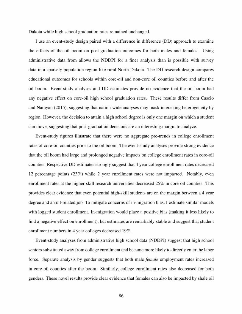
Dakota while high school graduation rates remained unchanged.

I use an event-study design paired with a difference in difference (DD) approach to examine

the effects of the oil boom on post-graduation outcomes for both males and females. Using

administrative data from allows the NDDPI for a finer analysis than is possible with survey

data in a sparsely population region like rural North Dakota. The DD research design compares

educational outcomes for schools within core-oil and non-core oil counties before and after the

oil boom. Event-study analyses and DD estimates provide no evidence that the oil boom had

any negative effect on core-oil high school graduation rates. These results differ from Cascio

and Narayan (2015), suggesting that nation-wide analyses may mask interesting heterogeneity by

region. However, the decision to attain a high school degree is only one margin on which a student

can move, suggesting that post-graduation decisions are an interesting margin to analyze.

Event-study figures illustrate that there were no aggregate pre-trends in college enrollment

rates of core-oil counties prior to the oil boom. The event-study analyses provide strong evidence

that the oil boom had large and prolonged negative impacts on college enrollment rates in core-oil

counties. Respective DD estimates strongly suggest that 4 year college enrollment rates decreased

12 percentage points (23%) while 2 year enrollment rates were not impacted. Notably, even

enrollment rates at the higher-skill research universities decreased 25% in core-oil counties. This

provides clear evidence that even potential high-skill students are on the margin between a 4 year

degree and an oil-related job. To mitigate concerns of in-migration bias, I estimate similar models

with logged student enrollment. In-migration would place a positive bias (making it less likely to

find a negative effect on enrollment), but estimates are remarkably stable and suggest that student

enrollment numbers in 4 year colleges decreased 19%.

Event-study analyses from administrative high school data (NDDPI) suggest that high school

seniors substituted away from college enrollment and became more likely to directly enter the labor

force. Separate analysis by gender suggests that both male female employment rates increased

in core-oil counties after the boom. Similarly, college enrollment rates also decreased for both

genders. These novel results provide clear evidence that females can also be impacted by shale oil

86

boom. While shale oil booms in certain regions of the country may be dominated by oil-related

employment growth, the boom in North Dakota was also associated with growth in non-oil jobs.

Lastly, I find evidence that male military enrollment rates decreased in core-oil counties after the

boom. This is unsurprising give that both oil-related employers and the military recruit prime-age

males.

This is the first paper to analyze the impact of the ND oil boom on post-graduate educational

attainment. The majority of literature studying natural resource booms and educational attainment

focuses on high school graduation rates. Although high school gradation rates are an important

area of research, high school graduation rates in ND are high and steady throughout the time period

(around 87%). The insensitivity of high school graduation rates to job creation and wage shocks

does not suggest that higher level educational attainment decisions are unaffected. This paper has

policy implications for any region subject to natural resource booms. This analysis is especially

relevant to rural areas of Texas, Pennsylvania, or other states undergoing fracking booms. These

results are also relevant to North Dakota itself. Oil production in ND has curtailed since 2015.

Low world crude oil prices decreased below many oil rig break-even prices and overall job growth

stagnated. If future world crude prices increase significantly above $50 per barrel, North Dakota

oil activity will boom again and high school seniors will face similar incentives to those studied in

this paper. Regions that experience reductions in college enrollment rates in lieu of employment

may benefit during the boom, but will be left with a surplus of low-skill unemployed workers when

the boom goes bust.

87

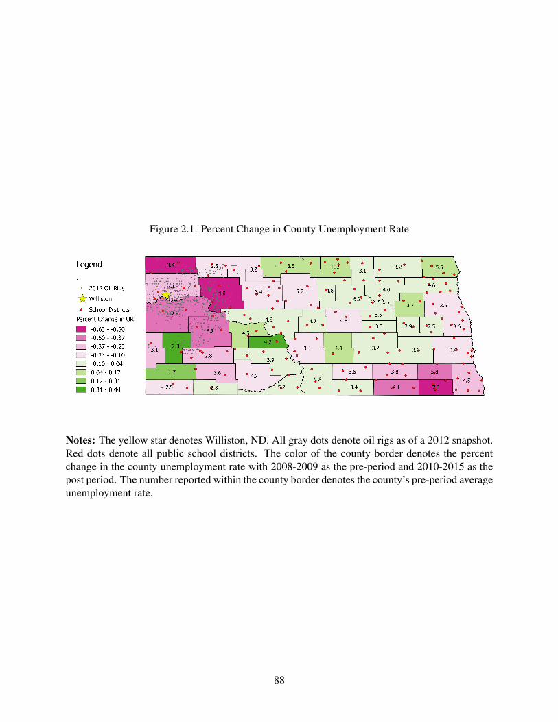
Figure 2.1: Percent Change in County Unemployment Rate

Notes: The yellow star denotes Williston, ND. All gray dots denote oil rigs as of a 2012 snapshot.Red dots denote all public school districts. The color of the county border denotes the percentchange in the county unemployment rate with 2008-2009 as the pre-period and 2010-2015 as thepost period. The number reported within the county border denotes the county’s pre-period averageunemployment rate.

88

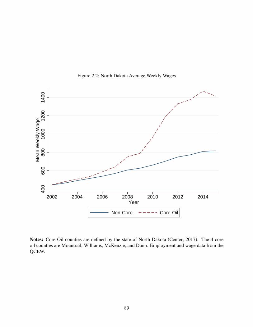
Figure 2.2: North Dakota Average Weekly Wages

400

600

800

1000

1200

1400

Mea

n W

eekl

y W

age

2002 2004 2006 2008 2010 2012 2014Year

Non-Core Core-Oil

Notes: Core Oil counties are defined by the state of North Dakota (Center, 2017). The 4 coreoil counties are Mountrail, Williams, McKenzie, and Dunn. Employment and wage data from theQCEW.

89

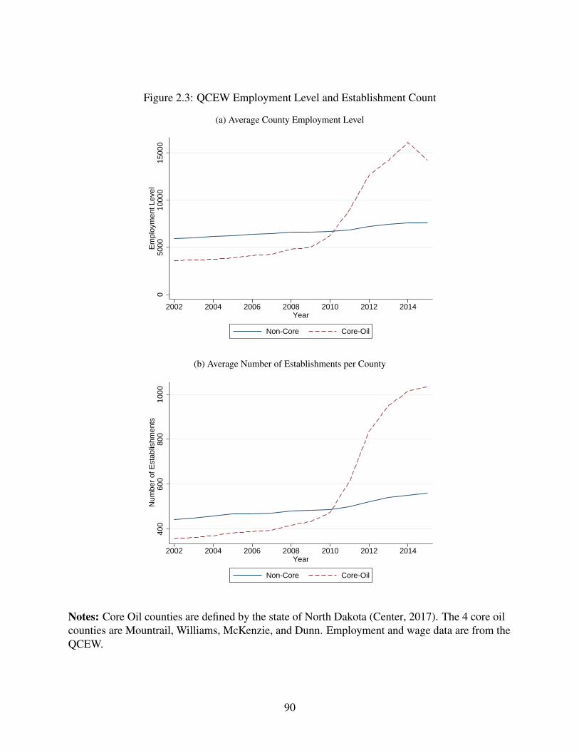
Figure 2.3: QCEW Employment Level and Establishment Count

(a) Average County Employment Level

050

0010

000

1500

0E

mpl

oym

ent L

evel

2002 2004 2006 2008 2010 2012 2014Year

Non-Core Core-Oil

(b) Average Number of Establishments per County

400

600

800

1000

Num

ber

of E

stab

lishm

ents

2002 2004 2006 2008 2010 2012 2014Year

Non-Core Core-Oil

Notes: Core Oil counties are defined by the state of North Dakota (Center, 2017). The 4 core oilcounties are Mountrail, Williams, McKenzie, and Dunn. Employment and wage data are from theQCEW.

90

Figure 2.4: Leisure & Hospitality Employment Level and Wages

(a) Leisure & Hospitality Employment Level

200

400

600

800

1000

Em

ploy

men

t Lev

el

2002 2004 2006 2008 2010 2012 2014Year

Non-Core Core-Oil

(b) Leisure & Hospitality Mean Wages

100

200

300

400

Mea

n W

eekl

y W

age

2002 2004 2006 2008 2010 2012 2014Year

Non-Core Core-Oil

Notes: Core Oil counties are defined by the state of North Dakota (Center, 2017). The 4 core oilcounties are Mountrail, Williams, McKenzie, and Dunn. Employment and wage data are from theQCEW.

91

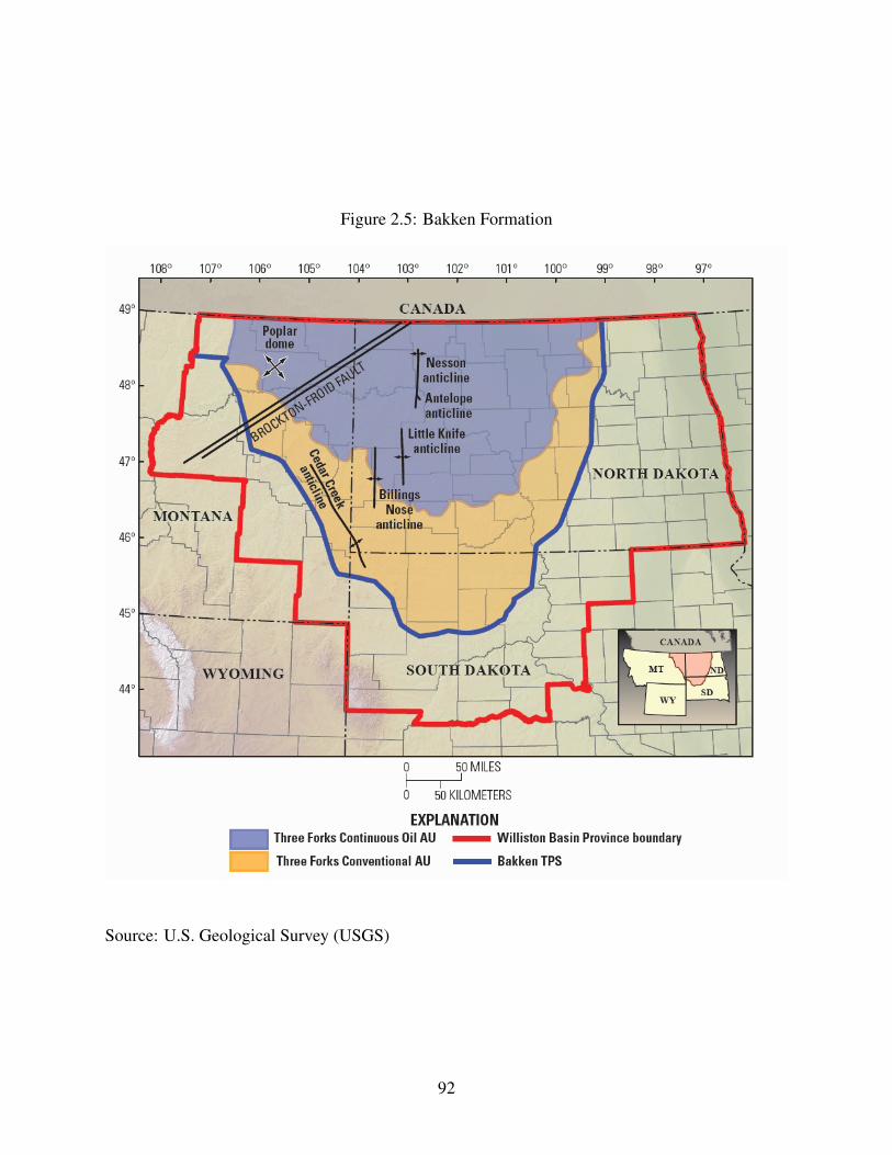
Figure 2.5: Bakken Formation

Source: U.S. Geological Survey (USGS)

92

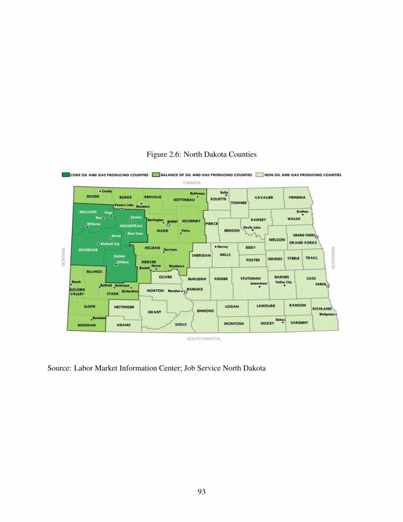
Figure 2.6: North Dakota Counties

Source: Labor Market Information Center; Job Service North Dakota

93

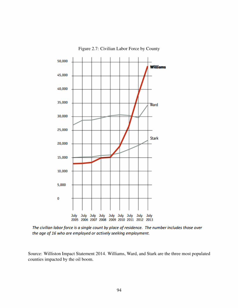
Figure 2.7: Civilian Labor Force by County

Source: Williston Impact Statement 2014. Williams, Ward, and Stark are the three most populatedcounties impacted by the oil boom.

94

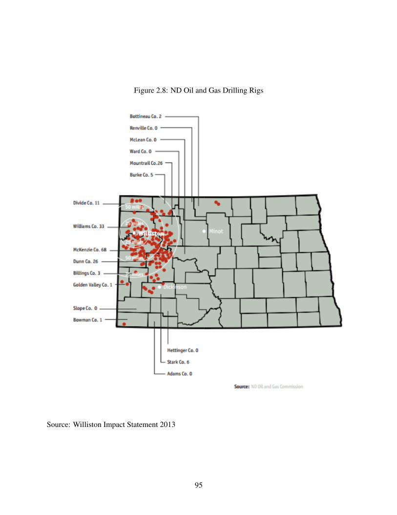
Figure 2.8: ND Oil and Gas Drilling Rigs

Source: Williston Impact Statement 2013

95

Figure 2.9: ND Oil Production

010

020

030

040

0O

il P

rodu

ctio

n (m

illio

ns o

f bar

rels

)

1998 2000 2002 2004 2006 2008 2010 2012 2014Year

Core-Oil Non-Core

Source: ND Department of Mineral Resources (ND DMR)

96

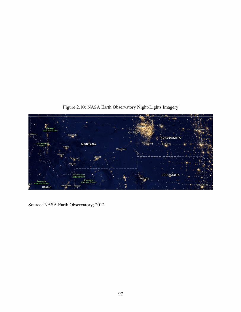
Figure 2.10: NASA Earth Observatory Night-Lights Imagery

Source: NASA Earth Observatory; 2012

97

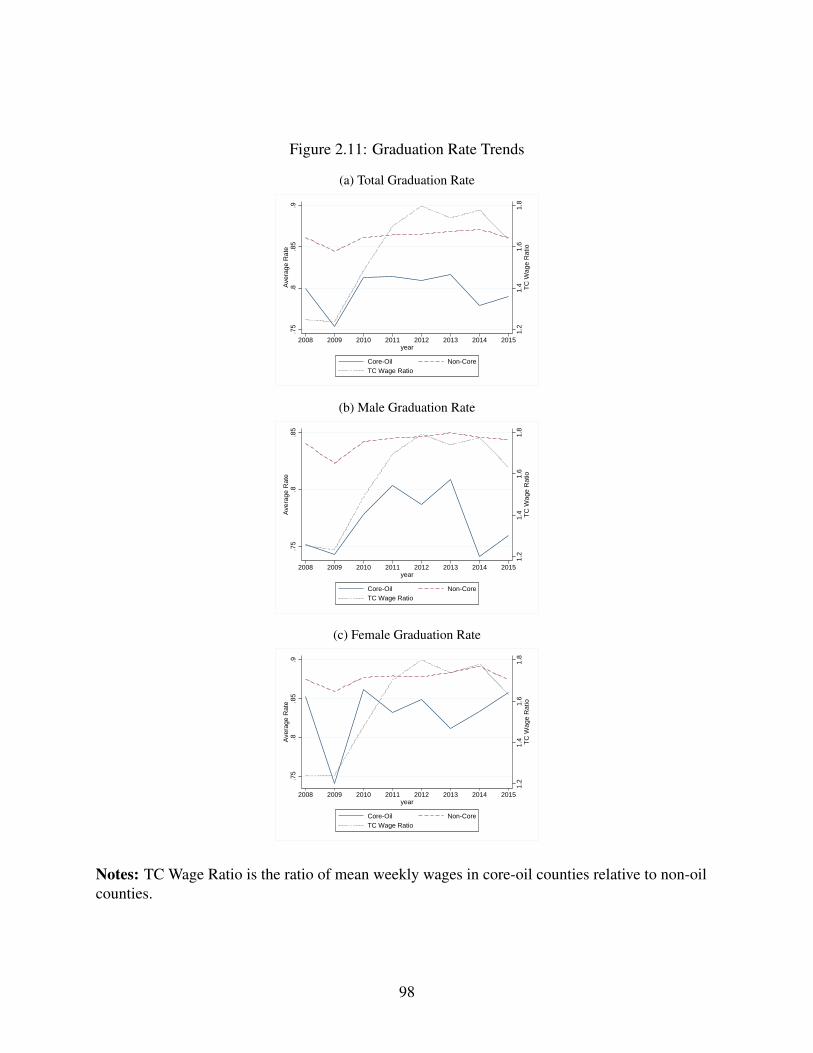
Figure 2.11: Graduation Rate Trends

(a) Total Graduation Rate

1.2

1.4

1.6

1.8

TC

Wag

e R

atio

.75

.8.8

5.9

Ave

rage

Rat

e

2008 2009 2010 2011 2012 2013 2014 2015year

Core-Oil Non-CoreTC Wage Ratio

(b) Male Graduation Rate

1.2

1.4

1.6

1.8

TC

Wag

e R

atio

.75

.8.8

5A

vera

ge R

ate

2008 2009 2010 2011 2012 2013 2014 2015year

Core-Oil Non-CoreTC Wage Ratio

(c) Female Graduation Rate

1.2

1.4

1.6

1.8

TC

Wag

e R

atio

.75

.8.8

5.9

Ave

rage

Rat

e

2008 2009 2010 2011 2012 2013 2014 2015year

Core-Oil Non-CoreTC Wage Ratio

Notes: TC Wage Ratio is the ratio of mean weekly wages in core-oil counties relative to non-oilcounties.

98

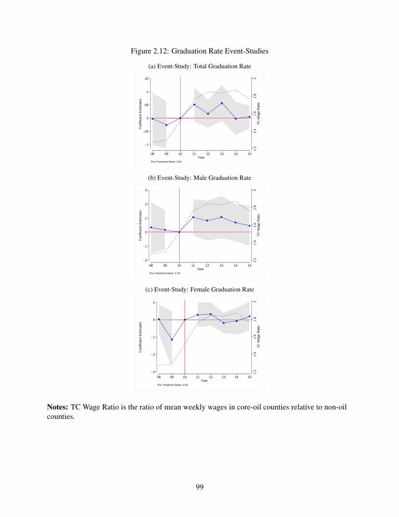
Figure 2.12: Graduation Rate Event-Studies

(a) Event-Study: Total Graduation Rate

1.2

1.4

1.6

1.8

2T

C W

age

Rat

io

-.1

-.05

0

.05

.1

.15

Coe

ffici

ent E

stim

ates

08 09 10 11 12 13 14 15 Year

Pre-Treatment Mean: 0.81

(b) Event-Study: Male Graduation Rate

1.2

1.4

1.6

1.8

2T

C W

age

Rat

io-.2

-.1

0

.1

.2

.3

Coe

ffici

ent E

stim

ates

08 09 10 11 12 13 14 15 Year

Pre-Treatment Mean: 0.79

(c) Event-Study: Female Graduation Rate

1.2

1.4

1.6

1.8

2T

C W

age

Rat

io

-.3

-.2

-.1

0

.1

Coe

ffici

ent E

stim

ates

08 09 10 11 12 13 14 15 Year

Pre-Treatment Mean: 0.82

Notes: TC Wage Ratio is the ratio of mean weekly wages in core-oil counties relative to non-oilcounties.

99

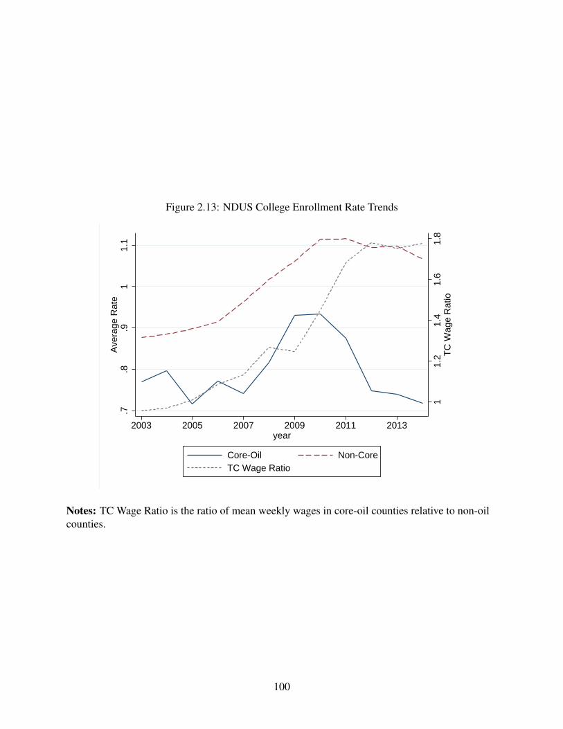
Figure 2.13: NDUS College Enrollment Rate Trends

11.

21.

41.

61.

8T

C W

age

Rat

io

.7.8

.91

1.1

Ave

rage

Rat

e

2003 2005 2007 2009 2011 2013year

Core-Oil Non-CoreTC Wage Ratio

Notes: TC Wage Ratio is the ratio of mean weekly wages in core-oil counties relative to non-oilcounties.

100

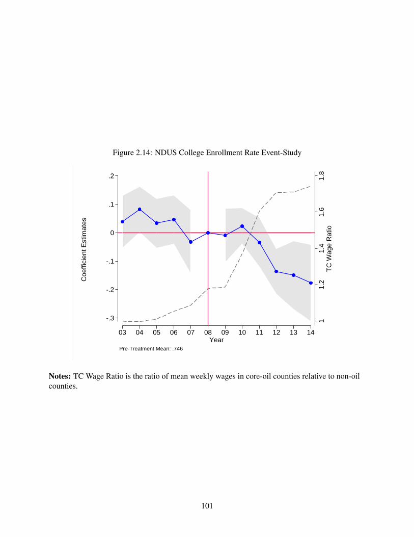
Figure 2.14: NDUS College Enrollment Rate Event-Study

11.

21.

41.

61.

8T

C W

age

Rat

io

-.3

-.2

-.1

0

.1

.2

Coe

ffici

ent E

stim

ates

03 04 05 06 07 08 09 10 11 12 13 14 Year

Pre-Treatment Mean: .746

Notes: TC Wage Ratio is the ratio of mean weekly wages in core-oil counties relative to non-oilcounties.

101

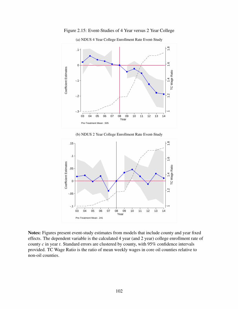
Figure 2.15: Event-Studies of 4 Year versus 2 Year College

(a) NDUS 4 Year College Enrollment Rate Event-Study

11.

21.

41.

61.

8T

C W

age

Rat

io

-.3

-.2

-.1

0

.1

Coe

ffici

ent E

stim

ates

03 04 05 06 07 08 09 10 11 12 13 14 Year

Pre-Treatment Mean: .505

(b) NDUS 2 Year College Enrollment Rate Event-Study

11.

21.

41.

61.

8T

C W

age

Rat

io

-.1

-.05

0

.05

.1

.15

Coe

ffici

ent E

stim

ates

03 04 05 06 07 08 09 10 11 12 13 14 Year

Pre-Treatment Mean: .241

Notes: Figures present event-study estimates from models that include county and year fixedeffects. The dependent variable is the calculated 4 year (and 2 year) college enrollment rate ofcounty c in year t. Standard errors are clustered by county, with 95% confidence intervalsprovided. TC Wage Ratio is the ratio of mean weekly wages in core oil counties relative tonon-oil counties.

102

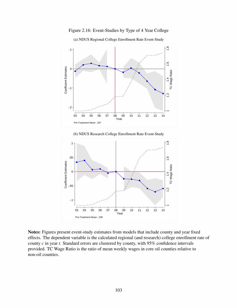
Figure 2.16: Event-Studies by Type of 4 Year College

(a) NDUS Regional College Enrollment Rate Event-Study

11.

21.

41.

61.

8T

C W

age

Rat

io

-.2

-.1

0

.1

Coe

ffici

ent E

stim

ates

03 04 05 06 07 08 09 10 11 12 13 14 Year

Pre-Treatment Mean: .267

(b) NDUS Research College Enrollment Rate Event-Study

11.

21.

41.

61.

8T

C W

age

Rat

io

-.1

-.05

0

.05

.1

Coe

ffici

ent E

stim

ates

03 04 05 06 07 08 09 10 11 12 13 14 Year

Pre-Treatment Mean: .238

Notes: Figures present event-study estimates from models that include county and year fixedeffects. The dependent variable is the calculated regional (and research) college enrollment rate ofcounty c in year t. Standard errors are clustered by county, with 95% confidence intervalsprovided. TC Wage Ratio is the ratio of mean weekly wages in core oil counties relative tonon-oil counties.

103

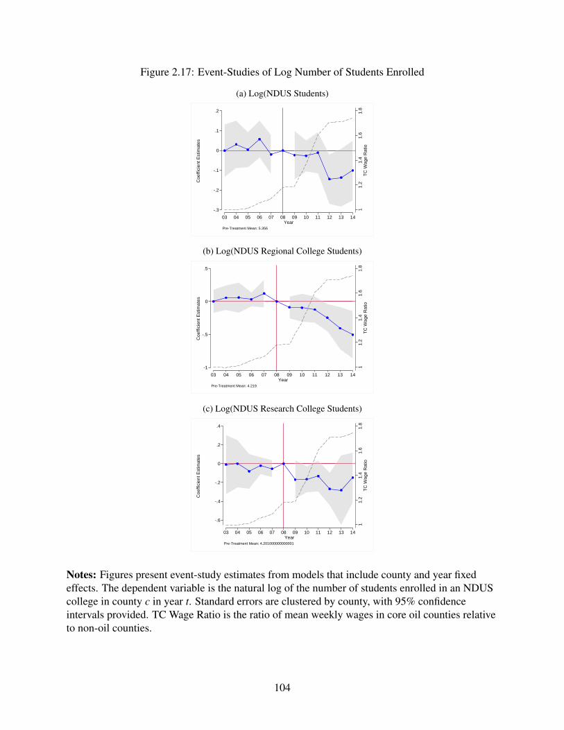
Figure 2.17: Event-Studies of Log Number of Students Enrolled

(a) Log(NDUS Students)

11.

21.

41.

61.

8T

C W

age

Rat

io

-.3

-.2

-.1

0

.1

.2

Coe

ffici

ent E

stim

ates

03 04 05 06 07 08 09 10 11 12 13 14 Year

Pre-Treatment Mean: 5.356

(b) Log(NDUS Regional College Students)

11.

21.

41.

61.

8T

C W

age

Rat

io-1

-.5

0

.5

Coe

ffici

ent E

stim

ates

03 04 05 06 07 08 09 10 11 12 13 14 Year

Pre-Treatment Mean: 4.219

(c) Log(NDUS Research College Students)

11.

21.

41.

61.

8T

C W

age

Rat

io

-.6

-.4

-.2

0

.2

.4

Coe

ffici

ent E

stim

ates

03 04 05 06 07 08 09 10 11 12 13 14 Year

Pre-Treatment Mean: 4.201000000000001

Notes: Figures present event-study estimates from models that include county and year fixedeffects. The dependent variable is the natural log of the number of students enrolled in an NDUScollege in county c in year t. Standard errors are clustered by county, with 95% confidenceintervals provided. TC Wage Ratio is the ratio of mean weekly wages in core oil counties relativeto non-oil counties.

104

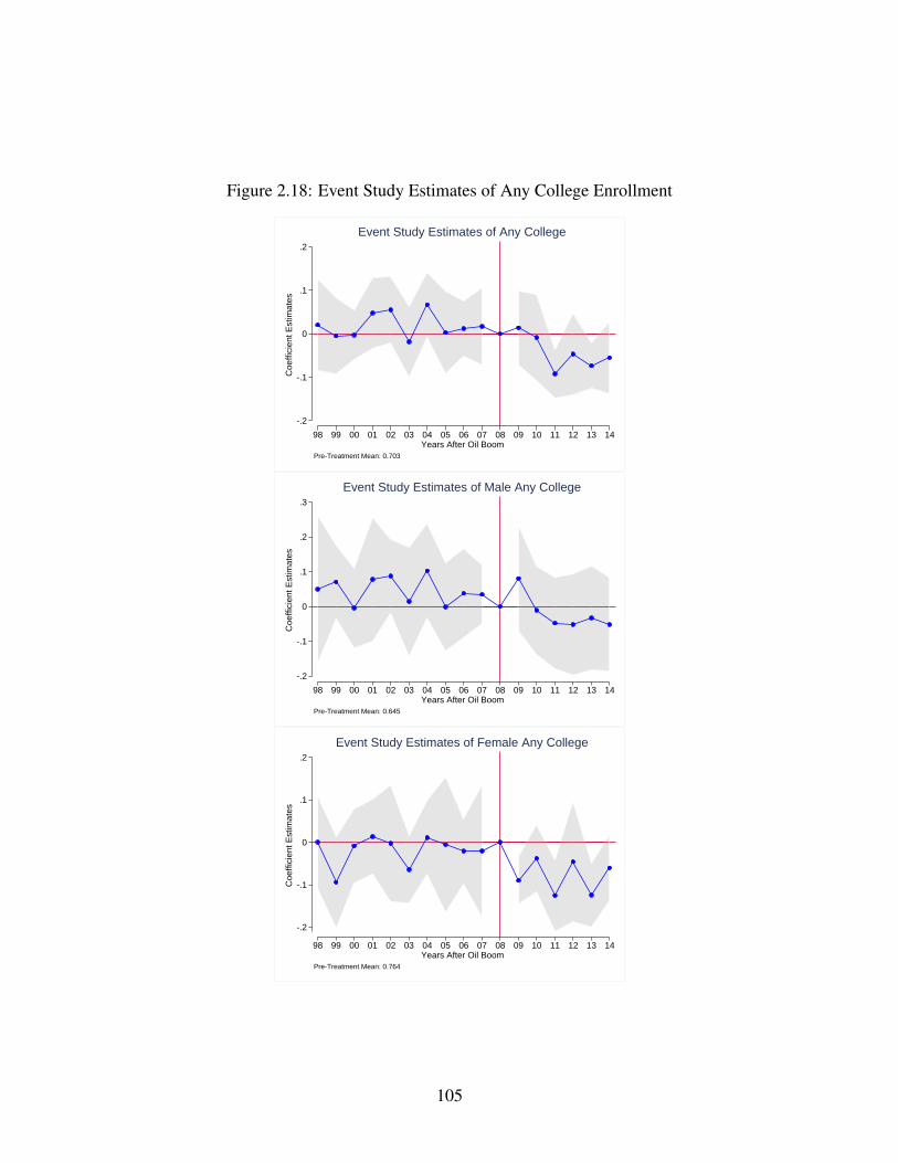
Figure 2.18: Event Study Estimates of Any College Enrollment

-.2

-.1

0

.1

.2

Coe

ffici

ent E

stim

ates

98 99 00 01 02 03 04 05 06 07 08 09 10 11 12 13 14Years After Oil Boom

Pre-Treatment Mean: 0.703

Event Study Estimates of Any College

-.2

-.1

0

.1

.2

.3

Coe

ffici

ent E

stim

ates

98 99 00 01 02 03 04 05 06 07 08 09 10 11 12 13 14Years After Oil Boom

Pre-Treatment Mean: 0.645

Event Study Estimates of Male Any College

-.2

-.1

0

.1

.2

Coe

ffici

ent E

stim

ates

98 99 00 01 02 03 04 05 06 07 08 09 10 11 12 13 14Years After Oil Boom

Pre-Treatment Mean: 0.764

Event Study Estimates of Female Any College

105

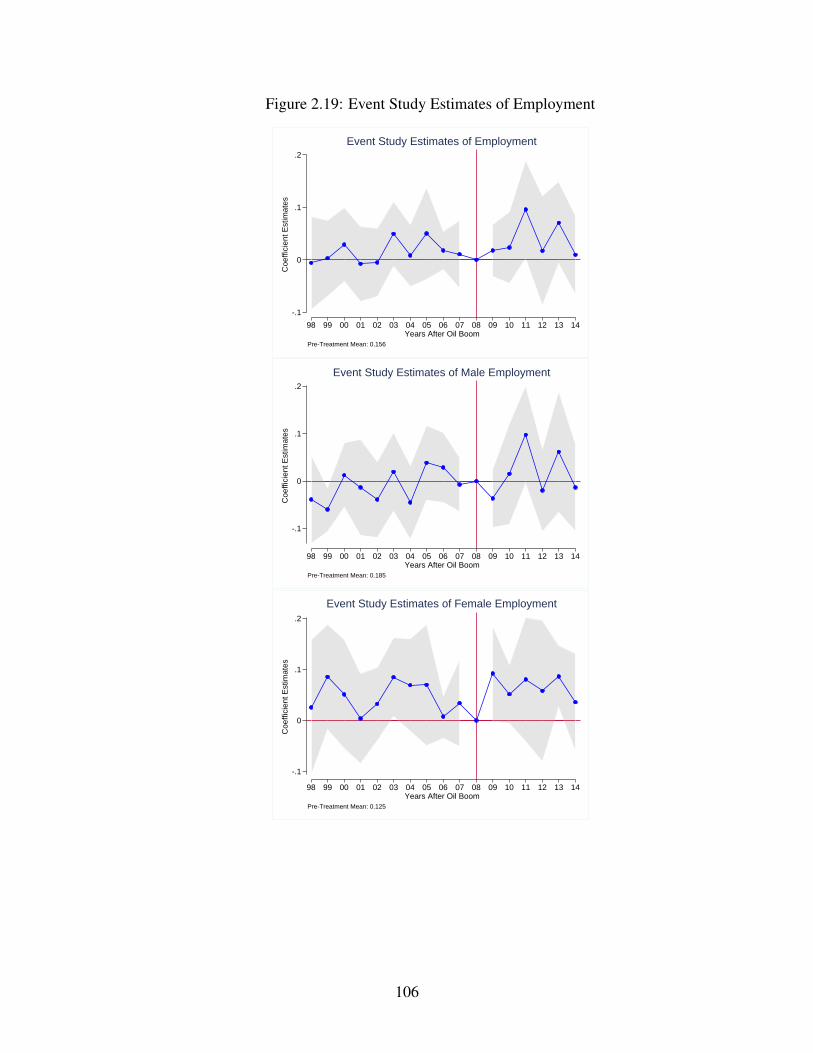
Figure 2.19: Event Study Estimates of Employment

-.1

0

.1

.2

Coe

ffici

ent E

stim

ates

98 99 00 01 02 03 04 05 06 07 08 09 10 11 12 13 14Years After Oil Boom

Pre-Treatment Mean: 0.156

Event Study Estimates of Employment

-.1

0

.1

.2

Coe

ffici

ent E

stim

ates

98 99 00 01 02 03 04 05 06 07 08 09 10 11 12 13 14Years After Oil Boom

Pre-Treatment Mean: 0.185

Event Study Estimates of Male Employment

-.1

0

.1

.2

Coe

ffici

ent E

stim

ates

98 99 00 01 02 03 04 05 06 07 08 09 10 11 12 13 14Years After Oil Boom

Pre-Treatment Mean: 0.125

Event Study Estimates of Female Employment

106

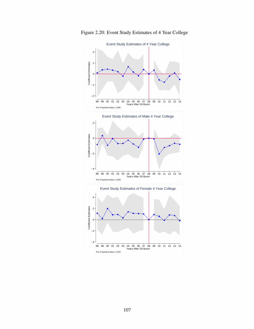
Figure 2.20: Event Study Estimates of 4 Year College

-.2

-.1

0

.1

.2

Coe

ffici

ent E

stim

ates

98 99 00 01 02 03 04 05 06 07 08 09 10 11 12 13 14Years After Oil Boom

Pre-Treatment Mean: 0.468

Event Study Estimates of 4 Year College

-.4

-.2

0

.2

Coe

ffici

ent E

stim

ates

98 99 00 01 02 03 04 05 06 07 08 09 10 11 12 13 14Years After Oil Boom

Pre-Treatment Mean: 0.409

Event Study Estimates of Male 4 Year College

-.4

-.2

0

.2

.4

Coe

ffici

ent E

stim

ates

98 99 00 01 02 03 04 05 06 07 08 09 10 11 12 13 14Years After Oil Boom

Pre-Treatment Mean: 0.529

Event Study Estimates of Female 4 Year College

107

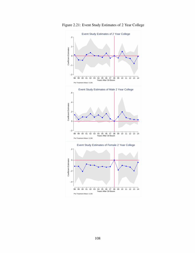
Figure 2.21: Event Study Estimates of 2 Year College

-.2

-.1

0

.1

.2

Coe

ffici

ent E

stim

ates

98 99 00 01 02 03 04 05 06 07 08 09 10 11 12 13 14Years After Oil Boom

Pre-Treatment Mean: 0.235

Event Study Estimates of 2 Year College

-.2

0

.2

.4

.6

Coe

ffici

ent E

stim

ates

98 99 00 01 02 03 04 05 06 07 08 09 10 11 12 13 14Years After Oil Boom

Pre-Treatment Mean: 0.236

Event Study Estimates of Male 2 Year College

-.4

-.2

0

.2

Coe

ffici

ent E

stim

ates

98 99 00 01 02 03 04 05 06 07 08 09 10 11 12 13 14Years After Oil Boom

Pre-Treatment Mean: 0.235

Event Study Estimates of Female 2 Year College

108

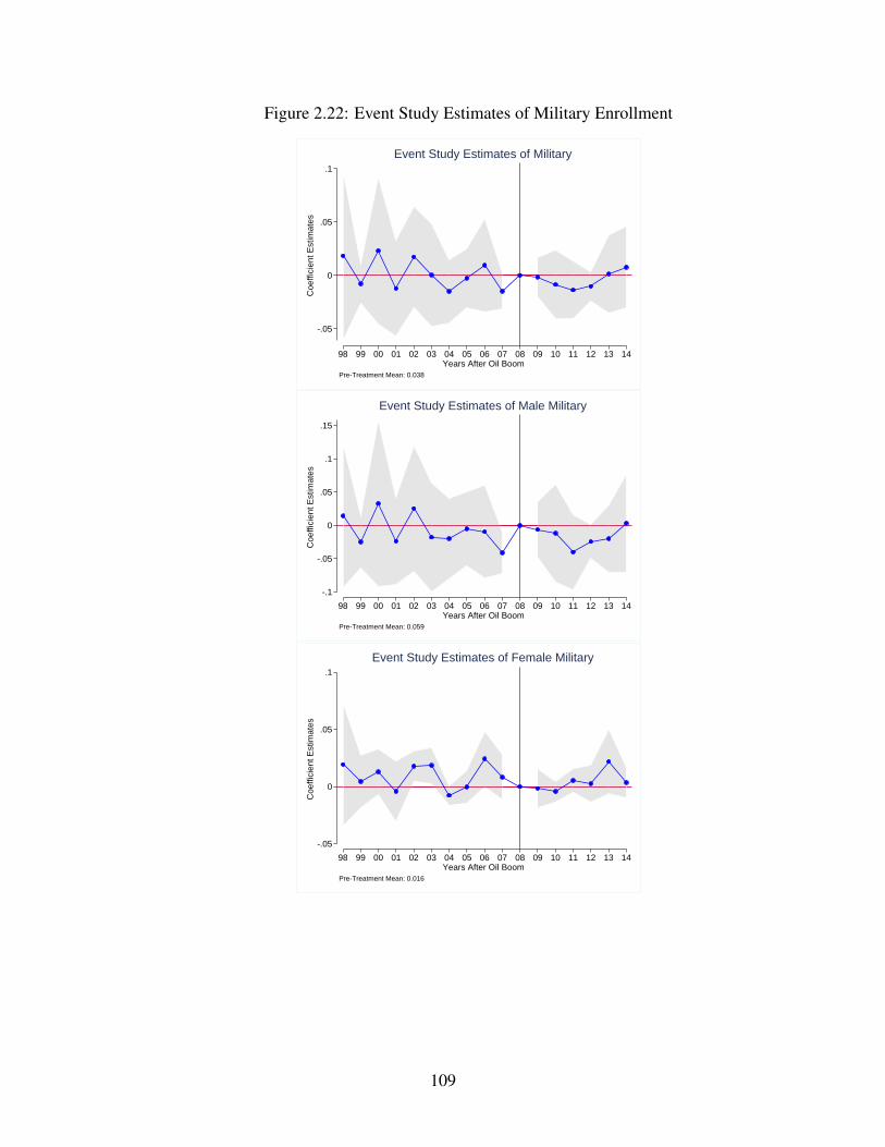
Figure 2.22: Event Study Estimates of Military Enrollment

-.05

0

.05

.1

Coe

ffici

ent E

stim

ates

98 99 00 01 02 03 04 05 06 07 08 09 10 11 12 13 14Years After Oil Boom

Pre-Treatment Mean: 0.038

Event Study Estimates of Military

-.1

-.05

0

.05

.1

.15

Coe

ffici

ent E

stim

ates

98 99 00 01 02 03 04 05 06 07 08 09 10 11 12 13 14Years After Oil Boom

Pre-Treatment Mean: 0.059

Event Study Estimates of Male Military

-.05

0

.05

.1

Coe

ffici

ent E

stim

ates

98 99 00 01 02 03 04 05 06 07 08 09 10 11 12 13 14Years After Oil Boom

Pre-Treatment Mean: 0.016

Event Study Estimates of Female Military

109

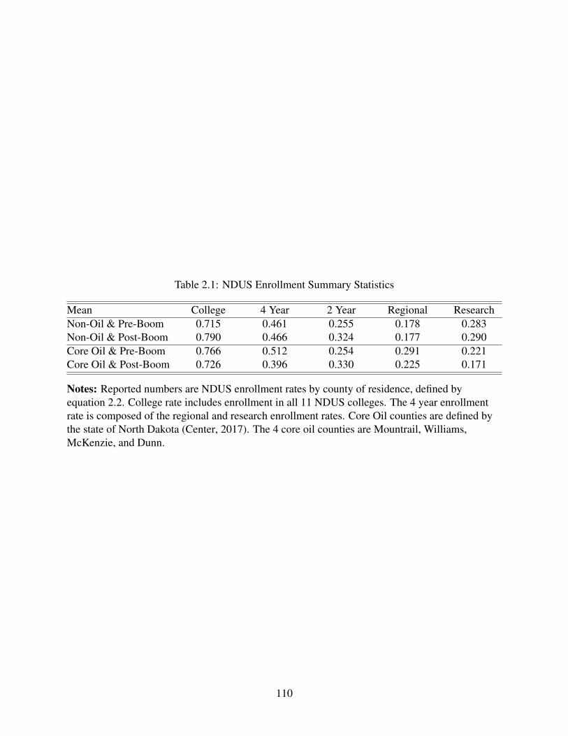
Table 2.1: NDUS Enrollment Summary Statistics

Mean College 4 Year 2 Year Regional ResearchNon-Oil & Pre-Boom 0.715 0.461 0.255 0.178 0.283Non-Oil & Post-Boom 0.790 0.466 0.324 0.177 0.290Core Oil & Pre-Boom 0.766 0.512 0.254 0.291 0.221Core Oil & Post-Boom 0.726 0.396 0.330 0.225 0.171

Notes: Reported numbers are NDUS enrollment rates by county of residence, defined byequation 2.2. College rate includes enrollment in all 11 NDUS colleges. The 4 year enrollmentrate is composed of the regional and research enrollment rates. Core Oil counties are defined bythe state of North Dakota (Center, 2017). The 4 core oil counties are Mountrail, Williams,McKenzie, and Dunn.

110

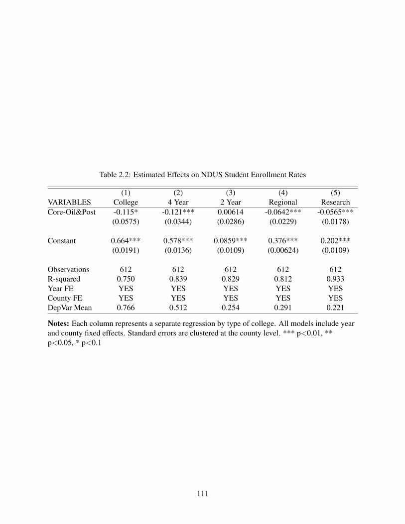
Table 2.2: Estimated Effects on NDUS Student Enrollment Rates

(1) (2) (3) (4) (5)VARIABLES College 4 Year 2 Year Regional ResearchCore-Oil&Post -0.115* -0.121*** 0.00614 -0.0642*** -0.0565***

(0.0575) (0.0344) (0.0286) (0.0229) (0.0178)

Constant 0.664*** 0.578*** 0.0859*** 0.376*** 0.202***(0.0191) (0.0136) (0.0109) (0.00624) (0.0109)

Observations 612 612 612 612 612R-squared 0.750 0.839 0.829 0.812 0.933Year FE YES YES YES YES YESCounty FE YES YES YES YES YESDepVar Mean 0.766 0.512 0.254 0.291 0.221

Notes: Each column represents a separate regression by type of college. All models include yearand county fixed effects. Standard errors are clustered at the county level. *** p<0.01, **p<0.05, * p<0.1

111

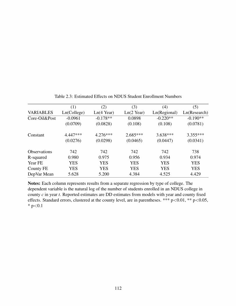
Table 2.3: Estimated Effects on NDUS Student Enrollment Numbers

(1) (2) (3) (4) (5)VARIABLES Ln(College) Ln(4 Year) Ln(2 Year) Ln(Regional) Ln(Research)Core-Oil&Post -0.0961 -0.178** 0.0898 -0.220** -0.190**

(0.0709) (0.0828) (0.108) (0.108) (0.0781)

Constant 4.447*** 4.276*** 2.685*** 3.638*** 3.355***(0.0276) (0.0298) (0.0465) (0.0447) (0.0341)

Observations 742 742 742 742 738R-squared 0.980 0.975 0.956 0.934 0.974Year FE YES YES YES YES YESCounty FE YES YES YES YES YESDepVar Mean 5.628 5.200 4.384 4.525 4.429

Notes: Each column represents results from a separate regression by type of college. Thedependent variable is the natural log of the number of students enrolled in an NDUS college incounty c in year t. Reported estimates are DD estimates from models with year and county fixedeffects. Standard errors, clustered at the county level, are in parentheses. *** p<0.01, ** p<0.05,* p<0.1

112

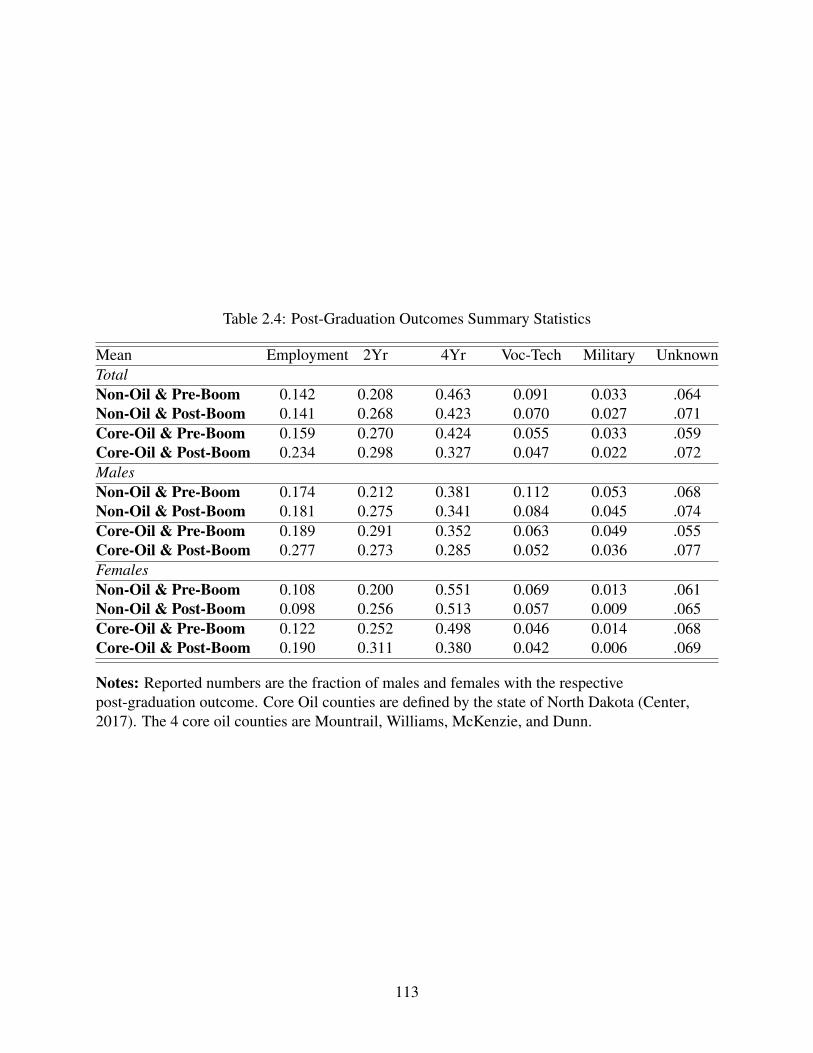
Table 2.4: Post-Graduation Outcomes Summary Statistics

Mean Employment 2Yr 4Yr Voc-Tech Military UnknownTotalNon-Oil & Pre-Boom 0.142 0.208 0.463 0.091 0.033 .064Non-Oil & Post-Boom 0.141 0.268 0.423 0.070 0.027 .071Core-Oil & Pre-Boom 0.159 0.270 0.424 0.055 0.033 .059Core-Oil & Post-Boom 0.234 0.298 0.327 0.047 0.022 .072MalesNon-Oil & Pre-Boom 0.174 0.212 0.381 0.112 0.053 .068Non-Oil & Post-Boom 0.181 0.275 0.341 0.084 0.045 .074Core-Oil & Pre-Boom 0.189 0.291 0.352 0.063 0.049 .055Core-Oil & Post-Boom 0.277 0.273 0.285 0.052 0.036 .077FemalesNon-Oil & Pre-Boom 0.108 0.200 0.551 0.069 0.013 .061Non-Oil & Post-Boom 0.098 0.256 0.513 0.057 0.009 .065Core-Oil & Pre-Boom 0.122 0.252 0.498 0.046 0.014 .068Core-Oil & Post-Boom 0.190 0.311 0.380 0.042 0.006 .069

Notes: Reported numbers are the fraction of males and females with the respectivepost-graduation outcome. Core Oil counties are defined by the state of North Dakota (Center,2017). The 4 core oil counties are Mountrail, Williams, McKenzie, and Dunn.

113

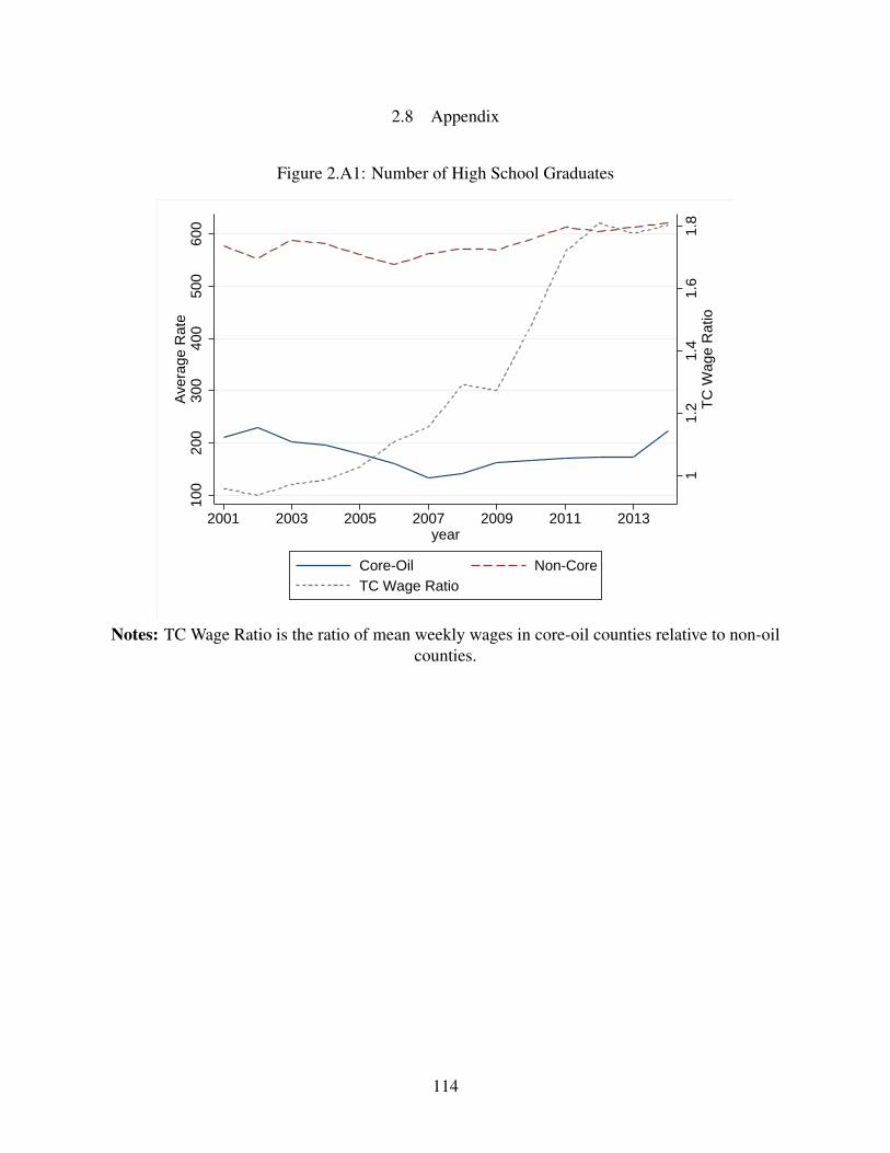
2.8 Appendix

Figure 2.A1: Number of High School Graduates

11.

21.

41.

61.

8T

C W

age

Rat

io

100

200

300

400

500

600

Ave

rage

Rat

e

2001 2003 2005 2007 2009 2011 2013year

Core-Oil Non-CoreTC Wage Ratio

Notes: TC Wage Ratio is the ratio of mean weekly wages in core-oil counties relative to non-oilcounties.

114

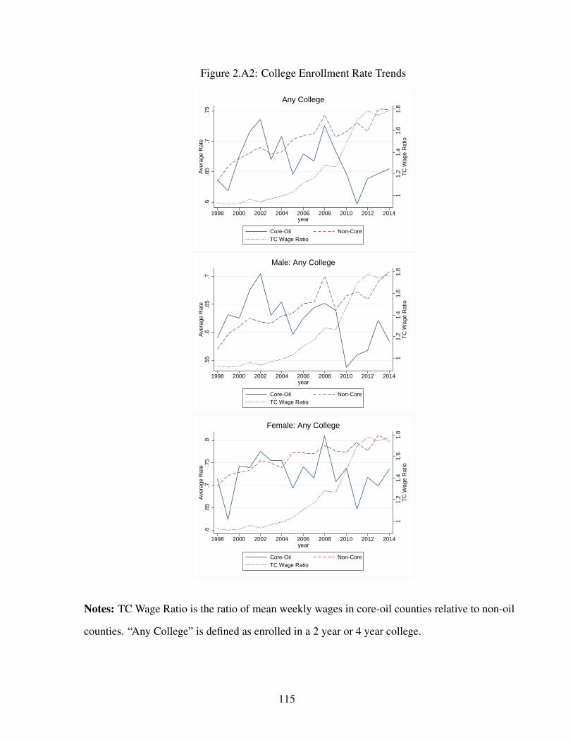
Figure 2.A2: College Enrollment Rate Trends

11.

21.

41.

61.

8T

C W

age

Rat

io

.6.6

5.7

.75

Ave

rage

Rat

e

1998 2000 2002 2004 2006 2008 2010 2012 2014year

Core-Oil Non-CoreTC Wage Ratio

Any College

11.

21.

41.

61.

8T

C W

age

Rat

io

.55

.6.6

5.7

Ave

rage

Rat

e

1998 2000 2002 2004 2006 2008 2010 2012 2014year

Core-Oil Non-CoreTC Wage Ratio

Male: Any College

11.

21.

41.

61.

8T

C W

age

Rat

io

.6.6

5.7

.75

.8A

vera

ge R

ate

1998 2000 2002 2004 2006 2008 2010 2012 2014year

Core-Oil Non-CoreTC Wage Ratio

Female: Any College

Notes: TC Wage Ratio is the ratio of mean weekly wages in core-oil counties relative to non-oil

counties. “Any College” is defined as enrolled in a 2 year or 4 year college.

115

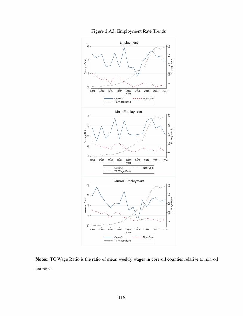
Figure 2.A3: Employment Rate Trends

11.

21.

41.

61.

8T

C W

age

Rat

io

.1.1

5.2

.25

Ave

rage

Rat

e

1998 2000 2002 2004 2006 2008 2010 2012 2014year

Core-Oil Non-CoreTC Wage Ratio

Employment

11.

21.

41.

61.

8T

C W

age

Rat

io

.1.1

5.2

.25

.3A

vera

ge R

ate

1998 2000 2002 2004 2006 2008 2010 2012 2014year

Core-Oil Non-CoreTC Wage Ratio

Male Employment

11.

21.

41.

61.

8T

C W

age

Rat

io

.05

.1.1

5.2

.25

Ave

rage

Rat

e

1998 2000 2002 2004 2006 2008 2010 2012 2014year

Core-Oil Non-CoreTC Wage Ratio

Female Employment

Notes: TC Wage Ratio is the ratio of mean weekly wages in core-oil counties relative to non-oil

counties.

116

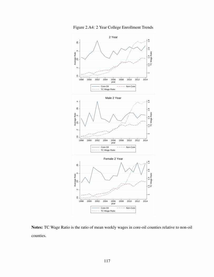
Figure 2.A4: 2 Year College Enrollment Trends

11.

21.

41.

61.

8T

C W

age

Rat

io

.15

.2.2

5.3

.35

Ave

rage

Rat

e

1998 2000 2002 2004 2006 2008 2010 2012 2014year

Core-Oil Non-CoreTC Wage Ratio

2 Year

11.

21.

41.

61.

8T

C W

age

Rat

io

.15

.2.2

5.3

.35

.4A

vera

ge R

ate

1998 2000 2002 2004 2006 2008 2010 2012 2014year

Core-Oil Non-CoreTC Wage Ratio

Male 2 Year

11.

21.

41.

61.

8T

C W

age

Rat

io

.15

.2.2

5.3

.35

Ave

rage

Rat

e

1998 2000 2002 2004 2006 2008 2010 2012 2014year

Core-Oil Non-CoreTC Wage Ratio

Female 2 Year

Notes: TC Wage Ratio is the ratio of mean weekly wages in core-oil counties relative to non-oil

counties.

117

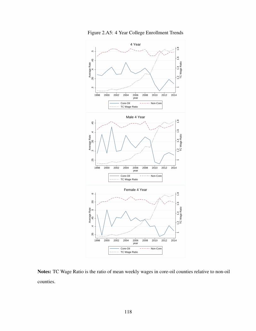
Figure 2.A5: 4 Year College Enrollment Trends

11.

21.

41.

61.

8T

C W

age

Rat

io

.3.3

5.4

.45

.5A

vera

ge R

ate

1998 2000 2002 2004 2006 2008 2010 2012 2014year

Core-Oil Non-CoreTC Wage Ratio

4 Year

11.

21.

41.

61.

8T

C W

age

Rat

io

.25

.3.3

5.4

.45

Ave

rage

Rat

e

1998 2000 2002 2004 2006 2008 2010 2012 2014year

Core-Oil Non-CoreTC Wage Ratio

Male 4 Year

11.

21.

41.

61.

8T

C W

age

Rat

io

.35

.4.4

5.5

.55

.6A

vera

ge R

ate

1998 2000 2002 2004 2006 2008 2010 2012 2014year

Core-Oil Non-CoreTC Wage Ratio

Female 4 Year

Notes: TC Wage Ratio is the ratio of mean weekly wages in core-oil counties relative to non-oil

counties.

118

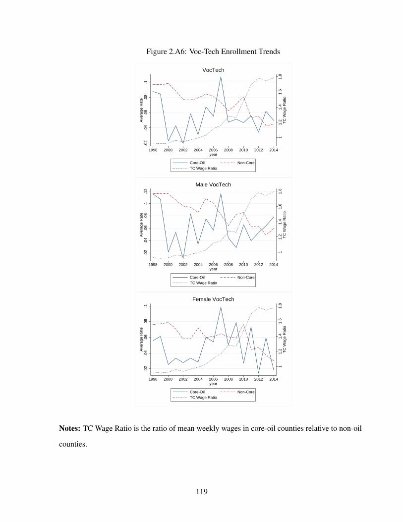
Figure 2.A6: Voc-Tech Enrollment Trends

11.

21.

41.

61.

8T

C W

age

Rat

io

.02

.04

.06

.08

.1A

vera

ge R

ate

1998 2000 2002 2004 2006 2008 2010 2012 2014year

Core-Oil Non-CoreTC Wage Ratio

VocTech

11.

21.

41.

61.

8T

C W

age

Rat

io

.02

.04

.06

.08

.1.1

2A

vera

ge R

ate

1998 2000 2002 2004 2006 2008 2010 2012 2014year

Core-Oil Non-CoreTC Wage Ratio

Male VocTech

11.

21.

41.

61.

8T

C W

age

Rat

io

.02

.04

.06

.08

.1A

vera

ge R

ate

1998 2000 2002 2004 2006 2008 2010 2012 2014year

Core-Oil Non-CoreTC Wage Ratio

Female VocTech

Notes: TC Wage Ratio is the ratio of mean weekly wages in core-oil counties relative to non-oil

counties.

119

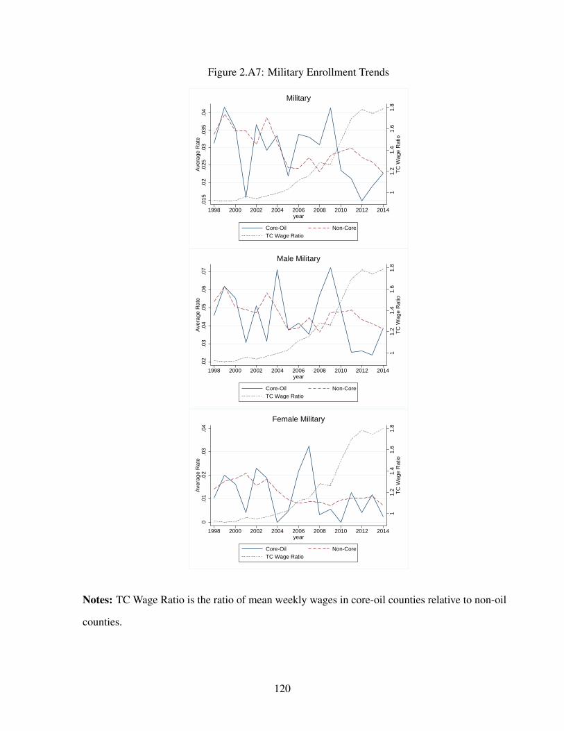
Figure 2.A7: Military Enrollment Trends

11.

21.

41.

61.

8T

C W

age

Rat

io

.015

.02

.025

.03

.035

.04

Ave

rage

Rat

e

1998 2000 2002 2004 2006 2008 2010 2012 2014year

Core-Oil Non-CoreTC Wage Ratio

Military

11.

21.

41.

61.

8T

C W

age

Rat

io

.02

.03

.04

.05

.06

.07

Ave

rage

Rat

e

1998 2000 2002 2004 2006 2008 2010 2012 2014year

Core-Oil Non-CoreTC Wage Ratio

Male Military

11.

21.

41.

61.

8T

C W

age

Rat

io

0.0

1.0

2.0

3.0

4A

vera

ge R

ate

1998 2000 2002 2004 2006 2008 2010 2012 2014year

Core-Oil Non-CoreTC Wage Ratio

Female Military

Notes: TC Wage Ratio is the ratio of mean weekly wages in core-oil counties relative to non-oil

counties.

120

Figure 2.A8: Unknown Decision Trends

11.

21.

41.

61.

8T

C W

age

Rat

io

.1.1

5.2

.25

Ave

rage

Rat

e

1998 2000 2002 2004 2006 2008 2010 2012 2014year

Core-Oil Non-CoreTC Wage Ratio

Employment

11.

21.

41.

61.

8T

C W

age

Rat

io

.1.1

5.2

.25

.3A

vera

ge R

ate

1998 2000 2002 2004 2006 2008 2010 2012 2014year

Core-Oil Non-CoreTC Wage Ratio

Male Employment

11.

21.

41.

61.

8T

C W

age

Rat

io

.05

.1.1

5.2

.25

Ave

rage

Rat

e

1998 2000 2002 2004 2006 2008 2010 2012 2014year

Core-Oil Non-CoreTC Wage Ratio

Female Employment

Notes: TC Wage Ratio is the ratio of mean weekly wages in core-oil counties relative to non-oil

counties.

121

CHAPTER 3

ECONOMIC CONDITIONS AND SLEEP

3.1 Introduction

The Centers for Disease Control and Prevention (CDC) recommends that adults ages 18

to 60 obtain at least 7-8 hours of sleep per night (CDC, 2017). Short term sleep deficiency

lowers cognitive performance and can increase the probability of motor vehicle and work related

accidents. Smith (2016) shows that even slight changes in sleep duration can have significant

societal costs. The author exploits daylight saving time, finding that the program increased fatal car

crash risk by over 5%, causing over 30 deaths per year between 2002-2011. Other literature studies

the link between sleep and productivity. Gibson and Shrader (2018) use exogenous variation in

sunset time, finding that a one-hour increase in location specific weekly sleep increases wages by

1.1% in the short run and 5% in the long run. The medical field has studied sleep and longer

term health outcomes. A CDC report from 2014 emphasized that sleeping less than 7 hours per

night is linked to increased risk for diabetes, high blood pressure, coronary heart disease, obesity,

and all-cause mortality (Liu et al., 2016). The report highlighted that more than one third of

adult respondents report less than 7 hours of sleep per night. Literature from multiple disciplines

suggests that sleep deficiency is a prevalent issue with significant societal costs.

Recent papers have exploited the American Time Use Survey (ATUS) to analyze economic

conditions and time use. Colman and Dave (2013) find that sleep duration is countercyclical. In

further support of this claim, Aguiar et al. (2013) estimate that about 30% of foregone market work

hours during the Great Recession were devoted to additional time spent sleeping and watching

television. However, no research has considered that economic conditions may differentially

impact weekday and weekend sleep behavior. Figure 3.1 motivates this separate analysis, showing

that individuals average 340 minutes of work on weekdays but only 89 minutes on weekends.

122

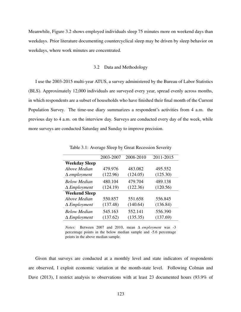
Meanwhile, Figure 3.2 shows employed individuals sleep 75 minutes more on weekend days than

weekdays. Prior literature documenting countercyclical sleep may be driven by sleep behavior on

weekdays, where work minutes are concentrated.

3.2 Data and Methodology

I use the 2003-2015 multi-year ATUS, a survey administered by the Bureau of Labor Statistics

(BLS). Approximately 12,000 individuals are surveyed every year, spread evenly across months,

in which respondents are a subset of households who have finished their final month of the Current

Population Survey. The time-use diary summarizes a respondent’s activities from 4 a.m. the

previous day to 4 a.m. on the interview day. Surveys are conducted every day of the week, while

more surveys are conducted Saturday and Sunday to improve precision.

Table 3.1: Average Sleep by Great Recession Severity

2003-2007 2008-2010 2011-2015Weekday SleepAbove Median 479.976 483.082 495.552∆ employment (122.96) (124.05) (125.30)Below Median 480.104 479.704 489.138∆ Employment (124.19) (122.36) (120.56)Weekend SleepAbove Median 550.857 551.658 556.845∆ Employment (137.48) (140.64) (136.84)Below Median 545.163 552.141 556.390∆ Employment (137.62) (135.35) (137.69)

Notes: Between 2007 and 2010, mean ∆ employment was -3percentage points in the below median sample and -5.6 percentagepoints in the above median sample.

Given that surveys are conducted at a monthly level and state indicators of respondents

are observed, I exploit economic variation at the month-state level. Following Colman and

Dave (2013), I restrict analysis to observations with at least 23 documented hours (93.9% of

123

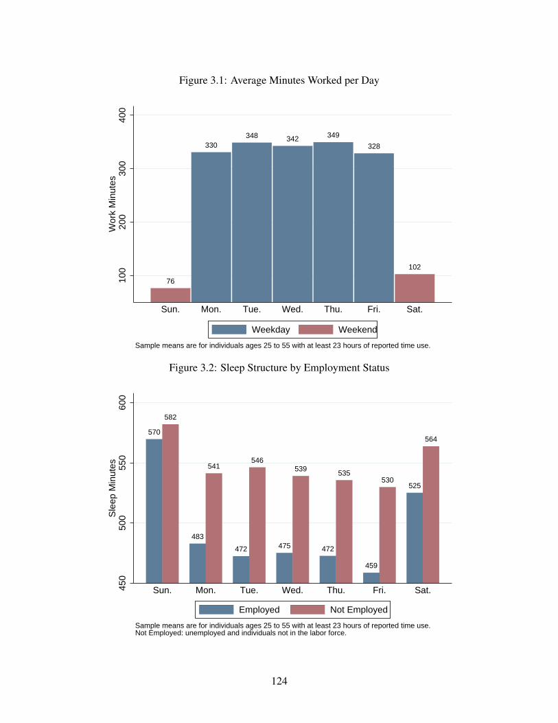
Figure 3.1: Average Minutes Worked per Day

76

330348 342 349

328

102

100

200

300

400

Wor

k M

inut

es

Sun. Mon. Tue. Wed. Thu. Fri. Sat.

Sample means are for individuals ages 25 to 55 with at least 23 hours of reported time use.

Weekday Weekend

Figure 3.2: Sleep Structure by Employment Status

570

582

483

541

472

546

475

539

472

535

459

530525

564

450

500

550

600

Sle

ep M

inut

es

Sun. Mon. Tue. Wed. Thu. Fri. Sat.

Sample means are for individuals ages 25 to 55 with at least 23 hours of reported time use.Not Employed: unemployed and individuals not in the labor force.

Employed Not Employed

124

observations) and to respondents ages 25 to 55. The descriptive statistics in Table 3.1 suggest

that weekday sleep increased more in states that experienced greater employment loss during the

Great Recession while weekend sleep increased more in states that were less impacted.

To empirically study the impact of economic conditions on sleep, I estimate model (3.1) via

OLS, where Yisdmt denotes minutes of sleep reported by individual i in state s on day of week d

in month m in year t. Xismt is a vector of individual characteristics that may affect sleep duration,

including age, gender, race, marital status, number of children, indicator for having a child under

3, education, gender and race interacted with education, industry occupation code, indicator for

whether the interview day was a holiday, and an indicator for incomplete time diary. Esmt is the

civilian employment-population ratio of state s in month m in year t. State fixed effects absorb

time invariant unobserved heterogeneity of state specific factors. Month, day of week, and year

fixed effects are also included while standard errors are clustered at the state level. This empirical

design parallels the large literature of economic conditions and health outcomes (Ruhm, 2000,

2005; Charles and DeCicca, 2008).

Yisdmt = βXismt + γEsmt +αs +θm +λd +ηt + εisdmt (3.1)

3.3 Results

Table 3.2 displays estimates of specification (3.1). A point estimate of -1.1 (similar to -.97

in Colman and Dave (2013)) in the first row of column 1 confirms previous literature in finding

that overall sleep is countercyclical. However, we may expect differential effects for weekdays

versus weekends due to sharp contrasts in work and sleep minutes illustrated in Figures 3.1-3.2.

Rows 2-3 of column 1 report results of specification (1) estimated separately by weekday versus

weekend sleep. Estimates suggest that a one percentage point increase in the employment rate

decreases weekday sleep by 2.3 minutes per night but actually increases weekend sleep by 1.8

minutes per night. The Great Recession was particularly salient for minorities and individuals

with less education (Engemann and Wall, 2009; Austin, 2009), motivating analysis by these

125

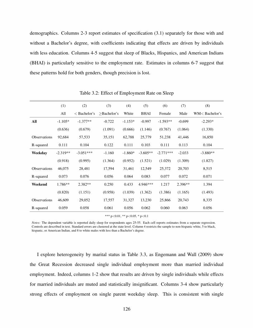
demographics. Columns 2-3 report estimates of specification (3.1) separately for those with and

without a Bachelor’s degree, with coefficients indicating that effects are driven by individuals

with less education. Columns 4-5 suggest that sleep of Blacks, Hispanics, and American Indians

(BHAI) is particularly sensitive to the employment rate. Estimates in columns 6-7 suggest that

these patterns hold for both genders, though precision is lost.

Table 3.2: Effect of Employment Rate on Sleep

(1) (2) (3) (4) (5) (6) (7) (8)

All < Bachelor’s ≥Bachelor’s White BHAI Female Male WM< Bachelor’s

All -1.105* -1.377** -0.722 -1.153* -0.997 -1.593** -0.699 -2.293*

(0.636) (0.679) (1.091) (0.666) (1.146) (0.767) (1.064) (1.330)

Observations 92,684 57,533 35,151 62,788 25,779 51,238 41,446 16,850

R-squared 0.111 0.104 0.122 0.111 0.103 0.111 0.113 0.104

Weekday -2.319** -3.051*** -1.160 -1.860* -3.605** -2.771*** -2.033 -3.880**

(0.918) (0.995) (1.364) (0.952) (1.521) (1.029) (1.309) (1.827)

Observations 46,075 28,481 17,594 31,461 12,549 25,372 20,703 8,515

R-squared 0.073 0.076 0.056 0.064 0.083 0.077 0.072 0.071

Weekend 1.786** 2.382** 0.250 0.433 4.946*** 1.217 2.396** 1.394

(0.820) (1.151) (0.958) (1.039) (1.362) (1.386) (1.165) (1.493)

Observations 46,609 29,052 17,557 31,327 13,230 25,866 20,743 8,335

R-squared 0.059 0.058 0.061 0.056 0.062 0.060 0.063 0.056

*** p<0.01, ** p<0.05, * p<0.1

Notes: The dependent variable is reported daily sleep for respondents ages 25-55. Each cell reports estimates from a separate regression.Controls are described in text. Standard errors are clustered at the state level. Column 4 restricts the sample to non-hispanic white, 5 to black,hispanic, or American Indian, and 8 to white males with less than a Bachelor’s degree.

I explore heterogeneity by marital status in Table 3.3, as Engemann and Wall (2009) show

the Great Recession decreased single individual employment more than married individual

employment. Indeed, columns 1-2 show that results are driven by single individuals while effects

for married individuals are muted and statistically insignificant. Columns 3-4 show particularly

strong effects of employment on single parent weekday sleep. This is consistent with single

126

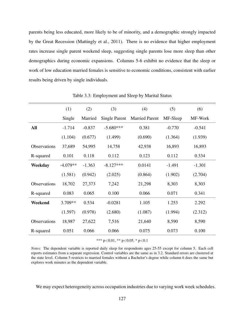
parents being less educated, more likely to be of minority, and a demographic strongly impacted

by the Great Recession (Mattingly et al., 2011). There is no evidence that higher employment

rates increase single parent weekend sleep, suggesting single parents lose more sleep than other

demographics during economic expansions. Columns 5-6 exhibit no evidence that the sleep or

work of low education married females is sensitive to economic conditions, consistent with earlier

results being driven by single individuals.

Table 3.3: Employment and Sleep by Marital Status

(1) (2) (3) (4) (5) (6)

Single Married Single Parent Married Parent MF-Sleep MF-Work

All -1.714 -0.837 -5.680*** 0.381 -0.770 -0.541

(1.104) (0.677) (1.499) (0.690) (1.364) (1.939)

Observations 37,689 54,995 14,758 42,938 16,893 16,893

R-squared 0.101 0.118 0.112 0.123 0.112 0.334

Weekday -4.079** -1.363 -8.127*** 0.0141 -1.491 -1.301

(1.581) (0.942) (2.025) (0.864) (1.902) (2.704)

Observations 18,702 27,373 7,242 21,298 8,303 8,303

R-squared 0.083 0.065 0.100 0.066 0.071 0.341

Weekend 3.709** 0.534 -0.0281 1.105 1.253 2.292

(1.597) (0.978) (2.680) (1.087) (1.994) (2.312)

Observations 18,987 27,622 7,516 21,640 8,590 8,590

R-squared 0.051 0.066 0.066 0.075 0.073 0.100

*** p<0.01, ** p<0.05, * p<0.1

Notes: The dependent variable is reported daily sleep for respondents ages 25-55 except for column 5. Each cellreports estimates from a separate regression. Control variables are the same as in 3.2. Standard errors are clustered atthe state level. Column 5 restricts to married females without a Bachelor’s degree while column 6 does the same butexplores work minutes as the dependent variable.

We may expect heterogeneity across occupation industries due to varying work week schedules.

127

For every CPS major industry code, I create the variable

Fracday =xwd

xwd + xwe,

where xwd (xwe) is mean reported work minutes on a weekday (weekend) day. Figure 3.3 shows

that Fracday ranges from .58 in leisure and hospitality to .86 in the financial activities sector.

An increase in the employment rate should particularly impact the weekday sleep of individuals

who work in weekday heavy industries. Columns 3-4 of Table 3.4 estimate specification (3.1)

separately for individuals who work in industries

Figure 3.3: Workweek Structure by Industry

.4.5

.6.7

.8.9

Fra

cday

Leisu

re &

Hos

pitali

ty

Armed

For

ces

Ag, F

ores

try, F

ishing

Who

lesale

& R

etail

Other

Ser

vices

Trans

pora

tion

& Utili

ties

Mini

ng

Educa

tion

& Hea

lth

Public

Adm

inistr

ation

Info

rmat

ion

Prof.

& Bus

iness

Constr

uctio

n

Man

ufac

turin

g

Financ

ial A

ctivit

ies

Notes: Fracday = xwdxwd+xwe

, where xwd (xwe) is mean reported work minutes on a weekday

(weekend) day.

128

Table 3.4: Employment Effects by Workweek Structure

(1) (2) (3) (4) (5) (6)

Employed Not Employed >Med Fracday ≤Med Fracday Blue-Collar White-Collar

All -1.346* 0.222 -1.384 -0.587 -3.308* 0.886

(0.791) (1.600) (0.957) (1.061) (1.732) (0.877)

Observations 74,324 18,360 36,640 42,599 14,744 15,392

R-squared 0.116 0.068 0.137 0.094 0.152 0.145

Weekday -2.275** -1.493 -2.923** -0.699 -6.001*** 0.0778

(1.050) (2.142) (1.116) (1.427) (1.830) (1.185)

Observations 37,088 8,987 18,320 21,094 7,310 7,791

R-squared 0.048 0.070 0.052 0.053 0.061 0.071

Weekend 1.089 3.859 2.857** -0.176 3.473 3.278**

(0.883) (2.316) (1.295) (1.408) (2.271) (1.476)

Observations 37,236 9,373 18,320 21,505 7,434 7,601

R-squared 0.061 0.060 0.079 0.052 0.099 0.084

*** p<0.01, ** p<0.05, * p<0.1

Notes: The dependent variable is reported daily sleep for respondents ages 25-55. Each cell reports estimates from a separate regression.

Column 1 restricts the sample to employed while column 2 restricts to the unemployed and out-of-labor force. Fracday = xwdxwd+xwe

, where xwd

(xwe) is mean reported work minutes on a weekday (weekend) day. Column 3 restricts to below median Fracday while 4 is above median.

Columns 5-6 split the ≥Med Fracday sample by work type. Blue-Collar: construction and manufacturing. White-Collar: financial activities

and professional and business services. Control variables are the same as in 3.2. Standard errors are clustered at the state level.

with above and below median Fracday values. Weekday and weekend sleep results are driven

by industries with weekday concentrated work schedules. Columns 5-6 split the top four “Fracday”

industries into blue-collar and white-collar segments. Estimates indicate that the strong negative

effect of employment on weekday sleep is driven by blue-collar, weekday centric industries.

3.4 Conclusion

This is the first paper to uncover that economic expansions decrease weekday sleep but actually

increase weekend sleep. A limitation of this analysis is that the welfare consequences of these

changes in sleep are not obvious. The CDC recommends a consistent sleep schedule and the

129

National Institutes of Health (NIH) emphasizes that sleeping more on the weekend doesn’t fully

correct one’s sleep debt (Patlak, 2005). If this is true, then the value of sleep depends on both

the average and variance of sleep within a week. If economic expansions reduce average sleep

and increase the gap between weekend and weekday sleep, then prior work relying on weekly

sleep averages underestimate the cost of lost sleep. As sleep deprivation is a key cause of

motor vehicle crashes, my findings have implications for papers researching economic conditions

and motor vehicle fatalities, accident related death, workplace injury, or other sleep related

outcomes. Differential results concerning economic conditions and sleep by day type may be

one mechanism for which to expect economic conditions to impact other sleep related outcomes

diversely depending on day of the week.

130

BIBLIOGRAPHY

Aguiar, Mark, Erik Hurst, and Loukas Karabarbounis, “Time use during the great recession,”The American Economic Review, 2013, 103 (5), 1664–1696.

Allen, Sarah and Kerry Daly, “The effects of father involvement: A summary of the researchevidence,” The FII-ONews, 2002, 1 (1-11).

Anderson, D. Mark, Joseph J. Sabia, and Erdal Tekin, “Child Access Prevention Laws andJuvenile Firearm-Related Homicides,” IZA Discussion Papers 11898, Institute for the Study ofLabor (IZA) 2018.

Anderson, Mark and Joseph Sabia, “Child Access Prevention Laws, Youth Gun Carrying, andSchool Shootings,” Journal of Law and Economics, in press.

Andrews, Rodney J. and Monica Deza, “Local natural resources and crime: Evidence fromoil price fluctuations in Texas,” Journal of Economic Behavior & Organization, 2018, 151 (C),123–142.

Aneja, Abhay, John J Donohue III, and Alexandria Zhang, “The impact of right-to-carry lawsand the NRC report: lessons for the empirical evaluation of law and policy,” American Law andEconomics Review, 2011, 13 (2), 565–631.

Austin, Algernon, “American Indians and the great recession. Economic disparities grow larger.,”2009.

Ayres, Ian and John J Donohue III, “The latest misfires in support of the “more guns, lesscrime" hypothesis,” Stanford Law Review, 2003, pp. 1371–1398.

and Steven D Levitt, “Measuring positive externalities from unobservable victim precaution:an empirical analysis of Lojack,” The Quarterly Journal of Economics, 1998, 113 (1), 43–77.

Azrael, Deborah, Lisa Hepburn, David Hemenway, and Matthew Miller, “The stock and flowof US firearms: results from the 2015 National Firearms Survey,” Russell Sage Foundation, 2017.

Bartik, Alexander, Janet Currie, Michael Greenstone, and Christopher R Knittel, “The localeconomic and welfare consequences of hydraulic fracturing,” 2016.

Bertrand, Marianne, Esther Duflo, and Sendhil Mullainathan, “How much should wetrust differences-in-differences estimates?,” The Quarterly journal of economics, 2004, 119 (1),249–275.

Black, Dan A and Daniel S Nagin, “Do right-to-carry laws deter violent crime?,” The Journalof Legal Studies, 1998, 27 (1), 209–219.

, Terra G McKinnish, and Seth G Sanders, “Tight labor markets and the demand foreducation: Evidence from the coal boom and bust,” Industrial & Labor Relations Review, 2005,59 (1), 3–16.

131

Blanden, Jo and Paul Gregg, “Family income and educational attainment: a review ofapproaches and evidence for Britain,” Oxford Review of Economic Policy, 2004, 20 (2), 245–263.

Boffy-Ramirez, Ernest, Benjamin Hansen, and Hani Mansour, “The effect of business cycleson educational attainment,” Available at SSRN 2294146, 2013.

Brown, Chip, “North Dakota Went Boom,” The New York Times, 2013.

Cameron, A Colin and Pravin K Trivedi, Microeconometrics: methods and applications,Cambridge university press, 2005.

Card, David and Thomas Lemieux, “Dropout and enrollment trends in the postwar period:What went wrong in the 1970s?,” in “Risky behavior among youths: An economic analysis,”University of Chicago Press, 2001, pp. 439–482.

Carpenter, Tom, “15 Tips for Opening Day of Gun Season,”https://www.realtree.com/deer-hunting/articles/15-tips-for-opening-day-of-gun-season 2018.Online; accessed 2018-07-05.

Cascio, Elizabeth U and Ayushi Narayan, “Who needs a fracking education? the educationalresponse to low-skill biased technological change,” Technical Report, National Bureau ofEconomic Research 2015.

Case, Anne and Lawrence Katz, “The Company You Keep: The Effects of Family andNeighborhood on Disadvanted Youths,” 1991. NBER Working Paper No. 3705.

CDC, “How much sleep do I need?,” 2017.

Center, Labor Market Information, “North Dakot’s Oil and Gas Economy,” Job Service NorthDakota, 2017.

Chapman, Simon, Phillip Alpers, Kingsley Agho, and Mike Jones, “AustraliaâAZs 1996 gunlaw reforms: faster falls in firearm deaths, firearm suicides, and a decade without mass shootings,”Injury Prevention, 2006, 12 (6), 365–372.

Charles, Kerwin Kofi and Philip DeCicca, “Local labor market fluctuations and health: is therea connection and for whom?,” Journal of health economics, 2008, 27 (6), 1532–1550.

Cheng, Cheng and Mark Hoekstra, “Does strengthening self-defense law deter crime orescalate violence? Evidence from expansions to castle doctrine,” Journal of Human Resources,2013, 48 (3), 821–854.

Cobb-Clark, Deborah A and Erdal Tekin, “Fathers and youthsâAZ delinquent behavior,”Review of Economics of the Household, 2014, 12 (2), 327–358.

Colman, Gregory and Dhaval Dave, “Exercise, physical activity, and exertion over the businesscycle,” Social Science & Medicine, 2013, 93, 11–20.

Conlin, Michael, Stacy Dickert-Conlin, and John Pepper, “The Deer Hunter: The UnintendedEffects of Hunting Regulations,” The Review of Economics and Statistics, 2009, 91 (1), 178–187.

132

Cook, Philip J and Jens Ludwig, “The social costs of gun ownership,” Journal of PublicEconomics, 2006, 90 (1-2), 379–391.

, , and Adam Samaha, “Gun control after Heller: litigating against regulation,” in “Regulationvs. Litigation: Perspectives from Economics and Law,” University of Chicago Press, 2010,pp. 103–135.

Cummings, Peter, David C Grossman, Frederick P Rivara, and Thomas D Koepsell, “Stategun safe storage laws and child mortality due to firearms,” JAMA, 1997, 278 (13), 1084–1086.

Dahl, Gordon and Stefano DellaVigna, “Does movie violence increase violent crime?,” TheQuarterly Journal of Economics, 2009, 124 (2), 677–734.

Dakota, North, “Legislative Highlights 2013,” http://governor.nd.gov/media-center/news/legislative-highlights-2013-legislature-providesmore-tax-relief-strong-funding-st2013. Accessed: 2015-04-13.

Dellas, Harris and Plutarchos Sakellaris, “On the cyclicality of schooling: theory andevidence,” Oxford Economic Papers, 2003, 55 (1), 148–172.

DeSimone, Jeffrey, Sara Markowitz, and Jing Xu, “Child access prevention laws and nonfatalgun injuries,” Southern economic journal, 2013, 80 (1), 5–25.

Dezhbakhsh, Hashem and Paul H Rubin, “Lives saved or lives lost? The effects ofconcealed-handgun laws on crime,” The American Economic Review, 1998, 88 (2), 468–474.

Dube, Arindrajit, Oeindrila Dube, and Omar García-Ponce, “Cross-border spillover: US gunlaws and violence in Mexico,” American Political Science Review, 2013, 107 (3), 397–417.

Duggan, Mark, “More guns, more crime,” Journal of political Economy, 2001, 109 (5),1086–1114.

, Randi Hjalmarsson, and Brian A Jacob, “The short-term and localized effect of gun shows:Evidence from California and Texas,” Review of Economics and Statistics, 2011, 93 (3), 786–799.

Edwards, Griffin, Erik Nesson, Joshua J Robinson, and Fredrick Vars, “Looking down thebarrel of a loaded gun: The effect of mandatory handgun purchase delays on homicide andsuicide,” The Economic Journal, 2018, 128 (616), 3117–3140.

Engemann, Kristie and Howard J Wall, “The effects of recessions across demographic groups,”2009.

Evans, William N, Craig Garthwaite, and Timothy J Moore, “Guns and Violence: TheEnduring Impact of Crack Cocaine Markets on Young Black Males,” Technical Report, NationalBureau of Economic Research 2018.

Evans, William, Wooyoung Kim et al., “The impact of local labor market conditions on thedemand for education: evidence from Indian casinos,” US Census Bureau Center for EconomicStudies Discussion Paper, 2006, 614.

133

Fabio, Anthony, Jessica Duell, Kathleen Creppage, Kerry O’Donnell, and Ron Laporte,“Gaps continue in firearm Surveillance: Evidence from a large US city Bureau of Police,” SocialMedicine, 2016, 10 (1), 13–21.

FBI, “National Incident-Based Reporting System, 1991,” Inter-university Consortium forPolitical and Social Research [distributor], 2009.

FBI, “Crime in the United States, 2015: Violent Crime,”https://ucr.fbi.gov/crime-in-the-u.s/2015/crime-in-the-u.s.-2015/offenses-known-to-law-enforcement/violent-crime/violentcrimemain_final.pdf 2016. Online; accessed2018-06-05.

Fetzer, Thiemo, “Fracking growth,” 2014.

Feyrer, James, Erin T. Mansur, and Bruce Sacerdote, “Geographic Dispersion of EconomicShocks: Evidence from the Fracking Revolution,” American Economic Review, April 2017, 107(4), 1313–34.

Gibson, Matthew and Jeffrey Shrader, “Time use and labor productivity: the returns to sleep,”Review of Economics and Statistics, 2018, (00).

Gius, Mark, “The effects of state and federal background checks on state-level gun-relatedmurder rates,” Applied economics, 2015, 47 (38), 4090–4101.

Glaeser, Edward L and Bruce Sacerdote, “Why is there more crime in cities?,” Journal ofpolitical economy, 1999, 107 (S6), S225–S258.

and Spencer Glendon, “Who owns guns? Criminals, victims, and the culture of violence,” TheAmerican Economic Review, 1998, 88 (2), 458–462.

Harper, Cynthia C and Sara S McLanahan, “Father absence and youth incarceration,” Journalof research on adolescence, 2004, 14 (3), 369–397.

hunter63, “How do you lose the guilt of hunting?,”http://www.wilderness-survival.net/forums/showthread.php?29321-How-do-you-lose-the-guilt-of-hunting 2017. Online; accessed 2018-09-20.

Igielnik, Ruth, “Rural and urban gun owners have different experiences, viewson gun policy,” http://www.pewresearch.org/fact-tank/2017/07/10/rural-and-urban-gun-owners-have-different-experiences-views-on-gun-policy/ 2017. Online; accessed 2018-08-08.

Jacob, Brian A and Lars Lefgren, “Are idle hands the devil’s workshop? Incapacitation,concentration, and juvenile crime,” American Economic Review, 2003, 93 (5), 1560–1577.

Jacobson, Louis S, Robert J LaLonde, and Daniel G Sullivan, “Earnings losses of displacedworkers,” The American economic review, 1993, pp. 685–709.

James, Alexander and Brock Smith, “There will be blood: Crime rates in shale-rich UScounties,” Journal of Environmental Economics and Management, 2017, 84, 125–152.

134

Jena, Anupam B and Andrew R Olenski, “Reduction in firearm injuries during NRA annualconventions,” New England journal of medicine, 2018, 378 (9), 866–867.

Jr, John R Lott and David B Mustard, “Crime, deterrence, and right-to-carry concealedhandguns,” The Journal of Legal Studies, 1997, 26 (1), 1–68.

and John E Whitley, “Safe-storage gun laws: accidental deaths, suicides, and crime,” TheJournal of Law and Economics, 2001, 44 (S2), 659–689.

JRSA, “Incident Based Reporting Resource Center,” http://www.jrsa.org/ibrrc/background-status/nibrs-states.html2018. Online; accessed 2018-06-05.

Kearney, Melissa S. and Riley Wilson, “Male Earnings, Marriageable Men, and NonmaritalFertility: Evidence from the Fracking Boom,” The Review of Economics and Statistics, 2018, 100(4), 678–690.

Kleck, Gary, “Measures of gun ownership levels for macro-level crime and violence research,”Journal of Research in Crime and Delinquency, 2004, 41 (1), 3–36.

and E Britt Patterson, “The impact of gun control and gun ownership levels on violence rates,”Journal of Quantitative Criminology, 1993, 9 (3), 249–287.

Knight, Brian, “State gun policy and cross-state externalities: Evidence from crime gun tracing,”American Economic Journal: Economic Policy, 2013, 5 (4), 200–229.

Koper, Christopher S, “Crime gun risk factors: buyer, seller, firearm, and transactioncharacteristics associated with gun trafficking and criminal gun use,” Journal of quantitativecriminology, 2014, 30 (2), 285–315.

Kovandzic, Tomislav, Mark E Schaffer, and Gary Kleck, “Estimating the causal effect of gunprevalence on homicide rates: A local average treatment effect approach,” Journal of quantitativecriminology, 2013, 29 (4), 477–541.

Langton, Lynn, Firearms stolen during household burglaries and other property crimes,2005-2010, US Department of Justice, Office of Justice Programs, Bureau of Justice Statistics,2012.

Leigh, Andrew and Christine Neill, “Do gun buybacks save lives? Evidence from panel data,”American Law and Economics Review, 2010, 12 (2), 509–557.

Lindo, Jason M and Charles Stoecker, “Drawn into violence: Evidence on “what makes acriminal” from the Vietnam draft lotteries,” Economic Inquiry, 2014, 52 (1), 239–258.

, Peter Siminski, and Isaac D Swensen, “College party culture and sexual assault,” AmericanEconomic Journal: Applied Economics, 2018, 10 (1), 236–65.

Liu, Y, AG Wheaton, DP Chapman, TJ Cunningham, H Lu, and JB Croft, “Prevalence ofHealthy Sleep Duration among Adults – United States, 2014,” Morbidity and Mortality WeeklyReport (CDC), 2016, 65, 137–141.

135

Lochner, Lance and Enrico Moretti, “The effect of education on crime: Evidence from prisoninmates, arrests, and self-reports,” American economic review, 2004, 94 (1), 155–189.

Ludwig, Jens, “Concealed-gun-carrying laws and violent crime: evidence from state panel data,”International Review of law and Economics, 1998, 18 (3), 239–254.

Manski, Charles F and David A Wise, College choice in America, Harvard University Press,1983.

Matthay, Ellicott C, Jessica Galin, Kara E Rudolph, Kriszta Farkas, Garen J Wintemute,and Jennifer Ahern, “In-state and interstate associations between gun shows and firearm deathsand injuries: a quasi-experimental study,” Annals of internal medicine, 2017, 167 (12), 837–844.

Mattingly, Marybeth J, Kristin Smith, and Jessica A Bean, “Unemployment in the GreatRecession: Single parents and men hit hard,” 2011.

Moody, Carlisle E and Thomas B Marvell, “Guns and crime,” Southern Economic Journal,2005, pp. 720–736.

Morral, Andrew R, Rajeev Ramchand, Rosanna Smart, Carole Roan Gresenz, SamanthaCherney, Nancy Nicosia, Carter C Price, Stephanie Brooks Holliday, Elizabeth L PetrunSayers, Terry L Schell et al., “The Science of Gun Policy,” 2018.

O’Flaherty, Brendan and Rajiv Sethi, “Homicide in black and white,” Journal of UrbanEconomics, 2010, 68 (3), 215–230.

Parker, Kim, “Among gun owners NRA members have a unique set ofviews and experiences,” http://www.pewresearch.org/fact-tank/2017/07/05/among-gun-owners-nra-members-have-a-unique-set-of-views-and-experiences 2018. Online; accessed2018-08-05.

Patlak, Margie, Your guide to healthy sleep, US Department of Health and Human Services,2005.

QDMA, “Whitetail Report,” https://www.qdma.com/about/whitetail-reports/ 2017. Online;accessed 2018-07-15.

Research, Pew, “Rural and urban gun owners have different experiences,views on gun policy,” http://www.pewresearch.org/fact-tank/2017/07/10/rural-and-urban-gun-owners-have-different-experiences-views-on-gun-policy 2017. Online; accessed2018-08-04.

Rivkin, Steven G, “Black/white differences in schooling and employment,” Journal of HumanResources, 1995, pp. 826–852.

Robinson, Steve, “What about the emotional impact of killing? How does that affect soldiers?,”https://www.pbs.org/wgbh/pages/frontline/shows/heart/themes/prep.html 2005. Online; accessed2018-09-20.

136

Rohlfs, Chris, “Does combat exposure make you a more violent or criminal person? Evidencefrom the Vietnam draft,” Journal of Human resources, 2010, 45 (2), 271–300.

Rosengart, Matthew, P Cummings, Avery Nathens, P Heagerty, Ronald Maier, andF Rivara, “An evaluation of state firearm regulations and homicide and suicide death rates,”Injury Prevention, 2005, 11 (2), 77–83.

Rowhani-Rahbar, Ali, Vivian H Lyons, Joseph A Simonetti, Deborah Azrael, and MatthewMiller, “Formal firearm training among adults in the USA: results of a national survey,” Injuryprevention, 2018, 24 (2), 161–165.

Rubin, Paul H and Hashem Dezhbakhsh, “The effect of concealed handgun laws on crime:beyond the dummy variables,” International Review of Law and Economics, 2003, 23 (2),199–216.

Rudolph, Kara E, Elizabeth A Stuart, Jon S Vernick, and Daniel W Webster, “Associationbetween ConnecticutâAZs permit-to-purchase handgun law and homicides,” American journal ofpublic health, 2015, 105 (8), e49–e54.

Ruhm, Christopher J., “Are Recessions Good For Your Health?,” Quarterly Journal ofEconomics, 2000, 115 (2), 617–650.

Ruhm, Christopher J, “Healthy living in hard times,” Journal of Health Economics, 2005, 24(2), 341–363.

Shapiro, Craig, “What do children learn when they’re taught tokill?,” https://www.ctpost.com/opinion/article/What-do-children-learn-when-they-re-taught-to-9517184.php 2016. Online; accessed 2018-09-20.

Smith, Austin C, “Spring forward at your own risk: Daylight saving time and fatal vehiclecrashes,” American Economic Journal: Applied Economics, 2016, 8 (2), 65–91.

Street, Brittany, “The Impact of Economic Opportunity on Criminal Behavior: Evidence fromthe Fracking Boom,” 2018. Working Paper.

Warner, John T, “The Effect of Civilian Economy on Recruiting and Retention,” Military Pay ;Defense.gov, 2012.

Webster, Daniel, Cassandra Kercher Crifasi, and Jon S Vernick, “Effects of the repeal ofMissouri’s handgun purchaser licensing law on homicides,” Journal of Urban Health, 2014, 91(2), 293–302.

Wilson, Riley, “Moving to economic opportunity: the migration response to the fracking boom,”Available at SSRN 2814147, 2016.

Wright, James D and Peter H Rossi, “Armed and considered dangerous: A survey of felons andtheir weapons,” 1986.

Yamane, David, “The sociology of US gun culture,” Sociology compass, 2017, 11 (7), e12497.

137

Zawitz, Marianne W, “Guns used in crime,” Washington, DC: US Department of Justice:Bureau of Justice Statistics Selected Findings, publication NCJ-148201, 1995.

138