MINISTRY OF EDUCATION AND SCIENCE OF UKRAINE

TERNOPIL NATIONAL ECONOMIC UNIVERSITY

Iryna Chyrak

MICROECONOMICS

Textbook

Ternopil TNEU 2018

2

UDK 330.101.542 C-64

Reviewers: Kyrylenko Volodymyr Ivanovych – Doctor of Economic Science, Professor, Head of the

Department of economic theory of Kyiv National Economic University named after Vadym Hetman.

Strishenets Olena Mykolayivna – Doctor of Economic Science, Professor, Head of the Department of analytical economy and nature management of the Eastern European National University named after Lesia Ukrayinka.

Kyrych Natalia Bohdanivna – Doctor of Economic Science, Professor, Head of the Department of management in the production area of the Ternopil National Technical University named after Ivan Pulyuy.

Recommended for publication

by the Academic Council of Ternopil National Economic University (Protocol No 5 dated December 21, 2018).

Chyrak Iryna

C-64 Microeconomics : Textbook / Edited by Iryna Chyrak. – Ternopil : TNEU, 2018. – 223 p.

The textbook provides an integrated statement of the theoretical and methodological foundations of microeconomics as a science about the basic laws of the market economy functioning at the level of producer and consumer, which reveals the mechanism of decision-making by business entities who seek to achieve maximum needs satisfaction due to limited resources. By its structure and content, the textbook will help students to form the knowledge about the mechanisms and principles of the functioning of economic agents in market conditions, their incentive motives and economic decisions, the ability to analyze the functional relationships between the main economic parameters of the theoretical models and determine the expected results of the decisions, accepted by economic agents in different market situations, use the microeconomic analysis toolkit to evaluate the choice rationality of microsystem decisions, optimize their behavior and apply microeconomic research techniques in order to explain phenomena and analysis of economic results of the business systems. The main textbook’s task is to provide students with the knowledge of the fundamental theoretical and methodological principles of microeconomics and explain the internal relations and relations between economic phenomena, the implantation of skills to use and apply acquired knowledge in solving practical problems, the ability to perform technical and economic calculations related to justification of the optimality of the microeconomic systems decisions, use the microeconomic analysis tools in their further professional activity. Each chapter is devoted to the research of specific phenomena and processes occurring in the microsystem and ends with training which includes basic terms and concepts, questions and tasks for students’ self-control, tasks and tests.

The textbook is recommended for students, postgraduates and lecturers of higher education institutions, as well as for anyone interested in microeconomics.

UDK 330.101.542

© Iryna Chyrak., 2018

3

CONTENT

INTRODUCTION....................................................................................................7 Theme 1.

The Subject and Methods of Microeconomics...................................................... 8 1.1 Microeconomics as a science and historical stages of its development...............8 1.2. Essence and structure of the Microsystem..........................................................12 1.3. Subject and methods of microeconomic research.............................................. 15 Training.......................................................................................................................18

CHAPTER I.

THE THEORY OF CONSUMER BEHAVIOR Theme 2. The Theory of Consumer Behavior. The Marginal Utility of Product..................21 2.1. The humans needs: essence and structure. The law of increasing needs........... 21 2.2. Utility and its functions. Marginal utility of product. The Gossen’s first law......25 2.3. The consumer’s equilibrium. The Gossen’s second law.................................... 31 Training..................................................................................................................... 33 Theme 3. The Ordinal Theory of Consumer’s Behavior......................................................38 3.1. The Consumer’s choice from ordinal positions and the axiom

of the rational consumer behavior.......................................................................38 3.2. Indifference curves and their properties............................................................. 40 3.3. The budget constraints of consumer and its graphical representation................43 3.4 The consumer’s optimum in providing the rational consumer’s choice............. 46 Training..................................................................................................................... 48 Theme 4.

The Analysis of Consumer’s Behavior.................................................................. 53 4.1. The consumer’s reaction to the change of own income. Engel’s curves........... 53 4.2. The consumer’s reaction to the change of prices of goods.

Curve “Price-consumption” and individual demand curve.................................56 4.3. The income and substitution effects. The Giffen paradox.....................................59 Training..................................................................................................................... 62

4

Theme 5.

Demand, Supply and Market Equilibrium............................................................67 5.1. Demand, factors of demand. The law of demand...............................................67 5.2. Supply, factors of supply. The law of supply......................................................70 5.3. The market equilibrium.........................................................................................72 5.4. Elasticity of demand: indicators and factors of impact...................................... 74 5.5. Elasticity of supply..............................................................................................77 Training..................................................................................................................... 78

СHAPTER II.

THE PRODUCER’S BEHAVIOR THEORY Theme 6.

The Microeconomic Model of the Enterprise....................................................... 82 6.1. Comparative features of the firm and enterprise.................................................82 6.2. The enterprise as a part of microeconomic system. Types of enterprises..............84 6.3. Instant, short-term and long-term market periods

of the enterprise functioning................................................................................87 6.4. The concept of production functions, their properties, types and forms

of presentation.....................................................................................................89 Training..................................................................................................................... 90 Theme 7. The Variation of Production Factors and the Producer’s Optimum...................91 7.1. The production function with one variable factor.

Total, average and marginal product...................................................................91 7.2. The production function with two variables. The curve of the same

product – isoquant. Marginal rate of technical substitution of resources.............93 7.3. The choice of a combination of production factors due to the minimizing

costs or maximizing output criterion. Isocost curve...........................................96 7.4. The producer’s optimum: graphical, algebraic, economic forms

of his equilibrium functioning............................................................................98 Training......................................................................................................................100 Theme 8. Cost and Income of Enterprise................................................................................104 8.1. Cost of the enterprise. Economic and accounting approaches

to cost determination...........................................................................................104 8.2. Cost of the enterprise in short-term market period..............................................106 8.3. Сost of the enterprise in long-term market period...............................................108 8.4. The concept of the minimal effective size of the enterprise

and the structure of the industry......................................................................... 110 8.5. The essence and forms of income of the enterprise............................................112 Training........................................................................................................................113

5

CHAPTER III.

BEHAVIOR OF FIRM IN DIFFERENT MARKET STRUCTURES Theme 9. The Market of Perfect Competition........................................................................118 9.1. Peculiarities and conditions of the competitive market model............................118 9.2. Demand for products, income and profit of the competitive firm......................120 9.3. Maximization of the firm’s profit in conditions of perfect competition..............122 Training.......................................................................................................................125 Theme 10. The Monopoly Market...................................................................................................131 10.1. The monopoly market and its features..............................................................131 10.2. The demand for products of monopoly firm and its income.............................133 10.3. Short-term and long-term equilibrium of monopoly market..............................135 10.4. Monopoly pricing, monopoly discrimination...................................................137 10.5. Economic consequences of market monopolization.

Necessity and methods of antitrust regulation....................................................139 Training.......................................................................................................................142 Theme 11. The Monopolistic Competition......................................................................................146 11.1. Peculiarities of the monopolistic market................................................................ 146 11.2. The equilibrium of monopolistic manufacturer in short-run

and long-run market periods......................................................................................147 11.3. Non-price competition.............................................................................................150 Training........................................................................................................................152 Theme 12. The Oligopoly...................................................................................................................156 12.1. The oligopoly features.............................................................................................156 12.2. Models of uncooperated oligopoly: models of the quantitative oligopoly

of Cournot and Stackelberg and the model of the Bertrand price oligopoly.......158 12.3. The model "broken demand curve"...................................................................161 12.4. Models of cooperative oligopolies: a model of a cartel and a model

of a dominant firm.............................................................................................163 12.5. Game theory..................................................................................................... 165 Training......................................................................................................................169 Theme 13. The Market of Factors of Production....................................................................172 13.1. Factors of production, the essence and classification.......................................172 13.2. The optimal use of productive resources in the long-run market period.............175

6

13.3. Peculiarities of the labor market functioning: demand, supply and market equilibrium.......................................................................................176

13.4. Capital as productive resource of long-term use. Forms of capital...................178 13.5. Justification of investment decisions concerning the use

of production factors in long-run market period...............................................182 Training.......................................................................................................................185

CHAPTER IV.

GENERAL EQUILIBRIUM AND INSTITUTIONAL PROVIDING

OF EFFECTIVE MARKET FUNCTIONING Theme 14. The General Equilibrium and Welfare Economy.................................................189 14.1. The market equilibrium and its analysis. Partial and general equilibrium...........189 14.2. Equilibrium in economy of exchange and the efficiency

of resources distribution....................................................................................191 14.3. The welfare economy to context general market equilibrium..........................196 Training..................................................................................................................... 199 Theme 15.

The Institutional Effects of Market Economy.......................................................200 15.1. The institutional environment of market economy. Transaction costs.............200 15.2. External effects. The Coase’s theorem.............................................................202 15.3. Peculiarities of public goods and conditions of its use.....................................204 15.4. The social choice theory and its role in market economy.................................207 Training.......................................................................................................................209 GLOSSARY..............................................................................................................210 REFERENCES.........................................................................................................221

7

INTRODUCTION

The textbook on discipline "Microeconomics" has been prepared for students of the English language program of the specialty "International Economics" in order to form their knowledge of the interaction of individual economic actors, their behavior and mechanisms by which they make decisions and seek to achieve the goal due to limited economic resources, and also about the mechanism of specific markets functioning.

The focus of Microeconomics is the consumer behavior model that generates demand for the desired preferences and budget, the activity of the manufacturer and its optimization, market demand and supply, factors determining the price and sales volumes at the market of a particular product, profit maximization due to the type of market structure, resource allocation efficiency, etc.

The textbook’s main purpose is to provide students with knowledge of the behavior of economic agents in market conditions, to equip them with a universal instrument for the adoption of optimal economic decisions making due to the limited resources. The consequences of these decisions are reflected in the person’s everyday life through a thoughtful and meaningful attitude to the economic environment phenomena, ability to solve economic problems, ability to apply elements of economic knowledge to specific economic situations.

The textbook explores the following main problems of Microeconomics such as: consumer behavior theory, production theory, peculiarities of cost forming in short and long-term market periods, the company's decision on prices and production volumes in conditions of different market models: perfect competition, monopoly, monopolistic competition and oligopoly, the origin of the demand for resources and the mechanism of formation of prices for them, as well as the mechanism for achieving the general equilibrium and the efficiency of the market system functioning at the macro level.

The structure of the textbook contains 15 themes each of which explores specific phenomena. Each theme ends with a training course that includes the main economic terms, questions for students’ self-control, test and tasks. At the end of the textbook there are glossary and references.

The textbook on discipline "Microeconomics" will promote the formation of the following competencies by students:

- possession of basic knowledge in economic discipline "Microeconomics"; - understanding of the principles of rational behavior of economic

microsystems in market conditions; - use of microeconomic analysis tools; - ability to make conclusions independently and carry out economic

calculations related to the analysis and justification of rational behavior of economic actors in market conditions;

- use of their knowledge in order to solve specific microeconomic problems.

8

Theme 1 The Subject and Methods

of Microeconomics

1.1. Microeconomics as a science and historical stages of its development.

1.2. Essence and structure of the Microsystem.

1.3. Subject and methods of microeconomic research.

1.1. Microeconomics as a science and historical stages of its development

The term “Microeconomics” consists of three words of ancient Greek origin where "micro" is translated as small, the least one, "oikos" means management, and "nomos" is a law. On the basis of this it should be noted that Microeconomics as a science claims to clarify the management laws that are based on the logic of business behavior of individual economic actors: consumers, manufacturers, etc.

Microeconomics – is a chapter of economic theory that studies the behavior of individual economic actors due to limited resources and alternative ways of their use.

Individual economic actors can be: consumers of goods, services or factors of production, owners, investors and consumers of products of individual companies, etc. On the one hand, it explains how and why individual economic actors make decisions, and, on the other hand, it studies the interaction of actors in the process of creation of larger-scale structures – industry markets.

As an independent chapter of economic theory Microeconomics was formed in the late XIX - early XX century. However, its formation has passed a long way of evolutionary development. The basics of microeconomic analysis are still in classical political economy. So one of the key problems clarified by Adam Smith (1723-1790) in his fundamental work "The Research of the Nature and Causes of Nations’

Welfare” was essentially the problem of microeconomic analysis. This is confirmed by the definition of the price of goods, that is, according to Smith, the cost of production of individual economically viable producers. The economic sphere is also of a microeconomic nature, which is reflected in the categories of rent and profit, especially in the aspect that Smith justifies the laws of reducing the profitability of firms by conneting it with competition and the effect of the law of decreasing returns of resources.

A peculiar predecessor in the formation of Microeconomics as a science was the research of Thomas Malthus (1766-1834) and Jean-Baptiste Say (1767-1832). So the Malthus's law of diminishing profitability and the Say’s theory of three factors of production are still widely used in microeconomic analysis. However, with all the

9

significance of these discoveries, the formation of Microeconomics as a science took place a lot later.

In the second half of the XIX century the formation of the economy with the predominantly market mechanism of its regulation is completed. Under these conditions the study of practical issues, in particular those related to the effective functioning of firms in a competitive environment, is particularly relevant, which has led to shift of attention from clarifying the general principles of political economy to the analysis of the problems of economic practice. As a rule, formation of Microeconomics as a science is associated with the names of Leon Walras from Switzerland, Carl Menger from Austria, and Alfred Marshal from England. These economists independently and in different ways, came up with the creation of a theory of market equilibrium, which was developed later by famous economists of Western Europe and the United States, in particular, by the Austrians F. Wieser and E. Böhm-Bawerk, by the Englishmen F. Egjourt and W. Jevons, Italians V. Pareto and S. Baron, Americans D. Clark and I. Fisher.

So the first stage of the historical development of Microeconomics as a science is defined by the period of time from the 40th to the 90th years of the XIX century. In this period, in the absence of the very name of science its foundations were already laid, and the main methodological foundations of microeconomic studies were developed.

The historical beginning of Microeconomics as a science is related to the name of the famous German economist Hermann Henry Gossen (1810-1853). It was him who substantiated the special laws of saturation of human needs that was based on the psychological factors of the analysis of single consumer behavior. In addition, he discovered the differences between the general and marginal utility of product and used the principles of marginal utility for the analysis of consumer behavior.

Another person who was involved in the birth of Microeconomics as a science was the Austrian economist Carl Menger (1840-1921). He focused his attention on substantiating of consumer logic. Menger considered human needs as a starting point. And he defined needs as a kind of dissatisfied needs or unpleasant feelings of a person arising due to violations of physiological balance. The less atisfying demand for Menger has a greater "final intensity" than the need is met to a greater extent.

The Austrian economist Frederick von Weiser (1851-1926), the follower of K. Menger, went down in history as the author of the term "marginalism", the theory of alternative production costs, and the original interpretation of the concept of implicit value. His compatriot Eigen Böhm Bawerk (1851-1914) systematized and developed the ideas of the marginal utility of goods and created the original concept of interest, based on a harmonious combination of principles of temporal superiority and marginal productivity.

Another representative of the first stage of the historical development of Microeconomics as a science was the American economist John Bates Clarke

(1847-1938). His contribution to the founding of Microeconomics is that for the first time the methodology of the analysis of the limit values was applied to commodity-factors of production. This allowed Clark to become the founder of the doctrine of

10

marginal productivity and, on this basis, to expand and deepen the microeconomic research agenda significantly.

The second stage of the historical development of Microeconomics as a science is defined by the period of time from the 90s of the XIX century to the beginning of the 30th years of the XX century. The most important feature of the second stage is that during this period Microeconomics was allocated to a separate branch of economic research despite the fact that the name "Microeconomics" has not been consolidated yet. It happened later. The work of the great British economist John Maynard Keynes (1883-1946) "The General Theory of Employment, Interest and Money" published in 1936 was the evidence of the actual birth of a new economic science – "Macroeconomics" with its claims to the generalization of economic phenomena at the level of the entire economy of the country. This is what prompted the scientists to conclusions about the fact that the existing work developed during the two previous stages of evolution, the system of knowledge about the regularities of the functioning of the economy at the structural level of the primary sectors of the economic system should be called "Microeconomics".

One of the most prominent representatives of the second stage of Microeconomic development is French economist Leon Walras (1834-1910). He was the first who showed how the mechanism of equilibrium prices based on the theory of marginal utility of goods is capable of organizing and largely coordinating the market economy of perfect competition. Founded by L. Walras, the equality of the relations of all boundary utility and marginal costs was included in the microeconomic theory as "the boundary conditions of the market equilibrium of Walras". These positions have been developed in the V. Pareto’s ordinal theory of utility.

Italian economist Wilfredo Pareto (1848-1923) formulated a criterion for the best distribution of resources, which is known now as the "optimum Pareto." In addition, V. Pareto's significant contributions to the development of Microeconomics were the results of the study of the problem of distribution of factor incomes.

An important role in the development of microeconomic science at the second stage of its historical evolution, especially in the aspect of the use of mathematical methods for the analysis of microeconomic processes, belongs to the British economist Francis Isidoro Ejourto (1845-1926). In particular, he was first who introduced indifference and so-called contractual curves into Microeconomics and used in his own theory of barter exchange. This approach allowed F. Ejourto to substantiate the original assumptions according to which the consumer value or the usefulness of any product is a function not only of this product, but also of all other socially useful goods.

The most important was the contribution to the development of microeconomic science at the second stage of its historical development, carried out by the prominent British economist Alfred Marshall (1842-1924). The fundamental idea behind the works of Marshall was that demand and supply determine the price of market equilibrium. Overcoming the one-sided views of the classical and Austrian schools, he succeeded in substantiating the concept of market pricing, which has not lost its

11

value to this day. By specifying the effect of the law of demand, Marshall drew the law of negative curvature, based on the fact that the marginal utility that consumers receive from goods is decreasing.

A. Marshall introduced the concept of demand elasticity in the microeconomic theory. It became the key for description of the extent of the demand’s reaction for goods by changing its price. Particularly valuable for the development of microeconomic science was comparison of the utility of goods in time dynamics and the invariability of time parameters made by Marshall. First one led him to justification of the theory of time preferences, and the second one – to substantiate the economic category of consumer surplus.

The third stage in the development of Microeconomics as a science begins with the 30th years of the XX century and continues till these days. The fundamental feature of this stage is that the market economy in the systems of developed countries has reached the stage of its maturity. That is why, with the acquisition of an adequate material base Microeconomics as science continues to develop on its own.

Another feature of modern Microeconomics is that since the second half of the 1980s, the emergence of effective microeconomic models and the implementation of market transformation processes in a number of post socialist countries arose.

Significant impact on the formation of modern microeconomic theory was made by the development of Ukrainian scientist Yevgeniy Slutsky (1880-1940). It belongs to him the primacy in the development of the orthodox version of the theory of marginal utility of the good, and mathematical formulas that have differentiated the consumer's response to changes in the price of the effect of income and the effect of substitution were called Slutsky’s equations.

A special place in the structure and tasks of modern microeconomic science belongs to the theory of economic games. It was initiated by O. Morgenstern and J. von Neumann's joint work "The Game Theory and Economic Behavior", published in 1944. The most recent modern developments in the theory of games are associated with J. Nesh. The importance of the games theory in the development of modern microeconomics is due to the fact that it explores the interaction of individual decisions, subject to certain assumptions concerning the decision-making under risk conditions in the functioning of individual microeconomic actors.

As an economic science, Microeconomics seeks to answer the questions posed by any economic system. This is primarily the question like "What to produce"? In market economy the manufacturer always has the opportunity of alternative production. To select an acceptable production option first of all it is necessary to determine the needs of the consumer, whose satisfaction is the ultimate goal of every production. Therefore, one of the key problems of Microeconomics is the study of consumer motives, consumer choice theory.

Another question Microeconomics has to answer is "How to produce"? The manufacturer must decide what resources he should involve in the production process and what amount of resources. Exploring the theory of production Microeconomics helps to find out the mechanism of distribution of resources between enterprises and industries.

12

Search of answers to all these questions allows Microeconomics to realize itself through certain functions.

The first of them is the function of explaining observed phenomena. Any science has its theoretical postulates as the starting positions taken for axioms. For math, for example, this is the notion of a point, pushing away from which one can determine what a line, plane, figure, etc. For Microeconomics, such a "point" is the thesis that when choosing behavioral variants, economic actors are aimed at their profit maximization. Of course, in life we meet irrational behavior of the subjects. However, it can be considered as a deviation from the norm. Most economic entities are characterized by rational behavior. Thus, the first function is reduced to the function of rational behavior of the subjects of the microeconomic process.

The second function is prediction of the behavior of economic actors. The effectiveness of the implementation of this microeconomic function depends on the accuracy of the initial provisions which are the basis of the forecast. These are economic laws formulated during research. Using the laws have been learned in the course of microeconomics in order to predict the behavior of economic actors it is necessary to understand that these laws act as tendencies and do not necessarily work in each particular case.

Explanation of economic phenomena and behavior prediction are part of the so-called positive analysis. It is also possible to investigate microeconomic problems from the standpoint of normative analysis which involves an assessment of the correctness or inaccuracy of actions and answers to the question "What should be"? However, this approach is closely linked to economic policy and goes beyond the scope of the course Microeconomics.

1.2. The essence and structure of the Microsystem

Microeconomics is one of the components of modern economic theory as a

fundamental science of the economy that explores the behavior of people and explains why and how they accept certain economic decisions.

The specific object of microeconomic research is a microsystem. Since the microsystem is a system of economic relations between business entities, then its research involves three main aspects: first of all, the clarification of the issue which subjects enters into economic relations; secondly, why these relations arise; and thirdly, what is the main content of these relations.

Subjects of microsystem consist of: 1. Domestic households that are groups of people who combine their income,

share ownership and make economic decisions together. The role of the household in the microsystem has two sides. On the one hand, they are the main buyers of consumer goods supplied by firms to the market. On the other hand, households are the owners of resources, and that’s why they act as sellers of factors of production at the market of resources.

13

2. Firms are economic entities engaged in industrial consumption of resources, they produce goods with the aim to get profit. For Microeconomics the concept of an enterprise is not important from the point of view of legislation, it is sufficient that it independently make decisions about output, acquisition of resources, prices and markets, and choosing alternatives is guided by the aim of maximizing its benefits.

3. Government is a set of authorities that coordinate and regulate economic life.

It should be noted that objects and subjects can transform to each other, but not every object can become a subject. For example, if households and enterprises have a government influence, so they are transformed from objects into microsystem objects. If the state is influenced by, for example, international financial or other organizations, then it becomes the object of the microeconomic system. It should be emphasized that the objects on which there are relations in the economy at the micro level are the resources of production and its results.

As it is known, resources of production are labor, capital, natural resources (land) and entrepreneurial skills. Work – is a purposeful activity of a person capable of modifying a natural substance in order to provide it with the necessary forms for consumption. Under capital means all means of production created by a person in previous production processes. Natural resources include those groups of work items that have not been processed yet. These include those forces of nature that are used in the production process. Most often natural resources are characterized by the general word "earth". A special component of production resources is entrepreneurial skills of people. They are considered as the special ability of individuals to take risk, mobilize resources, their organization in the production process and creative use for profit.

Particular importance for the understanding of the motives of economic entities and the construction of appropriate models is taking into account the properties of productive resources. One of them is the property of natural resource limitation. As a rule, Microeconomics deals not with the absolute, but with the relative limitation of resources. This does not mean the absolute lack of a resource, and the fact that it can no longer be obtained under the preconditions, because the attraction of this resource in production will cost the firm more expensive. In some cases, microeconomics specially investigates situations that arise as a result of the absolute limitation of resources.

An important property of productive resources is their substitutability. It means that to some extent some types of resources can be replaced by others. For example, a ditch can be drilled by an excavator that has spent a small amount of work for that, or manual shovels, which requires a significantly larger amount of work. Most often, Microeconomics considers the substitution of two types of resources: capital and labor.

Not less importancy has the property of complementarity of productive resources. In view of this, effective use of each type of resource is possible only if there is a certain correlation with others. Although resources are interchangeable, this ability is limited. For example, you can’t replace work by capital completely, and other way round.

14

As a result of production activity Microeconomics considers material product or service. Quantitatively it can be characterized both with the help of natural indicators and in value terms. To the large extent, the value expression depends on prices at which the result is calculated. They can be current, that is, at the time of calculation, or comparable ones which are fixed at a certain level. In Microeconomics both the first and second options are used.

If to consider the microeconomic system in terms of the content of economic relations then it is a market type system. The market here is shown as a way of interaction between economic actors which is based on price system and competition. It is the market that determines a special mechanism for coordinating economic actions.

The study of the behavior of participants in the microsystem is based on a number of basic economic categories, such as economic resources (goods), alternative cost, etc. Clarification of the content of these categories involves certain principles and assumptions the most important of which is the principle of rarity or limited resources, the principle of decreasing return, the principle of rational behavior of microeconomic actors.

Due to the limited resources of economic actors there is always a problem of choice. Choice is a compromise that economic actors have to go on to meet needs in limited resources as much as possible. Any economic choice is associated with an assessment of the alternative cost of the solution.

An alternative cost is the value of lost opportunity. It is determined by the amount of one good that needs to be sacrificed in order to receive an additional unit of other good.

The diminishing returns of the production factors is that under certain circumstances with the increase in the use of one resource for unchanged amounts of the other, each additional unit of variable resource yields less output per unit of time. This principle realizes itself as a law, the effect of which limits the number of individual resources in the production process and requires the search for an optimal correlation between the main factors of production. The reflection of the law of downward impact is the law of growing alternate costs.

The principle of behavior rationality means that the main motive for the activity of an economic entity is to maximize direct benefits. Microeconomic actors make decisions based on cost and benefit comparisons and implement them if the benefits outweigh the costs.

Specific signals that coordinate the behavior of economic actors, the main means of information transmission in a market economy are market prices. Change of their level stimulates the increase/decrease of consumption or production of one or another product, resulting in the formation of demand and supply of goods on the market.

Individual actors act on the market as open microsystems that are independent in decision making and their implementation. For market activity of economic actors there are equal opportunities that ensure competition regardless of their scale or sphere of functioning. The degree of competition’s development distinguishes market

15

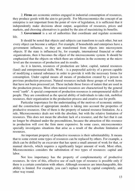
structures and determines the characteristics of the behavior of market participants. The microeconomic model can be represented with the help of the scheme of goods and money circulation (Fig.1.1)

Fig 1.1. The goods and money circulation

The main features of market behavior of microeconomic actors are: � equal status of participants; � use of the principle of economic profit as the main criterion of expediency of

entering market communication; � full economic responsibility of the participants for their actions.

The model of goods and money circulation shows how limitation of households’ resources constrains the ability of enterprises to produce more, and income growth, respectively. Therefore, the real task of economic actors is the desire to maximize the utility of scarce resources and incomes.

1.3. Subject and methods of microeconomic researches

On the basis of finding the content of the material of two previous paragraphs

out we can conclude that business behavior of microeconomic units is the subject of the microeconomics study, that is, the process of developing, adopting and implementing decisions regarding the selection and use of scarce resources in order to obtain the greatest possible benefits. Knowledge of the subject contributes to the efficient allocation of own funds, rational management of cases, assists in the management of the firm. During the process of knowledge there is a constant interaction between the subject and method. The subject involves a certain method and the method forms the subject. Now we need to focus on examining the methods of microeconomic research. Microeconomics like any science has its own method of cognition, that is, certain methods and means by which one can find out the essence

Households Firms

Of goods

Of productive

resources

16

and scientifically describe the object of research. There are general and specific methods of microeconomic research.

The general methods of the research of the subject include observation, selection of facts, statistical and economic analysis. Any research begins with the observation and selection of facts. It is important to select key facts that reflect the learning process. In order to streamline rather chaotic factual information, statistical analysis is used to identify the dynamics and trends of the research process. An economic analysis begins with abstraction, that is, the rejection of secondary, non-essential elements and the allocation of essential. This creates an ideal image that does not coincide with the actual subject, but allows tracing the properties and relationships that are characteristic of this process. The analysis also requires some assumptions. The most commonly used assumptions are "on other equal terms", which allows us showing the influence of each of the investigated factors more clearly.

Specific methods of Microeconomics include the method based on the analysis of the limit values, the method of economic modeling, the method of production capabilities, the graph-analytical method and others.

The method of analysis of marginal values is based on the use of growing characteristics when all factors, except for the investigated one, take invariable, thus applying the results of the influence of the infinitely small increment of the variable factor.

The method of economic modeling is a unique method of microeconomic research. It begins with a simplified description of the investigated microsystem by what it characterizes properties and essential aspects of a particular structure. An economic model is a conditional reflection of economic phenomena and processes. By means of expression the models can be distinguished as verbal, mathematical, graphic, table, computer and mixed models.

Each model is constructed according to certain rules and includes such obligatory elements as goal, limitation and choice of decision. The main task of the model is to determine the conditions and parameters of the balance of the microsystem. In a state of equilibrium, the subject fully implements all its capabilities, reaches the optimal state and has no incentive to change its position for the unchangeability of other conditions.

The method of production capability is used to provide the optimality of use of resources and the choice of the best alternatives of investments. The boundary of production capacity or the "transformation" of production capacity is a model that illustrates a situation of resource constraints, the need for a compromise choice and an assessment of its alternative value. It combines the points of maximum possible production of two benefits, provided that the use of limited resources is fully exploited.

In a situation of limited resources an increase in the production of one good is possible only by reducing the production of another. This situation is considered effective, since it provides the best result from the use of available resources. The margin of production capacity is a convex downward ascending downward slope,

17

which is a manifestation of the law of rising alternative cost, which operates due to imperfect interchangeability of resources.

The main microeconomic method is modeling. Microeconomic model – is a formal description of the economic process of

phenomena which illustrates the system of relationship between economic variables and parameters.

Naturally, there is no any model that can represent the real process completely. The criteria of usefulness of economic model is not the level of it compliance with real economic processes but the compliance with forecasts of future events got with the help of it.

Depending on the forms of illustration the models are divided to:

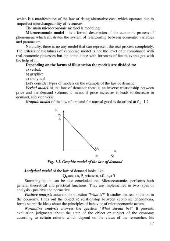
а) verbal; b) graphic; c) analytical. Let's consider types of models on the example of the law of demand. Verbal model of the law of demand: there is an inverse relationship between

price and the demand volume, it means if price increases it leads to decrease in demand, and vice verse.

Graphic model of the law of demand for normal good is described at fig. 1.2.

P

1

0

a

a−

QD a0 Q

Fig. 1.2. Graphic model of the law of demand

Analytical model of the law of demand looks like:

QD=a0+a1P, where a0>0, a1<0

Summing up, it can be also concluded that Microeconomics performs both general theoretical and practical functions. They are implemented in two types of analysis - positive and normative.

Positive analysis answers the question "What is?" It studies the real situation in the economy, finds out the objective relationship between economic phenomena, forms scientific ideas about the principles of behavior of microeconomic actors.

Normative analysis answers the question "What should be?" It presents evaluation judgments about the state of the object or subject of the economy according to certain criteria which depend on the views of the researcher, his

18

adherence to certain theoretical concepts. The results of a positive analysis enable us to determine the ways to achieve regulatory goals.

Training

Key terms and concepts

Microeconomics. Micro level. Economic laws. Economic subjects.

Microeconomic analysis. Microeconomic processes. Analysis of consumer’s

behavior. Positive analysis. Normative analysis. Microsystem. Household. Enterprise

(firm). State.

Economic resources. Limitation of economic resources. Interchangeability of

economic resources. Complementarity of economic resources. Material product.

Service.

Problem of choice. Alternative value. Diminishing returns of production

factors. The law of increasing opportunity cost. Principle of consumer’s rationality.

Subject of microeconomics. Methodology of microeconomics.

Questions and tasks for students’ self-control:

1. What does Microeconomics study? Which functions does it perform? 2. What are the main phases of development of Microeconomics as a science? 3. What is the contribution of famous domestic economist E. Slutskyi into

development of Microeconomics as a science? 4. Which components of the microsystem do you know? 5. What are subject and objects of Microeconomics study? 6. What is the structure of resources of production? 7. What do “limitation of resources” and “infinity of human’s needs” mean? 8. What are features of the resources of production? 9. How do you understand the problem of choice in business activity? 10. What does the curve of production opportunity mean? 11. Please characterize the methods of microeconomic analysis. 12. What do normative and positive Microeconomics means? 13. What is the basis of the method of marginal values in research of

microeconomic phenomena and processes? 14. What is the essence of the method of functional analysis in microeconomic

research and which role does it have? 15. Please give a characteristic of object of microsystem.

Tests

1.Which one from the following problems is a microeconomic problem? a) correlation between inflation and unemployment; b) correlation between price and demand for product; c) correlation between income and savings; d) correlation between interest rate and monetary demand.

19

2. The principle of rational behavior means that:

a) each economic subject spends money economically; b) each human makes a choice maximizing his own benefit; c) each subject has to act according to existed rules that reflect the optimal

variant of choice; d) all the people act similar when they are in similar conditions. 3. Microeconomics studies how the market mechanism determines: а) price of products; b) price of services; c) price of economic resources; d) any price.

4. The main motive of economic subjects’ behavior is: а) benefit maximization; b) help to neighbor; c) risk minimization; d) production of commodities.

5. Which one from the following problems is microeconomic problem?

а) impact of monetary supply on inflation; b) impact of government expenditures on the level of employment; c) impact of products deficit on savings; d) impact of the change of price of oil on automobile production. 6. Microeconomics: а) operates by concepts of general production level, employment and income; b) researches the behavior of consumers and firms in different market

structures; c) studies behavior of individual economic subjects in open economic system. d) studies behavior of individual economic subjects in closed economic system.

7. If the economy moves along the bound of production opportunities from

the top to the bottom, then: а) alternative cost decrease; b) alternative cost increase; c) alternative cost are not changed; d) the movement along the curve isn’t connected with alternative cost.

8. Microeconomics studies: а) behavior of the economy as a whole; b) behavior of individual economic subjects in different market structures; c) behavior of consumers at commodity and services markets; d) behavior of firms at commodity and resources markets.

20

9. Microeconomics as independent part of economic science appeared:

а) at the end of XX century; b) at the end of XIX century; c) in XVI century; d) in XVII century. 10. Normative analysis – is:

а) explanation of accuracy or fallacy of economic actions; b) explanation and forecast of economic actions; c) study of laws; d) there is no correct answer.

11. The term “economics” got it general recognition after it had been used in

scientific work of: а) J.B. Sey; b) J.S. Mill; c) A. Marshall; d) J.M. Keynes. 12. If the economy is studied as a whole system then it means that it is:

а) macroeconomic analysis; b) microeconomic analysis; c) positive analysis; d) normative analysis. 13. The product which has a high alternative value is, as a rule: а) deficit product; b) has high price; c) has low price; d) is sold difficult. 14. Microsystem – is: а) system of relationship; b) system of views; c) system of economic issues; d) system of laws.

21

CHAPTER 1.

THE THEORY OF CONSUMER’S BEHAVIOR

Theme 2 The Theory of Consumer Behavior.

The Marginal Utility of Product

2.1. The humans needs: essence and structure. The law of increase of needs.

2.2. Utility and its functions. Marginal utility of product. The Gossen’s first law.

2.3. The consumer’s equilibrium. The Gossen’s second law.

2.1. The human needs: essence and structure. The law of increase of needs

It is well known that human is the main driving force of social and economic

progress. At the same time, it is also the subject of economic relations, contradictions and interests. A human has an active influence on the economy and takes part in all spheres of life just only by his interests’ realization. That is why building of an effective system of management, achievement of social and economic progress can only be based on the state and dynamics of economic needs and interests of human.

By their nature, the needs are unlimited. Their infinity has different forms of manifestation. Firstly, the needs are constantly reproduced (it is impossible to satisfy the need for water completely by consuming it only once); and secondly, the development of society and production generates more and more needs; thirdly, it has no limits to the process of improving the structure of needs and their updating as it has no boundaries for the process of the human improvement as well.

Needs – are the state of satisfaction that consumer wants to maintain, or the state of dissatisfaction that he would like to change. Taking into account the huge variety of needs, they should to be classified according to certain features.

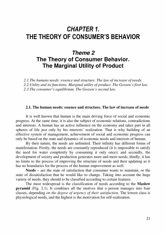
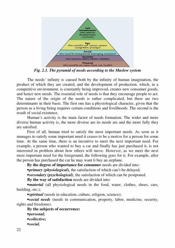
The most widespread is the classification of needs according to the Maslow

pyramid (Fig. 2.1). It combines all the motives that a person manages into four classes, depending on the degree of urgency of their satisfaction. The lowest class is physiological needs, and the highest is the motivation for self-realization.

22

Fig. 2.1. The pyramid of needs according to the Maslow system

The needs’ infinity is caused both by the infinity of human imagination, the

product of which they are created, and the development of production, which, in a competitive environment, is constantly being improved, creates new consumer goods, and hence new needs. The essential role of needs is that they encourage people to act. The nature of the origin of the needs is rather complicated, but there are two determinants in their basis. The first one has a physiological character, given that the person as a living being requires certain conditions and livelihoods. The second is the result of social existence.

Human’s activity is the main factor of needs formation. The wider and more diverse human activity is, the more diverse are its needs are and the more fully they are satisfied.

First of all, human tried to satisfy the most important needs. As soon as it manages to satisfy some important need it ceases to be a motive for a person for some time. At the same time, there is an incentive to meet the next important need. For example, a person who wanted to buy a car and finally has just purchased it, is not interested in problem about how others will move. However, as we meet the next most important need for the foreground, the following goes for it. For example, after the person has purchased the car he may want ti buy an airplane.

By the degree of importance for consumer needs are divided into:

• primary (physiological), the satisfaction of which can’t be delayed;

• secondary (psychological), the satisfaction of which can be postponed. By the way of satisfaction needs are divided into:

• material (all physiological needs in the food, water, clothes, shoes, cars, building, etc.);

• spiritual (needs in education, culture, religion, science);

• social needs (needs in communication, property, labor, medicine, security, rights and freedoms).

By the subjects of occurrence:

• personal;

• collective;

• social.

23

Part of needs is satisfied by itself (for example, air, water, sunshine, etc.), the other part is satisfied by people through social relations. However, most of needs are met by the economy - through the production and consumption of goods.

The needs that are satisfied through the production of goods and their consumption are called economic needs.

The availability of economic needs is a motive for production. Needs and production are two poles of the economy, among which there is all its diversity. These two poles are constantly interacting with each other.

The diversity of human needs has also caused ambiguity in the approaches to their classification. Thus, human needs are distinguished by: the nature of its

occurrence (labor, status needs), the importance of its satisfaction (absolute, valid, solvent, satisfied needs), by methods of needs’ satisfaction (material and nonmaterial needs).

In particular, labor needs are generated by the work itself, that is, by its content, conditions, organization of the labor process, and regime of labor.

Status needs are the internal motive of behavior associated with the desire of a person to embrace a senior position, to perform more complicated, responsible work, to work in the field of activity (organization), which is seems to be prestigious, socially significant. This is the desire of a person to be recognized as a specialist in his business, an informal leader, to use authority. The essence of absolute needs is in the only desire to own goods and use services. They are connected neither with production opportunities, nor with the incomes of consumers and have an abstract nature. The actual needs are formed within the limits of the achieved level of production. Like absolute needs they are not related to the solvency of consumers, but unlike the absolute ones, they are concrete, that is, they are aimed at a certain object or service, which are actually produced and offered to the consumer. Solvent needs are determined by the appropriate capabilities of consumers. With these needs the consumer goes to the market, and they are recruiting forms of solvent demand. Satisfied needs include those that are actually satisfied with the benefits and services available. Their satisfaction depends on the level of development of production and consumer solvency.

Solvent needs become satisfied when there is a sufficient number of goods and services at the market that meet customers’ requirements by their consumption qualities.

There is some connection between different kinds of needs. Thus, absolute

needs are transformed into real needs under the influence of the development of productive forces, scientific and technological progress. As a result of the participation of the population in social production and the division of the social product the last ones become forms of solvent demand, which is later subsequently satisfied at the market of goods and services.

24

Material needs – are the needs that are provided by things, and non-material needs are satisfied with services. Material needs are considered to be basic or essential requirements of humans.

Microeconomics considers also foolish (non-rational) human’s needs. Among the material needs of human they are distinguished by the fact that their satisfaction is detrimental for the health, interferes with spiritual development and causes degradation of the individual. For example, alcohol, tobacco, drugs, etc.

Nonmaterial needs include spiritual and social needs. Spiritual needs are the needs of education, development of qualification and professional skill, in artistic creativity, science and art development. Spiritual needs become as essential for human as same as material needs. Social needs are the human’s needs in medical service, children's upbringing, leisure time, rest, in proper working conditions and training.

The needs that are related to the sphere of economic activity are called economic needs, as the necessity of a person in life's goods, the desire to own them, use it for purpose. Every person at a certain point in time makes a decision about his or her choice. It is important to understand that this choice depends on the needs of each particular individual. Among the many products offered by the manufacturer, the consumer will choose the one that will bring him the most utility. And it is in this product that the consumer has a certain need, and it is precisely this product that he will provide the greatest advantage. Table 2.1 reflects the personal economic needs of human.

Table 2.1

Personal economic needs

Physiological Intellectual Social

- food - clothes, shoes - dwelling - household goods

- education - improvement of skills - rest - objects and cultural services

- health service - living conditions - work conditions - transportation, communication

People satisfy their needs with the help of goods and services. In this case,

goods and services act as economic benefits. Economic benefit is a rare limited benefit, that is a way to meet the needs of a limited number. That is, the good that a person creates specially, is produced in order to meet their needs, is called economic good. So, economic benefits are those goods that are created and manufactured at industrial enterprises. Examples of economic goods (goods) are food products (bread, milk, cereals, etc.), light industry goods (fabrics, clothing, etc.), other results of human economic activity (cars, bicycles, TVs, etc.). In addition, the economic benefits are provided by the necessary services for the person (communication, transport, etc.). Services are economic goods that do not have a commodity form, but they are provided to the people in the form of purposeful utility or service.

Due to the term of use economics goods are divided into long-term and short-term goods. Long-term goods can be used for many years, for example, furniture,

25

refrigerators, cars. Other economic goods are used by people only once. Short-term economic goods include food products, refined products, etc.

Consequently, the material needs of society are unlimited, and the economic resources necessary to meet these needs are limited.

Infinity of needs and limitation of resources generate the effect of two laws of social development – the law of growth needs and the law of labor saving. These two laws are interconnected and reflect the two sides of the general economic law of the growth of social and economic efficiency. At the level of society, the effect of this law is that in the conditions of infinite needs, a society that seeks to ensure their full satisfaction, that is, as close as possible to the goal, must seek a comprehensive saving of labor (both living and ordained), and, consequently, to the effective use of economic resources, their rational combination and distribution between the production of various goods.

The law of growing needs is a law of social progress. It characterizes not just growth, that is, the emergence of new and new needs, and a change in their structure, reflecting the progress of both human and society as a whole from biological (physiological) to more versatile rich life style.

Each step in the development of society is simultaneously meeting the needs at a new higher level. Society is always strictly limited by economic resources, so at each stage of its development it puts forward as a two-way goal: the satisfaction of equally high priority both social and economic needs, while allocating necessary parts of the aggregate working time fund.

2.2. Utility and its functions. Marginal utility of product.

The Gossen’s first law

As in the previous paragraph we have founded that evaluation of the same product by different people is different so we can state that utility is the satisfaction that the consumer receives from the acquisition and use of the good that brings him the maximum pleasure.

Utility serves as a criterion for choosing – it is the satisfaction from the consumption of goods or services. With the help of this category we can confirm the fact of the existence of consumer independence, his sovereignty and freedom of choice. Product will be bought if the consumer gives his advantage to it, he will enjoy it, seeing it has some usefulness for himself, and therefore he will choose it from a general range of goods or services.

The origin of the term "utility" dates back to the eighteenth century, in the writings of the eccentric English philosopher and sociologist Jeremy Bentham (1748-1832). In his opinion, utility is the purpose of consumption. It will increase if the quantity of goods consumed increases. In this case, the overall utility increases. But the growth in overall utility is slowing down with the expansion of consumption opportunities. This is a consequence of the fall in the added value of the good.

26

Both the concept of need and utility are quite individual and subjective because they depend on the tastes, preferences, ability and necessity for the individual consumer to buy the desired product or service.

Representatives of the utility theory confirmed that the starting point is a subject, an individual, and since this subject has certain needs, they also play a decisive role in the economic process. So the very consumer becomes the driving force behind the development of a market economy as the production is formed due to his needs. According to this concept, it is necessary to study the logic of the behavior of the subject of economic activity, that is, the psychology of a person engaged in the economic sphere. It was for this purpose that the theory of marginal utility of goods was born.

It arose in contrast to the labor theory and acquired a complete form in the last third of the XIX century. The most famous representatives of this theory were W. Jevons, A. Marshall, K. Menger, F. Wieser, E. Bom-Bawerk, D. Clark. Three main categories (utility, price and income) formed the basis of the theory of consumer behavior.

Supporters of the utility theory consider that consumer is the main person at the commodity market as it is inherent in labor theory, but not a seller. Adopted in the economics concepts "commodity" and "cost" were replaced by the notions of "good" and "value". The dominant factor of good in works of scientists was its value or utility. The last one they understood as that general power of material goods, which enables to meet the needs of an individual, to increase its welfare. Cost arises as a result of the relationship between human need and economic goods.

Value is the considering of the economic subjects about the importance for them of the goods that are in their possession, and therefore, outside of their consciousness, it does not exist. Human is dependent on the good necessary for satisfaction of his needs, so the object that can satisfy even the minimum need acquires value. This item is necessary to meet this particular need and none other. Such a value, being subjective, does not depend on aggregate, but on additional or marginal utility, which is higher or lower than the factual value that a person has of satisfying a particular good.

The microeconomic theory uses two main approaches for determining the utility: cardinal (quantitative) and ordinal (serial).

The cardinal concept is based on the fact that the consumer is able to quantify the level of his satisfaction. Due to the fact that there are no units of measurement of quantitative determination of utility, scientists have agreed to use a hypothetical conditional unit, which is called utils.

In the cardinal concept quantitative assessments have a subjective character, that is that for one consumer is of high utility, for another one is the very opposite. This means that the same product has different utility for different consumers.

The main factors influencing the consumer's choice are the price of the product and his own of income. That is, the consumer seeks to use his budget so as to maximize his needs and achieve the highest utility. This dependence represents a utility function.

27

The utility function is the model that reflects the relationship between the amount of goods that consumers try to buy and the level of utility that consumers try to achieve from it.

If to take into account the condition that the consumer uses only two products X and Y, then in general terms the utility function will have the following form:

U = f (Qx, Qy), where U – level of utility; f – functional dependence; Qx, Qy – number of products Х and У. One set of certain goods will be different from another one by different

combinations of goods. Therefore, there are different levels of quantitative determination of advantages of the utility of product.

It is possible to determine the level of satisfaction from the consumption of goods for each particular consumer, that is from the various combinations of sets of goods X and Y. This will be the total utility (TU), which is expressed in utils:

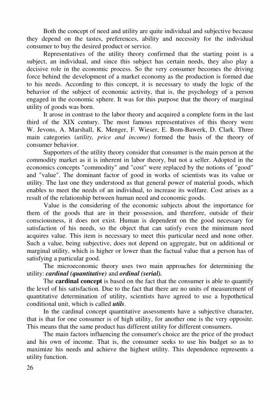
TU = f (Qx, Qy). The total utility curve is displayed at fig. 2.2.

Fig. 2.2. The total utility curve

In order to analyze how the increase of consumption of product X (with constant consumption of product Y) will influence the total utility level value it is used the concept of marginal utility of good (MU).

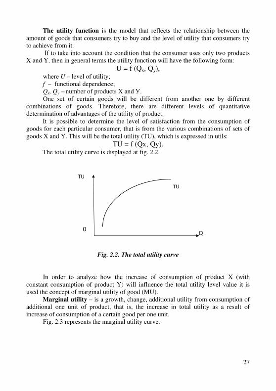
Marginal utility – is a growth, change, additional utility from consumption of additional one unit of product, that is, the increase in total utility as a result of increase of consumption of a certain good per one unit.

Fig. 2.3 represents the marginal utility curve.

Q 0

TU

TU

28

Fig. 2.3. The marginal utility curve

The marginal utility curve has a negative slope as the utility of an increasing

number of consumed goods gradually decreases. The marginal utility of product shows how the increase of the consumption of a

certain good may cause a negative impact on the individual. Here is a simple example with a glass of water. When a person suffers from thirst in the summer he drinks the first glass of water with great pleasure, the second glass is also perceived in favor, but the subsequent consumption of water brings less and less useful to man, and, reaching a certain moment, even negative. Let’s observe the behavior of a person who consumes seven bananas during one day.

Table 2.2

Quantity and utility from consumption of bananas

Quantity of bananas,

Q

Marginal utility,

MU (utils)

Total utility,

TU (utils)

1 10 10

2 9 19 3 7 26

4 4 30

5 1 31 6 0 31 7 -3 28

Let the consumption of the first banana bring satisfaction to 10 utils, the

second banana is also tasty and its additional utility is 9 utils, the third banana has an additional utility 7 utils, etc. As it is seen, the consumption of each next banana reduces the marginal utility that reaches the consumption of the sixth banana zero value, and already at the consumption of the seventh passes into uselessness, that is, damage to the human’s body. For example, we can find the general utility from consumption of four bananas: (TU / Q): 30/4 = 7.5 utils. Each of the four bananas brings an average utility or a satisfaction 7.5 utils.

Mathematically, the marginal utility of a good can be represented as follows:

Q 0

MU

MU

29

X

UMUx

∆

∆=

Besides this, Microeconomics considers the average utility of product (AU) – it is the total utility per each one unit of consumed product.

Marginal utility can be determined by the slope of the total utility curve. Graphical representation of the relationship of total and marginal utility of product is presented in Fig. 2.4.

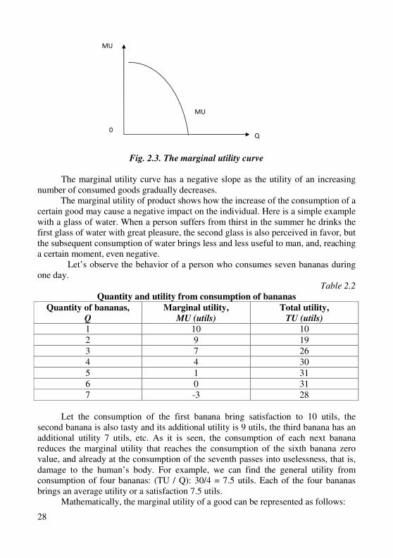
Point A shown in Fig. 2.4a is the point of maximal utility (maximal satisfaction), or the point of saturation. It corresponds to a zero value of marginal utility. According to table 2.2 and the above figure we can see that the curve of marginal utility goes from top to the left and shows a decrease in the marginal utility as the number of consumed goods increases (in our case, bananas). The law of decreasing marginal utility implies that all other factors, such as income, tastes and preferences are constant values. In general, this law applies to the absolute majority of goods, although there are some exceptions. These are antiques, various collectible stamps or coins, etc.

Fig. 2.4. Connection between total and marginal utility

Thus, grafically is confirmed that (see Fig. 2.4): � if to consume more and more amount of , for example, product X, then total

utility becomes higher;

TU

MU

MU

A

TU

Good X

Good X

a)

b)

•

•

30

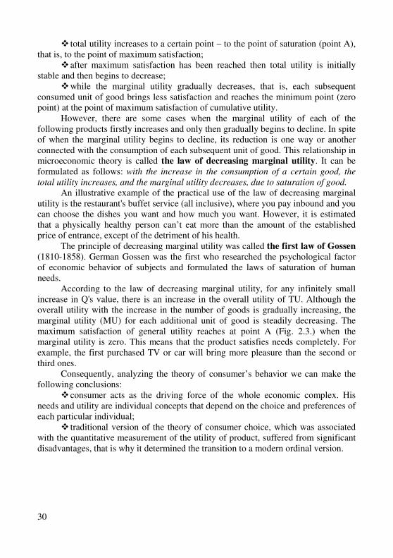
� total utility increases to a certain point – to the point of saturation (point A), that is, to the point of maximum satisfaction;

� after maximum satisfaction has been reached then total utility is initially stable and then begins to decrease;

� while the marginal utility gradually decreases, that is, each subsequent consumed unit of good brings less satisfaction and reaches the minimum point (zero point) at the point of maximum satisfaction of cumulative utility.

However, there are some cases when the marginal utility of each of the following products firstly increases and only then gradually begins to decline. In spite of when the marginal utility begins to decline, its reduction is one way or another connected with the consumption of each subsequent unit of good. This relationship in microeconomic theory is called the law of decreasing marginal utility. It can be formulated as follows: with the increase in the consumption of a certain good, the

total utility increases, and the marginal utility decreases, due to saturation of good.

An illustrative example of the practical use of the law of decreasing marginal utility is the restaurant's buffet service (all inclusive), where you pay inbound and you can choose the dishes you want and how much you want. However, it is estimated that a physically healthy person can’t eat more than the amount of the established price of entrance, except of the detriment of his health.

The principle of decreasing marginal utility was called the first law of Gossen (1810-1858). German Gossen was the first who researched the psychological factor of economic behavior of subjects and formulated the laws of saturation of human needs.

According to the law of decreasing marginal utility, for any infinitely small increase in Q's value, there is an increase in the overall utility of TU. Although the overall utility with the increase in the number of goods is gradually increasing, the marginal utility (MU) for each additional unit of good is steadily decreasing. The maximum satisfaction of general utility reaches at point A (Fig. 2.3.) when the marginal utility is zero. This means that the product satisfies needs completely. For example, the first purchased TV or car will bring more pleasure than the second or third ones.

Consequently, analyzing the theory of consumer’s behavior we can make the following conclusions:

� consumer acts as the driving force of the whole economic complex. His needs and utility are individual concepts that depend on the choice and preferences of each particular individual;

� traditional version of the theory of consumer choice, which was associated with the quantitative measurement of the utility of product, suffered from significant disadvantages, that is why it determined the transition to a modern ordinal version.

31

2.3. The consumer’s equilibrium. The Gossen’s second law

After we have find out the essence and objective dynamics of the marginal utility of product, there is a need to specify the logic of consumer behavior in terms of clarifying the conditions for ensuring its equilibrium functioning.

The principle of decreasing marginal utility is the basis for achieving the consumer's balance of power situation. Here is an example, you went to the store, where the croissant cost $1,5 and ice cream $ 3. You have $ 9 in your wallet. Your goal is to choose a set of products that will bring you the greatest pleasure. Of course you can buy three portions of ice cream, but you will not get as much satisfaction from the last portion as from the first one. However, if you buy two croissants instead of the third portion of the ice cream, then you will get the increase the total utility, since the first two croissants will enjoy you a lot more than the third portion of the ice cream. And, other way round, as the consumption of ice cream decreases and the consumption of croissants increases, the marginal utility of ice cream will increase, and of croissants will decrease. And, ultimately, you will reach the point of the consumer equilibrium, in which you will not be able to increase the total utility, spending more money on one product and less – on the other due to your limited budget. The marginal utility per each one dollar for the value of one product equals the marginal utility per each one dollar of price of another good.

Otherwise, this can be formulated as follows: the ratio of the marginal utility of

product to its price should be same for all products:

Pn

MUn

Pz

MUz

Py

MUy

Px

MUx==== ... ,

where MUх, MUу,… MUn – marginal utilities of different products; Pх, Pу,… Pn – prices of different products. It was this dependence that Gossen discovered and formulated as a law. This

second law of Gossen states that utility maximization is possible in case when the last monetary unit that is spent on the purchase of any product brings the same measure of satisfaction (utility).

The second law of Gossen was formulated in two versions. The first option came from the fact that the consumer was viewed from the standpoint of a natural economy, that is, as a human who was isolated from society. In the presence of a certain number of diverse products of the own economy, the consumer within a certain period can consume them in different combinations, one of which should be most advantageous and bring maximum pleasure, which is achieved by the condition of equality of the marginal utility of all products.

The second option takes into account the conditions of commodity production. Both prices, goods, and the amount of money available to the consumer are the main factors that restrict consumption.

The most rational variant of consumption is established on the condition of reaching the equilibrium between the marginal utilities achieved from the last monetary units had been spent on the purchase of individual goods.

32

The second law has been widely used to explain demand and pricing. The main methodological disadvantages of Gossen's theory lie in the subjective and psychological and idealistic approaches to economic phenomena, and the ignoring of production, which plays a decisive role in the economic life of society.

From the theory of Gossen it follows that the nature of consumption and distribution of material goods between people does not depend on the social and economic form of production. The theory of Gossen in his time did not receive proper recognition, but was restored by scholars-economists of the XIX century.

To give a practical explanation of the essence of Gossen's laws, let's look at this situation. Let the marginal utility of the product X (chips) is 80 utils per 1 kg, with the price of 1 kg is $ 4. The marginal utility of product Y (crackers) is 60 utils per 1 kg with the price of 1 kg – $ 6 UAH. This implies:

MUx / Px = 80/4 = 20 utiles/kg,

MUy / Py = 60/6 = 10 utiles/kg. It means that for both products (chips and crackers) MUx / Px > MUy / Py. If a consumer wants to reduce the consumption of crackers at least by 1 kg, he

will lose 60 utils. However, in this case he saves $ 6 that he will be able to spend on the purchase of 1.5 kg of chips and will receive 120 utils from its consumption.

Consequently, the consumer must spend his income in such a way that to satisfy his purchasing needs in both chips and crackers completely.

Economists who developed the theory of consumer’s behavior on the basis of the concept of marginal utility traditionally believed that consumption was a momentary period. The theory was designed in such a way that to ensure that the economic value of time is taken into account.

It is logically to confirm that prices of products should include not only market prices, but also the value of the time needed to consume the product. In other words, the time spent on rest and all kinds of consumer activity becomes more expensive. As a result, the consumer makes every effort to use "non-working hours" more effectively. The consumer tries to increase the amount of satisfaction or utility received per hour by increasing the amount of consumption per unit of time. In some cases, this is equivalent to an increase in commodity intensity of consumption. Consequently, in the theory of consumer behavior the time acts in the form of the value of economic resources.

The advantage of the cardinal concept is in the fact that it not only simplifies the explanation of the motivation of consumer’s behavior, but can also be used for the analysis of the choice among the set of goods – two, three, and more goods that it is difficult to make in other models. A set of consumer goods is called a market consumer basket. Consequently, it is possible to provide a quantitative ranking of consumer baskets: a rational consumer will choose a basket with the largest amount of utility (utils). However, in real life it is difficult to imagine that the consumer is able to estimate the difference in the utility of products.

It’s also advisable to focus on the following conclusion about the theory of consumer’s behavior: a rational consumer within the limits of his budget will make purchases in such a way that each purchased product would bring him the same

33

marginal utility that is proportional to the price of that product. Only in this case he will get maximum pleasure. That is, we will get the expression:

Py

Px

MUy

MUx= ;

Pn

Py

MUn

MUy=

This is the law of utility maximization or condition of consumer’s

equilibrium. Consequently, the cardinal approach to determining the utility of product is

based on the fact that the consumer subjectively assesses the level of his satisfaction. With the aim of maximizing the utility, the consumer evaluates the consumer property of each product in the utils and selects the products with the maximum number of utils. The value of utility depends not only on the properties of product, but also on its quantity, that is, is determined functionally.

Cardinal theory proceeds from the premise that any consumer is able to measure the utility of each product quantitatively, as well as the level of his wealth and income. According to the axiom of the marginal utility reduction (the first law of

Gossen) the volume of purchases decreases with rising prices. Cardinal theory has a vulnerable place: in real life no one consumer is able to determine properly how much additional value he has received from an additional unit of product. Therefore, no one consumer is able to quantify the maximum satisfaction of his need for the purchase of goods. However, every consumer is able to compare sets of goods and make his own choices. The cardinal approach limits the possibilities of microeconomic analysis as it contains significant disadvantages:

� it is based on subjective assessments of the utility of product, and therefore does not allow to make objective generalizations;

� there is no possibility of a clear quantitative assessment and comparison method, for implementation of calculations.

That is why there was a transition from the cardinal version of utility of product to the ordinal version.

Training

Key terms and concepts Human needs. Infinity of needs. Working needs. Status needs. Absolute needs.

Real needs. Solvent needs. Material needs. Nonmaterial needs. Spiritual needs.

Social needs. Economic needs. Economic product. Services. The law of needs

increasing. The saving labor law. The theory of consumer’s behavior. Consumer’s

purpose. Independence of consumer. Limitation of consumer. Choice of consumer.

Rankings of needs. Transitivity of benefits.

Utility. Value. Cardinal concept of product utility. Ordinal concept of

consumer. Utility. Util. Utility function. Total utility. Average utility. Marginal utility.

The law of diminishing marginal utility. The first law of Gossen. The second law of

Gossen. Market consumption basket. Equilibrium of consumer.

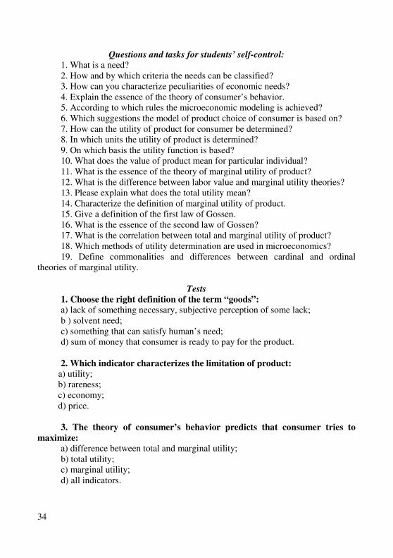
34

Questions and tasks for students’ self-control:

1. What is a need? 2. How and by which criteria the needs can be classified? 3. How can you characterize peculiarities of economic needs? 4. Explain the essence of the theory of consumer’s behavior. 5. According to which rules the microeconomic modeling is achieved? 6. Which suggestions the model of product choice of consumer is based on? 7. How can the utility of product for consumer be determined? 8. In which units the utility of product is determined? 9. On which basis the utility function is based? 10. What does the value of product mean for particular individual? 11. What is the essence of the theory of marginal utility of product? 12. What is the difference between labor value and marginal utility theories? 13. Please explain what does the total utility mean? 14. Characterize the definition of marginal utility of product. 15. Give a definition of the first law of Gossen. 16. What is the essence of the second law of Gossen? 17. What is the correlation between total and marginal utility of product? 18. Which methods of utility determination are used in microeconomics? 19. Define commonalities and differences between cardinal and ordinal

theories of marginal utility.

Tests

1. Choose the right definition of the term “goods”:

а) lack of something necessary, subjective perception of some lack; b ) solvent need; c) something that can satisfy human’s need; d) sum of money that consumer is ready to pay for the product. 2. Which indicator characterizes the limitation of product:

а) utility; b) rareness; c) economy; d) price.

3. The theory of consumer’s behavior predicts that consumer tries to

maximize:

а) difference between total and marginal utility; b) total utility; c) marginal utility; d) all indicators.

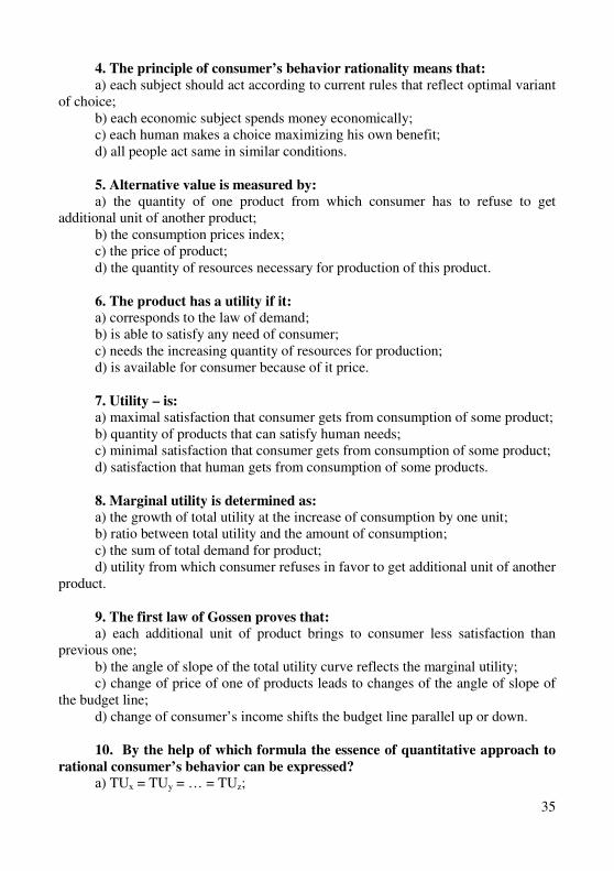
35

4. The principle of consumer’s behavior rationality means that:

а) each subject should act according to current rules that reflect optimal variant of choice;

b) each economic subject spends money economically; c) each human makes a choice maximizing his own benefit; d) all people act same in similar conditions.

5. Alternative value is measured by:

а) the quantity of one product from which consumer has to refuse to get additional unit of another product;

b) the consumption prices index; c) the price of product; d) the quantity of resources necessary for production of this product. 6. The product has a utility if it:

а) corresponds to the law of demand; b) is able to satisfy any need of consumer; c) needs the increasing quantity of resources for production; d) is available for consumer because of it price. 7. Utility – is:

а) maximal satisfaction that consumer gets from consumption of some product; b) quantity of products that can satisfy human needs; c) minimal satisfaction that consumer gets from consumption of some product; d) satisfaction that human gets from consumption of some products. 8. Marginal utility is determined as:

а) the growth of total utility at the increase of consumption by one unit; b) ratio between total utility and the amount of consumption; c) the sum of total demand for product; d) utility from which consumer refuses in favor to get additional unit of another

product. 9. The first law of Gossen proves that:

а) each additional unit of product brings to consumer less satisfaction than previous one;

b) the angle of slope of the total utility curve reflects the marginal utility; c) change of price of one of products leads to changes of the angle of slope of

the budget line; d) change of consumer’s income shifts the budget line parallel up or down. 10. By the help of which formula the essence of quantitative approach to

rational consumer’s behavior can be expressed?

а) TUx = TUy = … = TUz;

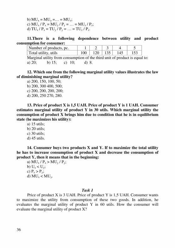
36

b) MUx = MUy =… = MUz; c) MUx / Px = MUу / Py = … = MUz / Pz; d) TUx / Px = TUy / Py = … = TUz / Pz.

11.There is a following dependence between utility and product

consumption for consumer:

Number of products, pc. 1 2 3 4 5

Total utility, utils 100 120 135 145 153 Marginal utility from consumption of the third unit of product is equal to: а) 20; b) 15; c) 10; d) 8.

12. Which one from the following marginal utility values illustrates the law

of diminishing marginal utility?

а) 200, 150, 100, 50; b) 200, 300 400, 500; c) 200, 200, 200, 200; d) 200, 250 270, 280.

13. Price of product X is 1,5 UAH. Price of product Y is 1 UAH. Consumer

estimates marginal utility of product Y in 30 utils. Which marginal utility the

consumption of product X brings him due to condition that he is in equilibrium

state (he maximizes his utility):

а) 15 utils; b) 20 utils; c) 30 utils; d) 45 utils.

14. Consumer buys two products X and Y. If to maximize the total utility

he has to increase consumption of product X and decrease the consumption of

product Y, then it means that in the beginning:

а) MUх / Pх > MUу / Pу; b) Uх < Uу; c) Рх > Ру; d) МUх < МUу.

Task 1 Price of product X is 3 UAH. Price of product Y is 1,5 UAH. Consumer wants

to maximize the utility from consumption of these two goods. In addition, he evaluates the marginal utility of product Y in 60 utils. How the consumer will evaluate the marginal utility of product X?

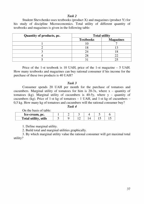
37

Task 2

Student Shevchenko uses textbooks (product X) and magazines (product Y) for his study of discipline Microeconomics. Total utility of different quantity of textbooks and magazines is given in the following table:

Total utility Quantity of products, pc.

Textbooks Magazines

1 10 7 2 18 13

3 24 18 4 28 22

5 31 25

Price of the 1-st textbook is 10 UAH, price of the 1-st magazine – 5 UAH.

How many textbooks and magazines can buy rational consumer if his income for the purchase of these two products is 40 UAH?

Task 3

Consumer spends 20 UAH per month for the purchase of tomatoes and cucumbers. Marginal utility of tomatoes for him is 20-3x, where x – quantity of tomatoes (kg). Marginal utility of cucumbers is 40-5y, where y – quantity of cucumbers (kg). Price of 1-st kg of tomatoes – 1 UAH, and 1-st kg of cucumbers – 0,5 kg. How many kg of tomatoes and cucumbers will the rational consumer buy?

Task 4

On the basis of table:

Ice-cream, pc. 1 2 3 4 5 6

Total utility, utils 5 9 12 14 15 15

1. Define marginal utility. 2. Build total and marginal utilities graphically. 3. By which marginal utility value the rational consumer will get maximal total

utility?

38

Theme 3 The Ordinal Theory of Consumer’s Behavior

3.1. The Consumer’s choice from ordinal positions and axiom of the rational

consumer’s behavior.

3.2. The indifference curves and its properties.

3.3. The budget constraints of consumer and its graphical representation.

3.4. The consumer’s optimum in providing the rational consumer’s choice.

3.1. The consumer’s choice from the ordinal positions

and the axiom of the rational consumer’s behavior

If consumer is not able to quantify the level of satisfaction of needs, then in this case the ordinal level of utility measure (ordinal) can be used. This approach to consumer behavior can be called relative. Ordinance scholars consider the preferences ratio for all commodities, but for the sake of simplicity, they usually take into account the combination of sets of two products (X and Y) and determine which of these combinations gives the consumer more and less utility. This assumption comes from a link in which: what is right for two products is true for any number of good.

A method of measurement of the utility of two different goods for a given consumer can be considered as a fixed relationship of advantage granted to one another with respect to the equivalence (indifference) relation to the goods. A rational consumer can streamline his attitude towards all the goods he considers when choosing, placing it in a certain hierarchy. In this case, not individual goods are compared, but the market baskets and the following selection criteria are used: "more", "less", "identical". Without such a hierarchy, in general, any rational, consistent consumer behavior is impossible. Such an option of the utility measurement is called "ordinal".

Ordinal (serial) approach was proposed at the beginning of the 20th century by F. Ejourt, V. Pareto, and I. Fischer as an alternative to the quantitative theory of utility. This theory does not require the need for a quantitative measurement of utility. All that is necessary for the consumer is to be able to rank all possible product sets according to their preferences. In the 30th of the XX century, after publishing the works of R. Allen and J. Hicks, this theory acquired a completed canonical form and still remains the most widespread one till this day.

The serial approach to the analysis of utility and demand, as we see, is more modern and based on considerably less rigid preconditions comparing to a quantitative approach. The consumer does not need to measure the utility of good in

39

some artificial units of measurement. It is necessary for the consumer to arrange all possible product sets according to their consumer preferences.

The ordinal theory has the task of identifying of such a set of two benefits that would allow a consumer to get the maximal utility from the consumption of this set of goods for a limited period of time. This selection process has two different sides:

� it is necessary to take into account the wishes of consumer, his tastes and preferences;

� it is necessary to take into account the possibilities of consumer, based on his available cash income, which always has a limited value. The essence of consumer’s choice is that the consumer's desire coincides with his possibilities.

The ordinal concept of utility implies several assumptions: � preferences of each particular consumer have been already formed; � practically all goods are desirable; � consumer always prefers a greater quantity of goods than the smaller one; � consumers are independent from each other in satisfying their needs. Assumptions about preferences relate solely to one person. If to talk about a

group of people (for example, a family) then preferences may not coincide: for each family member another set of goods may be attractive.

The situation with mismatches of preferences is called the paradox of Arrow: the transitivity of the preferences of each individual may lead to non-transitivity of

collective preferences. Consumer decisions are always made at a certain period in time. They are

stable in time if other conditions remain unchanged, and consumer behavior is constant. However, there are a large number of consumption baskets at the market. Consumer can always find such baskets that are equally attractive to him as they have the same level of utility. It is this set of consumption baskets with the same level of utility that are called a set of indifference.

The benefits of consumers are determined by the ratio of consumer choice to certain goods and services. When one product, for example, peaches, is better for consumer comparing to apricots then in a free market economy consumers' tastes coupled with relative prices affect the distribution of consumer spending between existing alternatives. In this way, the distribution of a limited amount of resources during production of different goods will depend on: type of products, their prices, as well as on tastes and preferences of consumers.

Consumer preferences – are a ranking of alternative options for meeting needs. In the opinion of the consumer, those options are able to meet their needs better, it will take higher places in their ranking. So, having been appeared on the market, consumer has to choose how to satisfy his needs the best way without spending more than the budget allows. The ordinal approach is based on the determination of the ratio of preferences or indifference between different products without quantitative utility measurements. Such an approach makes it possible to substantiate the objective logic of consumer behavior based on subjective assessments.

40

The basic concept of the ordinal utility theory is the marginal rate of substitution (MRS).

The marginal rate of substitution of product Y by product X (MRSхy) – is the amount of the product Y, from which the consumer refuses to obtain an additional unit of product X. Same time, the level of satisfaction of consumer’s needs remains unchanged.

The quantity of product Y which will replace the unit of product X, will have the form:

MRSxy = ∆Qy/∆Qх Marginal rate of substitution MRSxy has a tendency to decrease as more units

of product X are replaced by commodity U. Consequently, in the theoretical substantiation of the logic of consumer’s choice

according to ordinal version it was discovered that the consumer can rotate all sets of goods, but he will prefer a set with more quantity of goods.

That is, every consumer will resort to such a choice, according to which he will receive maximum utility from the purchase of a particular product. The marginal level of substitution measures the consumer’s desire to replace one product by another one.

3.2. Indifference curves and their properties

In the ordinal version of marginality the new key tool of analysis is the indifference curves with the help of which it is possible to determine the desire (demand) of each individual. The indifference curves radically change the cardinal conception of the marginal utility of good.

For the first time the indifference curves were used for the analysis of consumer behavior by F. Ejworth. Later this method was improved by E. Slutsky, V. Pareto, J. Hicks and others. The most common is the Hick’s model.

The indifference curve – is a graphic representation of different combinations of the sets of benefits that provide the consumer with the same level of utility. All points in this line reflect the same level of customer’s satisfaction.

Same time the line of indifference serves as a graphical representation of the amount of goods that the consumer buys, that is, it is also a line of demand. After all, the demand for goods is characterized by exactly same quantity of goods that, at this price level, consumer can and wants to get at the market. A line of indifference characterizes the consumer's demand in the aspect of what he wants and can get due to his limited income.

Any combination of two goods X and Y can be represented by any point on the coordinate system. By combining points with such combinations of goods that provide the same level of satisfaction of needs, we will receive a curve of indifference (Fig. 3.1.).

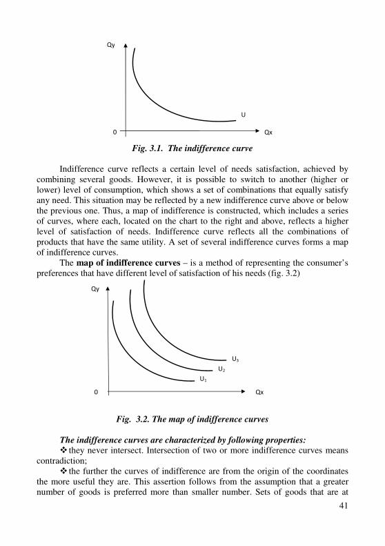
41

Fig. 3.1. The indifference curve

Indifference curve reflects a certain level of needs satisfaction, achieved by

combining several goods. However, it is possible to switch to another (higher or lower) level of consumption, which shows a set of combinations that equally satisfy any need. This situation may be reflected by a new indifference curve above or below the previous one. Thus, a map of indifference is constructed, which includes a series of curves, where each, located on the chart to the right and above, reflects a higher level of satisfaction of needs. Indifference curve reflects all the combinations of products that have the same utility. A set of several indifference curves forms a map of indifference curves.

The map of indifference curves – is a method of representing the consumer’s preferences that have different level of satisfaction of his needs (fig. 3.2)

Fig. 3.2. The map of indifference curves

The indifference curves are characterized by following properties: � they never intersect. Intersection of two or more indifference curves means

contradiction; � the further the curves of indifference are from the origin of the coordinates

the more useful they are. This assertion follows from the assumption that a greater number of goods is preferred more than smaller number. Sets of goods that are at

Qx

U

0

x

Qy

Qx

U1

0

Qy

U2

U3

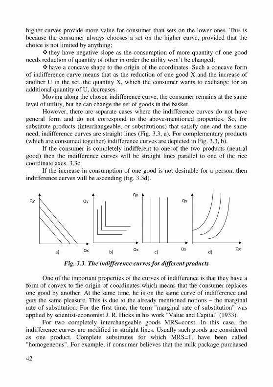
42

higher curves provide more value for consumer than sets on the lower ones. This is because the consumer always chooses a set on the higher curve, provided that the choice is not limited by anything;

� they have negative slope as the consumption of more quantity of one good needs reduction of quantity of other in order the utility won’t be changed;

� have a concave shape to the origin of the coordinates. Such a concave form of indifference curve means that as the reduction of one good X and the increase of another U in the set, the quantity X, which the consumer wants to exchange for an additional quantity of U, decreases.

Moving along the chosen indifference curve, the consumer remains at the same level of utility, but he can change the set of goods in the basket.

However, there are separate cases where the indifference curves do not have general form and do not correspond to the above-mentioned properties. So, for substitute products (interchangeable, or substitutions) that satisfy one and the same need, indifference curves are straight lines (Fig. 3.3, a). For complementary products (which are consumed together) indifference curves are depicted in Fig. 3.3, b).

If the consumer is completely indifferent to one of the two products (neutral good) then the indifference curves will be straight lines parallel to one of the rice coordinate axes. 3.3c.

If the increase in consumption of one good is not desirable for a person, then indifference curves will be ascending (fig. 3.3d).

Fig. 3.3. The indifference curves for different products

One of the important properties of the curves of indifference is that they have a form of convex to the origin of coordinates which means that the consumer replaces one good by another. At the same time, he is on the same curve of indifference and gets the same pleasure. This is due to the already mentioned notions – the marginal rate of substitution. For the first time, the term "marginal rate of substitution" was applied by scientist-economist J. R. Hicks in his work "Value and Capital" (1933).

For two completely interchangeable goods MRS=const. In this case, the indifference curves are modified in straight lines. Usually such goods are considered as one product. Complete substitutes for which MRS=1, have been called "homogeneous". For example, if consumer believes that the milk package purchased

а) b) c) d) Qx Qx Qx Qx

Qy

Qy Qy Qy

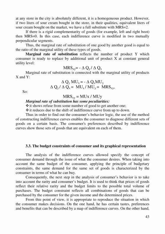
43

at any store in the city is absolutely different, it is a homogeneous product. However, if two liters of sour cream bought in the store, in their qualities, equivalent liters of sour cream bought on the market, we have a full substitute with MRS=2.

If there is a rigid complementarity of goods (for example, left and right boot) then MRS=0. In this case, each indifference curve is modified in two mutually perpendicular segments.

Thus, the marginal rate of substitution of one good by another good is equal to the ratio of the marginal utility of these types of goods.

Marginal rate of substitution reflects the number of product Y which consumer is ready to replace by additional unit of product X at constant general utility level:

МRSxy= - ∆ Qy / ∆ Qx Marginal rate of substitution is connected with the marginal utility of products

X and Y: ∆ Qy МUx = - ∆ QxМUy

∆ Qy / ∆ Qx = МUx / МUy = МRSxy, So:

МRSxy = МUx / МUy Marginal rate of substitution has some peculiarities: � it shows refuse from some number of good to get another one; � it reduces due to the shift of indifference curve from up to down. Thus in order to find out the consumer’s behavior logic, the use of the method

of constructing indifference curves enables the consumer to diagnose different sets of goods on a certain basis. The consumer's preferences described by indifference curves show those sets of goods that are equivalent on each of them.

3.3. The budget constraints of consumer and its graphical representation

The analysis of the indifference curves allowed specify the concept of consumer demand through the issue of what the consumer desires. When taking into account the same budget of the consumer, applying the principle of budgetary constraints, the same demand for the same set of goods is characterized by the consumer in terms of what he can buy.

Consequently, the next step in the analysis of consumer’s behavior is to take into account the rarity and consumer’s budget. It is used to think that prices of goods reflect their relative rarity and the budget limits to the possible total volume of purchases. The budget constraint reflects all combinations of goods that can be purchased by the consumer for the given income and the determined prices.

From thie point of view, it is appropriate to reproduce the situation in which the consumer makes decisions. On the one hand, he has certain tastes, preferences and benefits that can be described by a map of indifference curves. On the other hand,

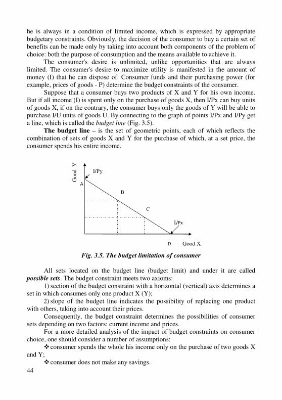
44

he is always in a condition of limited income, which is expressed by appropriate budgetary constraints. Obviously, the decision of the consumer to buy a certain set of benefits can be made only by taking into account both components of the problem of choice: both the purpose of consumption and the means available to achieve it.

The consumer's desire is unlimited, unlike opportunities that are always limited. The consumer's desire to maximize utility is manifested in the amount of money (I) that he can dispose of. Consumer funds and their purchasing power (for example, prices of goods - P) determine the budget constraints of the consumer.

Suppose that a consumer buys two products of X and Y for his own income. But if all income (I) is spent only on the purchase of goods X, then I/Px can buy units of goods X, if on the contrary, the consumer buys only the goods of Y will be able to purchase I/U units of goods U. By connecting to the graph of points I/Px and I/Py get a line, which is called the budget line (Fig. 3.5).

The budget line – is the set of geometric points, each of which reflects the combination of sets of goods X and Y for the purchase of which, at a set price, the consumer spends his entire income.

Fig. 3.5. The budget limitation of consumer

All sets located on the budget line (budget limit) and under it are called possible sets. The budget constraint meets two axioms:

1) section of the budget constraint with a horizontal (vertical) axis determines a set in which consumes only one product X (Y);

2) slope of the budget line indicates the possibility of replacing one product with others, taking into account their prices.

Consequently, the budget constraint determines the possibilities of consumer sets depending on two factors: current income and prices.

For a more detailed analysis of the impact of budget constraints on consumer choice, one should consider a number of assumptions:

� consumer spends the whole his income only on the purchase of two goods X and Y;

� consumer does not make any savings.

Good Х

Go

od У

D

І/Рх

І/Ру

А

В

С

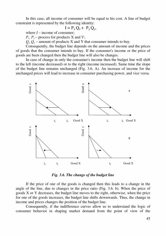
45

In this case, all income of consumer will be equal to his cost. A line of budget constraint is represented by the following identity:

I = Рх Qx + Рy Qy, where I – income of consumer; Рх, Рy – process for products Х and У; Qx, Qy – amount of products X and Y that consumer intends to buy. Consequently, the budget line depends on the amount of income and the prices

of goods that the consumer intends to buy. If the consumer's income or the price of goods are been changed then the budget line will also be changes.

In case of change in only the consumer's income then the budget line will shift to the left (income decreased) or to the right (income increased). Same time the slope of the budget line remains unchanged (Fig. 3.6. A). An increase of income for the unchanged prices will lead to increase in consumer purchasing power, and vice versa.

Fig. 3.6. The change of the budget line

If the price of one of the goods is changed then this leads to a change in the angle of the line, due to changes in the price ratio (Fig. 3.6. b). When the price of goods X or Y decreases, the budget line moves to the right, otherwise, when the price for one of the goods increases, the budget line shifts downwards. Thus, the change in income and prices changes the position of the budget line.

Consequently, if the indifference curves allow us to understand the logic of consumer behavior in shaping market demand from the point of view of the

Goo

d у

І1 І2 І2

Goo

d у

Good Х

а

б

І1 І2 І1 І2

Go

od

у

Goo

d у

Good Х

Good Х Good Х

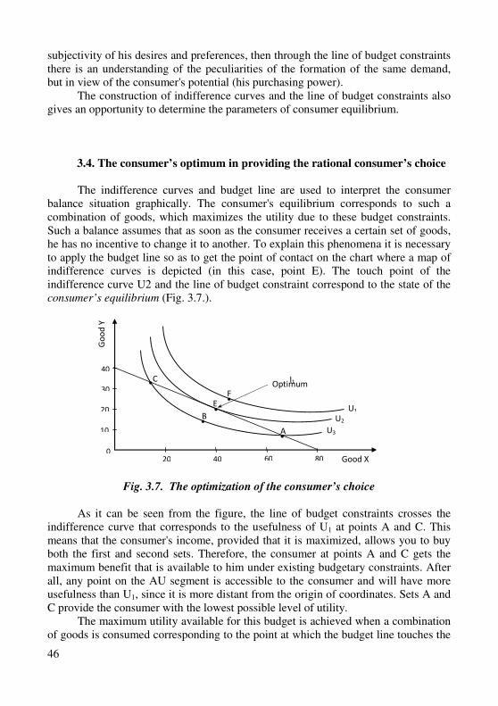
46

subjectivity of his desires and preferences, then through the line of budget constraints there is an understanding of the peculiarities of the formation of the same demand, but in view of the consumer's potential (his purchasing power).

The construction of indifference curves and the line of budget constraints also gives an opportunity to determine the parameters of consumer equilibrium.

3.4. The consumer’s optimum in providing the rational consumer’s choice

The indifference curves and budget line are used to interpret the consumer balance situation graphically. The consumer's equilibrium corresponds to such a combination of goods, which maximizes the utility due to these budget constraints. Such a balance assumes that as soon as the consumer receives a certain set of goods, he has no incentive to change it to another. To explain this phenomena it is necessary to apply the budget line so as to get the point of contact on the chart where a map of indifference curves is depicted (in this case, point E). The touch point of the indifference curve U2 and the line of budget constraint correspond to the state of the consumer’s equilibrium (Fig. 3.7.).

Fig. 3.7. The optimization of the consumer’s choice

As it can be seen from the figure, the line of budget constraints crosses the indifference curve that corresponds to the usefulness of U1 at points A and C. This means that the consumer's income, provided that it is maximized, allows you to buy both the first and second sets. Therefore, the consumer at points A and C gets the maximum benefit that is available to him under existing budgetary constraints. After all, any point on the AU segment is accessible to the consumer and will have more usefulness than U1, since it is more distant from the origin of coordinates. Sets A and C provide the consumer with the lowest possible level of utility.

The maximum utility available for this budget is achieved when a combination of goods is consumed corresponding to the point at which the budget line touches the

І1

40

Good X

•

•

•

•

Go

od

Y

Optimum F

•

С

В

Е

А

U1 U2

U3

30

20

10

0 20 40 60 80

47

most distant indirection curve. Therefore, moving along the budget line from the set of C to E, the consumer goes to the highest indifference curve and, accordingly, increases the utility. That is why the point E is the point of maximum satisfaction of the consumer from the acquisition of two goodies X and Y with a limited budget.

If the equilibrium is reached at the point of the touchdown of the budget line to the indifference curve U2, then this means that at the point E the inclination of these two lines coincides (the slope of the curve at any point corresponds to the inclination of the tangent to it at that point). At this point, the slope of the budget line (Px / Py) is equal to the slope of the indifference curve (dy / dx).

Equilibrium of the consumer can be given mathematical interpretation:

МUx / МUy = Рx / Рy, The consumer who maximizes the utility will buy two types of goods in such a

volume that their marginal utility per unit price is equal. The utility function is maximized when the marginal rate of substitution, which

expresses the slope of the indifference curve, is equal to the relative value of the benefits, which expresses the slope of the budget line. Or in an analytical form:

МRSxy = Рx / Рy = МUx / МUy This is the equation of consumer choice theory. This equation is also called the

law of equal marginal utility per monetary unit. The consumer's equilibrium can be substantiated algebraically. Only at point E,

where the budget line and the indifference curve are tangent, their inclination is same. As it is known, the slope of the indifference curve reflects the marginal rate of substitution, and the slope of the budget line – is the ratio of prices. This equality is the equilibrium of the consumer, similar to that obtained under the cardinal concept. The equilibrium equation reflects not only the conditions for optimizing consumer choice, but also the optimization conditions in a market economy as a whole: optimization is achieved when the marginal benefit equals the marginal cost.

The analysis of the ordinal version of consumer’s behavior theory makes it possible to draw the following conclusions:

� consumer’s demand for products can be used to place goods at the markets effectively;

� consumer’s choice is based on the preferences of the individual, which is a system of human’s values in relation to those goods that satisfy his vital needs;

� each individual consumer has individual tastes and preferences, on the basis of which he makes his choice so as to obtain the maximum benefit from the consumption of one or another benefit in accordance with product prices and available cash income;

� the consumer is able to rank his needs according to which there are such axioms of the ordinal theory as: the axiom of completeness, unsaturation, transitivity, independence;

� consumer preferences can be described using indifference curves that represent equivalent sets of goods for each of these curves from the consumer's point of view;

48

� consumer tastes are described by a map of indifference curves, which reflects the orderly ranking of all sets of benefits for consumer;

� the budget constraint shows the consumer's ability to buy a product for his income and for the corresponding prices for these goods;

� the ratio of the prices of two goods – is the absolute magnitude of the angle of inclination of the budget constraint, reflecting the possible price of one product through another;

� the consumer's balance is determined by the point of contact of the budget constraint and the most distant indifference curve, and corresponds to the state of the equilibrium, when the consumer does not want to change his choice.

Training

Key terms and concepts Ordinal theory of consumer’s behavior. Consumer’s preferences. Desires of

consumer. Consumer’s possibilities. Paradox of Errow. Axiom of transitiveness

benefits.

Utility of product. Marginal rate of substitution. Indifference curve. Model of J.

Hicks. Map of indifference curves. Complementarity of products. Rankings of

products.

Budget limitation. Budget line. Equation of the budget line. Purchasing

possibility of consumer. Equilibrium of consumer. The principle of equal utility. The

law of equal marginal utility.

Questions and tasks for students’ self-control:

1. What is the essence of the ordinal theory of utility of product? 2. What is the basis of consumer’s preferences and how it appears? 3. Which axioms of the theory of consumer choice do you know? 4. In which phenomena the Errow’s paradox appear? 5. What is the indifference curve? 6. Who was the first who offered indifference curves for the analysis of

consumer’s behavior? 7. Please characterize the map of indifference curves. 8. Give a definition to the concept “marginal rate of substitution”. 9. How can the marginal rate of substitution be determined graphically? 10. Which products are called “products-substitutes”? 11. What is the equation of the consumer’s choice theory? 12. What is the b budget line? 13. Justify the equation of the budget line. 14. What is the essence of the budget limitation of consumer? 15. Under the influence of which factors the slope of budget line is changed? 16. How can the consumer’s equilibrium in ordinal theory be determined?

49

Tests

1. Indifference curves have following features:

а) all answers are correct; b) they never intersect; c) for the vast majority of products they have negative slope; d) indifference curves that are situated farther from the origin, correspond to

sets of products with higher utility level. 2. The map of indifference curves – is:

а) the totality of total and marginal utility curves; b) the totality of curves of different income levels each of which represents

different income level of consumer; c) the totality of curves of similar income levels of consumer each of which

represents the same income level; d) the totality of curves if similar utility levels each of which represents

different level.

3. The position and slope of indifference curve for particular consumer

can be explained by:

а) only his preferences; b) only prices of products; c) income level of consumer; d) preferences, income level and prices of products.

4. Budget lines:

а) are always straight lines; b) are always broken lines; c) at any circumstances cannot be broken; d) can be both straight and broken.

5. Budget limitation of consumer – is:

а) income of consumer; b) prices of products; c) the totality of consumption baskets, available for consumer at given price

level and his budget; d) consumer’s income, prices of products and it utility. 6. Increase of consumer’s income at other unchanged conditions

graphically corresponds to:

а) parallel shift of the budget line to the right; b) parallel shift of the budget line to the left; c) decrease of slope of budget line; d) increase of slope of budget line.

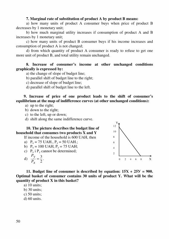
50

7. Marginal rate of substitution of product A by product B means:

а) how many units of product A consumer buys when price of product B decreases by 1 monetary unit;

b) how much marginal utility increases if consumption of product A and B increases by 1 monetary unit;

c) how many units of product B consumer buys if his income increases and consumption of product A is not changed;

d) from which quantity of product A consumer is ready to refuse to get one more unit of product B, and total utility remain unchanged.

8. Increase of consumer’s income at other unchanged conditions

graphically is expressed by:

а) the change of slope of budget line; b) parallel shift of budget line to the right; c) decrease of slope of budget line; d) parallel shift of budget line to the left.

9. Increase of price of one product leads to the shift of consumer’s

equilibrium at the map of indifference curves (at other unchanged conditions):

а) up to the right; b) down to the right; c) to the left, up or down; d) shift along the same indifference curve.

10. The picture describes the budget line of

household that consumes two products X and Y If income of the household is 600 UAH, then а) Рх = 75 UAH., Ру = 50 UAH.; b) Рх = 100 UAH, Ру = 75 UAH; c) Рх і Ру cannot be determined;

d) 2

3=

xP

yP.

11. Budget line of consumer is described by equation: 15Х + 25У = 900.

Optimal basket of consumer contains 30 units of product Y. What will be the

quantity of product X in this basket?

а) 10 units; b) 30 units; c) 50 units; d) 60 units.

Y 12

10

8

6

4

2

0 2 4 6 8 X

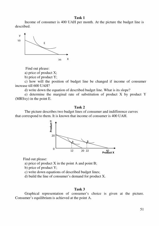
51

Task 1

Income of consumer is 400 UAH per month. At the picture the budget line is described.

Find out please: а) price of product Х; b) price of product Y; c) how will the position of budget line be changed if income of consumer

increase till 600 UAH? d) write down the equation of described budget line. What is its slope? e) determine the marginal rate of substitution of product X by product Y

(MRSxy) in the point E.

Task 2

The picture describes two budget lines of consumer and indifference curves that correspond to them. It is known that income of consumer is 400 UAH.

Find out please: а) price of product X in the point A and point B; b) price of product Y; c) write down equations of described budget lines; d) build the line of consumer’s demand for product X.

Task 3

Graphical representation of consumer’s choice is given at the picture. Consumer’s equilibrium is achieved at the point A.

20

10

Х

Е

У

Pro

du

ct Y

Product Х

B • •

20

0 12 20 22 40

A

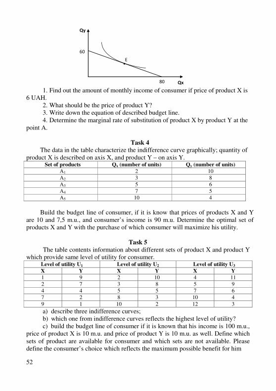
52

1. Find out the amount of monthly income of consumer if price of product X is 6 UAH.

2. What should be the price of product Y? 3. Write down the equation of described budget line. 4. Determine the marginal rate of substitution of product X by product Y at the

point A.

Task 4

The data in the table characterize the indifference curve graphically; quantity of product X is described on axis X, and product Y – on axis Y.

Set of products Qх (number of units) Qу (number of units)

А1 2 10

А2 3 8

А3 5 6

А4 7 5

А5 10 4

Build the budget line of consumer, if it is know that prices of products X and Y

are 10 and 7,5 m.u., and consumer’s income is 90 m.u. Determine the optimal set of products X and Y with the purchase of which consumer will maximize his utility.

Task 5

The table contents information about different sets of product X and product Y which provide same level of utility for consumer.

Level of utility U1 Level of utility U2 Level of utility U3

X Y X Y X Y

1 9 2 10 4 11

2 7 3 8 5 9

4 4 5 5 7 6

7 2 8 3 10 4

9 1 10 2 12 3

a) describe three indifference curves; b) which one from indifference curves reflects the highest level of utility? c) build the budget line of consumer if it is known that his income is 100 m.u.,

price of product X is 10 m.u. and price of product Y is 10 m.u. as well. Define which sets of product are available for consumer and which sets are not available. Please define the consumer’s choice which reflects the maximum possible benefit for him

60

Qy

Qx

E •

80

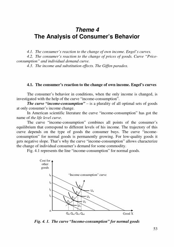
53

Theme 4 The Analysis of Consumer’s Behavior

4.1. The consumer’s reaction to the change of own income. Engel’s curves.

4.2. The consumer’s reaction to the change of prices of goods. Curve “Price-

consumption” and individual demand curve.

4.3. The income and substitution effects. The Giffen paradox.

4.1. The consumer’s reaction to the change of own income. Engel’s curves

The consumer’s behavior in conditions, when the only income is changed, is investigated with the help of the curve “income-consumption”.

The curve “income-consumption” – is a plurality of all optimal sets of goods at only consumer’s income change.

In American scientific literature the curve “income-consumption” has got the name of the life level curve.

The curve “income-consumption” combines all points of the consumer’s equilibrium that correspond to different levels of his income. The trajectory of this curve depends on the type of goods the consumer buys. The curve “income-consumption” for normal goods is permanently growing. For low-quality goods it gets negative slope. That’s why the curve “income-consumption” allows characterize the change of individual consumer’s demand for some commodity.

Fig. 4.1 represents the line “income-consumption” for normal goods.

Fig. 4. 1. The curve “Income-consumption” for normal goods

Cost for other goods

“Income-consumption” curve

•

U1

U2

U3 І1

0Qx1

U4

Е1

Е2

Е3

Е4

•

•

•

Qx2 Qx3 Qx4

І2

І3

І4

Good Х

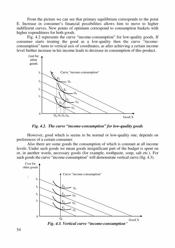
54

From the picture we can see that primary equilibrium corresponds to the point E. Increase in consumer’s financial possibilities allows him to move to higher indifferent curves. New points of optimum correspond to consumption baskets with higher expenditures for both goods.

Fig. 4.2 represents the curve “income-consumption” for low-quality goods. If consumer starts treating the good as a low-quality then the curve “income-consumption” turns to vertical axis of coordinates, as after achieving a certain income level further increase in his income leads to decrease in consumption of this product.

Fig. 4.2. The curve “income-consumption” for low-quality goods

However, good which is seems to be normal or low-quality one, depends on preferences of a certain consumer.

Also there are some goods the consumption of which is constant at all income levels. Under such goods we mean goods insignificant part of the budget is spent on or, in another words, necessary goods (for example, toothpaste, soup, salt etc.). For such goods the curve “income-consumption” will demonstrate vertical curve (fig. 4.3).

.

Fig. 4.3. Vertical curve “income-consumption”

Cost for

other

goods

Curve "income-consumption"

•

U1

U2

U3 І1

0Qx1

U4

Е1 Е2

Е3

Е4

•

•

•

Qx2 Qx3 Qx4

І2

І3

І4

Good Х

Cost for other goods

Curve "income-consumption"

•

U1

U2

U3

І1

0

U4

Е1

Е2

Е3

Е4

•

•

•

Qx

І2

І3

І4

Good Х

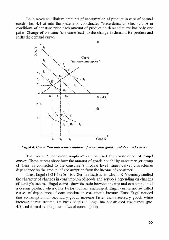
55

Let’s move equilibrium amounts of consumption of product in case of normal goods (fig. 4.4 a) into the system of coordinates “price-demand” (fig. 4.4. b) in conditions of constant price each amount of product on demand curve has only one point. Change of consumer’s income leads to the change in demand for product and shifts the demand curve.

Fig. 4.4. Curve “income-consumption” for normal goods and demand curves

The model “income-consumption” can be used for construction of Engel

curves. These curves show how the amount of goods bought by consumer (or group of them) is connected to the consumer’s income level. Engel curves characterize dependence on the amount of consumption from the income of consumer.

Ernst Engel (1821-1896) – is a German statistician who in XIX century studied the character of changes in consumption of goods and services depending on changes of family’s income. Engel curves show the ratio between income and consumption of a certain product when other factors remain unchanged. Engel curves are so called curves of dependence of consumption on consumer’s income. Ernst Engel noticed that consumption of secondary goods increase faster than necessary goods while increase of real income. On basis of this E. Engel has constructed few curves (pic. 4.5) and formulated empirical laws of consumption.

Curve

"income-consumption"

Y3

Y2

Y1

0

І3

І2

І1

*

1E

U1

U2

U3

X1 X2 X3 Good X

P

*

2E

*

3E

*

1E *

2E *

3E

D2 D3 D1

X1 X2 X3

P*

a)

б)

Good Y

Good X

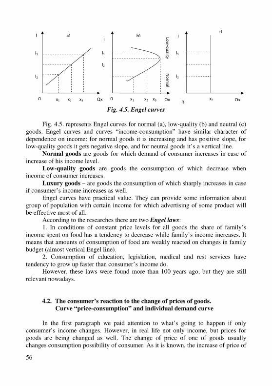
56

Fig. 4.5. Engel curves

Fig. 4.5. represents Engel curves for normal (a), low-quality (b) and neutral (c) goods. Engel curves and curves “income-consumption” have similar character of dependence on income: for normal goods it is increasing and has positive slope, for low-quality goods it gets negative slope, and for neutral goods it’s a vertical line.

Normal goods are goods for which demand of consumer increases in case of increase of his income level.

Low-quality goods are goods the consumption of which decrease when income of consumer increases.

Luxury goods – are goods the consumption of which sharply increases in case if consumer’s income increases as well.

Engel curves have practical value. They can provide some information about group of population with certain income for which advertising of some product will be effective most of all.

According to the researches there are two Engel laws: 1. In conditions of constant price levels for all goods the share of family’s

income spent on food has a tendency to decrease while family’s income increases. It means that amounts of consumption of food are weakly reacted on changes in family budget (almost vertical Engel line).

2. Consumption of education, legislation, medical and rest services have tendency to grow up faster than consumer’s income do.

However, these laws were found more than 100 years ago, but they are still relevant nowadays.

4.2. The consumer’s reaction to the change of prices of goods.

Curve “price-consumption” and individual demand curve

In the first paragraph we paid attention to what’s going to happen if only consumer’s income changes. However, in real life not only income, but prices for goods are being changed as well. The change of price of one of goods usually changes consumption possibility of consumer. As it is known, the increase of price of

c)

х1 х2 х3

I1

I2

х1 х2 х3 х1 Qx Qx Qx 0

0 0

I I Lo

w-q

ua

lity

N

orm

al

I1

I2

а) b)

I1

I2

І

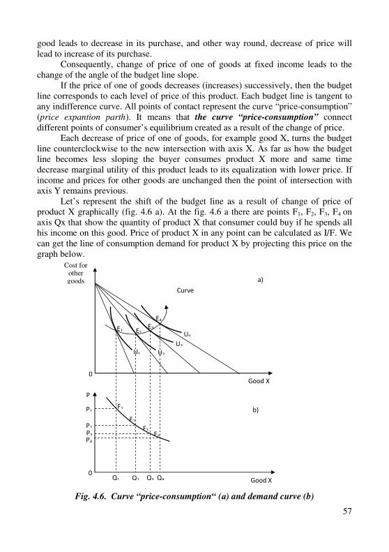
57

good leads to decrease in its purchase, and other way round, decrease of price will lead to increase of its purchase.

Consequently, change of price of one of goods at fixed income leads to the change of the angle of the budget line slope.

If the price of one of goods decreases (increases) successively, then the budget line corresponds to each level of price of this product. Each budget line is tangent to any indifference curve. All points of contact represent the curve “price-consumption” (price expantion parth). It means that the curve “price-consumption” connect different points of consumer’s equilibrium created as a result of the change of price.

Each decrease of price of one of goods, for example good X, turns the budget line counterclockwise to the new intersection with axis X. As far as how the budget line becomes less sloping the buyer consumes product X more and same time decrease marginal utility of this product leads to its equalization with lower price. If income and prices for other goods are unchanged then the point of intersection with axis Y remains previous.

Let’s represent the shift of the budget line as a result of change of price of product X graphically (fig. 4.6 a). At the fig. 4.6 a there are points F1, F2, F3, F4 on axis Qx that show the quantity of product X that consumer could buy if he spends all his income on this good. Price of product X in any point can be calculated as I/F. We can get the line of consumption demand for product X by projecting this price on the graph below.

Fig. 4.6. Curve “price-consumption“ (а) and demand curve (b)

Curve

Е4 Е3

Е2 Е1

U1 U2

U3

U4

Cost for other goods

Good Х

Р

P1

P2 P3 P4

F1

F2

F3 F4

0

0 Q1 Q2 Q3 Q4

a)

b)

Good Х

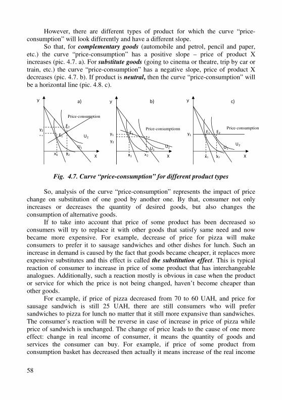
58

У

Price-consumption

Е2

Е1 у1 у2

х1 х2 Х

U1

U2

а)

Е1 Е2

Price-consumptionn у1

у2

х1 х2 Х

У У

Х

Е2 Е1

х1 х2

у1

U1 U2 U1

U2

b) c)

However, there are different types of product for which the curve “price-consumption” will look differently and have a different slope.

So that, for complementary goods (automobile and petrol, pencil and paper, etc.) the curve “price-consumption” has a positive slope – price of product X increases (pic. 4.7. a). For substitute goods (going to cinema or theatre, trip by car or train, etc.) the curve “price-consumption” has a negative slope, price of product X decreases (pic. 4.7. b). If product is neutral, then the curve “price-consumption” will be a horizontal line (pic. 4.8. c).

Fig. 4.7. Curve “price-consumption” for different product types

So, analysis of the curve “price-consumption” represents the impact of price change on substitution of one good by another one. By that, consumer not only increases or decreases the quantity of desired goods, but also changes the consumption of alternative goods.

If to take into account that price of some product has been decreased so consumers will try to replace it with other goods that satisfy same need and now became more expensive. For example, decrease of price for pizza will make consumers to prefer it to sausage sandwiches and other dishes for lunch. Such an increase in demand is caused by the fact that goods became cheaper, it replaces more expensive substitutes and this effect is called the substitution effect. This is typical reaction of consumer to increase in price of some product that has interchangeable analogues. Additionally, such a reaction mostly is obvious in case when the product or service for which the price is not being changed, haven’t become cheaper than other goods.

For example, if price of pizza decreased from 70 to 60 UAH, and price for sausage sandwich is still 25 UAH, there are still consumers who will prefer sandwiches to pizza for lunch no matter that it still more expansive than sandwiches. The consumer’s reaction will be reverse in case of increase in price of pizza while price of sandwich is unchanged. The change of price leads to the cause of one more effect: change in real income of consumer, it means the quantity of goods and services the consumer can buy. For example, if price of some product from consumption basket has decreased then actually it means increase of the real income

Price-consumption

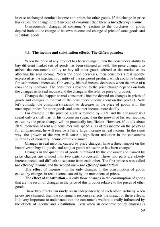
59

in case unchanged nominal income and prices for other goods. If the change in price has caused the change of real income of consumer then there is the effect of income.

Consequently, changes of consumer’s reaction to the purchases of goods depend both on the change of his own income and change of price of some goods and substitute goods.

4.3. The income and substitution effects. The Giffen paradox

When the price of any product has been changed, then the consumer's ability to buy different market sets of goods has been changed as well. The price change also affects the consumer's ability to buy all other goods offered at the market as its affecting his real income. When the price decreases, then consumer’s real income expressed as the maximum quantity of the proposed product, which could be bought for cash income, increases. Conversely, his real income decreases when the price of a commodity increases. The consumer’s reaction to the price change depends on both the changes in its real income and the change in the relative price of product.

Changes that happen to real consumer’s income depend on changes in prices of goods and changes in the part of the consumer's income spent on this product. Now let's consider the consumer's reaction to decrease in the price of goods with the unchanged prices for other goods and consumer income more detaily.

For example, if the price of sugar is reduced by 20 % and the consumer will spend only a small part of his income on sugar, then the growth of his real income, caused by the price change, will be practically insufficient. However, if to talk about 20 % reduction of rent and consumer will spend a 1/3 of his income on the payment for an apartment, he will receive a fairly large increase in real income. In the same way, the growth of the rent will cause a significant reduction in the consumer's suitability of monetary income of the consumer.

Changes in real income, caused by price changes, have a direct impact on the incentives to buy all goods, and not just goods whose price has been changed.

Changes in the quantities of goods purchased by the consumer and caused by price changes are divided into two parts (processes). These two parts are closely interconnected and difficult to separate from each other. The first process was called the effect of income, and the second one – the effect of substitution.

The effect of income – is the only changes in the consumption of goods caused by changes in real income, caused by the movement of prices.

The effect of substitution – is only those changes in the consumption of goods that are the result of changes in the price of this product relative to the prices of other goods.

These two effects can rarely occur independently of each other. Actually when prices are changed, then the consumer's response reflects the impact of these effects. It is very important to understand that the consumer's welfare is really influenced by the effects of income and substitution. Even when an economic policy analysis is

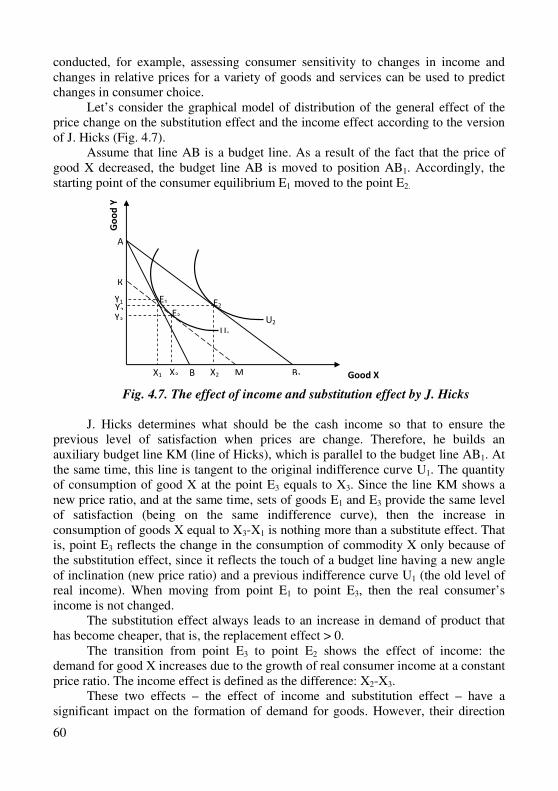
60

Good Х

conducted, for example, assessing consumer sensitivity to changes in income and changes in relative prices for a variety of goods and services can be used to predict changes in consumer choice.

Let’s consider the graphical model of distribution of the general effect of the price change on the substitution effect and the income effect according to the version of J. Hicks (Fig. 4.7).

Assume that line AB is a budget line. As a result of the fact that the price of good X decreased, the budget line AB is moved to position AB1. Accordingly, the starting point of the consumer equilibrium E1 moved to the point E2.

Fig. 4.7. The effect of income and substitution effect by J. Hicks

J. Hicks determines what should be the cash income so that to ensure the previous level of satisfaction when prices are change. Therefore, he builds an auxiliary budget line KM (line of Hicks), which is parallel to the budget line AB1. At the same time, this line is tangent to the original indifference curve U1. The quantity of consumption of good X at the point E3 equals to X3. Since the line KM shows a new price ratio, and at the same time, sets of goods E1 and E3 provide the same level of satisfaction (being on the same indifference curve), then the increase in consumption of goods X equal to X3-X1 is nothing more than a substitute effect. That is, point E3 reflects the change in the consumption of commodity X only because of the substitution effect, since it reflects the touch of a budget line having a new angle of inclination (new price ratio) and a previous indifference curve U1 (the old level of real income). When moving from point E1 to point E3, then the real consumer’s income is not changed.

The substitution effect always leads to an increase in demand of product that has become cheaper, that is, the replacement effect > 0.

The transition from point E3 to point E2 shows the effect of income: the demand for good X increases due to the growth of real consumer income at a constant price ratio. The income effect is defined as the difference: X2-X3.

These two effects – the effect of income and substitution effect – have a significant impact on the formation of demand for goods. However, their direction

Е1

Е3 Е2

А

В В1

К

М Х1 Х3 Х2

Y1 Y2 Y3

U1 U2

Go

od

Y

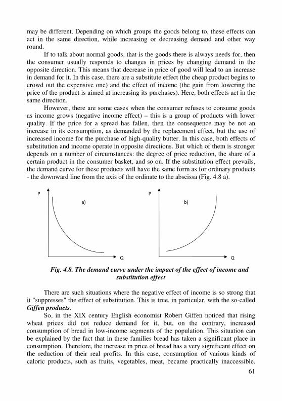
61

may be different. Depending on which groups the goods belong to, these effects can act in the same direction, while increasing or decreasing demand and other way round.

If to talk about normal goods, that is the goods there is always needs for, then the consumer usually responds to changes in prices by changing demand in the opposite direction. This means that decrease in price of good will lead to an increase in demand for it. In this case, there are a substitute effect (the cheap product begins to crowd out the expensive one) and the effect of income (the gain from lowering the price of the product is aimed at increasing its purchases). Here, both effects act in the same direction.

However, there are some cases when the consumer refuses to consume goods as income grows (negative income effect) – this is a group of products with lower quality. If the price for a spread has fallen, then the consequence may be not an increase in its consumption, as demanded by the replacement effect, but the use of increased income for the purchase of high-quality butter. In this case, both effects of substitution and income operate in opposite directions. But which of them is stronger depends on a number of circumstances: the degree of price reduction, the share of a certain product in the consumer basket, and so on. If the substitution effect prevails, the demand curve for these products will have the same form as for ordinary products - the downward line from the axis of the ordinate to the abscissa (Fig. 4.8 a).

Fig. 4.8. The demand curve under the impact of the effect of income and

substitution effect

There are such situations where the negative effect of income is so strong that

it "suppresses" the effect of substitution. This is true, in particular, with the so-called Giffen products.

So, in the XIX century English economist Robert Giffen noticed that rising wheat prices did not reduce demand for it, but, on the contrary, increased consumption of bread in low-income segments of the population. This situation can be explained by the fact that in these families bread has taken a significant place in consumption. Therefore, the increase in price of bread has a very significant effect on the reduction of their real profits. In this case, consumption of various kinds of caloric products, such as fruits, vegetables, meat, became practically inaccessible.

Р Р

Q Q

а) b)

62

Therefore, their consumption had to be offset by the same bread that has risen in price.

So Giffen product must simultaneously correspond to following requirements: � to be low-quality product in mind of consumer; � to be essential part of consumer’s cost. A similar situation can happen to some other commodities: potatoes, low-grade

cereals if costs for consumption of them take a significant place in the budget of consumers. Giffen's paradox is not a very common situation, but it is quite realistic when the demand curve reflects the positive values of the demand-price function and increases from the origin (Fig. 4.8 b).

However, there is a case where the curve will same shape if consumers increase the number of purchases of more expensive goods for reasons of prestige. Subjects from the rich or those who want to appear in response to a higher price, react not to a decrease but to an increase in demand. There is the so-called Veblen effect.

Summarizing the foregoing, we can make the following conclusions: � the consumer's reaction to the change in his budget is reflected by the line of

"income-consumption", which shows the points of equilibrium corresponding to each level of income;

� the reaction of the consumer to the change price of one of the goods, under unchanged other conditions, reflects the line "consumption price". Each point on this line reflects the equilibrium states of the consumer when the price of one of the goods is changed;

� Engel’s curves reflect the relationship between the amount of consumption and the income of the consumer.

The theory of consumer’s choice is based on the assumption of rational consumer behavior which is based on attempts to maximize utility by acquiring different goods and services. By making his choice the consumer focuses on the following three components: own preferences, available budget, prices of goods.

Consumer equilibrium is achieved with such a combination of good, in which the ratio of marginal utility and price of goods is the same for the consumer. Change of the consumer’s income level and commodity prices (due to the effect of substitution and the effect of income) impacts on the change in consumer equilibrium.

Training

Key terms and concepts Curve “income-consumption”. Engel curves. Engel laws. Normal goods. Low-

quality goods. Luxury goods. Curve “price-consumption”. Substitution effect. Effect

of income. Commodity of Giffen. The Giffen paradox. Commodity of Veblen.

Questions and tasks for self-testing and monitoring of learned knowledge 1. What is the essence of the theory of analysis of consumer’s behavior? 2. How the curve “income-consumption” is built? Characterize it. 3. How does the curve “income-consumption” for normal goods look like?

63

4. What does the Engel’s curve represent? 5. Which Engel’s laws do you know? 6. What does the curve “income-consumption” represent? How to build it? 7. How does the curve “income-consumption” for different types of products

look like? 8. On the basis of which curve is the demand curve built? 9. What does the effect of income mean? 10. Give explanation of the substitution effect in justification of consumer’s

behavior. 11. How does the paradox of Giffen achieve? Give examples of commodities

of Giffen and Veblen.

Tests

1. Curve “income-consumption” shows:

а) all points of consumer’s equilibrium according to increase of income; b) dependence of utility level on income; c) dependence of products consumption on prices; d) set of products that bring certain level of satisfaction to consumer. 2. Curve “price-consumption” combines:

а) all points of consumer’s equilibrium connected with change of price of both products;

b) all points of consumer’s equilibrium connected with change of income; c) all points of consumer’s equilibrium that are connected with change of one

product; d) all combinations of two products that provide the same utility level.

3. Which curve is the basis for creation of the individual demand curve:

а) curve “price-consumption”; b) curve “income-consumption”; c) Engel’s curve; d) indifference curve. 4. Engel’s curves characterize:

а) dependence of the amount of product consumption on income of consumer; b) dependence of the amount of product consumption on its price; c) dependence of utility of product on the amount of it consumption; d) dependence of cost of consumer on the price of product. 5. For the commodity of Giffen typically is:

а) amount of consumption of product increases with the decrease of price; b) amount of consumption of product increases with the increase of price; c) amount of consumption increases with the increase of income; d) amount of consumption increases with the decrease of income.

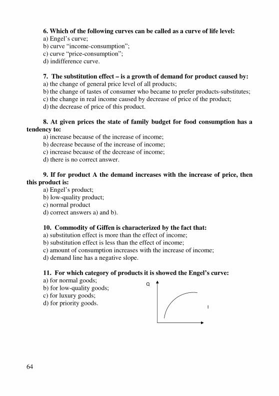
64

6. Which of the following curves can be called as a curve of life level:

а) Engel’s curve; b) curve “income-consumption”; c) curve “price-consumption”; d) indifference curve. 7. The substitution effect – is a growth of demand for product caused by:

а) the change of general price level of all products; b) the change of tastes of consumer who became to prefer products-substitutes; c) the change in real income caused by decrease of price of the product; d) the decrease of price of this product.

8. At given prices the state of family budget for food consumption has a

tendency to:

а) increase because of the increase of income; b) decrease because of the increase of income; c) increase because of the decrease of income; d) there is no correct answer.

9. If for product A the demand increases with the increase of price, then

this product is:

а) Engel’s product; b) low-quality product; c) normal product d) correct answers a) and b).

10. Commodity of Giffen is characterized by the fact that: а) substitution effect is more than the effect of income; b) substitution effect is less than the effect of income; c) amount of consumption increases with the increase of income; d) demand line has a negative slope.

11. For which category of products it is showed the Engel’s curve:

а) for normal goods; b) for low-quality goods; c) for luxury goods; d) for priority goods.

I

Q

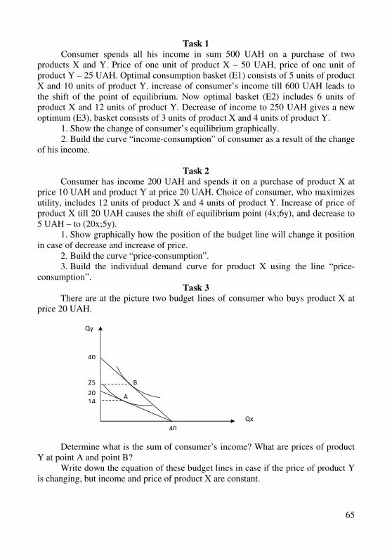
65

Task 1

Consumer spends all his income in sum 500 UAH on a purchase of two products X and Y. Price of one unit of product X – 50 UAH, price of one unit of product Y – 25 UAH. Optimal consumption basket (E1) consists of 5 units of product X and 10 units of product Y. increase of consumer’s income till 600 UAH leads to the shift of the point of equilibrium. Now optimal basket (E2) includes 6 units of product X and 12 units of product Y. Decrease of income to 250 UAH gives a new optimum (E3), basket consists of 3 units of product X and 4 units of product Y.

1. Show the change of consumer’s equilibrium graphically. 2. Build the curve “income-consumption” of consumer as a result of the change

of his income.

Task 2

Consumer has income 200 UAH and spends it on a purchase of product X at price 10 UAH and product Y at price 20 UAH. Choice of consumer, who maximizes utility, includes 12 units of product X and 4 units of product Y. Increase of price of product X till 20 UAH causes the shift of equilibrium point (4x;6y), and decrease to 5 UAH – to (20x;5y).

1. Show graphically how the position of the budget line will change it position in case of decrease and increase of price.

2. Build the curve “price-consumption”. 3. Build the individual demand curve for product X using the line “price-

consumption”. Task 3

There are at the picture two budget lines of consumer who buys product X at price 20 UAH.

Determine what is the sum of consumer’s income? What are prices of product Y at point A and point B?

Write down the equation of these budget lines in case if the price of product Y is changing, but income and price of product X are constant.

25

14 А

В

40

20

40

Qy

Qx

66

Task 4

The budget of consumer per week is 200 UAH and he spends it for the purchase of product X at price 4 UAH, product Y at price 5 UAH. The choice of consumer who maximizes utility includes 2,5 units of product X and 2 units of product Y. Increase of income by 20 UAH leads to the shift of equilibrium point and now consumption basket includes 5x and 4y. And increase of income by 10 UAH more – in accordance 5,5x and 5,6y.

Build the curve “income-consumption”.

Task 5

From all offered variants rational consumer has chosen the one that consist of 20 units of product х1 and 25 units of product х2. The utility function of consumer looks like: U(х1; х2) = х1

2+ х2 ; while income of consumer is 100 UAH per month.

Define how the income of consumer will be changed if a new set includes 10 units of product х1 and 15 units of product х2, income level has not been changed.

Task 6

Build the curve “income-consumption” for consumer with the utility function. 1) U(х1; х2) = х1

1/2+ х2

3/2

2) U(х1; х2) = min{2 х1;5 х2} Price of first product is 15 UAH, price of the second one – 30 UAH.

67

Theme 5

Demand, Supply and Market Equilibrium

5.1. Demand, factors of demand. The law of demand. 5.2. Supply, factors of supply. The law of supply. 5.3. The market equilibrium. 5.4. Elasticity of demand: indicators and factors of impact. 5.5. Elasticity of supply.

5.1. Demand, factors of demand. The law of demand

It is known that all microeconomic actors interact through the market which is characterized by the interconnection of such variables as demand, supply and price. They are closely linked and mutually affect each other, forming a market mechanism for self-regulation.

Consumers who need certain goods appear on the market and form demand. Demand – is a form of needs expression that is represented at the market by the

amount of goods and services that consumers want and ready to buy at a certain price level during a certain period of time.

The law of demand proves that there is inverse connection between price and amount of demand: the amount of demand decreases when price increases, and other way round.

Inverse dependence of the demand dynamics on changes of price level is caused by following reasons:

� first, prices reduction will increase the number of buyers; � secondly, prices reduction increases the purchasing power of consumers (the

effect of income); � thirdly, the saturation of the market leads to a decrease in the usefulness of

additional units of products, so buyers are ready to buy them only at lower prices (the law of decreasing marginal productivity);

� fourth, the increase of price of this product induces the buyer to reduce consumption of this product and replace it with cheaper one(the effect of substitution).

The connection between price and demand is not unconditional. There are goods the demand for which does not reflect a stable reverse causal relationship with the price. These paradoxes include:

1. The effect of Giffen: as the price of goods increases demand for it increases. For the first time, this effect was researched by the British economist R. Giffen when at the end of the nineteenth century in Ireland the rapid rise in prices for potatoes and bread led to a sharp increase in demand for them. Therefore, such goods include necessity goods. The demand curve will have a positive slope, that is,

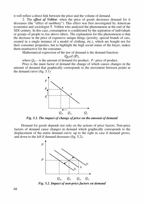
68

it will reflect a direct link between the price and the volume of demand. 2. The effect of Veblen: when the price of goods decreases demand for it

decreases (the “effect of snobbery”). This effect was first investigated by American economist and sociologist T. Veblen who analyzed the phenomenon at the end of the XIX century. In this case, consumption is conditioned by the aspiration of individuals or groups of people to rise above others. The explanation for this phenomenon is that the decrease in the price of expensive unique things (jewelry, special brands of cars, created in a single instance of a model of clothing, etc.), which are bought not for their consumer properties, but to highlight the high social status of the buyer, makes them unattractive for the consumer.

Mathematical expression of the law of demand is the demand function:

QD=f (P), where QD – is the amount of demand for product; P– price of product. Price is the main factor of demand the change of which causes changes in the

amount of demand that graphically corresponds to the movement between points at the demand curve (fig. 5.1)

Fig. 5.1. The impact of change of price on the amount of demand

Demand for goods depends not only on the actions of price factors. Non-price factors of demand cause changes in demand which graphically corresponds to the displacement of the entire demand curve: up to the right in case if demand grows, and down to the left if demand decreases (fig. 5.2).

Fig. 5.2. Impact of non-price factors on demand

2DQ1DQ DQ

1P

2P A

Б

P

2DQ1DQ DQ

D2

P

P

DQ

D

D1

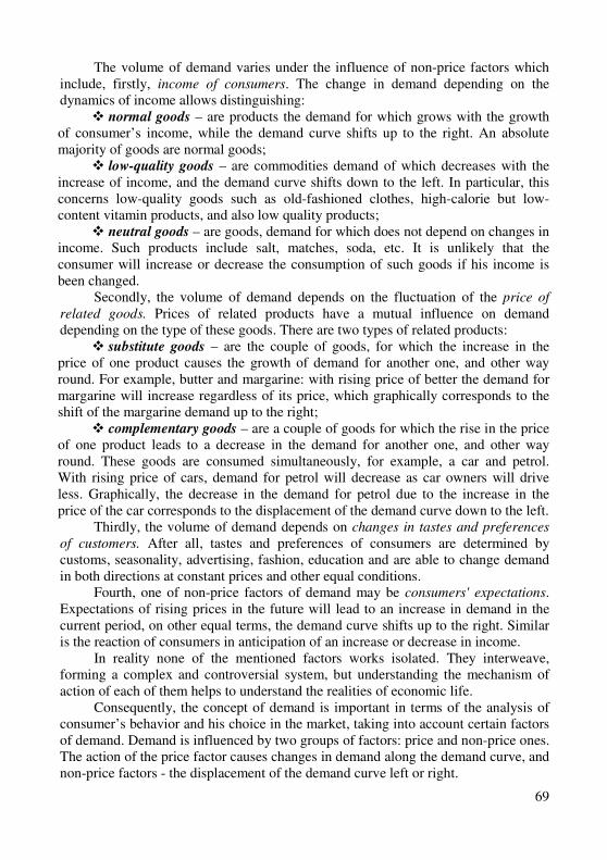
69

The volume of demand varies under the influence of non-price factors which include, firstly, income of consumers. The change in demand depending on the dynamics of income allows distinguishing:

� normal goods – are products the demand for which grows with the growth of consumer’s income, while the demand curve shifts up to the right. An absolute majority of goods are normal goods;

� low-quality goods – are commodities demand of which decreases with the increase of income, and the demand curve shifts down to the left. In particular, this concerns low-quality goods such as old-fashioned clothes, high-calorie but low-content vitamin products, and also low quality products;

� neutral goods – are goods, demand for which does not depend on changes in income. Such products include salt, matches, soda, etc. It is unlikely that the consumer will increase or decrease the consumption of such goods if his income is been changed.

Secondly, the volume of demand depends on the fluctuation of the price of

related goods. Prices of related products have a mutual influence on demand depending on the type of these goods. There are two types of related products:

� substitute goods – are the couple of goods, for which the increase in the price of one product causes the growth of demand for another one, and other way round. For example, butter and margarine: with rising price of better the demand for margarine will increase regardless of its price, which graphically corresponds to the shift of the margarine demand up to the right;

� complementary goods – are a couple of goods for which the rise in the price of one product leads to a decrease in the demand for another one, and other way round. These goods are consumed simultaneously, for example, a car and petrol. With rising price of cars, demand for petrol will decrease as car owners will drive less. Graphically, the decrease in the demand for petrol due to the increase in the price of the car corresponds to the displacement of the demand curve down to the left.

Thirdly, the volume of demand depends on changes in tastes and preferences

of customers. After all, tastes and preferences of consumers are determined by customs, seasonality, advertising, fashion, education and are able to change demand in both directions at constant prices and other equal conditions.

Fourth, one of non-price factors of demand may be consumers' expectations. Expectations of rising prices in the future will lead to an increase in demand in the current period, on other equal terms, the demand curve shifts up to the right. Similar is the reaction of consumers in anticipation of an increase or decrease in income.

In reality none of the mentioned factors works isolated. They interweave, forming a complex and controversial system, but understanding the mechanism of action of each of them helps to understand the realities of economic life.

Consequently, the concept of demand is important in terms of the analysis of consumer’s behavior and his choice in the market, taking into account certain factors of demand. Demand is influenced by two groups of factors: price and non-price ones. The action of the price factor causes changes in demand along the demand curve, and non-price factors - the displacement of the demand curve left or right.

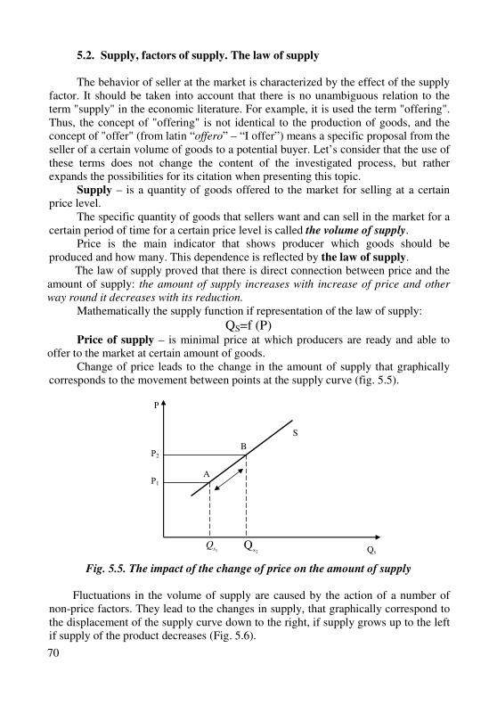
70

5.2. Supply, factors of supply. The law of supply

The behavior of seller at the market is characterized by the effect of the supply

factor. It should be taken into account that there is no unambiguous relation to the term "supply" in the economic literature. For example, it is used the term "offering". Thus, the concept of "offering" is not identical to the production of goods, and the concept of "offer" (from latin “offero” – “I offer”) means a specific proposal from the seller of a certain volume of goods to a potential buyer. Let’s consider that the use of these terms does not change the content of the investigated process, but rather expands the possibilities for its citation when presenting this topic.

Supply – is a quantity of goods offered to the market for selling at a certain price level.

The specific quantity of goods that sellers want and can sell in the market for a certain period of time for a certain price level is called the volume of supply.

Price is the main indicator that shows producer which goods should be produced and how many. This dependence is reflected by the law of supply.

The law of supply proved that there is direct connection between price and the amount of supply: the amount of supply increases with increase of price and other

way round it decreases with its reduction. Mathematically the supply function if representation of the law of supply:

QS=f (P) Price of supply – is minimal price at which producers are ready and able to

offer to the market at certain amount of goods. Change of price leads to the change in the amount of supply that graphically

corresponds to the movement between points at the supply curve (fig. 5.5).

Fig. 5.5. The impact of the change of price on the amount of supply

Fluctuations in the volume of supply are caused by the action of a number of

non-price factors. They lead to the changes in supply, that graphically correspond to the displacement of the supply curve down to the right, if supply grows up to the left if supply of the product decreases (Fig. 5.6).

Р

Qs

S

Р2

2sQ

B

A

1sQ

Р1

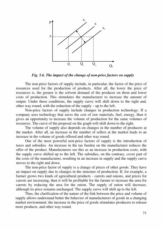
71

Fig. 5.6. The impact of the change of non-price factors on supply

The non-price factors of supply include, in particular, the factor of the price of

resources used for the production of products. After all, the lower the price of resources is, the greater is the solvent demand of the producer on them and lower costs of production. This stimulates the manufacturer to increase the amount of output. Under these conditions, the supply curve will shift down to the right and, other way round, with the reduction of the supply – up to the left.

Non-price factors of supply include changes in production technology. If a company uses technology that saves the cost of raw materials, fuel, energy, then it gives an opportunity to increase the volume of production for the same volumes of resources. The curve of the proposal on the graph will shift down to the right.

The volume of supply also depends on changes in the number of producers at the market. After all, an increase in the number of sellers at the market leads to an increase in the volume of goods offered and other way round.

One of the most powerful non-price factors of supply is the introduction of taxes and subsidies. An increase in the tax burden on the manufacturer reduces the offer of the product. Manufacturers see this as an increase in production costs, with the supply curve shifted up to the left. The subsidies, on the contrary, cover part of the costs of the manufacturer, resulting in an increase in supply and the supply curve moves to the right and down.

The non-price factor of supply is a change of prices of other goods. They have an impact on supply due to changes in the structure of production. If, for example, a farmer grows two kinds of agricultural products - carrots and onions, and prices for carrots are increasing, then it will be profitable for the farmer to increase the area for carrots by reducing the area for the onion. The supply of onion will decrease, although its price remains unchanged. The supply curve will shift up to the left. Thus, the clarification of the nature of the link between the price and volume of supply allows understand better the behavior of manufacturers of goods in a changing market environment: the increase in the price of goods stimulates producers to release more products, and other way round.

Р

Qs

S1

Р

2sQ

1sQ

S

S2

sQ

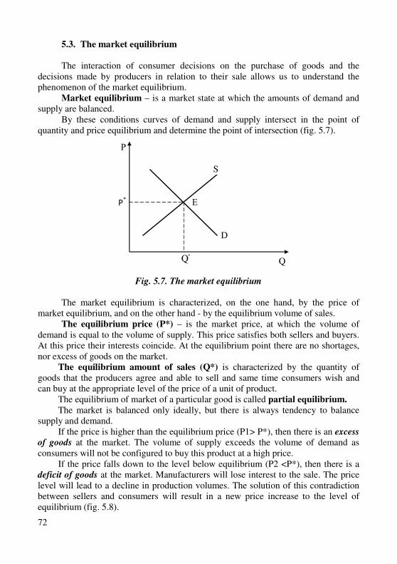
72

5.3. The market equilibrium

The interaction of consumer decisions on the purchase of goods and the

decisions made by producers in relation to their sale allows us to understand the phenomenon of the market equilibrium.

Market equilibrium – is a market state at which the amounts of demand and supply are balanced.

By these conditions curves of demand and supply intersect in the point of quantity and price equilibrium and determine the point of intersection (fig. 5.7).

Fig. 5.7. The market equilibrium

The market equilibrium is characterized, on the one hand, by the price of market equilibrium, and on the other hand - by the equilibrium volume of sales.

The equilibrium price (P*) – is the market price, at which the volume of demand is equal to the volume of supply. This price satisfies both sellers and buyers. At this price their interests coincide. At the equilibrium point there are no shortages, nor excess of goods on the market.

The equilibrium amount of sales (Q*) is characterized by the quantity of goods that the producers agree and able to sell and same time consumers wish and can buy at the appropriate level of the price of a unit of product.

The equilibrium of market of a particular good is called partial equilibrium.

The market is balanced only ideally, but there is always tendency to balance supply and demand.

If the price is higher than the equilibrium price (P1> P*), then there is an excess

of goods at the market. The volume of supply exceeds the volume of demand as consumers will not be configured to buy this product at a high price.

If the price falls down to the level below equilibrium (P2 <P*), then there is a deficit of goods at the market. Manufacturers will lose interest to the sale. The price level will lead to a decline in production volumes. The solution of this contradiction between sellers and consumers will result in a new price increase to the level of equilibrium (fig. 5.8).

Р

Q

Р*

*Q

S

D

Е

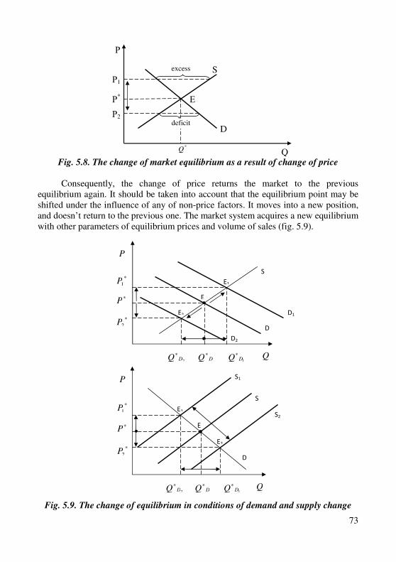
73

Fig. 5.8. The change of market equilibrium as a result of change of price

Consequently, the change of price returns the market to the previous

equilibrium again. It should be taken into account that the equilibrium point may be shifted under the influence of any of non-price factors. It moves into a new position, and doesn’t return to the previous one. The market system acquires a new equilibrium with other parameters of equilibrium prices and volume of sales (fig. 5.9).

Fig. 5.9. The change of equilibrium in conditions of demand and supply change

Р

Q

Р*

*Q

S

D

Е

Р1

Р2

excess

deficit

2DQ∗

1DQ∗

D2

P

∗P

DQ∗

D

D1

S

E

E1

E2 ∗

2P

∗

1P

Q

2DQ∗

1DQ∗

S1 P

∗P

DQ∗

D

S2

S

E

E1

E2 ∗

2P

∗

1P

Q

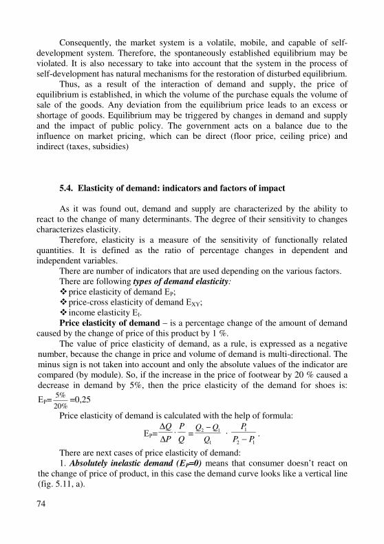
74

Consequently, the market system is a volatile, mobile, and capable of self-development system. Therefore, the spontaneously established equilibrium may be violated. It is also necessary to take into account that the system in the process of self-development has natural mechanisms for the restoration of disturbed equilibrium. Thus, as a result of the interaction of demand and supply, the price of equilibrium is established, in which the volume of the purchase equals the volume of sale of the goods. Any deviation from the equilibrium price leads to an excess or shortage of goods. Equilibrium may be triggered by changes in demand and supply and the impact of public policy. The government acts on a balance due to the influence on market pricing, which can be direct (floor price, ceiling price) and indirect (taxes, subsidies)

5.4. Elasticity of demand: indicators and factors of impact

As it was found out, demand and supply are characterized by the ability to

react to the change of many determinants. The degree of their sensitivity to changes characterizes elasticity.

Therefore, elasticity is a measure of the sensitivity of functionally related quantities. It is defined as the ratio of percentage changes in dependent and independent variables.

There are number of indicators that are used depending on the various factors. There are following types of demand elasticity: � price elasticity of demand ЕР; � price-cross elasticity of demand ЕXY; � income elasticity ЕІ. Price elasticity of demand – is a percentage change of the amount of demand

caused by the change of price of this product by 1 %. The value of price elasticity of demand, as a rule, is expressed as a negative

number, because the change in price and volume of demand is multi-directional. The minus sign is not taken into account and only the absolute values of the indicator are compared (by module). So, if the increase in the price of footwear by 20 % caused a decrease in demand by 5%, then the price elasticity of the demand for shoes is:

ЕР=%20

%5=0,25

Price elasticity of demand is calculated with the help of formula:

ЕР=Q

P

P

Q⋅

∆

∆ =

1

12

Q

QQ −·

12

1

PP

P

−.

There are next cases of price elasticity of demand: 1. Absolutely inelastic demand (ЕР=0) means that consumer doesn’t react on

the change of price of product, in this case the demand curve looks like a vertical line (fig. 5.11, a).

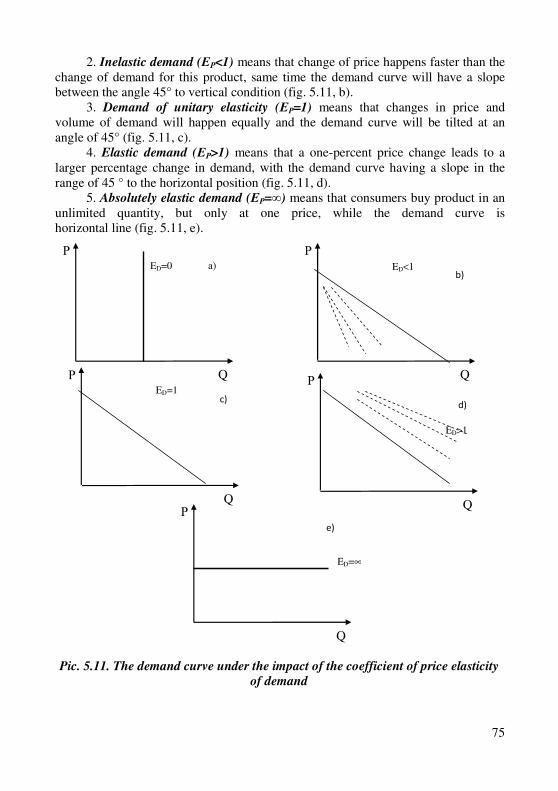
75

2. Inelastic demand (ЕР<1) means that change of price happens faster than the change of demand for this product, same time the demand curve will have a slope between the angle 45° to vertical condition (fig. 5.11, b).

3. Demand of unitary elasticity (ЕР=1) means that changes in price and volume of demand will happen equally and the demand curve will be tilted at an angle of 45° (fig. 5.11, c).

4. Elastic demand (ЕР>1) means that a one-percent price change leads to a larger percentage change in demand, with the demand curve having a slope in the range of 45 ° to the horizontal position (fig. 5.11, d).

5. Absolutely elastic demand (ЕР=∞) means that consumers buy product in an unlimited quantity, but only at one price, while the demand curve is horizontal line (fig. 5.11, e).

Pic. 5.11. The demand curve under the impact of the coefficient of price elasticity

of demand

Р

Q

ED=0 а)

Р

Q

ED<1 b)

Р

Q

ED=1 c)

Р

Q

ED>1

d)

Р

Q

ED=∞

e)

76

Factors of price elasticity of demand are: � the presence of substitute products: the more close and perfect substitutes

have a product, the more elastic is the demand for it, and other way round; � the proportion of goods in consumer spending: the greater the proportion is

the product in consumer spending, the more elastic is the demand for it, and other way round;

� period of consumption: in the short term, demand is less elastic than long-term, as changing the tastes, preferences and patterns of consumption takes time;

� the importance of goods for consumer: the demand for essential goods is inelastic, on luxury goods - elastic at the price;

� the breadth of the range of use of this product: the more functions the product performs, the demand for it is more elastic.

For non-price factors of demand it is distinguished a cross-elasticity of demand and elasticity of demand for consumer income. Both indicators allow determine by how many percent the demand curve will shift under the influence of this non-price factor.

In particular, the price-cross elasticity of demand characterizes the degree of change in the volume of demand for goods X when the price of goods Y is changed by 1%. It is determined by the ratio of the relative change in the volume of demand for product X to the relative change of price of product Y:

ЕXY=%Y

X

P

Q

∆

∆=

1

12

X

XX

Q

QQ −·

12

1

YY

Y

PP

P

−

Indicator of price-cross elasticity of demand is determined for a group of goods that are substitute or complementary goods.

The income elasticity of demand represents the nature and speed of the consumer's reaction to the purchase of goods as a result of changes in its income and shows how the amount of demand caused by 1 % change in income.

Elasticity of demand for income is defined as the ratio of relative change in demand to the relative change in consumer income:

ЕІ=%I

Q

∆

∆=

1

12

Q

QQ −

12

1

II

I

−

The concept of elasticity has many areas of practical application. One of them is the definition of the price strategy of sellers: what price to assign in order to get the most sales revenue, whether to lower the price or increase it. The aggregate (gross) income of sellers (TR=P•Q) is at the same time a cost to consumers, so the link between the elasticity indicator and cost change is extremely important for both parties.

The theory of elasticity and adaptation of the market is also important for the analysis and forecasting of the consequences of changes in market conditions. For example, if drought is expected to reduce the supply of any agricultural product on the world market, then to determine the impact of this event on the world price of the product can depict the curves of actual demand and supply, and then calculate their bias and determine the change in equilibrium prices.

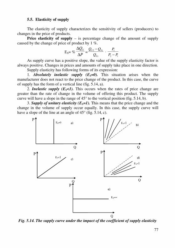
77

5.5. Elasticity of supply

The elasticity of supply characterizes the sensitivity of sellers (producers) to

changes in the price of products. Price elasticity of supply – is percentage change of the amount of supply

caused by the change of price of product by 1 %.

ЕS= %P

QS

∆

∆=

1

12

S

SS

Q

QQ − ·

12

1

PP

P

−

As supply curve has a positive slope, the value of the supply elasticity factor is always positive. Changes in prices and amounts of supply take place in one direction.

Supply elasticity has following forms of its expression: 1. Absolutely inelastic supply (ЕS=0). This situation arises when the

manufacturer does not react to the price change of the product. In this case, the curve of supply has the form of a vertical line (fig. 5.14, а).

2. Inelastic supply (ЕS<1). This occurs when the rates of price change are greater than the rate of change in the volume of offering this product. The supply curve will have a slope in the range of 45° to the vertical position (fig. 5.14, b).

3. Supply of unitary elasticity (ЕS=1). This means that the price change and the change in the volume of supply occur equally. In this case, the supply curve will have a slope of the line at an angle of 45° (fig. 5.14, c).

Fig. 5.14. The supply curve under the impact of the coefficient of supply elasticity

Р

Q

ES=0 a)

Р

Q

ES<1 b)

Р

Q

ES=1 c)

Р

Q

ES>1

d)

Р

Q

ES=∞

e)

78

The main factors of elasticity of supply are: � the period of time during which the production is carried out – in the long-

term period supply is more elastic than in the short-term period, and in the short-term period it is more elastic than in the instant;

� the interchangeability of production resources (the more substitutes has resource, the more elastic is the supply of a product that is made from this resource);

� the level of use of production capacity – the higher the percentage of use of production equipment is, the more elastic is supply, and other way round;

� the cost of storing the goods - the better the possibilities and the lower cost of storage of goods is, the more elastic is supply;

� mobility of factors of production and output – provides for the possibility of purchasing resources from other fields of production. The most important factors of production are components, equipment and labor. Mobile resources are labor and equipment, while component products are not flexible and mobile, and counteract the elasticity of supply. Consequently, the supply of goods is a necessary component of market relations. The efforts of the manufacturer to be ready to use the opportunities offered by the market, to create new facilities by introducing innovations in technology and organization of production, at risk, make this process well-ordered.

Training

Key terms and concepts

Demand. Amount of demand. Supply. Amount of supply. Market equilibrium.

Equilibrium price. Equilibrium amount of sale. Surplus. The law of demand. The law

of supply. Deficit. Demand price. Supply price. Elasticity. Price elasticity of demand.

Income elasticity of demand. Cross price elasticity of demand. Elastic demand.

Inelastic demand. Demand with unitary elasticity. Absolutely elastic demand.

Absolutely inelastic demand. Supply elasticity. Elastic supply. Inelastic supply.

Supply with unitary elasticity. Absolutely elastic supply. Absolutely inelastic supply.

“Price celling”. “Price floor”.

Questions and tasks for students’ self-control:

1. Give definition of demand of product. 2. What does the law of demand prove? What are exceptions from the law of

demand? 3. Characterize the impact of price and non-price factors on demand. 4. How do you understand the essence of the law of supply? 5. Characterize the methods of determination of market equilibrium

parameters. 6. Give definition of the concept “elasticity of demand”. Which typed of

elasticity of demand do you know? 7. Explain the methodology of calculation of demand and supply elasticity. 8. Which factors affecting elasticity demand and supply do you know?

79

Tests

1. The law of demand proves that: а) excess of demand over supply leads to the decrease of price; b) if income of consumers increases so then they buy more products; c) demand curve has positive slope; d) demand of product increases when its price decreases; 2. How can the shift of demand curve for product X be explained? а) supply of product X has been decreased; b) price of product X has been increased and as a result of this consumers

became purchase this product less; c) tastes of consumers attracted interest to the product X and that’s why they

want to buy it at any price; d) price of product has been decreased, that’s why consumers decided to buy

this product more than before. 3. The increase of price of materials necessary for production of product X

will lead to: а) the shift of demand curve up to the right; b) the shift of supply curve up to the left; c) the shift of demand and supply curve up; d) the shift of supply curve up to the right.

4. Market demand is not affected by changes of: а) income of consumers; b) prices for products-substitutes; c) prices for resources; d) number of customers in the market. 5. Demand for product seems to be elastic if: а) the coefficient of price elasticity is less than 1; b) total income of seller increases if the price rises; c) consumers almost don’t react on the change of price; d) change of the amount of demand is more than change of price. 6. If decrease of price by 5 % leads to decrease of the amount of supply by

8 % so this supply is: а) inelastic; b) of unitary elasticity; c) elastic; d) absolutely inelastic

80

7. The commodity is seemed to be the priority product if the coefficient of demand elasticity by income is:

а) less than 0; b) more than 0, but less than 1; c) more than 1; d) equals to 1. 8. Elasticity of demand depends on following factors: а) income of producers of commodity of big demand; b) breadth of range of possibility of use this product; c) supply elasticity; d) resource productivity from which the product is produced. 9. The curve of absolutely inelastic supply looks like: а) horizontal line; b) straight line with negative slope; c) curve; d) vertical line.

10. The technology improvement shifts: а) the demand curve up to the right; b) the demand curve down to the left; c) the supply curve down to the right; d) the supply curve up to the left. 11. The product may be referred to luxury products if the coefficient of

demand elasticity by income: а) more than 0, but less than 1; b) less than 0; c) equals to 0; d) more than 1. 12. Then decrease of price or product X from 4 UAH to 3 UAH will lead to: а) increase QD of product Х by 4%; b) increase QD by 40%; c) increase QD by 80%; d) there is no correct answer. 13. Demand is represented by equation QD=–120–4P. If price of product

decreases then till which level of the decrease of price will be profitable for producers?

а) 30 UAH; b) 25 UAH; c) 20 UAH; d) 15 UAH.

81

Task 1

The demand function for product: QD = 9 – 2Р. The supply function: QS = - 3 + 2Р. а) Please determine equilibrium amount and price. b) Which situation will happen to the market at established fixed price 4 UAH? c) Suppose that the amount of demand has decreased by 20 %. What will

happen to equilibrium amount and price? d) The government is going to establish tax in sum 1 UAH per 1 unit of

product. What will happen to equilibrium amount and price? e) The producer gets subsidy 2 UAH per 1 unit of product. How will it

influence on equilibrium price and sales amount?

Task 2

The family Shevchenko consumes 1000 liters of petrol at price 20 UAH per 1 liter. The coefficient of price elasticity of demand for petrol ЕР = – 0,5. How will expenditures for petrol of the family be changed if it price increases by 65?

Task 3

Please define the coefficient of price-cross elasticity of demand if it is know that increase of price of product Y from 10 UAH to 15 UAH has led to increase of amount of purchases of family of product X from 5 kg to 8 kg per month.

Is demand of product X elastic? Explain what kind of commodities are products X and Y: substitutes or compliments?

Task 4

Demand function of cucumbers is Qd=9-2P. Supply function is: Qs=-3+2P. Tasks: a) define equilibrium indicators at the market (P and Q); b) define how decrease of demand by 5% impact on price of cucumbers.

Task 5

When price of 1 kg of fish was 50 UAH Ukrainian family bought 2 kg of fish every week. After the price increased to 60 UAH the consumption of fish in family decreased to 1 kg per week. Please define the coefficient of elasticity of fish. Is this product elastic?

Task 6

Qd = 40-0,8P, Qs = -58+2P. As a result of implementation of new technology of production Qs of product X is changed: Qs = -16+2P.

Please define the equilibrium price and equilibrium amount of consumption before and after implementation of new technology.

82

СHAPTER 2.

THE PRODUCER’S BEHAVIOR THEORY

Theme 6 The Microeconomic Model of the Enterprise

6.1. Comparative features of the firm and enterprise.

6.2. The enterprise as a part of microeconomic system. Types of enterprises.

6.3. Instant, short-term and long-term market periods of the enterprise

functioning.

6.4. The concept of production functions, their properties, types and forms of

presentation

6.1. Comparative features of the firm and enterprise

Considering the microeconomic model of the enterprise, first of all we should

find out the distinctive features of the microeconomic characteristics of the category "firm".

The firm is an administrative company of people, united by certain interrelated activities.

The firm is a market and production system as it simultaneously acts as a buyer of factors of production on the market of resources and their consumer in the process of production, and as a producer and seller of products in the market of goods and services.

The main organizational and legal forms of firms are: individual entrepreneurial firm, partnership and corporation. Each of them has both advantages and disadvantages. In microeconomics, attention is paid to the diversity of forms, sizes and functions of firms. The general concept of "firm" is united by all enterprises and organizations.

The model of the company's behavior is based on the general rules of microeconomic modeling. The purpose of the company is to obtain maximum profit for a certain period of time. The limitations here are: productivity of factors of production, production costs, price of products and demand for it. The choice of the decision on the volume of production depends on the specific type of market structure in which the company manages.

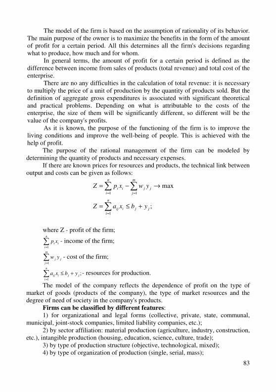
83

The model of the firm is based on the assumption of rationality of its behavior. The main purpose of the owner is to maximize the benefits in the form of the amount of profit for a certain period. All this determines all the firm's decisions regarding what to produce, how much and for whom.

In general terms, the amount of profit for a certain period is defined as the difference between income from sales of products (total revenue) and total cost of the enterprise.

There are no any difficulties in the calculation of total revenue: it is necessary to multiply the price of a unit of production by the quantity of products sold. But the definition of aggregate gross expenditures is associated with significant theoretical and practical problems. Depending on what is attributable to the costs of the enterprise, the size of them will be significantly different, so different will be the value of the company's profits.

As it is known, the purpose of the functioning of the firm is to improve the living conditions and improve the well-being of people. This is achieved with the help of profit.

The purpose of the rational management of the firm can be modeled by determining the quantity of products and necessary expenses.

If there are known prices for resources and products, the technical link between output and costs can be given as follows:

;

max

1

11

jj

n

i

iij

m

j

jj

n

i

ii

ybxaZ

ywxpZ

+≤=

→−=

∑

∑∑

=

==

where Z - profit of the firm;

∑=

n

i

ii xp1

- income of the firm;

∑=

m

j

jj yw1

- cost of the firm;

;1

jj

n

i

iij ybxa +≤∑=

- resources for production.

The model of the company reflects the dependence of profit on the type of market of goods (products of the company), the type of market resources and the degree of need of society in the company's products.

Firms can be classified by different features: 1) for organizational and legal forms (collective, private, state, communal,

municipal, joint-stock companies, limited liability companies, etc.); 2) by sector affiliation: material production (agriculture, industry, construction,

etc.), intangible production (housing, education, science, culture, trade); 3) by type of production structure (objective, technological, mixed); 4) by type of organization of production (single, serial, mass);

84

5) by the share of firm at the market; 6) by the level of profitability.

6.2. Enterprise as a part of microeconomic system. Types of enterprises

The basis of the national economy of country is formed by its own production, the primary focus of which is the enterprise.

Despite the variety of forms in which the enterprise can be: a factory, a mill, a factory, a power plant, an atelier, a port, a farm, a quarry, etc., all of them have the common features that give the basis to consider the company as the main link of the economy. The main ones of them are:

1. Production and technical unity, which manifests itself in the relationship of structural units of the enterprise, which is determined by the commonality of the destination of the finished product or the unity of the processes of its production.

2. Economic unity of the enterprise manifests itself in the unity of the plan, accounting, analysis, evaluation of the results of activities, the community of material, labor and financial resources.

3. Organizational unity of the enterprise is based on giving it the rights of the legal entity and responsibility for the results of work and provides for the presence of a single team of employees and a unified system of guidance.

Based on this, we can distinguish the main tasks of the manufacturers: � profit achievement; � ensuring demand for the products of the enterprise at the least cost for its

production and sale; � after-sale service; � environmental protection; � improvement of the production technology; � expansion of the assortment of products and increase of its quality; � compliance with legislation and established standards and norms; � provision of staff with salary, normal working conditions and professional

growth opportunities. The activity of each enterprise is subordinated to the implementation of its

main production function – creation of the optimal number of goods or services to meet the needs of society at the lowest cost of production.

The implementation of this function involves the activities of the enterprise in various spheres, which is conditioned by the fulfillment of the specific functions of each of them. Such functions are productive, technical, economic, and social ones.

Production and technical functions of the enterprise are connected with provision of the production process by necessary means, organization of their use, introduction of new technologies, rationalization of production processes and inventing.

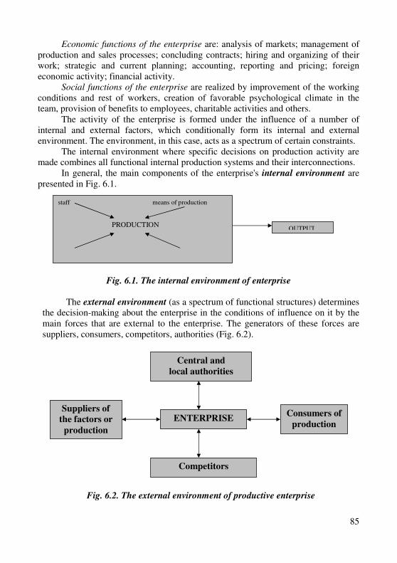
85

Economic functions of the enterprise are: analysis of markets; management of production and sales processes; concluding contracts; hiring and organizing of their work; strategic and current planning; accounting, reporting and pricing; foreign economic activity; financial activity.

Social functions of the enterprise are realized by improvement of the working conditions and rest of workers, creation of favorable psychological climate in the team, provision of benefits to employees, charitable activities and others.

The activity of the enterprise is formed under the influence of a number of internal and external factors, which conditionally form its internal and external environment. The environment, in this case, acts as a spectrum of certain constraints.

The internal environment where specific decisions on production activity are made combines all functional internal production systems and their interconnections.

In general, the main components of the enterprise's internal environment are presented in Fig. 6.1.

Fig. 6.1. The internal environment of enterprise

The external environment (as a spectrum of functional structures) determines

the decision-making about the enterprise in the conditions of influence on it by the main forces that are external to the enterprise. The generators of these forces are suppliers, consumers, competitors, authorities (Fig. 6.2).

Fig. 6.2. The external environment of productive enterprise

staff means of production

PRODUCTION OUTPUT

Central and

local authorities

ENTERPRISE

Competitors

Suppliers of

the factors or

production

Consumers of

production

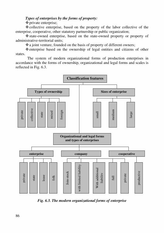
86

Types of enterprises by the forms of property:

� private enterprise; � collective enterprise, based on the property of the labor collective of the

enterprise, cooperative, other statutory partnership or public organization; � state-owned enterprise, based on the state-owned property or property of

administrative-territorial units; � a joint venture, founded on the basis of property of different owners; � enterprise based on the ownership of legal entities and citizens of other

states. The system of modern organizational forms of production enterprises in

accordance with the forms of ownership, organizational and legal forms and scales is reflected in Fig. 6.3.

Fig. 6.3. The modern organizational forms of enterprise

Classification features

Types of ownership Sizes of enterprise

pri

vat

e

mix

ed

stat

e

coll

ecti

ve

fore

ign

smal

l

med

ium

larg

e

Organizational and legal forms

and types of enterprises

company enterprise cooperative

pri

vat

e

stat

e

leas

e

Wit

h a

dd

itio

nal

liab

ilit

y

full

pri

vat

e

pro

du

ctiv

e

folk

Join

-sto

ck

wit

h l

imit

ed l

iab

ilit

y

87

The main organizational and legal forms of enterprise associations are: � associations – are contractual associations that are created for the purpose of

permanent coordination of economic activities without any right to interfere with the production and commercial activities of any of its participants;

� corporations – are contractual associations that are created on the basis of a combination of industrial, scientific and commercial interests of the united enterprises, delegated by them separate powers of the centralized regulation of the activities of each of the participants (corporate governance bodies);

� consortia – are temporary statutory associations of industrial and bank capital, created for the purpose of realizing a common goal. Enterprises maintain its full autonomy and are subject to joint management only in that part of the activities related to the objectives of the consortium;

� concerns – are statutory unions of industrial enterprises, scientific organizations, transport, banks, trade, etc. based on full financial dependence on one or a group of enterprises.

According to the number of employees and the volume of production of the enterprise are divided into small, medium and large.

Each enterprise has its own productive process. Productive process is a totality of organized processes of work and natural

processes as a result of what raw materials are transformed into final products. Enterprise – is an independent economic entity created by the competent state

or local authorities or other entities to meet social and personal needs through the systematic implementation of industrial, research, trade and other activities in accordance with the procedure provided for by the current legislation.

6.3. Instant, short-term and long-term market periods

of the enterprise functioning

Further characterization of the microeconomic model of the enterprise is ensured by inclusion the time factor into the analysis. It is known that there are some periods during which an enterprise may be able or not be able to change its capacities, to introduce new means of production into the manufacturing process, to change the product range, and to react to changing market conditions.

The nature of the manufacturer's behavior is largely determined by the time factor. At the end of the XIX century J. B. Sey’s concept was specified by the development of the theory of decreasing marginal productivity of factors of production, according to which the return from the variable factor decreases with the increase in the volume of its use. In particular, A. Marshall limited the effect of the law of declining productivity by the factor of time, having distinguished three time periods of production: instant, short-term and long-term. Therefore, in the theory of production we distinguish: an instant market period, as a period during which the firm can’t change the use of factors of production; short-term market period in which

88

the company is able to change the use of only some resources (often the amount of involvement of the factor of labor changes, and the amount of capital remains constant); a long market period - sufficient to change the volumes of use of all factors of production without exception.

According to A. Marshall in the instant period there are no any changes in production.

The concepts of "short-term" and "long-term" have different meanings, economic sense to characterize the state of production at the structural level of firms and enterprises.

From the point of view of the firm, the short-term period is a period of time during which the production capacities of the firm are fixed, but the volume of production can be expanded or reduced at the expense of more or less labor, raw materials, etc. From the point of the industry, the short-term period is the period during which the number of existing firms in the industry does not change.

From the point of view of a firm, a long-term period – is a long period of time sufficient to change the amount of all resources, including production capacities. From the industry point of view, it is a period during which existing firms can be disbanded and left behind, while new firms may emerge and enter the industry. Consequently, in the long-term period, the number of firms in the industry are not been changed.

If, starting up the production of a particular product, the firm in the short term hires fewer staff than the available equipment requires, then the production efficiency will be low. Hired workers will be forced to perform not their functions, and part of the equipment will idle. Increase of the number of employees will take advantage of the specialization and fully load capacity. Under such conditions, the return of factors of production and their productivity will increase with each subsequent employee.

But the expansion of production at unchanged capacities can’t last indefinitely. In the short run period, when all the power will be used as much as possible, the additional worker will have little to add to the release, because he will have to wait until the necessary equipment is released. From now on, the productivity of an additional employee will be reduced. The aggregate output will grow ever slower, and with the achievement of a certain level of output will begin to decline: the absolute change in the ratio of "number of employees - the number of equipment" will lead to the fact that one additional worker is more likely to interfere with the work of others than to produce additional products.

The law of decreasing returns is based on the assumption of high-quality homogeneity of all additional units of variable resources. The additional product of each subsequent employee decreases not due to the fact that the firm recruits less skilled workers, but because they become relatively more expensive than the existing equipment.

89

6.4. The concept of production functions, their properties, types and forms of presentation

Any production process can be submitted as a production function because the

search of the profit maximization ways, first of all, means for the firm the maximization of the manufacture process where production is treated as the process transformation of cost of production into output of the firm. Factors of production that include labor, land, capital, organization or entrepreneurship, time and technology are considered as benefits that must be purchased by a firm to ensure the production of other goods – consumption products.

There are few assumptions used in the analysis of mechanisms of action of productive factors:

� assumption of absolute necessity of the main factors: if at least one type of resources is absent, the production is impossible;

� assumption of monotony: additional use of any factor promotes the increase of output;

� assumption of interchangeability of the main factors of production: some quantity of one factor can be replaced by some quantity of another factor. This property is connected to the problem of choice of the technology for every firm.

According to the J.-B. Say’s production factors theory, there are three factors that in equal shares take part in the product manufacturing: labor, capital and land. Each factor has its own productivity, it means the ability to create its own share in the product value. After goods realization owners of each factor get his income share (salary, profit, rent) according to his productivity.

By using the peculiarity of resources interchangeability it is possible to produce same number of products during same period of time with the help of different methods: or to hire a big number of workers and give them hand tools only, or to use the complex of automated equipment and very few workers. The firm makes decision about the choice of technology by comparing productivity and cost for resources. It evaluates the methods of production from the point of technological and economic effectiveness.

It is used to consider that the method of production is effective if there is no other method to produce given output with less number of resources. In other words, the method of production is technologically effective if the production of output is possible by use definitely determined amount of the output.

The production function gives general information about connection between cost of productive factors and amount of output in physical expression. With the help of this function it is possible to determine the technologically effective method of production.

The production function specifies the maximum output that company can produce for each specific combination of inputs. In the model of firm behavior to simplify the analysis, only two resources for the long-term period are considered - labor and capital, and only one variable factor - labor - for the short-term period. The general analytical expression of a production function can be presented as follows:

( ),F...F,FfQ n21= or ( ),L,KfQ = or ( ).LfQ =

The first, the most famous variant of the production function was the

90

production function of Cobb-Douglas (1929), which describes the dependence of production volumes on two factors - capital and labor:

,βα LKAQ ⋅⋅=

whereА – coefficient of proportionality or magnitude; βα , – coefficients of elasticity of production, which characterize an increase in

production volumes for the growth of the relevant factors by 1%. Each firm has its own production function. It describes the technological

method of production chosen by the firm. The production function describes what is technically possible under the condition of effective activity.

It is used to consider that an economically effective method of production is the method which minimizes the alternative cost of all types of production costs of a given volume. Economic efficiency depends on the market price of various types of resources. There are many technologically efficient methods of production and only one cost-effective – is the cheapest one that provides the company's minimum costs at a given level of prices for used input resources at the moment.

In theory as same as in economic practice the definition and calculation of costs are quite complex. As costs are the main limitation of the firm in achieving its goal, many scholars focused their search on explaining the economic nature of production costs, and, in accordance with their understanding of their essence, determined the level of costs and associated with the level of profits.

Training

Key terms and concepts

Total product. Marginal product. Variable product. The law of diminishing marginal productivity. Short-run production function. One-factor function of production. Two-factor function of production. Isoquant curve. The map if isoquant curves. Izocost curve. The map of izocost curves. Marginal rate of technological substitution. Producer’s optimum. Trajectory of growth.

Questions and tasks for students’ self-control: 1. What is the function of production with one variable factor? 2. How the law of diminishing marginal productivity of variable production

factor can be represented? 3. How the amount of total, average and marginal product be calculated? Give

definitions of these indicators. 4. On which patterns the production function with two variable factors can be built? 5. What does isoquant mean? 6. How the map of isoquant curves is formed and represented? 7. Which features of isoquant curves do you know? 8. What does the norm of technical substitution of resources mean and how it

can be calculated? 9. Explain positive and negative consequences of the effect of production scale.

Give some examples. 10. What is izocost curve? Write down the equation of izocost curve.

91

Theme 7 The Variation of Production Factors

and the Producer’s Optimum

7.1. The production function with one variable factor. Total, average and

marginal product.

7.2. The production function with two variables. The curve of the same

product – isoquant. Marginal rate of technical substitution of resources.

7.3. The choice of a combination of production factors due to the minimizing

costs or maximizing output criterion. Isocost curve.

7.4. The producer’s optimum: graphical, algebraic, economic forms of his

equilibrium functioning

7.1. The production function with one variable factor. Total, average and

marginal product

The economic nature of the production function, explained in the previous

section, allows us to carry a more specific analysis out, in particular, to consider the nature of the impact of one variable factor, namely, the factor of labor, on the volume of production of the enterprise. This approach will allow us to reach the definition of aggregate, average, marginal productivity of labor through the prism of the rule of decreasing return of the variable factor. The dependence of the total, average and marginal product on changes in the amount of labor expended will be obvious.

In the short-term period with the aim of increasing production volumes, the firm can manipulate the change in volumes of only some resources. Other factors remain fixed. In this case, the short-term production function will look like:

( )LfQ = .

It provides the information about the contribution of each unit of the variable factor to the increase in total output and allows us to determine by what costs of variable factor the maximum output can be achieved over a certain period of time, and all this occurs with the consideration of the law of the diminishing return. The contribution of the variable factor to the production process is calculated by indicators of total, average and marginal product in physical units.

Thus the total productivity of the variable factor (TP) can be given as the total quantity of products produced by all units of the variable factor under the conditions of other factors.

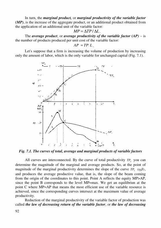
92

In turn, the marginal product, or marginal productivity of the variable factor

(MP), is the increase of the aggregate product, or an additional product obtained from the application of an additional unit of the variable factor:

LTPMP ∆∆= / . The average product, or average productivity of the variable factor (AP) – is

the number of products produced per unit cost of the variable factor:

LTPAP = .

Let's suppose that a firm is increasing the volume of production by increasing only the amount of labor, which is the only variable for unchanged capital (Fig. 7.1).

Fig. 7.1. The curves of total, average and marginal products of variable factors

All curves are interconnected. By the curve of total productivity

LTP you can

determine the magnitude of the marginal and average products. So, at the point of magnitude of the marginal productivity determines the slope of the curve LTP )( βtg ,

and produces the average productive value, that is, the slope of the beam coming from the origin of the coordinates to this point. Point A reflects the equity MP>AP, since the point B corresponds to the level MP=max. We get an equilibriun at the point C where MP=AP that means the most efficient use of the variable resource is achieved, since the corresponding curves intersect at the maximum value of average productivity.

Reduction of the marginal productivity of the variable factor of production was called the law of decreasing return of the variable factor, or the law of decreasing

93

marginal productivity. The essence of the law is that, starting with a certain amount of production, the next increase in the use of an alternating factor, for constant volumes of use of other production factors, is accompanied by a decrease in the marginal product of the variable factor.

The law of decreasing returns has formed the basis of the theory of British economist Thomas Robert Malthus (1766 - 1834), who believed that a relatively constant amount of land cultivated on the globe and the current law of decreasing return would become the cause of mass starvation in the future. Malthus was mistaken in his predictions, since he did not take into account that the law of decreasing returns is fair for the short-term period of time and unchanging technology. Over time, the inventions, technological improvements led to the rise of the production curve and the curves of the marginal and average product (Fig. 7.1). The action of this law on our graph begins to manifest itself after using the work in volume B1, when the function of the boundary product reaches the maximum and then gets the form of the down line.

7.2. A production function with two variables.

The curve of the same product – isoquant curve.

Marginal rate of technical substitution of resources

If there is one factor affecting the volume of production, there may be two or more. In addition, the period during which production is carried out may also be long-term one.

The long-term market period is long enough to provide the improvement of production, when the firm has enough time to use two or more factors of production.

In the long-term period the firm can change both the technology of production and its scale. Changing technology leads to a change in the functional relationship between the structure of the cost of production resources and the volume of output. The analysis uses two- and multifactor production functions. When capital and labor can replace each other in the production process, then the ratio of resources is measured by labor productivity ( )LK / . Function of production gets the form:

( )L,KfQ = .

The two-factor production function can be represented in a tabular (production net), graphic (isoquant) and analytical forms.

In particular, the isoquant is represented by the curve of the same quantity of product, which reflects the set of combinations of input resources that provide a certain fixed level of output (Fig. 7.2.).

In turn, the isoquant map is a plurality of isoquants, which graphically reflects a certain production function.

Properties of isoquants are similar to the properties of indifference curves. First, the isoquants do not intersect, and secondly, they have a negative slope. Also

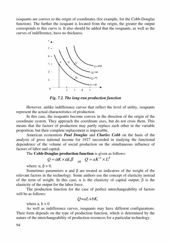
94

isoquants are convex to the origin of coordinates (for example, for the Cobb-Douglas function). The further the isoquant is located from the origin, the greater the output corresponds to this curve is. It also should be added that the isoquants, as well as the curves of indifference, have no thickness.

Fig. 7.2. The long-run production function However, unlike indifference curves that reflect the level of utility, isoquants

represent the actual characteristics of production. In this case, the isoquants become convex in the direction of the origin of the

coordinate system. They approach the coordinate axes, but do not cross them. This means that the factors of production may partly replace each other in the variable proportion, but their complete replacement is impossible.

American economists Paul Douglas and Charles Cobb on the basis of the analysis of gross national income for 1927 succeeded in studying the functional dependence of the volume of social production on the simultaneous influence of factors of labor and capital.

The Cobb-Douglas production function is given as follows:

βαα LKQ ×= or βα

LaKQ ×=

where: α, β > 0. Sometimes parameters α and β are treated as indicators of the weight of the

relevant factors in the technology. Some authors use the concept of elasticity instead of the term of weight. In this case, α is the elasticity of capital output; β is the elasticity of the output for the labor force.

The production function for the case of perfect interchangeability of factors will be as follows:

Q=aL+bK,

where а, b > 0 As well as indifference curves, isoquants may have different configurations.

Their form depends on the type of production function, which is determined by the nature of the interchangeability of production resources for a particular technology.

95

Every combinations of production factors on the isoquant reflects its technological mode of production. For example, at the point A (Fig. 7.2) machine technology prevails, and at the point D production is done mainly due to manual labor.

Analytically the construction of isoquant curve is based on the equation of production function:

constLKf =),(

With the help of the production function it is possible to analyze the possibilities of changing the technology, provided by the achieved level of production. For example, if the amount of capital has decreased by K∆ , then the same amount of output at the same time can produce additional labor-generated production L∆ :

),(),( LLKKfLKfQ ∆+∆−==

Indicator that determines the proportion of replacement of factors of production is called the marginal rate of technological substitution – MRST.

Marginal rate of technological substitution shows from which quantity of one factor we should refuse to engage in the production of an additional unit of another factor.

LKMRTS KL ∆∆−= /,

Marginal rate of capital replacement by labor shows how many units of capital can replace a unit of labor.

Marginal rate of technological substitution has always a negative value. It is only possible to maintain a certain level of production under a new technology if an increase in one factor will be accompanied by a corresponding decrease in the other, and vice versa.

The dynamics of the marginal rate of technological substitution in the process of development of technological model of production is influenced by the law of decreasing returns of resources. So, as the saturation of production by any factor, its marginal productivity will fall. This form of communication was called the law of

decreasing marginal rate of technological substitution: with increasing use in the production of any factor, the marginal rate of technological substitution unit of this factor to others is reduced, and vice versa. In other words, the following equality must be fulfilled:

,KMPLMP KL 0=∆⋅+∆⋅

or KMPLMP KL ∆⋅−=∆⋅ ,

or LMPKMP LK ∆⋅−=∆⋅ .

From here, the marginal rate of technological substitution of labor by capital will look like:

KLKL MPMPLKMRTS //, −=∆∆= ,

or marginal rate of technological substitution of capital by labor:

LKLK MPMPKLMRTS //, −=∆∆= ,

96

it means K,LL,K MRTS/MRTS 1= .

The dynamics of the marginal rate of technological substitution in the process of development of technological way of production is influenced by the law of decreasing returns of resources. So, as the saturation of production by any factor, its marginal productivity will fall. This form of communication was called the law of

lowering the marginal rate of technological substitution: with increasing use in the production of any factor, the marginal rate of technological substitution unit of this factor to others is reduced, and vice versa.

The analysis of the production function in the context of the long-term market period is of great practical importance, especially for the effective planning of the company's development.

Consequently, the production function can be both single-factor and two-factor. Tabular this dependence has the form of a production net, and a graphically – line, which is called an isoquant curve. In its turn, the isoquant curve shows the model desired by the manufacturer. Graphically, the isoquant coincides with the indifference curve in the consumer behavior theory, which also reflects the model of the desired, but for the consumer. In addition to the isoquant curved to the origin, there is also a broken isoquant curve. There is also the factor of the marginal rate of technological substitution in the two-factor model.

7.3. The choice of a combination of production factors due

to the minimizing costs or maximizing output criterion. Isocost curve

According to the fact that there is an isoquant as a model of the desired choice of factors of production for the firm, of particular urgency is the question: "What costs will the manufacturer incur from the use of production resources?" In particular, it is necessary to consider a combination of production factors, based on the criteria for cost minimization or output maximization. Graphically, from now on it will be demonstrated by the line of model possible, which was called the isocost curve.

Technologically efficient output of the same volume of production can be provided by different variants of a combination of factors of production. But from an economic point of view, each combination of resources will cause different cost for the firm. Therefore, there is a problem of choosing a cost-effective structure of factors that would ensure the production of this volume at minimum cost.

For each period of time the firm has some limited financial resources that can be spent on production improvement. Therefore, allowable cost for labor and capital can be described by the following equation:

KPLPKLfLC KL ⋅+⋅== ),( ,

where LP – wage rate per hour (unit of labor cost);

KP – rent per hour of equipment use (unit price).

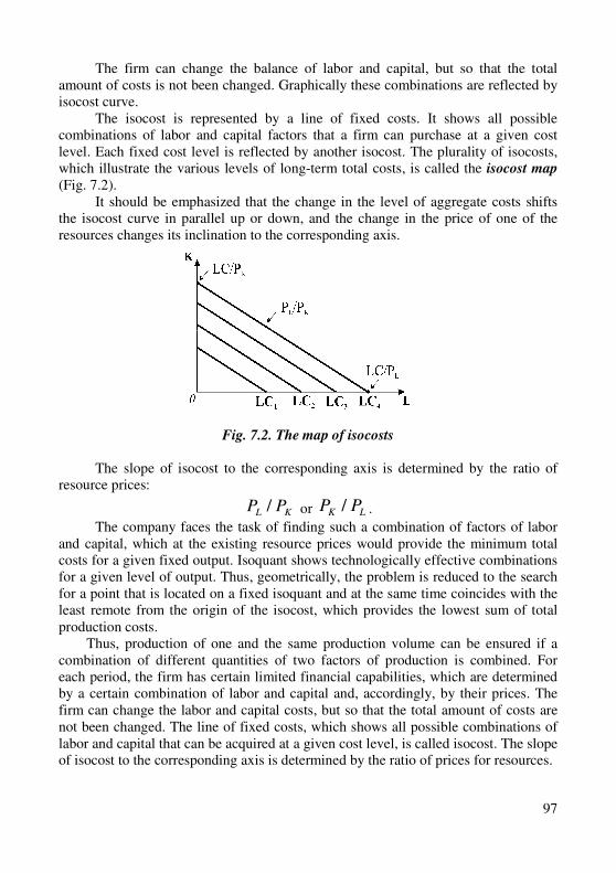
97

The firm can change the balance of labor and capital, but so that the total amount of costs is not been changed. Graphically these combinations are reflected by isocost curve.

The isocost is represented by a line of fixed costs. It shows all possible combinations of labor and capital factors that a firm can purchase at a given cost level. Each fixed cost level is reflected by another isocost. The plurality of isocosts, which illustrate the various levels of long-term total costs, is called the isocost map (Fig. 7.2).

It should be emphasized that the change in the level of aggregate costs shifts the isocost curve in parallel up or down, and the change in the price of one of the resources changes its inclination to the corresponding axis.

Fig. 7.2. The map of isocosts

The slope of isocost to the corresponding axis is determined by the ratio of

resource prices:

KL PP / or LK PP / .

The company faces the task of finding such a combination of factors of labor and capital, which at the existing resource prices would provide the minimum total costs for a given fixed output. Isoquant shows technologically effective combinations for a given level of output. Thus, geometrically, the problem is reduced to the search for a point that is located on a fixed isoquant and at the same time coincides with the least remote from the origin of the isocost, which provides the lowest sum of total production costs.

Thus, production of one and the same production volume can be ensured if a combination of different quantities of two factors of production is combined. For each period, the firm has certain limited financial capabilities, which are determined by a certain combination of labor and capital and, accordingly, by their prices. The firm can change the labor and capital costs, but so that the total amount of costs are not been changed. The line of fixed costs, which shows all possible combinations of labor and capital that can be acquired at a given cost level, is called isocost. The slope of isocost to the corresponding axis is determined by the ratio of prices for resources.

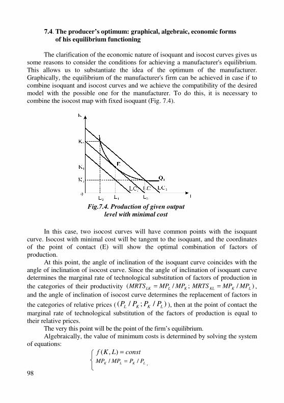
98

7.4. The producer’s optimum: graphical, algebraic, economic forms

of his equilibrium functioning

The clarification of the economic nature of isoquant and isocost curves gives us some reasons to consider the conditions for achieving a manufacturer's equilibrium. This allows us to substantiate the idea of the optimum of the manufacturer. Graphically, the equilibrium of the manufacturer's firm can be achieved in case if to combine isoquant and isocost curves and we achieve the compatibility of the desired model with the possible one for the manufacturer. To do this, it is necessary to combine the isocost map with fixed isoquant (Fig. 7.4).

In this case, two isocost curves will have common points with the isoquant

curve. Isocost with minimal cost will be tangent to the isoquant, and the coordinates of the point of contact (E) will show the optimal combination of factors of production.

At this point, the angle of inclination of the isoquant curve coincides with the angle of inclination of isocost curve. Since the angle of inclination of isoquant curve determines the marginal rate of technological substitution of factors of production in

the categories of their productivity ;/( KLLK MPMPMRTS = )/ LKKL MPMPMRTS = ,

and the angle of inclination of isocost curve determines the replacement of factors in

the categories of relative prices ( )/;/( LKKL PPPP ), then at the point of contact the

marginal rate of technological substitution of the factors of production is equal to their relative prices.

The very this point will be the point of the firm’s equilibrium. Algebraically, the value of minimum costs is determined by solving the system

of equations:

constLKf =),( LKLK PPMPMP // = .

Fig.7.4. Production of given output

level with minimal cost

99

The first equation is the equation of a given isoquant, and the second equation is an equation of equilibrium. It will mean that, at the point of contact, the ratio of the boundary products of labor and capital is equal to the ratio of their prices. Having

given the equation of equilibrium as LLKK PMPPMP // = , we obtain the equilibrium

condition known under the name of the principle of equality of boundary values. Both geometric and algebraic methods of solution of the task of minimizing

costs for a fixed volume of output are directed to the same equilibrium condition: the

minimum cost for a given level of production is achieved if the firm uses such a

combination of factors for which the marginal productivity of the resources is

proportional to the prices for or the ratio of the product's marginal factor to its price

is the same for all input resources. If the volumes of the use of production factors are changed in one direction,

that is, when the firm increases the use of all input resources, there will be a change in the scale of production.

The long-term production function also presents a scale effect, but however involves an ambiguous reaction. So, if the growth rate of output exceeds the growth rate of resources, then there will be a growing scale effect. If production volumes grow at the same pace as the volumes of borrowed resources, then there will be a permanent scale effect. If the growth of output volumes will be lagging behind the pace of growth in the volume of resources involved, then a declining scale effect will be observed.

By increasing the financial expenditures on all production factors the firm is able to grow, to move to more and more significant scale of production. It should be noted that for each desired volume of output, reflected by the series of isoquant curves, one can find isocost curve that minimizes the costs of the firm. These will be isocost curves that are tangent to the corresponding isoquant curves.

In the long-run period when all resources become variable the firm has the opportunity to have less total cost comparing to the short-run period.

So, to determine the coordinates of the point of optimal choice of production volume can be combined with the desired and possible lines, that is, isoquant and isocost curves. When crossing the isoquant curve which is located as far from the origin of coordinates and means the largest volume of production at certain labor and capital costs, and isocost curve, which shows the lowest level of resource costs, is the optimal production point that can satisfy the manufacturer.

Summing up the above, it becomes possible to formulate the following conclusions: the enterprise can do production by using one, two and many factors of production, that is, there are one-two and multi-factor models of production; the application of two factors of production-labor and capital-forms a curve called an isoquant curve; the golden rule of microeconomics is respected in relation to resource constraints, the choice of a combination of production factors on the criterion of minimizing costs or maximizing output must be carried out using a line called an isocost curve; the combination of isoquant and isocost curves will provide the optimal point - the point of equilibrium of the manufacturer.

100

Training

Key terms and concepts Total product. Marginal product. Variable product. The law of diminishing

marginal productivity. Short-run production function. One-factor function of

production. Two-factor function of production. Isoquant curve. The map if isoquant

curves. Isocost curve. The map of isocost curves. Marginal rate of technological

substitution. Producer’s optimum. Trajectory of growth.

Questions and tasks for students’ self-control:

1. What is the function of production with one variable factor? 2. How the law of diminishing marginal productivity of variable production

factor can be represented? 3. How the amount of total, average and marginal product be calculated? Give

definitions of these indicators. 4. Which patterns the production function with two factors can be built on? 5. What does isoquant mean? 6. How the map of isoquant curves is formed and represented? 7. Which features of isoquant curves do you know? 8. What does the norm of technical substitution of resources mean and how it

can be calculated? 9. Explain positive and negative consequences of the effect of production scale.

Give some examples. 10. What is isocost curve? Write down the equation of isocost curve. 11. Which variants can get the trajectory of growth of production activity of

firm?

Tests

1. Any point on isoquant or isocost curve means: а) the number of products; b) the amount of products in monetary expression; c) combination of physical amount of resources; d) the sum of variable cost. 2. If the total product gets maximal value then in this case: а) average product equals to marginal product; b) marginal product (МР) is equal to 0; c) average product (АР) equals 0; d) fixed cost are minimal.

3. If with the increase of output the angle of slope of the total product curve

increases then the marginal product curve that corresponds to this segment will be: а) vertical; b) horizontal;

101

c) has a positive slope; d) has a negative slope.

4. The function of production is expressed by: 5,05,0

02

1KLQ ××= . It is

characterized by: а) positive effect of scale; b) constant effect of scale; c) negative effect of production scale; d) there is no definite answer.

5. Isoquant curve illustrates:

а) the curve of total amount of output; b) the function of production; c) different amount of output cab be produced by given number of resources; d) the curve of average product.

6. The function of production shows:

а) cost that provides the amount of output; b) the most profitable amount of the output for the firm at given prices of

resources; c) the maximal number of products can be achieved by using different

combinations of resources; d) minimal amount of products can be achieved by using a certain quantity

of resources. 7. In the short-term period: а) all resources are fixed; b) the amount of at least one of resources cannot be changed; c) all resources are variable; d) it’s impossible to change the number of resources.

8. Long-term period of the firm functioning – is …: а) the longest period of enterprise activity: b) maximally possible period of the firm functioning in this industry; c) the period necessary for substitution of all resources; d) the time period during which the firm can get economic profit. 9. Average product of variable factor gets its maximum in case if: а) total product of variable factor is maximal; b) marginal product of variable factor is maximal; c) marginal product of variable factor equals to 0: d) marginal product is equal to average product.

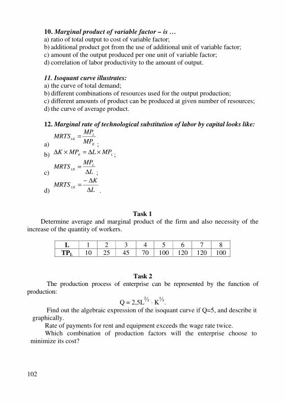
102

10. Marginal product of variable factor – is …

а) ratio of total output to cost of variable factor; b) additional product got from the use of additional unit of variable factor; c) amount of the output produced per one unit of variable factor; d) correlation of labor productivity to the amount of output.

11. Isoquant curve illustrates:

а) the curve of total demand; b) different combinations of resources used for the output production; c) different amounts of product can be produced at given number of resources; d) the curve of average product.

12. Marginal rate of technological substitution of labor by capital looks like:

а) K

L

LKMP

MPMRTS =

;

b) LKMPLMPK ×∆=×∆ ;

c) L

MPMRTS L

LK∆

=;

d) L

KMRTS

LK∆

∆−=

.

Task 1

Determine average and marginal product of the firm and also necessity of the increase of the quantity of workers.

L 1 2 3 4 5 6 7 8

TPL 10 25 45 70 100 120 120 100

Task 2

The production process of enterprise can be represented by the function of production:

Q = 2,5L⅔ · K⅓. Find out the algebraic expression of the isoquant curve if Q=5, and describe it

graphically. Rate of payments for rent and equipment exceeds the wage rate twice. Which combination of production factors will the enterprise choose to

minimize its cost?

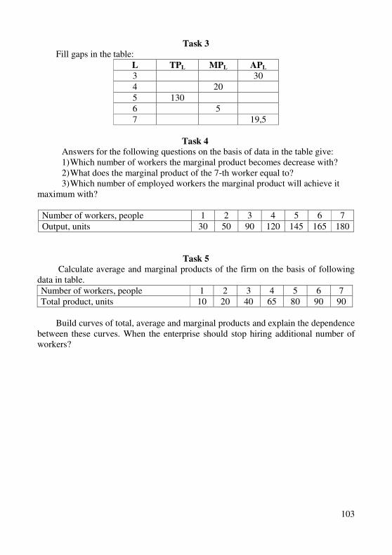
103

Task 3

Fill gaps in the table:

L TPL MPL APL

3 30

4 20

5 130 6 5 7 19,5

Task 4

Answers for the following questions on the basis of data in the table give: 1) Which number of workers the marginal product becomes decrease with? 2) What does the marginal product of the 7-th worker equal to? 3) Which number of employed workers the marginal product will achieve it

maximum with?

Number of workers, people 1 2 3 4 5 6 7

Output, units 30 50 90 120 145 165 180

Task 5

Calculate average and marginal products of the firm on the basis of following data in table.

Number of workers, people 1 2 3 4 5 6 7 Total product, units 10 20 40 65 80 90 90

Build curves of total, average and marginal products and explain the dependence

between these curves. When the enterprise should stop hiring additional number of workers?

104

Theme 8 Cost and Income of Enterprise

8.1. Cost of the enterprise. Economic and accounting approaches to cost

determination.

8.2. Cost of the enterprise in short-term market period.

8.3. Сost of the enterprise in long-term market period.

8.4. The concept of the minimal effective size of the enterprise and the

structure of the industry.

8.5. The essence and forms of income of the enterprise.

8.1. Cost of the enterprise. Economic and accounting approaches

to cost determination

The main previous topic’s model was production function that reflects the

dependence of cost of production factors in natural expression and amount of output. If to evaluate the amount of production factors used in manufactiruing process by cost measure, then costs of production factors will be transformed into costs of production.

The costs of enterprise are characterized by the cost of production factors used by them to create a certain amount of production.

The existence of costs is caused by the rarity of resources and the alternative ways of their use. In this aspect, the economic costs are used to be distinguished.

Economic costs are payments that should provide the revenue for providers of resources. These resources can’t be used alternatively. There are a lot of approaches to cost determination and its classification.

In particular, theoretical and methodical approaches provide the classification of cost into private and social. Private costs are connected with the manufacturing of some particulat enterprise. Social costs have general social character where, first of all, external effects are taken into account. Social and private costs are equal in case of absence of external effects or of balance of their positive abd negative parts.

Additionally, there are actual and alternative costs of enterprise. In first case, costs of enterprise are evaluated in actual prices of production factors used in the manufacturing process. In another case, we should take into account the value of goods that could be achieved at the best alternative way of use among factors in order to calculate the amount of alternative costs.

Because of this reason there are two approaches for the cost of enterprise determination: accounting and economic ones.

105

Accounting (external, explicit) costs – are the cost of the enterprise for the use of external resources, that is, they are associated with resources that do not belong to the owners of the enterprise.

Internal (implicit) costs are considered as cash payments that property owners could receive from the alternative use of resources held by them (implicit wages of the owner of the enterprise, whatever he could receive, hired by the employee, profit that could he obtains, by investing in any other enterprise or financial instrument, a rent for the alternative use of his property).

It is important to emphasize that internal costs also include normal returns. Normal profit is built on the basis of competition and alternative pay for the

entrepreneur's functions. The size of such profit is determined by the level of profitability of the industry (normative or average). The amount of accounting and internal costs will be economic costs.

Consequently, economic costs are the costs of enterprises for the use of both external and internal resources owned by the owners of the enterprise. In another way, this is the amount of both accounting (external, explicit costs) and internal (implicit) costs. Economic costs always have an alternative cost.

The difference between revenue and economic costs is an economic profit. If the economic profit is zero, so that getting a normal profit by the entrepreneur keeps him in the industry.

The special type of costs of enterprise is irreversible costs. Irreversable costs are costs of resources that have no alternative use. They are

not part of internal costs, never come back to the manufacturer and can’t be alternative. An example of such costs can be expenditures connected with payments for unique equipment that has no alternative way of use.

It is possible to justify the costs function by modeling the firm’s activity concerning costs.

The costs’ function characterizes the dependence of the amount of output and minimally possible costs necessary for its keeping.

The function of costs is a function of the amount of output and prices of resources. It can have such a look in analytical form:

С (Q) = f [Q (K, L), r, w], or С = с (w1, w2, y),

where С - ..., Q - ..., K - …, L - …, r, w - …, w1 - …, w2 - …, y - …, f, с – functional dependence.

Summarizing the material above, we can make some conlcusions: costs of enterprise – is cost of production factors. Costs can be economical, accounting, private, social, internal, and irreversable. The model of costs is a function that characterizes the dependence of the amount of output and minimally possible costs that are necessary for its getting.

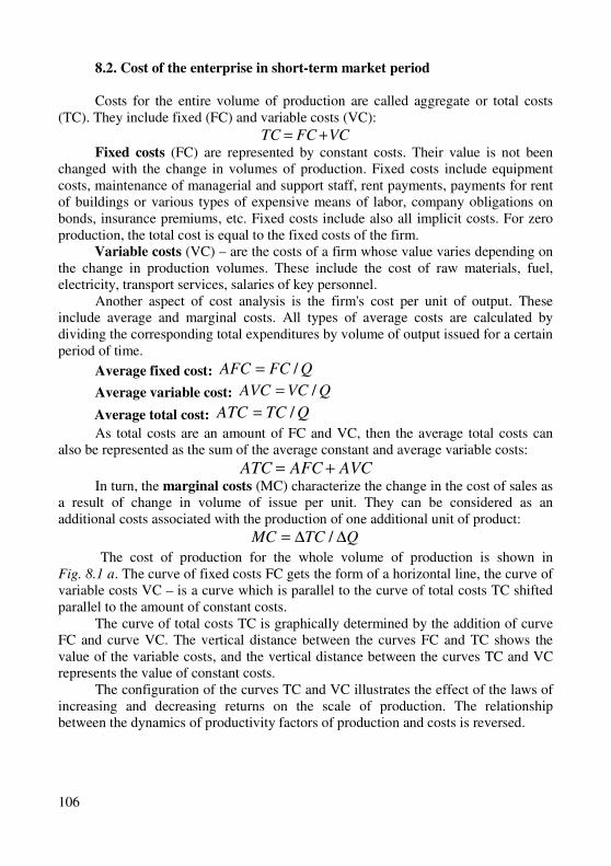
106

8.2. Cost of the enterprise in short-term market period

Costs for the entire volume of production are called aggregate or total costs (TC). They include fixed (FC) and variable costs (VC):

VCFCTC += Fixed costs (FC) are represented by constant costs. Their value is not been

changed with the change in volumes of production. Fixed costs include equipment costs, maintenance of managerial and support staff, rent payments, payments for rent of buildings or various types of expensive means of labor, company obligations on bonds, insurance premiums, etc. Fixed costs include also all implicit costs. For zero production, the total cost is equal to the fixed costs of the firm.

Variable costs (VC) – are the costs of a firm whose value varies depending on the change in production volumes. These include the cost of raw materials, fuel, electricity, transport services, salaries of key personnel.

Another aspect of cost analysis is the firm's cost per unit of output. These include average and marginal costs. All types of average costs are calculated by dividing the corresponding total expenditures by volume of output issued for a certain period of time.

Average fixed cost: QFCAFC /=

Average variable cost: QVCAVC /=

Average total cost: QTCATC /=

As total costs are an amount of FC and VC, then the average total costs can also be represented as the sum of the average constant and average variable costs:

AVCAFCATC += In turn, the marginal costs (MC) characterize the change in the cost of sales as

a result of change in volume of issue per unit. They can be considered as an additional costs associated with the production of one additional unit of product:

QTCMC ∆∆= /

The cost of production for the whole volume of production is shown in Fig. 8.1 a. The curve of fixed costs FC gets the form of a horizontal line, the curve of variable costs VC – is a curve which is parallel to the curve of total costs TC shifted parallel to the amount of constant costs.

The curve of total costs TC is graphically determined by the addition of curve FC and curve VC. The vertical distance between the curves FC and TC shows the value of the variable costs, and the vertical distance between the curves TC and VC represents the value of constant costs.

The configuration of the curves TC and VC illustrates the effect of the laws of increasing and decreasing returns on the scale of production. The relationship between the dynamics of productivity factors of production and costs is reversed.

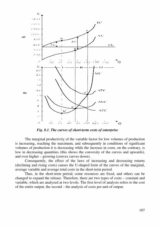
107

The marginal productivity of the variable factor for low volumes of production is increasing, reaching the maximum, and subsequently in conditions of significant volumes of production it is decreasing while the increase in costs, on the contrary, is low in decreasing quantities (this shows the convexity of the curves and upwards), and over higher – growing (convex curves down).

Consequently, the effect of the laws of increasing and decreasing returns (declining and rising costs) causes the U-shaped form of the curves of the marginal, average variable and average total costs in the short-term period.

Thus, in the short-term period, some resources are fixed, and others can be changed to expand the release. Therefore, there are two types of costs – constant and variable, which are analyzed at two levels. The first level of analysis refers to the cost of the entire output, the second – the analysis of costs per unit of output.

Fig. 8.1. The curves of short-term costs of enterprise

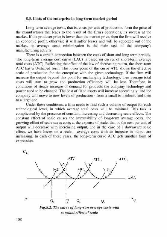
108

8.3. Costs of the enterprise in long-term market period

Long-term average costs, that is, costs per unit of production, form the price of

the manufacturer that leads to the result of the firm's operations, its success at the market. If the producer price is lower than the market price, then the firm will receive an economic profit, otherwise it will suffer losses and will be squeezed out of the market, so average costs minimization is the main task of the company's manufacturing activity.

There is a certain connection between the costs of short and long term periods. The long-term average cost curve (LAC) is based on curves of short-term average total costs (ATC). Reflecting the effect of the law of decreasing return, the short-term ATC has a U-shaped form. The lower point of the curve ATC shows the effective scale of production for the enterprise with the given technology. If the firm will increase the output beyond this point for unchanging technology, then average total costs will start to grow and production efficiency will be lost. Therefore, in conditions of steady increase of demand for products the company technology and power need to be changed. The cost of fixed assets will increase accordingly, and the company will move to new levels of production - from a small to medium, and then to a large one.

Under these conditions, a firm needs to find such a volume of output for each technological level, in which average total costs will be minimal. This task is complicated by the presence of constant, increasing and decreasing scale effects. The constant effect of scale causes the immutability of long-term average costs, the growing effect of scale saves costs at the expense of scale, that is, the cost per unit of output will decrease with increasing output, and in the case of a downward scale effect, we have losses on a scale – average costs with an increase in output are increasing. In each of these cases, the long-term curve ATC gets another form of expression.

Fig.8.2. The curve of long-run average costs with

constant effect of scale

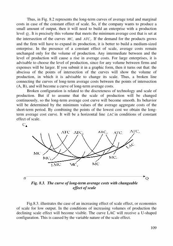
109

Thus, in Fig. 8.2 represents the long-term curves of average total and marginal costs in case of the constant effect of scale. So, if the company wants to produce a small amount of output, then it will need to build an enterprise with a production level 1Q . It is precisely this volume that meets the minimum average cost that is set at

the intersection of the curves 1MC and 1ATC . If the demand for the products grows

and the firm will have to expand its production, it is better to build a medium-sized enterprise. In the presence of a constant effect of scale, average costs remain unchanged only for the volume of production. Any intermediate between and the level of production will cause a rise in average costs. For large enterprises, it is advisable to choose the level of production, since for any volume between firms and expenses will be larger. If you submit it in a graphic form, then it turns out that: the abscissa of the points of intersection of the curves will show the volume of production, in which it is advisable to change its scale. Thus, a broken line connecting the curves of long-term average costs between the points of intersection (A, B), and will become a curve of long-term average costs.

Broken configuration is related to the discreteness of technology and scale of production. But if to assume that the scale of production will be changed continuously, so the long-term average cost curve will become smooth. Its behavior will be determined by the minimum values of the average aggregate costs of the short-term period. By combining the points of the lowest cost we obtain the long-term average cost curve. It will be a horizontal line LAC in conditions of constant effect of scale.

Fig.8.3. illustrates the case of an increasing effect of scale effect, or economies

of scale for low output. In the conditions of increasing volumes of production the declining scale effect will become visible. The curve LAC will receive a U-shaped configuration. This is caused by the variable nature of the scale effect.

Fig. 8.3. The curve of long-term average costs with changeable

effect of scale

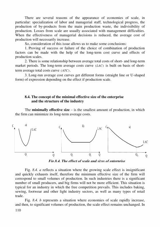
110

There are several reasons of the appearance of economies of scale, in particular: specialization of labor and managerial staff, technological progress, the production of by-products from the main production waste, the indivisibility of production. Losses from scale are usually associated with management difficulties. When the effectiveness of managerial decisions is reduced, the average cost of production will necessarily increase.

So, consideration of this issue allows us to make some conclusions: 1. Proving of success or failure of the choice of combination of production

factors can be made with the help of the long-term cost curve and effects of production scales.

2. There is some relationship between average total costs of short- and long-term market periods. The long-term average costs curve )(LAC is built on basis of short-

term average total costs curve )(ATC .

3. Long-run average cost curves get different forms (straight line or U-shaped form) of expression depending on the effect if production scale.

8.4. The concept of the minimal effective size of the enterprise

and the structure of the industry

The minimally effective size – is the smallest amount of production, in which

the firm can minimize its long-term average costs.

Fig. 8.4. a reflects a situation where the growing scale effect is insignificant

and quickly exhausts itself, therefore the minimum effective size of the firm will correspond to small volumes of production. In such industries there is a significant number of small producers, and big firms will not be more efficient. This situation is typical for an industry in which the free competition prevails. This includes baking, sewing, footwear and other light industry sectors, as well as many types of retail trade.

Fig. 8.4. b represents a situation where economies of scale rapidly increase, and then, to significant volumes of production, the scale effect remains unchanged. In

Fig.8.4. The effect of scale and sizes of enterprise

111

this area, the firm achieves a minimum of average costs for relatively low production volumes. That is why the firm will be competitive even compared to medium and

large enterprises with the same average costs (per segment 21QQ ). In industries with

such conditions of the formation of average costs the enterprises of different sizes can effectively coexist. Such are the branches that produce furniture, books, etc.

Fig. 8.4. c illustrates the situation of a long-lasting increasing effect of scale. Here it is taken into account the fact that the enterprise can achieve minimal expenses at very large volumes of production. Small firms are not able to provide such low costs, so they will not compete and will be not viable. In real life, such tendencies can be observed in automotive, aluminum, steelmaking and other industries of heavy industry. In these industries, production can be concentrated in one firm, which will satisfy the entire volume of demand and will guarantee a minimum of costs. Such a market situation will acquire the features of a natural monopoly.

Positive and negative effects of scale are the most important factors that determine the structure of each industry and the level of development of competition in it.

So, modeling the company's activities of the enterprise in terms of its scale it is necessary to be based on the fact that the growth of the scale of the enterprise can cause a growing and decreasing return on the scale.

There are couple reasons of the emergence of the increasing returns on the

scale of production: � Division of labor, as big enterprises gives an opportunity for deeper internal

specialization. It causes increase in labor productivity and leads to increase in average product.

� Improvement of management of the firm, as in condition of larger sizes of enterprises there is deepening specialization in management sphere. In particular, there appear highly specialized specialists on advertisement, logistics, marketing, etc.

But increase in production scales has also negative sides. It may cause the downturn on the enterprise scales and cumbersome management system, strengthening bureaucratic tendencies in management, loss of production flexibility.

Consequently, the minimally effective size of the firm is the less amount of the output at which firm can minimize its long-run average costs. When increasing effect of scale of production is insignificant and it quickly exhausts itself, then minimally effective size of firm corresponds to small amount of output. Both positive and negative effects of scale are the most important factors that determine the structure of every industry and level of competition development there.

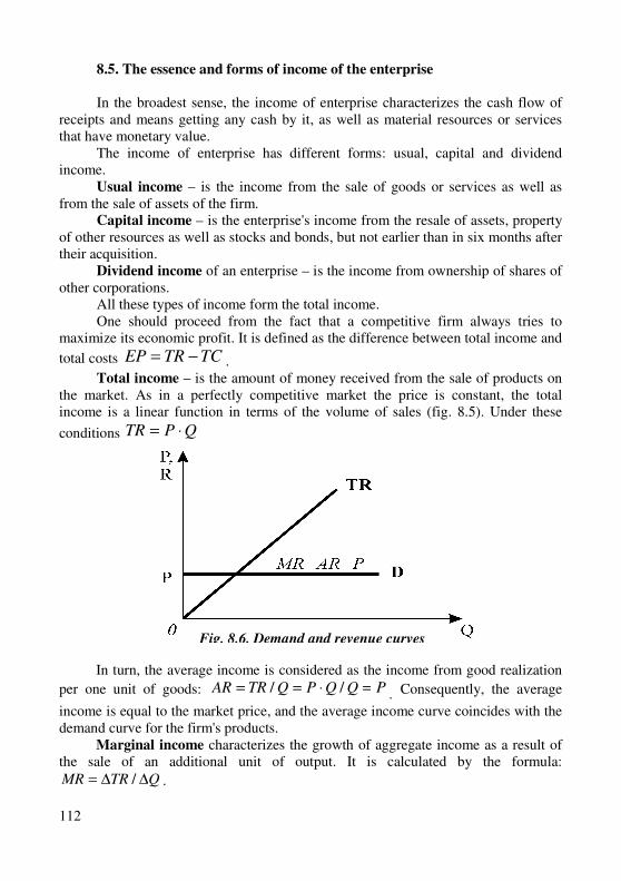
112

8.5. The essence and forms of income of the enterprise In the broadest sense, the income of enterprise characterizes the cash flow of

receipts and means getting any cash by it, as well as material resources or services that have monetary value.

The income of enterprise has different forms: usual, capital and dividend income.

Usual income – is the income from the sale of goods or services as well as from the sale of assets of the firm.

Capital income – is the enterprise's income from the resale of assets, property of other resources as well as stocks and bonds, but not earlier than in six months after their acquisition.

Dividend income of an enterprise – is the income from ownership of shares of other corporations.

All these types of income form the total income. One should proceed from the fact that a competitive firm always tries to

maximize its economic profit. It is defined as the difference between total income and

total costs TCTREP −= .

Total income – is the amount of money received from the sale of products on the market. As in a perfectly competitive market the price is constant, the total income is a linear function in terms of the volume of sales (fig. 8.5). Under these

conditions QPTR ⋅=

In turn, the average income is considered as the income from good realization

per one unit of goods: PQQPQTRAR =⋅== // . Consequently, the average

income is equal to the market price, and the average income curve coincides with the demand curve for the firm's products.

Marginal income characterizes the growth of aggregate income as a result of the sale of an additional unit of output. It is calculated by the formula:

QTRMR ∆∆= / .

Fig. 8.6. Demand and revenue curves

113

When comparing total income with aggregate costs, as well as market price with average and marginal costs, the firm decides whether to produce products at all, and if they produce, to decide what quantity should be, and also determine what the results of activities in these conditions will be.

There are two approaches to determining the optimal volume of production.

The first is based on the comparison of total income and total costs (model TRTC ). And the second involves comparing marginal revenue and marginal costs (model

MRMC ). Let’s we formulate general rule of choosing the optimal volume of

production, or general condition for maximizing profits: profit is maximized in the

volume of production, for which the marginal revenue is equal to the marginal cost:

MCMR = .

This rule is valid for all firms in any market structure. Since in a market of

perfect competition PMR = , for a competitive firm, the general rule of maximizing profit is the choice of such volume of output, at which the marginal costs will be

equal to the price: PMRMC == . Taking into account all information mentioned before, we can make some

conclusions: in a broad sence income of enterprise means getting by it any money, as well as material resources or services that have money expression. There are following types of income: usual, dividend, capital, total, average and marginal. Comparing total income with total costs at each amount of output, and also market price with average and marginal costs, the firm makes decision: is it necessary to produce, and if it is, so how many, and what is going to be the result of manufacturing activity?

There are two approaches to determination of the optimal amount of output: 1) correlation of total income and total costs (model TRTC); 2) correlation of marginal income and marginal costs (model MRMC).

Training

Key terms and concepts Cost of the enterprise. Economic cost. Private cost. Accounting cost. External

cost. Internal cost.

Function of cost. Total cost. Variable cost. Average cost. Marginal cost. Long-

run average cost.

Normal profit. Economic profit. Accounting profit. Usual income. Capital

income. Dividend income. Total income. Average income. Marginal income.

Functions of profit.

Effective size of the enterprise. Scale of production.

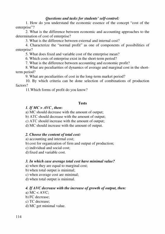
114

Questions and tasks for students’ self-control:

1. How do you understand the economic essence of the concept “cost of the enterprise”?

2. What is the difference between economic and accounting approaches to the determination of cost of enterprise?

3. What is the difference between external and internal cost? 4. Characterize the “normal profit” as one of components of possibilities of

enterprise? 5. What does fixed and variable cost of the enterprise mean? 6. Which costs of enterprise exist in the short-term period? 7. What is the difference between accounting and economic profit? 8. What are peculiarities of dynamics of average and marginal cost in the short-

term period? 9. What are peculiarities of cost in the long-term market period? 10. By which criteria can be done selection of combinations of production

factors? 11.Which forms of profit do you know?

Tests

1. If МС > АVС , then:

а) МС should decrease with the amount of output; b) АТС should decrease with the amount of output; c) АТС should increase with the amount of output; d) МС should increase with the amount of output.

2. Choose the content of total cost: а) accounting and internal cost; b) cost for organization of firm and output of production; c) individual and social cost; d) fixed and variable cost.

3. In which case average total cost have minimal value?

а) when they are equal to marginal cost; b) when total output is minimal; c) when average cost are minimal; d) when total output is minimal. 4. If AVC decrease with the increase of growth of output, then:

а) МС < AVC; b) FС decrease; c) ТС decrease; d) МС get minimal value.

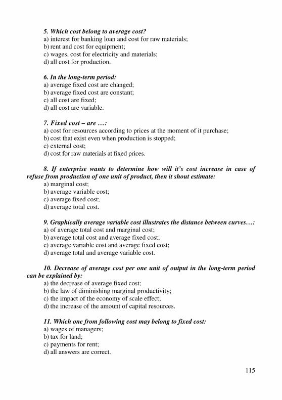
115

5. Which cost belong to average cost?

а) interest for banking loan and cost for raw materials; b) rent and cost for equipment; c) wages, cost for electricity and materials; d) all cost for production. 6. In the long-term period:

а) average fixed cost are changed; b) average fixed cost are constant; c) all cost are fixed; d) all cost are variable.

7. Fixed cost – are …:

а) cost for resources according to prices at the moment of it purchase; b) cost that exist even when production is stopped; c) external cost; d) cost for raw materials at fixed prices.

8. If enterprise wants to determine how will it’s cost increase in case of

refuse from production of one unit of product, then it shout estimate:

а) marginal cost; b) average variable cost; c) average fixed cost; d) average total cost.

9. Graphically average variable cost illustrates the distance between curves…: а) of average total cost and marginal cost; b) average total cost and average fixed cost; c) average variable cost and average fixed cost; d) average total and average variable cost. 10. Decrease of average cost per one unit of output in the long-term period

can be explained by:

а) the decrease of average fixed cost; b) the law of diminishing marginal productivity; c) the impact of the economy of scale effect; d) the increase of the amount of capital resources.

11. Which one from following cost may belong to fixed cost:

а) wages of managers; b) tax for land; c) payments for rent; d) all answers are correct.

116

12. Total cost are calculated as:

а) FCVC − ; b) VCFC + ; c) MCVCFC ++ ;

d) Q

VCFC )( +.

13. Total cost of firm for any amount of output equals to: а) average total cost multiplied to the amount of output; b) average total cost minus average variable cost; c) average variable cost multiplied to the amount of output; d) average fixed cost plus average variable cost. 14. Marginal cost – are… а) growth of TC as a result of growth the amount of output per one unit; b) qrowth of variable cost as a result of growth of the amount of output per

one unit of product; c) additional cost connected with production of additional unit of product; d) all answers are right.

Task 1

There is dependence of total cost of enterprise from the amount of output. Please, calculate following types of cost: FC, VC, MC, AFC, AVC, ATC.

Describe graphically the last four indicators.

Q 0 1 2 3 4

TC 60 140 180 240 420

Task 2

The table represents information about cost and revenue of some firm:

Q TC FC VC ATC MC P TR MR

0 150 ? ? ? ? 200 0 ? 1 ? ? 120 ? ? ? 190 ? 2 340 ? ? ? ? 180 ? ?

3 400 ? ? ? ? ? 500 ? 4 ? ? 240 ? ? 140 ? ?

5 500 ? ? ? ? 100 ? ?

Fill the gaps in table. Which values of P and Q proves that firm is in

equilibrium state? By which values of P and Q the profit will be maximal?

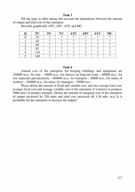
117

Task 3

Fill the gaps in table taking into account the dependence between the amount of output and total cost of the enterprise.

Describe graphically ATC, AFC, AVC and MC.

Q TC FC VC ATC AFC AVC MC

0 35 ? ? ? ? ? ?

1 45 ? ? ? ? ? ? 2 60 ? ? ? ? ? ?

3 85 ? ? ? ? ? ? 4 110 ? ? ? ? ? ?

5 140 ? ? ? ? ? ?

Task 4

Annual cost of the enterprise for keeping buildings and equipment are 150000 m.u., for rent – 10000 m.u., for interest on long-run loans – 60000 m.u., for raw materials and electricity – 600000 m.u., for transport – 20000 m.u., for salary of workers – 360000 m.u., for salary for managers – 95000 m.u.

Please define the amount of fixed and variable cost, and also average total cost, average fixed cost and average variable cost of the enterprise if it known it produces 5000 units of product annually. Define the amount of marginal cost of the enterprise of output increased by 250 units and total cost increased till 1,36 mln. m.u. Is it profitable for the enterprise to increase the output?

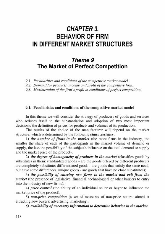
118

CHAPTER 3.

BEHAVIOR OF FIRM

IN DIFFERENT MARKET STRUCTURES

Theme 9 The Market of Perfect Competition

9.1. Peculiarities and conditions of the competitive market model.

9.2. Demand for products, income and profit of the competitive firm.

9.3. Maximization of the firm’s profit in conditions of perfect competition.

9.1. Peculiarities and conditions of the competitive market model

In this theme we will consider the strategy of producers of goods and services

who reduces itself to the substantiation and adoption of two most important decisions: the definition of prices for products and volumes of its production.

The results of the choice of the manufacturer will depend on the market structure, which is determined by the following characteristics:

1) the number of firms in the market (the more firms in the industry, the smaller the share of each of the participants in the market volume of demand or supply, the less the possibility of the subject's influence on the total demand or supply and the market price of the product);

2) the degree of homogeneity of products in the market (classifies goods by substitutes in them: standardized goods – are the goods offered by different producers are completely substitute; differentiated goods - are goods that satisfy the same need, but have some differences, unique goods - are goods that have no close substitutes);

3) the possibility of entering new firms in the market and exit from the

market (the presence of legislative, financial, technological or other barriers to entry into the industry of new firms);

4) price control (the ability of an individual seller or buyer to influence the market price of the product);

5) non-price competition (a set of measures of non-price nature, aimed at attracting new buyers: advertising, marketing);

6) availability of necessary information to determine behavior in the market.

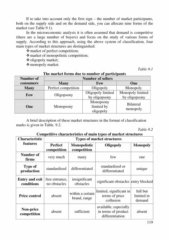
119

If to take into account only the first sign – the number of market participants, both on the supply side and on the demand side, you can allocate nine forms of the market (see Table 9.1).

In the microeconomic analysis it is often assumed that demand is competitive (there are a large number of buyers) and focus on the study of various forms of supply. According to this approach, using the above system of classification, four main types of market structures are distinguished:

� market of perfect competition; � market of monopolistic competition; � oligopoly market; � monopoly market.

Table 9.1

The market forms due to number of participants

Number of sellers Number of

consumers Many Few One

Many Perfect competition Oligopoly Monopoly

Few Oligopsony Oligopoly limited

by oligopsony Monopoly limited

by oligopsony

One Monopsony Monopsony limited by oligopoly

Bilateral monopoly

A brief description of these market structures in the format of classification

marks is given in Table. 9.2. Table 9.2

Competitive characteristics of main types of market structures

Types of market structures Characteristic

features Perfect

competition

Monopolistic

competition

Oligopoly Monopoly

Number of

firms very much many few one

Type of

production standardized differentiated

standardized or differentiated

unique

Entry and exit

conditions

free entrance, no obstacles

insignificant obstacles

significant obstacles entry blocked

Price control absent within a certain

brand, range

limited, significant in terms of price

collusion

full but limited in demand

Non-price

competition absent sufficient

available, especially in terms of product

differentiation absent

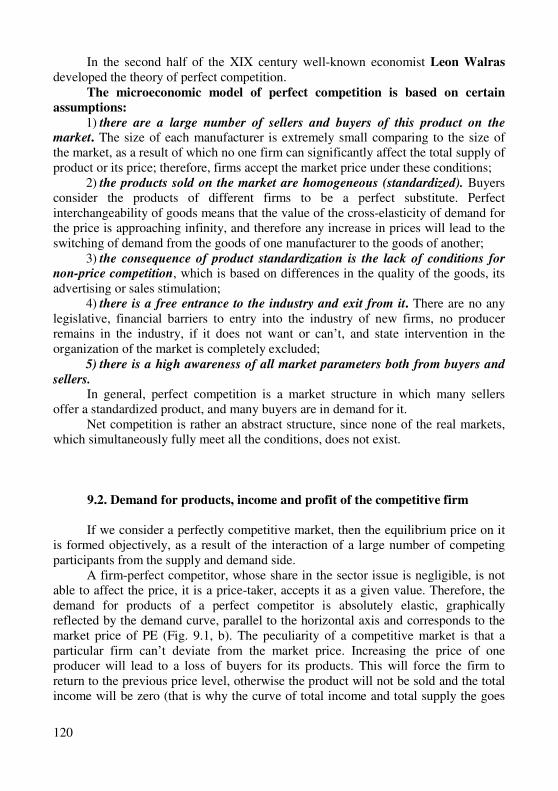
120

In the second half of the XIX century well-known economist Leon Walras developed the theory of perfect competition.

The microeconomic model of perfect competition is based on certain

assumptions:

1) there are a large number of sellers and buyers of this product on the market. The size of each manufacturer is extremely small comparing to the size of the market, as a result of which no one firm can significantly affect the total supply of product or its price; therefore, firms accept the market price under these conditions;

2) the products sold on the market are homogeneous (standardized). Buyers consider the products of different firms to be a perfect substitute. Perfect interchangeability of goods means that the value of the cross-elasticity of demand for the price is approaching infinity, and therefore any increase in prices will lead to the switching of demand from the goods of one manufacturer to the goods of another;

3) the consequence of product standardization is the lack of conditions for non-price competition, which is based on differences in the quality of the goods, its advertising or sales stimulation;

4) there is a free entrance to the industry and exit from it. There are no any legislative, financial barriers to entry into the industry of new firms, no producer remains in the industry, if it does not want or can’t, and state intervention in the organization of the market is completely excluded;

5) there is a high awareness of all market parameters both from buyers and

sellers. In general, perfect competition is a market structure in which many sellers

offer a standardized product, and many buyers are in demand for it. Net competition is rather an abstract structure, since none of the real markets,

which simultaneously fully meet all the conditions, does not exist.

9.2. Demand for products, income and profit of the competitive firm

If we consider a perfectly competitive market, then the equilibrium price on it

is formed objectively, as a result of the interaction of a large number of competing participants from the supply and demand side.

A firm-perfect competitor, whose share in the sector issue is negligible, is not able to affect the price, it is a price-taker, accepts it as a given value. Therefore, the demand for products of a perfect competitor is absolutely elastic, graphically reflected by the demand curve, parallel to the horizontal axis and corresponds to the market price of PE (Fig. 9.1, b). The peculiarity of a competitive market is that a particular firm can’t deviate from the market price. Increasing the price of one producer will lead to a loss of buyers for its products. This will force the firm to return to the previous price level, otherwise the product will not be sold and the total income will be zero (that is why the curve of total income and total supply the goes

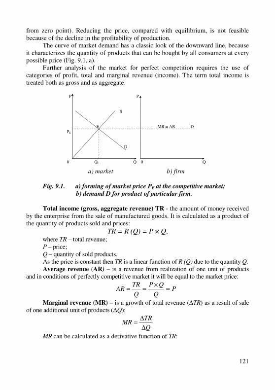
121

from zero point). Reducing the price, compared with equilibrium, is not feasible because of the decline in the profitability of production.

The curve of market demand has a classic look of the downward line, because it characterizes the quantity of products that can be bought by all consumers at every possible price (Fig. 9.1, a).

Further analysis of the market for perfect competition requires the use of categories of profit, total and marginal revenue (income). The term total income is treated both as gross and as aggregate.

Р Р S E MR = AR D РE D 0 QE Q 0 Q

а) market b) firm

Fig. 9.1. а) forming of market price РЕ at the competitive market;

b) demand D for product of particular firm.

Total income (gross, aggregate revenue) TR - the amount of money received

by the enterprise from the sale of manufactured goods. It is calculated as a product of the quantity of products sold and prices:

TR = R (Q) = P × Q,

where TR – total revenue; Ρ – price; Q – quantity of sold products. As the price is constant then TR is a linear function of R (Q) due to the quantity Q. Average revenue (AR) – is a revenue from realization of one unit of products

and in conditions of perfectly competitive market it will be equal to the market price:

PQ

QP

Q

TRAR =

×==

Marginal revenue (MR) – is a growth of total revenue (∆TR) as a result of sale

of one additional unit of products (∆Q):

Q

TRMR

∆

∆=

MR can be calculated as a derivative function of TR:

122

PdQ

dQP

dQ

QPd

dQ

dTRMR =

×=

×==

)(

So in conditions of perfect market AR=MR=P, it means that the demand curve at

the fig. 9.1. b is at the same time a line of price, average and marginal revenue. Profit (π) of any firm is formed as the difference between the income from the

sale of products (total income) and the total costs for its production and sale:

π = TR – TC,

where ТС – are total costs. Depending on the type of expenditure (accounting or economic), the

accounting and economic profit are calculated accordingly. The difference between accounting and economic profit is due to what costs

are taken into account when calculating it. Accounting profit equals the difference between total income and accounting (external, explicit) costs. Economic profit is considered to be the difference between total income and economic (external and internal) costs. The sum of external and internal costs is equivalent to the sum of explicit and implicit costs. The category of internal (implicit) costs associated with such a concept as a normal profit.

Normal profit – is an economic condition that occurs when the difference between a firm’s total revenue and total cost is equal to zero. Normal profit is the minimum level of profit needed for a company to remain competitive in the market.

It can be assumed that normal profits should compensate costs of own resources that belongs to the owner of the firm, in particular its labor, entrepreneurial abilities at the level of market prices for these resources. As a result of this, the economic profit differs from the accounting for the amount of normal profit.

Consequently, considering the peculiarities of the demand for the goods of the firm of a perfect competitor, the formation of various forms of income and profits, we can conclude that:

1) the competitive firm has a horizontal curve of demand, the height of which is determined by the market price;

2) the main indicator of the effectiveness of the firm in the microeconomic analysis is its economic profit.

9.3. Maximization of the firm’s profit in conditions of perfect competition

According to the assumption of rational behavior of the manufacturer and the

marginal concept the main purpose of the functioning of the enterprise is the profit maximization.

The value of profit is a kind of signal for the enterprise about the most profitable areas of activity and serves as the basis for developing the economic strategy of the manufacturer in the market of goods. The incentive function of profit is manifested in the fact that in order to maximize the enterprise, they constantly

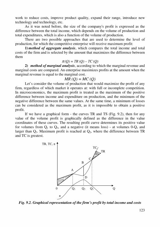
123

work to reduce costs, improve product quality, expand their range, introduce new technology and technology, etc.

As it was noted before, the size of the company's profit is expressed as the difference between the total income, which depends on the volume of production and total expenditures, which is also a function of the volume of production.

There are two possible approaches that are used to determine the level of production, for which the competitive enterprise will receive maximum profit:

1) method of aggregate analysis, which compares the total income and total costs of the firm and is selected by the amount that maximizes the difference between them

π (Q) = ТR (Q) – ТC (Q) 2) method of marginal analysis, according to which the marginal revenue and

marginal costs are compared. An enterprise maximizes profits at the amount when the marginal revenue is equal to the marginal cost.

MR (Q) = MC (Q) Let’s consider the volume of production that would maximize the profit of any

firm, regardless of which market it operates at: with full or incomplete competition. In microeconomics, the maximum profit is treated as the maximum of the positive difference between income and expenditure on production, and the minimum of the negative difference between the same values. At the same time, a minimum of losses can be considered as the maximum profit, as it is impossible to obtain a positive profit.

If we have a graphical form - the curves TR and TS (Fig. 9.2), then for any value of the volume profit is graphically defined as the difference in the value coordinates of these curves. The resulting profit curve determines its positive value for volumes from Q1 to Q3, and a negative (it means loss) - at volumes 0-Q1 and larger than Q3. Maximum profit is reached at Q2, where the difference between TR and TC is greatest.

TR, TC, π TC TR C B A D 0 Q1 Q2 Q3 Q π

Fig. 9.2. Graphical representation of the firm’s profit by total income and costs

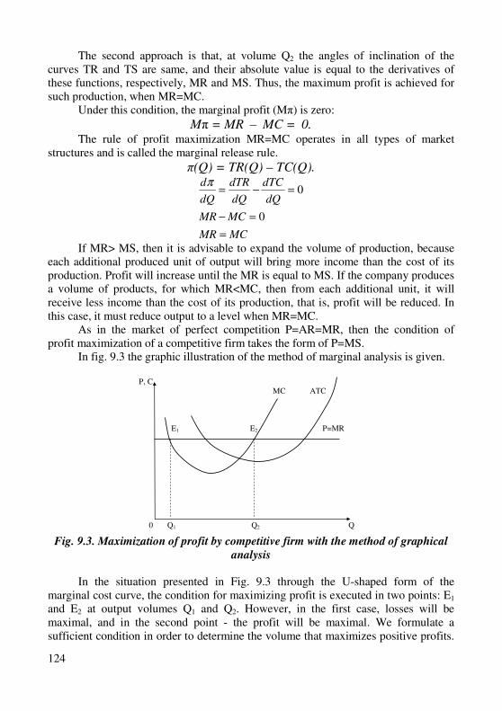
124

The second approach is that, at volume Q2 the angles of inclination of the curves TR and TS are same, and their absolute value is equal to the derivatives of these functions, respectively, MR and MS. Thus, the maximum profit is achieved for such production, when MR=MC.

Under this condition, the marginal profit (Mπ) is zero:

Mπ = MR – MC = 0. The rule of profit maximization MR=MC operates in all types of market

structures and is called the marginal release rule.

π(Q) = TR(Q) – TC(Q).

MCMR

MCMR

dQ

dTC

dQ

dTR

dQ

d

=

=−

=−=

0

0π

If MR> MS, then it is advisable to expand the volume of production, because each additional produced unit of output will bring more income than the cost of its production. Profit will increase until the MR is equal to MS. If the company produces a volume of products, for which MR<MC, then from each additional unit, it will receive less income than the cost of its production, that is, profit will be reduced. In this case, it must reduce output to a level when MR=MC.

As in the market of perfect competition P=AR=MR, then the condition of profit maximization of a competitive firm takes the form of P=MS.

In fig. 9.3 the graphic illustration of the method of marginal analysis is given.

P, C MC ATC E1 E2 P=MR

0 Q1

Q2 Q

Fig. 9.3. Maximization of profit by competitive firm with the method of graphical

analysis

In the situation presented in Fig. 9.3 through the U-shaped form of the marginal cost curve, the condition for maximizing profit is executed in two points: E1 and E2 at output volumes Q1 and Q2. However, in the first case, losses will be maximal, and in the second point - the profit will be maximal. We formulate a sufficient condition in order to determine the volume that maximizes positive profits.

125

Algebraically this means that the second derivative of the profit function must be negative.

0

0dQ

Pd

2

2

2

2

2

2

<−

<

dQ

TCd

dQ

TRd

0<−dQ

dMC

dQ

dMR

dQ

dMC

dQ

dMR<

The left side of the inequality characterizes the inclination of the marginal revenue curve MR, and the right is the slope of the marginal cost curve MC. Accordingly, a sufficient condition for maximum profit requires that the slope of the marginal cost curve is greater than the marginal income curve. Since for a perfectly competitive enterprise the price does not depend on the volume of output, then the slope of the marginal income curve is zero.

0)(

2

2

=dQ

TRd, 0=

dQ

dMR

Then a sufficient condition will look like:

0)(

2

2

>dQ

TCd, 0>

dQ

dMC

This means that the profit will be maximal if the marginal cost curve at the point of intersection of MR and MC will have a positive slope. In other words, at the maximum profit point the marginal cost curve should increase, it means, cross the marginal revenue curve from the bottom up. Returning to Fig. 9.3 the conditions for maximizing profit corresponds to the point E2 with the optimal output Q2.

Thus, the derived rules for maximization of the company's profits are of a general nature. They are acceptable to firms operating in different types of markets and are called "universal rules of market structures."

Training

Key terms and concepts Perfect competition. Market structure. Industry. Equilibrium at the market of

perfect competition. Paradox of profit. Breakeven price. Efficiency of production.

Efficiency of resources allocation. Point of closure. Surplus of production.

Questions and tasks for students’ self-control:

1. Which criteria of the market structure are necessary for classification of market of perfect competition?

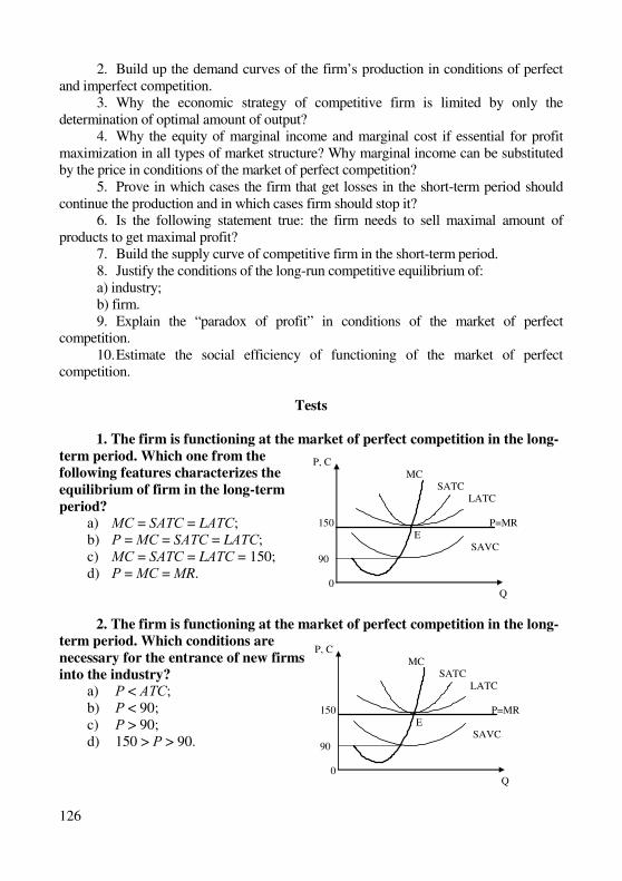
126

2. Build up the demand curves of the firm’s production in conditions of perfect and imperfect competition.

3. Why the economic strategy of competitive firm is limited by only the determination of optimal amount of output?

4. Why the equity of marginal income and marginal cost if essential for profit maximization in all types of market structure? Why marginal income can be substituted by the price in conditions of the market of perfect competition?

5. Prove in which cases the firm that get losses in the short-term period should continue the production and in which cases firm should stop it?

6. Is the following statement true: the firm needs to sell maximal amount of products to get maximal profit?

7. Build the supply curve of competitive firm in the short-term period. 8. Justify the conditions of the long-run competitive equilibrium of: а) industry; b) firm. 9. Explain the “paradox of profit” in conditions of the market of perfect

competition. 10. Estimate the social efficiency of functioning of the market of perfect

competition.

Tests

1. The firm is functioning at the market of perfect competition in the long-

term period. Which one from the

following features characterizes the

equilibrium of firm in the long-term

period?

а) МС = SАТС = LАТС; b) Р = МС = SАТС = LАТС; c) МС = SАТС = LАТС = 150; d) Р = МС = МR.

2. The firm is functioning at the market of perfect competition in the long-

term period. Which conditions are

necessary for the entrance of new firms

into the industry?

а) Р < АТС; b) Р < 90; c) Р > 90; d) 150 > Р > 90.

P, C MC SATC LATC 150 P=MR

E SAVC 90 0 Q

P, C MC SATC LATC 150 P=MR

E SAVC 90 0 Q

127

3. Which features characterize the market of perfect competition?

а) demand curve of some firm has a positive slope; b) there are 2-3 big and a lot of small firms in the industry; c) particular firm doesn’t has impact on the price of product and doesn’t take

part in non-price competition; d) marginal revenue of firm is always less than average revenue.

4. When for competitive firm ТR > ТС:

а) if МС < Р; b) if МR > МС; c) if the firm has economic profit; d) if Р < АТС. 5. In which cases for competitive firm Р > МR:

а) for products with high cross elasticity; b) when the amount of output exceeds the equilibrium amount; c) when the amount of output is less than equilibrium amount; d) never as in condition of perfect competition for any amount of output this

values are equal.

6. For competitive firm in short-term period the profit maximization is

provided by condition:

а) Р = МR; b) Р = МС = МR; c) Р > АТС; d) АТС > Р > LАVС.

7. If at the market of perfect competition price of product X is 20 UAH, so

that means that one particular firm:

а) will extend amount of output until AR=20 UAH; b) will extend the amount of output until TR=TC; c) will achieve equilibrium when P=MR; d) will achieve equilibrium when P=MC.

8. If firm is in equilibrium in the long-term period and it average cost are

not changed with the change of output, so that the supply curve:

а) has a negative slope; b) has a positive slope; c) is horizontal; d) is vertical.

9. Which reason means that the firm in conditions of perfect competition

has to stop production?

а) if Р < АТС;

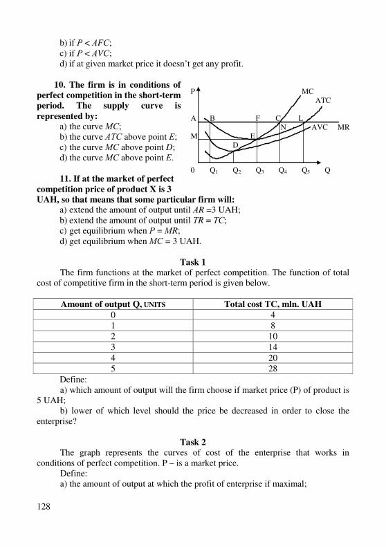
128

b) if Р < АFС; c) if Р < АVС; d) if at given market price it doesn’t get any profit.

10. The firm is in conditions of

perfect competition in the short-term

period. The supply curve is

represented by:

а) the curve МС; b) the curve АТС above point Е; c) the curve МС above point D; d) the curve МС above point Е.

11. If at the market of perfect

competition price of product X is 3

UAH, so that means that some particular firm will:

а) extend the amount of output until АR =3 UAH; b) extend the amount of output until ТR = ТС; c) get equilibrium when Р = МR; d) get equilibrium when МС = 3 UAH.

Task 1

The firm functions at the market of perfect competition. The function of total cost of competitive firm in the short-term period is given below.

Amount of output Q, UNITS Total cost ТС, mln. UAH

0 4 1 8 2 10

3 14

4 20 5 28

Define: а) which amount of output will the firm choose if market price (P) of product is

5 UAH; b) lower of which level should the price be decreased in order to close the

enterprise?

Task 2

The graph represents the curves of cost of the enterprise that works in conditions of perfect competition. P – is a market price.

Define: а) the amount of output at which the profit of enterprise if maximal;

P MC ATC A В F C L N AVC MR M E D 0 Q1 Q2 Q3 Q4 Q5 Q

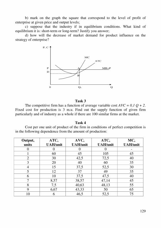
129

b) mark on the graph the square that correspond to the level of profit of enterprise at given price and output levels;

c) suppose that the industry if in equilibrium conditions. What kind of equilibrium it is: short-term or long-term? Justify you answer;

d) how will the decrease of market demand for product influence on the strategy of enterprise?

P, С

МС

АТС

Р А MR=P

D

B

0 Q1 Q

Task 3

The competitive firm has a function of average variable cost AVC = 0,1 Q + 2. Fixed cost for production is 3 m.u. Find out the supply function of given firm particularly and of industry as a whole if there are 100 similar firms at the market.

Task 4

Cost per one unit of product of the firm in conditions of perfect competition is in the following dependence from the amount of production:

Output,

units

ATC,

UAH/unit

AVC,

UAH/unit

ATC,

UAH/unit

MC,

UAH/unit

0 0 0 0 -

1 60 45 105 45 2 30 42,5 72,5 40 3 20 40 60 35

4 15 37,5 52,5 30

5 12 37 49 35 6 10 37,5 47,5 40

7 8,57 38,57 47,14 45 8 7,5 40,63 48,13 55 9 6,67 43,33 50 65

10 6 46,5 52,5 75

130

a) Will the enterprise produce output in the short-term period if the price of product is 32 UAH? Why “yes” or why “no”? If the enterprise produces so what amount of output will maximize profit or minimize loss? Explain please. Define the amount of economic profit or loss.

b) give the answer for the last question if the price of product is 41 UAH; c) give the answer for the last question if the price of product is 52 UAH.

Task 5

The firm is in conditions of perfect competition. There is a total cost function in the short-term period in the table:

Q, units ТС, UAH TVC, UAH AVC, UAH ATC, UAH MC, UAH

0 9 1 11 2 15

3 21

4 29 5 39

There are 1000 firms in the industry. The market demand curve is represented in

the table:

Price Р,

UAH

Amount of

demand Qd, units

Р Qs

of firm

Qs

Of industry

3 3000

5 2000 7 1500

9 1000 Define, what is the equilibrium price? What is the amount of output of each firm in the industry? What is going to happen in the long-term period: will firms move to another

industry or will exit from it?

131

Theme 10 The Monopoly Market

10.1. The monopoly market and its features.

10.2. The demand for products of monopoly firm and its income.

10.3. Short-term and long-term equilibrium of monopoly market.

10.4. Monopoly pricing, monopoly discrimination.

10.5. Economic consequences of market monopolization. Necessity and

methods of antitrust regulation.

10.1. The monopoly market and its features

In general, the term "monopoly" means the existence of a certain economic exclusivity of the firm. Regardless of the nature of the emergence, actually the monopoly denies competition.

Monopoly – is a type of market construction, where only one seller offers the entire market volume of goods for which there are no close substitutes.

The main features of monopoly: 1) the output of the whole industry is controlled by only the one seller of this

product, that is, the only firm is the supplier of the product at the market and it represents the whole industry;

2) the product produced by the monopoly is special and has no close substitutes. Accordingly, the demand for goods at a change in prices varies slightly, cross-elasticity of demand for monopolized goods is very low;

3) the entrance of new firms into the market is blocked, that’s why there is no competition in conditions of a monopoly;

4) consumers of monopolized product do not interact with each other, there are no collusive agreements between them;

5) there is complete awareness of consumers about the volumes, prices and

demand for goods. The firm in the conditions of a monopoly is called a monopolist, and the

market where the monopolist functions is called a monopoly market. A perfect monopoly as same as perfect competition that was discussed in the

preceding lecture, is usually considered as an abstract, scientific model. Almost monopoly markets include markets with violation of some conditions. For example, a monopoly firm can produce 80-90 % of the sectorial volume of output, and 10-20 % small producers will supply.

132

A monopoly is possible when the entrance of other producers' into the market is unprofitable or impossible. If other companies appear at the market, then the monopoly disappears.

Consequently, the presence of entry barriers is a prerequisite for the emergence and existence of a monopoly. Entrance barriers block entry into the monopoly market, or create unfavorable conditions for newcomers compared to the firm that already operates in the market.

Input barriers are numerous and varied. The main ones are: а) scale of production. As a rule, a monopoly firm is a large enterprise,

therefore, to create a decent, efficient competition it needs to have a large capital, which is impossible for most potential competitors;

b) legal barriers. Often in the form of government licenses, quotas or customs duties on imported goods or patents and copyrights that provide legal protection of innovative products from unauthorized use by competitors;

c) ownership of resources. The monopoly position is maintained because of the monopoly ownership of the entire scope of the offer of the resource, which is absolutely limited;

d) high transport costs or non-transportability of individual goods and

services. Conditions are created for the formation of local monopolies, whose scope is limited to a specific region;

e) unfair competition. Some monopoly firm use methods to fight competitors that not only do not comply with the code of honor of a businessman, but are also prohibited by the law (pressure on resource providers, banks, trade unions, industrial espionage, price wars for the purpose of bankruptcy of a competitor, etc.).

Markets that are closed for competitors to enter by legal barriers are called closed monopolies. This form of monopoly is administrative, as it arises because the government/local government creates exclusive, privileged conditions for economic activity for individual firms or industries.

An open monopoly occurs when the firm first launches at the market with new products that have no legal protection.

The monopoly that exists by the expense of economies of scale is called a natural monopoly. At the same time, a minimum of long-term average costs is ensured only when one firm serves the market as a whole. This means that natural monopoly arises in those industries where the minimum effective scale of production is coincided with demand (gas and electricity transportation, railways, underground).

Concentration of production of the whole market volume products on one firm is more economically effective than on several ones. Therefore, natural monopolies are usually supported by the state, which undertakes the regulation of their activities.

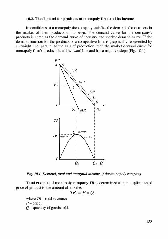
133

10.2. The demand for products of monopoly firm and its income

In conditions of a monopoly the company satisfies the demand of consumers in the market of their products on its own. The demand curve for the company's products is same as the demand curve of industry and market demand curve. If the demand function for the products of a competitive firm is graphically represented by a straight line, parallel to the axis of production, then the market demand curve for monopoly firm’s products is a downward line and has a negative slope (Fig. 10.1).

Fig. 10.1. Demand, total and marginal income of the monopoly company Total revenue of monopoly company TR is determined as a multiplication of

price of product to the amount of its sales:

,QPTR ×=

where TR – total revenue; Р – price; Q – quantity of goods sold.

P

Pc C

C MR=0

MR< 0 MR> 0

MR

0Qc

Qc

B

D

Q

TRc

QB

A

Ed=1

Ed>1

Ed<1

0

QB

TR

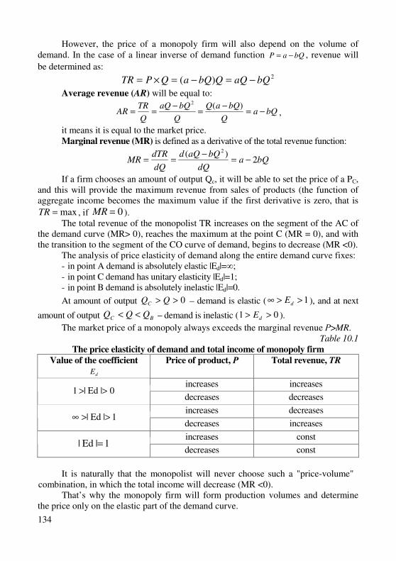
134

However, the price of a monopoly firm will also depend on the volume of demand. In the case of a linear inverse of demand function bQaP −= , revenue will

be determined as: 2)( bQaQQbQaQPTR −=−=×=

Average revenue (AR) will be equal to:

bQaQ

bQaQ

Q

bQaQ

Q

TRAR −=

−=

−==

)(2

,

it means it is equal to the market price. Marginal revenue (MR) is defined as a derivative of the total revenue function:

bQadQ

bQaQd

dQ

dTRMR 2

)( 2

−=−

==

If a firm chooses an amount of output Qc, it will be able to set the price of a PC, and this will provide the maximum revenue from sales of products (the function of aggregate income becomes the maximum value if the first derivative is zero, that is

max=TR , if 0=MR ). The total revenue of the monopolist TR increases on the segment of the AC of

the demand curve (MR> 0), reaches the maximum at the point C (MR = 0), and with the transition to the segment of the CO curve of demand, begins to decrease (MR <0).

The analysis of price elasticity of demand along the entire demand curve fixes: - in point A demand is absolutely elastic |Ed|=∞; - in point C demand has unitary elasticity |Ed|=1; - in point B demand is absolutely inelastic |Ed|=0.

At amount of output 0>> QQC – demand is elastic ( 1>>∞ dE ), and at next

amount of output BC QQQ << – demand is inelastic ( 01 >> dE ).

The market price of a monopoly always exceeds the marginal revenue Р>MR. Table 10.1

The price elasticity of demand and total income of monopoly firm

Value of the coefficient

dE Price of product, Р Total revenue, TR

increases increases 0|Ed|1 >>

decreases decreases

increases decreases 1|Ed| >>∞

decreases increases

increases сonst 1|Ed| =

decreases сonst

It is naturally that the monopolist will never choose such a "price-volume"

combination, in which the total income will decrease (MR <0). That’s why the monopoly firm will form production volumes and determine

the price only on the elastic part of the demand curve.

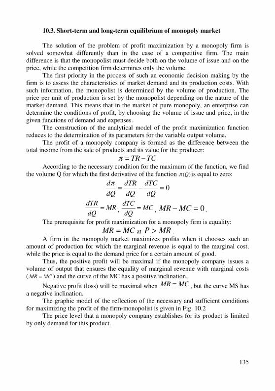
135

10.3. Short-term and long-term equilibrium of monopoly market

The solution of the problem of profit maximization by a monopoly firm is solved somewhat differently than in the case of a competitive firm. The main difference is that the monopolist must decide both on the volume of issue and on the price, while the competition firm determines only the volume.

The first priority in the process of such an economic decision making by the firm is to assess the characteristics of market demand and its production costs. With such information, the monopolist is determined by the volume of production. The price per unit of production is set by the monopolist depending on the nature of the market demand. This means that in the market of pure monopoly, an enterprise can determine the conditions of profit, by choosing the volume of issue and price, in the given functions of demand and expenses.

The construction of the analytical model of the profit maximization function reduces to the determination of its parameters for the variable output volume.

The profit of a monopoly company is formed as the difference between the total income from the sale of products and its value for the producer:

TCTR −=π According to the necessary condition for the maximum of the function, we find

the volume Q for which the first derivative of the function )(Qπ is equal to zero:

0=−=dQ

dTC

dQ

dTR

dQ

dπ

MRdQ

dTR= , MC

dQ

dTC= , 0=− MCMR .

The prerequisite for profit maximization for a monopoly firm is equality:

MCMR = at MRP > . A firm in the monopoly market maximizes profits when it chooses such an

amount of production for which the marginal revenue is equal to the marginal cost, while the price is equal to the demand price for a certain amount of good.

Thus, the positive profit will be maximal if the monopoly company issues a volume of output that ensures the equality of marginal revenue with marginal costs ( MCMR = ) and the curve of the MC has a positive inclination.

Negative profit (loss) will be maximal when MCMR = , but the curve MS has a negative inclination.

The graphic model of the reflection of the necessary and sufficient conditions for maximizing the profit of the firm-monopolist is given in Fig. 10.2

The price level that a monopoly company establishes for its product is limited by only demand for this product.

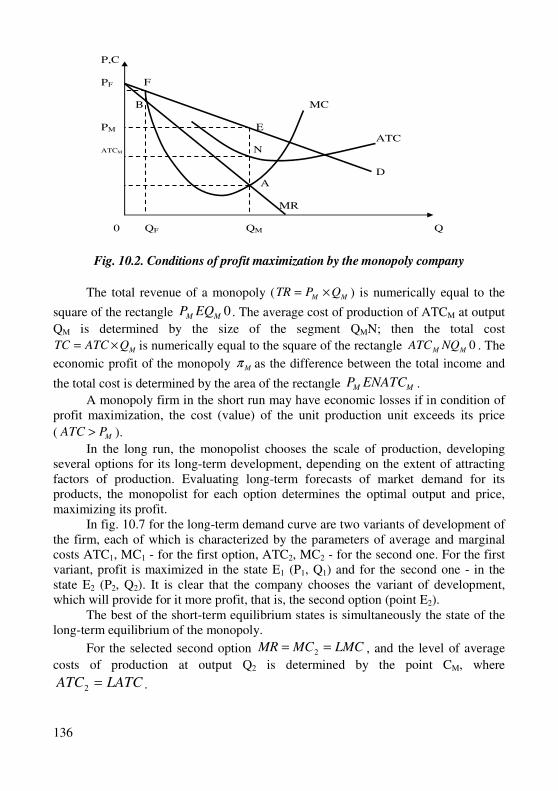
136

P,C PF F B MC PM E ATC ATCM N D A MR 0 QF QM Q

Fig. 10.2. Conditions of profit maximization by the monopoly company

The total revenue of a monopoly ( MM QPTR ×= ) is numerically equal to the

square of the rectangle 0MM EQP . The average cost of production of ATCM at output

QM is determined by the size of the segment QMN; then the total cost

MQATCTC ×= is numerically equal to the square of the rectangle 0MM NQATC . The

economic profit of the monopoly Mπ as the difference between the total income and

the total cost is determined by the area of the rectangle MM ENATCP .

A monopoly firm in the short run may have economic losses if in condition of profit maximization, the cost (value) of the unit production unit exceeds its price

( MPATC > ).

In the long run, the monopolist chooses the scale of production, developing several options for its long-term development, depending on the extent of attracting factors of production. Evaluating long-term forecasts of market demand for its products, the monopolist for each option determines the optimal output and price, maximizing its profit.

In fig. 10.7 for the long-term demand curve are two variants of development of the firm, each of which is characterized by the parameters of average and marginal costs ATC1, MC1 - for the first option, ATC2, MC2 - for the second one. For the first variant, profit is maximized in the state E1 (P1, Q1) and for the second one - in the state E2 (P2, Q2). It is clear that the company chooses the variant of development, which will provide for it more profit, that is, the second option (point E2).

The best of the short-term equilibrium states is simultaneously the state of the long-term equilibrium of the monopoly.

For the selected second option LMCMCMR == 2 , and the level of average

costs of production at output Q2 is determined by the point CM, where

LATCATC =2 .

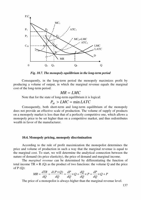
137

Fig. 10.7. The monopoly equilibrium in the long-term period

Consequently, in the long-term period the monopoly maximizes profit by producing a volume of output, in which the marginal revenue equals the marginal cost of the long-term period:

LMCMR = Note that for the state of long-term equilibrium it is logical:

LATCLMCPM min=>

Consequently, both short-term and long-term equilibrium of the monopoly does not provide an effective scale of production. The volume of supply of products on a monopoly market is less than that of a perfectly competitive one, which allows a monopoly price to be set higher than on a competitive market, and thus redistributes wealth in favor of the manufacturer.

10.4. Monopoly pricing, monopoly discrimination

According to the rule of profit maximization the monopolist determines the price and volume of production in such a way that the marginal revenue is equal to the marginal cost. To start, we will determine the analytical connection between the nature of demand (its price elasticity), the price of demand and marginal income.

The marginal revenue can be determined by differentiating the function of total income TR = R (Q) as the product of two functions: the volume Q and the price of P (Q):

PQdQ

dPP

dQ

dQQ

dQ

dP

dQ

QPd

dQ

dTRMR +×=×+×=

×==

)(

The price of a monopolist is always higher than the marginal revenue level.

P,C

MC1

P1 E1 ATC1 C

P2 E2 B MC2=LMC

ATC2 СМ A C LMC

LAТC B F

D MR

0 Q1 Q2 QF Q

138

As practice shows, monopoly uses the principle of pricing "cost plus" - that is, the price is set at the level of marginal costs plus a certain increase.

In order to generate additional income by monopoly, it is widely used by price discrimination – when seller establishes different price levels for different consumers. At the same time, there is no any difference in production cost. Just the price is different.

Price discrimination is possible under the following conditions:

− the firm has a sufficient level of market power to control the production of the product and the formation of its price;

− consumers have no desire and conditions to resell the purchased products to other buyers;

− possible segmentation of the market - the division of consumers into separate groups according to their willingness to pay (for example, by age, social status, income level, etc.).

The concept of price discrimination was introduced into the economic theory by Alfred Pigou, a British economist in the first third of the XX century. He proposed to distinguish between three types or degrees of price discrimination.

Discrimination of the first degree, or absolute price discrimination, is carried out by the monopolist by setting a price for each consumer at the level of his readiness to pay for this benefit.

The phenomenon of price discrimination of the 1st degree in practice is rare and is rather a theoretical model.

More often, the monopolist uses the second type of price discrimination - selling at different prices of individual batches of goods. It is also known as a case of non-linear pricing, since it means that the price per unit of a product is not constant, but depends on sales volumes.

Price discrimination of the second degree is carried out in the form of: � wholesale discounts (the bigger the lot, the lower the price per unit of the

product); � cumulative discounts (monthly cards for travel in public transport); � price discrimination in time (different prices for daytime and evening

sessions in cinema); � a subscription fee in combination with a proportional payment for the

amount of goods purchased. Third-degree price discrimination is established in case of allocating certain

categories of consumers with varying demand elasticity, it means market segmentation.

This most widespread version of price discrimination is as follows:

� pricing in “hot” periods (fixing the highest prices during periods of high demand);

� intermittent discrimination (setting a high price for impatient buyers, and gradually reducing prices for others);

� introduction of different tariffs; � sale of goods in the set;

139

� differentiation of the cost of transport services, depending on the quality of service and comfort (business class and economy class, cars of grades 1 and 2);

� different prices for non-food products of seasonal demand (at the end of the season, prices are lower than at the beginning).

Having considered the various types of price discrimination, it is impossible to give an unequivocal answer, whether it is desirable for society. On the one hand, a differentiated approach to monopoly pricing allows a company to increase the volume of monopoly profits at the expense of revenues of the buyer, leading to their redistribution in favor of the one who conducts it. But, on the other hand, price discrimination leads to an increase in output and, consequently, it leads to lower net costs and a higher efficiency of resource allocation. In addition, price discrimination of the 3rd degree allows serve different price-elastic markets in which the producer does not reach the same price.

10.5. Economic consequences of the market monopolization.

Necessity and methods of antitrust regulation

To analyze the state of monopolization of the market, the indicator of price influence is used - the value of exceeding the price of the monopolist over its marginal costs. This approach for measuring of the monopoly power of the company was proposed by Abba Lerner in 1934.

The coefficient of Lerner's monopoly power is calculated by the formula:

M

KM

P

PPL

−= ,

where, РМ – price of product established by monopoly firm (monopoly price); РК – price of competitive product. As in a competitive market the price of a product is equal to the marginal cost,

you can write:

M

M

P

MCPL

−=

Indicator values can range from 0 to 1. Note that for a competitively perfect company this indicator is zero. The value of the indicator is closer to one, the higher the cost increase when establishing a monopoly price.

The situation when only a few companies capture most of the market is called market concentration.

The market concentration can be measured by following indicators: а) coefficient of concentration; b) Herfindahl-Hirschman index. The concentration coefficient is defined as the sum of market shares of n

largest sellers.

140

∑=

=n

i

in SCR1

,

where, CRn – coefficient of concentration of n-sellers,%; Si – the share of sales of the seller in the volume of sales of the market,%; n – number of firms at the market

This indicator allows compare the levels of concentration of different industries, analyze their dynamics, establish at the expense of which enterprises (large, medium, small) will be a rearrangement of market power.

The share of different enterprises is calculated in different countries. In the USA and France there is a share of 4, 8, 20, 50, 100 of largest companies, in Germany – 3, 6, 10 enterprises. Moreover, in most developed countries, the concentration factor is necessary for statistical monitoring of market conditions. The State Statistics Committee of Ukraine does not expect such an indicator, although it is important in the development of anti-monopoly policies.

The Herfindahl-Hirschman index is calculated by the formula:

22

3

2

2

1

2

1

2 ... n

n

i

i SSSSSHHI ++++==∑=

,

where n – number of firms at the market; Si – marker share of i-th enterprise, %. If the industry is represented by only one firm (the situation of a monopoly)

then the index has a maximum value 10000. The value of the index decreases with the increase in the number of firms and increases with increasing inequality between firms in any of their number.

There are three levels of concentration according to the meaning of the Herfindahl-Hirschman index;

- highly concentrated type of market – 2000 < HHI < 10000; - moderately concentrated type of market – 1000 < HHI < 2000; - low concentrated type of market – HHI < 1000. The specified parameters are not official but serve as indicative indicators of

the level of market concentration for the analysis of the consequences of merger and acquisition processes in order to make decisions on the permission of such processes.

Existence of a monopoly leads to economic costs of society, since no production efficiency is ensured (for the optimal output price exceeds the minimum average total costs), nor distribution efficiency (price exceeds the marginal cost).

Only monopolies can be an exception. Their occurrence is a logical consequence of the interaction of market forces, since they provide a minimization of costs due to the positive effect of scale. To reduce the negative manifestations of monopoly power, the state can promote the transformation of monopolized industries into more competitive, transform private monopolies into state or regulate the activities of a monopoly.

Let’s consider what kind of consequences may be because of the monopoly.

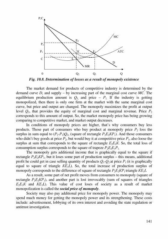
141

P,C C МС E2 Р2 Р1 К Е1 АТС С L D MR 0 Q2 Q1 Q

Fig. 10.8. Determination of losses as a result of monopoly existence

The market demand for products of competitive industry is determined by the

demand curve D, and supply – by increasing part of the marginal cost curve MC. The equilibrium production amount is Q1, and price – Р1. If the industry is getting monopolized, then there is only one firm at the market with the same marginal cost curve, but price and output are changed. The monopoly maximizes the profit at output level Q2, that provides the equity of marginal cost and marginal revenue. Price Р2

corresponds to this amount of output. So, the market monopoly price has being growing comparing to competitive market, and market output decreases.

In conditions of monopoly prices are higher, that’s why consumers buy less products. Those part of consumers who buy product at monopoly price Р2 loss the surplus in sum equal to (Р2-Р1)Q2, (square of rectangle Р2Е2КР1). And those consumers who didn’t buy goods at price Р2, but would buy it at competitive price Р1, also loose the surplus at sum that corresponds to the square of rectangle Е2Е1К. So, the total loss of consumption surplus corresponds to the square of trapeze Р2Е2Е1Р1.

The monopoly gets additional income that is graphically equal to the square if rectangle Р2Е2КР1, but it loses some part of production surplus – this means, additional profit he could get in case selling quantity of products Q1-Q2 at price Р1 (it is graphically equal to square of triangle КЕ1L). So, the total increase of production surplus of monopoly corresponds to the difference of square of rectangle Р2Е2КР1 triangle КЕ1L

As a result, some part of net profit moves from consumers to monopoly (square of rectangle Р2Е2КР1), and another part is lost irrevocably (sum of squares of triangles Е2Е1К and КЕ1L). This value of cost loses of society as a result of market monopolization is called the social price of monopoly.

Society may also pay additional price for monopoly power. The monopoly may spend much money for getting the monopoly power and its strengthening. These costs include: advertisement, lobbying of its own interest and avoiding the state regulation or antitrust investigation.

142

The monopoly is not interested in the amount of output maximization, but it wants to maximize profit. The absence of competitors weakens its incentives for innovations.

The existence of monopoly leads to economic costs of society, as not productive

(price exceeds minimal average total costs) neither distributive effectiveness (price

exceeds marginal costs) is provided. The exception of the rule may be natural monopolies. Their appearance is a

consequent of interaction of market power as they provide cost minimization according to positive effect of scale. In order to weaken negative features of monopoly power the state may transform monopoly industries into more competitive ones, private monopolies into state ones or to regulate the activity of monopoly.

In order to prevent the abuse of monopolies and increase the efficiency of the market functioning all countries use the antitrust legislation, the first antitrust law was adopted in USA in 1890 (Sherman’s law). According to the legislation of countries with developed economy it is used to consider a monopoly as a firm the market share of which is 60 % (in USA), 33 % (in Germany), 50 % (in Japan).

Training

Key terms and concepts Absolute price discrimination. Anti-trust policy. Open monopoly. The power

monopoly. Closed monopoly. The Herfindahl-Hirschman Index. The Lerner Index.

Concentration factor. Intertemporal price discrimination. Monopolist. Monopoly.

Monopsony.

Incomplete (imperfect) competition. Natural monopoly. Market power. Market

segmentation. Social monopoly price. Price discrimination. Price. discrimination of

the second degree. Price discrimination of the third degree. Net monopoly.

Questions and tasks for students’ self-control: 1. What are the main features of the monopoly market? 2. Prove that the marginal revenue curve of the monopoly is situated below its

demand curve. Why is the marginal revenue curve getting far from the demand curve when it moves down?

3. What is the difference between the monopolist’s demand curve and the firm’s demand curve at the competitive market? Why can’t the monopolist’s demand curve be absolutely elastic?

4. Will the firm-monopolist always get a profit? What is the reason of that? 5. What is the connection between price demand elasticity of product of the

firm-monopolist and its marginal income? 6. Why can’t we build the supply curve of firm-monopolist? 7. What does the monopolist’s equilibrium in the long-term period mean? 8. What is the essence of the price discrimination? What types of price

discrimination do you know? Why the price discrimination is inherent to monopoly market and is profitable for society?

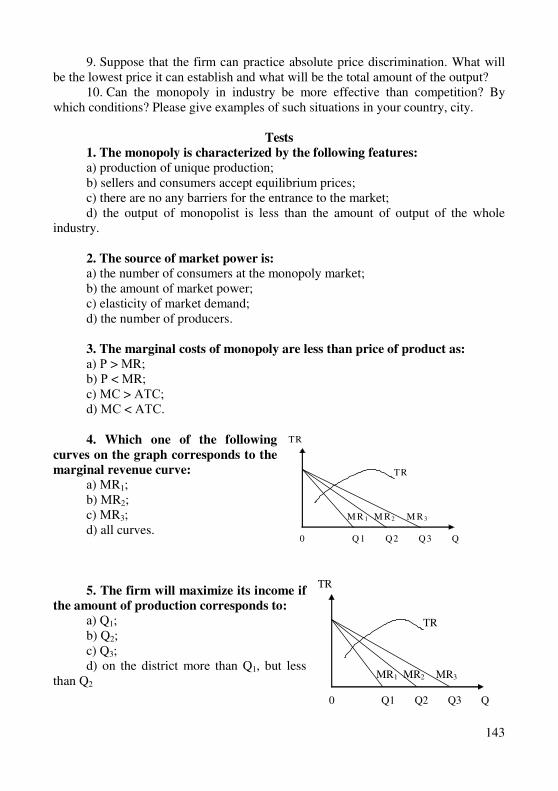
143

9. Suppose that the firm can practice absolute price discrimination. What will be the lowest price it can establish and what will be the total amount of the output?

10. Can the monopoly in industry be more effective than competition? By which conditions? Please give examples of such situations in your country, city.

Tests

1. The monopoly is characterized by the following features:

а) production of unique production; b) sellers and consumers accept equilibrium prices; c) there are no any barriers for the entrance to the market; d) the output of monopolist is less than the amount of output of the whole

industry. 2. The source of market power is:

а) the number of consumers at the monopoly market; b) the amount of market power; c) elasticity of market demand; d) the number of producers.

3. The marginal costs of monopoly are less than price of product as:

а) Р > МR; b) Р < МR; c) МС > АТС; d) МС < АТС.

4. Which one of the following

curves on the graph corresponds to the

marginal revenue curve:

а) МR1; b) МR2; c) МR3; d) all curves.

5. The firm will maximize its income if

the amount of production corresponds to:

а) Q1; b) Q2; c) Q3; d) on the district more than Q1, but less

than Q2

TR TR M R 1 M R2 M R3 0 Q 1 Q2 Q 3 Q

TR TR MR1 MR2 MR3 0 Q1 Q2 Q3 Q

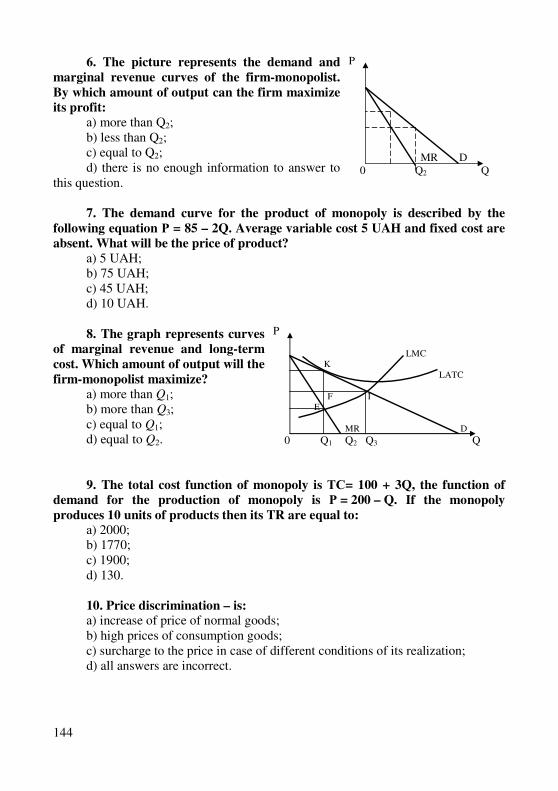
144

6. The picture represents the demand and

marginal revenue curves of the firm-monopolist.

By which amount of output can the firm maximize

its profit:

а) more than Q2; b) less than Q2; c) equal to Q2; d) there is no enough information to answer to

this question.

7. The demand curve for the product of monopoly is described by the

following equation Р = 85 – 2Q. Average variable cost 5 UAH and fixed cost are

absent. What will be the price of product?

а) 5 UAH; b) 75 UAH; c) 45 UAH; d) 10 UAH.

8. The graph represents curves

of marginal revenue and long-term

cost. Which amount of output will the

firm-monopolist maximize?

а) more than Q1; b) more than Q3; c) equal to Q1; d) equal to Q2. 9. The total cost function of monopoly is ТС= 100 + 3Q, the function of

demand for the production of monopoly is Р = 200 – Q. If the monopoly

produces 10 units of products then its TR are equal to:

а) 2000; b) 1770; c) 1900; d) 130.

10. Price discrimination – is:

а) increase of price of normal goods; b) high prices of consumption goods; c) surcharge to the price in case of different conditions of its realization; d) all answers are incorrect.

P

MR D 0 Q2 Q

P LMC K LATC F I E MR D

0 Q1 Q2 Q3 Q

145

Task 1

The cost function of monopoly is TC=50+Q2 (it means that fixed cost FC equal to 50 UAH, and variable VC – Q2).

Demand for products of monopoly is represented by the function QP −= 40 .

Find out what the amount of output will the monopolist produce to maximize its profit.

Task 2

There is information about the demand function for products of monopolist and its total cost for the production of output is given in the following table:

The amount of output Q, units Price Р, UAH Total cost TC, UAH

0 13 12

1 12 14

2 11 18 3 10 24

4 9 32 5 8 42 6 7 54

By which amounts of the output will the monopolist maximizes its profit, which price will it establish?

Task 3

The monopoly’s function of cost is TC = 20 + 8Q. The demand functions at both markets are: P1=38 – 6Q, P2=120 – 14Q.

Find out the amounts of sales and price at each of markets that maximize monopoly profit.

Task 4

The monopoly’s function of cost is TС = 16 + 9Q, and the demand function is P = 105 – 4Q.

Determine the amount of the output, price and sum of maximal profit of monopoly. How will the amount of production and the sum of maximal profit be changed if the monopoly will provide perfect price discrimination?

Task 5

The monopoly sells its product at two different markets. The demand curves at markets look like: 11 200 QP −= та 22 190 QP −=

The function of cost for production is QTC 400500 += , where 21 QQQ += .

а) What are prices and the quantity of sold goods that maximize the monopoly’s profit when it can sell the product at these markets at different prices?

b) What is total demand for product is supposed to be if the monopoly firm cannot provide price discrimination policy? What will be the price and amount of output in such conditions?

146

Theme 11 The Monopolistic Competition

11.1. Peculiarities of the monopolistic market. 11.2. The equilibrium of monopolistic manufacturer in short-run and long-run

market periods. 11.3. Non-price competition.

11.1. Peculiarities of the monopolistic market

Most of really functioning markets are characterized by the features that are

typical for industries with both perfect competition and monopoly power of producer. The market of monopolistic competition is such a intermediate market structure. The theory of monopolistic competition was discovered in 30-th of XX century by British economist Joan Robinson and American scientist E. Chemberlin.

Monopolistic competition – is a type of market where a large number of sellers compete for sale of a differentiated product.

Features of monopolistic competition: Firstly, there are quite a large number of manufacturers on the market offering

similar, but not identical products:

− there may be few tens firms acting at the market, but not thousands firms as it is in the case of the market of perfect competition;

− each producer satisfies a relatively small share of market demand; − sizes of enterprises, as a rule, are medium or small; − presence of a relatively large number of firms makes it impossible to create

secret schemes for raising prices or limiting sales volumes. Secondly, goods of each enterprise are an imperfect substitute for goods sold

by other market participants, that is, they are differentiated. Differentiation is based on both real and apparent differences. The real differences in the product are achieved at the expense of:

− quality of goods, which may have rather significant differences. Goods may differ in certain functional features, materials from which they are made, design and so on;

− deepening of after-sales service by increasing the duration of warranty service, free delivery and so on;

− place of sale of goods. This applies to goods whose need arises in a particular place: public catering facilities in a crowded place, etc.

The product's distinctive differences are supported by active advertising policies of firms, using well-known trademarks or trademarks.

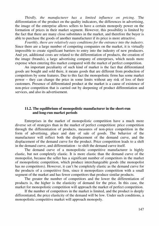
147

Thirdly, the manufacturer has a limited influence on pricing. The differentiation of the product on the quality indicators, the differences in advertising, the image of the enterprise allows sellers to have a certain monopoly power on the formation of prices in their market segment. However, this possibility is limited by the fact that there are many close substitutes in the market, and therefore the buyer is able to purchase the goods of another manufacturer if its price is more attractive.

Fourthly, there are relatively easy conditions for the entrance into the industry. Since there are a large number of competing companies on the market, it is virtually impossible to create significant barriers to entry into the industry of new producers. And yet, additional costs are related to the differentiation of products, the creation of the image (brands), a large advertising company of enterprises, which needs more expense when entering this market compared with the market of perfect competition.

An important peculiarity of such kind of market is the fact that differentiated goods are bought and sold there, it means goods that are different from production of competitors by some features. Due to this fact the monopolistic firms has some market power – they can change the price in some limits without any risk of loss of their customers. Presence of differentiated product at the market is a cause of existence of non-price competition that is carried out by deepening of product differentiation and services, and also its advertisement.

11.2. The equilibrium of monopolistic manufacturer in the short-run

and long-run market periods Enterprises in the market of monopolistic competition have a much more

diverse set of strategies than in the market of perfect competition: price competition through the differentiation of products, measures of non-price competition in the form of advertising, place and date of sale of goods. The behavior of the manufacturer will reflect both the displacement of the demand curve, and the displacement of the demand curve for the product. Price competition leads to a shift in the demand curve, and differentiation - to shift the demand curve itself.

The demand curve of a monopolistic competitive manufacturer is highly elastic, but not completely elastic. It is more elastic than the demand curve of the monopolist, because the seller has a significant number of competitors in the market of monopolistic competition, which produce interchangeable goods (the monopolist has no competitors). However, it can’t be completely elastic as the demand curve for the products of a competitive firm, since it monopolizes competition with a small segment of the market and has fewer competitors that produce similar products.

The greater the number of competitors and the lower the differentiation of products is, the higher is the elasticity of demand for the price. In this case, the market for monopolistic competition will approach the market of perfect competition.

If the number of competitors in the market is limited, and the product is deeply differentiated, the price elasticity of the demand will be low. Under such conditions, a monopolistic competitive market will approach monopoly.

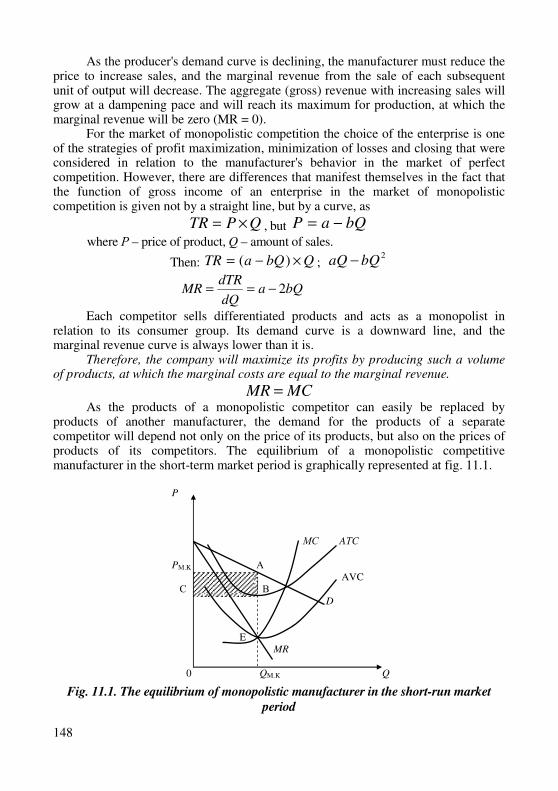
148

As the producer's demand curve is declining, the manufacturer must reduce the price to increase sales, and the marginal revenue from the sale of each subsequent unit of output will decrease. The aggregate (gross) revenue with increasing sales will grow at a dampening pace and will reach its maximum for production, at which the marginal revenue will be zero (MR = 0).

For the market of monopolistic competition the choice of the enterprise is one of the strategies of profit maximization, minimization of losses and closing that were considered in relation to the manufacturer's behavior in the market of perfect competition. However, there are differences that manifest themselves in the fact that the function of gross income of an enterprise in the market of monopolistic competition is given not by a straight line, but by a curve, as

QPTR ×= , but bQaP −=

where Р – price of product, Q – amount of sales.

Then: QbQaTR ×−= )( ; 2

bQaQ −

bQadQ

dTRMR 2−==

Each competitor sells differentiated products and acts as a monopolist in relation to its consumer group. Its demand curve is a downward line, and the marginal revenue curve is always lower than it is.

Therefore, the company will maximize its profits by producing such a volume of products, at which the marginal costs are equal to the marginal revenue.

MCMR = As the products of a monopolistic competitor can easily be replaced by

products of another manufacturer, the demand for the products of a separate competitor will depend not only on the price of its products, but also on the prices of products of its competitors. The equilibrium of a monopolistic competitive manufacturer in the short-term market period is graphically represented at fig. 11.1.

P

МС AТC

B PМ.K A AVC С В D E MR

0 QM.K Q

Fig. 11.1. The equilibrium of monopolistic manufacturer in the short-run market

period

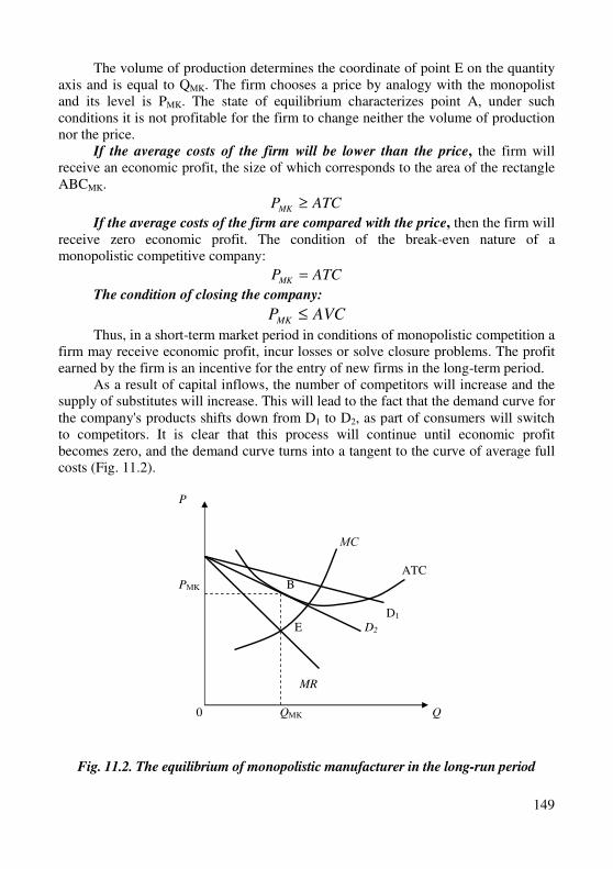
149

The volume of production determines the coordinate of point E on the quantity axis and is equal to QMK. The firm chooses a price by analogy with the monopolist and its level is PMK. The state of equilibrium characterizes point A, under such conditions it is not profitable for the firm to change neither the volume of production nor the price.

If the average costs of the firm will be lower than the price, the firm will receive an economic profit, the size of which corresponds to the area of the rectangle ABCMK.

ATCPMK ≥

If the average costs of the firm are compared with the price, then the firm will receive zero economic profit. The condition of the break-even nature of a monopolistic competitive company:

ATCPMK =

The condition of closing the company:

AVCPMK ≤

Thus, in a short-term market period in conditions of monopolistic competition a firm may receive economic profit, incur losses or solve closure problems. The profit earned by the firm is an incentive for the entry of new firms in the long-term period.

As a result of capital inflows, the number of competitors will increase and the supply of substitutes will increase. This will lead to the fact that the demand curve for the company's products shifts down from D1 to D2, as part of consumers will switch to competitors. It is clear that this process will continue until economic profit becomes zero, and the demand curve turns into a tangent to the curve of average full costs (Fig. 11.2).

P

МС ATC PМK B D1 E D2 MR

0 QMK Q

Fig. 11.2. The equilibrium of monopolistic manufacturer in the long-run period

150

If the firm receives economic losses, then the volume of production of unprofitable goods will be reduced, and the demand curve for the firm remaining in the market will shift upwards to the right until it becomes tangent to the curve of average full costs.

The company's equilibrium in the long-run period is achieved in case if the price of the product is equal to the average total cost for a certain volume of production. The firm will have zero economic profit, but it can keep in the industry the availability of normal profits:

LATCP = , MRMC = However, it should be noted that the establishment of prices at the level of

average costs and obtaining zero economic profit by the firm is only a tendency. The overflow of capital in the long-term period into a profitable segment of the market may change the company's position due to a more in-depth product differentiation or through increase of non-price competition.

11.3. Non-price competition

Monopolistic competition is widespread where there is a need for product differentiation, where it is necessary to take consumer tastes into account consumer in order to sell products successfully. Monopolistic competition is characteristic of light and food products markets, where product differentiation may involve differences in its physical characteristics and in those services that complement or accompany it. The reason of consumer’s choice can be an attractive package, a trademark, company image, provided by advertising. Perfectly homogeneous goods may be heterogeneous in view of the convenient location and time of the seller, better customer service, availability of the card, providing a discount on the price of the goods. That is, in the face of monopolistic competition, price competition goes into the background, giving way to non-price competition.

Non-price competition is provided by a number of tools, among them: advertising, terms of sale, the possibility of acquiring goods on credit, the presence or absence of guarantee and after-sales service, etc.

The most important factor of non-price competition, which makes products more expensive, is the cost of advertising. Advertising is aimed at increasing the market quota of the manufacturer in the market and on increasing consumer commitment to its differentiated product. If a perfectly competitive manufacturer does not run advertising companies because of the fact that the effect of the event will be greatly achieved by others, and that monopoly advertising is not needed because of the lack of competitors in the market, for a monopolistic competitive manufacturer, advertising is generally justified as a means of struggle for existence. Possibilities of the influence of advertising on increasing the producer's revenue reproduced in fig. 11.3.

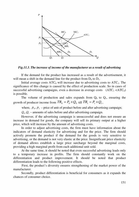
151

P

B MC0 МC1 ATC1 P1 P0 ATC0 MR1 MR0 D0 D1

Q0 Q1 Q

Fig.11.3. The increase of income of the manufacturer as a result of advertising

If the demand for the product has increased as a result of the advertisement, it

will mean a shift in the demand line for the product from D0 to D1. Initial average costs ATC0 will increase due to advertising costs to ATC1. The

significance of this change is caused by the effect of production scale. So in cases of successful advertising campaigns, even a decrease in average costs (ATC1 <ATC0) is possible.

The volume of production and sales expands from Q0 to Q1, ensuring the

growth of producer income from 000 QPTR ×= till 111 QPTR ×= ,

where, 10 , pp – price of unit of product before and after advertising campaign;

10 ,QQ – amounts of sales before and after advertising campaign.

However, if the advertising campaign is unsuccessful and does not ensure an increase in demand for goods, the company will sell its primary output at a higher price, which will increase by the amount of advertising costs.

In order to adjust advertising costs, the firm must have information about the indicators of demand elasticity for advertising and for the price. The firm should actively promote the product if the demand for the goods is very sensitive to advertising, or the demand is not very elastic at the price. Insignificant price elasticity of demand allows establish a large price surcharge beyond the marginal costs, providing a high marginal profit from each additional unit sold.

At the same time, it should be noted that even successful advertising leads only to a temporary increase in profits. The firm should constantly work on the differentiation and product improvement. It should be noted that product differentiation leads to the following positive effects.

First, the product’s diversity ensures strengthening of the market power of the manufacturer.

Secondly, product differentiation is beneficial for consumers as it expands the chances of consumer choice.

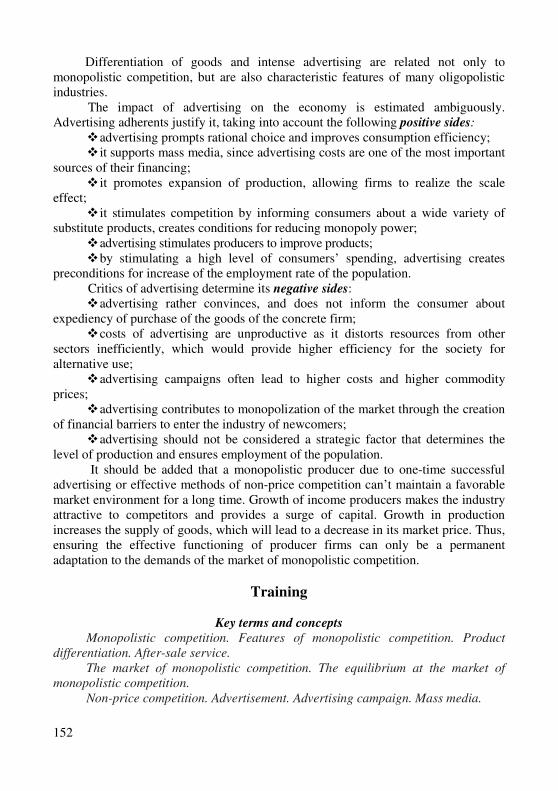
152

Differentiation of goods and intense advertising are related not only to monopolistic competition, but are also characteristic features of many oligopolistic industries.

The impact of advertising on the economy is estimated ambiguously. Advertising adherents justify it, taking into account the following positive sides:

� advertising prompts rational choice and improves consumption efficiency; � it supports mass media, since advertising costs are one of the most important

sources of their financing; � it promotes expansion of production, allowing firms to realize the scale

effect; � it stimulates competition by informing consumers about a wide variety of

substitute products, creates conditions for reducing monopoly power; � advertising stimulates producers to improve products; � by stimulating a high level of consumers’ spending, advertising creates

preconditions for increase of the employment rate of the population. Critics of advertising determine its negative sides: � advertising rather convinces, and does not inform the consumer about

expediency of purchase of the goods of the concrete firm; � costs of advertising are unproductive as it distorts resources from other

sectors inefficiently, which would provide higher efficiency for the society for alternative use;

� advertising campaigns often lead to higher costs and higher commodity prices;

� advertising contributes to monopolization of the market through the creation of financial barriers to enter the industry of newcomers;

� advertising should not be considered a strategic factor that determines the level of production and ensures employment of the population.

It should be added that a monopolistic producer due to one-time successful advertising or effective methods of non-price competition can’t maintain a favorable market environment for a long time. Growth of income producers makes the industry attractive to competitors and provides a surge of capital. Growth in production increases the supply of goods, which will lead to a decrease in its market price. Thus, ensuring the effective functioning of producer firms can only be a permanent adaptation to the demands of the market of monopolistic competition.

Training

Key terms and concepts

Monopolistic competition. Features of monopolistic competition. Product

differentiation. After-sale service.

The market of monopolistic competition. The equilibrium at the market of

monopolistic competition.

Non-price competition. Advertisement. Advertising campaign. Mass media.

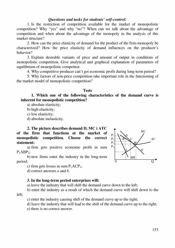
153

Questions and tasks for students’ self-control:

1. Is the restriction of competition available for the market of monopolistic competition? Why “yes” and why “no”? When can we talk about the advantage of competition and when about the advantage of the monopoly in the analysis of this market structure?

2. How can the price elasticity of demand for the product of the firm-monopoly be characterized? How the price elasticity of demand influences on the producer’s behavior?

3. Explain desirable variants of price and amount of output in conditions of monopolistic competition. Give analytical and graphical explanation of parameters of equilibrium of monopolistic competitor.

4. Why competitive producer can’t get economic profit during long-term period? 5. Why factors of non-price competition take important role in the functioning of

the market model of monopolistic competition?

Tests

1. Which one of the following characteristics of the demand curve is

inherent for monopolistic competition?

а) absolute elasticity; b) high elasticity; c) low elasticity; d) absolute inelasticity. 2. The picture describes demand D, МС і АТС

of the firm that functions at the market of

monopolistic competition. Choose the correct

statement:

а) firm gets positive economic profit in sum Р1АВР2;

b) new firms enter the industry in the long-term period;

c) firm gets losses in sum Р1АСР3; d) correct answers a and b.

3. In the long-term period enterprises will:

a) leave the industry that will shift the demand curve down to the left; b) enter the industry as a result of which the demand curve will shift down to the left; c) enter the industry causing shift of the demand curve up to the right; d) leave the industry that will lead to the shift of the demand curve up to the right; e) there is no correct answer.

MC

P1 A

P2 B C AC P3 M

P4 L D

MR 0 Q

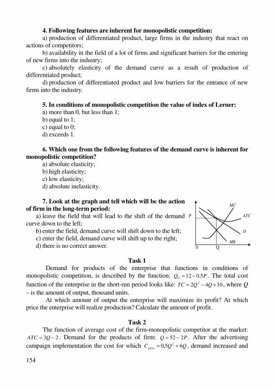
154

4. Following features are inherent for monopolistic competition:

а) production of differentiated product, large firms in the industry that react on actions of competitors;

b) availability in the field of a lot of firms and significant barriers for the entering of new firms into the industry;

c) absolutely elasticity of the demand curve as a result of production of differentiated product;

d) production of differentiated product and low barriers for the entrance of new firms into the industry.

5. In conditions of monopolistic competition the value of index of Lerner:

а) more than 0, but less than 1; b) equal to 1; c) equal to 0; d) exceeds 1.

6. Which one from the following features of the demand curve is inherent for

monopolistic competition?

а) absolute elasticity; b) high elasticity; c) low elasticity; d) absolute inelasticity.

7. Look at the graph and tell which will be the action

of firm in the long-term period:

а) leave the field that will lead to the shift of the demand curve down to the left; b) enter the field, demand curve will shift down to the left; c) enter the field, demand curve will shift up to the right; d) there is no correct answer.

Task 1 Demand for products of the enterprise that functions in conditions of

monopolistic competition, is described by the function: PQd 5,012 −= . The total cost

function of the enterprise in the short-run period looks like: 1042 2 +−= QQTC , where Q

– is the amount of output, thousand units. At which amount of output the enterprise will maximize its profit? At which

price the enterprise will realize production? Calculate the amount of profit.

Task 2

The function of average cost of the firm-monopolistic competitor at the market: 23 −= QATC . Demand for the products of firm: PQ 252 −= . After the advertising

campaign implementation the cost for which QQC рекл 65,0 2 += , demand increased and

MC

P ATC D

MR 0 Q

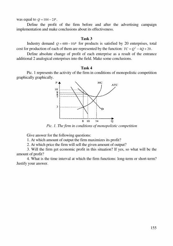
155

was equal to PQ 2104 −= .

Define the profit of the firm before and after the advertising campaign implementation and make conclusions about its effectiveness.

Task 3

Industry demand PQ 10600 −= for products is satisfied by 20 enterprises, total

cost for production of each of them are represented by the function: 2042 +−= QQTC .

Define absolute change of profit of each enterprise as a result of the entrance additional 2 analogical enterprises into the field. Make some conclusions.

Task 4

Pic. 1 represents the activity of the firm in conditions of monopolistic competition graphically graphically.

Рic. 1. The firm in conditions of monopolistic competition

Give answer for the following questions: 1. At which amount of output the firm maximizes its profit? 2. At which price the firm will sell the given amount of output? 3. Will the firm get economic profit in this situation? If yes, so what will be the

amount of profit? 4. What is the time interval at which the firm functions: long-term or short-term?

Justify your answer.

156

Theme 12 The Oligopoly

12.1. The oligopoly features.

12.2. Models of uncooperated oligopoly: models of the quantitative oligopoly

of Cournot and Stackelberg and the model of the Bertrand price oligopoly.

12.3. The model "broken demand curve".

12.4. Models of cooperative oligopolies: a model of a cartel and a model of a

dominant firm.

12.5. Game theory.

12.1. The oligopoly features

The oligopolistic market structure occupies an intermediate position between monopoly and monopolistic competition and is the prevailing form of modern market structures.

The term "oligopoly" comes from the Greek words "oligos" – several and "poleo" – I sell. There is no clearly defined number of producers in the oligopolistic market. They can be two or more dozen, but in each case there is a limited number of firms that produce all or a significant part of the market volume of products. Also other signs of oligopoly not always have an unambiguous interpretation, namely:

− goods that are produced by oligopolies can be standardized or differentiated. If the enterprises of the industry produce standard products, the industry is called pure oligopoly (production of ferrous and non-ferrous metals, cement, fuel, explosives, etc.). If the oligopoly produces a heterogeneous, but one functional product, the industry is called differentiated oligopoly (production of cars, home appliances, toothpaste, cigarettes, etc.);

− the possibility of entrance of new producers into the oligopolistic industry

is substantially limited: from a completely blocked entrance (as a pure monopoly) to a completely free (as in the model of perfect competition). Significant barriers to entering the industry are associated with significant investment. Economies of scale of production (scale effect) are the most important reason for the widespread and prolonged functioning of oligopolistic structures. For example, in the oil refining industry, the least efficient plant would cost about 1 billion USD, and the manufacturer of cars in order to achieve efficient production should produce at least 300 thousand passenger cars per year. Such large investments are not available to all firms, so the objective conditions for maintaining the leading positions of automobile factories are giants. In science-intensive industries, patent protection usually works,

157

which protects the oligopoly firm from internal competition for the duration of the patent. Control over the rare sources of raw materials (world markets for petroleum products, diamonds), high advertising costs (show business, production of beverages) serve as barriers to entry into the industry of new firms;

− in the oligopolistic market as same as in case of monopolistic competition,

the unusual importance is attached to methods of non-price competition, since

price maneuvers are not always acceptable and successful;

− the main distinctive feature of the oligopolistic model is the general interdependence of participants in the oligopolistic market. This is explained by the fact that the oligopoly occurs when the number of firms participating in the market is small, so each of them, in shaping the strategy, tactics of their business behavior is compelled to take into account the possible reaction of competitors. For example, when one company announces a price change or introduces a new product to the market, competitors must decide how they will react in response. Competition in oligopoly is highly personalized. Here, every manufacturer knows that his most effective strategy depends on the strategy of competitors. The interdependence of participants in the oligopolistic market extends to all areas of competition: price, sales volumes, market segment, product differentiation, customer service, etc. Forecasting of the corresponding reaction of competitors is one of the most difficult decisions taken by participants of oligopolistic competitions. The inability to predict the opponents' response to the oligopolistic decision complicates the substantiation of the parameters of behavior (production volume and price) that maximize its profit.

− only oligopoly is characterized by price wars. They have the form of cycles

of gradual reduction of the current price level in order to crowd competitors from the oligopolistic market out. The price war continues until the firms-manufacturers have reached the level of break-even, that is, the market will be in a state of competitive equilibrium. Consumers and losers get benefits from price wars. However, price wars are fleeting and in today's conditions are rare. The competition of manufacturers often leads to agreements, explicit or secret conspiracies.

The essence of cooperation between competitors is an important factor that affects the structure of the market and determines the strategic interaction of its participants.

That is why there is no single, general model of oligopoly, as it is in case of a model of perfect competition or monopoly.

The models of firms’ behavior in conditions of oligopoly are quite diverse and are based on different approaches to the company's strategic behavior scenarios: a variety of ways to compete and interact with rivals.

If producers act independently of each other, then their strategy can be described by models of unopposed oligopoly.

If manufacturers make conspiracy in an explicit or secret way, they agree on their decisions on prices and supply volumes then such a strategy is represented by models of onordered oligopoly.

158

12.2. Models of unordered oligopoly: models of the quantitative

oligopoly of Cournot and Stackelberg and the model

of the Bertrand price oligopoly

Let's consider the model of an unopposed oligopoly which is based on the models of the quantitative oligopoly by Cournot and Stackelberg.

As you know, historically the first model of the relationship between the two firms in the conditions of oligopoly was discovered by French economist Antoine

Cournot in the 30's of the XIX century. He is considered to be the founder of the theory of oligopoly. The Cournot model explains how two oligopolies make a choice of production, having approximately the same economic potential and producing homogeneous products. Making decisions about the volume of production, each enterprise takes into account the response of its competitor. It is believed that both oligopolies take decisions simultaneously and independently under the condition of known market demand.

The essence of the Cournot model is in the fact that each manufacturer considers the level of production of a competitor as fixed, and then decides how much to produce in order to maximize profits.

We will conduct an analytical proof of the Cournot equilibrium. Under the function of market demand:

,bQaP −=

where Q – amount of market demand. At 21 QQQ += we get:

,)( 21 QQbaP +−=

where Q1 – amount of output of I producer; Q2 – amount of output of II producer. The profit of the first manufacturer can be defined as the difference between its

income and costs, that is:

,TR 11111 CQPQTC −=−=π

where С – costs per unit of product Substituting to the right of the equation the value of P, we obtain:

121

2

1111211 )]([ CQQbQbQaQCQQQQba −−−=−+−=π

The profit will reach the maximum when the first derivative of the function is zero:

0)[

1

121

2

11

1

1 =−−−

=dQ

CQQbQbQaQd

dQ

dπ

02 21 =−−− CbQbQa

CbQbQa =−− 212

Where it follows that in order to maximize profits, the first company should produce output Q1:

222

221

Q

b

Ca

b

CbQaQ −

−=

−−=

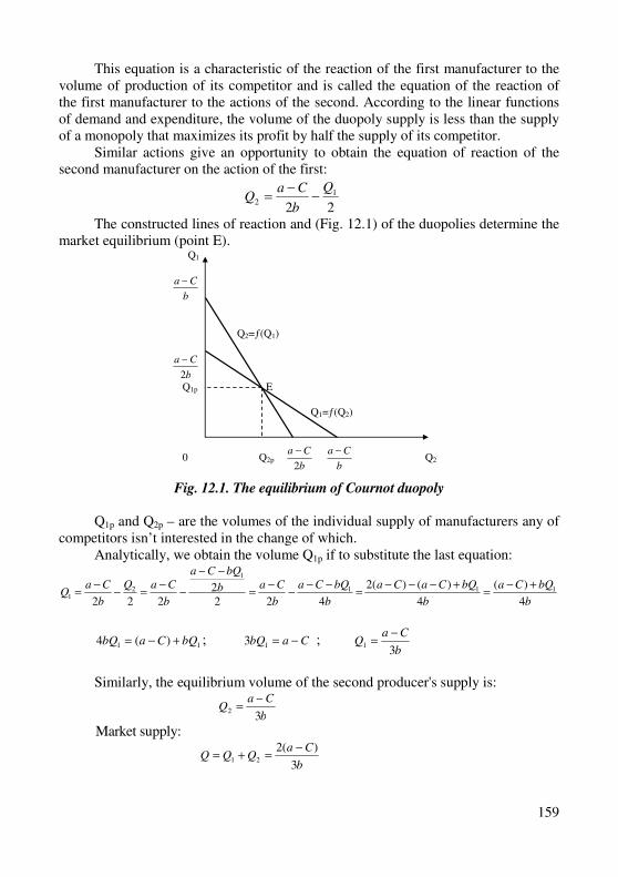
159

This equation is a characteristic of the reaction of the first manufacturer to the volume of production of its competitor and is called the equation of the reaction of the first manufacturer to the actions of the second. According to the linear functions of demand and expenditure, the volume of the duopoly supply is less than the supply of a monopoly that maximizes its profit by half the supply of its competitor.

Similar actions give an opportunity to obtain the equation of reaction of the second manufacturer on the action of the first:

221

2

Q

b

CaQ −

−=

The constructed lines of reaction and (Fig. 12.1) of the duopolies determine the market equilibrium (point E).

Q1

b

Ca −

Q2=ƒ(Q1) B

b

Ca

2

−

Q1p E Q1=ƒ(Q2)

0 Q2p b

Ca

2

−

b

Ca − Q2

Fig. 12.1. The equilibrium of Cournot duopoly

Q1p and Q2p – are the volumes of the individual supply of manufacturers any of

competitors isn’t interested in the change of which. Analytically, we obtain the volume Q1p if to substitute the last equation:

b

bQCa

b

bQCaCa

b

bQCa

b

Cab

bQCa

b

CaQ

b

CaQ

4

)(

4

)()(2

4222

222111

1

21

+−=

+−−−=

−−−

−=

−−

−−

=−−

=

11 )(4 bQCabQ +−= ; CabQ −=13 ; b

CaQ

31

−=

Similarly, the equilibrium volume of the second producer's supply is:

b

CaQ

32

−=

Market supply:

b

CaQQQ

3

)(221

−=+=

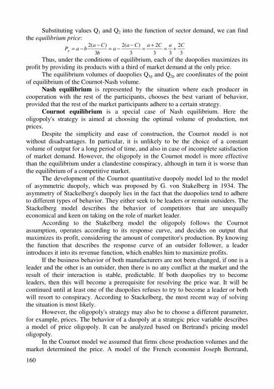
160

Substituting values Q1 and Q2 into the function of sector demand, we can find the equilibrium price:

3

2

33

2

3

)(2

3

)(2 CaCaCaa

b

CabaPp +=

+=

−−=

−−=

Thus, under the conditions of equilibrium, each of the duopolies maximizes its profit by providing its products with a third of market demand at the only price.

The equilibrium volumes of duopolies Q1p and Q2p are coordinates of the point of equilibrium of the Cournot-Nash volume.

Nash equilibrium is represented by the situation where each producer in cooperation with the rest of the participants, chooses the best variant of behavior, provided that the rest of the market participants adhere to a certain strategy.

Cournot equilibrium is a special case of Nash equilibrium. Here the oligopoly's strategy is aimed at choosing the optimal volume of production, not prices.

Despite the simplicity and ease of construction, the Cournot model is not without disadvantages. In particular, it is unlikely to be the choice of a constant volume of output for a long period of time, and also in case of incomplete satisfaction of market demand. However, the oligopoly in the Cournot model is more effective than the equilibrium under a clandestine conspiracy, although in turn it is worse than the equilibrium of a competitive market.

The development of the Cournot quantitative duopoly model led to the model of asymmetric duopoly, which was proposed by G. von Stakelberg in 1934. The asymmetry of Stackelberg's duopoly lies in the fact that the duopolies tend to adhere to different types of behavior. They either seek to be leaders or remain outsiders. The Stackelberg model describes the behavior of competitors that are unequally economical and keen on taking on the role of market leader.

According to the Stakelberg model the oligopoly follows the Cournot assumption, operates according to its response curve, and decides on output that maximizes its profit, considering the amount of competitor's production. By knowing the function that describes the response curve of an outsider follower, a leader introduces it into its revenue function, which enables him to maximize profits.

If the business behavior of both manufacturers are not been changed, if one is a leader and the other is an outsider, then there is no any conflict at the market and the result of their interaction is stable, predictable. If both duopolies try to become leaders, then this will become a prerequisite for resolving the price war. It will be continued until at least one of the duopolies refuses to try to become a leader or both will resort to conspiracy. According to Stackelberg, the most recent way of solving the situation is most likely.

However, the oligopoly's strategy may also be to choose a different parameter, for example, prices. The behavior of a duopoly at a strategic price variable describes a model of price oligopoly. It can be analyzed based on Bertrand's pricing model oligopoly.

In the Cournot model we assumed that firms chose production volumes and the market determined the price. A model of the French economist Joseph Bertrand,

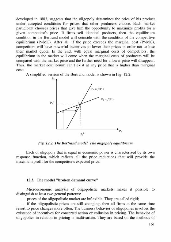
161

developed in 1883, suggests that the oligopoly determines the price of his product under accepted conditions for prices that other producers choose. Each market participant chooses prices that give him the opportunity to maximize profits for a given competitor's price. If firms sell identical products, then the equilibrium condition in the Bertrand model will coincide with the condition of the competitive equilibrium (P=MC). After all, if the price exceeds the marginal cost (P>MC), competitors will have powerful incentives to lower their prices in order not to lose their market quota. In the end, with equal marginal costs of competitors, the equilibrium in the market will come when the marginal costs of producers will be compared with the market price and the further need for a lower price will disappear. Thus, the market equilibrium can’t exist at any price that is higher than marginal costs.

A simplified version of the Bertrand model is shown in Fig. 12.2. Р2 P1 = ƒ(P2) B P2 = ƒ(P1) P2

P Е

Р1

Р1P

Fig. 12.2. The Bertrand model. The oligopoly equilibrium

Each of oligopoly that is equal in economic power is characterized by its own

response function, which reflects all the price reductions that will provide the maximum profit for the competitor's expected price.

12.3. The model "broken demand curve"

Microeconomic analysis of oligopolistic markets makes it possible to distinguish at least two general patterns:

− prices of the oligopolistic market are inflexible. They are called rigid;

− if the oligopolistic prices are still changing, then all firms at the same time resort to price changes more often. The business behavior of oligopolies involves the existence of incentives for concerted action or collusion in pricing. The behavior of oligopolies in relation to pricing is multivariate. They are based on the methods of

162

secret transactions, leadership in prices, pricing by the principle of cost plus. For example, such a variant of the pricing policy, based on the model of the broken demand curve for goods in the cell of the oligopolistic market, is also used.

The model of a broken demand curve explains the relative inflexibility of prices for oligopoly products in case of change of marginal costs. The model was offered by British economists R. Hall with K. Kitsch and American Paul Souzy independently of each other in 1939.

The main assumption of the model is the different reaction of competitors to increase and decrease the price of a separate firm. If the firms do not resort to illegal, secret deals, then the competitor's reaction to the price change is as follows: if the oligopoly company raises the price, the competitor will leave this action unattended and the oligopoly will rapidly lose it’s buyers (demand curve D1 will be elastic (Fig. 12.3)).

When the oligopoly company lowers the price for his product, then the competitor, imitating his actions, in order not to lose market shares, will also reduce the price of goods (the D2 curve will be less elastic).

P, MС,

MR

MC1 MC2 В D1B Е PЕ MR1 A K MR2 D2 F

QE Q

Fig. 12.3. Broken demand curve for products of oligopoly firm

The combined demand curve has the form of a broken line consisting of two segments of BE and EF with a break in point E. If QE sales volumes are reached, then the marginal income curve will have a vertical gap AK and will consist of two segments MC1 (for Q <QE) and MC2 (for Q> QE). Change of marginal cost in the range from MC1 to MC2 does not lead to either a change in the volume of QE, or to a change in price PE.

However, it should be taken into account that the model of the broken demand curve explains only the general pricing principle, but does not allow determine the initial price level. In addition, the conclusion that oligopolies are not interested in changing prices is not always consistent with reality: the prices of the oligopolistic market have a steady tendency to increase.

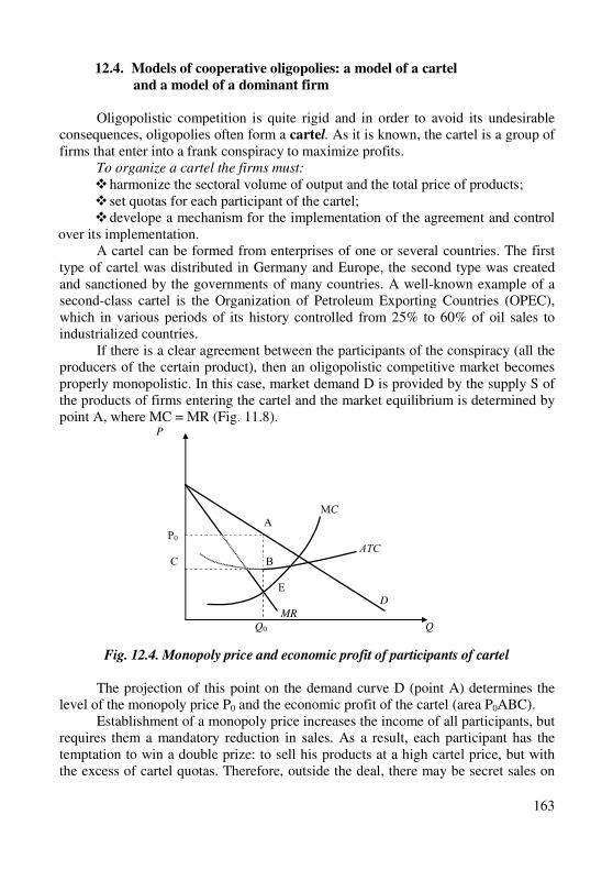
163

12.4. Models of cooperative oligopolies: a model of a cartel

and a model of a dominant firm

Oligopolistic competition is quite rigid and in order to avoid its undesirable consequences, oligopolies often form a cartel. As it is known, the cartel is a group of firms that enter into a frank conspiracy to maximize profits.

To organize a cartel the firms must: � harmonize the sectoral volume of output and the total price of products; � set quotas for each participant of the cartel; � develope a mechanism for the implementation of the agreement and control

over its implementation. A cartel can be formed from enterprises of one or several countries. The first

type of cartel was distributed in Germany and Europe, the second type was created and sanctioned by the governments of many countries. A well-known example of a second-class cartel is the Organization of Petroleum Exporting Countries (OPEC), which in various periods of its history controlled from 25% to 60% of oil sales to industrialized countries.

If there is a clear agreement between the participants of the conspiracy (all the producers of the certain product), then an oligopolistic competitive market becomes properly monopolistic. In this case, market demand D is provided by the supply S of the products of firms entering the cartel and the market equilibrium is determined by point A, where MC = MR (Fig. 11.8).

P

B МC А Р0 АТС

С В Е D MR

Q0 Q

Fig. 12.4. Monopoly price and economic profit of participants of cartel

The projection of this point on the demand curve D (point A) determines the

level of the monopoly price P0 and the economic profit of the cartel (area P0ABC). Establishment of a monopoly price increases the income of all participants, but

requires them a mandatory reduction in sales. As a result, each participant has the temptation to win a double prize: to sell his products at a high cartel price, but with the excess of cartel quotas. Therefore, outside the deal, there may be secret sales on

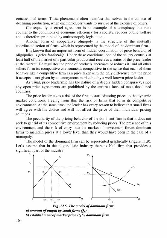
164

concessional terms. These phenomena often manifest themselves in the context of declining production, when each producer wants to survive at the expense of others.

Consequently, a cartel agreement is an example of a conspiracy that runs counter to the conditions of economic efficiency for a society, reduces public welfare and is therefore prohibited by antimonopoly legislation.

Another form of cooperative oligopoly is the structure of the mutually coordinated action of firms, which is represented by the model of the dominant firm.

It is known that an important form of hidden coordination of price behavior of oligopolies is price leadership. Under these conditions, one of the sellers controls at least half of the market of a particular product and receives a status of the price leader at the market. He regulates the price of products, increases or reduces it, and all other sellers form its competitive environment; competitive in the sense that each of them behaves like a competitive firm as a price taker with the only difference that the price it accepts is not given by an anonymous market but by a well-known price leader.

As usual, price leadership has the nature of a deeply hidden conspiracy, since any open price agreements are prohibited by the antitrust laws of most developed countries.

The price leader takes a risk of the first to start adjusting prices to the dynamic market conditions, freeing from this the risk of firms that form its competitive environment. At the same time, the leader has every reason to believe that small firms will agree with his choice and will not affect the price of their individual pricing solutions.

The peculiarity of the pricing behavior of the dominant firm is that it does not seek to get rid of its competitive environment by reducing prices. The presence of this environment and the risk of entry into the market of newcomers forces dominant firms to maintain prices at a lower level than they would have been in the case of a monopoly.

The model of the dominant firm can be represented graphically (Figure 11.9). Let’s assume that in the oligopolistic industry there is N+1 firm that provides a significant part of the industry.

PА

SN P0 B PA B C D

0 QB QА QC Q

а)

PА

P0 МС

B PA A D0 MR0

0 QА Q

б) Fig. 12.5. The model of dominant firm:

а) amount of output by small firms QB;

b) establishment of market price PA by dominant firm.

165

The intersection of the market demand curve D and the supply curve SN from N small firms, which are the competitive environment of the dominant firm (Fig. 11.9, a), determine the price of P0 of small firms, which would offer as many products as consumers agree to buy (Q0). Fig. 11.9, b shows the demand curve for products of the firm's leader (D0) and the curve of its marginal costs (MC). At the expense of lower average costs, the dominant firm may sell at below-market prices than P0 the amount needed to meet market demand. The volume of demand that may satisfy a dominant firm is equal to the difference between the volume of market demand and the volume that is willing to offer firm-followers at such a price. The dominant company in the state of equilibrium A, when it maximizes its own profit, will offer QA volume at the price of PA. The volume of market demand for this price is QC (Fig. 11.9, a): one part of which is satisfied by the followers QB, and the second – by dominant firm – the volume (QA = QС-QV).

Consequently, the dominant firm defines the market price and its volume of production, and followers who accept the given price, establish only the volume of production. Therefore, this kind of oligopolistic pricing is called price leadership.

Naturally, that the company with the lowest average cost, formed at the expense of better management or use of the most advanced technology, longest existence in the field, can be a dominant one comparing to other firms in the industry.

The second factor contributing to the emergence of the firm-leader is the differentiation of products. Dominating can be achieved thanks to the reputation of the company as a supplier of impeccable quality products, which is largely promoted by its advertising.

12.5.Game theory

The firm in Cournot’s model do not anticipate the moves of the competition. Yet in choosing strategies in a oligopolistic market, firms can and try to guess what the opposition will do in response.

In 1944, John von Neumann and Oskar Morgenstern published a path-breaking work in which the analyzed a set of problems, or games, in which no one of them can dictate the outcome. During the last few years, game theory has become an increasingly popular firld of study and a fertile area for research. The notions of game theory have been applied to analyses of firm behavior, politics, international relations, and foreign policy. In 1944 the Nobel Prize in Economic Science was awarded jointly to three early game theorists: John F. Nash, John C. Harsanyi and Reinhard Selten of the University of Bonn.

Game theory analyses oligopolistic behavior as a complex series of strategic moves and reactive countermoves among rival firms. In game theory, firms are assumed to anticipate rival reactions.

Game theory goes something like this: in all conflict situations, and thus all games, there are decision makers (or players), rules of the game, and payoffs (or prizers).

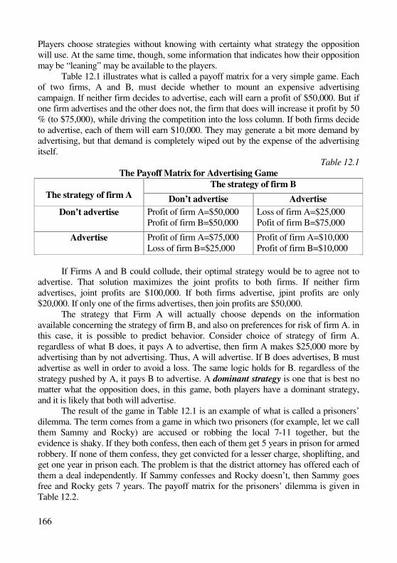
166

Players choose strategies without knowing with certainty what strategy the opposition will use. At the same time, though, some information that indicates how their opposition may be “leaning” may be available to the players.

Table 12.1 illustrates what is called a payoff matrix for a very simple game. Each of two firms, A and B, must decide whether to mount an expensive advertising campaign. If neither firm decides to advertise, each will earn a profit of $50,000. But if one firm advertises and the other does not, the firm that does will increase it profit by 50 % (to $75,000), while driving the competition into the loss column. If both firms decide to advertise, each of them will earn $10,000. They may generate a bit more demand by advertising, but that demand is completely wiped out by the expense of the advertising itself.

Table 12.1

The Payoff Matrix for Advertising Game

The strategy of firm B

The strategy of firm A Don’t advertise Advertise

Don’t advertise Profit of firm A=$50,000 Profit of firm B=$50,000

Loss of firm A=$25,000 Pofit of firm B=$75,000

Advertise Profit of firm A=$75,000 Loss of firm B=$25,000

Profit of firm A=$10,000 Profit of firm B=$10,000

If Firms A and B could collude, their optimal strategy would be to agree not to

advertise. That solution maximizes the joint profits to both firms. If neither firm advertises, joint profits are $100,000. If both firms advertise, jpint profits are only $20,000. If only one of the firms advertises, then join profits are $50,000.

The strategy that Firm A will actually choose depends on the information available concerning the strategy of firm B, and also on preferences for risk of firm A. in this case, it is possible to predict behavior. Consider choice of strategy of firm A. regardless of what B does, it pays A to advertise, then firm A makes $25,000 more by advertising than by not advertising. Thus, A will advertise. If B does advertises, B must advertise as well in order to avoid a loss. The same logic holds for B. regardless of the strategy pushed by A, it pays B to advertise. A dominant strategy is one that is best no matter what the opposition does, in this game, both players have a dominant strategy, and it is likely that both will advertise.

The result of the game in Table 12.1 is an example of what is called a prisoners’ dilemma. The term comes from a game in which two prisoners (for example, let we call them Sammy and Rocky) are accused or robbing the local 7-11 together, but the evidence is shaky. If they both confess, then each of them get 5 years in prison for armed robbery. If none of them confess, they get convicted for a lesser charge, shoplifting, and get one year in prison each. The problem is that the district attorney has offered each of them a deal independently. If Sammy confesses and Rocky doesn’t, then Sammy goes free and Rocky gets 7 years. The payoff matrix for the prisoners’ dilemma is given in Table 12.2.

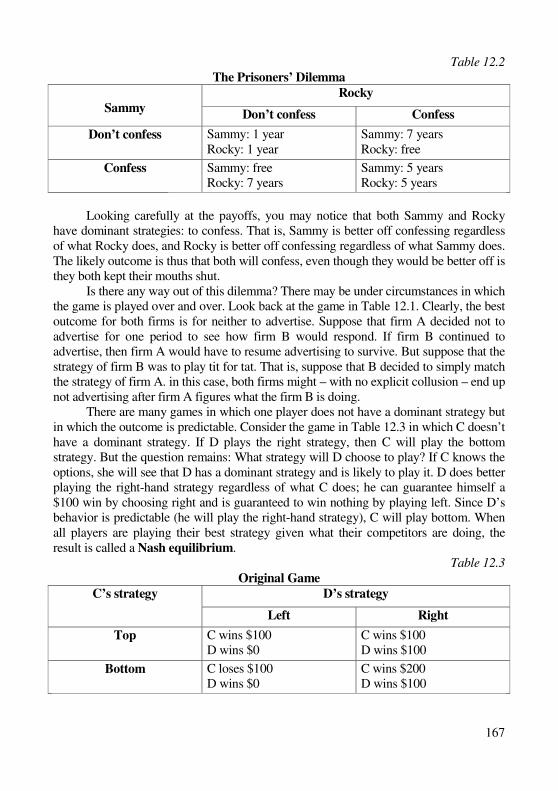
167

Table 12.2

The Prisoners’ Dilemma

Rocky

Sammy Don’t confess Confess

Don’t confess Sammy: 1 year Rocky: 1 year

Sammy: 7 years Rocky: free

Confess Sammy: free Rocky: 7 years

Sammy: 5 years Rocky: 5 years

Looking carefully at the payoffs, you may notice that both Sammy and Rocky

have dominant strategies: to confess. That is, Sammy is better off confessing regardless of what Rocky does, and Rocky is better off confessing regardless of what Sammy does. The likely outcome is thus that both will confess, even though they would be better off is they both kept their mouths shut.

Is there any way out of this dilemma? There may be under circumstances in which the game is played over and over. Look back at the game in Table 12.1. Clearly, the best outcome for both firms is for neither to advertise. Suppose that firm A decided not to advertise for one period to see how firm B would respond. If firm B continued to advertise, then firm A would have to resume advertising to survive. But suppose that the strategy of firm B was to play tit for tat. That is, suppose that B decided to simply match the strategy of firm A. in this case, both firms might – with no explicit collusion – end up not advertising after firm A figures what the firm B is doing.

There are many games in which one player does not have a dominant strategy but in which the outcome is predictable. Consider the game in Table 12.3 in which C doesn’t have a dominant strategy. If D plays the right strategy, then C will play the bottom strategy. But the question remains: What strategy will D choose to play? If C knows the options, she will see that D has a dominant strategy and is likely to play it. D does better playing the right-hand strategy regardless of what C does; he can guarantee himself a $100 win by choosing right and is guaranteed to win nothing by playing left. Since D’s behavior is predictable (he will play the right-hand strategy), C will play bottom. When all players are playing their best strategy given what their competitors are doing, the result is called a Nash equilibrium.

Table 12.3

Original Game

D’s strategy C’s strategy

Left Right

Top C wins $100 D wins $0

C wins $100 D wins $100

Bottom C loses $100 D wins $0

C wins $200 D wins $100

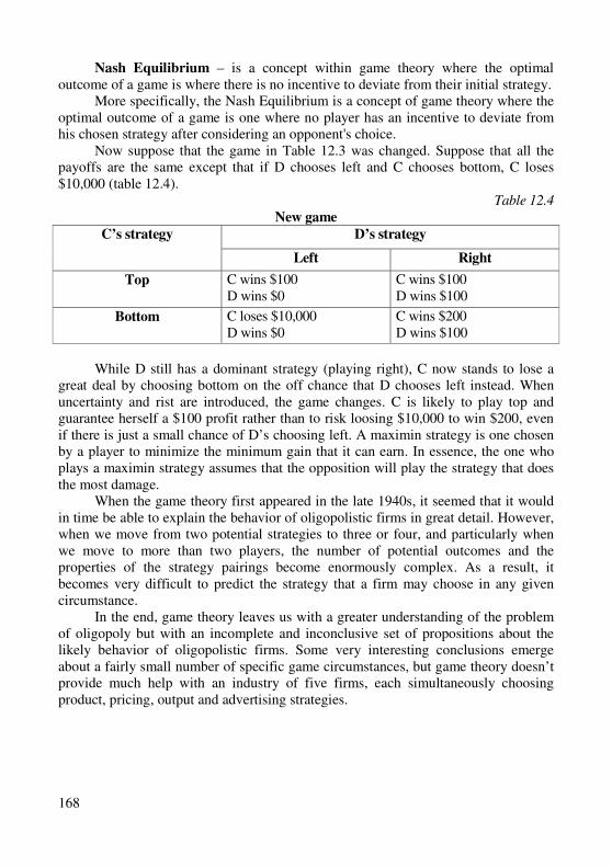
168

Nash Equilibrium – is a concept within game theory where the optimal outcome of a game is where there is no incentive to deviate from their initial strategy.

More specifically, the Nash Equilibrium is a concept of game theory where the optimal outcome of a game is one where no player has an incentive to deviate from his chosen strategy after considering an opponent's choice.

Now suppose that the game in Table 12.3 was changed. Suppose that all the payoffs are the same except that if D chooses left and C chooses bottom, C loses $10,000 (table 12.4).

Table 12.4

New game

D’s strategy C’s strategy

Left Right

Top C wins $100 D wins $0

C wins $100 D wins $100

Bottom C loses $10,000 D wins $0

C wins $200 D wins $100

While D still has a dominant strategy (playing right), C now stands to lose a

great deal by choosing bottom on the off chance that D chooses left instead. When uncertainty and rist are introduced, the game changes. C is likely to play top and guarantee herself a $100 profit rather than to risk loosing $10,000 to win $200, even if there is just a small chance of D’s choosing left. A maximin strategy is one chosen by a player to minimize the minimum gain that it can earn. In essence, the one who plays a maximin strategy assumes that the opposition will play the strategy that does the most damage.

When the game theory first appeared in the late 1940s, it seemed that it would in time be able to explain the behavior of oligopolistic firms in great detail. However, when we move from two potential strategies to three or four, and particularly when we move to more than two players, the number of potential outcomes and the properties of the strategy pairings become enormously complex. As a result, it becomes very difficult to predict the strategy that a firm may choose in any given circumstance.

In the end, game theory leaves us with a greater understanding of the problem of oligopoly but with an incomplete and inconclusive set of propositions about the likely behavior of oligopolistic firms. Some very interesting conclusions emerge about a fairly small number of specific game circumstances, but game theory doesn’t provide much help with an industry of five firms, each simultaneously choosing product, pricing, output and advertising strategies.

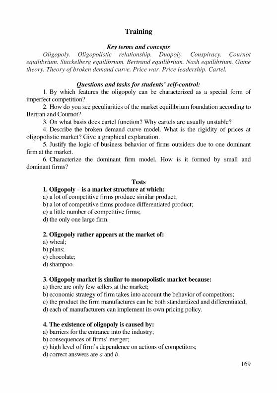
169

Training

Key terms and concepts Oligopoly. Oligopolistic relationship. Duopoly. Conspiracy. Cournot

equilibrium. Stackelberg equilibrium. Bertrand equilibrium. Nash equilibrium. Game

theory. Theory of broken demand curve. Price war. Price leadership. Cartel.

Questions and tasks for students’ self-control: 1. By which features the oligopoly can be characterized as a special form of

imperfect competition? 2. How do you see peculiarities of the market equilibrium foundation according to

Bertran and Cournot? 3. On what basis does cartel function? Why cartels are usually unstable? 4. Describe the broken demand curve model. What is the rigidity of prices at

oligopolistic market? Give a graphical explanation. 5. Justify the logic of business behavior of firms outsiders due to one dominant

firm at the market. 6. Characterize the dominant firm model. How is it formed by small and

dominant firms?

Tests

1. Oligopoly – is a market structure at which:

а) a lot of competitive firms produce similar product; b) a lot of competitive firms produce differentiated product; c) a little number of competitive firms; d) the only one large firm. 2. Oligopoly rather appears at the market of:

а) wheal; b) plans; c) chocolate; d) shampoo.

3. Oligopoly market is similar to monopolistic market because:

а) there are only few sellers at the market; b) economic strategy of firm takes into account the behavior of competitors; c) the product the firm manufactures can be both standardized and differentiated; d) each of manufacturers can implement its own pricing policy. 4. The existence of oligopoly is caused by:

а) barriers for the entrance into the industry; b) consequences of firms’ merger; c) high level of firm’s dependence on actions of competitors; d) correct answers are a and b.

170

5. Market equilibrium according to the Cournot model provides:

а) amounts of output are more that according to secret conspiracy; b) amounts of output are equal to amounts at competitive equilibrium; c) amounts of output are less than amounts at competitive equilibrium; d) amounts of output are equal to amounts at secret conspiracy. 6. «Broken» demand curve for oligopoly firm means:

а) equal demand elasticity along the whole curve; b) change of price for products at change of price for its production; c) gap of the marginal income curve; d) gap of the marginal cost curve.

7. Conspiratorial oligopoly – is an open and hidden agreement about:

а) fixation of prices; b) division of market; c) restriction of competition between firms; d) all answers are correct.

8. Under the term “pricing” was it is understood:

а) gradual decrease of current price level to average cost level with the aim to squeezing competitors out of the market;

b) gradual decrease of price to the level that will provide maximal profit; c) division of markets where own prices of realization are established; d) economic strategy of producers that provides them maximal benefits while

consumers don’t get any benefits.

Task 1

In the duopoly Cournot model there is inverse demand function Р=120 – Q. Marginal cost of both firms for goods manufacturing in conditions of constant return on the scale are same and equal 9.

Define: 1) output of each firm, of industry and market price for production of the firm,

and also profit; 2) how these indicators will be changed if to suppose that producers can make

agreement about cooperation; 3) how will be changed the parameters of equilibrium at the market in conditions

of perfect competition.

Task 2

At the oligopoly market there is a firm-leader that has the cost function

QQTC 32 += .

The function of market demand is QP −= 90 .

171

Other firms outsiders can supply 45 units of production to the market at price of leader.

Define output and price of leader.

Task 3

Transportation company “Alfa” functions in conditions of oligopoly. Find out the line of demand and marginal income of the company “Alfa” if it is

known that at the market the price is set at level Р = 17 m.u., and the amount of output Q = 15000 units.

Demand for services of the company has two areas: if price exceeds 17 m.u. then

demand is more elastic and is characterized by the function PQ 51001 −= , if price is less

than 17 m.u. then demand is less elastic and is characterized by the function

PQ 5,1402 −= .

1. Which oligopoly model given services market can belong to? Represent the model graphically.

2. If it is known that marginal cost in given conditions are changed according to

the level 8,42,002,0 2

1 +−= QQMC till 122,002,0 2

2 +−= QQMC , so what is going

to be price and amount of offered services?

Task 4

At the oligopoly market there are only two enterprises with similar marginal cost values equal to 300 UAH.

Industry demand is represented by the function PQ 5,0400 −= where Q – amount of demand, units, Р – price of one unit of products, UAH. Define the equilibrium price and amount of output of each of duopoly firms if

they act: а) according to the Cournot model; b) as participants of cartel. Due to which strategy oligopolists get the biggest profit?

172

Theme 13 The Market of Factors of Production

13.1. Factors of production, the essence and classification.

13.2. The optimal use of productive resources in the long-run market period.

13.3. Peculiarities of the labor market functioning: demand, supply and

market equilibrium.

13.4. Capital as productive resource of long-term use. Forms of capital.

13.5. Justification of investment decisions concerning the use of production

factors in long-run market period.

13.1. Factors of production, the essence and classification

Factors of production – are the main elements of the production process that

are at the disposal of the enterprise and used by them to achieve specific goals. Under the factors of production we understand all natural, financial, human and

man-made resources that are used to produce goods and services. Production resources are divided into material and human resources.

Material resources include: а) land or raw materials; b) capital as a resource of long-term use, which covers all means of labor; c) investments that are divided into productive, financial and intellectual. Industrial investments are real investment of capital in the means of labor in

order to increase the output of a particular product. Financial investments are the investment of cash in equity securities. Intelligent investments are the investment of funds in staff training, know-

how, research, etc. Human productive resources include: а) work as physical and mental abilities of a person who use in the production

of goods, except for such a resource, as entrepreneurial activity; b) entrepreneurial activity as a special ability of a person, which is associated

with the ability to effectively use own funds and organize the process of production at their own risk in order to profit.

Consequently, the market of production factors is a system of social and economic relations concerning to the sale and purchase of the most economic services provided by them.

173

The resources market, as others, regulates the factors of demand and supply. Demand of firm for resources of production has common peculiarities for all types of resources when supply of each of resource has its own peculiarities.

Demand for resources is determined by some number of production resources that are used for production output at appropriate price for it.

The law of demand is as same fare for the market of resources, as well as for the market of goods: the higher the price of resource is, the less will be demand for it. But, however, forming demand for resources has its own peculiarities.

First of all, as resources are used for production of some amount of output, it satisfies consumers’ needs indirectly, it means through production. That’s why demand for resources is called derived from demand for goods.

Derived character of the demand for resources means that demand stability for any resource depends on its productivity and market value of goods produced with the help of this resource.

If the resource is highly productive while production output that is highly evaluated by customers, then it will be of great demand from the producers’ side. If the resource is unproductive in case if the demand for goods is big enough, then demand of producers for such resource will be insufficient.

Secondly, the technological process’ regularities provide that all the resources are in constant interaction while the production process. The result of such interaction is a correlation: the quantity of necessary labor depends on the wages level. Additionally, demand for labor depends also on a price level for equipment. In this way, demand for resources depends on the price level of all types of production resources, but not only on price of one of resources.

Demand for production resources is also affected by non-price factors one of which is demand for goods produced from given resource (increase in demand for goods leads to increase in demand for resource used for production of these goods, and vice versa).

Another non-price factor is the resource productivity. As the more goods can be produced from unit of resource, the more demand for resource is, and vice versa.

Demand for resource depends also on the number of producers. The more this resource is used by producers for output production, the more great demand for it is.

One of non-price factors of resources is income level of producers-customers of production resources, as while increasing income the producer has possibility to buy this resource more, and vice versa.

The impact of price and non-price factors on the demand for resources is represented with the help of the curve of demand for resource: change of price of resource leads to change of the demand volume for resource along the demand curve, and non-price factors shifts the demand curve up-to the right in case if demand is growing, and down-to the left in case if demand decreases in conditions of price of resources immutability. The peculiarity of the demand for resource curve is that while its construction the concept of marginal income of resource is used.

Marginal return on the resource (MRPL) – is monetary expression of marginal productivity of variable production factor or growth of total revenue from

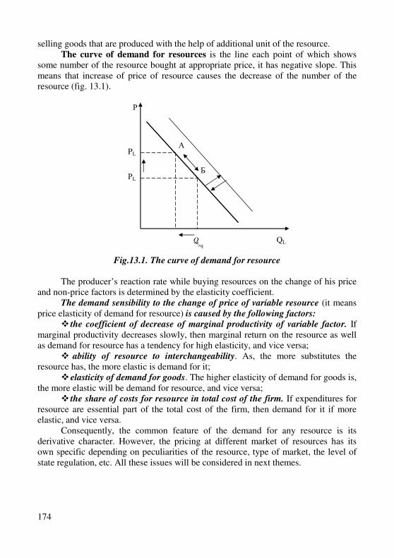
174

selling goods that are produced with the help of additional unit of the resource. The curve of demand for resources is the line each point of which shows

some number of the resource bought at appropriate price, it has negative slope. This means that increase of price of resource causes the decrease of the number of the resource (fig. 13.1).

Fig.13.1. The curve of demand for resource

The producer’s reaction rate while buying resources on the change of his price

and non-price factors is determined by the elasticity coefficient. The demand sensibility to the change of price of variable resource (it means

price elasticity of demand for resource) is caused by the following factors:

� the coefficient of decrease of marginal productivity of variable factor. If marginal productivity decreases slowly, then marginal return on the resource as well as demand for resource has a tendency for high elasticity, and vice versa;

� ability of resource to interchangeability. As, the more substitutes the resource has, the more elastic is demand for it;

� elasticity of demand for goods. The higher elasticity of demand for goods is, the more elastic will be demand for resource, and vice versa;

� the share of costs for resource in total cost of the firm. If expenditures for resource are essential part of the total cost of the firm, then demand for it if more elastic, and vice versa.

Consequently, the common feature of the demand for any resource is its derivative character. However, the pricing at different market of resources has its own specific depending on peculiarities of the resource, type of market, the level of state regulation, etc. All these issues will be considered in next themes.

Б

А

Р

QL

PL

РL

QдЙД

Q1

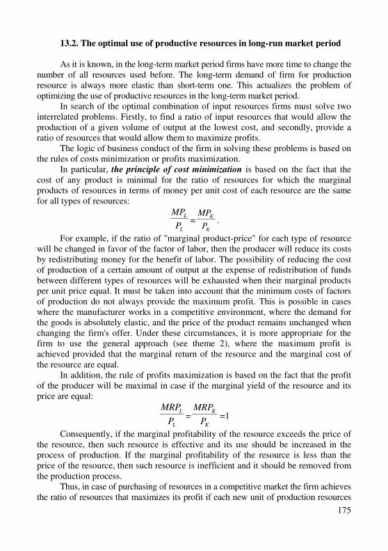
175

13.2. The optimal use of productive resources in long-run market period

As it is known, in the long-term market period firms have more time to change the number of all resources used before. The long-term demand of firm for production resource is always more elastic than short-term one. This actualizes the problem of optimizing the use of productive resources in the long-term market period.

In search of the optimal combination of input resources firms must solve two interrelated problems. Firstly, to find a ratio of input resources that would allow the production of a given volume of output at the lowest cost, and secondly, provide a ratio of resources that would allow them to maximize profits.

The logic of business conduct of the firm in solving these problems is based on the rules of costs minimization or profits maximization.

In particular, the principle of cost minimization is based on the fact that the cost of any product is minimal for the ratio of resources for which the marginal products of resources in terms of money per unit cost of each resource are the same for all types of resources:

L

L

P

MP=

K

K

P

MP.

For example, if the ratio of "marginal product-price" for each type of resource will be changed in favor of the factor of labor, then the producer will reduce its costs by redistributing money for the benefit of labor. The possibility of reducing the cost of production of a certain amount of output at the expense of redistribution of funds between different types of resources will be exhausted when their marginal products per unit price equal. It must be taken into account that the minimum costs of factors of production do not always provide the maximum profit. This is possible in cases where the manufacturer works in a competitive environment, where the demand for the goods is absolutely elastic, and the price of the product remains unchanged when changing the firm's offer. Under these circumstances, it is more appropriate for the firm to use the general approach (see theme 2), where the maximum profit is achieved provided that the marginal return of the resource and the marginal cost of the resource are equal.

In addition, the rule of profits maximization is based on the fact that the profit of the producer will be maximal in case if the marginal yield of the resource and its price are equal:

L

L

P

MRP=

K

K

P

MRP=1

Consequently, if the marginal profitability of the resource exceeds the price of the resource, then such resource is effective and its use should be increased in the process of production. If the marginal profitability of the resource is less than the price of the resource, then such resource is inefficient and it should be removed from the production process.

Thus, in case of purchasing of resources in a competitive market the firm achieves the ratio of resources that maximizes its profit if each new unit of production resources

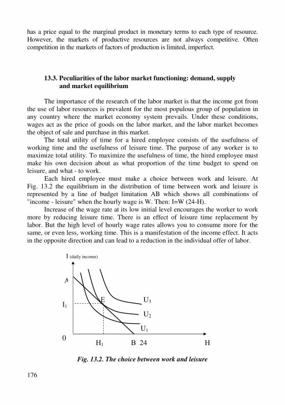
176

has a price equal to the marginal product in monetary terms to each type of resource. However, the markets of productive resources are not always competitive. Often competition in the markets of factors of production is limited, imperfect.

13.3. Peculiarities of the labor market functioning: demand, supply

and market equilibrium

The importance of the research of the labor market is that the income got from

the use of labor resources is prevalent for the most populous group of population in any country where the market economy system prevails. Under these conditions, wages act as the price of goods on the labor market, and the labor market becomes the object of sale and purchase in this market.

The total utility of time for a hired employee consists of the usefulness of working time and the usefulness of leisure time. The purpose of any worker is to maximize total utility. To maximize the usefulness of time, the hired employee must make his own decision about as what proportion of the time budget to spend on leisure, and what - to work.

Each hired employee must make a choice between work and leisure. At Fig. 13.2 the equilibrium in the distribution of time between work and leisure is represented by a line of budget limitation AB which shows all combinations of "income - leisure" when the hourly wage is W. Then: I=W (24-H).

Increase of the wage rate at its low initial level encourages the worker to work more by reducing leisure time. There is an effect of leisure time replacement by labor. But the high level of hourly wage rates allows you to consume more for the same, or even less, working time. This is a manifestation of the income effect. It acts in the opposite direction and can lead to a reduction in the individual offer of labor.

Fig. 13.2. The choice between work and leisure

Е І1

І (daily income)

Н

U3

Н1

А

0 В 24

U2

U1

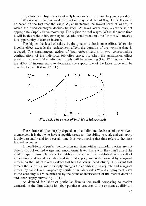
177

So, a hired employee works 24 – H1 hours and earns І1 monetary units per day. When wages rise, the worker's reaction may be different (Fig. 12.3). It should

be based on the fact that the value W0 characterizes the lowest level of wages, in which the hired employee decides to work. At level lower than W0 work is not appropriate. Supply curve moves up. The higher the real wages (W) is, the more time it will be desirable to hire employee. An additional vacation time for him will mean a lost opportunity to earn an income.

The higher the level of salary is, the greater is the income effect. When the income effect exceeds the replacement effect, the duration of the working time is reduced. The simultaneous action of both effects results in two corresponding configurations of the individual job offer curve. So, when the substitution effect prevails the curve of the individual supply will be ascending (Fig. 12.3, a), and when the effect of income starts to dominate, the supply line of the labor force will be diverted to the left (Fig. 12.3, b).

The volume of labor supply depends on the individual decisions of the workers themselves. It is they who have a specific product – the ability to work and can apply it only personally and for a certain time. It is worth noting that time refers to the most limited resources.

In conditions of perfect competition nor firm neither particular worker are not able to control existed wages and employment level, that’s why they can’t affect the market equilibrium. The market equilibrium salary rate is established as a result of interaction of demand for labor and its total supply and is determined by marginal returns on the last of hired workers that has the lowest productivity. Any event that affects the labor demand or supply changes the equilibrium salary rate and marginal returns by same level. Graphically equilibrium salary rates W and employment level in the economy L are determined by the point of intersection of the market demand and labor supply curves (fig. 13.4).

As demand for labor of particular firm is too small comparing to market demand, so the firm adapts its labor purchases amounts to the existent equilibrium

Fig. 13.3. The curves of individual labor supply

178

hourly wage rate. Same time workers make decisions on celling their working power to some firm considering the existent wage rate. Their supply curve (Sf

L) coincides with the line of equilibrium wage rate (W*).

The firms determines equilibrium amount of labor (fig. 13.4b) due to the rule of optimal use of resource MRPL=MCL and maximizes the profit: DL=SL –MRPL=W. In conditions of equilibrium salary always equals the marginal returns of the last worker.

The gain, or the firm’s revenue from hiring some members of staff, is

determined as the difference between marginal returns of all hired workers and costs for salary. This sum will correspond to the normal (average) profit of the firm.

If both markets – labor market and market of goods – are perfectly competitive ones, then the effective division of labor in society will be achieved during the process of the general market equilibrium establishment in point of equilibrium MRPL = MCL, and it will mean that marginal costs for labor factor will be equal to the value of marginal labor product. This equity can be considered as criteria of the

effectiveness of resources distribution.

13.4. Capital as productive resource of long-term use. Forms of capital

In addition to the labor, as is known, capital and land are also factors of

production. They both have a monetary form of expression. But it should be taken into account that the money itself does not belong to economic resources, although they are a means of acquiring all other capital and natural resources.

The common feature and the main feature of capital markets and land (natural resources) is that these resources are durable goods, so the firm's decision to attract them should always take into account the time factor.

Fig. 13.4. The market equilibrium and firm’s

equilibrium at the labor market

179

There are three forms of capital markets:

� market of financial capital; � market of capital assets; � market of capital services, or rental market. Securities and cash loans are sold and bought at the financial capital market.

Financial capital has value as it provides the opportunity to acquire real wealth, it means physical capital (equipment, buildings, buildings of production purpose, etc.).

An increase in the stock of physical capital is caused by investment, which is considered as a process of creating new capital at the expense of financial resources. The firm has three sources of financing of long-term investment projects:

– own money resources (retained earnings); – involved money resources (issue of shares); – borrowed money resources (corporate bonds, bank loans, etc.). The main participants in the financial capital market are firms that form the

demand for credit funds for long-term investment projects and households. They determine the volume of offer of borrowed funds at the expense of savings. The purpose of the capital market is not only to focus and provide investment resources to firms, but also to transfer money from those sectors of the economy where their surpluses exist to those where their lack is observed. The market for investment resources today is one of the few very competitive markets. Its subjects are the set of independent sellers and buyers who form the supply and demand for investment resources, respectively.

The demand for an investment resource – is the amount of investment funds that consumers are ready to purchase and at the appropriate price.

Subjects of demand are firms that seek to use the money received for the purchase of productive assets.

The supply of investment resources – is the volume of investment funds provided by their owners at a loan at the appropriate price.

Subjects of the proposal are firms that borrow money, waiting for payment for a temporary loss of liquidity in the form of a loan interest.

The cost of loan capital is a loan interest. It is defined as the amount of money that the borrower must pay for the possibility of temporarily using someone else's money. It is usually to operate with the concept of a rate or rate of interest. They are not an absolute, but a relative characteristic of the price of a loan.

As it is known, the annual interest rate (i) is calculated as the ratio of the amount of the loan interest (R) paid to the loan amount (K):

i=K

R·100

Nominal and real interest rates are distinguished. The nominal interest rate (r) – is the interest rate expressed in monetary terms

at the current monetary rate. The real interest rate (R) – is the nominal interest rate minus expected rate of

inflation. Only real interest rates are used to make investment decisions.

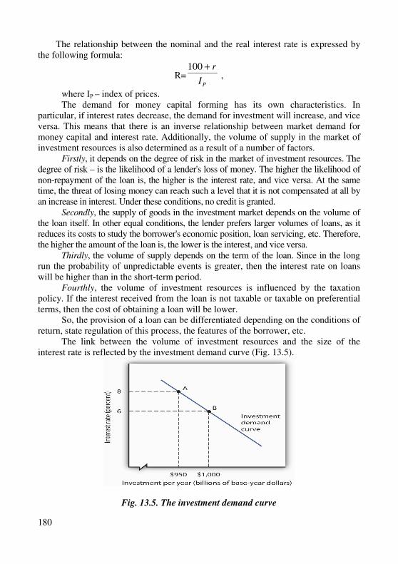
180

The relationship between the nominal and the real interest rate is expressed by the following formula:

R=PI

r+100 ,

where ІР – index of prices. The demand for money capital forming has its own characteristics. In

particular, if interest rates decrease, the demand for investment will increase, and vice versa. This means that there is an inverse relationship between market demand for money capital and interest rate. Additionally, the volume of supply in the market of investment resources is also determined as a result of a number of factors.

Firstly, it depends on the degree of risk in the market of investment resources. The degree of risk – is the likelihood of a lender's loss of money. The higher the likelihood of non-repayment of the loan is, the higher is the interest rate, and vice versa. At the same time, the threat of losing money can reach such a level that it is not compensated at all by an increase in interest. Under these conditions, no credit is granted.

Secondly, the supply of goods in the investment market depends on the volume of the loan itself. In other equal conditions, the lender prefers larger volumes of loans, as it reduces its costs to study the borrower's economic position, loan servicing, etc. Therefore, the higher the amount of the loan is, the lower is the interest, and vice versa.

Thirdly, the volume of supply depends on the term of the loan. Since in the long run the probability of unpredictable events is greater, then the interest rate on loans will be higher than in the short-term period.

Fourthly, the volume of investment resources is influenced by the taxation policy. If the interest received from the loan is not taxable or taxable on preferential terms, then the cost of obtaining a loan will be lower.

So, the provision of a loan can be differentiated depending on the conditions of return, state regulation of this process, the features of the borrower, etc.

The link between the volume of investment resources and the size of the interest rate is reflected by the investment demand curve (Fig. 13.5).

Fig. 13.5. The investment demand curve

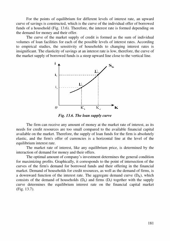
181

For the points of equilibrium for different levels of interest rate, an upward curve of savings is constructed, which is the curve of the individual offer of borrowed funds of a household (Fig. 13.6). Therefore, the interest rate is formed depending on the demand for money and their offer.

The curve of the market supply of credit is formed as the sum of individual volumes of loan facilities for each of the possible levels of interest rates. According to empirical studies, the sensitivity of households to changing interest rates is insignificant. The elasticity of savings at an interest rate is low, therefore, the curve of the market supply of borrowed funds is a steep upward line close to the vertical line.

Fig. 13.6. The loan supply curve

The firm can receive any amount of money at the market rate of interest, as its

needs for credit resources are too small compared to the available financial capital available on the market. Therefore, the supply of loan funds for the firm is absolutely elastic, and the firm's offer of currencies is a horizontal line at the level of the equilibrium interest rate.

The market rate of interest, like any equilibrium price, is determined by the interaction of demand for money and their offers.

The optimal amount of company’s investment determines the general condition for maximizing profits. Graphically, it corresponds to the point of intersection of the curves of the firm's demand for borrowed funds and their offering in the financial market. Demand of households for credit resources, as well as the demand of firms, is a downward function of the interest rate. The aggregate demand curve (DK), which consists of the demand of households (Dh) and firms (Df) together with the supply curve determines the equilibrium interest rate on the financial capital market (Fig. 13.7).

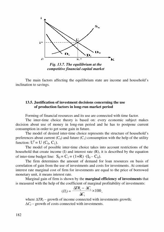
182

The main factors affecting the equilibrium state are income and household’s

inclination to savings. 13.5. Justification of investment decisions concerning the use

of production factors in long-run market period

Forming of financial resources and its use are connected with time factor. The inter-time choice theory is based on: every economic subject makes

decision about use of money in long-run period and he has to postpone current consumption in order to get some gain in future.

The model of desired inter-time choice represents the structure of household’s preferences about current (C0) and future (C1) consumption with the help of the utility

function: Ut = U (C0, C1).

The model of possible inter-time choice takes into account restrictions of the household that create income (I) and interest rate (R), it is described by the equation

of inter-time budget line: S0 = C1 = (1+R) ·(I0 – C0). The firm determines the amount of demand for loan resources on basis of

correlation of gain from the use of investments and costs for investments. At constant interest rate marginal cost of firm for investments are equal to the price of borrowed monetary unit, it means interest rate.

Marginal gain of firm is shown by the marginal efficiency of investments that is measured with the help of the coefficient of marginal profitability of investments:

(Пі) = 100Δ ΔΔII ×

−

IC

CTR,

where ∆TRI – growth of income connected with investments growth; ∆CI – growth of costs connected with investments.

Fig. 13.7. The equilibrium at the

competitive financial capital market

183

In practice investors often use the rate of return for the determination of gain from investments.

The rate of return is calculated as correlation of profit minus interest for loan to net investments:

%100×−

=I

RPRH I .

Physical capital is bought and sold at the capital assets market. Price of capital asset – is a sum of money by which the unit of capital can be

bought or realized every moment. It includes the current value of future payments flow.

Current (present) value of future payments – is a present value of sum that may be paid in future.

The current value of the sum that may be got in future can be calculated by procedure called discounting.

Calculation of current discounted value of payment is an inverse task for the calculation of complex interest. With the help of the method of complex interests it is possible to calculate by how much the current sum will increase within some period of time. The discounting method can help to define which sum of money should be invested in bank at some interest in order to get the desired sum of money in future. If invested sum PR, the norm of interest – R, and future sum – FC, then:

� in 1 year: )1(1 RPVRPVPVFV +=⋅+= ;

� in 2 years: 2

2 )1()1()1( RPVRRPVRPVFV +=⋅+++= ;

� in t years: t

t RPVFV )1( += .

Present value PV is called the present discounted value of desired sum FV: t

t RFVPV )1/( += , or [ ]t

t FVRPV ⋅+= )1/(1 .

Expression t

R)1/(1 + is discounted value of monetary unit in t years.

Any capital brings flow of payments every year. In order to define the price of asset it is necessary to find out present value of this payment flow, it means to calculate the sum of present discounted values of all payments for every year during all term of use of capital:

∑ ×+

++×+

+×+

= ttFV

RFV

RFV

RPV

)1(

1...

)1(

1

1

1221 .

The formulas of discounting is used while calculating the expedience of equipment, other investments, insurance contributions, loans, assessment of the real value of securities, etc.

Price of perpetual asset is defined as: RПPV /= . Present discounted value of securities, for example, shares that have variable

payment flows, are calculated by the following formula: t

tt RПRПRПPV )1/(...)1/()1/( 2

2211 ++++++= ,

where П1, П2, П3 – payments in appropriate year,

184

R1, R2, R3 – interest rates in appropriate years. Present value of shares PV gives imagination about yield of shares. Net present value is discounted value of expected profits flows minus sum of

investments costs (СІ):

.)1(

...)1()1(

С - NPV2

21I t

t

R

П

R

П

R

П

+++

++

++=

On this basis we can generate some investment criteria: the firm should invest only when the net gain is positive, it means net present value of expected profit from investments will be more than sum of investment costs (NPV>0). In case if NPV<0, then the investment project should be rejected.

Interest rate or discount rate is marked with a symbol i. Discount rate is different from the norm of interest that sum of interest is added to the borrowed sum when debt is paid, and sum of discount is subtracted when loan issuance straight away. Discount rate can be considered from the point of alternative costs of capital. The firm should compare discount rates for the choice of capital investment directions. It may invest investments in another object that will bring more profits or to choice the way of purchase that brings more income depending on the value of discount rate.

The value of discount rate at which net present value 0=NPV , is called internal norm of returns (profitability) of project.

Let’s consider now the capital assets market. The market of assets services if rental market. Price of capital services is based on rental assessment of capital and is determined by rent for capital resources leased.

The minimally acceptable rental evaluation of capital )( kr is rent that allows

owner of capital asset to reimburse alternative costs connected with the ownership of given asset, and to get normal profit. Its level is determined by price of capital, real interest rate and depreciation norm. It is formed on basis equilibrium price as a result of interaction of demand and supply at the capital services market.

Demand for capital services depends on its marginal yield. Logically, the firm will expand the demand until marginal yield of services equal rental evaluation of capital. Supply of capital services is a function of rental evaluation of capital and it depends on time period. Short-run supply of capital services reflects limited stock of physical capital and, as usually, it is absolutely inelastic. Long-run supply of capital services may be absolutely elastic. In short-term market period the price of capital asset will be equal to present discounted value of future income flow, and in conditions of long-term equilibrium it should be equal both the value of its production and present discounted value.

Peculiarities of the land market functioning are connected with that total supple of it can’t be changed. The supply of land is absolutely inelastic, that’s why price of

land )( NR depends only on changes in demand for it (fig. 13.8).

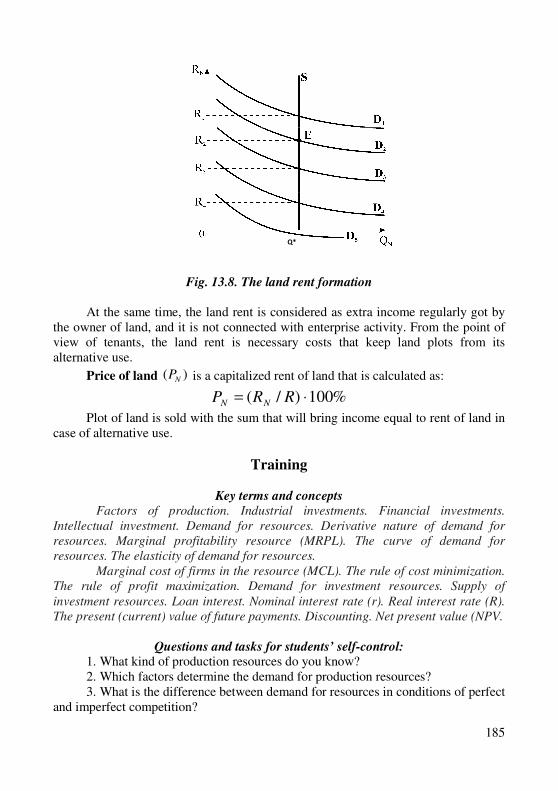
185

Fig. 13.8. The land rent formation

At the same time, the land rent is considered as extra income regularly got by

the owner of land, and it is not connected with enterprise activity. From the point of view of tenants, the land rent is necessary costs that keep land plots from its alternative use.

Price of land )( NP is a capitalized rent of land that is calculated as:

%100)/( ⋅= RRP NN

Plot of land is sold with the sum that will bring income equal to rent of land in case of alternative use.

Training

Key terms and concepts Factors of production. Industrial investments. Financial investments.

Intellectual investment. Demand for resources. Derivative nature of demand for

resources. Marginal profitability resource (MRPL). The curve of demand for

resources. The elasticity of demand for resources.

Marginal cost of firms in the resource (MCL). The rule of cost minimization.

The rule of profit maximization. Demand for investment resources. Supply of

investment resources. Loan interest. Nominal interest rate (r). Real interest rate (R).

The present (current) value of future payments. Discounting. Net present value (NPV.

Questions and tasks for students’ self-control: 1. What kind of production resources do you know? 2. Which factors determine the demand for production resources? 3. What is the difference between demand for resources in conditions of perfect

and imperfect competition?

Q*

186

4. What does represent the law of optimal use of production resources in the long-term market period?

5. What is the difference between demand for labor from the side of particular enterprise and from the side of industry?

6. What peculiarities of the labor market functioning do you know? 7. Under what conditions the equilibrium at the labor market is established? 8. What is the role of trade unions at the labor market forming? 9. Justify the essence of the concepts “capital” and “investments”. 10. What are the peculiarities of forming of demand and supply at the

investment market? 11. How the interest rate is formed? What types of interests do you know? 12. What factors determine interest rate? 13. What does the process of discounting of cash flows at the market of

investment resources mean? 14. Characterize the essence of current discounted value. 15. What are the peculiarities of the functioning of the land market? 16. Which factors have impact on the demand for the land?

Tests

1. Marginal product of factor of production in monetary form is equal to:

а) cost of the last unit of product; b) change of total income at use of additional unit of factor of production; c) amount of production at the use of additional unit of production factor; d) change of price for goods produced with the help of given production factor. 2. Demand for resources depends on:

а) price of product manufactured with the help of some resource; b) price of substitute resources; c) price of certain resource; d) all answers are correct.

3. If the competitive firm maximizes its profit by selling products at price

2 UAH per one unit and buys resource at price 10 UAH, then monetary

expression of marginal product of resource is equal to:

а) 2 UAH; b) 5 UAH; c) 10 UAH; d) 20 UAH.

4. Marginal cost of firm for resource – is:

а) additional cost per one additional unit of resource; b) additional cost connected with selling of additional unit of product; c) difference between total and average cost of firm for resource; d) sum of average and total cost of firm for resource.

187

5. Derivative character of demand for resource means that:

а) demand of firm for resource depends on demand for production of the firm; b) demand of firm for resource depends on price of resource; c) demand of firm for resource depends on marginal productivity of resource; d) demand of firm for resource depends on marginal cost of it.

6. The demand curve for resource of competitive firm is:

a) curve of marginal profitability of resource; b) curve of marginal cost for resource; c) utility curve of marginal product; d) correct answers are a and b.

7. According to the law of optimal use of resource:

а) use of resource is profitable if marginal profitability or resource is equal to marginal cost for it;

b) use of resource is profitable if prices of all involved resources are equal; c) use of resources is profitable if the firm purchases it at the competitive

market; d) use of resources is profitable to the point where MR = МС.

8. If nominal interest rate is 12 % and the inflation rate is 8 %, so the real

interest rate equals to:

а) 3,7 %; b) 1,5 %; c) 4 %; d) 96 %.

9. Norm of loan interest – is:

а) maximal amount of the loan fee established by government; b) ratio of loan interest to the amount of fee; c) the difference between sum of money that is returned and borrowed; d) the difference between nominal and real loan interest.

10. The minimal wages established by government – is:

а) recommended lower limit of individual income; b) the size of the subsistence minimum; c) the lower limit of salary of an employee of any enterprise; d) the cost of the main consumption products for a certain period of time.

11. The loan interest rate does not depend on:

а) the term of the loan; b) riskiness of the project; c) loan volume; d) there is no correct answer.

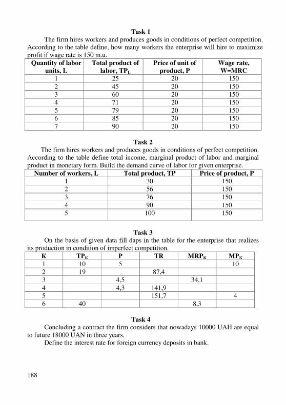
188

Task 1

The firm hires workers and produces goods in conditions of perfect competition. According to the table define, how many workers the enterprise will hire to maximize profit if wage rate is 150 m.u.

Quantity of labor

units, L

Total product of

labor, TPL

Price of unit of

product, P

Wage rate,

W=MRC

1 25 20 150

2 45 20 150 3 60 20 150

4 71 20 150 5 79 20 150

6 85 20 150

7 90 20 150

Task 2

The firm hires workers and produces goods in conditions of perfect competition. According to the table define total income, marginal product of labor and marginal product in monetary form. Build the demand curve of labor for given enterprise.

Number of workers, L Total product, TP Price of product, P

1 30 150 2 56 150

3 76 150

4 90 150 5 100 150

Task 3

On the basis of given data fill daps in the table for the enterprise that realizes its production in condition of imperfect competition.

К ТРК Р ТR MRPК МРК

1 10 5 10 2 19 87,4

3 4,5 34,1

4 4,3 141,9 5 151,7 4 6 40 8,3

Task 4

Concluding a contract the firm considers that nowadays 10000 UAH are equal to future 18000 UAN in three years.

Define the interest rate for foreign currency deposits in bank.

189

CHAPTER 4.

GENERAL EQUILIBRIUM

AND INSTITUTIONAL PROVIDING

OF EFFECTIVE MARKET FUNCTIONING

Theme 14 The General Equilibrium and Welfare Economy

14.1. The market equilibrium and its analysis. Partial and general

equilibrium.

14.2. Equilibrium in economy of exchange and the efficiency of resources

distribution.

14.3. The welfare economy to context general market equilibrium.

14.1. The market equilibrium and its analysis.

Partial and general equilibrium

In this theme the interdependence between markets and mutual impact of partial and general market equilibrium has been clarified. Ech of microeconomic subjects is an object of analysis of partial market equilibrium that allows justifying the logic of their business behavior. However, the economy doesn’t consist of particulat isolated markets. It functions as manycomponental system of connected market characteristics (prices, costs, incomes, etc.), when the change of one of them causes a lot of changes at other markets. That’s why the analysis of general market equilibrium researches all microeconomic subjects interact and how successfully the problem “what?”, “how?” and “for whom to produce?” is solved.

Partial market eauilibrium is provided by establishment of equilibrium price and equilibrium amount of output under the influence of factors acting only at given local market.

At the same time, the general market equilibrium provides the equilibrium price formation and equilibrium amount of output at given market taking into account changes of equilibeium state at all other markets. It may be considered that the general equilibrium state is a composition of all partial equilibrium states at interdepended markets of factors and goods.

190

General economic equilibrium describes the circulation of economic life where consumers need goods and offer production factors. Firms buy production factors and supple good into the market, same time paying factoral incomes. By this firms get profits from sales of goods, and consumers – desired goods.

On the basis of the general market equilibrium analysis let’s consider features of competitive markets totality.

There are the main suggestions in the analisys if general equilibrium:

� all markets are competitive; � natural monopolies are absent; � each product is produced in case of constant or descending effect of scale; � there is no pollution of the environment caused be economic activity; � restrictive regulation of entrance into the market is absent; � in all cases prices of production factors and goods are changed quite elastical

in order to balance demand and supply By analyzing the situation we are based on that the logic of consumer’s

behavior will be rational. In other words, consumers will distribute their income beyween different goods in such a way that to maximize their satisfaction. It will mean that they will choice goods in such a way that marginal utilities of each of them per monetary cost unit are same till the last unit of goods.

In general equilibrium marginal utilities of all goods per one monetary unit are equal to marginal social cost of production of these goods. This means that general market equilibrium determines prices and amounts of production in such a way that marginal utility of every product for consumers equals marginal cost of each product of society. General equilibrium – is a state of economy when prices of equilibrium are established. Equilibrium prices and amount of goods are established with taking inro account the effect of feedback that reflects the change of partial equilibrium at given market.

It should be noted that general equilibrium is achieved when prices react to the change of demand or supply in such a way that demand become equal to supply at all markets.

In algebraic way the interdependence of commodity markets can be represented through the equation system. It was Swiss economist Leon Walras (1834–1910) who tried to descrice the economic equilibrium with the help of equation system for the first time. On his opinion, market economy prices cuase the amount of output, and same time the amount of output determines price level. Prices of goods and services depend on prices of resources and prices of resources depend on goods that are of demand. In the Walras’ model the general economic equilibrium – is a result of solution of the equation system where prices of goods and their quantity are unknown.

The Walras’ general equilibrium model represents the interdependence between markets of goods and markets of production factors in conditions of perfect competition. The very this allows providing the equilibrium of plurality of markets.

The Walras’ law determines internal, cause-effect relationships between particular markets in conditions of perfect competition when sum of excess demand

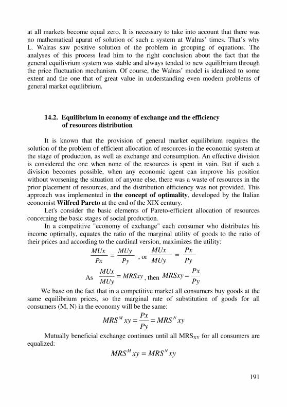
191

at all markets become equal zero. It is necessary to take into account that there was no mathematical aparat of solution of such a system at Walras’ times. That’s why L. Walras saw positive solution of the problem in grouping of equations. The analyses of this process lead him to the right conclusion about the fact that the general equilivrium system was stable and always tended to new equilibrium through the price fluctuation mechanism. Of course, the Walras’ model is idealized to some extent and the one that of great value in understanding even modern problems of general market equilibrium.

14.2. Equilibrium in economy of exchange and the efficiency

of resources distribution

It is known that the provision of general market equilibrium requires the

solution of the problem of efficient allocation of resources in the economic system at the stage of production, as well as exchange and consumption. An effective division is considered the one when none of the resources is spent in vain. But if such a division becomes possible, when any economic agent can improve his position without worsening the situation of anyone else, there was a waste of resources in the prior placement of resources, and the distribution efficiency was not provided. This approach was implemented in the concept of optimality, developed by the Italian economist Wilfred Pareto at the end of the XIX century.

Let's consider the basic elements of Pareto-efficient allocation of resources concerning the basic stages of social production.

In a competitive "economy of exchange" each consumer who distributes his income optimally, equates the ratio of the marginal utility of goods to the ratio of their prices and according to the cardinal version, maximizes the utility:

Py

MUy

Px

MUx= , or

Py

Px

MUy

MUx=

As MRSxyMUy

MUx= , then

Py

PxMRSxy =

We base on the fact that in a competitive market all consumers buy goods at the same equilibrium prices, so the marginal rate of substitution of goods for all consumers (M, N) in the economy will be the same:

xyMRSPy

PxxyMRS NM ==

Mutually beneficial exchange continues until all MRSXY for all consumers are equalized:

xyMRSxyMRS NM =

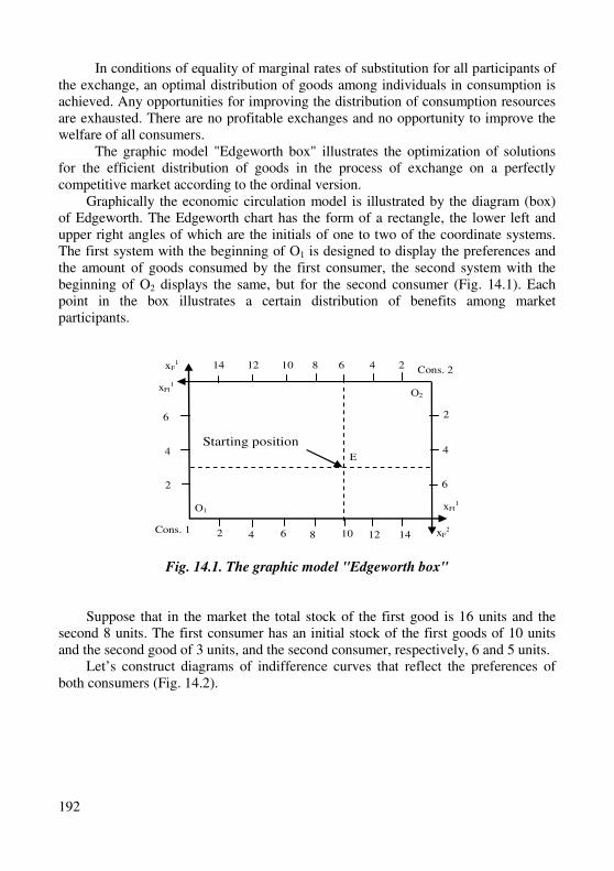
192

In conditions of equality of marginal rates of substitution for all participants of the exchange, an optimal distribution of goods among individuals in consumption is achieved. Any opportunities for improving the distribution of consumption resources are exhausted. There are no profitable exchanges and no opportunity to improve the welfare of all consumers.

The graphic model "Edgeworth box" illustrates the optimization of solutions for the efficient distribution of goods in the process of exchange on a perfectly competitive market according to the ordinal version.

Graphically the economic circulation model is illustrated by the diagram (box) of Edgeworth. The Edgeworth chart has the form of a rectangle, the lower left and upper right angles of which are the initials of one to two of the coordinate systems. The first system with the beginning of O1 is designed to display the preferences and the amount of goods consumed by the first consumer, the second system with the beginning of O2 displays the same, but for the second consumer (Fig. 14.1). Each point in the box illustrates a certain distribution of benefits among market participants.

2 4

E

8 10 12 14

2

4

6

Cons. 1

Cons. 2 2 4 6 8 10 12 14

2

4

6

Starting position

xF1

xFl1

xFl1

xF2

6

О1

О2

Fig. 14.1. The graphic model "Edgeworth box"

Suppose that in the market the total stock of the first good is 16 units and the second 8 units. The first consumer has an initial stock of the first goods of 10 units and the second good of 3 units, and the second consumer, respectively, 6 and 5 units.

Let’s construct diagrams of indifference curves that reflect the preferences of both consumers (Fig. 14.2).

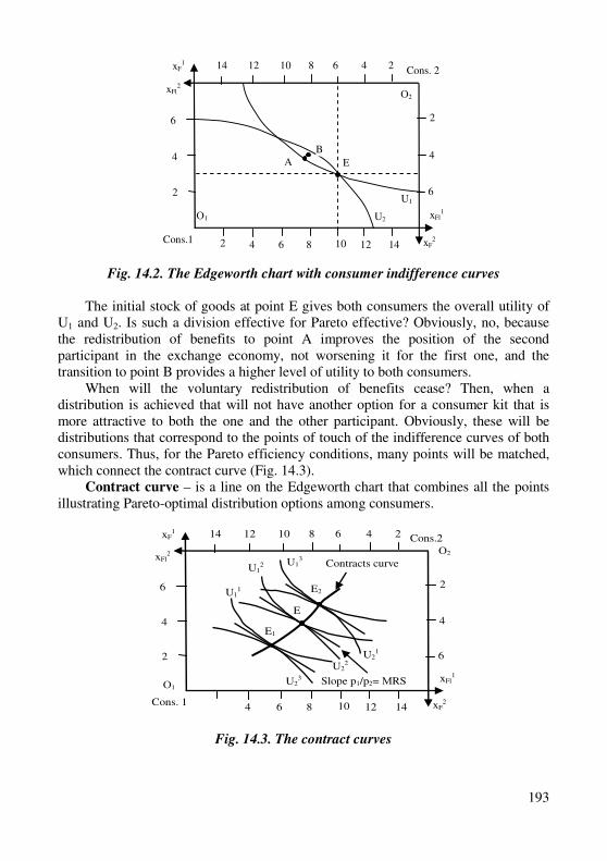
193

2 4

E

8 10 12 14

2

4

6

Cons.1

Cons. 2 2 4 6 8 10 12 14

2

4

6

xF1

xFl2

xFl1

xF2

6

A B

U1

U2 О1

О2

Fig. 14.2. The Edgeworth chart with consumer indifference curves

The initial stock of goods at point E gives both consumers the overall utility of

U1 and U2. Is such a division effective for Pareto effective? Obviously, no, because the redistribution of benefits to point A improves the position of the second participant in the exchange economy, not worsening it for the first one, and the transition to point B provides a higher level of utility to both consumers.

When will the voluntary redistribution of benefits cease? Then, when a distribution is achieved that will not have another option for a consumer kit that is more attractive to both the one and the other participant. Obviously, these will be distributions that correspond to the points of touch of the indifference curves of both consumers. Thus, for the Pareto efficiency conditions, many points will be matched, which connect the contract curve (Fig. 14.3).

Contract curve – is a line on the Edgeworth chart that combines all the points illustrating Pareto-optimal distribution options among consumers.

U11

4

E

8 10 12 14

2

4

6

Cons. 1

Cons.2 2 4 6 8 10 12 14

2

4

6

xF1

xFl2

xFl1

xF2

6

Slope p1/p2= МRS

Contracts curve

О1

О2

U12 U1

3

U21

U22

U23

E1

E2

Fig. 14.3. The contract curves

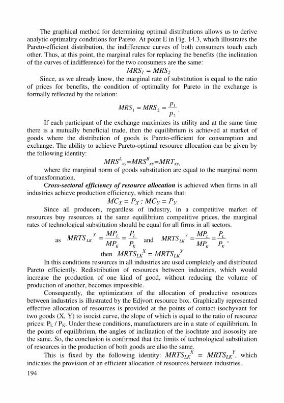
194

The graphical method for determining optimal distributions allows us to derive analytic optimality conditions for Pareto. At point E in Fig. 14.3, which illustrates the Pareto-efficient distribution, the indifference curves of both consumers touch each other. Thus, at this point, the marginal rules for replacing the benefits (the inclination of the curves of indifference) for the two consumers are the same:

MRS1 = MRS2

Since, as we already know, the marginal rate of substitution is equal to the ratio of prices for benefits, the condition of optimality for Pareto in the exchange is formally reflected by the relation:

2

121

p

pMRSMRS == .

If each participant of the exchange maximizes its utility and at the same time there is a mutually beneficial trade, then the equilibrium is achieved at market of goods where the distribution of goods is Pareto-efficient for consumption and exchange. The ability to achieve Pareto-optimal resource allocation can be given by the following identity:

MRSA

xy=MRSBхy=MRТхy,

where the marginal norm of goods substitution are equal to the marginal norm of transformation.

Cross-sectoral efficiency of resource allocation is achieved when firms in all industries achieve production efficiency, which means that:

МСХ = РХ ; MCУ = РУ Since all producers, regardless of industry, in a competitive market of

resources buy resources at the same equilibrium competitive prices, the marginal rates of technological substitution should be equal for all firms in all sectors.

as K

L

K

LX

LKP

P

MP

MPMRTS == and

K

L

K

LY

LKP

P

MP

MPMRTS == ,

then MRTSLKX = MRTSLK

У

In this conditions resources in all industries are used completely and distributed Pareto efficiently. Redistribution of resources between industries, which would increase the production of one kind of good, without reducing the volume of production of another, becomes impossible.

Consequently, the optimization of the allocation of productive resources between industries is illustrated by the Edjvort resource box. Graphically represented effective allocation of resources is provided at the points of contact isochyvant for two goods (X, Y) to isocist curve, the slope of which is equal to the ratio of resource prices: PL / PK. Under these conditions, manufacturers are in a state of equilibrium. In the points of equilibrium, the angles of inclination of the isochtate and isososity are the same. So, the conclusion is confirmed that the limits of technological substitution of resources in the production of both goods are also the same.

This is fixed by the following identity: MRTSLKX = MRTSLK

Y, which

indicates the provision of an efficient allocation of resources between industries.

195

For the efficient functioning of the whole competitive market system the resources must be distributed among different types of goods production so that the structure of production meets the structure of social needs. Consumers should be prepared to replace the goods in the consumer basket in the same proportion in which the economy can transform one good into another. In this case, the full efficiency of the distribution of economic resources is achieved.

Since both producers and consumers equate the marginal norms of substitution of goods to the same market prices, the marginal rate of transformation of any good into another in the production sector will be equal to the marginal rate of substitution of these goods for each consumer:

MRTху = MRSху This identity means that there is no way to improve the position of consumers

through changes in the production of these goods. In the economic system a general equilibrium is introduced that meets the Pareto-optimality criterion. It provides the optimal structure of the economy, balance of interests of consumers and producers.

The general conditions for the efficiency of a perfectly competitive economy are described by a system of equations:

– equilibrium in a competitive economy is effective in consumption and exchange if:

XYN

Y

XXY

MMRS

P

PMRS ==

– the manufacturer's equilibrium in a competitive economy is effective in allocating resources between industries if:

K

LY

LK

X

LKP

PMRTSMRTS ==

– the equilibrium is effective in case of use of resources in production, if:

Y

X

Y

XXY

P

P

MC

MCMRT ==

– the general equilibrium of economic system is Pareto-effective in allocating resources in all spheres if:

MRSXY = MRTху Consequently, the total efficiency of the economic system – is a concept that

takes into account the efficiency of production, the efficiency of consumption and a certain balance between the interests of producers and consumers in the markets.

196

14.3. The welfare economy to context general market equilibrium

There are preconditions and situations where a self-regulated market is

incapable of ensuring the efficient functioning of the economy. After all, along with the positive features, it has many disadvantages. That is why there is a need for state intervention in the economic activity of microeconomic actors.

The effectiveness of market regulation is limited for the following reasons: � the existence of different forms of manifestation of monopoly market power; � opacity of markets; � incomplete or asymmetric information; � presence of external factors that arise when a certain activity (in production

or consumption) has a side effect on other activities, but in circumstances where this dependence is not reflected directly in market prices;

� increasing the influence of factors of public goods. In this situation, market failure arises when markets are unable (not capable or not interested) to offer goods that are useful to many consumers;

� presence of non-market activities of market participants and non-market mechanisms of regulation. Relations between business entities can be regulated not only by the market mechanism, but also through non-market mechanisms.

These reasons are called the reasons for the limited capacity of market regulation that is they constitute a set of prerequisites and situations where the operation of the mechanism of competitive markets does not lead to the public utility maximization.

The presence of a number of reasons for the limited capacity of market regulation makes it impossible to achieve the maximum effectiveness of the economic system. Under these conditions, the overall equilibrium is achieved at a new level - at the quasi-optimum level. The quasi-optimum theory argues that if in one industry (or in a group of industries) distortions can’t be eliminated, it is better to refuse from achievement of maximum efficiency in another industry (or in a group of industries) in order to balance the economy as a whole.

The theory of general market equilibrium plays a significant role in determining the scientific principles of policy in the field of welfare economics. Obviously, in a generally balanced economy, the distribution of benefits is also effective.

The welfare economy finds out the issues of economic efficiency in all areas of management: production, exchange of benefits, distribution and redistribution. In particular, the distribution of resources among the goods and benefits among consumers is Pareto-optimal or effective if it is impossible to restructure production and consumption which improves the condition of some individuals without worsening the condition of others. Any change that raises the welfare of some individuals without reducing the welfare of others increases the welfare of society as a whole.

There are a number of problems when using the Pareto-criterion. Often, when evaluating various government programs, there is a need for an interpersonal

197

comparison of distributions. But, for example, if both distributions x and y are Pareto-efficient, it is impossible to use the Pareto criterion for their ranking.

We are interested in a given set of effective allocations for possible selection criteria among them.

If you move the contract curve in exchange from the space of production of goods in the space of utility, then you can get a curve of possible utility. That is, the curve of possible utility will determine the various combinations of benefits that individuals A and B receive when the economy is in a state of equilibrium simultaneously in terms of both production and exchange. The curve, which is an envelope to all curves that represents possible utility options at Pareto-optimal points in production and exchange, has been called the main utility-options frontier.

Based on this, the following criteria for assessing welfare can be

distinguished: 1) Equality criteria, by which the distribution corresponding to the equal value

of the individual's usefulness (U1 = U2 = ... = Un) is the social optimum. 2) Utilitarian criterion (Bentham, 1867). According to Bentham, society must

maximize the utility of all members of society (aggregate utility) or the overall welfare of society.

3) The Rawls criterion (1971). According to this criterion, it is considered that the main goal of political institutions is social justice. Rawls suggests that society is in an "initial position" when each individual has a goal that promotes the possession of "original goods". Rationalized by behavior are those individuals who are concerned only about their own interests and try to achieve the principle of justice together. Their rational choice is to maximize the welfare of the least secured individual (or group of individuals).

In this case, the criterion of the efficiency of the welfare economy is presented as follows:

W = min {U1(A),U2(A),…,Un(A)}.

Thus, according to Rawls, social welfare depends only on the welfare of the least secured individual. Rawls suggests that many options for efficient distribution of wealth may not be socially desirable, so society may prefer the principles of equality, even at a significant cost for its achievement.

Let’s note that the Rawls criterion is criticized by economists who believe that the criterion gives the optimal result only for very limited assumptions. In addition, the very interpretation of social justice depends strongly on the type of society.

To the criteria for assessing the welfare economy we should add and consider Pareto's criterion earlier. After all, according to this criterion, any change that improves the state (increases the welfare) of some individuals without deteriorating the condition of others, improves the welfare of society as a whole. In other words, according to the Pareto criterion, the distribution of x is better than y, or the advantage of, the distribution of x compared with y, if at the x point the condition of some individuals improves and the condition of other individuals does not deteriorate.

Another option for assessing the welfare economy is based on the compensation criterion of N. Kaldor and J. Hicks (1939). According to this

198

criterion, welfare increases if those who get gains from changes in exchange and distribution estimate their income gains higher than those suffered by the victim, and if the value of the winnings exceeds the value of the losses. This criterion measures the changes in welfare in monetary terms and is an attempt to evaluate the winnings in the monetary units of those individuals who have won, and to compensate in money the losses of those individuals who have lost.

The criterion is based on the compensation principle: the change in

government policy is considered to be an improvement of the situation if those individuals who have benefited from changes in distribution can potentially

completely offset losses for those who have lost and then remain in the win. But there are following problems when applying this criterion: probably there

is such a situation when after the change in the system of relations of exchange and distribution, the movement back to the starting point also causes an increase in the level of social welfare.

In this case, if the curves of possible utility intersect, the criterion will give an indefinite result.

It is important to note that each of the above criteria has its own disadvantages, and therefore the development of criteria for assessing the welfare remains an urgent task of modern economic theory.

The fundamental consequence of the theory of general equilibrium is that a perfectly competitive economy is effective. From here, all competitive results are on the brink of production opportunities and on the verge of possible benefits. Market failures that are associated with monopoly or environmental pollution "push" the economy to the left of both boundaries.

If the firm has reached the monopoly of its position in a certain market, it is able to raise the price of its product to a level necessarily higher level of its marginal costs. Consumers will buy fewer such products than under competitive conditions, and therefore their satisfaction will necessarily be smaller. This reduction in consumer satisfaction is a typical manifestation of the ineffectiveness of a deformed market caused by imperfect competition.

Another important failure of the market is the adverse effects of economic activity. If the company does not pay for harmful effects of its influence on the environment, then high levels of environmental pollution will occur, and therefore will suffer consumer well-being. On the other hand, there are also beneficial side effects associated with, for example, scientific activities.

A perfect and absolutely effective competitive mechanism has never been and never will be. However, in broader terms, the statements of the theory of competition contain a lot of real. In the long-run period of time, many defects are eliminated and they are temporary, for example, the monopoly eliminates competing technologies. At the same time, too much simplified competitive model points to many important hypotheses of economic behavior, especially in the long-run period of time.

Thus, due to the interdependence of the prices of all the benefits and factors of production, a complete picture of the mechanism of market pricing and its role in the national economy can be obtained only on the basis of constructing a model of general economic equilibrium, reflecting the interaction of all markets. From this

199

model, a system of equilibrium prices is introduced, which ensures a general equilibrium in all markets, and determines the conditions for its existence.

The system of equilibrium prices can direct the production and exchange to Pareto-efficient use of society's resources and with the help of the state's distributive policy it is possible to support the distribution of welfare among citizens according to social perceptions of social justice. But at the same time, the state should apply such a redistribution tools that do not distort the system of equilibrium prices.

Training

Key terms and concepts Market equilibrium. Partial equilibrium. General equilibrium. Equilibrium

price. Equilibrium output. Local market. Market of factors of production. Commodity

market. Competitive markets. Marginal utility. Marginal social costs for producing goods. Primary market

changes.

Changes in the market of substitute products. Changes in the market of complementary products. Changes in the effect of feedback. The Walras model of

general economic equilibrium. Equilibrium in the economy of exchange. The efficiency of resource’s allocation.

Pareto-efficient allocation of resources. Graphic model "Edgeworth box".

Curve of contrasts. Curve of consumer’s opportunities. Line production capabilities. Welfare Economics. Social welfare. Market regulation. Equality criteria. Utilitarion criteria. Rawls criterion. Pareto criterion. Kaldor-Hicks criteria. Scitovsky criteria.

Questions and tasks for self-testing and monitoring of learned knowledge: 1. What does the partial market equilibrium mean?

2. What is the difference between general and partial market equilibrium?

3. Describe the features of totality of competitive markets on the basis of general market equilibrium analysis.

4. What does the Walras model of general market equilibrium justify?

5. Explain the basic elements if Pareto-effective distribution. 6. How each consumer maximizes his utility in the “economy of exchange”

according to cardinal version of consumer’s behavior?

7. What does the graphic model "Edgeworth box" show?

8. Describe the curve of contrasts and explain it. 9. What does the curve of consumer’s opportunities represent? What factors have

impact on it? 10. How can you characterize the welfare economics?

11. What are the reasons of ineffective market regulation?

12. What criteria of welfare assessment do you know? Characterize it.

200

Theme 15 The Institutional Effects of Market Economy

15.1. The institutional environment of market economy. Transaction costs

15.2. External effects. The Coase’s theorem.

15.3. Peculiarities of public goods and conditions of its use

15.4. The social choice theory and its role in market economy

15.1. The institutional environment of market economy. Transaction costs

There is a system of institutions in the economy – formal and informal norms

and rules of behavior developed and established by the state, society, it allows individuals to structure and coordinate their activities.

The institutional environment of the functioning of economic entities is largely determined by the property rights.

Property rights – is a collection of power rights, authorized behavioral relationships, drawn up between people about the use of economic goods. Ownership of property consists of the following powers: the right to use property; the right to benefit or utility; the right to change its form and substance; the right to transfer it to other persons at an agreed price.

The effectiveness of these norms directly depends on the dominant form of ownership in society, as well as on the structure of existing forms of ownership and trends in its development. There are three main forms of ownership:

� private; � communal; � state. In conditions of private property a separate person has all rights. Advantages of this form of ownership are: � the exclusive right of use, which can be considered as the right to "exclude"

other individuals from the range of subjects who can use the property (only the owner has all positive and negative results from the possession and use of the good);

� the exclusive right to receive income from the use of property; � the full right to transfer of property, which includes the right to conclude

agreements and choose their form; � the possibility of "splitting" the ownership of separate powers and creating

new combinations from them (the entire set of rights for goods may belong to several agents or each individual authority may belong to different agents, which are the basis of cooperation and specialization).

201

In conditions of state ownership a decision is made on the basis of established rules and procedures that regulate the interests of society as a whole.

The advantages of such a form of ownership include: � only the government is able to provide large-scale investments necessary for

the technical modernization of leading industries in the developing countries; � only direct state control of the enterprises concerned can prevent an increase

in prices for the most important commodities and services for the population, such as electricity, housing or transport;

� only the preservation of state ownership of large industrial enterprises can prevent the problem of mass unemployment, etc.

However, the experience of many countries confirms that state-owned enterprises in their economic activity are often less effective than private ones. This is explained by the fact that the managerial staff of such enterprises is not sufficiently interested in ensuring their profitability. Possibility of getting of state subsidies or preferential loans makes the threat of bankruptcy to them practically unrealistic, and the profitability of production - if desired, then optional. In addition, profitability analysis for state-owned enterprises is often not possible either because of the government's regulated (lowered) level of product prices. In countries with a large number of state-owned enterprises, the relatively low efficiency of their production negatively affects economic growth. Due to the need to cover their losses by means of the state budget, fewer free resources remain available for various social programs, and there is a threat to the state budget deficit.

In conditions of communal ownership, all members of the organization have the general right to use the good (before it is assigned) and the private right to use after it has been able to obtain (assign) it for temporary or permanent possession. Communal property occurs there where the costs of specification and protection of private property rights are extremely high. The benefits of establishing private property rights are either zero or clearly less than the costs associated with their establishment.

Firms are usually connected by contractual obligations to minimize transaction costs.

Transaction costs – are expenditures associated with the installation, transfer and protection of property rights to resources. The most important factor affecting the size of this type of expenditure is the number of economic actors involved in the negotiations. It is necessary for all participants to evaluate their benefits and losses in case of signing the agreement for successful internalization of externalities through negotiations

The concept of “transaction costs” was introduced into economic science by Professor of the University of Chicago Ronald Coase and today has become widespread.

There are five main forms of transaction costs: 1) information search costs; 2) costs of negotiation and contracting; 3) measurement costs;

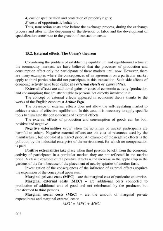
202

4) cost of specification and protection of property rights; 5) costs of opportunistic behavior. Thus, transaction costs arise before the exchange process, during the exchange

process and after it. The deepening of the division of labor and the development of specialization contribute to the growth of transaction costs.

15.2. External effects. The Coase’s theorem

Considering the problem of establishing equilibrium and equilibrium factors at

the commodity markets, we have believed that the processes of production and consumption affect only the participants of these markets until now. However, there are many examples where the consequences of an agreement on a particular market apply to third parties who did not participate in this transaction. Such side effects of economic activity have been called the external effects or externalities.

External effects are additional gains or costs of economic activity (production and consumption) that are attributable to persons not directly involved in it.

The concept of external effects appeared in economic theory thanks to the works of the English economist Arthur Pigu.

The presence of external effects does not allow the self-regulating market to achieve a state of effective equilibrium. In this case, it is necessary to apply specific tools to eliminate the consequences of external effects.

The external effects of production and consumption of goods can be both positive and negative.

Negative externalities occur when the activities of market participants are harmful to others. Negative external effects are the cost of resources used by the manufacturer, but not paid at a market price. An example of the negative effects is the pollution by the industrial enterprise of the environment, for which no compensation is paid.

Positive externalities take place when third persons benefit from the economic activity of participants in a particular market, they are not reflected in the market price. A classic example of the positive effects is the increase in the apple crop in the gardens of the farm because of the placement of nearby apiaries of another farm.

Investigation of the consequences of the influence of external effects requires the expansion of the conceptual apparatus:

Marginal private costs (MPC) – are the marginal cost of particular enterprise. Marginal external costs (MEC) – are additional costs connected to

production of additional unit of good and not reimbursed by the producer, but transformed to third persons.

Marginal social costs (МSС) – are the amount of marginal private expenditures and marginal external costs:

МSС = МРС + МЕС

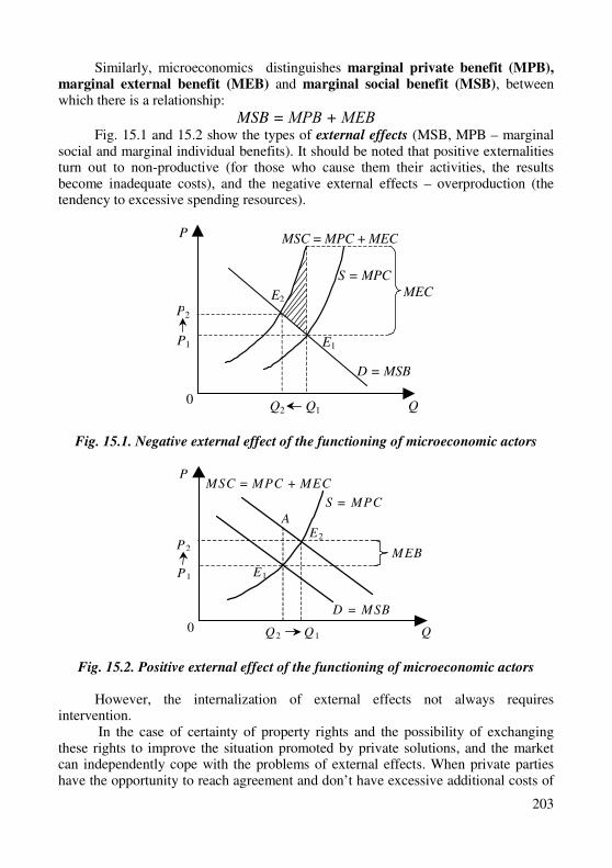
203

Similarly, microeconomics distinguishes marginal private benefit (MPB),

marginal external benefit (MEB) and marginal social benefit (MSB), between which there is a relationship:

MSB = МРВ + МЕВ Fig. 15.1 and 15.2 show the types of external effects (MSB, MPB – marginal

social and marginal individual benefits). It should be noted that positive externalities turn out to non-productive (for those who cause them their activities, the results become inadequate costs), and the negative external effects – overproduction (the tendency to excessive spending resources).

MEC

S = MPC

D = MSB

E1

MSC = MPC + MEC

E2

P2

P1

Q2 Q1 Q

P

0

Fig. 15.1. Negative external effect of the functioning of microeconomic actors

P

MEB

S = MPC

D = MSB

E1

MSC = MPC + MEC

E2

Q

P2

P1

Q2 Q1

A

0

Fig. 15.2. Positive external effect of the functioning of microeconomic actors

However, the internalization of external effects not always requires

intervention. In the case of certainty of property rights and the possibility of exchanging

these rights to improve the situation promoted by private solutions, and the market can independently cope with the problems of external effects. When private parties have the opportunity to reach agreement and don’t have excessive additional costs of

204

resource allocation, they are able to conclude a mutually beneficial agreement and achieve an effective outcome. This statement was called the Coase theorem. The main prerequisite for the use of such a mechanism is the certainty of the right of private property to an object that is influenced by the production process which induces a negative external effect.

The Coase's theorem emphasizes the importance of establishing private ownership of local natural goods the absence of which causes ineffectiveness of their use as a result of the "squeeze effect".

15.3. Peculiarities of public goods and conditions of its use In modern economy there are so-called public goods besides the goods the

production and distribution of which takes place by using the market mechanism of prices, Public goods are the commodities that provide the needs of all members of

society equally (national defense, education, public order, scientific researches, environmental protection, etc.).

Characteristic features of public goods are their non-exclusiveness and uncompetitiveness.

� Non-exclusive (impossibility to exclude any entity from consumption) means that it is inappropriate to restrict anyone in the use of public good for purely technical considerations or because of too high costs. The nature of the good does not prevent it from being consumed by an individual who fails to comply with the supplier's demand, since sanctions against non-payers would be a disadvantage for good-quality users, and the possible Pareto-upgrade would not have been realized.

� Uncompetitiveness (lack of competition in consumption) means that the consumption of goods by one entity does not prevent the consumption of the same good by others. The marginal cost of providing public goods to the individual consumer is zero, and the emergence of an additional consumer represents Pareto-improvement.

Classical examples of "net" public goods are the country's defense, lighthouses, traffic lights, foreign policy, art monuments, and prisons. Public goods include national parks, fundamental science, highways and bridges.

Public goods can be divided into "net" and "imperfect" (mixed). The number of individuals benefiting from their availability can increase indefinitely without additional costs, and limiting access to these goods, if possible, for entire groups, and not for an individual personally only for a few public goods (such as legislation, strategic nuclear weapons),

It should be confidently noted that such goods that possess the properties of the public in the absolute sense ("pure" public goods) are indivisible to the elements (they can’t be produced by "small" batches for sale). The most famous examples of "net" public goods are defense of the country (the benefit of peaceful life extends to the entire population of the country, regardless of who participated in financing the relevant costs), as well as the lighthouse (none of the ships within the radius of visibility can’t be excluded from it’s "use ").

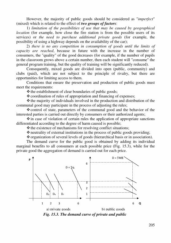
205

However, the majority of public goods should be considered as "imperfect" (mixed) which is related to the effect of two groups of factors:

1) limitation of the possibilities of use that may be caused by geographical

location (for example, how close the fire station is from the possible users of its services) or the need to purchase additional private goods (for example, the possibility of using a highway depends on the availability of the car);

2) there is no any competition in consumption of goods until the limits of

capacity are reached, because in future with the increase in the number of consumers, the "quality" of the good decreases (for example, if the number of pupils in the classroom grows above a certain number, then each student will "consume" the general program training, but the quality of training will be significantly reduced).

Consequently, mixed goods are divided into open (public, community) and clubs (paid), which are not subject to the principle of rivalry, but there are opportunities for limiting access to them.

Conditions that ensure the preservation and production of public goods must meet the requirements:

� the establishment of clear boundaries of public goods; � coordination of rules of appropriation and financing of expenses; � the majority of individuals involved in the production and distribution of the

communal good may participate in the process of adjusting the rules; � control of state, parameters of the communal good and the behavior of the

interested parties is carried out directly by consumers or their authorized agents; � in case of violation of certain rules the application of appropriate sanctions

differentiated according to the degree of harm caused is possible; � the existence of mechanisms for resolving conflict situations; � neutrality of external institutions in the process of public goods providing; � organization of several levels of goods (hierarchical basis or in association). The demand curve for the public good is obtained by adding its individual

marginal benefits to all consumers at each possible price (Fig. 15.3), while for the private good the aggregation of demand is carried out for each price.

D = ∑МВ

3

DС DВ DА

D = ∑qi

6 3 2 1

Р

2

1

Q 6

6

а) private goods b) public goods

Fig. 15.3. The demand curve of private and public

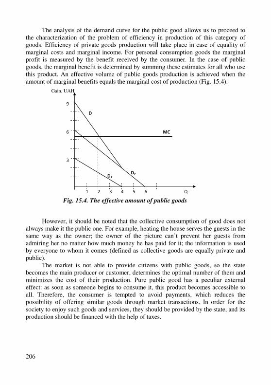
206

The analysis of the demand curve for the public good allows us to proceed to the characterization of the problem of efficiency in production of this category of goods. Efficiency of private goods production will take place in case of equality of marginal costs and marginal income. For personal consumption goods the marginal profit is measured by the benefit received by the consumer. In the case of public goods, the marginal benefit is determined by summing these estimates for all who use this product. An effective volume of public goods production is achieved when the amount of marginal benefits equals the marginal cost of production (Fig. 15.4).

However, it should be noted that the collective consumption of good does not always make it the public one. For example, heating the house serves the guests in the same way as the owner; the owner of the picture can’t prevent her guests from admiring her no matter how much money he has paid for it; the information is used by everyone to whom it comes (defined as collective goods are equally private and public).

The market is not able to provide citizens with public goods, so the state becomes the main producer or customer, determines the optimal number of them and minimizes the cost of their production. Pure public good has a peculiar external effect: as soon as someone begins to consume it, this product becomes accessible to all. Therefore, the consumer is tempted to avoid payments, which reduces the possibility of offering similar goods through market transactions. In order for the society to enjoy such goods and services, they should be provided by the state, and its production should be financed with the help of taxes.

Gain, UAH

D

D2 D1

4 5 6 2 3 1 Q

МС

3

6

9

Fig. 15.4. The effective amount of public goods

207

15.4. The social choice theory and its role in market economy

The social choice of a way to provide citizens with public goods is determined

not by the market but by political processes. The distribution of resources for the production of public goods and services lies with the state authorities, and the government itself, which must organize the production and distribution of public goods, must coordinate their scope and structure with members of society, the choice of subjects that will carry out this production, the choice of methods and the mechanism for the distribution of public goods. The theoretical comprehension of these problems is reflected by the social choice theory.

During a long period of time Western politics and economics the idea that decisions taken by individual politicians, state and non-governmental organizations should aim at maximizing the benefits to society as a whole was dominated. In 1897 K.Viksel first identified politics as a mutually exchange between citizens and social structures by goods. Subsequently, this idea was developed and found its embodiment in the theory of social choice.

Unlike traditional economic research, in the public choice theory, a political market is interacting with politicians (legislators), voters and government officials or bureaucrats. By analogy with the traditional market of goods and services, in this case the seller is a politician, the buyer is a voter, and the state is called to act as an intermediary. Politicians offer packages of various action programs, and voters, are calculated by their votes in case of choosing one of them. The very purchase and sale of election programs and forms are the essence of modern representative democracy.

The simplest model of political and economic cycle can be described as follows: citizen-voters form social benefits; in the political market select the most popular politicians who delegate their powers through voting, and politicians, in turn, pass laws and organize the provision of voters with public goods. By competing for the votes of voters, politicians carry out political advertising that supplies voters with political information. Strategically oriented politicians are trying to take into account the most important needs of their voters.

A simple model of political and economic circle may be complicated by the inclusion of bureaucracy in it. In this model, voters vote for politicians, and politicians appoint bureaucrats who directly influence voters. The bureaucracy is not directly related to the interests of voters, serving, first of all, the interests of different echelons of legislative and executive power. Bureaucrats not only implement already adopted laws, but also actively participate in their preparation, provide policy information and implement through the system of orders bills adopted by them. Through the bureaucrats of the group with special interests, "cultivate" politicians, submitting information in a favorable light for them (Fig. 15.5). In the political market, instead of the principle "one dollar - one vote", the principle "one person - one voice" operates. It is with these theorists of public choice that there is a high probability of emerging in the field of policy results that are not optimal in terms of society.

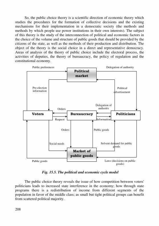
208

So, the public choice theory is a scientific direction of economic theory which studies the procedures for the formation of collective decisions and the existing mechanisms for their implementation in a democratic society (the methods and methods by which people use power institutions in their own interests). The subject of this theory is the study of the interconnection of political and economic factors in the choice of the volume and structure of public goods that should be provided by the citizens of the state, as well as the methods of their production and distribution. The object of the theory is the social choice in a direct and representative democracy. Areas of analysis of the theory of public choice include the electoral process, the activities of deputies, the theory of bureaucracy, the policy of regulation and the constitutional economy.

The public choice theory reveals the issue of how competition between voters' politicians leads to increased state interference in the economy; how through state programs there is a redistribution of income from different segments of the population in favor of the middle class; as small but tight political groups can benefit from scattered political majority.

Information

Orders Public goods

Request

Orders

Pre-election information

Political

advertisement

Public preferences

Social needs

Laws (decisions on public goods)

Delegation of authority

Public goods

Delegation of authority

Solvent demand for public goods

Political

market

Market of

public goods

Politicians Voters Bureaucracy

Fig. 15.5. The political and economic cycle model

209

Training

Key terms and concepts Market economy. Institutions. Institutional environment. Transaction cost.

Property rights. Usus. Abusus. State property. Society interests. Communal

property.

Cost for searching information. External effects. Correction of external effects.

Negative external effect. Positive external effect.

Administrative regulation. Pigou's tax. Pigou's subsidy. Pareto-optimum.

Coase theorem.

Goods. Social goods. Public goods. Pareto-improvement. Imperfect goods.

Mixed goods. Effective size of production of public goods. Free-rider problem.

Theory of public choice. Political market. Market of public goods. Model of

political and economic circle. Referendum. Elections.

Questions and tasks for students’ self-control: 1. Give the explanation of the concept property rights. What is the structure of

property rights?

2. Mention the advantages of private property. 3. What is the basis of decision making in conditions of state property?

4. What do you understand under the concept “transaction cost”? What are the forms of transaction cost?

5. Explain both positive and negative effects of the functioning of micro subjects. 6. What are the main approaches to external effects correction of micro subjects?

7. What does the Piqou’s tax mean and what factors have impact on implementation of this tax?

8. Do you think that external effect always needs state regulation? Justify your answer.

9. What are public goods and which peculiarities do they have?

10. How many groups of public goods there are?

11. Explain the free-rider problem. When does this problem appear?

12. What is the essence of the theory of public choice?

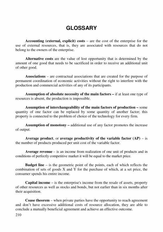
210

GLOSSARY

Accounting (external, explicit) costs – are the cost of the enterprise for the use of external resources, that is, they are associated with resources that do not belong to the owners of the enterprise.

Alternative costs are the value of lost opportunity that is determined by the

amount of one good that needs to be sacrificed in order to receive an additional unit of other good.

Associations – are contractual associations that are created for the purpose of

permanent coordination of economic activities without the right to interfere with the production and commercial activities of any of its participants.

Assumption of absolute necessity of the main factors – if at least one type of

resources is absent, the production is impossible. Assumption of interchangeability of the main factors of production – some

quantity of one factor can be replaced by some quantity of another factor; this property is connected to the problem of choice of the technology for every firm.

Assumption of monotony – additional use of any factor promotes the increase

of output. Average product, or average productivity of the variable factor (AP) – is

the number of products produced per unit cost of the variable factor. Average revenue – is an income from realization of one unit of products and in

conditions of perfectly competitive market it will be equal to the market price.

Budget line – is the geometric point of the points, each of which reflects the combination of sets of goods X and Y for the purchase of which, at a set price, the consumer spends his entire income.

Capital income – is the enterprise's income from the resale of assets, property of other resources as well as stocks and bonds, but not earlier than in six months after their acquisition.

Coase theorem – when private parties have the opportunity to reach agreement

and don’t have excessive additional costs of resource allocation, they are able to conclude a mutually beneficial agreement and achieve an effective outcome.

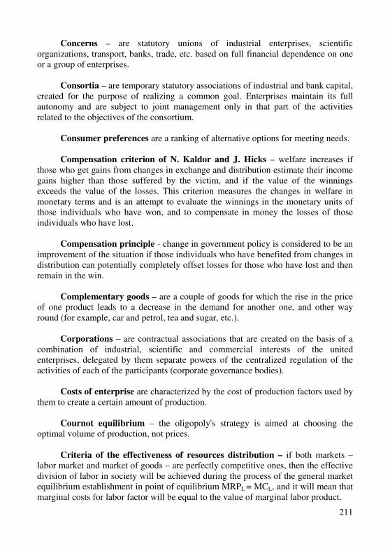
211

Concerns – are statutory unions of industrial enterprises, scientific organizations, transport, banks, trade, etc. based on full financial dependence on one or a group of enterprises.

Consortia – are temporary statutory associations of industrial and bank capital,

created for the purpose of realizing a common goal. Enterprises maintain its full autonomy and are subject to joint management only in that part of the activities related to the objectives of the consortium.

Consumer preferences are a ranking of alternative options for meeting needs. Compensation criterion of N. Kaldor and J. Hicks – welfare increases if

those who get gains from changes in exchange and distribution estimate their income gains higher than those suffered by the victim, and if the value of the winnings exceeds the value of the losses. This criterion measures the changes in welfare in monetary terms and is an attempt to evaluate the winnings in the monetary units of those individuals who have won, and to compensate in money the losses of those individuals who have lost.

Compensation principle - change in government policy is considered to be an

improvement of the situation if those individuals who have benefited from changes in distribution can potentially completely offset losses for those who have lost and then remain in the win.

Complementary goods – are a couple of goods for which the rise in the price

of one product leads to a decrease in the demand for another one, and other way round (for example, car and petrol, tea and sugar, etc.).

Corporations – are contractual associations that are created on the basis of a

combination of industrial, scientific and commercial interests of the united enterprises, delegated by them separate powers of the centralized regulation of the activities of each of the participants (corporate governance bodies).

Costs of enterprise are characterized by the cost of production factors used by

them to create a certain amount of production. Cournot equilibrium – the oligopoly's strategy is aimed at choosing the

optimal volume of production, not prices. Criteria of the effectiveness of resources distribution – if both markets –

labor market and market of goods – are perfectly competitive ones, then the effective division of labor in society will be achieved during the process of the general market equilibrium establishment in point of equilibrium MRPL = MCL, and it will mean that marginal costs for labor factor will be equal to the value of marginal labor product.

212

Current (present) value of future payments – is a present value of sum that may be paid in future.

Curve of demand for resources is the line each point of which shows some number of the resource bought at appropriate price, it has negative slope. This means that increase of price of resource causes the decrease of the number of the resource.

Curve “income-consumption” – is a plurality of all optimal sets of goods at only consumer’s income change.

Curve “price-consumption” connects different points of consumer’s equilibrium created as a result of the change of price.

Declining scale effect – if growth of output volumes will be lagging behind the pace of growth in the volume of resources involved.

Demand – is a form of needs expression that are represented at the market and provided with cash that is solvent need of consumer in some goods.

Demand for investment resource – is the amount of investment funds that consumers are ready to purchase and at the appropriate price.

Demand for resources is determined by some number of production resources

that are used for production output at appropriate price for it. Derived character of the demand for resources means that demand stability

for any resource depends on its productivity and market value of goods produced with the help of this resource.

Diminishing returns of the factors of production is that under certain

circumstances with the increase in the use of one resource for unchanged amounts of the other, each additional unit of variable resource yields less output per unit of time.

Discounting – is a procedure of calculation of the current value of the sum that

may be got in future. Discrimination of the first degree (absolute price discrimination) – is carried

out by the monopolist by setting a price for each consumer at the level of his readiness to pay for this benefit.

Dividend income of an enterprise – is the income from ownership of shares of

other corporations.

Economic costs are payments that should provide the revenue for providers of resources.

213

Economic needs are satisfied through the production of goods and their consumption.

Economic profit – is the difference between revenue and economic costs. Effect of Giffen means that as the price of goods increases demand for it

increases. Effect of income – is the only changes in the consumption of goods caused by

changes in real income, caused by the movement of prices. Effect of substitution – is only those changes in the consumption of goods that

are the result of changes in the price of this product relative to the prices of other goods.

Effect of Veblen – when the price of goods decreases demand for it decreases

(the “effect of snobbery”). Engel curves show how the amount of goods bought by consumer (or group of

them) is connected to the consumer’s income level; they characterize dependence on the amount of consumption from the income of consumer.

Enterprise – is an independent economic entity created by the competent state

or local authorities or other entities to meet social and personal needs through the systematic implementation of industrial, research, trade and other activities in accordance with the procedure provided for by the current legislation.

Equilibrium amount of sales is characterized by the quantity of goods that the

producers agree and able to sell and same time consumers wish and can buy at the appropriate level of the price of a unit of product.

Equilibrium by Nash is represented by the situation where each producer in

cooperation with the rest of the participants, chooses the best variant of behavior, provided that the rest of the market participants adhere to a certain strategy.

Equality criteria – by which the distribution corresponding to the equal value

of the individual's usefulness (U1 = U2 = ... = Un) is the social optimum. Equilibrium price is the market price, at which the volume of demand is equal

to the volume of supply. External effects are additional gains or costs of economic activity (production

and consumption) that are attributable to persons not directly involved in it.

214

Factors of production – are the main elements of the production process that are at the disposal of the enterprise and used by them to achieve specific goals.

Firm is an administrative company of people, united by certain interrelated

activities. Fixed costs are expenditures which value is not been changed with the change

in volumes of production. Function of cost characterizes the dependence of the amount of output and

minimally possible costs necessary for its keeping.

General economic equilibrium describes the circulation of economic life where consumers need goods and offer production factors.

General rule of choosing the optimal volume of production, or general

condition for maximizing profits – profit is maximized in the volume of production, for which the marginal revenue is equal to the marginal cost.

Government is a set of authorities that coordinate and regulate economic life. Growing scale effect – if the growth rate of output exceeds the growth rate of

resources.

Households are groups of people who combine their income, share ownership and make economic decisions together.

Indifference curve – is a graphic representation of different combinations of the sets of benefits that provide the consumer with the same level of utility. All points in this line reflect the same level of customer’s satisfaction.

Internal (implicit) costs are considered as cash payments that property owners

could receive from the alternative use of resources held by them (implicit wages of the owner of the enterprise, whatever he could receive, hired by the employee, profit that could he obtains, by investing in any other enterprise or financial instrument, a rent for the alternative use of his property).

Irreversable costs are costs of resources that have no alternative use; they are

not part of internal costs, never come back to the manufacturer and can’t be alternative.

Isocost curve – shows all possible combinations of labor and capital factors

that a firm can purchase at a given cost level.

215

Isocost map – is the plurality of isocost curves, which illustrate different levels of long-term total costs.

Law of decreasing marginal rate of technological substitution – with increasing use in the production of any factor, the marginal rate of technological substitution unit of this factor to others is reduced, and vice versa.

Law of decreasing marginal utility proves that the total utility increases in

case of increase in consumption of certain goods, and the marginal utility decreases. Law of decreasing return of the variable factor, or the law of decreasing

marginal productivity proves that starting with a certain amount of production, the next increase in the use of an alternating factor, for constant volumes of use of other production factors, is accompanied by a decrease in the marginal product of the variable factor.

Law of demand proves that there is inverse connection between price and

amount of demand: the amount of demand decreases when price increases, and other way round.

Law of supply proves that there is direct connection between price and the

amount of supply: the amount of supply increases with increase of price and other way round it decreases with its reduction.

Long-term period – is a long period of time sufficient to change the amount of

all resources, including production capacities. From the industry point of view, it is a period during which existing firms can be disbanded and left behind, while new firms may emerge and enter the industry. Consequently, in the long-term period, the number of firms in the industry are not been changed.

Low-quality goods are goods the consumption of which decrease when

income of consumer increases. Luxury goods – are goods the consumption of which sharply increases in case

if consumer’s income increases as well.

Map of indifference curves – is a method of representing the consumer’s preferences that have different level of satisfaction of his needs.

Marginal costs characterize the change in the cost of sales as a result of

change in volume of issue per unit; they can be considered as an additional costs associated with the production of one additional unit of product.

216

Marginal external costs – are additional costs connected to production of additional unit of good and not reimbursed by the producer, but transformed to third persons.

Marginal income characterizes the growth of aggregate income as a result of

the sale of an additional unit of output. Marginal private costs – are the marginal cost of particular enterprise. Marginal product, or the marginal productivity of the variable factor (MP)

– is the increase of the aggregate product, or an additional product obtained from the application of an additional unit of the variable factor.

Marginal rate of substitution of product Y by product X (MRSхy) – is the

amount of the product Y, from which the consumer refuses to obtain an additional unit of product X, at the same time, the level of satisfaction of consumer’s needs remains unchanged.

Marginal rate of technological substitution shows from which quantity of

one factor we should refuse to engage in the production of an additional unit of another factor.

Marginal return on the resource – is monetary expression of marginal

productivity of variable production factor or growth of total revenue from selling goods that are produced with the help of additional unit of the resource.

Marginal revenue – is a growth of total revenue as a result of sale of one

additional unit of products. Marginal social costs – are the amount of marginal private expenditures and

marginal external costs. Marginal utility – is a growth, change, additional utility from the consumption

of another one unit of product, that is, the increase in the total utility from the increase of consumption of a certain good per one unit.

Market concentration – is the situation when only a few companies capture

most of the market. Market equilibrium – is a market state at which the amounts of demand and

supply are balanced. Material needs are provided by things, and non-material needs are satisfied

with services, they are considered to be basic or essential requirements of humans.

217

Microeconomics – is a chapter of economic theory that studies the behavior of individual economic actors due to limited resources and alternative ways of their use.

Microeconomic model – is a formal description of the economic process of phenomena which illustrates the system of relationship between economic variables and parameters.

Method of aggregate analysis compares the total income and total costs of the firm and is selected by the amount that maximizes the difference between them.

Method of marginal analysis compares marginal revenue and marginal costs.

Minimally effective size – is the smallest amount of production, in which the firm can minimize its long-term average costs.

Monopoly – is a type of market construction, where only one seller offers the entire market volume of goods for which there are no close substitutes.

Monopolistic competition – is a type of market where a large number of sellers compete for sale of a differentiated product.

Negative externalities occur when the activities of market participants are harmful to others. Negative external effects are the cost of resources used by the manufacturer, but not paid at a market price. An example of the negative effects is the pollution by the industrial enterprise of the environment, for which no compensation is paid.

Needs – are the state of satisfaction the consumer wants to maintain, or the state of dissatisfaction that he would like to change.

Net present value is discounted value of expected profits flows minus sum of investments costs.

Nominal interest rate – is the interest rate expressed in monetary terms at the current monetary rate.

Non-exclusive (impossibility to exclude any entity from consumption) means that it is inappropriate to restrict anyone in the use of public good for purely technical considerations or because of too high costs.

Normal goods are goods for which demand of consumer increases in case of increase of his income level.

Normal profit is built on the basis of competition and alternative pay for the entrepreneur's functions; the amount of such profit is determined by the level of profitability of the industry (normative or average).

218

Normative analysis presents evaluation judgments about the state of the object or subject of the economy according to certain criteria which depend on the views of the researcher, his adherence to certain theoretical concepts.

Ordinal theory has the task of identifying of such a set of two benefits that would allow a consumer to get the maximal utility from the consumption of this set of goods for a limited period of time.

Paradox of Arrow: the transitivity of the preferences of each individual may lead to non-transitivity of collective preferences.

Partial market eauilibrium is provided by establishment of equilibrium price

and equilibrium amount of output under the influence of factors acting only at given local market.

Permanent scale effect – if production volumes grow at the same pace as the

volumes of borrowed resources. Positive analysis studies the real situation in the economy, finds out the

objective relationship between economic phenomena, forms scientific ideas about the principles of behavior of microeconomic actors.

Positive externalities take place when third persons benefit from the economic

activity of participants in a particular market, they are not reflected in the market price (for example, increase in the apple crop in the gardens of the farm because of the placement of nearby apiaries of another farm).

Price of capital asset – is a sum of money by which the unit of capital can be

bought or realized every moment. It includes the current value of future payments flow.

Price discrimination – the seller establishes different price levels for different

consumers; at the same time, there is no any difference in production cost, the only the price is different.

Price elasticity of demand – is a percentage change of the amount of demand

caused by the change of price of this product by 1 %. Price elasticity of supply – is percentage change of the amount of supply

caused by the change of price of product by 1 %. Price of supply – is minimal price at which producers are ready and able to

offer to the market at certain amount of goods.

219

Principle of pricing "cost plus" – that is, the price is set at the level of marginal costs plus a certain increase.

Productive process is a totality of organized processes of work and natural

processes as a result of what raw materials are transformed into final products. Public goods are the commodities that provide the needs of all members of

society equally (national defense, education, public order, scientific researches, environmental protection, etc.).

Rate of return is a correlation of profit minus interest for loan to net investments.

Rawls criterion – it is considered that the main goal of political institutions is

social justice. Real interest rate – is the nominal interest rate minus expected rate of

inflation. Only real interest rates are used to make investment decisions.

Second law of Gossen states that maximization of utility is possible in case when the last monetary unit that is spent on the purchase of any product brings the same measure of satisfaction (utility).

Second type of price discrimination – is selling of individual batches of

goods at different prices. Set of indifference – is this set of consumption baskets with the same level of

utility. Short-term period is a period of time during which the production capacities

of the firm are fixed, but the volume of production can be expanded or reduced at the expense of more or less labor, raw materials, etc. From the point of the industry, the short-term period is the period during which the number of existing firms in the industry does not change.

Social price of monopoly – is amount of cost that society loses as a result of the

market monopolization. Substitute goods – are the couple of goods, for which the increase in the price

of one product causes the growth of demand for another one, and other way round (for example, coffee and tea, trip by train or by bus, etc.).

Supply – is a quantity of goods offered to the market for selling at a certain price

level.

220

Supply of investment resources – is the volume of investment funds provided by their owners at a loan at the appropriate price.

Transaction costs – are expenditures associated with the installation, transfer and protection of property rights to resources.

Third-degree price discrimination – is established in case of allocating

certain categories of consumers with varying demand elasticity, it means market segmentation.

Total income – is the amount of money received from the sale of products on

the market.

Uncompetitiveness (lack of competition in consumption) means that the consumption of goods by one entity does not prevent the consumption of the same good by others.

Usual income – is the income from the sale of goods or services as well as

from the sale of assets of the firm. Utility – is satisfaction the consumer gets from consumption of goods or

services. Utilitarian criterion – society must maximize the utility of all members of

society (aggregate utility) or the overall welfare of society. Utility function is the model that reflects the relationship between the amount

of goods consumers try to buy and the level of utility that consumers try to achieve from it.

Variable costs – are the costs of a firm whose value varies depending on the change in production volumes.

Walras’ general equilibrium model represents the interdependence between markets of goods and markets of production factors in conditions of perfect competition. The very this allows providing the equilibrium of plurality of markets.

Welfare economy finds out the issues of economic efficiency in all areas of

management: production, exchange of benefits, distribution and redistribution.

221

REFERENCES

1. Andreu Mas-Colell. Microeconomic Theory. Hardcover, 1995. – 1008 p. 2. Bade, Robin; Michael Parkin (2001). Foundations of Microeconomics.

Addison Wesley Paperback 1st Edition. 3. Baumol, W. and Blinder, A. (2011). Microeconomics: Principles and Policy.

12th ed. Mason: Cengage Learning, p.504. 4. Bouman, John: Principles of Microeconomics – free fully comprehensive

Principles of Microeconomics and Macroeconomics texts. Columbia, Maryland, 2011.

5. Colander, David. Microeconomics. McGraw-Hill Paperback, 7th Edition: 2008.

6. Frank, Robert H. Microeconomics and behavior. – 4-th ed. Irwin Mc Graw Hill. 2000.

7. Frank, Robert H.; Microeconomics and Behavior. McGraw-Hill/Irwin, 6th Edition: 2006.

8. Gans, J., King, S., Stonecash, R. and Mankiw, G. (2012). Principles of Economics. 5th ed.

9. Jehle, Geoffrey A.; and Philip J. Reny. Advanced Microeconomic Theory. Addison Wesley Paperback, 2nd Edition: 2000.

10. Hal R. Varian. Microeconomic Analysis. Hardcover, Third Edition, 1992. – 576 p.

11. Harnerger, Arnold C. (2008). "Microeconomics". In David R. Henderson (ed.). Concise Encyclopedia of Economics (2nd ed.). Indianapolis: Library of Economics and Liberty. ISBN 978-0865976658. OCLC 237794267.

12. Hirshleifer, Jack., Glazer, Amihai, and Hirshleifer, David, Price theory and applications: Decisions, markets, and information. Cambridge University Press, 7th Edition: 2005.

13. Katz M.L., Rosen H.S. Microeconomics. – 2th. ed. Irwin. Burr Ridge, Illinois, Boston. Massachusettts, Sydney, Australia. 1994.

14. Mankiw, N. Gregory. Principles of Microeconomics. South-Western Pub, 2nd Edition: 2000.

15. Mansfield E. Microeconomics: theory, application. – 7th ed. W. W. Norton & company. New York – London. 1991.

16. Microeconomics : A Contemporary Introduction Wall Street Journal Edition. InfoTrac College Edition by William A. McEachern, Paperback: 480 pages, Publisher: South-Western College.

17. N. Gregory Mankiw. Principles of Microeconomics. Paperback, 4-th Edition, 2006. – 568 p.

222

18. Pindyck R.S., Rubinfield D.L.Microeconomicz. 5th. ed. Prentice-Hall, Inc., Upper Saddle River, New Jercey, 2001.

19. Pindyck, Robert S.; and Daniel L. Rubinfeld. Microeconomics. Prentice Hall, 7th Edition: 2008.

20. Robert S. Pindyck, Daniel L. Rubinfeld. Microeconomics. Hardcover, 6th Edition, 2004. – 720 p.

21. Student guide for learning Microeconomics to accompany Byrns/Stone. Harper Collins College Publishers,1991.

22. Study guide Parcin Microeconomics. Mark Rush. Addison-Welsey Publishing Company,1996.

Internet-resources

1. www.iir.kiev.ua 2. www.bank.gov.ua 3. www.marketing.net.ua 4. www.minfin.gov.ua 5. www.ukrstat.gov.ua 6. www.nas.gov.ua 7. www.iweir.org.ua 8. www.i-soc.kiev.ua 9. www.idss.org.ua 10. www.rvps.kiev.ua 11. www.oecd.org 12. www.goldmansachs.com 13. www.federalreserve.gov 14. www.bloomberg.com 15. www.morganstanley.com 16. www.nber.org 17. www.freedomhouse.org 18. www.imf.org 19. www.worldbank.org 20. www.ebrd.org 21. www.ecb.int 22. www.iie.com 23. www.cato.org 24. www.thelockeinstitute.org www.gmu.edu 25. www.nbia.org 26. www.bis.org 27. www.pubchoicesoc.org 28. www.roubini.com

223

Навчальне видання

Чирак Ірина Миколаївна

МІКРОЕКОНОМІКА

Навчальний посібник

Підписано до друку 21.12.2018 р. Формат 60х90/8. Гарнітура Times.

Папір офсетний. Друк на дублікаторі. Ум.-друк. арк. 12,91. Обл.-вид. арк. 15,18.

Зам № Н0112-18. Тираж 200 прим.

Видавець та виготовлювач Тернопільський національний економічний університет

вул. Львівська, 11, м. Тернопіль, 46004

Свідоцтво про внесення суб’єкта видавничої справи

до Державного реєстру видавців ДК № 3467 від 23.04.2009 р.