noise prediction within conceptual aircraft design - elib-dlr
TRANSCRIPT
Eberhard-Lothar Bertsch
Deutsches Zentrum für Luft- und RaumfahrtInstitut für Aerodynamik und StrömungstechnikBraunschweig
Noise Predictionwithin ConceptualAircraft Design
Forschungsbericht 2013-20

Noise Prediction within ConceptualAircraft Design
Eberhard-Lothar Bertsch
Institute of Aerodynamics and FlowTechnologyBraunschweig
165 Pages95 Figures52 Tables
128 References


TU Braunschweig - Campus Forschungsflughafen
Berichte aus der Luft- und Raumfahrttechnik
Forschungsbericht 2013-05
Noise Prediction within Conceptual Aircraft Design
Eberhard-Lothar Bertsch
Deutsches Zentrum für Luft- und Raumfahrt Institut für Aerodynamik und Strömungstechnik
Braunschweig Diese Veröffentlichung wird gleichzeitig in der Berichtsreihe „Campus Forschungsflughafen - Forschungsberichte“ geführt. Diese Arbeit erscheint gleichzeitig als von der Fakultät für Maschinenbau der Technischen Universität Carolo-Wilhelmina zu Braunschweig zur Erlangung des akademischen Grades eines Doktor-Ingenieurs genehmigte Dissertation.

Noise Prediction within Conceptual Aircraft Design
Von der Fakultät für Maschinenbauder Technischen Universität Carolo-Wilhelmina zu Braunschweig
zur Erlangung der Würdeeines Doktor-Ingenieurs (Dr.-Ing.)
genehmigte Dissertation
vonDipl.-Ing. Eberhard-Lothar Bertsch, M.Sc.
aus Stuttgart
Eingereicht am: 06.12.2012
Mündliche Prüfung am: 13.08.2013
Berichterstatter: Prof. Dr.-Ing. Jan DelfsProf. Dr.-Ing. Peter Horst
Vorsitzender: Prof. Dr.-Ing. Rolf Radespiel
2013

Eidesstattliche Erklärung
Hiermit versichere ich an Eides statt, dass ich die vorliegende Arbeit selb-ständig angefertigt habe. Alle benutzten Hilfsmittel sind angegeben. DieseArbeit ist bisher weder veröffentlicht noch an einer anderen Hochschule ein-gereicht worden.Aus Aktualitätsgründen wurden Auszüge der vorliegenden Arbeit in wis-senschaftlichen Artikeln vorveröffentlicht [40–44, 84, 94, 104, 112, 123–126].
Göttingen, im Dezember 2012(Unterschrift)
Eberhard-Lothar Bertsch
Abstract
Motivation for the presented activities is the integration of noise as an additional objectivein conceptual aircraft design. Therefore, the Parametric Aircraft Noise Analysis Module(PANAM) is developed to account for individual noise sources depending on their geom-etry and operating conditions. Each major noise source is modeled with an individualsemi-empirical noise source model. These models capture the major relevant correlations,can still be executed on a standard desktop PC, and provide comprehensive simulation re-sults. All models and approximations are based on physics, thus PANAM can be classifiedas a scientific prediction method. Dedicated validation with experimental data confirmsfeasible overall aircraft noise prediction. The noise tool is integrated into an existing air-craft design framework in order to realize an overall design process with integrated noiseprediction capabilities. A multiple criteria design evaluation is introduced, to quicklyassess the environmental and economical performance of different vehicles under variousscenarios. The process is applied to identify promising low-noise aircraft concepts with thefocus on realizable, medium term solutions. It is demonstrated, that the aircraft designer’sinfluence on the environmental vehicle performance is significant at the conceptual designphase. Extensive engine noise shielding is achieved for over-the-fuselage mounted enginesresulting in a 10 EPNdB overall noise reduction. In conclusion, PANAM can be ranked aswell suitable to assess all four measures of ICAO’s balanced approach.
Keywords: Aircraft noise prediction, low-noise aircraft design, parametric and com-ponential noise source modeling, engine noise shielding, scientific prediction method,noise abatement procedure design, helical noise abatement procedure, PANAM, PrADO,SHADOW, HeNAP

Zusammenfassung
Die Motivation der Arbeit ist die Einbindung von Lärm als zusätzlichem Entscheidungskri-terium innerhalb des Flugzeugvorentwurfs. Daher wird ein Programm PANAM zurFluglärmvorhersage entwickelt, das den Beitrag ausgewählter Lärmquellen anhand derenGeometrie und Betriebsbedingungen berücksichtigt. Dabei kommen für jede Einzelquelleindividuelle und semi-empirische Rechenmodellen zum Einsatz. Die ausgewähltenModelle berücksichtigen die wesentlichen Zusammenhänge, stellen geringe Rechner-anforderungen und generieren dabei nachvollziehbare Ergebnisse. PANAM kann alswissenschaftliches Berechnungsverfahren klassifiziert werden, da alle implementiertenModelle und Näherungsverfahren auf physikalischen Grundlagen basieren. Ein direkterVergleich von Simulationsergebnissen mit experimentellen Daten bekräftigt die Richtigkeitder berechneten Ergebnisse. Durch die Integration von PANAM in eine existierendeFlugzeugentwurfsumgebung wird der konventionelle Entwurfsprozess um die Fähigkeitzur Lärmvorhersage erweitert. Eine neu eingeführte Bewertungsmetrik erlaubt den di-rekten Vergleich von Wirtschaftlichkeit und erzeugtem Fluglärm für unterschiedlichsteFlugzeugkonzepte. Der erweiterte Prozess wird schließlich angewendet, um vielver-sprechende, lärmarme Entwürfe zu identifizieren. Dabei liegt der Schwerpunkt aufmittelfristig realisierbaren Konzepten und Technologien. Es kann gezeigt werden, dassdurch Entscheidungen im Flugzeugvorentwurf ein signifikanter Einfluss auf die ökologis-che Flugleistung des finalen Entwurfes genommen wird. Dabei können durch geeigneteAbschattung des Triebwerklärms lokal bis zu 10 EPNdB Lärmreduktion erreicht werden.Allgemein kann PANAM dazu eingesetzt werden, alle von der ICAO als "balanced ap-proach" vorgeschlagenen Maßnahmen zur Lärmreduktion zu untersuchen.
Schlagwörter: Fluglärmvorhersage, lärmarmer Flugzeugentwurf, parametrische und kom-ponentenweise Lärmquellmodellierung, Treibwerkslärmabschattung, wissenschaftlicheVorhersagemethode, lärmarme An- und Abflugverfahren, Spiralanflug, PANAM, PrADO,SHADOW, HeNAP

iv Noise Prediction within Conceptual Aircraft Design
Danksagung
Diese multidisziplinäre Arbeit ist parallel zu meiner Tätigkeit als wissenschaftlicher Mi-tarbeiter am DLR Institut für Aerodynamik und Strömungstechnik entstanden. Jeglichemultidiziplinäre Aufgabe ist ohne Unterstützung und gute Zusammenarbeit mit den Ex-perten der jeweiligen Disziplinen nicht denkbar. An dieser Stelle möchte ich die tolleKollegialität hervorheben, die ich institutsübergreifend innerhalb des DLR und von ex-terner Seite erfahren habe.Besonders bedanken möchte ich mich bei folgenden ausgewiesenen Experten für diegute Zusammenarbeit: Dr. Wolfgang Heinze (Flugzeugentwurf, TU Braunschweig), Dr. Se-bastien Guérin und Dr. Werner Dobrzynski (Lärmquellmodellierung, DLR) und Dr. MarkusLummer (Abschattungseffekte, DLR). Weiterhin danke ich Dr. Ullrich Isermann und Dr.Rainer Schmid (Fluglärmvorhersage, DLR), Dr. Gertjan Looye (Flugmechanik, DLR) undTom Otten (Triebwerksmodellierung, DLR) für ihre Unterstützung.Vielen Dank für stets offene Türen und für viele Diskussionen und Anregungen.
Ich bedanke mich bei Prof. Jan Delfs (DLR) für die sehr gute Betreuung dieser Arbeit.Insbesondere bedanke ich mich für viele interessante Diskussionen und Treffen trotz seinesprall gefüllten Terminkalenders! Ich habe mich sehr gefreut, Prof. Peter Horst als zweitenBerichterstatter und Prof. Rolf Radespiel als Vorsitzenden zu gewinnen (beide TU Braun-schweig) und bedanke mich bei beiden dafür.
Schließlich möchte ich mich an dieser Stelle noch herzlich für den positiven Zuspruchund den Rückhalt durch meine Eltern und Geschwister, sowie im Freundeskreis bedanken.
2013-20
Contents
1 Introduction 11.1 Background . . . . . . . . . . . . . . . . . . . . . . . . . . . . . . . . . . . . . . 1
1.2 Motivation . . . . . . . . . . . . . . . . . . . . . . . . . . . . . . . . . . . . . . . 3
2 Related Work & Literature Overview 52.1 Overall Aircraft Noise Prediction . . . . . . . . . . . . . . . . . . . . . . . . . . 5
2.2 Aircraft Noise Reduction Concepts . . . . . . . . . . . . . . . . . . . . . . . . . 10
3 Methods, Tools, and overall Process 133.1 Requirements . . . . . . . . . . . . . . . . . . . . . . . . . . . . . . . . . . . . . 13
3.2 Overall Aircraft Noise Prediction Tool . . . . . . . . . . . . . . . . . . . . . . . 14
3.2.1 Concept . . . . . . . . . . . . . . . . . . . . . . . . . . . . . . . . . . . . 15
3.2.2 Noise Source Modeling . . . . . . . . . . . . . . . . . . . . . . . . . . . 18
3.2.3 Tool Input . . . . . . . . . . . . . . . . . . . . . . . . . . . . . . . . . . . 42
3.2.4 Modi operandi . . . . . . . . . . . . . . . . . . . . . . . . . . . . . . . . 44
3.2.5 Tool Output . . . . . . . . . . . . . . . . . . . . . . . . . . . . . . . . . . 44
3.3 Aircraft Design with Integrated Noise Prediction Capabilities . . . . . . . . . 46
4 Validation 494.1 Conceptual Design vs. Aircraft Data and Specifications . . . . . . . . . . . . . 49
4.2 Flight Simulation vs. Recorded Flight Data . . . . . . . . . . . . . . . . . . . . 50
4.3 Noise Prediction vs. Textbook Theory . . . . . . . . . . . . . . . . . . . . . . . 51
4.4 Noise Prediction vs. Measurements . . . . . . . . . . . . . . . . . . . . . . . . . 59
4.4.1 A319 Flyover Campaign . . . . . . . . . . . . . . . . . . . . . . . . . . . 59
4.4.2 Additional comparison . . . . . . . . . . . . . . . . . . . . . . . . . . . 64
5 Application 675.1 Low-Noise Vehicle Design . . . . . . . . . . . . . . . . . . . . . . . . . . . . . . 67
5.1.1 Reference Vehicle and Design Mission . . . . . . . . . . . . . . . . . . . 68
5.1.2 Evaluation Metric . . . . . . . . . . . . . . . . . . . . . . . . . . . . . . . 70
5.1.3 Solution Space Limitations . . . . . . . . . . . . . . . . . . . . . . . . . 73
v
vi Noise Prediction within Conceptual Aircraft Design
5.1.4 Vehicle Variants . . . . . . . . . . . . . . . . . . . . . . . . . . . . . . . . 74
5.1.5 Alternative Propulsion Technologies . . . . . . . . . . . . . . . . . . . . 83
5.2 Decision Making Support . . . . . . . . . . . . . . . . . . . . . . . . . . . . . . 89
5.2.1 Noise Abatement Flight Procedures . . . . . . . . . . . . . . . . . . . . 89
5.2.2 Airspace and Airtraffic Management . . . . . . . . . . . . . . . . . . . . 91
6 Results and Discussion 93
7 Conclusions 97
A Figures, Tables, and Derivations 107A.1 Weighting, Sound Propagation, and Ground Effects . . . . . . . . . . . . . . . 107
A.2 Textbook Theory . . . . . . . . . . . . . . . . . . . . . . . . . . . . . . . . . . . 108
A.3 A319 Flyover Campaign . . . . . . . . . . . . . . . . . . . . . . . . . . . . . . . 111
A.4 Low-Noise Vehicle Design . . . . . . . . . . . . . . . . . . . . . . . . . . . . . . 125
B Additional Items 157
2013-20
Glosary & Nomenclature
Abbreviations
ACARE Advisory Council for Aeronautics Research in EuropeANoPP Aircraft Noise Prediction Program, NASAATA Air Transport AssociationCDA Continuous Descent ApproachCROR Counter-Rotating-Open-RotorEMPA Federal Laboratories for Materials Testing and Research, SwitzerlandEPNL Effective Perceived Noise LevelFAA Federal Aviation AdministrationFLULA Noise prediction tool by EMPAFW-H Ffowcs-Williams and Hawkings (equation, surface)FMP Fast-Multipole Code, DLRGTF Geared Turbofan EngineHeNAP Helical Noise Abatement ProcedureHTP Horizontal Tail PlaneICAO International Civil Aviation OrganizationIESTA Infrastructure for Evaluating Air Transport
Systems simulation framework, ONERAINM Integrated Noise Model, FAAIOPANAM PrADO - PANAM interface moduleLEQ Equivalent Sound Pressure LevelLDEN Day-Evening-Night Sound LevelLNA DLR’s Low Noise Aircraft conceptMLW Maximum Landing WeightMTOW Maximum Take-off WeightMZFW Zero-fuel weightNPD Noise-Power-Distance tablesOEW Operational Empty WeightPANAM Parametric Aircraft Noise Analysis Module, DLRPrADO Preliminary Aircraft Design and Optimization, TU BraunschweigSAE Society of Automotive EngineersSHADOW Ray-Tracing tool to evaluate engine noise shielding, DLRSIMUL Noise prediction tool by DLRSIMMOD Fast time airport capacity analysis tool, FAASOPRANO Silencer Common Platform for Aircraft Noise Calculations, ANOTECSPL, SPL(A) Sound Pressure Level, A-weighted SPLTAS True Air SpeedTLAR Top Level Aircraft Requirements
vii
viii Noise Prediction within Conceptual Aircraft Design
TIVA Simulation environment, DLRVTP Vertical Tail Plane
Scripting
0, 0⃝ Freestream conditions (engine station numbering), characteristic level2, 2⃝ Fan front face9, 9⃝ Primary exhaust nozzle throat, far-field conditions13, 13⃝ Secondary flow: fan exit plane19, 19⃝ Secondary exhaust nozzle throat, far-field conditions21, 21⃝ Primary flow: fan exit plane∞ Ambient conditionsa Airfoil, Axles on selected landing geara/c Aircraft, aircraft fixedbbn Broadband noisec-jet Coaxial, shock-free jetscon Convectivectn Combination-tone noisedir Directivity adjustmentdtn Discrete-tone noisee Emissioneq Equivalentex Fan exhaust engine stationexp Experimental dataf Flap elementfg Front landing gearg Earth-fixed coordinate system, landing geargeo Geometry adjustmenti Impact, immission, scenarioin Fan inlet engine stationis IsentropicISA Levels at sea level (0 m) according to the International Standard Atmosphere (ISA)jet Isolated, shock-free jetl Liftlam Laminarm Mean valuemg Main landing gearnorm Reference normal level (base level)p Coaxial jet: primary flowr Rotorref Reference valuerecX Flight test no. X, Parchim Campaign (see Tab. A.7)s Coaxial jet: secondary flow, slat element, statorspec Spectral shape adjustmentt Total, overallTE Trailing edgevel Velocity dependent adjustment
2013-20
ix
Symbols
< a2 > Root-mean-square value (RMS), time averageA Time average level−→a b Unit vector a in coordinate system b−→A b Vector A in coordinate system bAb
c Component c of vector A in coordinate system b
Variables
A Area, reference area m2
α Angle of attack ◦
α∗ Polar noise emission angle ◦
β Bank angle ◦
β∗ Longitudinal noise emission angle ◦
c Mean chordlength, speed of sound,correction, local coefficient m, m/s, dB, -
C Overall vehicle coefficient, empirical constant -, -d Relative distance between aircraft and
observer: d = |−→Da/c| m
D (Hydraulic) diameter, distance m, mδ Boundary layer thickness, cut-off condition,
deployment angle, extraction factor ◦, -, m, -∆ Level difference, time difference dB, sδ∗ Boundary layer displacement thickness mη Efficiency -f Frequency Hzf(x) Function of "x" -γ Flight path angle, installation angle ◦, ◦
i Acoustic intensity per noise W/m5
source volume; normal to trailing edgeI Acoustic intensity normal to trailing edge W/m2
Iref Reference value of acoustic intensity, Iref = 10−12 W/m2
l Length mL Sound pressure level (SPL) dBΛ Aspect ratio -Ma Mach number -µ Observer location -n Number of elements -ν Dihedral angle, kinematic viscosity ◦, m2/sO Observer location mP Aircraft location mp Pressure signal PaΠ Total pressure ratio -
2013-20
x Noise Prediction within Conceptual Aircraft Design
Ψ Sweep angle ◦
ρ Flow density kg/m3
rss Rotor-stator-spacing mStr Strouhal number -t Event time sT Thrust force Nu Velocity scale for the turbulence m/sv Velocity (True Air Speed) m/sV Volume m3
φ Aircraft flight position -w Element width, density exponent (hot jet) m, -W Weight force Nx Length my Wall distance of the maximum turbulent kinetic energy m
Vehicle Design Nomenclature
v Vehicle variantsV Final vehicle designSubscriptsr Design category: Reference vehicle0 Design category: Over-the-wing installed engines1, 1-1, 1-2 Design category: Rear fuselage mounted engines2 Design category: Over-the-fuselage mounted enginesx Design category: Wing/empennage integration with covered enginesg Alternative propulsion: GTFc Alternative propulsion: CROR
Multiple criteria design evaluation
κi Predefined (user selected) environmental weighting, applicable to ξiK Scenario dependent overall environmental weighting, applicable to ξλi Predefined (user selected) economical weighting, applicable to ζiΛ Scenario dependent overall economical weighting, applicable to ζσ Overall scenario score: Environmental and economical performanceξi Environmental performance indicator (vehicle specific)ξ Overall environmental performance indicator (vehicle specific)ζi Economical performance indicator (vehicle specific)ζ Overall economical performance indicator (vehicle specific)
2013-20
1 Introduction
1.1 Background
According to the Advisory Council for Aeronautics Research in Europe (ACARE), the worldwidegrowth of air traffic over the last 50 years will continue in the future [1]. The demand for airtransportation is expected to rise with increasing population density, especially in growingmarkets; e.g., India and China. Consequently, the percentage of world population subject toaircraft noise is expected to grow significantly. High airspace traffic density, additional run-ways and airports ultimately require new air traffic routing of approaching and departingaircraft. This means, installation of new routes or displacement of existing flight corridorswill affect additional communities. This significant increase in aviation noise pollutioncan be directly associated with unfavorable effects on people’s health and with negativeeconomical effects for individuals as well as for aircraft and airport operators.
According to Smith [16], aircraft can be assigned to the most dominating noise sourcesof our times. Sound pressure levels close to a jet aircraft engine under take-off conditionscan reach the human threshold of pain with respect to noise [76]. Aircraft ground noiselevels comparable to a heavy truck passing by, i.e. noise levels in the order of 70 − 80 dBA,can still be measured at large distances up to 20 kilometers from the airport location1. As aconsequence, communities far beyond the direct vicinity of an airport can still be subject tosignificant aircraft noise perception.
Residents living in close proximity to airports have established numerous consortiumsand dedicated citizen’s initiatives against aircraft noise pollution in the past. Nearly allcommunities located in the neighborhood of a German airport are engaged in one of theseinitiatives in order to fight aircraft noise pollution and the associated negative implicationson personal health and local economy. Independent scientific studies directly correlateaircraft ground noise levels in Germany with community annoyance and, more so, withadverse effects on the health of exposed individuals [2]. As identified in various extensiveresearch activities, the communities in close proximity to major airports are subject toincreased noise annoyance, occurrences of sleep interruptions, and even cardiovascular dis-eases [3, 4]. Obviously, there is no direct correlation of medical implications into monetaryvalues available, thus it is extremely difficult to assess a feasible economical impact.In general, no direct local economical impact of aviation noise pollution can be identified.Yet, there are initial studies with respect to real estate values in aviation noise affected com-munities. A dedicated study correlates real estate value with aviation noise levels for theRhein-Main-Area according to realtors and monetary institutions [5]. A negative impact of
1e.g. Frankfurt airport noise monitoring system, http://franom.fraport.de/franom.php (accessed08 January 2012)
1
2 Noise Prediction within Conceptual Aircraft Design
high aviation noise levels on real estate values and corresponding economical implicationsis predicted. In 2010 the German Federal Constitutional Court (Bundesverfassungsgericht)strengthened the legal rights of private property owners against traffic noise exposure. Inthe event of unacceptable noise exposure they are entitled to increased financial compensa-tion2.According to the German Aviation Noise Protection Law (Fluglärmgesetz), airport opera-tors are required to identify and label areas subject to long-term elevated noise levels. Theseareas are declared as noise protection zones where affected private homes are entitled topassive noise protection measures on the expense of the airport operator.
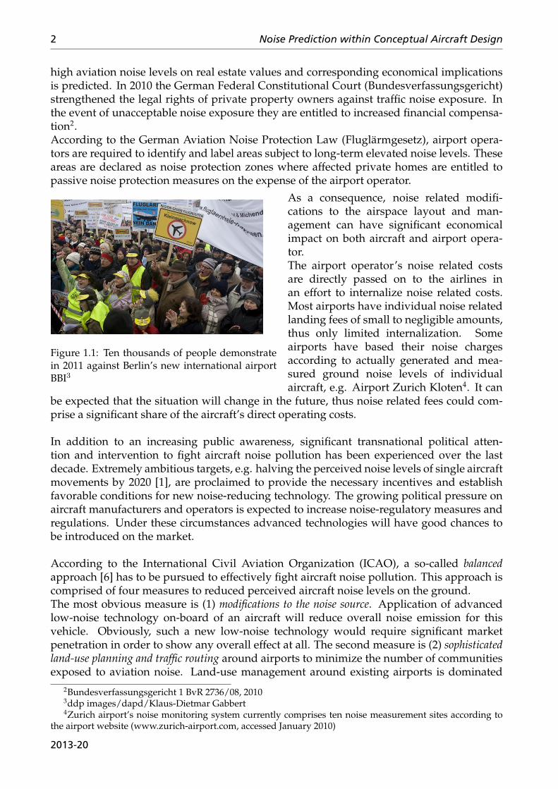
As a consequence, noise related modifi-
Figure 1.1: Ten thousands of people demonstratein 2011 against Berlin’s new international airportBBI3
cations to the airspace layout and man-agement can have significant economicalimpact on both aircraft and airport opera-tor.The airport operator’s noise related costsare directly passed on to the airlines inan effort to internalize noise related costs.Most airports have individual noise relatedlanding fees of small to negligible amounts,thus only limited internalization. Someairports have based their noise chargesaccording to actually generated and mea-sured ground noise levels of individualaircraft, e.g. Airport Zurich Kloten4. It can
be expected that the situation will change in the future, thus noise related fees could com-prise a significant share of the aircraft’s direct operating costs.
In addition to an increasing public awareness, significant transnational political atten-tion and intervention to fight aircraft noise pollution has been experienced over the lastdecade. Extremely ambitious targets, e.g. halving the perceived noise levels of single aircraftmovements by 2020 [1], are proclaimed to provide the necessary incentives and establishfavorable conditions for new noise-reducing technology. The growing political pressure onaircraft manufacturers and operators is expected to increase noise-regulatory measures andregulations. Under these circumstances advanced technologies will have good chances tobe introduced on the market.
According to the International Civil Aviation Organization (ICAO), a so-called balancedapproach [6] has to be pursued to effectively fight aircraft noise pollution. This approach iscomprised of four measures to reduced perceived aircraft noise levels on the ground.The most obvious measure is (1) modifications to the noise source. Application of advancedlow-noise technology on-board of an aircraft will reduce overall noise emission for thisvehicle. Obviously, such a new low-noise technology would require significant marketpenetration in order to show any overall effect at all. The second measure is (2) sophisticatedland-use planning and traffic routing around airports to minimize the number of communitiesexposed to aviation noise. Land-use management around existing airports is dominated
2Bundesverfassungsgericht 1 BvR 2736/08, 20103ddp images/dapd/Klaus-Dietmar Gabbert4Zurich airport’s noise monitoring system currently comprises ten noise measurement sites according to
the airport website (www.zurich-airport.com, accessed January 2010)
2013-20
1. Introduction 3
by economical interests and aircraft noise pollution will have only very limited influence.Yet, aircraft noise significantly influences land-use management when planning additionalrunways at existing airports or investigating locations for new airports. Most major airportsreroute their approaching and departing air traffic according to the surrounding populationdensity. Traffic is detoured via selected low-populated areas instead of using the shortestavailable and most economic route to the airport. The third approach to reduce aircraftnoise is (3) the installation of operational constraints at a specific airport. These constraints, e.g.night curfews, can limit the overall number of flight operations or reduce overall operatinghours of the selected airport. Furthermore, constraints and quota regulations will havean impact on flight schedule and fleet mix at the airport, e.g. noisy aircraft types can bebanned from operation in order to reduce surrounding ground noise pollution. A verygeneral and effective approach to reduce overall ground noise levels are (4) noise abatementflight procedures. Noise abatement procedures are approach or departure flights that alongwhich the aircraft can be operated with reduced ground noise impact or with favorablenoise dislocation effects. Any aircraft with current engine and airframe technology provid-ing the required navigational and flight performance can operate along such a procedure.Implementing new low-noise flight procedures at an airport could immediately reducecommunity noise levels.In addition to ICAO’s balanced approach, modifications to the receiver/observer instantlydecrease perceived noise levels for each fly-over event. For example, sound proof windowscan be counted toward these so-called passive protection measures.
1.2 Motivation
The focus of the presented work lies on the aircraft designer’s influence on overall aircraftnoise reduction, e.g. advanced on-board technology and new low-noise vehicles. The fullpotential of low-noise vehicle design can only be exploited if underlying discipline interde-pendencies, e.g. modifications to the noise source versus flight performance, are identifiedand simultaneously accounted for in a so called concurrent approach [7]. Maximum noisereduction from the aircraft designer’s perspective can only be achieved through a combina-tion of low-noise technology and dedicated overall aircraft design to enable low-noise flightperformance.
In the context of overall aircraft design, major interactions of involved engineering dis-ciplines have to be accounted for early within the decision making process. Early withinthis process, e.g. at the conceptual aircraft design stage, major aircraft and engine designparameters are still subject to change. At this point the dominating design parameters,e.g. wing span, are determined by underlying mission requirements which drive the finalaircraft concept. There are only few parameter limitations at the conceptual design stageresulting in an extensive solution space. Low-noise technology needs to be investigated atthat design level in order to identify and incorporate resultant and necessary modificationsto the overall aircraft and engine layout. Moreover, negative or adverse effects of selectedlow-noise technology and systems on correlated disciplines can be identified and coun-teracted. Depending on available noise prediction capabilities, the setting of basic designparameters can be optimized for best economical and acoustical performance according tothe selected Top Level Aircraft Requirements (TLAR). The identification of such an optimalparameter setting completes the conceptual aircraft design phase that dominates the final
2013-20
4 Noise Prediction within Conceptual Aircraft Design
vehicle layout. Major modifications to the basic vehicle layout are ruled out in subsequentand more detailed design stages due to a large number of fixed design parameters anddefined constraints. Ultimately, sophisticated noise prediction capabilities at early vehicledesign stages are fundamental when it comes to overall aircraft noise reduction.
Despite obvious advantages of noise analysis in conceptual aircraft design, noise evalu-ation is usually not accounted for in that early design stage due to the lack of appropriatenoise prediction methods. Parametric and componential prediction methods are requiredin order to account for the impact of geometry modifications and operating conditions onboth component and overall aircraft noise emission. Such methods would allow to monitorindividual noise sources throughout simulated flight operation thus noise related effectscould be identified and analyzed. The quantity and complexity of required input parame-ters for the noise prediction have to be adequate for conceptual design hence impose furtherrequests on a suitable noise prediction methodology. A modular and simple implementa-tion of the method is required to allow for direct integration into existing multidisciplinaryconceptual aircraft design codes. High fidelity prediction methods such as ComputationalAeroacoustics or time-accurate Computational Fluid Dynamics are ruled out due to theirCPU requirements which are not compatible with an iterative conceptual design process.Therefore, fast prediction methods are required to finally determine the level and directivityof the aircraft noise emission according to conceptual aircraft and engine design, configura-tion, and operating conditions.
In conclusion, the main objective of the presented work is to establish a conceptual air-craft design process with integrated noise prediction capabilities. Thereby it is inevitableto account for both vehicle design and operating condition in order to address noise inthe context of the overall aircraft system. A direct process implementation results in noiseas a new constraint in the overall design process. This could enable a fully automatedlow-noise aircraft design optimization. Each new vehicle concept can then simultaneouslybe evaluated for its resulting economical and environmental performance. Different vehicleconcepts out of an available solution space can directly be compared with each other toobtain the most promising solution under preselected requirements. Ultimately, promisingdesign drivers and sensitivities toward economically efficient overall noise reduction can beidentified from an aircraft designer’s point of view. These findings can be correlated to themodeled physical effects within the simulation, thus can directly be assigned to their cause.Obviously, adequate simulation of the underlying multidisciplinary interdependenciesbecomes crucial in order to evaluate promising technologies and their impact on the overallsystem.
2013-20
2 Related Work & Literature Overview
In this chapter, an overview of related work in the context of aircraft noise prediction andlow-noise design is presented. In order to assess the environmental impact of an overallaircraft system, a fast and robust noise prediction software is required [9]. Several tools areavailable that meet this general requirement. Each of these tools can be assigned to a cer-tain development background and to specific applications in the context of overall aircraftnoise prediction. Based on these inherent simulation characteristics, a general classifica-tion for noise prediction tools is introduced. In accordance to the new classification, a briefoverview of the most important available tools is presented.Furthermore, a literature overview of existing aircraft noise reduction concepts is presented,including low-noise design modifications and operational concepts. Promising suggestionsare discussed and selected for further investigation within this work. Based on these sug-gestions, an initial solution space for promising low-noise technology can be derived.
2.1 Overall Aircraft Noise Prediction
Existing fast overall aircraft noise prediction tools can be separated into three main cate-gories, referred to as best practice, hybrid, and scientific prediction methodologies.
Best-practice prediction methodology
Tools assigned to the best-practice methods are based on (fully) empirical models derivedfrom ground noise measurements of a specific aircraft. The measured noise immission iscorrected by simulated propagation effects in order to determine the originating emissionnoise level of this aircraft. The underlying noise level database and the applied methodsare verified and standardized, as described in corresponding literature [10–12]. The noisesource modeling is inherently reduced to one overall noise source for the entire aircraft,i.e. mainly engine noise contribution. As a result, alternating dominance of airframeand engine noise contribution during realistic (approach) flight procedures, precisely thecomplex schedule of configurational changes along typical flight procedures, can not beaccounted for. Consequently, the application of these tools should be limited to the simu-lation of (take-off) procedures with dominating engine noise contribution. Modeling of theoverall aircraft noise is significantly simplified caused by the mixing of noise generationand propagation effects. Defined corrections are applied to the underlying data in order tosimulate the influence of flight velocity and/or thrust on noise levels, i.e. under varyingoperational conditions. Some tools use simple methods to account for directivity effects,others incorporate noise directivity within their underlying data bases.Initially, the application of a best-practice tool is limited to the existing vehicles and tech-
5
6 Noise Prediction within Conceptual Aircraft Design
nology stored in the underlying database. In order to evaluate new technology, the originaldatabase can be modified with available data representing the new vehicle, i.e. referred toas substitution.Best-practice tools are usually developed for the evaluation of medium to long term averagenoise levels around airports rather than for prediction of single flyover events [14]. Bestagreement to experimental data can be achieved if multiple flyover events and airspacescenarios are evaluated. Results can be accurate to approximately ± 1 to ± 2 dB [13, 15]for observers located along the flight ground track with the aircraft operating in loweraltitudes. Although, if predicting long-term average noise contours, even these small varia-tions have an impact, i.e. a 20% deviation in predicted isocontour areas per 1 dB [16]. Resultaccuracy can be significantly reduced for observers located off-side the flight ground track,for shallow angles of incidence, and with increasing distance between aircraft and observerlocation [15].Due to their prediction accuracy for longterm scenarios, best-practice tools qualify forapplication in air traffic management and legislation processes. The focus of applicationslies on noise protection zones, land-use planing, and consulting. Potential users are foundat airports, airlines, and in legislation. Often, such tools have a commercial or corporatebackground in order to compensate the high development costs.
The most prominent example for this kind of tool is the Integrated Noise Model (INM) bythe Federal Aviation Administration [17]. INM is applied by researchers, airport planners,and authorities world-wide to evaluate the impact of airspace management on communitynoise impact. With INM, the impact of modifications to flight path, runway/airport layout,and fleet mix on overall ground noise can be accounted for. In this context, INM can forexample output maximum or time-integrated noise levels and corresponding isocontourareas.INM uses Noise-Power-Distance (NPD) tables based on aircraft noise certification data topredict ground noise immission. The NPD data has been normalized to specified, straighthorizontal flight segments with constant operational and configurational setting. To predictground noise immission along a selected flight path, the corresponding trajectory is assem-bled from these straight flight segments. To account for curved flight segments, specificmodifications are applied to the noise data.At Delft University of Technology INM has been implemented into their trajectory op-timization process to study environmental friendly departure procedures for a selectedairport scenario [18]. Conventional departure trajectories have been optimized for minimalcommunity noise impact by integrating a geographic information system into the process.
A second example for this group of noise prediction tools is FLULA [19] by the SwissFederal Laboratories for Materials Testing and Research, EMPA. The noise prediction isbased on dedicated aircraft noise measurements recorded along individual flyover eventswith an array of microphones. Polynomial functions are derived from measured spectralnoise levels and directivity patterns for best fitting of experimental data and predictions.Rotational symmetry in noise directivity is assumed hence the polynomials are functionsof the polar angle and the distance between aircraft and observer only. Correspondingcoefficients are identified and derived from the measurements for each individual aircrafttype. To incorporate the influence of aircraft speed, further modifications are applied to thepolynomial. Finally, relevant sound propagation effects are accounted for.
2013-20
2. Related Work & Literature Overview 7
Hybrid prediction methodology
In contrast to the best-practice methods, hybrid prediction models separate the overallaircraft noise into its major contributions. Instead of approximating the aircraft as onesingle noise source, a number of individual noise contributions is accounted for. Thiscomponential modeling can be limited to a separation into airframe and engine noise, or befurther subdivided into individual components such as high-lift system noise. The noiseemission of each noise source is modeled according to an individual database, e.g. derivedfrom flyover noise measurements (array), componential wind-tunnel experiments, andcomputational findings. Based on this data, physics-based approximations are derived inorder to account for specific operational conditions, e.g. flight speed and thrust setting. Asa consequence, hybrid prediction models enable to investigate low-noise flight procedures,especially approach procedures with varying configurational setting. Low-noise modifica-tions to individual noise sources can be accounted for by manipulating the correspondingcomponent’s data base. Yet, parameter variations with respect to aircraft or engine designare not possible due to the fact that noise source modeling is based on stored and prepro-cessed data.As a conclusion, the data-based noise source modeling results in fast computation timesand a good agreement of prediction and measurements.
An example for hybrid prediction methods has been developed at DLR, the tool SIMUL [20].Several flight tests have been performed to identify dominating noise sources and their di-rectivity corresponding to current speed, thrust, and configurational settings [21]. Thisextensive database allowed to further break down overall aircraft noise into contributionsof airframe, jet, and fan. This separation is inevitable for a reasonable overall noise predic-tion along arbitrary flight procedures, especially for approaching vehicles. Consequently,SIMUL enables a realistic simulation and even optimization of approach and departureprocedures accounting for complex configurational changes [22]. A general application ofSIMUL is currently limited by the aircraft models available in the data base.
Scientific prediction methodology
Tools that can be assigned to this category are based on a semi-empirical and componentialnoise prediction, i.e. somewhat similar to the hybrid models. Yet, scientific noise predictionis furthermore characterized by a parametric modeling of each individual noise source.Such a parametric source definition allows to account for the impact of operational settings,i.e. similar to a hybrid model, and moreover to incorporate the impact of airframe/enginegeometry modifications on noise generation. Ultimately, the overall aircraft noise is assem-bled from all these individual noise sources and then propagated to the ground.Obviously, to identify design trends and run noise sensitivity studies, a scientific predictionmethodology is inevitable. As a consequence, other prediction models can be excludedfrom application within this work. Limitation of the prediction capabilities to existingaircraft technology and fixed aircraft/engine geometries would be in direct contrast to theanticipated comparative low-noise evaluation. The key characteristics of scientific noiseprediction, namely semi-empirical, componential, and parametric, are inevitable in order toexpand prediction capabilities beyond existing aircraft and radical flight procedures.
Definition of the componential noise source models requires dedicated noise measure-
2013-20
8 Noise Prediction within Conceptual Aircraft Design
ments and is characterized by increased scientific complexity. As a consequence, theseparametric tools are more likely to be found in state-subsidized environments such asresearch institutions and universities.Compared to the best-practice tools, scientific tools represent a good compromise betweenresult accuracy and flexibility toward design modifications. The scientific prediction modelsenable evaluation of new aircraft/engine concepts, simulate arbitrary flyover scenarios, andstill reflect the basic underlying physical effects. Noise sensitivity studies within the aircraftdesign phase are enabled and promising design trends can quickly be identified.
The most prominent example of this group of tools is the Aircraft Noise Prediction Program(ANoPP) developed at NASA [23]. Initially, the tool was developed to predict noise forsingle flyover events. Airframe noise components within ANoPP are modeled with Fink’sapproach [24], whereas engine noise is approximated with the methods of Stone [25] forjet noise and Heidmann [26] for fan noise. To enhance fan noise prediction capabilities tomodern high bypass engines, empirical coefficients within Heidmann’s original model havebeen modified. In 2008, two dedicated studies [27, 28] to assess NASA’s current jet andfan noise prediction capabilities have been published. It was demonstrated that ANoPP’scurrent methods for jet and fan noise prediction result in reasonably good overall agreementwith the experimental data. Optionally, additional engine noise sources can be accountedfor such as turbine and core noise. The code is continuously updated and new noise sourcemodels are implemented.ANoPP was embedded within a low-noise aircraft design framework established at Stan-ford University. The main objective has been to evaluate the feasibility of such a processaccounting for the overall environmental impact. Required aircraft design parameters forthe noise prediction with ANOPP are provided by the design modules. Certification noiselevels are used as an acoustic constraint within the low-noise design process. The initialapplication of their process was presented in 2004 [29].Furthermore, ANOPP has been applied in a joint effort of NASA and Georgia Tech. Theoverall goal was to evaluate the interaction of multiple engineering disciplines at earlierstages in the aircraft design process. A so-called concurrent approach including ground noiseimpact has been established in 2006 [7]. Again, certification noise levels have been usedas new design constraints within their process. The focus of the work has been on theoverall process and the optimization approach rather than on the noise prediction itself.An extensive number of aircraft and engine design variations has been studied to generateresponse surface equations for quick overall technology assessment.
NASA announced the release of a new version referred to as ANoPP 2.0 beta for theend of 2011 [30]. The new ANoPP is set up as a framework in order to implement higherfidelity acoustic tools in the overall noise prediction process [31]. According to the selectedtask, available tools of different fidelity can be arranged into individual processes. The maintask for ANoPP 2.0 is to enable a noise prediction process outside the semi-empirical expe-rience base by applying first principles and multi fidelity approaches [31]. Default methodsfor engine and airframe noise prediction are based on the older AnOPP. Optionally, thesebasic methods can then be replaced with available tools and methods of similar or higherfidelity. For example, a recent airframe prediction method by Boeing is available [31]. Initialcomparison of this up-to-date method with Fink’s approach results in significantly differentnoise levels and level-time histories1; especially different results are predicted for landing
1Fig.12 and 13 of Ref. [31]
2013-20
2. Related Work & Literature Overview 9
gear, flap, and slat whereas trailing edge noise remains the same.In order to enable compatibility and communication among all of the available NASA tools,specific interfaces for tool data I/O are defined. According to the fidelity of a selectedtool, the data surfaces only store acoustic pressure data (low fidelity) or are comprisedof both pressure and velocity data (high fidelity). Data surfaces containing pressure andvelocity data are referred to as nested Ffowcs Williams and Hawkings surfaces (FW-H). A FW-Hsurface completely defines all noise sources within the surface with respect to an outsideobserver [31]. FW-H surfaces can contain individual or multiple noise sources, e.g. theoverall aircraft. Noise sources can be located at their true locations in order to accountfor interaction effects. FW-H surfaces enable common data exchange for tools of differentfidelity in order to make each tool’s result directly accessible within the overall process.Finally, the overall noise level is evaluated by assembling the individual results with respectto sound propagation effects.
A second tool example is the European tool SOPRANO (Silencer Common Platform forAircraft Noise calculations). The tool has been developed within the European aircraftnoise research program called SILENCE(R). ANOTEC consulting developed the tool to pro-vide "a common software platform to assess noise reduction techniques within Europeanprojects"; cited from Ref. [32]. The 2007 version models several airframe and engine noisecomponents. The airframe noise is currently modeled with Fink’s approach [24] as well.Major engine noise components are modeled with the SAE methods, Stone’s method [25](jet noise), and Heidmann’s model [26] (fan noise). Furthermore, core and turbine noiseare accounted for with models found in the literature. Preprocessed or measured sourcenoise data stored in tables is also accepted. Relevant propagation and installation effects aremodeled with public domain approaches. The framework is set up to enable future additionof new models. SOPRANO allows the evaluation of individual sources or sum of severalcomponents in order to study noise generating effects. The main focus lies on the noiseprediction for single flyover events at multiple observer locations. Direct implementationof the code within an aero engine design process was realized 2010 with the TERA2020(Techno-economic, Environmental and Risk Assessment for 2020) software, a multidisci-plinary optimization tool developed by a consortium of university partners, e.g. CranfieldUniversity [33].
The third example is ONERA’s IESTA (Infrastructure for Evaluating Air Transport Sys-tems) simulation framework [34, 35]. IESTA was specifically developed with the focus onmultiple flyover events and the modeling of current and future air traffic with respect tothe environmental impact. Future air traffic is comprised of new vehicles and advancedoperational procedures hence requires more physics-based models. The models for enginenoise as implemented in IESTA are similar to the before mentioned methods, i.e. modelsfor jet and fan noise. Predictions by the embedded engine noise models were comparedwith dedicated experimental data providing reasonably good agreement. Implementedairframe noise sources are modeled according to Fink [24], except of the slat noise whichis simulated with Dobrzynski’s approach [36]. For the study of advanced new vehicledesigns, airframe noise shielding and interaction effects have to be considered. Therefore,these effects are directly incorporated via an ONERA ray tracing method. Overall, IESTAwas mainly developed for integration into more complex simulation environments in orderto evaluate the overall air transport system.
2013-20
10 Noise Prediction within Conceptual Aircraft Design
Other prediction methodologies
It can be expected, that major aircraft manufacturers run their own confidential noise pre-diction tools. Due to the lack of information, these tools can not be allocated into one specificgroup. Most likely, the tools are based on each manufacturer’s extensive available data baseand customized for each specific aircraft and engine type under consideration. Furthermore,the tools are probably still parametric to some extend in order to account for configurationaland operational noise generating effects.
2.2 Aircraft Noise Reduction Concepts
In order to achieve relevant aircraft noise reduction, more or less radical solutions havebeen proposed by various researchers. In the context of the presented work, the focus lieson more realistic, medium term solutions with respect to both aircraft design and operation.Futuristic vehicle concepts such as blended wing bodies with embedded or distributedpropulsion will not be in the scope of this work. Dobrzynski has identified feasible ap-proaches and realistic achievements with respect to overall aircraft noise reduction. Basedon the experience and knowledge obtained in various DLR research activities over thelast decades [22, 36, 59, 61, 100], both operational and vehicle design guidelines have beenproposed and published by Dobrzynski in 2007 [62]. Furthermore, earlier DLR low-noisevehicle concepts [37, 38] are revisited in order to identify most promising approaches. Thepresented design modifications and vehicle layouts within this report are based on (or atleast influenced by) these basic concepts and ideas.
Proposed operational guidelines [37, 62] include fast and steep climb-out flight segmentsalong departure procedures. Increasing the flight altitude from dref to dnew would resultin an overall noise reduction of ∆L = −20 · log10(dnew/dref ), e.g. doubling the distancecould result in a theoretical noise reduction of 6 dB. This applies to any type of soundsource, i.e. engine as well as airframe. Low-noise approach procedures are comprised ofsteep descents with preferably very low flight speeds. Increasing the flight altitude andreducing the flight speed from vref to vnew along the approach would result in an additionalairframe noise reduction of ∆L = 55 · log10(vnew/vref ). Low flight velocities could requirehigher angles of attack which has been found to have only negligible impact on airframenoise generation. The operation of high lift elements should be reduced to a minimum. Ifrequired, the deployment and operation of the high lift system should be delayed as long aspossible along the approach path. The same guideline can be applied to the most dominat-ing airframe noise source, the landing gear. Obviously, the operation should be reduced toa minimum with late gear extraction along approach procedures and instant gear retractionafter take-off. Furthermore, the landing gear should not be used to intentionally increaseaircraft drag thus decelerate the aircraft along (steep) approaches [62].
Design Principles are suggested to minimize noise generation and emission from domi-nating sources [37, 62]. The most dominant individual noise source is the aircraft engine,thus optimization of engine design and operation is very effective. Major parameters withrespect to noise generation are jet exhaust velocities, fan (tip) flow conditions, and geomet-rical details, e.g. lean, sweep, and spacing of fan rotor and stator blades. For a constantthrust, the noise levels of turbofan or jet engines decrease with a reduced exhaust velocityvnew by ∆L = 60 · log10(vnew/vref ) with respect to the reference velocity vref . All modern
2013-20
2. Related Work & Literature Overview 11
turbofan engines come with large bypass ratios, thus already have significantly reducedjet exhaust velocities compared to early designs [16, 39]. Even larger bypass ratios can beachieved by geared turbofan engine concepts. In addition to decreased jet velocities, gearedengines can operate with reduced fan rotational speeds, thus reduced fan (tip) velocities.As a consequence, a geared engine concept can be beneficial toward both jet and fan noisereduction.Noise generation due to the fan and the core engine can effectively be reduced by acousticlining material. If acoustic lining is installed into the engine inlet and the fan exhaust duct,fan and core noise emission will be significantly reduced. Optimization of acoustic liningmaterial and proper installation on the engine is very promising [16].
Integration of the overall engine on-board of the aircraft should be optimized accord-ing to potential noise shielding effects. In order to shield forward fan noise emission, theengine inlet duct could be placed above large airframe structures, e.g. wing or controlsurfaces. A clever over-the-wing engine installation would allow to fully exploit potentialshielding effects. If an engine location is selected, unfavorable noise reflection toward theground has to be avoided. Jet or fan noise might adversely be reflected by adjacent high-liftelements, extracted control surfaces, vertical or horizontal stabilizers. In general, no air-frame components should be installed in the wake of preceding lifting surfaces or alongthe engine exhaust flow in order to avoid interaction noise. Especially direct contact of theengine exhaust jet with structural elements, e.g. jet flow over the wing or flap deflection intothe jet, is not desirable due to strong interaction effects. To reduce fan noise generation, anundisturbed, uniform, and axis-symmetric in-flow is desirable. Therefore, curved or bentengine inlet ducts, e.g. semi-buried engines, are rather disadvantageous with respect to fannoise generation.
To decrease the dominating airframe noise source, i.e. the landing gear, its length should bereduced to a minimum. For example, a low-wing configuration with over-the-wing engineinstallation could allow for a shortened landing gear, thus significantly decreased noisecontribution. On-board of a high-wing aircraft, the landing gear should be integrated intothe fuselage rather than into the wing in order to minimize the device length. In general,landing gear noise is highly dependent on the local flow velocities at its location. Therefore,the selection of a feasible landing gear location with reduced local flow velocities is mostadvantageous. Advanced design of upstream bay doors might enable an active decelerationof the local flow velocities at the landing gear, thus reducing noise generation. At the sametime, open landing gear bays should be closed in order to avoid additional cavity noisegeneration. Complex gear kinematics and linkages should be relocated into the landing gearbay. In general, it is more advantageous to equip a landing gear with few large tires insteadof more smaller tires, if there are no adverse effects with respect to fuselage integration.Noise generation through high-lift elements is proportional to a high order of the normalinflow velocity component, thus can be reduced by sweeping the wing. Compared toslotted leading edge devices, droop nose or Kruger flap designs are more advantageous inthe context of noise reduction. If slotted devices are required at the leading or trailing edge,deflection angles and gap widths should be kept at a minimum. Especially, multiple slottedtrailing edge devices counteract any high-lift system noise reduction. Isolated side edges ofany high-lift or control element are subject to significant noise generation, thus should beavoided. If possible, any in-flight breaking devices such as spoilers could be installed at therear fuselage so that other devices are not affected by wake interactions.
2013-20

3 Methods, Tools, and overall Process
3.1 Requirements
The main goal of the presented work is to establish a conceptual aircraft design process withintegrated noise prediction capabilities. Such a multidisciplinary approach requires specificcharacteristics and systematic features of both vehicle design and noise prediction method-ology. Therefore, in a first step the essential requirements need to be identified and specified.
Key requirement for a feasible noise prediction is a (1) parametric and (2) componentialsimulation approach. Depending on the operating conditions and the configurational set-ting, overall aircraft noise is dominated by different vehicle components that have to beaccounted for. Aircraft noise generation can be separated into contribution of the airframeand the engine. Airframe noise is generated by interaction of the vehicle structure withthe surrounding turbulent flow field. All structural elements directly exposed to a relative(turbulent) flow velocity cause fluctuating pressure disturbances thus generate noise [16].Major airframe noise sources can be identified and allocated to individual structural com-ponents.Each of these components has to be modeled individually as well as parametrically in orderto account for the influence of operating condition, configurational setting, and componentdesign parameters on the specific component’s noise generation. Obviously, the influenceand dominance of individual components is varying during flight operation. Only if eachdominating noise source is adequately represented and modeled, overall aircraft noisecan be sufficiently approximated during the relevant flight segments. The selected noisesource models have to be suitable with respect to data complexity and input availability atthe conceptual aircraft design phase. Implementation into an overall design code requiresautarkic, script-based operation without user interface. Furthermore, low CPU costs areessential to avoid a slow down of the overall process if a large number of designs is to beevaluated.Multiple disciplines and research areas are involved if vehicle concepts and technologiesare to be evaluated for their environmental performance. Within DLR, specialized institutesand departments investigate different aspects of aircraft noise in detail. Consequently, anew overall noise prediction tool needs to act as an integration framework to combine theimpact of individual disciplines and technologies in order to access overall vehicle noise.The corresponding in-house capabilities have to be fully exploited and incorporated into theprocess to ultimately establish a DLR-wide accessible tool for a wide range of applications.Obviously, a flexible and modular tool setup is required to enable interfaces to other existingtools or methods.
An applicable design method has to allow for the automated execution of three essen-
13
14 Noise Prediction within Conceptual Aircraft Design
tial tasks: (1) provide input information for the noise prediction, e.g. geometry and operatingconditions, (2) operate the noise prediction from within the overall design process, and (3)finally collect the acoustic output data in order to process it within an overall design optimiza-tion. Obviously, prerequisite for the integration of noise prediction capabilities is a modularvehicle design framework with an accessible data structure. Furthermore, such a process re-quires adequate simulation of all underlying multidisciplinary interdependencies, i.e. fromindividual component design to vehicle flight performance. Only if major physical effectsand interactions between vehicle design and noise generation are accounted for, findingsof the overall concept evaluation provide reasonable results thus noise related effects candirectly be assigned to their underlying cause. In order to generate input data for the noiseprediction, it becomes inevitable to simulate airframe and engine components individuallyand in a parametric mode. Noise generation of individual noise sources can be highly pro-portional to specific aircraft and engine parameters. Consequently, these parameters requirededicated and detailed modeling in order to ensure sufficient prediction accuracy. Finally,straightforward implementation of recent findings and methods into the design process isa prerequisite in order to investigate future technology and vehicle concepts. Interfaces toother existing tools or methods require a flexible and modular setup of the design tool.
Meeting these basic requirements for both the noise prediction and the design method-ology will enable an overall aircraft design process with integrated noise prediction capa-bilities. Ultimately, such a process will provide comprehensible solutions for the selectedassignments based on scientific and physics-based models.
3.2 Overall Aircraft Noise Prediction Tool
The Parametric Aircraft Noise Analysis Module (PANAM [40–44]) is developed to addressoverall aircraft noise at the conceptual vehicle design stage where available input data islimited in quantity and complexity. PANAM’s main assignments are associated with theinvestigation of new low-noise technology hence a parametric prediction methodology asoutlined in section 2.1 was developed. A noise component break-down is applied, i.e. sepa-ration of overall aircraft noise into individual noise contributing components, in order to in-vestigate and optimize individual noise sources, to further reduce complexity, and to speedup computational time. This is a simplification of the overall prediction process since in-teraction between individual sources will not be accounted for. Instead of simulating theoverall system, only selected individual components have to be modeled and accounted forby specific semi-empirical and parametrical source models. These models capture majorphysical effects and correlations, reflect each component’s geometry and operational con-ditions, and most importantly promise a fast noise prediction of satisfying accuracy. Indi-vidual sources can be monitored and rank-ordered throughout simulated flight operation.If the dominating noise components are identified and accounted for, it is possible to suffi-ciently represent the overall aircraft noise by superposition of these components.To determine overall aircraft noise of an operating vehicle, mechanisms and disciplines fromnoise generation to ground impact have to simultaneously be accounted for. Aircraft noisegeneration is determined by the basic vehicle design, the configurational setting, and the op-erating conditions along the flight path. Prevailing sound propagation effects, noise sourcemovement, distance and orientation relative to the observer, and surrounding ground prop-erties determine the resulting ground noise impact. Corresponding methods developed
2013-20
3. Methods, Tools, and overall Process 15
by DLR and other research institutions are available and are implemented into PANAM.Hereby, PANAM acts as a framework for detailed expert knowledge and related methodsin order to enable overall aircraft noise prediction. Due to the modular setup of the pro-gram frame, one is not restricted to the current stage of source description, but can easilyintegrate recent findings. Additional or updated noise source models reflecting progress inmodeling the physics of noise source mechanisms and their parametrical dependencies canstraightforwardly be implemented. This feature is inevitable when it comes to identifyingand predicting the impact of new technologies on overall aircraft performance and noisepollution.
3.2.1 Concept
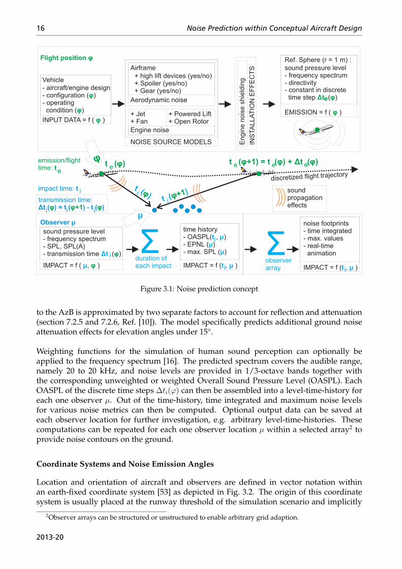
PANAM predicts ground noise impact along a simulated flight path of an aircraft accord-ing to Fig. 3.1. Definition of aircraft and observer locations in vector notation within anearth-fixed coordinate system [53] allows for the evaluation of arbitrary three-dimensionalflight trajectories [40]. The flight trajectory is discretized into single quasi-stationary air-craft positions. For each position φ, the configuration, location, orientation, and operatingconditions of the aircraft are assumed to remain constant, i.e. constant input data for theemission prediction during a time increment ∆te(φ) = te(φ + 1) − te(φ). A sufficiently finediscretization of the flight trajectory into the quasi-stationary aircraft positions φ is crucialfor an adequate accuracy of the predictions1. Consequently, it is assumed that the receivedsound signal at the observer location is constant within each one transmission time step.The transmission time step ∆ti(φ) starts when the observer receives the signal from oneaircraft position φ at the time ti(φ). This time step lasts until the emitted sound from theconsecutive aircraft position φ + 1 has reached the observer location at the time ti(φ + 1).According to the aircraft configuration and engine operating condition the relevant noisesources are accounted for and the sound emission at a reference distance of 1 m is predicted.For each time step ∆ti(φ) the farfield sound pressure level frequency spectrum is computed.Optionally, SPL level differences due to engine noise shielding effects can be applied to thenoise emission of affected noise sources.
To transfer the sound field data at the reference distance, i.e. 1 m, to the perceivednoise levels at a specific observer location µ, sound propagation effects have to be con-sidered, see Figs. A.1 and A.2, Appendix. PANAM accounts for the effects of geometricalspreading [16,54], atmospheric absorption [56], convection effects (convective amplification,frequency Doppler shift [16, 54]) and ground attenuation [10, 55] if required.A large number of models for ground noise attenuation is available. Ref. [52] provides agood overview and detailed comparison of fully empirical models. Preselected methods areimplemented in PANAM in order to compare the results: AzB [10], Flula [19], Nortim [57],and SAE [58]. Each attenuation model has a different development background, e.g. au-tomotive or aviation, with specific applications. As a consequence, the simulation resultsshow similar tendencies but overall levels can be subject to large deviations as depictedin Fig. A.3, Appendix. Yet, all models predict comparable levels for the relevant distancesand elevation angles with respect to an aircraft flyover event. For the predictions presentedwithin this report, the ground attenuation model of the German AzB is applied as defined inRef. [10]. The AzB was specifically derived for aircraft noise prediction and is standardizedwith straight-forward instructions [10] on its implementation. The ground effect according
1Flight positions do not have to be uniformly distributed, neither in time nor in space.
2013-20
16 Noise Prediction within Conceptual Aircraft Design
Figure 3.1: Noise prediction concept
to the AzB is approximated by two separate factors to account for reflection and attenuation(section 7.2.5 and 7.2.6, Ref. [10]). The model specifically predicts additional ground noiseattenuation effects for elevation angles under 15°.
Weighting functions for the simulation of human sound perception can optionally beapplied to the frequency spectrum [16]. The predicted spectrum covers the audible range,namely 20 to 20 kHz, and noise levels are provided in 1/3-octave bands together withthe corresponding unweighted or weighted Overall Sound Pressure Level (OASPL). EachOASPL of the discrete time steps ∆ti(φ) can then be assembled into a level-time-history foreach one observer µ. Out of the time-history, time integrated and maximum noise levelsfor various noise metrics can then be computed. Optional output data can be saved ateach observer location for further investigation, e.g. arbitrary level-time-histories. Thesecomputations can be repeated for each one observer location µ within a selected array2 toprovide noise contours on the ground.
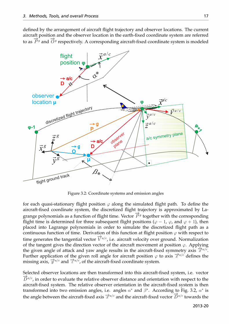
Coordinate Systems and Noise Emission Angles
Location and orientation of aircraft and observers are defined in vector notation withinan earth-fixed coordinate system [53] as depicted in Fig. 3.2. The origin of this coordinatesystem is usually placed at the runway threshold of the simulation scenario and implicitly
2Observer arrays can be structured or unstructured to enable arbitrary grid adaption.
2013-20
3. Methods, Tools, and overall Process 17
defined by the arrangement of aircraft flight trajectory and observer locations. The currentaircraft position and the observer location in the earth-fixed coordinate system are referredto as
−→P g and
−→O g respectively. A corresponding aircraft-fixed coordinate system is modeled
Figure 3.2: Coordinate systems and emission angles
for each quasi-stationary flight position φ along the simulated flight path. To define theaircraft-fixed coordinate system, the discretized flight trajectory is approximated by La-grange polynomials as a function of flight time. Vector
−→P g together with the corresponding
flight time is determined for three subsequent flight positions (φ − 1, φ, and φ + 1), thenplaced into Lagrange polynomials in order to simulate the discretized flight path as acontinuous function of time. Derivation of this function at flight position φ with respect totime generates the tangential vector
−→V a/c, i.e. aircraft velocity over ground. Normalization
of the tangent gives the direction vector of the aircraft movement at position φ. Applyingthe given angle of attack and yaw angle results in the aircraft-fixed symmetry axis −→x a/c.Further application of the given roll angle for aircraft position φ to axis −→x a/c defines themissing axis, −→y a/c and −→z a/c, of the aircraft-fixed coordinate system.
Selected observer locations are then transformed into this aircraft-fixed system, i.e. vector−→Da/c, in order to evaluate the relative observer distance and orientation with respect to theaircraft-fixed system. The relative observer orientation in the aircraft-fixed system is thentransformed into two emission angles, i.e. angles α∗ and β∗. According to Fig. 3.2, α∗ isthe angle between the aircraft-fixed axis −→x a/c and the aircraft-fixed vector
−→Da/c towards the
2013-20
18 Noise Prediction within Conceptual Aircraft Design
observer. Angle β∗ is the angle between the aircraft symmetry plane and the observer planeas depicted. The observer plane is the plane between axis −→x a/c and vector
−→Da/c toward the
observer. The relevant transformations and definitions are according to industry standardLN 9300 [53].
To speed up computations the code can run forward and backward in time along a giventrajectory. The noise computation for one selected observer location does not start withthe first aircraft position on the trajectory. Instead, the starting point for the computationis selected to be the nearest aircraft position relative to the observer. It is assumed thatclose to this position the maximum noise levels occur. From this position calculations areperformed backward and forward in time. If the noise level for a number of consecutiveaircraft positions is below a predefined threshold, calculations are stopped. The levels areset equal to the threshold and the influence of the remaining trajectory is neglected. Thenumber of consecutive positions ξ and the threshold are empirical values. This modificationaccelerates the computation especially for the combination of large observer arrays andenduring flight simulation.
3.2.2 Noise Source Modeling
Major aircraft noise components have to be simulated for each quasi-stationary flight posi-tion. Each component is represented by its individual noise source model. These modelsaccount for physics-based influences on the component’s noise generation. Consequently,any fully empirical approach can be ruled out and instead parametric and semi-empiricalsource models are implemented. These models represent a trade-off between fully empiricalmethods, i.e. best agreement to experimental data, and fully analytical methods, i.e. bestagreement to underlying physics and theory.
The models predict static noise emission levels and directivities according to the underly-ing geometry and operating condition. The selected models allow for low computationaldemand but yet capture major physical effects throughout simulated flight operations,i.e. influence of aircraft/engine geometry, in-flight configurational setting, and currentaircraft/engine operating conditions. According to the emission angles α∗ and β∗, de-picted in Fig. 3.2, the free-field noise emission out of each noise source, i.e. directional1/3-octave-band SPL spectra, is predicted on a reference sphere of radius 1 m. To translatethese individual contributions into perceived overall ground noise at selected observer loca-tions, the emitted signals are combined and effects of noise source movement are applied3.Furthermore, the influence of noise propagation through the atmosphere, ground noisereflection, and human sound perception4 are accounted for.
3.2.2.1 Airframe Noise
The implemented airframe noise source models have been developed by Dobrzynski et al.at the Institute of Aerodynamics and Flow Technology, DLR Braunschweig [59–63]. Ac-cording to Dobrzynski [9], rank-ordering the major airframe noise sources on-board of a
3Movement of a noise source results in a change in source strength, directivity, and perceived frequencies.These effects have to be accounted for.
4weighting functions
2013-20
3. Methods, Tools, and overall Process 19
conventional aircraft yields (1) the front and main landing gears, (2) leading edge high liftelements, (3) flap or rudder side edges, (4) flap or rudder tracks, (5) spoilers, and (6) compo-nent interaction noise sources.Dobrzynski derived approximation models for the most dominating components as de-scribed in Refs. [59–63]. The overall airframe noise is approximated as a combination ofthese individual models.
1. clean airfoil
2. trailing edge device (fowler flap)
3. leading edge device (slat)
4. spoiler
5. landing gear
An additional prediction model for flap side edge noise is currently under developmentat DLR [64, 65] but not yet implemented into PANAM. Initial results of the new approachare in good agreement with available experimental data [65]. The results indicate that flapside edge noise of conventional high-lift systems can contribute to overall airframe noise athigh frequencies if the landing gear is still retracted [65]. Yet, due to the high frequenciesthe contribution to overall aircraft flyover noise is strongly reduced by A-weighting andatmospheric damping. Therefore, it is assumed that for the aircraft designs consideredwithin this work, flap side edge noise does not effect the overall aircraft noise as perceivedon the ground. Aside from that, the required input parameters for the model, e.g. localvelocities, are yet not available at the conceptual aircraft design phase.
Each of the implemented prediction models provides a directional noise emission func-tion for an unmoved source under fixed operating conditions, i.e. comparable to a staticwindtunnel experiment. For a selected observer location, i.e. distance d = |
−→Da/c| and
relative source location, i.e. angles α∗ and β∗, these functions provide a free-field, 1/3-octave-band SPL emission spectrum. Each SPL spectrum is defined by a summation ofindividual terms depending on the simulated noise source:
• normalized reference level Lnorm
• spectral shape function ∆Lspec(Str)
• velocity dependent term ∆Lvel
• geometry dependent term ∆Lgeo
• directivity term ∆Ldir
Lnorm is an empirical based reference level for the specific noise source and can be eitherconstant or a function of the Strouhal number Str. The Strouhal number is defined asStr = f · xref/vref , with f as the frequency, xref as a noise source reference dimension,and vref as a reference velocity. In the case that Lnorm is a constant, the spectral shape can bedefined as a dedicated function of the Strouhal number, i.e. ∆Lspec(Str). Then, ∆Lspec(Str)is a simplified function of two linear segments converging at a peak frequency Strmax. Theslope and shape of each segment and the location of the maximum Strouhal number Strmax
2013-20
20 Noise Prediction within Conceptual Aircraft Design
are determined according to the specific source’s geometry and prevailing flow conditions.The shape of the frequency spectrum is not affected by directivity effects of the source. Theinherent emission directivity of certain noise sources is simulated with a dedicated direc-tional term ∆Ldir that is directly applied to the overall SPL spectrum. Directivity effects aresimulated according to the measured data with respect to known underlying physics. Veloc-ity and geometry dependent adjustments, ∆Lvel and ∆Lgeo, are determined for the selectedoperating conditions and source geometry with respect to the parameter setting of the un-derlying experimental data. A relevant freestream velocity vm is evaluated according to theprevailing angle of attack and yaw, i.e. the velocity component parallel to the aircraft sym-metry axis. Finally, for a noise source θ and a given set of reference parameters, the free-field1/3-octave-band SPL emission spectrum can be evaluated.
Lθ(Str) = Lnorm +∆Lspec(Str) + ∆Lgeo +∆Lvel +∆Ldir (3.1)
(1) Clean Airfoil - Clean airfoil noise prediction is based on a concept by Lockard and Lil-ley [66] adapted by Dobrzynski. Turbulent flow passing a semi-infinite flat plate generatesnoise. Only the upper surface or suction side of the airfoil has to be considered because itdominates the noise generation. Lockard and Lilley introduce an approximation for the timeaveraged rate at which this noise energy is emitted perpendicular to the plate trailing edge5.The acoustic intensity i per noise source volume is defined at the trailing edge as a functionof the characteristic turbulent velocity scale u0, ambient flow density ρ∞, ambient speed ofsound c∞, characteristic noise source frequency f0, and the observer distance d.
i =c3∞ρ∞
· f02 · π3 · d2
· ρ2∞ · u4
0
c5∞per unit source volume (3.2)
Lockard [66] and Dobrzynski [62] show that this formulation is applicable for airfoils underlow load conditions, i.e. prevailing lift coefficient ≤ 0.5. According to Lockard [66] thefollowing Strouhal relation can be defined for the turbulent flow, with lref as a noise sourcereference dimension.
Str0 =f0 · lref
u0
≈ 1.7 (3.3)
Furthermore, the acoustic noise source volume can be defined as the product of airfoil meanchordlength la, element length ∆w, and boundary layer thickness δ. Evaluating Eq. 3.2 withrespect to the source volume V and application of the Strouhal relation lead to a formulationof the acoustic intensity I normal to the flat plate’s trailing edge.
I =
[1.7
2 · π3· ρ∞c2∞
·(u0
vm
)5
· la ·∆w · δlref · d2
· v5m
]TE
(3.4)
According to Ref. [66] the strength of the acoustic sources is proportional to the maximumturbulent kinetic energy. Furthermore, it is assumed that the reference dimension lref of thenoise source is equal to the source distance from the airfoil wall. The wall distance of themaximum turbulent kinetic energy is denoted by ym, hence lref = ym. Lockard sets lref inthe proximity of the wing trailing edge equal to the turbulent boundary layer displacement
5Eq. 3 in Ref. [66]
2013-20
3. Methods, Tools, and overall Process 21
thickness δ∗. The integral can then be evaluated at the wing trailing edge (TE).
I =1.7
2 · π3· ρ∞c2∞
· v5m · la ·∆w
d2·
[(u0
vm
)5
· δ
δ∗
]TE
(3.5)
=1.7
2 · π3· ρ∞ · v3m · Ma2 · (la ·∆w)
d2·
[(u0
vm
)5
· δ
δ∗
]TE
with vm = Ma · c∞ (3.6)
Eq. 3.6 is according to Lockhard’s derivation6. Dobrzynski adds a directivity factor to thisequation in order to specifically account for the element’s trailing edge sweep angle Ψ7:
I =1.7
2 · π3· ρ∞c2∞
· v5m · la ·∆w
d2·
[(u0
vm
)5
· δ
δ∗
]TE
· cos3(Ψ) (3.7)
The ratio of boundary layer and displacement thickness for turbulent flow over a flat platecan be assumed as δ
δ∗= 8, Ref. [67]. According to recent high fidelity computations and wind
tunnel data, Dobrzynski defines the ratio of characteristic velocity scale for the turbulence u0
and mean inflow velocity vm as u0
vm= 0.046, whereas Lockard used u0
vm= 0.066 in the original
version. Obviously, this results in a significant level difference between the two methods,i.e. Lockard predicts intensity levels by ≈ 8 dB higher than Dobrzynski.In the context of the presented work, the noise source models and inherent assumptionsof Dobrzynski have been selected. Therefore, the far field noise emission spectra for cleanairfoils under limited load conditions can be predicted as follows, i.e. the noise componentthat is emitted perpendicular to the airfoil trailing edge.
I =8 · 1.72 · π3
· ρ∞c2∞
· la ·∆w
d2· 0.0465 · vm5 · cos3(Ψ) (3.8)
Normalizing this equation with the reference value of the intensity Iref = 10−12 W/m2 pro-vides the corresponding SPL. This value represents a normalized reference level with com-bined velocity and geometry adjustments, Lnorm/vel/geo.
Lnorm/vel/geo = 10 · log10(
I
Iref
)= 120 + 10 · log10 (I) (3.9)
For example, a TE sweep angle of Ψ = 30◦ would result in an additional 1.9 dB noise levelreduction compared to an unswept airfoil (Eq. 3.8). Limited available experimental dataindicates no polar emission directivity. Therefore, the clean wing emission directivity ∆Ldir
is approximated as a function of only the lateral emission angle β∗ and the wing segment’sdihedral angle ν. The dihedral angle has to be accounted for because the maximum noise isemitted with respect to the airfoil trailing edge.
∆Ldir = 10 · log10(|cos(β∗ − ν)|+ |cos(β∗ + ν)|
2
)(3.10)
To describe the spectral noise emission of a clean airfoil element, the Strouhal number isdefined as a function of frequency f , mean element chord length la, and reference velocityof vref = vm. The shape is approximated with two segments converging at a peak frequency
6Eq. 4 in Ref. [66]7Eq. 3.9 in Ref. [62]
2013-20
22 Noise Prediction within Conceptual Aircraft Design
Strmax. According to Lockard [66] the max. Strouhal number Strmax is defined as a functionof la, vm, u0, and the boundary layer parameters at the trailing edge, namely δTE and
[δδ∗
]TE
.
Strmax =1.7
2 · πu0
vm· laδTE
·[δ
δ∗
]TE
(3.11)
The boundary layer thickness for a turbulent flow over a flat plate is defined as function ofthe Reynolds number Re(x) along the plate. According to Schlichting, Ref. [67], the thicknesscan be evaluated as a function of vm, location x, and the ambient kinematic viscosity ν∞.
δ(x) = (0.37·x)/( 5√
vm·xν∞ ) (3.12)
With the known quantity δδ∗
= 8, Eq. 3.11 can be evaluated at the trailing edge.
Strmax =13.6
0.74 · π· u0
vm
5
√vm · laν∞
(3.13)
The spectral shape function can be expressed with respect to the maximum Strouhal number.Thereby, the nearest 1/3-octave-band center frequency is selected for further analysis.
∆Lspec(Str) =
10 · log10
(Str
Strmax
)− 9.0 dB for Str ≤ Strmax
10 · log10(Strmax
Str
)− 9.0 dB for Str > Strmax
(3.14)
Finally, the overall SPL emission is defined as:
Lcl≤0.5(Str) = Lnorm/vel/geo +∆Ldir +∆Lspec(Str) (3.15)
This approach is limited to airfoils under low wing loading, i.e. lift coefficients cl ≤ 0.5.
In order to account for natural or hybrid laminar flow over a clean airfoil, the reducedturbulent run length and boundary layer thickness have to be accounted for. Again, onlythe noise originating from the upper surface/suction side of the airfoil has to be considered.For simplicity, the new turbulent run length is assumed to be equal to the airfoil chordlength la minus the simulated laminar run length xlam. For a realistic clean airfoil, a maxi-mum laminar run length xlam of ≈ 55% of the airfoil chord length la can be achieved thusthe flow over the trailing edge remains turbulent [68]. Therefore, the same noise generatingmechanisms as described above are prevailing and the derived equations can be applied aswell. Yet, the reduction of turbulent kinetic velocity scale (u0) and turbulent boundary layerthickness (δ) at the trailing edge have to be known and be accounted for.The boundary layer thickness at the trailing edge is evaluated with respect to the reducedturbulent run length and kinetic energy.
δ(x)lam = (u0,lam
vm·(la−xlam))/
(5√
vm·(la−xlam)
ν∞
)(3.16)
A modified max. Strouhal number can then be derived:
Strmax,lam =13.6
0.74 · π· u0,lam
vm
5
√vm · laν∞
(3.17)
With this new Strouhal number, Eq. 3.10, 3.14, and 3.22 or 3.8 can directly be applied. If anyhigh lift devices or control surfaces are deployed, it can be assumed that the flow over theairfoil turns fully turbulent again.
2013-20
3. Methods, Tools, and overall Process 23
(2) Trailing Edge Device - To predict noise emission of clean airfoils under increased wingloading and to account for deployment of trailing edge devices, modifications to the cleanairfoil approach are necessary. Deploying high lift devices will increase wing area and fi-nally results in significantly higher overall lift. To account for these effects, Lockard [66]published scaling factors for the turbulent fluctuation velocity and boundary layer thicknessbased on recent findings from higher fidelity computations (RANS) and from wind tunnelexperiments. It is assumed, that the correlation ym = δ∗ is no longer valid [66]. Therefore,scaling of the boundary layer thickness with respect to the actual location of the maximumturbulent kinetic energy is applied. Furthermore, the velocity ratio u0
vmhas to be adapted to
higher loads on the wing element. The scaling factors for velocity and length scales givenby Lockard are derived from NACA 4412 experiments8. Again, the mean reference veloc-ity is assumed equal to the inflow velocity parallel to the main airfoil chord. Furthermore,Dobrzynski’s approximation is selected, i.e.
[u0
vm
]TE, cl≤0.5
≈ 0.046.
[δ
ym
]TE, cl>0.5
∼ 10.0(1 +
c2l4
) (3.18)
[u0
vm
]TE, cl>0.5
∼[u0
vm
]TE, cl≤0.5
·(1 +
c2l4
)(3.19)
∼ 0.046 ·(1 +
c2l4
)A correlation between the low and increased load case can be defined.[(
u0
vm
)5
· δ
ym
]TE, cl>0.5
=10
8·(1 +
c2l4
)4
·
[(u0
vm
)5
· δ
ym
]TE, cl≤0.5
(3.20)
Finally, an explicit formulation for the acoustic intensity I of wing segments with deployedtrailing edge devices and/or increased wing loading can be derived, i.e. emission compo-nent perpendicular to the leading edge. The wing element chord length is defined as thesum of airfoil chord length la and chord length of the deployed trailing edge flap lf .
I =1.7
2 · π3· ρ∞c2∞
· v5m · (la + lf ) ·∆w
d2· cos3(Ψ) ·
[(u0
vm
)5
· δ
ym
]TE, cl>0.5
(3.21)
=1.7
2 · π3· ρ∞c2∞
· v5m · (la + lf ) ·∆w
d2· cos3(Ψ) · 10
8·(1 +
c2l4
)4
·
[(u0
vm
)5
· δ
ym
]TE, cl≤0.5
=8 · 1.72 · π3
· 108
· ρ∞c2∞
· v5m · (la + lf )) ·∆w
d2· 0.0465 · cos3(Ψ) ·
(1 +
c2l4
)4
8Note that equations 10 - 11 published by Lockard in Ref. [66] have missing terms. Dobrzynski usesLockards scaling factors but Dobrzynski’s equation 3.25 yields two typos: factor "1/10" should be "10". Fur-thermore, the factor δ
δ∗ on the right hand side of the equation is redundant and should be canceled.
2013-20
24 Noise Prediction within Conceptual Aircraft Design
The intensity is transformed into an SPL to obtain the reference level Lnorm/vel/geo.
Lnorm/vel/geo = 120 dB + 10 · log10(
1.7
2 · π3· ρ∞c2∞
· v5m · (la + lf ) ·∆w
d2· cos3(Ψ)
)(3.22)
+10 · log10
10
8·(1 +
c2l4
)4
·
[(u0
vm
)5
· δ
ym
]TE, cl≤0.5
= 120 dB + 10 · log10
(8 · 1.72 · π3
· ρ∞c2∞
· (la + lf ) ·∆w
d2· cos3(Ψ) · (0.046 · vm)5
)+10 · log10
(10
8·(1 +
c2l4
)4)
︸ ︷︷ ︸∆Lcl>0.5
Comparing this equation with the cl ≤ 0.5 case, an additional factor ∆Lcl>0.5 can be identi-fied to account for the increase in lift.
∆Lcl>0.5 = 0.97 + 40 · log10(1 +
c2l4
)(3.23)
According to this additional factor, a wing segment under a typical landing load of cl = 2would result in a 13 dB level increase compared to the low lift case, i.e. cl < 0.5. Obviously,this effect would be counter-acted by a required increase in flight velocity by a factor "x"for the cl < 0.5 case. As a consequence, additional noise due to the velocity increase isgenerated, i.e. ∆Lvel = 50 · log10(x).
The directivity and spectral shape for the high lift wing element is similar to the lowlift case because of the inverse lift dependency of equations 3.18 and 3.20. Therefore,Eq. 3.10 and 3.14 remain valid and can be applied to the high lift airfoil.
Lcl>0.5 = Lnorm/vel/geo︸ ︷︷ ︸cl>0.5
+∆Ldir +∆Lspec(Str) (3.24)
(3) Leading Edge Devices - Leading edge devices can dominate airframe noise as long asthe landing gear is retracted [9]. The prediction method as proposed by Dobrzynski is ap-plicable to two- and three-position leading-edge slats as described in Ref. [69]. The methodis based on the concept of a spanwise distribution of uncorrelated dipole noise sources, i.e.so-called lift and drag dipoles. Both lift and drag dipoles are aligned along the trailing edge ofeach slat element but have different dipole reference axis orientation. Reference axes of liftdipoles are oriented approximately perpendicular with respect to the slat chord line [21, 36].This arrangement results in major noise emission perpendicular to the slat chord. Predic-tion accuracy can be improved with respect to the measurements by adding drag dipoles atthe location of the lift dipoles. Drag dipoles are aligned parallel to the element chord henceare emitting noise primarily in this direction. To evaluate the noise emission of an installedand deployed slat element, the dipole noise sources are finally rotated along with the slatelement according to the slat installation angle γ and the selected slat deployment angle δs.The final orientation of the dipoles with respect to the overall aircraft symmetry axis influ-ences the noise emission directivity.Each slat element is defined by four geometry parameters, i.e. slat mean chord length ls,
2013-20
3. Methods, Tools, and overall Process 25
mean element width ∆w, mean sweep angle Ψ of the element, and installation angle γ be-tween aircraft symmetry axis and element mean chord line. The reference velocity for theStrouhal number is v∞ hence the dimensionless frequency can be defined as Str = f ·ls
v∞.
The normalized reference level Lnorm/spec is expressed as a function of the Strouhal num-ber and of the high lift configurational setting, i.e. deployment of leading and trailing edgedevices. An empirical relation was developed to account for the impact of flap and slatdeflection, i.e. angles δf and δs, on the local flow conditions. Two empirical constants areintroduced as C1 = 104.6 db and C2 = 113.1 dB. For Strouhal numbers below a certain limit,Str ≤ Strmax, an adjustment factor ∆Lconf to account for the selected configurational settingis defined.
∆Lconf = −15.6 + 0.416 · (δs + δf )− 0.0025 · (δs + δf )2 for Str ≤ Strmax (3.25)
The maximum Strouhal number Strmax is related to the empirical constants and the adjust-ment factor for the configurational setting.
Strmax = 10.0C2−C1−∆Lconf
21.0 (3.26)
Finally, the normalized reference level Lnorm/spec is a function of the Strouhal number Str,comprised by two linear segments converging at the peak frequency Strmax.
Lnorm/spec(Str) =
{C1 + 3 · log10 (Str) + ∆Lconf for Str ≤ Strmax
C2 − 18 · log10 (Str) for Str > Strmax
(3.27)
The geometry dependent adjustment factor ∆Lgeo is defined with respect to the parametersetting of the underlying experimental data (marked with exp). With the known geometryparameters, a reference noise source area can be defined as A = ls ·∆w/cos(Ψ). The ratio ofthese source areas and the observer distances determines the adjustment factor.
∆Lgeo = 10 · log10(d2expd2
)+ 10 · log10
(ls ·∆w/cos(Ψ)
ls, exp ·∆wexp/cos(Ψexp)
)(3.28)
The formulation is simplified by plugging in the given experimental reference parameters,i.e. slat sweep angle Ψexp = 27◦, slat chord ls, exp = 0.0701m, slat width ∆wexp = 4.03m, andobserver distance dexp = 1m.
∆Lgeo = 5.0 + 10 · log10(
ls ·∆w
cos(Ψ) · d2
)(3.29)
The velocity dependence is approximated as a function of leading edge sweep angle Ψ andthe reference velocity v∞ with respect to the corresponding experimental parameters, i.e.vexp = 100m/s.
∆Lvel = 50 · log10(
v∞100m/s
)+ 30 · log10
(cos(Ψ)
cos(27◦)
)(3.30)
According to the predefined emission angles α∗ and β∗, the emission directivity correlation∆Ldir is subdivided into two components, i.e. ∆Ldir = ∆Ldir(α
∗) + ∆Ldir(β∗). The polar
directivity factor ∆Ldir(α∗) with respect to angle α∗ is defined as a function of polar angle
α∗, installation angle γ, slat deployment δslat, and the aircraft angle of attack α.
∆Ldir(α∗) = 10 · log10
(sin2(|α∗ − γ − δs + α|) + 0.1 · cos2(|α∗ − γ − δs + α|)
)(3.31)
2013-20
26 Noise Prediction within Conceptual Aircraft Design
Lateral directivity is defined as a function of emission angle β∗ and the wing dihedral angleν.
∆Ldir(β∗) = 10 · log10
(|cos(β∗ − ν)|+ |cos(β∗ + ν)|
2
)(3.32)
Finally, the SPL spectrum can be evaluated.
Lslat = Lnorm/spec(Str) + ∆Lgeo +∆Lvel +∆Ldir (3.33)
(4) Spoiler - Spoiler noise is currently modeled with a very simple and fully empiricalmodel. Spoiler operation obviously has huge impact on the overall flow field around thecorresponding wing segment hence has a dominating influence on adjacent noise sourcesas well. Spoiler deflection significantly reduces the overall lift hence changes the flow con-ditions at both leading and trailing edge of the wing. To evaluate these effects, local flowconditions would have to be evaluated and accounted for. Since these data are not available,a simple and fully empirical model has been developed by Dobrzynski [62]. Due to limitedexperimental data, only fully extracted spoilers can be accounted for with the model. A ref-erence source dimension of xref = 1m is selected, thus the Strouhal number is defined asStr = f ·1m
v∞.
The normalized reference level Lnorm is defined as a function of the Strouhal number.
Lnorm = 91.6− 9.0 · log10 (Str + 1.0) (3.34)
According to the experimental data base, geometry and velocity depending adjustments aredefined. The underlying experimental data only comprises spoilers of constant height andfull deflection. Therefore, geometry dependence is defined as a function of the actual spoilerwidth ∆w and the observer distance d. The ratio of reference and measured velocity definesthe velocity correction factor; with vexp = 100m/s as the measured velocity of the underlyingexperiment.
∆Lgeo = 20 · log10(∆w
d
)(3.35)
∆Lvel = 50 · log10(vrefvexp
)= 50 · log10
(vref
100m/s
)(3.36)
Spectral shape function and directivity effects are combined into one approximation formula∆Ldir/spec(Str). Lateral directivity effects are negligible hence only polar directivity effectswith respect to emission angle α∗ are accounted for.
∆Ldir/spec(Str) = |A1| · cos2(α∗
2
)+ |A2| · cos2
(α∗
2+ 90◦
)(3.37)
with A1 = 7.0− 10 · log10 (Str + 1.0)
and A2 = −2.0 + 10 · log10 (Str + 1.0)
Overall, spoiler SPL levels are defined as:
Lspoiler = Lnorm +∆Lgeo +∆Lvel +∆Ldir/spec(Str) (3.38)
2013-20
3. Methods, Tools, and overall Process 27
(5) Landing Gear - Landing gear can be the most dominating airframe noise source of con-ventional transportation aircraft during approach due to bluff body vortex shedding [8, 9].The implemented noise source models [59, 60, 63] simulate noise emission of each landinggear according to the specific geometry parameters, installation effects and flow conditions.Geometry parameters are extended length lg of the gear, wheel diameter Dg, and number ofaxles na as an empirical indicator for the component’s overall complexity [62]. Operationalparameters are gear extraction factor δg (0 - 1) and the corresponding mean flow velocity atthe bogie9 of the landing gear.The mean flow velocity vm is approximated for each landing gear by taking local installationeffects into account, i.e. possible variation of the freefield velocity due to circulation effects.The focus of this work lies on tricycle landing gear arrangements as described in Ref. [51],i.e. one gear in front of the aircraft and two main gears located at the wing/fuselage junc-tion. The front gear is subject to a mean velocity equal to the freestream velocity v∞ whereasvm at the main landing gear bogie is reduced by the flow field around the main wing. Thelocal wing circulation at the spanwise gear position is modeled according to the wing chordlength and any presence of extended high lift devices. The mean flow velocity vm at themain gear bogie is then approximated as the freefield velocity v∞ subtracted by the circu-lation induced velocity component vΓ. vΓ is simply approximated by application of Kutta-Joukowski’s theorem, i.e. the relation of freestream velocity, lift and circulation around anairfoil.Experimental data has shown no significant directivity effect [62], thus each landing gearis modeled as a non-directional noise source, i.e. ∆Ldir = 0. The normalized level Lnorm
is an empirical constant of 110.0 dB whereas ∆Lvel and ∆Lgeo are determined by flow con-ditions and geometry of the specific gear, respectively. With a selected reference velocityfrom the underlying experiment of vexp = 100m/s and the known geometry parameters, thecorrections can be defined.
∆Lgeo = 10 · log10((lg · δg) ·Dg · 4
√na
d2
)(3.39)
∆Lvel = 60 · log10(
vmvexp
)(3.40)
According to the type of landing gear, i.e. main or front installation, a different spectralshape function is applied [62]. With the corresponding Strouhal number Str the shape func-tions can be evaluated. The Strouhal number is defined as Str = f ·lref
vm, with a selected source
reference dimension of lref = 1m. The spectral shape function of a main landing gear (mg)is given as:
∆Lspec,mg(Str) =
{log10
(Str−0.769
)for Str ≤ 20
12.96 + log10(Str−10.7301
)for Str > 20
(3.41)
The spectral shape function of a front landing gear (fg) is given as:
∆Lspec, fg(Str) =
{log10
(Str1.1143
)for Str ≤ 10
10.45 + log10(Str−9.3367
)for Str > 10
(3.42)
Ultimately, the SPL spectra for a main or front landing gear can be evaluated.
Lgear = Lnorm +∆Lgeo +∆Lvel +
{∆Lspec,mg(Str) main gear∆Lspec, fg(Str) front gear
(3.43)
9According to Dobrzynski [62], the bogie is considered to be the main source of noise generation on aconventional landing gear.
2013-20
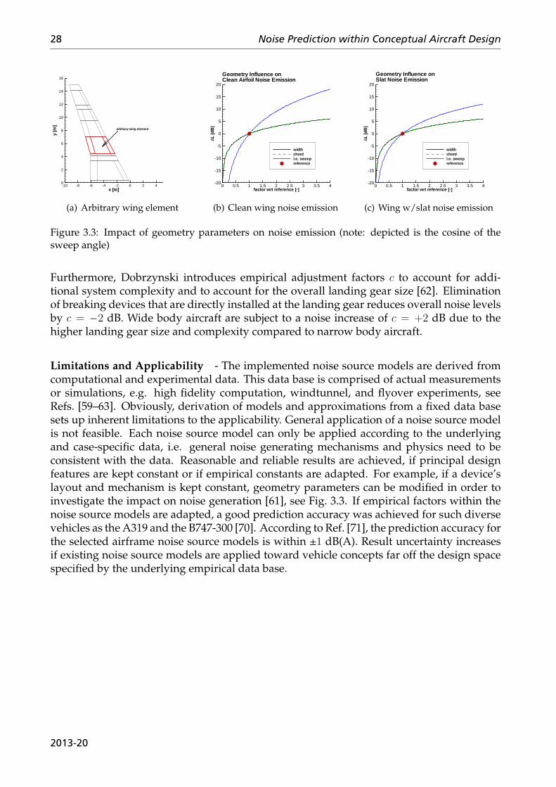
28 Noise Prediction within Conceptual Aircraft Design
x [m]
y[m
]
-10 -8 -6 -4 -2 0 2 40
2
4
6
8
10
12
14
16
arbitrary wing element
(a) Arbitrary wing element
factor wrt reference [-]
∆L[d
B]
0 0.5 1 1.5 2 2.5 3 3.5 4-20
-15
-10
-5
0
5
10
15
20
widthchordl.e. sweepreference
Geometry Influence onClean Airfoil Noise Emission
(b) Clean wing noise emission
factor wrt reference [-]
∆L[d
B]
0 0.5 1 1.5 2 2.5 3 3.5 4-20
-15
-10
-5
0
5
10
15
20
widthchordl.e. sweepreference
Geometry Influence onSlat Noise Emission
(c) Wing w/slat noise emission
Figure 3.3: Impact of geometry parameters on noise emission (note: depicted is the cosine of thesweep angle)
Furthermore, Dobrzynski introduces empirical adjustment factors c to account for addi-tional system complexity and to account for the overall landing gear size [62]. Eliminationof breaking devices that are directly installed at the landing gear reduces overall noise levelsby c = −2 dB. Wide body aircraft are subject to a noise increase of c = +2 dB due to thehigher landing gear size and complexity compared to narrow body aircraft.
Limitations and Applicability - The implemented noise source models are derived fromcomputational and experimental data. This data base is comprised of actual measurementsor simulations, e.g. high fidelity computation, windtunnel, and flyover experiments, seeRefs. [59–63]. Obviously, derivation of models and approximations from a fixed data basesets up inherent limitations to the applicability. General application of a noise source modelis not feasible. Each noise source model can only be applied according to the underlyingand case-specific data, i.e. general noise generating mechanisms and physics need to beconsistent with the data. Reasonable and reliable results are achieved, if principal designfeatures are kept constant or if empirical constants are adapted. For example, if a device’slayout and mechanism is kept constant, geometry parameters can be modified in order toinvestigate the impact on noise generation [61], see Fig. 3.3. If empirical factors within thenoise source models are adapted, a good prediction accuracy was achieved for such diversevehicles as the A319 and the B747-300 [70]. According to Ref. [71], the prediction accuracy forthe selected airframe noise source models is within ±1 dB(A). Result uncertainty increasesif existing noise source models are applied toward vehicle concepts far off the design spacespecified by the underlying empirical data base.
2013-20
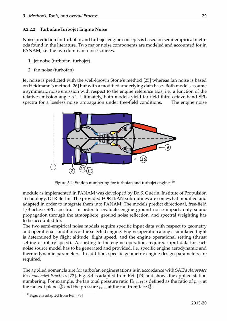
3. Methods, Tools, and overall Process 29
3.2.2.2 Turbofan/Turbojet Engine Noise
Noise prediction for turbofan and turbojet engine concepts is based on semi-empirical meth-ods found in the literature. Two major noise components are modeled and accounted for inPANAM, i.e. the two dominant noise sources.
1. jet noise (turbofan, turbojet)
2. fan noise (turbofan)
Jet noise is predicted with the well-known Stone’s method [25] whereas fan noise is basedon Heidmann’s method [26] but with a modified underlying data base. Both models assumea symmetric noise emission with respect to the engine reference axis, i.e. a function of therelative emission angle α∗. Ultimately, both models yield far field third-octave band SPLspectra for a lossless noise propagation under free-field conditions. The engine noise
21132
19
9
Figure 3.4: Station numbering for turbofan and turbojet engines10
module as implemented in PANAM was developed by Dr. S. Guérin, Institute of PropulsionTechnology, DLR Berlin. The provided FORTRAN subroutines are somewhat modified andadapted in order to integrate them into PANAM. The models predict directional, free-field1/3-octave SPL spectra. In order to evaluate engine ground noise impact, only soundpropagation through the atmosphere, ground noise reflection, and spectral weighting hasto be accounted for.The two semi-empirical noise models require specific input data with respect to geometryand operational conditions of the selected engine. Engine operation along a simulated flightis determined by flight altitude, flight speed, and the engine operational setting (thrustsetting or rotary speed). According to the engine operation, required input data for eachnoise source model has to be generated and provided, i.e. specific engine aerodynamic andthermodynamic parameters. In addition, specific geometric engine design parameters arerequired.
The applied nomenclature for turbofan engine stations is in accordance with SAE’s AerospaceRecommended Practices [72]. Fig. 3.4 is adapted from Ref. [73] and shows the applied stationnumbering. For example, the fan total pressure ratio Πt, 2−13 is defined as the ratio of pt,13 atthe fan exit plane 13⃝ and the pressure pt,13 at the fan front face 2⃝.
10Figure is adapted from Ref. [73]
2013-20
30 Noise Prediction within Conceptual Aircraft Design
It has to be noted, that stations 9⃝ and 19⃝ denote the fully expanded far-field exit conditionsfor core and bypass flow, respectively.
The jet noise model can address single and mixed dual jets. A normalized referencelevel Lnorm is predicted for the single jet. Lnorm is defined according to the nozzle geometryand the operating condition. Based on an empirical data base, a combined term for spec-tral shape and directivity ∆Ldir/spec as a function of Strouhal number Str is applied. Anadditional term ∆Lc−jet and a modified ∆Ldir,spec is defined to account for the secondary jet.
Ljet =
{Lnorm +∆Ldir/spec(Str9, α
∗cor) for single jet
Lnorm +∆Ldir/spec(Strc−jet, α∗cor) + ∆Lc−jet for coaxial jets
(3.44)
Fan noise Lfan is separated into fan inlet Lfan, in and fan exhaust Lfan, ex noise contribution.Both contributions are modeled individually and are each comprised of 4 basic terms andadditional correction factors c if required. The basic terms are comprised of a normalizedreference level, i.e. constant for inlet and exhaust, and the contributions of (a) broadband, (b)discrete-tone, and (c) combination-tone noise, if applicable. Energetic summation of theseindividual contributions yields the overall fan inlet and outlet noise emission.
Lfan, in = Lnorm + Lbbn, in︸ ︷︷ ︸(a)
+Ldtn, in︸ ︷︷ ︸(b)
+Lctn, in︸ ︷︷ ︸(c)
+ci (3.45)
Lfan, ex = Lnorm + Lbbn, ex︸ ︷︷ ︸(a)
+Ldtn, ex︸ ︷︷ ︸(b)
+cj (3.46)
Lfan = Lfan, in + Lfan, ex (3.47)
(1) Jet noise - The method by Stone can be applied to predict jet noise for single (turbojet)and mixed dual jets (turbofan) up to bypass ratios of 15 [25, 27]. The predicted noise levelsare free-field, far field, and lossless [25]. According to Bridges [27], the results for roundjets are very good with nearly all predicted noise levels within the underlying experimentaluncertainty bands, i.e. a standard deviation of 1.8 dB for jet velocities up to 800m/s. Ingeneral, the model can be applied to subsonic or supersonic jet flows up to exhaust Machnumbers of 2.5 and higher [27]. There are a few inherent limitations to the applicability ofthe method [25]: required conditions are (1) co-axial and coplanar nozzle11, (2) no low-noisenozzle modifications12, and (3) no inverse velocity profile13.If jet flows are supersonic, broadband shock noise is generated in addition to the jet mixingnoise. For coaxial supersonic flow, it is assumed that there is no interaction with respect tobroadband shock noise, hence each individual jet [25] can separately be evaluated. In thecontext of the presented work, shock noise is not an issue because exhaust velocities of con-sidered turbofan engines remain subsonic during the considered approach and departuresflight segments. Therefore, overall jet noise is simulated as jet mixing noise only.
The first step in order to evaluate mixed coaxial jets is the simulation of an isolated(primary) jet without refraction effects14. Stone defines a normalized sound pressure level
11No short or long buried nozzles can be simulated.12No serrations or a lobbed mixer can be simulated.13The method cannot be (directly) applied, if bypass or flight velocity are greater than the velocity of the
core flow.14Note: In the following simplified description of the noise source model, possible engine installation angles
γ are not accounted for.
2013-20
3. Methods, Tools, and overall Process 31
Lnorm for mixing noise of an isolated and shock-free jet. Lnorm is defined as a function of (a)atmospheric conditions, (b) area, density, and velocity of the jet, (c) eddy convective ampli-fication, (d) flight effects, and (e) nozzle shape. The required parameters to evaluate theseeffects can be derived from the following basic input parameters for the isolated (primary)jet, i.e. exhaust flow velocity, exhaust flow total temperature, nozzle exhaust area, meanfree flow velocity, ambient temperature, ambient speed of sound, and ambient density. Allof these parameters are required input information to the jet noise prediction.
(a) The ambient flow density ρ∞ and speed of sound c∞ are evaluated. Reference lev-els are defined at sea level (0 m) according to the International Standard Atmosphere, i.e.p∞, ISA = 1013N/m2 and T∞, ISA = 288K.(b) Parameters of the isolated (primary) jet, i.e. density ρ9, nozzle exhaust area A9, and aneffective jet speed v9, are accounted for with respect to observer distance d, ambient densityρ∞, and ambient speed of sound c∞. Stone defines the effective jet speed v9 as a function ofv∞
15, and jet exhaust velocity v9.
v9 = v9 ·[1− v∞
v9· cos(α∗)
]2/3(3.48)
Furthermore, Stone introduces a density exponent ω as a function of the effective jet speedv9 and the ambient speed of sound c∞. This exponent applies to hot jets.
ω =3.0 · (v9/c∞)3.5
0.6 + (v9/c∞)3.5− 1 (3.49)
(c) Eddy convective amplification is determined as a function of a convective Mach numberMacon and the polar angle α∗. Stone defines the convective Mach number Macon as a functionof v∞, jet exhaust velocity v9, the ambient speed of sound c∞, and the polar angle α∗
Macon = 0.62 · v9 − v∞ · cos(α∗)
c∞(3.50)
(d) Flight effects are defined as a function of v∞ and the polar angle α∗.(e) Nozzle shape of the jet exhaust is determined as a function of nozzle area A9 and thenozzle hydraulic diameter D9.
Finally, the reference noise level of an isolated and shock-free jet without refraction ef-
15For simplicity, it is assumed that the mean inflow velocity is parallel to the engine symmetry axis, i.e.vm = v∞.
2013-20
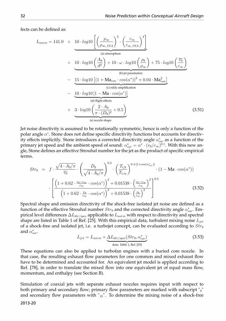
32 Noise Prediction within Conceptual Aircraft Design
fects can be defined as:
Lnorm = 141.0 + 10 · log10
[(ρ∞
ρ∞, ISA
)2
·(
c∞c∞, ISA
)4]
︸ ︷︷ ︸(a) atmosphere
+ 10 · log10(A9
d2
)+ 10 · ω · log10
(ρ9ρ∞
)+ 75 · log10
(v9c∞
)︸ ︷︷ ︸
(b) jet parameters
− 15 · log10[(1 + Macon · cos(α∗))2 + 0.04 · Ma2
con
]︸ ︷︷ ︸(c) eddy amplification
− 10 · log10 [1− Ma · cos(α∗)]︸ ︷︷ ︸(d) flight effects
+ 3 · log10(
2 · A9
π · (D9)2+ 0.5
)︸ ︷︷ ︸
(e) nozzle shape
(3.51)
Jet noise directivity is assumed to be rotationally symmetric, hence is only a function of thepolar angle α∗. Stone does not define specific directivity functions but accounts for directiv-ity effects implicitly. Stone introduces a corrected directivity angle α∗
cor as a function of theprimary jet speed and the ambient speed of sound: α∗
cor = α∗ · (v9/c∞)0.1. With this new an-gle, Stone defines an effective Strouhal number for the jet as the product of specific empiricalterms.
Str9 = f ·√
4 · A9/π
v9·
(D9√
4 · A9/π
)0.4
·(
Tt,9
Tt,∞
)0.4·[1+cos(α∗cor)]
· (1− Ma · cos(α∗))
·
(1 + 0.62 · v9−v∞
c∞· cos(α∗)
)2+ 0.01538 ·
(v9−v∞c∞
)2(1 + 0.62 · v9
c∞· cos(α∗)
)2+ 0.01538 ·
(v9c∞
)2
0.5
(3.52)
Spectral shape and emission directivity of the shock-free isolated jet noise are defined as afunction of the effective Strouhal number Str9 and the corrected directivity angle α∗
cor. Em-pirical level differences ∆Ldir/spec applicable to Lnorm with respect to directivity and spectralshape are listed in Table 1 of Ref. [25]. With this empirical data, turbulent mixing noise Ljet
of a shock-free and isolated jet, i.e. a turbojet concept, can be evaluated according to Str9and α∗
cor.Ljet = Lnorm +∆Ldir/spec(Str9, α
∗cor)︸ ︷︷ ︸
data: Table 1, Ref. [25]
(3.53)
These equations can also be applied to turbofan engines with a buried core nozzle. Inthat case, the resulting exhaust flow parameters for one common and mixed exhaust flowhave to be determined and accounted for. An equivalent jet model is applied according toRef. [78], in order to translate the mixed flow into one equivalent jet of equal mass flow,momentum, and enthalpy (see Section B).
Simulation of coaxial jets with separate exhaust nozzles requires input with respect toboth primary and secondary flow; primary flow parameters are marked with subscript "9"and secondary flow parameters with "19". To determine the mixing noise of a shock-free
2013-20
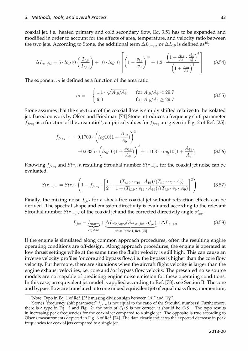
3. Methods, Tools, and overall Process 33
coaxial jet, i.e. heated primary and cold secondary flow, Eq. 3.51 has to be expanded andmodified in order to account for the effects of area, temperature, and velocity ratio betweenthe two jets. According to Stone, the additional term ∆Lc−jet or ∆L19 is defined as16:
∆Lc−jet = 5 · log10(
Tt,9
Tt,19
)+ 10 · log10
(1− v19v9
)m
+ 1.2 ·
(1 + A19
A9· v219
v29
)4(1 + A19
A9
)3 (3.54)
The exponent m is defined as a function of the area ratio.
m =
{1.1 ·
√A19/A9 for A19/A9 < 29.7
6.0 for A19/A9 ≥ 29.7(3.55)
Stone assumes that the spectrum of the coaxial flow is simply shifted relative to the isolatedjet. Based on work by Olsen and Friedman [74] Stone introduces a frequency shift parameterffreq as a function of the area ratio17; empirical values for ffreq are given in Fig. 2 of Ref. [25].
ffreq = 0.1709 ·(log10(1 +
A19
A9
)
)3
−0.6335 ·(log10(1 +
A19
A9
)
)2
+ 1.1037 · log10(1 + A19
A9
) (3.56)
Knowing ffreq and Str9, a resulting Strouhal number Strc−jet for the coaxial jet noise can beevaluated.
Strc−jet = Str9 ·
(1− ffreq ·
[1
2+
(Tt,19 · v19 · A19)/(Tt,9 · v9 · A9)
1 + (Tt,19 · v19 · A19)/(Tt,9 · v9 · A9)
]2)(3.57)
Finally, the mixing noise Ljet for a shock-free coaxial jet without refraction effects can bederived. The spectral shape and emission directivity is evaluated according to the relevantStrouhal number Strc−jet of the coaxial jet and the corrected directivity angle α∗
cor.
Ljet = Lnorm︸ ︷︷ ︸Eq.3.51
+∆Ldir/spec(Strc−jet, α∗cor)︸ ︷︷ ︸
data: Table 1, Ref. [25]
+∆Lc−jet (3.58)
If the engine is simulated along common approach procedures, often the resulting engineoperating conditions are off-design. Along approach procedures, the engine is operated atlow thrust settings while at the same time the flight velocity is still high. This can cause aninverse velocity profiles for core and bypass flow, i.e. the bypass is higher than the core flowvelocity. Furthermore, there are situations when the aircraft flight velocity is larger than theengine exhaust velocities, i.e. core and/or bypass flow velocity. The presented noise sourcemodels are not capable of predicting engine noise emission for these operating conditions.In this case, an equivalent jet model is applied according to Ref. [78], see Section B. The coreand bypass flow are translated into one mixed equivalent jet of equal mass flow, momentum,
16Note: Typo in Eq. 1 of Ref. [25]; missing division sign between "A1" and "V 21 ".
17Stones "frequency shift parameter" ffreq is not equal to the ratio of the Strouhal numbers! Furthermore,there is a typo in Eq. 3 and Fig. 2: the ratio of S1/S is not correct, it should be S/S1. The typo resultsin increasing peak frequencies for the coaxial jet compared to a single jet. The opposite is true according toOlsens measurements depicted in Fig. 6 of Ref. [74]. The data clearly indicates the expected decrease in peakfrequencies for coaxial jets compared to a single jet.
2013-20
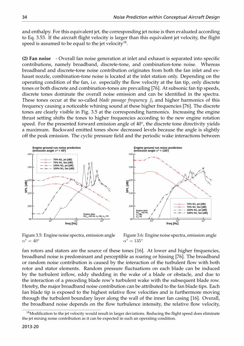
34 Noise Prediction within Conceptual Aircraft Design
and enthalpy. For this equivalent jet, the corresponding jet noise is then evaluated accordingto Eq. 3.53. If the aircraft flight velocity is larger than this equivalent jet velocity, the flightspeed is assumed to be equal to the jet velocity18.
(2) Fan noise - Overall fan noise generation at inlet and exhaust is separated into specificcontributions, namely broadband, discrete-tone, and combination-tone noise. Whereasbroadband and discrete-tone noise contribution originates from both the fan inlet and ex-haust nozzle, combination-tone noise is located at the inlet station only. Depending on theoperating condition of the fan, i.e. especially the flow velocity at the fan tip, only discretetones or both discrete and combination-tones are prevailing [76]. At subsonic fan tip speeds,discrete tones dominate the overall noise emission and can be identified in the spectra.These tones occur at the so-called blade passage frequency fb and higher harmonics of thisfrequency causing a noticeable whining sound at these higher frequencies [76]. The discretetones are clearly visible in Fig. 3.5 at the corresponding harmonics. Increasing the enginethrust setting shifts the tones to higher frequencies according to the new engine rotationspeed. For the presented forward emission angle of 40°, the discrete tone directivity yieldsa maximum. Backward emitted tones show decreased levels because the angle is slightlyoff the peak emission. The cyclic pressure field and the periodic wake interactions between
freq [Hz]
SP
L [d
B]
102 103 10490
100
110
120
130
140
70% N1, jet [dB]70% N1, fan [dB]100% N1, jet [dB]100% N1, fan [dB]
Engine ground run noise prediction(emission angle α* = 40°)
Engine data:N1max=83 Hz; n fr=36; n fs=70
Figure 3.5: Engine noise spectra, emission angleα∗ = 40°
freq [Hz]
SP
L [d
B]
102 103 10490
100
110
120
130
140
70% N1, jet [dB]70% N1, fan [dB]100% N1, jet [dB]100% N1, fan [dB]
Engine ground run noise prediction(emission angle α* = 135°)
Engine data:N1max=83 Hz; nfr=36; nfs=70
Figure 3.6: Engine noise spectra, emission angleα∗ = 135°
fan rotors and stators are the source of these tones [16]. At lower and higher frequencies,broadband noise is predominant and perceptible as roaring or hissing [76]. The broadbandor random noise contribution is caused by the interaction of the turbulent flow with bothrotor and stator elements. Random pressure fluctuations on each blade can be inducedby the turbulent inflow, eddy shedding in the wake of a blade or obstacle, and due tothe interaction of a preceding blade row’s turbulent wake with the subsequent blade row.Hereby, the major broadband noise contribution can be attributed to the fan blade tips. Eachfan blade tip is exposed to the highest relative flow velocities and is furthermore movingthrough the turbulent boundary layer along the wall of the inner fan casing [16]. Overall,the broadband noise depends on the flow turbulence intensity, the relative flow velocity,
18Modification to the jet velocity would result in larger deviations. Reducing the flight speed does eliminatethe jet mixing noise contribution as it can be expected in such an operating condition.
2013-20
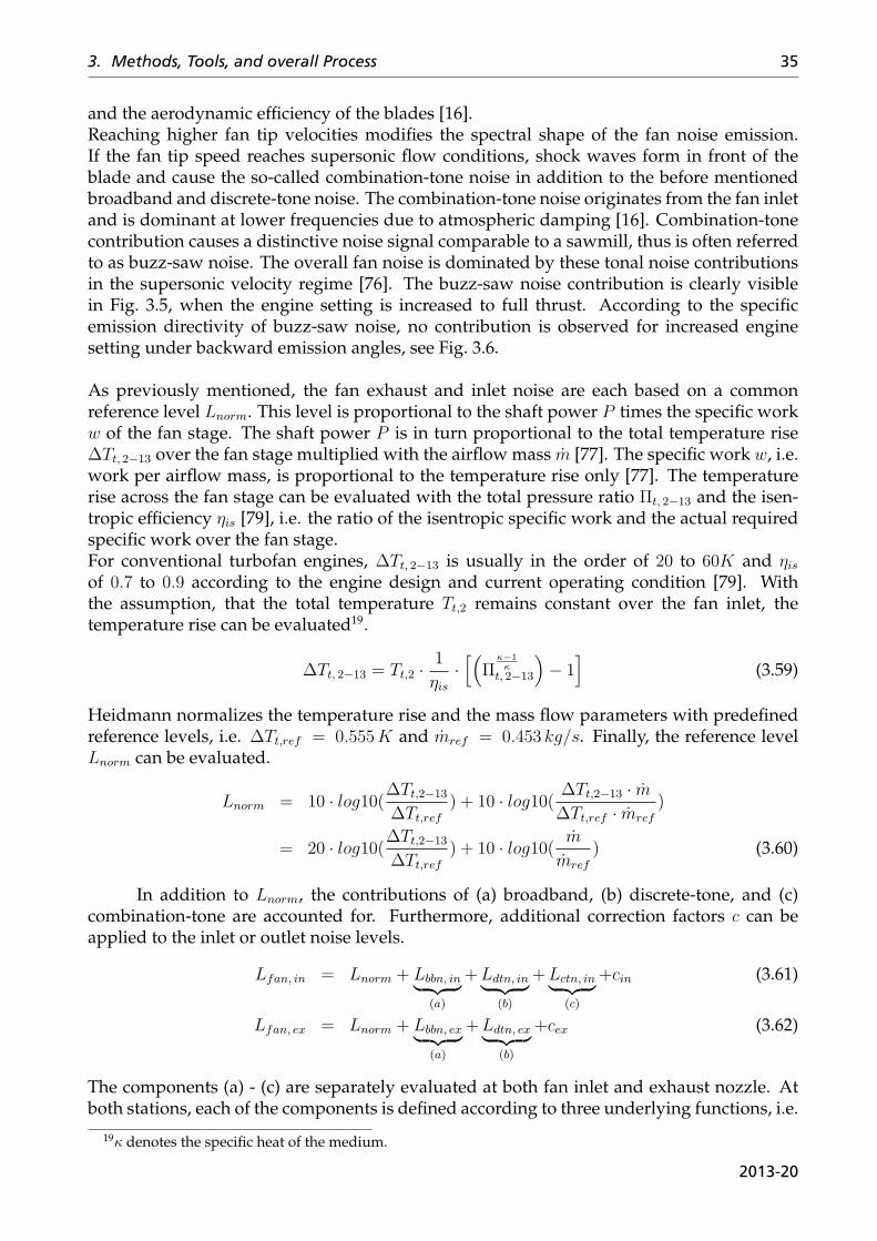
3. Methods, Tools, and overall Process 35
and the aerodynamic efficiency of the blades [16].Reaching higher fan tip velocities modifies the spectral shape of the fan noise emission.If the fan tip speed reaches supersonic flow conditions, shock waves form in front of theblade and cause the so-called combination-tone noise in addition to the before mentionedbroadband and discrete-tone noise. The combination-tone noise originates from the fan inletand is dominant at lower frequencies due to atmospheric damping [16]. Combination-tonecontribution causes a distinctive noise signal comparable to a sawmill, thus is often referredto as buzz-saw noise. The overall fan noise is dominated by these tonal noise contributionsin the supersonic velocity regime [76]. The buzz-saw noise contribution is clearly visiblein Fig. 3.5, when the engine setting is increased to full thrust. According to the specificemission directivity of buzz-saw noise, no contribution is observed for increased enginesetting under backward emission angles, see Fig. 3.6.
As previously mentioned, the fan exhaust and inlet noise are each based on a commonreference level Lnorm. This level is proportional to the shaft power P times the specific workw of the fan stage. The shaft power P is in turn proportional to the total temperature rise∆Tt, 2−13 over the fan stage multiplied with the airflow mass m [77]. The specific work w, i.e.work per airflow mass, is proportional to the temperature rise only [77]. The temperaturerise across the fan stage can be evaluated with the total pressure ratio Πt, 2−13 and the isen-tropic efficiency ηis [79], i.e. the ratio of the isentropic specific work and the actual requiredspecific work over the fan stage.For conventional turbofan engines, ∆Tt, 2−13 is usually in the order of 20 to 60K and ηisof 0.7 to 0.9 according to the engine design and current operating condition [79]. Withthe assumption, that the total temperature Tt,2 remains constant over the fan inlet, thetemperature rise can be evaluated19.
∆Tt, 2−13 = Tt,2 ·1
ηis·[(
Πκ−1κ
t, 2−13
)− 1]
(3.59)
Heidmann normalizes the temperature rise and the mass flow parameters with predefinedreference levels, i.e. ∆Tt,ref = 0.555K and mref = 0.453 kg/s. Finally, the reference levelLnorm can be evaluated.
Lnorm = 10 · log10(∆Tt,2−13
∆Tt,ref
) + 10 · log10( ∆Tt,2−13 · m∆Tt,ref · mref
)
= 20 · log10(∆Tt,2−13
∆Tt,ref
) + 10 · log10( m
mref
) (3.60)
In addition to Lnorm, the contributions of (a) broadband, (b) discrete-tone, and (c)combination-tone are accounted for. Furthermore, additional correction factors c can beapplied to the inlet or outlet noise levels.
Lfan, in = Lnorm + Lbbn, in︸ ︷︷ ︸(a)
+Ldtn, in︸ ︷︷ ︸(b)
+Lctn, in︸ ︷︷ ︸(c)
+cin (3.61)
Lfan, ex = Lnorm + Lbbn, ex︸ ︷︷ ︸(a)
+Ldtn, ex︸ ︷︷ ︸(b)
+cex (3.62)
The components (a) - (c) are separately evaluated at both fan inlet and exhaust nozzle. Atboth stations, each of the components is defined according to three underlying functions, i.e.
19κ denotes the specific heat of the medium.
2013-20
36 Noise Prediction within Conceptual Aircraft Design
a directivity function ∆Ldir, a spectral shape function ∆Lspec(f), and term ∆Lvel dependingon the specific flow velocity at the fan tip. Within the presented work, Heidmanns originaldirectivity and spectral shape functions are applied. Yet, the original formulations for ∆Lvel
by Heidmann20 have been adapted by Guérin to account for recent findings in fan design21.The modified formulations are still functions of the relative Mach numbers22, i.e. underselected (off-design) operating condition (Marel) and for the design point (Mad
rel), but withdifferent coefficients. Knowing Marel and Mad
rel, the velocity dependent terms for (a) broad-band, (b) discrete-tone, and (c) combination-tone can be evaluated at the correspondingengine station.
At the fan inlet, i.e. station 2⃝, the broadband noise contribution Lbbn, in is defined. Fullyempirical data is provided for the emission directivity of the inlet broadband noise, i.e.Ldir
23. Assuming rotational symmetry, the directivity is a function of the emission angle α∗
only. Heidmann’s original data defines the characteristic fan noise peaks for α∗ in the rangeof 20− 45°.The spectral shape of the broadband emission is approximated as a function of frequency fand engine rotation speed times the blade count, i.e. blade passing frequency fb.
∆Lspec(f) = 10 · log10
(exp
[−0.5 ·
(log(
f
2.5 · fb)/log(2.2)
)2])
(3.63)
This characteristic 1/3-octave spectrum for fan broadband noise is assumed constant forboth fan inlet and discharge.In contrast to the directivity and the spectral shape function, the original velocity dependentterm Lvel has been adapted to account for current findings in fan design. Modificationsby Guérin to the semi-empirical factors of the original Heidmann model result in accuracyimprovement for modern turbofan engines with high by-pass ratios [44]. The parameteradaption results in the following new formulation.
∆Lvel =
58.5 for Madrel ≤ 1.0 ∧ Marel ≤ 0.9
58.5 + 20 · log10(Madrel) for Mad
rel > 1.0 ∧ Marel ≤ 0.9
58.5 + 20 · log10(Madrel)
− 50 · log10(Marel/0.9) for Madrel > 1.0 ∧ Marel > 0.9
58.5− 20 · log10(Madrel/0.9) for Mad
rel ≤ 1.0 ∧ Marel > 0.9
(3.64)
Finally, broadband noise emission from the fan inlet at station 2⃝ can be defined.
Lbbn, in = Lnorm +∆Ldir +∆Lspec(f) + ∆Lvel (3.65)
(b) Discrete-tone contribution to the fan inlet noise is referred to as Ldtn, in. As for the broad-band contribution, the directivity is a fully empirical function, i.e. ∆Ldir
24. The peak emis-sion is predicted for α∗ in the range of 20 to 40°.
20Term "F1", Fig. 4 in Ref. [26]21Institute of Propulsion Technology, DLR Berlin. Modifications are based on a NASA Contractor Report:
K.B.Kontos, B.A.Janardan, P.R.Gliebe: Improved NASA-ANOPP Noise Prediction Computer Code for AdvancedSubsonic Propulsion Systems, NASA-CR-195480, 1996
22"Relative" Mach numbers are relative with respect to fan blade tip, i.e. contribution of axial and radial flowvelocity.
23Fig. 7 (a) in Ref. [26]24Term "F1", Fig. 13 (a) in Ref. [26]
2013-20
3. Methods, Tools, and overall Process 37
For the rotor-stator interaction, levels for each discrete tone are defined by Heidmann.A noise level delta ∆Lh(i) is assigned to each harmonic "i". Heidmann assumes a 3 dBfalloff per harmonic "i" and only accounts for the first five harmonics. For the first har-monic ∆Lh(1), a cut-off condition is evaluated in order to check whether the harmonic ispropagable. The cut-off condition δ is defined according to the fan blade tip axial Machnumber Ma and the number of rotors nr and stators ns.
δ =
∣∣∣∣ Ma1− ns/nr
∣∣∣∣ (3.66)
For δ > 1.05, the first harmonic is propagable. Guérin defines different level deltas accordingto Ma, i.e. for Ma < 1.15, the following delta levels are applied:
∆Lh(i) =
6.0− 6.0 · i for δ > 1.05
− 8.0 for δ > 1.05 ∧ i = 1
6.0− 6.0 · i for δ > 1.05 ∧ i ∈ [2, 5]
(3.67)
For Marel ≥ 1.15 the following delta levels are applied:
∆Lh(i) =
9.0− 9.0 · i for δ > 1.05
− 8.0 for δ > 1.05 ∧ i = 1
9.0− 9.0 · i for δ > 1.05 ∧ i ∈ [2, 5]
(3.68)
According to the frequency of harmonic "i", the discrete tones are arranged into 1/3-octavebands. If multiple harmonics fall into one frequency band, energetic summation is applied.Finally, a spectral contribution can be defined, i.e. ∆Lspec(f).Again, a velocity dependent term ∆Lvel is defined as a function of the Mach numbers at arepresentative blade section. As mentioned before, the empirical factors have been adaptedby Guérin [44].
∆Lvel =
60.5 for Mad
rel ≤ 1.0 ∧ Marel ≤ 0.72
60.5 + 20 · log10(Madrel) for Mad
rel > 1.0 ∧ Marel ≤ 0.72
C for Madrel > 1.0 ∧ Marel > 0.72
(3.69)
The auxiliary term C is evaluated with one of the following formulations. The formulationwith the lowest value for the selected Mach numbers is selected.
C =
{60.5 + 20 · log10(Mad
rel) + 50 · log10(Marel/0.72)
64.5 + 80 · log10(Madrel/Marel)
If the engine is operated in flight, an empirical correction for the inlet flow distortion isapplied, i.e. cdist. Operation on the ground does not require a correction.Finally, the discrete tone contribution to the forward fan emission can be defined.
Ldtn, in = Lnorm +∆Lvel +∆Ldir +∆Lh(f) + cdist (3.70)
(c) Combination-tone noise is defined as Lctn and occurs if the relative tip Mach numberMarel ≥ 1, thus no combination-tone noise is generated for the subsonic case. Heidmanndescribes the directivity of the buzzsaw noise with empirical functions, i.e. ∆Ldir
25. The
25Fig. 16 in Ref. [26]
2013-20
38 Noise Prediction within Conceptual Aircraft Design
buzzsaw noise spectral content is approximated by three functions according to Heidmann’smodel26. Noise peaks are defined at a half, fourth, and eighth of the blade passing frequencyfb. Noise levels are linearly increasing up to the peak and decreasing after the peak. Threecombination-tone noise functions are defined: ∆L1/2 fb , ∆L1/4 fb , and ∆L1/8 fb . Individualpeak levels with respect to the engine operating condition, i.e. Marel, are assigned to eachof these functions. For each function, such a empirical and velocity dependent peak value∆Lvel is defined. Due to the somewhat antique underlying database for Heidmann’s orig-inal model, especially the buzzsaw noise contribution has been overpredicted in the past.Therefore, modifications to each ∆Lvel are applied by Guérin to account for recent findings.
∆Lvel, 1/2 fb =
30.0 for Marel ≤ 1.0
72.5 for 1.0 < Marel ≤ 1.14
4.4 for 1.14 < Marel ≤ 2.0
(3.71)
∆Lvel, 1/4 fb =
30.0 for Marel ≤ 1.0
68.6 for 1.0 < Marel ≤ 1.25
10.5 for 1.25 < Marel ≤ 2.0
(3.72)
∆Lvel, 1/8 fb =
36.0 for Marel ≤ 1.0
60.6 for 1.0 < Marel ≤ 1.61
56.5 for 1.61 < Marel ≤ 2.0
(3.73)
Finally, the three spectral shape functions can be defined.
∆L1/2 fb = ∆Lvel, 1/2 fb +
− 30.0 · log10(2f
fb) for
f
fb> 0.5
+ 30.0 · log10(2ffb
) forf
fb≤ 0.5
(3.74)
∆L1/4 fb = ∆Lvel, 1/4 fb +
− 50.0 · log10(4f
fb) for
f
fb> 0.25
+ 50.0 · log10(4ffb
) forf
fb≤ 0.25
(3.75)
∆L1/8 fb = ∆Lvel, 1/8 fb +
− 30.0 · log10(8f
fb) for
f
fb> 0.125
+ 30.0 · log10(8ffb
) forf
fb≤ 0.125
(3.76)
These separate shape functions are finally arranged into 1/3-octave bands to yield the over-all spectrum, i.e. ∆Lspec(f).Ultimately, the combination-tone or buzzsaw noise contribution for Marel ≥ 1 can be de-fined. If required, some empirical correction is applied in order to account for inlet flowdistortion, i.e. cdist.
Lctn, in = Lnorm +∆Ldir +∆Lspec(f) + cdist (3.77)
26Fig. 14 in Ref. [26]
2013-20
3. Methods, Tools, and overall Process 39
Two contributions, namely (a) broadband and (b) discrete-tone noise are defined at the fanexhaust, i.e. station 13⃝.
Lfan, ex = Lnorm + Lbbn︸︷︷︸(a)
+Ldtn︸︷︷︸(b)
(3.78)
In accordance with the fan inlet definition, each of the contributions (a) and (b) is comprisedof directivity, spectral shape, and velocity dependent terms.(a) The velocity dependence of the fan broadband noise is defined as ∆Lvel. In contrast toHeidmanns original formulation, Guérins modifications are applied.
∆Lvel =
63.0 for Mad
rel ≤ 1.0 ∧ Marel < 1.0
63.0 + 20 · log10(Madrel) for Mad
rel > 1.0 ∧ Marel ≤ 1.0
63.0 + 20 · log10(Madrel)− 30 · log10(Marel) for Mad
rel > 1.0 ∧ Marel > 1.0(3.79)
For the directivity of the broadband exhaust noise emission, Heidmann’s original empiricalfunctions are selected27. The directivity function ∆Ldir predicts noise peaks under emissionangles of α∗ = 120 − 140 °. Furthermore, the characteristic 1/3-octave broadband noisespectrum, i.e. ∆Lspec(f), is applied as described in Eq. 3.63.An additional contribution c is defined to account for the spacing between rotor and statordisc, ξrss. In contrast to Heidmanns original formulation, Guérin only applies c to the fandischarge at station 13⃝.
c = −5 · log10(13· ξrss) (3.80)
Ultimately, broadband noise emission from the fan discharge is defined as:
∆Lbbn, ex = Lnorm +∆Lvel +∆Ldir +∆Lspec(f) + c (3.81)
(b) A velocity dependent term is defined for the discrete-tone noise contribution at the fanexhaust. In contrast to the formulations for the fan inlet, no modifications to Heidmannsoriginal definitions are applied28.
∆Lvel =
63.0 for Mad
rel ≤ 1.0 ∧ Marel ≤ 1.0
63.0 + 20 · log10(Madrel) for Mad
rel > 1.0 ∧ Marel ≤ 1.0
63.0 + 20 · log10(Madrel)− 20 · log10(Marel) for Mad
rel > 1.0 ∧ Marel > 1.0(3.82)
Furthermore, the empirical functions for spectral shape and directivity of the discrete-toneemission are Heidmanns original formulations, i.e. ∆Lfreq(f) and ∆Ldir
29. To account forgeometrical effects, the correction factor cξ, as described in Eq. 3.80, is applied. Ultimately,the discrete-tone noise contribution of to the fan exhaust noise can be evaluated.
Ldtn, ex = Lnorm +∆Lvel +∆Ldir +∆Lspec(f) + cξ (3.83)
Limitations and Applicability - Reliability and validity of results is limited to the un-derlying database because extrapolation is not recommended [75]. Stone’s database doesnot impose significant restrictions to jet noise modeling because the relevant parameter do-main for the presented work is covered, i.e. preferred engine sizes and thrust requirements
27Fig. 7 (b) in Ref. [26]28Fig. 10 (b) in Ref. [26]29Figs. 8 and 13 (b) in Ref. [26]
2013-20
40 Noise Prediction within Conceptual Aircraft Design
are mapped. The selected fan noise model by Heidmann is based on a somewhat antiquedatabase hence application should be limited to older engine types with low bypass ra-tios. In order to apply Heidmann’s approach to modern turbofan engines, adaption andmodification of the inherent empirical constants becomes necessary. Recent studies fromNASA [28] show that such a modified approach can be applied for quite a wide range offan pressure ratios, tip speeds, and bypass ratios. It is demonstrated, that predicted resultsare usually within a ± 4 dB margin with respect to the measurements [28] for bypass ratiosup to 13.3, i.e. a satisfying agreement to the experimental data. PANAM’s implementedfan noise model features similar modifications of Heidmann’s original constants. Therefore,it is assumed that the implemented engine noise source models can be applied to modernturbofan engines up to high bypass ratios around 15. Application of the methods to engineconcepts other than turbofan or even higher bypass ratios does not seem feasible. Apply-ing the models that far off from the experimental and knowledge database will result inunpredictable uncertainties [28, 75].
3.2.2.3 Noise Shielding Effects
The analysis of noise shielding effects is of growing importance with regard to future air-craft concepts, e. g. blended wing bodies or the DLR low-noise aircraft (LNA). At DLR, theray tracing tool SHADOW [83] has been developed in order to investigate different engineinstallations with respect to structural noise shielding. The tool by M. Lummer30 combinesfast computation and at the same time simplified input requirements. As a consequence, thetool is well suited for application within conceptual aircraft design. The required input datafor SHADOW, i.e. aircraft geometry and engine alignment, can directly be generated at theconceptual design phase. For a selected aircraft/engine design, frequency dependent noiseattenuation factors are predicted with SHADOW and then fed back into PANAM for furtherprocessing. The attenuation factors are then accounted for in PANAM when simulating thefan noise contribution [84].
SHADOW is based on a high frequency approximation of the linearized Euler equa-tions where the pressure field is calculated by solving ordinary differential equations alonglines in space, so-called rays. These rays originate in a point source, which approximatesthe center of the fan disc. Furthermore, no mean flow effects are taken into account and theaircraft geometry is approximated by a triangulated surface. If required, the triangulatedsurfaces may optionally be refined with tools such as ADMesh. This surface definitionallows for great flexibility in representation of complex geometries. Furthermore, a local2nd-order polynomial geometry approximation is applied to take into account the surfacecurvature, thus enable proper calculation of the ray reflection.
The pressure amplitude along each ray is calculated based on an energy conservationprinciple, which requires the calculation of the Jacobian of the ray-field. Evaluating theJacobian with a difference approximation can lead to problems due to strong divergence ofthe rays after multiple reflections. Therefore, a differential equation for the Jacobian wasderived and integrated along with the ray equations [83].
In order to calculate the acoustic shielding at prescribed points in space, a shooting proce-dure using a Newton algorithm is applied. In the high frequency limit the diffractive part of
30Institute of Aerodynamics and Flow Technology, DLR Braunschweig
2013-20
3. Methods, Tools, and overall Process 41
the solution of the wave equation is lost. Thus, in ray-tracing the diffraction has to be takeninto account by special approximations, like, e.g., the geometrical theory of diffraction [85].While this approach yields quite accurate results, its implementation for arbitrary geome-tries is complicated. Therefore, a more simple approach based on the Maggi-Rubinowiczformulation of the Kirchhoff diffraction theory has been implemented [86, 87]. In this case,the diffracted field is calculated by a line integral along the shadow boundary on the surfaceof the diffracting body. In contrast to the ray field, the diffraction correction is frequencydependent. Since only the acoustic far field is calculated in the implemented form of thehigh frequency approximation, it is sufficient to consider acoustic point sources [83].
3.2.2.4 Acoustic Lining
A model to account for noise absorption due to acoustic liners has been implemented. Themethod as developed by Moreau, Guérin, and Busse [81] improves result accuracy especiallyunder take-off conditions [125]. The original source code by Guérin is adapted and inte-grated into PANAM. The liner damping model is derived from the ray theory which makesit fast enough for applications at the conceptual aircraft design phase. Liners mounted inboth the engine intake and bypass duct can be investigated. As a consequence, the respec-tive length of the lining is required as an input. The following brief description is based onRef. [125].In a first step, the sound field generated by the fan stage is synthetically decomposed intorelevant acoustic modes (m,n). Assuming hard-wall boundary conditions and applying aray theory, the ray structures of the cut-on modes can be determined. According to the an-gle at which a ray impinges on the wall and the number of bounces along this ray, a soundattenuation is predicted for each mode. Here, it is assumed that the liners do not signifi-cantly modify the propagation angles nor induce mode scattering. The far-field directivityis supposed to remain unchanged despite an existing effect by acoustic lining in real appli-cations. A model based on the liner geometry and inflow conditions is applied to predictthe wall impedance. A modal content is synthesized for each individual engine operatingpoint of the simulation. A specific approach is used for the three noise components identi-fied by Heidmann [26]. For broadband noise, all the cut-on modes are contained and sup-posed to propagate the same acoustic energy (Equal Modal Energy Model). Furthermore, inorder to reduce computational requirements, the liner attenuation is calculated only for thecenter-frequencies of each one-third octave band. The tones at multiple of the blade pass-ing frequency are all assumed to be generated by the rotor-stator interaction mechanism.The azimuthal order of those modes can be calculated according to the number of rotor andstator blades with the Tyler and Sofrin rule [82]. The same power amplitude is given to allthe radial orders. Finally, the modal content of buzz-saw noise has to be determined in thetransonic regime of the fan [81]. Since buzz-saw is a rotor-locked mechanism, the azimuthalorder of each engine order tone can be assumed to have the same value as the engine or-der itself. Then, within a given one-third octave band all the engine orders are consideredto have the same amplitude [81]. The energy of the radial order components is chosen tobe equal, too. The implementation of Guérins liner model makes it possible to predict andinvestigate the influence of the acoustic lining on the noise contribution of the fan.
2013-20
42 Noise Prediction within Conceptual Aircraft Design
3.2.3 Tool Input
Input data requirement is defined according to the implemented noise source models forboth airframe and engine. The required input data for PANAM is comprised of (1) aircraftdesign, (2) engine design parameters with a detailed engine performance deck, (3) a simu-lated flight trajectory with configuration settings/operating conditions, and (4) the locationof the respective observer. Relevant input data can be generated with corresponding toolsor has to be provided by the user in order to initiate a noise prediction.PANAM simulates the overall aircraft noise as a combination of relevant components, i.e.wing/control surface(s), landing gear(s), and engine(s). Each type of component is simu-lated with a corresponding noise source model as described in the previous sections. Theselected models are defined by a broad parameter set, especially if compared to other pre-diction models such as Fink’s Airframe Noise Prediction Method [24]. According to thisparametrical definition, specific input data is required for each modeled noise source. Morethan one noise source of the same type but with different parameter setting can exist, e.g. ifa wing or control surface is represented by several segments. In this case, each segment hasto be defined according to the individual shape, high lift, and spoiler design.As a consequence, the amount of required input data can become quite extensive. Never-theless, the complexity of these parameters is well suitable for conceptual aircraft designand the required information can be generated with available and standard vehicle designmethods. If only limited input data is available, it is possible to switch back to a simplifiedgeometry representation, i.e. only accounting for one representative and averaged elementper noise source type.
3.2.3.1 Aircraft design
Wing and control surfaces are separated into acoustically relevant segments, i.e. segmentswith constant flap, slat, and airfoil geometry. Dealing with unconventional aircraft con-figurations, such a segmentation is inevitable to guarantee feasible representation of thegeometry. Each segment is defined by multiple and individual parameters instead of work-ing with averaged and representative dimensions for each major noise source. The requiredinput parameters are segment type and corresponding geometry details. Four segmenttypes are accounted for: (1) clean airfoil, (2) airfoil with leading edge devices (led), (3) airfoilwith trailing edge devices (ted), and (4) airfoil with led and ted. Each of these segmenttypes is defined by 9 parameters: (a) width, (b) chord length, (c) twist distribution, (d)dihedral angle, (e) leading and (f) trailing edge sweep angle of the segment. Furthermore,if equipped with a high lift devices, the corresponding chord length of leading (g) and/ortrailing edge (h) device is required. Additional installation of a spoiler element on a segmentrequires (i) the width of this component.Each landing gear is defined by three parameters: (a) wheel diameter, (b) extended length ofthe gear, and (c) number of axles. Furthermore, if an under-the-wing installation is selected,a fourth parameter, the main wing chord length (d) has to be evaluated at the location of thegear-wing-junction.The relative location of each engine and the actual overall weight of the vehicle completethe list of required aircraft design parameters for a PANAM run. If all parameters aregenerated, the individual noise sources can be assembled into one acoustically analogousmodel of the overall aircraft.
An additional 3D vehicle description has to be provided, if noise shielding effects are
2013-20
3. Methods, Tools, and overall Process 43
investigated. To evaluate shielding effects with the DLR ray tracing tool SHADOW [83], asurface mesh of the corresponding vehicle is required, e.g. a triangulated surface model inStandard Tessellation Language (STL). Furthermore, the precise location of the engines isevaluated and provided as an input for SHADOW.
Engine design
Engine design parameters and performance decks are required for the engine noise simu-lation. The required input data is comprised of detailed engine geometry parameters andan overall engine performance map. This so-called engine performance deck is comprisedof precomputed thermodynamic and aerodynamic parameters for each one combination offlight altitude, flight speed, and engine operational setting (thrust or rotational speed set-ting). According to the simulated engine operation, relevant parameters are extracted fromthe stored performance deck.Required geometry parameters and design constants are (1) number of fan rotor and statorblades, (2) spacing between rotor and stator, (3) fan hub-to-tip ratio, (4) fan diameter, (5)maximum rotation speed, (6) fan blade chord length, (7) design Mach number at the fan tip,and (8) core and bypass flow exhaust areas.For each selected operating condition of the engine, multiple input variables are required.These performance parameters depend on the operating condition and comprise (1) by-pass/core exhaust jet velocities, (2) bypass/core exhaust temperatures, (3) bypass/core ex-haust flow densities, (4) fan total pressure ratio, (5) isentropic fan efficiency, and (6) maxi-mum turbine entry temperature. All additional input parameters for a PANAM noise pre-diction can be derived from these basic requirements.If acoustical lining is accounted for, additional geometry parameters are required, i.e. theliner length in both bypass and core duct, if available.
Flight trajectories
For each simulated flight position of the vehicle, specific data is required with respect to lo-cation, orientation and operation of the aircraft. Hereby, the aircraft location can be providedas either GPS information, including flight altitude over ground, or directly in relative co-ordinates with respect to a defined ground location. Aircraft orientation is described by thethree Euler angles with respect to the flight path angle or inflow direction. The inflow direc-tion is determined according to three consecutive flight positions, as previously described.Finally, the aircraft operation is described by (1) the flight velocity, (2) the commanded en-gine operation (thrust or rotational speed setting), and (3) the vehicle configuration. Theconfigurational setting is defined by the deflection angles of (a) trailing edge and leadingedge high lift device, (b) spoiler elements, and (c) the position of each landing gear.
Observer locations
Arbitrary observer locations can be selected for the noise prediction. Depending on theselected task, level-time-histories or isocontour areas, individual observers or microphonearrays can be processed. Individual observer property settings can be defined for each lo-cation, i.e. ground resistivity to air, observer altitude, microphone height, and populationdensity if required. This allows to define and simulate arbitrary airport surroundings witha realistic population distribution, if available.
2013-20
44 Noise Prediction within Conceptual Aircraft Design
3.2.4 Modi operandi
Providing the required input data as previously described, a PANAM run can be initiated.PANAM’s flexible setup allows for three different run-modes: (1) autarkic/stand-alone mode,(2) controlled operation within a multidisciplinary simulation environment, and (3) modularoperation directly embedded within an overall aircraft design process.
For the (1) autarkic/stand-alone operation, the necessary input data has to be providedby the user. In this modus, a simple graphical user interface supports the user to commandand operate the noise prediction process31. After the computation, the prediction results canthen manually be evaluated by the user.If PANAM is operated within a (2) simulation environment, required input data is auto-matically generated if corresponding tools are embedded in the simulation process underconsideration. To enable automated operation within the simulated process, PANAM fea-tures script-based operation without user interface.PANAM can be operated within DLR’s TIVA [45] simulation environment. DLR has es-tablished a common system to enable distributed multidisciplinary conceptual aircraftdesign [46]. The TIVA system is based upon a common data exchange format to estab-lish a framework for the integration of tools and methods from multiple disciplines andexperts. The implemented tools come from specialized DLR institutes, are harmonized ininput/output format and are integrated into one fully automated analysis process. ThePHX ModelCenter framework [47] allows for a DLR-wide accessible server/client architec-ture. Currently, tools from corresponding disciplines are available and can be implementedinto individual process chains to provide input data for the noise prediction. Interfaces tovarious DLR high fidelity and expert tools are established, e.g. flight simulation tools.Ultimately, noise prediction input and output data can be made accessible for other toolsvia network connection. Parts of the input data for the noise prediction can remain constantwhereas other input parameters will be generated and provided by embedded expert tools.For example, to investigate low-noise flight operation of a specific aircraft, PANAM isconnected to a flight performance tool whereas predefined aircraft and engine parametersare made accessible as stored input data [84, 92, 93]. Furthermore, linking PANAM to highfidelity simulation tools can improve result accuracy, e.g. due to detailed engine cycleanalysis with the VarCycle [80] tool32.PANAM’s (3) modular run-mode allows for direct operation within an overall aircraftdesign process. This third PANAM run-mode is of dominating importance in the contextof the presented work, enabling an aircraft design process with integrated noise predictioncapabilities.
3.2.5 Tool Output
3.2.5.1 Individual Flyover Event
Individual flyover events are the default application for PANAM. The data output includesnoise levels for each individually modeled aircraft component as well as levels for the over-all aircraft. Noise level frequency spectra for individual components can be provided for
31GUI is based on a concept by IFL, Technical University Braunschweig32VarCycle is an one-dimensional, off-design performance calculation program developed by the Institute
of Propulsion Technology (AT)
2013-20
3. Methods, Tools, and overall Process 45
any specified operating condition along a simulated flight path. Furthermore, level-time-histories, weighted or time-integrated noise metrics can be predicted for each flyover event.The time-integrated and weighted output data includes the standard flyover noise mea-sures, e.g. (A-weighted) Sound Pressure Level and Effective Perceived Noise Level (EPNL).For a grid of observer locations the distribution of noise levels as received on the ground canbe generated. Animated noise footprints for each one time step as well as visualizations oftime-integrated noise footprints can be generated. This allows for real-time evaluation of theinfluence of aircraft operating conditions and configurational settings on the overall noiseradiation. Noise related effects can be identified, visualized, and ultimately analyzed [84].Isocontour areas of the max. Sound Pressure Level (SPL) can be translated into a probabilitydistribution of aircraft noise induced awakenings [3]. Multiplied with a given populationdensity, one can evaluate the number of affected people, i.e. awake people due to a singleaircraft flyover noise event. This scalar value is well suited as a design objective within anoptimization process. Obviously, the population density around a typical airport is veryinhomogeneous. But due to the complexity of modeling the communities around a real air-port and the lack of available data, usually an average and constant population density isassumed33.
3.2.5.2 Multiple Flyover Events
Multiple flyover events can be simulated with the code as well. Arbitrary combinations ofindividual flyover events are arranged into a multiple flyover scenario. Equivalent SoundPressure Levels (aequivalenter Dauerschallpegel, Leq) are computed for arbitrary combinationsof aircraft, fleet mix, flight operation, and runway layout. The computations are performedaccording to Ref. [90].
Leq = k · log10
(trefT
·N∑i=1
gi · 10LE,i/k
)+ C (3.84)
The flyover events (N ) within a predefined time span (T ) are summed up for an arbitraryobserver location. LE,i is the noise level for one individual flyover event (i), tref is thespecific time span defined for LE , gi is the time dependent weighting factor. Parameter k de-pends on the summation of the individual noise levels, e.g. k = 10 for energetic summation.Finally, the resulting levels are scaled/normalized by factor C. The most common noisemetrics can be evaluated according to the parameter setting defined in Section B, Appendix.To speed up computational time, the ground noise distribution for each combination of (1)aircraft, (2) flight procedure, and (3) selected runway is precomputed and stored within adatabase. Simulating a selected flight plan, comprised of arbitrary combinations of availablesettings (1) to (3), is then predicted based on the precomputed database within seconds.
The most commonly used Leq is the Day-Evening-Night Sound Level (LDEN ). A noiseresponse relationship by the European Commission translates the LDEN into aircraftnoise induced annoyance [91]. Ultimately, LDEN isocontour areas for multiple flyoverevents/scenarios can be reduced to one scalar value applicable as a design objective withinan optimization process.
33For example, current population density of Germany with 231 people per square kilometer.
2013-20
46 Noise Prediction within Conceptual Aircraft Design
3.2.5.3 Optional Output Data
Geographical Noise Impact Visualization Geographical noise impact visualization en-ables a better understanding on how aviation impacts local communities and their annoy-ance toward noise pollution. Overlapping noise isocontour plots with maps of local com-munities will identify noise affected areas and population. Hereby, noise impact on sensitiveareas such as highly populated residential areas can directly be evaluated. For a predefinedairport scenario with given runway layout and airspace routing, PANAM transforms theflight trajectories and resulting noise isocontour areas into WGS84 coordinates to load theminto a geographical visualization tool, e.g. Google Earth [89]. Various noise metrics for indi-vidual or multiple flyover events can be visualized.
Gaseous Engine Emissions Gaseous engine emissions are summed up along simulatedflight procedures. Obviously, this optional output depends on the availability of emissiondata for the selected engine. If emission data is available, e.g. by DLR tool VarCycle [80],flight procedures can be modified for best environmental performance, i.e. evaluation ofnoise vs. gaseous emissions vs. required fuel. Results of an initial trade study for individualflyover events have been published in 2009 [84].
3.3 Aircraft Design with Integrated Noise Prediction Capa-bilities
PANAM was specifically developed for direct application within the aircraft design syn-thesis code PrADO [48–50], an in-house development of the Technical University Braun-schweig, Germany. PrADO can assess the feasibility of new aircraft concepts at the con-ceptual aircraft design stage. The PrADO framework is comprised of individual designmodules, each dedicated to a certain task or discipline. All modules are embedded into amonolithic structure resulting in one large program code and therefore very fast compu-tation times [45]. Each of PrADO’s design modules offers a selection of methodologies tosolve its designated task. The selected methodology determines the overall computationalrequirement, result accuracy, and most importantly the input data requirement.The top level aircraft requirements and a basic vehicle layout comprise the input for thedesign synthesis process. The overall design process is a sequential execution of individualPrADO design modules in a predefined order. This simulation sequence is repeated untilpredefined design parameters reach convergence. Selected design parameters can be forexample aircraft mass, thrust requirement, design mission performance, and field lengthrequirement. If the predefined parameters reach convergence, the simulation process issuccessfully ended and a final vehicle design is identified. Implementation of new method-ologies into preexisting modules as well as integration of new design modules into theframework are possible due to PrADOs flexible setup.
A dedicated module for noise related data I/O is implemented into the PrADO frame-work to connect the aircraft design process to PANAM [40, 42]. This additional module,referred to as IOPANAM, was developed to perform three specific tasks: (1) provide re-quired data input for PANAM, (2) execute the noise prediction, and (3) collect output dataand return the PANAM results into the PrADO process. IOPANAM performs these tasksfully automatically, thus can be operated as one of the self-contained modules within the
2013-20
3. Methods, Tools, and overall Process 47
PrADO framework [44, 88, 94]. Returning PANAM results back to the PrADO frameworkestablishes a design process with integrated noise prediction capabilities, i.e. introducingnoise as a new design constraint. Thereby, arbitrary PANAM results can be selected asoverall design criteria, e.g. noise isocontour areas along approach and departure.The three essential tasks of IOPANAM are briefly discussed in following sections.
IOPANAM can be operated in an autarkic and PrADO independent run-mode, if a com-plete PrADO data set is available. Saving the complete data set after a successful PrADOvehicle synthesis, comprises the required basic information for IOPANAM to generated thePANAM input data. Based on the PrADO data set, IOPANAM can then perform the flightsimulation and finally initiate the noise prediction. In conclusion, having the correspondingPrADO data set for a specific aircraft, enables an autarkic IOPANAM analysis of low-noiseflight operation for the underlying vehicle.
In order to investigate engine noise shielding effects, an interface to the tool SHADOW [83]is implemented into IOPANAM. IOPANAM automatically generates the required inputdata for a SHADOW run, i.e. a triangulated surface of the vehicle and the position of theengine (fan disc center). Yet, SHADOW is not fully automated within the conceptual designprocess but still an external process. After IOPANAM generates the input, SHADOW isexecuted as a postprocess and the simulation results can then be returned back for the finaloverall aircraft noise simulation with PANAM.
Input data
Based on PrADO simulation results, IOPANAM generates the required input data, i.e. air-craft geometry, engine data, and the flight procedure.
Vehicle design - A geometry separation algorithm for wing and control surfaces is imple-mented into IOPANAM [44,88]. Relevant acoustical component segments are automaticallyidentified and assigned according to their classification as described in Section 3.2.3.1. Deal-ing with complex and exotic configurations, the segmentation approach becomes inevitableto guarantee feasible representation of the geometry, see Fig. 3.7. Yet, if a conventional air-craft design is evaluated, the segmentation only seemingly improves the prediction accu-racy [70, 71].
Engine data - PrADO’s standard engine simulation model is based on the concept of Mat-tingly34, thus considered to be very sophisticated and computational expensive for a con-ceptual aircraft synthesis code. Due to this profound engine simulation, most of PANAM’srequired input data can be generated after some IOPANAM data transformation. Whilegeneral thermodynamic performance parameters, e.g. exhaust jet velocities, are direct out-puts of the Mattingly model, additional effort is required to generate engine rotational speedaccording to a selected thrust setting [88,94]. Any correlation between thrust setting and ro-tation speed is a simplification, thus can be subject to large uncertainties. Specific enginegeometry parameters and performance characteristics, e.g. maximum turbine entry temper-ature, can not be generated at the conceptual design phase. These detail parameters have
34Mattingly, Heiser, Pratt:Aircraft Engine Design, AIAA Education Series, 2002, 2nd Edition, 719 pages, ISBN:1-56347-538-3.
2013-20
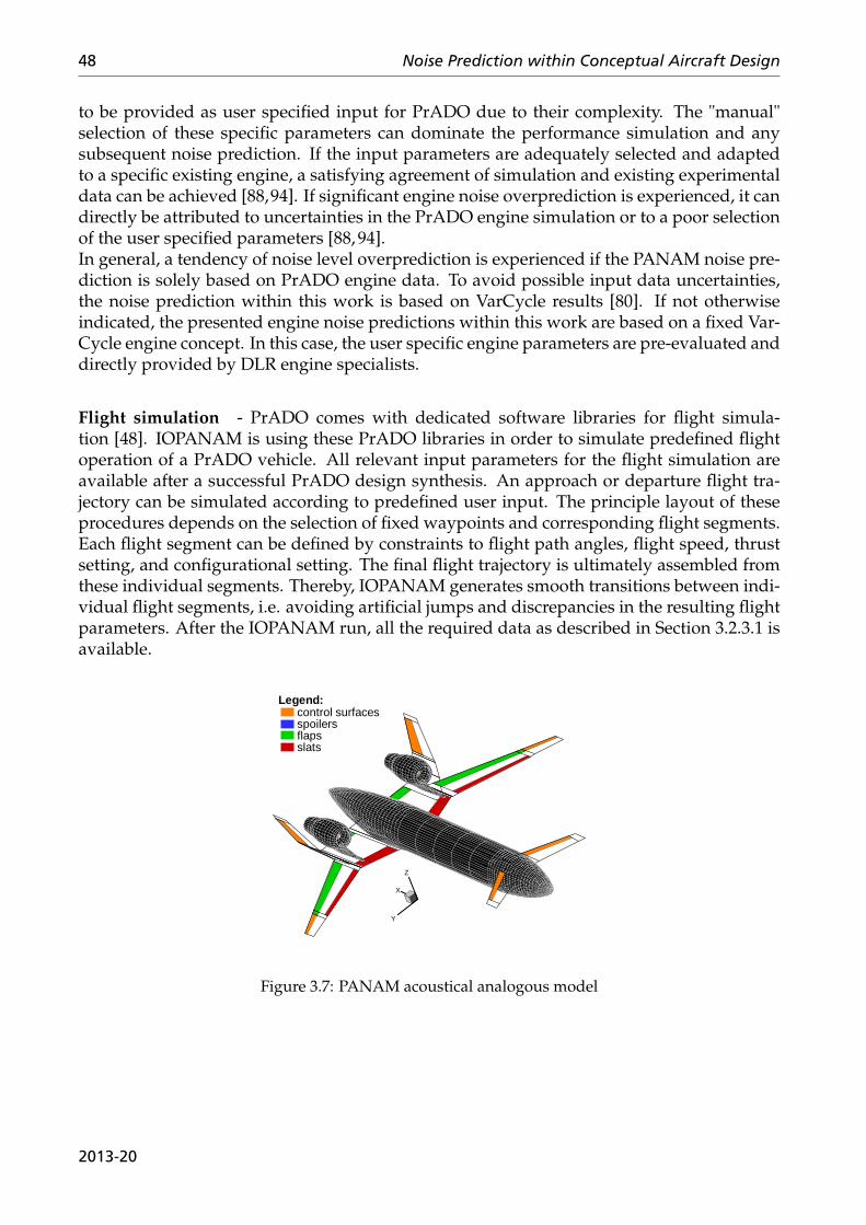
48 Noise Prediction within Conceptual Aircraft Design
to be provided as user specified input for PrADO due to their complexity. The "manual"selection of these specific parameters can dominate the performance simulation and anysubsequent noise prediction. If the input parameters are adequately selected and adaptedto a specific existing engine, a satisfying agreement of simulation and existing experimentaldata can be achieved [88,94]. If significant engine noise overprediction is experienced, it candirectly be attributed to uncertainties in the PrADO engine simulation or to a poor selectionof the user specified parameters [88, 94].In general, a tendency of noise level overprediction is experienced if the PANAM noise pre-diction is solely based on PrADO engine data. To avoid possible input data uncertainties,the noise prediction within this work is based on VarCycle results [80]. If not otherwiseindicated, the presented engine noise predictions within this work are based on a fixed Var-Cycle engine concept. In this case, the user specific engine parameters are pre-evaluated anddirectly provided by DLR engine specialists.
Flight simulation - PrADO comes with dedicated software libraries for flight simula-tion [48]. IOPANAM is using these PrADO libraries in order to simulate predefined flightoperation of a PrADO vehicle. All relevant input parameters for the flight simulation areavailable after a successful PrADO design synthesis. An approach or departure flight tra-jectory can be simulated according to predefined user input. The principle layout of theseprocedures depends on the selection of fixed waypoints and corresponding flight segments.Each flight segment can be defined by constraints to flight path angles, flight speed, thrustsetting, and configurational setting. The final flight trajectory is ultimately assembled fromthese individual segments. Thereby, IOPANAM generates smooth transitions between indi-vidual flight segments, i.e. avoiding artificial jumps and discrepancies in the resulting flightparameters. After the IOPANAM run, all the required data as described in Section 3.2.3.1 isavailable.
X
Y
Z
Legend:control surfacesspoilersflapsslats
Figure 3.7: PANAM acoustical analogous model
2013-20
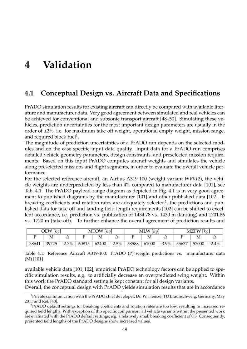
4 Validation
4.1 Conceptual Design vs. Aircraft Data and Specifications
PrADO simulation results for existing aircraft can directly be compared with available liter-ature and manufacturer data. Very good agreement between simulated and real vehicles canbe achieved for conventional and subsonic transport aircraft [48–50]. Simulating these ve-hicles, prediction uncertainties for the most important design parameters are usually in theorder of ±2%, i.e. for maximum take-off weight, operational empty weight, mission range,and required block fuel1.The magnitude of prediction uncertainties of a PrADO run depends on the selected mod-ules and on the case specific input data quality. Input data for a PrADO run comprisesdetailed vehicle geometry parameters, design constraints, and preselected mission require-ments. Based on this input PrADO computes aircraft weights and simulates the vehiclealong preselected missions and flight segments, in order to evaluate the overall vehicle per-formance.For the selected reference aircraft, an Airbus A319-100 (weight variant WV012), the vehi-cle weights are underpredicted by less than 4% compared to manufacturer data [101], seeTab. 4.1. The PrADO payload-range diagram as depicted in Fig. 4.1 is in very good agree-ment to published diagrams by the manufacturer [101] and other published data [102]. Ifbreaking coefficients and rotation rates are adequately selected2, the predictions and pub-lished data for take-off and landing field length requirements [102] can be shifted to excel-lent accordance, i.e. prediction vs. publication of 1434.78 vs. 1430 m (landing) and 1701.86vs. 1720 m (take-off). To further enhance the overall agreement of prediction results and
OEW [kg] MTOW [kg] MLW [kg] MZFW [kg]P M ∆ P M ∆ P M ∆ P M ∆
38641 39725 -2.7% 60815 62400 -2.5% 58588 61000 -3.9% 55637 57000 -2.4%
Table 4.1: Reference Aircraft A319-100: PrADO (P) weight predictions vs. manufacturer data(M) [101]
available vehicle data [101,102], empirical PrADO technology factors can be applied to spe-cific simulation results, e.g. to artificially decrease an overpredicted wing weight. Withinthis work the PrADO standard setting is kept constant for all design variants.Overall, the conceptual design with PrADO yields simulation results that are in accordance
1Private communication with the PrADO chief developer, Dr. W. Heinze, TU Braunschweig, Germany, May2011 and Ref. [48].
2PrADO default settings for breaking coefficients and rotation rates are too low, resulting in increased re-quired field lengths. With exception of this specific comparison, all vehicle variants within the presented workare evaluated with the PrADO default settings, e.g. a relatively small breaking coefficient of 0.3. Consequently,presented field lengths of the PrADO designs show increased values.
49
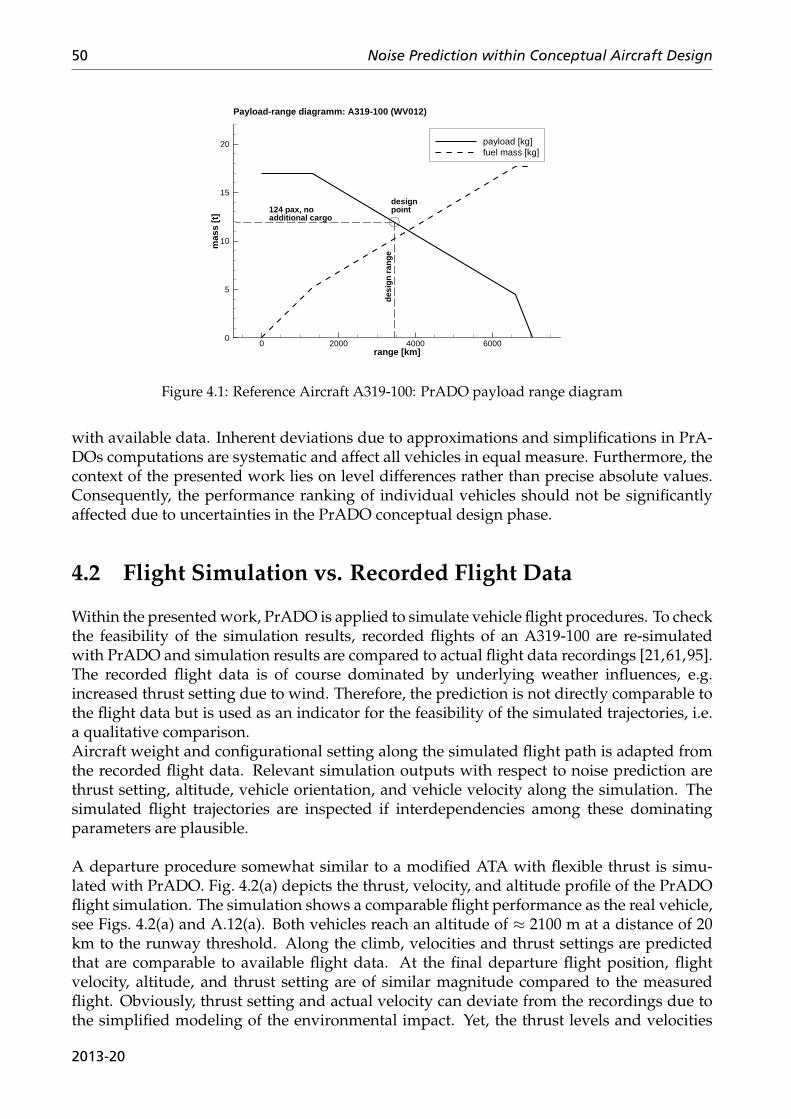
50 Noise Prediction within Conceptual Aircraft Design
range [km]
mas
s [t]
0 2000 4000 60000
5
10
15
20 payload [kg]fuel mass [kg]
Payload-range diagramm: A319-100 (WV012)
desi
gn r
ange
designpoint124 pax, no
additional cargo
Figure 4.1: Reference Aircraft A319-100: PrADO payload range diagram
with available data. Inherent deviations due to approximations and simplifications in PrA-DOs computations are systematic and affect all vehicles in equal measure. Furthermore, thecontext of the presented work lies on level differences rather than precise absolute values.Consequently, the performance ranking of individual vehicles should not be significantlyaffected due to uncertainties in the PrADO conceptual design phase.
4.2 Flight Simulation vs. Recorded Flight Data
Within the presented work, PrADO is applied to simulate vehicle flight procedures. To checkthe feasibility of the simulation results, recorded flights of an A319-100 are re-simulatedwith PrADO and simulation results are compared to actual flight data recordings [21,61,95].The recorded flight data is of course dominated by underlying weather influences, e.g.increased thrust setting due to wind. Therefore, the prediction is not directly comparable tothe flight data but is used as an indicator for the feasibility of the simulated trajectories, i.e.a qualitative comparison.Aircraft weight and configurational setting along the simulated flight path is adapted fromthe recorded flight data. Relevant simulation outputs with respect to noise prediction arethrust setting, altitude, vehicle orientation, and vehicle velocity along the simulation. Thesimulated flight trajectories are inspected if interdependencies among these dominatingparameters are plausible.
A departure procedure somewhat similar to a modified ATA with flexible thrust is simu-lated with PrADO. Fig. 4.2(a) depicts the thrust, velocity, and altitude profile of the PrADOflight simulation. The simulation shows a comparable flight performance as the real vehicle,see Figs. 4.2(a) and A.12(a). Both vehicles reach an altitude of ≈ 2100 m at a distance of 20km to the runway threshold. Along the climb, velocities and thrust settings are predictedthat are comparable to available flight data. At the final departure flight position, flightvelocity, altitude, and thrust setting are of similar magnitude compared to the measuredflight. Obviously, thrust setting and actual velocity can deviate from the recordings due tothe simplified modeling of the environmental impact. Yet, the thrust levels and velocities
2013-20
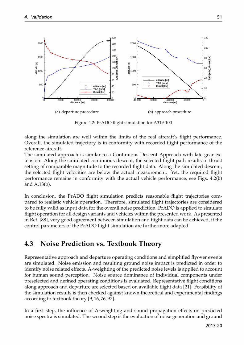
4. Validation 51
distance [m]
altit
ude
[m]
TA
S[m
/s],
thru
st[k
N]
0 5000 10000 15000 200000
500
1000
1500
2000
0
20
40
60
80
100
120
140
160
180
200
altitude [m]TAS [m/s]thrust [kN]
(a) departure procedure
distance [m]
altit
ude
[m]
TA
S[m
/s],
thru
st[k
N]
-40000 -30000 -20000 -10000 00
500
1000
1500
2000
0
20
40
60
80
100
120
altitude [m]TAS [m/s]thrust [kN]
(b) approach procedure
Figure 4.2: PrADO flight simulation for A319-100
along the simulation are well within the limits of the real aircraft’s flight performance.Overall, the simulated trajectory is in conformity with recorded flight performance of thereference aircraft.The simulated approach is similar to a Continuous Descent Approach with late gear ex-tension. Along the simulated continuous descent, the selected flight path results in thrustsetting of comparable magnitude to the recorded flight data. Along the simulated descent,the selected flight velocities are below the actual measurement. Yet, the required flightperformance remains in conformity with the actual vehicle performance, see Figs. 4.2(b)and A.13(b).
In conclusion, the PrADO flight simulation predicts reasonable flight trajectories com-pared to realistic vehicle operation. Therefore, simulated flight trajectories are consideredto be fully valid as input data for the overall noise prediction. PrADO is applied to simulateflight operation for all design variants and vehicles within the presented work. As presentedin Ref. [88], very good agreement between simulation and flight data can be achieved, if thecontrol parameters of the PrADO flight simulation are furthermore adapted.
4.3 Noise Prediction vs. Textbook Theory
Representative approach and departure operating conditions and simplified flyover eventsare simulated. Noise emission and resulting ground noise impact is predicted in order toidentify noise related effects. A-weighting of the predicted noise levels is applied to accountfor human sound perception. Noise source dominance of individual components underpreselected and defined operating conditions is evaluated. Representative flight conditionsalong approach and departure are selected based on available flight data [21]. Feasibility ofthe simulation results is then checked against known theoretical and experimental findingsaccording to textbook theory [9, 16, 76, 97].
In a first step, the influence of A-weighting and sound propagation effects on predictednoise spectra is simulated. The second step is the evaluation of noise generation and ground
2013-20
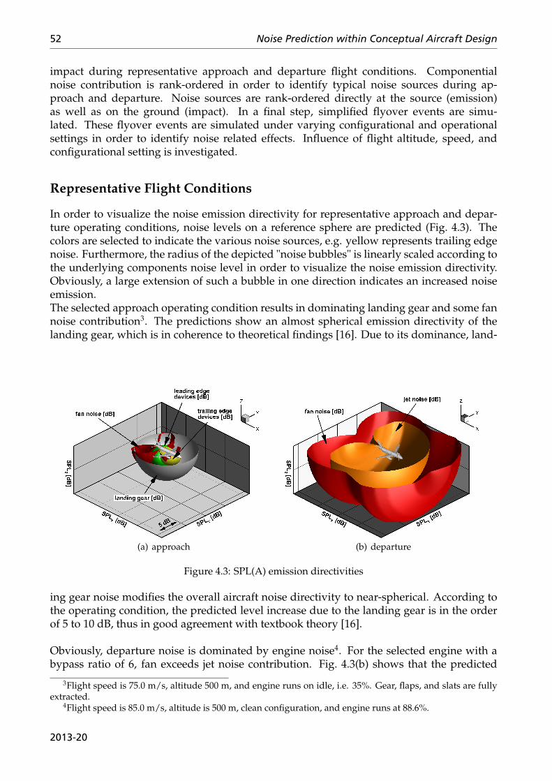
52 Noise Prediction within Conceptual Aircraft Design
impact during representative approach and departure flight conditions. Componentialnoise contribution is rank-ordered in order to identify typical noise sources during ap-proach and departure. Noise sources are rank-ordered directly at the source (emission)as well as on the ground (impact). In a final step, simplified flyover events are simu-lated. These flyover events are simulated under varying configurational and operationalsettings in order to identify noise related effects. Influence of flight altitude, speed, andconfigurational setting is investigated.
Representative Flight Conditions
In order to visualize the noise emission directivity for representative approach and depar-ture operating conditions, noise levels on a reference sphere are predicted (Fig. 4.3). Thecolors are selected to indicate the various noise sources, e.g. yellow represents trailing edgenoise. Furthermore, the radius of the depicted "noise bubbles" is linearly scaled according tothe underlying components noise level in order to visualize the noise emission directivity.Obviously, a large extension of such a bubble in one direction indicates an increased noiseemission.The selected approach operating condition results in dominating landing gear and some fannoise contribution3. The predictions show an almost spherical emission directivity of thelanding gear, which is in coherence to theoretical findings [16]. Due to its dominance, land-
(a) approach (b) departure
Figure 4.3: SPL(A) emission directivities
ing gear noise modifies the overall aircraft noise directivity to near-spherical. According tothe operating condition, the predicted level increase due to the landing gear is in the orderof 5 to 10 dB, thus in good agreement with textbook theory [16].
Obviously, departure noise is dominated by engine noise4. For the selected engine with abypass ratio of 6, fan exceeds jet noise contribution. Fig. 4.3(b) shows that the predicted
3Flight speed is 75.0 m/s, altitude 500 m, and engine runs on idle, i.e. 35%. Gear, flaps, and slats are fullyextracted.
4Flight speed is 85.0 m/s, altitude is 500 m, clean configuration, and engine runs at 88.6%.
2013-20
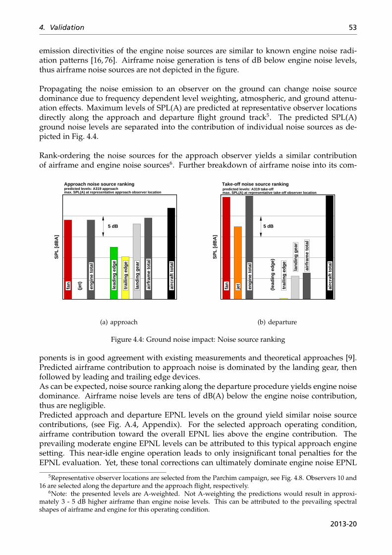
4. Validation 53
emission directivities of the engine noise sources are similar to known engine noise radi-ation patterns [16, 76]. Airframe noise generation is tens of dB below engine noise levels,thus airframe noise sources are not depicted in the figure.
Propagating the noise emission to an observer on the ground can change noise sourcedominance due to frequency dependent level weighting, atmospheric, and ground attenu-ation effects. Maximum levels of SPL(A) are predicted at representative observer locationsdirectly along the approach and departure flight ground track5. The predicted SPL(A)ground noise levels are separated into the contribution of individual noise sources as de-picted in Fig. 4.4.
Rank-ordering the noise sources for the approach observer yields a similar contributionof airframe and engine noise sources6. Further breakdown of airframe noise into its com-
SP
L [
dB
A]
airc
raft
to
tal
airf
ram
e to
tal
trai
ling
ed
ge
eng
ine
tota
l
fan
(jet
)
lead
ing
ed
ge
lan
din
g g
ear
5 dB
Approach noise source rankingpredicted levels: A319 approachmax. SPL(A) at representative approach observer location
(a) approach
SP
L [d
BA
]
airc
raft
tota
l
airf
ram
e to
tal
trai
ling
edge
engi
ne to
tal
fan
jet
(lead
ing
edge
)
land
ing
gear
5 dB
Take-off noise source rankingpredicted levels: A319 take-offmax. SPL(A) at representative take-off observer loc ation
(b) departure
Figure 4.4: Ground noise impact: Noise source ranking
ponents is in good agreement with existing measurements and theoretical approaches [9].Predicted airframe contribution to approach noise is dominated by the landing gear, thenfollowed by leading and trailing edge devices.As can be expected, noise source ranking along the departure procedure yields engine noisedominance. Airframe noise levels are tens of dB(A) below the engine noise contribution,thus are negligible.Predicted approach and departure EPNL levels on the ground yield similar noise sourcecontributions, (see Fig. A.4, Appendix). For the selected approach operating condition,airframe contribution toward the overall EPNL lies above the engine contribution. Theprevailing moderate engine EPNL levels can be attributed to this typical approach enginesetting. This near-idle engine operation leads to only insignificant tonal penalties for theEPNL evaluation. Yet, these tonal corrections can ultimately dominate engine noise EPNL
5Representative observer locations are selected from the Parchim campaign, see Fig. 4.8. Observers 10 and16 are selected along the departure and the approach flight, respectively.
6Note: the presented levels are A-weighted. Not A-weighting the predictions would result in approxi-mately 3 - 5 dB higher airframe than engine noise levels. This can be attributed to the prevailing spectralshapes of airframe and engine for this operating condition.
2013-20
54 Noise Prediction within Conceptual Aircraft Design
for increasing thrust settings. This is the case for the departure situation as depicted inFig. A.4, Appendix.
Overall, the noise source ranking and emission directivities for the selected flight con-ditions are in good agreement with existing experimental data and theoretical knowledge,e.g. published data from aircraft manufacturers [97] and textbook theory [16, 76].
Simplified Flyover Events
The selected procedures are comprised of non-accelerated and straight flight segments withpreselected and constant speed, thrust setting, configuration, and flight path angle. Thesimulated reference aircraft is a PrADO [48] model of an A319-100. Additional requiredinput parameters come from VarCycle [80], i.e. a detailed engine performance map. Theselected aircraft mass for the simulation is 45000 kg, the wing area is 122.6 m, and the centerof gravity is located at 14.4% mean airfoil chord (MAC). The forces on the overall aircraftif simulated as a point mass can be written according to Ref. [96]. Cd and Cl are the over-all aircraft drag and lift coefficients, T the thrust force, W the weight force, v the vehicleacceleration, γ the flight path angle, and g the gravitational acceleration. Accounting forthe selected flight conditions, i.e. non-accelerated and horizontal flight segments7, furthersimplifies the equation.
sin(γ) +v
g=
T
W− Cd
Cl
→ T
W=
Cd
Cl
(4.1)
With known weight and wing area, the required Cl can be evaluated for each selected flightspeed v and ambient density ρ.
Cl =2 ·W
ρ · A · v2(4.2)
Depending on the configuration and ambient flow conditions, the required lift coefficient isdirectly linked to the overall drag coefficient via the aircraft polar. Overall aircraft polars aregenerated with PrADO for each selected flight condition, i.e. altitude, speed, and configura-tional setting. From these PrADO polars, the corresponding Cd can be determined for eachrequired Cl. With known values for W , Cl and Cd, the required thrust force is evaluatedaccording to Eq. 4.1.For the required thrust force, thermodynamic engine cycle modeling yields the correspond-ing engine rotation speed. The selected reference aircraft produces the required thrust levelswith two engines, thus each engine has to generate a thrust force of T/2. At this point, allrequired geometrical and operational input parameters for the overall noise prediction areavailable.
Three noise related effects are simulated and investigated in more detail, i.e. (1) sourcedistance, (2) flight speed, and (3) configurational setting. The resulting main operationalparameters are provided in Tab. A.1, Appendix. The selected flight conditions and param-eter settings along the simulated flights are comparable to real flight data recorded undersimilar operational conditions [21, 61, 95]. Therefore, the simulated flight conditions are
7v = 0, γ = 0, lift force equals weight force
2013-20
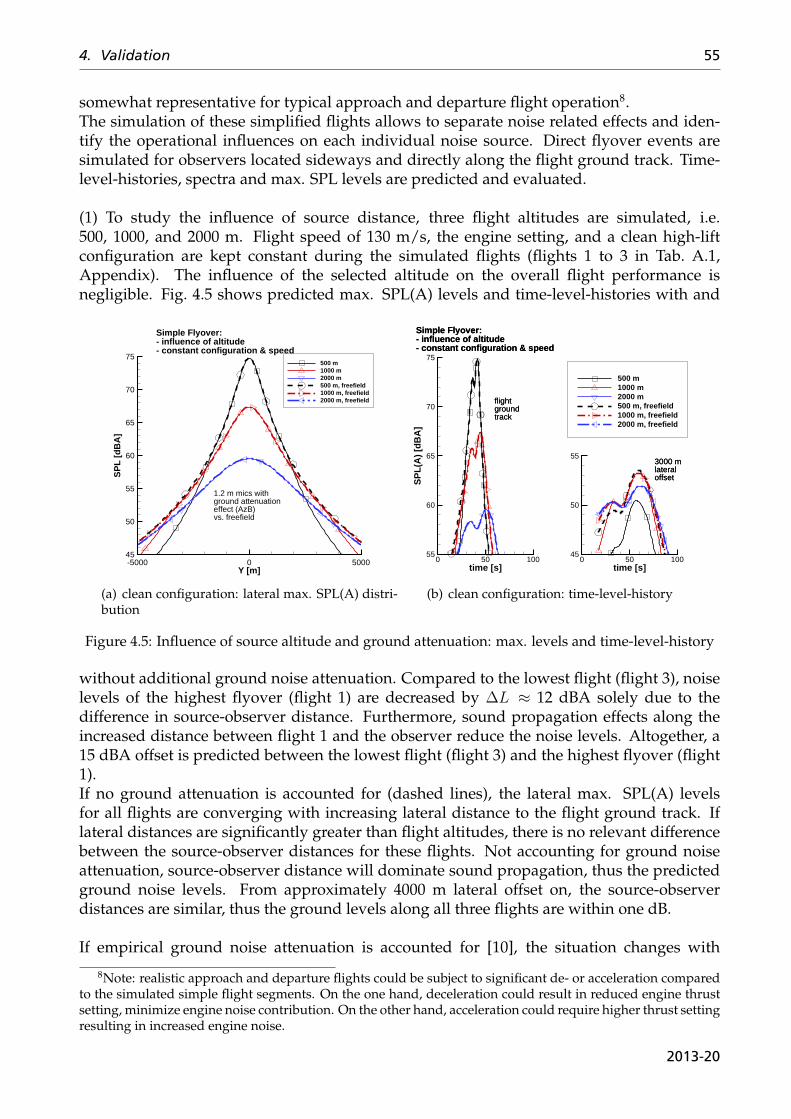
4. Validation 55
somewhat representative for typical approach and departure flight operation8.The simulation of these simplified flights allows to separate noise related effects and iden-tify the operational influences on each individual noise source. Direct flyover events aresimulated for observers located sideways and directly along the flight ground track. Time-level-histories, spectra and max. SPL levels are predicted and evaluated.
(1) To study the influence of source distance, three flight altitudes are simulated, i.e.500, 1000, and 2000 m. Flight speed of 130 m/s, the engine setting, and a clean high-liftconfiguration are kept constant during the simulated flights (flights 1 to 3 in Tab. A.1,Appendix). The influence of the selected altitude on the overall flight performance isnegligible. Fig. 4.5 shows predicted max. SPL(A) levels and time-level-histories with and
Y [m]
SP
L [d
BA
]
-5000 0 500045
50
55
60
65
70
75500 m1000 m2000 m500 m, freefield1000 m, freefield2000 m, freefield
Simple Flyover: - influence of altitude- constant configuration & speed
1.2 m mics with ground attenuationeffect (AzB) vs. freefield
(a) clean configuration: lateral max. SPL(A) distri-bution
time [s]0 50 100
45
50
553000 m lateraloffset
Simple Flyover:- influence of altitude- constant configuration & speed
flightgroundtrack
time [s]
SP
L(A
) [d
BA
]
0 50 10055
60
65
70
75
500 m1000 m2000 m500 m, freefield1000 m, freefield2000 m, freefield
3000 m lateraloffset
Simple Flyover:- influence of altitude- constant configuration & speed
flightgroundtrack
(b) clean configuration: time-level-history
Figure 4.5: Influence of source altitude and ground attenuation: max. levels and time-level-history
without additional ground noise attenuation. Compared to the lowest flight (flight 3), noiselevels of the highest flyover (flight 1) are decreased by ∆L ≈ 12 dBA solely due to thedifference in source-observer distance. Furthermore, sound propagation effects along theincreased distance between flight 1 and the observer reduce the noise levels. Altogether, a15 dBA offset is predicted between the lowest flight (flight 3) and the highest flyover (flight1).If no ground attenuation is accounted for (dashed lines), the lateral max. SPL(A) levelsfor all flights are converging with increasing lateral distance to the flight ground track. Iflateral distances are significantly greater than flight altitudes, there is no relevant differencebetween the source-observer distances for these flights. Not accounting for ground noiseattenuation, source-observer distance will dominate sound propagation, thus the predictedground noise levels. From approximately 4000 m lateral offset on, the source-observerdistances are similar, thus the ground levels along all three flights are within one dB.
If empirical ground noise attenuation is accounted for [10], the situation changes with
8Note: realistic approach and departure flights could be subject to significant de- or acceleration comparedto the simulated simple flight segments. On the one hand, deceleration could result in reduced engine thrustsetting, minimize engine noise contribution. On the other hand, acceleration could require higher thrust settingresulting in increased engine noise.
2013-20
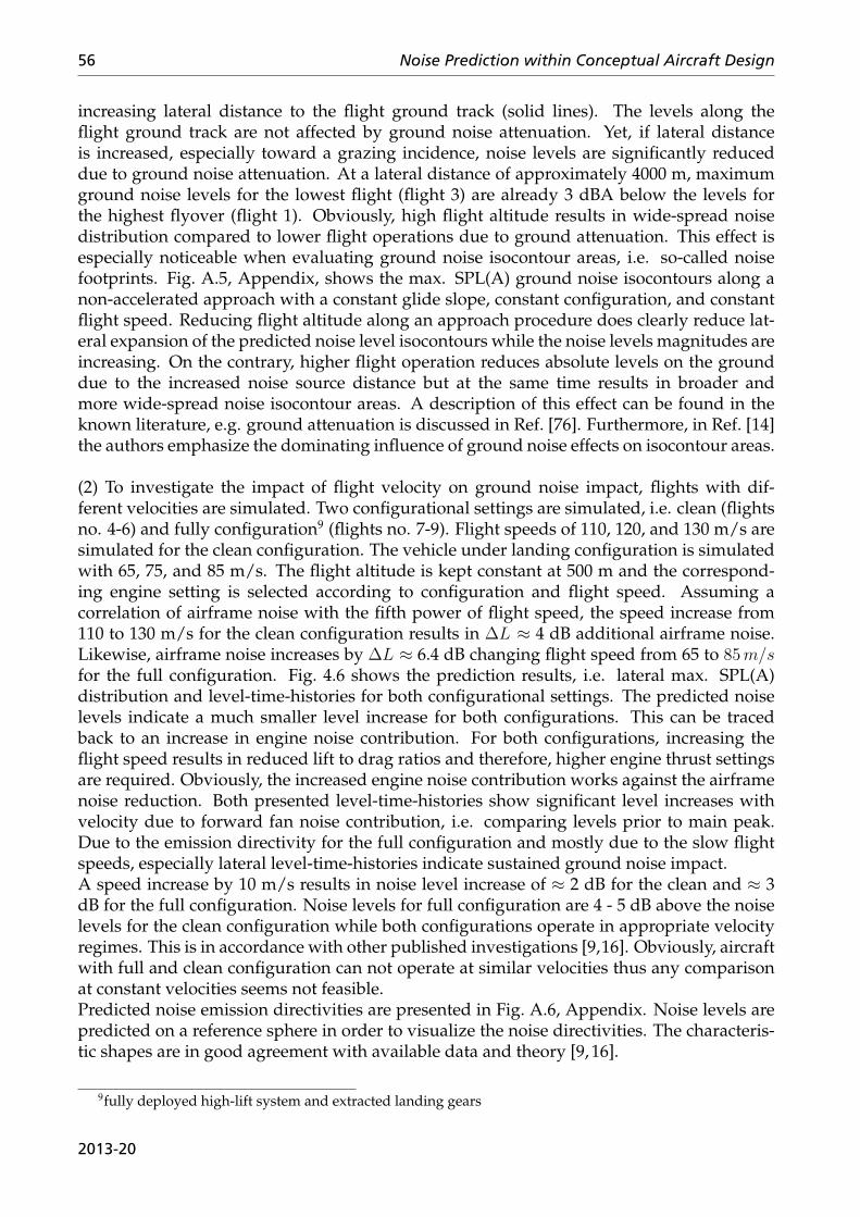
56 Noise Prediction within Conceptual Aircraft Design
increasing lateral distance to the flight ground track (solid lines). The levels along theflight ground track are not affected by ground noise attenuation. Yet, if lateral distanceis increased, especially toward a grazing incidence, noise levels are significantly reduceddue to ground noise attenuation. At a lateral distance of approximately 4000 m, maximumground noise levels for the lowest flight (flight 3) are already 3 dBA below the levels forthe highest flyover (flight 1). Obviously, high flight altitude results in wide-spread noisedistribution compared to lower flight operations due to ground attenuation. This effect isespecially noticeable when evaluating ground noise isocontour areas, i.e. so-called noisefootprints. Fig. A.5, Appendix, shows the max. SPL(A) ground noise isocontours along anon-accelerated approach with a constant glide slope, constant configuration, and constantflight speed. Reducing flight altitude along an approach procedure does clearly reduce lat-eral expansion of the predicted noise level isocontours while the noise levels magnitudes areincreasing. On the contrary, higher flight operation reduces absolute levels on the grounddue to the increased noise source distance but at the same time results in broader andmore wide-spread noise isocontour areas. A description of this effect can be found in theknown literature, e.g. ground attenuation is discussed in Ref. [76]. Furthermore, in Ref. [14]the authors emphasize the dominating influence of ground noise effects on isocontour areas.
(2) To investigate the impact of flight velocity on ground noise impact, flights with dif-ferent velocities are simulated. Two configurational settings are simulated, i.e. clean (flightsno. 4-6) and fully configuration9 (flights no. 7-9). Flight speeds of 110, 120, and 130 m/s aresimulated for the clean configuration. The vehicle under landing configuration is simulatedwith 65, 75, and 85 m/s. The flight altitude is kept constant at 500 m and the correspond-ing engine setting is selected according to configuration and flight speed. Assuming acorrelation of airframe noise with the fifth power of flight speed, the speed increase from110 to 130 m/s for the clean configuration results in ∆L ≈ 4 dB additional airframe noise.Likewise, airframe noise increases by ∆L ≈ 6.4 dB changing flight speed from 65 to 85m/sfor the full configuration. Fig. 4.6 shows the prediction results, i.e. lateral max. SPL(A)distribution and level-time-histories for both configurational settings. The predicted noiselevels indicate a much smaller level increase for both configurations. This can be tracedback to an increase in engine noise contribution. For both configurations, increasing theflight speed results in reduced lift to drag ratios and therefore, higher engine thrust settingsare required. Obviously, the increased engine noise contribution works against the airframenoise reduction. Both presented level-time-histories show significant level increases withvelocity due to forward fan noise contribution, i.e. comparing levels prior to main peak.Due to the emission directivity for the full configuration and mostly due to the slow flightspeeds, especially lateral level-time-histories indicate sustained ground noise impact.A speed increase by 10 m/s results in noise level increase of ≈ 2 dB for the clean and ≈ 3dB for the full configuration. Noise levels for full configuration are 4 - 5 dB above the noiselevels for the clean configuration while both configurations operate in appropriate velocityregimes. This is in accordance with other published investigations [9,16]. Obviously, aircraftwith full and clean configuration can not operate at similar velocities thus any comparisonat constant velocities seems not feasible.Predicted noise emission directivities are presented in Fig. A.6, Appendix. Noise levels arepredicted on a reference sphere in order to visualize the noise directivities. The characteris-tic shapes are in good agreement with available data and theory [9, 16].
9fully deployed high-lift system and extracted landing gears
2013-20
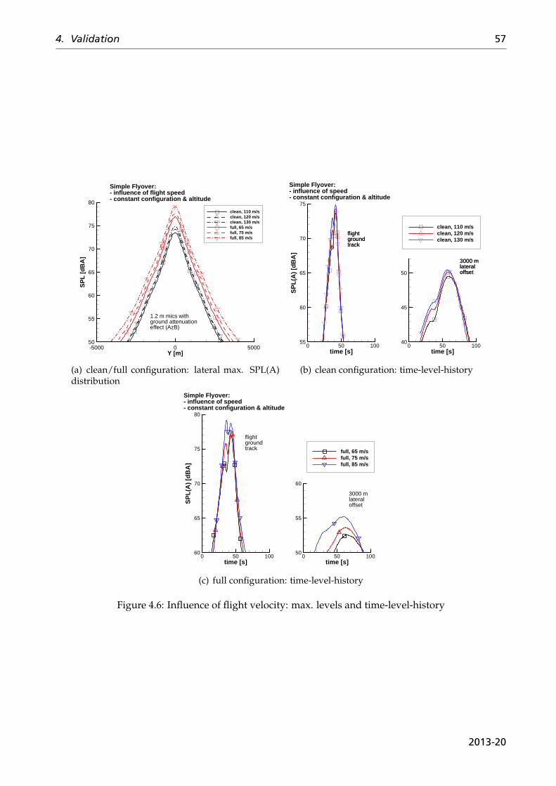
4. Validation 57
Y [m]
SP
L [d
BA
]
-5000 0 500050
55
60
65
70
75
80
clean, 110 m/sclean, 120 m/sclean, 130 m/sfull, 65 m/sfull, 75 m/sfull, 85 m/s
Simple Flyover: - influence of flight speed- constant configuration & altitude
1.2 m mics withground attenuationeffect (AzB)
(a) clean/full configuration: lateral max. SPL(A)distribution
time [s]0 50 100
40
45
50
3000 mlateraloffset
flightgroundtrack
time [s]
SP
L(A
) [d
BA
]
0 50 10055
60
65
70
75
clean, 110 m/sclean, 120 m/sclean, 130 m/s
3000 mlateraloffset
flightgroundtrack
Simple Flyover:- influence of speed- constant configuration & altitude
(b) clean configuration: time-level-history
time [s]0 50 100
50
55
60
3000 mlateraloffset
flightgroundtrack
time [s]
SP
L(A
) [d
BA
]
0 50 10060
65
70
75
80
full, 65 m/sfull, 75 m/sfull, 85 m/s
Simple Flyover:- influence of speed- constant configuration & altitude
(c) full configuration: time-level-history
Figure 4.6: Influence of flight velocity: max. levels and time-level-history
2013-20
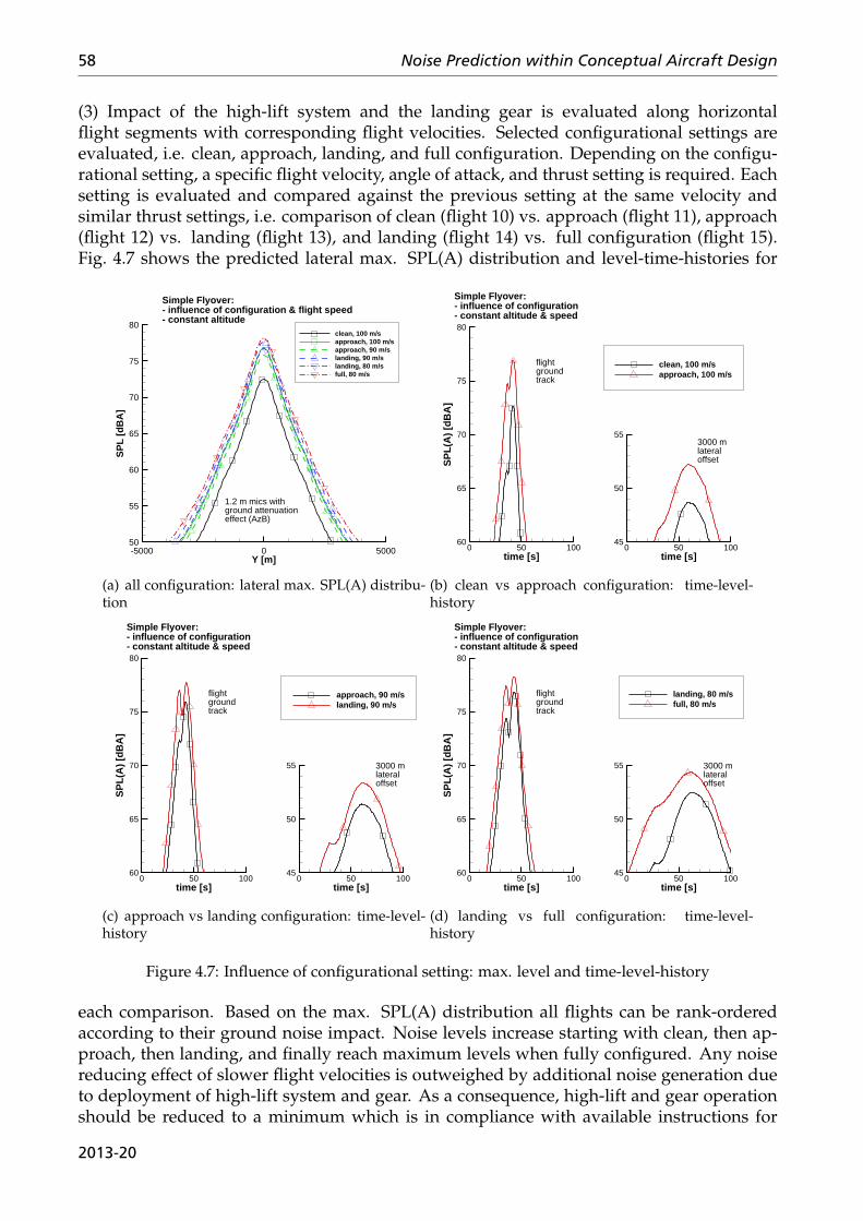
58 Noise Prediction within Conceptual Aircraft Design
(3) Impact of the high-lift system and the landing gear is evaluated along horizontalflight segments with corresponding flight velocities. Selected configurational settings areevaluated, i.e. clean, approach, landing, and full configuration. Depending on the configu-rational setting, a specific flight velocity, angle of attack, and thrust setting is required. Eachsetting is evaluated and compared against the previous setting at the same velocity andsimilar thrust settings, i.e. comparison of clean (flight 10) vs. approach (flight 11), approach(flight 12) vs. landing (flight 13), and landing (flight 14) vs. full configuration (flight 15).Fig. 4.7 shows the predicted lateral max. SPL(A) distribution and level-time-histories for
Y [m]
SP
L [d
BA
]
-5000 0 500050
55
60
65
70
75
80clean, 100 m/sapproach, 100 m/sapproach, 90 m/slanding, 90 m/slanding, 80 m/sfull, 80 m/s
Simple Flyover: - influence of configuration & flight speed- constant altitude
1.2 m mics withground attenuationeffect (AzB)
(a) all configuration: lateral max. SPL(A) distribu-tion
time [s]0 50 100
45
50
553000 mlateraloffset
flightgroundtrack
time [s]
SP
L(A
) [d
BA
]
0 50 10060
65
70
75
80
clean, 100 m/sapproach, 100 m/s
Simple Flyover:- influence of configuration- constant altitude & speed
(b) clean vs approach configuration: time-level-history
time [s]0 50 100
45
50
55 3000 mlateraloffset
flightgroundtrack
time [s]
SP
L(A
) [d
BA
]
0 50 10060
65
70
75
80
approach, 90 m/slanding, 90 m/s
Simple Flyover:- influence of configuration- constant altitude & speed
(c) approach vs landing configuration: time-level-history
time [s]0 50 100
45
50
55 3000 mlateraloffset
flightgroundtrack
time [s]
SP
L(A
) [d
BA
]
0 50 10060
65
70
75
80
landing, 80 m/sfull, 80 m/s
Simple Flyover:- influence of configuration- constant altitude & speed
(d) landing vs full configuration: time-level-history
Figure 4.7: Influence of configurational setting: max. level and time-level-history
each comparison. Based on the max. SPL(A) distribution all flights can be rank-orderedaccording to their ground noise impact. Noise levels increase starting with clean, then ap-proach, then landing, and finally reach maximum levels when fully configured. Any noisereducing effect of slower flight velocities is outweighed by additional noise generation dueto deployment of high-lift system and gear. As a consequence, high-lift and gear operationshould be reduced to a minimum which is in compliance with available instructions for
2013-20
4. Validation 59
low-noise procedures, see Section 2.2 and Ref. [9]. Again, characteristic directivity shapesare in good agreement with available data and theory [9, 16], see Fig. A.7, Appendix.
In conclusion, predicted influence of flight altitude, speed, and configurational settingis consistent with existing experimental and theoretical findings. The presented comparisonof PANAM results with textbook theory indicates that the major noise generating effectsare adequately accounted for. In general, the predicted shape of level-time-histories isin good agreement with theoretical level variations for turbofan vehicles. In consistencewith Ref. [76], the time-histories show two level peaks before and after the time step corre-sponding to a direct overhead position of the aircraft. The level peaks can be more or lessintensified depending on the dominating sources noise emission and the flyover event, i.e.flight speed and altitude.
4.4 Noise Prediction vs. Measurements
Each implemented noise source model has individually been validated with componen-tial windtunnel and or computational data [21, 28, 36, 95]. Experimental windtunnel datais recorded under steady laboratory conditions and computations are defined by simplifiedand artificial boundary conditions. Therefore, it is necessary to judge the feasibility of theassumptions and models under realistic operating conditions. Studies indicate an accuracyfor dedicated airframe noise prediction of ±1 dB [71] and ±4 dB for engine noise predic-tion [28]. Yet, it has to be verified, that overall aircraft noise can be approximated by anassembly of these separate noise sources in a real environment. A feasible validation re-quires a comparison with actual aircraft flyover noise measurements. Such flyover noisedata reflects realistic operating conditions, thus is compromised by noise source movementand sound propagation effects. If working with flyover noise measurements one has tokeep in mind that such data is subject to inherent imprecision and limited replicability [15].Therefore, very good overall agreement of predicted noise levels with actual measurementsbecomes very difficult and can only be achieved to a certain extend. Furthermore, PANAMonly accounts for the most dominating noise sources and simplifies noise source interaction.Various design details, e.g. cavities, on-board of real aircraft can contribute significantly tothe overall noise levels [9] but cannot be accounted for. As a consequence, Dobrzynski ac-centuates that perfect or very good agreement of measurements and simple predictions cannot be achieved and if so they would not be plausible [9]. Nevertheless, if the major domi-nating noise sources are accurately modeled, a satisfying overall accuracy can be expected.Only a dedicated comparison of simulated versus measured aircraft ground noise levels canindicate the feasibility and the quality of the applied prediction methodology.
4.4.1 A319 Flyover Campaign
Within the presented work, the focus lies on medium-range, single-aisle transport aircraft.Therefore, the prediction results are compared to flyover noise measurements for suchan aircraft type. Due to extensive available data, especially detailed engine design, anA319 with CFM56 engines is selected. The required input data for PANAM comes fromPrADO [48] (vehicle geometry), SHADOW [83] (noise shielding effects), Varcycle [80](engine performance map and detail design), and recorded flight data (trajectory withconfiguration and engine setting).
2013-20
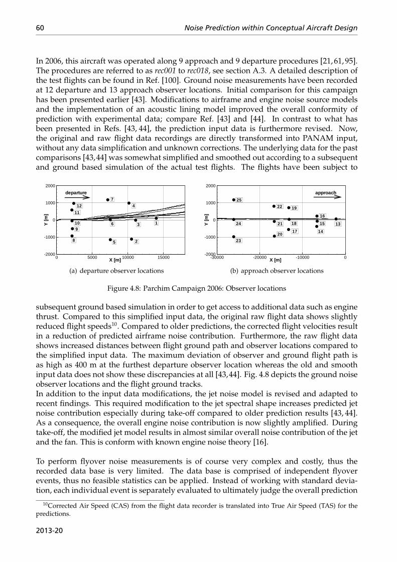
60 Noise Prediction within Conceptual Aircraft Design
In 2006, this aircraft was operated along 9 approach and 9 departure procedures [21, 61, 95].The procedures are referred to as rec001 to rec018, see section A.3. A detailed description ofthe test flights can be found in Ref. [100]. Ground noise measurements have been recordedat 12 departure and 13 approach observer locations. Initial comparison for this campaignhas been presented earlier [43]. Modifications to airframe and engine noise source modelsand the implementation of an acoustic lining model improved the overall conformity ofprediction with experimental data; compare Ref. [43] and [44]. In contrast to what hasbeen presented in Refs. [43, 44], the prediction input data is furthermore revised. Now,the original and raw flight data recordings are directly transformed into PANAM input,without any data simplification and unknown corrections. The underlying data for the pastcomparisons [43,44] was somewhat simplified and smoothed out according to a subsequentand ground based simulation of the actual test flights. The flights have been subject to
X [m]
Y[m
]
0 5000 10000 15000-2000
-1000
0
1000
2000
departure
12
1
2
3
4
5
6
7
8
910
11
(a) departure observer locations
X [m]
Y[m
]
-30000 -20000 -10000 0-2000
-1000
0
1000
2000
approach
25
13
14
16
19
17
18
22
23
24 15
20
21
(b) approach observer locations
Figure 4.8: Parchim Campaign 2006: Observer locations
subsequent ground based simulation in order to get access to additional data such as enginethrust. Compared to this simplified input data, the original raw flight data shows slightlyreduced flight speeds10. Compared to older predictions, the corrected flight velocities resultin a reduction of predicted airframe noise contribution. Furthermore, the raw flight datashows increased distances between flight ground path and observer locations compared tothe simplified input data. The maximum deviation of observer and ground flight path isas high as 400 m at the furthest departure observer location whereas the old and smoothinput data does not show these discrepancies at all [43,44]. Fig. 4.8 depicts the ground noiseobserver locations and the flight ground tracks.In addition to the input data modifications, the jet noise model is revised and adapted torecent findings. This required modification to the jet spectral shape increases predicted jetnoise contribution especially during take-off compared to older prediction results [43, 44].As a consequence, the overall engine noise contribution is now slightly amplified. Duringtake-off, the modified jet model results in almost similar overall noise contribution of the jetand the fan. This is conform with known engine noise theory [16].
To perform flyover noise measurements is of course very complex and costly, thus therecorded data base is very limited. The data base is comprised of independent flyoverevents, thus no feasible statistics can be applied. Instead of working with standard devia-tion, each individual event is separately evaluated to ultimately judge the overall prediction
10Corrected Air Speed (CAS) from the flight data recorder is translated into True Air Speed (TAS) for thepredictions.
2013-20
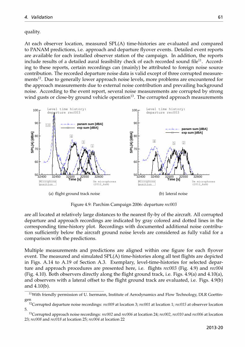
4. Validation 61
quality.
At each observer location, measured SPL(A) time-histories are evaluated and comparedto PANAM predictions, i.e. approach and departure flyover events. Detailed event reportsare available for each installed observer station of the campaign. In addition, the reportsinclude results of a detailed aural feasibility check of each recorded sound file11. Accord-ing to these reports, certain recordings can (mainly) be attributed to foreign noise sourcecontribution. The recorded departure noise data is valid except of three corrupted measure-ments12. Due to generally lower approach noise levels, more problems are encountered forthe approach measurements due to external noise contribution and prevailing backgroundnoise. According to the event report, several noise measurements are corrupted by strongwind gusts or close-by ground vehicle operation13. The corrupted approach measurements
Time [s]
SP
L(A
)[d
BA
]
32400 32450 32500 32550 3260050
60
70
80
90
100
panam sum [dBA]exp sum [dBA]
Level time history:departure rec003
Microphoneposition
0m microphones(2012_AzB)
10
6
13
(a) flight ground track noise
Time [s]
SP
L(A
)[d
BA
]
32400 32450 32500 32550 3260050
60
70
80
90
100
panam sum [dBA]exp sum [dBA]
Level time history:departure rec003
Microphoneposition
0m microphones(2012_AzB)
85 2
(b) lateral noise
Figure 4.9: Parchim Campaign 2006: departure rec003
are all located at relatively large distances to the nearest fly-by of the aircraft. All corrupteddeparture and approach recordings are indicated by gray colored and dotted lines in thecorresponding time-history plot. Recordings with documented additional noise contribu-tion sufficiently below the aircraft ground noise levels are considered as fully valid for acomparison with the predictions.
Multiple measurements and predictions are aligned within one figure for each flyoverevent. The measured and simulated SPL(A) time-histories along all test flights are depictedin Figs. A.14 to A.19 of Section A.3. Exemplary, level-time-histories for selected depar-ture and approach procedures are presented here, i.e. flights rec003 (Fig. 4.9) and rec004(Fig. 4.10). Both observers directly along the flight ground track, i.e. Figs. 4.9(a) and 4.10(a),and observers with a lateral offset to the flight ground track are evaluated, i.e. Figs. 4.9(b)and 4.10(b).
11With friendly permission of U. Isermann, Institute of Aerodynamics and Flow Technology, DLR Goettin-gen
12Corrupted departure noise recordings: rec009 at location 3; rec001 at location 1; rec015 at observer location5.
13Corrupted approach noise recordings: rec002 and rec006 at location 24; rec002, rec010 and rec006 at location23; rec008 and rec018 at location 25; rec004 at location 22
2013-20
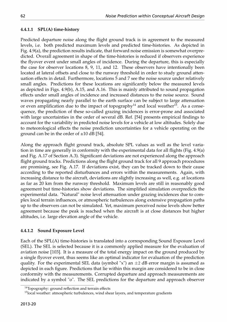
62 Noise Prediction within Conceptual Aircraft Design
4.4.1.1 SPL(A) time-history
Predicted departure noise along the flight ground track is in agreement to the measuredlevels, i.e. both predicted maximum levels and predicted time-histories. As depicted inFig. 4.9(a), the prediction results indicate, that forward noise emission is somewhat overpre-dicted. Overall agreement in shape of the time-histories is reduced if observers experiencethe flyover event under small angles of incidence. During the departure, this is especiallythe case for observer locations 8, 9, 11, and 12. These observers have intentionally beenlocated at lateral offsets and close to the runway threshold in order to study ground atten-uation effects in detail. Furthermore, locations 5 and 7 see the noise source under relativelysmall angles. Predictions for these locations are significantly below the measured levelsas depicted in Figs. 4.9(b), A.15, and A.16. This is mainly attributed to sound propagationeffects under small angles of incidence and increased distances to the noise source. Soundwaves propagating nearly parallel to the earth surface can be subject to large attenuationor even amplification due to the impact of topography14 and local weather15. As a conse-quence, the prediction of these so-called grazing incidences is error-prone and associatedwith large uncertainties in the order of several dB. Ref. [54] presents empirical findings toaccount for the variability in predicted noise levels for a vehicle at low altitudes. Solely dueto meteorological effects the noise prediction uncertainties for a vehicle operating on theground can be in the order of ±10 dB [54].
Along the approach flight ground track, absolute SPL values as well as the level varia-tion in time are generally in conformity with the experimental data for all flights (Fig. 4.9(a)and Fig. A.17 of Section A.3). Significant deviations are not experienced along the approachflight ground tracks. Predictions along the flight ground track for all 9 approach proceduresare promising, see Fig. A.17. If deviations exist, they can be tracked down to their causeaccording to the reported disturbances and errors within the measurements. Again, withincreasing distance to the aircraft, deviations are slightly increasing as well, e.g. at locationsas far as 20 km from the runway threshold. Maximum levels are still in reasonably goodagreement but time-histories show deviations. The simplified simulation overpredicts theexperimental data. "Natural" noise level attenuation under grazing incidences due to com-plex local terrain influences, or atmospheric turbulences along extensive propagation pathsup to the observers can not be simulated. Yet, maximum perceived noise levels show betteragreement because the peak is reached when the aircraft is at close distances but higheraltitudes, i.e. large elevation angle of the vehicle.
4.4.1.2 Sound Exposure Level
Each of the SPL(A) time-histories is translated into a corresponding Sound Exposure Level(SEL). The SEL is selected because it is a commonly applied measure for the evaluation ofaviation noise [103]. It is a measure of the total energy impact on the ground produced bya single flyover event, thus seems like an optimal indicator for evaluation of the predictionquality. For the experimental SEL data (symbol "x") an ±2 dB error margin is assumed asdepicted in each figure. Predictions that lie within this margin are considered to be in closeconformity with the measurements. Corrupted departure and approach measurements areindicated by a symbol "o". The SEL predictions for the departure and approach observer
14Topography: ground reflection and terrain effects15local weather: atmospheric turbulences, wind shear layers, and temperature gradients
2013-20
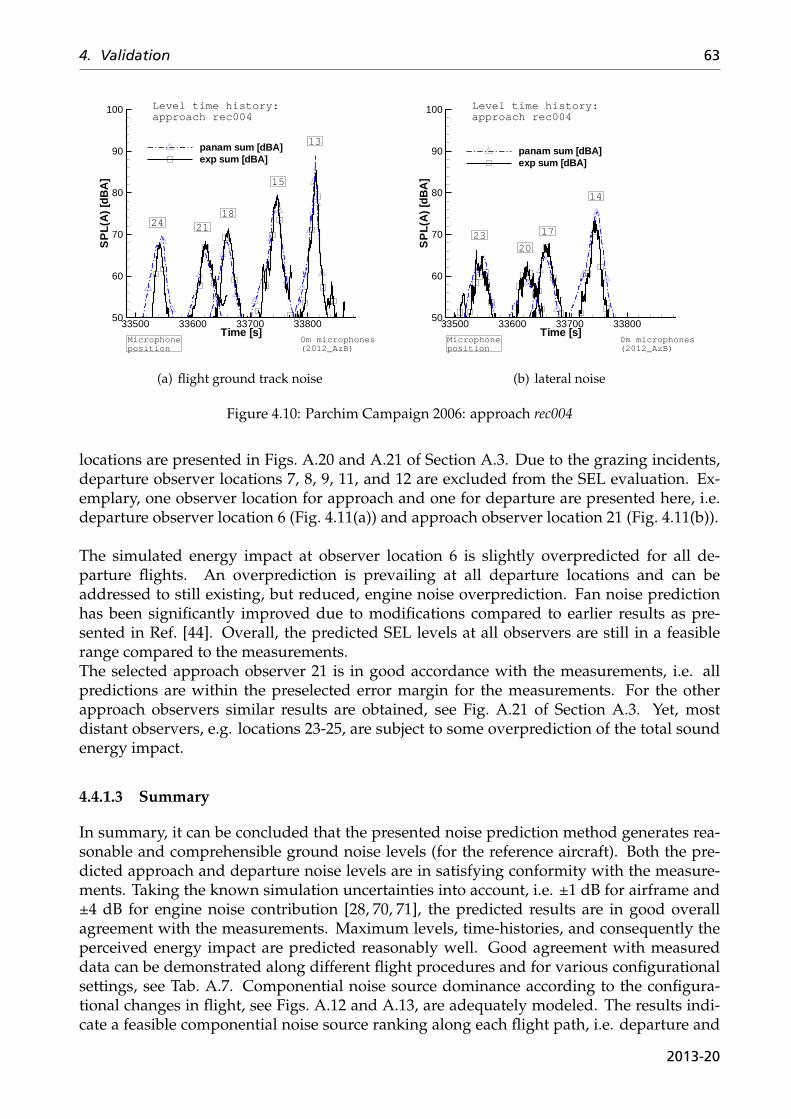
4. Validation 63
Time [s]
SP
L(A
)[d
BA
]
33500 33600 33700 3380050
60
70
80
90
100
panam sum [dBA]exp sum [dBA]
Level time history:approach rec004
Microphoneposition
0m microphones(2012_AzB)
24 21
13
18
15
(a) flight ground track noise
Time [s]
SP
L(A
)[d
BA
]
33500 33600 33700 3380050
60
70
80
90
100
panam sum [dBA]exp sum [dBA]
Level time history:approach rec004
Microphoneposition
0m microphones(2012_AzB)
2320
14
17
(b) lateral noise
Figure 4.10: Parchim Campaign 2006: approach rec004
locations are presented in Figs. A.20 and A.21 of Section A.3. Due to the grazing incidents,departure observer locations 7, 8, 9, 11, and 12 are excluded from the SEL evaluation. Ex-emplary, one observer location for approach and one for departure are presented here, i.e.departure observer location 6 (Fig. 4.11(a)) and approach observer location 21 (Fig. 4.11(b)).
The simulated energy impact at observer location 6 is slightly overpredicted for all de-parture flights. An overprediction is prevailing at all departure locations and can beaddressed to still existing, but reduced, engine noise overprediction. Fan noise predictionhas been significantly improved due to modifications compared to earlier results as pre-sented in Ref. [44]. Overall, the predicted SEL levels at all observers are still in a feasiblerange compared to the measurements.The selected approach observer 21 is in good accordance with the measurements, i.e. allpredictions are within the preselected error margin for the measurements. For the otherapproach observers similar results are obtained, see Fig. A.21 of Section A.3. Yet, mostdistant observers, e.g. locations 23-25, are subject to some overprediction of the total soundenergy impact.
4.4.1.3 Summary
In summary, it can be concluded that the presented noise prediction method generates rea-sonable and comprehensible ground noise levels (for the reference aircraft). Both the pre-dicted approach and departure noise levels are in satisfying conformity with the measure-ments. Taking the known simulation uncertainties into account, i.e. ±1 dB for airframe and±4 dB for engine noise contribution [28, 70, 71], the predicted results are in good overallagreement with the measurements. Maximum levels, time-histories, and consequently theperceived energy impact are predicted reasonably well. Good agreement with measureddata can be demonstrated along different flight procedures and for various configurationalsettings, see Tab. A.7. Componential noise source dominance according to the configura-tional changes in flight, see Figs. A.12 and A.13, are adequately modeled. The results indi-cate a feasible componential noise source ranking along each flight path, i.e. departure and
2013-20
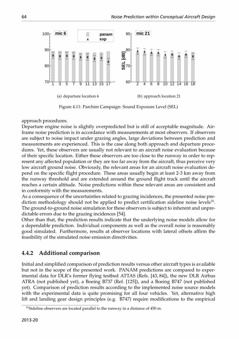
64 Noise Prediction within Conceptual Aircraft Design
x x x x x x x xx
1 3 5 7 9 11 13 15 1770
80
90
100 panamexpx
mic 6
(a) departure location 6
x x x x x x x x x
SE
L[d
B]
2 4 6 8 10 12 14 16 1860
70
80
90 mic 21
(b) approach location 21
Figure 4.11: Parchim Campaign: Sound Exposure Level (SEL)
approach procedures.Departure engine noise is slightly overpredicted but is still of acceptable magnitude. Air-frame noise prediction is in accordance with measurements at most observers. If observersare subject to noise impact under grazing angles, large deviations between prediction andmeasurements are experienced. This is the case along both approach and departure proce-dures. Yet, these observers are usually not relevant to an aircraft noise evaluation becauseof their specific location. Either these observers are too close to the runway in order to rep-resent any affected population or they are too far away from the aircraft, thus perceive verylow aircraft ground noise. Obviously, the relevant areas for an aircraft noise evaluation de-pend on the specific flight procedure. These areas usually begin at least 2-3 km away fromthe runway threshold and are extended around the ground flight track until the aircraftreaches a certain altitude. Noise predictions within these relevant areas are consistent andin conformity with the measurements.As a consequence of the uncertainties related to grazing incidences, the presented noise pre-diction methodology should not be applied to predict certification sideline noise levels16.The ground-to-ground noise simulation for these observers is subject to inherent and unpre-dictable errors due to the grazing incidences [54].Other than that, the prediction results indicate that the underlying noise models allow fora dependable prediction. Individual components as well as the overall noise is reasonablygood simulated. Furthermore, results at observer locations with lateral offsets affirm thefeasibility of the simulated noise emission directivities.
4.4.2 Additional comparison
Initial and simplified comparison of prediction results versus other aircraft types is availablebut not in the scope of the presented work. PANAM predictions are compared to exper-imental data for DLR’s former flying testbed ATTAS (Refs. [43, 84]), the new DLR AirbusATRA (not published yet), a Boeing B737 (Ref. [125]), and a Boeing B747 (not publishedyet). Comparison of prediction results according to the implemented noise source modelswith the experimental data is quite promising for all four vehicles. Yet, alternative highlift and landing gear design principles (e.g. B747) require modifications to the empirical
16Sideline observers are located parallel to the runway in a distance of 450 m.
2013-20
4. Validation 65
factors. If the empirical factors are modified, the results show good agreement with themeasurements [70, 71].A sophisticated prediction for these various vehicles would require detailed engine designwith higher fidelity tools, e.g. Varcycle [80], not being available at the time of finalization ofthis work. Therefore, initial predictions of ATRA, B737, and B747 are based on simplifiedPrADO engine models. Obviously, the major and dominating influence of engine operatingconditions on noise emission is crucial to accurate modeling for a feasible noise prediction.It is demonstrated, that result accuracy can be significantly improved if more detailedengine data is available, e.g. high-fidelity thermodynamic engine modeling [125].
A direct tool-to-tool comparison with other existing scientific noise prediction tools hasbeen initiated and is currently under progress. As presented in Ref. [104], an initial com-parison with the University of Manchester’s FLIGHT code confirms the feasibility andresult accuracy of PANAM. In the long run, these tool-to-tool comparisons will contributeto establish defined validation standards and realistic accuracy margins for scientific noiseprediction tools.
2013-20

5 Application
The presented applications of PANAM can be grouped into two research areas, i.e. low-noisevehicle design and decision making support. The main focus of the presented applicationslies on low-noise vehicle retrofit and overall design.Low-noise design modifications do not only apply to the corresponding noise source geome-tries, but can have an influence on the overall flight performance. The flight performancedefines the operating conditions for all noise sources, thus overall noise generation can beinfluenced. Consequently, for the evaluation of low-noise concepts and promising technolo-gies, individual flyover events have to be simulated for each new or modified vehicle design.The second area of application for PANAM is to support (political) decision making with re-spect to noise abatement flight procedures and airspace management. Single and multipleflyover events can be analyzed in order to support the identification of promising low-noiseflight procedures, spatial airtraffic routing, and flight schedules.
5.1 Low-Noise Vehicle Design
The focus of the presented design study lies on single-aisle, medium-range transport air-craft. The two main reasons for this selection are today’s large market share for this aircraftcategory and the availability of extensive validation data. Independent market forecasts ofmajor aircraft manufacturers even predict an increase in market share to over 70% for theseaircraft types by the year 2030 [105, 106]. As a consequence, single-aisle aircraft representthe majority of all flight operations at larger airports thus have a dominating impact onairport community noise pollution.
The main goal of this study is the identification of promising low-noise design trendsand technologies within the conceptual aircraft design phase, i.e. a reduction of perceivedground noise levels without adverse effects on economical performance of the vehicle.At this early design level, only few key parameters are fixed so that major geometry andconcept modifications are still feasible. This flexibility allows for an extensive solutionspace. Existing and new low-noise concepts can directly be compared within the commonmultidisciplinary design process as described in Section 3.3. New low-noise vehicles areevaluated according to their individual flight performance along a predefined referenceflight procedure.Optional and further detail investigations of the identified vehicles through "high fidelity"methods or wind tunnel tests are not in the scope of the presented work.
Noise level reduction in certain frequency ranges is less important due to human noiseperception and prevailing sound propagation effects [16, 54]. Noise levels below 250 andabove 10 000 Hz are significantly reduced in human sound perception, i.e. A-weighted
67
68 Noise Prediction within Conceptual Aircraft Design
noise levels as depicted in Fig. A.2, Appendix. Furthermore, noise levels above 2000 Hz aresubject to extensive atmospheric attenuation with increasing distance between source andobserver. The effect of atmospheric damping is depicted in Fig. A.1, Appendix. For exam-ple, relevant distances between source and observer along typical approach procedures arein the range of 200 to 1000 meters. For these distances, atmospheric damping significantlyreduces high frequency noise. Noise emission around 8000 Hz is reduced by as much as 15(200 m) to 50 dB (1000 m) under ISA weather conditions.As a consequence, aircraft noise emission in the frequency range from 250 to 2000 Hz is mostdominant with respect to ground noise perception1, thus most promising to any low-noisemodification and technology. Reducing noise emission within this limited frequency rangecan effectively decrease perceived overall noise levels.
Starting from a predefined reference aircraft, various approaches toward overall noisereduction are investigated. Hereby, the solution space is limited to the overall vehiclelayout, i.e. vehicle shape and engine installation effects. Changes to the specific designof the engines are excluded and not in the scope of the presented work. A fixed enginedesign is selected as the reference engine for all vehicle variations. Simulation of futureand non-validated engine concepts with the existing engine performance tools results inunpredictable uncertainties, thus falsifies the overall vehicle evaluation. Consequently, allselected vehicle variations are equipped with the identical reference engine thus can besimulated with available and validated methods. New vehicles and retrofit solutions candirectly be compared and rank-ordered according to their individual performance.To give a forecast on future developments with respect to alternative engine concepts, aninitial and rough evaluation of two promising engine concepts is presented. Due to the lackof experimental data and validated simulation models, simulation results for these conceptscan not directly be compared to results of the previous design study. The results for thesealternative concepts only indicate trends with respect to the reference engine concept, i.e.based on noise emission directivities.
5.1.1 Reference Vehicle and Design Mission
A representative single-aisle transport aircraft is the A319-100 with CFM56 engines. Forthis aircraft, an extensive DLR in-house data base is available thus allowing to validatecomputational results, see Chapter 4. Validation data includes aircraft geometry and enginedesign, flight data recordings, and detailed noise measurements from the Parchim flyovercampaign [21, 61, 95]. Thermodynamic engine data and required engine design details forthe CFM56 are provided by T. Otten, DLR Institute of Propulsion2.Having access to this extensive validation data base offers a unique opportunity for feasi-bility checks of simulated design modifications. The simulated impact of arbitrary designmodifications on flight performance and noise emission can be checked for feasibility ac-cording to experimental data for the underlying original design. Ultimately, the plausibilityof predicted noise level differences for new technologies can be assessed, thus enabling aquick identification of unrealistic predictions.
The A319-100 originates from the bigger A320 aircraft with a shortened fuselage due to
1The frequency range of relevant ground noise levels is based on experience, thus is a best-practice value.Private communication with U. Isermann and R. Schmid, DLR Goettingen, April 2012.
2Engine cycle modeling is performed with the DLR tool Varcycle [80] by the Institute of Propulsion.
2013-20
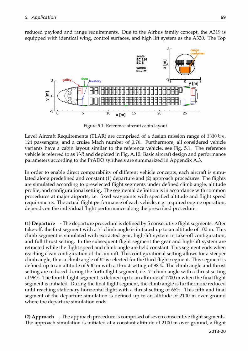
5. Application 69
reduced payload and range requirements. Due to the Airbus family concept, the A319 isequipped with identical wing, control surfaces, and high lift system as the A320. The Top
x [m]
y [m
]
0 5 10 15 20 25-3
0
3
cargo:51.2 m³
galley lavatory
cargocontainer
seats:EC 116BC 8
door
y [m]
z [m
]
-3 0 3-3
0
3
Figure 5.1: Reference aircraft cabin layout
Level Aircraft Requirements (TLAR) are comprised of a design mission range of 3330 km,124 passengers, and a cruise Mach number of 0.76. Furthermore, all considered vehiclevariants have a cabin layout similar to the reference vehicle, see Fig. 5.1. The referencevehicle is referred to as V-R and depicted in Fig. A.10. Basic aircraft design and performanceparameters according to the PrADO synthesis are summarized in Appendix A.3.
In order to enable direct comparability of different vehicle concepts, each aircraft is simu-lated along predefined and constant (1) departure and (2) approach procedures. The flightsare simulated according to preselected flight segments under defined climb angle, altitudeprofile, and configurational setting. The segmental definition is in accordance with commonprocedures at major airports, i.e. fixed waypoints with specified altitude and flight speedrequirements. The actual flight performance of each vehicle, e.g. required engine operation,depends on the individual flight performance along the prescribed procedure.
(1) Departure - The departure procedure is defined by 5 consecutive flight segments. Aftertake-off, the first segment with a 7◦ climb angle is initiated up to an altitude of 100 m. Thisclimb segment is simulated with extracted gear, high-lift system in take-off configuration,and full thrust setting. In the subsequent flight segment the gear and high-lift system areretracted while the flight speed and climb angle are held constant. This segment ends whenreaching clean configuration of the aircraft. This configurational setting allows for a steeperclimb angle, thus a climb angle of 9◦ is selected for the third flight segment. This segment isdefined up to an altitude of 900 m with a thrust setting of 98%. The climb angle and thrustsetting are reduced during the forth flight segment, i.e. 7◦ climb angle with a thrust settingof 96%. The fourth flight segment is defined up to an altitude of 1700 m when the final flightsegment is initiated. During the final flight segment, the climb angle is furthermore reduceduntil reaching stationary horizontal flight with a thrust setting of 65%. This fifth and finalsegment of the departure simulation is defined up to an altitude of 2100 m over groundwhere the departure simulation ends.
(2) Approach - The approach procedure is comprised of seven consecutive flight segments.The approach simulation is initiated at a constant altitude of 2100 m over ground, a flight
2013-20
70 Noise Prediction within Conceptual Aircraft Design
speed of 420 km/h, and the vehicle in cruise configuration. The first flight segment is a −3◦
descent down to an altitude of 1200 m. While the aircraft remains in clean configuration,the airspeed is uniformly reduced down to 320 km/h. At 1200 m a second, short flightsegment is initiated. During this flight segment, the previous glide path and speed are keptconstant. Flaps and slats are extracted into the approach configuration prior initiation ofthe next flight segment. Maintaining the −3◦ descent, flight altitude is reduced to 600 mand flight speed down to 280 km/h. The subsequent flight segment holds the glide slopeand speed settings, while the configurational setting is uniformly modified. Flaps andslats are furthermore extracted in order to initiate the final approach. The final approach iscomprised of three more descent segments. Along the first segment of the final approach,the velocity is reduced to 250 km/h until the aircraft reaches an altitude of 350 m. Duringthis descent, the flaps and slats are fully extracted. During the next short flight segmentthe landing gear deployment is initiated. Starting from this segment on, the flight velocityis finally reduced down to the aircraft specific individual landing speed, i.e. the stall speedmultiplied with a constant safety factor. Hereafter, along the final segment the flight altitudeis reduced to 50 ft in order to enable flare-out, touch-down, and deceleration.
The defined reference flight procedures are not equal to available and practical proce-dures as established at major airports. A simplified and more general definition of theflight procedures is required to ensure that each vehicle variant can be operated along theseprocedure. Only if similar procedural constraints are established for each vehicle variant, acomprehensive analysis and fair comparison of the predicted effects is enabled.
5.1.2 Evaluation Metric
At this point, a generic metric would be required in order to directly compare cost efficiencyand environmental performance of new vehicles within the conceptual design phase. Suchan approach could translate the predicted noise levels directly into monetary values. Thesenoise expenses could simply be accumulated with the direct operating costs in order to eval-uated and rank-order the economical efficiency of each vehicle. Obviously, such a correla-tion is extremely difficult to assess. In order to establish a general and comprehensive ap-proach seems rather impossible. Up to this day, there is no accepted and common agreementon how to fix a price for ground noise pollution. For each airport individual and local noisecharges and fees can be established, if any. As a consequence, the European Union plans toharmonize the various existing noise based charges for Europe within the next decade [107].Existing local noise related fees and scientific models are only based on measurements at thethree noise certification points, thus a low-noise modification or improvement to an existingaircraft or flight procedure has very limited to no direct effect [108,109]. Consequently, exist-ing models for noise related charges are apparently meaningless in context of the presentedwork, thus can be ruled out.More importantly, as long as existing noise related fees remain at insignificant magnitudes[108, 109], there is no incentive to investigate and establish more sophisticated metrics andsystems. This situation might change in the future due to the unpredictable influence ofpolitics and rulemakers, e.g. legislation of more radical environmental hurdles for airports.
2013-20
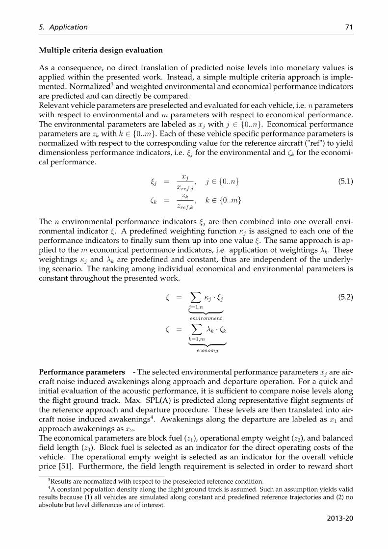
5. Application 71
Multiple criteria design evaluation
As a consequence, no direct translation of predicted noise levels into monetary values isapplied within the presented work. Instead, a simple multiple criteria approach is imple-mented. Normalized3 and weighted environmental and economical performance indicatorsare predicted and can directly be compared.Relevant vehicle parameters are preselected and evaluated for each vehicle, i.e. n parameterswith respect to environmental and m parameters with respect to economical performance.The environmental parameters are labeled as xj with j ∈ {0..n}. Economical performanceparameters are zk with k ∈ {0..m}. Each of these vehicle specific performance parameters isnormalized with respect to the corresponding value for the reference aircraft ("ref") to yielddimensionless performance indicators, i.e. ξj for the environmental and ζk for the economi-cal performance.
ξj =xj
xref,j
, j ∈ {0..n} (5.1)
ζk =zk
zref,k, k ∈ {0..m}
The n environmental performance indicators ξj are then combined into one overall envi-ronmental indicator ξ. A predefined weighting function κj is assigned to each one of theperformance indicators to finally sum them up into one value ξ. The same approach is ap-plied to the m economical performance indicators, i.e. application of weightings λk. Theseweightings κj and λk are predefined and constant, thus are independent of the underly-ing scenario. The ranking among individual economical and environmental parameters isconstant throughout the presented work.
ξ =∑j=1,n
κj · ξj︸ ︷︷ ︸environment
(5.2)
ζ =∑
k=1,m
λk · ζk︸ ︷︷ ︸economy
Performance parameters - The selected environmental performance parameters xj are air-craft noise induced awakenings along approach and departure operation. For a quick andinitial evaluation of the acoustic performance, it is sufficient to compare noise levels alongthe flight ground track. Max. SPL(A) is predicted along representative flight segments ofthe reference approach and departure procedure. These levels are then translated into air-craft noise induced awakenings4. Awakenings along the departure are labeled as x1 andapproach awakenings as x2.The economical parameters are block fuel (z1), operational empty weight (z2), and balancedfield length (z3). Block fuel is selected as an indicator for the direct operating costs of thevehicle. The operational empty weight is selected as an indicator for the overall vehicleprice [51]. Furthermore, the field length requirement is selected in order to reward short
3Results are normalized with respect to the preselected reference condition.4A constant population density along the flight ground track is assumed. Such an assumption yields valid
results because (1) all vehicles are simulated along constant and predefined reference trajectories and (2) noabsolute but level differences are of interest.
2013-20
72 Noise Prediction within Conceptual Aircraft Design
take-off and landing operation (STOL). Such low-noise STOL vehicle could be operated atunderutilized airports with shorter runways enabling new transportation business mod-els [110].Obviously, in order to improve the overall vehicle performance the selected individual pa-rameters have to be minimized. The corresponding environmental and economical predic-tions for the reference vehicle are summarized in Tab. 5.1. The specific performance param-
environment, xref,i economy, zref,kdep. awakenings [-] app. awakenings [-] oew [kg] bal. field length [m] block fuel [kg]
xref,1 xref,2 zref,1 zref,2 zref,3
8.15 14.37 38664 1949 10222
Table 5.1: Reference vehicle performance parameters
eters are selected based on engineering judgment and the opinion of the author. Obviously,a different selection is feasible and would probably lead to more or less different results forthe overall vehicle evaluation.
Weighting factors and overall performance indicators - The corresponding weighting fac-tors for departure and approach noise are selected to be equal, κ1 = κ2. Reduction of noisealong approach and departure procedures is assessed to be of equal importance. Block fuelis selected as the far most important economical factor, thus an appropriate weighting factorof λ1 = 0.7 is selected. Operational empty weight is defined as twice the factor for balancedfield length, i.e. λ2 = 0.2 and λ3 = 0.1. The weighting factors λ1 to λ3 are predefinedindependently of the underlying scenario. The factors are selected to reflect the major costdrivers for aircraft acquisition and operation.No specific business case is represented and different weighting factors or additional per-formance parameters could be selected by other users.Now, the overall environmental and economical performance indicators, i.e. ξ and ζ can beevaluated.
ξ =1
2︸︷︷︸κ1
·ξ1 +1
2︸︷︷︸κ2
·ξ2 (5.3)
ζ =7
10︸︷︷︸λ1
·ζ1 +2
10︸︷︷︸λ2
·ζ2 +1
10︸︷︷︸λ3
·ζ3
These two overall performance indicators ξ and ζ are predefined and vehicle specific con-stants, thus independent of the selected scenario.
Scenario specific vehicle ranking - In order to evaluate a vehicle under specific boundaryconditions, e.g. dominating environmental requirements, corresponding weighting can beapplied to the vehicle specific performance indicators ξ and ζ (as specified in Eq. 5.4). Spe-cific weighting of environmental, i.e. Ki, and economical performance, i.e. Λi, in a scenario"i" determines the overall ranking of a vehicle within this scenario. Ki and Λi are definedunder the following conditions:
Ki + Λi = 1 ∧ Ki ∈ [0, 1] ∧ Λi ∈ [0, 1] (5.4)
2013-20
5. Application 73
Applying these scenario weighting factors to the vehicle specific and constant performanceindicators ξ and ζ results in a scenario specific ranking. Within an arbitrary scenario "i",defined by the ratio of Ki and Λi, each vehicle can be assigned a score σi according to itsenvironmental and economical performance within this specific scenario.
σi = Ki · ξ + Λi · ζ (5.5)
= Ki ·∑j=1,n
(κj · ξj) + Λi ·∑j=1,m
(λj · ζj)
= Ki ·(1
2· x1
xref,1
+1
2· x2
xref,2
)+ Λi ·
(7
10· z1zref,1
+2
10· z2zref,2
+1
10· z3zref,3
)Economical and environmental performance weighting factors are varied in 10% steps re-sulting in 11 different scenarios. These scenarios include an economically driven scenario"0" (K0 = 0.0 and Λ0 = 1.0) and a low-noise scenario "10" (K10 = 1.0 and Λ10 = 0.0). Anaircraft ranking within todays scenario could be described by a dominating economical andnegligible environmental weighting, i.e. Λnow > 0.99 and Know ≤ 0.01.
5.1.3 Solution Space Limitations
The design synthesis code PrADO and the implemented noise source models restrict thepotential solution space. Obviously, only parameters that are both simulated in PrADO andare captured by the noise source models affect the noise prediction thus can be subject to anylow-noise analysis. Furthermore, each noise source model imposes specific requirementswith respect to data input and component design principles as outlined in section 3.2.2.According to section 3.2.2, each modification to the reference engine or airframe design hasto be checked for compatibility against the inherent design principles of the correspondingnoise model.
According to Dobrzynski [9], operational effects have a dominating impact on noisegeneration. Relevant operational parameters along a simulated flight path are captured bythe models. Therefore, the operational impact on noise generation can be studied in detail,i.e. engine thrust setting, flight speed, altitude, flight path angle, selected configurationalong the simulated flight path. Furthermore, overall aircraft design can be modified inorder to support low-noise flight operation, i.e. steeper flight segments and reduced flightvelocities [37,62]. Improving the vehicles Lift-to-Drag ratio allows to reduce wing area5 thusenabling slower approach flight velocities. Reduction of vehicle take-off weight increasesthe thrust-to-weight ratio for a fixed engine, thus enables steeper climb angles during de-parture. Obviously, modification to these basic aircraft parameters does not only influencethe overall aircraft performance with respect to low-noise flight operation but also changesthe noise emission of the corresponding airframe noise sources.Both airframe and engine noise source models are parametric with respect to predefinedmajor design parameters, see section 3.2.2. Variation of these design parameters will de-termine the componential noise emission, thus can be investigated. Due to the requiredsimplicity of the source models, detailed geometry parameters, e.g. local cavities, kinemat-ics, or linkages, can not be accounted for. As a consequence, Dobrzynski’s suggestions withrespect to certain design details can not be investigated with the available models. Althougha direct parameter study is not possible, these geometry details could be accounted for by
5Reduction of wing loading is the main driver for reducing the flight velocity [37].
2013-20
74 Noise Prediction within Conceptual Aircraft Design
reading in measured noise level deltas. The significant influence of structural shielding onengine noise emission can be accounted for with the DLR ray-tracing tool SHADOW [83],see Section 3.2.2.3. Engine location and airframe layout can be modified in order to investi-gate engine noise shielding effects.
In the context of the presented aircraft design study, only preselected engine conceptsare considered. For these concepts, underlying noise models have been checked in detailprior each application. Variation of engine design details is not investigated, thus engineperformance decks and geometry parameters are precomputed for each selected engineconcept and kept constant during further vehicle design modifications.
5.1.4 Vehicle Variants
Based on the solution space limitations, different basic vehicle layouts are selected forfurther investigation. As outlined in section 2.2, Dobrzynski and others identified severalpromising short- to mid-term solutions towards aircraft ground noise reduction [37, 38, 62].Several of these suggestions are within the limitations, thus can be investigated within thepresented process.
The selected vehicle variants can be assigned to 5 main categories according to theirmost important noise related design features. Obviously, this has to be the approach towarda reduction of perceived engine noise levels on the ground. Engine noise is still the mostdominant noise source on-board of any flying vehicle. Not considering advanced enginenor futuristic vehicle design, e.g. a blended wing body with fully embedded engines, thesituation is not likely to change within the next decades. Within this timeframe, no signif-icant noise reduction is expected for existing, conventional turbofan engines [79]. Other,more optimistic references estimate a theoretically achievable, maximum noise reductionwithin the next decades to be in the order of 3 to a maximum of 5 dB [113, 114].Alternative propulsion concepts could have a significant impact on engine noise contribu-tion, i.e. either positive or negative. Yet, this impact is difficult to assess due to the lackof simulation models and (unrestricted) validation data. As a consequence, the selectedvehicle variants are simulated with the reference engine.As an outlook on future applications, some alternative propulsion concepts are discussed ina reduced detail level according to available data and simulation methods.
Consequently, exploitation of structural noise shielding is the most effective vehicle de-sign solution to significantly reduce perceived engine noise levels. The implemented fannoise source model [26] yields a characteristic noise emission directivity for the fan. Foraircraft under take-off conditions, maximum fan noise levels are observed for polar anglesα∗ between 20 and 60° in the forward direction and 110 to 140° in the backward direction.Under approach conditions, i.e. low engine thrust settings, significant fan noise contributionis limited to the backward direction with polar angles between 110 and 140°. Consequently,noise barriers should be placed directly in these relevant emission directions for effectivefan noise shielding.
The selected vehicle variants are assigned into the following main categories.
• main wing shielding of over-the-wing installed engines: Design variants v-0
2013-20
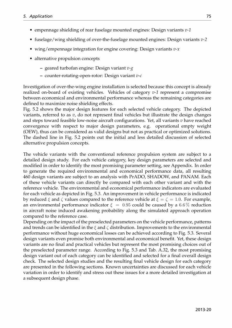
5. Application 75
• empennage shielding of rear fuselage mounted engines: Design variants v-1
• fuselage/wing shielding of over-the-fuselage mounted engines: Design variants v-2
• wing/empennage integration for engine covering: Design variants v-x
• alternative propulsion concepts
– geared turbofan engine: Design variant v-g
– counter-rotating-open-rotor: Design variant v-c
Investigation of over-the-wing engine installation is selected because this concept is alreadyrealized on-board of existing vehicles. Vehicles of category v-1 represent a compromisebetween economical and environmental performance whereas the remaining categories aredefined to maximize noise shielding effects.Fig. 5.2 shows the major design features for each selected vehicle category. The depictedvariants, referred to as v, do not represent final vehicles but illustrate the design changesand steps toward feasible low-noise aircraft configurations. Yet, all variants v have reachedconvergence with respect to major design parameters, e.g. operational empty weight(OEW), thus can be considered as valid designs but not as practical or optimized solutions.The dashed line in Fig. 5.2 points out the initial and less detailed discussion of selectedalternative propulsion concepts.
The vehicle variants with the conventional reference propulsion system are subject to adetailed design study. For each vehicle category, key design parameters are selected andmodified in order to identify the most promising parameter setting, see Appendix. In orderto generate the required environmental and economical performance data, all resulting460 design variants are subject to an analysis with PrADO, SHADOW, and PANAM. Eachof these vehicle variants can directly be compared with each other variant and with thereference vehicle. The environmental and economical performance indicators are evaluatedfor each vehicle as depicted in Fig. 5.3. An improvement in vehicle performance is indicatedby reduced ξ and ζ values compared to the reference vehicle at ξ = ζ = 1.0. For example,an environmental performance indicator ξ = 0.95 could be caused by a 6.6% reductionin aircraft noise induced awakening probability along the simulated approach operationcompared to the reference case.Depending on the impact of the preselected parameters on the vehicle performance, patternsand trends can be identified in the ξ and ζ distribution. Improvements to the environmentalperformance without huge economical losses can be achieved according to Fig. 5.3. Severaldesign variants even promise both environmental and economical benefit. Yet, these designvariants are no final and practical vehicles but represent the most promising choices out ofthe preselected parameter range. According to Fig. 5.3 and Tab. A.32, the most promisingdesign variant out of each category can be identified and selected for a final overall designcheck. The selected design studies and the resulting final vehicle design for each categoryare presented in the following sections. Known uncertainties are discussed for each vehiclevariation in order to identify and stress out these issues for a more detailed investigation ata subsequent design phase.
2013-20
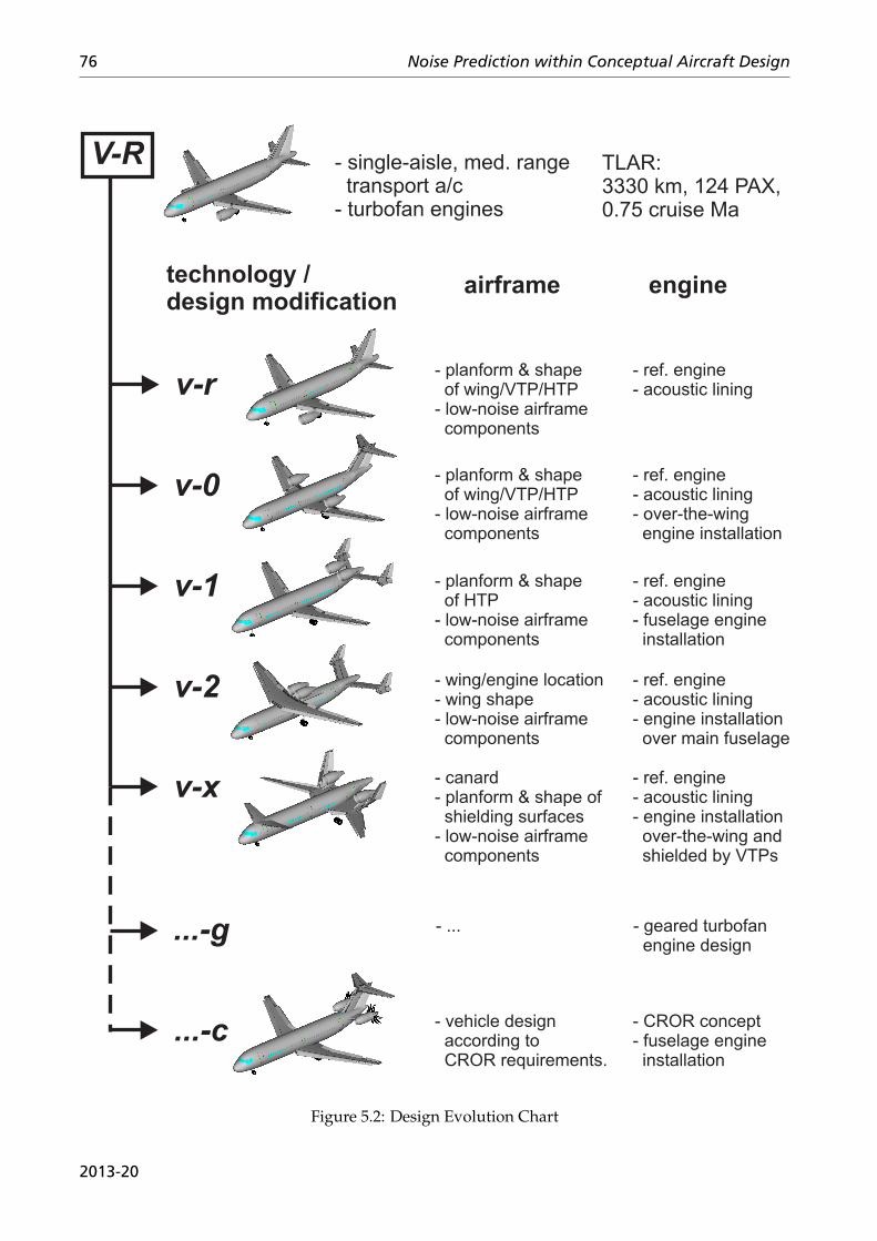
76 Noise Prediction within Conceptual Aircraft Design
Figure 5.2: Design Evolution Chart
2013-20
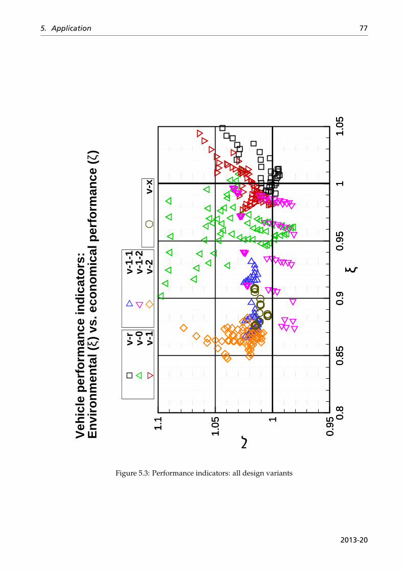
5. Application 77
ξ
ζ
0.8
0.85
0.9
0.95
11.
050.
951
1.051.
1
v-r
v-0
v-1
ξ
ζ
0.8
0.85
0.9
0.95
11.
050.
951
1.051.
1v-
x
ξ
ζ
0.8
0.85
0.9
0.95
11.
050.
951
1.051.
1
v-1-
1v-
1-2
v-2
Veh
icle
per
form
ance
indi
cato
rs:
Env
ironm
enta
l (ξ)
vs.
eco
nom
ical
per
form
ance
(ζ)
Figure 5.3: Performance indicators: all design variants
2013-20
78 Noise Prediction within Conceptual Aircraft Design
5.1.4.1 Vehicle Geometry Variation
For some of the selected vehicle variants, engine noise is shielded by the main wing.Moreover, the flight performance of each vehicle depends on the lift and control surfaces.Therefore, all variants are subject to a parameter variation of the main wing planform andrelative location along the fuselage. Thereby, the high lift system components are linearlyadapted according to the new wing planform.From an aerodynamic point of view, a large aspect ratio is desirable because it improves thevehicle aerodynamics. As a result, this could reduce required engine thrust settings alongthe predefined flight procedures. A large wing area Aw, i.e. reduced wing loading, enablesslow aircraft specific flight velocities along the final approach resulting in reduced airframenoise generation [37]. Reducing the wing loading decreases aerodynamic loading on highlift and lifting surfaces thus furthermore decreases airframe noise. Yet, wing weight doesincrease with both area and aspect ratio, thus has negative implications on flight perfor-mance. Furthermore, reduced wing loading can have negative implications on passengerride quality during cruise, i.e. buffeting. Obviously, a trade-off between additional wingweight and desirable flight performance is necessary.
The resulting vehicle variants are valid PrADO designs but might require further de-sign adaptions due to the new wing planform. These variants are therefore no final oroptimized PrADO designs. From each category, the most promising vehicle variant isidentified and selected for a final detail investigation.
Modified reference vehicle (category v-r) - According to each parameter variation, theresulting global aircraft parameters (PrADO) and the selected environmental prediction re-sults (SHADOW, PANAM) are evaluated (Tab. A.9 and Fig. A.23, Appendix). Normalizingthese results with the reference data yields ξ and ζ , as depicted in Fig. A.24.The most promising variants out of the parameter space feature high aspect ratios. Es-pecially, the environmental impact is strongly influenced by Λw, as it is clearly visible inFig. A.23. This can be mainly attributed to reduced thrust requirement along the predefinedapproach procedure, i.e. significantly reduced ground noise levels for Λw = 11 comparedto a vehicle with Λw = 7. The advantageous economical impact of high Λw is based on thereduction in block fuel, which is furthermore accentuated by a strong weighting factor. Anobvious increase in wing weight, thus overall empty weight, due to high aspect ratio doesnot counteract the overall advantage. Furthermore, the most promising design variant hasa reduced wing area (-7.7%) compared to the reference vehicle. This is in good agreementwith the known oversizing of the reference wing due to the Airbus family concept.Ultimately, the most promising design variant is no. 20 of parameter variation 1. The sec-ond parameter variation is not discussed in detail because no improvements with respect toneither environmental nor economical performance could be achieved, see Fig. A.24.
Main wing shielding (category v-0) - The V-R is modified to exploit fan noise shieldingdue to an over-the-wing engine installation. Due to flight stability reasons, the main wingis shifted closer to the fuselage tail. Furthermore, a T-tail arrangement is selected in orderto avoid direct jet impingement on the control surfaces. The engine arrangement pushes thecenter of gravity (CG) backward along the fuselage, thus requires increased control surfaceareas at the tail. Fig. A.25 depicts the principal vehicle layout. For this concept, variationof Aw and Λw does not only influence the flight performance but directly determines en-
2013-20
5. Application 79
gine noise shielding. To increase noise shielding, increasing Aw and low values of Λw aremost promising. The second parameter variation is based on a relatively small Aw, there-fore an increased economical performance but reduced shielding effects. A direct impact ofincreased Aw on noise shielding is clearly visible in Fig. A.27(a). Therefore, the most promis-ing vehicle variant from parameter variation 1 is selected, precisely variant 24. This variantyields a significantly increased environmental performance although flight operation is lesseconomical compared to vehicles from parameter variation 2.
Empennage Shielding (category v-1) - If engines are mounted at the back of the fuselage,the empennage can be applied for noise shielding. Compared to the reference vehicle, thisdesign shifts the overall center of gravity (CG) to the back of the vehicle. This can causeproblems with respect to the overall aircraft flight stability.In a first step, an H-tail design with rear-mounted engines is selected as depicted inFigs. A.29 and A.30, Appendix. The H-tail design promises some shielding of the backwardfan noise and at the same time assures stable flight behavior of the vehicle. Yet, the H-taildesign increases the empennage weight, thus results in generally increased OEW comparedto the reference layout. With this initial, backward-swept H-tail design, no shielding offorward fan noise is achieved, thus the concepts results in low environmental performance(Fig. A.31(a)).
As a consequence, a forward-swept H-tail is investigated in order to achieve sufficientengine noise shielding (Figs. A.33 and A.34, Appendix). This new design v-1-1 results insignificantly improved environmental performance, i.e. an extensive reduction in aircraftnoise induced awakenings (Fig. A.35(a)). Yet, due to the forward-swept H-tail, distancesbetween aircraft CG and control surfaces are significantly reduced, thus massive controlsurfaces would be required for reasonable flight stability and control. Because the requiredtail volume coefficient can not be realized, the v-1-1 variants are not considered as practicalsolutions.
In a next step, a third vertical tailplane is added to the v-1-1 variant. This third tailplaneis supposed to reduce the required size of the former H-tail. The so-called v-1-2 variant,as depicted in Fig. A.37, results in improved flight stability, yet is still not sufficient for apractical flight operation. The v-1-2 has similar shielding characteristics compared to thev-1-1 but increased economical performance. This can be attributed to the three-tailplanedesign which results in reduced weight of the empennage, i.e. reduced overall weight ofthe aircraft.
The previous findings indicate, that a forward-swept empennage is promising but aforward-swept H-tail can be excluded as a practical solution. Consequently, a conventionaltail layout with forward-swept horizontal stabilizers is selected for further investigation(Fig. A.38, Appendix). This empennage layout promises sufficient tail volume coefficientsfor stable flight operation. Yet, the acceptable margin for a CG movement during flight islittle, i.e. under 1 m, so that safe flight operation would require further dedicated inves-tigation. The general layout results in reduced weight of the aircraft and consequently alow block fuel requirement. These v-1-2 variants (2nd parameter variation) show the besteconomical flight performance of all v-1 design variants. Compared to the reference vehicle,the simulations even indicate an improvement in economical performance for the v-1-2(Fig. A.40, Appendix).
2013-20
80 Noise Prediction within Conceptual Aircraft Design
For the v-1-2 variants, an optimal shape of the horizontal stabilizer is identified, i.e. withrespect to aspect ratio and sweep angle. The design variant 1 of parameter variation 2 isselected for further investigation.
Fuselage/wing shielding (category v-2) - Maximum engine noise shielding requires anextensive shielding barrier. A high wing design provides such a barrier, precisely abovethe fuselage-wing junction. Extensive noise shielding can be achieved, if both engines aredirectly mounted above this junction. As a consequence, a H-tail is required to avoid directjet impingement. Due to the H-tail, the aircraft structural weight is increased. Compared tothe reference vehicle, all v-2 variants result in decreased economical performance (Fig. A.44,Appendix).Starting with a basic design (Fig. A.41), further parameter variations are applied in order tofind the most promising wing planform and location. According to the simulation results,extensive noise shielding is achievable (Fig. A.43(a), Appendix).For the final assessment, variant 27 of parameter variation 1 is selected. This design variantpromises significant noise shielding at the price of reduced economical flight performance.
Wing/empennage integration (category v-x) - The original DLR Low-Noise Aircraft(LNA) concept [37, 38] is modified in order to meet the TLAR as described in Section5.1.1.The modifications result in a reduced fuselage length and decreased wing/control sur-face areas. The underlying PrADO input data set is adapted from an earlier short-rangeLNA model (LNA-SR) by C. Liersch, Institute of Aerodynamics and Flow Technology, DLR,Braunschweig.The selected canard configuration allows to move the main wing toward the rear sectionof the fuselage. Such a backward main wing location enables an integrated design of mainwing and vertical tail plane (VTP). The fuselage mounted VTP of the reference aircraft isthus modified into two VTPs. The engines can then be mounted over-the-wing, in-betweenfuselage and VTP, thus are subject to significant polar and lateral fan noise shielding. Start-ing from this initial geometry (Fig. A.45), the main wing planform and the final arrangementof the two VTPs are modified in order to maximize noise shielding effects. Out of the avail-able vehicle variants, variant 25 is selected due to efficient noise shielding and still feasibleeconomical performance.With respect to the reference aircraft, the cabin layout had to be rearranged, i.e. a new loca-tion of main door and emergency exit.
5.1.4.2 Final Vehicle Designs
The selected most promising vehicle variants are subject to a feasibility check and somedesign modifications, if required. Some parameters that have been kept constant duringthe parameter variations might require further adaption, e.g. final matching of main wingand empennage due to control and stability issues. These modifications do not affect theidentified optimal engine noise shielding but can have an impact on the overall flight per-formance, e.g. due to increased aircraft weight. The final PrADO vehicles are labeled withan upper-case letter, namely V, and detailed results are presented in Section A.4, Appendix.Key design and performance parameters for each vehicle are listed. The resulting environ-mental and economical performance indicators for each vehicle are collected and subject toa final scenario evaluation.
2013-20
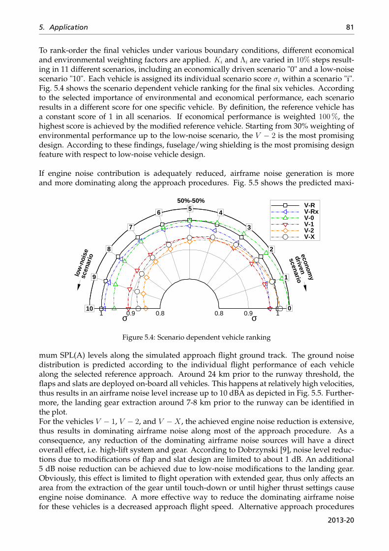
5. Application 81
To rank-order the final vehicles under various boundary conditions, different economicaland environmental weighting factors are applied. Ki and Λi are varied in 10% steps result-ing in 11 different scenarios, including an economically driven scenario "0" and a low-noisescenario "10". Each vehicle is assigned its individual scenario score σi within a scenario "i".Fig. 5.4 shows the scenario dependent vehicle ranking for the final six vehicles. Accordingto the selected importance of environmental and economical performance, each scenarioresults in a different score for one specific vehicle. By definition, the reference vehicle hasa constant score of 1 in all scenarios. If economical performance is weighted 100%, thehighest score is achieved by the modified reference vehicle. Starting from 30% weighting ofenvironmental performance up to the low-noise scenario, the V − 2 is the most promisingdesign. According to these findings, fuselage/wing shielding is the most promising designfeature with respect to low-noise vehicle design.
If engine noise contribution is adequately reduced, airframe noise generation is moreand more dominating along the approach procedures. Fig. 5.5 shows the predicted maxi-
σ σ0.80.8 0.90.9 11
V-RV-RxV-0V-1V-2V-X
economy
driven
scenario
10
low
-noi
sesc
enar
io
0
1
2
3
45
6
7
8
9
50%-50%
Figure 5.4: Scenario dependent vehicle ranking
mum SPL(A) levels along the simulated approach flight ground track. The ground noisedistribution is predicted according to the individual flight performance of each vehiclealong the selected reference approach. Around 24 km prior to the runway threshold, theflaps and slats are deployed on-board all vehicles. This happens at relatively high velocities,thus results in an airframe noise level increase up to 10 dBA as depicted in Fig. 5.5. Further-more, the landing gear extraction around 7-8 km prior to the runway can be identified inthe plot.For the vehicles V − 1, V − 2, and V −X , the achieved engine noise reduction is extensive,thus results in dominating airframe noise along most of the approach procedure. As aconsequence, any reduction of the dominating airframe noise sources will have a directoverall effect, i.e. high-lift system and gear. According to Dobrzynski [9], noise level reduc-tions due to modifications of flap and slat design are limited to about 1 dB. An additional5 dB noise reduction can be achieved due to low-noise modifications to the landing gear.Obviously, this effect is limited to flight operation with extended gear, thus only affects anarea from the extraction of the gear until touch-down or until higher thrust settings causeengine noise dominance. A more effective way to reduce the dominating airframe noisefor these vehicles is a decreased approach flight speed. Alternative approach procedures
2013-20
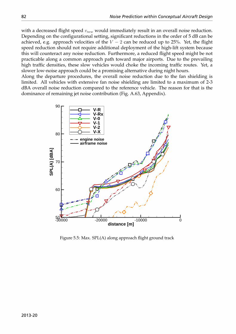
82 Noise Prediction within Conceptual Aircraft Design
with a decreased flight speed vnew would immediately result in an overall noise reduction.Depending on the configurational setting, significant reductions in the order of 5 dB can beachieved, e.g. approach velocities of the V − 2 can be reduced up to 25%. Yet, the flightspeed reduction should not require additional deployment of the high-lift system becausethis will counteract any noise reduction. Furthermore, a reduced flight speed might be notpracticable along a common approach path toward major airports. Due to the prevailinghigh traffic densities, these slow vehicles would choke the incoming traffic routes. Yet, aslower low-noise approach could be a promising alternative during night hours.Along the departure procedures, the overall noise reduction due to the fan shielding islimited. All vehicles with extensive fan noise shielding are limited to a maximum of 2-3dBA overall noise reduction compared to the reference vehicle. The reason for that is thedominance of remaining jet noise contribution (Fig. A.63, Appendix).
distance [m]
SP
L(A
) [d
BA
]
-30000 -20000 -10000 050
60
70
80
90V-RV-RxV-0V-1V-2V-X
engine noiseairframe noise
Figure 5.5: Max. SPL(A) along approach flight ground track
2013-20
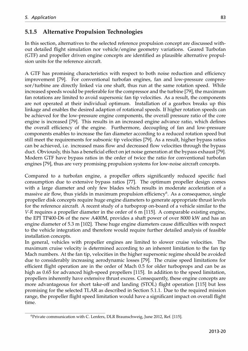
5. Application 83
5.1.5 Alternative Propulsion Technologies
In this section, alternatives to the selected reference propulsion concept are discussed with-out detailed flight simulation nor vehicle/engine geometry variations. Geared Turbofan(GTF) and propeller driven engine concepts are identified as plausible alternative propul-sion units for the reference aircraft.
A GTF has promising characteristics with respect to both noise reduction and efficiencyimprovement [79]. For conventional turbofan engines, fan and low-pressure compres-sor/turbine are directly linked via one shaft, thus run at the same rotation speed. Whileincreased speeds would be preferable for the compressor and the turbine [79], the maximumfan rotations are limited to avoid supersonic fan tip velocities. As a result, the componentsare not operated at their individual optimum. Installation of a gearbox breaks up thislinkage and enables the desired adaption of rotational speeds. If higher rotation speeds canbe achieved for the low-pressure engine components, the overall pressure ratio of the coreengine is increased [79]. This results in an increased engine advance ratio, which definesthe overall efficiency of the engine. Furthermore, decoupling of fan and low-pressurecomponents enables to increase the fan diameter according to a reduced rotation speed butstill meet the requirements for subsonic tip velocities [79]. As a result, higher bypass ratioscan be achieved, i.e. increased mass flow and decreased flow velocities through the bypassduct. Obviously, this has a beneficial effect on jet noise generation at the bypass exhaust [79].Modern GTF have bypass ratios in the order of twice the ratio for conventional turbofanengines [79], thus are very promising propulsion systems for low-noise aircraft concepts.
Compared to a turbofan engine, a propeller offers significantly reduced specific fuelconsumption due to extensive bypass ratios [77]. The optimum propeller design comeswith a large diameter and only few blades which results in moderate acceleration of amassive air flow, thus yields in maximum propulsion efficiency6. As a consequence, singlepropeller disk concepts require huge engine diameters to generate appropriate thrust levelsfor the reference aircraft. A recent study of a turboprop on-board of a vehicle similar to theV-R requires a propeller diameter in the order of 6 m [115]. A comparable existing engine,the EPI TP400-D6 of the new A400M, provides a shaft power of over 8000 kW and has anengine diameter of 5.3 m [102]. These huge engine diameters cause difficulties with respectto the vehicle integration and therefore would require further detailed analysis of feasibleinstallation concepts.In general, vehicles with propeller engines are limited to slower cruise velocities. Themaximum cruise velocity is determined according to an inherent limitation to the fan tipMach numbers. At the fan tip, velocities in the higher supersonic regime should be avoideddue to considerably increasing aerodynamic losses [79]. The cruise speed limitations forefficient flight operation are in the order of Mach 0.5 for older turboprops and can be ashigh as 0.65 for advanced high-speed propellers [115]. In addition to the speed limitation,propellers inherently have extensive thrust excess. Consequently, these engine concepts aremore advantageous for short take-off and landing (STOL) flight operation [115] but lesspromising for the selected TLAR as described in Section 5.1.1. Due to the required missionrange, the propeller flight speed limitation would have a significant impact on overall flighttime.
6Private communication with C. Lenfers, DLR Braunschweig, June 2012, Ref. [115].
2013-20
84 Noise Prediction within Conceptual Aircraft Design
A more promising concept for a propeller engine is the Counter-Rotating-Open-Rotor(CROR). The CROR promises significant advantages over the conventional turboprop de-sign according to Refs. [116–119]. Most importantly, flight cruise Mach numbers of up to0.75 can be achieved for an optimized CROR design as presented in Refs. [116,117]. Accord-ing to Ref. [116], CROR engines mark a "step change in propulsion efficiency" due to theirultra-high bypass ratios. Compared to turboprop concepts, the CROR offers an increasedefficiency for the same disk loading [118]. This can be attributed to the counter-rotatingrotors, precisely the avoidance of swirl behind the engine, thus reducing additional effi-ciency losses to a minimum [118]. Consequently, for a required disk loading and propulsionefficiency, the CROR design results in significantly reduced fan diameters compared to aturboprop7. For example, a recent DLR concept for an aircraft similar to the V-R has a maxi-mum diameter of 4.2 m [116, 117]. Compared to a turboprop design, the engine integrationon-board of the vehicle is simplified.Due to the low specific thrust, extremely favorable specific fuel consumption (SFC) isachievable. Simulations indicate a potential SFC reduction in the order of 30% compared toa conventional turbofan concept [119].Another advantage of a counter-rotating engine is the avoidance of dynamic rotor torqueand therefore reduced loads on engine mountings [118]. Transmitting the engine powerand torque via two shafts, reduces the loads and simplifies the gearing of the propellersaccording to Ref. [118].
In conclusion, an advanced CROR almost fulfills the predefined TLAR for the referenceaircraft V-R and is therefore preferred over a conventional turboprop.
5.1.5.1 Geared Turbofan Engine
Investigation of a geared turbofan is straight forward due to its (geometrical) similarity withthe reference engine. Vehicle installation considerations are similar but the increase in di-ameter and engine weight has to be accounted for. While the implemented noise predictionmethods are still valid for a GTF, the generation of required input data for the noise predic-tion is not possible within conceptual aircraft design. The complexity of the required enginedetails is not suited for conceptual design, thus simplified engine performance simulationcannot be applied. Tools of higher fidelity are required in order to simulate interactions andinterdependencies of fan, compressor, and turbine with respect to the gear box.The (re-) design of a current geared turbofan engine concept, e.g. PW-1000 on-board of thenew A320neo, is still under investigation at DLR. So far, no simulation results nor measure-ments are available. Due to the lack of alternatives, an existing but outdated GTF design isselected for further investigation8. The DLR engine concept as introduced in 2009 [112] is notoptimized for low-noise performance but was designed for short take-off and landing flightoperation (STOL), thus comes with significant thrust excess. Consequently, the GTF engineis overdimensioned for the reference aircraft V-R. During standard and non-STOL flight op-eration of the V-R, the selected GTF can therefore be operated with reduced thrust settings.In Ref. [112], the predicted extensive noise reduction for the GTF is mainly attributed to thiseffect and not directly to conceptual advantages. Furthermore, low-noise performance ofthe GTF is overestimated in Ref. [112] due to predominant PANAM fan noise overprediction
7Private communication with C.O. Márquez, DLR Braunschweig, June 2012, Ref. [117].8The engine performance map and detail design parameters are VarCycle [80] results provided by Tom
Otten, DLR Institute of Propulsion Technology.
2013-20
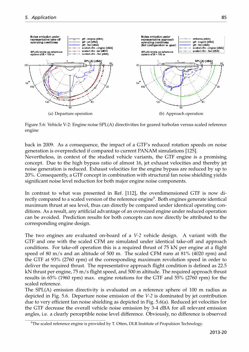
5. Application 85
(a) Departure operation (b) Approach operation
Figure 5.6: Vehicle V-2: Engine noise SPL(A) directivities for geared turbofan versus scaled referenceengine
back in 2009. As a consequence, the impact of a GTF’s reduced rotation speeds on noisegeneration is overpredicted if compared to current PANAM simulations [125].Nevertheless, in context of the studied vehicle variants, the GTF engine is a promisingconcept. Due to the high bypass ratio of almost 16, jet exhaust velocities and thereby jetnoise generation is reduced. Exhaust velocities for the engine bypass are reduced by up to20%. Consequently, a GTF concept in combination with structural fan noise shielding yieldssignificant noise level reduction for both major engine noise components.
In contrast to what was presented in Ref. [112], the overdimensioned GTF is now di-rectly compared to a scaled version of the reference engine9. Both engines generate identicalmaximum thrust at sea level, thus can directly be compared under identical operating con-ditions. As a result, any artificial advantage of an oversized engine under reduced operationcan be avoided. Prediction results for both concepts can now directly be attributed to thecorresponding engine design.
The two engines are evaluated on-board of a V-2 vehicle design. A variant with theGTF and one with the scaled CFM are simulated under identical take-off and approachconditions. For take-off operation this is a required thrust of 75 kN per engine at a flightspeed of 80 m/s and an altitude of 500 m. The scaled CFM runs at 81% (4020 rpm) andthe GTF at 93% (2760 rpm) of the corresponding maximum revolution speed in order todeliver the required thrust. The representative approach flight condition is defined as 22.5kN thrust per engine, 75 m/s flight speed, and 500 m altitude. The required approach thrustresults in 65% (1960 rpm) max. engine rotations for the GTF and 55% (2760 rpm) for thescaled reference.The SPL(A) emission directivity is evaluated on a reference sphere of 100 m radius asdepicted in Fig. 5.6. Departure noise emission of the V-2 is dominated by jet contributiondue to very efficient fan noise shielding as depicted in Fig. 5.6(a). Reduced jet velocities forthe GTF decrease the overall vehicle noise emission by 3-4 dBA for all relevant emissionangles, i.e. a clearly perceptible noise level difference. Obviously, no difference is observed
9The scaled reference engine is provided by T. Otten, DLR Institute of Propulsion Technology.
2013-20
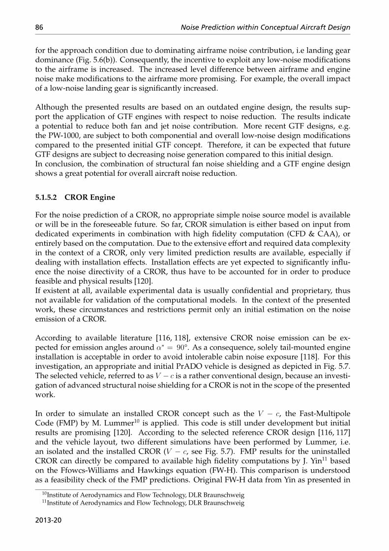
86 Noise Prediction within Conceptual Aircraft Design
for the approach condition due to dominating airframe noise contribution, i.e landing geardominance (Fig. 5.6(b)). Consequently, the incentive to exploit any low-noise modificationsto the airframe is increased. The increased level difference between airframe and enginenoise make modifications to the airframe more promising. For example, the overall impactof a low-noise landing gear is significantly increased.
Although the presented results are based on an outdated engine design, the results sup-port the application of GTF engines with respect to noise reduction. The results indicatea potential to reduce both fan and jet noise contribution. More recent GTF designs, e.g.the PW-1000, are subject to both componential and overall low-noise design modificationscompared to the presented initial GTF concept. Therefore, it can be expected that futureGTF designs are subject to decreasing noise generation compared to this initial design.In conclusion, the combination of structural fan noise shielding and a GTF engine designshows a great potential for overall aircraft noise reduction.
5.1.5.2 CROR Engine
For the noise prediction of a CROR, no appropriate simple noise source model is availableor will be in the foreseeable future. So far, CROR simulation is either based on input fromdedicated experiments in combination with high fidelity computation (CFD & CAA), orentirely based on the computation. Due to the extensive effort and required data complexityin the context of a CROR, only very limited prediction results are available, especially ifdealing with installation effects. Installation effects are yet expected to significantly influ-ence the noise directivity of a CROR, thus have to be accounted for in order to producefeasible and physical results [120].If existent at all, available experimental data is usually confidential and proprietary, thusnot available for validation of the computational models. In the context of the presentedwork, these circumstances and restrictions permit only an initial estimation on the noiseemission of a CROR.
According to available literature [116, 118], extensive CROR noise emission can be ex-pected for emission angles around α∗ = 90°. As a consequence, solely tail-mounted engineinstallation is acceptable in order to avoid intolerable cabin noise exposure [118]. For thisinvestigation, an appropriate and initial PrADO vehicle is designed as depicted in Fig. 5.7.The selected vehicle, referred to as V − c is a rather conventional design, because an investi-gation of advanced structural noise shielding for a CROR is not in the scope of the presentedwork.
In order to simulate an installed CROR concept such as the V − c, the Fast-MultipoleCode (FMP) by M. Lummer10 is applied. This code is still under development but initialresults are promising [120]. According to the selected reference CROR design [116, 117]and the vehicle layout, two different simulations have been performed by Lummer, i.e.an isolated and the installed CROR (V − c, see Fig. 5.7). FMP results for the uninstalledCROR can directly be compared to available high fidelity computations by J. Yin11 basedon the Ffowcs-Williams and Hawkings equation (FW-H). This comparison is understoodas a feasibility check of the FMP predictions. Original FW-H data from Yin as presented in
10Institute of Aerodynamics and Flow Technology, DLR Braunschweig11Institute of Aerodynamics and Flow Technology, DLR Braunschweig
2013-20
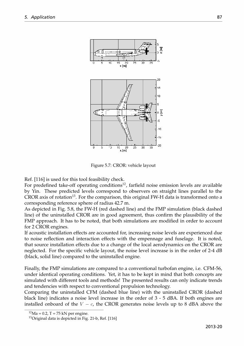
5. Application 87
Figure 5.7: CROR: vehicle layout
Ref. [116] is used for this tool feasibility check.For predefined take-off operating conditions12, farfield noise emission levels are availableby Yin. These predicted levels correspond to observers on straight lines parallel to theCROR axis of rotation13. For the comparison, this original FW-H data is transformed onto acorresponding reference sphere of radius 42.7 m.As depicted in Fig. 5.8, the FW-H (red dashed line) and the FMP simulation (black dashedline) of the uninstalled CROR are in good agreement, thus confirm the plausibility of theFMP approach. It has to be noted, that both simulations are modified in order to accountfor 2 CROR engines.If acoustic installation effects are accounted for, increasing noise levels are experienced dueto noise reflection and interaction effects with the empennage and fuselage. It is noted,that source installation effects due to a change of the local aerodynamics on the CROR areneglected. For the specific vehicle layout, the noise level increase is in the order of 2-4 dB(black, solid line) compared to the uninstalled engine.
Finally, the FMP simulations are compared to a conventional turbofan engine, i.e. CFM-56,under identical operating conditions. Yet, it has to be kept in mind that both concepts aresimulated with different tools and methods! The presented results can only indicate trendsand tendencies with respect to conventional propulsion technology.Comparing the uninstalled CFM (dashed blue line) with the uninstalled CROR (dashedblack line) indicates a noise level increase in the order of 3 - 5 dBA. If both engines areinstalled onboard of the V − c, the CROR generates noise levels up to 8 dBA above the
12Ma = 0.2, T = 75 kN per engine.13Original data is depicted in Fig. 21-b, Ref. [116]
2013-20
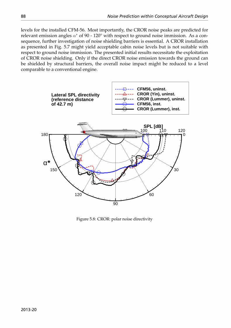
88 Noise Prediction within Conceptual Aircraft Design
levels for the installed CFM-56. Most importantly, the CROR noise peaks are predicted forrelevant emission angles α∗ of 90 - 120° with respect to ground noise immission. As a con-sequence, further investigation of noise shielding barriers is essential. A CROR installationas presented in Fig. 5.7 might yield acceptable cabin noise levels but is not suitable withrespect to ground noise immission. The presented initial results necessitate the exploitationof CROR noise shielding. Only if the direct CROR noise emission towards the ground canbe shielded by structural barriers, the overall noise impact might be reduced to a levelcomparable to a conventional engine.
α*
SPL [dB]
0
30
60
90
120
150
18090 100 110 120
CFM56, uninst.CROR (Yin), uninst.CROR (Lummer), uninst.CFM56, inst.CROR (Lummer), inst.
Lateral SPL directivity(reference distanceof 42.7 m)
Figure 5.8: CROR: polar noise directivity
2013-20
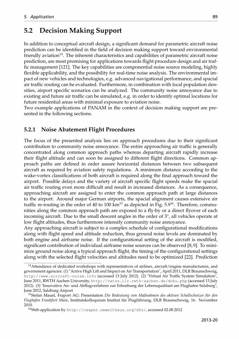
5. Application 89
5.2 Decision Making Support
In addition to conceptual aircraft design, a significant demand for parametric aircraft noiseprediction can be identified in the field of decision making support toward environmentalfriendly aviation14. The inherent characteristics and capabilities of parametric aircraft noiseprediction, are most promising for applications towards flight procedure design and air traf-fic management [121]. The key capabilities are componential noise source modeling, highlyflexible applicability, and the possibility for real-time noise analysis. The environmental im-pact of new vehicles and technologies, e.g. advanced navigational performance, and spacialair traffic routing can be evaluated. Furthermore, in combination with local population den-sities, airport specific scenarios can be analyzed. The community noise annoyance due toexisting and future air traffic can be simulated, e.g. in order to identify optimal locations forfuture residential areas with minimal exposure to aviation noise.Two example applications of PANAM in the context of decision making support are pre-sented in the following sections.
5.2.1 Noise Abatement Flight Procedures
The focus of the presented analysis lies on approach procedures due to their significantcontribution to community noise annoyance. The entire approaching air traffic is generallyconcentrated along common approach paths whereas departing aircraft rapidly increasetheir flight altitude and can soon be assigned to different flight directions. Common ap-proach paths are defined in order assure horizontal distances between two subsequentaircraft as required by aviation safety regulations. A minimum distance according to thewake-vortex classifications of both aircraft is required along the final approach toward theairport. Possible delays and the variety of aircraft specific flight speeds make the spacialair traffic routing even more difficult and result in increased distances. As a consequence,approaching aircraft are assigned to enter the common approach path at large distancesto the airport. Around major German airports, the spacial alignment causes extensive airtraffic re-routing in the order of 40 to 100 km15 as depicted in Fig. 5.916. Therefore, commu-nities along the common approach path are exposed to a fly-by or a direct flyover of eachincoming aircraft. Due to the small descent angles in the order of 3°, all vehicles operate atlow flight altitudes, thus furthermore intensify community noise annoyance.Any approaching aircraft is subject to a complex schedule of configurational modificationsalong with flight speed and altitude reduction, thus ground noise levels are dominated byboth engine and airframe noise. If the configurational setting of the aircraft is modified,significant contribution of individual airframe noise sources can be observed [8,9]. To mini-mize ground noise along a typical approach flight, the timing of the configurational settingsalong with the selected flight velocities and altitudes need to be optimized [22]. Prediction
14Attendance of dedicated workshops with representatives of airlines, aircraft/engine manufacturers, andgovernment agencies: (1) "Active High Lift and Impact on Air Transportation", April 2011, DLR Braunschweig,http://www.aircraft-noise.info (accessed 13 July 2012). (2) "Virtual Air Traffic System Simulation",June 2011, RWTH Aachen University, http://vatss.ilr.rwth-aachen.de/doku.php (accessed 13 July2012). (3) "Innovative An- und Abflugverfahren zur Erhoehung der Lebensqualitaet am Flughafen Salzburg",June 2012, Salzburg Airport
15Stefan Mauel, Fraport AG: Presentation Die Bedeutung von Maßnahmen des aktiven Schallschutzes für denFlughafen Frankfurt Main, Institutskolloquium Institut für Flugführung, DLR Braunschweig, 16. November2010.
16Web-application by http://casper.umwelthaus.org/dfs/, accessed 02.08.2012
2013-20
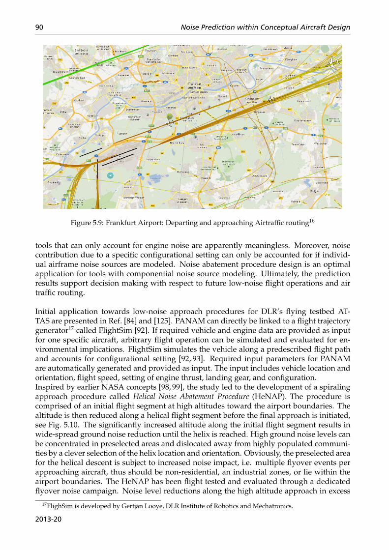
90 Noise Prediction within Conceptual Aircraft Design
Figure 5.9: Frankfurt Airport: Departing and approaching Airtraffic routing16
tools that can only account for engine noise are apparently meaningless. Moreover, noisecontribution due to a specific configurational setting can only be accounted for if individ-ual airframe noise sources are modeled. Noise abatement procedure design is an optimalapplication for tools with componential noise source modeling. Ultimately, the predictionresults support decision making with respect to future low-noise flight operations and airtraffic routing.
Initial application towards low-noise approach procedures for DLR’s flying testbed AT-TAS are presented in Ref. [84] and [125]. PANAM can directly be linked to a flight trajectorygenerator17 called FlightSim [92]. If required vehicle and engine data are provided as inputfor one specific aircraft, arbitrary flight operation can be simulated and evaluated for en-vironmental implications. FlightSim simulates the vehicle along a predescribed flight pathand accounts for configurational setting [92, 93]. Required input parameters for PANAMare automatically generated and provided as input. The input includes vehicle location andorientation, flight speed, setting of engine thrust, landing gear, and configuration.Inspired by earlier NASA concepts [98, 99], the study led to the development of a spiralingapproach procedure called Helical Noise Abatement Procedure (HeNAP). The procedure iscomprised of an initial flight segment at high altitudes toward the airport boundaries. Thealtitude is then reduced along a helical flight segment before the final approach is initiated,see Fig. 5.10. The significantly increased altitude along the initial flight segment results inwide-spread ground noise reduction until the helix is reached. High ground noise levels canbe concentrated in preselected areas and dislocated away from highly populated communi-ties by a clever selection of the helix location and orientation. Obviously, the preselected areafor the helical descent is subject to increased noise impact, i.e. multiple flyover events perapproaching aircraft, thus should be non-residential, an industrial zones, or lie within theairport boundaries. The HeNAP has been flight tested and evaluated through a dedicatedflyover noise campaign. Noise level reductions along the high altitude approach in excess
17FlighSim is developed by Gertjan Looye, DLR Institute of Robotics and Mechatronics.
2013-20
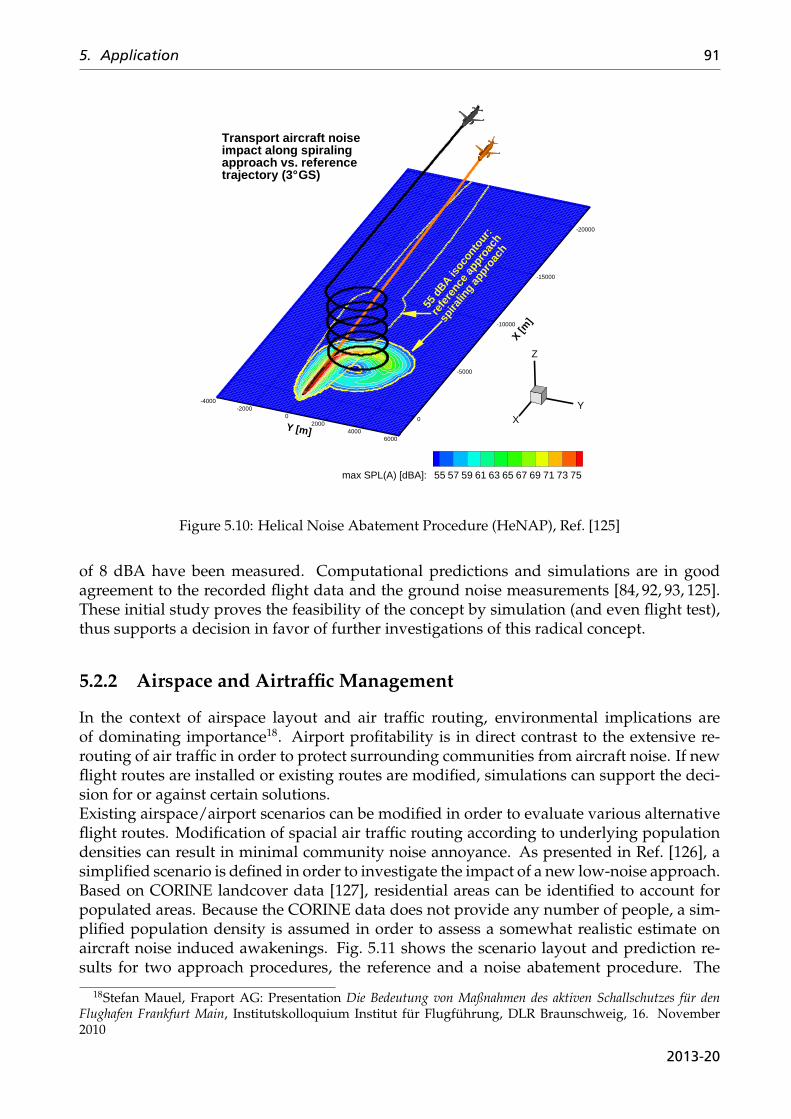
5. Application 91
X [m]
-20000
-15000
-10000
-5000
0
Y [m]
-4000-2000
02000
40006000
XY
Z
max SPL(A) [dBA]: 55 57 59 61 63 65 67 69 71 73 75
55 d
BA isoc
onto
ur:
refe
renc
e ap
proa
ch
spira
ling
appr
oach
Transport aircraft noise impact along spiraling approach vs. reference trajectory (3° GS)
Figure 5.10: Helical Noise Abatement Procedure (HeNAP), Ref. [125]
of 8 dBA have been measured. Computational predictions and simulations are in goodagreement to the recorded flight data and the ground noise measurements [84, 92, 93, 125].These initial study proves the feasibility of the concept by simulation (and even flight test),thus supports a decision in favor of further investigations of this radical concept.
5.2.2 Airspace and Airtraffic Management
In the context of airspace layout and air traffic routing, environmental implications areof dominating importance18. Airport profitability is in direct contrast to the extensive re-routing of air traffic in order to protect surrounding communities from aircraft noise. If newflight routes are installed or existing routes are modified, simulations can support the deci-sion for or against certain solutions.Existing airspace/airport scenarios can be modified in order to evaluate various alternativeflight routes. Modification of spacial air traffic routing according to underlying populationdensities can result in minimal community noise annoyance. As presented in Ref. [126], asimplified scenario is defined in order to investigate the impact of a new low-noise approach.Based on CORINE landcover data [127], residential areas can be identified to account forpopulated areas. Because the CORINE data does not provide any number of people, a sim-plified population density is assumed in order to assess a somewhat realistic estimate onaircraft noise induced awakenings. Fig. 5.11 shows the scenario layout and prediction re-sults for two approach procedures, the reference and a noise abatement procedure. The
18Stefan Mauel, Fraport AG: Presentation Die Bedeutung von Maßnahmen des aktiven Schallschutzes für denFlughafen Frankfurt Main, Institutskolloquium Institut für Flugführung, DLR Braunschweig, 16. November2010
2013-20
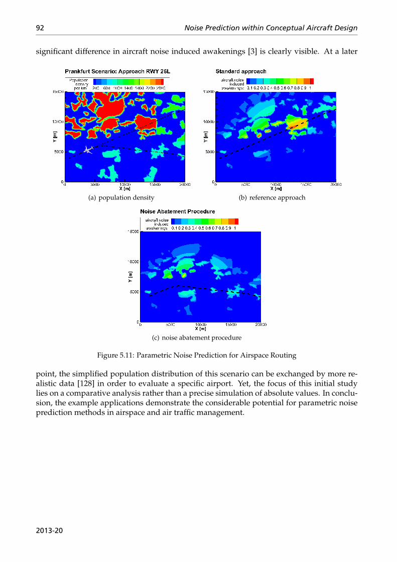
92 Noise Prediction within Conceptual Aircraft Design
significant difference in aircraft noise induced awakenings [3] is clearly visible. At a later
(a) population density (b) reference approach
(c) noise abatement procedure
Figure 5.11: Parametric Noise Prediction for Airspace Routing
point, the simplified population distribution of this scenario can be exchanged by more re-alistic data [128] in order to evaluate a specific airport. Yet, the focus of this initial studylies on a comparative analysis rather than a precise simulation of absolute values. In conclu-sion, the example applications demonstrate the considerable potential for parametric noiseprediction methods in airspace and air traffic management.
2013-20
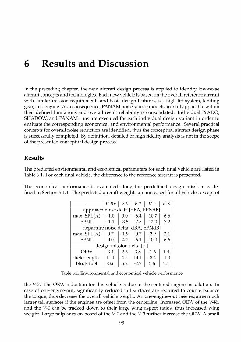
6 Results and Discussion
In the preceding chapter, the new aircraft design process is applied to identify low-noiseaircraft concepts and technologies. Each new vehicle is based on the overall reference aircraftwith similar mission requirements and basic design features, i.e. high-lift system, landinggear, and engine. As a consequence, PANAM noise source models are still applicable withintheir defined limitations and overall result reliability is consolidated. Individual PrADO,SHADOW, and PANAM runs are executed for each individual design variant in order toevaluate the corresponding economical and environmental performance. Several practicalconcepts for overall noise reduction are identified, thus the conceptual aircraft design phaseis successfully completed. By definition, detailed or high fidelity analysis is not in the scopeof the presented conceptual design process.
Results
The predicted environmental and economical parameters for each final vehicle are listed inTable 6.1. For each final vehicle, the difference to the reference aircraft is presented.
The economical performance is evaluated along the predefined design mission as de-fined in Section 5.1.1. The predicted aircraft weights are increased for all vehicles except of
- V-Rx V-0 V-1 V-2 V-Xapproach noise delta [dBA, EPNdB]
max. SPL(A) -1.0 0.0 -6.4 -10.7 -6.6EPNL -1.1 -3.5 -7.5 -12.0 -7.2
departure noise delta [dBA, EPNdB]max. SPL(A) 0.7 -1.9 -0.7 -2.9 -2.1
EPNL 0.0 -4.2 -6.1 -10.0 -6.6design mission delta [%]
OEW 3.4 2.6 3.8 -1.6 1.4field length 11.1 4.2 14.1 -8.4 -1.0block fuel -3.6 5.2 -2.7 3.6 2.1
Table 6.1: Environmental and economical vehicle performance
the V-2. The OEW reduction for this vehicle is due to the centered engine installation. Incase of one-engine-out, significantly reduced tail surfaces are required to counterbalancethe torque, thus decrease the overall vehicle weight. An one-engine-out case requires muchlarger tail surfaces if the engines are offset from the centerline. Increased OEW of the V-Rxand the V-1 can be tracked down to their large wing aspect ratios, thus increased wingweight. Large tailplanes on-board of the V-1 and the V-0 further increase the OEW. A small
93
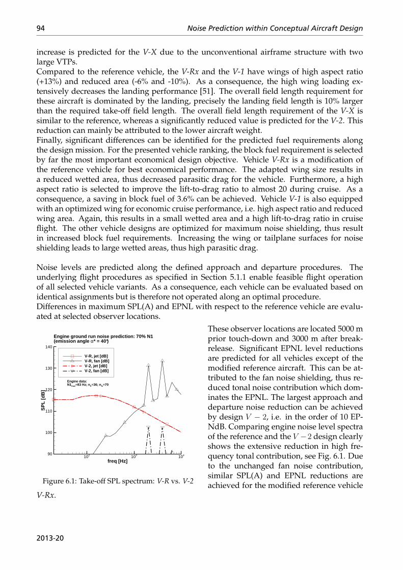
94 Noise Prediction within Conceptual Aircraft Design
increase is predicted for the V-X due to the unconventional airframe structure with twolarge VTPs.Compared to the reference vehicle, the V-Rx and the V-1 have wings of high aspect ratio(+13%) and reduced area (-6% and -10%). As a consequence, the high wing loading ex-tensively decreases the landing performance [51]. The overall field length requirement forthese aircraft is dominated by the landing, precisely the landing field length is 10% largerthan the required take-off field length. The overall field length requirement of the V-X issimilar to the reference, whereas a significantly reduced value is predicted for the V-2. Thisreduction can mainly be attributed to the lower aircraft weight.Finally, significant differences can be identified for the predicted fuel requirements alongthe design mission. For the presented vehicle ranking, the block fuel requirement is selectedby far the most important economical design objective. Vehicle V-Rx is a modification ofthe reference vehicle for best economical performance. The adapted wing size results ina reduced wetted area, thus decreased parasitic drag for the vehicle. Furthermore, a highaspect ratio is selected to improve the lift-to-drag ratio to almost 20 during cruise. As aconsequence, a saving in block fuel of 3.6% can be achieved. Vehicle V-1 is also equippedwith an optimized wing for economic cruise performance, i.e. high aspect ratio and reducedwing area. Again, this results in a small wetted area and a high lift-to-drag ratio in cruiseflight. The other vehicle designs are optimized for maximum noise shielding, thus resultin increased block fuel requirements. Increasing the wing or tailplane surfaces for noiseshielding leads to large wetted areas, thus high parasitic drag.
Noise levels are predicted along the defined approach and departure procedures. Theunderlying flight procedures as specified in Section 5.1.1 enable feasible flight operationof all selected vehicle variants. As a consequence, each vehicle can be evaluated based onidentical assignments but is therefore not operated along an optimal procedure.Differences in maximum SPL(A) and EPNL with respect to the reference vehicle are evalu-ated at selected observer locations.
These observer locations are located 5000 m
freq [Hz]
SP
L [d
B]
102 103 10490
100
110
120
130
140
V-R, jet [dB]V-R, fan [dB]V-2, jet [dB]V-2, fan [dB]
Engine ground run noise prediction: 70% N1(emission angle α* = 40°)
Engine data:N1max=83 Hz; n fr=36; n fs=70
Figure 6.1: Take-off SPL spectrum: V-R vs. V-2
prior touch-down and 3000 m after break-release. Significant EPNL level reductionsare predicted for all vehicles except of themodified reference aircraft. This can be at-tributed to the fan noise shielding, thus re-duced tonal noise contribution which dom-inates the EPNL. The largest approach anddeparture noise reduction can be achievedby design V − 2, i.e. in the order of 10 EP-NdB. Comparing engine noise level spectraof the reference and the V −2 design clearlyshows the extensive reduction in high fre-quency tonal contribution, see Fig. 6.1. Dueto the unchanged fan noise contribution,similar SPL(A) and EPNL reductions areachieved for the modified reference vehicle
V-Rx.
2013-20
6. Results and Discussion 95
Discussion
The presented vehicle ranking is based on a selection of environmental and economicalperformance parameters. These parameters are then weighted in order to evaluate theoverall ranking of a design variant. The selection of these parameters and the correspond-ing weightings reflect the opinion of the author, thus can seem somewhat arbitrary. Yet,the presented selection results in feasible and comprehensive simulation results, thus isrecommended as a best practice or default setting.For example, selecting different weighting factors can change the overall rank-order of thefinal designs. Different environmental weightings κj have no relevant influence on therank-order of the presented vehicles because noise shielding is advantageous along bothapproach and departure procedures. Yet, the situation changes with a different λi setting.For example, a stronger weighting of the balanced field length does change the vehicleranking within the economically driven scenarios (Fig. A.64, Appendix). Vehicles with areduced field length would get better ratings despite higher block fuel or increased vehicleweight. Moreover, the preceding selection of promising vehicle variants out of the availablesolution space could change with different weighting factors, i.e. selecting variants withshort field length requirements.
Furthermore, it has to be kept in mind, that the presented vehicle ranking takes placeat the conceptual design phase. At this early design phase, simulations can be subject tosystematic errors and inherent uncertainties due to simplified methods and approximations.If vehicle variants within one category are compared, it is expected that these uncertaintiesand errors in the simulation process equally affect each variant. If that is the case, the com-parative variant ranking within a specific category is not influenced. Yet, uncertainties canhave an impact if comparing substantially different vehicles, thus necessitate a subsequentand "manual" feasibility check. Therefore, simulation results should be compared withvalidated and reliable reference data.At the conceptual aircraft design phase, detailed investigations for inherent disadvantagesdue to specific engine installation are not possible. This would require a simulation withfar more advanced methods and higher fidelity tools. As a consequence, some inherentdisadvantages with respect to the new vehicles cannot be evaluated but are identified for amore detailed investigation at later design phases.
Uncertainties are most likely to affect vehicles V-0, V-2, and V-X. For example, over-the-wing engine installation can cause a negative impact on the cruise performance due tothe development of shocks between engine and fuselage. As a consequence, such conceptsmight require strict limitations on maximum flight speed, e.g. as it is the case for the VFW-614.Engine installation above the fuselage can result in disadvantageous or even critical op-erational conditions. If flow separation occurs at the wing-fuselage junction or above thefuselage, the engines can directly be subject to disturbed inflow conditions. This can havesevere effects on the performance and efficiency of the engine. Furthermore, when theaircraft is stalled in case of an emergency, the engines can be fully exposed to a separatedflow and can not assist to recover a stable flight condition.Early within the design process, only few and selected structural load cases can be ac-counted for. Whereas certain load cases are of no significance to some vehicles they canrequire structural reinforcement for others. High fidelity investigations of the DLR LNA, aspresented in Ref. [50], indicate further performance disadvantages compared to the simpli-
2013-20
96 Noise Prediction within Conceptual Aircraft Design
fied PrADO analysis. This can be attributed to a dedicated load case, precisely the landingimpact. During the landing impact, extensive fuselage bending moments are predicted forthe LNA configuration, which require an increased fuselage wall thickness [50]. The defaultPrADO sizing does not account for this special load case, thus does not lead to a fuselagethickness increase. This underprediction of the overall empty weight results in artificiallyimproved flight performance. High fidelity analysis indicates an additional fuselage andwing weight in the order of 15%, respectively. Accounting for these additional weights inPrADO, increases the balanced field length (+13%), block fuel (+3.6%), and OEW (+8%) ofthe V-X. More awakenings along both the departure (+2.6%) and the approach procedure(+1%) are predicted due to an increase in required thrust setting. Consequently, worsevehicle specific performance indicators are achieved.
In conclusion, simplified methods at the conceptual aircraft design phase cannot iden-tify inherent disadvantages of certain design details. Therefore, a feasibility check withavailable data and similar vehicle designs is performed for each final vehicle design. Thischeck indicates, that certain design specifics and load cases need further and higher fidelityinvestigation. Especially, for vehicle V-X it can be demonstrated, that conceptual designleads to artificially improved vehicle performance. The V-X concept needs further detailinvestigations at a later design phase. For the other presented vehicles it can be assumed,that feasible results are achieved with the PrADO simulation. Yet, certain design detailsrequire further adaption, e.g. improving the flight stability of the V-1 with an advanceddefueling scheme. Furthermore, it can be expected that specific absolute values can showdiscrepancies if compared to results of high fidelity computational analysis.Ultimately, the reliability of the new simulation process is confirmed due to feasible andcomprehensive results, i.e. all relevant effects can directly be attributed to a physical cause.
2013-20
7 Conclusions
The main motivation for the presented research activities is the integration of noise as anadditional design objective and the identification of promising low-noise aircraft concepts.Thereby, it is most effective if noise is accounted for as early as possible within the over-all design process. At early design levels only few key parameters are fixed, thus majorgeometry modifications are still feasible and significantly varying concepts can directlybe compared. For all modifications and new concepts, the impact on environmental andeconomical performance has to be assessed. This requires a concurrent approach, i.e. allrelevant interdependencies among the involved disciplines have to be accounted for at thesame time. In conclusion, two main topics have to be addressed, i.e. development of anappropriate noise prediction tool and integration of noise into the design process of newaircraft. Thereby, the intended investigations aim at realizable, medium term solutions withrespect to both aircraft and engine design. Futuristic vehicle concepts such as blended wingbodies with embedded or distributed propulsion are not in the scope of this research activity.
A new noise prediction software is developed for application at the conceptual aircraftdesign phase, the Parametric Aircraft Noise Analysis Module (PANAM). PANAM featurescomponential and parametric noise prediction, thus can consider individual noise sourcesdepending on their geometry and operating conditions during simulated flight operation.Thereby, each major noise source is modeled with an individual semi-empirical noise sourcemodel. These models capture the major physical effects and correlations but yet allow forquick noise predictions, i.e. executable on a standard desktop PC. This simulation approachprovides comprehensive results as each noise relevant effect can be attributed to its cause.The selected semi-empirical models as implemented into PANAM come from various DLRInstitutions and are derived from flyover noise measurements and different full-scale ormodel scale component wind-tunnel tests. These models are well suitable for the availablequantity and complexity of input data at the conceptual aircraft design phase. All modelsand approximations are based on physics, thus PANAM can be classified as a scientificprediction method. Recent findings and detail solutions from related disciplines can beintegrated into the PANAM framework to enable an evaluation on a system level.Dedicated comparison of simulation and measurement indicates feasible overall aircraftnoise prediction capabilities. Prediction results and noise related effects are in good agree-ment to available experimental data and theoretical knowledge. The result reliability isreduced, if the noise source models are applied toward vehicle concepts far off the designspace as specified by the underlying empirical data. Yet, if general noise generating mech-anisms are kept consistent with the empirical data base, i.e. fixed design principles forindividual noise sources, reasonable and reliable results can be expected.
In order to establish an overall low-noise design process, the existing design synthesiscode PrADO is selected and modified. The PrADO tool, as developed at the Technical
97
98 Noise Prediction within Conceptual Aircraft Design
University of Braunschweig, is updated with noise prediction capabilities. PANAM isdirectly executed within the modular and sequential PrADO design process. The predictionresults are then collected and returned to the overall design process. Any of these resultscan be selected as final design objectives. To quickly assess the environmental versus theeconomical performance under different scenarios, a multiple criteria design evaluationis introduced. As a result, different vehicle concepts can directly be compared in order toidentify the most promising concepts within a certain scenario. Ultimately, a comparativeanalysis of both environmental and economical performance under various boundary con-ditions is established. The identification and initial evaluation of promising concepts outof the available solution space concludes the assigned task. Subsequently, these conceptscan be subject to further and more detailed investigations, e.g. high fidelity computation orwind tunnel tests, which is not in the scope of the presented activities.
It is demonstrated, that the aircraft designer’s influence on the environmental vehicleperformance is significant at the conceptual design phase. Early modifications to thebasic vehicle layout result in extensive reduction of ground noise levels. Initial PrADOevaluations indicate, that this can be achieved for small decreases in economical vehicleperformance. Maximum engine noise shielding is achieved for fuselage/wing shielding ofover-the-fuselage mounted engines. Compared to the reference vehicle, noise level reduc-tions in excess of 10 EPNdB are predicted along both approach and departure procedure.Reduction in maximum SPL(A) is smaller along the departure because SPL does not accountfor tonal corrections and broadband jet noise is dominating. But at the same time, block fuelincreases by 3.6%. As an alternative propulsion concept for this vehicle, a geared turbofanpromises reduced block fuel requirements and further reduction of jet noise contribution.If economical performance is selected as the highest priority, modifications to the referencevehicle can decrease block fuel by 3.6% under similar ground noise immissions.In conclusion, promising and feasible concepts are identified at an early design phase andcan be recommended for subsequent investigations at increased fidelity levels.
Ultimately, PANAM can be ranked as well suitable to assess all four measures of ICAO’sbalanced approach, including (1) modifications to the noise source, (2) sophisticated trafficrouting, (3) operational constraints, and (4) noise abatement flight procedures. Further-more, real-time noise prediction could support pilots or air traffic controllers to identifyideal flight routes with respect to ground noise pollution. A real-time noise evaluation couldaugment cockpit in-flight information or enable pilot environmental awareness training inground-based flight simulators.
Future work has to focus on the weighting of individual noise sources. Especially, theweighting of jet versus fan noise contribution under various operating conditions needsfurther validation. Additional noise sources are under investigation at DLR and will beimplemented into PANAM.The focus of the presented work lies on low-noise vehicle design but it will become in-evitable for future analysis to optimize both aircraft and operational procedure at thesame time. In order to achieve maximum noise reduction, a low-noise vehicle needs tobe operated on its individual, aircraft type specific noise abatement flight procedure. Thedevelopment of PANAM provides the key prerequisites for any of these future activities.
2013-20

Bibliography
[1] ACARE - Beyond Vision 2020, LEAFLET_ACARE_beyond_V2020_exe_summary.pdf, online version,http://www.acare4europe.com (accessed 10 January 2010)
[2] U. Heudorf: Fluglärm und Gesundheit, Ergebnisse epidemiologischer Studien - Literaturübersicht, Amt fürGesundheit Frankfurt, Abteilung Medizinische Dienste und Hygiene, Frankfurt, Dec 2008
[3] M. Basner, B. Griefahn, M. Berg: Aircraft noise effects on sleep: mechanisms, mitigation and research needs,Noise & Health Journal, Vol. 12 (47), pages 95-109, 2010
[4] Burden of disease from environmental noise - Quantification of healthy life years lost in Europe, World HealthOrganization, 108 pages, ISBN 978928-900229-5, 2011
[5] F. Thiessen, S. Schnorr: Immobilien und Fluglärm, Fakultät für Wirtschaftswissenschaften, Technische Uni-versität Chemniz, Bericht Nr. WWDP 69/2005, ISSN 1618-1352, 2005
[6] International Civil Aviation Organization (ICAO), Air Transport Bureau (ATB): Concept of a balancedapproach principle to aircraft noise management, appendix C of Assembly Resolution A35-5, 2007, http://www.icao.int/env/noise.htm (accessed 21 April 2011)
[7] E.D. Olson, D.N. Mavris: Aircraft Conceptual Design and Risk Analysis Using Physics-Based Noise Predic-tion, AIAA 2006-2619, 12th AIAA/CEAS Aeroacoustics Conference, 8 - 19 May 2006, Cambridge, Mas-sachusetts, USA
[8] F. Farassat, J.H. Casper: Towards an Airframe Noise Prediction Methodology: Survey of Current Approaches,AIAA-2006-0210, 44th AIAA Aerospace Sciences Meeting and Exhibit, Reno, Nevada, January 9-12, 2006
[9] W. Dobrzynski: Almost 40 Years of Airframe Noise Research: What did we Achieve?, Journal of Aircraft, Vol.47 (No. 2), pages 353-367, DOI: 10.2514/1.44457, March - April 2010
[10] Bundesministerium der Justiz: Erste Verordnung zur Durchführung des Gesetzes zum Schutz gegen Fluglärm(Verordnung über die Datenerfassung und das Berechnungsverfahren für die Festsetzung von Lärmschutzbere-ichen - 1.FlugLSV), Bundesgesetzblatt BGBl I, 27th December 2008
[11] European Civil Aviation Conference (ECAC): Methodology for Computing Noise Contours around Civil Air-ports, Vol. 1 and 2 (applications and technical guide), ECAC/CEAC Doc.29, 3rd Edition, December 2005
[12] International Civil Aviation Organization (ICAO): ICAO DOC 9911 Recomended Method for ComputingNoise Contours Around Airports, Order Number 9911, ISBN 978-92-9231-225-1, 2008
[13] Society of Automotive Engineers SAE, A-21 Aircraft Noise Measure Noise Aviation Emission Modeling:Procedure for the Computation of Airplane Noise in the Vicinity of Airports, SAE-AIR-1845, 1986
[14] U. Isermann, R. Schmid: Description and Calculation of Aircraft Noise (German), DLR-Forschungsbericht2000-20, German Aerospace Center (DLR), ISSN 1434-8454, June 2000
[15] S. Fidell, P. Schomer:Uncertainties in measuring aircraft noise and predicting community response to it, NoiseControl Engineering Journal (NCEJ), Vol. 55 (No. 1), pages 82 - 88, ISSN 0736-2501
99
100 Noise Prediction within Conceptual Aircraft Design
[16] M.J.T. Smith: Aircraft Noise, Cambridge Aerospace Series, Cambridge University Press, ISBN 0-521-61699-9, 2004
[17] J.R. Olmstead, G.G. Fleming, J.M. Gulding, C.J. Roof, P.J. Gerbi, and A.S. Rapoza:Integrated Noise Model(INM) Version 6.0 Technical Manual, U.S. Department of Transportation Federal Aviation Administration,Report No. FAA-AEE-02-01, January 2002, Washington, D.C., USA
[18] S. Hartjes, H.G. Visser, S.J. Hebly: Optimization of RNAV Noise and Emission Abatement Departure Proce-dures, AIAA-2009-6953, 9th AIAA Aviation Technology, Integration, and Operations Conference (ATIO),September 2009, Hilton Head Island, South Carolina, USA
[19] W. Krebs, G. Thomann, R. Buetikofer: FLULA2 - Ein Verfahren zur Berechnung und Darstellung derFluglaermbelastung, Technical Manual Version 4, EMPA, (Flula2-V4-mBV1.pdf), 2010
[20] U. Isermann: Calculation of Aircraft Noise in the Vicinity of Civil Airports by a Simulation Procedure (German),Dissertation, Report 7/1988, Max-Planck-Institut fuer Stroemungsforschung, 1988
[21] M. Pott-Pollenske, W. Dobrzynski, H. Buchholz, S. Guérin, G. Saueressig, and U.Finke: Airframe NoiseCharacteristics from Flyover Measurements and Predictions, AIAA-2006-2567, 12th AIAA/CEAS Aeroacous-tics Conference (27th AIAA Aeroacoustics Conference), May 2006, Cambridge, Massachusetts, USA
[22] R. Koenig, J. Heider, M. Maierhofer: Aircraft Flight Procedure Design with Respect to Noise Abatement as wellas Economical and Pilot Workload Aspects, Inter-noise Congress and Exposition on Noise Control Engineer-ing 2005, August 2005, Rio de Janeiro, Brazil
[23] R.E. Gillian: Aircraft Noise Prediction Program User’s Manual, NASA Langley Research Center, 1982
[24] M.R. Fink: Airframe Noise Prediction Method, FAA Research Report, FAA-RD-77-29, March 1977
[25] J.R. Stone, D.E. Groesbeck, C.L. Zola: Conventional profile coaxial jet noise prediction, AIAA Journal, 21(1)(1983), pp. 336-342
[26] M.F. Heidmann: Interim prediction method for fan and compressor source noise, NASA Technical Report TM-X-71763, 1979
[27] J. Bridges, A. Khavaran, C.A. Hunter: Assessment of Current Jet Noise Prediction Capabilities, AIAA-2008-2933, 14th AIAA/CEAS Aeroacoustics Conference (29th AIAA Aeroacoustics Conference), 5 - 7 May2008, Vancouver, British Columbia Canada
[28] E. Envia, D.L. Tweedt, R.P. Woodward, D.M. Elliott, E.B.Fite, C.E. Hughes, G.G. Podboy, and D.L. Sut-liff:An Assessment of Current Fan Noise Prediction Capability, AIAA-2008-2991, 14th AIAA/CEAS Aeroa-coustics Conference (29th AIAA Aeroacoustics Conference), 5 - 7 May 2008, Vancouver, British ColumbiaCanada
[29] N. Antoine, I. Kroo, K. Willcox, and G. Barter: A Framework for Aircraft Conceptual Design and Environmen-tal Performance Studies, AIAA-2004-4314, 10th AIAA/ISSMO Multidisciplinary Analysis and Optimiza-tion Conference, August 2004, Albany, New York, USA
[30] C. Burley, L. Lopez: ANOPP2: Progress Update, NASA Spring Acoustics Technical Working Group, pre-sentation, April 21-22 2011, Cleveland, OH
[31] L. Lopez, C. Burley: Design of the Next Generation Aircraft Noise Prediction Program: ANOPP2, AIAA-2011-2854, 17th AIAA/CEAS Aeroacoustics Conference, Portland, Oregon, June 2011
[32] N. Van Oosten: SOPRANO Presentation (PDF), SOPRANO Workshop, 21 - 22 June 2007, Madrid, Spain
[33] A.M. Rolt, K.G. Kyprianidis: Assessment of new aeroengine core concepts and technologies in the EU framework6 NEWAC programme, paper icas-408, 27th International Congress of the Aeronautical Sciences (ICAS2010), 19 - 24 September 2010, Nice, France
[34] Y. Rozenberga, J. Bultéb: Fast Aircraft Noise Prediction Including Installation Effects for the Evaluation ofAir Transport Systems, paper in08-0342, 37th International Congress and Exposition on Noise ControlEngineering (inter-noise 2008), 26 - 29 October 2008, Shanghai, China
2013-20
BIBLIOGRAPHY 101
[35] M. Brunet, T. Chaboud, N. Huynh, P. Malbequi, and W. Ghedhaifi: Environmental Impact Evaluation of AirTransport Systems Through Physical Modeling and Simulation, AIAA-2009-6936, 9th AIAA Aviation Tech-nology, Integration, and Operations Conference (ATIO), September 2009, Hilton Head Island, SouthCarolina, USA
[36] W. Dobrzynski, M. Pott-Pollenske: Slat Noise Source Studies for Farfield Noise Prediction, AIAA-2001-2158,7th AIAA/CEAS Aeroacoustics Conference, 28 - 30 May 2001, Maastricht, Netherlands
[37] M. Hepperle: Environmental Friendly Transport Aircraft, Notes on Numerical Fluid Mechanics and Mul-tidisciplinary Design, Vol. 87, pages 26-33, Springer Verlag, 13th STAB/DGLR Symposium, 12 - 14 Nov2002, Muenchen, Germany, ISBN 3-540-20258-7
[38] M. Lummer, M. Hepperle, J. Delfs: Towards a Tool for the Noise Assessment of Aircraft Configurations, Aeroa-coustics of New Aircraft and Engine Configurations, 8th ASC-CEAS Workshop, Budapest, Hungary, 11- 12 Nov 2004, ISBN 963-420-842-8
[39] R. Schmid: Half-empirical, physical model for the directional characteristic of sound radiated by modern turbofanengines, Doctoral Thesis University of Goettingen, Germany, DLR-Forschungsbericht 1999-47, ISSN 1434-8454, 2000
[40] L. Bertsch: Stand der Arbeiten zur akustischen Bewertung von Flugzeugkonfigurationen im Projekt QSTOL, In-ternal Report IB 124-2007/4, Institute of Aerodynamics and Flow Technology, German Aerospace Center,ISSN 1614-7790
[41] L. Bertsch, P. Krammer: PANAM - a noise prediction tool for conceptual aircraft design, Internal Report IB124-2008/902, Institute of Aerodynamics and Flow Technology, German Aerospace Center
[42] L. Bertsch, W. Dobrzynski, S. Guérin: Tool development for Low-Noise Aircraft Design, AIAA-2008-2995,14th AIAA/CEAS Aeroacoustics Conference, Mai 2008, Vancouver, British Columbia, Canada
[43] L. Bertsch, W. Dobrzynski, S. Guérin: Tool Development for Low-Noise Aircraft Design, Journal of Aircraft,47 (2), Seiten 694-699, DOI: 10.2514/1.43188, March - April 2010
[44] L. Bertsch, S. Guérin, G. Looye, M. Pott-Pollenske: The Parametric Aircraft Noise Analysis Module - statusoverview and recent applications, AIAA-2011-2855, 17th AIAA/CEAS Aeroacoustics Conference, 5-8 June2011, Portland, Oregon, USA
[45] C. Liersch, M. Hepperle: A Unified Approach for Multidisciplinary Preliminary Aircraft Design, accepted forpresentation at the CEAS 2009 European Air and Space Conference, 26 - 29 Oct 2009
[46] M. Kunde, A. Bachmann, M. Litz: A dynamic data integration approach to build scientific workflow sys-tems, Institute of Electrical and Electronics Engineers, International Workshop on Workflow Management(IWWM 2009), pages 27-33, May 2009
[47] Phoenix Integration: PHX ModelCenter and Analysis Server, http://www.phoenix-int.com
[48] W. Heinze: Ein Beitrag zur quantitativen Analyse der technischen und wirtschaftlichen Auslegungsgrenzenverschiedener Flugzeugkonzepte für den Transport großer Nutzlasten, ZLR-Forschungsbericht 94-01, ISBN 3-928628-14-3
[49] W. Heinze, C.M. Oesterheld, P. Horst: Multidisziplinaeres Flugzeugentwurfsverfahren PrADO - Program-mentwurf und Anwendung im Rahmen von Flugzeugkonzeptstudien, DLRK 2001-194, Deutscher Luft- undRaumfahrtkongress 2001, September 2001, Bonn, Germany
[50] W. Werner-Westphal, W. Heinze, P. Horst: Multidisciplinary Integrated Preliminary Design Applied to Uncon-ventional Aircraft Configurations, Journal of Aircraft, 45 (2), pages 581-589, DOI: 10.2514/1.32138, March -April 2008
[51] D.P. Raymer:Aircraft design: a conceptual approach, third edition, AIAA education series, American Insti-tute of Aeronautics and Astronautics, ISBN 1563472813, 1999
2013-20
102 Noise Prediction within Conceptual Aircraft Design
[52] G. Thomann: Uncertainties of measured and calculated aircraft noise and consequences in relation to noise limits,PhD Thesis ETH Zuerich, No. 17433, 2007
[53] International Organisation for Standardisation, ISO: ISO LN 9300, Luftfahrtnorm, Juli 1976
[54] D.A. Bies: Engineering Noise Control, Theory and Practice, Third Edition, Spon Press, ISBN 0-415-26714-5,2003
[55] A. Le Duc, P. Spiegel, F. Guntzer, M. Lummer, J. Goetz, and H. Buchholz: Simulation of complete helicopternoise in maneuver flight using aeroacoustic flight test database, American Helicopter Society, 64th AnnualForum, and Technology Display, Montreal, Canada, April 2008
[56] Method for the Calculation of the Absorption of Sound by the Atmosphere, ANSI S1.26-1978, 1995
[57] I.L.N. Granoien, R.T. Randeberg: Corrective measures for aircraft noise models, new algorithms for lateralattenuation, Baltic-Nordic Acoustics Meeting 2004, BNAM, 8-10 June 2004, Mariehamn, Alan
[58] Society of Automotive Engineers, Committee A-21: Prediction Method for Lateral Attenuation of AirplaneNoise During Takeoff and Landing, Aerospace Information Report No. 1751, Warrendale, Society of Auto-motive Engineers, Inc., March 1981
[59] W. Dobrzynski, L. Chow, P. Guion, D. Shiells: A European Study on Landing Gear Airframe Noise Sources,6th AIAA/CEAS Aeroacoustics Conference, 12-14 June 2000, La-haina Hawaii/USA
[60] W. Dobrzynski, L.C. Chow, P. Guion, and D. Shiells: Research into Landing Gear Airframe Noise Reduction,AIAA-2002-2409, 8th AIAA/CEAS Aeroacoustics Conference, June 2002, Breckenridge, USA
[61] DLR: Entwicklung von Quellmodellen für den Umströmungslärm von Verkehrsflugzeugen durch Auswertungvon Windkanal-Messdaten und Überflugmessungen an einem Airbus A319 - Arbeiten im Rahmen des ProjektsLAnAb, Abschlussbericht für den BMFT, DLR IB 124-2006/05
[62] W. Dobrzynski: Konfigurationen 2020 Abschlussbericht - Konfigurative Lärmkriterien, final project report,ref.-nr.: K2020-DLR-000-017-P4-Final_Report, Braunschweig, Germany, 16 July 2007
[63] W. Dobrzynski, L.C. Chow, M. Smith, A. Boillot, O. Dereure, and N. Molin: Experimental Assessment ofLow Noise Landing Gear Component Design, AIAA 2009-3276, 15th AIAA/CEAS Aeroacoustics Conference,11 - 13 May 2009, Miami, Florida, USA
[64] K.-S. Rossignol: Development of an empirical prediction model for flap side-edge noise, AIAA-2010-3836, 16thAIAA/CEAS Aeroacoustics Conference, 7 - 9 June 2010, Stockholm, Sweden
[65] K.-S. Rossignol: Empirical Prediction of Airfoil Tip Noise, AIAA-2011-273, 17th AIAA/CEAS AeroacousticsConference, 6-8 June 2011, Portland, Oregon, USA
[66] D.P. Lockard, G.M. Lilley: The Airframe Noise Reduction Challenge, NASA Technical Manual TM-2004-213013, 2004
[67] H. Schlichting, E. Truckenbrodt: Aerodynamik des Flugzeuges - Erster Band, second edition, Springer-Verlag, ISBN 3-540-03970-8, 1967
[68] M. Braun, K. Wicke, A. Koch, T. Wunderlich: Analysis of Natural Laminar Flow Aircraft based on Airline Net-work Design and Fleet Assignment, 11th AIAA Aviation Technology, Integration, and Operations (ATIO)Conference 2011, paper AIAA-2011-6807
[69] P.K.C. Rudolph: High-Lift Systems on Commercial Subsonic Airliners, NASA Contractor Report CR 4746,Sept. 1996
[70] W. Dobrzynski, K.S. Rossignol, and D.Almoneit: Handbuch zum modularen Quellmodell fuer das Umstroe-mungsgeraeusch von Verkehrsflugzeugen, Version 4.0, Internal Report IB 124-2011/? (t.b.d.), Institute ofAerodynamics and Flow Technology, German Aerospace Center
2013-20
BIBLIOGRAPHY 103
[71] W. Dobrzynski, M. Herr, M. Pott-Pollenske: Airframe Noise Source Modeling - Application and Limitations,Presentation, Campus Research Airport Symposium 2011: Active High Lift and Impact on Air Trans-portation, DLR Braunschweig, 11-12 April, 2011, http://www.aircraft-noise.info (accessed 23July 2011)
[72] Gas Turbine Engine Performance Station Identification and Nomenclature, Aerospace Recommended Practice,ARP 755A, Society of Automotive Engineers, Warrandale, Pennsylvania, USA
[73] J. Kurzke: Fundamental Differences between Conventional and Geared Turbofans, GT-2009-59745, Proceedingsof ASME Turbo Expo 2009 Gas Turbine Technical Congress and Exhibition June 8-12, 2009, Orlando,Florida, USA
[74] W. Olsen, R. Friedman: Jet noise from co-axial nozzles over a wide range of geometric and flow parameters,NASA Technical Report TM-X-71503, Lewis Research Center, Cleveland, Ohio 44135, 1979
[75] S. Guérin, A. Moreau, C. Weckmüller: Engine Noise Source Modeling - Limitations and Perspectives, Presen-tation, Campus Research Airport Symposium 2011: Active High Lift and Impact on Air Transportation,DLR Braunschweig, 11-12 April, 2011, http://www.aircraft-noise.info (accessed 23 July 2011)
[76] G.J.J. Ruijgrok: Elements of Aviation Acoustics, Delft University Press, ISBN 90-6275-899-1, 1993
[77] P.G. Hill, C.R. Peterson: Mechanics and thermodynamics of propulsion (2nd revised and enlarged edition), Read-ing, MA, Addison-Wesley Publishing Co., ISBN 0-201-14659-2, 1992
[78] S. Guérin: Impact on Serrations on the Circumferential Structure of Jet Turbulence and Relation to Jet NoiseReduction, 14th AIAA/CEAS Aeroacoustics Conference 2008, paper AIAA-2008-3025
[79] W.J.G. Braeunling: Flugzeugtriebwerke, Springer Verlag, ISBN 3-540-40589-5, 2004
[80] F. Deidewig: Ermittlung der Schadstoffemissionen im Unter- und Ueberschallflug, German Aerospace Center,DLR Forschungsbericht 98-10, Collogne, Germany, 1998
[81] A. Moreau, S. Guérin, and S.Busse: A method based on the ray structure of acoustic modes for predicting theliner performance in annular ducts with flow, NAG/DAGA International Conference on Acoustics, Rotter-dam, 23 - 26 March 2009
[82] J.M. Tyler, T.G. Sofrin: Axial flow compressor noise studies, SAE Transactions 70, 309-332, 1962
[83] M. Lummer: Maggi-Rubinowicz Diffraction Correction for Ray-Tracing Calculations of Engine Noise Shielding,14th AIAA/CEAS Aeroacoustics Conference 2008, paper AIAA-2008-3050
[84] L. Bertsch, G. Looye, T. Otten, M. Lummer: Integration and application of a tool chain for environmentalanalysis of aircraft flight trajectories, AIAA-2009-6954, 9th AIAA Aviation Technology, Integration, andOperations Conference (ATIO), September 2009, Hilton Head Island, South Carolina, USA
[85] J.B. Keller: Geometrical Theory of Diffraction, Journal of the Optical Society of America, vol. 52, no. 2, pages116-130, Feb 1962
[86] K. Miyamoto, E. Wolf: Generalization of the Maggi-Rubinowicz Theory of the Boundary Diffraction Wave - PartI, Journal of the Optical Society of America, vol. 52, no. 6, pages 615-625, June 1962
[87] K. Miyamoto, E. Wolf: Generalization of the Maggi-Rubinowicz Theory of the Boundary Diffraction Wave - PartII, Journal of the Optical Society of America, vol. 52, no. 6, pages 626-637, June 1962
[88] C. Kott: Entwurf von laermarmen Flugzeugkonfigurationen unter Beruecksichtigung von Abschattungseffekten(German), final diploma thesis, German Aerospace Center in cooperation with Fachhochschule Aachen,Faculty of Aerospace Engineering, Aachen, Germany, 2010
[89] Google: Google Earth software, http:\\earth.google.com
[90] G. Mueller, M. Moeser: Taschenbuch der Technischen Akustik, 3rd edition, Springer Press, Berlin, ISBN978-3-540-41242-7, 2004
2013-20
104 Noise Prediction within Conceptual Aircraft Design
[91] Position paper on dose response relationships between transportation noise and annoyance, European Commu-nities, 2002
[92] G. Looye: Flight testing of autopilot control laws: fly the helix!, German Aerospace Congress 2009, paperDLRK-2009-1375
[93] G. Looye: Aircraft Mission Simulation for Environmental Analysis with Flight Test Validation, Presentation,DGLR workshop "Umweltfreundliches Fliegen", Braunschweig, Germany, June 16-17, 2010, http://www.dglr.de (accessed 23 January 2011)
[94] P. Krammer, L. Bertsch, C. Werner-Spatz: Multidisciplinary Preliminary Aircraft Design with Integrated NoiseAnalysis Capabilities, DLRK 2009 121177, Deutscher Luft- und Raumfahrtkongress 2009, September 2009,Hamburg, Germany
[95] S. Guérin, U. Michel: Prediction of aero-engine noise: comparison with A319 flyover measurements, Tech. Rep.,DLR, 2007, IB 92517-04/B3
[96] W. Durham: Aircraft Dynamics and Control, Vorlesungsskript an der Virginia Polytechnic Insitute andState University, Blacksburg, VA, USA, 2004
[97] Airbus Flight Operations Support & Line Assistance: Getting to grips with aircraft noise, PDF, "Gettingto grips" advisory publications, Airbus Customer Services, rond-point Maurice Bellonte 1, BP 33, 31707Blagnac, France
[98] C. Hange: Assessment of a C-17 flight test of an ESTOL transport landing approach for operational viability, pilotperceptions and workload, and passenger ride acceptance, AIAA 2007-1398
[99] C. Hange: Trajectory kinematics of a simultaneous non-interfering landing approach and the impact on ESTOLregional transport performance and flight control, AIAA 2003-6857
[100] R. Koenig: Lärmoptimierte An- und Abflugverfahren, Zusammenfassender Schlussbericht, ForschungsverbundLeiser Verkehr, Bereich Leises Verkehrsflugzeug, Projekt 1600 Lärmoptimierte An- und Abflugverfahren(LAnAb), 2007
[101] Airbus: A319 airplane characteristics for airport planning, PDF, technical document, AIRBUS S.A.S., Cus-tomer Services, Technical Data Support and Services, 31707 Blagnac Cedex, France, Issue: Jul 01/95, Rev:May 01/11
[102] P. Jackson, K. Munson, L. Peacock (Editors): Jane’s All the World’s Aircraft [Hardcover], 2009 - 2010 Version,Jane’s Information Group, United Kingdom, ISBN 0-710-62837-4, June 2008
[103] Brüel & Kjaer: Leq, SEL, what? Why? When?, Application Notes 1989 - 1980, Brüel & Kjaer, Sound& Vibration Measurement A/S, Denmark, http://www.bksv.com/doc/BO0051.pdf (accessed 12May 2011)
[104] A. Filippone, L. Bertsch, M. Pott-Pollenske: Validation Strategies for Comprehensive Aircraft Noise PredictionMethods, AIAA 2012-5411, 12th AIAA Aviation Technology, Integration, and Operations (ATIO) Confer-ence, 17 - 19 September 2012, Indianapolis, Indiana, USA
[105] Airbus Company: Airbus Market Forecast 2011-2030, online pdf, http://www.airbus.com/company/market/forecast/passenger-aircraft-market-forecast/Airbus\_GMF\_2011-2030\_delivering\_the\_future\_-\_full\_book.pdf (accessed 09 January 2012)
[106] Boeing Company: Boeing Current Market Outlook 2011-2030, online version, http://www.boeing.com/commercial/cmo/ (accessed 12 January 2012)
[107] European Union: Noise Charge Harmonization within Europe, online version, http://ec.europa.eu/environment/noise/home.htm (accessed 02 January 2012)
[108] Berlin Airport: Airport Charges, pdf version, http://www.berlin-airport.de/EN/GeschaeftskundenUndPartner/Entgelte/Download/110401\_Entgeltordnung\_engl.pdf (accessed 02 January 2012)
2013-20
BIBLIOGRAPHY 105
[109] Frankfurt Airport: Airport Charges, pdf version, http://www.fraport.com/content/fraport-ag/en/misc/binaer/products_services/airport-charges/Flughafenentgelte\_Airport\_charges\_202012.pdf (accessed 02 January 2012)
[110] R. Henke, T. Lammering, E. Anton: Impact of an Innovative Quiet Regional Aircraft on the Air TransportationSystem, Journal of Aircraft, 47 (3), pages 875-886, DOI: 10.2514/1.45785, May - June 2010
[111] S. Guérin, A. Moreau, C. Menzel, C. Weckmueller: Open-rotor noise prediction with a RANS-informed ana-lytical method, abstract proposed for presentation at the 18th AIAA/CEAS Aeroacoustics Confernce (33rdAIAA Aeroacoustics Conference), 4 - 6 June 2012, Colorado Springs, Colorado, USA
[112] L. Bertsch, O. Schneider, H. Hemmer, M. Hepperle, O. Macke: Process Implementation for the SystemEvaluation of new Low-Noise STOL Transportation Concepts, Paper No. 2, CEAS/KATnet II Conference onKey Aerodynamic Technologies, May 2009, Bremen, Germany
[113] N. Arndt: Environmentally friendly aero-engines for the 21st century, Rolls-Royce presentation, First CEASEuropean Air and Space Conference, 10 - 13 September 2007, Berlin, Germany, http://www.dlr.de/pa/Portaldata/33/Resources/dokumente/ceas/CEAS_WS_Arndt.pdf (accessed 02 March2011)
[114] J.J. Korsia: VITAL Project overview, Snecma presentation, Aeronautics Days 2006 - Sustainable Solutionsfor New Horizons, 19 - 21 June 2006, Vienna, Austria, http://www.aerodays2006.org/sessions/A_Sessions/A4/A44.pdf (accessed 12 June 2011)
[115] C. Lenfers: Propeller Design for a future QESTOL Aircraft in the BNF Project, AIAA 2012-3334, 30th AIAAApplied Aerodynamics Conference, 25 - 28 June 2012, New Orleans, Louisiana, USA
[116] A. Stuermer, J. Yin: Low-Speed Aerodynamics and Aeroacoustics of CROR Propulsion Systems, AIAA-2009-3134, 15th AIAA/CEAS Aeroacoustics Conference, 11-13 May 2009, Miami, Florida, USA
[117] C.O. Márquez, A. Stuermer, C. Clemen: Installation Effects of a CROR Propulsion System on a ModifiedDLR-F6 Aircraft Configuration, ISABE-2011-1307, 20th International Society of Airbreathing Engines Con-ference, 12-16 September 2011, Goeteborg, Sweden
[118] H. Grieb, D. Eckardt: Turbofan and Propfan as Basis for Future Economic Propulsion Concepts, AIAA-86-1474,AIAA/ASME/SAE/ASEE 22nd Joint Propulsion Conference, 16-18 June 1986, Huntsville, Alabama
[119] M. Kingan, R.H. Self: Advanced Open Rotor Noise Modelling Tool and Compari-son Study Technical Dissemination Workshop, Institute of Sound and Vibration re-search, University of Southampton, December 2008, http://www.omega.mmu.ac.uk/workshop-integrated-study-of-advanced-open-rotor-powered-aircraft.htm (ac-cessed 02 June 2012)
[120] L. Mueller: Quellformulierung für Fernfeldschallberechnung mit einem Schallstrahlenverfahren bei installiertengegenlaeufigen Propellern, Diploma thesis, University of Braunschweig, Germany, 2009
[121] M. Arntzen, T.A. van Veen, H.G. Visser, D.G. Simons: Aircraft Noise Simulation for a Virtual Reality Envi-ronment, AIAA-2011-2991, 17th AIAA/CEAS Aeroacoustics Conference, 5-8 June 2011, Portland, Oregon,USA
[122] S. Kreth: Projekt LEISA Abschlussbericht, final project report, DLR-IB 111-2011/24, Institute of Flight Sys-tems, German Aerospace Center (DLR)
[123] L. Bertsch, G. Looye, E. Anton, S. Schwanke: Flyover noise measurements of a spiraling noise abatementapproach procedure, AIAA-2010-11, 47th AIAA Aerospace Sciences Meeting and Exhibit, Januar 2010, Or-lando, Florida, USA
[124] O. Schneider, S. Kreth, L. Bertsch: Towards a Quiet Short Take-Off and Landing Transportation System: Con-cept Evaluation and ATM Integration, IPLC-2010-0037, International Powered Lift Conference, October2010, Philadelphia, USA
2013-20

106 Noise Prediction within Conceptual Aircraft Design
[125] L. Bertsch, G. Looye, E. Anton, S. Schwanke: Flyover Noise Measurements of a Spiraling Noise AbatementApproach Procedure, Journal of Aircraft, 48 (2), pages 436-448, DOI: 10.2514/1.C001005, March - April 2011
[126] H.H. Toebben, V. Mollwitz, L. Bertsch, B. Korn, D. Kuegler: Flight Testing of Noise Abating RNP Proce-dures and Steep Approaches, abstract proposed for presentation at the 28th International Congress of theAeronautical Sciences (ICAS), 23 - 28 September 2012, Brisbane, Australia
[127] CORINE Land Cover (CLC2006), Umweltbundesamt (German Federal Environmental Agency), DLR-DFD 2009
[128] F. Batista E Silva, J. Gallego, C. Lavalle: A high resolution population grid map for Europe, under reviewprocess, Journal of Maps
2013-20
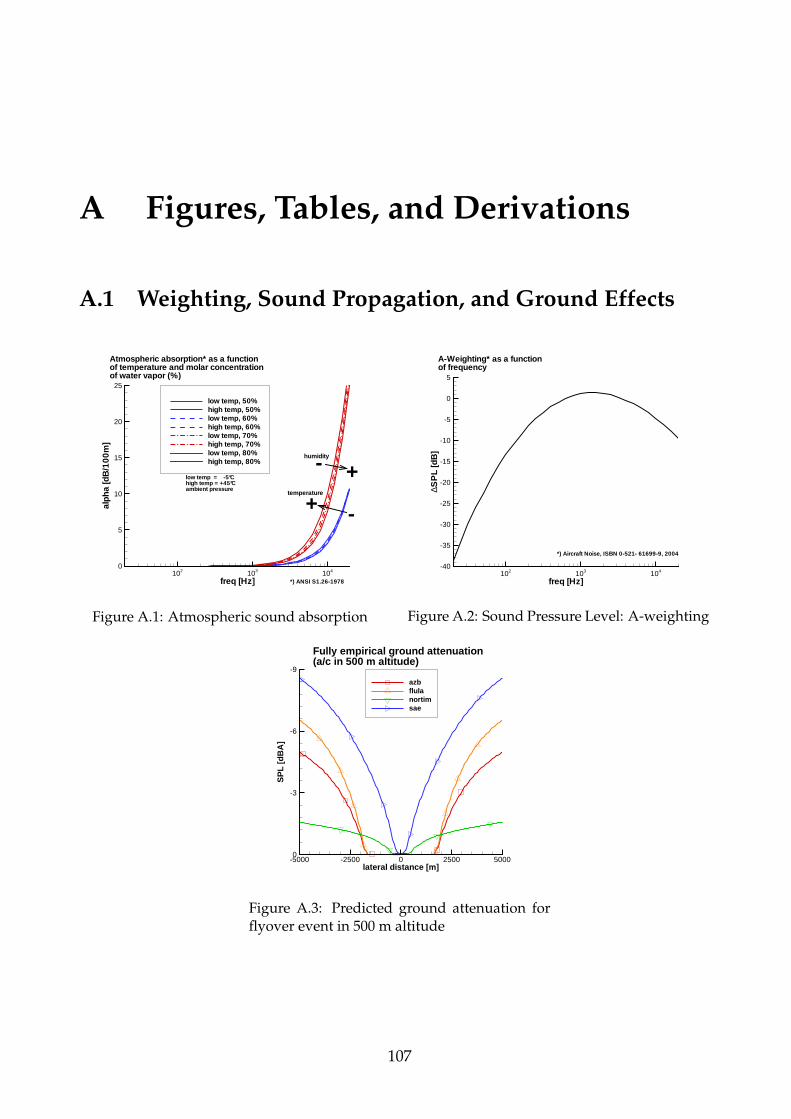
A Figures, Tables, and Derivations
A.1 Weighting, Sound Propagation, and Ground Effects
freq [Hz]
alph
a[d
B/1
00m
]
102 103 1040
5
10
15
20
25
low temp, 50%high temp, 50%low temp, 60%high temp, 60%low temp, 70%high temp, 70%low temp, 80%high temp, 80%
low temp = -5°Chigh temp = +45°Cambient pressure
Atmospheric absorption* as a functionof temperature and molar concentrationof water vapor (%)
humidity
temperature
+ -
+-
*) ANSI S1.26-1978
Figure A.1: Atmospheric sound absorption
freq [Hz]
∆SP
L[d
B]
102 103 104-40
-35
-30
-25
-20
-15
-10
-5
0
5
A-Weighting* as a functionof frequency
*) Aircraft Noise, ISBN 0-521- 61699-9, 2004
Figure A.2: Sound Pressure Level: A-weighting
lateral distance [m]
SP
L [
dB
A]
-5000 -2500 0 2500 5000
-9
-6
-3
0
azbflulanortimsae
Fully empirical ground attenuation(a/c in 500 m altitude)
Figure A.3: Predicted ground attenuation forflyover event in 500 m altitude
107
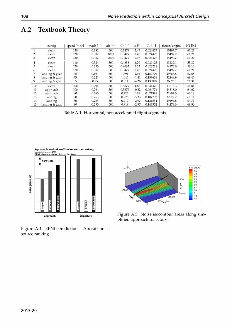
108 Noise Prediction within Conceptual Aircraft Design
A.2 Textbook Theory
- config speed [m/s] mach [−] alt [m] Cl [−] α [°] Cd [−] thrust/engine N1 [%]
1 clean 130 0.382 500 0.3479 2.47 0.024427 15497.7 61.212 clean 130 0.382 1000 0.3479 2.47 0.024427 15497.7 61.213 clean 130 0.382 2000 0.3479 2.47 0.024427 15497.7 61.21
4 clean 110 0.324 500 0.4858 4.20 0.029123 13232.1 55.325 clean 120 0.353 500 0.4082 3.22 0.026218 14176.8 58.166 clean 130 0.382 500 0.3479 2.47 0.024427 15497.7 61.217 landing & gear 65 0.191 500 1.391 2.91 0.187709 29785.8 62.688 landing & gear 75 0.221 500 1.045 -1.41 0.153626 32448.9 66.459 landing & gear 85 0.25 500 0.814 -4.26 0.135809 36826.1 71.31
10 clean 100 0.294 500 0.5879 4.68 0.031470 11815.3 51.8411 approach 100 0.294 500 0.5879 -0.82 0.064771 24318.0 64.0212 approach 90 0.265 500 0.726 0.89 0.071991 21887.3 60.1813 landing 90 0.265 500 0.726 -5.33 0.107793 32772.2 69.1114 landing 80 0.235 500 0.919 -2.97 0.121554 29194.8 64.7115 landing & gear 80 0.235 500 0.919 -2.97 0.143552 34478.3 68.80
Table A.1: Horizontal, non-accelerated flight segments
engi
ne
airc
raft
tota
l
airf
ram
e
departure
EP
NL
[EP
NdB
]
engi
ne
airc
raft
tota
l
airf
ram
e
approach
5 EPNdB
predicted levels: A319EPNL at representative observer locations
Approach and take-off noise source ranking
Figure A.4: EPNL predictions: Aircraft noisesource ranking
x [m]
-15000
-10000
-5000
0
y [m]
-5000
0
5000
alt [m]
0
1500
XY
Z
SPL [dBA]
7572696663605754514845
Figure A.5: Noise isocontour areas along sim-plified approach trajectory
2013-20
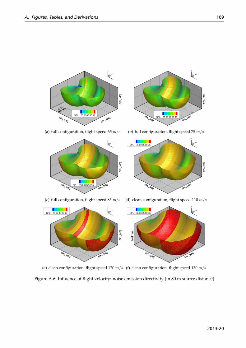
A. Figures, Tables, and Derivations 109
SPLX [dB] SPL Y
[dB]S
PL
Z [
dB
]
Y
Z
X
SPL: 75 80 85 90 95
5 dB
(a) full configuration, flight speed 65 m/s
SPLX [dB] SPL Y
[dB]
SP
LZ [
dB
]
Y
Z
X
SPL: 75 80 85 90 95
(b) full configuration, flight speed 75 m/s
SPLX [dB] SPL Y
[dB]
SP
LZ [
dB
]
Y
Z
X
SPL: 75 80 85 90 95
(c) full configuration, flight speed 85 m/s
SPLX [dB] SPL Y
[dB]
SP
LZ [
dB
]
Y
Z
X
SPL: 75 80 85 90 95
(d) clean configuration, flight speed 110 m/s
SPLX [dB] SPL Y
[dB]
SP
LZ [
dB
]
Y
Z
X
SPL: 75 80 85 90 95
(e) clean configuration, flight speed 120 m/s
SPLX [dB] SPL Y
[dB]
SP
LZ [d
B]
Y
Z
X
SPL: 75 80 85 90 95
(f) clean configuration, flight speed 130 m/s
Figure A.6: Influence of flight velocity: noise emission directivity (in 80 m source distance)
2013-20
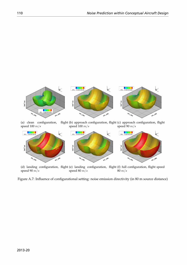
110 Noise Prediction within Conceptual Aircraft Design
SPLX [dB] SPL Y
[dB]
SP
LZ [d
B]
Y
Z
X
SPL: 75 80 85 90 95
(a) clean configuration, flightspeed 100 m/s
SPLX [dB] SPL Y
[dB]S
PL
Z [dB
]
Y
Z
X
SPL: 75 80 85 90 95
(b) approach configuration, flightspeed 100 m/s
SPLX [dB] SPL Y
[dB]
SP
LZ [d
B]
Y
Z
X
SPL: 75 80 85 90 95
(c) approach configuration, flightspeed 90 m/s
SPLX [dB] SPL Y
[dB]
SP
LZ [d
B]
Y
Z
X
SPL: 75 80 85 90 95
(d) landing configuration, flightspeed 90 m/s
SPLX [dB] SPL Y
[dB]
SP
LZ [d
B]
Y
Z
X
SPL: 75 80 85 90 95
(e) landing configuration, flightspeed 80 m/s
SPLX [dB] SPL Y
[dB]
SP
LZ [d
B]
Y
Z
X
SPL: 75 80 85 90 95
(f) full configuration, flight speed80 m/s
Figure A.7: Influence of configurational setting: noise emission directivity (in 80 m source distance)
2013-20
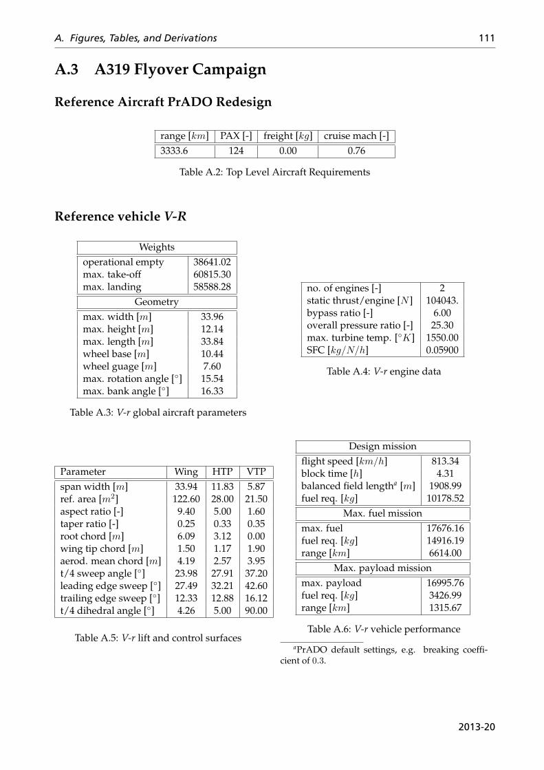
A. Figures, Tables, and Derivations 111
A.3 A319 Flyover Campaign
Reference Aircraft PrADO Redesign
range [km] PAX [-] freight [kg] cruise mach [-]3333.6 124 0.00 0.76
Table A.2: Top Level Aircraft Requirements
Reference vehicle V-R
Weightsoperational empty 38641.02max. take-off 60815.30max. landing 58588.28
Geometrymax. width [m] 33.96max. height [m] 12.14max. length [m] 33.84wheel base [m] 10.44wheel guage [m] 7.60max. rotation angle [◦] 15.54max. bank angle [◦] 16.33
Table A.3: V-r global aircraft parameters
no. of engines [-] 2static thrust/engine [N ] 104043.bypass ratio [-] 6.00overall pressure ratio [-] 25.30max. turbine temp. [◦K] 1550.00SFC [kg/N/h] 0.05900
Table A.4: V-r engine data
Parameter Wing HTP VTPspan width [m] 33.94 11.83 5.87ref. area [m2] 122.60 28.00 21.50aspect ratio [-] 9.40 5.00 1.60taper ratio [-] 0.25 0.33 0.35root chord [m] 6.09 3.12 0.00wing tip chord [m] 1.50 1.17 1.90aerod. mean chord [m] 4.19 2.57 3.95t/4 sweep angle [◦] 23.98 27.91 37.20leading edge sweep [◦] 27.49 32.21 42.60trailing edge sweep [◦] 12.33 12.88 16.12t/4 dihedral angle [◦] 4.26 5.00 90.00
Table A.5: V-r lift and control surfaces
Design missionflight speed [km/h] 813.34block time [h] 4.31balanced field lengtha [m] 1908.99fuel req. [kg] 10178.52
Max. fuel missionmax. fuel 17676.16fuel req. [kg] 14916.19range [km] 6614.00
Max. payload missionmax. payload 16995.76fuel req. [kg] 3426.99range [km] 1315.67
Table A.6: V-r vehicle performance
aPrADO default settings, e.g. breaking coeffi-cient of 0.3.
2013-20
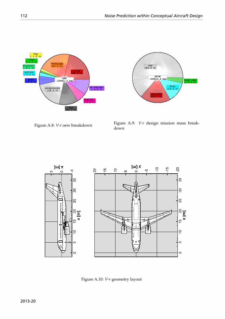
112 Noise Prediction within Conceptual Aircraft Design
wing(21.7 %)
fuselage(21.2 %)
htp( 1.3 %)
vtp( 1.1 %)
winglets( 0.1 %)
pylons( 2.4 %)
gear( 5.6 %)
propulsion(18.3 %)
sys(12.3 %)
equipm.( 6.2 %)
op.equipm.( 9.8 %)
OEW (38641.0 kg)
Figure A.8: V-r oew breakdown
oew(63.5 %)
payload(19.7 %)
fuel(13.2 %)
fuel res.( 3.5 %)
MTOW (60815.6 kg)
Figure A.9: V-r design mission mass break-down
Figure A.10: V-r geometry layout
2013-20
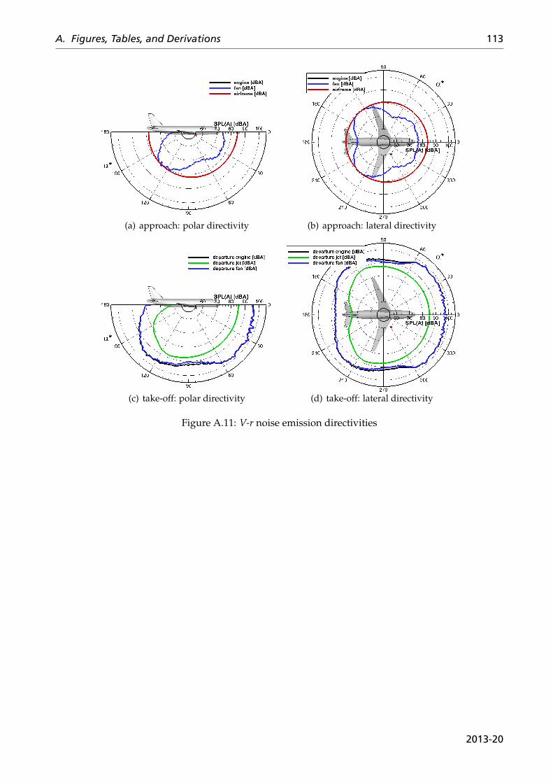
A. Figures, Tables, and Derivations 113
(a) approach: polar directivity (b) approach: lateral directivity
(c) take-off: polar directivity (d) take-off: lateral directivity
Figure A.11: V-r noise emission directivities
2013-20
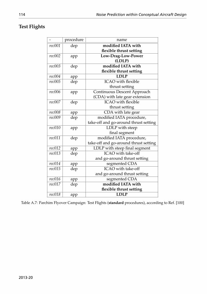
114 Noise Prediction within Conceptual Aircraft Design
Test Flights
- procedure namerec001 dep modified IATA with
flexible thrust settingrec002 app Low-Drag-Low-Power
(LDLP)rec003 dep modified IATA with
flexible thrust settingrec004 app LDLPrec005 dep ICAO with flexible
thrust settingrec006 app Continuous Descent Approach
(CDA) with late gear extensionrec007 dep ICAO with flexible
thrust settingrec008 app CDA with late gearrec009 dep modified IATA procedure,
take-off and go-around thrust settingrec010 app LDLP with steep
final segmentrec011 dep modified IATA procedure,
take-off and go-around thrust settingrec012 app LDLP with steep final segmentrec013 dep ICAO with take-off
and go-around thrust settingrec014 app segmented CDArec015 dep ICAO with take-off
and go-around thrust settingrec016 app segmented CDArec017 dep modified IATA with
flexible thrust settingrec018 app LDLP
Table A.7: Parchim Flyover Campaign: Test Flights (standard procedures), according to Ref. [100]
2013-20
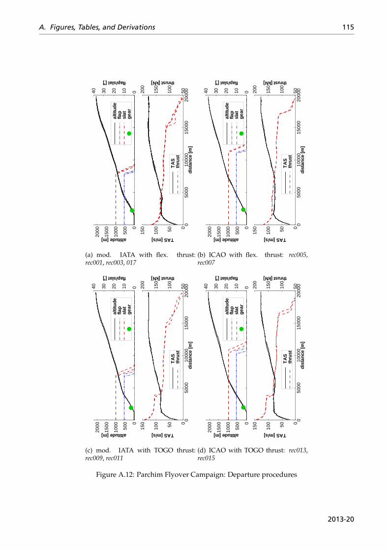
A. Figures, Tables, and Derivations 115
altitude[m]
flap/slat[°]
0
500
1000
1500
2000
010203040
altit
ude
flap
slat
gear
dist
ance
[m]
TAS[m/s]
thrust[kN]
050
0010
000
1500
020
000
050100
150
50100
150
200
TA
Sth
rust
(a) mod. IATA with flex. thrust:rec001, rec003, 017
altitude[m]
flap/slat[°]
0
500
1000
1500
2000
010203040
altit
ude
flap
slat
gear
dist
ance
[m]
TAS[m/s]
thrust[kN]
050
0010
000
1500
020
000
050100
150
50100
150
200
TA
Sth
rust
(b) ICAO with flex. thrust: rec005,rec007
altitude[m]
flap/slat[°]
0
500
1000
1500
2000
010203040
altit
ude
flap
slat
gear
dist
ance
[m]
TAS[m/s]
thrust[kN]
050
0010
000
1500
020
000
050100
150
50100
150
200
TA
Sth
rust
(c) mod. IATA with TOGO thrust:rec009, rec011
altitude[m]
flap/slat[°]
0
500
1000
1500
2000
010203040
altit
ude
flap
slat
gear
dist
ance
[m]
TAS[m/s]
thrust[kN]
050
0010
000
1500
020
000
050100
150
50100
150
200
TA
Sth
rust
(d) ICAO with TOGO thrust: rec013,rec015
Figure A.12: Parchim Flyover Campaign: Departure procedures
2013-20
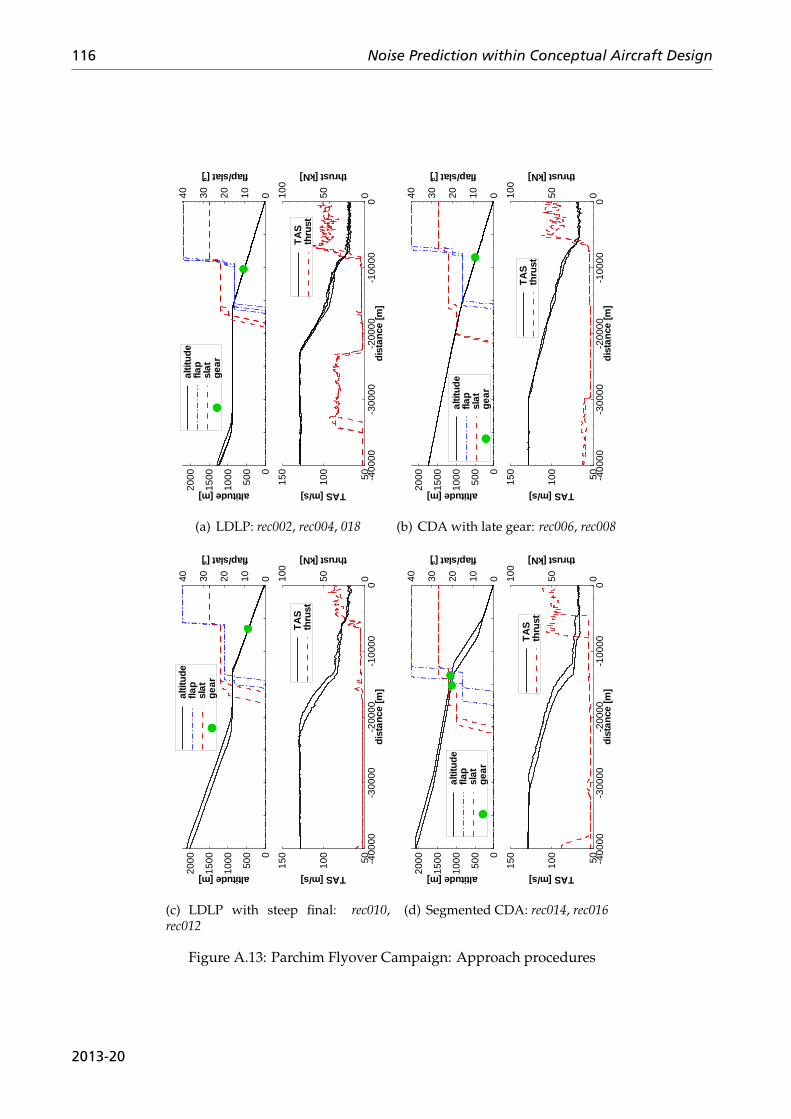
116 Noise Prediction within Conceptual Aircraft Design
altitude[m]
flap/slat[°]
0
500
1000
1500
2000
010203040al
titud
efla
psl
atge
ar
dist
ance
[m]
TAS[m/s]
thrust[kN]
-400
00-3
0000
-200
00-1
0000
05010
0
150
050100
TA
Sth
rust
(a) LDLP: rec002, rec004, 018
altitude[m]
flap/slat[°]
0
500
1000
1500
2000
010203040
altit
ude
flap
slat
gear
dist
ance
[m]
TAS[m/s]
thrust[kN]
-400
00-3
0000
-200
00-1
0000
05010
0
150
050100
TA
Sth
rust
(b) CDA with late gear: rec006, rec008
altitude[m]
flap/slat[°]
0
500
1000
1500
2000
010203040al
titud
efla
psl
atge
ar
dist
ance
[m]
TAS[m/s]
thrust[kN]
-400
00-3
0000
-200
00-1
0000
05010
0
150
050100
TA
Sth
rust
(c) LDLP with steep final: rec010,rec012
altitude[m]
flap/slat[°]
0
500
1000
1500
2000
010203040
altit
ude
flap
slat
gear
dist
ance
[m]
TAS[m/s]
thrust[kN]
-400
00-3
0000
-200
00-1
0000
05010
0
150
050100
TA
Sth
rust
(d) Segmented CDA: rec014, rec016
Figure A.13: Parchim Flyover Campaign: Approach procedures
2013-20
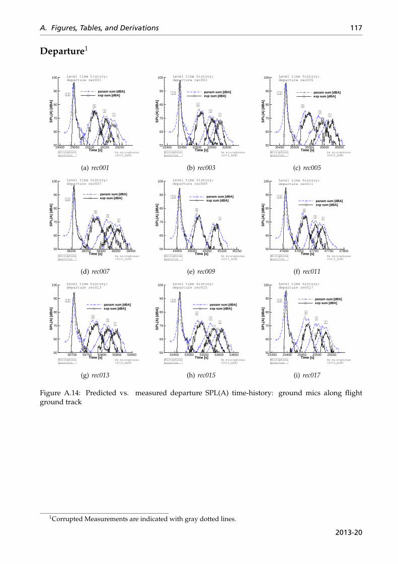
A. Figures, Tables, and Derivations 117
Departure1
Time [s]
SP
L(A
)[d
BA
]
29000 29050 29100 29150 2920050
60
70
80
90
100
panam sum [dBA]exp sum [dBA]
Level time history:departure rec001
Microphoneposition
0m microphones(2012_AzB)
10
6
13
(a) rec001
Time [s]
SP
L(A
)[d
BA
]
32400 32450 32500 32550 3260050
60
70
80
90
100
panam sum [dBA]exp sum [dBA]
Level time history:departure rec003
Microphoneposition
0m microphones(2012_AzB)
10
6
13
(b) rec003
Time [s]
SP
L(A
)[d
BA
]
35450 35500 35550 35600 3565050
60
70
80
90
100
panam sum [dBA]exp sum [dBA]
Level time history:departure rec005
Microphoneposition
0m microphones(2012_AzB)
10
6
13
(c) rec005
Time [s]
SP
L(A
)[d
BA
]
38200 38250 38300 38350 3840050
60
70
80
90
100
panam sum [dBA]exp sum [dBA]
Level time history:departure rec007
Microphoneposition
0m microphones(2012_AzB)
10
6
13
(d) rec007
Time [s]
SP
L(A
)[d
BA
]
44950 45000 45050 45100 4515050
60
70
80
90
100
panam sum [dBA]exp sum [dBA]
Level time history:departure rec009
Microphoneposition
0m microphones(2012_AzB)
10
6
1
(e) rec009
Time [s]
SP
L(A
)[d
BA
]
47600 47650 47700 47750 4780050
60
70
80
90
100
panam sum [dBA]exp sum [dBA]
Level time history:departure rec011
Microphoneposition
0m microphones(2012_AzB)
10
6
13
(f) rec011
Time [s]
SP
L(A
)[d
BA
]
50700 50750 50800 50850 5090050
60
70
80
90
100
panam sum [dBA]exp sum [dBA]
Level time history:departure rec013
Microphoneposition
0m microphones(2012_AzB)
10
6
13
(g) rec013
Time [s]
SP
L(A
)[d
BA
]
53450 53500 53550 53600 5365050
60
70
80
90
100
panam sum [dBA]exp sum [dBA]
Level time history:departure rec015
Microphoneposition
0m microphones(2012_AzB)
10
6
13
(h) rec015
Time [s]
SP
L(A
)[d
BA
]
25350 25400 25450 25500 2555050
60
70
80
90
100
panam sum [dBA]exp sum [dBA]
Level time history:departure rec017
Microphoneposition
0m microphones(2012_AzB)
10
6
13
(i) rec017
Figure A.14: Predicted vs. measured departure SPL(A) time-history: ground mics along flightground track
1Corrupted Measurements are indicated with gray dotted lines.
2013-20
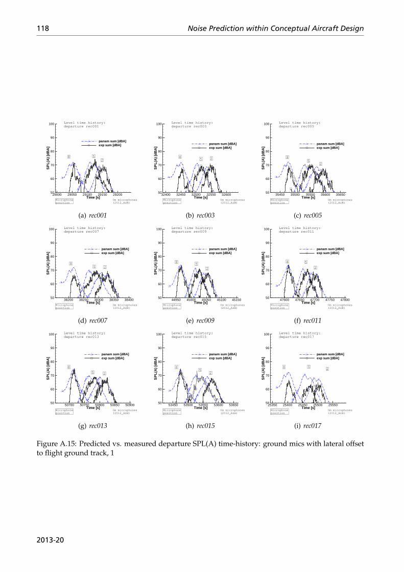
118 Noise Prediction within Conceptual Aircraft Design
Time [s]
SP
L(A
)[d
BA
]
29000 29050 29100 29150 2920050
60
70
80
90
100
panam sum [dBA]exp sum [dBA]
Level time history:departure rec001
Microphoneposition
0m microphones(2012_AzB)
8 52
(a) rec001
Time [s]
SP
L(A
)[d
BA
]
32400 32450 32500 32550 3260050
60
70
80
90
100
panam sum [dBA]exp sum [dBA]
Level time history:departure rec003
Microphoneposition
0m microphones(2012_AzB)
85 2
(b) rec003
Time [s]
SP
L(A
)[d
BA
]
35450 35500 35550 35600 3565050
60
70
80
90
100
panam sum [dBA]exp sum [dBA]
Level time history:departure rec005
Microphoneposition
0m microphones(2012_AzB)
85
2
(c) rec005
Time [s]
SP
L(A
)[d
BA
]
38200 38250 38300 38350 3840050
60
70
80
90
100
panam sum [dBA]exp sum [dBA]
Level time history:departure rec007
Microphoneposition
0m microphones(2012_AzB)
85 2
(d) rec007
Time [s]
SP
L(A
)[d
BA
]
44950 45000 45050 45100 4515050
60
70
80
90
100
panam sum [dBA]exp sum [dBA]
Level time history:departure rec009
Microphoneposition
0m microphones(2012_AzB)
85
2
(e) rec009
Time [s]
SP
L(A
)[d
BA
]
47600 47650 47700 47750 4780050
60
70
80
90
100
panam sum [dBA]exp sum [dBA]
Level time history:departure rec011
Microphoneposition
0m microphones(2012_AzB)
8 5
2
(f) rec011
Time [s]
SP
L(A
)[d
BA
]
50700 50750 50800 50850 5090050
60
70
80
90
100
panam sum [dBA]exp sum [dBA]
Level time history:departure rec013
Microphoneposition
0m microphones(2012_AzB)
8
5 2
(g) rec013
Time [s]
SP
L(A
)[d
BA
]
53450 53500 53550 53600 5365050
60
70
80
90
100
panam sum [dBA]exp sum [dBA]
Level time history:departure rec015
Microphoneposition
0m microphones(2012_AzB)
85
2
(h) rec015
Time [s]
SP
L(A
)[d
BA
]
25350 25400 25450 25500 2555050
60
70
80
90
100
panam sum [dBA]exp sum [dBA]
Level time history:departure rec017
Microphoneposition
0m microphones(2012_AzB)
8 52
(i) rec017
Figure A.15: Predicted vs. measured departure SPL(A) time-history: ground mics with lateral offsetto flight ground track, 1
2013-20
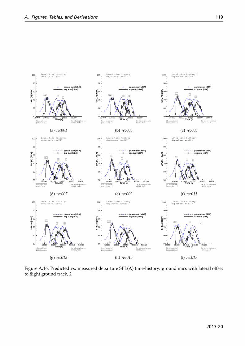
A. Figures, Tables, and Derivations 119
Time [s]
SP
L(A
)[d
BA
]
29000 29050 29100 29150 2920050
60
70
80
90
100
panam sum [dBA]exp sum [dBA]
Level time history:departure rec001
Microphoneposition
0m microphones(2012_AzB)
127
4
(a) rec001
Time [s]
SP
L(A
)[d
BA
]
32400 32450 32500 32550 3260050
60
70
80
90
100
panam sum [dBA]exp sum [dBA]
Level time history:departure rec003
Microphoneposition
0m microphones(2012_AzB)
127 4
(b) rec003
Time [s]
SP
L(A
)[d
BA
]
35450 35500 35550 35600 3565050
60
70
80
90
100
panam sum [dBA]exp sum [dBA]
Level time history:departure rec005
Microphoneposition
0m microphones(2012_AzB)
127
4
(c) rec005
Time [s]
SP
L(A
)[d
BA
]
38200 38250 38300 38350 3840050
60
70
80
90
100
panam sum [dBA]exp sum [dBA]
Level time history:departure rec007
Microphoneposition
0m microphones(2012_AzB)
127 4
(d) rec007
Time [s]
SP
L(A
)[d
BA
]
44950 45000 45050 45100 4515050
60
70
80
90
100
panam sum [dBA]exp sum [dBA]
Level time history:departure rec009
Microphoneposition
0m microphones(2012_AzB)
12
47
(e) rec009
Time [s]
SP
L(A
)[d
BA
]
47600 47650 47700 47750 4780050
60
70
80
90
100
panam sum [dBA]exp sum [dBA]
Level time history:departure rec011
Microphoneposition
0m microphones(2012_AzB)
127 4
(f) rec011
Time [s]
SP
L(A
)[d
BA
]
50700 50750 50800 50850 5090050
60
70
80
90
100
panam sum [dBA]exp sum [dBA]
Level time history:departure rec013
Microphoneposition
0m microphones(2012_AzB)
12
7 4
(g) rec013
Time [s]
SP
L(A
)[d
BA
]
53450 53500 53550 53600 5365050
60
70
80
90
100
panam sum [dBA]exp sum [dBA]
Level time history:departure rec015
Microphoneposition
0m microphones(2012_AzB)
12
7 4
(h) rec015
Time [s]
SP
L(A
)[d
BA
]
25350 25400 25450 25500 2555050
60
70
80
90
100
panam sum [dBA]exp sum [dBA]
Level time history:departure rec017
Microphoneposition
0m microphones(2012_AzB)
12 74
(i) rec017
Figure A.16: Predicted vs. measured departure SPL(A) time-history: ground mics with lateral offsetto flight ground track, 2
2013-20
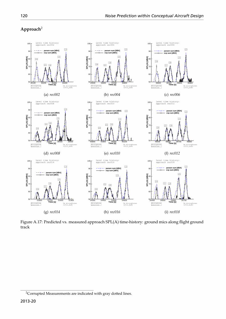
120 Noise Prediction within Conceptual Aircraft Design
Approach2
Time [s]
SP
L(A
)[d
BA
]
30100 30200 30300 3040050
60
70
80
90
100
panam sum [dBA]exp sum [dBA]
Level time history:approach rec002
Microphoneposition
0m microphones(2012_AzB)
24
21
13
18
15
(a) rec002
Time [s]S
PL(
A)
[dB
A]
33500 33600 33700 3380050
60
70
80
90
100
panam sum [dBA]exp sum [dBA]
Level time history:approach rec004
Microphoneposition
0m microphones(2012_AzB)
24 21
13
18
15
(b) rec004
Time [s]
SP
L(A
)[d
BA
]
36600 36700 36800 3690050
60
70
80
90
100
panam sum [dBA]exp sum [dBA]
Level time history:approach rec006
Microphoneposition
0m microphones(2012_AzB)
24
21
13
18
15
(c) rec006
Time [s]
SP
L(A
)[d
BA
]
39200 39300 39400 3950050
60
70
80
90
100
panam sum [dBA]exp sum [dBA]
Level time history:approach rec008
Microphoneposition
0m microphones(2012_AzB)
24
21
13
18
15
(d) rec008
Time [s]
SP
L(A
)[d
BA
]
45800 45900 46000 4610050
60
70
80
90
100
panam sum [dBA]exp sum [dBA]
Level time history:approach rec010
Microphoneposition
0m microphones(2012_AzB)
24
21
13
18
15
(e) rec010
Time [s]
SP
L(A
)[d
BA
]
48500 48600 48700 4880050
60
70
80
90
100
panam sum [dBA]exp sum [dBA]
Level time history:approach rec012
Microphoneposition
0m microphones(2012_AzB)
2421
13
18
15
(f) rec012
Time [s]
SP
L(A
)[d
BA
]
51600 51700 51800 5190050
60
70
80
90
100
panam sum [dBA]exp sum [dBA]
Level time history:approach rec014
Microphoneposition
0m microphones(2012_AzB)
24
21
13
18
15
(g) rec014
Time [s]
SP
L(A
)[d
BA
]
54300 54400 54500 5460050
60
70
80
90
100
panam sum [dBA]exp sum [dBA]
Level time history:approach rec016
Microphoneposition
0m microphones(2012_AzB)
24
21
13
18
15
(h) rec016
Time [s]
SP
L(A
)[d
BA
]
26400 26500 26600 2670050
60
70
80
90
100
panam sum [dBA]exp sum [dBA]
Level time history:approach rec018
Microphoneposition
0m microphones(2012_AzB)
2421
13
18
15
(i) rec018
Figure A.17: Predicted vs. measured approach SPL(A) time-history: ground mics along flight groundtrack
2Corrupted Measurements are indicated with gray dotted lines.
2013-20
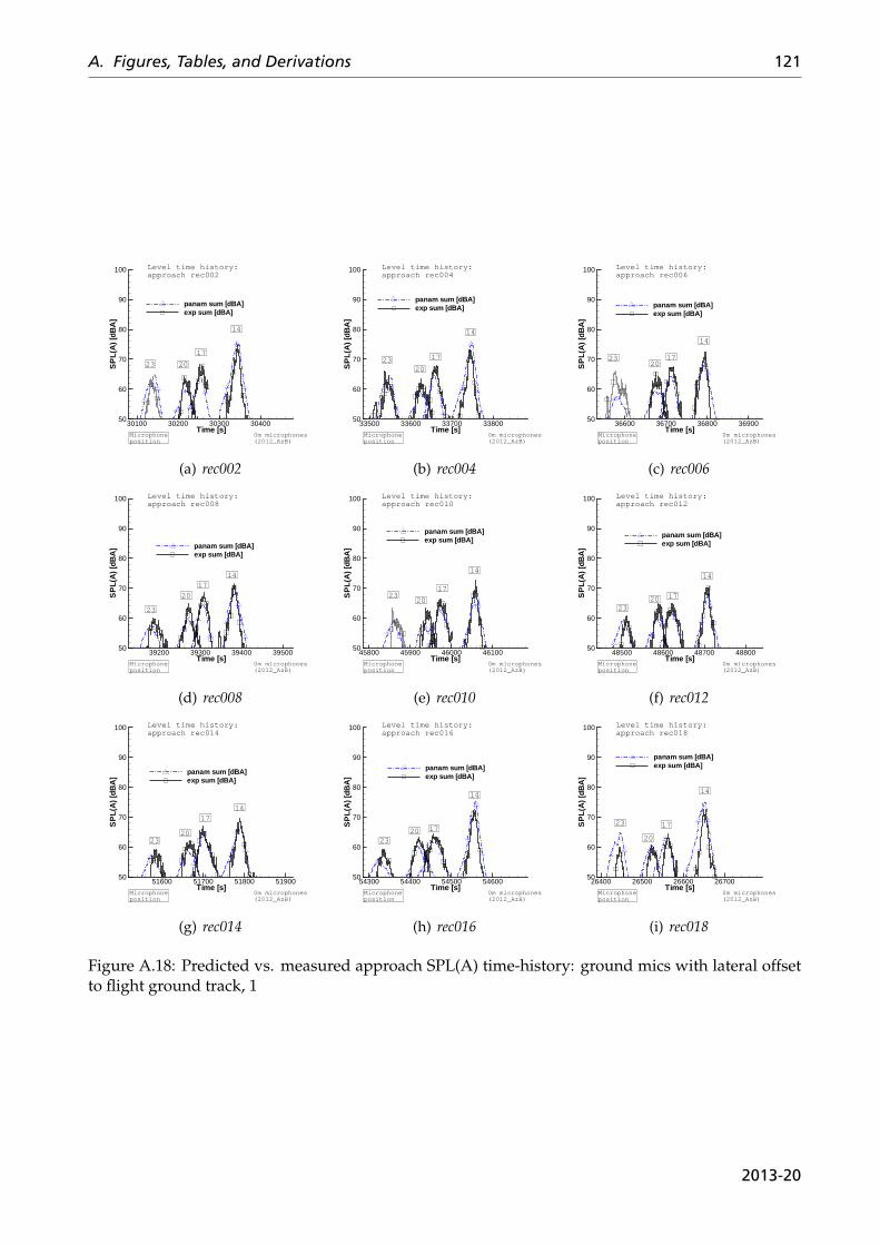
A. Figures, Tables, and Derivations 121
Time [s]
SP
L(A
)[d
BA
]
30100 30200 30300 3040050
60
70
80
90
100
panam sum [dBA]exp sum [dBA]
Level time history:approach rec002
Microphoneposition
0m microphones(2012_AzB)
23 20
14
17
(a) rec002
Time [s]
SP
L(A
)[d
BA
]
33500 33600 33700 3380050
60
70
80
90
100
panam sum [dBA]exp sum [dBA]
Level time history:approach rec004
Microphoneposition
0m microphones(2012_AzB)
2320
14
17
(b) rec004
Time [s]
SP
L(A
)[d
BA
]
36600 36700 36800 3690050
60
70
80
90
100
panam sum [dBA]exp sum [dBA]
Level time history:approach rec006
Microphoneposition
0m microphones(2012_AzB)
2320
14
17
(c) rec006
Time [s]
SP
L(A
)[d
BA
]
39200 39300 39400 3950050
60
70
80
90
100
panam sum [dBA]exp sum [dBA]
Level time history:approach rec008
Microphoneposition
0m microphones(2012_AzB)
23
20
1417
(d) rec008
Time [s]
SP
L(A
)[d
BA
]
45800 45900 46000 4610050
60
70
80
90
100
panam sum [dBA]exp sum [dBA]
Level time history:approach rec010
Microphoneposition
0m microphones(2012_AzB)
2320
14
17
(e) rec010
Time [s]
SP
L(A
)[d
BA
]
48500 48600 48700 4880050
60
70
80
90
100
panam sum [dBA]exp sum [dBA]
Level time history:approach rec012
Microphoneposition
0m microphones(2012_AzB)
2320
14
17
(f) rec012
Time [s]
SP
L(A
)[d
BA
]
51600 51700 51800 5190050
60
70
80
90
100
panam sum [dBA]exp sum [dBA]
Level time history:approach rec014
Microphoneposition
0m microphones(2012_AzB)
2320
1417
(g) rec014
Time [s]
SP
L(A
)[d
BA
]
54300 54400 54500 5460050
60
70
80
90
100
panam sum [dBA]exp sum [dBA]
Level time history:approach rec016
Microphoneposition
0m microphones(2012_AzB)
2320
14
17
(h) rec016
Time [s]
SP
L(A
)[d
BA
]
26400 26500 26600 2670050
60
70
80
90
100
panam sum [dBA]exp sum [dBA]
Level time history:approach rec018
Microphoneposition
0m microphones(2012_AzB)
23
20
14
17
(i) rec018
Figure A.18: Predicted vs. measured approach SPL(A) time-history: ground mics with lateral offsetto flight ground track, 1
2013-20
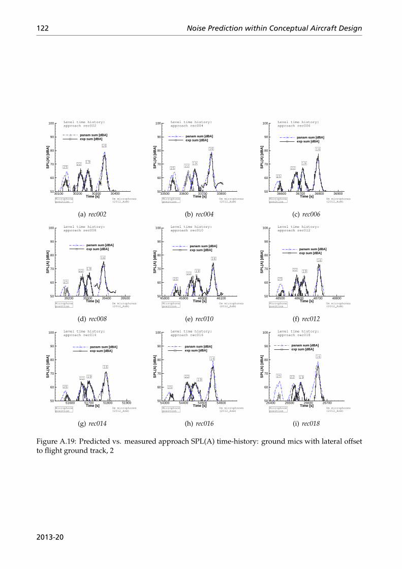
122 Noise Prediction within Conceptual Aircraft Design
Time [s]
SP
L(A
)[d
BA
]
30100 30200 30300 3040050
60
70
80
90
100
panam sum [dBA]exp sum [dBA]
Level time history:approach rec002
Microphoneposition
0m microphones(2012_AzB)
2522
16
19
(a) rec002
Time [s]
SP
L(A
)[d
BA
]
33500 33600 33700 3380050
60
70
80
90
100
panam sum [dBA]exp sum [dBA]
Level time history:approach rec004
Microphoneposition
0m microphones(2012_AzB)
2522
16
19
(b) rec004
Time [s]
SP
L(A
)[d
BA
]
36600 36700 36800 3690050
60
70
80
90
100
panam sum [dBA]exp sum [dBA]
Level time history:approach rec006
Microphoneposition
0m microphones(2012_AzB)
25
22
16
19
(c) rec006
Time [s]
SP
L(A
)[d
BA
]
39200 39300 39400 3950050
60
70
80
90
100
panam sum [dBA]exp sum [dBA]
Level time history:approach rec008
Microphoneposition
0m microphones(2012_AzB)
25
22
16
19
(d) rec008
Time [s]
SP
L(A
)[d
BA
]
45800 45900 46000 4610050
60
70
80
90
100
panam sum [dBA]exp sum [dBA]
Level time history:approach rec010
Microphoneposition
0m microphones(2012_AzB)
25
22
16
19
(e) rec010
Time [s]
SP
L(A
)[d
BA
]
48500 48600 48700 4880050
60
70
80
90
100
panam sum [dBA]exp sum [dBA]
Level time history:approach rec012
Microphoneposition
0m microphones(2012_AzB)
25
22
16
19
(f) rec012
Time [s]
SP
L(A
)[d
BA
]
51600 51700 51800 5190050
60
70
80
90
100
panam sum [dBA]exp sum [dBA]
Level time history:approach rec014
Microphoneposition
0m microphones(2012_AzB)
25
22
16
19
(g) rec014
Time [s]
SP
L(A
)[d
BA
]
54300 54400 54500 5460050
60
70
80
90
100
panam sum [dBA]exp sum [dBA]
Level time history:approach rec016
Microphoneposition
0m microphones(2012_AzB)
25
22
16
19
(h) rec016
Time [s]
SP
L(A
)[d
BA
]
26400 26500 26600 2670050
60
70
80
90
100
panam sum [dBA]exp sum [dBA]
Level time history:approach rec018
Microphoneposition
0m microphones(2012_AzB)
25 22
16
19
(i) rec018
Figure A.19: Predicted vs. measured approach SPL(A) time-history: ground mics with lateral offsetto flight ground track, 2
2013-20
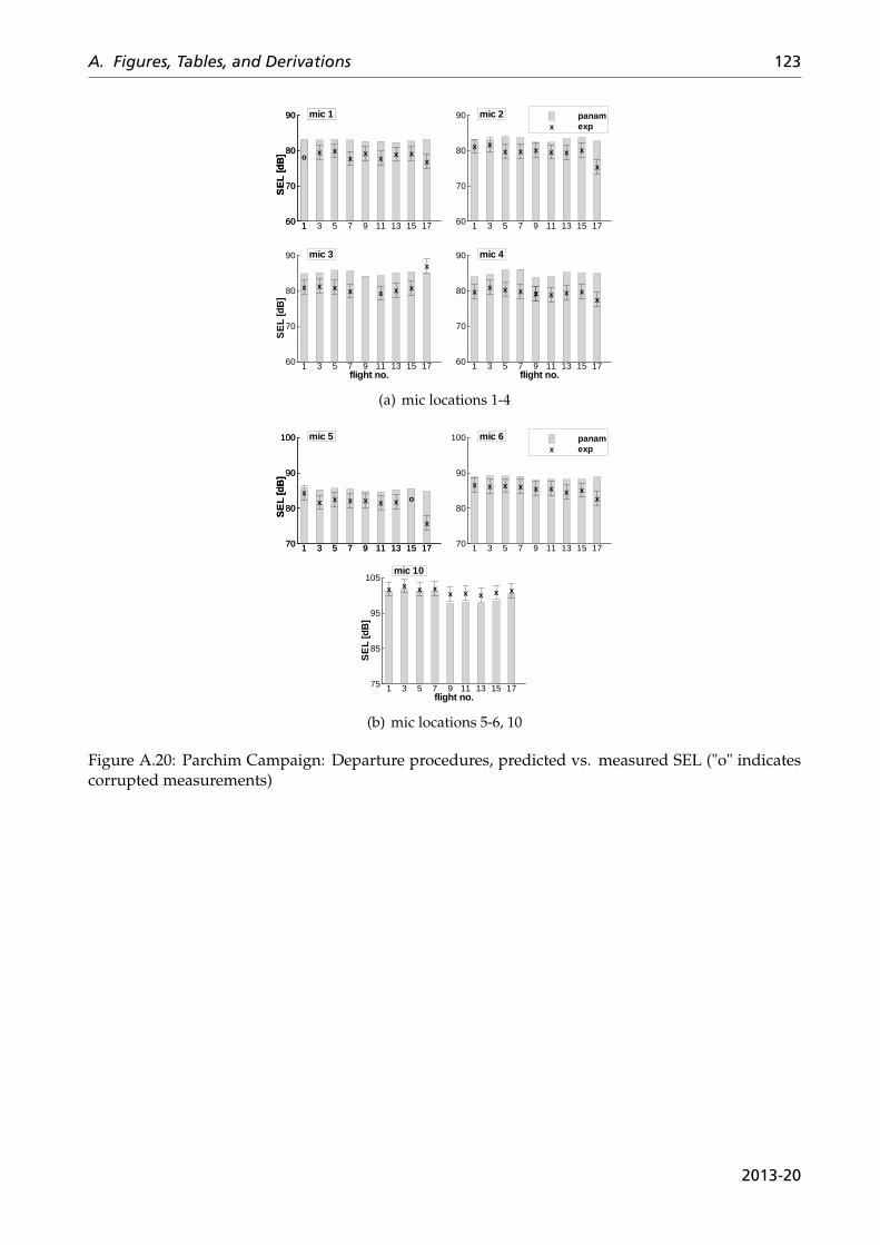
A. Figures, Tables, and Derivations 123
x x xx
xx x x
x
SE
L[d
B]
1 3 5 7 9 11 13 15 1760
70
80
90 mic 1
x xx x x x x x
x
1 3 5 7 9 11 13 15 1760
70
80
90 panamexpx
mic 2
x x x x xx x x xx
flight no.1 3 5 7 9 11 13 15 1760
70
80
90 mic 4
x x x x x x x
x
flight no.
SE
L[d
B]
1 3 5 7 9 11 13 15 1760
70
80
90 mic 3
o
SE
L[d
B]
160
70
80
90 mic 1
(a) mic locations 1-4
xx x x x x x x
x
SE
L[d
B]
1 3 5 7 9 11 13 15 1770
80
90
100 mic 5
x x x x x x x xx
1 3 5 7 9 11 13 15 1770
80
90
100 panamexpx
mic 6
x x x xx x x x x
flight no.
SE
L[d
B]
1 3 5 7 9 11 13 15 1775
85
95
105mic 10
o
SE
L[d
B]
1 3 5 7 9 11 13 15 1770
80
90
100 mic 5
(b) mic locations 5-6, 10
Figure A.20: Parchim Campaign: Departure procedures, predicted vs. measured SEL ("o" indicatescorrupted measurements)
2013-20
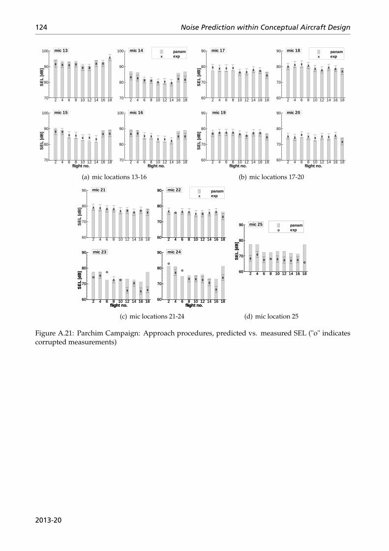
124 Noise Prediction within Conceptual Aircraft Design
x x x xx x
x x
x
SE
L[d
B]
2 4 6 8 10 12 14 16 1870
80
90
100 mic 13
x x x x x x xx x
2 4 6 8 10 12 14 16 1870
80
90
100 panamexpx
mic 14
x xx x
x x xx x
flight no.
SE
L[d
B]
2 4 6 8 10 12 14 16 1870
80
90
100 mic 15
x xx x
x x xx x
flight no.2 4 6 8 10 12 14 16 1870
80
90
100 mic 16
(a) mic locations 13-16
x x x xx x x x
x
SE
L[d
B]
2 4 6 8 10 12 14 16 1860
70
80
90 mic 17
x x x xx x
x xx
2 4 6 8 10 12 14 16 1860
70
80
90 panamexpx
mic 18
x x x x x xx x
x
flight no.
SE
L[d
B]
2 4 6 8 10 12 14 16 1860
70
80
90 mic 19
x xx x x x x x
x
flight no.2 4 6 8 10 12 14 16 1860
70
80
90 mic 20
(b) mic locations 17-20
x
x x xx
x
x
flight no.2 4 6 8 10 12 14 16 1860
70
80
90 mic 24
oo
o
flight no.
SE
L[d
B]
2 4 6 8 10 12 14 16 1860
70
80
90 mic 23
x x x x x x xx
2 4 6 8 10 12 14 16 1860
70
80
90 panamexpx
mic 22
o
2 4 6 8 10 12 14 16 1860
70
80
90 mic 22
x x x x x x x x x
SE
L[d
B]
2 4 6 8 10 12 14 16 1860
70
80
90 mic 21
xx
x
x
x x
flight no.
SE
L[d
B]
2 4 6 8 10 12 14 16 1860
70
80
90 mic 23
o
o
flight no.2 4 6 8 10 12 14 16 1860
70
80
90 mic 24
(c) mic locations 21-24
xx
x x x x xSE
L[d
B]
2 4 6 8 10 12 14 16 1860
70
80
90 panamexpx
mic 25
oo
SE
L[d
B]
2 4 6 8 10 12 14 16 1860
70
80
90 panamexpo
mic 25
(d) mic location 25
Figure A.21: Parchim Campaign: Approach procedures, predicted vs. measured SEL ("o" indicatescorrupted measurements)
2013-20

A. Figures, Tables, and Derivations 125
A.4 Low-Noise Vehicle Design
Vehicle category v-r
Figure A.22: v-r vehicle layout: pa-rameter variation 1
PPPPPPAw
Λw 7.0 8.0 9.0 10.0 11.0
100.0 1 2 3 4 5105.0 6 7 8 9 10110.0 11 12 13 14 15115.0 16 17 18 19 20120.0 21 22 23 24 25125.0 26 27 28 29 30130.0 31 32 33 34 35
Table A.8: v-r variants: parameter variation 1(wing area & aspect ratio)
weights performance
design OEW[kg]
MTOW[kg]
MLW[kg]
flightspeed[km/h]
blocktime[h]
balancedfieldlength[m]
fuel req.[kg]
1 34730.07 57762.96 55166.97 813.34 4.32 2108.18 11037.12 35609.48 58188.24 55787.32 813.34 4.31 2095.42 10583.03 36466.28 58713.75 56455.88 813.34 4.31 2175.79 10251.74 37471.09 59469.67 57318.06 813.34 4.31 2258.10 10002.85 38695.33 60522.28 58445.11 813.34 4.31 2345.99 9831.26 35052.26 58070.72 55480.49 813.34 4.32 2032.48 11022.77 35814.43 58364.33 55975.75 813.34 4.31 2015.87 10554.18 36893.03 59149.63 56887.62 813.34 4.31 2101.07 10260.89 38022.32 60051.03 57886.78 813.34 4.31 2185.05 10033.010 39241.93 61101.08 59009.88 813.34 4.31 2269.67 9863.411 35215.89 58199.77 55624.87 813.34 4.32 1950.46 10988.112 36159.02 58715.51 56324.31 813.34 4.31 1948.09 10560.713 37125.99 59379.40 57118.25 813.34 4.31 2026.96 10257.714 38456.08 60507.91 58333.76 813.34 4.31 2114.82 10056.115 39706.36 61592.13 59489.62 813.34 4.31 2196.07 9890.016 35390.34 58359.57 55790.54 813.34 4.32 1879.21 10973.517 36495.35 59066.58 56668.89 813.34 4.31 1886.03 10575.518 37631.08 59922.01 57644.87 813.34 4.31 1967.76 10295.219 38883.60 60968.90 58780.54 813.34 4.31 2049.46 10089.520 40166.64 62096.91 59975.29 813.34 4.31 2128.92 9934.521 35650.56 58606.82 56043.35 813.34 4.32 1824.51 10960.522 36879.59 59475.34 57067.10 813.34 4.31 1830.52 10600.023 38043.89 60364.36 58074.35 813.34 4.31 1910.47 10324.724 39284.03 61399.90 59198.64 813.34 4.31 1988.40 10120.125 40765.39 62753.50 60607.05 813.34 4.31 2071.41 9992.326 36019.57 58996.12 56424.44 813.34 4.32 1781.59 10980.827 37152.60 59756.79 57344.86 813.34 4.31 1776.34 10608.428 38427.36 60773.53 58472.56 813.34 4.31 1856.06 10350.429 39825.23 61988.29 59766.46 813.34 4.31 1936.25 10167.330 41216.02 63246.54 61081.66 813.34 4.31 2014.21 10034.831 36392.25 59391.90 56809.87 813.34 4.32 1742.22 11003.932 37408.87 60036.17 57614.60 813.34 4.31 1724.23 10631.533 38824.78 61225.90 58901.53 813.34 4.31 1806.60 10405.434 40271.96 62495.13 60247.47 813.34 4.31 1885.97 10227.435 41780.32 63864.00 61676.37 813.34 4.31 1964.63 10087.9
Table A.9: v-r global aircraft parameters: parameter variation 1
2013-20
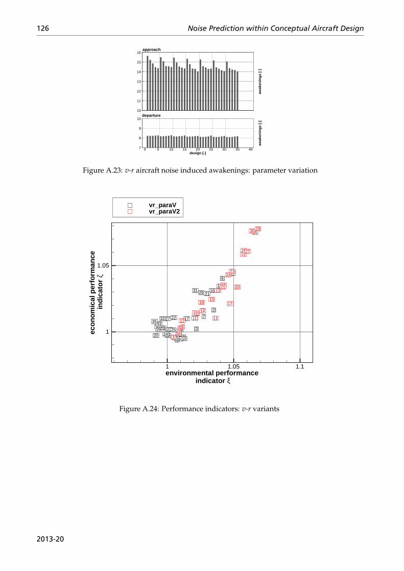
126 Noise Prediction within Conceptual Aircraft Design
awak
enin
gs [-
]
10
11
12
13
14
15
16approach
design [-]
awak
enin
gs [-
]
0 5 10 15 20 25 30 35 407
8
9
10departure
Figure A.23: v-r aircraft noise induced awakenings: parameter variation
1
2
3
45
6
7
8
910
11
12
131415
16
17
181920
21
22
2324
25
26
27
282930
31
323334
351
23
4
56
7
89
10
1112
13
1415
16
1718
19
2021
22
2324
25
2627
2930
environmental performance indicator ξ
eco
no
mic
al p
erfo
rman
ce in
dic
ato
r ζ
1 1.05 1.1
1
1.05
vr_paraVvr_paraV2
Figure A.24: Performance indicators: v-r variants
2013-20

A. Figures, Tables, and Derivations 127
Vehicle category v-0
v-0: Parameter study 1
Figure A.25: v-0 vehicle layout: pa-rameter variation 1
PPPPPPAw
Λw 7.0 8.0 9.0 10.0 11.0
100.0 1 2 3 4 5105.0 6 7 8 9 10110.0 11 12 13 14 15115.0 16 17 18 19 20120.0 21 22 23 24 25125.0 26 27 28 29 30130.0 31 32 33 34 35
Table A.10: v-0 variants: parameter variation 1(wing area & aspect ratio)
weights performance
design OEW[kg]
MTOW[kg]
MLW[kg]
flightspeed[km/h]
blocktime[h]
balancedfieldlength[m]
fuel req.[kg]
1 34951.14 58530.63 55699.46 813.34 4.32 2266.90 11583.72 35941.32 59022.62 56405.59 813.34 4.32 2184.59 11085.53 36828.62 59556.49 57091.38 813.34 4.32 2167.00 10732.14 37965.63 60447.35 58088.52 813.34 4.31 2244.33 10486.05 39073.07 61391.26 59102.77 813.34 4.31 2323.97 10322.46 35313.75 58912.94 56073.09 813.34 4.32 2197.99 11603.47 36201.49 59308.01 56680.16 813.34 4.32 2104.88 11110.88 37304.04 60086.06 57597.69 813.34 4.32 2103.56 10786.39 38415.30 60946.63 58566.52 813.34 4.31 2166.39 10535.610 39641.87 62016.71 59703.76 813.34 4.31 2247.05 10379.111 35542.69 59160.57 56312.62 813.34 4.32 2125.17 11622.112 36568.48 59716.37 57070.71 813.34 4.32 2043.17 11152.113 37740.15 60569.79 58060.84 813.34 4.32 2043.47 10833.914 38900.25 61486.59 59082.86 813.34 4.31 2096.71 10590.615 40178.16 62610.91 60273.25 813.34 4.31 2173.91 10437.016 35854.70 59501.17 56641.05 813.34 4.32 2069.70 11650.717 36918.03 60101.61 57440.58 813.34 4.32 1986.85 11187.818 38142.29 61013.19 58486.82 813.34 4.32 1987.64 10875.119 39347.91 61986.99 59560.54 813.34 4.31 2029.99 10643.320 40746.18 63260.98 60887.87 813.34 4.31 2108.24 10519.021 36214.28 59880.22 57011.68 813.34 4.32 2026.36 11670.222 37409.59 60648.79 57963.94 813.34 4.32 1948.15 11243.423 38570.02 61486.83 58940.81 813.34 4.32 1939.45 10921.124 39789.53 62477.68 60029.90 813.34 4.32 1967.93 10692.425 41371.53 63965.69 61558.60 813.34 4.31 2049.47 10598.426 36539.20 60247.04 57360.44 813.34 4.32 1988.54 11712.127 37743.83 61027.62 58323.32 813.34 4.32 1902.35 11288.028 38989.36 61964.59 59393.52 813.34 4.32 1896.50 10979.529 40360.21 63121.93 60642.48 813.34 4.32 1927.23 10766.030 41789.14 64443.13 62010.20 813.34 4.32 1989.43 10658.231 36868.23 60623.43 57716.64 813.34 4.32 1972.16 11759.432 38036.69 61364.77 58641.57 813.34 4.32 1858.65 11332.333 39425.71 62462.52 59865.15 813.34 4.32 1859.51 11041.034 40900.97 63748.63 61232.19 813.34 4.32 1900.64 10851.935 42371.51 65108.90 62640.41 813.34 4.32 1950.40 10741.6
Table A.11: v-0 global aircraft parameters: parameter variation 1
2013-20
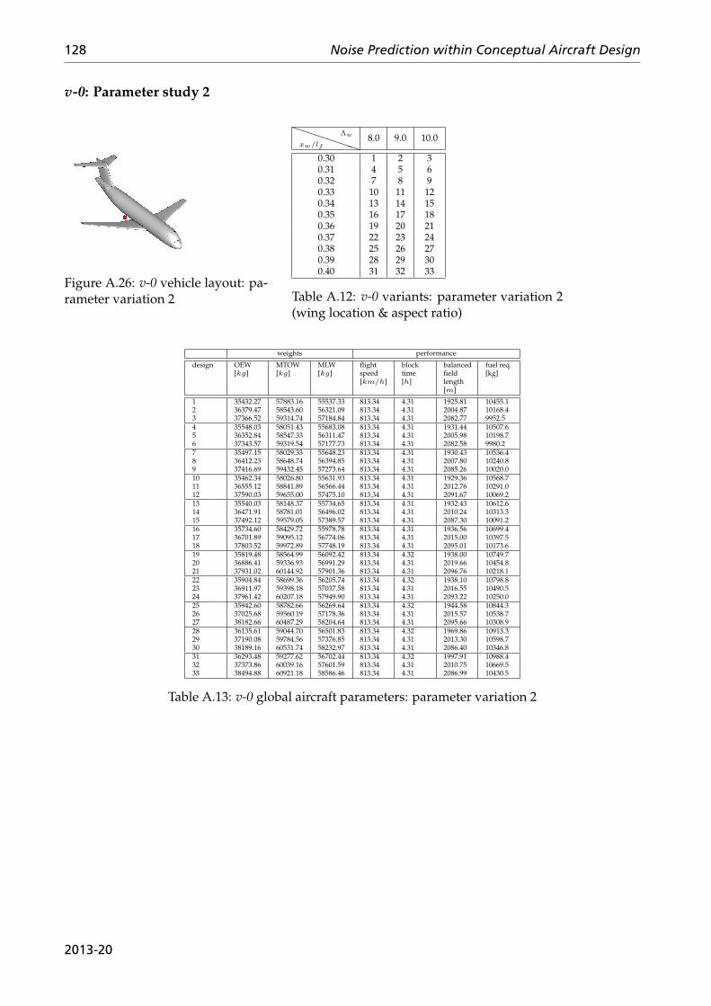
128 Noise Prediction within Conceptual Aircraft Design
v-0: Parameter study 2
Figure A.26: v-0 vehicle layout: pa-rameter variation 2
PPPPPPxw/lf
Λw 8.0 9.0 10.0
0.30 1 2 30.31 4 5 60.32 7 8 90.33 10 11 120.34 13 14 150.35 16 17 180.36 19 20 210.37 22 23 240.38 25 26 270.39 28 29 300.40 31 32 33
Table A.12: v-0 variants: parameter variation 2(wing location & aspect ratio)
weights performance
design OEW[kg]
MTOW[kg]
MLW[kg]
flightspeed[km/h]
blocktime[h]
balancedfieldlength[m]
fuel req.[kg]
1 35432.27 57883.16 55537.33 813.34 4.31 1925.81 10455.12 36379.47 58543.60 56321.09 813.34 4.31 2004.87 10168.43 37366.52 59314.74 57184.84 813.34 4.31 2082.77 9952.54 35548.03 58051.43 55683.08 813.34 4.31 1931.44 10507.65 36352.84 58547.33 56311.47 813.34 4.31 2005.98 10198.76 37343.57 59319.54 57177.73 813.34 4.31 2082.58 9980.27 35497.15 58029.33 55648.23 813.34 4.31 1930.43 10536.48 36412.23 58648.74 56394.85 813.34 4.31 2007.80 10240.89 37416.69 59432.45 57273.64 813.34 4.31 2085.26 10020.010 35462.34 58026.80 55631.93 813.34 4.31 1929.36 10568.711 36555.12 58841.89 56566.44 813.34 4.31 2012.76 10291.012 37590.03 59655.00 57475.10 813.34 4.31 2091.67 10069.213 35540.03 58148.37 55734.65 813.34 4.31 1932.43 10612.614 36471.91 58781.01 56496.02 813.34 4.31 2010.24 10313.315 37492.12 59579.05 57389.57 813.34 4.31 2087.30 10091.216 35734.60 58429.72 55978.78 813.34 4.31 1936.56 10699.417 36701.89 59095.12 56774.06 813.34 4.31 2015.00 10397.518 37803.52 59972.89 57748.19 813.34 4.31 2095.01 10173.619 35819.48 58564.99 56092.42 813.34 4.32 1938.00 10749.720 36886.41 59336.93 56991.29 813.34 4.31 2019.66 10454.821 37931.02 60144.92 57901.36 813.34 4.31 2096.76 10218.122 35904.84 58699.36 56205.74 813.34 4.32 1938.10 10798.823 36911.97 59398.18 57037.58 813.34 4.31 2016.55 10490.524 37961.42 60207.18 57949.90 813.34 4.31 2093.22 10250.025 35942.60 58782.66 56269.64 813.34 4.32 1944.58 10844.326 37025.68 59560.19 57178.36 813.34 4.31 2015.57 10538.727 38182.66 60487.29 58204.64 813.34 4.31 2095.66 10308.928 36135.61 59044.70 56501.83 813.34 4.32 1969.86 10913.329 37190.08 59784.56 57376.85 813.34 4.31 2013.30 10598.730 38189.16 60531.74 58232.97 813.34 4.31 2086.40 10346.831 36293.48 59277.62 56702.44 813.34 4.32 1997.91 10988.432 37373.86 60039.16 57601.59 813.34 4.31 2010.75 10669.533 38494.88 60921.18 58586.46 813.34 4.31 2086.99 10430.5
Table A.13: v-0 global aircraft parameters: parameter variation 2
2013-20
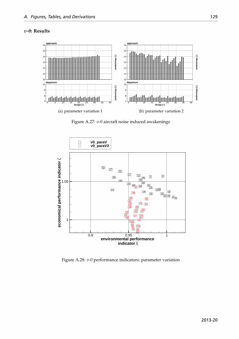
A. Figures, Tables, and Derivations 129
v-0: Results
awak
enin
gs [-
]
10
11
12
13
14
15
16approach
design [-]
awak
enin
gs [-
]
0 5 10 15 20 25 30 35 407
8
9
10departure
(a) parameter variation 1
awak
enin
gs [-
]
10
11
12
13
14
15
16approach
design [-]
awak
enin
gs [-
]
0 5 10 15 20 25 30 35 407
8
9
10departure
(b) parameter variation 2
Figure A.27: v-0 aircraft noise induced awakenings
2
3
4 5
7
8
910
12
13
14 15
17
18
1920
22
23
24
25
27
28
2930
32
3334
35
1
2
4
5
6
7
8
9
10
11
12
13
14
15
16
17
18
19
20
21
22
23
24
25
26
27
28
29
30
31
32
33
environmental performance indicator ξ
eco
no
mic
al p
erfo
rman
ce in
dic
ato
r ζ
0.9 0.95 1
1
1.05
v0_paraVv0_paraV2
Figure A.28: v-0 performance indicators: parameter variation
2013-20
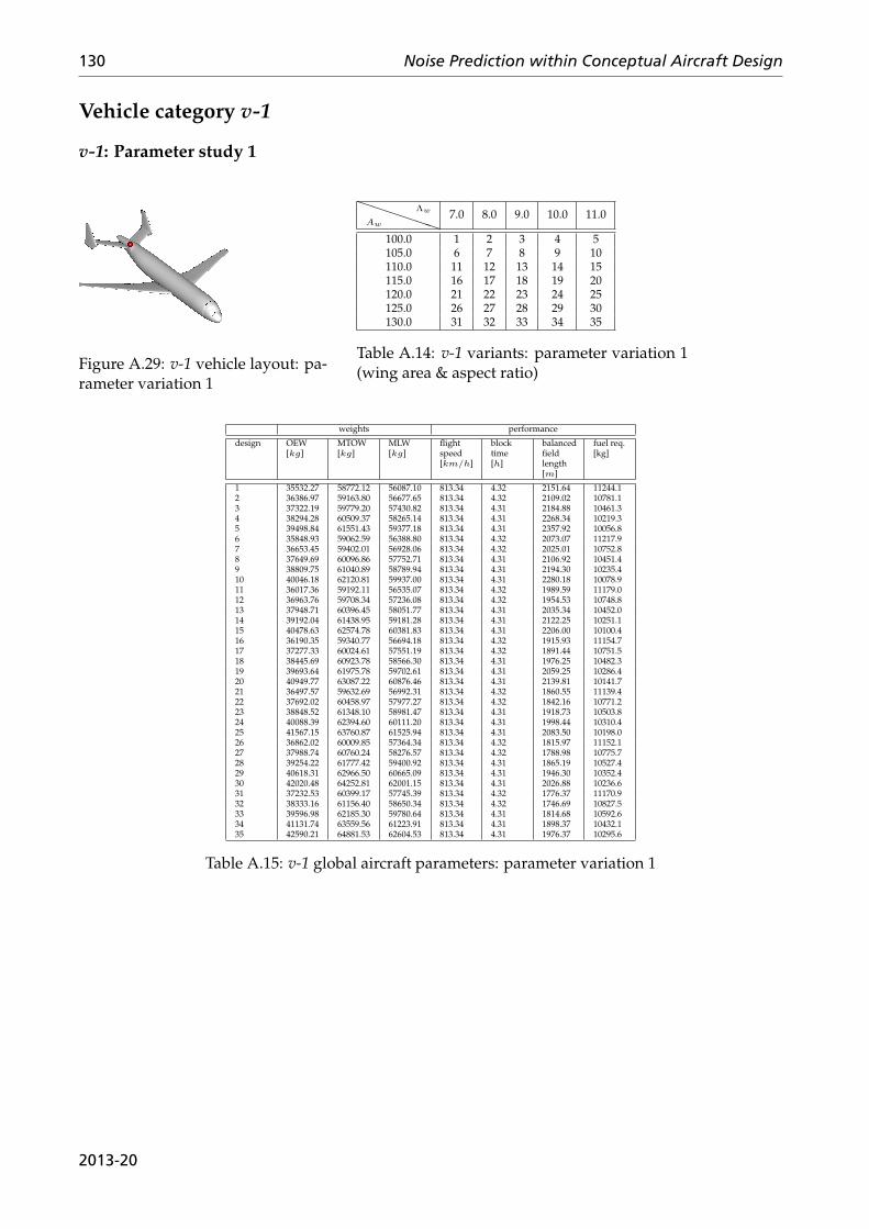
130 Noise Prediction within Conceptual Aircraft Design
Vehicle category v-1
v-1: Parameter study 1
Figure A.29: v-1 vehicle layout: pa-rameter variation 1
PPPPPPAw
Λw 7.0 8.0 9.0 10.0 11.0
100.0 1 2 3 4 5105.0 6 7 8 9 10110.0 11 12 13 14 15115.0 16 17 18 19 20120.0 21 22 23 24 25125.0 26 27 28 29 30130.0 31 32 33 34 35
Table A.14: v-1 variants: parameter variation 1(wing area & aspect ratio)
weights performance
design OEW[kg]
MTOW[kg]
MLW[kg]
flightspeed[km/h]
blocktime[h]
balancedfieldlength[m]
fuel req.[kg]
1 35532.27 58772.12 56087.10 813.34 4.32 2151.64 11244.12 36386.97 59163.80 56677.65 813.34 4.32 2109.02 10781.13 37322.19 59779.20 57430.82 813.34 4.31 2184.88 10461.34 38294.28 60509.37 58265.14 813.34 4.31 2268.34 10219.35 39498.84 61551.43 59377.18 813.34 4.31 2357.92 10056.86 35848.93 59062.59 56388.80 813.34 4.32 2073.07 11217.97 36653.45 59402.01 56928.06 813.34 4.32 2025.01 10752.88 37649.69 60096.86 57752.71 813.34 4.31 2106.92 10451.49 38809.75 61040.89 58789.94 813.34 4.31 2194.30 10235.410 40046.18 62120.81 59937.00 813.34 4.31 2280.18 10078.911 36017.36 59192.11 56535.07 813.34 4.32 1989.59 11179.012 36963.76 59708.34 57236.08 813.34 4.32 1954.53 10748.813 37948.71 60396.45 58051.77 813.34 4.31 2035.34 10452.014 39192.04 61438.95 59181.28 813.34 4.31 2122.25 10251.115 40478.63 62574.78 60381.83 813.34 4.31 2206.00 10100.416 36190.35 59340.77 56694.18 813.34 4.32 1915.93 11154.717 37277.33 60024.61 57551.19 813.34 4.32 1891.44 10751.518 38445.69 60923.78 58566.30 813.34 4.31 1976.25 10482.319 39693.64 61975.78 59702.61 813.34 4.31 2059.25 10286.420 40949.77 63087.22 60876.46 813.34 4.31 2139.81 10141.721 36497.57 59632.69 56992.31 813.34 4.32 1860.55 11139.422 37692.02 60458.97 57977.27 813.34 4.32 1842.16 10771.223 38848.52 61348.10 58981.47 813.34 4.31 1918.73 10503.824 40088.39 62394.60 60111.20 813.34 4.31 1998.44 10310.425 41567.15 63760.87 61525.94 813.34 4.31 2083.50 10198.026 36862.02 60009.85 57364.34 813.34 4.32 1815.97 11152.127 37988.74 60760.24 58276.57 813.34 4.32 1788.98 10775.728 39254.22 61777.42 59400.92 813.34 4.31 1865.19 10527.429 40618.31 62966.50 60665.09 813.34 4.31 1946.30 10352.430 42020.48 64252.81 62001.15 813.34 4.31 2026.88 10236.631 37232.53 60399.17 57745.39 813.34 4.32 1776.37 11170.932 38333.16 61156.40 58650.34 813.34 4.32 1746.69 10827.533 39596.98 62185.30 59780.64 813.34 4.31 1814.68 10592.634 41131.74 63559.56 61223.91 813.34 4.31 1898.37 10432.135 42590.21 64881.53 62604.53 813.34 4.31 1976.37 10295.6
Table A.15: v-1 global aircraft parameters: parameter variation 1
2013-20
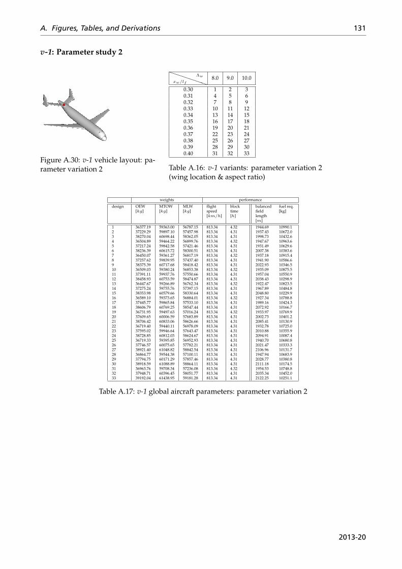
A. Figures, Tables, and Derivations 131
v-1: Parameter study 2
Figure A.30: v-1 vehicle layout: pa-rameter variation 2
PPPPPPxw/lf
Λw 8.0 9.0 10.0
0.30 1 2 30.31 4 5 60.32 7 8 90.33 10 11 120.34 13 14 150.35 16 17 180.36 19 20 210.37 22 23 240.38 25 26 270.39 28 29 300.40 31 32 33
Table A.16: v-1 variants: parameter variation 2(wing location & aspect ratio)
weights performance
design OEW[kg]
MTOW[kg]
MLW[kg]
flightspeed[km/h]
blocktime[h]
balancedfieldlength[m]
fuel req.[kg]
1 36377.19 59363.00 56787.15 813.34 4.32 1944.69 10990.12 37229.29 59897.10 57457.98 813.34 4.31 1937.43 10672.03 38270.04 60698.44 58362.05 813.34 4.31 1998.73 10432.64 36504.89 59464.22 56899.76 813.34 4.32 1947.67 10963.65 37217.24 59842.58 57421.46 813.34 4.31 1931.49 10629.66 38236.39 60615.72 58300.51 813.34 4.31 2007.38 10383.67 36450.07 59361.27 56817.19 813.34 4.32 1937.18 10915.48 37257.62 59839.95 57437.40 813.34 4.31 1941.90 10586.69 38375.39 60717.68 58418.42 813.34 4.31 2022.93 10346.510 36509.03 59380.24 56853.38 813.34 4.32 1935.09 10875.511 37391.11 59937.76 57550.66 813.34 4.31 1957.04 10550.912 38458.93 60753.59 58474.87 813.34 4.31 2038.43 10298.913 36447.67 59266.89 56762.34 813.34 4.32 1922.47 10823.514 37275.24 59755.76 57397.15 813.34 4.31 1967.89 10484.815 38353.98 60579.66 58330.64 813.34 4.31 2048.80 10229.916 36589.10 59373.65 56884.01 813.34 4.32 1927.34 10788.817 37445.77 59865.84 57533.10 813.34 4.31 1989.16 10424.318 38606.79 60769.25 58547.44 813.34 4.31 2072.92 10166.719 36731.95 59497.63 57016.24 813.34 4.32 1933.97 10769.920 37609.65 60006.59 57683.89 813.34 4.31 2002.73 10401.221 38706.42 60833.06 58626.66 813.34 4.31 2085.41 10130.922 36719.40 59440.11 56978.09 813.34 4.31 1932.78 10725.023 37595.02 59946.64 57643.47 813.34 4.31 2010.88 10355.924 38728.85 60812.03 58624.67 813.34 4.31 2094.91 10087.425 36719.33 59395.85 56952.93 813.34 4.31 1940.70 10680.826 37746.57 60075.65 57782.21 813.34 4.31 2021.47 10333.327 38921.40 61048.82 58842.54 813.34 4.31 2106.96 10131.728 36864.77 59544.38 57100.11 813.34 4.31 1947.94 10683.929 37794.75 60171.29 57857.46 813.34 4.31 2028.77 10380.830 38918.59 61088.89 58864.11 813.34 4.31 2111.18 10174.531 36963.76 59708.34 57236.08 813.34 4.32 1954.53 10748.832 37948.71 60396.45 58051.77 813.34 4.31 2035.34 10452.033 39192.04 61438.95 59181.28 813.34 4.31 2122.25 10251.1
Table A.17: v-1 global aircraft parameters: parameter variation 2
2013-20
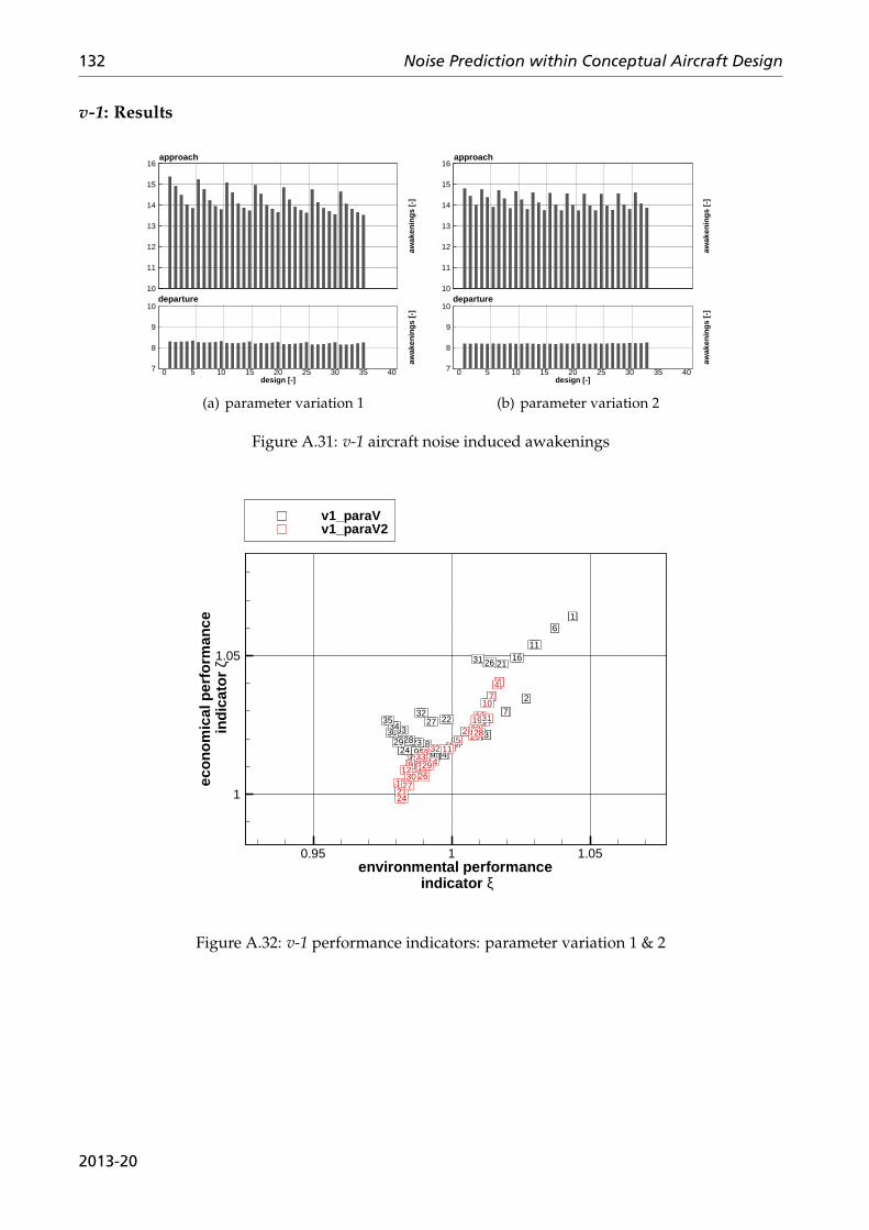
132 Noise Prediction within Conceptual Aircraft Design
v-1: Results
awak
enin
gs [-
]
10
11
12
13
14
15
16approach
design [-]
awak
enin
gs [-
]
0 5 10 15 20 25 30 35 407
8
9
10departure
(a) parameter variation 1
awak
enin
gs [-
]
10
11
12
13
14
15
16approach
design [-]
awak
enin
gs [-
]
0 5 10 15 20 25 30 35 407
8
9
10departure
(b) parameter variation 2
Figure A.31: v-1 aircraft noise induced awakenings
1
2
3
45
6
7
8910
11
12
131415
16
17
181920
21
22
2324
25
26
27
282930
31
32
333435
1
2
3
4
5
6
7
8
9
10
11
12
13
14
15
16
17
18
19
20
21
22
23
24
25
2627
28
2930
31
3233
environmental performance indicator ξ
eco
no
mic
al p
erfo
rman
ce in
dic
ato
r ζ
0.95 1 1.05
1
1.05
v1_paraVv1_paraV2
Figure A.32: v-1 performance indicators: parameter variation 1 & 2
2013-20
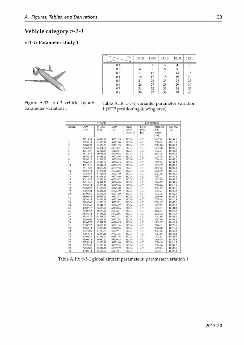
A. Figures, Tables, and Derivations 133
Vehicle category v-1-1
v-1-1: Parameter study 1
Figure A.33: v-1-1 vehicle layout:parameter variation 1
XXXXXXXXxvtp/lhtp
Aw 105.0 110.0 115.0 120.0 125.0
0.1 1 2 3 4 50.2 6 7 8 9 100.3 11 12 13 14 150.4 16 17 18 19 200.5 21 22 23 24 250.6 26 27 28 29 300.7 31 32 33 34 350.8 36 37 38 39 40
Table A.18: v-1-1 variants: parameter variation1 (VTP positioning & wing area)
weights performance
design OEW[kg]
MTOW[kg]
MLW[kg]
flightspeed[km/h]
blocktime[h]
balancedfieldlength[m]
fuel req.[kg]
1 38313.44 60593.42 58321.15 813.34 4.31 2147.14 10284.22 38750.14 61056.41 58772.86 813.34 4.31 2078.69 10310.53 39188.52 61530.30 59231.55 813.34 4.31 2014.70 10346.04 39663.31 62051.68 59733.04 813.34 4.31 1957.28 10392.65 40113.87 62545.89 60208.51 813.34 4.31 1903.91 10436.36 38312.45 60591.51 58319.62 813.34 4.31 2147.08 10283.37 38750.14 61056.41 58772.86 813.34 4.31 2078.75 10310.58 39187.12 61527.95 59229.58 813.34 4.31 2014.69 10345.19 39661.42 62048.64 59730.43 813.34 4.31 1957.24 10391.510 40112.11 62542.82 60205.99 813.34 4.31 1903.97 10435.011 38311.28 60589.46 58317.93 813.34 4.31 2147.02 10282.412 38750.14 61056.41 58772.86 813.34 4.31 2078.79 10310.513 39185.51 61525.38 59227.40 813.34 4.31 2014.68 10344.114 39660.28 62046.43 59728.69 813.34 4.31 1957.22 10390.415 40110.42 62539.86 60203.57 813.34 4.31 1903.99 10433.716 38310.41 60587.79 58316.58 813.34 4.31 2146.97 10281.617 38750.14 61056.41 58772.86 813.34 4.31 2078.76 10310.518 39183.90 61522.77 59225.20 813.34 4.31 2014.67 10343.119 39659.24 62044.28 59726.99 813.34 4.31 1957.21 10389.320 40108.86 62536.96 60201.20 813.34 4.31 1903.95 10432.321 38308.86 60585.43 58314.57 813.34 4.31 2146.90 10280.822 38750.14 61056.41 58772.86 813.34 4.31 2078.74 10310.523 39182.82 61520.68 59223.52 813.34 4.31 2014.67 10342.124 39657.68 62041.60 59724.77 813.34 4.31 1957.19 10388.225 40107.17 62533.97 60198.76 813.34 4.31 1903.91 10431.026 38307.53 60583.21 58312.71 813.34 4.31 2146.84 10279.927 38750.14 61056.41 58772.86 813.34 4.31 2078.72 10310.528 39181.19 61518.04 59221.31 813.34 4.31 2014.66 10341.129 39656.02 62038.94 59722.54 813.34 4.31 1957.16 10387.230 40105.75 62531.31 60196.65 813.34 4.31 1903.87 10429.831 38307.23 60582.10 58311.94 813.34 4.31 2146.81 10279.132 38750.14 61056.41 58772.86 813.34 4.31 2078.70 10310.533 39179.81 61515.75 59219.41 813.34 4.31 2014.66 10340.234 39655.33 62037.25 59721.28 813.34 4.31 1957.16 10386.235 40104.31 62528.63 60194.46 813.34 4.31 1903.83 10428.636 38306.14 60580.22 58310.43 813.34 4.31 2146.75 10278.337 38750.14 61056.41 58772.86 813.34 4.31 2078.68 10310.538 39178.55 61513.49 59217.54 813.34 4.31 2014.66 10339.239 39653.85 62034.71 59719.19 813.34 4.31 1957.14 10385.140 40103.14 62526.27 60192.61 813.34 4.31 1903.81 10427.4
Table A.19: v-1-1 global aircraft parameters: parameter variation 1
2013-20
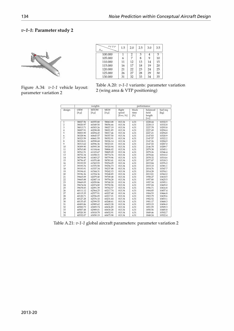
134 Noise Prediction within Conceptual Aircraft Design
v-1-1: Parameter study 2
Figure A.34: v-1-1 vehicle layout:parameter variation 2
PPPPPPAw
xV TP 1.5 2.0 2.5 3.0 3.5
100.000 1 2 3 4 5105.000 6 7 8 9 10110.000 11 12 13 14 15115.000 16 17 18 19 20120.000 21 22 23 24 25125.000 26 27 28 29 30130.000 31 32 33 34 35
Table A.20: v-1-1 variants: parameter variation2 (wing area & VTP positioning)
weights performance
design OEW[kg]
MTOW[kg]
MLW[kg]
flightspeed[km/h]
blocktime[h]
balancedfieldlength[m]
fuel req.[kg]
1 38027.56 60355.80 58063.08 813.34 4.31 2228.44 10332.52 38020.97 60349.50 58056.66 813.34 4.31 2228.13 10332.83 38013.71 60303.26 58027.19 813.34 4.31 2227.78 10293.84 38007.91 60298.08 58021.85 813.34 4.31 2227.49 10294.45 38003.90 60294.45 58017.46 813.34 4.31 2227.21 10294.86 38328.96 60645.57 58357.50 813.34 4.31 2147.83 10320.97 38323.59 60641.55 58352.91 813.34 4.31 2147.57 10322.28 38318.01 60598.68 58326.14 813.34 4.31 2147.26 10284.99 38313.62 60596.36 58323.01 813.34 4.31 2147.02 10287.010 38309.90 60595.38 58320.94 813.34 4.31 2146.78 10289.711 38763.80 61104.66 58806.02 813.34 4.31 2079.38 10345.112 38761.51 61103.67 58805.09 813.34 4.31 2079.26 10346.413 38752.34 61058.31 58774.76 813.34 4.31 2078.66 10310.214 38754.90 61065.27 58779.96 813.34 4.31 2078.32 10314.615 38756.47 61070.48 58783.41 813.34 4.31 2077.87 10318.316 39193.93 61565.93 59254.05 813.34 4.31 2015.84 10376.217 39193.76 61570.58 59256.73 813.34 4.31 2015.33 10381.118 39193.91 61537.34 59237.88 813.34 4.31 2014.76 10347.719 39194.41 61544.31 59242.15 813.34 4.31 2014.28 10354.120 39196.36 61554.36 59248.85 813.34 4.31 2013.81 10362.221 39665.09 62079.40 59749.48 813.34 4.31 1958.27 10418.522 39665.88 62087.14 59754.28 813.34 4.31 1957.80 10425.523 39669.05 62059.86 59740.20 813.34 4.31 1957.34 10395.124 39674.04 62074.80 59750.96 813.34 4.31 1957.04 10405.025 39678.83 62091.39 59762.57 813.34 4.31 1956.71 10416.826 40111.12 62564.25 60217.74 813.34 4.31 1904.85 10457.427 40115.35 62577.91 60227.40 813.34 4.31 1904.53 10466.828 40120.71 62556.05 60217.21 813.34 4.31 1903.79 10439.629 40127.28 62576.10 60231.64 813.34 4.31 1902.52 10453.130 40135.45 62599.55 60248.61 813.34 4.31 1901.17 10468.331 40493.86 62985.62 60622.28 813.34 4.31 1853.23 10496.032 40500.73 63005.74 60636.85 813.34 4.31 1851.95 10509.333 40507.48 62989.01 60630.28 813.34 4.31 1850.56 10485.834 40520.30 63018.78 60652.91 813.34 4.31 1849.46 10502.735 40532.07 63050.19 60675.98 813.34 4.31 1848.24 10522.4
Table A.21: v-1-1 global aircraft parameters: parameter variation 2
2013-20
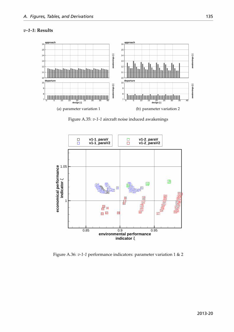
A. Figures, Tables, and Derivations 135
v-1-1: Results
awak
enin
gs [-
]
10
11
12
13
14
15
16approach
design [-]
awak
enin
gs [-
]
0 5 10 15 20 25 30 35 407
8
9
10departure
(a) parameter variation 1
awak
enin
gs [-
]
10
11
12
13
14
15
16approach
design [-]
awak
enin
gs [-
]
0 5 10 15 20 25 30 35 407
8
9
10departure
(b) parameter variation 2
Figure A.35: v-1-1 aircraft noise induced awakenings
v1-2_paraVv1-2_paraV2
1234
5
6789
10
11121314
15
16171819
20
21222324
25
26272829
30
31323334
35
36373839
40 1234 567
89 101112
1314 151617
1819 202122
2324 2526272829 3031323334 35
123456789101112 131415161718
1 2
3 45
678
9 10111213141516
1718192021222324
2526272829303132
33343536373839
environmental performance indicator ξ
econ
omic
al p
erfo
rman
ce in
dica
tor
ζ
0.85 0.9 0.95
1
1.05
v1-1_paraVv1-1_paraV2
Figure A.36: v-1-1 performance indicators: parameter variation 1 & 2
2013-20

136 Noise Prediction within Conceptual Aircraft Design
Vehicle category v-1-2
v-1-2: Parameter study 1
Figure A.37: v-1-2 vehicle layout:parameter variation 1
`````````νAvtp,1 − Avtp,2−320-8 22-7 24-6 26-5 28-4 30-3
-30.0 1 2 3 4 5 6-35.0 7 8 9 10 11 12-40.0 13 14 15 16 17 18-45.0 19 20 21 22 23 24-50.0 25 26 27 28 29 30
Table A.22: v-1-2 variants: parameter variation1 (HTP sweep angle & VTP area ratios)
weights performance
design OEW[kg]
MTOW[kg]
MLW[kg]
flightspeed[km/h]
blocktime[h]
balancedfieldlength[m]
fuel req.[kg]
1 38656.28 61108.99 58762.21 813.34 4.31 2067.88 10456.92 38625.95 61073.49 58728.91 813.34 4.31 2066.97 10451.83 38653.19 61102.79 58757.36 813.34 4.31 2067.65 10453.84 38728.37 61187.84 58838.36 813.34 4.31 2069.65 10463.75 38710.46 61164.15 58817.11 813.34 4.31 2069.08 10457.96 38739.63 61194.49 58846.63 813.34 4.31 2069.83 10459.17 38776.78 61251.43 58895.42 813.34 4.31 2071.09 10478.98 38746.12 61215.04 58861.45 813.34 4.31 2070.14 10473.29 38772.91 61245.74 58890.31 813.34 4.31 2070.83 10477.110 38850.48 61336.09 58975.60 813.34 4.31 2072.98 10489.911 38830.64 61310.00 58952.06 813.34 4.31 2072.34 10483.612 38858.33 61339.56 58980.99 813.34 4.31 2073.08 10485.513 38917.29 61421.69 59053.12 813.34 4.31 2075.12 10508.614 38884.44 61382.83 59016.81 813.34 4.31 2074.09 10502.615 38910.58 61412.76 59045.17 813.34 4.31 2074.78 10506.416 38987.16 61502.07 59129.22 813.34 4.31 2076.60 10519.217 38964.37 61472.75 59102.63 813.34 4.31 2075.89 10512.618 38994.51 61504.96 59134.04 813.34 4.31 2076.48 10514.719 39063.12 61597.31 59216.18 813.34 4.31 2078.11 10538.420 39032.61 61561.25 59182.45 813.34 4.31 2077.16 10532.921 39057.91 61590.48 59210.05 813.34 4.31 2077.63 10536.822 39129.83 61675.50 59289.32 813.34 4.31 2079.20 10549.923 39112.32 61652.56 59268.70 813.34 4.31 2078.60 10544.524 39139.74 61681.87 59297.18 813.34 4.31 2079.13 10546.425 39231.09 61799.17 59403.40 813.34 4.31 2081.62 10572.326 39196.38 61758.35 59365.20 813.34 4.31 2080.53 10566.227 39220.51 61786.44 59391.59 813.34 4.31 2080.96 10570.228 39294.41 61873.20 59472.93 813.34 4.31 2082.63 10583.029 39274.13 61847.09 59449.30 813.34 4.31 2081.93 10577.230 39299.37 61874.10 59475.55 813.34 4.31 2082.41 10579.0
Table A.23: v-1-2 global aircraft parameters: parameter variation 1
2013-20
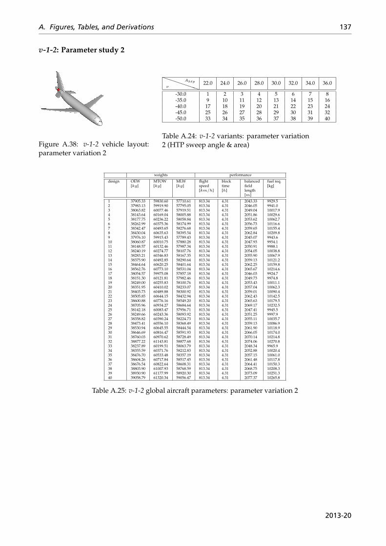
A. Figures, Tables, and Derivations 137
v-1-2: Parameter study 2
Figure A.38: v-1-2 vehicle layout:parameter variation 2
PPPPPPν
Ahtp 22.0 24.0 26.0 28.0 30.0 32.0 34.0 36.0
-30.0 1 2 3 4 5 6 7 8-35.0 9 10 11 12 13 14 15 16-40.0 17 18 19 20 21 22 23 24-45.0 25 26 27 28 29 30 31 32-50.0 33 34 35 36 37 38 39 40
Table A.24: v-1-2 variants: parameter variation2 (HTP sweep angle & area)
weights performance
design OEW[kg]
MTOW[kg]
MLW[kg]
flightspeed[km/h]
blocktime[h]
balancedfieldlength[m]
fuel req.[kg]
1 37905.33 59830.60 57710.61 813.34 4.31 2043.33 9929.52 37983.13 59919.90 57795.05 813.34 4.31 2046.05 9941.03 38063.82 60077.46 57919.51 813.34 4.31 2049.04 10017.94 38143.64 60169.04 58005.88 813.34 4.31 2051.86 10029.65 38177.75 60236.22 58058.84 813.34 4.31 2053.62 10062.76 38262.99 60375.36 58174.99 813.34 4.31 2056.73 10116.67 38342.47 60493.65 58276.68 813.34 4.31 2059.65 10155.48 38430.04 60635.63 58395.54 813.34 4.31 2062.84 10209.89 37976.10 59915.43 57789.43 813.34 4.31 2045.07 9943.610 38060.87 60010.75 57880.28 813.34 4.31 2047.93 9954.111 38148.57 60132.46 57987.34 813.34 4.31 2050.91 9988.112 38240.19 60274.77 58107.76 813.34 4.31 2054.05 10038.813 38283.21 60346.83 58167.35 813.34 4.31 2055.90 10067.914 38375.90 60492.85 58290.64 813.34 4.31 2059.13 10121.215 38464.64 60620.25 58401.64 813.34 4.31 2062.25 10159.816 38562.76 60773.10 58531.04 813.34 4.31 2065.67 10214.617 38054.57 59975.08 57857.18 813.34 4.31 2046.03 9924.718 38151.30 60121.81 57982.46 813.34 4.31 2049.73 9974.819 38249.00 60255.83 58100.76 813.34 4.31 2053.43 10011.120 38351.95 60410.02 58233.07 813.34 4.31 2057.04 10062.321 38403.73 60489.88 58300.92 813.34 4.31 2059.01 10090.422 38505.85 60644.15 58432.94 813.34 4.31 2062.43 10142.523 38600.88 60776.16 58549.20 813.34 4.31 2065.63 10179.524 38705.96 60934.27 58684.64 813.34 4.31 2069.17 10232.525 38142.18 60083.47 57956.71 813.34 4.31 2047.41 9945.526 38249.66 60243.36 58093.92 813.34 4.31 2051.25 9997.927 38358.82 60390.24 58224.73 813.34 4.31 2055.11 10035.728 38473.41 60556.10 58368.49 813.34 4.31 2059.13 10086.929 38530.94 60645.55 58444.54 813.34 4.31 2061.90 10118.930 38646.69 60816.47 58591.93 813.34 4.31 2066.05 10174.031 38760.03 60970.62 58728.49 813.34 4.31 2070.14 10214.832 38877.22 61143.81 58877.68 813.34 4.31 2074.06 10270.833 38237.89 60199.51 58063.79 813.34 4.31 2048.34 9965.934 38355.59 60371.76 58212.83 813.34 4.31 2052.88 10020.435 38476.70 60533.48 58357.19 813.34 4.31 2057.15 10061.036 38604.26 60717.84 58517.45 813.34 4.31 2061.48 10117.837 38676.54 60822.64 58608.31 813.34 4.31 2064.41 10150.338 38803.90 61007.93 58768.59 813.34 4.31 2068.75 10208.339 38930.90 61177.99 58920.30 813.34 4.31 2073.09 10251.340 39058.79 61320.34 59056.47 813.34 4.31 2077.37 10265.8
Table A.25: v-1-2 global aircraft parameters: parameter variation 2
2013-20
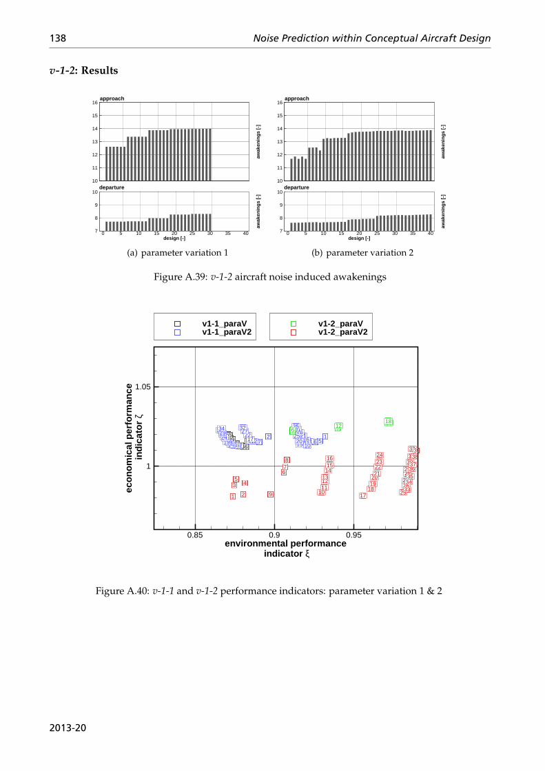
138 Noise Prediction within Conceptual Aircraft Design
v-1-2: Results
awak
enin
gs [-
]
10
11
12
13
14
15
16approach
design [-]
awak
enin
gs [-
]
0 5 10 15 20 25 30 35 407
8
9
10departure
(a) parameter variation 1
awak
enin
gs [-
]
10
11
12
13
14
15
16approach
design [-]
awak
enin
gs [-
]
0 5 10 15 20 25 30 35 407
8
9
10departure
(b) parameter variation 2
Figure A.39: v-1-2 aircraft noise induced awakenings
v1-2_paraVv1-2_paraV2
1234
5
6789
10
11121314
15
16171819
20
21222324
25
26272829
30
31323334
35
36373839
40 1234 567
89 101112
1314 151617
1819 202122
2324 2526272829 3031323334 35
123456789101112 131415161718
1 2
3 45
678
9 10111213141516
1718192021222324
2526272829303132
33343536373839
environmental performance indicator ξ
econ
omic
al p
erfo
rman
ce in
dica
tor
ζ
0.85 0.9 0.95
1
1.05
v1-1_paraVv1-1_paraV2
Figure A.40: v-1-1 and v-1-2 performance indicators: parameter variation 1 & 2
2013-20

A. Figures, Tables, and Derivations 139
Vehicle category v2
v-2: Parameter study 1
Figure A.41: v-2 vehicle layout: pa-rameter variation 1
PPPPPPAwΛw7.0 8.0 9.0 10.0 11.0
100.0 1 2 3 4 5105.0 6 7 8 9 10110.0 11 12 13 14 15115.0 16 17 18 19 20120.0 21 22 23 24 25125.0 26 27 28 29 30130.0 31 32 33 34 35
Table A.26: v-2 variants: parameter variation 1(wing area & aspect ratio)
weights performance
design OEW[kg]
MTOW[kg]
MLW[kg]
flightspeed[km/h]
blocktime[h]
balancedfieldlength[m]
fuel req.[kg]
1 36123.08 59485.01 56747.07 813.34 4.32 2189.10 11366.22 36777.28 59641.45 57117.80 813.34 4.32 2099.06 10868.43 37593.73 60124.01 57744.15 813.34 4.31 2148.47 10534.54 38609.82 60993.99 58677.26 813.34 4.31 2236.04 10388.45 39540.07 61735.57 59500.02 813.34 4.31 2317.54 10199.76 36328.30 59585.53 56892.72 813.34 4.32 2091.89 11261.57 37059.34 59849.49 57357.75 813.34 4.32 2013.23 10794.48 37909.14 60383.66 58027.37 813.34 4.31 2072.32 10478.89 38882.26 61213.12 58919.22 813.34 4.31 2155.67 10335.110 39955.42 62122.55 59899.14 813.34 4.31 2239.39 10171.411 36557.66 59728.24 57072.70 813.34 4.32 2007.81 11174.812 37374.09 60107.61 57640.19 813.34 4.32 1939.56 10737.813 38211.54 60636.64 58301.79 813.34 4.31 2002.74 10429.314 39239.18 61538.39 59258.33 813.34 4.31 2085.45 10303.415 40440.20 62596.54 60377.70 813.34 4.31 2169.20 10160.616 36717.34 59798.36 57181.31 813.34 4.32 1925.68 11085.317 37640.68 60312.35 57871.56 813.34 4.31 1869.14 10675.918 38535.72 60916.91 58601.03 813.34 4.31 1939.88 10385.419 39617.37 61894.17 59623.68 813.34 4.31 2021.32 10281.020 40880.23 63024.46 60810.79 813.34 4.31 2103.76 10148.521 36986.23 60000.01 57411.87 813.34 4.32 1861.81 11018.022 37932.82 60591.90 58156.24 813.34 4.31 1810.32 10663.323 38901.54 61399.83 59033.77 813.34 4.31 1884.54 10502.524 39996.52 62308.39 60022.86 813.34 4.31 1962.66 10316.125 41245.86 63423.20 61195.20 813.34 4.31 2042.24 10181.626 37285.35 60304.49 57714.23 813.34 4.32 1811.40 11023.427 38216.72 60891.31 58449.05 813.34 4.31 1757.76 10678.828 39282.74 61815.79 59434.83 813.34 4.31 1833.04 10537.329 40411.69 62764.58 60461.41 813.34 4.31 1909.70 10357.130 41725.83 63955.45 61705.12 813.34 4.31 1988.96 10233.931 37496.07 60521.37 57928.54 813.34 4.32 1758.61 11029.532 38535.13 61236.12 58782.65 813.34 4.32 1712.54 10705.233 39653.23 62225.65 59827.28 813.34 4.31 1784.98 10576.734 40853.85 63254.84 60930.99 813.34 4.31 1861.58 10405.235 42192.25 64453.05 62189.15 813.34 4.31 1939.42 10265.0
Table A.27: v-2 global aircraft parameters: parameter variation 1
2013-20
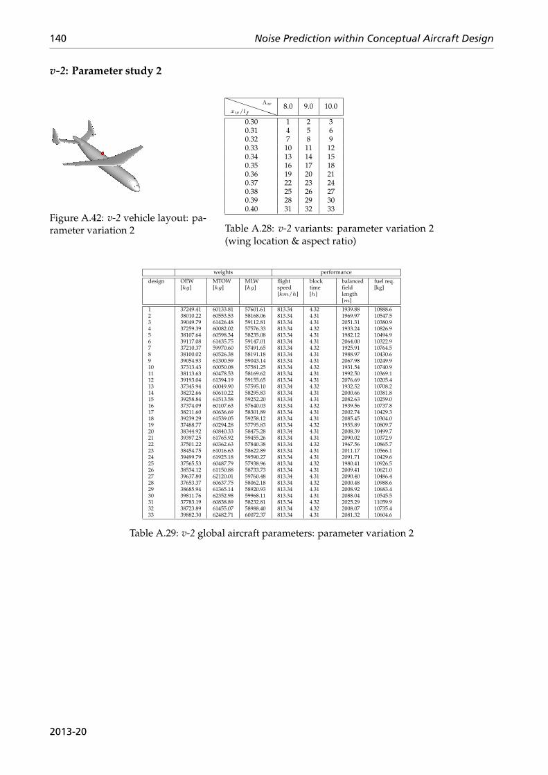
140 Noise Prediction within Conceptual Aircraft Design
v-2: Parameter study 2
Figure A.42: v-2 vehicle layout: pa-rameter variation 2
PPPPPPxw/lf
Λw 8.0 9.0 10.0
0.30 1 2 30.31 4 5 60.32 7 8 90.33 10 11 120.34 13 14 150.35 16 17 180.36 19 20 210.37 22 23 240.38 25 26 270.39 28 29 300.40 31 32 33
Table A.28: v-2 variants: parameter variation 2(wing location & aspect ratio)
weights performance
design OEW[kg]
MTOW[kg]
MLW[kg]
flightspeed[km/h]
blocktime[h]
balancedfieldlength[m]
fuel req.[kg]
1 37249.41 60133.81 57601.61 813.34 4.32 1939.88 10888.62 38010.22 60553.53 58168.06 813.34 4.31 1969.97 10547.53 39049.79 61426.48 59112.81 813.34 4.31 2051.31 10380.94 37259.39 60082.02 57576.33 813.34 4.32 1933.24 10826.95 38107.64 60598.34 58235.08 813.34 4.31 1982.12 10494.96 39117.08 61435.75 59147.01 813.34 4.31 2064.00 10322.97 37210.37 59970.60 57491.65 813.34 4.32 1925.91 10764.58 38100.02 60526.38 58191.18 813.34 4.31 1988.97 10430.69 39054.93 61300.59 59043.14 813.34 4.31 2067.98 10249.910 37313.43 60050.08 57581.25 813.34 4.32 1931.54 10740.911 38113.63 60478.53 58169.62 813.34 4.31 1992.50 10369.112 39193.04 61394.19 59155.65 813.34 4.31 2076.69 10205.413 37345.94 60049.90 57595.10 813.34 4.32 1932.52 10708.214 38232.66 60610.22 58295.83 813.34 4.31 2000.66 10381.815 39258.84 61513.58 59252.20 813.34 4.31 2082.63 10259.016 37374.09 60107.63 57640.03 813.34 4.32 1939.56 10737.817 38211.60 60636.69 58301.89 813.34 4.31 2002.74 10429.318 39239.29 61539.05 59258.12 813.34 4.31 2085.45 10304.019 37488.77 60294.28 57795.83 813.34 4.32 1955.89 10809.720 38344.92 60840.33 58475.28 813.34 4.31 2008.39 10499.721 39397.25 61765.92 59455.26 813.34 4.31 2090.02 10372.922 37501.22 60362.63 57840.38 813.34 4.32 1967.56 10865.723 38454.75 61016.63 58622.89 813.34 4.31 2011.17 10566.124 39499.79 61925.18 59590.27 813.34 4.31 2091.71 10429.625 37565.53 60487.79 57938.96 813.34 4.32 1980.41 10926.526 38534.12 61150.88 58733.73 813.34 4.31 2009.41 10621.027 39637.80 62120.01 59760.48 813.34 4.31 2090.40 10486.428 37653.37 60637.75 58062.18 813.34 4.32 2000.48 10988.629 38685.94 61365.14 58920.93 813.34 4.31 2008.92 10683.430 39811.76 62352.98 59968.11 813.34 4.31 2088.04 10545.531 37783.19 60838.89 58232.81 813.34 4.32 2025.29 11059.932 38723.89 61455.07 58988.40 813.34 4.32 2008.07 10735.433 39882.30 62482.71 60072.37 813.34 4.31 2081.32 10604.6
Table A.29: v-2 global aircraft parameters: parameter variation 2
2013-20
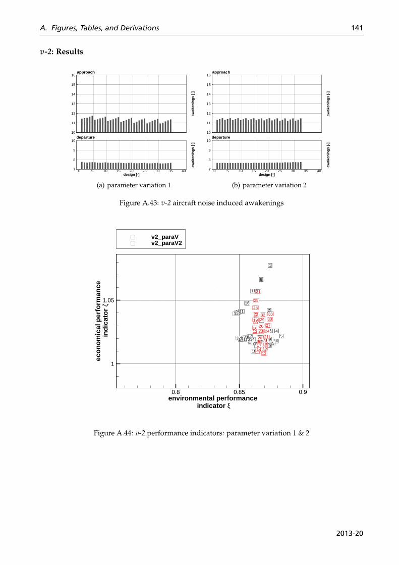
A. Figures, Tables, and Derivations 141
v-2: Results
awak
enin
gs [-
]
10
11
12
13
14
15
16approach
design [-]
awak
enin
gs [-
]
0 5 10 15 20 25 30 35 407
8
9
10departure
(a) parameter variation 1
awak
enin
gs [-
]
10
11
12
13
14
15
16approach
design [-]
awak
enin
gs [-
]
0 5 10 15 20 25 30 35 407
8
9
10departure
(b) parameter variation 2
Figure A.43: v-2 aircraft noise induced awakenings
1
2
3 45
6
7
8 9 10
11
12
13 14 15
16
17
1819 20
21
2223
24 25
26
27 2829
30
31
32 33 34 35
1
23
4
56
7
89
10
11 12
13
14 15
16
17 18
19
20 21
22
23 24
25
26 27
28
29 30
31
32 33
environmental performance indicator ξ
eco
no
mic
al p
erfo
rman
ce in
dic
ato
r ζ
0.8 0.85 0.9
1
1.05
v2_paraVv2_paraV2
Figure A.44: v-2 performance indicators: parameter variation 1 & 2
2013-20
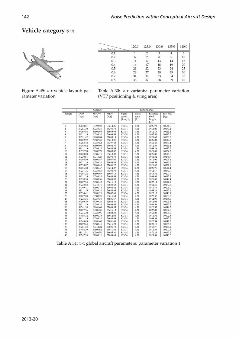
142 Noise Prediction within Conceptual Aircraft Design
Vehicle category v-x
Figure A.45: v-x vehicle layout: pa-rameter variation
XXXXXXXXxvtp/lwAw120.0 125.0 130.0 135.0 140.0
0.1 1 2 3 4 50.2 6 7 8 9 100.3 11 12 13 14 150.4 16 17 18 19 200.5 21 22 23 24 250.6 26 27 28 29 300.7 31 32 33 34 350.8 36 37 38 39 40
Table A.30: v-x variants: parameter variation(VTP positioning & wing area)
weights performance
design OEW[kg]
MTOW[kg]
MLW[kg]
flightspeed[km/h]
blocktime[h]
balancedfieldlength[m]
fuel req.[kg]
1 37073.01 59590.29 55614.06 813.34 4.31 2025.73 10521.52 37266.30 59739.31 55795.78 813.34 4.31 1961.05 10477.23 37393.54 59802.68 55905.06 813.34 4.31 1912.19 10413.44 38111.19 60599.20 56644.98 813.34 4.31 1867.93 10492.25 38531.42 61083.84 57083.13 813.34 4.31 1820.65 10556.76 37072.59 59587.35 55613.01 813.34 4.31 2026.02 10519.07 37268.48 59739.62 55797.43 813.34 4.31 1961.43 10475.48 37393.82 59800.96 55904.70 813.34 4.31 1912.53 10411.49 38111.19 60599.20 56644.98 813.34 4.31 1868.26 10492.210 38532.78 61082.79 57083.87 813.34 4.31 1821.01 10554.211 37073.73 59586.11 55613.39 813.34 4.31 2026.38 10516.612 37270.81 59741.25 55798.78 813.34 4.31 1961.82 10474.713 37396.50 59801.87 55907.00 813.34 4.31 1912.96 10409.614 38111.19 60599.20 56644.98 813.34 4.31 1868.58 10492.215 38535.87 61083.43 57086.27 813.34 4.31 1821.42 10551.816 37075.28 59585.47 55614.37 813.34 4.31 2026.75 10514.417 37271.36 59739.69 55798.79 813.34 4.31 1962.17 10472.618 37397.24 59800.69 55907.13 813.34 4.31 1913.31 10407.719 38111.19 60599.20 56644.98 813.34 4.31 1868.91 10492.220 38538.20 61083.36 57088.00 813.34 4.31 1821.80 10549.421 37077.55 59585.42 55616.10 813.34 4.31 2027.14 10512.122 37273.88 59740.15 55800.63 813.34 4.31 1962.56 10470.523 37399.41 59801.13 55908.82 813.34 4.31 1913.73 10406.024 38111.19 60599.20 56644.98 813.34 4.31 1869.24 10492.225 38538.61 61081.29 57087.60 813.34 4.31 1822.15 10546.926 37077.78 59583.28 55615.54 813.34 4.31 2027.47 10509.727 37275.36 59739.75 55801.67 813.34 4.31 1962.93 10468.628 37399.70 59799.30 55908.36 813.34 4.31 1914.08 10403.829 38111.19 60599.20 56644.98 813.34 4.31 1869.56 10492.230 38541.39 61081.68 57089.95 813.34 4.31 1822.55 10544.531 37077.96 59581.35 55616.13 813.34 4.31 2027.83 10507.632 37276.30 59738.96 55802.30 813.34 4.31 1963.29 10466.933 37403.72 59801.75 55912.06 813.34 4.31 1914.54 10402.334 38111.19 60599.20 56644.98 813.34 4.31 1869.89 10492.235 38543.63 61081.65 57091.49 813.34 4.31 1822.94 10542.336 37079.64 59580.41 55616.20 813.34 4.31 2028.18 10505.037 37281.38 59742.24 55806.78 813.34 4.31 1963.77 10465.138 37404.39 59800.62 55911.64 813.34 4.31 1914.89 10400.539 38111.51 60599.51 56645.30 813.34 4.31 1870.23 10492.240 38547.39 61083.11 57094.69 813.34 4.31 1823.38 10540.0
Table A.31: v-x global aircraft parameters: parameter variation 1
2013-20
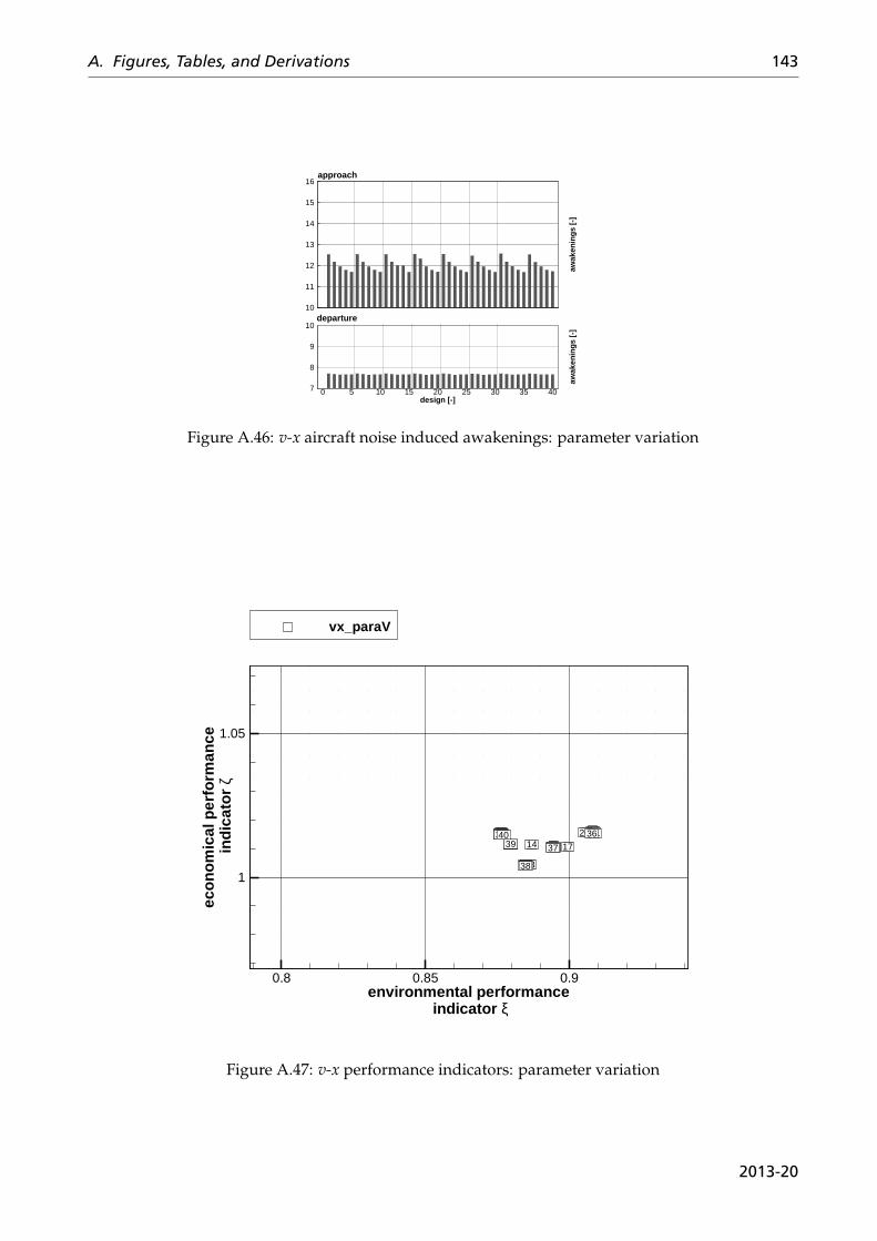
A. Figures, Tables, and Derivations 143
awak
enin
gs [-
]
10
11
12
13
14
15
16approach
design [-]
awak
enin
gs [-
]
0 5 10 15 20 25 30 35 407
8
9
10departure
Figure A.46: v-x aircraft noise induced awakenings: parameter variation
1
2
3
45 6
7
8
910 11
12
13
1415 16
17
18
1920 21
22
23
2425 26
27
28
2930 31
32
33
3435 36
37
38
3940
environmental performance indicator ξ
eco
no
mic
al p
erfo
rman
ce in
dic
ato
r ζ
0.8 0.85 0.9
1
1.05
vx_paraV
Figure A.47: v-x performance indicators: parameter variation
2013-20
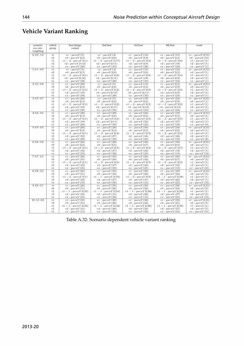
144 Noise Prediction within Conceptual Aircraft Design
Vehicle Variant Ranking
scenario: vehicle best design 2nd best 3rd best 4th best worsteco.-env. group variant
weighting
0: 0.0 - 1.0 vr vr : paraV (5) vr : paraV (4) vr : paraV (10) vr : paraV (15) vr : paraV 2(31)v0 v0 : paraV 2(3) v0 : paraV 2(6) v0 : paraV 2(9) v0 : paraV 2(2) v0 : paraV (31)v1 v1 − 2 : paraV 2(1) v1 − 2 : paraV 2(17) v1 − 2 : paraV 2(2) v1 − 2 : paraV 2(9) v1 : paraV (1)v2 v2 : paraV 2(12) v2 : paraV 2(11) v2 : paraV 2(9) v2 : paraV (18) v2 : paraV (1)vx vx : paraV (38) vx : paraV (33) vx : paraV (28) vx : paraV (23) vx : paraV (1)
1: 0.1 - 0.9 vr vr : paraV (5) vr : paraV (4) vr : paraV (15) vr : paraV (10) vr : paraV 2(31)v0 v0 : paraV 2(3) v0 : paraV 2(6) v0 : paraV 2(9) v0 : paraV 2(2) v0 : paraV (1)v1 v1 − 2 : paraV 2(1) v1 − 2 : paraV 2(2) v1 − 2 : paraV 2(9) v1 − 2 : paraV 2(3) v1 : paraV (1)v2 v2 : paraV 2(12) v2 : paraV 2(11) v2 : paraV (18) v2 : paraV 2(9) v2 : paraV (1)vx vx : paraV (38) vx : paraV (28) vx : paraV (33) vx : paraV (23) vx : paraV (1)
2: 0.2 - 0.8 vr vr : paraV (20) vr : paraV (5) vr : paraV (15) vr : paraV 2(3) vr : paraV 2(31)v0 v0 : paraV 2(3) v0 : paraV 2(6) v0 : paraV 2(2) v0 : paraV 2(9) v0 : paraV (1)v1 v1 − 2 : paraV 2(1) v1 − 2 : paraV 2(2) v1 − 2 : paraV 2(9) v1 − 2 : paraV 2(3) v1 : paraV (1)v2 v2 : paraV (18) v2 : paraV 2(12) v2 : paraV 2(11) v2 : paraV 2(9) v2 : paraV (1)vx vx : paraV (38) vx : paraV (28) vx : paraV (33) vx : paraV (23) vx : paraV (1)
3: 0.3 - 0.7 vr vr : paraV (20) vr : paraV (5) vr : paraV (19) vr : paraV (24) vr : paraV 2(31)v0 v0 : paraV 2(3) v0 : paraV 2(6) v0 : paraV 2(2) v0 : paraV 2(9) v0 : paraV (1)v1 v1 − 2 : paraV 2(1) v1 − 2 : paraV 2(2) v1 − 2 : paraV 2(3) v1 − 2 : paraV 2(9) v1 : paraV (1)v2 v2 : paraV (18) v2 : paraV 2(11) v2 : paraV 2(12) v2 : paraV 2(14) v2 : paraV (1)vx vx : paraV (28) vx : paraV (38) vx : paraV (33) vx : paraV (23) vx : paraV (1)
4: 0.4 - 0.6 vr vr : paraV (20) vr : paraV (29) vr : paraV (24) vr : paraV (19) vr : paraV 2(31)v0 v0 : paraV 2(3) v0 : paraV 2(6) v0 : paraV 2(2) v0 : paraV 2(5) v0 : paraV (1)v1 v1 − 2 : paraV 2(1) v1 − 2 : paraV 2(2) v1 − 2 : paraV 2(3) v1 − 2 : paraV 2(5) v1 : paraV (1)v2 v2 : paraV (18) v2 : paraV 2(11) v2 : paraV (32) v2 : paraV (27) v2 : paraV (1)vx vx : paraV (28) vx : paraV (38) vx : paraV (23) vx : paraV (18) vx : paraV (6)
5: 0.5 - 0.5 vr vr : paraV (20) vr : paraV (29) vr : paraV (30) vr : paraV (24) vr : paraV 2(31)v0 v0 : paraV 2(2) v0 : paraV 2(3) v0 : paraV 2(5) v0 : paraV 2(6) v0 : paraV (1)v1 v1 − 2 : paraV 2(1) v1 − 2 : paraV 2(2) v1 − 2 : paraV 2(3) v1 − 2 : paraV 2(5) v1 : paraV (1)v2 v2 : paraV (32) v2 : paraV (27) v2 : paraV (18) v2 : paraV (22) v2 : paraV (1)vx vx : paraV (28) vx : paraV (38) vx : paraV (23) vx : paraV (18) vx : paraV (6)
6: 0.6 - 0.4 vr vr : paraV (20) vr : paraV (29) vr : paraV (30) vr : paraV (35) vr : paraV 2(31)v0 v0 : paraV 2(2) v0 : paraV 2(5) v0 : paraV 2(7) v0 : paraV 2(3) v0 : paraV (1)v1 v1 − 2 : paraV 2(1) v1 − 2 : paraV 2(3) v1 − 2 : paraV 2(2) v1 − 2 : paraV 2(5) v1 : paraV (1)v2 v2 : paraV (32) v2 : paraV (27) v2 : paraV (22) v2 : paraV (18) v2 : paraV (1)vx vx : paraV (35) vx : paraV (30) vx : paraV (25) vx : paraV (15) vx : paraV (31)
7: 0.7 - 0.3 vr vr : paraV (20) vr : paraV (35) vr : paraV (29) vr : paraV (30) vr : paraV 2(31)v0 v0 : paraV (31) v0 : paraV (24) v0 : paraV (32) v0 : paraV 2(7) v0 : paraV (5)v1 v1 − 2 : paraV 2(1) v1 − 2 : paraV 2(3) v1 − 2 : paraV 2(5) v1 − 2 : paraV 2(2) v1 : paraV (1)v2 v2 : paraV (32) v2 : paraV (27) v2 : paraV (22) v2 : paraV (33) v2 : paraV (1)vx vx : paraV (35) vx : paraV (30) vx : paraV (25) vx : paraV (15) vx : paraV (31)
8: 0.8 - 0.2 vr vr : paraV (20) vr : paraV (35) vr : paraV (30) vr : paraV (29) vr : paraV 2(31)v0 v0 : paraV (31) v0 : paraV (32) v0 : paraV (26) v0 : paraV (24) v0 : paraV (5)v1 v1 − 2 : paraV 2(1) v1 − 1 : paraV 2(33) v1 − 2 : paraV 2(3) v1 − 1 : paraV 2(28) v1 : paraV (1)v2 v2 : paraV (32) v2 : paraV (27) v2 : paraV (31) v2 : paraV (26) v2 : paraV (1)vx vx : paraV (35) vx : paraV (30) vx : paraV (15) vx : paraV (25) vx : paraV (31)
9: 0.9 - 0.1 vr vr : paraV (20) vr : paraV (35) vr : paraV (30) vr : paraV (29) vr : paraV 2(31)v0 v0 : paraV (31) v0 : paraV (26) v0 : paraV (32) v0 : paraV (24) v0 : paraV (5)v1 v1 − 1 : paraV 2(33) v1 − 1 : paraV 2(34) v1 − 1 : paraV 2(28) v1 − 1 : paraV 2(29) v1 : paraV (1)v2 v2 : paraV (32) v2 : paraV (31) v2 : paraV (26) v2 : paraV (27) v2 : paraV (5)vx vx : paraV (35) vx : paraV (30) vx : paraV (15) vx : paraV (25) vx : paraV (31)
10: 1.0 - 0.0 vr vr : paraV (35) vr : paraV (20) vr : paraV (30) vr : paraV (33) vr : paraV 2(31)v0 v0 : paraV (31) v0 : paraV (26) v0 : paraV (32) v0 : paraV (21) v0 : paraV (5)v1 v1 − 1 : paraV 2(33) v1 − 1 : paraV 2(34) v1 − 1 : paraV 2(28) v1 − 1 : paraV 2(29) v1 : paraV (1)v2 v2 : paraV (31) v2 : paraV (26) v2 : paraV (32) v2 : paraV (27) v2 : paraV (5)vx vx : paraV (15) vx : paraV (35) vx : paraV (30) vx : paraV (25) vx : paraV (31)
Table A.32: Scenario dependent vehicle variant ranking
2013-20
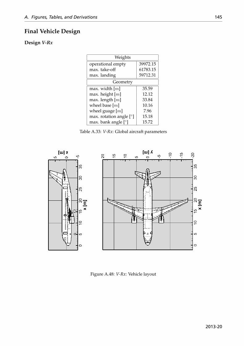
A. Figures, Tables, and Derivations 145
Final Vehicle Design
Design V-Rx
Weightsoperational empty 39972.15max. take-off 61783.15max. landing 59712.31
Geometrymax. width [m] 35.59max. height [m] 12.12max. length [m] 33.84wheel base [m] 10.16wheel guage [m] 7.96max. rotation angle [◦] 15.18max. bank angle [◦] 15.72
Table A.33: V-Rx: Global aircraft parameters
Figure A.48: V-Rx: Vehicle layout
2013-20
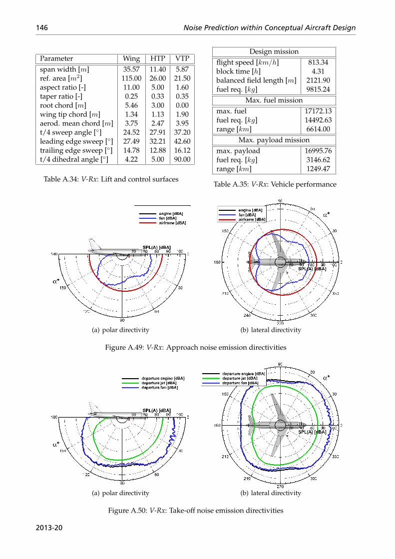
146 Noise Prediction within Conceptual Aircraft Design
Parameter Wing HTP VTPspan width [m] 35.57 11.40 5.87ref. area [m2] 115.00 26.00 21.50aspect ratio [-] 11.00 5.00 1.60taper ratio [-] 0.25 0.33 0.35root chord [m] 5.46 3.00 0.00wing tip chord [m] 1.34 1.13 1.90aerod. mean chord [m] 3.75 2.47 3.95t/4 sweep angle [◦] 24.52 27.91 37.20leading edge sweep [◦] 27.49 32.21 42.60trailing edge sweep [◦] 14.78 12.88 16.12t/4 dihedral angle [◦] 4.22 5.00 90.00
Table A.34: V-Rx: Lift and control surfaces
Design missionflight speed [km/h] 813.34block time [h] 4.31balanced field length [m] 2121.90fuel req. [kg] 9815.24
Max. fuel missionmax. fuel 17172.13fuel req. [kg] 14492.63range [km] 6614.00
Max. payload missionmax. payload 16995.76fuel req. [kg] 3146.62range [km] 1249.47
Table A.35: V-Rx: Vehicle performance
(a) polar directivity (b) lateral directivity
Figure A.49: V-Rx: Approach noise emission directivities
(a) polar directivity (b) lateral directivity
Figure A.50: V-Rx: Take-off noise emission directivities
2013-20
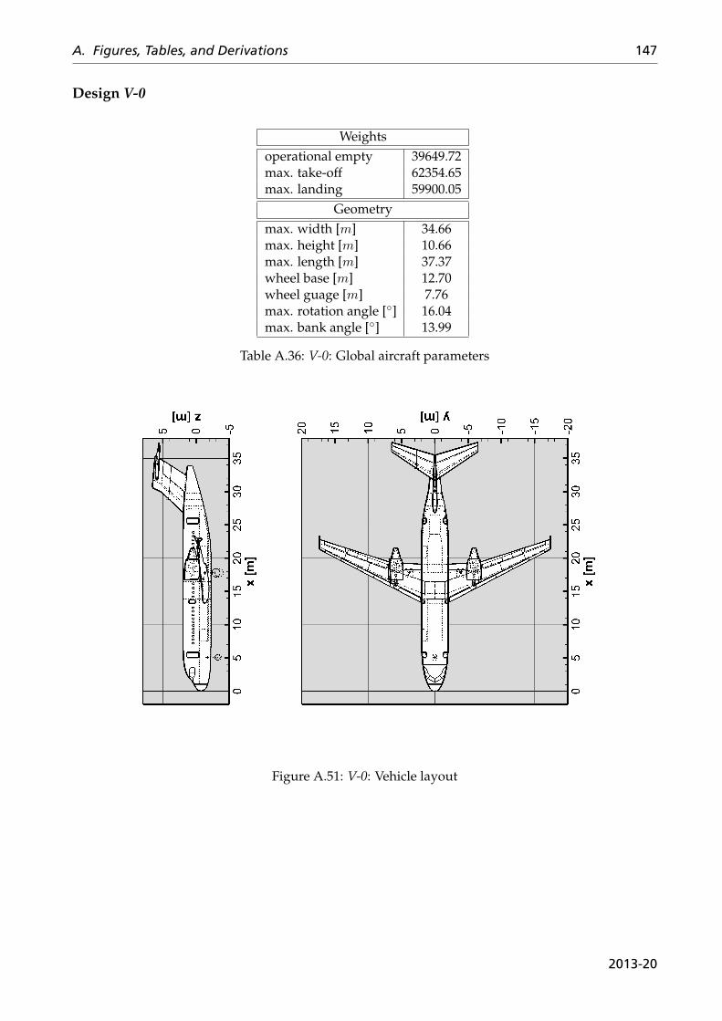
A. Figures, Tables, and Derivations 147
Design V-0
Weightsoperational empty 39649.72max. take-off 62354.65max. landing 59900.05
Geometrymax. width [m] 34.66max. height [m] 10.66max. length [m] 37.37wheel base [m] 12.70wheel guage [m] 7.76max. rotation angle [◦] 16.04max. bank angle [◦] 13.99
Table A.36: V-0: Global aircraft parameters
Figure A.51: V-0: Vehicle layout
2013-20
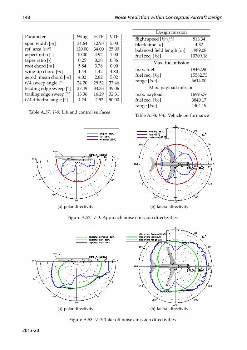
148 Noise Prediction within Conceptual Aircraft Design
Parameter Wing HTP VTPspan width [m] 34.64 12.93 5.00ref. area [m2] 120.00 34.00 25.00aspect ratio [-] 10.00 4.92 1.00taper ratio [-] 0.25 0.38 0.86root chord [m] 5.84 3.78 0.00wing tip chord [m] 1.44 1.42 4.80aerod. mean chord [m] 4.02 2.82 5.02t/4 sweep angle [◦] 24.20 29.52 37.46leading edge sweep [◦] 27.49 33.33 39.06trailing edge sweep [◦] 13.36 16.29 32.31t/4 dihedral angle [◦] 4.24 -2.92 90.00
Table A.37: V-0: Lift and control surfaces
Design missionflight speed [km/h] 813.34block time [h] 4.32balanced field length [m] 1989.08fuel req. [kg] 10709.18
Max. fuel missionmax. fuel 18462.90fuel req. [kg] 15582.73range [km] 6614.00
Max. payload missionmax. payload 16995.76fuel req. [kg] 3840.17range [km] 1404.19
Table A.38: V-0: Vehicle performance
(a) polar directivity (b) lateral directivity
Figure A.52: V-0: Approach noise emission directivities
(a) polar directivity (b) lateral directivity
Figure A.53: V-0: Take-off noise emission directivities
2013-20
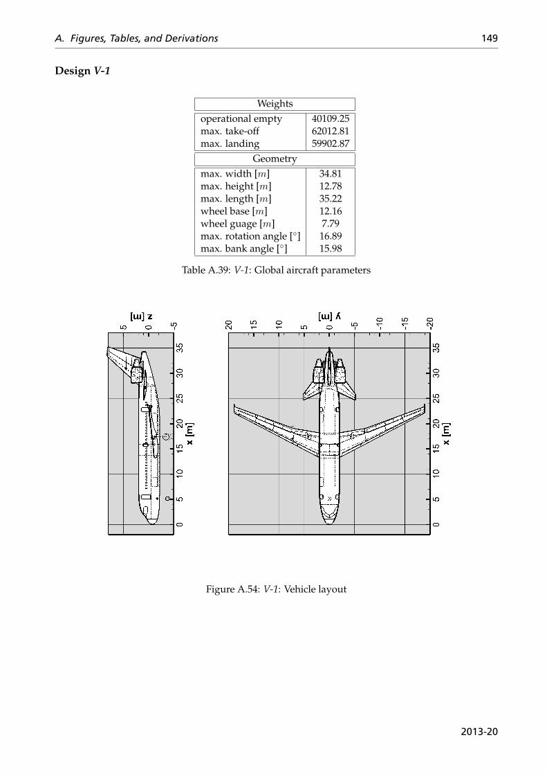
A. Figures, Tables, and Derivations 149
Design V-1
Weightsoperational empty 40109.25max. take-off 62012.81max. landing 59902.87
Geometrymax. width [m] 34.81max. height [m] 12.78max. length [m] 35.22wheel base [m] 12.16wheel guage [m] 7.79max. rotation angle [◦] 16.89max. bank angle [◦] 15.98
Table A.39: V-1: Global aircraft parameters
Figure A.54: V-1: Vehicle layout
2013-20
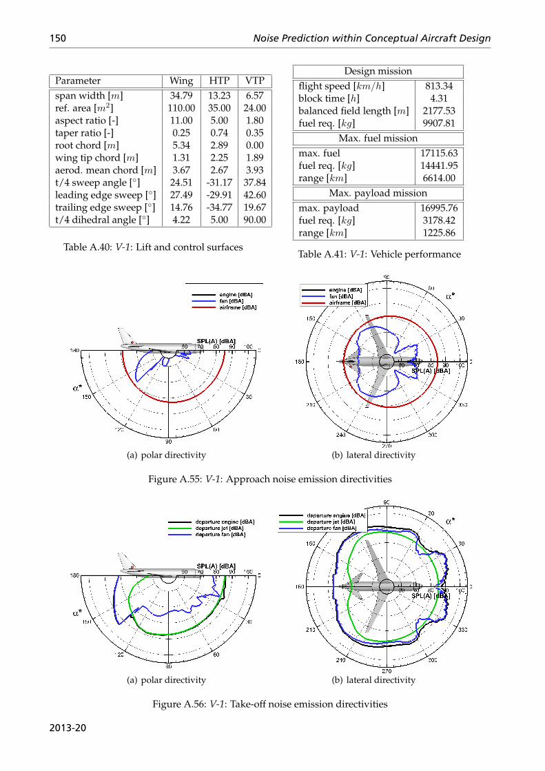
150 Noise Prediction within Conceptual Aircraft Design
Parameter Wing HTP VTPspan width [m] 34.79 13.23 6.57ref. area [m2] 110.00 35.00 24.00aspect ratio [-] 11.00 5.00 1.80taper ratio [-] 0.25 0.74 0.35root chord [m] 5.34 2.89 0.00wing tip chord [m] 1.31 2.25 1.89aerod. mean chord [m] 3.67 2.67 3.93t/4 sweep angle [◦] 24.51 -31.17 37.84leading edge sweep [◦] 27.49 -29.91 42.60trailing edge sweep [◦] 14.76 -34.77 19.67t/4 dihedral angle [◦] 4.22 5.00 90.00
Table A.40: V-1: Lift and control surfaces
Design missionflight speed [km/h] 813.34block time [h] 4.31balanced field length [m] 2177.53fuel req. [kg] 9907.81
Max. fuel missionmax. fuel 17115.63fuel req. [kg] 14441.95range [km] 6614.00
Max. payload missionmax. payload 16995.76fuel req. [kg] 3178.42range [km] 1225.86
Table A.41: V-1: Vehicle performance
(a) polar directivity (b) lateral directivity
Figure A.55: V-1: Approach noise emission directivities
(a) polar directivity (b) lateral directivity
Figure A.56: V-1: Take-off noise emission directivities
2013-20

A. Figures, Tables, and Derivations 151
Design V-2
Weightsoperational empty 38005.21max. take-off 60541.78max. landing 58158.99
Geometrymax. width [m] 31.64max. height [m] 8.14max. length [m] 36.61wheel base [m] 12.38wheel guage [m] 4.62max. rotation angle [◦] 10.94max. bank angle [◦] 20.63
Table A.42: V-2: Global aircraft parameters
Figure A.57: V-2: Vehicle layout
2013-20
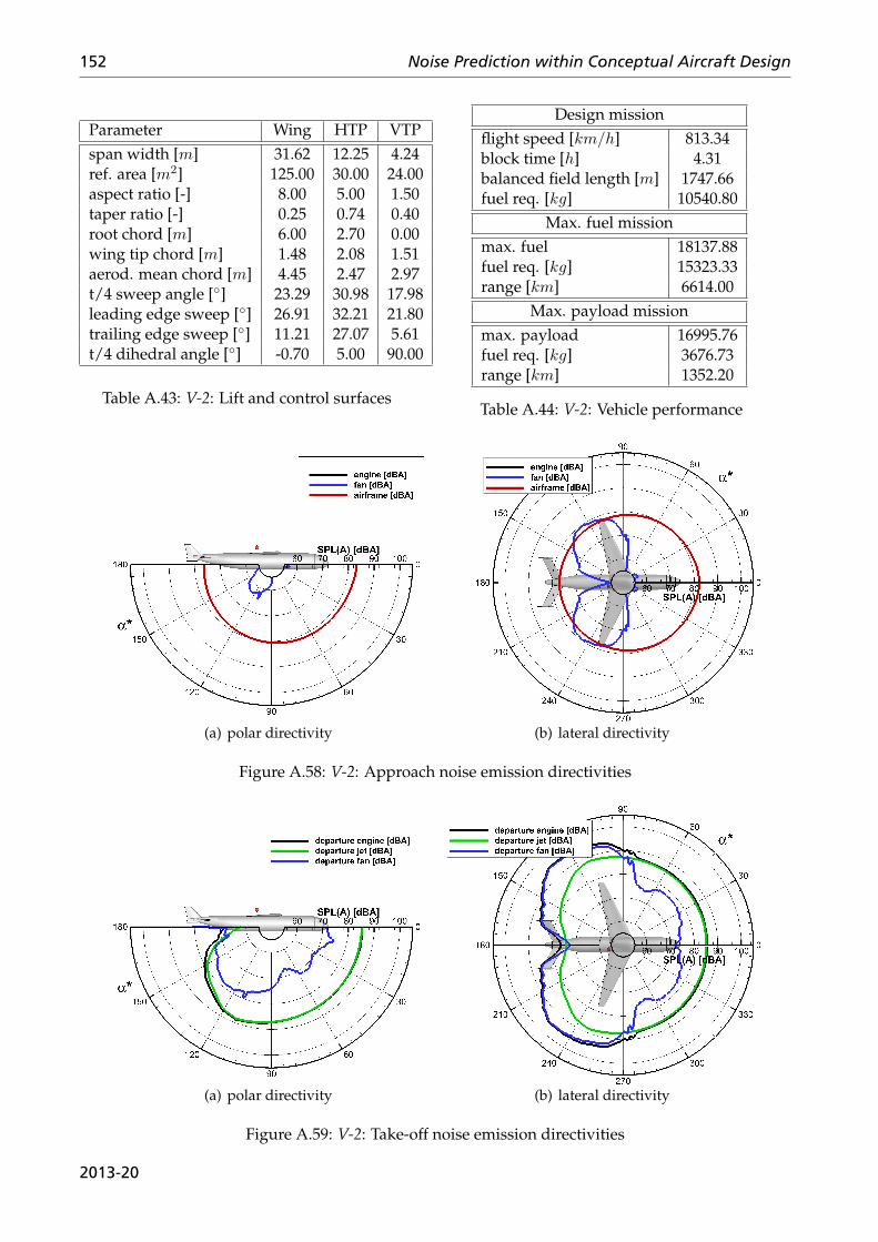
152 Noise Prediction within Conceptual Aircraft Design
Parameter Wing HTP VTPspan width [m] 31.62 12.25 4.24ref. area [m2] 125.00 30.00 24.00aspect ratio [-] 8.00 5.00 1.50taper ratio [-] 0.25 0.74 0.40root chord [m] 6.00 2.70 0.00wing tip chord [m] 1.48 2.08 1.51aerod. mean chord [m] 4.45 2.47 2.97t/4 sweep angle [◦] 23.29 30.98 17.98leading edge sweep [◦] 26.91 32.21 21.80trailing edge sweep [◦] 11.21 27.07 5.61t/4 dihedral angle [◦] -0.70 5.00 90.00
Table A.43: V-2: Lift and control surfaces
Design missionflight speed [km/h] 813.34block time [h] 4.31balanced field length [m] 1747.66fuel req. [kg] 10540.80
Max. fuel missionmax. fuel 18137.88fuel req. [kg] 15323.33range [km] 6614.00
Max. payload missionmax. payload 16995.76fuel req. [kg] 3676.73range [km] 1352.20
Table A.44: V-2: Vehicle performance
(a) polar directivity (b) lateral directivity
Figure A.58: V-2: Approach noise emission directivities
(a) polar directivity (b) lateral directivity
Figure A.59: V-2: Take-off noise emission directivities
2013-20
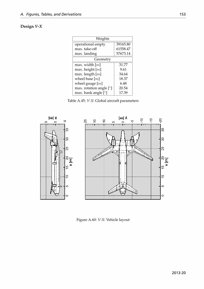
A. Figures, Tables, and Derivations 153
Design V-X
Weightsoperational empty 39165.80max. take-off 61558.47max. landing 57673.14
Geometrymax. width [m] 31.77max. height [m] 9.61max. length [m] 34.64wheel base [m] 18.37wheel guage [m] 6.48max. rotation angle [◦] 20.54max. bank angle [◦] 17.39
Table A.45: V-X: Global aircraft parameters
Figure A.60: V-X: Vehicle layout
2013-20
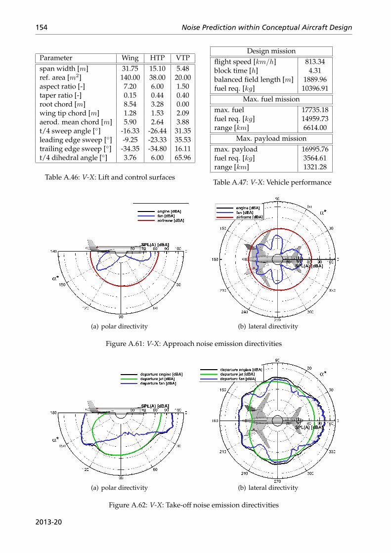
154 Noise Prediction within Conceptual Aircraft Design
Parameter Wing HTP VTPspan width [m] 31.75 15.10 5.48ref. area [m2] 140.00 38.00 20.00aspect ratio [-] 7.20 6.00 1.50taper ratio [-] 0.15 0.44 0.40root chord [m] 8.54 3.28 0.00wing tip chord [m] 1.28 1.53 2.09aerod. mean chord [m] 5.90 2.64 3.88t/4 sweep angle [◦] -16.33 -26.44 31.35leading edge sweep [◦] -9.25 -23.33 35.53trailing edge sweep [◦] -34.35 -34.80 16.11t/4 dihedral angle [◦] 3.76 6.00 65.96
Table A.46: V-X: Lift and control surfaces
Design missionflight speed [km/h] 813.34block time [h] 4.31balanced field length [m] 1889.96fuel req. [kg] 10396.91
Max. fuel missionmax. fuel 17735.18fuel req. [kg] 14959.73range [km] 6614.00
Max. payload missionmax. payload 16995.76fuel req. [kg] 3564.61range [km] 1321.28
Table A.47: V-X: Vehicle performance
(a) polar directivity (b) lateral directivity
Figure A.61: V-X: Approach noise emission directivities
(a) polar directivity (b) lateral directivity
Figure A.62: V-X: Take-off noise emission directivities
2013-20
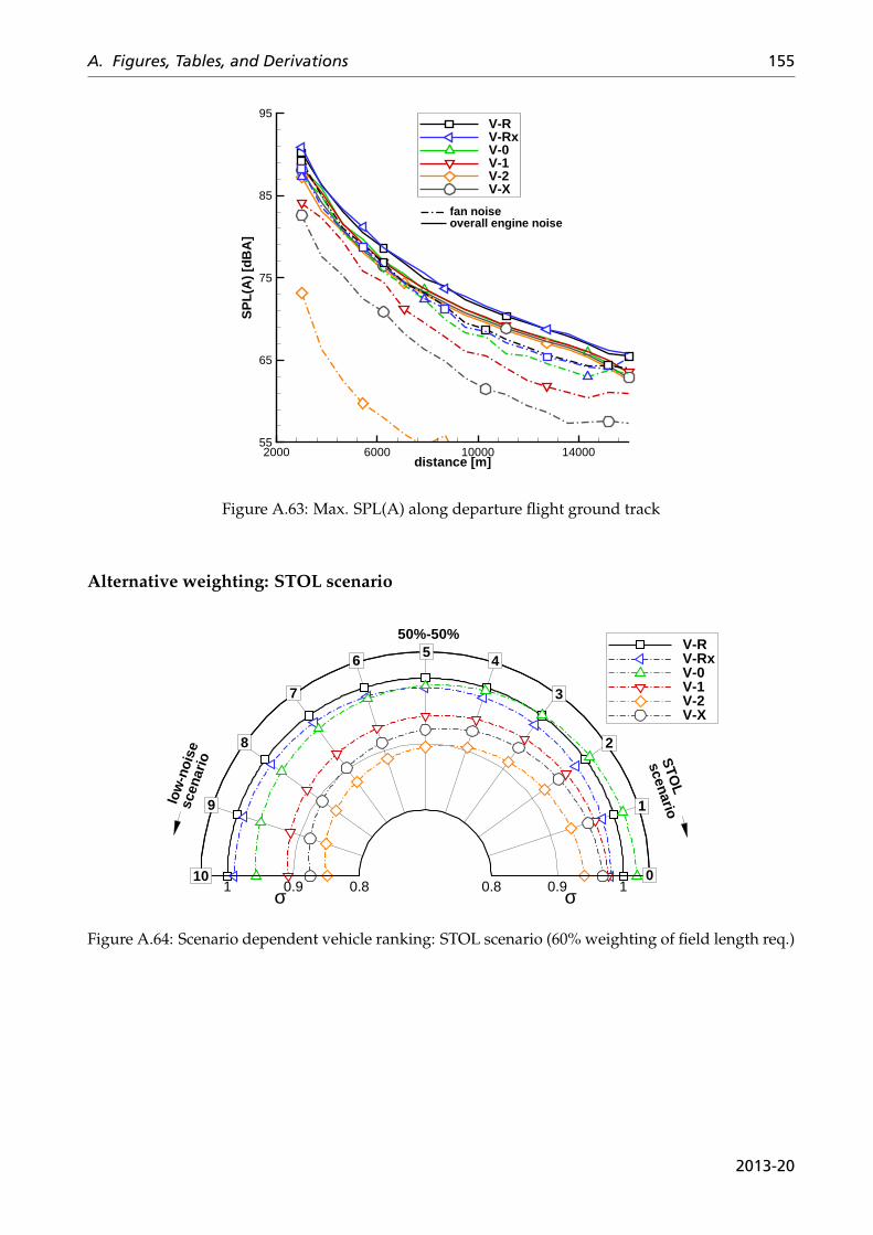
A. Figures, Tables, and Derivations 155
distance [m]
SP
L(A
) [d
BA
]
2000 6000 10000 1400055
65
75
85
95V-RV-RxV-0V-1V-2V-X
fan noiseoverall engine noise
Figure A.63: Max. SPL(A) along departure flight ground track
Alternative weighting: STOL scenario
σ σ0.80.8 0.90.9 11
V-RV-RxV-0V-1V-2V-X
STO
L
scenario
10
low
-noi
sesc
enar
io
0
1
2
3
45
6
7
8
9
50%-50%
Figure A.64: Scenario dependent vehicle ranking: STOL scenario (60% weighting of field length req.)
2013-20

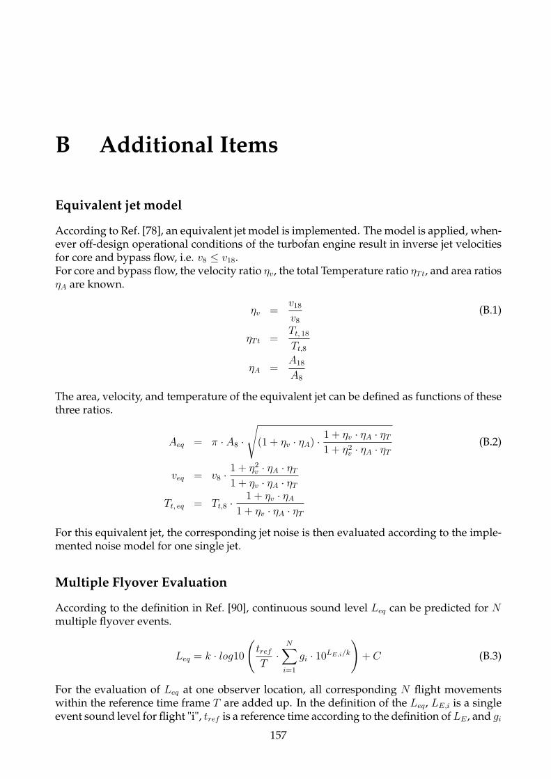
B Additional Items
Equivalent jet model
According to Ref. [78], an equivalent jet model is implemented. The model is applied, when-ever off-design operational conditions of the turbofan engine result in inverse jet velocitiesfor core and bypass flow, i.e. v8 ≤ v18.For core and bypass flow, the velocity ratio ηv, the total Temperature ratio ηTt, and area ratiosηA are known.
ηv =v18v8
(B.1)
ηTt =Tt, 18
Tt,8
ηA =A18
A8
The area, velocity, and temperature of the equivalent jet can be defined as functions of thesethree ratios.
Aeq = π · A8 ·
√(1 + ηv · ηA) ·
1 + ηv · ηA · ηT1 + η2v · ηA · ηT
(B.2)
veq = v8 ·1 + η2v · ηA · ηT1 + ηv · ηA · ηT
Tt, eq = Tt,8 ·1 + ηv · ηA
1 + ηv · ηA · ηT
For this equivalent jet, the corresponding jet noise is then evaluated according to the imple-mented noise model for one single jet.
Multiple Flyover Evaluation
According to the definition in Ref. [90], continuous sound level Leq can be predicted for Nmultiple flyover events.
Leq = k · log10
(trefT
·N∑i=1
gi · 10LE,i/k
)+ C (B.3)
For the evaluation of Leq at one observer location, all corresponding N flight movementswithin the reference time frame T are added up. In the definition of the Leq, LE,i is a singleevent sound level for flight "i", tref is a reference time according to the definition of LE , and gi
157
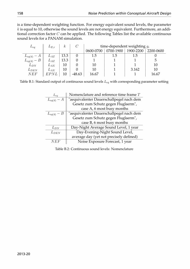
158 Noise Prediction within Conceptual Aircraft Design
is a time-dependent weighting function. For energy equivalent sound levels, the parameterk is equal to 10, otherwise the sound levels are not energy equivalent. Furthermore, an addi-tional correction factor C can be applied. The following Tables list the available continuoussound levels for a PANAM simulation.
Leq LE,i k C time-dependent weighting gi0600-0700 0700-1900 1900-2200 2200-0600
Leq(4) − A LAZ 13.3 0 1.5 1.5 1.5 0Leq(4) −B LAZ 13.3 0 1 1 1 5
LDN LAX 10 0 10 1 1 10LDEN LAX 10 0 10 1 3.162 10NEF EPNL 10 -48.63 16.67 1 1 16.67
Table B.1: Standard output of continuous sound levels Leq with corresponding parameter setting
Leq Nomenclature and reference time frame TLeq(4) − A "aequivalenter Dauerschallpegel nach dem
Gesetz zum Schutz gegen Fluglaerm",case A, 6 most busy months
Leq(4) −B "aequivalenter Dauerschallpegel nach demGesetz zum Schutz gegen Fluglaerm",
case B, 6 most busy monthsLDN Day-Night Average Sound Level, 1 yearLDEN Day-Evening-Night Sound Level,
average day (yet not precisely defined)NEF Noise Exposure Forecast, 1 year
Table B.2: Continuous sound levels: Nomenclature
2013-20
List of Figures
1.1 Ten thousands of people demonstrate in 2011 against Berlin’s new interna-tional airport BBI3 . . . . . . . . . . . . . . . . . . . . . . . . . . . . . . . . . . . 2
3.1 Noise prediction concept . . . . . . . . . . . . . . . . . . . . . . . . . . . . . . . 16
3.2 Coordinate systems and emission angles . . . . . . . . . . . . . . . . . . . . . . 17
3.3 Impact of geometry parameters on noise emission (note: depicted is the cosineof the sweep angle) . . . . . . . . . . . . . . . . . . . . . . . . . . . . . . . . . . 28
3.4 Station numbering for turbofan and turbojet engines10 . . . . . . . . . . . . . . 29
3.5 Engine noise spectra, emission angle α∗ = 40° . . . . . . . . . . . . . . . . . . . 34
3.6 Engine noise spectra, emission angle α∗ = 135° . . . . . . . . . . . . . . . . . . 34
3.7 PANAM acoustical analogous model . . . . . . . . . . . . . . . . . . . . . . . . 48
4.1 Reference Aircraft A319-100: PrADO payload range diagram . . . . . . . . . . 50
4.2 PrADO flight simulation for A319-100 . . . . . . . . . . . . . . . . . . . . . . . 51
4.3 SPL(A) emission directivities . . . . . . . . . . . . . . . . . . . . . . . . . . . . 52
4.4 Ground noise impact: Noise source ranking . . . . . . . . . . . . . . . . . . . . 53
4.5 Influence of source altitude and ground attenuation: max. levels and time-level-history . . . . . . . . . . . . . . . . . . . . . . . . . . . . . . . . . . . . . . 55
4.6 Influence of flight velocity: max. levels and time-level-history . . . . . . . . . 57
4.7 Influence of configurational setting: max. level and time-level-history . . . . . 58
4.8 Parchim Campaign 2006: Observer locations . . . . . . . . . . . . . . . . . . . 60
4.9 Parchim Campaign 2006: departure rec003 . . . . . . . . . . . . . . . . . . . . . 61
4.10 Parchim Campaign 2006: approach rec004 . . . . . . . . . . . . . . . . . . . . . 63
4.11 Parchim Campaign: Sound Exposure Level (SEL) . . . . . . . . . . . . . . . . 64
5.1 Reference aircraft cabin layout . . . . . . . . . . . . . . . . . . . . . . . . . . . . 69
5.2 Design Evolution Chart . . . . . . . . . . . . . . . . . . . . . . . . . . . . . . . 76
5.3 Performance indicators: all design variants . . . . . . . . . . . . . . . . . . . . 77
5.4 Scenario dependent vehicle ranking . . . . . . . . . . . . . . . . . . . . . . . . 81
5.5 Max. SPL(A) along approach flight ground track . . . . . . . . . . . . . . . . . 82
5.6 Vehicle V-2: Engine noise SPL(A) directivities for geared turbofan versusscaled reference engine . . . . . . . . . . . . . . . . . . . . . . . . . . . . . . . . 85
159
160 Noise Prediction within Conceptual Aircraft Design
5.7 CROR: vehicle layout . . . . . . . . . . . . . . . . . . . . . . . . . . . . . . . . . 87
5.8 CROR: polar noise directivity . . . . . . . . . . . . . . . . . . . . . . . . . . . . 88
5.9 Frankfurt Airport: Departing and approaching Airtraffic routing16 . . . . . . 90
5.10 Helical Noise Abatement Procedure (HeNAP), Ref. [125] . . . . . . . . . . . . 91
5.11 Parametric Noise Prediction for Airspace Routing . . . . . . . . . . . . . . . . 92
6.1 Take-off SPL spectrum: V-R vs. V-2 . . . . . . . . . . . . . . . . . . . . . . . . . 94
A.1 Atmospheric sound absorption . . . . . . . . . . . . . . . . . . . . . . . . . . . 107
A.2 Sound Pressure Level: A-weighting . . . . . . . . . . . . . . . . . . . . . . . . 107
A.3 Predicted ground attenuation for flyover event in 500 m altitude . . . . . . . . 107
A.4 EPNL predictions: Aircraft noise source ranking . . . . . . . . . . . . . . . . . 108
A.5 Noise isocontour areas along simplified approach trajectory . . . . . . . . . . 108
A.6 Influence of flight velocity: noise emission directivity (in 80 m source distance) 109
A.7 Influence of configurational setting: noise emission directivity (in 80 m sourcedistance) . . . . . . . . . . . . . . . . . . . . . . . . . . . . . . . . . . . . . . . . 110
A.8 V-r oew breakdown . . . . . . . . . . . . . . . . . . . . . . . . . . . . . . . . . . 112
A.9 V-r design mission mass breakdown . . . . . . . . . . . . . . . . . . . . . . . . 112
A.10 V-r geometry layout . . . . . . . . . . . . . . . . . . . . . . . . . . . . . . . . . . 112
A.11 V-r noise emission directivities . . . . . . . . . . . . . . . . . . . . . . . . . . . 113
A.12 Parchim Flyover Campaign: Departure procedures . . . . . . . . . . . . . . . 115
A.13 Parchim Flyover Campaign: Approach procedures . . . . . . . . . . . . . . . . 116
A.14 Predicted vs. measured departure SPL(A) time-history: ground mics alongflight ground track . . . . . . . . . . . . . . . . . . . . . . . . . . . . . . . . . . 117
A.15 Predicted vs. measured departure SPL(A) time-history: ground mics withlateral offset to flight ground track, 1 . . . . . . . . . . . . . . . . . . . . . . . . 118
A.16 Predicted vs. measured departure SPL(A) time-history: ground mics withlateral offset to flight ground track, 2 . . . . . . . . . . . . . . . . . . . . . . . . 119
A.17 Predicted vs. measured approach SPL(A) time-history: ground mics alongflight ground track . . . . . . . . . . . . . . . . . . . . . . . . . . . . . . . . . . 120
A.18 Predicted vs. measured approach SPL(A) time-history: ground mics withlateral offset to flight ground track, 1 . . . . . . . . . . . . . . . . . . . . . . . . 121
A.19 Predicted vs. measured approach SPL(A) time-history: ground mics withlateral offset to flight ground track, 2 . . . . . . . . . . . . . . . . . . . . . . . . 122
A.20 Parchim Campaign: Departure procedures, predicted vs. measured SEL ("o"indicates corrupted measurements) . . . . . . . . . . . . . . . . . . . . . . . . . 123
A.21 Parchim Campaign: Approach procedures, predicted vs. measured SEL ("o"indicates corrupted measurements) . . . . . . . . . . . . . . . . . . . . . . . . . 124
A.22 v-r vehicle layout: parameter variation 1 . . . . . . . . . . . . . . . . . . . . . . 125
A.23 v-r aircraft noise induced awakenings: parameter variation . . . . . . . . . . . 126
A.24 Performance indicators: v-r variants . . . . . . . . . . . . . . . . . . . . . . . . 126
2013-20
LIST OF FIGURES 161
A.25 v-0 vehicle layout: parameter variation 1 . . . . . . . . . . . . . . . . . . . . . . 127
A.26 v-0 vehicle layout: parameter variation 2 . . . . . . . . . . . . . . . . . . . . . . 128
A.27 v-0 aircraft noise induced awakenings . . . . . . . . . . . . . . . . . . . . . . . 129
A.28 v-0 performance indicators: parameter variation . . . . . . . . . . . . . . . . . 129
A.29 v-1 vehicle layout: parameter variation 1 . . . . . . . . . . . . . . . . . . . . . . 130
A.30 v-1 vehicle layout: parameter variation 2 . . . . . . . . . . . . . . . . . . . . . . 131
A.31 v-1 aircraft noise induced awakenings . . . . . . . . . . . . . . . . . . . . . . . 132
A.32 v-1 performance indicators: parameter variation 1 & 2 . . . . . . . . . . . . . . 132
A.33 v-1-1 vehicle layout: parameter variation 1 . . . . . . . . . . . . . . . . . . . . 133
A.34 v-1-1 vehicle layout: parameter variation 2 . . . . . . . . . . . . . . . . . . . . 134
A.35 v-1-1 aircraft noise induced awakenings . . . . . . . . . . . . . . . . . . . . . . 135
A.36 v-1-1 performance indicators: parameter variation 1 & 2 . . . . . . . . . . . . . 135
A.37 v-1-2 vehicle layout: parameter variation 1 . . . . . . . . . . . . . . . . . . . . 136
A.38 v-1-2 vehicle layout: parameter variation 2 . . . . . . . . . . . . . . . . . . . . 137
A.39 v-1-2 aircraft noise induced awakenings . . . . . . . . . . . . . . . . . . . . . . 138
A.40 v-1-1 and v-1-2 performance indicators: parameter variation 1 & 2 . . . . . . 138
A.41 v-2 vehicle layout: parameter variation 1 . . . . . . . . . . . . . . . . . . . . . . 139
A.42 v-2 vehicle layout: parameter variation 2 . . . . . . . . . . . . . . . . . . . . . . 140
A.43 v-2 aircraft noise induced awakenings . . . . . . . . . . . . . . . . . . . . . . . 141
A.44 v-2 performance indicators: parameter variation 1 & 2 . . . . . . . . . . . . . . 141
A.45 v-x vehicle layout: parameter variation . . . . . . . . . . . . . . . . . . . . . . . 142
A.46 v-x aircraft noise induced awakenings: parameter variation . . . . . . . . . . . 143
A.47 v-x performance indicators: parameter variation . . . . . . . . . . . . . . . . . 143
A.48 V-Rx: Vehicle layout . . . . . . . . . . . . . . . . . . . . . . . . . . . . . . . . . 145
A.49 V-Rx: Approach noise emission directivities . . . . . . . . . . . . . . . . . . . . 146
A.50 V-Rx: Take-off noise emission directivities . . . . . . . . . . . . . . . . . . . . . 146
A.51 V-0: Vehicle layout . . . . . . . . . . . . . . . . . . . . . . . . . . . . . . . . . . 147
A.52 V-0: Approach noise emission directivities . . . . . . . . . . . . . . . . . . . . . 148
A.53 V-0: Take-off noise emission directivities . . . . . . . . . . . . . . . . . . . . . . 148
A.54 V-1: Vehicle layout . . . . . . . . . . . . . . . . . . . . . . . . . . . . . . . . . . 149
A.55 V-1: Approach noise emission directivities . . . . . . . . . . . . . . . . . . . . . 150
A.56 V-1: Take-off noise emission directivities . . . . . . . . . . . . . . . . . . . . . . 150
A.57 V-2: Vehicle layout . . . . . . . . . . . . . . . . . . . . . . . . . . . . . . . . . . 151
A.58 V-2: Approach noise emission directivities . . . . . . . . . . . . . . . . . . . . . 152
A.59 V-2: Take-off noise emission directivities . . . . . . . . . . . . . . . . . . . . . . 152
A.60 V-X: Vehicle layout . . . . . . . . . . . . . . . . . . . . . . . . . . . . . . . . . . 153
A.61 V-X: Approach noise emission directivities . . . . . . . . . . . . . . . . . . . . 154
A.62 V-X: Take-off noise emission directivities . . . . . . . . . . . . . . . . . . . . . 154
2013-20

162 Noise Prediction within Conceptual Aircraft Design
A.63 Max. SPL(A) along departure flight ground track . . . . . . . . . . . . . . . . . 155
A.64 Scenario dependent vehicle ranking: STOL scenario (60% weighting of fieldlength req.) . . . . . . . . . . . . . . . . . . . . . . . . . . . . . . . . . . . . . . . 155
2013-20
List of Tables
4.1 Reference Aircraft A319-100: PrADO (P) weight predictions vs. manufacturerdata (M) [101] . . . . . . . . . . . . . . . . . . . . . . . . . . . . . . . . . . . . . 49
5.1 Reference vehicle performance parameters . . . . . . . . . . . . . . . . . . . . 72
6.1 Environmental and economical vehicle performance . . . . . . . . . . . . . . . 93
A.1 Horizontal, non-accelerated flight segments . . . . . . . . . . . . . . . . . . . . 108
A.2 Top Level Aircraft Requirements . . . . . . . . . . . . . . . . . . . . . . . . . . 111
A.3 V-r global aircraft parameters . . . . . . . . . . . . . . . . . . . . . . . . . . . . 111
A.4 V-r engine data . . . . . . . . . . . . . . . . . . . . . . . . . . . . . . . . . . . . 111
A.5 V-r lift and control surfaces . . . . . . . . . . . . . . . . . . . . . . . . . . . . . 111
A.6 V-r vehicle performance . . . . . . . . . . . . . . . . . . . . . . . . . . . . . . . 111
A.7 Parchim Flyover Campaign: Test Flights (standard procedures), according toRef. [100] . . . . . . . . . . . . . . . . . . . . . . . . . . . . . . . . . . . . . . . . 114
A.8 v-r variants: parameter variation 1 (wing area & aspect ratio) . . . . . . . . . . 125
A.9 v-r global aircraft parameters: parameter variation 1 . . . . . . . . . . . . . . . 125
A.10 v-0 variants: parameter variation 1 (wing area & aspect ratio) . . . . . . . . . . 127
A.11 v-0 global aircraft parameters: parameter variation 1 . . . . . . . . . . . . . . . 127
A.12 v-0 variants: parameter variation 2 (wing location & aspect ratio) . . . . . . . 128
A.13 v-0 global aircraft parameters: parameter variation 2 . . . . . . . . . . . . . . . 128
A.14 v-1 variants: parameter variation 1 (wing area & aspect ratio) . . . . . . . . . . 130
A.15 v-1 global aircraft parameters: parameter variation 1 . . . . . . . . . . . . . . . 130
A.16 v-1 variants: parameter variation 2 (wing location & aspect ratio) . . . . . . . 131
A.17 v-1 global aircraft parameters: parameter variation 2 . . . . . . . . . . . . . . . 131
A.18 v-1-1 variants: parameter variation 1 (VTP positioning & wing area) . . . . . . 133
A.19 v-1-1 global aircraft parameters: parameter variation 1 . . . . . . . . . . . . . . 133
A.20 v-1-1 variants: parameter variation 2 (wing area & VTP positioning) . . . . . . 134
A.21 v-1-1 global aircraft parameters: parameter variation 2 . . . . . . . . . . . . . . 134
A.22 v-1-2 variants: parameter variation 1 (HTP sweep angle & VTP area ratios) . . 136
A.23 v-1-2 global aircraft parameters: parameter variation 1 . . . . . . . . . . . . . . 136
A.24 v-1-2 variants: parameter variation 2 (HTP sweep angle & area) . . . . . . . . 137
163
A.25 v-1-2 global aircraft parameters: parameter variation 2 . . . . . . . . . . . . . . 137
A.26 v-2 variants: parameter variation 1 (wing area & aspect ratio) . . . . . . . . . . 139
A.27 v-2 global aircraft parameters: parameter variation 1 . . . . . . . . . . . . . . . 139
A.28 v-2 variants: parameter variation 2 (wing location & aspect ratio) . . . . . . . 140
A.29 v-2 global aircraft parameters: parameter variation 2 . . . . . . . . . . . . . . . 140
A.30 v-x variants: parameter variation (VTP positioning & wing area) . . . . . . . . 142
A.31 v-x global aircraft parameters: parameter variation 1 . . . . . . . . . . . . . . . 142
A.32 Scenario dependent vehicle variant ranking . . . . . . . . . . . . . . . . . . . . 144
A.33 V-Rx: Global aircraft parameters . . . . . . . . . . . . . . . . . . . . . . . . . . 145
A.34 V-Rx: Lift and control surfaces . . . . . . . . . . . . . . . . . . . . . . . . . . . . 146
A.35 V-Rx: Vehicle performance . . . . . . . . . . . . . . . . . . . . . . . . . . . . . . 146
A.36 V-0: Global aircraft parameters . . . . . . . . . . . . . . . . . . . . . . . . . . . 147
A.37 V-0: Lift and control surfaces . . . . . . . . . . . . . . . . . . . . . . . . . . . . 148
A.38 V-0: Vehicle performance . . . . . . . . . . . . . . . . . . . . . . . . . . . . . . . 148
A.39 V-1: Global aircraft parameters . . . . . . . . . . . . . . . . . . . . . . . . . . . 149
A.40 V-1: Lift and control surfaces . . . . . . . . . . . . . . . . . . . . . . . . . . . . 150
A.41 V-1: Vehicle performance . . . . . . . . . . . . . . . . . . . . . . . . . . . . . . . 150
A.42 V-2: Global aircraft parameters . . . . . . . . . . . . . . . . . . . . . . . . . . . 151
A.43 V-2: Lift and control surfaces . . . . . . . . . . . . . . . . . . . . . . . . . . . . 152
A.44 V-2: Vehicle performance . . . . . . . . . . . . . . . . . . . . . . . . . . . . . . . 152
A.45 V-X: Global aircraft parameters . . . . . . . . . . . . . . . . . . . . . . . . . . . 153
A.46 V-X: Lift and control surfaces . . . . . . . . . . . . . . . . . . . . . . . . . . . . 154
A.47 V-X: Vehicle performance . . . . . . . . . . . . . . . . . . . . . . . . . . . . . . 154
B.1 Standard output of continuous sound levels Leq with corresponding parame-ter setting . . . . . . . . . . . . . . . . . . . . . . . . . . . . . . . . . . . . . . . . 158
B.2 Continuous sound levels: Nomenclature . . . . . . . . . . . . . . . . . . . . . . 158

Curriculum vitae of Eberhard-Lothar Bertsch
Educational History
Feb 2006 Diplom-Ingenieur Luft- und Raumfahrttechnik, Department ofAerospace Engineering, Universität Stuttgart, Stuttgart
July ’05 - Jan ’06 Final thesis (towards Diplom): "Numerical investigation of tur-bine blade film cooling", Institute of Applied ThermodynamicsITLR, Universität Stuttgart, and Rolls Royce, Berlin (Aerodynam-ics and Cooling Group)
Aug ’03 - Dec ’04 Master of Science Aerospace Engineering, Department ofAerospace and Ocean Engineering, Virginia Polytechnic Instituteand State University, Blacksburg, Virginia, USA
Jan ’04 - Dec ’04 Student thesis (towards Diplom): "Advanced Boundary ElementApproximation And Sound Quality Evaluation", Department ofAerospace and Ocean Engineering, Virginia Tech, and Instituteof Aero- and Gasdynamics IAG, Universität Stuttgart
Oct ’99 - Sept ’01 Vordiplom Luft- und Raumfahrttechnik, Department ofAerospace Engineering, Universität Stuttgart
Working Experience
April ’12 - present Research engineer at DLR’s Institute of Aerodynamics and FlowTechnology, Göttingen (aircraft system noise prediction)
• Initiator of an international workgroup on aircraft noisesimulation; ANSWeR (2012)
April ’06 - April ’12 Research engineer at DLR’s Institute of Aerodynamics and FlowTechnology, Braunschweig (conceptual aircraft design and air-craft system noise prediction)
• Initiator and organisator of an international workshop onactive high-lift technology (2011)
• Initiator of and principal investigator for a dedicated fly-over noise campaign with DLR’s flying testbed ATTAS(2009)
• Work package leader and substitute project manager forDLR project QSTOL (2006-2010)
• Scientific publications & presentations on national and in-ternational conferences, reviewer for the AIAA Journal ofAircraft
Contact information: [email protected] Göttingen, November 2012


ISSN 1434-8454
ISRN DLR-FB-2013-20