1st act global trajectory optimisation competition: results found at dlr
TRANSCRIPT

Acta Astronautica 61 (2007) 742–752www.elsevier.com/locate/actaastro
1stACT global trajectory optimisation competition:Results found at DLR
Bernd Dachwald∗, Andreas OhndorfGerman Aerospace Center (DLR), Institute of Space Simulation, Linder Hoehe, 51147 Cologne, Germany
Available online 25 April 2007
Abstract
This paper describes the DLR team solution method and results for ESA’s 1st ACT global trajectory optimisation competitionproblem. The other articles in this volume demonstrate that the design and the optimisation of low-thrust trajectories are usually avery difficult task that involves much experience and expert knowledge. We have used evolutionary neurocontrol—a method thatfuses artificial neural networks and evolutionary algorithms—to find a solution for the given low-thrust trajectory optimisationproblem. This method requires less experience/knowledge in astrodynamics and in optimal control theory than the traditionalmethods. In this paper, the implementation of evolutionary neurocontrol is outlined and its performance for the given problemis shown.© 2007 Elsevier Ltd. All rights reserved.
Keywords: Evolutionary neurocontrol; Global trajectory optimisation; Low-thrust propulsion; Kinetic impact; Asteroid deflection
1. Introduction
This paper deals with the problem of searching theoptimal trajectory for ESA’s 1st ACT (advanced con-cepts team) global trajectory optimisation competition(see the article “1st ACT global trajectory optimisationcompetition: problem description and summary of theresults” by Izzo in this volume).
In simple words, a spacecraft trajectory is the space-craft’s path from A (the initial body or orbit) to B (thetarget body or orbit). In general, the optimality of a tra-jectory can be defined according to several objectives,like minimising the transfer time or minimising the
∗ Corresponding author. Current address: German Aerospace Cen-ter (DLR), Mission Operations Section, Oberpfaffenhofen, 82234Wessling, Germany. Tel.: +49 8153 28 2772; fax: +49 8153 28 1455.
E-mail addresses: [email protected] (B. Dachwald),[email protected] (A. Ohndorf).
0094-5765/$ - see front matter © 2007 Elsevier Ltd. All rights reserved.doi:10.1016/j.actaastro.2007.03.011
propellant consumption. These objectives are mostlycompeting, so that one objective can only be optimisedat the cost of the other (Pareto-optimality). Spacecrafttrajectories are typically also classified with respect tothe final constraint(s). If, at arrival, the position rSC andthe velocity vSC of the spacecraft must match that ofthe target rT and vT, respectively, one has a rendezvousproblem. If only the position must match, one has aflyby problem. The problem of the 1st ACT global tra-jectory optimisation competition is an impact/deflectionproblem, which is a sub-class of the flyby problem thatrequires a special flyby-geometry (defined by a specialobjective function), as it will be shown below.
For spacecraft with high thrust, optimal trajecto-ries can be found relatively easily1 because few thrustphases are necessary. These are very short comparedto the transfer time, so that they can be approximated
1 As long as no planetary gravity assist manoeuvres are required.

B. Dachwald, A. Ohndorf / Acta Astronautica 61 (2007) 742–752 743
by singular events that change the spacecraft’s velocityinstantaneously while its position remains fixed. In con-trast to those high-thrust propulsion systems, low-thrustpropulsion systems must operate for a significant partof the transfer to generate the necessary �V . A low-thrust trajectory is obtained from the numerical inte-gration of the spacecraft’s equations of motion. Besidesthe inalterable external forces, the spacecraft trajectoryxSC[t]�(rSC[t], vSC[t]) is determined entirely by thethrust vector history F[t] (‘[t]’ denotes the time historyof the preceding variable, xSC is called the spacecraftstate). The thrust vector F(t) of low-thrust propulsionsystems is a continuous function of time. It is manip-ulated through the nu-dimensional spacecraft controlfunction u(t), which is also a continuous function oftime. Therefore, the trajectory optimisation problem isto find (in infinite-dimensional function space) the op-timal spacecraft control function u∗(t) that yields theoptimal trajectory x∗
SC[t]. This renders low-thrust tra-jectory optimisation a very difficult problem that cannotbe solved except for very simple cases. What can besolved, at least numerically, however, is a discrete ap-proximation of the problem. Dividing the allowed trans-fer time interval [t0, tf,max] into � finite elements, thediscrete trajectory optimisation problem is to find theoptimal spacecraft control history u∗[t̄] that yields theoptimal trajectory x∗
SC[t] (the symbol t̄ denotes a pointin discrete time; note that only the spacecraft controlhistory is discrete, whereas the trajectory is still continu-ous). Through discretisation, the problem of finding theoptimal control function u∗(t) in infinite-dimensionalfunction space is reduced to the problem of finding theoptimal control history u∗[t̄] in a finite but usually stillvery high-dimensional parameter space. For optimal-ity, some objective function J(+) must be maximised orsome cost function J(−) must be minimised (note thatevery objective function can be converted into a costfunction by J(−) = −J(+) and vice versa, so that wecan omit the index). In the following we assume that J
must be maximised.For the objective function of the 1st ACT global tra-
jectory optimisation competition problem, an asteroiddeflection problem, not only the propellant consump-tion (that defines the final mass at impact, mf �m(t̄f ))has to be minimised, but also the impact velocityvimp�vT(t̄f ) − vSC(t̄f ) has to be maximised, where vTis the target velocity vector and vSC is the spacecraftvelocity vector. It follows from simple astrodynam-ical reasoning that, for a given impact velocity, thedeflection is most effective if the impact is in the orbit-tangential direction at the targets perihelion, where vT ismaximal. For the ACT problem, all those sub-objectives
have been combined into the objective function
J�mf · |vimp · vT(t̄f )|, (1)
which is subject to maximisation. The spacecraft to beconsidered was a nuclear electric propelled spacecraftwith a specific impulse of Isp = 2500 s, a maximumthrust of 40 mN, and a wet mass of 1500 kg. The drymass was to be considered as zero. The spacecraft hadto be transferred from Earth to the target (asteroid 2001TW229) with a launch between the years 2010 and 2030and a maximum flight time of 30 years. The launcherwas assumed to provide a hyperbolic escape velocity of√
C3=2.5 km/s with no constraint on the escape asymp-tote direction. A last important constraint to be obeyedwas a minimum allowed solar distance of 0.2AU. Amore detailed description of the 1st ACT global trajec-tory optimisation competition and the given problemcan be found in the article by Izzo in this volume.
2. Evolutionary neurocontrol
2.1. Traditional local low-thrust trajectoryoptimisation methods
Traditionally, low-thrust trajectories are optimisedby the application of numerical optimal control meth-ods that are based on the calculus of variations. Thesemethods can be divided into direct methods, such asnonlinear programming (NLP) methods, and indirectmethods, such as neighbouring extremal and gradientmethods. All these methods can generally be classifiedas local trajectory optimisation methods, where the termoptimisation does not mean to find the best solution, butrather to find a solution. Prior to optimisation, the NLPmethods and the gradient methods require an initialguess for the control history, whereas the neighbouringextremal methods require an initial guess for the start-ing adjoint vector of Lagrange multipliers (costate vec-tor) [7]. Unfortunately, the convergence behaviour oflocal trajectory optimisation methods (especially of theindirect methods) is very sensitive to the initial guess,so that an adequate initial guess is often hard to find,even for an expert in astrodynamics and optimal con-trol theory. Similar initial guesses often produce verydissimilar optimisation results, so that the initial guesscannot be improved iteratively and trajectory optimisa-tion becomes more of an art than science [3]. Even ifthe optimiser finally converges to an optimal trajectory,this trajectory is typically close to the initial guess andthat is rarely close to the (unknown) global optimum.Because the optimisation process requires nearlypermanent expert attendance, the search for a good

744 B. Dachwald, A. Ohndorf / Acta Astronautica 61 (2007) 742–752
trajectory can become very time consuming and thusexpensive.
2.2. Evolutionary neurocontrol as a smart globallow-thrust trajectory optimisation method
To evade the drawbacks of local trajectory optimi-sation methods, a smart global optimisation methodwas adapted to low-thrust trajectory optimisationproblems by the author [4]. This method—termedevolutionary neurocontrol (ENC)—fuses artificial neu-ral networks (ANNs) and evolutionary algorithms(EAs) into so-called evolutionary neurocontrollers(ENCs). The implementation of ENC for low-thrusttrajectory optimisation was termed InTrance, whichstands for Intelligent Trajectory optimisation usingneurocontroller evolution. It does not require an initialguess or the attendance of a trajectory optimisationexpert. The remainder of this section will sketch theunderlying concepts of ENC and outline its applicationto low-thrust trajectory optimisation.
2.3. Low-thrust trajectory optimisation as a delayedreinforcement learning problem
One important and difficult class of learningproblems are reinforcement learning (RL) problems,where the optimal behaviour of the learning system(called agent) has to be learnt solely through interactionwith the environment, which gives an immediate ordelayed evaluation2 J (also called reward or reinforce-ment) [6,8]. The agent’s behaviour is defined by anassociative mapping from situations to actions S:X �→A.3 Within this paper, this associative mapping thatis typically called policy in the RL-related literature, istermed strategy. The optimal strategy S� of the agent isdefined as the one that maximises the sum of positivereinforcements and minimises the sum of negative rein-forcements over time. If, given a situation X ∈ X, theagent tries an action A ∈ A and the environment im-mediately returns an evaluation J (X, A) of the (X, A)
pair, one has an immediate reinforcement learningproblem. A more difficult class of learning problemsare delayed reinforcement learning problems, where theenvironment gives only a single evaluation J (X, A)[t],collectively for the sequence of (X, A) pairs occurringin time during the agent’s operation.
2 This evaluation is analogous to the objective function and willtherefore also be denoted by the symbol J .
3 X is called state space and A is called action space.
From the perspective of machine learning, a space-craft steering strategy may be defined as an asso-ciative mapping S that gives—at any time along thetrajectory—the current spacecraft control u from someinput X that comprises the variables that are relevantfor the optimal steering of the spacecraft (the currentstate of the relevant environment). Because the trajec-tory is the result of the spacecraft steering strategy, thetrajectory optimisation problem is actually a problemof finding the optimal spacecraft steering strategy S�.This is a delayed reinforcement learning problem be-cause a spacecraft steering strategy cannot be evaluatedbefore its trajectory is known under the given environ-mental conditions (constellation of the initial and thetarget body, etc.) and a reward can be given accordingto the fulfillment of the optimisation objective(s) andconstraint(s). One obvious way to implement spacecraftsteering strategies is to use ANNs because they havealready been applied successfully to learn associativemappings for a wide range of problems.
2.4. Evolutionary neurocontrol
For the work described within this paper, feedforwardANNs with a sigmoid neural transfer function have beenused. Such an ANN can be considered as a continuousparameterized function (called network function)
Nw:X ⊆ Rni → Y ⊆ (0, 1)no (2)
that maps from an ni-dimensional input space X ontoan no-dimensional output space Y. The parameter setw = {w1, . . . , wnw } of the network function comprisesthe nw internal parameters of the ANN, i.e., the weightsof the neuron connections and the biases of the neurons.
ANNs have already been applied successfully as neu-rocontrollers (NCs) for reinforcement learning prob-lems [5]. The most simple way to apply an ANN forcontrolling a dynamical system is by letting the ANNprovide the control u(t̄) = Y(t̄) ∈ Y from some inputX(t̄) ∈ X that contains the relevant information for thecontrol task. The NC’s behaviour is completely charac-terised by its network function Nw (that is—for a givennetwork topology—again completely characterised byits parameter set w). If the correct output is known fora set of given inputs (the training set), the differencebetween the resulting output and the known correct out-put can be utilized to learn the optimal network func-tion N��Nw� by adapting w in a way that minimisesthis difference for all input/output pairs in the train-ing set. A variety of learning algorithms have been de-veloped for this kind of learning, the backpropagationalgorithm being the most widely known. Unfortunately,

B. Dachwald, A. Ohndorf / Acta Astronautica 61 (2007) 742–752 745
learning algorithms that rely on a training set fail whenthe correct output for a given input is not known, as it isthe case for delayed reinforcement learning problems.EAs may be used for determining N� in this case be-cause they have proven to be robust learning methodsfor ANNs [9–11]. EAs can be employed for searchingN� because w can be mapped onto a real-valued stringc (also called chromosome or individual) that providesan equivalent description of a network function.
2.5. Neurocontroller input and output
Two fundamental questions arise concerning theapplication of a NC for spacecraft steering:
(1) “What input should the NC get?” (or “What shouldthe NC know to steer the spacecraft?”) and
(2) “What output should the NC give?” (or “Whatshould the NC do to steer the spacecraft?”).
To be robust, a spacecraft steering strategy should betime independent: to determine the currently optimalspacecraft control u(t̄i ), the spacecraft steering strategyshould have to know—at any time step t̄i—only thecurrent spacecraft state xSC(t̄i ), the current target statexT(t̄i ), and the current propellant mass mP(t̄i ), henceS: {(xSC, xT, mP)} �→ {u}. The number of potential in-put sets, however, is still large because xSC and xT maybe given in coordinates of any reference frame (carte-sian, polar, orbital elements, etc.) and in combinationsof them. The difference xT − xSC may be used as well,also in coordinates of any reference frame and in com-binations of them. A potential input set is depicted inFig. 1.
At any time step t̄i , each output neuron j ∈{1, . . . , no} gives a value Yj (t̄i ) ∈ (0, 1). The numberof potential output sets is also large because there aremany alternatives to define u, and to calculate u fromY. The following approach gave good results for themajority of problems that have been investigated sofar: the NC provides a three-dimensional output vectord′′ ∈ (0, 1)3 from which a unit vector d is calculated via
d′�2d′′ −(1
11
)∈ (−1, 1)3 and d�d′/|d′|. (3)
This unit vector is interpreted as the desired thrust di-rection and is therefore called direction unit vector. Theoutput must also include the engine throttle 0���1, sothat u�(d, �), hence S: {(xSC, xT, mP)} �→ {d, �} (seeFig. 1). For bang-bang control, two alternative outputsmight be considered: (1) The output of the neuron that
Fig. 1. Example for a neurocontroller that implements a spacecraftsteering strategy.
is associated to the throttle u� is interpreted so that �=0if u� < 0.5 and � = 1 if u� �0.5. (2) Two output neu-rons (providing the output values u�=0 and u�=1) areused to determine the throttle. �=0 if u�=0 > u�=1 and�=1 if u�=0 �u�=1. Our preliminary calculations haveshown that method (2) is preferable.
2.6. Neurocontroller fitness assignment
In EAs, the optimality of a chromosome is ratedby a fitness function4 J . To make it easier to under-stand the implementation of the fitness function for theACT problem (which is described in Section 4), weshow in this section, how fitness functions might beimplemented for the more straightforward rendezvousand flyby problem.5 The optimality of a trajectorymight be defined with respect to various primary ob-jectives (e.g., transfer time or propellant consumption).When an ENC is used for trajectory optimisation, theaccuracies of the trajectory with respect to the finalconstraints must also be considered as secondaryoptimisation objectives because they are not enforcedotherwise. If, for example, the transfer time for a ren-dezvous is to be minimised, the fitness function mustinclude the transfer time T �t̄f − t̄0, the final distance tothe target �rf �|rT(t̄f )− rSC(t̄f )|, and the final relativevelocity to the target �vf �|vT(t̄f ) − vSC(t̄f )|, henceJ = J (T , �rf , �vf ). If, for example, the propellant
4 This fitness function is also analogous to the objective functionand will therefore also be denoted by the symbol J .
5 For the general flyby problem, the flyby velocity and the flybygeometry are arbitrary.

746 B. Dachwald, A. Ohndorf / Acta Astronautica 61 (2007) 742–752
mass for a flyby problem is to be minimised, T and�vf are not relevant, but the consumed propellant�mP must be included in the fitness function, henceJ = J (�mP, �rf ) in this case. Because the ENC un-likely generates a trajectory that satisfies the final con-straints exactly (�rf = 0 m, �vf = 0 m/s), a maximumallowed distance �rf,max and a maximum allowed rela-tive velocity �vf,max have to be defined. Using �rf,maxand �vf,max, the distance and relative velocity at thetarget can be normalized:
�Rf � �rf
�rf,maxand �Vf � �vf
�vf,max. (4)
Because in the beginning of the search process mostindividuals do not meet the final constraints with the re-quired accuracy (�Rf �1, �Vf �1), a maximum trans-fer time Tmax must be defined for the numerical inte-gration of the trajectory.
Sub-fitness functions may be defined with respect toall primary and secondary optimisation objectives. Itwas found that the performance of ENC strongly de-pends on an adequate choice of the sub-fitness func-tions and on their composition to the (overall) fitnessfunction. This is reasonable because the fitness functionhas not only to decide autonomously which trajectoriesare good and which are not, but also which trajectoriesmight be promising in the future optimisation process.The primary sub-fitness function
JmP�mP(t̄0)
2mP(t̄0) − mP(t̄f )− 1
3
and the secondary sub-fitness functions
Jr� log
(1
�Rf
)and Jv� log
(1
�Vf
)
were empirically found to produce good results for ren-dezvous and flyby trajectories, if the propellant con-sumption is to be minimised. Jr and Jv are positive,if the respective accuracy requirement is fulfilled andnegative, if it is not. Another empirical finding was thatthe search process should first concentrate on the accu-racy of the trajectory and then on the primary optimi-sation objective. Therefore, the sub-fitness function forthe primary optimisation objective is modified to
J ′mP
�{
0 if Jr < 0 ∨ Jv < 0,
JmP if Jr �0 ∧ Jv �0,
for the rendezvous problem and
J ′mP
�{
0 if Jr < 0,
JmP if Jr �0,
for the flyby problem.
To minimise the propellant mass for a rendezvous,for example, the following fitness function might beconceived:
J (�mP, �rf , �vf )�J ′mP
+ 1√�R2
f + �V 2f
.
To minimise the propellant mass for a flyby, only thepositions must match:
J (�mP, �rf )�J ′mP
+ 1
�Rf
.
2.7. Evolutionary neurocontroller design
Fig. 2 shows how an ENC may be applied for low-thrust trajectory optimisation. To find the optimal space-craft trajectory, the ENC method runs in two loops.Within the (inner) trajectory integration loop, an NCk steers the spacecraft according to its network func-tion Nwk
that is completely defined by its parameterset wk . The EA in the (outer) NC optimisation loopholds a population P = {c1 = w1, . . . , cq = wq} of NCparameter sets, and examines them for their suitability togenerate an optimal trajectory. Within the trajectory op-timisation loop, the NC takes the current spacecraft statexSC(t̄i∈{0,...,�−1}), the current target state xT(t̄i ), and thecurrent propellant mass mP(t̄i ) as input, and maps themonto the spacecraft control u(t̄i ), which is calculated inthe following way: the first three output values are in-terpreted as the components of d′′(t̄i ), from which thedirection unit vector d(t̄i ) is calculated via Eq. (3), andthe remaining (one or two) output value(s) determine(s)the current throttle �(t̄i ). Then, xSC(t̄i ), mP(t̄i ), and u(t̄i )
are inserted into the equations of motion and numeri-cally integrated over one time step to yield xSC(t̄i+1) andmP(t̄i+1). The new state is fed back into the NC. The tra-jectory integration loop stops when the final constraintsare met with sufficient accuracy (e.g., Jr �0, Jv �0)or when a given time limit is reached (t̄i+1 = t̄f,max).Then, back in the NC optimisation loop, the trajectory israted by the EA’s fitness function J (ck). The fitness ofck is crucial for its probability to reproduce and createoffspring. Under this selection pressure, the EA breedsmore and more suitable steering strategies that gener-ate better and better trajectories. Finally, the EA that isused within this work converges against a single steer-ing strategy, which gives in the best case a near-globallyoptimal trajectory x�
SC[t].Fig. 3 sketches the transformation of a chromosome
into a trajectory: by searching for the fittest individualc�, the EA searches for the optimal spacecraft trajectoryx�
SC[t].

B. Dachwald, A. Ohndorf / Acta Astronautica 61 (2007) 742–752 747
Fig. 2. Low-thrust trajectory optimisation using ENC.
chromosome/individual/string c=
NC parameter set w
NC network function N=
spacecraft control function u[t]
spacecraft steering strategy S
spacecraft trajectory xsc[t]
Fig. 3. Transformation of a chromosome into a trajectory.
3. Analysis of the ACT problem
Because the implementation of low-thrust gravity as-sist optimisation into InTrance is not yet solved suf-ficiently, we have only investigated direct trajectorieswithout gravity assists.
Our first step in finding a solution for the 1st ACTglobal trajectory optimisation competition problem wasto use some two-dimensional astrodynamic reasoningto guess the optimal launch and impact geometry. Onecan easily see from the objective function in Eq. (1)that it is advantageous to hit the target during one of itsperihelion passages (at 1.8815AU), where vT is max-imal (24.504 km/s). It is also clear from Eq. (1) that
the orbit-tangential component of the impact velocityhas to be maximised. Without gravity assists, the maxi-mal impact velocity comes from a retrograde orbit (forthe parabolic case it is 55.212 km/s). Unfortunately, wehave considered the �V to attain a retrograde orbit tobe too large for the given propulsion system, so that wehave excluded retrograde impact trajectories right fromthe beginning. This, however, is possible, as the resultsof other ACT competition participants have proved.6
Focusing on prograde orbits only, we have consideredthe impact velocity to be maximal from an orbit thathas its perihelion at the given solar distance limit of0.2AU and its aphelion at the target’s perihelion of1.8815AU. The impact velocity from this orbit wouldbe 14.985 km/s. Our next goal was to find the optimallaunch geometry for attaining this impact orbit. To dothis, we have first assumed an impulsive transfer with ahypothetical Isp=2500 s-engine. For an impulsive trans-fer, two launch options can be considered: (1) the firstimpulse raises the spacecraft’s aphelion to the target’sperihelion and the second impulse lowers the space-craft’s perihelion to 0.2AU. (2) The first impulse low-ers the spacecraft’s perihelion to 0.2AU and the secondimpulse raises the spacecraft’s aphelion to the target’sperihelion.
6 This is a good example of how even experts make decisionsthat prune the solution space in the wrong way, so that the globaloptimum becomes impossible to find.
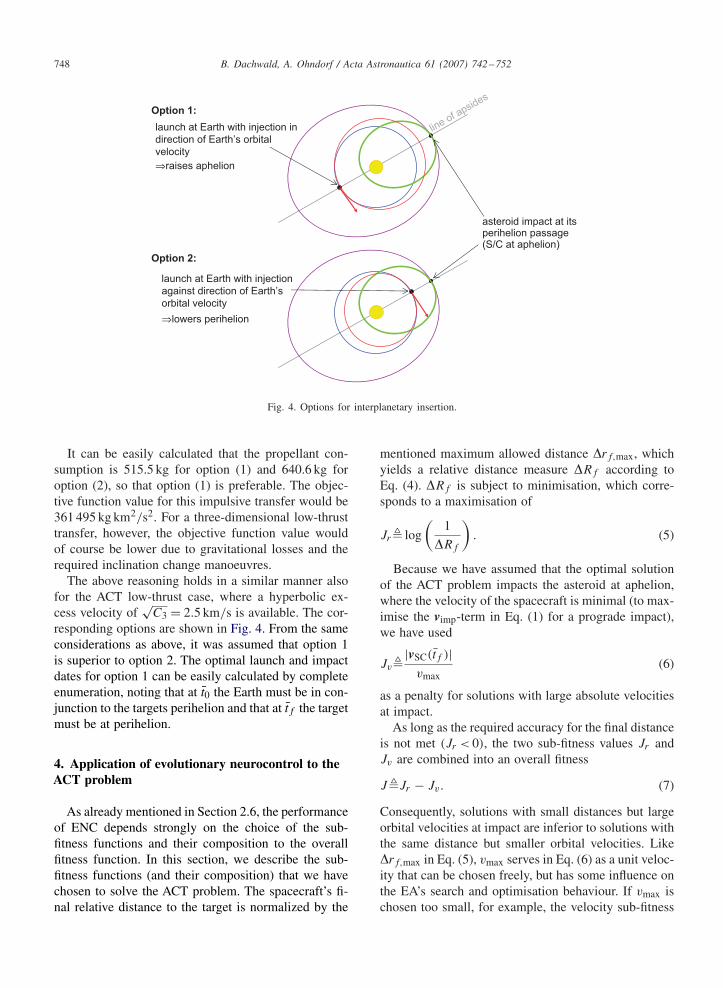
748 B. Dachwald, A. Ohndorf / Acta Astronautica 61 (2007) 742–752
launch at Earth with injection in
direction of Earth’s orbital
velocity
⇒raises aphelion
asteroid impact at itsperihelion passage (S/C at aphelion)
Option 1:
launch at Earth with injection
against direction of Earth’s
orbital velocity
⇒lowers perihelion
Option 2:
line of a
psides
Fig. 4. Options for interplanetary insertion.
It can be easily calculated that the propellant con-sumption is 515.5 kg for option (1) and 640.6 kg foroption (2), so that option (1) is preferable. The objec-tive function value for this impulsive transfer would be361 495 kg km2/s2. For a three-dimensional low-thrusttransfer, however, the objective function value wouldof course be lower due to gravitational losses and therequired inclination change manoeuvres.
The above reasoning holds in a similar manner alsofor the ACT low-thrust case, where a hyperbolic ex-cess velocity of
√C3 = 2.5 km/s is available. The cor-
responding options are shown in Fig. 4. From the sameconsiderations as above, it was assumed that option 1is superior to option 2. The optimal launch and impactdates for option 1 can be easily calculated by completeenumeration, noting that at t̄0 the Earth must be in con-junction to the targets perihelion and that at t̄f the targetmust be at perihelion.
4. Application of evolutionary neurocontrol to theACT problem
As already mentioned in Section 2.6, the performanceof ENC depends strongly on the choice of the sub-fitness functions and their composition to the overallfitness function. In this section, we describe the sub-fitness functions (and their composition) that we havechosen to solve the ACT problem. The spacecraft’s fi-nal relative distance to the target is normalized by the
mentioned maximum allowed distance �rf,max, whichyields a relative distance measure �Rf according toEq. (4). �Rf is subject to minimisation, which corre-sponds to a maximisation of
Jr� log
(1
�Rf
). (5)
Because we have assumed that the optimal solutionof the ACT problem impacts the asteroid at aphelion,where the velocity of the spacecraft is minimal (to max-imise the vimp-term in Eq. (1) for a prograde impact),we have used
Jv�|vSC(t̄f )|
vmax(6)
as a penalty for solutions with large absolute velocitiesat impact.
As long as the required accuracy for the final distanceis not met (Jr < 0), the two sub-fitness values Jr andJv are combined into an overall fitness
J�Jr − Jv . (7)
Consequently, solutions with small distances but largeorbital velocities at impact are inferior to solutions withthe same distance but smaller orbital velocities. Like�rf,max in Eq. (5), vmax serves in Eq. (6) as a unit veloc-ity that can be chosen freely, but has some influence onthe EA’s search and optimisation behaviour. If vmax ischosen too small, for example, the velocity sub-fitness

B. Dachwald, A. Ohndorf / Acta Astronautica 61 (2007) 742–752 749
dominates the one for the distance. If it is too large,solutions that precisely reach the target but have largeorbital velocities at impact are preferred. Finding suit-able values for this parameter requires some test runs.For our calculations, we have used values in the range6 km/s < vmax < 8 km/s.
We have employed Eq. (7) as long as the requireddistance at time of impact is not met and afterwards theACT objective function JACT�mf · |vimp · vT(t̄f )|, thus
J�{
Jr − Jv if Jr �0,
JACT if Jr > 0.(8)
Therefore, as it can be seen from Eq. (8), as long asthe required distance at time of impact is not achieved,the EA first tries to achieve the required distance throughJr , while at the same time trying to reduce the orbitalvelocity at impact through Jv . After having achievedthe required distance at time of impact, the optimisationprocess focuses solely on achieving the highest possiblevalue of JACT. Note that the value of JACT is alwayspositive and the value of Jr − Jv is always negative,as long as �rf > �rf,max, so that all trajectories withJr > 0 have a larger J than all trajectories with Jr �0.
5. Results
5.1. Solutions for variable thrust control
First, we have tried to find the optimal solution withvariable thrust control, i.e., 0���1. A 25–30–4 neu-rocontroller (25 input neurons, 1 hidden layer with 30hidden neurons, 4 output neurons) was used, where theinput neurons receive the current spacecraft state xSCand the current target body state xT in cartesian coordi-nates (12 values) and in polar coordinates (12 values),and the current propellant mass mP (1 value), and theoutput neurons define the thrust direction unit vector(3 values) and the throttle (1 value). To speed up the op-timisation process, we have set the transfer time to onlyTmax = 7660 days (21.0 years), which is less than theallowed maximum value of 30 years. For discretisation,this time interval was cut into � = 7660 finite elementsof equal length, so that the spacecraft was “allowed” tochange its thrust vector once every day. The final accu-racy limit was set to �rf,max = 100 000 km. As for allInTrance-calculations within this paper, the populationsize was set to q = 50 and a Runge–Kutta–Fehlbergmethod of order 4(5) with an absolute and a relative er-ror of 10−9 was used for the numerical integration ofthe trajectories.
Fig. 5 shows the trajectory of the best found InTrancesolution. Fig. 6 shows the same trajectory with the
y [A
U]
-1
-1
0
0
1
1
2
2
-1 -1
0
1
1.5
0.5
-0.5
x [AU]
-0.5
0.5
0
1.5
1
Fig. 5. Best InTrance-trajectory for variable thrust control.
-1
-1
0
0
1
1
2
2
-1
0 0
1
1.5
y [A
U]
1.5
1
0.5 0.5
-0.5-50
-1
x [AU]
Fig. 6. Best InTrance-thrusting profile for variable thrust control.
associated thrust steering profile, the current magnitudeand direction of the trust vector being denoted by thearrows. Table 1 shows the values of the relevant quan-tities.
Looking at Fig. 6, one can see that no coast phasesoccur. The spacecraft is thrusting all along the trajectorywith a relatively uniform throttle of 0.63 < � < 0.73.This is clearly suboptimal because the thrust should belarger at locations on the trajectory where the semi-major axis and the inclination can be changed very effi-ciently (i.e., at perihelion and the nodes, respectively).On the other hand, too much propellant is spent on parts

750 B. Dachwald, A. Ohndorf / Acta Astronautica 61 (2007) 742–752
Table 1Best InTrance solution for variable thrust control
Launch date 19 April 2014Hyperbolic excess velocity 2.5 km/sArrival date 09 April 2035Impact velocity 16.28552 km/sFlight time 7660 days (20.972 years)Final mass 768.0744 kgObjective function value 292 071.194 kg km2/s2
Final distance to target 99 952 km
of the trajectory where changing those orbital elementsis not that efficient.
One can also see from Fig. 5 that the farthest aphelionof the spacecraft’s trajectory is larger than the target’sperihelion, so that the line of apsides of the impact orbitis slightly rotated with respect to the target orbit’s line ofapsides. This shows that the optimiser performs a trade-off between the aphelion distance of the impact orbitand the consumed propellant. More propellant must bespent to attain a trajectory with a large aphelion, but thetransversal velocity component at impact is smaller, sothat the impact velocity is larger.
5.2. Solutions for bang-bang thrust control
After having obtained suboptimal results with vari-able thrust steering, we have tried to find the optimalsolution with bang-bang thrust control, i.e., � ∈ {0, 1}.After some preliminary test runs with different neuro-controller topologies, a 25–5 neurocontroller (25 inputneurons, no hidden layer, 5 output neurons) was used,where the input neurons receive the same input as forthe variable thrust control case, and the output neuronsdefine the thrust direction unit vector (3 values) and thethrottle according to option (2) in Section 2.5 (2 val-ues). The transfer time was set to Tmax = 10 894 days(29.8 years). For discretisation, this time interval wascut into � = 10 894 finite elements of equal length, sothat the spacecraft was again “allowed” to change itsthrust vector once every day. The final accuracy limitwas set to �rf,max = 10 000 000 km because InTrancehad difficulties in finding more accurate trajectories.
Fig. 7 shows the trajectory of the best found In-Trance solution. Fig. 8 shows the same trajectory withthe associated thrust steering profile, the current magni-tude and direction of the trust vector being denoted bythe arrows. Table 2 shows the values of the relevantquantities.
Looking at Fig. 8, one can see that now coast phasesoccur. The distribution of thrust and coast phases, how-ever, is clearly sub-optimal. The spacecraft is not thrust-
y [A
U]
-1
-1
0
0
1
1
2
2
-1 -1
0
0.5
0
1
1.5
1
1.5
0.5
-0.5
x [AU]
-0.5
Fig. 7. Best InTrance-trajectory for bang-bang thrust control.
y [
AU
]
-1
-1
0
0
1
1
2
2
-1 -1
0
1
1.51.5
0.5
-0.5
x [AU]
-0.5
0.5
1
0
Fig. 8. Best InTrance-thrusting profile for bang-bang thrust control.
Table 2Best InTrance solution for bang-bang thrust control
Launch date 15 April 2026Hyperbolic excess velocity 2.5 km/sArrival date 11 February 2056Impact velocity 18.58612 km/sFlight time 10 894 days (29.826 years)Final mass 838.3076 kgObjective function value 337 015.018 kg km2/s2
Final distance to target 9 991 860 km (0.0679AU)
ing at every passage close to perihelion and close tothe nodes, where the semi-major axis and the inclina-tion can be changed very efficiently. One can see from

B. Dachwald, A. Ohndorf / Acta Astronautica 61 (2007) 742–752 751
Fig. 7 that the farthest aphelion of the spacecraft trajec-tory is again larger than the target’s perihelion, so thatthe line of apsides of the impact orbit is again slightlyrotated with respect to the target orbit’s line of apsides.All in all, the trajectory and the distribution of the trustphases look very “ugly”.
5.3. Interpretation of the results
The results found by InTrance reveal that InTrancehas problems with locating the global optimum as wellas with fine-tuning the found solution locally. The latterproblem can be easily explained by noting that ENC isnot an analytic method.
We believe that the problem of locating the globaloptimum is associated with the current implementationof the fitness function. InTrance is not very suitable forproblems with very tight final constraints because it firstoptimises the accuracy of the final constraint and thenthe objective function. As soon as InTrance has found atrajectory that meets the accuracy of the final constraint,it is not allowed to “loose” it again because this wouldbe associated with a strong decrease of the fitness (seeEq. (8)). Therefore, the tighter the final constraint, theeasier InTrance gets stuck to a local optimum.
For the ACT problem, the basin of attraction of theglobal solution seems to be very small because slightestchanges in the thrusting profile result in “loosing” thefinal constraint. Therefore, InTrance searches for morerobust solutions w.r.t. changes in the thrusting profile,i.e., solutions that do not “loose” the final constrainteasily.
Two straightforward, though effortful, ways can beimagined to improve the results of InTrance on the 1stACT global trajectory optimisation competition prob-lem: (1) InTrance should be hybridized with an analyt-ical local optimisation method to achieve faster conver-gence and to exactly locate the local optimum withinthe found global basin of attraction. (2) Gravity assisttrajectory optimisation should be implemented into In-Trance. First investigations in the latter direction havealready been done by Carnelli with promising but im-provable results [1,2], so that more research in thisdirection is necessary.
6. Conclusions and outlook
We have attacked the 1st ACT global trajectory opti-misation competition problem from the perspective ofmachine learning. We have used evolutionary neurocon-trol to solve the problem. Evolutionary neurocontrol isa novel method for spacecraft trajectory optimisation
that, inspired by natural archetypes, fuses artificial neu-ral networks and evolutionary algorithms into so-calledevolutionary neurocontrollers. Our method is termed In-Trance, which stands for Intelligent Trajectory optimi-sation using neurocontroller evolution. From the per-spective of machine learning, a trajectory is regarded asthe result of a spacecraft steering strategy that manipu-lates the spacecraft’s thrust vector according to the cur-rent state of the spacecraft and the target. An artificialneural network is used as a so-called neurocontroller toimplement such a spacecraft steering strategy. This way,the trajectory is defined by the internal parameters ofthe neurocontroller. An evolutionary algorithm is usedto find the optimal network parameters. The trajectoryoptimisation problem is solved if the parameter set thatgenerates the optimal trajectory is found. InTrance runswithout an initial guess and does not require the atten-dance of an expert in astrodynamics and optimal controltheory.
The results found by InTrance reveal that InTrancehas problems with locating the global optimum as wellas with fine-tuning the found solution locally. Thoseproblems can be explained by noting that ENC is notan analytic optimisation method and by a sub-optimalchoice of the fitness function. It must be noted that, afteronly four years of small-scale research by the authors,InTrance is still at the beginning of its “product lifecycle”, i.e., there are many possible ways to improveits performance significantly, while the more traditionaloptimisation methods have already reached a very ma-ture state in their “product life cycle”. Being problem-independent, the application field of evolutionary neu-rocontrol may be extended to a variety of other optimalcontrol problems.
References
[1] I. Carnelli, Optimization of interplanetary trajectoriescombining low-thrust and gravity assists with evolutionaryneurocontrol’, Master Thesis, Politechnico di Milano, Facoltàdi Ingegneria, Dipartimento di Ingegneria Aerospaziale, 2005.
[2] I. Carnelli, B. Dachwald, M. Vasile, W. Seboldt, A. Finzi, Lowthrust gravity assist trajectory optimization using evolutionaryneurocontrollers, Lake Tahoe, USA, AAS Paper 05-374,2005.
[3] V. Coverstone-Carroll, J. Hartmann, J. Mason, Optimal multi-objective low-thrust spacecraft trajectories, Computer Methodsin Applied Mechanics and Engineering 186 (2000) 387–402.
[4] B. Dachwald, Low-thrust trajectory optimization andinterplanetary mission analysis using evolutionary neurocontrol,Doctoral Thesis, Universität der Bundeswehr München, Fakultätfür Luft- und Raumfahrt technik, 2004.
[5] D. Dracopoulos, Evolutionary Learning Algorithms for NeuralAdaptive Control Perspectives in Neural Computing, Springer,Berlin, Heidelberg, New York, 1997.

752 B. Dachwald, A. Ohndorf / Acta Astronautica 61 (2007) 742–752
[6] S. Keerthi, B. Ravindran, A tutorial survey of reinforcementlearning, Technical Report, Department of Computer Scienceand Automation, Indian Institute of Science, Bangalore, 1995.
[7] R. Stengel, Optimal Control and Estimation, Dover Books onMathematics, Dover Publications, Inc., New York, 1994.
[8] R. Sutton, A. Barto, Reinforcement Learning, MIT Press,Cambridge, London, 1998.
[9] L. Tsinas, B. Dachwald, A combined neural and geneticlearning algorithm, in: Proceedings of the 1st IEEE Conference
on Evolutionary Computation, IEEE World Congress onComputational Intelligence, 27–29 June 1994, Orlando, USA,vol. 2, Piscataway, USA, 1994, pp. 770–774.
[10] D. Whitley, S. Dominic, R. Das, C. Anderson, 1993, Geneticreinforcement learning for neurocontrol problems, MachineLearning 13 (1993) 259–284.
[11] X. Yao, Evolutionary artificial neural networks, in: A. Kentet al. (Ed.), Encyclopedia of Computer Science and Technology,vol. 33, Marcel Dekker Inc., New York, 1995, pp. 137–170.