Microscopic description of a magnet

S

L

HHM

M

HOrbital (and spin) moments

Magneto Crystalline Anisotropy(MAE)

Applications

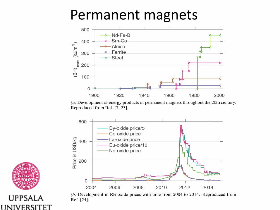
Permanent magnets

2.1.2 Spin-Orbit Coupling and the MagnetocrystallineAnisotropy

Magnetocrystalline anisotropy is the free energy dependence on magnetisa-

tion direction, i.e. F = F(M), where M = (sinθ cosφ ,sinθ sinφ ,cosθ) is

the direction of the magnetisation (spin quantisation axis) relative to the crys-

tal lattice. This effect was first experimentally observed and described phe-

nomenologically, based on anisotropy constants and crystal symmetries, with

the requirement that the dependence of the free energy on the magnetisation

direction should have the same symmetries as the crystal lattice [59]. Further-

more, time reversal symmetry dictates that F(M) = F(−M), whereby only

even powers of sinθ are allowed. For example, in a uniaxial (e.g. tetragonal

or hexagonal) crystal the leading contributions are [28, 59]

F = F0 +K1 sin2 θ +K2 sin4 θ + ..., (2.22)

where F0 contains all isotropic energy contributions and Ki are the anisotropy

constants. Further terms will depend on the particular uniaxial crystal sym-

metry and also contain φ dependence. For a tetragonal crystal a term of

the form K3 sin6 θ cos4φ appears. For a hexagonal crystal with six-fold rota-

tional symmetry a K3 sin6 θ cos6φ term appears, while for hexagonal crystals

with three-fold rotational symmetry (for example the Laves phase structure

of Fe2Ta1−xWx studied in Paper XI) an additional K′3 sin6 θ cos3φ is allowed.

For a cubic structure on the other hand, the leading contribution is of fourth

order and the energy is

F = F0 +K1(α2x α2

y +α2x α2

z +α2y α2

z )+K2α2x α2

y α2z + ..., (2.23)

where αi are the directional cosines of the magnetisation direction (αx = x ·Mand similarly for y and z).

That the microscopic origin of this anisotropy is related to the SOC was

suggested by Van Vleck [60], since this is the link coupling the spin to the

real space crystal symmetry via the orbital angular momentum. As described

in the previous section, the spin-orbit Hamiltonian is HSOC = ξ L ·S, which is

often conveniently rewritten using

L ·S =1

2(L+S−+L−S+)+LzSz, (2.24)

where we have introduced the ladder operators L± = Lx± iLy and S± = Sx±iSy. If one is mainly interested in the transition metal d-electron magnetism,

then the SOC can be treated as a perturbation. This is motivated by the size of

the SOC constant ξ being much smaller (less than 100 meV) than the band-

width (several eV) in the relevant magnetic 3d-metals2, so that the size of

2It is interesting to note that the size of the SOC constant determines an upper limit for the

MAE. At most one could therefore expect an MAE of 50-100 meV in 3d magnets. In practice it

22

the perturbation is much smaller than the typical separation of energy states

under consideration. A study based on perturbation theory was done in sem-

inal work by Brooks [62], who attempted to describe the anisotropy in cubic

iron and nickel, but did not have access to an accurate description of the elec-

tronic structure. Important contributions in this line of work was also done

by Kondorskii and Straube [63], who used a Hartree-Fock band structure with

perturbative SOC to calculate and analyse the MAE of fcc Ni. They reached

the important conclusion that regions in the Brillouin zone which allow for

coupling between occupied and unoccupied states very near the Fermi energy

are crucial for the MAE, as will be discussed further below, while they also

emphasised the importance of taking into account deformations of the Fermi

surface. A perturbative treatment of SOC also allowed Bruno [31] to find the

simple relation that the MAE is proportional to the orbital magnetic moment

anisotropy, as will be discussed further in a later part of this section.

The SOC energy shift, to second order, of a particular energy eigenvalue Enis

ΔEn = ξ 〈n|L ·S |n〉+ξ 2 ∑k �=n

∣∣〈n|L ·S |k〉∣∣2En−Ek

, (2.25)

where |n〉 and |k〉 denote eigenstates of the unperturbed Hamiltonian and Enand Ek are the associated energy eigenvalues. The unperturbed states have a

well defined spin character (in contrast to the perturbed ones) and it is suitable

to consider states such as

|n〉= ∑i

cn,i |k,dn,i,σn〉 , (2.26)

where σ denotes the spin, the index i runs over the d-orbitals (xy, yz, z2, xz,x2− y2) and in the case of a periodic system k denotes a point in the Bril-louin zone. In the ten-dimensional space which is a direct product of the two-dimensional spin space and the five-dimensional space of d-states, the spin-orbit coupling operator is a 10×10 hermitian matrix with elements which arestraightforward to evaluate3 and listed in Table 2.1. The angles θ and φ arethe angular spherical coordinates describing the spin quantisation axis and thisdependence on magnetisation direction of the spin-orbit coupling matrix is thesource of the magnetocrystalline anisotropy energy. Inserting Eq. 2.26 andEq. 2.24 into the first term of Eq. 2.25 and noting that all diagonal elementsin Table 2.1 are zero, as well as that 〈di|Lz |di〉= 0, one finds that the first or-der perturbation contribution of the SOC is zero. Consequently, the spin-orbitcoupling is at most a second order perturbation. This can also be related to the

tends to be much smaller, usually less than 1 meV (around 1 μeV in bcc Fe). For single atoms

on surfaces, fulfilling certain symmetry requirements, magnetic anisotropy of similar size as

that of the SOC constant has been observed [61].3For example by first introducing the spin states |↑〉n = cos θ

2 |↑〉z + eiφ sin θ2 |↓〉z in arbitrary

direction n.

23

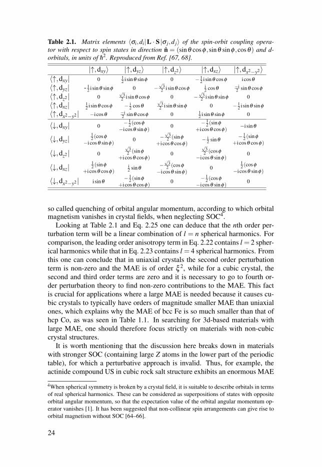
Table 2.1. Matrix elements 〈σi,di|L · S |σ j,d j〉 of the spin-orbit coupling opera-tor with respect to spin states in direction n = (sinθ cosφ ,sinθ sinφ ,cosθ) and d-orbitals, in units of h2. Reproduced from Ref. [67, 68].

|↑,dxy〉 |↑,dyz〉 |↑,dz2〉 |↑,dxz〉 |↑,dx2−y2〉〈↑,dxy| 0 1

2 isinθ sinφ 0 − 12 i sinθ cosφ i cosθ

〈↑,dyz| - 12 i sinθ sinφ 0 −

√3

2 i sinθ cosφ i2 cosθ −i

2 sinθ cosφ

〈↑,dz2 | 0√

32 i sinθ cosφ 0 −

√3

2 i sinθ sinφ 0

〈↑,dxz| 12 i sinθ cosφ − i

2 cosθ√

32 i sinθ sinφ 0 − 1

2 i sinθ sinφ〈↑,dx2−y2 | −i cosθ −i

2 sinθ cosφ 0 12 isinθ sinφ 0

〈↓,dxy| 0− 1

2 (cosφ−i cosθ sinφ) 0

− 12 (sinφ

+i cosθ cosφ) −i sinθ

〈↓,dyz|12 (cosφ

−i cosθ sinφ) 0−√

32 (sinφ

+i cosθ cosφ)− i

2 sinθ − 12 (sinφ

+i cosθ cosφ)

〈↓,dz2 | 0

√3

2 (sinφ+i cosθ cosφ)

0

√3

2 (cosφ−i cosθ sinφ)

0

〈↓,dxz|12 (sinφ

+i cosθ cosφ)i2 sinθ −

√3

2 (cosφ−i cosθ sinφ)

012 (cosφ

−i cosθ sinφ)

〈↓,dx2−y2 | i sinθ − 12 (sinφ

+i cosθ cosφ) 0− 1

2 (cosφ−i cosθ sinφ) 0

so called quenching of orbital angular momentum, according to which orbitalmagnetism vanishes in crystal fields, when neglecting SOC4.

Looking at Table 2.1 and Eq. 2.25 one can deduce that the nth order per-

turbation term will be a linear combination of l = n spherical harmonics. For

comparison, the leading order anisotropy term in Eq. 2.22 contains l = 2 spher-

ical harmonics while that in Eq. 2.23 contains l = 4 spherical harmonics. From

this one can conclude that in uniaxial crystals the second order perturbation

term is non-zero and the MAE is of order ξ 2, while for a cubic crystal, the

second and third order terms are zero and it is necessary to go to fourth or-

der perturbation theory to find non-zero contributions to the MAE. This fact

is crucial for applications where a large MAE is needed because it causes cu-

bic crystals to typically have orders of magnitude smaller MAE than uniaxial

ones, which explains why the MAE of bcc Fe is so much smaller than that of

hcp Co, as was seen in Table 1.1. In searching for 3d-based materials with

large MAE, one should therefore focus strictly on materials with non-cubic

crystal structures.

It is worth mentioning that the discussion here breaks down in materials

with stronger SOC (containing large Z atoms in the lower part of the periodic

table), for which a perturbative approach is invalid. Thus, for example, the

actinide compound US in cubic rock salt structure exhibits an enormous MAE

4When spherical symmetry is broken by a crystal field, it is suitable to describe orbitals in terms

of real spherical harmonics. These can be considered as superpositions of states with opposite

orbital angular momentum, so that the expectation value of the orbital angular momentum op-

erator vanishes [1]. It has been suggested that non-collinear spin arrangements can give rise to

orbital magnetism without SOC [64–66].

24

in the order of 109 J/m3 [69], i.e., orders of magnitude larger than that of

Nd2Fe14B, albeit being in a cubic crystal structure.

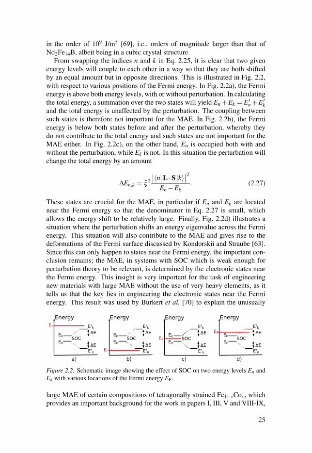
From swapping the indices n and k in Eq. 2.25, it is clear that two given

energy levels will couple to each other in a way so that they are both shifted

by an equal amount but in opposite directions. This is illustrated in Fig. 2.2,

with respect to various positions of the Fermi energy. In Fig. 2.2a), the Fermi

energy is above both energy levels, with or without perturbation. In calculating

the total energy, a summation over the two states will yield En +Ek = E ′n +E ′kand the total energy is unaffected by the perturbation. The coupling between

such states is therefore not important for the MAE. In Fig. 2.2b), the Fermi

energy is below both states before and after the perturbation, whereby they

do not contribute to the total energy and such states are not important for the

MAE either. In Fig. 2.2c), on the other hand, En is occupied both with and

without the perturbation, while Ek is not. In this situation the perturbation will

change the total energy by an amount

ΔEn,k = ξ 2

∣∣〈n|L ·S |k〉∣∣2En−Ek

. (2.27)

These states are crucial for the MAE, in particular if En and Ek are located

near the Fermi energy so that the denominator in Eq. 2.27 is small, which

allows the energy shift to be relatively large. Finally, Fig. 2.2d) illustrates a

situation where the perturbation shifts an energy eigenvalue across the Fermi

energy. This situation will also contribute to the MAE and gives rise to the

deformations of the Fermi surface discussed by Kondorskii and Straube [63].

Since this can only happen to states near the Fermi energy, the important con-

clusion remains; the MAE, in systems with SOC which is weak enough for

perturbation theory to be relevant, is determined by the electronic states near

the Fermi energy. This insight is very important for the task of engineering

new materials with large MAE without the use of very heavy elements, as it

tells us that the key lies in engineering the electronic states near the Fermi

energy. This result was used by Burkert et al. [70] to explain the unusually

Figure 2.2. Schematic image showing the effect of SOC on two energy levels En and

Ek with various locations of the Fermi energy EF.

large MAE of certain compositions of tetragonally strained Fe1−xCox, which

provides an important background for the work in papers I, III, V and VIII-IX,

25

and it is discussed further in Sec. 4.1.1. Similar reasoning has also been used,

for example, by Costa et al. [71] to analyse the large MAE of Fe2P.

In addition to the separation of the states that appears in the denominator

of Eq. 2.27, the energy shift is determined by numerator, where the matrix

elements in Table 2.1 enter. In the important case described in Fig. 2.2c), with

En < EF < Ek, there is a negative energy shift ΔEn,k < 0 and hence a lowering

of energy whenever 〈n|L ·S |k〉 is non-zero. Thus, any coupling containing a

cosθ in Table 2.1 will contribute with an energy reduction for θ = 0, corre-

sponding to magnetisation along the z-axis, whereas sinθ terms will favour

θ = π/2, i.e. magnetisation in the xy-plane. Coupling between any two states

with the same d-orbital type is zero and does not contribute to the MAE. Fur-

ther analysis of the SOC matrix elements and assignment of the quantum num-

ber |m|= 0 to dz2 , |m|= 1 to dxz and dyz and |m|= 2 to dxy and dx2−y2 , leads to

the observation that |m|= 0 states do not couple to |m|= 2 states (which can be

understood since the ladder operators in Eq. 2.24 can only couple states that

differ by m= 1). Furthermore, coupling between states with the same spin and

|m| (e.g. 〈↑,dxy| coupled to |↑,dx2−y2〉, but not another |↑,dxy〉 since diagonal

elements are zero) contain cosθ and favour magnetisation along the z-axis (a

uniaxial magnetic anisotropy along the z-axis is often wanted in technological

applications), while states with same spin but |m| differing by 1 have a sinθcoupling, favouring magnetisation in the xy-plane. For opposite spin states

this situation is reversed. From this analysis it is possible to look at the unper-

turbed electronic structure near the Fermi energy and, by determining the spin

and orbital character of the important occupied and unoccupied states, one can

deduce how these states will contribute to the MAE. Often the band structure

is very complicated with many states contributing in competing ways, making

a useful analysis difficult, but in some simple cases one might be able to de-

duce, e.g., the easy axis of magnetisation by looking at the dominating states

near the Fermi energy.

Based on the discussion so far in this section and considering the band

structure of a solid, a large MAE might appear if there are many occupied

and unoccupied states with energies very near the Fermi energy. A schematic

illustration of a such a band structure is shown in Fig. 2.3. The emphasised

region contains relatively flat bands just above and below the Fermi energy.

This allows for many pairs of occupied and unoccupied states to be near each

other in energy and couple strongly via SOC. If these states have the right

spin and orbital character, they will contribute significantly to the MAE. For

example, if k denotes a spin up dxy state while n denotes a spin up dx2−y2 state,

there is a strong contribution towards an easy magnetisation axis along the

z-direction. A problem in many real materials is that there are few such flat

bands near the Fermi energy and additionally there are often different regions

in k-space yielding opposite contributions to the MAE, resulting in a large

degree of cancellation as an integration is performed over the Brillouin zone.

26

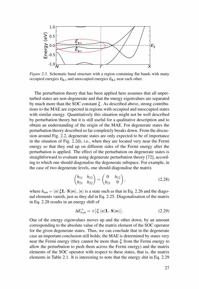
Figure 2.3. Schematic band structure with a region containing flat bands with many

occupied energies Ek,n and unoccupied energies Ek,k near each other.

The perturbation theory that has been applied here assumes that all unper-

turbed states are non-degenerate and that the energy eigenvalues are separated

by much more than the SOC constant ξ . As described above, strong contribu-

tions to the MAE are expected in regions with occupied and unoccupied states

with similar energy. Quantitatively this situation might not be well described

by perturbation theory but it is still useful for a qualitative description and to

obtain an understanding of the origin of the MAE. For degenerate states the

perturbation theory described so far completely breaks down. From the discus-

sion around Fig. 2.2, degenerate states are only expected to be of importance

in the situation of Fig. 2.2d), i.e., when they are located very near the Fermi

energy so that they end up on different sides of the Fermi energy after the

perturbation is applied. The effect of the perturbation on degenerate states is

straightforward to evaluate using degenerate perturbation theory [72], accord-

ing to which one should diagonalise the degenerate subspace. For example, in

the case of two degenerate levels, one should diagonalise the matrix(h11 h12

h21 h22

)=

(0 h12

h21 0

), (2.28)

where hnm = 〈n|ξ L ·S |m〉, |n〉 is a state such as that in Eq. 2.26 and the diago-

nal elements vanish, just as they did in Eq. 2.25. Diagonalisation of the matrix

in Eq. 2.28 results in an energy shift of

ΔE±n,m =±∣∣ξ 〈n|L ·S |m〉∣∣ . (2.29)

One of the energy eigenvalues moves up and the other down, by an amount

corresponding to the absolute value of the matrix element of the SOC operator

for the given degenerate states. Thus, we can conclude that in the degenerate

case an important conclusion still holds; the MAE is determined by states very

near the Fermi energy (they cannot be more than ξ from the Fermi energy to

allow the perturbation to push them across the Fermi energy) and the matrix

elements of the SOC operator with respect to these states, that is, the matrix

elements in Table 2.1. It is interesting to note that the energy shit in Eq. 2.29

27

Z20 2000 4000 6000 8000

(meV

)

0

50

100

150

200

250

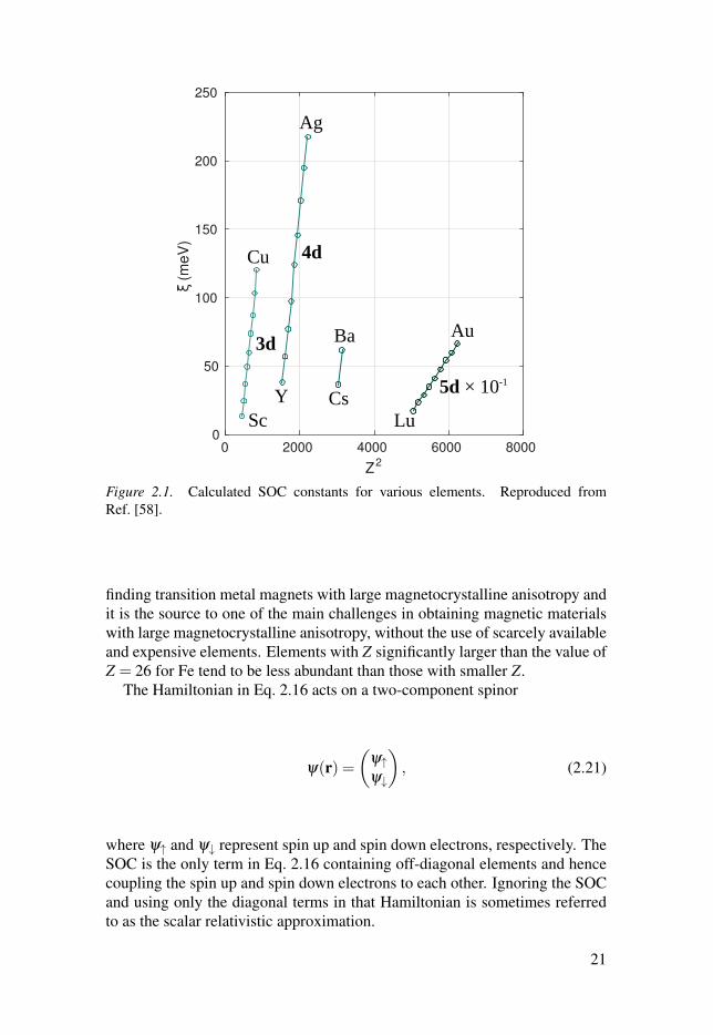
Figure 2.1. Calculated SOC constants for various elements. Reproduced from

Ref. [58].

finding transition metal magnets with large magnetocrystalline anisotropy and

it is the source to one of the main challenges in obtaining magnetic materials

with large magnetocrystalline anisotropy, without the use of scarcely available

and expensive elements. Elements with Z significantly larger than the value of

Z = 26 for Fe tend to be less abundant than those with smaller Z.

The Hamiltonian in Eq. 2.16 acts on a two-component spinor

ψ(r) =(

ψ↑ψ↓

), (2.21)

where ψ↑ and ψ↓ represent spin up and spin down electrons, respectively. The

SOC is the only term in Eq. 2.16 containing off-diagonal elements and hence

coupling the spin up and spin down electrons to each other. Ignoring the SOC

and using only the diagonal terms in that Hamiltonian is sometimes referred

to as the scalar relativistic approximation.

21