Magneto-Rheological Damper ModellingJorge Lozoya-Santos, Ruben Morales-Menendez and Ricardo Ramirez-Mendoza

Abstract— A comparative analysis of different models of aMagneto-Rheological (MR) damper was done. Three modelswere tested: a non-linear ARX, a semi-phenomenological and aphenomenological. Although the non-linear ARX model shownthe best result, this is a black-box model with limited use.However, the Semi-Phenomenological model represented an ex-cellent option considering the physical meaning of its parameters.Modified versions of models were proposed by incorporatingthe electrical current dependency. This modification improvedthe performance of models in all cases. Experimental data of acommercial MR damper validates the results.

I. INTRODUCTION

A Magneto-Rheological (MR) fluid is a smart material thatchanges its rheological properties when a magnetic field is ap-plied. A MR damper is an example of a commercial applicationof this type of fluids. A control system based on a MR damperexhibits high nonlinear behavior. Achieving a precise model ofthis damper in order to accomplish good control performancein different applications represents a research challenge.

There are two key steps in order to get accurate MR dampermodel. First, the Design of Experiments (DoE) for the traininginputs, and second, the structure of the model. This paperis organized as follows. Section II reviews the state of theart. Section III describes the experimental setup. The DoE isincluded in section IV. Results are shown in section V anddiscussed in section VI. Finally, section VII concludes thepaper.

II. STATE OF THE ART

The problem of developing an adequate model to predictthe response of a MR damper does not have an uniquesolution. There are complex behaviors such as hysteresiswhich characterization is not a trivial task. Several modellingapproaches have been proposed. Each approach presents a dif-ferent DoE. The selected model and the DoE have high impactin the identification process [1]. [2] divide the identificationprocedure in DoE and Modelling. Subsection II-A outlinesthe training inputs configuration, and subsection II-B reviewsseveral modelling approaches.

A. Training inputs

Training inputs configuration is used to excite a MR damperin order to obtain useful output data for modelling purposes.Richness of training inputs generates full spectrum of possiblebehaviors. Several features are key in the training signals.

J. Lozoya-Santos is PhD Student, Tecnologico de Monterrey, Mexico,jorge.lozoya@itesm.mx

R. Morales-Menendez is Associate Director of Research, Tecnologico deMonterrey, rmm@itesm.mx

R. Ramirez-Mendoza is Director of the CIDyT, Tecnologico de Monterrey,ricardo.ramirez@itesm.mx

According to the displacement signal, training inputs couldbe classified as in Table I.

TABLE I: DISPLACEMENT SIGNAL FEATURES

Signal DescriptionSSS Sine Sweep testS with amplitude and frequency.XSP Signal coming from seismic records where frequency BW is

less than 5 hz.BWN Bandwidth White Noise are Gaussian noises filtered to

interested frequencies.S Sinusoidal simple signal, with fixed amplitude and frequency.

SoS A sine wave gives a ride to other higher frequency sine wave.Low amplitude displacements for high frequency and highamplitude for low frequency.

ICPS Increased Clock Period Signal or random walk which amplitudevaries randomly, each constant period defined by the application.

Tr Triangular signal with constant amplitude.SFS This signal has a period which is decreased each definite number

of full periods by 0.5 Hz.RP Road Profiles [3], in this case a smooth runway.

CHS CHirp Sinusoidal in frequencies of interest less than 5 hz.FM The modulation signal is an Increased Clock Period Signal

with frequencies of interest.It is generated by using a voltage-controlled oscillator.

Electrical current excitation to MR damper also has manyvariants, Table II shows the most representative.

TABLE II: ELECTRIC CURRENT SIGNAL FEATURES

Signal DescriptionC Constant current where values are manually set .

BWN Same as defined for displacement.R Ramp signal is useful for determination of ratio changes.S Sinusoidal signal, usually employed for model testing.

APRBS Amplitude Pseudo-Random Binary Signal. The minimumamplitude period must be greater than settlement time fromelectric current to force.

SSS Sine Sweep Signal, it does not offer identification characteristicsapart from the test fitted models.

RS Step train with Random amplitude and duration.After one step, signal always returns to zero value

PWM Pulse Width Modulation Signal.Ost One step. Rise/down transitions are defined by displacement. If

it’s constant, only the effect of current over force is extracted.SC Stepped Constant current, driven by hardware.RC Positive constant ramp.

ADRC Positive-Negative constant ramp.ICPS Same as defined for displacement where minimum period was

100 ms for full magnetization.PRBS Minimum period was 100 ms

The use of SSS, C and rich frequency displacement signals(XSP, BWN) in conjunction with constant current are popularfeatures of training inputs in the MR damper domain.

B. Modelling approaches.Several models had been developed. Five of the most im-

portant will be reviewed for completeness. Table III describes

the key variables of these models.

TABLE III: DESCRIPTION OF MODELS’ VARIABLES.

Variable Descriptiont Continuous timek Discrete sample, discrete timei,j Subindexes

x(i) Damper displacement, continuousxk Damper displacement, discreteI(i) Electric current, continuousIk Electric current, discrete

x(i) Damper velocity, continuousxk Damper velocity, discrete

fMR(i) Damping force, continuousfMRk Damping force, discrete

θ Parameters of neural network, vectoraj , bj , cj Modelling coefficients

n Time delays in x(i)m Time delays in x(i)p Time delays in fMR(i)d Maximum number of delays

q, r Exponentsα Tuning parameter

1) Auto Regressive with eXogenous (ARX) Inputs basedon Neural Networks (NNARX): It is common to re-use theinput structures from the linear ARX models while letting theinternal architecture be a feed-forward multi-layer perceptronnetwork. The structure can be gradually expanded based on theinsight and complexity of physical behavior. Eqn (1) shows apredictor based on NN.

f(t|θ) = g[ϕ(t, θ), θ] (1)

where g is the feed-forward function, and ϕ(t, θ) is a regres-sion vector. The structure that emulates the system is [4]:

fMR(i) = g[x(i− 1), . . . , x(i− n), I(i− 1), . . . , I(i−m)fMR(i− 1), .., fMR(i− p)|ϕ(wi,n+m+p, θ)] (2)

There are two hidden layers with n + m + p neurons eachone, NNARX(n,m,p).

2) Polynomial Approach: The hysteresis loop can be di-vided into two regions: positive acceleration (lower loop) andnegative acceleration (upper loop). Both loops can be modelledby a polynomial equation [5].

fMR(i) =∑

(bj + cj · I(i)) · x(i)j (3)

where {bj , cj} are computed values from hysteresis slopes.3) Non-linear ARX model: It uses a black-box structure [6]:

fMRk= a1fMRk−1 + a2fMRk−2 + a3fMRk−3

+a4xk−1 + a5xk−2 + a6xk−3

+a7xk−1 + a8xk−2 + a9xk−3 (4)

Coefficients {aj} are function of the electric current.4) Semi-Phenomenological model: It captures the bi-

viscous and hysteretic behavior with a smooth and conciseform [7]:

fMR = a1tanh

(a3

(x +

b0

c0x

))+ a2

(x +

b0

c0x

)(5)

Coefficients have physical meaning in this model; a1 is thedynamic yield fMR, a2 and a3 are related to the post-yield and pre-yield viscous damping coefficients respectively.When fMR = 0, b0 and c0 represent the absolute value ofhysteretic critical velocity and hysteretic critical displacementrespectively.

5) Phase-Transition model: The MR fluid dynamics insidethe damper piston are approximated by several assumptions.First, hysteretic behavior of the MR damper is purely caused byhysteretic friction force. It occurs caused when the fluid is un-dergoing a shear deformation. Second, velocity distribution ofthe flow between piston chambers is linear. Third, polarizationchains in the MR fluids are broken or reformed uniformly. Inconsequence, shear strain rate between the two plates becameuniform, as shear stress does too. This phenomenologicalmodel was proposed by [8]:

a1fMR + a2fMR + a3fMR + a4f3MR + a5f

5MR = x (6)

where a1 and a2 model the post-yield region transitions; a3,a4, a5 model the hysteretic behavior. This is a 2nd-ordernonlinear ordinary differential equation, where dynamics aredependent on x, because both the inertial and damping effectsare taken into account for the phase transition.

It is claimed that inertial overshoot and hysteretic behaviorpresented by the experimental data can be captured. Since themodel is a differential equation in time domain, frequencydependence is included naturally as a special case of a moregeneral loading-rate dependency.

Table IV summarizes the most important research works.The modelling approach nomenclature is P: Phenomenolog-ical, S-P: Semi-Phenomenological, S: Statistical, BB: Black-Box. The model parameters column shows the number of pa-rameters in the model. The last column indicates identificationalgorithm used in each research work, LS: Least Square, RLS:Recursive LS, and PAA: Parameter Adaptation Algorithm.

TABLE IV: MR DAMPER MODELLING APPROACHES.

Reference Modelling Models’ IdentificationApproach Parameters Algorithm

[9, Bingham] P 6 RLS, PAA[10, mod Bouc Wen] P 14 NonLinear LS[4, NNARX(2,2,2)] BB - Back-propagation

[5, Polynomial] BB 28 RLS, PAA[7, Hysteretic] SP 5 RLS, PAA

[8, Phase Transition] P 4 NonLinear LS[2, Force by RMS] S 10 Response Surface[6, NARX(3,3,3)] BB 9 RLS, PAA

III. EXPERIMENTAL SETUP

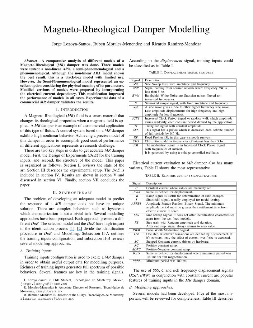
The MR damper exploited in this research was a DelphiGabriel MR damper. This damper is part of the DelphiMagneRideTM commercial system. The system consists offour MR fluid-based mono-tube dampers (struts and/or shockabsorbers), a sensor set, and an on-board Electronic ControlUnit (ECU). The underlying MR damper is a standard mono-tube configuration with 36 mm piston.

The testing system is the MTSTM which can deliver enoughforce and time response with respect to damper’s peak forceand bandwidth, Fig. 11. The stroke (displacement) of theMR damper was used as an input variable of the model, thevelocity was computed by using an adequate filter. A dataacquisition system (i.e. Software TestlinkTM and TestwareTM

II) performed the data collection.

IV. DESIGN OF EXPERIMENTS

Several experiments were implemented on the system Fig. 1.A signal with sinusoidal displacement of 0.025 m, a frequencyof 30 periods and a constant current was generated followingthis procedure:

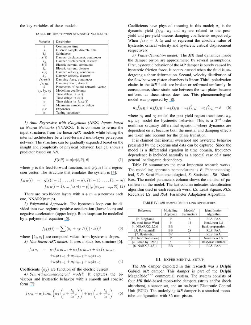
1) Set the electric current in 0 A2) Set frequency in 0.5 Hz.3) After 30 periods, increase the frequency in 0.5 Hz.4) If frequency is less than 14.5 Hz go to step 3.5) Increase the electric current in 0.25 A6) If electric current is less than 4 A go to step 2.The resultant force was in 0−2850 N range. Fig. 2 shows a

3D-plot (current-velocity-force) of the experimental results forhigh frequency. Fig. 3 shows the behavior of the MR damperfor 1 Hz frequency.

Using these experimental data sets a semi-phenomenological model, equation (5), was learned withexcellent results. This model was exploited as simulator ofthe MR damper.

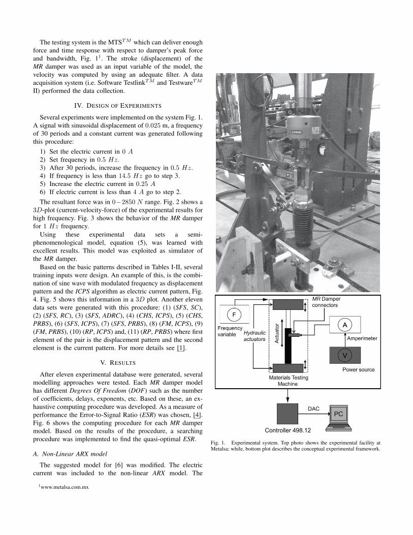
Based on the basic patterns described in Tables I-II, severaltraining inputs were design. An example of this, is the combi-nation of sine wave with modulated frequency as displacementpattern and the ICPS algorithm as electric current pattern, Fig.4. Fig. 5 shows this information in a 3D plot. Another elevendata sets were generated with this procedure: (1) (SFS, SC),(2) (SFS, RC), (3) (SFS, ADRC), (4) (CHS, ICPS), (5) (CHS,PRBS), (6) (SFS, ICPS), (7) (SFS, PRBS), (8) (FM, ICPS), (9)(FM, PRBS), (10) (RP, ICPS) and, (11) (RP, PRBS) where firstelement of the pair is the displacement pattern and the secondelement is the current pattern. For more details see [1].

V. RESULTS

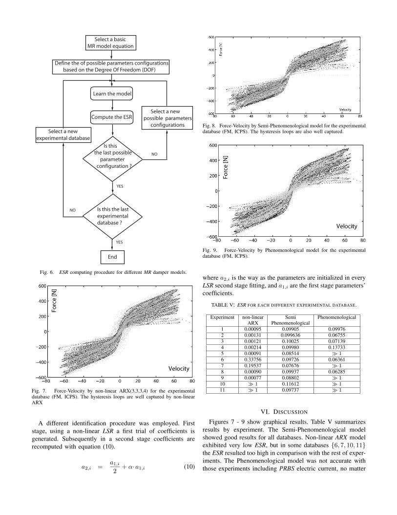
After eleven experimental database were generated, severalmodelling approaches were tested. Each MR damper modelhas different Degrees Of Freedom (DOF) such as the numberof coefficients, delays, exponents, etc. Based on these, an ex-haustive computing procedure was developed. As a measure ofperformance the Error-to-Signal Ratio (ESR) was chosen, [4].Fig. 6 shows the computing procedure for each MR dampermodel. Based on the results of the procedure, a searchingprocedure was implemented to find the quasi-optimal ESR.

A. Non-Linear ARX model

The suggested model for [6] was modified. The electriccurrent was included to the non-linear ARX model. The

1www.metalsa.com.mx

Fig. 1. Experimental system. Top photo shows the experimental facility atMetalsa; while, bottom plot describes the conceptual experimental framework.

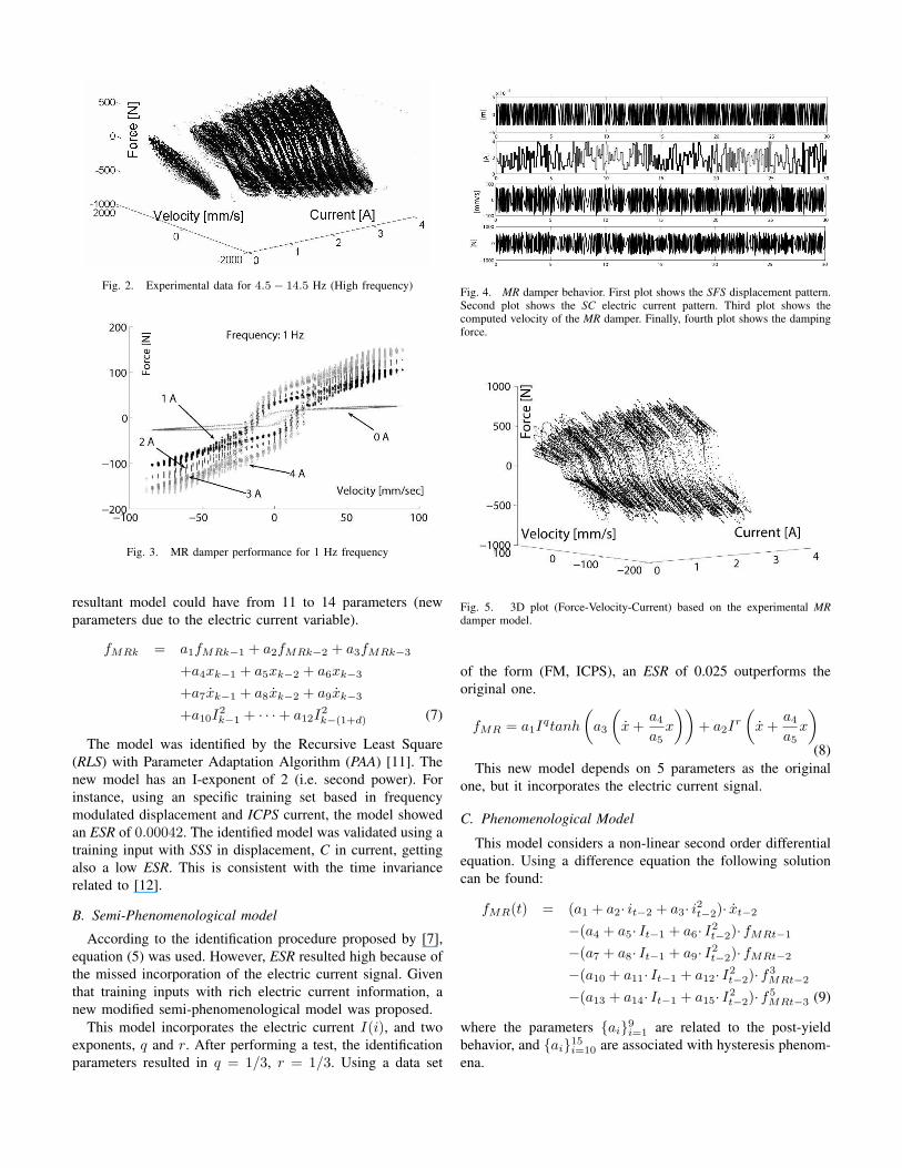
Fig. 2. Experimental data for 4.5− 14.5 Hz (High frequency)

Fig. 3. MR damper performance for 1 Hz frequency

resultant model could have from 11 to 14 parameters (newparameters due to the electric current variable).

fMRk = a1fMRk−1 + a2fMRk−2 + a3fMRk−3

+a4xk−1 + a5xk−2 + a6xk−3

+a7xk−1 + a8xk−2 + a9xk−3

+a10I2k−1 + · · ·+ a12I

2k−(1+d) (7)

The model was identified by the Recursive Least Square(RLS) with Parameter Adaptation Algorithm (PAA) [11]. Thenew model has an I-exponent of 2 (i.e. second power). Forinstance, using an specific training set based in frequencymodulated displacement and ICPS current, the model showedan ESR of 0.00042. The identified model was validated using atraining input with SSS in displacement, C in current, gettingalso a low ESR. This is consistent with the time invariancerelated to [12].

B. Semi-Phenomenological model

According to the identification procedure proposed by [7],equation (5) was used. However, ESR resulted high because ofthe missed incorporation of the electric current signal. Giventhat training inputs with rich electric current information, anew modified semi-phenomenological model was proposed.

This model incorporates the electric current I(i), and twoexponents, q and r. After performing a test, the identificationparameters resulted in q = 1/3, r = 1/3. Using a data set

Fig. 4. MR damper behavior. First plot shows the SFS displacement pattern.Second plot shows the SC electric current pattern. Third plot shows thecomputed velocity of the MR damper. Finally, fourth plot shows the dampingforce.

Fig. 5. 3D plot (Force-Velocity-Current) based on the experimental MRdamper model.

of the form (FM, ICPS), an ESR of 0.025 outperforms theoriginal one.

fMR = a1Iqtanh

(a3

(x +

a4

a5x

))+ a2I

r

(x +

a4

a5x

)

(8)This new model depends on 5 parameters as the original

one, but it incorporates the electric current signal.

C. Phenomenological Model

This model considers a non-linear second order differentialequation. Using a difference equation the following solutioncan be found:

fMR(t) = (a1 + a2· it−2 + a3· i2t−2)· xt−2

−(a4 + a5· It−1 + a6· I2t−2)· fMRt−1

−(a7 + a8· It−1 + a9· I2t−2)· fMRt−2

−(a10 + a11· It−1 + a12· I2t−2)· f3

MRt−2

−(a13 + a14· It−1 + a15· I2t−2)· f5

MRt−3 (9)

where the parameters {ai}9i=1 are related to the post-yieldbehavior, and {ai}15i=10 are associated with hysteresis phenom-ena.

Select a basic

MR model equation

Define the of possible parameters configurations

based on the Degree Of Freedom (DOF)

Learn the model

Compute the ESR

Is this

the last possible

parameter

configuration ?

Select a new

possible parameters

configurations

Is this the last

experimental

database ?

End

NO

YES

YES

Select a new

experimental database

NO

Fig. 6. ESR computing procedure for different MR damper models.

Fig. 7. Force-Velocity by non-linear ARX(3,3,3,4) for the experimentaldatabase (FM, ICPS). The hysteresis loops are well captured by non-linearARX

A different identification procedure was employed. Firststage, using a non-linear LSR a first trial of coefficients isgenerated. Subsequently in a second stage coefficients arerecomputed with equation (10).

a2,i =a1,i

2+ α· a1,i (10)

Fig. 8. Force-Velocity by Semi-Phenomenological model for the experimentaldatabase (FM, ICPS). The hysteresis loops are also well captured.

Fig. 9. Force-Velocity by Phenomenological model for the experimentaldatabase (FM, ICPS).

where a2,i is the way as the parameters are initialized in everyLSR second stage fitting, and a1,i are the first stage parameters’coefficients.

TABLE V: ESR FOR EACH DIFFERENT EXPERIMENTAL DATABASE.

Experiment non-linear Semi PhenomenologicalARX Phenomenological

1 0.00095 0.09905 0.099762 0.00131 0.099636 0.067553 0.00121 0.10025 0.071394 0.00214 0.09980 0.137335 0.00091 0.08514 À 16 0.33756 0.09726 0.063617 0.19537 0.07676 À 18 0.00090 0.09937 0.062859 0.00077 0.08802 À 110 À 1 0.11612 À 111 À 1 0.09737 À 1

VI. DISCUSSION

Figures 7 - 9 show graphical results. Table V summarizesresults by experiment. The Semi-Phenomenological modelshowed good results for all databases. Non-linear ARX modelexhibited very low ESR, but in some databases {6, 7, 10, 11}the ESR resulted too high in comparison with the rest of exper-iments. The Phenomenological model was not accurate withthose experiments including PRBS electric current, no matter

non-linear ARX Semi

PhenomenologicalPhenomenological

0

0.2

0.4

0.6

0.8

1

ES

R

Fig. 10. Box and Whisker plots for each MR damper model.

the displacement shape. In addition, road profiles pattern didnot contribute to the fitting procedure. Therefore, it is clearthat Phenomenological model needs signals with differentelectric current levels and uniform frequency bandwidth indisplacement patterns.

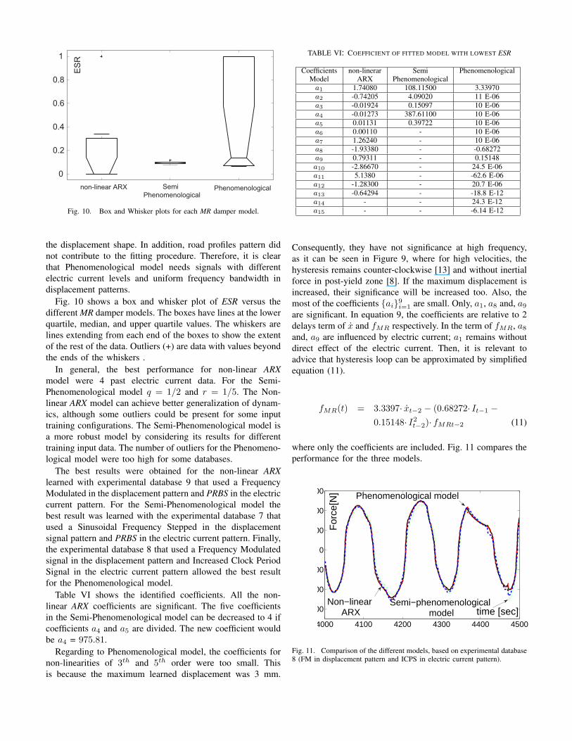
Fig. 10 shows a box and whisker plot of ESR versus thedifferent MR damper models. The boxes have lines at the lowerquartile, median, and upper quartile values. The whiskers arelines extending from each end of the boxes to show the extentof the rest of the data. Outliers (+) are data with values beyondthe ends of the whiskers .

In general, the best performance for non-linear ARXmodel were 4 past electric current data. For the Semi-Phenomenological model q = 1/2 and r = 1/5. The Non-linear ARX model can achieve better generalization of dynam-ics, although some outliers could be present for some inputtraining configurations. The Semi-Phenomenological model isa more robust model by considering its results for differenttraining input data. The number of outliers for the Phenomeno-logical model were too high for some databases.

The best results were obtained for the non-linear ARXlearned with experimental database 9 that used a FrequencyModulated in the displacement pattern and PRBS in the electriccurrent pattern. For the Semi-Phenomenological model thebest result was learned with the experimental database 7 thatused a Sinusoidal Frequency Stepped in the displacementsignal pattern and PRBS in the electric current pattern. Finally,the experimental database 8 that used a Frequency Modulatedsignal in the displacement pattern and Increased Clock PeriodSignal in the electric current pattern allowed the best resultfor the Phenomenological model.

Table VI shows the identified coefficients. All the non-linear ARX coefficients are significant. The five coefficientsin the Semi-Phenomenological model can be decreased to 4 ifcoefficients a4 and a5 are divided. The new coefficient wouldbe a4 = 975.81.

Regarding to Phenomenological model, the coefficients fornon-linearities of 3th and 5th order were too small. Thisis because the maximum learned displacement was 3 mm.

TABLE VI: COEFFICIENT OF FITTED MODEL WITH LOWEST ESR

Coefficients non-linerar Semi PhenomenologicalModel ARX Phenomenological

a1 1.74080 108.11500 3.33970a2 -0.74205 4.09020 11 E-06a3 -0.01924 0.15097 10 E-06a4 -0.01273 387.61100 10 E-06a5 0.01131 0.39722 10 E-06a6 0.00110 - 10 E-06a7 1.26240 - 10 E-06a8 -1.93380 - -0.68272a9 0.79311 - 0.15148a10 -2.86670 - 24.5 E-06a11 5.1380 - -62.6 E-06a12 -1.28300 - 20.7 E-06a13 -0.64294 - -18.8 E-12a14 - - 24.3 E-12a15 - - -6.14 E-12

Consequently, they have not significance at high frequency,as it can be seen in Figure 9, where for high velocities, thehysteresis remains counter-clockwise [13] and without inertialforce in post-yield zone [8]. If the maximum displacement isincreased, their significance will be increased too. Also, themost of the coefficients {ai}9i=1 are small. Only, a1, a8 and, a9

are significant. In equation 9, the coefficients are relative to 2delays term of x and fMR respectively. In the term of fMR, a8

and, a9 are influenced by electric current; a1 remains withoutdirect effect of the electric current. Then, it is relevant toadvice that hysteresis loop can be approximated by simplifiedequation (11).

fMR(t) = 3.3397· xt−2 − (0.68272· It−1 −0.15148· I2

t−2)· fMRt−2 (11)

where only the coefficients are included. Fig. 11 compares theperformance for the three models.

4000 4100 4200 4300 4400 4500

−600

−400

−200

0

200

400

600

time [sec]

For

ce[N

]

Semi−phenomenological model

Non−linear ARX

Phenomenological model

Fig. 11. Comparison of the different models, based on experimental database8 (FM in displacement pattern and ICPS in electric current pattern).

VII. CONCLUSIONS

A comparative analysis of different modelling approachesfor Magneto-Rheological (MR) damper was done. Experimen-tal validation with a commercial MR damper was carriedout. Three models were tested: non-linear ARX, a Semi-Phenomenological and Phenomenological. The non-linearARX model, a black-box type model with limited use incontrol systems, exhibited the best performance. The Semi-Phenomenological model represented a robust option consid-ering the low variance of its parameters with respect to inputconfiguration and the simplicity of the model. Incorporating anelectric current dependency on the parameters of these modelsimprove significantly their performance in all cases. Findingsrelated to the Phenomenological model are relevant in thesense that can they be used to get hysteresis estimators. On theside, the low average in its ESR makes it an excellent candidateto validate control systems and to be integrated to systemsexpressed also as difference equations in order to study othertechniques (i. e. LPV models).

Additionally, it was identified that training inputs play acrucial role in the identification process. Selection of traininginputs can reduce the overuse of the damper, number ofexperiments and configurations of training inputs are mainfeatures of this approach.

REFERENCES

[1] J. Lozoya-Santos, R. Morales-Menendez, and R. Ramirez-Mendoza,“Design of Experiments for MR Damper Modelling,” in to appear inInt Joint Conf on Neural Networks, Atlanta, USA, June 2009.

[2] A. C. Shivaram and K. V. Gangadharan, “Statistical Modeling of a MRFluid Damper using the Design of Experiments Approach,” Smart Mater.and Struct., vol. 16, no. 4, pp. 1310–1314, 2007.

[3] J. Y. Wong, Theory of Ground Vehicles. John Wiley, 2001.[4] S. M. Savaresi, S. Bittanti, and M. Montiglio, “Identification of Semi-

Physical and Black-Box Non-Linear Models: the Case of MR-Dampersfor Vehicles Control,” Automatica,, vol. 41, no. 1, pp. 113–127, 1 2005.

[5] S. B. Choi, S. K. Lee, and Y. P. Park, “A Hysteresis Model for Field-Dependent Damping Force of a Magnetorheological Damper,” Soundand Vibration, vol. 245, pp. 375–383, 2001.

[6] E. Nino-Juarez, R. Morales-Menendez, R. Ramirez-Mendoza, andL. Dugard, “Minimizing the Frequency in a Black Box Model of a MRDamper,” in 11th Mini Conf on Vehicle Sys. Dyn., Ident. and Anomalies,2008.

[7] S. Guo, S. Yang, and C. Pan, “Dynamical Modeling of Magneto-rheological Damper Behaviors,” Int. Mater, Sys. and Struct., vol. 17,pp. 3–14, 2006.

[8] L. X. Wang and H. Kamath, “Modelling Hysteretic Behaviour in MRFluids and Dampers using Phase-Transition Theory,” Smart Mater.Struct., vol. 15, pp. 1725–1733, 2006.

[9] D. R. Gamota and F. E. Filisko, “Dynamic Mechanical Studies ofElectro-Rheological Materials: Moderated Frequencies,” J of Rheology,vol. 35, pp. 399–425, 1991.

[10] B. Spencer, S. Dyke, M. Sain, and J. Carlson, “Phenomenological Modelof a MR Damper,” ASCE J of Eng Mechanics, 1996.

[11] Y. D. Landau, R. Lozano, and M. M’Saad, Adaptive control. SpringerVerlag, 1998.

[12] T. Soderstrom and P. Stoica, System Identification. Prentice Hall, 1989.[13] I. Mayergoyz, Mathematical Models of Hysteresis and their Applica-

tions. Elsevier, 2003.