1

Liquidity Risk and Competition in Banking

Yoram Landskroner Stern School of Business, New York University and School of Business Administration, Hebrew University. ylandskr@stern.nyu.edu

Jacob Paroush

Department of Economics, Bar-Ilan University and Ashkelon Academic College. parousj@mail.biu.ac.il

Last Revision 30 January 2008

JEL Classification: G21 Key words: Liquidity risk; liquid assets; volatile liabilities; loan commitments;

deposit withdrawal; liquidity shortage (deficit).

2

Abstract

Liquidity risk is one of the major risks faced by banks in addition to credit risk,

market risk and operating risk. In this paper we construct a stylized model of bank

management where the asset and liabilities liquidity structure are a key element in

determining the bank's exposure to liquidity risk. The main results of our model are

that liquidity risk increases when competition in the credit market increases while

increasing competition in the deposit market will decrease the liquidity shortage. Our

results are of particular importance as banks face increased liquidity risk due to the

recent developments in the financial markets.

3

I. Introduction The traditional functions of banks are transformation of maturity and the provision of

liquidity. Banks transform short-term liquid liabilities into long term illiquid assets.

Banks provide liquidity to demand depositors and also to borrowers via lines of

credit.1 In doing that they are undertaking liquidity risk of their customers thus

exposing themselves to this risk. In extreme cases bank liquidity problems can result

in bank runs when depositors withdraw their funds on a massive scale, such problems

can be contagious, spreading in the banking system. The classical role of the central

band as a lender of last resort was supposed to serve as a buffer for this risk. More

important today are the government provision of deposit insurance and capital

requirements that should prevent a liquidity crisis and bank runs2. Recently in the

summer of 2007 following the sub-prime crisis in the U.S. we have witnessed the

return of the runs however this time the target has been not banks but asset backed

securities. Investment funds that were leveraged and holding these assets were hurt by

the “evaporation” of liquidity in the markets.

Kashyap, Rajan and Stein (2002) show that the function of banks as liquidity

providers may explain why banks tie together the activities of deposit taking and

lending under the same roof based on risk management motivation. Gatev,

Schuerman, and Strahan (2006) test the KRS model and find that bank risk increases

with unused loan commitments but the risk is mitigated by deposits. There is an

incompatibility between the two activities: the timing demand for liquidity may force

fire sale of illiquid assets. Bank deposits that are subject to runs (“fragile”) create an

incentive for banks to provide liquidity, on the other hand capital requirements may

reduce the liquidity creation by banks but increases their ability to overcome distress,

see Diamond and Rajan (2001).

Liquidity in banking is conventionally defined as the ability to fund increases in assets

and meet obligations as they become due3. Liquidity involves uncertainty resulting for

example from unexpected deposit withdrawals and or utilization of loan

commitments.. Liquidity and liquidity risk have two related dimensions: first, funding

liquidity is the ability to borrow in the market, accordingly funding risk as defined by 1 Fama (1985) argues that liquidity production makes bank unique and private information from deposits gives banks an advantage in lending 2 For a now classical model of liquidity, bank runs and deposit insurance see Diamond and Dybvig (1983) 3 Basel (2000) on sound practices for managing liquidity in banking organizations.

4

the Federal Reserve is the possibility that the bank will face difficulties in meeting its

obligations as they come due because of increasing costs of new funds or of

liquidating assets. The second dimension is market liquidity, the risk involved here is

the possibility that the bank will not be able to sell or unwind its asset position

without adversely affecting market prices due to market illiquidity. The first risk is

more important in the context of maturity transformation in the banking book while

the second risk is more important in the trading book.

The bank acting as a risk bearing maturity transformer and provider of liquidity faces

the usual trade-off between risk and return. Holding more liquid assets and better

matching cash-flows of assets and liabilities will reduce the liquidity risk of the bank

but also its profitability. Liquidity management involves finding the right balance

between liquidity risk and profitability.

There has been extensive academic and regulatory discussion of the different major

banking risks: credit risk, market risk and even operational risk. However relative

little attention has been paid to liquidity risk that has become one of the major risks

faced by banks and other financial institutions in recent years. The Basel II Accord

(2004) for example sets out regulatory standards for credit risk, market risk and

operational risks but says little about liquidity risk. Recent developments in domestic

and international financial markets such as globalization, deregulation and financial

innovation have increased competition in these markets and enhanced financial

instability. These developments have contributed to the increase in relative

importance of liquidity risk a risk that cannot be hedged in the market.

Liquidity is crucial to the viability of the bank and therefore managing it is among the

most important activities of the bank. In this paper we present a model for the

management of liquidity by the bank taking a (cash) flow approach to quantify

liquidity risk. The model is stylized so that it can be solved and explicit results

obtained. When considering the asset and liability structure of the bank a key issue is

the distinction between liquid and illiquid assets and stable (core) vs. volatile

liabilities. In the model for managing liquidity we relate liquid assets to volatile

liabilities where the difference between liquid assets and volatile liabilities is the net

liquidity position of the bank. The main result of our models is that: liquidity risk

increases when competition in the credit market increases. This is consistent with

recent increased liquidity risk faced by banks due to the developments in the markets

mentioned above.

5

II. The Model Liquidity risk has two stochastic sides that is related to the likelihood of net

repayment of liabilities (funding liquidity risk) and/or inability unwillingness to

unwind their asset positions to meet short term obligations (asset liquidity risk). The

probability of shifts in asset liquidity and liabilities structure will differ under normal

business conditions, in an individual bank crisis when the bank’s access to liquidity

may be restricted and in a general market crisis when marketability of assets

deteriorates.

Liquidity management involves primarily balancing the cost benefit trade-off between

profitability and risk of illiquidity. A high level of liquidity, a bank holding a stock of

high quality liquid assets (“liquidity warehouse”), indicates a capacity to meet

liquidity needs and take advantage of business opportunities. However such assets are

generally associated with lower returns and therefore too much liquidity in the form

of cash and low-earning assets will reduce profitability. On the liability side banks

raise core deposits (small demand deposits) that provide the bank a long term stable

asource of funding but these may limit the growth of the bank.

Our model is based on a static balance sheet of the bank ( we do not consider loan

growth and deposit growth). For liquidity measurement and management we define

liquid assets and volatile liabilities4. Liquid assets, considered as a primary source of

liquidity, generally include excess cash (balances over and above those needed for

daily operations) and deposits with other financial institutions; money market

instruments and investment securities (designated as available for sale or trading and

those maturing over the short term). The main assets of the bank are illiquid term

loans. The two sources of debt funding of banks are retail deposits and wholesale

funding. Many banks are increasing their use of wholesale funding to replace lost

retail deposits or to keep up with loan growth that cannot be sustained by deposits.5

4 We follow the definitions of the Office of Thrift Supervision (OTS) regulatory bulletin (2003) on liquidity on the dichotomy in the balance sheet on the assets and liability sides. 5 In several European countries banks had to rely more on market financing and wholesale deposits to keep up with strong loan growth, see ECB (2002) study.

6

Retail deposits are received from the general public, individuals and small businesses

and usually are fully insured.6 These “core” sources of funds are considered to be

stable. Volatile liabilities on the other hand include wholesale rate- sensitive deposits

and short-term liabilities (market funding) that are sensitive to credit risk and market

conditions causing them to be more volatile and pose greater liquidity risk to the

bank. This “hot money” includes large uninsured deposits, repurchase agreements,

federal funds, lines of credit with other financial institutions brokered deposits and

other short term rate sensitive borrowings.

The model is a single period model of liquidity management that relates liquid assets

to volatile liabilities where the size of the bank is given and normalized to one, the

initial balance sheet of the bank (at T=0) is in relative terms7:

( ) ( ) ( )111 ββαα −+=−+

Where (1-α) is the proportion of liquid assets and (1-β) is the proportion of volatile

liabilities. At time 0, the bank extends illiquid term loans that are paid off (mature) at

time 1 (end of period). The interest rate on these loans is rL(α), we assume imperfect

competition in the loan market that is the bank has some market power in this market

due to geographic or industry concentration and thus the bank is facing a downward

sloping demand curve , thus 0<∂∂ αLr . In addition the bank holds liquid assets

with a rate of return rs which are assumed to be trade d in a perfectly competitive

market. The bank also has off-balance sheet assets in the form of loan commitments

that are assumed to be a proportion λ of the loans α. A random fraction z ( )10 ≤≤ z of

these commitments will be exercised at some random point in time t where 0≤t≤1.

The bank is charging a fee φ on the unused commitments.

The bank finances its assets by retail deposits, the bank is assumed to have some

market power in this market which is assumed to be mostly a local market, and thus is

facing an upward sloping supply curve. The rate paid on these deposits is r0(β) with

00 >∂∂ βr . The second source of financing is wholesale volatile funding on which

the bank is paying a rate of r1 in a national or even international market and thus is

assumed a perfectly competitive market (horizontal supply curve). We assume that a

6 In the U.S. they include demand deposits (DD), negotiable order of withdrawal accounts (NOW), Money-Market Demand Accounts (MMDA), saving accounts and certificate of deposits. These accounts usually maintain balances up to $100,000 to be fully insured by the FDIC. 7 Size may be an additional choice variable however we assume that in the short run it is fixed.

7

random proportion y ( )10 ≤≤ y of these volatile deposits will be withdrawn at time t.8

For simplicity we assume the same timing of the exercise of the loan commitments

and withdrawal of deposits.9

The bank finances the commitments that are taken down and deposits withdrawn by

first drawing down its liquid assets (we assume no new deposits are raised beyond

time 0). We define a random variable x which is the liquidity shortage (deficit):

x = zλα+ (1-β) y - (1-α) = (α-β) + αλz-(1-y) (1- β). (2)

The liquidity shortage is composed of two parts, the liquidity gap (decisions of the

bank) g= (1-β)-(1-α) =α-β that is the proportion of illiquid assets (loans) financed by

volatile deposits and a random component, ω:

x= g+ω where ω= αλz-(1-y) (1- β). (3)

The deficit x can be either positive or negative however we confine ourselves to the

case where the bank is facing a non-negative expected liquidity deficit. This deficit

will have to be financed by increasingly expensive sources of contingent funds that

have an expected cost R(x). These sources of funds may include borrowing in the

money market, interbank borrowing and the usually more expensive borrowing from

the central bank. 10As can be seen in (3) the bank’s liquidity position is determined in

part by its two control variables: illiquid assets and its stable liabilities that is α and β

and in addition we introduce uncertainty explicitly via the random variables z and y.

Note that the impact of the two control variables on the liquidity deficit is not

symmetric: ∂x/∂α>1 and ∂x/∂β >-1. That is to maintain its liquidity position the bank

needs to raise more than $1 of stable deposits for each $1 of loans. This is because in

our model loan commitments are a proportion of loans and thus are added to loans.

The end of the period balance sheet of the bank (time T=1) is given by:

α (1+zλ) = β+ (1-β) (1-y) +x (4)

Note that it includes the financing of a liquidity shortage x.

8 Illiquidity may be interpreted as a signal of insolvency and can cause massive outflows of deposits. 9 Empirical studies indicate that these variables are positively correlated. According to Gatev and Strahan (2006) these variables may have low positive or even negative correlation. 10 These are the "discount window" borrowing from the Federal Reserve in the US and the standing facilities of the European Central Bank (ECB) in the EU.

8

The bank’s objective function is maximizing expected profits w.r.t. α and β:

( )( ) ( ) ( )( )( )[ ] ( )( ) )5(111)1()(

1111)(

10 txRtytrr

trztzr sL

−−−−+−−−

−−+−+−+=Π

βββ

αλϕαλαα

Where t , z , y indicate the conditional expected values of the respective variables;

the expected cost R is assumed an increasing function of x, where the function is

increasing at an increasing rate, i.e. R'(x)>0 and R"(x)>0.We assume that the bank

operates within the efficiency zone so that at the optimum the expected liquidity

shortage is not negative: ( ) ( ) 0111 >−−++= yzx βλα

Combining the two first order conditions of βα andtrw ..Π (See Appendix

equations (A1) and (A2)) yields the equilibrium equation

( ) ( )( ) ( )

( ) ( )( )( ) ( )( )[ ] ( )6111111

11111

1'

0 tytrtryztxRr

ztzr

s

L

−−+−+−+−+⎟⎠⎞

⎜⎝⎛ +=

=−+−+⎟⎟⎠

⎞⎜⎜⎝

⎛−

λε

β

λϕλη

α

where α

αη L

L

rdrd

−= is demand elasticity for loans, and β

βε 0

0

rdrd

= is the elasticity of

supply of retail deposits

This equation equates the marginal revenues from loans and loan commitments (first

term on the LHS) and from unused loan commitments (second term on the LHS) to

the marginal cost of obtaining liquidity in the deposit markets (first term on RHS) and

from selling liquid assets and obtaining contingent funds. The second order conditions

hold globally (See Appendix (A3)-(A5)).

9

III. Comparative Statics Analysis

In this section we perform comparative statics analysis of α and β and x w.r.t the

different parameters of the model.

Consider a change in a generic parameter θ; we differentiate the FOC (see Appendix

(A1) and (A2)) w.r.t θ:

( )72

22

2

22

∆∂Π∂

∂∂Π∂

−=∆∂Π∂

∂∂Π∂

−= αθβθββθα

θα

ddand

dd

Using the second order conditions (See Appendix (A3)-(A5)) we obtain that

)8(22

θβθβ

θαθα

∂∂Π∂

=∂∂Π∂

= signddsignandsign

ddsign

We now use (7) and (8) to analyze the effect of a change in the parameters of our

model: η,ε, R, ϕ, tyz ,, , r1 on the decision variables α, β and the expected liquidity

shortage x . First analyze the effect of the elasticity of the demand for loans η

Combining (2) and (9) yields 0>∂∂

ηx that is an increase in the elasticity of demand

for loans, that may result from an increase in competition in the credit market, will

increase the expected liquidity shortage of the bank. As can be seen an increase in the

elasticity affects the loans (α) but not the deposits of the bank (β): increase in the

proportion of loans on the banks balance sheet and hence an increase in its liquidity

needs. Recent globalization and integration of financial markets may have such an

effect of increased competition in the loan market that increases liquidity risk faced

by banks.

( ) ( )[ ]

)9(00

0011

2

2

2

=∂∂

⇒=∂∂Π∂

>∂∂

⇒>−+⎟⎠⎞

⎜⎝⎛=

∂∂Π∂

ηβ

ηβ

ηαλη

αηα

tzrL

10

Analyze now the effect of change in elasticity of the supply of the stable deposits ε

on α, β and the expected liquidity shortage x

( ) ( )1000

00

20

2

2

>∂∂

⇒>=∂∂Π∂

=∂∂

⇒=∂∂Π∂

εβ

εβ

εβ

εα

εαr

Combining (2) and (10) yields 0<∂∂εx

Thus, an increase in competition in the deposit market will increase the proportion of

stable deposits without affecting the asset side of the balance sheet thus reducing the

expected liquidity shortage of the bank. Recent deregulation especially in the US that

removed geographical and product barriers on the activity of financial intermediaries

has also increased competition in the markets where these firms raise funds, thus

reducing the liquidity shortage in our model.

Analyze now the effect of an increase in the fee charged on unused loan commitments

φ. Since loan commitments are proportional to the amount of loans an increase in the

fee will increase α without affecting β and thus increase the liquidity shortage:

We now analyze the effects of a change in the return on the liquid assets rs and the

cost of volatile deposits r1 ; interestingly both have the same effect on the liquidity

position of the bank

( )

)11(0

00

001

2

2

>∂∂

⇒

=∂∂

⇒=∂∂Π∂

>∂∂

⇒>−=∂∂Π∂

ϕ

ϕβ

ϕβ

ϕαλ

ϕα

x

z

11

( )( )

( )120

0000

0

00

0011

22

1

11

2

11

2

<∂∂

⇒

=∂∂

⇒=∂∂Π∂

<∂∂

⇒<−=∂∂Π∂

<∂∂

⇒

=∂∂

⇒=∂∂Π∂

>∂∂

⇒>−−+=∂∂Π∂

S

SSSS

rx

rrrt

r

Andrx

rr

rtyt

r

ββ

αα

αα

ββ

Thus an increase in r1 will increase β the proportion of stable deposits but will not

affect α, and an increase in rs will reduce α, the proportion of loans, but will not affect

β, so that an increase in both rates will cause the expected liquidity needs of the bank

to decline.

The comparative statics analysis yield ambiguous results with respect to the deposits

withdrawls and loan commitments yz, . Therefore we assume for simplicity that the

expected cost R is a linear function of x , i.e. R ( x ) =R x , where R is now a constant.

From the first order conditions we obtain

Note that yandz have positive direct effects on x i.e.,

010 >−=∂∂

>=∂∂ βλα

yxand

zx

( ) ( ) ( )

00

)14(00

)13(1111111

22

1

2

2

==⇒=∂∂Π∂

=∂∂Π∂

>⇒>−=∂∂Π∂

⎥⎥⎦

⎤

⎢⎢⎣

⎡−−⎟⎟

⎠

⎞⎜⎜⎝

⎛−⎟⎟

⎠

⎞⎜⎜⎝

⎛−=−−−−⎟⎟

⎠

⎞⎜⎜⎝

⎛−=

∂∂Π∂

zdd

ydd

zyand

yddrR

y

tRrtRtrz LL

βαβα

ββ

ϕη

λλλϕληα

12

The total effects however include also indirect effects via α and β

( ) ( )1511yd

dyydxdandz

zdd

zdxd ββλαλα −−=++=

The indirect effect of xonz is negative i.e. 0<zd

dα

If t

rR L −−⎟⎟

⎠

⎞⎜⎜⎝

⎛−>

111 ϕη

(See (13)) .

Also since 0>yd

dβ (See (14), the indirect effect of xony is always negative. Thus the

total effects are positive if and only if the negative indirect effects do not offset the

positive direct effects. The necessary and sufficient conditions for that is that the

elasticities of ytrwandztrw ..)1(.. βα − are not too large. The specific conditions

obtained from (15) are

( )( ) 11

11

<−

−+

<β

βλλ

αα y

yddand

zzz

zdd Note this will depend on the

difference 1rR − see (14). Following the Subprime crisis of 2007 in the US the

Federal Reserve has reduced the cost of borrowing from its facility thus reducing R.

This has reduced the elasticity (in absolute terms) of (1-β) w.r.t y .

Empirical studies indicate that there is a positive correlation between yandz ; this will

increase the effects of yandz on x since in this case another positive factor is added

to the effects as follows

( ) ( )

( )

⎟⎟⎠

⎞⎜⎜⎝

⎛++−−=

−+++=

ydzd

yddy

ydxd

andzdydz

zdd

zdxd

λαββ

βλαλα

11

16

11

Finally consider an increase in R the cost of obtaining contingent liquidity, this will

reduce the proportion of illiquid assets (loans) and increase stable deposits thus as

expected reducing the expected liquidity shortage:

( )

)17(0

00

001

2

2

<∂∂

⇒

>∂∂

⇒>=∂∂Π∂

<∂∂

⇒<+−=∂∂Π∂

Rx

Ry

R

Rz

Rβ

β

αλα

13

It should be noted that in general the effect of a change a random variable on the

liquidity shortage of the bank is ambiguous. It will depend, among other things, on the

cost of obtaining contingent liquid funds R relative to the cost of wholesale funds and

relative to the marginal revenue from loans that is determined by the interest rate on

loans and the elasticity of demand for loans.

Insert Table 1

The major results are presented in Table 1. Other results concerning market interest

rates and behavior of depositors and borrowers are: a change in the return on the

liquid assets rs and the cost of volatile deposits r1 will have a similar effect on the

liquidity position of the bank but for different reasons. An increase in r1 will cause the

bank to increase its stable deposits while an increase in rs will reduce the proportion

of loans on the balance sheet of the banks. It should be noted that the random

variables (z, y and t) have ambiguous effects on the liquidity position of the bank due

to their direct as well as indirect effects on the optimal expected liquidity shortage.

IV. Summary and Concluding Remarks An obvious trade-off exists between the risk and return of liquidity. The bank when

transforming liquid liabilities into illiquid assets earns a profit on this activity, mostly

reflected in the net interest income of the bank. On the other hand the bank is exposed

to the risk (cost) of not having sufficient funds to meet its obligations.

Within a stylized model that considers the cost and benefits of liquidity we show how

the bank's optimal asset-liability management produces an equilibrium expected

liquidity shortage.

Comparative statics analysis with respect to the bank's competitive environment

yields that increased competition in the credit market will increase the optimal

liquidity shortage of the bank while increasing competition in the deposit market will

reduce it.

Our results are compatible with recent increased competition in capital markets due to

globalization and deregulation of markets. It is of importance therefore that national

and international (BIS Basel Committee) regulators pay more attention to liquidity

risk.

14

References Basel Committee on Banking Supervision, 2000, Sound Practices for Managing Liquidity in Banking Organizations, BIS. Basel Committee on Banking Supervision, 2004, Basel II: International Convergence of Capital Measurement and Capital Standards: a Revised Framework, BIS. Diamond, Douglas W. and Philip H. Dybvig, 1983, Bank Runs, Deposit Insurance and Liquidity, Journal of Political Economy 91, 401-419. Diamond, Douglas W. and Raghuram G. Rajan, 2001, Liquidity Risk, Liquidity Creation and Financial Fragility: A Theory of Banking, Journal of Political Economy 109, 287-327. European Central Bank, 2002, Developments in Bank’s Liquidity Profile and Management, Frankfurt. Gatev Evan and Philip E. Strahan, 2006, Banks Advantage in Hedging Liquidity Risk: Theory and Evidence from the Commercial Paper Market, Journal of Finance, 61(2), 867-92. Gatev Evan, Til Schuermann and Philip E. Strahan, 2006, Managing Bank Liquidity Risk: How Deposit-Loan Synergies Vary With Market Conditions, Working Paper Boston Colllege. Kashyap Anil K., Raghuram G. Rajan and Jeremy C. Stein, 2002,”Banks as Liquidity Providers: An Explanation for the Co-Existence of Lending and Deposit-Taking” Journal of Finance, 57 (1), 33-73. Malz Allan K., 2003, Liquidity Risk: Current Research and Practice, RiskMetrics Journal Fall, 35-72. Matz Leonard M. 2004, Liquidity Risk Management, Thomson. Office of Thrift Supervision 2003, Liquidity, Regulatory Bulletin RB 32-32 Thrift Activities Regulatory Handbook Update Section: 530. Qi Jianping, 1998, Deposit Liquidity and Bank Monitoring, Journal of Financial Intermediation 7, 198-218. Rajan Raghuram, 1998, Liquidity: An Overview, Journal of Financial Intermediation 7, 126-129. Sharma Paul, 2004, Liquidity Risk, FSA, BBA’s Annual Supervision Conference. Wolf Wagner, 2004, The Liquidity of Bank Assets and Bank Stability, University of Cambridge Working Paper.

15

Table 1: Summary Results of Comparative Statics Analysis Parameter/ Variable

α β g x

Elasticity of demand for loans η

+ 0 + +

Elasticity of supply of deposits ε

0 + - -

R Cost of contingent funds

- + - -

Fee on unused loan commitments ϕ

+ 0 + +

Interest rate on volatile deposits r1

0 + - -

Interest rate on liquid assets rs

- 0 - -

Exercise of loan commitments z (R is high)*

- 0 - - indirect effect + total effect

Withdrawal of deposits y *

0 + - - indirect effect + total effect

*Positive correlation between yandz will increase the positive effect total effects of these variables on x .

16

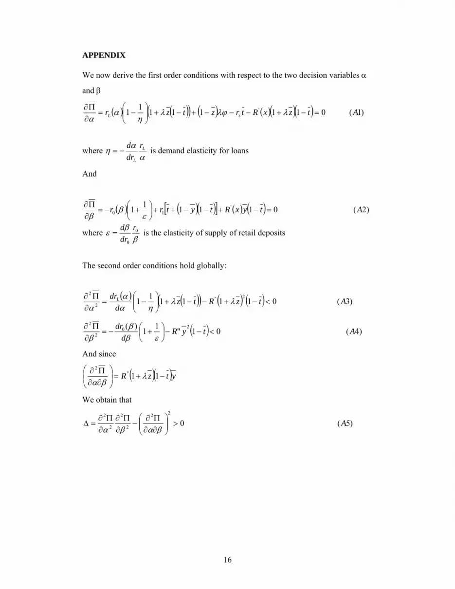
APPENDIX We now derive the first order conditions with respect to the two decision variables α

and β

( ) ( )( ) ( ) ( )( )( ) )1(01111111 ' AtzxRtrztzr sL =−+−−−+−+⎟⎟⎠

⎞⎜⎜⎝

⎛−=

∂Π∂ λλϕλ

ηα

α

where α

αη L

L

rdrd

−= is demand elasticity for loans

And

( ) ( )( )[ ] ( ) ( ) )2(011111 '10 AtyxRtytrr =−+−−++⎟

⎠⎞

⎜⎝⎛ +−=

∂Π∂

εβ

β

where β

βε 0

0

rdrd

= is the elasticity of supply of retail deposits

The second order conditions hold globally:

( ) ( )( ) ( ) ( ) )3(01111112"

2

2

AtzRtzd

drL <−+−−+⎟⎟⎠

⎞⎜⎜⎝

⎛−=

∂Π∂ λλ

ηαα

α

( ) )4(01"11)( 202

2

AtyRd

dr<−−⎟

⎠⎞

⎜⎝⎛ +−=

∂Π∂

εββ

β

And since

( )( )ytzR −+=⎟⎟⎠

⎞⎜⎜⎝

⎛∂∂Π∂ 11"

2

λβα

We obtain that

)5(022

2

2

2

2

A>⎟⎟⎠

⎞⎜⎜⎝

⎛∂∂Π∂

−∂Π∂

∂Π∂

=∆βαβα