Banking competition, collateral constraints and optimal

monetary policy�

Javier Andrés

University of Valencia

Óscar Arce

Economic Bureau of the Prime Minister

Carlos Thomas

Bank of Spain

June 1, 2009

Abstract

We analyze optimal monetary policy in a model where borrowing is subject to collateral

constraints and credit �ows are intermediated by a monopolistically competitive banking

sector. We show that, under certain conditions and up to a second order approximation,

welfare maximization is equivalent to stabilization of four goals: in�ation, output gap, the

consumption gap between constrained and unconstrained consumers, and the distribution

of the collateralizable asset between both groups. Following both productivity and credit-

crunch shocks, the optimal monetary policy commitment implies a short-run trade-o¤

between these goals. Finally, such trade-o¤s become ampli�ed as banking competition

increases, due to the increase in �nancial leveraging.

1 Introduction

In this paper we provide a theoretical framework for the analysis of the optimal conduct of

monetary policy in the presence of �nancial frictions. Both optimal monetary policy and the

macroeconomic e¤ects of �nancial frictions have attracted much attention in recent times.�We are very garteful to Tommaso Monacelli and the seminar paticipans at the Bank of Spain "Workshop

on Monetary Policy" for their useful comments and suggestions.

1

However, much less e¤ort has been devoted to exploring the connections between both �elds in

the context of modern dynamic stochastic general equilibrium (DSGE) models.

Here we perform such an exploration in the context of a model economy featuring two

distinct �nancial frictions: borrowing constraints and endogenous bank-lending spreads. In

this way, our setup nests two of the most prominent hypotheses in the macroeconomic liter-

ature on �nancial frictions: one that emphasizes the role of endogenous collateral constraints

(Kiyotaki and Moore, 1997; Iacoviello, 2005), and another one that stresses the role of endoge-

nous lending spreads, as exempli�ed by the "�nancial accelerator" literature (Bernanke and

Gertler, 1989; Bernanke, Gertler and Gilchrist, 1999) and by the recent literature on banking

and macroeconomics (Goodfriend and McCallum, 2007).

Speci�cally, we consider an economy in which consumers are divided into households and

entrepreneurs, where the former are assumed to be relatively more patient and therefore act

as savers. The latter do not lend directly to entrepreneurs. Instead, they provide banks with

deposits that are then used to make loans to entrepreneurs. Banks are assumed to have some

monopolistic power in the loans market. In particular, following Andrés and Arce (2008) we

assume that a �xed number of identical banks compete to attract investors as in the spatial

competition model of Salop (1979).1 In this framework, each bank is able to charge a positive

lending spread on the deposit rate. Entrepreneurs face endogenous credit limits that link their

borrowing capacity to the expected value of their real estate holdings, which we assume is

the only collateralizable asset available. Real estate can also be used by entrepreneurs as a

production factor in the form of commercial real estate, and by households in the form of

residential housing.

In our framework, borrowers optimally select their lending bank and the size of the loan.

Both decisions determine the two margins of the demand for loans: the extensive margin (i.e.

the market share of each bank) and the intensive margin (i.e. the volume of funds demanded

by each borrower). Banks set their pro�t-maximizing lending rates taking into account that a

higher lending rate raises unit margins but reduces both the demand for funds by each borrower

and their market share. Due to the e¤ect of collateral constraints, the entrepreneurs�demand

for loans depends not only on loan rates but also on the expected growth rate of housing

prices and on the pledgeability ratio (which is understood as the maximum fraction of the

expected value of a borrower�s real estate holdings that can be pledged as collateral). These

factors, along with the number of competing banks, are the major determinants of the optimal

1Andrés and Arce (2008) analyze the macroeconomic e¤ects of imperfect banking competition and collateralconstraints from a positive perspective. Here, we perform a normative analysis within a simpli�ed version oftheir model.

2

lending margins, through their in�uence on the elasticity of the demand schedule faced by each

individual bank. In particular, lending margins are lower when housing prices are expected to

rise, when borrowing constraints are looser, or when there is a larger pool of banks. Further,

there is also a positive relationship between the monetary policy rate, which corresponds to the

banks�marginal cost, and the lending margin. We show that our model generates a monetary

policy accelerator, since a change in the policy rate produces a more than proportional change

in the lending rate. Also, our economy features two familiar nominal frictions: nominal (non-

state-contingent) debt and staggered nominal price adjustment à la Calvo (1983), both of which

open two additional channels of in�uence for monetary policy.

Our main focus in this paper is to understand the nature of optimal monetary policy in

this framework. To this aim we follow the linear-quadratic approach pioneered by Rotemberg

and Woodford (1997) and extensively applied by Woodford (2003) and Benigno and Woodford

(2003), among others. This approach consists of deriving a second-order approximation to the

aggregate welfare criterion, and a �rst-order approximation to the equilibrium conditions. The

central bank�s optimal monetary policy commitment is the one that maximizes the quadratic

welfare criterion subject to the linear equilibrium constraints. This approach allows us to clarify

what the stabilization goals of the central bank are, and what trade-o¤s exist between these

goals.

Speci�cally, we show that the central bank�s quadratic welfare criterion features four sta-

bilization goals: in�ation, the output gap, the di¤erences in consumption between households

and entrepreneurs (consumption gap) and the ine¢ ciency in the distribution of real estate be-

tween both groups (or housing gap). The �rst two, in�ation and the output gap, are related to

the existence of staggered price adjustment and are therefore standard in the New Keynesian

literature. The last two are novel and are directly related to the existence of �nancial frictions.

First, borrowing constraints prevent constrained consumers from smoothing their consumption

the way unconstrained consumers do, thus giving rise to ine¢ cient risk sharing between both

consumer types. Second, the distribution of the housing stock between both groups will gen-

erally be ine¢ cient, due to the distortionary e¤ect of collateral constraints on entrepreneurs�

demand for real estate. In turn, the magnitude of these two sources of ine¢ ciency is ampli�ed

by the existence of banks with monopolistic power.

Regarding the linear equilibrium constraints, we show that the consumption gap arises as

an endogenous cost-push term in the New Keynesian Phillips curve; that is, ine¢ cient risk-

sharing creates a short-run trade-o¤ between in�ation and output gap. In addition, we show

that closing the consumption and housing gaps requires ine¢ cient �uctuations in in�ation and

the output gap. Therefore, the optimal policy commitment must yield a compromise between

3

stabilization goals.

Once our model is calibrated, we analyze how the stabilization goals and other variables of

interest respond both to productivity shocks and credit-crunch shocks (in the form of exogenous

reductions in the pledgeability ratio). We consider the responses under the optimal policy

commitment, as well as under simple policy rules such as in�ation targeting. Our results can

be summarized as follows. Following a negative productivity shock, real estate prices fall and

entrepreneurs�consumption (which is tied to their net worth) falls substantially more than the

consumption of unconstrained households. To prevent a large consumption gap from arising,

the central bank �nds it optimal to allow for surprise increases in in�ation and the output

gap. This way, it de�ates the entrepreneurs� real debt burden and increases their pro�ts,

hence ameliorating the negative impact of the shock on their net worth and consumption. The

narrowing of the consumption gap in turn improves the output-in�ation trade-o¤ in subsequent

periods. Following a credit-crunch shock, real estate demand by entrepreneurs reacts strongly

and a large housing gap arises. In order to close the later, the central bank must again allow

for deviations in in�ation and output gap; the resulting adjustment in entrepreneurs�net worth

allows them to smooth their demand for real estate.

For each policy rule and shock type, we also calculate the volatility of stabilization goals

and the associated average welfare loss. For instance, conditional on productivity shocks with

a standard deviation of 1%, welfare losses under the optimal commitment amount to 0:03%

of steady-state consumption, compared to 0:11% under in�ation targeting and 0:09% under

output gap targeting. We also analyze the e¤ect of varying the degree of competition in

the banking industry on the severity of the policy trade-o¤s and the resulting welfare losses.

Regardless of the nature of the shock, we �nd that an increase in banking competition increases

average welfare losses both under the optimal commitment and (especially) under suboptimal

policy rules. Conditional on productivity shocks, welfare losses increase from 0:03% to 0:05%

of steady-state consumption under the optimal commitment, and from 0:11% to 0:92% under

in�ation targeting. The reason is that, as lending spreads fall, entrepreneurs can borrow more

for given real estate holdings, thus driving their leverage ratio up. Higher leverage, in turn,

implies that �uctuations in real estate prices have stronger e¤ects on entrepreneurs�net worth

and hence on the consumption gap. A similar mechanism operates conditional on credit-

crunch shocks. However, in this case the increase in welfare losses is proportionately much

smaller (from 0:03% to 0:04% under the optimal commitment, and from 0:04% to 0:05% under

in�ation targeting). The reason is that, under imperfect banking competition, lending margins

react counter-cyclically to credit-crunch shocks and thus amplify their e¤ects; under perfect

competition, lending margins are zero and their amplifying role disappears.

4

In a recent paper, Monacelli (2007) simulates the Ramsey optimal monetary policy in a

model with collateral constraints and quadratic price adjustment costs. He �nds that optimal

in�ation volatility depends on some preference parameters and the degree of price rigidity. In

term of focus and methodology, Cúrdia and Woodford (2008; CW, for short) is the closest

reference to this paper. They also focus on the design of optimal monetary rules in the context

of a model economy in which a positive spread exists between lending and deposit rates. CW

assume that the lending spread is determined by an ad-hoc function of banks� loan volume,

aimed at capturing the costs of originating and monitoring loans. We di¤er from CW in two

important respects regarding the nature of credit frictions. First, we model credit spreads

as arising endogenously in an environment in which banks enjoy some monopolistic power in

the loans market. Second, we subject borrowers to endogenous collateral constraints, thus

providing a link between asset prices and the borrowing capacity of constrained consumers.

As in CW, we cast our optimal policy problem in a linear-quadratic representation, motivated

by its potential for delivering analytical results. Importantly, both CW and our paper �nd

that cyclical �uctuations in lending spreads have minor quantitative e¤ects on the nature of

optimal monetary policy design. However, in our model the average level of lending spreads has

important quantitative e¤ects that arise from the interaction between spreads and collateral

constraints, a channel which is missing in CW. We conclude that the welfare loss incurred when

deviating from the optimal policy is sensitive with respect to the level of lending spreads.

The rest of the paper is organized as follows. Section 2 contains the model. In section

3 we analyze the e¢ cient equilibrium which corresponds to the normative benchmark for the

optimizing central bank. We derive the optimizing monetary policy criterion in section 4

and discuss the several trade-o¤s faced by the monetary authority. In section 5 we use some

calibrated versions of the model to perform a number of quantitative exercises in order to

illustrate the working of optimal and suboptimal monetary rules. Section 6 concludes.

2 Model

In this section we describe a model economy that relies on Iacoviello (2005) and Andrés and

Arce (2008). The population of consumers, whose size is normalized to 1, is composed of two

types of agents: there is a fraction ! of households and a fraction 1 � ! of entrepreneurs.The later are assumed to be more impatient than the former and, in the class of equilibria we

analyze later, they borrow up to a limit proportional to the expected present-discounted resale

value of their real estate holdings at the time of repaying debts, which is assumed to be one

5

period ahead.

2.1 Households

The representative household maximizes its welfare criterion,

E0

1Xt=0

�t

log ct �

(lst )1+'

1 + '+ #t log ht

!;

where ct are units of a Dixit-Stiglitz basket of �nal consumption goods, lst is labor supply,

ht is residential housing, #t = # exp(zht ) is an exogenously time-varying weight on utility from

housing services (where zht follows a zero-mean AR(1) process) and � 2 (0; 1) is the household�ssubjective discount factor. (Unless otherwise indicated, we use lower case for real variables and

upper case for nominal variables. All quantities are expressed in per capita terms.)

Maximization is subject to the following budget constraint expressed in real terms,

wtlst + t + st +

Rdt�1�t

dt�1 = ct + pht

��1 + �h

�ht � ht�1

�+ dt;

where wt is the hourly wage, t are dividends from the corporate sector (other than entrepre-

neurs), and st are lump-sum subsidies from the government. We assume that nominal, risk-free,

one-period bank deposits are the only �nancial asset available to households, where dt is the real

value of deposits at the end of period t, Rdt is the gross nominal deposit rate and �t � Pt=Pt�1is the gross in�ation rate, where Pt is the Dixit-Stiglitz aggregate price index. Households

can also buy and sell real estate for residential purposes, where ht are housing units, pht is the

unit price of housing in terms of consumption goods and �h is a tax rate on housing purchases

by households (the role of which is discussed later on). We assume that real estate does not

depreciate. The �rst order conditions of the problem above are standard:

wt = ct (lst )' ; (1)

1

ct= �RdtEt

�1

ct+1

PtPt+1

�; (2)�

1 + �h�pht

ct=#tht+ �Et

pht+1ct+1

: (3)

6

2.2 Entrepreneurs (intermediate good producers)

Entrepreneurs produce a homogenous intermediate good that is sold under perfect competition

to a �nal goods sector. They operate a Cobb-Douglas production technology,

yt = eat�ldt�1�� �

het�1��; (4)

where yt is output of the intermediate good, ldt is labor demand, het�1 is the stock of commercial

real estate and at is a zero-mean AR(1) exogenous productivity process. Entrepreneurs also de-

mand consumption goods and loans. The budget constraint of the representative entrepreneur

is given by

bt + (1� � e)�pIt yt � wtldt

�= cet + p

ht (h

et � het�1) +

Ret�1�t

bt�1; (5)

where bt is the real value of nominal loans at the end of period t, Ret is the gross nominal

loan rate, pIt is the real price of the intermediate good, �e is a tax rate on entrepreneur pro�ts

(the role of which is explained below) and cet is entrepreneur consumption. Banks impose

a collateral constraint on entrepreneurs: the nominal loan gross of interest payments cannot

exceed a certain fraction (the pledgeability ratio) of the expected nominal resale value of the

entrepreneur�s real estate holdings. The collateral constraint can be expressed in real terms as,

bt � mtEt�t+1Ret

pht+1het ; (6)

where mt = m exp(zmt ) is the exogenously time-varying pledgeability ratio and zmt is a zero-

mean AR(1) process. In order to obtain a loan, the entrepreneur must �rst travel to a bank,

incurring a utility cost which is proportional to the distance between his and the bank�s location.

We assume that entrepreneurs and banks are uniformly distributed on a circle of length one.

Subject to (4), (5) and (6), an entrepreneur located at point k 2 (0; 1] maximizes

E0

1Xt=0

(�e)t (log cet � �dk;it );

where dk;it is the distance between the entrepreneur and the lending bank which is denoted by

i 2 f1; 2; :::; ng, and � is the utility cost per distance unit. Entrepreneurs are assumed to bemore impatient than savers, i.e. �e < �. The �rst order conditions of this problem are

wt = pIt (1� �)

ytldt; (7)

7

1

cet= �eRetEt

�1

cet+1

PtPt+1

�+ �t; (8)

phtcet= Et

�e

cet+1

�(1� � e) pIt+1�

yt+1het

+ pht+1

�+ �tmtEt

�t+1Ret

pht+1; (9)

where �t is the Lagrange multiplier on the collateral constraint and pIt�yt=h

et�1 is the marginal

revenue product of commercial real estate. When binding (�t > 0), the collateral constraint

has two e¤ects on the entrepreneurs decisions: �rst, it prevents them from smoothing their

consumption the way households do (equation (8)); second, it increases the marginal value of

real estate due to its role as collateral (equation (9)).

Due to the assumption that �e < �, it is easy to check that the borrowing constraint binds

in the steady state. Provided the �uctuations in the endogenous variables around their steady

state are su¢ ciently small, the borrowing constraint will also bind along the dynamics; that

is, equation (6) holds with equality. It is then possible to show that the entrepreneur simply

consumes a fraction 1� �e of her real net worth,2

cet = (1� �e)�(1� � e) �pIt yt + pht het�1 �

Ret�1�t

bt�1

�; (10)

where (1� � e) �pIt yt are after-tax real pro�ts, pht het�1 is commercial real estate wealth and�Ret�1=�t

�bt�1 are real debt repayments.

2.3 Banks

Banks are assumed to intermediate all credit �ows between households (savers) and entrepre-

neurs (borrowers). We assume that banks are perfectly competitive on the deposits market,

but competition in the loans market is imperfect so that each bank enjoys some monopolistic

power. In order to model imperfect competition in the loans market we use a version of Sa-

lop�s (1979) circular-city model. Banks are located symmetrically on the unit circle and their

position is time-invariant, whereas entrepreneurs�locations vary each period according to an

iid stochastic process.3 Bank i chooses the gross nominal interest rate on its loans, Ret (i), to

maximize

Et

1Xs=0

�sctct+s

t+s(i)

Pt+s

2See the proof in the Appendix.3This last assumption removes the possibility that banks exploit strategically the knowledge about the

current position of each entrepreneur to charge higher rates in the future.

8

where �sct=ct+s is the time t+s stochastic discount factor of the bank�s owners (the households)

and t+s(i) is the bank�s nominal pro�t �ow. Denoting by Bt(i) and Dt(i) the nominal stock

of loans and deposits of bank i at the end of time t; respectively, we can write its �ow of funds

constraint as

t (i) +Bt (i) +Rdt�1Dt�1 (i) = R

et�1 (i)Bt�1 (i) +Dt (i) :

Further, bank i must also obey the balance-sheet identity, Dt (i) = Bt (i). To solve for the

bank�s optimal loan rate, it is convenient to express its real loan volume as

Bt(i)

PT= bt(i)~bt(i);

where bt(i) is the intensive business margin (the size of each loan) and ~bt(i) is the extensive

business margin (the number of customers, or market share).4 The �rst order condition of this

problem can be written as

Ret (i) = Rdt +

1

�t(i) + ~�t(i); (11)

where, �t(i) � [�@bt(i)=@Ret (i)] =bit is the semi-elasticity of the intensive business margin and~�t(i) � [�@~bt(i)=@Ret (i)]=~bt(i) is the semi-elasticity of the extensive business margin. Thus thespread between the lending and the deposit rate is a negative function of the bank�s market

power, as represented by the semi-elasticities of the intensive margin and the market share.

As shown in Andrés and Arce (2008), in a symmetric equilibrium (i.e. Ret�1 (i) = Ret�1 8i),

the optimal lending rate can be expressed as

Ret = Rdt +

Rdt �mtEt��t+1p

ht+1=p

ht

��mtEt

��t+1pht+1=p

ht

��Rdt

Rdt ; (12)

where

� � 1 + n

�e�e

1� �e :

Therefore, the lending spread is decreasing in expected house price in�ation, Et��t+1p

ht+1=p

ht

�,

the pledgeability ratio, mt, and the degree of banking competition, as captured by the ratio

n=�e; and it is increasing in the nominal deposit rate, Rdt . The intuition for these e¤ects is

the following. An increase in expected house price in�ation or the pledgeability ratio increase

entrepreneurs�borrowing capacity. As their indebtedness rises, their demand for loans becomes

more elastic, which reduces banks�market power and compresses lending spreads. Similarly,

4See Andrés and Arce (2008) for analytical derivations of both margins.

9

as entrepreneurs become more indebted, the utility cost of servicing the debt becomes more

important in the choice of bank relative to the distance utility cost. As a result, small changes

in loan rates lead to large �ows of customers in search for the lowest loan rate. This pushes

lending spreads down. Similar intuitions can be provided regarding the e¤ects of the nominal

deposit rate. Finally, an increase in the degree of banking competition compresses lending

spreads through an increase in the elasticity of banks�market share with respect to the lending

rate.

2.4 Final goods producers

There exist a measure-one continuum of �rms that purchase the intermediate good from en-

trepreneurs and transform it one-for-one into di¤erentiated �nal goods or varieties. For these

�rms, the real price of the intermediate good, pIt , represents the real marginal cost. Cost min-

imization by households implies that each �nal good producer j 2 [0; 1] faces the followingdemand curve for its product variety,

yft (j) =

�Pt(j)

Pt

��"yft ; (13)

where Pt(j) is the �rm�s nominal price, " > 1 is the elasticity of substitution between �nal good

varieties and

yft = !ct + (1� !) cet (14)

is the aggregate demand for �nal goods. As is standard in the New Keynesian literature, we

assume staggered nominal price adjustment à la Calvo (1983). Letting � denote the constant

probability of price adjustment, the optimal price decision of the price-setting �rms is given by

Et

1XT=t

(��)T�tctcT

((1 + �)

~PtPT

� "

"� 1pIt

)P "Ty

fT = 0; (15)

where � > 0 is a subsidy rate on the revenue of �nal goods producers (the role of which is

explained below) and ~Pt is the optimal price decision. Under Calvo price adjustment, the

aggregate price index evolves as follows,

Pt =h�P 1�"t�1 + (1� �) ~P 1�"t

i1=(1�"): (16)

10

2.5 Market clearing

Total supply of the intermediate good equals (1� !) yt. Total demand from �nal good produc-ers equals

R 10yft (j)dj, where each �rm�s demand is given by (13). Equilibrium in the interme-

diate good market therefore requires

(1� !) yt = �tyft ; (17)

where �t �R 10(Pt(j)=Pt)

�" dj is a measure of price dispersion in �nal goods. Notice that price

dispersion increases the amount of the intermediate good that must be produced in order to

satisfy a certain level of �nal consumption demand.

Equilibrium in the housing market implies

�h = !ht + (1� !)het ; (18)

where �h is the �xed aggregate stock of real estate.

The labor market equilibrium condition is

!lst = (1� !) ldt : (19)

2.6 Monetary policy

The model is closed by means of a monetary policy rule.5 The latter can be a simple rule,

such as strict in�ation targeting, or a policy that is optimal with respect to some criterion.

Sections 4 and 5 below are devoted to characterizing both types of policy rules and their e¤ects

on equilibrium allocations.

3 E¢ cient equilibrium

In this section we analyze the e¢ cient equilibrium in our model, which will be the normative

benchmark for the monetary authority. We assume that, when maximizing aggregate welfare,

the social planner assigns to entrepreneurs the same discount factor as that of households, �.6

5Regarding the budget constraint of the government, by Walras Law such a constraint is implied by allmarket equilibrium conditions and the �ow of funds constraints of all agents in the economy. In particular, thepublic surplus is the sum of tax receipts from house purchases and entrepreneur pro�ts, minus subsidies to �nalgoods producers. The resulting surplus is rebated to households in the form of lump-sum subsidies, st.

6Otherwise, the social planner equilibrium would assign less and less consumption to the impatient con-sumers (the entrepreneurs) relative to the patient ones (the households) as time went by. This would make the

11

The social planner therefore maximizes

E0

1Xt=0

�t

(!

"log(ct)�

(lst )1+'

1 + '+ #t log(ht)

#+ (1� !) log(cet )

)

subject to the aggregate resource constraints for consumption goods and real estate,

(1� !) eat�het�1

�� � !

1� ! lst

�1��= !ct + (1� !) cet ; (20)

�h = !ht + (1� !)het ; (21)

where we have used equation (19) to substitute for ldt in the left-hand side of equation (20).

Using equations (20) and (21) to solve for ct and ht, respectively, the social-planner problem

simpli�es to the choice of the optimal state-contingent path of cet , het and l

st . The �rst-order

conditions of this problem can be expressed as

ct = cet ; (22)

�Et1

ct+1�eat+1 (het )

� �!lst+1= (1� !)�1��het

=#tht; (23)

ct (lst )' =

1� !!

(1� �) ytlst: (24)

Notice that equations (20) and (22) jointly imply (1� !) eat�het�1

��[!lst= (1� !)]

1�� = ct.

Using this in equation (23), we have that the e¢ cient distribution of the housing stock is given

byhetht=

��

(1� !)#t: (25)

This, combined with equation (21), implies the following solution for aggregate residential

housing,

!ht =!#t

!#t + ���h: (26)

Using equations (20) and (22) in equation (24) we obtain the following solution for e¢ cient

labor supply,

lst =

�1� �!

�1=(1+'): (27)

equilibrium allocation dependent on the time elapsed since the implementation of the social planner solution,and the system of equations would not have a recursive representation.

12

Substituting this expression into the production function, we obtain the e¢ cient level of output,

yt = eat�het�1

�� � !

1� !

�1�� �1� �!

�(1��)=(1+'): (28)

To summarize, the e¢ cient equilibrium is characterized by full consumption risk sharing be-

tween households and entrepreneurs (equation (22)), a distribution of the housing stock that

changes only with shocks to housing utility (equation (25)) and a constant labor supply (equa-

tion (27)).7 These features will help us understand the stabilization goals and trade-o¤s of

monetary policy. We turn to this now.

4 Optimal monetary policy

In order to analyze optimal monetary policy, we follow the linear-quadratic approach pioneered

by Rotemberg and Woodford (1997) and extensively applied in Woodford (2003). The linear-

quadratic method consists of deriving a log-quadratic approximation of aggregate welfare (which

will represent the objective function of the central bank) and a log-linear approximation of

the equilibrium conditions (which will be the constraints on the central bank�s optimization

problem). As is well known, this method is helpful at clarifying what the stabilization goals are

for the central bank and what trade-o¤s exist among those goals. Indeed, the application of this

method in our setup delivers a set of analytical results that facilitate greatly the interpretation

of our subsequent numerical results.

4.1 Quadratic loss function

As emphasized by Benigno and Woodford (2008), the approximation of the aggregate welfare

criterion must be purely quadratic in order for the linear-quadratic approach to provide a correct

welfare ranking (with an accuracy of up to second order) of alternative monetary policy rules.

Derivation of a purely quadratic approximation is greatly simpli�ed by the assumption of an

e¢ cient steady state for the welfare-relevant variables. As shown in the Appendix, steady-state

e¢ ciency for such variables can be implemented in our framework by making the following

three assumptions.

7The fact that neither labor hours nor the distribution of real estate are a¤ected by productivity shocks inthe e¢ cient equilibrium is due to our assumption of logarithmic utility of consumption. Deviating from thelatter assumption would complicate the algebra without adding much to our main insights about the nature ofoptimal monetary policy.

13

Assumption 1 The subsidy rate on the revenue of �nal goods producers is given by

� ="

"� 1 � 1 > 0:

Assumption 2 The tax rate on entrepreneur pro�ts is given by

� e = 1� 1� !(1� �e) �

1� �e �m (1=Ress � �e)1�m=Ress

:

Assumption 3 The subsidy rate on residential housing purchases is given by

�h =�

�e1� �e �m (1=Ress � �e)

1� � e � 1 + �:

The �rst assumption eliminates the monopolistic distortion in �nal goods markets, such

that steady-state real marginal costs are unity (pIss = 1). The second assumption guarantees

e¢ cient risk-sharing between households and entrepreneurs in the steady state (css = cess). The

third one implements the e¢ cient steady-state distribution of real estate between commercial

and residential uses (hess=hss = ��= [(1� !)#]). Under assumptions 1 to 3, aggregate welfarecan be approximated by8

1Xt=0

�t

(!

"log ct + #t log ht �

(lst )1+'

1 + '

#+ (1� !) log cet

)= �

1Xt=0

�tLt + t:i:p:+O3;

where t:i:p: are terms independent of policy, O3 are terms of order third and higher, and

Lt = ���2t + �y

�yt � y�jht

�2+ �c (ct � cet )

2 + �h

�ht � h�t

�2(29)

is a purely quadratic period loss function, where hats denote log-deviations from steady state

and weight coe¢ cients are given by

�� �"�

(1� �) (1� ��) ; �y �1 + '

1� � ; �c � ! (1� !) ; �h � !#!#+ ��

��:

The loss function illustrates the existence of four stabilization goals for the central bank. The

�rst one is in�ation. As is well known, under staggered price adjustment in�ation creates

8See the proof in the Appendix.

14

ine¢ cient price dispersion and hence a welfare loss. The second goal is the output gap, where

y�jht � at + �het�1

is e¢ cient output conditional on the stock of commercial housing (see equation (28)).9 Nominal

price rigidities produce ine¢ cient �uctuations in output which, given the stock of commercial

property, generates in turn ine¢ cient �uctuations in labor hours. These �rst two goals are

standard in the New Keynesian model.

The third and fourth goals are directly related to the existence of credit frictions in this

model. The third goal is the (log) di¤erence between the consumption of households and

entrepreneurs, i.e. between unconstrained and constrained consumers, which we may refer to

as the consumption gap. This term captures the aggregate welfare losses produced by ine¢ cient

risk sharing between households and entrepreneurs, which is in turn the result of collateral

constraints on entrepreneurs. The fourth goal is the (log) di¤erence between the actual and

the e¢ cient level of residential real estate, or housing gap, where

h�t ���

!#+ ��zht (30)

is e¢ cient residential housing (see equation (26)). Notice that, given the �xed supply of real

estate, an ine¢ cient level of residential real estate is equivalent to an ine¢ cient distribution of

real estate between residential and commercial uses. Ine¢ ciency in the real estate distribution

in our framework can arise for various reasons. First, demand of commercial property by

entrepreneurs is distorted by its role as collateral in loan agreements. Second, since households

and entrepreneurs di¤er in their degree of impatience and their consumption, they also use

di¤erent stochastic discount factors for pricing future state-contingent payo¤s from housing.

Finally, the fact that commercial real estate purchases are partly �nanced by loans implies that

they are prone to su¤ering the e¤ects of credit-crunch shocks.

4.2 Policy trade-o¤s

The second step of the linear-quadratic approach consists of log-linearizing the equilibrium

conditions around the steady state. For brevity, the complete list of log-linear equations is

9This is di¤erent from unconditionally e¢ cient output, which depends on the path of commercial housingthat would have been observed in an e¢ cient equilibrium. For a discussion on this issue, see Woodford (2003,section 5.3) and Neiss and Nelson (2003).

15

deferred to the Appendix.10 Here, we restrict our attention to those equations that are helpful

for understanding the trade-o¤s among stabilization goals. We start by log-linearizing and

combining equations (15) and (16), which yields

�t =(1� �) (1� ��)

�pIt + �Et�t+1: (31)

In order to �nd an expression for real marginal costs, pIt , we �rst log-linearize equations (1),

(7) and (19), and combine them into

ct + 'lst = p

It + yt � lst : (32)

That is, the labor supply schedule (the marginal rate of substitution between consumption and

leisure) must intersect the labor demand schedule (the marginal revenue product of labor).

Second, we log-linearize the production function and solve for labor hours, obtaining

lst =1

1� �

�yt � at � �het�1

�=

1

1� �

�yt � y�jht

�: (33)

Third, we log-linearize the equilibrium conditions in the �nal goods and intermediate good

markets, equations (14) and (17) respectively, and combine them into

yt = !ct + (1� !) cet ; (34)

where we have used the fact that (1� !) yss = css = cess in the e¢ cient steady state.11 Com-bining equations (32) to (34), we can express real marginal costs as

pIt =1 + '

1� �

�yt � y�jht

�+ (1� !) (ct � cet ) : (35)

Using this in equation (31) yields the following New Keynesian Phillips curve,

�t = �1 + '

1� �

�yt � y�jht

�+ �Et�t+1 + � (1� !) (ct � cet) ; (36)

10Simulation results not reported here indicate that the Ramsey optimal long-run gross rate of in�ation is�ss = 1, regardless of whether the steady state is assumed to be e¢ cient or not. Therefore, our log-linearizationis performed around a zero net in�ation steady state. The reason for this result is essentially the same as thereason why the optimal long-run net rate of in�ation is zero in the standard New Keynesian model, namely thatthe welfare losses of committing to positive in�ation rates in the future outweigh the welfare gains of exploitingthe short-run output-in�ation trade-o¤ when output is ine¢ ciently low (see e.g. Woodford, 2003).11As shown in the Appendix, the price dispersion term �t is of second order and therefore drops out of the

log-linear approximation of equation (17).

16

where � � (1� �) (1� ��) =�. Equation (36) has the same form as the standard New Key-

nesian Phillips curve, with the exception of the last term on the right hand side, which is

proportional to the consumption gap. Therefore, collateral constraints and the resulting ine¢ -

cient risk-sharing create an endogenous trade-o¤ between output gap and in�ation. The reason

is the following. From equation (32), real marginal costs pIt depend on labor hours and the

di¤erence between aggregate demand and household consumption. Because of ine¢ cient risk

sharing, �uctuations in aggregate demand and household consumption will be unequal. As a

result, keeping labor hours constant (that is, closing the output gap) is not enough to prevent

�uctuations in real marginal costs and hence in in�ation.

From the preceding analysis, it follows that closing the consumption gap has two bene�cial

e¤ects on aggregate welfare. First, it improves the trade-o¤ between in�ation and output gap.

Second, since the consumption gap is itself a stabilization goal, closing it has a direct bene�cial

e¤ect on welfare. A third normative reason for closing the consumption gap is that it relaxes the

borrowing constraint on entrepreneurs. This makes the real estate distribution more e¢ cient

over the cycle and thus helps closing the housing gap.

While desirable, consumption gap stabilization requires itself ine¢ cient �uctuations in other

stabilization goals. To see this, consider the log-linear approximation of the entrepreneur

consumption equation around the e¢ cient steady state (cess=yss = 1� !),

cet = (1� �e)�(1� � e) �1� !

�pIt + yt

�+phssh

ess

cess

�pht + h

et�1

��mp

hssh

ess

cess

�Ret�1 + bt�1 � �t

��;

(37)

where both sides have been normalized by cess and we have used bssRess = mphssh

ess. The

borrowing constraint, equation (6) holding with equality, can be approximated by Ret + bt =

zmt + Etpht+1 + h

et + Et�t+1. Substituting this into equation (37) and rearranging terms, we

obtain

cet = (1-�e)

�(1-� e) �1� !

�pIt+yt

�+phssh

ess

cess

h�pht �mEt-1pht

�+ (1�m) het-1 +m (�t � Et-1�t)�mzmt-1

i�:

(38)

Therefore, entrepreneur pro�ts (pIt + yt), in�ation surprises (�t � Et�1�t) and quasi-surprisesin real estate prices (pht � mEt�1pht ) are the major endogenous determinants of entrepreneurconsumption. The latter will therefore di¤er from household consumption, which is driven

exclusively by intertemporal substitution considerations. In response to unexpected shocks,

it is however possible for the central bank to bring entrepreneur and household consumption

closer to each other. First, by engineering in�ation surprises it can manipulate the real value of

17

debt repayments and hence the equilibrium path of entrepreneurial net worth. Second, notice

that entrepreneur pro�ts can be expressed in terms of stabilization goals as follows,

pIt + yt =

�1 + '

1� � + 1��yt � y�jht

�+ (1� !) (ct � cet) + y

�jht ;

where we have used equation (35) to substitute for pIt . Therefore, the central bank can also

resort to output-gap management so as to manipulate entrepreneur pro�ts in a way that reduces

the consumption gap.

To summarize, optimal monetary policy will involve a trade-o¤between all four stabilization

goals. We now turn to the quantitative analysis of these trade-o¤s.

5 Quantitative analysis

5.1 Calibration

We calibrate our model to quarterly US data. The calibration is largely based on Andrés

and Arce (2008) and Iacoviello (2005). The household discount factor, � = 0:993, is chosen

such that the annual real interest rate equals 3%. The entrepreneur discount factor is set

to 0:95, within the range of values for constrained consumers typically used in the literature.

The elasticity of production with respect to commercial housing, � = 0:05, is set in order to

generate a steady-state ratio of commercial housing wealth to annual output of 62%. Similarly,

the weight on housing utility, # = 0:11, is chosen to match an average ratio of residential

housing wealth to annual output of 140%. Regarding the banking parameters, what matters

for the steady-state level of lending spreads is the ratio n=�. We arbitrarily set the number

of banks to 10, and then set the distance utility parameter, �, to obtain a steady-state annual

lending spread of 2:5%. The size of the household population, ! = 0:979, is chosen such that

the tax rate on entrepreneur pro�ts equals zero in the steady state.12 The loan-to-value ratio

is set to m = 0:85, as in Iacoviello (2005). The labor supply elasticity is set to one half, which

is broadly consistent with micro evidence. The elasticity of demand curves is set to 6, which

would imply a monopolistic mark-up of 20% in the absence of subsidies. The Calvo parameter

implies a mean duration of price contracts of 3 quarters, consistent with recent micro evidence

(Bils and Klenow, 2004, Nakamura and Steinsson, 2008). The subsidy rates on residential

12Alternatively, we could have calibrated ! empirically and then chosen the tax rate �e that implementse¢ cient risk-sharing in the steady state. Since the share of entrepreneurs in the population is small, thisalternative approach would produce a very similar calibration.

18

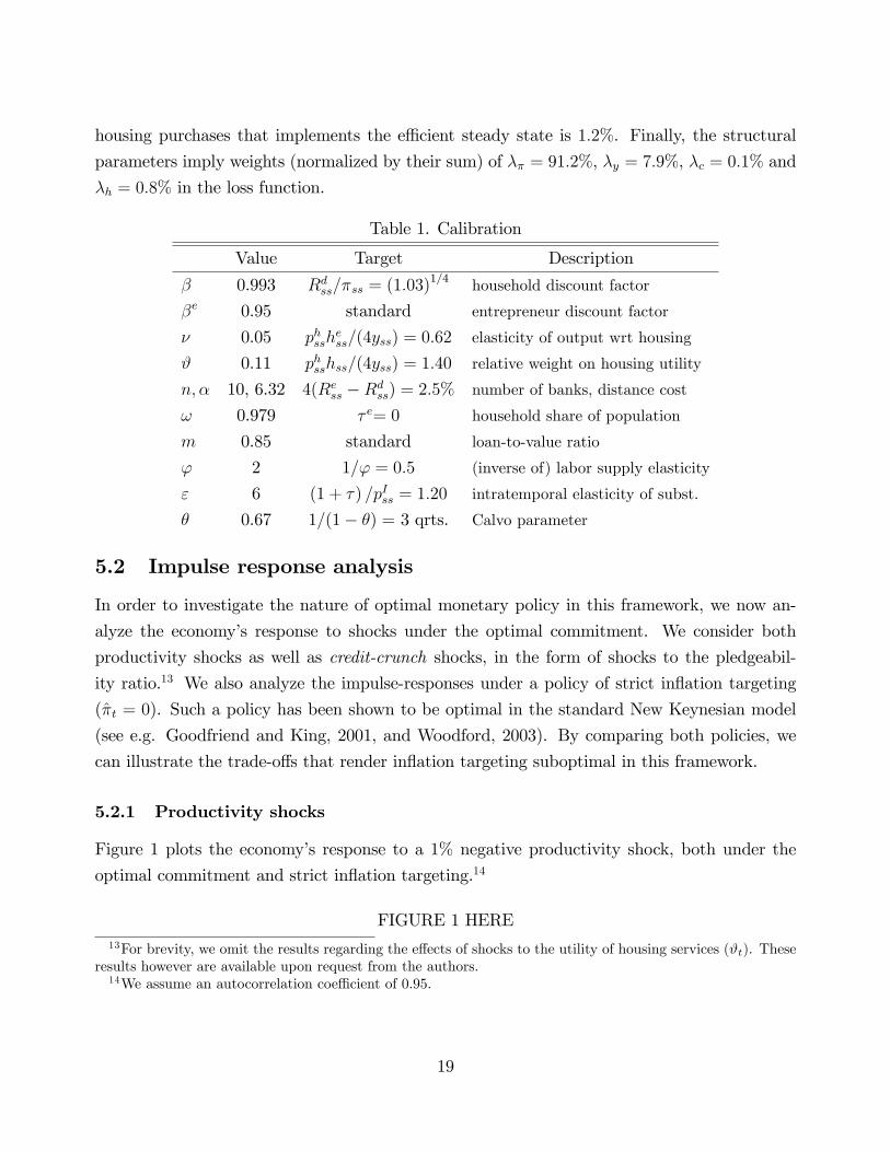
housing purchases that implements the e¢ cient steady state is 1:2%. Finally, the structural

parameters imply weights (normalized by their sum) of �� = 91:2%, �y = 7:9%, �c = 0:1% and

�h = 0:8% in the loss function.

Table 1. Calibration

Value Target Description

� 0.993 Rdss=�ss = (1:03)1=4 household discount factor

�e 0.95 standard entrepreneur discount factor

� 0.05 phsshess=(4yss) = 0:62 elasticity of output wrt housing

# 0.11 phsshss=(4yss) = 1:40 relative weight on housing utility

n; � 10, 6.32 4(Ress �Rdss) = 2:5% number of banks, distance cost

! 0.979 � e= 0 household share of population

m 0.85 standard loan-to-value ratio

' 2 1=' = 0:5 (inverse of) labor supply elasticity

" 6 (1 + �) =pIss = 1:20 intratemporal elasticity of subst.

� 0.67 1=(1� �) = 3 qrts. Calvo parameter

5.2 Impulse response analysis

In order to investigate the nature of optimal monetary policy in this framework, we now an-

alyze the economy�s response to shocks under the optimal commitment. We consider both

productivity shocks as well as credit-crunch shocks, in the form of shocks to the pledgeabil-

ity ratio.13 We also analyze the impulse-responses under a policy of strict in�ation targeting

(�t = 0). Such a policy has been shown to be optimal in the standard New Keynesian model

(see e.g. Goodfriend and King, 2001, and Woodford, 2003). By comparing both policies, we

can illustrate the trade-o¤s that render in�ation targeting suboptimal in this framework.

5.2.1 Productivity shocks

Figure 1 plots the economy�s response to a 1% negative productivity shock, both under the

optimal commitment and strict in�ation targeting.14

FIGURE 1 HERE13For brevity, we omit the results regarding the e¤ects of shocks to the utility of housing services (#t). These

results however are available upon request from the authors.14We assume an autocorrelation coe¢ cient of 0:95.

19

Let us focus �rst on the case of strict in�ation targeting (dotted lines). The fall in total fac-

tor productivity reduces the marginal product of housing, which leads to a fall in entrepreneur

pro�ts, their demand for real estate and real estate prices. Lower pro�ts and real estate wealth,

in turn, trigger a large fall in entrepreneur net worth and hence in entrepreneur consumption.

Household consumption also falls, but it does so by a relatively small amount, thanks to house-

holds�ability to smooth consumption. As a result, the consumption gap increases sharply on

impact. In addition to lowering welfare, the increase in the consumption gap also shifts the

New Keynesian Phillips curve upwards. In order to keep in�ation at zero, the central bank is

obliged to engineer a drop in the output gap. On the other hand, the fall in entrepreneurs�

holdings of real estate produces an increase in the housing gap (remember that productivity

shocks do not a¤ect the e¢ cient real estate distribution; see equation (30)). To summarize,

strict in�ation targeting requires ine¢ cient �uctuations in the output gap and, especially, in

the consumption and housing gaps.

Relative to the situation under in�ation targeting, the optimal policy can improve matters

by allowing for a certain amount of surprise in�ation. This way, it can reduce the real value of

entrepreneurs�debt burden. At the same time, the central bank engineers an increase in the

output gap (that is, it reduces the drop in aggregate demand) also on impact. Both actions

have a bene�cial e¤ect on entrepreneurs�real net worth and therefore on their consumption.

As a result, the consumption gap experiences a substantially smaller increase. This in turn

contains the upward shift in the Phillips curve, thus improving the trade-o¤ between in�ation

and output gap. Indeed, both variables return to zero very quickly.

The optimal policy is implemented via a sharper cut in the nominal interest rate (lower

right panel in Figure 1). Such an aggressive monetary response implies that housing prices fall

by less than under in�ation targeting, both on impact and along the whole recovery path. This

way, the optimal policy reduces the cyclical response of credit, which is positively linked to the

value of collateral, and hence facilitates a smoother adjustment of entrepreneur consumption.

Finally, the endogenous response in lending spreads (not shown in the �gure) is very small under

both policy regimes, with peak drops of 1 and 0:2 basis points, respectively. This suggests that,

given a level of banking competition, the endogenous �uctuations in lending margins do not

seem to amplify the e¤ects of productivity shocks.15

15Andrés and Arce (2008) provide a detailed analysis of the various opposite-sign e¤ects that explain such alow responsiveness of spreads following a productivity shock. Section 5.3 below analyzes the e¤ects of changesin the average (steady-state) levels of bank lending margins.

20

5.2.2 Credit crunch shocks

Figure 2 plots the impulse-responses to a 1% negative shock to the pledgeability ratio (mt)

under the optimal policy and in�ation targeting.16 Again, we focus �rst on the case of in�ation

targeting. The fall in the pledgeability ratio reduces the amount of borrowing by entrepreneurs,

and hence their real estate holdings are immediately reduced. This produces a symmetric

increase in the housing gap (the e¢ cient real estate distribution is invariant to this shock too;

see again equation (30)). Regarding the other stabilization goals, the responses are of minor

importance. First, notice that the consumption gap �rst reacts negatively and then positively.17

Since the reaction of household consumption is relatively small, the consumption gap basically

mirrors the behavior of entrepreneur consumption. And because what matters for in�ation

dynamics is the entire present-discounted path of consumption gaps, the shift in the Phillips

curve is very small, such that a tiny correction in the output gap is enough to keep in�ation at

zero.

FIGURE 2 HERE

Therefore, the optimal policy is primarily aimed at reducing the housing gap. In order to

achieve this, the monetary authority engineers surprise increases in in�ation and the output

gap. Following the same logic as in the analysis of productivity shocks, both actions have

positive e¤ects on entrepreneur net worth. Real estate demand by entrepreneurs is the sum of

unmortgaged real estate wealth (which equals �e times real net worth) plus borrowing. Thanks

to the increase in their net worth, entrepreneurs can increase their holdings of unmortgaged

real estate. This partially compensates the drop in entrepreneurial borrowing, hence producing

a smaller reaction in commercial real estate and the housing gap.

The optimal policy is implemented again by means of a stronger cut in nominal interest

rates than under in�ation targeting. Regarding lending margins (lower left panel in Figure 2),

they experience a non-negligible impact increase of 15 basis points in annualized terms. That

is, the response of spreads now is much more pronounced than in the case of a productivity

shock since in this case banks take advantage of the fact that credit scarcity goes hand in hand

with a more inelastic demand for funds. However, such a response is nearly the same under

both scenarios, which indicates that it is mostly due to the direct e¤ect of the shock to mt (see

equation (12)).16We assume an autocorrelation coe¢ cient of 0:75, such that the shock has a half-life of four quarters.17The reason is the following. The fall in the pledgeability ratio has two opposing e¤ects on entrepreneurs�

net worth and consumption. First, it reduces their real estate wealth. Second, by reducing entrepreneurs�borrowing it also reduces debt repayments from the second period onwards. As can be seen in �gure 2, the �rste¤ect dominates on impact but the second one becomes dominant from the third period onwards.

21

5.3 Volatility of stabilization goals and welfare loss

The previous section characterized the responses of the stabilization goals to productivity and

credit-crunch shocks. These goals however enter with di¤erent weights in the loss function of

the central bank, and therefore have di¤erent quantitative e¤ects on welfare. We are ultimately

concerned with the welfare implications of alternative monetary policy rules. The next section

quanti�es the welfare losses that arise under di¤erent monetary policy regimes.

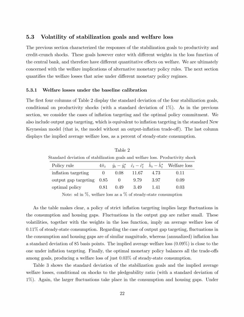
5.3.1 Welfare losses under the baseline calibration

The �rst four columns of Table 2 display the standard deviation of the four stabilization goals,

conditional on productivity shocks (with a standard deviation of 1%). As in the previous

section, we consider the cases of in�ation targeting and the optimal policy commitment. We

also include output gap targeting, which is equivalent to in�ation targeting in the standard New

Keynesian model (that is, the model without an output-in�ation trade-o¤). The last column

displays the implied average welfare loss, as a percent of steady-state consumption.

Table 2

Standard deviation of stabilization goals and welfare loss. Productivity shock

Policy rule 4�t yt � y�t ct � cet ht � h�t Welfare loss

in�ation targeting 0 0.08 11.67 4.73 0.11

output gap targeting 0.85 0 9.79 3.97 0.09

optimal policy 0.81 0.49 3.49 1.41 0.03

Note: sd in %, welfare loss as a % of steady-state consumption

As the table makes clear, a policy of strict in�ation targeting implies large �uctuations in

the consumption and housing gaps. Fluctuations in the output gap are rather small. These

volatilities, together with the weights in the loss function, imply an average welfare loss of

0:11% of steady-state consumption. Regarding the case of output gap targeting, �uctuations in

the consumption and housing gaps are of similar magnitude, whereas (annualized) in�ation has

a standard deviation of 85 basis points. The implied average welfare loss (0:09%) is close to the

one under in�ation targeting. Finally, the optimal monetary policy balances all the trade-o¤s

among goals, producing a welfare loss of just 0:03% of steady-state consumption.

Table 3 shows the standard deviation of the stabilization goals and the implied average

welfare losses, conditional on shocks to the pledgeability ratio (with a standard deviation of

1%). Again, the larger �uctuations take place in the consumption and housing gaps. Under

22

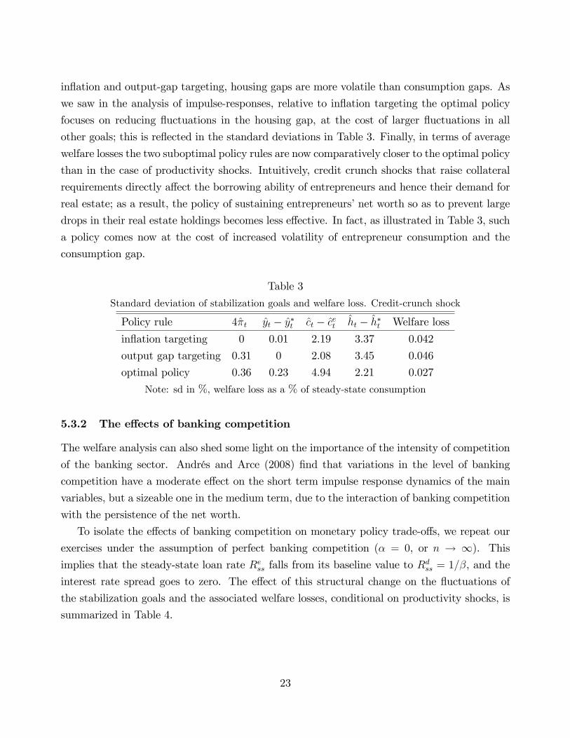
in�ation and output-gap targeting, housing gaps are more volatile than consumption gaps. As

we saw in the analysis of impulse-responses, relative to in�ation targeting the optimal policy

focuses on reducing �uctuations in the housing gap, at the cost of larger �uctuations in all

other goals; this is re�ected in the standard deviations in Table 3. Finally, in terms of average

welfare losses the two suboptimal policy rules are now comparatively closer to the optimal policy

than in the case of productivity shocks. Intuitively, credit crunch shocks that raise collateral

requirements directly a¤ect the borrowing ability of entrepreneurs and hence their demand for

real estate; as a result, the policy of sustaining entrepreneurs�net worth so as to prevent large

drops in their real estate holdings becomes less e¤ective. In fact, as illustrated in Table 3, such

a policy comes now at the cost of increased volatility of entrepreneur consumption and the

consumption gap.

Table 3

Standard deviation of stabilization goals and welfare loss. Credit-crunch shock

Policy rule 4�t yt � y�t ct � cet ht � h�t Welfare loss

in�ation targeting 0 0.01 2.19 3.37 0.042

output gap targeting 0.31 0 2.08 3.45 0.046

optimal policy 0.36 0.23 4.94 2.21 0.027

Note: sd in %, welfare loss as a % of steady-state consumption

5.3.2 The e¤ects of banking competition

The welfare analysis can also shed some light on the importance of the intensity of competition

of the banking sector. Andrés and Arce (2008) �nd that variations in the level of banking

competition have a moderate e¤ect on the short term impulse response dynamics of the main

variables, but a sizeable one in the medium term, due to the interaction of banking competition

with the persistence of the net worth.

To isolate the e¤ects of banking competition on monetary policy trade-o¤s, we repeat our

exercises under the assumption of perfect banking competition (� = 0, or n ! 1). Thisimplies that the steady-state loan rate Ress falls from its baseline value to Rdss = 1=�, and the

interest rate spread goes to zero. The e¤ect of this structural change on the �uctuations of

the stabilization goals and the associated welfare losses, conditional on productivity shocks, is

summarized in Table 4.

23

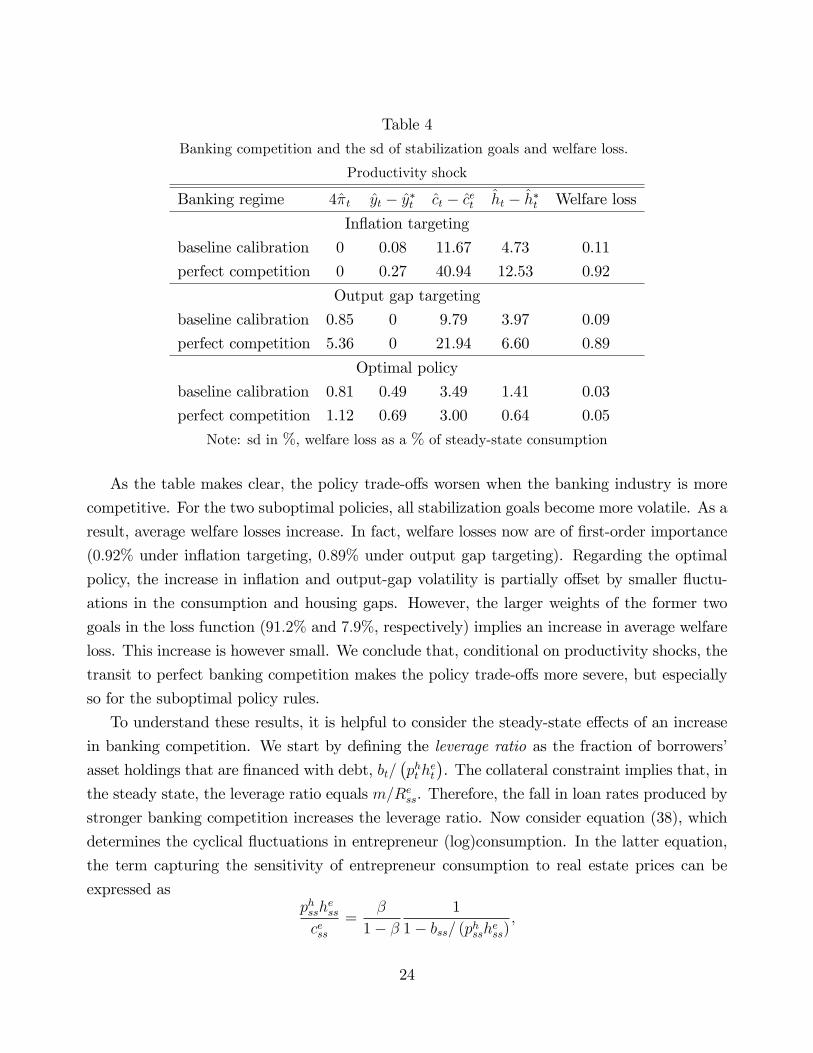
Table 4

Banking competition and the sd of stabilization goals and welfare loss.

Productivity shock

Banking regime 4�t yt � y�t ct � cet ht � h�t Welfare loss

In�ation targeting

baseline calibration 0 0.08 11.67 4.73 0.11

perfect competition 0 0.27 40.94 12.53 0.92

Output gap targeting

baseline calibration 0.85 0 9.79 3.97 0.09

perfect competition 5.36 0 21.94 6.60 0.89

Optimal policy

baseline calibration 0.81 0.49 3.49 1.41 0.03

perfect competition 1.12 0.69 3.00 0.64 0.05

Note: sd in %, welfare loss as a % of steady-state consumption

As the table makes clear, the policy trade-o¤s worsen when the banking industry is more

competitive. For the two suboptimal policies, all stabilization goals become more volatile. As a

result, average welfare losses increase. In fact, welfare losses now are of �rst-order importance

(0:92% under in�ation targeting, 0:89% under output gap targeting). Regarding the optimal

policy, the increase in in�ation and output-gap volatility is partially o¤set by smaller �uctu-

ations in the consumption and housing gaps. However, the larger weights of the former two

goals in the loss function (91:2% and 7:9%, respectively) implies an increase in average welfare

loss. This increase is however small. We conclude that, conditional on productivity shocks, the

transit to perfect banking competition makes the policy trade-o¤s more severe, but especially

so for the suboptimal policy rules.

To understand these results, it is helpful to consider the steady-state e¤ects of an increase

in banking competition. We start by de�ning the leverage ratio as the fraction of borrowers�

asset holdings that are �nanced with debt, bt=�pht h

et

�. The collateral constraint implies that, in

the steady state, the leverage ratio equals m=Ress. Therefore, the fall in loan rates produced by

stronger banking competition increases the leverage ratio. Now consider equation (38), which

determines the cyclical �uctuations in entrepreneur (log)consumption. In the latter equation,

the term capturing the sensitivity of entrepreneur consumption to real estate prices can be

expressed asphssh

ess

cess=

�

1� �1

1� bss= (phsshess);

24

where we have used the fact that entrepreneurs devote a fraction 1� � of their real net worthto consumption, cess, and the remaining fraction � to �nancing the part of real estate holdings

that exceeds the amount of borrowing, phsshess � bss. Therefore, the increase in the leverage

ratio ampli�es the e¤ect of �uctuations in real estate prices on entrepreneur consumption.

Since household consumption is not a¤ected by collateral constraints, the increased volatility

of entrepreneur consumption carries over to the consumption gap. As we have seen, this has a

direct negative e¤ect on welfare, but it also worsens the output-in�ation trade-o¤ (by causing

larger shifts in the Phillips curve) and ampli�es the distortions in the distribution of real estate.

Taking all these e¤ects together, we have that the increase in banking competition tends to

exacerbate the trade-o¤s of monetary policy and the associated welfare losses.

Table 5 shows the e¤ects on goal volatility and welfare of increasing banking competition,

conditional on credit-crunch shocks. The main message from the table is that stabilization goals

also tend to become more volatile, but only by relatively small amounts. As a result, the average

welfare loss increases under all the policy rules considered, but the increases are proportionately

more modest than in the case of productivity shocks. The intuition for this can be found in

the behavior of the lending spread. The latter is zero under perfect banking competition, but

in the baseline case it is positive and countercyclical in response to credit-crunch shocks. In

the perfect competition case, the ampli�cation mechanism emphasized for productivity shocks

applies as well to credit-crunch shocks: the increase in �nancial leveraging reinforces the e¤ects

of housing price �uctuations on consumption and housing gaps.18 However, under the baseline

calibration the lending spread reacts countercyclically to changes in the pledgeability ratio,

thus amplifying the negative e¤ect of the shock. These two opposite e¤ects (leverage and

interest rate spread) dampen the di¤erences in welfare loss between both scenarios of banking

competition.

18In addition, according to equation (38) the increase in phsshess=c

ess also ampli�es the lagged e¤ect of credit-

crunch shocks, zmt�1, on entrepreneur consumption.

25

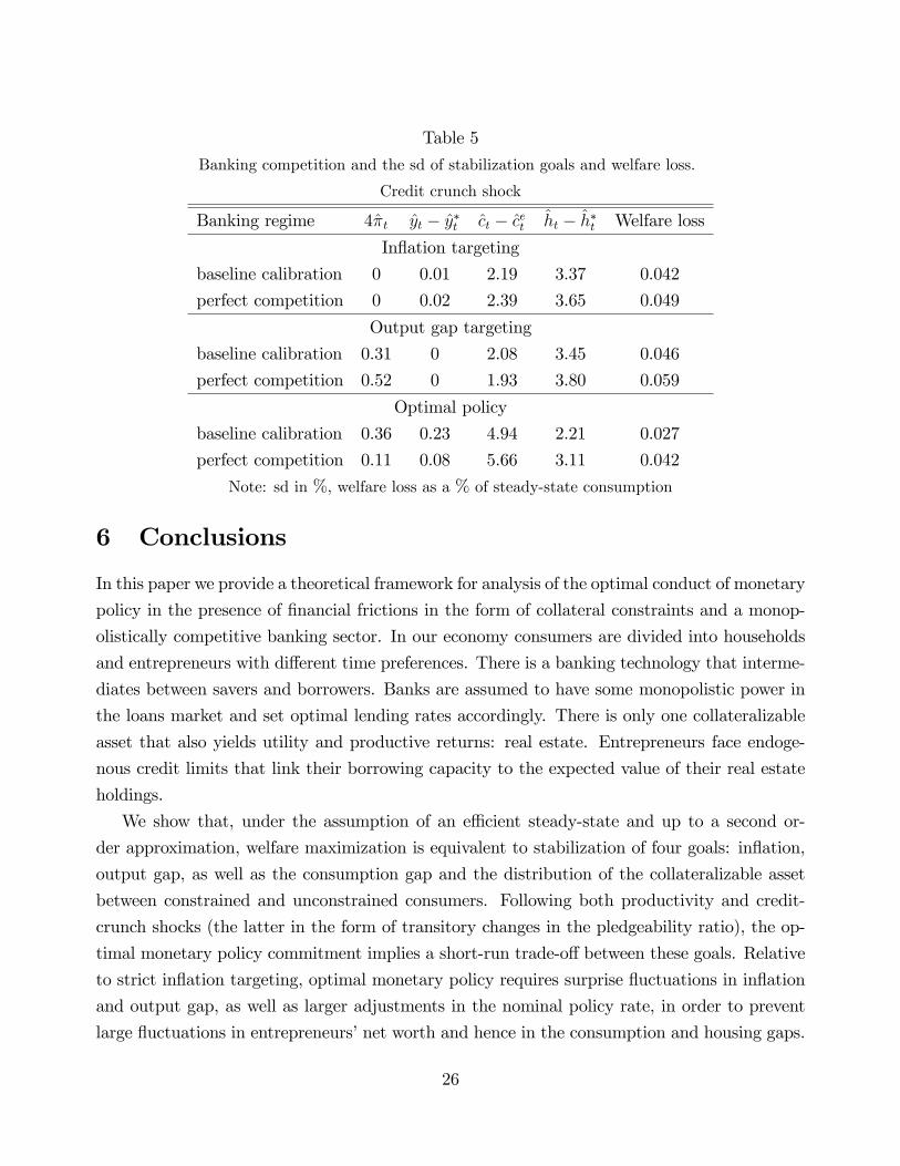
Table 5

Banking competition and the sd of stabilization goals and welfare loss.

Credit crunch shock

Banking regime 4�t yt � y�t ct � cet ht � h�t Welfare loss

In�ation targeting

baseline calibration 0 0.01 2.19 3.37 0.042

perfect competition 0 0.02 2.39 3.65 0.049

Output gap targeting

baseline calibration 0.31 0 2.08 3.45 0.046

perfect competition 0.52 0 1.93 3.80 0.059

Optimal policy

baseline calibration 0.36 0.23 4.94 2.21 0.027

perfect competition 0.11 0.08 5.66 3.11 0.042

Note: sd in %, welfare loss as a % of steady-state consumption

6 Conclusions

In this paper we provide a theoretical framework for analysis of the optimal conduct of monetary

policy in the presence of �nancial frictions in the form of collateral constraints and a monop-

olistically competitive banking sector. In our economy consumers are divided into households

and entrepreneurs with di¤erent time preferences. There is a banking technology that interme-

diates between savers and borrowers. Banks are assumed to have some monopolistic power in

the loans market and set optimal lending rates accordingly. There is only one collateralizable

asset that also yields utility and productive returns: real estate. Entrepreneurs face endoge-

nous credit limits that link their borrowing capacity to the expected value of their real estate

holdings.

We show that, under the assumption of an e¢ cient steady-state and up to a second or-

der approximation, welfare maximization is equivalent to stabilization of four goals: in�ation,

output gap, as well as the consumption gap and the distribution of the collateralizable asset

between constrained and unconstrained consumers. Following both productivity and credit-

crunch shocks (the latter in the form of transitory changes in the pledgeability ratio), the op-

timal monetary policy commitment implies a short-run trade-o¤ between these goals. Relative

to strict in�ation targeting, optimal monetary policy requires surprise �uctuations in in�ation

and output gap, as well as larger adjustments in the nominal policy rate, in order to prevent

large �uctuations in entrepreneurs�net worth and hence in the consumption and housing gaps.

26

The welfare gain of pursuing optimal polices is comparatively higher under technology-driven

�uctuations. Shocks to the pledgeability ratio have a direct e¤ect on the borrowing ability

of entrepreneurs, such that policies aimed at sustaining their net worth are less e¤ective in

preventing large swings in entrepreneurial real estate holdings.

We also compare the nature of these trade-o¤s under alternative assumptions about the

degree of competition in the banking industry. We �nd that, both under optimal and subop-

timal policies, welfare losses due to cyclical �uctuations are ampli�ed as banking competition

increases. This ampli�cation is moderate in �nancially driven (credit-crunch) �uctuations but

is substantial if productivity shocks dominate. Key to these results is the interplay between

two endogenous mechanisms at work in our model: leverage and lending margins. As banking

competition increases, the constrained consumers (entrepreneurs) become more leveraged, thus

amplifying the response of their consumption and real estate holdings to exogenous shocks; this

worsens the aforementioned trade-o¤s and makes the use of optimal polices more compelling.

The countercyclical response of lending margins to shocks aggravates the policy trade-o¤s and

is stronger in less competitive environments. The �rst mechanism is equally important regard-

less of the nature of the shocks, whereas the second one is very weak under productivity shocks

and signi�cant if shocks to the pledgeability ratio are the driving force behind �uctuations.

27

References

[1] Andrés, J. and O. Arce (2008): �Banking Competition, Housing Prices and Macroeconomic

Stability,�Banco de España WP no. 830.

[2] Benigno, P. and M. Woodford (2003): "Optimal Monetary and Fiscal Policy: A Linear-

Quadratic Approach," NBER Macroeconomics Annual, 18, 271-364.

[3] Benigno, P. and M.Woodford (2008): �Linear-Quadratic Approximation of Optimal Policy

Problems�. Working paper.

[4] Bernanke, B. and M. Gertler (1989), �Agency Costs, Net Worth, and Business Fluctua-

tions�, American Economic Review, March, Vol. 79(1), pp. 14-31.

[5] Bernanke, B., M. Gertler and S. Gilchrist (1999), �The Financial Accelerator in a Quan-

titative Business Cycle Framework,� in J.B. Taylor and M. Woodford, eds., Handbook of

Macroeconomics, vol. 1C. Amsterdam: Elsevier Science, North-Holland.

[6] Bils, M., and P. J. Klenow (2004), "Some Evidence on the Importance of Sticky Prices,"

Journal of Political Economy, 112(5), 947-985.

[7] Calvo, G. (1983): �Staggered Prices in a Utility-Maximizing Framework,�Journal of Mon-

etary Economics 12: 383-398.

[8] Cúrdia, V. and M. Woodford (2008), "Credit Frictions and Optimal Monetary Policy,"

mimeo.

[9] Goodfriend, M., and R. G. King (2001). "The Case for Price Stability," NBER Working

Papers 8423.

[10] Goodfriend, M. , B. McCallum (2007): "Banking and interest rates in monetary policy

analysis: A quantitative exploration", Journal of Monetary Economics 54 1480�1507.

[11] Iacoviello, M. (2005): �House Prices, Borrowing Constraints, and Monetary Policy in the

Business Cycle,�American Economic Review 95, no. 3: 739-764.

[12] Kiyotaki, N. and J. H. Moore (1997). �Credit Cycles,�Journal of Political Economy, 105,

211-248.

28

[13] Monacelli, T. (2007): "Optimal Monetary Policy with Collateralized Household Debt and

Borrowing Constraints", in Asset Prices and Monetary Policy, J. Campbell (ed.), Univer-

sity of Chicago Press.

[14] Nakamura, E., and J. Steinsson (2008). "Five Facts about Prices: A Reevaluation of Menu

Cost Models," Quarterly Journal of Economics, 123(4), 1415-1464.

[15] Neiss, K., and E. Nelson (2003). "The Real-Interest-Rate Gap As An In�ation Indicator,"

Macroeconomic Dynamics, 7(02), 239-262.

[16] Rotemberg, J. and M. Woodford (1997): �An Optimization-Based Econometric Model for

the Evaluation of Monetary Policy�. NBER Macroeconomics Annual, 12, 297-346.

[17] Salop, S. (1979): �Monopolistic Competition with Outside Goods,�Bell Journal of Eco-

nomics 10: 141-156.

[18] Woodford, M. (2003): Interest and Prices: Foundations of a Theory of Monetary Policy,

Princeton University Press.

29

7 Appendix

7.1 The entrepreneur�s consumption decision

Equations (8) and (9) in the text can be combined as follows,

pht � �tcet

= �eEt

�(1� � e) �pIt+1yt+1=het + pht+1 �Ret�t=�t+1

cet+1

�; (39)

where �t � mtEt�t+1pht+1=R

et . The latter de�nition allows us in turn to write the collateral

constraint (equation 6) as

bt = �thet : (40)

De�ne real net worth, nwt, as the sum of after-tax real pro�ts and beginning-of-period real

estate wealth, minus real debt repayments,

nwt � (1� � e)�pIt yt � wtldt

�+ pht h

et�1 �

Ret�1�t

bt�1

= (1� � e) �pIt yt + pht het�1 �Ret�1�t

�t�1het�1

=

�(1� � e) �pIt yt=het�1 + pht �

Ret�1�t

�t�1

�het�1; (41)

where in the �rst equality we have used (7) to substitute for wtldt and (40) to substitute for

bt�1. We now guess that the entrepreneur consumes a fraction 1� �e of her real net worth,

cet = (1� �e)nwt: (42)

Using (41) and (42) in equation (39), the latter collapses to

pht � �tcet

=�e

1� �e1

het: (43)

At the same time, the de�nition of real net worth and equation (40) allow us write the entre-

preneur�s budget constraint (equation 5) as

�thet + nwt = c

et + p

ht h

et ;

Combining the latter with equation (43), we �nally obtain equation (42), which veri�es our

guess.

30

7.2 Implementation of the e¢ cient steady state

Equations (1), (7) and (19) in the steady state jointly imply

css (lsss)

' =1� !!

(1� �) pIssyssslsss

The latter corresponds to its e¢ cient counterpart (the steady state of equation 24) only if

pIss = 1. In the steady state, equation (15) becomes 1 + � = ["= ("� 1)] pIss, where � is thesubsidy rate on the revenue of �nal goods producers. Therefore, steady-state e¢ ciency requires

setting the subsidy rate to

� ="

"� 1 � 1:

On the other hand, the steady-state counterpart of equation (10), rescaled by yss, is given by

cessyss

= (1� �e)�(1� � e) � + (1�m) p

hssh

ess

yss

�; (44)

where we have imposed pIss = 1 and we have also used the steady-state collateral constraint,

Ressbss = mphsshess. Similarly, the steady-state counterparts of equations (9) and (8) jointly

implyphssh

ess

yss= �e

�(1� � e) � + p

hssh

ess

yss

�+

�1

Ress� �e

�mphssh

ess

yss;

which implies the following steady-state ratio of entrepreneurial real estate wealth over output,

phsshess

yss=

�e (1� � e) �1� �e �m (1=Ress � �e)

: (45)

Using (45) to substitute for phsshess=y

sss in (44), and imposing the steady-state e¢ ciency require-

ment that cess=yss = 1� ! (as a result of css = cess and [1� !] yss = !css + [1� !] cess), we cansolve for the tax rate that implements an e¢ cient allocation in the steady state,

� e = 1� 1� !(1� �e) �

1� �e �m (1=Ress � �e)1�m=Ress

:

Finally, equation (3) implies that, in the steady state,

phsshsscss

=#

1� � + �h :

31

Combining this with equation (45) and the e¢ ciency requirement css = cess = (1� !) yss, wehave that the steady-state distribution of real estate in the decentralized economy is given by

hsshess

=(1� !)#�e (1� � e) �

1� �e �m (1=Ress � �e)1� � + �h :

The latter coincides with the e¢ cient steady-state distribution, (1� !)#= (��), only if

�h =�

�e1� �e �m (1=Ress � �e)

1� � e � (1� �) :

7.3 Derivation of the quadratic loss function

We start by performing a second order approximation (in logs) of the period utility function

around the steady-state,

Ut � !

"log(ct) + #t log(ht)�

(lst )1+'

1 + '

#+ (1� !) log(cet)

= !ct + (1� !) cet � ! (lsss)1+'

�lt +

1 + '

2l2t

�+ !#

�ht + z

ht ht

�+ t:i:p:+O3; (46)

where hats denote log-deviations from steady state, the subscript ss indicates steady state

values, t:i:p: are terms independent of policy and O3 collects all terms of order third and higher

in the size of the shocks.

The aggregate resource constraint in goods markets, (1� !) yt=�t = !ct + (1� !) cet , canbe approximated by

(1� !)�yt +

1

2y2t � �t

�= !

cssyss

�ct +

1

2c2t

�+ (1� !) c

ess

yss

�cet +

1

2(cet )

2

�+O3; (47)

where we have used the fact that �t is already a second-order term (see below). Equation (47)

implies that

y2t =

�!

1� !cssyss

�2c2t +

�cessyss

�2(cet)

2 + 2!

1� !cssyss

cessyssctc

et +O

3:

32

Using this to substitute for y2t in (47) and rearranging terms, we obtain

yt =!

1� !cssyssct +

cessysscet + �t +O

3

+1

2

�!

1� !cssyss

�1� !

1� !cssyss

�c2t +

cessyss

�1� cess

yss

�(cet)

2 � 2 !

1� !cssyss

cessyssctc

et

�: (48)

We now make use of our assumption of e¢ cient steady state. This implies css = cess =

(1� !) yss. Using this in (48) yields

yt = !ct + (1� !) cet + �t +! (1� !)

2(ct � cet)

2 +O3: (49)

The production function, yt = eat [!lst= (1� !)]1�� �het�1�� , admits the following exact log-linear

representation,

yt = at + (1� �) lst + �het�1: (50)

Using (49) and (50) to substitute for !ct + (1� !) cet and lst respectively in (46), we obtain

Ut = yt � �t � ! (lsss)1+'

24 yt � �het�11� � +

1 + '

2

yt � at � �het�1

1� �

!235�! (1� !)

2(ct � cet)

2 + !#�ht + z

ht ht

�+ t:i:p:+O3: (51)

In an e¢ cient steady state, labor market equilibrium implies css (lsss)' = (1� �) ysss=

�!1�! l

sss

�,

which combined with css = (1� !) yss implies ! (lsss)1+' = 1� �. Using this in (51), we have

Ut = �het�1 + !#

�ht + z

ht ht

�� 1 + '

2 (1� �)

�yt � y�jht

�2� ! (1� !)

2(ct � cet )

2 � �t + t:i:p:+O3;

(52)

where we have used the de�nition of e¢ cient output (in log-deviations), y�jht � at + �het�1.

Taking the present discount sum of (52), we have

1Xt=0

�tUt = �12

1Xt=0

�t�1 + '

1� �

�yt � y�jht

�2+ ! (1� !) (ct � cet)

2

�+

1Xt=0

�th��het + !#

�ht + z

ht ht

�i�

1Xt=0

�t�t + t:i:p:+O3; (53)

where we have used the fact that he�1 and ��1 are independent of policy as of time 0. The

33

equilibrium condition in the real estate market, �h = !ht + (1� !)het , can be approximated asfollows,

!hss

ht +

h2t2

!+ (1� !)hess

0B@het +�het

�22

1CA = O3: (54)

The latter equation implies that�het

�2= [!= (1� !)]2 (hss=hess)

2 h2t + O3. Using this and the

e¢ cient distribution of real estate in the steady state, hss=hess = (1� !)#= (��), equation (54)becomes

!#ht + ��het = �

!#

2

�� + !#

��h2t +O

3:

This implies

1Xt=0

�th��het + !#

�ht + z

ht ht

�i= �!#

2

1Xt=0

�t��� + !#

��h2t � 2zht ht

�+O3

= �!#2

�� + !#

��

1Xt=0

�t�ht � h�t

�2+ t:i:p:+O3; (55)

where in the second equality we have used the de�nition of the e¢ cient level of housing, h�t �[��= (!#+ ��)] zht .

It is possible to show (see e.g. Woodford, 2003) that

1Xt=0

�t�t ="

2

�

(1� �) (1� ��)

1Xt=0

�t�2t + t:i:p:+O3: (56)

Using (55) and (56) in (53), we �nally obtain

1Xt=0

�tUt = �1

2

1Xt=0

�tLt + t:i:p:+O3; (57)

where

Lt =1 + '

1� �

�yt � y�jht

�2+ ! (1� !) (ct � cet )

2 + !#�� + !#

��

�ht � h�t

�2+

"�

(1� �) (1� ��) �2t :

QED.

34

7.4 Log-linear equations

All variables in log-deviations from the e¢ cient steady state. The log-linear constraints of the

central bank�s problem are the following.

1. Household�s consumption Euler equation,

ct = Etct+1 � Et�Rdt � �t+1

�:

2. Household�s demand for housing,

�1 + �h

� �pht � ct

�=�1 + �h � �

� �zht � ht

�+ �Et

�pht+1 � ct+1

�:

3. Entrepreneur�s borrowing constraint,

bt = zmt + Etp

ht+1 + h

et �

�Ret � Et�t+1

�:

4. Entrepreneur�s consumption Euler equation,

cet = �eRessEt

�cet+1 � Ret + �t+1

�� (1� �eRess) �t:

5. Entrepreneur�s demand for real estate,

pht � cet = �eEt

�(1� � e) �

seh

�yt+1 + p

It+1 � het

�+ pht+1 �

�(1� � e) �

seh+ 1

�cet+1

�+m

�1

Ress� �e

�hzmt + �t + Etp

ht+1 �

�Ret � Et�t+1

�i;

where seh � phsshess=yss.

6. Entrepreneur consumption,

cet =1� �e

1� !

h(1� � e) �

�yt + p

It

�+ seh

�pht + h

et�1

�� sehm

�Ret�1 + bt�1 � �t

�i:

35

7. Bank lending margin,

Ret = Rdt

+�Ress � 1�Ress

24Rdt + pht �m�Et ��t+1 + pht+1 + zmt �1�m� �

�m�Et��t+1 + p

ht+1 + z

mt

���Rdt + p

ht

��m� � 1

35 :8. New Keynesian Phillips curve,

�t =(1� �) (1� ��)

�pIt + �Et�t+1:

9. Real marginal costs,

pIt = ct � yt +1 + '

1� �

�yt � at � �het�1

�:

10. Equilibrium in goods markets,

yt = !ct + (1� !) cet :

11. Equilibrium in the real estate market,

ht = ���

!#het :

.

36

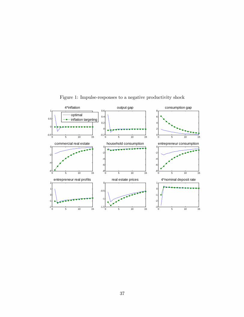
Figure 1: Impulse-responses to a negative productivity shock

0 5 10 15-0.5

0

0.5

14*inflation

0 5 10 15-0.2

0

0.2

0.4

0.6output gap

0 5 10 150

2

4

6

8consumption gap

0 5 10 15-6

-4

-2

0commercial real estate

0 5 10 15-8

-6

-4

-2

0household consumption

0 5 10 15-8

-6

-4

-2

0entrepreneur consumption

0 5 10 15-2

-1

0

1

2entrepreneur real profits

0 5 10 15-1.5

-1

-0.5

0real estate prices

0 5 10 15-3

-2

-1

0

14*nominal deposit rate

optimalinflation targeting

37

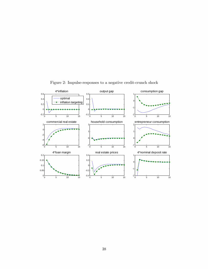
Figure 2: Impulse-responses to a negative credit-crunch shock

0 5 10 15-0.2

0

0.2

0.4

0.64*inflation

optimalinflation targeting

0 5 10 15-0.1

0

0.1

0.2

0.3output gap

0 5 10 15-2

-1

0

1consumption gap

0 5 10 15-6

-4

-2

0

2commercial real estate

0 5 10 15-1

0

1

2household consumption

0 5 10 15-1

0

1

2entrepreneur consumption

0 5 10 150

0.05

0.1

0.15

0.24*loan margin

0 5 10 15-0.4

-0.2

0

0.2

0.4real estate prices

0 5 10 15-2

-1

0

14*nominal deposit rate

38