Identifying Cross-Sided Liquidity Externalities *

Johannes A. SkjeltorpNorges Bank

Elvira SojliErasmus University and Duisenberg School of Finance

Wing Wah Tham�

Erasmus University

July 31, 2012

Abstract

We investigate the cross-sided liquidity externality between market makers andtakers, by testing the empirical implications of the Foucault, Kadan, and Kandel(2012) model. We use exogenous changes in the make/take fee structure and atechnological shock for liquidity takers, as experiments to identify a new type ofliquidity externality and cross-side complementarities of liquidity makers and takersin the U.S. equity market. We find support for strong liquidity externalities betweenliquidity providers and takers. Shocks to fees of takers cause changes in the lengthof the liquidity cycles of both makers and takers. A change in technology thatimproves market takers ability to monitor the market reduces both the maker andthe taker liquidity cycles. Thus, positive shocks to liquidity takers’ monitoringincentives, which reduce the take cycle, are transmitted to the make cycle throughcross-liquidity externalities. Our findings shed light on the way the order postingbehavior of market makers and takers is interrelated and on different factors thataffect this relation and contribute to the on-going policy debate on the maker/takerpractices in U.S. equity markets.

Keywords: Liquidity cycle; Liquidity externality; Make/take cycles; Make/takefees.

JEL Classification: G10; G20; G14.

*We are grateful to Thierry Foucault for very helpful discussions. We thank Denis Gromb, TerryHendershott, Frank Hatheway, Harrison Hong, Richard Payne, Avi Wohl and participants at the EMG-ESRC Market Microstructure Workshop for helpful comments. Sojli gratefully acknowledges the financialsupport of the European Commission Grant PIEF-GA-2008-236948. Tham gratefully acknowledges thefinancial support of the European Commission Grant PIEF-GA-2009-255330. The views expressed arethose of the authors and should not be interpreted as reflecting those of Norges Bank (Central Bank ofNorway).

�Corresponding author. Address: Erasmus School of Economics, Erasmus University, PO Box 1738,Rotterdam, 3000DR, the Netherlands. Email: tham@ese.eur.nl, Phone: +31(0)10 4081424. Otherauthors’ email addresses: johannes-a.skjeltorp@norges-bank.no (Skjeltorp), esojli@rsm.nl (Sojli).

1 Introduction

Understanding liquidity externalities is very important because it has implications for

changes in trading activities (Biais, Glosten, and Spatt, 2005), commonality in liquidity

(Chordia, Roll, and Subrahmanyam, 2000; Hasbrouck and Seppi, 2001), leverage buyout

activity (Gaspar and Lescourret, 2009), privatization (Borttolotti, de Jong, Nicodano,

and Schindele, 2007), market design and transparency (Madhavan, 2000; Barclay and

Hendershott, 2004; Bessembinder, Maxwell, and Venkataraman, 2006), and market regu-

lation (Macey and O’Hara, 1999; Hendershott and Jones, 2005). Despite its importance,

there is little empirical work on liquidity externalities, because identifying and empirically

measuring liquidity externalities is extremely challenging (see, Barclay and Hendershott,

2004; Hendershott and Jones, 2005). The difficulty stems from the fact that liquidity

is endogenously determined and there are few good instruments for identification. In

this paper, we attempt to identify empirically the liquidity externality between liquidity

consumption and provision, motivated by the theoretical work of Foucault, Kadan, and

Kandel (2012). We address the issue of identification by using two exogenous instru-

ments, a fee change and a technological shock. In doing so, we contribute to the liquidity

externality literature and join the handful of papers that identify the presence of liquidity

externalities in financial markets.

Foucault et al. (2012) develop a model which provides an explanation for the widespread

adoption of maker/taker pricing and presents a rationale for differentiating trading fees

between liquidity makers and takers. They propose that the speed of reaction of liquidity

suppliers (makers) and liquidity demanders (takers) is endogenous to trading opportu-

nities. A trader’s choice of reaction speed is determined by the trade-off between the

benefits associated with being the first to identify (and seize) trading opportunities, and

the monitoring cost associated with such identification. Foucault et al. (2012) introduce

a new type of liquidity externality (cross-sided) between liquidity makers and takers,

where an increase in the monitoring intensity of e.g. liquidity makers induces a positive

externality on liquidity takers, which increases the speed of liquidity consumption. This

1

induced increase in liquidity consumption in return affects the actions of market makers

and begets liquidity supply. A positive cross-sided liquidity externality exists in Foucault

et al. (2012) because it is beneficial for liquidity makers and takers to find each other.

However, there can be negative cross-sided liquidity externalities if liquidity makers

and takers incur a cost from meeting each-other. For example, such a cost can occur

if makers are afraid of being adversely selected or face information uncertainty. Given

that there is no liquidity provision obligations on today’s liquidity makers, they might

abstain from providing liquidity resulting in a negative liquidity externality.1 A negative

externality might also occur if one relaxes the assumption of market-making and taking

specialization in Foucault, Kadan, and Kandel (2012).2 Although there is undoubtedly

market making and taking specialization in the market, there are also high-frequency

market makers and smart routers who use both market and limit orders. If a venue alters

its take fee to entice more takers, a maker, who is concerned about execution certainty

and speed of execution, might withdraw its liquidity provision to become a taker if the

overall cost of posting a market order is lower. Thus, the existence and the sign of

cross-sided liquidity externality are unclear and remain an empirical question.

To establish causality and to identify the cross-sided liquidity externality, we study

two exogenous events that should affect the monitoring intensity of market takers through

a reduction in their monitoring costs. First, we use an increase in the takers’ rebate as an

instrument for the speed of reaction to trading opportunities for liquidity demanders. An

increase in the taker’s rebate directly incentivizes liquidity demanders (but not liquidity

providers) to increase their monitoring intensities which ought to decrease take cycles.

Our second identification strategy uses a technology shock that reduces the monitoring

cost (and hence increases the monitoring intensity) of the taker side. Because the exoge-

nous shocks affect only the take cycle directly, we can use them to identify the cross-sided

liquidity externality and the causal effect of take cycles on make cycles.

1Senator Kaufman has expressed concerns about the voluntary liquidity provision role of high-frequency trading and statistical arbitrage firms for a large proportion of the U.S. market. He sug-gests that the SEC should impose liquidity provision obligations on high-frequency traders. Seewww.sec.gov/comments/s7-27-09/s72709-96.pdf

2See p.10 in Foucault, Kadan, and Kandel (2012)

2

We apply two methods to identify the cross-sided externality: (i) an event study

around the two exogenous shocks (the change in taker rebate and the introduction of

the new technology), (ii) an instrumental variable (IV) regression for the sample period:

October 1, 2010 - March 31, 2011. The event study approach minimizes the impact of

any confounding effects in our analysis. The instrumental variable regression allows us to

pin down causality, and to account for confounding effects and for potential estimation

problems.

We investigate and identify the cross-sided liquidity externality using a set of high

quality and detailed limit order book data from the NASDAQ OMX BX, formerly known

as Boston Stock Exchange (BX hereafter).3 To measure the speed of liquidity consump-

tion and provision, we build the limit order book for all points in time with microsecond

accuracy and construct measures of the time it takes for liquidity to replenish (make cycle)

after periods of liquidity consumption (take cycle), consistent with Foucault et al. (2012).

The excellent data quality and the existence of a technological shock and a fee change

that only affect liquidity consumption in BX provide an ideal setup for the identification

of liquidity externalities.

We identify a positive and strong liquidity externality between liquidity providers

and takers. In particular, we find that an increase in the taker rebate, which reduces the

monitoring cost for liquidity takers, increases the takers’ response speed to changes in

liquidity. As a consequence, there is an increased intensity of market orders that consume

the liquidity available at the best quotes and that leads to a wider bid-ask spread. This

drop in liquidity, which increases the number of profit opportunities for market makers,

attracts more liquidity suppliers who post new aggressive limit orders that replenish

liquidity. The new best prices in turn create new trading opportunities for liquidity takers.

Thus, our first instrument, the increase in the taker rebate, supports the hypothesis of

the existence of positive cross-sided liquidity externalities where liquidity demand begets

liquidity supply. This result is further substantiated by our alternate instrument, based on

3NASDAQ OMX completed the acquisition of the Boston Stock Exchange on August 29, 2008. OnFriday January 16, 2009 NASDAQ OMX launched NASDAQ OMX BX.

3

a technological change that reduces the monitoring cost of market takers. Such a change

in technology that improves market takers ability to monitor the market naturally reduces

the duration of taker liquidity cycles. Using the improvement in technology for takers’

monitoring as an instrument, we find that a reduction in the duration of taker liquidity

cycles causes a decrease in the duration of maker liquidity cycles. Using an alternative

estimation strategy of a two-sample, or split sample, instrumental variable estimator to

address any potential concerns about weak instruments and as a robustness check, our

results remain qualitatively similar.4

Amihud, Mendelson, and Lauterbach (1997) is the first paper to introduce the term

liquidity externality and to document how a change in trading mechanisms not only im-

proves liquidity for affected stocks but also for correlated non-affected stocks. Barclay

and Hendershott (2004) examine how the large differences in the amount of informed

trading between regular trading hours and off-exchange trading hours affect adverse se-

lection costs. Hendershott and Jones (2005) study how the reduction of transparency in

one market affects the trading cost of other trading venues where transparency does not

change. Bessembinder et al. (2006) shows how the introduction of transaction reporting

for corporate bonds through TRACE on a subset of bonds also decreases the trading

cost of non-TRACE-eligible bonds. Differently from the existing work which focuses on

liquidity externalities related to trading costs across assets, this is the first paper to ex-

amine the temporal liquidity externalities of liquidity cycles related to the provision and

consumption of liquidity.

Resiliency, a less studied dimension of liquidity, is an important measure of liquidity

especially in today’s electronic limit order book markets. Resiliency measures how fast

the limit order book is replenished after a large trade has occurred. Given the apparent

relation between resiliency and make cycles, we join the theoretical works of Foucault,

Kadan, and Kandel (2005), Goettler, Parlour, and Rajan (2005), Rosu (2009), Rosu

(2010), and Foucault et al. (2012) and the empirical works of Biais et al. (1999), Degryse,

4In the split sample two stage least square, we randomly split our sample in half and use one halfof the sample to estimate parameters of the first stage equation. We then use estimated first stageparameters to construct fitted values and estimate the second stage from the other half of the data.

4

De Jong, Ravenswaaij, and Wuyts (2005), and Large (2007) in studying how the limit

order book is replenished after trades. Differently from the empirical papers in this liter-

ature, which focus on measuring resiliency i.e. only make cycles, our results suggest that

take and make cycles are endogenous and ought to be studied together when measuring

and discussing resiliency. In addition, our empirical measure for maker cycle durations

constitutes a new empirical proxy of resiliency.

The recent episodes of “flash crash”, introduction of maker/taker pricing structure by

trading venues, innovations of new trading products and services offered by competing

trading venues and a shift towards automation in trading has led regulators, politicians,

and market participants to question the new dynamic relation between liquidity providers

and demanders in an environment without obligatory liquidity provision responsibility.

Despite the importance of understanding the new dynamics of liquidity provision and

consumption as well as the interest in the impact of the maker/taker pricing model on

the U.S. equity market, there has been little empirical work on this issue.

While the main focus of our paper is to identify the liquidity externality between

liquidity provision and consumption, this paper also contributes to the political and reg-

ulatory debates on obligatory liquidity provision in today’s market and to works studying

the impact of make and take fees on market quality. Colliard and Foucault (2011) analyze

a microstructure model with make and take fees where investors can chose to be makers

or takers when deciding how to execute their trades. In a related paper, Malinova and

Park (2011) empirically study the impact of a change in both the make and the take

fee schedule on market quality of 60 cross-listed stocks in the Toronto Stock Exchange.

Finally, Battalio, Shkilko, and Ness (2012) show that the cost of liquidity in pay-for-

order flow and in maker/taker exchanges is similar when taking into account the make

fee rebates. Differently from this work, we focus on identifying liquidity externalities and

the impact of make/take fees changes on the highly traded U.S. market, using one-sided

exogenous events. To our knowledge, this paper is one of the first to empirically study

the impact of changes in the make/take fee structure on market liquidity in the U.S.

equity markets. Our findings shed light on the way the order posting behavior of makers

5

and takers is interrelated and on different factors that affect this relation. Finally, our

results contribute to the on-going policy debate on the maker/taker practices in U.S.

equity markets.

The next section provides a discussion of the theoretical foundation for the existence

of cross-sided liquidity externalities. The data and preliminary analysis is presented in

Section 3. Section 4 describes the identification strategy. Section 5 presents and discusses

the results and Section 6 addresses robustness issues. Section 7 concludes.

2 Cross-sided Liquidity Externality

Foucault et al. (2012) develop a model of trading, with specialized market making and

taking sides, in which the speed of reaction to trading opportunities for liquidity suppliers

and demanders is endogenous. They interpret the market making side as proprietary

trading firms that specialize in high-frequency market making and the market taking

side as brokers using smart order routers to executed market orders when liquidity is

ample and cost of trading is low. They show that the maker/taker pricing model is a

way for the trading platform to minimize the duration of liquidity cycles and therefore

maximize its expected profit. Foucault et al. (2012) define liquidity cycles to consist of

two phases: a “make liquidity” and a “take liquidity” phase. A “make liquidity” phase

(make cycle) is the period when liquidity suppliers (makers) compete to provide liquidity

after a trade. A “take liquidity” phase (take cycle) is the period when liquidity demanders

(takers) compete to consume liquidity, depicted in Figure 1.

Figure 1Flows of Events in a Cycle (Foucault et al., 2012)

Market-takers submit market orders. Trade takes place. Liquidity is consumed and becomes sparse. Bid-ask spread widen.

Make Liquidity Phase

Take Liquidity Phase

Market-makers submit limit orders in sparce-liquidity state. Bid-ask spread narrows as market moves into a state with ample liquidity.

Market-takers submit market orders. Trade takes place. Liquidity is consumed and becomes sparse. Bid-ask spread widen.

6

Thus a fluid trading process with short liquidity cycles requires makers to aggressively

compete for providing liquidity when liquidity is low and takers to consume liquidity

when it is available at favorable prices. The liquidity cycle is a time-dimension measure

of liquidity and is analogous to the liquidity measure of resiliency (Harris, 1990).5

In the Foucault et al. (2012) model, make/take fees and monitoring costs affect the

gains from trade of liquidity makers and takers, while the number of makers (takers)

affects the competition for supplying (consuming) liquidity. One implication of the model

is that changes in fee structures, monitoring costs, and the number of market makers and

takers will affect the monitoring intensities of makers and takers and the make/take

cycles. Because the speed of reaction to trading opportunities is endogenous, an increase

in monitoring intensity of liquidity makers (takers) will increase the monitoring intensity

of takers (makers). This reinforcing effect between makers and takers implies that an

improvement in the monitoring technology for either makers or takers or an increase

in the number of either market makers or takers will reduce the duration of liquidity

cycles, and thus increase the trading rate and the profitability of the trading venue.

This endogenity of the monitoring intensities introduces a cross-side liquidity externality

between liquidity provision and consumption. More specifically, the traders’ monitoring

intensities in equilibrium are given in Proposition 2 of Foucault et al. (2012) as:

µ∗i =

M+ (M− 1)V∗

(1+ V∗)2× πm

Mβi = 1, . . . ,M (1)

τ∗j =V∗((1+ V∗)N− 1)

(1+ V∗)2× πt

Nγj = 1, . . . ,N (2)

where V∗ = µ∗

τ∗= Dt

Dmmeasures the relative speed of reaction of the market making side

relative to the market taking side in equilibrium. µ∗ = µ∗1+ . . .+µ

∗M and τ = τ∗1+ . . .+τ

∗M

are the aggregate market making and taking monitoring levels in equilibrium, respectively.

Dt =1τ

and Dm = 1µ

are the expected durations of the make and take phase respectively.

β and γ are the monitoring cost parameters for the makers and the takers respectively.

5Resiliency reflects the speed at which liquidity is replenished after a large trade has occurred.

7

The monitoring costs for participants decrease with β and γ. M and N denote the

number of makers and takers respectively. πm = a − ν0 − cm and πt = v0 + Γ − a − ct

are gains from trade for makers and takers which are negatively related to the make fee

cm and the take ct fee, respectively.

In this paper, we are interested in identifying this cross-sided liquidity externality and

we test the following hypotheses based on corollary 6 of Foucault et al. (2012):

Hypothesis 1a: An increase (decrease) in the liquidity makers’ monitoring intensity

(make cycle) increases (decreases) the liquidity takers’ monitoring intensities (take cycle).

Hypothesis 1b: An increase (decrease) in the liquidity takers’ monitoring inten-

sity (take cycle) increases (decreases) the liquidity makers’ monitoring intensities (make

cycle).

Equations 1 and 2 and the second part of Corollary 6 of Foucault et al. (2012) suggest

that the make phase increases in market-makers monitoring cost (β) and the make fee

(cm), while it decreases in the number of market makers (M). The take phase increases in

market-takers monitoring cost (γ) and the take fee (ct), while it decreases in the number

of market takers (N). This implies that shocks or changes to monitoring cost, make/take

fees, and the number of market makers or takers can be used as instruments for the

identification of cross-sided liquidity externalities.

3 Data

This paper uses the complete set of quotes and trades in the NASDAQ OMX BX system

for the period October 1, 2010 to March 31, 2011. The data is obtained from NASDAQ

ITCH-TotalView system on special order. We retain stocks for which information is

available in Trades and Quotes (TAQ), Center for Research in Security Prices (CRSP),

and Compustat. Following the literature, we retain only common stocks (Common Stock

Indicator Type=1) and focus only on common shares (Share Code 10 and 11) and stocks

that do not change primary exchange, ticker symbol or CUSIP over the sample period

(Hasbrouck, 2009; Goyenko, Holden, and Trzcinka, 2009; Chordia, Roll, and Subrah-

8

manyam, 2000). We also exclude stocks that exhibit a price lower than $5 or higher than

$1000, and market capitalization less than $1,000,000 at any point in time during the

sample period. Finally, we exclude any day/stock observation with less than 10 trades a

day. Our final sample comprises 1,867 stocks and 101,176 stock/day observations.

We employ the complete dataset of new order messages, updates, cancelations, dele-

tions, executions, and executions against hidden orders and cross-network orders, to

reconstruct the complete limit order book (LOB) for all the stocks in BX for the whole

sample period following Kavajecz (1999). We use the LOB information to also calculate

daily stock characteristic variables in BX. Specifically, we construct realized volatility

(Volatility) as the sum of squared five minute returns, number of trades (Trades) as the

sum of trades per stock during the day, number of traded shares (Traded Shares) as the

sum of the number of shares traded across all trades during the day, trading volume (Vol-

ume) as Traded Shares times price of trade, and the proportion of aggressive limit orders

to the total of aggressive orders and trades (LO Ratio). All the variables constructed

from the LOB are defined in Table A1 in the Appendix.

In BX, there is a rebate for taking liquidity and a fee is paid for filling the limit order

book for NASDAQ and NYSE listed stocks (Tape A and C). For all non-NASDAQ and

non-NYSE listed stocks (Tape B) and stocks with a price less than $1, there is a rebate

for providing liquidity and a fee is paid for taking liquidity. Tape B stocks constitute

about 2% of our total number of day/stock observations. Table A2 in the Appendix

shows that Tape B stocks are quite small and not very heavily traded. Make/take fee

changes affect Tape B stocks in the opposite way of Tape A and C stocks. We exclude

Tape B stocks from the sample because they can confound our results. The exclusion

of the small number of Tape B stocks in our sample is not likely to result in any loss of

generality for the findings.

In order to carry out our analysis, we need to conceptualize and create a measure of

cycles that is compatible with Foucault et al. (2012) and matches Figure 1. We calculate

take cycles as the difference in time between the first market order (MO, take) and the

first limit order that improves the best price (ALO) after the last trade. We calculate

9

make cycles as the difference in time between the first limit order that improves the best

prevailing quote (ALO) after one or a series of market orders and the first market order

(MO). Figure 2 below depicts how we calculate the cycles.

Figure 2Make Take Cycles

ALO1 LO2 LO3 ALO4 MO4 MO3 MO2 MO1 LO5 ALO6 MO5 MO6

Make Cycle MO1-ALO1

Take Cycle ALO4-MO1

Make Cycle MO5-ALO4

For the calculation of make cycles, it is important to use limit orders that improve

the best price, because the make cycle should capture how the LOB is replenished after

one (or more) trade(s) that takes away the best price. Limit orders that add depth to

the existing LOB quotes at either the best price or in other layers do not replenish what

was taken away from the trade.

3.1 Fee structure in BX

Island ECN introduced the maker/taker pricing model in 1997. This pricing model was

designed to incentivize liquidity provision, because it rewards liquidity providers, by

giving them rebates, and charges participants who remove liquidity from the exchange.

NYSE, NYSE Euronext’s Arca, BATS, Direct Edge X, NASDAQ OMX and NASDAQ

PSX are some of the trading venues in U.S. that use a maker/taker pricing system. An

inverse maker/taker pricing system also exists, taker/maker pricing hereafter, which was

first adopted by Direct Edge in 2008. The inverse pricing aims to encourage traders to

“take”, or execute against prices quoted on the exchange, by offering them rebates. This

10

pricing system aims to profit from transaction costs by attracting brokerages/investors

that execute large volumes of trades. The target clients of such a pricing system are

agency automated trading strategies that aim to trade at the volume-weighted average

price (VWAP) and not at a single price. The inverted pricing model was also directed

towards low-price stocks with lots of dark pool activity. There are three venues that have

adopted the taker/maker model, namely, BX, BATS-Y and Direct Edge A, but Direct

Edge A discontinued taker-maker in August 1, 2011.

3.2 Summary statistics

Table 1 provides an overview of the sample characteristics. On average there are 290

trades a day per stock. The trade size of 107 shares is much smaller than the order size of

196 shares in BX. The cumulative depth is calculated as the sum of all shares available at

a particular price or better on the LOB, at successively distant prices, following Goldstein

and Kavajecz (2000). The table presents depth at 5 and 10 levels away from the best

quotes. On average there are 3,700 and 6,149 shares in the first five and 10 levels of the

book, respectively. On average, depth increases by 188 shares per tick for the first five

levels of the book (Slope5) and 394 shares for the first 10 levels of the book (Slope10),

on the bid and ask side. The average daily dollar trading volume is about $2 million and

the average number of traded shares is 38,725.

The cycles are calculated first by taking the mean and the median daily cycle within

stocks and then generating statistics across stocks. Table 2 shows characteristics of

the cycle durations across stocks measured in seconds. The mean represents the cross-

sectional characteristics of the within stock mean, while the median represents the cross-

sectional characteristics of the within stock median. First, the take cycles are much

shorter than the make cycles, given the larger number of market takers compared to

market makers willing to supply at the best price. It takes on average about 631 seconds

for liquidity to be filled in the market before liquidity is consumed in about 62 seconds.

The standard deviations are quite large. In addition, median cycle times, i.e. the cross-

11

sectional mean and median of the within stock median, are much lower than mean cycle

times implying that there are periods and stocks that have very long cycle durations.

The differences between the mean and the median cycles and between the make and take

cycles are statistically different from zero.

Next, we sort stocks in terciles based on market capitalization and the daily number of

trades. Table 3 presents the statistics for the make and take cycles for stocks grouped by

trade (Panel A) and market capitalization (Panel B) terciles. Tercile 1 refers to small-cap

stocks and Tercile 3 corresponds to large-cap stocks. We present the statistics for both

the mean and the median within stocks. The make cycle continues to be longer than

the take cycle across different size and trade terciles. Within the terciles, the difference

between the mean and the median is smaller than for the whole sample and the standard

deviations are lower than in Table 2. We also find that there is a cross sectional difference

in the make/take cycle between stocks that have different sizes and numbers of trades

a day. Larger and more traded stocks have shorter make and take cycles. Panel A of

Table 3 shows that cycles are much longer for stocks that are less traded. Panel B of

Table 3 shows that cycles are much longer for smaller stocks compared to larger stocks.

The difference between size terciles is not as pronounced as the difference between trade

terciles.

We also provide a graph of the variation in liquidity cycles during the day. Figure

3 shows the average cycle length across the day for BX stocks. The intraday length of

the make and take cycles is highly positively correlated, 94%, which is suggestive about

the existence of cross-sided liquidity externality. The make/take cycles are relatively

faster/shorter in the morning as information and news are updated into the market.

The cycles become longer as the day progresses and decrease towards the end of the

day, when investors trade more aggressively to complete their portfolio rebalancing and

market makers balance their positions or close their inventories.

Table 4 presents univariate daily correlations between the make and take cycles (means

and medians) and number of trades, trade size, spreads, volume, and market capitaliza-

tion. It is interesting to note that the correlation between daily make and take cycles

12

is large and positive. This matches the intraday-correlation evidence in Figure 3. There

is a positive correlation among make and take cycles, and spreads: quoted and relative

spreads. The make and take cycles are negatively correlated to the number of trades and

traded shares. The relation is a mechanical one in the theoretical model of Foucault et al.

(2012) and shows the reason why a trading platform would like to shorten make/take cy-

cles. Shorter cycles imply a larger number of trades and traded shares which will increase

the trading venue’s profit. All cycle variable are significantly autocorrelated.

3.3 Panel regression

We specify regressions for our daily panel as follows:

D(maker)it = αmakeri + γmakert + βmakerD

(taker)it + δmakerXit + ε

makerit (3)

and,

D(taker)it = αtakeri + γtakert + βtakerD

(maker)it + δtakerXit + ε

takerit , (4)

whereD(maker)it andD

(taker)it are the make and take cycle durations (in seconds) respectively

for stock i in day t and Xit is a vector of control variables, including trade size, volatility,

and quoted spread. αi are firm fixed effects and γt are calendar fixed effects. The fixed

effects capture the impact of the level of make/take fees and number of market makers

and takers on the level of the cycles.

Table 5 provides the result for the two-way fixed effects panel regression with clustered

standard errors at the stock level. It is not clear what the determinants of make/take

cycles should be, so we use the correlation table as a guidance for our control variables.

We use the trade size, number of trades, traded shares, volatility, and quoted spread as

control variables. The sign of the take and the make cycle coefficients in Equation 3 and

4 is positive and statistically significant, indicating that an increase in the take cycle is

associated with an increase in the make cycle and vice versa. The impact of take cycles on

make cycles appears to be stronger than the opposite effect. An increase by one standard

13

deviation in the make cycle increases the take cycle by 55 seconds, while an increase in

the take cycle by one standard deviation increases the make cycle by 114 seconds. From

the control variables, number of trades, shares traded, and quoted spread have a strong

and significant impact on both the make and take cycles.

The panel regression allows us to establish a positive time-series association between

make and take cycles. As both are endogenous variables, the results are insufficient to

make any statement about the existence of cross-sided liquidity externality. We need to

rely on instrumental variables to establish causality and to identify the liquidity exter-

nality.

4 Identification

4.1 Identification using changes in make/take fees

Liquidity makers usually receive a rebate (make rebate) for their services while liquidity

takers pay a fee (take fee), because good prices take a longer time to be posted by

liquidity makers due to the free option problem related to limit orders (Copeland and

Galai, 1983). When liquidity provision is slow and suboptimal, a trading platform can

increase its rebate for market makers to provide a stronger incentive to quickly reinject

liquidity and increase the trade rate. Thus, changes in either the make or take fees only

in one trading venue will allow us to identify this cross-side liquidity externality. For

example in the case of the reverse fee structure in BX, an increase in take rebate should

increase the takers’ monitoring intensity (take cycle) because it serves as a monetary

incentive for liquidity consumption but not liquidity provision. However, the increase in

the speed of liquidity consumption will increase the speed of liquidity provision, because

it exerts a positive externality on market makers. Higher liquidity consumption increases

the rate at which liquidity makers find trading opportunities that will make liquidity

providers better off. Our first identification channel for the cross-side externality is to

use changes in either make or take fees/rebates in BX.

14

We exploit one change of the maker/taker pricing in BX on November 1, 2010 to

identify the impact of make/take fees on the liquidity cycle. On November 1, 2010 BX

increased the take rebate by 100%, from a cent to two cents per 100 shares.6 This event

significantly decreases the trading cost of takers and it should increase their monitoring

and result in shorter take cycles in BX.

4.2 Identification using technological shock to liquidity takers

Since monitoring the market can be costly, Foucault et al. (2012) argue that the liquidity

cycle depends on the monitoring decisions of liquidity makers and takers. Liquidity

makers and takers decide on their optimal monitoring activity by considering the trade

off between being the first to identify a profitable opportunity and the cost of monitoring.

Thus, a shock to the monitoring cost of takers (makers) will have an impact on the

monitoring intensity of makers (takers) because of the cross-side externality. Our second

identification strategy of the cross-side liquidity externality uses a specific technological

change at the BX, which decreased the monitoring cost of the takers. As the technological

shock only affects the monitoring cost of the takers, it provides an ideal instrument

to identify how the change in taker’s monitoring intensity (take cycle) will affect the

monitoring of liquidity makers (make cycle).

More specifically, we use the introduction of the CART order routing strategy offered

from March 7, 2011. CART is aimed at minimizing the trading costs for liquidity de-

manders and automatically routes the order to different venues in a specific sequence to

obtain execution. Orders entered using CART are first routed to BX (receiving a rebate

if executed) and, if unexecuted, routed to PSX (paying a fee if executed). Then, if the

order remains unexecuted, the algorithm checks the NASDAQ book, where they pay a

fee if executed. Finally, if the order remains unexecuted in all three OMX venues and is

not an immediate-or-cancel order, it will be posted on the NASDAQ limit order book as

a regular limit order (receiving a regular rebate offered to make orders if executed).

6For more details about the fee change, see www.sec.gov/rules/sro/bx/2010/34-63285.pdf.

15

The CART facility clearly reduces the monitoring cost for market takers, because

the CART routing system does the monitoring for the taker, while the CART strategy

offers no benefit to a market maker.7 In the analysis, the introduction of this routing

technology is treated as an exogenous event that affects the take side monitoring cost

in BX, to identify the make side liquidity externality. We expect the durations of the

make/take cycles in BX to decrease substantially after the introduction of CART.

4.3 Validity of instruments

As both the liquidity take and make cycles are endogenous variables, the slope coefficients

from estimating Equations (3) and (4) via OLS are biased estimates of the causal effect

of a change in the take cycle on the make cycle (and vice versa). To address this problem,

we have to find an instrumental variable that affects take cycles but is uncorrelated with

the error term εmakerit , the exogeneity assumption. In addition, it is important that the

instrument does not suffer from the weak instrument problem highlighted by Bound,

Jaeger, and Baker (1995).

We believe that the validity of both our instruments is well supported and motivated

by the theoretical and structural model of Foucault et al. (2012), described in Section 2.

The theoretical grounding of our instruments addresses the common criticism of many

instrumental variable studies where there is no underlying theoretical relation among the

variables, see Rosenzweig and Wolpin (2000).

The exogeneity assumption of our instruments is strengthened by BX stating in their

SEC filing that the reason for the BX fee change is a direct and immediate response to fee

changes by competitors like EDGA Exchange, EDGX Exchange and BATS Y-Exchange in

October 2010 and not observed changes in cycles within the exchange.8 This is consistent

with Foucault et al. (2012), where the trading platform chooses its make/take fee in the

7At the same time as the CART facility was introduced, NASDAQ also introduced the QSAV strategywhich behaves similarly to CART, but checks the NASDAQ book before routing to other destinations.Pricing for QSAV is the same as CART.

8See www.sec.gov/rules/sro/bx/2010/34-63285.pdf, www.sec.gov/rules/sro/edga/2010/34-63053.pdf, www.sec.gov/rules/sro/byx/2010/34-63154.pdf, and www.sec.gov/rules/sro/byx/2010/34-63149.pdf.

16

first stage of the game and liquidity makers and takers choose their monitoring intensities

given the make/take fees. Moreover, the validity of the instrument is further supported

by the fact that the U.S. equity market is a competitive market with a large number of

market makers and takers, where makers and takers are likely to be price takers to the

make/take fees provided by various trading venues.

BX states that the purpose for the introduction of CART, which reduces the taker’s

monitoring cost, is to provide market participants with an additional voluntary routing

option that will enable them to easily access liquidity available on all of the national

securities exchanges operated by the NASDAQ OMX Group. The routing strategy aims

to benefit participants that do not employ high-frequency trading strategies, with rapid

access to liquidity provided on the multiple venues.9 Moreover, announcements of these

changes occur many weeks before they are implemented, and it seems highly unlikely

that the introduction is correlated with idiosyncratic make cycles weeks into the future.

Based on the reasons given by BX SEC filings, we argue that both our instruments are

exogenous to the take and make cycles.

Lastly, the exclusion restriction requires the instruments to affect the make cycle only

via the take cycle. We have argued that our instruments are only relevant for the take

cycle and our instruments are unlikely to affect the make cycle via non-taker cycle related

reasons. One potential alternative avenue that our instruments can affect the make cycle

is through other liquidity variables like the bid-ask spread. This channel is possible if

liquidity makers widen the bid-ask spread by not posting limit orders at the best bid-ask

prices in anticipation of the reduction in taker’s fee and monitoring cost. We argue that

this is a suboptimal strategy for market makers, because the expected payoff of being

the first to post a limit order at the best bid-ask price is higher than waiting at other

bid-ask prices with wider spread. An equilibrium where the bid-ask spread is widened,

as a response to increased benefits to takers, is likely to be unstable when one considers

the possibility of off-the-equilibrium play or the trembling hand equilibrium. Even if one

considers the bid-ask spread channel despite our argument, the impact of bid-ask spread

9See www.sec.gov/rules/sro/nasdaq/2011/34-63900.pdf.

17

on make cycle will only bias against us not finding or finding a negative cross-sided

liquidity externality. However, we admit that we cannot test these conjectures and our

conclusions on causality rely on the intuitively attractive and logical argument above, but

the exclusion assumption is ultimately untestable. We will address the potential issue of

weak instrument in the next section.

5 Results

5.1 Event study

We first conduct event studies around the days of each external shock to the cycles. We

use an eight days event window, four days before and four days after the introduction of

the change. The four days window minimizes the impact of other confounding effects.

Note that there are no leakage effects in our study, as the behavior of market partici-

pants only changes when the pricing/technology changes, not when announced. Market

participants can take advantage of the changes only after they occur. In the event study,

we compare the make and take cycles and numbers of trades for the pre- and post-event

window in BX. This gives us a preliminary illustration of the impact of our instruments

on the endogenous variable, similar to what one would see from the result in the first

stage of a two stage least square procedure. Tables 6 and 7 show the results of the event

study in terciles according to number of trades and size. The tables present the changes

in both mean and median cycles.10

Fee changes

Panel A of Tables 6 and 7 show that when the take rebate in BX increases, both the

make and take cycle durations decrease. The effect is observed across all terciles. The

largest improvements seem to be coming from stocks that have the least trades, Table

6 and from the smallest stocks, Table 7. In addition, the number of trades increases

10The results are robust to using other event windows of 6 and 10 days. The results are availablefrom the authors upon demand.

18

significantly during this event, 43%, 22%, and 15% for the smallest, medium and largest

stocks respectively in Table 7.

Technology shock

The technology shock to the market takers leads to a substantial reductions in the make

and take cycle durations in BX, Panel B of Tables 6 and 7. Mean take cycles decrease

by 54%, 57%, and 6% for the smallest, medium, and largest stocks respectively. The

technology shock leads to decreases in mean make cycles by 24%, 31%, and 30% for the

smallest, medium, and largest stocks respectively, as presented in Panel B of Table 7. The

results imply that liquidity externalities exist and they are very strong. These changes

are statistically and economically significant. In addition, the number of trades increases

substantially around the introduction of the technological shock. The effects are quite

similar both in magnitude and significance when sorting by trade terciles, Panel B of

Table 6.

5.2 Regressions

While the event studies show that the take cycle is reduced after the fee change and the

technological shock, the results are only indicative that the shocks are valid instruments.

We investigate this relation more closely with a two-stage least squares procedure. Given

that we want to identify the cross-sided liquidity externality in an endogenous system

of liquidity makers’ and takers’ monitoring intensities, we use changes in the take fee

and the exogenous technological shock as instruments. We use the instrumental variables

(IV) methodology in which the endogenous variables are the make and the take cycles,

to address the endogenity problem.

In order to control for other important conditioning variables like number of trades,

volatility, and spread, we run a two-stage least squares regression of the make cycle using

the two shocks as instruments. Fee Shock is a dummy variable equal to 1 for the period

November 01, 2010 - December 31, 2010, and zero otherwise, and Technology Shock is

19

a dummy variable equal to 1 for the period March 07, 2011 - March 31, 2011, and zero

otherwise. We include the trade size, the number of trades, the number of traded shares,

volatility, and quoted spread as control variables. In addition, we include firm and time

fixed effects and cluster standard errors by firm. Columns (1)-(4) in Table 8 show the

results for the just identified IV regression analysis, one instrument per IV regression. The

first stage results shows that the two shocks lead to a significant decrease in take cycles.

The Angrist-Pischke F -test statistic (Angrist and Pischke, 2009) for the hypothesis that

instruments do not enter the first stage regression is greater than 10 with a p-value (0.000)

for all regressions. The null hypothesis of under-identification is also rejected with a p-

value of 0.000 using the Kleibergen-Paap LM test. Thus we are unlikely to be affected

by an under-identification or a weak instrument problem.

In addition the second stage of the regression results confirms the previously finding

that there are strong and statistically significant positive externalities between liquidity

cycles. Spread appears to be statistically significant for both the make and take cycles

and larger spreads lead to longer cycles.11

In addition to using each instrument separately, we use both shocks as instruments

in the IV regression. The use of two instruments leads to overidentification. Columns

(5) and (6) in Table 8 show the results for the overidentified IV regression analysis. The

first stage results shows that the two shocks lead to a significant decrease in take cycles.

In addition the second stage regression results confirm the previously found results that

there are strong and statistically significant externalities between make and take liquidity

cycles. The test statistics for under- and weak-identification are even stronger than for

the single instrument regressions, as expected.

5.3 Internal vs. External Validity

The market share of BX across the period of our sample is about 5% and one potential

concern is whether the average treatment effect that we have estimated representative of

11The results are robust to using other measures of liquidity like relative spread. The results are notpresented to conserve space but are available from the authors upon demand.

20

those of the population or across the whole U.S. market. In other words, one might have

concerns over the estimated average treatment effect in our paper, which is a local average

treatment effect (LATEs) estimated across a subsample of the population. Ideally, we

would like to have natural experiments and valid instruments to estimate the average

treatment effect of the population but unfortunately such a setup is always difficult and

rare in all social science studies. Motivated by and consistent with the econometric and

labor economics literature, we argue that it is more important to have good and credible

estimates of the average treatment of a subpopulation over poor and biased estimates

without a valid instruments with little credibility of the whole population. In the words

of the causal inference literature, there is a trade-off between internal validity and external

validity. In the spirit of Imbens and Wooldridge (2009) and Imbens (2010), we focus on

the importance of having internal validity and claim that it is “better to have LATEs

than nothing”.

6 Robustness

6.1 Median effect

It is obvious from Table 2 that the average daily distribution of cycles is very skewed. In

order to ensure that the results we obtain are not driven by outliers, we re-estimate the

instrumental variable regression on the median cycles. The results in Table 9 show the

existence of positive and statistically significant cross-sided liquidity externalities for the

median cycles. The impact of take cycles on make cycles is even larger when using the

within-stock median cycles compared to the within-stock mean cycles.

6.2 Split sample IV

Two-stage least squares (2SLS) estimates are biased toward the probability limit of OLS

in finite samples with normal disturbances. This problem is exacerbated in samples with

non-normal disturbances. All things equal, the bias of 2SLS is greater if the excluded

21

instruments explain a smaller share of the variation in the endogenous variable. Angrist

and Krueger (1995) propose a split-sample instrumental variables (SSIV) estimator that

is not biased towards OLS. In SSIV, the sample is randomly split in two halves. The first

half of the sample is used to estimate the first stage regression parameters and to obtain

the fitted values of the instrumented variable. The instrumented variable is then used in

the second stage of the regression estimated in the second part of the sample. SSIV is a

special case of the two-sample instrumental variables estimator in Angrist and Krueger

(1992). In addition, Angrist and Krueger (1995) introduce the unbiased SSIV in order to

account for the SSIV bias towards 0.

Table 10 presents the results for the split sample IV regression. The first stage re-

gression results, estimated on half the sample, are very close to the first stage results

presented in the full sample estimates in Table 8. The second stage coefficients of the in-

strumented variable, take cycle, are positive and larger than those in the 2SLS estimation

in Table 8 and highly statistically significant.

7 Conclusion

The recent propagation of alternative trading systems (ATS) and electronic communi-

cation networks (ECNs) has promoted intense competition among trading venues in the

U.S. equity market. This competition has reduced overall trading costs because trading

venues regularly alter their pricing strategies to attract more order flow (O’Hara and Ye,

2011). One of the pricing strategies that has received enormous attention from the Se-

curity Exchange Commission (SEC), industry analysts, and other commentators, is the

practice of paying liquidity providers a credit while charging a debit to liquidity removers,

also known as the maker/taker pricing model. Angel, Harris, and Spatt (2011) argue that

make/take pricing has significantly distorted trading in the U.S. because orders are priced

differently in different markets, resulting in distortions in order routing decisions and a

deterioration in agency problems between brokers and clients. Despite the debate over

maker/taker pricing and its implications for the U.S. equity market, there has been little

22

empirical work on the issue.

In this paper, we investigate the liquidity externality between market makers and

takers, by testing the empirical implications of the Foucault, Kadan, and Kandel (2012)

model. We use exogenous changes in the make/take fee structure and technological shocks

for liquidity takers as instruments to cleanly identify a new type of liquidity externality

and cross-side complementarities of liquidity makers and takers in U.S. equity markets.

In addition, we also study the impact of make/take fee structures on market liquidity. We

find a positive and strong cross-sided liquidity externalities between liquidity providers

and takers. Shock to fees of either makers or takers cause changes in the length of the

liquidity cycles of both makers and takers. A change in technology that improves market

takers ability to monitor the market reduces both the maker and taker liquidity cycle.

Our findings shed light on the way the order posting behavior of makers and takers is

interrelated and on different factors that affect this relation. Our results provide first hand

evidence that contributes to the on-going policy debate on the maker/taker practices in

U.S. equity markets.

23

Table

1Sam

ple

Chara

cteri

stic

s

Tab

lesh

ows

the

dai

lysa

mp

lech

arac

teri

stic

sfo

rth

ep

erio

dO

ctob

er1,

2010

toM

arc

h31,

2011.

Tra

des

isth

ed

ail

ynu

mb

erof

trad

es,

Tra

de

Siz

eis

the

aver

age

size

oftr

ades

,O

rder

Siz

eis

the

aver

age

size

ofli

mit

ord

ers,

Spre

ad

isth

eb

id-a

sksp

read

,ask

pri

ce-

bid

pri

cein

$,

Rel

.S

pre

ad

isS

pre

ad

/((

ask

+b

id)/

2)

in%

,S

lope

5an

d10

are

the

slop

esfo

rth

efi

rst

five

an

dte

nle

vel

sof

the

lim

itord

erb

ook,

resp

ecti

vely

,an

dD

epth

5an

d10

isth

ecu

mu

lati

venu

mb

erof

shar

esst

and

ing

inth

efi

rst

five

and

ten

leve

lsof

the

book,

resp

ecti

vely

,IL

Ris

the

illi

qu

idit

yra

tio|return

|/d

oll

ar

volu

me

for

am

illi

on

share

s,V

ola

tili

tyis

the

real

ized

vola

tili

tyca

lcu

late

das

the

sum

ofsq

uar

edfive

min

ute

retu

rns,

Volu

me

isth

etr

ad

ing

dollar

volu

me

in000s,

Tra

ded

Share

sis

the

nu

mb

erof

trad

edsh

ares

,L

OR

ati

ois

the

pro

por

tion

ofag

gres

sive

lim

itord

ers

toth

eto

tal

of

aggre

ssiv

eord

ers

an

dtr

ad

es.

All

vari

ab

les

are

defi

ned

inT

ab

leA

1.

Tra

des

Tra

de

Ord

erSpre

adR

elat

ive

Slo

pe

Slo

pe

Dep

thD

epth

ILR

Vol

atilit

yV

olum

eT

raded

LO

Siz

eSiz

eSpre

ad5

105

10Shar

esR

atio

Mea

n29

010

719

60.

322

0.80

018

839

43,

700

6,14

92.

400.

062,

269

38,7

250.

81M

edia

n59

101

171

0.23

20.

621

5817

93,

877

4,79

61.

140.

0324

26,

181

0.86

25th

2395

132

0.08

10.

283

4279

2,85

63,

860

0.56

0.02

812,

300

0.75

75th

213

112

233

0.45

71.

062

118

395

4,10

05,

623

2.33

0.06

829

22,7

330.

91St.

Dev

.79

127

980.

332

0.70

973

190

74,

078

10,1

205.

560.

9831

9,44

215

4,14

80.

16

24

Table 2Make Take Cycles

Table shows the average cycle durations in seconds. Make and Take are calculated using only limitorders that improve the best price, as described in Figure 2. The cycles are calculated by taking themean and the median daily cycle within stocks. Mean represents the cross-sectional characteristics ofthe within stock mean, Median represents the cross-sectional characteristics of the within stock median.Obs refers to the total number of firm/date observations.

Mean MedianMake Take Make Take

Mean 631 62 265 27Median 391 24 100 725th 121 12 30 375th 957 49 327 16St. Dev. 687 306 458 271Obs 101,176 101,176 101,176 101,176

25

Table 3Make Take Cycles - Terciles

Table shows the average cycle durations in seconds across three trade and market capitalization tercilesfor liquidity cycles. Make and Take are calculated using limit orders improving the best price, asdescribed in Figure 2. Panel A shows the average cycle durations across three trade terciles. Tercilesare calculated using the average number of trades per stock over the sample period. Panel B showsthe average cycle durations across three market capitalization terciles. Terciles are calculated usingthe average size (market capitalization) per stock over the sample period. Tercile 1 contains the leasttraded/lowest size stocks, and tercile 3 contains the most traded/larges market capitalization stocks.

Tercile 1 Tercile 2 Tercile 3Make Take Make Take Make Take

Panel 1. Number of Trades

Panel A. MeanMean 1335 100 440 56 94 29Median 1226 43 378 24 70 1225th 885 25 254 14 36 675th 1661 81 549 42 120 23St. Dev. 695 423 294 291 95 108

Panel B. MedianMean 598 48 157 23 31 9Median 452 14 111 7 22 325th 236 7 60 3 12 275th 786 28 201 13 40 7St. Dev. 636 393 187 245 33 51

Panel 2. Market Cap

Panel A. MeanMean 1016 124 604 42 260 18Median 889 46 415 25 123 1325th 408 25 162 14 41 775th 1468 92 885 44 337 22St. Dev. 820 512 570 80 348 22

Panel B. MedianMean 448 60 244 14 99 5Median 261 14 109 7 31 325th 87 6 39 3 13 275th 605 31 307 15 101 6St. Dev. 637 462 344 33 186 8

26

Table

4C

orr

ela

tions

Tab

lesh

ows

the

dai

lysa

mp

lech

aract

eris

tics

for

the

per

iod

Oct

ob

er1,

2010

toM

arc

h31,

2011.

Make

Mea

nis

the

cross

-sec

tion

al

chara

cter

isti

csof

the

wit

hin

stock

mea

nm

ake

cycl

e,T

ake

Mea

nis

the

cros

s-se

ctio

nal

chara

cter

isti

csof

the

wit

hin

stock

mea

nta

kecy

cle,

Make

Med

isth

ecr

oss

-sec

tion

al

med

ian

make

cycl

eof

the

wit

hin

stock

mea

nm

ake

cycl

e,T

ake

Med

isth

ecr

oss

-sec

tion

al

med

ian

take

cycl

eof

the

wit

hin

stock

mea

nta

kecy

cle,

Tra

des

isth

ed

ail

ynu

mb

erof

trad

es,

Tra

de

Siz

eis

the

aver

age

size

oftr

ades

,O

rder

Siz

eis

the

aver

age

size

of

lim

itord

ers,

Fil

lR

ate

isth

eav

erage

fill

rate

,S

pre

ad

isth

eb

id-a

sksp

read

,as

kp

rice

-b

idp

rice

in$,

Rel

.S

pre

ad

isS

pre

ad/(

(ask

+b

id)/

2)

in%

,S

lope

5an

d10

are

the

slop

esfo

rth

efi

rst

five

an

dte

nle

vels

of

the

lim

itord

erb

ook,

resp

ecti

vely

,an

dD

epth

5an

d10

isth

ecu

mu

lati

ve

nu

mb

erof

share

sst

an

din

gin

the

firs

tfi

vean

dte

nle

vels

of

the

book,

resp

ecti

vel

y,IL

Ris

the

illi

qu

idit

yra

tio|return

|/d

olla

rvol

um

efo

ra

mil

lion

shar

es,

Vola

tili

tyis

the

reali

zed

vola

tili

tyca

lcu

late

das

the

sum

of

squ

are

dfi

vem

inu

tere

turn

s,V

olu

me

isth

etr

ad

ing

dol

lar

volu

me

in00

0s,

Tra

ded

Share

sis

the

nu

mb

erof

trad

edsh

are

s,L

OR

ati

ois

the

pro

port

ion

of

aggre

ssiv

eli

mit

ord

ers

toth

eto

tal

of

aggre

ssiv

eord

ers

and

trad

es.

AR

(1)

isth

eau

toco

rrel

atio

nco

effici

ent.

All

vari

ab

les

are

defi

ned

inT

ab

leA

1.

Coeffi

cien

tsin

bold

are

sign

ifica

nt

at

the

10%

level

.

Mak

eT

ake

Mak

eT

ake

Tra

des

Tra

de

Sp

read

Rel

ati

veV

ola

tili

tyV

olu

me

Tra

ded

LO

Mea

nM

ean

Med

Med

Siz

eS

pre

ad

Sh

are

sR

ati

oT

ake

Mea

n0.23

1.00

Mak

eM

ed0.82

0.27

1.00

Tak

eM

ed0.19

0.93

0.25

1.00

Tra

des

-0.29

-0.05

-0.19

-0.03

1.00

Tra

de

Siz

e-0.13

0.07

-0.10

0.04

0.33

1.00

Sp

read

0.38

0.02

0.27

0.0

0-0.25

-0.15

1.00

Rel

ativ

eS

pre

ad0.53

0.10

0.37

0.06

-0.29

-0.13

0.67

1.00

Vol

atil

ity

0.04

0.00

0.03

0.0

0-0.02

-0.0

10.09

0.09

1.00

Vol

um

e-0.01

0.00

0.00

0.0

00.03

0.02

0.0

0-0.01

0.0

01.00

Tra

ded

Sh

ares

-0.20

-0.03

-0.13

-0.02

0.92

0.42

-0.19

-0.21

-0.02

0.03

1.00

LO

rati

o0.20

-0.30

0.20

-0.36

-0.40

-0.33

0.14

0.02

0.01

-0.01

-0.30

1.00

Mkt.

Cap

-0.26

-0.07

-0.17

-0.03

0.52

0.17

-0.10

-0.27

-0.02

0.01

0.43

0.45

AR

(1)

0.64

0.48

0.41

0.32

27

Table 5Preliminary Panel Regressions

Table shows panel regressions of make and take cycles on each other and control variables. D(maker)it =

αmakeri + γmaker

t + βmakerD(taker)it + δmakerXit + εmaker

it and D(taker)it = αtaker

i + γtakert +

βtakerD(maker)it + δtakerXit + ε

takerit . Make and Take are calculated using limit orders improving the

best price, as described in Figure 2. Trade Size is the average number of shares per trade, Trades is theaverage number of trades per day, Traded Shares is the average number of shares traded a day, per 1000shares, Volatility is average daily realized volatility, and Spread is the quoted spread. All regressionsinclude firm and time fixed effects. Standard errors are clustered at firm level.

Take MakeCoef. t-stat p-value Coef. t-stat p-value

Take 0.37 3.91 0.00Make 0.08 7.78 0.00Trade Size 0.09 0.48 0.63 0.21 0.91 0.37Trades 0.01 2.71 0.01 -0.19 -5.72 0.00Traded Shares -0.04 -1.88 0.06 0.51 4.53 0.00Volatility -28.77 -1.64 0.10 -125.41 -1.01 0.31Spread 12.23 1.70 0.09 304.69 7.47 0.00

28

Table 6Event Study by Trade Terciles

Table shows the eight day event study of changes in make cycle and take cycle durations and number oftrades according to terciles based on number of trades per day. Diff is the difference between the postand pre-period. t-test is the p-value for the t-test for difference in variables, and Wilcoxon is the p-valueof the Wilcoxon test for the difference in variables. Tercile 1 contains the stocks with the least number oftrades, and tercile 3 contains the most traded stocks. Panel A shows the event study for the fee changeevent on November 1, 2011. Panel B shows the event study for the technology shock, introduction ofCART, on March 7, 2011.

Panel A. Fee Change

Mean MedianTercile Make Take Make Take Trades

0 1 1544 236 692 122 181 1326 124 410 64 23Diff -218 -112 -282 -58 5t-test 0.00 0.06 0.00 0.29 0.00Wilcox 0.00 0.00 0.00 0.06 0.000 2 842 58 344 21 451 578 69 168 22 63Diff -264 11 -176 1 18t-test 0.00 0.49 0.00 0.91 0.00Wilcox 0.00 0.00 0.00 0.00 0.000 3 226 32 71 9 4931 167 32 46 8 616Diff -59 0 -25 -1 124t-test 0.00 0.97 0.00 0.78 0.00Wilcox 0.00 0.00 0.00 0.00 0.00

Panel B. Technology Shock

0 1 1579 195 788 131 181 1314 73 652 35 21Diff -265 -122 -135 -96 3t-test 0.00 0.00 0.06 0.02 0.00Wilcox 0.00 0.00 0.00 0.00 0.000 2 992 80 434 33 451 527 47 225 15 86Diff -465 -33 -209 -18 40t-test 0.00 0.01 0.00 0.00 0.00Wilcox 0.00 0.00 0.00 0.00 0.000 3 232 38 95 13 5721 101 25 37 7 793Diff -131 -13 -58 -5 221t-test 0.00 0.02 0.00 0.00 0.00Wilcox 0.00 0.00 0.00 0.05 0.00

29

Table 7Event Study by Size Terciles

Table shows the eight day event study of changes in make cycle and take cycle durations and number oftrades according to terciles based on market capitalization. Diff is the difference between the post andpre-period. t-test is the p-value for the t-test for difference in variables, and Wilcoxon is the p-value ofthe Wilcoxon test for the difference in variables. Tercile 1 contains the smallest market capitalizationstocks, and tercile 3 contains the largest market capitalization stocks. Panel A shows the event studyfor the fee change event on November 1, 2011. Panel B shows the event study for the technology shock,introduction of CART, on March 7, 2011.

Panel A. Fee Change

Mean Median NumberTercile Make Take Make Take Trades

0 1 1155 234 495 123 531 996 157 387 75 76Diff -159 -77 -108 -48 23t-test 0.02 0.19 0.01 0.34 0.00Wilcox 0.01 0.06 0.02 0.12 0.000 2 774 61 312 18 1091 633 52 194 14 133Diff -141 -9 -118 -4 24t-test 0.00 0.14 0.00 0.02 0.00Wilcox 0.00 0.07 0.00 0.40 0.000 3 328 22 121 6 4421 309 21 94 6 510Diff -19 -1 -27 0 68t-test 0.32 0.43 0.80 0.80 0.07Wilcox 0.21 0.01 0.00 0.00 0.00

Panel B. Technology Shock

0 1 1225 222 563 106 631 934 102 436 43 90Diff -291 -120 -127 -63 27t-test 0.00 0.00 0.03 0.00 0.00Wilcox 0.00 0.00 0.01 0.00 0.000 2 904 82 395 41 1021 616 35 297 11 168Diff -288 -47 -98 -30 66t-test 0.00 0.00 0.00 0.05 0.00Wilcox 0.00 0.00 0.00 0.00 0.000 3 313 21 140 6 5291 218 15 87 4 690Diff -95 -6 -53 -2 161t-test 0.00 0.00 0.00 0.00 0.00Wilcox 0.00 0.00 0.00 0.00 0.00

30

Table

8In

stru

menta

lV

ari

able

Regre

ssio

n

Tab

lesh

ows

the

inst

rum

enta

lva

riab

lere

gres

sion

for

take

cycl

esh

ock

son

the

make

cycl

e.1st

Sta

gep

rese

nts

the

resu

ltfo

rth

efi

rst

stage

regre

ssio

nof

Take

Cycl

eon

the

inst

rum

ent

(th

esh

ock

du

mm

yva

riab

le)

an

dco

ntr

ol

vari

ab

les

an

d2n

dS

tage

pre

sents

the

resu

lts

for

the

seco

nd

stage

regre

ssio

n,

wh

ere

the

Mak

eC

ycl

eis

regr

esse

don

the

Fit

ted

Tak

eC

ycl

ean

dco

ntr

ol

vari

ab

les.

Make

an

dT

ake

are

calc

ula

ted

usi

ng

lim

itord

ers

imp

rovin

gth

eb

est

pri

ce,

as

des

crib

edin

Fig

ure

2.F

eeS

hoc

kis

ad

um

my

vari

able

equ

al

to1

for

the

per

iod

Nov

emb

er1,

2010

-D

ecem

ber

31,

2010,

an

dze

rooth

erw

ise,

an

dT

echn

olo

gyS

hoc

kis

ad

um

my

vari

able

equ

alto

1fo

rth

ep

erio

dM

arc

h7,

2011

-M

arc

h31,

2011,

an

dze

rooth

erw

ise.

Tra

de

Siz

eis

the

aver

age

nu

mb

erof

share

sp

ertr

ade,

Tra

des

isth

eav

erag

enu

mb

erof

trad

esp

erday

,T

raded

Share

sis

the

aver

age

nu

mb

erof

share

str

ad

eda

day

,p

er1,0

00

share

s,V

ola

tili

tyis

aver

age

dai

lyre

aliz

edvo

lati

lity

,an

dS

pre

ad

isth

equ

ote

dsp

read

.A

PT

est

pre

sents

the

An

gri

st-P

isch

keF

-sta

tist

for

wea

kid

enti

fica

tion

an

dth

eass

oci

ate

dp

-val

ue,

Un

der

-Iden

tifi

cati

on

pre

sents

the

LM

stat

isti

cfo

rth

eK

leib

ergen

-Paap

un

der

-id

enti

fica

tion

test

an

dth

eass

oci

ate

dp

-valu

e,W

eak-

Iden

tifi

cati

on

an

dK

leib

erge

n-P

aap

Wald

pre

sent

the

Cra

gg-D

onal

dan

dK

leib

ergen

-Paap

Fst

ati

stic

for

wea

k-i

den

tifi

cati

on

,re

spec

tivel

y.A

llre

gre

ssio

ns

incl

ud

efi

rman

dti

me

fixed

effec

ts.

p-v

alu

esin

bra

cket

sar

eca

lcu

late

du

sin

gfi

rmcl

ust

ered

stan

dard

erro

rs.

Eve

nt

1-

Fee

Shock

Eve

nt

2-

Tec

hnol

ogy

Shock

Com

bin

edE

vents

1st

Sta

ge2n

dSta

ge1s

tSta

ge2n

dSta

ge1s

tSta

ge2n

dSta

ge(1

)(2

)(3

)(4

)(5

)(6

)T

ake

1.63

(0.0

8)11

.10

(0.0

0)4.

22(0

.00)

Fee

Shock

-7.7

2(0

.00)

-9.5

8(0

.00)

Tec

hnol

ogy

Shock

-5.5

5(0

.00)

-9.8

2(0

.00)

Tra

de

Siz

e0.

11(0

.59)

0.06

(0.8

2)0.

11(0

.60)

-1.0

2(0

.67)

0.10

(0.6

4)-0

.23

(0.7

6)T

rades

-0.0

1(0

.01)

-0.1

9(0

.00)

-0.0

1(0

.04)

-0.1

3(0

.00)

-0.0

1(0

.02)

-0.1

7(0

.00)

Tra

ded

Shar

es0.

00(0

.89)

0.51

(0.0

0)0.

00(1

.00)

0.50

(0.0

4)0.

00(0

.92)

0.50

(0.0

0)V

olat

ilit

y-4

0.68

(0.0

0)-7

4.92

(0.5

0)-4

0.26

(0.0

0)30

4.31

(0.1

5)-4

1.25

(0.0

0)28

.61

(0.7

9)Spre

ad37

.59

(0.0

0)25

6.97

(0.0

0)36

.62

(0.0

0)-1

01.4

8(0

.50)

35.4

0(0

.00)

159.

11(0

.01)

AP

Tes

t9.

38(0

.00)

8.42

(0.0

0)11

.75

(0.0

0)U

nder

-Iden

tifica

tion

9.30

(0.0

0)8.

43(0

.00)

23.2

3(0

.00)

Wea

k-I

den

tifica

tion

27.6

57.

6624

.20

Kle

iber

gen-P

aap

Wal

d9.

388.

4211

.75

31

Table 9Instrumental Variable Regression - Median

Table shows the 2nd stage of the instrumental variable regression for the median take cycle shocks onthe make cycle. The 2nd stage presents the results for the second stage regression, where the MakeCycle is regressed on the Fitted Take Cycle and control variables. Make and Take are calculated usinglimit orders improving the best price, as described in Figure 2. Fee Shock is a dummy variable equalto 1 for the period November 1, 2010 - December 31, 2010, and zero otherwise, and Technology Shockis a dummy variable equal to 1 for the period March 7, 2011 - March 31, 2011, and zero otherwise.Trade Size is the average number of shares per trade, Trades is the average number of trades per day,Traded Shares is the average number of shares traded a day, per 1,000 shares, Volatility is average dailyrealized volatility, and Spread is the quoted spread. AP Test presents the Angrist-Pischke F-statist forweak identification and the associated p-value, Under-Identification presents the LM statistic for theKleibergen-Paap under-identification test and the associated p-value. All regressions include firm andtime fixed effects. p-values are calculated using firm clustered standard errors.

Fee Shock Technology Shock Combined EventsCoef. p-value Coef. p-value Coef. p-value

Take 7.48 0.00 3.77 0.02 6.67 0.00Trade Size -0.02 0.99 -0.02 0.96 -0.02 0.98Trades -0.06 0.00 -0.07 0.00 -0.06 0.00Traded Shares 0.20 0.06 0.20 0.00 0.20 0.04Volatility 89.28 0.14 32.90 0.59 77.22 0.17Spread 38.22 0.32 79.47 0.00 47.04 0.15AP Test 13.20 0.00 9.33 0.00 12.00 0.00Under-identification 13.09 0.00 9.35 0.00 23.79 0.00

32

Table 10Split Sample Instrumental Variable

Table shows the split sample instrumental variable regression, Angrist and Krueger (1995), for take cycleshocks on the make cycle. 1st Stage presents the result for the first stage regression of Take Cycle onthe instrument (the shock dummy variable) and control variables for half the sample, randomly selected.2nd Stage presents the results for the second stage regression, where the Make Cycle is regressed onthe Fitted Take Cycle in the 1st Stage and control variables for the other half of the sample, randomlyselected, see Section 5.1 for more details on the methodology. Fee Shock is a dummy variable equal to1 for the period November 1, 2010 - December 31, 2010, and zero otherwise, and Technology Shock is adummy variable equal to 1 for the period March 7, 2011 - March 31, 2011, and zero otherwise. Makeand Take are calculated using limit orders improving the best price, as described in Figure 2. TradeSize is the average number of shares per trade, Trades is the average number of trades per day, SharesTraded is the average number of shares traded a day, per 1,000 shares, Volatility is average daily realizedvolatility, and Spread is the quoted spread. All regressions include firm and time fixed effects. p-valuesare calculated using firm clustered standard errors. Panel A presents the first stage regression results.Panels B and C present the second stage regression results using the split sample IV (SSIV) and theunbiased split sample IV (USSIV) estimator.

Fee Shock Technology Shock Combined EventsCoef. p-value Coef. p-value Coef. p-value

Panel A. First StageFee Shock -5.83 0.03 -7.66 0.01Technology Shock -5.12 0.01 -8.28 0.00Trade Size 0.27 0.23 0.27 0.24 0.26 0.25Trades -0.01 0.10 0.00 0.16 0.00 0.12Shares Traded 0.00 0.94 0.00 0.85 0.00 0.91Volatility -29.87 0.00 -29.24 0.00 -29.83 0.00Spread 37.43 0.00 36.43 0.00 35.50 0.00

Panel B. SSIVTake 2.57 0.04 13.04 0.00 6.10 0.00Trade Size -0.30 0.48 -3.20 0.00 -1.27 0.00Trades -0.19 0.00 -0.13 0.00 -0.17 0.00Shares Traded 0.59 0.00 0.63 0.00 0.60 0.00Volatility -91.90 0.47 215.48 0.12 11.54 0.93Spread 197.24 0.00 -196.37 0.02 64.79 0.15

Panel C. USSIVTake 2.57 0.09 13.04 0.01 6.10 0.00Trade Size -0.30 0.63 -3.20 0.39 -1.27 0.38Trades -0.19 0.00 -0.13 0.00 -0.17 0.00Shares Traded 0.59 0.00 0.63 0.04 0.60 0.00Volatility -91.90 0.42 215.48 0.20 11.54 0.91Spread 197.24 0.00 -196.37 0.29 64.79 0.44

33

Figure 3Intraday Variation in Make/Take Cycles

The figure presents the average time of a make cycle and of a take cycle at 15 minute intervals foraggressive limit orders.

10

15

20

25

30

35

100

150

200

250

300

350

Take

cyc

le (s

econ

ds)

Mak

e C

ycle

(sec

onds

)

Make Cycle (left axis)Take Cycle (right axis)Correlation=0 98

0

5

0

50

09:4

5

10:1

5

10:4

5

11:1

5

11:4

5

12:1

5

12:4

5

13:1

5

13:4

5

14:1

5

14:4

5

15:1

5

15:4

5

16:1

5Correlation=0.98

34

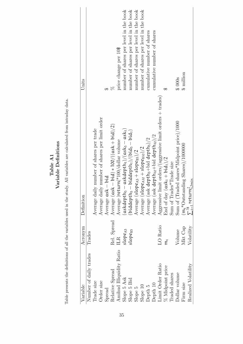
Table

A1

Vari

able

Definit

ions

Tab

lep

rese

nts

the

defi

nit

ion

sof

all

the

vari

able

su

sed

inth

est

ud

y.A

llva

riab

les

are

calc

ula

ted

from

intr

ad

ayd

ata

.

Var

iable

Acr

onym

Defi

nit

ion

Unit

sN

um

ber

ofdai

lytr

ades

Tra

des

Tra

de

size

Ave

rage

dai

lynum

ber

ofsh

ares

per

trad

eO

rder

size

Ave

rage

dai

lynum

ber

ofsh

ares

per

lim

itor

der

Spre

adA

vera

geask

−bid

$

Rel

ativ

eSpre

adR

el.

Spre

adA

vera

ge(ask

−bid)∗100/((ask

+bid)/2)

%A

mih

ud

Illiquid

ity

Rat

ioIL

RA

vera

ge|return

|*10

0/dol

lar

volu

me

pri

cech

ange

per

10$

Slo

pe

5A

skslopeA5

(askdepth

5−askdepth

1)/(ask

5−ask

1)

num

ber

ofsh

ares

per

leve

lin

the

book

Slo

pe

5B

idslopeB5

(biddepth

5−biddepth

1)/(bid5−bid1)

num

ber

ofsh

ares

per

leve

lin

the

book

Slo

pe

5A

vera

ge(slopeA5+slopeB5)/2

num

ber

ofsh

ares

per

leve

lin

the

book

Slo

pe

10A

vera

ge(slopeA10+slopeB10)/2

num

ber

ofsh

ares

per

leve

lin

the

book

Dep

th5

Ave

rage

(askdepth

5+

biddepth

5)/

2cu

mula

tive

num

ber

ofsh

ares

Dep

th10

Ave

rage

(askdepth

10+

biddepth

10)/

2cu

mula

tive

num

ber

ofsh

ares

Lim

itO

rder

Rat

ioL

OR

atio

Agg

ress

ive

lim

itor

der

s/(a

ggre

ssiv

elim

itor

der

s+

trad

es)

%M

idp

oint

pri

cemt

End

ofday

(ask

1+bid1)/2

$

Tra

ded

shar

esSum

ofT

rades

*Tra

de

size

Dol

lar

volu

me

Vol

um

eSum

of(T

raded

shar

es*M

idp

oint

pri

ce)/

1000

$00

0sF

irm

size

Mkt

Cap

(mt*

Outs

tandin

gShar

es)/

1000

000

$m

illion

Rea

lize

dV

olat

ilit

yV

olat

ilit

y∑ 78 t=

1return

2 t,5min

35

Table A2Listing Descriptions

Table shows the average daily characteristics for stocks listed in different exchanges and classified as TapeA, B, and C. Tape A are NYSE listed stocks, Tape C are NASDAQ listed stock, and all other stocks areclassified as Tape C. Panel A presents the characteristics of all the Tape A and C stocks (45,254 day-stockobservations). Panel B shows the characteristics for the Tape B stocks (1,067 day-stock observations).All variables are defined in Table A1.

Price Volume Returns Mkt Cap

Panel A. AC Stocks

Mean 35 55 0.07 6,427Median 27 8 0.02 1,22125th 16 1 0.01 38875th 43 38 0.04 3,949St. Dev. 37 207 0.22 20,995

Panel B. B Stocks

Mean 33 0.82 0.31 267Median 18 0.09 0.14 9025th 11 0.01 0.05 4375th 66 0.45 0.40 271St. Dev. 56 3.47 0.43 469

36

References

Amihud, Y., H. Mendelson, and B. Lauterbach(1997). “Market microstructure and securitiesvalues: Evidence from the Tel Aviv stock ex-change.” Journal of Financial Economics, 45,365–390.

Angel, J., L. Harris, and C. Spatt (2011). “Equitytrading in the 21st century.” Quarterly Journalof Finance, 1, 1–53.

Angrist, J. D. and A. B. Krueger (1992). “The ef-fect of age at school entry on educational attain-ment: An application of instrumental variableswith moments from two samples.” Journal ofAmerican Statistical Association, 87(418), 328–336.

Angrist, J. D. and A. B. Krueger (1995). “Split-sample instrumental variables estimates of thereturn to schooling.” Journal of Business andEconomic Statistics, 13(2), 225–235.

Angrist, J. D. and J.-S. Pischke (2009). MostlyHarmless Econometrics: An Empiricist’s Com-panion. Princeton University Press.

Barclay, M. and T. Hendershott (2004). “Liquid-ity externalities and adverse selection: Evidencefrom trading after hours.” Journal of Finance,59, 681–710.

Battalio, R. H., A. Shkilko, and R. A. V. Ness(2012). “To pay or be paid? the impact of takerfees and order flow inducements on trading costsin u.s. options markets.”

Bessembinder, H., W. Maxwell, and K. Venkatara-man (2006). “Market transparency, liquidity ex-ternalities, and institutional trading costs in cor-porate bonds.” Journal of Financial Economics,82, 251–288.

Biais, B., L. Glosten, and C. Spatt (2005). “Mar-ket microstructure: A survey of microfounda-tion, empirical results and policy implications.”Journal of Financial Markets, 8, 111–264.

Biais, B., P. Hillion, and C. Spatt (1999). “Pricediscovery and learning during the preopening pe-riod in the paris bourse.” Journal of PoliticalEconomy, 107(6), 1218–1248.

Borttolotti, B., F. de Jong, G. Nicodano, andI. Schindele (2007). “Privatization and stockmarket liquidity.” Journal of Banking and Fi-nance, 31.

Bound, J., D. Jaeger, and R. Baker (1995).“Problems with instrumental variables estima-tion when the correlation between the instru-ments and the endogenous explanatory variableis weak.” Journal of the American StatisticalAssociation, 90, 443–450.

Chordia, T., R. Roll, and A. Subrahmanyam(2000). “Commonality in liquidity.” Journal ofFinancial Economics, 56(1), 3 – 28.

Colliard, J. E. and T. Foucault (2011). “Tradingfees and efficiency in limit order markets.” Dis-cussion Paper Series 8395, CEPR.

Copeland, T. E. and D. Galai (1983). “Informationeffects on the bid-ask spread.” The Journal ofFinance, 38(5), 1457–1469.

Degryse, H., F. De Jong, M. V. Ravenswaaij, andG. Wuyts (2005). “Aggressive orders and theresiliency of a limit order market.” Review ofFinance, 9, 201–242.

Foucault, T., O. Kadan, and E. Kandel (2005).“Limit order book as a market for liquidity.” Re-view of Financial Studies, 18, 1171–1217.

Foucault, T., O. Kadan, and E. Kandel (2012).“Liquidity cycles, and make/take fees in elec-tronic markets.” Journal of Finance, forthcom-ing.

Gaspar, J.-M. and L. Lescourret (2009). “Liquid-ity externalities and buyout delisting activity.”Working paper.

Goettler, R., C. Parlour, and U. Rajan (2005).“Equilibrium in a dynamic limit order market.”Journal of Finance, 60, 2149–2192.

Goldstein, M. A. and K. A. Kavajecz (2000).“Eighths, sixteenths, and market depth:Changes in tick size and liquidity provision onthe nyse.” Journal of Financial Economics, 56,125–149.

Goyenko, R. Y., C. W. Holden, and C. A. Trzcinka(2009). “Do liquidity measures measure liquid-ity?” Journal of Financial Economics, 92(2),153 – 181.

Harris, L. (1990). “Liquidity, trading rules, andelectronic trading systems.” New york univer-sity salomon center monograph series in financeand economics.

Hasbrouck, J. (2009). “Trading costs and returnsfor U.S. equities: Estimating effective costs fromdaily data.” Journal of Finance, 64(3), 1445–1477.

37

Hasbrouck, J. and D. Seppi (2001). “Common fac-tors in prices, order flows and liquidity.” Journalof Financial Economics, 59, 383–411.

Hendershott, T. and C. M. Jones (2005). “Islandgoes dark: Transparency, fragmentation and reg-ulation.” Review of Financial Studies, 18, 743–793.

Imbens, G. W. (2010). “Better late than nothing:Some comments on deaton (2009) and heckmanand urzua (2009).” Journal of Economic Liter-ature, 48, 399–423.

Imbens, G. W. and J. M. Wooldridge (2009). “Re-cent developments in the econometrics of pro-gram evaluation.” Journal of Economic Litera-ture, 47, 5–86.

Kavajecz, K. (1999). “A specialist’s quoted depthand the limit order.” Journal of Finance, 54,747–771.

Large, J. (2007). “Measuring the resiliency of anelectronic limit order book.” Journal of Finan-cial Markets, 1–25.

Macey, J. and M. O’Hara (1999). “Regulating ex-changes and alternative trading system: A lawand economics perspective.” Journal of LegalStudies, 28, 17–54.

Madhavan, A. (2000). “Market microstructure: Asurvey.” Journal of Financial Markets, 3, 205–258.

Malinova, K. and A. Park (2011). “Subsidizing liq-uidity: The impact of make/take fees on marketquality.” Working paper, University of Toronto.

O’Hara, M. and M. Ye (2011). “Is market frag-mentation harming market quality?” Journal ofFinancial Economics, 100(3), 459–474.

Rosenzweig, M. R. and K. I. Wolpin (2000). “Natu-ral ‘natural experiments’ in economics.” Journalof Economic Literature, 38, 827–874.

Rosu, I. (2009). “A dynamic model of the limitorder book.” Review of Financial Studies, 22,4601–4641.

Rosu, I. (2010). “Liquidity and information in or-der driven markets.” Chicago Booth School ofBusiness.

38