lecture notes – trigonometric functions
TRANSCRIPT
IntroductionTrigonometric Functions
Trigonometric ModelsModel Properties
Calculus for the Life Sciences
Lecture Notes – Trigonometric Functions
Joseph M. Mahaffy,〈[email protected]〉
Department of Mathematics and StatisticsDynamical Systems Group
Computational Sciences Research Center
San Diego State UniversitySan Diego, CA 92182-7720
http://www-rohan.sdsu.edu/∼jmahaffy
Spring 2017
Joseph M. Mahaffy, 〈[email protected]〉Lecture Notes – Trigonometric Functions —(1/68)
IntroductionTrigonometric Functions
Trigonometric ModelsModel Properties
Outline
1 IntroductionAnnual Temperature CyclesSan Diego and Chicago
2 Trigonometric FunctionsBasic Trig FunctionsRadian MeasureProperties of Sine and CosineIdentities
3 Trigonometric ModelsVertical Shift and AmplitudeFrequency and PeriodPhase ShiftExamples
4 Model PropertiesPhase Shift of Half a PeriodEquivalent Sine and Cosine ModelsReturn to Annual Temperature VariationOther Examples
Joseph M. Mahaffy, 〈[email protected]〉Lecture Notes – Trigonometric Functions —(2/68)
IntroductionTrigonometric Functions
Trigonometric ModelsModel Properties
Annual Temperature CyclesSan Diego and Chicago
Introduction — Trigonometric Functions
Introduction — Trigonometric Functions
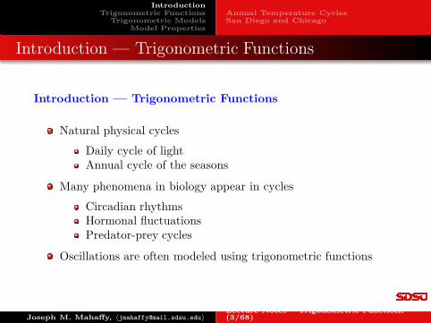
Natural physical cycles
Daily cycle of lightAnnual cycle of the seasons
Many phenomena in biology appear in cycles
Circadian rhythmsHormonal fluctuationsPredator-prey cycles
Oscillations are often modeled using trigonometric functions
Joseph M. Mahaffy, 〈[email protected]〉Lecture Notes – Trigonometric Functions —(3/68)
IntroductionTrigonometric Functions
Trigonometric ModelsModel Properties
Annual Temperature CyclesSan Diego and Chicago
Annual Temperature Cycles
Annual Temperature Cycles
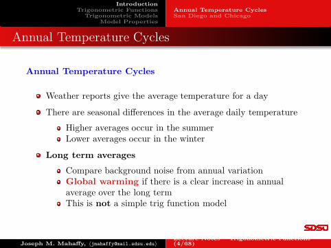
Weather reports give the average temperature for a day
There are seasonal differences in the average daily temperature
Higher averages occur in the summerLower averages occur in the winter
Long term averages
Compare background noise from annual variationGlobal warming if there is a clear increase in annualaverage over the long termThis is not a simple trig function model
Joseph M. Mahaffy, 〈[email protected]〉Lecture Notes – Trigonometric Functions —(4/68)
IntroductionTrigonometric Functions
Trigonometric ModelsModel Properties
Annual Temperature CyclesSan Diego and Chicago
Modeling Annual Temperature Cycles
Modeling Annual Temperature Cycles
What mathematical tools can help predict the annualtemperature cycles?
Polynomials and exponentials do not exhibit the periodicbehavior
Trigonometric functions exhibit periodicity
Fit any specific periodManage amplitude of variationShift the maximum or minimum for a data set
Joseph M. Mahaffy, 〈[email protected]〉Lecture Notes – Trigonometric Functions —(5/68)
IntroductionTrigonometric Functions
Trigonometric ModelsModel Properties
Annual Temperature CyclesSan Diego and Chicago
Average Temperatures for San Diego and Chicago 1
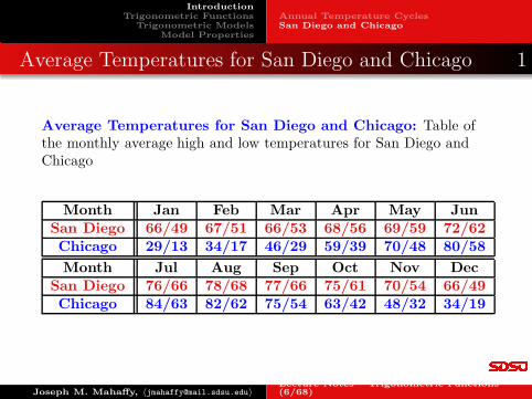
Average Temperatures for San Diego and Chicago: Table ofthe monthly average high and low temperatures for San Diego andChicago
Month Jan Feb Mar Apr May JunSan Diego 66/49 67/51 66/53 68/56 69/59 72/62Chicago 29/13 34/17 46/29 59/39 70/48 80/58
Month Jul Aug Sep Oct Nov DecSan Diego 76/66 78/68 77/66 75/61 70/54 66/49Chicago 84/63 82/62 75/54 63/42 48/32 34/19
Joseph M. Mahaffy, 〈[email protected]〉Lecture Notes – Trigonometric Functions —(6/68)
IntroductionTrigonometric Functions
Trigonometric ModelsModel Properties
Annual Temperature CyclesSan Diego and Chicago
Average Temperatures for San Diego and Chicago 2
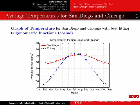
Graph of Temperature for San Diego and Chicago with best fittingtrigonometric functions (cosine)
Jan Feb Mar Apr May Jun Jul Aug Sep Oct Nov Dec Jan20
30
40
50
60
70
80
90
Month
Ave
rage
Tem
pera
ture
, o F
Temperatures for San Diego and Chicago
San DiegoChicago
Joseph M. Mahaffy, 〈[email protected]〉Lecture Notes – Trigonometric Functions —(7/68)
IntroductionTrigonometric Functions
Trigonometric ModelsModel Properties
Annual Temperature CyclesSan Diego and Chicago
Average Temperatures for San Diego and Chicago 3
Models of Annual Temperature Cycles for San Diego andChicago
The two graphs have similarities and differences
Same seasonal period as expectedSeasonal variation or amplitude of oscillation for Chicago ismuch greater than San DiegoOverall average temperature for San Diego is greater thanthe average for Chicago
Overlying models use cosine functions (could equally fit withsine functions)
Joseph M. Mahaffy, 〈[email protected]〉Lecture Notes – Trigonometric Functions —(8/68)
IntroductionTrigonometric Functions
Trigonometric ModelsModel Properties
Basic Trig FunctionsRadian MeasureProperties of Sine and CosineIdentities
Trigonometric Functions 1
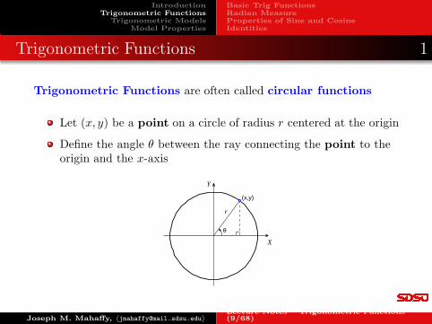
Trigonometric Functions are often called circular functions
Let (x, y) be a point on a circle of radius r centered at the origin
Define the angle θ between the ray connecting the point to theorigin and the x-axis
(x,y)
r
θ
X
Y
Joseph M. Mahaffy, 〈[email protected]〉Lecture Notes – Trigonometric Functions —(9/68)
IntroductionTrigonometric Functions
Trigonometric ModelsModel Properties
Basic Trig FunctionsRadian MeasureProperties of Sine and CosineIdentities
Trigonometric Functions
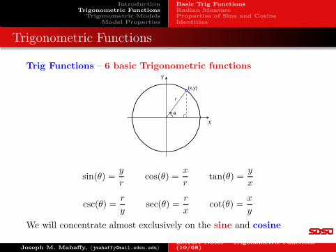
Trig Functions – 6 basic Trigonometric functions
(x,y)
r
θ
X
Y
sin(θ) =y
rcos(θ) =
x
rtan(θ) =
y
x
csc(θ) =r
ysec(θ) =
r
xcot(θ) =
x
y
We will concentrate almost exclusively on the sine and cosine
Joseph M. Mahaffy, 〈[email protected]〉Lecture Notes – Trigonometric Functions —(10/68)
IntroductionTrigonometric Functions
Trigonometric ModelsModel Properties
Basic Trig FunctionsRadian MeasureProperties of Sine and CosineIdentities
Radian Measure
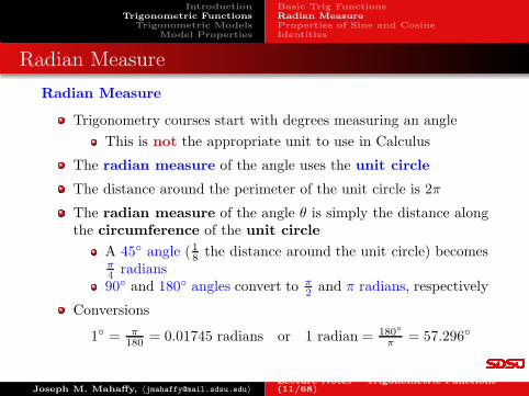
Radian Measure
Trigonometry courses start with degrees measuring an angle
This is not the appropriate unit to use in Calculus
The radian measure of the angle uses the unit circle
The distance around the perimeter of the unit circle is 2π
The radian measure of the angle θ is simply the distance alongthe circumference of the unit circle
A 45◦ angle (18the distance around the unit circle) becomes
π
4radians
90◦ and 180◦ angles convert to π
2and π radians, respectively
Conversions
1◦ = π
180= 0.01745 radians or 1 radian = 180
◦
π= 57.296◦
Joseph M. Mahaffy, 〈[email protected]〉Lecture Notes – Trigonometric Functions —(11/68)
IntroductionTrigonometric Functions
Trigonometric ModelsModel Properties
Basic Trig FunctionsRadian MeasureProperties of Sine and CosineIdentities
Sine and Cosine 1
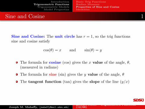
Sine and Cosine: The unit circle has r = 1, so the trig functionssine and cosine satisfy
cos(θ) = x and sin(θ) = y
The formula for cosine (cos) gives the x value of the angle, θ,(measured in radians)
The formula for sine (sin) gives the y value of the angle, θ
The tangent function (tan) gives the slope of the line (y/x)
Joseph M. Mahaffy, 〈[email protected]〉Lecture Notes – Trigonometric Functions —(12/68)
IntroductionTrigonometric Functions
Trigonometric ModelsModel Properties
Basic Trig FunctionsRadian MeasureProperties of Sine and CosineIdentities
Sine and Cosine 2
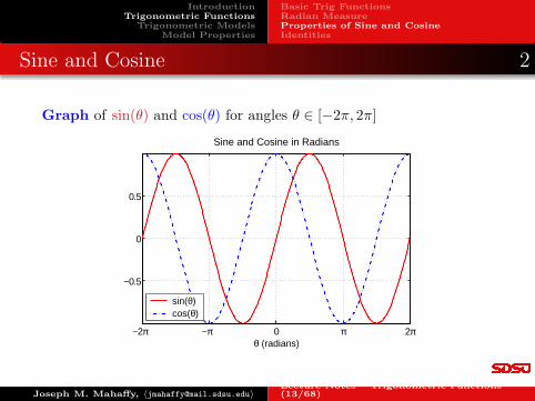
Graph of sin(θ) and cos(θ) for angles θ ∈ [−2π, 2π]
−2π −π 0 π 2π
−0.5
0
0.5
θ (radians)
Sine and Cosine in Radians
sin(θ)cos(θ)
Joseph M. Mahaffy, 〈[email protected]〉Lecture Notes – Trigonometric Functions —(13/68)
IntroductionTrigonometric Functions
Trigonometric ModelsModel Properties
Basic Trig FunctionsRadian MeasureProperties of Sine and CosineIdentities
Sine and Cosine 3
Sine and Cosine - Periodicity and Bounded
Notice the 2π periodicity: The functions repeat the samepattern every 2π radians
Consider a point moving around a circleAfter 2π radians, the point returns to the same position(circular function)
Note: Both the sine and cosine functions are boundedbetween −1 and 1
Joseph M. Mahaffy, 〈[email protected]〉Lecture Notes – Trigonometric Functions —(14/68)
IntroductionTrigonometric Functions
Trigonometric ModelsModel Properties
Basic Trig FunctionsRadian MeasureProperties of Sine and CosineIdentities
Sine and Cosine 6
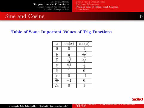
Table of Some Important Values of Trig Functions
x sin(x) cos(x)0 0 1π
6
1
2
√3
2
π
4
√2
2
√2
2
π
3
√3
2
1
2π
21 0
π 0 −13π
2−1 0
2π 0 1
Joseph M. Mahaffy, 〈[email protected]〉Lecture Notes – Trigonometric Functions —(15/68)

IntroductionTrigonometric Functions
Trigonometric ModelsModel Properties
Basic Trig FunctionsRadian MeasureProperties of Sine and CosineIdentities
Properties of Sine and Cosine 1
Properties of Cosine
Periodic with period 2π and bounded by −1 and 1
Cosine is an even function
Maximum at x = 0, cos(0) = 1
By periodicity, other maxima at xn = 2nπ with cos(2nπ) = 1 (nany integer)
Minimum at x = π, cos(π) = −1
By periodicity, other minima at xn = (2n+ 1)π withcos(xn) = −1 (n any integer)
Zeroes of cosine separated by π with cos(xn) = 0 whenxn = π
2+ nπ (n any integer)
Joseph M. Mahaffy, 〈[email protected]〉Lecture Notes – Trigonometric Functions —(16/68)
IntroductionTrigonometric Functions
Trigonometric ModelsModel Properties
Basic Trig FunctionsRadian MeasureProperties of Sine and CosineIdentities
Properties of Sine and Cosine 2
Properties of Sine
Periodic with period 2π and bounded by −1 and 1
Sine is an odd function
Maximum at x = π
2, sin
(
π
2
)
= 1
By periodicity, other maxima at xn = π
2+ 2nπ with sin(xn) = 1
(n any integer)
Minimum at x = 3π
2, sin
(
3π
2
)
= −1
By periodicity, other minima at xn = 3π
2+ 2nπ with
sin(xn) = −1 (n any integer)
Zeroes of sine separated by π with sin(xn) = 0 when xn = nπ(n any integer)
Joseph M. Mahaffy, 〈[email protected]〉Lecture Notes – Trigonometric Functions —(17/68)
IntroductionTrigonometric Functions
Trigonometric ModelsModel Properties
Basic Trig FunctionsRadian MeasureProperties of Sine and CosineIdentities
Some Identities for Sine and Cosine
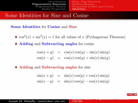
Some Identities for Cosine and Sine
cos2(x) + sin2(x) = 1 for all values of x (Pythagorean Theorem)
Adding and Subtracting angles for cosine
cos(x + y) = cos(x) cos(y)− sin(x) sin(y)
cos(x − y) = cos(x) cos(y) + sin(x) sin(y)
Adding and Subtracting angles for sine
sin(x+ y) = sin(x) cos(y) + cos(x) sin(y)
sin(x− y) = sin(x) cos(y)− cos(x) sin(y)
Joseph M. Mahaffy, 〈[email protected]〉Lecture Notes – Trigonometric Functions —(18/68)
IntroductionTrigonometric Functions
Trigonometric ModelsModel Properties
Basic Trig FunctionsRadian MeasureProperties of Sine and CosineIdentities
Example of Shifts 1
Example of Shifts for Sine and Cosine:
Use the trigonometric identities to show
cos(x) = sin(
x+ π
2
)
sin(x) = cos(
x− π
2
)
This first example shows the cosine is the same as the sine functionshifted to the left by π
2(a quarter period)
This second example shows the sine is the same as the cosine functionshifted to the right by π
2(a quarter period)
Joseph M. Mahaffy, 〈[email protected]〉Lecture Notes – Trigonometric Functions —(19/68)
IntroductionTrigonometric Functions
Trigonometric ModelsModel Properties
Basic Trig FunctionsRadian MeasureProperties of Sine and CosineIdentities
Example of Shifts 2
Solution: Use the additive identity for sine
sin(
x+π
2
)
= sin(x) cos(π
2
)
+ cos(x) sin(π
2
)
Since cos(
π
2
)
= 0 and sin(
π
2
)
= 1, sin(
x+ π
2
)
= cos(x)
Similarly,
cos(
x−π
2
)
= cos(x) cos(π
2
)
+ sin(x) sin(π
2
)
Again cos(
π
2
)
= 0 and sin(
π
2
)
= 1, so cos(
x− π
2
)
= sin(x)
Joseph M. Mahaffy, 〈[email protected]〉Lecture Notes – Trigonometric Functions —(20/68)
IntroductionTrigonometric Functions
Trigonometric ModelsModel Properties
Vertical Shift and AmplitudeFrequency and PeriodPhase ShiftExamples
Model of Predator 1
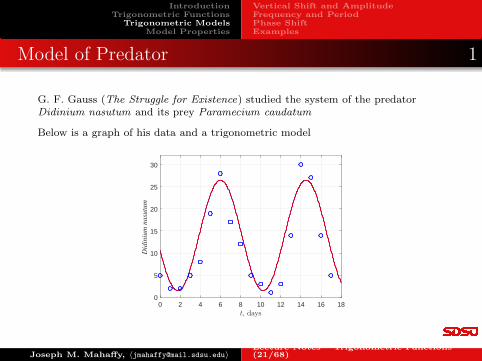
G. F. Gauss (The Struggle for Existence) studied the system of the predatorDidinium nasutum and its prey Paramecium caudatum
Below is a graph of his data and a trigonometric model
0 2 4 6 8 10 12 14 16 18t, days
0
5
10
15
20
25
30
Did
iniu
m n
asu
tum
Joseph M. Mahaffy, 〈[email protected]〉Lecture Notes – Trigonometric Functions —(21/68)
IntroductionTrigonometric Functions
Trigonometric ModelsModel Properties
Vertical Shift and AmplitudeFrequency and PeriodPhase ShiftExamples
Model of Predator 2
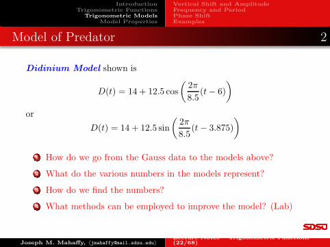
Didinium Model shown is
D(t) = 14 + 12.5 cos
(
2π
8.5(t− 6)
)
or
D(t) = 14 + 12.5 sin
(
2π
8.5(t− 3.875)
)
1 How do we go from the Gauss data to the models above?
2 What do the various numbers in the models represent?
3 How do we find the numbers?
4 What methods can be employed to improve the model? (Lab)
Joseph M. Mahaffy, 〈[email protected]〉Lecture Notes – Trigonometric Functions —(22/68)
IntroductionTrigonometric Functions
Trigonometric ModelsModel Properties
Vertical Shift and AmplitudeFrequency and PeriodPhase ShiftExamples
Model of Predator 3
Observations:
1 The population fluctuates about an average
2 The population appears to have a regular periodic cycle
3 The degree of fluctuation or amplitude of variation is fairlyconsistent
4 The maximum population is shifted from t = 0
These observations can be converted into the 4 key parameters of themodel.
Joseph M. Mahaffy, 〈[email protected]〉Lecture Notes – Trigonometric Functions —(23/68)
IntroductionTrigonometric Functions
Trigonometric ModelsModel Properties
Vertical Shift and AmplitudeFrequency and PeriodPhase ShiftExamples
Trigonometric Models
Trigonometric Models are appropriate when data follows a simpleoscillatory behavior (as seen in the example above)
The Cosine Model
y(t) = A+B cos(ω(t− φ))
The Sine Model
y(t) = A+B sin(ω(t− φ))
Each model has Four Parameters
Joseph M. Mahaffy, 〈[email protected]〉Lecture Notes – Trigonometric Functions —(24/68)
IntroductionTrigonometric Functions
Trigonometric ModelsModel Properties
Vertical Shift and AmplitudeFrequency and PeriodPhase ShiftExamples
Vertical Shift and Amplitude
Trigonometric Model Parameters: For the cosine model
y(t) = A+B cos(ω(t− φ))
The model parameter A is the vertical shift, which isassociated with the average height of the model
The model parameter B gives the amplitude, whichmeasures the distance from the average, A, to themaximum (or minimum) of the model
There are similar parameters for the sine model
Joseph M. Mahaffy, 〈[email protected]〉Lecture Notes – Trigonometric Functions —(25/68)
IntroductionTrigonometric Functions
Trigonometric ModelsModel Properties
Vertical Shift and AmplitudeFrequency and PeriodPhase ShiftExamples
Frequency and Period
Trigonometric Model Parameters: For the cosine model
y(t) = A+B cos(ω(t− φ))
The model parameter ω is the frequency, which gives thenumber of periods of the model that occur as t varies over2π radians
The period is given by T =2π
ω
There are similar parameters for the sine model
Joseph M. Mahaffy, 〈[email protected]〉Lecture Notes – Trigonometric Functions —(26/68)
IntroductionTrigonometric Functions
Trigonometric ModelsModel Properties
Vertical Shift and AmplitudeFrequency and PeriodPhase ShiftExamples
Phase Shift
Trigonometric Model Parameters: For the cosine model
y(t) = A+B cos(ω(t− φ))
The model parameter φ is the phase shift, which shiftsour models to the left or right
This gives a right horizontal shift for positive φ
If the period is denoted T = 2πω , then the principle phase
shift satisfies φ ∈ [0, T )
By periodicity of the model, if φ is any phase shift
φ1 = φ+ nT = φ+ 2nπω , n an integer
is a phase shift for an equivalent model
There is a similar parameter for the sine modelJoseph M. Mahaffy, 〈[email protected]〉
Lecture Notes – Trigonometric Functions —(27/68)
IntroductionTrigonometric Functions
Trigonometric ModelsModel Properties
Vertical Shift and AmplitudeFrequency and PeriodPhase ShiftExamples
Model Parameters
Trigonometric Model Parameters: For the cosine and sine models
y(t) = A+B cos(ω(t− φ))
y(t) = A+B sin(ω(t− φ))
The vertical shift parameter A is unique
The amplitude parameter B is unique in magnitude but thesign can be chosen by the modeler
The frequency parameter ω is unique in magnitude but thesign can be chosen by the modeler
By periodicity, phase shift has infinitely many choices
One often selects the unique principle phase shift satisfying0 ≤ φ < T
Joseph M. Mahaffy, 〈[email protected]〉Lecture Notes – Trigonometric Functions —(28/68)
IntroductionTrigonometric Functions
Trigonometric ModelsModel Properties
Vertical Shift and AmplitudeFrequency and PeriodPhase ShiftExamples
Parameters for Didinium Model
Overview: Consider the cosine model for Didinium
D(t) = 14 + 12.5 cos
(
2π
8.5(t − 6)
)
Best fit would use the Sum of Square Errors (SSE), but narrow peaks indicatethat the best model is not quite sinusoidal, which skews the parameters
1 Observe the average between the high and low is approximated by 14, sothe vertical shift, A = 14.
2 A reasonable approximation to the distance between the average and thehigh or low data is 12.5, so the amplitude, B = 12.5.
3 The distance between peaks (or troughs) is about 8.5, the period, T = 8.5,which gives ω = 2π
8.5= 0.73930.
4 A first maximum of this cosine model occurs at t = 6. Since cosine is at amaximum when its argument is zero, the phase shift, φ = 6.
Joseph M. Mahaffy, 〈[email protected]〉Lecture Notes – Trigonometric Functions —(29/68)
IntroductionTrigonometric Functions
Trigonometric ModelsModel Properties
Vertical Shift and AmplitudeFrequency and PeriodPhase ShiftExamples
Improved Didinium Model
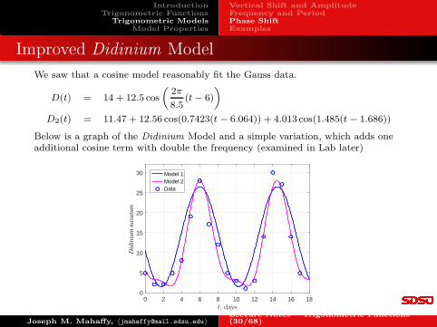
We saw that a cosine model reasonably fit the Gauss data.
D(t) = 14 + 12.5 cos
(
2π
8.5(t− 6)
)
D2(t) = 11.47 + 12.56 cos(0.7423(t − 6.064)) + 4.013 cos(1.485(t − 1.686))
Below is a graph of the Didinium Model and a simple variation, which adds oneadditional cosine term with double the frequency (examined in Lab later)
0 2 4 6 8 10 12 14 16 18t, days
0
5
10
15
20
25
30
Did
iniu
m n
asu
tum
Model 1Model 2Data
Joseph M. Mahaffy, 〈[email protected]〉Lecture Notes – Trigonometric Functions —(30/68)
IntroductionTrigonometric Functions
Trigonometric ModelsModel Properties
Vertical Shift and AmplitudeFrequency and PeriodPhase ShiftExamples
Example: Sine Function 1
Example 1: Consider the model
y(x) = 3 sin(2x)− 2
Skip Example
Find the vertical shift, amplitude, and period
Sketch a graph
Determine all maxima and minima for x ∈ [0, 2π]
Joseph M. Mahaffy, 〈[email protected]〉Lecture Notes – Trigonometric Functions —(31/68)
IntroductionTrigonometric Functions
Trigonometric ModelsModel Properties
Vertical Shift and AmplitudeFrequency and PeriodPhase ShiftExamples
Example: Sine Function 2
Solution: Fory(x) = 3 sin(2x)− 2
The vertical shift is A = −2
The amplitude is B = 3, so solution oscillates with−5 ≤ y(x) ≤ 1
The frequency is ω = 2, so the period, T , satisfies
T =2π
ω=
2π
2= π
No phase shift, so divide the period into 4 even parts,x = 0, π
4, π
2, 3π
4, π
Joseph M. Mahaffy, 〈[email protected]〉Lecture Notes – Trigonometric Functions —(32/68)
IntroductionTrigonometric Functions
Trigonometric ModelsModel Properties
Vertical Shift and AmplitudeFrequency and PeriodPhase ShiftExamples
Example: Sine Function 3
Graphing: Steps for graphing y(x) = 3 sin(2x)− 2.
1 With no phase shift, start at x = 0. Create a line along theaverage value y = −2, which extends the length of one period.
2 The amplitude of 3 means creating parallel lines above andbelow y = −2 at y = 1 and y = −5, then complete the rectanglefor one period.
3 Finally draw parallel vertical lines along each quarter of theperiod, x = 0, π/4, π/2, 3π/4, π.
4 This drawing is on next slide.
Joseph M. Mahaffy, 〈[email protected]〉Lecture Notes – Trigonometric Functions —(33/68)
IntroductionTrigonometric Functions
Trigonometric ModelsModel Properties
Vertical Shift and AmplitudeFrequency and PeriodPhase ShiftExamples
Example: Sine Function 4
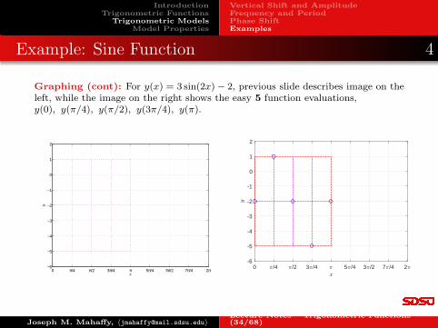
Graphing (cont): For y(x) = 3 sin(2x)− 2, previous slide describes image on theleft, while the image on the right shows the easy 5 function evaluations,y(0), y(π/4), y(π/2), y(3π/4), y(π).
0 π/4 π/2 3π/4 π 5π/4 3π/2 7π/4 2π−6
−5
−4
−3
−2
−1
0
1
2
x
y
0 π/4 π/2 3π/4 π 5π/4 3π/2 7π/4 2πx
-6
-5
-4
-3
-2
-1
0
1
2
y
Joseph M. Mahaffy, 〈[email protected]〉Lecture Notes – Trigonometric Functions —(34/68)
IntroductionTrigonometric Functions
Trigonometric ModelsModel Properties
Vertical Shift and AmplitudeFrequency and PeriodPhase ShiftExamples
Example: Sine Function 5
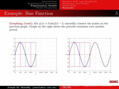
Graphing (cont): For y(x) = 3 sin(2x) − 2, smoothly connect the points on theprevious graph. Graph on the right shows the periodic extension over anotherperiod.
0 π/4 π/2 3π/4 π 5π/4 3π/2 7π/4 2πx
-6
-5
-4
-3
-2
-1
0
1
2
y
0 π/4 π/2 3π/4 π 5π/4 3π/2 7π/4 2πx
-6
-5
-4
-3
-2
-1
0
1
2
y
Joseph M. Mahaffy, 〈[email protected]〉Lecture Notes – Trigonometric Functions —(35/68)
IntroductionTrigonometric Functions
Trigonometric ModelsModel Properties
Vertical Shift and AmplitudeFrequency and PeriodPhase ShiftExamples
Example: Sine Function 6
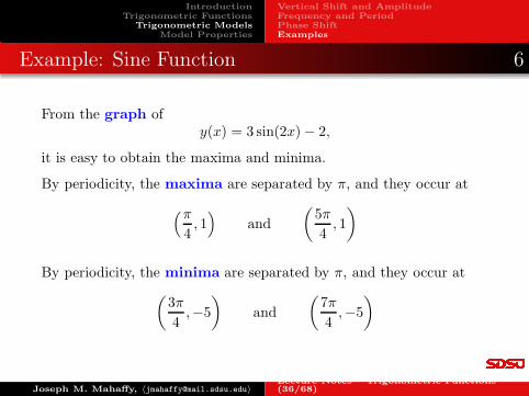
From the graph ofy(x) = 3 sin(2x)− 2,
it is easy to obtain the maxima and minima.
By periodicity, the maxima are separated by π, and they occur at
(π
4, 1)
and
(
5π
4, 1
)
By periodicity, the minima are separated by π, and they occur at
(
3π
4,−5
)
and
(
7π
4,−5
)
Joseph M. Mahaffy, 〈[email protected]〉Lecture Notes – Trigonometric Functions —(36/68)
IntroductionTrigonometric Functions
Trigonometric ModelsModel Properties
Vertical Shift and AmplitudeFrequency and PeriodPhase ShiftExamples
Example: Cosine Function 1
Example 2: Consider the model
y(x) = 4− 3 cos(π
4(x− 3)
)
Skip Example
Find the vertical shift, amplitude, and period
Sketch a graph
Determine all maxima and minima for x ∈ [0, 16]
Joseph M. Mahaffy, 〈[email protected]〉Lecture Notes – Trigonometric Functions —(37/68)
IntroductionTrigonometric Functions
Trigonometric ModelsModel Properties
Vertical Shift and AmplitudeFrequency and PeriodPhase ShiftExamples
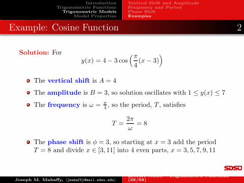
Example: Cosine Function 2
Solution: Fory(x) = 4− 3 cos
(π
4(x− 3)
)
The vertical shift is A = 4
The amplitude is B = 3, so solution oscillates with 1 ≤ y(x) ≤ 7
The frequency is ω = π
4, so the period, T , satisfies
T =2π
ω= 8
The phase shift is φ = 3, so starting at x = 3 add the periodT = 8 and divide x ∈ [3, 11] into 4 even parts, x = 3, 5, 7, 9, 11
Joseph M. Mahaffy, 〈[email protected]〉Lecture Notes – Trigonometric Functions —(38/68)

IntroductionTrigonometric Functions
Trigonometric ModelsModel Properties
Vertical Shift and AmplitudeFrequency and PeriodPhase ShiftExamples
Example: Cosine Function 3
Graphing: Steps for graphing y(x) = 4− 3 cos(
π
4(x− 3)
)
.
1 With phase shift, φ = 3, start at x = 3. Create a line along theaverage value y = 4, which extends the length of one period.
2 The amplitude of 3 means creating parallel lines above andbelow y = 4 at y = 1 and y = 7, then complete the rectangle forone period.
3 Finally draw parallel vertical lines along each quarter of theperiod, x = 3, 5, 7, 9, 11.
4 This drawing is on next slide.
Joseph M. Mahaffy, 〈[email protected]〉Lecture Notes – Trigonometric Functions —(39/68)
IntroductionTrigonometric Functions
Trigonometric ModelsModel Properties
Vertical Shift and AmplitudeFrequency and PeriodPhase ShiftExamples
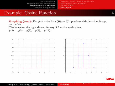
Example: Cosine Function 4
Graphing (cont): For y(x) = 4− 3 cos(
π
4(x− 3)
)
, previous slide describes imageon the left.The image on the right shows the easy 5 function evaluations,y(3), y(5), y(7), y(9), y(11).
0 2 4 6 8 10 12 14 160
1
2
3
4
5
6
7
8
x
y
0 2 4 6 8 10 12 14 160
1
2
3
4
5
6
7
8
x
y
Joseph M. Mahaffy, 〈[email protected]〉Lecture Notes – Trigonometric Functions —(40/68)
IntroductionTrigonometric Functions
Trigonometric ModelsModel Properties
Vertical Shift and AmplitudeFrequency and PeriodPhase ShiftExamples
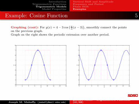
Example: Cosine Function 5
Graphing (cont): For y(x) = 4− 3 cos(
π
4(x− 3)
)
, smoothly connect the pointson the previous graph.Graph on the right shows the periodic extension over another period.
0 2 4 6 8 10 12 14 160
1
2
3
4
5
6
7
8
x
y
0 2 4 6 8 10 12 14 160
1
2
3
4
5
6
7
8
x
y
Joseph M. Mahaffy, 〈[email protected]〉Lecture Notes – Trigonometric Functions —(41/68)
IntroductionTrigonometric Functions
Trigonometric ModelsModel Properties
Vertical Shift and AmplitudeFrequency and PeriodPhase ShiftExamples
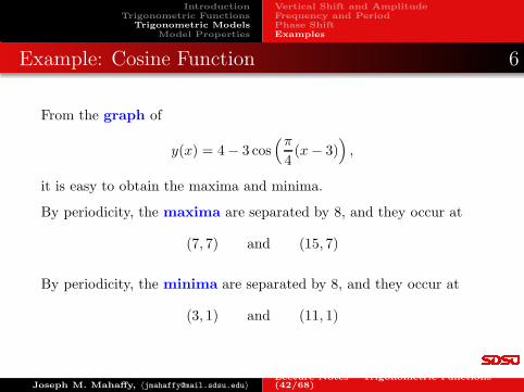
Example: Cosine Function 6
From the graph of
y(x) = 4− 3 cos(π
4(x− 3)
)
,
it is easy to obtain the maxima and minima.
By periodicity, the maxima are separated by 8, and they occur at
(7, 7) and (15, 7)
By periodicity, the minima are separated by 8, and they occur at
(3, 1) and (11, 1)
Joseph M. Mahaffy, 〈[email protected]〉Lecture Notes – Trigonometric Functions —(42/68)
IntroductionTrigonometric Functions
Trigonometric ModelsModel Properties
Vertical Shift and AmplitudeFrequency and PeriodPhase ShiftExamples
Example: Cosine Function 7
0 2 4 6 8 10 12 14 160
1
2
3
4
5
6
7
8
x
y
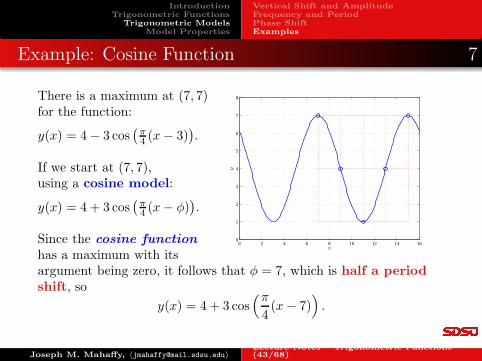
There is a maximum at (7, 7)for the function:
y(x) = 4− 3 cos(
π
4(x− 3)
)
.
If we start at (7, 7),using a cosine model:
y(x) = 4 + 3 cos(
π
4(x− φ)
)
.
Since the cosine function
has a maximum with itsargument being zero, it follows that φ = 7, which is half a periodshift, so
y(x) = 4 + 3 cos(π
4(x− 7)
)
.
Joseph M. Mahaffy, 〈[email protected]〉Lecture Notes – Trigonometric Functions —(43/68)
IntroductionTrigonometric Functions
Trigonometric ModelsModel Properties
Phase Shift of Half a PeriodEquivalent Sine and Cosine ModelsReturn to Annual Temperature VariationOther Examples
Phase Shift in Models
Phase Shift of Half a Period
A phase shift of half a period creates an equivalent sine orcosine model with the sign of the amplitude reversed
Models Matching Data
Phase shifts are important matching data in periodicmodels
The cosine model is easiest to match, since themaximum of the cosine function occurs when theargument is zero
The maximum of the sine model occurs when theargument is π
2
Joseph M. Mahaffy, 〈[email protected]〉Lecture Notes – Trigonometric Functions —(44/68)
IntroductionTrigonometric Functions
Trigonometric ModelsModel Properties
Phase Shift of Half a PeriodEquivalent Sine and Cosine ModelsReturn to Annual Temperature VariationOther Examples
Example: Cosine Model with Phase Shift 1
Example 3: Consider the model
y(x) = 4 + 6 cos(
1
2(x− π)
)
, x ∈ [0, 8π]
Skip Example
Find the vertical shift, amplitude, period, and phase shift
Sketch a graph
Determine all maxima and minima for x ∈ [0, 4π]
Find the equivalent sine model
Joseph M. Mahaffy, 〈[email protected]〉Lecture Notes – Trigonometric Functions —(45/68)
IntroductionTrigonometric Functions
Trigonometric ModelsModel Properties
Phase Shift of Half a PeriodEquivalent Sine and Cosine ModelsReturn to Annual Temperature VariationOther Examples
Example: Cosine Model with Phase Shift 2
Solution: For the model
y(x) = 4 + 6 cos(
1
2(x− π)
)
The vertical shift is A = 4
The amplitude is B = 6, so y(x) oscillates between −2 and 10
The frequency is ω = 1
2
The period, T , satisfies
T = 2π
ω= 4π
The phase shift is φ = π, which means the cosine model isshifted horizontally x = π units to the right
Since cosine has a maximum with argument zero, a maximumwill occur at x = π
Joseph M. Mahaffy, 〈[email protected]〉Lecture Notes – Trigonometric Functions —(46/68)
IntroductionTrigonometric Functions
Trigonometric ModelsModel Properties
Phase Shift of Half a PeriodEquivalent Sine and Cosine ModelsReturn to Annual Temperature VariationOther Examples
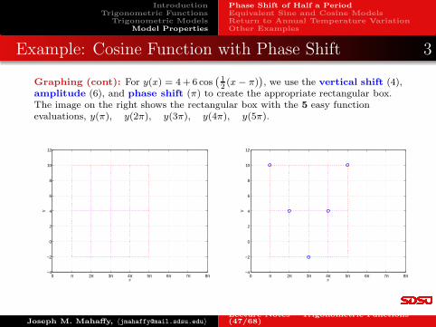
Example: Cosine Function with Phase Shift 3
Graphing (cont): For y(x) = 4+6 cos(
12(x− π)
)
, we use the vertical shift (4),amplitude (6), and phase shift (π) to create the appropriate rectangular box.The image on the right shows the rectangular box with the 5 easy functionevaluations, y(π), y(2π), y(3π), y(4π), y(5π).
0 π 2π 3π 4π 5π 6π 7π 8π−4
−2
0
2
4
6
8
10
12
x
y
0 π 2π 3π 4π 5π 6π 7π 8π−4
−2
0
2
4
6
8
10
12
x
y
Joseph M. Mahaffy, 〈[email protected]〉Lecture Notes – Trigonometric Functions —(47/68)
IntroductionTrigonometric Functions
Trigonometric ModelsModel Properties
Phase Shift of Half a PeriodEquivalent Sine and Cosine ModelsReturn to Annual Temperature VariationOther Examples
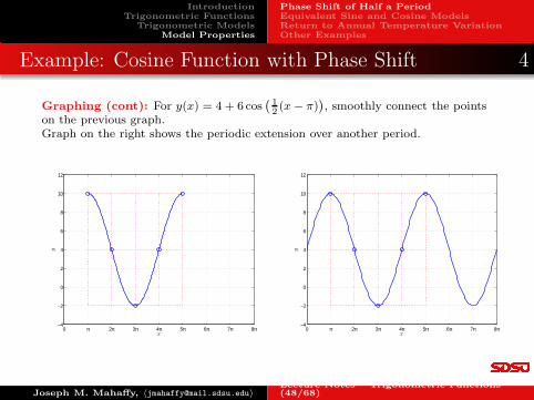
Example: Cosine Function with Phase Shift 4
Graphing (cont): For y(x) = 4 + 6 cos(
12(x− π)
)
, smoothly connect the pointson the previous graph.Graph on the right shows the periodic extension over another period.
0 π 2π 3π 4π 5π 6π 7π 8π−4
−2
0
2
4
6
8
10
12
x
y
0 π 2π 3π 4π 5π 6π 7π 8π−4
−2
0
2
4
6
8
10
12
x
y
Joseph M. Mahaffy, 〈[email protected]〉Lecture Notes – Trigonometric Functions —(48/68)
IntroductionTrigonometric Functions
Trigonometric ModelsModel Properties
Phase Shift of Half a PeriodEquivalent Sine and Cosine ModelsReturn to Annual Temperature VariationOther Examples
Example: Cosine Model with Phase Shift 5
Solution (cont): From the graph of
y(x) = 4 + 6 cos(
1
2(x− π)
)
,
there are clearly maxima at x = π and 5π, so for x ∈ [0, 4π], themaximum is (π, 10), (which agrees with the phase shift).
It is easily seen that the minima occur at x = 3π and 7π, so forx ∈ [0, 4π], the minimum is (3π,−2).
Joseph M. Mahaffy, 〈[email protected]〉Lecture Notes – Trigonometric Functions —(49/68)
IntroductionTrigonometric Functions
Trigonometric ModelsModel Properties
Phase Shift of Half a PeriodEquivalent Sine and Cosine ModelsReturn to Annual Temperature VariationOther Examples
Example: Cosine Model with Phase Shift 6
Solution (cont): The appropriate sine model has the same verticalshift, A, amplitude, B, and frequency, ω,
y(x) = 4 + 6 sin(
1
2(x− ψ)
)
We must find the appropriate phase shift, ψ
The maximum of the sine function occurs when its argument is π
2
Since the maximum occurs at x = π, it follows that
1
2(π − ψ) =
π
2or ψ = 0
The equivalent sine model is
y(x) = 4 + 6 sin(
x
2
)
= 4 + 6 cos(
1
2(x− π)
)
Joseph M. Mahaffy, 〈[email protected]〉Lecture Notes – Trigonometric Functions —(50/68)
IntroductionTrigonometric Functions
Trigonometric ModelsModel Properties
Phase Shift of Half a PeriodEquivalent Sine and Cosine ModelsReturn to Annual Temperature VariationOther Examples
Equivalent Sine and Cosine Models
Phase Shift for Equivalent Sine and Cosine Models
Suppose that the sine and cosine models are equivalent, so
sin(ω(x− φ1)) = cos(ω(x− φ2)).
The relationship between the phase shifts, φ1 and φ2 satisfies:
φ1 = φ2 −π
2ω,
which is a quarter period shift
Note: Remember that the phase shift is not uniqueIt can vary by integer multiples of the period, T = 2π
ω
Joseph M. Mahaffy, 〈[email protected]〉Lecture Notes – Trigonometric Functions —(51/68)
IntroductionTrigonometric Functions
Trigonometric ModelsModel Properties
Phase Shift of Half a PeriodEquivalent Sine and Cosine ModelsReturn to Annual Temperature VariationOther Examples
Return to Annual Temperature Model 1
Annual Temperature Model: Started section with data andgraphs of average monthly temperatures for Chicago and SanDiego
Fit data to cosine model for temperature, T ,
T (m) = A+B cos(ω(m− φ))
where m is in months
Find best model parameters, A, B, ω, and φ
The frequency, ω, is constrained by a period of 12 months
It follows that
12ω = 2π or ω = π6 = 0.5236
Joseph M. Mahaffy, 〈[email protected]〉Lecture Notes – Trigonometric Functions —(52/68)
IntroductionTrigonometric Functions
Trigonometric ModelsModel Properties
Phase Shift of Half a PeriodEquivalent Sine and Cosine ModelsReturn to Annual Temperature VariationOther Examples
Return to Annual Temperature Model 2
Annual Temperature Model:
T (m) = A+B cos(ω(m− φ))
Choose A to be the average annual temperature
Average for San Diego is A = 64.29Average for Chicago is A = 49.17
Perform least squares best fit to data for B and φ
For San Diego, obtain B = 7.29 and φ = 6.74For Chicago, obtain B = 25.51 and φ = 6.15
Joseph M. Mahaffy, 〈[email protected]〉Lecture Notes – Trigonometric Functions —(53/68)
IntroductionTrigonometric Functions
Trigonometric ModelsModel Properties
Phase Shift of Half a PeriodEquivalent Sine and Cosine ModelsReturn to Annual Temperature VariationOther Examples
Return to Annual Temperature Model 3
Annual Temperature Model for San Diego:
T (m) = 64.29 + 7.29 cos(0.5236(m − 6.74))
Annual Temperature Model for Chicago:
T (m) = 49.17 + 25.51 cos(0.5236(m − 6.15))
The amplitude of models
Temperature in San Diego only varies ±7.29◦F, giving it a“Mediterranean” climateTemperature in Chicago varies ±25.51◦F, indicating coldwinters and hot summers
Joseph M. Mahaffy, 〈[email protected]〉Lecture Notes – Trigonometric Functions —(54/68)
IntroductionTrigonometric Functions
Trigonometric ModelsModel Properties
Phase Shift of Half a PeriodEquivalent Sine and Cosine ModelsReturn to Annual Temperature VariationOther Examples
Return to Annual Temperature Model 4
Annual Temperature Model for San Diego:
T (m) = 64.29 + 7.29 cos(0.5236(m − 6.74))
Annual Temperature Model for Chicago:
T (m) = 49.17 + 25.51 cos(0.5236(m − 6.15))
The phase shift for the models
For San Diego, the phase shift of φ = 6.74, so the maximumtemperature occurs at 6.74 months (late July)For Chicago, the phase shift of φ = 6.15, so the maximumtemperature occurs at 6.15 months (early July)
Joseph M. Mahaffy, 〈[email protected]〉Lecture Notes – Trigonometric Functions —(55/68)
IntroductionTrigonometric Functions
Trigonometric ModelsModel Properties
Phase Shift of Half a PeriodEquivalent Sine and Cosine ModelsReturn to Annual Temperature VariationOther Examples
Return to Annual Temperature Model 5
Convert Cosine Model to Sine Model:
T (m) = A+B sin(ω(m− φ2))
Formula showsφ2 = φ− π
2ω
where φ is from the cosine modelFor San Diego, φ2 = 3.74For Chicago, φ2 = 3.15
Sine Model for San Diego:
T (m) = 64.29 + 7.29 sin(0.5236(m − 3.74))
Sine Model for Chicago:
T (m) = 49.17 + 25.51 sin(0.5236(m − 3.15))
Joseph M. Mahaffy, 〈[email protected]〉Lecture Notes – Trigonometric Functions —(56/68)
IntroductionTrigonometric Functions
Trigonometric ModelsModel Properties
Phase Shift of Half a PeriodEquivalent Sine and Cosine ModelsReturn to Annual Temperature VariationOther Examples
Population Model with Phase Shift 1
Population Model: Suppose population data show a 10 yearperiodic behavior with a maximum population of 26 (thousand)at t = 2 and a minimum population of 14 (thousand) at t = 7
Assume a model of the form
y(t) = A+B sin(ω(t− φ))
Skip Example
Find the constants A, B, ω, and φ with B > 0, ω > 0,andφ ∈ [0, 10)
Since φ is not unique, find values of φ with φ ∈ [−10, 0)and φ ∈ [10, 20)
Sketch a graph
Find the equivalent cosine model
Joseph M. Mahaffy, 〈[email protected]〉Lecture Notes – Trigonometric Functions —(57/68)
IntroductionTrigonometric Functions
Trigonometric ModelsModel Properties
Phase Shift of Half a PeriodEquivalent Sine and Cosine ModelsReturn to Annual Temperature VariationOther Examples
Population Model with Phase Shift 2
Solution: Compute the various parameters
The vertical shift satisfies
A =26 + 14
2= 20
The amplitude satisfies
B = 26− 20 = 6
Since the period is T = 10 years, the frequency, ω,satisfies
ω = 2π10 = π
5
Joseph M. Mahaffy, 〈[email protected]〉Lecture Notes – Trigonometric Functions —(58/68)
IntroductionTrigonometric Functions
Trigonometric ModelsModel Properties
Phase Shift of Half a PeriodEquivalent Sine and Cosine ModelsReturn to Annual Temperature VariationOther Examples
Population Model with Phase Shift 3
Solution (cont): Compute the phase shift
The maximum of 26 occurs at t = 2, so the model satisfies:
y(2) = 26 = 20 + 6 sin(
π5 (2− φ)
)
Clearlysin
(
π5 (2− φ)
)
= 1
The sine function is at its maximum when its argument isπ2 , so
π5 (2− φ) = π
2
2− φ = 52
φ = −12
Joseph M. Mahaffy, 〈[email protected]〉Lecture Notes – Trigonometric Functions —(59/68)
IntroductionTrigonometric Functions
Trigonometric ModelsModel Properties
Phase Shift of Half a PeriodEquivalent Sine and Cosine ModelsReturn to Annual Temperature VariationOther Examples
Population Model with Phase Shift 4
Solution (cont): Continuing, the phase shift was
φ = −12
This value of φ is not in the interval [0, 10)
The periodicity, T = 10, of the model is also reflected inthe phase shift, φ
φ = −12 + 10n, n an integer
φ = ...− 10.5,−0.5, 9.5, 19.5, ...
The principle phase shift is φ = 9.5
Joseph M. Mahaffy, 〈[email protected]〉Lecture Notes – Trigonometric Functions —(60/68)
IntroductionTrigonometric Functions
Trigonometric ModelsModel Properties
Phase Shift of Half a PeriodEquivalent Sine and Cosine ModelsReturn to Annual Temperature VariationOther Examples
Population Model with Phase Shift 5
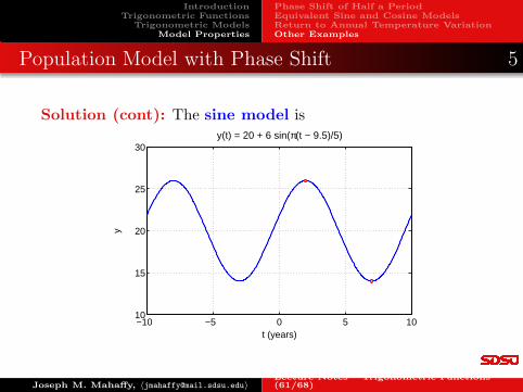
Solution (cont): The sine model is
−10 −5 0 5 1010
15
20
25
30
t (years)
y
y(t) = 20 + 6 sin(π(t − 9.5)/5)
Joseph M. Mahaffy, 〈[email protected]〉Lecture Notes – Trigonometric Functions —(61/68)
IntroductionTrigonometric Functions
Trigonometric ModelsModel Properties
Phase Shift of Half a PeriodEquivalent Sine and Cosine ModelsReturn to Annual Temperature VariationOther Examples
Population Model with Phase Shift 6
Solution (cont): The cosine model has the form
y(t) = 20 + 6 cos(
π5 (t− φ2)
)
,
The vertical shift, amplitude, and frequency match the sinemodel
The maximum of the cosine function occurs when itsargument is zero, so
π5 (2− φ2) = 0,
φ2 = 2.
The cosine model satisfies
y(t) = 20 + 6 cos(
π5 (t− 2)
)
Joseph M. Mahaffy, 〈[email protected]〉Lecture Notes – Trigonometric Functions —(62/68)
IntroductionTrigonometric Functions
Trigonometric ModelsModel Properties
Phase Shift of Half a PeriodEquivalent Sine and Cosine ModelsReturn to Annual Temperature VariationOther Examples
Body Temperature 1
Circadian Rhythms:
Humans, like many organisms, undergo circadianrhythms for many of their bodily functions
Circadian rhythms are the daily fluctuations that aredriven by the light/dark cycle of the Earth
Seems to affect the pineal gland in the head
This temperature normally varies a few tenths of a degreein each individual with distinct regularity
The body is usually at its hottest around 10 or 11 AM andat its coolest in the late evening, which helps encouragesleep
Joseph M. Mahaffy, 〈[email protected]〉Lecture Notes – Trigonometric Functions —(63/68)
IntroductionTrigonometric Functions
Trigonometric ModelsModel Properties
Phase Shift of Half a PeriodEquivalent Sine and Cosine ModelsReturn to Annual Temperature VariationOther Examples
Body Temperature 2
Body Temperature Model: Suppose that measurements ona particular individual show
A high body temperature of 37.1◦C at 10 am
A low body temperature of 36.7◦C at 10 pm
Assume body temperature T and a model of the form
T (t) = A+B cos(ω(t− φ))
Find the constants A, B, ω, and φ with B > 0, ω > 0,andφ ∈ [0, 24)
Graph the model
Find the equivalent sine model
Joseph M. Mahaffy, 〈[email protected]〉Lecture Notes – Trigonometric Functions —(64/68)
IntroductionTrigonometric Functions
Trigonometric ModelsModel Properties
Phase Shift of Half a PeriodEquivalent Sine and Cosine ModelsReturn to Annual Temperature VariationOther Examples
Body Temperature 3
Solution: Compute the various parameters
The vertical shift satisfies
A =37.1 + 36.7
2= 36.9
The amplitude satisfies
B = 37.1 − 36.9 = 0.2
Since the period is P = 24 hours, the frequency, ω,satisfies
ω =2π
24=
π
12
Joseph M. Mahaffy, 〈[email protected]〉Lecture Notes – Trigonometric Functions —(65/68)
IntroductionTrigonometric Functions
Trigonometric ModelsModel Properties
Phase Shift of Half a PeriodEquivalent Sine and Cosine ModelsReturn to Annual Temperature VariationOther Examples
Body Temperature 4
Solution (cont): Compute the phase shift
The maximum of 37.1◦C occur at t = 10 am
The cosine function has its maximum when its argument is0 (or any integer multiple of 2π)
The appropriate phase shift solves
ω(10− φ) = 0 or φ = 10
Joseph M. Mahaffy, 〈[email protected]〉Lecture Notes – Trigonometric Functions —(66/68)
IntroductionTrigonometric Functions
Trigonometric ModelsModel Properties
Phase Shift of Half a PeriodEquivalent Sine and Cosine ModelsReturn to Annual Temperature VariationOther Examples
Body Temperature 5
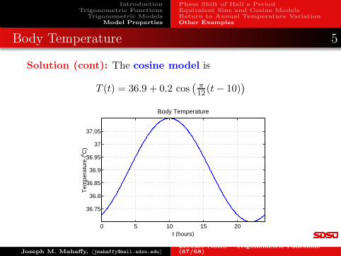
Solution (cont): The cosine model is
T (t) = 36.9 + 0.2 cos(
π12 (t− 10)
)
0 5 10 15 20
36.75
36.8
36.85
36.9
36.95
37
37.05
t (hours)
Tem
pera
ture
(o C)
Body Temperature
Joseph M. Mahaffy, 〈[email protected]〉Lecture Notes – Trigonometric Functions —(67/68)
IntroductionTrigonometric Functions
Trigonometric ModelsModel Properties
Phase Shift of Half a PeriodEquivalent Sine and Cosine ModelsReturn to Annual Temperature VariationOther Examples
Body Temperature 6
Solution (cont): The sine model for body temperature is
T (t) = 36.9 + 0.2 sin(
π12(t− φ2)
)
The vertical shift, amplitude, and frequency match thecosine model
From our formula above
φ2 = 10−π
2ω= 10− 6 = 4
The sine model satisfies
T (t) = 36.9 + 0.2 sin(
π12(t− 4)
)
Joseph M. Mahaffy, 〈[email protected]〉Lecture Notes – Trigonometric Functions —(68/68)