lecture notes for ecen 671
TRANSCRIPT
Lecture Notes For ECEN 671
Wynn C. Stirling
Contents
1 Lecture 1 6
1.1 Metric Spaces and Topological Spaces . . . . . . . . . . . . . . . . . . . . . . 6
1.2 Vector Spaces . . . . . . . . . . . . . . . . . . . . . . . . . . . . . . . . . . . 10
2 Lecture 2 15
2.1 Norms and Normed Vector Spaces . . . . . . . . . . . . . . . . . . . . . . . . 15
2.2 Inner Product Spaces . . . . . . . . . . . . . . . . . . . . . . . . . . . . . . . 16
2.3 The Cauchy-Schwarz Inequality . . . . . . . . . . . . . . . . . . . . . . . . . 18
3 Lecture 3 21
3.1 Orthogonality . . . . . . . . . . . . . . . . . . . . . . . . . . . . . . . . . . . 21
3.2 Hilbert and Banach Spaces . . . . . . . . . . . . . . . . . . . . . . . . . . . . 22
3.3 Orthogonal Subspaces . . . . . . . . . . . . . . . . . . . . . . . . . . . . . . 24
3.4 Linear Transformations: Range and Null Space . . . . . . . . . . . . . . . . 24
4 Lecture 4 30
4.1 Inner Sum and Direct Sum Spaces . . . . . . . . . . . . . . . . . . . . . . . . 30
4.2 Projections . . . . . . . . . . . . . . . . . . . . . . . . . . . . . . . . . . . . 33
4.3 Gram-Schmidt Orthogonalization . . . . . . . . . . . . . . . . . . . . . . . . 41
1
5 Lecture 5 43
5.1 Approximations in Hilbert Space . . . . . . . . . . . . . . . . . . . . . . . . 43
6 Lecture 6 51
6.1 Error Minimization via Gradients . . . . . . . . . . . . . . . . . . . . . . . . 51
6.2 Linear Least Squares Approximation . . . . . . . . . . . . . . . . . . . . . . 52
6.3 Approximation by Continuous Polynomials . . . . . . . . . . . . . . . . . . . 55
7 Lecture 7 58
7.1 Linear Regression . . . . . . . . . . . . . . . . . . . . . . . . . . . . . . . . . 58
7.2 Minimum Mean-Square Estimation . . . . . . . . . . . . . . . . . . . . . . . 62
8 Lecture 8 68
8.1 Minimum-Norm Problems . . . . . . . . . . . . . . . . . . . . . . . . . . . . 68
9 Lecture 9 77
9.1 Approximation of Periodic Functions . . . . . . . . . . . . . . . . . . . . . . 77
9.2 Generalized Fourier Series . . . . . . . . . . . . . . . . . . . . . . . . . . . . 78
9.3 Matched Filtering . . . . . . . . . . . . . . . . . . . . . . . . . . . . . . . . . 83
10 Lecture 10 87
10.1 Operator Norms . . . . . . . . . . . . . . . . . . . . . . . . . . . . . . . . . . 87
11 Lecture 11 96
11.1 Linear Functionals . . . . . . . . . . . . . . . . . . . . . . . . . . . . . . . . 96
2
11.2 Four Fundamental Subspaces . . . . . . . . . . . . . . . . . . . . . . . . . . 103
12 Lecture 12 108
12.1 The Fredholm Alternative Theorem . . . . . . . . . . . . . . . . . . . . . . . 108
12.2 Dual Optimization . . . . . . . . . . . . . . . . . . . . . . . . . . . . . . . . 109
13 Lecture 13 117
13.1 Matrix Norms . . . . . . . . . . . . . . . . . . . . . . . . . . . . . . . . . . . 117
13.2 Matrix Conditioning . . . . . . . . . . . . . . . . . . . . . . . . . . . . . . . 120
13.2.1 The Matrix Inversion Lemma . . . . . . . . . . . . . . . . . . . . . . 123
14 Lecture 14 125
14.1 LU Factorization . . . . . . . . . . . . . . . . . . . . . . . . . . . . . . . . . 125
14.2 Cholesky Decomposition . . . . . . . . . . . . . . . . . . . . . . . . . . . . . 136
15 Lecture 15 140
15.1 QR Factorization . . . . . . . . . . . . . . . . . . . . . . . . . . . . . . . . . 140
16 Lecture 16 148
16.1 A Brief Review of Eigenstu! . . . . . . . . . . . . . . . . . . . . . . . . . . . 148
16.2 Left and Right Eigenvectors . . . . . . . . . . . . . . . . . . . . . . . . . . . 153
16.3 Multiple Eigenvalues . . . . . . . . . . . . . . . . . . . . . . . . . . . . . . . 156
16.4 Diagonalization of a Dynamic System . . . . . . . . . . . . . . . . . . . . . . 158
17 Lecture 17 161
3
17.1 Diagonalization of Self-Adjoint Matrices . . . . . . . . . . . . . . . . . . . . 161
17.2 Some Miscellaneous Eigenfacts . . . . . . . . . . . . . . . . . . . . . . . . . . 165
18 Lecture 18 169
18.1 Quadratic Forms . . . . . . . . . . . . . . . . . . . . . . . . . . . . . . . . . 169
18.2 Gershgorin Circle Theorem . . . . . . . . . . . . . . . . . . . . . . . . . . . . 174
19 Lecture 19 178
19.1 Discrete-time Signals in Noise . . . . . . . . . . . . . . . . . . . . . . . . . . 178
19.2 Signal Subspace Techniques . . . . . . . . . . . . . . . . . . . . . . . . . . . 182
20 Lecture 20 186
20.1 Matrix Polynomials . . . . . . . . . . . . . . . . . . . . . . . . . . . . . . . . 186
20.2 Eigenvalues and Eigenvectors in Control Theory . . . . . . . . . . . . . . . . 192
21 Lecture 21 201
21.1 Matrix Square Roots . . . . . . . . . . . . . . . . . . . . . . . . . . . . . . . 201
21.2 Polar and Singular-Value Decompositions . . . . . . . . . . . . . . . . . . . . 203
22 Lecture 22 211
22.0.1 Generalized Inverses . . . . . . . . . . . . . . . . . . . . . . . . . . . 211
22.1 The SVD and Least Squares . . . . . . . . . . . . . . . . . . . . . . . . . . . 220
23 Lecture 23 224
23.1 SVD’s and Matrix Norms . . . . . . . . . . . . . . . . . . . . . . . . . . . . 224
4
23.2 Approximating a Matrix by one of Lower Rank . . . . . . . . . . . . . . . . 224
23.3 System Identification . . . . . . . . . . . . . . . . . . . . . . . . . . . . . . . 227
23.4 Total Least-Squares . . . . . . . . . . . . . . . . . . . . . . . . . . . . . . . . 231
24 Lecture 24 237
24.1 Toeplitz Matrices . . . . . . . . . . . . . . . . . . . . . . . . . . . . . . . . . 237
24.2 Vandermonde Matrices . . . . . . . . . . . . . . . . . . . . . . . . . . . . . . 239
24.3 Circulant Matrices . . . . . . . . . . . . . . . . . . . . . . . . . . . . . . . . 240
24.4 Companion Matrices . . . . . . . . . . . . . . . . . . . . . . . . . . . . . . . 241
24.5 Kronecker Products . . . . . . . . . . . . . . . . . . . . . . . . . . . . . . . . 243
25 Lecture 25 250
25.1 Solving Nonlinear Equations . . . . . . . . . . . . . . . . . . . . . . . . . . . 250
25.2 Contractive Mappings and Fixed Points . . . . . . . . . . . . . . . . . . . . . 251
25.3 Newton’s Method . . . . . . . . . . . . . . . . . . . . . . . . . . . . . . . . . 257
25.4 Minimizing Nonlinear Scalar Functions of Vectors . . . . . . . . . . . . . . . 259
26 Lecture 26 262
26.1 Static Optimization with Equality Constraints . . . . . . . . . . . . . . . . . 262
26.2 Closed-Form Solutions . . . . . . . . . . . . . . . . . . . . . . . . . . . . . . 269
26.3 Numerical Methods . . . . . . . . . . . . . . . . . . . . . . . . . . . . . . . . 271
5
1 Lecture 1
1.1 Metric Spaces and Topological Spaces
Definition 1 Let X be an arbitrary set. A metric d : X ! X " R satisfies
• d(x, y) = d(y, x) (Symmetry)
• d(x, y) # 0 (Non-negativity)
• d(x, y) = 0 i! x = y (Non-degeneracy)
• d(x, z) $ d(x, y) + d(y, z) %x, y (Triangle inequality)
!
Some examples
1. X = R, d(x, y) = |x & y| (!1)
2. X = Rn, d(x, y) = (!n
i=1(xi & yi)2)12 (!2)
3. X = Rn, d(x, y) = (!n
i=1(xi & yi)p)1p (!p)
4. X = Rn, d(x, y) = maxi |xi & yi| (!!)
Definition 2 The 2-tuple (X, d) is called a metric space. !
More examples: Let X be the set of real-valued functions on the interval [a, b].
dp(x, y) =
"# b
a
|x(t) & y(t)|pdt
$ 1p
(Lp)
d!(x, y) = sup{|x(t) & y(t)|: a $ t $ b} (L!).
6
Definition 3 Let X be an arbitrary set. A collection " of subsets of X is said to be a
topology in X if
• ' ( " and X ( " .
• Finite intersections of elements of " are in "
• Arbitrary unions (finite, countable, or uncountable) are in "
If " is a topology in X, then X is called a topological space, and the members of " are
called the open sets in X.
If X and Y are topological spaces and if f : X " Y , then f is continuous provided that
the inverse image of open sets in Y are open in X, that is, V ( "Y implies
f"1(V ) = {x ( X: f(x) ( V } ( "X .
!
Now let’s look at topologies defined by metrics.
Definition 4 Let X be a metric space. A ball centered at x0 of radius # is the set of points
B(x0, #) = {x ( X: d(x0, x) < #}.
B(x0, #) is called a neighborhood of x0.
x0 is an interior point of a set S if )# > 0: B(x0, #) ( S.
S is open if every point of S is an interior point of S.
S is closed of Sc is open.
x is a boundary point of S, denoted bdy (S), if B(x, #)*S += ' but B(x, #) +, S %# > 0.
7
The closure of S, denoted closure (S), is closure (S) = S - bdy (S).
x is a cluster point in X if every neighborhood of x contains infinitely many points of
X.
The support of a function f :A " B is the closure of the set of points where f(x) does
not vanish.
!
Some observations:
1. The union of open sets is open.
2. The intersection of closed sets is closed.
3. The intersection of open sets need not be open.
4. The union of closed sets need not be closed
Definition 5 Let {x1, x2, x3, . . .} , also denoted {xn} be a sequence in the set X. {xn}
converges to x# if, for every # > 0, there is an integer n0 such that, for n > n0, d(x#, xn) < #.
Then x# is the limit of xn, and {xn} is said to be a convergent sequence.
!
Observations:
• The closure of a set A is the set of all limits of converging sequences of points in A
• A is closed i! it contains the limit of all convergent sequences whose points lie in A.
8
Definition 6 x# is said to be a limit point of a sequence {xn} if xn returns infinitely often
to a neighborhood of x#.
Example:
bn = 1 + (&1)n
has two limit points, 0 and 2.
The largest limit point is the limsup, lim supn$! xn , and the smallest limit point is the
liminf, lim infn$! xn.
!
Definition 7 Monotonic sequences:
• Increasing x1 $ x2 $ x3 . . .
• Decreasing x1 # x2 # x3 . . .
All bounded monotonic sequences are convergent. !
Definition 8 A sequence {xn} is a Cauchy sequence if, for every $ > 0, there is an N > 0
such that d(xn, xm) < $ %m, n > N .
!
All convergent sequences in X are Cauchy, but not all Cauchy sequences are convergent
in X (i.e., the limit may not be a point in X).
Definition 9 A metric space (X, d) is complete if every Cauchy sequence converges to a
limit in X. !
9
1.2 Vector Spaces
Definition 10 A set K is called field if two operations, called addition (+) and multi-
plication (·) are defined such that
1. For any two elements a, b ( K, the sum a + b ( K
(a) Addition is commutative: a + b = b + a.
(b) Addition is associative: (a + b) + c = a + (b + c).
(c) There exists a zero element, denoted 0, such that a + 0 = a %a ( K.
2. For any two elements a, b ( K, the product a · b ( K.
(a) Multiplication is commutative: a · b = b · a.
(b) Multiplication is associative: (a · b) · c = a · (b · c).
(c) There exists a unity element, denoted 1, such that a · 1 = a.
3. The distributive law holds: a · (b + c) = a · b + a · c.
When no possibility for ambiguity exists, we will usually omit the multiplication operator
and write a · b as ab, etc. !
Examples of fields:
• The real numbers
• The complex numbers
• The rational numbers
10
Definition 11 Suppose we are given a set S and a field K (called the field of scalars such
that
• There exists a binary operation called vector addition of elements of S such that,
%x,y ( S, x + y ( S.
• Given an arbitrary element a ( K and an arbitrary x ( S, the scalar multiple of x by
%, denoted %x, is in S, that is, %% ( K and %x ( S, %x ( S.
The set S is called a vector space over K (or a linear space over K) if
1. Vector addition is commutative: x + y = y + x.
2. Vector addition is associative: (x + y) + z = x + (y + z).
3. There exists a zero vector, denoted 0, such that x + 0 = x.
4. For every x ( S there exists an additive inverse, y = &x ( S, such that x + y = 0.
5. The distributive law holds: for every scalar % ( K and every x,y ( S, %(x + y) =
%x + %y.
6. The scalar associative law holds: for all scalars %, & ( K, %(&x) = &(%x).
7. The scalar distributive law holds: for all scalars %, & ( K, (% + &)x) = %x + &x.
8. There is a unity element of K, denoted 1, such that, %x ( S, 1x = x.
The elements of K are called scalars, and the elements of S are called vectors.
!
Examples of vector spaces
11
• Let S = Rn and K = R. Then vectors are n-tuples of real numbers.
x =
%
&&&'
x1
x2...
xn
(
)))*
, %x =
%
&&&'
%x1
%x2...
%xn
(
)))*
• Sequences in K. All infinite sequences in a field K form a vector space over K.
• Real-valued functions over the interval [a,b], with (f + g)(x) = f(x) + g(x) and
(%f)(x) = %f(x).
• Polynomials with real coe"cients.
Definition 12 If S is a vector space and V , S is a subset such that V itself is a vector
space, then V is said to be a subspace of S. !
Example: R2 is a subspace of R3.
Definition 13 A vector x ( S is said to be a linear combination of the vectors p1, . . . ,pm
if there exist scalars c1, . . . cm such that
x = c1p1 + · · · cmpm.
The vectors p1, . . .pm is said to be linearly independent if the only combination of scalars
satisfying the equation
0 = c1p1 + · · · cmpm
is the set c1 = · · · = cm = 0.
If vectors are not linearly independent, they they are linearly dependent, in which case,
we may express any of the pi’s as a linear combination of the other vectors in the set.
12
The set of all linear combinations of a set of vectors p1, . . . ,pm is called the span of the
set of vectors.
For T an arbitrary set of vectors, the vectors V that can be expressed as linear combi-
nations of elements of T are denoted V = span T .
If T is a set of vectors in S and V is a subspace of S, and if every element of V can be
expressed as a linear combination of vectors in T , then T is said to be a spanning set of V .
!
Theorem 1 Let S be a vector space, and let T be a nonempty subset of S. The set T is
linearly independent if and only if for each nonzero x ( span (T ), there is exactly one finite
subset of T , denoted {p1, . . .pm} and a unique set of scalars {c1, . . . cm}, such that
x =m+
i=1
cipi.
Definition 14 A linearly independent spanning set of a vector space S is called a Hamel
basis for S. !
Theorem 2 All Hamel bases for a vector space have the same cardinality.
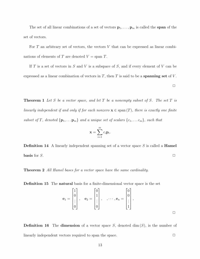
Definition 15 The natural basis for a finite-dimensional vector space is the set
e1 =
%
&&&'
10...0
(
)))*
, e2 =
%
&&&'
01...0
(
)))*
, , · · · , en =
%
&&&'
00...1
(
)))*
,
!
Definition 16 The dimension of a vector space S, denoted dim (S), is the number of
linearly independent vectors required to span the space. !
13
Example: Finite-dimensional vector spaces. Suppose dim (S) = n, and p1, . . . ,pn form
a Hamel basis. Let us arrange these vectors in a matrix as
A =,
p1 p2 · · · pn
-
For any vector c = [c1, · · · , cn]T , we may form a new vector x = Ac as a linear combination
of basis vectors.
14
2 Lecture 2
2.1 Norms and Normed Vector Spaces
Recall that a metric is a distance measure between two elements of a set. A norm is a very
similar concept: it is a measure of length of a single vector. In fact, if a metric space contains
a zero element, we may define the norm of an element as the metric between the element
and the zero element.
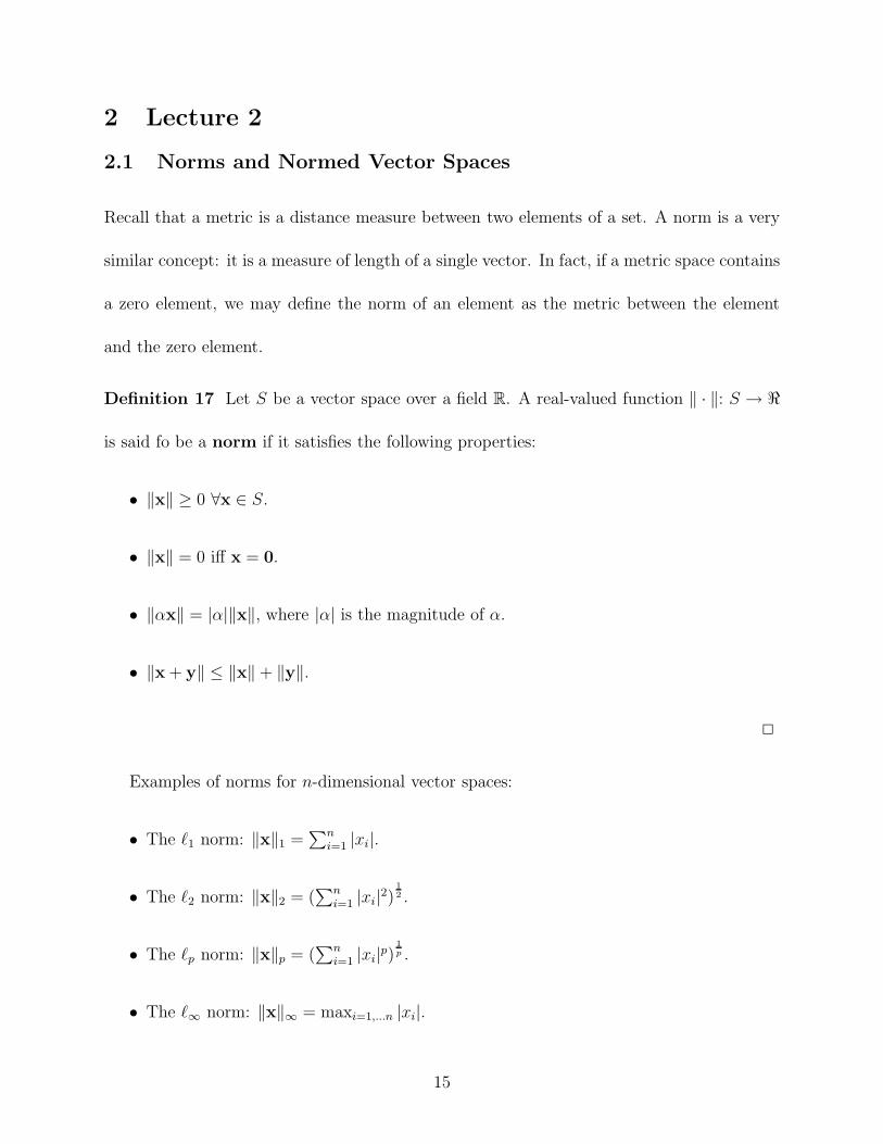
Definition 17 Let S be a vector space over a field R. A real-valued function . · .: S " /
is said fo be a norm if it satisfies the following properties:
• .x. # 0 %x ( S.
• .x. = 0 i! x = 0.
• .%x. = |%|.x., where |%| is the magnitude of %.
• .x + y. $ .x. + .y..
!
Examples of norms for n-dimensional vector spaces:
• The !1 norm: .x.1 =!n
i=1 |xi|.
• The !2 norm: .x.2 = (!n
i=1 |xi|2)12 .
• The !p norm: .x.p = (!n
i=1 |xi|p)1p .
• The !! norm: .x.! = maxi=1,...n |xi|.
15

Examples of norms of functions over the interval [a, b].
• The L1 norm: .x(t).1 =. b
a|x(t)|dt.
• The L2 norm: .x(t).2 =/. b
a|x(t)|2dt
0 12.
• The Lp norm: .x(t).p =/. b
a|x(t)|pdt
0 1p
.
• The L! norm: .x(t).! = supt%[a,b] |x(t)|.
Definition 18 A normed vector space is the pair (S, . · .).
A vector x is said to be normalized if .x. = 1. Such a vector is also termed a unit
vector. Any non-zero vector can be normlized by multipying it by the scalar 1&x& :
y =1
.x.x.
!
Theorem 3 All norms are equivalent in the sense that if . · . and . · .' are two norms, then
for any vector sequence {xn}, .xn. " 0 i! .xn.' " 0.
2.2 Inner Product Spaces
Thus far, we have progressed from topological spaces (i.e., defining the notion of “openness”)
to to metric spaces (i.e,, defining the notion of “distance”) to normed vector spaces (i.e.,
defining the notion of “length”). We now introduce even more struture, which will give us a
notion of “direction.”
Definition 19 Let S be a vector space (not necessarily normed) over a scalar field R. An
inner product is a function 0·, ·1: S ! S " R such that
16

• 0x,y1 = 0y,x1 (The overbar denotes complex conjugation)
• For any scalar %, 0%x,y1 = %0x,y1
• 0x + y, z1 = 0x, z1 + 0y, z1.
• 0x,x1 # 0 and 0x,x1 = 0 i! x = 0.
A vector space equipped with an inner product is called an inner product space.
!
Examples for finite dimensional vector spaces
• Let S = Rn and 0x,y1 =!n
i=1 xiyi = xTy (The dot product—the superscript T
denotes matrix transpose).
• Let S = Cn and 0x,y1 =!n
i=1 xiyi = yHx. (The superscript H denotes the Hermitian
transpose, that is, conjugate and matrix transpose).
Examples for function spaces
• Let S = the set of real-valued functions on [a,b]: 0x,y1 =. b
ax(t)y(t)dt.
• Let S = the set of complex-valued functions on [a,b]: 0x,y1 =. b
ax(t)y(t)dt.
Once we have an inner product defined on a vector space, it is straightforward to define
a norm, called the induced norm, from the inner product, as
.x. = 0x,x1 12 .
17
2.3 The Cauchy-Schwarz Inequality
The Cauchy-Schwarz inequality is one of the more important results from analysis, hence it
will serve us well to prove this theorem (the proof provided here is slightly di!erent from the
one in the text)
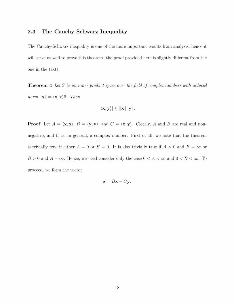
Theorem 4 Let S be an inner product space over the field of complex numbers with induced
norm .x. = 0x,x1 12 . Then
|0x,y1| $ .x..y..
Proof Let A = 0x,x1, B = 0y,y1, and C = 0x,y1. Clearly, A and B are real and non-
negative, and C is, in general, a complex number. First of all, we note that the theorem
is trivially true if either A = 0 or B = 0. It is also trivially true if A > 0 and B = 2 or
B > 0 and A = 2. Hence, we need consider only the case 0 < A < 2 and 0 < B < 2. To
proceed, we form the vector
z = Bx & Cy.
18
Then, using the defining properties of the inner product,
0 $ 0z, z1 = 0Bx & Cy, Bx & Cy1
= 0Bx, Bx1 & 0Bx, Cy1 & 0Cy, Bx1 + 0Cy, Cy1
= B0x, Bx1 & B0x, Cy1 & C0y, Bx1 + C0y, Cy1
= B0Bx,x1 & B0Cy,x1 & C0Bx,y1 + C0Cy,y1
= B20x,x1 & BC0y,x1 & CB0x,y1 + CC0y,y1
= B2A & BCC & BCC + BCC
= B2A & B|C|2
= B(AB & |C|2).
Since 0 < B < 2, the only way the right hand side of this expression can be non-negative
is if
AB & |C|2 # 0,
or
|0x,y1|2 $ .x.2.y.2.
Taking square roots of both sides yieids the final result. !
Examples of the Cauchy-Schwarz inequality
• Let S = Rn. Then
|(xTy)| $ .x..y.
or, equivalently,
(xTy)2 $1
xTx221
yTy22
.
19
• Let S be the space of real-valued functions over the interval [a, b]. Then
3# b
a
f(t)g(t)dt
$2
$# b
a
f 2(t)dt
# b
a
g2(t)dt.
As a contextual note, the Cauchy-Schwarz inequality is a special case of the more general
Holder’s inequality:
# b
a
f(t)g(t)dt $3# b
a
f p(t)dt
$ 1p3# b
a
gq(t)dt
$ 1q
,
for all p and q such that 1 < p < 2 and q is the so-called conjugate exponent of p, that
is, p and q satisfy the relation
1
p+
1
q= 1.
Then the Cauchy-Schwarz case corresponds to p = q = 2.
We may also verify that the induced norm obeys the triangle inequality; namely, consid-
ering the real case only,
.x + y.2 = 0x + y,x + y1
= 0x,x1 + 20x,y1 + 0y,y1
$ 0x,x1 + 2.x..y. + 0y,y1
=1
.x. + .y.22
.
20
3 Lecture 3
3.1 Orthogonality
The inner product can be used to define the directional orientation of vectors. Recall from
elementary vector analysis that the dot product satisfies the relationship for R2 and R3
(using the induced norm)
0x,y1 = .x..y. cos ',
where ' is the angle between the two vectors (this is a special case of the Cauchy-Schwarz
inequality). Geometrically, we see that when ' = n( for any positive or negative integer n,
then | cos '| = 1, and the Cauchy-Schwarz inequality becomes an equality. This means that
the vectors x and y are co-linear, that is, there exists some scalar % such that x = %y.
On the other hand, if ' is an odd multiple of !2 , then cos ' = 0, and the dot product is
zero. In this situation, we say that x and y are orthogonal, meaning that they are oriented
at right angles to each other.
The notions of co-linearity and orthogonality also apply to the general case.
Definition 20 Let S be an arbitrary inner product space. Two non-zero vectors x and y
are said to be co-linear if there exists a scalar % such that x = %y.
The vectors are said to be orthogonal if the inner product is zero, i.e., 0x,y1 = 0.
Orthogonality is such an important property that we introduce a special symbol. If
0x,y1 = 0, then we write x 3 y. Obviously, z 3 0 for every vector z.
A set of vectors {p1,p2, . . .pn} is said to be an orthonormal set if they are pairwise
21
orthogonal and each have unity length. We denote this structure by
0pi,pj1 = #ij ,
where #ij is the Kronecker delta function
#ij =
4
1 i = j0 i += j
!
The Pythagorean theorem is a manifestation of orthogonality. It is easy to see that, if
x 3 y, then
.x + y. = .x. + .y..
The concept of an inner product can easily be generalized to form weighted inner
products of the form
0x,y1W = xHWy,
where W is a Hermitian matrix. If W is also positive definite, then this weighted inner
product also induces a norm, otherwise, not.
In an inner product space of functions, we may also define weighted inner products of
the form
0f, g1w =
# b
a
w(t)f(t)g(t)dt.
3.2 Hilbert and Banach Spaces
Recall that a vector space is complete if every Cauchy sequence converges to a point in the
space.
22
Definition 21 A complete normed vector space is called a Banach space. If the norm is
induced from an inner product, then the space is a said to be a Hilbert space.
!
Examples of Banach Spaces
1. The space of continuous function on [a, b] with the sup norm is a Banach space.
2. The space of continuous functions on [a, b] with the Lp norm, p < 2, is not a Banach
space, since it is not complete.
3. The sequence space lp is a Banach space; for p = 2, it is a Hilbert space.
4. The space Lp[a, b] is a Banach space, it is is a Hilbert space when p = 2.
Definition 22 The Cartesian product of two Hilbert spaces H1 and H2 is the vector
space of all pairs (x1,x2), with x1 ( H1 and x2 ( H2, under the operations
(x1,x2) + (y1,y2) = (x1 + y1,x2 + y2)
%(x1,x2) = (%x1, %x2),
and endowed with the inner product
0(x1,x2), (y1,y2)1 = 0x1,y11 + 0x2,y21.
The Cartesian product space will be denoted H1 ! H2. This definition can clearly be
extended to a finite number of Hilbert spaces, Hi, i = 1, . . . , n. When the Hilbert
spaces are the same we sometimes use the notation Hn = H1 ! H2 ! . . . ! Hn. !
23

3.3 Orthogonal Subspaces
Definition 23 Let V and W be subspaces of a vector space S. V and W are said to
be orthogonal subspaces if every vector v ( V is orthogonal to every vector w ( W .
For any subset V , S, the space of all vectors orthogonal to V is called the orthogonal
complement of V , denoted V (. !
Theorem 5 Let V and W be subsets of an inner product space S (not necessarily
complete). Then:
(a) V ( is a closed subspace of S.
(b) V , V ((.
(c) If V , W , then W( , V (.
(d) V ((( = V (.
(e) If x ( V * V (, then x = 0.
(f) {0}( = S and S( = {0}.
3.4 Linear Transformations: Range and Null Space
Definition 24 A transformation, or operator, L: X " Y , is a mapping from
one vector space to another vector space. A transformation is linear if superposition
applies; namely, it is additive and homogeneous:
• L(%x) = %L(x) for all scalars % and all vectors x ( X.
24
• L(x1 + x2) = L(x1) + L(x2).
Notation: We will often omit the parentheses when dealing with linear operators, and
write Lx for L(x).
A linear operator from an arbitrary vector space to the complex scalar scalar field
(which is also a vector space with the vector addition defined as scalar addition) is
called a linear functional.
!
Examples:
(a) Convolution Lx(t) =.!"! h(")x(t & ")d" .
(b) General integral operators Lx(t) =. b
ak(t, ")x(")d" .
(c) Fourier Transforms Fx(t) =.!"! x(t)e"j"tdt.
(d) Matrix operators from Rn to Rm
Definition 25 The range space of an operator L: X " Y is the set of all vectors in
Y that can be reached from X under L:
R(L) = {y = Lx: x ( X}
The nullspace of L is the set of all values x ( X that map to the zero vector in Y :
N (L) = {x ( X: Lx = 0}.
The nullspace is also called the kernel of the operator. !
25
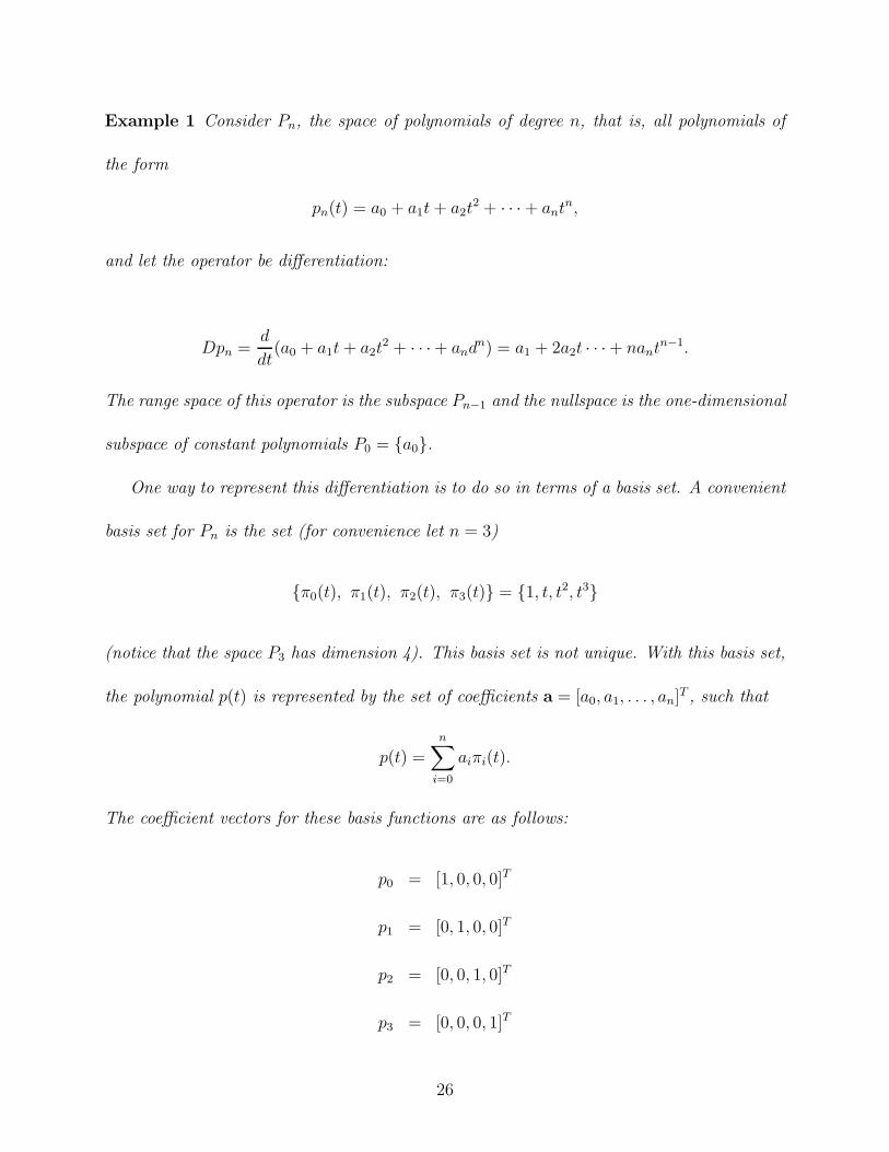
Example 1 Consider Pn, the space of polynomials of degree n, that is, all polynomials of
the form
pn(t) = a0 + a1t + a2t2 + · · · + antn,
and let the operator be di!erentiation:
Dpn =d
dt(a0 + a1t + a2t
2 + · · ·+ andn) = a1 + 2a2t · · ·+ nantn"1.
The range space of this operator is the subspace Pn"1 and the nullspace is the one-dimensional
subspace of constant polynomials P0 = {a0}.
One way to represent this di!erentiation is to do so in terms of a basis set. A convenient
basis set for Pn is the set (for convenience let n = 3)
{(0(t), (1(t), (2(t), (3(t)} = {1, t, t2, t3}
(notice that the space P3 has dimension 4). This basis set is not unique. With this basis set,
the polynomial p(t) is represented by the set of coe"cients a = [a0, a1, . . . , an]T , such that
p(t) =n+
i=0
ai(i(t).
The coe"cient vectors for these basis functions are as follows:
p0 = [1, 0, 0, 0]T
p1 = [0, 1, 0, 0]T
p2 = [0, 0, 1, 0]T
p3 = [0, 0, 0, 1]T
26
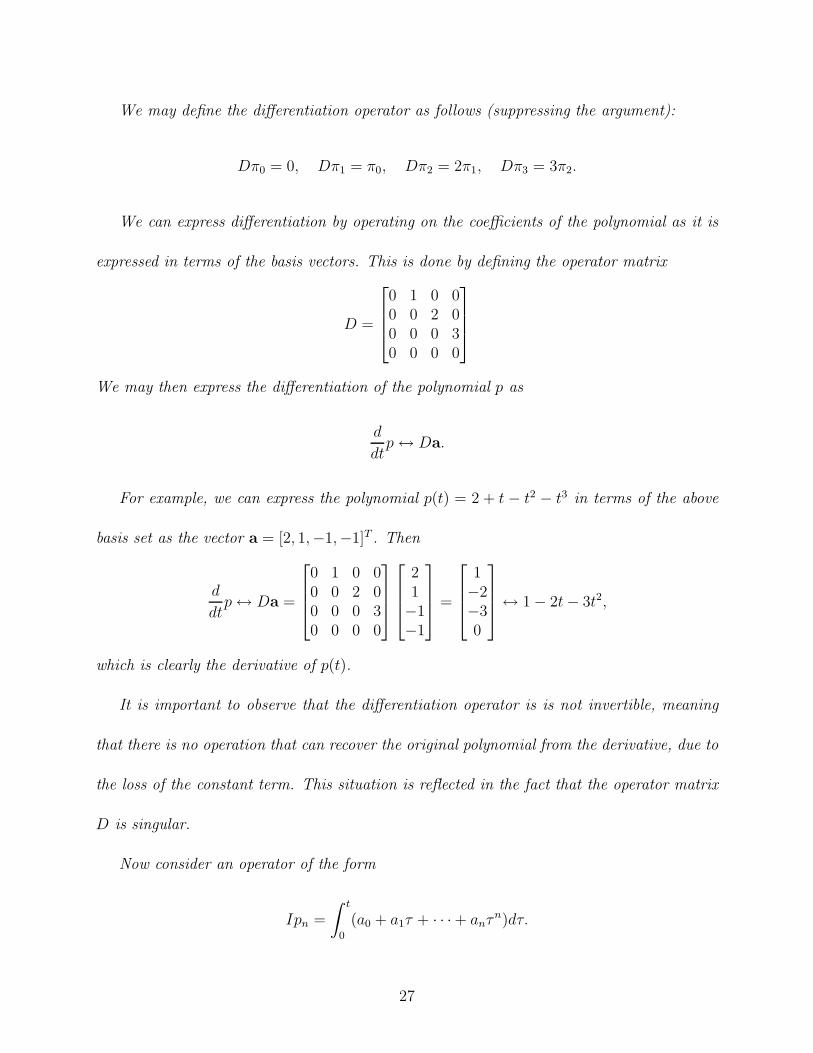
We may define the di!erentiation operator as follows (suppressing the argument):
D(0 = 0, D(1 = (0, D(2 = 2(1, D(3 = 3(2.
We can express di!erentiation by operating on the coe"cients of the polynomial as it is
expressed in terms of the basis vectors. This is done by defining the operator matrix
D =
%
&&'
0 1 0 00 0 2 00 0 0 30 0 0 0
(
))*
We may then express the di!erentiation of the polynomial p as
d
dtp 4 Da.
For example, we can express the polynomial p(t) = 2 + t & t2 & t3 in terms of the above
basis set as the vector a = [2, 1,&1,&1]T . Then
d
dtp 4 Da =
%
&&'
0 1 0 00 0 2 00 0 0 30 0 0 0
(
))*
%
&&'
21&1&1
(
))*
=
%
&&'
1&2&30
(
))*4 1 & 2t & 3t2,
which is clearly the derivative of p(t).
It is important to observe that the di!erentiation operator is is not invertible, meaning
that there is no operation that can recover the original polynomial from the derivative, due to
the loss of the constant term. This situation is reflected in the fact that the operator matrix
D is singular.
Now consider an operator of the form
Ipn =
# t
0
(a0 + a1" + · · ·+ an"n)d".
27
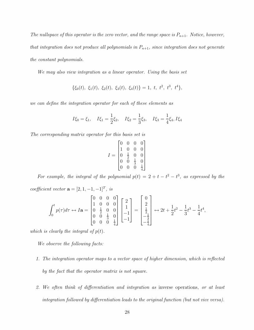
The nullspace of this operator is the zero vector, and the range space is Pn+1. Notice, however,
that integration does not produce all polynomials in Pn+1, since integration does not generate
the constant polynomials.
We may also view integration as a linear operator. Using the basis set
{)0(t), )1(t), )2(t), )3(t), )4(t)} = 1, t, t2, t3, t4},
we can define the integration operator for each of these elements as
I)0 = )1, I)1 =1
2)2, I)2 =
1
3)3, I)3 =
1
4)4, I)4
The corresponding matrix operator for this basis set is
I =
%
&&&&'
0 0 0 01 0 0 00 1
2 0 00 0 1
3 00 0 0 1
4
(
))))*
For example, the integral of the polynomial p(t) = 2 + t & t2 & t3, as expressed by the
coe"cient vector a = [2, 1,&1,&1]T , is
# t
0
p(")d" 4 Ia =
%
&&&&'
0 0 0 01 0 0 00 1
2 0 00 0 1
3 00 0 0 1
4
(
))))*
%
&&'
21&1&1
(
))*
=
%
&&&&'
0212&1
3&1
4
(
))))*
4 2t +1
2t2 & 1
3t3 & 1
4t4,
which is clearly the integral of p(t).
We observe the following facts:
1. The integration operator maps to a vector space of higher dimension, which is reflected
by the fact that the operator matrix is not square.
2. We often think of di!erentiation and integration as inverse operations, or at least
integration followed by di!erentiation leads to the original function (but not vice versa).
28
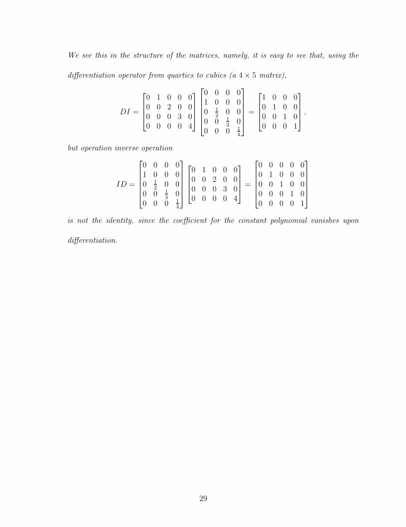
We see this in the structure of the matrices, namely, it is easy to see that, using the
di!erentiation operator from quartics to cubics (a 4 ! 5 matrix),
DI =
%
&&'
0 1 0 0 00 0 2 0 00 0 0 3 00 0 0 0 4
(
))*
%
&&&&'
0 0 0 01 0 0 00 1
2 0 00 0 1
3 00 0 0 1
4
(
))))*
=
%
&&'
1 0 0 00 1 0 00 0 1 00 0 0 1
(
))*
,
but operation inverse operation
ID =
%
&&&&'
0 0 0 01 0 0 00 1
2 0 00 0 1
3 00 0 0 1
4
(
))))*
%
&&'
0 1 0 0 00 0 2 0 00 0 0 3 00 0 0 0 4
(
))*
=
%
&&&&'
0 0 0 0 00 1 0 0 00 0 1 0 00 0 0 1 00 0 0 0 1
(
))))*
is not the identity, since the coe"cient for the constant polynomial vanishes upon
di!erentiation.
29
4 Lecture 4
4.1 Inner Sum and Direct Sum Spaces
Recall that a subspace is a subset of a vector space that is itself a vector space. The elements
of the subspace are still elements of the original vector space, the only additional conditions
to which the elements of the subspace must comply is that sums of such elements and scalar
products of such elements must lie in the subspace. For example, the rationals over the
rational field is a subspace of the reals.
Now suppose we are to consider more than one subspace of a vector space. It is desirable
to characterise the behavior of vectors that lie in these di!erent subspaces.
Definition 26 Let V and W be subspaces of some vector space S. We define the inner
sum of elements of these two vector spaces as the ordinary vector sum; i.e., for v ( V and
w ( W , the inner sum is
x = v + w.
!
As it stands, this definition is not very remarkable. It gains some additional interest,
however, if we add some structure.
Definition 27 Two linear subspaces V and W are said to be disjoint subspaces if
V * W = {0}, that is, if the only vector they have in common is the zero vector.
Furthermore, if every vector in S can be expressed as the inner sum of elements of disjoint
subspaces V and W , then we write
S = V + W,
30
and say that W is the orthogonal complement of V (and vice versa). !
Lemma 1 Let V and W be subspaces of a vector space S. Then for each x ( V + W , there
is a unique v ( V and a unique w ( W such that x = v + w if and only if V and W are
disjoint.
Example 2 Let S = R2 and let V and W be two non-co-linear lines that both intersect the
origin (they need not be oriented at right angles to each other). Since these two vectors are
linearly independent, they span S; thus every vector in x ( S can be expressed uniquely as
the sum of vectors v ( V and w ( W .
Definition 28 We say that a vector space S is the direct sum of two subspaces V and W
if every vector x ( S has a unique representation as an ordered pair of the form
x = (v,w),
where v ( V and w ( W . We denote this situation as
S = V 5 W.
Vector addition and scalar multiplication are defined, for v1,w1 ( V and v2,w2 ( W , as
(v1,w1) + (v2,w2) = (v1 + v2,w1 + w2)
%(v1,w1) = (%v1, %w1),
If the subspaces are also inner product spaces, then we may define the inner product for the
direct sum space as
0(v1,w1), (v2,w2)1S = 0v1,v21V + 0w1,w21W ,
31
where 0·, ·1V and 0·, ·1W are the inner products for the subspaces V and W , respectively. !
Now let V and W be two disjoint subspaces of a vector space S. We ask: what is
the relationship between the inner sum V + W and the direct sum V 5 W ? The answer:
they are two representations of exactly the same thing, in the following sense: there exists
a mapping from the inner sum to the direct sum the operational behavior. Somewhat
informally speaking, two vector spaces are said to be isomorphic if there is a one-to-one
linear mapping of one onto the other which preserves all relevant properties, such as inner
products.
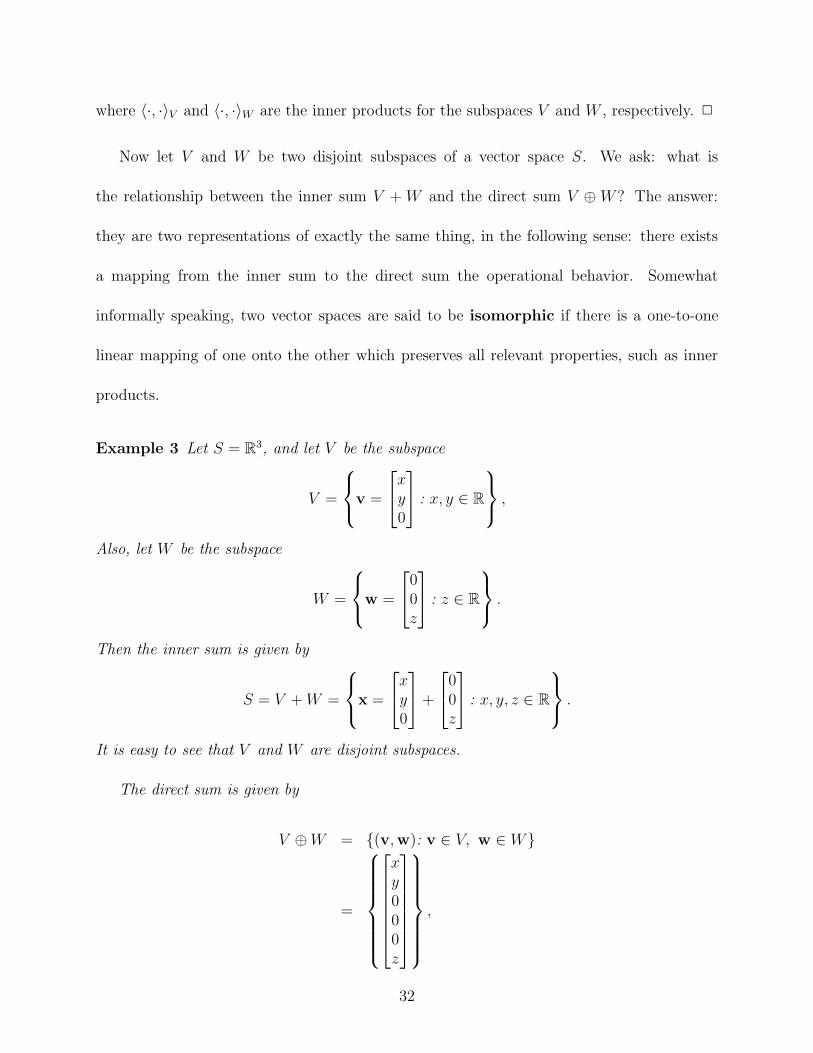
Example 3 Let S = R3, and let V be the subspace
V =
5
6
7v =
%
'
xy0
(
* : x, y ( R
8
9
:,
Also, let W be the subspace
W =
5
6
7w =
%
'
00z
(
* : z ( R
8
9
:.
Then the inner sum is given by
S = V + W =
5
6
7x =
%
'
xy0
(
*+
%
'
00z
(
* : x, y, z ( R
8
9
:.
It is easy to see that V and W are disjoint subspaces.
The direct sum is given by
V 5 W = {(v,w): v ( V, w ( W}
=
5
;;;;;;6
;;;;;;7
%
&&&&&&'
xy000z
(
))))))*
8
;;;;;;9
;;;;;;:
,
32

where we have arranged the ordered pair by concatenating the column vectors.
The isomorphism relating the two vector spaces is the mapping
*(v,w) = v + w =
%
'
xyz
(
* .
It may seem that the above discussion is overly pedantic, and it may be. However, you
will find that notation is not always standard on this issue. Some books conflate the two
concepts and it sometimes leads to confusion. For example, some authors call expressions
such as x = v + w a direct sum and write expressions such as v + w ( V 5 W . Strictly
speaking, this is an abuse of notation since the elements of V 5 W are ordered pairs of
vectors, but we get a way with this kind of abuse because of the isomorphism. Perhaps a
little care now will avoid conceptual problems in the future.
4.2 Projections
We now turn our attention to the idea of projecting a vector from a given vector space onto
a subspace.
Definition 29 A linear transformation P of a vector space into itself is called a projection
if
P 2 = P.
Such an operator is said to be idempotent. !
Example 4 Let S = R3, and let x and y be arbitrary non-zero vectors in this space. Intu-
itively, we want to find the vector yx = %x that is co-linear with x such that the line from
33
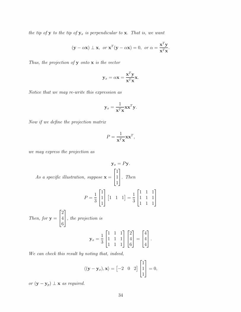
the tip of y to the tip of yx is perpendicular to x. That is, we want
(y & %x) 3 x, or xT (y & %x) = 0, or % =xTy
xTx.
Thus, the projection of y onto x is the vector
yx = %x =xTy
xTxx.
Notice that we may re-write this expression as
yx =1
xTxxxT y.
Now if we define the projection matrix
P =1
xTxxxT ,
we may express the projection as
yx = Py.
As a specific illustration, suppose x =
%
'
111
(
*. Then
P =1
3
%
'
111
(
*,
1 1 1-
=1
3
%
'
1 1 11 1 11 1 1
(
*
Then, for y =
%
'
246
(
*, the projection is
yx =1
3
%
'
1 1 11 1 11 1 1
(
*
%
'
246
(
* =
%
'
444
(
* .
We can check this result by noting that, indeed,
0(y & yx),x1 =,
&2 0 2-
%
'
111
(
* = 0,
or (y & yp) 3 x as required.
34
The above is an example of a rank-one projection; that is, a projection of a vector onto
a line. We can also consider the projection of a vector onto a plane.
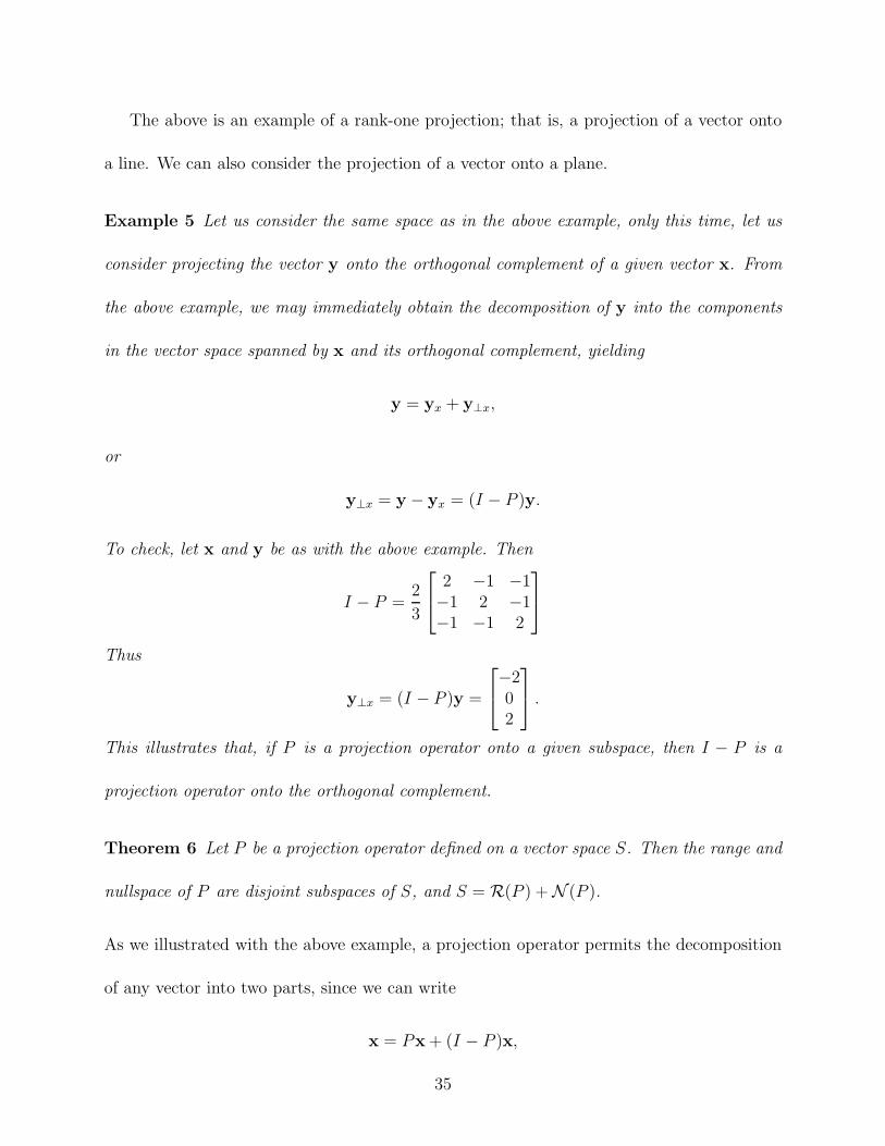
Example 5 Let us consider the same space as in the above example, only this time, let us
consider projecting the vector y onto the orthogonal complement of a given vector x. From
the above example, we may immediately obtain the decomposition of y into the components
in the vector space spanned by x and its orthogonal complement, yielding
y = yx + y(x,
or
y(x = y & yx = (I & P )y.
To check, let x and y be as with the above example. Then
I & P =2
3
%
'
2 &1 &1&1 2 &1&1 &1 2
(
*
Thus
y(x = (I & P )y =
%
'
&202
(
* .
This illustrates that, if P is a projection operator onto a given subspace, then I & P is a
projection operator onto the orthogonal complement.
Theorem 6 Let P be a projection operator defined on a vector space S. Then the range and
nullspace of P are disjoint subspaces of S, and S = R(P ) + N (P ).
As we illustrated with the above example, a projection operator permits the decomposition
of any vector into two parts, since we can write
x = Px + (I & P )x,
35

where Px ( /(P ) and (I & P )x ( N (P ). Since the range and null spaces are algebraic
complements, (I & P ) also qualifies as a projection, as was demonstrated in the example.
We may further specialize projection operators as follows:
Definition 30 A projection operator P is said to be an orthogonal projection if the
range and nullspace are orthogonal, that is, if R(P ) 3 N (P ). !
Recall the above example involving projection of vectors in R3 to a line. This is an
example of a rank-one projection, and we demonstrated that it had the form (which can be
written in two ways to make a point:
P =1
xTxxxT = x
1
xTx2"1
xT .
We will see in the sequel that this is a special case of a more general projection matrix
projection operator, or projection matrix. Let A be an m ! n dimensional matrix mapping
Rn into Rm. Let us define the subspace V as the span of the columns of A. This is the range
space of A, also denoted as the column space of A. Then the projection onto the column
space of A is given by the matrix
PA = A1
AT A)"1AT .
This projection matrix is of tremendous importance, and is the key component of much of
linear filtering theory.
Since the range and nullspace of an orthogonal projection operator are orthogonal, we
have the following theorem:
Theorem 7 A matrix P is an orthogonal projection matrix if and only if P 2 = P and
P is symmetric, i.e., if P = P T .
36
The idea of projection is obvious in geometrical spaces such as R3, where we can easily
visualize what it means to project a vector onto a subspace. The beauty and utility of the
notion of projection, however, extends far beyond such simple applications. The main result
we now consider is the classical projection theorem.
Theorem 8 (The Projection Theorem). Let S be a Hilbert space and let V be a closed
subspace of S. For any vector x ( S, there exists a unique vector v0 ( V closest to x, that
is, .x&v0. $ .x&v. for all v ( V . Furthermore, the point v0 is the minimizer of .x&v0.
if and only if x & v0 is orthogonal to every element of V .
Proof This proof requires several steps:
1. Existence of v0. This proof makes use of the parallelogram law, which we now
formally state.
Lemma 2 The Parallelogram Law. In an inner product space with induced norm,
.x + y.2 + .x & y.2 = 2.x.2 + 2.y.2.
This lemma follows immediately by direct expansion of the norms in terms of the inner
product (see Exercize 2.5-43 of Moon and Stirling).
Now to prove existence. Suppose x +( V . Let # = infv%V .x & v.. Let {vi} be a
sequence of vectors in V such that .x & vi. " #. We need to show that {vi} is a
Cauchy sequence in V . Then, since V is closed by hypothesis, it follows that the limit
is an element of V . We proceed by applying the parallelogram law as follows:
.(vj & x) + (x & vi).2 + .(vj & x) & (x & vi).2 = 2.vj & x.2 + 2.x & vi.2.
37
Noting that the first term on the left simplifies to .vj & vi.2 and the second term on
the left can be rearranged to become
.(vj & x) & (x & vi).2 = .vj + vi & 2x.2
= 4
<<<<x & vj + vi
2
<<<<
2
,
the parallelogram law expression can be rearranged to become
.vj & vi.2 = 2.vj & x.2 + 2.x & vi.2 & 4
<<<<x & vj + vi
2
<<<<
2
.
Since S is a vector space, we have vj+vi
2 ( V . Also, by construction of #,
<<<<x & vj + vi
2
<<<<# #.
It follows that
.vj & vi.2 $ 2.vj & x.2 + 2.x& vi.2 & 4#2.
Now, as i, j " 2, the first two terms on the right hand side of the above inequality
both tend to #2, and we conclude that
.vj & vi.2 " 0
as i, j " 2. Thus {vi} is a Cauchy sequence in V , and since V is closed, the limit,
which we denote as v0, is an element of V .
2. Necessity of orthogonality. We need to show that if v0 minimizes .x & v0., then
(x&v0) 3 V . We prove this result by contradiction. Assume that there exists a vector
v ( V that is not orthogonal to x & v0. Without loss of generality, we assume that
.v. = 1. Let
0(x & v0),v1 = # += 0.
38
Now define the vector z = v0 +#v. Then, by the properties of the inner product (recall
the proof of the Cauchy-Schwarz inequality),
.x & z.2 = .x & v0 & #v.2
= .x & v0.2 & 2Re0x & v0, #v1 + |#|2.v.2
= .x & v0.2 & |#|2.
where the last equality obtains by the construction of # and the fact that v is a unit
vector. The result of this string of inequalities is the claim that
.x & z. < .x & v0.,
which violates the claim that v0 is a minimizing vector. Thus there can exist no v ( V
such that 0(x & v0),v1 += 0. This proves the necessity of orthogonality.
3. Su"ciency of orthogonality. We need to show that orthogonality implies minimality.
Suppose that (x & v0) 3 v for all v ( V . Let v ( V with v += v0, and consider the
vector
x & v = (x & v0) + (v0 & v).
Since v0 & v ( V , and every vector in V is orthogonal to x & v0, we may apply the
Pythagorean theorem to obtain
.x & v.2 = .(x & v0) + (v0 & v).2
= .x & v0.2 + .v0 & v.2.
Since the second entry on the right hand side is non-negative, it follows that
.x & v.2 # .x & v0.2,
39

which establishes su"ciency.
4. Uniqueness of v0. Suppose there are two distinct orthogonal decompositions of x, that
is, we have
x = v0 + w0
and
x = v1 + w1,
where that v0 += v1. Observe that w0,w1 ( V (. Subtracting the left- and right-hand
sides of these two equations obtains
0 = v0 + w0 & v1 & w1,
or, upon rearranging,
v0 & v1 = w1 & v0.
The di!erence v0 & v1 ( V , it follows that w1 & w0 ( V . Also, since w1,w0 ( V (, it
follows that w1&w0 ( V (. But, since the two di!erences are equal, it also follows that
v0 & v1 ( V ( as well. But the only vector that can lie in both V and its orthogonal
complement is the zero vector, so we must conclude that v0 = v1, which establishes
uniqueness.
!
Theorem 9 An orthogonal set of non-zero vectors is a linearly independent set.
40
Proof Suppose {pi, i = 1, . . . , n} is an orthogonal set of non-zero vectors, and suppose there
exists a set of scalars {ai, i = 1, . . . , n} such that
n+
i=1
aipi = 0.
For each i, form the inner product of both sides of this equation.
=
pk,n+
i=1
aipi
>
=n+
i=1
ai0pk,pi1 = ak.pk.2 == 0pk, 01 = 0,
which implies that ak = 0 for k = 1, . . . , n, so the only linear combination of orthonormal
vectors that equals the null vector is the trivial combination, hence the orthogonal set is
linearly independent. !
4.3 Gram-Schmidt Orthogonalization
The next theorem describes a method of converting an arbitrary set of linearly independent
vectors into an orthonormal set.
Theorem 10 ((Gram-Schmidt). Let {pi, i = 1, 2, . . .} be a countable or finite sequence
of linearly independent vectors in an inner product space S. Then, there is an orthonormal
sequence {qi, i = 1, 2, } such that for each n the space generated by the first n qi’s is the same
as the space generated by the the first n pi’s; i.e., span (q1, . . . ,qn) = span (p1, . . . ,pn).
Proof For the first vector, take
q1 =p1
.pk.
which obviously generates the same space as p1. Form q2 in two steps:
41

1. Put
e2 = p2 & 0p2,q11q1.
The vector e2 is formed by subtracting the projection of p2 on q1 from p2. The vector
e2 cannot be zero since p2 and q1 are linearly independent.
2. Normalize:
q2 =e2
.e2..
By direct calculation, we can verify that e2 3 q1 and hence that q2 3 q1. Furthermore, q1
and q2 span exactly the same space as p1 and p2.
The remaining qi’s are defined by induction.
1. The vector en is formed according to the equation
en = pn &n"1+
i=1
0pn,qi1qi,
which subtracts the projections of pn onto the preceding qi’s from pn.
2. Normalize:
qn =en
.en..
Again, it is easily verified by direct computation that en 3 qi for all i < n, and en += 0 since
it is a linear combination of independent vectors. It is clear b induction that the qi’s span
exactly the same space as do the pi’s. If the original collection {pk} is finite, the process
terminates; otherwise the process produces an infinite set of orthonormal vectors. !
42
5 Lecture 5
5.1 Approximations in Hilbert Space
The basic approximation problem:
Let1
S, . · .2
be a normed vector space, let T = {p1, . . . ,pm} , S be a set of linearly
independent vectors and let
V = span (T ).
Given an arbitrary vector x ( S, find a linear combination of elements of V that approximate
x as closely as possible. We will denote this approximation as
x =m+
i=1
cipi.
Stated another way, the problem is to find a representation of x of the form
x = x + e
such that the norm of the error term e = x & x is minimized; i.e.,
{c1, . . . , cn} = arg mina1,...,am
<<<<x &
m+
i=1
aipi
<<<<.
The choice of norm is often motivated by both mathematical and physical reasons. Some
popular possibilities include the following.
1. The L1 (!1) (absolute value error) norm weights all errors proportionally. This can
be advantageous in some situations. Evidently, many image processing professionals
claim that minimizing the absolute value of the error when reconstructing an image
from a noisy source is more subjectively pleasing and informative to the viewer than
43
other criteria. Mathematically, however, this norm is not easily accommodated, since
it is generally not possible to find the minimizing set of coe"cients via calculus.
2. The L! (!!) (maximum error) norm penalizes the maximum value of the error. This
approach also leads to somewhat di"cult mathematics.
3. The L2 (!2) (squared error) norm weights large errors disproportionally more than small
ones, and is an e!ective means of penalizing excessively large errors. This norm also
leads to very tractable mathematics, since calculus can be used to find the minimizing
set of coe"cients. There are also a number of mathematical reasons to consider this
norm:
(a) In stochastic settings, minimizing this norm yields the conditional expectation.
Also, for Gaussian systems, the resulting estimate is a linear function of the
observables, leading to easy computation.
(b) This norm has illuminating connections to control theory, including Riccati equa-
tions, matrix inversions, and observers. A remarkable and useful fact is that
the optimal approximation problem under this norm is a mathematical dual to
the optimal control problem using the same norm! Much of the mathematical
machinery developed under one of those applications is easily transferred to the
other—thus providing a convenient unification of ideas.
(c) Sub-optimal approximations are easy to obtain if the strict optimization problem
is too computationally di"cult.
44
(d) There are also important connections with martingale theory, likelihood ratios,
and nonlinear estimation.
For these reasons, the L2 norm is the one most deserving (and amenable to) detailed
study, and we will primarily focus on this norm.
Let us first consider the approximating the vector x ( R2 by another vector p ( R2. Let
V be the subspace spanned by p. Then V consists of the line passing through the origin and
the tip of p. As we saw earlier, the projection of x onto V produces the minimum-length
vector in the norm induced from the dot product. So the best approximation, with respect
to that norm, of x in V is the projection
x =1
pTpppTx
which we can write more descriptively, for our present purposes, as
x =1
.p.20x,p1x.
Notice that we could also obtain this result by calculus. To do this, we form the quantity
.x & cp.2 & 0x & cp,x & cp1 = (x & cp)T (x & cp).
We then note that this is a function of the parameter c. Furthermore, since it is quadratic in
c, it possesses a well-defined minimum, which may be obtained by di!erentiating. Formally,
therefore, we consider the function
g(c) = (x & cp)T (x & cp) = xTx & 2cxTp + c2pT p,
45
di!erentiate with respect to c and setting the result to zero, yielding
dg(c)
dc= &2xTp + 2cpTp = 0,
and solve for c to obtain
c =xTp
pT p,
which yields the minimum-error solution
x =xTp
pT px,
which is identical to the orthogonal projection.
Next, let us consider approximating a vector in R3 by two vectors p1 and p2 (not
necessarily orthogonal) that span R2. We need to decompose x into its projection onto
V = span (p1,p2) and its orthogonal complement, yielding
x = c1p1 + c2p2 + e,
where e ( V (. To accomplish this decomposition, we need The approximation error vector
e to be orthogonal to both p1 and p2, that is,
0x & (c1p1 + c2p2),p11 = 0
0x & (c1p1 + c2p2),p21 = 0.
Re-arranging this expression, we obtain
0x,p11 = c10p1,p11 + c20p2,p11
0x,p21 = c10p1,p21 + c20p2,p21,
46
which may be expressed in matrix notation as
"
0p1,p11 0p2,p110p2,p11 0p2,p21
? "
c1
c2
?
=
"
0x,p110x,p21
?
.
As we will see below, the matrix
"
0p1,p11 0p2,p110p2,p11 0p2,p21
?
is invertible, so we can obtain the desired coe"cients as
"
c1
c2
?
=
"
0p1,p11 0p2,p110p2,p11 0p2,p21
?"1 "0x,p110x,p21
?
.
Generalizing, suppose x ( Rn and we wish to approximate x by a set of m linearly
independent vectors {p1, . . . ,pm}, where m < n, that is, we desire to decompose x as
x =m+
i=1
cipi + e.
The desired projection is obtained by choosing the coe"cients {c1, . . . cn} such that
=
x &m+
i=1
cipi,pj
>
= 0, j = 1, 2, . . . , m.
Expanding our earlier analysis to higher dimensions yields the matrix expression%
&&&'
0p1,p11 0p2,p11 . . . 0pm,p110p1,p21 0p2,p21 . . . 0pm,p21
......
0p1,pm1 0p2,pm1 . . . 0pm,pm1
(
)))*
%
&&&'
c1
c1...
cm
(
)))*
=
%
&&&'
0x,p110x,p21
...0x,pm1
(
)))*
This system of equations is call the normal equations, and the matrix
R =
%
&&&'
0p1,p11 0p2,p11 . . . 0pm,p110p1,p21 0p2,p21 . . . 0pm,p21
......
0p1,pm1 0p2,pm1 . . . 0pm,pm1
(
)))*
is called the Grammian of the set p1, . . . ,pm. It is easy to see that, by properties of the
inner product, R = RH .
47
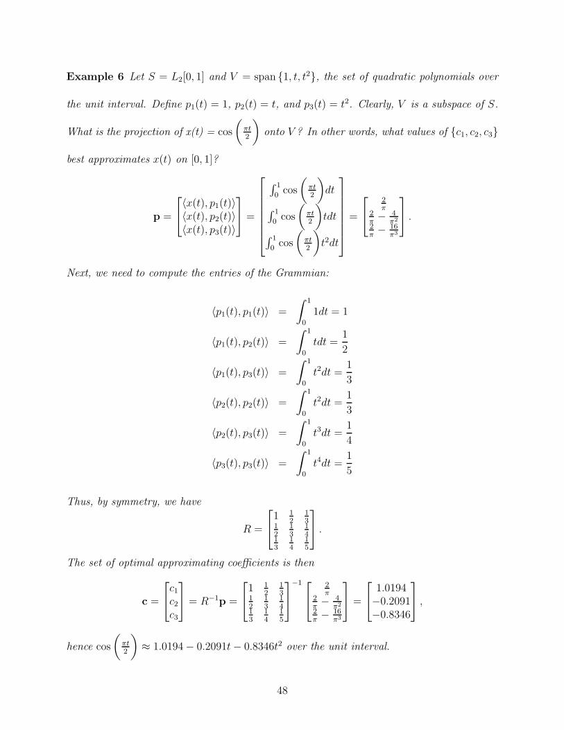
Example 6 Let S = L2[0, 1] and V = span {1, t, t2}, the set of quadratic polynomials over
the unit interval. Define p1(t) = 1, p2(t) = t, and p3(t) = t2. Clearly, V is a subspace of S.
What is the projection of x(t) = cos
3
!t2
$
onto V ? In other words, what values of {c1, c2, c3}
best approximates x(t) on [0, 1]?
p =
%
'
0x(t), p1(t)10x(t), p2(t)10x(t), p3(t)1
(
* =
%
&&&&&&'
. 1
0 cos
3
!t2
$
dt
. 1
0 cos
3
!t2
$
tdt
. 1
0 cos
3
!t2
$
t2dt
(
))))))*
=
%
'
2!
2!& 4
!22!& 16
!3
(
* .
Next, we need to compute the entries of the Grammian:
0p1(t), p1(t)1 =
# 1
0
1dt = 1
0p1(t), p2(t)1 =
# 1
0
tdt =1
2
0p1(t), p3(t)1 =
# 1
0
t2dt =1
3
0p2(t), p2(t)1 =
# 1
0
t2dt =1
3
0p2(t), p3(t)1 =
# 1
0
t3dt =1
4
0p3(t), p3(t)1 =
# 1
0
t4dt =1
5
Thus, by symmetry, we have
R =
%
'
1 12
13
12
13
14
13
14
15
(
* .
The set of optimal approximating coe"cients is then
c =
%
'
c1
c2
c3
(
* = R"1p =
%
'
1 12
13
12
13
14
13
14
15
(
*
"1 %
'
2!
2!& 4
!22!& 16
!3
(
* =
%
'
1.0194&0.2091&0.8346
(
* ,
hence cos
3
!t2
$
6 1.0194 & 0.2091t& 0.8346t2 over the unit interval.
48
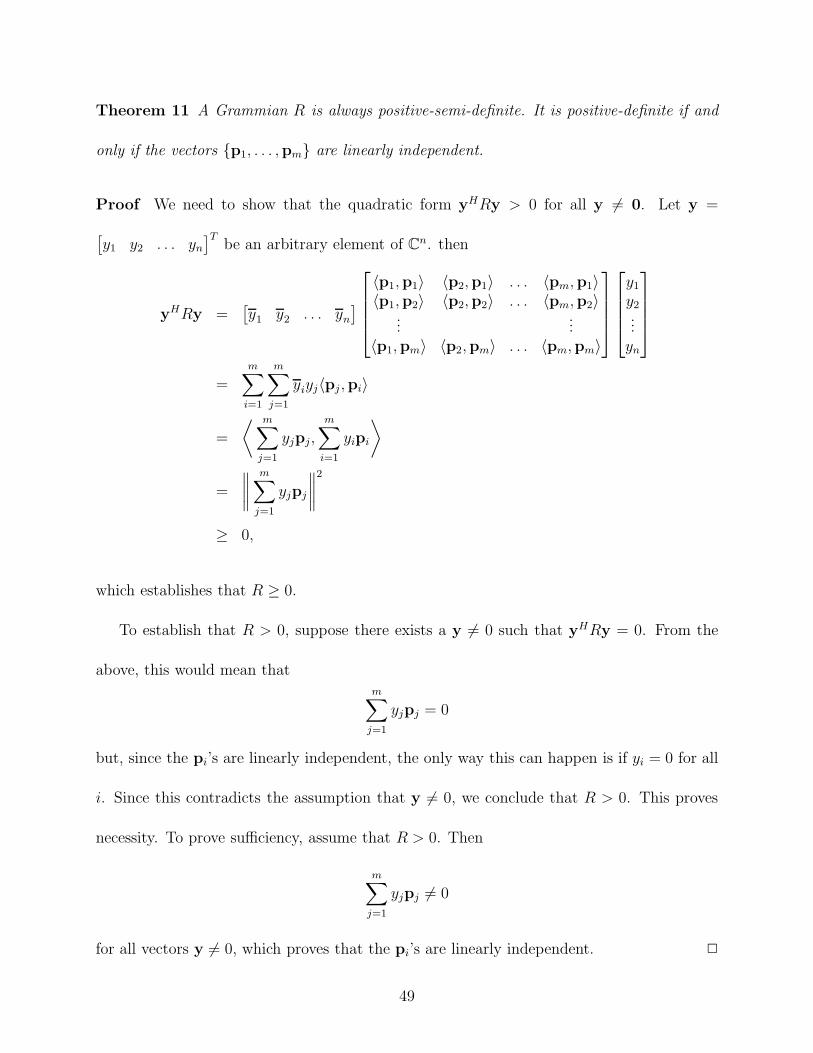
Theorem 11 A Grammian R is always positive-semi-definite. It is positive-definite if and
only if the vectors {p1, . . . ,pm} are linearly independent.
Proof We need to show that the quadratic form yHRy > 0 for all y += 0. Let y =
,
y1 y2 . . . yn
-Tbe an arbitrary element of Cn. then
yHRy =,
y1 y2 . . . yn
-
%
&&&'
0p1,p11 0p2,p11 . . . 0pm,p110p1,p21 0p2,p21 . . . 0pm,p21
......
0p1,pm1 0p2,pm1 . . . 0pm,pm1
(
)))*
%
&&&'
y1
y2...
yn
(
)))*
=m+
i=1
m+
j=1
yiyj0pj ,pi1
=
= m+
j=1
yjpj,m+
i=1
yipi
>
=
<<<<
m+
j=1
yjpj
<<<<
2
# 0,
which establishes that R # 0.
To establish that R > 0, suppose there exists a y += 0 such that yHRy = 0. From the
above, this would mean thatm+
j=1
yjpj = 0
but, since the pi’s are linearly independent, the only way this can happen is if yi = 0 for all
i. Since this contradicts the assumption that y += 0, we conclude that R > 0. This proves
necessity. To prove su"ciency, assume that R > 0. Then
m+
j=1
yjpj += 0
for all vectors y += 0, which proves that the pi’s are linearly independent. !
49
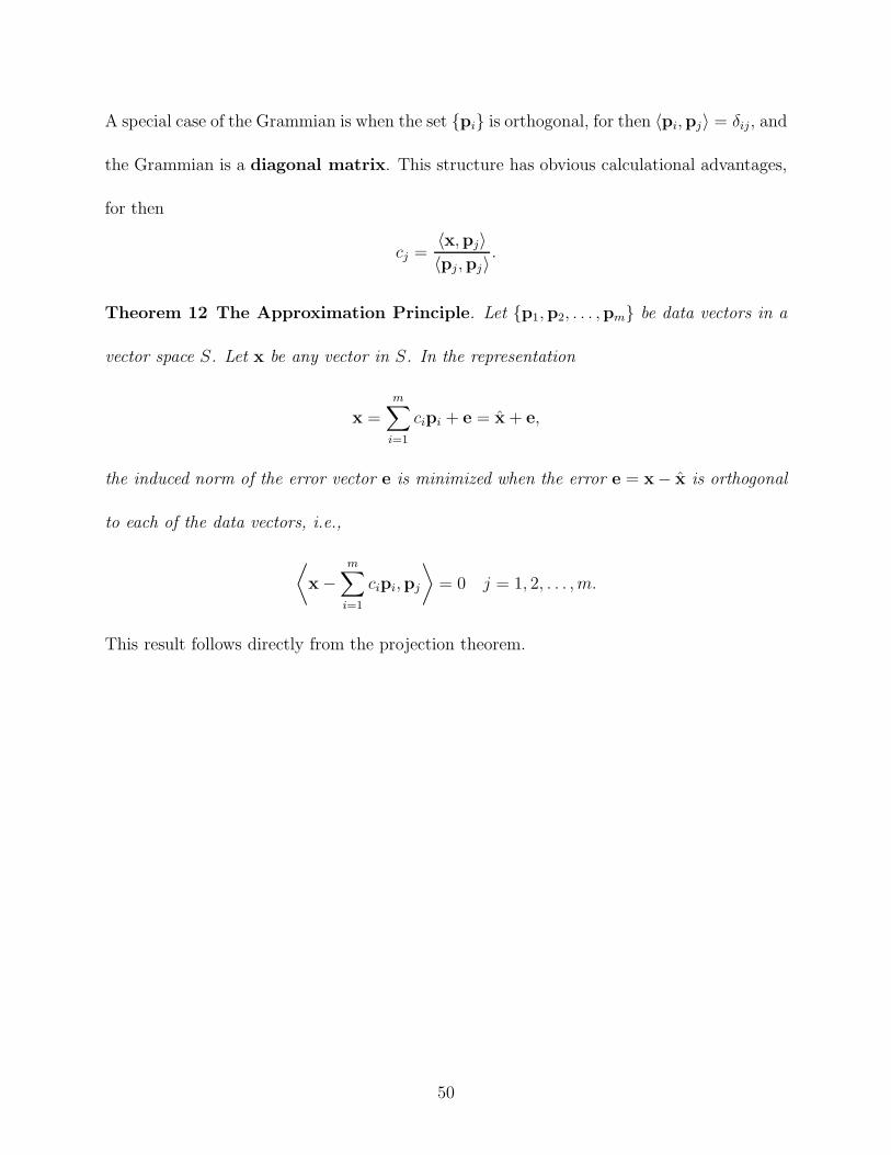
A special case of the Grammian is when the set {pi} is orthogonal, for then 0pi,pj1 = #ij, and
the Grammian is a diagonal matrix. This structure has obvious calculational advantages,
for then
cj =0x,pj10pj,pj1
.
Theorem 12 The Approximation Principle. Let {p1,p2, . . . ,pm} be data vectors in a
vector space S. Let x be any vector in S. In the representation
x =m+
i=1
cipi + e = x + e,
the induced norm of the error vector e is minimized when the error e = x& x is orthogonal
to each of the data vectors, i.e.,
=
x &m+
i=1
cipi,pj
>
= 0 j = 1, 2, . . . , m.
This result follows directly from the projection theorem.
50
6 Lecture 6
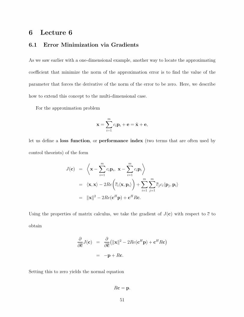
6.1 Error Minimization via Gradients
As we saw earlier with a one-dimensional example, another way to locate the approximating
coe"cient that minimize the norm of the approximation error is to find the value of the
parameter that forces the derivative of the norm of the error to be zero. Here, we describe
how to extend this concept to the multi-dimensional case.
For the approximation problem
x =m+
i=1
cipi + e = x + e,
let us define a loss function, or performance index (two terms that are often used by
control theorists) of the form
J(c) =
=
x &m+
i=1
cipi, x &m+
i=1
cipi
>
= 0x,x1 & 2Re
3
ci0x,pi1$
+m+
i=1
m+
j=1
cjci0pj ,pi1
= .x.2 & 2Re(cHp) + cHRc.
Using the properties of matrix calculus, we take the gradient of J(c) with respect to c to
obtain
+
+cJ(c) =
+
+c
1
.x.2 & 2Re(cHp) + cHRc2
= &p + Rc.
Setting this to zero yields the normal equation
Rc = p.
51

This approach works because the functional J has a unique extremum which, it can
easily be shown, is a minimum. This is a consequence of the quadratic structure of J , and
arises because of the linear approximation model. If the model were not linear, then the
performance index may not be quadratic and there may exist multiple extrema that cannot
be distinguished by gradient-based methods.
It is important to emphasize that the methods we are developing here apply most directly
to linear models. The general nonlinear approximation problem is much harder.
6.2 Linear Least Squares Approximation
The approximation theory we are developing is linear, in the sense that the quantity to be
estimated (i.e., approximating) is a linear combination of the vectors that span the subspace
into which we wish to project. The projection theorem establishes that there exists a unique
error-norm minimizing projection vector, but it does not provide an explicit construction
of the operator that produces the projection. Also, the normal equations give us a way to
compute the coe"cient vector, but, again, does not directly identify the projection operator.
To extend our understanding of what is going on, it will be useful to identify the projection
operator explicitly (which we already have done for a couple of simple cases).
In this development, we will restrict our attention to vector spaces of finite dimension. In
this context, we may exploit the power of matrix theory. Let S be an n-dimensional vector
space and let V be an m-dimensional subspace that is spanned by a set of linearly independent
vectors {p1,p2, . . . ,pm}, where we assume that m < n. For any vector x ( S, we may
52
uniquely decompose it into components that lie in V and V (, yielding the representation
x = x + e =m+
i=1
cipi + e,
where x ( V and e ( V (. We can express x in matrix notation by defining the n!m matrix
A =,
p1 p2 · · · pm
-
and writing
x = Ac.
Since the projection must be orthogonal, we require that
0x & Ac,pj1 = pHj (x & Ac) = 0 j = 1, . . . , m.
Stacking these expressions into a single column yields%
&&&'
pH1 (x & Ac)
pH2 (x & Ac)
...pH
m(x & Ac)
(
)))*
=
%
&&&'
pH1
pH2...
pHm
(
)))*
(x & Ac) =
%
&&&'
00...0
(
)))*
or
AH(x & Ac) = 0.
Rearranging, we obtain
AHAc = AHx.
Notice that, by identifying AHA as R, the Grammian, and AHx as p, the cross-correlation
vector, the above expression is nothing more than the normal equations.
By assumption, the set of n-dimensional vectors {p1,p2, . . . ,pm} is linearly independent
and m < n, the matrix A is of full rank, hence the matrix AHA is of full rank, so we may
53
solve for c as
c =1
AHA2"1
AHx.
Finally, substituting this into the expression
x = Ac,
we obtain an explicit representation of the projection operator as
x = A1
AHA2"1
AHx;
namely,
P = A1
AHA2"1
AH .
This result can be somewhat generalized by incorporating a Hermitian weighting matrix W
to obtain the projection operator
PW = A1
AHWA2"1
AHW.
This approach would be appropriate if we wish to vary the weighting of the approximation
on the basis vectors.
It is important to appreciate the fact that, just because an approximation is optimal
does not mean that it is a good approximation. We may only be making the best of a bad
situation if the norm of the error e = x & x is not small. Thus, to complete our discussion
we need to characterize this quantity.
A consequence of orthogonality is that the error vector is orthogonal to the approxima-
54
tion, therefore
0e, e1 = 0x & x, e1
= 0x, e1@ AB C
)x,x"x*
& 0x, e1@ AB C
=0 by (
= 0x,x1 & 0x + e, e1
= 0x,x1 & 0x, e1@ AB C
0
&0e, e1.
Thus,
.x.2 = .x.2 + .e.2
or
.e.2 = .x.2 & .x.2.
We can express this norm more descriptively by substituting Ac for x, to obtain
.e.2 = xHx & cHp.
6.3 Approximation by Continuous Polynomials
We saw earlier that we could approximate cos
3
!t2
$
over the unit interval by a quadratic.
We now extend this result to the general case.
Suppose we wish to find a real polynomial of degree n that best fits a given real function
f(t) over the interval [a, b]. Let
p(t) = c0 + c1t + c2t2 + · · · + cnt
n
denote the form of the approximating polynomials. We wish to find the coe"cient vector
{c0, c1, . . . , cn}. that renders the error f(t) & p(t) orthogonal to the space spanned by the
55
set of all n-th order real polynomials, that is , we require
0f(t) & p(t), p(t)1 =
# b
a
1
f(t) & p(t)2
p(t)dt = 0
for all polynomials of degree $ n. To proceed, we first must define a basis set, which may
be any linearly independent set of polynomials that span the set of all polynomials of degree
$ n. For example, as we did earlier, we can take basis set
,
p0(t) p1(t) p2(t) · · · pn(t)-
=,
1 t t2 · · · tn-
.
The normal equations are%
&&&'
01, 11 01, t1 · · · 01, tn10t, 11 0t, t1 · · · 0t, tn1
......
0tn, 11 0tn, t1 · · · 0tn, tn1
(
)))*
%
&&&'
c0
c1...cn
(
)))*
=
%
&&&'
0f(t), 110f(t), t1
...0f(t), tn1
(
)))*
,
where
0ti, tj1 =
# b
a
ti+jdt, i, j = 0, 1, . . . , n
and
0f(t), ti1 =
# b
a
f(t)tidt, i = 0, 1, . . . n.
Although the polynomials,
1 t t2 · · · tn-
span the n + 1 dimensional space of n-th
order polynomials, these polynomials do not form an orthogonal basis, since
# b
a
titjdt += 0
for i += j. This makes it necessary to compute a large number of integrals. Furthermore,
the resulting Grammian may be di"cult to invert. Even though, theoretically, it is of full
rank, it may be ill conditioned, meaning that it is very nearly singular and finite-precision
arithmetic may generate significant errors in the computed inverse.
56
There is another problem that may also arise with the use of non-orthogonal bases; that
is, slow convergence. Think of it this way. Suppose, for a given non-orthogonal basis set,
some of the basis elements are highly correlated with others, that is, for i < j,
0pi(t), pj(t)1 6 .pi(t)..pj(t)..
Thus, if we were to perform a Gram-Schmidt orthogonalization of pj relative to pi, we would
that the orthogonal component (before normalization),
e(t) = pj(t) &=
pj(t),pi(t)
.pi(t).
>pi(t)
.pi(t).
would be very near zero. This means that the amount of new information provided by pj is
very small compared to the information provided by pi. The Gram-Schmidt orthogonaliza-
tion procedure corrects this problem by amplifying the length of this orthogonal component
by dividing by its length, thereby e!ectively increasing the amount of information charac-
terized by the resulting polynomial.
There is yet a third reason for using an orthogonal basis if it can be found: the resulting
Grammian is diagonal, leading to greatly simplified calculation of its inverse. Even more
to the point, if the basis is also normalized (which is what Gram-Schmidt also does), the
inversion is trivial, and we immediately obtain the coe"cients as the inner product of the
function with the basis elements:
ci =
# b
a
f(t)qi(t)dt,
where qi(t) is the ith element of the orthonormal basis set.
57
7 Lecture 7
7.1 Linear Regression
Consider the following scenario. A collection of observations is obtained. These observations
are functions of parameters that are of interest. The problem is to determine the parameters.
This is a classical statistical inference problem. For example, suppose the resistance of a
simple electric circuit is an unknown constant. We know, by Ohm’s law, that the voltage
and current are related linearly, i.e.,
I =1
RV,
where I, V , and R denote current, voltage, and resistance, respectively.
Now suppose we were not aware of Ohm’s law, but had access to a variable voltage
source and an ammeter. We might be tempted to take an empirical, rather than theoretical,
approach to this problem. We could step through a number of voltage values, each time
measuring the current. The result would be a table of values of the form
V1 I1
V2 I2...
...Vn In
To relate these two table entries, we first need to hypothesize a model. This is the
critical point. What characteristics should we consider when searching for a good model?
The guiding principle in many instances is Occam’s Razor: When two or more models are
hypothesized to characterize a phenomenon, the simplest model is to be preferred. This
suggests that we start our analysis with the most simple model possible, and if that is not
good enough, we add complications. Perhaps the most important simple assumption is that
58
the quantities are related linearly, that is,
Ii = aVi.
If the data {Vi, Ii, i = 1, 2, . . .} were to fit this model exactly, they would appear on a graph
as a straight line passing through the origin. Even if this model were valid, however, this
exact relationship is not likely to obtain, since ammeters, and sensors in general, are not
perfect. There are two main sources of error:
1. Bias errors. Unless an instrument is perfectly calibrated, it may contain a bias error,
that is, the quantity we measure, I, is the sum of the true current and an unknown
constant o!set, b.
2. Random errors. All real-world measurements are corrupted by random errors (e.g.,
thermal noise in resistors, parallax errors by human eyeballs, quantization, etc).
Consequently, it is too much to expect that any deterministic model will be an exact fit to
the data. The best that can be hoped for is a model of the form
Ii = aVi + b + ei,
where a is an unknown coe"cient of proportionality, b is an unknown bias, and the sequence
{ei, i = 1, 2, . . .} is a sequence of unknown quantities that, we assume, have an average
value of zero but are otherwise unknown. Although the bias term, b, is also assumed to be
unknown, it, as well as the coe"cient, a, are at least assumed to be constants, whereas the
quantities ei vary from observation to observation.
59

The inference problem is to find the slope and intercept of the line that best fits the data
in the sense that the squared error is minimized, that is, we wish to choose values for a and
b that minimize the quantity
J(a, b) =n+
i=1
(Ii & aVi & b)2.
Fortunately, this is a problem we know how to solve. In matrix form, we may express this
model as
y = Ac + e,
where
y =
%
&&&'
I1
I2...In
(
)))*
,
A =
%
&&&'
V1 1V2 1...
...Vn 1
(
)))*
,
and
c =
"
ab
?
We now recognize this as a projection problem. We form V , the subspace spanned by
two vectors in Rn, namely, the vectors
p1 =
%
&&&'
V1
V2...
Vn
(
)))*
, p2 =
%
&&&'
11...1
(
)))*
,
yielding A =,
p1 p2
-
.
60
We then project the observations vector y =,
I1 I2 · · · In
-Tonto this subspace,
yielding
y = A1
AT A2"1
ATy.
The projection coe"cients, given by
c =
"
ab
?
=1
AT A)"1ATy
=
%
&&&'
"
V1 V2 · · · Vn
1 1 · · · 1
?
%
&&&'
V1 1V2 1...
...Vn 1
(
)))*
(
)))*
"1
"
V1 V2 · · · Vn
1 1 · · · 1
?
%
&&&'
I1
I2...In
(
)))*
=
D!ni=1 V 2
i
!ni=1 Vi
!ni=1 n
E"1 D!ni=1 ViIi!n
i=1 Ii
E
=1
n!n
i=1 V 2i & (
!ni=1 Vi)
2
D
n &!n
i=1 Vi
&!n
i=1 Vi
!ni=1 V 2
i
ED!ni=1 ViIi!n
i=1 Ii
E
=1
n!n
i=1 V 2i & (
!ni=1 Vi)
2
D
n!n
i=1 ViIi & (!n
i=1 Vi) (!n
i=1 Ii)
& (!n
i=1 Vi) (!n
i=1 Ii) + (!n
i=1 V 2i ) (!n
i=1 Ii)
E
constitute the corresponding parameter values. For our problem, we interpret these coef-
ficients as the resistance of the resistor and the bias of the ammeter, respectively. In the
parlance of statistics, these computed values are called estimates.
Notice that the fitted values, y, lie on the line defined by the parameters c. That is,
Ii = aVi + b.
The residual is the di!erence between the observed values and the fitted values
$i = Ii & IiVi.
The projection operation acts to minimize the sum of the squared error between the observed
61
and fitted values:
.!.2 =n+
i=1
1
Ii & IiVi
22,
where
! =
%
&&&'
$1
$2...$n
(
)))*
.
Much of regression analysis has to do with analyzing the residual. Recalling our modeling
assumption that the random errors ei are have zero average value, a quick test of the fit is
to check the average of the elements of the residual vector. If it is not close to zero, then
we may conclude that our model is inadequate. We may also look for trends (systematic
deviations) in the residuals. If there are no trends, then a plot of the residuals will indicate no
systematic patterns. If such patterns exist, this also is an indication of modeling inadequacy.
An important sub-discipline of statistics involves the detailed investigation of the residuals
such as analysis-of-variance methods.
7.2 Minimum Mean-Square Estimation
Suppose we have two real random variables X, Y , with a known joint density function
fXY (x, y), and assume Y is observed (measured). What can be said about the value X
takes? In other words, we wish to estimate X given that Y = y. To be specific, we desire to
invoke an estimation rule
X = h(Y ),
62
where the random variable X is an estimate of X. The mapping h : R " R is some function
only of Y . Thus, given Y = y, we will assign the value
x = h(y)
to the estimate of X.
Let us now specialize to the linear case. Let X and Y be two zero-mean real random
variables. Suppose we wish to find an estimator of the form
X = hY
where h is a constant chosen such E(X & X)2 is minimized. (Thus, the function h(Y ) = hY
is linear.)
To approach this problem from our Hilbert-space perspective, we need to define the the
appropriate spaces and subspaces and endow them with an inner product.
Claim. Let S be the set of real random variables with finite first and second moments, and
define the real-valued function 0·, ·1 " S ! S 7" R by
0X, Y 1 = E[XY ] =
# !
"!
# !
"!xyfXY (x, y)dxdy,
where fXY is the joint density function of the random variables X and Y . Then 0·, ·1 is
an inner product and S is a Hilbert space. The inner product of two random variables is
termed the correlation.
We won’t verify this claim at this time, except to demonstrate that the correlation satisfies
the conditions that qualify it to be an inner product. It is easy to see that E[XY ] = E[Y X],
E[aXY ] = aE[XY ], E[(X + Y )Z] = E[XZ] + E[Y Z], and that E[X2] # 0. What is not so
63

obvious is that E[X2] = 0 implies X 8 0. This is a technical issue that we will not plumb,
but will content ourselves with the statement that X = 0 almost everywhere, meaning
that it is zero except possibly on a set of probability zero. To interpret correlation as an
inner product, we have to make this small concession to the definition of an inner product,
but it is a very small concession and one that does not violate the concept that is important
to us here; namely, orthogonality. Thus, we can say that two uncorrelated random variables
are orthogonal.
With this brief background, we can now bring our Hilbert space machinery to bear on the
following estimation problem: Suppose we observe the random variables {Y1, Y2, . . . , Yn}, and
we wish to use the observed values to estimate the value that another unobserved random
variable, X, assumes.
We desire to set up the structure of this problem before we conduct the experiment,
that is, before values for X and {Yi}, are realized. Then, once the experiment is conducted
and values for the Yi’s are obtained, we may then infer the value that X obtained. This is
an important issue that is easy to miss. To elaborate, before the experiment is conducted,
we view the quantities X, {Yi} as real-valued functions over a sample space of elementary
events. By conducting an experiment, we mean that a particular elementary event is chosen
(e.g., by nature). Let , denote this elementary event. Then all of the random variables
are evaluated at this elementary event, yielding the real numbers x = X(,), yi = Yi(,),
i = 1, 2, . . . , n. It is critical to understand that our Hilbert space context deals with the
functions, and not the particular values they assume.
Let V = span {Y1, Y2, . . . , Yn} (we might refer to this subspace as the observation space).
64
Then, the best estimate of X is its orthogonal projection onto V .
The normal equations for this problem are%
&&&'
0Y1, Y11 0Y2, Y11 · · · 0Yn, Y110Y1, Y21 0Y2, Y21 · · · 0Yn, Y21
......
...0Yn, Y11 0Yn, Y21 · · · 0Yn, Yn1
(
)))*
%
&&&'
h1
h2...
hn
(
)))*
=
%
&&&'
0X, Y110X, Y21
...0X, Yn1
(
)))*
.
The entries in the Grammian are
0Yi, Yi1 = E[Y 2i ] = -2
i , i = 1, 2, . . . , n
0Yi, Yj1 = E[YiYj] = .ij-i-j , j += i
and the entries in the cross-correlation vector are
0X, Yi1 = E[XYi] = .xi-X-i
where -i =F
E,
Y 2i
-
, i = 1, 2, . . . , n, -X =F
E,
X2-
, .ij is the correlation coe"cient for Yi
and Yj, and .xi is the correlation coe"cient for X and Yi, i = 1, 2, . . . , n.
As an example, let us consider the simple circuit problem described earlier, with the
following di!erence. Whereas, before, we observed both the current and the voltage and
the problem was to estimate the resistance, the setup here is that we know the resistance,
measure the current, and desire to estimate a fixed voltage observed multiple times. The
model for this scenario is
Yi = RX + Ni, i = 1, 2, . . . , n,
where the random variables {Ni} are measurement errors. Let us assume that the To facil-
itate our development, let us assume that these errors are uncorrelated, that is, E[NiNj] =
-2N#ij. We further assume that the noise is uncorrelated with the value of the input voltage
65
(e.g., Ni is thermal noise in the resistor). Then
E,
XYi
-
= E,
X(RX + Ni)-
= RE[X2] + E[XNi] = R-2X ,
E,
YiYj
-
= E,
(RX + Ni)(RX + Nj)-
= R2E,
X2-
+ RE,
XNj
-
+ RE,
NjX-
+ E,
NiNj
-
= R2-2X + -2
N#ij .
To illustrate, suppose R = 1 and n = 1. Then the normal equation becomes
,
-2X + -N
-
h = -2X ,
so the minimum mean-square estimate of X is
X =-2
X
-2X + -2
N
Y.
Notice that this is still a “hypothetical” situation in that the experiment has not yet been
performed. Once the experiment is conducted, we obtain the measurement Y = y where y
is some real number, and the estimated realization of X
x =-2
X
-2X + -2
N
y.
We can make the following observations about this estimate.
1. IF the noise source is small such that -N 9 -X , then the noise is essentially ignored
and we have X 6 Y .
2. If the noise source is large such that -X 9 -N , then the observation is essentially
ignored, and we have X 6 0.
It is useful to compare the regression problem with the MMSE problem.
66

1. Both use the concept of orthogonal projections. The regression scenario projects the
space of observations (from the ammeter) onto the space spanned by the (assumed
perfectly known) voltages, and the problem is to determine the resistance and bias
coe"cients. On the other hand, the MMSE scenario projects the unknown voltage onto
the space spanned by the observations, and the problem is to estimate the unknown
voltage.
In the regression context, the projection is onto a subspace defined by two vectors in
n-dimensional Euclidean space, while in the MMSE context, the projection is onto an
n-dimensional subspace spanned by the observable random variables.
2. The regression problem is an empirical data-fitting problem. No probabilistic concepts
are involved. On the other hand, the MMSE approach requires the specification of the
means, variances, and correlations, and cross-correlations of all random variables.
67
8 Lecture 8
8.1 Minimum-Norm Problems
When dealing with equations of the form
Ax = b,
with A an m! n matrix, there are a number of possible scenarios to consider (we assume A
is of full rank).
1. m > n. In this case, the system of equations is over-determined—there are more
equations than unknowns. If, as would occur in general, b lies outside the column
space of A, then there is no value x such that Ax = b. That is, b cannot be expressed
as a linear combination of the columns of A. The best we can do, in such a situation,
is to find an x that minimizes the error b&Ax. Under the !2 norm, we have seen that
least squares (i..e., the projection theorem) provides the solution:
x =1
AT A2"1
ATb.
2. m = n. This is the determined case. Then a unique solution exist of the form
x = A"1b. Notice that, in this case, we have
1
AT A2"1
AT = A"1A"T AT = A"1,
and there is no error. This is really a special case of the projection theorem.
3. m < n. In this case, the system of equations is under-determined, since there are
fewer equations than unknowns. In this case, not only will there be a solution, there
68
will be an infinity of them, and the problem is to choose the one that makes the most
sense. This is the issue we now discuss.
To illustrate, consider the system
Ax = b,
where A is an m ! n matrix with m < n, such as
"
1 2 &3&5 4 1
?%
'
x1
x2
x3
(
* =
"
&46
?
.
One solution is
x =
%
'
123
(
* .
However, we observe that the vector v =,
1 1 1-
lies in the nullspace of the above matrix,
i.e.,"
1 2 &3&5 4 1
?%
'
123
(
* =
"
00
?
,
and so any vector of the form%
'
123
(
*+ t
%
'
111
(
* ,
t ( R, is also a solution. The question becomes: can we formulate a notion of which of
the possible solutions is the “best” one, and if so, how can we find it? One approach to
this problem is to view the equations Ax = b as a constraint, and find the vector x with
minimum norm that satisfies this constraint. To address problems such as this, it is useful
to develop what is called a dual approximation problem.
69
Suppose we are interested in all values of x ( S (some vector space) that satisfy the
constraints
0x,y11 = a1
...
0x,ym1 = am.
Claim: Let M = span {y1, . . . ,ym} and suppose we know that x0 satisfies the constraints.
The set of all solutions to the constraint equation is given by the linear variety
V = x0 + M( = {x0 + v: v ( M(}.
Verification: x ( V if and only if
0x,yi1 = 0x0,yi1 + 0v,yi1
= ai + 0,
for i = 1, . . . , m.
The question we now address is this: Which element of V (that is, which element that
satisfies the constraints) has minimum norm?
Theorem 13 Dual Approximation. Let {y1, . . . ,ym} be a linearly independent set of
vectors in a Hilbert space S, and consider the subspace M = span {y1, . . . ,ym}. The element
70
x ( S that satisfies the constraints
0x,y11 = a1
0x,y21 = a2
...
0x,ym1 = am
with minimum (induced) norm lies in M . In particular,
x =m+
i=1
ciyi,
where %
&&&'
0y1,y11 0y2,y11 · · · 0ym,y110y1,y21 0y2,y21 · · · 0ym,y21
......
...0y1,ym1 0y2,ym1 · · · 0ym,ym1
(
)))*
%
&&&'
c1
c2...
cm
(
)))*
=
%
&&&'
a1
a2...
am
(
)))*
.
Proof If x satisfies the constraints, then x ( V = x0+M( for some vector x0. Now suppose
x0 has a non-zero projection on M(. Then it may be expressed as
x0 = xM + xM!
and
.x0.2 = .xM.2 + .xM!.2,
where xM ( M and therefore may be expressed as a linear combination of the yi’s. But if
xM! += 0, then x0 would not be the minimum-norm solution. Therefore, since
0x0,yk1 = 0xM ,yk1 + 0xM!,yk1
=G
m+
i=1
ciyi,yk
H
,
71

we may conclude that x0 = xM . Thus
x = x0 + v
where x0 ( M and v ( M(, and
0x,yk1 = 0x0,yk1 + 0v,yk1
=m+
i=1
ci0yi,yk1 = ak.
!
We illustrate the use of the dual approximation theorem with two examples.
Example 7 Under-determined linear equations Consider the system of linear equa-
tions
Ax = b
where A is m ! n with m < n (we still require A to be of full rank in order to avoid
inconsistency problems). Our solution concept is as follows: We wish to find the vector x of
minimum norm that satisfies the constraint Ax = b.
To proceed, it is convenient to write A as
A =
%
&&&'
yH1
yH2...
yNm
(
)))*
72
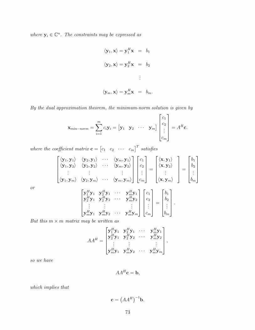
where yi ( Cn. The constraints may be expressed as
0y1,x1 = yH1 x = b1
0y2,x1 = yH2 x = b2
...
0ym,x1 = yHmx = bm.
By the dual approximation theorem, the minimum-norm solution is given by
xmin"norm =m+
i=1
ciyi =,
y1 y2 · · · ym
-
%
&&&'
c1
c2...
cm
(
)))*
= AHc.
where the coe"cient matrix c =,
c1 c2 · · · cm
-Tsatisfies
%
&&&'
0y1,y11 0y2,y11 · · · 0ym,y110y1,y21 0y2,y21 · · · 0ym,y21
......
...0y1,ym1 0y2,ym1 · · · 0ym,ym1
(
)))*
%
&&&'
c1
c2...
cm
(
)))*
=
%
&&&'
0x,y110x,y21
...0x,ym1
(
)))*
=
%
&&&'
b1
b2...
bm
(
)))*
or %
&&&'
yH1 y1 yH
2 y1 · · · yHmy1
yH2 y1 yH
2 y2 · · · yHmy2
......
...yH
my1 yHmy2 · · · yH
mym
(
)))*
%
&&&'
c1
c2...
cm
(
)))*
=
%
&&&'
b1
b2...
bm
(
)))*
.
But this m ! m matrix may be written as
AAH =
%
&&&'
yH1 y1 yH
2 y1 · · · yHmy1
yH2 y1 yH
2 y2 · · · yHmy2
......
...yH
my1 yHmy2 · · · yH
mym
(
)))*
,
so we have
AAHc = b,
which implies that
c =1
AAH2"1
b.
73

In other words,
xmin"norm = AH1
AAH2"1
b.
Notational Comment: The over-determined and under-determined solutions to
Ax = b
are, respectively,
x =1
AHA2"1
AHb
and
xmin"norm = AH1
AAH2"1
b.
Notice that if we pre-multiply A by1
AHA2"1
AH we obtain
I1
AT A2"1
ATJ
A = Im+m,
and if we pre-multiply A by AH1
AAH2"1
we obtain
AI
AH1
AAH2"1J
= In+n.
For this reason, the matrix1
AHA2"1
AH is called a left pseudo inverse if A and the matrix
AH1
AAH2"1
is called a right pseudo inverse of A. If m = n, it is easy to see that these
two pseudo inverses are indeed inverses. It is also easy to see that, for m + n, the left and
right pseudo inverses are not unique, since an arbitrary positive definite weighting matrix
can be inserted as was discussed with weighted least squares (one can obviously also define
a weighted minimum-norm solution).
74
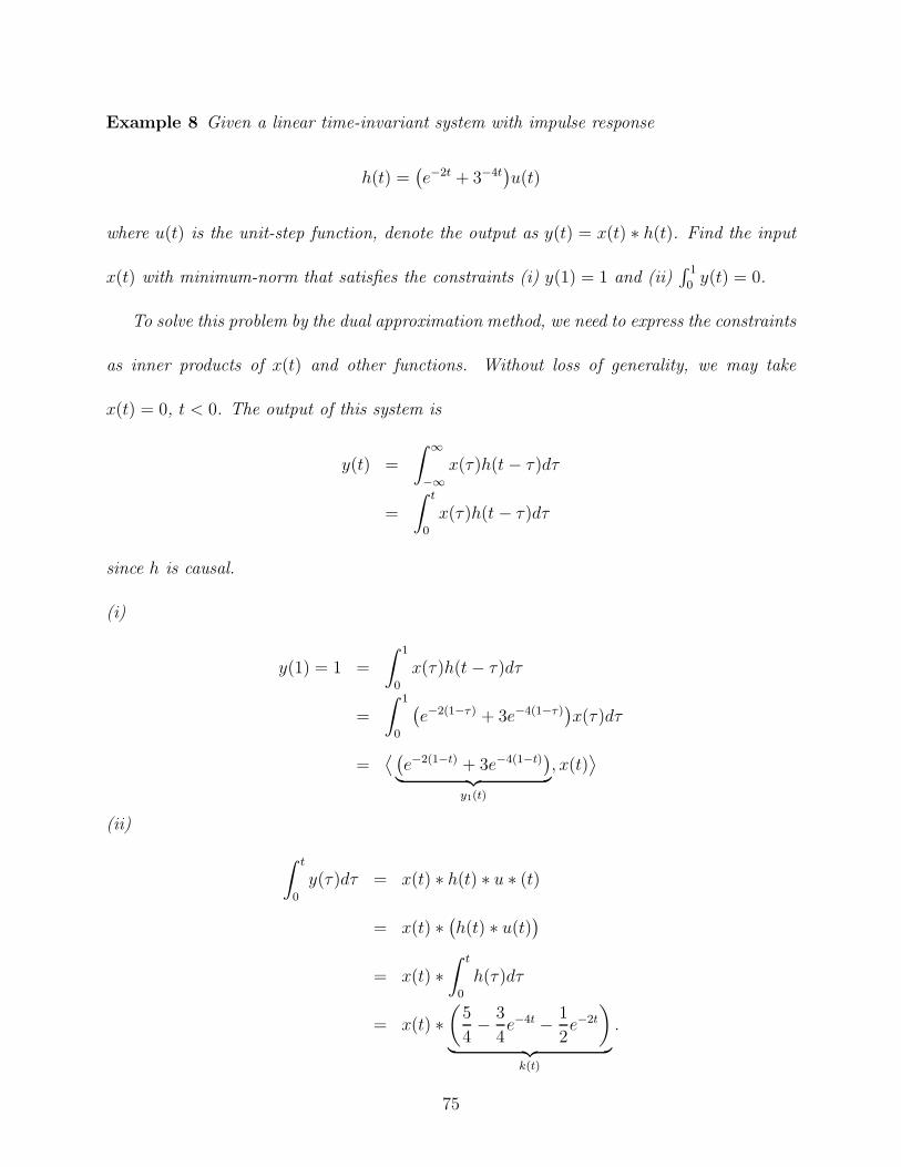
Example 8 Given a linear time-invariant system with impulse response
h(t) =1
e"2t + 3"4t2
u(t)
where u(t) is the unit-step function, denote the output as y(t) = x(t) : h(t). Find the input
x(t) with minimum-norm that satisfies the constraints (i) y(1) = 1 and (ii). 10 y(t) = 0.
To solve this problem by the dual approximation method, we need to express the constraints
as inner products of x(t) and other functions. Without loss of generality, we may take
x(t) = 0, t < 0. The output of this system is
y(t) =
# !
"!x(")h(t & ")d"
=
# t
0
x(")h(t & ")d"
since h is causal.
(i)
y(1) = 1 =
# 1
0
x(")h(t & ")d"
=
# 1
0
1
e"2(1"#) + 3e"4(1"#)2
x(")d"
=G 1
e"2(1"t) + 3e"4(1"t)2
@ AB C
y1(t)
, x(t)H
(ii)
# t
0
y(")d" = x(t) : h(t) : u : (t)
= x(t) :1
h(t) : u(t)2
= x(t) :# t
0
h(")d"
= x(t) :3
5
4& 3
4e"4t & 1
2e"2t
$
@ AB C
k(t)
.
75
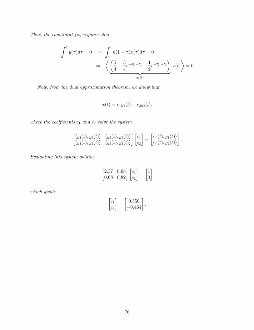
Thus, the constraint (ii) requires that
# 1
0
y(")d" = 0 ;# 1
0
k(1 & ")x(")d" = 0
;=3
5
4& 3
4e"4(1"t) & 1
2e"2(1"t)
$
@ AB C
y2(t)
, x(t)
>
= 0
Now, from the dual approximation theorem, we know that
x(t) = c1y1(t) + c2y2(t),
where the coe"cients c1 and c2 solve the system
"
0y1(t), y1(t)1 0y2(t), y1(t)10y1(t), y2(t)1 0y2(t), y2(t)1
? "
c1
c2
?
=
"
0x(t), y1(t)10x(t), y2(t)1
?
.
Evaluating this system obtains
"
2.37 0.680.68 0.82
? "
c1
c2
?
=
"
10
?
which yields"
c1
c2
?
=
"
0.556&0.464
?
.
76
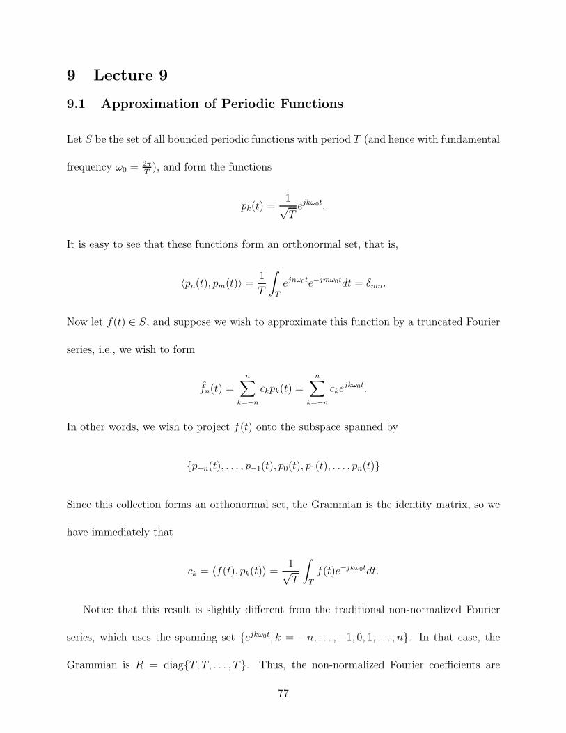
9 Lecture 9
9.1 Approximation of Periodic Functions
Let S be the set of all bounded periodic functions with period T (and hence with fundamental
frequency ,0 = 2!T
), and form the functions
pk(t) =1<T
ejk"0t.
It is easy to see that these functions form an orthonormal set, that is,
0pn(t), pm(t)1 =1
T
#
T
ejn"0te"jm"0tdt = #mn.
Now let f(t) ( S, and suppose we wish to approximate this function by a truncated Fourier
series, i.e., we wish to form
fn(t) =n+
k="n
ckpk(t) =n+
k="n
ckejk"0t.
In other words, we wish to project f(t) onto the subspace spanned by
{p"n(t), . . . , p"1(t), p0(t), p1(t), . . . , pn(t)}
Since this collection forms an orthonormal set, the Grammian is the identity matrix, so we
have immediately that
ck = 0f(t), pk(t)1 =1<T
#
T
f(t)e"jk"0tdt.
Notice that this result is slightly di!erent from the traditional non-normalized Fourier
series, which uses the spanning set {ejk"0t, k = &n, . . . ,&1, 0, 1, . . . , n}. In that case, the
Grammian is R = diag{T, T, . . . , T}. Thus, the non-normalized Fourier coe"cients are
77
related to the normalized Fourier coe"cients as
ak =1<T
ck.
One if the important questions of mathematical analysis is the issue of the convergence
of fn(t) to f(t) as n " 2.
9.2 Generalized Fourier Series
The familiar Trigonometric series discussed above is but one example of a way to represent
functions in terms as a sum of orthonormal basis functions. In fact, there are many such
representations. We will not discuss many of them in detail, but it is important to present
the basic theorems that pertain.
Theorem 14 (Bessel Inequality). Let {p1, p2, . . .} be an orthonormal basis for a Hilbert
space S. Then, for x ( S and m < 2,
m+
i=1
|0x, pi1|2 $ .x.2.
Proof Since
xm =m+
i=1
0x, pi1pi
is the minimum L2 norm approximation to x, the triangle inequality (.x.2 = .x.2+.x&x.2)
yields<<<<<x &
m+
i=1
0x, pi1pi
<<<<<
2
= .x.2 &m+
i=1
|0x, pi1|2 .
Since the error cannot be negative, the result follows. !
78
Theorem 15 Let {pi, i = 1, 2, . . .} be an orthonormal set in a Hilbert space S. Each of the
following four conditions implies the other three:
(a) {pi, i = 1, 2, . . .} is a maximal orthonormal set in S.
(b) The set M of all linear combinations of members of {pi, i = 1, 2, . . .} is dense in S.
(c) For every x ( S, we have
.x.2 =!+
i=1
.0x, pi1.2.
(d) If x ( S and y ( S, then
0x, y1 =!+
i=1
0x, pi10y, pi1.
To say that {pi, i = 1, 2, . . .} is maximal means simply that no vector of S can be adjoined
to {pi, i = 1, 2, . . .} in such a way that the resulting set is still orthonormal. This happens
precisely when there is no x += 0 in S which is orthogonal to every pi.
To say that M , S is dense in S means that the closure of M equals S. This means that
every Cauchy sequence in M converges to an element of S.
The last formula is known as Parseval’s identity. Also, observe that condition (c) is
a special case of condition (d). Maximal orthonormal sets are frequently called complete
orthonormal sets or orthonormal bases.
Proof We will show that (a) " (b) " (c) " (d) " (a).
(a) " (b)
Let H be the closure of M . Since M is a subspace, so is H . If M is not dense in S, then
H += S, so that H( contains a vector z += 0 such that 0z, pi1 = 0 for all i = 1, 2, . . .. Thus
{pi} is not maximal if M is not dense, and (a) implies (b).
79
(b) " (c)
Suppose (b) holds, and fix x ( S and $ > 0. Since M is dense, there is a finite set
{p1, p2, . . . , pm} such that some linear combination of these vectors has distance less than
$ from x. Since the coe"cients 0x, pi1 minimize the error, the approximation can only be
improved by taking 0x, pi1 as the coe"cients. Thus, if
z =m+
i=1
0x, pi1pi,
then .x & z. < $, hence .x. < .z. + $. Thus,
(.x. & $)2 < .z.2 =m+
i=1
|0x, pi1|2 $!+
i=1
|0x, pi1|2.
Since $ is arbitrary, (c) follows from the above and Bessel’s inequality.
(c) " (d).
The expression
0x, y1 =!+
i=1
0x, pi10y, pi1.
can be written as
0x, x1 = 0x, y1,
where x and y are the vectors in !2 comprising the complex numbers {0x, p11, 0x, p21, 0x, p31, . . .}
and {0y, p11, 0y, p21, 0y, p31, . . .}, respectively. The inner product on the left is taken in the
Hilbert space S and the inner product on the right is taken in !2. Fix x ( S and y ( S. If
(c) holds, then
0x + /y, x + /y1 = 0x + /y, x + /y1
for every scalar /. Hence
/0x, y1 + /0x, y1 = /0x, y1 + /0x, y1.
80
Take / = 1 and / = j. Then the above expression shows that 0x, y1 and 0x, y1 have the
same real and imaginary parts, hence are equal. Thus, (c) implies (d).
(d) " (a)
If (a) is false, then there exists a p += 0 in S such that 0p, pi1 = 0 for i = 1, 2, . . .. If
x = y = p, then 0x, y1 = .p.2 += 0, but 0x, pi1 = 0 for i = 1, 2, . . ., hence (d) fails. Thus, (d)
implies (a) and the proof is complete. !
The practical implication of this theorem is that, given a Hilbert space S and an ortho-
normal basis {pi}, we may express any element x of S as
x =!+
i=1
0x, pi1pi.
We should note, however, that this equality is defined in terms of the L2 norm, and this
calls for a note of qualification. Strictly speaking, when Lp is regarded as a metric space,
the space that is really under consideration is not a space whose elements are functions,
but a space whose elements are equivalence classes of functions, that is, functions which are
identical except on a set of Lebesgue measure zero. Thus, convergence need not be pointwise.
In particular, for Trigonometric series, let C(T ) denote the set of continuous functions in
L2 with period T . It may be conjectured that, for x(t) ( C(T ), the trigonometric series
converges pointwise (that is, for all t). However, this conjecture is not true. Examples can
be constructed of continuous periodic functions whose Fourier series diverges at some points!
Such examples are of mathematical significance, but are of little engineering importance.
It is important to understand, however, the sense in which convergence occurs. It is L2-
convergence (zero energy in the error).
81
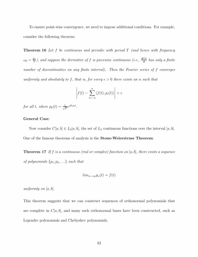
To ensure point-wise convergence, we need to impose additional conditions. For example,
consider the following theorem:
Theorem 16 Let f be continuous and periodic with period T (and hence with frequency
,0 = 2!T
), and suppose the derivative of f is piecewise continuous (i.e., df(t)dt
has only a finite
number of discontinuities on any finite interval). Then the Fourier series of f converges
uniformly and absolutely to f , that is, for every $ > 0 there exists an n such that
KKKKKf(t) &
n+
i="n
0f(t), pi(t)1
KKKKK< $
for all t, where pk(t) = 1,Tejk"0t.
General Case:
Now consider C[a, b] ( L2[a, b], the set of L2 continuous functions over the interval [a, b].
One of the famous theorems of analysis is the Stone-Weierstrass Theorem:
Theorem 17 If f is a continuous (real or complex) function on [a, b], there exists a sequence
of polynomials {p1, p2, . . .} such that
limn$!pn(t) = f(t)
uniformly on [a, b].
This theorem suggests that we can construct sequences of orthonormal polynomials that
are complete in C[a, b], and many such orthonormal bases have been constructed, such as
Legendre polynomials and Chebyshev polynomials.
82
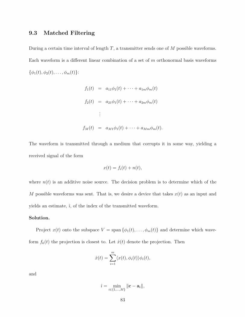
9.3 Matched Filtering
During a certain time interval of length T , a transmitter sends one of M possible waveforms.
Each waveform is a di!erent linear combination of a set of m orthonormal basis waveforms
{*1(t), *2(t), . . . , *m(t)}:
f1(t) = a11*1(t) + · · ·+ a1m*m(t)
f2(t) = a21*1(t) + · · ·+ a2m*m(t)
...
fM(t) = aM1*1(t) + · · · + aMm*m(t).
The waveform is transmitted through a medium that corrupts it in some way, yielding a
received signal of the form
x(t) = fi(t) + n(t),
where n(t) is an additive noise source. The decision problem is to determine which of the
M possible waveforms was sent. That is, we desire a device that takes x(t) as an input and
yields an estimate, ı, of the index of the transmitted waveform.
Solution.
Project x(t) onto the subspace V = span {*1(t), . . . , *m(t)} and determine which wave-
form fk(t) the projection is closest to. Let x(t) denote the projection. Then
x(t) =m+
i=1
0x(t), *i(t)1*i(t),
and
ı = mini%{1,...,M}
.c & ai.,
83
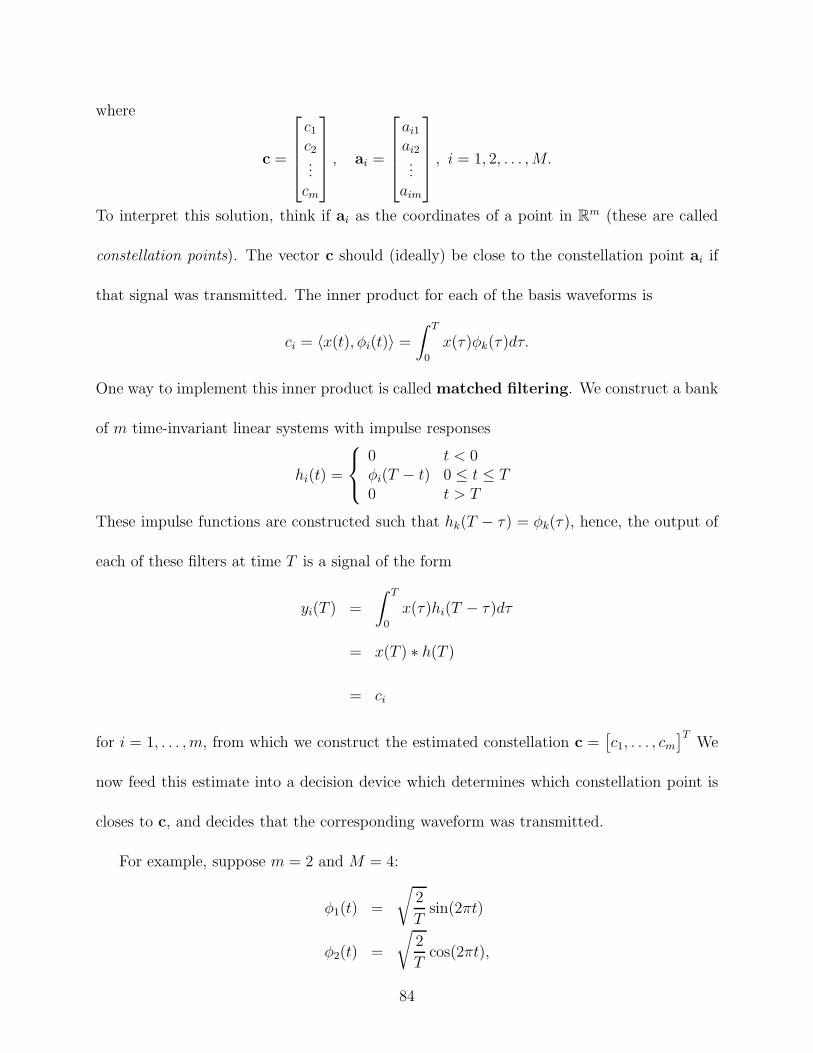
where
c =
%
&&&'
c1
c2...
cm
(
)))*
, ai =
%
&&&'
ai1
ai2...
aim
(
)))*
, i = 1, 2, . . . , M.
To interpret this solution, think if ai as the coordinates of a point in Rm (these are called
constellation points). The vector c should (ideally) be close to the constellation point ai if
that signal was transmitted. The inner product for each of the basis waveforms is
ci = 0x(t), *i(t)1 =
# T
0
x(")*k(")d".
One way to implement this inner product is called matched filtering. We construct a bank
of m time-invariant linear systems with impulse responses
hi(t) =
5
6
7
0 t < 0*i(T & t) 0 $ t $ T0 t > T
These impulse functions are constructed such that hk(T & ") = *k("), hence, the output of
each of these filters at time T is a signal of the form
yi(T ) =
# T
0
x(")hi(T & ")d"
= x(T ) : h(T )
= ci
for i = 1, . . . , m, from which we construct the estimated constellation c =,
c1, . . . , cm
-TWe
now feed this estimate into a decision device which determines which constellation point is
closes to c, and decides that the corresponding waveform was transmitted.
For example, suppose m = 2 and M = 4:
*1(t) =
L
2
Tsin(2(t)
*2(t) =
L
2
Tcos(2(t),
84
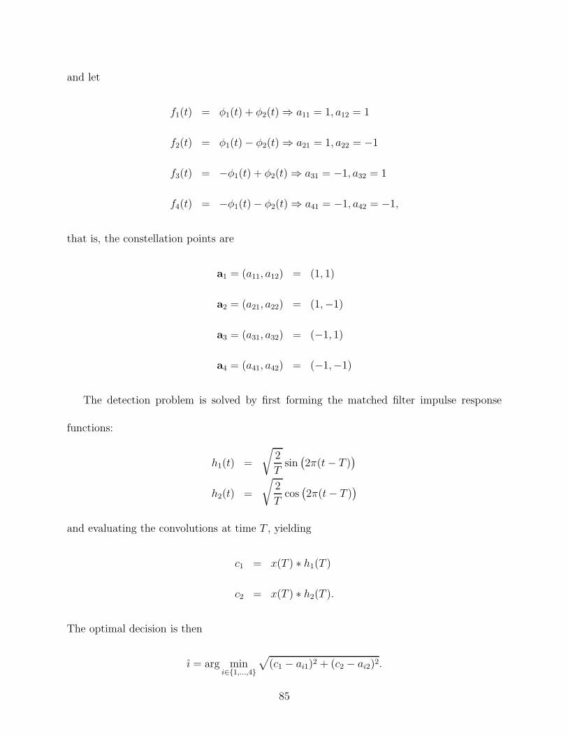
and let
f1(t) = *1(t) + *2(t) ; a11 = 1, a12 = 1
f2(t) = *1(t) & *2(t) ; a21 = 1, a22 = &1
f3(t) = &*1(t) + *2(t) ; a31 = &1, a32 = 1
f4(t) = &*1(t) & *2(t) ; a41 = &1, a42 = &1,
that is, the constellation points are
a1 = (a11, a12) = (1, 1)
a2 = (a21, a22) = (1,&1)
a3 = (a31, a32) = (&1, 1)
a4 = (a41, a42) = (&1,&1)
The detection problem is solved by first forming the matched filter impulse response
functions:
h1(t) =
L
2
Tsin1
2((t & T )2
h2(t) =
L
2
Tcos1
2((t & T )2
and evaluating the convolutions at time T , yielding
c1 = x(T ) : h1(T )
c2 = x(T ) : h2(T ).
The optimal decision is then
ı = arg mini%{1,...,4}
M
(c1 & ai1)2 + (c2 & ai2)2.
85

That is, we conclude that fı(t) was sent.
86

10 Lecture 10
10.1 Operator Norms
Definition 31 Let S be a normed vector space, and let A be a linear operator mapping S
into itself (we write A: S " S). We say that A is bounded if there exists a real number M
such that
.Ax.p $ M.x.p
for all x ( S; M will be called a bound for A. Let us denote the least of these bounds by
.A.p, and denote this as the operator norm of A.
Useful equivalent characterizations of .A. are given by
.A.p = supx -=0
.Ax.p
.x.p
and
.A.p = sup&x&p=1
.Ax.p.
!
Example 9 The space of real-valued continuous functions on [a, b] is a vector space with
real scalars. For a continuous function f we have defined the uniform norm (the L! norm)
.f.! = supa.t.b
|f(t)|.
where |f(t)| here is ordinary absolute value of a real number, while .f. applies to the function
f , not to real numbers. Let us denote this normed linear space by C[a, b]. C[a, b] is complete;
this is not obvious but theorems in calculus tell us that a sequence of continuous functions
87
satisfying the Cauchy criterion uniformly converge to a continuous function. Recall that fn
convergesuniformly to f if, for every $, there exists an integer N such that n # N implies
that |f(t) & fn(t)| $ $ for all t ( [a, b] (in other words, N does not depend on t).
For any function * ( C, the operator
A$: f(t) 7" *(t)f(t)
is a bounded linear operator and
.A$. = supa.t.b
|*(t)|.
Also, if k(x, y) is a continuous function on the square {(x, y): a $ x $ b, a $ y $ b}.
then the operator Fk: f 7". b
ak(x, t)f(t)dt is a bounded linear operator taking C[a, b] into
C[a, b]; in fact,
.Fkf.! $# b
a
|k(x, t)||f(t)|dt $ supa.x.b,a.t.b
{k(x, t)}.f.!(b & a).
As a special case, it is easy to see that
.f.1 =
# b
a
|f(t)|dt
defines a norm. Clearly,
.f.1 $ (b & a).f.!
for every continuous function f . However, under the norm .·.1, C[a, b] is not complete, since
we can define an L1-Cauchy sequence of continuous functions whose limit is not continuous.
Theorem 18 If S is a normed vector space, then the set of bounded linear operators mapping
S into self forms a normed vector space with operator norm .A.p defined as above.
88
Proof
Let A1 and A2 be two arbitrary operators, and define vector addition as
(A1 + A2)x = A1x + A2x
for all x ( S, and define scalar multiplication as
(%A)x = %(Ax)
for all x ( S and all scalars %.
To establish boundedness, let M1 and M2 be bounds for A1 and A2, respectively. Then
.A1 + A2. = sup&x&=1
.A1x + A2x.
$ sup&x&=1
{.A1x. + .A2x.}
$ sup&x&=1
.A1x. + sup&x&=1
.A2x.
$ M1 + M2.
Also, .%Ax. = |%|Ax $ |%|M.x.. !
Theorem 19 If S is a complete normed vector space then the space of linear operators
taking S into itself is also a complete normed vector space.
Proof Suppose {A1, A2, A3 . . .} is a Cauchy sequence of operators (i.e., .An & Am. " 0 as
n, m," 2). Then for any x ( S, let xn = Anx (a vector in S). The sequence {x1, x2, . . .}
is a Cauchy sequence in S since
.xn & xm. = .Anx & Amx. = .(An & Am)x. $ .An & Am..x. " 0
89

as m, n " 2. Thus, {xn} has a limit for each x. Let x' = limn$! xn, and define the
operator A by the requirement that, %x ( S, Ax = x'. We shall show that A is a bounded
linear operator and that limn$! An = A (i.e., .An & A. " 0, the zero operator).
First, note that An = An & Am + Am, hence
.An. $ .An & Am. + .Am.,
and
.An. & .Am. $ .An & Am..
Similarly,
.Am. & .An. $ .Am & An. = .An & Am..
Hence,
KK.An. & .Am.
KK $ .An & Am..
This means that the sequence of real numbers .An. is a Cauchy sequence and therefore is
bounded, that is, .An. < Q for some real number Q for every n. Now, for any given x ( S,
Ax = Ax & Anx + Anx and
.Ax. = .Ax & Anx + Anx.
$ .Ax & Anx. + .Anx.
= .x' & xn. + .Anx.
$ .x' & xn. + Q.x..
But x' = limn$! xn, so .x' & xn. " 0 as n " 2; thus
.Ax. $ B.x..
90

This shows that A is bounded.
To show that A is linear, we must show that it is homogeneous and additive. Homogeneity
requires thatA(%x) = %Ax. To establish this property, we write
A(%x) & %Ax = A(%x) & An(%x) + An(%x) & %Ax + %Anx & %Anx.
Hence
.A(%x) & %Ax. $ .A(%x) & An(%x). + |%|.Ax & Anx. + .An(%x) & %Anx..
But, as n " 2, .A(%x)&An(%x). " 0 and |%|.Ax&Anx. " 0 since A(%x) = limn$! An(%x)
and Ax = limn$! Anx. Also, .An(%x) & %Anx. = 0 since An is linear. Thus, .A(%x) &
%Ax. = 0 so A(%x) = %Ax.
To show that A is additive, we must establish that A(x + y) = Ax + Ay. We write
A(x + y) = A(x + y) + An(x + y) & An(x + y)
= [A(x + y) & An(x + y)] + Anx + Any.
But, letting z = x + y, we see that the term in brackets on the right of the above expression
is Anz & Az, which, by construction, converges to zero. Thus, as n " 2, we have
A(x + y) = Ax + Ay.
We have thus established that A is linear and bounded. To complete our proof, however,
we still need to show that .An. " .A.. Fix $ > 0. Then for each x += 0, there exists an
integer m0 (depending on x) such that
.Ax & Am0x. <$
2.x.,
91
and
.An & Am0. <$
2
when n > m0. Then, if n > m0,
.Ax & Anx. $ .Ax & Am0x. + .Am0x & Anx.
$ $
2.x. + .Am0 & An..x.
$ $.x..
Hence, .An & A. $ $ when n > 0. Thus, An " A as n " 2 (i.e., .An & a. " 0). !
Theorem 20 If A and B are bounded linear operators taking a normed vector space into
itself, then the product AB is a bounded linear operator and .AB. $ .A..B..
Proof
.AB. = sup&Bx&=1
.ABx. = .A..Bx. $ .A. sup&x&
.Bx. = .A..B.,
thus AB is bounded. To establish linearity,
AB(%x + &y) = A(%Bx + &By) = %ABx + &ABy.
!
A consequence of this theorem is that, if A is bounded linear operator, then Ak is also a
bounded linear operator for k = 0, 1, 2, . . .. We may form the infinite series of operators of
the form
An = A0 + A1 + A2 + · · ·+ An,
92
thereby generating a sequence {An} of linear operators. Note that A0 = I. We consider the
case .A. < 1. Then,
.An & Am. = .Am+1 + Am+2 + · · · + An. $ .Am+1. + .Am+2. + · · ·+ .An..
Note that the geometric series (with .A0. = 1)
1 + .A. + .A.2 + .A.3 + · · ·
is convergent to 11"&A& . Hence the sequence {An} is a convergent sequence of operators. From
the completeness theorem, the sequence {An} has a limit, call this limit K. By analogy with
the infinite series of real numbers, we call K the sum of the series of operators:
K = I + A + A2 + A3 + · · · .
Multiplying both sides by A yields
AK = KA = A(I + A + A2 + A3 + · · · ) = A + A2 + A3 + · · · .
Then
K & KA = I
and
K & AK = I.
Hence,
K(I & A) = (I & A)K = I,
and K is a two-sided inverse of (I & A).
93
Theorem 21 In any multiplication which is associative (i.e., (ab)c = a(bc)), if an element
a has a left inverse ba = I and a right inverse ac = I, where I is a two-sided identity, then
b = c and the inverse is of a unique.
Proof To establish that b = c, we observe that, by associativity,
bI = b(ac) = (ba)c = Ic.
which establishes that b = c. Suppose there exists another left inverse b' += b. But then
b'a = I = ba,
and multiplying both sides on the right by c yields
b' = b'ac = bac = b.
!
This theorem establishes that there is a unique two-sided inverse of K, which may prop-
erly be denoted as (I&A)"1. Thus, if A is a linear operator taking a complete normed vector
space S into itself and .A. < 1, then (I & A)"1 exists and
(I & A)"1 = I + A + A2 + A3 + · · · .
This expression is often called the Neumann series for A.
Example 10 For f ( C[a, b], define the operator A by
Af =
# b
a
k(x, t)f(t)dt,
94
where k is continuous on the square {(x, t): a $ x $ b, a $ t $ b}. Suppose
(b & a) sup |k(x, t)| < 1.
Then .A. < 1 and for any given g ( C, the integral equation
f(x) &# b
a
k(x, t)f(t)dt = g(x)
has a unique continuous solution for f . In fact,
f = (I & A)"1g = g + Ag + A2g + · · ·
is a uniformly convergent sequence of functions.
95
11 Lecture 11
11.1 Linear Functionals
Let X be a vector space. As we have seen, the set of all linear operators mapping X onto
another space Y is also a vector space, with vector operations
(%A1 + &A2)x = %A1x + &A2x
for all x ( X.
Definition 32 A linear operator that maps a vector space X into R is called a linear
functional. The vector space of linear functionals over a vector space X is called the dual
space, or algebraic conjugate space of X, denoted X#. !
Theorem 22 The Riesz-Frechet Theorem. For every bounded linear functional A defined
over a Hilbert space X, there is a vector xA ( X such that Ax = 0x, xA1 for every x ( A.
(In other words, every linear functional can be expressed as an inner product.)
Proof Let M = .A. = sup&x&=1 .Ax.. Then there is a sequence {x'n} in X with .x'
n. = 1
such that
limn$!
.Ax'n. = M.
If M = 0 then the result of the theorem is obvious since then A = 0 and xA = 0. Suppose
M += 0; then we may assume Ax'n += 0 (we may have to discard a finite number of terms
from this sequence if necessary). Let
qn =.Ax'
n.Ax'
n
.
96
Then qn is a complex number with |qn| = 1 and let
xn = qnx'n.
Then .xn. = 1 and
Axn = qnAx'n = .Axn. " M
as n " 2. Thus we have a sequence of unit vectors {xn} such that Axn is real and Axn " M .
We shall use the identity
.x + y.2 + .x & y.2 = 2.x.2 + 2.y.2
(which holds for every x, y ( X) to show that {xn} is a Cauchy sequence. Using this identity,
we have
.xm & xn.2 = 2 · 1 + 2 · 1 & .xm + xn.2 $ 4 & .A(xm + xn).2
M2" 4 & 4M2
M2= 0
as m, n " 2. Then, since X is complete, there is a vector x'A ( X such that xn " x'
A.
Clearly, .x'A. = 1 and Ax'
A = M . That is, A actually attains its upper bound on a unit
vector x'A. Now let xA = Mx'
A. Then
Ax'A = M = 0x'
A, xA1.
Suppose Ax0 = 0; we shall show that 0x0, x'A1 = 0. In fact, for any complex /, we have
M2 = [A(x'A & /x0)]
2 $ M2.x'A & /x0.2 = M2
1
1 & /0x0, x'A1 & /0x'
A, x01 + //0x0, x012
.
Hence, for any complex /,
&/0x0, x'A1 & /0x'
A, x01 + //0x0, x01 # 0.
97
For convenience, let us write /0x0, x'A1 = a + jb; then the above expression becomes
&/(a + jb) & /(a & jb) + |/|2.x0.2 # 0
or
&a(/ + /) & jb(/ & /) + |/|2.x0.2 # 0,
or
&2a/(/) & j2b=(/) + |/|2.x0.2 # 0
This implies that b = 0, since the quantity must be real for all values of /. Now suppose
a += 0. Then set / = a&x0&2 , which yields
&2a2
.x0.2+
a2
.x0.4.x0.2 > 0,
which can obtain only if a = 0. Thus,
0x0, x'A1 = a + jb = 0.
Now, for any x ( X, let x0 = x & AxM
x'A. (of course, Ax
Mis a scalar). Then
Ax0 = Ax & Ax
MAx'
A = Ax & AxAx'
A
M= Ax & Ax = 0,
and
Ax = A
3
x0 +Ax
Mx'
A
$
= Ax0 +Ax
MAx'
A
= 0x0, xA1 +
=
Ax
Mx'
A, xA
>
=
=3
x0 +Ax
Mx'
A
$
, xA
>
= 0x, xA1
98
as required. !
Let A be a bounded linear operator taking vector space X into vector space Y . For fixed
y ( Y , define a bounded linear functional F on X by
Fx = 0Ax, y1
(F depends on both A and y). By the Riesz theorem, there exists a unique vector xF ( X
such that
Fx = 0Ax, y1 = 0x, xF 1.
Now define a transformation A# by A#y = xF . Substituting, we obtain
0x, xF 1 = 0x, A#y1.
Hence
0Ax, y1 = 0x, A#y1.
It is critical to appreciate that these two inner products are defined over di!erent vector
spaces. The one on the left is defined over Y , the range of A, Y , and the one on the right is
defined over X, the range of A#.
Theorem 23 A# is a bounded linear operator mapping Y into X. Furthermore,
A## = A,
(aA#) = aA#,
(A1 + A2)# = A#
1 + A#2,
99
and
(A1A2)# = A#
2A#1.
Finally, if X = Y and A has an inverse, then A# also has an inverse and
1
A#2"1=1
A"12#
.
Proof To show homogeneity, we have
0x, A#(ay)1 = 0Ax, ay1 = a0Ax, y1
= a0x, A#y1 = 0x, aA#y1.
To show additivity, we have
0x, A#(y1 + y2)1 = 0Ax, y1 + y21 = 0Ax, y11 + 0Ax, y21
= 0x, A#y11 + 0x, A#y21 = 0x, A#y1 + A#y21.
To establish the equality of the norms, we observe that
.A#y.2 = 0A#y, A#y1 = 0AA#y, y1
$ .AA#y..y. $ .A..A#y..y.,
thus .A#y. $ .A..y., which proves that .A#. $ .A.. By a similar argument, we can show
that .A. $ .A#., hence equality obtains.
The remaining properties are demonstrated by straightforward manipulations of the de-
finition. For example, to show that1
A#2"1
=1
A"12#
, we write
0x, y1 = 0x, A#(A#)"1y1 = 0Ax, (A#)"1y1.
100
Now let B# = (A#)"1, so we obtain 0x, y1 = 0BAx, y1, which requires that BA = I so
B = A"1. Thus,1
A#2"1=1
A"12#
. !
Example 11 Let A: Rn " Rm. Then A can be represented as an m ! n matrix; that
is A = {aij}, where 1 = 1, 2, . . . , m and j = 1, 2, . . . , n. Let x = {x1, . . . xn} ( Rn and
y = {y1, . . . , ym} ( Rm. Then, using the Euclidean inner product (the “dot” product),
0Ax,y1 =m+
i=1
n+
j=1
yiaijxj =n+
j=1
xj
m+
i=1
aijyi = 0x, AHy1
Thus, the adjoint of a matrix is the conjugate transpose,
A# = AT = AH .
Definition 33 If A = A#, then A is said to be self-adjoint. A real matrix that is self-
adjoint is symmetric. A complex matrix that is self-adjoint is said to be Hermitian. !
Example 12 Convolution. Let A: L2 " L2 be defined by
Ax =
# t
0
h(t & ")x(")d",
for x ( L2. Then, for y ( L2, we have
0Ax, y1 =
# !
0
"# t
0
h(t & ")x(")d"
?
y(t)dt
=
# !
0
# !
0
h(t & ")x(")I("!,t](")y(t)d"dt
=
# !
0
# !
0
h(t & ")x(")I("!,t](")y(t)dtd"
=
# !
0
# !
0
h(t & ")x(")I[#,!)(t)y(t)dtd"
=
# !
0
x(")
"# !
#
h(t & ")y(t)dt
?
d",
101
where we have used the indicator function
IA(t) =
4
1 t ( A0 t +( A
to facilitate changing the order of integration by noting that
I("!,t](") = I[#,!)(t).
Consequently, since
0Ax, y1 = 0x, A#y1,
we identify the adjoint operator
A#y =
# !
t
h(" & t)y(")dt.
Example 13 Linear ODE’s. Consider the linear matrix di!erential equation
x(t) = Fx(t), t # 0, x(0) = x0,
where F is an n ! n matrix and x0 ( Rn. Let A: Rn " L2[0, T ] be given by
Ax0 = eFtx0.
The adjoint operator, A#, must satisfy, for y ( L2[0, T ] the equation
0Ax, y1L2 = 0xA#y1Rn,
where we have suppled subscripts to 0·, ·1 to reinforce the fact that the inner product on the
left is in L2 and the inner product on the right is in Rn. Thus, we require
# T
0
xT0 eF T ty(t)dt = xT
0 A#y,
102

or
xT0
# T
0
eF T ty(t)dt = xT0 A#y,
which implies that
A#y =
# T
0
eF T ty(t)dt.
11.2 Four Fundamental Subspaces
Recall the definitions of range and nullspace of an operator:
Definition 34 The range, R(A), of a linear operator A: X " Y is the set of all vectors
y ( Y such that there exists a corresponding x ( X that maps to y; that is,
R(A) = {y ( Y : )x ( X: Ax = y}.
The nullspace, N (A), of a linear operator A: X " Y is the set of vectors x ( X that
map to the zero vector in Y ; that is,
N (A) = {x ( X: Ax = 0}.
The dimension of N (A) is called the nullity of A. It is easy to confirm that the range
and nullspace are legitimate subspaces, since they are closed under addition and scalar
multiplication. !
Definition 35 An operator A: X " Y is said to be one-to-one if Ax1 += Ax1 whenever
x1 += x2, that is, no two vectors map to the same point in the range. A one-to-one mapping
is called an injection. It is easy to see that the null space of an injection is the zero vector
in X. !
103
If A is not an injection, then the nullspace is non-trivial, and the equation Ax = b will
have an infinity of solutions since, if xb is a solution to Ax = b and x0 ( N (A), then
x = xb + x0 is also a solution:
Ax = A(xb + x0) = Axb + Ax0 = b + 0.
Definition 36 For an operator A: X " Y , The range of the adjoint, denoted R(A#) is
the set of all vectors x ( X such that there exists a corresponding y ( Y that maps to x;
that is,
R(A#) = {x ( X: )y ( Y : A#y = x}.
The nullspace of the adjoint, denoted N (A#), is the set of vectors y ( Y that map to the
zero vector in X; that is,
N (A#) = {y ( Y : A#y = 0}.
!
Theorem 24 Set X and Y be Hilbert spaces, and let A: X " Y be a bounded linear operator.
If R(A) and R(A#) are closed subspaces (of Y and X, respectively), then
[R(A)]( = N (A#)
[R(A#)]( = N (A)
R(A) = [N (A#)](
R(A#) = [N (A)]( .
104
Proof We first show that N (A#) , [R(A)](. Let n ( N (A#) and let y ( R(A). Then there
exists some x ( X such that y = Ax, and
0y, n1Y = 0Ax, n1Y = 0x, A#n1X = 0x, 01X = 0.
This demonstrates that n 3 y, and since n and y are arbitrary, we may conclude every
element of the nullspace of A# is orthogonal to every element of the range of A. Thus, every
element of the nullspace of A# lies in the orthogonal complement of the range space of A;
i.e., N (A#) , [R(A)](.
We next show that [R(A)]( , N (A#). Let y ( [R(A)](. Then y is orthogonal to the
image of every x ( X. Thus,
0 = 0Ax, y1Y = 0x, A#y1X .
This must hold for every x ( X, but the only vector that is orthogonal to every vector in X is
the zero vector, thus we must conclude that A#y = 0, which means that y lies in the nullspace
of A#. Thus, [R(A)]( , N (A#). Finally, since N (A#) , [R(A)]( and [R(A)]( , N (A#), we
conclude that N (A#) = [R(A)](.
To establish [R(A#)]( = N (A), we can follow the above procedure with A# replacing A
and use the fact that A## = A.
We complete the proof by noting that, since by hypothesis R(A) and R(A#) are closed,
we may simply take the orthogonal complements of the above results to obtain
R(A) = [N (A#)](
R(A#) = [N (A)]( .
105
!
Theorem 25 Under the hypothesis of the above theorem,
X = R(A#) 5N (A)
Y = R(A) 5N (A#),
where we employ the isomorphic interpretation of the direct sum. Also,
dim (X) = dim1
R(A#)2
+ dim1
N (A)2
dim (Y ) = dim1
R(A)2
+ dim1
N (A#)2
,
and
dim1
R(A)2
= dim1
R(A#)2
.
Proof Let x ( X. Then, by the projection theorem, there is a unique v0 ( R(A#) such that
.x& v0. $ .x& v. for all v ( R(A#). Then the vector w0 = x& v0 ( [R(A#)]. We can thus
decompose any vector in x ( X into x = v0+w0 with v0 ( R(A#) and w0 ( [R(A#)] = N (A).
Thus, X = R(A#) 5N (A). A similar argument establishes that Y = R(A) 5N (A#). The
claims dim (X) = dim1
R(A#)2
+ dim1
N (A)2
and dim (Y ) = dim1
R(A)2
+ dim1
N (A#)2
then follow immediately.
We show dim1
R(A)2
= dim1
R(A#)2
by establishing that (i) dim1
R(A)2
$ dim1
R(A#)2
and (ii) dim1
R(A)2
# dim1
R(A#)2
. To show (i), let P = {p1, p2, . . .} be a basis set for
R(A). Then dim1
R(a)2
equals the cardinality of P . Since P , R(A), each pi ( P may be
expressed as the mapping of some vector qi ( A, that is, pi = Aqi.
106
Since X = R(A#) 5N (A), there is a unique decomposition
qi = qi + ni,
where qi ( R(A#) and ni ( N (A). Therefore,
pi = Aqi.
For any index set I, we have
+
i%I
cipi =+
i%I
ciAqi = A+
i%I
ciqi.
Since!
i%I ciqi is an element of R(A#), it is orthogonal to N (A). Therefore, the only way
this vector can map to the nullspace of A is if!
i%I ciqi = 0. But then this would mean
that!
i%I cipi = 0, and since the {pi}’s form a linearly independent set, the only way that
can happen is for ci = 0 for all i ( I. Thus, the only way for!
i%I ciqi = 0 to occur is for
ci = 0 for all i ( I. This implies that the set Q = {q1, q2, . . .} is a linearly independent set
in R(A#). This implies that the cardinality of the space spanned by Q is at least as large as
the cardinality of the space spanned by P . Thus, dim1
R(A)2
$ dim1
R(A#)2
.
To show that dim1
R(A)2
# dim1
R(A#)2
, we replace A by A# and A# by A and repeat
the above argument. !
107
12 Lecture 12
12.1 The Fredholm Alternative Theorem
We need to address, as generally as possible, the question of precisely when a solution to the
operator equation Ax = b has an exact solution.
Theorem 26 The Fredholm Alternative Theorem. Let A be a bounded linear operator map-
ping the Hilbert space X into the Hilbert space Y . The equation Ax = b has a solution if and
only if 0b, v1 = 0 for every vector v ( N (A#); that is, if
b ( R(A) if and only if b 3 N (A#).
For the special case A: Cn " Cm; that is, A is an m! n matrix, then Ax = b has a solution
if and only if vHb = 0 for every v ( Cm such that AHv = 0.
Proof We first prove the “if” part of the theorem. Suppose there exists an x such that
Ax = b (which means that b ( R(A)) and let v ( N (A#). Then
0b, v1Y = 0Ax, v1Y = 0x, A#v1X = 0x, 01X = 0.
Since v was an arbitrary element of N (A#) this implies that b is orthogonal to the nullspace
of A#.
To establish the “only if” part, we employ a contradiction. Suppose that 0b, v1 = 0 for
all v ( N (A#), but there is no x such that Ax = b; that is, b +( R(A). We may decompose b
as
b = br + b0,
108
where br ( R(A) and b0 ( N (A#). By assumption, 0b, v1 = 0, but then
0 = 0b, v1 = 0br, v0+0b0, v1,
which implies that
0br, v1 = &0b0, v1.
Note, however, that since br ( R(A) and v ( N (A#) = [R(A)](, the left hand side of this
equation is zero. However, since both b0 and v are elements of N (A#), the only way this
inner product can be zero for all v ( N (A#) is for b0 to be zero. But then b = br and
therefore would lie in the range of A, contrary to the supposition that no solution to Ax = b
exists. !
12.2 Dual Optimization
One of the applications of adjoint operators is to solve certain optimization problems. Recall
the minimum-norm problem discussed earlier, where we wish to find the minimum-norm
solution that satisfies a set of constraints. The following theorem applies to this situation.
Theorem 27 Dual Optimization Theorem A: X " Y be a bounded linear operator from
the Hilbert space X to the Hilbert space Y . The vector x of minimum norm satisfying the
constraint Ax = y is given by
x = A#z
where z is any solution of A#Az = y. If the operator AA# is invertible, then the minimizing
solution takes the form
x = A#1AA#2"1y.
109
Proof If x0 is a solution of Ax = y, the general solution is x = x0 + n, where n ( N (A).
Since N (A) is closed (because X is a Hilbert space), it follows that there exists a unique
vector x of minimum norm satisfying Ax = y and that this vector is orthogonal to N (A).
Thus, since R(A) is assumed closed, the decomposition theorem proved earlier applies, and
x ( [N (A)]( = R(A#).
Thus, the minimizing vector lies in the range of the adjoint operator, which means that
there is a vector z ( Y such that
x = A#z.
Substituting this into the constraint equation yields
AA#z = y.
Finally, if AA# is invertible, then z =1
AA#2"1
y, and we conclude that the minimum-norm
solution is
x = A#1AA#2"1y.
!
Example 14 The Linear Quadratic Regulator. Suppose a linear dynamic system is gov-
erned by a set of di!erential equations
x(t) = Fx(t) + bu(t), t # 0,
where x is an n ! 1vector of time functions, F is an n ! n constant matrix, b is an n ! 1
constant vector, and u(t) is a scalar control function.
110

Assume that this system starts at the origin at time t = 0, that is, x(0) = 0, and that it is
desired to transfer the system at time T to a terminal state x1, that is, we require x(T ) = x1
by application of a suitable control function u(t), 0 $ t $ T . Of the class of controls that will
accomplish this task, we desire the one of minimum energy, that is, we desire to minimize
# T
0
u2(t)dt,
subject to the terminal constraint x(T ) = x1. The explicit solution to the equation of motion
is
x(T ) =
# T
0
eF (T"t)bu(t)dt.
We may express this solution in operator form by defining A: L2[0, T ] " Rn by
Au =
# T
0
eF (T"t)bu(t)dt.
We wish to find a solution to the constraint Au = x1 that minimizes. T
0 u2(t)dt.
According to the Dual Optimization Theorem, the optimal solution is
u = A#z
for some z ( Rn such that
AA#z = x1.
It remains to calculate the operators A# and AA#. For any u ( L2[0, T ] and y ( Rn,
0Au, y1Rn = yT
# T
0
eF (T"t)bu(t)dt =
# T
0
yTeF (T"t)bu(t)dt = 0u, A#y1L2,
with
A#(t)y = bT eF T (T"t)y,
111
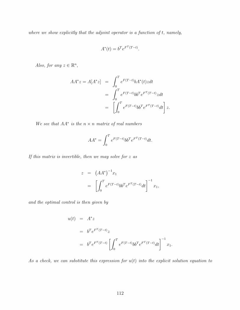
where we show explicitly that the adjoint operator is a function of t, namely,
A#(t) = bT eF T (T"t).
Also, for any z ( Rn,
AA#z = A[A#z] =
# T
0
eF (T"t)bA#(t)zdt
=
# T
0
eF (T"t)bbT eF T (T"t)zdt
=
"# T
0
eF (T"t)bbT eF T (T"t)dt
?
z.
We see that AA# is the n ! n matrix of real numbers
AA# =
# T
0
eF (T"t)bbT eF T (T"t)dt.
If this matrix is invertible, then we may solve for z as
z =1
AA#2"1x1
=
"# T
0
eF (T"t)bbT eF T (T"t)dt
?"1
x1,
and the optimal control is then given by
u(t) = A#z
= bT eF T (T"t)z
= bT eF T (T"t)
"# T
0
eF (T"t)bbT eF T (T"t)dt
?"1
x1.
As a check, we can substitute this expression for u(t) into the explicit solution equation to
112

obtain
x(T ) =
# T
0
eF (T"t)bu(t)dt
=
# T
0
eF (T"t)bbT eF T (T"t)dt
"# T
0
eF (T"s)bbT eF T (T"s)ds
?"1
x1
= x1
as required. Thus, the adjoint operator not only provided a solution (there is an infinity of
them), it provided the best one in the sense of minimizing the energy in the control signal.
In the control theory literature, the matrix. T
0 eF (T"t)bbT eF T (T"t)dt is called the control-
lability Grammian. If this matrix is non-singular, then the system is said to be control-
lable, and it is then theoretically possible to find a control input that can drive the system
from any initial condition to any terminal condition in finite time.
Let us explore the above example a but further. Consider the two di!erential systems
x = Fx + bu, x(0) = 0, (1)
and
/ = &F T /, /(T ) = /0 (2)
y = bT /,
where x and / are n ! 1 vectors, F is an n ! n matrix, b is an n ! 1 vector, and /0 is an
n ! 1 vector.
From our above development, we may express the solution to (1) in operator notation as
x(T ) = Au =
# T
0
eF (T"t)bu(t)dt.
113

For any vector z in Rn, we may form the inner product
0Au, z1Rn =
=# T
0
eF (T"t)bu(t)dt, z
>
Rn
= zT
# T
0
eF (T"t)bu(t)dt
=
=
u(t), bT eF T (T"t)z
>
L2
= 0u, A#z1L2 ,
from which we may identify the adjoint of A as A# = bT eF T (T"t).
Now let us examine the system given by (2). The solution to the di!erential equation is
/(t) = eF T (T"t)/0,
yielding the output
y(t) = bT eF T (T"t)/0.
In operator notation, this becomes
y(t) = B/0 = bT eF T (T"t)/0
or, in other words, B = bT eF T (T"t).
Now, for any function w(t) in L2, we may form the inner product
0[B/0](t), w(t)1L2 =
# T
0
bT eF T (T"t)/0w(t)dt
=
"# T
0
eF (T"t)bw(t)dt
?T
/0
=
=
/0,
# T
0
bT eF T (T"t)w(t)dt
>
Rn
= 0/0, B#w1Rn.
114
From these results we observe that A# = B and B# = A. For this reason, the two systems
given by (1) and (2) are termed dual systems. If we think of the original system given
by (1) as a model of some physical system we wish to characterize, then we refer to (2) as
the adjoint system. This notion of duality is a very powerful concept that couples control
and estimation theory in a very fundamental way. For example, it can be shown that if it is
possible to find a control that drives the original system from the origin to an arbitrary value
at time T , then it is possible, by observing the values y in the dual system, to reconstruct
the trajectory of / over the interval [0, T ]. In other words, a system is controllable if and
only if its adjoint system is observable.
It should be noted that the solution given in the above example is only one way to obtain
the optimal control. That solution is in the form of what is called open-loop control, since
u(t) does not depend on the current state x(t), but only on the initial (x(0) = 0) and final
(x(T ) = x1) state, and is pre-computed and then applied for all t. If, for some reason, the
state is perturbed of the predicted optimal trajectory, then such an open-loop controller will
not, in general result in x(T ) = x1. This observation prompts us to consider exploring ways
to implement this optimal control law in a closed-loop fashion, where u(t) is computed as
a function of the current state x(t) via a feedback mechanism, that is,
u(t) = K(t)x(t).
The matrix function K(t) is called the feedback gain matrix. One of the elegant results of
optimal control theory is the demonstration that the optimal controller can be implemented
via state feedback! Feedback controllers are more robust with respect to perturbations, as
115

well as being more simple to implement, since the computation of the observability Grammian
can be very expensive and messy. By making use of the dual system, however, it is possible
to design optimal feedback controllers that are robust and economical.
The power of duality is manifest by the fact that the very same mathematics that is
used to design an optimal controller can also be used to design an optimal estimator. This
unification of theories o!ers great elegance as well as economy for the design of controllers
and estimators.
116
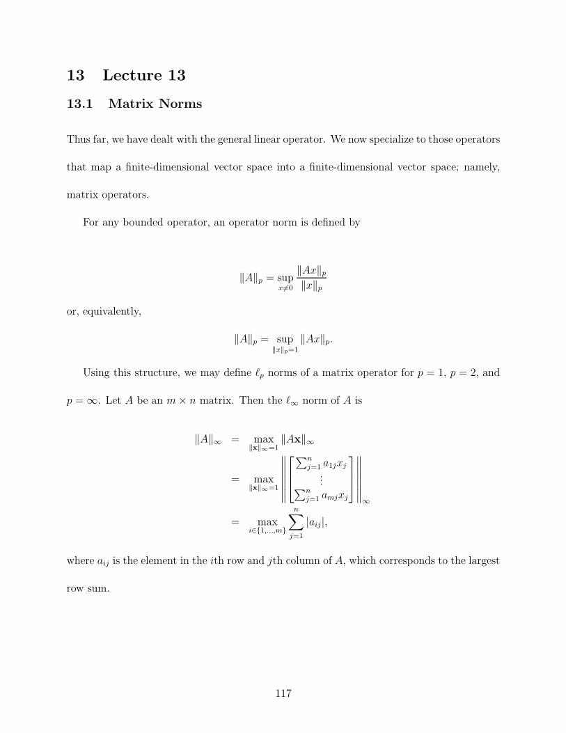
13 Lecture 13
13.1 Matrix Norms
Thus far, we have dealt with the general linear operator. We now specialize to those operators
that map a finite-dimensional vector space into a finite-dimensional vector space; namely,
matrix operators.
For any bounded operator, an operator norm is defined by
.A.p = supx -=0
.Ax.p
.x.p
or, equivalently,
.A.p = sup&x&p=1
.Ax.p.
Using this structure, we may define !p norms of a matrix operator for p = 1, p = 2, and
p = 2. Let A be an m ! n matrix. Then the !! norm of A is
.A.! = max&x&"=1
.Ax.!
= max&x&"=1
<<<<<<<
%
&'
!nj=1 a1jxj
...!n
j=1 amjxj
(
)*
<<<<<<<!
= maxi%{1,...,m}
n+
j=1
|aij|,
where aij is the element in the ith row and jth column of A, which corresponds to the largest
row sum.
117
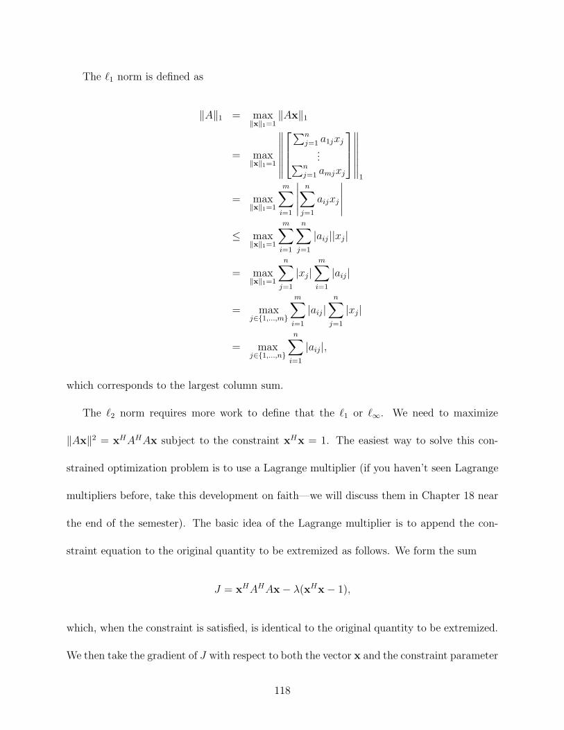
The !1 norm is defined as
.A.1 = max&x&1=1
.Ax.1
= max&x&1=1
<<<<<<<
%
&'
!nj=1 a1jxj
...!n
j=1 amjxj
(
)*
<<<<<<<
1
= max&x&1=1
m+
i=1
KKKKK
n+
j=1
aijxj
KKKKK
$ max&x&1=1
m+
i=1
n+
j=1
|aij ||xj|
= max&x&1=1
n+
j=1
|xj|m+
i=1
|aij |
= maxj%{1,...,m}
m+
i=1
|aij |n+
j=1
|xj |
= maxj%{1,...,n}
n+
i=1
|aij|,
which corresponds to the largest column sum.
The !2 norm requires more work to define that the !1 or !!. We need to maximize
.Ax.2 = xHAHAx subject to the constraint xHx = 1. The easiest way to solve this con-
strained optimization problem is to use a Lagrange multiplier (if you haven’t seen Lagrange
multipliers before, take this development on faith—we will discuss them in Chapter 18 near
the end of the semester). The basic idea of the Lagrange multiplier is to append the con-
straint equation to the original quantity to be extremized as follows. We form the sum
J = xHAHAx & /(xHx & 1),
which, when the constraint is satisfied, is identical to the original quantity to be extremized.
We then take the gradient of J with respect to both the vector x and the constraint parameter
118
/, yielding
+J
+x= AHAx & /x = 0 ; AHAx = /x (3)
+J
+/= xHx & 1 = 0 ; xHx = 1. (4)
The solutions to (3) are the eigenvalues of AHA. Furthermore, by multiplying both sides
of (3) by xH and invoking (4), we obtain
xHAHAx = /xHx = /.
We thus see that the quantity that maximizes xHAHAx is the maximum eigenvalue of AHA.
Thus,
.A.2 = maxi
{M
/i},
where /i are the eigenvalues of AHA. This is known as the spectral norm. We will have
much more to say about eigenvalues subsequently, but for now we simply observe that the
computation of the !2 norm is more complicated than the computation of !1 or !! norms.
If A is an invertible matrix, then the A and the norm of the inverse matrix A"1 are
related as follows. Let Ax = b, then A"1b = x. Thus,
<<A"1
<< = max
b-=0
.A"1b..b.
= maxx -=0
.x..Ax.
=1
minx -=0&Ax&&x&
.
Equivalently,
<<A"1
<<"1
= min&x&=1
.Ax..
For example, if p = 2, then the !2 norm of A"1 is 1,%min
, where /min is the smallest
eigenvalue of AHA.
119

We may obtain another useful norm by means of the Cauchy-Schwarz inequality. Let the
m ! n matrix A = {aij} have row vectors ATi . The elements of bi of the product C = Ax is
given by ci = Aix. By the Cauchy-Schwarz inequality,
m+
i=1
|ci|2 =m+
i=1
|ATi x|2 $
m+
i=1
.Ai.22.x.2
2.
Since Ai is a vector, its !2 norm is .Ai.22 =
!nj=1 |aij |, hence we may define the Frobenius
norm
.A.F =
NOOP
m+
i=1
n+
j=1
|aij|2.
To see the di!erence between the Frobenius norm and the spectral norm, consider A = In+n.
The Frobenius norm is<
n but the spectral norm is unity.
13.2 Matrix Conditioning
Except for low-dimensional “toy” problems that are employed for pedagogical purposes,
real-world matrix equations must be solved by numerical methods using a computer with
finite precision numbers. Algorithms such as Gauss elimination and its many variants will
produce results that are not identical to the theoretically exact solution. Numerical analysis
is a branch of mathematics that deals, among other things, with ways to the sensitivity of
results to perturbations in the value of the system parameters. One of the fundamental
issues of this discipline is the notion of conditioning. Suppose we are interested in solving
the system Ax = b for x, but due to circumstances beyond our control, we cannot guarantee
that the matrix A will be represented exactly. Let us assume, therefore, the actual system
we will solve is of the form
(A & $E)x = b, (5)
120
where E is an unknown error matrix and $ is a scaling parameter. This system is called
a perturbation equation. Let x0 denote the (unknown) solution to the exact equation
Ax = b, that is, x0 = A"1b. The first issue confronting us is the question of whether or
not the system given by (5) has a unique solution, that is we need to establish conditions
under which the perturbed matrix A & E$ is invertible. The following theorem establishes
su"cient conditions.
Theorem 28 Let S be a Banach space with a unit element I. and suppose A: S " S has
an inverse A"1. If #: S " S is such that .#. < 1&A#1& , then (A & #)"1 exists.
Proof We write
1
A & #2
= A1
I & A"1#2
.
Since .A"1#. $ .A"1..#. < .A"1. 1&A#1& = 1, the discussion on Lecture Notes 10 applies
regarding the Neumann series for the operator A"1#, and I &A"1# has a two-sided inverse.
Thus,
(A & #)"1 =1
I & A"1#2"1
A"1.
!
Definition 37 The condition number of a matrix operator A, denoted 0(A), is the
product of the norm of the matrix and the norm of its inverse,
0(A) = .A..A"1..
!
121
Note that, for !p norms, the Cauchy-Schwarz inequality gives
1 = .I..AA"1. $ .A..A"1. = 0(A).
The condition number is used as a measure of how sensitive the solution is to perturbations.
Theorem 29 Let S be a Banach space and suppose A: S " S is a bounded linear operator
and A"1 exists. Let #: S " S be such that .#. < 1|&A#1& . If x ( S and x + # ( S are such
that
Ax = b (6)
and
(A + #)(x + ") = b, (7)
and 0(A) is the condition number of A, then
.".
.x. $0(A)&!&
&A&
1 & 0(A)&!&&A&
.
Proof Since .#. < 1&A#1& it follows from the above theorem that (A + #)"1 exists. From
(6) and (7) we obtain
(A + #)" + Ax + #x = b
(A + #)" = &#x
" = &(A + #)"1#x,
Thus,
.". $ .(A + #)"1..#..x.. (8)
122
Now, by the above theorem,
(A + #)"1 =1
A(I + A"1#)2"1
= (I + A"1#)"1A"1,
and by the above corollary,
.(A + #)"1. = .(I + A"1#)"1A"1.
$ .(I + A"1#)"1..A"1.
$ .A"1. 1
1 & .A"1#.
$ .A"1. 1
1 & .A"1..#..
Substituting this result into (8) yields
.". $ .A"1.1 & .A"1..#..#..x.
or
.".
.x. $ .A..A"1.1 & &A&&A#1&&!&
&A&
.#.
.A.
=0(A)
1 & 0(A)&!&&A&
.#.
.A. .
!
The content of this theorem is that, if the perturbation is small enough so that its norm is
less than unity, then the condition number serves as a scale factor on the relative error of
the solution with respect to the relative size of the perturbation.
13.2.1 The Matrix Inversion Lemma
Let A be an invertible matrix, and suppose A is perturbed (i.e., modified) by adding to it a
rank-one matrix of the form xyH . Suppose we know A"1. Is it possible to use this knowledge
123
to facilitate the computation of B"1? The answer is, yes, and the result is a famous lemma
known as the Matrix Inversion Lemma (which generalizes).
Lemma 3 Matrix Inversion Lemma. Let A be an invertible n ! n matrix, and let x and y
be n ! 1 vectors. Define B = A + xyH . Then
B"1 =1
A + xyH2"1
= A"1 & A"1xyHA"1
1 + yHA"1x.
Proof We simply multiply both sides of the equation by B to obtain
BB"1 =1
A + xyH2"
A"1 & A"1xyHA"1
1 + yHA"1x
?
= I & xyHA"1
1 + yHA"1x+ xyHA"1 & xyHA"1xyHA"1
1 + yHA"1x
= I +&xyHA"1 + xyHA"1 + xyHA"1(yHA"1x) & x(yHA"1x)yHA"1
1 + yHA"1x
= I +(xyHA"1 & xyHA"1)(yHA"1x)
1 + yHA"1x
= I.
!
124
14 Lecture 14
14.1 LU Factorization
We are interested in solving the equation Ax = b, where A is an invertible n!n matrix and
x and b are n ! 1 vectors. The problem is to compute A"1 in an e"cient and numerically
stable way. One approach is to first factor A into the product of a lower-triangular matrix L
and an upper-triangular matrix U , so that A = LU . Once this factorization is accomplished,
solving for x is straightforward.
Let us consider the system of equations where aij and bj are real numbers:
a11x1 + a12x2 + · · ·+ a1nxn = b1 (9)
a21x1 + a22x2 + · · ·+ a2nxn = b2 (10)
...
ai1x1 + ai2x2 + · · ·+ ainxn = bi (i)
...
an1x1 + an2x2 + · · ·+ annxn = bn (n)
In matrix notation, this system is expressed as
%
&&&&&&&'
a11 a12 · · · a1n
a21 a22 · · · a2n...
......
ai1 ai2 · · · ain...
......
an1 an2 · · · ann
(
)))))))*
%
&&&&&&&'
x1
x2...xi...
xn
(
)))))))*
=
%
&&&&&&&'
b1
b2...bi...bn
(
)))))))*
We seek real values for xi, i = 1, . . . , n which satisfy these equations. The Gauss elimi-
nation procedure involve the successive elimination of variables as follows. Assume for the
125
moment that a11 += 0. We form the multipliers mi1 = ai1a11
, i = 1, . . . , n. To eliminate x1
from equation i, i = 2, . . . , n, we multiply Equation (9) by mi1 and subtract the result from
Equation (i), i = 2, . . . , n. We then eliminate x2 from equations 3, . . . , n using a new set of
multipliers and so on for x3, . . . , xn"1.
More precisely, suppose x1 has been eliminated from (2), . . . , (n), and x1 and x2 from
(3), . . . , (n) and so on up to the elimination of x1, x2, . . . , xk"1 from Equations (k) . . . , (n).
In the elimination process for xk"1 new coe"cients a(k)ij are computed for equations (k), . . . ,
(n) so that these equations appear as
n+
j=k
a(k)ij xj = b(k)
i , i = k, . . . , n.
To eliminate the xk from Equations (k + 1), . . . (n), we form the multipliers mik =a(k)ik
a(k)kk
,
i = k + 1, . . . , n, assuming that a(k)kk += 0. We multiply Equation (k) by mik and subtract the
result from Equation (i) for i = k + 1, . . . , n. This yields a new set of equations
n+
j=k+1
a(k+1)ij xj = b(k+1)
i , i = k + 1, . . . , n,
where for k = 1, . . . , n,
a(k+1)ij = a(k)
ij & a(k)kj
a(k)ik
a(k)kk
, i, j = k + 1, . . . , n.
b(k+1)i = b(k)
i & b(k)k
a(k)ik
a(k)kk
, i = k + 1, . . . , n.
If all of the a(k)kk += 0, this process yields an upper-triangular matrix of coe"cients in the
system of n equationsn+
j=k
a(k)kj xj = b(k)
k , k = 1, . . . , n,
126
where a(1)ij = aij are the original elements of the first row of A. This triangular system is
then solved by backward substitution:
xn =b(n)n
a(n)nn
xk =1
a(k)kk
Q
b(k)k &
n+
j=k+1
a(k)jk xj
R
, k = n & 1, . . . , 1.
The above development defines the Gaussian elimination procedure for the special case
where a(k)kk += 0 at each step. If, for any given k, this condition is not satisfied, then we must
rearrange the system of equations by the method of pivoting. There are two ways to pivot.
The first is called pivoting for maximum size, and the second is called partial pivoting.
Recall that an elementary row operator (elementary column operator) obtained
from the identity matrix I by any combination of the following three types of operations:
1. Interchange any two rows (columns).
2. Add a scalar multiple of a row (column) to another row (column).
3. Multiply a row (column) by a non-zero scalar.
Thus, we may express Gauss elimination as a sequence of pre-multiplies by elementary
operators. For example, we eliminate the the first column (except, of course for a11 by
127
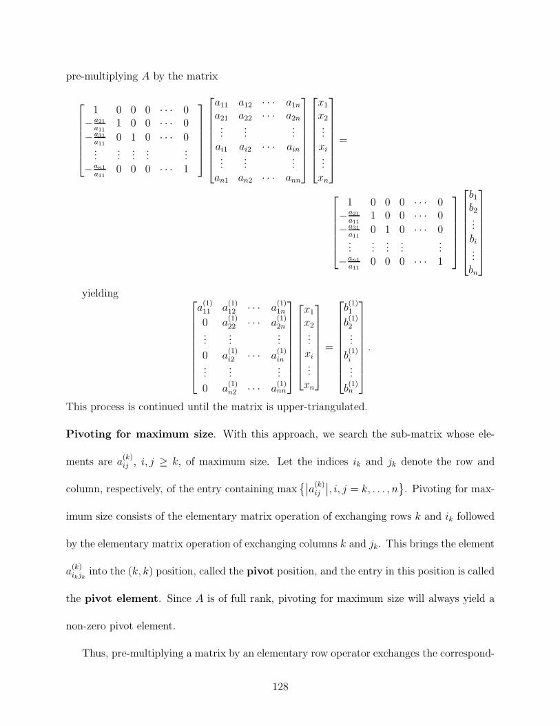
pre-multiplying A by the matrix
%
&&&&&'
1 0 0 0 · · · 0&a21
a111 0 0 · · · 0
&a31a11
0 1 0 · · · 0...
......
......
&an1a11
0 0 0 · · · 1
(
)))))*
%
&&&&&&&'
a11 a12 · · · a1n
a21 a22 · · · a2n...
......
ai1 ai2 · · · ain...
......
an1 an2 · · · ann
(
)))))))*
%
&&&&&&&'
x1
x2...xi...
xn
(
)))))))*
=
%
&&&&&'
1 0 0 0 · · · 0&a21
a111 0 0 · · · 0
&a31a11
0 1 0 · · · 0...
......
......
&an1a11
0 0 0 · · · 1
(
)))))*
%
&&&&&&&'
b1
b2...bi...bn
(
)))))))*
yielding%
&&&&&&&&'
a(1)11 a(1)
12 · · · a(1)1n
0 a(1)22 · · · a(1)
2n...
......
0 a(1)i2 · · · a(1)
in...
......
0 a(1)n2 · · · a(1)
nn
(
))))))))*
%
&&&&&&&'
x1
x2...xi...
xn
(
)))))))*
=
%
&&&&&&&&'
b(1)1
b(1)2...
b(1)i...
b(1)n
(
))))))))*
.
This process is continued until the matrix is upper-triangulated.
Pivoting for maximum size. With this approach, we search the sub-matrix whose ele-
ments are a(k)ij , i, j # k, of maximum size. Let the indices ik and jk denote the row and
column, respectively, of the entry containing maxSKKa(k)
ij
KK, i, j = k, . . . , n
T
. Pivoting for max-
imum size consists of the elementary matrix operation of exchanging rows k and ik followed
by the elementary matrix operation of exchanging columns k and jk. This brings the element
a(k)ikjk
into the (k, k) position, called the pivot position, and the entry in this position is called
the pivot element. Since A is of full rank, pivoting for maximum size will always yield a
non-zero pivot element.
Thus, pre-multiplying a matrix by an elementary row operator exchanges the correspond-
128
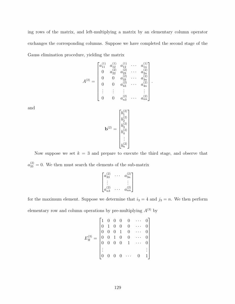
ing rows of the matrix, and left-multiplying a matrix by an elementary column operator
exchanges the corresponding columns. Suppose we have completed the second stage of the
Gauss elimination procedure, yielding the matrix
A(2) =
%
&&&&&&&&'
a(1)11 a(1)
12 a(1)12 · · · a(1)
1n
0 a(2)22 a(2)
23 · · · a(2)2n
0 0 a(2)33 · · · a(2)
3n
0 0 a(2)43 · · · a(2)
4n...
......
...
0 0 a(2)n3 · · · a(2)
nn
(
))))))))*
.
and
b(2) =
%
&&&&&&&&'
b(2)1
b(2)2
b(2)3
b(2)4...
b(2)n
(
))))))))*
Now suppose we set k = 3 and prepare to execute the third stage, and observe that
a(2)33 = 0. We then must search the elements of the sub-matrix
%
&'
a(2)33 · · · a(2)
3n...
...
a(2)n3 · · · a(2)
nn
(
)*
for the maximum element. Suppose we determine that i3 = 4 and j3 = n. We then perform
elementary row and column operations by pre-multiplying A(3) by
E(3)R =
%
&&&&&&&&&'
1 0 0 0 0 · · · 00 1 0 0 0 · · · 00 0 0 1 0 · · · 00 0 1 0 0 · · · 00 0 0 0 1 · · · 0...
...0 0 0 0 · · · 0 1
(
)))))))))*
129
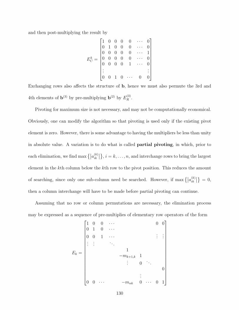
and then post-multiplying the result by
E3C =
%
&&&&&&&&&'
1 0 0 0 0 · · · 00 1 0 0 0 · · · 00 0 0 0 0 · · · 10 0 0 0 0 · · · 00 0 0 0 1 · · · 0...
...0 0 1 0 · · · 0 0
(
)))))))))*
Exchanging rows also a!ects the structure of b, hence we must also permute the 3rd and
4th elements of b(3) by pre-multiplying b(2) by E(3)R .
Pivoting for maximum size is not necessary, and may not be computationally economical.
Obviously, one can modify the algorithm so that pivoting is used only if the existing pivot
element is zero. However, there is some advantage to having the multipliers be less than unity
in absolute value. A variation is to do what is called partial pivoting, in which, prior to
each elimination, we find maxSKKa(k)
ik
KKT
, i = k, . . . , n, and interchange rows to bring the largest
element in the kth column below the kth row to the pivot position. This reduces the amount
of searching, since only one sub-column need be searched. However, if maxSKKa(k)
ik
KKT
= 0,
then a column interchange will have to be made before partial pivoting can continue.
Assuming that no row or column permutations are necessary, the elimination process
may be expressed as a sequence of pre-multiplies of elementary row operators of the form
Ek =
%
&&&&&&&&&&&&&&&&&'
1 0 0 · · · 0 00 1 0 · · ·0 0 1 · · · ...
......
.... . .
1&mk+1,k 1
... 0. . .
0...
0 0 · · · &mnk 0 · · · 0 1
(
)))))))))))))))))*
130
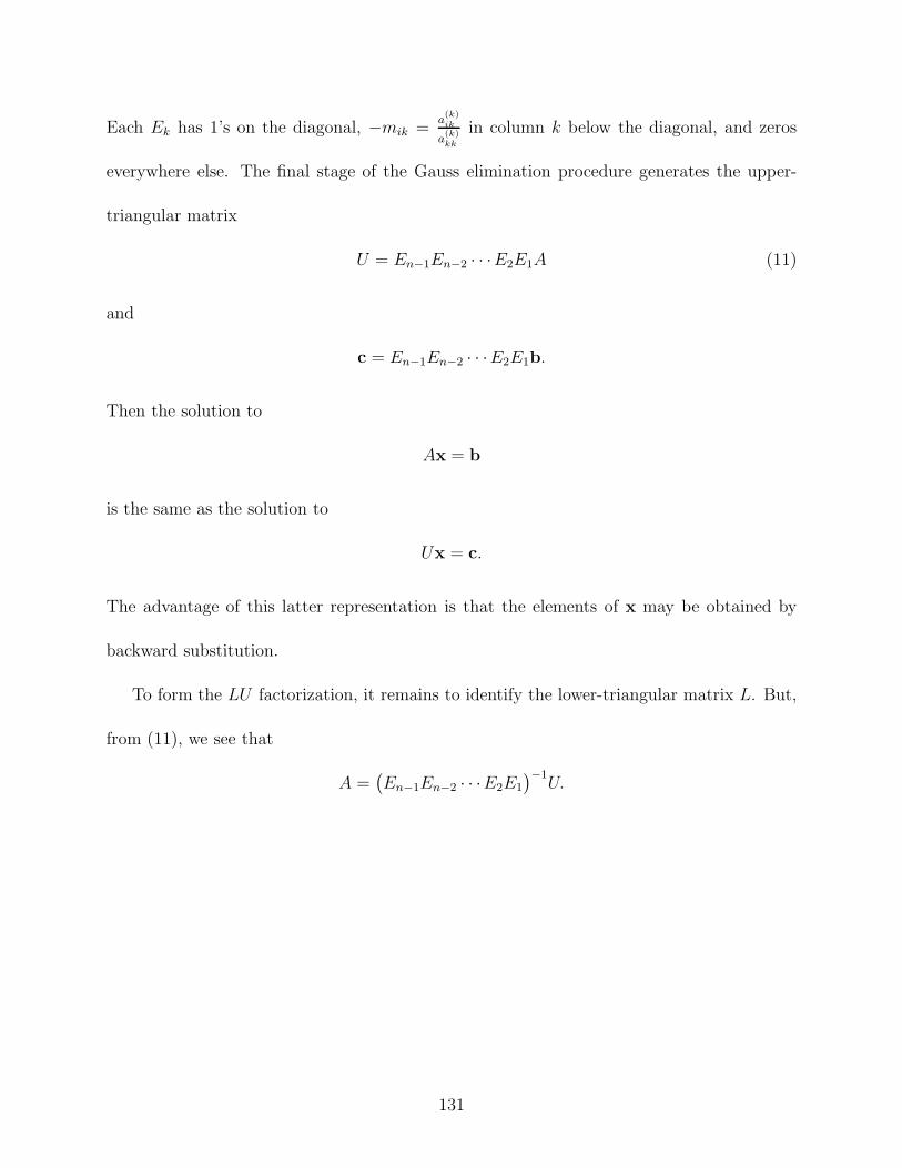
Each Ek has 1’s on the diagonal, &mik =a(k)ik
a(k)kk
in column k below the diagonal, and zeros
everywhere else. The final stage of the Gauss elimination procedure generates the upper-
triangular matrix
U = En"1En"2 · · ·E2E1A (11)
and
c = En"1En"2 · · ·E2E1b.
Then the solution to
Ax = b
is the same as the solution to
Ux = c.
The advantage of this latter representation is that the elements of x may be obtained by
backward substitution.
To form the LU factorization, it remains to identify the lower-triangular matrix L. But,
from (11), we see that
A =1
En"1En"2 · · ·E2E1
2"1U.
131

Now, it is easily verified that
E"1k =
%
&&&&&&&&&&&&&&&&&'
1 0 0 · · · 0 00 1 0 · · ·0 0 1 · · · ...
......
.... . .
1mk+1,k 1
... 0. . .
0...
0 0 · · · mnk 0 · · · 0 1
(
)))))))))))))))))*
,
which is a lower triangular matrix. Thus, the matrix
1
En"1En"2 · · ·E2E1
2"1= E"1
1 E"12 · · ·E"1
n"2E"1n"1
is the product of lower-triangular matrices and hence is lower-triangular, so we identify L as
L = E"11 E"1
2 · · ·E"1n"2E
"1n"1.
Carrying out these matrix multiplications, it is straightforward to see that
L =
%
&&&&&'
1 0 · · · 0m21 1 · · · 0m31 m32 1 0
......
. . ....
mn1 mn2 · · · mn,n"1 1
(
)))))*
and we have established the LU decomposition
A = LU
for the case when there are no row or column permutations. If partial pivoting occurs at
the kth step, then there will be non-triangular row-permutation matrices in the factor Ek of
U . Let P be the product of all the permutation matrices in the order in which they occur
132
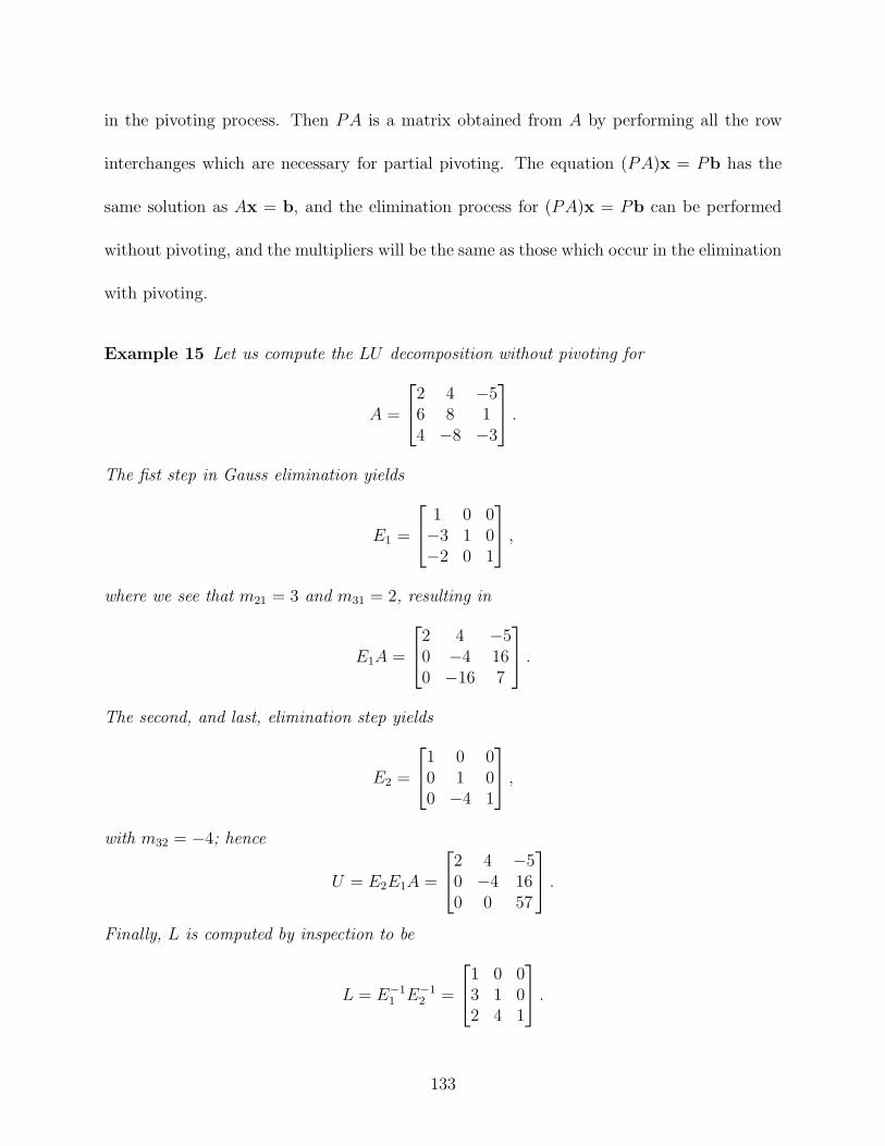
in the pivoting process. Then PA is a matrix obtained from A by performing all the row
interchanges which are necessary for partial pivoting. The equation (PA)x = Pb has the
same solution as Ax = b, and the elimination process for (PA)x = Pb can be performed
without pivoting, and the multipliers will be the same as those which occur in the elimination
with pivoting.
Example 15 Let us compute the LU decomposition without pivoting for
A =
%
'
2 4 &56 8 14 &8 &3
(
* .
The fist step in Gauss elimination yields
E1 =
%
'
1 0 0&3 1 0&2 0 1
(
* ,
where we see that m21 = 3 and m31 = 2, resulting in
E1A =
%
'
2 4 &50 &4 160 &16 7
(
* .
The second, and last, elimination step yields
E2 =
%
'
1 0 00 1 00 &4 1
(
* ,
with m32 = &4; hence
U = E2E1A =
%
'
2 4 &50 &4 160 0 57
(
* .
Finally, L is computed by inspection to be
L = E"11 E"1
2 =
%
'
1 0 03 1 02 4 1
(
* .
133
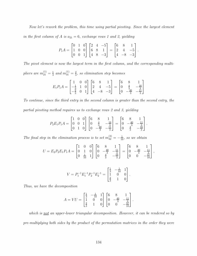
Now let’s rework the problem, this time using partial pivoting. Since the largest element
in the first column of A is a21 = 6, exchange rows 1 and 2, yielding
P1A =
%
'
0 1 01 0 00 0 1
(
*
%
'
2 4 &56 8 14 8 &3
(
* =
%
'
6 8 12 4 &54 &8 &3
(
* .
The pivot element is now the largest term in the first column, and the corresponding multi-
pliers are m(1)21 = 1
3 and m(1)31 = 2
3 , so elimination step becomes
E1P1A =
%
'
1 0 0&1
3 1 0&2
3 0 1
(
*
%
'
6 8 12 4 &54 &8 &3
(
* =
%
'
6 8 10 4
3 &163
0 &403 &11
3
(
*
To continue, since the third entry in the second column is greater than the second entry, the
partial pivoting method requires us to exchange rows 2 and 3, yielding
P2E1P1A =
%
'
1 0 00 0 10 1 0
(
*
%
'
6 8 10 4
3 &163
0 &403 &11
3
(
* =
%
'
6 8 10 &40
3 &113
0 43 &16
3
(
* .
The final step in the elimination process is to set m(2)32 = & 1
10 , so we obtain
U = E2P2E1P1A =
%
'
1 0 00 1 00 1
10 1
(
*
%
'
6 8 10 &40
3 &113
0 43 &16
3
(
* =
%
'
6 8 10 &40
3 &113
0 0 &5710
(
* ,
V = P"11 E"1
1 P"12 E"1
2 =
%
'
13 & 1
10 11 0 023 1 0
(
* .
Thus, we have the decomposition
A = V U =
%
'
13 & 1
10 11 0 023 1 0
(
*
%
'
6 8 10 &40
3 &113
0 0 &5710
(
* .
which is not an upper-lower triangular decomposition. However, it can be rendered so by
pre-multiplying both sides by the product of the permutation matrices in the order they were
134
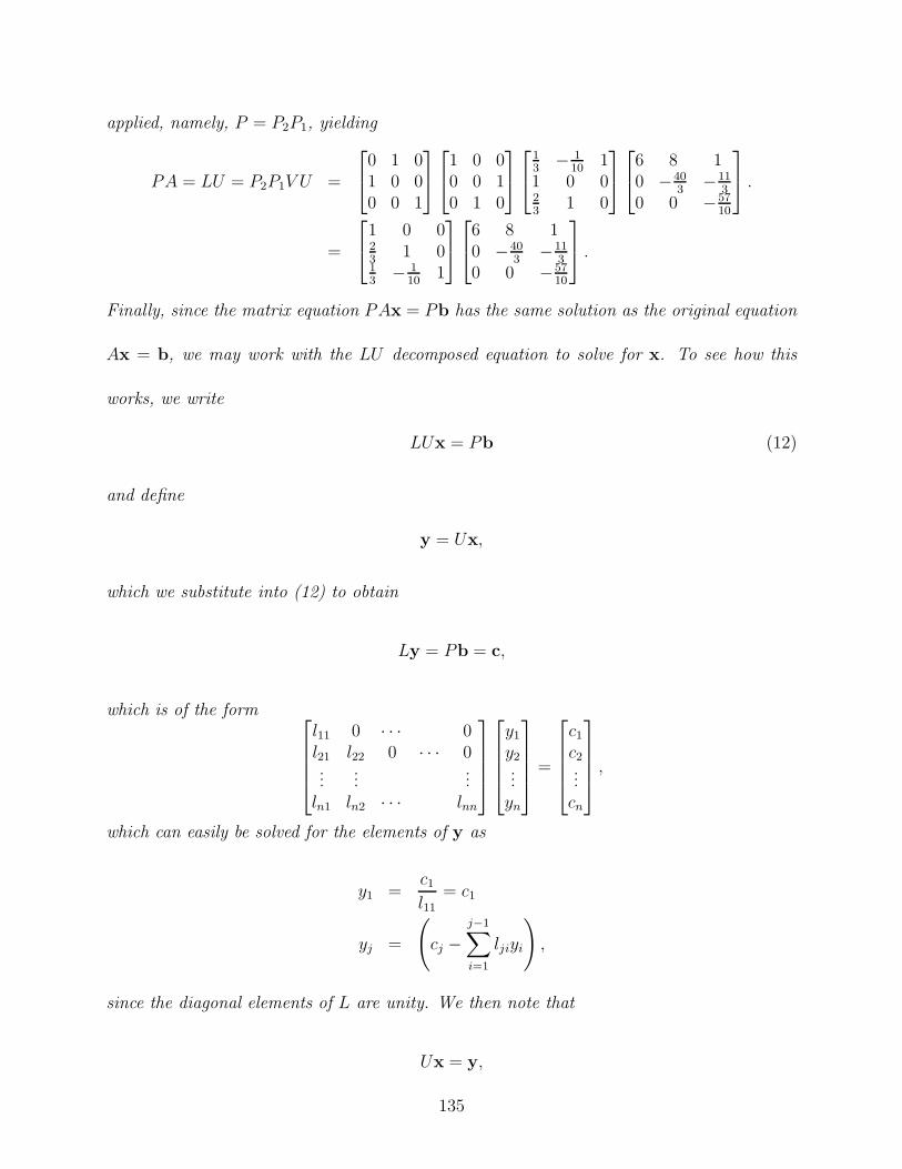
applied, namely, P = P2P1, yielding
PA = LU = P2P1V U =
%
'
0 1 01 0 00 0 1
(
*
%
'
1 0 00 0 10 1 0
(
*
%
'
13 & 1
10 11 0 023 1 0
(
*
%
'
6 8 10 &40
3 &113
0 0 &5710
(
* .
=
%
'
1 0 023 1 013 & 1
10 1
(
*
%
'
6 8 10 &40
3 &113
0 0 &5710
(
* .
Finally, since the matrix equation PAx = Pb has the same solution as the original equation
Ax = b, we may work with the LU decomposed equation to solve for x. To see how this
works, we write
LUx = Pb (12)
and define
y = Ux,
which we substitute into (12) to obtain
Ly = Pb = c,
which is of the form%
&&&'
l11 0 · · · 0l21 l22 0 · · · 0...
......
ln1 ln2 · · · lnn
(
)))*
%
&&&'
y1
y2...yn
(
)))*
=
%
&&&'
c1
c2...cn
(
)))*
,
which can easily be solved for the elements of y as
y1 =c1
l11= c1
yj =
Q
cj &j"1+
i=1
ljiyi
R
,
since the diagonal elements of L are unity. We then note that
Ux = y,
135
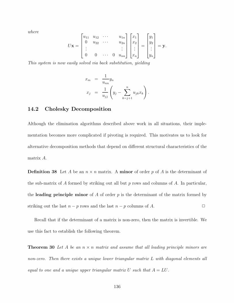
where
Ux =
%
&&&'
u11 u12 · · · u1n
0 u22 · · · u2n...
...0 0 · · · 0 unn
(
)))*
%
&&&'
x1
x2...
xn
(
)))*
=
%
&&&'
y1
y2...yn
(
)))*
= y.
This system is now easily solved via back substitution, yielding
xm =1
unn
yn
xj =1
ujj
Q
yj &n+
k=j+1
ujkxk
R
.
14.2 Cholesky Decomposition
Although the elimination algorithms described above work in all situations, their imple-
mentation becomes more complicated if pivoting is required. This motivates us to look for
alternative decomposition methods that depend on di!erent structural characteristics of the
matrix A.
Definition 38 Let A be an n ! n matrix. A minor of order p of A is the determinant of
the sub-matrix of A formed by striking out all but p rows and columns of A. In particular,
the leading principle minor of A of order p is the determinant of the matrix formed by
striking out the last n & p rows and the last n & p columns of A. !
Recall that if the determinant of a matrix is non-zero, then the matrix is invertible. We
use this fact to establish the following theorem.
Theorem 30 Let A be an n ! n matrix and assume that all leading principle minors are
non-zero. Then there exists a unique lower triangular matrix L with diagonal elements all
equal to one and a unique upper triangular matrix U such that A = LU .
136
Proof The proof is by induction on n, the size of A. Clearly, if n = 1, that is, if A = a11,
then letting L = 1 and U = a11 provides the unique factorization.
Now assume the theorem is true for all square matrices of dimension (n & 1) ! (n & 1)
that satisfy the hypothesis of the theorem. We need to show that it is true for all matrices
of dimension n ! n that also satisfy the hypothesis. We may express A as
A =
"
An"1 a1
aT2 ann
?
(13)
where An"1 is the (n&1)!(n&1) sub-matrix comprising the elements in the upper left-hand
corner of A, a1 is n (n & 1) ! 1 vector, aT2 is an 1 ! (n & 1) row vector, and ann is is the
element of A in the nth row and nth column.
By the inductive hypothesis, the theorem can be applied to An"1, yielding the triangular
factorization
An"1 = Ln"1Un"1
where Ln"1 has diagonal elements all equal to one. Since det(An"1) is the (n & 1)st leading
principle minor of A, it is non-zero, thus Ln"1 and Un"1 are non-singular.
Now consider the n ! n partitioned triangular matrices
Ln =
"
Ln"1 0dT 1
?
and Un =
"
Un"1 c0 ann
?
,
where c and d are (n & 1)-dimensional vectors to be determined. From the product
LnUn =
"
Ln"1 0dT 1
? "
Un"1 c0 ann
?
=
"
Ln"1Un"1 Ln"1cdT Un"1 ann
?
, (14)
and compare the result with (13). It is clear that if c and d are chosen so that
Ln"1c = a1 and dT Un"1 = aT2 , (15)
137
then (14) will give the required factorization of (13). But Equations (15) are uniquely solvable
for c and d because Ln"1 and Un"1 are non-singular. Thus,
c = L"1n"1a1 and dT = aT
2 U"1n"1,
and substitution into (14) determines the unique triangular factors of A required by the
theorem. !
We now specialize the results of this theorem to obtain the so-called Cholesky decompo-
sition.
Cholesky Decomposition. Let B be a positive definite Hermitian matrix. Then B may
be factored into
B = UHDU,
where U is an upper-triangular matrix with ones along the diagonal and D is of the form
D = diag(l11, l22, · · · , lnn).
This result follows from the above theorem specialized to the case a1 = a2 and letting l2ii
denote the diagonal elements of the resulting upper-triangular matrix.
Example 16 Recall that the solution to minx .Ax & b. is given by the normal equations
AHAx = AHb.
If A is of full rank, then Q = AHA will be non-singular, hence all of its principle minors
will be non-zero. In fact, Q will be positive definite. Let p = AHb and compute the Cholesky
factorization of
Qx = p, .
138

resulting in
UHDUx = p,
which can be solved by forward- and back-substitution.
139
15 Lecture 15
15.1 QR Factorization
Definition 39 An n ! n matrix Q is said to be unitary if
QHQ = I.
If Q has real elements and QT Q = I, then Q is said to be orthogonal. !
We note the following facts about unitary matrices
1. Q is invertible (obvious).
2. Q"1 = QH (obvious).
3. det(Q) = 1. To see, write 1 = det(I) = det(QHQ) = det(Q) det(QH) Since det(Q) =
det(QH), the result follows.
4. QH is unitary. To see, note that QQH = Q(QHQ)QH = (QQH)(QQH), and since Q is
invertible, so is QQH . Multiplying both sides by (QQH)"1 yields the result.
Unitary matrices are rotations.
1. They preserve length: .Qx.22 = xHQHQx = xHx = .x.2
2.
2. They preserve angles; !(Qx, Qy) = |)Qx,Qy*||Qx&&Qy& = |xHQHQy|
&Qx&&Qy& = |xHy|&x&&y& = !(x,y)
The matrix
Q =
"
cos ' sin '& sin ' cos '
?
140
is unitary (orthogonal) and the operation Qx rotates the vector x ' degrees clockwise. It is
easy to check that Q"1 = QT .
One of the most important properties of unitary matrices is that they can be used to
form yet another factorization of a matrix, and therefore has application for solving matrix
equations of the form Ax = b. The fundamental result is the following theorem.
Theorem 31 Let A be an m ! n matrix with m # n. Then there exists an m ! n matrix
Q with orthogonal columns and an upper triangular n ! n matrix R such that A = QR. If
m = n, then Q is unitary; if m > n, then we may append m & n orthogonal columns to Q
to form a unitary matrix Q, and we may append m & n zero rows to R to form a matrix R
such that A = QR.
Proof We restrict our proof to the case were A is of full rank. The proof is constructive.
Let A be written in terms of its column vectors as A =,
a1, · · · , an
-
. By the Gram-Schmidt
orthogonalization procedure, we may form columns qi of Q as
q1 =1
.a1.a1
qi =1
.ri.ri, i = 2, . . . , n,
where the n ! 1 vectors ri are defined by
ri = ai &i"1+
k=0
(qHk ai)qk, i = 1, . . . , n. (16)
Equation (16) can be rearranged to yield
ai = (qH1 ai)q1 + (qH
2 ai)q2 + · · ·+ (qHi"1ai)qi"1 +
F
rHi riqi
141
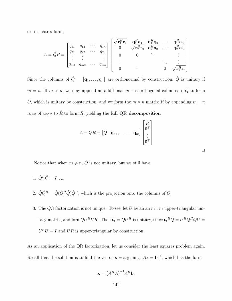
or, in matrix form,
A = QR =
%
&&&'
q11 q12 · · · q1n
q21 q22 · · · q2n...
......
qm1 qm2 · · · qmn
(
)))*
%
&&&&&&'
M
rH1 r1 qH
1 a1 qH1 q2 · · · qH
1 an
0M
rH2 r2 qH
2 a2 · · · qH2 an
0 0. . .
......
. . ....
0 · · · 0M
rHn rn
(
))))))*
Since the columns of Q =,
q1, . . . ,qn
-
are orthonormal by construction, Q is unitary if
m = n. If m > n, we may append an additional m & n orthogonal columns to Q to form
Q, which is unitary by construction, and we form the m! n matrix R by appending m & n
rows of zeros to R to form R, yielding the full QR decomposition
A = QR =,
Q qn+1 · · · qm
-
%
&&&'
R0T
...0T
(
)))*
!
Notice that when m += n, Q is not unitary, but we still have
1. QHQ = In+n.
2. QQH = Q(QHQ)QH , which is the projection onto the columns of Q.
3. The QR factorization is not unique. To see, let U be an an m!m upper-triangular uni-
tary matrix, and formQUHUR. Then Q = QUH is unitary, since QHQ = UHQHQU =
UHU = I and UR is upper-triangular by construction.
As an application of the QR factorization, let us consider the least squares problem again.
Recall that the solution is to find the vector x = arg minx .Ax = b.2, which has the form
x =1
AHA2"1
AHb.
142
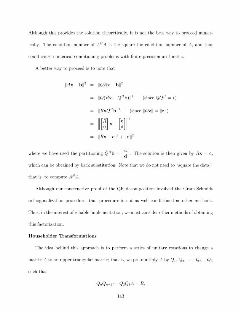
Although this provides the solution theoretically, it is not the best way to proceed numer-
ically. The condition number of AHA is the square the condition number of A, and that
could cause numerical conditioning problems with finite-precision arithmetic.
A better way to proceed is to note that
.Ax & b.2 = .QRx & b.2
= .Q(Rx & QHb).2 (since QQH = I)
= .RxQHb.2 (since .Qz. = .z.)
=
<<<<
"
R0
?
x &"
cd
?<<<<
2
= .Rx & c.2 + .d.2
where we have used the partitioning QHb =
"
cd
?
. The solution is then given by Rx = c,
which can be obtained by back substitution. Note that we do not need to “square the data,”
that is, to compute AHA.
Although our constructive proof of the QR decomposition involved the Gram-Schmidt
orthogonalization procedure, that procedure is not as well conditioned as other methods.
Thus, in the interest of reliable implementation, we must consider other methods of obtaining
this factorization.
Householder Transformations
The idea behind this approach is to perform a series of unitary rotations to change a
matrix A to an upper triangular matrix; that is, we pre-multiply A by Q1, Q2, . . . , Qn", Qn
such that
QnQn"1 · · ·Q2Q1A = R,
143

that is
Q = QH1 QH
2 · · ·QHn"1Q
Hn .
Since all of the i’s are unitary, then Q is unitary. Note that this procedure di!ers from the
LU factorization in that the elementary row operator matrices are not necessarily unitary.
To motivate the structure of these unitary transformations, suppose we wish to rotate a
vector x, with a unitary transformation Q1 so that the transformed vector, Q1x, is aligned
with the first element of an orthogonal basis set, e0 =,
1 0 · · · 0-
. Since the transforma-
tion is unitary, the norm will be unchanged, thus the transformed vector will be %e0, where
%2 = .x.2.
!
" %e0
x
v = x & %e0
Figure 1: Geometric interpretation of the Householder transformation.
To motivate the Householder transformation, let us form the vector v = x & %e0, as
depicted in the figure. The triangle with sides x, %e0, v is an isosceles triangle. If we drop
a perpendicular from the origin of x to the vector v, it will divide the segment v into two
equal parts. The upper part is nothing but the projection of the vector x onto the vector v.
The length of this segment is=
x,v
.v.
>
,
144

so we write
x & %e0 = 2
=
x,v
.v.
>v
.v. = 20x,v1 v
.v.2
or
%e0 = x & 20x,v1 v
.v.2.
This transformation is called a reflection because it reflects the vector x across the perpen-
dicular to v. Expressing this vector in matrix notation, we obtain
%e0 = x & 2vHx(vHv)"1v
= x & 2vvH
vHvx
=
3
I & 2vvH
vHv
$
x
= Qx
where
Q = I & 2vvH
vHv.
This is called a Householder transformation. It is easy to see that Q = QH , and that
Q2 = I, thus, Q is a unitary matrix.
A sequence of Householder transformations can be used to triangularize a given m ! n
matrix A. To do this, we first find a transformation H1 that rotates the first column of A
to lie along e0. Let Q1 = H1R, so that we have Q1A of the form (where ! denotes entries
whose exact values are not of current interest)
Q1A =
%
&&&&&'
%1 ! ! · · · !0 ! ! · · · !0 ! ! · · · !...
......
...0 ! ! · · · !
(
)))))*
145
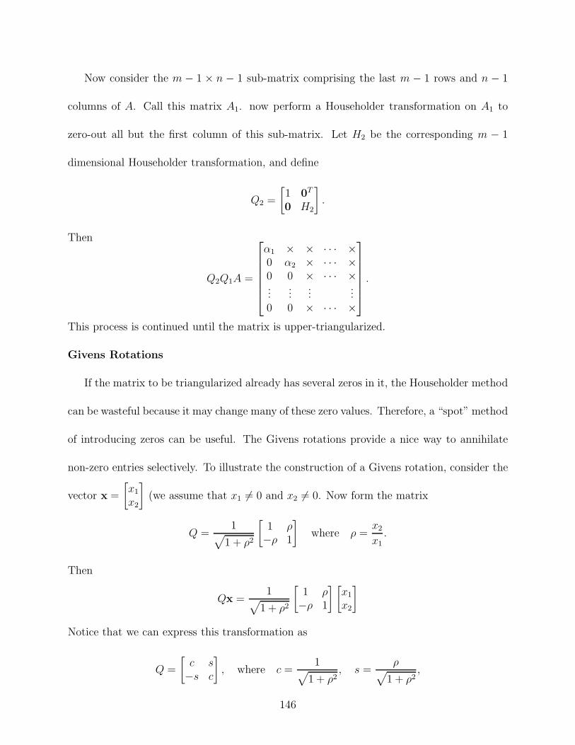
Now consider the m & 1 ! n & 1 sub-matrix comprising the last m & 1 rows and n & 1
columns of A. Call this matrix A1. now perform a Householder transformation on A1 to
zero-out all but the first column of this sub-matrix. Let H2 be the corresponding m & 1
dimensional Householder transformation, and define
Q2 =
"
1 0T
0 H2
?
.
Then
Q2Q1A =
%
&&&&&'
%1 ! ! · · · !0 %2 ! · · · !0 0 ! · · · !...
......
...0 0 ! · · · !
(
)))))*
.
This process is continued until the matrix is upper-triangularized.
Givens Rotations
If the matrix to be triangularized already has several zeros in it, the Householder method
can be wasteful because it may change many of these zero values. Therefore, a “spot” method
of introducing zeros can be useful. The Givens rotations provide a nice way to annihilate
non-zero entries selectively. To illustrate the construction of a Givens rotation, consider the
vector x =
"
x1
x2
?
(we assume that x1 += 0 and x2 += 0. Now form the matrix
Q =1
M
1 + .2
"
1 .&. 1
?
where . =x2
x1.
Then
Qx =1
M
1 + .2
"
1 .&. 1
? "
x1
x2
?
Notice that we can express this transformation as
Q =
"
c s&s c
?
, where c =1
M
1 + .2, s =
.M
1 + .2,
146
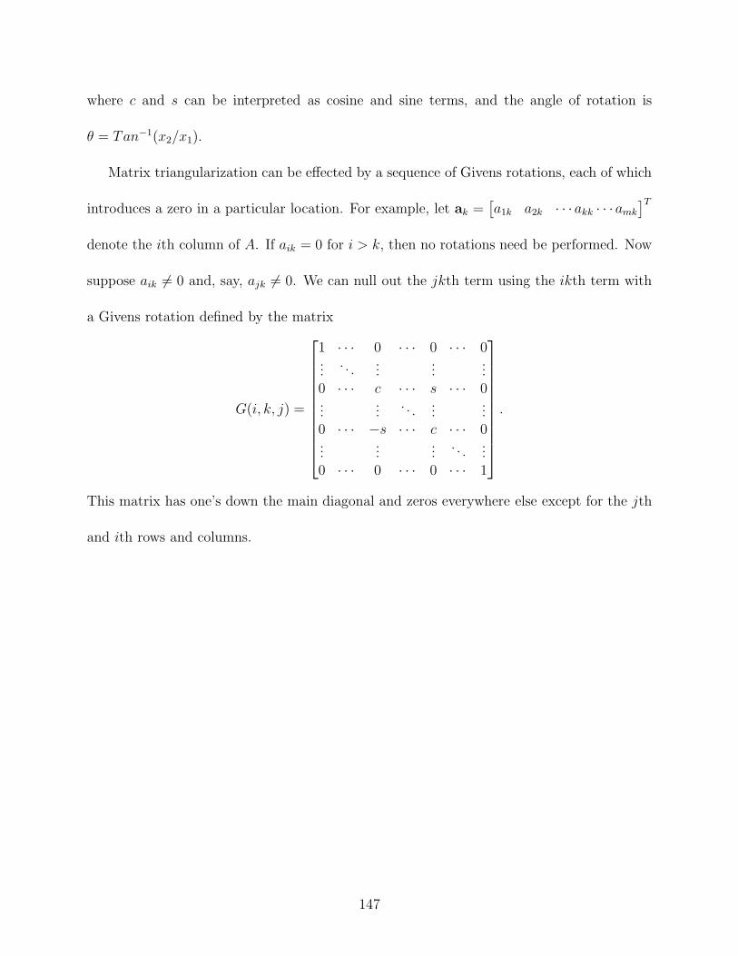
where c and s can be interpreted as cosine and sine terms, and the angle of rotation is
' = Tan"1(x2/x1).
Matrix triangularization can be e!ected by a sequence of Givens rotations, each of which
introduces a zero in a particular location. For example, let ak =,
a1k a2k · · ·akk · · ·amk
-T
denote the ith column of A. If aik = 0 for i > k, then no rotations need be performed. Now
suppose aik += 0 and, say, ajk += 0. We can null out the jkth term using the ikth term with
a Givens rotation defined by the matrix
G(i, k, j) =
%
&&&&&&&&&&'
1 · · · 0 · · · 0 · · · 0...
. . ....
......
0 · · · c · · · s · · · 0...
.... . .
......
0 · · · &s · · · c · · · 0...
......
. . ....
0 · · · 0 · · · 0 · · · 1
(
))))))))))*
.
This matrix has one’s down the main diagonal and zeros everywhere else except for the jth
and ith rows and columns.
147

16 Lecture 16
16.1 A Brief Review of Eigenstu!
Definition 40 A number / is an eigenvalue of an n ! n matrix A if there is a non-zero
n-vector x such that
Ax = /x.
The corresponding vector x is said to be an eigenvector of A. !
The geometric interpretation of an eigenvector is that operation by A on the vector
merely scales the length (and perhaps the sign) of the vector. It does not rotate the vector
to a new orientation.
For a given value of /, the eigenvector equation
Ax = /x
is equivalent to the linear homogeneous equation
[A & /I]x = 0.
From our earlier development, we know that this system has a non-zero solution if and only
if the columns matrix A & /I are linearly dependent, and this obtains if and only if the
determinant of A & /I is zero. Therefore, a necessary and su"cient condition for a value /
to be an eigenvalue of A is that
det(A & /I) = 0.
This equation is called the characteristic equation of A.
148
The value of det(A&/I) is a function of the variable /. It can be shown that det(A&/I),
when expanded out, is a polynomial of degree n in / with the coe"cient of /n being (&1)n.
The polynomial, denoted p(/), is called the characteristic polynomial of A. It is clear
that there is a direct correspondence between the roots of the characteristic polynomial and
the eigenvalues of A.
From the fundamental theorem of algebra it is known that every polynomial of degree
n > 1 has at least one (possibly complex) root, and can be decomposed into first-degree
factors. Thus, the characteristic polynomial can be written in factored form as
p(/) = (/1 & /)(/2 & /) · · · (/n & /).
The /i are the (not necessarily distinct) roots of the polynomial. It follows that there is
always at least one solution to the characteristic equation, and hence always at least one
eigenvalue. To summarize:
Theorem 32 Every n ! n matrix A possesses at least one eigenvalue and a corresponding
(non-zero) eigenvector.
It is a general property that eigenvectors are defined only to with a scalar multiple. If x is
an eigenvectors, then so is %x for any scalar %.
Theorem 33 Let /1, /2, . . . , /n be distinct eigenvalues of an n ! n dimensional matrix A.
Then the set of corresponding eigenvectors, x1,x2, . . . ,xn are linearly independent.
Proof Assume that the eigenvectors are linearly dependent. Then there exists a non-zero
linear combination of these vectors which is equal to zero. Of the possible numerous such
149
linear combinations, select one which has the minimum number of non-zero coe"cients.
Without loss of generality it can be assumed that these coe"cients correspond to the first k
eigenvectors, and that the first coe"cient is unity. That is, the relation is of the form
x1 +k+
i=2
%ixi = 0 (17)
for some set of %i’s, i = 2, . . . , k, all non-zero.
Multiplication of this equation by A gives
Ax1 +k+
i=2
%iAxi = 0.
Using the fact that the xi’s are eigenvectors, this last equation is equivalent to
/1x1 +k+
i=2
%i/ixi = 0. (18)
Now, multiplication of (17) by /1 and subtraction from (18) yields
k+
i=2
%i(/i & /1)xi = 0.
This, however, is a linear combination of only k & 1 terms, contradicting the definition of k
as the minimum possible value. Thus, the theorem is established. !
Suppose the n ! n matrix A has n distinct eigenvalues and, consequently, n linearly
independent eigenvectors. Then the eigenvectors constitute a basis set, and any vector x can
be expressed as a linear combination of the form
x =n+
i=1
%ixi
for some constants %1, %2, . . . , %n. Expressed in this form, it follows that
Ax =n+
i=1
%iAxi =n+
i=1
%i/ixi.
150
Thus, the coe"cients of the transformed vector are just multiples of the original coe"cients.
There is no mixing among coe"cients as there would be in an arbitrary basis. This simple
but valuable result can be translated into the mechanics of matrix manipulation. Define the
modal matrix of A as th the n ! n matrix
S =,
x1 x2 · · · xn
-
.
We see immediately that
AS = A,
x1 x2 · · · xn
-
=,
Ax1 Ax2 · · · Axn
-
=,
/1x1 /2x2 · · · /nxn
-
=,
x1 x2 · · · xn
-
%
&&&&&'
/1 0 0 · · · 00 /2 0 · · · 00 0 /3 · · · 0...
.... . .
...0 0 · · · /n
(
)))))*
= S$
where $ = diag(/1, /2, . . . , /n).
This expression obtains even if the eigenvectors are not linearly independent. If they are,
then S is invertible, and we may rearrange the above to yield
$ = S"1AS
and
A = S$S"1.
Example 17 Let
A =
"
2 12 3
?
.
151
The characteristic polynomial is
KKKK
2 & / 12 3 & /
KKKK= (2 & /)(3 & /) & 2 = /2 & 5/ + 4.
The characteristic polynomial can be factored as /2 & 5/ + 4 = (/ & 1)(/ & 4). Therefore,
the eigenvalues are /1 = 1 and /2 = 4. To find the corresponding eigenvectors we first set
/ = 1 in the homogeneous equation [A & /I] = 0. This leads to
"
1 12 2
? "
x1
x2
?
=
"
00
?
The two scalar equations defined by this set are equivalent to x1 = &x2. Thus, the general
solution is
x1 =
"
a&a
?
for a += 0.
For / = 4, we have"
&2 1&2 1
? "
x1
x2
?
=
"
00
?
,
which leads to the general solution for the second eigenvector as
x2 =
"
b2b
?
for b += 0. Taking a = b = 1, the modal matrix is
S =
"
1 1&1 2
?
and
S"1 =1
3
"
2 &11 1
?
.
152
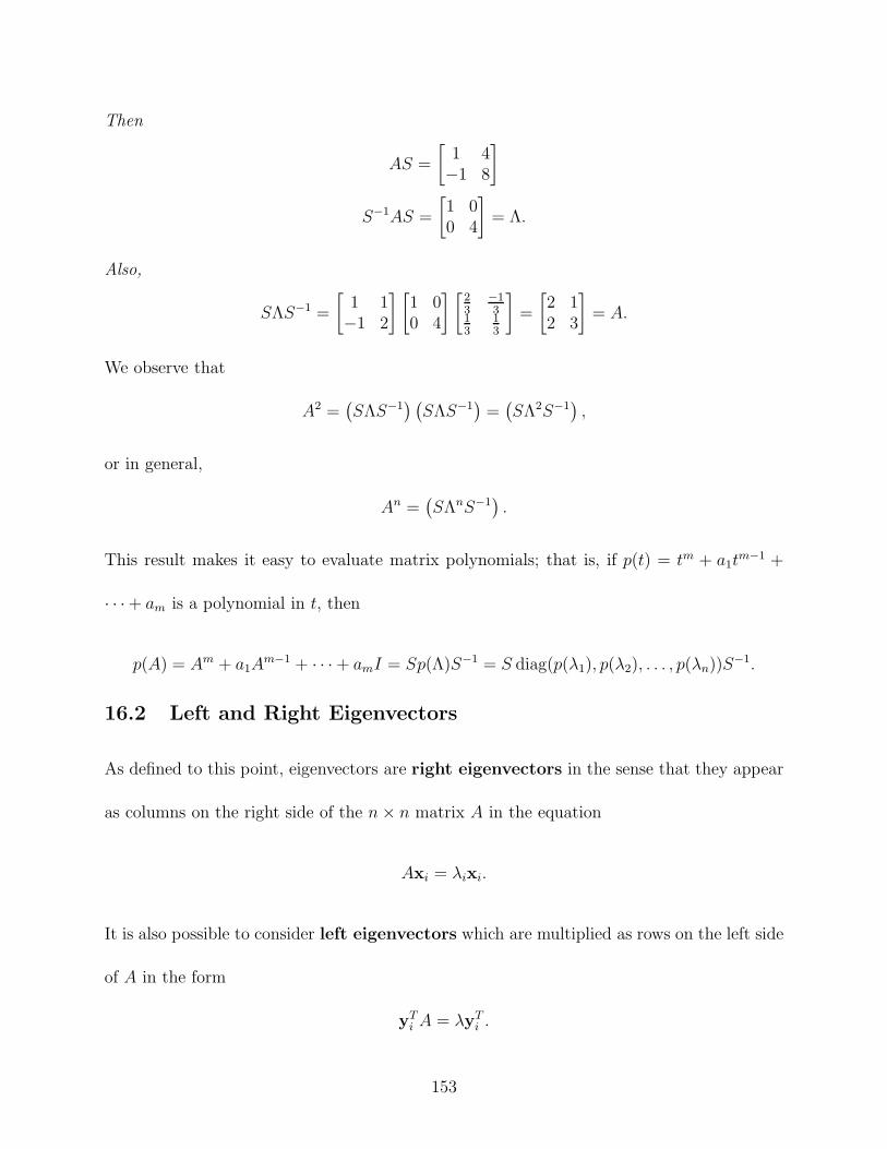
Then
AS =
"
1 4&1 8
?
S"1AS =
"
1 00 4
?
= $.
Also,
S$S"1 =
"
1 1&1 2
? "
1 00 4
? "23
"13
13
13
?
=
"
2 12 3
?
= A.
We observe that
A2 =1
S$S"12 1
S$S"12
=1
S$2S"12
,
or in general,
An =1
S$nS"12
.
This result makes it easy to evaluate matrix polynomials; that is, if p(t) = tm + a1tm"1 +
· · ·+ am is a polynomial in t, then
p(A) = Am + a1Am"1 + · · · + amI = Sp($)S"1 = S diag(p(/1), p(/2), . . . , p(/n))S
"1.
16.2 Left and Right Eigenvectors
As defined to this point, eigenvectors are right eigenvectors in the sense that they appear
as columns on the right side of the n ! n matrix A in the equation
Axi = /ixi.
It is also possible to consider left eigenvectors which are multiplied as rows on the left side
of A in the form
yTi A = /yT
i .
153
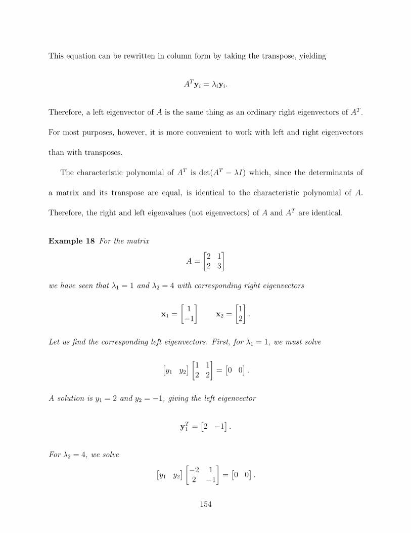
This equation can be rewritten in column form by taking the transpose, yielding
ATyi = /iyi.
Therefore, a left eigenvector of A is the same thing as an ordinary right eigenvectors of AT .
For most purposes, however, it is more convenient to work with left and right eigenvectors
than with transposes.
The characteristic polynomial of AT is det(AT & /I) which, since the determinants of
a matrix and its transpose are equal, is identical to the characteristic polynomial of A.
Therefore, the right and left eigenvalues (not eigenvectors) of A and AT are identical.
Example 18 For the matrix
A =
"
2 12 3
?
we have seen that /1 = 1 and /2 = 4 with corresponding right eigenvectors
x1 =
"
1&1
?
x2 =
"
12
?
.
Let us find the corresponding left eigenvectors. First, for /1 = 1, we must solve
,
y1 y2
-"
1 12 2
?
=,
0 0-
.
A solution is y1 = 2 and y2 = &1, giving the left eigenvector
yT1 =
,
2 &1-
.
For /2 = 4, we solve
,
y1 y2
-"
&2 12 &1
?
=,
0 0-
.
154
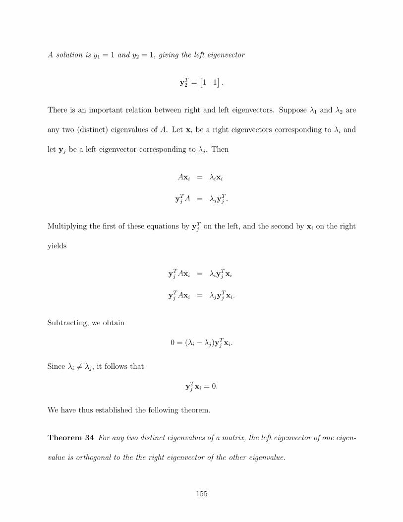
A solution is y1 = 1 and y2 = 1, giving the left eigenvector
yT2 =
,
1 1-
.
There is an important relation between right and left eigenvectors. Suppose /1 and /2 are
any two (distinct) eigenvalues of A. Let xi be a right eigenvectors corresponding to /i and
let yj be a left eigenvector corresponding to /j . Then
Axi = /ixi
yTj A = /jy
Tj .
Multiplying the first of these equations by yTj on the left, and the second by xi on the right
yields
yTj Axi = /iy
Tj xi
yTj Axi = /jy
Tj xi.
Subtracting, we obtain
0 = (/i & /j)yTj xi.
Since /i += /j, it follows that
yTj xi = 0.
We have thus established the following theorem.
Theorem 34 For any two distinct eigenvalues of a matrix, the left eigenvector of one eigen-
value is orthogonal to the the right eigenvector of the other eigenvalue.
155
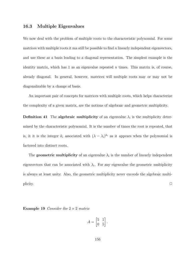
16.3 Multiple Eigenvalues
We now deal with the problem of multiple roots to the characteristic polynomial. For some
matrices with multiple roots it ma still be possible to find n linearly independent eigenvectors,
and use these as a basis leading to a diagonal representation. The simplest example is the
identity matrix, which has 1 as an eigenvalue repeated n times. This matrix is, of course,
already diagonal. In general, however, matrices will multiple roots may or may not be
diagonalizable by a change of basis.
An important pair of concepts for matrices with multiple roots, which helps characterize
the complexity of a given matrix, are the notions of algebraic and geometric multiplicity.
Definition 41 The algebraic multiplicity of an eigenvalue /i is the multiplicity deter-
mined by the characteristic polynomial. It is the number of times the root is repeated, that
is, it it is the integer ki associated with (/ & /i)ki as it appears when the polynomial is
factored into distinct roots.
The geometric multiplicity of an eigenvalue /i is the number of linearly independent
eigenvectors that can be associated with /i. For any eigenvalue the geometric multiplicity
is always at least unity. Also, the geometric multiplicity never exceeds the algebraic multi-
plicity. !
Example 19 Consider the 2 ! 2 matrix
A =
"
5 10 5
?
.
156

It has a characteristic polynomial (5 & /)2, and hence the only eigenvalue is / = 5, with
algebraic multiplicity of two. The corresponding eigenvector must satisfy the equation
"
0 10 0
? "
x1
x2
?
=
"
00
?
The only non-zero solutions to this set are o the form x =
"
%0
?
for some % += 0. Thus there
is only one linearly independent eigenvector, which can be taken to be x =
"
10
?
. Thus the
geometric multiplicity of A is unity.
If the geometric multiplicity equals the algebraic multiplicity for an eigenvalue /i, that
eigenvalue is said to be simple. If every eigenvalue of a matrix is simple, then the total
number of linearly independent eigenvectors is equal to n, and these eigenvectors can be used
to form a basis just as in the case of distinct eigenvalues, to obtain a diagonal representation.
In the general case, where not all eigenvalues are simple, a matrix cannot be transformed
to diagonal form by a change of basis. It is, however, always possible to find a basis in
which the matrix is nearly diagonal, as defined below. The resulting matrix is referred to
as the Jordan Canonical Form of the matrix. Since the derivation of this general result
is quite complex and because the Jordan form is only of modest importance, we state the
result without proof.
Theorem 35 Jordan Canonical Form. Denote by Jk(/) the k!k Jordan block matrix
Jk(/) =
%
&&&&&&&'
/ 1 0 · · · 00 / 1 0 · · · 0... / 1
.... . . . . .
10 0 · · · 0 /
(
)))))))*
157
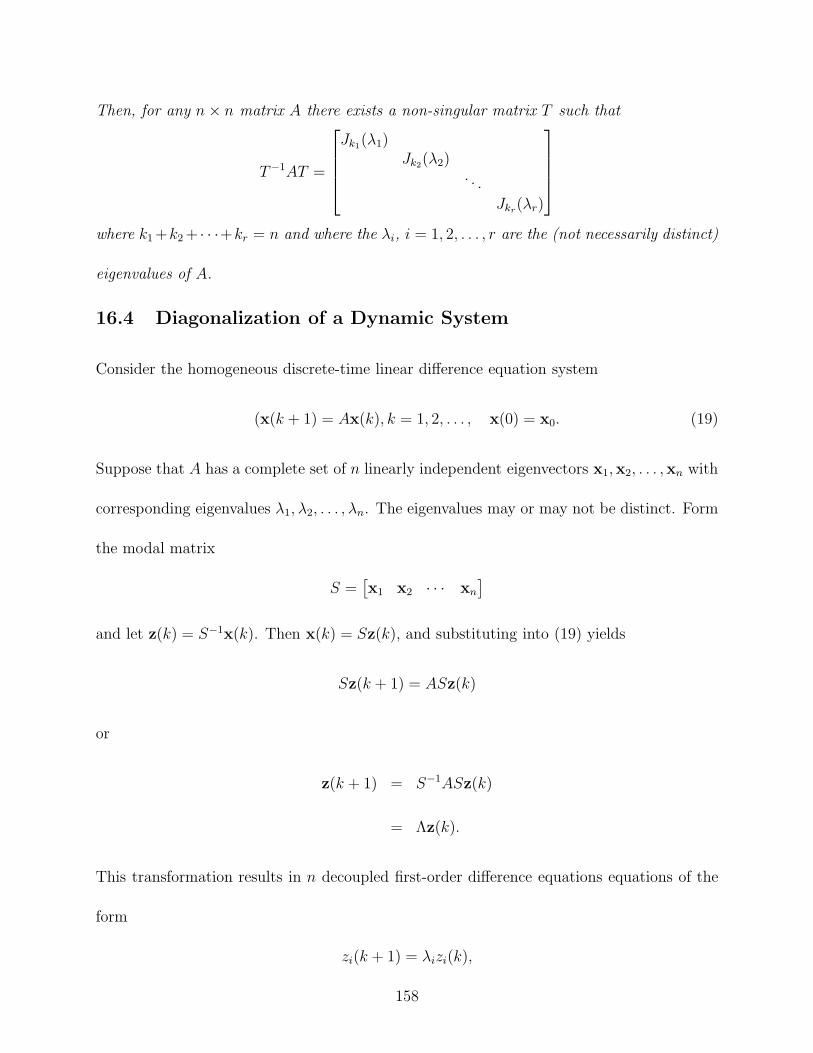
Then, for any n ! n matrix A there exists a non-singular matrix T such that
T"1AT =
%
&&&'
Jk1(/1)Jk2(/2)
. . .Jkr(/r)
(
)))*
where k1 +k2 + · · ·+kr = n and where the /i, i = 1, 2, . . . , r are the (not necessarily distinct)
eigenvalues of A.
16.4 Diagonalization of a Dynamic System
Consider the homogeneous discrete-time linear di!erence equation system
(x(k + 1) = Ax(k), k = 1, 2, . . . , x(0) = x0. (19)
Suppose that A has a complete set of n linearly independent eigenvectors x1,x2, . . . ,xn with
corresponding eigenvalues /1, /2, . . . , /n. The eigenvalues may or may not be distinct. Form
the modal matrix
S =,
x1 x2 · · · xn
-
and let z(k) = S"1x(k). Then x(k) = Sz(k), and substituting into (19) yields
Sz(k + 1) = ASz(k)
or
z(k + 1) = S"1ASz(k)
= $z(k).
This transformation results in n decoupled first-order di!erence equations equations of the
form
zi(k + 1) = /izi(k),
158
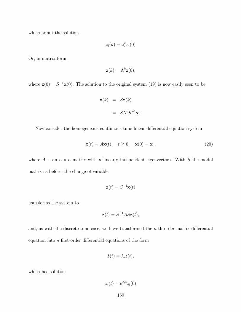
which admit the solution
zi(k) = /ki zi(0)
Or, in matrix form,
z(k) = $kz(0),
where z(0) = S"1x(0). The solution to the original system (19) is now easily seen to be
x(k) = Sz(k)
= S$kS"1x0.
Now consider the homogeneous continuous time linear di!erential equation system
x(t) = Ax(t), t # 0, x(0) = x0, (20)
where A is an n ! n matrix with n linearly independent eigenvectors. With S the modal
matrix as before, the change of variable
z(t) = S"1x(t)
transforms the system to
z(t) = S"1ASz(t),
and, as with the discrete-time case, we have transformed the n-th order matrix di!erential
equation into n first-order di!erential equations of the form
z(t) = /iz(t),
which has solution
zi(t) = e%itzi(0)
159

Or, in matrix form,
z(t) = diag(e%1t, e%2t, . . . e%nt)z(0),
where z(0) = S"1x(0). The solution to the original system (20) is now easily seen to be
x(t) = Sz(t)
= S diag(e%1t, e%2t, . . . e%nt)S"1x(0).
160
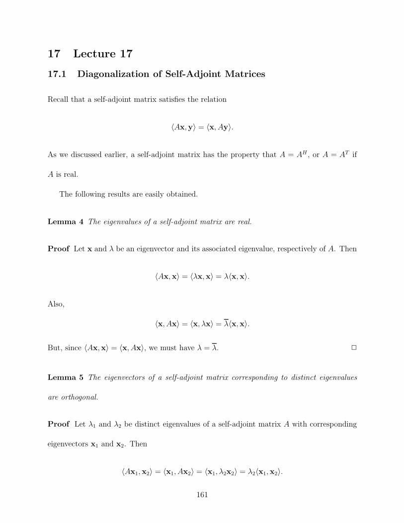
17 Lecture 17
17.1 Diagonalization of Self-Adjoint Matrices
Recall that a self-adjoint matrix satisfies the relation
0Ax,y1 = 0x, Ay1.
As we discussed earlier, a self-adjoint matrix has the property that A = AH , or A = AT if
A is real.
The following results are easily obtained.
Lemma 4 The eigenvalues of a self-adjoint matrix are real.
Proof Let x and / be an eigenvector and its associated eigenvalue, respectively of A. Then
0Ax,x1 = 0/x,x1 = /0x,x1.
Also,
0x, Ax1 = 0x, /x1 = /0x,x1.
But, since 0Ax,x1 = 0x, Ax1, we must have / = /. !
Lemma 5 The eigenvectors of a self-adjoint matrix corresponding to distinct eigenvalues
are orthogonal.
Proof Let /1 and /2 be distinct eigenvalues of a self-adjoint matrix A with corresponding
eigenvectors x1 and x2. Then
0Ax1,x21 = 0x1, Ax21 = 0x1, /2x21 = /20x1,x21.
161

Also,
0Ax1x21 = 0/1x1,x21 = /10x1,x21.
Subtracting,
(/1 & /2)0x1,x21 = 0,
but since /1 += /2, the only way for the di!erence to be zero is for 0x1,x21 = 0. !
Lemma 6 (Schur’s Lemma) For any square matrix A there exists a unitary matrix U
such that
UHAU = T,
where T is upper triangular.
Proof The proof is by induction. The theorem is obviously true when n = 1. Assume it
holds for matrices of order n& 1. Suppose A is an n! n matrix and let u be an eigenvector
of A corresponding to eigenvalue /. We may assume that u is a unit-vector.
Au = /u. (21)
By Gram-Schmidt, we may create a unitary matrix with u as the first column, of the form
Q =,
u x12 · · · x1n
-
for some unit vectors x12, . . . ,x1n. Then we may write
u = Q
%
&&&'
10...0
(
)))*
.
162
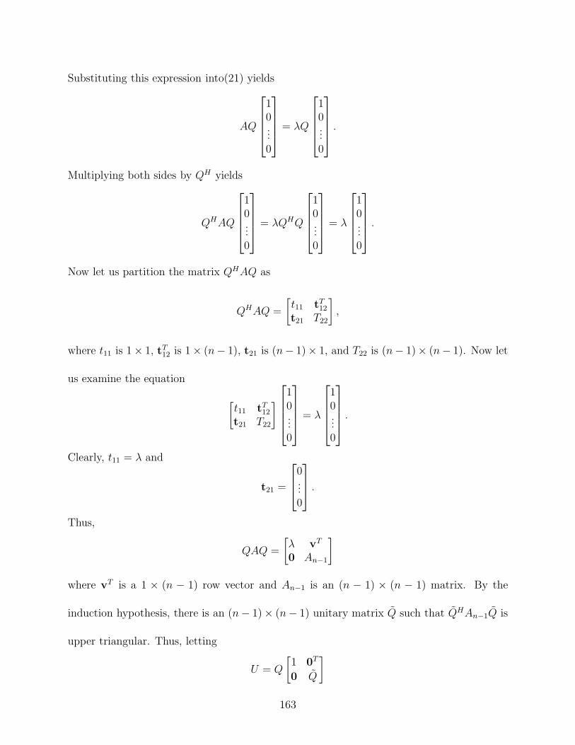
Substituting this expression into(21) yields
AQ
%
&&&'
10...0
(
)))*
= /Q
%
&&&'
10...0
(
)))*
.
Multiplying both sides by QH yields
QHAQ
%
&&&'
10...0
(
)))*
= /QHQ
%
&&&'
10...0
(
)))*
= /
%
&&&'
10...0
(
)))*
.
Now let us partition the matrix QHAQ as
QHAQ =
"
t11 tT12
t21 T22
?
,
where t11 is 1! 1, tT12 is 1! (n& 1), t21 is (n& 1)! 1, and T22 is (n& 1)! (n& 1). Now let
us examine the equation
"
t11 tT12
t21 T22
?
%
&&&'
10...0
(
)))*
= /
%
&&&'
10...0
(
)))*
.
Clearly, t11 = / and
t21 =
%
&'
0...0
(
)* .
Thus,
QAQ =
"
/ vT
0 An"1
?
where vT is a 1 ! (n & 1) row vector and An"1 is an (n & 1) ! (n & 1) matrix. By the
induction hypothesis, there is an (n & 1)! (n& 1) unitary matrix Q such that QHAn"1Q is
upper triangular. Thus, letting
U = Q
"
1 0T
0 Q
?
163
we obtain the desired transformation. !
Definition 42 The spectrum of of a Hermitian matrix is the set of eigenvalues of the
matrix. !
Theorem 36 (The Spectral Theorem) Every Hermitian m!m matrix A can be diago-
nalized by a unitary matrix U :
UHAU = $, (22)
where $ is a diagonal matrix.
Proof We first observe that, from Schur’s lemma, there exists a unitary matrix U that
transforms A into triangular form:
UHAU = T.
We then note that since A is self-adjoint, then T is also. To see this, we observe that
(UHAU)H = UHAHU = UHAU since A is self-adjoint, thus,
0UHAUx,y1 = yHUHAUx = [(UHAU)Hy]Hx = (UHAUy)Hx = 0x, UHAUy1.
Since T is upper-triangular by construction and T = T H , then T H is also upper-triangular.
But any non-zero above-diagonal elements in T would become non-zero below-diagonal el-
ements of TH , which would contradict the upper-triangular structure of T H . Thus, T =
UHAU is diagonal. !
For an m ! m Hermitian matrix A we may rewrite (22) to obtain
A = U$UH =,
x1 x2 · · · xm
-
%
&&&'
/1
/2
. . ./m
(
)))*
%
&&&'
xH1
xH2...
xHm
(
)))*
=m+
i=1
/ixixHi .
164
where the xi’s are the orthonormal eigenvectors of A (sometimes called the eigenbasis) and
the /i’s are the corresponding eigenvalues.
17.2 Some Miscellaneous Eigenfacts
The following statements about matrices, their eigenvalues and eigenvectors, are presented.
Fact 1 Let x be an eigenvector of A with eigenvalue /. Then
A2x = A(Ax) = A(/x) = /Ax = /2x,
which implies that x is an eigenvector of A2 with eigenvalue /2. In general, x is an eigen-
vector of Am with eigenvalue /m for all integers m > 0.
Fact 2 If an m ! m matrix A is diagonalizable, then A = X$X"1 where X is the matrix
whose columns are eigenvectors and $ = diag(/1, · · · , /m). Thus,
Am = X$X"1 · X$X"1 · · ·X$X"1 = X$mX"1.
Fact 3 Two n ! n matrices A and B are said to be similar if A = TBT"1 for some n ! n
matrix T . Similar matrices have identical eigenvalues. To see, let X =,
x1 x2 · · · xn
-
be the matrix whose columns are the eigenvectors of A and let $ = diag(/1, /2, · · · , /n) be
the diagonal matrix whose diagonal entries are the corresponding eigenvalues of A. Then
AX = X$ ; TBT"1X = X$
; BT"1X = T"1X$
; BX ' = X '$.
Thus, the eigenvalues of B are the entries of $ and the corresponding eigenvectors are the
columns of X ' = T"1X.
165
Fact 4 Let A be an m ! m matrix of rank r < m. Then at least m & r of the eigenvalues
of A are equal to zero. To see, we note that, by the above fact and the Schur Lemma, the
triangularization T = UHAU has the same eigenvalues as A. Similarity preserves rank, so T
has the same rank as A. But if rank (T ) = r < m, the last m&r columns of T can be written
as linear combinations of the first r columns. Since the entries in the first r columns are zero
below the rth entry, the lower-right (m& r)! (m& r) submatrix must be zero. But since the
eigenvalues of T are the diagonal elements, we must have at least m & r zero eigenvalues.
Fact 5 The eigenvalues of a unitary matrix U lie on the unit circle.
Ux = /x ; .Ux.2 = ./x.2
; xHUHUx = |/|2xHx
; xHx = |/|2xHx
; |/| = 1.
Fact 6 The eigenvalues of a positive-definite matrix Q = QH are positive. To see, let x be
an eigenvector for eigenvalue /.
Qx = /x ; xHQx = /xHx > 0
; / > 0
If Q is positive-semi-definite, then / # 0.
Fact 7 A matrix P is said to be idempotent if P 2 = P . The eigenvalues of an idempotent
matrix are either 0 or 1. To see, let /, x be an eigenvalue and vector of P . Then
P 2x = Px = /Px
166
But, since P 2 = P , we have
/x = Px = P 2x = /2x,
so /2 = /, and the roots of the quadratic equation /(1 & /) & 0 are / = 1 and / = 0.
Fact 8 A matrix P is said to be nilpotent if P n = 0 for some integer n # 1. The eigen-
values of a nilpotent matrix are all zero. To see, we observe that 0 = P nx = /nx, which
implies / = 0. Example: P =
"
0 10 0
?
.
Fact 9 Let S be a subspace of the range of an m ! m matrix A. Then S is said to be an
invariant subspace for A if x ( S implies that Ax ( S. Subspaces formed by sets of
eigenvectors are invariant. To see, let x1, . . . ,xm be normalized eigenvectors of A, and let
Xi = {xi1 , . . . ,xik} be any subset of eigenvectors. For any linear combination x =!k
j=1 %jxij
of the elements of Xi, we have Ax =!k
j=1 %jAxij =!k
j=1 %j/xij , which is another linear
combination of the elements of Xi.
If there are k $ m distinct eigenvalues of A, let Xi be the eigenvectors associated with
/i. Clearly, the subspace Ri = span (Xi) is invariant. Define
Pi =+
xj%Xi
xjxTj
is a projection onto Ri. Then,
1. Spectral decomposition: A =!k
i=1 /iPi.
2. Resolution of the identity: I =!k
i=1 Pi.
The proof is straightforward and left as an exercise.
167
Fact 10 The inertia of a Hermitian matrix Ais the set1
/+(A), /"(A), /0(A)2
, where /+(A),
/"(A), and /0(A) are the number of positive, negative, and zero eigenvalues, respectively, of
A. The signature of A is /+(A) & /"(A). Then Sylvester”s Law of inertia states that,
if A and B are m ! m Hermitian matrices, then there is a nonsingular matrix S such that
A = SBSH if and only if A and B have the same inertia. The proof is left as an exercise.
Fact 11 If /# is an eigenvalue of a matrix A, then /# + r is an eigenvalue of A + rI, and
A and A + rI have the same eigenvectors. To see this, note that, if /# is an eigenvalue
of A, then det(/#I & A) = 0. Also, the eigenvalues of A + rI are given by the equation
det1
/ & (A + rI)2
= det1
(/ & r)I & A2
, which is zero when / & r = /#. Thus, / = /# + r
is an eigenvalue of A + rI. Let u be an eigenvector of A + rI. Then
(A + rI)u = (/# + r)u.
Subtracting ru from both sides obtains
Au = /#u,
thus u is an eigenvector of A.
168
18 Lecture 18
18.1 Quadratic Forms
Definition 43 A quadratic form of a self-adjoint matrix is the inner product of the matrix
operating on the vector, denoted
QA(y) = 0Ay,y1 = yHAy = yHAHy.
!
Quadratic forms occur in many applications. For example, consider the level curves of
the multivariate normal density function,
f(x) =1
2(()m2 |R| 12
exp&1
2
,
(x & µ)T R"1(x & µ)-
= C,
where R is a positive-definite real symmetric matrix. The values of x that satisfy the con-
straint (x&µ)T R"1(x&µ) = C ', where C ' = &2 logI
(()m2 |R| 12
J
represents a hyperellipsoid
that specifies boundary of the volume in m-dimensional space that has probability C of
occurring. This volume may be expressed as the quadratic form
yT R"1y = C ',
where y = x & µ. The orientation of this volume in m-dimensional space depends on the
eigenvectors of R"1. Since R"1 is Hermitian (i.e., real and symmetric), its eigenvectors are
mutually orthogonal, and therefore define an m-dimension coordinate system. By transform-
ing the original random variable x by the transform
z = QT y,
169

where Q =,
q1 q2 · · · qm
-
with the qi’s denoting the eigenvectors of R. Using the fact
(a homework problem) that the eigenvalues of R"1 are the reciprocals of the eigenvalues of
R and that the eigenvectors of R"1 are the eigenvectors of R, we obtain
yHR"1y = zT QT R"1Qz = z$"1z.
where $ = diag(/1, /2, . . . , /m) is the matrix of eigenvalues of R. The coordinate system
defined by the eigenvectors of R permit the random variable x resolved into orthogonal
components such that the corresponding eigenvalues are the variances of m uncorrelated
(independent in the Gaussian case) random variables. This permits the joint Gaussian
density function to be decomposed into the product of marginal density functions of m
independent random variables.
Theorem 37 (Maximum Principle) For a positive-semidefinite self-adjoint m!m matrix
A with QA(x) = 0Ax,x1 = xHAx, let the eigenvalues be arranged in descending order, i.e.,
/1 # /2 # · · · # /m.
Then the maximum
max&x&2=1
QA(x)
is /1, the largest eigenvalue of A, and the maximizing x is x1, the eigenvector corresponding
to /1.
Furthermore, if we maximize QA(x) subject to the constraint that the maximizing vector
is orthogonal to the eigenvectors corresponding to the k & 1 largest eigenvalues of A, that is,
1. 0x,xj1 = 0, j = 1, 2, . . . , k & 1, and
170
2. .x.2 = 1,
then the maximizing value is /k and the maximizing x is the corresponding eigenvector xk.
Proof The first part of this proof we have seen before, with our derivation of the spectral
norm of a matrix. We use a Lagrange multiplier to embed the constraint into the cost
function, and seek to minimize
J(x) = xHAx + /(xHx & 1).
As we computed earlier, the solution is an eigenvector; specifically, the eigenvector corre-
sponding to the largest eigenvalue.
To establish second part of the theorem, we must find the maximizing vector subject to
the constraint that it lies in the span of the eigenvectors corresponding to the m&k smallest
eigenvalues (this is because the eigenvectors of a Hermitian matrix are orthogonal). So we
need
x =xk + %k+1xk+1 + %k+2xk+2 + · · · + %mxm
.xk + %k+1xk+1 + %k+2xk+2 + · · · + %mxm.
=xk + %k+1xk+1 + %k+2xk+2 + · · · + %mxmM
1 + |%k+1|2 + |%k+2|2 + · · ·+ |%m|2
for some constants %i, i = k + 1, . . . , m. The quadratic form then becomes (exploiting
orthogonality)
QA(x) = xHAx
=/k + |%k+1|2/k+1 + |%k+2|2/k+2 + · · ·+ |%m|2/m
1 + |%k+1|2 + |%k+2|2 + · · · + |%m|2
= /k
1 + |%k+1|2 %k+1
%k+ |%k+2|2 %k+2
%k+ · · ·+ |%m|2 %m
%k
1 + |%k+1|2 + |%k+2|2 + · · · + |%m|2.
171
Since the eigenvalues are arranged in descending order, the ratio in the above expression is
maximized by setting %i = 0, for i > k. Thus, the maximum value of QA(x) subject to the
constraint is /k, and the maximizing vector is the corresponding eigenvector xk. !
Notice that, for R positive-semidefinite self-adjoint matrix, we may rewrite
max&x&2=1
xHRx
as
maxx -=0
xHRx
xHx.
This ratio is called the Raleigh quotient. We may conclude, therefore, that the Raleigh
quotient is maximized by the eigenvector corresponding to the largest eigenvalue, and, in
the case where the optimizing vector is constrained to be orthogonal to the eigenvectors
corresponding to the k & 1 largest eigenvalues, the Raleigh quotient is maximized by the
eigenvector corresponding to the kth largest eigenvalue.
We demonstrate with the following application. We first require the following definition.
Definition 44 A discrete-time weakly stationary random process is a sequence of
random variables {f [i]} such that
ES
f [i]T
= a constant
and
ES
f [i]f [j]T
= a function of i & j.
!
172
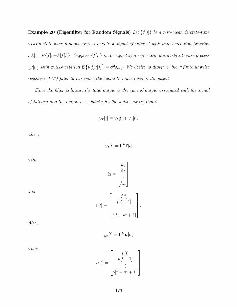
Example 20 (Eigenfilter for Random Signals) Let {f [i]} be a zero-mean discrete-time
weakly stationary random process denote a signal of interest with autocorrelation function
r[k] = E{f [i+k]f [i]}. Suppose {f [i]} is corrupted by a zero-mean uncorrelated noise process
{1[i]} with autocorrelation ES
1[i]1[j]T
= -2#i"j. We desire to design a linear finite impulse
response (FIR) filter to maximize the signal-to-noise ratio at its output.
Since the filter is linear, the total output is the sum of output associated with the signal
of interest and the output associated with the noise source; that is,
yT [t] = yf [t] + yn[t],
where
yf [t] = hHf [t]
with
h =
%
&&&'
h1
h2...
hm
(
)))*
and
f [t] =
%
&&&'
f [t]f [t & 1]
...f [t & m + 1]
(
)))*
.
Also,
yn[t] = hH#[t],
where
#[t] =
%
&&&'
1[t]1[t & 1]
...1[t & m + 1].
(
)))*
173

By signal-to-noise ratio, we mean the ratio of the average power of the signal to the average
power of the noise source. The average power of the signal is the expected value of the power,
namely,
Po = ES
y[t]2T
= ES
hHf [t]fH [t]hT
= hHES
f [t]fH [t]T
h = hHRh,
where R = ES
f [t]fH [t]T
is the autocorrelation matrix of f [t] Also, the noise power is given
by
No = ES
|yn[t]|2T
= ES
hH#[t]#H [t]hT
= hHES
#[t]#H [t]T
h = -2hHIh.
Thus, the signal-to-noise ratio is
SNR =Po
No
=hHRh
-2hHh.
This is nothing more than 1&2 times the Raleigh quotient hHRh
hHh, which is maximized by taking
h = x1,
the eigenvector corresponding to the largest eigenvalue of the autocorrelation matrix. The
maximum SNR is then
SNRmax =/1
-2.
be the noise sequence.
18.2 Gershgorin Circle Theorem
Sometimes it is important to at least obtain bounds for the values of eigenvalues of a matrix,
even though it may not be necessary or practical to compute the actual values. One way to
do this is via the Gershgorin theorem.
Before developing this theory, we state, the following fact.
174

Fact 12 The eigenvalues of a matrix A depend continuously on the elements of A. Since
the eigenvalues are nothing more than the zeros of the characteristic polynomial, the fact
that the zeros of a polynomial depend continuously on the coe"cients establishes the desired
property. The interested reader can consult the reference cited in the text for a proof of this
fact.
Definition 45 The sets in the complex plane defined by
Ri(A) =
5
;;;;;6
;;;;;7
x ( C:KKx & aii
KK $
n+
j = 1j += i
|aij |
8
;;;;;9
;;;;;:
, i = 1, . . . , n,
are called Gershgorin disks, and the boundaries of these disks are called Gershgorin
circles. The union of the Gershgorin disks is denoted
G(A) =nU
i=1
Ri(A).
!
Theorem 38 The eigenvalues of an m!m matrix A all lie in the union of the Gershgorin
disks of A, that is, /(A) , G(A). Furthermore, if any Gershgorin disk Ri(A) is disjoint from
the other Gershgorin disks of A, then it contains exactly one eigenvalue of A. By extension,
the union of any k of these disks that do not intersect the remaining m & i remaining disks
must contain precisely k of the eigenvalues, counting multiplicies.
Proof Let / be an eigenvalue of A with associated eigenvector x. Then Ax = /x or, writing
175
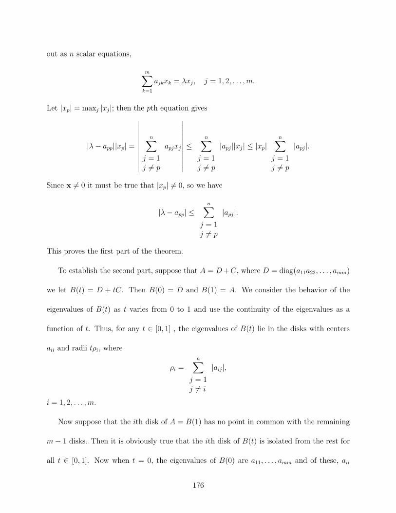
out as n scalar equations,
m+
k=1
ajkxk = /xj , j = 1, 2, . . . , m.
Let |xp| = maxj |xj |; then the pth equation gives
|/ & app||xp| =
KKKKKKKKKKK
n+
j = 1j += p
apjxj
KKKKKKKKKKK
$n+
j = 1j += p
|apj||xj | $ |xp|n+
j = 1j += p
|apj|.
Since x += 0 it must be true that |xp| += 0, so we have
|/ & app| $n+
j = 1j += p
|apj|.
This proves the first part of the theorem.
To establish the second part, suppose that A = D +C, where D = diag(a11a22, . . . , amm)
we let B(t) = D + tC. Then B(0) = D and B(1) = A. We consider the behavior of the
eigenvalues of B(t) as t varies from 0 to 1 and use the continuity of the eigenvalues as a
function of t. Thus, for any t ( [0, 1] , the eigenvalues of B(t) lie in the disks with centers
aii and radii t.i, where
.i =n+
j = 1j += i
|aij|,
i = 1, 2, . . . , m.
Now suppose that the ith disk of A = B(1) has no point in common with the remaining
m & 1 disks. Then it is obviously true that the ith disk of B(t) is isolated from the rest for
all t ( [0, 1]. Now when t = 0, the eigenvalues of B(0) are a11, . . . , amm and of these, aii
176

is the only one in the ith (degenerate) disk. Since the eigenvalues of B(t) are continuous
functions of t, and the ith disk is always isolated from the rest, it follows that there is one
and only one eigenvalue of B(t) in the ith disk for all t ( [0, 1]. In particular, this is the case
when t = 1 and B(1) = A. The remainder of the proof is left as an exercise. !
177
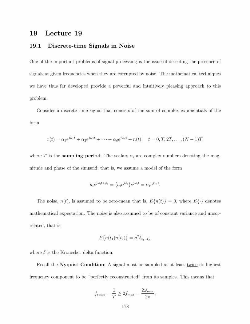
19 Lecture 19
19.1 Discrete-time Signals in Noise
One of the important problems of signal processing is the issue of detecting the presence of
signals at given frequencies when they are corrupted by noise. The mathematical techniques
we have thus far developed provide a powerful and intuitively pleasing approach to this
problem.
Consider a discrete-time signal that consists of the sum of complex exponentials of the
form
x(t) = %1ej"1t + %2e
j"2t + · · ·+ %dej"dt + n(t), t = 0, T, 2T, . . . , (N & 1)T,
where T is the sampling period. The scalars %i are complex numbers denoting the mag-
nitude and phase of the sinusoid; that is, we assume a model of the form
aiej"it+$i =
1
aiej$i2
ej"it = %iej"it.
The noise, n(t), is assumed to be zero-mean that is, E{n(t)} = 0, where E{·} denotes
mathematical expectation. The noise is also assumed to be of constant variance and uncor-
related, that is,
E{n(t1)n(t2)} = -2#t1"t2 ,
where # is the Kronecker delta function.
Recall the Nyquist Condition: A signal must be sampled at at least twice its highest
frequency component to be “perfectly reconstructed” from its samples. This means that
fsamp =1
T# 2fmax =
2,max
2(,
178

which implies
T $ (
,max
.
Problem Statement:
Given the sampled sequence {x(0), x(T ), x(2T ), . . . , x((N & 1)T )}, there are two issues
to be resolved.
Detection: Determine whether or not sinusoids are present, and if so, how many,
Estimation: Determine the amplitude, phase, and frequency of any sinusoids present.
This basic problem occurs in radar, sonar, speech recognition, medical imaging, communi-
cations, and many other applications.
In the interest of simplicity, let us assume that T = 1. Suppose for the moment that
there is only one sinusoid present. We then can stack the data in a vector as follows:
x =
%
&&&&&'
x(0)x(1)x(2)
...x(N & 1)
(
)))))*
=
%
&&&&&'
%%ej"
%ej2"
...%ej(N"1)"
(
)))))*
+
%
&&&&&'
n(0)n(1)n(2)
...n(N & 1)
(
)))))*
= %
%
&&&&&'
1ej"
ej2"
...ej(N"1)"
(
)))))*
+ n
= %s(,) + n.
The vector s(,) =
%
&&&&&'
1ej"
ej2"
...ej(N"1)"
(
)))))*
is called a Vandermonde vector.
179
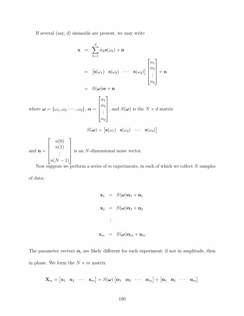
If several (say, d) sinusoids are present, we may write
x =d+
k=1
%ks(,k) + n
=,
s(,1) s(,2) · · · s(,d)-
%
&&&'
%1
%2...
%d
(
)))*
+ n
= S($)% + n
where $ = {,1, ,2, · · · , ,d}, % =
%
&&&'
%1
%2...
%d
(
)))*
, and S($) is the N ! d matrix
S($) =,
s(,1) s(,2) · · · s(,d)-
and n =
%
&&&'
n(0)n(1)
...n(N & 1)
(
)))*
is an N -dimensional noise vector.
Now suppose we perform a series of m experiments, in each of which we collect N samples
of data:
x1 = S($)%1 + n1
x2 = S($)%2 + n2
...
xm = S($)%m + nm
The parameter vectors %i are likely di!erent for each experiment; if not in amplitude, then
in phase. We form the N ! m matrix
Xm =,
x1 x2 · · · xm
-
= S($),
%1 %2 · · · %m
-
+,
n1 n2 · · · nm
-
180
or
Xm = S($)Am + Nm
with obvious definitions for the d ! m dimensional matrix Am and the N ! m dimensional
noise matrix Nm.
Now let us form the empirical autocorrelation matrix
Rmxx =
1
mXmXH
m
=1
m
,
x1 x2 · · · xm
-
%
&&&'
xH1
xH2...
xHm
(
)))*
=1
m
%
&&&'
x1(0) x2(0) · · · xm(0)x1(1) x2(1) · · · xm(1)
......
x1(N & 1) x2(N & 1) · · · xm(N & 1)
(
)))*
%
&&&'
x1(0) x1(1) · · · x1(N & 1)x2(0) x2(1) · · · x2(N & 1)
......
xm(0) xm(1) · · · xm(N & 1)
(
)))*
=1
m
%
&&&&&'
!
xi(0)xi(0)!
xi(0)xi(1) · · ·!
xi(0)xi(N & 1)!
xi(1)xi(0)!
xi(1)xi(1) · · ·!
xi(1)xi(N & 1)
......
!
xi(N & 1)xi(0)!
xi(N & 1)xi(1) · · ·!
xi(N & 1)xi(N & 1)
(
)))))*
,
where the index i in the above summations ranges from 1 to m.
Under the appropriate conditions (which is a topic for ECEn 580), the autocorrelation
matrix of x is obtained as the limit
Rxx = limm$!
Rmxx.
We also have
XmXHm =
1
S($)Am + Nm
21
AHmSH($) + NH
m
2
= S($)AmAHmSH($) + S($)AmNH
m + NmSH($)AHm + NmNH
m.
181
Thus,
Rxx = limm$!
1
m
3
S($)AmAHmSH($) + S($)AmNH
m + NmSH($)AHm + NmNH
m
$
.
Under the assumption that the noise and signals are uncorrelated, we have
limm$!
1
mS($)AmNH
m = 0.
Also, under the assumption that the noise is temporally uncorrelated, we have
limm$!
1
mNmNH
m = -2I.
Thus, the N ! N autocorrelation matrix is of the form
Rxx = S($)R''SH($) + -2I. (23)
where
R'' = limm$!
1
mAmAH
m.
Now, since R'' is a d ! d dimensional matrix, the rank of S($)R''SH($) is at most d.
19.2 Signal Subspace Techniques
We now study the autocorrelation matrix Rxx defined by (23). Suppose N > d, that is,
there are more observations than there are signals. This matrix is full rank because -2I is
full rank, but the matrix S($)R''SH($) is not full rank.
Let us now form the eigendecomposition of Rxx. Let µ1 # µ2 # · · · # µN be the eigen-
values of Rxx sorted in descending order (recall that, since Rxx is Hermitian, all eigenvalues
are real). Let ui be the eigenvector associated with µi.
182
Now let /1 # /2 # · · · # /d be the non-zero eigenvalues of S($)R''SH($). Then
µi = /i + -2,
i = 1, 2, . . . , d are the first d eigenvalues of Rxx. Furthermore, the eigenvectors associated
with the first d eigenvalues of Rxx are the same as the eigenvectors of S($)R''SH($). These
eigenvectors define the signal subspace.
The eigendecomposition of Rxx can be written as
Rxx = U$UH
=,
u1 · · ·ud ud+1 · · ·uN
-
%
&&&&&&&'
/1 + -2
. . ./d + -2
-2
. . .-2
(
)))))))*
%
&&&&&&&'
uH1...
uHd
uHd+1...
uHN
(
)))))))*
=,
Us Un
-"
$s + -2I 00 -2I
? "
UHs
UHn
?
= Us($s + -2I)UHs + -2UnUH
n
= Us$sUHs + -2UsU
Hs + -2UnUH
n
= Us$sUHs + -2I
where
Us =,
u1 · · · ud
-
Un =,
ud+1 · · · uN
-
$s = diag1
/1, · · · , /d
2
.
Thus, by the definition of Rxx, we have
S($)R''SH($) = Us$UHs .
183
This establishes that the span of the columns of S(,) is equal to the span of the columns of
Us (assuming that S(,) and R'' are full rank).
The eigenvectors associated with the remaining N & d eigenvalues of Rxx are orthogonal
to the signal subspace, and define what may be termed the noise subspace. Any vector in
the signal subspace is orthogonal to the noise subspace.
We are now in a position to exploit this structure to perform detection and estimation.
One way to do this is to invoke Ralph Schmidt’s MUSIC (MUltiple SIgnal Classification)
algorithm (1979).
1. For some su"ciently large m, calculate Rmxx = 1
mXmXH
m.
2. Perform an eigendecomposition of Rmxx, yielding eigenvalues (arranged in descending
order) µ1 # µ2 # · · · # µn and corresponding eigenvectors u1,u1, . . . ,uN .
3. Invoke a decision rule to determine the estimate d of d, the number of sinusoidal
signals present. If the model is reasonably accurate, there should be N &d eigenvalues
of approximately the same magnitude (the noise power), and d larger eigenvalues (the
power in the signal plus noise).
4. Partition the eigenvectors corresponding to the d largest eigenvalues into the matrix
Us, with the remaining eigenvectors forming Un. The columns of these two matrices
define the signal subspace and the noise subspace, respectively.
5. Now look for s(,) vectors that are (nearly) orthogonal to the noise subspace. One way
184

to do this is to form the function
P (,) =1
!Nk=d+1 .sH(,)uk.
and look for peaks in this function. Theoretically, when , = ,i, P (,) should be
infinite.
185
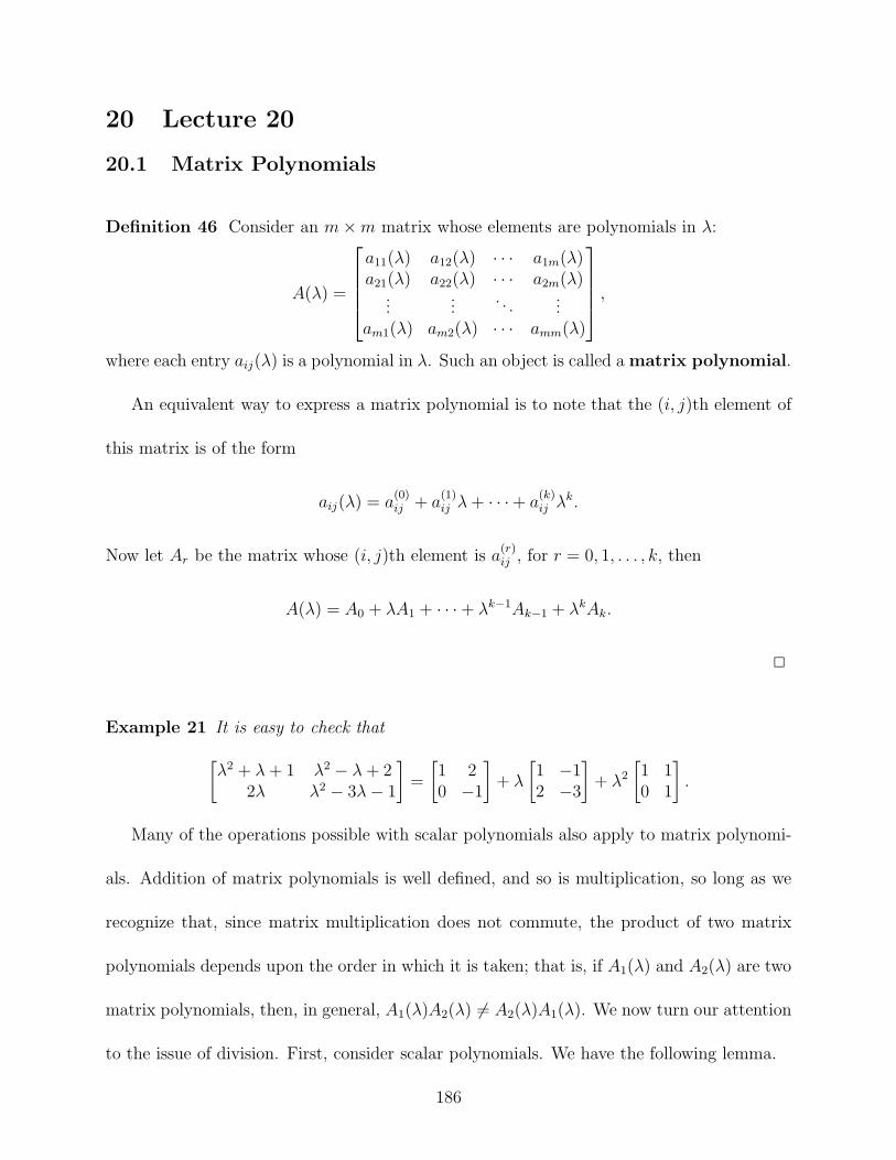
20 Lecture 20
20.1 Matrix Polynomials
Definition 46 Consider an m ! m matrix whose elements are polynomials in /:
A(/) =
%
&&&'
a11(/) a12(/) · · · a1m(/)a21(/) a22(/) · · · a2m(/)
......
. . ....
am1(/) am2(/) · · · amm(/)
(
)))*
,
where each entry aij(/) is a polynomial in /. Such an object is called a matrix polynomial.
An equivalent way to express a matrix polynomial is to note that the (i, j)th element of
this matrix is of the form
aij(/) = a(0)ij + a(1)
ij / + · · ·+ a(k)ij /k.
Now let Ar be the matrix whose (i, j)th element is a(r)ij , for r = 0, 1, . . . , k, then
A(/) = A0 + /A1 + · · · + /k"1Ak"1 + /kAk.
!
Example 21 It is easy to check that
"
/2 + / + 1 /2 & / + 22/ /2 & 3/ & 1
?
=
"
1 20 &1
?
+ /
"
1 &12 &3
?
+ /2
"
1 10 1
?
.
Many of the operations possible with scalar polynomials also apply to matrix polynomi-
als. Addition of matrix polynomials is well defined, and so is multiplication, so long as we
recognize that, since matrix multiplication does not commute, the product of two matrix
polynomials depends upon the order in which it is taken; that is, if A1(/) and A2(/) are two
matrix polynomials, then, in general, A1(/)A2(/) += A2(/)A1(/). We now turn our attention
to the issue of division. First, consider scalar polynomials. We have the following lemma.
186
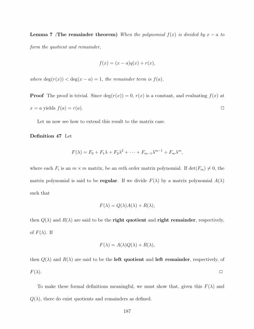
Lemma 7 (The remainder theorem) When the polynomial f(x) is divided by x & a to
form the quotient and remainder,
f(x) = (x & a)q(x) + r(x),
where deg(r(x)) < deg(x & a) = 1, the remainder term is f(a).
Proof The proof is trivial. Since deg(r(x)) = 0, r(x) is a constant, and evaluating f(x) at
x = a yields f(a) = r(a). !
Let us now see how to extend this result to the matrix case.
Definition 47 Let
F (/) = F0 + F1/ + F2/2 + · · ·+ Fm"1/
m"1 + Fm/m,
where each Fi is an m!m matrix, be an mth order matrix polynomial. If det(Fm) += 0, the
matrix polynomial is said to be regular. If we divide F (/) by a matrix polynomial A(/)
such that
F (/) = Q(/)A(/) + R(/),
then Q(/) and R(/) are said to be the right quotient and right remainder, respectively,
of F (/). If
F (/) = A(/)Q(/) + R(/),
then Q(/) and R(/) are said to be the left quotient and left remainder, respectively, of
F (/). !
To make these formal definitions meaningful, we must show that, given this F (/) and
Q(/), there do exist quotients and remainders as defined.
187

Theorem 39 Let F (/) =!(
i=0 /iFi and A(/) =!n
i=0 /iAi be m!m matrix polynomials of
degree ! and n, respectively, with det(An) += 0. Then there exists a right quotient and a right
remainder of F (/) on division by A(/), and similarly for a left quotient and left remainder.
Furthermore, these quotients and remainders are unique.
Proof If ! < n we put Q(/) = 0 and R(/) = F (/) to obtain the result.
Now consider the case l # n. Since, by hypothesis, det(An) += 0, we begin by forming
the matrix polynomial
F(A"1n /("nA(/) = F(A
"1n /("n(An/
n + · · · + A0)
= F(/( + matrix polynomial of degree < !.
Thus, we may express F (/) as
F (/) = F(A"1n /("nA(/) + F (1)(/),
where F (1)(/) is a matrix polynomial of degree !1 $ ! & 1. Writing F (1)(/) in decreasing
powers, let
F (1)(/) = F (1)(1
/(1 + · · · + F (1)0 , !1 < !.
If !1 # n we repeat the process, but on F (1)(/) rather than F (/) to obtain
F (1)(/) = F (1)(1
A"1n /(1"nA(/) + F (2)(/),
where
F (2)(/) = F (2)(2
/(2 + · · · + F (2)0 , !2 < !1.
In this manner we construct a sequence of matrix polynomials F (/), F (1)(/), F (2)(/), . . .
whose degrees are strictly decreasing, and after a finite number of terms we arrive at a
188
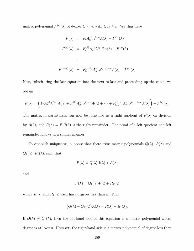
matrix polynomial F (r)(/) of degree !r < n, with !r"1 # n. We thus have
F (/) = F(A"1n /("nA(/) + F (1)(/)
F (1)(/) = F (1)(1
A"1n /(1"nA(/) + F (2)(/)
...
F (r"1)(/) = F (r"1)(r#1
A"1n /(r#11"nA(/) + F (r)(/)
Now, substituting the last equation into the next-to-last and proceeding up the chain, we
obtain
F (/) =
3
F(A"1n /("nA(/) + F (1)
(1A"1
n /(1"nA(/) + · · ·+ F (r"1)(r#1
A"1n /(r#11"nA(/)
$
+ F (r)(/).
The matrix in parentheses can now be identified as a right quotient of F (/) on division
by A(/), and R(/) = F (r)(/) is the right remainder. The proof of a left quotient and left
remainder follows in a similar manner.
To establish uniqueness, suppose that there exist matrix polynomials Q(/), R(/) and
Q1(/), R1(/), such that
F (/) = Q(/)A(/) + R(/)
and
F (/) = Q1(/)A(/) + R1(/)
where R(/) and R1(/) each have degrees less than n. Then
1
Q(/) & Q1(/)2
A(/) = R(/) & R1(/).
If Q(/) += Q1(/), then the left-hand side of this equation is a matrix polynomial whose
degree is at least n. However, the right-hand side is a matrix polynomial of degree less than
189

n. Hence Q(/) = Q1(/) and, consequently, R(/) = R1(/). A similar argument establishes
the uniqueness of the left quotient and remainder. !
We now consider matrix polynomials whose arguments are also matrices.
Definition 48 For a matrix polynomial F (/) and a matrix A, we may form the right value
of F (A) as
Fr(A) = FmAm + Fm"1Am"1 + · · ·+ F0
and the left value of F (A) as
Fl(A) = AmFm + Am"1Fm"1 + · · · + F0.
!
We now generalize the remainder theorem to the matrix case.
Theorem 40 The right and left remainders of a matrix polynomial F (/) on division by the
first-degree polynomial /I & A are Fr(A) and Fl(A), respectively.
Proof The factorization
/iI & Ai =
3
/i"1I + /i"2A + · · ·+ /Ai"2 + Ai"1
$
(/I & A)
can be verified by multiplying out the product on the right. Pre-multiplying both sides of
this equation by Fi and summing the resulting equations yields
m+
i=1
Fi/i &
m+
i=1
FiAi = C(/)(/I & A),
where C(/) is a matrix polynomial. But the left side of this equation is
m+
i=1
Fi/i &
m+
i=1
FiAi =
m+
i=0
Fi/i &
m+
i=0
FiAi = F (/) & Fr(A).
190
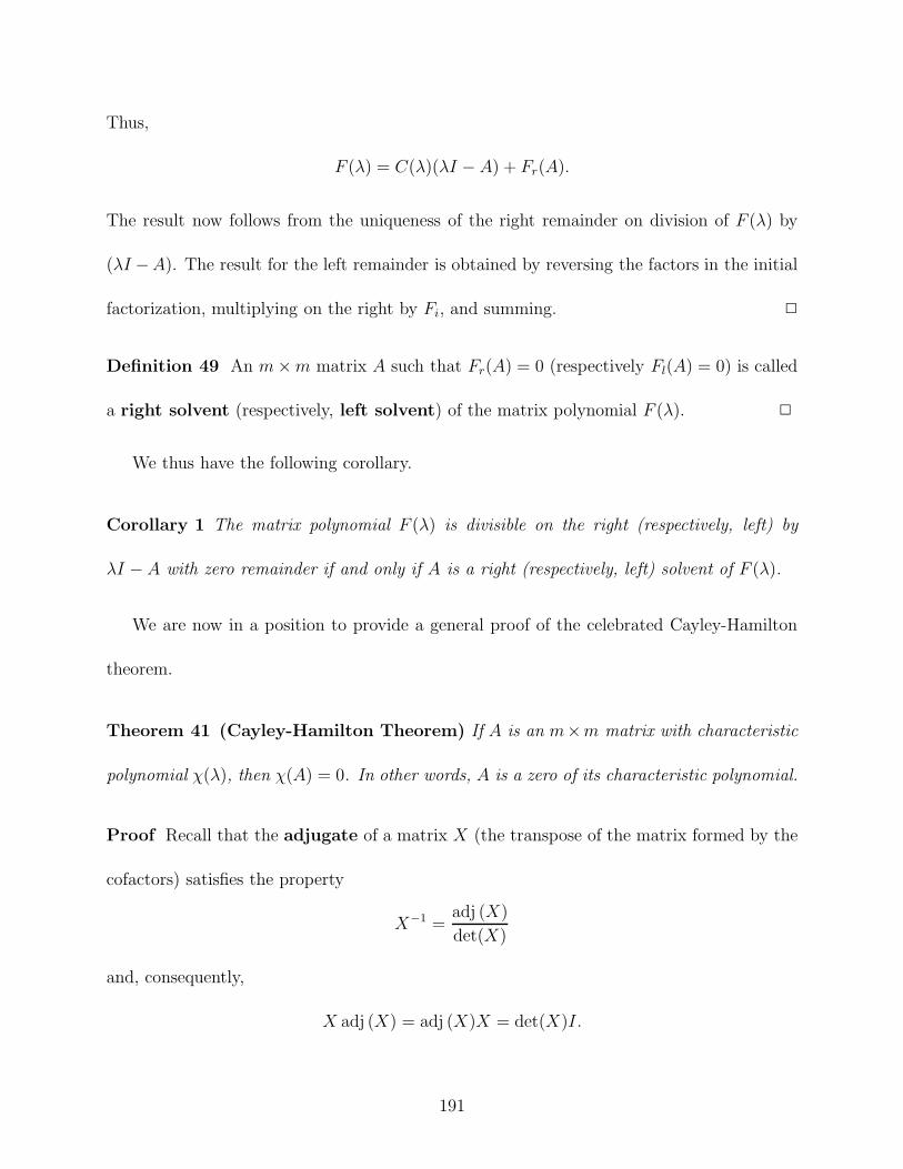
Thus,
F (/) = C(/)(/I & A) + Fr(A).
The result now follows from the uniqueness of the right remainder on division of F (/) by
(/I &A). The result for the left remainder is obtained by reversing the factors in the initial
factorization, multiplying on the right by Fi, and summing. !
Definition 49 An m ! m matrix A such that Fr(A) = 0 (respectively Fl(A) = 0) is called
a right solvent (respectively, left solvent) of the matrix polynomial F (/). !
We thus have the following corollary.
Corollary 1 The matrix polynomial F (/) is divisible on the right (respectively, left) by
/I & A with zero remainder if and only if A is a right (respectively, left) solvent of F (/).
We are now in a position to provide a general proof of the celebrated Cayley-Hamilton
theorem.
Theorem 41 (Cayley-Hamilton Theorem) If A is an m!m matrix with characteristic
polynomial 2(/), then 2(A) = 0. In other words, A is a zero of its characteristic polynomial.
Proof Recall that the adjugate of a matrix X (the transpose of the matrix formed by the
cofactors) satisfies the property
X"1 =adj (X)
det(X)
and, consequently,
X adj (X) = adj (X)X = det(X)I.
191
Now, with X = /I &A, define the matrix B(/) = adj (/I &A) and observe that B(/) is an
m ! m matrix polynomial of degree m & 1 and that
(/I & A)B(/) = B(/)(/I & A) = 2(/)I.
But 2(/)I is a matrix polynomial of degree m that is divisible on both the left and on the
right by /I & A with zero remainder. By the above corollary, we conclude that
2(A) = 0.
!
For the special case where the matrix A is diagonalizable, the proof of the Cayley-
Hamilton theorem is extremely simple.
Proof (Alternate proof when A is diagonalizable). Let S be a the matrix of linearly inde-
pendent eigenvectors, such that A = S$S"1. Then
2(A) = 2(S$S"1) = S2($)S"1 = S diag1
2(/1), . . . , 2(/m)2
S"1 = 0.
!
20.2 Eigenvalues and Eigenvectors in Control Theory
Let us consider the causal, finite-dimensional, linear time-invariant, single-input-single-output
system model
x(t) = Ax(t) + bu(t), t # 0
y(t) = cTx(t) + du(t),
192

where A is an m!m matrix termed the system matrix , b and c are m!1 vectors termed
the input distribution matrix and output distribution matrix, respectively, and d is a
scalar, termed the direct feed-through parameter. u(t) is the input function and y(t)
is the output function. The vector x(t) is the state vector of the system. The control
problem is to choose an input function such that a desired output is achieved.
We may obtain the transfer function by taking the Laplace transforms of the above
system equations and rearranging as follows. Assuming zero initial conditions, we have
sX(s) = AX(s) + bU(s)
Y (s) = cT X(s) + dU(s).
Rearranging the first of these equations yields
X(s) = (sI & A)"1bU(s),
and substituting into the second equation yields
Y (s) =
3
cT (sI & A)"1b + d
$
U(s),
so the transfer function is
H(s) =Y (s)
U(s)= cT (sI & A)"1b + d.
Using the properties of the adjugate, we obtain
H(s) =cT adj (sI & A)b + d det(sI & A)
det(sI & A).
We observe that the numerator cT adj (sI&A)b+d det(sI&A) and the denominator det(sI&
A) are both polynomials in s. Thus, the transfer function is of the form
H(s) =b(s)
a(s),
193
where b(s) = cT adj (sI & A)b + d det(sI & A) and a(s) = det(sI & A).
Definition 50 Let H(s) be the transfer function of a finite-dimensional linear time-invariant
system. The zeros of H(s) are those values of s such that H(s) = 0. The poles of H(s) are
those values of s such that |H(s)| = 2. !
We observe that the finite poles of the system are exactly the eigenvalues of the system
matrix A. To interpret the poles, we can perform a partial fraction expansion of the transfer
function to obtain
H(s) =bmsm + bm"1sm"1 + · · · + b0
sm + am"1sm"1 + · · · + a0
= K! +K11
(s & /1)+
K12
(s & /1)2+ · · · K1m1
(s & /1)m1
+K21
(s & /2)+
K22
(s & /2)2+ · · · K2m1
(s & /2)m2
+ · · ·
+K(1
(s & /()+
K(2
(s & /()2+ · · · K(m1
(s & /()m!
where /i, i = 1, . . . , ! denote the distinct eigenvalues, each with algebraic multiplicity mi,
so that m1 + m2 + · · · + m( = m. The constants Kij are the partial fraction expansion
coe"cients. Inverting this function, the impulse response function is
h(t) = K!#(t) + K11e%1t +
K12te%1t
1!+ · · ·+ K1m1t
m1"1e%1t
(m1 & 1)!
+K21e%2t +
K22te%2t
1!+ · · ·+ K2m2t
m2"1e%2t
(m2 & 1)!
+ · · ·
+K(1e%!t +
K(2te%!t
1!+ · · ·+ K(m2t
m!"1e%!t
(m( & 1)!
for t # 0.
194
Definition 51 A linear time-invariant system is said to be bounded-input-bounded
output (BIBO) stable if a bounded input produces a bounded output. !
Clearly, if K! += 0, the presence of the delta function in the output generates an un-
bounded output, so a bounded system must have K! = 0. It can be shown that conditions
for BIBO stability are that
1. The degree of the numerator of H(s) must be less than the degree of the denominator.
This condition is satisfied if d = 0, since the degree of cT adj (SI & A)b is strictly less
than m.
2. The poles of H(s) must lie strictly in the left-half complex plane; that is, /(/i) < 0.
This can be seen by inspection of a typical term
Kimitmi"1e%it
mi & 1,
which tends to zero in the limit as t " 2 if and only if /(/i) < 0.
Example 22 (Pole-placement using full state feedback) Consider the time-invariant
linear system model
x(t) = Ax(t) + bu(t), t # 0, x(0) = x0
y(t) = cTx(t)
with transfer function
H(s) =Y (s)
U(s)= cT (sI & A)"1b =
cT adj (sI & A)b
det(sI & A).
195
Suppose it is desired that a system be controlled such that it stays close to the origin, such
that, if any perturbations to the system should occur, it will quickly return to the origin. An
elegant way to accomplish this task is to use feedback. Suppose, by some means (which need
not concern us at the moment) we are able to obtain knowledge of the state vector x(t) at
every point in time. We could then apply state feedback of the form
u(t) = kTx(t),
where kT is an m ! 1 feedback gain matrix. The resulting closed-loop system then is
described by the di!erential equation
x(t) = Ax(t) + bkT x(t) =1
A + bkT2
x(t).
The gain matrix k is chosen to place the poles of the closed-loop system matrix A + bkT so
as to regulate the system in an appropriate manner.
For a specific numerical example, suppose
"
x1(t)x2(t)
?
=
"
0 12 &1
? "
x1(t)x2(t)
?
+
"
01
?
u(t).
The characteristic equation for this system is
2(s) = det(sI & A) = s2 + s & 2,
which has poles at s1 = 1 and s2 = &2. This system is unstable, and any perturbation from
x(0) = 0 will cause the system to diverge from the origin. We desire to choose a feedback
gain matrix kT =,
k1 k2
-
to stabilize this system. The closed-loop system matrix is of the
form
A + bkT =
"
0 12 &1
?
b +
"
01
?,
k1 k2
-
=
"
0 12 + k1 k2 & 1
?
.
196
The characteristic equation for the closed-loop system matrix is
2c(s) = det(sI & A & bkT ) = det
3"
s &1&2 & k1 s + 1 & k2
?$
= s2 + s(1 & k2) & 2 & k1.
Now suppose we desire to place the closed-loop poles securely in the left-half plane, say at
s = &1 and s = &2. Then the characteristic equation for the desired system is then
2d(s) = s2 + 3s + 2.
We can achieve this performance by choosing k such that 2c(s) = 2d(s), which is achieved
by setting
1 & k2 = 3 ; k2 = &2
&2 & k1 = 2 ; k1 = &4.
The closed-loop system is of the form
"
x1(t)x2(t)
?
=
"
0 1&2 &3
? "
x1(t)x2(t)
?
which is stable. Any perturbations will generate a feedback signal that will tend to drive it
back to the origin.
This solution is somewhat artificial because we simply assumed that we had knowledge of
the entire state. With a single-input-single-output system, however, we only have access to
a linear combination of the output, that is,
y(t) = cTx(t).
Thus, if we are to make any practical use out of the pole-placement approach to system
control, we will need to find a way to gain access to the full state. To do this, we will apply a
197
very simple idea: we start by constructing a computer-based simulator of the actual physical
system of the form
˙x(t) = Ax(t) + bu(t), x(0) = x0,
This system would run in parallel with the actual plant, and if our model were correct and
we knew the exact initial conditions of the plant (that is, if x0 = x0), then our simulation
would reproduce the state and we could use x in place of x to e!ect the state feedback so that
the resulting system would be of the form
"
x(t)˙x(t)
?
=
"
A bkT
0 A
? "
x(t)x(t)
?
,
"
x(0)x(0)
?
=
"
x0
x0
?
.
This approach would work if we could be assurred that the error x(t) = x(t) & x(t) can be
made to be arbitrarily small. Unfortunately, this condition cannot be guaranteed with the
above simulation even if the model is accurate, because the initial conditions are not known.
But there is a way to improve things. We can use the di!erence between the actual output
y(t) and the simulated output y(t) = cT x(t) to design another feedback system as follows.
Suppose we were to modify the simulated system to be of the form
˙x(t) = Ax(t) + bu(t) + ![y(t) & y(t)], x(0) = x0
= Ax(t) + bu(t) + !cT [x(t) & x(t)],
where ! is a feedback gain vector to be suitably chosen. This system is called an asymptotic
observer. The goal is to choose ! such that the state error,
x(t) = x(t) & x(t)
tends to zero rapidly as t " 2. Subtracting the actual plant dynamics from the observer
198
dynamics, we obtain a di!erential equation in the error; namely,
˙x(t) = x(t) & ˙x(t) = Ax(t) + bu(t) & Ax(t) & bu(t) & !cT [x(t) & x(t)]
or, collecting terms,
˙x(t) = (A & !cT )x(t).
Now, it should be clear that, if we can place the eigenvalues of the matrix A & !cT into the
left-half plane, the error will asymptotically die out, and we may substitute x(t) for x(t) with
confidence.
To continue our numerical example, suppose cT =,
1 0-
. Then
A & !cT =
"
0 12 &1
?
&"
l1l2
?,
1 0-
=
"
&l1 12 & l2 &1
?
.
The characteristic equation for this observer is
2o(s) = (s + l1)(S + 1) & 2 + l2 = s2 + (l1 + 1)s + l1 + l2 & 2
A good rule of thumb is that the dynamics of the observer should be five or so times faster
than the dominant mode of the controller. This means that the poles of the observer should
be at, say, &5. Thus, the desired characteristic equation of the observer is
2d(s) = (s + 5)2 = s2 + 10s + 25.
Equating 2d(s) with 2o(s) yields
l1 + 1 = 10 ; l1 = 9
l1 + l2 & 2 = 25 ; l2 = 18
199
The resulting observer error dynamics equation is then
˙x(t) =
"
&9 &172 &1
?
x(t), x(0) = x(0) & x0
The observer dynamic system is
˙x(t) = Ax(t) + bu(t) + ![y(t) & cTx(T )],
and since we set u(t) = kT x(t), we obtain
˙x(t) = Ax(t) + bkT x(t) + ![y(t) & cTx(T )]
= (A + bkT & !cT )x(t) + !y(t).
Together, the controller and the observer form the system
"
x(t)˙x(t)
?
=
"
A bkT
0 A & !cT + bkT
? "
x(t)x(t)
?
+
"
0!
?
y(t).
These two dynamic equations form what is called a compensator.
200

21 Lecture 21
21.1 Matrix Square Roots
Definition 52 Let A be an m ! m matrix. By analogy with real numbers, we consider
the existence of a matrix A0 such AH0 A0 = A. Such a matrix A0 is called a square root
of A. Notationally, we often write A12 for the square root of A. Also, some authors use the
notation AT2 for
1
A12
2T. !
It is easy to see that all diagonalizable matrices possess a square root. In general, square
roots of a matrix are not unique, since if A12 is a square root, then QA
12 is also a square root
for every m ! m unitary matrix Q.
Let us now specialize to Hermitian matrices.
Theorem 42 A matrix A is positive definite (or semi-definite) if and only if it has a positive
definite (respectively, semi-definite) square root A0. Also, rank (A0) = rank (A).
Moreover, the positive definite (respectively, semi-definite) square-root of A is unique.
Proof Let A be an m!m positive semi-definite matrix. Then its eigenvalues /1, /2, . . . , /m
are non-negative and we can define a real matrix D0 = diag(<
/1,<
/2, . . . ,<
/m). Let
D = D20. By the spectral decomposition theorem, there is a unitary matrix of eigenvectors
of A such that A = UDUH . Let
A0 = UD0UH .
Then
A20 = UD0U
HUD0UH = UD2
0UH = UDUH ,
201
thus A0 is a square root of A. This construction shows that the eigenvalues of A0 are the
square roots of the eigenvalues of the eigenvalues of A. This proves that the two matrices
are of the same rank.
Conversely, if A = A20 and A0 # 0, then can form the spectral decomposition of A0 as
A0 = UD0UH , so that A = A20 = UD2
0UH and we see that the eigenvalues of A are the
squares of the eigenvalues of A0, hence are non-negative. This fact also implies equality of
the ranks.
To establish uniqueness, suppose A1 # 0 satisfies A21 = A. By an argument similar to the
one above, the eigenvalues of A1 must be the same as the eigenvalues of A0. Furthermore,
A1 is Hermitian and, therefore, has a spectral decomposition A1 = UD0UH , where U is a
unitary matrix comprising the eigenvectors of A. Thus, A1 = A0.
The same argument proves the theorem for the positive definite case.
!
Although spectral decompositions of matrices are restricted to square matrices, the ques-
tion arises as to what, if anything, can be said about the spectral structure of non-square
matrices.
Definition 53 Consider an arbitrary m ! n matrix A. The matrix AHA is positive semi-
definite (or definite), and therefore has a unique positive semi-definite (or definite) square
root H1 =1
AHA2 1
2 such that AHA = H21 . The eigenvalues -1, -2, . . . , -m of the matrix
H1 =1
AHA2 1
2 are called the singular values of A. !
Theorem 43 Let A be an arbitrary m!n matrix. The non-zero eigenvalues of the matrices
202
1
AHA2 1
2 and1
AAH2 1
2 coincide.
Proof It su"ces to prove the theorem for the matrices AHA and AAH . Let /1, /2, . . . , /n be
the eigenvalues of AHA, with corresponding orthonormal eigenvectors x1,x2, . . . ,xn. Then
0AHAxi,xj1 = /i0xi,xj1 = /i#ij , 1 $ i, j $ n.
Since 0AHAxi,xj1 = 0Axi, Axj1, it follows that 0Axi, Axi1 = /i, i = 1, 2, . . . , n. thus,
Axi = 0 if and only if /i = 0. For the case /i += 0, we have
AAH(Axi) = A(AHAxi) = /iAxi, 1 $ i $ n,
which shows that the vector Axi is an eigenvector of AAH . Thus, if /i is a non-zero eigenvalue
of AHA (with eigenvector xi), then /i is also an eigenvalue of AAH (with eigenvector Axi).
Thus, all non-zero eigenvalues of AHA are also non-zero eigenvalues of AAH .
If we exchange the roles of A and AH and follow exactly the same argument as above,
we see that all non-zero eigenvalues of AAH are also non-zero eigenvalues of AHA. Thus the
two sets of non-zero eigenvalues coincide. !
The eigenvalues of AHA and AAH , and hence of1
AHA2 1
2 and1
AAH2 1
2 , di!er only in the
geometric multiplicity of the zero eigenvalue. If there are r $ min(m, n) non-zero eigenvalues,
then the geometric multiplicity of the zero eigenvalue for AHA is n & r, and the geometric
multiplicity of the zero eigenvalue for AAH is m & r.
21.2 Polar and Singular-Value Decompositions
Recall that any complex number z can be expressed as z = .ej), where . # 0 and 0 $ ' $ 2(.
The matrix analogue to that result is the following theorem.
203
Theorem 44 Polar Decomposition. Any n! n matrix A can be represented in the form
A = HU, (24)
where H # 0 and U is unitary. Moreover, the matrix H is unique and given by H =1
AAH2 1
2 .
Proof Suppose AHA has r $ n non-zero eigenvalues, indexed as
/1 # /2 # · · · # /r > 0 = /r+1 = · · · = /n
with corresponding orthonormal eigenvectors x1,x2, . . . ,xn. As we saw above, for i $ r, the
vectors Axi are eigenvectors of AAH , and hence, the normalized vectors
yi =1
.Axi.Axi =
1</i
Axi (25)
are orthonormal eigenvectors of AAH corresponding to the eigenvalues /1, /2, . . . , /r, respec-
tively. We may then choose n& r orthonormal vectors yr+1, . . . ,yn in the nullspace of AAH
to extend this set to an orthonormal eigenbasis for AAH .
Let H =1
AAH2 1
2 . Since yi is an eigenvector of AAH corresponding to eigenvalue /i, it
is also an eigenvector of H corresponding to eigenvalue<
/i. That is, using (25),
Hyi =M
/iyi = Axi, i = 1, 2, . . . , n.
Now let us define the matrix U by the relationship
Uxi = yi,
that is, U maps the orthonormal basis defined by the eigenvectors of AHA into the ortho-
normal basis defined by the eigenvectors of AAH . Thus U is a unitary matrix.
204
Exercise: Show that a matrix U is unitary if and only if it transforms an orthonormal basis
into an orthonormal basis.
Thus,
HUxi = Hyi =M
/iyi = Axi, i = 1, 2, . . . , r.
Since 0Axi, Axi1 = 0AHAxi,xi1 = /i = 0 for i = r + 1, r + 2, . . . , rn, it follows that
Axi = 0 for r + 1 $ i $ n. Furthermore, as we saw earlier, AAHyi = 0 implies Hyi = 0.
Thus,
HUxi = Hyi = 0 = Axi, i = r + 1, . . . , n.
We thus have
HUxi = Axi
for all members of the eigenbasis x1,x2, . . . ,xn of Cn. Since every x ( Cn can be written as
a linear combination of this basis set, we have
HUx = Ax
for every x ( Cn. Since this holds for every x, it follows that
A = HU.
!
By exchanging the roles of A and AH , we have the immediate corollary
Corollary 2 Any n ! n matrix A can be represented in the form
A = H1U1, (26)
205
where H1 # 0 and U1 is unitary. Moreover, the matrix H1 is unique and given by H1 =
1
AHA2 1
2 .
Equations (24) and (26) are called the polar decompositions of A. By analogy with the
polar representation of a scalar z = .ej), the positive semi-definite matrix H corresponds
to . and unitary matrix (a rotation) corresponds to the rotation through the angle ' in the
complex plane in the scalar case.
Theorem 45 Singular-Value Decomposition. Let A be an arbitrary m ! n matrix and
let -1, -2, . . . , -r be the non-zero singular values of A. Then A can be represented in the form
A = U%V H , (27)
where U is an m ! m unitary matrix, V is an n ! n unitary matrix, and % is an m ! n
matrix that has has -i in the (i, i)th entry for i = 1, 2, . . . , r and zero everywhere else.
The representation given by (27) is referred to as a singular-value decomposition (SVD)
of the matrix A.
Proof From our earlier development, we know that the systems of eigenvectors {x1,x2, . . . ,xn}
for AHA and {y1,y2, . . . ,yn} for AAH are orthonormal eigenbases for Cn and Cm, respec-
tively, and that
Axi =M
/iyi, i = 1, 2, . . . , r. (28)
We have also established that
Axi = 0, i = r + 1, . . . , n.
206
Now define the matrices
V =,
x1 x2 · · · xn
-
and U =,
y1 y2 · · · ym
-
,
and note that they are unitary. Since by definition
-i =M
/i, i = 1, 2, . . . , r,
Equation (28) implies that
AV =,
-1y1 -2y2 · · · -ryr 0 · · ·0-
= U%,
where % is the matrix in (27). Finally, since V is unitary, we have
A = U%V H .
!
By exchanging the roles of A and AH , we may show that the SVD of AH is
AH = V %HUH ,
and that, for eigenbases {x1, . . . ,xn} of AHA and {y1, . . . ,ym} of AAH ,
AHyi =
4
-ixi if i = 1, 2, . . . , r0 if i = r + 1, , . . . , m
.
The structure of the SVD becomes apparent with the three possible cases
Case 1: m = n
% =
%
&&&'
-1 0 · · · 00 -2...
. . .0 -n
(
)))*
207
Case 2: m > n
% =
%
&&&&&&&&&'
-1 0 · · · 00 -2...
. . .0 -n
0 · · · 0...
...0 · · · 0
(
)))))))))*
Case 3: m < n
% =
%
&&&'
-1 0 · · · 0 0 · · · 00 -2 0 0 · · · 0...
. . ....
0 -m 0 · · · 0
(
)))*
Definition 54 Let A be an arbitrary m ! n matrix with SVD A = U%V H . The diagonal
elements of % are called the singular values of A. The columns of U are called the left
singular vectors or left singular bases of A. The columns of V are called the right
singular vectors or right singular bases of A. !
Example 23 Let
A =
%
'
1 00 11 0
(
*
To find an SVD for A, we compute AHA and AAH and construct orthonormal eigenbases
for these matrices. We obtain
AHA =
"
1 0 10 1 0
?%
'
1 00 11 0
(
* =
"
2 00 1
?
and
AAH =
%
'
1 00 11 0
(
*
"
1 0 10 1 0
?
=
%
'
1 0 10 1 01 0 1
(
* .
The singular values are immediately seen to be -1 =<
2 and -2 = 1. The eigenbases are
208
computed to be
U =
%
'
1,2
0 1,2
0 1 01,2
0 & 1,2
(
*
and
V =
"
1 00 1
?
.
The matrix of singular values is
% =
%
'
<2 0
0 10 0
(
* .
The corresponding SVD is
A =
%
'
1,2
0 1,2
0 1 01,2
0 & 1,2
(
*
%
'
<2 0
0 10 0
(
*
"
1 00 1
?
.
Some facts about SVD’s
1. The singular values are always ordered in descending order.
2. The singular values are always real and positive.
3. If A is real, then U and V are real and orthogonal.
4. The singular values are the square roots of the eigenvalues of AHA and of AAH (which
may involve extra zeros).
Theorem 46 Let A be an m ! n matrix of rank r, and express the SVD of A as
A =,
U1 U2
-"
%1 00 0
? "
V H1
V H2
?
,
209
where U1 is m! r, U2 is m! (m& r), %1 is r! r, V H1 is n! r, and V H
2 is n! (n& r). Then
R(A) = span (U1)
N (A) = span (V2)
R(AH) = span (V1)
N (AH) = span (U2)
Proof The nullspace of A must have dimension n & r. Let v2 be any column taken from
V2 (there are n & r such columns). Then
Av2 = U1%1VH1 v2 = 0
since the columns of V are mutually orthogonal. Thus, span (V2) , N (A). Conversely, if
v += 0 and v ( N (A), then Av = 0, then v 3 v1, where v1 is any column of V1. Since N (A)
and R(A) are orthogonal subspaces, we have that v ( span (V2). Thus, N (A) , span (V2),
and
N (A) = span (V2).
The rest of this proof is left as an exercise. !
210
22 Lecture 22
22.0.1 Generalized Inverses
We have previously discussed matrix pseudo-inverses, and have established that if an m! n
matrix A is full rank, then it possesses a left pseudo-inverse of the form1
AT A2"1
AT if m > n
and it possesses a right pseudo-inverse of the form AT1
AAT )"1 if m < n. We now address
the question: Can we define a concept of matrix inverse if A is not full rank?
Definition 55 Let A be an arbitrary m! n matrix. A generalized inverse, denoted AI ,
of A is a matrix that satisfies the equation
AAIA = A (29)
AIAAI = AI . (30)
!
Theorem 47 A generalized inverse AI exists for every matrix A.
Proof We first observe that if A is an m ! n identically zero matrix, then the n ! m zero
matrix satisfies the defining equations. Now suppose rank (A) = r > 0, and let the SVD of
A be given by
A = U%V H =,
U1 U2
-"
%1 00 0
? "
V H1
V H2
?
where U1 is m ! r, U2 is m ! (m & r), %1 is a diagonal r ! r matrix with positive diagonal
elements, V H1 is n ! r, and V H
2 is n ! (n & r). We can re-write this SVD as
A =I
U1%121 U2
J"
Ir 00 0
?D
%121 V H
1
V H2
E
= R
"
Ir 00 0
?
S, (31)
211
where Ir is an r! r identity matrix, R =I
U1%121 U2
J
and S =
D
%121 V H
1
V H2
E
. It is easily verified
that the matrix
AI = S"1
"
Ir B1
B2 B2B1
?
R"1
satisfies conditions (29) and (30) for any r ! (n & r) matrix B1 and any (m& r)! r matrix
B2. !
An immediate consequence of the construction of a generalized inverse is that
1. AIA and AAI are idempotent matrices, e.g., from (30)
(AAI)2 = (AAI)(AAI) = A(AIAAI) = AAI ,
and by a similar argument, (AIA)2 = AIA.
2. rank (A) = rank (AI), since the rank of the product of two matrices is equal to the
minimum rank of the matrices.
3. If AI is a generalized inverse of A, then the matrix1
AI2H
is a generalized inverse of
AH , i.e., taking the Hermitian of (29),
AH =1
AAIA2H
= AH1
AI2H
AH .
A similar result holds for (30).
Theorem 48 If A is an m ! n matrix and if AI is a generalized inverse of A, then
R(A) + N (AI) = Cm (32)
N (A) + R(AI) = Cn, (33)
212
that is, the inner sum of the range of A and the null space of AI constitutes Cm, and the
inner sum of the range of AI and the null space of A constitutes Cn.
Proof Since AAI is a projection matrix (i.e., it is idempotent), it is clear that R(AAI) ,
R(A). Now let y = Ax ( R(A). Since A = AAIA, we have that y = (AAI)(Ax) ( R(AAI).
Thus R(A) , R(AAI) and hence R(AAI) = R(A).
Furthermore, rank (A) = rank (AAI) = rank (AI). Obviously, N (AI) , N (AAI). But
dim1
N (AI)2
= m & rank (AI) = m & rank (AAI) = dim1
N (AAI)2
,
so it follows that N (AI) = N (AAI). Combining this result with the fact that AAI is a
projection matrix,
Cm = R(AAI) + N (AAI) = R(A) + N (AI).
This establishes (32). Since the defining equations for AI are symmetric in A and AI , we
can replace A, AI by AI , A respectively, and repeat the above procedure to obtain (33). !
Although the above theorem establishes that Cm can be decomposed into algebraic comple-
ments, they need not be orthogonal. Let us further impose the requirement that R(A) 3
N (AI). We begin with a definition.
Definition 56 Let A be an arbitrary m ! n matrix, and let AI be a generalized inverse
such that
1
AAI2H
= AAI (34)
1
AIA2H
= AIA. (35)
The AI is said to be a Moore-Penrose Inverse of A, and is denoted A†. !
213

Since A†A and AA† are idempotent matrices, they are projection operators. In fact, as
the following theorem shows, they are orthogonal projection operators.
Theorem 49 Let A be an arbitrary m ! n matrix. then the Moore-Penrose inverse A† is
unique, R(A) 3 N (A†), and R(A†) 3 N (A), that is,
R(A) 5N (A†) = Cm
R(A†) 5N (A) = Cn.
Proof Since the Moore-Penrose inverse must comply with (34) and (35), Let x ( N (AA†)
and y ( R(AA†). Note that since AA† projects elements of Cm onto R(AA†) and R(AA†)
is disjoint from N (AA†), we have
0x,y1 = 0x, (AA†)y1 =G1
AA†2Hx,y1 = 00,y1 = 0.
This establishes that N1
AA†2
5R1
AA†2
, and from the previous theorem, N (A†) = N (AA†),
etc., hence the result follows.
To establish uniqueness, suppose A†1 and A†
2 are two Moore-Penrose inverses of A, con-
sequently, they both possess the following properties:
AA†iA = A (36)
A†iAA†
i = A†i (37)
1
AA†i
2H= AA†
i (38)
1
A†iA2H
= A†iA, (39)
for i = 1, 2. By (37) and (38), we have
1
A†i
2H=1
A†i
2HAH1
A†i
2H= AA†
i
1
A†i
2H, i = 1, 2,
214
and hence
1
A†1
2H &1
A†2
2H= A
3
A†1
1
A†1
2H & A†2
1
A†2
2H$
.
Now let y ( R31
A†1
2H &1
A†2
2H$
. Then there exists x ( Cm such that
I1
A†1
2H &1
A†2
2HJ
x = y.
By setting
x' =I
A†1
1
A†1
2H & A†2
1
A†2
2HJ
x,
we have that Ax' = y, thus
R31
A†1
2H &1
A†2
2H$
, R(A).
On the other hand, using (36) and (39), we see that
AH = AH1
A†i
2HAH = A†
iAAH , i = 1, 2,
which implies that1
A†1 &A†
2
2
AAH = 0, or, transposing, AAH
31
A†1
2H &1
A†2
2H$
= 0. Thus,
R31
A†1
2H &1
A†2
2H$
, N (AAH) = N (AH).
But N (AH) is orthogonal to R(A), so the only vector they have in common is 0. Thus,
1
A†1
2H &1
A†2
2Hmaps all vectors to the zero vector, which implies that A†
1 = A†2. !
Corollary 3 For any matrix A,
N (A†) = N (AH)
R(A†) = R(AH)
215
and, consequently,
A†Ax = x, x ( R(AH)
AA†y = y, y ( R(A).
Proof This follows from Theorem 49 and the fact that
R(A) 5N (AH) = Cm
N (A) 5R(AH) = Cn
and the fact that AA† and AAH are projection operators. !
Definition 57 Recalling (31) where rank (A) = r, we write
A =,
R1 R2
-"
Ir 00 0
? "
S1
S2
?
= R1S1, (40)
where R1 is m ! r and S1 = r ! n and both are rank r. Equation (40) is called a rank
decomposition of A. !
Theorem 50 Let A be an arbitrary m ! n matrix, and let
A = RSH ,
where R is m ! r and S is n ! r be a rank decomposition of A. Then
A† = S1
SHS2"11
RHR2"1
RH (41)
is the Moore-Penrose inverse of A. Furthermore,
1.1
AH2†
=1
A†2H
216
2. For unitary U and V ,1
UAV2†
= V HA†UH .
3.1
A†2† = A.
4.1
AAH2†
=1
A†2HA† and1
AHA2†
= A†1A†2H .
Proof To establish (41), it su"ces to show that the conditions defined by (36) through (39)
hold, which are verified by direct computation.
We now prove selected portions of the theorem, leaving the remaining portions as exer-
cises.
To show that1
UAV2†
= V HA†UH , we note that if A = RSH is a rank decomposition of
A, then (UR)(SHV ) is a rank decomposition of UAV . Then, applying the structure of (41),
we have
1
UAV2†
=1
V HS2
(SHV V HS2"1
(RHUUH2"11
RHUH2
= V HA†UH .
To show that1
AAH2†
=1
A†2HA†, we note that, if A = RSH is a rank decomposition of
A, then
AAH = RSHSRH = R1
SHSRH2
is a rank decomposition of AAH . Applying the structure of (41), we obtain
1
AAH2†
= RSHS1
SHSRHRSHS2"11
RHR2"1
RH
= RSHS1
SHS2"11
RHR2"11
SHS2"11
RHR2"1
RH
= R1
RHR2"11
SHS2"11
RHR2"1
RH .
217
Also,
1
A†2HA† = R1
RHR)"11
SHS2"1
SHS1
SHS2"11
RHR2"1
RH
= R1
RHR2"11
SHS2"11
RHR2"1
RH .
!
Recall that the singular value decomposition of a matrix A of rank r involves a pair of
orthonormal eigenbases {x1,x2, . . . ,xn} and {y1,y2, . . . ,ym} of the matrices AHA and AAH ,
respectively, such that
Axi =
4
-iyi if i = 1, 2, . . . , r0 if i = r + 1, , . . . , n
(42)
and
AHyi =
4
-ixi if i = 1, 2, . . . , r0 if i = r + 1, , . . . , m
. (43)
The following theorem provides some deep insight into the structure of the Moore-Penrose
inverse.
Theorem 51 Let A be an m ! n matrix with singular values -1 # -2 # · · · # -r > 0 =
-r+1 = · · · = -n. Then -"11 , -"1
2 , · · · , -"1r are the nonzero singular values of A†. Moreover,
{x1,x2, . . . ,xn} are the right singular bases of A and {y1,y2, . . . ,ym} are the left singular
bases of A, that is,
A†yi =
4
-"1i xi if i = 1, 2, . . . , r
0 if i = r + 1, , . . . , m(44)
and
1
A†2Hxi =
4
-"1i yi if i = 1, 2, . . . , r
0 if i = r + 1, , . . . , n. (45)
218
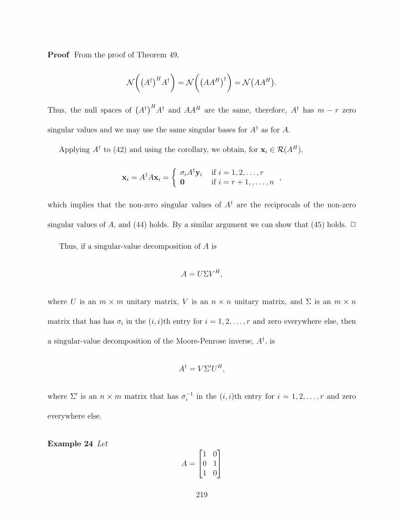
Proof From the proof of Theorem 49,
N31
A†2HA†$
= N31
AAH2†$
= N1
AAH2
.
Thus, the null spaces of1
A†2H
A† and AAH are the same, therefore, A† has m & r zero
singular values and we may use the same singular bases for A† as for A.
Applying A† to (42) and using the corollary, we obtain, for xi ( R(AH),
xi = A†Axi =
4
-iA†yi if i = 1, 2, . . . , r0 if i = r + 1, , . . . , n
,
which implies that the non-zero singular values of A† are the reciprocals of the non-zero
singular values of A, and (44) holds. By a similar argument we can show that (45) holds. !
Thus, if a singular-value decomposition of A is
A = U%V H ,
where U is an m ! m unitary matrix, V is an n ! n unitary matrix, and % is an m ! n
matrix that has has -i in the (i, i)th entry for i = 1, 2, . . . , r and zero everywhere else, then
a singular-value decomposition of the Moore-Penrose inverse, A†, is
A† = V %'UH ,
where %' is an n ! m matrix that has -"1i in the (i, i)th entry for i = 1, 2, . . . , r and zero
everywhere else.
Example 24 Let
A =
%
'
1 00 11 0
(
*
219
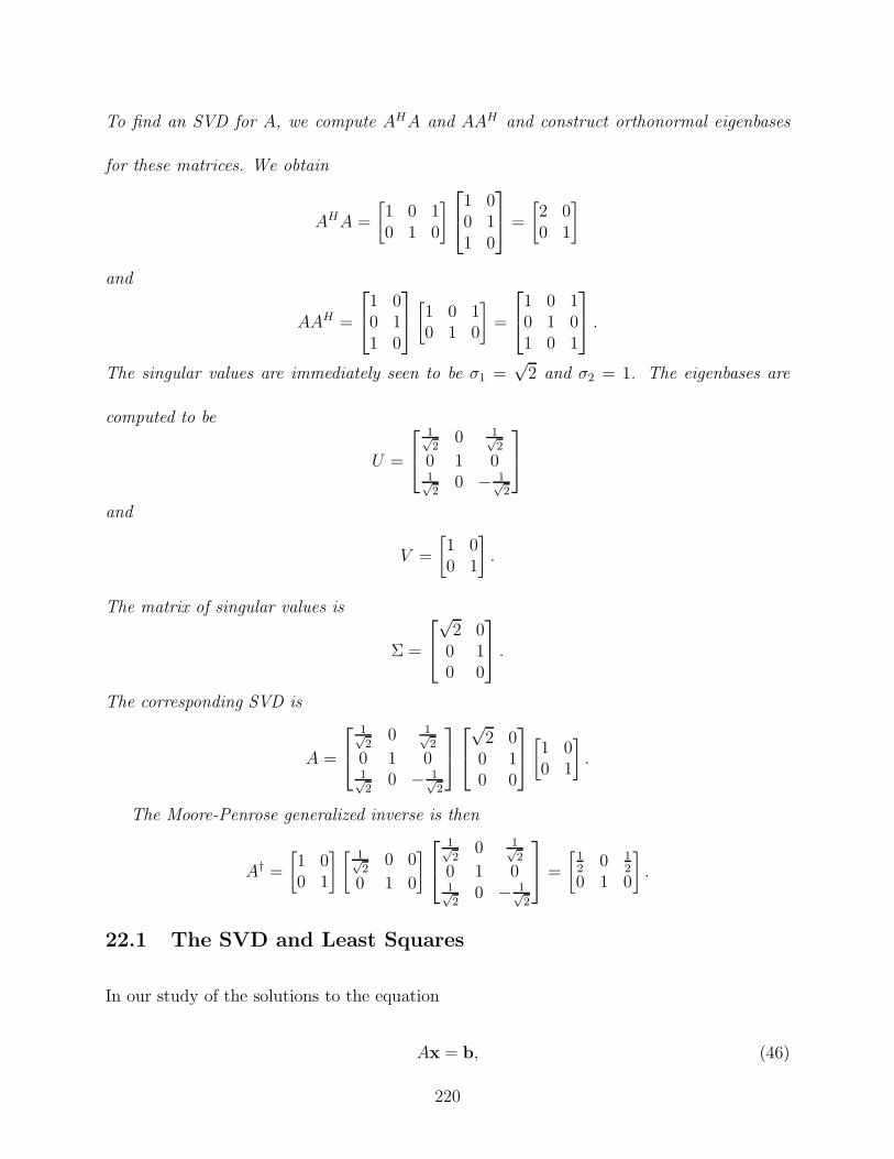
To find an SVD for A, we compute AHA and AAH and construct orthonormal eigenbases
for these matrices. We obtain
AHA =
"
1 0 10 1 0
?%
'
1 00 11 0
(
* =
"
2 00 1
?
and
AAH =
%
'
1 00 11 0
(
*
"
1 0 10 1 0
?
=
%
'
1 0 10 1 01 0 1
(
* .
The singular values are immediately seen to be -1 =<
2 and -2 = 1. The eigenbases are
computed to be
U =
%
'
1,2
0 1,2
0 1 01,2
0 & 1,2
(
*
and
V =
"
1 00 1
?
.
The matrix of singular values is
% =
%
'
<2 0
0 10 0
(
* .
The corresponding SVD is
A =
%
'
1,2
0 1,2
0 1 01,2
0 & 1,2
(
*
%
'
<2 0
0 10 0
(
*
"
1 00 1
?
.
The Moore-Penrose generalized inverse is then
A† =
"
1 00 1
? " 1,2
0 0
0 1 0
?%
'
1,2
0 1,2
0 1 01,2
0 & 1,2
(
* =
"12 0 1
20 1 0
?
.
22.1 The SVD and Least Squares
In our study of the solutions to the equation
Ax = b, (46)
220
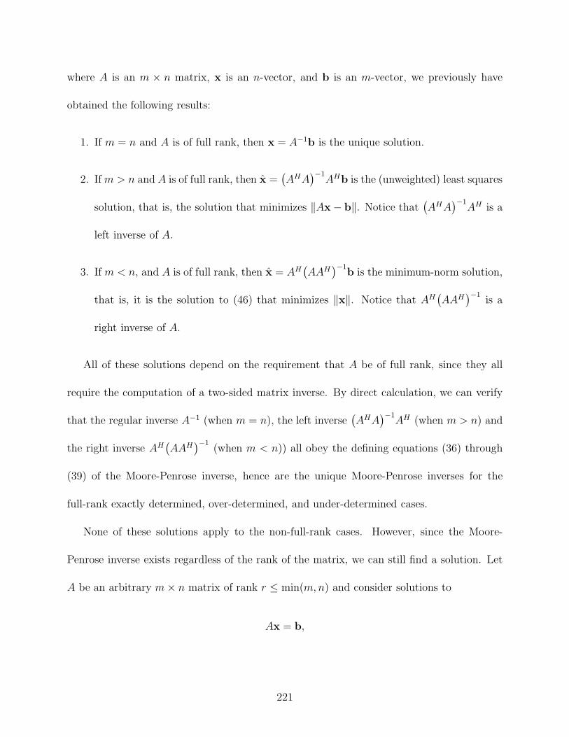
where A is an m ! n matrix, x is an n-vector, and b is an m-vector, we previously have
obtained the following results:
1. If m = n and A is of full rank, then x = A"1b is the unique solution.
2. If m > n and A is of full rank, then x =1
AHA2"1
AHb is the (unweighted) least squares
solution, that is, the solution that minimizes .Ax & b.. Notice that1
AHA2"1
AH is a
left inverse of A.
3. If m < n, and A is of full rank, then x = AH1
AAH2"1
b is the minimum-norm solution,
that is, it is the solution to (46) that minimizes .x.. Notice that AH1
AAH2"1
is a
right inverse of A.
All of these solutions depend on the requirement that A be of full rank, since they all
require the computation of a two-sided matrix inverse. By direct calculation, we can verify
that the regular inverse A"1 (when m = n), the left inverse1
AHA2"1
AH (when m > n) and
the right inverse AH1
AAH2"1
(when m < n)) all obey the defining equations (36) through
(39) of the Moore-Penrose inverse, hence are the unique Moore-Penrose inverses for the
full-rank exactly determined, over-determined, and under-determined cases.
None of these solutions apply to the non-full-rank cases. However, since the Moore-
Penrose inverse exists regardless of the rank of the matrix, we can still find a solution. Let
A be an arbitrary m ! n matrix of rank r $ min(m, n) and consider solutions to
Ax = b,
221
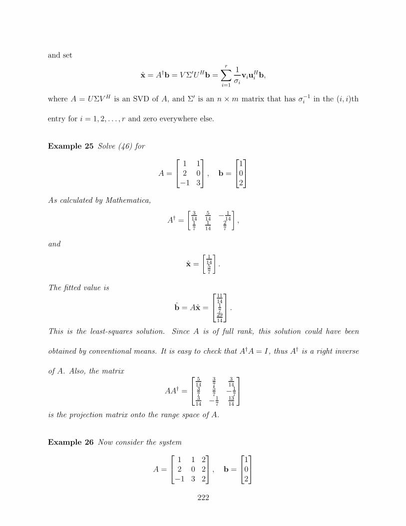
and set
x = A†b = V %'UHb =r+
i=1
1
-i
viuHi b,
where A = U%V H is an SVD of A, and %' is an n ! m matrix that has -"1i in the (i, i)th
entry for i = 1, 2, . . . , r and zero everywhere else.
Example 25 Solve (46) for
A =
%
'
1 12 0&1 3
(
* , b =
%
'
102
(
*
As calculated by Mathematica,
A† =
"314
514 & 1
1417
114
27
?
,
and
x =
"11457
?
.
The fitted value is
b = Ax =
%
'
1114172914
(
* .
This is the least-squares solution. Since A is of full rank, this solution could have been
obtained by conventional means. It is easy to check that A†A = I, thus A† is a right inverse
of A. Also, the matrix
AA† =
%
'
514
37
314
37
57 &1
7314 &1
71314
(
*
is the projection matrix onto the range space of A.
Example 26 Now consider the system
A =
%
'
1 1 22 0 2&1 3 2
(
* , b =
%
'
102
(
*
222
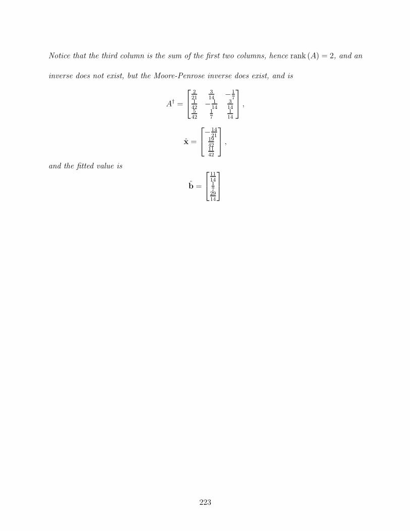
Notice that the third column is the sum of the first two columns, hence rank (A) = 2, and an
inverse does not exist, but the Moore-Penrose inverse does exist, and is
A† =
%
'
221
314 &1
7142 & 1
14314
542
17
114
(
* ,
x =
%
'
&1421
19421142
(
* ,
and the fitted value is
b =
%
'
1114172914
(
*
223
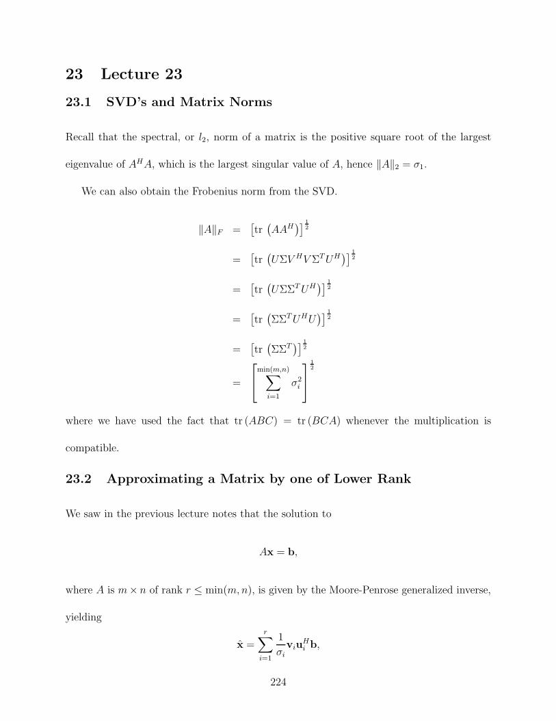
23 Lecture 23
23.1 SVD’s and Matrix Norms
Recall that the spectral, or l2, norm of a matrix is the positive square root of the largest
eigenvalue of AHA, which is the largest singular value of A, hence .A.2 = -1.
We can also obtain the Frobenius norm from the SVD.
.A.F =,
tr1
AAH2- 1
2
=,
tr1
U%V HV %T UH2- 1
2
=,
tr1
U%%T UH2- 1
2
=,
tr1
%%T UHU2- 1
2
=,
tr1
%%T2- 1
2
=
%
'
min(m,n)+
i=1
-2i
(
*
12
where we have used the fact that tr (ABC) = tr (BCA) whenever the multiplication is
compatible.
23.2 Approximating a Matrix by one of Lower Rank
We saw in the previous lecture notes that the solution to
Ax = b,
where A is m! n of rank r $ min(m, n), is given by the Moore-Penrose generalized inverse,
yielding
x =r+
i=1
1
-i
viuHi b,
224
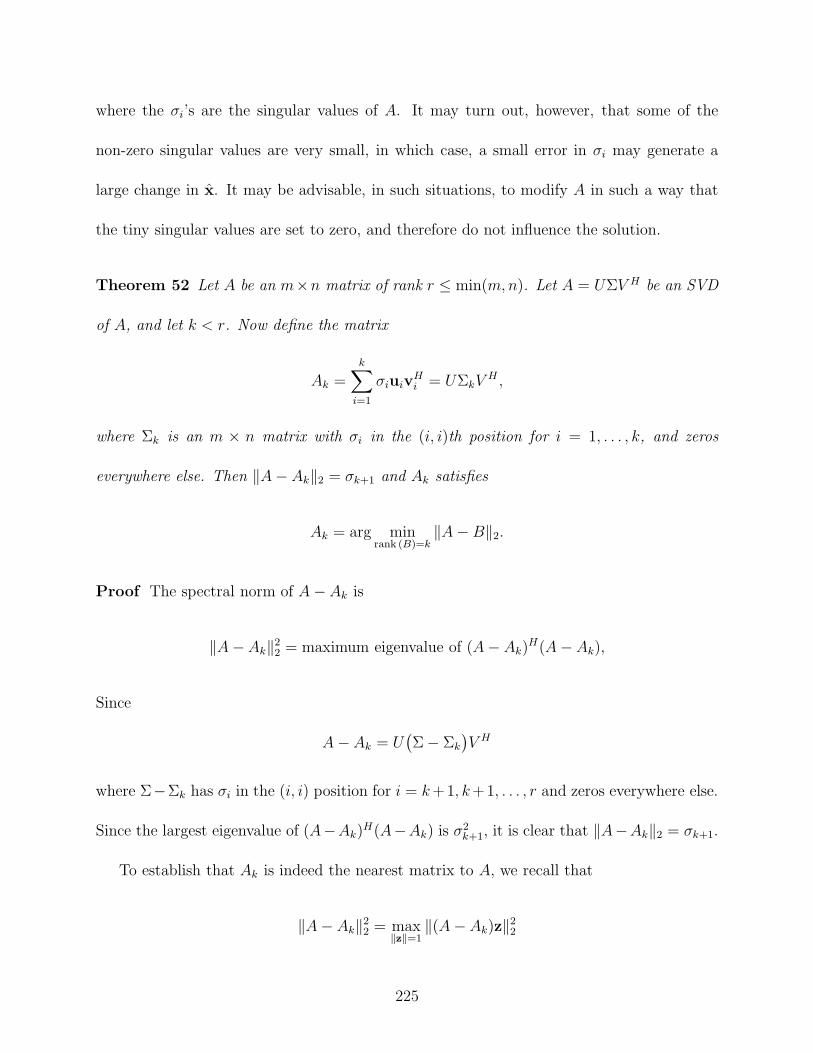
where the -i’s are the singular values of A. It may turn out, however, that some of the
non-zero singular values are very small, in which case, a small error in -i may generate a
large change in x. It may be advisable, in such situations, to modify A in such a way that
the tiny singular values are set to zero, and therefore do not influence the solution.
Theorem 52 Let A be an m!n matrix of rank r $ min(m, n). Let A = U%V H be an SVD
of A, and let k < r. Now define the matrix
Ak =k+
i=1
-iuivHi = U%kV
H ,
where %k is an m ! n matrix with -i in the (i, i)th position for i = 1, . . . , k, and zeros
everywhere else. Then .A & Ak.2 = -k+1 and Ak satisfies
Ak = arg minrank (B)=k
.A & B.2.
Proof The spectral norm of A & Ak is
.A & Ak.22 = maximum eigenvalue of (A & Ak)
H(A & Ak),
Since
A & Ak = U1
% & %k
2
V H
where %&%k has -i in the (i, i) position for i = k +1, k+1, . . . , r and zeros everywhere else.
Since the largest eigenvalue of (A&Ak)H(A&Ak) is -2k+1, it is clear that .A&Ak.2 = -k+1.
To establish that Ak is indeed the nearest matrix to A, we recall that
.A & Ak.22 = max
&z&=1.(A & Ak)z.2
2
225
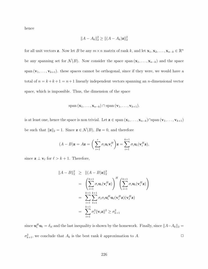
hence
.A & Ak.22 # .(A & Ak)z.2
2
for all unit vectors z. Now let B be any m!n matrix of rank k, and let x1,x2, . . . ,xn"k ( Rn
be any spanning set for N (B). Now consider the space span (x1, . . . ,xn"k) and the space
span (v1, . . . ,vk+1). these spaces cannot be orthogonal, since if they were, we would have a
total of n = k+k +1 = n+1 linearly independent vectors spanning an n-dimensional vector
space, which is impossible. Thus, the dimension of the space
span (x1, . . . ,xn"k) * span (v1, . . . ,vk+1).
is at least one, hence the space is non trivial. Let z ( span (x1, . . . ,xn"k)*span (v1, . . . ,vk+1)
be such that .z.2 = 1. Since z ( N (B), Bz = 0, and therefore
(A & B)z = Az =
3 r+
i=1
-iuivHi
$
z =k+1+
i=1
-iui(vHi z),
since z 3 v( for ! > k + 1. Therefore,
.A & B.22 # .(A & B)z.2
2
=
Qk+1+
i=1
-iui(vHi z)
RH Qk+1+
i=1
-iui(vHi z)
R
=k+1+
i=1
k+1+
(=1
-i-(uHi u((v
Hi z)(vH
( z)
=k+1+
i=1
-2i .viz.2 # -2
k+1
since uHi u( = #i( and the last inequality is shown by the homework. Finally, since .A&Ak.2 =
-2k+1, we conclude that Ak is the best rank k approximation to A. !
226
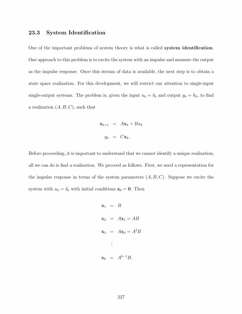
23.3 System Identification
One of the important problems of system theory is what is called system identification.
One approach to this problem is to excite the system with an impulse and measure the output
as the impulse response. Once this stream of data is available, the next step is to obtain a
state space realization. For this development, we will restrict our attention to single-input
single-output systems. The problem is, given the input uk = #k and output yk = hk, to find
a realization (A, B, C), such that
xk+1 = Axk + Buk
yk = Cxk.
Before proceeding, it is important to understand that we cannot identify a unique realization;
all we can do is find a realization. We proceed as follows. First, we need a representation for
the impulse response in terms of the system parameters (A, B, C). Suppose we excite the
system with uk = #k with initial conditions x0 = 0. Then
x1 = B
x2 = Ax1 = AB
x3 = Ax2 = A2B
...
xk = Ak"1B.
227
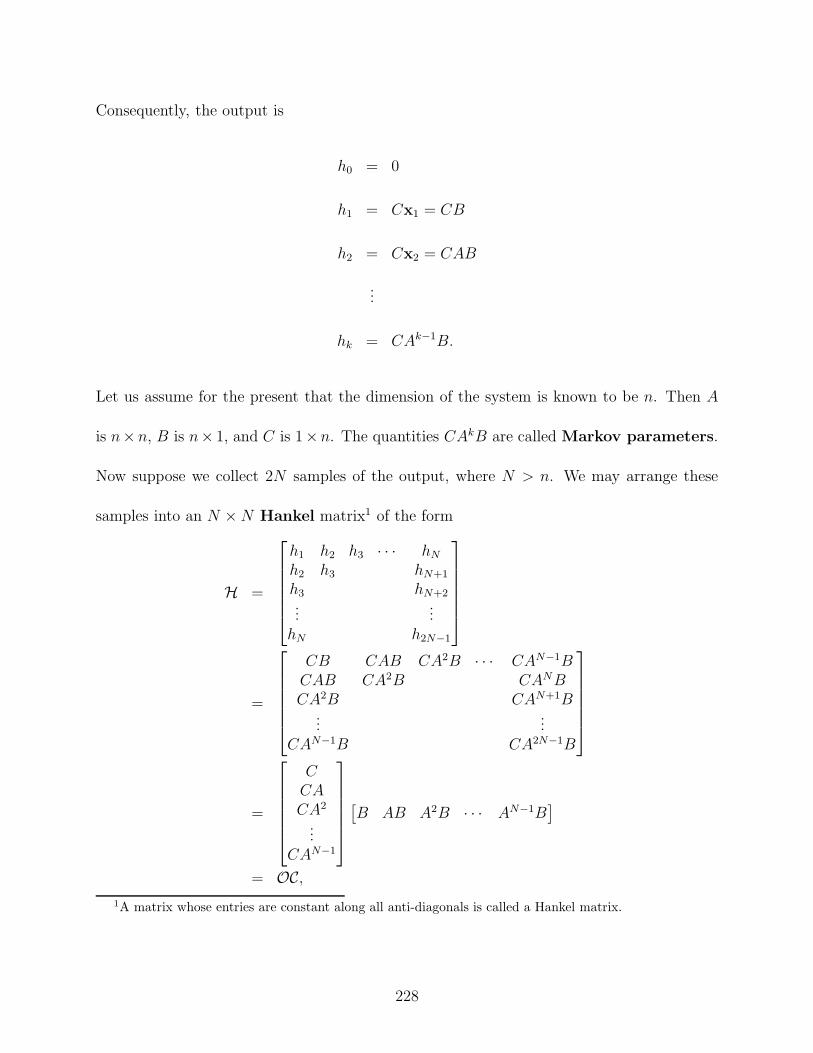
Consequently, the output is
h0 = 0
h1 = Cx1 = CB
h2 = Cx2 = CAB
...
hk = CAk"1B.
Let us assume for the present that the dimension of the system is known to be n. Then A
is n! n, B is n! 1, and C is 1!n. The quantities CAkB are called Markov parameters.
Now suppose we collect 2N samples of the output, where N > n. We may arrange these
samples into an N ! N Hankel matrix1 of the form
H =
%
&&&&&'
h1 h2 h3 · · · hN
h2 h3 hN+1
h3 hN+2...
...hN h2N"1
(
)))))*
=
%
&&&&&'
CB CAB CA2B · · · CAN"1BCAB CA2B CANBCA2B CAN+1B
......
CAN"1B CA2N"1B
(
)))))*
=
%
&&&&&'
CCACA2
...CAN"1
(
)))))*
,
B AB A2B · · · AN"1B-
= OC,
1A matrix whose entries are constant along all anti-diagonals is called a Hankel matrix.
228
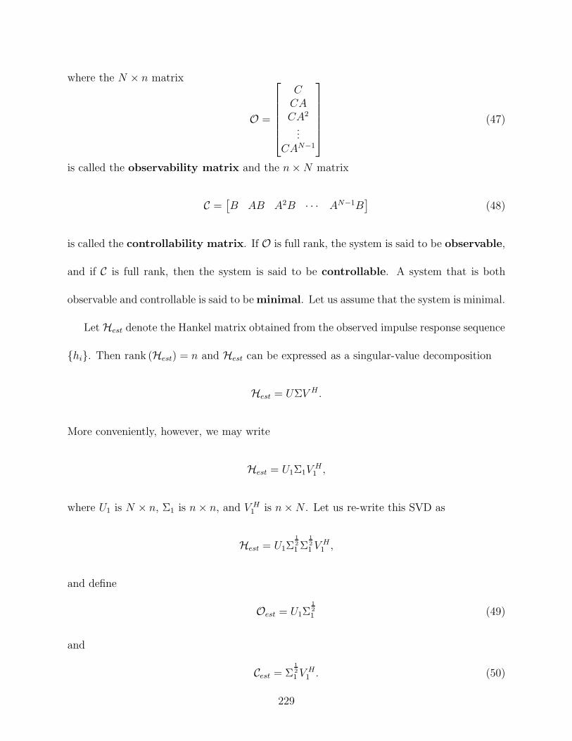
where the N ! n matrix
O =
%
&&&&&'
CCACA2
...CAN"1
(
)))))*
(47)
is called the observability matrix and the n ! N matrix
C =,
B AB A2B · · · AN"1B-
(48)
is called the controllability matrix. If O is full rank, the system is said to be observable,
and if C is full rank, then the system is said to be controllable. A system that is both
observable and controllable is said to be minimal. Let us assume that the system is minimal.
Let Hest denote the Hankel matrix obtained from the observed impulse response sequence
{hi}. Then rank (Hest) = n and Hest can be expressed as a singular-value decomposition
Hest = U%V H .
More conveniently, however, we may write
Hest = U1%1VH1 ,
where U1 is N ! n, %1 is n ! n, and V H1 is n ! N . Let us re-write this SVD as
Hest = U1%121 %
121 V H
1 ,
and define
Oest = U1%121 (49)
and
Cest = %121 V H
1 . (50)
229
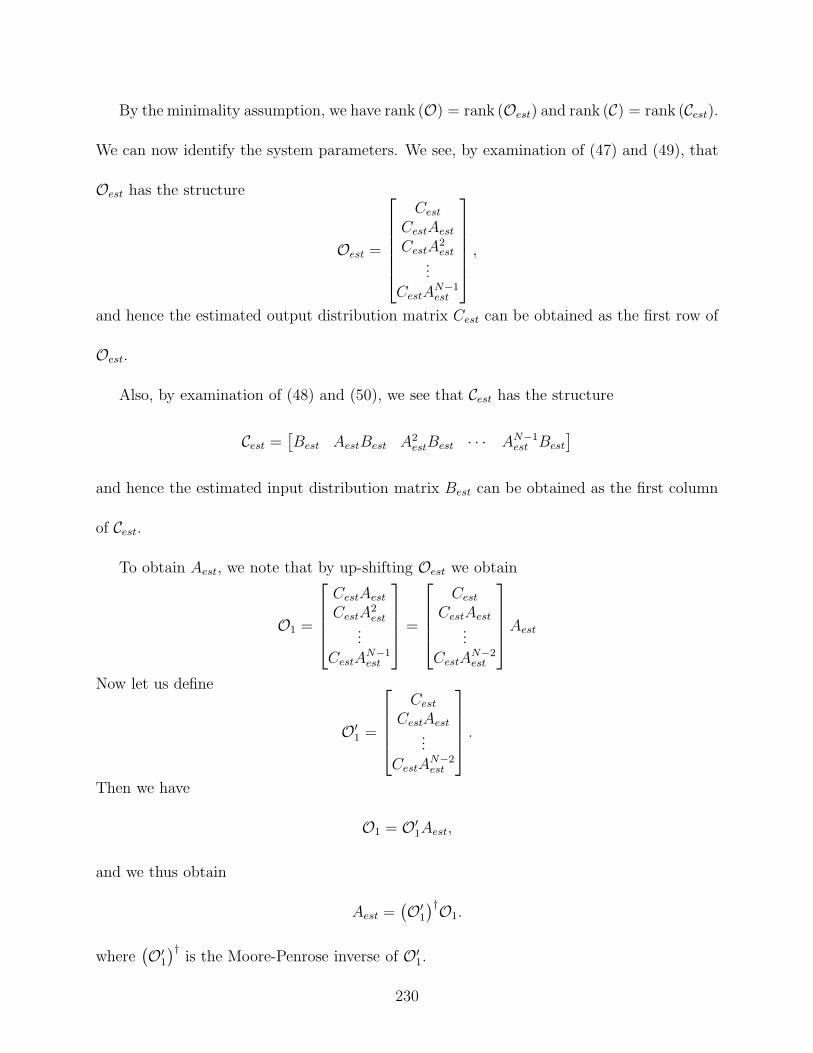
By the minimality assumption, we have rank (O) = rank (Oest) and rank (C) = rank (Cest).
We can now identify the system parameters. We see, by examination of (47) and (49), that
Oest has the structure
Oest =
%
&&&&&'
Cest
CestAest
CestA2est
...CestA
N"1est
(
)))))*
,
and hence the estimated output distribution matrix Cest can be obtained as the first row of
Oest.
Also, by examination of (48) and (50), we see that Cest has the structure
Cest =,
Best AestBest A2estBest · · · AN"1
est Best
-
and hence the estimated input distribution matrix Best can be obtained as the first column
of Cest.
To obtain Aest, we note that by up-shifting Oest we obtain
O1 =
%
&&&'
CestAest
CestA2est
...CestA
N"1est
(
)))*
=
%
&&&'
Cest
CestAest...
CestAN"2est
(
)))*
Aest
Now let us define
O'1 =
%
&&&'
Cest
CestAest...
CestAN"2est
(
)))*
.
Then we have
O1 = O'1Aest,
and we thus obtain
Aest =1
O'1
2†O1.
where1
O'1
2†is the Moore-Penrose inverse of O'
1.
230
23.4 Total Least-Squares
Consider the equation
Ax = b,
where A is N ! n, x is n ! 1, and b is N ! 1 with N > n, and suppose we desire to find
the least-squares solution. With standard least-squares formulations, we generally assume
that the only source or error is in b and the matrix A is known to be correct. The solution
concept is then to project b onto the range space of A. Recall, for example, the linear
regression problem considered in Lecture Notes 7, that both the current and the voltage
are obtained from observations, but we assumed that the only source or error was with the
current observations. We formulated that estimation problem as follows.
y = Ac + e,
where
y =
%
&&&'
I1
I2...In
(
)))*
,
A =
%
&&&'
V1 1V2 1...
...Vn 1
(
)))*
,
and
c =
"
ab
?
.
The standard least-squares solution is
c =
"
ab
?
=1
AT A)"1ATy.
231
This solution corresponds to minimizing the sum of the squares of the vertical distance
!Ni=1(yi & yi)2, and implicitly assumes that there is no horizontal error in the values of the
matrix A comprising the voltages Vi. A legitimate question to consider, however, is the
validity of the claim that A is correct. A more realistic approach is to acknowledge that
both the current and the voltage are subject to error, and devise an estimator that accounts
for this situation. This is the goal of the total least-squares solution concept.
Under the total least-squares concept, we account for perturbations to both sides of the
equation Ax = b. Consider the equation
(A + E)x = b + r, (51)
where E is a perturbation matrix and r is a perturbation vector. Our goal is to solve for E
and r such that (b + r) ( R(A + E) and the norm of the perturbations is minimized. We
may re-write (51) as
I
A + E... b + r
J"
x&1
?
= 0,
or, equivalently,"I
A... b
J
+I
E... rJ? "
x&1
?
= 0,
whereI
A... b
J
is the N ! (n + 1) dimensional matrix formed by appending the column b
to the matrix A, andI
E... rJ
is the N ! (n + 1) dimensional matrix formed by appending
the column r to the matrix E, Now define the N ! (n + 1) dimensional matrices
C =I
A... b
J
# =I
E... rJ
232
and the n + 1 dimensional vector
z =
"
x&1
?
,
yielding
(C + #)z = 0.
This formulation is motivated by our earlier result involving reduced-rank approxima-
tions. Assuming that C is of rank n + 1, we desire to find an N ! n matrix C that is the
best reduced-rank approximation to the N ! (n + 1) matrix C. We proceed as follows.
1. Since both A and b are given, we may compute the the SVD of C, yielding
C = U1%1VH =
n+1+
k=1
-kukvHk , (52)
where U1 is N ! (n + 1), %1 is (n + 1) ! (n + 1), and V is (n + 1) ! (n + 1).
2. From the reduced-rank approximation theorem, the rank n matrix that is closest to C
is the matrix
C = C + # =n+
k=1
-kuivHk . (53)
Comparing (52) and (53), we can solve for the perturbation matrix # as
# = C & C = &-n+1un+1vHn+1.
3. Since vn+1 is orthogonal to span (C + #), the rank of C is n, and the one-dimensional
nullspace of C is spanned by vn+1. Thus,
z =
"
x&1
?
= %vn+1 = %
%
&&&'
vn+1,1
vn+1,2...
vn+1,n+1
(
)))*
233

for some constant %. if vn+1,n+1 += 0, then setting % = "1vn+1,n+1
yields
x =&1
vn+1,n+1
%
&&&'
vn+1,1
vn+1,2...
vn+1,n
(
)))*
.
If vn+1,n+1 = 0, then there is no solution to the total least-squares problem.
Example 27 Suppose we observe the following values for current, Iil, and voltage Vi:
y = {2.3, 3.8, 6.3, 8.1, 10.2, 12.5}
and
w = {1.7, 4.0, 5.8, 8.3, 10., 12.1}.
With
A =
%
&&&&&&'
1.7 14.0 15.8 18.3 110.0 112.1 1
(
))))))*
,
The standard least-squares solution is formed as
cls = (AT A)"1ATy
=
"
0.01329 &0.09283&0.09283 0.81492
? "
1.7 4.0 5.8 8.3 10.0 12.11 1 1 1 1 1
?
%
&&&&&&'
2.33.86.38.110.212.5
(
))))))*
=
"
0.98960.2889
?
To compute the total least-squares solution, we must first form the augmented matrix
C =I
A... b
J
=
%
&&&&&&'
1.7 1 2.34.0 1 3.65.8 1 6.38.3 1 8.110.0 1 10.212.1 1 12.5
(
))))))*
234
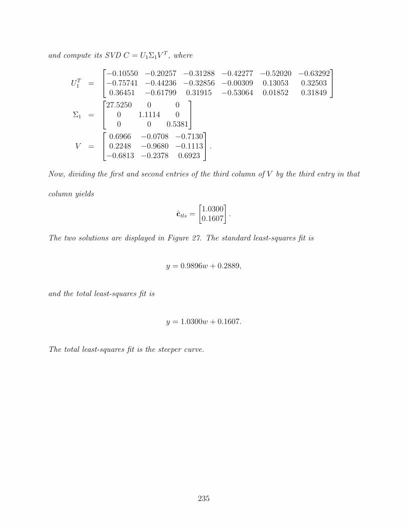
and compute its SVD C = U1%1V T , where
UT1 =
%
'
&0.10550 &0.20257 &0.31288 &0.42277 &0.52020 &0.63292&0.75741 &0.44236 &0.32856 &0.00309 0.13053 0.325030.36451 &0.61799 0.31915 &0.53064 0.01852 0.31849
(
*
%1 =
%
'
27.5250 0 00 1.1114 00 0 0.5381
(
*
V =
%
'
0.6966 &0.0708 &0.71300.2248 &0.9680 &0.1113&0.6813 &0.2378 0.6923
(
* .
Now, dividing the first and second entries of the third column of V by the third entry in that
column yields
ctls =
"
1.03000.1607
?
.
The two solutions are displayed in Figure 27. The standard least-squares fit is
y = 0.9896w + 0.2889,
and the total least-squares fit is
y = 1.0300w + 0.1607.
The total least-squares fit is the steeper curve.
235

2 4 6 8 10 12voltage
2
4
6
8
10
12
current
Figure 2: Least-Squares and total least-squares solutions.
236
24 Lecture 24
We have already been exposed to several matrix structures.
1. Grammian matrices
2. Projection (idempotent) matrices
3. Permutation matrices
4. Hermitian matrices
5. Positive definite(semi-definite) matrices
6. Triangular matrices
7. Unitary matrices
8. Vandermonde matrices
9. Hankel matrices
We now encounter some additional matrix structures.
24.1 Toeplitz Matrices
Definition 58 An n!n matrix A = {aij} that is constant along all its diagonals is termed
a Toeplitz matrix. That is, the entries are of the form
aij = ai"j, i, j = 0, 1, . . . , n & 1.
!
237
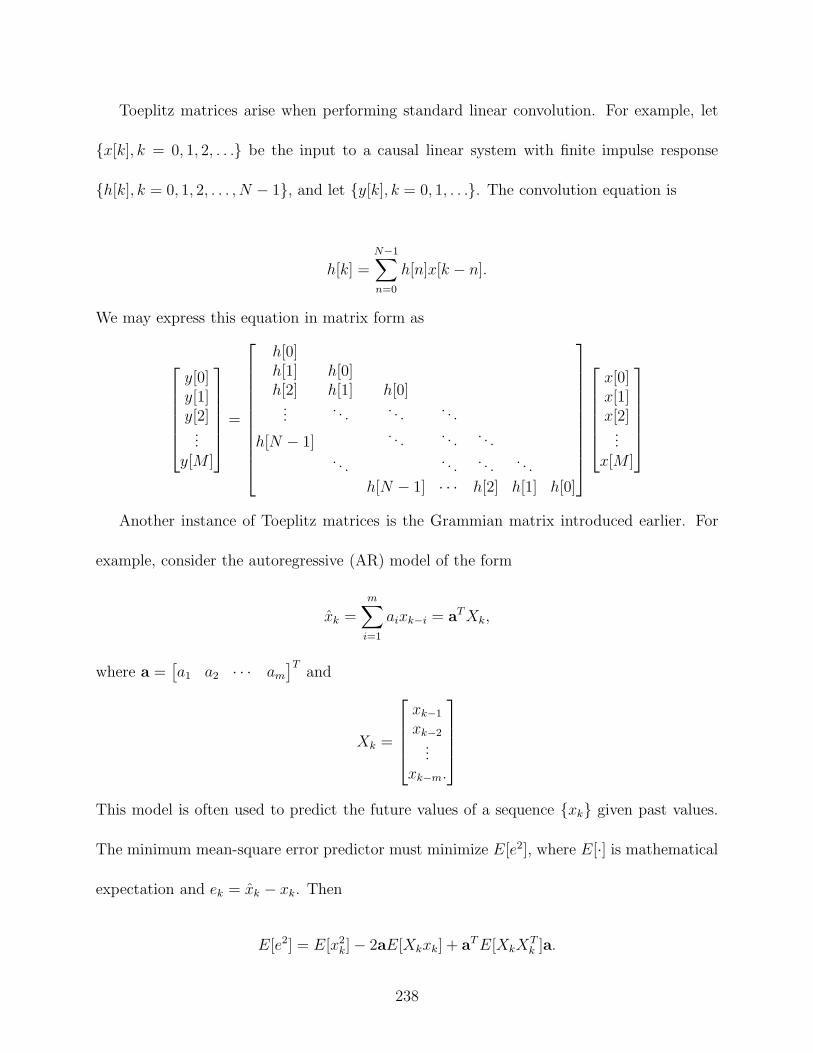
Toeplitz matrices arise when performing standard linear convolution. For example, let
{x[k], k = 0, 1, 2, . . .} be the input to a causal linear system with finite impulse response
{h[k], k = 0, 1, 2, . . . , N & 1}, and let {y[k], k = 0, 1, . . .}. The convolution equation is
h[k] =N"1+
n=0
h[n]x[k & n].
We may express this equation in matrix form as
%
&&&&&'
y[0]y[1]y[2]...
y[M ]
(
)))))*
=
%
&&&&&&&&&&'
h[0]h[1] h[0]h[2] h[1] h[0]
.... . . . . . . . .
h[N & 1]. . . . . . . . .
. . . . . . . . . . . .h[N & 1] · · · h[2] h[1] h[0]
(
))))))))))*
%
&&&&&'
x[0]x[1]x[2]
...x[M ]
(
)))))*
Another instance of Toeplitz matrices is the Grammian matrix introduced earlier. For
example, consider the autoregressive (AR) model of the form
xk =m+
i=1
aixk"i = aT Xk,
where a =,
a1 a2 · · · am
-Tand
Xk =
%
&&&'
xk"1
xk"2...
xk"m.
(
)))*
This model is often used to predict the future values of a sequence {xk} given past values.
The minimum mean-square error predictor must minimize E[e2], where E[·] is mathematical
expectation and ek = xk & xk. Then
E[e2] = E[x2k] & 2aE[Xkxk] + aT E[XkX
Tk ]a.
238
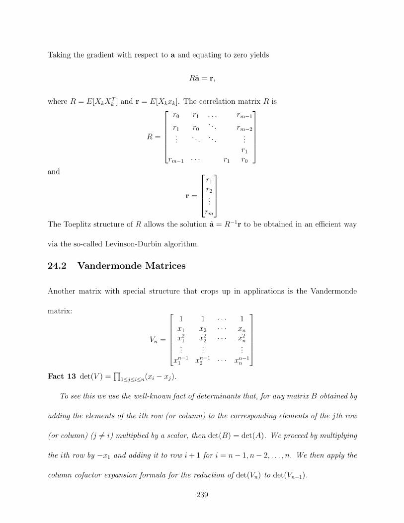
Taking the gradient with respect to a and equating to zero yields
Ra = r,
where R = E[XkXTk ] and r = E[Xkxk]. The correlation matrix R is
R =
%
&&&&&'
r0 r1 . . . rm"1
r1 r0. . . rm"2
.... . . . . .
...r1
rm"1 · · · r1 r0
(
)))))*
and
r =
%
&&&'
r1
r2...
rm
(
)))*
The Toeplitz structure of R allows the solution a = R"1r to be obtained in an e"cient way
via the so-called Levinson-Durbin algorithm.
24.2 Vandermonde Matrices
Another matrix with special structure that crops up in applications is the Vandermonde
matrix:
Vn =
%
&&&&&'
1 1 · · · 1x1 x2 · · · xn
x21 x2
2 · · · x2n
......
...xn"1
1 xn"12 · · · xn"1
n
(
)))))*
Fact 13 det(V ) =V
1.j.i.n(xi & xj).
To see this we use the well-known fact of determinants that, for any matrix B obtained by
adding the elements of the ith row (or column) to the corresponding elements of the jth row
(or column) (j += i) multiplied by a scalar, then det(B) = det(A). We proceed by multiplying
the ith row by &x1 and adding it to row i + 1 for i = n & 1, n& 2, . . . , n. We then apply the
column cofactor expansion formula for the reduction of det(Vn) to det(Vn"1).
239
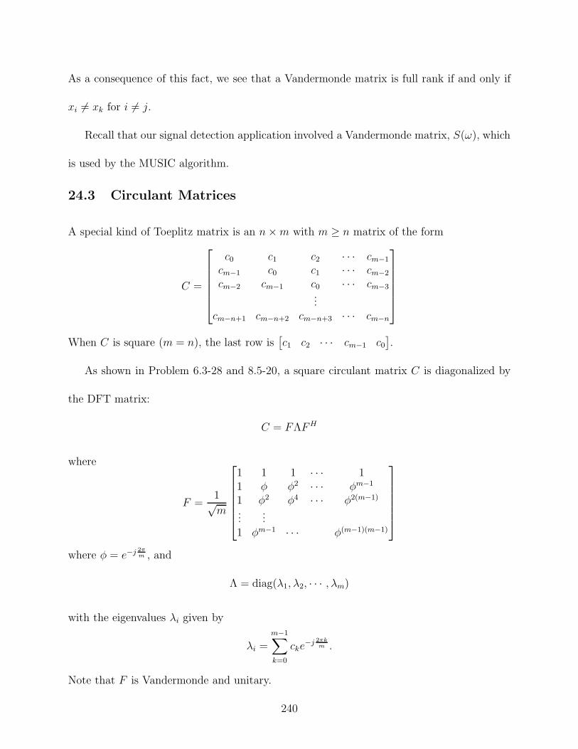
As a consequence of this fact, we see that a Vandermonde matrix is full rank if and only if
xi += xk for i += j.
Recall that our signal detection application involved a Vandermonde matrix, S(,), which
is used by the MUSIC algorithm.
24.3 Circulant Matrices
A special kind of Toeplitz matrix is an n ! m with m # n matrix of the form
C =
%
&&&&&'
c0 c1 c2 · · · cm"1
cm"1 c0 c1 · · · cm"2
cm"2 cm"1 c0 · · · cm"3...
cm"n+1 cm"n+2 cm"n+3 · · · cm"n
(
)))))*
When C is square (m = n), the last row is,
c1 c2 · · · cm"1 c0
-
.
As shown in Problem 6.3-28 and 8.5-20, a square circulant matrix C is diagonalized by
the DFT matrix:
C = F$F H
where
F =1<m
%
&&&&&'
1 1 1 · · · 11 * *2 · · · *m"1
1 *2 *4 · · · *2(m"1)
......
1 *m"1 · · · *(m"1)(m"1)
(
)))))*
where * = e"j 2"m , and
$ = diag(/1, /2, · · · , /m)
with the eigenvalues /i given by
/i =m"1+
k=0
cke"j 2"k
m .
Note that F is Vandermonde and unitary.
240
An interesting observation from the above result is that all square m ! m circulant
matrices have the same set of eigenvectors give by the columns of F . This implies that, for
any two square circulant matrices C1 and C2 of the same dimension,
C1C2 = F$1FHF$2F
H = F$1$2FH = F$2$1F
H = F$2FHF$2F
H = C2C1.
Thus, all circulant matrices commute!
24.4 Companion Matrices
A class of matrices that are important in control theory are companion matrices.
Definition 59 Let A be an n ! n matrix of the form
Cb =
%
&&&&&'
0 1 0 · · · 0... 1
.... . . . . . 0
0 · · · 0 1&a0 &a1 &a2 · · · &an"1
(
)))))*
are called bottom-companion matrices. The matrix CTb is called a right-companion
matrix, and the matrix
Ct =
%
&&&&&'
&a0 &a1 &a2 · · · &an"1
1 0 0 · · · 0... 1
.... . . . . . 0
0 · · · 0 1 0
(
)))))*
and its transpose are called top-companion and left-companion matrices, respectively.
!
These matrices are called companion matrices because they are companions to the n-th
order monic polynomial
a(/) = /n + an"1/n"1 + · · ·+ a1/ + a0
241

in the sense that
det(/I & C) = a(/).
Companion matrices are important to control theory because they provide an easy way to
obtain a state-space realization of a transfer function. Let H(s) = b(s)a(s) be a rational transfer
function with deg (b) < deg (a). To illustrate, let m = 2 be the degree of the numerator,
with n = 3 the degree of the denominator. Then
H(s) =b(s)
a(s)=
b2s2 + b1s + b0
s3 + a2s2 + a1s + a0.
Now consider the state space model
x1(t) = x2(t)
x2(t) = x3(t)
x3(t) = a0x1(t) + a1x2(t) + a2x3(t) + u(t)
with output
y(t) = b0x1(t) + b1x2(t) + b3x3(t).
In matrix form, this system may be expressed as
%
'
x1(t)x2(t)x(3)
(
* =
%
'
0 1 00 0 1
&a0 &a1 &a2
(
*
%
'
x1(t)x2(t)x3(t)
(
*+
%
'
001
(
*u((t),
with output
y(t) =,
b0 b1 b2
-
%
'
x1(t)x2(t)x3(t)
(
*
242
or
x(t) = Ax(t) + Bu(t)
y(t) = Cx
with the obvious definitions of (A, B, C). The transfer function for this system is
H '(s) =C adj (sI & A)B
det(sI & A)
=1
s3 + a2s2 + a1s + a0
,
b0 b1 b2
-
adj
%
'
s &1 00 s &1a0 a1 s + a2
(
*
%
'
001
(
* .
Since we will be post-multiplying the adjugate by the vector
%
'
001
(
*, we need compute only
the last row of the adjugate matrix, yielding the numerator
C adj (sI & A)B =,
b0 b1 b2
-
%
'
! ! 1! ! s! ! s2
(
*
%
'
001
(
* = b2s2 + b1s + b0.
Thus, we see that H '(s) = H(s), and the given realization corresponds to the given transfer
function.
24.5 Kronecker Products
The Kronecker product, also known as the direct product or tensor product, is a concept
having its origin in group theory and has applications in particle physics.
Definition 60 Consider a matrix A = {aij} of order m ! n and a matrix B = {bij} of
order r! s. The Kronecker product of the two matrices, denoted A>B, is defined as the
partitioned matrix
A > B =
%
&&&'
a11B a12B · · · a1nBa21B a22B · · · a2nB
......
...am1B am2B · · · amnB
(
)))*
243
A>B is thus seen to be a mr!ns matrix. It has mn blocks, the (i, j)th block is the matrix
aijB of order r ! s. !
For example, let
A =
"
a11 a12
a21 a22
?
, B =
"
b11 b12
b21 b22
?
,
then
A > B =
"
a11B a12Ba21B a22B
?
=
%
&&'
a11b11 a11b12 a12b11 a12b12
a11b21 a11b22 a12b21 a12b22
a21b11 a21b12 a22b11 a22b12
a21b21 a21b22 a22b21 a22b22
(
))*
Fact 14 If % is a scalar, then A> (%B) = %(A>B). To prove this, we note that the (i, j)th
block of A> (%B) is aij(%B) = %aijB, but this is simply % times the (i, j)th block of A>B.
The result follows.
Fact 15 The Kronecker product is distributive with respect to addition, that is
(A + B) > C = A > C + B > C
A > (B + C) = A > B + A > C.
To establish the first of these claims, we note that the (i, j)th block of (A+B)>C is (aij+bij)C
and the (i, j)th block of A>C +B>C is aijC + bijC. Since the two block are equal for every
(i, j), the result follows. The second claim is similarly established.
Fact 16 The Kronecker product is associative, that is, A > (B > C) = (A > B) > C. This
fact is established by direct computation.
Fact 17 (A > B)T = AT > BT . This obtains since the (i, j)th block of (A > B)T is ajiBT .
244
Fact 18 The “Mixed Product Rule”
(A > B)(C > D) = AC > BD
provided the dimensions are all compatible. To establish this result, note that the (ij)th block
of the left-hand side is obtained by taking the product of the ith row of (A > B) and the jth
column of block (C > D), this is of the following form
,
ai1B ai2B · · ·ainB-
%
&&&'
cijDc2jD
...cnjD
(
)))*
=+
r
aijcriBD.
The (ij)th block on the right-hand side is (by definition of the Kronecker product) gijBD,
where gij is the (ikj)th element of the matrix AC. But by the rule of matrix multiplication,
gij =!
r aircrj. Since the (i, j)th blocks are all equal, the result follows.
Fact 19 (A > B)"1 = A"1 > B"1 . To see, we apply the mixed product rule as follows.
(A > B)(A"1 > B"1) = AA"1 > BB"1 = Im > In = Imn
Notation. Let A = {aij} be an m ! n matrix. We denote the columns of A as
A·j =
%
&&&'
a1j
a2j...
amj
(
)))*
, j = 1, 2, . . . , n
and the rows of A as
Ai· =
%
&&&'
ai1
ai2...
ain
(
)))*
, i = 1, 2, . . . , m.
With this notation, both A·j and Ai· are column vectors. With this notation, we can write
A as
A =,
A·1 A·2 · · · A·n-
245
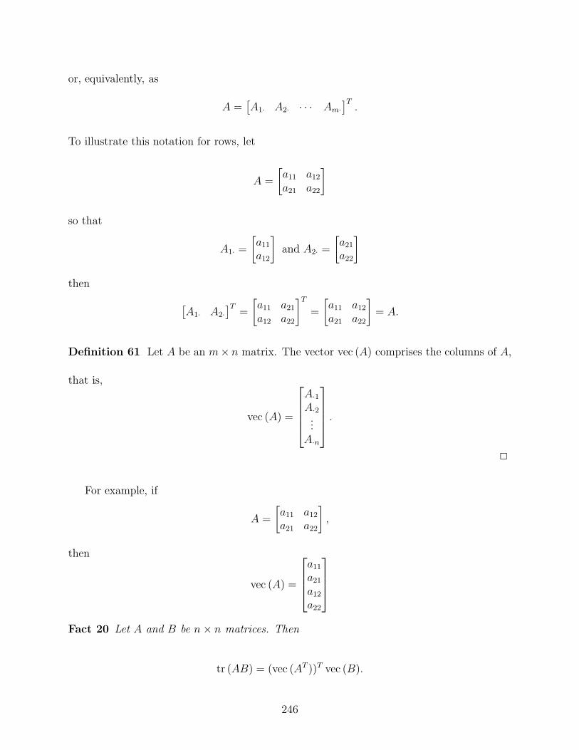
or, equivalently, as
A =,
A1· A2· · · · Am·-T
.
To illustrate this notation for rows, let
A =
"
a11 a12
a21 a22
?
so that
A1· =
"
a11
a12
?
and A2· =
"
a21
a22
?
then
,
A1· A2·-T
=
"
a11 a21
a12 a22
?T
=
"
a11 a12
a21 a22
?
= A.
Definition 61 Let A be an m! n matrix. The vector vec (A) comprises the columns of A,
that is,
vec (A) =
%
&&&'
A·1A·2...
A·n
(
)))*
.
!
For example, if
A =
"
a11 a12
a21 a22
?
,
then
vec (A) =
%
&&'
a11
a21
a12
a22
(
))*
Fact 20 Let A and B be n ! n matrices. Then
tr (AB) = (vec (AT ))T vec (B).
246
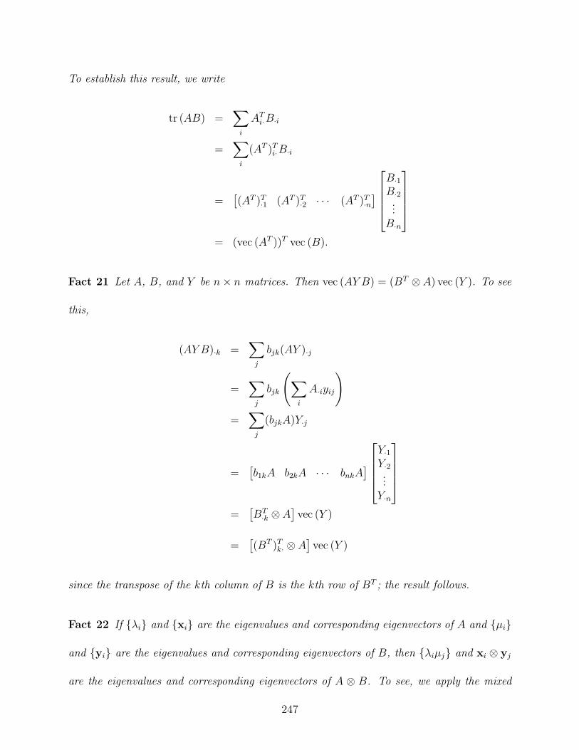
To establish this result, we write
tr (AB) =+
i
ATi·B·i
=+
i
(AT )Ti·B·i
=,
(AT )T·1 (AT )T
·2 · · · (AT )T·n-
%
&&&'
B·1B·2...
B·n
(
)))*
= (vec (AT ))T vec (B).
Fact 21 Let A, B, and Y be n ! n matrices. Then vec (AY B) = (BT > A) vec (Y ). To see
this,
(AY B)·k =+
j
bjk(AY )·j
=+
j
bjk
Q
+
i
A·iyij
R
=+
j
(bjkA)Y·j
=,
b1kA b2kA · · · bnkA-
%
&&&'
Y·1Y·2...
Y·n
(
)))*
=,
BT·k > A
-
vec (Y )
=,
(BT )Tk· > A
-
vec (Y )
since the transpose of the kth column of B is the kth row of BT ; the result follows.
Fact 22 If {/i} and {xi} are the eigenvalues and corresponding eigenvectors of A and {µi}
and {yi} are the eigenvalues and corresponding eigenvectors of B, then {/iµj} and xi > yj
are the eigenvalues and corresponding eigenvectors of A > B. To see, we apply the mixed
247
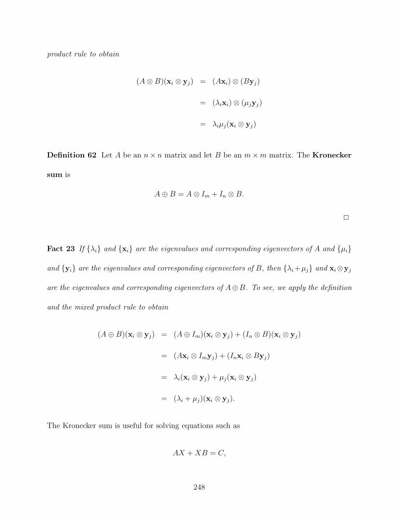
product rule to obtain
(A > B)(xi > yj) = (Axi) > (Byj)
= (/ixi) > (µjyj)
= /iµj(xi > yj)
Definition 62 Let A be an n! n matrix and let B be an m!m matrix. The Kronecker
sum is
A 5 B = A > Im + In > B.
!
Fact 23 If {/i} and {xi} are the eigenvalues and corresponding eigenvectors of A and {µi}
and {yi} are the eigenvalues and corresponding eigenvectors of B, then {/i +µj} and xi>yj
are the eigenvalues and corresponding eigenvectors of A5B. To see, we apply the definition
and the mixed product rule to obtain
(A 5 B)(xi > yj) = (A 5 Im)(xi > yj) + (In > B)(xi > yj)
= (Axi > Imyj) + (Inxi > Byj)
= /i(xi > yj) + µj(xi > yj)
= (/i + µj)(xi > yj).
The Kronecker sum is useful for solving equations such as
AX + XB = C,
248
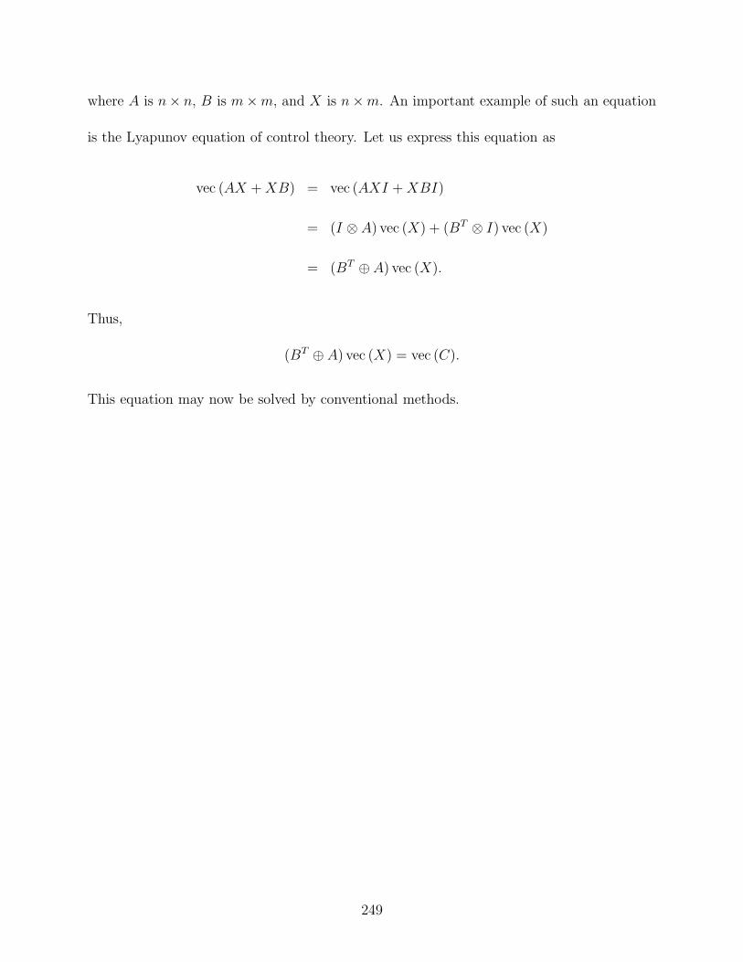
where A is n! n, B is m!m, and X is n !m. An important example of such an equation
is the Lyapunov equation of control theory. Let us express this equation as
vec (AX + XB) = vec (AXI + XBI)
= (I > A) vec (X) + (BT > I) vec (X)
= (BT 5 A) vec (X).
Thus,
(BT 5 A) vec (X) = vec (C).
This equation may now be solved by conventional methods.
249

25 Lecture 25
25.1 Solving Nonlinear Equations
Thus far, we have concentrated exclusively on linear models, and have explored in great deal
ways to solve equations of the form Ax = b. In this section we turn our attention to the
examination of nonlinear equations.
Consider the equation f(x) = 0. One way to approach this problem is to form a Taylor
series by expanding about some initial guess x0, yielding
f(x) = f(x0) + f '(x0)(x & x0) + higher-order terms.
Suppose we ignore the higher-order terms and solve for the value of x that satisfies the
linearized equation
f(x) = f(x0) + f '(x0)(x & x0) = 0;
call this value x1. Then
x1 = x0 &f(x0)
f '(x0).
We might hope that x1 is a better approximation to the solution than is x0. This suggests
that we consider the iteration
xn+1 = xn & f(xn)
f '(xn)
for n = 0, 1, 2, . . .. Let’s look at an example.
Example 28 Suppose f(x) = a & x2 where a > 0. Then the solution to f(x) = 0 is<
a.
The corresponding iteration is
xn+1 = xn +a & x2
n
2xn
=1
2
3
xn +a
xn
$
.
250

After a few iterations, it will become clear that this procedure does vindeed converge to the
square root of a (try it). This is the way we used to compute square roots in the “old days”
before hand-held calculators. With a little practice, one could use the old Frieden mechanical
adding-multiplying-dividing machines to compute square roots rather quickly to better than
slide-rule accuracy. Of course, those were the days when we had to walk up hill both ways in
the snow—you guys have it much easier these days than we did :-)
Emboldened by the success of this simple example, we might consider asking some ques-
tions, such as
1. What conditions on f and x0 are necessary for the above procedure to to converge?
2. If it does converge, how fast does it converge?
3. If it does appear to converge, will it always converge to the same result, regardless of
the how it is initialized?
4. Can this result be generalized?
25.2 Contractive Mappings and Fixed Points
Definition 63 Let X be a Banach space with norm . · . and suppose f : X " X and there
exists a positive number 3 < 1 such that
.f(x) & f(y). $ 3.x & y. %x, y ( X.
Then f is called a contraction on X, or a contractive map on X. !
251
Fact 24 If f is a contractive mapping, then f is continuous. This follows since, if {xn} is
a Cauchy sequence, then so is {f(xn)}. Hence, if xn " x, then f(xn) " f(x) as n " 2.
Definition 64 Let X be a Banach space and suppose f : X " X. If x# ( X is such that
f(x#) = x#, then x# is called a fixed point of f . !
Consider the equation
g(x) = f(x) + x.
Then x# is a fixed of g if and only if f(x#) = 0. The simplest method of determining fixed
points is the method of successive approximation defined by the iterative scheme
xm+1 = g(xm), m = 0, 1, 2, . . . ,
where x0 is chosen arbitrarily. The simplest convergence result is obtained when g is a
contractive mapping.
Theorem 53 The Contractive Mapping Theorem Suppose f is a contraction on X
and x0 ( X. Define the sequence {x1, x2, . . .} by the iteration
xn+1 = f(xn), n = 0, 1, 2, . . . . (54)
Then xn " x# where x# is the unique fixed point of f .
Proof Let the sequence {xn}, n = 0, 1, 2, . . ., be defined by (54). Then
.xn+1 & xn. $ 3.xn & xn"1. $ · · · $ 3n.x1 & x0..
252

Hence, for m # n, the triangle inequality requires that
.xm & xn..x1 & x0.
$1
.xm & xm"1. + · · ·+ .xn+1 & xn.2
.x1 & x0.
$ 3m"1 + · · ·+ 3n
= 3n1
3m"n"1 + · · ·+ 12
= 3n 1 & 3m"n
1 & 3
<3n
1 & 3.
Since 0 < 3 < 1, we see that {xn} is a Cauchy sequence. By completeness of the Banach
space, then there exists x# ( X such that xn " x# as n " 2. Since f is continuous, we
have
f(x#) = f( limn$!
xn) = limn$!
f(xn) = limn$!
xn+1 = x#.
To establish uniqueness, suppose x# and x' are both fixed points but x# += x'. By the
contractive property,
0 < .x# & x'. = .f(x#) & f(x'). $ 3.x# & x'. < .x# & x'..
This result claims that a positive number is strictly less than itself, which is impossible.
Thus, x# = x' and the fixed point is unique. !
Example 29 Iterative solutions to linear equations Suppose we want to solve Ax = b and
A is “near” some matrix Ae for which the equation Aex = b is easy to solve (e.g., Ae
is triangular). One method is to consider an iterative approach by defining the successive
approximations
xn+1 = xn & A"1e (Axn & b) = g(xn). (55)
253
If g is a contraction, then by the contractive mapping theorem the successive approximations
will converge to the unique fixed point which is a solution to f(x) = Ax & b. To qualify as
a contractive mapping, we require
.g(x) & g(y). =<<1
I & A"1e A
2
(x & y)<< $ 3.x & y.
for some 3 < 1 and all x and y. This will obtain if and only if the induced norm<<I &
A"1e A
<< < 1. If we let A = Ae + #, then
<<I & A"1
e A<< = .I & A"1
e (Ae + #)<< = .A"1
e #<<.
Thus, the successive approximations defined by (55) will converge to the unique fixed point
if .A"1e #
<< < 1. This is precise meaning of Ae being “close enough” to A.
To illustrate, let
A =
%
'
2 &1 01 4 00 0 1
(
* Ae =
%
'
2 0 00 4 00 0 1
(
* b =
%
'
213
(
*
Then
# =
%
'
0 &1 01 0 00 0 0
(
*
and the successive approximations equation is
xn+1 =
%
'
0 &12 0
14 0 00 0 0
(
*xn +
%
'
1143
(
*
Letting x0 =,
1 1 1-T
, after three iterations, x3 =,
1516 0 3
-T, which compares well with
the exact solution x# =,
1 0 3-T
. Of course, the number of iterative calculations can easily
exceed the number of calculations for the exact solution, but at least we illustrate the point.
254
The contractive mapping theorem establishes conditions for a unique fixed point to exist
as the limit of sequence of successive approximations. Now suppose that the existence of a
fixed point has already been established by some other method. What can be said about
the successive approximations if the mapping is not contractive?
Theorem 54 Let X be a Banach space and let x# be a fixed point of g: X " X, that is,
g(x#) = x#. If there exists a ball
B(x#, r) = {x ( X: .x & x#. < r}
and a 3 ( (0, 1) such that for all x ( B(x#, r),
.g(x) & g(x#). $ 3.x & x#.,
then for any x0 ( B(x#, r), all the successive approximations {xn} are in B(x#, r) and
limn$! xn = x# is the unique fixed point of g in B(x#, r).
Proof We will establish this result via induction. Let x1 = g(x0). Then by hypothesis,
x1 ( B(x#, r). Now suppose xn ( B(x#, r) and define xn+1 = g(xn).
.xn+1&x#. = .g(xn)&g(x#). $ 3.xn&x#. < .g(xn"1)&g(x#). $ 32.xn"1&x#. < · · · < 3n+1r < r,
thus xn+1 ( B(x#, r) and limn$! xn = x#. Uniqueness is proven as with the contraction
mapping theorem. !
Notice that this theorem does not imply that g is a contraction in B(x#, r), since, as
a technical point, a contraction must satisfy the relation .g(x) & g(y). $ 3.x & y. for all
x ( B(x#, r) and all y ( B(x#, r). With this theorem, however, one of the two points is fixed
at x#.
255

Corollary 4 Let g: R " R and suppose there exists a point x# such that g(x#) = x#. If
|g'(x#)| < 1 and g is defined in a neighborhood of x#, then there exists a ball B(x#, r) in
which
.g(x) & g(x#). $ 3.x & x#.
holds and the successive approximations converge.
Proof By definition of the derivative,
g(x) & g(x#) = g'(x)(x & x#) + $,
where *|x"x$| " 0 as x " x#. This,
|g(x) & g(x#)| $ |g'(x)||(x & x#)| + |$|.
Thus, for su"ciently small $, we have
|g(x) & g(x#)| < |(x & x#)|.
!
Corollary 5 Let g: R " R and suppose there exists a point x# such that g(x#) = x#. If
|g'(x#)| = 0, then there exists a ball B(x#, r) in which
.g(x) & g(x#). $ 3.x & x#.
holds and the successive approximations converge.
Furthermore, if g''(x) exists and is bounded and g'(x) is continuous in B(x#, r), then there
exists a C > 0 such that
|xn+1 & x#| $ C|xn & x#|2.
256
Proof By definition of the derivative and using the fact that |g'(x#)| = 0,
g(x) & g(x#) = g'(x)(x & x#) + $ = $.
For |x & x#| < r and r su"ciently small,
|g(x) & g(x#)| = |$| $ 3|x & x#|
with 3 < 1. By the above theorem, successive approximations converge.
Now, if g''(x) exists in some ball B(x#, r), Taylor’s formula yields
g(xn) & g(x#) = g'(x#)(xn & x#) +g''())(xn & x#)2
2
for some ) ( B(x#, r). By the boundedness hypothesis, there exists C such that |g''())| $ 2C,
and since g'(x#) = 0, we have
|xn+1 & x#| =
KKKK
g''())(xn & x#)2
2
KKKK$ C|xn & x#|2,
as was to be proved. !
If the hypotheses of Corollary 5 are satisfied, then the convergence of the successive ap-
proximations is said to be second-order, or quadratic, meaning that the “error” at the
(n + 1)th iteration behaves like the square of the error at the nth iteration.
25.3 Newton’s Method
Let us now return to the original problem we considered, namely, the problem of solving for
f(x) = 0. We proceeded by defining the Newton iteration:
xn+1 = g(xn) = xn & f(xn)
f '(xn).
257
This method of successive approximations is called Newton’s method. Notice that x# is
a zero of f and a fixed point of g. Furthermore, note that, if f '' exists and f '(x) += 0 in a
neighborhood of x#, then
g'(x) = 1 & f '(x)
f '(x)+
f ''(x)f(x)1
f '(x)22 ,
and since f(x#) = 0, we have that g'(x#) = 0. We thus have the following theorem:
Theorem 55 Newton’s Method Let f : R " R such that f(x#) = 0. If f '(x) and f ''(x)
exist in a neighborhood of x# and f '(x) += 0 in a neighborhood of x#, then there is a ball
B(x#, r) such that for any value x0 ( B(x#, r), the Newton iterates converge to x#. Further-
more, if f ''(x) is continuous in the closed ball B(x#, r) and f ''(x) exists and is bounded for
all x ( B(x#, r), then the convergence is quadratic.
The proof is this theorem follows from Corollary 5.
We interpret Newton’s method as follows. At a given point, say xn, the function f(xn)
is approximated by its tangent line. This line passes through the point (xn, f(xn)) and
intercepts the x axis at the point xn+1 = xn & f(xn)f %(xn) . This process is then repeated from the
new point.
We now extend Newton’s method to vector functions. The underlying idea of Newton’s
method is the linearization of f(x), that is, the replacement of f(x) by its linear part. This
requires the concept of a derivative. Therefore, to extend Newton’s method to the case where
f is a mapping of a normed vector space into itself, we need to calculate the derivative of a
vector with respect to a vector.
258
Definition 65 Let f : Rn " Rn, that is,
f(x) =
%
&&&'
f1(x1, x2, . . . , xn)f2(x1, x2, . . . , xn)
...fn(x1, x2, . . . , xn)
(
)))*
,
and suppose the partial derivative of each fi with respect to each xj exists. Then the Frechet
derivative of f with respect to x is the matrix of partial derivatives arranged as follows:
fx(x) =+f(x)
+x=
%
&&&'
+f1
+x1
+f1
+x2· · · +f1
+xn+f2
+x1
+f2
+x2· · · +f2
+xn...
......
+fn
+x1
+fn
+x2· · · +fn
+xn
(
)))*
,
where we have suppressed the argument in the interest of brevity. !
Definition 66 The vector Newton iteration equation is
xn+1 = xn &1
fx(xn)2"1
f(xn).
!
The conditions that guarantee quadratic convergence to a unique fixed point are very
technical and di"cult to apply, hence we forego formalizing this procedure with a theorem.
25.4 Minimizing Nonlinear Scalar Functions of Vectors
Definition 67 Let g: Rn " R. A point x0 is said to be a relative minimum of g if there
is an open ball B containing x0 such that g(x0) $ g(x) for all x ( B. The point x0 is said
to be a strict relative minimum of g if g(x0) < g(x) for every x ( B such that x += x0.
Relative maxima are defined similarly.
We will use the term extremum to refer to either a maximum or a minimum. A relative
extremum is also referred to as a local extremum. !
259
Suppose we wish to find the value x# that minimizes (or maximizes) a function g: Rn " R.
If the partial derivative of g with respect to each of its independent variables exists, then we
may achieve an extremum of g by setting this system of derivatives to zero. We may then
test to see if this extremum is a minimum (or a maximum).
Definition 68 Let g: Rn " R. The gradient of g with respect to x is the vector of partial
derivatives, Multiple notations for the gradient are in common use:
gx(x) =+g(x)
+x= ?g =
%
&&&'
+g+x1+g+x2...
+g+xn
(
)))*
The Hessian of g is the matrix of mixed partials,
gxx(x) = ?2g =
%
&&&&'
+2g+x1+x1
+2g+x1+x2
· · · +2g+x1+xn
+2g+x2+x1
+2g+x2+x2
· · · +2g+x2+xn
......
...+2g
+xn+x1
+2g+xn+x2
· · · +2g+xn+xn
(
))))*
.
!
Suppose we wish to find
x# = arg minx%Rn
g(x)
for g: Rn " R. A necessary condition that x# must satisfy is gx(x#) = 0. We can find
this value via Newton’s method. To proceed, we expand g(x) about some initial point x0,
yielding
g(x) = g(x0) + (x & x0)T gx(x0) +
1
2(x & x0)
Tgxx(x0)(x & x0) + higher-order terms.
Ignoring the higher order terms and setting the gradient with respect to x of what remains
to zero yields
gxx(x0)(x & x0) + gx(x0) = 0.
260
Rearranging into the form suitable for Newton iteration yields
xn+1 = xn &1
gxx(xn)2"1
gx(xn).
We can ascertain the characteristics of the fixed point by examining the Hessian. If
gxx(x#) is positive-definite, then the extremum is a local minimum; if it is negative definite,
it is a local maximum. If the matrix is non-singular is but is neither positive nor negative
definite, then it is a saddle point. If the matrix is singular, then we cannot ascertain the
nature of the fixed point without examining higher derivatives.
Newton’s method is attractive because, as we established earlier, under fairly general
conditions, Newton’s method converges quadratically. The reason for this is that the method
takes advantage of the curvature of the function g. Essentially, this obtains because the
method approximates the tangent to the derivative of g, which corresponds to the second
derivative of g. The cost for computing this derivative is expensive, however, and may not
be tractable in many real-world situations.
261

26 Lecture 26
26.1 Static Optimization with Equality Constraints
One of the important problems of optimal control is that of maximizing a performance index
subject to constraints on the parameters of the system under consideration. We illustrate
this situation with a static optimization problem (we use the term “static” since there are
no equations of motion—dynamics—involved in the system).
Example 30 Maximum steady rate of climb for an aircraft. Suppose an aircraft is to fly at
a steady rate of climb, and we wish to maximize this rate. Letting
V = velocity
3 = flight path angle to the horizontal
% = angle-of-attack
The climb rate for this vehicle is
r = V sin 3.
Our problem is to choose % such that r is held constant at its maximum value. To do so, the
net force on the vehicle must be zero. The corresponding force equilibrium equations are
f1(V, 3, %) = T (V ) cos(% + $) & D(V, %) & mg sin 3 = 0
f2(V, 3, %) = T (V ) sin(% + $) + L(V, %) & mg cos 3 = 0,
262
where
m = mass of aircraft
g = gravitational force per unit mass
$ = angle between thrust axis and zero-lift axis
L(v, %) = lift force
D(V, %) = drag force
T (V ) = thrust of engine.
As formulated, this example is an optimization problem (maximizing r) subject to con-
straints (force equilibrium). To address such problems, it would be helpful to have a sys-
tematic methodology. We can recognize this as a static constrained optimization problem.
It is termed static since the parameters V , 3, and % are all constants—the only “dynamic”
equation is a trivial one:
r = 0.
We desire a general solution methodology for this class of problems. Let the vector
x ( Rn denote the state parameters and let u ( Rm denote control parameters. For
our example, the state parameters vector is x =,
V 3-T
, and the control parameter is
u = %. Let
L(x,u)
denote a performance index, that is, the quantity to be optimized (maximized or mini-
mized, as the case may be). For our problem, L(V, 3, %) = V sin 3. Although % does not
263

appear explicitly in this equation, it is clear that both V and 3 are dependent on %. Also,
let
f(x,u) =
%
&'
f1(x,u)...
fn(x,u)
(
)* = 0
denote the set of constraint relations that the optimal solution must satisfy.
Assuming all functions are as smooth and di!erentiable as needed, a necessary condition
for L to be extremized is that its total di!erential be zero, that is, if dx and du represent
small perturbations in x and u, respectively, then we require that the total di!erential of L
be zero, i.e.,
dL = LTu du + LT
x dx = 0, (56)
where
Lu =+L
+uthe gradient of L with respect to u (holding x constant)
Lx =+L
+xthe gradient of L with respect to x (holding u constant)
Furthermore, it is necessary that, not only must the constraints be satisfied (i.e., f(x,u) = 0,
but that small perturbations in x and u do not violate the constraints. In other words, we
also need the total di!erential of f to be zero; i.e.,
df = fxdx + fudu = 0, (57)
where
fx =+f
+x, the Frchet derivative of f with respect to x (holding u constant)
fu =+f
+u, the Frechet derivative of f with respect to u (holding x constant).
264
If x and u are such that both dL(x,u) = 0 and df(x,u) = 0, then (x,u) is called a
stationary point. Obviously, stationarity is a necessary condition for optimality. To ensure
that a stationary point yields an optimal solution, however, we must ensure that if we wish
to minimize (maximize) L, then the curvature of L at a stationary point must be positive
(negative) for every perturbation du, which means that Luu
KKf=0
, the Hessian of L with respect
to u while holding f = 0, must be positive-definite (negative-definite) when evaluated at the
stationary point.
Let us proceed to formulate a method for solving for stationary points. To begin, we
assume that the matrix fx is non-singular. Then, solving (57) for dx obtains
dx = &f"1x fudu
which, when substituted into (56), yields
dL =1
LTu & LT
x f"1x fu)du.
The derivative of L with respect to u, holding f(x,u) constant at zero, is therefore given by
+L
+u
KKKKdf=0
=1
LTu & LT
x f"1x fu
2T= Lu & fT
u f"Tx Lx,
where we use the notation f"Tx =
1
f"1x
2T. Notice that this derivative is di!erent from Lu,
i.e.,
+L
+u
KKKKdx=0
= Lu.
265
Thus, in order to constrain dL = 0 for an arbitrary increment du while keeping df = 0, we
must have
Lu(x,u) &1
fu(x,u)2T 1
fx(x,u)2"T
Lx(x,u) = 0 (58)
f(x,u) = 0. (59)
To gain some insight into the structure of this result, let us consider the two perturbation
equations (56) and (57) simultaneously in matrix notation, yielding
"
dLdf
?
=
"
LTx LT
u
fx fu
? "
dxdu
?
=
"
00
?
.
This set of linear equations defines a stationary point. The only way this system of equations
can have a non-trivial solution is if the rank of the (n + 1) ! (n + m) matrix
"
LTx LT
u
fx fu
?
is
less than n + 1; that is, the rows of this matrix must be linearly dependent, so there exists
an n-dimensional vector & such that
,
1 &T-"
LTx LT
u
fx fu
?
= 0.
Then
LTx + &T fx = 0 (60)
LTu + &T fu = 0. (61)
Solving (60) for & gives
&T = <x f"1
x , (62)
and substituting (62) into (61) yields (58); namely,
LTu & LT
x f"1x fu = 0.
266

The vector & ( Rn is called a Lagrange multiplier, which turns out to be a useful tool
in optimal control theory. To give some insight into the interpretation of &, let us constrain
du = 0 in (56) and (57) and solve for dL to obtain
dL = LTx f"1
x df .
Comparing this result with (62), we see that / is the negative of the partial derivative of L
while holding u constant, i.e.,
+L
+x
KKKKdu=0
= &&. (63)
It is convenient to combine all of this structure into a single function.
Definition 69 Let L be a performance index to be extremized and let f be a constraint
function. The adjoined equation
H(x,u, &) = L(x,u) + &T f(x,u)
is called the Hamiltonian. !
The total di!erential of H is
dH = HTx dx + HT
u du + HT% d&.
By our construction, we obtain the following:
1. Suppose we choose some control value u. The only admissible values of x are those
such that the constraint f = 0 is satisfied. Thus,
H% =+H(x,u, &)
+&= f(x,u) = 0 (64)
267
must obtain. When this occurs, we note that
H(x,u, &)KKf=0
= L(x,u).
2. We now observe that, with & given by (62),
Hx =+H
+x= Lx + fT
x / = Lx & fTx f"T
x Lx = 0. (65)
3. Once (64) and (65) hold, then
dL = dH = HTu du,
which must be zero at a stationary point. Thus we require that Hu = 0 at a stationary
point.
We have thus established that necessary conditions for a stationary point are that
H% = f = 0
Hx = Lx + fTx & = 0
Hu = Lu + fTu & = 0.
This system consists of 2n + m equations in the 2n + m quantities x, &, and u.
To establish su"cient conditions for a minimum (maximum), we need to show that the
curvature of the performance index L at the stationary point is positive (negative) for all
increments du. To perform this analysis, we need to consider second-order perturbations of
the performance index and constraint functions. To second order, we have
dL =,
LTx LT
u
-"
dxdu
?
+1
2
,
dxT duT-"
Lxx Lxu
Lux Luu
? "
dxdu
?
268
and
df =,
fx fu-"
dxdu
?
+1
2
,
dxT duT-"
fxx fxu
fux fuu
? "
dxdu
?
.
Combining these equations, we obtain
dH =,
1 &-"
dLdf
?
=,
HTx HT
u
-"
dxdu
?
+1
2
,
dxT duT-"
Hxx Hxu
Hux Huu
? "
dxdu
?
. (66)
At a stationary point, we have, to first-order,
dx = &f"1x fudu
which, when substituted into (66) and using the fact that the first-order component of dH
vanishes at a stationary point, we have
dL = dHKKstationary point
=1
2
,
dxT duT-"
Hxx Hxu
Hux Huu
? "
dxdu
?
.
Thus, the Hessian of L under the constraint that f = 0 is
Luu
KKf=0
=,
dxT duT-"
Hxx Hxu
Hux Huu
? "
dxdu
?
(67)
= Huu & fTu f"T
x Hxu & Huxf"1x fu + fT
u f"Tx Hxxf
"1x fu. (68)
If, at a stationary point, Luu
KKf=0
> 0, then all increments in du increase, implying that the
stationary point is a local minimum. Similarly, Luu
KKf=0
< 0 implies a maximum. If Luu
KKf=0
is indeterminant but full rank, then the stationary point is a saddle point. If the matrix is
not full rank, then there is insu"cient information to determine the nature of the extremum.
26.2 Closed-Form Solutions
Some problems admit closed-form optimal solutions. An example that is by no means trivial
involves quadratic performance indices and linear constraints.
269
Example 31 Consider the quadratic performance index
L =1
2xT Qx +
1
2uT Ru
with linear constraint
f(x,u) = x + Bu + c = 0,
where Q and R are positive-definite matrices. The Hamiltonian is (suppressing arguments)
H =1
2xT Qx +
1
2uT Ru + &T (x + Bu + c,
and the conditions for a stationary point are
H% = x + Bu + c = 0 (69)
Hx = Qx + & = 0 (70)
Hu = Ru + BT & = 0. (71)
To solve these equations, we first rearrange (71) to obtain
u = &R"1BT &. (72)
We then solve (70) to obtain
& = &Qx. (73)
Substituting this result into (69) multiplied by Q yields
& = QBu + Qc.
Substituting into (72) yields
u = &R"1BT (QBu + Qc)
270
or
(I + R"1BT QB)u = &R"1BT Qc
which can be rearranged to become
(R + BT QB)u = &BT Qc,
which, since R is full rank, admits the solution
u = &(R + BT QB)"1BT Qc.
Substituting this result into (69) and (73) yields
x = &1
I & B(R + BT QB)"1BT Q2
c
& =1
Q & QB(R + BT QB)"1BT Q2
c.
To verify that this solution is a minimum, we compute the Hessian of L with respect to u
according to (68). With
Huu = R, Hxu = 0, Hux = 0, Hxx = Q, fx = I, fu = B,
we obtain
Luu
KKf=0
= R + BT QB,
which is positive definite; thus the stationary point is a minimum (in this case, it is a global
minimum since L is a quadratic function).
26.3 Numerical Methods
It is rare that we can obtain closed-form solutions for optimization problems. Consider the
following example.
271
Example 32 Continuing with the climb-rate problem, we identify a two-dimensional state
vector x =,
V 3-T
and a scalar control u = %. Thus,
L(V, 3, %) = V sin %.
The Hamiltonian is
H(V, 3, %, /1, /2) = V sin 3 + /1
1
T (V ) cos(% + $) & D(V, %) & mg sin 32
+ /2
1
T (V ) sin(% + $) + L(V, %) & mg cos 3)
Hence, the necessary conditions for a stationary point are
+H
+/1= T (V ) cos(% + $) & D(V, %) & mg sin 3 = 0
+H
+/2= T (V ) sin(% + $) + L(V, %) & mg cos 3 = 0
+H
+V= sin 3 + /1
3+T (V )
+Vcos(% + $) & +D(V, 3)
+V
$
+ /2
3+T (V )
+Vsin(% + $) +
+L(V, 3)
+V
$
= 0
+H
+3= V cos 3 & /1mg cos 3 + /2mg sin 3 = 0
+H
+%= /1
3
& T (V ) sin(% + $) & +D(V, %)
+%
$
+ /2
3
T (V ) cos(% + $) ++L(V, %)
+%
$
= 0
These five equations are to be solved for the five unknowns V , 3, %, /1, and /2. In general,
for realistic lift, drag, and thrust functions, these equations are most conveniently solved by
numerical means rather than by closed-form analytical expressions.
In principle, the solution to the above example can be obtained by Newton’s method. To do
so, however, requires the calculation of the Frechet derivative of the function
h =
%
&&&&'
f1
f2
HV
H,
H'
(
))))*
.
272
Such calculations are apt to be extremely tedious, and most likely intractable. Furthermore,
even if the derivative matrix can be computed and inverted, it must be done at each step
in the Newton iteration, which could involve considerable computational complexity. Thus,
it may be profitable to seek more economical methods of solving this system of nonlinear
equations.
In the scalar case it is easy to see why Newton’s method converges so rapidly. At a
given point, say xn, the function f(xn) is approximated by its tangent line. This line passes
through the point (xn, f(xn) and intercepts the x axis at the point
xn+1 = xn & f(xn)
f '(xn).
This process is then repeated from the new point. To illustrate, suppose we wish to minimize
the quadratic function g(x) = rx2. We proceed by finding the zero of the gradient, f(x) =
gx(x) = 2rx. Then f '(x) = 2r, and the first iteration of Newton’s method yields
x1 = x0 &2rx0
2r= 0,
which is x#, the minimizing value. Thus, Newton’s method yields the exact solution after one
iteration for a quadratic function! This fact obtains because Newton’s method accounts for
the curvature in the function g by approximating it with a parabola, and this approximation
is exact if the function to be minimized is itself a parabola.
As we see with more complicated functions, however, the price to be paid for quadratic
convergence is the need to compute the Hessian of the function, and this can be a very steep
price indeed if the function is complicated, as with the climb-rate problem.
273

What if we do not wish to compute the Hessian? Consider, again, the simple problem of
finding the minimum to g(x) = rx2 by iterative means. Let us consider an iteration of the
form
xn+1 = xn & kg'(xn) = xn & k2rxn = (1 & k2r)xn.
If we choose k < 12r
, then after n iterations,
xn = (1 & k2r)nx0,
which will converge asymptotically to the minimizing value x# = 0. The reason for this slower
convergence is that, whereas Newton’s method accounts for the curvature of the function g
at xn, this new method accounts only for the slope of the function at xn. This approach
is called the method of steepest descent, since it changes the iterate in direction of
maximum sensitivity. The general expression for a function g: Rn " R is
xn+1 = xn & kngx(xn).
The parameter kn determines how far we move at each step. Often, it will be convenient to let
kn = k, a constant. It is seen that this method updates the iterated value proportionally to
its gradient. For this reason, the method is sometimes termed a gradient descent method
for finding a local minimum. A steepest-descent algorithm for the constrained optimization
problem is as follows.
1. Select an initial value for u.
2. Solve for x from f(x,u) = 0.
3. Determine & from & = &f"Tx Lx.
274
4. Determine the gradient vector Hu = Lu + fTx &, which in general will not be zero.
5. Update the control vector by #u = &kHu, where k is a positive scalar constant (to
find a maximum, use #u = +kHu).
6. Repeat steps 2 through 5, using the revised estimate of u, until HTu Hu is very small.
Example 33 Let us now apply the steepest-descent algorithm to the climb-rate problem. The
steps in using this method are as follows:
1. Guess a value for %.
2. Determine the values of V and 3 from f1(V, 3, %) = f2(V, 3, %) = 0.
3. Determine the values for /1 and /2; i.e.,
,
/1 /2
-
= &,
LV L,
-
D+f1
+V+f1
+,+f2
+V+f2
+,
E"1
4. Determine the values of H'. Since L' = 0 for this problem we have
H' =,
/1 /2
-"
+f1
+'+f2
+'
?
5. Change the estimate of % by an amount #% = &kH'.
6. Repeat steps 2 through 5, using the revised estimates of %, until H2' is very small.
Steepest descent, or first-order gradient, methods usually show substantial improvements
in the first few iterations but have slow convergence characteristics as the optimal solution is
approached. This observation prompts us to consider gradient methods that are somewhat
275
similar to Newton’s method in that they take into consideration the “curvature” as well as
the “slope.”
Our approach is as follows: We guess a control parameter (assume a scalar control para-
meter in the interest of clarity) u0, and then solve the constraint equation f(x0, u0) for x0,
from which we compute L(x0, u0). We then determine the first and second derivatives of L
with respect to u0, holding f(x0, u0) = 0, and approximate L by a quadratic curve
L 6 L(x0, u0) + Lu0(u & u0) +1
2
+L
+u0(u & u0)
2.
The value of u that yields the maximum of this approximate curve is easily determined, call
it u1. This value is taken as an improved guess and the process is repeated.
There are many variations of the gradient descent methods described above. Obviously,
as in all gradient descent methods, convergence is not guaranteed. The success of this
approach depends heavily on the quality of the initial guess. Furthermore, the second-order
gradient method may fail even if the first-order approach succeeds.
276